Chi square

Chi-square

Applications of Chi-Square• Goodness of fit (適合度檢驗 )• Independence (獨立性檢驗 )• Homogenecity (同質性檢驗 )

Chi-Square Test on Numerical Data• The researcher may believe there’s a relationship between X and Y,

but doesn’t want to use regression.• There are outliers or anomalies that prevent us from assuming that

the data came from a normal population.• The researcher has numerical data for one variable but not the other.

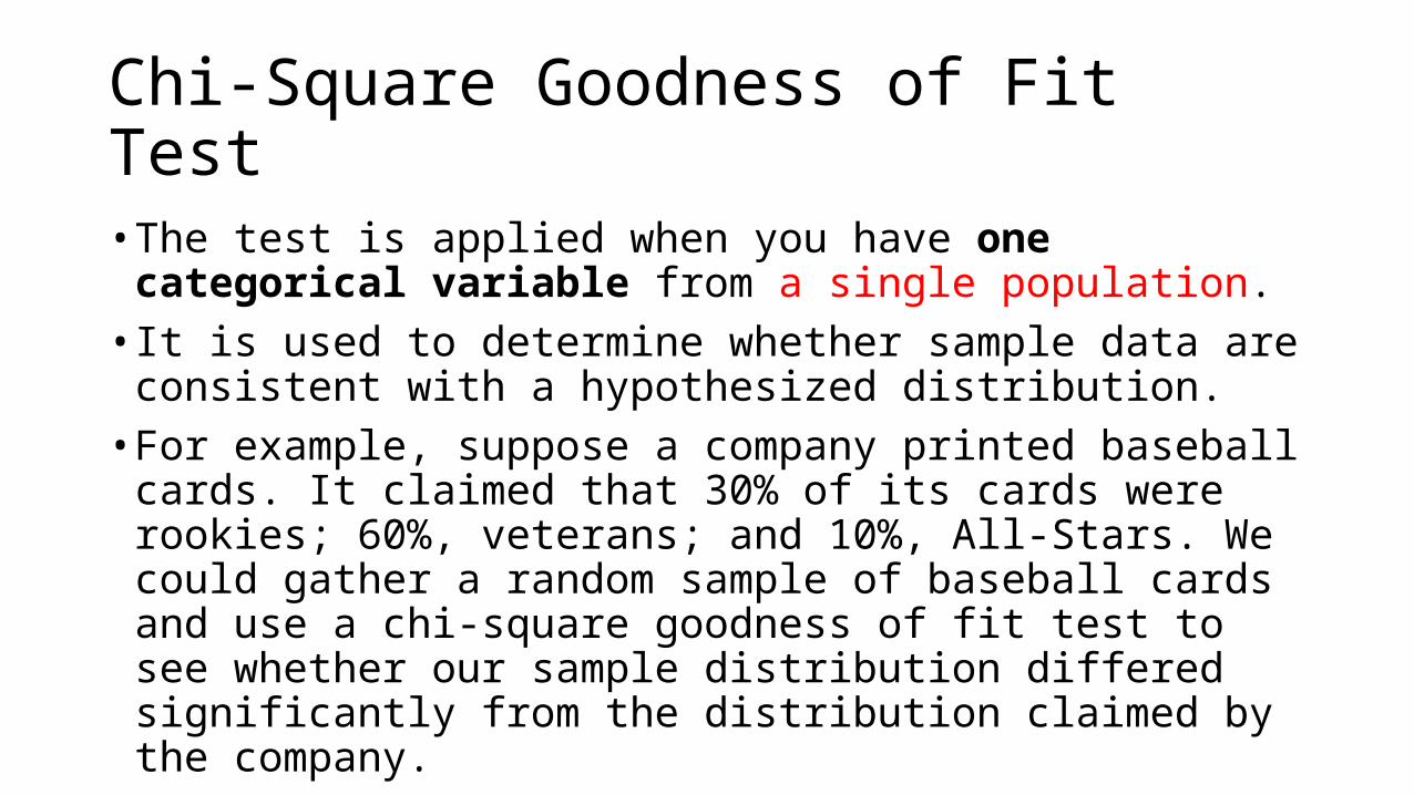
Chi-Square Goodness of Fit Test• The test is applied when you have one categorical variable from a

single population.• It is used to determine whether sample data are consistent with a

hypothesized distribution.• For example, suppose a company printed baseball cards. It claimed

that 30% of its cards were rookies; 60%, veterans; and 10%, All-Stars. We could gather a random sample of baseball cards and use a chi-square goodness of fit test to see whether our sample distribution differed significantly from the distribution claimed by the company.

Chi-Square Test for Independence• The test is applied when you have two categorical variables from a

single population.• It is used to determine whether there is a significant association

between the two variables.• For example, in an election survey, voters might be classified by

gender (male or female) and voting preference (Democrat, Republican, or Independent). We could use a chi-square test for independence to determine whether gender is related to voting preference.

Chi-Square Test of Homogeneity• The test is applied to a single categorical variable from two different

populations.• To determine whether frequency counts are distributed identically

across different populations.• In a survey of TV viewing preferences, we might ask respondents to

identify their favorite program. We might ask the same question of two different populations, such as males and females. We could use a chi-square test for homogeneity to determine whether male viewing preferences differed significantly from female viewing preferences.

Chi-Square Test for Goodness-of-Fit

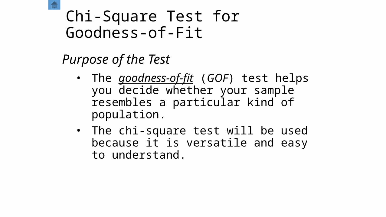
• The goodness-of-fit (GOF) test helps you decide whether your sample resembles a particular kind of population.

• The chi-square test will be used because it is versatile and easy to understand.

Purpose of the Test


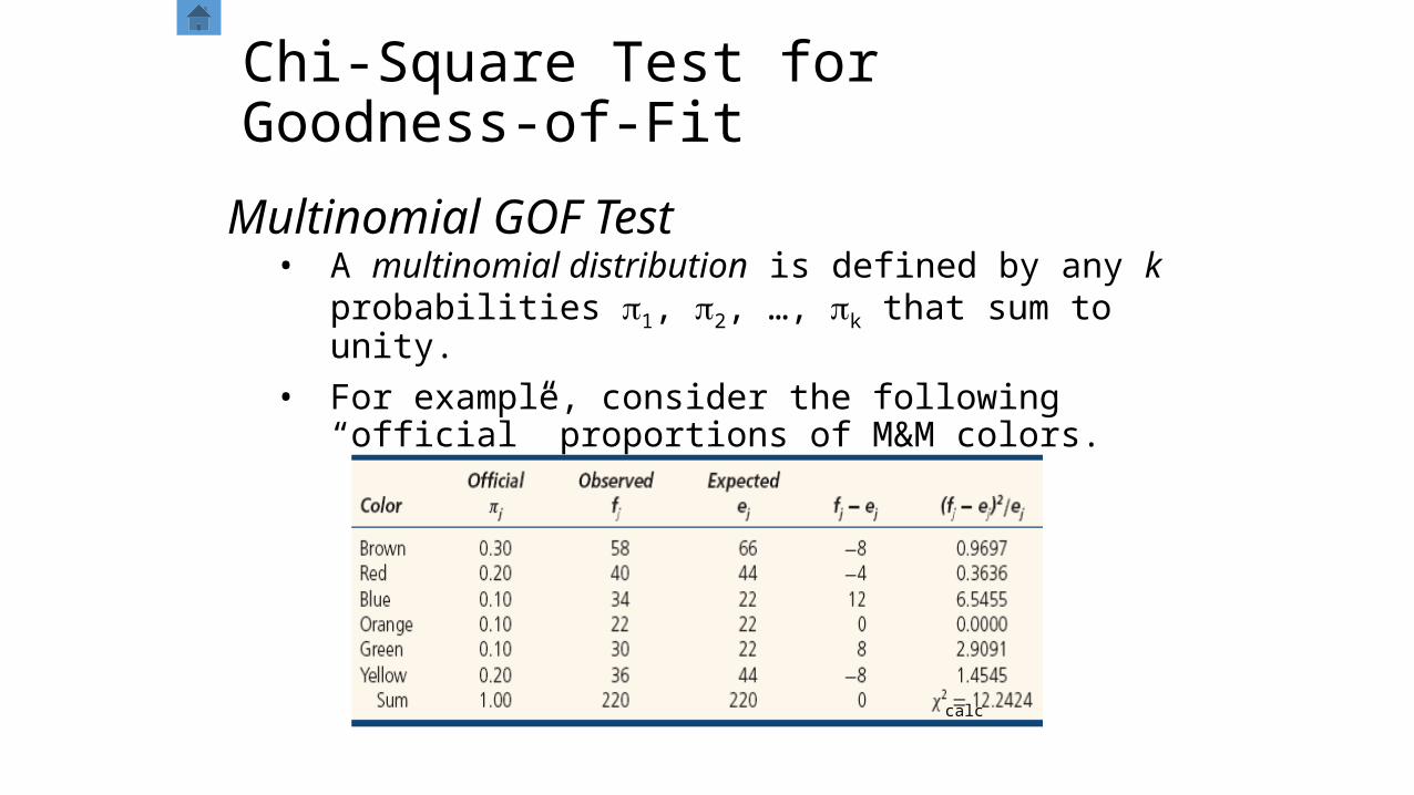
• A multinomial distribution is defined by any k probabilities p1, p2, …, pk that sum to unity.

• For example, consider the following “official” proportions of M&M colors.

Multinomial GOF Test

calc


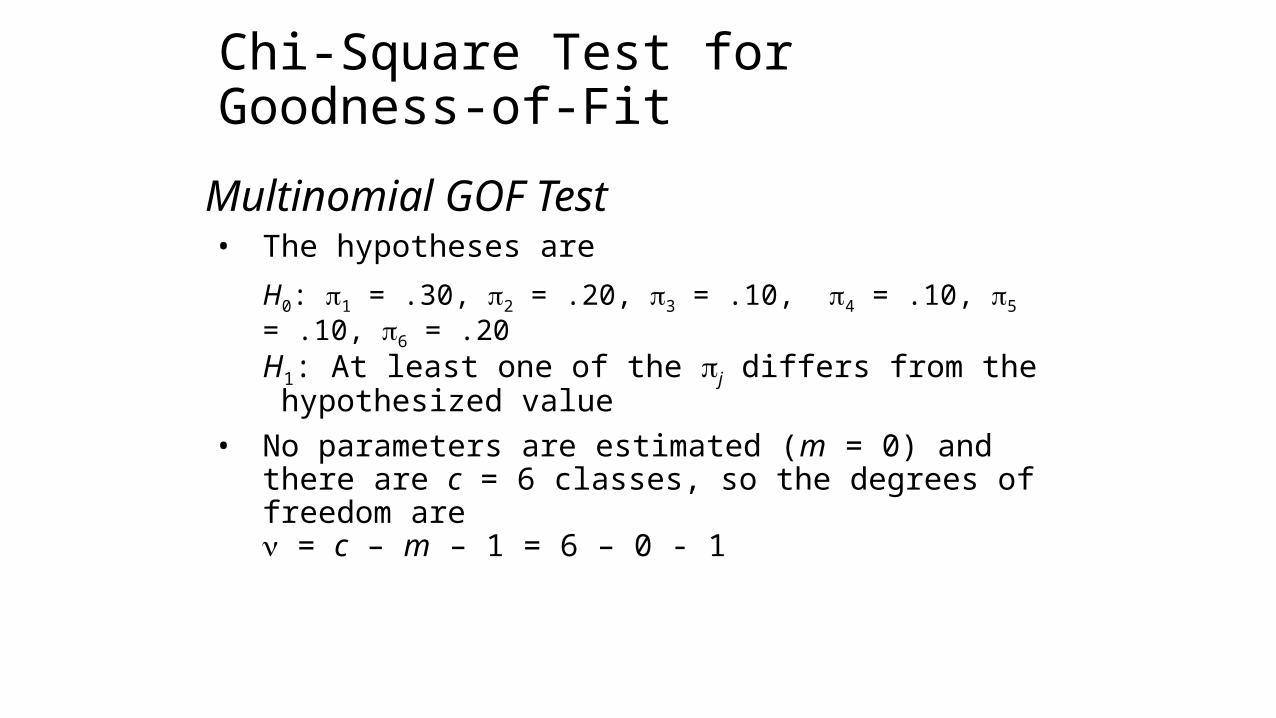
• The hypotheses areH0: p1 = .30, p2 = .20, p3 = .10, p4 = .10, p5 = .10, p6 = .20H1: At least one of the pj differs from the hypothesized value

• No parameters are estimated (m = 0) and there are c = 6 classes, so the degrees of freedom are

n = c – m – 1 = 6 – 0 - 1

Multinomial GOF Test


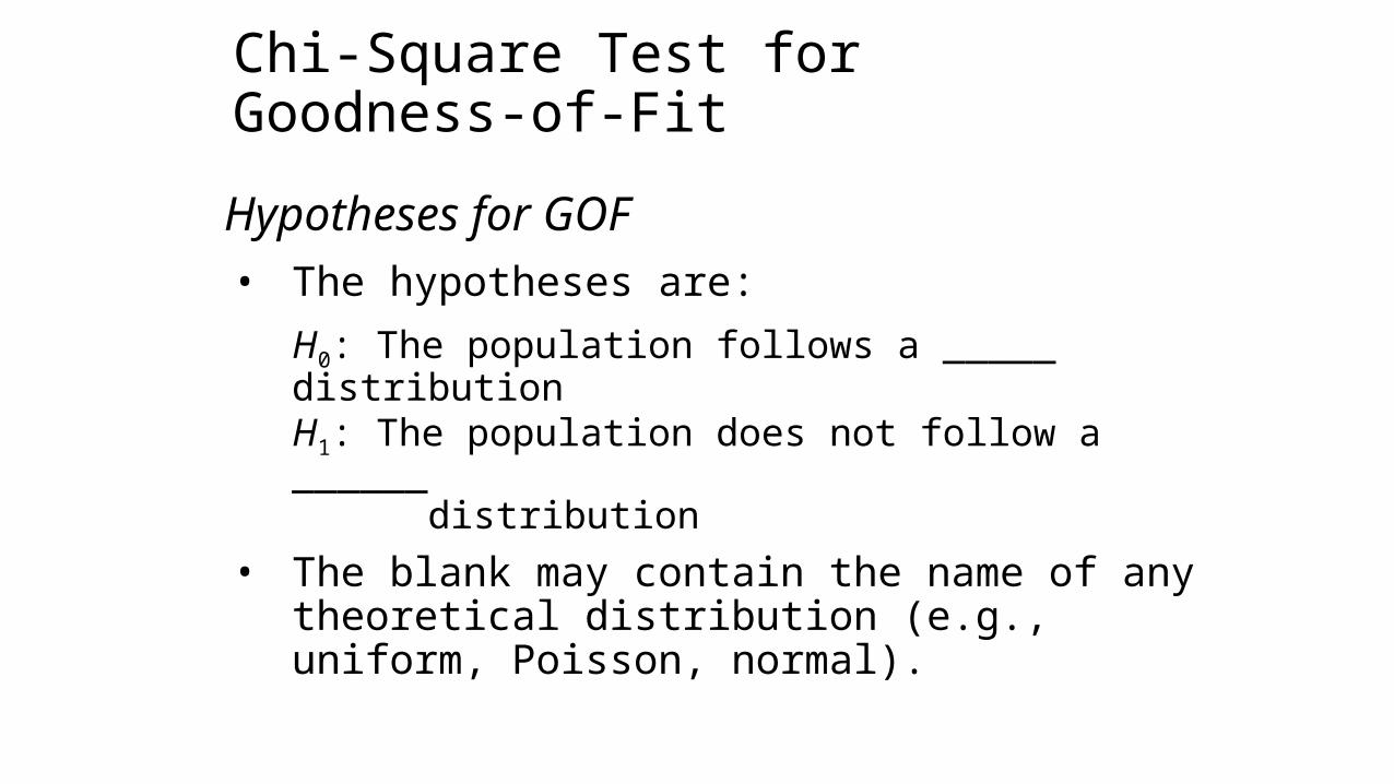
• The hypotheses are:H0: The population follows a _____ distributionH1: The population does not follow a ______ distribution

• The blank may contain the name of any theoretical distribution (e.g., uniform, Poisson, normal).

Hypotheses for GOF


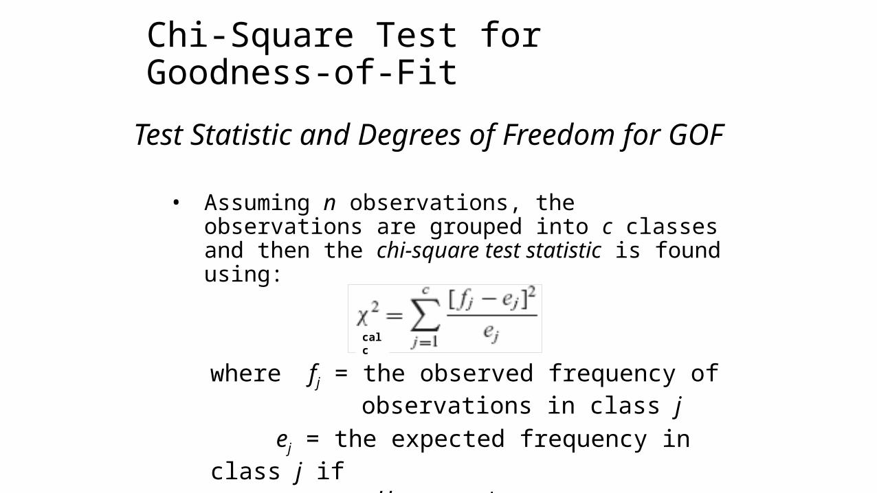
• Assuming n observations, the observations are grouped into c classes and then the chi-square test statistic is found using:

Test Statistic and Degrees of Freedom for GOF

where fj = the observed frequency of observations in class jej = the expected frequency in class j if H0 were true

calc


• If the proposed distribution gives a good fit to the sample, the test statistic will be near zero.

• The test statistic follows the chi-square distribution with degrees of freedom

n = c – m – 1 wherec is the no. of classes used in the test m is the no. of parameters estimated




110 ccmcv

211 ccmcv

312 ccmcv

• For example, for n = 6 and a = .05, c2.05 = 12.59.



• Instead of “fishing” for a good-fitting model, visualize a priori the characteristics of the underlying data-generating process.

Data-Generating Situations

• Mixtures occur when more than one data-generating process is superimposed on top of one another.

Mixtures: A Problem


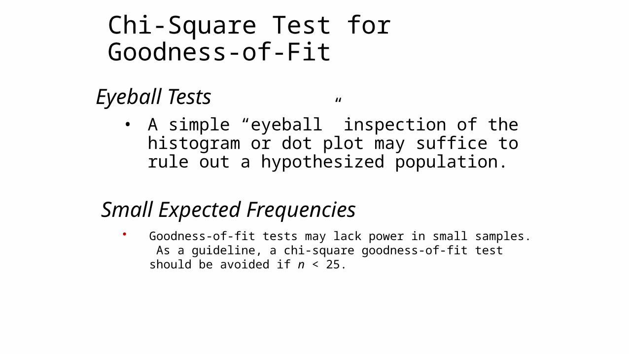
• A simple “eyeball” inspection of the histogram or dot plot may suffice to rule out a hypothesized population.

Eyeball Tests

• Goodness-of-fit tests may lack power in small samples. As a guideline, a chi-square goodness-of-fit test should be avoided if n < 25.

Small Expected Frequencies

Normal Chi-Square Goodness-of-Fit Test

• Two parameters, m and s, fully describe the normal distribution.

• Unless m and s are know a priori, they must be estimated from a sample by using x and s.

• Using these statistics, the chi-square goodness-of-fit test can be used.

Normal Data Generating Situations


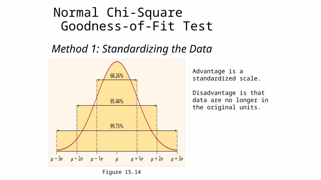
• Transform the sample observations x1, x2, …, xn into standardized values.

• Count the sample observations fj within intervals of the form and compare them with the known frequencies ej based on the normal distribution.

Method 1: Standardizing the Data

x + ks


Method 1: Standardizing the Data

Advantage is a standardized scale.

Disadvantage is that data are no longer in the original units.

Figure 15.14

• The chi-square test is unreliable if the expected frequencies are too small.

• Rules of thumb:• Cochran’s Rule requires that ejk > 5 for all cells.• Up to 20% of the cells may have ejk < 5


• Most agree that a chi-square test is infeasible if ejk < 1 in any cell.

• If this happens, try combining adjacent rows to enlarge the expected frequencies.

Chi-Square Test for Independence

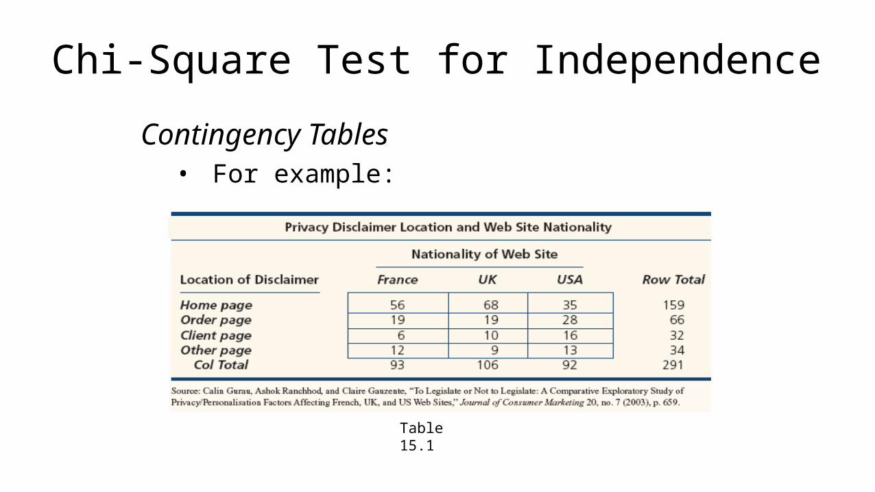
• A contingency table is a cross-tabulation of n paired observations into categories.

• Each cell shows the count of observations that fall into the category defined by its row (r) and column (c)heading.

Contingency Tables

A

B


• For example: Contingency Tables

Table 15.1


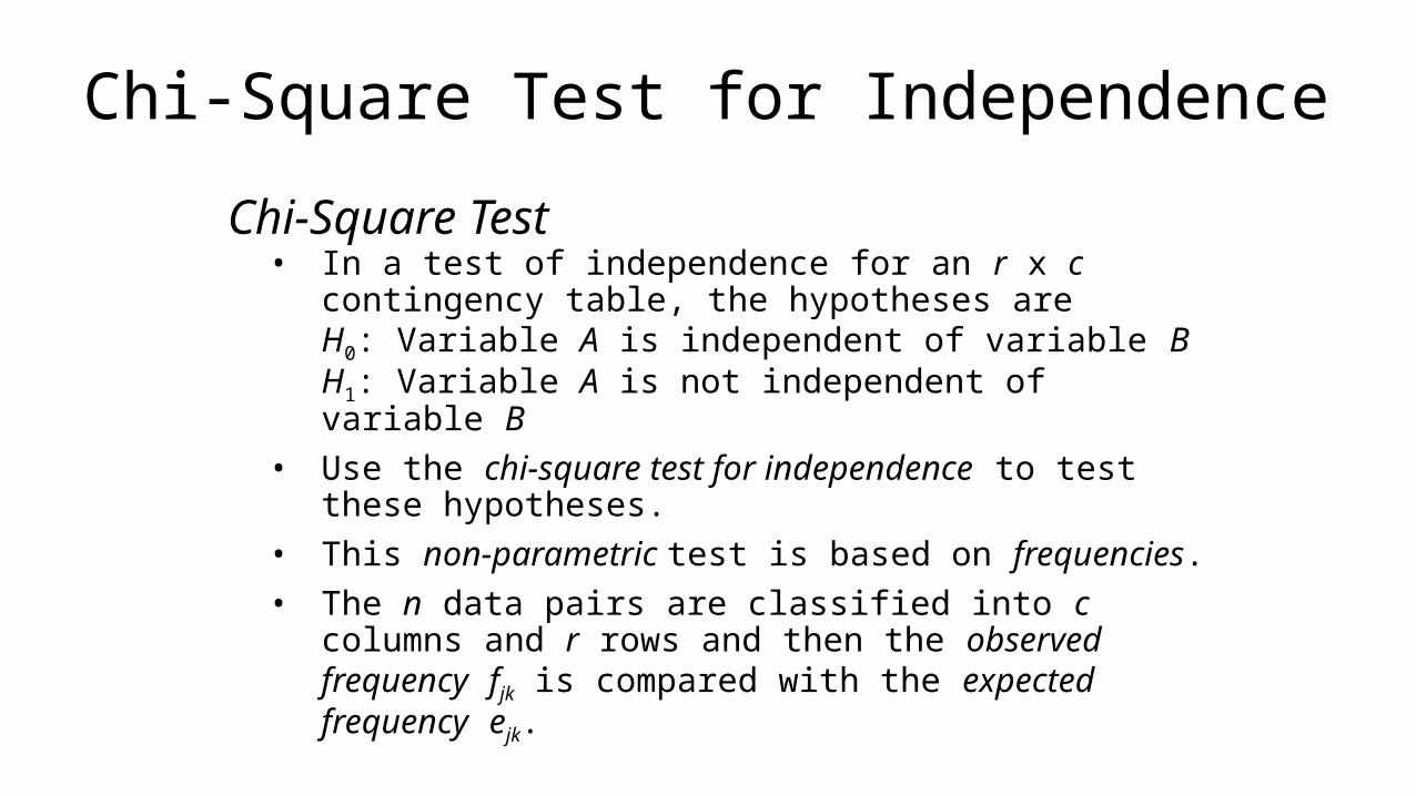
• In a test of independence for an r x c contingency table, the hypotheses areH0: Variable A is independent of variable BH1: Variable A is not independent of variable B

• Use the chi-square test for independence to test these hypotheses.

• This non-parametric test is based on frequencies.• The n data pairs are classified into c columns and r rows

and then the observed frequency fjk is compared with the expected frequency ejk.

Chi-Square Test


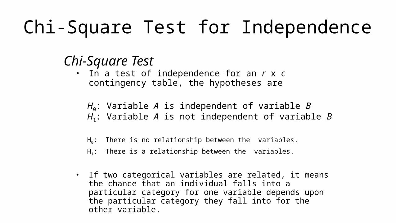
• In a test of independence for an r x c contingency table, the hypotheses are

H0: Variable A is independent of variable BH1: Variable A is not independent of variable B

H0: There is no relationship between the variables.

H1: There is a relationship between the variables.

• If two categorical variables are related, it means the chance that an individual falls into a particular category for one variable depends upon the particular category they fall into for the other variable.

Chi-Square Test


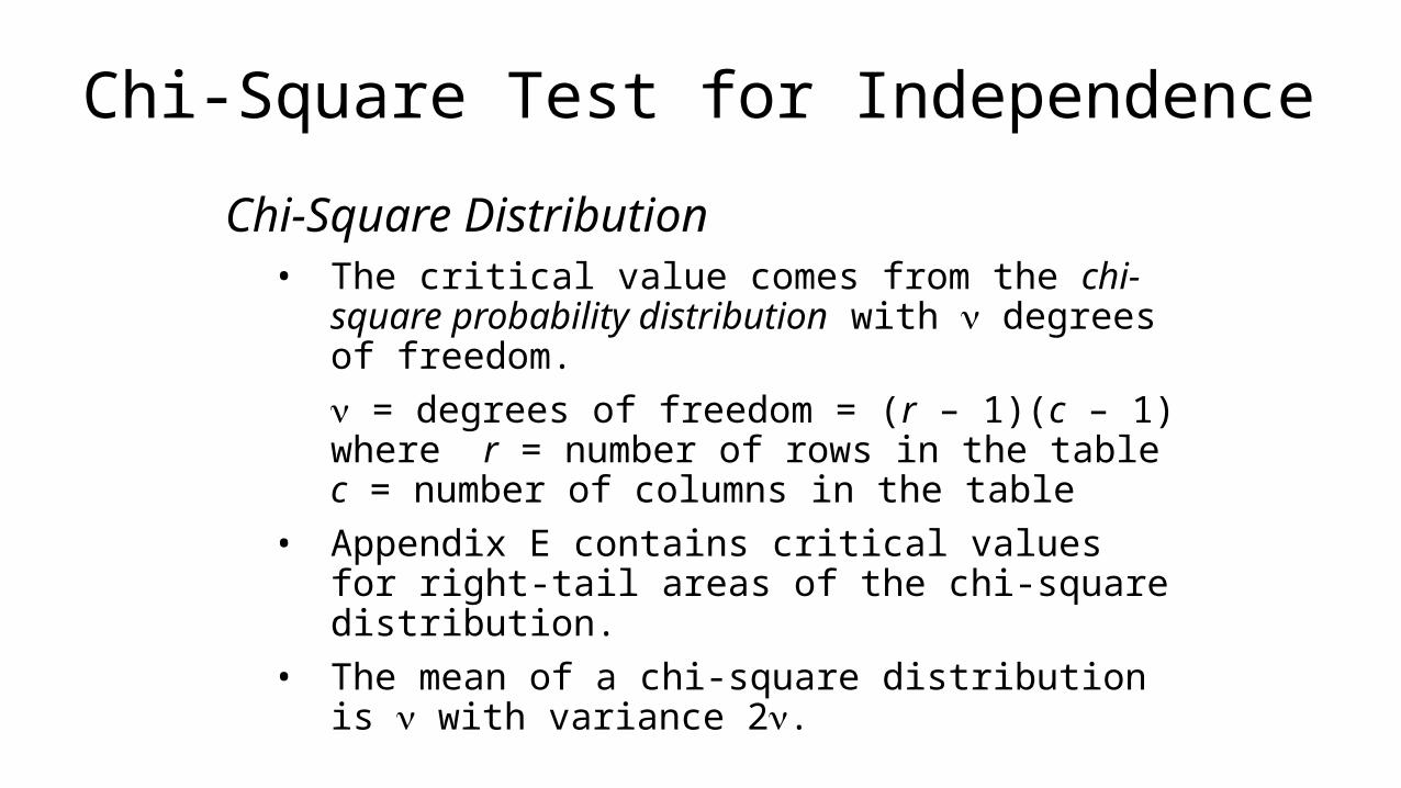
• The critical value comes from the chi-square probability distribution with n degrees of freedom.

n = degrees of freedom = (r – 1)(c – 1)where r = number of rows in the table

c = number of columns in the table• Appendix E contains critical values for right-tail areas of

the chi-square distribution.• The mean of a chi-square distribution is n with

variance 2n.

Chi-Square Distribution


• Assuming that H0 is true, the expected frequency of row j and column k is:

ejk = RjCk/nwhere Rj = total for row j (j = 1, 2, …, r)

Ck = total for column k (k = 1, 2, …, c)n = sample size

Expected Frequencies


• Step 1: State the HypothesesH0: Variable A is independent of variable B H1: Variable A is not independent of variable B

• Step 2: Specify the Decision RuleCalculate n = (r – 1)(c – 1) For a given a, look up the right-tail critical value (c2

R) from Appendix E or by using Excel.

Reject H0 if c2R > test statistic.

Steps in Testing the Hypotheses


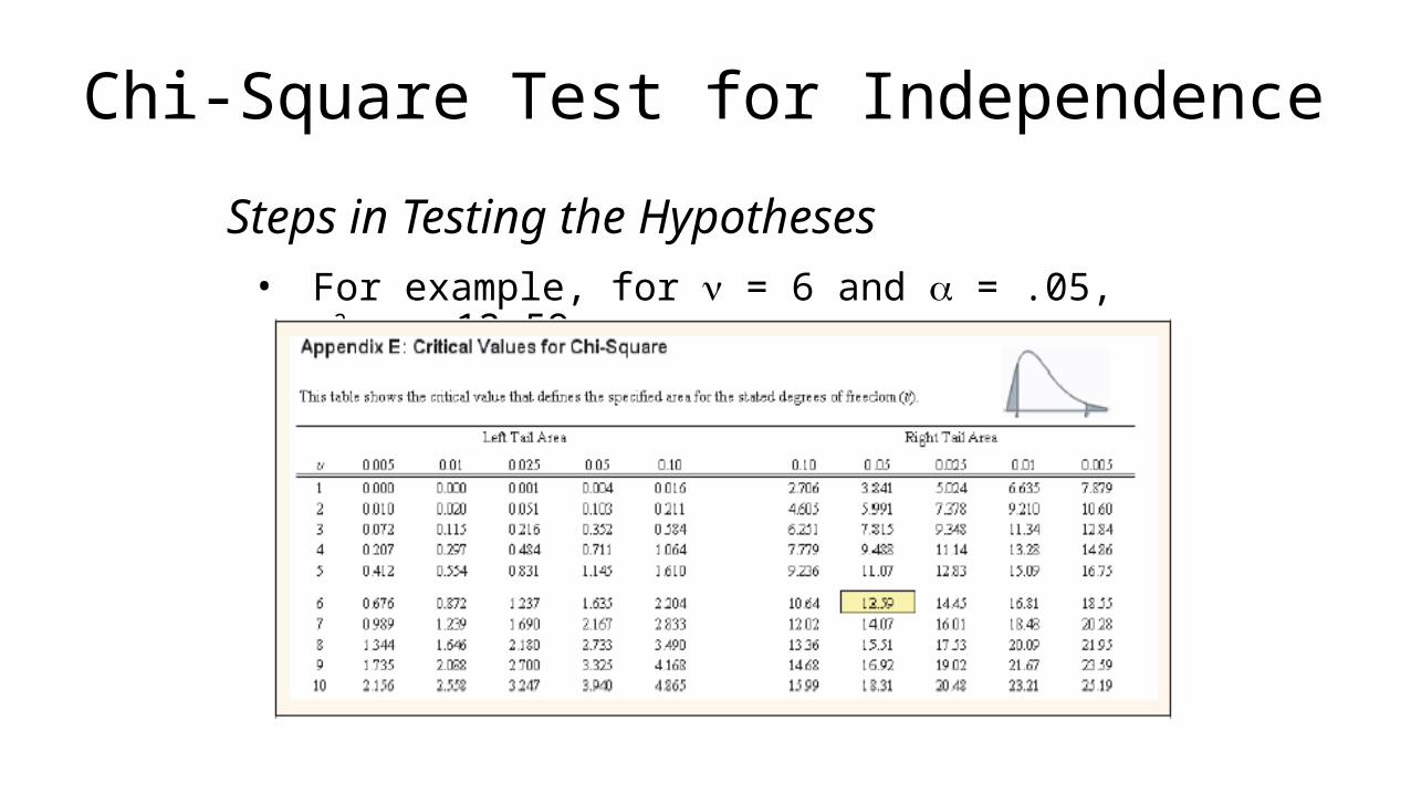
• For example, for n = 6 and a = .05, c2.05 = 12.59.



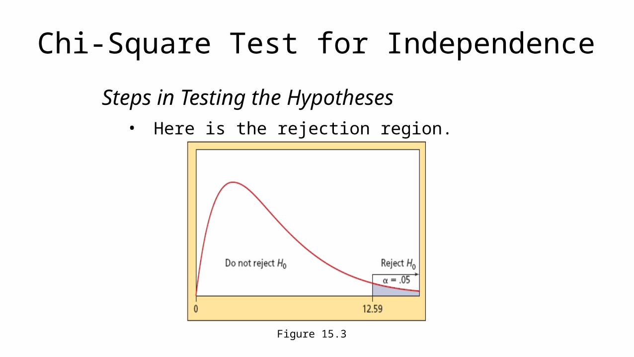
• Here is the rejection region.


Figure 15.3


• Step 3: Calculate the Expected Frequenciesejk = RjCk/n

• For example,



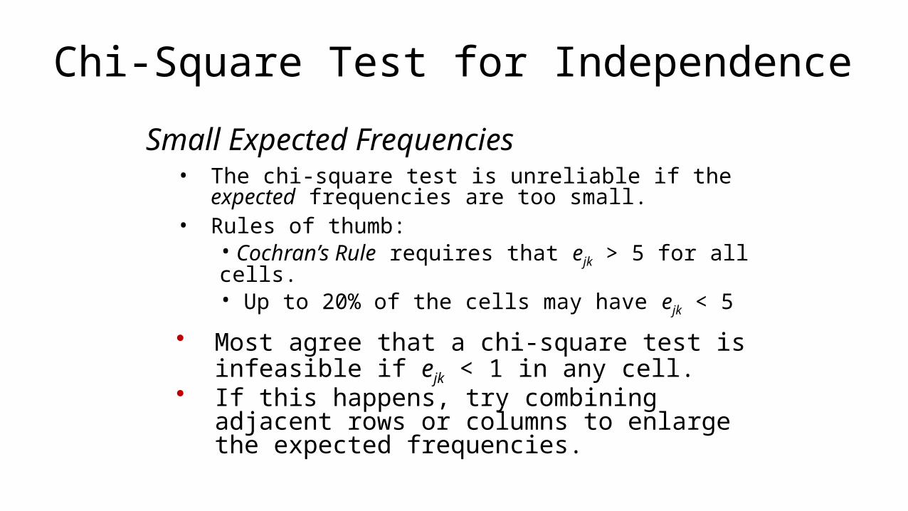
• The chi-square test is unreliable if the expected frequencies are too small.

• Rules of thumb:• Cochran’s Rule requires that ejk > 5 for all cells.• Up to 20% of the cells may have ejk < 5


• Most agree that a chi-square test is infeasible if ejk < 1 in any cell.

• If this happens, try combining adjacent rows or columns to enlarge the expected frequencies.


• Chi-square tests for independence can also be used to analyze quantitative variables by coding them into categories.

Cross-Tabulating Raw Data

For example, the variables Infant Deaths per 1,000 and Doctors per 100,000 can each be coded into various categories:

Chi square

Science