Chapter 3

11111

Chapter 3

22222

Measurement concepts

There are no two things in the world that are exactly the same…

And if there was, we would say they’re different.

- unknown

33333

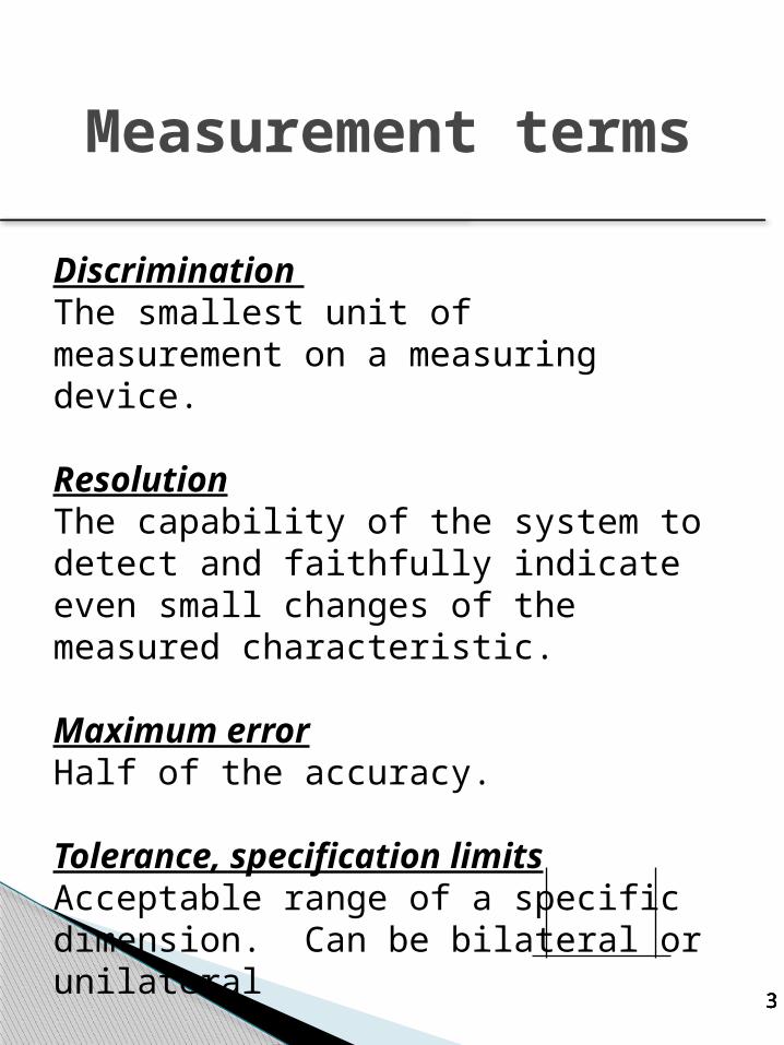
Measurement termsDiscrimination The smallest unit of measurement on a measuring device.

ResolutionThe capability of the system to detect and faithfully indicate even small changes of the measured characteristic.

Maximum errorHalf of the accuracy.

Tolerance, specification limitsAcceptable range of a specific dimension. Can be bilateral or unilateral

44444

Measurement termsDistributionA graphical representation of a group of numbers based on frequency.

Variation The difference between things.

PopulationSet of all possible values.

SampleA subset of the population.

55555

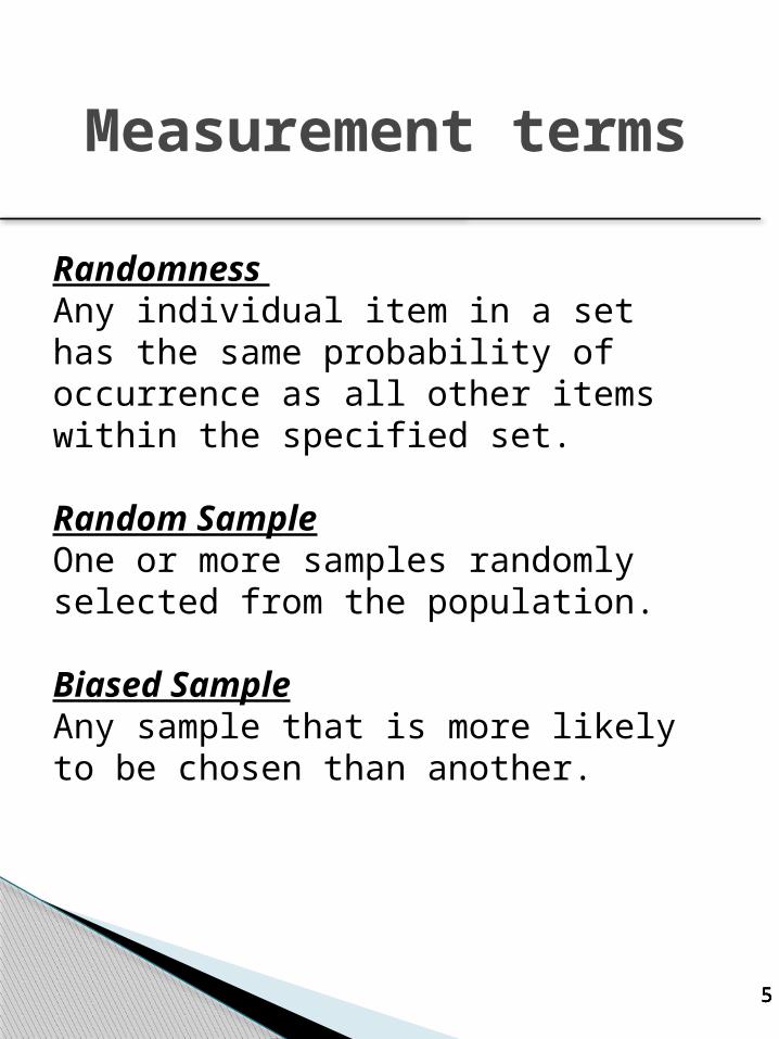
Measurement termsRandomness Any individual item in a set has the same probability of occurrence as all other items within the specified set.

Random SampleOne or more samples randomly selected from the population.

Biased SampleAny sample that is more likely to be chosen than another.

66666

It is impossible for us to improve our processes if our gaging system cannot discriminate between parts or if we cannot repeat our measurement values.

Every day we ask “Show me the data” - yet we rarely ask is the data accurate and how do you know?

Initial thoughts

77777

Success depends upon the ability to measure performance.

Rule #1: A process is only as good as the ability to reliably measure.

Rule #2: A process is only as good as the ability to repeat.

Gordy Skattum, CQE

Initial thoughts

88888

Difficult or impossible to make process improvements

Can make our processes worse! Causes quality, cost, delivery

problems False alarm signals, increases

process variation, loss of process stability

Improperly calculated control limits

Impact of bad measurements on SPC

99999

Some variation can be experienced with natural senses:◦ The visual difference in height

between someone who is 6'7" and someone who is 5'2".

Some variation is so small that an extremely sensitive instrument is required to detect it:◦ The diametrical difference between

a shaft that is ground to ∅.50002 and one that is ground to ∅.50004.

Variation

1010101010

Normal variation◦ running in an expected,

consistent manner, we would consider it normal or common cause variation.

Non-normal variation◦ running in a sudden, unexpected

manner, we would consider it non-normal, or assignable cause variation.

Types of variation

We only want normal variation in our processes

1111111111

Statistical control - shows if the inherent variability of a process is being caused by normal causes of variation, as opposed to assignable or non-normal causes.

Why only normal variation?

Assignable Cause?

Assignable Cause?

1212121212

What is a distribution?

Each unit of measure is a numerical value on a continuous scale

Size Size Size Size

Pieces vary from each other

Variation common and special causes

But they form a pattern that, if stable, is called a distribution

Histogram

Normal Distribution

1313131313

Distributions

There are three terms used to describe distributions

3. Location

1. Shape

2. Spread

1414141414

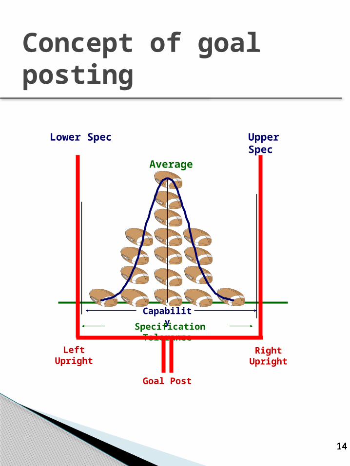
Capability Specification Tolerance

Lower Spec Upper Spec

Average

Left Upright Right Upright

Goal Post

Concept of goal posting

1515151515

Pote

ntia

l Fa

ilure

s

Cos

tMea

n (ta

rget

)

Waste

Lower Spec

Upper Spec

The Taguchi Loss Function Concept

Cost at lower spec

Cost at upper spec

Cost at mean

1616161616

Because we are using all of our tolerance, we’re forced to keep the process exactly centered. If the process shifts at all, nonconforming parts will be produced

What happens when “Shift Happens?”

TargetUpper

Specification Limit

Lower Specification

Limit

1717171717

Using 75% or less of a tolerance will allow processes to shift slightly with little chance of producing any defects

The goal is to improve your process in order to use the least amount of tolerance possible◦ Reduce the opportunity to produce

defects◦ Reduce the cost of the process

Getting started

We need to calculate process capability

1818181818

Spread Too Large

Low High

Off Center & SpreadCombination

Low High

65 73.5 75

Low High

Off Center

65 70 75

65 68 75

Pictures of “BAD” quality

1919191919 6 s

Lower SpecificationLimit

Upper SpecificationLimit

65 7570

World-class Quality

Using only 50% of the tolerance or

less

2020202020

What is statistics? How are statistics used with:

◦ Baseball Scouts◦ Bankers◦ Weathermen◦ Television Networks◦ Insurance Agents

Statistics

2121212121

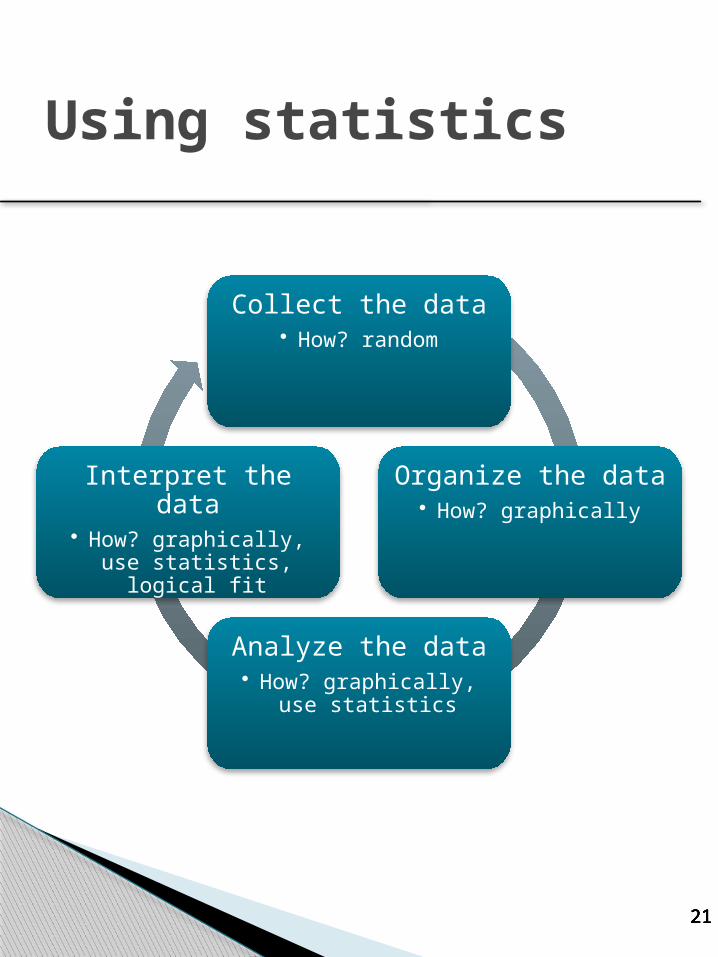
Collect the data• How? random

Organize the data• How? graphically

Analyze the data• How? graphically, use

statistics

Interpret the data• How? graphically, use

statistics, logical fit

Using statistics

2222222222

Mean - can be found of a group of values by adding them together, and dividing by the number of values. The mean is the average of a group of numbers. We will use it to find out where the center of a distribution lies.

Central tendency

House 1 $110K What is your total? ________ House 2 $105K House 3 $100K How many houses were there? ________ House 4 $95K House 5 $90K What is the average price? ________

Remember - Average and Mean are synonymous!!!

xNx

population

nx

xsample

x

** 100k is the mean because it is the middle weighted value.**

2323232323

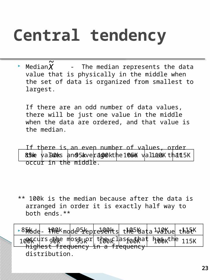
Median - The median represents the data value that is physically in the middle when the set of data is organized from smallest to largest.

 If there are an odd number of data values, there will be just one value in the middle when the data are ordered, and that value is the median.

 If there is an even number of values, order the values and average the two values that occur in the middle.

** 100k is the median because after the data is arranged in order it is exactly half way to both ends.**

Mode- The mode represents the data value that occurs the most or the class that has the highest frequency in a frequency distribution.

** 100k is the mode because it occurs more than the others in the data table.**

Central tendencyx~

85k 90k 95k 100k 105K 110K 115K

85k 100k 95k 100k 105K 110K 115K100k 90k 95k 100k 100K 100K 115K

2424242424

Range is a measure that shows the difference between the highest and lowest values in a group. To find range, subtract from the highest value the lowest value.

  The formula for range is: R = H - L

R = rangeH = highest valueL = lowest value

Dispersion

2525252525

Range examples

Example #1 Using the following numbers, lets find

the range:The data is 4,7,6,1,15,10.R = H - LR = 15 - 1R = 14 The range is 14.

 Example #2

Two consecutive parts in an order have the following sizes: .250, .2535

R = H - LR = .2535 - .250R = .0035

2626262626

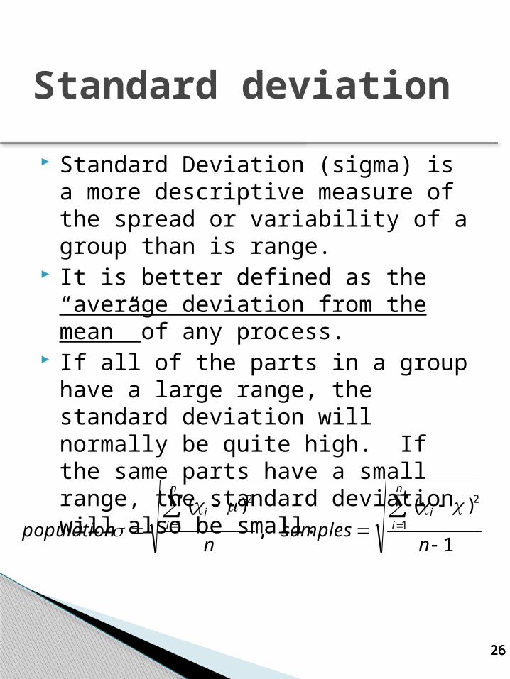
Standard Deviation (sigma) is a more descriptive measure of the spread or variability of a group than is range.

It is better defined as the “average deviation from the mean” of any process.

If all of the parts in a group have a large range, the standard deviation will normally be quite high. If the same parts have a small range, the standard deviation will also be small.

Standard deviation

1

)( ,

)( 1

2

1

2

nssample

npopulation

n

ii

n

ii

s

2727272727

 Although the method we just used to calculate standard

deviation is accurate, it is also very time consuming. Because time is money in industry, we find that it becomes more cost effective to estimate standard deviation rather than calculate the exact number. This gives us a number very close to the exact number, but in a very short time period. The following formula is used to estimate standard deviation: 

Where.......   = Estimate of Standard Deviation = the average range among the samples in each subgroup and, = a constant based on the number of samples in each subgroup An Individuals X and Moving Range chart, which we will discuss in detail later, uses subgroup sizes of two. The d2 value for subgroups of size two = 1.128. Therefore, we can easily calculate an estimate of standard deviation for IX & MR charts by dividing the average of all range values by 1.128. The numbers are .3472, .3476, .3478, .3479, .3474, .3472: 

Estimating sigma – The Shewhart Formula

.3472

.3476

.3478

.3479

.3474

.3472

.0004

.0002

.0001

.0005

.0002

ValuesRange

.0014.00028

.000248

TotalAverage

Est. Std. Dev.

2

ˆdR

s

sR

2d

See Table B.1 for d2 values

Your book also calls this “s”

2828282828

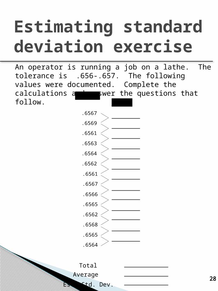
Estimating standard deviation exerciseAn operator is running a job on a lathe. The tolerance is .656-.657. The following values were documented. Complete the calculations and answer the questions that follow. 

.6567

.6569

.6561

.6563

.6564

.6562

ValuesRange

TotalAverage

Est. Std. Dev.

.6564

.6565

.6568

.6562

.6565

.6566

.6567

.6561

2929292929

HistogramsHistograms A histogram is a chart that shows how often an event occurs. As the name implies, a histogram shows us the history of a process. The left side of the chart shows how many times an event occurred. The bottom of the chart shows the variable measurement value. Histograms help you to discern if the process you are running is capable of meeting a given tolerance, and also shows you if there are assignable causes of variation affecting the process. The following diagram shows what a basic histogram looks like.

10 9 8 X 7 X 6 X 5 X X 4 X X X 3 X X X X 2 X X X X X 1 X X X X X X X

t .493 .494 .495 .496 .497 .498 .499 .500 .501 .502 .503 .504 .505 .506 .507

As you can see the size classes are located on the horizontal axis, with the frequency listed on the vertical axis. An “X” is placed over each class for every part that measures that size. After all parts have been plotted, you can begin to understand the inherent variability patterns of the process better. If you superimpose the specification limits on the graph, you can easily see where all of the parts are located in the tolerance spectrum.

Tally histogram

10987654321

3030303030

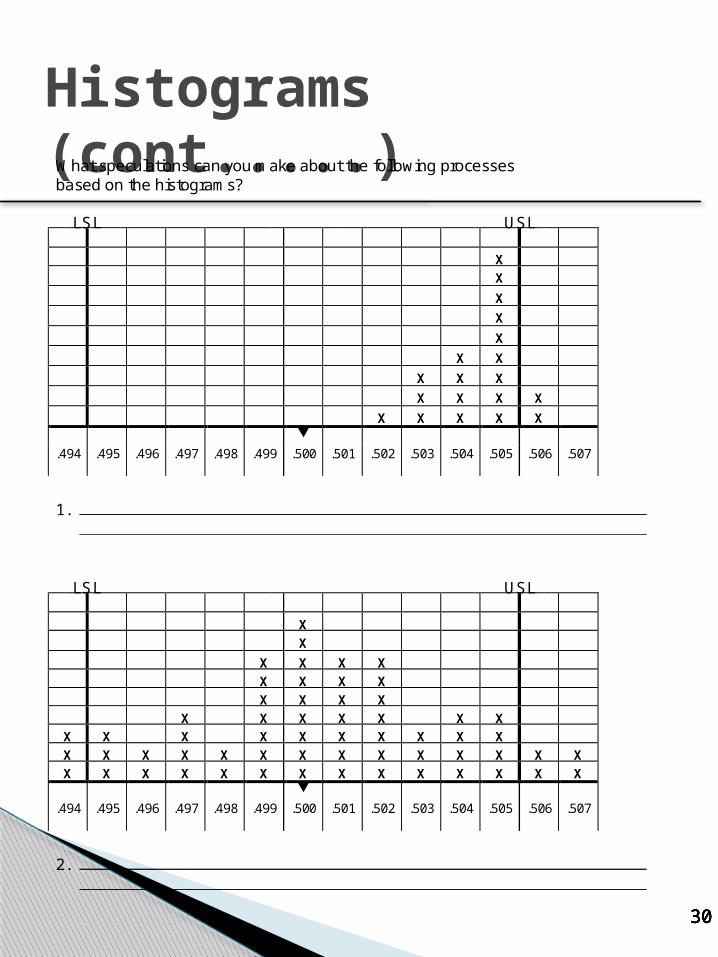
Histograms (cont.....)What speculations can you make about the following processes

based on the histograms?

LSL USL 10 9 X 8 X 7 X 6 X 5 X 4 X X 3 X X X 2 X X X X 1 X X X X X

.493 .494 .495 .496 .497 .498 .499 .500 .501 .502 .503 .504 .505 .506 .507

1.

LSL USL 10 9 X 8 X 7 X X X X 6 X X X X 5 X X X X 4 X X X X X X X 3 X X X X X X X X X X 2 X X X X X X X X X X X X X X X 1 X X X X X X X X X X X X X X X

.493 .494 .495 .496 .497 .498 .499 .500 .501 .502 .503 .504 .505 .506 .507

2.

3131313131

Histograms (cont.....)

LSL USL 10 9 X 8 X 7 X 6 X 5 X X X 4 X X X 3 X X X 2 X X X X X 1 X X X X X X X

.493 .494 .495 .496 .497 .498 .499 .500 .501 .502 .503 .504 .505 .506 .507

3.

LSL USL 10 X 9 X 8 X 7 X X X 6 X X X X 5 X X X X X 4 X X X X X 3 X X X X X X X 2 X X X X X X X X 1 X X X X X X X X

.493 .494 .495 .496 .497 .498 .499 .500 .501 .502 .503 .504 .505 .506 .507

4.

3232323232

Let’s look at how this fits together…

3333333333

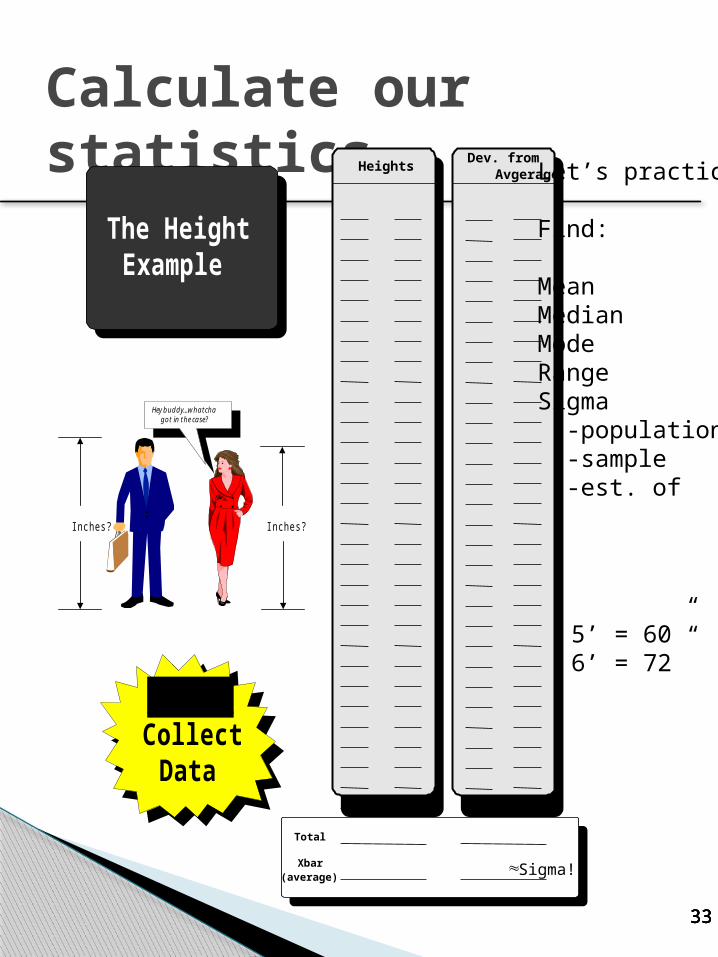
Calculate our statistics

The HeightExample

Inches? Inches?

Hey buddy...whatchagot in the case?

Step 1Collect

Data

Heights Dev. from Avgerage.

Total

Xbar(average) Sigma!!

Let’s practice

Find:

MeanMedianModeRangeSigma -population -sample -est. of

5’ = 60”6’ = 72”

3434343434

Plot height data and use the statistics

Step 2Create a

Histogram

Xbar =

Scale - (Use 2"increments)

Sigma Area % Height Span Realistic? (Y/N)+/- 1 Sigma+/- 2 Sigma+/- 3 Sigma+/- 6 Sigma

Step 3Add Sigma

Limits

Step 4Analyze

3535353535

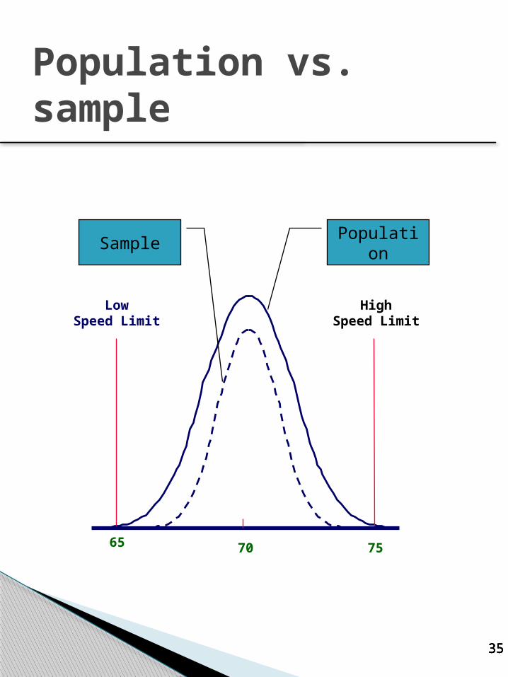
LowSpeed Limit

HighSpeed Limit

65 7570

Population vs. sample

PopulationSample