BioMagnetic Research and Technology - Springer LINK

BioMed Central

BioMagnetic Research and Technology

ss
Open AcceResearchPseudo current density maps of electrophysiological heart, nerve or brain function and their physical basisWolfgang Haberkorn1, Uwe Steinhoff1, Martin Burghoff1, Olaf Kosch1, Andreas Morguet2 and Hans Koch*1
Address: 1Physikalisch-Technische Bundesanstalt, Berlin, Germany and 2Charité Campus Benjamin Franklin, Clinic II, Berlin, Germany

Email: Wolfgang Haberkorn - [email protected]; Uwe Steinhoff - [email protected]; Martin Burghoff - [email protected]; Olaf Kosch - [email protected]; Andreas Morguet - [email protected]; Hans Koch* - [email protected]

* Corresponding author

AbstractBackground: In recent years the visualization of biomagnetic measurement data by so-calledpseudo current density maps or Hosaka-Cohen (HC) transformations became popular.

Methods: The physical basis of these intuitive maps is clarified by means of analytically solvableproblems.

Results: Examples in magnetocardiography, magnetoencephalography and magnetoneurographydemonstrate the usefulness of this method.

Conclusion: Hardware realizations of the HC-transformation and some similar transformationsare discussed which could advantageously support cross-platform comparability of biomagneticmeasurements.

BackgroundIn 1976 Cohen et al. introduced in a sequence of publica-tions a method to construct so-called pseudo current den-sity- or arrow-maps from multichannel biomagneticsignals obtained by magnetocardiography (MCG) [1-4].The purpose was to transform the measured magneticfield values in a way that the resulting maps could bemore easily related to the underlying current density dis-tribution. Later this method was frequently referred to asthe Hosaka-Cohen (HC) transformation and its perform-ance was analyzed in some detail [5,6]. However, it didnot find widespread application until recent years, whena kind of renaissance of this method occurred. Recently,the HC-transformation is used in MCG [7-21], fetal MCG[22-24], magnetoencephalography (MEG) [25-27] andmagnetoneurography (MNG) [28].

A reason for this new development may be the advance ofcomputing power and visualization tools. In addition, informer times system designers preferred to display mag-netic field maps (MFM), since they were interested in themeasured physical quantity. However, for the end-user -the physicians- MFMs are not very instructive, as the MFMmaximum values do not occur above those positionswhere the generating currents are flowing.

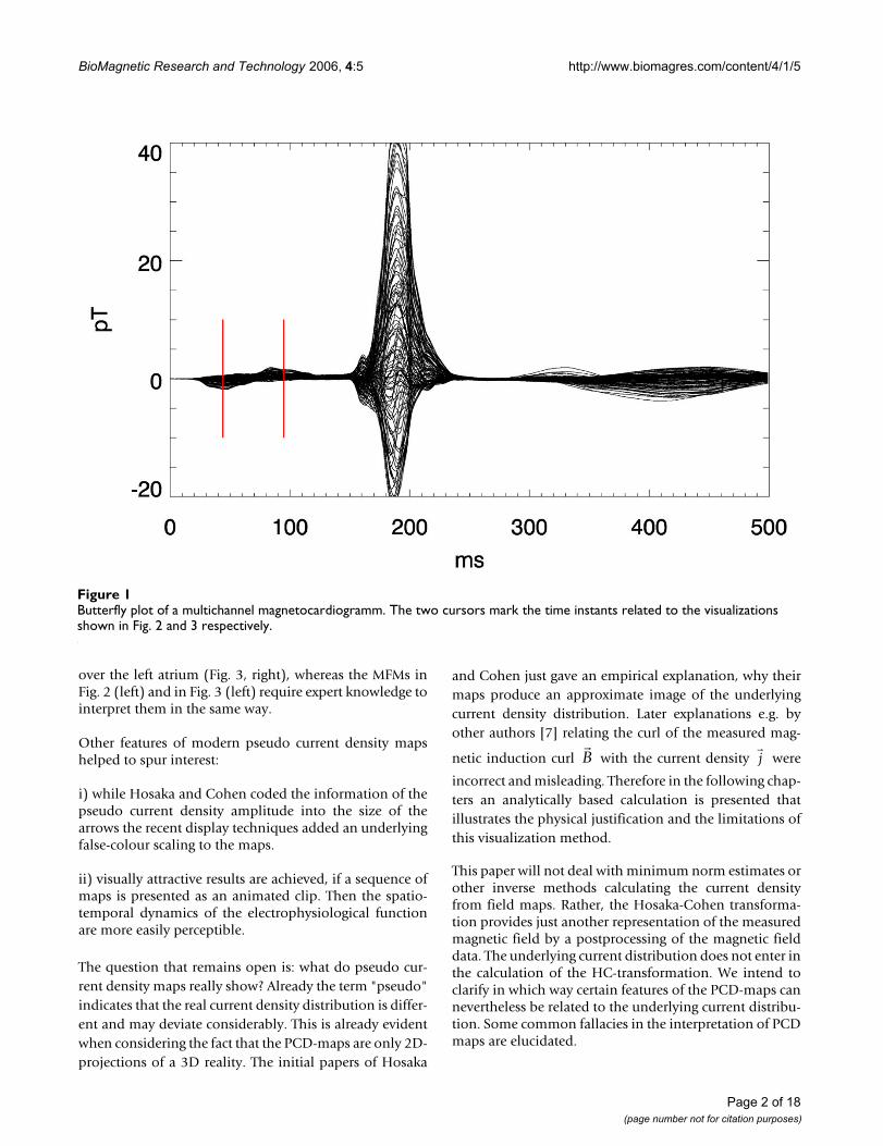
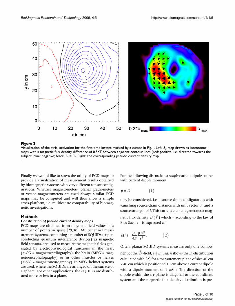
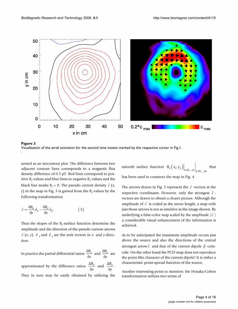
Figs. 1, 2, 3 illustrate this point: it shows two instants ofthe atrial excitation marked by the cursors in the MCG-butterfly-plot in Fig. 1 (a butterfly-plot is obtained bysuperpositioning the MCG-Signals of all channels in onedisplay). The respective pseudo current density (PCD-)plots show very clearly and intuitively the preceding acti-vation over the right atrium (Fig. 2, right) followed by that

Published: 13 October 2006

BioMagnetic Research and Technology 2006, 4:5 doi:10.1186/1477-044X-4-5

Received: 04 August 2006Accepted: 13 October 2006

This article is available from: http://www.biomagres.com/content/4/1/5

© 2006 Haberkorn et al; licensee BioMed Central Ltd. This is an Open Access article distributed under the terms of the Creative Commons Attribution License (http://creativecommons.org/licenses/by/2.0), which permits unrestricted use, distribution, and reproduction in any medium, provided the original work is properly cited.

Page 1 of 18(page number not for citation purposes)

http://www.biomagres.com/content/4/1/5

http://creativecommons.org/licenses/by/2.0

http://www.ncbi.nlm.nih.gov/entrez/query.fcgi?cmd=Retrieve&db=PubMed&dopt=Abstract&list_uids=17040559

http://www.biomedcentral.com/

http://www.biomedcentral.com/info/about/charter/

BioMagnetic Research and Technology 2006, 4:5 http://www.biomagres.com/content/4/1/5

over the left atrium (Fig. 3, right), whereas the MFMs inFig. 2 (left) and in Fig. 3 (left) require expert knowledge tointerpret them in the same way.

Other features of modern pseudo current density mapshelped to spur interest:

i) while Hosaka and Cohen coded the information of thepseudo current density amplitude into the size of thearrows the recent display techniques added an underlyingfalse-colour scaling to the maps.

ii) visually attractive results are achieved, if a sequence ofmaps is presented as an animated clip. Then the spatio-temporal dynamics of the electrophysiological functionare more easily perceptible.

The question that remains open is: what do pseudo cur-rent density maps really show? Already the term "pseudo"indicates that the real current density distribution is differ-ent and may deviate considerably. This is already evidentwhen considering the fact that the PCD-maps are only 2D-projections of a 3D reality. The initial papers of Hosaka

and Cohen just gave an empirical explanation, why theirmaps produce an approximate image of the underlyingcurrent density distribution. Later explanations e.g. byother authors [7] relating the curl of the measured mag-

netic induction curl with the current density were

incorrect and misleading. Therefore in the following chap-ters an analytically based calculation is presented thatillustrates the physical justification and the limitations ofthis visualization method.

This paper will not deal with minimum norm estimates orother inverse methods calculating the current densityfrom field maps. Rather, the Hosaka-Cohen transforma-tion provides just another representation of the measuredmagnetic field by a postprocessing of the magnetic fielddata. The underlying current distribution does not enter inthe calculation of the HC-transformation. We intend toclarify in which way certain features of the PCD-maps cannevertheless be related to the underlying current distribu-tion. Some common fallacies in the interpretation of PCDmaps are elucidated.

B j

Butterfly plot of a multichannel magnetocardiogrammFigure 1Butterfly plot of a multichannel magnetocardiogramm. The two cursors mark the time instants related to the visualizations shown in Fig. 2 and 3 respectively.



Finally we would like to stress the utility of PCD maps toprovide a visualization of measurement results obtainedby biomagnetic systems with very different sensor config-urations. Whether magnetometers, planar gradiometersor vector magnetometers are used always similar PCDmaps may be computed and will thus allow a simplecross-platform, i.e. multicentre comparability of biomag-netic investigations.

MethodsConstruction of pseudo current density mapsPCD-maps are obtained from magnetic field values at anumber of points in space [29,30]. Multichannel meas-urement systems, containing a number of SQUIDs (super-conducting quantum interference devices) as magneticfield sensors, are used to measure the magnetic fields gen-erated by electrophysiological functions in the heart(MCG = magnetocardiography), the brain (MEG = mag-netoencephalography) or in other muscles or nerves(MNG = magnetoneurography). In MEG, helmet systemsare used, where the SQUIDs are arranged on the surface ofa sphere. For other applications, the SQUIDs are distrib-uted more or less in a plane.

For the following discussion a simple current dipole sourcewith current dipole moment

may be considered, i.e. a source-drain configuration with

vanishing source-drain distance with unit vector and asource strength of I. This current element generates a mag-

netic flux density ( ) which – according to the law ofBiot-Savart – is expressed as

Often, planar SQUID-systems measure only one compo-

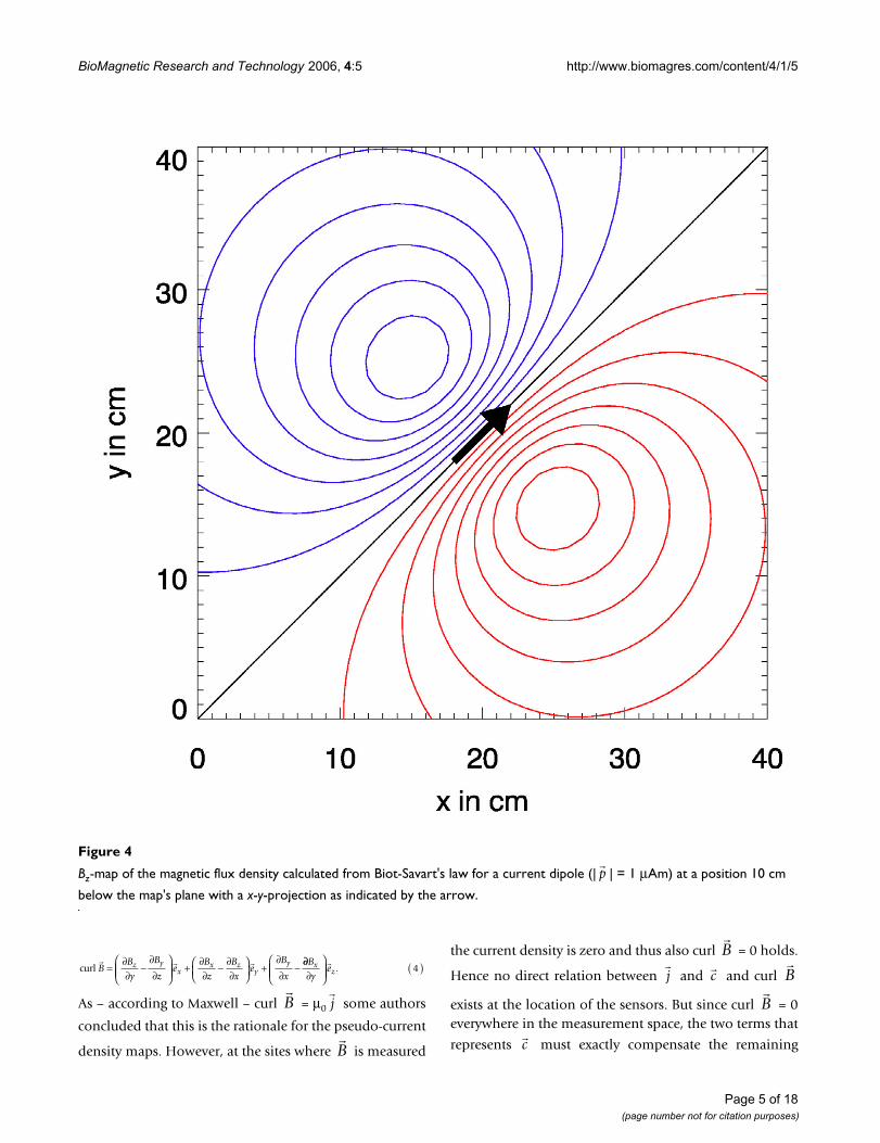
nent of the -field, e.g.Bz. Fig. 4 shows the Bz-distribution

calculated with (2) for a measurement plane of size 40 cm× 40 cm which is positioned 10 cm above a current dipole

with a dipole moment of 1 μAm. The direction of thedipole within the x-y-plane is diagonal to the coordinatesystem and the magnetic flux density distribution is pre-

p Is= ( )1

s

B r

B rp r

r( ) .= × ( )μ

π0

342

B

Visualization of the atrial activation for the first time instant marked by a cursor in Fig.1Figure 2Visualization of the atrial activation for the first time instant marked by a cursor in Fig.1. Left: Bz-map drawn as isocontour maps with a magnetic flux density difference of 0.5pT between adjacent contour lines (red: positive, i.e. directed towards the subject; blue: negative; black: Bz = 0). Right: the corresponding pseudo current density map.



sented as an isocontour plot. The difference between twoadjacent contour lines corresponds to a magnetic fluxdensity difference of 0.5 pT. Red lines correspond to pos-itive Bz-values and blue lines to negative Bz-values and the

black line marks Bz = 0. The pseudo current density (x,

y) in the map in Fig. 5 is gained from the Bz-values by the

following transformation

Thus the slopes of the Bz-surface function determine the

amplitude and the direction of the pseudo current arrows

(x, y). x and y are the unit vectors in x- and y-direc-

tion.

In practice the partial differential ratios and are

approximated by the difference ratios and .

They in turn may be easily obtained by utilizing the

smooth surface function that

has been used to construct the map in Fig. 4.

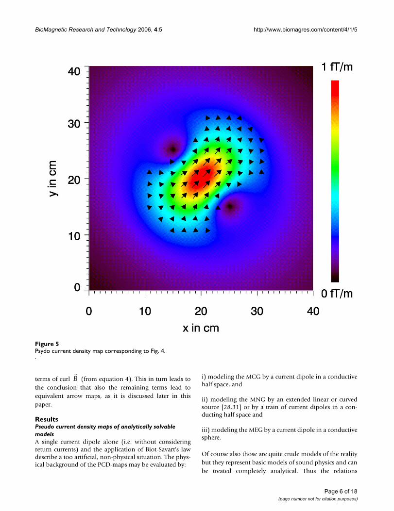
The arrows drawn in Fig. 5 represent the -vectors at the

respective coordinates. However, only the strongest -vectors are drawn to obtain a clearer picture. Although the

amplitude of is coded as the arrow length, a map withjust those arrows is not as intuitive as the image shown. By

underlying a false-color map scaled by the amplitude | |a considerable visual enhancement of the information isachieved.

As to be anticipated the maximum amplitude occurs justabove the source and also the directions of the central

strongest arrow and that of the current dipole coin-

cide. On the other hand the PCD-map does not reproducethe point-like character of the current dipole! It is rather acharacteristic point-spread function of the source.

Another interesting point to mention: the Hosaka-Cohentransformation utilizes two terms of

c

cB

ye

B

xez

xz

y=∂∂

−∂∂

( ). 3

c e e

∂∂B

xz ∂

∂B

yz

ΔΔB

xz Δ

ΔB

yz

B x yz i ji n j m

,,..., ,...,

( )= =0 0

c

c

c

c

c p

Visualization of the atrial activation for the second time instant marked by the respective cursor in Fig.1Figure 3Visualization of the atrial activation for the second time instant marked by the respective cursor in Fig.1.



As – according to Maxwell – curl = μ0 some authors

concluded that this is the rationale for the pseudo-current

density maps. However, at the sites where is measured

the current density is zero and thus also curl = 0 holds.

Hence no direct relation between and and curl

exists at the location of the sensors. But since curl = 0everywhere in the measurement space, the two terms that

represents must exactly compensate the remaining

curl BB

y

B

ze

B

z

B

xe

B

xz y

xx z

yy=

∂∂

−∂∂

⎛

⎝⎜⎜

⎞

⎠⎟⎟ +

∂∂

−∂∂

⎛⎝⎜

⎞⎠⎟

+∂∂

−∂∂∂

⎛

⎝⎜⎜

⎞

⎠⎟⎟ ( )B

yex

z . 4

B j

B

B

j c B

B

c

Bz-map of the magnetic flux density calculated from Biot-Savart's law for a current dipole (|| = 1 μAm) at a position 10 cm below the map's plane with a x-y-projection as indicated by the arrowFigure 4

Bz-map of the magnetic flux density calculated from Biot-Savart's law for a current dipole (| | = 1 μAm) at a position 10 cm

below the map's plane with a x-y-projection as indicated by the arrow.

p



terms of curl (from equation 4). This in turn leads tothe conclusion that also the remaining terms lead toequivalent arrow maps, as it is discussed later in thispaper.

ResultsPseudo current density maps of analytically solvable modelsA single current dipole alone (i.e. without consideringreturn currents) and the application of Biot-Savart's lawdescribe a too artificial, non-physical situation. The phys-ical background of the PCD-maps may be evaluated by:

i) modeling the MCG by a current dipole in a conductivehalf space, and

ii) modeling the MNG by an extended linear or curvedsource [28,31] or by a train of current dipoles in a con-ducting half space and

iii) modeling the MEG by a current dipole in a conductivesphere.

Of course also those are quite crude models of the realitybut they represent basic models of sound physics and canbe treated completely analytical. Thus the relations

B

Psydo current density map corresponding to Fig.4Figure 5Psydo current density map corresponding to Fig. 4.



between source and PCD-map and the role of curl areexactly traceable.

Current dipole in a conductive half space

To a first approximation the MCG may be modeled by a

current dipole = (px, py, pz) at 0 = (x0, y0, z0), represent-

ing the heart's electrical activity, in a conductive halfspace, representing the torso. The coordinate system ischosen such that z = 0 at the boundary between the"torso" with constant conductivity and the non-conduct-ing space containing the measurement sites.

The magnetic flux density at coordinate = (x, y, z) abovethe half space (z > 0) is according to [32] given by

with = - 0, R = | |, K = R (R + z), and

, where ∇ is the nabla operator.

In Cartesian coordinates can be explicitly written as

with X = (x - x0), Y = (y - y0) and Z = (z - z0).

An inspection of (6)–(8) shows that

• pz does not contribute to ( ) above z > 0,

• Bx( ), By( ), and Bz( ) do not depend on the position

of the torso boundary as long as it is between measure-ment point and current dipole,

• the difference to the – field calculated by Biot-Savart'slaw for an isolated current dipole occurs only in (6) and(7),

• ( ) is independent of the value of the constant con-ductivity in the half space.

Note that the above field properties are also valid for ahorizontally layered conductor, i.e. for a conductivity σ =σ (z).

Now the Hosaka-Cohen transformation (3) is applied to(8) and yields

Particularly for X = 0, Y = 0, i.e. directly above the currentdipole, one obtains

In this case is directly proportional to the x-y-projection

of the current dipole moment .

This supports the argument that the Hosaka-Cohen trans-formation is really related to the underlying currentsource. However, it is also evident from (9) that addi-tional terms are blurring and distorting the image.

On first sight the distribution of arrows might suggest thatthis is an image not only of the current dipole but also ofthe return currents (also termed: volume currents). Andindeed, the model "dipole current in a conductive halfspace" considers the role of the return currents. However,in this special geometry, the volume currents do not con-

tribute to Bz( )as can be seen above. It becomes also evi-

dent, that the spatial distribution of away from X = 0, Y= 0 does not represent the return currents if Z is varied.Without loss in validity of equations (6)–(8) one may

consider that is very close to the half space interface z =

0 and the measurement of Bz(x, y) is performed at differ-

ent distances approaching . In this theoretical case, the

image approximates in the limit (z - z0) = 0 a point-like

distribution with vanishing (x, y) apart from the originX = 0, Y = 0. However, the volume currents keep theiramplitude independently from z as only the measurementdevice is moved and not the current dipole source. Thus

B

p r

r

B rK

p R e K K e pz z( ) = ×( )⎡⎣

⎤⎦ ∇ − ×{ } ( )μ

π0

245

R r r R R e

∇ = + +

KR e

RR Rz

z( ) e2

B

B r pXY

X Y X Y

ZR

Z

R

pX Y

x x

y

( ) =+ +

−⎛⎝⎜

⎞⎠⎟

−⎡⎣⎢

⎤⎦⎥

++

μπ

μπ

02 2 2 2 3

02

42

1

41

22

2 2

2 2

2

31

6Y X

X Y

ZR

X Z

R

−+

−⎛⎝⎜

⎞⎠⎟

+⎡

⎣⎢⎢

⎤

⎦⎥⎥

( ),

B r pX Y

Y X

X Y

ZR

Y Z

Ry x( ) =

+−+

−⎛⎝⎜

⎞⎠⎟

−⎡

⎣⎢⎢

⎤

⎦⎥⎥

−

μπ

μπ

02 2

2 2

2 2

2

3

0

41

1

4pp

XY

X Y X Y

ZR

Z

Ry 2 2 2 2 3

21

7

+ +−⎛

⎝⎜⎞⎠⎟

−⎡⎣⎢

⎤⎦⎥

( ),

B rYp Xp

Rz

x y( ) =−

( )μπ0

348

B r

r r r

B

B r

cp e p e

R

p Y p XY e p X p XY e

R

x x y y x y x y x y=

+−

−⎡⎣

⎤⎦ + −⎡

⎣⎤⎦{ }μ

π0

3

2 2

4

3

559

⎡

⎣

⎢⎢⎢

⎤

⎦

⎥⎥⎥

( ).

cp e p e

Z

x x y y=+

( )μπ0

3410.

c

p

rc

p

p

c



the nature of the – image is a point spread function ofnon-radial symmetry.

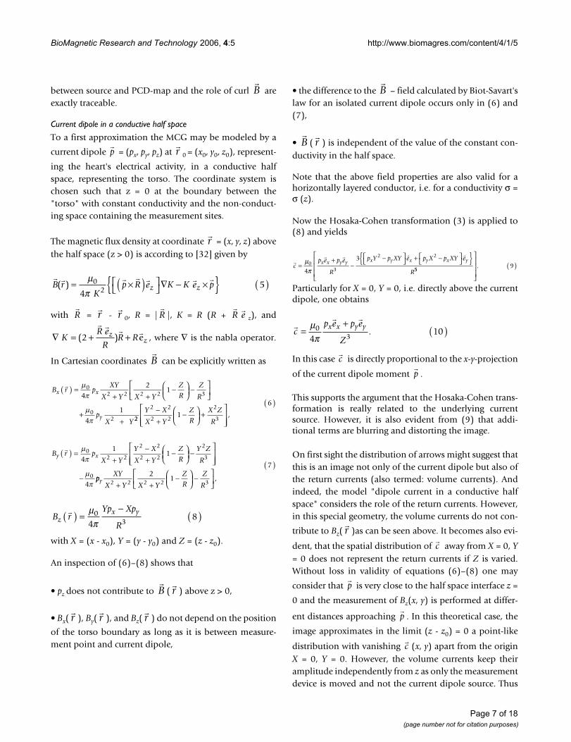
A closer look to just one component (e.g. the x-compo-

nent) of reveals that it is composed of two terms The spatial distribution of both terms is shown in Fig. 6 asa solid line. While the first term – shown as a dotted line

c

c

cB

y

p

R

Y Yp Xp

Rx

z x x y=

∂∂

= −−⎡⎣ ⎤⎦

⎡

⎣

⎢⎢

⎤

⎦

⎥⎥

μπ0

3 54

3. (11))

Spatial dependence of |p| along the symmetry axis orthogonal to the dipole directionFigure 6Spatial dependence of | p| along the symmetry axis orthogonal to the dipole direction. Dashed line: refers to the first term in eq. (11); dotted line: refers to the second term in eq. (11); solid line: both terms. Same data as in Fig. 5, however the direction of the dipole is in x-direction.

c



– is radially symmetric the second term is not. Along thesymmetry axis parallel to the direction of the dipole thislatter term is vanishing, see the dotted line in Fig. 6.Unfortunately the second term is of the same order ofmagnitude as the first term. Thus cx is not directly propor-tional to px as the second term contains mixed terms.However, it contributes a kind of focussing effect.

Current dipole in a conductive sphere

For a current dipole at 0 in a conductive sphere simi-

lar relations can be obtained in terms of spherical coordi-

nates r, ϑ, j. The magnetic flux density outside the sphereis given by [32]

with F = R(r R + ), = - 0, R = | |, r = | |, and

∇F = [r-1 R2 + R-1 ( ) + 2R +2r] - [R + 2r + R-1

( )] 0.

This expression is valid for a conductivity profile σ = σ (r).

For the case of the dipole being positioned on the z-axis at

0 = (0, 0, z0) the radial component of ( ) becomes

with R = (r2 - 2 z0 r cosϑ + )1/2.

Then for the pseudo current density the following relation

gained from curl in spherical coordinates may beapplied to (13) leading to

Particularly for ϑ = 0, i. e. directly above the currentdipole, one obtains

Thus the discussion of the results follows the same lines asin the preceding chapter.

Pseudo current density maps for MNG and MEG recordingsIn Fig. 7 isocontour and PCD-maps of an MNG recordingusing 49 channels of a planar SQUID system are shown.The centre of the system was placed over the lumbar spinewith a distance of approximately 8 cm between the mag-netic sensors and leg nerves coming from the left leg enter-ing the spine. The nerve response to electrical stimulationat the ankle with amplitude of about 10 mA and durationof 100 μs was recorded. 9.000 responses were averaged toimprove the pure signal-to-noise ratio. In Fig. 7, top, anisocontour map of the Bz-field component 15 ms after thestimulus and in Fig. 7, bottom, the corresponding PCD-map are shown. Inspecting the isocontour map from Fig.7 only a raw understanding of an underlying current andits direction corresponding to the zero line of the map ispossible for an expert. The PCD-map allows a more intu-itive conclusion that the underlying nerve current isextremely extended and slightly curved.

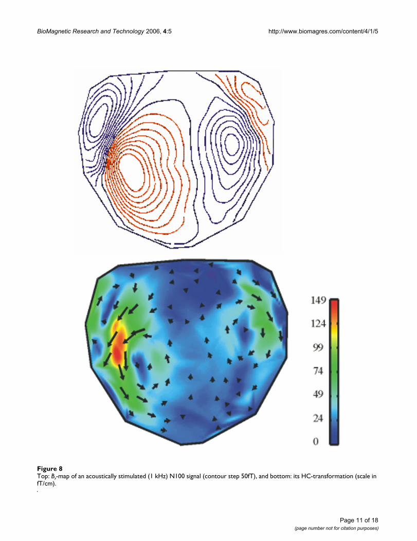
Fig. 8 displays maps of an acoustically evoked MEGrecorded in a helmet system with 93 channels. The spher-ical maps are unfolded, the nose is situated at the top, andears are at the right and left side, respectively. The meas-urement recorded the brain response to acoustic stimula-tion with a 1 kHz sinusoidal tone. 30 stimuli wereaveraged. In Fig. 8, top, an isocontour map of the radialfield component at the occurrence of the maximum of theresponse (about 100 ms after stimulus; termed "N100") isshown and in Fig. 8, bottom, the corresponding PCD-map. Using the isocontour map from Fig. 8 the number ofsources and their configuration cannot be concluded. Onthe other hand from inspecting the PCD-map one canconclude that two separate focal sources are active, one ineach hemisphere in the corresponding acoustic cortex.

DiscussionAlternative pseudo current density maps and corresponding hardware realizations

The Hosaka-Cohen transformation is nothing else but acombination of partial derivatives of components of

( ). Planar gradiometers are hardware realizations thatprovide an approximation of the partial derivative of

( ). Thus, the SQUID-chip introduced by [33], whichis a combination of x- and y-gradiometers, provides -if

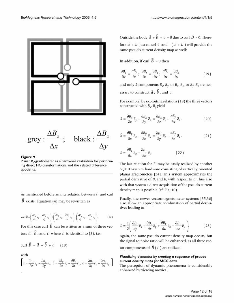
wired accordingly- just the approximation of (x, y) (cf.Fig. 9). Consequently, the software of the first SQUID-sys-tems of that design contained a program called "arrowmapper".

p r

B rF

F p r p r r F( ) ( ) ( )= × − × ⋅⎡⎣ ⎤⎦ ∇{ } ( )μπ

02 0 0

412

r R R r r R r

r R r

r R r

r B r

Bz p p

Rr

x y=−

( )μπ

ϕ ϕ0 034

13sin ( sin cos )ϑ

z02

cr

Be

r

Ber r=

∂∂

−∂∂

( )1 114

sinϑ ϑϑϕ ϕ

B

cz

r Rp p e p p

z rx y x y= +( ) − −( ) −

μπ

ϕ ϕ ϕ ϕ0 03

0

4

3

cos sin sin cos cos

siϑ ϑ

nn2

215

ϑR

e⎛

⎝⎜⎜

⎞

⎠⎟⎟

⎡

⎣⎢⎢

⎤

⎦⎥⎥

( )ϕ

cz

z z zp e p ex x y y=

−+( ) ( )μ

π0 0

034

16( )

.

B r

B r

c




Top: Bz-map of an electrically stimulated nerve signal recorded over the lumbar spine (contour step 1fT), and bottom: its HC-transformation (scale in fT/cm)Figure 7Top: Bz-map of an electrically stimulated nerve signal recorded over the lumbar spine (contour step 1fT), and bottom: its HC-transformation (scale in fT/cm).



Top: Br-map of an acoustically stimulated (1 kHz) N100 signal (contour step 50fT), and bottom: its HC-transformation (scale in fT/cm)Figure 8Top: Br-map of an acoustically stimulated (1 kHz) N100 signal (contour step 50fT), and bottom: its HC-transformation (scale in fT/cm).


As mentioned before an interrelation between and curl

exists. Equation (4) may be rewritten as

For this case curl can be written as a sum of three vec-

tors , , and where is identical to (3), i.e.

curl = + + (18)

with

.

Outside the body + + = 0 due to curl = 0. There-

fore + just cancel and – ( + ) will provide thesame pseudo current density map as well!

In addition, if curl = 0 then

and only 2 components Bx, By, or Bx, Bz, or By, Bz are nec-

essary to construct , , and .

For example, by exploiting relations (19) the three vectorsconstructed with Bx, By yield

The last relation for may be easily realized by anotherSQUID-system hardware consisting of vertically orientedplanar gradiometers [34]. This system approximates thepartial derivative of By and Bx with respect to z. Thus also

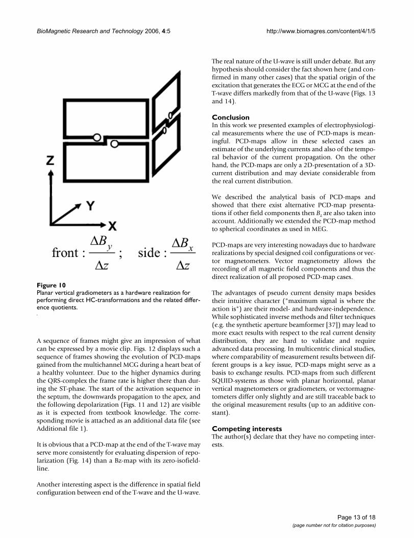
with that system a direct acquisition of the pseudo currentdensity map is possible (cf. Fig. 10).

Finally, the newer vectormagnetometer systems [35,36]also allow an appropriate combination of partial deriva-tives leading to

Again, the same pseudo current density map occurs, butthe signal to noise ratio will be enhanced, as all three vec-

tor components of ( ) are utilized.

Visualizing dynamics by creating a sequence of pseudo current density maps for MCG dataThe perception of dynamic phenomena is considerablyenhanced by viewing movies.

c

B

curl BB

ze

B

ye

B

xe

B

zex

yx

zy

zy

x=∂∂

−∂∂

⎛

⎝⎜

⎞

⎠⎟ +

∂∂

−∂∂

⎛

⎝⎜⎜

⎞

⎠⎟⎟ +

∂∂∂

−∂∂

⎛

⎝⎜

⎞

⎠⎟ ( )B

ye

B

xez

xz

y . 17

B

a b c c

B a b c

[ ; ;aB

ze

B

ye b

B

xe

B

ze c

B

yex

yx

zy

zy

xz

x= ∂∂

− ∂∂

=∂∂

−∂∂

= ∂∂

− ∂

BB

xezy∂.]

a b c B

a b c a b

B

∂∂

=∂∂

∂∂

=∂∂

∂∂

=∂∂

( )B

y

B

z

B

z

B

x

B

x

B

yz y x z y x; ; 19

a b c

aB

ze

B

ye

B

ze

B

xex

yx

zx

yy

z=∂∂

−∂∂

=∂∂

−∂∂

( ), 20

bB

xe

B

ze

B

ye

B

ze

yz

yx

xz

yx=

∂∂

−∂∂

=∂∂

−∂∂

( ), 21

cB

ze

B

ze

yx

xy=

∂∂

−∂∂

( ). 22

c

cB

ye

B

xe

B

ze

B

zez

xz

yy

xx

y=∂∂

−∂∂

+∂∂

−∂∂

⎛

⎝⎜⎜

⎞

⎠⎟⎟ ( )1

223.

B r

Planar Bz-gradiometer as a hardware realization for perform-ing direct HC-transformations and the related difference quotientsFigure 9Planar Bz-gradiometer as a hardware realization for perform-ing direct HC-transformations and the related difference quotients.



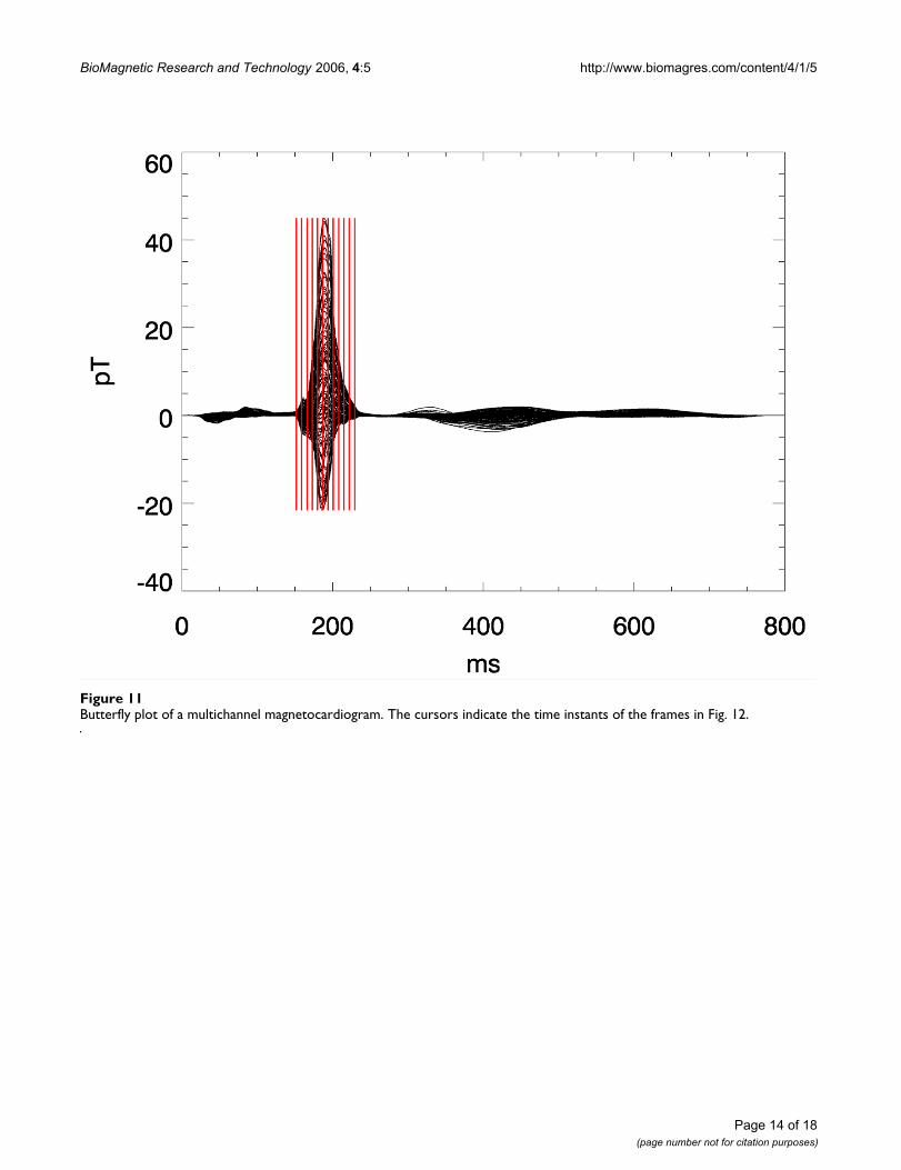
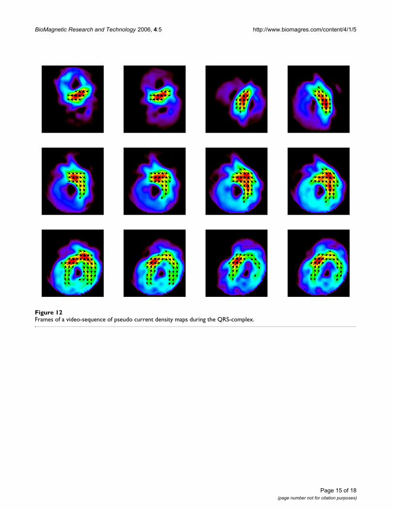
A sequence of frames might give an impression of whatcan be expressed by a movie clip. Figs. 12 displays such asequence of frames showing the evolution of PCD-mapsgained from the multichannel MCG during a heart beat ofa healthy volunteer. Due to the higher dynamics duringthe QRS-complex the frame rate is higher there than dur-ing the ST-phase. The start of the activation sequence inthe septum, the downwards propagation to the apex, andthe following depolarization (Figs. 11 and 12) are visibleas it is expected from textbook knowledge. The corre-sponding movie is attached as an additional data file (seeAdditional file 1).

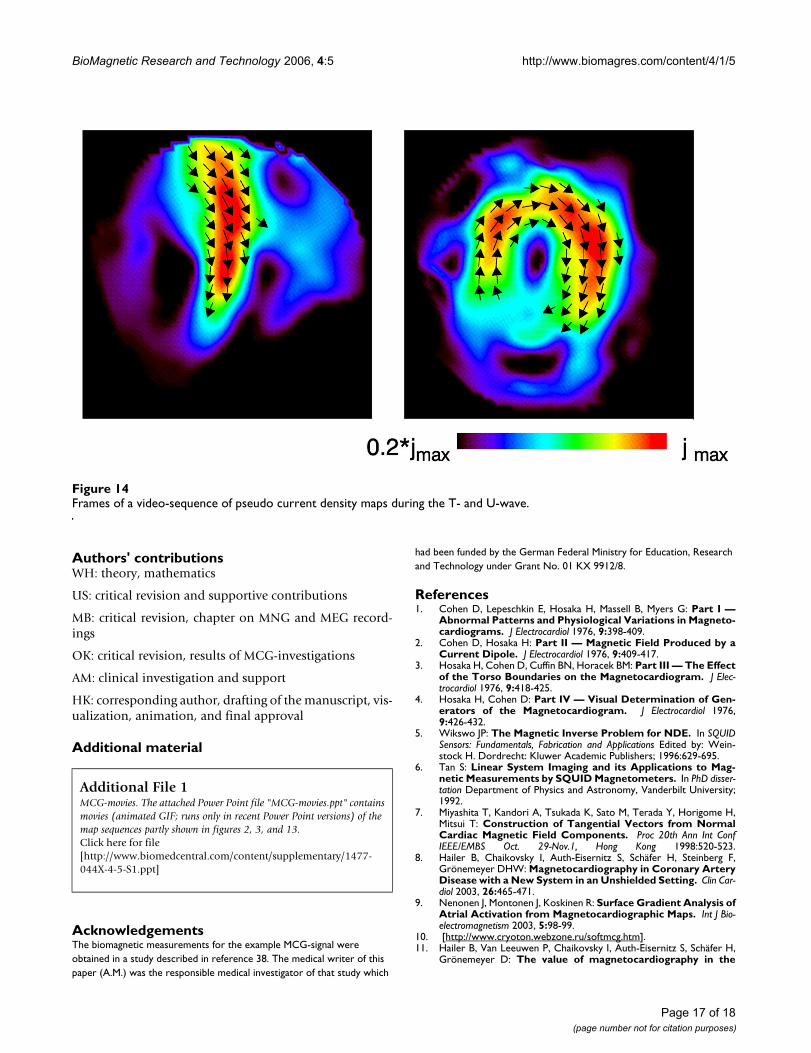
It is obvious that a PCD-map at the end of the T-wave mayserve more consistently for evaluating dispersion of repo-larization (Fig. 14) than a Bz-map with its zero-isofield-line.

Another interesting aspect is the difference in spatial fieldconfiguration between end of the T-wave and the U-wave.

The real nature of the U-wave is still under debate. But anyhypothesis should consider the fact shown here (and con-firmed in many other cases) that the spatial origin of theexcitation that generates the ECG or MCG at the end of theT-wave differs markedly from that of the U-wave (Figs. 13and 14).

ConclusionIn this work we presented examples of electrophysiologi-cal measurements where the use of PCD-maps is mean-ingful. PCD-maps allow in these selected cases anestimate of the underlying currents and also of the tempo-ral behavior of the current propagation. On the otherhand, the PCD-maps are only a 2D-presentation of a 3D-current distribution and may deviate considerable fromthe real current distribution.

We described the analytical basis of PCD-maps andshowed that there exist alternative PCD-map presenta-tions if other field components then Bz are also taken intoaccount. Additionally we extended the PCD-map methodto spherical coordinates as used in MEG.

PCD-maps are very interesting nowadays due to hardwarerealizations by special designed coil configurations or vec-tor magnetometers. Vector magnetometry allows therecording of all magnetic field components and thus thedirect realization of all proposed PCD-map cases.

The advantages of pseudo current density maps besidestheir intuitive character ("maximum signal is where theaction is") are their model- and hardware-independence.While sophisticated inverse methods and filter techniques(e.g. the synthetic aperture beamformer [37]) may lead tomore exact results with respect to the real current densitydistribution, they are hard to validate and requireadvanced data processing. In multicentric clinical studies,where comparability of measurement results between dif-ferent groups is a key issue, PCD-maps might serve as abasis to exchange results. PCD-maps from such differentSQUID-systems as those with planar horizontal, planarvertical magnetometers or gradiometers, or vectormagne-tometers differ only slightly and are still traceable back tothe original measurement results (up to an additive con-stant).

Competing interestsThe author(s) declare that they have no competing inter-ests.

Planar vertical gradiometers as a hardware realization for performing direct HC-transformations and the related differ-ence quotientsFigure 10Planar vertical gradiometers as a hardware realization for performing direct HC-transformations and the related differ-ence quotients.




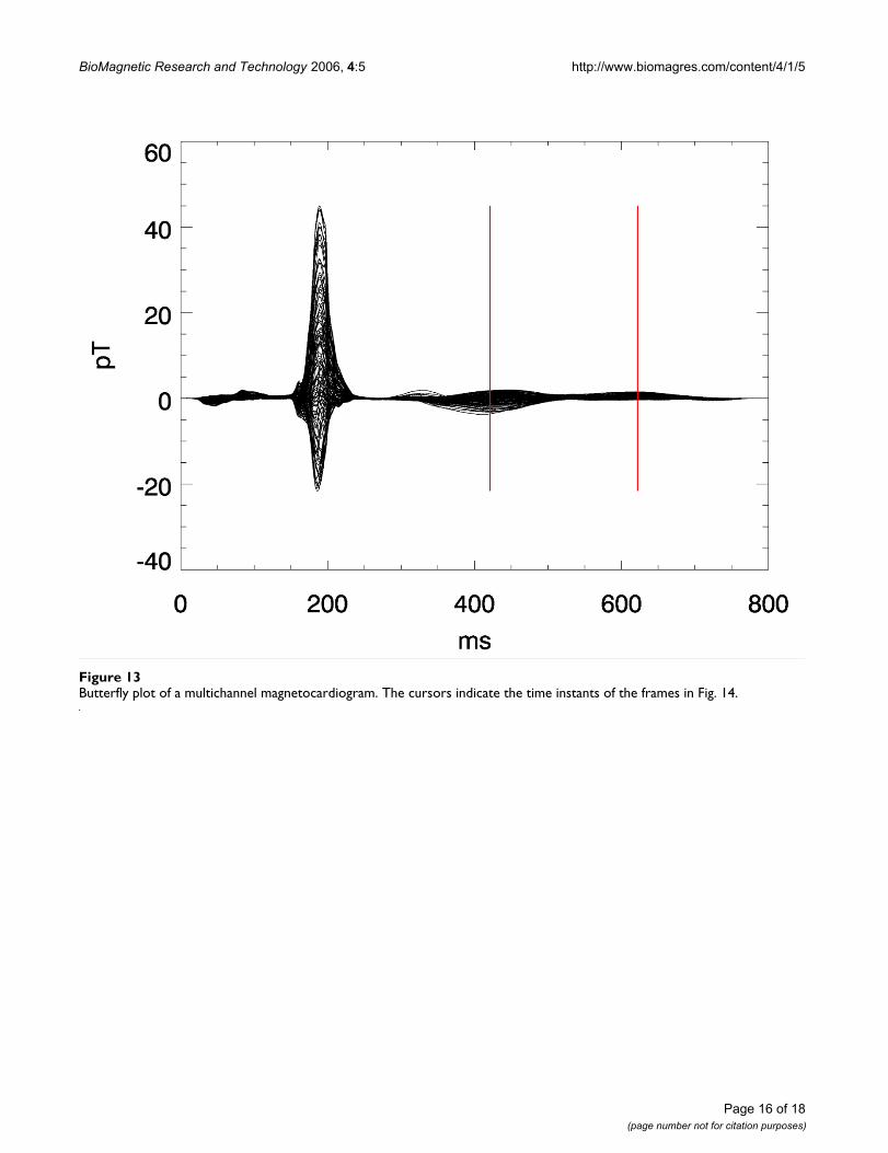
Butterfly plot of a multichannel magnetocardiogramFigure 11Butterfly plot of a multichannel magnetocardiogram. The cursors indicate the time instants of the frames in Fig. 12.



Frames of a video-sequence of pseudo current density maps during the QRS-complexFigure 12Frames of a video-sequence of pseudo current density maps during the QRS-complex.



Butterfly plot of a multichannel magnetocardiogramFigure 13Butterfly plot of a multichannel magnetocardiogram. The cursors indicate the time instants of the frames in Fig. 14.


Authors' contributionsWH: theory, mathematics

US: critical revision and supportive contributions

MB: critical revision, chapter on MNG and MEG record-ings

OK: critical revision, results of MCG-investigations

AM: clinical investigation and support

HK: corresponding author, drafting of the manuscript, vis-ualization, animation, and final approval

Additional material

AcknowledgementsThe biomagnetic measurements for the example MCG-signal were obtained in a study described in reference 38. The medical writer of this paper (A.M.) was the responsible medical investigator of that study which

had been funded by the German Federal Ministry for Education, Research and Technology under Grant No. 01 KX 9912/8.

References1. Cohen D, Lepeschkin E, Hosaka H, Massell B, Myers G: Part I —

Abnormal Patterns and Physiological Variations in Magneto-cardiograms. J Electrocardiol 1976, 9:398-409.

2. Cohen D, Hosaka H: Part II — Magnetic Field Produced by aCurrent Dipole. J Electrocardiol 1976, 9:409-417.

3. Hosaka H, Cohen D, Cuffin BN, Horacek BM: Part III — The Effectof the Torso Boundaries on the Magnetocardiogram. J Elec-trocardiol 1976, 9:418-425.

4. Hosaka H, Cohen D: Part IV — Visual Determination of Gen-erators of the Magnetocardiogram. J Electrocardiol 1976,9:426-432.

5. Wikswo JP: The Magnetic Inverse Problem for NDE. In SQUIDSensors: Fundamentals, Fabrication and Applications Edited by: Wein-stock H. Dordrecht: Kluwer Academic Publishers; 1996:629-695.

6. Tan S: Linear System Imaging and its Applications to Mag-netic Measurements by SQUID Magnetometers. In PhD disser-tation Department of Physics and Astronomy, Vanderbilt University;1992.

7. Miyashita T, Kandori A, Tsukada K, Sato M, Terada Y, Horigome H,Mitsui T: Construction of Tangential Vectors from NormalCardiac Magnetic Field Components. Proc 20th Ann Int ConfIEEE/EMBS Oct. 29-Nov.1, Hong Kong 1998:520-523.

8. Hailer B, Chaikovsky I, Auth-Eisernitz S, Schäfer H, Steinberg F,Grönemeyer DHW: Magnetocardiography in Coronary ArteryDisease with a New System in an Unshielded Setting. Clin Car-diol 2003, 26:465-471.

9. Nenonen J, Montonen J, Koskinen R: Surface Gradient Analysis ofAtrial Activation from Magnetocardiographic Maps. Int J Bio-electromagnetism 2003, 5:98-99.

10. [http://www.cryoton.webzone.ru/softmcg.htm].11. Hailer B, Van Leeuwen P, Chaikovsky I, Auth-Eisernitz S, Schäfer H,

Grönemeyer D: The value of magnetocardiography in the

Additional File 1MCG-movies. The attached Power Point file "MCG-movies.ppt" contains movies (animated GIF; runs only in recent Power Point versions) of the map sequences partly shown in figures 2, 3, and 13.Click here for file[http://www.biomedcentral.com/content/supplementary/1477-044X-4-5-S1.ppt]

Frames of a video-sequence of pseudo current density maps during the T- and U-waveFigure 14Frames of a video-sequence of pseudo current density maps during the T- and U-wave.


http://www.biomedcentral.com/content/supplementary/1477-044X-4-5-S1.ppt












http://www.cryoton.webzone.ru/softmcg.htm



Publish with BioMed Central and every scientist can read your work free of charge

"BioMed Central will be the most significant development for disseminating the results of biomedical research in our lifetime."

Sir Paul Nurse, Cancer Research UK

Your research papers will be:

available free of charge to the entire biomedical community

peer reviewed and published immediately upon acceptance

cited in PubMed and archived on PubMed Central

yours — you keep the copyright

Submit your manuscript here:http://www.biomedcentral.com/info/publishing_adv.asp

BioMedcentral

course of coronary intervention. Ann Noninvasive Electrocardiol2005, 10(2):188-96.

12. Hailer B, Chaikovsky I, Auth-Eisernitz S, Schafer H, Van Leeuwen P:The value of magnetocardiography in patients with and with-out relevant stenoses of the coronary arteries using anunshielded system. Pacing Clin Electrophysiol 2005, 28(1):8-16.

13. Koch H: Recent advances in magnetocardiography. J Electro-cardiol 2004, 37(Suppl):117-22.

14. Kandori A, Shimizu W, Yokokawa M, Kamakura S, Miyatake K,Murakami M, Miyashita T, Ogata K, Tsukada K: Reconstruction ofaction potential of repolarization in patients with congenitallong-QT syndrome. Phys Med Biol 2004, 49(10):2103-15.

15. Kandori A, Shimizu W, Yokokawa M, Noda T, Kamakura S, MiyatakeK, Murakami M, Miyashita T, Ogata K, Tsukada K: Identifying pat-terns of spatial current dispersion that characterise and sep-arate the Brugada syndrome and complete right-bundlebranch block. Med Biol Eng Comput 2004, 42(2):236-44.

16. Kandori A, Shimizu W, Yokokawa M, Maruo T, Kanzaki H, NakataniS, Kamakura S, Miyatake K, Murakami M, Miyashita T, Ogata K, Tsu-kada K: Detection of spatial repolarization abnormalities inpatients with LQT1 and LQT2 forms of congenital long-QTsyndrome. Physiol Meas 2002, 23(4):603-14.

17. Sato M, Terada Y, Mitsui T, Miyashita T, Kandori A, Tsukada K: Vis-ualization of atrial excitation by magnetocardiogram. Int JCardiovasc Imaging 2002, 18(4):305-12.

18. Kandori A, Kanzaki H, Miyatake K, Hashimoto S, Itoh S, Tanaka N,Miyashita T, Tsukada K: A method for detecting myocardialabnormality by using a current-ratio map calculated from anexercise-induced magnetocardiogram. Med Biol Eng Comput2001, 39(1):29-34.

19. Tsukada K, Miyashita T, Kandori A, Mitsui T, Terada Y, Sato M,Shiono J, Horigome H, Yamada S, Yamaguchi I: An iso-integralmapping technique using magnetocardiogram, and its possi-ble use for diagnosis of ischemic heart disease. Int J Card Imag-ing 2000, 16(1):55-66.

20. Kandori A, Kanzaki H, Miyatake K, Hashimoto S, Itoh S, Tanaka N,Miyashita T, Tsukada K: A method for detecting myocardialabnormality by using a total current-vector calculated fromST-segment deviation of a magnetocardiogram signal. MedBiol Eng Comput 2001, 39(1):21-8.

21. Weber Dos Santos R, Kosch O, Steinhoff U, Bauer S, Trahms L, KochH: MCG to ECG source differences: measurements and atwo-dimensional computer model study. J Electrocardiol 2004,37(Suppl):123-7.

22. Kandori A, Miyashita T, Tsukada K, Hosono T, Miyashita S, Chiba Y,Horigome H, Shigemitsu S, Asaka M: Prenatal diagnosis of QTprolongation by fetal magnetocardiogram – use of QRS andT-wave current-arrow maps. Physiol Meas 2001, 22(2):377-87.

23. Kandori A, Hosono T, Kanagawa T, Miyashita S, Chiba Y, MurakamiM, Miyashita T, Tsukada K: Detection of atrial-flutter and atrial-fibrillation waveforms by fetal magnetocardiogram. Med BiolEng Comput 2002, 40(2):213-7.

24. Hosono T, Shinto M, Chiba Y, Kandori A, Tsukada K: Prenatal diag-nosis of fetal complete atrioventricular block with QT pro-longation and alternating ventricular pacemakers usingmulti-channel magnetocardiography and current-arrowmaps. Fetal Diagn Ther 2002, 17(3):173-6.

25. Kandori A, Oe H, Miyashita K, Ohira S, Naritomi H, Chiba Y, OgataK, Murakami M, Miyashita T, Tsukada K: Magneto-encephalo-graphic measurement of neural activity during period of ver-tigo induced by cold caloric stimulation. Neurosci Res 2003,46(3):281-8.

26. Oe H, Kandori A, Murakami M, Miyashita K, Tsukada K, Naritomi H:Cortical functional abnormality assessed by auditory-evokedmagnetic fields and therapeutic approach in patients withchronic dizziness. Brain Res 2002, 957(2):373-81.

27. Kandori A, Oe H, Miyashita K, Date H, Yamada N, Naritomi H, ChibaY, Murakami M, Miyashita T, Tsukada K: Visualisation method ofspatial interictal discharges in temporal epilepsy patientsusing magneto-encephalogram. Med Biol Eng Comput 2002,40(3):327-31.

28. Burghoff M, Mackert BM, Haberkorn W: Visualization of actioncurrents in peripheral nerves from the biomagnetic field.Biomed Tech 2005, 50(Suppl 1/1):179-80.

29. Koch H: SQUID Magnetocardiography: Status and Perspec-tives. IEEE Trans Appl Superconductivity 2001, 11:49-59.

30. Hämäläinen M, Hari R, Ilmoniemi RJ, Knuutila J, Lounasmaa O: Mag-netoencephalography – Theory, Instrumentation, and Appli-cations to Noninvasive Studies of the Working HumanBrain. Rev Mod Phys 1993, 65:413-497.

31. Kosch O, Burghoff M, Jazbinsek V, Steinhoff U, Trontelj Z, Trahms L:Extended source models in integrated body surface poten-tial and magnetic field mapping. Biomed Eng 2001, 46(Suppl2):144-146.

32. Sarvas J: Basic Mathematical and Electromagnetic Conceptsof the Biomagnetic Inverse Problem. Phys Med Biol 1987,32:11-22.

33. Hämäläinen MS: A 24-Channel Planar Gradiometer: SystemDesign and Analysis of Neuromagnetic Data. In Advances inBiomagnetism Edited by: Williamson SJ, Hoke M, Stroink G, Kotani M.New York: Plenum Press; 1989:639-644.

34. Kandori A, Tsukada K, Haruta Y, Noda Y, Terada Y, Mitsui T, Seki-hara K: Reconstruction of two-dimensional Current Distribu-tion from Tangential MCG measurement. Phys Med Biol 1996,41:1705-1716.

35. Burghoff M, Schleyerbach H, Drung D, Trahms L, Koch H: A VectorMagnetometer Module for Biomagnetic Application. IEEETrans Appl Superconductivity 1999, 9:4069-4072.

36. Stolz R, Zakosarenko V, Schulz M, Chwala A, Fritzsch L, Meyer HG,Koestlin EO: Magnetic full-tensor SQUID gradiometer systemfor geophysical applications. The Leading Edge 2006,25(2):178-180.

37. Robinson SE, Vrba J: Functional Neuroimaging by SyntheticAperture Magnetometry (SAM). In Recent Advances in Biomag-netism, Proc 11th Int Conf Biomagnetism Edited by: Yoshimoto T, KotaniM, Kuriki S, Karibe H, Nakasato N. Sendai: Tohoku University Press;1999:302-305.

38. Morguet A, Behrens S, Kosch O, Lange C, Zabel M, Selbig D, MunzDL, Schultheiss HP, Koch H: Myocardial Viability Evaluationusing Magnetocardiography in Patients with CoronaryArtery Disease. Coronary Artery Disease 2004, 15(3):155-162.






















































http://www.biomedcentral.com/info/publishing_adv.asp


BioMagnetic Research and Technology - Springer LINK

Documents