B.Data V6.0 - Operation ___________________ ___________________ ___________________ ___________________ ___________________ ___________________ ___________________ ___________________ ___________________ ___________________ ___________________ ___________________ ___________________ SIMATIC B.Data V6.0 - Operation Operating Manual 04/2014 A5E31981489-AB Introduction 1 B.Data Plant Explorer 2 Configuring master data 3 Calculation level 1 "The loop concept" 4 Calculation level 2 "The MEVA concept" 5 Calculation level 3 "Report and visualization concept" 6 Historizing calculation logic 7 Schedule management 8 Document management 9 Administration 10 Using B.Data Web 11 Using B.Data Mobile 12 Reference 13

Welcome message from author
This document is posted to help you gain knowledge. Please leave a comment to let me know what you think about it! Share it to your friends and learn new things together.
Transcript
B.Data V6.0 - Operation
___________________
___________________
___________________
___________________
___________________
___________________
___________________
___________________
___________________
___________________
___________________
___________________
___________________
SIMATIC
B.Data V6.0 - Operation
Operating Manual
04/2014 A5E31981489-AB
Introduction 1
B.Data Plant Explorer 2
Configuring master data 3
Calculation level 1 "The loop concept"
4
Calculation level 2 "The MEVA concept"
5
Calculation level 3 "Report and visualization concept"
6
Historizing calculation logic 7
Schedule management 8
Document management 9
Administration 10
Using B.Data Web 11
Using B.Data Mobile 12
Reference 13
Siemens AG Industry Sector Postfach 48 48 90026 NÜRNBERG GERMANY
A5E31981489-AB Ⓟ 04/2014 Subject to change
Copyright © Siemens AG 2012 - 2014. All rights reserved
Legal information Warning notice system
This manual contains notices you have to observe in order to ensure your personal safety, as well as to prevent damage to property. The notices referring to your personal safety are highlighted in the manual by a safety alert symbol, notices referring only to property damage have no safety alert symbol. These notices shown below are graded according to the degree of danger.
DANGER indicates that death or severe personal injury will result if proper precautions are not taken.
WARNING indicates that death or severe personal injury may result if proper precautions are not taken.
CAUTION indicates that minor personal injury can result if proper precautions are not taken.
NOTICE indicates that property damage can result if proper precautions are not taken.
If more than one degree of danger is present, the warning notice representing the highest degree of danger will be used. A notice warning of injury to persons with a safety alert symbol may also include a warning relating to property damage.
Qualified Personnel The product/system described in this documentation may be operated only by personnel qualified for the specific task in accordance with the relevant documentation, in particular its warning notices and safety instructions. Qualified personnel are those who, based on their training and experience, are capable of identifying risks and avoiding potential hazards when working with these products/systems.
Proper use of Siemens products Note the following:
WARNING Siemens products may only be used for the applications described in the catalog and in the relevant technical documentation. If products and components from other manufacturers are used, these must be recommended or approved by Siemens. Proper transport, storage, installation, assembly, commissioning, operation and maintenance are required to ensure that the products operate safely and without any problems. The permissible ambient conditions must be complied with. The information in the relevant documentation must be observed.
Trademarks All names identified by ® are registered trademarks of Siemens AG. The remaining trademarks in this publication may be trademarks whose use by third parties for their own purposes could violate the rights of the owner.
Disclaimer of Liability We have reviewed the contents of this publication to ensure consistency with the hardware and software described. Since variance cannot be precluded entirely, we cannot guarantee full consistency. However, the information in this publication is reviewed regularly and any necessary corrections are included in subsequent editions.
B.Data V6.0 - Operation Operating Manual, 04/2014, A5E31981489-AB 3
Table of contents
1 Introduction ........................................................................................................................................... 11
1.1 Why we need energy management ............................................................................................. 11
1.2 How can B.Data support energy management? .......................................................................... 12
1.3 Areas of application ..................................................................................................................... 13
1.4 Preface ......................................................................................................................................... 14
2 B.Data Plant Explorer ............................................................................................................................ 15
2.1 Plant Explorer as navigation tool ................................................................................................. 15
2.2 Objects in Plant Explorer ............................................................................................................. 17 2.2.1 Object basics ................................................................................................................................ 17 2.2.2 Creating an object ........................................................................................................................ 20 2.2.3 Object properties .......................................................................................................................... 21 2.2.3.1 Opening properties ...................................................................................................................... 21 2.2.3.2 Assigning properties .................................................................................................................... 23 2.2.3.3 Defining custom properties .......................................................................................................... 25 2.2.4 Object management ..................................................................................................................... 26 2.2.4.1 Object management basics ......................................................................................................... 26 2.2.4.2 Managing objects ......................................................................................................................... 28 2.2.5 Displaying object relations ........................................................................................................... 30 2.2.6 Object naming conventions .......................................................................................................... 32 2.2.7 Search for object .......................................................................................................................... 33
2.3 Configuring Quicklinks ................................................................................................................. 35 2.3.1 Create Quicklinks ......................................................................................................................... 35 2.3.2 Edit Quicklinks.............................................................................................................................. 37
3 Configuring master data ........................................................................................................................ 39
3.1 Configuring data acquisition ......................................................................................................... 39 3.1.1 Creating hardware ....................................................................................................................... 39 3.1.2 Logging the acquisition component onto the B.Data server ........................................................ 41 3.1.2.1 Logging the acquisition component onto the B.Data server for the first time .............................. 41 3.1.2.2 Managing the acquisition component .......................................................................................... 44 3.1.2.3 Areas in the B.Data acquisition configuration .............................................................................. 45 3.1.3 Configuring interfaces for data acquisition ................................................................................... 50 3.1.3.1 Interface management basics ...................................................................................................... 50 3.1.3.2 Acquisition wizard for interface configuration .............................................................................. 51 3.1.3.3 Configuring data acquisition via the "S7" interface ...................................................................... 57 3.1.3.4 Configuring data acquisition via the "WinCC/PCS7" interface .................................................... 59 3.1.3.5 Configuring data acquisition via the "Modbus" interface .............................................................. 61 3.1.3.6 Configuring data acquisition via the "OPC-DA / OPC-HDA" interface ......................................... 64 3.1.3.7 Configuring data acquisition via the "OLE-DB" interface ............................................................. 67 3.1.3.8 Configuring data acquisition via the "FTP" interface .................................................................... 69 3.1.3.9 Configuring data acquisition via the "Simulation" interface.......................................................... 71 3.1.4 Advanced configuration ............................................................................................................... 72
Table of contents
B.Data V6.0 - Operation 4 Operating Manual, 04/2014, A5E31981489-AB
3.1.5 Starting the kernel service ........................................................................................................... 74
3.2 Create printer and directory ........................................................................................................ 76 3.2.1 Fundamentals of creating printer and directory .......................................................................... 76 3.2.2 Creating a printer ........................................................................................................................ 77 3.2.3 Creating a folder .......................................................................................................................... 79
3.3 Configuring authorizations .......................................................................................................... 81 3.3.1 Basic information on authorizations ............................................................................................ 81 3.3.2 Setting up users .......................................................................................................................... 83 3.3.3 Configuring authorizations .......................................................................................................... 90
3.4 Configuring units ......................................................................................................................... 97
3.5 Configuring cycle times ............................................................................................................... 99
3.6 Configuring query types ............................................................................................................ 100
3.7 Creating objects for Enterprise Resource Planning .................................................................. 102 3.7.1 Basics on objects for Enterprise Resource Planning ................................................................ 102 3.7.2 Creating ERP domains .............................................................................................................. 103 3.7.3 Creating service types ............................................................................................................... 104 3.7.4 Creating cost centers ................................................................................................................ 105 3.7.5 Creating cost center relations ................................................................................................... 106
3.8 Managing energy efficiency measures ..................................................................................... 107 3.8.1 Basics on managing energy efficiency measures ..................................................................... 107 3.8.2 Creating energy efficiency measures ........................................................................................ 108 3.8.3 Entering financial saving potentials for an energy efficiency measure ..................................... 110 3.8.4 Calculating cost efficiency for energy efficiency measures ...................................................... 112 3.8.5 Specifying responsibilities for an energy efficiency measure ................................................... 114 3.8.6 Specifying clients for an energy efficiency measure ................................................................. 115 3.8.7 Inserting documents for an energy efficiency measure ............................................................ 116 3.8.8 Displaying information about an energy efficiency measure .................................................... 117 3.8.9 Generating a filtered overview object ........................................................................................ 118
4 Calculation level 1 "The loop concept" .................................................................................................. 121
4.1 Basic information on calculation level 1 .................................................................................... 121
4.2 Creating data points .................................................................................................................. 124 4.2.1 Creating generic data point ....................................................................................................... 124 4.2.2 Creating data points .................................................................................................................. 127 4.2.3 Creating constants .................................................................................................................... 130 4.2.4 Creating derived data points ..................................................................................................... 133 4.2.5 Configuring data point versioning ............................................................................................. 136 4.2.6 Configuring substitute value strategies for a data point ............................................................ 143 4.2.7 Configuring data point counters ................................................................................................ 145 4.2.8 Configuring data point limits ...................................................................................................... 148 4.2.9 Configuring the compression function for a data point ............................................................. 151 4.2.10 Configuring the export function for a data point ........................................................................ 154
4.3 Creating prototypes ................................................................................................................... 156 4.3.1 Configuring prototypes .............................................................................................................. 156
4.4 Creating loops ........................................................................................................................... 158 4.4.1 Configuring loops ...................................................................................................................... 158
4.5 Manual data acquisition ............................................................................................................ 162
Table of contents
B.Data V6.0 - Operation Operating Manual, 04/2014, A5E31981489-AB 5
4.5.1 Basics on the measured value editor ......................................................................................... 162 4.5.2 Opening the measured value editor ........................................................................................... 162 4.5.3 Manipulating values ................................................................................................................... 163 4.5.4 Filtering in the measurement value editor .................................................................................. 167 4.5.5 Exporting and importing process data ....................................................................................... 167 4.5.6 Configuring a matrix ................................................................................................................... 170
5 Calculation level 2 "The MEVA concept" ............................................................................................. 175
5.1 Introduction ................................................................................................................................ 175
5.2 Creating parameters .................................................................................................................. 177 5.2.1 Configuring parameters ............................................................................................................. 177
5.3 Configuring measurement variables .......................................................................................... 179
6 Calculation level 3 "Report and visualization concept" ......................................................................... 181
6.1 Basic information on calculation level 3 ..................................................................................... 181
6.2 Creating a report ........................................................................................................................ 183 6.2.1 Basics on reports ....................................................................................................................... 183 6.2.2 Creating a report ........................................................................................................................ 185 6.2.3 Configuring the query type for a report ...................................................................................... 187 6.2.4 Configuring a module for reports ............................................................................................... 190 6.2.5 Basic information on configuring the report template in Microsoft Excel ................................... 193 6.2.6 Configuring a report template .................................................................................................... 195 6.2.7 Entering values in reports .......................................................................................................... 197 6.2.8 Generating reports ..................................................................................................................... 198 6.2.9 Opening report results ............................................................................................................... 202
6.3 Creating trends........................................................................................................................... 204 6.3.1 Basics on trends......................................................................................................................... 204 6.3.2 Configuring trends ...................................................................................................................... 205 6.3.3 Generating trends ...................................................................................................................... 208 6.3.4 Importing data into the MS Office environment ......................................................................... 210
6.4 Creating visualization ................................................................................................................. 212 6.4.1 Basics on visualizations ............................................................................................................. 212 6.4.2 Configuring visualization ............................................................................................................ 213 6.4.3 Generating visualization ............................................................................................................. 221
6.5 Creating dashboards .................................................................................................................. 222 6.5.1 Dashboard basics ...................................................................................................................... 222 6.5.2 "Dashboard" editor ..................................................................................................................... 226 6.5.3 Create dashboard ...................................................................................................................... 229 6.5.4 Creating the dashboard layout ................................................................................................... 230 6.5.5 Configuring dashboard objects .................................................................................................. 233 6.5.6 Aligning dashboard objects ........................................................................................................ 237 6.5.7 Exporting/importing dashboards ................................................................................................ 238 6.5.8 Displaying the dashboard in full-screen mode ........................................................................... 239 6.5.9 Example of configuring a dashboard ......................................................................................... 241 6.5.9.1 Example of creating data points for the dashboard ................................................................... 241 6.5.9.2 Example for creating a dashboard ............................................................................................. 243 6.5.9.3 Example for displaying a dashboard .......................................................................................... 249
6.6 Using the Quick Chart ................................................................................................................ 251 6.6.1 Basic information on the Quick Chart ........................................................................................ 251
Table of contents
B.Data V6.0 - Operation 6 Operating Manual, 04/2014, A5E31981489-AB
6.6.2 Visualizing measured values in the Quick Chart ...................................................................... 256 6.6.3 Displaying details in the Quick Chart ........................................................................................ 257
7 Historizing calculation logic .................................................................................................................. 259
7.1 History management basics ...................................................................................................... 259
7.2 History management of data points .......................................................................................... 263
7.3 History management of measure variables .............................................................................. 265
7.4 History management of reports ................................................................................................. 266
8 Schedule management ........................................................................................................................ 269
8.1 Basic information on schedule management ............................................................................ 269
8.2 Creating a profile ....................................................................................................................... 273 8.2.1 Basic information on profile ....................................................................................................... 273 8.2.2 Configuring states ..................................................................................................................... 274 8.2.3 Configuring typical day .............................................................................................................. 275 8.2.4 Configuring profiles ................................................................................................................... 277 8.2.4.1 Configuring profiles ................................................................................................................... 277 8.2.4.2 Selecting holidays for profile ..................................................................................................... 280 8.2.4.3 Using a calendar for a profile .................................................................................................... 282 8.2.5 Configuring root profiles ............................................................................................................ 284 8.2.6 Production-dependent forecasts ............................................................................................... 286 8.2.7 Special effects ........................................................................................................................... 286
8.3 Creating plants and material definitions .................................................................................... 288 8.3.1 Basic information on plants and material definitions ................................................................. 288 8.3.2 Configuring material .................................................................................................................. 290 8.3.3 Configuring the plant ................................................................................................................. 292 8.3.4 Using the batch list .................................................................................................................... 295 8.3.5 Creating consumption types...................................................................................................... 299
8.4 Example of schedule management ........................................................................................... 301 8.4.1 Configuring analysis reports...................................................................................................... 301 8.4.2 Configuring long-term forecast reports ..................................................................................... 307 8.4.3 Configuring schedule reports .................................................................................................... 312 8.4.4 Configuring daily load course reports ....................................................................................... 316 8.4.5 Configuring controlling reports .................................................................................................. 320 8.4.6 Configuring "Batch analysis" reports ......................................................................................... 323
9 Document management ....................................................................................................................... 331
9.1 Document management basics ................................................................................................ 331
9.2 Inserting documents .................................................................................................................. 333
9.3 Saving documents ..................................................................................................................... 334
9.4 Editing documents ..................................................................................................................... 336
10 Administration ...................................................................................................................................... 337
10.1 Logging Viewer ......................................................................................................................... 337 10.1.1 Using the Logging Viewer ......................................................................................................... 337 10.1.2 Security settings / Logging ........................................................................................................ 341
10.2 Message lists ............................................................................................................................ 343
Table of contents
B.Data V6.0 - Operation Operating Manual, 04/2014, A5E31981489-AB 7
10.2.1 Basic information on message lists............................................................................................ 343 10.2.2 Configuring custom message list ............................................................................................... 345 10.2.3 Configuring filter for a message list............................................................................................ 347 10.2.4 Configuring message notification ............................................................................................... 349 10.2.5 Configuring the view for a message list ..................................................................................... 351
10.3 Job queue .................................................................................................................................. 352 10.3.1 Using the job queue ................................................................................................................... 352
10.4 B.Data options............................................................................................................................ 354
10.5 B.Data Configuration .................................................................................................................. 368
10.6 Service Cockpit .......................................................................................................................... 370 10.6.1 Service Cockpit basics ............................................................................................................... 370 10.6.2 Using the Service Cockpit .......................................................................................................... 372
10.7 Task Management ..................................................................................................................... 377 10.7.1 Creating objects for Task Management ..................................................................................... 377
10.8 Countries .................................................................................................................................... 382 10.8.1 Basics of "Country" object type .................................................................................................. 382 10.8.2 Creating a "Country" object ........................................................................................................ 383 10.8.3 Assign time zone for acquisition or calculation .......................................................................... 386
10.9 Exporting and importing data ..................................................................................................... 389 10.9.1 Basic principles of export and import ......................................................................................... 389 10.9.2 Exporting data ............................................................................................................................ 390 10.9.3 Importing data ............................................................................................................................ 392
11 Using B.Data Web .............................................................................................................................. 395
11.1 Basics ......................................................................................................................................... 395 11.1.1 Basic information on B.Data Web .............................................................................................. 395 11.1.2 Navigation in B.Data Web .......................................................................................................... 398
11.2 Working with B.Data Web .......................................................................................................... 400 11.2.1 Logging on to the B.Data Web ................................................................................................... 400 11.2.2 Working with reports in B.Data Web .......................................................................................... 402 11.2.3 Working with trends in B.Data Web ........................................................................................... 407 11.2.4 Working with visualizations in B.Data Web ................................................................................ 410 11.2.5 Working with matrixes in B.Data Web ....................................................................................... 413 11.2.6 Using document management in B.Data Web ........................................................................... 415 11.2.7 Working with energy efficiency measures in B.Data Web ......................................................... 416 11.2.8 Working with dashboards in B.Data Web .................................................................................. 418 11.2.9 Configuring Quicklinks ............................................................................................................... 421 11.2.9.1 Create Quicklinks ....................................................................................................................... 421 11.2.9.2 Edit Quicklinks............................................................................................................................ 424
11.3 Administering B.Data Web ......................................................................................................... 428 11.3.1 Defining an entry point ............................................................................................................... 428 11.3.2 Authorizations for navigation ...................................................................................................... 429 11.3.3 Configuring Quicklinks in the B.Data client ................................................................................ 430
12 Using B.Data Mobile ........................................................................................................................... 433
12.1 B.Data Mobile basics ................................................................................................................. 433
12.2 Navigation structure of the "B.Data Mobile" application ............................................................ 434
Table of contents
B.Data V6.0 - Operation 8 Operating Manual, 04/2014, A5E31981489-AB
12.3 Configuring mobile devices in B.Data ....................................................................................... 435
12.4 Measured value input on the mobile device .............................................................................. 437
12.5 Synchronizing data on the mobile device ................................................................................. 439
12.6 Generating barcode .................................................................................................................. 440
13 Reference ............................................................................................................................................ 441
13.1 Acquisition status of a value...................................................................................................... 441
13.2 Correction status of a value ...................................................................................................... 442
13.3 Query types ............................................................................................................................... 443
13.4 Filter criteria for a message list ................................................................................................. 450
13.5 Time unit abbreviations ............................................................................................................. 451
13.6 Module overview ....................................................................................................................... 452
13.7 Display modes ........................................................................................................................... 493
13.8 Existing functional groups ......................................................................................................... 494
13.9 Operations for generating calculation blocks (prototypes) ........................................................ 496
13.10 Description of MCL .................................................................................................................... 506
13.11 Database functions for measurement variables........................................................................ 509
13.12 "Trends" editor........................................................................................................................... 549 13.12.1 Trender menu bar ..................................................................................................................... 549 13.12.2 Trender toolbar .......................................................................................................................... 551 13.12.3 Trender status bar ..................................................................................................................... 552 13.12.4 Trender legend .......................................................................................................................... 552 13.12.5 The configuration dialog ............................................................................................................ 553
13.13 Database jobs ........................................................................................................................... 570
13.14 Functions for Task Management .............................................................................................. 584
13.15 ASCII FTP formats .................................................................................................................... 589 13.15.1 ASCII FTP import interface ....................................................................................................... 589 13.15.2 APROL ...................................................................................................................................... 590 13.15.3 BDATA ...................................................................................................................................... 592 13.15.4 BDATA_XML_Format ................................................................................................................ 594 13.15.5 DALOG ...................................................................................................................................... 596 13.15.6 EXCELCSV ............................................................................................................................... 598 13.15.7 EXCELCSVNODST .................................................................................................................. 600 13.15.8 FREJA ....................................................................................................................................... 602 13.15.9 TextValue .................................................................................................................................. 604 13.15.10 ZenOn ....................................................................................................................................... 606
13.16 XML stylesheets ........................................................................................................................ 608 13.16.1 XML export interface ................................................................................................................. 608 13.16.2 bdatadanmk_1.xsl ..................................................................................................................... 609 13.16.3 bdatadanmk_8.xsl ..................................................................................................................... 610 13.16.4 bdatastd.xsl ............................................................................................................................... 611 13.16.5 bdatastdu.xsl ............................................................................................................................. 611 13.16.6 Freja.xsl ..................................................................................................................................... 613
Table of contents
B.Data V6.0 - Operation Operating Manual, 04/2014, A5E31981489-AB 9
13.16.7 LOKE_IDAP.xsl .......................................................................................................................... 614
13.17 SAP interface ............................................................................................................................. 615 13.17.1 DTD for the ERP interface ......................................................................................................... 615 13.17.2 Structure of the "Archive.CMD" file ............................................................................................ 618
13.18 Dashboard objects ..................................................................................................................... 619 13.18.1 Configuring the dashboard ......................................................................................................... 619 13.18.2 Configuring the time range ......................................................................................................... 620 13.18.3 Rounded rectangle ..................................................................................................................... 620 13.18.4 Ellipsis ........................................................................................................................................ 623 13.18.5 Line ............................................................................................................................................ 624 13.18.6 Polyline ....................................................................................................................................... 625 13.18.7 Image ......................................................................................................................................... 626 13.18.8 Traffic light .................................................................................................................................. 627 13.18.9 Value .......................................................................................................................................... 630 13.18.10 Value difference ......................................................................................................................... 633 13.18.11 Time selection ............................................................................................................................ 636 13.18.12 Status ......................................................................................................................................... 638 13.18.13 Bar chart ..................................................................................................................................... 641 13.18.14 Pie chart ..................................................................................................................................... 643 13.18.15 Line chart ................................................................................................................................... 645 13.18.16 Gauge ........................................................................................................................................ 647 13.18.17 Panel switch ............................................................................................................................... 649 13.18.18 Data table ................................................................................................................................... 653 13.18.19 Line for Sankey chart ................................................................................................................. 655 13.18.20 Polyline for Sankey chart ........................................................................................................... 657 13.18.21 Flow info ..................................................................................................................................... 659 13.18.22 Process ...................................................................................................................................... 661 13.18.23 Process overview ....................................................................................................................... 663
Index................................................................................................................................................... 665

Table of contents
B.Data V6.0 - Operation 10 Operating Manual, 04/2014, A5E31981489-AB
B.Data V6.0 - Operation Operating Manual, 04/2014, A5E31981489-AB 11
Introduction 1 1.1 Why we need energy management
Energy costs take a substantial slice in the cost balance of many companies. However, it is possible to significantly reduce this cost factor by optimizing energy consumption and taking advantage of the benefits offered by the liberalized energy market. Investments in this optimization process can be amortized on a short-term basis in many cases. Utilization of the entire spectrum of energy cost reduction demands integrated system solutions: the range covers the monitoring, analysis, and evaluation of the relevant energy and operational data, as well as energy forecasts and optimization functions. Under the aspect of a continuous adaptation process that is enforced based on requirements of the liberalized energy market, it must be possible to adapt the systems used without considerable investment. The following sections provide more arguments in favor of energy management.
● Rising energy costs.
● Only partial transparency across infrastructure processes, preventing an overall assessment of all processes and media.
● Cost centers or cost units change continuously.
● The existing heterogeneous system environment poses high demands on interface management.
● Equipment for automatic measurement data recording is not available in the relevant areas.
● Poor transparency prevents further optimization of energy supply contracts.
● In many cases, energy costs represent an extremely high portion of unmanaged production costs.
Introduction 1.2 How can B.Data support energy management?
B.Data V6.0 - Operation 12 Operating Manual, 04/2014, A5E31981489-AB
1.2 How can B.Data support energy management? B.Data provides exactly the functionalities that are indispensable for the comprehensive analysis of energy management. Thanks to its flexible scalability, B.Data can provide solutions for both medium-sized companies and large corporations with location-spanning requirements.
Firstly, the customizable interface management function supports current standards such as OPC, ODBC, ASCII, or XML. Secondly, the interface management provides direct interfaces to Siemens products such as WinCC and PCS 7. which support synchronization of the configuration of data points.
B.Data offers a highly diversified Real-time kernel in its interface management. The calculation core supports numerous mathematical functions, as well as the mapping of non-linear cohesions.
B.Data provides functions for data plausibility checks and various substitute value strategies that enhance database quality.
Transparency of the energy flows in all types of media in a company is indispensible for energy management. B.Data is the ideal tool for calculating energy and material balances as well as key figures that can be used to compare different processes, including different operations.
The diversity of the liberalized energy market demands a precise forecast of future energy consumption. Use B.Data's Schedule Management to make forecasts that are derived from basic load profiles and current production plans at company or division level.
Only the allocation of energy costs based on the cost-by-cause principle generates cost transparency and sensitization with regard to energy costs. The Cost Center Management tool of B.Data maps cost centers and allocates consumption accordingly based on distribution codes, area data, employees, or measured data.
It also enables the mapping of cost center changes during the year, as the calculation logic and all changes are recorded. Reproducibility of report results is of particular importance in this area. All changes made to the data are also recorded. This means that users can always rely on the old data for their evaluations.
An automatic reporting system that is easy to configure forms a key factor that has considerable influence on the reduction of personnel workload. At the same time, the quality of the reports is significantly improved. In addition to the fully-fledged client, you can also use B.Data Web to view the reports and results.
B.Data provides functions for the batch-related recording and evaluation of data to support more detailed analyses of the various processes.
B.Data Trender can be used for graphic visualization of historic and current measured values to allow rapid analysis. Moreover, online values can be displayed in a graph using B.Data visualization.
B.Data's Document Management enables users to generate links to their documents in the system, or to save these to the database in order to make them generally available to other users.
B.Data Task Management enables scheduled reporting, interfaces, calculations, etc.

Introduction 1.3 Areas of application
B.Data V6.0 - Operation Operating Manual, 04/2014, A5E31981489-AB 13
1.3 Areas of application B.Data interfaces the process and office environments in the following segments:
● Industry
● Power plant operators
● Municipal enterprises
Introduction 1.4 Preface
B.Data V6.0 - Operation 14 Operating Manual, 04/2014, A5E31981489-AB
1.4 Preface
Purpose of this documentation This documentation contains information pertaining to the functionality of B.Data.
This documentation is aimed at plant managers, planners, and plant operators as well as service and maintenance personnel.
Basic knowledge required General knowledge in the fields of IT, automation engineering, as well as general electrical engineering is indispensable for comprehension of this manual.
WARNING
Working with electrical systems
B.Data does not exempt users from responsibilities in terms of the handling of electrical systems.
Moreover, it is presumed that users have appropriate knowledge related to the use of computers running on a Windows operating system.
Scope of this manual This manual is valid for B.Data V6.0.
Guides in the manual The manual contains the following guides that support rapid access to the information you require:
● A complete table of contents and a list of all tables are available in the opening section of the manual.
● An overview of the topical contents is provided at the beginning of each chapter.
B.Data V6.0 - Operation Operating Manual, 04/2014, A5E31981489-AB 15
B.Data Plant Explorer 2 2.1 Plant Explorer as navigation tool
The Plant Explorer is the Windows-oriented user interface of B.Data. Plant Explorer is used to configure all objects that you need for energy management in your organization:
● You configure the objects that contain your operating data, such as data points or matrices.
With the object-oriented approach of Plant Explorer, you can use an object in several areas, such as for the calculation of performance indicators or in reports. Modifications will automatically be applied to all points of application and are recorded simultaneously in change management to ensure reproducibility of older configurations.
● You evaluate your operating data, or performance indicators using reports or trends, or display this data clearly in a visualization or dashboard.
● You configure the interfaces using a wizard that provides you with operating data, such as WinCC or OPC.
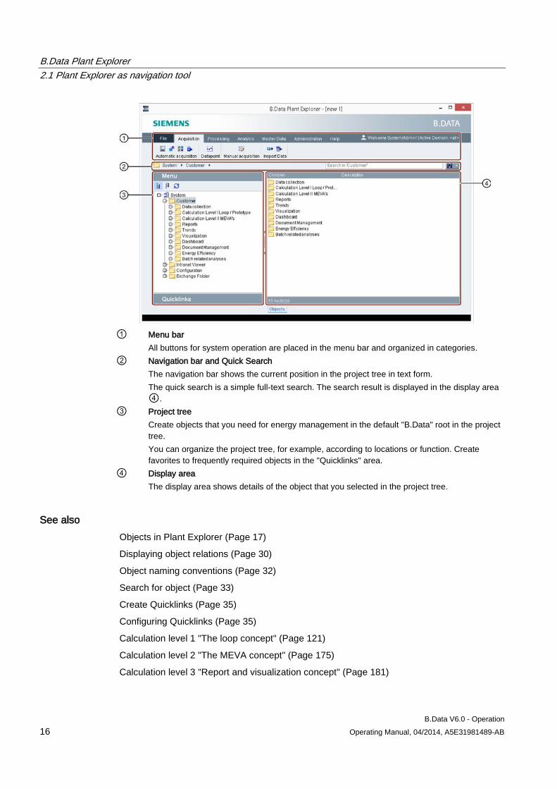
Plant Explorer has the following structure:
B.Data Plant Explorer 2.1 Plant Explorer as navigation tool
B.Data V6.0 - Operation 16 Operating Manual, 04/2014, A5E31981489-AB
① Menu bar
All buttons for system operation are placed in the menu bar and organized in categories. ② Navigation bar and Quick Search
The navigation bar shows the current position in the project tree in text form. The quick search is a simple full-text search. The search result is displayed in the display area ④.
③ Project tree Create objects that you need for energy management in the default "B.Data" root in the project tree. You can organize the project tree, for example, according to locations or function. Create favorites to frequently required objects in the "Quicklinks" area.
④ Display area The display area shows details of the object that you selected in the project tree.
See also Objects in Plant Explorer (Page 17)
Displaying object relations (Page 30)
Object naming conventions (Page 32)
Search for object (Page 33)
Create Quicklinks (Page 35)
Configuring Quicklinks (Page 35)
Calculation level 1 "The loop concept" (Page 121)
Calculation level 2 "The MEVA concept" (Page 175)
Calculation level 3 "Report and visualization concept" (Page 181)
B.Data Plant Explorer 2.2 Objects in Plant Explorer
B.Data V6.0 - Operation Operating Manual, 04/2014, A5E31981489-AB 17
2.2 Objects in Plant Explorer
2.2.1 Object basics
Object definition Objects let you configure all of the components you need for energy management in your organization in B.Data :
The following objects are available, for example.
● Folder
Object for structuring in the project tree of Plant Explorer
● Data point
Object for saving the measured values of a measuring point
● Prototype, loop
Objects for processing measured values during import
● Parameters, measuring variables
Objects for time-independent processing of measured values
● ERP domain, cost center relation, cost center, service type
Objects for Enterprise Resource Planning
● Report, trend, visualization, dashboard
Objects for the display of measured values
● User, user group, functional group, domain
Objects for configuring authorizations in B.Data
● Hardware, process, driver source, IO buffer
Objects for configuring data acquisition in B.Data
Object properties A property is a characteristic that is assigned to a specific object. In B.Data, an object can have the following properties:
● Automatically generated properties
The system automatically generate these properties,, e.g. "Name" and "Description", when you create an object.
● Manually assigned properties
You can assign these properties to an object, such as "Created on" or "Created by".
Manually assigned properties are then subdivided into the following categories:
B.Data Plant Explorer 2.2 Objects in Plant Explorer
B.Data V6.0 - Operation 18 Operating Manual, 04/2014, A5E31981489-AB
● Default properties
You can assign an object a property that is already defined in B.Data, "Created on" for example.
● User-defined properties
You can also create your own properties, which you can then assign to an object.
You can use object properties for the following purpose:
● To search for these properties
● For titles in reports
Access rights for objects You can prevent unauthorized read access to specific objects by defining these in B.Data:
● Authority level
You specify the authority level with a value between 0 and 1000:
– "0"
All users can view the object.
– "1" to "1000"
If you enter "50", for example, the object is visible to all users assigned authority level equal to or higher than 50.
You can automatically assign the authority level of an object to all nested objects.
● Domain
The domain represents a location of a business, for example. Users can be assigned to one or several domains.
Only the objects of the domain you activated are displayed. Newly objects are assigned exclusively to this domain.
Using and copying objects Once an object is created, you can use it elsewhere in the project tree, e.g. in a report or calculation. You can also create a copy of the object in order to create a similar object.
This is done using the following B.Data commands:
● "Copy", to duplicate the object and use it elsewhere.
● "Disconnect", to cancel the use of the object.
● "Delete", to remove the object from the project tree.
"Delete" removes all instances of an object in the project.
● "Clone", to duplicate the object.

B.Data Plant Explorer 2.2 Objects in Plant Explorer
B.Data V6.0 - Operation Operating Manual, 04/2014, A5E31981489-AB 19
See also Object properties (Page 21)
Object management (Page 26)
Configuring authorizations (Page 81)
B.Data Plant Explorer 2.2 Objects in Plant Explorer
B.Data V6.0 - Operation 20 Operating Manual, 04/2014, A5E31981489-AB
2.2.2 Creating an object
Overview If you are installing B.Data for the first time, the project tree contains only one default object: the "System" root.
Note
You cannot edit or delete the "System" root.
You may create and configure further objects in the project tree. Rule: Objects are always created as child object of the selected parent object.
Procedure 1. Select the folder in which you want to create the object.
2. Click the object that you want to create in the menu bar, for example, "Data point".
The object configuration dialog opens.
3. Select the respective object and click "OK".
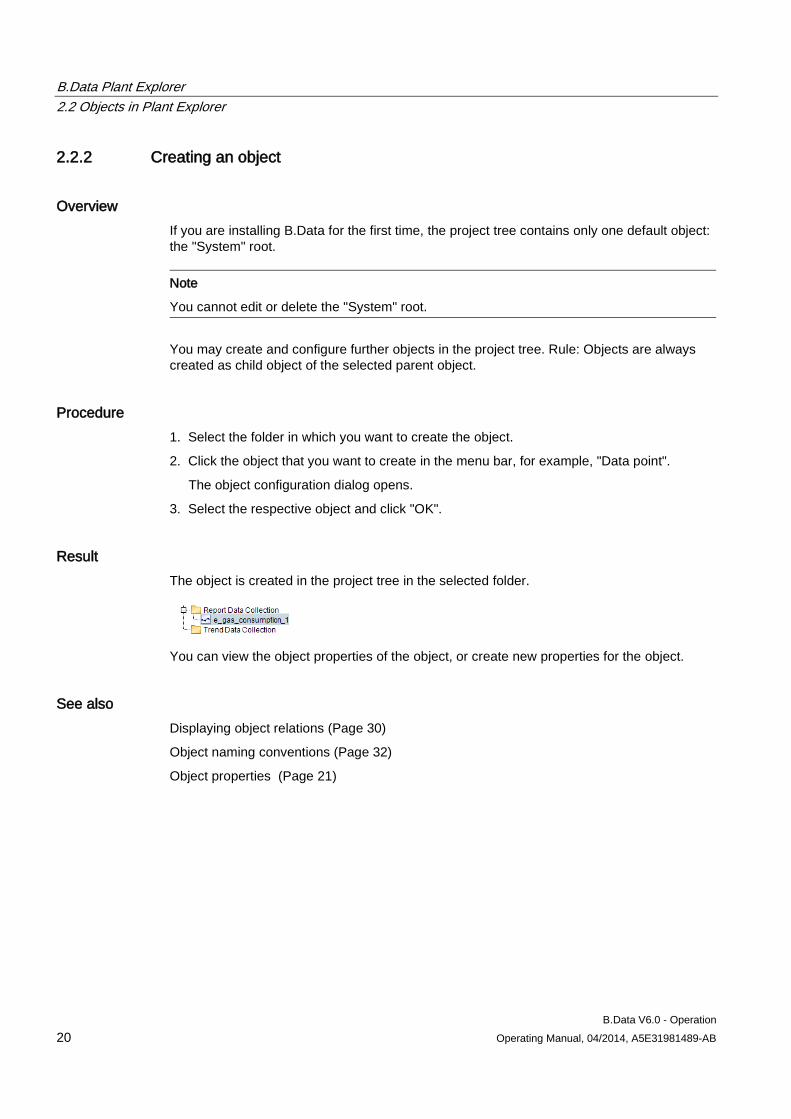
Result The object is created in the project tree in the selected folder.
You can view the object properties of the object, or create new properties for the object.
See also Displaying object relations (Page 30)
Object naming conventions (Page 32)
Object properties (Page 21)
B.Data Plant Explorer 2.2 Objects in Plant Explorer
B.Data V6.0 - Operation Operating Manual, 04/2014, A5E31981489-AB 21
2.2.3 Object properties
2.2.3.1 Opening properties
Requirement You have created the object.
Procedure 1. Select the object and click the "Properties" command in the shortcut menu.
The object properties dialog opens.
2. Edit the name and description of the object as required.
3. Enter a value in "Authorization level" to specify the access rights for the object.
The authority level is set to "0" by default.
4. You can transfer the authority level to all child objects by activating the "Children inherit authority level".
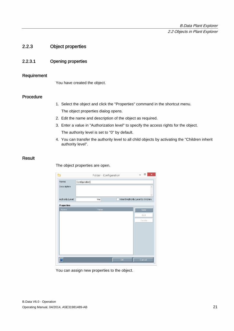
Result The object properties are open.
You can assign new properties to the object.

B.Data Plant Explorer 2.2 Objects in Plant Explorer
B.Data V6.0 - Operation 22 Operating Manual, 04/2014, A5E31981489-AB
See also Assigning properties (Page 23)
Creating an object (Page 20)
Object basics (Page 17)
B.Data Plant Explorer 2.2 Objects in Plant Explorer
B.Data V6.0 - Operation Operating Manual, 04/2014, A5E31981489-AB 23
2.2.3.2 Assigning properties
Requirement ● You have created the object.
● The object properties are open.
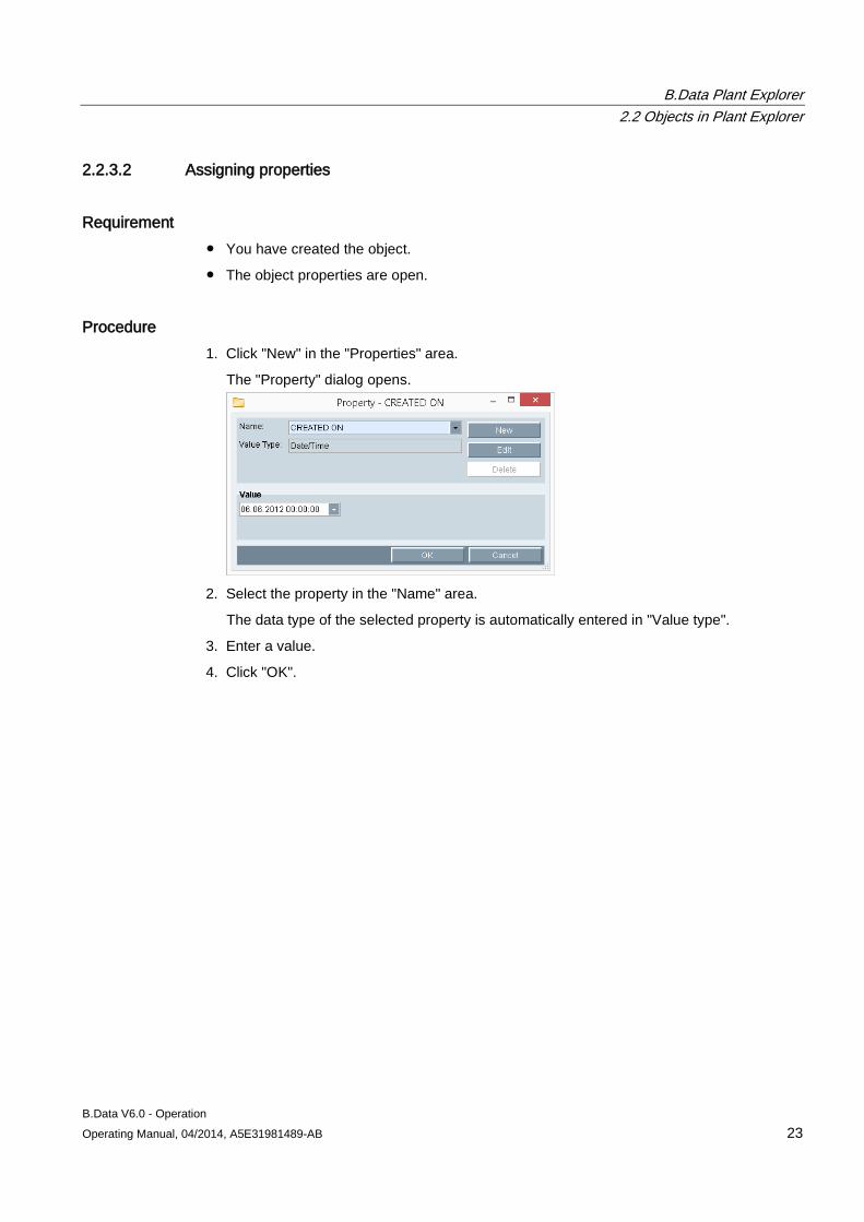
Procedure 1. Click "New" in the "Properties" area.
The "Property" dialog opens.
2. Select the property in the "Name" area.
The data type of the selected property is automatically entered in "Value type".
3. Enter a value.
4. Click "OK".
B.Data Plant Explorer 2.2 Objects in Plant Explorer
B.Data V6.0 - Operation 24 Operating Manual, 04/2014, A5E31981489-AB
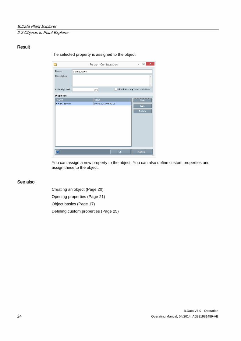
Result The selected property is assigned to the object.
You can assign a new property to the object. You can also define custom properties and assign these to the object.
See also Creating an object (Page 20)
Opening properties (Page 21)
Object basics (Page 17)
Defining custom properties (Page 25)
B.Data Plant Explorer 2.2 Objects in Plant Explorer
B.Data V6.0 - Operation Operating Manual, 04/2014, A5E31981489-AB 25
2.2.3.3 Defining custom properties
Requirement ● The object properties are open.
● The "Property" dialog is open.
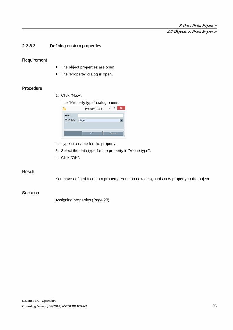
Procedure 1. Click "New".
The "Property type" dialog opens.
2. Type in a name for the property.
3. Select the data type for the property in "Value type".
4. Click "OK".
Result You have defined a custom property. You can now assign this new property to the object.
See also Assigning properties (Page 23)
B.Data Plant Explorer 2.2 Objects in Plant Explorer
B.Data V6.0 - Operation 26 Operating Manual, 04/2014, A5E31981489-AB
2.2.4 Object management
2.2.4.1 Object management basics
Overview The following B.Data commands are available for managing objects in the project tree:
● Move
● Copy and disconnect
● Clone and delete
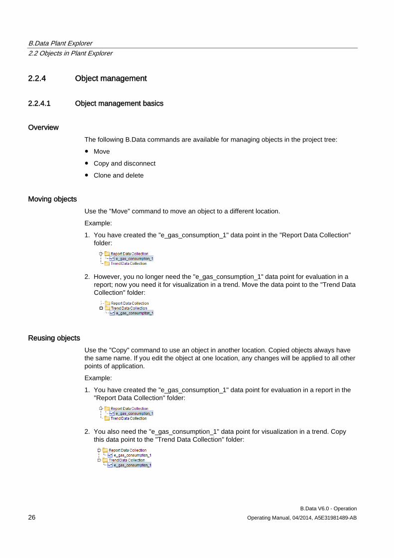
Moving objects Use the "Move" command to move an object to a different location.
Example:
1. You have created the "e_gas_consumption_1" data point in the "Report Data Collection" folder:
2. However, you no longer need the "e_gas_consumption_1" data point for evaluation in a
report; now you need it for visualization in a trend. Move the data point to the "Trend Data Collection" folder:
Reusing objects Use the "Copy" command to use an object in another location. Copied objects always have the same name. If you edit the object at one location, any changes will be applied to all other points of application.
Example:
1. You have created the "e_gas_consumption_1" data point for evaluation in a report in the "Report Data Collection" folder:
2. You also need the "e_gas_consumption_1" data point for visualization in a trend. Copy
this data point to the "Trend Data Collection" folder:
B.Data Plant Explorer 2.2 Objects in Plant Explorer
B.Data V6.0 - Operation Operating Manual, 04/2014, A5E31981489-AB 27
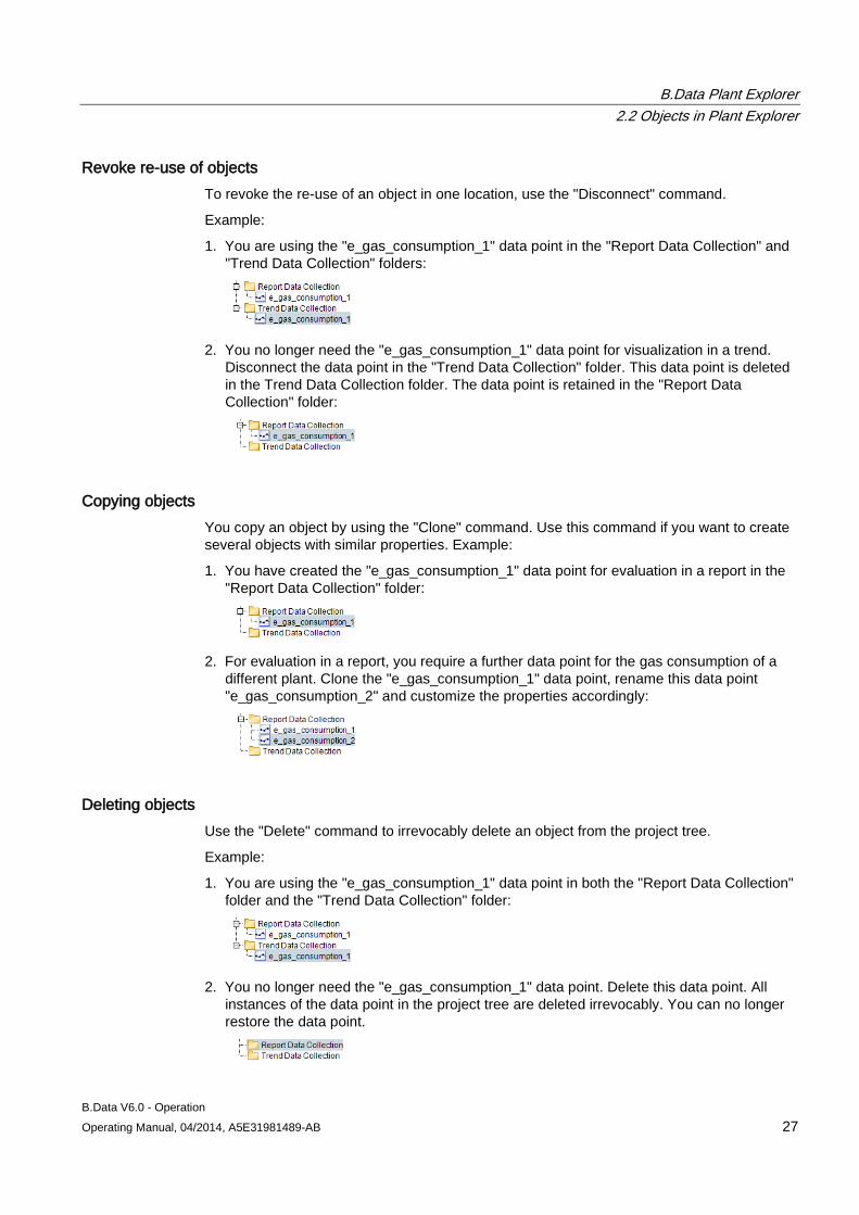
Revoke re-use of objects To revoke the re-use of an object in one location, use the "Disconnect" command.
Example:
1. You are using the "e_gas_consumption_1" data point in the "Report Data Collection" and "Trend Data Collection" folders:
2. You no longer need the "e_gas_consumption_1" data point for visualization in a trend.
Disconnect the data point in the "Trend Data Collection" folder. This data point is deleted in the Trend Data Collection folder. The data point is retained in the "Report Data Collection" folder:
Copying objects You copy an object by using the "Clone" command. Use this command if you want to create several objects with similar properties. Example:
1. You have created the "e_gas_consumption_1" data point for evaluation in a report in the "Report Data Collection" folder:
2. For evaluation in a report, you require a further data point for the gas consumption of a
different plant. Clone the "e_gas_consumption_1" data point, rename this data point "e_gas_consumption_2" and customize the properties accordingly:
Deleting objects Use the "Delete" command to irrevocably delete an object from the project tree.
Example:
1. You are using the "e_gas_consumption_1" data point in both the "Report Data Collection" folder and the "Trend Data Collection" folder:
2. You no longer need the "e_gas_consumption_1" data point. Delete this data point. All
instances of the data point in the project tree are deleted irrevocably. You can no longer restore the data point.
B.Data Plant Explorer 2.2 Objects in Plant Explorer
B.Data V6.0 - Operation 28 Operating Manual, 04/2014, A5E31981489-AB
2.2.4.2 Managing objects
Requirement The objects have already been created.
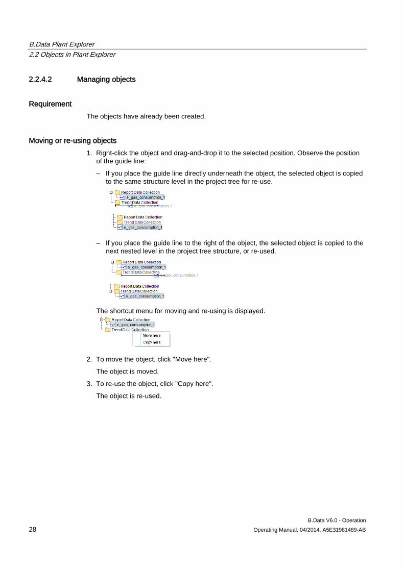
Moving or re-using objects 1. Right-click the object and drag-and-drop it to the selected position. Observe the position
of the guide line:
– If you place the guide line directly underneath the object, the selected object is copied to the same structure level in the project tree for re-use.
– If you place the guide line to the right of the object, the selected object is copied to the
next nested level in the project tree structure, or re-used.
The shortcut menu for moving and re-using is displayed.
2. To move the object, click "Move here".
The object is moved.
3. To re-use the object, click "Copy here".
The object is re-used.
B.Data Plant Explorer 2.2 Objects in Plant Explorer
B.Data V6.0 - Operation Operating Manual, 04/2014, A5E31981489-AB 29
Deleting/copying/canceling the re-use of an object
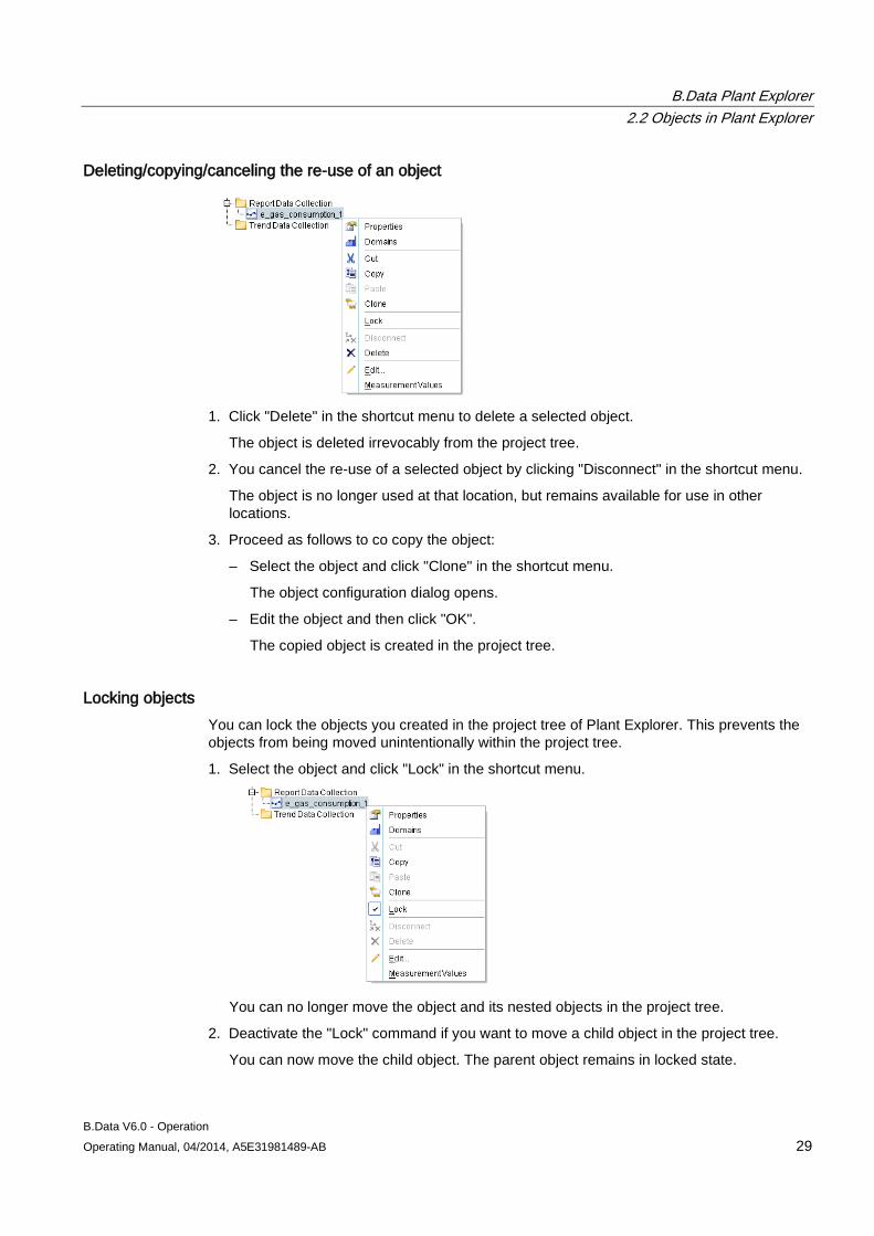
1. Click "Delete" in the shortcut menu to delete a selected object.
The object is deleted irrevocably from the project tree.
2. You cancel the re-use of a selected object by clicking "Disconnect" in the shortcut menu.
The object is no longer used at that location, but remains available for use in other locations.
3. Proceed as follows to co copy the object:
– Select the object and click "Clone" in the shortcut menu.
The object configuration dialog opens.
– Edit the object and then click "OK".
The copied object is created in the project tree.
Locking objects You can lock the objects you created in the project tree of Plant Explorer. This prevents the objects from being moved unintentionally within the project tree.
1. Select the object and click "Lock" in the shortcut menu.
You can no longer move the object and its nested objects in the project tree.
2. Deactivate the "Lock" command if you want to move a child object in the project tree.
You can now move the child object. The parent object remains in locked state.
B.Data Plant Explorer 2.2 Objects in Plant Explorer
B.Data V6.0 - Operation 30 Operating Manual, 04/2014, A5E31981489-AB
2.2.5 Displaying object relations
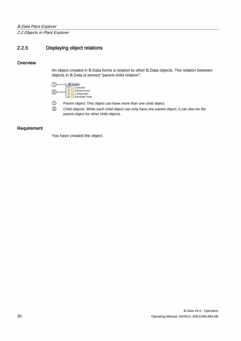
Overview An object created in B.Data forms a relation to other B.Data objects. The relation between objects in B.Data is termed "parent-child relation":
① Parent object: This object can have more than one child object. ② Child objects: While each child object can only have one parent object, it can also be the
parent object for other child objects.
Requirement You have created the object.
B.Data Plant Explorer 2.2 Objects in Plant Explorer
B.Data V6.0 - Operation Operating Manual, 04/2014, A5E31981489-AB 31
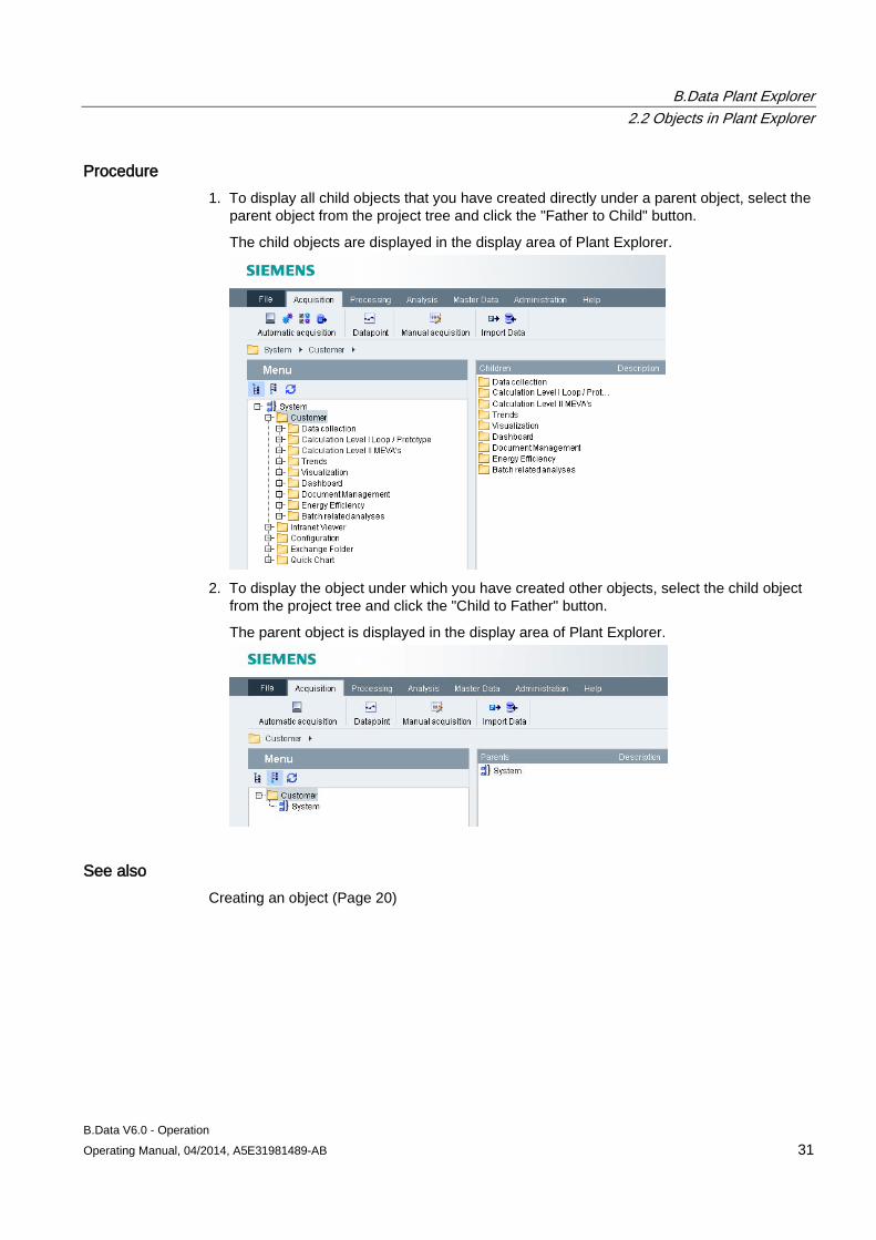
Procedure 1. To display all child objects that you have created directly under a parent object, select the
parent object from the project tree and click the "Father to Child" button.
The child objects are displayed in the display area of Plant Explorer.
2. To display the object under which you have created other objects, select the child object
from the project tree and click the "Child to Father" button.
The parent object is displayed in the display area of Plant Explorer.
See also Creating an object (Page 20)
B.Data Plant Explorer 2.2 Objects in Plant Explorer
B.Data V6.0 - Operation 32 Operating Manual, 04/2014, A5E31981489-AB
2.2.6 Object naming conventions
Notes on the naming of objects Observe the following when naming objects:
● Use an unambiguous name.
● Use a maximum of 255 characters.
● Use the following characters:
– "A" to "Z"
– "a" to "z"
– "0" to "9"
– "_"
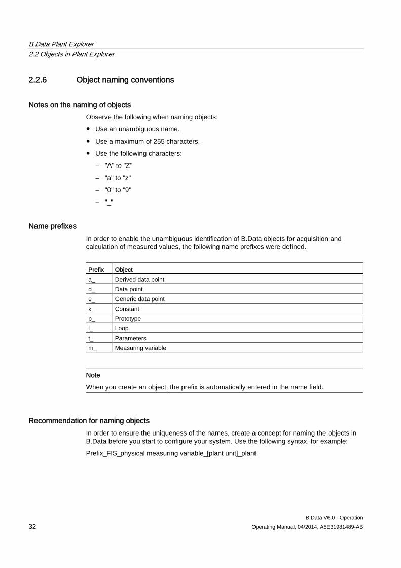
Name prefixes In order to enable the unambiguous identification of B.Data objects for acquisition and calculation of measured values, the following name prefixes were defined.
Prefix Object a_ Derived data point d_ Data point e_ Generic data point k_ Constant p_ Prototype l_ Loop t_ Parameters m_ Measuring variable
Note
When you create an object, the prefix is automatically entered in the name field.
Recommendation for naming objects In order to ensure the uniqueness of the names, create a concept for naming the objects in B.Data before you start to configure your system. Use the following syntax. for example:
Prefix_FIS_physical measuring variable_[plant unit]_plant
B.Data Plant Explorer 2.2 Objects in Plant Explorer
B.Data V6.0 - Operation Operating Manual, 04/2014, A5E31981489-AB 33
2.2.7 Search for object
Overview The B.Data search function evaluates the following information:
● Object name
● Description of the object
● Object properties
● Object ID
A separate tab with search results is created for each search in the display area of the Plant Explorer. All tabs with search results are deleted when you close the B.Data client.
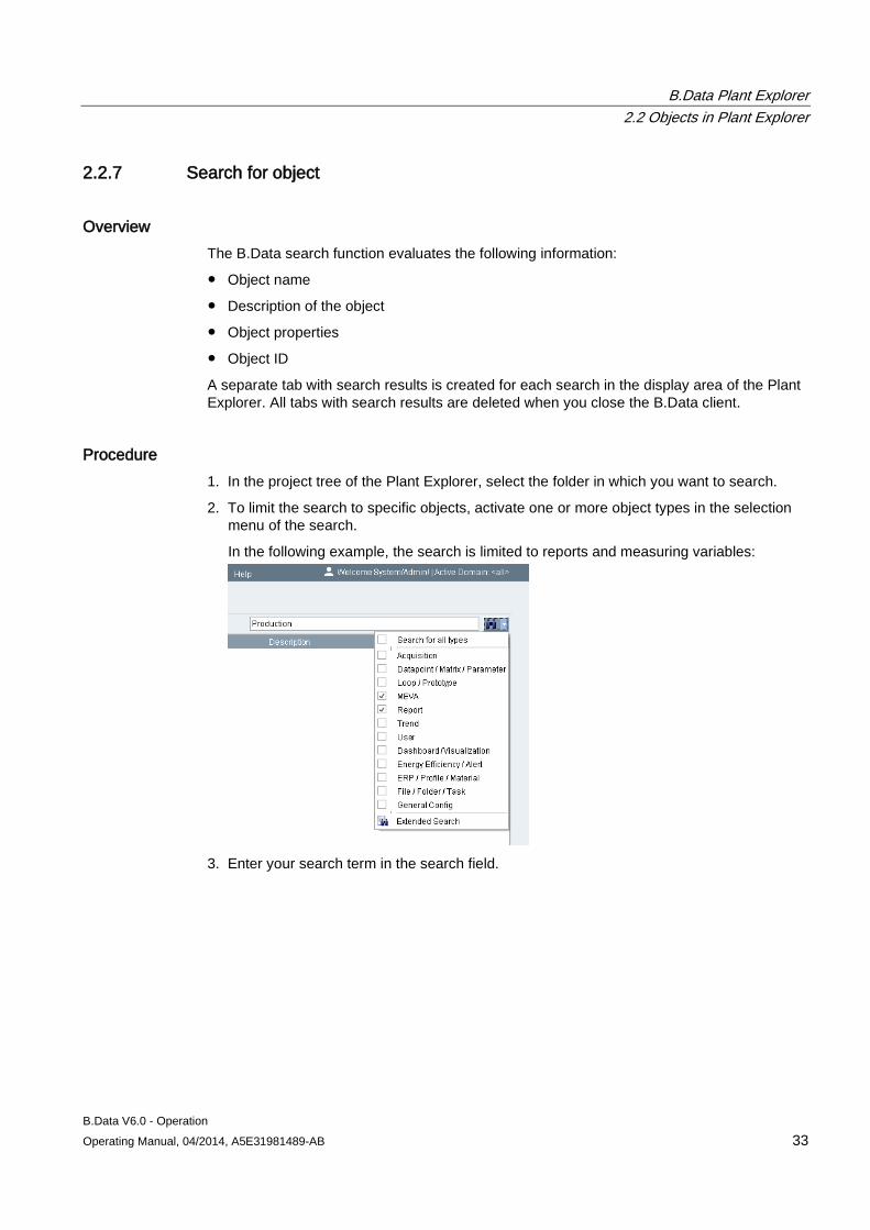
Procedure 1. In the project tree of the Plant Explorer, select the folder in which you want to search.
2. To limit the search to specific objects, activate one or more object types in the selection menu of the search.
In the following example, the search is limited to reports and measuring variables:
3. Enter your search term in the search field.
B.Data Plant Explorer 2.2 Objects in Plant Explorer
B.Data V6.0 - Operation 34 Operating Manual, 04/2014, A5E31981489-AB
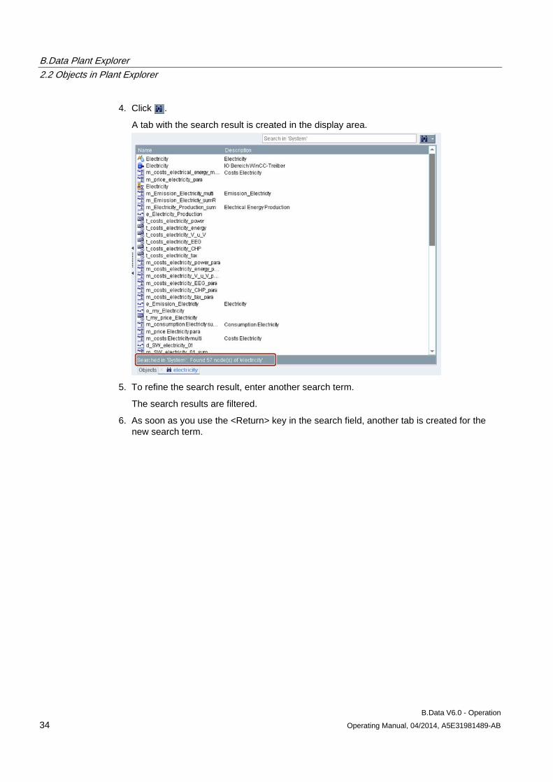
4. Click .
A tab with the search result is created in the display area.
5. To refine the search result, enter another search term.
The search results are filtered.
6. As soon as you use the <Return> key in the search field, another tab is created for the new search term.
B.Data Plant Explorer 2.3 Configuring Quicklinks
B.Data V6.0 - Operation Operating Manual, 04/2014, A5E31981489-AB 35
2.3 Configuring Quicklinks
2.3.1 Create Quicklinks
Overview Quicklinks are references to objects in B.Data that are used frequently, for example, reports. Quicklinks are available to the user for which you have created the Quicklinks.
You can create Quicklinks for the B.Data Client as well as the B.Data Web.
Requirement You have the "Create Quicklinks" authorization.
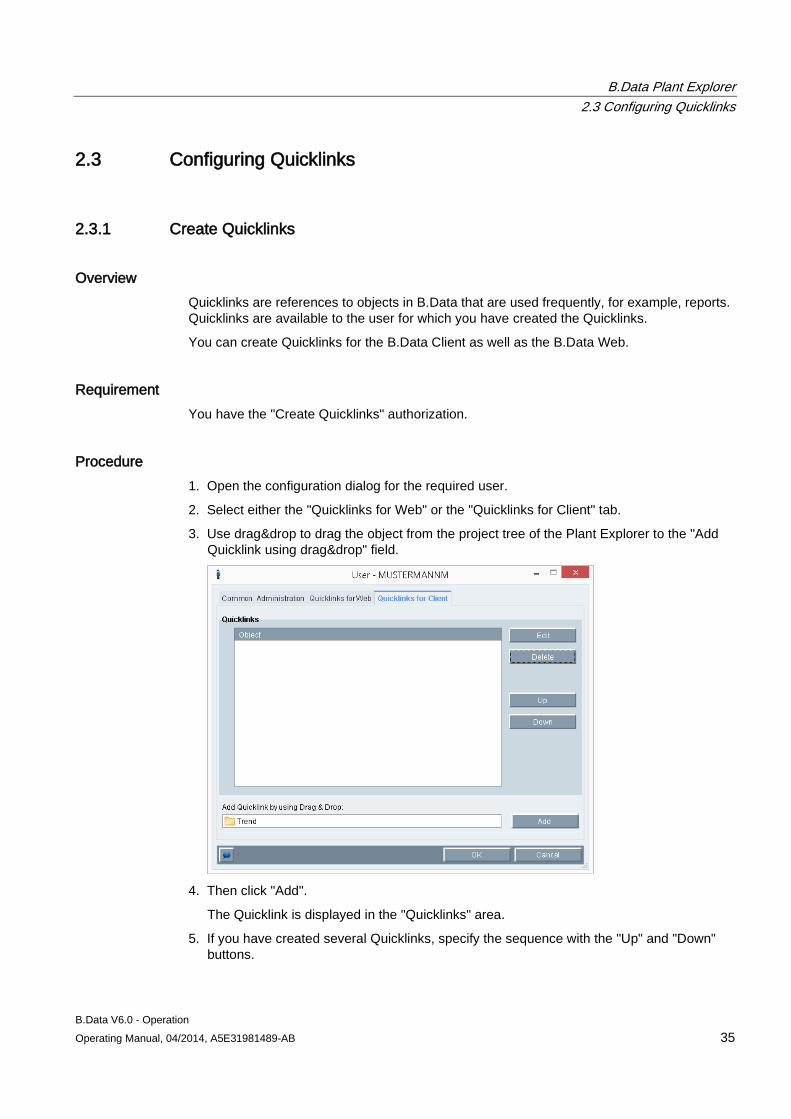
Procedure 1. Open the configuration dialog for the required user.
2. Select either the "Quicklinks for Web" or the "Quicklinks for Client" tab.
3. Use drag&drop to drag the object from the project tree of the Plant Explorer to the "Add Quicklink using drag&drop" field.
4. Then click "Add".
The Quicklink is displayed in the "Quicklinks" area.
5. If you have created several Quicklinks, specify the sequence with the "Up" and "Down" buttons.
B.Data Plant Explorer 2.3 Configuring Quicklinks
B.Data V6.0 - Operation 36 Operating Manual, 04/2014, A5E31981489-AB
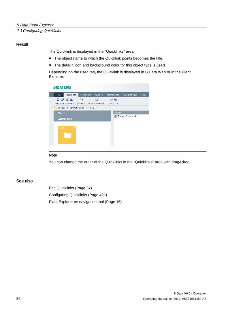
Result The Quicklink is displayed in the "Quicklinks" area:
● The object name to which the Quicklink points becomes the title.
● The default icon and background color for this object type is used.
Depending on the used tab, the Quicklink is displayed in B.Data Web or in the Plant Explorer.
Note
You can change the order of the Quicklinks in the "Quicklinks" area with drag&drop.
See also Edit Quicklinks (Page 37)
Configuring Quicklinks (Page 421)
Plant Explorer as navigation tool (Page 15)
B.Data Plant Explorer 2.3 Configuring Quicklinks
B.Data V6.0 - Operation Operating Manual, 04/2014, A5E31981489-AB 37
2.3.2 Edit Quicklinks
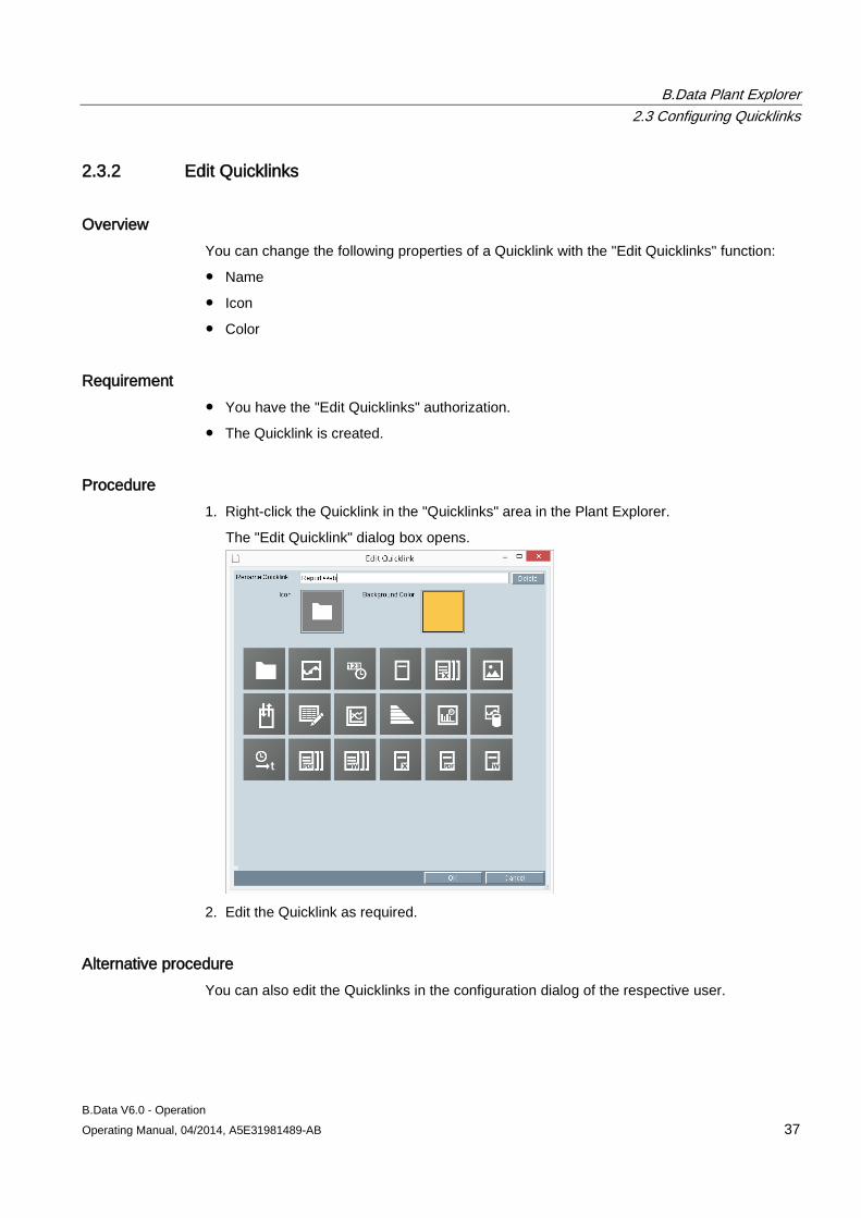
Overview You can change the following properties of a Quicklink with the "Edit Quicklinks" function:
● Name
● Icon
● Color
Requirement ● You have the "Edit Quicklinks" authorization.
● The Quicklink is created.
Procedure 1. Right-click the Quicklink in the "Quicklinks" area in the Plant Explorer.
The "Edit Quicklink" dialog box opens.
2. Edit the Quicklink as required.
Alternative procedure You can also edit the Quicklinks in the configuration dialog of the respective user.

B.Data Plant Explorer 2.3 Configuring Quicklinks
B.Data V6.0 - Operation 38 Operating Manual, 04/2014, A5E31981489-AB
B.Data V6.0 - Operation Operating Manual, 04/2014, A5E31981489-AB 39
Configuring master data 3 3.1 Configuring data acquisition
3.1.1 Creating hardware
Overview If you want to acquire data automatically with B.Data, you must map at least one acquisition component as object of the type "Hardware". An acquisition component is, for example, a PC or a mobile device (PDA). You configure the data acquisition for this hardware in an additional step by means of a wizard.
Procedure 1. Select the folder in which the hardware is going to be created.
2. Click "Add hardware" in the menu bar under "Acquisition > Automatic acquisition".
The "Hardware" configuration dialog opens.
3. Enter a name and, if necessary, a description.
Recommendation: Also use the prefix "h_" as unique identification.
4. Assign the PC or the mobile device to the "Hardware" object using the "..." button.
Note
The name "localhost" is not permitted as computer name.
Configuring master data 3.1 Configuring data acquisition
B.Data V6.0 - Operation 40 Operating Manual, 04/2014, A5E31981489-AB
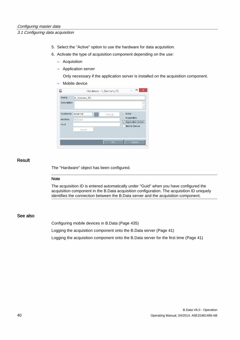
5. Select the "Active" option to use the hardware for data acquisition.
6. Activate the type of acquisition component depending on the use:
– Acquisition
– Application server
Only necessary if the application server is installed on the acquisition component.
– Mobile device
Result The "Hardware" object has been configured.
Note
The acquisition ID is entered automatically under "Guid" when you have configured the acquisition component in the B.Data acquisition configuration. The acquisition ID uniquely identifies the connection between the B.Data server and the acquisition component.
See also Configuring mobile devices in B.Data (Page 435)
Logging the acquisition component onto the B.Data server (Page 41)
Logging the acquisition component onto the B.Data server for the first time (Page 41)
Configuring master data 3.1 Configuring data acquisition
B.Data V6.0 - Operation Operating Manual, 04/2014, A5E31981489-AB 41
3.1.2 Logging the acquisition component onto the B.Data server
3.1.2.1 Logging the acquisition component onto the B.Data server for the first time
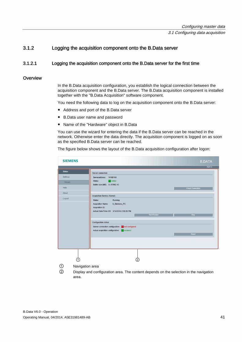
Overview In the B.Data acquisition configuration, you establish the logical connection between the acquisition component and the B.Data server. The B.Data acquisition component is installed together with the "B.Data Acquisition" software component.
You need the following data to log on the acquisition component onto the B.Data server:
● Address and port of the B.Data server
● B.Data user name and password
● Name of the "Hardware" object in B.Data
You can use the wizard for entering the data if the B.Data server can be reached in the network. Otherwise enter the data directly. The acquisition component is logged on as soon as the specified B.Data server can be reached.
The figure below shows the layout of the B.Data acquisition configuration after logon:
① Navigation area ② Display and configuration area. The content depends on the selection in the navigation
area.
Configuring master data 3.1 Configuring data acquisition
B.Data V6.0 - Operation 42 Operating Manual, 04/2014, A5E31981489-AB
Requirement ● The "B.Data Acquisition" software component is installed on the PC.
● Microsoft Internet Information Service (IIS) is installed on the PC.
● The PC is connected to the B.Data server (optional).
● The "Hardware" object is set up on the B.Data server.
● A user with the "Configure acquisition" authorization is set up on the B.Data server.
Procedure 1. Start the web browser on the acquisition component and enter the following address:
http://[computer name]/BDataAcquisition/Login.aspx
2. Log on using your Windows user data of the acquisition component.
The "Status" page of the B.Data acquisition configuration is displayed. If the acquisition component is logged on to the B.Data server yet, the "Configure the acquisition" dialog is displayed.
3. Select the required option in the "Configure the acquisition" dialog:
– Starting the connection wizard
– Configuring the connection manually
4. Enter the following connection data:
– Address and port of the B.Data server
– B.Data user name and password
– Name of the "Hardware" object in B.Data
Note
Only with manual configuration: If you are using the name of a "Hardware" object that is already connected to another acquisition component, the existing connection is replaced.
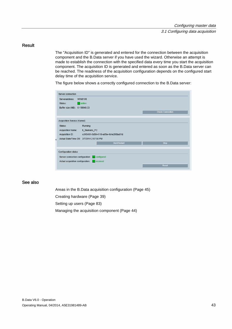
Configuring master data 3.1 Configuring data acquisition
B.Data V6.0 - Operation Operating Manual, 04/2014, A5E31981489-AB 43
Result The "Acquisition ID" is generated and entered for the connection between the acquisition component and the B.Data server if you have used the wizard. Otherwise an attempt is made to establish the connection with the specified data every time you start the acquisition component. The acquisition ID is generated and entered as soon as the B.Data server can be reached. The readiness of the acquisition configuration depends on the configured start delay time of the acquisition service.
The figure below shows a correctly configured connection to the B.Data server:
See also Areas in the B.Data acquisition configuration (Page 45)
Creating hardware (Page 39)
Setting up users (Page 83)
Managing the acquisition component (Page 44)
Configuring master data 3.1 Configuring data acquisition
B.Data V6.0 - Operation 44 Operating Manual, 04/2014, A5E31981489-AB
3.1.2.2 Managing the acquisition component
Overview You use the B.Data acquisition component for the following tasks:
● Start or stop acquisition service
● Modify or reset the connection data
● Execute the software update for the acquisition component
Requirement The B.Data acquisition configuration is displayed in the Web browser.
Procedure 1. To start or stop the acquisition service:
– Click "Status" in the navigation area.
– Click the appropriate button.
If the acquisition service is stopped, data is not acquired.
2. To reset the configuration settings:
– Click "Status" in the navigation area.
– Click the appropriate button.
The configuration settings of the acquisition component are deleted after confirmation. The acquisition component is not acquiring data any longer.
– Log on the acquisition component onto a B.Data server again afterward.
3. To change the configuration settings:
– If you want to assign the acquisition component to another "Hardware" object, reset the acquisition service.
– If you want to change the user data, stop the acquisition service.
– Click on "Settings" or "Wizard" in the navigation area.
– Enter the connection data.
4. To update the acquisition software:
– Click "About" in the navigation area.
– Enter the path and file name of the setup file under "Software update", for example, "C:\Installation\Setup.exe".
– Click "Update".
The acquisition service is stopped and the acquisition software is updated. The acquisition service is started once again when the installation is complete.
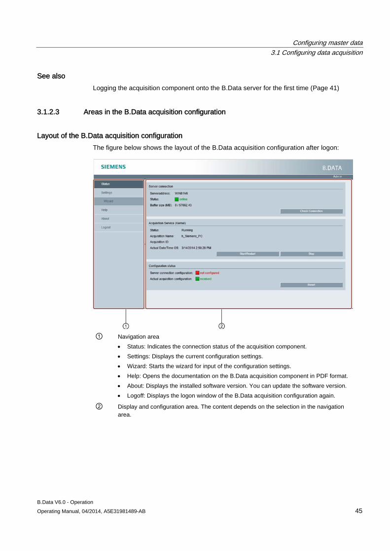
Configuring master data 3.1 Configuring data acquisition
B.Data V6.0 - Operation Operating Manual, 04/2014, A5E31981489-AB 45
See also Logging the acquisition component onto the B.Data server for the first time (Page 41)
3.1.2.3 Areas in the B.Data acquisition configuration
Layout of the B.Data acquisition configuration The figure below shows the layout of the B.Data acquisition configuration after logon:
① Navigation area
• Status: Indicates the connection status of the acquisition component. • Settings: Displays the current configuration settings. • Wizard: Starts the wizard for input of the configuration settings. • Help: Opens the documentation on the B.Data acquisition component in PDF format. • About: Displays the installed software version. You can update the software version. • Logoff: Displays the logon window of the B.Data acquisition configuration again.
② Display and configuration area. The content depends on the selection in the navigation area.
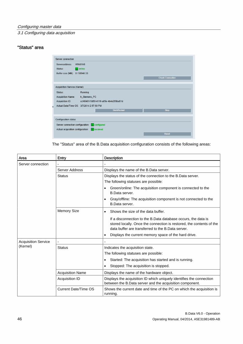
Configuring master data 3.1 Configuring data acquisition
B.Data V6.0 - Operation 46 Operating Manual, 04/2014, A5E31981489-AB
"Status" area
The "Status" area of the B.Data acquisition configuration consists of the following areas:
Area Entry Description Server connection - -
Server Address Displays the name of the B.Data server. Status Displays the status of the connection to the B.Data server.
The following statuses are possible: • Green/online: The acquisition component is connected to the
B.Data server. • Gray/offline: The acquisition component is not connected to the
B.Data server.
Memory Size • Shows the size of the data buffer.
If a disconnection to the B.Data database occurs, the data is stored locally. Once the connection is restored, the contents of the data buffer are transferred to the B.Data server.
• Displays the current memory space of the hard drive.
Acquisition Service (Kernel)
- - Status Indicates the acquisition state.
The following statuses are possible: • Started: The acquisition has started and is running. • Stopped: The acquisition is stopped.
Acquisition Name Displays the name of the hardware object. Acquisition ID Displays the acquisition ID which uniquely identifies the connection
between the B.Data server and the acquisition component. Current Date/Time OS Shows the current date and time of the PC on which the acquisition is
running.
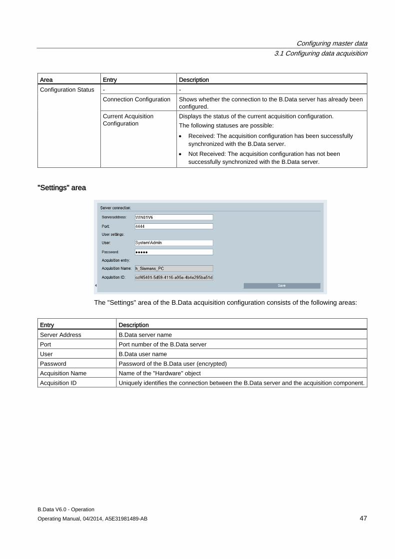
Configuring master data 3.1 Configuring data acquisition
B.Data V6.0 - Operation Operating Manual, 04/2014, A5E31981489-AB 47
Area Entry Description Configuration Status - -
Connection Configuration Shows whether the connection to the B.Data server has already been configured.
Current Acquisition Configuration
Displays the status of the current acquisition configuration. The following statuses are possible: • Received: The acquisition configuration has been successfully
synchronized with the B.Data server. • Not Received: The acquisition configuration has not been
successfully synchronized with the B.Data server.
"Settings" area
The "Settings" area of the B.Data acquisition configuration consists of the following areas:
Entry Description Server Address B.Data server name Port Port number of the B.Data server User B.Data user name Password Password of the B.Data user (encrypted) Acquisition Name Name of the "Hardware" object Acquisition ID Uniquely identifies the connection between the B.Data server and the acquisition component.
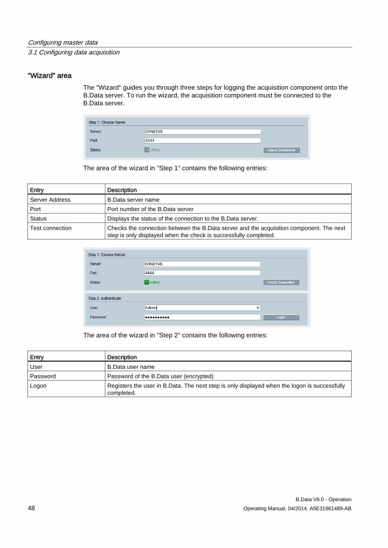
Configuring master data 3.1 Configuring data acquisition
B.Data V6.0 - Operation 48 Operating Manual, 04/2014, A5E31981489-AB
"Wizard" area The "Wizard" guides you through three steps for logging the acquisition component onto the B.Data server. To run the wizard, the acquisition component must be connected to the B.Data server.
The area of the wizard in "Step 1" contains the following entries:
Entry Description Server Address B.Data server name Port Port number of the B.Data server Status Displays the status of the connection to the B.Data server. Test connection Checks the connection between the B.Data server and the acquisition component. The next
step is only displayed when the check is successfully completed.
The area of the wizard in "Step 2" contains the following entries:
Entry Description User B.Data user name Password Password of the B.Data user (encrypted) Logon Registers the user in B.Data. The next step is only displayed when the logon is successfully
completed.
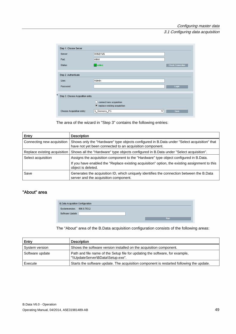
Configuring master data 3.1 Configuring data acquisition
B.Data V6.0 - Operation Operating Manual, 04/2014, A5E31981489-AB 49
The area of the wizard in "Step 3" contains the following entries:
Entry Description Connecting new acquisition Shows only the "Hardware" type objects configured in B.Data under "Select acquisition" that
have not yet been connected to an acquisition component. Replace existing acquisition Shows all the "Hardware" type objects configured in B.Data under "Select acquisition". Select acquisition Assigns the acquisition component to the "Hardware" type object configured in B.Data.
If you have enabled the "Replace existing acquisition" option, the existing assignment to this object is deleted.
Save Generates the acquisition ID, which uniquely identifies the connection between the B.Data server and the acquisition component.
"About" area
The "About" area of the B.Data acquisition configuration consists of the following areas:
Entry Description System version Shows the software version installed on the acquisition component. Software update Path and file name of the Setup file for updating the software, for example,
"\\UpdateServer\BData\Setup.exe". Execute Starts the software update. The acquisition component is restarted following the update.
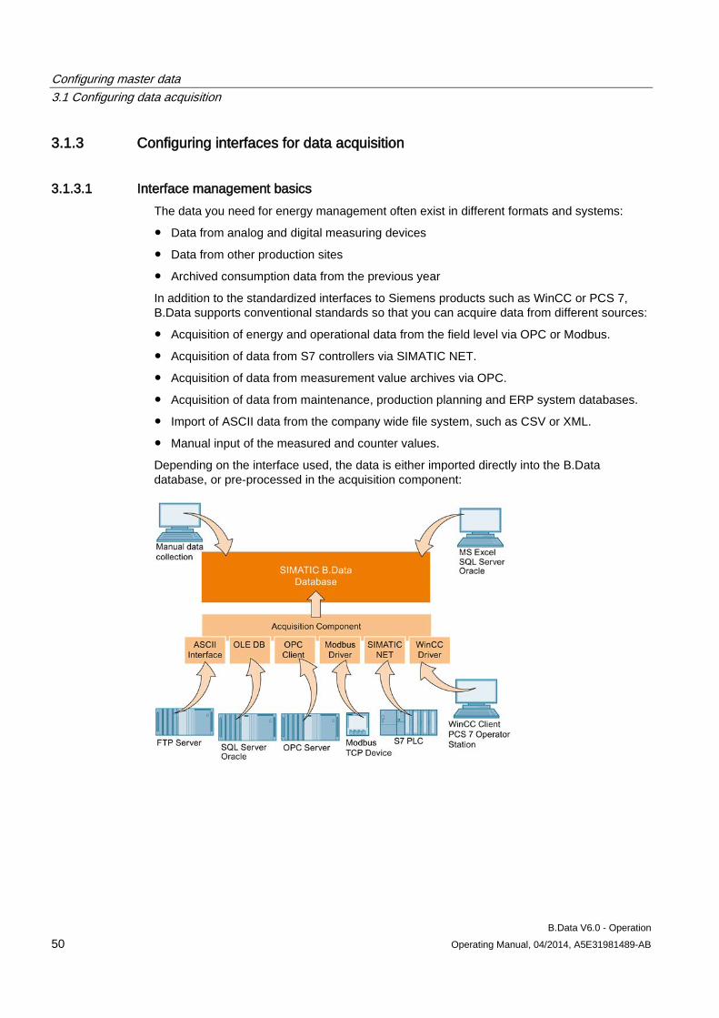
Configuring master data 3.1 Configuring data acquisition
B.Data V6.0 - Operation 50 Operating Manual, 04/2014, A5E31981489-AB
3.1.3 Configuring interfaces for data acquisition
3.1.3.1 Interface management basics The data you need for energy management often exist in different formats and systems:
● Data from analog and digital measuring devices
● Data from other production sites
● Archived consumption data from the previous year
In addition to the standardized interfaces to Siemens products such as WinCC or PCS 7, B.Data supports conventional standards so that you can acquire data from different sources:
● Acquisition of energy and operational data from the field level via OPC or Modbus.
● Acquisition of data from S7 controllers via SIMATIC NET.
● Acquisition of data from measurement value archives via OPC.
● Acquisition of data from maintenance, production planning and ERP system databases.
● Import of ASCII data from the company wide file system, such as CSV or XML.
● Manual input of the measured and counter values.
Depending on the interface used, the data is either imported directly into the B.Data database, or pre-processed in the acquisition component:
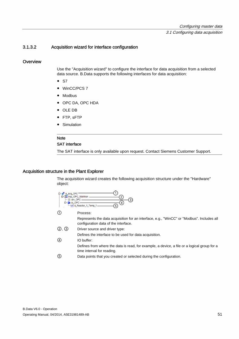
Configuring master data 3.1 Configuring data acquisition
B.Data V6.0 - Operation Operating Manual, 04/2014, A5E31981489-AB 51
3.1.3.2 Acquisition wizard for interface configuration
Overview Use the "Acquisition wizard" to configure the interface for data acquisition from a selected data source. B.Data supports the following interfaces for data acquisition:
● S7
● WinCC/PCS 7
● Modbus
● OPC DA, OPC HDA
● OLE DB
● FTP, sFTP
● Simulation
Note SAT interface
The SAT interface is only available upon request. Contact Siemens Customer Support.
Acquisition structure in the Plant Explorer The acquisition wizard creates the following acquisition structure under the "Hardware" object:
① Process:
Represents the data acquisition for an interface, e.g., "WinCC" or "Modbus". Includes all configuration data of the interface.
②, ③ Driver source and driver type: Defines the interface to be used for data acquisition.
④ IO buffer: Defines from where the data is read, for example, a device, a file or a logical group for a time interval for reading.
⑤ Data points that you created or selected during the configuration.
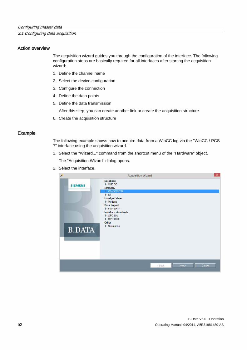
Configuring master data 3.1 Configuring data acquisition
B.Data V6.0 - Operation 52 Operating Manual, 04/2014, A5E31981489-AB
Action overview The acquisition wizard guides you through the configuration of the interface. The following configuration steps are basically required for all interfaces after starting the acquisition wizard:
1. Define the channel name
2. Select the device configuration
3. Configure the connection
4. Define the data points
5. Define the data transmission
After this step, you can create another link or create the acquisition structure.
6. Create the acquisition structure
Example The following example shows how to acquire data from a WinCC log via the "WinCC / PCS 7" interface using the acquisition wizard.
1. Select the "Wizard..." command from the shortcut menu of the "Hardware" object.
The "Acquisition Wizard" dialog opens.
2. Select the interface.
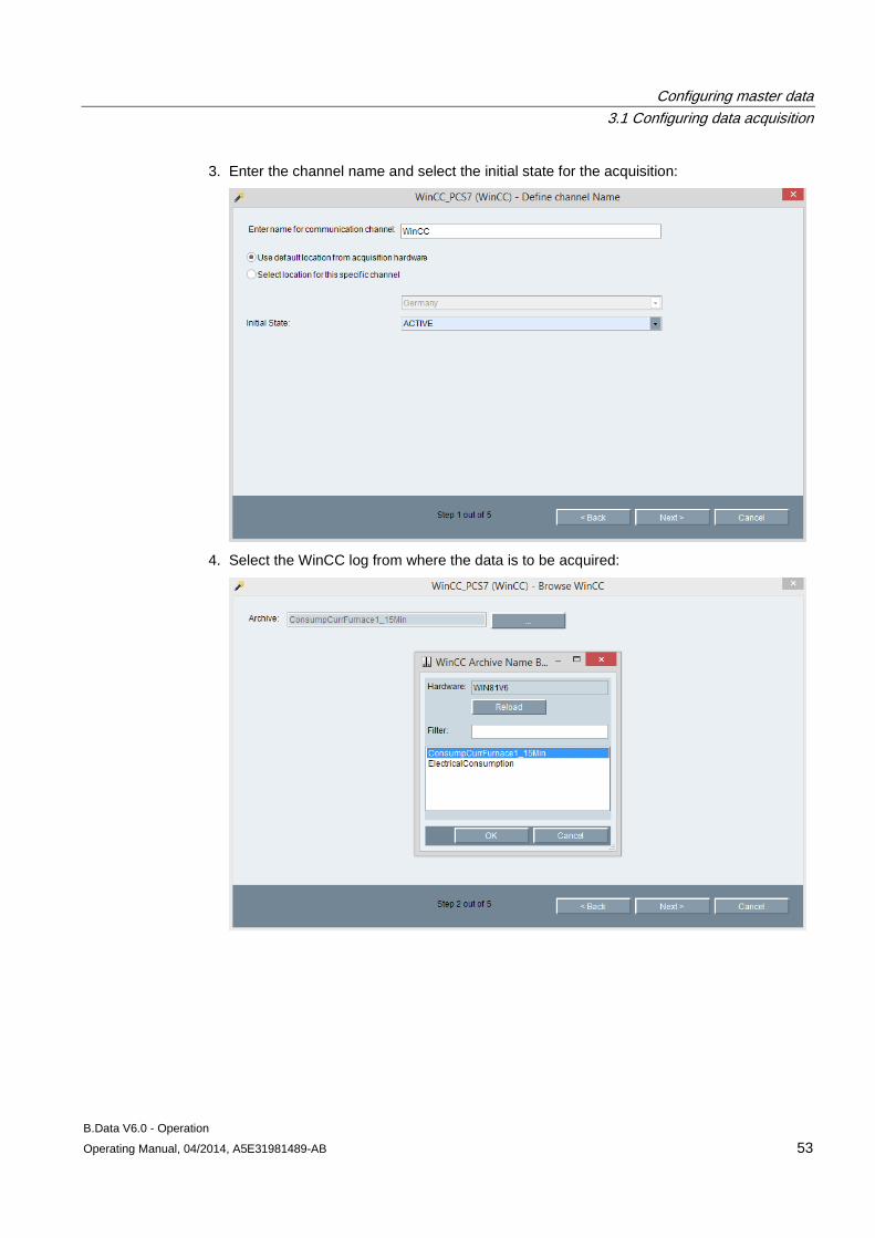
Configuring master data 3.1 Configuring data acquisition
B.Data V6.0 - Operation Operating Manual, 04/2014, A5E31981489-AB 53
3. Enter the channel name and select the initial state for the acquisition:
4. Select the WinCC log from where the data is to be acquired:
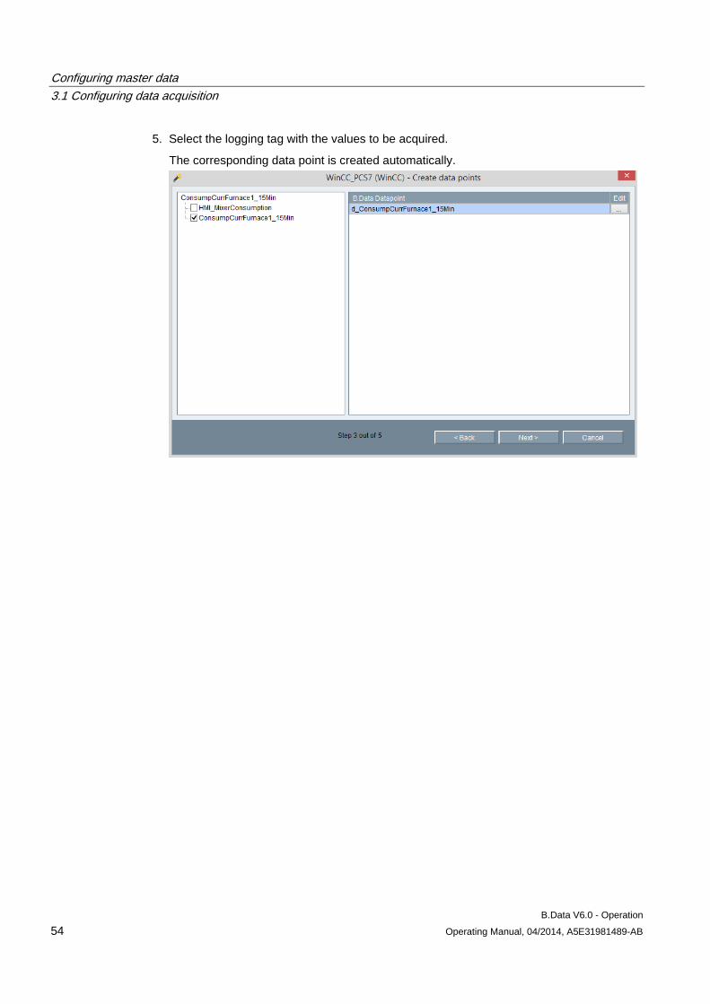
Configuring master data 3.1 Configuring data acquisition
B.Data V6.0 - Operation 54 Operating Manual, 04/2014, A5E31981489-AB
5. Select the logging tag with the values to be acquired.
The corresponding data point is created automatically.
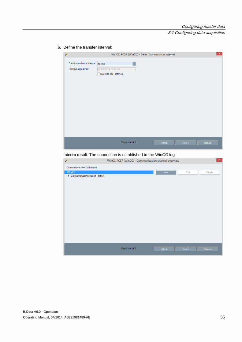
Configuring master data 3.1 Configuring data acquisition
B.Data V6.0 - Operation Operating Manual, 04/2014, A5E31981489-AB 55
6. Define the transfer interval:
Interim result: The connection is established to the WinCC log:
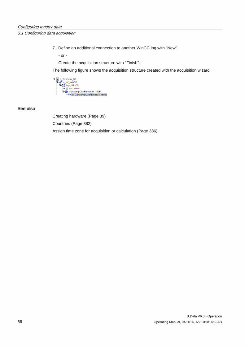
Configuring master data 3.1 Configuring data acquisition
B.Data V6.0 - Operation 56 Operating Manual, 04/2014, A5E31981489-AB
7. Define an additional connection to another WinCC log with "New".
- or -
Create the acquisition structure with "Finish".
The following figure shows the acquisition structure created with the acquisition wizard:
See also Creating hardware (Page 39)
Countries (Page 382)
Assign time zone for acquisition or calculation (Page 386)
Configuring master data 3.1 Configuring data acquisition
B.Data V6.0 - Operation Operating Manual, 04/2014, A5E31981489-AB 57
3.1.3.3 Configuring data acquisition via the "S7" interface
Overview You use the "S7" interface to retrieve data from an S7 controller with the help of SIMATIC NET. You address the memory areas of the S7 controller absolutely.
Requirement ● The "Hardware" object has been created.
● The acquisition component is logged on to the B.Data server and switched on.
● SIMATIC NET is installed on the acquisition component and licensed.
● An understanding of addressing and communication with S7 controllers.
Starting the wizard 1. In the project tree of the Plant Explorer, select the "Hardware" object and select the
"Wizard..." command from the shortcut menu.
The "Acquisition Wizard" dialog opens.
2. Click the "S7" entry.
Define the channel name 1. Enter a meaningful channel name, for example, "Acq_S7_ColorMixing_Consumption".
2. Select the country whose time zone is used for the time stamp of the acquired values.
3. Specify the status of the data acquisition on the acquisition component:
– ACTIVE: Data are acquired.
– NOT ACTIVE: Data are not acquired.
Select the device configuration 1. Activate "Create user-defined configuration".
Configuring master data 3.1 Configuring data acquisition
B.Data V6.0 - Operation 58 Operating Manual, 04/2014, A5E31981489-AB
Configure the connection 1. Enter a meaningful channel name for the IO buffer under "Connection name", for
example, "IO_S7-CleaningStation".
2. Enter the following data under "Acquisition":
– Number of the CPU slot.
– Connection Resource
3. Enter the connection data to the S7 controller under "Partner":
– Used interface
– Address of the S7 controller depends on the selected interface
– Numbers of the rack and the slot
– Connection Resource
Define the data points 1. Click "New definition" under "New address".
The "Data Point" dialog opens.
2. Enter a meaningful name for the data point.
3. Under "Object" select the source from which you want to retrieve the values:
– DB: Data block
– I: Input
– M: Bit memory
4. Enter the "Data type", "Address" and "Bit no." depending on the "Object".
The "Number" is only relevant for "DB" and identifies the data block.
5. Activate the data point type under "New address".
Define the data transmission 1. Select the interval in which the acquisition component acquires the values.
Result The acquisition structure for the "S7" interface is created below the "Hardware" object. Data acquisition starts once you have restarted the B.Data kernel on the acquisition component.
You can change the acquisition structure at any time with the wizard or add additional connections.
Configuring master data 3.1 Configuring data acquisition
B.Data V6.0 - Operation Operating Manual, 04/2014, A5E31981489-AB 59
3.1.3.4 Configuring data acquisition via the "WinCC/PCS7" interface
Overview You use the "WinCC / PCS 7" interface to retrieve values from a process value log or compressed log. You need a separate channel for each log.
Requirement ● The "Hardware" object has been created.
● The acquisition component is logged on to the B.Data server.
● A WinCC client or WinCC server is installed on the acquisition component.
● A WinCC project is activated.
Starting the wizard 1. In the project tree of the Plant Explorer, select the "Hardware" object and select the
"Wizard..." command from the shortcut menu.
The "Acquisition Wizard" dialog opens.
2. Click on the "WinCC / PCS 7" entry.
Define the channel name 1. Enter a meaningful channel name, for example, "Acq_WinCC_ProcessValues".
2. Select the country whose time zone is used for the time stamp of the acquired values.
3. Specify the status of the data acquisition on the acquisition component:
– ACTIVE: Data are acquired.
– NOT ACTIVE: Data are not acquired.
Browse WinCC 1. Select the log whose data you want to retrieve.
Define the data points 1. Activate the logging tags whose values you want to retrieve.
Configuring master data 3.1 Configuring data acquisition
B.Data V6.0 - Operation 60 Operating Manual, 04/2014, A5E31981489-AB
Define the data transmission 1. Select the interval in which the acquisition component acquires the values.
2. To change the start of the acquisition period, activate "Overwrite TSP settings".
Result The acquisition structure for the "WinCC / PCS 7" interface is created below the "Hardware" object. Data acquisition starts once you have restarted the B.Data kernel on the acquisition component.
You can change the acquisition structure at any time with the wizard or add additional connections.
Configuring master data 3.1 Configuring data acquisition
B.Data V6.0 - Operation Operating Manual, 04/2014, A5E31981489-AB 61
3.1.3.5 Configuring data acquisition via the "Modbus" interface
Overview You use the "Modbus" interface to retrieve data from measuring devices with Modbus support and Ethernet interface, for example, SENTRON PAC measuring devices. The "Modbus" interface supports the following modes:
● Modbus TCP
● Modbus RTU over TCP
All data points acquired by the SENTRON PAC 3200 / 4200 measuring devices are pre-configured in B.Data. You define the addresses of the parameters for all other measuring devices using the associated operating instructions.
Requirement ● The "Hardware" object has been created.
● The acquisition component is logged on to the B.Data server and switched on.
● TCP/IP connection data of the measuring device are available.
● Operating instructions of the measuring device are available1.
● An understanding of the Modbus protocol1. 1: Only required for manual configuration of a measuring device.
Starting the wizard 1. In the project tree of the Plant Explorer, select the "Hardware" object and select the
"Wizard..." command from the shortcut menu.
The "Acquisition Wizard" dialog opens.
2. Click the "Modbus" entry.
Define the channel name 1. Enter a meaningful channel name, for example, "Acq_Modbus".
2. Select the country whose time zone is used for the time stamp of the acquired values.
3. Specify the status of the data acquisition on the acquisition component:
– ACTIVE: Data are acquired.
– NOT ACTIVE: Data are not acquired.
Configuring master data 3.1 Configuring data acquisition
B.Data V6.0 - Operation 62 Operating Manual, 04/2014, A5E31981489-AB
Select the device configuration 1. If you acquire data from a SENTRON PAC 3200 / 4200, activate "Select device type from
database".
2. If you want to acquire data from any measuring device, activate "Create user-defined configuration".
Configure the connection 1. Enter a meaningful channel name for the IO buffer under "Device name", for example,
"IO_CleaningStation".
2. Select the Modbus mode.
The default port is entered. You can adapt the port number for specific devices.
3. Enter the TCP/IP connection data of the measuring device.
4. If the measuring device is connected with the acquisition component, check if it is available with "Test connection", if necessary.
The Modbus protocol is used to establish the connection.
Define the data points 1. If you acquire data from a SENTRON PAC 3200 / 4200:
– Activate the required parameters.
The data point names are made up of the "Device name" and the "Parameter".
2. If you are creating a user-defined configuration:
– Click "New definition" under "New address".
The "Data Point" dialog opens.
– Enter a meaningful name for the data point.
– Enter the parameter addresses using the operating instructions of the measuring device.
Note
The word sequence for 32-bit values and the byte sequence for 16-bit values are not clearly specified in the Modbus specification. Device manufacturers often use the "Big Endian" coding for 32-bit values. This coding is therefore the default in data point configuration.
– Activate the data point type under "New address".

Configuring master data 3.1 Configuring data acquisition
B.Data V6.0 - Operation Operating Manual, 04/2014, A5E31981489-AB 63
Define the data transmission 1. Select the interval in which the acquisition component acquires the values.
Result The acquisition structure for the "Modbus" interface is created below the "Hardware" object. Data acquisition starts once you have restarted the B.Data kernel on the acquisition component.
You can change the acquisition structure at any time with the wizard or add additional connections.
Configuring master data 3.1 Configuring data acquisition
B.Data V6.0 - Operation 64 Operating Manual, 04/2014, A5E31981489-AB
3.1.3.6 Configuring data acquisition via the "OPC-DA / OPC-HDA" interface
Overview You use the "OPC" interface to retrieve the data provided by an OPC server. The "OPC" interface supports the OPC specifications "OPC-DA" and "OPC-HDA" as well as the following data types:
● Integer
● Float
● Boolean
The "OPC" interface converts the Boolean values "True" and "False" to "1" and "0".
Note
You can select the values for the data points directly under the following prerequisites: • OPC server is installed on the acquisition component. • OPC server supports reading of OPC items.
Note OPC server is not installed on the acquisition component
If possible, use "OPC TCP Tunnelling" software to establish the connection to the OPC server. Accessing an external OPC server via DCOM is not supported for security reasons.
Requirement ● The "Hardware" object has been created.
● The acquisition component is logged on to the B.Data server and switched on.
● OPC server and / or OPC client are installed on the acquisition component.
● An understanding of addressing and communication with OPC.
Starting the wizard 1. In the project tree of the Plant Explorer, select the "Hardware" object and select the
"Wizard..." command from the shortcut menu.
The "Acquisition Wizard" dialog opens.
2. Click the "OPC-DA" or "OPC-HDA" entry.
Configuring master data 3.1 Configuring data acquisition
B.Data V6.0 - Operation Operating Manual, 04/2014, A5E31981489-AB 65
Define the channel name 1. Enter a meaningful channel name, for example, "Acq_OPC-DA".
2. Select the country whose time zone is used for the time stamp of the acquired values.
3. Specify the status of the data acquisition on the acquisition component:
– ACTIVE: Data are acquired.
– NOT ACTIVE: Data are not acquired.
Select the device configuration 1. Activate "Create user-defined configuration".
Configure the connection 1. Enter a meaningful channel name for the IO buffer under "Group name", for example,
"IO_OPC-DA".
2. Select the OPC server under "OPC-DA data points" or "OPC-HDA data points.
3. If you have selected "OPC-HDA", select the "OPC-HDA aggregate type", if necessary.
The acquired values are compressed accordingly, for example, the mean of the reading interval is formed.
Define the data points 1. If the OPC server supports browsing:
– Activate the required data points.
The data point names are made up of the "Group name" and the "Data point".
2. If you are creating a user-defined configuration:
– Click "New definition" under "New address".
The "Data Point" dialog opens.
– Enter a meaningful name for the data point.
– Enter the identification of the OPC data point under "Data point ID".
– Activate the data point type under "New address".
Configuring master data 3.1 Configuring data acquisition
B.Data V6.0 - Operation 66 Operating Manual, 04/2014, A5E31981489-AB
Define the data transmission 1. Select the interval in which the acquisition component acquires the values.
2. Only for OPC-HDA: To change the start of the acquisition period, activate "Overwrite TSP settings".
Result The acquisition structure for the "OPC" interface is created below the "Hardware" object. Data acquisition starts once you have restarted the B.Data kernel on the acquisition component.
You can change the acquisition structure at any time with the wizard or add additional connections.
Configuring master data 3.1 Configuring data acquisition
B.Data V6.0 - Operation Operating Manual, 04/2014, A5E31981489-AB 67
3.1.3.7 Configuring data acquisition via the "OLE-DB" interface
Overview The "OLE DB" interface allows access to Excel tables as well as complex databases such as SQL Server or Oracle. You have to install the OLE-DB providers required for access separately, if it has not been installed with the Windows operating system.
Requirement ● The "Hardware" object has been created.
● The acquisition component is logged on to the B.Data server and switched on.
● The OLE-DB data source can be accessed from the acquisition component.
● An understanding of OLE-DB.
Starting the wizard 1. In the project tree of the Plant Explorer, select the "Hardware" object and select the
"Wizard..." command from the shortcut menu.
The "Acquisition Wizard" dialog opens.
2. Click on the "OLE-DB" entry.
Define the channel name 1. Enter a meaningful channel name, for example, "Acq_OLE-DB".
2. Select the country whose time zone is used for the time stamp of the acquired values.
3. Specify the status of the data acquisition on the acquisition component:
– ACTIVE: Data are acquired.
– NOT ACTIVE: Data are not acquired.
Select the device configuration 1. Activate "Create user-defined configuration".
Configure the connection 1. Select the "OLE-DB Provider".
2. Enter the "Connection String".
Additional information on the Connection String is available on the Internet under "http://msdn.microsoft.com/de-de/library/ms254500(v=vs.110).aspx".
3. Click on "Test connection".
Configuring master data 3.1 Configuring data acquisition
B.Data V6.0 - Operation 68 Operating Manual, 04/2014, A5E31981489-AB
Server connection 1. Enter a meaningful channel name for the IO buffer under "Interface name", for example,
"IO_OLEDB".
2. Select the table.
3. Then select the columns which contain the data acquisition information:
– Address of the data point that is to be acquired.
– Acquired measured value
– Time stamp of the measurement acquisition
– Measurement acquisition state (optional)
4. If necessary, enter those values under "Status mapping" which are to be recognized as valid in connection with the status selection.
If you enter the value "0" under "Status mapping", for example, the values with status "0" are recognized as valid. Separate multiple entries with commas.
Define the data points 1. Click "New definition" under "New address".
The "Data Point" dialog opens.
2. Enter a meaningful name for the data point.
3. Enter the name of the data point from the table under "Data point ID".
4. Activate the data point type under "New address".
Define the data transmission 1. Select the interval in which the acquisition component acquires the values.
2. To change the start of the acquisition period, activate "Overwrite TSP settings".
Result The acquisition structure for the "OLE-DB" interface is created below the "Hardware" object. Data acquisition starts once you have restarted the B.Data kernel on the acquisition component.
You can change the acquisition structure at any time with the wizard or add additional connections.
Configuring master data 3.1 Configuring data acquisition
B.Data V6.0 - Operation Operating Manual, 04/2014, A5E31981489-AB 69
3.1.3.8 Configuring data acquisition via the "FTP" interface
Overview You use the "FTP" interface to retrieve data from ASCII files. The "FTP_Import_Task" task is configured in the Windows Task Scheduler to transfer ASCII files from the FTP directory to the B.Data acquisition component . This task is started automatically with the B.Data function, "HotFolder".
After successful data transfer, the files are moved from the FTP directory to a directory under "..\BDATA\mcl\...". This means the user who runs the "Hotfolder Manager" service must have write access to the FTP directory.
Requirement ● The "Hardware" object has been created.
● The acquisition component is logged on to the B.Data server.
● The FTP server is available.
● Connection data for the FTP server are available.
Starting the wizard 1. In the project tree of the Plant Explorer, select the "Hardware" object and select the
"Wizard..." command from the shortcut menu.
The "Acquisition Wizard" dialog opens.
2. Click the "FTP, sFTP" entry.
Define the channel name 1. Enter a meaningful channel name, for example, "Acq_FTP".
2. Select the country whose time zone is used for the time stamp of the acquired values.
3. Specify the status of the data acquisition on the acquisition component:
– ACTIVE: Data are acquired.
– NOT ACTIVE: Data are not acquired.
4. If the FTP server supports "sFTP", activate "Secure connection".
Select the device configuration 1. Activate "Create user-defined configuration".
Configuring master data 3.1 Configuring data acquisition
B.Data V6.0 - Operation 70 Operating Manual, 04/2014, A5E31981489-AB
Configure the connection 1. Enter a meaningful channel name for the IO buffer under "File name", for example,
"FTP_S7-CleaningStation".
2. Enter the connection data to the FTP server, for example "ftp:\\[Host name]\[FTP directory]".
The "FTP directory" is where the ASCII data are stored.
3. Select the format in which the data exist in the ASCII files.
Define the data points 1. Click "New definition" under "New address".
The "Data Point" dialog opens.
2. Enter a meaningful name for the data point.
3. Enter the name under "Data point ID" which uniquely identifies the data point in the ASCII file.
4. Activate the data point type under "New address".
Define the data transmission 1. Select the interval in which the acquisition component acquires the values.
Result The acquisition structure for the "FTP" interface is created below the "Hardware" object. Data acquisition starts once you have restarted the B.Data kernel on the acquisition component.
You can change the acquisition structure at any time with the wizard or add additional connections.
Configuring master data 3.1 Configuring data acquisition
B.Data V6.0 - Operation Operating Manual, 04/2014, A5E31981489-AB 71
3.1.3.9 Configuring data acquisition via the "Simulation" interface
Overview You use the "Simulation" interface to simulate data acquisition.
Requirement ● The "Hardware" object has been created.
● The acquisition component is logged on to the B.Data server and switched on.
Starting the wizard 1. In the project tree of the Plant Explorer, select the "Hardware" object and select the
"Wizard..." command from the shortcut menu.
The "Acquisition Wizard" dialog opens.
2. Click the "Simulation" entry.
Define the channel name 1. Enter a meaningful channel name, for example, "Acq_Simulation".
2. Select the country whose time zone is used for the time stamp of the acquired values.
3. Specify the status of the data acquisition on the acquisition component:
– ACTIVE: Data are acquired.
– NOT ACTIVE: Data are not acquired.
Select the device configuration 1. Activate "Create user-defined configuration".
Configure the connection 1. Enter a meaningful channel name for the IO buffer under "Group name", for example,
"IO_Simulation".
Define the data transmission 1. Select the interval in which the acquisition component acquires the values.
Result The acquisition structure for the "Simulation" interface is created below the "Hardware" object.
You can edit the acquisition structure at any time with the wizard.
Configuring master data 3.1 Configuring data acquisition
B.Data V6.0 - Operation 72 Operating Manual, 04/2014, A5E31981489-AB
3.1.4 Advanced configuration
Overview The interface configuration of objects of the "Hardware", "Driver Source" or "IO Buffer" type is saved to an INI file. If you are an administrator and want to adjust the interface configuration of an object, use the integrated editor in B.Data. The editor lists all interfaces that are available for the object, including the corresponding values.
You can open the INI file in the following cases:
● You can always open the INI file of the "Hardware" type object.
● You can open the INI file of the "Driver Source" type object if one of the following two interfaces is configured: "WinCC" or "OPC".
● You can open the INI file of the "IO Buffer" type object if this object contains data.
Note
Changes to the INI file may lead to unpredictable system behavior. Edit the INI file only in exceptional situations. Always contact Customer Support beforehand.
Requirement The object from one of the following types is created:
● "Hardware"
● "Driver Source"
● "IO Buffer"
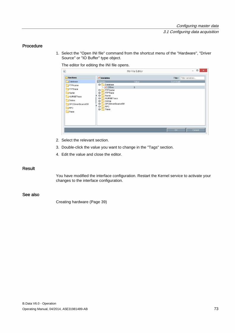
Configuring master data 3.1 Configuring data acquisition
B.Data V6.0 - Operation Operating Manual, 04/2014, A5E31981489-AB 73
Procedure 1. Select the "Open INI file" command from the shortcut menu of the "Hardware", "Driver
Source" or "IO Buffer" type object.
The editor for editing the INI file opens.
2. Select the relevant section.
3. Double-click the value you want to change in the "Tags" section.
4. Edit the value and close the editor.
Result You have modified the interface configuration. Restart the Kernel service to activate your changes to the interface configuration.
See also Creating hardware (Page 39)
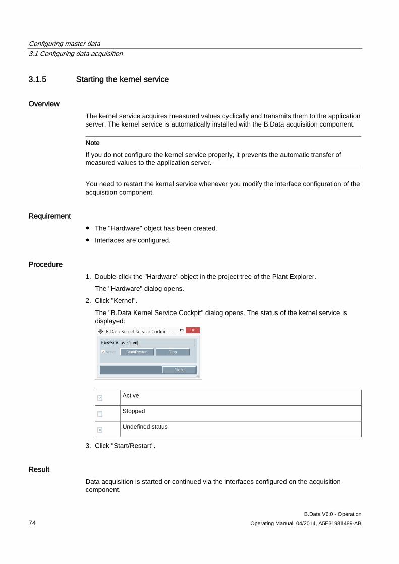
Configuring master data 3.1 Configuring data acquisition
B.Data V6.0 - Operation 74 Operating Manual, 04/2014, A5E31981489-AB
3.1.5 Starting the kernel service
Overview The kernel service acquires measured values cyclically and transmits them to the application server. The kernel service is automatically installed with the B.Data acquisition component.
Note
If you do not configure the kernel service properly, it prevents the automatic transfer of measured values to the application server.
You need to restart the kernel service whenever you modify the interface configuration of the acquisition component.
Requirement ● The "Hardware" object has been created.
● Interfaces are configured.
Procedure 1. Double-click the "Hardware" object in the project tree of the Plant Explorer.
The "Hardware" dialog opens.
2. Click "Kernel".
The "B.Data Kernel Service Cockpit" dialog opens. The status of the kernel service is displayed:
Active
Stopped
Undefined status
3. Click "Start/Restart".
Result Data acquisition is started or continued via the interfaces configured on the acquisition component.

Configuring master data 3.1 Configuring data acquisition
B.Data V6.0 - Operation Operating Manual, 04/2014, A5E31981489-AB 75
Alternative procedure You can also restart the kernel service for an acquisition component from the Service Cockpit.
Configuring master data 3.2 Create printer and directory
B.Data V6.0 - Operation 76 Operating Manual, 04/2014, A5E31981489-AB
3.2 Create printer and directory
3.2.1 Fundamentals of creating printer and directory In B.Data you can automatically print reports, send them by e-mail or save them to a directory.
To automatically print reports, send them by e-mail or save them to a directory, follow these steps:
1. Create a printer or a directory in the selected hardware.
2. Create a user with an e-mail address.
3. Copy the printer, the directory and/or the user in the query type of the required report.
4. Activate the "Print automatically" and/or "Mail/save automatically" options in the query type of the selected report.
5. Run the Windows service "B.Data Report Server".
Restart the Windows service "B.Data Report Server" after having made changes.
See also Creating a printer (Page 77)
Creating a folder (Page 79)
Configuring the query type for a report (Page 187)
Setting up users (Page 83)
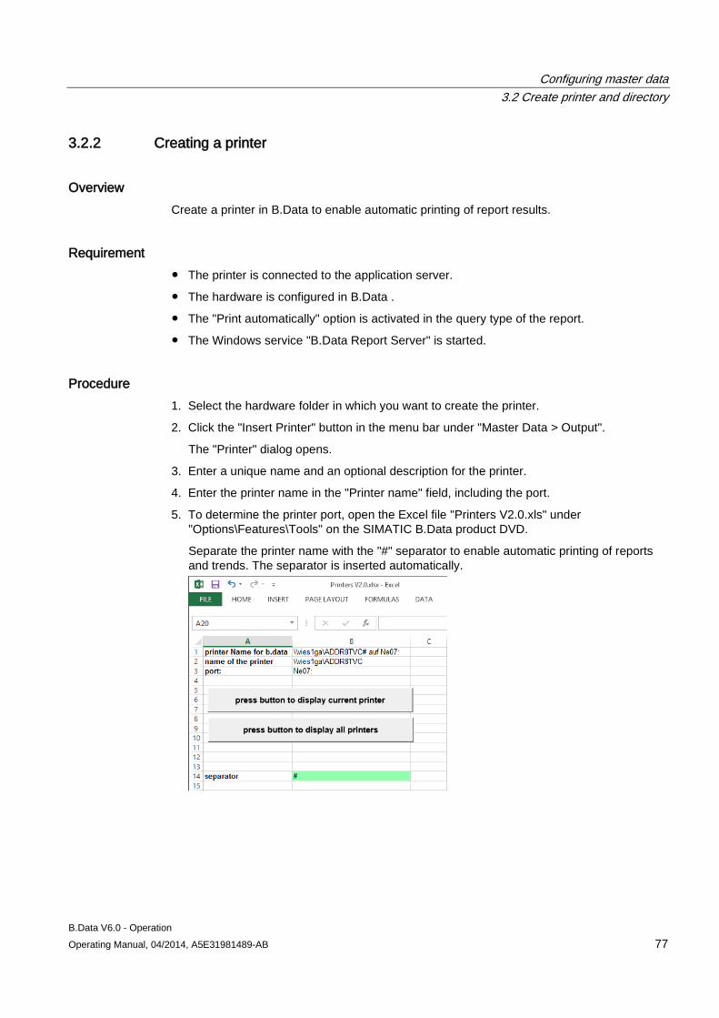
Configuring master data 3.2 Create printer and directory
B.Data V6.0 - Operation Operating Manual, 04/2014, A5E31981489-AB 77
3.2.2 Creating a printer
Overview Create a printer in B.Data to enable automatic printing of report results.
Requirement ● The printer is connected to the application server.
● The hardware is configured in B.Data .
● The "Print automatically" option is activated in the query type of the report.
● The Windows service "B.Data Report Server" is started.
Procedure 1. Select the hardware folder in which you want to create the printer.
2. Click the "Insert Printer" button in the menu bar under "Master Data > Output".
The "Printer" dialog opens.
3. Enter a unique name and an optional description for the printer.
4. Enter the printer name in the "Printer name" field, including the port.
5. To determine the printer port, open the Excel file "Printers V2.0.xls" under "Options\Features\Tools" on the SIMATIC B.Data product DVD.
Separate the printer name with the "#" separator to enable automatic printing of reports and trends. The separator is inserted automatically.
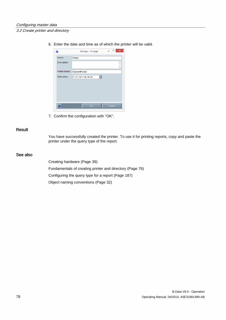
Configuring master data 3.2 Create printer and directory
B.Data V6.0 - Operation 78 Operating Manual, 04/2014, A5E31981489-AB
6. Enter the date and time as of which the printer will be valid.
7. Confirm the configuration with "OK".
Result You have successfully created the printer. To use it for printing reports, copy and paste the printer under the query type of the report.
See also Creating hardware (Page 39)
Fundamentals of creating printer and directory (Page 76)
Configuring the query type for a report (Page 187)
Object naming conventions (Page 32)
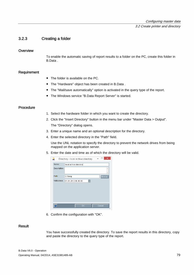
Configuring master data 3.2 Create printer and directory
B.Data V6.0 - Operation Operating Manual, 04/2014, A5E31981489-AB 79
3.2.3 Creating a folder
Overview To enable the automatic saving of report results to a folder on the PC, create this folder in B.Data .
Requirement ● The folder is available on the PC.
● The "Hardware" object has been created in B.Data .
● The "Mail/save automatically" option is activated in the query type of the report.
● The Windows service "B.Data Report Server" is started.
Procedure 1. Select the hardware folder in which you want to create the directory.
2. Click the "Insert Directory" button in the menu bar under "Master Data > Output".
The "Directory" dialog opens.
3. Enter a unique name and an optional description for the directory.
4. Enter the selected directory in the "Path" field.
Use the UNL notation to specify the directory to prevent the network drives from being mapped on the application server.
5. Enter the date and time as of which the directory will be valid.
6. Confirm the configuration with "OK".
Result You have successfully created the directory. To save the report results in this directory, copy and paste the directory to the query type of the report.

Configuring master data 3.2 Create printer and directory
B.Data V6.0 - Operation 80 Operating Manual, 04/2014, A5E31981489-AB
See also Fundamentals of creating printer and directory (Page 76)
Creating hardware (Page 39)
Configuring the query type for a report (Page 187)
Object naming conventions (Page 32)
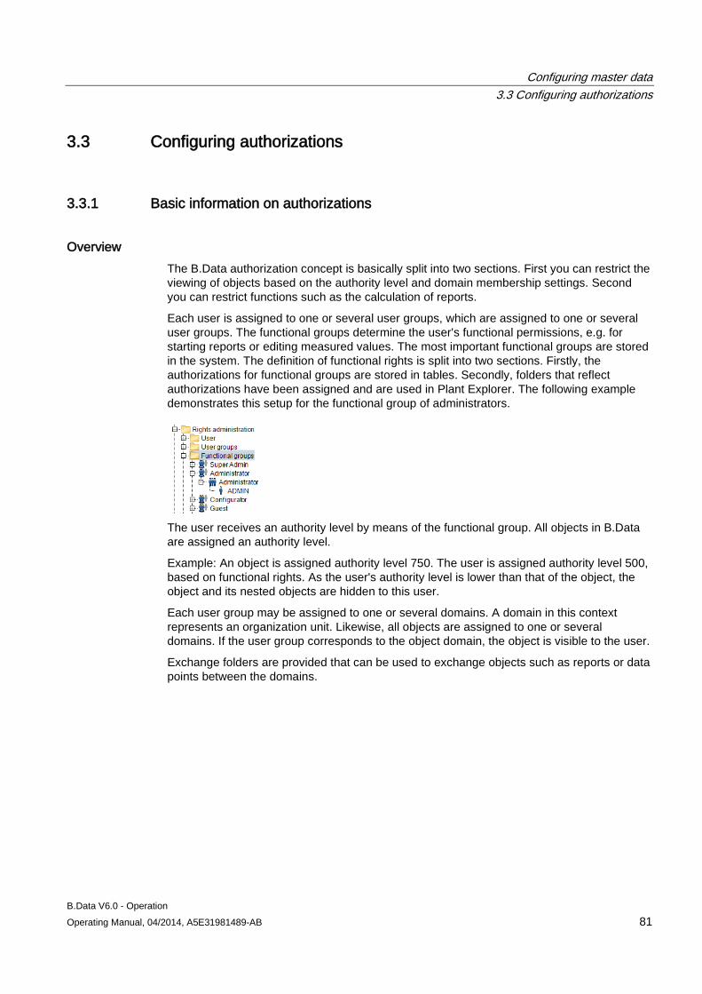
Configuring master data 3.3 Configuring authorizations
B.Data V6.0 - Operation Operating Manual, 04/2014, A5E31981489-AB 81
3.3 Configuring authorizations
3.3.1 Basic information on authorizations
Overview The B.Data authorization concept is basically split into two sections. First you can restrict the viewing of objects based on the authority level and domain membership settings. Second you can restrict functions such as the calculation of reports.
Each user is assigned to one or several user groups, which are assigned to one or several user groups. The functional groups determine the user's functional permissions, e.g. for starting reports or editing measured values. The most important functional groups are stored in the system. The definition of functional rights is split into two sections. Firstly, the authorizations for functional groups are stored in tables. Secondly, folders that reflect authorizations have been assigned and are used in Plant Explorer. The following example demonstrates this setup for the functional group of administrators.
The user receives an authority level by means of the functional group. All objects in B.Data are assigned an authority level.
Example: An object is assigned authority level 750. The user is assigned authority level 500, based on functional rights. As the user's authority level is lower than that of the object, the object and its nested objects are hidden to this user.
Each user group may be assigned to one or several domains. A domain in this context represents an organization unit. Likewise, all objects are assigned to one or several domains. If the user group corresponds to the object domain, the object is visible to the user.
Exchange folders are provided that can be used to exchange objects such as reports or data points between the domains.
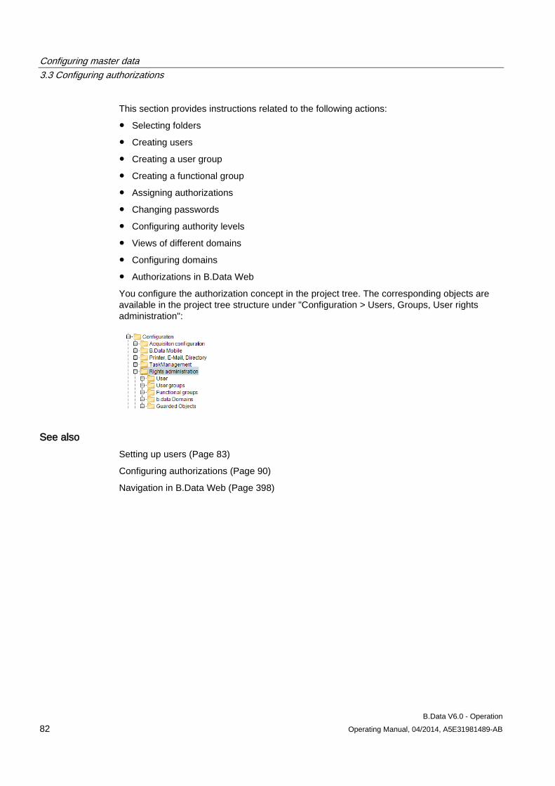
Configuring master data 3.3 Configuring authorizations
B.Data V6.0 - Operation 82 Operating Manual, 04/2014, A5E31981489-AB
This section provides instructions related to the following actions:
● Selecting folders
● Creating users
● Creating a user group
● Creating a functional group
● Assigning authorizations
● Changing passwords
● Configuring authority levels
● Views of different domains
● Configuring domains
● Authorizations in B.Data Web
You configure the authorization concept in the project tree. The corresponding objects are available in the project tree structure under "Configuration > Users, Groups, User rights administration":
See also Setting up users (Page 83)
Configuring authorizations (Page 90)
Navigation in B.Data Web (Page 398)
Configuring master data 3.3 Configuring authorizations
B.Data V6.0 - Operation Operating Manual, 04/2014, A5E31981489-AB 83
3.3.2 Setting up users
Overview You can create a user in B.Data. You create a user mainly in the following cases:
● For a user to log on to B.Data, B.Data Web or B.Data Mobile.
● For a user to receive B.Data reports or messages per e-mail.
The e-mail client that is installed on your PC, e.g. Microsoft Outlook, is used for mailing.
If you create a user in B.Data, the information you specify includes the following:
● B.Data user name and password for the user to log on to B.Data, B.Data Web or B.Data Mobile
For the initial logon, the user enters the user name in uppercase letters as the password, for example, if the user name is "SmithJ", the password is "SMITHJ". The authority level is not assigned until the user has been assigned to a user group or functional group. Once you have created the user, you can change the password in the "User" object.
● Contact information, for example, address or e-mail address for sending B.Data reports or messages by e-mail
● Unlocking a user
If a user has entered the wrong password several times during logon to B.Data, this user is locked out by the system. You can then use the "Unlock" option to restore the user's access to the system.
● Activating the "Single sign on" option
Once a user has started the B.Data Plant Explorer, B.Data checks if the Windows user name of this user is entered in B.Data. It is no longer necessary for you to enter login data if B.Data can identify the name. You will otherwise have to log on to B.Data.
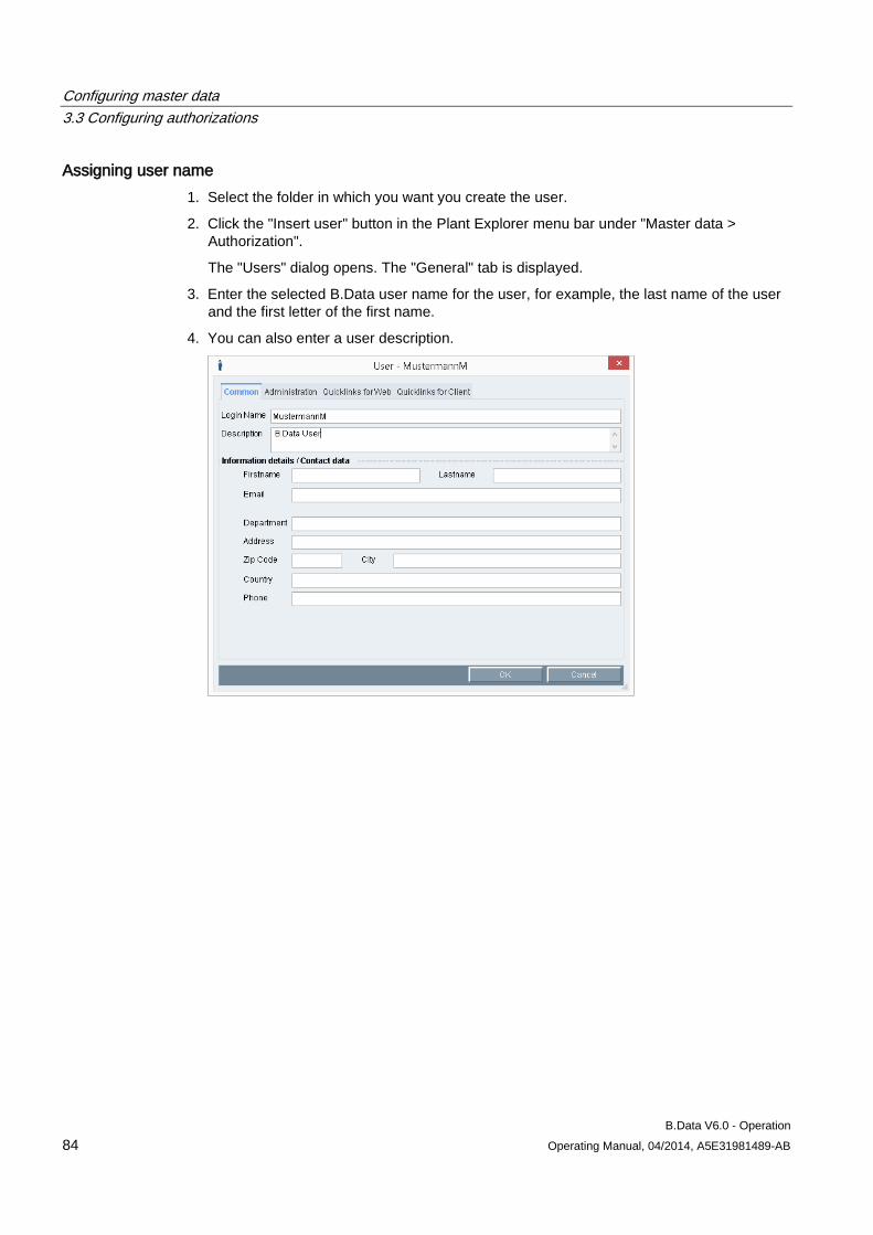
Configuring master data 3.3 Configuring authorizations
B.Data V6.0 - Operation 84 Operating Manual, 04/2014, A5E31981489-AB
Assigning user name 1. Select the folder in which you want you create the user.
2. Click the "Insert user" button in the Plant Explorer menu bar under "Master data > Authorization".
The "Users" dialog opens. The "General" tab is displayed.
3. Enter the selected B.Data user name for the user, for example, the last name of the user and the first letter of the first name.
4. You can also enter a user description.
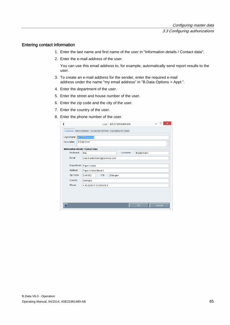
Configuring master data 3.3 Configuring authorizations
B.Data V6.0 - Operation Operating Manual, 04/2014, A5E31981489-AB 85
Entering contact information 1. Enter the last name and first name of the user in "Information details / Contact data".
2. Enter the e-mail address of the user.
You can use this email address to, for example, automatically send report results to the user.
3. To create an e-mail address for the sender, enter the required e-mail address under the name "my email address" in "B.Data Options > Appl.".
4. Enter the department of the user.
5. Enter the street and house number of the user.
6. Enter the zip code and the city of the user.
7. Enter the country of the user.
8. Enter the phone number of the user.

Configuring master data 3.3 Configuring authorizations
B.Data V6.0 - Operation 86 Operating Manual, 04/2014, A5E31981489-AB
Editing logon information 1. Select the "Administration" tab.
2. To deactivate the user, activate the "User disabled" option.
The user cannot log on to B.Data Client, B.Data Web-Client, B.Data Mobile.

Configuring master data 3.3 Configuring authorizations
B.Data V6.0 - Operation Operating Manual, 04/2014, A5E31981489-AB 87
The user continues to receive e-mails that are configured for him/her in B.Data, for example, e-mails with B.Data reports.
3. You can unlock user access again by clicking "Unlock".
4. To set a password for the user, follow these steps:
– Click "Set password".
The "Change Password" dialog opens.
– Enter the selected password and confirm the password.
– Click "OK".
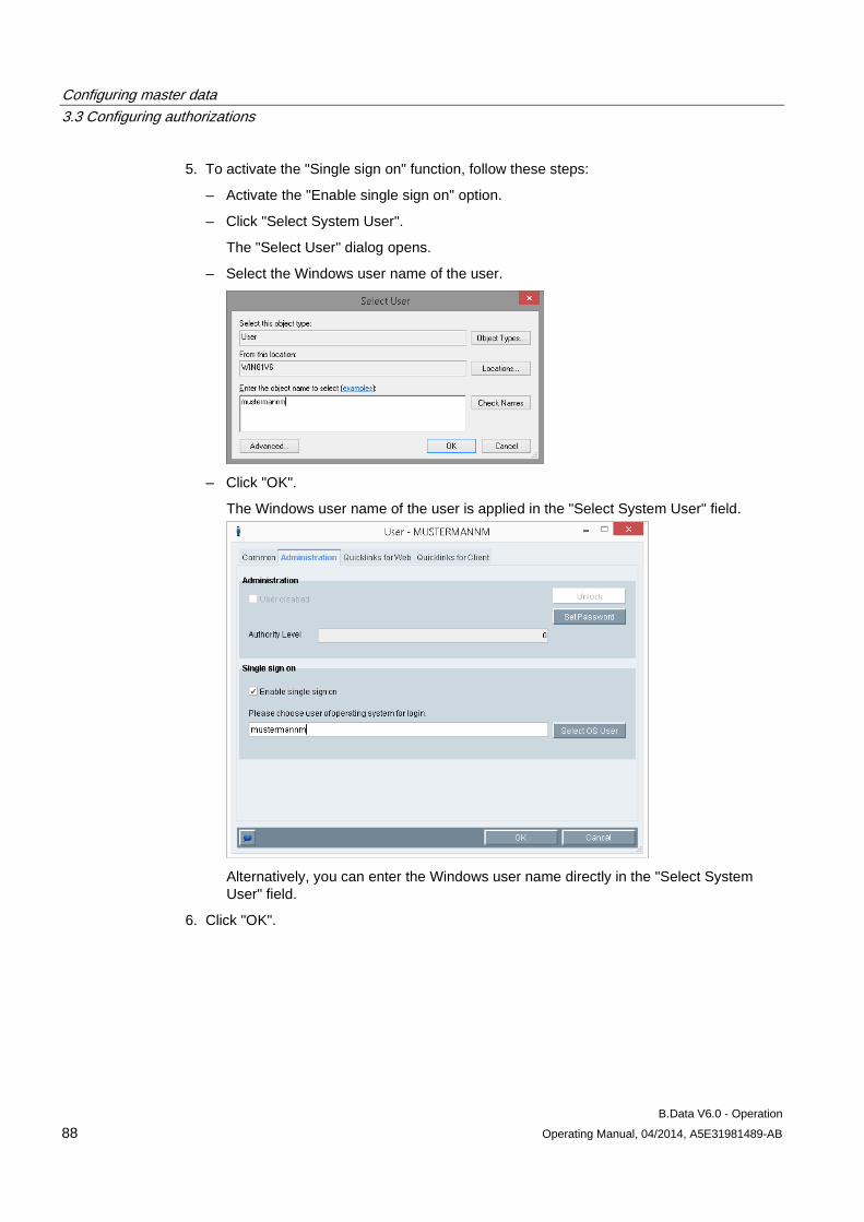
Configuring master data 3.3 Configuring authorizations
B.Data V6.0 - Operation 88 Operating Manual, 04/2014, A5E31981489-AB
5. To activate the "Single sign on" function, follow these steps:
– Activate the "Enable single sign on" option.
– Click "Select System User".
The "Select User" dialog opens.
– Select the Windows user name of the user.
– Click "OK".
The Windows user name of the user is applied in the "Select System User" field.
Alternatively, you can enter the Windows user name directly in the "Select System User" field.
6. Click "OK".
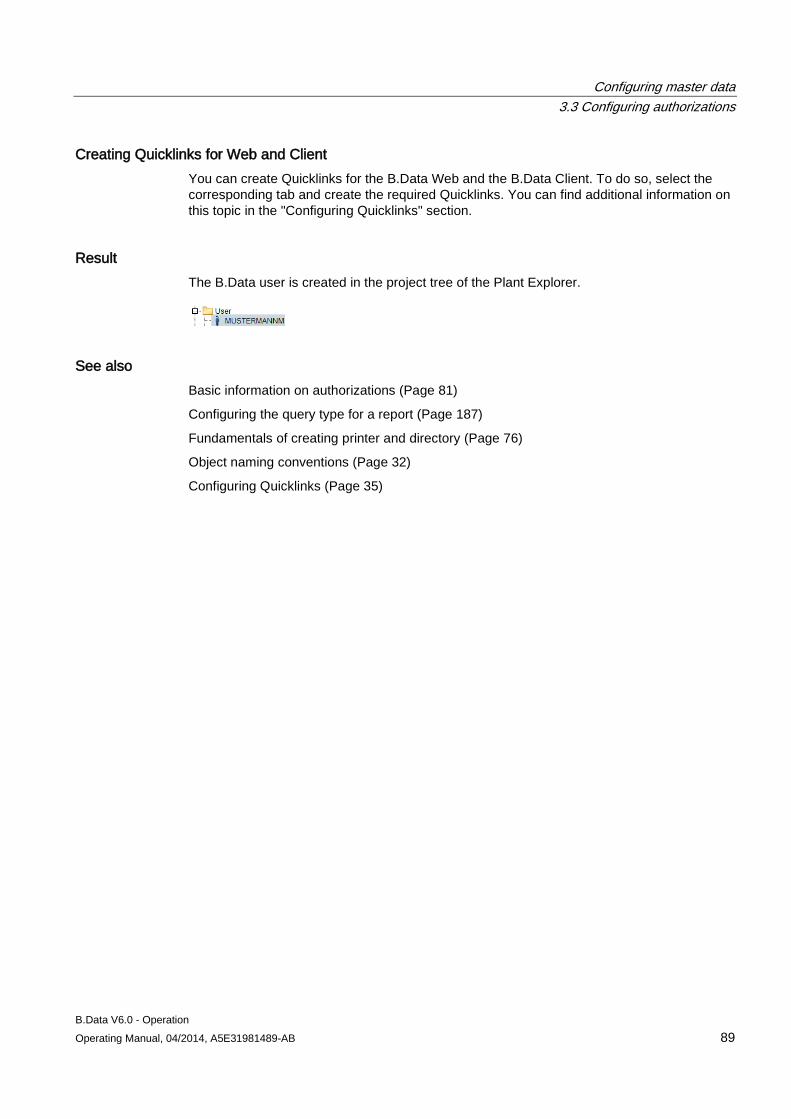
Configuring master data 3.3 Configuring authorizations
B.Data V6.0 - Operation Operating Manual, 04/2014, A5E31981489-AB 89
Creating Quicklinks for Web and Client You can create Quicklinks for the B.Data Web and the B.Data Client. To do so, select the corresponding tab and create the required Quicklinks. You can find additional information on this topic in the "Configuring Quicklinks" section.
Result The B.Data user is created in the project tree of the Plant Explorer.
See also Basic information on authorizations (Page 81)
Configuring the query type for a report (Page 187)
Fundamentals of creating printer and directory (Page 76)
Object naming conventions (Page 32)
Configuring Quicklinks (Page 35)
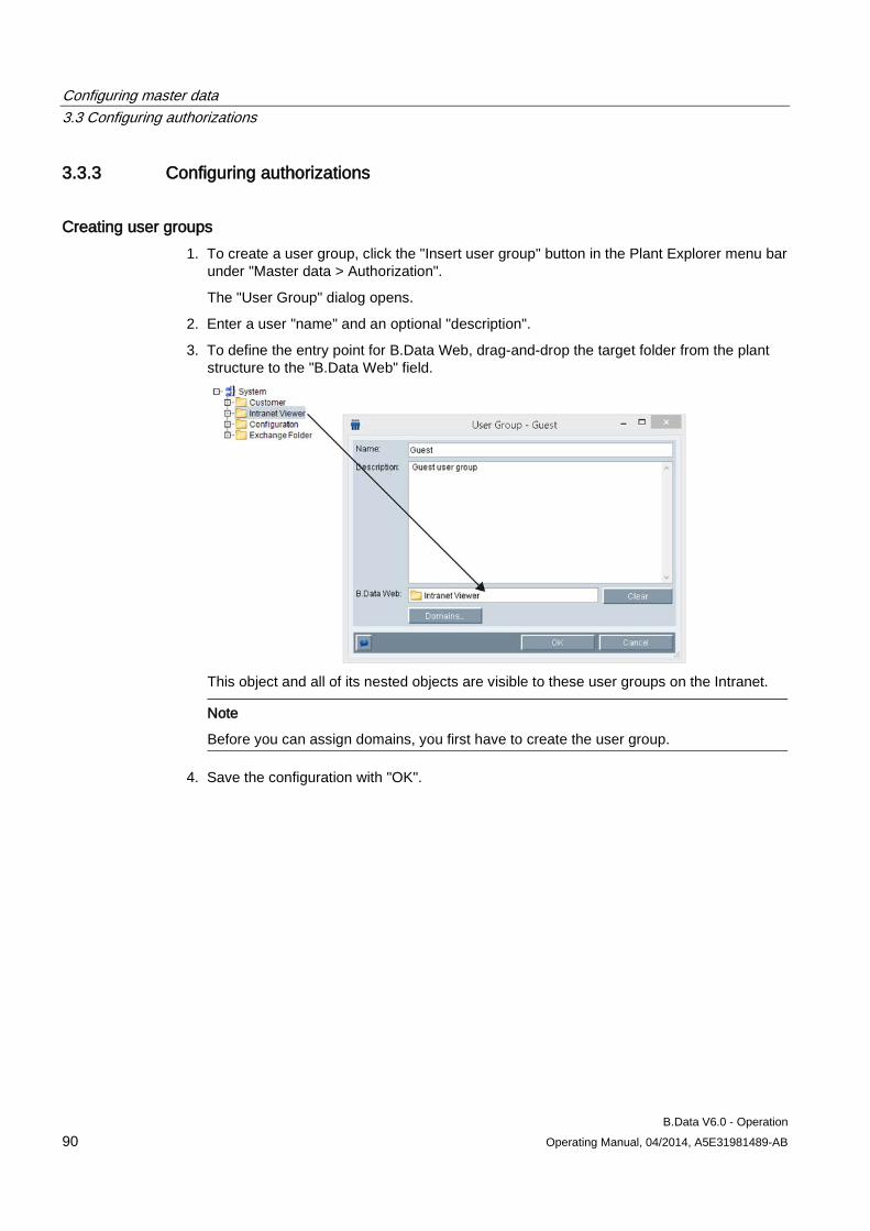
Configuring master data 3.3 Configuring authorizations
B.Data V6.0 - Operation 90 Operating Manual, 04/2014, A5E31981489-AB
3.3.3 Configuring authorizations
Creating user groups 1. To create a user group, click the "Insert user group" button in the Plant Explorer menu bar
under "Master data > Authorization".
The "User Group" dialog opens.
2. Enter a user "name" and an optional "description".
3. To define the entry point for B.Data Web, drag-and-drop the target folder from the plant structure to the "B.Data Web" field.
This object and all of its nested objects are visible to these user groups on the Intranet.
Note
Before you can assign domains, you first have to create the user group.
4. Save the configuration with "OK".
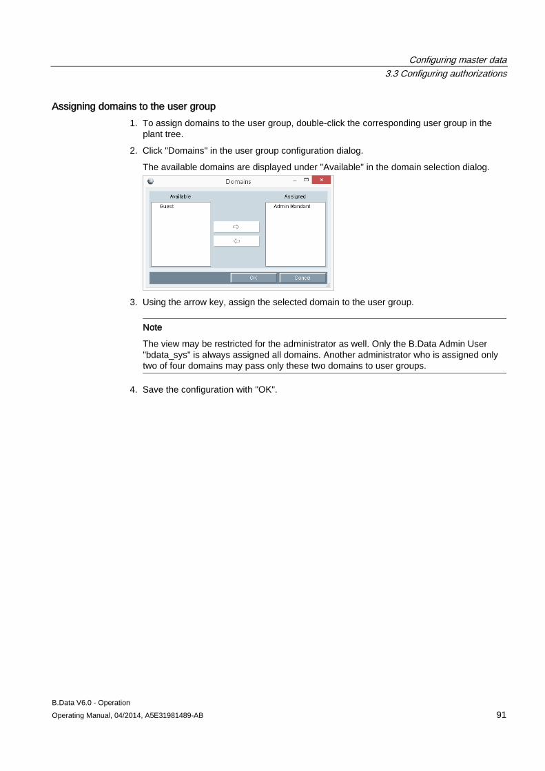
Configuring master data 3.3 Configuring authorizations
B.Data V6.0 - Operation Operating Manual, 04/2014, A5E31981489-AB 91
Assigning domains to the user group 1. To assign domains to the user group, double-click the corresponding user group in the
plant tree.
2. Click "Domains" in the user group configuration dialog.
The available domains are displayed under "Available" in the domain selection dialog.
3. Using the arrow key, assign the selected domain to the user group.
Note
The view may be restricted for the administrator as well. Only the B.Data Admin User "bdata_sys" is always assigned all domains. Another administrator who is assigned only two of four domains may pass only these two domains to user groups.
4. Save the configuration with "OK".
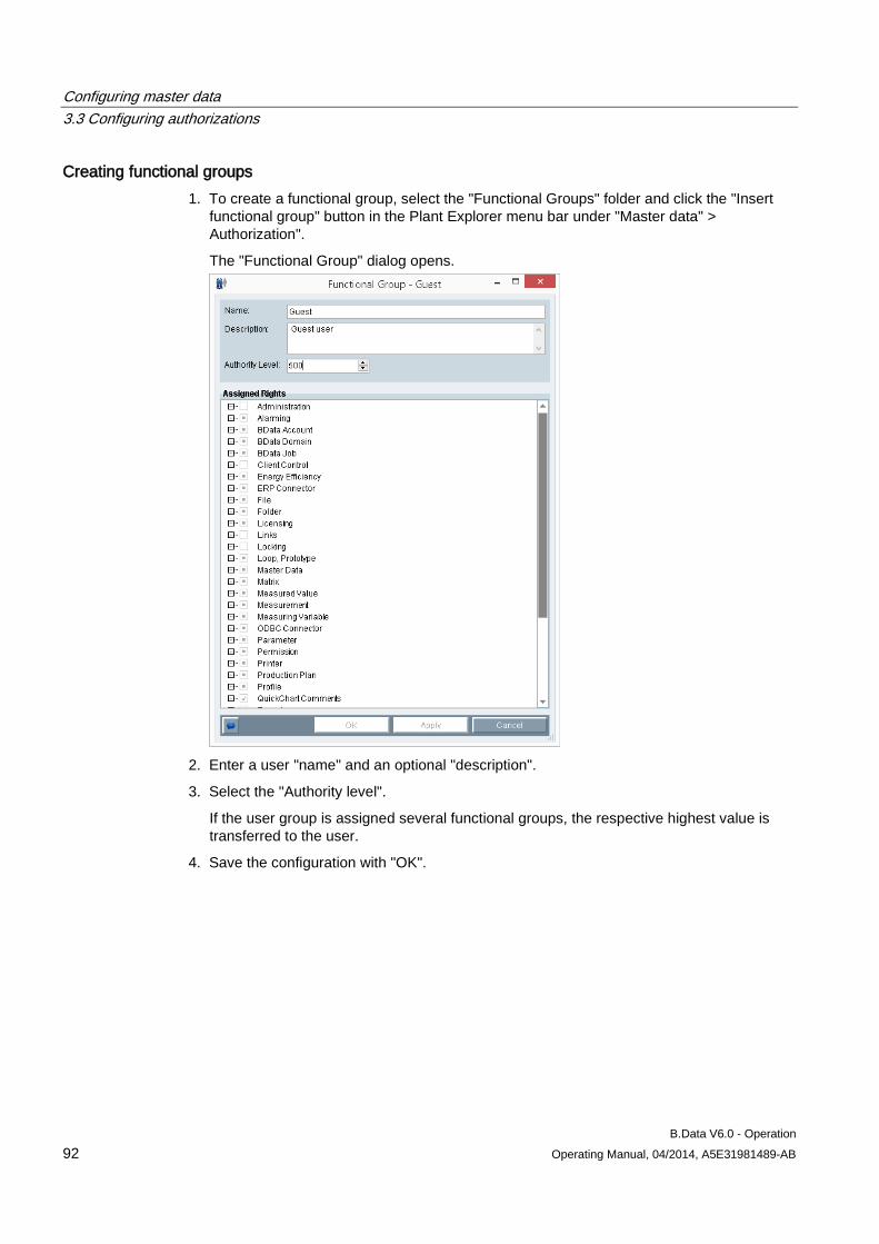
Configuring master data 3.3 Configuring authorizations
B.Data V6.0 - Operation 92 Operating Manual, 04/2014, A5E31981489-AB
Creating functional groups 1. To create a functional group, select the "Functional Groups" folder and click the "Insert
functional group" button in the Plant Explorer menu bar under "Master data" > Authorization".
The "Functional Group" dialog opens.
2. Enter a user "name" and an optional "description".
3. Select the "Authority level".
If the user group is assigned several functional groups, the respective highest value is transferred to the user.
4. Save the configuration with "OK".
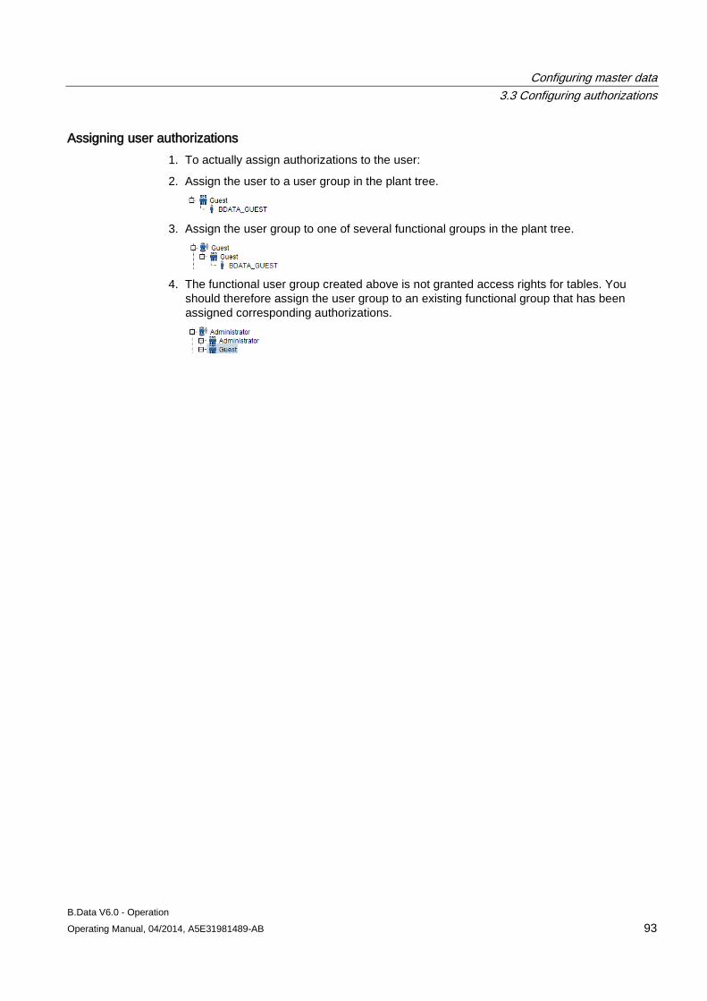
Configuring master data 3.3 Configuring authorizations
B.Data V6.0 - Operation Operating Manual, 04/2014, A5E31981489-AB 93
Assigning user authorizations 1. To actually assign authorizations to the user:
2. Assign the user to a user group in the plant tree.
3. Assign the user group to one of several functional groups in the plant tree.
4. The functional user group created above is not granted access rights for tables. You
should therefore assign the user group to an existing functional group that has been assigned corresponding authorizations.
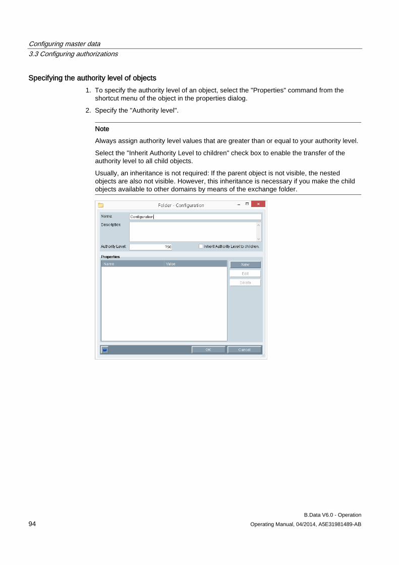
Configuring master data 3.3 Configuring authorizations
B.Data V6.0 - Operation 94 Operating Manual, 04/2014, A5E31981489-AB
Specifying the authority level of objects 1. To specify the authority level of an object, select the "Properties" command from the
shortcut menu of the object in the properties dialog.
2. Specify the "Authority level".
Note
Always assign authority level values that are greater than or equal to your authority level.
Select the "Inherit Authority Level to children" check box to enable the transfer of the authority level to all child objects.
Usually, an inheritance is not required: If the parent object is not visible, the nested objects are also not visible. However, this inheritance is necessary if you make the child objects available to other domains by means of the exchange folder.
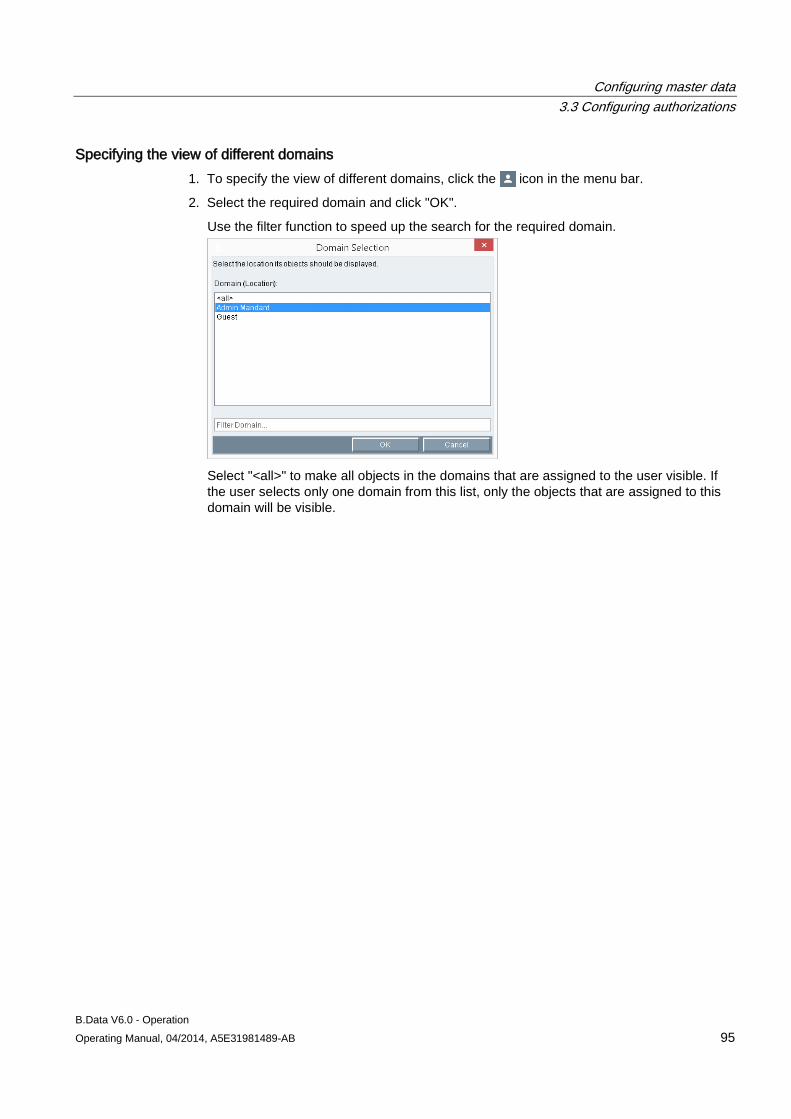
Configuring master data 3.3 Configuring authorizations
B.Data V6.0 - Operation Operating Manual, 04/2014, A5E31981489-AB 95
Specifying the view of different domains 1. To specify the view of different domains, click the icon in the menu bar.
2. Select the required domain and click "OK".
Use the filter function to speed up the search for the required domain.
Select "<all>" to make all objects in the domains that are assigned to the user visible. If the user selects only one domain from this list, only the objects that are assigned to this domain will be visible.
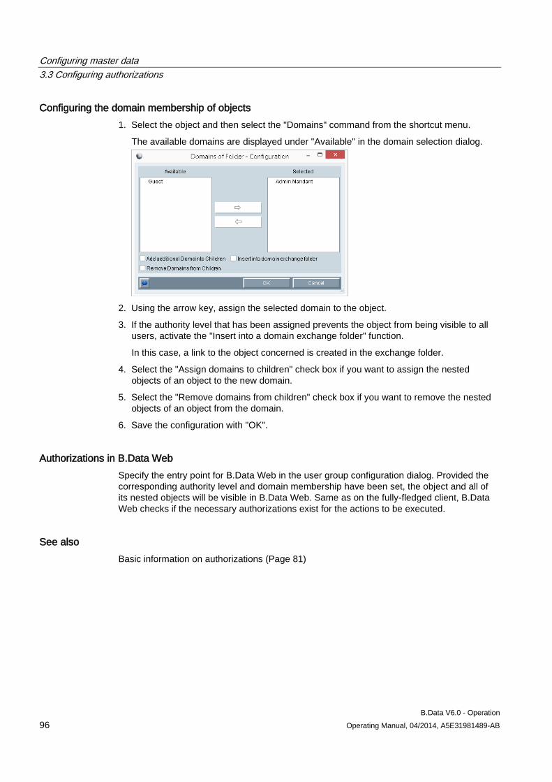
Configuring master data 3.3 Configuring authorizations
B.Data V6.0 - Operation 96 Operating Manual, 04/2014, A5E31981489-AB
Configuring the domain membership of objects 1. Select the object and then select the "Domains" command from the shortcut menu.
The available domains are displayed under "Available" in the domain selection dialog.
2. Using the arrow key, assign the selected domain to the object.
3. If the authority level that has been assigned prevents the object from being visible to all users, activate the "Insert into a domain exchange folder" function.
In this case, a link to the object concerned is created in the exchange folder.
4. Select the "Assign domains to children" check box if you want to assign the nested objects of an object to the new domain.
5. Select the "Remove domains from children" check box if you want to remove the nested objects of an object from the domain.
6. Save the configuration with "OK".
Authorizations in B.Data Web Specify the entry point for B.Data Web in the user group configuration dialog. Provided the corresponding authority level and domain membership have been set, the object and all of its nested objects will be visible in B.Data Web. Same as on the fully-fledged client, B.Data Web checks if the necessary authorizations exist for the actions to be executed.
See also Basic information on authorizations (Page 81)
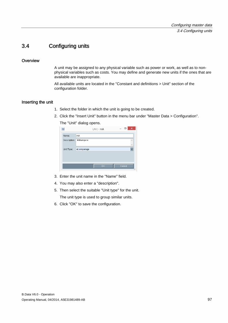
Configuring master data 3.4 Configuring units
B.Data V6.0 - Operation Operating Manual, 04/2014, A5E31981489-AB 97
3.4 Configuring units
Overview A unit may be assigned to any physical variable such as power or work, as well as to non-physical variables such as costs. You may define and generate new units if the ones that are available are inappropriate.
All available units are located in the "Constant and definitions > Unit" section of the configuration folder.
Inserting the unit 1. Select the folder in which the unit is going to be created.
2. Click the "Insert Unit" button in the menu bar under "Master Data > Configuration".
The "Unit" dialog opens.
3. Enter the unit name in the "Name" field.
4. You may also enter a "description".
5. Then select the suitable "Unit type" for the unit.
The unit type is used to group similar units.
6. Click "OK" to save the configuration.
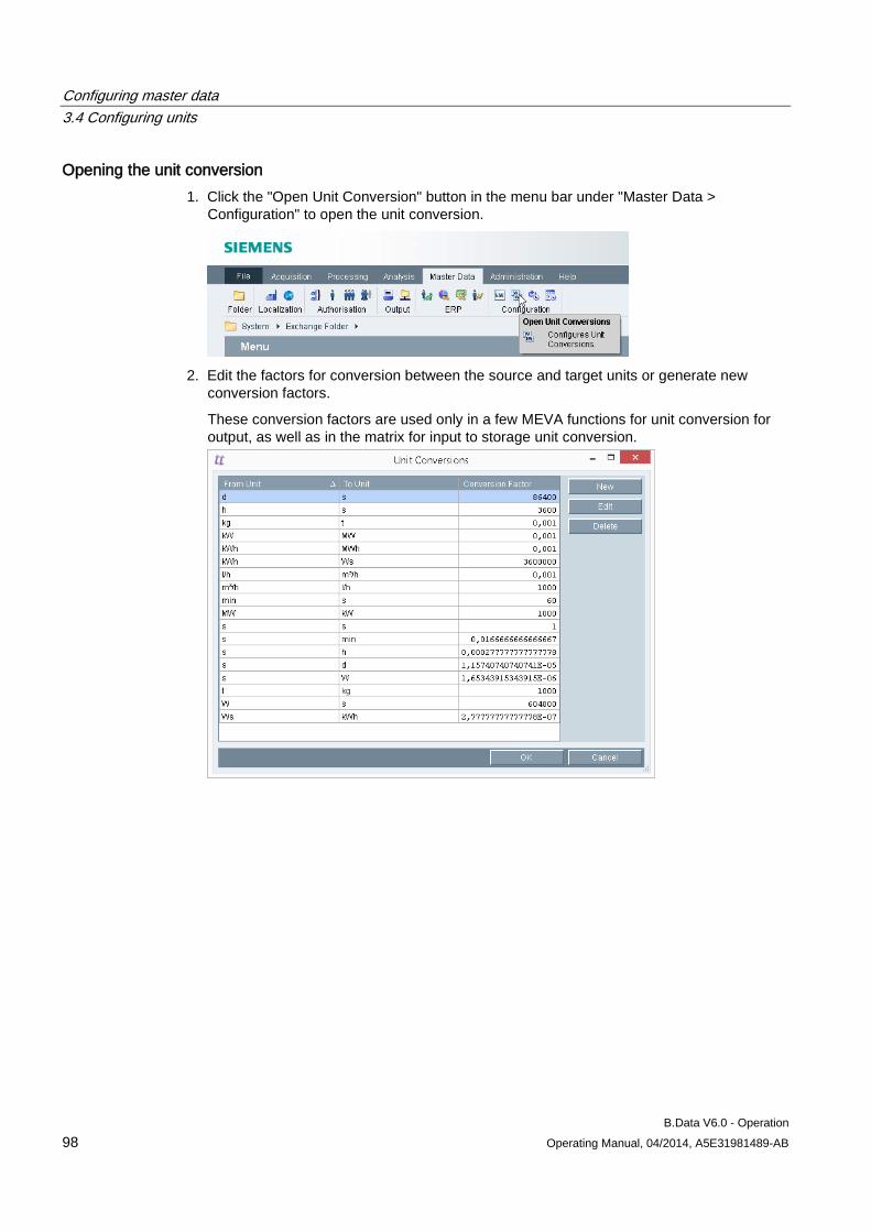
Configuring master data 3.4 Configuring units
B.Data V6.0 - Operation 98 Operating Manual, 04/2014, A5E31981489-AB
Opening the unit conversion 1. Click the "Open Unit Conversion" button in the menu bar under "Master Data >
Configuration" to open the unit conversion.
2. Edit the factors for conversion between the source and target units or generate new
conversion factors.
These conversion factors are used only in a few MEVA functions for unit conversion for output, as well as in the matrix for input to storage unit conversion.
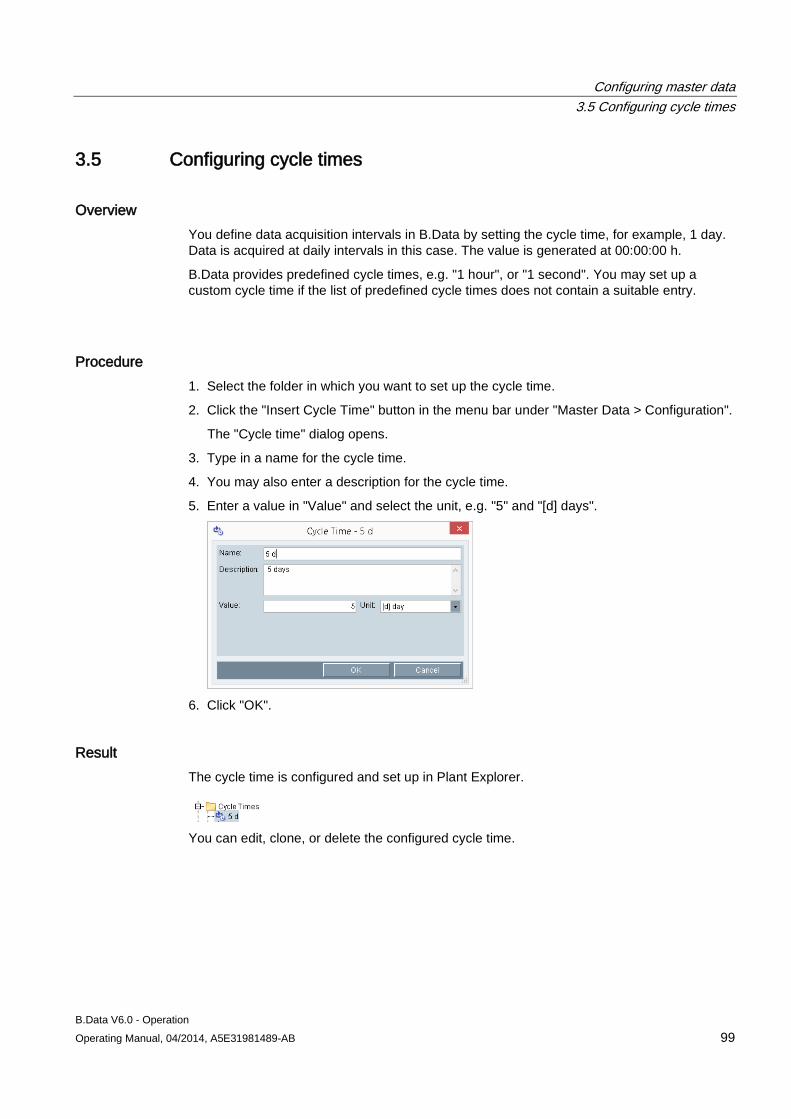
Configuring master data 3.5 Configuring cycle times
B.Data V6.0 - Operation Operating Manual, 04/2014, A5E31981489-AB 99
3.5 Configuring cycle times
Overview You define data acquisition intervals in B.Data by setting the cycle time, for example, 1 day. Data is acquired at daily intervals in this case. The value is generated at 00:00:00 h.
B.Data provides predefined cycle times, e.g. "1 hour", or "1 second". You may set up a custom cycle time if the list of predefined cycle times does not contain a suitable entry.
Procedure 1. Select the folder in which you want to set up the cycle time.
2. Click the "Insert Cycle Time" button in the menu bar under "Master Data > Configuration".
The "Cycle time" dialog opens.
3. Type in a name for the cycle time.
4. You may also enter a description for the cycle time.
5. Enter a value in "Value" and select the unit, e.g. "5" and "[d] days".
6. Click "OK".
Result The cycle time is configured and set up in Plant Explorer.
You can edit, clone, or delete the configured cycle time.
Configuring master data 3.6 Configuring query types
B.Data V6.0 - Operation 100 Operating Manual, 04/2014, A5E31981489-AB
3.6 Configuring query types
Overview Use a query type in B.Data to specify the period to be queried in a report.
B.Data provides predefined query types, e.g. "week", or "year". You may set up a custom query type if the list of predefined query types does not contain a suitable entry.
Specify the following values when setting a query type:
● Duration
Use the "Duration" setting to specify the period to be queried in the report, e.g. 1 month.
A period of one month is queried in the report, e.g. from 01.02.2013 to 28.02.2013.
● Offset
Use the "Offset" setting to specify the time shift, e.g. 1 day, for the period specified in "Duration".
A period of one month with an offset of one day is queried in the report, e.g. from 02.02.2013 to 01.03.2013.
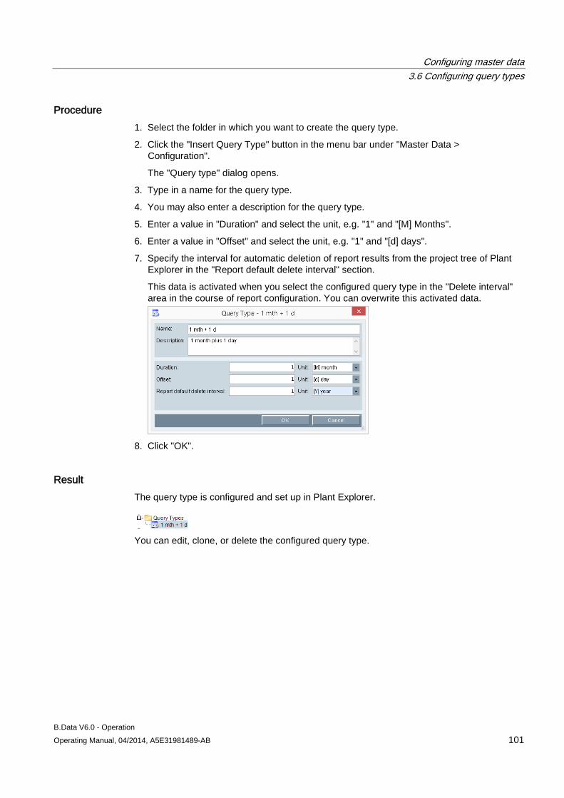
Configuring master data 3.6 Configuring query types
B.Data V6.0 - Operation Operating Manual, 04/2014, A5E31981489-AB 101
Procedure 1. Select the folder in which you want to create the query type.
2. Click the "Insert Query Type" button in the menu bar under "Master Data > Configuration".
The "Query type" dialog opens.
3. Type in a name for the query type.
4. You may also enter a description for the query type.
5. Enter a value in "Duration" and select the unit, e.g. "1" and "[M] Months".
6. Enter a value in "Offset" and select the unit, e.g. "1" and "[d] days".
7. Specify the interval for automatic deletion of report results from the project tree of Plant Explorer in the "Report default delete interval" section.
This data is activated when you select the configured query type in the "Delete interval" area in the course of report configuration. You can overwrite this activated data.
8. Click "OK".
Result The query type is configured and set up in Plant Explorer.
You can edit, clone, or delete the configured query type.
Configuring master data 3.7 Creating objects for Enterprise Resource Planning
B.Data V6.0 - Operation 102 Operating Manual, 04/2014, A5E31981489-AB
3.7 Creating objects for Enterprise Resource Planning
3.7.1 Basics on objects for Enterprise Resource Planning Additional information is needed when booking services in ERP. In B.Data , this information is mapped in the form of the following objects:
1. ERP domain
2. Service type
3. Cost center
4. Cost center relation
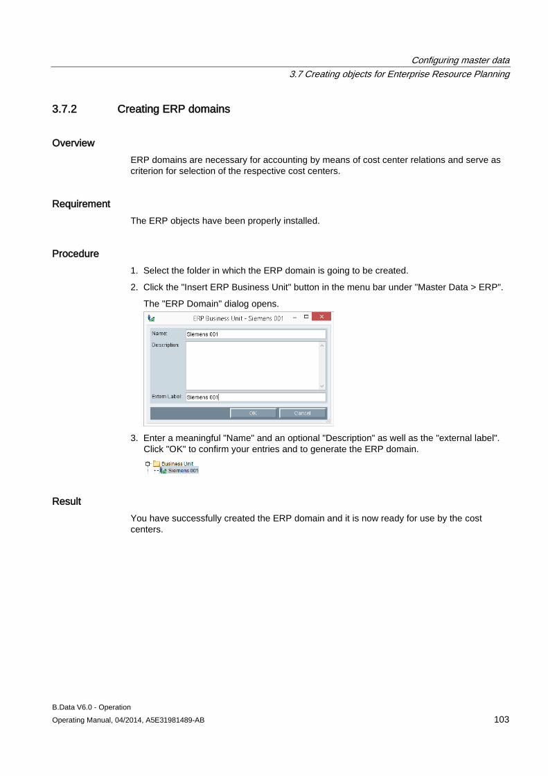
Configuring master data 3.7 Creating objects for Enterprise Resource Planning
B.Data V6.0 - Operation Operating Manual, 04/2014, A5E31981489-AB 103
3.7.2 Creating ERP domains
Overview ERP domains are necessary for accounting by means of cost center relations and serve as criterion for selection of the respective cost centers.
Requirement The ERP objects have been properly installed.
Procedure 1. Select the folder in which the ERP domain is going to be created.
2. Click the "Insert ERP Business Unit" button in the menu bar under "Master Data > ERP".
The "ERP Domain" dialog opens.
3. Enter a meaningful "Name" and an optional "Description" as well as the "external label".
Click "OK" to confirm your entries and to generate the ERP domain.
Result You have successfully created the ERP domain and it is now ready for use by the cost centers.
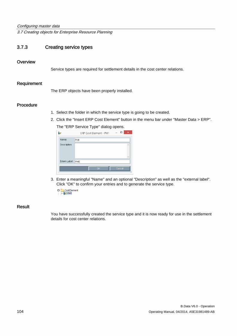
Configuring master data 3.7 Creating objects for Enterprise Resource Planning
B.Data V6.0 - Operation 104 Operating Manual, 04/2014, A5E31981489-AB
3.7.3 Creating service types
Overview Service types are required for settlement details in the cost center relations.
Requirement The ERP objects have been properly installed.
Procedure 1. Select the folder in which the service type is going to be created.
2. Click the "Insert ERP Cost Element" button in the menu bar under "Master Data > ERP".
The "ERP Service Type" dialog opens.
3. Enter a meaningful "Name" and an optional "Description" as well as the "external label".
Click "OK" to confirm your entries and to generate the service type.
Result You have successfully created the service type and it is now ready for use in the settlement details for cost center relations.
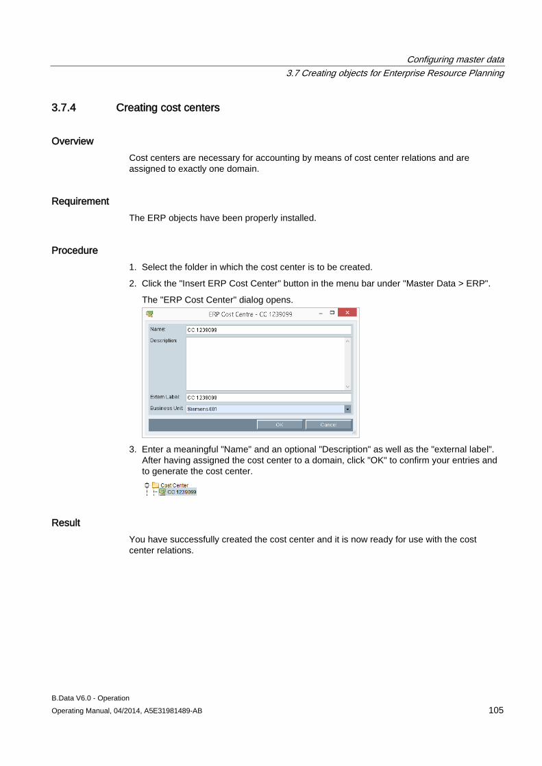
Configuring master data 3.7 Creating objects for Enterprise Resource Planning
B.Data V6.0 - Operation Operating Manual, 04/2014, A5E31981489-AB 105
3.7.4 Creating cost centers
Overview Cost centers are necessary for accounting by means of cost center relations and are assigned to exactly one domain.
Requirement The ERP objects have been properly installed.
Procedure 1. Select the folder in which the cost center is to be created.
2. Click the "Insert ERP Cost Center" button in the menu bar under "Master Data > ERP".
The "ERP Cost Center" dialog opens.
3. Enter a meaningful "Name" and an optional "Description" as well as the "external label".
After having assigned the cost center to a domain, click "OK" to confirm your entries and to generate the cost center.
Result You have successfully created the cost center and it is now ready for use with the cost center relations.
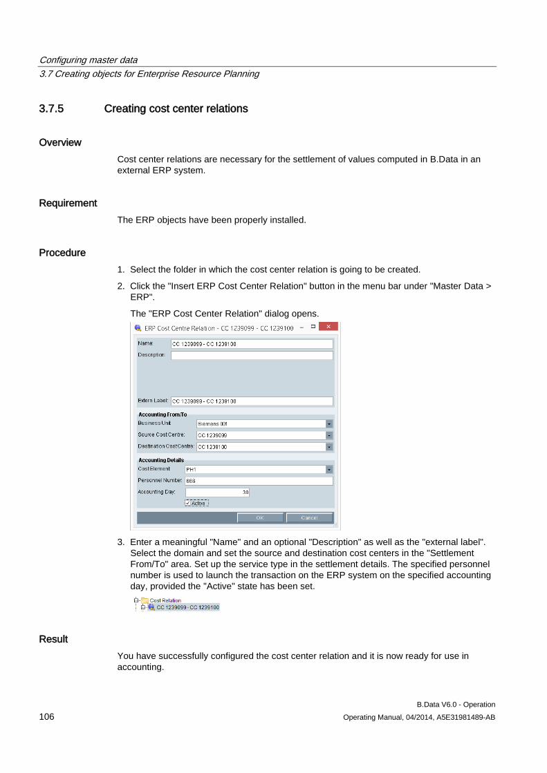
Configuring master data 3.7 Creating objects for Enterprise Resource Planning
B.Data V6.0 - Operation 106 Operating Manual, 04/2014, A5E31981489-AB
3.7.5 Creating cost center relations
Overview Cost center relations are necessary for the settlement of values computed in B.Data in an external ERP system.
Requirement The ERP objects have been properly installed.
Procedure 1. Select the folder in which the cost center relation is going to be created.
2. Click the "Insert ERP Cost Center Relation" button in the menu bar under "Master Data > ERP".
The "ERP Cost Center Relation" dialog opens.
3. Enter a meaningful "Name" and an optional "Description" as well as the "external label".
Select the domain and set the source and destination cost centers in the "Settlement From/To" area. Set up the service type in the settlement details. The specified personnel number is used to launch the transaction on the ERP system on the specified accounting day, provided the "Active" state has been set.
Result You have successfully configured the cost center relation and it is now ready for use in accounting.
Configuring master data 3.8 Managing energy efficiency measures
B.Data V6.0 - Operation Operating Manual, 04/2014, A5E31981489-AB 107
3.8 Managing energy efficiency measures
3.8.1 Basics on managing energy efficiency measures The "Energy Efficiency" module in B.Data provides company-wide transparency in the management of energy efficiency measures. The "Energy Efficiency" module in B.Data was developed in accordance with DIN EN ISO 50001.
The "Energy Efficiency" module in B.Data provides the following options for management of the energy efficiency measures:
● You can enter all energy efficiency measures for all locations of your company.
● You can enter the saving potential and cost of the energy efficiency measure and calculate its cost efficiency.
● You can assign a status that indicates the degree to which the energy efficiency measure has been implemented.
Procedure for managing energy efficiency measures 1. Create an energy efficiency measure.
2. Enter the plant and location for which you defined the energy efficiency measure.
3. Enter the financial saving potential for the plant.
4. Enter the running costs for the plant and calculate the cost effectiveness of your energy efficiency measure.
5. Define a user responsible for the energy efficiency measure.
6. Create one or several domains that are permitted to view and edit an energy efficiency measure.
7. Select a status for the energy efficiency measure.
See also Creating energy efficiency measures (Page 108)
Entering financial saving potentials for an energy efficiency measure (Page 110)
Calculating cost efficiency for energy efficiency measures (Page 112)
Specifying responsibilities for an energy efficiency measure (Page 114)
Specifying clients for an energy efficiency measure (Page 115)
Displaying information about an energy efficiency measure (Page 117)
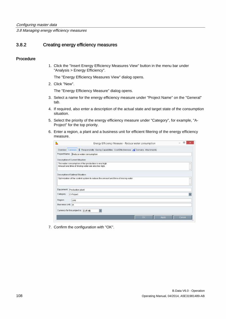
Configuring master data 3.8 Managing energy efficiency measures
B.Data V6.0 - Operation 108 Operating Manual, 04/2014, A5E31981489-AB
3.8.2 Creating energy efficiency measures
Procedure 1. Click the "Insert Energy Efficiency Measures View" button in the menu bar under
"Analysis > Energy Efficiency".
The "Energy Efficiency Measures View" dialog opens.
2. Click "New".
The "Energy Efficiency Measure" dialog opens.
3. Select a name for the energy efficiency measure under "Project Name" on the "General" tab.
4. If required, also enter a description of the actual state and target state of the consumption situation.
5. Select the priority of the energy efficiency measure under "Category", for example, "A-Project" for the top priority.
6. Enter a region, a plant and a business unit for efficient filtering of the energy efficiency measure.
7. Confirm the configuration with "OK".
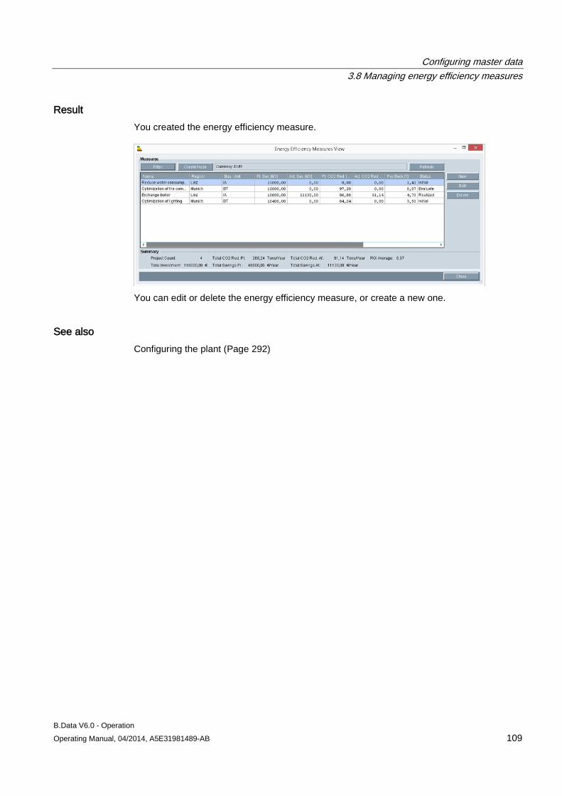
Configuring master data 3.8 Managing energy efficiency measures
B.Data V6.0 - Operation Operating Manual, 04/2014, A5E31981489-AB 109
Result You created the energy efficiency measure.
You can edit or delete the energy efficiency measure, or create a new one.
See also Configuring the plant (Page 292)
Configuring master data 3.8 Managing energy efficiency measures
B.Data V6.0 - Operation 110 Operating Manual, 04/2014, A5E31981489-AB
3.8.3 Entering financial saving potentials for an energy efficiency measure
Overview Enter the financial saving potential of an energy efficiency measure in the "Saving Capabilities" tab separately for each consumption medium. The saving potentials comprise:
● Costs incurred prior to the introduction of the energy efficiency measure
● Scheduled costs following the introduction of the energy efficiency measure
● Costs incurred after introduction of the energy efficiency measure
Requirement You created the energy efficiency measure.
Procedure 1. Double-click the relevant energy efficiency measure in the overview of energy efficiency
measures.
The "Energy Efficiency Measure" dialog opens.
2. Select the "Saving Capabilities" tab.
3. Enter a consumption medium.
4. Select a unit for the consumption medium.
5. Select a parameter, or enter a constant value for the costs and the CO2 production per unit.
6. Enter your values for the post measure state and the planned state of consumption.
7. Confirm the configuration with "OK".
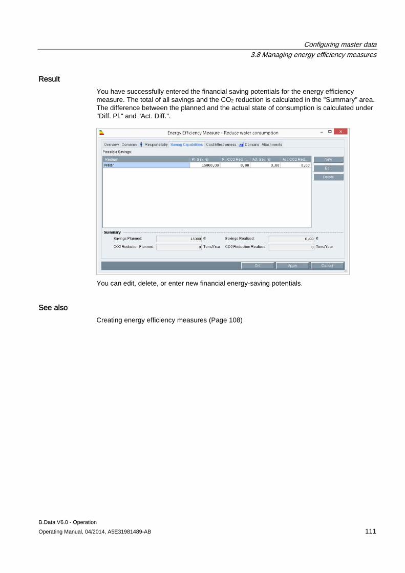
Configuring master data 3.8 Managing energy efficiency measures
B.Data V6.0 - Operation Operating Manual, 04/2014, A5E31981489-AB 111
Result You have successfully entered the financial saving potentials for the energy efficiency measure. The total of all savings and the CO2 reduction is calculated in the "Summary" area. The difference between the planned and the actual state of consumption is calculated under "Diff. Pl." and "Act. Diff.".
You can edit, delete, or enter new financial energy-saving potentials.
See also Creating energy efficiency measures (Page 108)
Configuring master data 3.8 Managing energy efficiency measures
B.Data V6.0 - Operation 112 Operating Manual, 04/2014, A5E31981489-AB
3.8.4 Calculating cost efficiency for energy efficiency measures
Overview Implementation of an energy efficiency measure is initially subject to costs, e.g. purchase of a generator with lower consumption figures. On the "Cost Effectiveness" tab, enter the investment costs, the running costs, and the time period for the costs of the energy efficiency measure. Continue by calculating the cost efficiency of the energy efficiency measure.
Requirement You created the energy efficiency measure.
Procedure 1. Double-click the relevant energy efficiency measure in the overview of energy efficiency
measures.
The "Energy Efficiency Measure" dialog opens.
2. Select the "Cost Effectiveness" tab.
3. Select a period for which you want to calculate the cost efficiency of an energy efficiency measure.
4. Enter a name and a value for the annual active costs.
5. Enter the values for the investment costs and for the internal interest rate.
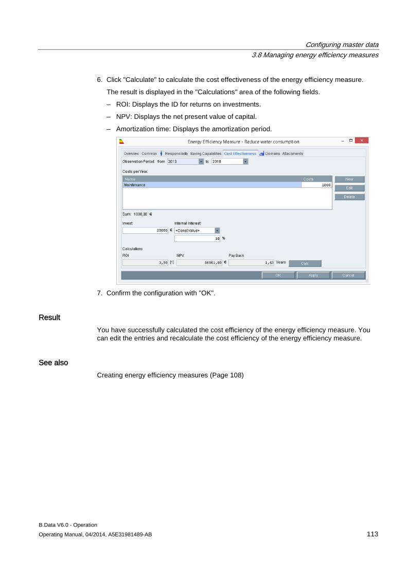
Configuring master data 3.8 Managing energy efficiency measures
B.Data V6.0 - Operation Operating Manual, 04/2014, A5E31981489-AB 113
6. Click "Calculate" to calculate the cost effectiveness of the energy efficiency measure.
The result is displayed in the "Calculations" area of the following fields.
– ROI: Displays the ID for returns on investments.
– NPV: Displays the net present value of capital.
– Amortization time: Displays the amortization period.
7. Confirm the configuration with "OK".
Result You have successfully calculated the cost efficiency of the energy efficiency measure. You can edit the entries and recalculate the cost efficiency of the energy efficiency measure.
See also Creating energy efficiency measures (Page 108)
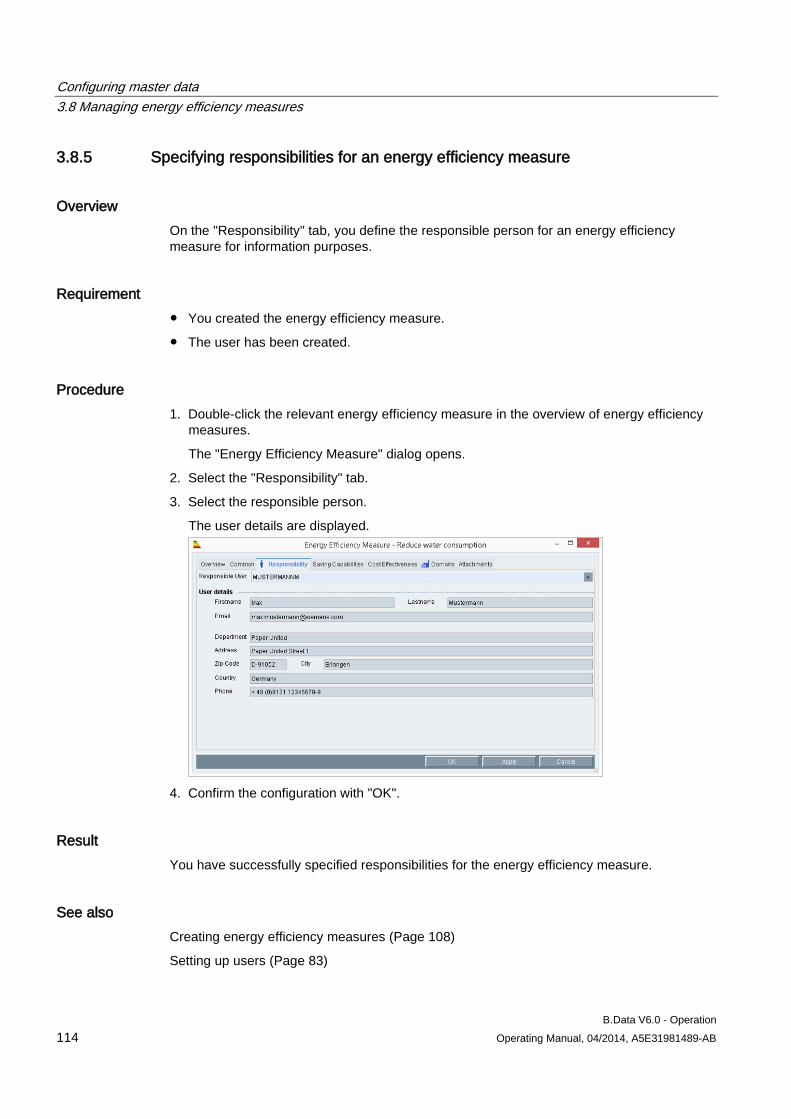
Configuring master data 3.8 Managing energy efficiency measures
B.Data V6.0 - Operation 114 Operating Manual, 04/2014, A5E31981489-AB
3.8.5 Specifying responsibilities for an energy efficiency measure
Overview On the "Responsibility" tab, you define the responsible person for an energy efficiency measure for information purposes.
Requirement ● You created the energy efficiency measure.
● The user has been created.
Procedure 1. Double-click the relevant energy efficiency measure in the overview of energy efficiency
measures.
The "Energy Efficiency Measure" dialog opens.
2. Select the "Responsibility" tab.
3. Select the responsible person.
The user details are displayed.
4. Confirm the configuration with "OK".
Result You have successfully specified responsibilities for the energy efficiency measure.
See also Creating energy efficiency measures (Page 108)
Setting up users (Page 83)
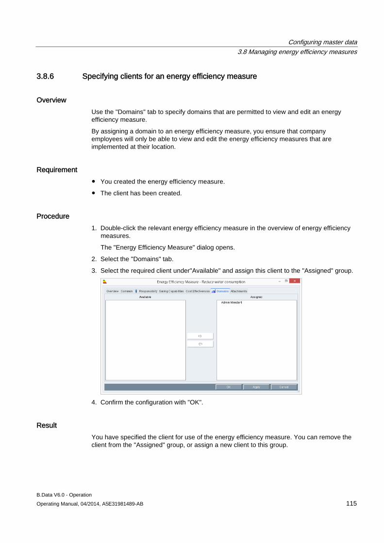
Configuring master data 3.8 Managing energy efficiency measures
B.Data V6.0 - Operation Operating Manual, 04/2014, A5E31981489-AB 115
3.8.6 Specifying clients for an energy efficiency measure
Overview Use the "Domains" tab to specify domains that are permitted to view and edit an energy efficiency measure.
By assigning a domain to an energy efficiency measure, you ensure that company employees will only be able to view and edit the energy efficiency measures that are implemented at their location.
Requirement ● You created the energy efficiency measure.
● The client has been created.
Procedure 1. Double-click the relevant energy efficiency measure in the overview of energy efficiency
measures.
The "Energy Efficiency Measure" dialog opens.
2. Select the "Domains" tab.
3. Select the required client under"Available" and assign this client to the "Assigned" group.
4. Confirm the configuration with "OK".
Result You have specified the client for use of the energy efficiency measure. You can remove the client from the "Assigned" group, or assign a new client to this group.
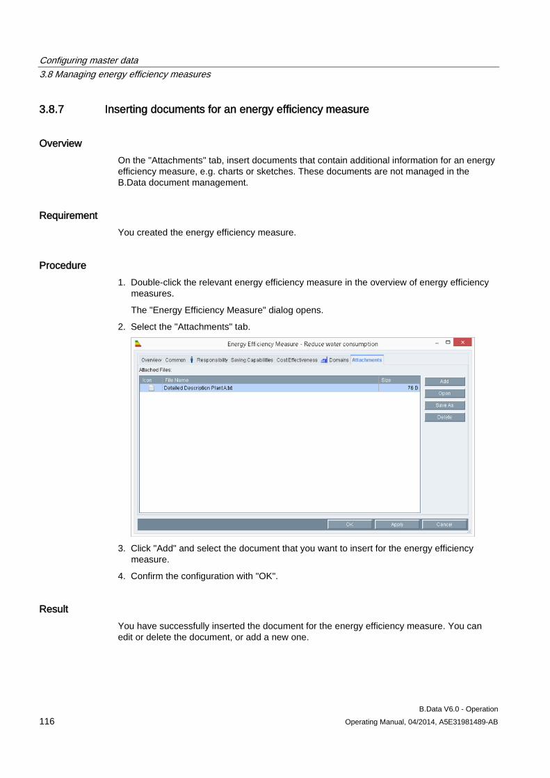
Configuring master data 3.8 Managing energy efficiency measures
B.Data V6.0 - Operation 116 Operating Manual, 04/2014, A5E31981489-AB
3.8.7 Inserting documents for an energy efficiency measure
Overview On the "Attachments" tab, insert documents that contain additional information for an energy efficiency measure, e.g. charts or sketches. These documents are not managed in the B.Data document management.
Requirement You created the energy efficiency measure.
Procedure 1. Double-click the relevant energy efficiency measure in the overview of energy efficiency
measures.
The "Energy Efficiency Measure" dialog opens.
2. Select the "Attachments" tab.
3. Click "Add" and select the document that you want to insert for the energy efficiency
measure.
4. Confirm the configuration with "OK".
Result You have successfully inserted the document for the energy efficiency measure. You can edit or delete the document, or add a new one.
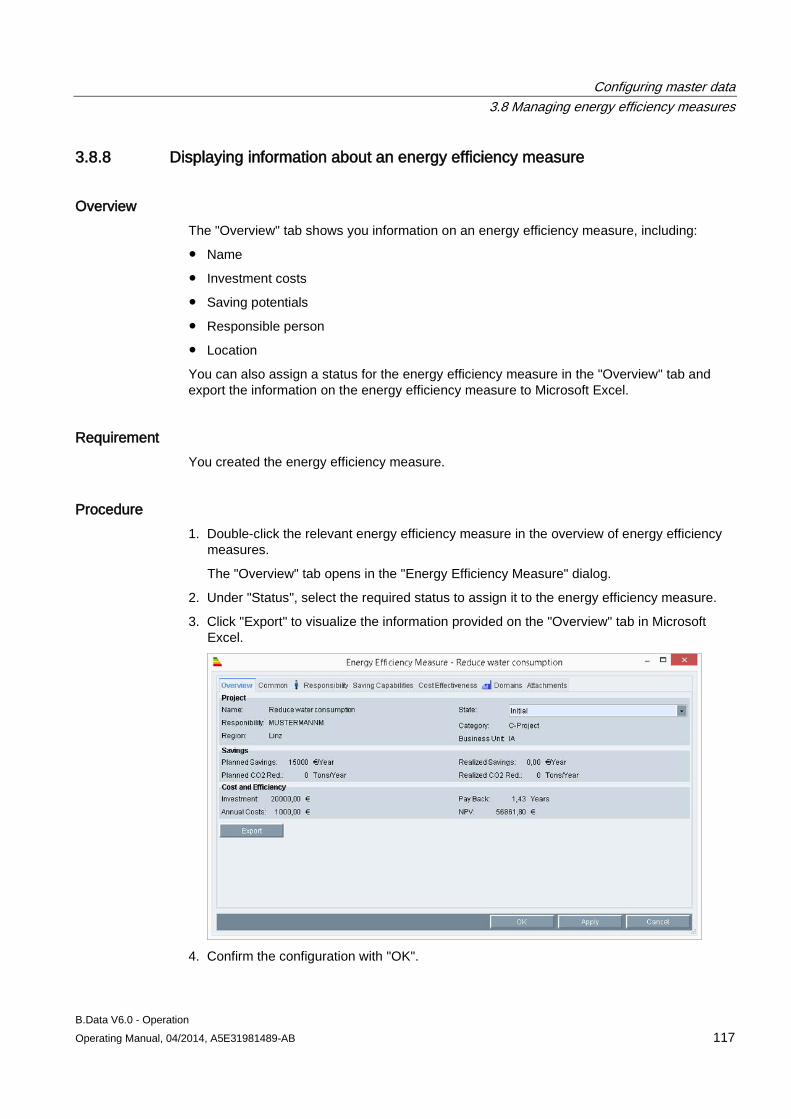
Configuring master data 3.8 Managing energy efficiency measures
B.Data V6.0 - Operation Operating Manual, 04/2014, A5E31981489-AB 117
3.8.8 Displaying information about an energy efficiency measure
Overview The "Overview" tab shows you information on an energy efficiency measure, including:
● Name
● Investment costs
● Saving potentials
● Responsible person
● Location
You can also assign a status for the energy efficiency measure in the "Overview" tab and export the information on the energy efficiency measure to Microsoft Excel.
Requirement You created the energy efficiency measure.
Procedure 1. Double-click the relevant energy efficiency measure in the overview of energy efficiency
measures.
The "Overview" tab opens in the "Energy Efficiency Measure" dialog.
2. Under "Status", select the required status to assign it to the energy efficiency measure.
3. Click "Export" to visualize the information provided on the "Overview" tab in Microsoft Excel.
4. Confirm the configuration with "OK".
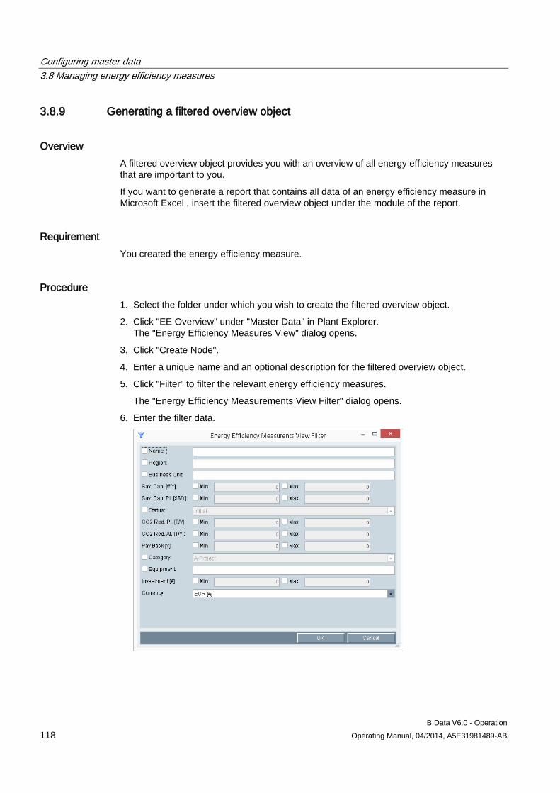
Configuring master data 3.8 Managing energy efficiency measures
B.Data V6.0 - Operation 118 Operating Manual, 04/2014, A5E31981489-AB
3.8.9 Generating a filtered overview object
Overview A filtered overview object provides you with an overview of all energy efficiency measures that are important to you.
If you want to generate a report that contains all data of an energy efficiency measure in Microsoft Excel , insert the filtered overview object under the module of the report.
Requirement You created the energy efficiency measure.
Procedure 1. Select the folder under which you wish to create the filtered overview object.
2. Click "EE Overview" under "Master Data" in Plant Explorer. The "Energy Efficiency Measures View" dialog opens.
3. Click "Create Node".
4. Enter a unique name and an optional description for the filtered overview object.
5. Click "Filter" to filter the relevant energy efficiency measures.
The "Energy Efficiency Measurements View Filter" dialog opens.
6. Enter the filter data.
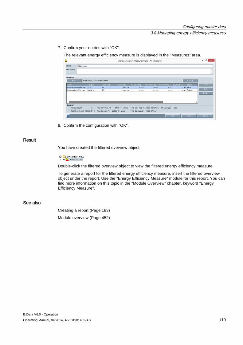
Configuring master data 3.8 Managing energy efficiency measures
B.Data V6.0 - Operation Operating Manual, 04/2014, A5E31981489-AB 119
7. Confirm your entries with "OK".
The relevant energy efficiency measure is displayed in the "Measures" area.
8. Confirm the configuration with "OK".
Result You have created the filtered overview object.
Double-click the filtered overview object to view the filtered energy efficiency measure.
To generate a report for the filtered energy efficiency measure, insert the filtered overview object under the report. Use the "Energy Efficiency Measure" module for this report. You can find more information on this topic in the "Module Overview" chapter, keyword "Energy Efficiency Measure".
See also Creating a report (Page 183)
Module overview (Page 452)

Configuring master data 3.8 Managing energy efficiency measures
B.Data V6.0 - Operation 120 Operating Manual, 04/2014, A5E31981489-AB
B.Data V6.0 - Operation Operating Manual, 04/2014, A5E31981489-AB 121
Calculation level 1 "The loop concept" 4 4.1 Basic information on calculation level 1
Overview You can pre-process the measured values you import to B.Data before you save these to the database. For example, you can compress the acquisition values to daily values or calculate a conditional average value of different measurement series.
B.Data provides two options for real-time pre-processing of measured values:
● Compression of measured values during import
● Processing measured values with loops
The processing of values before entering them into the database is known as "Calculation level 1".
The following diagram illustrates the pre-processing of measured values imported to B.Data. You can use the loop concept to individually process or link the measured values of different data points: This allows you to calculate average, minimum and maximum values, for example.
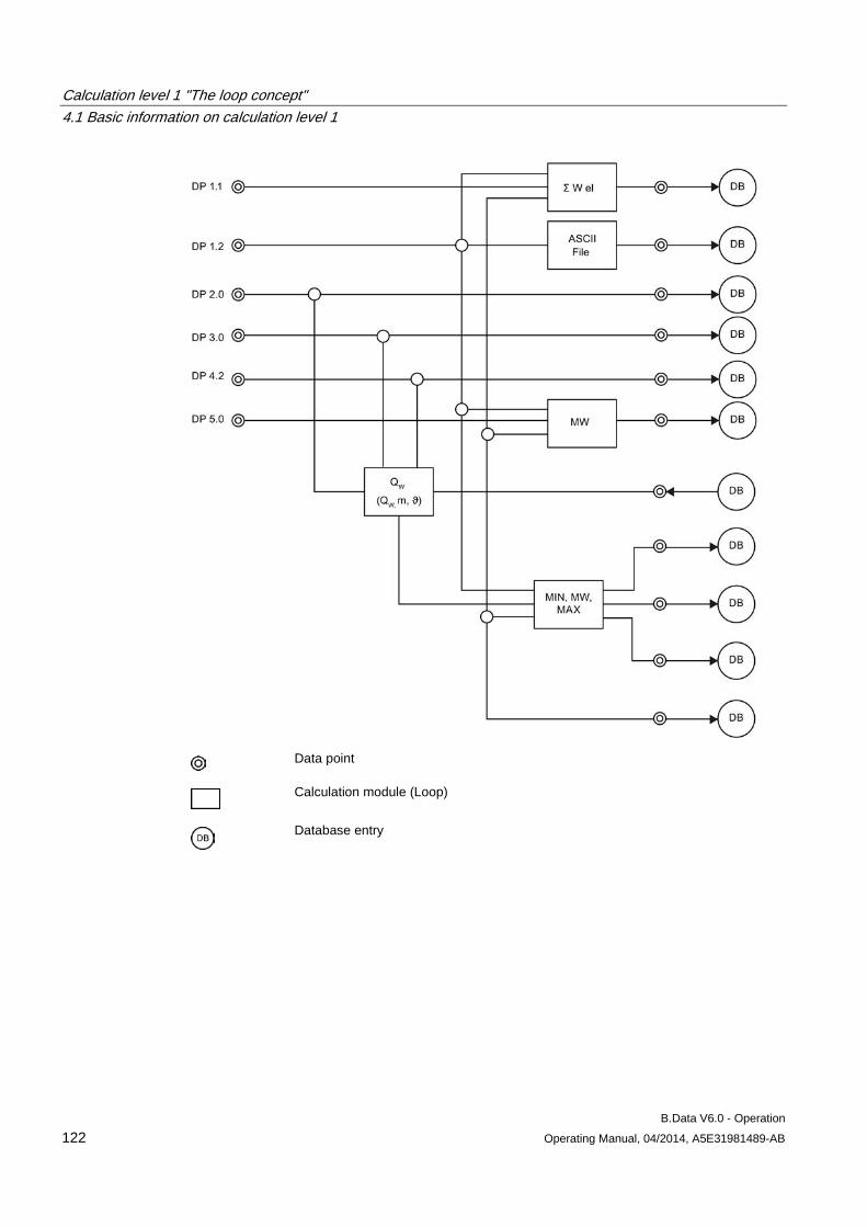
Calculation level 1 "The loop concept" 4.1 Basic information on calculation level 1
B.Data V6.0 - Operation 122 Operating Manual, 04/2014, A5E31981489-AB
Data point
Calculation module (Loop)
Database entry
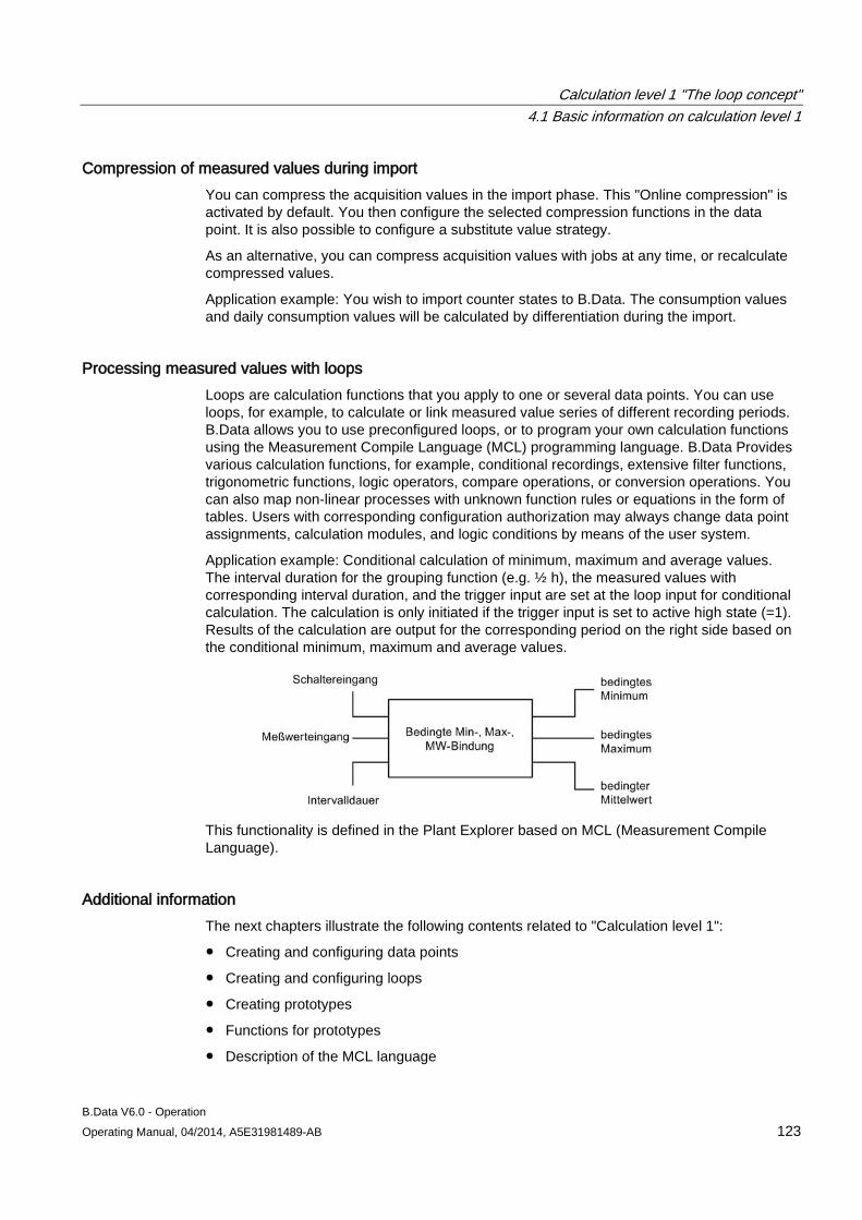
Calculation level 1 "The loop concept" 4.1 Basic information on calculation level 1
B.Data V6.0 - Operation Operating Manual, 04/2014, A5E31981489-AB 123
Compression of measured values during import You can compress the acquisition values in the import phase. This "Online compression" is activated by default. You then configure the selected compression functions in the data point. It is also possible to configure a substitute value strategy.
As an alternative, you can compress acquisition values with jobs at any time, or recalculate compressed values.
Application example: You wish to import counter states to B.Data. The consumption values and daily consumption values will be calculated by differentiation during the import.
Processing measured values with loops Loops are calculation functions that you apply to one or several data points. You can use loops, for example, to calculate or link measured value series of different recording periods. B.Data allows you to use preconfigured loops, or to program your own calculation functions using the Measurement Compile Language (MCL) programming language. B.Data Provides various calculation functions, for example, conditional recordings, extensive filter functions, trigonometric functions, logic operators, compare operations, or conversion operations. You can also map non-linear processes with unknown function rules or equations in the form of tables. Users with corresponding configuration authorization may always change data point assignments, calculation modules, and logic conditions by means of the user system.
Application example: Conditional calculation of minimum, maximum and average values. The interval duration for the grouping function (e.g. ½ h), the measured values with corresponding interval duration, and the trigger input are set at the loop input for conditional calculation. The calculation is only initiated if the trigger input is set to active high state (=1). Results of the calculation are output for the corresponding period on the right side based on the conditional minimum, maximum and average values.
This functionality is defined in the Plant Explorer based on MCL (Measurement Compile Language).
Additional information The next chapters illustrate the following contents related to "Calculation level 1":
● Creating and configuring data points
● Creating and configuring loops
● Creating prototypes
● Functions for prototypes
● Description of the MCL language
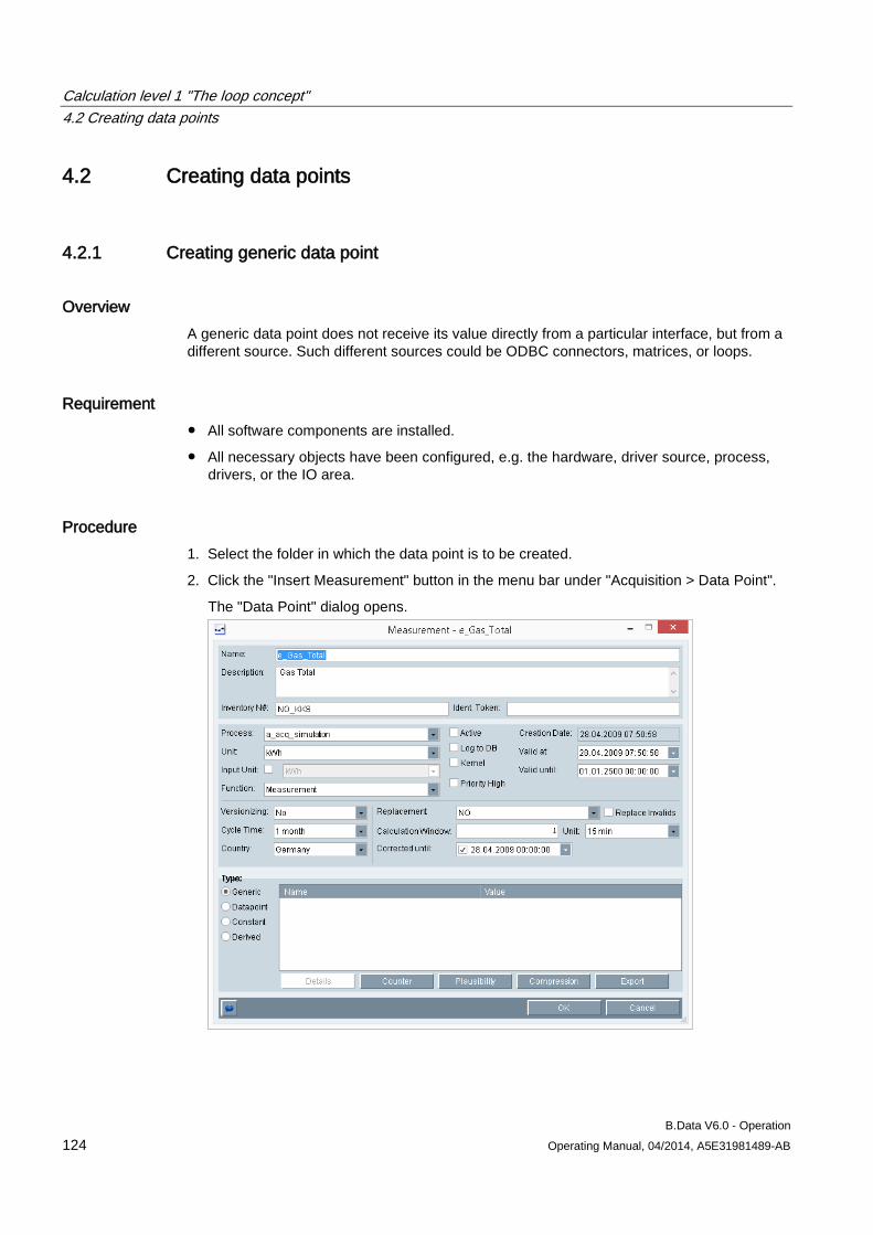
Calculation level 1 "The loop concept" 4.2 Creating data points
B.Data V6.0 - Operation 124 Operating Manual, 04/2014, A5E31981489-AB
4.2 Creating data points
4.2.1 Creating generic data point
Overview A generic data point does not receive its value directly from a particular interface, but from a different source. Such different sources could be ODBC connectors, matrices, or loops.
Requirement ● All software components are installed.
● All necessary objects have been configured, e.g. the hardware, driver source, process, drivers, or the IO area.
Procedure 1. Select the folder in which the data point is to be created.
2. Click the "Insert Measurement" button in the menu bar under "Acquisition > Data Point".
The "Data Point" dialog opens.
Calculation level 1 "The loop concept" 4.2 Creating data points
B.Data V6.0 - Operation Operating Manual, 04/2014, A5E31981489-AB 125
3. Parameterize the fields.
– Enter the "Name" for the measurement, taking naming conventions into account.
– You may also enter a "description".
– Enter the "Inventory N#".
The inventory number is a KKS or FIS number. The inventory number is output if you select the "KKS Text" mode for a report.
– Enter "Ident. Token" as additional identifier, if necessary.
The "Ident. Token" is used only by a special import/export interface.
– You can select a "Process" that is not actively used for data acquisition, e.g. "a_erf_null", or "a_rech_PDS".
– Select the physical unit.
The unit may depend on the processing routine (loop), or on the lower-level data type.
– Select the "Input Unit" check box and select the unit.
The "Input Unit" is used for the manual input of matrix data.
Example: You selected the "kW" unit and defined the "MW" input unit. The value 500,000 W is stored in the database with the notation "500 kW". You can enter the value "0.5 MW" manually in the matrix.
– Enable or disable versioning of the data of this measurement using the "Versioning" drop-down list box.
– Enter the "Cycle Time" for cyclic availability of the values.
– Under "Country", select the country whose time zone you want to use for the acquisition.
– Select the "Active" check box if the measurement is used in the system (e.g. loops).
– Select the "Log to DB" check box to write the values returned from a loop to a database.
– Select the "Kernel" check box to enable the use of the acquisition component of this measurement.
– Select the "Priority High" check box to enable write protection for manual matrix input.
– Select "Measurement" from the "Function" field.
– Accept the "NO" setting in the "Replacement" field.
– Set the "Generic" radio button in the "Type" area.
4. Confirm your entries with "OK".
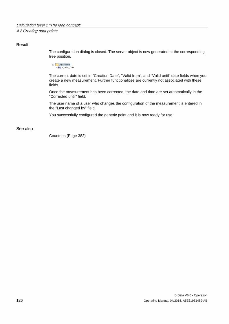
Calculation level 1 "The loop concept" 4.2 Creating data points
B.Data V6.0 - Operation 126 Operating Manual, 04/2014, A5E31981489-AB
Result The configuration dialog is closed. The server object is now generated at the corresponding tree position.
The current date is set in "Creation Date", "Valid from", and "Valid until" date fields when you create a new measurement. Further functionalities are currently not associated with these fields.
Once the measurement has been corrected, the date and time are set automatically in the "Corrected until" field.
The user name of a user who changes the configuration of the measurement is entered in the "Last changed by" field.
You successfully configured the generic point and it is now ready for use.
See also Countries (Page 382)
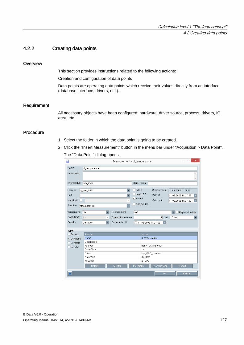
Calculation level 1 "The loop concept" 4.2 Creating data points
B.Data V6.0 - Operation Operating Manual, 04/2014, A5E31981489-AB 127
4.2.2 Creating data points
Overview This section provides instructions related to the following actions:
Creation and configuration of data points
Data points are operating data points which receive their values directly from an interface (database interface, drivers, etc.).
Requirement All necessary objects have been configured: hardware, driver source, process, drivers, IO area, etc.
Procedure 1. Select the folder in which the data point is going to be created.
2. Click the "Insert Measurement" button in the menu bar under "Acquisition > Data Point".
The "Data Point" dialog opens.
Calculation level 1 "The loop concept" 4.2 Creating data points
B.Data V6.0 - Operation 128 Operating Manual, 04/2014, A5E31981489-AB
3. Fill out or parameterize the fields as follows:
– Enter the "Name" of the measurement (data point type). Observe the naming conventions.
– You can enter additional information on the measurement in the Description field.
– You can enter a KKS or FIS number, or a user-specific text in the "Inventory no." field. This text will be output, for example, if the "KKS Text" mode is selected for a report.
– Select the process from which the data is acquired.
– Select the required unit.
– Select the "Input Unit" check box to use a unit for the manual input of matrix data.
You may define the "kW" unit and the "MW" input unit. The value 500,000 W is then stored in the database with the notation "500 kW". The value is displayed or entered in the format 0.5 MW for manual matrix input.
– The user who most recently modified the measurement configuration is entered automatically in the "Last changed by" field.
– The Corrected until date field is set automatically by a job after the measurement has been revised. The default is set to 01/01/2007.
– Enable or disable versioning of the data of this measurement using the "Versioning" drop-down list box.
– In the Cycle Time field, enter the period during which the values will be available cyclically. For data points, this period is copied automatically from the cycle time entry specified the detail settings.
– Under "Country", select the country whose time zone you want to use for the acquisition.
– Select the "Active" check box if the measurement is to be used (logged) by the system.
– The Log to DB check box is only set if the acquired values are transferred directly to the database without having been calculated.
– Select the "Kernel" check box to enable the use of the acquisition component of this measurement.
– The current date is set in "Creation Date", "Valid from", and "Valid until" date fields when you create a new measurement. The "Valid until" field is set to the default date 01/01/2500. Further functionalities are currently not associated with these fields.
– You may enter an additional identifier in the "Ident. Token" field. However, this ID is used only by a special import/export interface.
– Select "Measurement" from the "Function" drop-down list box.
– The substitute value" is set to "NO" by default.
– Select the "Data point" radio button in the "Type:" area.
– After having selected the "Datapoint" type, click "Details…" to open the Data point dialog for detailed configuration:
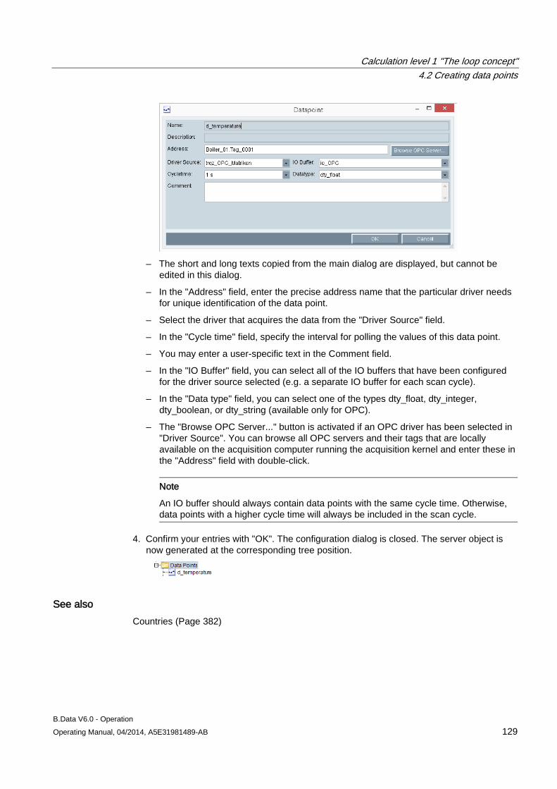
Calculation level 1 "The loop concept" 4.2 Creating data points
B.Data V6.0 - Operation Operating Manual, 04/2014, A5E31981489-AB 129
– The short and long texts copied from the main dialog are displayed, but cannot be
edited in this dialog.
– In the "Address" field, enter the precise address name that the particular driver needs for unique identification of the data point.
– Select the driver that acquires the data from the "Driver Source" field.
– In the "Cycle time" field, specify the interval for polling the values of this data point.
– You may enter a user-specific text in the Comment field.
– In the "IO Buffer" field, you can select all of the IO buffers that have been configured for the driver source selected (e.g. a separate IO buffer for each scan cycle).
– In the "Data type" field, you can select one of the types dty_float, dty_integer, dty_boolean, or dty_string (available only for OPC).
– The "Browse OPC Server..." button is activated if an OPC driver has been selected in "Driver Source". You can browse all OPC servers and their tags that are locally available on the acquisition computer running the acquisition kernel and enter these in the "Address" field with double-click.
Note
An IO buffer should always contain data points with the same cycle time. Otherwise, data points with a higher cycle time will always be included in the scan cycle.
4. Confirm your entries with "OK". The configuration dialog is closed. The server object is now generated at the corresponding tree position.
See also Countries (Page 382)

Calculation level 1 "The loop concept" 4.2 Creating data points
B.Data V6.0 - Operation 130 Operating Manual, 04/2014, A5E31981489-AB
4.2.3 Creating constants
Overview A constant represents a special type of data point that is used as default for data acquisition or for generation of a substitute value. For example, if the averaging period of loops is set by means of a constant, a change to this constant will instantaneously change the averaging period of all loops concerned. Otherwise, you would have to parameterize each loop individually. A replacement value can be generated for each data point and may be used to substitute missing values, provided the "Substitute value" strategy has been selected.
Requirement All software components are installed.
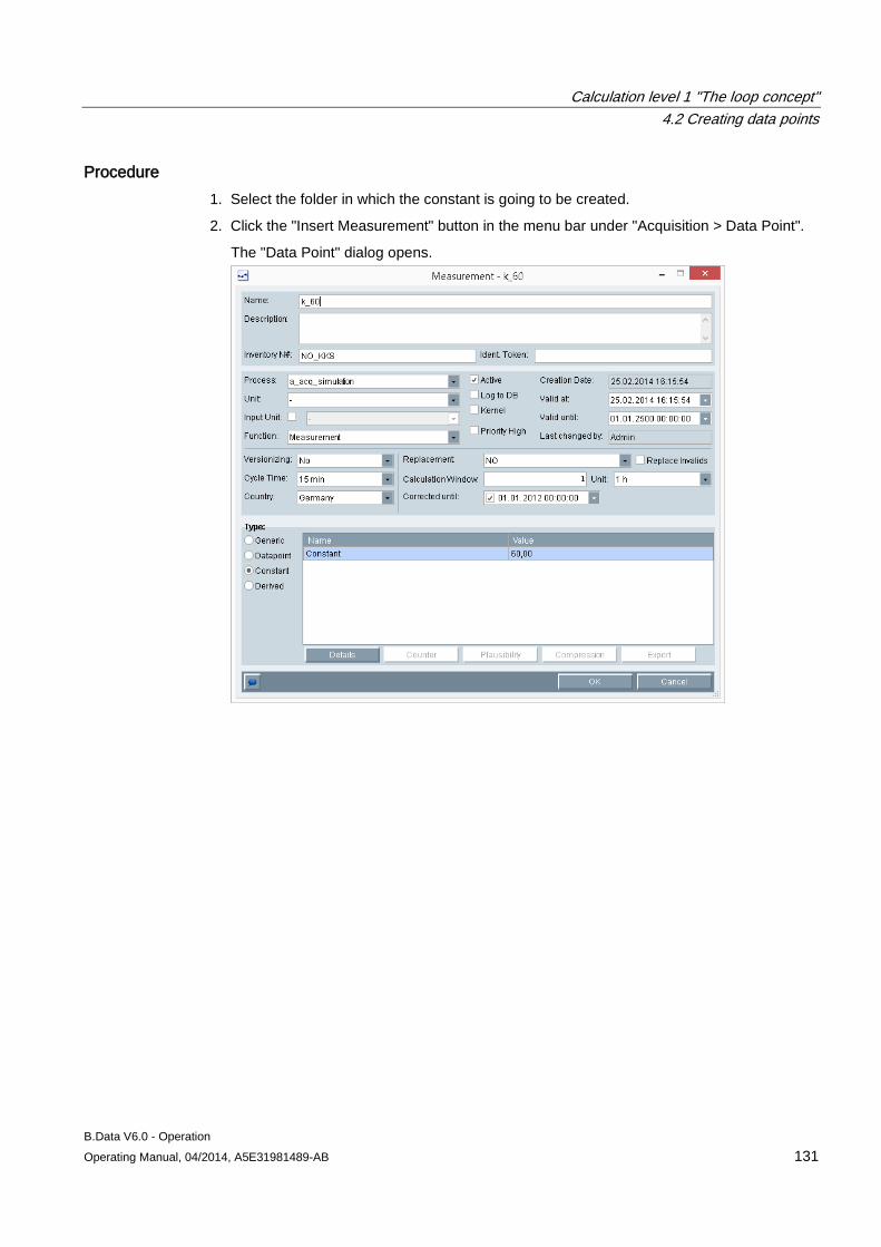
Calculation level 1 "The loop concept" 4.2 Creating data points
B.Data V6.0 - Operation Operating Manual, 04/2014, A5E31981489-AB 131
Procedure 1. Select the folder in which the constant is going to be created.
2. Click the "Insert Measurement" button in the menu bar under "Acquisition > Data Point".
The "Data Point" dialog opens.
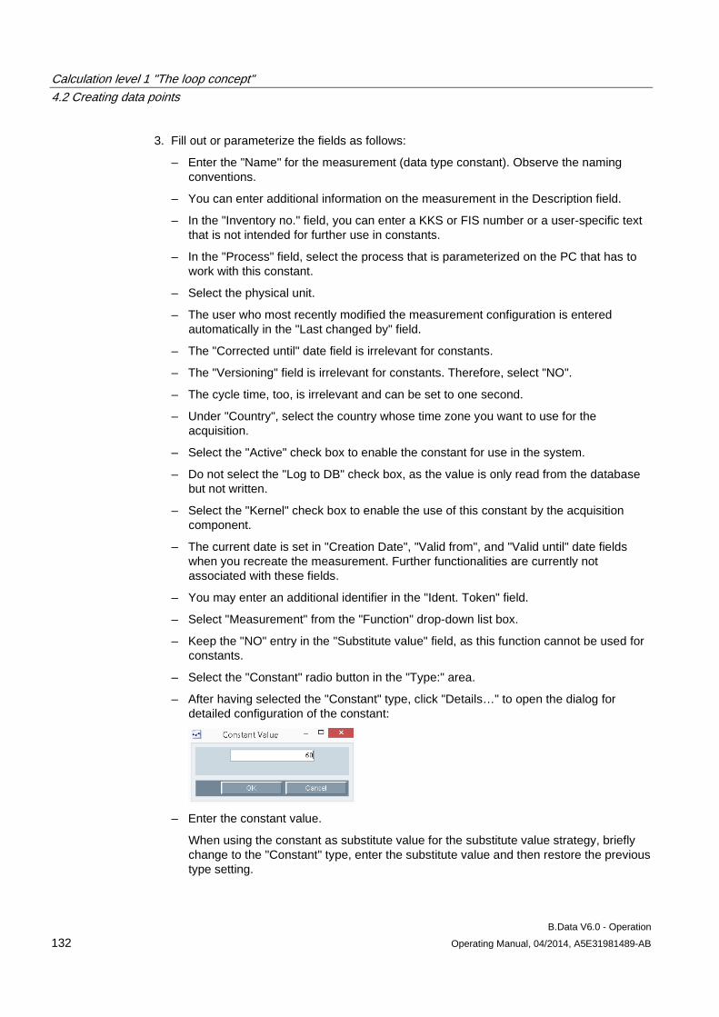
Calculation level 1 "The loop concept" 4.2 Creating data points
B.Data V6.0 - Operation 132 Operating Manual, 04/2014, A5E31981489-AB
3. Fill out or parameterize the fields as follows:
– Enter the "Name" for the measurement (data type constant). Observe the naming conventions.
– You can enter additional information on the measurement in the Description field.
– In the "Inventory no." field, you can enter a KKS or FIS number or a user-specific text that is not intended for further use in constants.
– In the "Process" field, select the process that is parameterized on the PC that has to work with this constant.
– Select the physical unit.
– The user who most recently modified the measurement configuration is entered automatically in the "Last changed by" field.
– The "Corrected until" date field is irrelevant for constants.
– The "Versioning" field is irrelevant for constants. Therefore, select "NO".
– The cycle time, too, is irrelevant and can be set to one second.
– Under "Country", select the country whose time zone you want to use for the acquisition.
– Select the "Active" check box to enable the constant for use in the system.
– Do not select the "Log to DB" check box, as the value is only read from the database but not written.
– Select the "Kernel" check box to enable the use of this constant by the acquisition component.
– The current date is set in "Creation Date", "Valid from", and "Valid until" date fields when you recreate the measurement. Further functionalities are currently not associated with these fields.
– You may enter an additional identifier in the "Ident. Token" field.
– Select "Measurement" from the "Function" drop-down list box.
– Keep the "NO" entry in the "Substitute value" field, as this function cannot be used for constants.
– Select the "Constant" radio button in the "Type:" area.
– After having selected the "Constant" type, click "Details…" to open the dialog for detailed configuration of the constant:
– Enter the constant value.
When using the constant as substitute value for the substitute value strategy, briefly change to the "Constant" type, enter the substitute value and then restore the previous type setting.
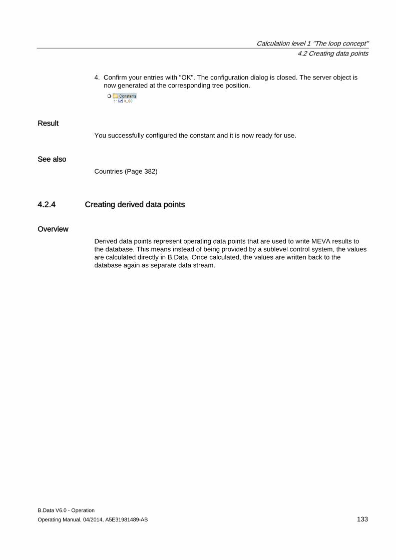
Calculation level 1 "The loop concept" 4.2 Creating data points
B.Data V6.0 - Operation Operating Manual, 04/2014, A5E31981489-AB 133
4. Confirm your entries with "OK". The configuration dialog is closed. The server object is now generated at the corresponding tree position.
Result You successfully configured the constant and it is now ready for use.
See also Countries (Page 382)
4.2.4 Creating derived data points
Overview Derived data points represent operating data points that are used to write MEVA results to the database. This means instead of being provided by a sublevel control system, the values are calculated directly in B.Data. Once calculated, the values are written back to the database again as separate data stream.
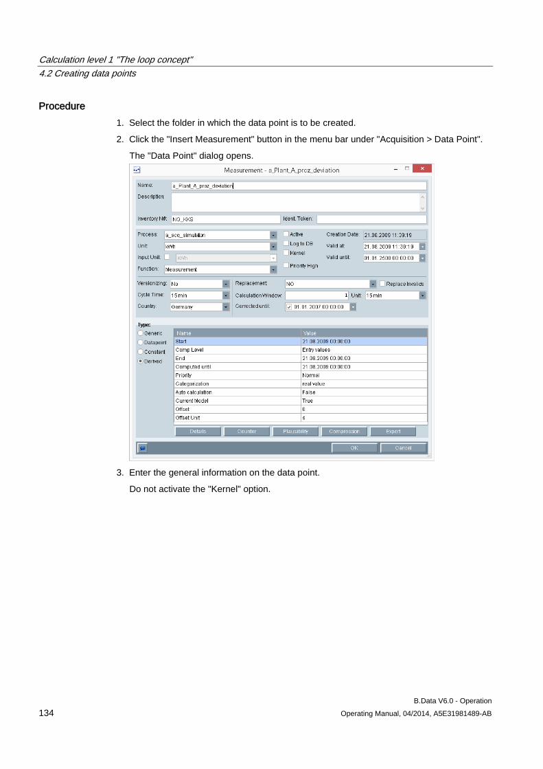
Calculation level 1 "The loop concept" 4.2 Creating data points
B.Data V6.0 - Operation 134 Operating Manual, 04/2014, A5E31981489-AB
Procedure 1. Select the folder in which the data point is to be created.
2. Click the "Insert Measurement" button in the menu bar under "Acquisition > Data Point".
The "Data Point" dialog opens.
3. Enter the general information on the data point.
Do not activate the "Kernel" option.
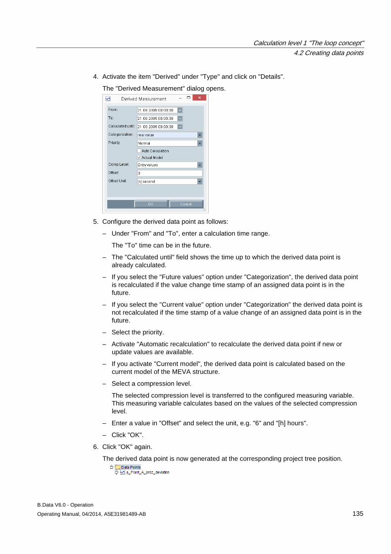
Calculation level 1 "The loop concept" 4.2 Creating data points
B.Data V6.0 - Operation Operating Manual, 04/2014, A5E31981489-AB 135
4. Activate the item "Derived" under "Type" and click on "Details".
The "Derived Measurement" dialog opens.
5. Configure the derived data point as follows:
– Under "From" and "To", enter a calculation time range.
The "To" time can be in the future.
– The "Calculated until" field shows the time up to which the derived data point is already calculated.
– If you select the "Future values" option under "Categorization", the derived data point is recalculated if the value change time stamp of an assigned data point is in the future.
– If you select the "Current value" option under "Categorization" the derived data point is not recalculated if the time stamp of a value change of an assigned data point is in the future.
– Select the priority.
– Activate "Automatic recalculation" to recalculate the derived data point if new or update values are available.
– If you activate "Current model", the derived data point is calculated based on the current model of the MEVA structure.
– Select a compression level.
The selected compression level is transferred to the configured measuring variable. This measuring variable calculates based on the values of the selected compression level.
– Enter a value in "Offset" and select the unit, e.g. "6" and "[h] hours".
– Click "OK".
6. Click "OK" again.
The derived data point is now generated at the corresponding project tree position.
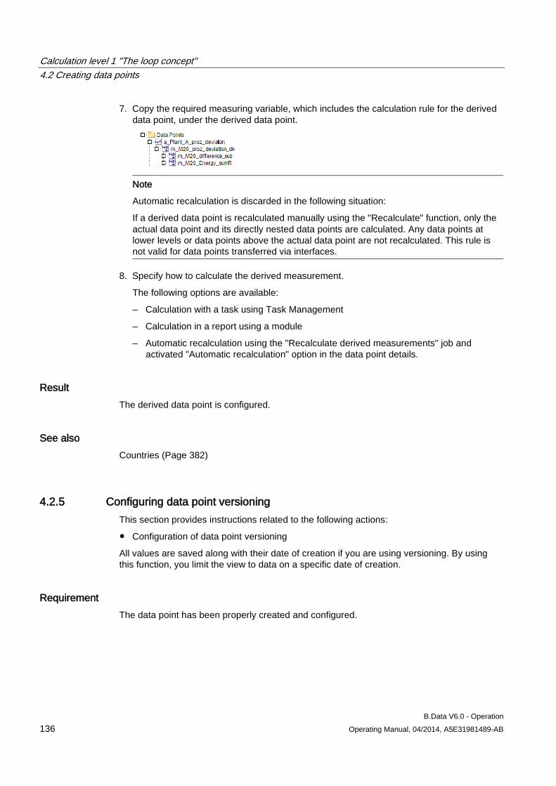
Calculation level 1 "The loop concept" 4.2 Creating data points
B.Data V6.0 - Operation 136 Operating Manual, 04/2014, A5E31981489-AB
7. Copy the required measuring variable, which includes the calculation rule for the derived data point, under the derived data point.
Note
Automatic recalculation is discarded in the following situation:
If a derived data point is recalculated manually using the "Recalculate" function, only the actual data point and its directly nested data points are calculated. Any data points at lower levels or data points above the actual data point are not recalculated. This rule is not valid for data points transferred via interfaces.
8. Specify how to calculate the derived measurement.
The following options are available:
– Calculation with a task using Task Management
– Calculation in a report using a module
– Automatic recalculation using the "Recalculate derived measurements" job and activated "Automatic recalculation" option in the data point details.
Result The derived data point is configured.
See also Countries (Page 382)
4.2.5 Configuring data point versioning This section provides instructions related to the following actions:
● Configuration of data point versioning
All values are saved along with their date of creation if you are using versioning. By using this function, you limit the view to data on a specific date of creation.
Requirement The data point has been properly created and configured.
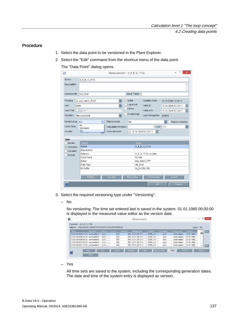
Calculation level 1 "The loop concept" 4.2 Creating data points
B.Data V6.0 - Operation Operating Manual, 04/2014, A5E31981489-AB 137
Procedure 1. Select the data point to be versioned in the Plant Explorer.
2. Select the "Edit" command from the shortcut menu of the data point.
The "Data Point" dialog opens.
3. Select the required versioning type under "Versioning".
– No
No versioning. The time set entered last is saved in the system. 01.01.1980 00:00:00 is displayed in the measured value editor as the version date.
– Yes
All time sets are saved to the system, including the corresponding generation dates. The date and time of the system entry is displayed as version.
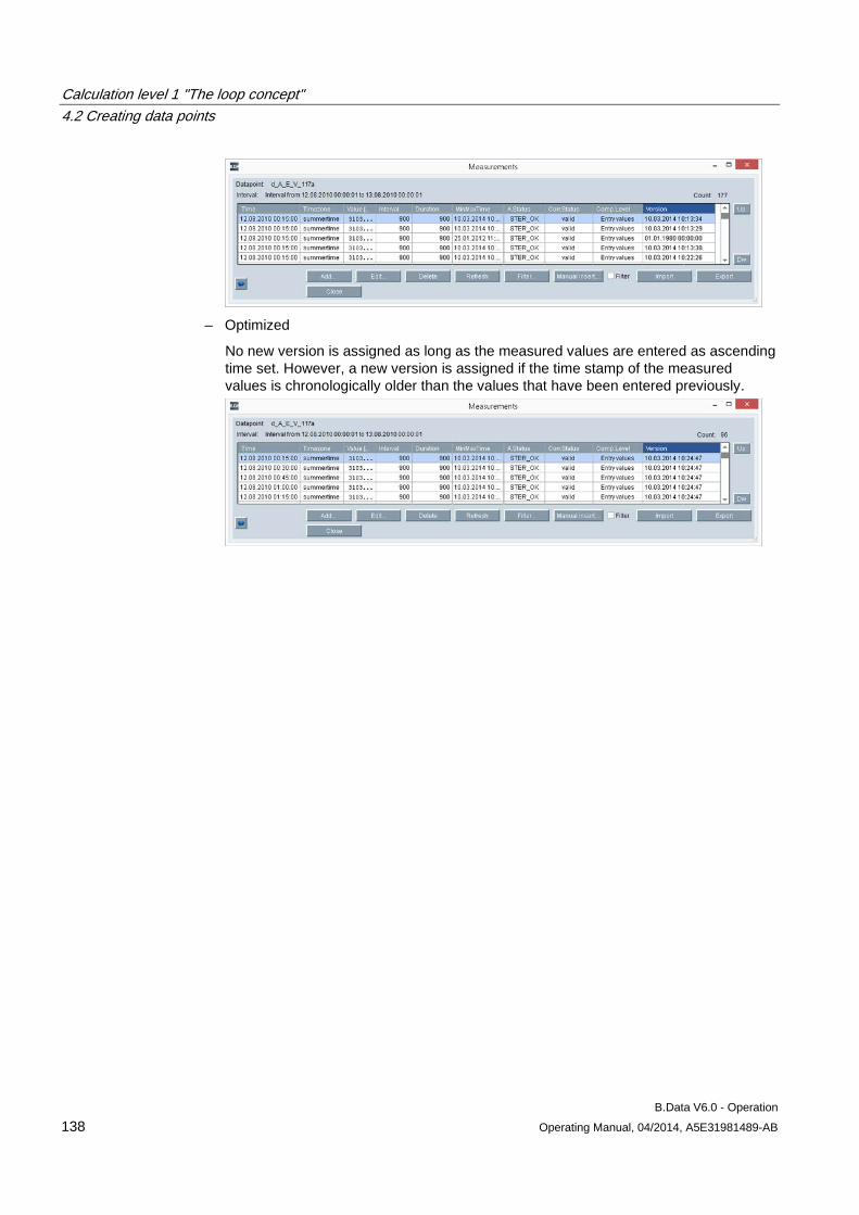
Calculation level 1 "The loop concept" 4.2 Creating data points
B.Data V6.0 - Operation 138 Operating Manual, 04/2014, A5E31981489-AB
– Optimized
No new version is assigned as long as the measured values are entered as ascending time set. However, a new version is assigned if the time stamp of the measured values is chronologically older than the values that have been entered previously.
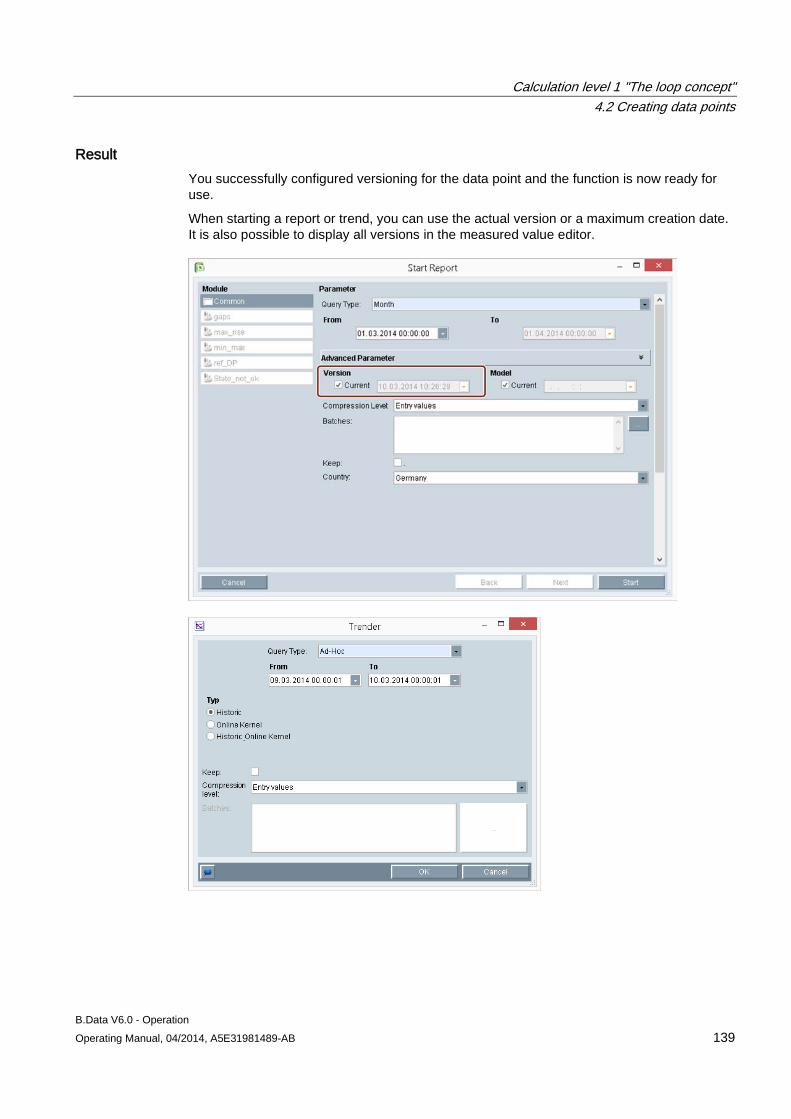
Calculation level 1 "The loop concept" 4.2 Creating data points
B.Data V6.0 - Operation Operating Manual, 04/2014, A5E31981489-AB 139
Result You successfully configured versioning for the data point and the function is now ready for use.
When starting a report or trend, you can use the actual version or a maximum creation date. It is also possible to display all versions in the measured value editor.
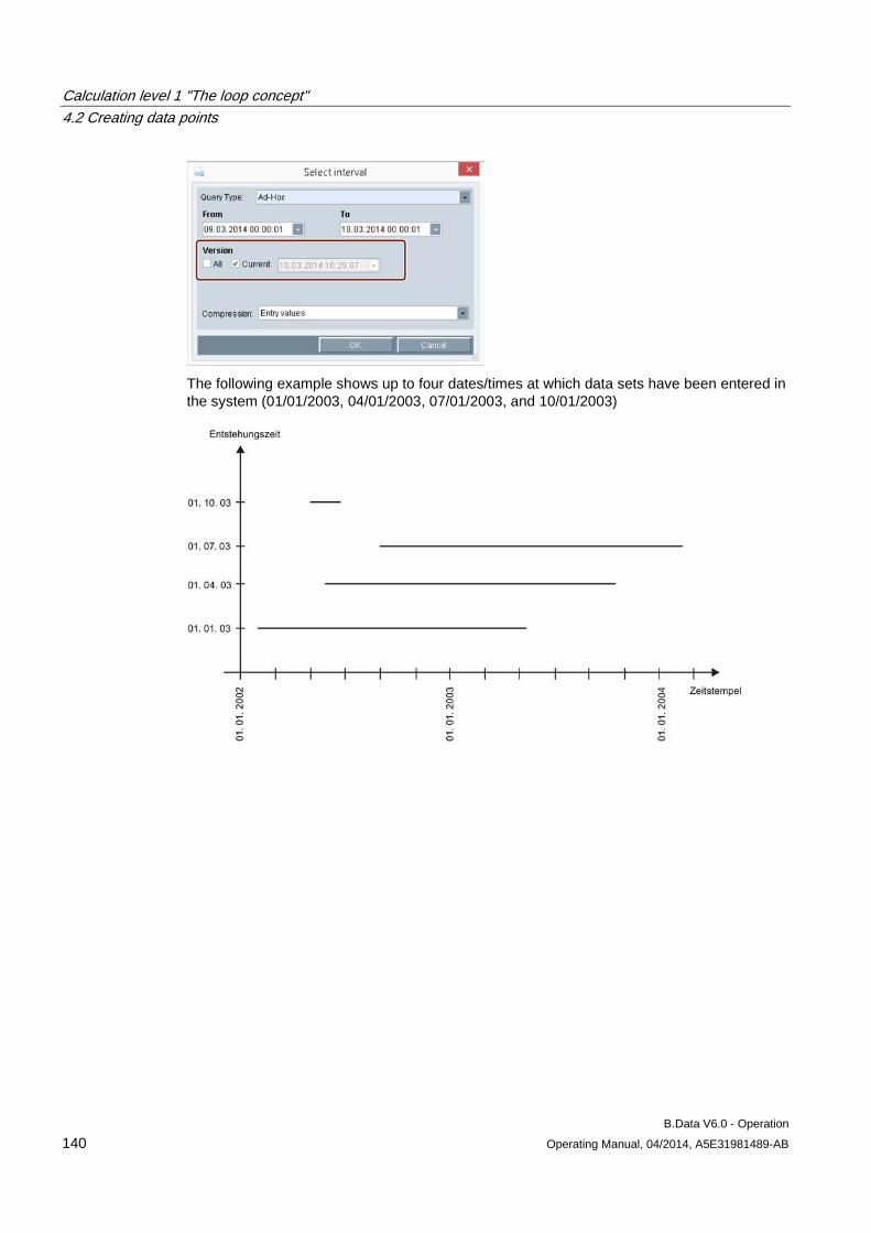
Calculation level 1 "The loop concept" 4.2 Creating data points
B.Data V6.0 - Operation 140 Operating Manual, 04/2014, A5E31981489-AB
The following example shows up to four dates/times at which data sets have been entered in the system (01/01/2003, 04/01/2003, 07/01/2003, and 10/01/2003)
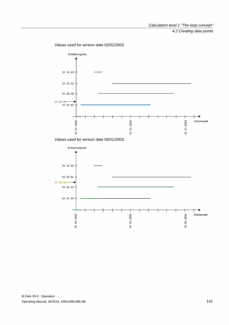
Calculation level 1 "The loop concept" 4.2 Creating data points
B.Data V6.0 - Operation Operating Manual, 04/2014, A5E31981489-AB 141
Values used for version date 02/01/2003:
Values used for version date 06/01/2003:
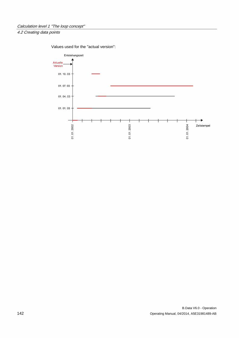
Calculation level 1 "The loop concept" 4.2 Creating data points
B.Data V6.0 - Operation 142 Operating Manual, 04/2014, A5E31981489-AB
Values used for the "actual version":
Calculation level 1 "The loop concept" 4.2 Creating data points
B.Data V6.0 - Operation Operating Manual, 04/2014, A5E31981489-AB 143
4.2.6 Configuring substitute value strategies for a data point
Overview The following substitute value strategies are available for closing gaps in measured values or compressed values of a data point:
● You can use the measured values of a different data point to eliminate gaps in the measured value series of a data point.
● You can use fixed values to eliminate gaps in the measured value series of a data point.
● You cannot eliminate gaps in the measured value series of a data point.
● You can use the most recent valid measured value to eliminate a gap in the measured value series of a data point.
Requirement ● The data point is configured.
● The measuring journal contains at least one entry for the data point.
Procedure 1. Click "Edit" in the shortcut menu of the selected data point.
The data point configuration dialog opens.
2. Proceed as follows to eliminate gaps in the measured value series of a data point using the measured values of a different data point:
– Select "PIS" under "Substitute".
– Insert the other data point underneath the data point that contains the gap.
3. Proceed as follows to eliminate a gap in the measured value series of a data point using a fixed value:
– Select "Substitute value" under "Substitute".
– Select "Constant" under "Type".
– Enter the selected substitute value under "Details" and confirm the configuration with "OK".
– Change back to the original type of the data point.
4. Select "NONE" under "Substitute" if you do not want to eliminate the gap in the measurement series of the data point.
5. Select "LRU" under "Substitute" if you want use the last valid value to eliminate the gap in the measurement series of the data point.
6. Activate "Replace invalid" to replace invalid measured values of the data point with the selected equivalent value strategy.
7. Select the time as of which you want to replace the gap under "Corrected until".
8. Confirm the configuration with "OK".
Calculation level 1 "The loop concept" 4.2 Creating data points
B.Data V6.0 - Operation 144 Operating Manual, 04/2014, A5E31981489-AB
Result You have successfully configured the substitute value strategy for the data point. Select "Administration > Job queue" to run one of the following jobs for closing gaps with substitute values:
● If you want to close gaps in measured values series: "Job for correcting the measuring journal".
● If you want to close gaps in compressed values: "Job for general recalculation".
See also Using the job queue (Page 352)
Database jobs (Page 570)
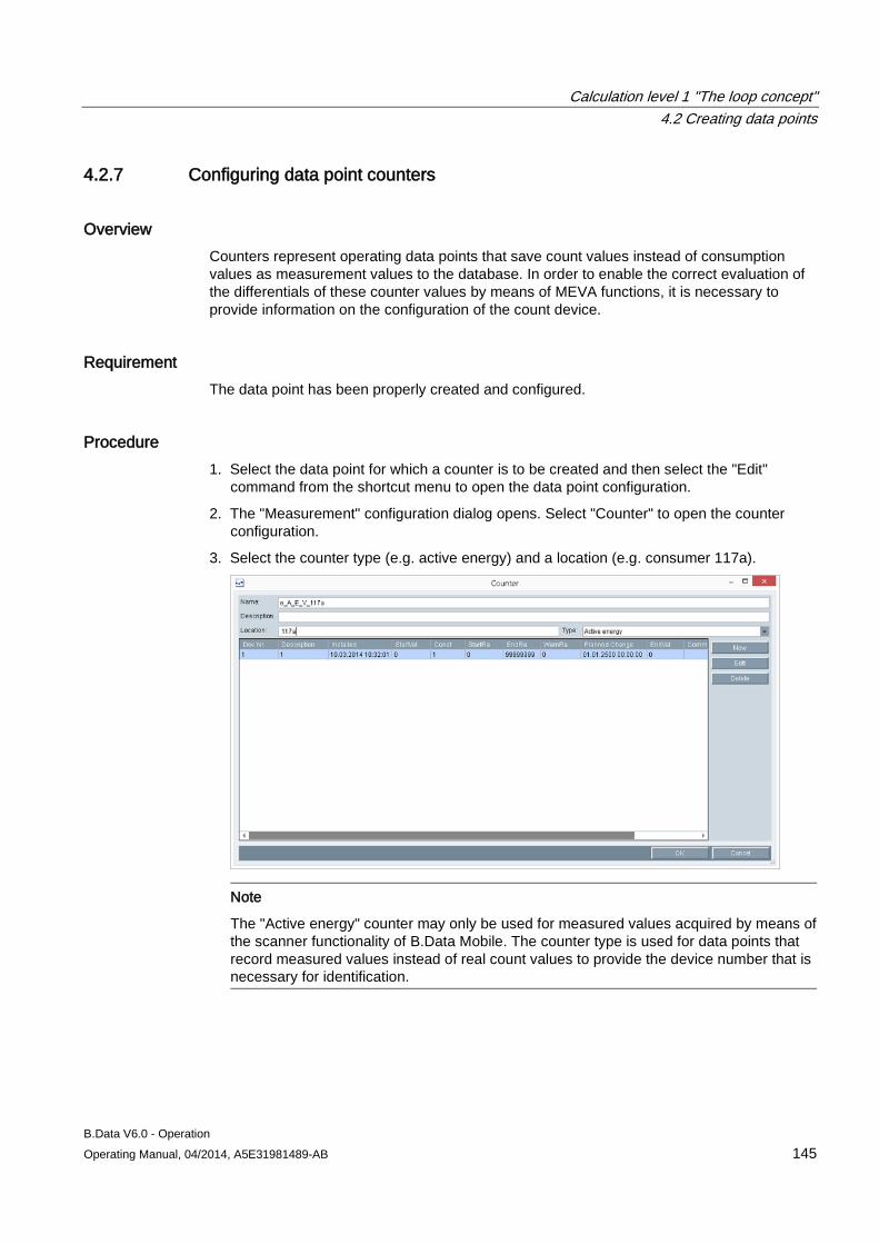
Calculation level 1 "The loop concept" 4.2 Creating data points
B.Data V6.0 - Operation Operating Manual, 04/2014, A5E31981489-AB 145
4.2.7 Configuring data point counters
Overview Counters represent operating data points that save count values instead of consumption values as measurement values to the database. In order to enable the correct evaluation of the differentials of these counter values by means of MEVA functions, it is necessary to provide information on the configuration of the count device.
Requirement The data point has been properly created and configured.
Procedure 1. Select the data point for which a counter is to be created and then select the "Edit"
command from the shortcut menu to open the data point configuration.
2. The "Measurement" configuration dialog opens. Select "Counter" to open the counter configuration.
3. Select the counter type (e.g. active energy) and a location (e.g. consumer 117a).
Note
The "Active energy" counter may only be used for measured values acquired by means of the scanner functionality of B.Data Mobile. The counter type is used for data points that record measured values instead of real count values to provide the device number that is necessary for identification.
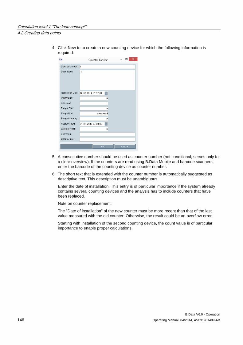
Calculation level 1 "The loop concept" 4.2 Creating data points
B.Data V6.0 - Operation 146 Operating Manual, 04/2014, A5E31981489-AB
4. Click New to to create a new counting device for which the following information is required:
5. A consecutive number should be used as counter number (not conditional, serves only for
a clear overview). If the counters are read using B.Data Mobile and barcode scanners, enter the barcode of the counting device as counter number.
6. The short text that is extended with the counter number is automatically suggested as descriptive text. This description must be unambiguous.
Enter the date of installation. This entry is of particular importance if the system already contains several counting devices and the analysis has to include counters that have been replaced.
Note on counter replacement:
The "Date of installation" of the new counter must be more recent than that of the last value measured with the old counter. Otherwise, the result could be an overflow error.
Starting with installation of the second counting device, the count value is of particular importance to enable proper calculations.
Calculation level 1 "The loop concept" 4.2 Creating data points
B.Data V6.0 - Operation Operating Manual, 04/2014, A5E31981489-AB 147
7. The default counter constant is set automatically to the value 1 and can be customized. The resultant difference is then multiplied with this constant.
The value at which the counter starts the count is entered as start value of the counting range and is of importance with regard to the proper calculation of differences upon overflow.
The value at which the counter sets an overflow flag and resumes the count at the start of the counting range is entered as value for the end of the counting range. This, too, is of importance for the proper calculation of differences upon overflow.
The counting range alarm is currently not functional and is merely informative.
In the "Planned Replacements" field, enter the estimated date of counting device replacement. Currently not functional and merely informative.
Starting with the removal of the second counting device, the count value is of particular importance to enable proper calculations.
The "Comments" field can be used to save comments related to the counting device.
8. The name of the counting device manufacturer can be saved by entering it in the "Manufacturer" field.
9. The counting device data is saved with OK and is used by the respective MEVA functions for calculation of the differential values.
Result You have successfully configured the counter configuration of the data point and it is now ready for use.
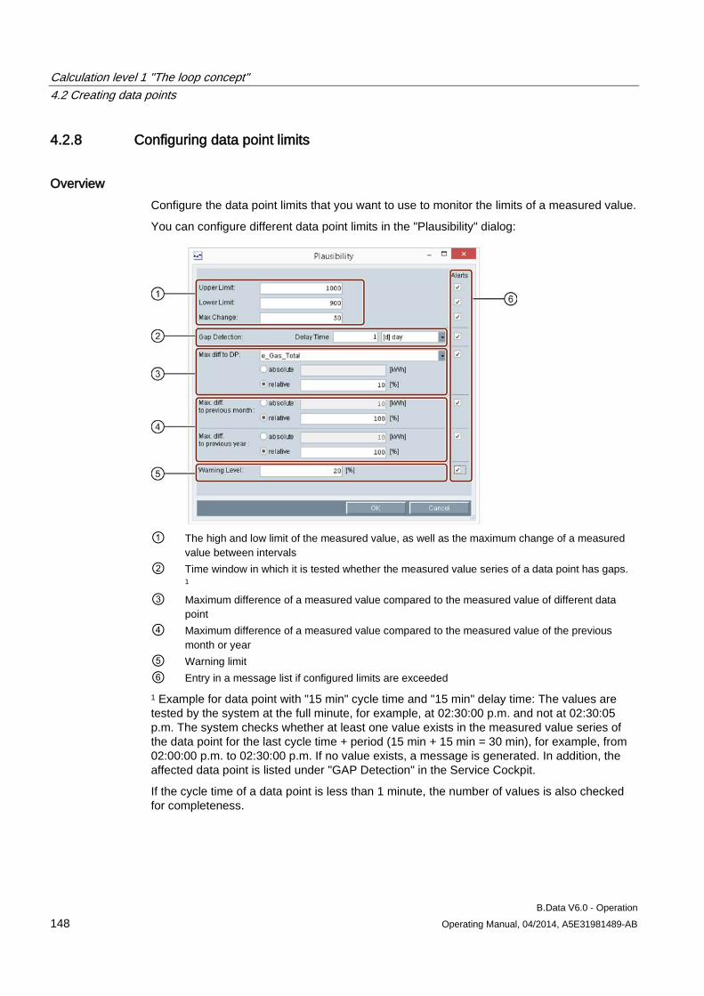
Calculation level 1 "The loop concept" 4.2 Creating data points
B.Data V6.0 - Operation 148 Operating Manual, 04/2014, A5E31981489-AB
4.2.8 Configuring data point limits
Overview Configure the data point limits that you want to use to monitor the limits of a measured value.
You can configure different data point limits in the "Plausibility" dialog:
① The high and low limit of the measured value, as well as the maximum change of a measured
value between intervals ② Time window in which it is tested whether the measured value series of a data point has gaps.
1 ③ Maximum difference of a measured value compared to the measured value of different data
point ④ Maximum difference of a measured value compared to the measured value of the previous
month or year ⑤ Warning limit ⑥ Entry in a message list if configured limits are exceeded 1 Example for data point with "15 min" cycle time and "15 min" delay time: The values are tested by the system at the full minute, for example, at 02:30:00 p.m. and not at 02:30:05 p.m. The system checks whether at least one value exists in the measured value series of the data point for the last cycle time + period (15 min + 15 min = 30 min), for example, from 02:00:00 p.m. to 02:30:00 p.m. If no value exists, a message is generated. In addition, the affected data point is listed under "GAP Detection" in the Service Cockpit.
If the cycle time of a data point is less than 1 minute, the number of values is also checked for completeness.
Calculation level 1 "The loop concept" 4.2 Creating data points
B.Data V6.0 - Operation Operating Manual, 04/2014, A5E31981489-AB 149
Example for data point with cycle time "10 s" and delay time "1 min": The values are tested by the system at the full minute, for example, at 02:30:00 p.m. and not at 02:30:05 p.m. The system checks whether at least one value exists in the measured value series of the data point for the last cycle time + period (10 sec + 1 min = 1:10 min), for example, from 02:28:50 p.m. to 02:30:00 p.m. In addition, the number of values is tested for completeness for the last minute, for example, from 02:27:50 p.m. to 02:28:50 p.m. / 6 values per minute at "10 s" cycle time.
Applications The limits of the measured values are evaluated for the following applications:
● Matrix in B.Data and in B.Data Web
● B.Data Mobile
● Message lists
● Module type for "Plaus. check deviation reference data point" report
● Module type for "Plausibility check of max. rate of rise" reports
● Module type for "Plausibility check of MIN/MAX" reports
The measured values at which the limits have been exceeded are marked in red color in the matrix and in B.Data Mobile .
Requirement The data point is configured.
Procedure
Note Subsequent modification of limits
Changes to the limit definitions only affect newly acquired data. Existing data is not updated.
1. Click "Edit" in the shortcut menu of the data point.
The data point configuration dialog opens.
2. Click "Plausibility".
The "Plausibility" dialog opens.
3. Enter the required limits for the measured value.
4. To determine gaps in the measured value series of a data point, select the desired entry in "Delay Time".
Calculation level 1 "The loop concept" 4.2 Creating data points
B.Data V6.0 - Operation 150 Operating Manual, 04/2014, A5E31981489-AB
5. Proceed as follows to enter the maximum difference to a different data point:
– Select "Active".
– Select a data point.
– Enter an absolute or a relative value.
6. Define a warning limit by entering the requested deviation in percent in the "Warning level" field.
7. Activate "Alarming" to generate a message in a message list if configured limits are exceeded.
8. Click "OK".
Result You have successfully configured the data point limits.
See also Message lists (Page 343)
Working with matrixes in B.Data Web (Page 413)
Using B.Data Mobile (Page 433)
Module overview (Page 452)
Service Cockpit (Page 370)
Calculation level 1 "The loop concept" 4.2 Creating data points
B.Data V6.0 - Operation Operating Manual, 04/2014, A5E31981489-AB 151
4.2.9 Configuring the compression function for a data point
Note
The compression of measured values is supported only for data points with function type "Measurement" and "Count value". The "Counter diff. (overflow, change) without range" and "Counter value diff. with overflow, counter change" compression levels are only available for the "Count value" function.
Note Activating online compression
To enable compression of the measured values during their import in B.Data, the administrator must activate online compression in B.Data options. 1. Click "B.Data options" under "Administration" in the Plant Explorer.
The "Administration" dialog opens. 2. Click the "Database" tab. 3. Enter the value "1" under "PREPROCESSOR_ENABLE".
Requirement The data point is configured.
Procedure 1. Click "Edit" in the shortcut menu of the selected data point.
The data point configuration dialog opens.
2. Click "Compression".
The "Compression" dialog opens.
3. Click "New" in the "Compression" dialog.
The "Compression" dialog opens.
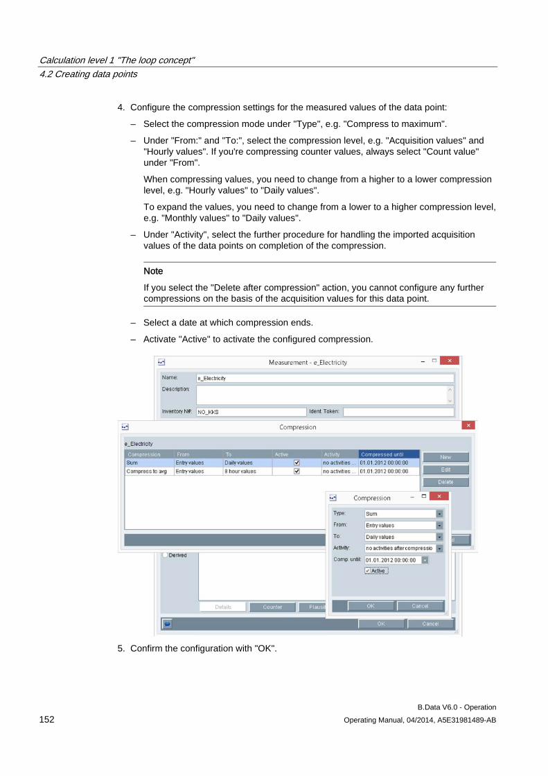
Calculation level 1 "The loop concept" 4.2 Creating data points
B.Data V6.0 - Operation 152 Operating Manual, 04/2014, A5E31981489-AB
4. Configure the compression settings for the measured values of the data point:
– Select the compression mode under "Type", e.g. "Compress to maximum".
– Under "From:" and "To:", select the compression level, e.g. "Acquisition values" and "Hourly values". If you're compressing counter values, always select "Count value" under "From".
When compressing values, you need to change from a higher to a lower compression level, e.g. "Hourly values" to "Daily values".
To expand the values, you need to change from a lower to a higher compression level, e.g. "Monthly values" to "Daily values".
– Under "Activity", select the further procedure for handling the imported acquisition values of the data points on completion of the compression.
Note
If you select the "Delete after compression" action, you cannot configure any further compressions on the basis of the acquisition values for this data point.
– Select a date at which compression ends.
– Activate "Active" to activate the configured compression.
5. Confirm the configuration with "OK".
Calculation level 1 "The loop concept" 4.2 Creating data points
B.Data V6.0 - Operation Operating Manual, 04/2014, A5E31981489-AB 153
Result You successfully configured compression of the measured values of the data point. A separate time column with time stamp is stored in the data point for each configured compression:
● All imported measured values will be compressed if online compression is activated. Incomplete measured values are initially saved to the buffer. Select "Administration > Job queue" to run the "General post-processing job" in order to compress measured values received at a later time.
● Launch the "Job for compressing the measurement journal" under "Administration > Job queue" if online compression is not activated.
See also B.Data options (Page 354)
Using the job queue (Page 352)
Database jobs (Page 570)
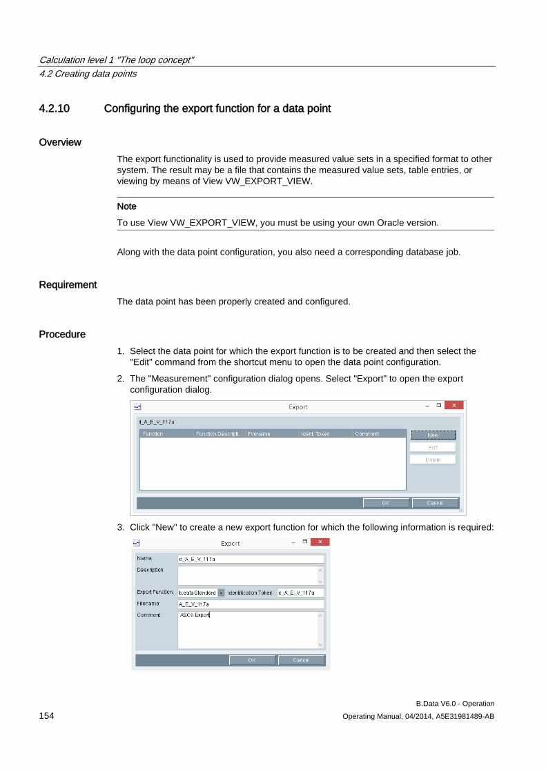
Calculation level 1 "The loop concept" 4.2 Creating data points
B.Data V6.0 - Operation 154 Operating Manual, 04/2014, A5E31981489-AB
4.2.10 Configuring the export function for a data point
Overview The export functionality is used to provide measured value sets in a specified format to other system. The result may be a file that contains the measured value sets, table entries, or viewing by means of View VW_EXPORT_VIEW.
Note
To use View VW_EXPORT_VIEW, you must be using your own Oracle version.
Along with the data point configuration, you also need a corresponding database job.
Requirement The data point has been properly created and configured.
Procedure 1. Select the data point for which the export function is to be created and then select the
"Edit" command from the shortcut menu to open the data point configuration.
2. The "Measurement" configuration dialog opens. Select "Export" to open the export configuration dialog.
3. Click "New" to create a new export function for which the following information is required:
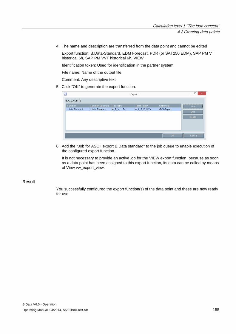
Calculation level 1 "The loop concept" 4.2 Creating data points
B.Data V6.0 - Operation Operating Manual, 04/2014, A5E31981489-AB 155
4. The name and description are transferred from the data point and cannot be edited
Export function: B.Data-Standard, EDM Forecast, PDR (or SAT250 EDM), SAP PM VT historical 6h, SAP PM VVT historical 6h, VIEW
Identification token: Used for identification in the partner system
File name: Name of the output file
Comment: Any descriptive text
5. Click "OK" to generate the export function.
6. Add the "Job for ASCII export B.Data standard" to the job queue to enable execution of
the configured export function.
It is not necessary to provide an active job for the VIEW export function, because as soon as a data point has been assigned to this export function, its data can be called by means of View vw_export_view.
Result You successfully configured the export function(s) of the data point and these are now ready for use.
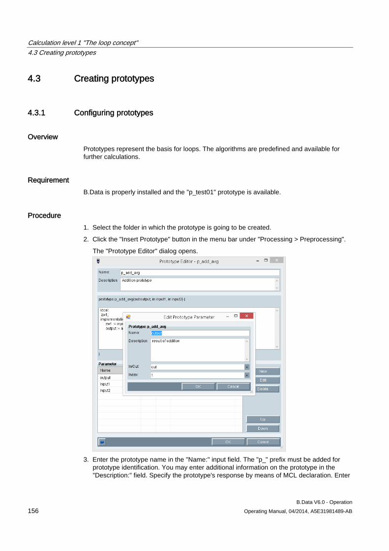
Calculation level 1 "The loop concept" 4.3 Creating prototypes
B.Data V6.0 - Operation 156 Operating Manual, 04/2014, A5E31981489-AB
4.3 Creating prototypes
4.3.1 Configuring prototypes
Overview Prototypes represent the basis for loops. The algorithms are predefined and available for further calculations.
Requirement B.Data is properly installed and the "p_test01" prototype is available.
Procedure 1. Select the folder in which the prototype is going to be created.
2. Click the "Insert Prototype" button in the menu bar under "Processing > Preprocessing".
The "Prototype Editor" dialog opens.
3. Enter the prototype name in the "Name:" input field. The "p_" prefix must be added for
prototype identification. You may enter additional information on the prototype in the "Description:" field. Specify the prototype's response by means of MCL declaration. Enter
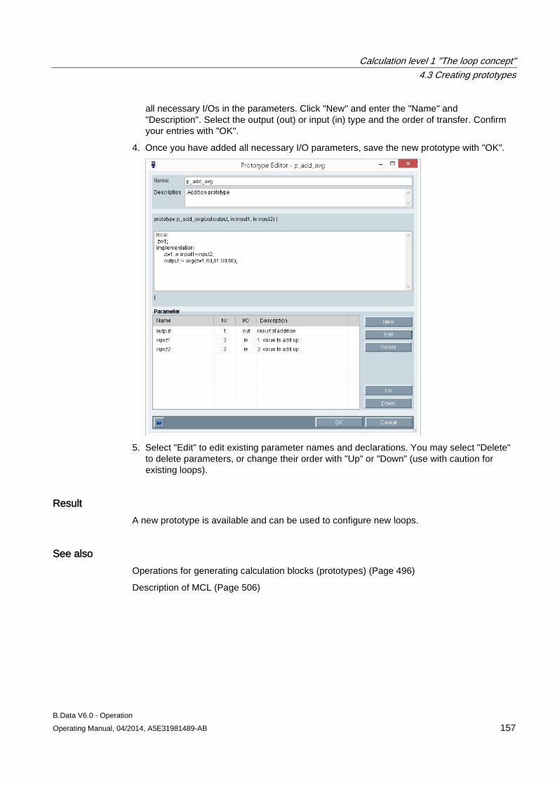
Calculation level 1 "The loop concept" 4.3 Creating prototypes
B.Data V6.0 - Operation Operating Manual, 04/2014, A5E31981489-AB 157
all necessary I/Os in the parameters. Click "New" and enter the "Name" and "Description". Select the output (out) or input (in) type and the order of transfer. Confirm your entries with "OK".
4. Once you have added all necessary I/O parameters, save the new prototype with "OK".
5. Select "Edit" to edit existing parameter names and declarations. You may select "Delete"
to delete parameters, or change their order with "Up" or "Down" (use with caution for existing loops).
Result A new prototype is available and can be used to configure new loops.
See also Operations for generating calculation blocks (prototypes) (Page 496)
Description of MCL (Page 506)
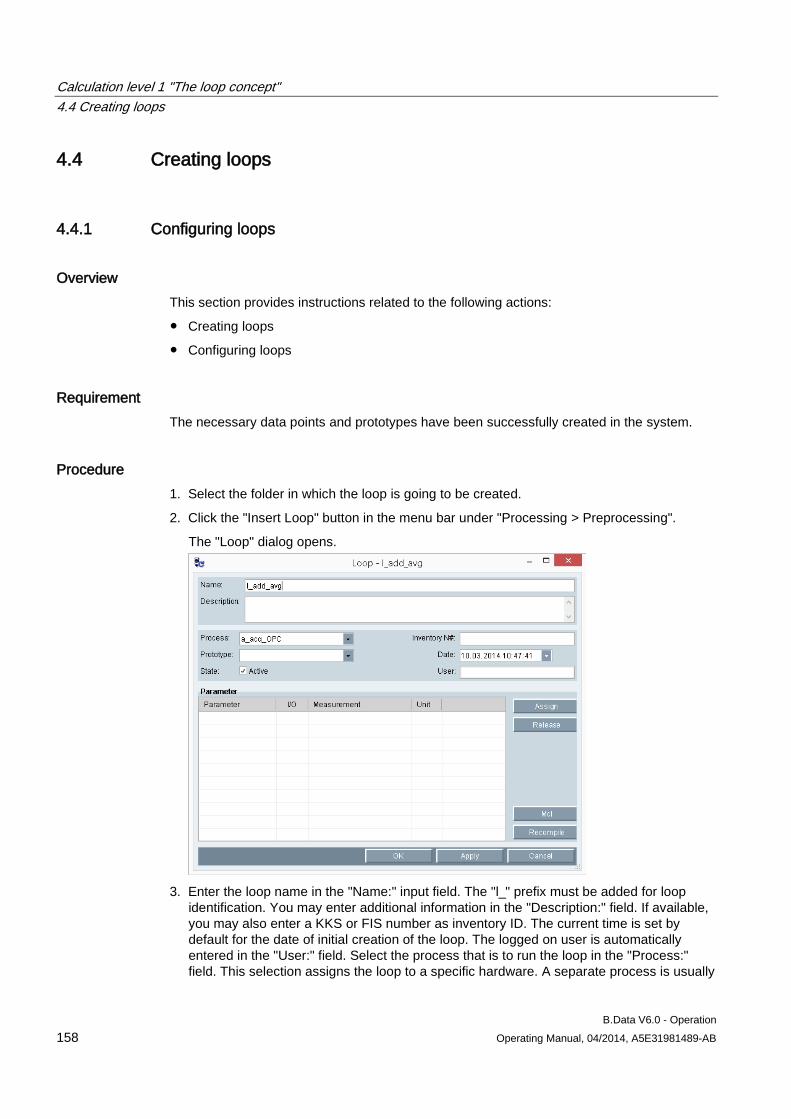
Calculation level 1 "The loop concept" 4.4 Creating loops
B.Data V6.0 - Operation 158 Operating Manual, 04/2014, A5E31981489-AB
4.4 Creating loops
4.4.1 Configuring loops
Overview This section provides instructions related to the following actions:
● Creating loops
● Configuring loops
Requirement The necessary data points and prototypes have been successfully created in the system.
Procedure 1. Select the folder in which the loop is going to be created.
2. Click the "Insert Loop" button in the menu bar under "Processing > Preprocessing".
The "Loop" dialog opens.
3. Enter the loop name in the "Name:" input field. The "l_" prefix must be added for loop
identification. You may enter additional information in the "Description:" field. If available, you may also enter a KKS or FIS number as inventory ID. The current time is set by default for the date of initial creation of the loop. The logged on user is automatically entered in the "User:" field. Select the process that is to run the loop in the "Process:" field. This selection assigns the loop to a specific hardware. A separate process is usually
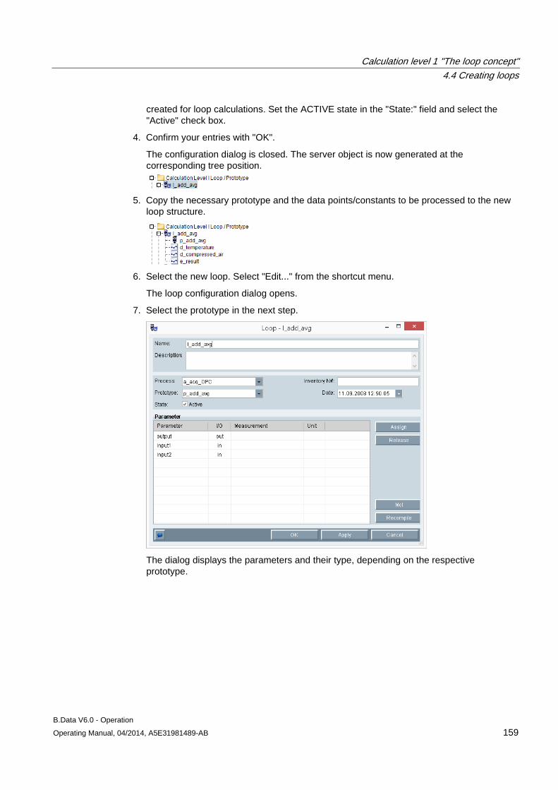
Calculation level 1 "The loop concept" 4.4 Creating loops
B.Data V6.0 - Operation Operating Manual, 04/2014, A5E31981489-AB 159
created for loop calculations. Set the ACTIVE state in the "State:" field and select the "Active" check box.
4. Confirm your entries with "OK".
The configuration dialog is closed. The server object is now generated at the corresponding tree position.
5. Copy the necessary prototype and the data points/constants to be processed to the new
loop structure.
6. Select the new loop. Select "Edit..." from the shortcut menu.
The loop configuration dialog opens.
7. Select the prototype in the next step.
The dialog displays the parameters and their type, depending on the respective prototype.
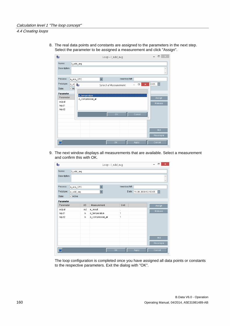
Calculation level 1 "The loop concept" 4.4 Creating loops
B.Data V6.0 - Operation 160 Operating Manual, 04/2014, A5E31981489-AB
8. The real data points and constants are assigned to the parameters in the next step. Select the parameter to be assigned a measurement and click "Assign".
9. The next window displays all measurements that are available. Select a measurement
and confirm this with OK.
The loop configuration is completed once you have assigned all data points or constants to the respective parameters. Exit the dialog with "OK".
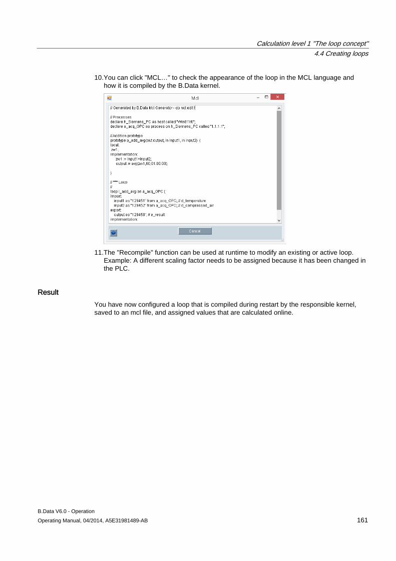
Calculation level 1 "The loop concept" 4.4 Creating loops
B.Data V6.0 - Operation Operating Manual, 04/2014, A5E31981489-AB 161
10.You can click "MCL…" to check the appearance of the loop in the MCL language and how it is compiled by the B.Data kernel.
11.The "Recompile" function can be used at runtime to modify an existing or active loop.
Example: A different scaling factor needs to be assigned because it has been changed in the PLC.
Result You have now configured a loop that is compiled during restart by the responsible kernel, saved to an mcl file, and assigned values that are calculated online.
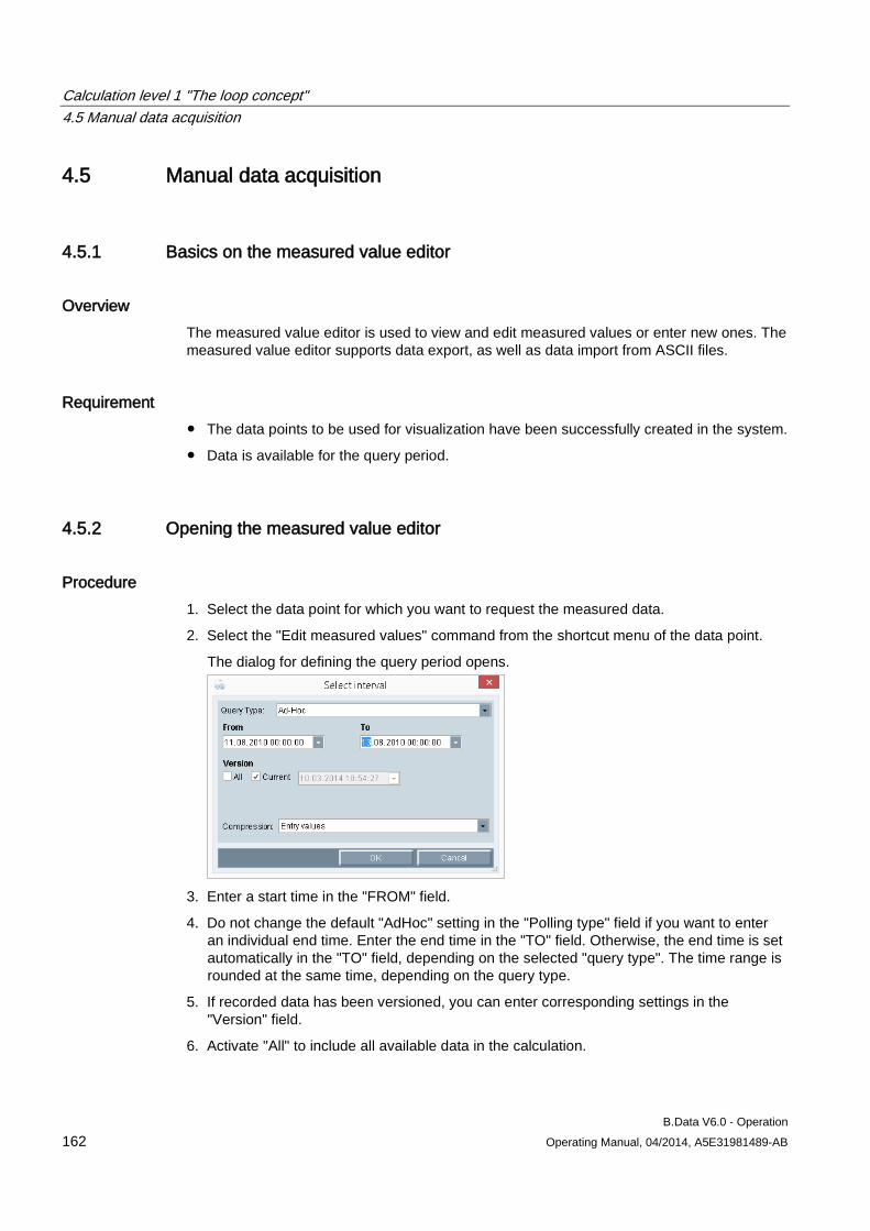
Calculation level 1 "The loop concept" 4.5 Manual data acquisition
B.Data V6.0 - Operation 162 Operating Manual, 04/2014, A5E31981489-AB
4.5 Manual data acquisition
4.5.1 Basics on the measured value editor
Overview The measured value editor is used to view and edit measured values or enter new ones. The measured value editor supports data export, as well as data import from ASCII files.
Requirement ● The data points to be used for visualization have been successfully created in the system.
● Data is available for the query period.
4.5.2 Opening the measured value editor
Procedure 1. Select the data point for which you want to request the measured data.
2. Select the "Edit measured values" command from the shortcut menu of the data point.
The dialog for defining the query period opens.
3. Enter a start time in the "FROM" field.
4. Do not change the default "AdHoc" setting in the "Polling type" field if you want to enter an individual end time. Enter the end time in the "TO" field. Otherwise, the end time is set automatically in the "TO" field, depending on the selected "query type". The time range is rounded at the same time, depending on the query type.
5. If recorded data has been versioned, you can enter corresponding settings in the "Version" field.
6. Activate "All" to include all available data in the calculation.
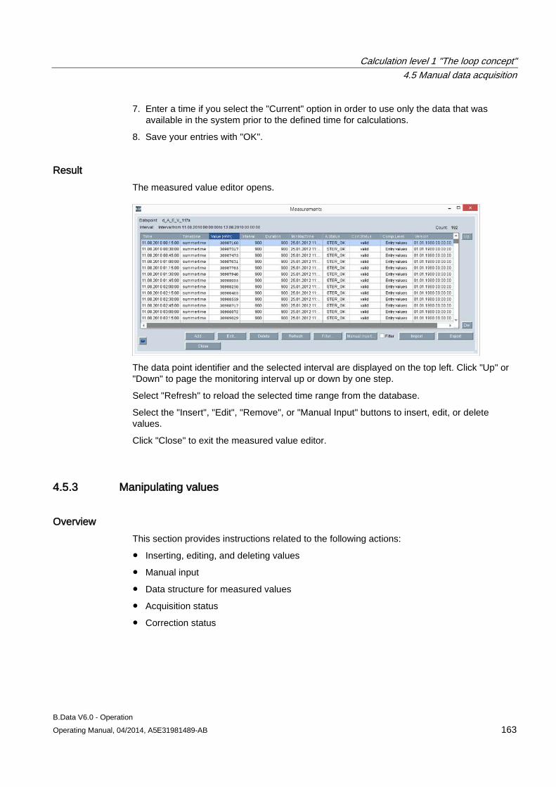
Calculation level 1 "The loop concept" 4.5 Manual data acquisition
B.Data V6.0 - Operation Operating Manual, 04/2014, A5E31981489-AB 163
7. Enter a time if you select the "Current" option in order to use only the data that was available in the system prior to the defined time for calculations.
8. Save your entries with "OK".
Result The measured value editor opens.
The data point identifier and the selected interval are displayed on the top left. Click "Up" or "Down" to page the monitoring interval up or down by one step.
Select "Refresh" to reload the selected time range from the database.
Select the "Insert", "Edit", "Remove", or "Manual Input" buttons to insert, edit, or delete values.
Click "Close" to exit the measured value editor.
4.5.3 Manipulating values
Overview This section provides instructions related to the following actions:
● Inserting, editing, and deleting values
● Manual input
● Data structure for measured values
● Acquisition status
● Correction status
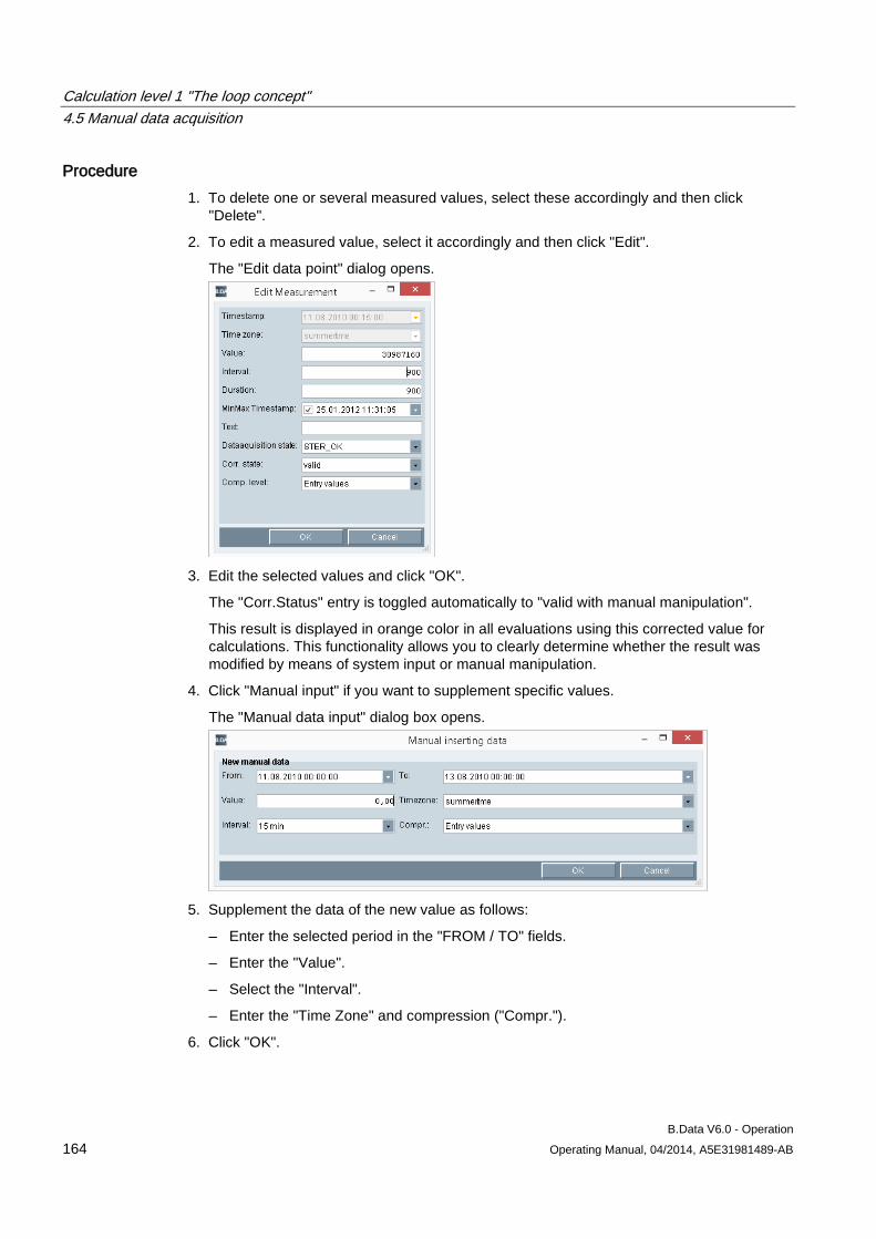
Calculation level 1 "The loop concept" 4.5 Manual data acquisition
B.Data V6.0 - Operation 164 Operating Manual, 04/2014, A5E31981489-AB
Procedure 1. To delete one or several measured values, select these accordingly and then click
"Delete".
2. To edit a measured value, select it accordingly and then click "Edit".
The "Edit data point" dialog opens.
3. Edit the selected values and click "OK".
The "Corr.Status" entry is toggled automatically to "valid with manual manipulation".
This result is displayed in orange color in all evaluations using this corrected value for calculations. This functionality allows you to clearly determine whether the result was modified by means of system input or manual manipulation.
4. Click "Manual input" if you want to supplement specific values.
The "Manual data input" dialog box opens.
5. Supplement the data of the new value as follows:
– Enter the selected period in the "FROM / TO" fields.
– Enter the "Value".
– Select the "Interval".
– Enter the "Time Zone" and compression ("Compr.").
6. Click "OK".
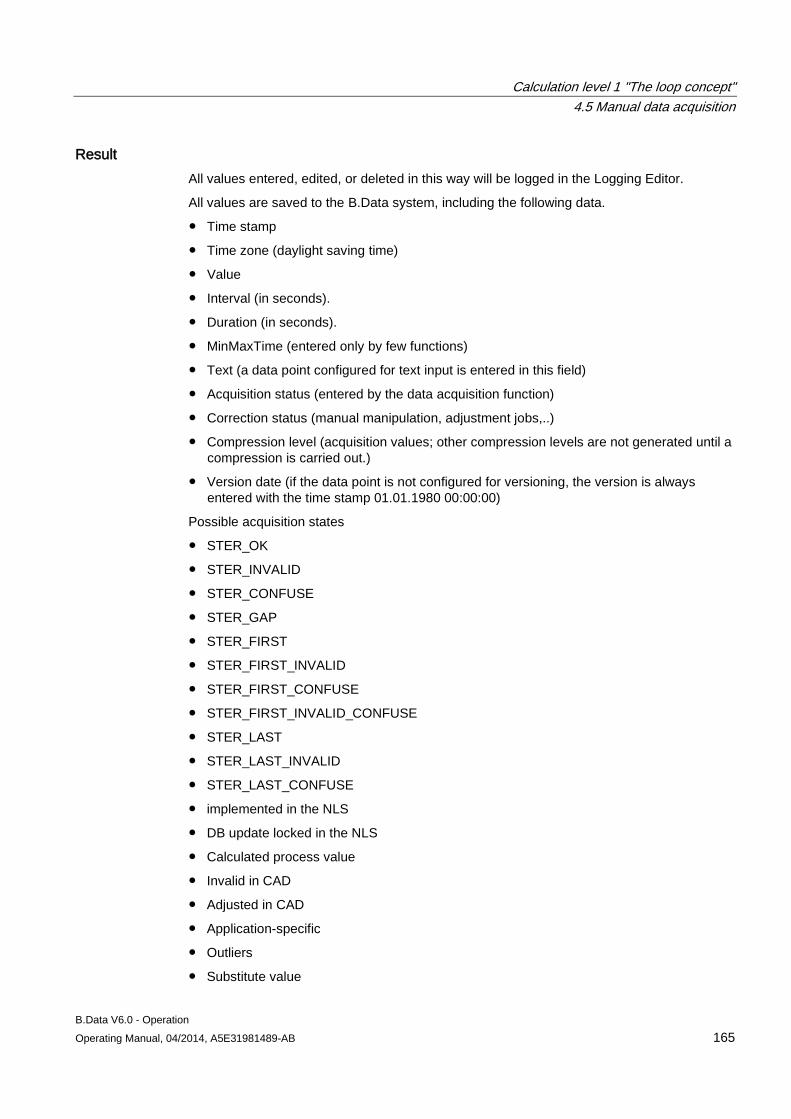
Calculation level 1 "The loop concept" 4.5 Manual data acquisition
B.Data V6.0 - Operation Operating Manual, 04/2014, A5E31981489-AB 165
Result All values entered, edited, or deleted in this way will be logged in the Logging Editor.
All values are saved to the B.Data system, including the following data.
● Time stamp
● Time zone (daylight saving time)
● Value
● Interval (in seconds).
● Duration (in seconds).
● MinMaxTime (entered only by few functions)
● Text (a data point configured for text input is entered in this field)
● Acquisition status (entered by the data acquisition function)
● Correction status (manual manipulation, adjustment jobs,..)
● Compression level (acquisition values; other compression levels are not generated until a compression is carried out.)
● Version date (if the data point is not configured for versioning, the version is always entered with the time stamp 01.01.1980 00:00:00)
Possible acquisition states
● STER_OK
● STER_INVALID
● STER_CONFUSE
● STER_GAP
● STER_FIRST
● STER_FIRST_INVALID
● STER_FIRST_CONFUSE
● STER_FIRST_INVALID_CONFUSE
● STER_LAST
● STER_LAST_INVALID
● STER_LAST_CONFUSE
● implemented in the NLS
● DB update locked in the NLS
● Calculated process value
● Invalid in CAD
● Adjusted in CAD
● Application-specific
● Outliers
● Substitute value
Calculation level 1 "The loop concept" 4.5 Manual data acquisition
B.Data V6.0 - Operation 166 Operating Manual, 04/2014, A5E31981489-AB
Possible correction states:
● Valid
● Invalid
● Corrected with LRU
● Corrected with substitute measurement
● Corrected with substitute value
● Valid with manual manipulation
● Valid corr. with LRU and manual manipulation
● Valid corr. with substitute m. and manual manipulation.
● Valid corr. with substitute v. and manual manipulation.
● Import
● Invalid import
● Import valid, corr. with LRU
● Import valid, corr. with substitute measurement
● Import valid, corrected with substitute value
● Import valid with manual manipulation
● Import valid, corrected LRU+manual manipulation.
● Import valid, corr. with substitute m.+manual manipulation.
● Import valid, corr. with substitute v.+manual manipulation.
● Corrected
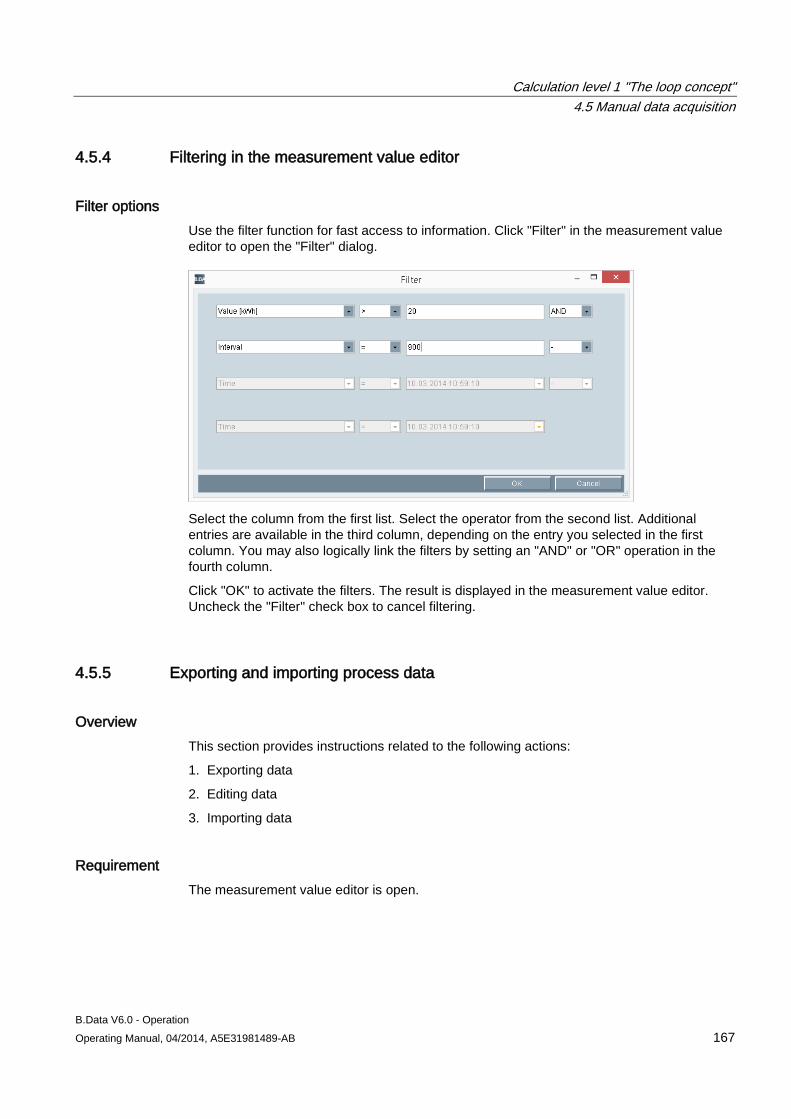
Calculation level 1 "The loop concept" 4.5 Manual data acquisition
B.Data V6.0 - Operation Operating Manual, 04/2014, A5E31981489-AB 167
4.5.4 Filtering in the measurement value editor
Filter options Use the filter function for fast access to information. Click "Filter" in the measurement value editor to open the "Filter" dialog.
Select the column from the first list. Select the operator from the second list. Additional entries are available in the third column, depending on the entry you selected in the first column. You may also logically link the filters by setting an "AND" or "OR" operation in the fourth column.
Click "OK" to activate the filters. The result is displayed in the measurement value editor. Uncheck the "Filter" check box to cancel filtering.
4.5.5 Exporting and importing process data
Overview This section provides instructions related to the following actions:
1. Exporting data
2. Editing data
3. Importing data
Requirement The measurement value editor is open.
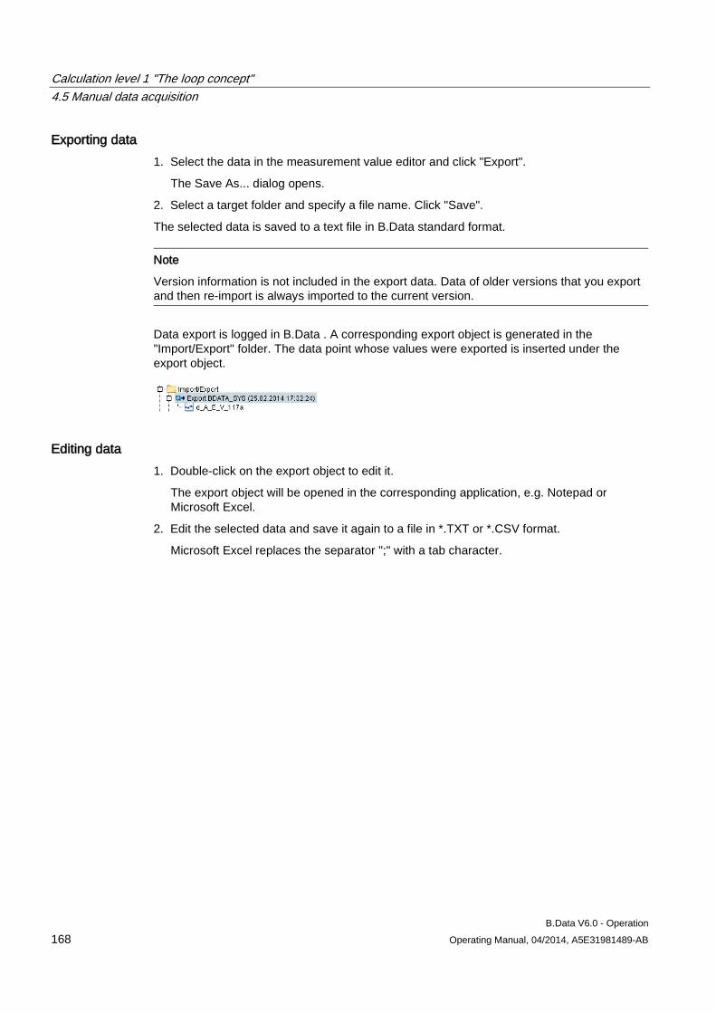
Calculation level 1 "The loop concept" 4.5 Manual data acquisition
B.Data V6.0 - Operation 168 Operating Manual, 04/2014, A5E31981489-AB
Exporting data 1. Select the data in the measurement value editor and click "Export".
The Save As... dialog opens.
2. Select a target folder and specify a file name. Click "Save".
The selected data is saved to a text file in B.Data standard format.
Note
Version information is not included in the export data. Data of older versions that you export and then re-import is always imported to the current version.
Data export is logged in B.Data . A corresponding export object is generated in the "Import/Export" folder. The data point whose values were exported is inserted under the export object.
Editing data 1. Double-click on the export object to edit it.
The export object will be opened in the corresponding application, e.g. Notepad or Microsoft Excel.
2. Edit the selected data and save it again to a file in *.TXT or *.CSV format.
Microsoft Excel replaces the separator ";" with a tab character.
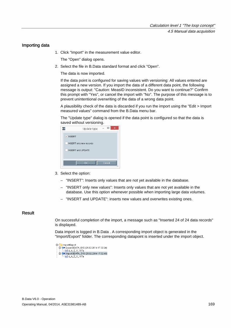
Calculation level 1 "The loop concept" 4.5 Manual data acquisition
B.Data V6.0 - Operation Operating Manual, 04/2014, A5E31981489-AB 169
Importing data 1. Click "Import" in the measurement value editor.
The "Open" dialog opens.
2. Select the file in B.Data standard format and click "Open".
The data is now imported.
If the data point is configured for saving values with versioning: All values entered are assigned a new version. If you import the data of a different data point, the following message is output: "Caution: MeasID inconsistent. Do you want to continue?" Confirm this prompt with "Yes", or cancel the import with "No". The purpose of this message is to prevent unintentional overwriting of the data of a wrong data point.
A plausibility check of the data is discarded if you run the import using the "Edit > Import measured values" command from the B.Data menu bar.
The "Update type" dialog is opened if the data point is configured so that the data is saved without versioning.
3. Select the option:
– "INSERT": Inserts only values that are not yet available in the database.
– "INSERT only new values": Inserts only values that are not yet available in the database. Use this option whenever possible when importing large data volumes.
– "INSERT and UPDATE": inserts new values and overwrites existing ones.
Result On successful completion of the import, a message such as "Inserted 24 of 24 data records" is displayed.
Data import is logged in B.Data . A corresponding import object is generated in the "Import/Export" folder. The corresponding datapoint is inserted under the import object.
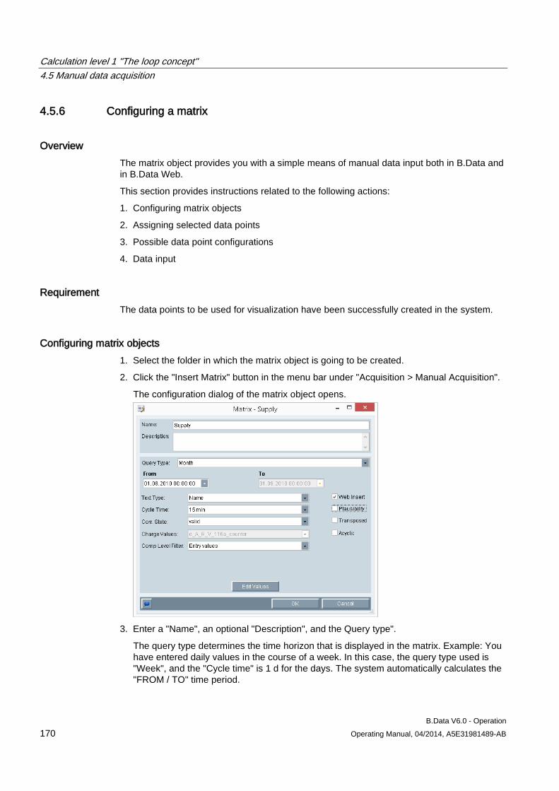
Calculation level 1 "The loop concept" 4.5 Manual data acquisition
B.Data V6.0 - Operation 170 Operating Manual, 04/2014, A5E31981489-AB
4.5.6 Configuring a matrix
Overview The matrix object provides you with a simple means of manual data input both in B.Data and in B.Data Web.
This section provides instructions related to the following actions:
1. Configuring matrix objects
2. Assigning selected data points
3. Possible data point configurations
4. Data input
Requirement The data points to be used for visualization have been successfully created in the system.
Configuring matrix objects 1. Select the folder in which the matrix object is going to be created.
2. Click the "Insert Matrix" button in the menu bar under "Acquisition > Manual Acquisition".
The configuration dialog of the matrix object opens.
3. Enter a "Name", an optional "Description", and the Query type".
The query type determines the time horizon that is displayed in the matrix. Example: You have entered daily values in the course of a week. In this case, the query type used is "Week", and the "Cycle time" is 1 d for the days. The system automatically calculates the "FROM / TO" time period.
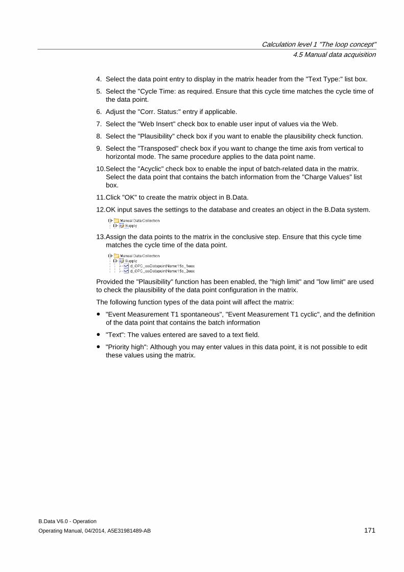
Calculation level 1 "The loop concept" 4.5 Manual data acquisition
B.Data V6.0 - Operation Operating Manual, 04/2014, A5E31981489-AB 171
4. Select the data point entry to display in the matrix header from the "Text Type:" list box.
5. Select the "Cycle Time: as required. Ensure that this cycle time matches the cycle time of the data point.
6. Adjust the "Corr. Status:" entry if applicable.
7. Select the "Web Insert" check box to enable user input of values via the Web.
8. Select the "Plausibility" check box if you want to enable the plausibility check function.
9. Select the "Transposed" check box if you want to change the time axis from vertical to horizontal mode. The same procedure applies to the data point name.
10.Select the "Acyclic" check box to enable the input of batch-related data in the matrix. Select the data point that contains the batch information from the "Charge Values" list box.
11.Click "OK" to create the matrix object in B.Data.
12.OK input saves the settings to the database and creates an object in the B.Data system.
13.Assign the data points to the matrix in the conclusive step. Ensure that this cycle time
matches the cycle time of the data point.
Provided the "Plausibility" function has been enabled, the "high limit" and "low limit" are used to check the plausibility of the data point configuration in the matrix.
The following function types of the data point will affect the matrix:
● "Event Measurement T1 spontaneous", "Event Measurement T1 cyclic", and the definition of the data point that contains the batch information
● "Text": The values entered are saved to a text field.
● "Priority high": Although you may enter values in this data point, it is not possible to edit these values using the matrix.
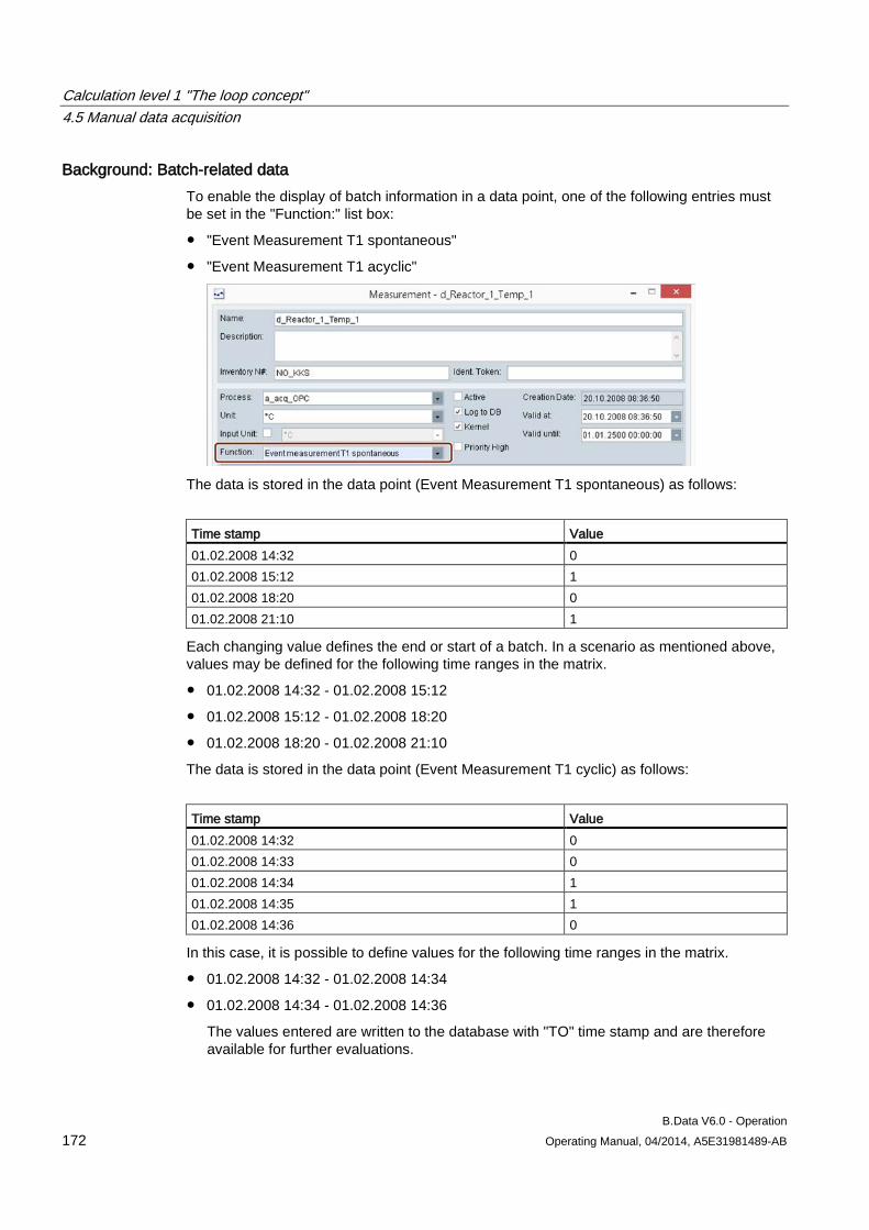
Calculation level 1 "The loop concept" 4.5 Manual data acquisition
B.Data V6.0 - Operation 172 Operating Manual, 04/2014, A5E31981489-AB
Background: Batch-related data To enable the display of batch information in a data point, one of the following entries must be set in the "Function:" list box:
● "Event Measurement T1 spontaneous"
● "Event Measurement T1 acyclic"
The data is stored in the data point (Event Measurement T1 spontaneous) as follows:
Time stamp Value 01.02.2008 14:32 0 01.02.2008 15:12 1 01.02.2008 18:20 0 01.02.2008 21:10 1
Each changing value defines the end or start of a batch. In a scenario as mentioned above, values may be defined for the following time ranges in the matrix.
● 01.02.2008 14:32 - 01.02.2008 15:12
● 01.02.2008 15:12 - 01.02.2008 18:20
● 01.02.2008 18:20 - 01.02.2008 21:10
The data is stored in the data point (Event Measurement T1 cyclic) as follows:
Time stamp Value 01.02.2008 14:32 0 01.02.2008 14:33 0 01.02.2008 14:34 1 01.02.2008 14:35 1 01.02.2008 14:36 0
In this case, it is possible to define values for the following time ranges in the matrix.
● 01.02.2008 14:32 - 01.02.2008 14:34
● 01.02.2008 14:34 - 01.02.2008 14:36
The values entered are written to the database with "TO" time stamp and are therefore available for further evaluations.
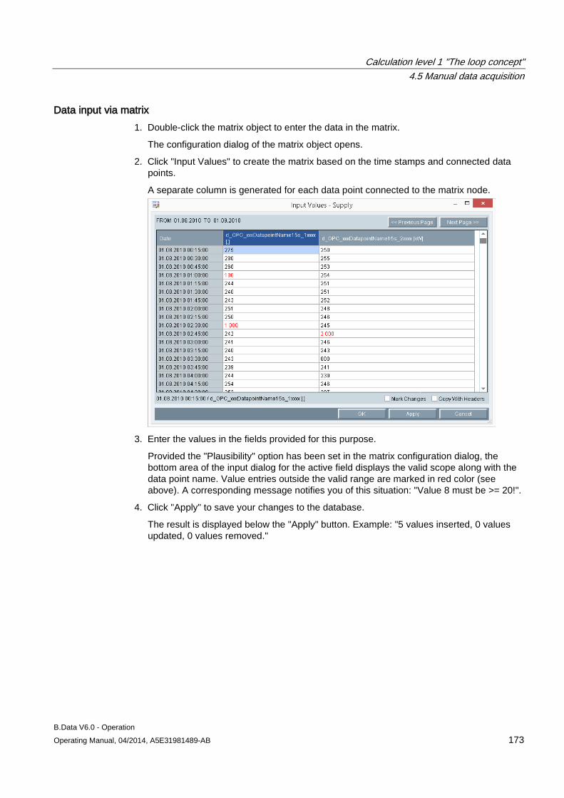
Calculation level 1 "The loop concept" 4.5 Manual data acquisition
B.Data V6.0 - Operation Operating Manual, 04/2014, A5E31981489-AB 173
Data input via matrix 1. Double-click the matrix object to enter the data in the matrix.
The configuration dialog of the matrix object opens.
2. Click "Input Values" to create the matrix based on the time stamps and connected data points.
A separate column is generated for each data point connected to the matrix node.
3. Enter the values in the fields provided for this purpose.
Provided the "Plausibility" option has been set in the matrix configuration dialog, the bottom area of the input dialog for the active field displays the valid scope along with the data point name. Value entries outside the valid range are marked in red color (see above). A corresponding message notifies you of this situation: "Value 8 must be >= 20!".
4. Click "Apply" to save your changes to the database.
The result is displayed below the "Apply" button. Example: "5 values inserted, 0 values updated, 0 values removed."
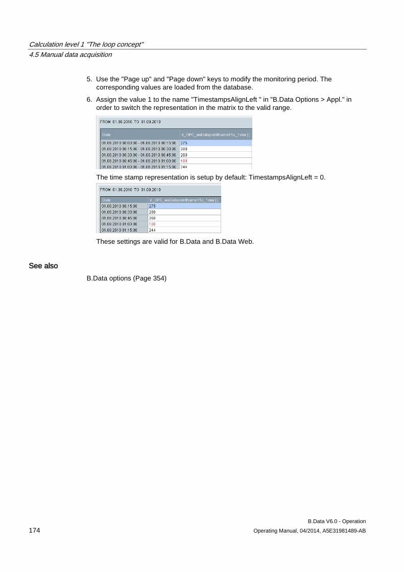
Calculation level 1 "The loop concept" 4.5 Manual data acquisition
B.Data V6.0 - Operation 174 Operating Manual, 04/2014, A5E31981489-AB
5. Use the "Page up" and "Page down" keys to modify the monitoring period. The corresponding values are loaded from the database.
6. Assign the value 1 to the name "TimestampsAlignLeft " in "B.Data Options > Appl." in order to switch the representation in the matrix to the valid range.
The time stamp representation is setup by default: TimestampsAlignLeft = 0.
These settings are valid for B.Data and B.Data Web.
See also B.Data options (Page 354)
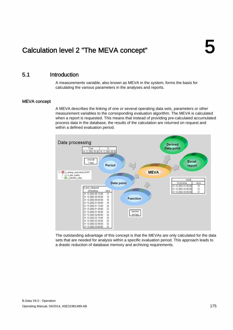
B.Data V6.0 - Operation Operating Manual, 04/2014, A5E31981489-AB 175
Calculation level 2 "The MEVA concept" 5 5.1 Introduction
A measurements variable, also known as MEVA in the system, forms the basis for calculating the various parameters in the analyses and reports.
MEVA concept A MEVA describes the linking of one or several operating data sets, parameters or other measurement variables to the corresponding evaluation algorithm. The MEVA is calculated when a report is requested. This means that instead of providing pre-calculated accumulated process data in the database, the results of the calculation are returned on request and within a defined evaluation period.
The outstanding advantage of this concept is that the MEVAs are only calculated for the data sets that are needed for analysis within a specific evaluation period. This approach leads to a drastic reduction of database memory and archiving requirements.
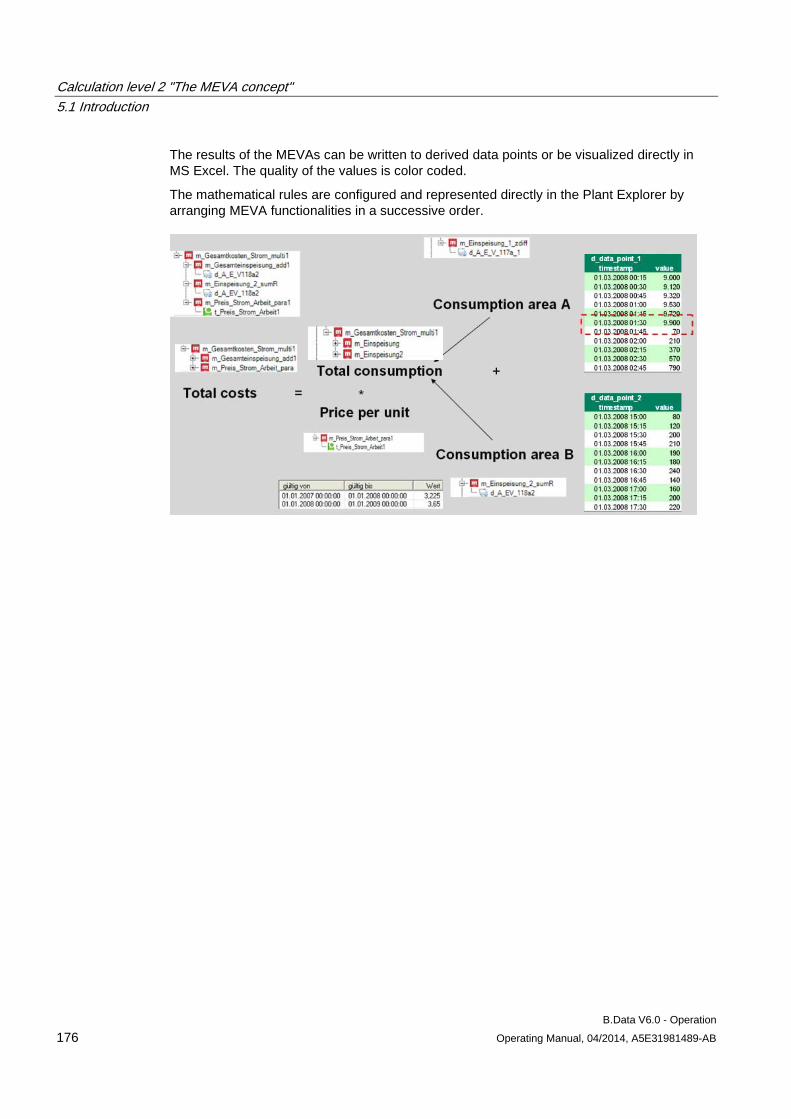
Calculation level 2 "The MEVA concept" 5.1 Introduction
B.Data V6.0 - Operation 176 Operating Manual, 04/2014, A5E31981489-AB
The results of the MEVAs can be written to derived data points or be visualized directly in MS Excel. The quality of the values is color coded.
The mathematical rules are configured and represented directly in the Plant Explorer by arranging MEVA functionalities in a successive order.
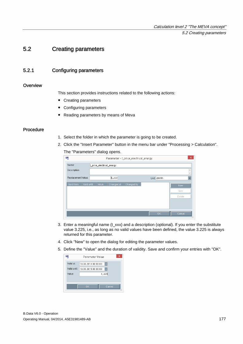
Calculation level 2 "The MEVA concept" 5.2 Creating parameters
B.Data V6.0 - Operation Operating Manual, 04/2014, A5E31981489-AB 177
5.2 Creating parameters
5.2.1 Configuring parameters
Overview This section provides instructions related to the following actions:
● Creating parameters
● Configuring parameters
● Reading parameters by means of Meva
Procedure 1. Select the folder in which the parameter is going to be created.
2. Click the "Insert Parameter" button in the menu bar under "Processing > Calculation".
The "Parameters" dialog opens.
3. Enter a meaningful name (t_xxx) and a description (optional). If you enter the substitute
value 3.225, i.e., as long as no valid values have been defined, the value 3.225 is always returned for this parameter.
4. Click "New" to open the dialog for editing the parameter values.
5. Define the "Value" and the duration of validity. Save and confirm your entries with "OK".
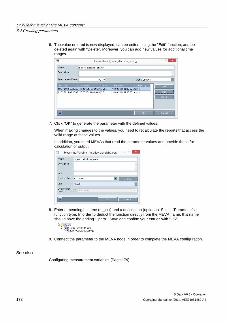
Calculation level 2 "The MEVA concept" 5.2 Creating parameters
B.Data V6.0 - Operation 178 Operating Manual, 04/2014, A5E31981489-AB
6. The value entered is now displayed, can be edited using the "Edit" function, and be deleted again with "Delete". Moreover, you can add new values for additional time ranges.
7. Click "OK" to generate the parameter with the defined values.
When making changes to the values, you need to recalculate the reports that access the valid range of these values.
In addition, you need MEVAs that read the parameter values and provide these for calculation or output.
8. Enter a meaningful name (m_xxx) and a description (optional). Select "Parameter" as
function type. In order to deduct the function directly from the MEVA name, this name should have the ending "_para". Save and confirm your entries with "OK".
9. Connect the parameter to the MEVA node in order to complete the MEVA configuration.
See also Configuring measurement variables (Page 179)
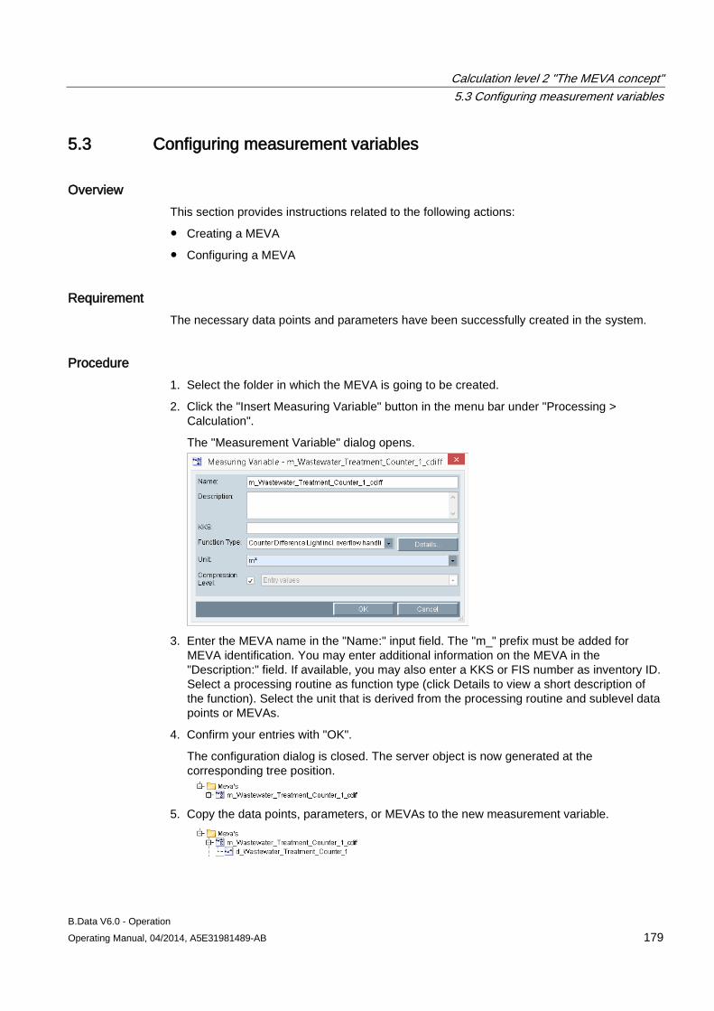
Calculation level 2 "The MEVA concept" 5.3 Configuring measurement variables
B.Data V6.0 - Operation Operating Manual, 04/2014, A5E31981489-AB 179
5.3 Configuring measurement variables
Overview This section provides instructions related to the following actions:
● Creating a MEVA
● Configuring a MEVA
Requirement The necessary data points and parameters have been successfully created in the system.
Procedure 1. Select the folder in which the MEVA is going to be created.
2. Click the "Insert Measuring Variable" button in the menu bar under "Processing > Calculation".
The "Measurement Variable" dialog opens.
3. Enter the MEVA name in the "Name:" input field. The "m_" prefix must be added for
MEVA identification. You may enter additional information on the MEVA in the "Description:" field. If available, you may also enter a KKS or FIS number as inventory ID. Select a processing routine as function type (click Details to view a short description of the function). Select the unit that is derived from the processing routine and sublevel data points or MEVAs.
4. Confirm your entries with "OK".
The configuration dialog is closed. The server object is now generated at the corresponding tree position.
5. Copy the data points, parameters, or MEVAs to the new measurement variable.
Calculation level 2 "The MEVA concept" 5.3 Configuring measurement variables
B.Data V6.0 - Operation 180 Operating Manual, 04/2014, A5E31981489-AB
Result You have now configured a MEVA that you can use for further processing in reports or derived data points.
See also Database functions for measurement variables (Page 509)
B.Data V6.0 - Operation Operating Manual, 04/2014, A5E31981489-AB 181
Calculation level 3 "Report and visualization concept" 6 6.1 Basic information on calculation level 3
Definition "Calculation level 3" denotes the time-independent processing and visualization of measuring values in reports. Microsoft Excel is used to visualize the reports.
You can process the data exported from B.Data using the entire Microsoft Excel functionality, for example, statistical functions such as correlation or regression analysis. You can also process the result data using graphics or diagrams.
Application "Calculation level 3" supports you in the following activities:
● Creation of company-specific reports for all departments and information demands.
● IT-related, system-wide analysis of different business units for holistic assessments of your company.
● The workflow system of B.Data reduces your staff's workload:
– Automatic and cyclical calculation of performance indicators and accounting results (task management).
– Automatic generation of standard analyses for predefined periods, e.g. day, month, shift, year.
– Automatic sending of evaluations to printers in the company-wide printer network.
– Automatic dispatch of analyses and accounting bases by means of e-mail attachment to internal and external recipients of the business unit.
When generating reports, you can always access previous configurations (historicization), or different measured value versions (versioning).
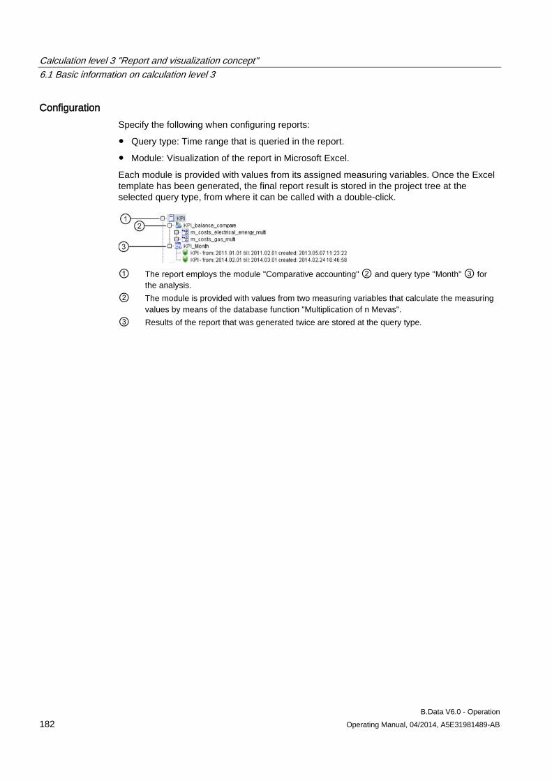
Calculation level 3 "Report and visualization concept" 6.1 Basic information on calculation level 3
B.Data V6.0 - Operation 182 Operating Manual, 04/2014, A5E31981489-AB
Configuration Specify the following when configuring reports:
● Query type: Time range that is queried in the report.
● Module: Visualization of the report in Microsoft Excel.
Each module is provided with values from its assigned measuring variables. Once the Excel template has been generated, the final report result is stored in the project tree at the selected query type, from where it can be called with a double-click.
① The report employs the module "Comparative accounting" ② and query type "Month" ③ for
the analysis. ② The module is provided with values from two measuring variables that calculate the measuring
values by means of the database function "Multiplication of n Mevas". ③ Results of the report that was generated twice are stored at the query type.
Calculation level 3 "Report and visualization concept" 6.2 Creating a report
B.Data V6.0 - Operation Operating Manual, 04/2014, A5E31981489-AB 183
6.2 Creating a report
6.2.1 Basics on reports
Overview You can use B.Data to visualize or process the acquired measured values. Microsoft Excel is used to display reports in B.Data. You may use all layout options of Microsoft Excel for your reports. You can visualize the acquired measured values in a cake diagram, for example.
Reports can be generated manually or automatically, dispatched by e-mail, print it, save to a file server, and view in B.Data.
Report results are stored in the structure tree of Plant Explorer. The name of report results consists of the name, calculation period and the creation date.
You can use the default reports provided in B.Data for your project. The default reports are available in "Customer > Reports".
Components for creating reports You need a query type and a module to create a report.
Use a query type specify the time range of report and to configure automatic reporting.
Use a module to specify the mode of calculation and visualization of the acquired measured values in Microsoft Excel . The following module types are available:
● Query module: Returns values without calculation, e.g. the measured values of a month on a daily basis.
● Balancing module: Returns a value for a time period, e.g. the monthly energy costs.
● Protocol module: Returns values for all intervals of a time period, e.g. the monthly energy costs on a daily basis.
Certain modules need additional parameters when you start a report. A protocol module, for example, needs interval as start parameter.
Calculation level 3 "Report and visualization concept" 6.2 Creating a report
B.Data V6.0 - Operation 184 Operating Manual, 04/2014, A5E31981489-AB
Procedure for creating reports Proceed as follows to create a report:
1. Create a report.
2. Configure a query type and a module for the report.
3. Configure an Excel template for the report.
4. Enter the reported values.
5. Generate the report.
See also Creating a report (Page 185)
Configuring the query type for a report (Page 187)
Configuring a module for reports (Page 190)
Configuring a report template (Page 195)
Entering values in reports (Page 197)
Opening report results (Page 202)
Using B.Data Web (Page 395)
Display modes (Page 493)
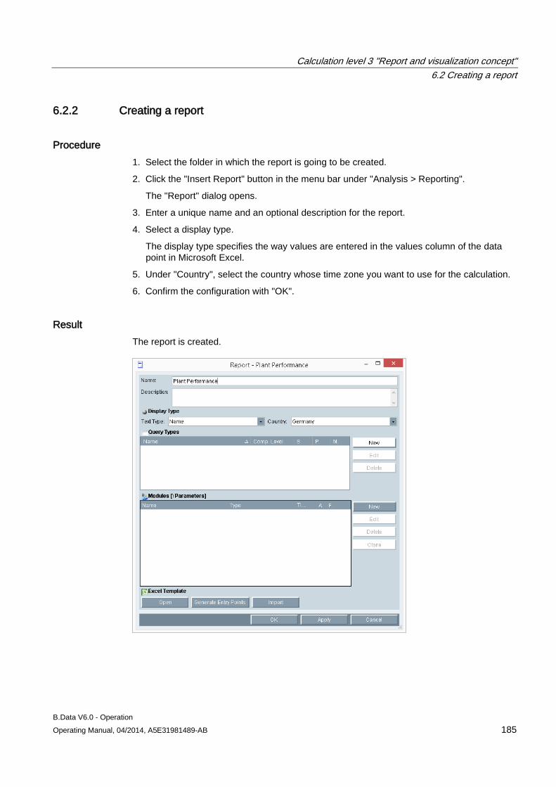
Calculation level 3 "Report and visualization concept" 6.2 Creating a report
B.Data V6.0 - Operation Operating Manual, 04/2014, A5E31981489-AB 185
6.2.2 Creating a report
Procedure 1. Select the folder in which the report is going to be created.
2. Click the "Insert Report" button in the menu bar under "Analysis > Reporting".
The "Report" dialog opens.
3. Enter a unique name and an optional description for the report.
4. Select a display type.
The display type specifies the way values are entered in the values column of the data point in Microsoft Excel.
5. Under "Country", select the country whose time zone you want to use for the calculation.
6. Confirm the configuration with "OK".
Result The report is created.
Calculation level 3 "Report and visualization concept" 6.2 Creating a report
B.Data V6.0 - Operation 186 Operating Manual, 04/2014, A5E31981489-AB
See also Configuring the query type for a report (Page 187)
Configuring a module for reports (Page 190)
Configuring a report template (Page 195)
Entering values in reports (Page 197)
Query types (Page 443)
Module overview (Page 452)
Display modes (Page 493)
Assign time zone for acquisition or calculation (Page 386)
Calculation level 3 "Report and visualization concept" 6.2 Creating a report
B.Data V6.0 - Operation Operating Manual, 04/2014, A5E31981489-AB 187
6.2.3 Configuring the query type for a report
Overview Use a query type to configure the time frame that is queried in a report. You may configure several query types in the report. A folder is created in the project tree of Plant Explorer for each query type of a report.
Requirement ● The report is configured.
● You have created the printer, the user, and the directory.
● For the "Send by Mail" option:
– The connection to an SMTP server is configured in the B.Data options.
● For the "Send Link to Recipient by Mail" option:
The B.Data Web URL is entered in the "B.Data Options", "Database" tab, "RSERV_SMTP_WEBSERVER" field, e.g. "http://localhost/BDataWeb".
Procedure 1. Double-click the selected report in the project tree of Plant Explorer.
The "Report" dialog opens.
2. Click "New" in the "Query types" field.
The "Query type" dialog opens.
3. Select a query type and enter a description if necessary.
4. Select a compression level.
Usually, you select "Entry values".
5. Go to "Delete interval" to set the interval for automatic deletion of report results from the project tree of Plant Explorer.
If you want to automatically delete the report results, you also need to start the "Job for deleting analyses".
6. Activate the corresponding options for automatic generation or printing of reports.
7. Proceed as follows to automatically save and email the report:
– Activate the "Send by Mail" option.
– Activate the report format for mailing, e.g. "PDF".
– Activate the "Send Link to Recipient by Mail" check box if you only want to email the link to the stored report.
The recipient will receive an email with the link instead of the PDF or Excel file.
The recipient accesses this report by clicking this link and logging on to B.Data Web to open the report in "PDF" or "Excel" format.
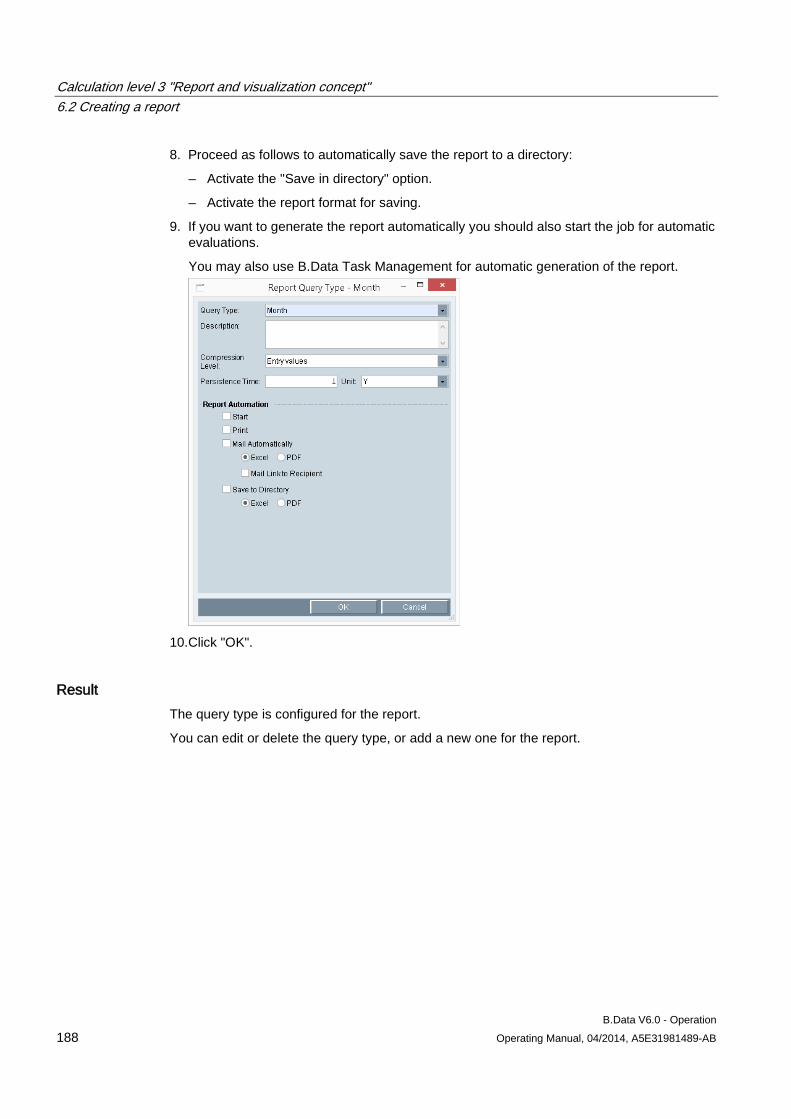
Calculation level 3 "Report and visualization concept" 6.2 Creating a report
B.Data V6.0 - Operation 188 Operating Manual, 04/2014, A5E31981489-AB
8. Proceed as follows to automatically save the report to a directory:
– Activate the "Save in directory" option.
– Activate the report format for saving.
9. If you want to generate the report automatically you should also start the job for automatic evaluations.
You may also use B.Data Task Management for automatic generation of the report.
10.Click "OK".
Result The query type is configured for the report.
You can edit or delete the query type, or add a new one for the report.
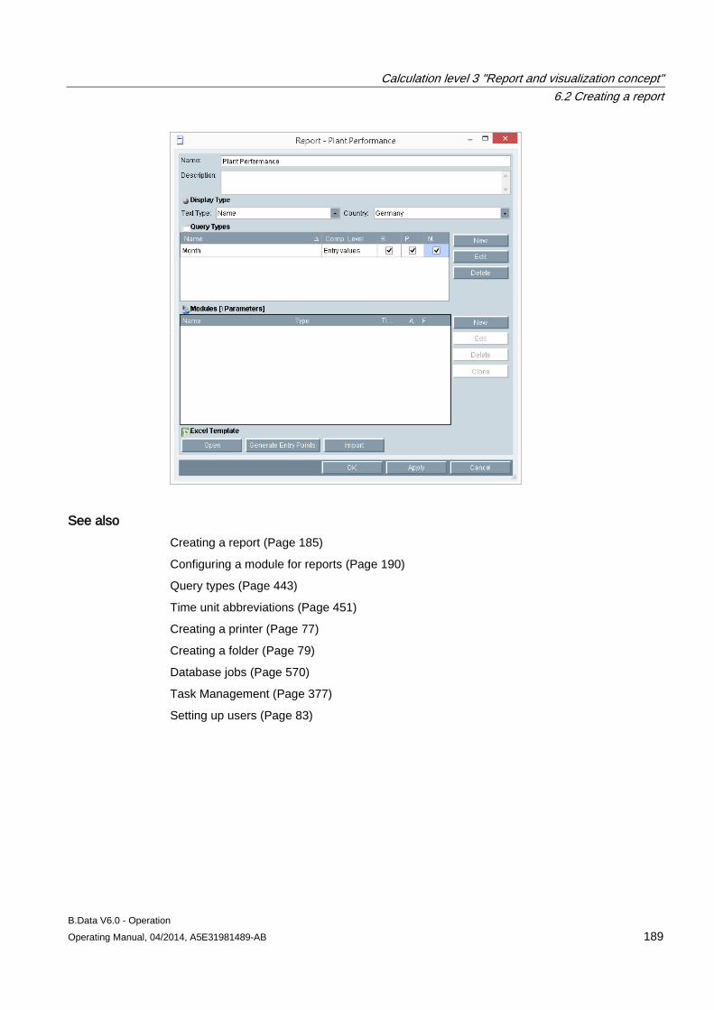
Calculation level 3 "Report and visualization concept" 6.2 Creating a report
B.Data V6.0 - Operation Operating Manual, 04/2014, A5E31981489-AB 189
See also Creating a report (Page 185)
Configuring a module for reports (Page 190)
Query types (Page 443)
Time unit abbreviations (Page 451)
Creating a printer (Page 77)
Creating a folder (Page 79)
Database jobs (Page 570)
Task Management (Page 377)
Setting up users (Page 83)
Calculation level 3 "Report and visualization concept" 6.2 Creating a report
B.Data V6.0 - Operation 190 Operating Manual, 04/2014, A5E31981489-AB
6.2.4 Configuring a module for reports
Overview Use a module to configure report visualization in Microsoft Excel. You can configure several modules for a report.
Note
Use a general name for the first protocol, e.g. "PROT", if you want to clone a report.
Requirement The report is configured.
Procedure 1. Double-click the selected report in the structure tree of Plant Explorer.
The "Report" dialog opens.
2. Click "New" in the "Module" area.
The module configuration dialog opens.
3. Enter a unique name and an optional description for the module.
Give the report module a name other than those for the worksheets and cells in Microsoft Excel. This will avoid conflicts with Microsoft Excel.
4. Select a module type.
– You need a data point to configure a query module.
– You need a measuring variable to configure a balancing module or a protocol module.
5. Activate "Query interval at start" to enter the interval at the start of the report.
6. Activate "Insert rows before insert values" to insert new values in Microsoft Excel rows. Corresponding rows will be inserted prior to the wiring of values. Activate this option, for example, when using graphic objects in the template.
Existing rows will be overwritten by default. Activate this option, for example, when using row operations in Microsoft Excel .
7. Click "time window correction" and select a time under "With query type" for starting report evaluation .
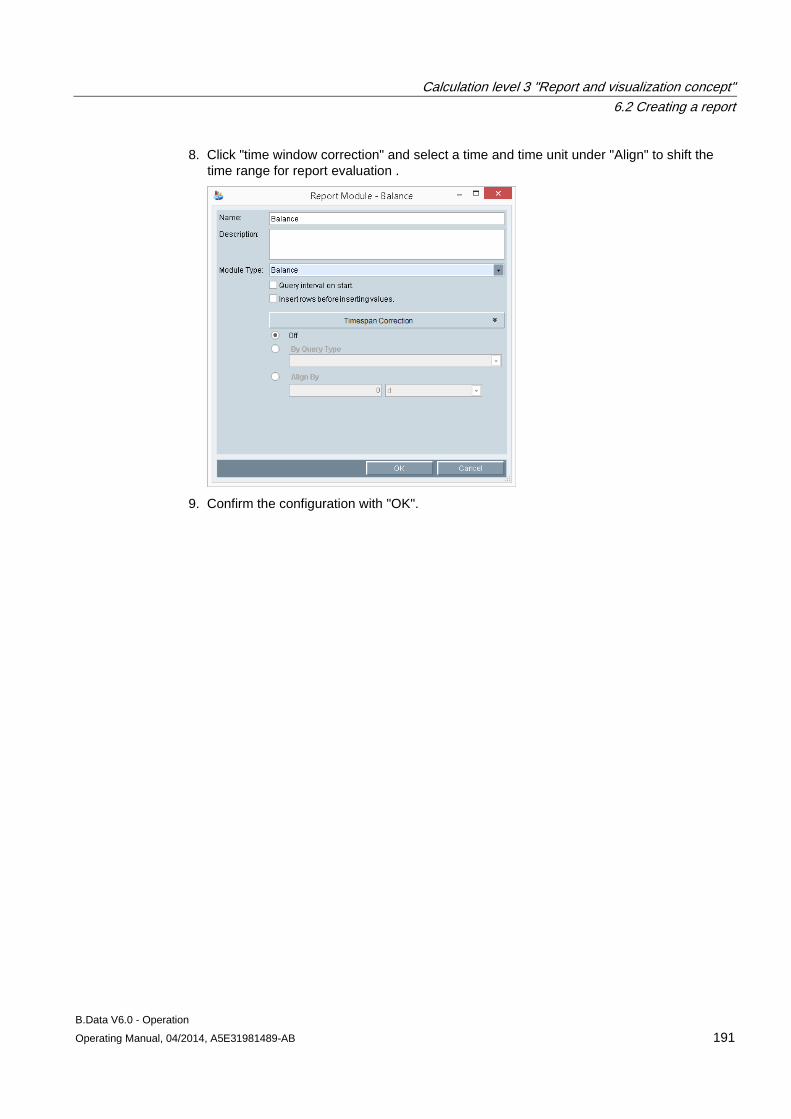
Calculation level 3 "Report and visualization concept" 6.2 Creating a report
B.Data V6.0 - Operation Operating Manual, 04/2014, A5E31981489-AB 191
8. Click "time window correction" and select a time and time unit under "Align" to shift the time range for report evaluation .
9. Confirm the configuration with "OK".
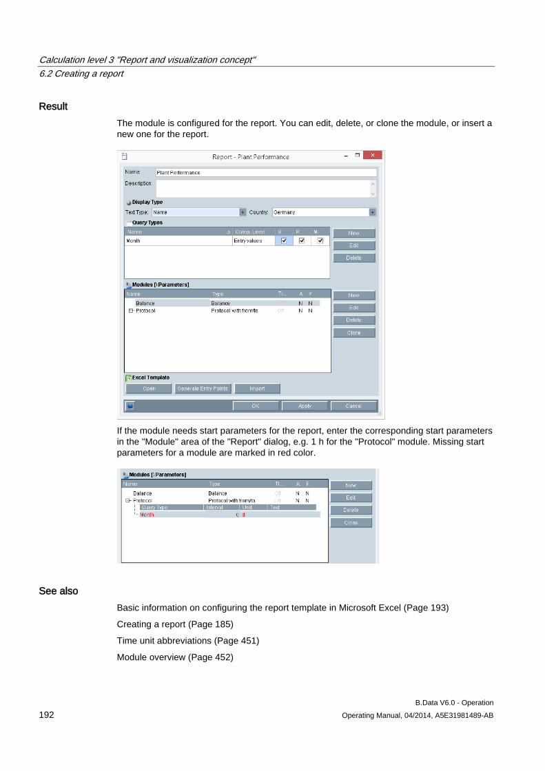
Calculation level 3 "Report and visualization concept" 6.2 Creating a report
B.Data V6.0 - Operation 192 Operating Manual, 04/2014, A5E31981489-AB
Result The module is configured for the report. You can edit, delete, or clone the module, or insert a new one for the report.
If the module needs start parameters for the report, enter the corresponding start parameters in the "Module" area of the "Report" dialog, e.g. 1 h for the "Protocol" module. Missing start parameters for a module are marked in red color.
See also Basic information on configuring the report template in Microsoft Excel (Page 193)
Creating a report (Page 185)
Time unit abbreviations (Page 451)
Module overview (Page 452)
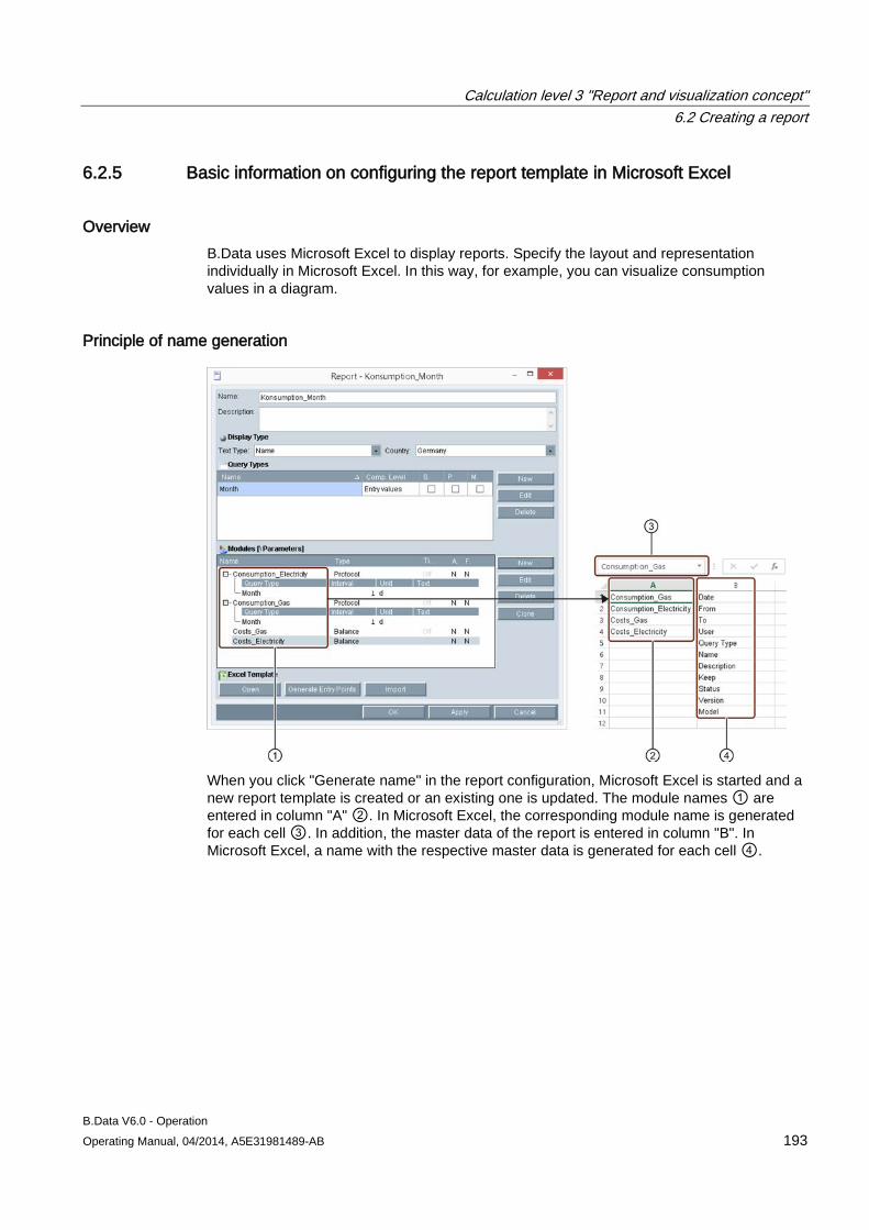
Calculation level 3 "Report and visualization concept" 6.2 Creating a report
B.Data V6.0 - Operation Operating Manual, 04/2014, A5E31981489-AB 193
6.2.5 Basic information on configuring the report template in Microsoft Excel
Overview B.Data uses Microsoft Excel to display reports. Specify the layout and representation individually in Microsoft Excel. In this way, for example, you can visualize consumption values in a diagram.
Principle of name generation
When you click "Generate name" in the report configuration, Microsoft Excel is started and a new report template is created or an existing one is updated. The module names ① are entered in column "A" ②. In Microsoft Excel, the corresponding module name is generated for each cell ③. In addition, the master data of the report is entered in column "B". In Microsoft Excel, a name with the respective master data is generated for each cell ④.
Calculation level 3 "Report and visualization concept" 6.2 Creating a report
B.Data V6.0 - Operation 194 Operating Manual, 04/2014, A5E31981489-AB
Entering values Values are entered as follows when you generate a report:
● Modules: The values are entered as of the cell below the corresponding name. For this reason, you need to shift each cell with a module name from column "A" to a position where contents will not be overwritten.
Example: The daily listing of consumption values of a month usually needs between 29 and 32 rows: One row for the header and, depending on the months, between 28 and 31 days.
You can use the naming manager in Microsoft Excel to view and edit the names and their cell ranges.
You may also distribute the cells to several sheets.
Note
If you distribute cells that contain module names to several sheets, activate the sheet that contains the original definition of names before closing.
● Master data: The values are entered as of the cell with the corresponding name.
Modifying or adding module names Whenever you change a module name in B.Data, you also need to adjust the corresponding name of the cell in Microsoft Excel. When adding a module to a report in B.Data, you must also assign this name to a cell in Microsoft Excel.
Use the naming manager for both actions.
See also Configuring a report template (Page 195)
Configuring a module for reports (Page 190)
Calculation level 3 "Report and visualization concept" 6.2 Creating a report
B.Data V6.0 - Operation Operating Manual, 04/2014, A5E31981489-AB 195
6.2.6 Configuring a report template
Overview You can configure an Excel template for a report. In this template, you specify how the measured values are displayed.
Requirement ● The report is configured.
● The query type is configured for the report.
● The module is configured for the report.
Procedure 1. Double-click the selected report in the structure tree of Plant Explorer.
The "Report" dialog opens.
2. To create a report template in Microsoft Excel, click "Generate name".
Microsoft Excel opens and the module name is entered in column "A".
3. Move the cell containing the module name to a position at which the module has sufficient space for its measured values.
4. Structure the template. You can find additional information in the Microsoft Excel online help.
5. If you want to run a macro in Microsoft Excel after you have generated the report, follow these steps:
– Open the macro editor in Microsoft Excel.
– Insert the Sub OnBDataLoadDone procedure in the spreadsheet that contains the original name definitions. Note that this entry is case-sensitive.
– Write the program code and close the macro editor.
– Set the security level to "low" in the Microsoft Excel security settings. Activate the "Trust access to Visual Basic projects" option under "Trusted Publishers".
Note
You cannot run a macro without having made the aforementioned security settings.
6. Save the template to an Microsoft Excel file.
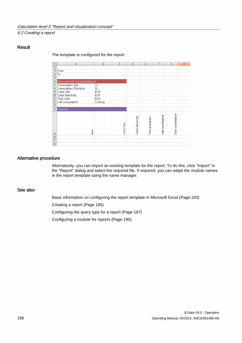
Calculation level 3 "Report and visualization concept" 6.2 Creating a report
B.Data V6.0 - Operation 196 Operating Manual, 04/2014, A5E31981489-AB
Result The template is configured for the report.
Alternative procedure Alternatively, you can import an existing template for the report. To do this, click "Import" in the "Report" dialog and select the required file. If required, you can adapt the module names in the report template using the name manager.
See also Basic information on configuring the report template in Microsoft Excel (Page 193)
Creating a report (Page 185)
Configuring the query type for a report (Page 187)
Configuring a module for reports (Page 190)
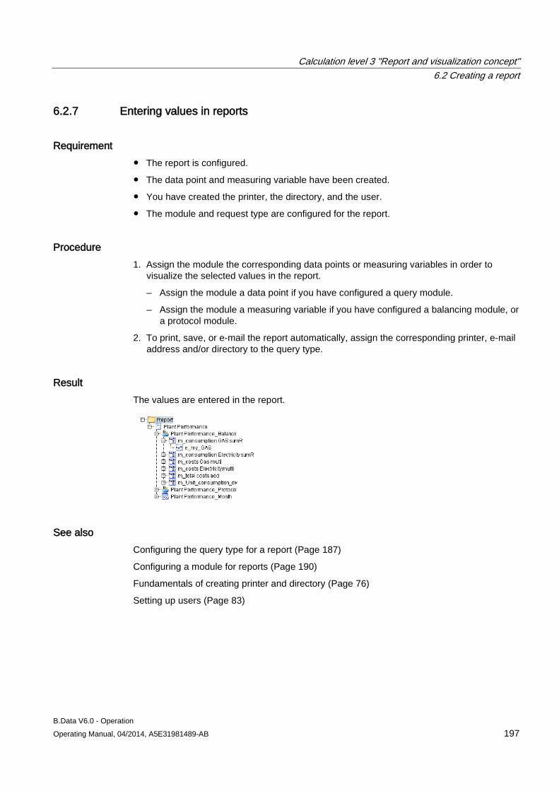
Calculation level 3 "Report and visualization concept" 6.2 Creating a report
B.Data V6.0 - Operation Operating Manual, 04/2014, A5E31981489-AB 197
6.2.7 Entering values in reports
Requirement ● The report is configured.
● The data point and measuring variable have been created.
● You have created the printer, the directory, and the user.
● The module and request type are configured for the report.
Procedure 1. Assign the module the corresponding data points or measuring variables in order to
visualize the selected values in the report.
– Assign the module a data point if you have configured a query module.
– Assign the module a measuring variable if you have configured a balancing module, or a protocol module.
2. To print, save, or e-mail the report automatically, assign the corresponding printer, e-mail address and/or directory to the query type.
Result The values are entered in the report.
See also Configuring the query type for a report (Page 187)
Configuring a module for reports (Page 190)
Fundamentals of creating printer and directory (Page 76)
Setting up users (Page 83)
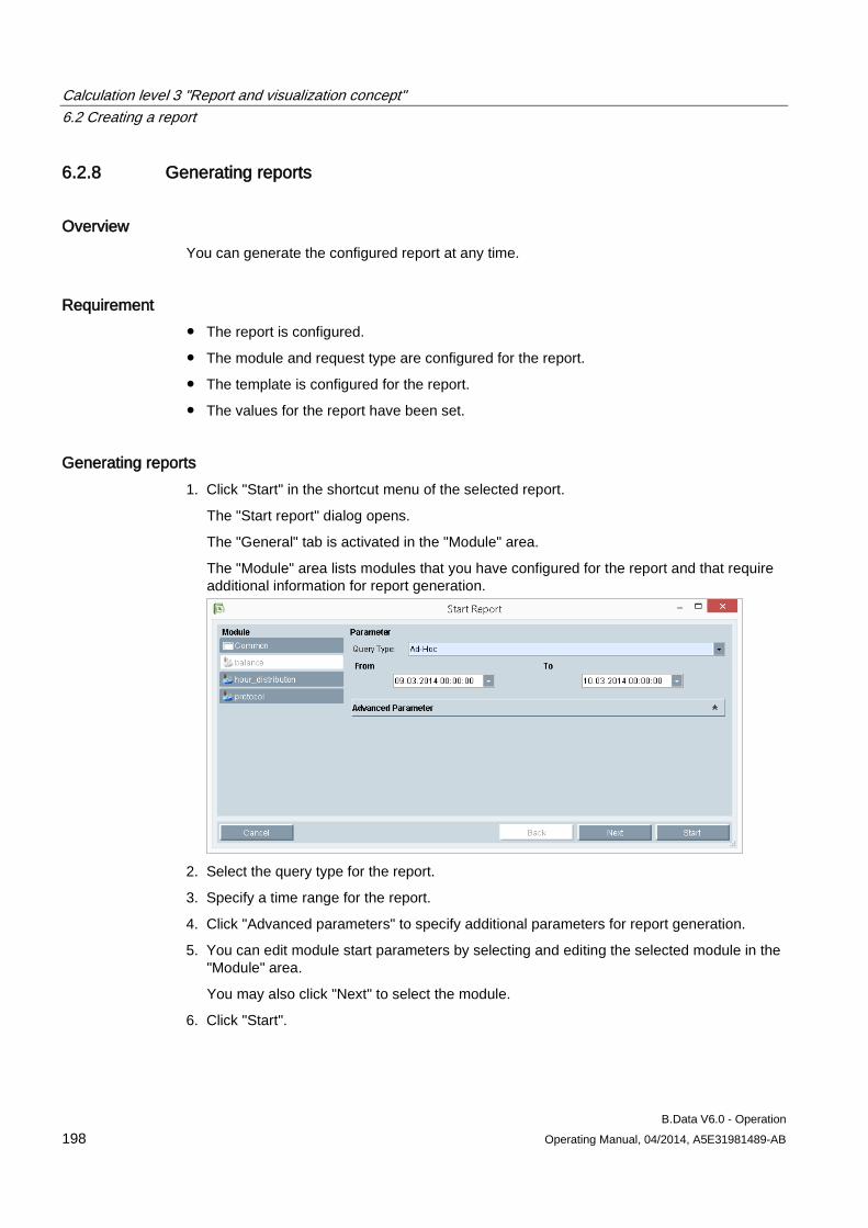
Calculation level 3 "Report and visualization concept" 6.2 Creating a report
B.Data V6.0 - Operation 198 Operating Manual, 04/2014, A5E31981489-AB
6.2.8 Generating reports
Overview You can generate the configured report at any time.
Requirement ● The report is configured.
● The module and request type are configured for the report.
● The template is configured for the report.
● The values for the report have been set.
Generating reports 1. Click "Start" in the shortcut menu of the selected report.
The "Start report" dialog opens.
The "General" tab is activated in the "Module" area.
The "Module" area lists modules that you have configured for the report and that require additional information for report generation.
2. Select the query type for the report.
3. Specify a time range for the report.
4. Click "Advanced parameters" to specify additional parameters for report generation.
5. You can edit module start parameters by selecting and editing the selected module in the "Module" area.
You may also click "Next" to select the module.
6. Click "Start".
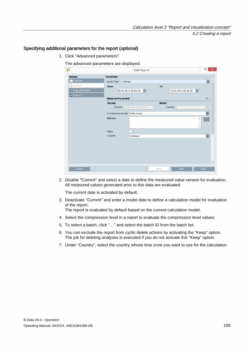
Calculation level 3 "Report and visualization concept" 6.2 Creating a report
B.Data V6.0 - Operation Operating Manual, 04/2014, A5E31981489-AB 199
Specifying additional parameters for the report (optional) 1. Click "Advanced parameters".
The advanced parameters are displayed.
2. Disable "Current" and select a date to define the measured value version for evaluation.
All measured values generated prior to this data are evaluated.
The current date is activated by default.
3. Deactivate "Current" and enter a model date to define a calculation model for evaluation of the report. The report is evaluated by default based on the current calculation model.
4. Select the compression level in a report to evaluate the compression level values.
5. To select a batch, click "…" and select the batch ID from the batch list.
6. You can exclude the report from cyclic delete actions by activating the "Keep" option. The job for deleting analyses is executed if you do not activate this "Keep" option.
7. Under "Country", select the country whose time zone you want to use for the calculation.
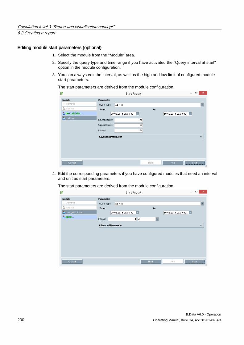
Calculation level 3 "Report and visualization concept" 6.2 Creating a report
B.Data V6.0 - Operation 200 Operating Manual, 04/2014, A5E31981489-AB
Editing module start parameters (optional) 1. Select the module from the "Module" area.
2. Specify the query type and time range if you have activated the "Query interval at start" option in the module configuration.
3. You can always edit the interval, as well as the high and low limit of configured module start parameters.
The start parameters are derived from the module configuration.
4. Edit the corresponding parameters if you have configured modules that need an interval
and unit as start parameters.
The start parameters are derived from the module configuration.
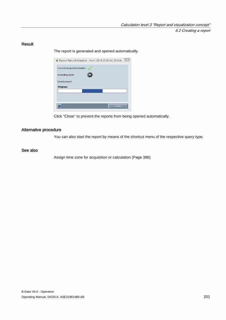
Calculation level 3 "Report and visualization concept" 6.2 Creating a report
B.Data V6.0 - Operation Operating Manual, 04/2014, A5E31981489-AB 201
Result The report is generated and opened automatically.
Click "Close" to prevent the reports from being opened automatically.
Alternative procedure You can also start the report by means of the shortcut menu of the respective query type.
See also Assign time zone for acquisition or calculation (Page 386)
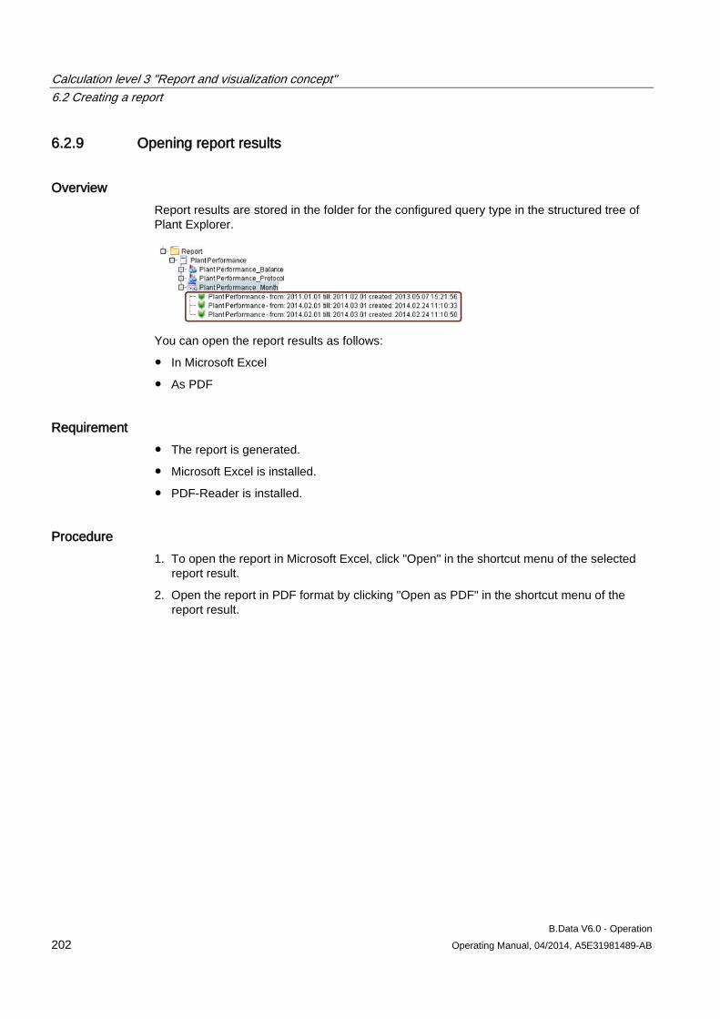
Calculation level 3 "Report and visualization concept" 6.2 Creating a report
B.Data V6.0 - Operation 202 Operating Manual, 04/2014, A5E31981489-AB
6.2.9 Opening report results
Overview Report results are stored in the folder for the configured query type in the structured tree of Plant Explorer.
You can open the report results as follows:
● In Microsoft Excel
● As PDF
Requirement ● The report is generated.
● Microsoft Excel is installed.
● PDF-Reader is installed.
Procedure 1. To open the report in Microsoft Excel, click "Open" in the shortcut menu of the selected
report result.
2. Open the report in PDF format by clicking "Open as PDF" in the shortcut menu of the report result.
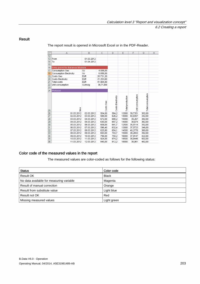
Calculation level 3 "Report and visualization concept" 6.2 Creating a report
B.Data V6.0 - Operation Operating Manual, 04/2014, A5E31981489-AB 203
Result The report result is opened in Microsoft Excel or in the PDF-Reader.
Color code of the measured values in the report The measured values are color-coded as follows for the following status:
Status Color code Result OK Black No data available for measuring variable Magenta Result of manual correction Orange Result from substitute value Light blue Result not OK Red Missing measured values Light green
Calculation level 3 "Report and visualization concept" 6.3 Creating trends
B.Data V6.0 - Operation 204 Operating Manual, 04/2014, A5E31981489-AB
6.3 Creating trends
6.3.1 Basics on trends
Overview The Trender is used to create graphic evaluations that can be used to visualize current and historical process values or operational parameters.
The Trender offers you extensive functions for simple extraction of useful information from the data pool.
This chapter provides you with an overview of the corresponding functionalities in B.Data Trender. It also provides detailed information on Trender configuration and startup.
The next chapters present the following contents related to the Trender.
1. Configuring trends
2. Starting trends
3. Data transfer to the Microsoft Office environment
4. Overview of the Trender functions
Requirement Successful installation of all software components.
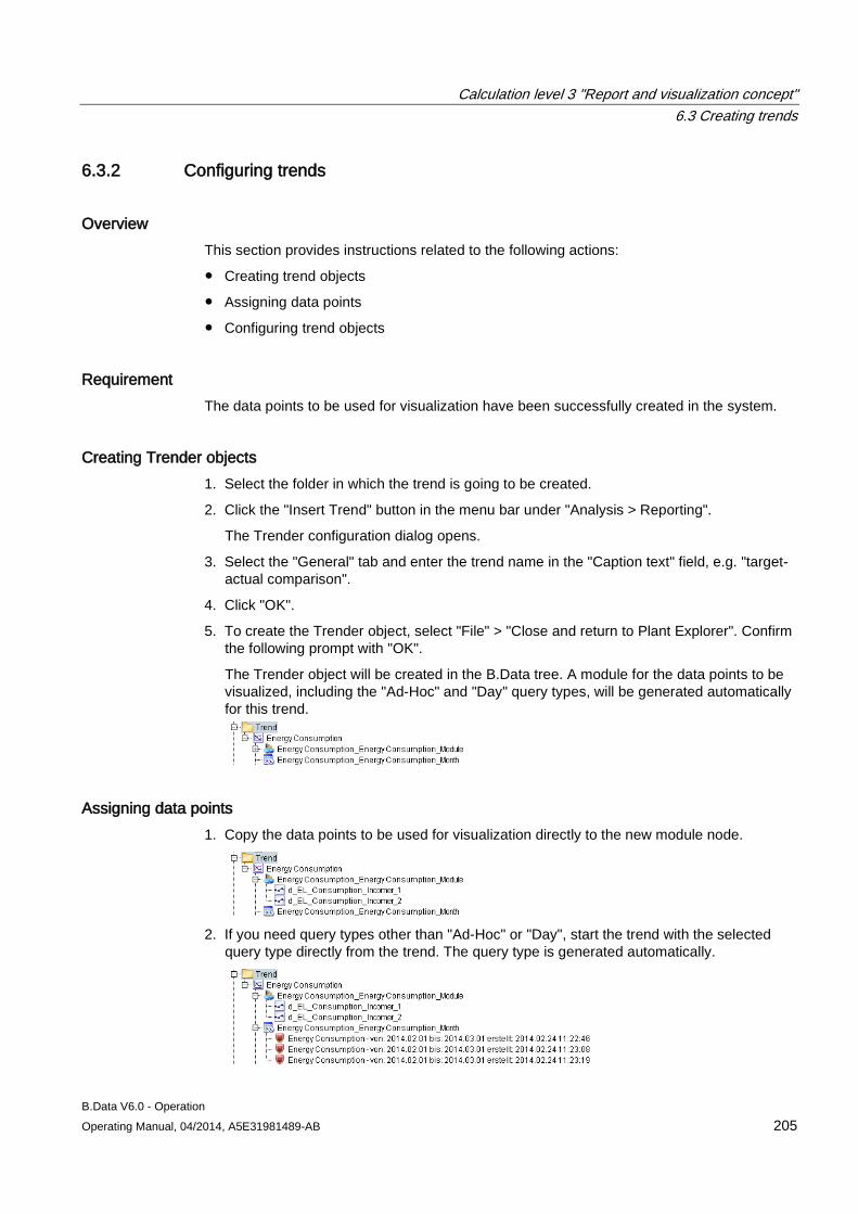
Calculation level 3 "Report and visualization concept" 6.3 Creating trends
B.Data V6.0 - Operation Operating Manual, 04/2014, A5E31981489-AB 205
6.3.2 Configuring trends
Overview This section provides instructions related to the following actions:
● Creating trend objects
● Assigning data points
● Configuring trend objects
Requirement The data points to be used for visualization have been successfully created in the system.
Creating Trender objects 1. Select the folder in which the trend is going to be created.
2. Click the "Insert Trend" button in the menu bar under "Analysis > Reporting".
The Trender configuration dialog opens.
3. Select the "General" tab and enter the trend name in the "Caption text" field, e.g. "target-actual comparison".
4. Click "OK".
5. To create the Trender object, select "File" > "Close and return to Plant Explorer". Confirm the following prompt with "OK".
The Trender object will be created in the B.Data tree. A module for the data points to be visualized, including the "Ad-Hoc" and "Day" query types, will be generated automatically for this trend.
Assigning data points 1. Copy the data points to be used for visualization directly to the new module node.
2. If you need query types other than "Ad-Hoc" or "Day", start the trend with the selected
query type directly from the trend. The query type is generated automatically.
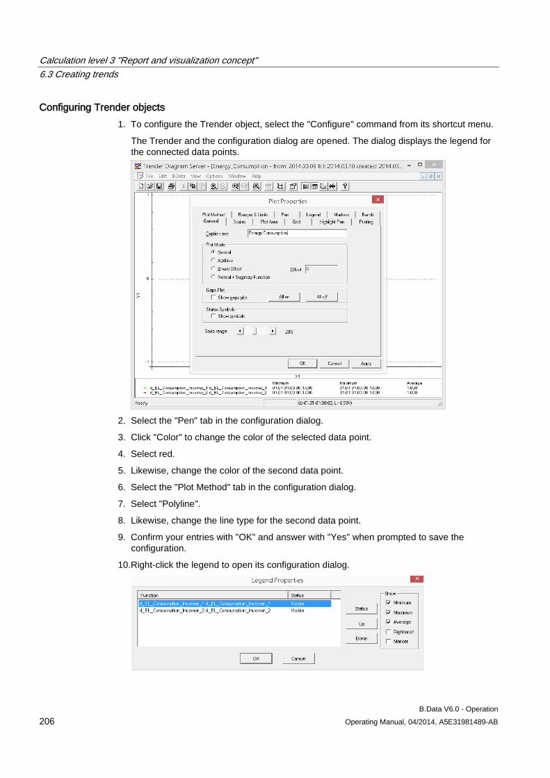
Calculation level 3 "Report and visualization concept" 6.3 Creating trends
B.Data V6.0 - Operation 206 Operating Manual, 04/2014, A5E31981489-AB
Configuring Trender objects 1. To configure the Trender object, select the "Configure" command from its shortcut menu.
The Trender and the configuration dialog are opened. The dialog displays the legend for the connected data points.
2. Select the "Pen" tab in the configuration dialog.
3. Click "Color" to change the color of the selected data point.
4. Select red.
5. Likewise, change the color of the second data point.
6. Select the "Plot Method" tab in the configuration dialog.
7. Select "Polyline".
8. Likewise, change the line type for the second data point.
9. Confirm your entries with "OK" and answer with "Yes" when prompted to save the configuration.
10.Right-click the legend to open its configuration dialog.
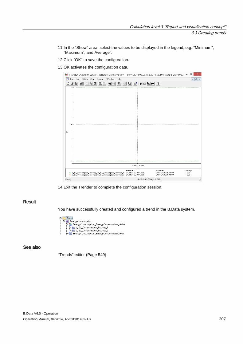
Calculation level 3 "Report and visualization concept" 6.3 Creating trends
B.Data V6.0 - Operation Operating Manual, 04/2014, A5E31981489-AB 207
11.In the "Show" area, select the values to be displayed in the legend, e.g. "Minimum", "Maximum", and Average".
12.Click "OK" to save the configuration.
13.OK activates the configuration data.
14.Exit the Trender to complete the configuration session.
Result You have successfully created and configured a trend in the B.Data system.
See also "Trends" editor (Page 549)
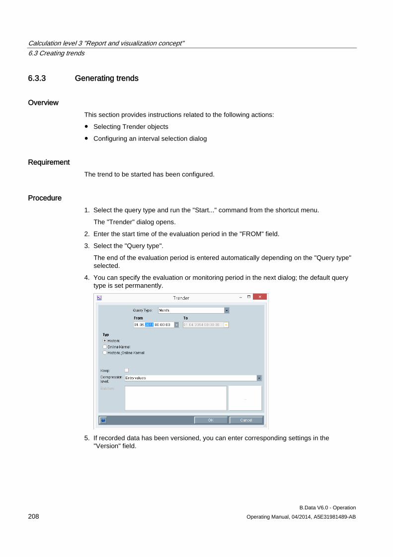
Calculation level 3 "Report and visualization concept" 6.3 Creating trends
B.Data V6.0 - Operation 208 Operating Manual, 04/2014, A5E31981489-AB
6.3.3 Generating trends
Overview This section provides instructions related to the following actions:
● Selecting Trender objects
● Configuring an interval selection dialog
Requirement The trend to be started has been configured.
Procedure 1. Select the query type and run the "Start..." command from the shortcut menu.
The "Trender" dialog opens.
2. Enter the start time of the evaluation period in the "FROM" field.
3. Select the "Query type".
The end of the evaluation period is entered automatically depending on the "Query type" selected.
4. You can specify the evaluation or monitoring period in the next dialog; the default query type is set permanently.
5. If recorded data has been versioned, you can enter corresponding settings in the
"Version" field.
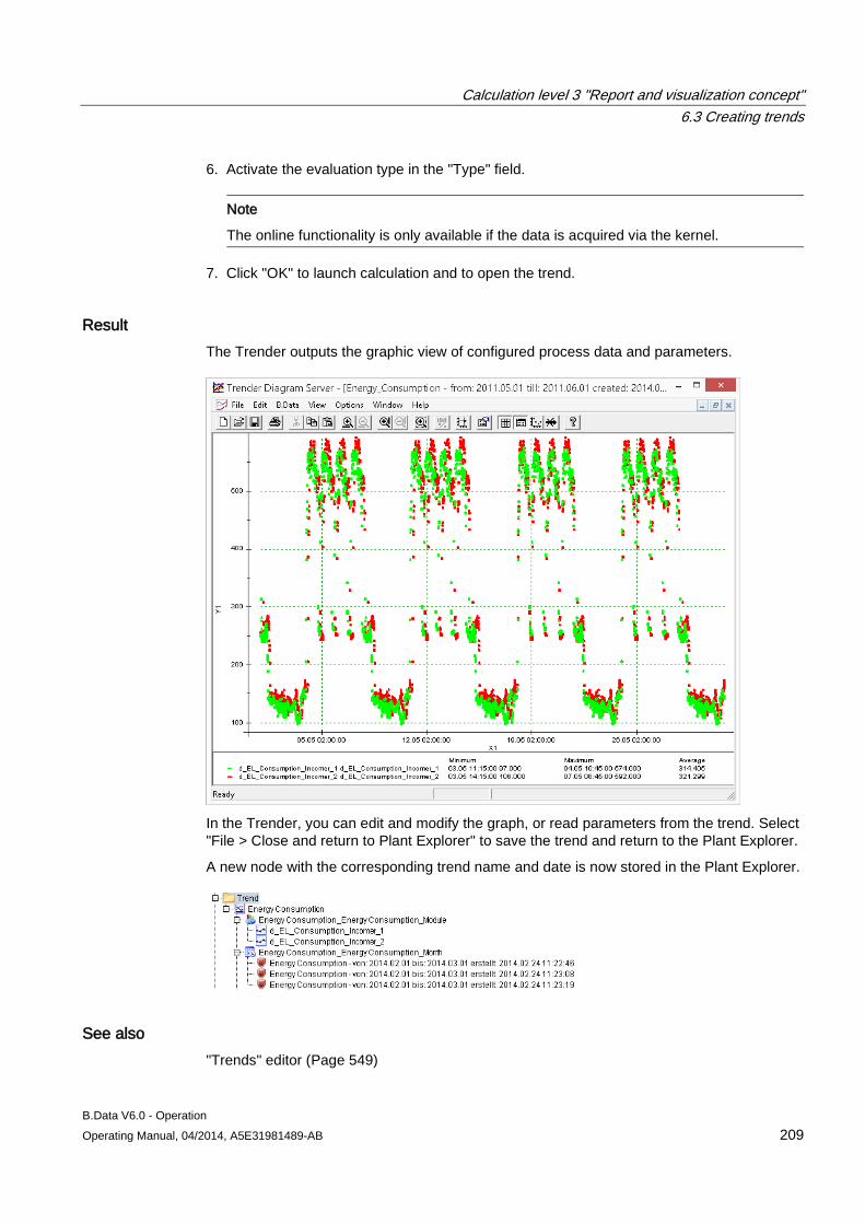
Calculation level 3 "Report and visualization concept" 6.3 Creating trends
B.Data V6.0 - Operation Operating Manual, 04/2014, A5E31981489-AB 209
6. Activate the evaluation type in the "Type" field.
Note
The online functionality is only available if the data is acquired via the kernel.
7. Click "OK" to launch calculation and to open the trend.
Result The Trender outputs the graphic view of configured process data and parameters.
In the Trender, you can edit and modify the graph, or read parameters from the trend. Select "File > Close and return to Plant Explorer" to save the trend and return to the Plant Explorer.
A new node with the corresponding trend name and date is now stored in the Plant Explorer.
See also "Trends" editor (Page 549)
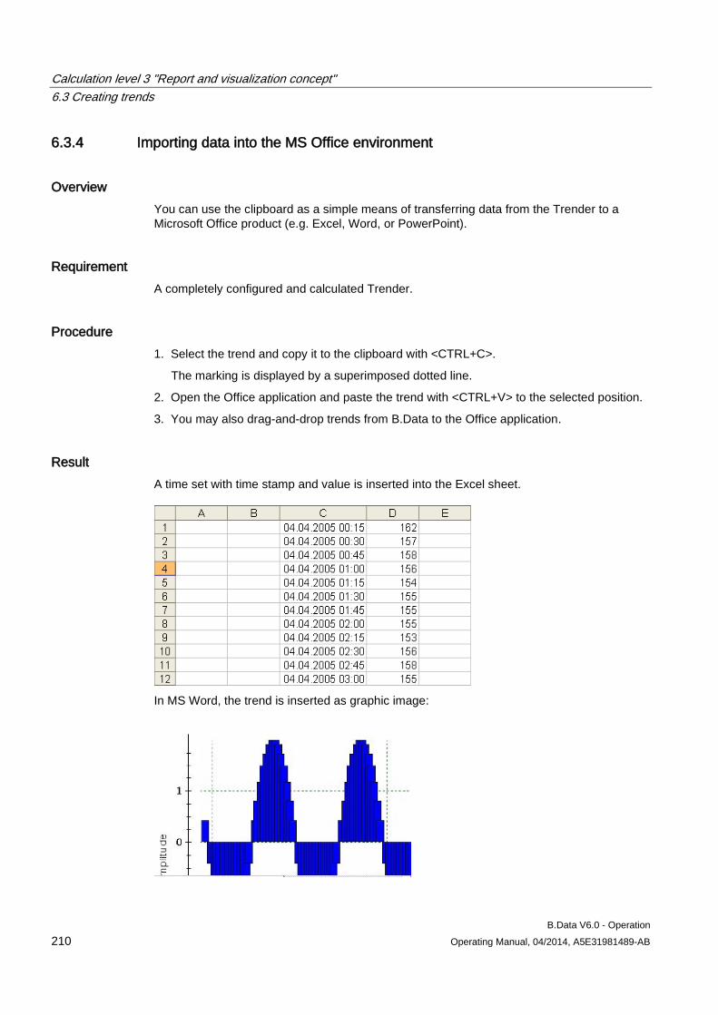
Calculation level 3 "Report and visualization concept" 6.3 Creating trends
B.Data V6.0 - Operation 210 Operating Manual, 04/2014, A5E31981489-AB
6.3.4 Importing data into the MS Office environment
Overview You can use the clipboard as a simple means of transferring data from the Trender to a Microsoft Office product (e.g. Excel, Word, or PowerPoint).
Requirement A completely configured and calculated Trender.
Procedure 1. Select the trend and copy it to the clipboard with <CTRL+C>.
The marking is displayed by a superimposed dotted line.
2. Open the Office application and paste the trend with <CTRL+V> to the selected position.
3. You may also drag-and-drop trends from B.Data to the Office application.
Result A time set with time stamp and value is inserted into the Excel sheet.
In MS Word, the trend is inserted as graphic image:

Calculation level 3 "Report and visualization concept" 6.3 Creating trends
B.Data V6.0 - Operation Operating Manual, 04/2014, A5E31981489-AB 211
Calculation level 3 "Report and visualization concept" 6.4 Creating visualization
B.Data V6.0 - Operation 212 Operating Manual, 04/2014, A5E31981489-AB
6.4 Creating visualization
6.4.1 Basics on visualizations
Overview B.Data Visualization enables the online presentation of process values in diagrams.
This chapter provides you with an overview of the corresponding functionalities in B.Data Visualization. It also provides detailed information on the configuration and start of visualization.
The next chapters present the following contents related to visualization.
● Configuring visualization
● Starting visualization
Requirement Successful installation of all software components.
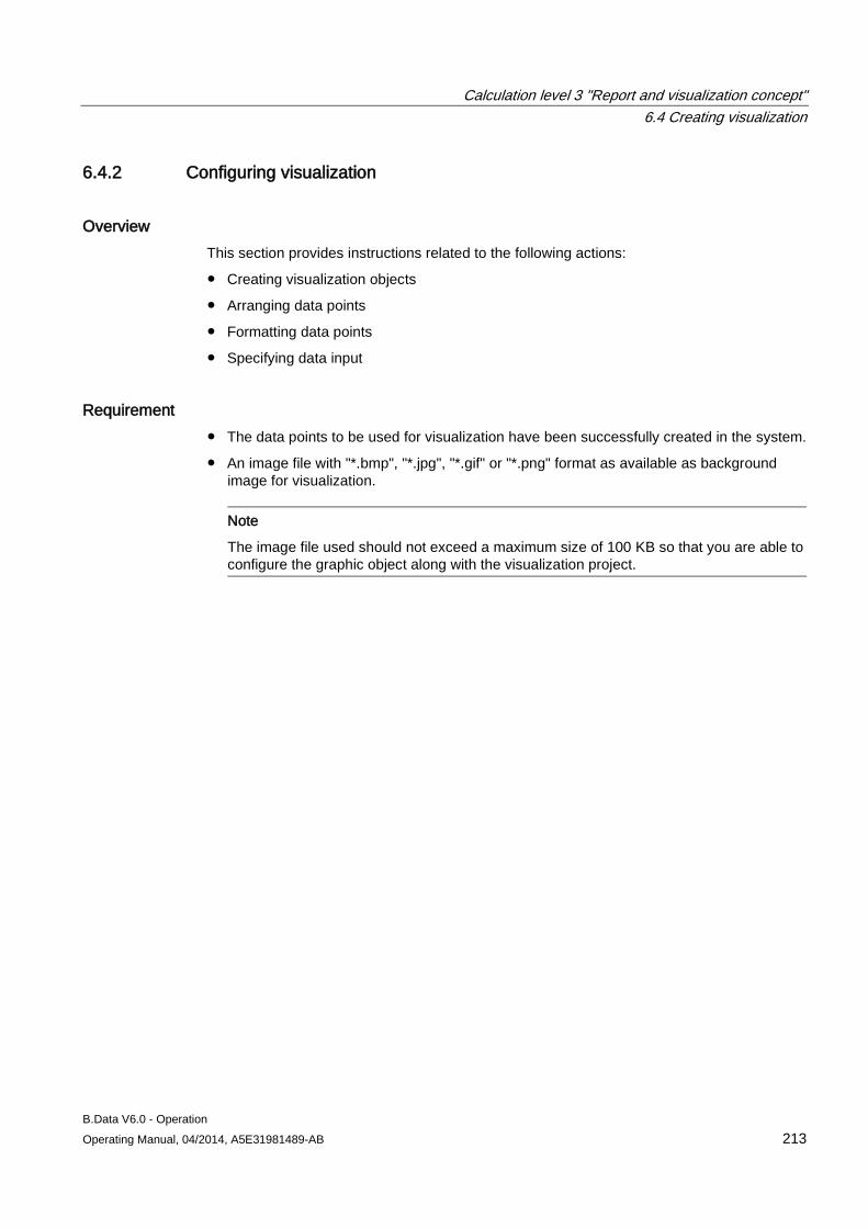
Calculation level 3 "Report and visualization concept" 6.4 Creating visualization
B.Data V6.0 - Operation Operating Manual, 04/2014, A5E31981489-AB 213
6.4.2 Configuring visualization
Overview This section provides instructions related to the following actions:
● Creating visualization objects
● Arranging data points
● Formatting data points
● Specifying data input
Requirement ● The data points to be used for visualization have been successfully created in the system.
● An image file with "*.bmp", "*.jpg", "*.gif" or "*.png" format as available as background image for visualization.
Note
The image file used should not exceed a maximum size of 100 KB so that you are able to configure the graphic object along with the visualization project.
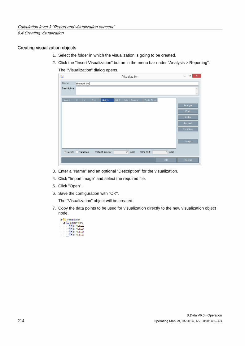
Calculation level 3 "Report and visualization concept" 6.4 Creating visualization
B.Data V6.0 - Operation 214 Operating Manual, 04/2014, A5E31981489-AB
Creating visualization objects 1. Select the folder in which the visualization is going to be created.
2. Click the "Insert Visualization" button in the menu bar under "Analysis > Reporting".
The "Visualization" dialog opens.
3. Enter a "Name" and an optional "Description" for the visualization.
4. Click "Import image" and select the required file.
5. Click "Open".
6. Save the configuration with "OK".
The "Visualization" object will be created.
7. Copy the data points to be used for visualization directly to the new visualization object node.
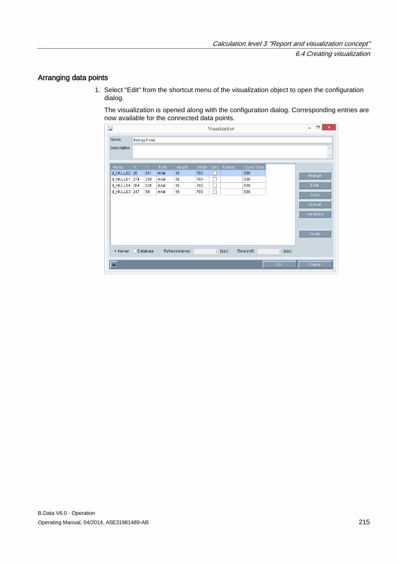
Calculation level 3 "Report and visualization concept" 6.4 Creating visualization
B.Data V6.0 - Operation Operating Manual, 04/2014, A5E31981489-AB 215
Arranging data points 1. Select "Edit" from the shortcut menu of the visualization object to open the configuration
dialog.
The visualization is opened along with the configuration dialog. Corresponding entries are now available for the connected data points.
Calculation level 3 "Report and visualization concept" 6.4 Creating visualization
B.Data V6.0 - Operation 216 Operating Manual, 04/2014, A5E31981489-AB
2. Select the data point to position in the visualization and click "Arrange".
The visualization opens.
3. Double-click the insert position for the data point.
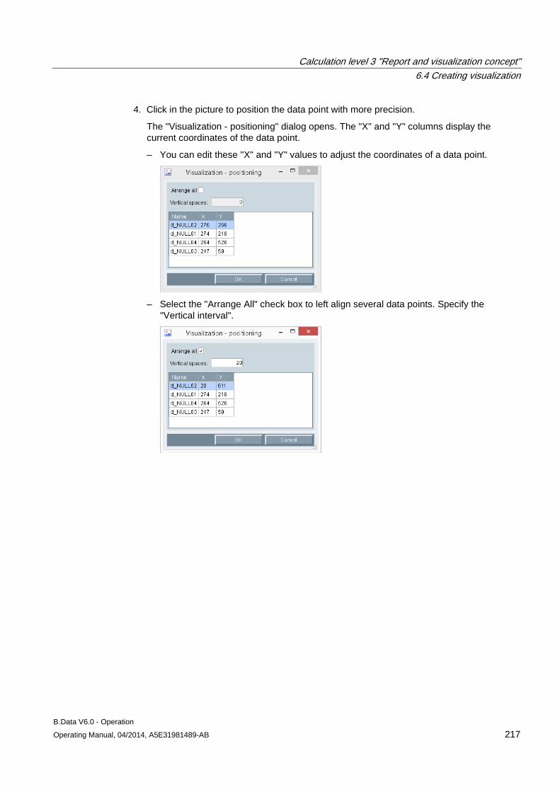
Calculation level 3 "Report and visualization concept" 6.4 Creating visualization
B.Data V6.0 - Operation Operating Manual, 04/2014, A5E31981489-AB 217
4. Click in the picture to position the data point with more precision.
The "Visualization - positioning" dialog opens. The "X" and "Y" columns display the current coordinates of the data point.
– You can edit these "X" and "Y" values to adjust the coordinates of a data point.
– Select the "Arrange All" check box to left align several data points. Specify the
"Vertical interval".
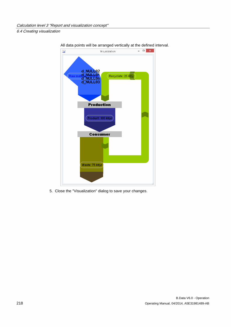
Calculation level 3 "Report and visualization concept" 6.4 Creating visualization
B.Data V6.0 - Operation 218 Operating Manual, 04/2014, A5E31981489-AB
All data points will be arranged vertically at the defined interval.
5. Close the "Visualization" dialog to save your changes.
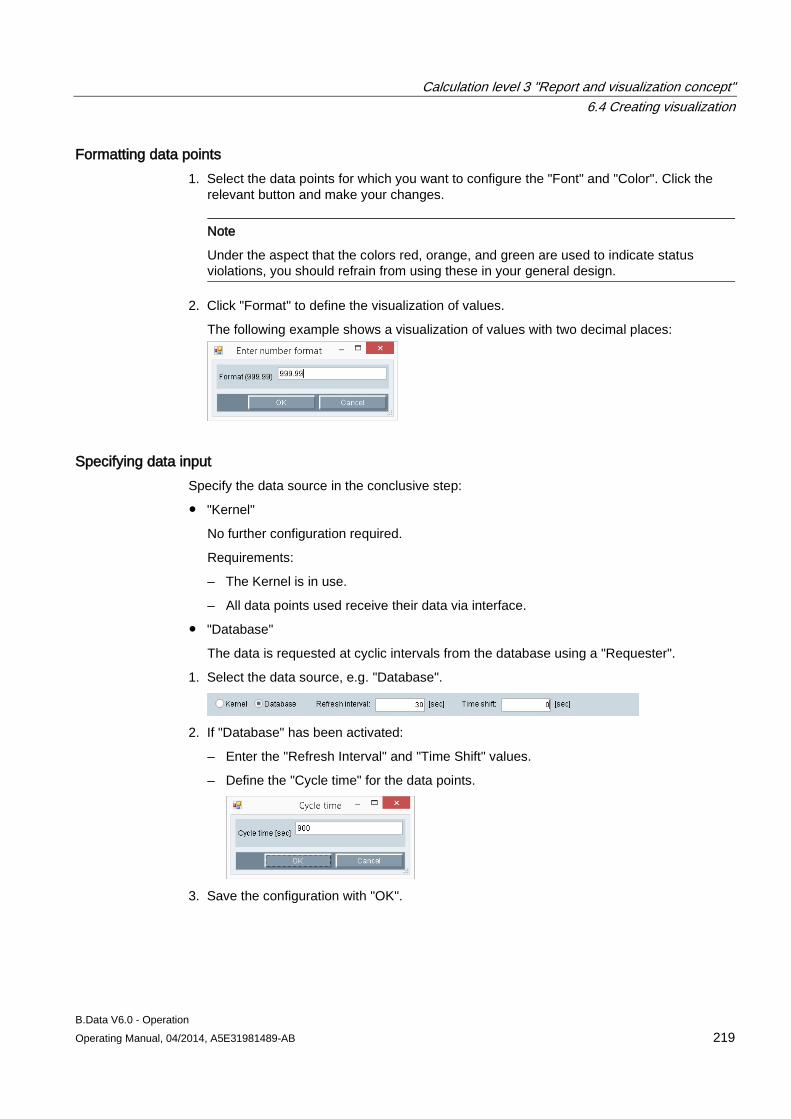
Calculation level 3 "Report and visualization concept" 6.4 Creating visualization
B.Data V6.0 - Operation Operating Manual, 04/2014, A5E31981489-AB 219
Formatting data points 1. Select the data points for which you want to configure the "Font" and "Color". Click the
relevant button and make your changes.
Note
Under the aspect that the colors red, orange, and green are used to indicate status violations, you should refrain from using these in your general design.
2. Click "Format" to define the visualization of values.
The following example shows a visualization of values with two decimal places:
Specifying data input Specify the data source in the conclusive step:
● "Kernel"
No further configuration required.
Requirements:
– The Kernel is in use.
– All data points used receive their data via interface.
● "Database"
The data is requested at cyclic intervals from the database using a "Requester".
1. Select the data source, e.g. "Database".
2. If "Database" has been activated:
– Enter the "Refresh Interval" and "Time Shift" values.
– Define the "Cycle time" for the data points.
3. Save the configuration with "OK".
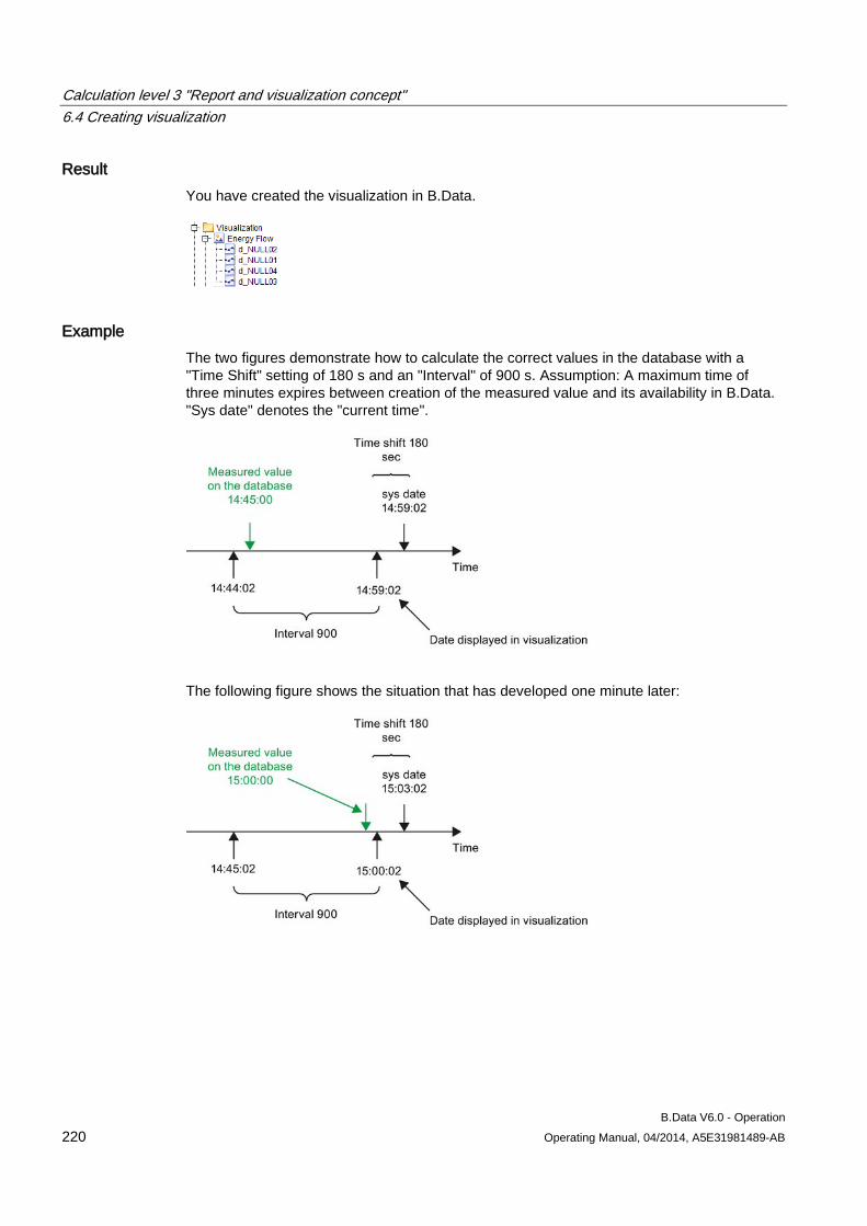
Calculation level 3 "Report and visualization concept" 6.4 Creating visualization
B.Data V6.0 - Operation 220 Operating Manual, 04/2014, A5E31981489-AB
Result You have created the visualization in B.Data.
Example The two figures demonstrate how to calculate the correct values in the database with a "Time Shift" setting of 180 s and an "Interval" of 900 s. Assumption: A maximum time of three minutes expires between creation of the measured value and its availability in B.Data. "Sys date" denotes the "current time".
The following figure shows the situation that has developed one minute later:
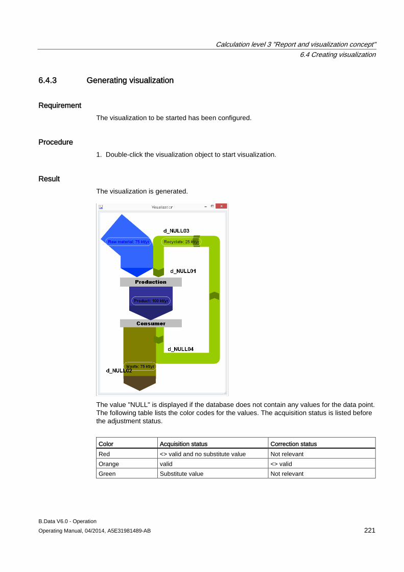
Calculation level 3 "Report and visualization concept" 6.4 Creating visualization
B.Data V6.0 - Operation Operating Manual, 04/2014, A5E31981489-AB 221
6.4.3 Generating visualization
Requirement The visualization to be started has been configured.
Procedure 1. Double-click the visualization object to start visualization.
Result The visualization is generated.
The value "NULL" is displayed if the database does not contain any values for the data point. The following table lists the color codes for the values. The acquisition status is listed before the adjustment status.
Color Acquisition status Correction status Red <> valid and no substitute value Not relevant Orange valid <> valid Green Substitute value Not relevant
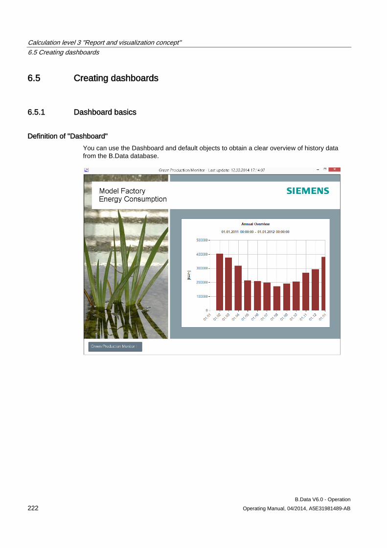
Calculation level 3 "Report and visualization concept" 6.5 Creating dashboards
B.Data V6.0 - Operation 222 Operating Manual, 04/2014, A5E31981489-AB
6.5 Creating dashboards
6.5.1 Dashboard basics
Definition of "Dashboard" You can use the Dashboard and default objects to obtain a clear overview of history data from the B.Data database.
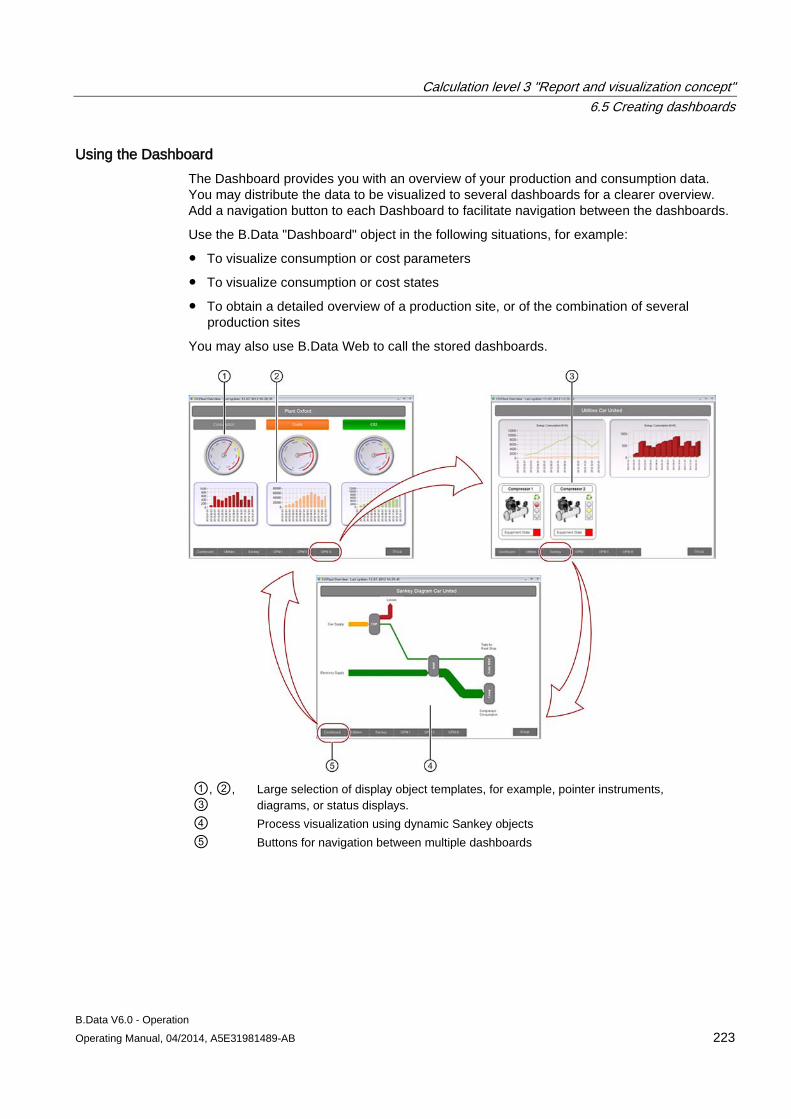
Calculation level 3 "Report and visualization concept" 6.5 Creating dashboards
B.Data V6.0 - Operation Operating Manual, 04/2014, A5E31981489-AB 223
Using the Dashboard The Dashboard provides you with an overview of your production and consumption data. You may distribute the data to be visualized to several dashboards for a clearer overview. Add a navigation button to each Dashboard to facilitate navigation between the dashboards.
Use the B.Data "Dashboard" object in the following situations, for example:
● To visualize consumption or cost parameters
● To visualize consumption or cost states
● To obtain a detailed overview of a production site, or of the combination of several production sites
You may also use B.Data Web to call the stored dashboards.
①, ②, ③
Large selection of display object templates, for example, pointer instruments, diagrams, or status displays.
④ Process visualization using dynamic Sankey objects ⑤ Buttons for navigation between multiple dashboards
Calculation level 3 "Report and visualization concept" 6.5 Creating dashboards
B.Data V6.0 - Operation 224 Operating Manual, 04/2014, A5E31981489-AB
Dashboard notes Observe the following information:
● Value input
A Dashboard visualizes only values of the following data points:
– "Generic" data point type
– "Derived" data point type
– "Datapoint" data point type
You can visualize values that are calculated based on measurement functions by assigning each measurement function a derived data point.
● Time range
Make sure that you set the time range to be visualized to a sufficient length. Moreover, the data points must contain measurement data for the specified time range.
Rules for creating dashboards Observe the following rules before you start to create a Dashboard:
● Plan the data quantity to be visualized and the corresponding distribution of this data.
● You can distribute large data quantities to several dashboards to improve the overview and performance.
Use a navigation button to switch between the dashboards; create this button in each Dashboard by means of dashboard object "Panel Switch".
● Recommendation: When configuring the refresh cycle for Dashboard, enter the time in seconds e.g. 900 seconds for a refresh cycle of 15 minutes.
You can use the B.Data object "Trend" to visualize the current values.
Configuring dashboards Create a graphic overview as follow:
1. Create one or several dashboards in the project tree of Plant Explorer.
2. Copy the data points to be visualized as nested entry to the Dashboard you created.
3. Create the Dashboard layout by compiling the selected dashboard objects in the "Dashboard" editor.
4. Assign the selected data points to the dashboard objects used and customize the layout of the dashboard objects.
5. If you have created several dashboards for a graphic overview, add one or several buttons to the Dashboard using dashboard object "Panel Switch" and assign the respective Dashboard to each button.
Use these buttons to switch between the dashboards.
6. Open the selected Dashboard in full-screen mode.
The Dashboard displays the values of the data points used for a defined period.
Calculation level 3 "Report and visualization concept" 6.5 Creating dashboards
B.Data V6.0 - Operation Operating Manual, 04/2014, A5E31981489-AB 225
See also Create dashboard (Page 229)
Dashboard objects (Page 619)
Configuring the time range (Page 620)
Example of configuring a dashboard (Page 241)
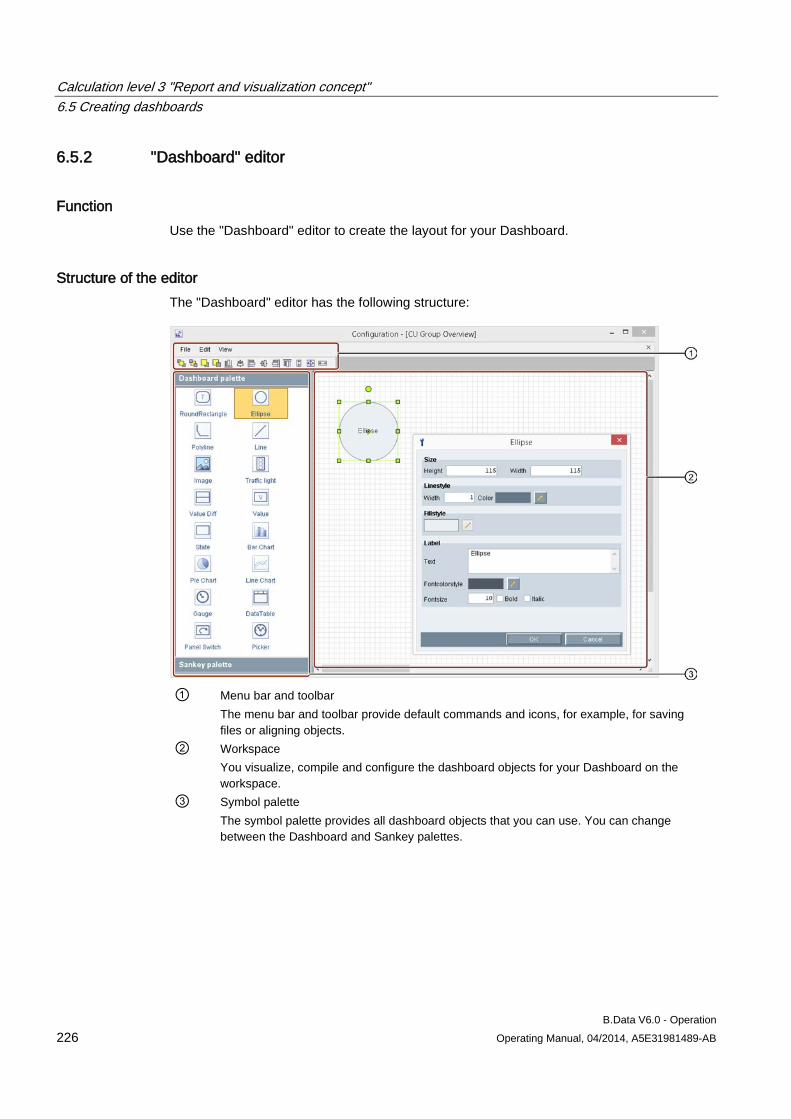
Calculation level 3 "Report and visualization concept" 6.5 Creating dashboards
B.Data V6.0 - Operation 226 Operating Manual, 04/2014, A5E31981489-AB
6.5.2 "Dashboard" editor
Function Use the "Dashboard" editor to create the layout for your Dashboard.
Structure of the editor The "Dashboard" editor has the following structure:
① Menu bar and toolbar
The menu bar and toolbar provide default commands and icons, for example, for saving files or aligning objects.
② Workspace You visualize, compile and configure the dashboard objects for your Dashboard on the workspace.
③ Symbol palette The symbol palette provides all dashboard objects that you can use. You can change between the Dashboard and Sankey palettes.
Calculation level 3 "Report and visualization concept" 6.5 Creating dashboards
B.Data V6.0 - Operation Operating Manual, 04/2014, A5E31981489-AB 227
Menu bar of the editor The menu bar of the "Dashboard" editor has the following structure:
● File
The "File" menu is used to save, close or export/import the current Dashboard.
Use the "Export"/"Import" function to make the Dashboard available to other B.Data users.
Note
Exporting a Dashboard
The exported Dashboard can only be opened on a B.Data system.
● Edit
The "Edit" menu commands are used to perform standard document editor actions such as copying or deleting objects.
● View
The "View" menu lets you hide or unhide the pallets.
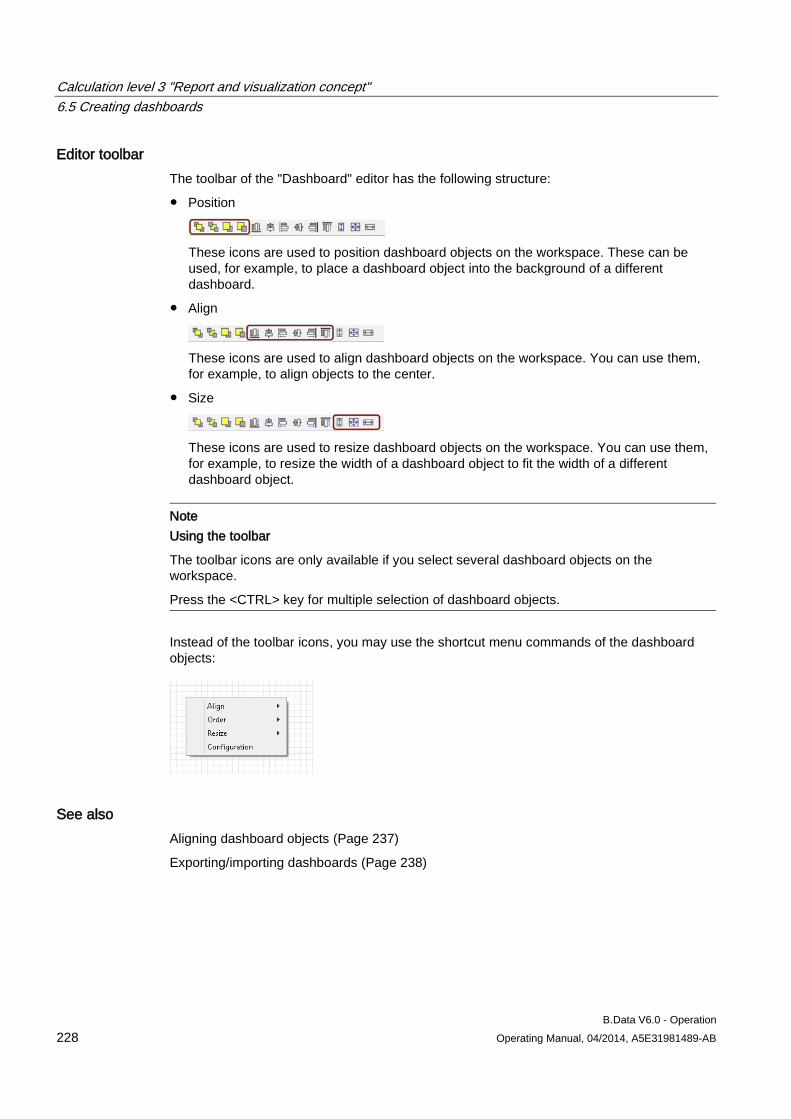
Calculation level 3 "Report and visualization concept" 6.5 Creating dashboards
B.Data V6.0 - Operation 228 Operating Manual, 04/2014, A5E31981489-AB
Editor toolbar The toolbar of the "Dashboard" editor has the following structure:
● Position
These icons are used to position dashboard objects on the workspace. These can be used, for example, to place a dashboard object into the background of a different dashboard.
● Align
These icons are used to align dashboard objects on the workspace. You can use them, for example, to align objects to the center.
● Size
These icons are used to resize dashboard objects on the workspace. You can use them, for example, to resize the width of a dashboard object to fit the width of a different dashboard object.
Note Using the toolbar
The toolbar icons are only available if you select several dashboard objects on the workspace.
Press the <CTRL> key for multiple selection of dashboard objects.
Instead of the toolbar icons, you may use the shortcut menu commands of the dashboard objects:
See also Aligning dashboard objects (Page 237)
Exporting/importing dashboards (Page 238)
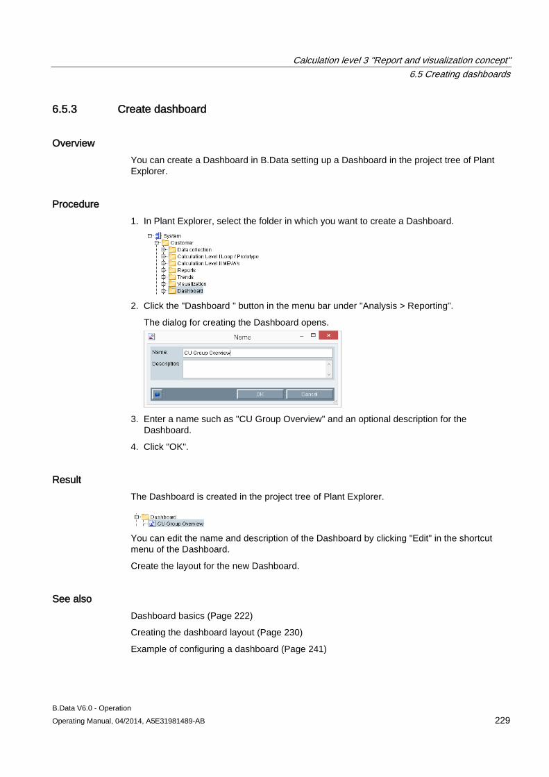
Calculation level 3 "Report and visualization concept" 6.5 Creating dashboards
B.Data V6.0 - Operation Operating Manual, 04/2014, A5E31981489-AB 229
6.5.3 Create dashboard
Overview You can create a Dashboard in B.Data setting up a Dashboard in the project tree of Plant Explorer.
Procedure 1. In Plant Explorer, select the folder in which you want to create a Dashboard.
2. Click the "Dashboard " button in the menu bar under "Analysis > Reporting".
The dialog for creating the Dashboard opens.
3. Enter a name such as "CU Group Overview" and an optional description for the
Dashboard.
4. Click "OK".
Result The Dashboard is created in the project tree of Plant Explorer.
You can edit the name and description of the Dashboard by clicking "Edit" in the shortcut menu of the Dashboard.
Create the layout for the new Dashboard.
See also Dashboard basics (Page 222)
Creating the dashboard layout (Page 230)
Example of configuring a dashboard (Page 241)
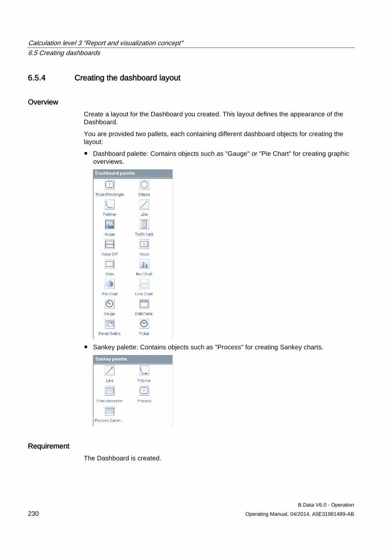
Calculation level 3 "Report and visualization concept" 6.5 Creating dashboards
B.Data V6.0 - Operation 230 Operating Manual, 04/2014, A5E31981489-AB
6.5.4 Creating the dashboard layout
Overview Create a layout for the Dashboard you created. This layout defines the appearance of the Dashboard.
You are provided two pallets, each containing different dashboard objects for creating the layout:
● Dashboard palette: Contains objects such as "Gauge" or "Pie Chart" for creating graphic overviews.
● Sankey palette: Contains objects such as "Process" for creating Sankey charts.
Requirement The Dashboard is created.
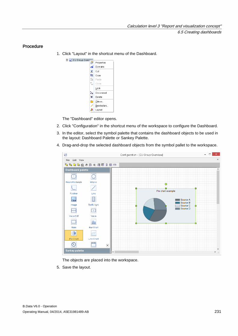
Calculation level 3 "Report and visualization concept" 6.5 Creating dashboards
B.Data V6.0 - Operation Operating Manual, 04/2014, A5E31981489-AB 231
Procedure 1. Click "Layout" in the shortcut menu of the Dashboard.
The "Dashboard" editor opens.
2. Click "Configuration" in the shortcut menu of the workspace to configure the Dashboard.
3. In the editor, select the symbol palette that contains the dashboard objects to be used in the layout: Dashboard Palette or Sankey Palette.
4. Drag-and-drop the selected dashboard objects from the symbol pallet to the workspace.
The objects are placed into the workspace.
5. Save the layout.
Calculation level 3 "Report and visualization concept" 6.5 Creating dashboards
B.Data V6.0 - Operation 232 Operating Manual, 04/2014, A5E31981489-AB
Result You have created the Dashboard layout.
Configure the dashboard objects used in order to customize them, or to link them with the selected data points.
See also Create dashboard (Page 229)
Dashboard objects (Page 619)
"Dashboard" editor (Page 226)
Configuring dashboard objects (Page 233)
Aligning dashboard objects (Page 237)
Configuring the dashboard (Page 619)
Example of configuring a dashboard (Page 241)
Calculation level 3 "Report and visualization concept" 6.5 Creating dashboards
B.Data V6.0 - Operation Operating Manual, 04/2014, A5E31981489-AB 233
6.5.5 Configuring dashboard objects
Overview After having created the Dashboard layout, configure the dashboard objects to be used as follows:
● Link the dashboard objects with the data points containing the values to be visualized on the Dashboard.
● Customize the appearance of the dashboard objects, for example, the background color or text layout.
Note Configuration of the dashboard objects
The following figures show the configuration of the "Pie Chart" dashboard object.
For information about the configuration of other dashboard objects, refer to chapter "Dashboard objects".
Requirement ● You have created the Dashboard layout and opened it in the "Dashboard" editor.
● The selected data points are set up in the project tree of Plant Explorer.
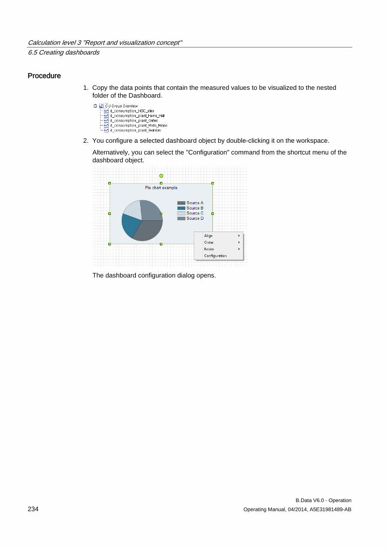
Calculation level 3 "Report and visualization concept" 6.5 Creating dashboards
B.Data V6.0 - Operation 234 Operating Manual, 04/2014, A5E31981489-AB
Procedure 1. Copy the data points that contain the measured values to be visualized to the nested
folder of the Dashboard.
2. You configure a selected dashboard object by double-clicking it on the workspace.
Alternatively, you can select the "Configuration" command from the shortcut menu of the dashboard object.
The dashboard configuration dialog opens.
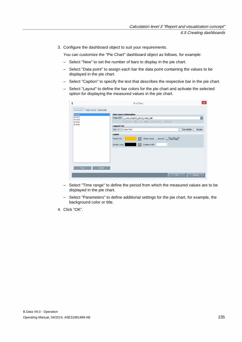
Calculation level 3 "Report and visualization concept" 6.5 Creating dashboards
B.Data V6.0 - Operation Operating Manual, 04/2014, A5E31981489-AB 235
3. Configure the dashboard object to suit your requirements.
You can customize the "Pie Chart" dashboard object as follows, for example:
– Select "New" to set the number of bars to display in the pie chart.
– Select "Data point" to assign each bar the data point containing the values to be displayed in the pie chart.
– Select "Caption" to specify the text that describes the respective bar in the pie chart.
– Select "Layout" to define the bar colors for the pie chart and activate the selected option for displaying the measured values in the pie chart.
– Select "Time range" to define the period from which the measured values are to be
displayed in the pie chart.
– Select "Parameters" to define additional settings for the pie chart, for example, the background color or title.
4. Click "OK".
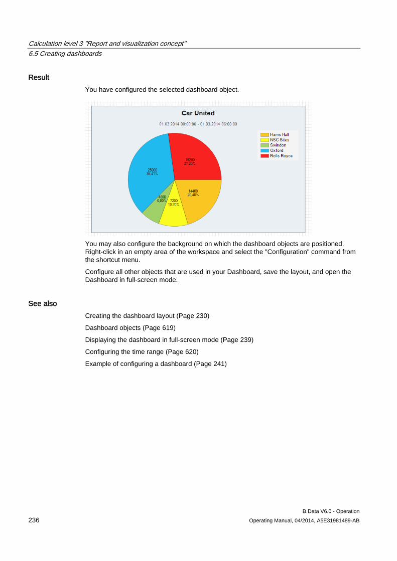
Calculation level 3 "Report and visualization concept" 6.5 Creating dashboards
B.Data V6.0 - Operation 236 Operating Manual, 04/2014, A5E31981489-AB
Result You have configured the selected dashboard object.
You may also configure the background on which the dashboard objects are positioned. Right-click in an empty area of the workspace and select the "Configuration" command from the shortcut menu.
Configure all other objects that are used in your Dashboard, save the layout, and open the Dashboard in full-screen mode.
See also Creating the dashboard layout (Page 230)
Dashboard objects (Page 619)
Displaying the dashboard in full-screen mode (Page 239)
Configuring the time range (Page 620)
Example of configuring a dashboard (Page 241)
Calculation level 3 "Report and visualization concept" 6.5 Creating dashboards
B.Data V6.0 - Operation Operating Manual, 04/2014, A5E31981489-AB 237
6.5.6 Aligning dashboard objects
Overview The "Dashboard" editor lets you set up different alignments for multiple dashboard objects. You need a reference object to which you can align other objects. Start by selecting an object in the "Dashboard" editor and define it as reference object.
Requirement ● The "Dashboard" editor is open.
● You have created the Dashboard layout.
Procedure 1. On the workspace, select the reference object to which you are going to align other
dashboard objects.
2. Select the dashboard objects by means of multiple selection.
3. Select the command from the toolbar, or from the shortcut menu of the dashboard objects.
Result The selected objects are aligned.
Calculation level 3 "Report and visualization concept" 6.5 Creating dashboards
B.Data V6.0 - Operation 238 Operating Manual, 04/2014, A5E31981489-AB
6.5.7 Exporting/importing dashboards
Overview You can make a Dashboard available to external B.Data users by exporting the Dashboard to a file. Distribute this file, for example, by E-Mail.
B.Data users can now import and use the export Dashboard file on their B.Data system.
Requirement You have created the Dashboard and opened it in the "Dashboard" editor.
Exporting dashboards 1. Select "File" > "Export" from the menu bar.
The dialog for saving the file opens.
2. Select the directory and enter the file name.
3. Save the file in EDD format, for example, "CU_Group_Overview.edd".
4. You can send the stored file by E-Mail.
Importing dashboards 1. Select "File" > "Import" from the menu bar.
The dialog for opening the file opens.
2. Select the file in EDD format and click "Open".
The Dashboard is displayed in the "Dashboard" editor on the workspace.
See also "Dashboard" editor (Page 226)
Calculation level 3 "Report and visualization concept" 6.5 Creating dashboards
B.Data V6.0 - Operation Operating Manual, 04/2014, A5E31981489-AB 239
6.5.8 Displaying the dashboard in full-screen mode
Overview Once you have created the Dashboard layout and configured the dashboard objects used, you can display the Dashboard in full-screen mode. In full-screen mode, the dashboard is updated with corresponding data at cyclic intervals.
Note Specifying the Dashboard update cycle
Specify the update cycle when configuring the Dashboard background.
The update cycle is set to 5 seconds by default.
Requirement ● You have created the Dashboard layout.
● You have configured the dashboard objects used.
Procedure 1. Select the Dashboard from the project tree of Plant Explorer and right-click "Open" in the
shortcut menu.
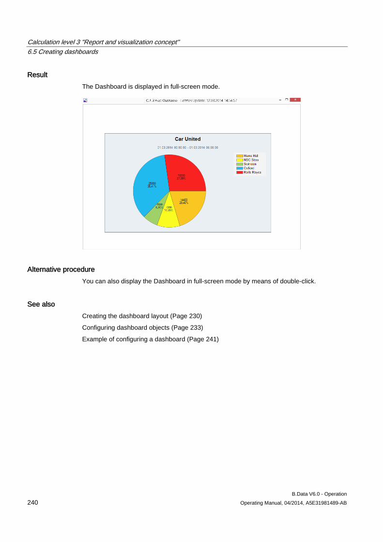
Calculation level 3 "Report and visualization concept" 6.5 Creating dashboards
B.Data V6.0 - Operation 240 Operating Manual, 04/2014, A5E31981489-AB
Result The Dashboard is displayed in full-screen mode.
Alternative procedure You can also display the Dashboard in full-screen mode by means of double-click.
See also Creating the dashboard layout (Page 230)
Configuring dashboard objects (Page 233)
Example of configuring a dashboard (Page 241)
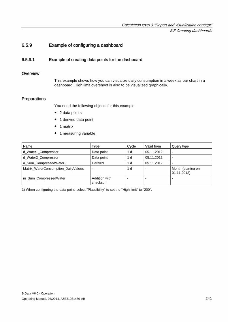
Calculation level 3 "Report and visualization concept" 6.5 Creating dashboards
B.Data V6.0 - Operation Operating Manual, 04/2014, A5E31981489-AB 241
6.5.9 Example of configuring a dashboard
6.5.9.1 Example of creating data points for the dashboard
Overview This example shows how you can visualize daily consumption in a week as bar chart in a dashboard. High limit overshoot is also to be visualized graphically.
Preparations You need the following objects for this example:
● 2 data points
● 1 derived data point
● 1 matrix
● 1 measuring variable
Name Type Cycle Valid from Query type d_Water1_Compressor Data point 1 d 05.11.2012 - d_Water2_Compressor Data point 1 d 05.11.2012 - a_Sum_CompressedWater1) Derived 1 d 05.11.2012 - Matrix_WaterConsumption_DailyValues - 1 d - Month (starting on
01.11.2012) m_Sum_CompressedWater Addition with
checksum - - -
1) When configuring the data point, select "Plausibility" to set the "High limit" to "200".
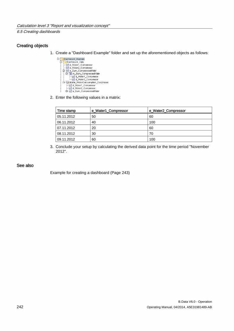
Calculation level 3 "Report and visualization concept" 6.5 Creating dashboards
B.Data V6.0 - Operation 242 Operating Manual, 04/2014, A5E31981489-AB
Creating objects 1. Create a "Dashboard Example" folder and set up the aforementioned objects as follows:
2. Enter the following values in a matrix:
Time stamp e_Water1_Compressor e_Water2_Compressor 05.11.2012 50 60 06.11.2012 40 100 07.11.2012 20 60 08.11.2012 30 70 09.11.2012 60 100
3. Conclude your setup by calculating the derived data point for the time period "November 2012".
See also Example for creating a dashboard (Page 243)
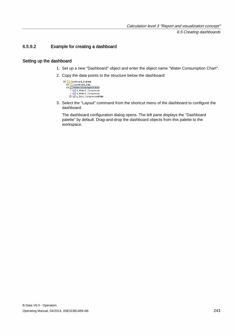
Calculation level 3 "Report and visualization concept" 6.5 Creating dashboards
B.Data V6.0 - Operation Operating Manual, 04/2014, A5E31981489-AB 243
6.5.9.2 Example for creating a dashboard
Setting up the dashboard 1. Set up a new "Dashboard" object and enter the object name "Water Consumption Chart".
2. Copy the data points to the structure below the dashboard:
3. Select the "Layout" command from the shortcut menu of the dashboard to configure the
dashboard.
The dashboard configuration dialog opens. The left pane displays the "Dashboard palette" by default. Drag-and-drop the dashboard objects from this palette to the workspace.
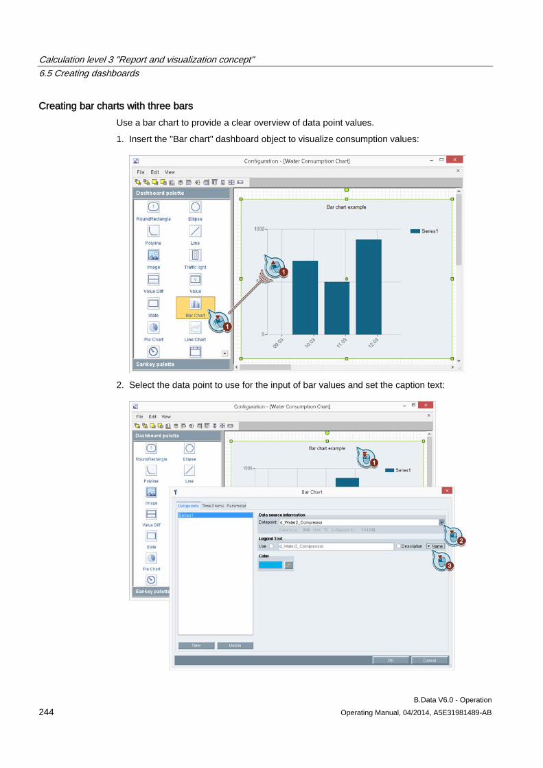
Calculation level 3 "Report and visualization concept" 6.5 Creating dashboards
B.Data V6.0 - Operation 244 Operating Manual, 04/2014, A5E31981489-AB
Creating bar charts with three bars Use a bar chart to provide a clear overview of data point values.
1. Insert the "Bar chart" dashboard object to visualize consumption values:
2. Select the data point to use for the input of bar values and set the caption text:
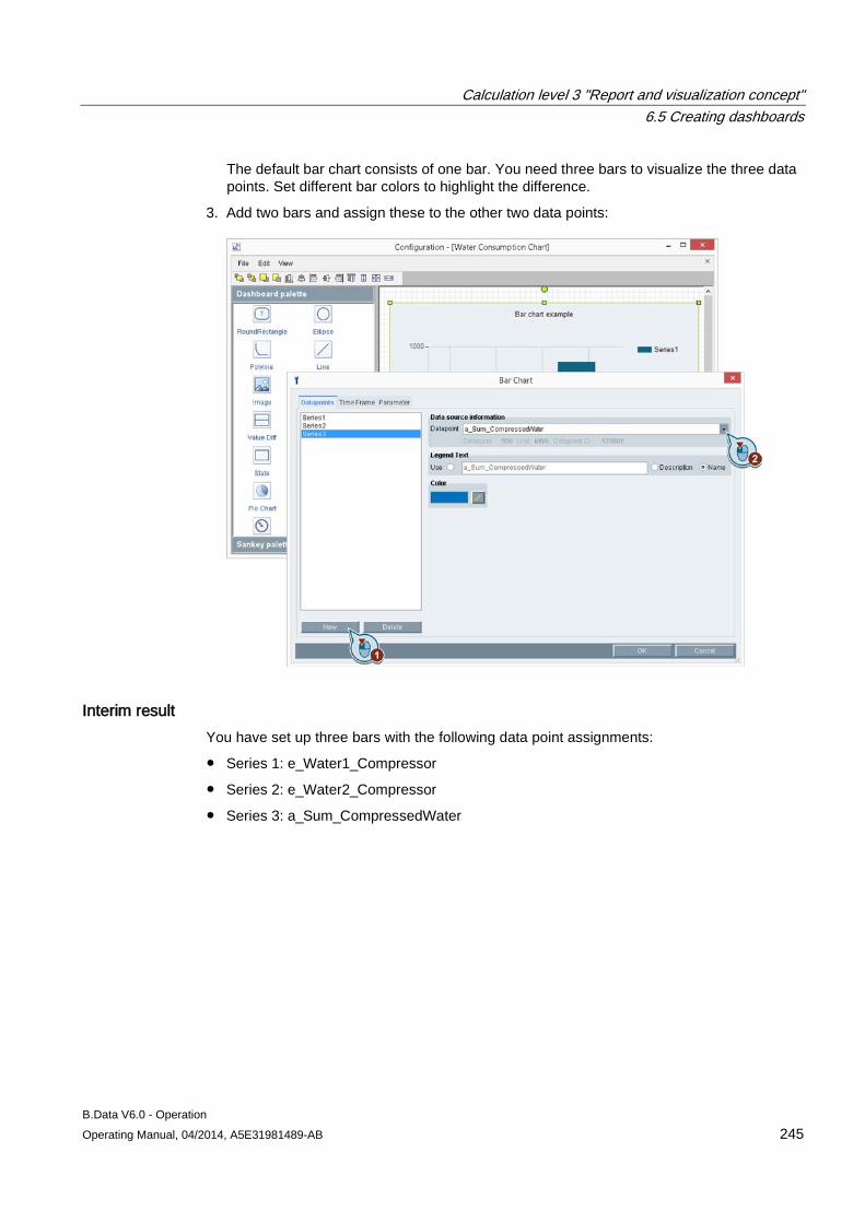
Calculation level 3 "Report and visualization concept" 6.5 Creating dashboards
B.Data V6.0 - Operation Operating Manual, 04/2014, A5E31981489-AB 245
The default bar chart consists of one bar. You need three bars to visualize the three data points. Set different bar colors to highlight the difference.
3. Add two bars and assign these to the other two data points:
Interim result You have set up three bars with the following data point assignments:
● Series 1: e_Water1_Compressor
● Series 2: e_Water2_Compressor
● Series 3: a_Sum_CompressedWater
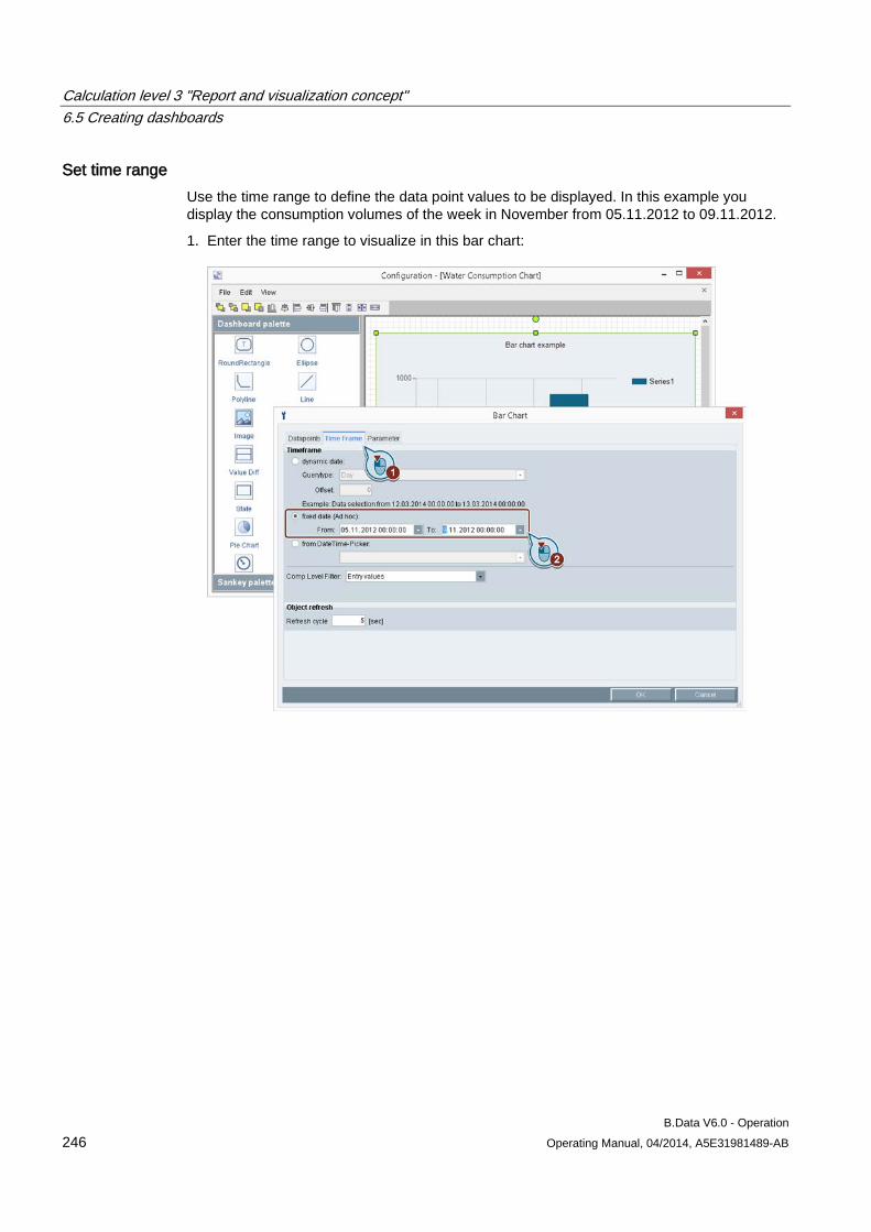
Calculation level 3 "Report and visualization concept" 6.5 Creating dashboards
B.Data V6.0 - Operation 246 Operating Manual, 04/2014, A5E31981489-AB
Set time range Use the time range to define the data point values to be displayed. In this example you display the consumption volumes of the week in November from 05.11.2012 to 09.11.2012.
1. Enter the time range to visualize in this bar chart:
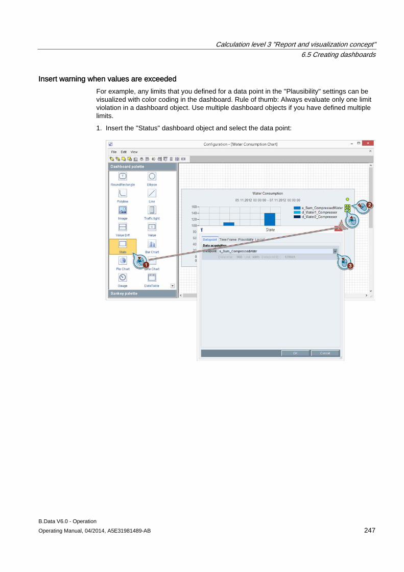
Calculation level 3 "Report and visualization concept" 6.5 Creating dashboards
B.Data V6.0 - Operation Operating Manual, 04/2014, A5E31981489-AB 247
Insert warning when values are exceeded For example, any limits that you defined for a data point in the "Plausibility" settings can be visualized with color coding in the dashboard. Rule of thumb: Always evaluate only one limit violation in a dashboard object. Use multiple dashboard objects if you have defined multiple limits.
1. Insert the "Status" dashboard object and select the data point:
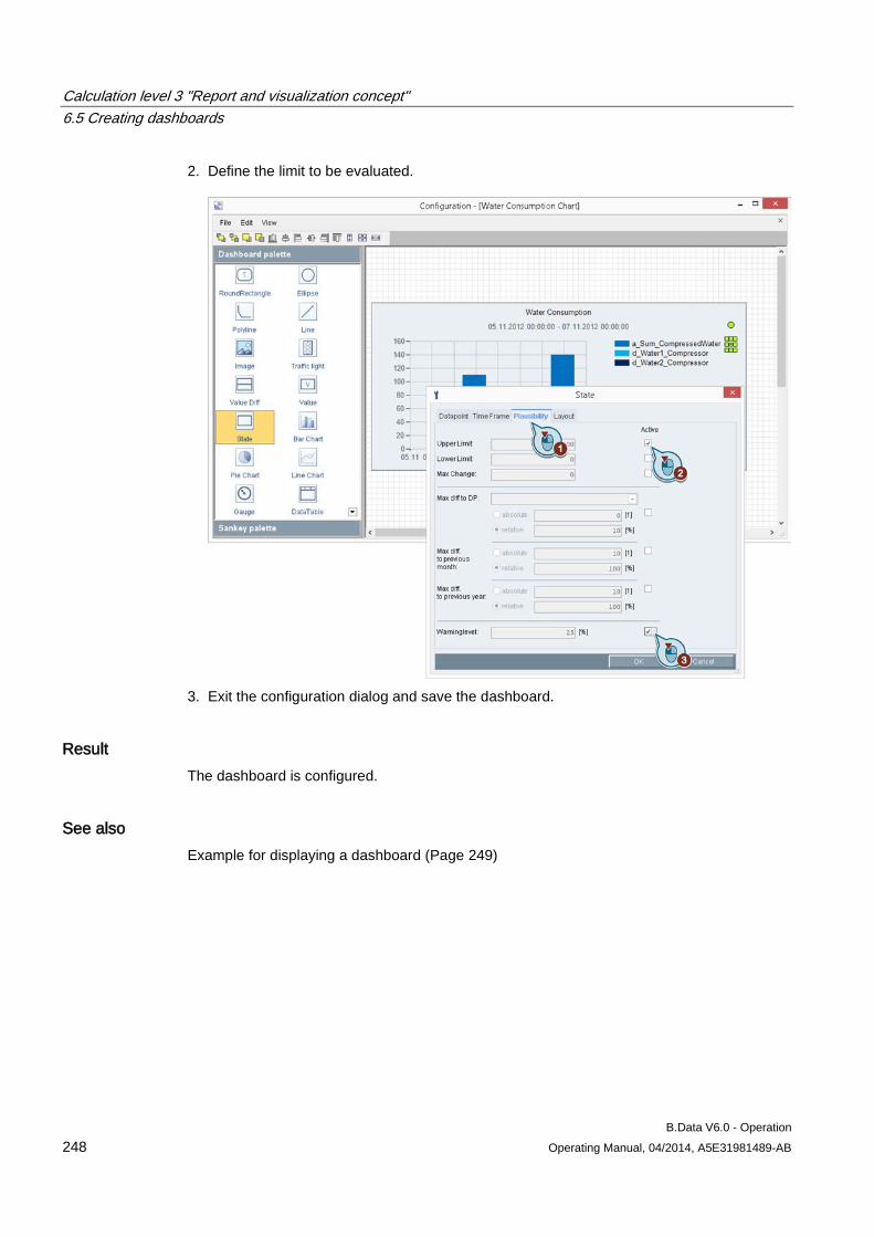
Calculation level 3 "Report and visualization concept" 6.5 Creating dashboards
B.Data V6.0 - Operation 248 Operating Manual, 04/2014, A5E31981489-AB
2. Define the limit to be evaluated.
3. Exit the configuration dialog and save the dashboard.
Result The dashboard is configured.
See also Example for displaying a dashboard (Page 249)
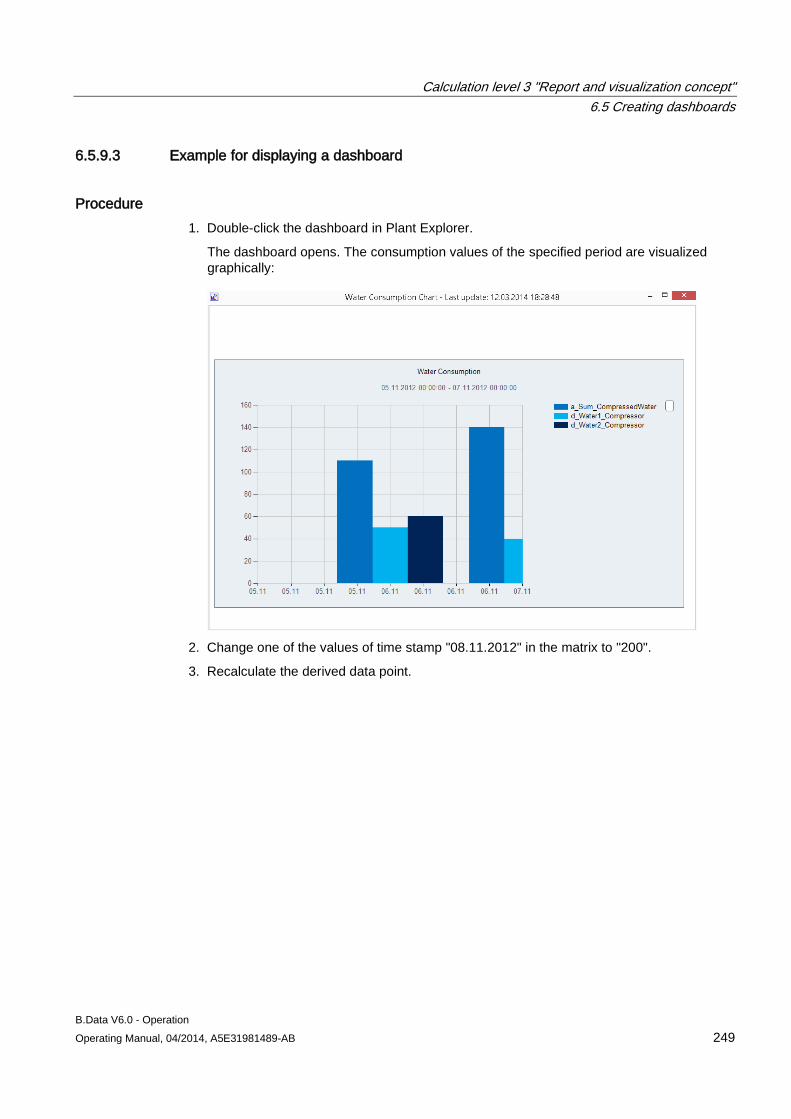
Calculation level 3 "Report and visualization concept" 6.5 Creating dashboards
B.Data V6.0 - Operation Operating Manual, 04/2014, A5E31981489-AB 249
6.5.9.3 Example for displaying a dashboard
Procedure 1. Double-click the dashboard in Plant Explorer.
The dashboard opens. The consumption values of the specified period are visualized graphically:
2. Change one of the values of time stamp "08.11.2012" in the matrix to "200".
3. Recalculate the derived data point.
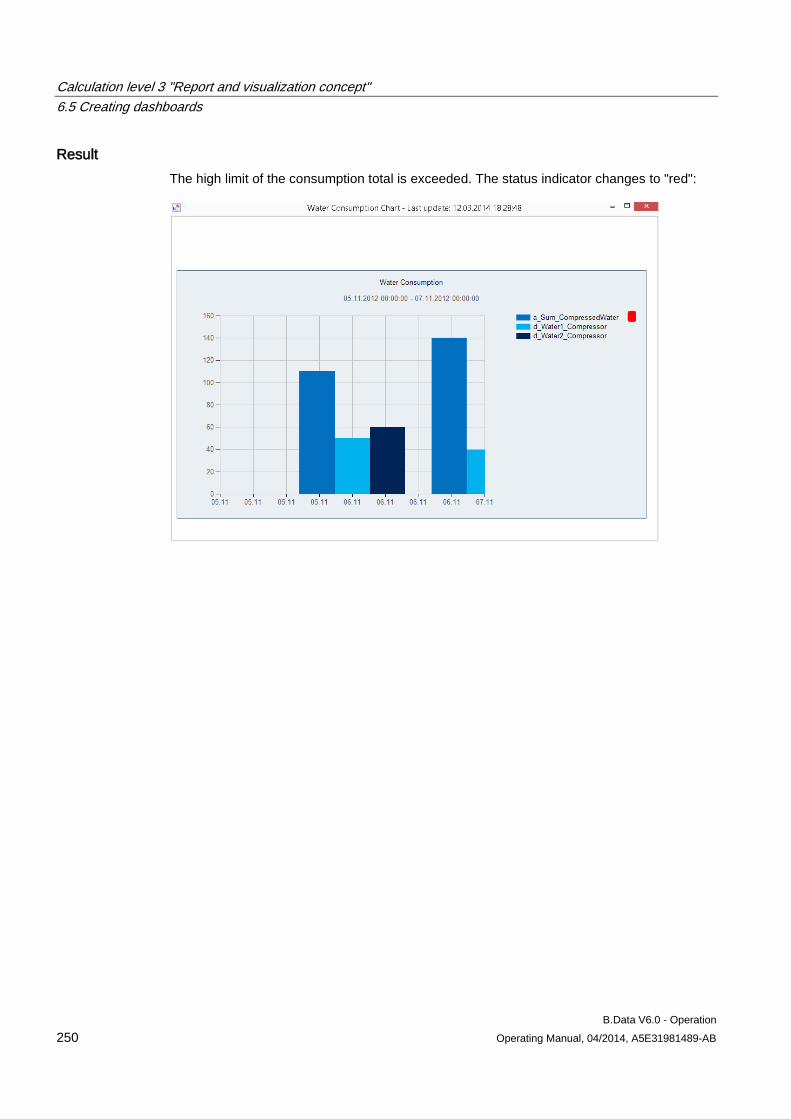
Calculation level 3 "Report and visualization concept" 6.5 Creating dashboards
B.Data V6.0 - Operation 250 Operating Manual, 04/2014, A5E31981489-AB
Result The high limit of the consumption total is exceeded. The status indicator changes to "red":
Calculation level 3 "Report and visualization concept" 6.6 Using the Quick Chart
B.Data V6.0 - Operation Operating Manual, 04/2014, A5E31981489-AB 251
6.6 Using the Quick Chart
6.6.1 Basic information on the Quick Chart
Overview You use the Quick Chart to display historical as well as current values as line graph. Use Quick Chart for quick visualization of measurement series.
You can display the values of the following objects in Quick Chart:
● Data points
● Matrix
● Report
● Trend
Quick Chart is also supported with identical functionality in B.Data Web.
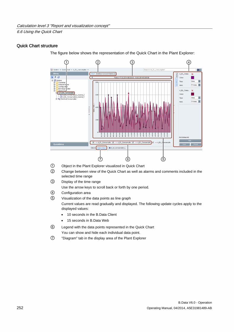
Calculation level 3 "Report and visualization concept" 6.6 Using the Quick Chart
B.Data V6.0 - Operation 252 Operating Manual, 04/2014, A5E31981489-AB
Quick Chart structure The figure below shows the representation of the Quick Chart in the Plant Explorer:
① Object in the Plant Explorer visualized in Quick Chart ② Change between view of the Quick Chart as well as alarms and comments included in the
selected time range ③ Display of the time range
Use the arrow keys to scroll back or forth by one period. ④ Configuration area ⑤ Visualization of the data points as line graph
Current values are read gradually and displayed. The following update cycles apply to the displayed values: • 10 seconds in the B.Data Client • 15 seconds in B.Data Web
⑥ Legend with the data points represented in the Quick Chart You can show and hide each individual data point.
⑦ "Diagram" tab in the display area of the Plant Explorer
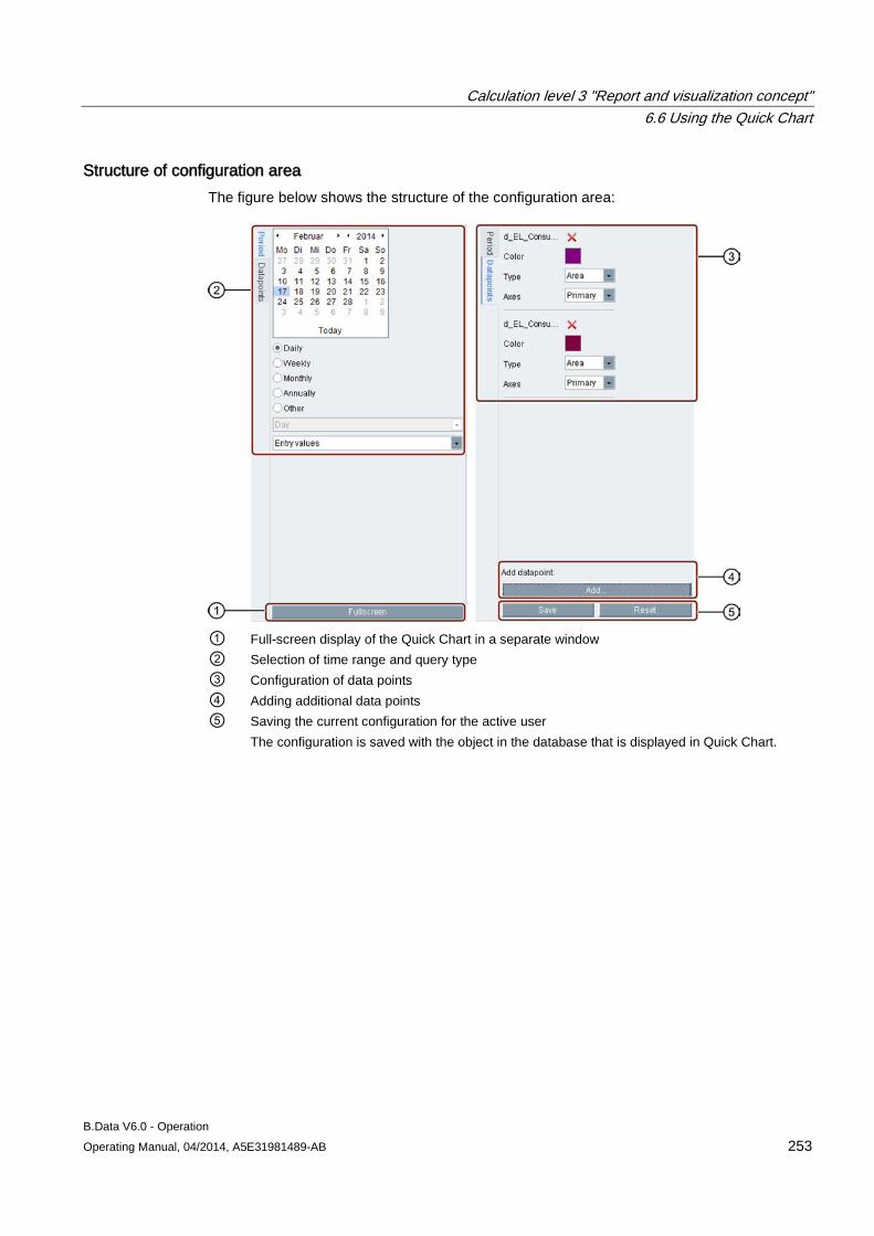
Calculation level 3 "Report and visualization concept" 6.6 Using the Quick Chart
B.Data V6.0 - Operation Operating Manual, 04/2014, A5E31981489-AB 253
Structure of configuration area The figure below shows the structure of the configuration area:
① Full-screen display of the Quick Chart in a separate window ② Selection of time range and query type ③ Configuration of data points ④ Adding additional data points ⑤ Saving the current configuration for the active user
The configuration is saved with the object in the database that is displayed in Quick Chart.
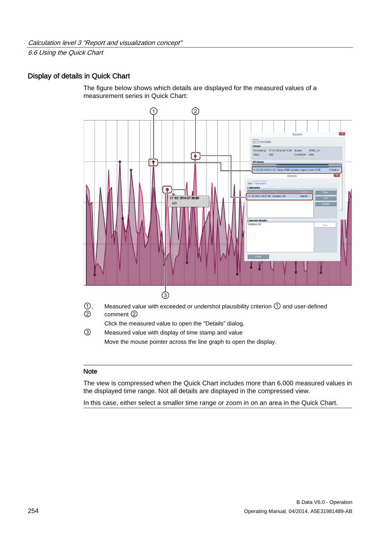
Calculation level 3 "Report and visualization concept" 6.6 Using the Quick Chart
B.Data V6.0 - Operation 254 Operating Manual, 04/2014, A5E31981489-AB
Display of details in Quick Chart The figure below shows which details are displayed for the measured values of a measurement series in Quick Chart:
①, ②
Measured value with exceeded or undershot plausibility criterion ① and user-defined comment ② Click the measured value to open the "Details" dialog.
③ Measured value with display of time stamp and value Move the mouse pointer across the line graph to open the display.
Note
The view is compressed when the Quick Chart includes more than 6,000 measured values in the displayed time range. Not all details are displayed in the compressed view.
In this case, either select a smaller time range or zoom in on an area in the Quick Chart.
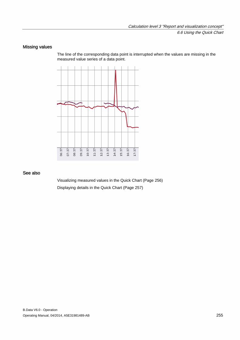
Calculation level 3 "Report and visualization concept" 6.6 Using the Quick Chart
B.Data V6.0 - Operation Operating Manual, 04/2014, A5E31981489-AB 255
Missing values The line of the corresponding data point is interrupted when the values are missing in the measured value series of a data point.
See also Visualizing measured values in the Quick Chart (Page 256)
Displaying details in the Quick Chart (Page 257)
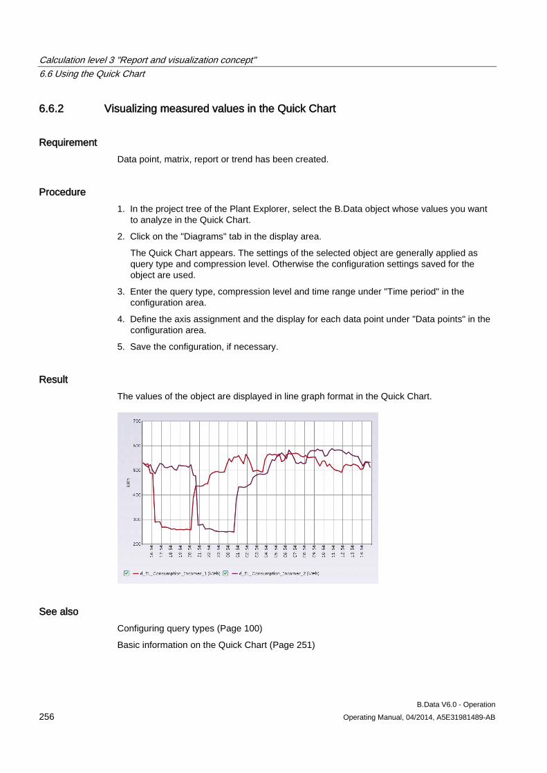
Calculation level 3 "Report and visualization concept" 6.6 Using the Quick Chart
B.Data V6.0 - Operation 256 Operating Manual, 04/2014, A5E31981489-AB
6.6.2 Visualizing measured values in the Quick Chart
Requirement Data point, matrix, report or trend has been created.
Procedure 1. In the project tree of the Plant Explorer, select the B.Data object whose values you want
to analyze in the Quick Chart.
2. Click on the "Diagrams" tab in the display area.
The Quick Chart appears. The settings of the selected object are generally applied as query type and compression level. Otherwise the configuration settings saved for the object are used.
3. Enter the query type, compression level and time range under "Time period" in the configuration area.
4. Define the axis assignment and the display for each data point under "Data points" in the configuration area.
5. Save the configuration, if necessary.
Result The values of the object are displayed in line graph format in the Quick Chart.
See also Configuring query types (Page 100)
Basic information on the Quick Chart (Page 251)
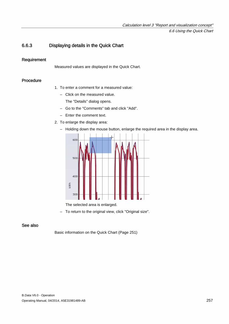
Calculation level 3 "Report and visualization concept" 6.6 Using the Quick Chart
B.Data V6.0 - Operation Operating Manual, 04/2014, A5E31981489-AB 257
6.6.3 Displaying details in the Quick Chart
Requirement Measured values are displayed in the Quick Chart.
Procedure 1. To enter a comment for a measured value:
– Click on the measured value.
The "Details" dialog opens.
– Go to the "Comments" tab and click "Add".
– Enter the comment text.
2. To enlarge the display area:
– Holding down the mouse button, enlarge the required area in the display area.
The selected area is enlarged.
– To return to the original view, click "Original size".
See also Basic information on the Quick Chart (Page 251)

Calculation level 3 "Report and visualization concept" 6.6 Using the Quick Chart
B.Data V6.0 - Operation 258 Operating Manual, 04/2014, A5E31981489-AB
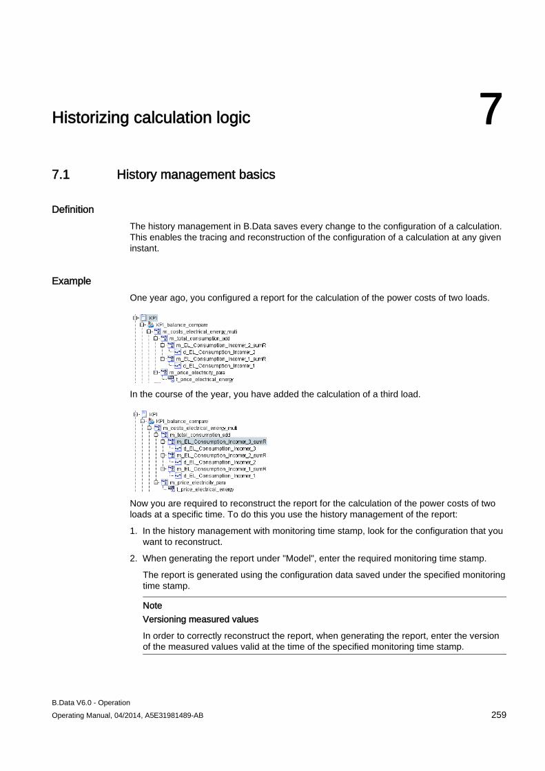
B.Data V6.0 - Operation Operating Manual, 04/2014, A5E31981489-AB 259
Historizing calculation logic 7 7.1 History management basics
Definition The history management in B.Data saves every change to the configuration of a calculation. This enables the tracing and reconstruction of the configuration of a calculation at any given instant.
Example One year ago, you configured a report for the calculation of the power costs of two loads.
In the course of the year, you have added the calculation of a third load.
Now you are required to reconstruct the report for the calculation of the power costs of two loads at a specific time. To do this you use the history management of the report:
1. In the history management with monitoring time stamp, look for the configuration that you want to reconstruct.
2. When generating the report under "Model", enter the required monitoring time stamp.
The report is generated using the configuration data saved under the specified monitoring time stamp.
Note
Versioning measured values
In order to correctly reconstruct the report, when generating the report, enter the version of the measured values valid at the time of the specified monitoring time stamp.
Historizing calculation logic 7.1 History management basics
B.Data V6.0 - Operation 260 Operating Manual, 04/2014, A5E31981489-AB
Objects for history management You can display configuration changes for the following B.Data objects:
● Data point of type "Derived"
● Measuring variable
● Report
The following configuration data are displayed during the history management of objects:
Configuration Meaning Calculation tree Shows objects of the calculation and their order in the calculation tree. Type Shows the type of the object, e.g. "Module".
"Type" is only used in the history management of the reports. Name Displays the name of the object. Function Displays the function of a data point or of a measuring variable, e.g.
"Measurement" or "Addition of MEVAs". Operation Displays the type of change to the object, e.g. "Delete". Unit Displays the unit of a data point or measuring variable, e.g. "kWh". Changed on Displays the date when the change was made to the object. Changed by Displays the user who made the change to the object. Description Displays the description of the changed object.
The following restrictions apply to the history management of reports:
● No history is kept of report templates.
● No history is kept of start values.
● Automatically generated reports are only calculated with the current configuration data.
● Reports that are generated in B.Data Web are only calculated with the current configuration data.
● Specific modules, e.g. plausibility modules, are only calculated with the current configuration data.
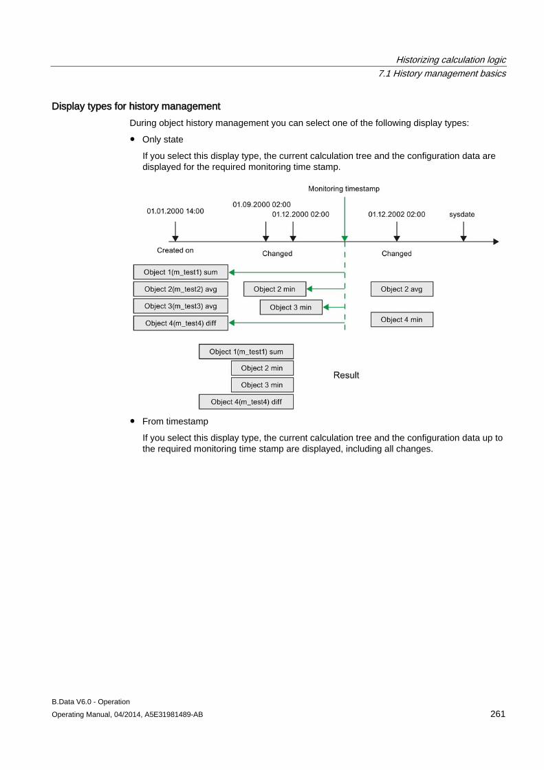
Historizing calculation logic 7.1 History management basics
B.Data V6.0 - Operation Operating Manual, 04/2014, A5E31981489-AB 261
Display types for history management During object history management you can select one of the following display types:
● Only state
If you select this display type, the current calculation tree and the configuration data are displayed for the required monitoring time stamp.
● From timestamp
If you select this display type, the current calculation tree and the configuration data up to the required monitoring time stamp are displayed, including all changes.
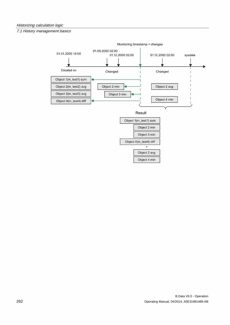
Historizing calculation logic 7.1 History management basics
B.Data V6.0 - Operation 262 Operating Manual, 04/2014, A5E31981489-AB
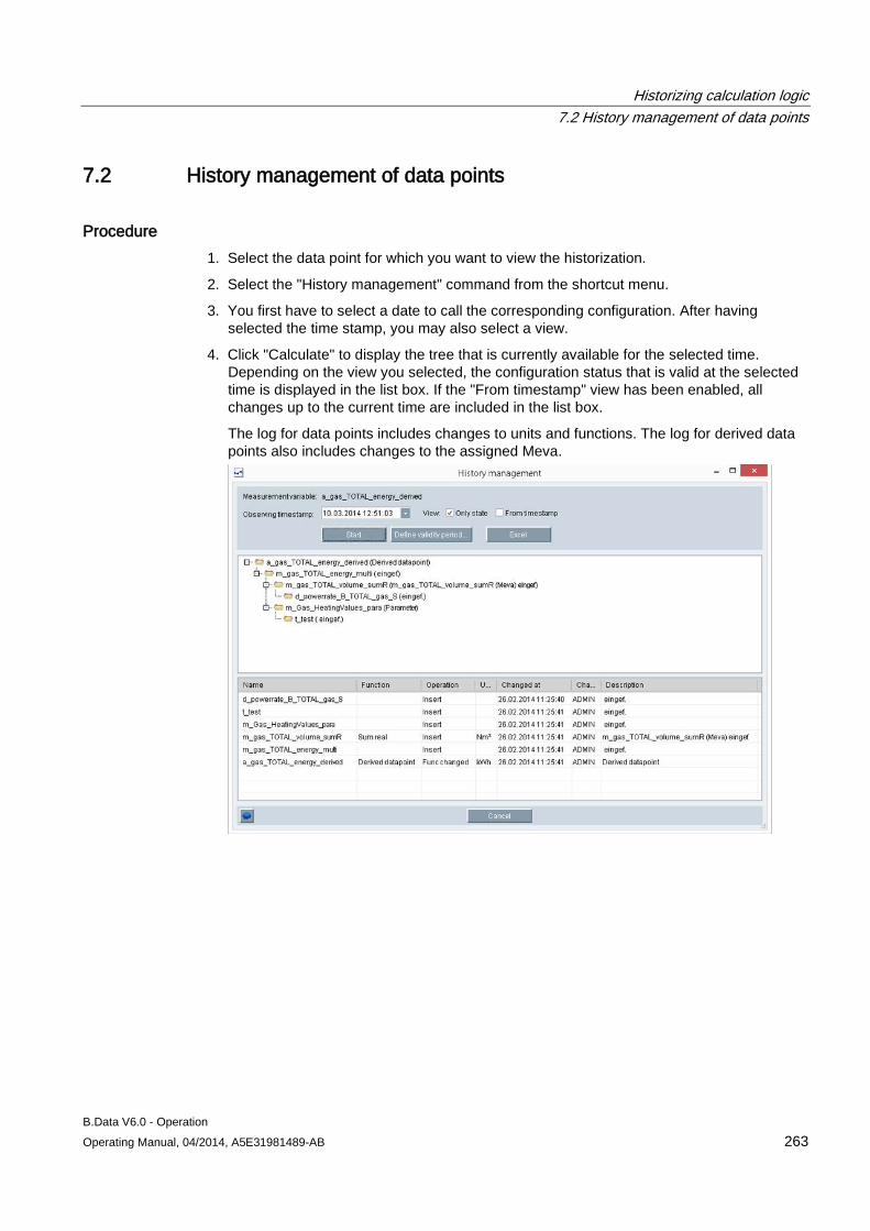
Historizing calculation logic 7.2 History management of data points
B.Data V6.0 - Operation Operating Manual, 04/2014, A5E31981489-AB 263
7.2 History management of data points
Procedure 1. Select the data point for which you want to view the historization.
2. Select the "History management" command from the shortcut menu.
3. You first have to select a date to call the corresponding configuration. After having selected the time stamp, you may also select a view.
4. Click "Calculate" to display the tree that is currently available for the selected time. Depending on the view you selected, the configuration status that is valid at the selected time is displayed in the list box. If the "From timestamp" view has been enabled, all changes up to the current time are included in the list box.
The log for data points includes changes to units and functions. The log for derived data points also includes changes to the assigned Meva.
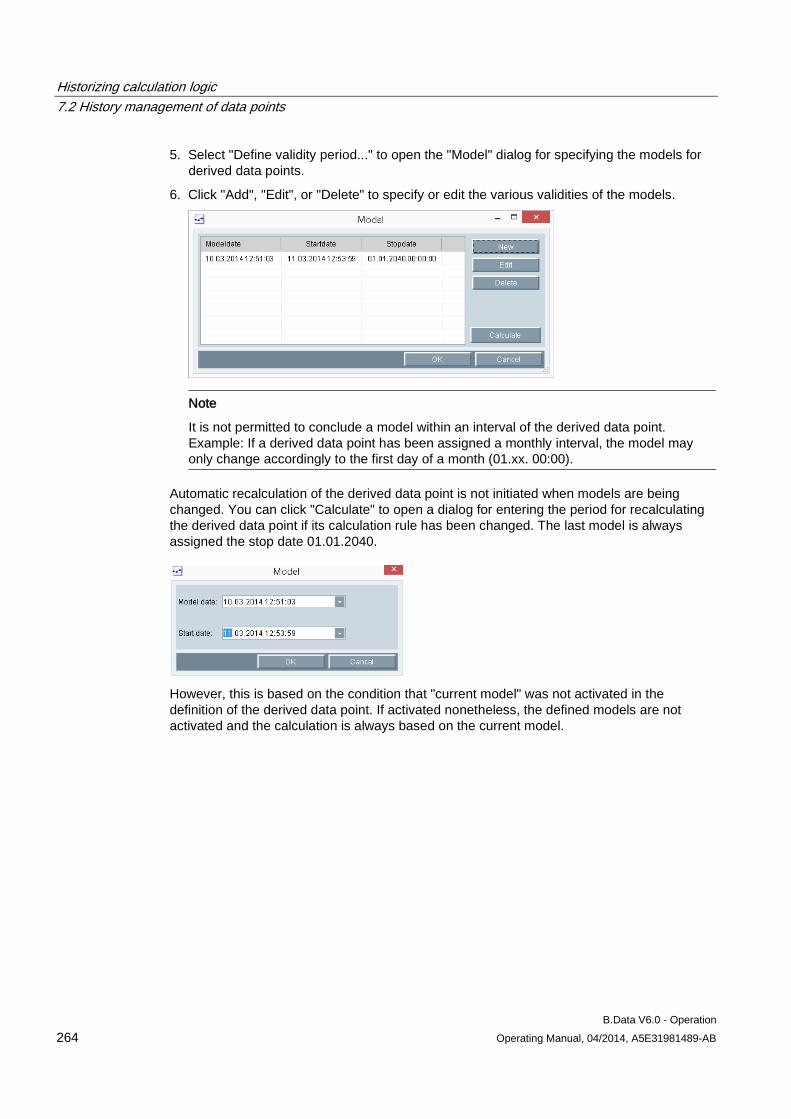
Historizing calculation logic 7.2 History management of data points
B.Data V6.0 - Operation 264 Operating Manual, 04/2014, A5E31981489-AB
5. Select "Define validity period..." to open the "Model" dialog for specifying the models for derived data points.
6. Click "Add", "Edit", or "Delete" to specify or edit the various validities of the models.
Note
It is not permitted to conclude a model within an interval of the derived data point. Example: If a derived data point has been assigned a monthly interval, the model may only change accordingly to the first day of a month (01.xx. 00:00).
Automatic recalculation of the derived data point is not initiated when models are being changed. You can click "Calculate" to open a dialog for entering the period for recalculating the derived data point if its calculation rule has been changed. The last model is always assigned the stop date 01.01.2040.
However, this is based on the condition that "current model" was not activated in the definition of the derived data point. If activated nonetheless, the defined models are not activated and the calculation is always based on the current model.
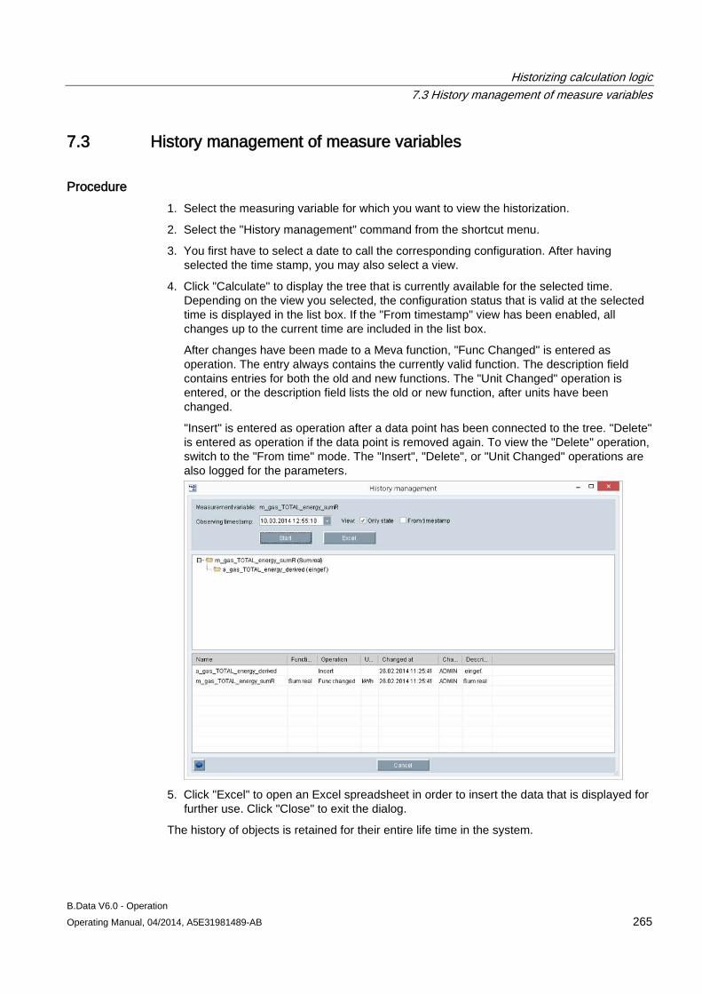
Historizing calculation logic 7.3 History management of measure variables
B.Data V6.0 - Operation Operating Manual, 04/2014, A5E31981489-AB 265
7.3 History management of measure variables
Procedure 1. Select the measuring variable for which you want to view the historization.
2. Select the "History management" command from the shortcut menu.
3. You first have to select a date to call the corresponding configuration. After having selected the time stamp, you may also select a view.
4. Click "Calculate" to display the tree that is currently available for the selected time. Depending on the view you selected, the configuration status that is valid at the selected time is displayed in the list box. If the "From timestamp" view has been enabled, all changes up to the current time are included in the list box.
After changes have been made to a Meva function, "Func Changed" is entered as operation. The entry always contains the currently valid function. The description field contains entries for both the old and new functions. The "Unit Changed" operation is entered, or the description field lists the old or new function, after units have been changed.
"Insert" is entered as operation after a data point has been connected to the tree. "Delete" is entered as operation if the data point is removed again. To view the "Delete" operation, switch to the "From time" mode. The "Insert", "Delete", or "Unit Changed" operations are also logged for the parameters.
5. Click "Excel" to open an Excel spreadsheet in order to insert the data that is displayed for
further use. Click "Close" to exit the dialog.
The history of objects is retained for their entire life time in the system.
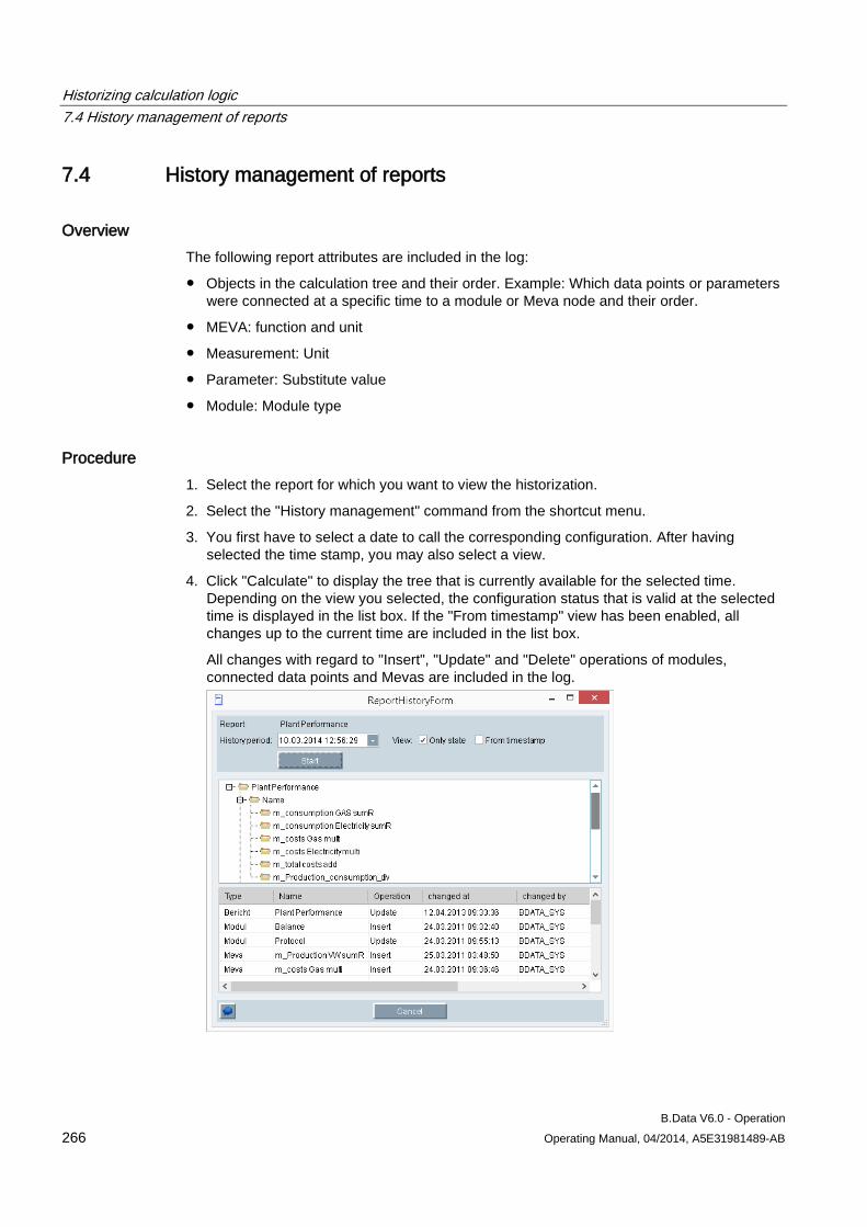
Historizing calculation logic 7.4 History management of reports
B.Data V6.0 - Operation 266 Operating Manual, 04/2014, A5E31981489-AB
7.4 History management of reports
Overview The following report attributes are included in the log:
● Objects in the calculation tree and their order. Example: Which data points or parameters were connected at a specific time to a module or Meva node and their order.
● MEVA: function and unit
● Measurement: Unit
● Parameter: Substitute value
● Module: Module type
Procedure 1. Select the report for which you want to view the historization.
2. Select the "History management" command from the shortcut menu.
3. You first have to select a date to call the corresponding configuration. After having selected the time stamp, you may also select a view.
4. Click "Calculate" to display the tree that is currently available for the selected time. Depending on the view you selected, the configuration status that is valid at the selected time is displayed in the list box. If the "From timestamp" view has been enabled, all changes up to the current time are included in the list box.
All changes with regard to "Insert", "Update" and "Delete" operations of modules, connected data points and Mevas are included in the log.
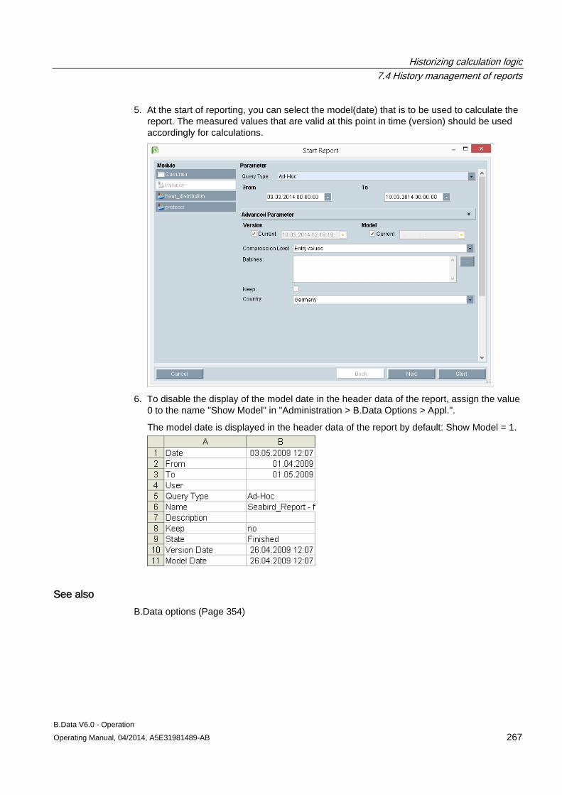
Historizing calculation logic 7.4 History management of reports
B.Data V6.0 - Operation Operating Manual, 04/2014, A5E31981489-AB 267
5. At the start of reporting, you can select the model(date) that is to be used to calculate the report. The measured values that are valid at this point in time (version) should be used accordingly for calculations.
6. To disable the display of the model date in the header data of the report, assign the value
0 to the name "Show Model" in "Administration > B.Data Options > Appl.".
The model date is displayed in the header data of the report by default: Show Model = 1.
See also B.Data options (Page 354)

Historizing calculation logic 7.4 History management of reports
B.Data V6.0 - Operation 268 Operating Manual, 04/2014, A5E31981489-AB
B.Data V6.0 - Operation Operating Manual, 04/2014, A5E31981489-AB 269
Schedule management 8 8.1 Basic information on schedule management
Definition The B.Data schedule management is used to plan and forecast the energy requirements of your company for a time period which can be freely selected.
Usage Planning and forecasting are preconditions for sustainable energy management. This is facilitated by generating forecasts of the energy requirements and load profiles for one or several locations, individual consumers, production areas, or buildings.
Energy requirements planning for a specific time period returns procurement benefits due to the tiered tariff systems of the energy providers. Maximum financial benefits are achieved at the following conditions:
● The difference between the expected and actual consumption is kept to a minimum.
● Load peaks are shifted to tariff times during which energy generation is at a lower cost.
Demands on an energy management system Load peaks in industrial plants are primarily determined by production processes, as well as shift or product cycles. The forecasting methods may differ even among different plant units:
● Forecasting in pulp mills, for example, is usually based on production quantities. The shredder and waste paper units are only in operation as required, which is why forecasting is based on production plans.
● By contrast, forecasting in the automobile industry is based on shift schedules.
Implementation in B.Data B.Data supports the following methods for planning and forecasting:
● Comparison days and shift model
● Production plans
● Daily consumption values
The forecasts can be compared with the ACTUAL data in future analyses.
Schedule management 8.1 Basic information on schedule management
B.Data V6.0 - Operation 270 Operating Manual, 04/2014, A5E31981489-AB
Comparison day principle The comparison day principle is based on shifts or type days that are examined across a reference time period, such as a quarter. The energy demand is calculated depending on the scheduled days and associated plant operating times.
● Examples of type days: Workday (8 hours), workday (6 hours), workday (10 hours), holiday
● Examples of shifts: Morning shift, evening shift, night shift, special shift
Usually, you plan type days on a weekly basis, while flexible planning without committing to an entire week is also possible. Holidays and other non-working days are taken into account automatically.
Use the calendar to react to changes: You can change type days or shift these to other weekdays. Therefore, your forecasts are always up-to-date.
The forecast result can be corrected, for example, to compensate for production data or temperature effects in order to provide a uniform basis for comparison. Evaluation of the forecast quality, i.e. the comparison with ACTUAL data, concludes the forecast. The result may affect the next forecast.
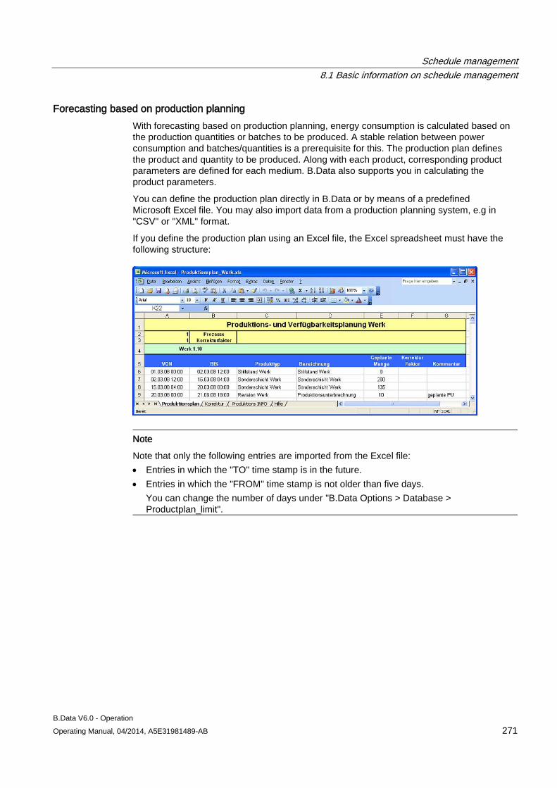
Schedule management 8.1 Basic information on schedule management
B.Data V6.0 - Operation Operating Manual, 04/2014, A5E31981489-AB 271
Forecasting based on production planning With forecasting based on production planning, energy consumption is calculated based on the production quantities or batches to be produced. A stable relation between power consumption and batches/quantities is a prerequisite for this. The production plan defines the product and quantity to be produced. Along with each product, corresponding product parameters are defined for each medium. B.Data also supports you in calculating the product parameters.
You can define the production plan directly in B.Data or by means of a predefined Microsoft Excel file. You may also import data from a production planning system, e.g in "CSV" or "XML" format.
If you define the production plan using an Excel file, the Excel spreadsheet must have the following structure:
Note
Note that only the following entries are imported from the Excel file: • Entries in which the "TO" time stamp is in the future. • Entries in which the "FROM" time stamp is not older than five days.
You can change the number of days under "B.Data Options > Database > Productplan_limit".
Schedule management 8.1 Basic information on schedule management
B.Data V6.0 - Operation 272 Operating Manual, 04/2014, A5E31981489-AB
Forecasting based on daily values Forecasting based on daily values is based on previously acquired ACTUAL values. In this case, the energy consumption is allocated to each daily production. In the forecast, you then calculate the expected energy requirements as a function of the expected production quantity.
You can analyze the daily production quantities and corresponding consumption data with the help of a regression analysis. The parameters for the linear equation y = k • x + d that are mapped in B.Data are derived from this analysis. Once the planned production quantity has been defined, calculate the energy demands to be expected.
See also Configuring the plant (Page 292)
Schedule management 8.2 Creating a profile
B.Data V6.0 - Operation Operating Manual, 04/2014, A5E31981489-AB 273
8.2 Creating a profile
8.2.1 Basic information on profile Based on the comparison day principle, you can generate media consumption forecasts at any time using a combination of master profiles, profiles, typical days, and special effects.
The next chapters cover the following components:
● Status
● Typical days
● Profiles
● Master profiles
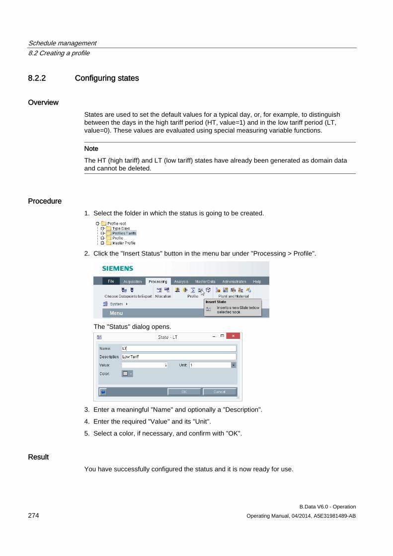
Schedule management 8.2 Creating a profile
B.Data V6.0 - Operation 274 Operating Manual, 04/2014, A5E31981489-AB
8.2.2 Configuring states
Overview States are used to set the default values for a typical day, or, for example, to distinguish between the days in the high tariff period (HT, value=1) and in the low tariff period (LT, value=0). These values are evaluated using special measuring variable functions.
Note
The HT (high tariff) and LT (low tariff) states have already been generated as domain data and cannot be deleted.
Procedure 1. Select the folder in which the status is going to be created.
2. Click the "Insert Status" button in the menu bar under "Processing > Profile".
The "Status" dialog opens.
3. Enter a meaningful "Name" and optionally a "Description".
4. Enter the required "Value" and its "Unit".
5. Select a color, if necessary, and confirm with "OK".
Result You have successfully configured the status and it is now ready for use.
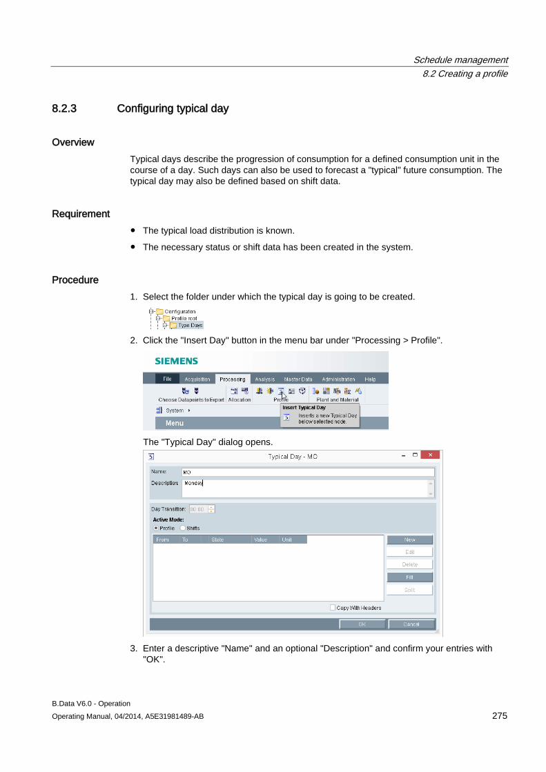
Schedule management 8.2 Creating a profile
B.Data V6.0 - Operation Operating Manual, 04/2014, A5E31981489-AB 275
8.2.3 Configuring typical day
Overview Typical days describe the progression of consumption for a defined consumption unit in the course of a day. Such days can also be used to forecast a "typical" future consumption. The typical day may also be defined based on shift data.
Requirement ● The typical load distribution is known.
● The necessary status or shift data has been created in the system.
Procedure 1. Select the folder under which the typical day is going to be created.
2. Click the "Insert Day" button in the menu bar under "Processing > Profile".
The "Typical Day" dialog opens.
3. Enter a descriptive "Name" and an optional "Description" and confirm your entries with
"OK".
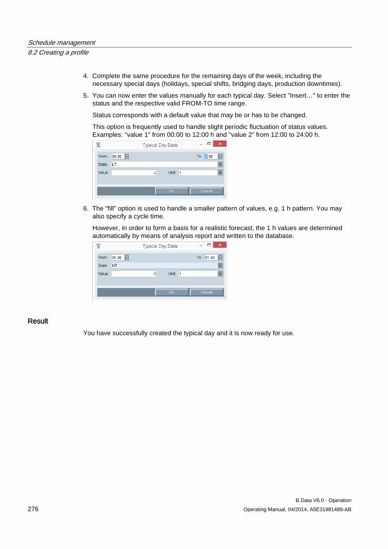
Schedule management 8.2 Creating a profile
B.Data V6.0 - Operation 276 Operating Manual, 04/2014, A5E31981489-AB
4. Complete the same procedure for the remaining days of the week, including the necessary special days (holidays, special shifts, bridging days, production downtimes).
5. You can now enter the values manually for each typical day. Select "Insert…" to enter the status and the respective valid FROM-TO time range.
Status corresponds with a default value that may be or has to be changed.
This option is frequently used to handle slight periodic fluctuation of status values. Examples: "value 1" from 00:00 to 12:00 h and "value 2" from 12:00 to 24:00 h.
6. The "fill" option is used to handle a smaller pattern of values, e.g. 1 h pattern. You may
also specify a cycle time.
However, in order to form a basis for a realistic forecast, the 1 h values are determined automatically by means of analysis report and written to the database.
Result You have successfully created the typical day and it is now ready for use.
Schedule management 8.2 Creating a profile
B.Data V6.0 - Operation Operating Manual, 04/2014, A5E31981489-AB 277
8.2.4 Configuring profiles
8.2.4.1 Configuring profiles
Overview A profile is used to configure the consumption of a typical week with the help of type days.
You can employ two modes to configure a profile:
● "Weekly": Configuration of a fixed sequence of seven days. In the "Weekly" mode, assign type days to the weekdays. The type day "Default" is assigned to a weekday by default.
● "Day sequence": Configuration of a flexible day sequence. Select the type days for the "Day sequence" mode and specify their sorting order for the profile.
Note
You must activate the calendar to enable the use of the "Day sequence" mode.
Requirement The type day is configured.
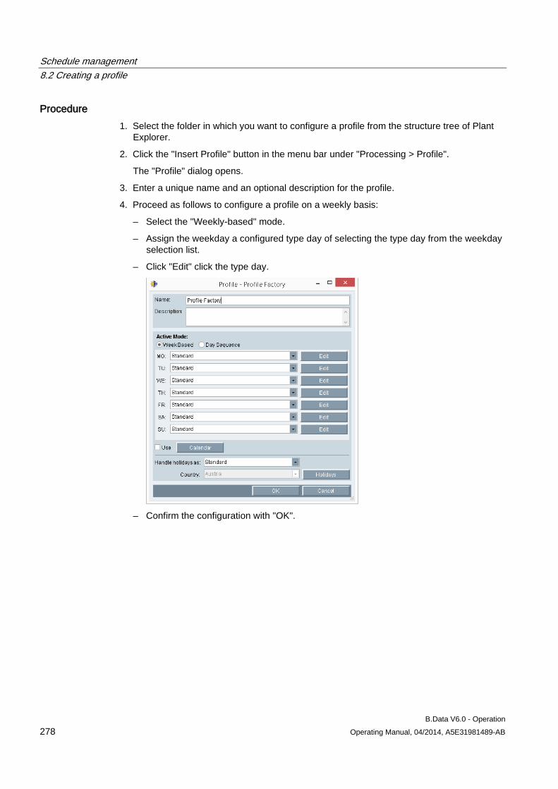
Schedule management 8.2 Creating a profile
B.Data V6.0 - Operation 278 Operating Manual, 04/2014, A5E31981489-AB
Procedure 1. Select the folder in which you want to configure a profile from the structure tree of Plant
Explorer.
2. Click the "Insert Profile" button in the menu bar under "Processing > Profile".
The "Profile" dialog opens.
3. Enter a unique name and an optional description for the profile.
4. Proceed as follows to configure a profile on a weekly basis:
– Select the "Weekly-based" mode.
– Assign the weekday a configured type day of selecting the type day from the weekday selection list.
– Click "Edit" click the type day.
– Confirm the configuration with "OK".
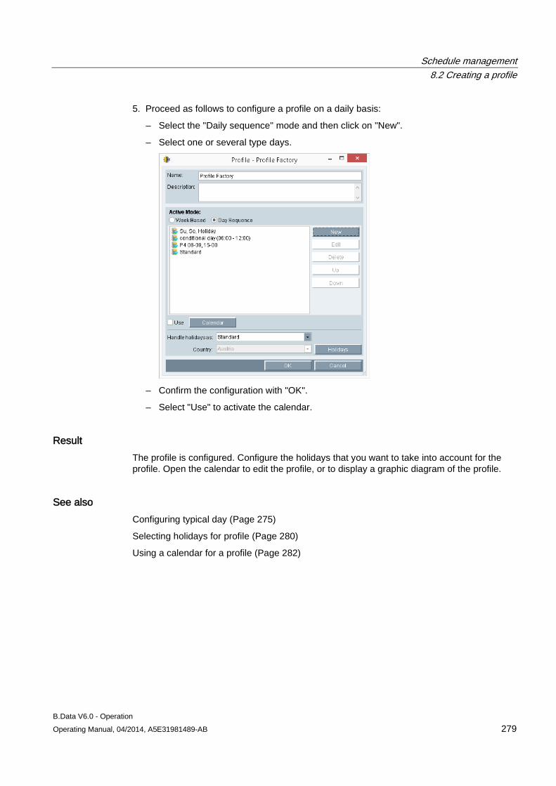
Schedule management 8.2 Creating a profile
B.Data V6.0 - Operation Operating Manual, 04/2014, A5E31981489-AB 279
5. Proceed as follows to configure a profile on a daily basis:
– Select the "Daily sequence" mode and then click on "New".
– Select one or several type days.
– Confirm the configuration with "OK".
– Select "Use" to activate the calendar.
Result The profile is configured. Configure the holidays that you want to take into account for the profile. Open the calendar to edit the profile, or to display a graphic diagram of the profile.
See also Configuring typical day (Page 275)
Selecting holidays for profile (Page 280)
Using a calendar for a profile (Page 282)
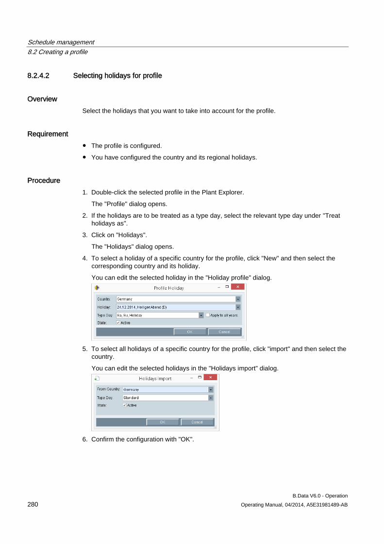
Schedule management 8.2 Creating a profile
B.Data V6.0 - Operation 280 Operating Manual, 04/2014, A5E31981489-AB
8.2.4.2 Selecting holidays for profile
Overview Select the holidays that you want to take into account for the profile.
Requirement ● The profile is configured.
● You have configured the country and its regional holidays.
Procedure 1. Double-click the selected profile in the Plant Explorer.
The "Profile" dialog opens.
2. If the holidays are to be treated as a type day, select the relevant type day under "Treat holidays as".
3. Click on "Holidays".
The "Holidays" dialog opens.
4. To select a holiday of a specific country for the profile, click "New" and then select the corresponding country and its holiday.
You can edit the selected holiday in the "Holiday profile" dialog.
5. To select all holidays of a specific country for the profile, click "import" and then select the
country.
You can edit the selected holidays in the "Holidays import" dialog.
6. Confirm the configuration with "OK".
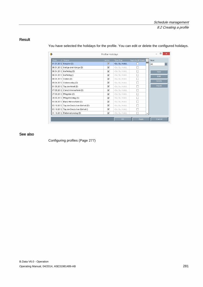
Schedule management 8.2 Creating a profile
B.Data V6.0 - Operation Operating Manual, 04/2014, A5E31981489-AB 281
Result You have selected the holidays for the profile. You can edit or delete the configured holidays.
See also Configuring profiles (Page 277)
Schedule management 8.2 Creating a profile
B.Data V6.0 - Operation 282 Operating Manual, 04/2014, A5E31981489-AB
8.2.4.3 Using a calendar for a profile
Overview Use the calendar to edit the configured day sequence, or to display a graphic diagram of the sequence.
Application example: You define a sequence with rollout for one quarter in the calendar. You can always respond to changes such as special shifts in the calendar. This functionality always keeps your consumption data and forecasts up to date.
The calendar consists of the following components:
● Detail view: Provides a graphic view of daily and shift information. The type days and shifts configured in the profile can be modified in the detail view.
● Monthly view: Allows you to select one of several days for visualization in the detail view. You can use the <CTRL> or <SHIFT> keys to select several days.
● Type day: Shows all type days you have configured.
Requirement The profile is configured.
Procedure 1. Double-click the selected profile in the Plant Explorer.
The "Profile" dialog opens.
2. Activate "Use" and then click "Calendar".
3. To transfer the configured day sequence to the calendar, click "Rollout" and select the time range.
The start date is set to Monday by default.
4. Confirm the configuration with "OK".
The day sequence is entered in the calendar.
5. To select all elements of a type day, click "Select day elements" in the shortcut menu of the type day.
6. To delete a type day, click on "Delete day(s)" in the shortcut menu of the type day.
7. To add a type day, select a type day under "type day", or drag-and-drop it to the calendar.
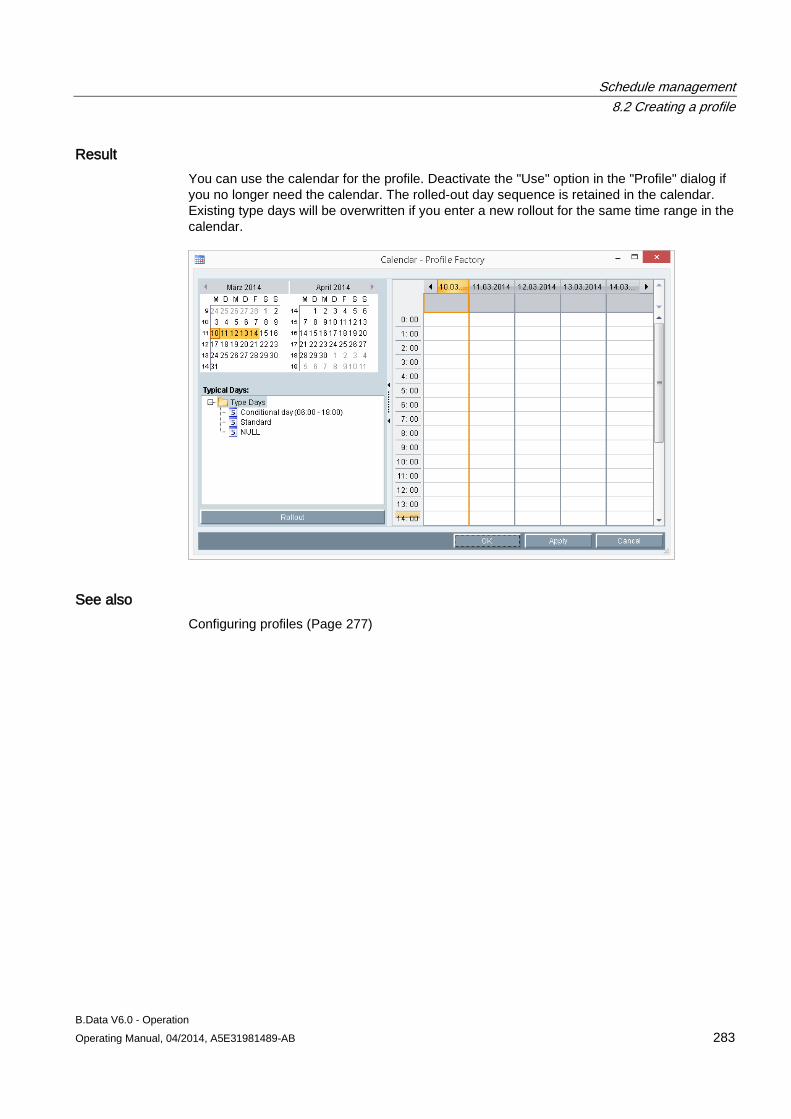
Schedule management 8.2 Creating a profile
B.Data V6.0 - Operation Operating Manual, 04/2014, A5E31981489-AB 283
Result You can use the calendar for the profile. Deactivate the "Use" option in the "Profile" dialog if you no longer need the calendar. The rolled-out day sequence is retained in the calendar. Existing type days will be overwritten if you enter a new rollout for the same time range in the calendar.
See also Configuring profiles (Page 277)
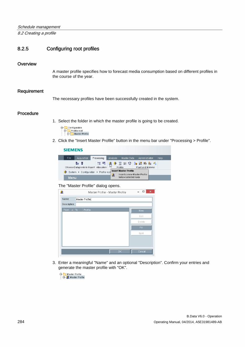
Schedule management 8.2 Creating a profile
B.Data V6.0 - Operation 284 Operating Manual, 04/2014, A5E31981489-AB
8.2.5 Configuring root profiles
Overview A master profile specifies how to forecast media consumption based on different profiles in the course of the year.
Requirement The necessary profiles have been successfully created in the system.
Procedure 1. Select the folder in which the master profile is going to be created.
2. Click the "Insert Master Profile" button in the menu bar under "Processing > Profile".
The "Master Profile" dialog opens.
3. Enter a meaningful "Name" and an optional "Description". Confirm your entries and
generate the master profile with "OK".
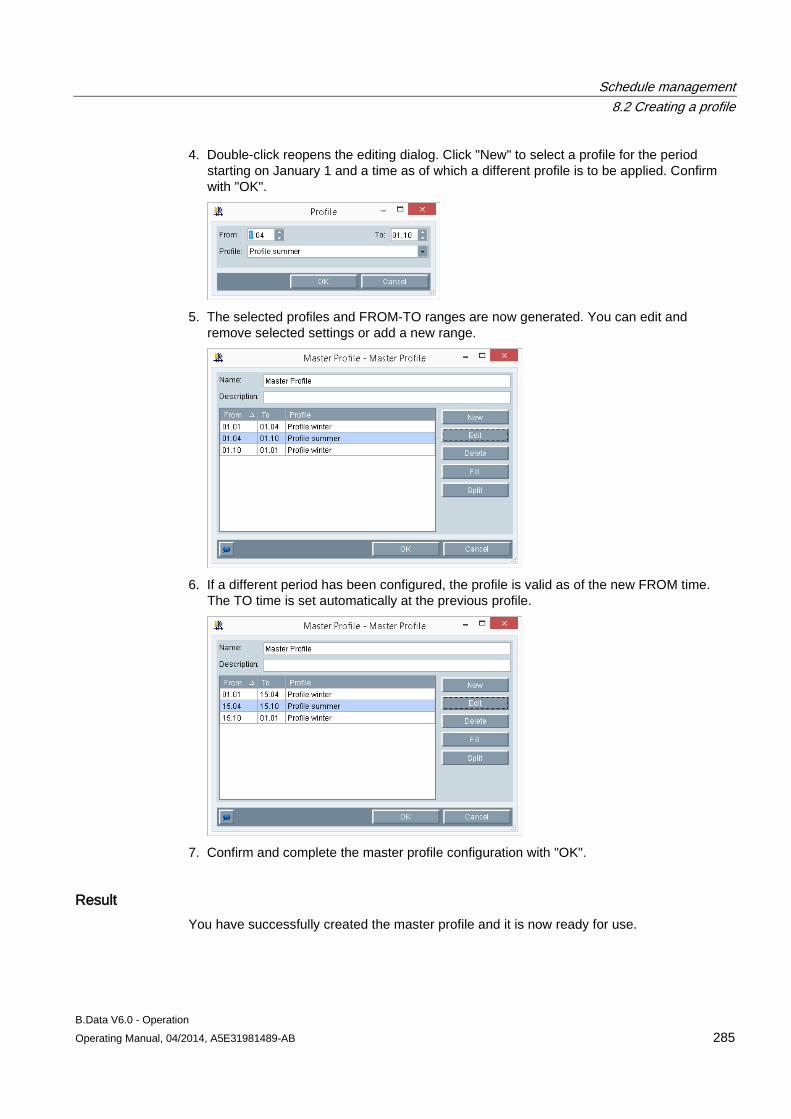
Schedule management 8.2 Creating a profile
B.Data V6.0 - Operation Operating Manual, 04/2014, A5E31981489-AB 285
4. Double-click reopens the editing dialog. Click "New" to select a profile for the period starting on January 1 and a time as of which a different profile is to be applied. Confirm with "OK".
5. The selected profiles and FROM-TO ranges are now generated. You can edit and
remove selected settings or add a new range.
6. If a different period has been configured, the profile is valid as of the new FROM time.
The TO time is set automatically at the previous profile.
7. Confirm and complete the master profile configuration with "OK".
Result You have successfully created the master profile and it is now ready for use.
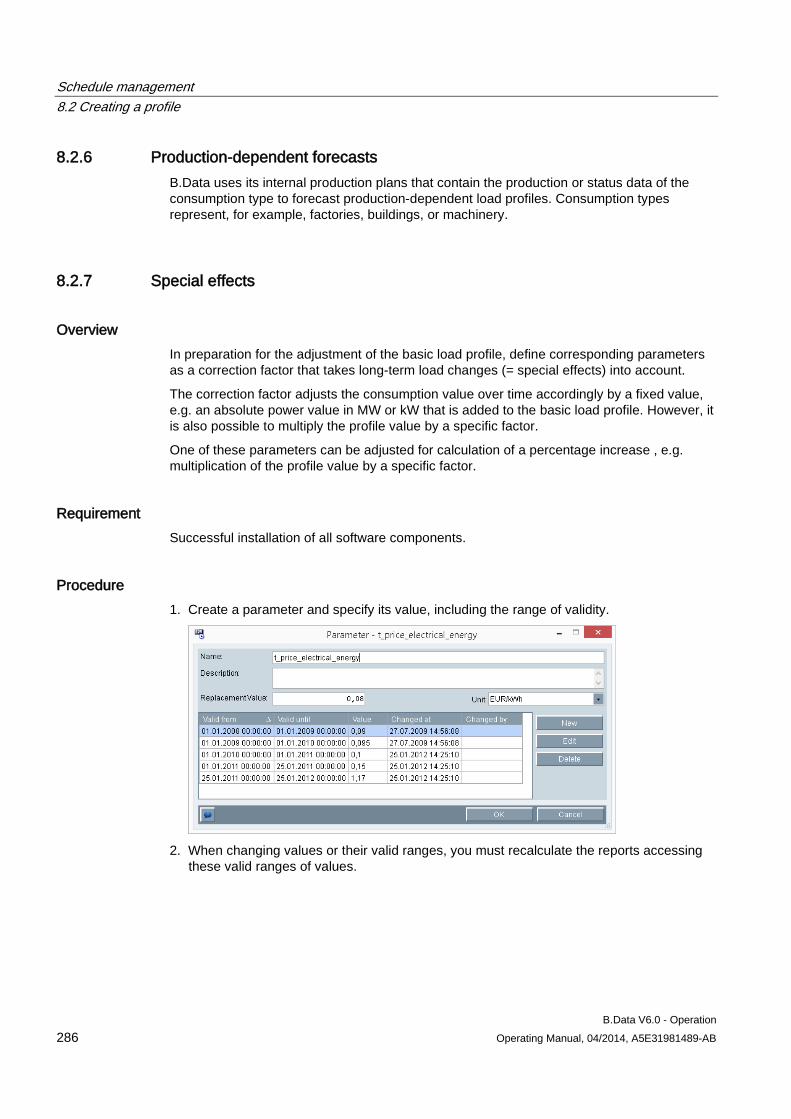
Schedule management 8.2 Creating a profile
B.Data V6.0 - Operation 286 Operating Manual, 04/2014, A5E31981489-AB
8.2.6 Production-dependent forecasts B.Data uses its internal production plans that contain the production or status data of the consumption type to forecast production-dependent load profiles. Consumption types represent, for example, factories, buildings, or machinery.
8.2.7 Special effects
Overview In preparation for the adjustment of the basic load profile, define corresponding parameters as a correction factor that takes long-term load changes (= special effects) into account.
The correction factor adjusts the consumption value over time accordingly by a fixed value, e.g. an absolute power value in MW or kW that is added to the basic load profile. However, it is also possible to multiply the profile value by a specific factor.
One of these parameters can be adjusted for calculation of a percentage increase , e.g. multiplication of the profile value by a specific factor.
Requirement Successful installation of all software components.
Procedure 1. Create a parameter and specify its value, including the range of validity.
2. When changing values or their valid ranges, you must recalculate the reports accessing
these valid ranges of values.
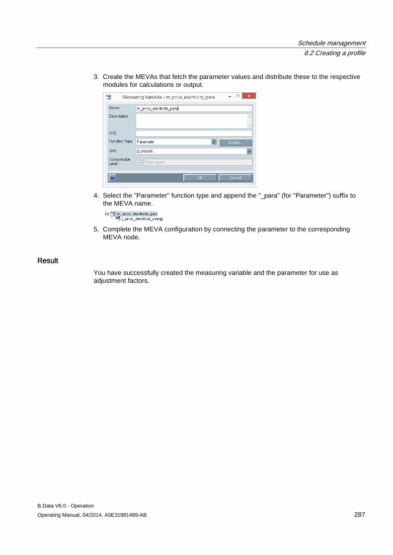
Schedule management 8.2 Creating a profile
B.Data V6.0 - Operation Operating Manual, 04/2014, A5E31981489-AB 287
3. Create the MEVAs that fetch the parameter values and distribute these to the respective modules for calculations or output.
4. Select the "Parameter" function type and append the "_para" (for "Parameter") suffix to
the MEVA name.
5. Complete the MEVA configuration by connecting the parameter to the corresponding
MEVA node.
Result You have successfully created the measuring variable and the parameter for use as adjustment factors.
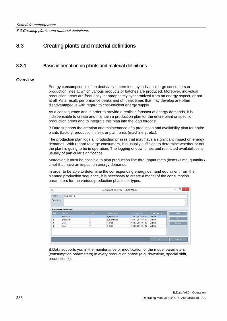
Schedule management 8.3 Creating plants and material definitions
B.Data V6.0 - Operation 288 Operating Manual, 04/2014, A5E31981489-AB
8.3 Creating plants and material definitions
8.3.1 Basic information on plants and material definitions
Overview Energy consumption is often decisively determined by individual large consumers or production lines at which various products or batches are produced. Moreover, individual production areas are frequently inappropriately synchronized from an energy aspect, or not at all. As a result, performance peaks and off peak times that may develop are often disadvantageous with regard to cost-efficient energy supply.
As a consequence and in order to provide a realistic forecast of energy demands, it is indispensable to create and maintain a production plan for the entire plant or specific production areas and to integrate this plan into the load forecast.
B.Data supports the creation and maintenance of a production and availability plan for entire plants (factory, production lines), or plant units (machinery, etc.).
The production plan logs all production phases that may have a significant impact on energy demands. With regard to large consumers, it is usually sufficient to determine whether or not the plant is going to be in operation. The logging of downtimes and restricted availabilities is usually of particular significance.
Moreover, it must be possible to plan production line throughput rates (items / time, quantity / time) that have an impact on energy demands.
In order to be able to determine the corresponding energy demand equivalent from the planned production sequence, it is necessary to create a model of the consumption parameters for the various production phases or types.
B.Data supports you in the maintenance or modification of the model parameters (consumption parameters) in every production phase (e.g. downtime, special shift, production x).
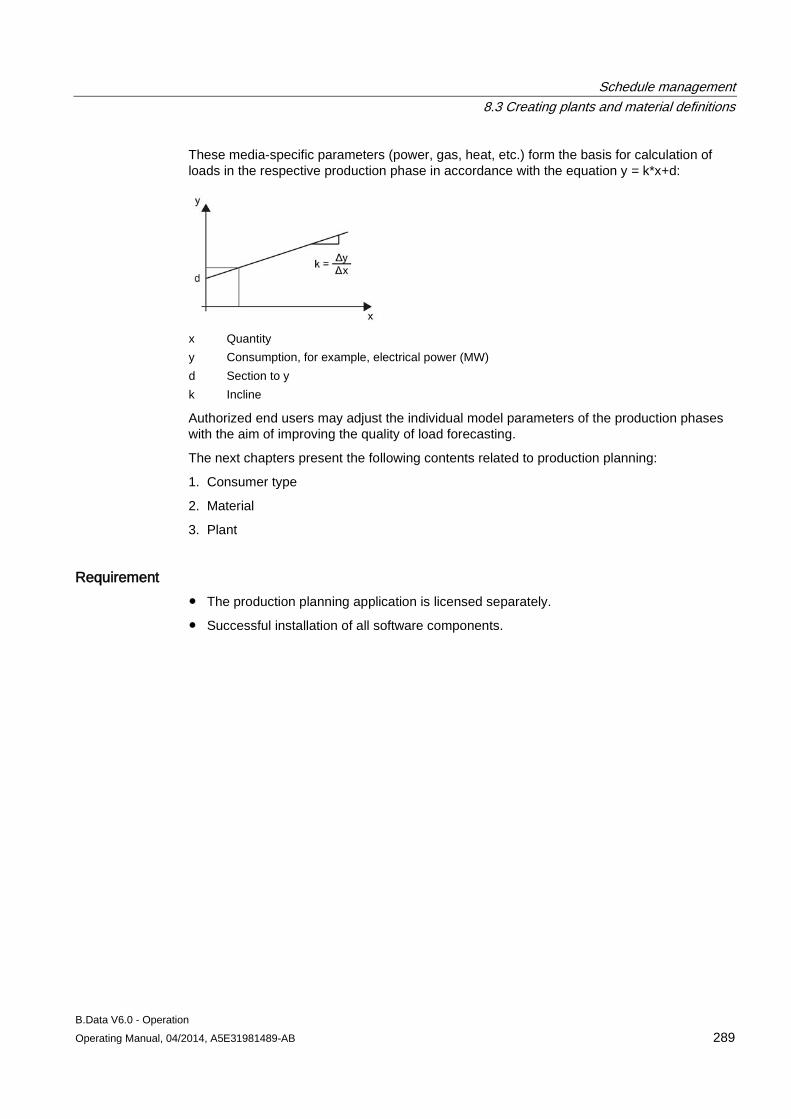
Schedule management 8.3 Creating plants and material definitions
B.Data V6.0 - Operation Operating Manual, 04/2014, A5E31981489-AB 289
These media-specific parameters (power, gas, heat, etc.) form the basis for calculation of loads in the respective production phase in accordance with the equation y = k*x+d:
x Quantity y Consumption, for example, electrical power (MW) d Section to y k Incline
Authorized end users may adjust the individual model parameters of the production phases with the aim of improving the quality of load forecasting.
The next chapters present the following contents related to production planning:
1. Consumer type
2. Material
3. Plant
Requirement ● The production planning application is licensed separately.
● Successful installation of all software components.
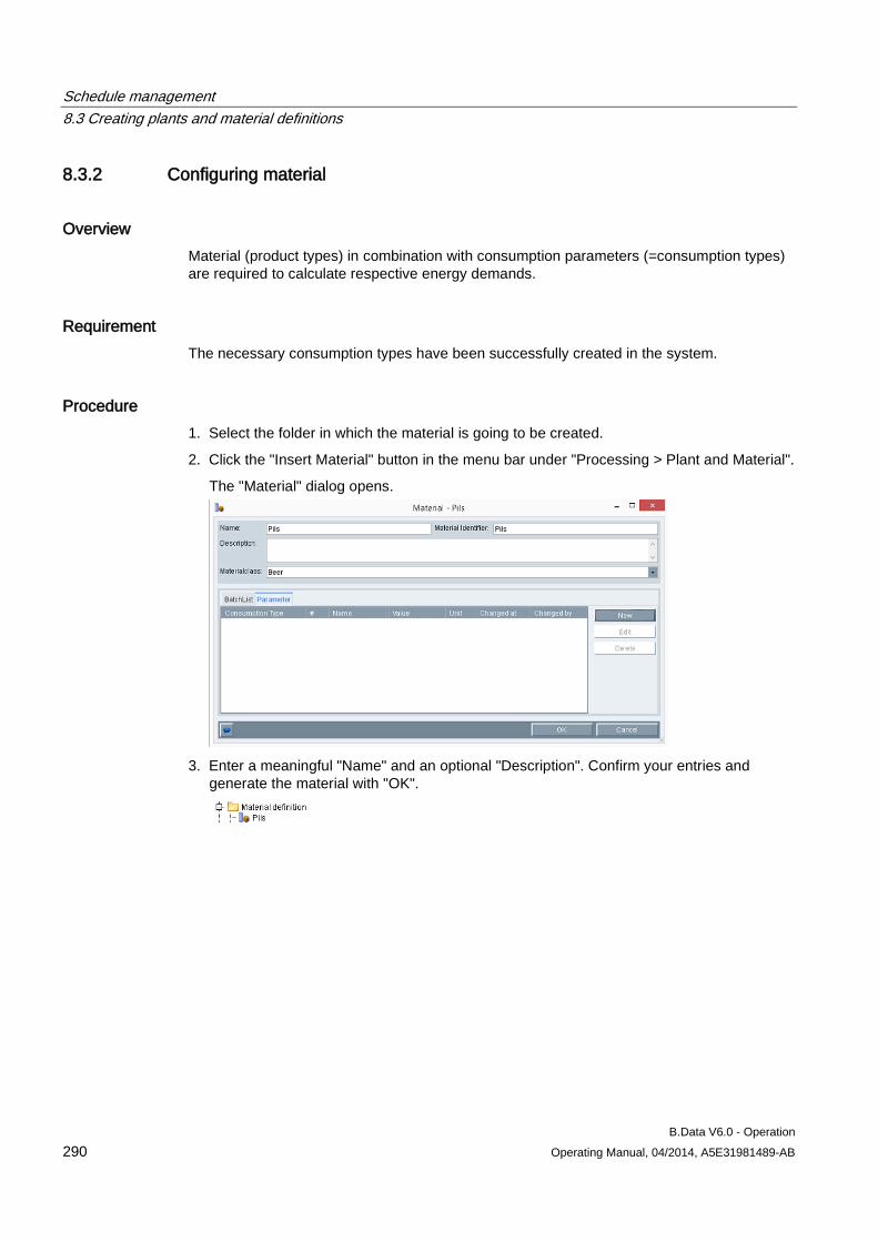
Schedule management 8.3 Creating plants and material definitions
B.Data V6.0 - Operation 290 Operating Manual, 04/2014, A5E31981489-AB
8.3.2 Configuring material
Overview Material (product types) in combination with consumption parameters (=consumption types) are required to calculate respective energy demands.
Requirement The necessary consumption types have been successfully created in the system.
Procedure 1. Select the folder in which the material is going to be created.
2. Click the "Insert Material" button in the menu bar under "Processing > Plant and Material".
The "Material" dialog opens.
3. Enter a meaningful "Name" and an optional "Description". Confirm your entries and
generate the material with "OK".
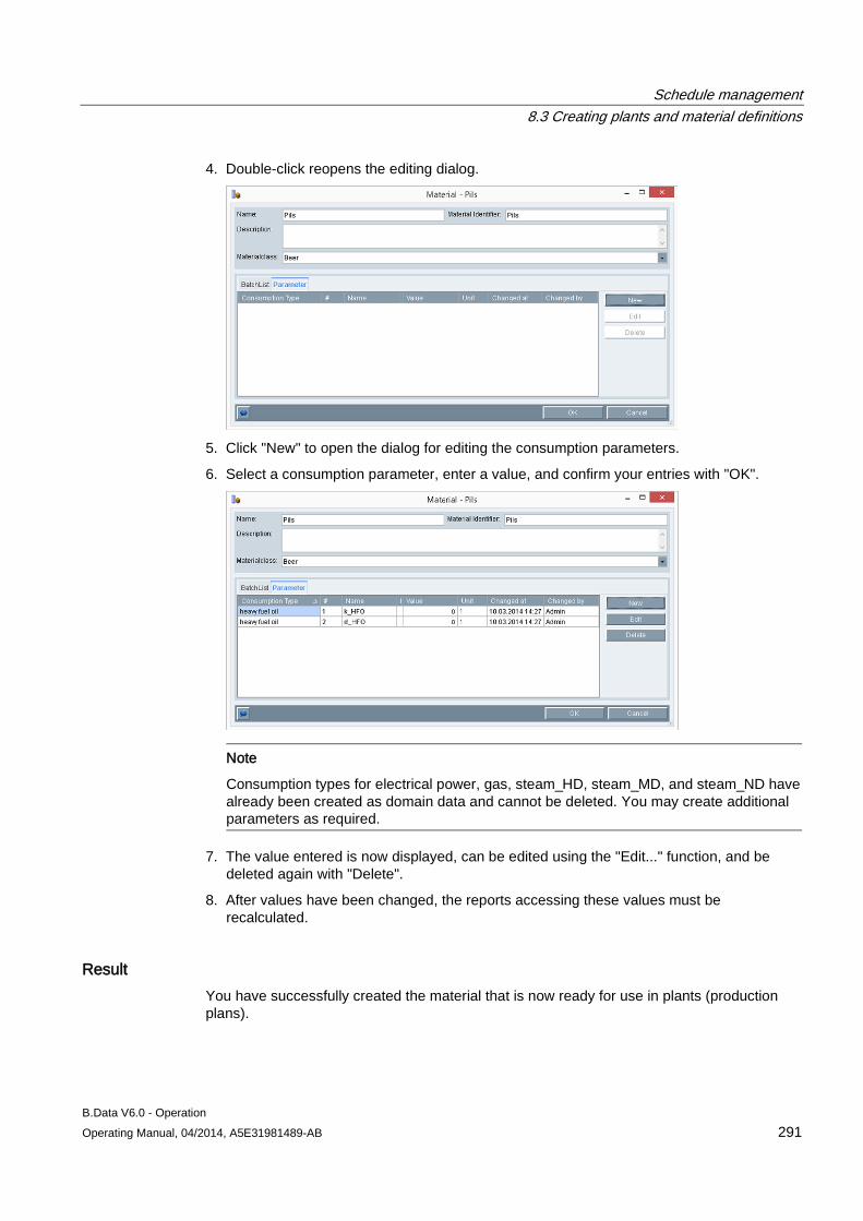
Schedule management 8.3 Creating plants and material definitions
B.Data V6.0 - Operation Operating Manual, 04/2014, A5E31981489-AB 291
4. Double-click reopens the editing dialog.
5. Click "New" to open the dialog for editing the consumption parameters.
6. Select a consumption parameter, enter a value, and confirm your entries with "OK".
Note
Consumption types for electrical power, gas, steam_HD, steam_MD, and steam_ND have already been created as domain data and cannot be deleted. You may create additional parameters as required.
7. The value entered is now displayed, can be edited using the "Edit..." function, and be deleted again with "Delete".
8. After values have been changed, the reports accessing these values must be recalculated.
Result You have successfully created the material that is now ready for use in plants (production plans).
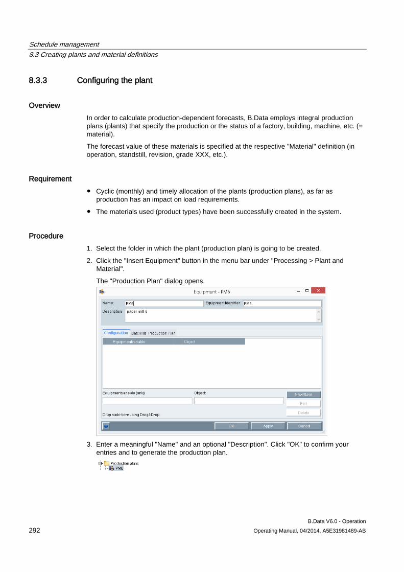
Schedule management 8.3 Creating plants and material definitions
B.Data V6.0 - Operation 292 Operating Manual, 04/2014, A5E31981489-AB
8.3.3 Configuring the plant
Overview In order to calculate production-dependent forecasts, B.Data employs integral production plans (plants) that specify the production or the status of a factory, building, machine, etc. (= material).
The forecast value of these materials is specified at the respective "Material" definition (in operation, standstill, revision, grade XXX, etc.).
Requirement ● Cyclic (monthly) and timely allocation of the plants (production plans), as far as
production has an impact on load requirements.
● The materials used (product types) have been successfully created in the system.
Procedure 1. Select the folder in which the plant (production plan) is going to be created.
2. Click the "Insert Equipment" button in the menu bar under "Processing > Plant and Material".
The "Production Plan" dialog opens.
3. Enter a meaningful "Name" and an optional "Description". Click "OK" to confirm your
entries and to generate the production plan.
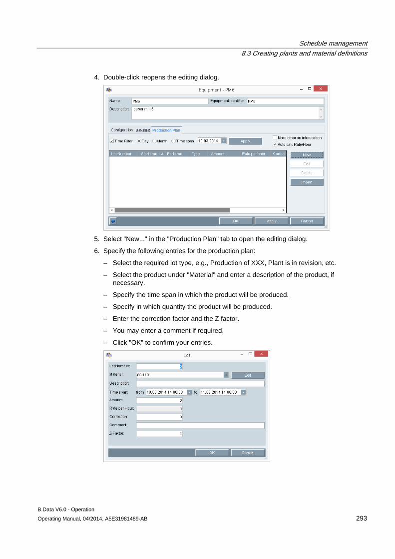
Schedule management 8.3 Creating plants and material definitions
B.Data V6.0 - Operation Operating Manual, 04/2014, A5E31981489-AB 293
4. Double-click reopens the editing dialog.
5. Select "New..." in the "Production Plan" tab to open the editing dialog.
6. Specify the following entries for the production plan:
– Select the required lot type, e.g., Production of XXX, Plant is in revision, etc.
– Select the product under "Material" and enter a description of the product, if necessary.
– Specify the time span in which the product will be produced.
– Specify in which quantity the product will be produced.
– Enter the correction factor and the Z factor.
– You may enter a comment if required.
– Click "OK" to confirm your entries.
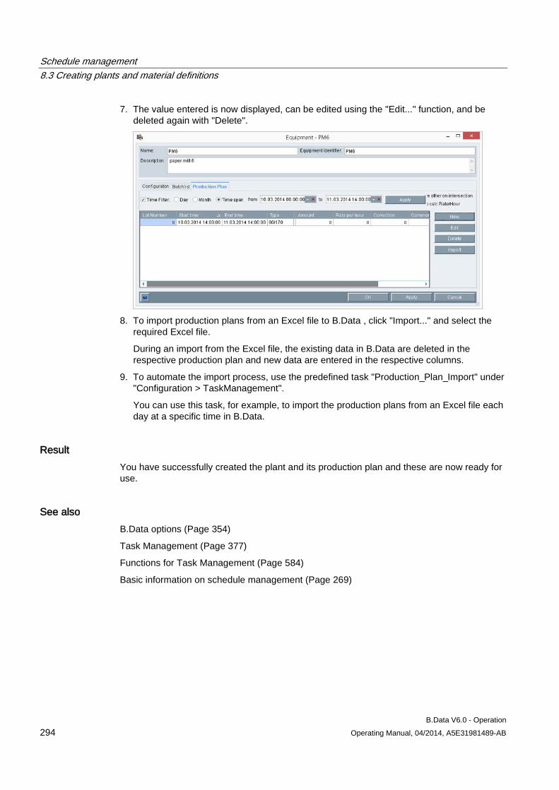
Schedule management 8.3 Creating plants and material definitions
B.Data V6.0 - Operation 294 Operating Manual, 04/2014, A5E31981489-AB
7. The value entered is now displayed, can be edited using the "Edit..." function, and be deleted again with "Delete".
8. To import production plans from an Excel file to B.Data , click "Import..." and select the
required Excel file.
During an import from the Excel file, the existing data in B.Data are deleted in the respective production plan and new data are entered in the respective columns.
9. To automate the import process, use the predefined task "Production_Plan_Import" under "Configuration > TaskManagement".
You can use this task, for example, to import the production plans from an Excel file each day at a specific time in B.Data.
Result You have successfully created the plant and its production plan and these are now ready for use.
See also B.Data options (Page 354)
Task Management (Page 377)
Functions for Task Management (Page 584)
Basic information on schedule management (Page 269)
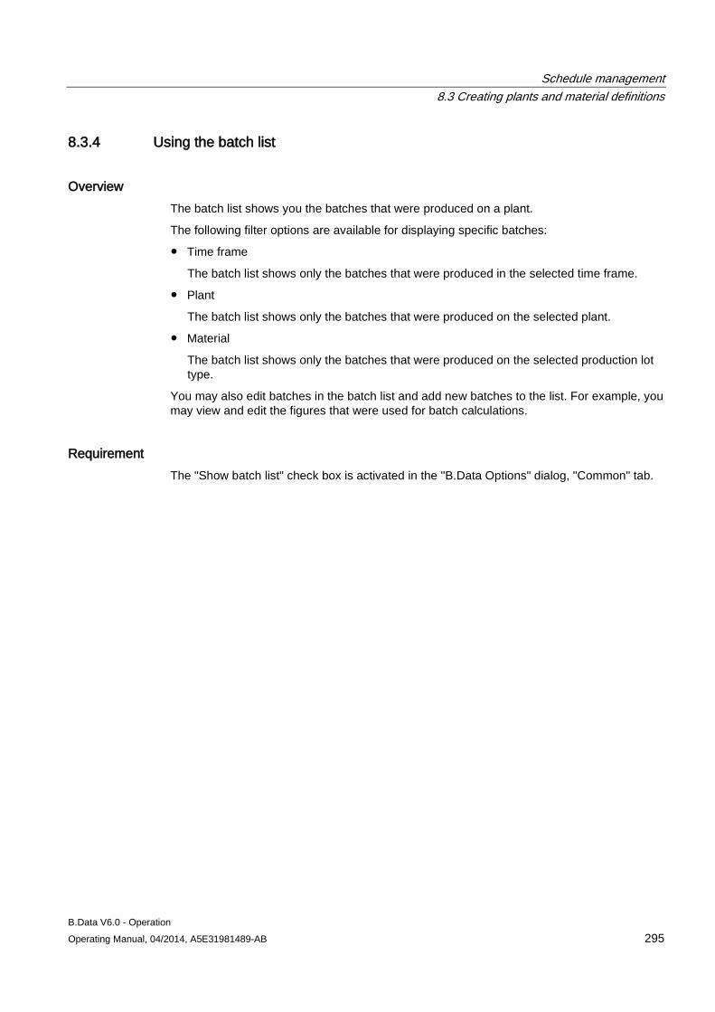
Schedule management 8.3 Creating plants and material definitions
B.Data V6.0 - Operation Operating Manual, 04/2014, A5E31981489-AB 295
8.3.4 Using the batch list
Overview The batch list shows you the batches that were produced on a plant.
The following filter options are available for displaying specific batches:
● Time frame
The batch list shows only the batches that were produced in the selected time frame.
● Plant
The batch list shows only the batches that were produced on the selected plant.
● Material
The batch list shows only the batches that were produced on the selected production lot type.
You may also edit batches in the batch list and add new batches to the list. For example, you may view and edit the figures that were used for batch calculations.
Requirement The "Show batch list" check box is activated in the "B.Data Options" dialog, "Common" tab.
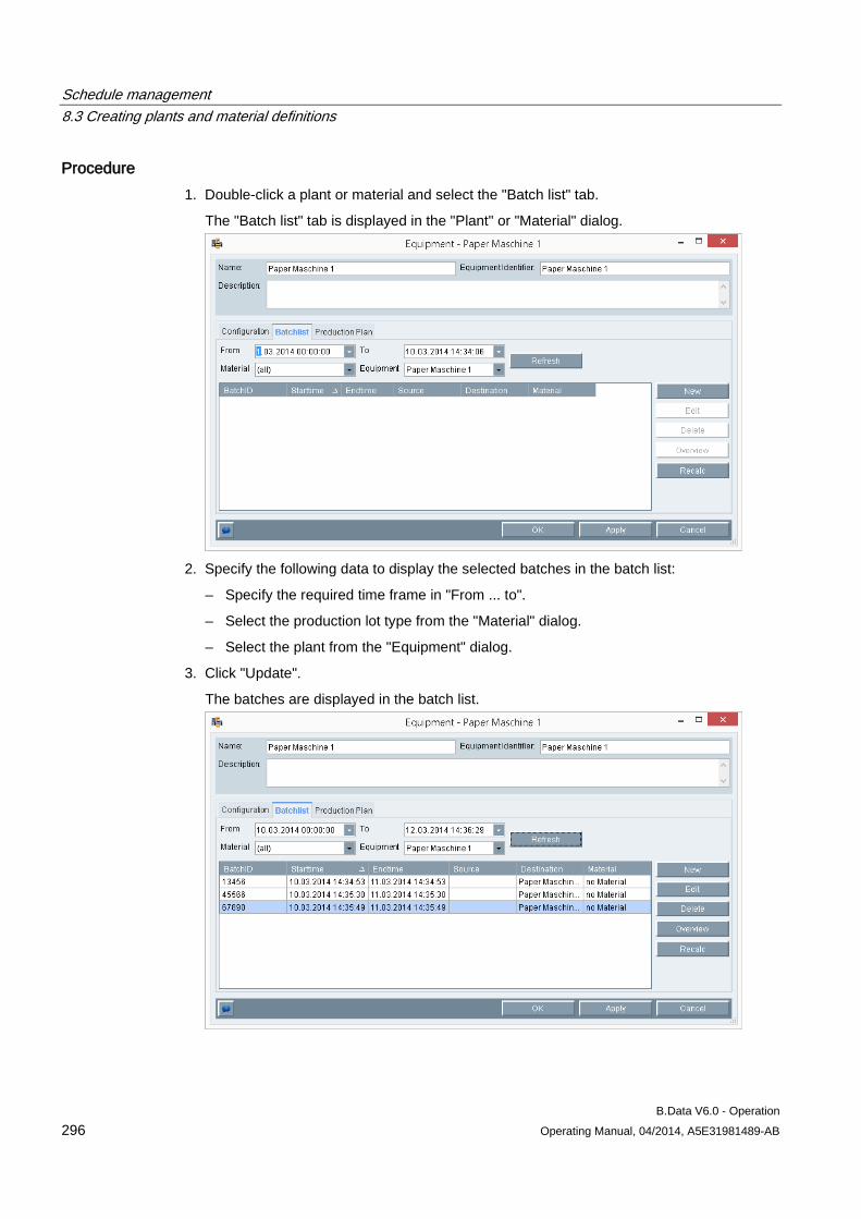
Schedule management 8.3 Creating plants and material definitions
B.Data V6.0 - Operation 296 Operating Manual, 04/2014, A5E31981489-AB
Procedure 1. Double-click a plant or material and select the "Batch list" tab.
The "Batch list" tab is displayed in the "Plant" or "Material" dialog.
2. Specify the following data to display the selected batches in the batch list:
– Specify the required time frame in "From ... to".
– Select the production lot type from the "Material" dialog.
– Select the plant from the "Equipment" dialog.
3. Click "Update".
The batches are displayed in the batch list.
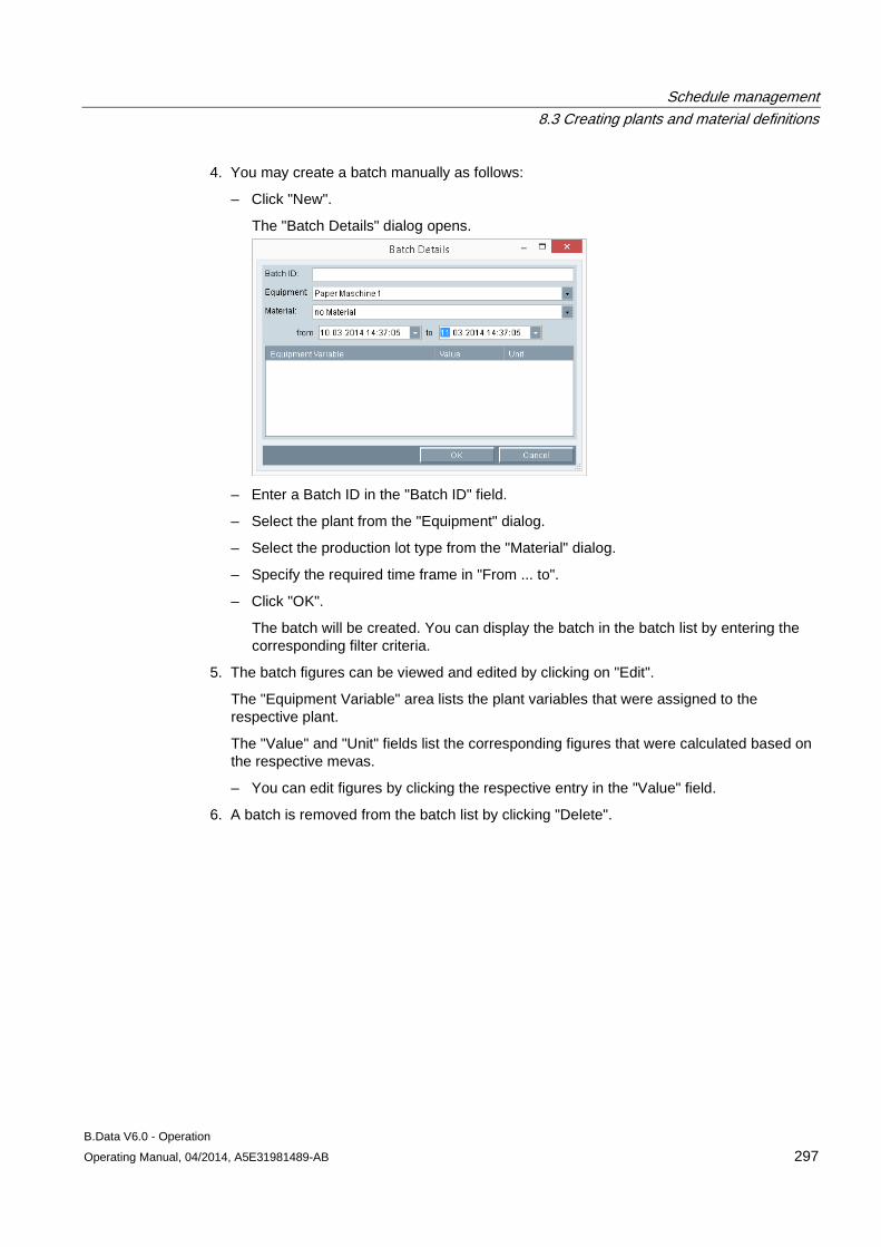
Schedule management 8.3 Creating plants and material definitions
B.Data V6.0 - Operation Operating Manual, 04/2014, A5E31981489-AB 297
4. You may create a batch manually as follows:
– Click "New".
The "Batch Details" dialog opens.
– Enter a Batch ID in the "Batch ID" field.
– Select the plant from the "Equipment" dialog.
– Select the production lot type from the "Material" dialog.
– Specify the required time frame in "From ... to".
– Click "OK".
The batch will be created. You can display the batch in the batch list by entering the corresponding filter criteria.
5. The batch figures can be viewed and edited by clicking on "Edit".
The "Equipment Variable" area lists the plant variables that were assigned to the respective plant.
The "Value" and "Unit" fields list the corresponding figures that were calculated based on the respective mevas.
– You can edit figures by clicking the respective entry in the "Value" field.
6. A batch is removed from the batch list by clicking "Delete".
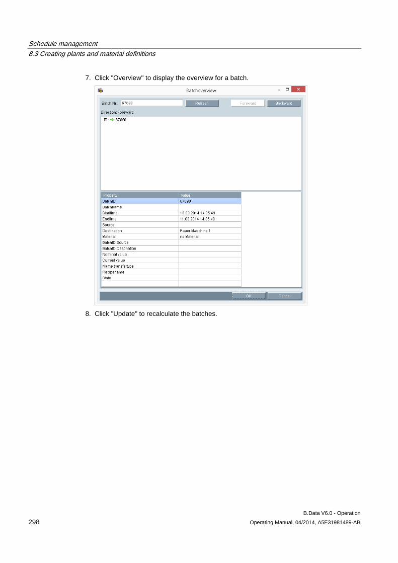
Schedule management 8.3 Creating plants and material definitions
B.Data V6.0 - Operation 298 Operating Manual, 04/2014, A5E31981489-AB
7. Click "Overview" to display the overview for a batch.
8. Click "Update" to recalculate the batches.
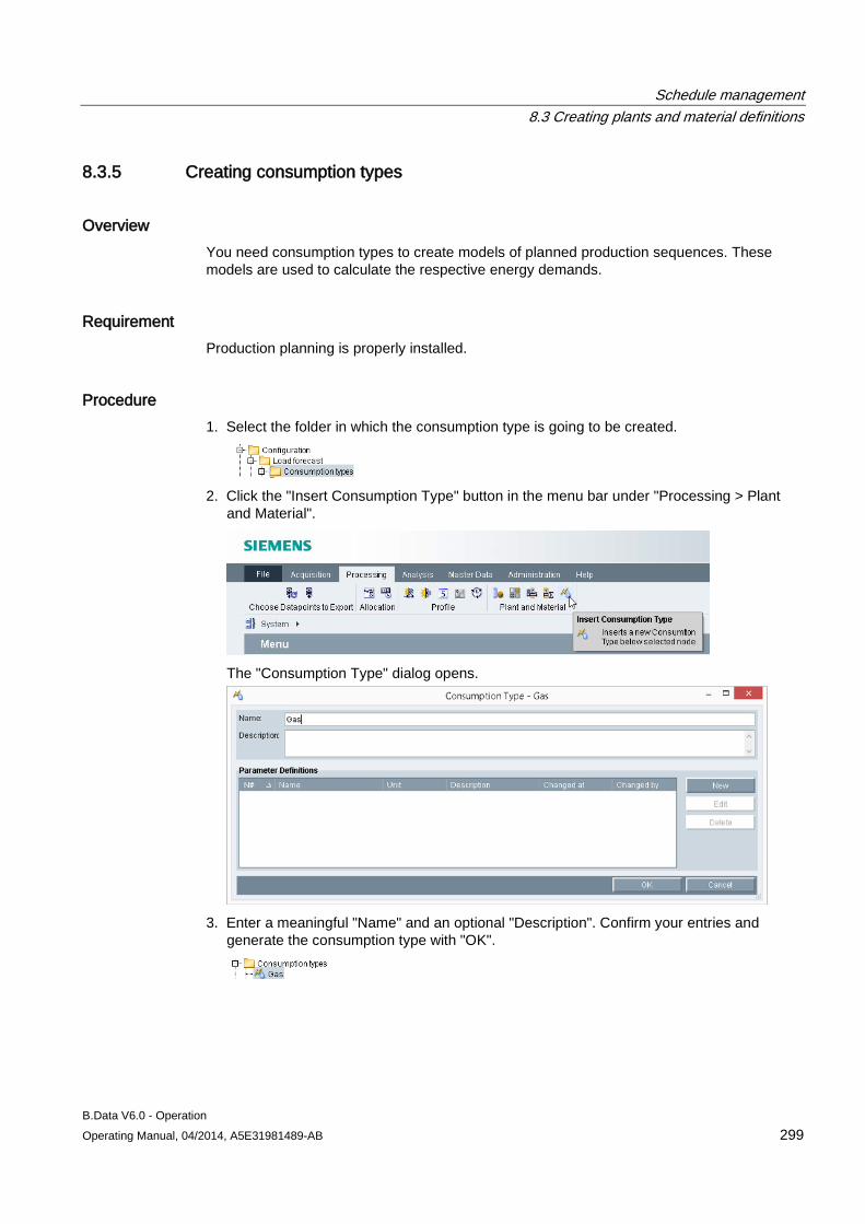
Schedule management 8.3 Creating plants and material definitions
B.Data V6.0 - Operation Operating Manual, 04/2014, A5E31981489-AB 299
8.3.5 Creating consumption types
Overview You need consumption types to create models of planned production sequences. These models are used to calculate the respective energy demands.
Requirement Production planning is properly installed.
Procedure 1. Select the folder in which the consumption type is going to be created.
2. Click the "Insert Consumption Type" button in the menu bar under "Processing > Plant
and Material".
The "Consumption Type" dialog opens.
3. Enter a meaningful "Name" and an optional "Description". Confirm your entries and
generate the consumption type with "OK".
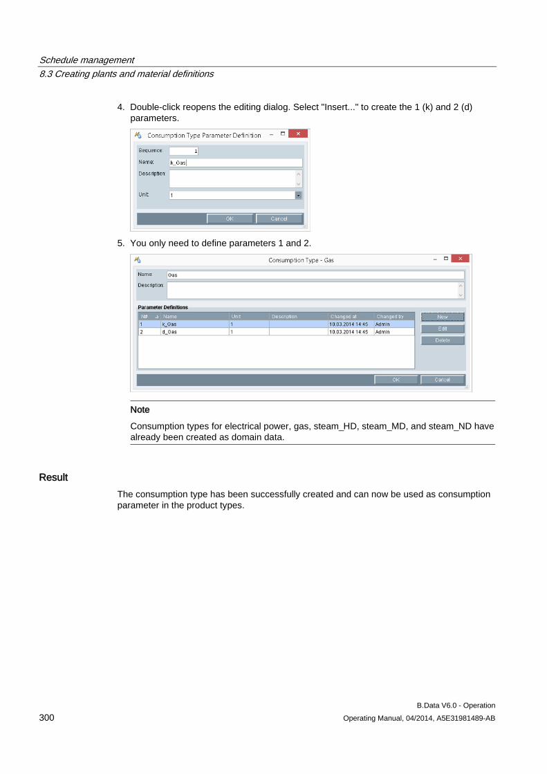
Schedule management 8.3 Creating plants and material definitions
B.Data V6.0 - Operation 300 Operating Manual, 04/2014, A5E31981489-AB
4. Double-click reopens the editing dialog. Select "Insert..." to create the 1 (k) and 2 (d) parameters.
5. You only need to define parameters 1 and 2.
Note
Consumption types for electrical power, gas, steam_HD, steam_MD, and steam_ND have already been created as domain data.
Result The consumption type has been successfully created and can now be used as consumption parameter in the product types.
Schedule management 8.4 Example of schedule management
B.Data V6.0 - Operation Operating Manual, 04/2014, A5E31981489-AB 301
8.4 Example of schedule management
8.4.1 Configuring analysis reports
Overview Analysis reports are used to examine the load progression with regard to a profile. Load distribution is determined for all existing typical days and special days across the evaluation period. The result returns the load profile, for example, of a typical Monday or Tuesday.
If an analysis is performed, for example, for each typical "Monday" in the year, all Mondays will be used for the calculation, except for any holidays or special days that coincide with a Monday. In a year with 48 Mondays, for example, the mean value is calculated for the time window from 00:00 to 01:00 for all Mondays and output as result. The same rule is applied to all other intervals.
Note
Special days that are not created and output as such will corrupt the result, as these would be treated as standard days.
Corrupted values are ignored in the analysis. However, you can force the inclusion of corrupted values with an entry in B.Data options (BDATA_LASTPRF_QS = 0).
After the results have been reviewed and a plausibility check has been completed, the calculated values are written directly to the typical days and special days by starting the report and activating the "save" parameter.
Requirement ● The module with the type "Load profile analysis module type" and a profile with the typical
days and special days to be analyzed have been created.
● The measuring variable for calculating the total load average has been created.
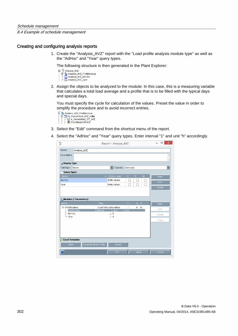
Schedule management 8.4 Example of schedule management
B.Data V6.0 - Operation 302 Operating Manual, 04/2014, A5E31981489-AB
Creating and configuring analysis reports 1. Create the "Analysis_AVZ" report with the "Load profile analysis module type" as well as
the "AdHoc" and "Year" query types.
The following structure is then generated in the Plant Explorer:
2. Assign the objects to be analyzed to the module: In this case, this is a measuring variable
that calculates a total load average and a profile that is to be filled with the typical days and special days.
You must specify the cycle for calculation of the values. Preset the value in order to simplify the procedure and to avoid incorrect entries.
3. Select the "Edit" command from the shortcut menu of the report.
4. Select the "AdHoc" and "Year" query types. Enter interval "1" and unit "h" accordingly.
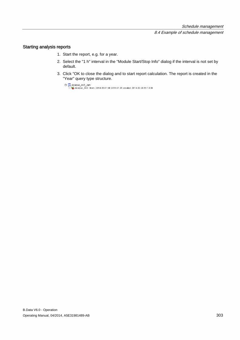
Schedule management 8.4 Example of schedule management
B.Data V6.0 - Operation Operating Manual, 04/2014, A5E31981489-AB 303
Starting analysis reports 1. Start the report, e.g. for a year.
2. Select the "1 h" interval in the "Module Start/Stop Info" dialog if the interval is not set by default.
3. Click "OK to close the dialog and to start report calculation. The report is created in the "Year" query type structure.
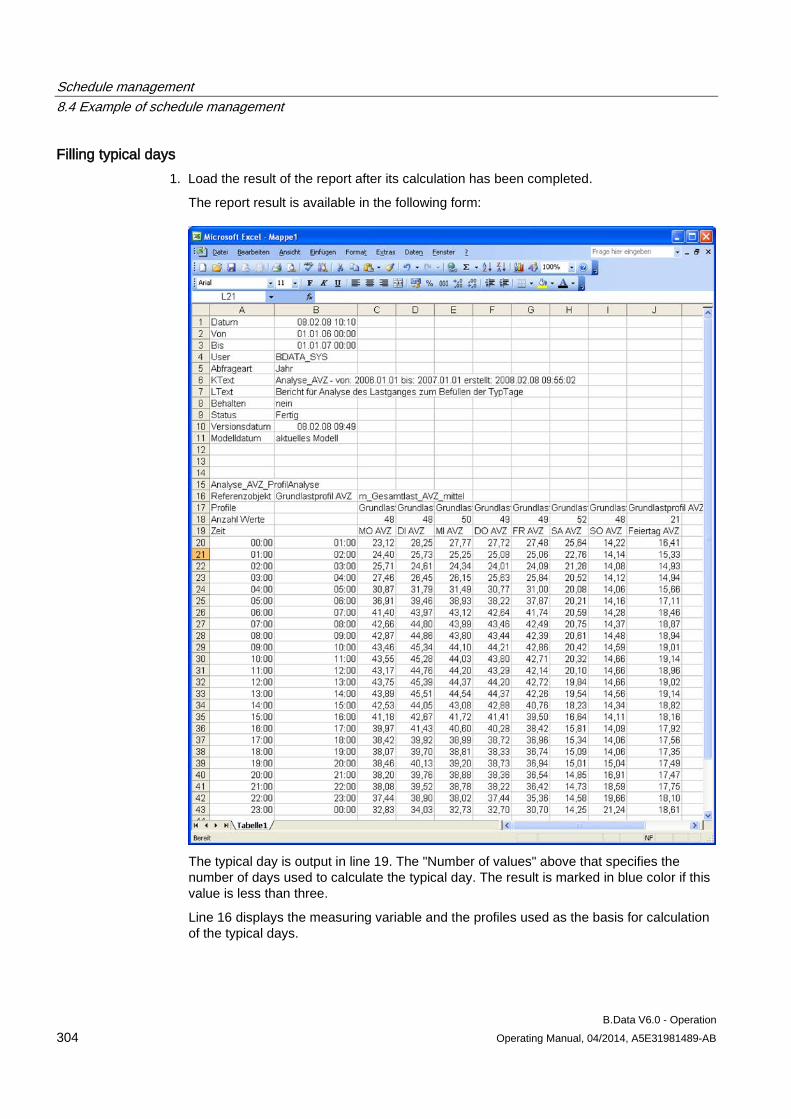
Schedule management 8.4 Example of schedule management
B.Data V6.0 - Operation 304 Operating Manual, 04/2014, A5E31981489-AB
Filling typical days 1. Load the result of the report after its calculation has been completed.
The report result is available in the following form:
The typical day is output in line 19. The "Number of values" above that specifies the number of days used to calculate the typical day. The result is marked in blue color if this value is less than three.
Line 16 displays the measuring variable and the profiles used as the basis for calculation of the typical days.
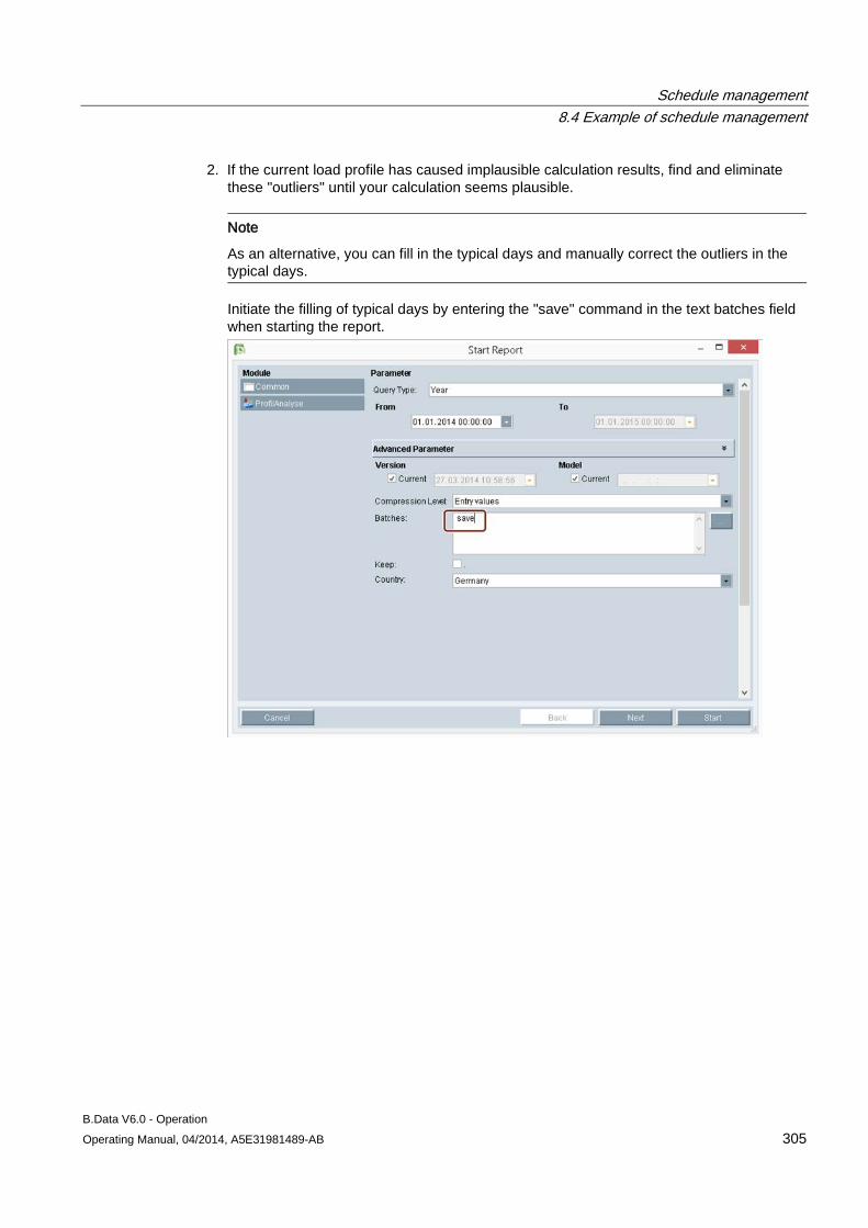
Schedule management 8.4 Example of schedule management
B.Data V6.0 - Operation Operating Manual, 04/2014, A5E31981489-AB 305
2. If the current load profile has caused implausible calculation results, find and eliminate these "outliers" until your calculation seems plausible.
Note
As an alternative, you can fill in the typical days and manually correct the outliers in the typical days.
Initiate the filling of typical days by entering the "save" command in the text batches field when starting the report.
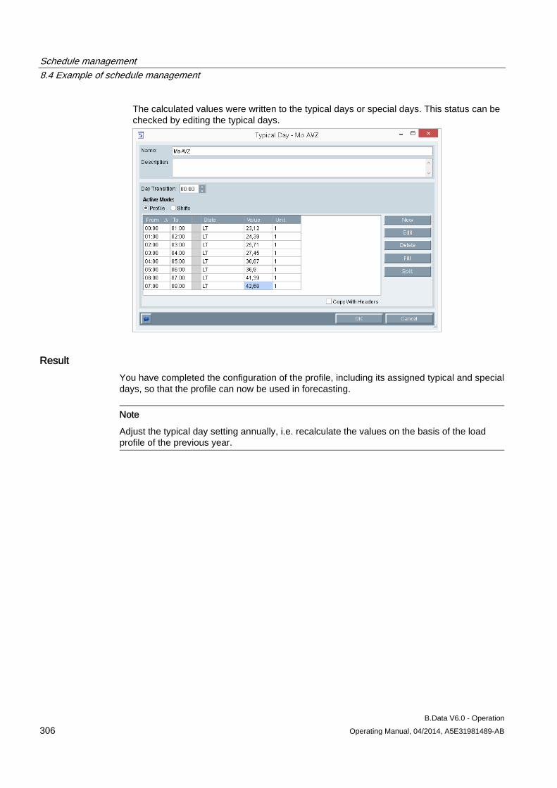
Schedule management 8.4 Example of schedule management
B.Data V6.0 - Operation 306 Operating Manual, 04/2014, A5E31981489-AB
The calculated values were written to the typical days or special days. This status can be checked by editing the typical days.
Result You have completed the configuration of the profile, including its assigned typical and special days, so that the profile can now be used in forecasting.
Note
Adjust the typical day setting annually, i.e. recalculate the values on the basis of the load profile of the previous year.
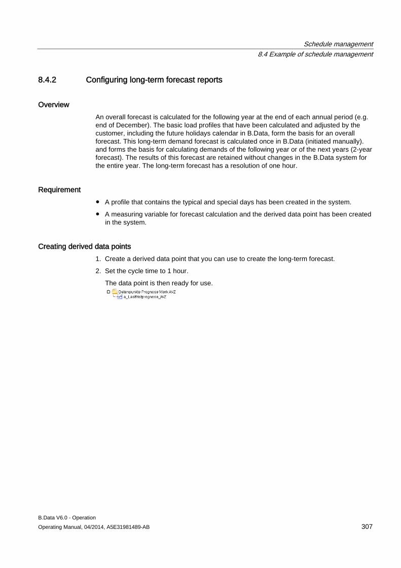
Schedule management 8.4 Example of schedule management
B.Data V6.0 - Operation Operating Manual, 04/2014, A5E31981489-AB 307
8.4.2 Configuring long-term forecast reports
Overview An overall forecast is calculated for the following year at the end of each annual period (e.g. end of December). The basic load profiles that have been calculated and adjusted by the customer, including the future holidays calendar in B.Data, form the basis for an overall forecast. This long-term demand forecast is calculated once in B.Data (initiated manually). and forms the basis for calculating demands of the following year or of the next years (2-year forecast). The results of this forecast are retained without changes in the B.Data system for the entire year. The long-term forecast has a resolution of one hour.
Requirement ● A profile that contains the typical and special days has been created in the system.
● A measuring variable for forecast calculation and the derived data point has been created in the system.
Creating derived data points 1. Create a derived data point that you can use to create the long-term forecast.
2. Set the cycle time to 1 hour.
The data point is then ready for use.
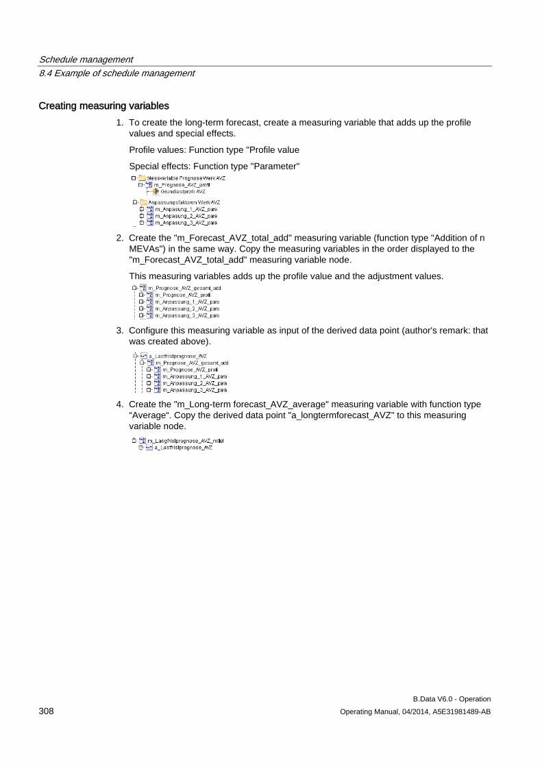
Schedule management 8.4 Example of schedule management
B.Data V6.0 - Operation 308 Operating Manual, 04/2014, A5E31981489-AB
Creating measuring variables 1. To create the long-term forecast, create a measuring variable that adds up the profile
values and special effects.
Profile values: Function type "Profile value
Special effects: Function type "Parameter"
2. Create the "m_Forecast_AVZ_total_add" measuring variable (function type "Addition of n
MEVAs") in the same way. Copy the measuring variables in the order displayed to the "m_Forecast_AVZ_total_add" measuring variable node.
This measuring variables adds up the profile value and the adjustment values.
3. Configure this measuring variable as input of the derived data point (author's remark: that
was created above).
4. Create the "m_Long-term forecast_AVZ_average" measuring variable with function type
“Average“. Copy the derived data point "a_longtermforecast_AVZ" to this measuring variable node.
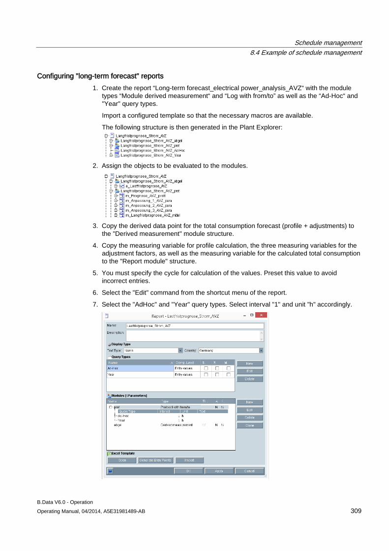
Schedule management 8.4 Example of schedule management
B.Data V6.0 - Operation Operating Manual, 04/2014, A5E31981489-AB 309
Configuring "long-term forecast" reports 1. Create the report “Long-term forecast_electrical power_analysis_AVZ“ with the module
types “Module derived measurement“ and “Log with from/to” as well as the “Ad-Hoc“ and "Year" query types.
Import a configured template so that the necessary macros are available.
The following structure is then generated in the Plant Explorer:
2. Assign the objects to be evaluated to the modules.
3. Copy the derived data point for the total consumption forecast (profile + adjustments) to
the "Derived measurement" module structure.
4. Copy the measuring variable for profile calculation, the three measuring variables for the adjustment factors, as well as the measuring variable for the calculated total consumption to the "Report module" structure.
5. You must specify the cycle for calculation of the values. Preset this value to avoid incorrect entries.
6. Select the "Edit" command from the shortcut menu of the report.
7. Select the "AdHoc" and "Year" query types. Select interval "1" and unit "h" accordingly.
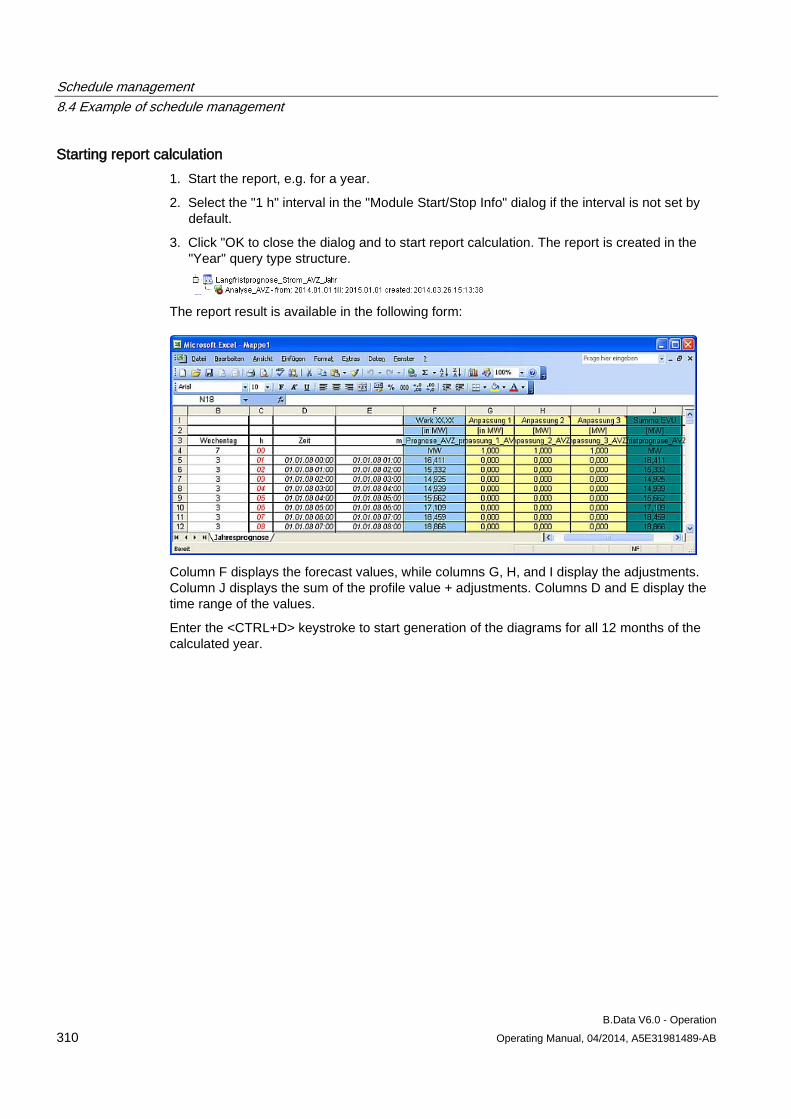
Schedule management 8.4 Example of schedule management
B.Data V6.0 - Operation 310 Operating Manual, 04/2014, A5E31981489-AB
Starting report calculation 1. Start the report, e.g. for a year.
2. Select the "1 h" interval in the "Module Start/Stop Info" dialog if the interval is not set by default.
3. Click "OK to close the dialog and to start report calculation. The report is created in the "Year" query type structure.
The report result is available in the following form:
Column F displays the forecast values, while columns G, H, and I display the adjustments. Column J displays the sum of the profile value + adjustments. Columns D and E display the time range of the values.
Enter the <CTRL+D> keystroke to start generation of the diagrams for all 12 months of the calculated year.
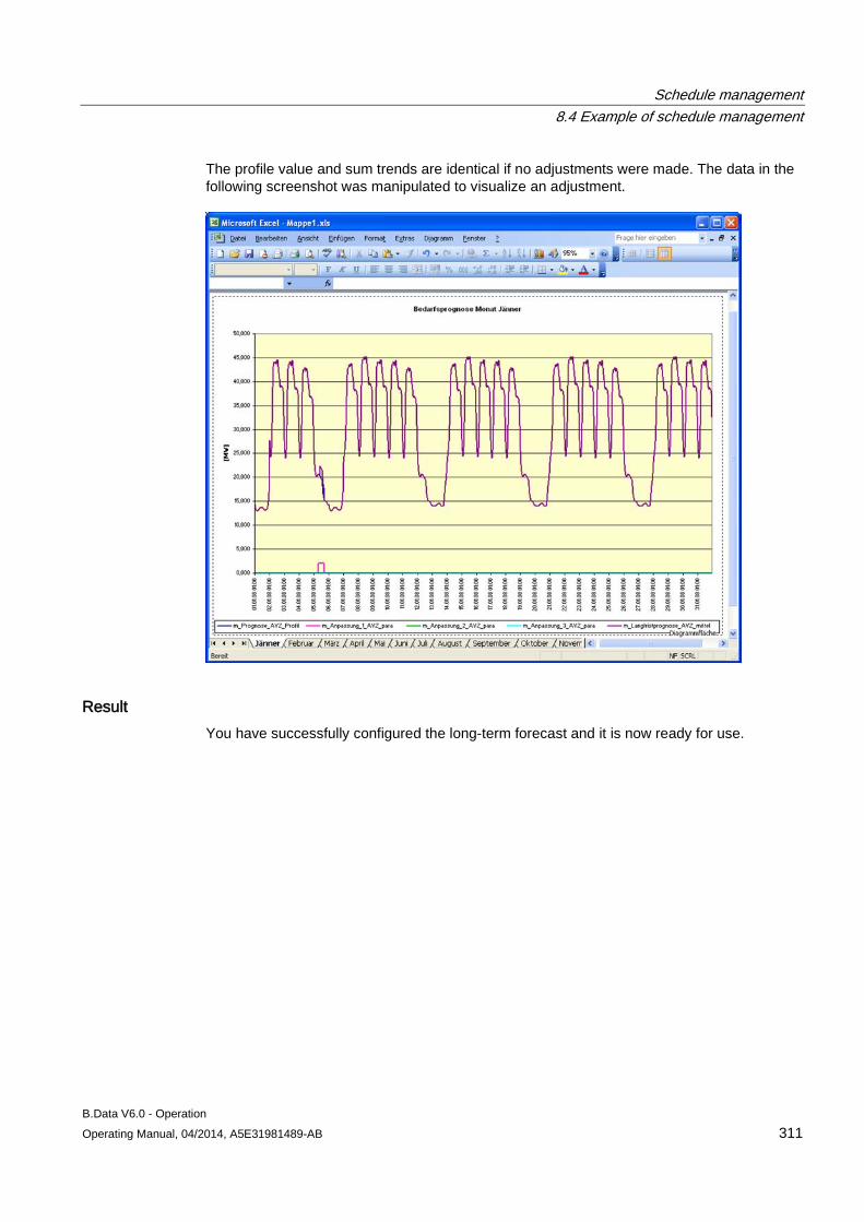
Schedule management 8.4 Example of schedule management
B.Data V6.0 - Operation Operating Manual, 04/2014, A5E31981489-AB 311
The profile value and sum trends are identical if no adjustments were made. The data in the following screenshot was manipulated to visualize an adjustment.
Result You have successfully configured the long-term forecast and it is now ready for use.
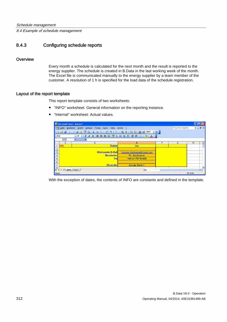
Schedule management 8.4 Example of schedule management
B.Data V6.0 - Operation 312 Operating Manual, 04/2014, A5E31981489-AB
8.4.3 Configuring schedule reports
Overview Every month a schedule is calculated for the next month and the result is reported to the energy supplier. The schedule is created in B.Data in the last working week of the month. The Excel file is communicated manually to the energy supplier by a team member of the customer. A resolution of 1 h is specified for the load data of the schedule registration.
Layout of the report template This report template consists of two worksheets:
● "INFO" worksheet: General information on the reporting instance.
● "Internal" worksheet: Actual values.
With the exception of dates, the contents of INFO are constants and defined in the template.
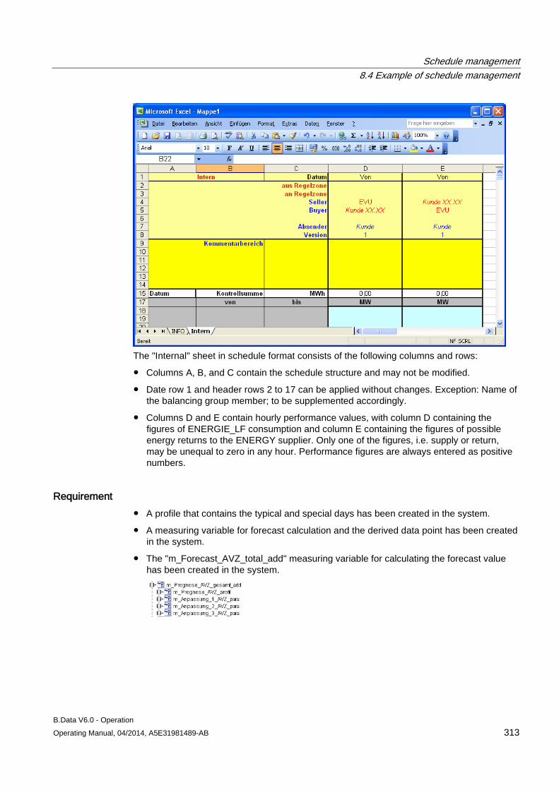
Schedule management 8.4 Example of schedule management
B.Data V6.0 - Operation Operating Manual, 04/2014, A5E31981489-AB 313
The "Internal" sheet in schedule format consists of the following columns and rows:
● Columns A, B, and C contain the schedule structure and may not be modified.
● Date row 1 and header rows 2 to 17 can be applied without changes. Exception: Name of the balancing group member; to be supplemented accordingly.
● Columns D and E contain hourly performance values, with column D containing the figures of ENERGIE_LF consumption and column E containing the figures of possible energy returns to the ENERGY supplier. Only one of the figures, i.e. supply or return, may be unequal to zero in any hour. Performance figures are always entered as positive numbers.
Requirement ● A profile that contains the typical and special days has been created in the system.
● A measuring variable for forecast calculation and the derived data point has been created in the system.
● The "m_Forecast_AVZ_total_add" measuring variable for calculating the forecast value has been created in the system.
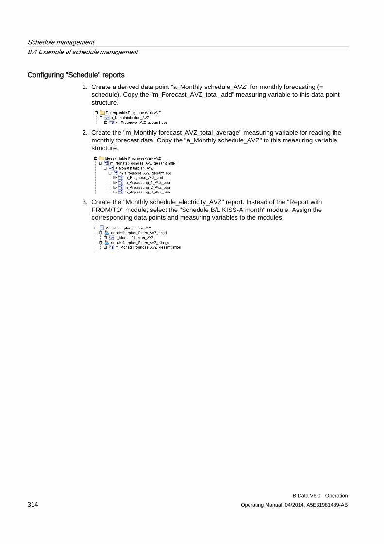
Schedule management 8.4 Example of schedule management
B.Data V6.0 - Operation 314 Operating Manual, 04/2014, A5E31981489-AB
Configuring "Schedule" reports 1. Create a derived data point "a_Monthly schedule_AVZ" for monthly forecasting (=
schedule). Copy the "m_Forecast_AVZ_total_add" measuring variable to this data point structure.
2. Create the "m_Monthly forecast_AVZ_total_average" measuring variable for reading the
monthly forecast data. Copy the "a_Monthly schedule_AVZ" to this measuring variable structure.
3. Create the "Monthly schedule_electricity_AVZ" report. Instead of the "Report with
FROM/TO" module, select the "Schedule B/L KISS-A month" module. Assign the corresponding data points and measuring variables to the modules.
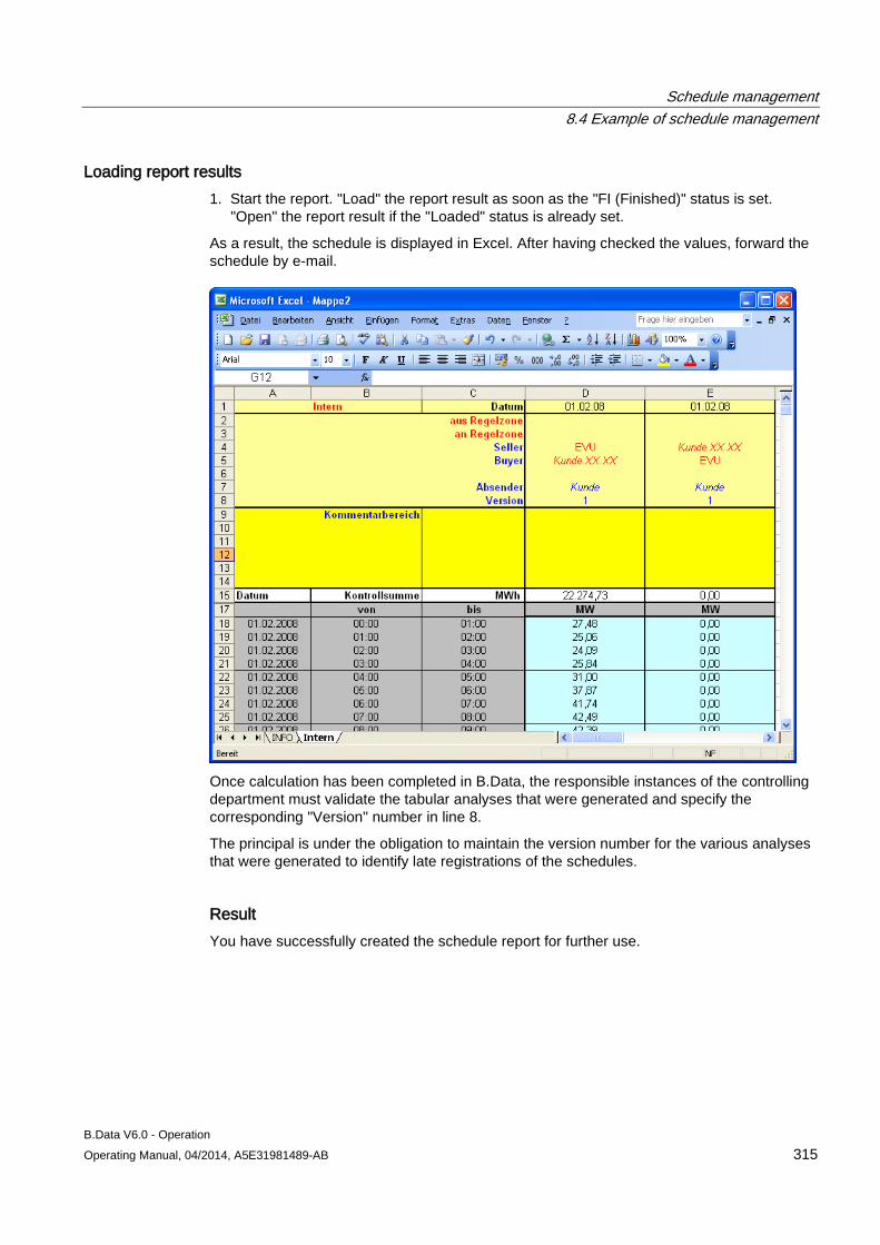
Schedule management 8.4 Example of schedule management
B.Data V6.0 - Operation Operating Manual, 04/2014, A5E31981489-AB 315
Loading report results 1. Start the report. "Load" the report result as soon as the "FI (Finished)" status is set.
"Open" the report result if the "Loaded" status is already set.
As a result, the schedule is displayed in Excel. After having checked the values, forward the schedule by e-mail.
Once calculation has been completed in B.Data, the responsible instances of the controlling department must validate the tabular analyses that were generated and specify the corresponding "Version" number in line 8.
The principal is under the obligation to maintain the version number for the various analyses that were generated to identify late registrations of the schedules.
Result You have successfully created the schedule report for further use.
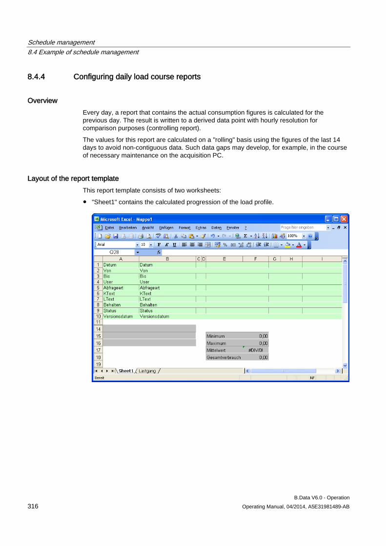
Schedule management 8.4 Example of schedule management
B.Data V6.0 - Operation 316 Operating Manual, 04/2014, A5E31981489-AB
8.4.4 Configuring daily load course reports
Overview Every day, a report that contains the actual consumption figures is calculated for the previous day. The result is written to a derived data point with hourly resolution for comparison purposes (controlling report).
The values for this report are calculated on a "rolling" basis using the figures of the last 14 days to avoid non-contiguous data. Such data gaps may develop, for example, in the course of necessary maintenance on the acquisition PC.
Layout of the report template This report template consists of two worksheets:
● "Sheet1" contains the calculated progression of the load profile.
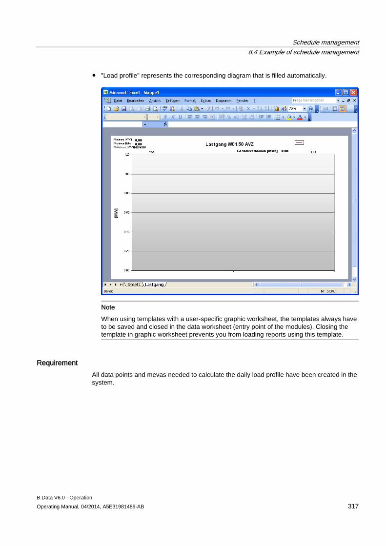
Schedule management 8.4 Example of schedule management
B.Data V6.0 - Operation Operating Manual, 04/2014, A5E31981489-AB 317
● "Load profile" represents the corresponding diagram that is filled automatically.
Note
When using templates with a user-specific graphic worksheet, the templates always have to be saved and closed in the data worksheet (entry point of the modules). Closing the template in graphic worksheet prevents you from loading reports using this template.
Requirement All data points and mevas needed to calculate the daily load profile have been created in the system.
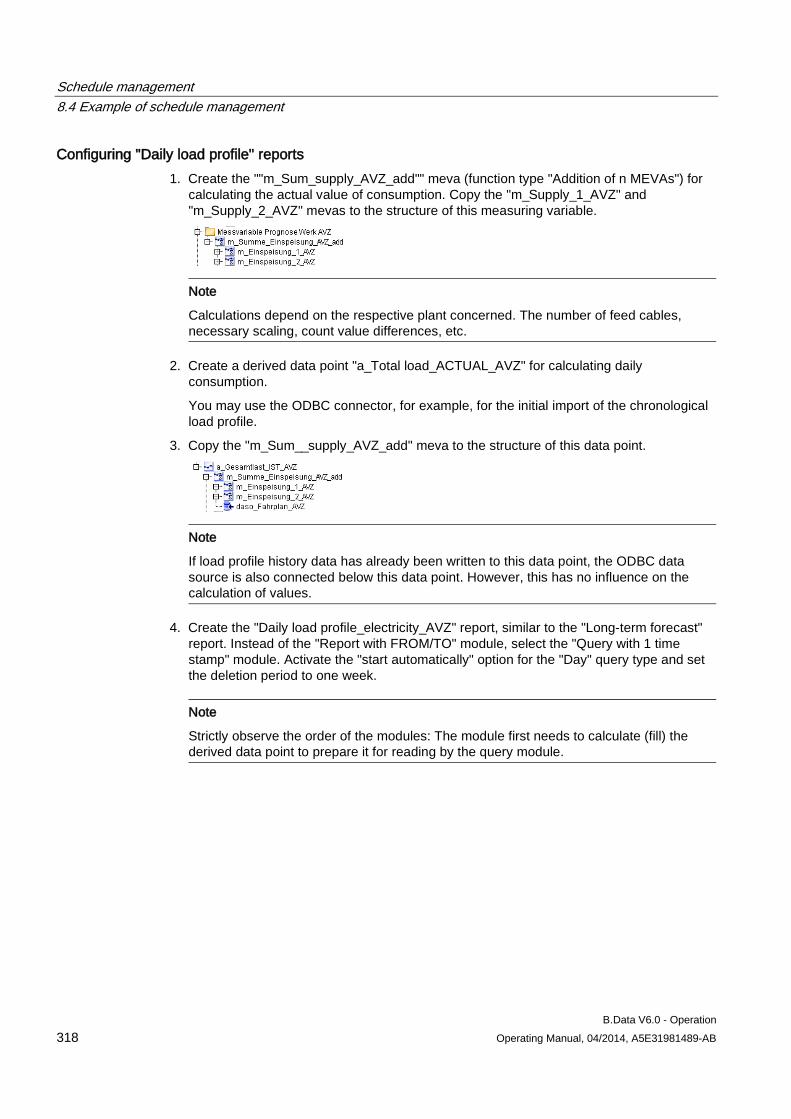
Schedule management 8.4 Example of schedule management
B.Data V6.0 - Operation 318 Operating Manual, 04/2014, A5E31981489-AB
Configuring "Daily load profile" reports 1. Create the ""m_Sum_supply_AVZ_add"" meva (function type "Addition of n MEVAs") for
calculating the actual value of consumption. Copy the "m_Supply_1_AVZ" and "m_Supply_2_AVZ" mevas to the structure of this measuring variable.
Note
Calculations depend on the respective plant concerned. The number of feed cables, necessary scaling, count value differences, etc.
2. Create a derived data point "a_Total load_ACTUAL_AVZ" for calculating daily consumption.
You may use the ODBC connector, for example, for the initial import of the chronological load profile.
3. Copy the "m_Sum__supply_AVZ_add" meva to the structure of this data point.
Note
If load profile history data has already been written to this data point, the ODBC data source is also connected below this data point. However, this has no influence on the calculation of values.
4. Create the "Daily load profile_electricity_AVZ" report, similar to the "Long-term forecast" report. Instead of the "Report with FROM/TO" module, select the "Query with 1 time stamp" module. Activate the "start automatically" option for the "Day" query type and set the deletion period to one week.
Note
Strictly observe the order of the modules: The module first needs to calculate (fill) the derived data point to prepare it for reading by the query module.
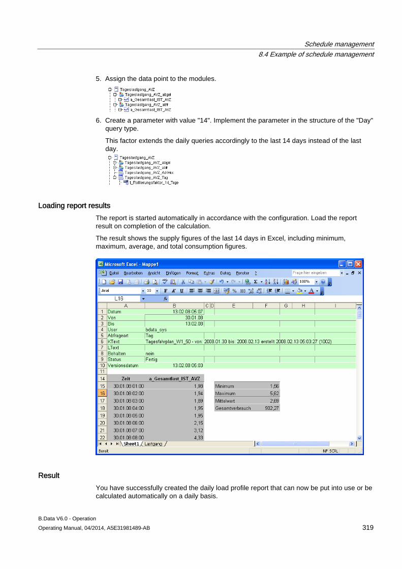
Schedule management 8.4 Example of schedule management
B.Data V6.0 - Operation Operating Manual, 04/2014, A5E31981489-AB 319
5. Assign the data point to the modules.
6. Create a parameter with value "14". Implement the parameter in the structure of the "Day"
query type.
This factor extends the daily queries accordingly to the last 14 days instead of the last day.
Loading report results The report is started automatically in accordance with the configuration. Load the report result on completion of the calculation.
The result shows the supply figures of the last 14 days in Excel, including minimum, maximum, average, and total consumption figures.
Result You have successfully created the daily load profile report that can now be put into use or be calculated automatically on a daily basis.
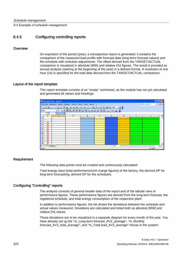
Schedule management 8.4 Example of schedule management
B.Data V6.0 - Operation 320 Operating Manual, 04/2014, A5E31981489-AB
8.4.5 Configuring controlling reports
Overview On expiration of the period (year), a retrospective report is generated; it contains the comparison of the measured load profile with forecast data (long-term forecast values) and the schedule with schedule adjustments. The offset derived from the TARGET/ACTUAL comparison is visualized in absolute (MW) and relative (%) figures. The result is provided as annual analysis (starting at the beginning of the year) in a defined format. A resolution of one hour (1h) is specified for the load data derived from the TARGET/ACTUAL comparison.
Layout of the report template This report template consists of an "empty" worksheet, as the module has not yet calculated and generated all values and headings.
Requirement The following data points must be created and continuously calculated:
Total energy input (total performance/unit charge figures) of the factory, the derived DP for long-term forecasting, derived DP for the schedules.
Configuring "Controlling" reports The analysis consists of general header data of the report and of the tabular view of performance figures. These performance figures are derived from the long-term forecast, the registered schedule, and total energy consumption of the respective plant.
In addition to performance figures, the list shows the deviations between the schedule and actual values measured. Deviations are calculated and listed both as absolute [MW] and relative [%] values.
These deviations are to be visualized in a separate diagram for every month of the year. You have already set up the "m_Long-term forecast_AVZ_average", "m_Monthly forecast_AVZ_total_average", and "m_Total load_AVZ_average" mevas in the system:
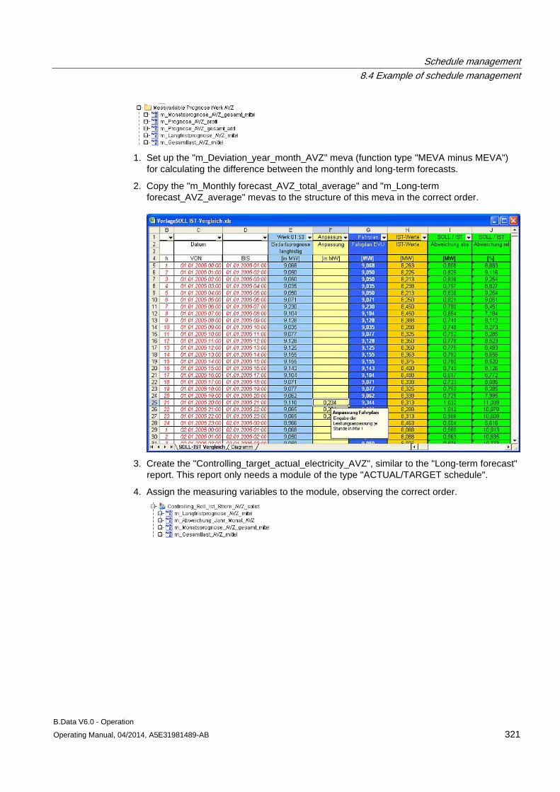
Schedule management 8.4 Example of schedule management
B.Data V6.0 - Operation Operating Manual, 04/2014, A5E31981489-AB 321
1. Set up the "m_Deviation_year_month_AVZ" meva (function type "MEVA minus MEVA")
for calculating the difference between the monthly and long-term forecasts.
2. Copy the "m_Monthly forecast_AVZ_total_average" and "m_Long-term forecast_AVZ_average" mevas to the structure of this meva in the correct order.
3. Create the "Controlling_target_actual_electricity_AVZ", similar to the "Long-term forecast"
report. This report only needs a module of the type "ACTUAL/TARGET schedule".
4. Assign the measuring variables to the module, observing the correct order.
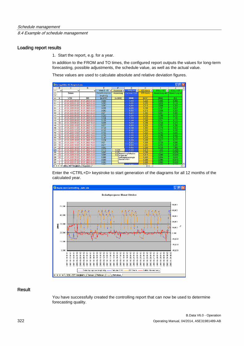
Schedule management 8.4 Example of schedule management
B.Data V6.0 - Operation 322 Operating Manual, 04/2014, A5E31981489-AB
Loading report results 1. Start the report, e.g. for a year.
In addition to the FROM and TO times, the configured report outputs the values for long-term forecasting, possible adjustments, the schedule value, as well as the actual value.
These values are used to calculate absolute and relative deviation figures.
Enter the <CTRL+D> keystroke to start generation of the diagrams for all 12 months of the calculated year.
Result You have successfully created the controlling report that can now be used to determine forecasting quality.
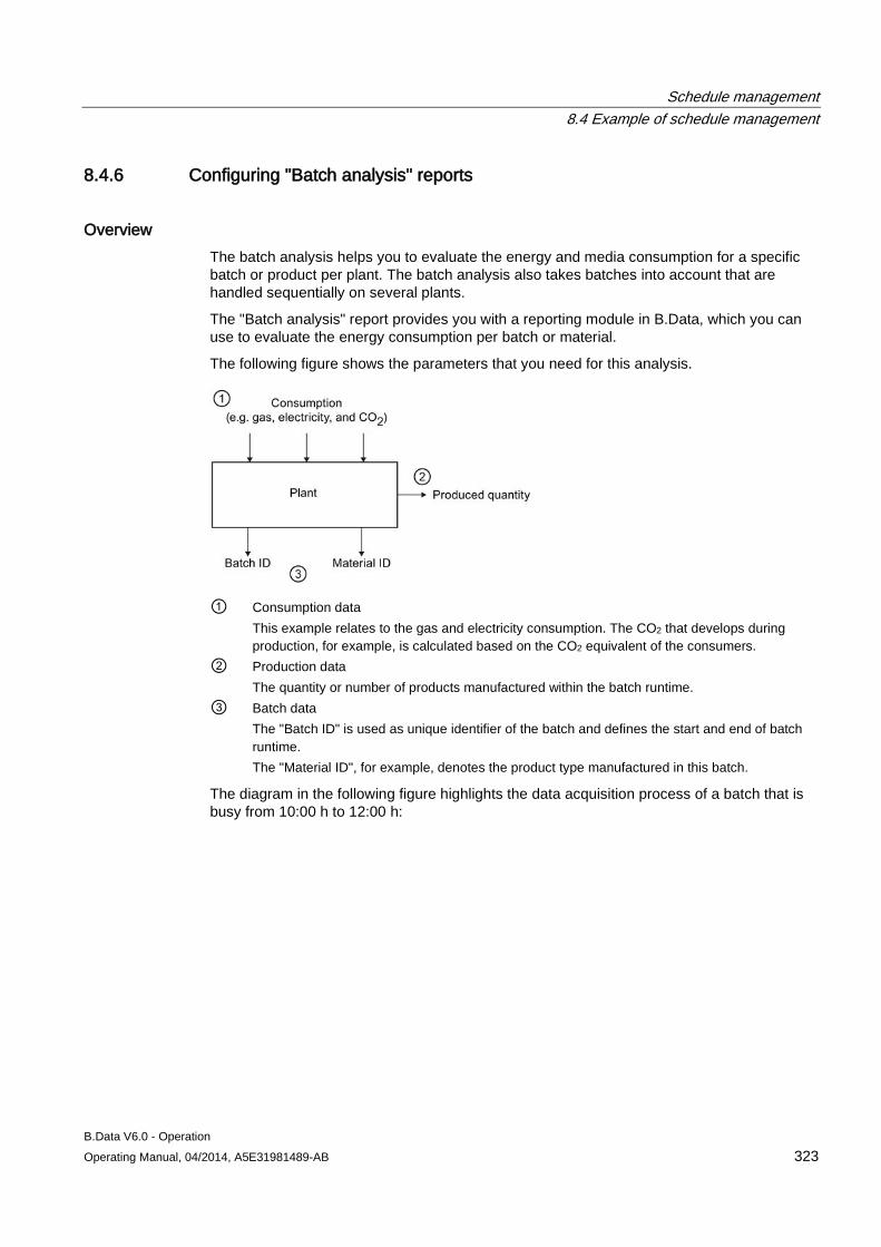
Schedule management 8.4 Example of schedule management
B.Data V6.0 - Operation Operating Manual, 04/2014, A5E31981489-AB 323
8.4.6 Configuring "Batch analysis" reports
Overview The batch analysis helps you to evaluate the energy and media consumption for a specific batch or product per plant. The batch analysis also takes batches into account that are handled sequentially on several plants.
The "Batch analysis" report provides you with a reporting module in B.Data, which you can use to evaluate the energy consumption per batch or material.
The following figure shows the parameters that you need for this analysis.
① Consumption data
This example relates to the gas and electricity consumption. The CO2 that develops during production, for example, is calculated based on the CO2 equivalent of the consumers.
② Production data The quantity or number of products manufactured within the batch runtime.
③ Batch data The "Batch ID" is used as unique identifier of the batch and defines the start and end of batch runtime. The "Material ID", for example, denotes the product type manufactured in this batch.
The diagram in the following figure highlights the data acquisition process of a batch that is busy from 10:00 h to 12:00 h:
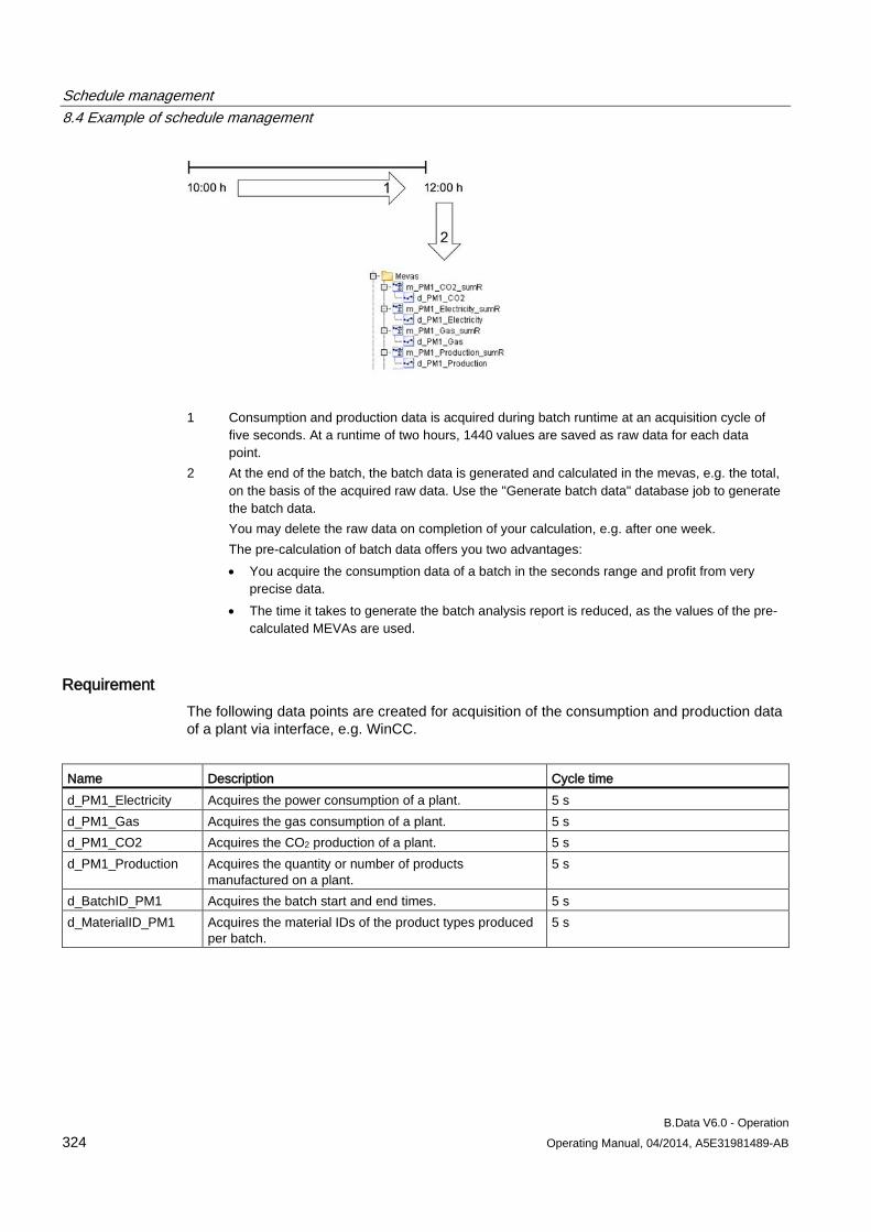
Schedule management 8.4 Example of schedule management
B.Data V6.0 - Operation 324 Operating Manual, 04/2014, A5E31981489-AB
1 Consumption and production data is acquired during batch runtime at an acquisition cycle of
five seconds. At a runtime of two hours, 1440 values are saved as raw data for each data point.
2 At the end of the batch, the batch data is generated and calculated in the mevas, e.g. the total, on the basis of the acquired raw data. Use the "Generate batch data" database job to generate the batch data. You may delete the raw data on completion of your calculation, e.g. after one week. The pre-calculation of batch data offers you two advantages: • You acquire the consumption data of a batch in the seconds range and profit from very
precise data. • The time it takes to generate the batch analysis report is reduced, as the values of the pre-
calculated MEVAs are used.
Requirement The following data points are created for acquisition of the consumption and production data of a plant via interface, e.g. WinCC.
Name Description Cycle time d_PM1_Electricity Acquires the power consumption of a plant. 5 s d_PM1_Gas Acquires the gas consumption of a plant. 5 s d_PM1_CO2 Acquires the CO2 production of a plant. 5 s d_PM1_Production Acquires the quantity or number of products
manufactured on a plant. 5 s
d_BatchID_PM1 Acquires the batch start and end times. 5 s d_MaterialID_PM1 Acquires the material IDs of the product types produced
per batch. 5 s
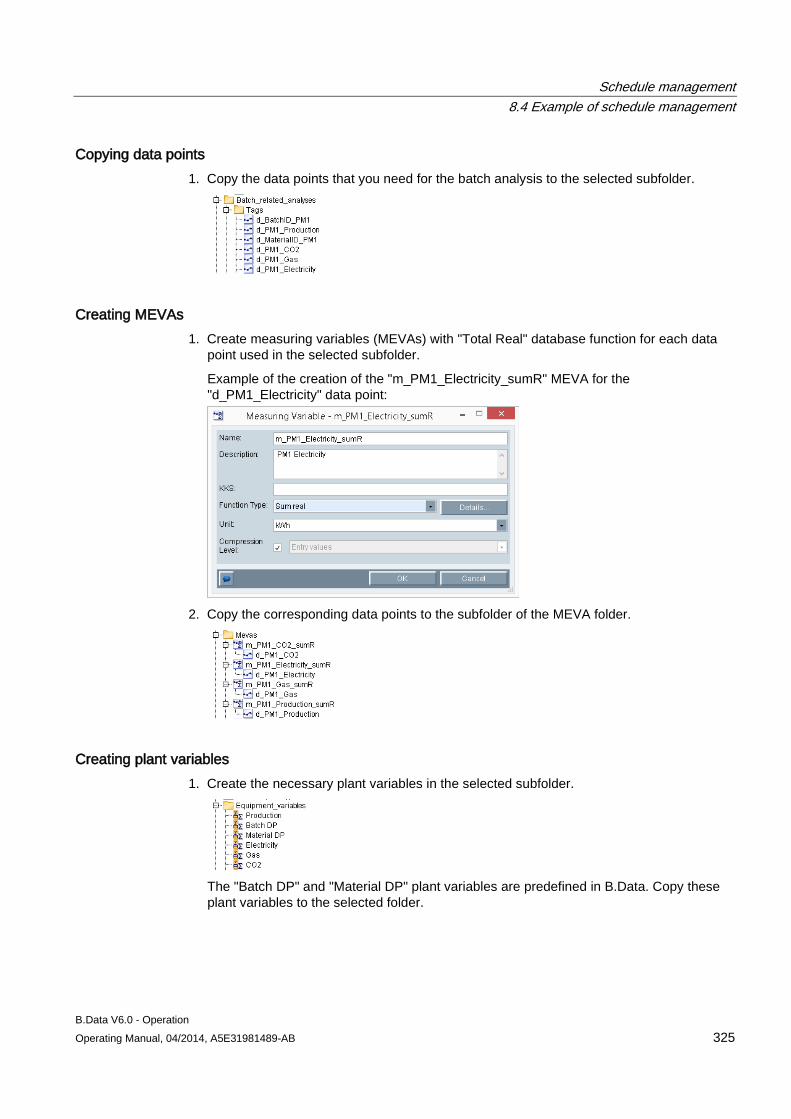
Schedule management 8.4 Example of schedule management
B.Data V6.0 - Operation Operating Manual, 04/2014, A5E31981489-AB 325
Copying data points 1. Copy the data points that you need for the batch analysis to the selected subfolder.
Creating MEVAs 1. Create measuring variables (MEVAs) with "Total Real" database function for each data
point used in the selected subfolder.
Example of the creation of the "m_PM1_Electricity_sumR" MEVA for the "d_PM1_Electricity" data point:
2. Copy the corresponding data points to the subfolder of the MEVA folder.
Creating plant variables 1. Create the necessary plant variables in the selected subfolder.
The "Batch DP" and "Material DP" plant variables are predefined in B.Data. Copy these plant variables to the selected folder.
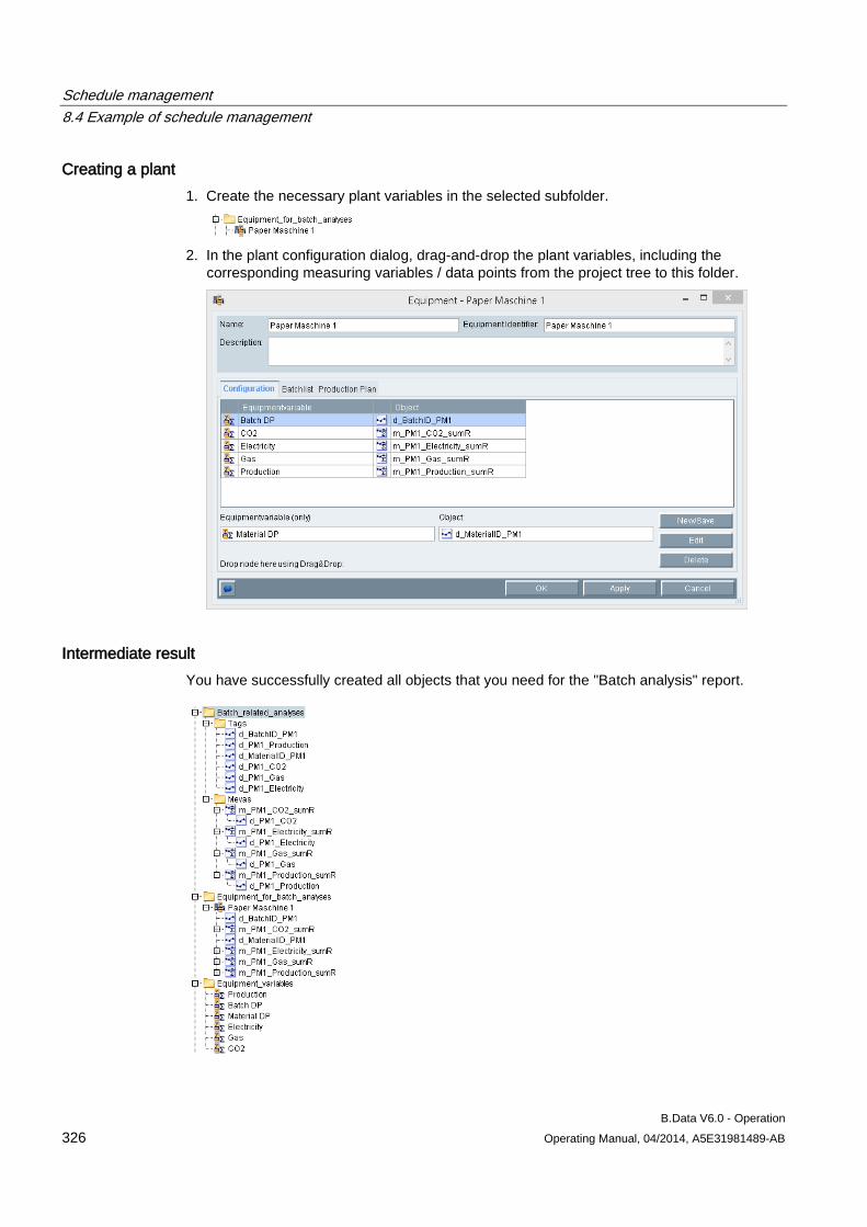
Schedule management 8.4 Example of schedule management
B.Data V6.0 - Operation 326 Operating Manual, 04/2014, A5E31981489-AB
Creating a plant 1. Create the necessary plant variables in the selected subfolder.
2. In the plant configuration dialog, drag-and-drop the plant variables, including the
corresponding measuring variables / data points from the project tree to this folder.
Intermediate result You have successfully created all objects that you need for the "Batch analysis" report.
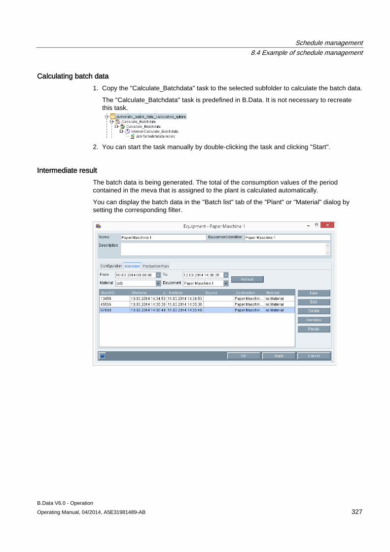
Schedule management 8.4 Example of schedule management
B.Data V6.0 - Operation Operating Manual, 04/2014, A5E31981489-AB 327
Calculating batch data 1. Copy the "Calculate_Batchdata" task to the selected subfolder to calculate the batch data.
The "Calculate_Batchdata" task is predefined in B.Data. It is not necessary to recreate this task.
2. You can start the task manually by double-clicking the task and clicking "Start".
Intermediate result The batch data is being generated. The total of the consumption values of the period contained in the meva that is assigned to the plant is calculated automatically.
You can display the batch data in the "Batch list" tab of the "Plant" or "Material" dialog by setting the corresponding filter.
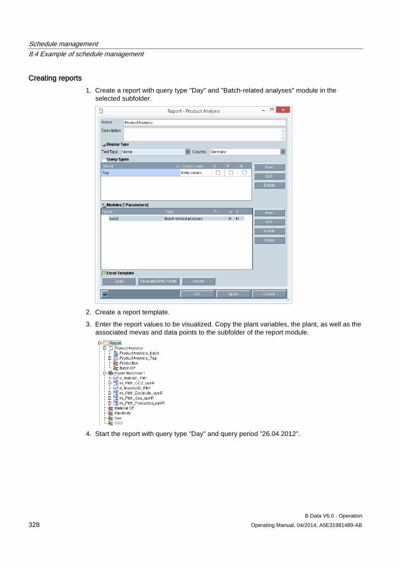
Schedule management 8.4 Example of schedule management
B.Data V6.0 - Operation 328 Operating Manual, 04/2014, A5E31981489-AB
Creating reports 1. Create a report with query type "Day" and "Batch-related analyses" module in the
selected subfolder.
2. Create a report template.
3. Enter the report values to be visualized. Copy the plant variables, the plant, as well as the associated mevas and data points to the subfolder of the report module.
4. Start the report with query type "Day" and query period "26.04.2012".
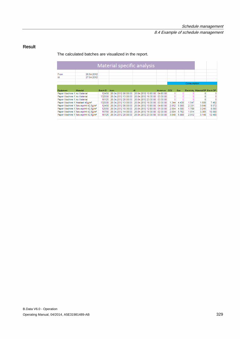
Schedule management 8.4 Example of schedule management
B.Data V6.0 - Operation Operating Manual, 04/2014, A5E31981489-AB 329
Result The calculated batches are visualized in the report.
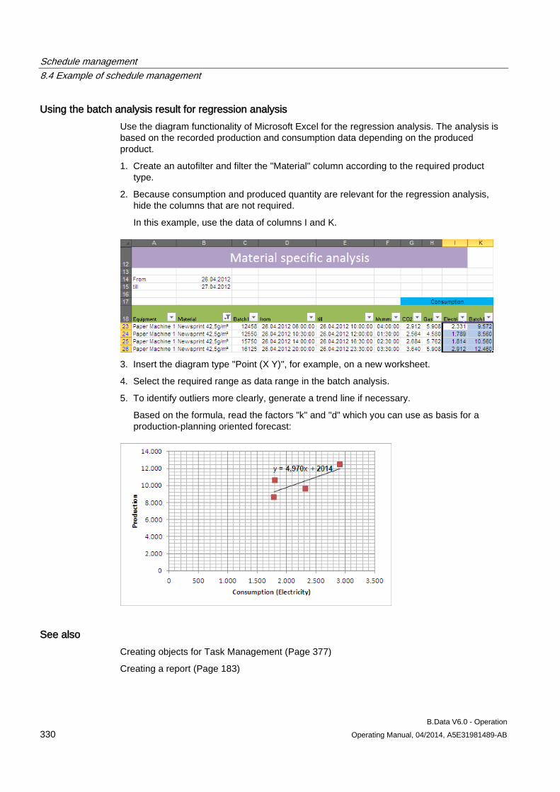
Schedule management 8.4 Example of schedule management
B.Data V6.0 - Operation 330 Operating Manual, 04/2014, A5E31981489-AB
Using the batch analysis result for regression analysis Use the diagram functionality of Microsoft Excel for the regression analysis. The analysis is based on the recorded production and consumption data depending on the produced product.
1. Create an autofilter and filter the "Material" column according to the required product type.
2. Because consumption and produced quantity are relevant for the regression analysis, hide the columns that are not required.
In this example, use the data of columns I and K.
3. Insert the diagram type "Point (X Y)", for example, on a new worksheet.
4. Select the required range as data range in the batch analysis.
5. To identify outliers more clearly, generate a trend line if necessary.
Based on the formula, read the factors "k" and "d" which you can use as basis for a production-planning oriented forecast:
See also Creating objects for Task Management (Page 377)
Creating a report (Page 183)
B.Data V6.0 - Operation Operating Manual, 04/2014, A5E31981489-AB 331
Document management 9 9.1 Document management basics
Definition The document management function lets you manage external documents in B.Data, e.g. documents in PDF, Excel or Word format.
Note Applications for external documents
If you want to open and edit an external document in B.Data, the correct application must be installed on your PC.
Usage You use document management if you require additional application for energy management in B.Data.
Using document management, you can manage external documents in B.Data as follows:
● Link documents
This option lets you insert a link for the document that is saved on your PC. Once inserted, you can use this link to call up the document in B.Data with the respective application. Please note that the document is only available to you. Other users do not have access to the document.
Note
General access to linked documents
To allow other users access to the linked document, save the document in a folder with general access.
● Load document to B.Data database
This option lets you save the document to the B.Data database. This means that you and all authorized users can access the document.
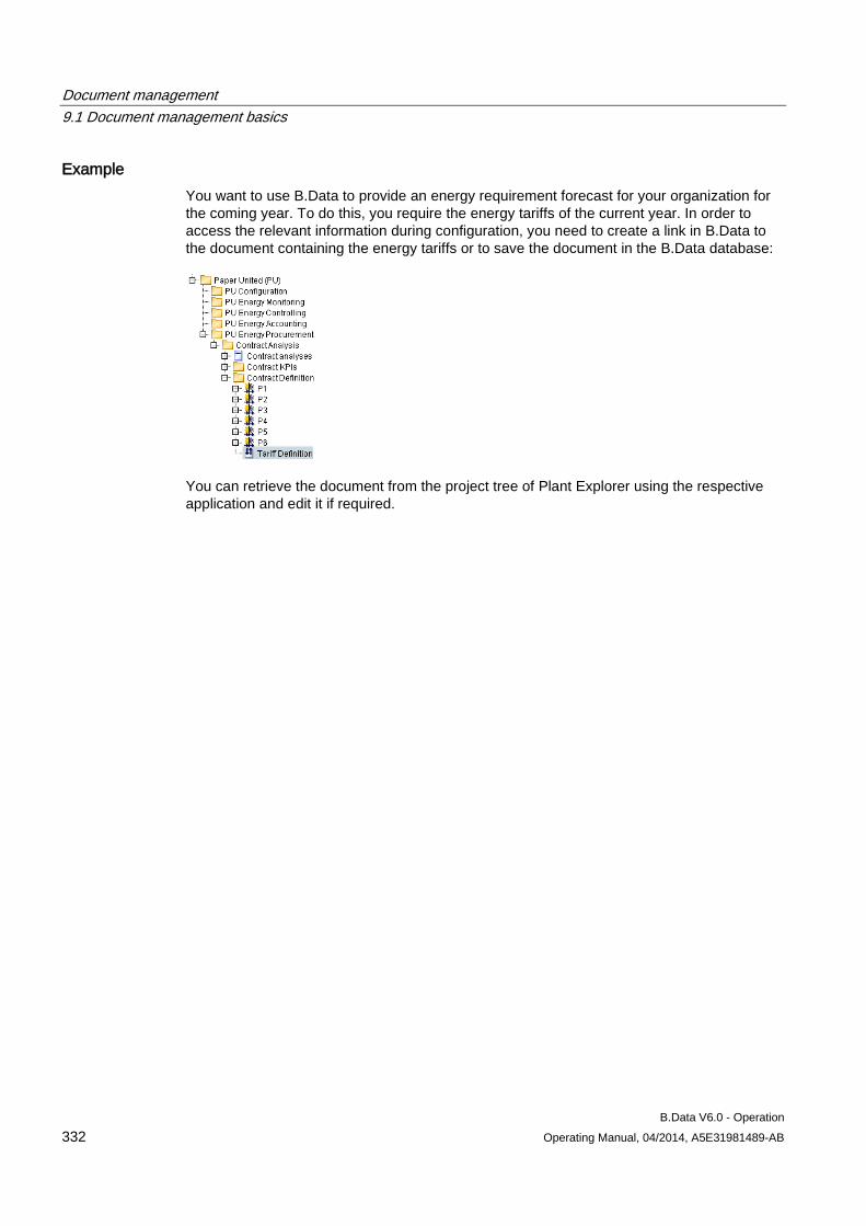
Document management 9.1 Document management basics
B.Data V6.0 - Operation 332 Operating Manual, 04/2014, A5E31981489-AB
Example You want to use B.Data to provide an energy requirement forecast for your organization for the coming year. To do this, you require the energy tariffs of the current year. In order to access the relevant information during configuration, you need to create a link in B.Data to the document containing the energy tariffs or to save the document in the B.Data database:
You can retrieve the document from the project tree of Plant Explorer using the respective application and edit it if required.
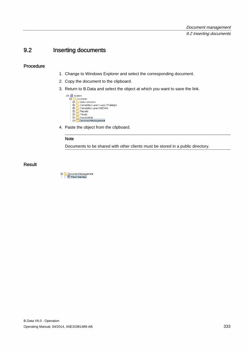
Document management 9.2 Inserting documents
B.Data V6.0 - Operation Operating Manual, 04/2014, A5E31981489-AB 333
9.2 Inserting documents
Procedure 1. Change to Windows Explorer and select the corresponding document.
2. Copy the document to the clipboard.
3. Return to B.Data and select the object at which you want to save the link.
4. Paste the object from the clipboard.
Note
Documents to be shared with other clients must be stored in a public directory.
Result
Document management 9.3 Saving documents
B.Data V6.0 - Operation 334 Operating Manual, 04/2014, A5E31981489-AB
9.3 Saving documents
Overview You can save files in all standard formats, e.g. image or document files, to the database. In this way you enable access of other users to these files.
Requirement ● Successful installation of all software components.
● The user has been assigned the following rights:
– "viewing existing files" to open files.
– "editing existing files": to save files to the database.
The following error messages are output if these rights are missing:
No permissions Error message Remedy "viewing existing files" <date><time>
You are not authorized to open this file. BDataError 0004-00000002
Assign the corresponding authorization.
"editing existing files" ("File \ Data \ fetch")
<date><time> You are not authorized to add this file. BDataError 0004-00000001
Assign the corresponding authorization.
File size limit exceeded The file may not exceed the size of <value>.
Request your system administrator to adjust the "FILE_MAX_SIZE_KB" in B.Data options.
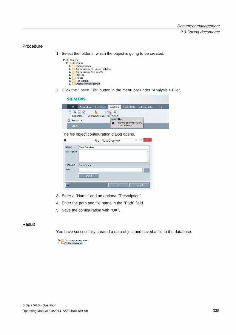
Document management 9.3 Saving documents
B.Data V6.0 - Operation Operating Manual, 04/2014, A5E31981489-AB 335
Procedure 1. Select the folder in which the object is going to be created.
2. Click the "Insert File" button in the menu bar under "Analysis > File".
The file object configuration dialog opens.
3. Enter a "Name" and an optional "Description".
4. Enter the path and file name in the "Path" field.
5. Save the configuration with "OK".
Result You have successfully created a data object and saved a file to the database.
Document management 9.4 Editing documents
B.Data V6.0 - Operation 336 Operating Manual, 04/2014, A5E31981489-AB
9.4 Editing documents
Requirement ● At least one link and one file have been saved to the database.
● The user is authenticated accordingly.
Procedure 1. Double-click the link or the file object.
Result The file opens in the corresponding application on the client.
B.Data V6.0 - Operation Operating Manual, 04/2014, A5E31981489-AB 337
Administration 10 10.1 Logging Viewer
10.1.1 Using the Logging Viewer
Overview The Logging Editor displays the most important system messages and error messages.
This section provides instructions related to the following actions:
1. Opening the Logging Editor
2. Fields in the Logging Editor
3. Filter options
4. Archiving messages
Requirement Successful installation of all software components.
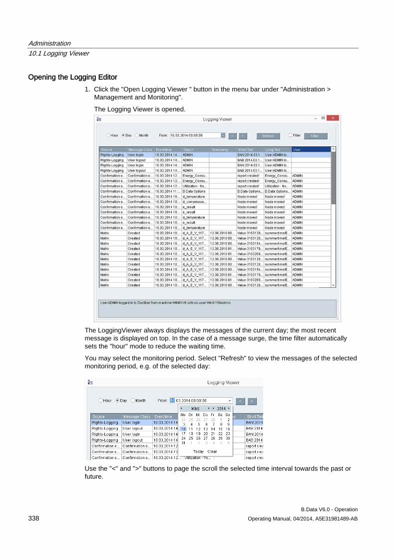
Administration 10.1 Logging Viewer
B.Data V6.0 - Operation 338 Operating Manual, 04/2014, A5E31981489-AB
Opening the Logging Editor 1. Click the "Open Logging Viewer " button in the menu bar under "Administration >
Management and Monitoring".
The Logging Viewer is opened.
The LoggingViewer always displays the messages of the current day; the most recent message is displayed on top. In the case of a message surge, the time filter automatically sets the "hour" mode to reduce the waiting time.
You may select the monitoring period. Select "Refresh" to view the messages of the selected monitoring period, e.g. of the selected day:
Use the "<" and ">" buttons to page the scroll the selected time interval towards the past or future.
Administration 10.1 Logging Viewer
B.Data V6.0 - Operation Operating Manual, 04/2014, A5E31981489-AB 339
All columns can be sorted in ascending or descending order. Click in the header of the respective column to sort it.
Fields of the LoggingViewer The following columns functions are available in the LoggingViewer:
● Source
The error source is the first sorting criterion. Three error sources are currently implemented in the system: Kernel, database, and measurements editor.
● Error class
The error class can be used to refine message filtering, e.g. evaluation error, job management error, deleted, or modified.
● Event time
The event time is used to record the time of error or event occurrence.
● Object
Certain messages include details on the object in this area. For example, the measurements editor logs the data point with name and the MESS_ID that has been processed.
● Time stamp
The specific time stamp affected by changes, deletion of creation of new measured values is logged in this area.
● Stext
The short text, for example, logs the way in which a value has been changed: Value 12.88 -> 13.54
● Ltext
The measurements editor logs the daylight saving and winter time as well as the compression level in this column. The remaining sources log the error message in plain text in this column.
● User
The user having triggered the event is logged, e.g. BDATA_SYS for automatic jobs and the respective user for changes in the measurements editor.
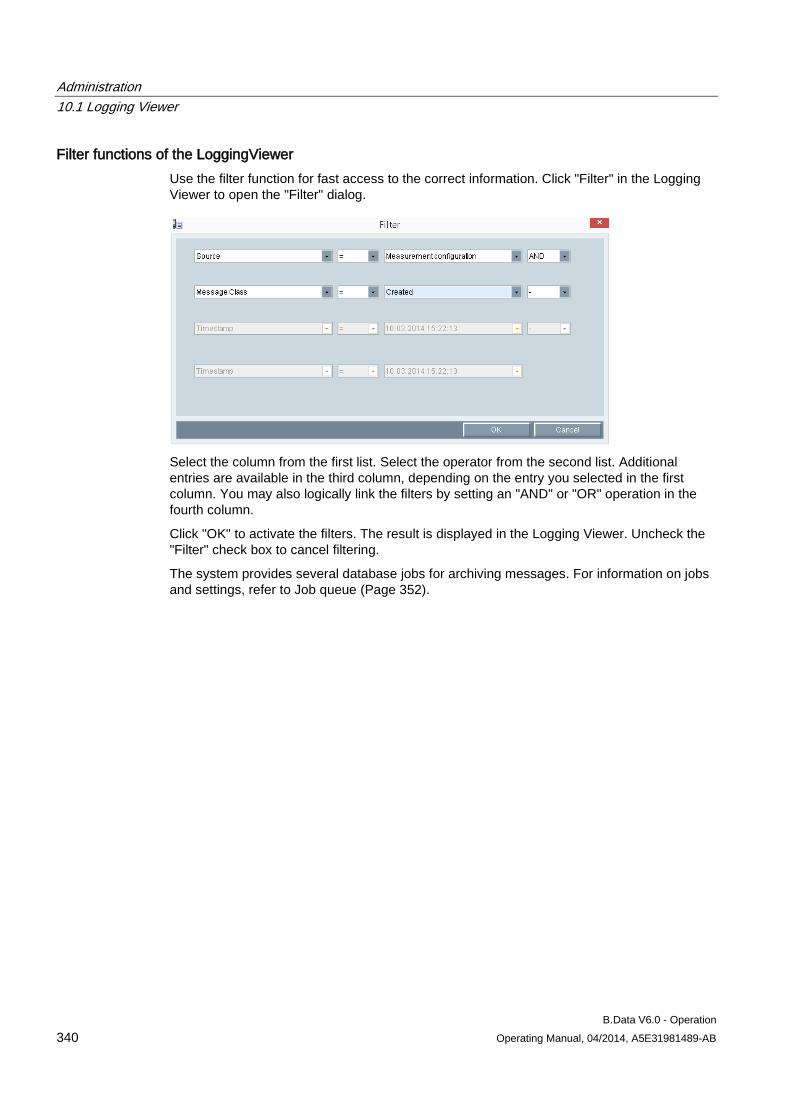
Administration 10.1 Logging Viewer
B.Data V6.0 - Operation 340 Operating Manual, 04/2014, A5E31981489-AB
Filter functions of the LoggingViewer Use the filter function for fast access to the correct information. Click "Filter" in the Logging Viewer to open the "Filter" dialog.
Select the column from the first list. Select the operator from the second list. Additional entries are available in the third column, depending on the entry you selected in the first column. You may also logically link the filters by setting an "AND" or "OR" operation in the fourth column.
Click "OK" to activate the filters. The result is displayed in the Logging Viewer. Uncheck the "Filter" check box to cancel filtering.
The system provides several database jobs for archiving messages. For information on jobs and settings, refer to Job queue (Page 352).
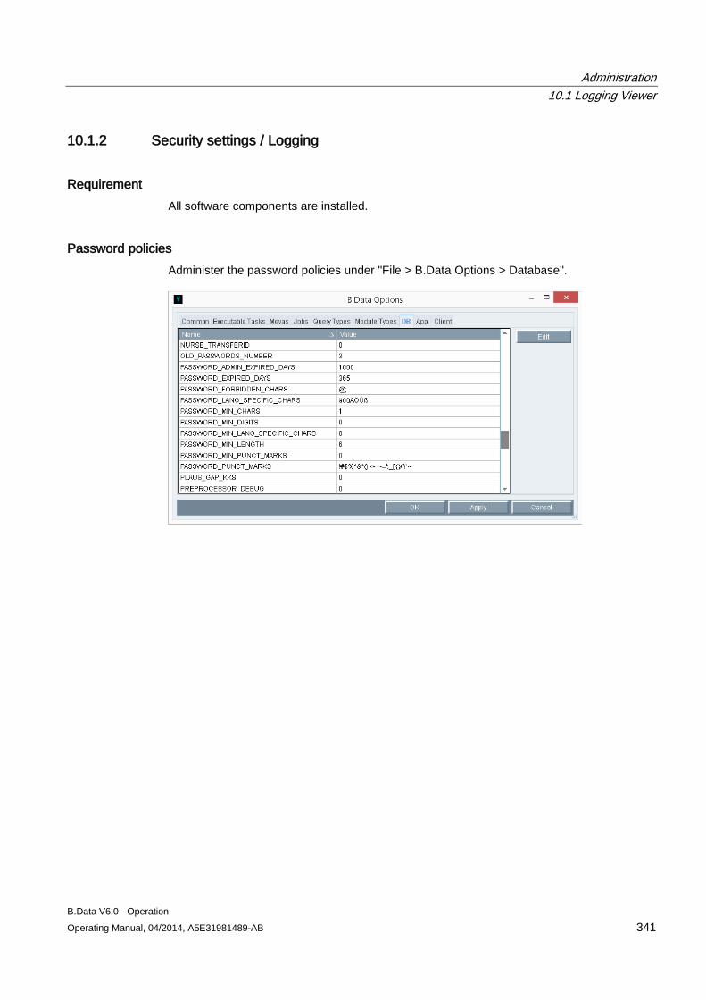
Administration 10.1 Logging Viewer
B.Data V6.0 - Operation Operating Manual, 04/2014, A5E31981489-AB 341
10.1.2 Security settings / Logging
Requirement All software components are installed.
Password policies Administer the password policies under "File > B.Data Options > Database".
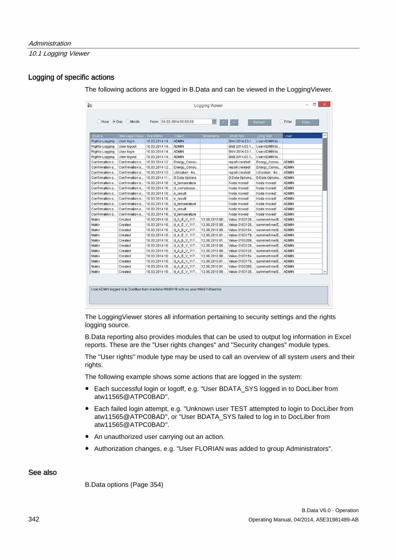
Administration 10.1 Logging Viewer
B.Data V6.0 - Operation 342 Operating Manual, 04/2014, A5E31981489-AB
Logging of specific actions The following actions are logged in B.Data and can be viewed in the LoggingViewer.
The LoggingViewer stores all information pertaining to security settings and the rights logging source.
B.Data reporting also provides modules that can be used to output log information in Excel reports. These are the "User rights changes" and "Security changes" module types.
The "User rights" module type may be used to call an overview of all system users and their rights.
The following example shows some actions that are logged in the system:
● Each successful login or logoff, e.g. "User BDATA_SYS logged in to DocLiber from atw11565@ATPC0BAD".
● Each failed login attempt, e.g. "Unknown user TEST attempted to login to DocLiber from atw11565@ATPC0BAD", or "User BDATA_SYS failed to log in to DocLiber from atw11565@ATPC0BAD".
● An unauthorized user carrying out an action.
● Authorization changes, e.g. "User FLORIAN was added to group Administrators".
See also B.Data options (Page 354)
Administration 10.2 Message lists
B.Data V6.0 - Operation Operating Manual, 04/2014, A5E31981489-AB 343
10.2 Message lists
10.2.1 Basic information on message lists
Overview A message list informs you of defined deviations of the measured values of a data point. You can view this information as follows:
● by means of a message list view
● by means of e-mail
Configure the deviation criteria for the measured values of a data point in the "Plausibility" area of a data point.
Message lists contain three categories:
● "Predefined": contains predefined message lists. The following predefined message lists are available:
– All: contains all messages and warnings.
– All Violations: contains all messages generated when a measured value violates a limit.
– All Warnings: contains all warnings generated when a measured value approaches a configured limit.
The predefined message lists cannot be edited or deleted.
● "Public": contains published message lists that can be used by all users.
● "My": contains message lists that you have configured.
Notes on message lists
NOTICE
Messages in B.Data do not replace the message configuration in the process control system
The message is not linked to the process control system. If you want to react to the message, you have to configure limit monitoring in the process control system.
To view the messages in a message list, you need to configure the limits for the required data point and activate their message.
Messages are disabled in the project by default. Contact your administrator if you want to enable the message for the project.

Administration 10.2 Message lists
B.Data V6.0 - Operation 344 Operating Manual, 04/2014, A5E31981489-AB
Procedure for configuring a message list To configure a message list, follow these steps:
1. Configure a message list.
2. Define the message list contents by means of a filter.
3. You can also configure a message notification, if necessary.
Administration 10.2 Message lists
B.Data V6.0 - Operation Operating Manual, 04/2014, A5E31981489-AB 345
10.2.2 Configuring custom message list
Overview You may configure a custom alarm list. In this alarm list you use filters to define which messages are displayed.
Requirement ● The data point is configured.
● The data point limit is configured.
● The message is activated for the limit.
Procedure 1. Click the "Open KPI Message Lists" button in the menu bar under "Administration >
Management and Monitoring".
2. Then click "New".
The alarm list configuration dialog opens.
3. Enter a unique name and an optional description for the alarm list.
The "Owner" field displays the name of the user who configures the alarm list.
4. Activate "Publish" to make the alarm list available to all users.
5. Confirm the configuration with "Save".
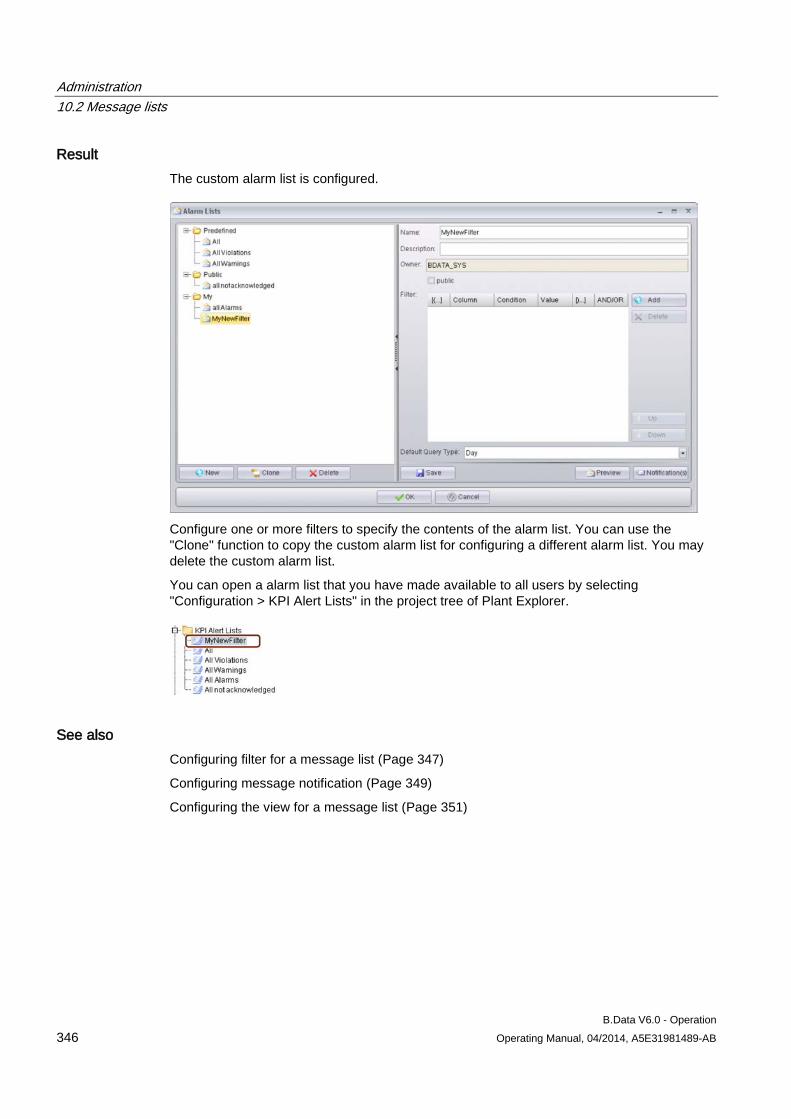
Administration 10.2 Message lists
B.Data V6.0 - Operation 346 Operating Manual, 04/2014, A5E31981489-AB
Result The custom alarm list is configured.
Configure one or more filters to specify the contents of the alarm list. You can use the "Clone" function to copy the custom alarm list for configuring a different alarm list. You may delete the custom alarm list.
You can open a alarm list that you have made available to all users by selecting "Configuration > KPI Alert Lists" in the project tree of Plant Explorer.
See also Configuring filter for a message list (Page 347)
Configuring message notification (Page 349)
Configuring the view for a message list (Page 351)
Administration 10.2 Message lists
B.Data V6.0 - Operation Operating Manual, 04/2014, A5E31981489-AB 347
10.2.3 Configuring filter for a message list
Overview A alarm list filter allows you to exclude messages that you do not need.
The following rules are valid for filters:
● For a alarm list configuration containing multiple filters, you need to logically link the filters by means of "AND" or "OR" operator.
● In a configuration with multiple filters, the filters in the list are evaluated from the top down.
Requirement The alarm list is configured.
Procedure 1. Select the required alarm list under "Administration > Alarm lists" in the Plant Explorer.
2. Click "Add" in the "Configuration" tab.
3. You may enter filter expressions in a parenthesis.
4. Select a filter criterion and a condition, e.g. "Value" and ">".
5. Enter a value, e.g. 1000.
6. Select an operator / additional operators to interconnect multiple filters.
7. Click "Up" or "Down" to specify the sorting order by which multiple filters are to be evaluated.
8. Confirm the configuration with "Save".
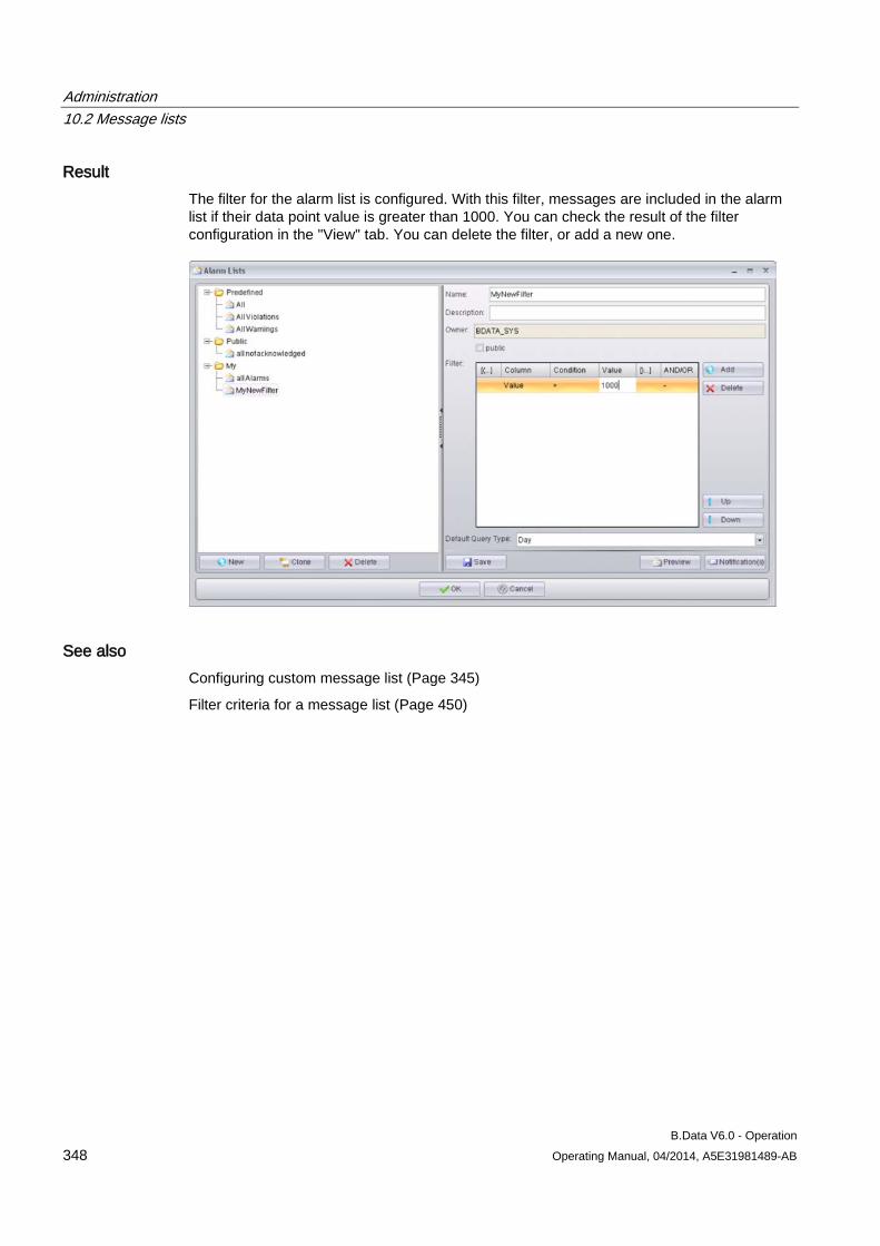
Administration 10.2 Message lists
B.Data V6.0 - Operation 348 Operating Manual, 04/2014, A5E31981489-AB
Result The filter for the alarm list is configured. With this filter, messages are included in the alarm list if their data point value is greater than 1000. You can check the result of the filter configuration in the "View" tab. You can delete the filter, or add a new one.
See also Configuring custom message list (Page 345)
Filter criteria for a message list (Page 450)
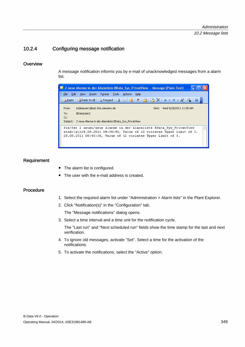
Administration 10.2 Message lists
B.Data V6.0 - Operation Operating Manual, 04/2014, A5E31981489-AB 349
10.2.4 Configuring message notification
Overview A message notification informs you by e-mail of unacknowledged messages from a alarm list.
Requirement ● The alarm list is configured.
● The user with the e-mail address is created.
Procedure 1. Select the required alarm list under "Administration > Alarm lists" in the Plant Explorer.
2. Click "Notification(s)" in the "Configuration" tab.
The "Message notifications" dialog opens.
3. Select a time interval and a time unit for the notification cycle.
The "Last run" and "Next scheduled run" fields show the time stamp for the last and next verification.
4. To ignore old messages, activate "Set". Select a time for the activation of the notifications.
5. To activate the notifications, select the "Active" option.
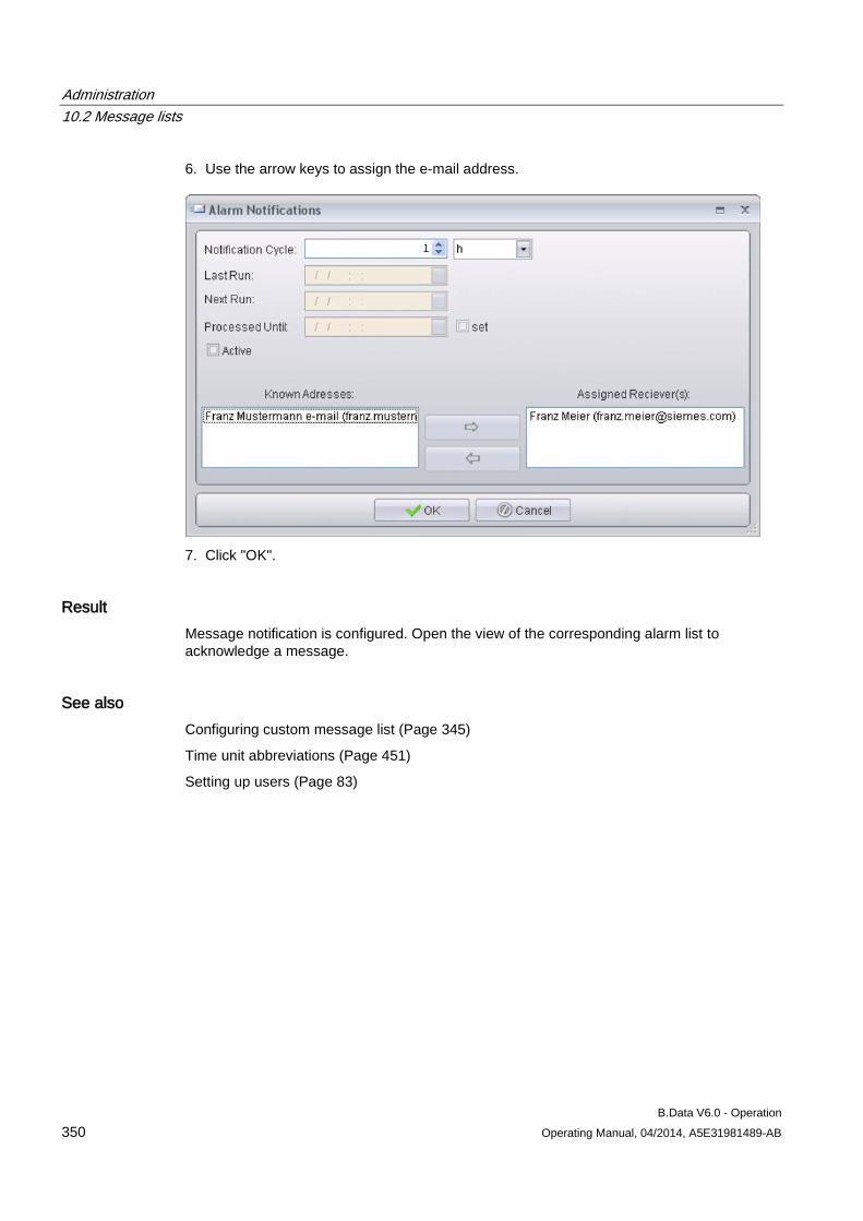
Administration 10.2 Message lists
B.Data V6.0 - Operation 350 Operating Manual, 04/2014, A5E31981489-AB
6. Use the arrow keys to assign the e-mail address.
7. Click "OK".
Result Message notification is configured. Open the view of the corresponding alarm list to acknowledge a message.
See also Configuring custom message list (Page 345)
Time unit abbreviations (Page 451)
Setting up users (Page 83)
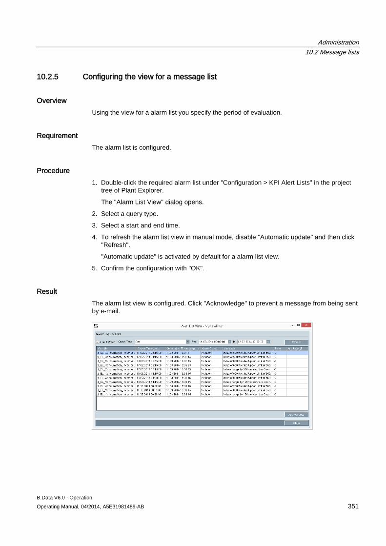
Administration 10.2 Message lists
B.Data V6.0 - Operation Operating Manual, 04/2014, A5E31981489-AB 351
10.2.5 Configuring the view for a message list
Overview Using the view for a alarm list you specify the period of evaluation.
Requirement The alarm list is configured.
Procedure 1. Double-click the required alarm list under "Configuration > KPI Alert Lists" in the project
tree of Plant Explorer.
The "Alarm List View" dialog opens.
2. Select a query type.
3. Select a start and end time.
4. To refresh the alarm list view in manual mode, disable "Automatic update" and then click "Refresh".
"Automatic update" is activated by default for a alarm list view.
5. Confirm the configuration with "OK".
Result The alarm list view is configured. Click "Acknowledge" to prevent a message from being sent by e-mail.
Administration 10.3 Job queue
B.Data V6.0 - Operation 352 Operating Manual, 04/2014, A5E31981489-AB
10.3 Job queue
10.3.1 Using the job queue
Overview B.Data Job Scheduling can be used to run database jobs once or at cyclic intervals. The Job Queue lists all configured database jobs.
Fields in the Job Queue The Job Queue provides the following information for each job.
● Job
Unique ID for handling the job in the system.
● Function
Name of the database job
● Tot.
duration [sec] of job execution.
● Interval
Job execution cycle.
● C
Status, if the job is canceled.
● Err
The status is entered in this item in case of a malfunction.
● Next
Time stamp that indicates the next job start.
● Last
Indicates the time of the last job session.
● Description
Short description of the database job
● SQL
SQL syntax
● User
User having started this job or entered it in the Job Queue.
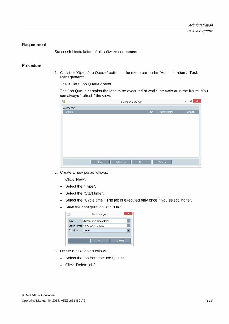
Administration 10.3 Job queue
B.Data V6.0 - Operation Operating Manual, 04/2014, A5E31981489-AB 353
Requirement Successful installation of all software components.
Procedure 1. Click the "Open Job Queue" button in the menu bar under "Administration > Task
Management".
The B.Data Job Queue opens.
The Job Queue contains the jobs to be executed at cyclic intervals or in the future. You can always "refresh" the view.
2. Create a new job as follows:
– Click "New".
– Select the "Type".
– Select the "Start time".
– Select the "Cycle time". The job is executed only once if you select "none".
– Save the configuration with "OK".
3. Delete a new job as follows:
– Select the job from the Job Queue.
– Click "Delete job".
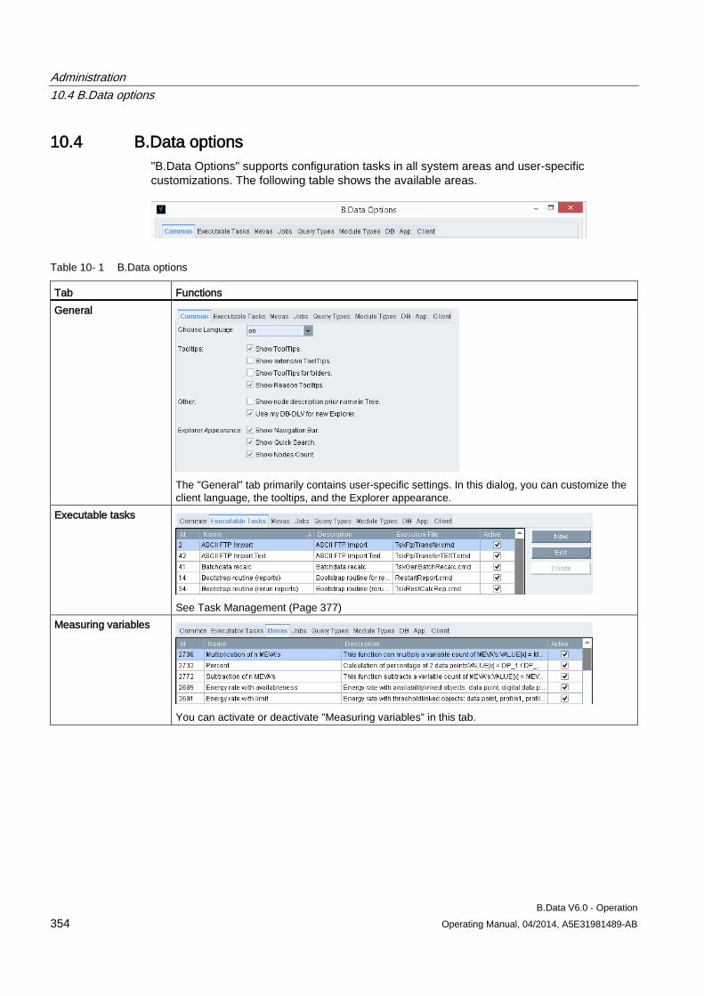
Administration 10.4 B.Data options
B.Data V6.0 - Operation 354 Operating Manual, 04/2014, A5E31981489-AB
10.4 B.Data options "B.Data Options" supports configuration tasks in all system areas and user-specific customizations. The following table shows the available areas.
Table 10- 1 B.Data options
Tab Functions General
The "General" tab primarily contains user-specific settings. In this dialog, you can customize the client language, the tooltips, and the Explorer appearance.
Executable tasks
See Task Management (Page 377)
Measuring variables
You can activate or deactivate "Measuring variables" in this tab.
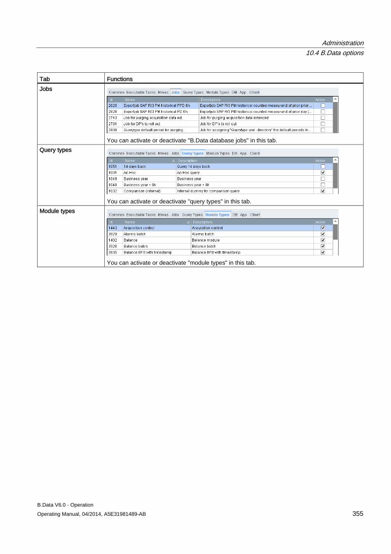
Administration 10.4 B.Data options
B.Data V6.0 - Operation Operating Manual, 04/2014, A5E31981489-AB 355
Tab Functions Jobs
You can activate or deactivate "B.Data database jobs" in this tab.
Query types
You can activate or deactivate "query types" in this tab.
Module types
You can activate or deactivate "module types" in this tab.
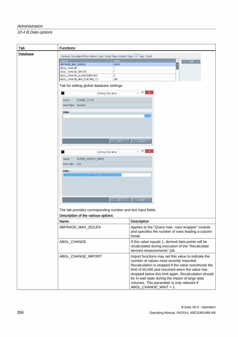
Administration 10.4 B.Data options
B.Data V6.0 - Operation 356 Operating Manual, 04/2014, A5E31981489-AB
Tab Functions Database
Tab for editing global database settings.
The tab provides corresponding number and text input fields. Description of the various options: Name Description ABFRAGE_MAX_ZEILEN Applies to the "Query max. rows wrapper" module
and specifies the number of rows leading a column break.
ABGL_CHANGE If this value equals 1, derived data points will be recalculated during execution of the "Recalculate derived measurements" job.
ABGL_CHANGE_IMPORT Import functions may set this value to indicate the number of values most recently imported. Recalculation is stopped if the value overshoots the limit of 50,000 and resumed when the value has dropped below this limit again. Recalculation should be in wait state during the import of large data volumes. This parameter is only relevant if ABGL_CHANGE_WAIT = 1.
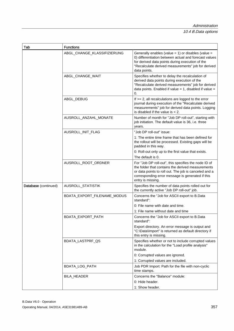
Administration 10.4 B.Data options
B.Data V6.0 - Operation Operating Manual, 04/2014, A5E31981489-AB 357
Tab Functions ABGL_CHANGE_KLASSIFIZIERUNG Generally enables (value = 1) or disables (value =
0) differentiation between actual and forecast values for derived data points during execution of the "Recalculate derived measurements" job for derived data points.
ABGL_CHANGE_WAIT Specifies whether to delay the recalculation of derived data points during execution of the "Recalculate derived measurements" job for derived data points. Enabled if value = 1, disabled if value = 0.
ABGL_DEBUG If >= 2, all recalculations are logged to the error journal during execution of the "Recalculate derived measurements" job for derived data points. Logging is disabled if the value is < 2.
AUSROLL_ANZAHL_MONATE Number of month for "Job DP roll-out", starting with job initiation. The default value is 36, i.e. three years.
AUSROLL_INIT_FLAG "Job DP roll-out" issue: 1: The entire time frame that has been defined for the rollout will be processed. Existing gaps will be padded in this way. 0: Roll-out only up to the first value that exists. The default is 0.
AUSROLL_ROOT_ORDNER For "Job DP roll-out", this specifies the node ID of the folder that contains the derived measurements or data points to roll out. The job is canceled and a corresponding error message is generated if this entry is missing.
Database (continued) AUSROLL_STATISTIK Specifies the number of data points rolled out for the currently active "Job DP roll-out" job.
BDATA_EXPORT_FILENAME_MODUS Concerns the "Job for ASCII export to B.Data standard": 0: File name with date and time. 1: File name without date and time
BDATA_EXPORT_PATH Concerns the "Job for ASCII export to B.Data standard": Export directory. An error message is output and "C:\Data\Import" is returned as default directory if this entry is missing.
BDATA_LASTPRF_QS Specifies whether or not to include corrupted values in the calculation for the "Load profile analysis" module. 0: Corrupted values are ignored. 1: Corrupted values are included.
BDATA_LOG_PATH Job PDR Import: Path for the file with non-cyclic time stamps.
BILA_HEADER Concerns the "Balance" module: 0: Hide header. 1: Show header.
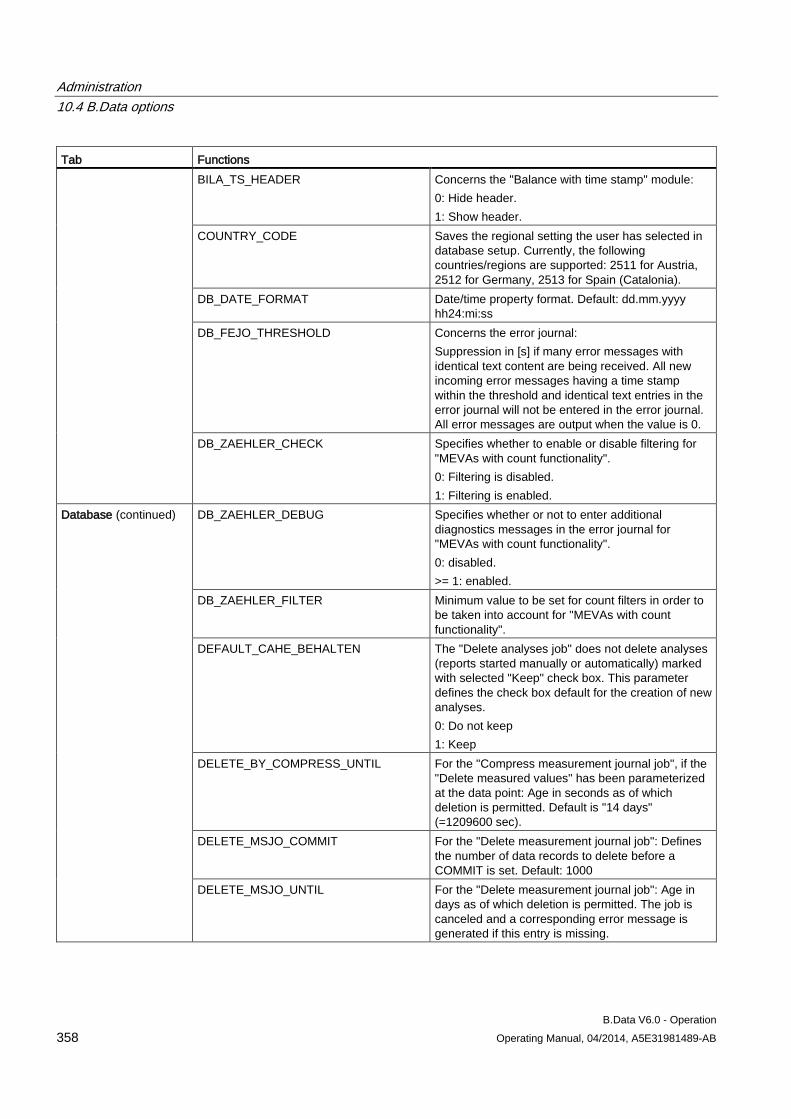
Administration 10.4 B.Data options
B.Data V6.0 - Operation 358 Operating Manual, 04/2014, A5E31981489-AB
Tab Functions BILA_TS_HEADER Concerns the "Balance with time stamp" module:
0: Hide header. 1: Show header.
COUNTRY_CODE Saves the regional setting the user has selected in database setup. Currently, the following countries/regions are supported: 2511 for Austria, 2512 for Germany, 2513 for Spain (Catalonia).
DB_DATE_FORMAT Date/time property format. Default: dd.mm.yyyy hh24:mi:ss
DB_FEJO_THRESHOLD Concerns the error journal: Suppression in [s] if many error messages with identical text content are being received. All new incoming error messages having a time stamp within the threshold and identical text entries in the error journal will not be entered in the error journal. All error messages are output when the value is 0.
DB_ZAEHLER_CHECK Specifies whether to enable or disable filtering for "MEVAs with count functionality". 0: Filtering is disabled. 1: Filtering is enabled.
Database (continued) DB_ZAEHLER_DEBUG Specifies whether or not to enter additional diagnostics messages in the error journal for "MEVAs with count functionality". 0: disabled. >= 1: enabled.
DB_ZAEHLER_FILTER Minimum value to be set for count filters in order to be taken into account for "MEVAs with count functionality".
DEFAULT_CAHE_BEHALTEN The "Delete analyses job" does not delete analyses (reports started manually or automatically) marked with selected "Keep" check box. This parameter defines the check box default for the creation of new analyses. 0: Do not keep 1: Keep
DELETE_BY_COMPRESS_UNTIL For the "Compress measurement journal job", if the "Delete measured values" has been parameterized at the data point: Age in seconds as of which deletion is permitted. Default is "14 days" (=1209600 sec).
DELETE_MSJO_COMMIT For the "Delete measurement journal job": Defines the number of data records to delete before a COMMIT is set. Default: 1000
DELETE_MSJO_UNTIL For the "Delete measurement journal job": Age in days as of which deletion is permitted. The job is canceled and a corresponding error message is generated if this entry is missing.
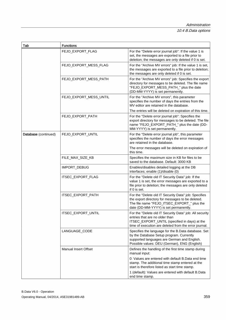
Administration 10.4 B.Data options
B.Data V6.0 - Operation Operating Manual, 04/2014, A5E31981489-AB 359
Tab Functions FEJO_EXPORT_FLAG For the "Delete error journal job": If the value 1 is
set, the messages are exported to a file prior to deletion; the messages are only deleted if 0 is set.
FEJO_EXPORT_MESS_FLAG For the "Archive MV errors" job: If the value 1 is set, the messages are exported to a file prior to deletion; the messages are only deleted if 0 is set.
FEJO_EXPORT_MESS_PATH For the "Archive MV errors" job: Specifies the export directory for messages to be deleted. The file name "FEJO_EXPORT_MESS_PATH_" plus the date (DD-MM-YYYY) is set permanently.
FEJO_EXPORT_MESS_UNTIL For the "Archive MV errors", this parameter specifies the number of days the entries from the MV editor are retained in the database. The entries will be deleted on expiration of this time.
FEJO_EXPORT_PATH For the "Delete error journal job": Specifies the export directory for messages to be deleted. The file name "FEJO_EXPORT_PATH_" plus the date (DD-MM-YYYY) is set permanently.
Database (continued) FEJO_EXPORT_UNTIL For the "Delete error journal job", this parameter specifies the number of days the error messages are retained in the database. The error messages will be deleted on expiration of this time.
FILE_MAX_SIZE_KB Specifies the maximum size in KB for files to be saved to the database. Default: 3000 KB
IMPORT_DEBUG Enables/disables detailed logging at the DB interfaces; enable (1)/disable (0)
ITSEC_EXPORT_FLAG For the "Delete old IT Security Data" job: If the value 1 is set, the error messages are exported to a file prior to deletion; the messages are only deleted if 0 is set.
ITSEC_EXPORT_PATH For the "Delete old IT Security Data" job: Specifies the export directory for messages to be deleted. The file name "FEJO_ITSEC_EXPORT_" plus the date (DD-MM-YYYY) is set permanently.
ITSEC_EXPORT_UNTIL For the "Delete old IT Security Data" job: All security entries that are no older than ITSEC_EXPORT_UNTIL (specified in days) at the time of execution are deleted from the error journal.
LANGUAGE_CODE Specifies the language for the B.Data database. Set by the Database Setup program. Currently supported languages are German and English. Possible values: DEU (German), ENG (English)
Manual Insert Offset Defines the handling of the first time stamp during manual input: 0: Values are entered with default B.Data end time stamp. The additional time stamp entered at the start is therefore listed as start time stamp. 1 (default): Values are entered with default B.Data end time stamp.
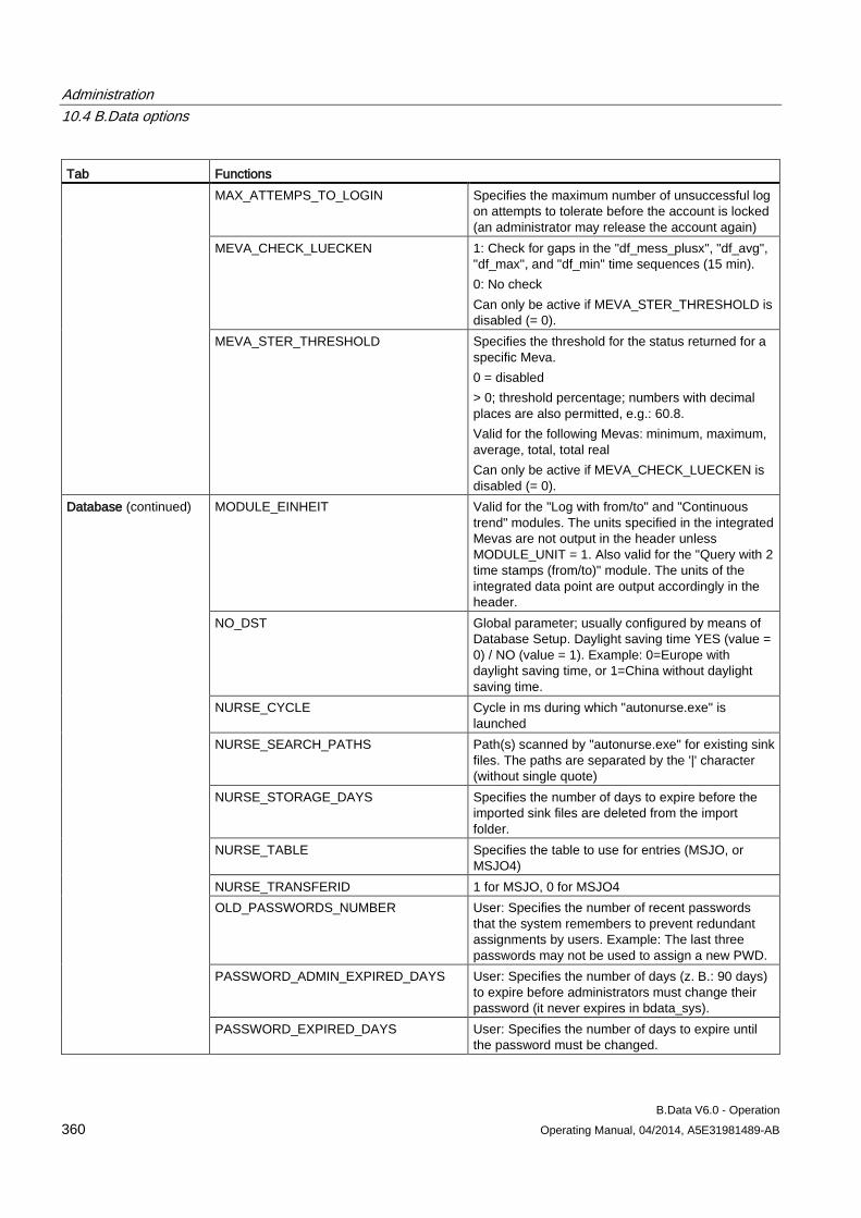
Administration 10.4 B.Data options
B.Data V6.0 - Operation 360 Operating Manual, 04/2014, A5E31981489-AB
Tab Functions MAX_ATTEMPS_TO_LOGIN Specifies the maximum number of unsuccessful log
on attempts to tolerate before the account is locked (an administrator may release the account again)
MEVA_CHECK_LUECKEN 1: Check for gaps in the "df_mess_plusx", "df_avg", "df_max", and "df_min" time sequences (15 min). 0: No check Can only be active if MEVA_STER_THRESHOLD is disabled (= 0).
MEVA_STER_THRESHOLD Specifies the threshold for the status returned for a specific Meva. 0 = disabled > 0; threshold percentage; numbers with decimal places are also permitted, e.g.: 60.8. Valid for the following Mevas: minimum, maximum, average, total, total real Can only be active if MEVA_CHECK_LUECKEN is disabled (= 0).
Database (continued) MODULE_EINHEIT Valid for the "Log with from/to" and "Continuous trend" modules. The units specified in the integrated Mevas are not output in the header unless MODULE_UNIT = 1. Also valid for the "Query with 2 time stamps (from/to)" module. The units of the integrated data point are output accordingly in the header.
NO_DST Global parameter; usually configured by means of Database Setup. Daylight saving time YES (value = 0) / NO (value = 1). Example: 0=Europe with daylight saving time, or 1=China without daylight saving time.
NURSE_CYCLE Cycle in ms during which "autonurse.exe" is launched
NURSE_SEARCH_PATHS Path(s) scanned by "autonurse.exe" for existing sink files. The paths are separated by the '|' character (without single quote)
NURSE_STORAGE_DAYS Specifies the number of days to expire before the imported sink files are deleted from the import folder.
NURSE_TABLE Specifies the table to use for entries (MSJO, or MSJO4)
NURSE_TRANSFERID 1 for MSJO, 0 for MSJO4 OLD_PASSWORDS_NUMBER User: Specifies the number of recent passwords
that the system remembers to prevent redundant assignments by users. Example: The last three passwords may not be used to assign a new PWD.
PASSWORD_ADMIN_EXPIRED_DAYS User: Specifies the number of days (z. B.: 90 days) to expire before administrators must change their password (it never expires in bdata_sys).
PASSWORD_EXPIRED_DAYS User: Specifies the number of days to expire until the password must be changed.
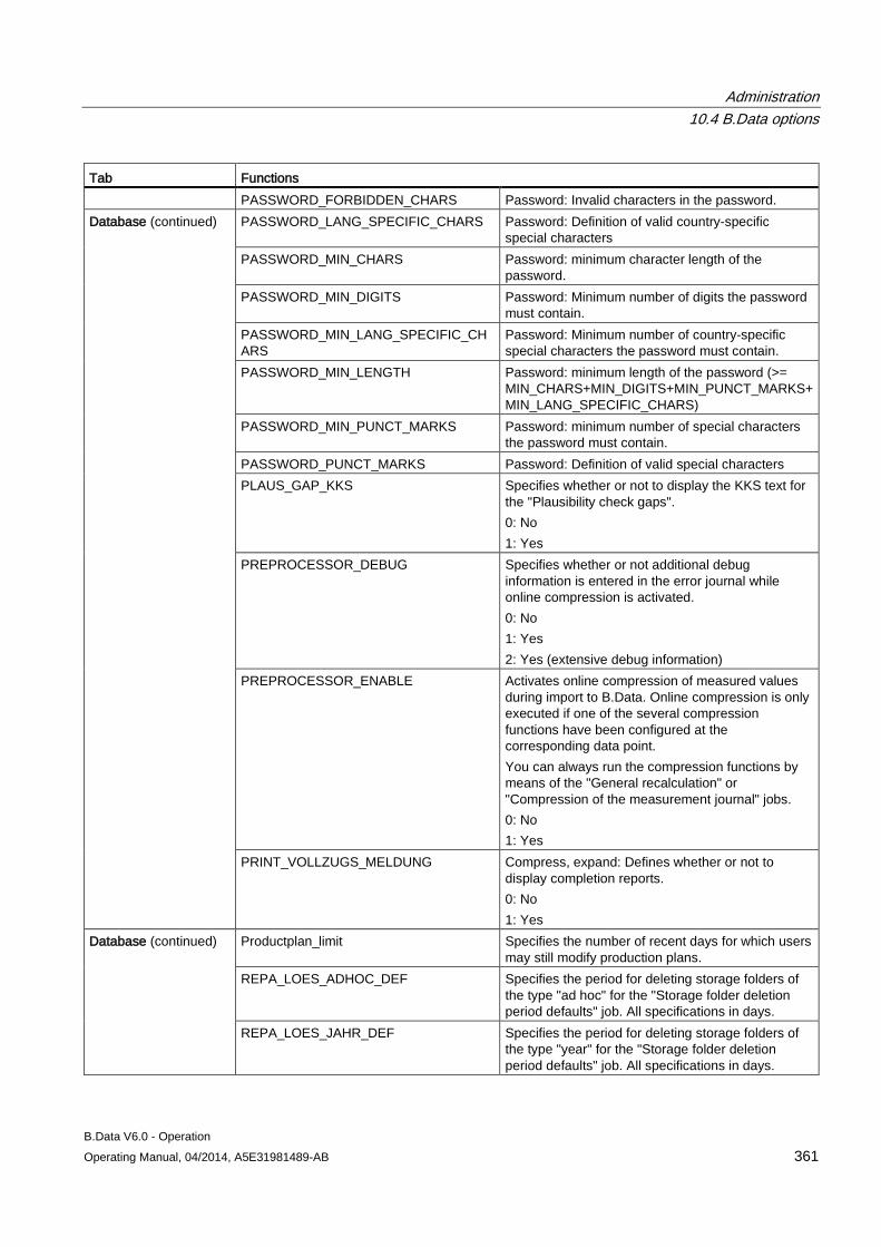
Administration 10.4 B.Data options
B.Data V6.0 - Operation Operating Manual, 04/2014, A5E31981489-AB 361
Tab Functions PASSWORD_FORBIDDEN_CHARS Password: Invalid characters in the password.
Database (continued) PASSWORD_LANG_SPECIFIC_CHARS Password: Definition of valid country-specific special characters
PASSWORD_MIN_CHARS Password: minimum character length of the password.
PASSWORD_MIN_DIGITS Password: Minimum number of digits the password must contain.
PASSWORD_MIN_LANG_SPECIFIC_CHARS
Password: Minimum number of country-specific special characters the password must contain.
PASSWORD_MIN_LENGTH Password: minimum length of the password (>= MIN_CHARS+MIN_DIGITS+MIN_PUNCT_MARKS+MIN_LANG_SPECIFIC_CHARS)
PASSWORD_MIN_PUNCT_MARKS Password: minimum number of special characters the password must contain.
PASSWORD_PUNCT_MARKS Password: Definition of valid special characters PLAUS_GAP_KKS Specifies whether or not to display the KKS text for
the "Plausibility check gaps". 0: No 1: Yes
PREPROCESSOR_DEBUG Specifies whether or not additional debug information is entered in the error journal while online compression is activated. 0: No 1: Yes 2: Yes (extensive debug information)
PREPROCESSOR_ENABLE Activates online compression of measured values during import to B.Data. Online compression is only executed if one of the several compression functions have been configured at the corresponding data point. You can always run the compression functions by means of the "General recalculation" or "Compression of the measurement journal" jobs. 0: No 1: Yes
PRINT_VOLLZUGS_MELDUNG Compress, expand: Defines whether or not to display completion reports. 0: No 1: Yes
Database (continued) Productplan_limit Specifies the number of recent days for which users may still modify production plans.
REPA_LOES_ADHOC_DEF Specifies the period for deleting storage folders of the type "ad hoc" for the "Storage folder deletion period defaults" job. All specifications in days.
REPA_LOES_JAHR_DEF Specifies the period for deleting storage folders of the type "year" for the "Storage folder deletion period defaults" job. All specifications in days.
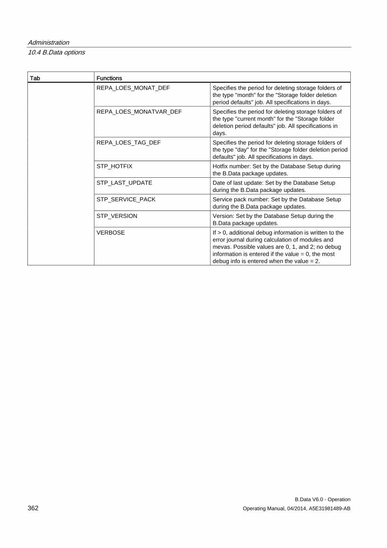
Administration 10.4 B.Data options
B.Data V6.0 - Operation 362 Operating Manual, 04/2014, A5E31981489-AB
Tab Functions REPA_LOES_MONAT_DEF Specifies the period for deleting storage folders of
the type "month" for the "Storage folder deletion period defaults" job. All specifications in days.
REPA_LOES_MONATVAR_DEF Specifies the period for deleting storage folders of the type "current month" for the "Storage folder deletion period defaults" job. All specifications in days.
REPA_LOES_TAG_DEF Specifies the period for deleting storage folders of the type "day" for the "Storage folder deletion period defaults" job. All specifications in days.
STP_HOTFIX Hotfix number: Set by the Database Setup during the B.Data package updates.
STP_LAST_UPDATE Date of last update: Set by the Database Setup during the B.Data package updates.
STP_SERVICE_PACK Service pack number: Set by the Database Setup during the B.Data package updates.
STP_VERSION Version: Set by the Database Setup during the B.Data package updates.
VERBOSE If > 0, additional debug information is written to the error journal during calculation of modules and mevas. Possible values are 0, 1, and 2; no debug information is entered if the value = 0, the most debug info is entered when the value = 2.
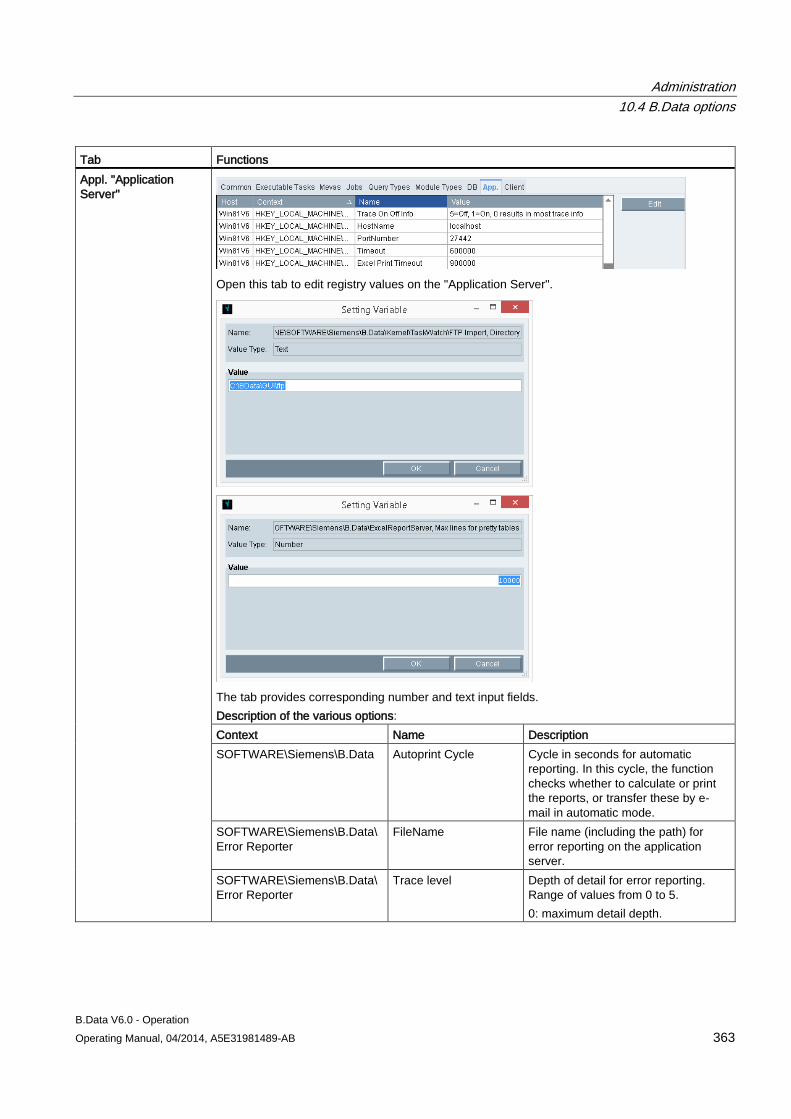
Administration 10.4 B.Data options
B.Data V6.0 - Operation Operating Manual, 04/2014, A5E31981489-AB 363
Tab Functions Appl. "Application Server"
Open this tab to edit registry values on the "Application Server".
The tab provides corresponding number and text input fields. Description of the various options: Context Name Description SOFTWARE\Siemens\B.Data Autoprint Cycle Cycle in seconds for automatic
reporting. In this cycle, the function checks whether to calculate or print the reports, or transfer these by e-mail in automatic mode.
SOFTWARE\Siemens\B.Data\Error Reporter
FileName File name (including the path) for error reporting on the application server.
SOFTWARE\Siemens\B.Data\Error Reporter
Trace level Depth of detail for error reporting. Range of values from 0 to 5. 0: maximum detail depth.
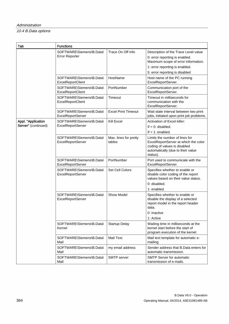
Administration 10.4 B.Data options
B.Data V6.0 - Operation 364 Operating Manual, 04/2014, A5E31981489-AB
Tab Functions SOFTWARE\Siemens\B.Data\Error Reporter
Trace On Off Info Description of the Trace Level value 0: error reporting is enabled. Maximum scope of error information. 1: error reporting is enabled. 5: error reporting is disabled
SOFTWARE\Siemens\B.Data\ExcelReportClient
HostName Host name of the PC running ExcelReportServer.
SOFTWARE\Siemens\B.Data\ExcelReportClient
PortNumber Communication port of the ExcelReportServer.
SOFTWARE\Siemens\B.Data\ExcelReportClient
Timeout Timeout in milliseconds for communication with the ExcelReportServer.
SOFTWARE\Siemens\B.Data\ExcelReportServer
Excel Print Timeout Wait state interval between two print jobs, initiated upon print job problems.
Appl. "Application Server" (continued)
SOFTWARE\Siemens\B.Data\ExcelReportServer
Kill Excel Activation of Excel killer: If = 0: disabled. If = 1: enabled.
SOFTWARE\Siemens\B.Data\ExcelReportServer
Max. lines for pretty tables
Limits the number of lines for ExcelReportServer at which the color coding of values is disabled automatically (due to their value status).
SOFTWARE\Siemens\B.Data\ExcelReportServer
PortNumber Port used to communicate with the ExcelReportServer.
SOFTWARE\Siemens\B.Data\ExcelReportServer
Set Cell Colors Specifies whether to enable or disable color coding of the report values based on their value status. 0: disabled. 1: enabled.
SOFTWARE\Siemens\B.Data\ExcelReportServer
Show Model Specifies whether to enable or disable the display of a selected report model in the report header data. 0: Inactive 1: Active
SOFTWARE\Siemens\B.Data\Kernel
Startup Delay Waiting time in milliseconds at the kernel start before the start of program execution of the kernel.
SOFTWARE\Siemens\B.Data\Mail
Mail Text Mail text template for automatic e-mailing
SOFTWARE\Siemens\B.Data\Mail
my email address Sender address that B.Data enters for automatic transmission.
SOFTWARE\Siemens\B.Data\Mail
SMTP server SMTP Server for automatic transmission of e-mails.
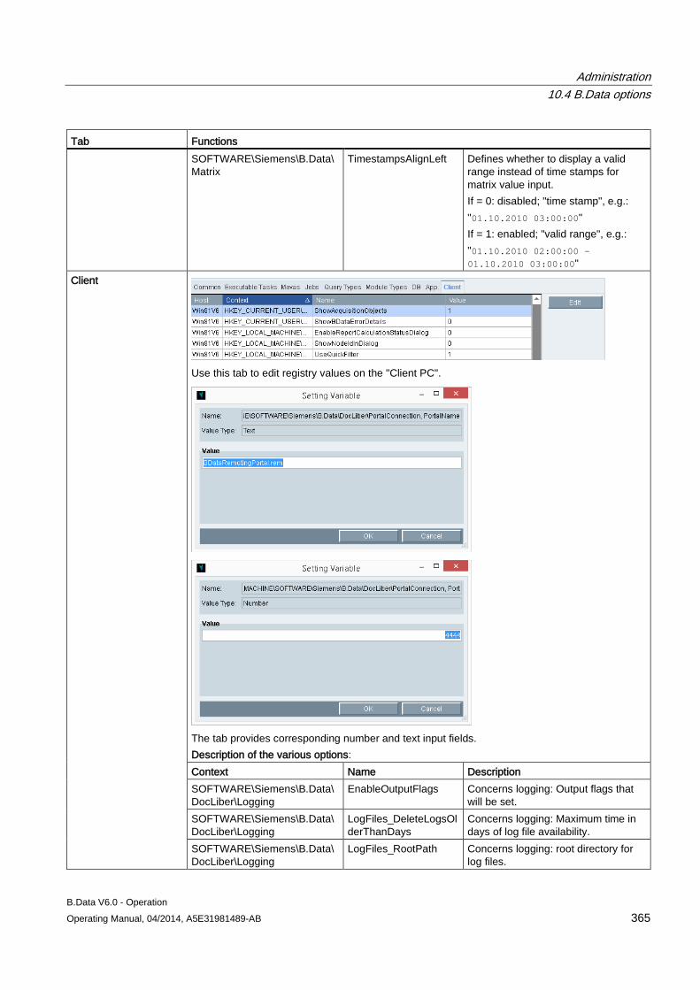
Administration 10.4 B.Data options
B.Data V6.0 - Operation Operating Manual, 04/2014, A5E31981489-AB 365
Tab Functions SOFTWARE\Siemens\B.Data\Matrix
TimestampsAlignLeft Defines whether to display a valid range instead of time stamps for matrix value input. If = 0: disabled; "time stamp", e.g.: "01.10.2010 03:00:00" If = 1: enabled; "valid range", e.g.: "01.10.2010 02:00:00 - 01.10.2010 03:00:00"
Client
Use this tab to edit registry values on the "Client PC".
The tab provides corresponding number and text input fields. Description of the various options: Context Name Description SOFTWARE\Siemens\B.Data\DocLiber\Logging
EnableOutputFlags Concerns logging: Output flags that will be set.
SOFTWARE\Siemens\B.Data\DocLiber\Logging
LogFiles_DeleteLogsOlderThanDays
Concerns logging: Maximum time in days of log file availability.
SOFTWARE\Siemens\B.Data\DocLiber\Logging
LogFiles_RootPath Concerns logging: root directory for log files.
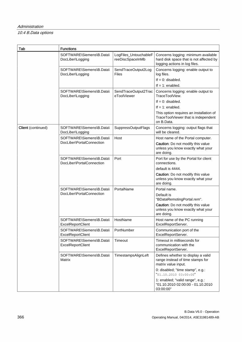
Administration 10.4 B.Data options
B.Data V6.0 - Operation 366 Operating Manual, 04/2014, A5E31981489-AB
Tab Functions SOFTWARE\Siemens\B.Data\DocLiber\Logging
LogFiles_UntouchableFreeDiscSpaceInMb
Concerns logging: minimum available hard disk space that is not affected by logging actions in log files.
SOFTWARE\Siemens\B.Data\DocLiber\Logging
SendTraceOutput2LogFiles
Concerns logging: enable output to log files. If = 0: disabled. If = 1: enabled.
SOFTWARE\Siemens\B.Data\DocLiber\Logging
SendTraceOutput2TraceToolViewer
Concerns logging: enable output to TraceToolView. If = 0: disabled. If = 1: enabled. This option requires an installation of TraceToolViewer that is independent on B.Data.
Client (continued) SOFTWARE\Siemens\B.Data\DocLiber\Logging
SuppressOutputFlags Concerns logging: output flags that will be cleared.
SOFTWARE\Siemens\B.Data\DocLiber\PortalConnection
Host Host name of the Portal computer. Caution: Do not modify this value unless you know exactly what your are doing.
SOFTWARE\Siemens\B.Data\DocLiber\PortalConnection
Port Port for use by the Portal for client connections. default is 4444. Caution: Do not modify this value unless you know exactly what your are doing.
SOFTWARE\Siemens\B.Data\DocLiber\PortalConnection
PortalName Portal name. Default is "BDataRemotingPortal.rem". Caution: Do not modify this value unless you know exactly what your are doing.
SOFTWARE\Siemens\B.Data\ExcelReportClient
HostName Host name of the PC running ExcelReportServer.
SOFTWARE\Siemens\B.Data\ExcelReportClient
PortNumber Communication port of the ExcelReportServer.
SOFTWARE\Siemens\B.Data\ExcelReportClient
Timeout Timeout in milliseconds for communication with the ExcelReportServer.
SOFTWARE\Siemens\B.Data\Matrix
TimestampsAlignLeft Defines whether to display a valid range instead of time stamps for matrix value input. 0: disabled; "time stamp", e.g.: "01.10.2010 03:00:00" 1: enabled; "valid range", e.g.: "01.10.2010 02:00:00 - 01.10.2010 03:00:00"
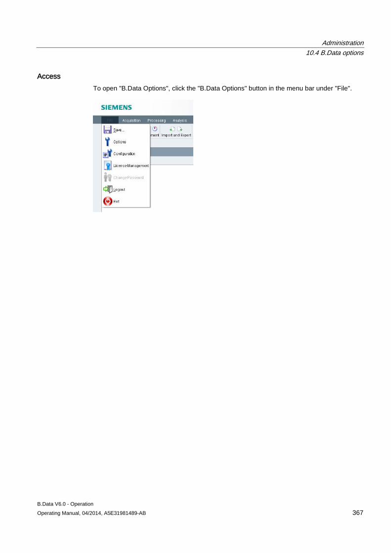
Administration 10.4 B.Data options
B.Data V6.0 - Operation Operating Manual, 04/2014, A5E31981489-AB 367
Access To open "B.Data Options", click the "B.Data Options" button in the menu bar under "File".
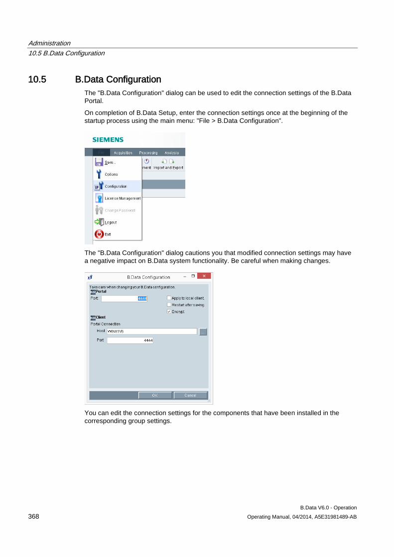
Administration 10.5 B.Data Configuration
B.Data V6.0 - Operation 368 Operating Manual, 04/2014, A5E31981489-AB
10.5 B.Data Configuration The "B.Data Configuration" dialog can be used to edit the connection settings of the B.Data Portal.
On completion of B.Data Setup, enter the connection settings once at the beginning of the startup process using the main menu: "File > B.Data Configuration".
The "B.Data Configuration" dialog cautions you that modified connection settings may have a negative impact on B.Data system functionality. Be careful when making changes.
You can edit the connection settings for the components that have been installed in the corresponding group settings.
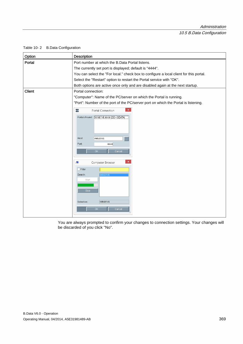
Administration 10.5 B.Data Configuration
B.Data V6.0 - Operation Operating Manual, 04/2014, A5E31981489-AB 369
Table 10- 2 B.Data Configuration
Option Description Portal Port number at which the B.Data Portal listens.
The currently set port is displayed; default is "4444". You can select the "For local." check box to configure a local client for this portal. Select the "Restart" option to restart the Portal service with "OK". Both options are active once only and are disabled again at the next startup.
Client Portal connection: "Computer": Name of the PC/server on which the Portal is running. "Port": Number of the port of the PC/server port on which the Portal is listening.
You are always prompted to confirm your changes to connection settings. Your changes will be discarded of you click "No".
Administration 10.6 Service Cockpit
B.Data V6.0 - Operation 370 Operating Manual, 04/2014, A5E31981489-AB
10.6 Service Cockpit
10.6.1 Service Cockpit basics
Definition The Service Cockpit provides you with an overview of the status of the acquisition components that are configured in the system.
Usage You can also use the Service Cockpit for the following purposes:
● To obtain an overview of all configured acquisition components.
● To view the log files that log all actions of an acquisition component.
● To determine the status of an acquisition component. To show whether the acquisition component is acquiring data, or whether an error has occurred.
● To control an acquisition component: You can restart the acquisition component if its fails to run.
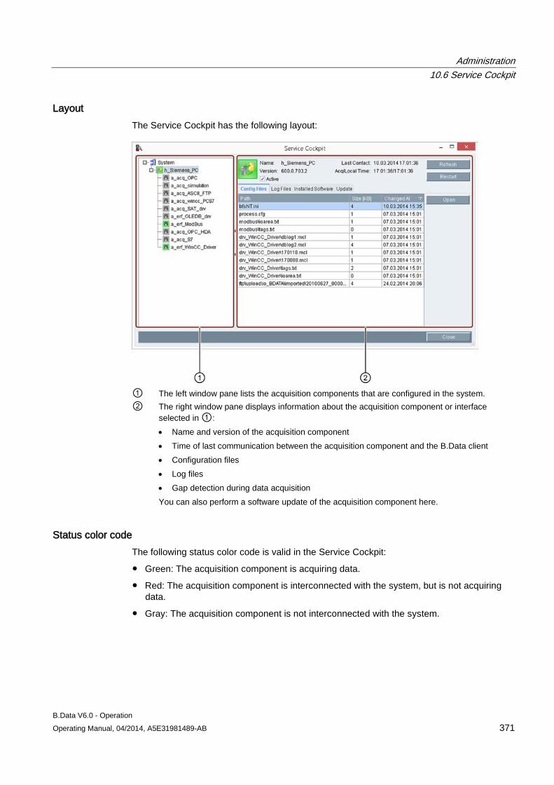
Administration 10.6 Service Cockpit
B.Data V6.0 - Operation Operating Manual, 04/2014, A5E31981489-AB 371
Layout The Service Cockpit has the following layout:
① The left window pane lists the acquisition components that are configured in the system. ② The right window pane displays information about the acquisition component or interface
selected in ①: • Name and version of the acquisition component • Time of last communication between the acquisition component and the B.Data client • Configuration files • Log files • Gap detection during data acquisition You can also perform a software update of the acquisition component here.
Status color code The following status color code is valid in the Service Cockpit:
● Green: The acquisition component is acquiring data.
● Red: The acquisition component is interconnected with the system, but is not acquiring data.
● Gray: The acquisition component is not interconnected with the system.
Administration 10.6 Service Cockpit
B.Data V6.0 - Operation 372 Operating Manual, 04/2014, A5E31981489-AB
10.6.2 Using the Service Cockpit
Overview You use the Service Cockpit to manage the available acquisition components and the drivers installed on them.
Requirement For the software update of the acquisition component:
● The acquisition component is installed on the PC.
● The PC is connected to the B.Data server.
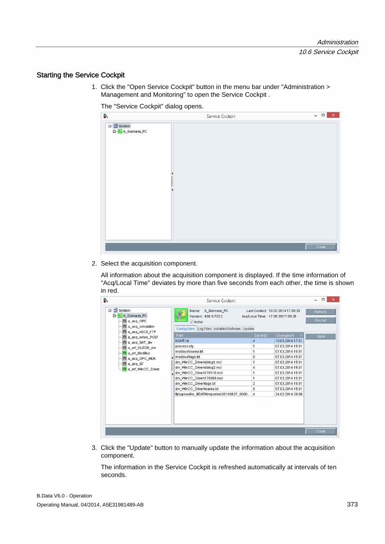
Administration 10.6 Service Cockpit
B.Data V6.0 - Operation Operating Manual, 04/2014, A5E31981489-AB 373
Starting the Service Cockpit 1. Click the "Open Service Cockpit" button in the menu bar under "Administration >
Management and Monitoring" to open the Service Cockpit .
The "Service Cockpit" dialog opens.
2. Select the acquisition component.
All information about the acquisition component is displayed. If the time information of "Acq/Local Time" deviates by more than five seconds from each other, the time is shown in red.
3. Click the "Update" button to manually update the information about the acquisition
component.
The information in the Service Cockpit is refreshed automatically at intervals of ten seconds.
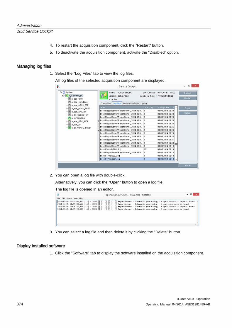
Administration 10.6 Service Cockpit
B.Data V6.0 - Operation 374 Operating Manual, 04/2014, A5E31981489-AB
4. To restart the acquisition component, click the "Restart" button.
5. To deactivate the acquisition component, activate the "Disabled" option.
Managing log files 1. Select the "Log Files" tab to view the log files.
All log files of the selected acquisition component are displayed.
2. You can open a log file with double-click.
Alternatively, you can click the "Open" button to open a log file.
The log file is opened in an editor.
3. You can select a log file and then delete it by clicking the "Delete" button.
Display installed software 1. Click the "Software" tab to display the software installed on the acquisition component.
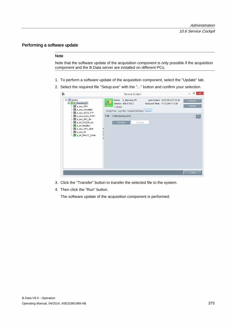
Administration 10.6 Service Cockpit
B.Data V6.0 - Operation Operating Manual, 04/2014, A5E31981489-AB 375
Performing a software update
Note
Note that the software update of the acquisition component is only possible if the acquisition component and the B.Data server are installed on different PCs.
1. To perform a software update of the acquisition component, select the "Update" tab.
2. Select the required file "Setup.exe" with the "..." button and confirm your selection.
3. Click the "Transfer" button to transfer the selected file to the system.
4. Then click the "Run" button.
The software update of the acquisition component is performed.
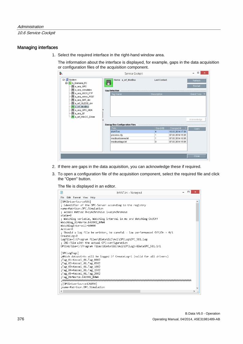
Administration 10.6 Service Cockpit
B.Data V6.0 - Operation 376 Operating Manual, 04/2014, A5E31981489-AB
Managing interfaces 1. Select the required interface in the right-hand window area.
The information about the interface is displayed, for example, gaps in the data acquisition or configuration files of the acquisition component.
2. If there are gaps in the data acquisition, you can acknowledge these if required.
3. To open a configuration file of the acquisition component, select the required file and click the "Open" button.
The file is displayed in an editor.
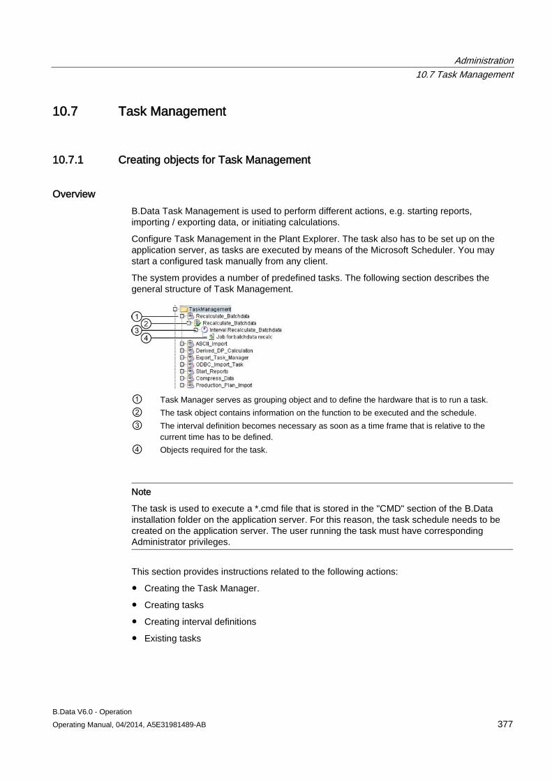
Administration 10.7 Task Management
B.Data V6.0 - Operation Operating Manual, 04/2014, A5E31981489-AB 377
10.7 Task Management
10.7.1 Creating objects for Task Management
Overview B.Data Task Management is used to perform different actions, e.g. starting reports, importing / exporting data, or initiating calculations.
Configure Task Management in the Plant Explorer. The task also has to be set up on the application server, as tasks are executed by means of the Microsoft Scheduler. You may start a configured task manually from any client.
The system provides a number of predefined tasks. The following section describes the general structure of Task Management.
① Task Manager serves as grouping object and to define the hardware that is to run a task. ② The task object contains information on the function to be executed and the schedule. ③ The interval definition becomes necessary as soon as a time frame that is relative to the
current time has to be defined. ④ Objects required for the task.
Note
The task is used to execute a *.cmd file that is stored in the "CMD" section of the B.Data installation folder on the application server. For this reason, the task schedule needs to be created on the application server. The user running the task must have corresponding Administrator privileges.
This section provides instructions related to the following actions:
● Creating the Task Manager.
● Creating tasks
● Creating interval definitions
● Existing tasks
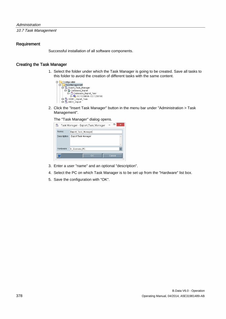
Administration 10.7 Task Management
B.Data V6.0 - Operation 378 Operating Manual, 04/2014, A5E31981489-AB
Requirement Successful installation of all software components.
Creating the Task Manager 1. Select the folder under which the Task Manager is going to be created. Save all tasks to
this folder to avoid the creation of different tasks with the same content.
2. Click the "Insert Task Manager" button in the menu bar under "Administration > Task
Management".
The "Task Manager" dialog opens.
3. Enter a user "name" and an optional "description".
4. Select the PC on which Task Manager is to be set up from the "Hardware" list box.
5. Save the configuration with "OK".
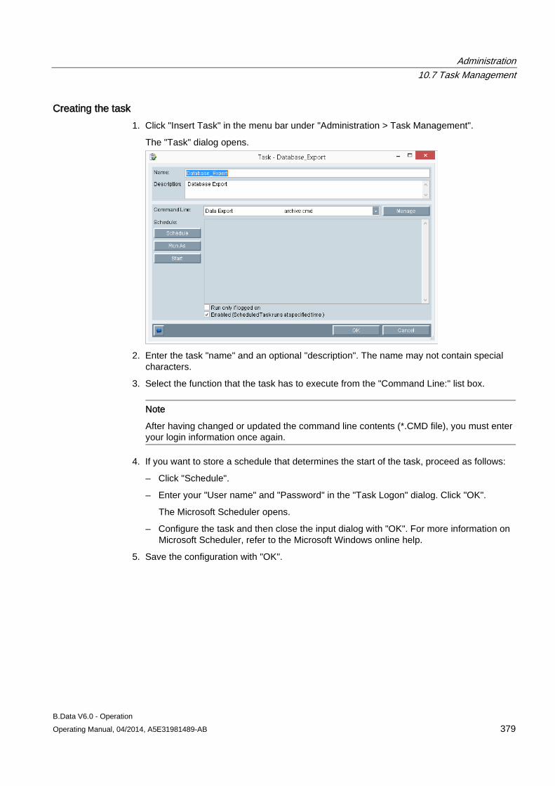
Administration 10.7 Task Management
B.Data V6.0 - Operation Operating Manual, 04/2014, A5E31981489-AB 379
Creating the task 1. Click "Insert Task" in the menu bar under "Administration > Task Management".
The "Task" dialog opens.
2. Enter the task "name" and an optional "description". The name may not contain special
characters.
3. Select the function that the task has to execute from the "Command Line:" list box.
Note
After having changed or updated the command line contents (*.CMD file), you must enter your login information once again.
4. If you want to store a schedule that determines the start of the task, proceed as follows:
– Click "Schedule".
– Enter your "User name" and "Password" in the "Task Logon" dialog. Click "OK".
The Microsoft Scheduler opens.
– Configure the task and then close the input dialog with "OK". For more information on Microsoft Scheduler, refer to the Microsoft Windows online help.
5. Save the configuration with "OK".
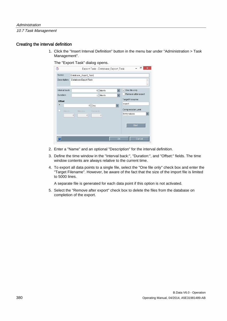
Administration 10.7 Task Management
B.Data V6.0 - Operation 380 Operating Manual, 04/2014, A5E31981489-AB
Creating the interval definition 1. Click the "Insert Interval Definition" button in the menu bar under "Administration > Task
Management".
The "Export Task" dialog opens.
2. Enter a "Name" and an optional "Description" for the interval definition.
3. Define the time window in the "Interval back:", "Duration:", and "Offset:" fields. The time window contents are always relative to the current time.
4. To export all data points to a single file, select the "One file only" check box and enter the "Target Filename". However, be aware of the fact that the size of the import file is limited to 5000 lines.
A separate file is generated for each data point if this option is not activated.
5. Select the "Remove after export" check box to delete the files from the database on completion of the export.
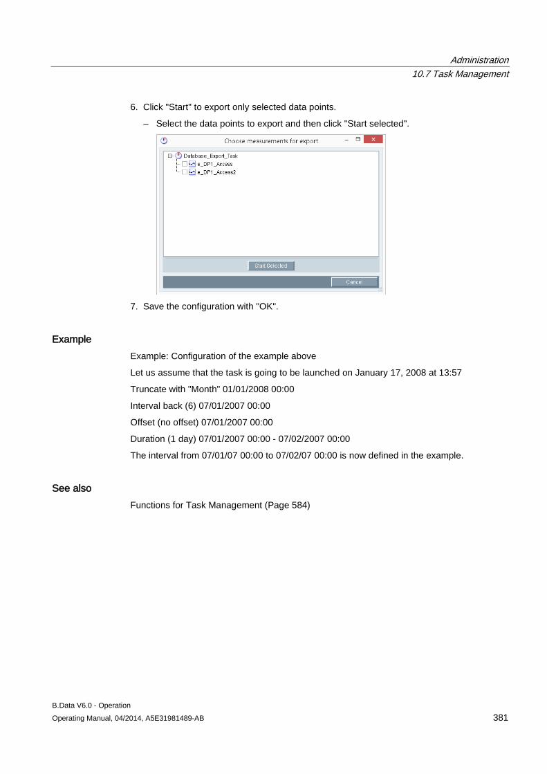
Administration 10.7 Task Management
B.Data V6.0 - Operation Operating Manual, 04/2014, A5E31981489-AB 381
6. Click "Start" to export only selected data points.
– Select the data points to export and then click "Start selected".
7. Save the configuration with "OK".
Example Example: Configuration of the example above
Let us assume that the task is going to be launched on January 17, 2008 at 13:57
Truncate with "Month" 01/01/2008 00:00
Interval back (6) 07/01/2007 00:00
Offset (no offset) 07/01/2007 00:00
Duration (1 day) 07/01/2007 00:00 - 07/02/2007 00:00
The interval from 07/01/07 00:00 to 07/02/07 00:00 is now defined in the example.
See also Functions for Task Management (Page 584)
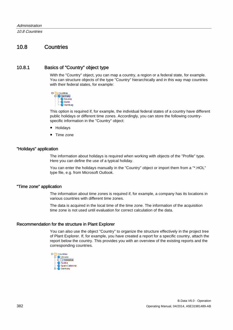
Administration 10.8 Countries
B.Data V6.0 - Operation 382 Operating Manual, 04/2014, A5E31981489-AB
10.8 Countries
10.8.1 Basics of "Country" object type With the "Country" object, you can map a country, a region or a federal state, for example. You can structure objects of the type "Country" hierarchically and in this way map countries with their federal states, for example:
This option is required if, for example, the individual federal states of a country have different public holidays or different time zones. Accordingly, you can store the following country-specific information in the "Country" object:
● Holidays
● Time zone
"Holidays" application The information about holidays is required when working with objects of the "Profile" type. Here you can define the use of a typical holiday.
You can enter the holidays manually in the "Country" object or import them from a "*.HOL" type file, e.g. from Microsoft Outlook.
"Time zone" application The information about time zones is required if, for example, a company has its locations in various countries with different time zones.
The data is acquired in the local time of the time zone. The information of the acquisition time zone is not used until evaluation for correct calculation of the data.
Recommendation for the structure in Plant Explorer You can also use the object "Country" to organize the structure effectively in the project tree of Plant Explorer. If, for example, you have created a report for a specific country, attach the report below the country. This provides you with an overview of the existing reports and the corresponding countries.
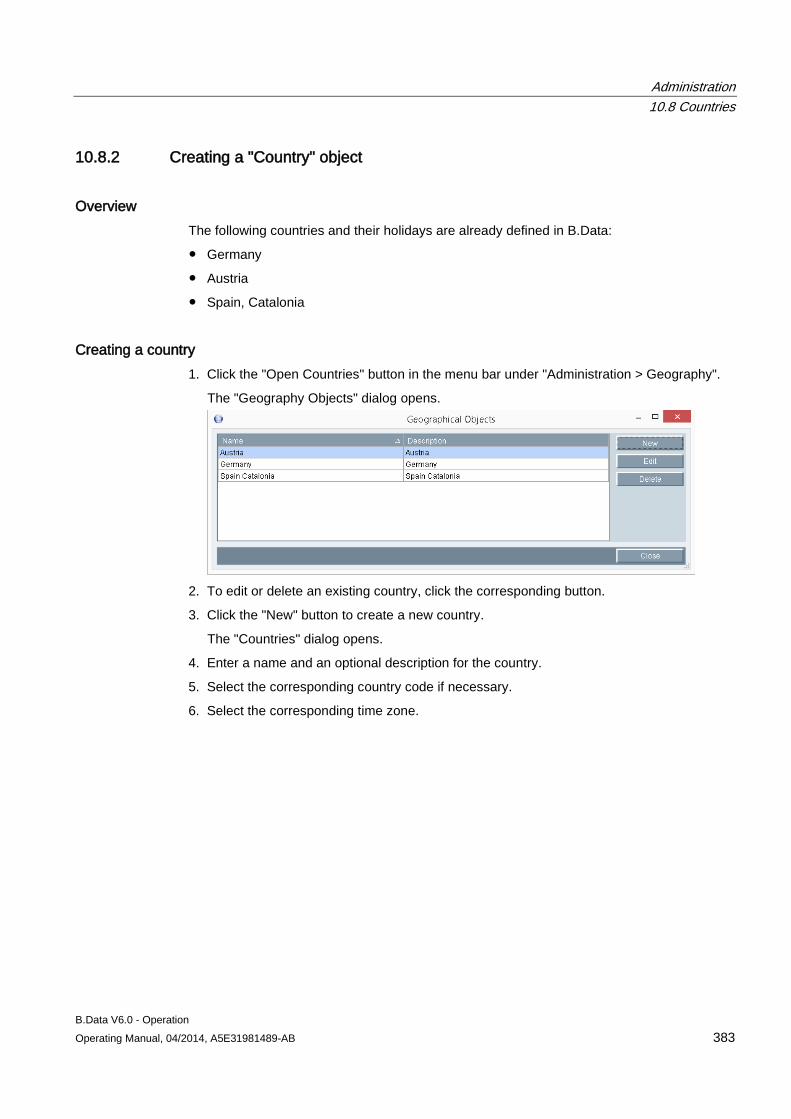
Administration 10.8 Countries
B.Data V6.0 - Operation Operating Manual, 04/2014, A5E31981489-AB 383
10.8.2 Creating a "Country" object
Overview The following countries and their holidays are already defined in B.Data:
● Germany
● Austria
● Spain, Catalonia
Creating a country 1. Click the "Open Countries" button in the menu bar under "Administration > Geography".
The "Geography Objects" dialog opens.
2. To edit or delete an existing country, click the corresponding button.
3. Click the "New" button to create a new country.
The "Countries" dialog opens.
4. Enter a name and an optional description for the country.
5. Select the corresponding country code if necessary.
6. Select the corresponding time zone.
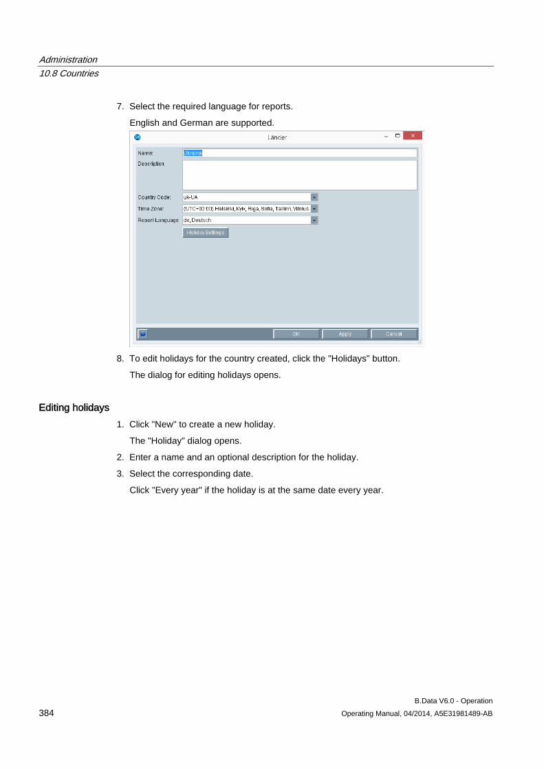
Administration 10.8 Countries
B.Data V6.0 - Operation 384 Operating Manual, 04/2014, A5E31981489-AB
7. Select the required language for reports.
English and German are supported.
8. To edit holidays for the country created, click the "Holidays" button.
The dialog for editing holidays opens.
Editing holidays 1. Click "New" to create a new holiday.
The "Holiday" dialog opens.
2. Enter a name and an optional description for the holiday.
3. Select the corresponding date.
Click "Every year" if the holiday is at the same date every year.
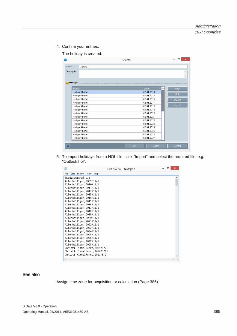
Administration 10.8 Countries
B.Data V6.0 - Operation Operating Manual, 04/2014, A5E31981489-AB 385
4. Confirm your entries.
The holiday is created.
5. To import holidays from a HOL file, click "Import" and select the required file, e.g.
"Outlook.hol":
See also Assign time zone for acquisition or calculation (Page 386)
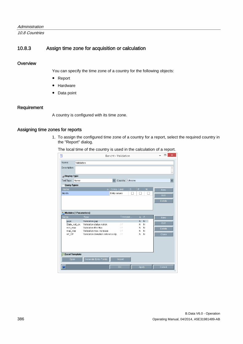
Administration 10.8 Countries
B.Data V6.0 - Operation 386 Operating Manual, 04/2014, A5E31981489-AB
10.8.3 Assign time zone for acquisition or calculation
Overview You can specify the time zone of a country for the following objects:
● Report
● Hardware
● Data point
Requirement A country is configured with its time zone.
Assigning time zones for reports 1. To assign the configured time zone of a country for a report, select the required country in
the "Report" dialog.
The local time of the country is used in the calculation of a report.
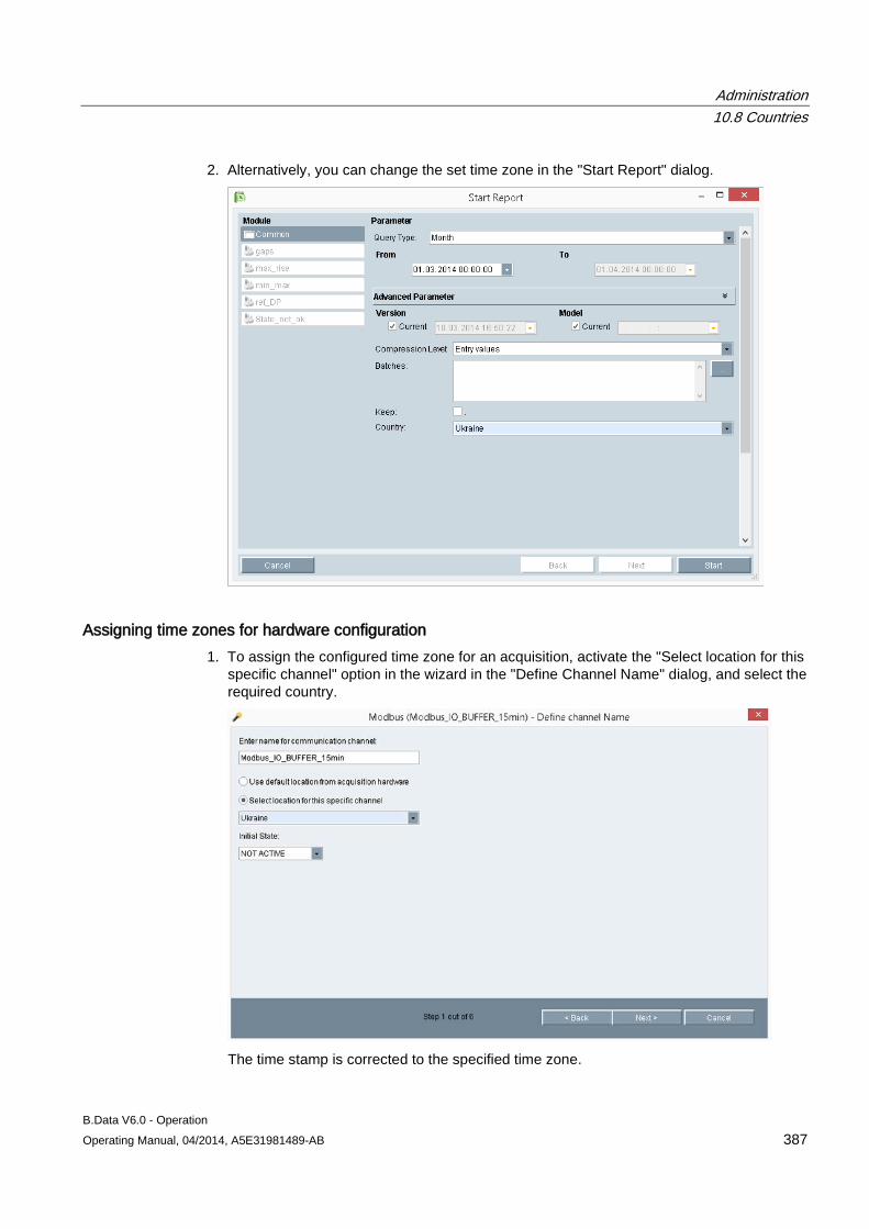
Administration 10.8 Countries
B.Data V6.0 - Operation Operating Manual, 04/2014, A5E31981489-AB 387
2. Alternatively, you can change the set time zone in the "Start Report" dialog.
Assigning time zones for hardware configuration 1. To assign the configured time zone for an acquisition, activate the "Select location for this
specific channel" option in the wizard in the "Define Channel Name" dialog, and select the required country.
The time stamp is corrected to the specified time zone.
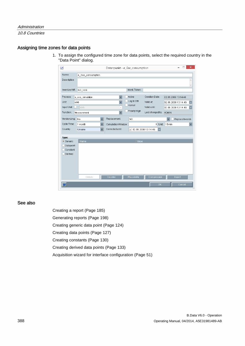
Administration 10.8 Countries
B.Data V6.0 - Operation 388 Operating Manual, 04/2014, A5E31981489-AB
Assigning time zones for data points 1. To assign the configured time zone for data points, select the required country in the
"Data Point" dialog.
See also Creating a report (Page 185)
Generating reports (Page 198)
Creating generic data point (Page 124)
Creating data points (Page 127)
Creating constants (Page 130)
Creating derived data points (Page 133)
Acquisition wizard for interface configuration (Page 51)
Administration 10.9 Exporting and importing data
B.Data V6.0 - Operation Operating Manual, 04/2014, A5E31981489-AB 389
10.9 Exporting and importing data
10.9.1 Basic principles of export and import
Overview You can export your configuration data in XML format in B.Data and import them again. Use the "Import / Export" option, for example, to back up your configuration data.
Conflict test during import The objects to be imported are compared with the objects in B.Data based on name and type during import. If an object already exists, you are prompted to make a selection: You can either keep the object or overwrite it.
Note You cannot undo the data import
Overwriting of objects during import can result in inconsistent data or evaluation errors due to changed values.
Prepare the import process carefully. Check if there are conflicts with existing data prior to the import. Note the following recommendations: • Divide a comprehensive data export into several steps. • If possible, export only data you have created yourself.
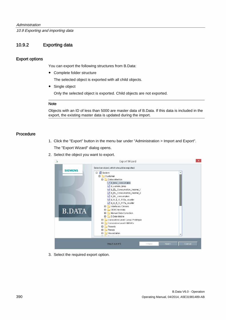
Administration 10.9 Exporting and importing data
B.Data V6.0 - Operation 390 Operating Manual, 04/2014, A5E31981489-AB
10.9.2 Exporting data
Export options You can export the following structures from B.Data:
● Complete folder structure
The selected object is exported with all child objects.
● Single object
Only the selected object is exported. Child objects are not exported.
Note
Objects with an ID of less than 5000 are master data of B.Data. If this data is included in the export, the existing master data is updated during the import.
Procedure 1. Click the "Export" button in the menu bar under "Administration > Import and Export".
The "Export Wizard" dialog opens.
2. Select the object you want to export.
3. Select the required export option.

Administration 10.9 Exporting and importing data
B.Data V6.0 - Operation Operating Manual, 04/2014, A5E31981489-AB 391
4. Select the directory in which the export files are to be stored.
The data is exported from B.Data. Two files are created during the export:
– "Nodes.xml" with the exported data
– "logdoc.txt" with detailed information on the export
5. Click "Finish".
Result The data export is complete.
Administration 10.9 Exporting and importing data
B.Data V6.0 - Operation 392 Operating Manual, 04/2014, A5E31981489-AB
10.9.3 Importing data
Import options You can import the following structures from B.Data:
● Complete folder structure that is saved in the XML file.
● Complete folder structure of the selected object
● Single object
Requirement The export data is stored in the file system.
Procedure 1. Click the "Import" button in the menu bar under "Administration > Import and Export".
The "Import Wizard" dialog opens.
2. Enter the folder in which the XML file you wish to import is located.
3. Select the required import option.
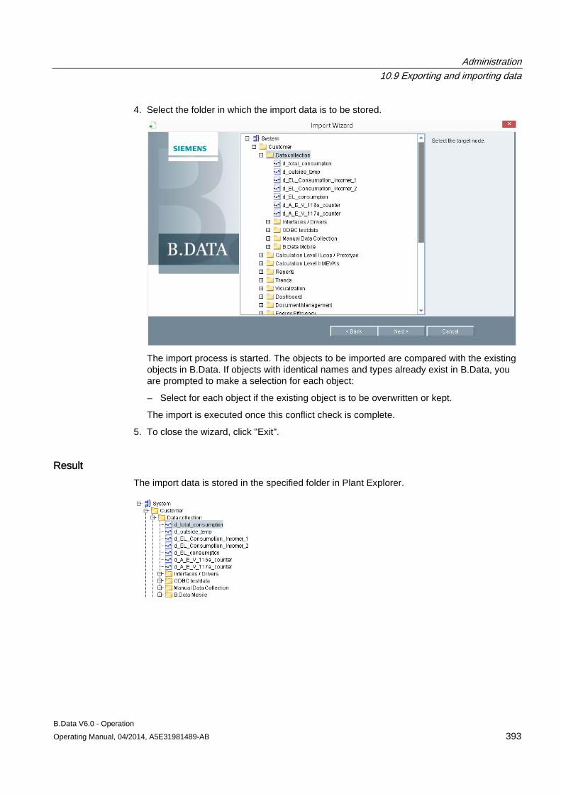
Administration 10.9 Exporting and importing data
B.Data V6.0 - Operation Operating Manual, 04/2014, A5E31981489-AB 393
4. Select the folder in which the import data is to be stored.
The import process is started. The objects to be imported are compared with the existing objects in B.Data. If objects with identical names and types already exist in B.Data, you are prompted to make a selection for each object:
– Select for each object if the existing object is to be overwritten or kept.
The import is executed once this conflict check is complete.
5. To close the wizard, click "Exit".
Result The import data is stored in the specified folder in Plant Explorer.

Administration 10.9 Exporting and importing data
B.Data V6.0 - Operation 394 Operating Manual, 04/2014, A5E31981489-AB
B.Data V6.0 - Operation Operating Manual, 04/2014, A5E31981489-AB 395
Using B.Data Web 11 11.1 Basics
11.1.1 Basic information on B.Data Web
Overview B.Data Web is a browser-based user interface for the SIMATIC B.Data energy management system. B.Data Web is used to access B.Data via the Internet/Intranet.
The administrator configures the data you may access in B.Data .
Note Installation of B.Data Web
You can find information on the installation of B.Data Web in the installation manual "B.Data V6.0 - Installation", section "Setting up B.Data Web ".
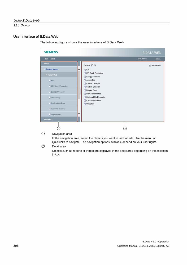
Using B.Data Web 11.1 Basics
B.Data V6.0 - Operation 396 Operating Manual, 04/2014, A5E31981489-AB
User interface of B.Data Web The following figure shows the user interface of B.Data Web:
① Navigation area
In the navigation area, select the objects you want to view or edit. Use the menu or Quicklinks to navigate. The navigation options available depend on your user rights.
② Detail area Objects such as reports or trends are displayed in the detail area depending on the selection in ①.
Using B.Data Web 11.1 Basics
B.Data V6.0 - Operation Operating Manual, 04/2014, A5E31981489-AB 397
Tasks in B.Data Web Use B.Data Web to handle the following tasks:
● Viewing reports and generating new reports
● Viewing trends and generating new trends
● Viewing visualizations
● Editing values in matrices
● Opening documents and uploading new documents in B.Data
● Viewing and editing energy efficiency measures
● Viewing dashboards
See also Configuring authorizations (Page 90)
Working with reports in B.Data Web (Page 402)
Working with trends in B.Data Web (Page 407)
Working with visualizations in B.Data Web (Page 410)
Working with matrixes in B.Data Web (Page 413)
Using document management in B.Data Web (Page 415)
Working with energy efficiency measures in B.Data Web (Page 416)
Working with dashboards in B.Data Web (Page 418)
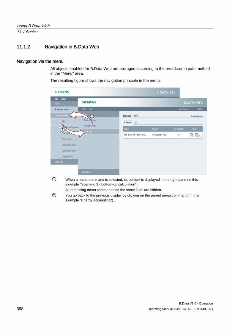
Using B.Data Web 11.1 Basics
B.Data V6.0 - Operation 398 Operating Manual, 04/2014, A5E31981489-AB
11.1.2 Navigation in B.Data Web
Navigation via the menu All objects enabled for B.Data Web are arranged according to the breadcrumb path method in the "Menu" area.
The resulting figure shows the navigation principle in the menu:
① When a menu command is selected, its content is displayed in the right pane (in this
example "Scenario 3 - bottom-up calculation"). All remaining menu commands on the same level are hidden.
② You go back to the previous display by clicking on the parent menu command (in this example "Energy accounting") .
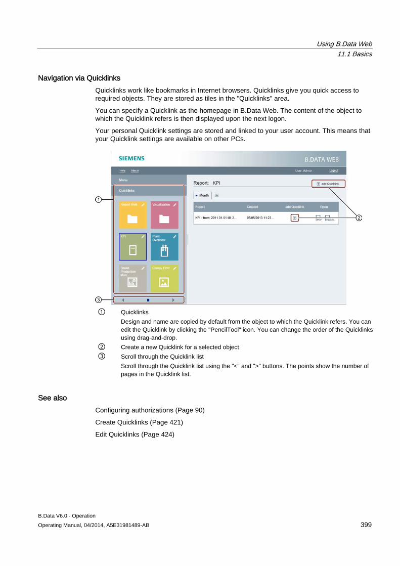
Using B.Data Web 11.1 Basics
B.Data V6.0 - Operation Operating Manual, 04/2014, A5E31981489-AB 399
Navigation via Quicklinks Quicklinks work like bookmarks in Internet browsers. Quicklinks give you quick access to required objects. They are stored as tiles in the "Quicklinks" area.
You can specify a Quicklink as the homepage in B.Data Web. The content of the object to which the Quicklink refers is then displayed upon the next logon.
Your personal Quicklink settings are stored and linked to your user account. This means that your Quicklink settings are available on other PCs.
① Quicklinks
Design and name are copied by default from the object to which the Quicklink refers. You can edit the Quicklink by clicking the "PencilTool" icon. You can change the order of the Quicklinks using drag-and-drop.
② Create a new Quicklink for a selected object ③ Scroll through the Quicklink list
Scroll through the Quicklink list using the "<" and ">" buttons. The points show the number of pages in the Quicklink list.
See also Configuring authorizations (Page 90)
Create Quicklinks (Page 421)
Edit Quicklinks (Page 424)
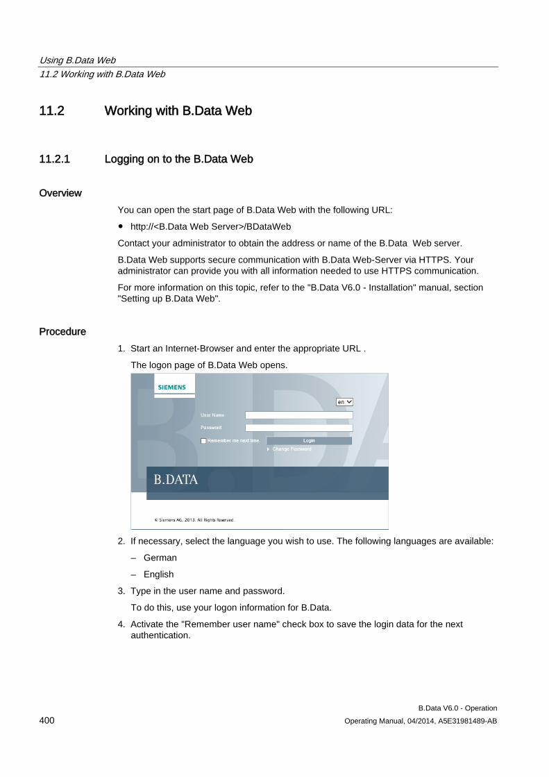
Using B.Data Web 11.2 Working with B.Data Web
B.Data V6.0 - Operation 400 Operating Manual, 04/2014, A5E31981489-AB
11.2 Working with B.Data Web
11.2.1 Logging on to the B.Data Web
Overview You can open the start page of B.Data Web with the following URL:
● http://<B.Data Web Server>/BDataWeb
Contact your administrator to obtain the address or name of the B.Data Web server.
B.Data Web supports secure communication with B.Data Web-Server via HTTPS. Your administrator can provide you with all information needed to use HTTPS communication.
For more information on this topic, refer to the "B.Data V6.0 - Installation" manual, section "Setting up B.Data Web".
Procedure 1. Start an Internet-Browser and enter the appropriate URL .
The logon page of B.Data Web opens.
2. If necessary, select the language you wish to use. The following languages are available:
– German
– English
3. Type in the user name and password.
To do this, use your logon information for B.Data.
4. Activate the "Remember user name" check box to save the login data for the next authentication.
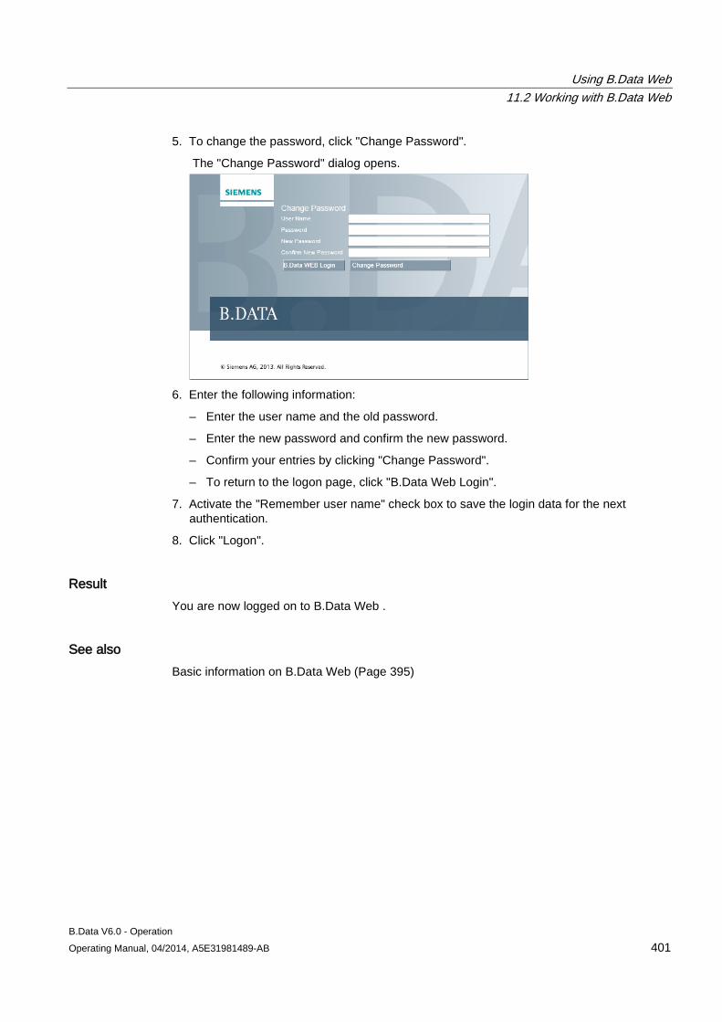
Using B.Data Web 11.2 Working with B.Data Web
B.Data V6.0 - Operation Operating Manual, 04/2014, A5E31981489-AB 401
5. To change the password, click "Change Password".
The "Change Password" dialog opens.
6. Enter the following information:
– Enter the user name and the old password.
– Enter the new password and confirm the new password.
– Confirm your entries by clicking "Change Password".
– To return to the logon page, click "B.Data Web Login".
7. Activate the "Remember user name" check box to save the login data for the next authentication.
8. Click "Logon".
Result You are now logged on to B.Data Web .
See also Basic information on B.Data Web (Page 395)
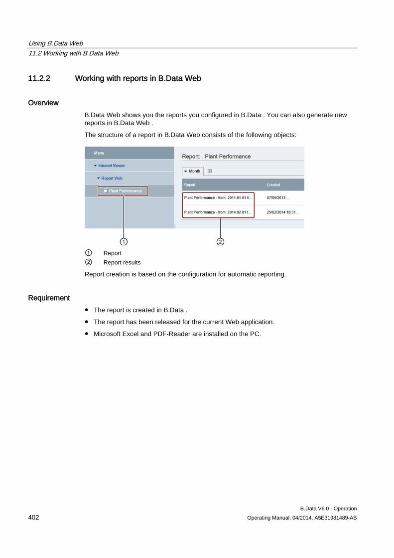
Using B.Data Web 11.2 Working with B.Data Web
B.Data V6.0 - Operation 402 Operating Manual, 04/2014, A5E31981489-AB
11.2.2 Working with reports in B.Data Web
Overview B.Data Web shows you the reports you configured in B.Data . You can also generate new reports in B.Data Web .
The structure of a report in B.Data Web consists of the following objects:
① Report ② Report results
Report creation is based on the configuration for automatic reporting.
Requirement ● The report is created in B.Data .
● The report has been released for the current Web application.
● Microsoft Excel and PDF-Reader are installed on the PC.
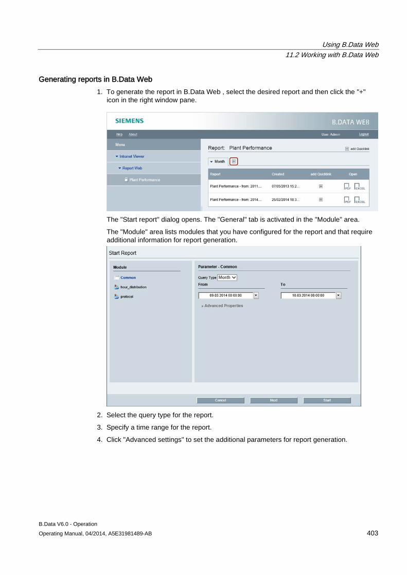
Using B.Data Web 11.2 Working with B.Data Web
B.Data V6.0 - Operation Operating Manual, 04/2014, A5E31981489-AB 403
Generating reports in B.Data Web 1. To generate the report in B.Data Web , select the desired report and then click the "+"
icon in the right window pane.
The "Start report" dialog opens. The "General" tab is activated in the "Module" area.
The "Module" area lists modules that you have configured for the report and that require additional information for report generation.
2. Select the query type for the report.
3. Specify a time range for the report.
4. Click "Advanced settings" to set the additional parameters for report generation.
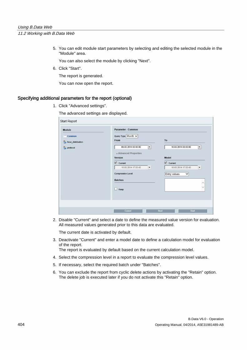
Using B.Data Web 11.2 Working with B.Data Web
B.Data V6.0 - Operation 404 Operating Manual, 04/2014, A5E31981489-AB
5. You can edit module start parameters by selecting and editing the selected module in the "Module" area.
You can also select the module by clicking "Next".
6. Click "Start".
The report is generated.
You can now open the report.
Specifying additional parameters for the report (optional) 1. Click "Advanced settings".
The advanced settings are displayed.
2. Disable "Current" and select a date to define the measured value version for evaluation.
All measured values generated prior to this data are evaluated.
The current date is activated by default.
3. Deactivate "Current" and enter a model date to define a calculation model for evaluation of the report. The report is evaluated by default based on the current calculation model.
4. Select the compression level in a report to evaluate the compression level values.
5. If necessary, select the required batch under "Batches".
6. You can exclude the report from cyclic delete actions by activating the "Retain" option. The delete job is executed later if you do not activate this "Retain" option.
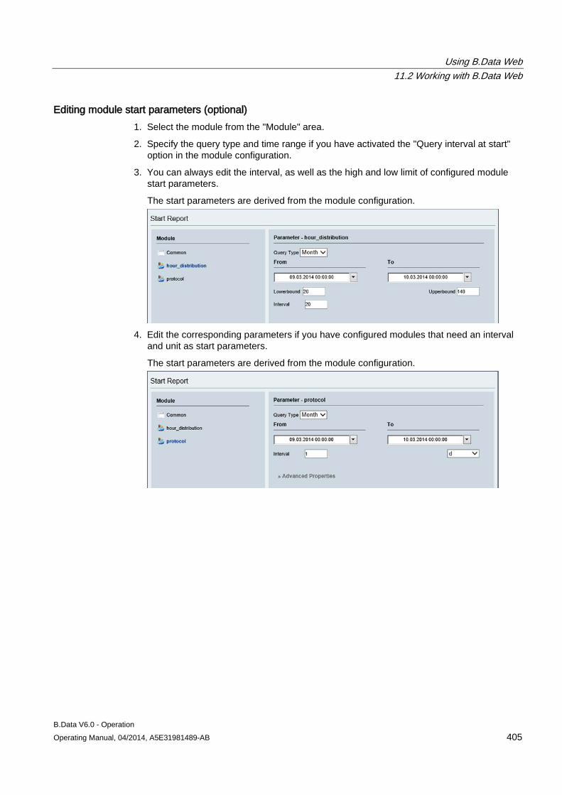
Using B.Data Web 11.2 Working with B.Data Web
B.Data V6.0 - Operation Operating Manual, 04/2014, A5E31981489-AB 405
Editing module start parameters (optional) 1. Select the module from the "Module" area.
2. Specify the query type and time range if you have activated the "Query interval at start" option in the module configuration.
3. You can always edit the interval, as well as the high and low limit of configured module start parameters.
The start parameters are derived from the module configuration.
4. Edit the corresponding parameters if you have configured modules that need an interval
and unit as start parameters.
The start parameters are derived from the module configuration.
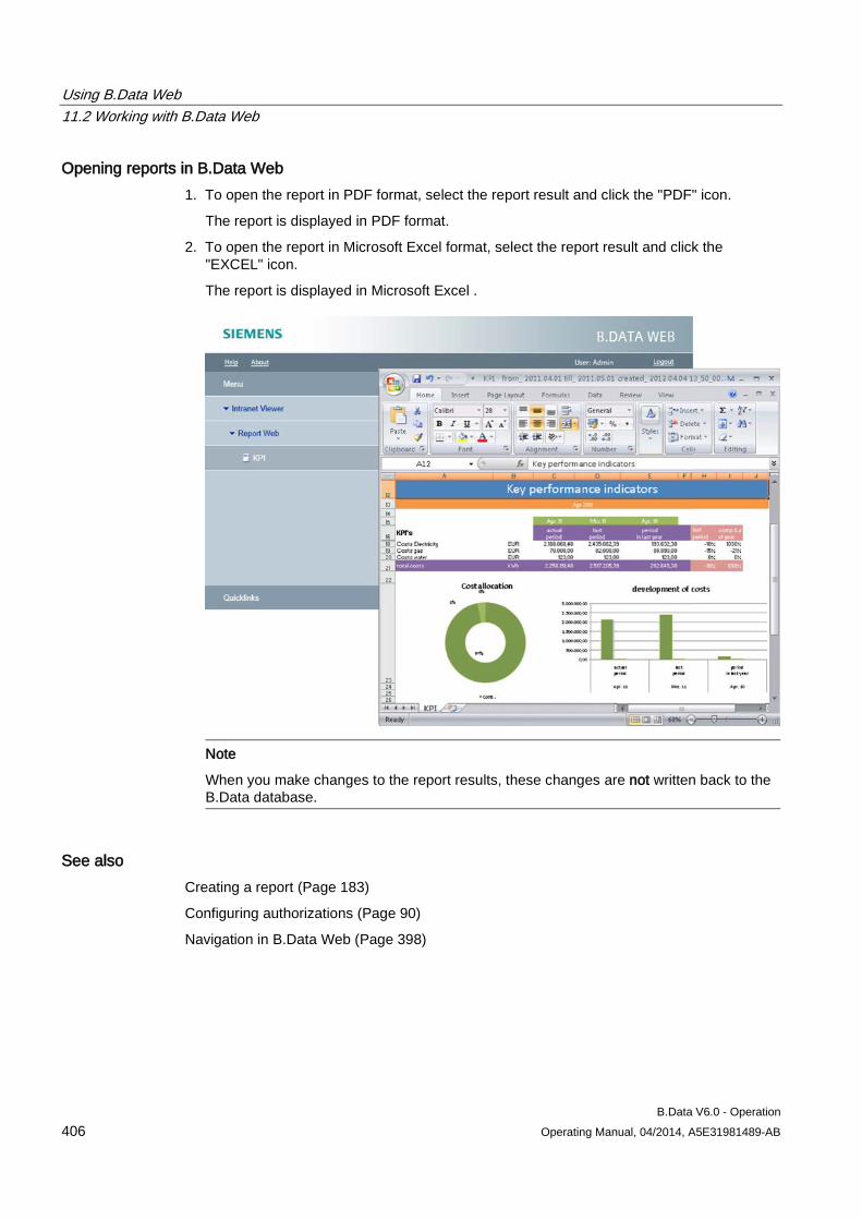
Using B.Data Web 11.2 Working with B.Data Web
B.Data V6.0 - Operation 406 Operating Manual, 04/2014, A5E31981489-AB
Opening reports in B.Data Web 1. To open the report in PDF format, select the report result and click the "PDF" icon.
The report is displayed in PDF format.
2. To open the report in Microsoft Excel format, select the report result and click the "EXCEL" icon.
The report is displayed in Microsoft Excel .
Note
When you make changes to the report results, these changes are not written back to the B.Data database.
See also Creating a report (Page 183)
Configuring authorizations (Page 90)
Navigation in B.Data Web (Page 398)
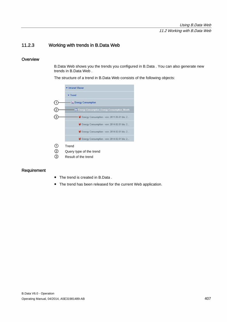
Using B.Data Web 11.2 Working with B.Data Web
B.Data V6.0 - Operation Operating Manual, 04/2014, A5E31981489-AB 407
11.2.3 Working with trends in B.Data Web
Overview B.Data Web shows you the trends you configured in B.Data . You can also generate new trends in B.Data Web .
The structure of a trend in B.Data Web consists of the following objects:
① Trend ② Query type of the trend ③ Result of the trend
Requirement ● The trend is created in B.Data .
● The trend has been released for the current Web application.
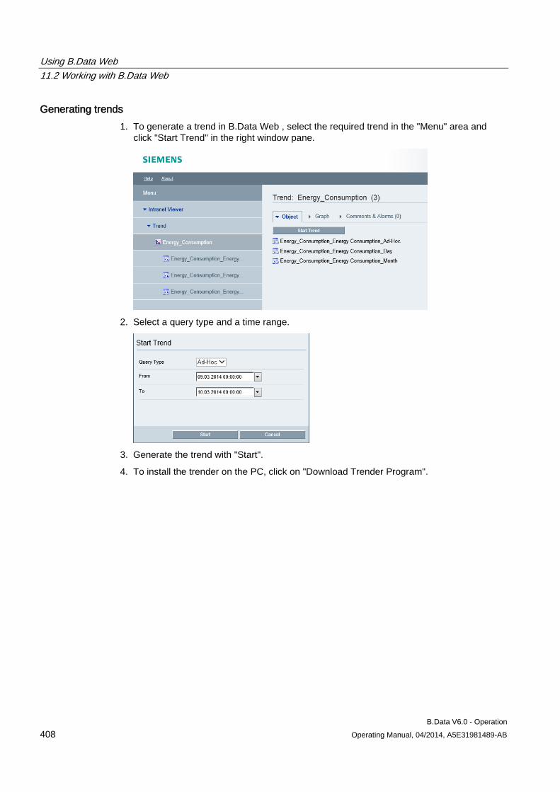
Using B.Data Web 11.2 Working with B.Data Web
B.Data V6.0 - Operation 408 Operating Manual, 04/2014, A5E31981489-AB
Generating trends 1. To generate a trend in B.Data Web , select the required trend in the "Menu" area and
click "Start Trend" in the right window pane.
2. Select a query type and a time range.
3. Generate the trend with "Start".
4. To install the trender on the PC, click on "Download Trender Program".
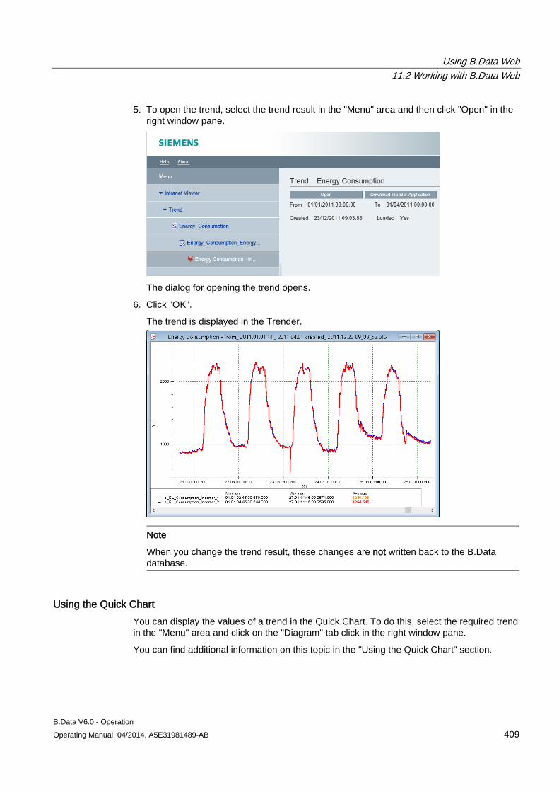
Using B.Data Web 11.2 Working with B.Data Web
B.Data V6.0 - Operation Operating Manual, 04/2014, A5E31981489-AB 409
5. To open the trend, select the trend result in the "Menu" area and then click "Open" in the right window pane.
The dialog for opening the trend opens.
6. Click "OK".
The trend is displayed in the Trender.
Note
When you change the trend result, these changes are not written back to the B.Data database.
Using the Quick Chart You can display the values of a trend in the Quick Chart. To do this, select the required trend in the "Menu" area and click on the "Diagram" tab click in the right window pane.
You can find additional information on this topic in the "Using the Quick Chart" section.
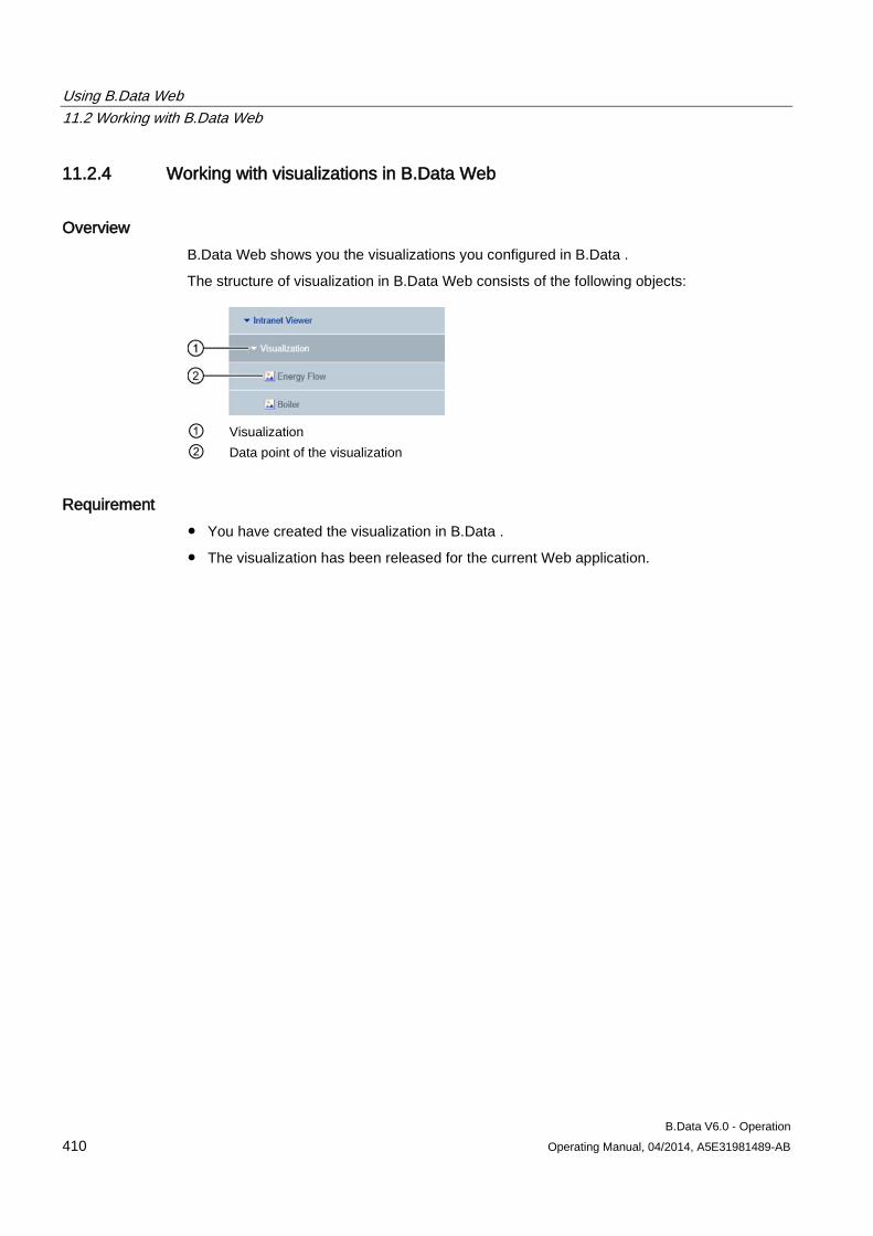
Using B.Data Web 11.2 Working with B.Data Web
B.Data V6.0 - Operation 410 Operating Manual, 04/2014, A5E31981489-AB
11.2.4 Working with visualizations in B.Data Web
Overview B.Data Web shows you the visualizations you configured in B.Data .
The structure of visualization in B.Data Web consists of the following objects:
① Visualization ② Data point of the visualization
Requirement ● You have created the visualization in B.Data .
● The visualization has been released for the current Web application.
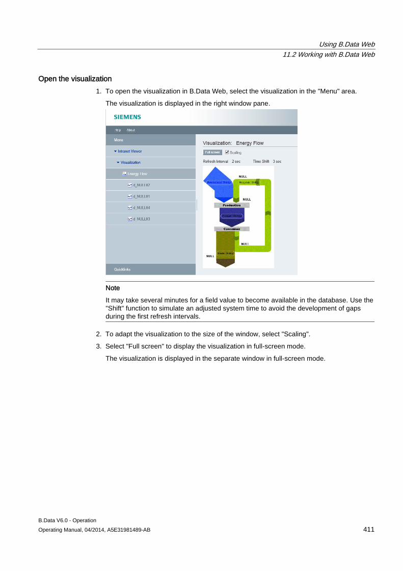
Using B.Data Web 11.2 Working with B.Data Web
B.Data V6.0 - Operation Operating Manual, 04/2014, A5E31981489-AB 411
Open the visualization 1. To open the visualization in B.Data Web, select the visualization in the "Menu" area.
The visualization is displayed in the right window pane.
Note
It may take several minutes for a field value to become available in the database. Use the "Shift" function to simulate an adjusted system time to avoid the development of gaps during the first refresh intervals.
2. To adapt the visualization to the size of the window, select "Scaling".
3. Select "Full screen" to display the visualization in full-screen mode.
The visualization is displayed in the separate window in full-screen mode.
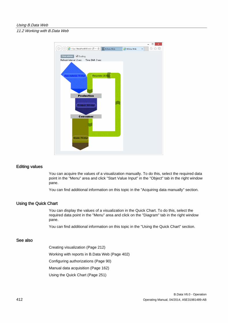
Using B.Data Web 11.2 Working with B.Data Web
B.Data V6.0 - Operation 412 Operating Manual, 04/2014, A5E31981489-AB
Editing values You can acquire the values of a visualization manually. To do this, select the required data point in the "Menu" area and click "Start Value Input" in the "Object" tab in the right window pane.
You can find additional information on this topic in the "Acquiring data manually" section.
Using the Quick Chart You can display the values of a visualization in the Quick Chart. To do this, select the required data point in the "Menu" area and click on the "Diagram" tab in the right window pane.
You can find additional information on this topic in the "Using the Quick Chart" section.
See also Creating visualization (Page 212)
Working with reports in B.Data Web (Page 402)
Configuring authorizations (Page 90)
Manual data acquisition (Page 162)
Using the Quick Chart (Page 251)
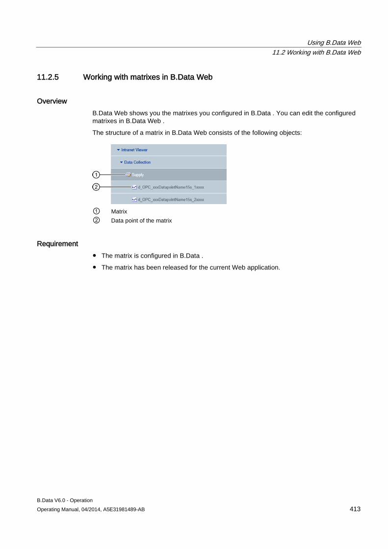
Using B.Data Web 11.2 Working with B.Data Web
B.Data V6.0 - Operation Operating Manual, 04/2014, A5E31981489-AB 413
11.2.5 Working with matrixes in B.Data Web
Overview B.Data Web shows you the matrixes you configured in B.Data . You can edit the configured matrixes in B.Data Web .
The structure of a matrix in B.Data Web consists of the following objects:
① Matrix ② Data point of the matrix
Requirement ● The matrix is configured in B.Data .
● The matrix has been released for the current Web application.
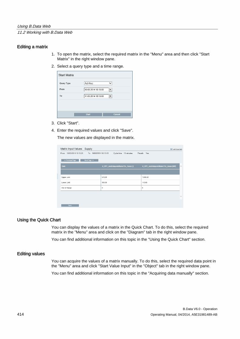
Using B.Data Web 11.2 Working with B.Data Web
B.Data V6.0 - Operation 414 Operating Manual, 04/2014, A5E31981489-AB
Editing a matrix 1. To open the matrix, select the required matrix in the "Menu" area and then click "Start
Matrix" in the right window pane.
2. Select a query type and a time range.
3. Click "Start".
4. Enter the required values and click "Save".
The new values are displayed in the matrix.
Using the Quick Chart You can display the values of a matrix in the Quick Chart. To do this, select the required matrix in the "Menu" area and click on the "Diagram" tab in the right window pane.
You can find additional information on this topic in the "Using the Quick Chart" section.
Editing values You can acquire the values of a matrix manually. To do this, select the required data point in the "Menu" area and click "Start Value Input" in the "Object" tab in the right window pane.
You can find additional information on this topic in the "Acquiring data manually" section.
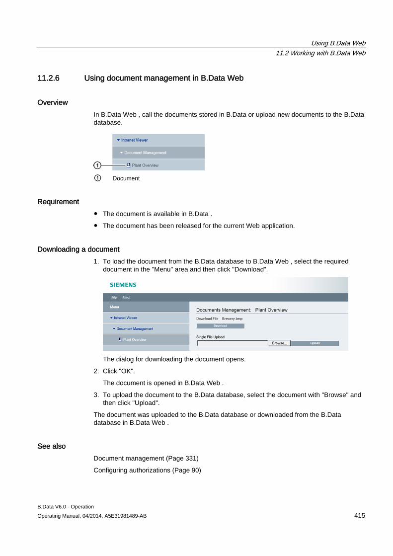
Using B.Data Web 11.2 Working with B.Data Web
B.Data V6.0 - Operation Operating Manual, 04/2014, A5E31981489-AB 415
11.2.6 Using document management in B.Data Web
Overview In B.Data Web , call the documents stored in B.Data or upload new documents to the B.Data database.
① Document
Requirement ● The document is available in B.Data .
● The document has been released for the current Web application.
Downloading a document 1. To load the document from the B.Data database to B.Data Web , select the required
document in the "Menu" area and then click "Download".
The dialog for downloading the document opens.
2. Click "OK".
The document is opened in B.Data Web .
3. To upload the document to the B.Data database, select the document with "Browse" and then click "Upload".
The document was uploaded to the B.Data database or downloaded from the B.Data database in B.Data Web .
See also Document management (Page 331)
Configuring authorizations (Page 90)
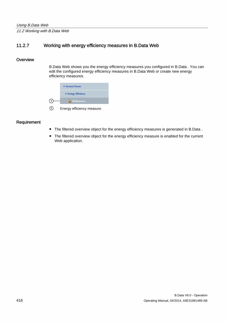
Using B.Data Web 11.2 Working with B.Data Web
B.Data V6.0 - Operation 416 Operating Manual, 04/2014, A5E31981489-AB
11.2.7 Working with energy efficiency measures in B.Data Web
Overview B.Data Web shows you the energy efficiency measures you configured in B.Data . You can edit the configured energy efficiency measures in B.Data Web or create new energy efficiency measures.
① Energy efficiency measure
Requirement ● The filtered overview object for the energy efficiency measures is generated in B.Data .
● The filtered overview object for the energy efficiency measure is enabled for the current Web application.
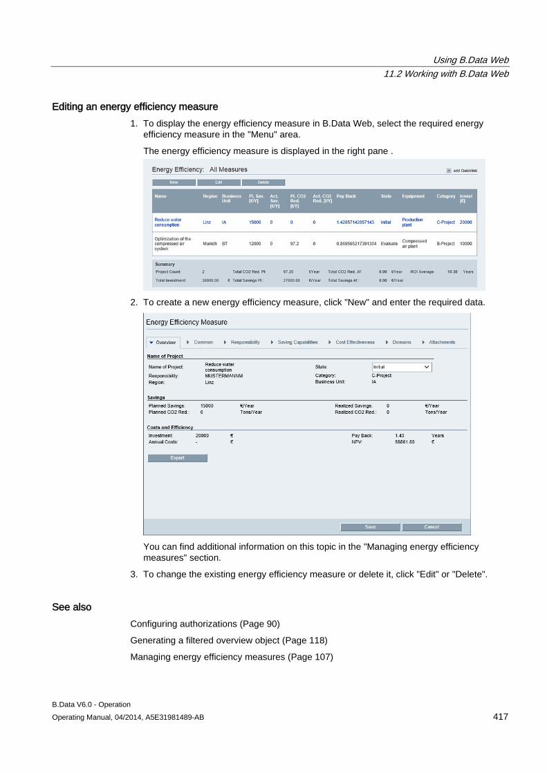
Using B.Data Web 11.2 Working with B.Data Web
B.Data V6.0 - Operation Operating Manual, 04/2014, A5E31981489-AB 417
Editing an energy efficiency measure 1. To display the energy efficiency measure in B.Data Web, select the required energy
efficiency measure in the "Menu" area.
The energy efficiency measure is displayed in the right pane .
2. To create a new energy efficiency measure, click "New" and enter the required data.
You can find additional information on this topic in the "Managing energy efficiency measures" section.
3. To change the existing energy efficiency measure or delete it, click "Edit" or "Delete".
See also Configuring authorizations (Page 90)
Generating a filtered overview object (Page 118)
Managing energy efficiency measures (Page 107)
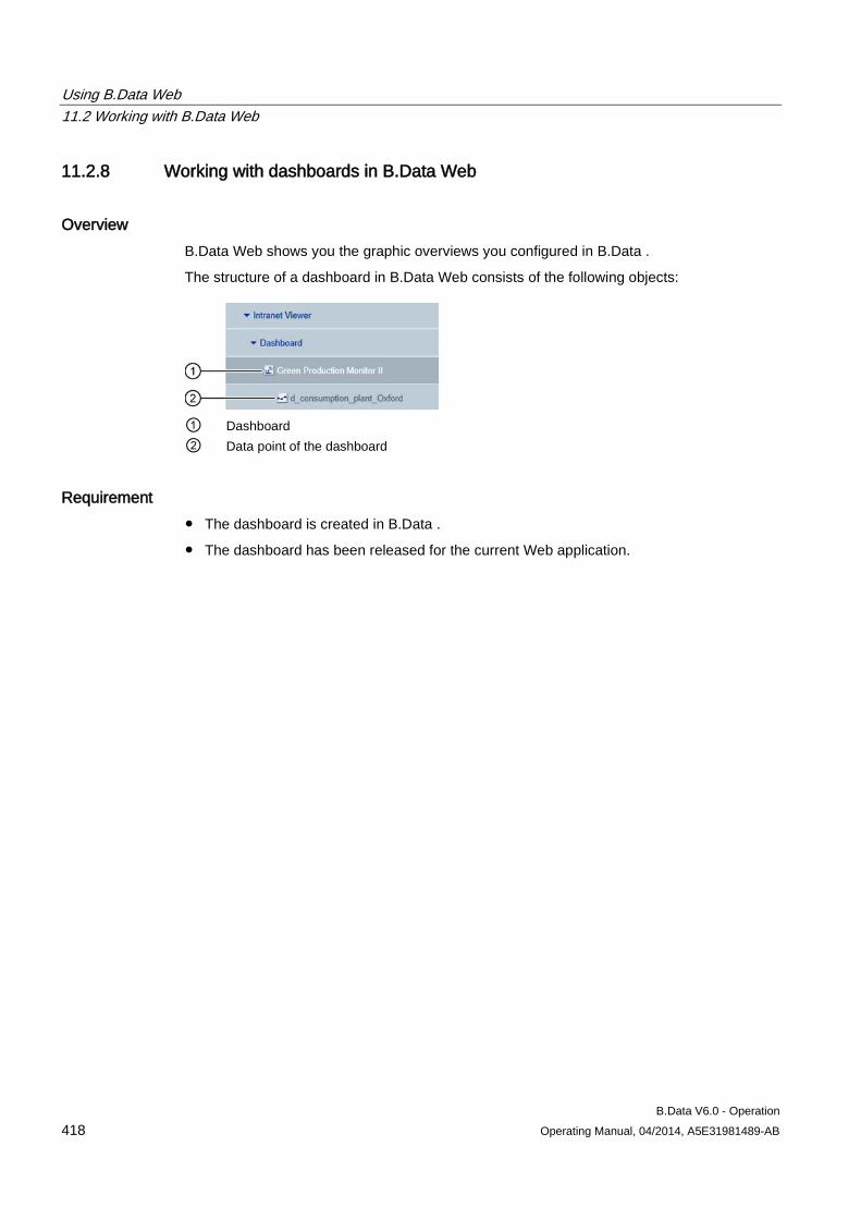
Using B.Data Web 11.2 Working with B.Data Web
B.Data V6.0 - Operation 418 Operating Manual, 04/2014, A5E31981489-AB
11.2.8 Working with dashboards in B.Data Web
Overview B.Data Web shows you the graphic overviews you configured in B.Data .
The structure of a dashboard in B.Data Web consists of the following objects:
① Dashboard ② Data point of the dashboard
Requirement ● The dashboard is created in B.Data .
● The dashboard has been released for the current Web application.
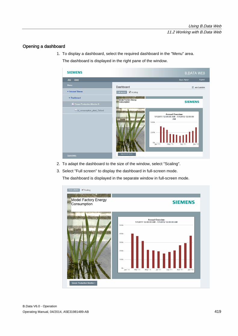
Using B.Data Web 11.2 Working with B.Data Web
B.Data V6.0 - Operation Operating Manual, 04/2014, A5E31981489-AB 419
Opening a dashboard 1. To display a dashboard, select the required dashboard in the "Menu" area.
The dashboard is displayed in the right pane of the window.
2. To adapt the dashboard to the size of the window, select "Scaling".
3. Select "Full screen" to display the dashboard in full-screen mode.
The dashboard is displayed in the separate window in full-screen mode.
Using B.Data Web 11.2 Working with B.Data Web
B.Data V6.0 - Operation 420 Operating Manual, 04/2014, A5E31981489-AB
Editing values You can acquire the values of a dashboard manually. To do this, select the required data point in the "Menu" area and click "Start Value Input" in the "Object" tab in the right window pane.
You can find additional information on this topic in the "Acquiring data manually" section.
Using the Quick Chart You can display the values of a dashboard in the Quick Chart. To do this, select the required data point in the "Menu" area and click on the "Diagram" tab in the right window pane.
You can find additional information on this topic in the "Using the Quick Chart" section.
See also Configuring authorizations (Page 90)
Manual data acquisition (Page 162)
Using the Quick Chart (Page 251)
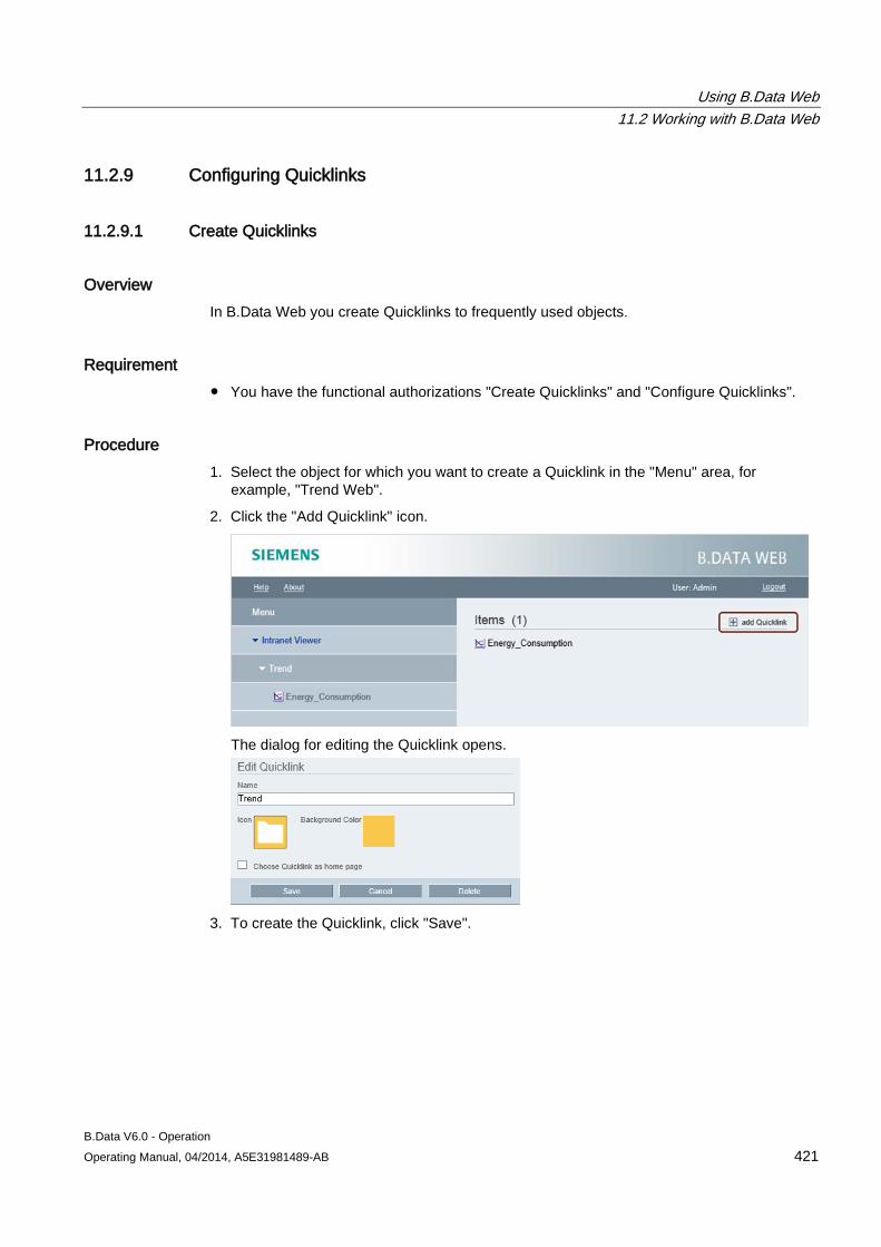
Using B.Data Web 11.2 Working with B.Data Web
B.Data V6.0 - Operation Operating Manual, 04/2014, A5E31981489-AB 421
11.2.9 Configuring Quicklinks
11.2.9.1 Create Quicklinks
Overview In B.Data Web you create Quicklinks to frequently used objects.
Requirement ● You have the functional authorizations "Create Quicklinks" and "Configure Quicklinks".
Procedure 1. Select the object for which you want to create a Quicklink in the "Menu" area, for
example, "Trend Web".
2. Click the "Add Quicklink" icon.
The dialog for editing the Quicklink opens.
3. To create the Quicklink, click "Save".
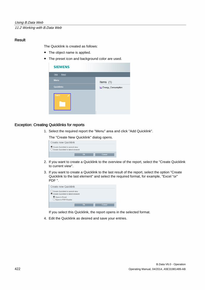
Using B.Data Web 11.2 Working with B.Data Web
B.Data V6.0 - Operation 422 Operating Manual, 04/2014, A5E31981489-AB
Result The Quicklink is created as follows:
● The object name is applied.
● The preset icon and background color are used.
Exception: Creating Quicklinks for reports 1. Select the required report the "Menu" area and click "Add Quicklink".
The "Create New Quicklink" dialog opens.
2. If you want to create a Quicklink to the overview of the report, select the "Create Quicklink
to current view".
3. If you want to create a Quicklink to the last result of the report, select the option "Create Quicklink to the last element" and select the required format, for example, "Excel "or" PDF ".
If you select this Quicklink, the report opens in the selected format.
4. Edit the Quicklink as desired and save your entries.

Using B.Data Web 11.2 Working with B.Data Web
B.Data V6.0 - Operation Operating Manual, 04/2014, A5E31981489-AB 423
See also Navigation in B.Data Web (Page 398)
Edit Quicklinks (Page 424)
Logging on to the B.Data Web (Page 400)
Configuring authorizations (Page 81)
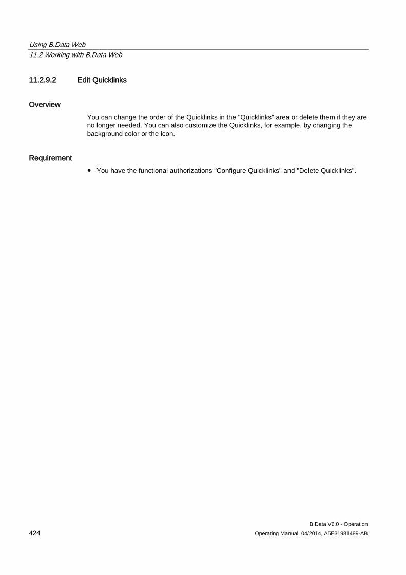
Using B.Data Web 11.2 Working with B.Data Web
B.Data V6.0 - Operation 424 Operating Manual, 04/2014, A5E31981489-AB
11.2.9.2 Edit Quicklinks
Overview You can change the order of the Quicklinks in the "Quicklinks" area or delete them if they are no longer needed. You can also customize the Quicklinks, for example, by changing the background color or the icon.
Requirement ● You have the functional authorizations "Configure Quicklinks" and "Delete Quicklinks".
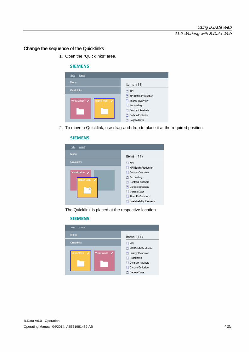
Using B.Data Web 11.2 Working with B.Data Web
B.Data V6.0 - Operation Operating Manual, 04/2014, A5E31981489-AB 425
Change the sequence of the Quicklinks 1. Open the "Quicklinks" area.
2. To move a Quicklink, use drag-and-drop to place it at the required position.
The Quicklink is placed at the respective location.
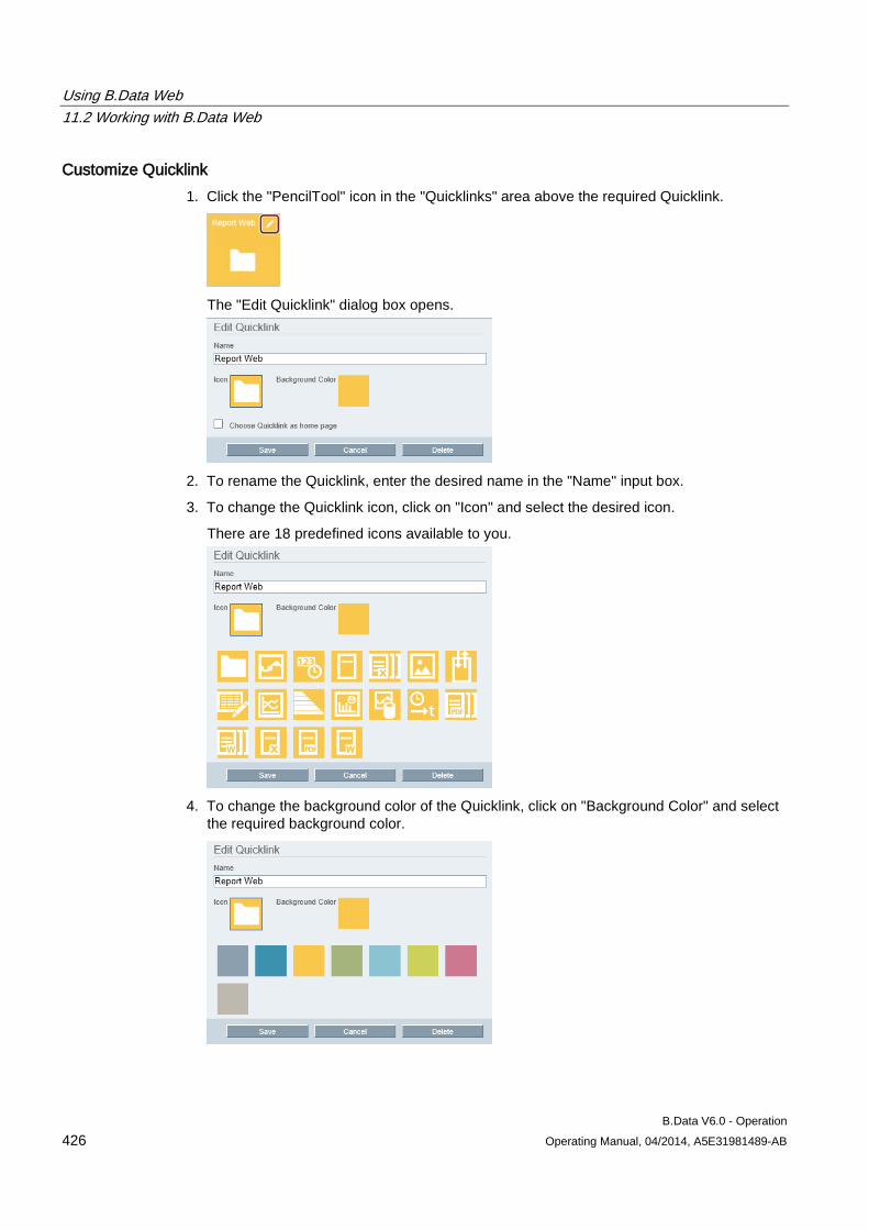
Using B.Data Web 11.2 Working with B.Data Web
B.Data V6.0 - Operation 426 Operating Manual, 04/2014, A5E31981489-AB
Customize Quicklink 1. Click the "PencilTool" icon in the "Quicklinks" area above the required Quicklink.
The "Edit Quicklink" dialog box opens.
2. To rename the Quicklink, enter the desired name in the "Name" input box.
3. To change the Quicklink icon, click on "Icon" and select the desired icon.
There are 18 predefined icons available to you.
4. To change the background color of the Quicklink, click on "Background Color" and select
the required background color.
Using B.Data Web 11.2 Working with B.Data Web
B.Data V6.0 - Operation Operating Manual, 04/2014, A5E31981489-AB 427
5. To specify the Quicklink as homepage, select the "Choose Quicklink as home page" check box.
Note
If you do not specify any Quicklink as homepage, the first Quicklink in the "Quicklinks" area is used as homepage page.
6. Save your changes to the Quicklink.
Delete Quicklink 1. Click the "PencilTool" icon above the desired Quicklink.
The "Edit Quicklink" dialog box opens.
2. Click "Delete".
The Quicklink is deleted.
See also Navigation in B.Data Web (Page 398)
Create Quicklinks (Page 421)
Configuring authorizations (Page 81)
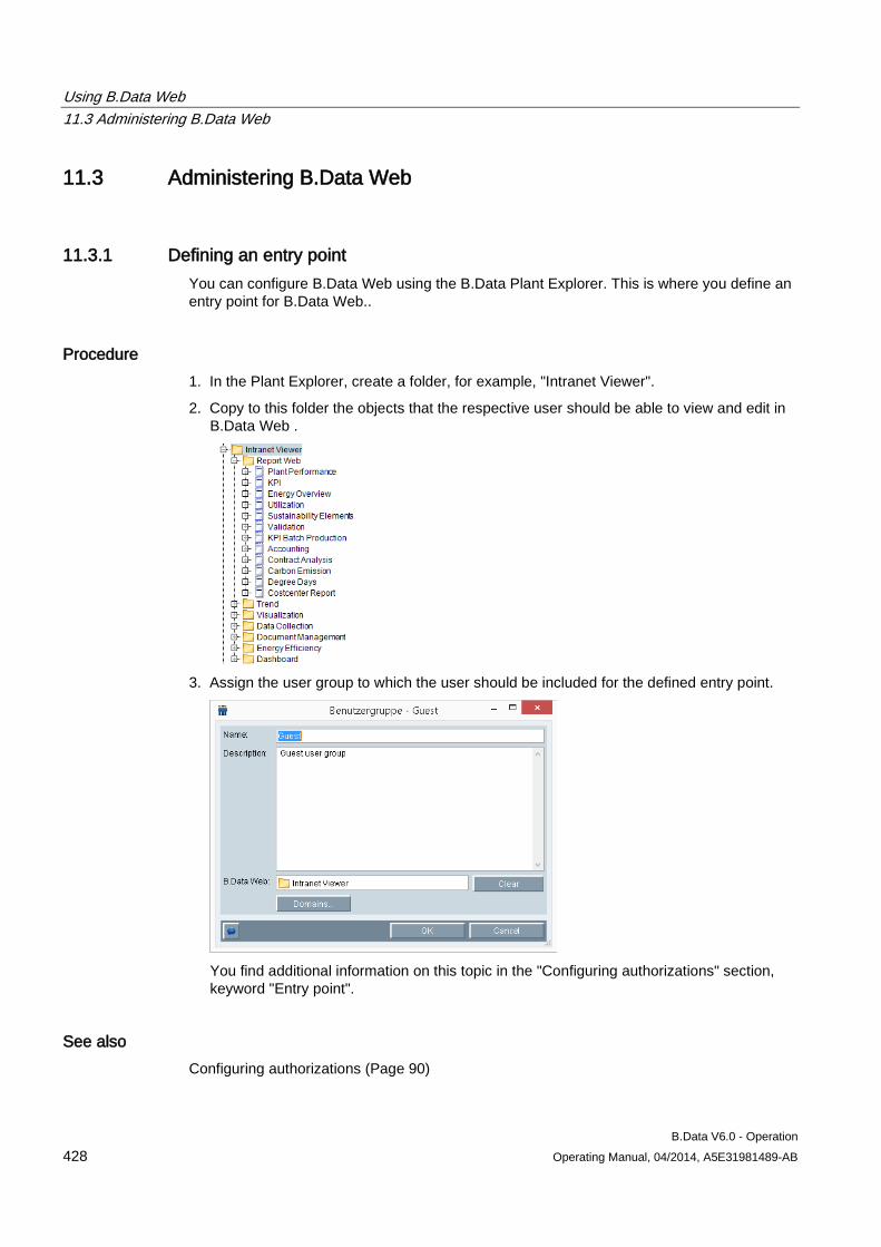
Using B.Data Web 11.3 Administering B.Data Web
B.Data V6.0 - Operation 428 Operating Manual, 04/2014, A5E31981489-AB
11.3 Administering B.Data Web
11.3.1 Defining an entry point You can configure B.Data Web using the B.Data Plant Explorer. This is where you define an entry point for B.Data Web..
Procedure 1. In the Plant Explorer, create a folder, for example, "Intranet Viewer".
2. Copy to this folder the objects that the respective user should be able to view and edit in B.Data Web .
3. Assign the user group to which the user should be included for the defined entry point.
You find additional information on this topic in the "Configuring authorizations" section, keyword "Entry point".
See also Configuring authorizations (Page 90)
Using B.Data Web 11.3 Administering B.Data Web
B.Data V6.0 - Operation Operating Manual, 04/2014, A5E31981489-AB 429
11.3.2 Authorizations for navigation As administrator, you use authorizations to specify which options are available to a specific user group for navigation in B.Data Web:
● "Menu view" for displaying the "Menu" area
● "Quicklinks view " for displaying the "Quicklinks" area
● "Quicklinks configure" for changing existing Quicklinks
● "Quicklinks create" for creating new Quicklinks
● "Quicklinks delete" for deleting Quicklinks
For information on exact procedures, refer to the "Configuring authorizations" section.
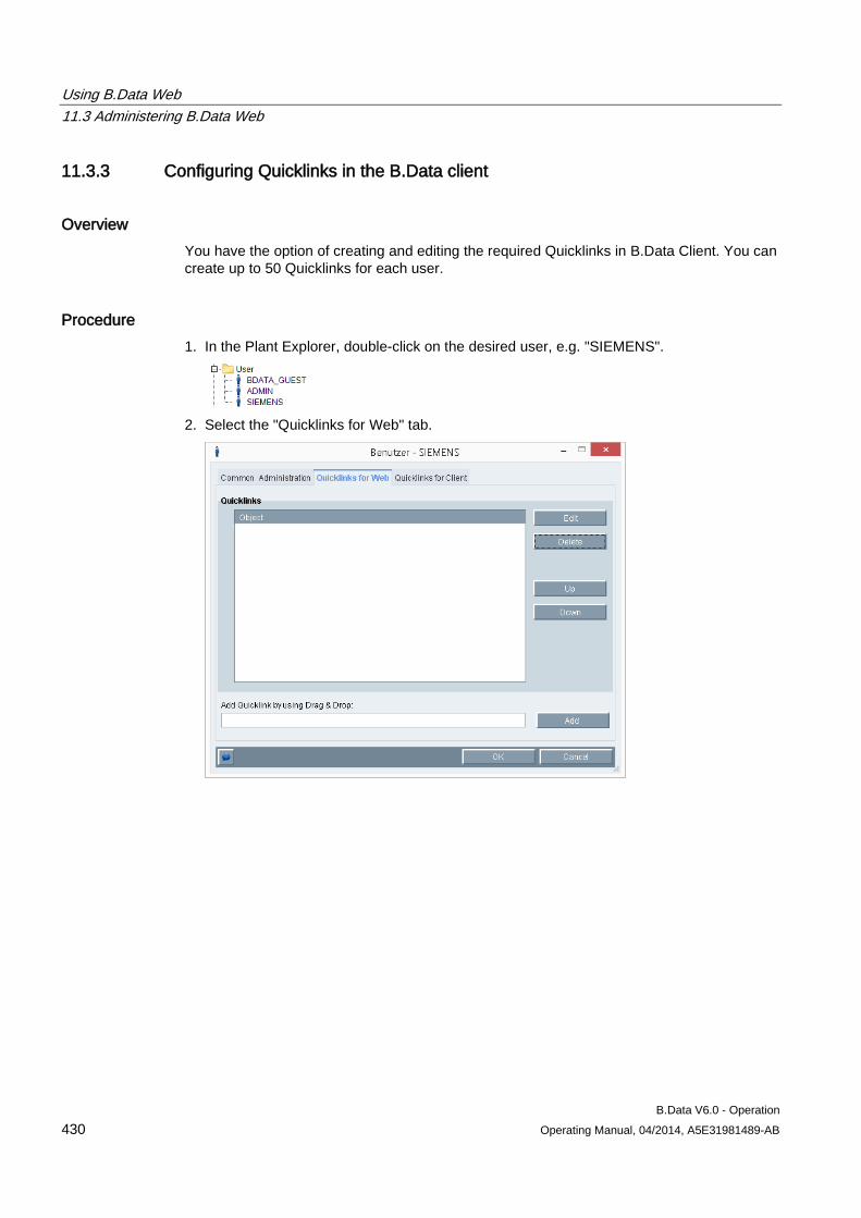
Using B.Data Web 11.3 Administering B.Data Web
B.Data V6.0 - Operation 430 Operating Manual, 04/2014, A5E31981489-AB
11.3.3 Configuring Quicklinks in the B.Data client
Overview You have the option of creating and editing the required Quicklinks in B.Data Client. You can create up to 50 Quicklinks for each user.
Procedure 1. In the Plant Explorer, double-click on the desired user, e.g. "SIEMENS".
2. Select the "Quicklinks for Web" tab.
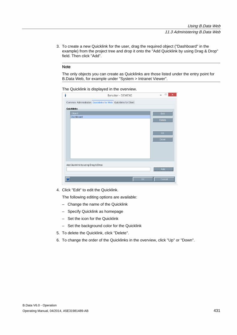
Using B.Data Web 11.3 Administering B.Data Web
B.Data V6.0 - Operation Operating Manual, 04/2014, A5E31981489-AB 431
3. To create a new Quicklink for the user, drag the required object ("Dashboard" in the example) from the project tree and drop it onto the "Add Quicklink by using Drag & Drop" field. Then click "Add".
Note
The only objects you can create as Quicklinks are those listed under the entry point for B.Data Web, for example under "System > Intranet Viewer".
The Quicklink is displayed in the overview.
4. Click "Edit" to edit the Quicklink.
The following editing options are available:
– Change the name of the Quicklink
– Specify Quicklink as homepage
– Set the icon for the Quicklink
– Set the background color for the Quicklink
5. To delete the Quicklink, click "Delete".
6. To change the order of the Quicklinks in the overview, click "Up" or "Down".
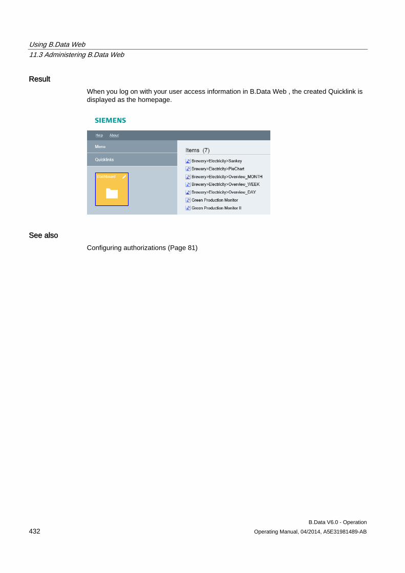
Using B.Data Web 11.3 Administering B.Data Web
B.Data V6.0 - Operation 432 Operating Manual, 04/2014, A5E31981489-AB
Result When you log on with your user access information in B.Data Web , the created Quicklink is displayed as the homepage.
See also Configuring authorizations (Page 81)
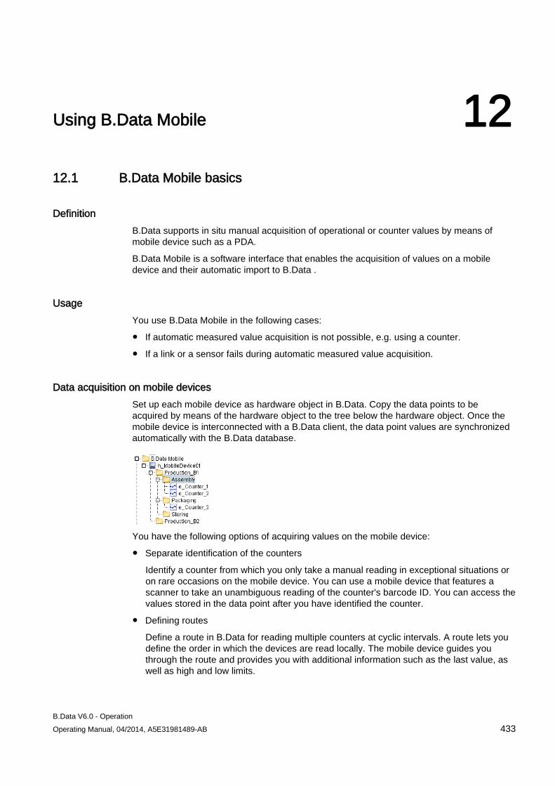
B.Data V6.0 - Operation Operating Manual, 04/2014, A5E31981489-AB 433
Using B.Data Mobile 12 12.1 B.Data Mobile basics
Definition B.Data supports in situ manual acquisition of operational or counter values by means of mobile device such as a PDA.
B.Data Mobile is a software interface that enables the acquisition of values on a mobile device and their automatic import to B.Data .
Usage You use B.Data Mobile in the following cases:
● If automatic measured value acquisition is not possible, e.g. using a counter.
● If a link or a sensor fails during automatic measured value acquisition.
Data acquisition on mobile devices Set up each mobile device as hardware object in B.Data. Copy the data points to be acquired by means of the hardware object to the tree below the hardware object. Once the mobile device is interconnected with a B.Data client, the data point values are synchronized automatically with the B.Data database.
You have the following options of acquiring values on the mobile device:
● Separate identification of the counters
Identify a counter from which you only take a manual reading in exceptional situations or on rare occasions on the mobile device. You can use a mobile device that features a scanner to take an unambiguous reading of the counter's barcode ID. You can access the values stored in the data point after you have identified the counter.
● Defining routes
Define a route in B.Data for reading multiple counters at cyclic intervals. A route lets you define the order in which the devices are read locally. The mobile device guides you through the route and provides you with additional information such as the last value, as well as high and low limits.
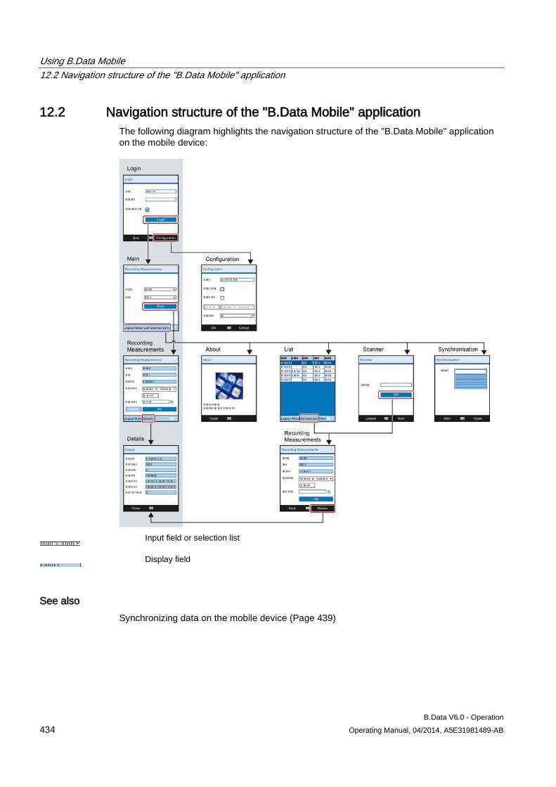
Using B.Data Mobile 12.2 Navigation structure of the "B.Data Mobile" application
B.Data V6.0 - Operation 434 Operating Manual, 04/2014, A5E31981489-AB
12.2 Navigation structure of the "B.Data Mobile" application The following diagram highlights the navigation structure of the "B.Data Mobile" application on the mobile device:
Input field or selection list
Display field
See also Synchronizing data on the mobile device (Page 439)
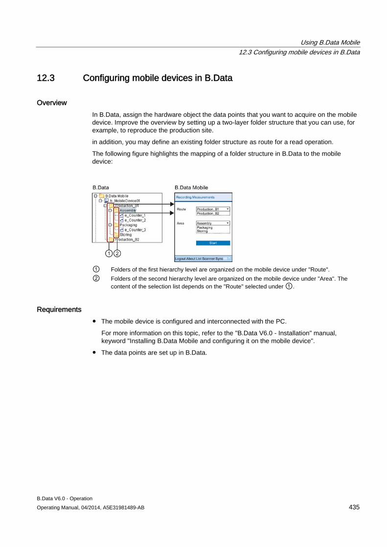
Using B.Data Mobile 12.3 Configuring mobile devices in B.Data
B.Data V6.0 - Operation Operating Manual, 04/2014, A5E31981489-AB 435
12.3 Configuring mobile devices in B.Data
Overview In B.Data, assign the hardware object the data points that you want to acquire on the mobile device. Improve the overview by setting up a two-layer folder structure that you can use, for example, to reproduce the production site.
in addition, you may define an existing folder structure as route for a read operation.
The following figure highlights the mapping of a folder structure in B.Data to the mobile device:
① Folders of the first hierarchy level are organized on the mobile device under "Route". ② Folders of the second hierarchy level are organized on the mobile device under "Area". The
content of the selection list depends on the "Route" selected under ①.
Requirements ● The mobile device is configured and interconnected with the PC.
For more information on this topic, refer to the "B.Data V6.0 - Installation" manual, keyword "Installing B.Data Mobile and configuring it on the mobile device".
● The data points are set up in B.Data.
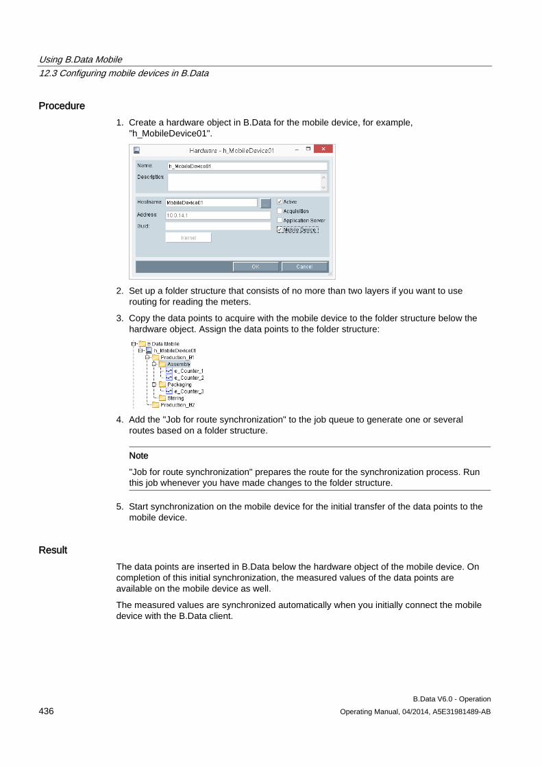
Using B.Data Mobile 12.3 Configuring mobile devices in B.Data
B.Data V6.0 - Operation 436 Operating Manual, 04/2014, A5E31981489-AB
Procedure 1. Create a hardware object in B.Data for the mobile device, for example,
"h_MobileDevice01".
2. Set up a folder structure that consists of no more than two layers if you want to use
routing for reading the meters.
3. Copy the data points to acquire with the mobile device to the folder structure below the hardware object. Assign the data points to the folder structure:
4. Add the "Job for route synchronization" to the job queue to generate one or several
routes based on a folder structure.
Note
"Job for route synchronization" prepares the route for the synchronization process. Run this job whenever you have made changes to the folder structure.
5. Start synchronization on the mobile device for the initial transfer of the data points to the mobile device.
Result The data points are inserted in B.Data below the hardware object of the mobile device. On completion of this initial synchronization, the measured values of the data points are available on the mobile device as well.
The measured values are synchronized automatically when you initially connect the mobile device with the B.Data client.
Using B.Data Mobile 12.4 Measured value input on the mobile device
B.Data V6.0 - Operation Operating Manual, 04/2014, A5E31981489-AB 437
12.4 Measured value input on the mobile device
Requirement ● You are logged on to the "B.Data Mobile" application on the mobile device.
● The "Main" picture is displayed on the mobile device.
● The synchronization process is concluded.
Procedure 1. Identify the meter.
2. Enter the measured value reading on the mobile device.
3. Enter the time stamp, if necessary.
The following figure shows how to enter measured values on the mobile device, based on the "Main" picture:
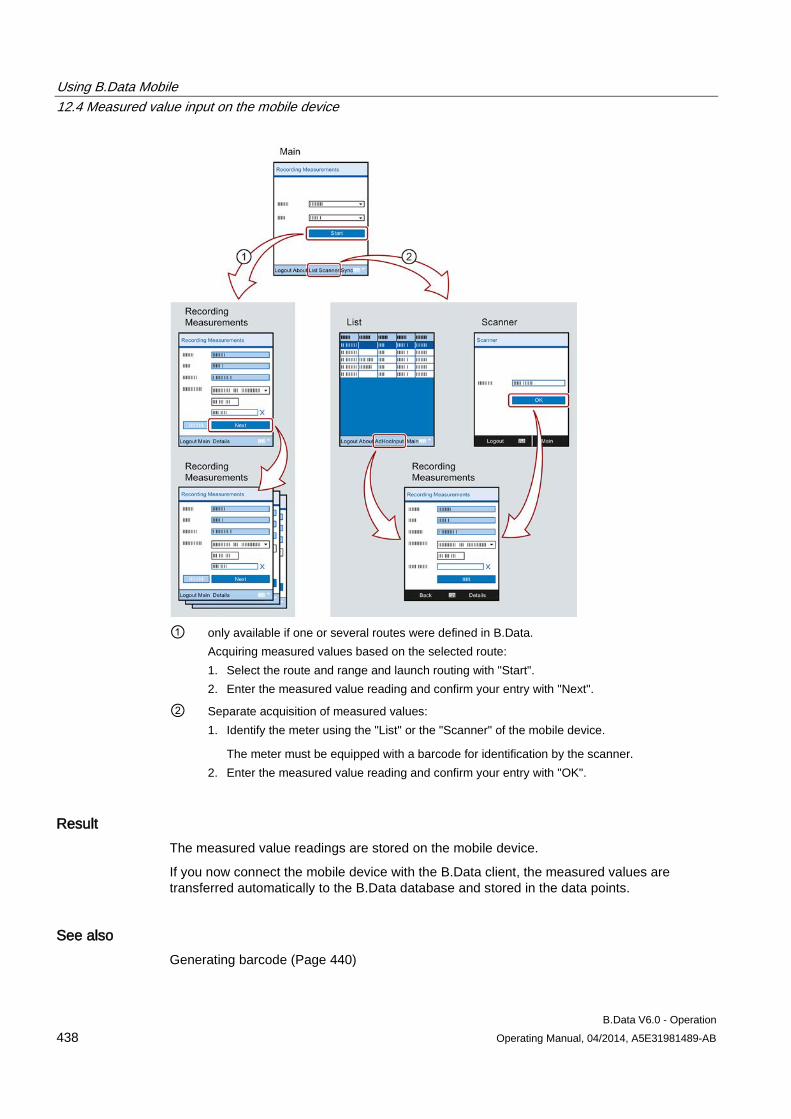
Using B.Data Mobile 12.4 Measured value input on the mobile device
B.Data V6.0 - Operation 438 Operating Manual, 04/2014, A5E31981489-AB
① only available if one or several routes were defined in B.Data.
Acquiring measured values based on the selected route: 1. Select the route and range and launch routing with "Start". 2. Enter the measured value reading and confirm your entry with "Next".
② Separate acquisition of measured values: 1. Identify the meter using the "List" or the "Scanner" of the mobile device.
The meter must be equipped with a barcode for identification by the scanner. 2. Enter the measured value reading and confirm your entry with "OK".
Result The measured value readings are stored on the mobile device.
If you now connect the mobile device with the B.Data client, the measured values are transferred automatically to the B.Data database and stored in the data points.
See also Generating barcode (Page 440)
Using B.Data Mobile 12.5 Synchronizing data on the mobile device
B.Data V6.0 - Operation Operating Manual, 04/2014, A5E31981489-AB 439
12.5 Synchronizing data on the mobile device
Overview The following actions are performed when you synchronize data on the mobile device:
● The routes and data points that you have configured in B.Data will be mapped to the mobile device.
● The values you have entered on the mobile device are saved to the corresponding data points in B.Data.
You can synchronize data on the mobile device as follows:
● Manually
Synchronize the data manually if using B.Data Mobile for the first time.
● Automatically
The measured values are synchronized automatically when you initially connect the mobile device with the B.Data client.
Requirement ● B.Data Mobile is installed and configured in B.Data and on the mobile device.
For more information, refer to the "B.Data V6.0 - Installation" manual, keyword "Installing B.Data Mobile".
● You are logged on to the mobile device with the B.Data access data.
● The mobile device displays the "Main" screen.
Synchronizing data manually 1. Select the "Synchronization" command.
The data is synchronized and the synchronization status is indicated in the "Synchronization" screen.
Result The data on the mobile device and in B.Data is synchronized.
Note Ignoring the values
The current value will be ignored if the B.Data database already contains a data point value with the same time stamp.
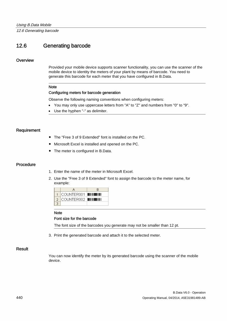
Using B.Data Mobile 12.6 Generating barcode
B.Data V6.0 - Operation 440 Operating Manual, 04/2014, A5E31981489-AB
12.6 Generating barcode
Overview Provided your mobile device supports scanner functionality, you can use the scanner of the mobile device to identity the meters of your plant by means of barcode. You need to generate this barcode for each meter that you have configured in B.Data.
Note Configuring meters for barcode generation
Observe the following naming conventions when configuring meters: • You may only use uppercase letters from "A" to "Z" and numbers from "0" to "9". • Use the hyphen "-" as delimiter.
Requirement ● The "Free 3 of 9 Extended" font is installed on the PC.
● Microsoft Excel is installed and opened on the PC.
● The meter is configured in B.Data.
Procedure 1. Enter the name of the meter in Microsoft Excel.
2. Use the "Free 3 of 9 Extended" font to assign the barcode to the meter name, for example:
Note Font size for the barcode
The font size of the barcodes you generate may not be smaller than 12 pt.
3. Print the generated barcode and attach it to the selected meter.
Result You can now identify the meter by its generated barcode using the scanner of the mobile device.
B.Data V6.0 - Operation Operating Manual, 04/2014, A5E31981489-AB 441
Reference 13 13.1 Acquisition status of a value
The following value acquisition states are possible:
● STER_OK
● STER_INVALID
● STER_CONFUSE
● STER_GAP
● STER_FIRST
● STER_FIRST_INVALID
● STER_FIRST_CONFUSE
● STER_FIRST_INVALID_CONFUSE
● STER_LAST
● STER_LAST_INVALID
● STER_LAST_CONFUSE
● Implemented in the NLS
● DB update disabled in the NLS
● Calculated process value
● Invalid in CAD
● Adjusted in CAD
● Application-specific
● Outliers
● Substitute value
Reference 13.2 Correction status of a value
B.Data V6.0 - Operation 442 Operating Manual, 04/2014, A5E31981489-AB
13.2 Correction status of a value The following value correction states are possible:
● Valid
● Invalid
● Corrected with LRU
● Corrected with substitute measurement
● Corrected with substitute value
● Valid with manual manipulation
● Valid corr. with LRU and manual manipulation
● Valid corr. with substitute m. and manual manipulation.
● Valid corr. with substitute v. and manual manipulation.
● Import
● Invalid import
● Import valid, corr. with LRU
● Import valid, corr. with substitute measurement
● Import valid, corrected with substitute value
● Import valid with manual manipulation
● Import valid, corr. with LRU+manual manipulation.
● Import valid, corr. with substitute m.+manual manipulation.
● Import valid, corr. with substitute v.+manual manipulation.
● Corrected
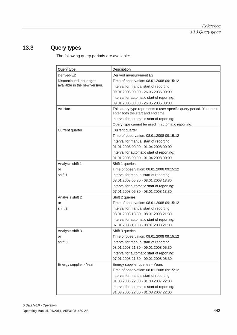
Reference 13.3 Query types
B.Data V6.0 - Operation Operating Manual, 04/2014, A5E31981489-AB 443
13.3 Query types The following query periods are available:
Query type Description Derived-E2 Discontinued, no longer available in the new version.
Derived measurement E2 Time of observation: 08.01.2008 09:15:12 Interval for manual start of reporting: 09.01.2008 00:00 - 26.05.2035 00:00 Interval for automatic start of reporting: 09.01.2008 00:00 - 26.05.2035 00:00
Ad-Hoc This query type represents a user-specific query period. You must enter both the start and end time. Interval for automatic start of reporting: Query type cannot be used in automatic reporting.
Current quarter Current quarter Time of observation: 08.01.2008 09:15:12 Interval for manual start of reporting: 01.01.2008 00:00 - 01.04.2008 00:00 Interval for automatic start of reporting: 01.01.2008 00:00 - 01.04.2008 00:00
Analysis shift 1 or shift 1
Shift 1 queries Time of observation: 08.01.2008 09:15:12 Interval for manual start of reporting: 08.01.2008 05:30 - 08.01.2008 13:30 Interval for automatic start of reporting: 07.01.2008 05:30 - 08.01.2008 13:30
Analysis shift 2 or shift 2
Shift 2 queries Time of observation: 08.01.2008 09:15:12 Interval for manual start of reporting: 08.01.2008 13:30 - 08.01.2008 21:30 Interval for automatic start of reporting: 07.01.2008 13:30 - 08.01.2008 21:30
Analysis shift 3 or shift 3
Shift 3 queries Time of observation: 08.01.2008 09:15:12 Interval for manual start of reporting: 08.01.2008 21:30 - 09.01.2008 05:30 Interval for automatic start of reporting: 07.01.2008 21:30 - 09.01.2008 05:30
Energy supplier - Year Energy supplier queries - Years Time of observation: 08.01.2008 09:15:12 Interval for manual start of reporting: 31.08.2006 22:00 - 31.08.2007 22:00 Interval for automatic start of reporting: 31.08.2006 22:00 - 31.08.2007 22:00
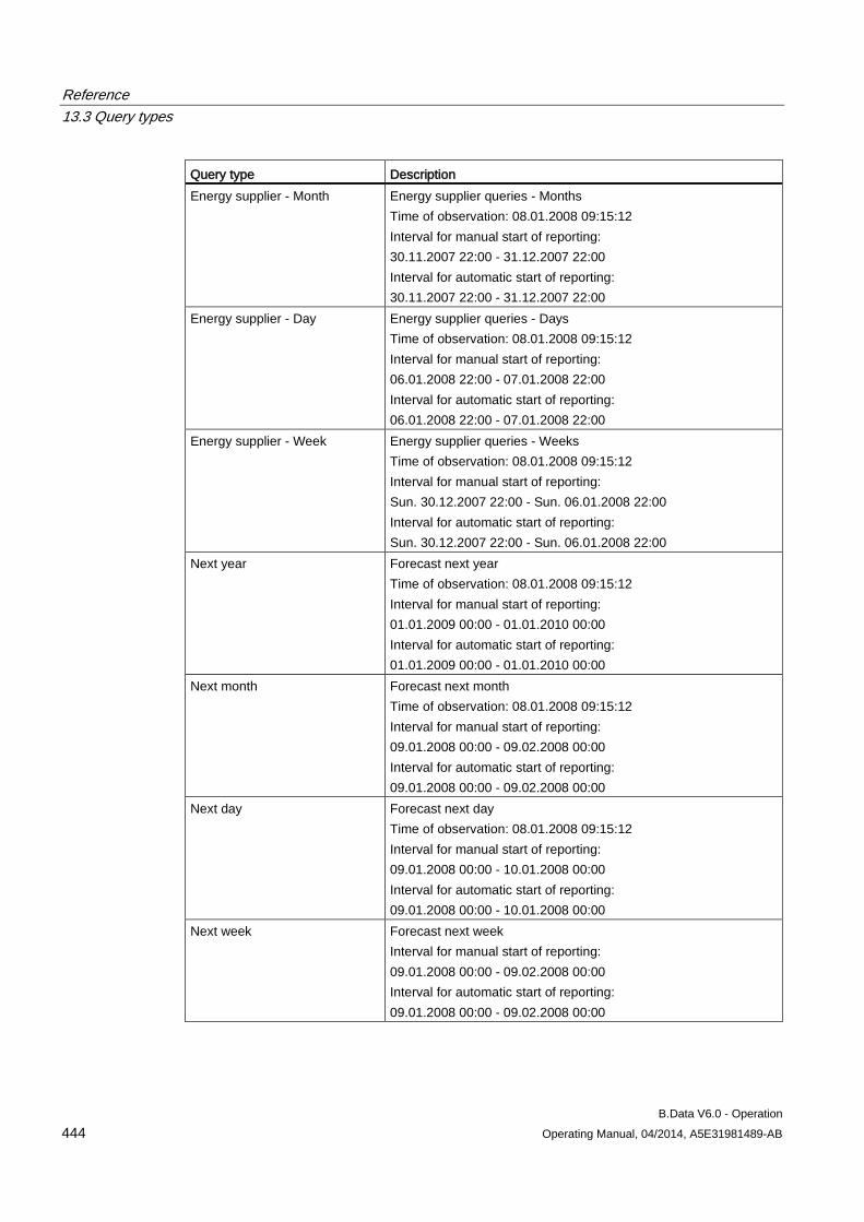
Reference 13.3 Query types
B.Data V6.0 - Operation 444 Operating Manual, 04/2014, A5E31981489-AB
Query type Description Energy supplier - Month Energy supplier queries - Months
Time of observation: 08.01.2008 09:15:12 Interval for manual start of reporting: 30.11.2007 22:00 - 31.12.2007 22:00 Interval for automatic start of reporting: 30.11.2007 22:00 - 31.12.2007 22:00
Energy supplier - Day Energy supplier queries - Days Time of observation: 08.01.2008 09:15:12 Interval for manual start of reporting: 06.01.2008 22:00 - 07.01.2008 22:00 Interval for automatic start of reporting: 06.01.2008 22:00 - 07.01.2008 22:00
Energy supplier - Week Energy supplier queries - Weeks Time of observation: 08.01.2008 09:15:12 Interval for manual start of reporting: Sun. 30.12.2007 22:00 - Sun. 06.01.2008 22:00 Interval for automatic start of reporting: Sun. 30.12.2007 22:00 - Sun. 06.01.2008 22:00
Next year Forecast next year Time of observation: 08.01.2008 09:15:12 Interval for manual start of reporting: 01.01.2009 00:00 - 01.01.2010 00:00 Interval for automatic start of reporting: 01.01.2009 00:00 - 01.01.2010 00:00
Next month Forecast next month Time of observation: 08.01.2008 09:15:12 Interval for manual start of reporting: 09.01.2008 00:00 - 09.02.2008 00:00 Interval for automatic start of reporting: 09.01.2008 00:00 - 09.02.2008 00:00
Next day Forecast next day Time of observation: 08.01.2008 09:15:12 Interval for manual start of reporting: 09.01.2008 00:00 - 10.01.2008 00:00 Interval for automatic start of reporting: 09.01.2008 00:00 - 10.01.2008 00:00
Next week Forecast next week Interval for manual start of reporting: 09.01.2008 00:00 - 09.02.2008 00:00 Interval for automatic start of reporting: 09.01.2008 00:00 - 09.02.2008 00:00
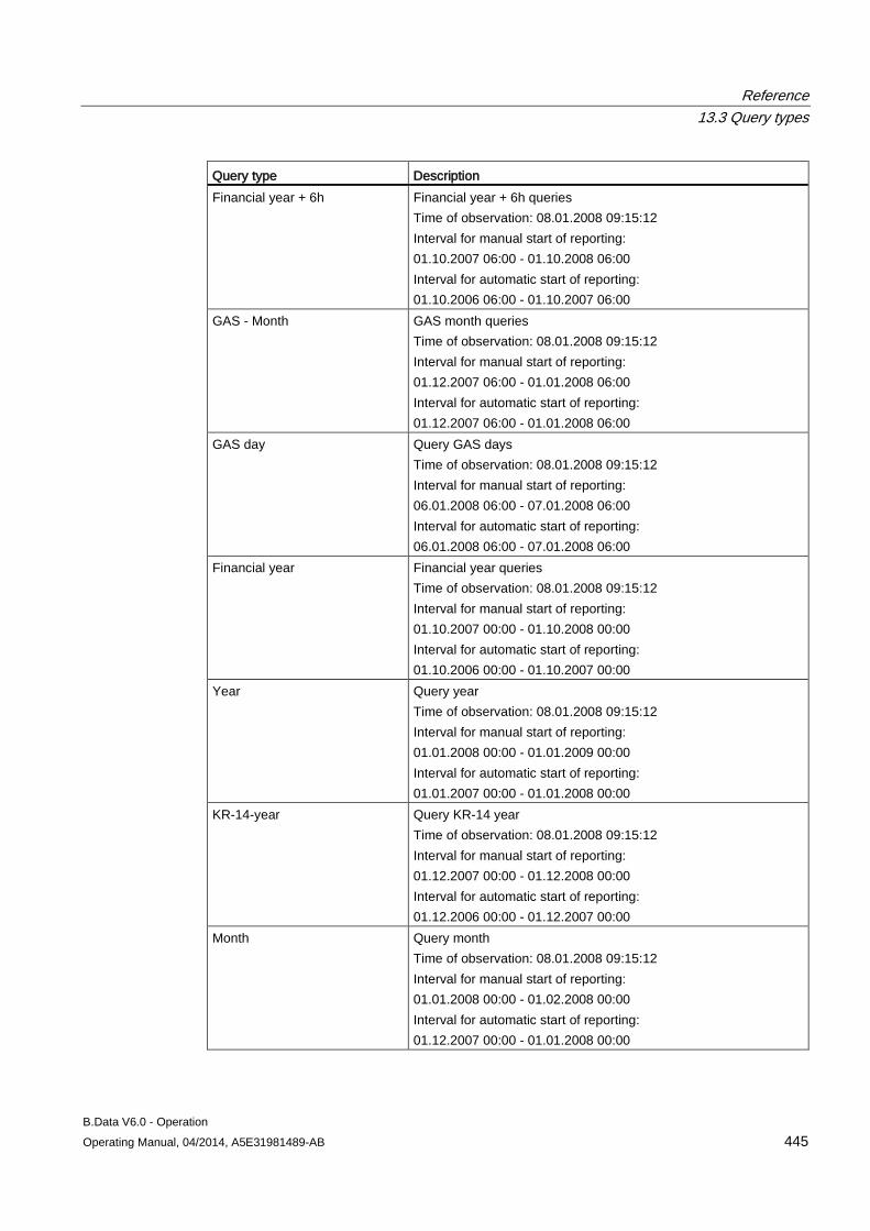
Reference 13.3 Query types
B.Data V6.0 - Operation Operating Manual, 04/2014, A5E31981489-AB 445
Query type Description Financial year + 6h Financial year + 6h queries
Time of observation: 08.01.2008 09:15:12 Interval for manual start of reporting: 01.10.2007 06:00 - 01.10.2008 06:00 Interval for automatic start of reporting: 01.10.2006 06:00 - 01.10.2007 06:00
GAS - Month GAS month queries Time of observation: 08.01.2008 09:15:12 Interval for manual start of reporting: 01.12.2007 06:00 - 01.01.2008 06:00 Interval for automatic start of reporting: 01.12.2007 06:00 - 01.01.2008 06:00
GAS day Query GAS days Time of observation: 08.01.2008 09:15:12 Interval for manual start of reporting: 06.01.2008 06:00 - 07.01.2008 06:00 Interval for automatic start of reporting: 06.01.2008 06:00 - 07.01.2008 06:00
Financial year Financial year queries Time of observation: 08.01.2008 09:15:12 Interval for manual start of reporting: 01.10.2007 00:00 - 01.10.2008 00:00 Interval for automatic start of reporting: 01.10.2006 00:00 - 01.10.2007 00:00
Year Query year Time of observation: 08.01.2008 09:15:12 Interval for manual start of reporting: 01.01.2008 00:00 - 01.01.2009 00:00 Interval for automatic start of reporting: 01.01.2007 00:00 - 01.01.2008 00:00
KR-14-year Query KR-14 year Time of observation: 08.01.2008 09:15:12 Interval for manual start of reporting: 01.12.2007 00:00 - 01.12.2008 00:00 Interval for automatic start of reporting: 01.12.2006 00:00 - 01.12.2007 00:00
Month Query month Time of observation: 08.01.2008 09:15:12 Interval for manual start of reporting: 01.01.2008 00:00 - 01.02.2008 00:00 Interval for automatic start of reporting: 01.12.2007 00:00 - 01.01.2008 00:00
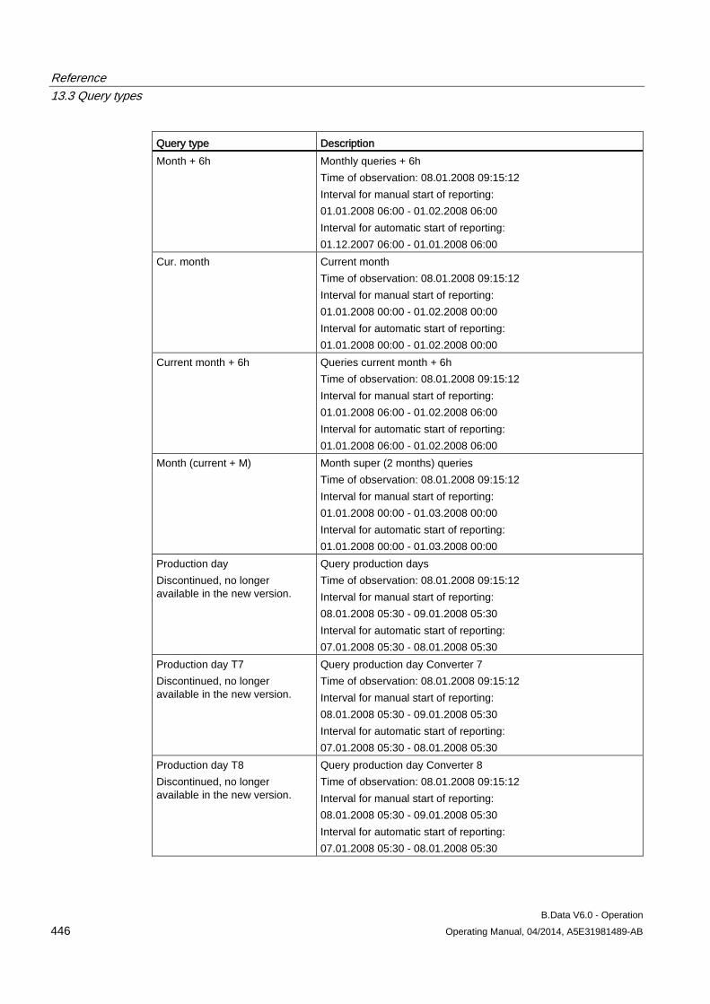
Reference 13.3 Query types
B.Data V6.0 - Operation 446 Operating Manual, 04/2014, A5E31981489-AB
Query type Description Month + 6h Monthly queries + 6h
Time of observation: 08.01.2008 09:15:12 Interval for manual start of reporting: 01.01.2008 06:00 - 01.02.2008 06:00 Interval for automatic start of reporting: 01.12.2007 06:00 - 01.01.2008 06:00
Cur. month Current month Time of observation: 08.01.2008 09:15:12 Interval for manual start of reporting: 01.01.2008 00:00 - 01.02.2008 00:00 Interval for automatic start of reporting: 01.01.2008 00:00 - 01.02.2008 00:00
Current month + 6h Queries current month + 6h Time of observation: 08.01.2008 09:15:12 Interval for manual start of reporting: 01.01.2008 06:00 - 01.02.2008 06:00 Interval for automatic start of reporting: 01.01.2008 06:00 - 01.02.2008 06:00
Month (current + M) Month super (2 months) queries Time of observation: 08.01.2008 09:15:12 Interval for manual start of reporting: 01.01.2008 00:00 - 01.03.2008 00:00 Interval for automatic start of reporting: 01.01.2008 00:00 - 01.03.2008 00:00
Production day Discontinued, no longer available in the new version.
Query production days Time of observation: 08.01.2008 09:15:12 Interval for manual start of reporting: 08.01.2008 05:30 - 09.01.2008 05:30 Interval for automatic start of reporting: 07.01.2008 05:30 - 08.01.2008 05:30
Production day T7 Discontinued, no longer available in the new version.
Query production day Converter 7 Time of observation: 08.01.2008 09:15:12 Interval for manual start of reporting: 08.01.2008 05:30 - 09.01.2008 05:30 Interval for automatic start of reporting: 07.01.2008 05:30 - 08.01.2008 05:30
Production day T8 Discontinued, no longer available in the new version.
Query production day Converter 8 Time of observation: 08.01.2008 09:15:12 Interval for manual start of reporting: 08.01.2008 05:30 - 09.01.2008 05:30 Interval for automatic start of reporting: 07.01.2008 05:30 - 08.01.2008 05:30
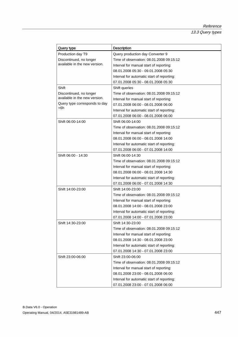
Reference 13.3 Query types
B.Data V6.0 - Operation Operating Manual, 04/2014, A5E31981489-AB 447
Query type Description Production day T9 Discontinued, no longer available in the new version.
Query production day Converter 9 Time of observation: 08.01.2008 09:15:12 Interval for manual start of reporting: 08.01.2008 05:30 - 09.01.2008 05:30 Interval for automatic start of reporting: 07.01.2008 05:30 - 08.01.2008 05:30
Shift Discontinued, no longer available in the new version. Query type corresponds to day +6h
Shift queries Time of observation: 08.01.2008 09:15:12 Interval for manual start of reporting: 07.01.2008 06:00 - 08.01.2008 06:00 Interval for automatic start of reporting: 07.01.2008 06:00 - 08.01.2008 06:00
Shift 06:00-14:00 Shift 06:00-14:00 Time of observation: 08.01.2008 09:15:12 Interval for manual start of reporting: 08.01.2008 06:00 - 08.01.2008 14:00 Interval for automatic start of reporting: 07.01.2008 06:00 - 07.01.2008 14:00
Shift 06:00 - 14:30 Shift 06:00-14:30 Time of observation: 08.01.2008 09:15:12 Interval for manual start of reporting: 08.01.2008 06:00 - 08.01.2008 14:30 Interval for automatic start of reporting: 07.01.2008 06:00 - 07.01.2008 14:30
Shift 14:00-23:00 Shift 14:00-23:00 Time of observation: 08.01.2008 09:15:12 Interval for manual start of reporting: 08.01.2008 14:00 - 08.01.2008 23:00 Interval for automatic start of reporting: 07.01.2008 14:00 - 07.01.2008 23:00
Shift 14:30-23:00 Shift 14:30-23:00 Time of observation: 08.01.2008 09:15:12 Interval for manual start of reporting: 08.01.2008 14:30 - 08.01.2008 23:00 Interval for automatic start of reporting: 07.01.2008 14:30 - 07.01.2008 23:00
Shift 23:00-06:00 Shift 23:00-06:00 Time of observation: 08.01.2008 09:15:12 Interval for manual start of reporting: 08.01.2008 23:00 - 08.01.2008 06:00 Interval for automatic start of reporting: 07.01.2008 23:00 - 07.01.2008 06:00
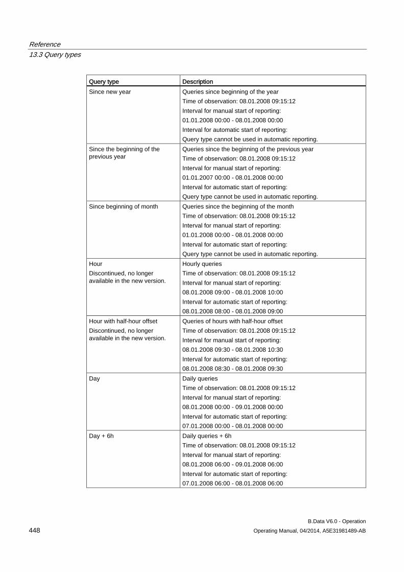
Reference 13.3 Query types
B.Data V6.0 - Operation 448 Operating Manual, 04/2014, A5E31981489-AB
Query type Description Since new year Queries since beginning of the year
Time of observation: 08.01.2008 09:15:12 Interval for manual start of reporting: 01.01.2008 00:00 - 08.01.2008 00:00 Interval for automatic start of reporting: Query type cannot be used in automatic reporting.
Since the beginning of the previous year
Queries since the beginning of the previous year Time of observation: 08.01.2008 09:15:12 Interval for manual start of reporting: 01.01.2007 00:00 - 08.01.2008 00:00 Interval for automatic start of reporting: Query type cannot be used in automatic reporting.
Since beginning of month Queries since the beginning of the month Time of observation: 08.01.2008 09:15:12 Interval for manual start of reporting: 01.01.2008 00:00 - 08.01.2008 00:00 Interval for automatic start of reporting: Query type cannot be used in automatic reporting.
Hour Discontinued, no longer available in the new version.
Hourly queries Time of observation: 08.01.2008 09:15:12 Interval for manual start of reporting: 08.01.2008 09:00 - 08.01.2008 10:00 Interval for automatic start of reporting: 08.01.2008 08:00 - 08.01.2008 09:00
Hour with half-hour offset Discontinued, no longer available in the new version.
Queries of hours with half-hour offset Time of observation: 08.01.2008 09:15:12 Interval for manual start of reporting: 08.01.2008 09:30 - 08.01.2008 10:30 Interval for automatic start of reporting: 08.01.2008 08:30 - 08.01.2008 09:30
Day Daily queries Time of observation: 08.01.2008 09:15:12 Interval for manual start of reporting: 08.01.2008 00:00 - 09.01.2008 00:00 Interval for automatic start of reporting: 07.01.2008 00:00 - 08.01.2008 00:00
Day + 6h Daily queries + 6h Time of observation: 08.01.2008 09:15:12 Interval for manual start of reporting: 08.01.2008 06:00 - 09.01.2008 06:00 Interval for automatic start of reporting: 07.01.2008 06:00 - 08.01.2008 06:00
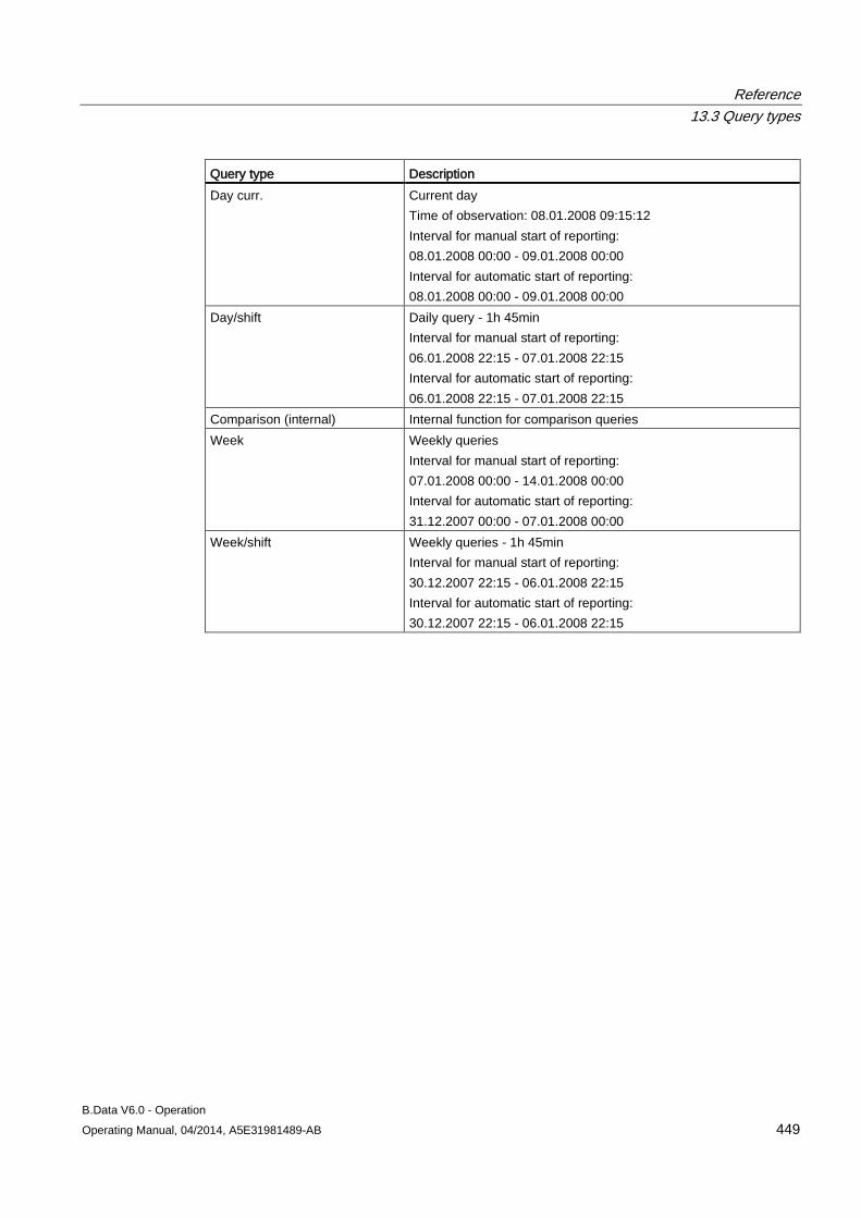
Reference 13.3 Query types
B.Data V6.0 - Operation Operating Manual, 04/2014, A5E31981489-AB 449
Query type Description Day curr. Current day
Time of observation: 08.01.2008 09:15:12 Interval for manual start of reporting: 08.01.2008 00:00 - 09.01.2008 00:00 Interval for automatic start of reporting: 08.01.2008 00:00 - 09.01.2008 00:00
Day/shift Daily query - 1h 45min Interval for manual start of reporting: 06.01.2008 22:15 - 07.01.2008 22:15 Interval for automatic start of reporting: 06.01.2008 22:15 - 07.01.2008 22:15
Comparison (internal) Internal function for comparison queries Week Weekly queries
Interval for manual start of reporting: 07.01.2008 00:00 - 14.01.2008 00:00 Interval for automatic start of reporting: 31.12.2007 00:00 - 07.01.2008 00:00
Week/shift Weekly queries - 1h 45min Interval for manual start of reporting: 30.12.2007 22:15 - 06.01.2008 22:15 Interval for automatic start of reporting: 30.12.2007 22:15 - 06.01.2008 22:15
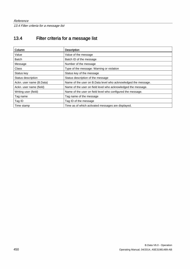
Reference 13.4 Filter criteria for a message list
B.Data V6.0 - Operation 450 Operating Manual, 04/2014, A5E31981489-AB
13.4 Filter criteria for a message list Column Description Value Value of the message Batch Batch ID of the message Message Number of the message Class Type of the message: Warning or violation Status key Status key of the message Status description Status description of the message Ackn. user name (B.Data) Name of the user on B.Data level who acknowledged the message. Ackn. user name (field) Name of the user on field level who acknowledged the message. Writing user (field) Name of the user on field level who configured the message. Tag name Tag name of the message Tag ID Tag ID of the message Time stamp Time as of which activated messages are displayed.
Reference 13.5 Time unit abbreviations
B.Data V6.0 - Operation Operating Manual, 04/2014, A5E31981489-AB 451
13.5 Time unit abbreviations Abbreviation Time unit d Day h Hour Y Year M Month min Minute s Second W Week
Reference 13.6 Module overview
B.Data V6.0 - Operation 452 Operating Manual, 04/2014, A5E31981489-AB
13.6 Module overview Specific modules must be assigned different objects. The following table lists all available modules, highlights all objects to be connected, or provides examples of the layout of result presentations.
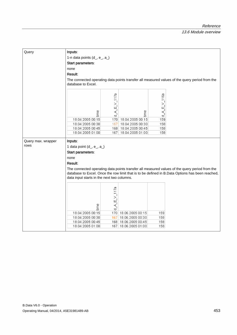
Reference 13.6 Module overview
B.Data V6.0 - Operation Operating Manual, 04/2014, A5E31981489-AB 453
Query Inputs:
1-n data points (d_, e_, a_) Start parameters: none Result: The connected operating data points transfer all measured values of the query period from the database to Excel.
Query max. wrapper rows
Inputs: 1 data point (d_, e_, a_) Start parameters: none Result: The connected operating data points transfer all measured values of the query period from the database to Excel. Once the row limit that is to be defined in B.Data Options has been reached, data input starts in the next two columns.
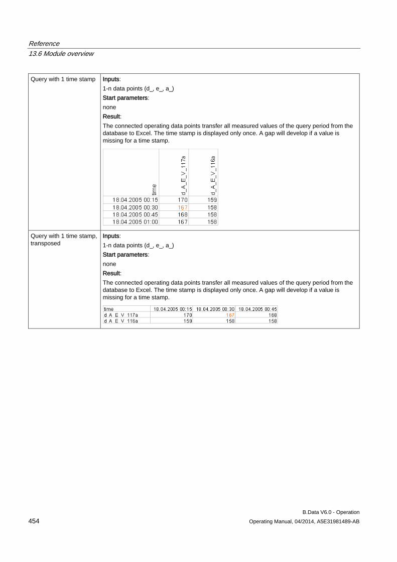
Reference 13.6 Module overview
B.Data V6.0 - Operation 454 Operating Manual, 04/2014, A5E31981489-AB
Query with 1 time stamp Inputs: 1-n data points (d_, e_, a_) Start parameters: none Result: The connected operating data points transfer all measured values of the query period from the database to Excel. The time stamp is displayed only once. A gap will develop if a value is missing for a time stamp.
Query with 1 time stamp, transposed
Inputs: 1-n data points (d_, e_, a_) Start parameters: none Result: The connected operating data points transfer all measured values of the query period from the database to Excel. The time stamp is displayed only once. A gap will develop if a value is missing for a time stamp.
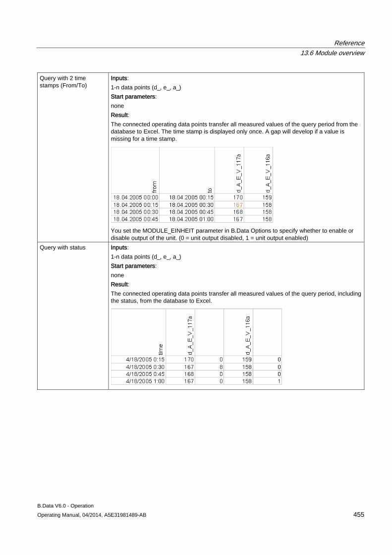
Reference 13.6 Module overview
B.Data V6.0 - Operation Operating Manual, 04/2014, A5E31981489-AB 455
Query with 2 time stamps (From/To)
Inputs: 1-n data points (d_, e_, a_) Start parameters: none Result: The connected operating data points transfer all measured values of the query period from the database to Excel. The time stamp is displayed only once. A gap will develop if a value is missing for a time stamp.
You set the MODULE_EINHEIT parameter in B.Data Options to specify whether to enable or disable output of the unit. (0 = unit output disabled, 1 = unit output enabled)
Query with status Inputs: 1-n data points (d_, e_, a_) Start parameters: none Result: The connected operating data points transfer all measured values of the query period, including the status, from the database to Excel.
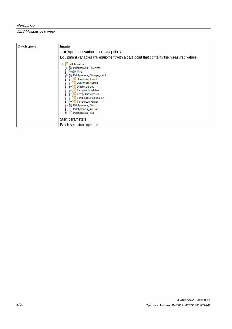
Reference 13.6 Module overview
B.Data V6.0 - Operation 456 Operating Manual, 04/2014, A5E31981489-AB
Batch query Inputs: 1..n equipment variables or data points Equipment variables link equipment with a data point that contains the measured values.
Start parameters: Batch selection; optional
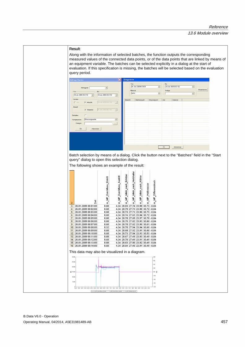
Reference 13.6 Module overview
B.Data V6.0 - Operation Operating Manual, 04/2014, A5E31981489-AB 457
Result: Along with the information of selected batches, the function outputs the corresponding measured values of the connected data points, or of the data points that are linked by means of an equipment variable. The batches can be selected explicitly in a dialog at the start of evaluation. If this specification is missing, the batches will be selected based on the evaluation query period.
Batch selection by means of a dialog. Click the button next to the "Batches" field in the "Start query" dialog to open this selection dialog. The following shows an example of the result:
This data may also be visualized in a diagram.
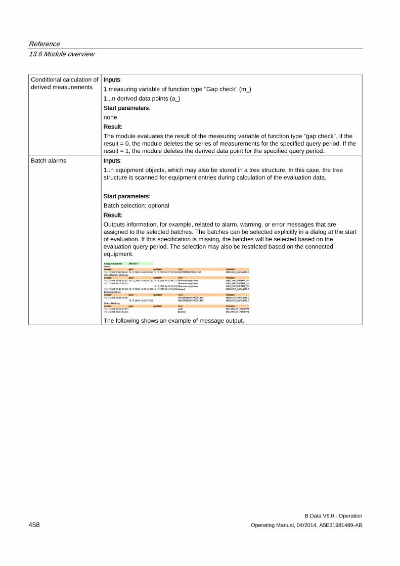
Reference 13.6 Module overview
B.Data V6.0 - Operation 458 Operating Manual, 04/2014, A5E31981489-AB
Conditional calculation of derived measurements
Inputs: 1 measuring variable of function type "Gap check" (m_) 1 ..n derived data points (a_) Start parameters: none Result: The module evaluates the result of the measuring variable of function type "gap check". If the result = 0, the module deletes the series of measurements for the specified query period. If the result = 1, the module deletes the derived data point for the specified query period.
Batch alarms Inputs: 1..n equipment objects, which may also be stored in a tree structure. In this case, the tree structure is scanned for equipment entries during calculation of the evaluation data. Start parameters: Batch selection; optional Result: Outputs information, for example, related to alarm, warning, or error messages that are assigned to the selected batches. The batches can be selected explicitly in a dialog at the start of evaluation. If this specification is missing, the batches will be selected based on the evaluation query period. The selection may also be restricted based on the connected equipment.
The following shows an example of message output.
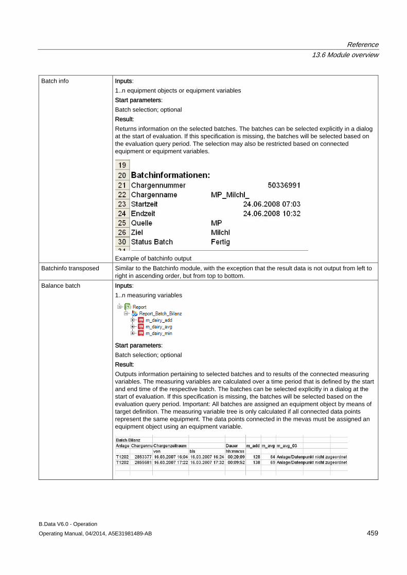
Reference 13.6 Module overview
B.Data V6.0 - Operation Operating Manual, 04/2014, A5E31981489-AB 459
Batch info Inputs: 1..n equipment objects or equipment variables Start parameters: Batch selection; optional Result: Returns information on the selected batches. The batches can be selected explicitly in a dialog at the start of evaluation. If this specification is missing, the batches will be selected based on the evaluation query period. The selection may also be restricted based on connected equipment or equipment variables.
Example of batchinfo output
Batchinfo transposed Similar to the Batchinfo module, with the exception that the result data is not output from left to right in ascending order, but from top to bottom.
Balance batch Inputs: 1..n measuring variables
Start parameters: Batch selection; optional Result: Outputs information pertaining to selected batches and to results of the connected measuring variables. The measuring variables are calculated over a time period that is defined by the start and end time of the respective batch. The batches can be selected explicitly in a dialog at the start of evaluation. If this specification is missing, the batches will be selected based on the evaluation query period. Important: All batches are assigned an equipment object by means of target definition. The measuring variable tree is only calculated if all connected data points represent the same equipment. The data points connected in the mevas must be assigned an equipment object using an equipment variable.
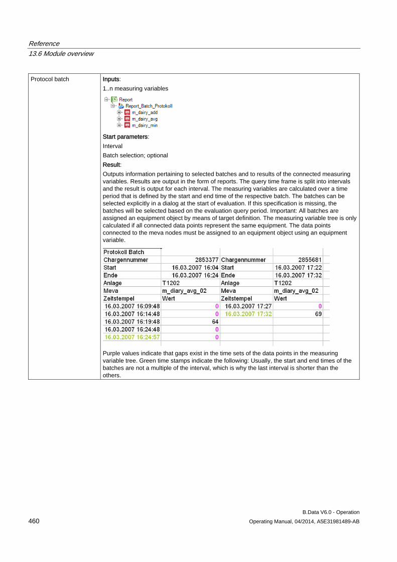
Reference 13.6 Module overview
B.Data V6.0 - Operation 460 Operating Manual, 04/2014, A5E31981489-AB
Protocol batch Inputs: 1..n measuring variables
Start parameters: Interval Batch selection; optional Result: Outputs information pertaining to selected batches and to results of the connected measuring variables. Results are output in the form of reports. The query time frame is split into intervals and the result is output for each interval. The measuring variables are calculated over a time period that is defined by the start and end time of the respective batch. The batches can be selected explicitly in a dialog at the start of evaluation. If this specification is missing, the batches will be selected based on the evaluation query period. Important: All batches are assigned an equipment object by means of target definition. The measuring variable tree is only calculated if all connected data points represent the same equipment. The data points connected to the meva nodes must be assigned to an equipment object using an equipment variable.
Purple values indicate that gaps exist in the time sets of the data points in the measuring variable tree. Green time stamps indicate the following: Usually, the start and end times of the batches are not a multiple of the interval, which is why the last interval is shorter than the others.
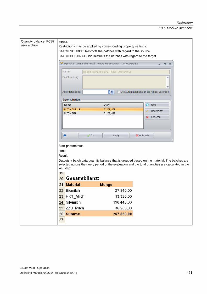
Reference 13.6 Module overview
B.Data V6.0 - Operation Operating Manual, 04/2014, A5E31981489-AB 461
Quantity balance, PCS7 user archive
Inputs: Restrictions may be applied by corresponding property settings. BATCH SOURCE: Restricts the batches with regard to the source. BATCH DESTINATION: Restricts the batches with regard to the target.
Start parameters: none Result: Outputs a batch data quantity balance that is grouped based on the material. The batches are selected across the query period of the evaluation and the total quantities are calculated in the last step.
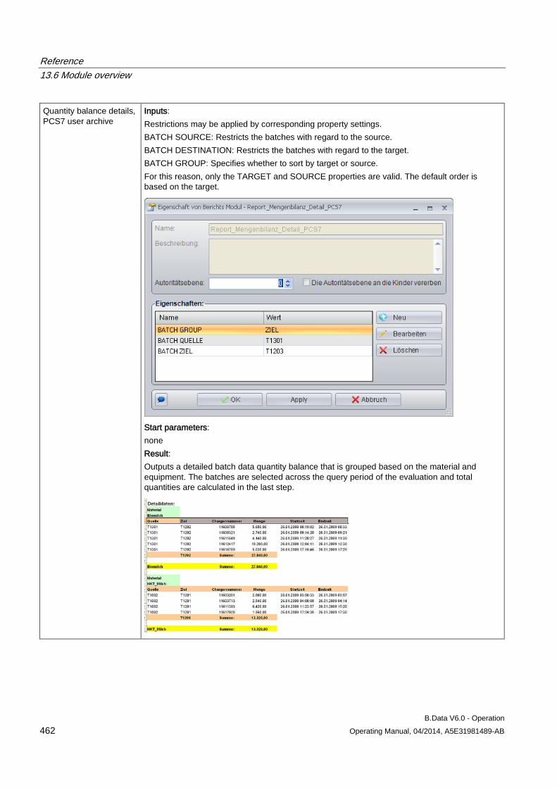
Reference 13.6 Module overview
B.Data V6.0 - Operation 462 Operating Manual, 04/2014, A5E31981489-AB
Quantity balance details, PCS7 user archive
Inputs: Restrictions may be applied by corresponding property settings. BATCH SOURCE: Restricts the batches with regard to the source. BATCH DESTINATION: Restricts the batches with regard to the target. BATCH GROUP: Specifies whether to sort by target or source. For this reason, only the TARGET and SOURCE properties are valid. The default order is based on the target.
Start parameters: none Result: Outputs a detailed batch data quantity balance that is grouped based on the material and equipment. The batches are selected across the query period of the evaluation and total quantities are calculated in the last step.
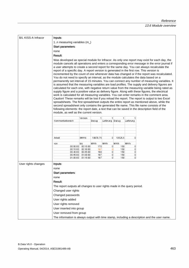
Reference 13.6 Module overview
B.Data V6.0 - Operation Operating Manual, 04/2014, A5E31981489-AB 463
B/L KISS-A Infracor Inputs: 1..n measuring variables (m_) Start parameters: none Result: Was developed as special module for Infracor. As only one report may exist for each day, the module cancels all operations and enters a corresponding error message in the error journal if a user attempts to create a second report for the same day. You can always recalculate the report of a specific day. A report version is generated in the first row. This version is incremented by the count of one whenever data has changed or if the report was recalculated. You do not need to specify an interval, as the module calculates the data based on a permanently set interval of 15 minutes. You can connect any number of measuring variables. It is assumed that the measuring variables are load profiles. The supply and delivery figures are calculated for each one, with negative return value from the measuring variable being rated as supply figure and a positive value as delivery figure. Along with these figures, the electrical work is calculated for all measuring variables. You can enter remarks in the comment area. Caution! These remarks will be lost if you reload the report. The report is output to two Excel spreadsheets. The first spreadsheet outputs the entire report as mentioned above, while the second spreadsheet only contains the generated file name. This file name consists of the following elements: the report date, a text that can be saved in the description field of the module, as well as the current version.
User rights changes Inputs: none Start parameters: none Result: The report outputs all changes to user rights made in the query period. Changed user rights Changed passwords User rights added User rights removed User inserted into group User removed from group The information is always output with time stamp, including a description and the user name.
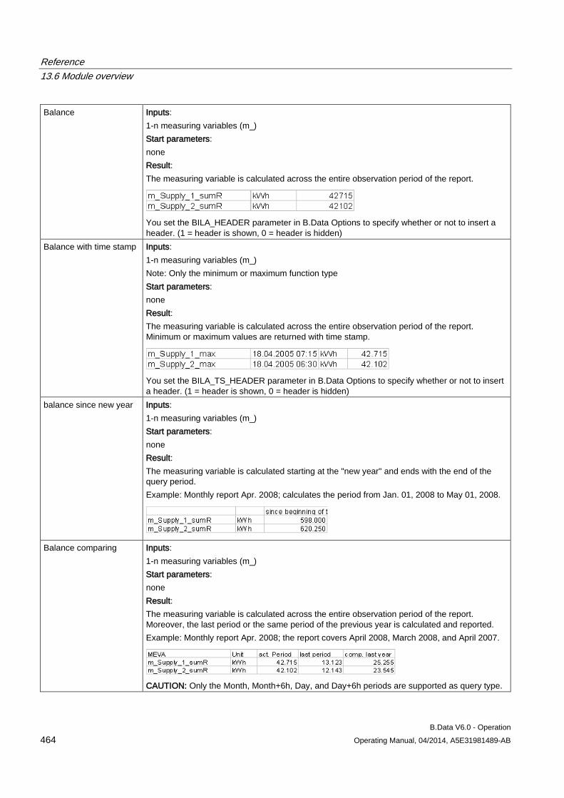
Reference 13.6 Module overview
B.Data V6.0 - Operation 464 Operating Manual, 04/2014, A5E31981489-AB
Balance Inputs: 1-n measuring variables (m_) Start parameters: none Result: The measuring variable is calculated across the entire observation period of the report.
You set the BILA_HEADER parameter in B.Data Options to specify whether or not to insert a header. (1 = header is shown, 0 = header is hidden)
Balance with time stamp Inputs: 1-n measuring variables (m_) Note: Only the minimum or maximum function type Start parameters: none Result: The measuring variable is calculated across the entire observation period of the report. Minimum or maximum values are returned with time stamp.
You set the BILA_TS_HEADER parameter in B.Data Options to specify whether or not to insert a header. (1 = header is shown, 0 = header is hidden)
balance since new year Inputs: 1-n measuring variables (m_) Start parameters: none Result: The measuring variable is calculated starting at the "new year" and ends with the end of the query period. Example: Monthly report Apr. 2008; calculates the period from Jan. 01, 2008 to May 01, 2008.
Balance comparing Inputs: 1-n measuring variables (m_) Start parameters: none Result: The measuring variable is calculated across the entire observation period of the report. Moreover, the last period or the same period of the previous year is calculated and reported. Example: Monthly report Apr. 2008; the report covers April 2008, March 2008, and April 2007.
CAUTION: Only the Month, Month+6h, Day, and Day+6h periods are supported as query type.
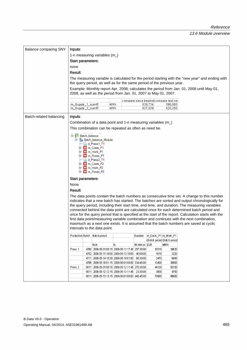
Reference 13.6 Module overview
B.Data V6.0 - Operation Operating Manual, 04/2014, A5E31981489-AB 465
Balance comparing SNY Inputs: 1-n measuring variables (m_) Start parameters: none Result: The measuring variable is calculated for the period starting with the "new year" and ending with the query period, as well as for the same period of the previous year. Example: Monthly report Apr. 2008; calculates the period from Jan. 01, 2008 until May 01, 2008, as well as the period from Jan. 01, 2007 to May 01, 2007.
Batch-related balancing Inputs: Combination of a data point and 1-n measuring variables (m_) This combination can be repeated as often as need be.
Start parameters: None Result: The data points contain the batch numbers as consecutive time set. A change to this number indicates that a new batch has started. The batches are sorted and output chronologically for the query period, including their start time, end time, and duration. The measuring variables connected behind the data point are calculated once for each determined batch period and once for the query period that is specified at the start of the report. Calculation starts with the first data point/measuring variable combination and continues with the next combination, inasmuch as a next one exists. It is assumed that the batch numbers are saved at cyclic intervals to the data point.
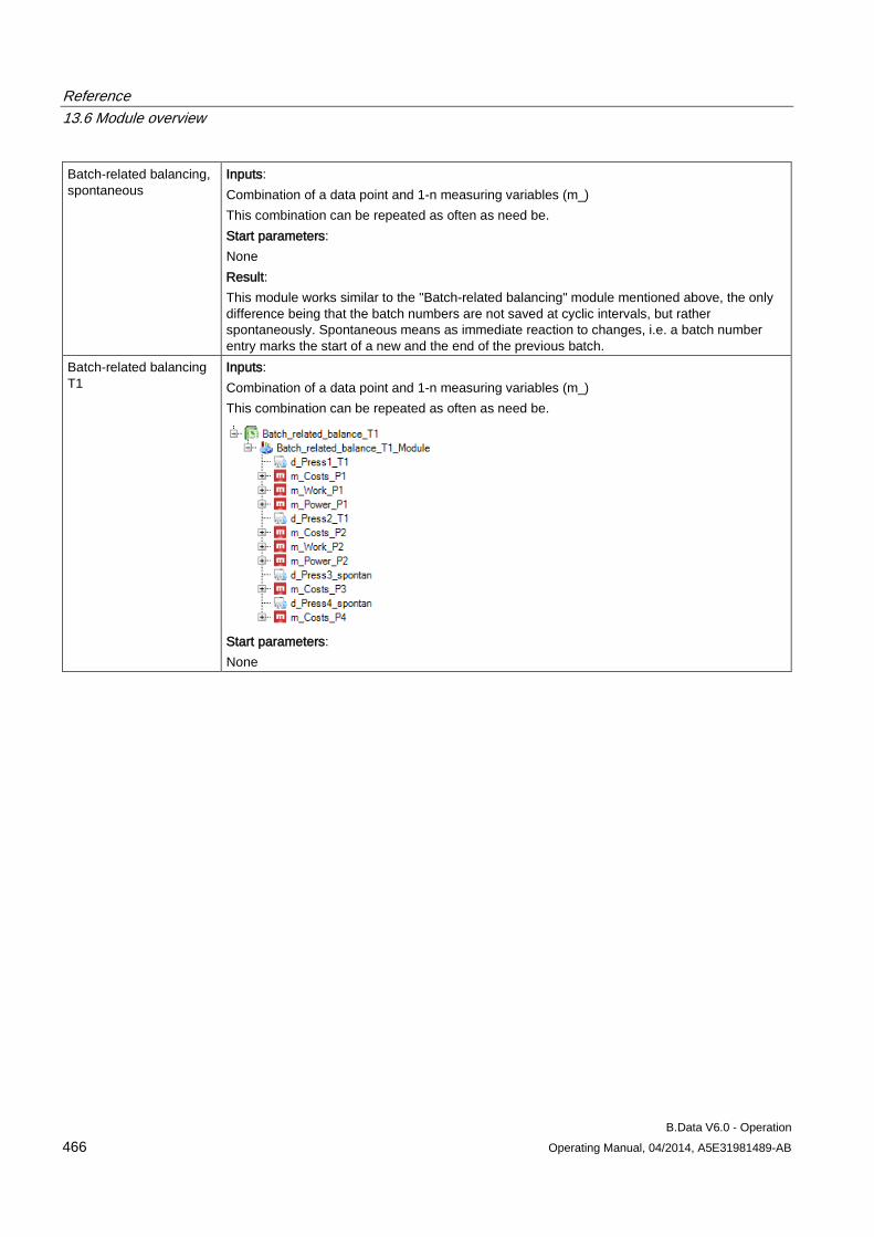
Reference 13.6 Module overview
B.Data V6.0 - Operation 466 Operating Manual, 04/2014, A5E31981489-AB
Batch-related balancing, spontaneous
Inputs: Combination of a data point and 1-n measuring variables (m_) This combination can be repeated as often as need be. Start parameters: None Result: This module works similar to the "Batch-related balancing" module mentioned above, the only difference being that the batch numbers are not saved at cyclic intervals, but rather spontaneously. Spontaneous means as immediate reaction to changes, i.e. a batch number entry marks the start of a new and the end of the previous batch.
Batch-related balancing T1
Inputs: Combination of a data point and 1-n measuring variables (m_) This combination can be repeated as often as need be.
Start parameters: None
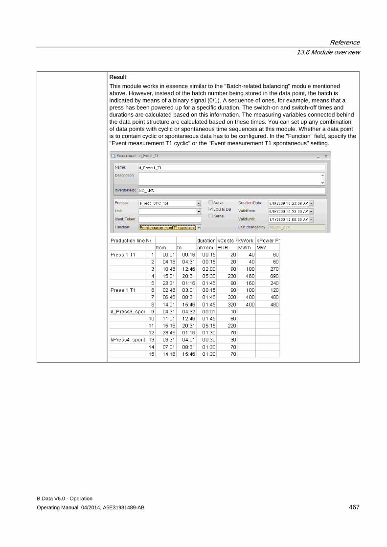
Reference 13.6 Module overview
B.Data V6.0 - Operation Operating Manual, 04/2014, A5E31981489-AB 467
Result: This module works in essence similar to the "Batch-related balancing" module mentioned above. However, instead of the batch number being stored in the data point, the batch is indicated by means of a binary signal (0/1). A sequence of ones, for example, means that a press has been powered up for a specific duration. The switch-on and switch-off times and durations are calculated based on this information. The measuring variables connected behind the data point structure are calculated based on these times. You can set up any combination of data points with cyclic or spontaneous time sequences at this module. Whether a data point is to contain cyclic or spontaneous data has to be configured. In the "Function" field, specify the "Event measurement T1 cyclic" or the "Event measurement T1 spontaneous" setting.
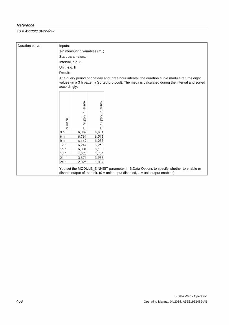
Reference 13.6 Module overview
B.Data V6.0 - Operation 468 Operating Manual, 04/2014, A5E31981489-AB
Duration curve Inputs: 1-n measuring variables (m_) Start parameters: Interval, e.g. 3 Unit: e.g. h Result: At a query period of one day and three hour interval, the duration curve module returns eight values (in a 3 h pattern) (sorted protocol). The meva is calculated during the interval and sorted accordingly.
You set the MODULE_EINHEIT parameter in B.Data Options to specify whether to enable or disable output of the unit. (0 = unit output disabled, 1 = unit output enabled)
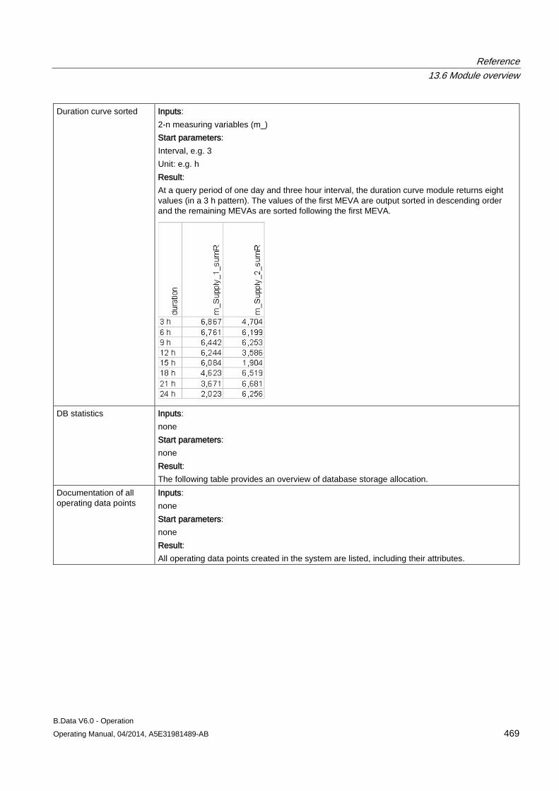
Reference 13.6 Module overview
B.Data V6.0 - Operation Operating Manual, 04/2014, A5E31981489-AB 469
Duration curve sorted Inputs: 2-n measuring variables (m_) Start parameters: Interval, e.g. 3 Unit: e.g. h Result: At a query period of one day and three hour interval, the duration curve module returns eight values (in a 3 h pattern). The values of the first MEVA are output sorted in descending order and the remaining MEVAs are sorted following the first MEVA.
DB statistics Inputs: none Start parameters: none Result: The following table provides an overview of database storage allocation.
Documentation of all operating data points
Inputs: none Start parameters: none Result: All operating data points created in the system are listed, including their attributes.
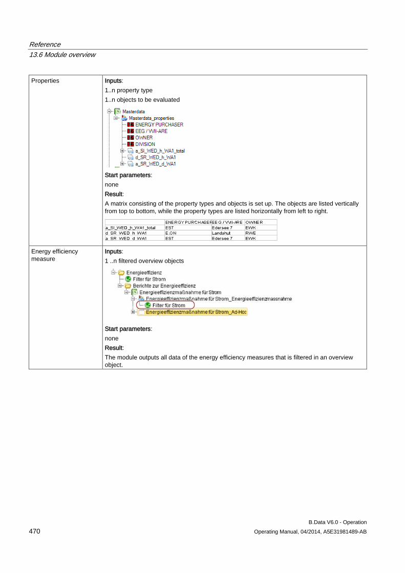
Reference 13.6 Module overview
B.Data V6.0 - Operation 470 Operating Manual, 04/2014, A5E31981489-AB
Properties Inputs: 1..n property type 1..n objects to be evaluated
Start parameters: none Result: A matrix consisting of the property types and objects is set up. The objects are listed vertically from top to bottom, while the property types are listed horizontally from left to right.
Energy efficiency measure
Inputs: 1 ..n filtered overview objects
Start parameters: none Result: The module outputs all data of the energy efficiency measures that is filtered in an overview object.
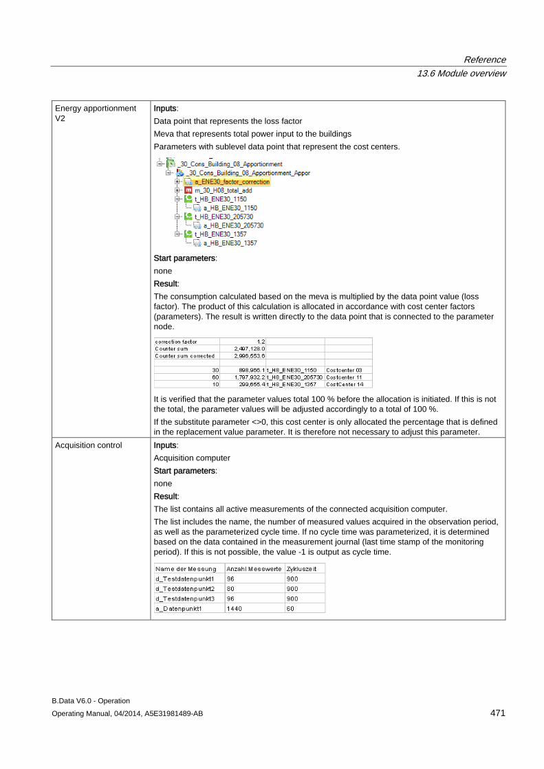
Reference 13.6 Module overview
B.Data V6.0 - Operation Operating Manual, 04/2014, A5E31981489-AB 471
Energy apportionment V2
Inputs: Data point that represents the loss factor Meva that represents total power input to the buildings Parameters with sublevel data point that represent the cost centers.
Start parameters: none Result: The consumption calculated based on the meva is multiplied by the data point value (loss factor). The product of this calculation is allocated in accordance with cost center factors (parameters). The result is written directly to the data point that is connected to the parameter node.
It is verified that the parameter values total 100 % before the allocation is initiated. If this is not the total, the parameter values will be adjusted accordingly to a total of 100 %. If the substitute parameter <>0, this cost center is only allocated the percentage that is defined in the replacement value parameter. It is therefore not necessary to adjust this parameter.
Acquisition control Inputs: Acquisition computer Start parameters: none Result: The list contains all active measurements of the connected acquisition computer. The list includes the name, the number of measured values acquired in the observation period, as well as the parameterized cycle time. If no cycle time was parameterized, it is determined based on the data contained in the measurement journal (last time stamp of the monitoring period). If this is not possible, the value -1 is output as cycle time.
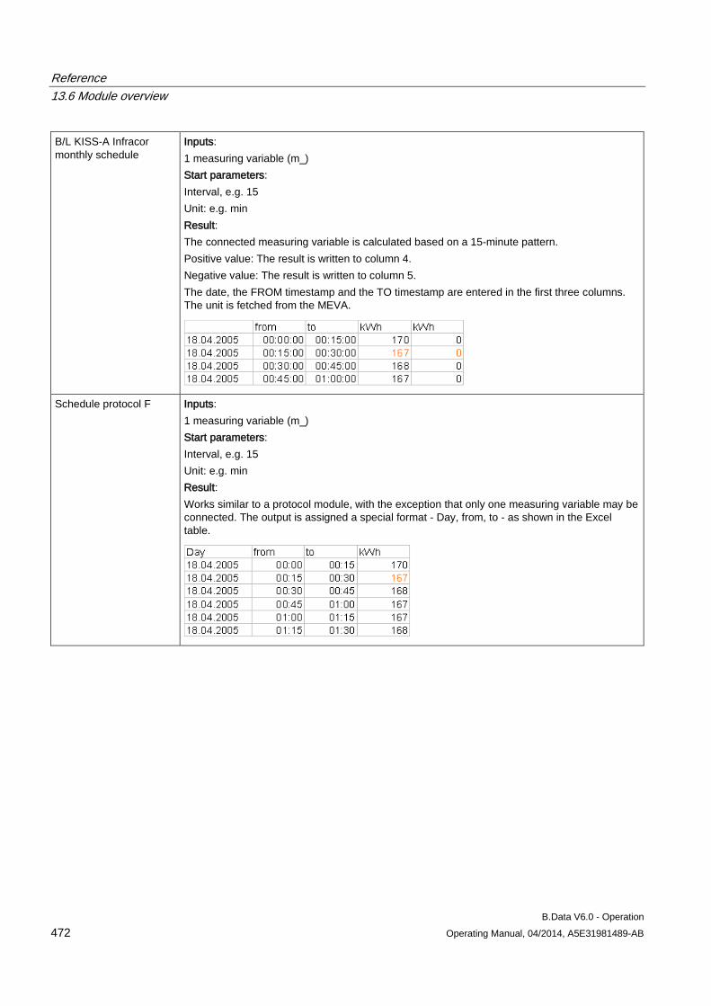
Reference 13.6 Module overview
B.Data V6.0 - Operation 472 Operating Manual, 04/2014, A5E31981489-AB
B/L KISS-A Infracor monthly schedule
Inputs: 1 measuring variable (m_) Start parameters: Interval, e.g. 15 Unit: e.g. min Result: The connected measuring variable is calculated based on a 15-minute pattern. Positive value: The result is written to column 4. Negative value: The result is written to column 5. The date, the FROM timestamp and the TO timestamp are entered in the first three columns. The unit is fetched from the MEVA.
Schedule protocol F Inputs: 1 measuring variable (m_) Start parameters: Interval, e.g. 15 Unit: e.g. min Result: Works similar to a protocol module, with the exception that only one measuring variable may be connected. The output is assigned a special format - Day, from, to - as shown in the Excel table.
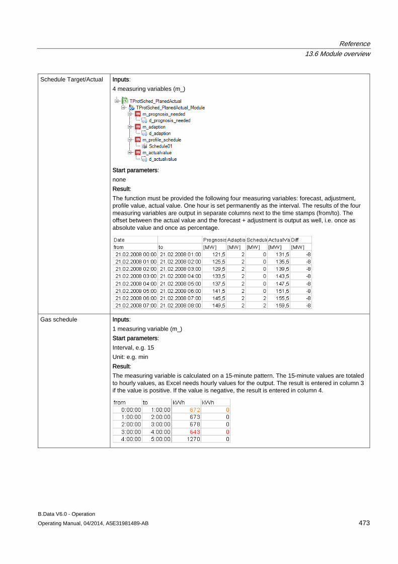
Reference 13.6 Module overview
B.Data V6.0 - Operation Operating Manual, 04/2014, A5E31981489-AB 473
Schedule Target/Actual Inputs: 4 measuring variables (m_)
Start parameters: none Result: The function must be provided the following four measuring variables: forecast, adjustment, profile value, actual value. One hour is set permanently as the interval. The results of the four measuring variables are output in separate columns next to the time stamps (from/to). The offset between the actual value and the forecast + adjustment is output as well, i.e. once as absolute value and once as percentage.
Gas schedule Inputs: 1 measuring variable (m_) Start parameters: Interval, e.g. 15 Unit: e.g. min Result: The measuring variable is calculated on a 15-minute pattern. The 15-minute values are totaled to hourly values, as Excel needs hourly values for the output. The result is entered in column 3 if the value is positive. If the value is negative, the result is entered in column 4.
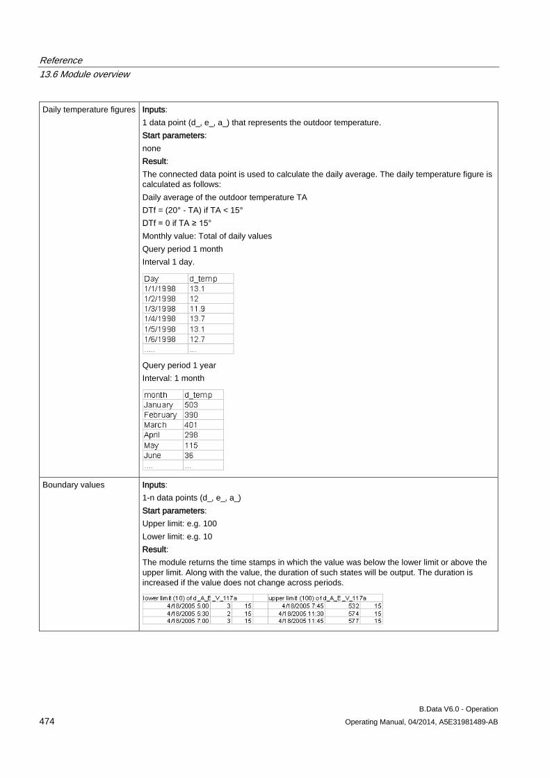
Reference 13.6 Module overview
B.Data V6.0 - Operation 474 Operating Manual, 04/2014, A5E31981489-AB
Daily temperature figures Inputs: 1 data point (d_, e_, a_) that represents the outdoor temperature. Start parameters: none Result: The connected data point is used to calculate the daily average. The daily temperature figure is calculated as follows: Daily average of the outdoor temperature TA DTf = (20° - TA) if TA < 15° DTf = 0 if TA ≥ 15° Monthly value: Total of daily values Query period 1 month Interval 1 day.
Query period 1 year Interval: 1 month
Boundary values Inputs: 1-n data points (d_, e_, a_) Start parameters: Upper limit: e.g. 100 Lower limit: e.g. 10 Result: The module returns the time stamps in which the value was below the lower limit or above the upper limit. Along with the value, the duration of such states will be output. The duration is increased if the value does not change across periods.
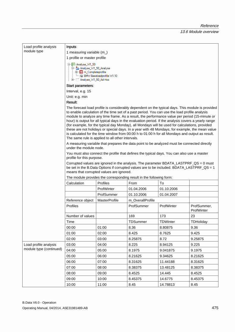
Reference 13.6 Module overview
B.Data V6.0 - Operation Operating Manual, 04/2014, A5E31981489-AB 475
Load profile analysis module type
Inputs: 1 measuring variable (m_) 1 profile or master profile
Start parameters: Interval, e.g. 15 Unit: e.g. min Result: The forecast load profile is considerably dependent on the typical days. This module is provided to enable calculation of the time set of a past period. You can use the load profile analysis module to analyze any time frame. As a result, the performance value per period (15-minute or hour) is output for all typical days in the evaluation period. If the analysis covers a yearly range (for example, for the typical day Monday), all Mondays will be used for calculations, provided these are not holidays or special days. In a year with 48 Mondays, for example, the mean value is calculated for the time window from 00:00 h to 01:00 h for all Mondays and output as result. The same rule is applied to all other intervals. A measuring variable that prepares the data point to be analyzed must be connected directly under the module node. You must also connect the profile that defines the typical days. You can also use a master profile for this purpose. Corrupted values are ignored in the analysis. The parameter BDATA_LASTPRF_QS = 0 must be set in the B.Data Options if corrupted values are to be included. BDATA_LASTPRF_QS = 1 means that corrupted values are ignored. The module provides the corresponding result in the following form: Calculation Profiles From To ProfWinter 01.04.2006 01.10.2006 ProfSummer 01.10.2006 01.04.2007 Reference object MasterProfile m_OverallProfile Profiles ProfSummer ProfWinter ProfSummer,
ProfWinter Number of values 169 173 23 Time TDSummer TDWinter TDHoliday 00:00 01:00 8.36 8.80875 9.36 01:00 02:00 8.425 8.7625 9.425 02:00 03:00 8.25875 8.72 9.25875
Load profile analysis module type (continued)
03:00 04:00 8.225 8.94125 9.225 04:00 05:00 8.1975 9.041875 9.1975 05:00 06:00 8.21625 9.34625 8.21625 06:00 07:00 8.31625 11.44188 8.31625 07:00 08:00 8.38375 13.48125 8.38375 08:00 09:00 8.4525 14.445 8.4525 09:00 10:00 8.45375 14.6775 8.45375 10:00 11:00 8.45 14.78813 8.45
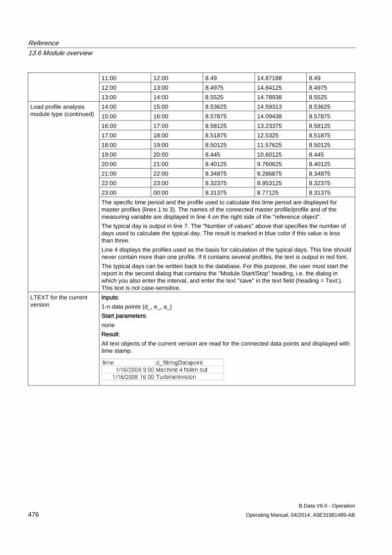
Reference 13.6 Module overview
B.Data V6.0 - Operation 476 Operating Manual, 04/2014, A5E31981489-AB
11:00 12:00 8.49 14.87188 8.49 12:00 13:00 8.4975 14.84125 8.4975 13:00 14:00 8.5525 14.78938 8.5525
Load profile analysis module type (continued)
14:00 15:00 8.53625 14.59313 8.53625 15:00 16:00 8.57875 14.09438 8.57875 16:00 17:00 8.58125 13.23375 8.58125 17:00 18:00 8.51875 12.5325 8.51875 18:00 19:00 8.50125 11.57625 8.50125 19:00 20:00 8.445 10.60125 8.445 20:00 21:00 8.40125 9.760625 8.40125 21:00 22:00 8.34875 9.286875 8.34875 22:00 23:00 8.32375 8.953125 8.32375 23:00 00:00 8.31375 8.77125 8.31375 The specific time period and the profile used to calculate this time period are displayed for master profiles (lines 1 to 3). The names of the connected master profile/profile and of the measuring variable are displayed in line 4 on the right side of the "reference object". The typical day is output in line 7. The "Number of values" above that specifies the number of days used to calculate the typical day. The result is marked in blue color if this value is less than three. Line 4 displays the profiles used as the basis for calculation of the typical days. This line should never contain more than one profile. If it contains several profiles, the text is output in red font. The typical days can be written back to the database. For this purpose, the user must start the report in the second dialog that contains the "Module Start/Stop" heading, i.e. the dialog in which you also enter the interval, and enter the text "save" in the text field (heading = Text:). This text is not case-sensitive.
LTEXT for the current version
Inputs: 1-n data points (d_, e_, a_) Start parameters: none Result: All text objects of the current version are read for the connected data points and displayed with time stamp.
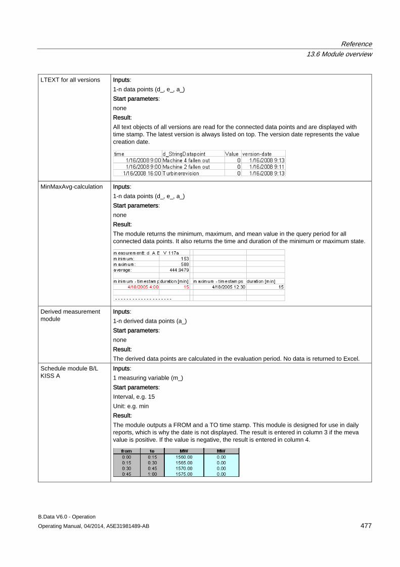
Reference 13.6 Module overview
B.Data V6.0 - Operation Operating Manual, 04/2014, A5E31981489-AB 477
LTEXT for all versions Inputs: 1-n data points (d_, e_, a_) Start parameters: none Result: All text objects of all versions are read for the connected data points and are displayed with time stamp. The latest version is always listed on top. The version date represents the value creation date.
MinMaxAvg-calculation Inputs: 1-n data points (d_, e_, a_) Start parameters: none Result: The module returns the minimum, maximum, and mean value in the query period for all connected data points. It also returns the time and duration of the minimum or maximum state.
Derived measurement module
Inputs: 1-n derived data points (a_) Start parameters: none Result: The derived data points are calculated in the evaluation period. No data is returned to Excel.
Schedule module B/L KISS A
Inputs: 1 measuring variable (m_) Start parameters: Interval, e.g. 15 Unit: e.g. min Result: The module outputs a FROM and a TO time stamp. This module is designed for use in daily reports, which is why the date is not displayed. The result is entered in column 3 if the meva value is positive. If the value is negative, the result is entered in column 4.
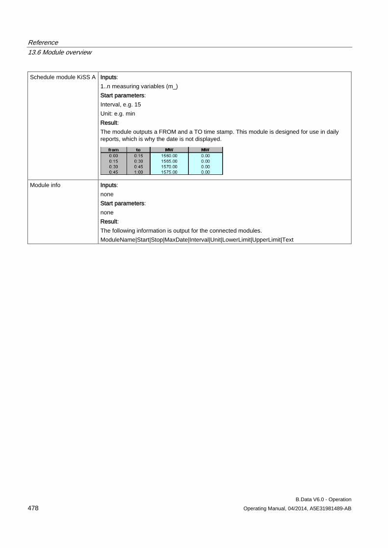
Reference 13.6 Module overview
B.Data V6.0 - Operation 478 Operating Manual, 04/2014, A5E31981489-AB
Schedule module KiSS A Inputs: 1..n measuring variables (m_) Start parameters: Interval, e.g. 15 Unit: e.g. min Result: The module outputs a FROM and a TO time stamp. This module is designed for use in daily reports, which is why the date is not displayed.
Module info Inputs: none Start parameters: none Result: The following information is output for the connected modules. ModuleName|Start|Stop|MaxDate|Interval|Unit|LowerLimit|UpperLimit|Text
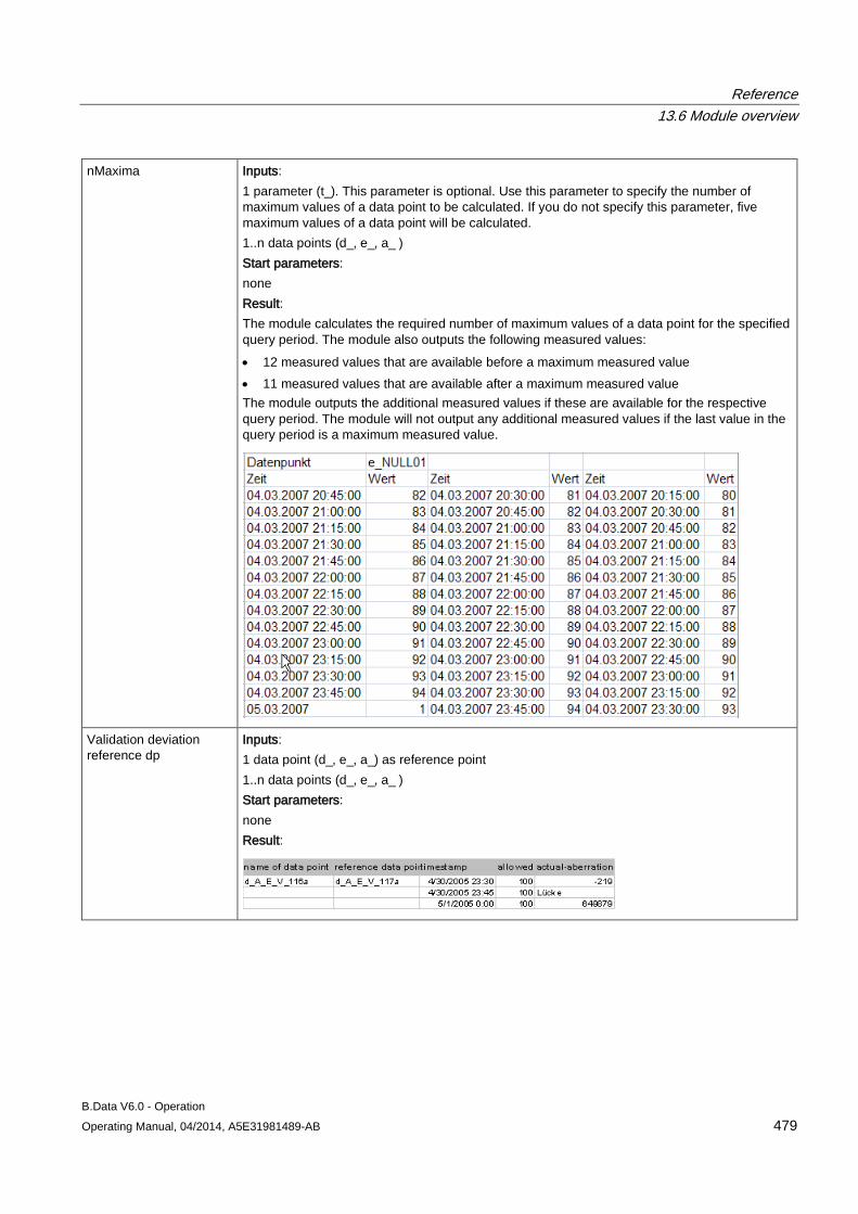
Reference 13.6 Module overview
B.Data V6.0 - Operation Operating Manual, 04/2014, A5E31981489-AB 479
nMaxima Inputs: 1 parameter (t_). This parameter is optional. Use this parameter to specify the number of maximum values of a data point to be calculated. If you do not specify this parameter, five maximum values of a data point will be calculated. 1..n data points (d_, e_, a_ ) Start parameters: none Result: The module calculates the required number of maximum values of a data point for the specified query period. The module also outputs the following measured values: • 12 measured values that are available before a maximum measured value • 11 measured values that are available after a maximum measured value The module outputs the additional measured values if these are available for the respective query period. The module will not output any additional measured values if the last value in the query period is a maximum measured value.
Validation deviation reference dp
Inputs: 1 data point (d_, e_, a_) as reference point 1..n data points (d_, e_, a_ ) Start parameters: none Result:
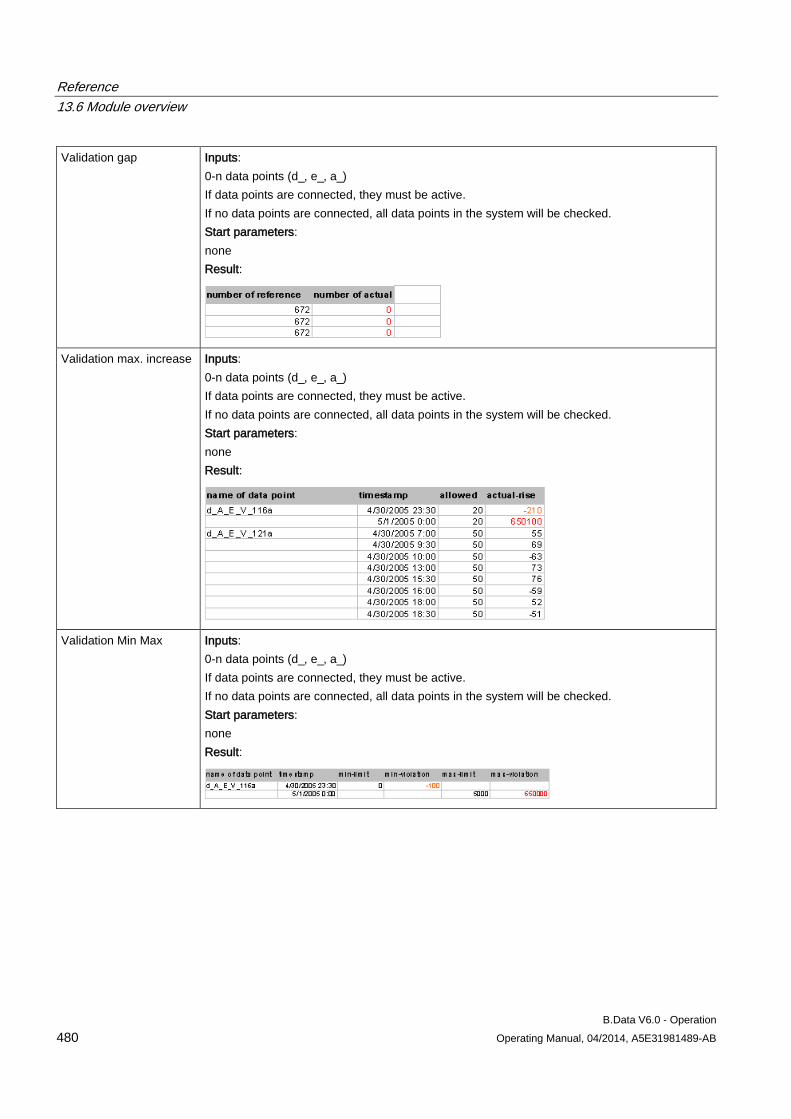
Reference 13.6 Module overview
B.Data V6.0 - Operation 480 Operating Manual, 04/2014, A5E31981489-AB
Validation gap Inputs: 0-n data points (d_, e_, a_) If data points are connected, they must be active. If no data points are connected, all data points in the system will be checked. Start parameters: none Result:
Validation max. increase Inputs: 0-n data points (d_, e_, a_) If data points are connected, they must be active. If no data points are connected, all data points in the system will be checked. Start parameters: none Result:
Validation Min Max Inputs: 0-n data points (d_, e_, a_) If data points are connected, they must be active. If no data points are connected, all data points in the system will be checked. Start parameters: none Result:
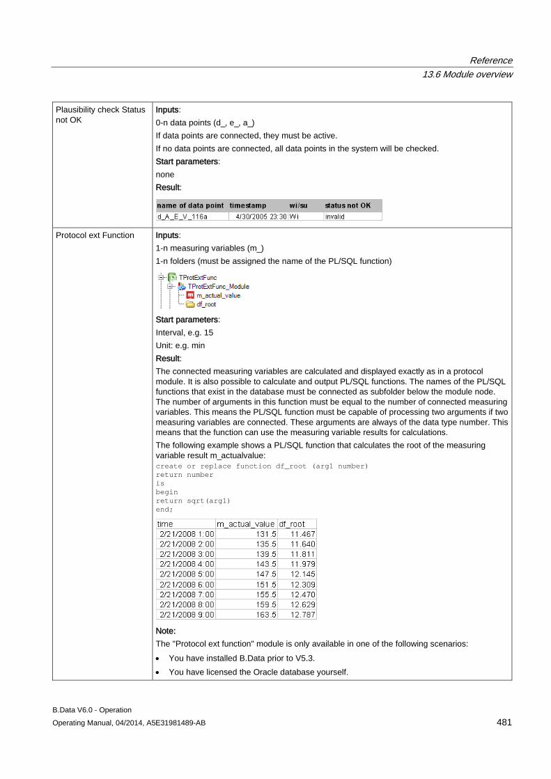
Reference 13.6 Module overview
B.Data V6.0 - Operation Operating Manual, 04/2014, A5E31981489-AB 481
Plausibility check Status not OK
Inputs: 0-n data points (d_, e_, a_) If data points are connected, they must be active. If no data points are connected, all data points in the system will be checked. Start parameters: none Result:
Protocol ext Function Inputs: 1-n measuring variables (m_) 1-n folders (must be assigned the name of the PL/SQL function)
Start parameters: Interval, e.g. 15 Unit: e.g. min Result: The connected measuring variables are calculated and displayed exactly as in a protocol module. It is also possible to calculate and output PL/SQL functions. The names of the PL/SQL functions that exist in the database must be connected as subfolder below the module node. The number of arguments in this function must be equal to the number of connected measuring variables. This means the PL/SQL function must be capable of processing two arguments if two measuring variables are connected. These arguments are always of the data type number. This means that the function can use the measuring variable results for calculations. The following example shows a PL/SQL function that calculates the root of the measuring variable result m_actualvalue: create or replace function df_root (arg1 number) return number is begin return sqrt(arg1) end;
Note: The "Protocol ext function" module is only available in one of the following scenarios: • You have installed B.Data prior to V5.3. • You have licensed the Oracle database yourself.
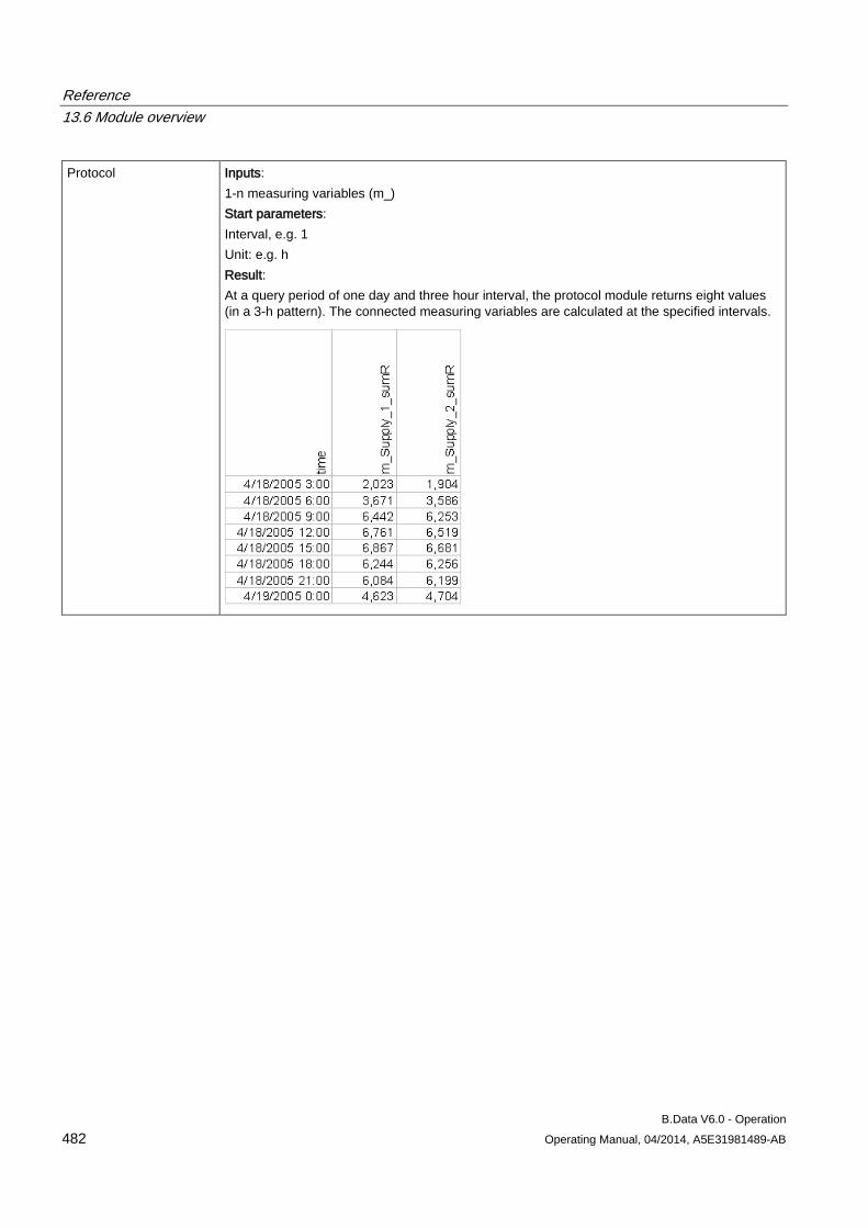
Reference 13.6 Module overview
B.Data V6.0 - Operation 482 Operating Manual, 04/2014, A5E31981489-AB
Protocol Inputs: 1-n measuring variables (m_) Start parameters: Interval, e.g. 1 Unit: e.g. h Result: At a query period of one day and three hour interval, the protocol module returns eight values (in a 3-h pattern). The connected measuring variables are calculated at the specified intervals.
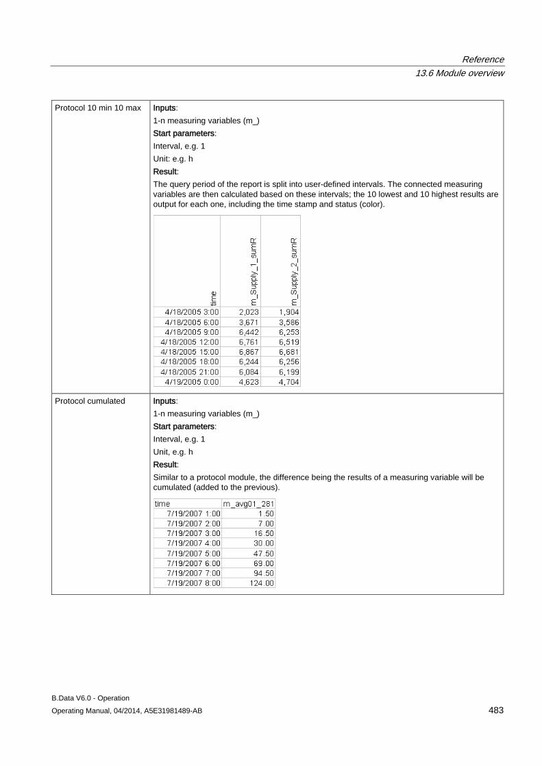
Reference 13.6 Module overview
B.Data V6.0 - Operation Operating Manual, 04/2014, A5E31981489-AB 483
Protocol 10 min 10 max Inputs: 1-n measuring variables (m_) Start parameters: Interval, e.g. 1 Unit: e.g. h Result: The query period of the report is split into user-defined intervals. The connected measuring variables are then calculated based on these intervals; the 10 lowest and 10 highest results are output for each one, including the time stamp and status (color).
Protocol cumulated Inputs: 1-n measuring variables (m_) Start parameters: Interval, e.g. 1 Unit, e.g. h Result: Similar to a protocol module, the difference being the results of a measuring variable will be cumulated (added to the previous).
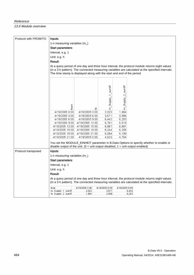
Reference 13.6 Module overview
B.Data V6.0 - Operation 484 Operating Manual, 04/2014, A5E31981489-AB
Protocol with FROM/TO Inputs: 1-n measuring variables (m_) Start parameters: Interval, e.g. 1 Unit: e.g. h Result: At a query period of one day and three hour interval, the protocol module returns eight values (in a 3-h pattern). The connected measuring variables are calculated at the specified intervals. The time stamp is displayed along with the start and end of the period.
You set the MODULE_EINHEIT parameter in B.Data Options to specify whether to enable or disable output of the unit. (0 = unit output disabled, 1 = unit output enabled)
Protocol transposed Inputs: 1-n measuring variables (m_) Start parameters: Interval, e.g. 1 Unit: e.g. h Result: At a query period of one day and three hour interval, the protocol module returns eight values (in a 3-h pattern). The connected measuring variables are calculated at the specified intervals.
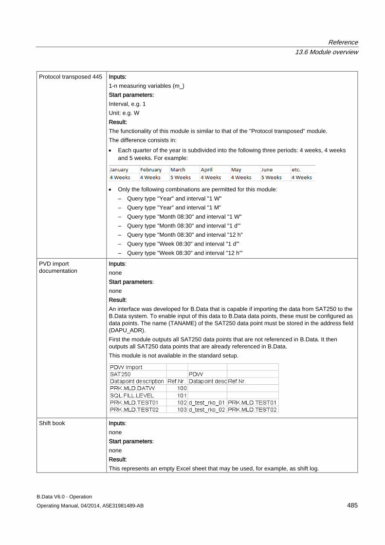
Reference 13.6 Module overview
B.Data V6.0 - Operation Operating Manual, 04/2014, A5E31981489-AB 485
Protocol transposed 445 Inputs: 1-n measuring variables (m_) Start parameters: Interval, e.g. 1 Unit: e.g. W Result: The functionality of this module is similar to that of the "Protocol transposed" module. The difference consists in: • Each quarter of the year is subdivided into the following three periods: 4 weeks, 4 weeks
and 5 weeks. For example:
• Only the following combinations are permitted for this module:
– Query type "Year" and interval "1 W" – Query type "Year" and interval "1 M" – Query type "Month 08:30" and interval "1 W" – Query type "Month 08:30" and interval "1 d'" – Query type "Month 08:30" and interval "12 h" – Query type "Week 08:30" and interval "1 d'" – Query type "Week 08:30" and interval "12 h'"
PVD import documentation
Inputs: none Start parameters: none Result: An interface was developed for B.Data that is capable if importing the data from SAT250 to the B.Data system. To enable input of this data to B.Data data points, these must be configured as data points. The name (TANAME) of the SAT250 data point must be stored in the address field (DAPU_ADR). First the module outputs all SAT250 data points that are not referenced in B.Data. It then outputs all SAT250 data points that are already referenced in B.Data. This module is not available in the standard setup.
Shift book Inputs: none Start parameters: none Result: This represents an empty Excel sheet that may be used, for example, as shift log.
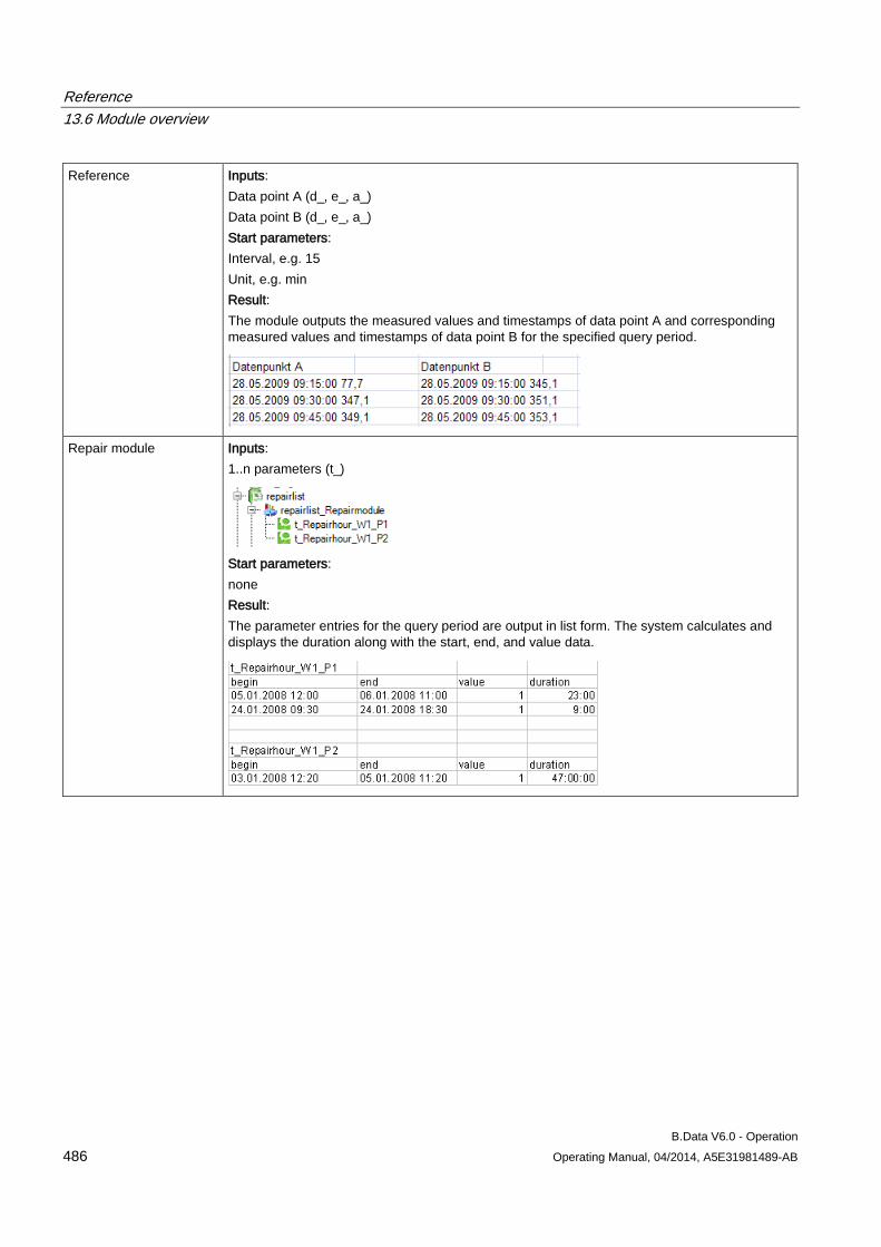
Reference 13.6 Module overview
B.Data V6.0 - Operation 486 Operating Manual, 04/2014, A5E31981489-AB
Reference Inputs: Data point A (d_, e_, a_) Data point B (d_, e_, a_) Start parameters: Interval, e.g. 15 Unit, e.g. min Result: The module outputs the measured values and timestamps of data point A and corresponding measured values and timestamps of data point B for the specified query period.
Repair module Inputs: 1..n parameters (t_)
Start parameters: none Result: The parameter entries for the query period are output in list form. The system calculates and displays the duration along with the start, end, and value data.
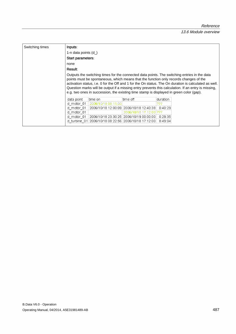
Reference 13.6 Module overview
B.Data V6.0 - Operation Operating Manual, 04/2014, A5E31981489-AB 487
Switching times Inputs: 1-n data points (d_) Start parameters: none Result: Outputs the switching times for the connected data points. The switching entries in the data points must be spontaneous, which means that the function only records changes of the activation status, i.e. 0 for the Off and 1 for the On status. The On duration is calculated as well. Question marks will be output if a missing entry prevents this calculation. If an entry is missing, e.g. two ones in succession, the existing time stamp is displayed in green color (gap).
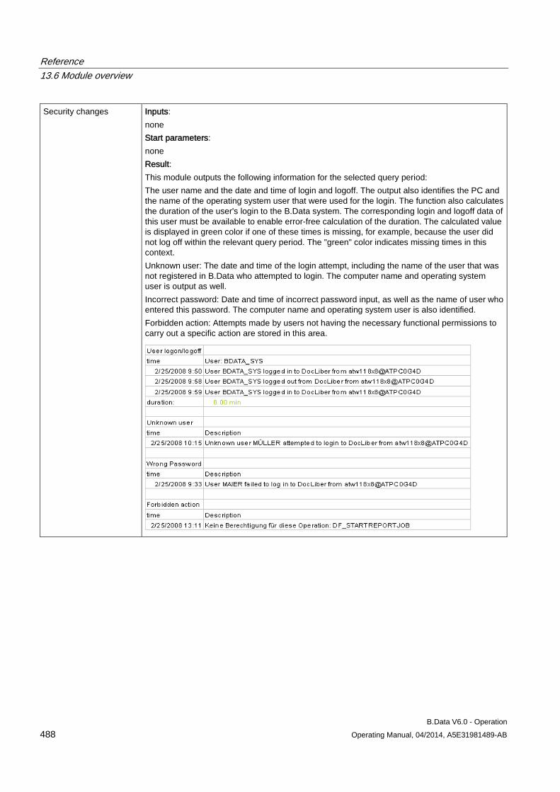
Reference 13.6 Module overview
B.Data V6.0 - Operation 488 Operating Manual, 04/2014, A5E31981489-AB
Security changes Inputs: none Start parameters: none Result: This module outputs the following information for the selected query period: The user name and the date and time of login and logoff. The output also identifies the PC and the name of the operating system user that were used for the login. The function also calculates the duration of the user's login to the B.Data system. The corresponding login and logoff data of this user must be available to enable error-free calculation of the duration. The calculated value is displayed in green color if one of these times is missing, for example, because the user did not log off within the relevant query period. The "green" color indicates missing times in this context. Unknown user: The date and time of the login attempt, including the name of the user that was not registered in B.Data who attempted to login. The computer name and operating system user is output as well. Incorrect password: Date and time of incorrect password input, as well as the name of user who entered this password. The computer name and operating system user is also identified. Forbidden action: Attempts made by users not having the necessary functional permissions to carry out a specific action are stored in this area.
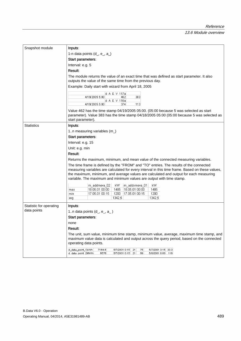
Reference 13.6 Module overview
B.Data V6.0 - Operation Operating Manual, 04/2014, A5E31981489-AB 489
Snapshot module Inputs: 1-n data points (d_, e_, a_) Start parameters: Interval: e.g. 5 Result: The module returns the value of an exact time that was defined as start parameter. It also outputs the value of the same time from the previous day. Example: Daily start with wizard from April 18, 2005
Value 462 has the time stamp 04/19/2005 05:00. (05:00 because 5 was selected as start parameter). Value 383 has the time stamp 04/18/2005 05:00 (05:00 because 5 was selected as start parameter).
Statistics Inputs: 1..n measuring variables (m_) Start parameters: Interval: e.g. 15 Unit: e.g. min Result: Returns the maximum, minimum, and mean value of the connected measuring variables. The time frame is defined by the "FROM" and "TO" entries. The results of the connected measuring variables are calculated for every interval in this time frame. Based on these values, the maximum, minimum, and average values are calculated and output for each measuring variable. The maximum and minimum values are output with time stamp.
Statistic for operating data points
Inputs: 1..n data points (d_, e_, a_ ) Start parameters: none Result: The unit, sum value, minimum time stamp, minimum value, average, maximum time stamp, and maximum value data is calculated and output across the query period, based on the connected operating data points.
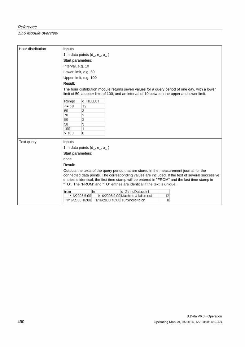
Reference 13.6 Module overview
B.Data V6.0 - Operation 490 Operating Manual, 04/2014, A5E31981489-AB
Hour distribution Inputs: 1..n data points (d_, e_, a_ ) Start parameters: Interval, e.g. 10 Lower limit, e.g. 50 Upper limit, e.g. 100 Result: The hour distribution module returns seven values for a query period of one day, with a lower limit of 50, a upper limit of 100, and an interval of 10 between the upper and lower limit.
Text query Inputs: 1..n data points (d_, e_, a_ ) Start parameters: none Result: Outputs the texts of the query period that are stored in the measurement journal for the connected data points. The corresponding values are included. If the text of several successive entries is identical, the first time stamp will be entered in "FROM" and the last time stamp in "TO". The "FROM" and "TO" entries are identical if the text is unique.
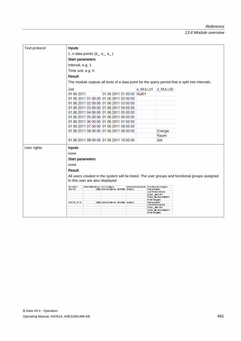
Reference 13.6 Module overview
B.Data V6.0 - Operation Operating Manual, 04/2014, A5E31981489-AB 491
Text protocol Inputs: 1..n data points (d_, e_, a_ ) Start parameters: Interval, e.g. 1 Time unit, e.g. h Result: The module outputs all texts of a data point for the query period that is split into intervals.
User rights Inputs: none Start parameters: none Result: All users created in the system will be listed. The user groups and functional groups assigned to this user are also displayed.
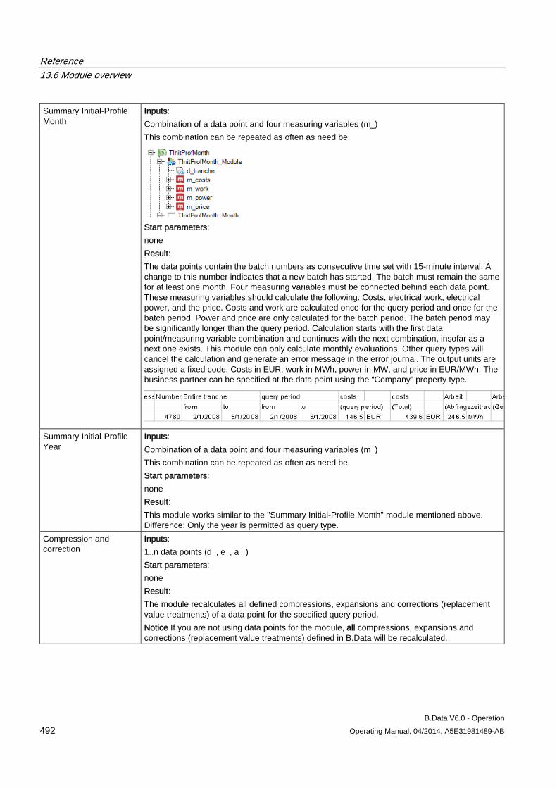
Reference 13.6 Module overview
B.Data V6.0 - Operation 492 Operating Manual, 04/2014, A5E31981489-AB
Summary Initial-Profile Month
Inputs: Combination of a data point and four measuring variables (m_) This combination can be repeated as often as need be.
Start parameters: none Result: The data points contain the batch numbers as consecutive time set with 15-minute interval. A change to this number indicates that a new batch has started. The batch must remain the same for at least one month. Four measuring variables must be connected behind each data point. These measuring variables should calculate the following: Costs, electrical work, electrical power, and the price. Costs and work are calculated once for the query period and once for the batch period. Power and price are only calculated for the batch period. The batch period may be significantly longer than the query period. Calculation starts with the first data point/measuring variable combination and continues with the next combination, insofar as a next one exists. This module can only calculate monthly evaluations. Other query types will cancel the calculation and generate an error message in the error journal. The output units are assigned a fixed code. Costs in EUR, work in MWh, power in MW, and price in EUR/MWh. The business partner can be specified at the data point using the “Company” property type.
Summary Initial-Profile Year
Inputs: Combination of a data point and four measuring variables (m_) This combination can be repeated as often as need be. Start parameters: none Result: This module works similar to the "Summary Initial-Profile Month" module mentioned above. Difference: Only the year is permitted as query type.
Compression and correction
Inputs: 1..n data points (d_, e_, a_ ) Start parameters: none Result: The module recalculates all defined compressions, expansions and corrections (replacement value treatments) of a data point for the specified query period. Notice If you are not using data points for the module, all compressions, expansions and corrections (replacement value treatments) defined in B.Data will be recalculated.
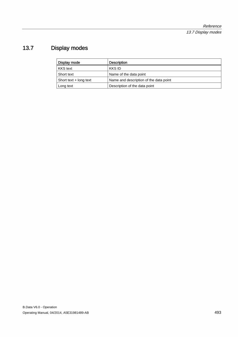
Reference 13.7 Display modes
B.Data V6.0 - Operation Operating Manual, 04/2014, A5E31981489-AB 493
13.7 Display modes Display mode Description KKS text KKS ID Short text Name of the data point Short text + long text Name and description of the data point Long text Description of the data point
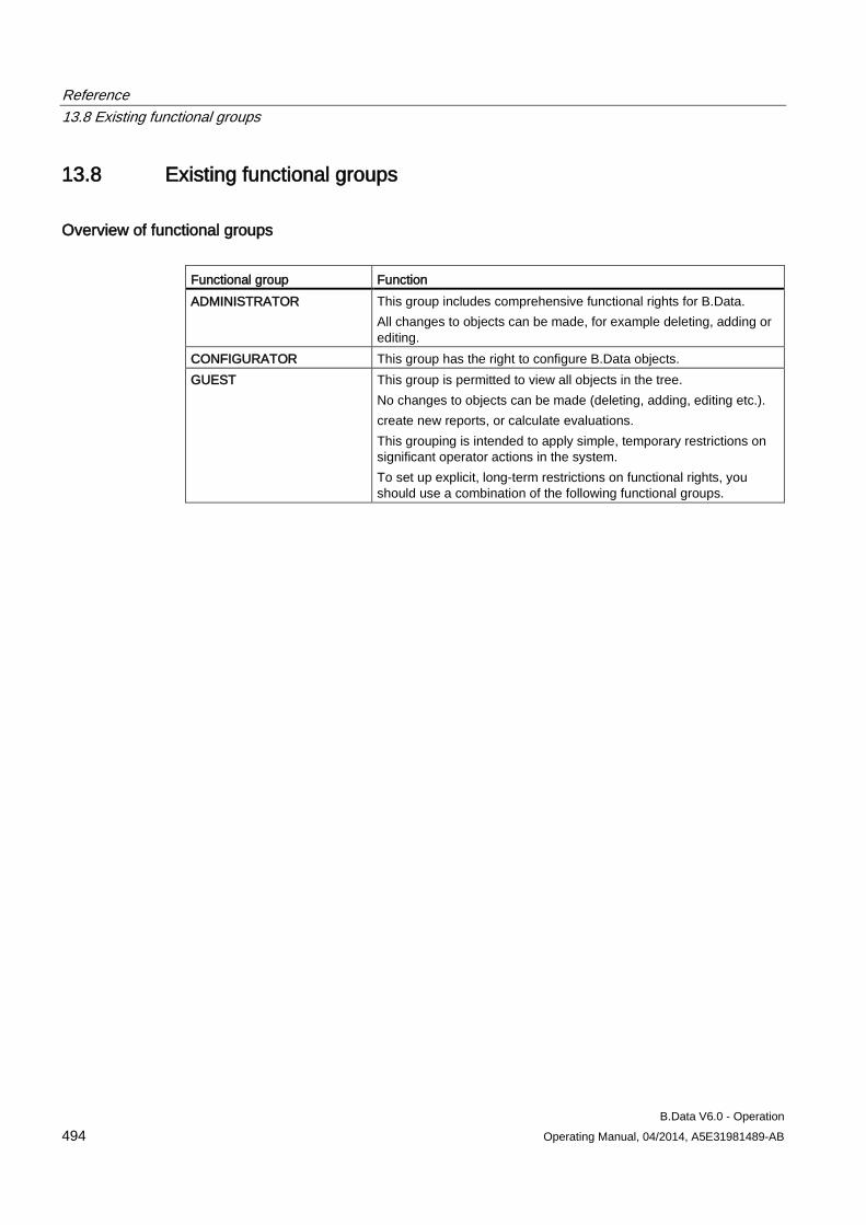
Reference 13.8 Existing functional groups
B.Data V6.0 - Operation 494 Operating Manual, 04/2014, A5E31981489-AB
13.8 Existing functional groups
Overview of functional groups Functional group Function ADMINISTRATOR This group includes comprehensive functional rights for B.Data.
All changes to objects can be made, for example deleting, adding or editing.
CONFIGURATOR This group has the right to configure B.Data objects. GUEST This group is permitted to view all objects in the tree.
No changes to objects can be made (deleting, adding, editing etc.). create new reports, or calculate evaluations. This grouping is intended to apply simple, temporary restrictions on significant operator actions in the system. To set up explicit, long-term restrictions on functional rights, you should use a combination of the following functional groups.
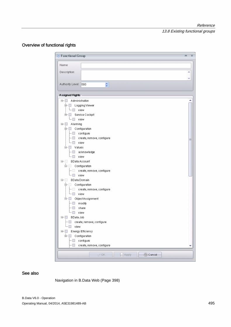
Reference 13.8 Existing functional groups
B.Data V6.0 - Operation Operating Manual, 04/2014, A5E31981489-AB 495
Overview of functional rights
See also Navigation in B.Data Web (Page 398)
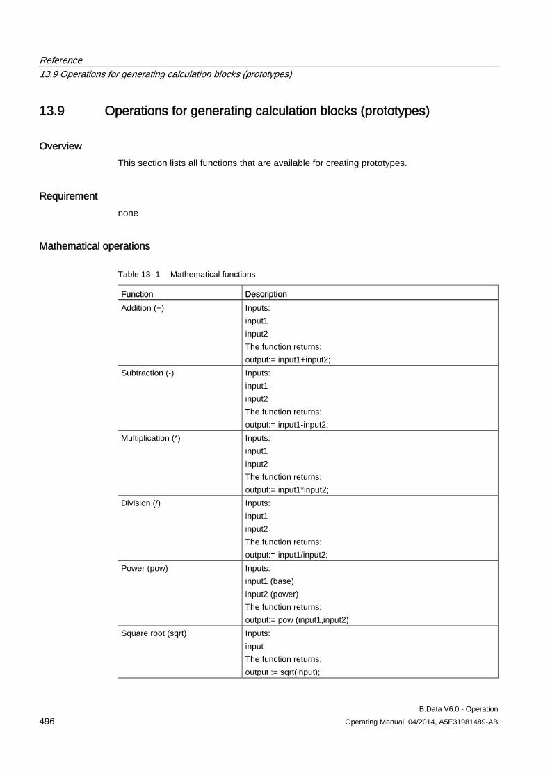
Reference 13.9 Operations for generating calculation blocks (prototypes)
B.Data V6.0 - Operation 496 Operating Manual, 04/2014, A5E31981489-AB
13.9 Operations for generating calculation blocks (prototypes)
Overview This section lists all functions that are available for creating prototypes.
Requirement none
Mathematical operations
Table 13- 1 Mathematical functions
Function Description Addition (+) Inputs:
input1 input2 The function returns: output:= input1+input2;
Subtraction (-) Inputs: input1 input2 The function returns: output:= input1-input2;
Multiplication (*) Inputs: input1 input2 The function returns: output:= input1*input2;
Division (/) Inputs: input1 input2 The function returns: output:= input1/input2;
Power (pow) Inputs: input1 (base) input2 (power) The function returns: output:= pow (input1,input2);
Square root (sqrt) Inputs: input The function returns: output := sqrt(input);
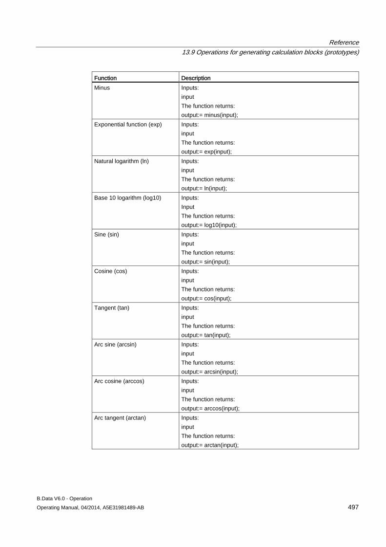
Reference 13.9 Operations for generating calculation blocks (prototypes)
B.Data V6.0 - Operation Operating Manual, 04/2014, A5E31981489-AB 497
Function Description Minus Inputs:
input The function returns: output:= minus(input);
Exponential function (exp) Inputs: input The function returns: output:= exp(input);
Natural logarithm (ln) Inputs: input The function returns: output:= ln(input);
Base 10 logarithm (log10) Inputs: Input The function returns: output:= log10(input);
Sine (sin) Inputs: input The function returns: output:= sin(input);
Cosine (cos) Inputs: input The function returns: output:= cos(input);
Tangent (tan) Inputs: input The function returns: output:= tan(input);
Arc sine (arcsin) Inputs: input The function returns: output:= arcsin(input);
Arc cosine (arccos) Inputs: input The function returns: output:= arccos(input);
Arc tangent (arctan) Inputs: input The function returns: output:= arctan(input);
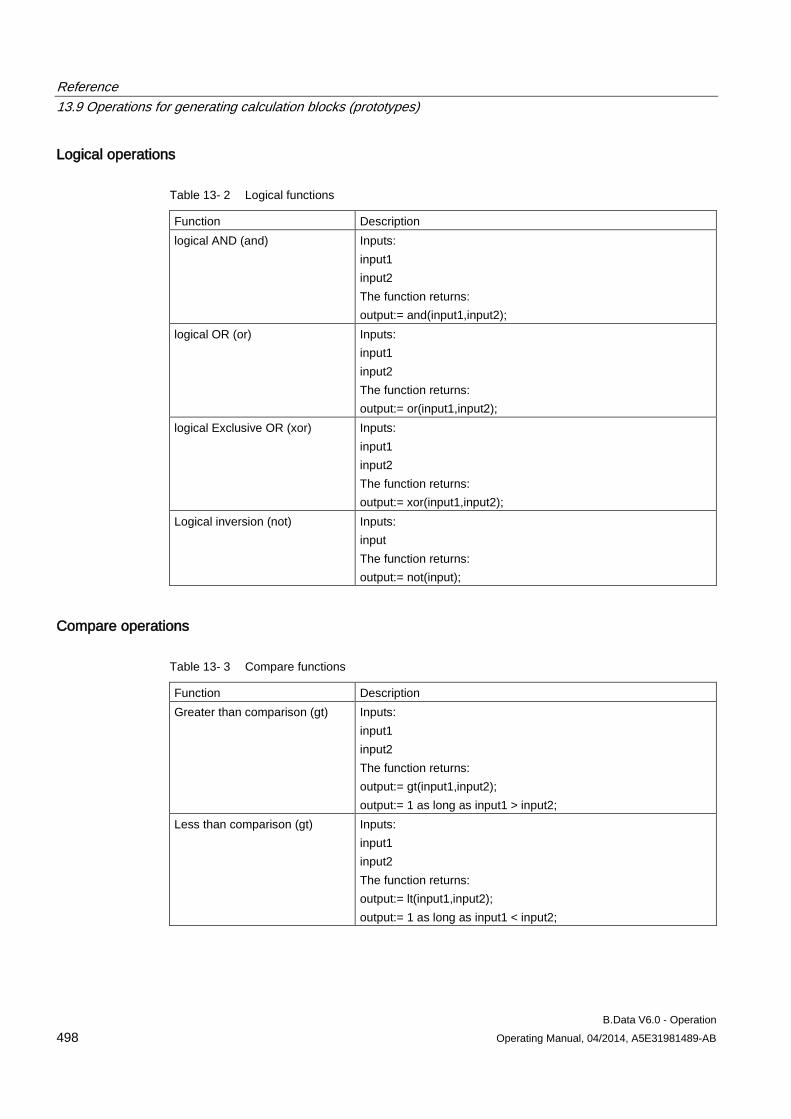
Reference 13.9 Operations for generating calculation blocks (prototypes)
B.Data V6.0 - Operation 498 Operating Manual, 04/2014, A5E31981489-AB
Logical operations
Table 13- 2 Logical functions
Function Description logical AND (and) Inputs:
input1 input2 The function returns: output:= and(input1,input2);
logical OR (or) Inputs: input1 input2 The function returns: output:= or(input1,input2);
logical Exclusive OR (xor) Inputs: input1 input2 The function returns: output:= xor(input1,input2);
Logical inversion (not) Inputs: input The function returns: output:= not(input);
Compare operations
Table 13- 3 Compare functions
Function Description Greater than comparison (gt) Inputs:
input1 input2 The function returns: output:= gt(input1,input2); output:= 1 as long as input1 > input2;
Less than comparison (gt) Inputs: input1 input2 The function returns: output:= lt(input1,input2); output:= 1 as long as input1 < input2;
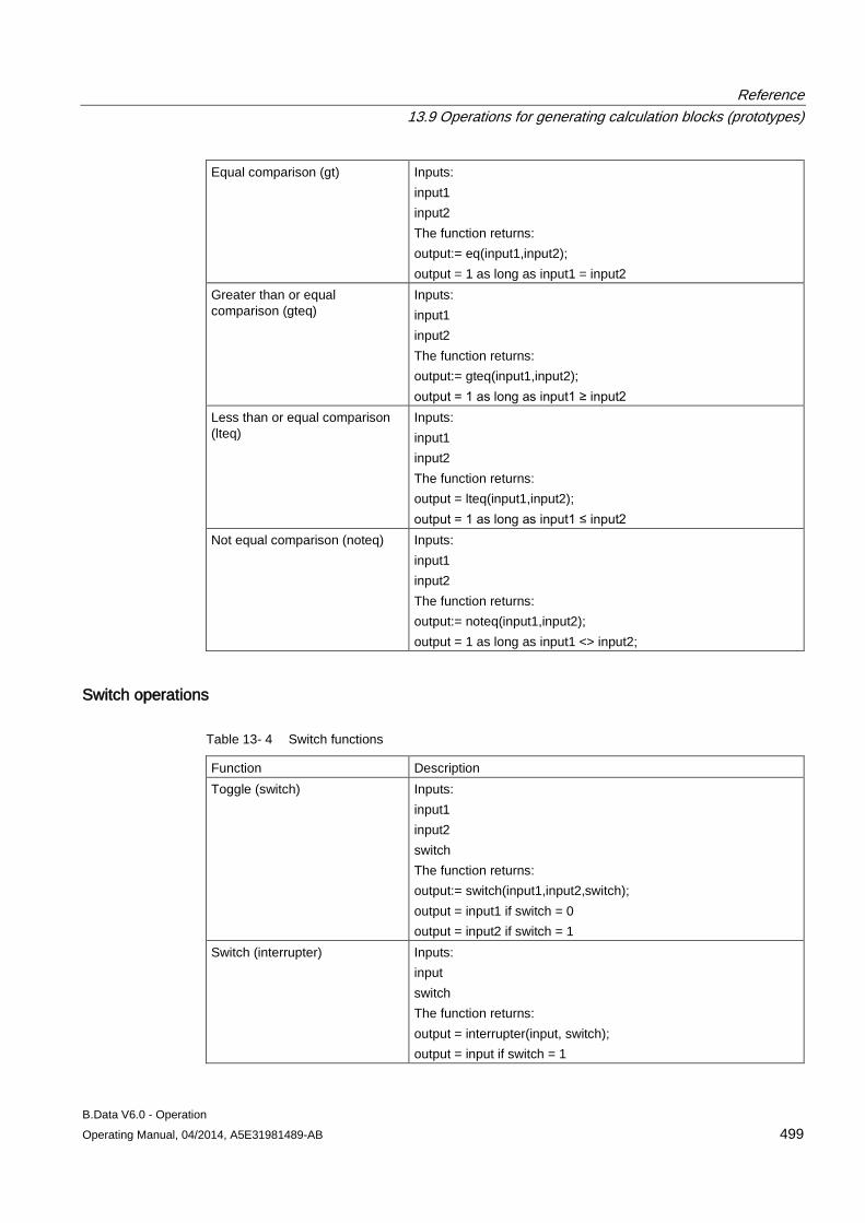
Reference 13.9 Operations for generating calculation blocks (prototypes)
B.Data V6.0 - Operation Operating Manual, 04/2014, A5E31981489-AB 499
Equal comparison (gt) Inputs: input1 input2 The function returns: output:= eq(input1,input2); output = 1 as long as input1 = input2
Greater than or equal comparison (gteq)
Inputs: input1 input2 The function returns: output:= gteq(input1,input2); output = 1 as long as input1 ≥ input2
Less than or equal comparison (lteq)
Inputs: input1 input2 The function returns: output = lteq(input1,input2); output = 1 as long as input1 ≤ input2
Not equal comparison (noteq) Inputs: input1 input2 The function returns: output:= noteq(input1,input2); output = 1 as long as input1 <> input2;
Switch operations
Table 13- 4 Switch functions
Function Description Toggle (switch) Inputs:
input1 input2 switch The function returns: output:= switch(input1,input2,switch); output = input1 if switch = 0 output = input2 if switch = 1
Switch (interrupter) Inputs: input switch The function returns: output = interrupter(input, switch); output = input if switch = 1
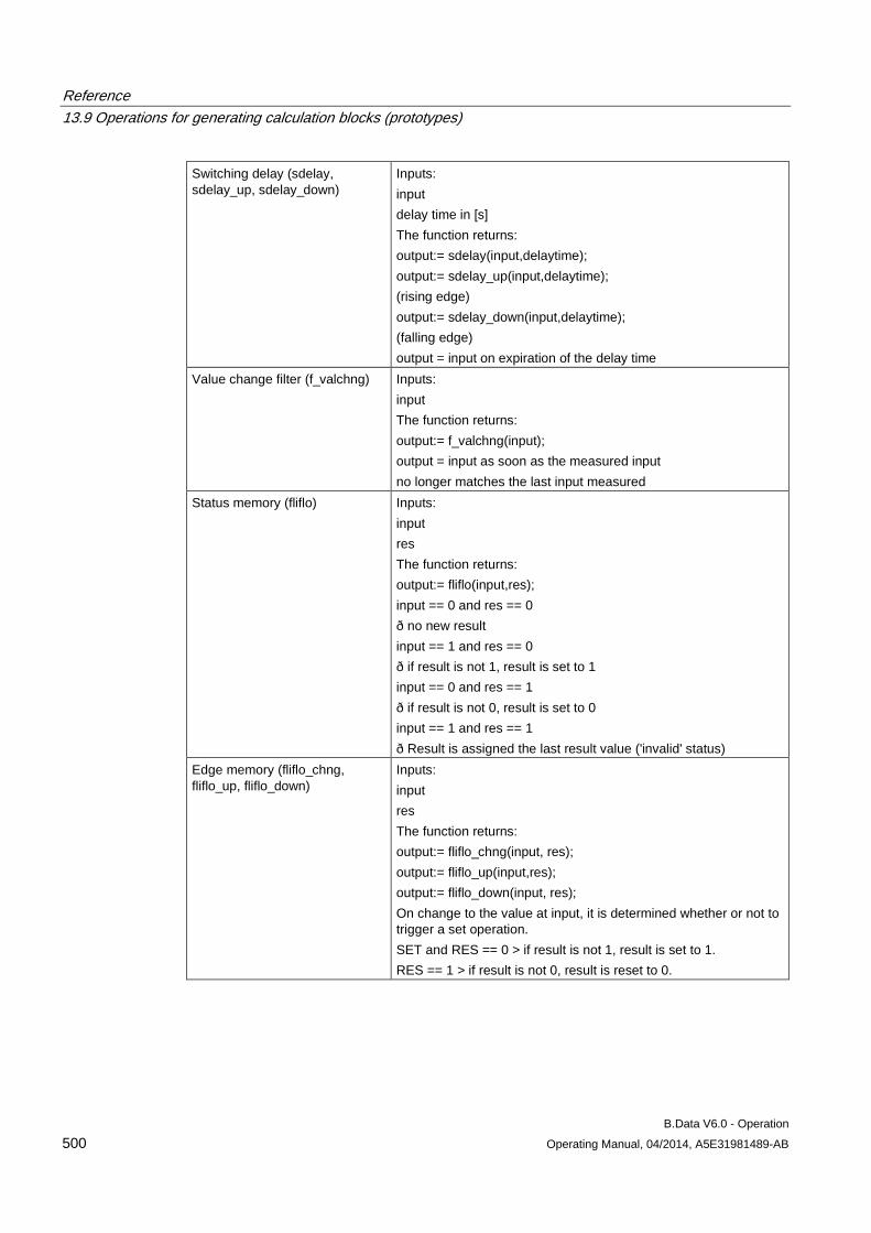
Reference 13.9 Operations for generating calculation blocks (prototypes)
B.Data V6.0 - Operation 500 Operating Manual, 04/2014, A5E31981489-AB
Switching delay (sdelay, sdelay_up, sdelay_down)
Inputs: input delay time in [s] The function returns: output:= sdelay(input,delaytime); output:= sdelay_up(input,delaytime); (rising edge) output:= sdelay_down(input,delaytime); (falling edge) output = input on expiration of the delay time
Value change filter (f_valchng) Inputs: input The function returns: output:= f_valchng(input); output = input as soon as the measured input no longer matches the last input measured
Status memory (fliflo) Inputs: input res The function returns: output:= fliflo(input,res); input == 0 and res == 0 ð no new result input == 1 and res == 0 ð if result is not 1, result is set to 1 input == 0 and res == 1 ð if result is not 0, result is set to 0 input == 1 and res == 1 ð Result is assigned the last result value ('invalid' status)
Edge memory (fliflo_chng, fliflo_up, fliflo_down)
Inputs: input res The function returns: output:= fliflo_chng(input, res); output:= fliflo_up(input,res); output:= fliflo_down(input, res); On change to the value at input, it is determined whether or not to trigger a set operation. SET and RES == 0 > if result is not 1, result is set to 1. RES == 1 > if result is not 0, result is reset to 0.
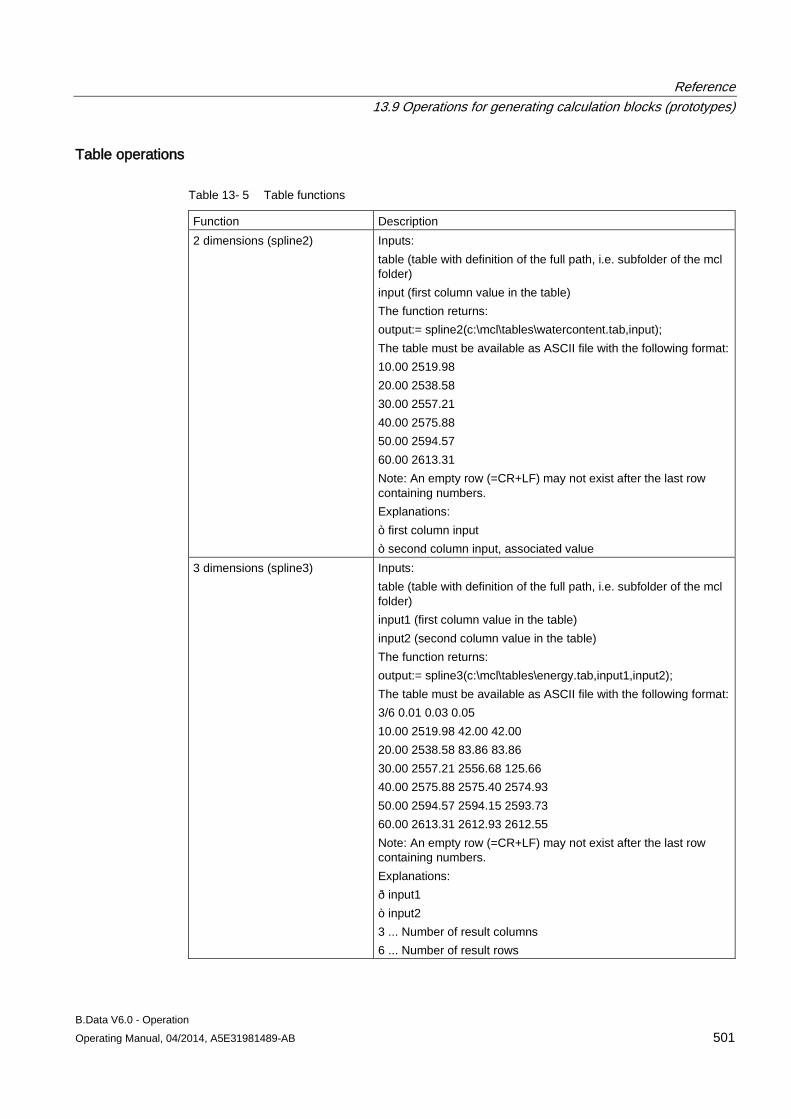
Reference 13.9 Operations for generating calculation blocks (prototypes)
B.Data V6.0 - Operation Operating Manual, 04/2014, A5E31981489-AB 501
Table operations
Table 13- 5 Table functions
Function Description 2 dimensions (spline2) Inputs:
table (table with definition of the full path, i.e. subfolder of the mcl folder) input (first column value in the table) The function returns: output:= spline2(c:\mcl\tables\watercontent.tab,input); The table must be available as ASCII file with the following format: 10.00 2519.98 20.00 2538.58 30.00 2557.21 40.00 2575.88 50.00 2594.57 60.00 2613.31 Note: An empty row (=CR+LF) may not exist after the last row containing numbers. Explanations: ò first column input ò second column input, associated value
3 dimensions (spline3) Inputs: table (table with definition of the full path, i.e. subfolder of the mcl folder) input1 (first column value in the table) input2 (second column value in the table) The function returns: output:= spline3(c:\mcl\tables\energy.tab,input1,input2); The table must be available as ASCII file with the following format: 3/6 0.01 0.03 0.05 10.00 2519.98 42.00 42.00 20.00 2538.58 83.86 83.86 30.00 2557.21 2556.68 125.66 40.00 2575.88 2575.40 2574.93 50.00 2594.57 2594.15 2593.73 60.00 2613.31 2612.93 2612.55 Note: An empty row (=CR+LF) may not exist after the last row containing numbers. Explanations: ð input1 ò input2 3 ... Number of result columns 6 ... Number of result rows
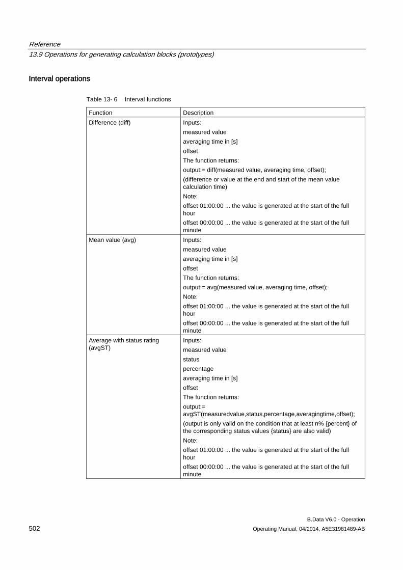
Reference 13.9 Operations for generating calculation blocks (prototypes)
B.Data V6.0 - Operation 502 Operating Manual, 04/2014, A5E31981489-AB
Interval operations
Table 13- 6 Interval functions
Function Description Difference (diff) Inputs:
measured value averaging time in [s] offset The function returns: output:= diff(measured value, averaging time, offset); (difference or value at the end and start of the mean value calculation time) Note: offset 01:00:00 ... the value is generated at the start of the full hour offset 00:00:00 ... the value is generated at the start of the full minute
Mean value (avg) Inputs: measured value averaging time in [s] offset The function returns: output:= avg(measured value, averaging time, offset); Note: offset 01:00:00 ... the value is generated at the start of the full hour offset 00:00:00 ... the value is generated at the start of the full minute
Average with status rating (avgST)
Inputs: measured value status percentage averaging time in [s] offset The function returns: output:= avgST(measuredvalue,status,percentage,averagingtime,offset); (output is only valid on the condition that at least n% {percent} of the corresponding status values {status} are also valid) Note: offset 01:00:00 ... the value is generated at the start of the full hour offset 00:00:00 ... the value is generated at the start of the full minute
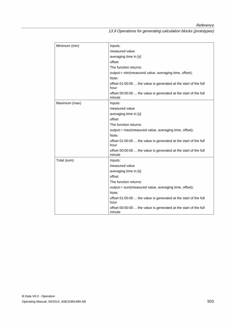
Reference 13.9 Operations for generating calculation blocks (prototypes)
B.Data V6.0 - Operation Operating Manual, 04/2014, A5E31981489-AB 503
Minimum (min) Inputs: measured value averaging time in [s] offset The function returns: output:= min(measured value, averaging time, offset); Note: offset 01:00:00 ... the value is generated at the start of the full hour offset 00:00:00 ... the value is generated at the start of the full minute
Maximum (max) Inputs: measured value averaging time in [s] offset The function returns: output:= max(measured value, averaging time, offset); Note: offset 01:00:00 ... the value is generated at the start of the full hour offset 00:00:00 ... the value is generated at the start of the full minute
Total (sum) Inputs: measured value averaging time in [s] offset The function returns: output:= sum(measured value, averaging time, offset); Note: offset 01:00:00 ... the value is generated at the start of the full hour offset 00:00:00 ... the value is generated at the start of the full minute
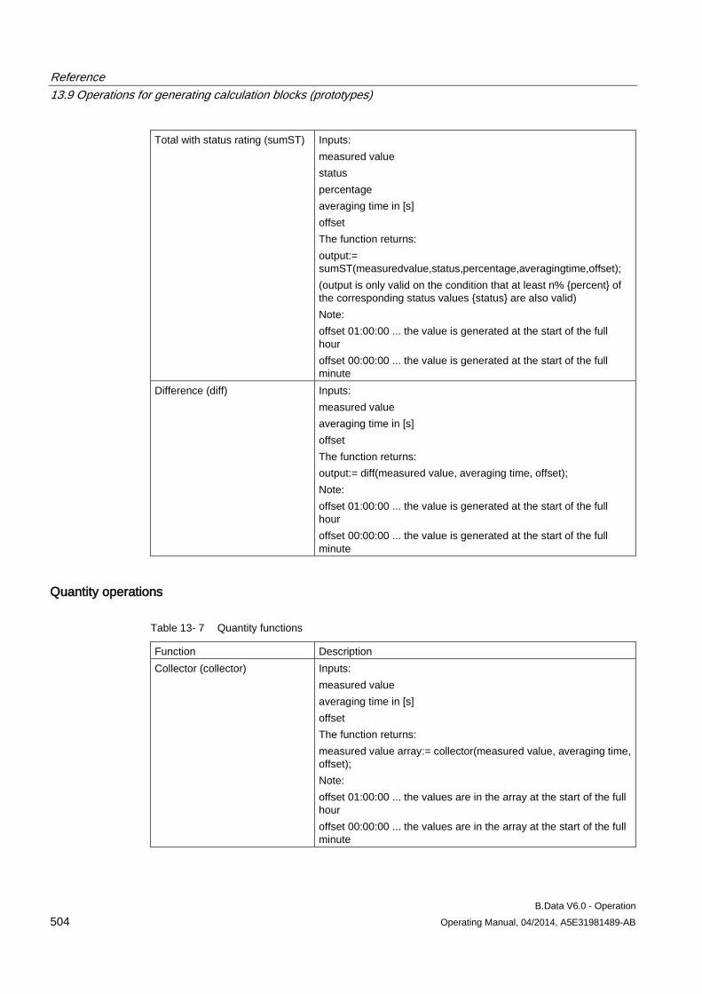
Reference 13.9 Operations for generating calculation blocks (prototypes)
B.Data V6.0 - Operation 504 Operating Manual, 04/2014, A5E31981489-AB
Total with status rating (sumST) Inputs: measured value status percentage averaging time in [s] offset The function returns: output:= sumST(measuredvalue,status,percentage,averagingtime,offset); (output is only valid on the condition that at least n% {percent} of the corresponding status values {status} are also valid) Note: offset 01:00:00 ... the value is generated at the start of the full hour offset 00:00:00 ... the value is generated at the start of the full minute
Difference (diff) Inputs: measured value averaging time in [s] offset The function returns: output:= diff(measured value, averaging time, offset); Note: offset 01:00:00 ... the value is generated at the start of the full hour offset 00:00:00 ... the value is generated at the start of the full minute
Quantity operations
Table 13- 7 Quantity functions
Function Description Collector (collector) Inputs:
measured value averaging time in [s] offset The function returns: measured value array:= collector(measured value, averaging time, offset); Note: offset 01:00:00 ... the values are in the array at the start of the full hour offset 00:00:00 ... the values are in the array at the start of the full minute
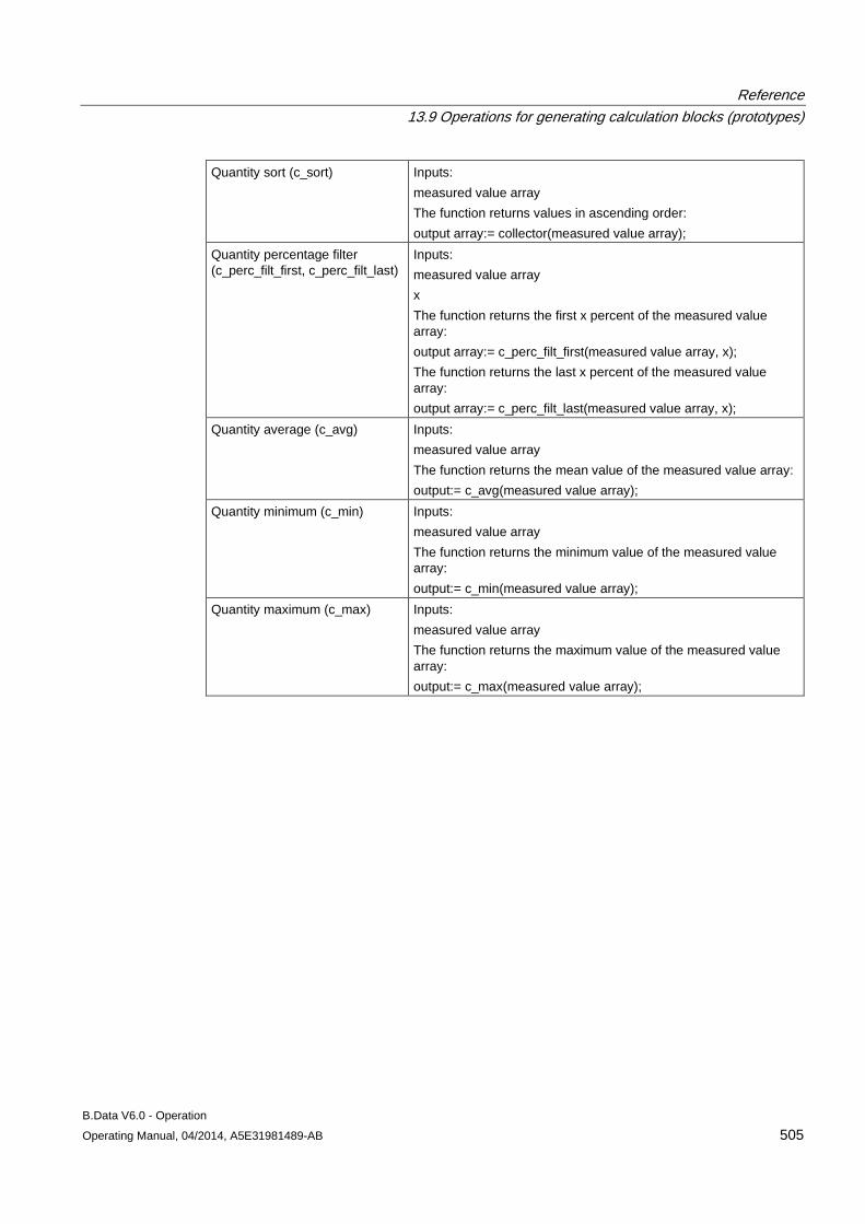
Reference 13.9 Operations for generating calculation blocks (prototypes)
B.Data V6.0 - Operation Operating Manual, 04/2014, A5E31981489-AB 505
Quantity sort (c_sort) Inputs: measured value array The function returns values in ascending order: output array:= collector(measured value array);
Quantity percentage filter (c_perc_filt_first, c_perc_filt_last)
Inputs: measured value array x The function returns the first x percent of the measured value array: output array:= c_perc_filt_first(measured value array, x); The function returns the last x percent of the measured value array: output array:= c_perc_filt_last(measured value array, x);
Quantity average (c_avg) Inputs: measured value array The function returns the mean value of the measured value array: output:= c_avg(measured value array);
Quantity minimum (c_min) Inputs: measured value array The function returns the minimum value of the measured value array: output:= c_min(measured value array);
Quantity maximum (c_max) Inputs: measured value array The function returns the maximum value of the measured value array: output:= c_max(measured value array);
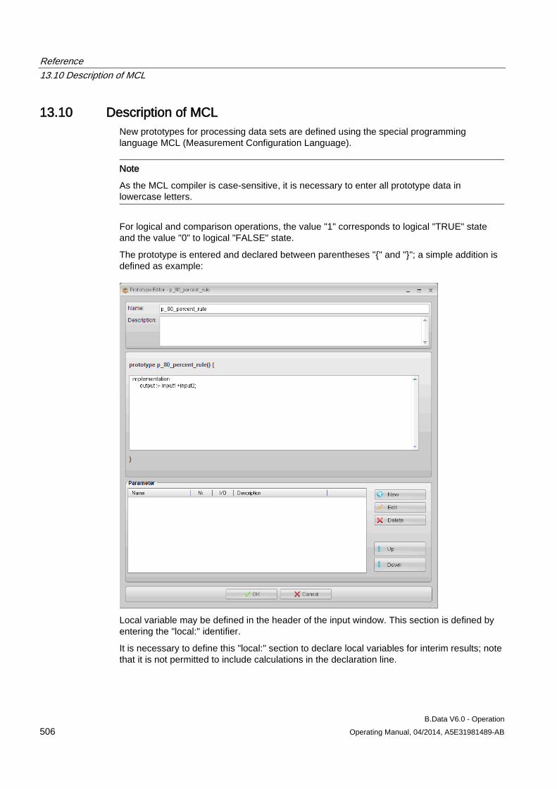
Reference 13.10 Description of MCL
B.Data V6.0 - Operation 506 Operating Manual, 04/2014, A5E31981489-AB
13.10 Description of MCL New prototypes for processing data sets are defined using the special programming language MCL (Measurement Configuration Language).
Note
As the MCL compiler is case-sensitive, it is necessary to enter all prototype data in lowercase letters.
For logical and comparison operations, the value "1" corresponds to logical "TRUE" state and the value "0" to logical "FALSE" state.
The prototype is entered and declared between parentheses "{" and "}"; a simple addition is defined as example:
Local variable may be defined in the header of the input window. This section is defined by entering the "local:" identifier.
It is necessary to define this "local:" section to declare local variables for interim results; note that it is not permitted to include calculations in the declaration line.
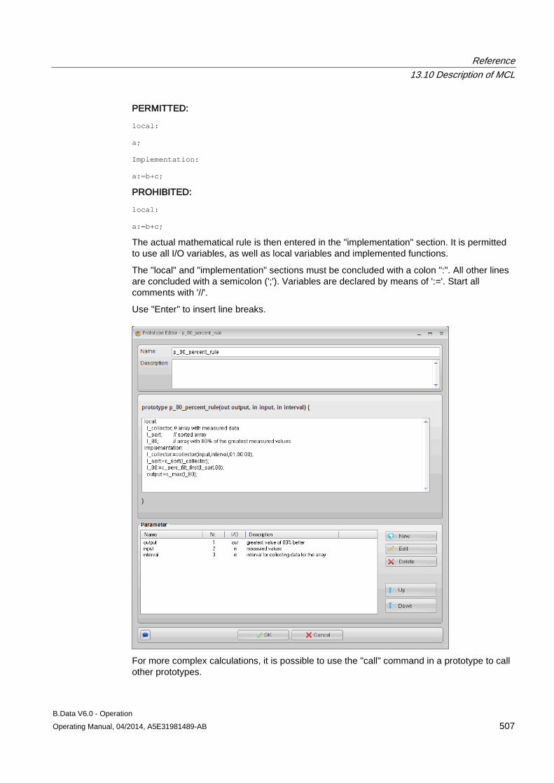
Reference 13.10 Description of MCL
B.Data V6.0 - Operation Operating Manual, 04/2014, A5E31981489-AB 507
PERMITTED:
local:
a;
Implementation:
a:=b+c;
PROHIBITED:
local:
a:=b+c;
The actual mathematical rule is then entered in the "implementation" section. It is permitted to use all I/O variables, as well as local variables and implemented functions.
The "local" and "implementation" sections must be concluded with a colon ":". All other lines are concluded with a semicolon (';'). Variables are declared by means of ':='. Start all comments with '//'.
Use "Enter" to insert line breaks.
For more complex calculations, it is possible to use the "call" command in a prototype to call other prototypes.
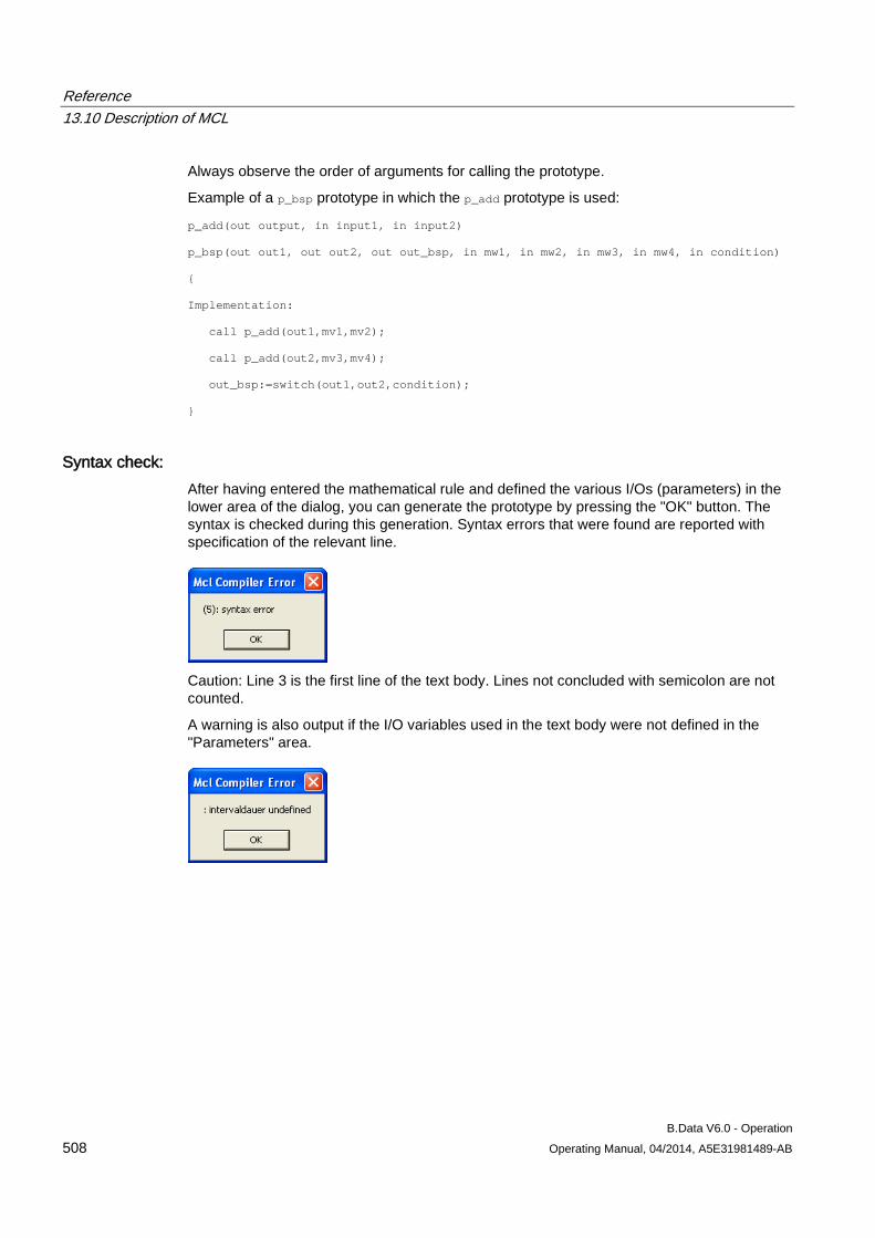
Reference 13.10 Description of MCL
B.Data V6.0 - Operation 508 Operating Manual, 04/2014, A5E31981489-AB
Always observe the order of arguments for calling the prototype.
Example of a p_bsp prototype in which the p_add prototype is used:
p_add(out output, in input1, in input2)
p_bsp(out out1, out out2, out out_bsp, in mw1, in mw2, in mw3, in mw4, in condition)
{
Implementation:
call p_add(out1,mv1,mv2);
call p_add(out2,mv3,mv4);
out_bsp:=switch(out1,out2,condition);
}
Syntax check: After having entered the mathematical rule and defined the various I/Os (parameters) in the lower area of the dialog, you can generate the prototype by pressing the "OK" button. The syntax is checked during this generation. Syntax errors that were found are reported with specification of the relevant line.
Caution: Line 3 is the first line of the text body. Lines not concluded with semicolon are not counted.
A warning is also output if the I/O variables used in the text body were not defined in the "Parameters" area.

Reference 13.11 Database functions for measurement variables
B.Data V6.0 - Operation Operating Manual, 04/2014, A5E31981489-AB 509
13.11 Database functions for measurement variables
General information A set of standard database functions for MEVA processing has been implemented in B.Data. Siemens AG reserves the right of creating any new evaluation algorithms that may be needed, including their implementation in the system.
Note
You must strictly adhere to the specified sorting order of operating data points, MEVAs, or parameters for the listings in the "Inputs:" field or in the Plant Explorer (see the figures), as the functions expect to receive the input values based on this sorting order. The same goes for units, if not specified otherwise with [1] or [x] as the unit.
The calculation results relate to the respective monitoring period that is transferred at the start of an evaluation (From, To).
Overview This section lists all functions that are available for use with the MEVAs.
Requirement Successful installation of all software components.
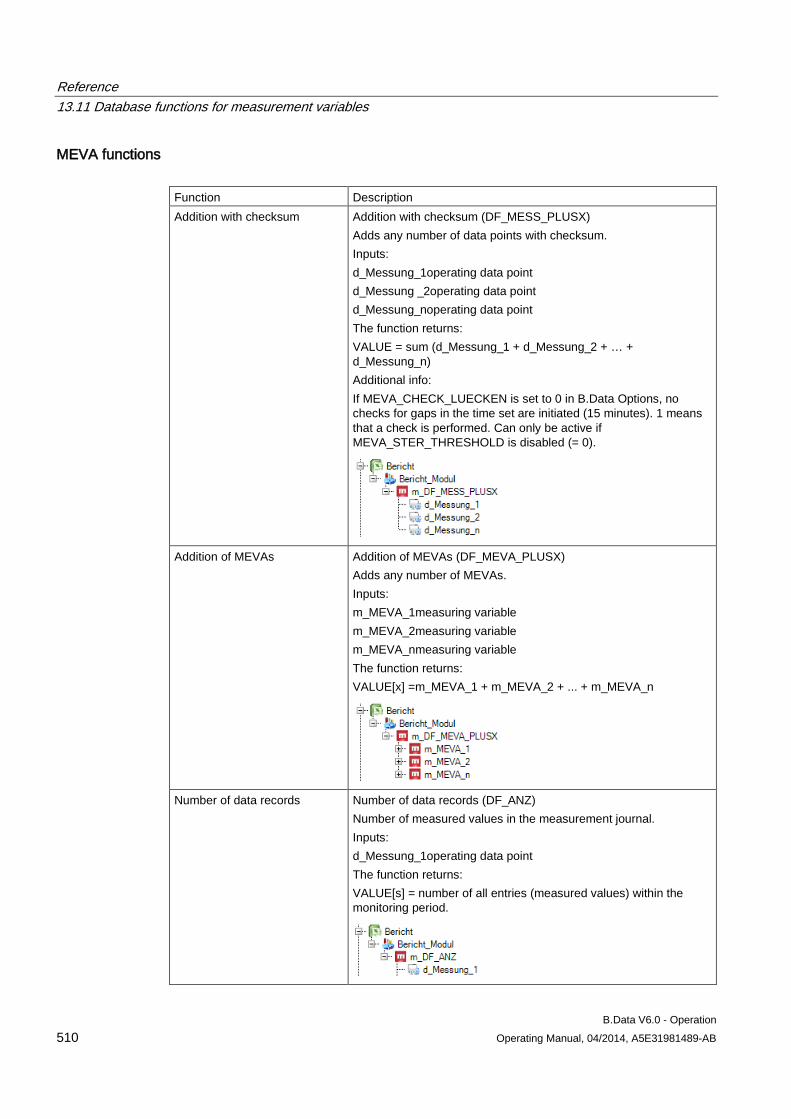
Reference 13.11 Database functions for measurement variables
B.Data V6.0 - Operation 510 Operating Manual, 04/2014, A5E31981489-AB
MEVA functions Function Description Addition with checksum Addition with checksum (DF_MESS_PLUSX)
Adds any number of data points with checksum. Inputs: d_Messung_1operating data point d_Messung _2operating data point d_Messung_noperating data point The function returns: VALUE = sum (d_Messung_1 + d_Messung_2 + … + d_Messung_n) Additional info: If MEVA_CHECK_LUECKEN is set to 0 in B.Data Options, no checks for gaps in the time set are initiated (15 minutes). 1 means that a check is performed. Can only be active if MEVA_STER_THRESHOLD is disabled (= 0).
Addition of MEVAs Addition of MEVAs (DF_MEVA_PLUSX) Adds any number of MEVAs. Inputs: m_MEVA_1measuring variable m_MEVA_2measuring variable m_MEVA_nmeasuring variable The function returns: VALUE[x] =m_MEVA_1 + m_MEVA_2 + ... + m_MEVA_n
Number of data records Number of data records (DF_ANZ) Number of measured values in the measurement journal. Inputs: d_Messung_1operating data point The function returns: VALUE[s] = number of all entries (measured values) within the monitoring period.
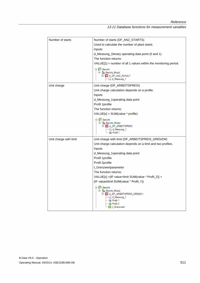
Reference 13.11 Database functions for measurement variables
B.Data V6.0 - Operation Operating Manual, 04/2014, A5E31981489-AB 511
Number of starts Number of starts (DF_ANZ_STARTS) Used to calculate the number of plant starts. Inputs: d_Messung_1binary operating data point (0 and 1) The function returns: VALUE[1] = number of all 1 values within the monitoring period.
Unit charge Unit charge (DF_ARBEITSPREIS) Unit charge calculation depends on a profile. Inputs: d_Messung_1operating data point Profil 1profile The function returns: VALUE[x] = SUM(value * profile)
Unit charge with limit Unit charge with limit (DF_ARBEITSPREIS_GRENZW) Unit charge calculation depends on a limit and two profiles. Inputs: d_Messung_1operating data point Profil 1profile Profil 2profile t_Grenzwertparameter The function returns: VALUE[x] ={IF value>limit SUM(value * Profil_2)} + {IF value≤limit SUM(value * Profil_1)}
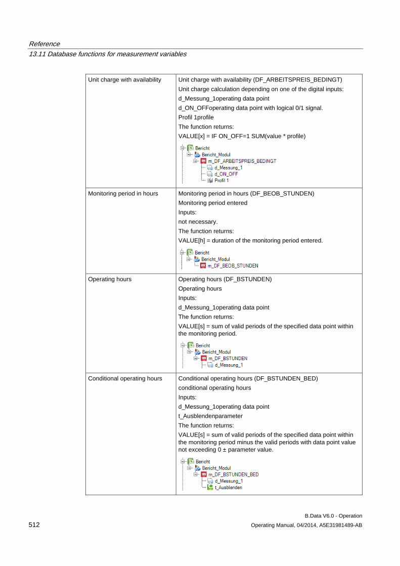
Reference 13.11 Database functions for measurement variables
B.Data V6.0 - Operation 512 Operating Manual, 04/2014, A5E31981489-AB
Unit charge with availability Unit charge with availability (DF_ARBEITSPREIS_BEDINGT) Unit charge calculation depending on one of the digital inputs: d_Messung_1operating data point d_ON_OFFoperating data point with logical 0/1 signal. Profil 1profile The function returns: VALUE[x] = IF ON_OFF=1 SUM(value * profile)
Monitoring period in hours Monitoring period in hours (DF_BEOB_STUNDEN) Monitoring period entered Inputs: not necessary. The function returns: VALUE[h] = duration of the monitoring period entered.
Operating hours Operating hours (DF_BSTUNDEN) Operating hours Inputs: d_Messung_1operating data point The function returns: VALUE[s] = sum of valid periods of the specified data point within the monitoring period.
Conditional operating hours Conditional operating hours (DF_BSTUNDEN_BED) conditional operating hours Inputs: d_Messung_1operating data point t_Ausblendenparameter The function returns: VALUE[s] = sum of valid periods of the specified data point within the monitoring period minus the valid periods with data point value not exceeding 0 ± parameter value.
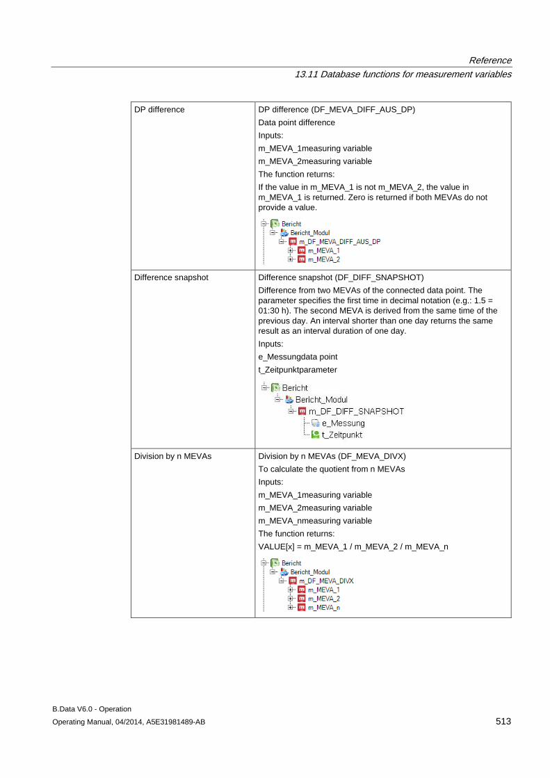
Reference 13.11 Database functions for measurement variables
B.Data V6.0 - Operation Operating Manual, 04/2014, A5E31981489-AB 513
DP difference DP difference (DF_MEVA_DIFF_AUS_DP) Data point difference Inputs: m_MEVA_1measuring variable m_MEVA_2measuring variable The function returns: If the value in m_MEVA_1 is not m_MEVA_2, the value in m_MEVA_1 is returned. Zero is returned if both MEVAs do not provide a value.
Difference snapshot Difference snapshot (DF_DIFF_SNAPSHOT) Difference from two MEVAs of the connected data point. The parameter specifies the first time in decimal notation (e.g.: 1.5 = 01:30 h). The second MEVA is derived from the same time of the previous day. An interval shorter than one day returns the same result as an interval duration of one day. Inputs: e_Messungdata point t_Zeitpunktparameter
Division by n MEVAs Division by n MEVAs (DF_MEVA_DIVX) To calculate the quotient from n MEVAs Inputs: m_MEVA_1measuring variable m_MEVA_2measuring variable m_MEVA_nmeasuring variable The function returns: VALUE[x] = m_MEVA_1 / m_MEVA_2 / m_MEVA_n
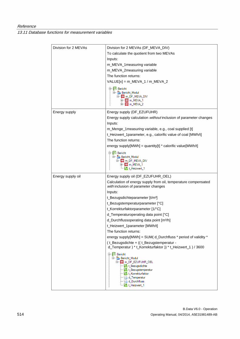
Reference 13.11 Database functions for measurement variables
B.Data V6.0 - Operation 514 Operating Manual, 04/2014, A5E31981489-AB
Division for 2 MEVAs Division for 2 MEVAs (DF_MEVA_DIV) To calculate the quotient from two MEVAs Inputs: m_MEVA_1measuring variable m_MEVA_2measuring variable The function returns: VALUE[x] = m_MEVA_1 / m_MEVA_2
Energy supply Energy supply (DF_EZUFUHR) Energy supply calculation without inclusion of parameter changes Inputs: m_Menge_1measuring variable, e.g., coal supplied [t] t_Heizwert_1parameter, e.g., calorific value of coal [MWh/t] The function returns: energy supply[MWh] = quantity[t] * calorific value[MWh/t]
Energy supply oil Energy supply oil (DF_EZUFUHR_OEL) Calculation of energy supply from oil, temperature compensated with inclusion of parameter changes Inputs: t_Bezugsdichteparameter [t/m³] t_Bezugstemperaturparameter [°C] t_Korrekturfaktorparameter [1/°C] d_Temperaturoperating data point [°C] d_Durchflussoperating data point [m³/h] t_Heizwert_1parameter [MWh/t] The function returns: energy supply[MWh] = SUM( d_Durchfluss * period of validity * ( t_Bezugsdichte + (( t_Bezugstemperatur - d_Temperatur ) * t_Korrekturfaktor )) * t_Heizwert_1 ) / 3600
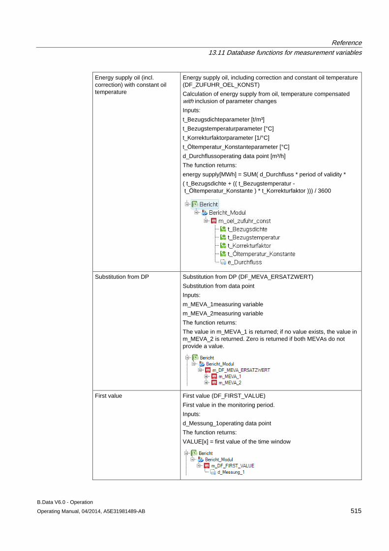
Reference 13.11 Database functions for measurement variables
B.Data V6.0 - Operation Operating Manual, 04/2014, A5E31981489-AB 515
Energy supply oil (incl. correction) with constant oil temperature
Energy supply oil, including correction and constant oil temperature (DF_ZUFUHR_OEL_KONST) Calculation of energy supply from oil, temperature compensated with inclusion of parameter changes Inputs: t_Bezugsdichteparameter [t/m³] t_Bezugstemperaturparameter [°C] t_Korrekturfaktorparameter [1/°C] t_Öltemperatur_Konstanteparameter [°C] d_Durchflussoperating data point [m³/h] The function returns: energy supply[MWh] = SUM( d_Durchfluss * period of validity * ( t_Bezugsdichte + (( t_Bezugstemperatur - t_Öltemperatur_Konstante ) * t_Korrekturfaktor ))) / 3600
Substitution from DP Substitution from DP (DF_MEVA_ERSATZWERT) Substitution from data point Inputs: m_MEVA_1measuring variable m_MEVA_2measuring variable The function returns: The value in m_MEVA_1 is returned; if no value exists, the value in m_MEVA_2 is returned. Zero is returned if both MEVAs do not provide a value.
First value First value (DF_FIRST_VALUE) First value in the monitoring period. Inputs: d_Messung_1operating data point The function returns: VALUE[x] = first value of the time window
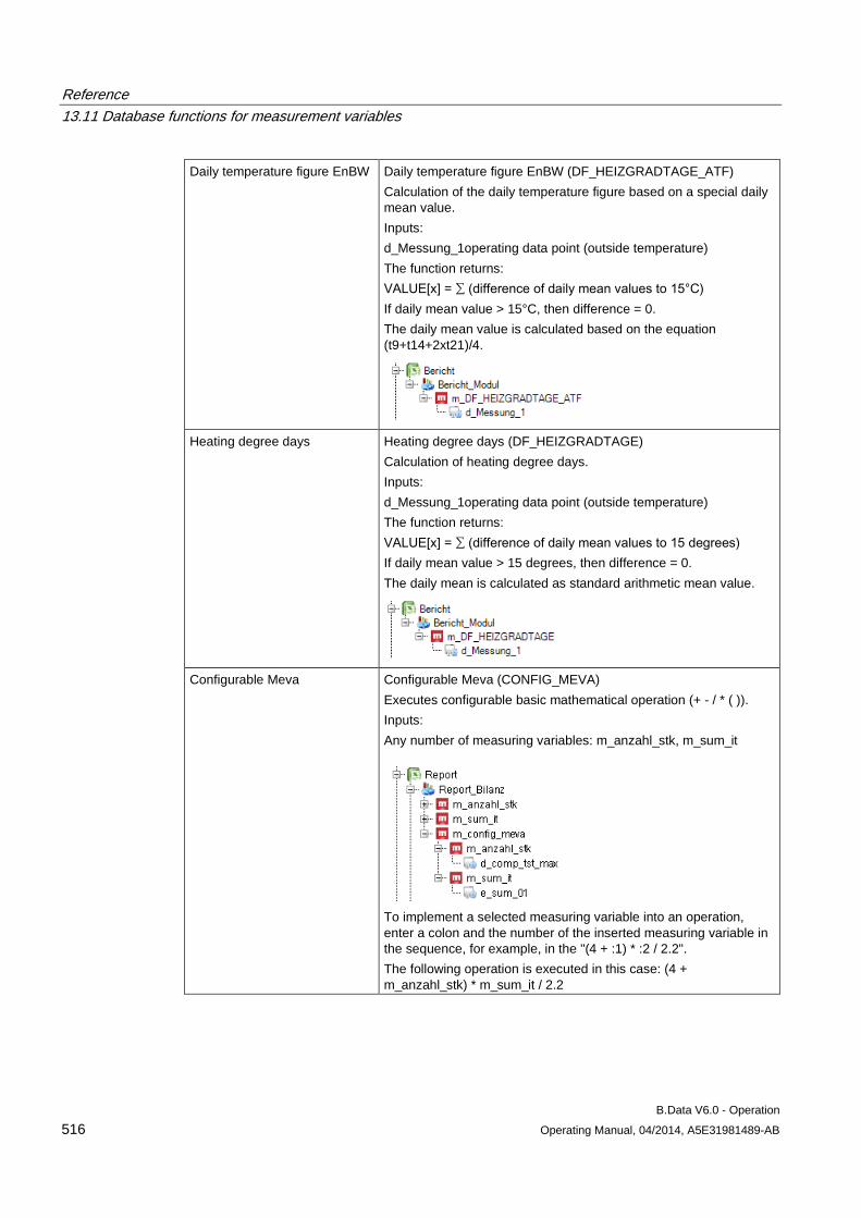
Reference 13.11 Database functions for measurement variables
B.Data V6.0 - Operation 516 Operating Manual, 04/2014, A5E31981489-AB
Daily temperature figure EnBW Daily temperature figure EnBW (DF_HEIZGRADTAGE_ATF) Calculation of the daily temperature figure based on a special daily mean value. Inputs: d_Messung_1operating data point (outside temperature) The function returns: VALUE[x] = ∑ (difference of daily mean values to 15°C) If daily mean value > 15°C, then difference = 0. The daily mean value is calculated based on the equation (t9+t14+2xt21)/4.
Heating degree days Heating degree days (DF_HEIZGRADTAGE) Calculation of heating degree days. Inputs: d_Messung_1operating data point (outside temperature) The function returns: VALUE[x] = ∑ (difference of daily mean values to 15 degrees) If daily mean value > 15 degrees, then difference = 0. The daily mean is calculated as standard arithmetic mean value.
Configurable Meva Configurable Meva (CONFIG_MEVA) Executes configurable basic mathematical operation (+ - / * ( )). Inputs: Any number of measuring variables: m_anzahl_stk, m_sum_it
To implement a selected measuring variable into an operation, enter a colon and the number of the inserted measuring variable in the sequence, for example, in the "(4 + :1) * :2 / 2.2". The following operation is executed in this case: (4 + m_anzahl_stk) * m_sum_it / 2.2
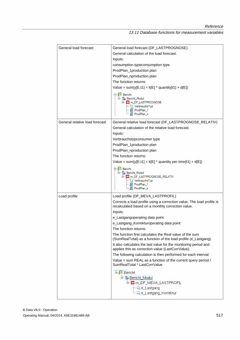
Reference 13.11 Database functions for measurement variables
B.Data V6.0 - Operation Operating Manual, 04/2014, A5E31981489-AB 517
General load forecast General load forecast (DF_LASTPROGNOSE) General calculation of the load forecast. Inputs: consumption typeconsumption type ProdPlan_1production plan ProdPlan_nproduction plan The function returns: Value = sum(y[E,t1] = k[E] * quantity[t1] + d[E])
General relative load forecast General relative load forecast (DF_LASTPROGNOSE_RELATIV) General calculation of the relative load forecast. Inputs: Verbrauchstypconsumer type ProdPlan_1production plan ProdPlan_nproduction plan The function returns: Value = sum(y[E,t1] = k[E] * quantity per time[t1] + d[E])
Load profile Load profile (DF_MEVA_LASTPROFIL) Corrects a load profile using a correction value. The load profile is recalculated based on a monthly correction value. Inputs: e_Lastgangoperating data point e_Lastgang_Korrekturoperating data point The function returns: The function first calculates the Real value of the sum (SumRealTotal) as a function of the load profile (e_Lastgang). It also calculates the last value for the monitoring period and applies this as correction value (LastCorrValue). The following calculation is then performed for each interval: Value = sum REAL as a function of the current query period / SumRealTotal * LastCorrValue
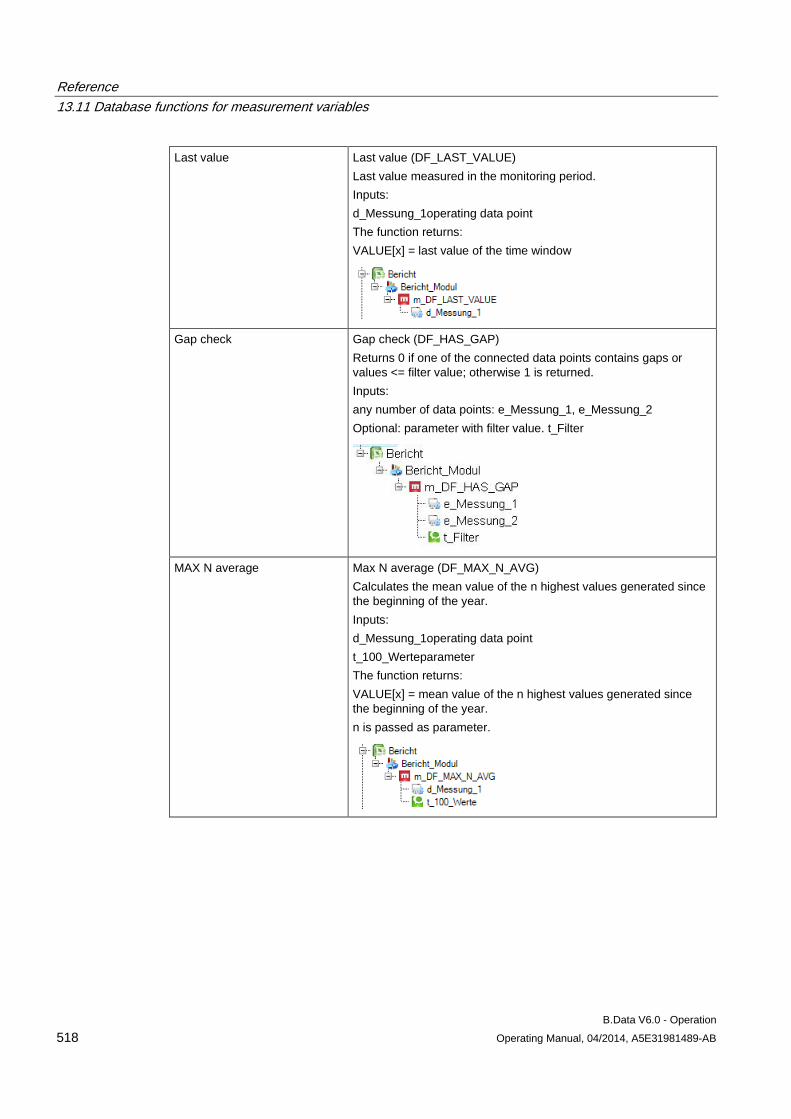
Reference 13.11 Database functions for measurement variables
B.Data V6.0 - Operation 518 Operating Manual, 04/2014, A5E31981489-AB
Last value Last value (DF_LAST_VALUE) Last value measured in the monitoring period. Inputs: d_Messung_1operating data point The function returns: VALUE[x] = last value of the time window
Gap check Gap check (DF_HAS_GAP) Returns 0 if one of the connected data points contains gaps or values <= filter value; otherwise 1 is returned. Inputs: any number of data points: e_Messung_1, e_Messung_2 Optional: parameter with filter value. t_Filter
MAX N average Max N average (DF_MAX_N_AVG) Calculates the mean value of the n highest values generated since the beginning of the year. Inputs: d_Messung_1operating data point t_100_Werteparameter The function returns: VALUE[x] = mean value of the n highest values generated since the beginning of the year. n is passed as parameter.
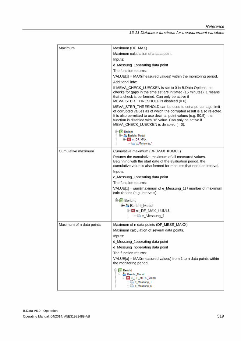
Reference 13.11 Database functions for measurement variables
B.Data V6.0 - Operation Operating Manual, 04/2014, A5E31981489-AB 519
Maximum Maximum (DF_MAX) Maximum calculation of a data point. Inputs: d_Messung_1operating data point The function returns: VALUE[x] = MAX(measured values) within the monitoring period. Additional info: If MEVA_CHECK_LUECKEN is set to 0 in B.Data Options, no checks for gaps in the time set are initiated (15 minutes). 1 means that a check is performed. Can only be active if MEVA_STER_THRESHOLD is disabled (= 0). MEVA_STER_THRESHOLD can be used to set a percentage limit of corrupted values as of which the corrupted result is also rejected. It is also permitted to use decimal point values (e.g. 50.5); the function is disabled with "0" value. Can only be active if MEVA_CHECK_LUECKEN is disabled (= 0).
Cumulative maximum Cumulative maximum (DF_MAX_KUMUL) Returns the cumulative maximum of all measured values. Beginning with the start date of the evaluation period, the cumulative value is also formed for modules that need an interval. Inputs: e_Messung_1operating data point The function returns: VALUE[x] = sum(maximum of e_Messung_1) / number of maximum calculations (e.g. intervals)
Maximum of n data points Maximum of n data points (DF_MESS_MAXX) Maximum calculation of several data points. Inputs: d_Messung_1operating data point d_Messung_noperating data point The function returns: VALUE[x] = MAX(measured values) from 1 to n data points within the monitoring period.
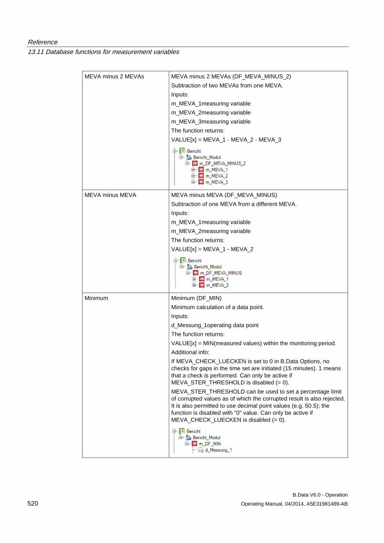
Reference 13.11 Database functions for measurement variables
B.Data V6.0 - Operation 520 Operating Manual, 04/2014, A5E31981489-AB
MEVA minus 2 MEVAs MEVA minus 2 MEVAs (DF_MEVA_MINUS_2) Subtraction of two MEVAs from one MEVA. Inputs: m_MEVA_1measuring variable m_MEVA_2measuring variable m_MEVA_3measuring variable The function returns: VALUE[x] = MEVA_1 - MEVA_2 - MEVA_3
MEVA minus MEVA MEVA minus MEVA (DF_MEVA_MINUS) Subtraction of one MEVA from a different MEVA. Inputs: m_MEVA_1measuring variable m_MEVA_2measuring variable The function returns: VALUE[x] = MEVA_1 - MEVA_2
Minimum Minimum (DF_MIN) Minimum calculation of a data point. Inputs: d_Messung_1operating data point The function returns: VALUE[x] = MIN(measured values) within the monitoring period. Additional info: If MEVA_CHECK_LUECKEN is set to 0 in B.Data Options, no checks for gaps in the time set are initiated (15 minutes). 1 means that a check is performed. Can only be active if MEVA_STER_THRESHOLD is disabled (= 0). MEVA_STER_THRESHOLD can be used to set a percentage limit of corrupted values as of which the corrupted result is also rejected. It is also permitted to use decimal point values (e.g. 50.5); the function is disabled with "0" value. Can only be active if MEVA_CHECK_LUECKEN is disabled (= 0).
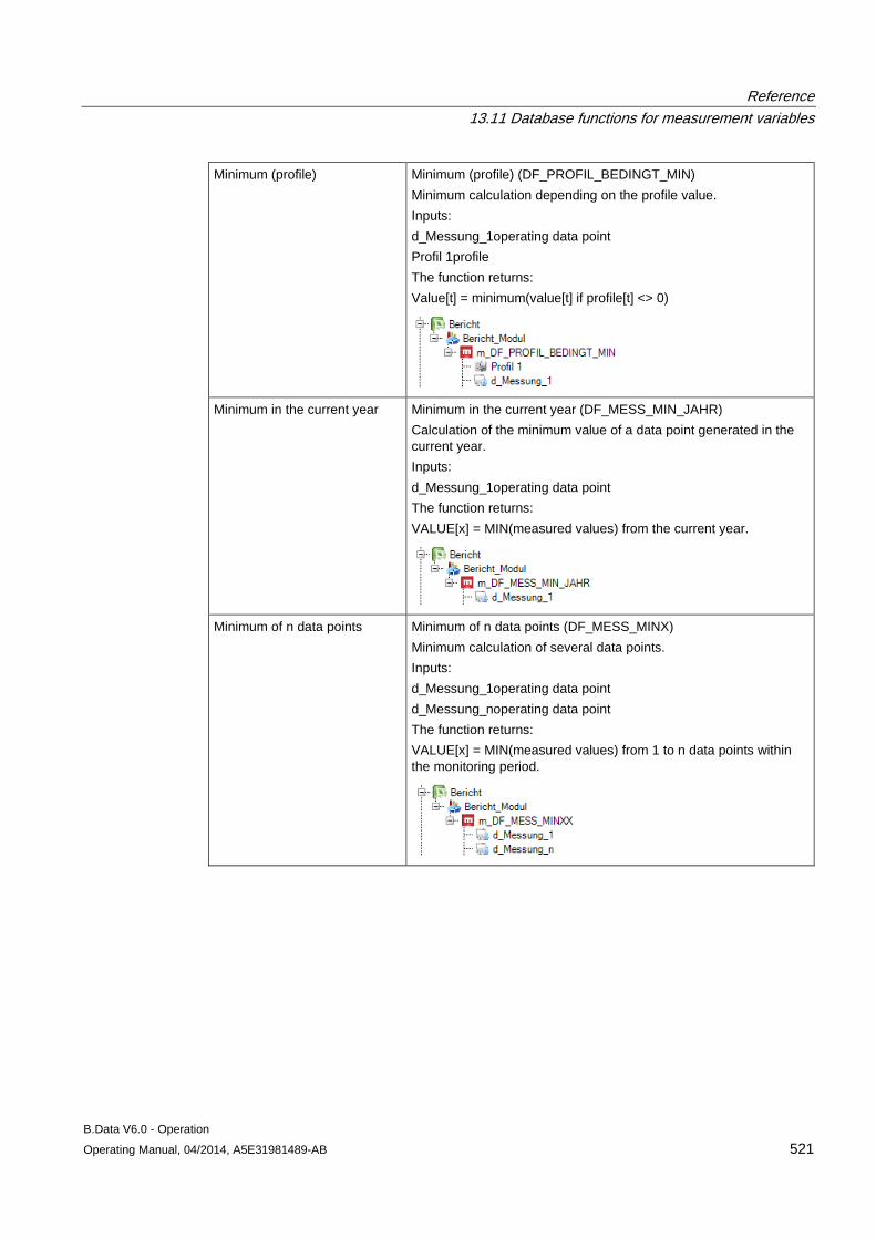
Reference 13.11 Database functions for measurement variables
B.Data V6.0 - Operation Operating Manual, 04/2014, A5E31981489-AB 521
Minimum (profile) Minimum (profile) (DF_PROFIL_BEDINGT_MIN) Minimum calculation depending on the profile value. Inputs: d_Messung_1operating data point Profil 1profile The function returns: Value[t] = minimum(value[t] if profile[t] <> 0)
Minimum in the current year Minimum in the current year (DF_MESS_MIN_JAHR) Calculation of the minimum value of a data point generated in the current year. Inputs: d_Messung_1operating data point The function returns: VALUE[x] = MIN(measured values) from the current year.
Minimum of n data points Minimum of n data points (DF_MESS_MINX) Minimum calculation of several data points. Inputs: d_Messung_1operating data point d_Messung_noperating data point The function returns: VALUE[x] = MIN(measured values) from 1 to n data points within the monitoring period.
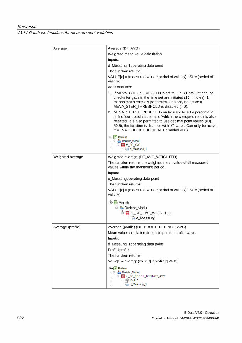
Reference 13.11 Database functions for measurement variables
B.Data V6.0 - Operation 522 Operating Manual, 04/2014, A5E31981489-AB
Average Average (DF_AVG) Weighted mean value calculation. Inputs: d_Messung_1operating data point The function returns: VALUE[x] = (measured value * period of validity) / SUM(period of validity) Additional info: 1. If MEVA_CHECK_LUECKEN is set to 0 in B.Data Options, no
checks for gaps in the time set are initiated (15 minutes). 1 means that a check is performed. Can only be active if MEVA_STER_THRESHOLD is disabled (= 0).
2. MEVA_STER_THRESHOLD can be used to set a percentage limit of corrupted values as of which the corrupted result is also rejected. It is also permitted to use decimal point values (e.g. 50.5); the function is disabled with "0" value. Can only be active if MEVA_CHECK_LUECKEN is disabled (= 0).
Weighted average Weighted average (DF_AVG_WEIGHTED) The function returns the weighted mean value of all measured values within the monitoring period. Inputs: e_Messungoperating data point The function returns: VALUE[x] = (measured value * period of validity) / SUM(period of validity)
Average (profile) Average (profile) (DF_PROFIL_BEDINGT_AVG) Mean value calculation depending on the profile value. Inputs: d_Messung_1operating data point Profil 1profile The function returns: Value[t] = average(value[t] if profile[t] <> 0)
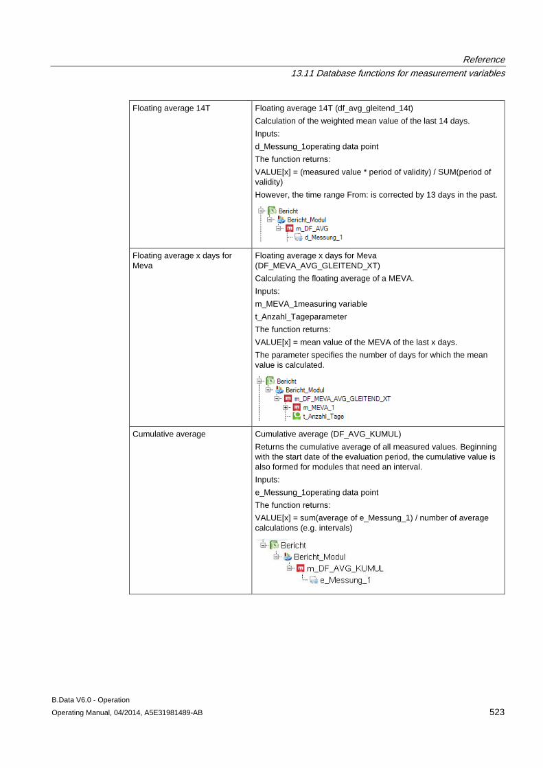
Reference 13.11 Database functions for measurement variables
B.Data V6.0 - Operation Operating Manual, 04/2014, A5E31981489-AB 523
Floating average 14T Floating average 14T (df_avg_gleitend_14t) Calculation of the weighted mean value of the last 14 days. Inputs: d_Messung_1operating data point The function returns: VALUE[x] = (measured value * period of validity) / SUM(period of validity) However, the time range From: is corrected by 13 days in the past.
Floating average x days for Meva
Floating average x days for Meva (DF_MEVA_AVG_GLEITEND_XT) Calculating the floating average of a MEVA. Inputs: m_MEVA_1measuring variable t_Anzahl_Tageparameter The function returns: VALUE[x] = mean value of the MEVA of the last x days. The parameter specifies the number of days for which the mean value is calculated.
Cumulative average Cumulative average (DF_AVG_KUMUL) Returns the cumulative average of all measured values. Beginning with the start date of the evaluation period, the cumulative value is also formed for modules that need an interval. Inputs: e_Messung_1operating data point The function returns: VALUE[x] = sum(average of e_Messung_1) / number of average calculations (e.g. intervals)
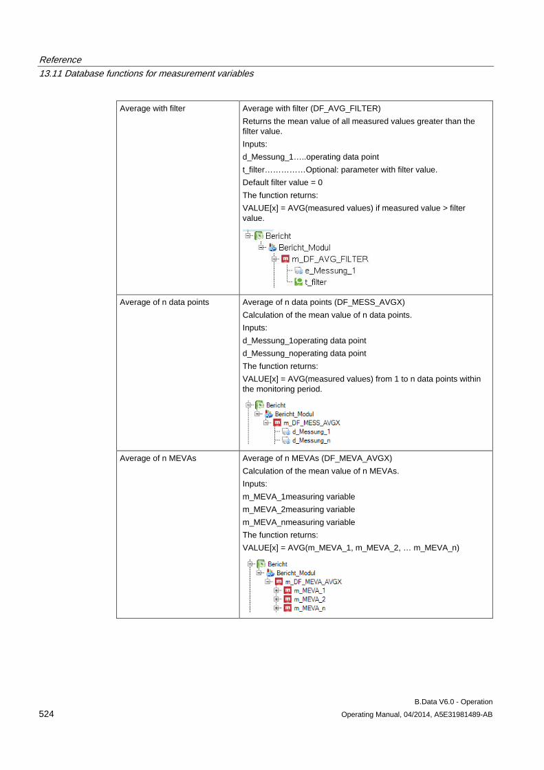
Reference 13.11 Database functions for measurement variables
B.Data V6.0 - Operation 524 Operating Manual, 04/2014, A5E31981489-AB
Average with filter Average with filter (DF_AVG_FILTER) Returns the mean value of all measured values greater than the filter value. Inputs: d_Messung_1…..operating data point t_filter……………Optional: parameter with filter value. Default filter value = 0 The function returns: VALUE[x] = AVG(measured values) if measured value > filter value.
Average of n data points Average of n data points (DF_MESS_AVGX) Calculation of the mean value of n data points. Inputs: d_Messung_1operating data point d_Messung_noperating data point The function returns: VALUE[x] = AVG(measured values) from 1 to n data points within the monitoring period.
Average of n MEVAs Average of n MEVAs (DF_MEVA_AVGX) Calculation of the mean value of n MEVAs. Inputs: m_MEVA_1measuring variable m_MEVA_2measuring variable m_MEVA_nmeasuring variable The function returns: VALUE[x] = AVG(m_MEVA_1, m_MEVA_2, … m_MEVA_n)
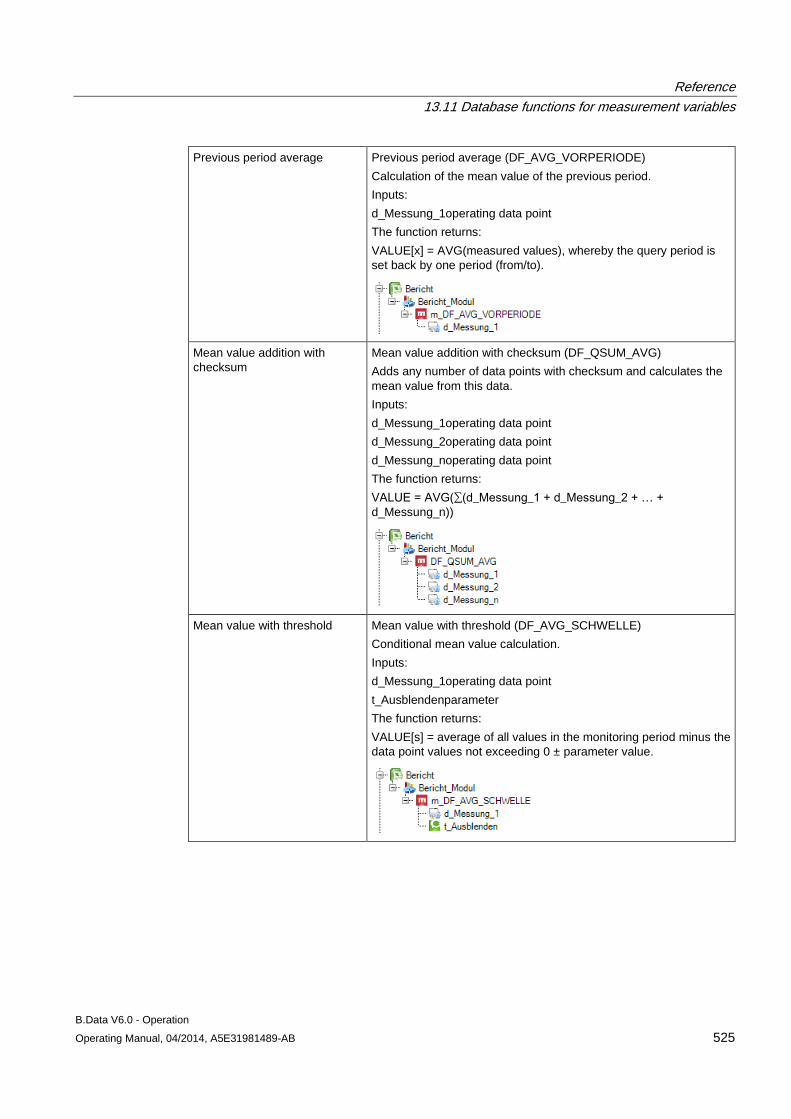
Reference 13.11 Database functions for measurement variables
B.Data V6.0 - Operation Operating Manual, 04/2014, A5E31981489-AB 525
Previous period average Previous period average (DF_AVG_VORPERIODE) Calculation of the mean value of the previous period. Inputs: d_Messung_1operating data point The function returns: VALUE[x] = AVG(measured values), whereby the query period is set back by one period (from/to).
Mean value addition with checksum
Mean value addition with checksum (DF_QSUM_AVG) Adds any number of data points with checksum and calculates the mean value from this data. Inputs: d_Messung_1operating data point d_Messung_2operating data point d_Messung_noperating data point The function returns: VALUE = AVG(∑(d_Messung_1 + d_Messung_2 + … + d_Messung_n))
Mean value with threshold Mean value with threshold (DF_AVG_SCHWELLE) Conditional mean value calculation. Inputs: d_Messung_1operating data point t_Ausblendenparameter The function returns: VALUE[s] = average of all values in the monitoring period minus the data point values not exceeding 0 ± parameter value.
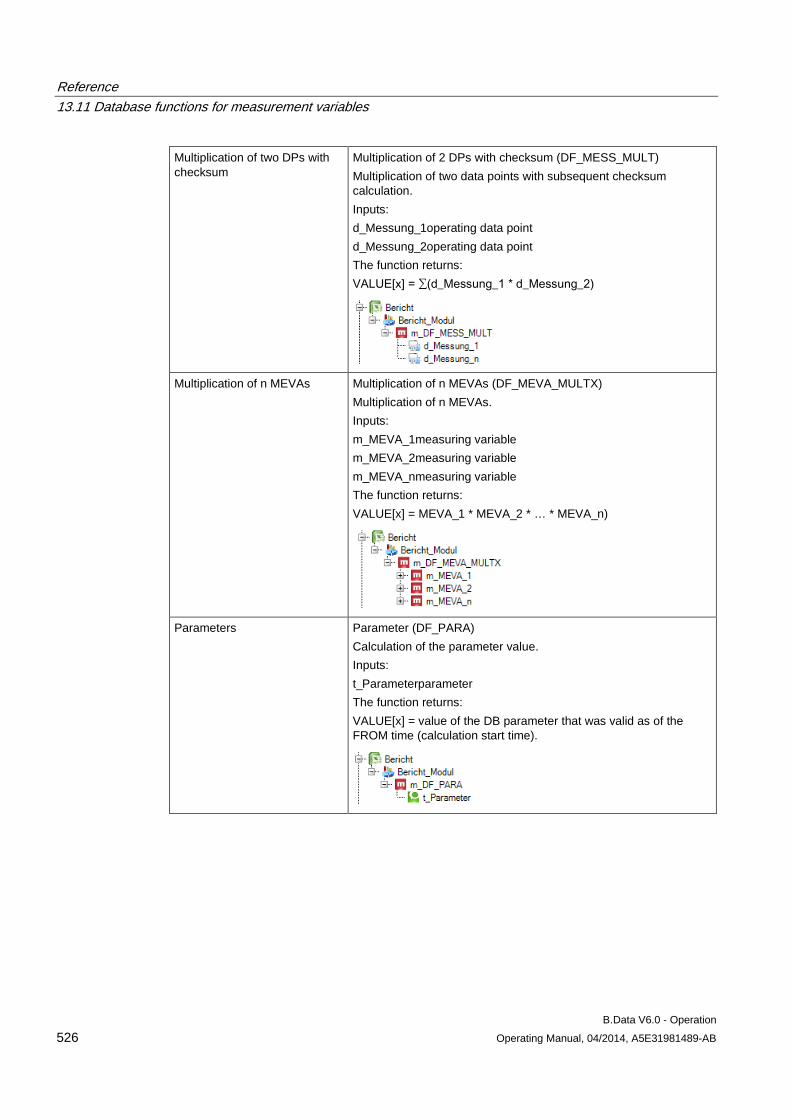
Reference 13.11 Database functions for measurement variables
B.Data V6.0 - Operation 526 Operating Manual, 04/2014, A5E31981489-AB
Multiplication of two DPs with checksum
Multiplication of 2 DPs with checksum (DF_MESS_MULT) Multiplication of two data points with subsequent checksum calculation. Inputs: d_Messung_1operating data point d_Messung_2operating data point The function returns: VALUE[x] = ∑(d_Messung_1 * d_Messung_2)
Multiplication of n MEVAs Multiplication of n MEVAs (DF_MEVA_MULTX) Multiplication of n MEVAs. Inputs: m_MEVA_1measuring variable m_MEVA_2measuring variable m_MEVA_nmeasuring variable The function returns: VALUE[x] = MEVA_1 * MEVA_2 * … * MEVA_n)
Parameters Parameter (DF_PARA) Calculation of the parameter value. Inputs: t_Parameterparameter The function returns: VALUE[x] = value of the DB parameter that was valid as of the FROM time (calculation start time).
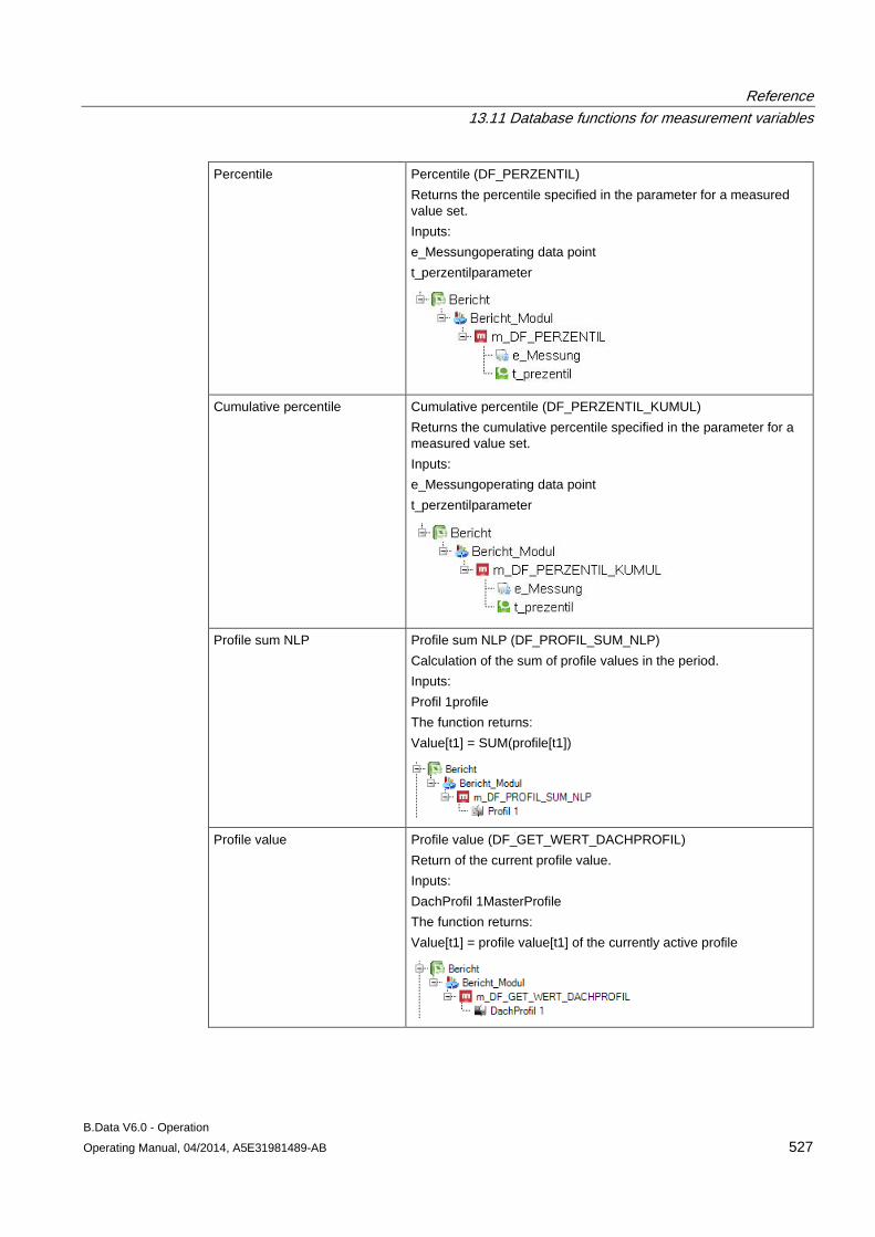
Reference 13.11 Database functions for measurement variables
B.Data V6.0 - Operation Operating Manual, 04/2014, A5E31981489-AB 527
Percentile Percentile (DF_PERZENTIL) Returns the percentile specified in the parameter for a measured value set. Inputs: e_Messungoperating data point t_perzentilparameter
Cumulative percentile Cumulative percentile (DF_PERZENTIL_KUMUL) Returns the cumulative percentile specified in the parameter for a measured value set. Inputs: e_Messungoperating data point t_perzentilparameter
Profile sum NLP Profile sum NLP (DF_PROFIL_SUM_NLP) Calculation of the sum of profile values in the period. Inputs: Profil 1profile The function returns: Value[t1] = SUM(profile[t1])
Profile value Profile value (DF_GET_WERT_DACHPROFIL) Return of the current profile value. Inputs: DachProfil 1MasterProfile The function returns: Value[t1] = profile value[t1] of the currently active profile
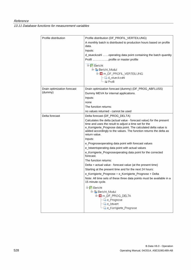
Reference 13.11 Database functions for measurement variables
B.Data V6.0 - Operation 528 Operating Manual, 04/2014, A5E31981489-AB
Profile distribution Profile distribution (DF_PROFIL_VERTEILUNG) A monthly batch is distributed to production hours based on profile data. Inputs: d_stueckzahl ……operating data point containing the batch quantity Profil ……………..profile or master profile
Drain optimization forecast (dummy)
Drain optimization forecast (dummy) (DF_PROG_ABFLUSS) Dummy MEVA for internal applications. Inputs: none The function returns: no values returned - cannot be used
Delta forecast Delta forecast (DF_PROG_DELTA) Calculates the delta (actual value - forecast value) for the present time and uses the result to adjust a time set for the e_Korrigierte_Prognose data point. The calculated delta value is added accordingly to the values. The function returns the delta as return value. Inputs: e_Prognoseoperating data point with forecast values e_Istwertoperating data point with actual values e_Korrigierte_Prognoseoperating data point for the corrected forecast. The function returns: Delta = actual value - forecast value (at the present time) Starting at the present time and for the next 24 hours: e_Korrigierte_Prognose = e_Korrigierte_Prognose + Delta Note: All time sets of these three data points must be available in a 15 minute cycle.
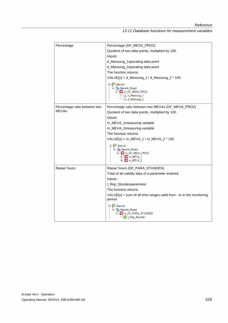
Reference 13.11 Database functions for measurement variables
B.Data V6.0 - Operation Operating Manual, 04/2014, A5E31981489-AB 529
Percentage Percentage (DF_MESS_PROZ) Quotient of two data points, multiplied by 100. Inputs: d_Messung_1operating data point d_Messung_2operating data point The function returns: VALUE[x] = d_Messung_1 / d_Messung_2 * 100
Percentage ratio between two MEVAs
Percentage ratio between two MEVAs (DF_MEVA_PROZ) Quotient of two data points, multiplied by 100. Inputs: m_MEVA_1measuring variable m_MEVA_2measuring variable The function returns: VALUE[x] = m_MEVA_1 / m_MEVA_2 * 100
Repair hours Repair hours (DF_PARA_STUNDEN) Total of all validity data of a parameter entered. Inputs: t_Rep_Stundenparameter The function returns: VALUE[x] = sum of all time ranges valid from - to in the monitoring period
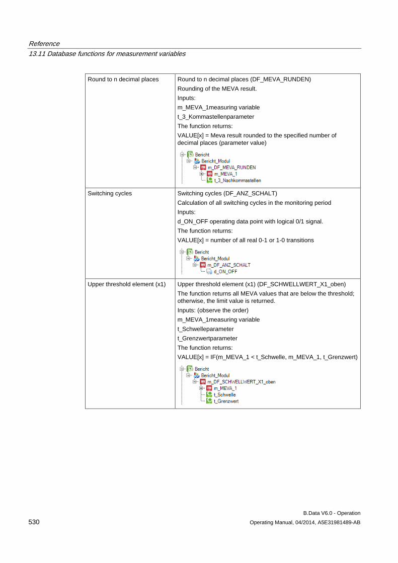
Reference 13.11 Database functions for measurement variables
B.Data V6.0 - Operation 530 Operating Manual, 04/2014, A5E31981489-AB
Round to n decimal places Round to n decimal places (DF_MEVA_RUNDEN) Rounding of the MEVA result. Inputs: m_MEVA_1measuring variable t_3_Kommastellenparameter The function returns: VALUE[x] = Meva result rounded to the specified number of decimal places (parameter value)
Switching cycles Switching cycles (DF_ANZ_SCHALT) Calculation of all switching cycles in the monitoring period Inputs: d_ON_OFF operating data point with logical 0/1 signal. The function returns: VALUE[x] = number of all real 0-1 or 1-0 transitions
Upper threshold element (x1) Upper threshold element (x1) (DF_SCHWELLWERT_X1_oben) The function returns all MEVA values that are below the threshold; otherwise, the limit value is returned. Inputs: (observe the order) m_MEVA_1measuring variable t_Schwelleparameter t_Grenzwertparameter The function returns: VALUE[x] = IF(m_MEVA_1 < t_Schwelle, m_MEVA_1, t_Grenzwert)
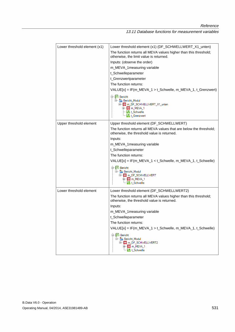
Reference 13.11 Database functions for measurement variables
B.Data V6.0 - Operation Operating Manual, 04/2014, A5E31981489-AB 531
Lower threshold element (x1) Lower threshold element (x1) (DF_SCHWELLWERT_X1_unten) The function returns all MEVA values higher than this threshold; otherwise, the limit value is returned. Inputs: (observe the order) m_MEVA_1measuring variable t_Schwelleparameter t_Grenzwertparameter The function returns: VALUE[x] = IF(m_MEVA_1 > t_Schwelle, m_MEVA_1, t_Grenzwert)
Upper threshold element Upper threshold element (DF_SCHWELLWERT) The function returns all MEVA values that are below the threshold; otherwise, the threshold value is returned. Inputs: m_MEVA_1measuring variable t_Schwelleparameter The function returns: VALUE[x] = IF(m_MEVA_1 < t_Schwelle, m_MEVA_1, t_Schwelle)
Lower threshold element Lower threshold element (DF_SCHWELLWERT2) The function returns all MEVA values higher than this threshold; otherwise, the threshold value is returned. Inputs: m_MEVA_1measuring variable t_Schwelleparameter The function returns: VALUE[x] = IF(m_MEVA_1 > t_Schwelle, m_MEVA_1, t_Schwelle)
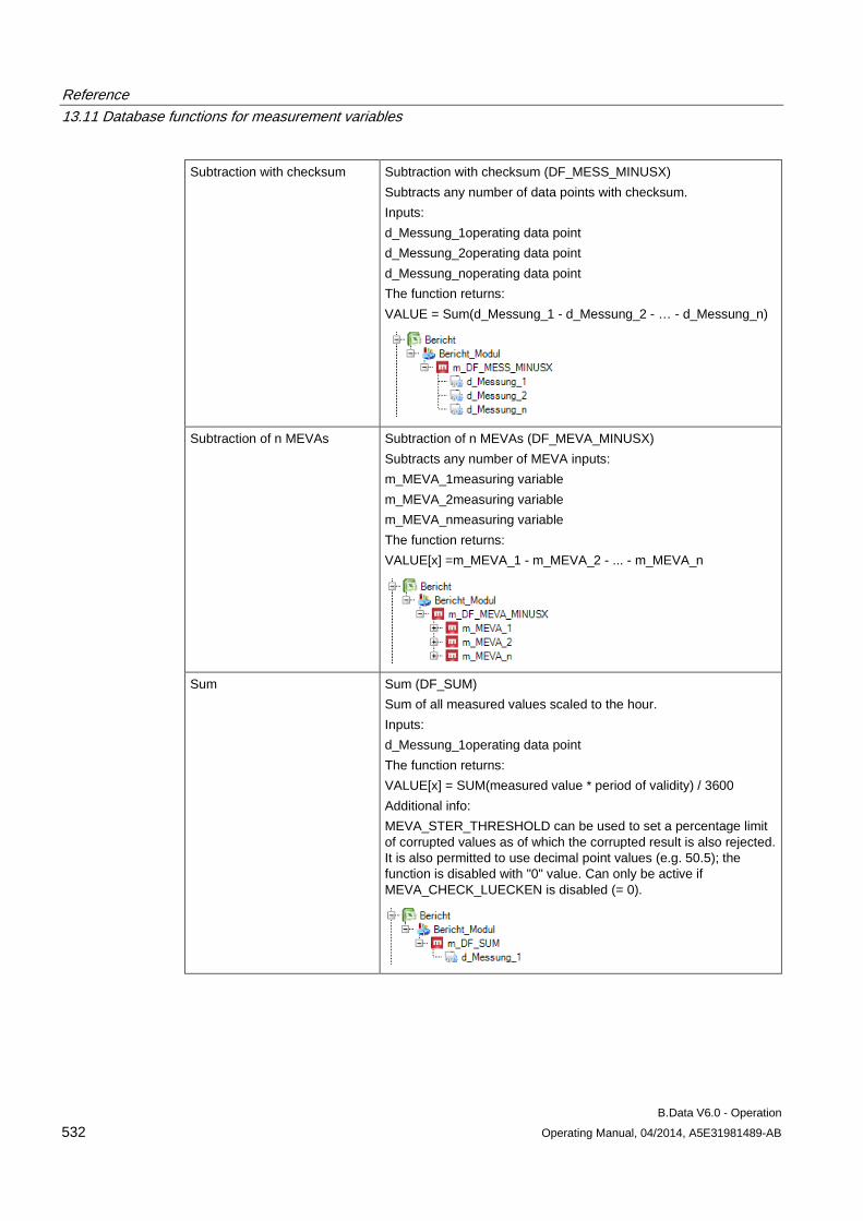
Reference 13.11 Database functions for measurement variables
B.Data V6.0 - Operation 532 Operating Manual, 04/2014, A5E31981489-AB
Subtraction with checksum Subtraction with checksum (DF_MESS_MINUSX) Subtracts any number of data points with checksum. Inputs: d_Messung_1operating data point d_Messung_2operating data point d_Messung_noperating data point The function returns: VALUE = Sum(d_Messung_1 - d_Messung_2 - … - d_Messung_n)
Subtraction of n MEVAs Subtraction of n MEVAs (DF_MEVA_MINUSX) Subtracts any number of MEVA inputs: m_MEVA_1measuring variable m_MEVA_2measuring variable m_MEVA_nmeasuring variable The function returns: VALUE[x] =m_MEVA_1 - m_MEVA_2 - ... - m_MEVA_n
Sum Sum (DF_SUM) Sum of all measured values scaled to the hour. Inputs: d_Messung_1operating data point The function returns: VALUE[x] = SUM(measured value * period of validity) / 3600 Additional info: MEVA_STER_THRESHOLD can be used to set a percentage limit of corrupted values as of which the corrupted result is also rejected. It is also permitted to use decimal point values (e.g. 50.5); the function is disabled with "0" value. Can only be active if MEVA_CHECK_LUECKEN is disabled (= 0).
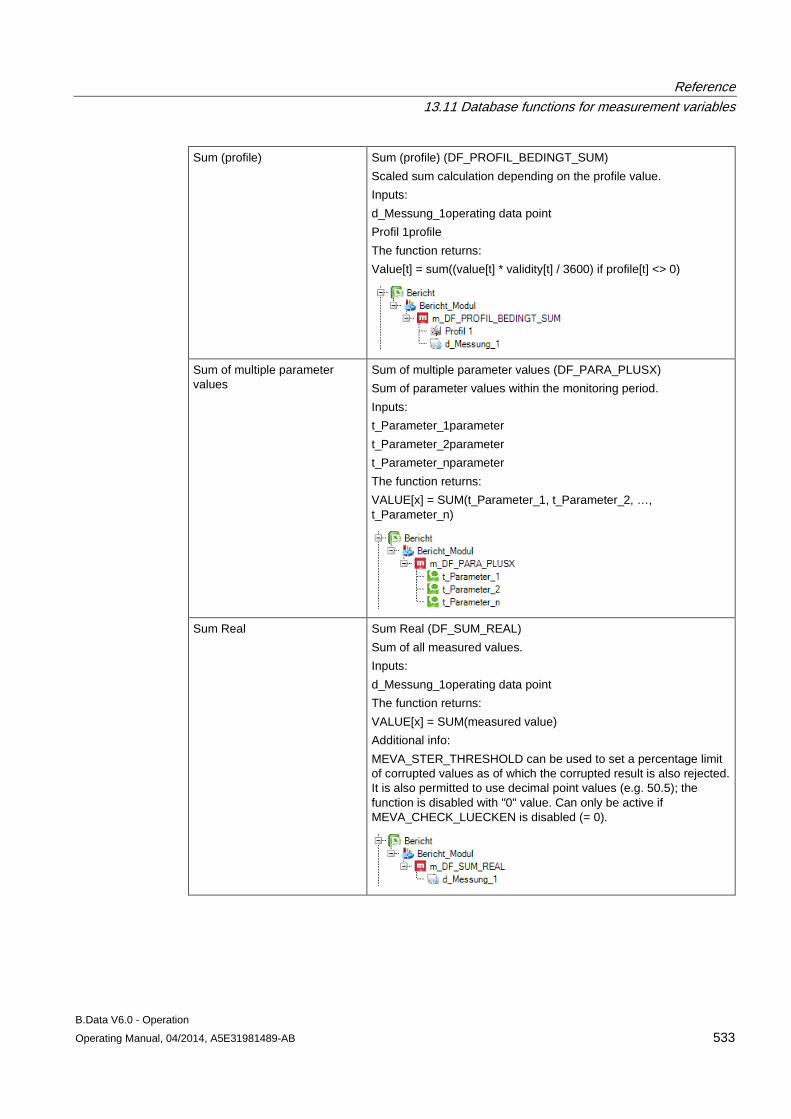
Reference 13.11 Database functions for measurement variables
B.Data V6.0 - Operation Operating Manual, 04/2014, A5E31981489-AB 533
Sum (profile) Sum (profile) (DF_PROFIL_BEDINGT_SUM) Scaled sum calculation depending on the profile value. Inputs: d_Messung_1operating data point Profil 1profile The function returns: Value[t] = sum((value[t] * validity[t] / 3600) if profile[t] <> 0)
Sum of multiple parameter values
Sum of multiple parameter values (DF_PARA_PLUSX) Sum of parameter values within the monitoring period. Inputs: t_Parameter_1parameter t_Parameter_2parameter t_Parameter_nparameter The function returns: VALUE[x] = SUM(t_Parameter_1, t_Parameter_2, …, t_Parameter_n)
Sum Real Sum Real (DF_SUM_REAL) Sum of all measured values. Inputs: d_Messung_1operating data point The function returns: VALUE[x] = SUM(measured value) Additional info: MEVA_STER_THRESHOLD can be used to set a percentage limit of corrupted values as of which the corrupted result is also rejected. It is also permitted to use decimal point values (e.g. 50.5); the function is disabled with "0" value. Can only be active if MEVA_CHECK_LUECKEN is disabled (= 0).
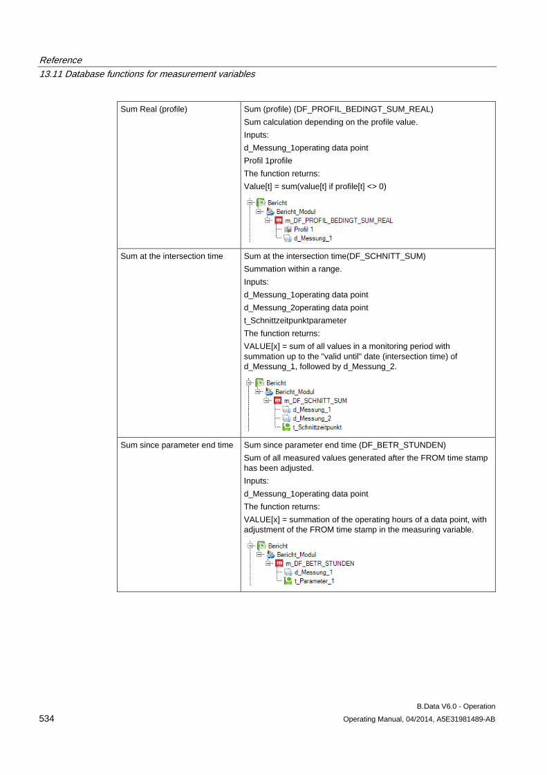
Reference 13.11 Database functions for measurement variables
B.Data V6.0 - Operation 534 Operating Manual, 04/2014, A5E31981489-AB
Sum Real (profile) Sum (profile) (DF_PROFIL_BEDINGT_SUM_REAL) Sum calculation depending on the profile value. Inputs: d_Messung_1operating data point Profil 1profile The function returns: Value[t] = sum(value[t] if profile[t] <> 0)
Sum at the intersection time Sum at the intersection time(DF_SCHNITT_SUM) Summation within a range. Inputs: d_Messung_1operating data point d_Messung_2operating data point t_Schnittzeitpunktparameter The function returns: VALUE[x] = sum of all values in a monitoring period with summation up to the "valid until" date (intersection time) of d_Messung_1, followed by d_Messung_2.
Sum since parameter end time Sum since parameter end time (DF_BETR_STUNDEN) Sum of all measured values generated after the FROM time stamp has been adjusted. Inputs: d_Messung_1operating data point The function returns: VALUE[x] = summation of the operating hours of a data point, with adjustment of the FROM time stamp in the measuring variable.
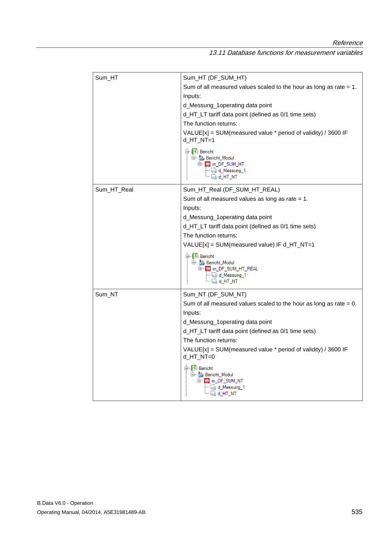
Reference 13.11 Database functions for measurement variables
B.Data V6.0 - Operation Operating Manual, 04/2014, A5E31981489-AB 535
Sum_HT Sum_HT (DF_SUM_HT) Sum of all measured values scaled to the hour as long as rate = 1. Inputs: d_Messung_1operating data point d_HT_LT tariff data point (defined as 0/1 time sets) The function returns: VALUE[x] = SUM(measured value * period of validity) / 3600 IF d_HT_NT=1
Sum_HT_Real Sum_HT_Real (DF_SUM_HT_REAL) Sum of all measured values as long as rate = 1. Inputs: d_Messung_1operating data point d_HT_LT tariff data point (defined as 0/1 time sets) The function returns: VALUE[x] = SUM(measured value) IF d_HT_NT=1
Sum_NT Sum_NT (DF_SUM_NT) Sum of all measured values scaled to the hour as long as rate = 0. Inputs: d_Messung_1operating data point d_HT_LT tariff data point (defined as 0/1 time sets) The function returns: VALUE[x] = SUM(measured value * period of validity) / 3600 IF d_HT_NT=0
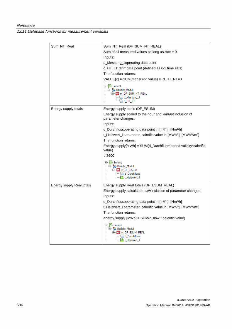
Reference 13.11 Database functions for measurement variables
B.Data V6.0 - Operation 536 Operating Manual, 04/2014, A5E31981489-AB
Sum_NT_Real Sum_NT_Real (DF_SUM_NT_REAL) Sum of all measured values as long as rate = 0. Inputs: d_Messung_1operating data point d_HT_LT tariff data point (defined as 0/1 time sets) The function returns: VALUE[x] = SUM(measured value) IF d_HT_NT=0
Energy supply totals Energy supply totals (DF_ESUM) Energy supply scaled to the hour and without inclusion of parameter changes. Inputs: d_Durchflussoperating data point in [m³/h], [Nm³/h] t_Heizwert_1parameter, calorific value in [MWh/t] ,[MWh/Nm³] The function returns: Energy supply[MWh] = SUM(d_Durchfluss*period validity*calorific value) / 3600
Energy supply Real totals Energy supply Real totals (DF_ESUM_REAL) Energy supply calculation with inclusion of parameter changes. Inputs: d_Durchflussoperating data point in [m³/h], [Nm³/h] t_Heizwert_1parameter, calorific value in [MWh/t] ,[MWh/Nm³] The function returns: energy supply [MWh] = SUM(d_flow * calorific value)
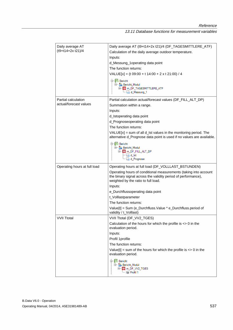
Reference 13.11 Database functions for measurement variables
B.Data V6.0 - Operation Operating Manual, 04/2014, A5E31981489-AB 537
Daily average AT (t9+t14+2x t21)/4
Daily average AT (t9+t14+2x t21)/4 (DF_TAGESMITTLERE_ATF) Calculation of the daily average outdoor temperature. Inputs: d_Messung_1operating data point The function returns: VALUE[x] = (t 09:00 + t 14:00 + 2 x t 21:00) / 4
Partial calculation actual/forecast values
Partial calculation actual/forecast values (DF_FILL_ALT_DP) Summation within a range. Inputs: d_Istoperating data point d_Prognoseoperating data point The function returns: VALUE[x] = sum of all d_Ist values in the monitoring period. The alternative d_Prognose data point is used if no values are available.
Operating hours at full load Operating hours at full load (DF_VOLLLAST_BSTUNDEN) Operating hours of conditional measurements (taking into account the binary signal across the validity period of performance), weighted by the ratio to full load. Inputs: e_Durchflussoperating data point t_Volllastparameter The function returns: Value[t] = Sum (e_Durchfluss.Value * e_Durchfluss.period of validity / t_Volllast)
VVII Ttotal VVII Ttotal (DF_VV2_TGES) Calculation of the hours for which the profile is <> 0 in the evaluation period. Inputs: Profil 1profile The function returns: Value[t] = sum of the hours for which the profile is <> 0 in the evaluation period.
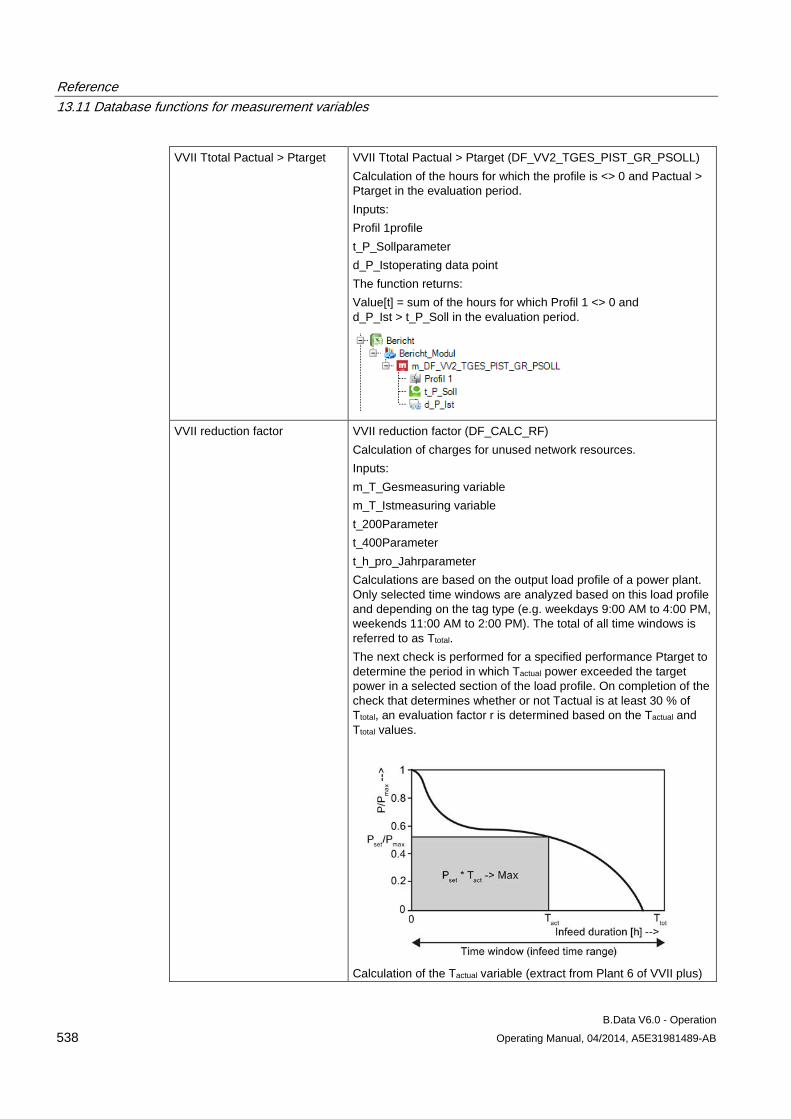
Reference 13.11 Database functions for measurement variables
B.Data V6.0 - Operation 538 Operating Manual, 04/2014, A5E31981489-AB
VVII Ttotal Pactual > Ptarget VVII Ttotal Pactual > Ptarget (DF_VV2_TGES_PIST_GR_PSOLL) Calculation of the hours for which the profile is <> 0 and Pactual > Ptarget in the evaluation period. Inputs: Profil 1profile t_P_Sollparameter d_P_Istoperating data point The function returns: Value[t] = sum of the hours for which Profil 1 <> 0 and d_P_Ist > t_P_Soll in the evaluation period.
VVII reduction factor VVII reduction factor (DF_CALC_RF) Calculation of charges for unused network resources. Inputs: m_T_Gesmeasuring variable m_T_Istmeasuring variable t_200Parameter t_400Parameter t_h_pro_Jahrparameter Calculations are based on the output load profile of a power plant. Only selected time windows are analyzed based on this load profile and depending on the tag type (e.g. weekdays 9:00 AM to 4:00 PM, weekends 11:00 AM to 2:00 PM). The total of all time windows is referred to as Ttotal. The next check is performed for a specified performance Ptarget to determine the period in which Tactual power exceeded the target power in a selected section of the load profile. On completion of the check that determines whether or not Tactual is at least 30 % of Ttotal, an evaluation factor r is determined based on the Tactual and Ttotal values.
Calculation of the Tactual variable (extract from Plant 6 of VVII plus)
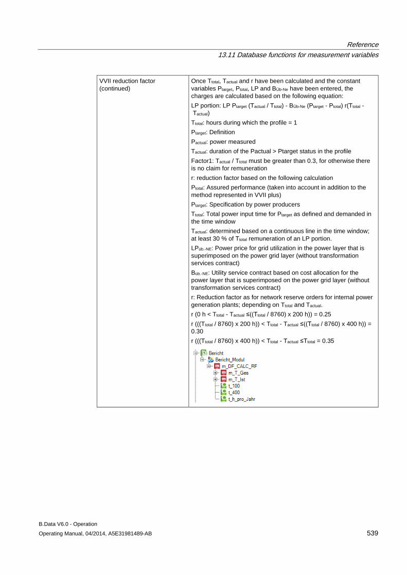
Reference 13.11 Database functions for measurement variables
B.Data V6.0 - Operation Operating Manual, 04/2014, A5E31981489-AB 539
VVII reduction factor (continued)
Once Ttotal, Tactual and r have been calculated and the constant variables Ptarget, Ptotal, LP and BÜb-Ne have been entered, the charges are calculated based on the following equation: LP portion: LP Ptarget (Tactual / Ttotal) - BÜb-Ne (Ptarget - Ptotal) r(Ttotal - Tactual) Ttotal: hours during which the profile = 1 Ptarget: Definition Pactual: power measured Tactual: duration of the Pactual > Ptarget status in the profile Factor1: Tactual / Ttotal must be greater than 0.3, for otherwise there is no claim for remuneration r: reduction factor based on the following calculation Ptotal: Assured performance (taken into account in addition to the method represented in VVII plus) Ptarget: Specification by power producers Ttotal: Total power input time for Ptarget as defined and demanded in the time window Tactual: determined based on a continuous line in the time window; at least 30 % of Ttotal remuneration of an LP portion. LPüb.-NE: Power price for grid utilization in the power layer that is superimposed on the power grid layer (without transformation services contract) Büb.-NE: Utility service contract based on cost allocation for the power layer that is superimposed on the power grid layer (without transformation services contract) r: Reduction factor as for network reserve orders for internal power generation plants; depending on Ttotal and Tactual. r (0 h < Ttotal - Tactual ≤((Ttotal / 8760) x 200 h)) = 0.25 r (((Ttotal / 8760) x 200 h)) < Ttotal - Tactual ≤((Ttotal / 8760) x 400 h)) = 0.30 r (((Ttotal / 8760) x 400 h)) < Ttotal - Tactual ≤Ttotal = 0.35
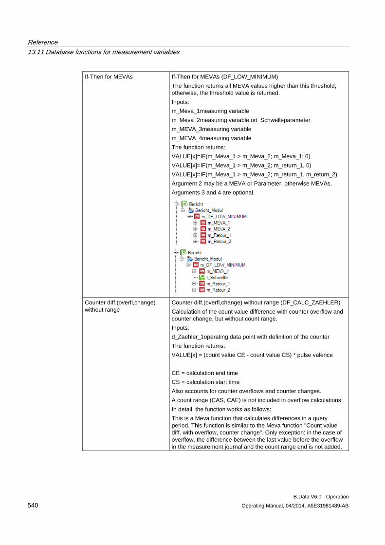
Reference 13.11 Database functions for measurement variables
B.Data V6.0 - Operation 540 Operating Manual, 04/2014, A5E31981489-AB
If-Then for MEVAs If-Then for MEVAs (DF_LOW_MINIMUM) The function returns all MEVA values higher than this threshold; otherwise, the threshold value is returned. Inputs: m_Meva_1measuring variable m_Meva_2measuring variable ort_Schwelleparameter m_MEVA_3measuring variable m_MEVA_4measuring variable The function returns: VALUE[x]=IF(m_Meva_1 > m_Meva_2; m_Meva_1; 0) VALUE[x]=IF(m_Meva_1 > m_Meva_2; m_return_1, 0) VALUE[x]=IF(m_Meva_1 > m_Meva_2; m_return_1, m_return_2) Argument 2 may be a MEVA or Parameter, otherwise MEVAs. Arguments 3 and 4 are optional.
Counter diff.(overfl,change) without range
Counter diff.(overfl,change) without range (DF_CALC_ZAEHLER) Calculation of the count value difference with counter overflow and counter change, but without count range. Inputs: d_Zaehler_1operating data point with definition of the counter The function returns: VALUE[x] = (count value CE - count value CS) * pulse valence CE = calculation end time CS = calculation start time Also accounts for counter overflows and counter changes. A count range (CAS, CAE) is not included in overflow calculations. In detail, the function works as follows: This is a Meva function that calculates differences in a query period. This function is similar to the Meva function "Count value diff. with overflow, counter change". Only exception: in the case of overflow, the difference between the last value before the overflow in the measurement journal and the count range end is not added.
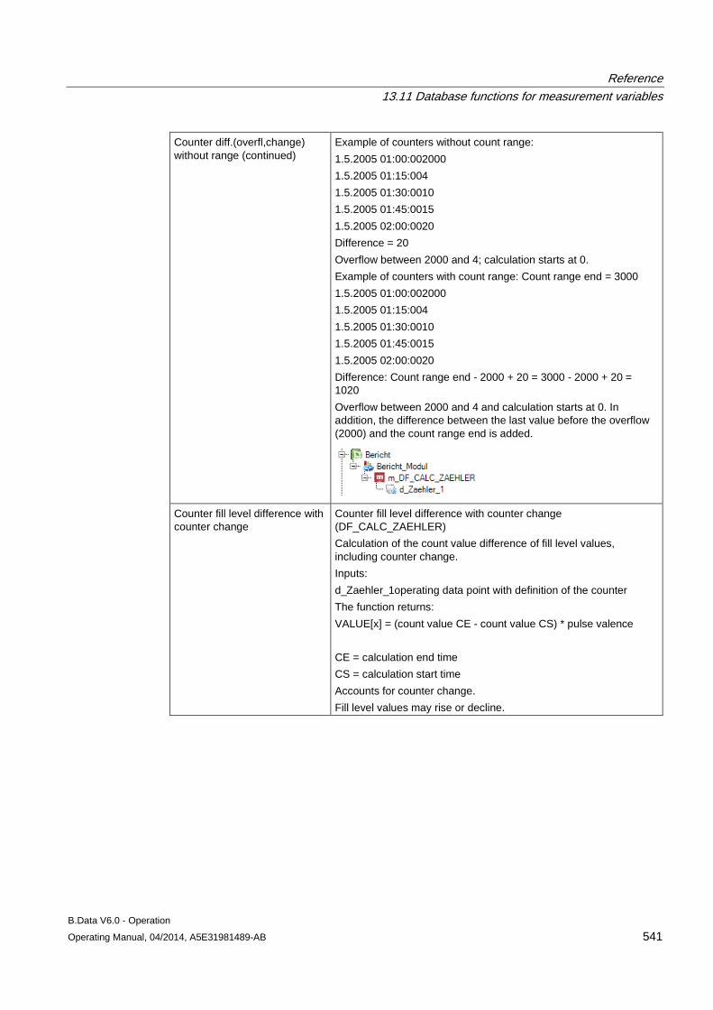
Reference 13.11 Database functions for measurement variables
B.Data V6.0 - Operation Operating Manual, 04/2014, A5E31981489-AB 541
Counter diff.(overfl,change) without range (continued)
Example of counters without count range: 1.5.2005 01:00:002000 1.5.2005 01:15:004 1.5.2005 01:30:0010 1.5.2005 01:45:0015 1.5.2005 02:00:0020 Difference = 20 Overflow between 2000 and 4; calculation starts at 0. Example of counters with count range: Count range end = 3000 1.5.2005 01:00:002000 1.5.2005 01:15:004 1.5.2005 01:30:0010 1.5.2005 01:45:0015 1.5.2005 02:00:0020 Difference: Count range end - 2000 + 20 = 3000 - 2000 + 20 = 1020 Overflow between 2000 and 4 and calculation starts at 0. In addition, the difference between the last value before the overflow (2000) and the count range end is added.
Counter fill level difference with counter change
Counter fill level difference with counter change (DF_CALC_ZAEHLER) Calculation of the count value difference of fill level values, including counter change. Inputs: d_Zaehler_1operating data point with definition of the counter The function returns: VALUE[x] = (count value CE - count value CS) * pulse valence CE = calculation end time CS = calculation start time Accounts for counter change. Fill level values may rise or decline.
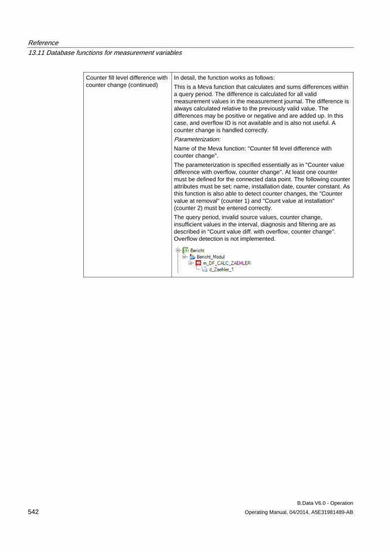
Reference 13.11 Database functions for measurement variables
B.Data V6.0 - Operation 542 Operating Manual, 04/2014, A5E31981489-AB
Counter fill level difference with counter change (continued)
In detail, the function works as follows: This is a Meva function that calculates and sums differences within a query period. The difference is calculated for all valid measurement values in the measurement journal. The difference is always calculated relative to the previously valid value. The differences may be positive or negative and are added up. In this case, and overflow ID is not available and is also not useful. A counter change is handled correctly. Parameterization: Name of the Meva function: "Counter fill level difference with counter change". The parameterization is specified essentially as in "Counter value difference with overflow, counter change". At least one counter must be defined for the connected data point. The following counter attributes must be set: name, installation date, counter constant. As this function is also able to detect counter changes, the "Counter value at removal" (counter 1) and "Count value at installation" (counter 2) must be entered correctly. The query period, invalid source values, counter change, insufficient values in the interval, diagnosis and filtering are as described in "Count value diff. with overflow, counter change". Overflow detection is not implemented.
Reference 13.11 Database functions for measurement variables
B.Data V6.0 - Operation Operating Manual, 04/2014, A5E31981489-AB 543
Counter light difference (overflow) without range
Counter light difference (overflow) without range (DF_CALC_ZAEHLER_LIGHT) Calculation of the count difference without counter change and count range. Inputs: d_Zaehler_1operating data point with definition of the counter The function returns: VALUE[x] = (count value CE - count value CS) * pulse valence CE = calculation end time CS = calculation start time A count range is not included in overflow calculations. Calculation interval equals data acquisition interval. Counter changes are ignored. In detail, the function works as follows: This is a Meva function that calculates differences in a query period. In comparison to the other functions described above, the Meva function was simplified in order to enhance performance. For example, counter change detection was dispensed with. Only the first and last values in the query period are used to calculate the difference. Any interim value is ignored. For this reason, the duration of the query period should not exceed the interval for measured values in this function. Overflow detection is not possible if this function is used in combination with a balancing module. It certainly makes sense to use a report module with a query interval that corresponds with the data acquisition interval. Parameterization: Name of the Meva function: "Counter light difference (overflow) without range" A data point must be connected to the Meva function node. It is not necessary to define a counter for this data point, as the permanent counter constant 1 is always used for the calculation.
Reference 13.11 Database functions for measurement variables
B.Data V6.0 - Operation 544 Operating Manual, 04/2014, A5E31981489-AB
Counter Light Diff.(overfl) without range (continued)
Query period The B.Data measurement journal is queried for the connected data point within the query period. The query uses the actual query period, e.g. one month: from = '1.4.2005 00:00:00' to = '1.5.2005 00:00:00' and NOT from = '1.4.2005 00:15:00' to = '1.5.2005 00:00:00'. In contrast to other functions, only the FROM and TO values are read from the measurement journal. All interim values will be ignored as specified in the short description. If the TO value is invalid or missing, the Meva function returns difference 0 and the STER_LUECKE status. If the TO value is valid and available, an attempt is made to calculate the difference based on the FROM value. However, a corresponding valid FROM value must be available. If this condition is not met, the function uses the last valid value that precedes the FROM value. The function performs a backward scan over a maximum period of one day. If no valid value that precedes the FROM value is found in the past 24 hours, the Meva function returns difference 0 and the STER_LUECKE status. Invalid source values All values having acquisition status 1 (invalid) or 9 (8 + 1 = last + invalid) will be ignored. Daylight saving time This function is capable of handling the daylight saving time without error for the 15-minute and 1 hour acquisition intervals. This problem is of no avail anyway for larger units (days, months).
Counter Light Diff.(overfl) without range (continued)
Counter change: Counter change is not supported. Overflow detection: Counter overflow detection without count range is implemented as well. The difference is calculated starting at 0 after counter overflow has been detected. Example: 1.5.2005 01:00:002000 1.5.2005 01:15:0010 Difference = 10 Insufficient number of values in the interval: See the description of the query interval above of a TO or FROM value is invalid or missing. Diagnostics: You can set a value greater than 0 for "DB_ZAEHLER_DEBUG" in B.Data Options to enter additional diagnostics messages in the error journal. Filtering: No filtering is performed. The "DB_ZAEHLER_CHECK" option is insignificant for this Meva function.
Reference 13.11 Database functions for measurement variables
B.Data V6.0 - Operation Operating Manual, 04/2014, A5E31981489-AB 545
Count value difference with overflow, counter change
Count value difference with overflow, counter change (DF_CALC_ZAEHLER) Calculation of the count value difference with counter overflow, including count range and counter change. Inputs: d_Zaehler_1operating data point with definition of the counter The function returns: VALUE[x] = (count value CE - count value CS) * pulse valence CE = calculation end time CS = calculation start time Also accounts for counter overflows and counter changes. The count range (CAS, CAE) is included in overflow calculations. In detail, the function works as follows: Query period The B.Data measurement journal is queried for the connected data point within the query period. The query uses the actual query period, e.g. one month: from = '1.4.2005 00:00:00' to = '1.5.2005 00:00:00' and NOT from = '1.4.2005 00:15:00' to = '1.5.2005 00:00:00'. Explanation: in the example above, the first value in the query period has the time stamp '1.4.2005 00:15:00' in accordance with the B.Data definition. The last value has the time stamp '1.5.2005 00:00:00'. It is not appropriate to calculate the difference between the first and last value in the month for monthly evaluations. You need to calculate the difference between the last value of the current month and the last value of the preceding month. Therefore, from = '1.4.2005 00:00:00'. Invalid source values All values having acquisition status 1 (invalid) or 9 (8 + 1 = last + invalid) will be ignored. The same rule applies to all values having the "acquisition values" compression level. Counter change: Counter changes in the query period are also handled correctly. At least two counters must be defined for the data point. Consistency of the attributes of both counters is conditional, of course. The installation date is decisive for the entry, while the "planned change" is being ignored. The "Count value at removal" (counter 1) and "Count value at installation" (counter 2) fields are of importance, too.
Reference 13.11 Database functions for measurement variables
B.Data V6.0 - Operation 546 Operating Manual, 04/2014, A5E31981489-AB
Count value difference with overflow, counter change (continued)
Overflow detection: Counter overflow detection is implemented as well. Prerequisite for error-free calculations are correct entries in the "Count range start" and "Count range end" fields. The "Count range warning" is not used by this Meva function. An overflow check is also carried out before and after count changes. The "Count value at removal" (counter 1) and "Count value at installation" (counter 2) fields are, of course, relevant for this check. The difference is calculated starting at 0 after counter overflow has been detected. In addition to this difference, the difference between the last value and the count range end value will be added. Example: Count range end = 2200 1.5.2005 01:00:002000 1.5.2005 01:15:000 1.5.2005 01:30:0010 Difference = count range end - 2000 + 10 = 2200 - 2000 + 10 = 210 Insufficient number of values in the interval: Given the situation, for example, that only one value is entered in the measurement journal in each month. However, you nonetheless want to evaluate the data on a monthly basis. An additional functionality has been created as a workaround to the fact that you need at least two values to calculate a difference. 1. The query period (FROM - TO) contains exactly one value that
corresponds with the FROM value with regard to its time stamp. As the TO value is missing, the Meva function is canceled and the STER_LUECKE status is returned.
2. The FROM value is missing. The query is now repeated with a new value, while the old TO value is retained. This situation is indicated in diagnostics mode by the following message in the error journal: "Delta = 0 > second attempt from: 31.04.2005 23:45:00 to: 1.6.2005 00:00:00".
The new FROM value is calculated based on the following rule: starting at the FROM value, the function scans the previous 24 hours to find the last valid value. If the second attempt also returns only one value, the Meva function is canceled, the STER_LUECKE status is set, and the following message is written to the error journal: "2. attempt, delta again 0 > cancel". Diagnostics: You can set a value greater than 0 for "DB_ZAEHLER_DEBUG" in B.Data Options to enter additional diagnostics messages in the error journal. The function name is frequently displayed with a three-digit suffix in parenthesis, e.g.: pr_check_counter(001). This number is used as additive for sorting the messages. Under the aspect that the smallest resolution of the incoming time stamp in the error journal is based on full seconds, it frequently happens that several messages are assigned the same incoming time stamp. Caution: These messages are very extensive so that it is advisable to disable this option as soon as the analysis has been completed.
Reference 13.11 Database functions for measurement variables
B.Data V6.0 - Operation Operating Manual, 04/2014, A5E31981489-AB 547
Count value difference with overflow, counter change (continued)
Filtering: Filtering serves primarily to ignore outliers. You can enable or disable this function by setting the "DB_ZAEHLER_CHECK" option in B.Data Options (1/0). The counter values are usually incremented continuously, which means that the current count value is higher than the previous. If the current counter value is now suddenly less than the previous value, the function rates this status as counter overflow or reset. However, it is possible in this scenario that corrupted source values generate outliers. This means that the current value is less than the previous, while the next value is, once again, greater than the previous. Example: 1.5.2005 01:00:002000 1.5.2005 01:15:000 1.5.2005 01:30:002010 The value for the time stamp of '1.5.2005 01:15:00' is apparently an outlier. With activated filter option, such outliers will be ignored. 1.5.2005 01:00:002000 1.5.2005 01:15:000 1.5.2005 01:30:0010 This situation is not rated as outlier, but rather as overflow.
Count value difference with overflow, counter change (continued)
The filter function provides a second option, namely "DB_ZAEHLER_FILTER". This option only has an effect if "DB_ZAEHLER_CHECK" is enabled (= 1). With active "DB_ZAEHLER_CHECK" option, identical values that were generated in immediate succession are ignored under certain circumstances, whereby the number of values selected for the query may not be less than two. In Debug mode, such entries are consequently generated in the error journal: 'Skip date: 1.5.2005 1:15:00 value: 2000' Example: 1.5.2005 01:00:002000 1.5.2005 01:15:002000 1.5.2005 01:30:002010 If "DB_ZAEHLER_CHECK" is enabled and the "DB_ZAEHLER_FILTER" entry exists, all values less than the value in "DB_ZAEHLER_FILTER" are ignored. Example: DB_ZAEHLER_CHECK = 1 and DB_ZAEHLER_FILTER = 9 01.05.2005 01:00:008 01.05.2005 01:15:009 01.05.2005 01:30:0010 The entry with time stamp '01.05.2005 01:00:00' and value 8 will be ignored.
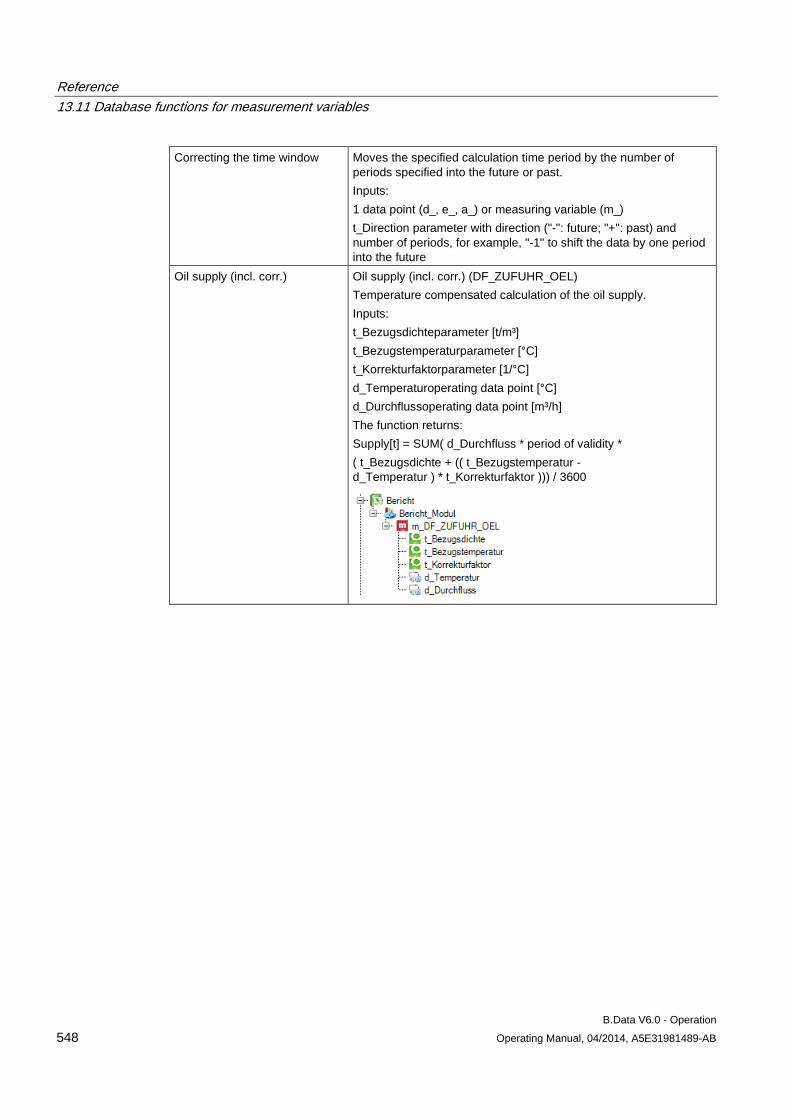
Reference 13.11 Database functions for measurement variables
B.Data V6.0 - Operation 548 Operating Manual, 04/2014, A5E31981489-AB
Correcting the time window Moves the specified calculation time period by the number of periods specified into the future or past. Inputs: 1 data point (d_, e_, a_) or measuring variable (m_) t_Direction parameter with direction ("-": future; "+": past) and number of periods, for example, "-1" to shift the data by one period into the future
Oil supply (incl. corr.) Oil supply (incl. corr.) (DF_ZUFUHR_OEL) Temperature compensated calculation of the oil supply. Inputs: t_Bezugsdichteparameter [t/m³] t_Bezugstemperaturparameter [°C] t_Korrekturfaktorparameter [1/°C] d_Temperaturoperating data point [°C] d_Durchflussoperating data point [m³/h] The function returns: Supply[t] = SUM( d_Durchfluss * period of validity * ( t_Bezugsdichte + (( t_Bezugstemperatur - d_Temperatur ) * t_Korrekturfaktor ))) / 3600
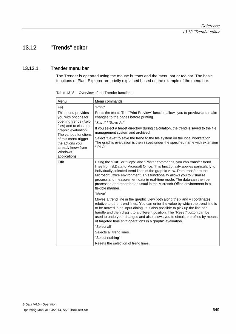
Reference 13.12 "Trends" editor
B.Data V6.0 - Operation Operating Manual, 04/2014, A5E31981489-AB 549
13.12 "Trends" editor
13.12.1 Trender menu bar The Trender is operated using the mouse buttons and the menu bar or toolbar. The basic functions of Plant Explorer are briefly explained based on the example of the menu bar:
Table 13- 8 Overview of the Trender functions
Menu Menu commands File This menu provides you with options for opening trends (*.plo files) and to close the graphic evaluation. The various functions of this menu trigger the actions you already know from Windows applications.
"Print" Prints the trend. The "Print Preview" function allows you to preview and make changes to the pages before printing. "Save" / "Save As" If you select a target directory during calculation, the trend is saved to the file management system and archived. Select "Save" to save the trend to the file system on the local workstation. The graphic evaluation is then saved under the specified name with extension *.PLO.
Edit Using the "Cut", or "Copy" and "Paste" commands, you can transfer trend lines from B.Data to Microsoft Office. This functionality applies particularly to individually selected trend lines of the graphic view. Data transfer to the Microsoft Office environment. This functionality allows you to visualize process and measurement data in real-time mode. The data can then be processed and recorded as usual in the Microsoft Office environment in a flexible manner. "Move" Moves a trend line in the graphic view both along the x and y coordinates, relative to other trend lines. You can enter the value by which the trend line is to be moved in an input dialog. It is also possible to pick up the line at a handle and then drag it to a different position. The "Reset" button can be used to undo your changes and also allows you to simulate profiles by means of targeted time shift operations in a graphic evaluation. "Select all" Selects all trend lines. "Select nothing" Resets the selection of trend lines.
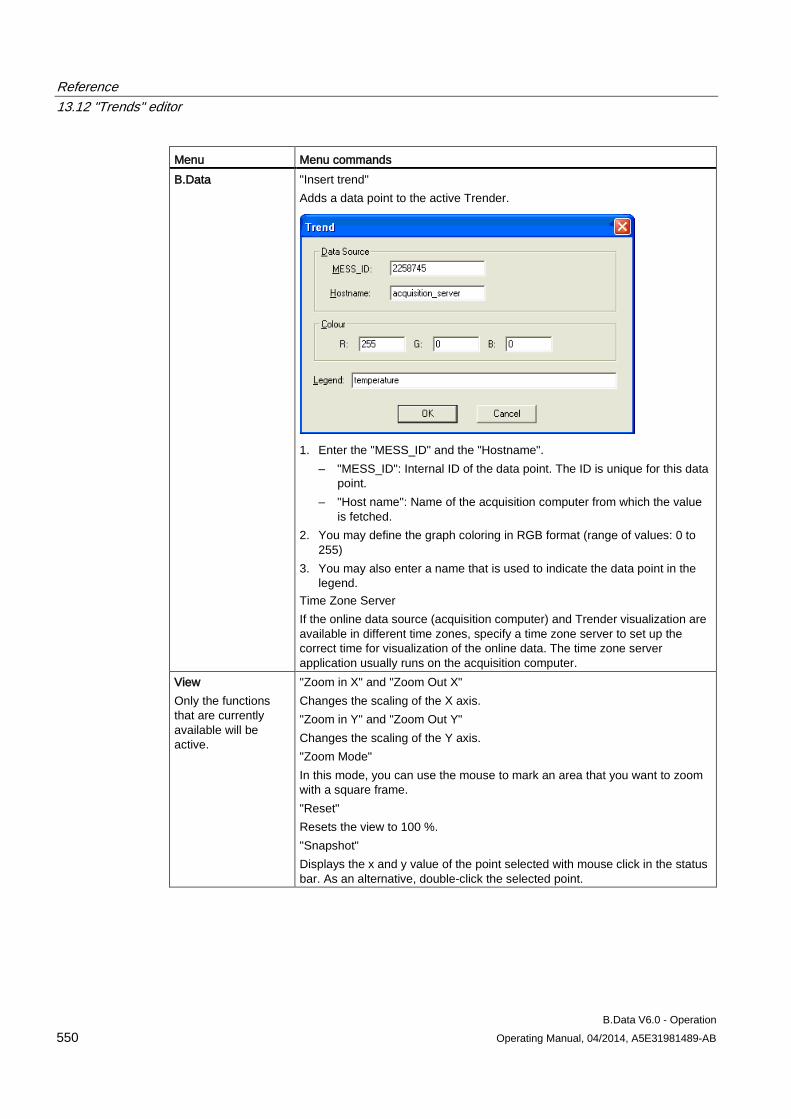
Reference 13.12 "Trends" editor
B.Data V6.0 - Operation 550 Operating Manual, 04/2014, A5E31981489-AB
Menu Menu commands B.Data "Insert trend"
Adds a data point to the active Trender.
1. Enter the "MESS_ID" and the "Hostname".
– "MESS_ID": Internal ID of the data point. The ID is unique for this data point.
– "Host name": Name of the acquisition computer from which the value is fetched.
2. You may define the graph coloring in RGB format (range of values: 0 to 255)
3. You may also enter a name that is used to indicate the data point in the legend.
Time Zone Server If the online data source (acquisition computer) and Trender visualization are available in different time zones, specify a time zone server to set up the correct time for visualization of the online data. The time zone server application usually runs on the acquisition computer.
View Only the functions that are currently available will be active.
"Zoom in X" and "Zoom Out X" Changes the scaling of the X axis. "Zoom in Y" and "Zoom Out Y" Changes the scaling of the Y axis. "Zoom Mode" In this mode, you can use the mouse to mark an area that you want to zoom with a square frame. "Reset" Resets the view to 100 %. "Snapshot" Displays the x and y value of the point selected with mouse click in the status bar. As an alternative, double-click the selected point.
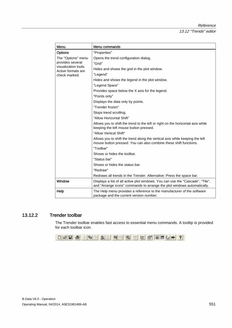
Reference 13.12 "Trends" editor
B.Data V6.0 - Operation Operating Manual, 04/2014, A5E31981489-AB 551
Menu Menu commands Options The "Options" menu provides several visualization tools. Active formats are check marked.
"Properties" Opens the trend configuration dialog. "Grid" Hides and shows the grid in the plot window. "Legend" Hides and shows the legend in the plot window. "Legend Space" Provides space below the X axis for the legend. "Points only" Displays the data only by points. "Trender frozen" Stops trend scrolling. "Allow Horizontal Shift" Allows you to shift the trend to the left or right on the horizontal axis while keeping the left mouse button pressed. "Allow Vertical Shift" Allows you to shift the trend along the vertical axis while keeping the left mouse button pressed. You can also combine these shift functions. "Toolbar" Shows or hides the toolbar. "Status bar" Shows or hides the status bar. "Redraw" Redraws all trends in the Trender. Alternative: Press the space bar.
Window Displays a list of all active plot windows. You can use the "Cascade", "Tile", and "Arrange icons" commands to arrange the plot windows automatically.
Help The Help menu provides a reference to the manufacturer of the software package and the current version number.
13.12.2 Trender toolbar The Trender toolbar enables fast access to essential menu commands. A tooltip is provided for each toolbar icon.
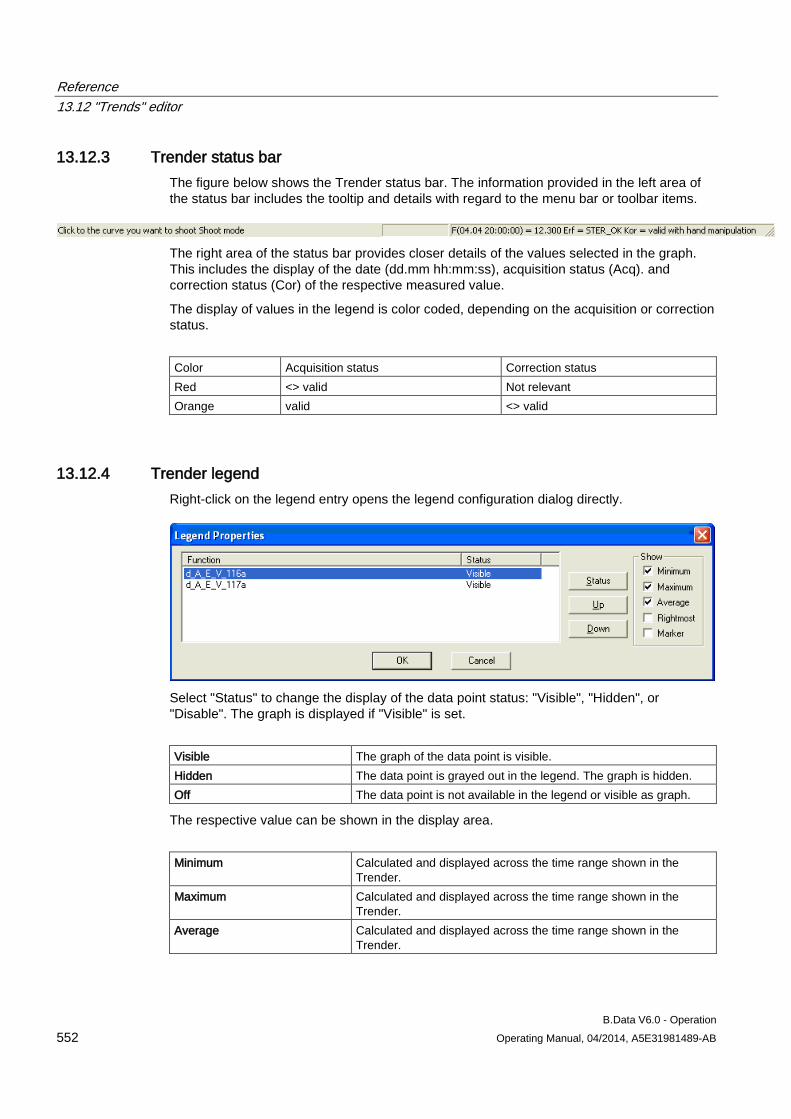
Reference 13.12 "Trends" editor
B.Data V6.0 - Operation 552 Operating Manual, 04/2014, A5E31981489-AB
13.12.3 Trender status bar The figure below shows the Trender status bar. The information provided in the left area of the status bar includes the tooltip and details with regard to the menu bar or toolbar items.
The right area of the status bar provides closer details of the values selected in the graph. This includes the display of the date (dd.mm hh:mm:ss), acquisition status (Acq). and correction status (Cor) of the respective measured value.
The display of values in the legend is color coded, depending on the acquisition or correction status.
Color Acquisition status Correction status Red <> valid Not relevant Orange valid <> valid
13.12.4 Trender legend Right-click on the legend entry opens the legend configuration dialog directly.
Select "Status" to change the display of the data point status: "Visible", "Hidden", or "Disable". The graph is displayed if "Visible" is set.
Visible The graph of the data point is visible. Hidden The data point is grayed out in the legend. The graph is hidden. Off The data point is not available in the legend or visible as graph.
The respective value can be shown in the display area.
Minimum Calculated and displayed across the time range shown in the
Trender. Maximum Calculated and displayed across the time range shown in the
Trender. Average Calculated and displayed across the time range shown in the
Trender.
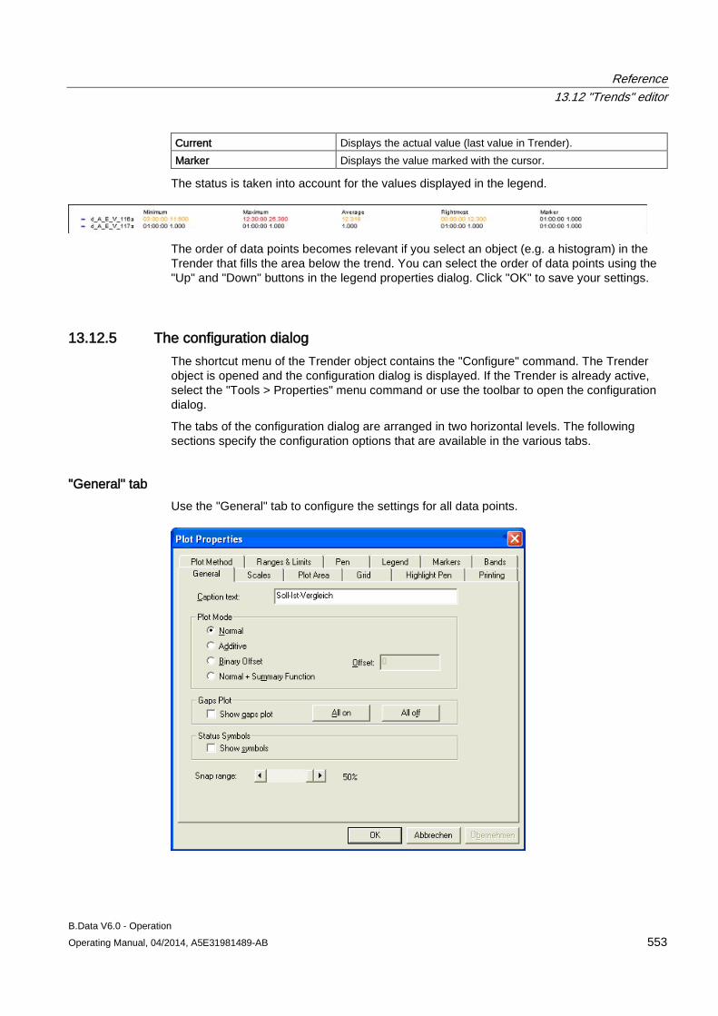
Reference 13.12 "Trends" editor
B.Data V6.0 - Operation Operating Manual, 04/2014, A5E31981489-AB 553
Current Displays the actual value (last value in Trender). Marker Displays the value marked with the cursor.
The status is taken into account for the values displayed in the legend.
The order of data points becomes relevant if you select an object (e.g. a histogram) in the Trender that fills the area below the trend. You can select the order of data points using the "Up" and "Down" buttons in the legend properties dialog. Click "OK" to save your settings.
13.12.5 The configuration dialog The shortcut menu of the Trender object contains the "Configure" command. The Trender object is opened and the configuration dialog is displayed. If the Trender is already active, select the "Tools > Properties" menu command or use the toolbar to open the configuration dialog.
The tabs of the configuration dialog are arranged in two horizontal levels. The following sections specify the configuration options that are available in the various tabs.
"General" tab Use the "General" tab to configure the settings for all data points.
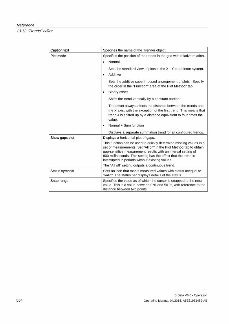
Reference 13.12 "Trends" editor
B.Data V6.0 - Operation 554 Operating Manual, 04/2014, A5E31981489-AB
Caption text Specifies the name of the Trender object. Plot mode Specifies the position of the trends in the grid with relative relation.
• Normal
Sets the standard view of plots in the X - Y coordinate system. • Additive
Sets the additive superimposed arrangement of plots . Specify the order in the "Function" area of the Plot Method" tab.
• Binary offset
Shifts the trend vertically by a constant portion.
The offset always affects the distance between the trends and the X axis, with the exception of the first trend. This means that trend 4 is shifted up by a distance equivalent to four times the value.
• Normal + Sum function
Displays a separate summation trend for all configured trends. Show gaps plot Displays a horizontal plot of gaps.
This function can be used to quickly determine missing values in a set of measurements. Set "All on" in the Plot Method tab to obtain gap-sensitive measurement results with an interval setting of 900 milliseconds. This setting has the effect that the trend is interrupted in periods without existing values. The "All off" setting outputs a continuous trend.
Status symbols Sets an icon that marks measured values with status unequal to "valid". The status bar displays details of the status.
Snap range Specifies the value as of which the cursor is snapped to the next value. This is a value between 0 % and 50 %, with reference to the distance between two points.
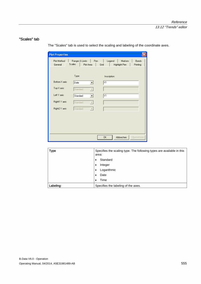
Reference 13.12 "Trends" editor
B.Data V6.0 - Operation Operating Manual, 04/2014, A5E31981489-AB 555
"Scales" tab The "Scales" tab is used to select the scaling and labeling of the coordinate axes.
Type Specifies the scaling type. The following types are available in this
area: • Standard • Integer • Logarithmic • Date • Time
Labeling: Specifies the labeling of the axes.
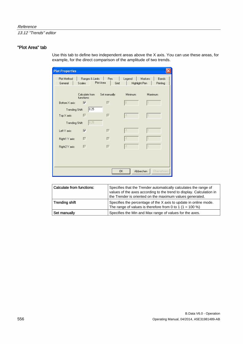
Reference 13.12 "Trends" editor
B.Data V6.0 - Operation 556 Operating Manual, 04/2014, A5E31981489-AB
"Plot Area" tab Use this tab to define two independent areas above the X axis. You can use these areas, for example, for the direct comparison of the amplitude of two trends.
Calculate from functions: Specifies that the Trender automatically calculates the range of
values of the axes according to the trend to display. Calculation in the Trender is oriented on the maximum values generated.
Trending shift Specifies the percentage of the X axis to update in online mode. The range of values is therefore from 0 to 1 (1 = 100 %)
Set manually Specifies the Min and Max range of values for the axes.
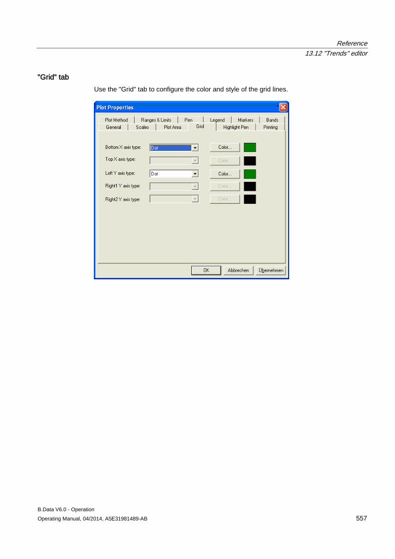
Reference 13.12 "Trends" editor
B.Data V6.0 - Operation Operating Manual, 04/2014, A5E31981489-AB 557
"Grid" tab Use the "Grid" tab to configure the color and style of the grid lines.
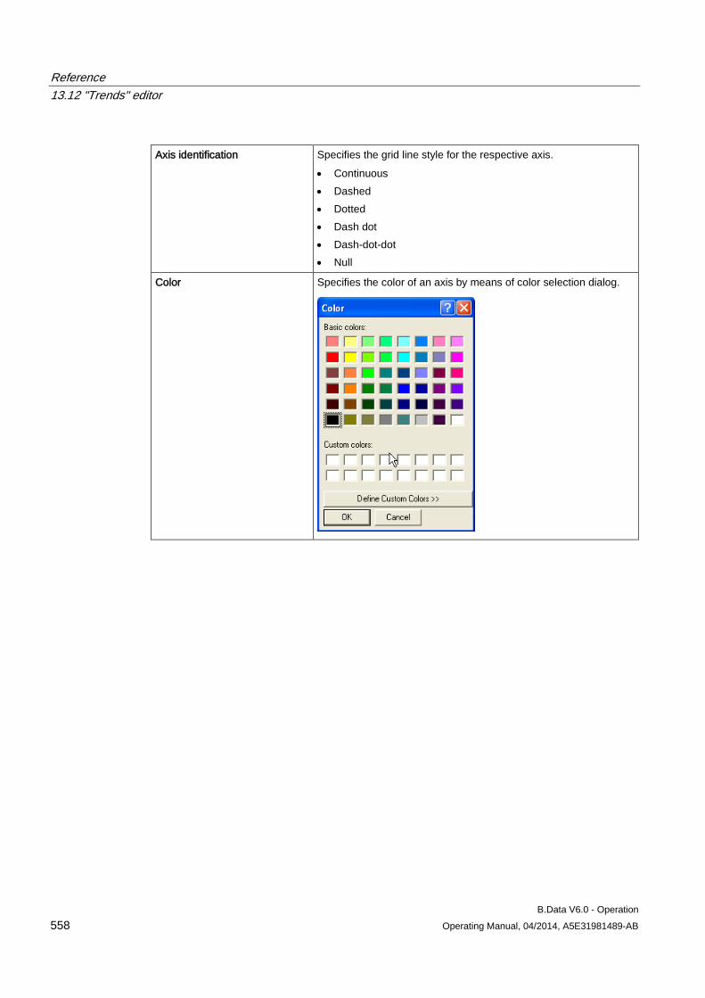
Reference 13.12 "Trends" editor
B.Data V6.0 - Operation 558 Operating Manual, 04/2014, A5E31981489-AB
Axis identification Specifies the grid line style for the respective axis.
• Continuous • Dashed • Dotted • Dash dot • Dash-dot-dot • Null
Color Specifies the color of an axis by means of color selection dialog.
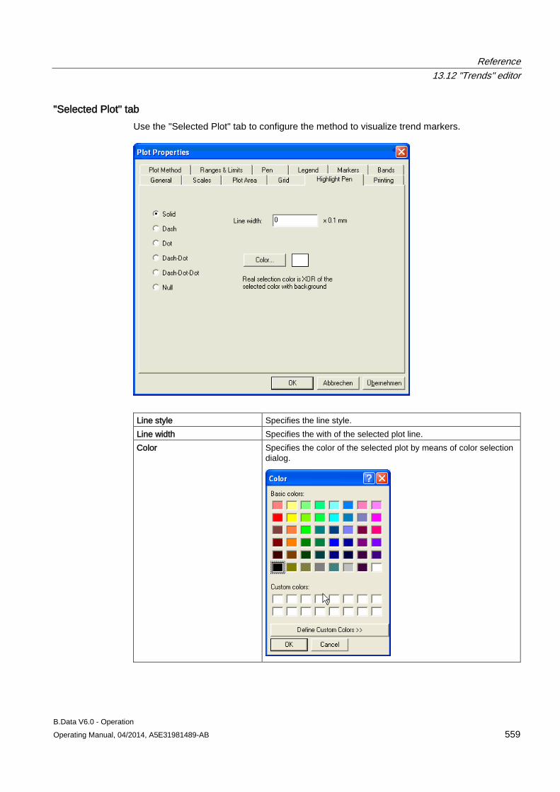
Reference 13.12 "Trends" editor
B.Data V6.0 - Operation Operating Manual, 04/2014, A5E31981489-AB 559
"Selected Plot" tab Use the "Selected Plot" tab to configure the method to visualize trend markers.
Line style Specifies the line style. Line width Specifies the with of the selected plot line. Color Specifies the color of the selected plot by means of color selection
dialog.
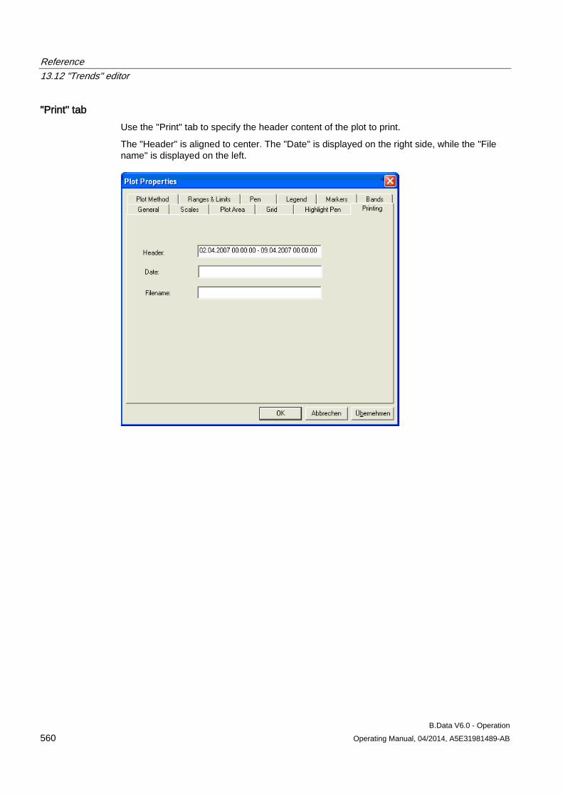
Reference 13.12 "Trends" editor
B.Data V6.0 - Operation 560 Operating Manual, 04/2014, A5E31981489-AB
"Print" tab Use the "Print" tab to specify the header content of the plot to print.
The "Header" is aligned to center. The "Date" is displayed on the right side, while the "File name" is displayed on the left.
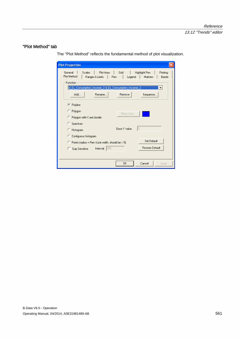
Reference 13.12 "Trends" editor
B.Data V6.0 - Operation Operating Manual, 04/2014, A5E31981489-AB 561
"Plot Method" tab The "Plot Method" reflects the fundamental method of plot visualization.
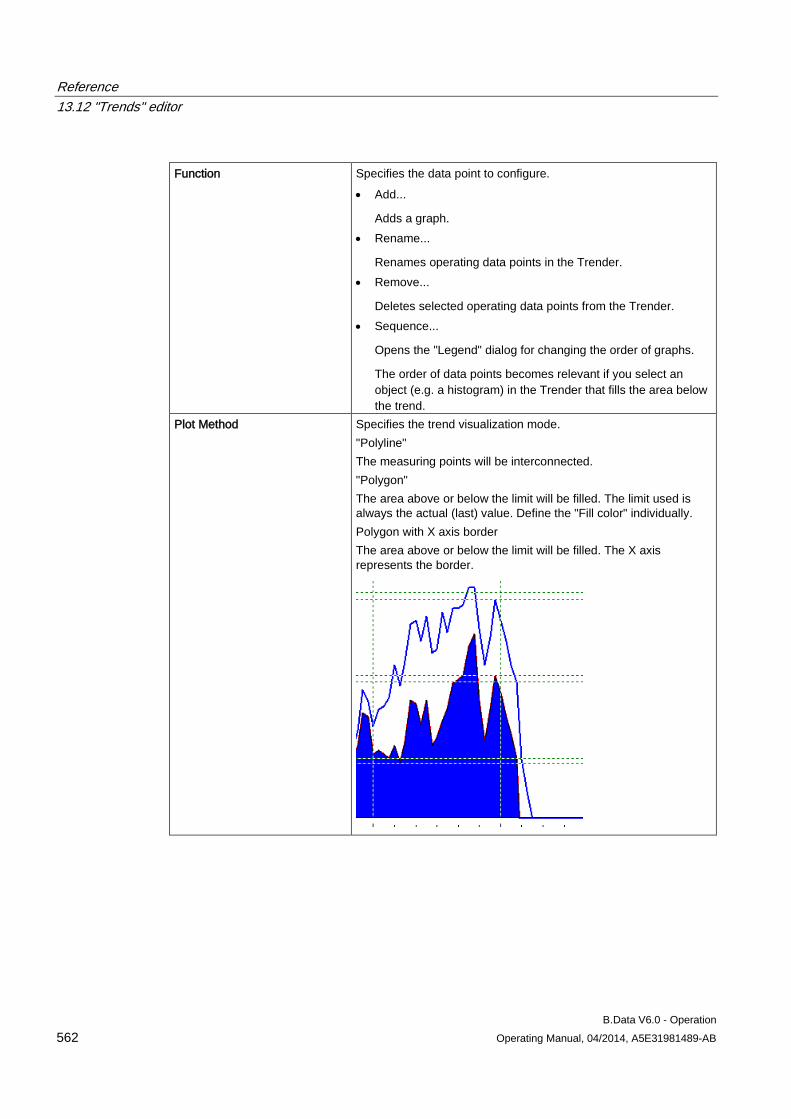
Reference 13.12 "Trends" editor
B.Data V6.0 - Operation 562 Operating Manual, 04/2014, A5E31981489-AB
Function Specifies the data point to configure.
• Add...
Adds a graph. • Rename...
Renames operating data points in the Trender. • Remove...
Deletes selected operating data points from the Trender. • Sequence...
Opens the "Legend" dialog for changing the order of graphs.
The order of data points becomes relevant if you select an object (e.g. a histogram) in the Trender that fills the area below the trend.
Plot Method Specifies the trend visualization mode. "Polyline" The measuring points will be interconnected. "Polygon" The area above or below the limit will be filled. The limit used is always the actual (last) value. Define the "Fill color" individually. Polygon with X axis border The area above or below the limit will be filled. The X axis represents the border.
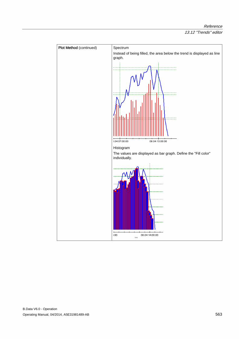
Reference 13.12 "Trends" editor
B.Data V6.0 - Operation Operating Manual, 04/2014, A5E31981489-AB 563
Plot Method (continued) Spectrum Instead of being filled, the area below the trend is displayed as line graph.
Histogram The values are displayed as bar graph. Define the "Fill color" individually.
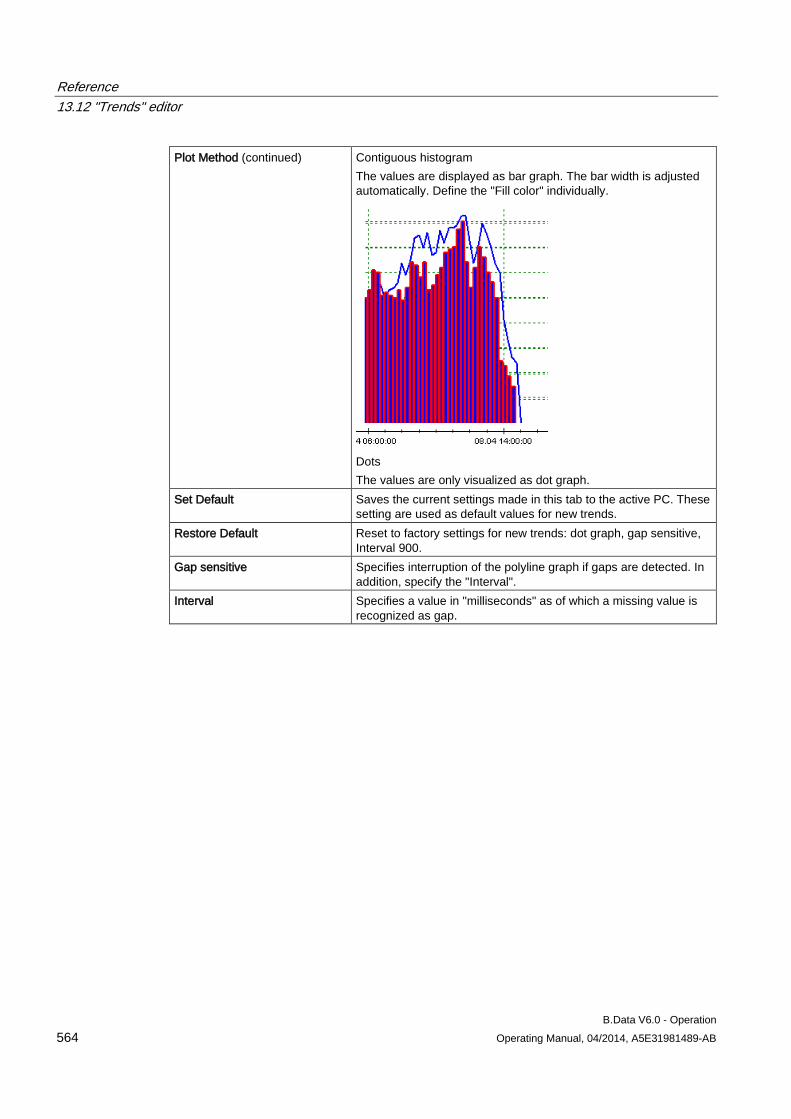
Reference 13.12 "Trends" editor
B.Data V6.0 - Operation 564 Operating Manual, 04/2014, A5E31981489-AB
Plot Method (continued) Contiguous histogram The values are displayed as bar graph. The bar width is adjusted automatically. Define the "Fill color" individually.
Dots The values are only visualized as dot graph.
Set Default Saves the current settings made in this tab to the active PC. These setting are used as default values for new trends.
Restore Default Reset to factory settings for new trends: dot graph, gap sensitive, Interval 900.
Gap sensitive Specifies interruption of the polyline graph if gaps are detected. In addition, specify the "Interval".
Interval Specifies a value in "milliseconds" as of which a missing value is recognized as gap.
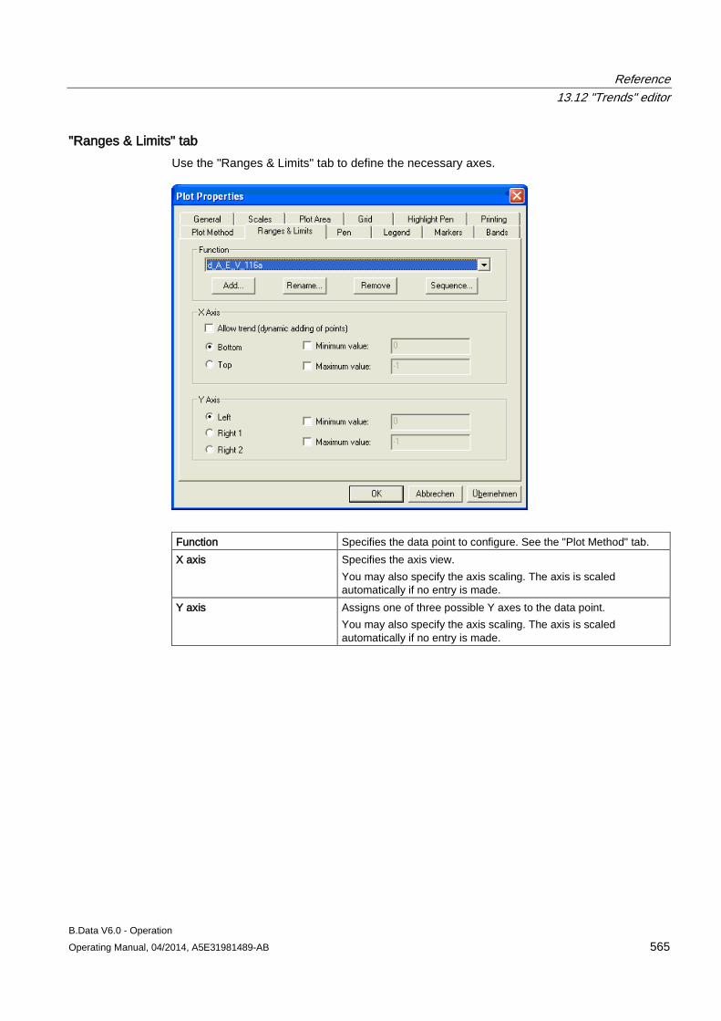
Reference 13.12 "Trends" editor
B.Data V6.0 - Operation Operating Manual, 04/2014, A5E31981489-AB 565
"Ranges & Limits" tab Use the "Ranges & Limits" tab to define the necessary axes.
Function Specifies the data point to configure. See the "Plot Method" tab. X axis Specifies the axis view.
You may also specify the axis scaling. The axis is scaled automatically if no entry is made.
Y axis Assigns one of three possible Y axes to the data point. You may also specify the axis scaling. The axis is scaled automatically if no entry is made.
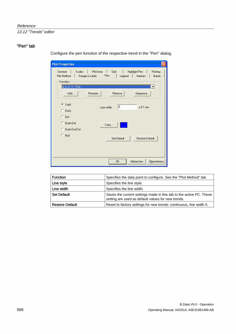
Reference 13.12 "Trends" editor
B.Data V6.0 - Operation 566 Operating Manual, 04/2014, A5E31981489-AB
"Pen" tab Configure the pen function of the respective trend in the "Pen" dialog.
Function Specifies the data point to configure. See the "Plot Method" tab. Line style Specifies the line style. Line width Specifies the line width. Set Default Saves the current settings made in this tab to the active PC. These
setting are used as default values for new trends. Restore Default Reset to factory settings for new trends: continuous, line width 5.
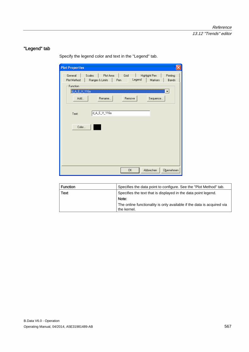
Reference 13.12 "Trends" editor
B.Data V6.0 - Operation Operating Manual, 04/2014, A5E31981489-AB 567
"Legend" tab Specify the legend color and text in the "Legend" tab.
Function Specifies the data point to configure. See the "Plot Method" tab. Text Specifies the text that is displayed in the data point legend.
Note: The online functionality is only available if the data is acquired via the kernel.
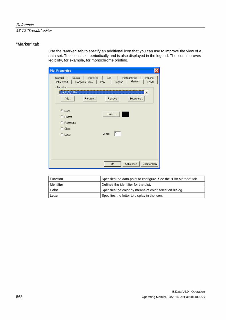
Reference 13.12 "Trends" editor
B.Data V6.0 - Operation 568 Operating Manual, 04/2014, A5E31981489-AB
"Marker" tab Use the "Marker" tab to specify an additional icon that you can use to improve the view of a data set. The icon is set periodically and is also displayed in the legend. The icon improves legibility, for example, for monochrome printing.
Function Specifies the data point to configure. See the "Plot Method" tab. Identifier Defines the identifier for the plot. Color Specifies the color by means of color selection dialog. Letter Specifies the letter to display in the icon.
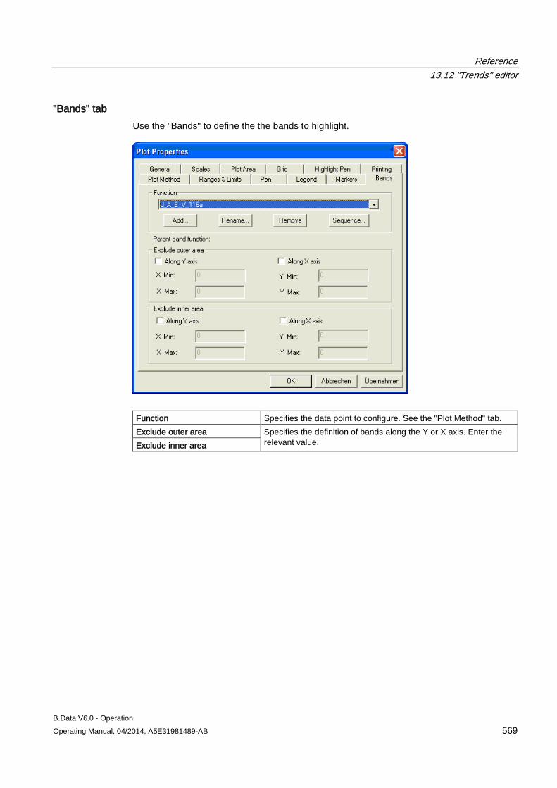
Reference 13.12 "Trends" editor
B.Data V6.0 - Operation Operating Manual, 04/2014, A5E31981489-AB 569
"Bands" tab Use the "Bands" to define the the bands to highlight.
Function Specifies the data point to configure. See the "Plot Method" tab. Exclude outer area Specifies the definition of bands along the Y or X axis. Enter the
relevant value. Exclude inner area
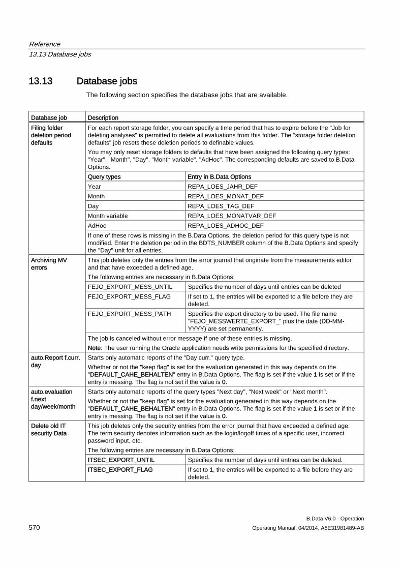
Reference 13.13 Database jobs
B.Data V6.0 - Operation 570 Operating Manual, 04/2014, A5E31981489-AB
13.13 Database jobs The following section specifies the database jobs that are available.
Database job Description Filing folder deletion period defaults
For each report storage folder, you can specify a time period that has to expire before the "Job for deleting analyses" is permitted to delete all evaluations from this folder. The "storage folder deletion defaults" job resets these deletion periods to definable values. You may only reset storage folders to defaults that have been assigned the following query types: "Year", "Month", "Day", "Month variable", "AdHoc". The corresponding defaults are saved to B.Data Options. Query types Entry in B.Data Options Year REPA_LOES_JAHR_DEF Month REPA_LOES_MONAT_DEF Day REPA_LOES_TAG_DEF Month variable REPA_LOES_MONATVAR_DEF AdHoc REPA_LOES_ADHOC_DEF If one of these rows is missing in the B.Data Options, the deletion period for this query type is not modified. Enter the deletion period in the BDTS_NUMBER column of the B.Data Options and specify the "Day" unit for all entries.
Archiving MV errors
This job deletes only the entries from the error journal that originate from the measurements editor and that have exceeded a defined age. The following entries are necessary in B.Data Options: FEJO_EXPORT_MESS_UNTIL Specifies the number of days until entries can be deleted FEJO_EXPORT_MESS_FLAG If set to 1, the entries will be exported to a file before they are
deleted. FEJO_EXPORT_MESS_PATH Specifies the export directory to be used. The file name
"FEJO_MESSWERTE_EXPORT_" plus the date (DD-MM-YYYY) are set permanently.
The job is canceled without error message if one of these entries is missing. Note: The user running the Oracle application needs write permissions for the specified directory.
auto.Report f.curr. day
Starts only automatic reports of the "Day curr." query type. Whether or not the "keep flag" is set for the evaluation generated in this way depends on the "DEFAULT_CAHE_BEHALTEN" entry in B.Data Options. The flag is set if the value 1 is set or if the entry is messing. The flag is not set if the value is 0.
auto.evaluation f.next day/week/month
Starts only automatic reports of the query types "Next day", "Next week" or "Next month". Whether or not the "keep flag" is set for the evaluation generated in this way depends on the "DEFAULT_CAHE_BEHALTEN" entry in B.Data Options. The flag is set if the value 1 is set or if the entry is messing. The flag is not set if the value is 0.
Delete old IT security Data
This job deletes only the security entries from the error journal that have exceeded a defined age. The term security denotes information such as the login/logoff times of a specific user, incorrect password input, etc. The following entries are necessary in B.Data Options: ITSEC_EXPORT_UNTIL Specifies the number of days until entries can be deleted. ITSEC_EXPORT_FLAG If set to 1, the entries will be exported to a file before they are
deleted.
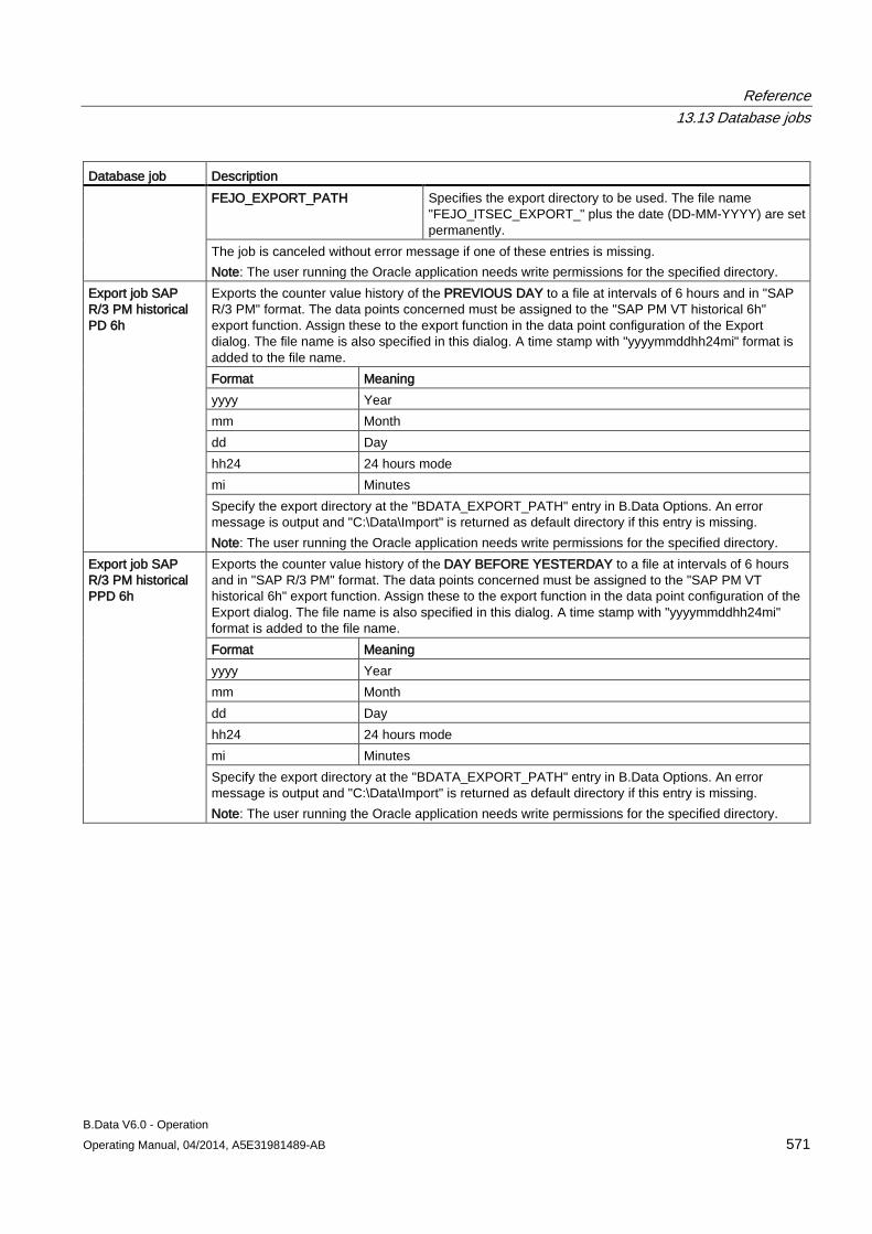
Reference 13.13 Database jobs
B.Data V6.0 - Operation Operating Manual, 04/2014, A5E31981489-AB 571
Database job Description FEJO_EXPORT_PATH Specifies the export directory to be used. The file name
"FEJO_ITSEC_EXPORT_" plus the date (DD-MM-YYYY) are set permanently.
The job is canceled without error message if one of these entries is missing. Note: The user running the Oracle application needs write permissions for the specified directory.
Export job SAP R/3 PM historical PD 6h
Exports the counter value history of the PREVIOUS DAY to a file at intervals of 6 hours and in "SAP R/3 PM" format. The data points concerned must be assigned to the "SAP PM VT historical 6h" export function. Assign these to the export function in the data point configuration of the Export dialog. The file name is also specified in this dialog. A time stamp with "yyyymmddhh24mi" format is added to the file name. Format Meaning yyyy Year mm Month dd Day hh24 24 hours mode mi Minutes Specify the export directory at the "BDATA_EXPORT_PATH" entry in B.Data Options. An error message is output and "C:\Data\Import" is returned as default directory if this entry is missing. Note: The user running the Oracle application needs write permissions for the specified directory.
Export job SAP R/3 PM historical PPD 6h
Exports the counter value history of the DAY BEFORE YESTERDAY to a file at intervals of 6 hours and in "SAP R/3 PM" format. The data points concerned must be assigned to the "SAP PM VT historical 6h" export function. Assign these to the export function in the data point configuration of the Export dialog. The file name is also specified in this dialog. A time stamp with "yyyymmddhh24mi" format is added to the file name. Format Meaning yyyy Year mm Month dd Day hh24 24 hours mode mi Minutes Specify the export directory at the "BDATA_EXPORT_PATH" entry in B.Data Options. An error message is output and "C:\Data\Import" is returned as default directory if this entry is missing. Note: The user running the Oracle application needs write permissions for the specified directory.
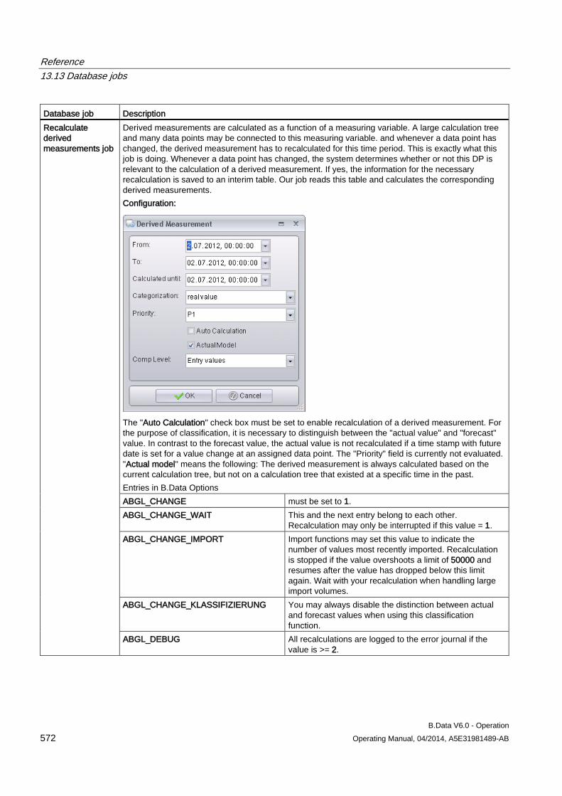
Reference 13.13 Database jobs
B.Data V6.0 - Operation 572 Operating Manual, 04/2014, A5E31981489-AB
Database job Description Recalculate derived measurements job
Derived measurements are calculated as a function of a measuring variable. A large calculation tree and many data points may be connected to this measuring variable. and whenever a data point has changed, the derived measurement has to recalculated for this time period. This is exactly what this job is doing. Whenever a data point has changed, the system determines whether or not this DP is relevant to the calculation of a derived measurement. If yes, the information for the necessary recalculation is saved to an interim table. Our job reads this table and calculates the corresponding derived measurements. Configuration:
The "Auto Calculation" check box must be set to enable recalculation of a derived measurement. For the purpose of classification, it is necessary to distinguish between the "actual value" and "forecast" value. In contrast to the forecast value, the actual value is not recalculated if a time stamp with future date is set for a value change at an assigned data point. The "Priority" field is currently not evaluated. "Actual model" means the following: The derived measurement is always calculated based on the current calculation tree, but not on a calculation tree that existed at a specific time in the past. Entries in B.Data Options ABGL_CHANGE must be set to 1. ABGL_CHANGE_WAIT This and the next entry belong to each other.
Recalculation may only be interrupted if this value = 1. ABGL_CHANGE_IMPORT Import functions may set this value to indicate the
number of values most recently imported. Recalculation is stopped if the value overshoots a limit of 50000 and resumes after the value has dropped below this limit again. Wait with your recalculation when handling large import volumes.
ABGL_CHANGE_KLASSIFIZIERUNG You may always disable the distinction between actual and forecast values when using this classification function.
ABGL_DEBUG All recalculations are logged to the error journal if the value is >= 2.
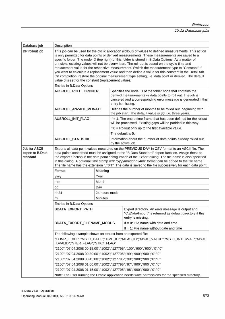
Reference 13.13 Database jobs
B.Data V6.0 - Operation Operating Manual, 04/2014, A5E31981489-AB 573
Database job Description DP rollout job This job can be used for the cyclic allocation (rollout) of values to defined measurements. This action
is only permitted for data points or derived measurements. These measurements are saved to a specific folder. The node ID (top right) of this folder is stored in B.Data Options. As a matter of principle, existing values will not be overwritten. The roll-out is based on the cycle time and replacement value for the respective measurement. Switch the measurement type to "Constant" if you want to calculate a replacement value and then define a value for this constant in the Detail tab. On completion, restore the original measurement type setting, i.e. data point or derived. The default value 0 is set for the constant (replacement value). Entries in B.Data Options AUSROLL_ROOT_ORDNER Specifies the node ID of the folder node that contains the
derived measurements or data points to roll out. The job is canceled and a corresponding error message is generated if this entry is missing.
AUSROLL_ANZAHL_MONATE Defines the number of months to be rolled out, beginning with the job start. The default value is 36, i.e. three years.
AUSROLL_INIT_FLAG If = 1: The entire time frame that has been defined for the rollout will be processed. Existing gaps will be padded in this way. If 0 = Rollout only up to the first available value. The default is 0.
AUSROLL_STATISTIK Information about the number of data points already rolled out by the active job.
Job for ASCII export to B.Data standard
Exports all data point values measured on the PREVIOUS DAY in CSV format to an ASCII file. The data points concerned must be assigned to the "B.Data Standard" export function. Assign these to the export function in the data point configuration of the Export dialog. The file name is also specified in this dialog. A optional time stamp with "yyyymmddhh24mi" format can be added to the file name. The file name has the extension ".TXT". The data is saved to the file successively for each data point. Format Meaning yyyy Year mm Month dd Day hh24 24 hours mode mi Minutes Entries in B.Data Options BDATA_EXPORT_PATH Export directory. An error message is output and
"C:\Data\Import" is returned as default directory if this entry is missing.
BDATA_EXPORT_FILENAME_MODUS If = 0: File name with date and time. If = 1: File name without date and time
The following example shows an extract from an exported file: "COMP_LEVEL";"MSJO_DATE";"TIME_ID";"MEAS_ID";"MSJO_VALUE";"MSJO_INTERVAL";"MSJO_DVALID";"STER_FLAG";"STKO_FLAG" "2100";"07.04.2008 00:15:00";"1002";"127795";"100";"900";"900";"0";"0" "2100";"07.04.2008 00:30:00";"1002";"127795";"99";"900";"900";"0";"0" "2100";"07.04.2008 00:45:00";"1002";"127795";"98";"900";"900";"0";"0" "2100";"07.04.2008 01:00:00";"1002";"127795";"97";"900";"900";"0";"0" "2100";"07.04.2008 01:15:00";"1002";"127795";"96";"900";"900";"0";"0" Note: The user running the Oracle application needs write permissions for the specified directory.
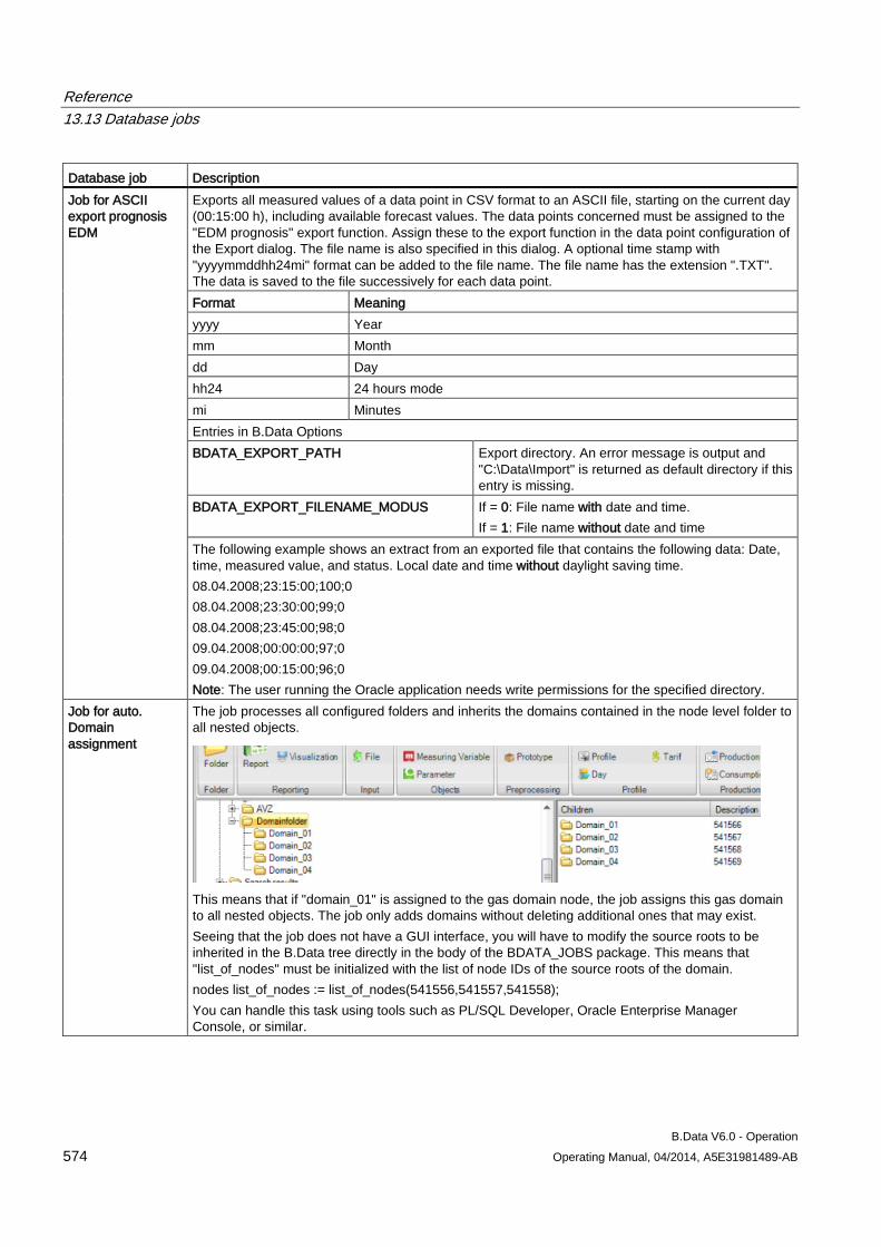
Reference 13.13 Database jobs
B.Data V6.0 - Operation 574 Operating Manual, 04/2014, A5E31981489-AB
Database job Description Job for ASCII export prognosis EDM
Exports all measured values of a data point in CSV format to an ASCII file, starting on the current day (00:15:00 h), including available forecast values. The data points concerned must be assigned to the "EDM prognosis" export function. Assign these to the export function in the data point configuration of the Export dialog. The file name is also specified in this dialog. A optional time stamp with "yyyymmddhh24mi" format can be added to the file name. The file name has the extension ".TXT". The data is saved to the file successively for each data point. Format Meaning yyyy Year mm Month dd Day hh24 24 hours mode mi Minutes Entries in B.Data Options BDATA_EXPORT_PATH Export directory. An error message is output and
"C:\Data\Import" is returned as default directory if this entry is missing.
BDATA_EXPORT_FILENAME_MODUS If = 0: File name with date and time. If = 1: File name without date and time
The following example shows an extract from an exported file that contains the following data: Date, time, measured value, and status. Local date and time without daylight saving time. 08.04.2008;23:15:00;100;0 08.04.2008;23:30:00;99;0 08.04.2008;23:45:00;98;0 09.04.2008;00:00:00;97;0 09.04.2008;00:15:00;96;0 Note: The user running the Oracle application needs write permissions for the specified directory.
Job for auto. Domain assignment
The job processes all configured folders and inherits the domains contained in the node level folder to all nested objects.
This means that if "domain_01" is assigned to the gas domain node, the job assigns this gas domain to all nested objects. The job only adds domains without deleting additional ones that may exist. Seeing that the job does not have a GUI interface, you will have to modify the source roots to be inherited in the B.Data tree directly in the body of the BDATA_JOBS package. This means that "list_of_nodes" must be initialized with the list of node IDs of the source roots of the domain. nodes list_of_nodes := list_of_nodes(541556,541557,541558); You can handle this task using tools such as PL/SQL Developer, Oracle Enterprise Manager Console, or similar.
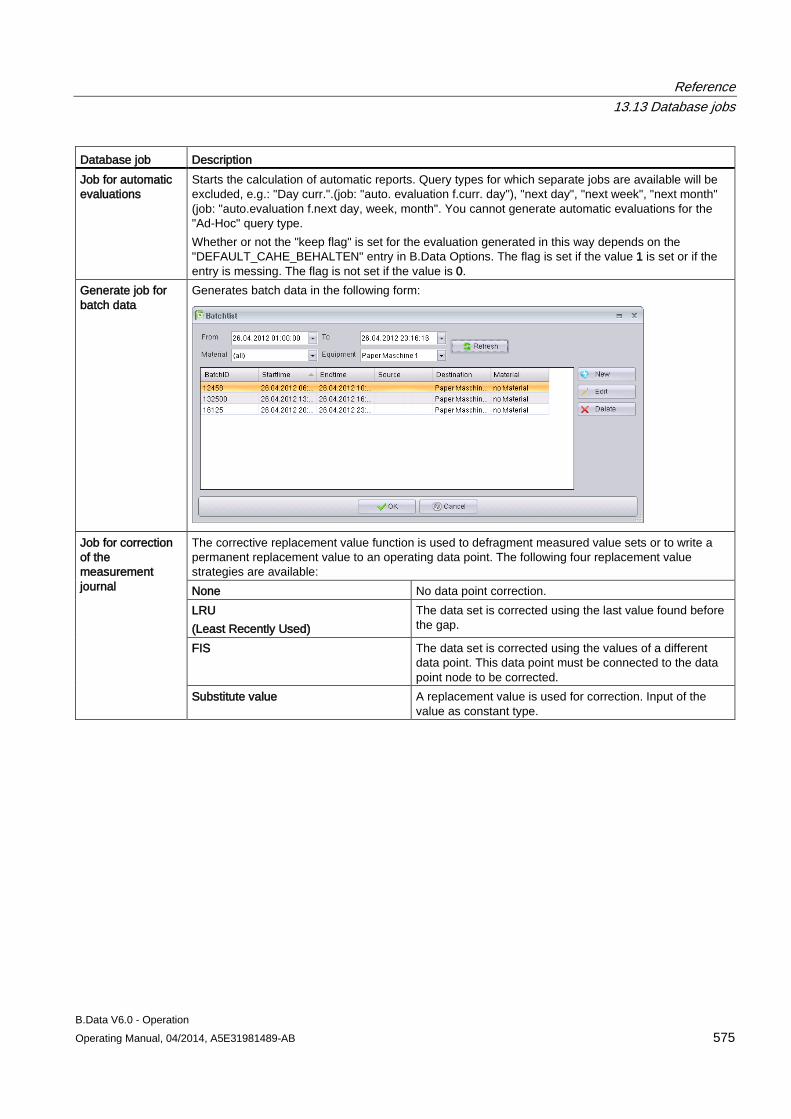
Reference 13.13 Database jobs
B.Data V6.0 - Operation Operating Manual, 04/2014, A5E31981489-AB 575
Database job Description Job for automatic evaluations
Starts the calculation of automatic reports. Query types for which separate jobs are available will be excluded, e.g.: "Day curr.".(job: "auto. evaluation f.curr. day"), "next day", "next week", "next month" (job: "auto.evaluation f.next day, week, month". You cannot generate automatic evaluations for the "Ad-Hoc" query type. Whether or not the "keep flag" is set for the evaluation generated in this way depends on the "DEFAULT_CAHE_BEHALTEN" entry in B.Data Options. The flag is set if the value 1 is set or if the entry is messing. The flag is not set if the value is 0.
Generate job for batch data
Generates batch data in the following form:
Job for correction of the measurement journal
The corrective replacement value function is used to defragment measured value sets or to write a permanent replacement value to an operating data point. The following four replacement value strategies are available: None No data point correction. LRU (Least Recently Used)
The data set is corrected using the last value found before the gap.
FIS The data set is corrected using the values of a different data point. This data point must be connected to the data point node to be corrected.
Substitute value A replacement value is used for correction. Input of the value as constant type.
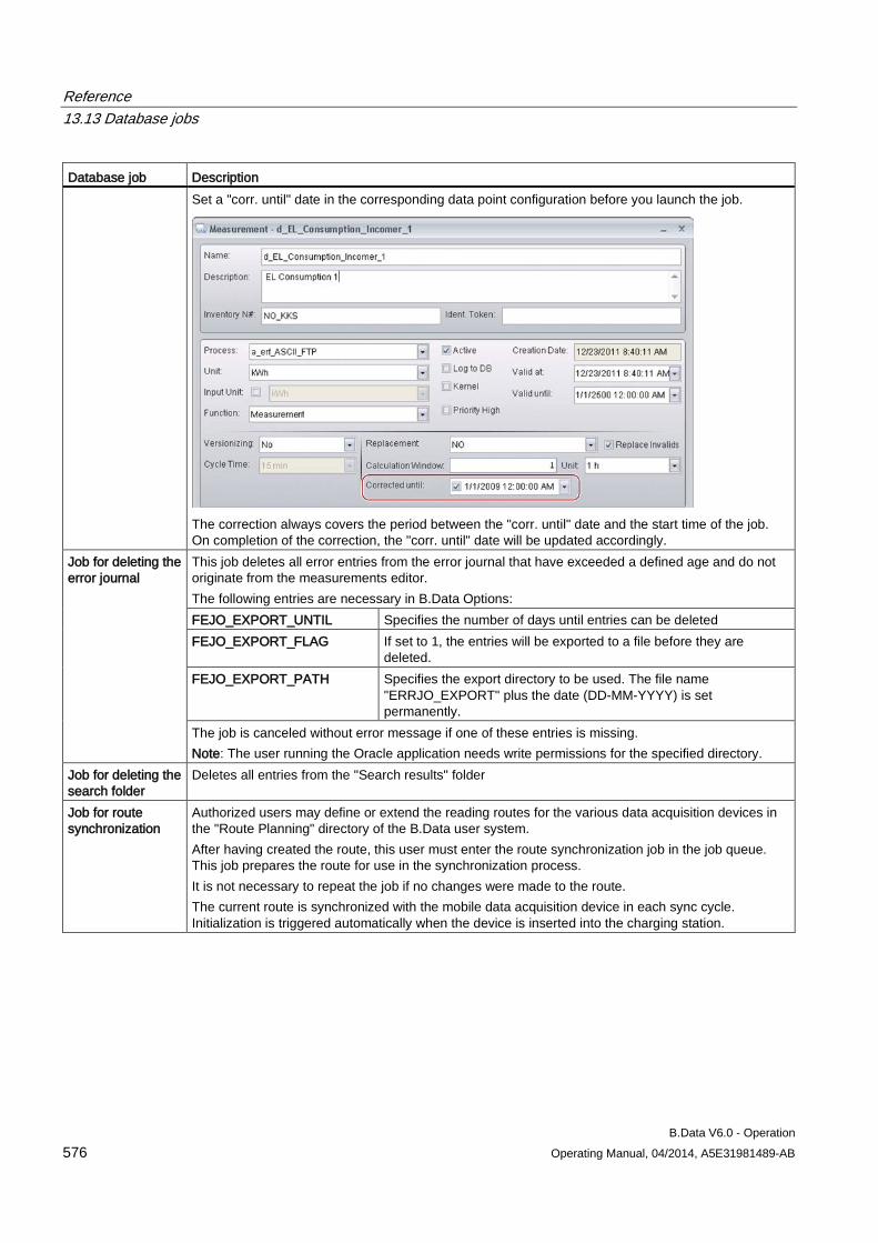
Reference 13.13 Database jobs
B.Data V6.0 - Operation 576 Operating Manual, 04/2014, A5E31981489-AB
Database job Description Set a "corr. until" date in the corresponding data point configuration before you launch the job.
The correction always covers the period between the "corr. until" date and the start time of the job. On completion of the correction, the "corr. until" date will be updated accordingly.
Job for deleting the error journal
This job deletes all error entries from the error journal that have exceeded a defined age and do not originate from the measurements editor. The following entries are necessary in B.Data Options: FEJO_EXPORT_UNTIL Specifies the number of days until entries can be deleted FEJO_EXPORT_FLAG If set to 1, the entries will be exported to a file before they are
deleted. FEJO_EXPORT_PATH Specifies the export directory to be used. The file name
"ERRJO_EXPORT" plus the date (DD-MM-YYYY) is set permanently.
The job is canceled without error message if one of these entries is missing. Note: The user running the Oracle application needs write permissions for the specified directory.
Job for deleting the search folder
Deletes all entries from the "Search results" folder
Job for route synchronization
Authorized users may define or extend the reading routes for the various data acquisition devices in the "Route Planning" directory of the B.Data user system. After having created the route, this user must enter the route synchronization job in the job queue. This job prepares the route for use in the synchronization process. It is not necessary to repeat the job if no changes were made to the route. The current route is synchronized with the mobile data acquisition device in each sync cycle. Initialization is triggered automatically when the device is inserted into the charging station.
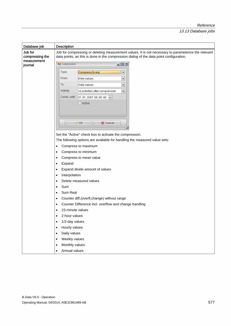
Reference 13.13 Database jobs
B.Data V6.0 - Operation Operating Manual, 04/2014, A5E31981489-AB 577
Database job Description Job for compressing the measurement journal
Job for compressing or deleting measurement values. It is not necessary to parameterize the relevant data points, as this is done in the compression dialog of the data point configuration.
Set the "Active" check box to activate the compression. The following options are available for handling the measured value sets: • Compress to maximum • Compress to minimum • Compress to mean value • Expand • Expand divide amount of values • Interpolation • Delete measured values • Sum • Sum Real • Counter diff.(overfl,change) without range • Counter Difference incl. overflow and change handling • 15-minute values • 2-hour values • 1/2-day values • Hourly values • Daily values • Weekly values • Monthly values • Annual values
Reference 13.13 Database jobs
B.Data V6.0 - Operation 578 Operating Manual, 04/2014, A5E31981489-AB
Database job Description Job for compressing the measurement journal (continued)
It is only possible to compress shorter intervals into a longer interval and to expand a longer interval to shorter intervals. Note that expansion to weekly intervals is not permitted. The term "entry values" denotes the measured values that were originally imported into the B.Data system. The input data can be deleted after compression. Based on the "compressed until" date and provided corresponding data is available, the intervals are always compressed, expanded, or deleted until the time of job start. The "compressed until" date is compressed accordingly on completion and may be edited manually by users. If "no action after compression" was activated, the entry and compressed values will be available in the same data point. The values to be displayed or processed depend on the compression status. Expansion encompasses the source values that are available as "entry values" and saved in accordance with the corresponding acquisition level. Example: A cycle time of "1 hour" is defined for a data point. Assuming that daily values are input for this data point (acquisition level = entry values) and expanded to these hourly values, the daily values are copied to acquisition level "daily values", which means that the expanded values are now stored as "entry values". This solution lets you work with expanded values in the "Entry values" dialog and access the output data in the "Daily values" dialog. The "Interpolation" type is only available for the compression of entry values and also serves to pad missing time stamps based on the acquisition pattern of the data point (non-cyclic counter readings). Whether or not to display a done message in the "Logging Editor" can be specified by means of an entry in the PRINT_VOLLZUGS_MELDUNG row of the B.Data Options. A message is only output if this setting equals 1.
MSQL import job The job imports data from a table in a Microsoft SQL Server database into the B.Data system. This table must be named "tblEmsExport". A data point to be imported must be active and assigned to the process with ID 572 (usually the "a_acq_DB" process). The data point address must correspond to the "tta_id" in the SQL Server table. It is assumed that the time stamps in the SQL Server table are available in local time format without daylight saving time. If a value greater than 0 is set in the IMPORT_DEBUG row in B.Data Options, a corresponding entry is written to the "Logging Editor" at the start and end of the job. At the end as statistics. This function is not included in the standard software package.
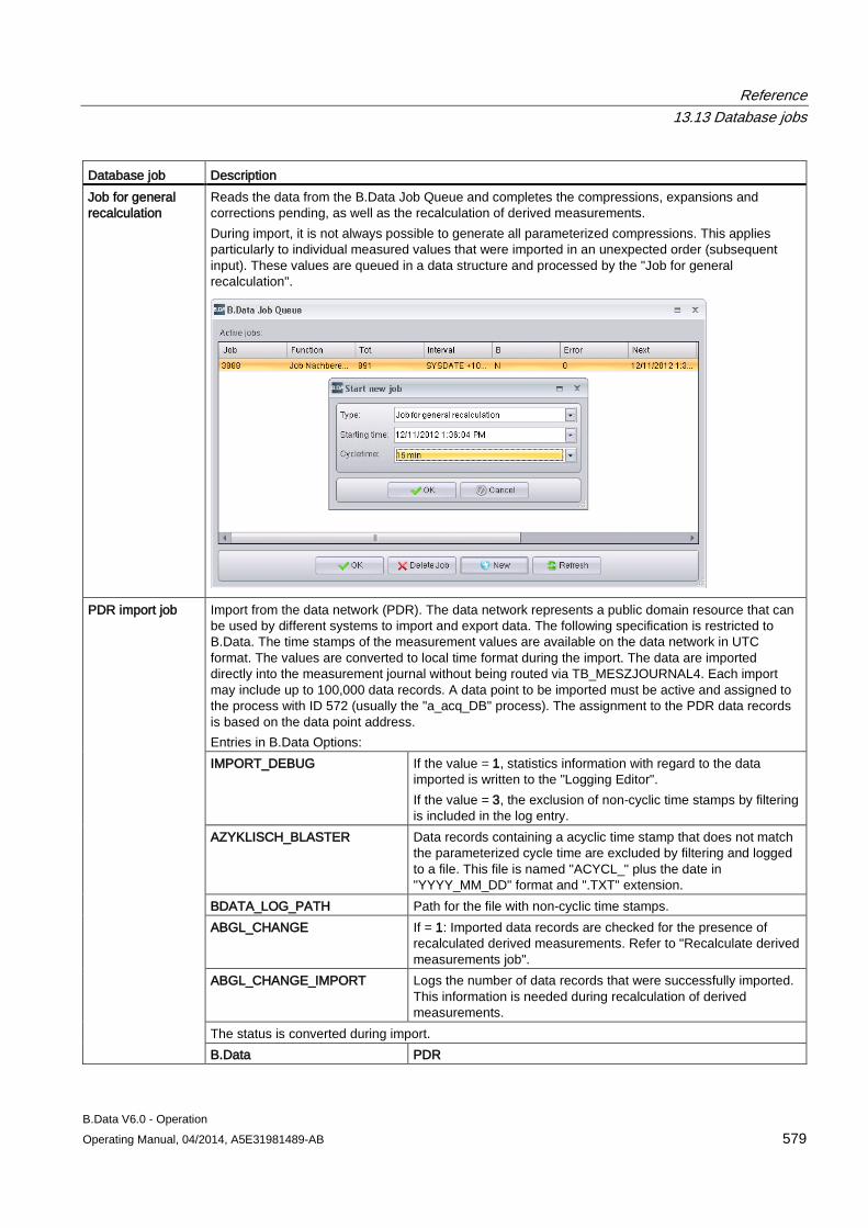
Reference 13.13 Database jobs
B.Data V6.0 - Operation Operating Manual, 04/2014, A5E31981489-AB 579
Database job Description Job for general recalculation
Reads the data from the B.Data Job Queue and completes the compressions, expansions and corrections pending, as well as the recalculation of derived measurements. During import, it is not always possible to generate all parameterized compressions. This applies particularly to individual measured values that were imported in an unexpected order (subsequent input). These values are queued in a data structure and processed by the "Job for general recalculation".
PDR import job Import from the data network (PDR). The data network represents a public domain resource that can be used by different systems to import and export data. The following specification is restricted to B.Data. The time stamps of the measurement values are available on the data network in UTC format. The values are converted to local time format during the import. The data are imported directly into the measurement journal without being routed via TB_MESZJOURNAL4. Each import may include up to 100,000 data records. A data point to be imported must be active and assigned to the process with ID 572 (usually the "a_acq_DB" process). The assignment to the PDR data records is based on the data point address. Entries in B.Data Options: IMPORT_DEBUG If the value = 1, statistics information with regard to the data
imported is written to the "Logging Editor". If the value = 3, the exclusion of non-cyclic time stamps by filtering is included in the log entry.
AZYKLISCH_BLASTER Data records containing a acyclic time stamp that does not match the parameterized cycle time are excluded by filtering and logged to a file. This file is named "ACYCL_" plus the date in "YYYY_MM_DD" format and ".TXT" extension.
BDATA_LOG_PATH Path for the file with non-cyclic time stamps. ABGL_CHANGE If = 1: Imported data records are checked for the presence of
recalculated derived measurements. Refer to "Recalculate derived measurements job".
ABGL_CHANGE_IMPORT Logs the number of data records that were successfully imported. This information is needed during recalculation of derived measurements.
The status is converted during import. B.Data PDR
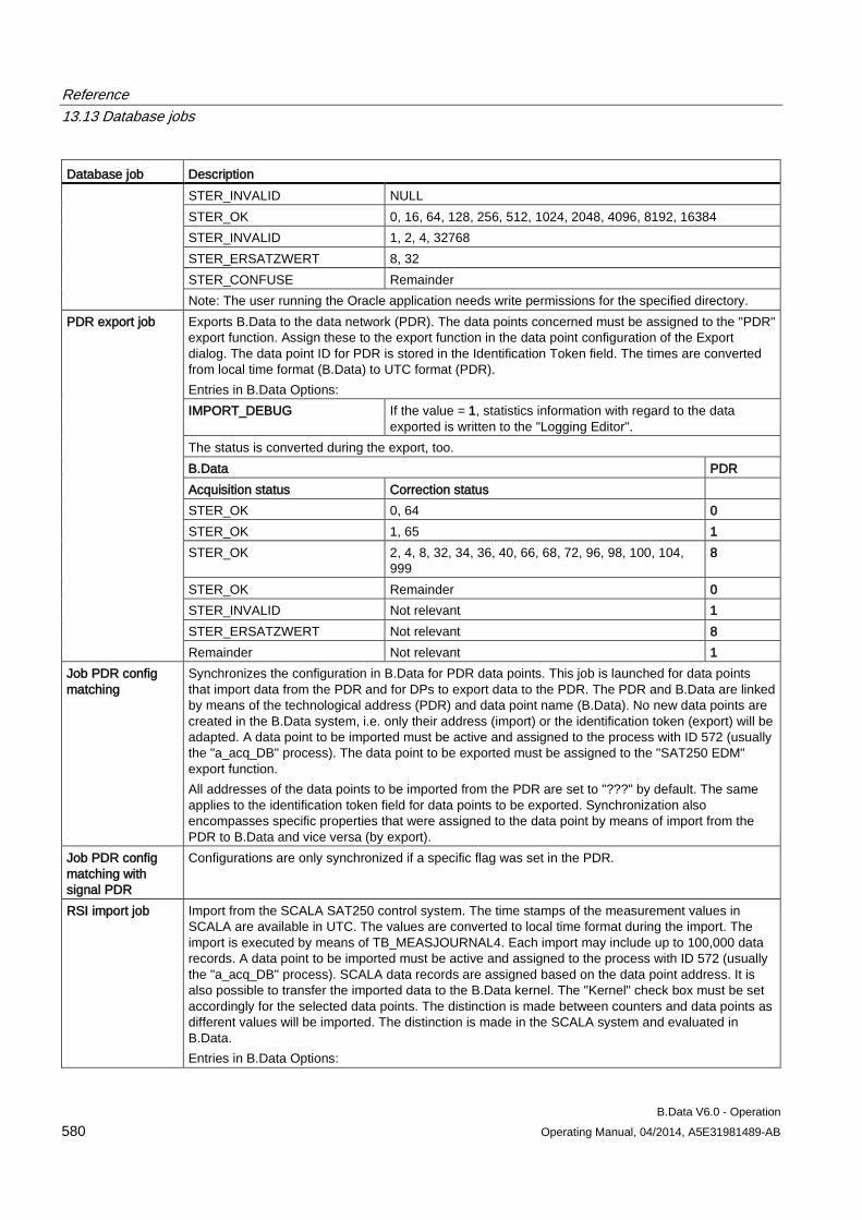
Reference 13.13 Database jobs
B.Data V6.0 - Operation 580 Operating Manual, 04/2014, A5E31981489-AB
Database job Description STER_INVALID NULL STER_OK 0, 16, 64, 128, 256, 512, 1024, 2048, 4096, 8192, 16384 STER_INVALID 1, 2, 4, 32768 STER_ERSATZWERT 8, 32 STER_CONFUSE Remainder Note: The user running the Oracle application needs write permissions for the specified directory.
PDR export job Exports B.Data to the data network (PDR). The data points concerned must be assigned to the "PDR" export function. Assign these to the export function in the data point configuration of the Export dialog. The data point ID for PDR is stored in the Identification Token field. The times are converted from local time format (B.Data) to UTC format (PDR). Entries in B.Data Options: IMPORT_DEBUG If the value = 1, statistics information with regard to the data
exported is written to the "Logging Editor". The status is converted during the export, too. B.Data PDR Acquisition status Correction status STER_OK 0, 64 0 STER_OK 1, 65 1 STER_OK 2, 4, 8, 32, 34, 36, 40, 66, 68, 72, 96, 98, 100, 104,
999 8
STER_OK Remainder 0 STER_INVALID Not relevant 1 STER_ERSATZWERT Not relevant 8 Remainder Not relevant 1
Job PDR config matching
Synchronizes the configuration in B.Data for PDR data points. This job is launched for data points that import data from the PDR and for DPs to export data to the PDR. The PDR and B.Data are linked by means of the technological address (PDR) and data point name (B.Data). No new data points are created in the B.Data system, i.e. only their address (import) or the identification token (export) will be adapted. A data point to be imported must be active and assigned to the process with ID 572 (usually the "a_acq_DB" process). The data point to be exported must be assigned to the "SAT250 EDM" export function. All addresses of the data points to be imported from the PDR are set to "???" by default. The same applies to the identification token field for data points to be exported. Synchronization also encompasses specific properties that were assigned to the data point by means of import from the PDR to B.Data and vice versa (by export).
Job PDR config matching with signal PDR
Configurations are only synchronized if a specific flag was set in the PDR.
RSI import job Import from the SCALA SAT250 control system. The time stamps of the measurement values in SCALA are available in UTC. The values are converted to local time format during the import. The import is executed by means of TB_MEASJOURNAL4. Each import may include up to 100,000 data records. A data point to be imported must be active and assigned to the process with ID 572 (usually the "a_acq_DB" process). SCALA data records are assigned based on the data point address. It is also possible to transfer the imported data to the B.Data kernel. The "Kernel" check box must be set accordingly for the selected data points. The distinction is made between counters and data points as different values will be imported. The distinction is made in the SCALA system and evaluated in B.Data. Entries in B.Data Options:
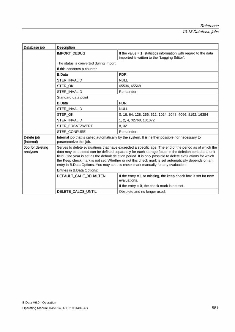
Reference 13.13 Database jobs
B.Data V6.0 - Operation Operating Manual, 04/2014, A5E31981489-AB 581
Database job Description IMPORT_DEBUG If the value = 1, statistics information with regard to the data
imported is written to the "Logging Editor". The status is converted during import. If this concerns a counter B.Data PDR STER_INVALID NULL STER_OK 65536, 65568 STER_INVALID Remainder Standard data point B.Data PDR STER_INVALID NULL STER_OK 0, 16, 64, 128, 256, 512, 1024, 2048, 4096, 8192, 16384 STER_INVALID 1, 2, 4, 32768, 131072 STER_ERSATZWERT 8, 32 STER_CONFUSE Remainder
Delete job (internal)
Internal job that is called automatically by the system. It is neither possible nor necessary to parameterize this job.
Job for deleting analyses
Serves to delete evaluations that have exceeded a specific age. The end of the period as of which the data may be deleted can be defined separately for each storage folder in the deletion period and unit field. One year is set as the default deletion period. It is only possible to delete evaluations for which the Keep check mark is not set. Whether or not this check mark is set automatically depends on an entry in B.Data Options. You may set this check mark manually for any evaluation. Entries in B.Data Options: DEFAULT_CAHE_BEHALTEN If the entry = 1 or missing, the keep check box is set for new
evaluations. If the entry = 0, the check mark is not set.
DELETE_CALCS_UNTIL Obsolete and no longer used.
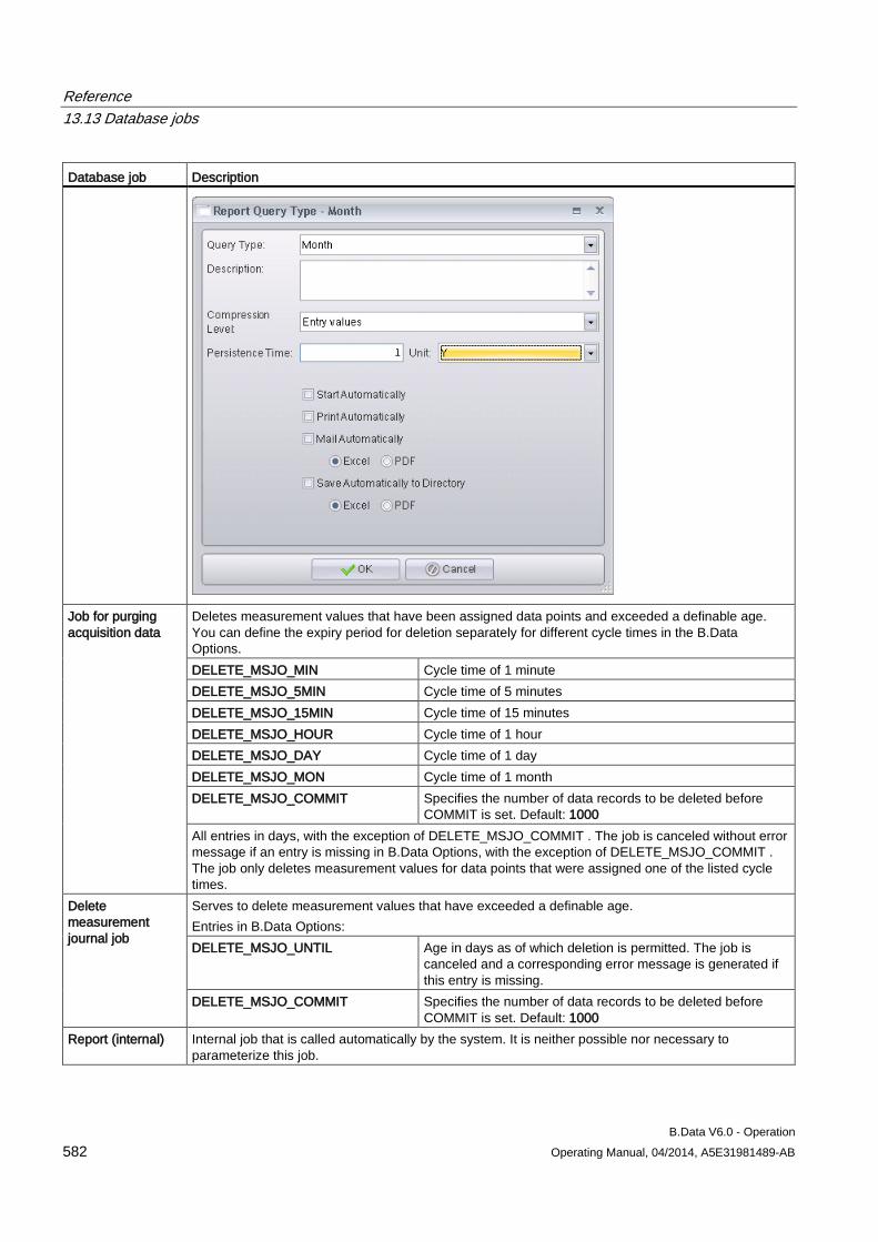
Reference 13.13 Database jobs
B.Data V6.0 - Operation 582 Operating Manual, 04/2014, A5E31981489-AB
Database job Description
Job for purging acquisition data
Deletes measurement values that have been assigned data points and exceeded a definable age. You can define the expiry period for deletion separately for different cycle times in the B.Data Options. DELETE_MSJO_MIN Cycle time of 1 minute DELETE_MSJO_5MIN Cycle time of 5 minutes DELETE_MSJO_15MIN Cycle time of 15 minutes DELETE_MSJO_HOUR Cycle time of 1 hour DELETE_MSJO_DAY Cycle time of 1 day DELETE_MSJO_MON Cycle time of 1 month DELETE_MSJO_COMMIT Specifies the number of data records to be deleted before
COMMIT is set. Default: 1000 All entries in days, with the exception of DELETE_MSJO_COMMIT . The job is canceled without error message if an entry is missing in B.Data Options, with the exception of DELETE_MSJO_COMMIT . The job only deletes measurement values for data points that were assigned one of the listed cycle times.
Delete measurement journal job
Serves to delete measurement values that have exceeded a definable age. Entries in B.Data Options: DELETE_MSJO_UNTIL Age in days as of which deletion is permitted. The job is
canceled and a corresponding error message is generated if this entry is missing.
DELETE_MSJO_COMMIT Specifies the number of data records to be deleted before COMMIT is set. Default: 1000
Report (internal) Internal job that is called automatically by the system. It is neither possible nor necessary to parameterize this job.

Reference 13.13 Database jobs
B.Data V6.0 - Operation Operating Manual, 04/2014, A5E31981489-AB 583
Database job Description Sort job (internal) Internal job that is called automatically by the system. It is neither possible nor necessary to
parameterize this job.
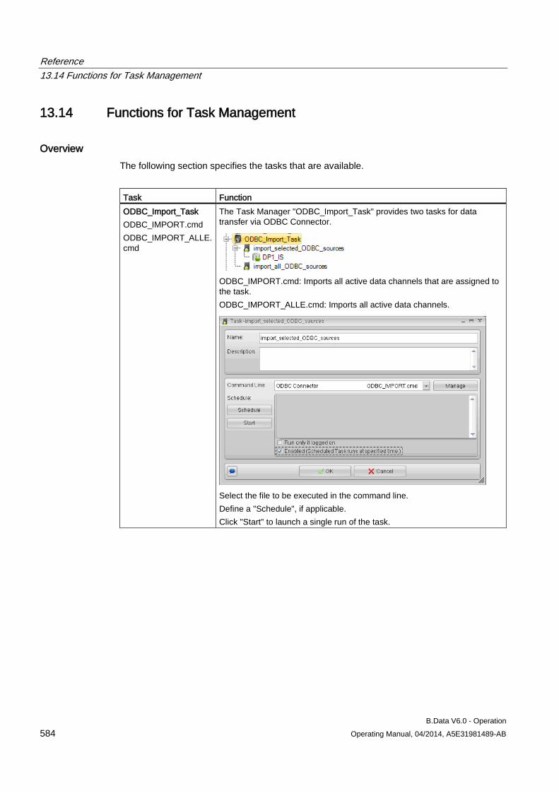
Reference 13.14 Functions for Task Management
B.Data V6.0 - Operation 584 Operating Manual, 04/2014, A5E31981489-AB
13.14 Functions for Task Management
Overview The following section specifies the tasks that are available.
Task Function ODBC_Import_Task ODBC_IMPORT.cmd ODBC_IMPORT_ALLE.cmd
The Task Manager "ODBC_Import_Task" provides two tasks for data transfer via ODBC Connector.
ODBC_IMPORT.cmd: Imports all active data channels that are assigned to the task. ODBC_IMPORT_ALLE.cmd: Imports all active data channels.
Select the file to be executed in the command line. Define a "Schedule", if applicable. Click "Start" to launch a single run of the task.
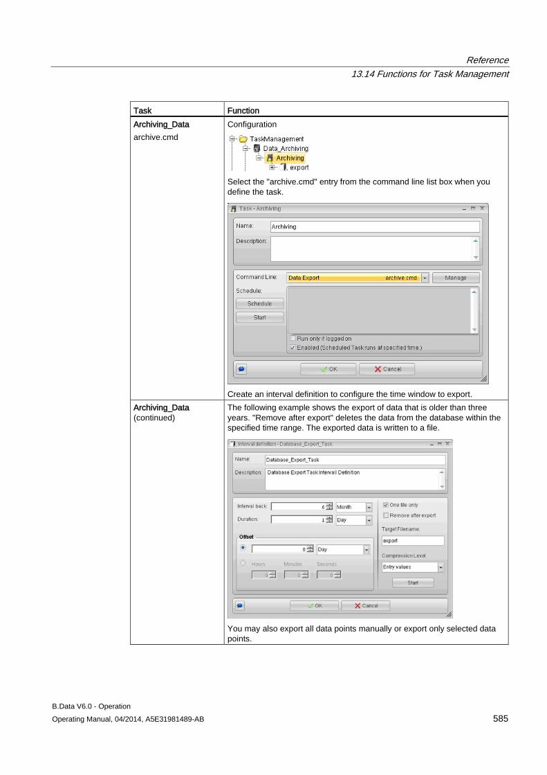
Reference 13.14 Functions for Task Management
B.Data V6.0 - Operation Operating Manual, 04/2014, A5E31981489-AB 585
Task Function Archiving_Data archive.cmd
Configuration
Select the "archive.cmd" entry from the command line list box when you define the task.
Create an interval definition to configure the time window to export.
Archiving_Data (continued)
The following example shows the export of data that is older than three years. "Remove after export" deletes the data from the database within the specified time range. The exported data is written to a file.
You may also export all data points manually or export only selected data points.
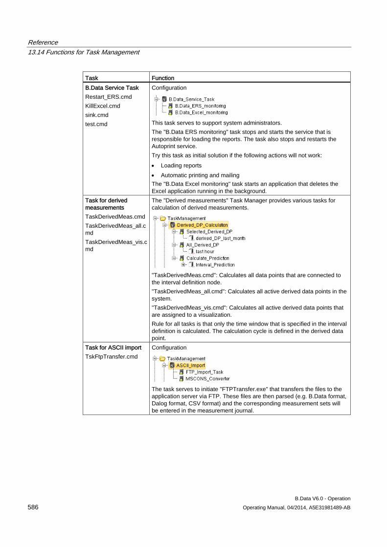
Reference 13.14 Functions for Task Management
B.Data V6.0 - Operation 586 Operating Manual, 04/2014, A5E31981489-AB
Task Function B.Data Service Task Restart_ERS.cmd KillExcel.cmd sink.cmd test.cmd
Configuration
This task serves to support system administrators. The "B.Data ERS monitoring" task stops and starts the service that is responsible for loading the reports. The task also stops and restarts the Autoprint service. Try this task as initial solution if the following actions will not work: • Loading reports • Automatic printing and mailing The "B.Data Excel monitoring" task starts an application that deletes the Excel application running in the background.
Task for derived measurements TaskDerivedMeas.cmd TaskDerivedMeas_all.cmd TaskDerivedMeas_vis.cmd
The "Derived measurements" Task Manager provides various tasks for calculation of derived measurements.
"TaskDerivedMeas.cmd": Calculates all data points that are connected to the interval definition node. "TaskDerivedMeas_all.cmd": Calculates all active derived data points in the system. "TaskDerivedMeas_vis.cmd": Calculates all active derived data points that are assigned to a visualization. Rule for all tasks is that only the time window that is specified in the interval definition is calculated. The calculation cycle is defined in the derived data point.
Task for ASCII import TskFtpTransfer.cmd
Configuration
The task serves to initiate "FTPTransfer.exe" that transfers the files to the application server via FTP. These files are then parsed (e.g. B.Data format, Dalog format, CSV format) and the corresponding measurement sets will be entered in the measurement journal.
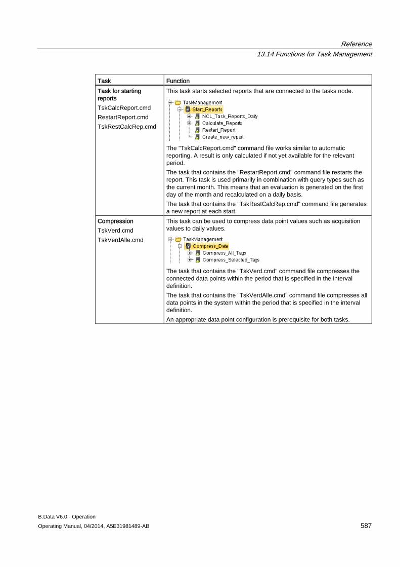
Reference 13.14 Functions for Task Management
B.Data V6.0 - Operation Operating Manual, 04/2014, A5E31981489-AB 587
Task Function Task for starting reports TskCalcReport.cmd RestartReport.cmd TskRestCalcRep.cmd
This task starts selected reports that are connected to the tasks node.
The "TskCalcReport.cmd" command file works similar to automatic reporting. A result is only calculated if not yet available for the relevant period. The task that contains the "RestartReport.cmd" command file restarts the report. This task is used primarily in combination with query types such as the current month. This means that an evaluation is generated on the first day of the month and recalculated on a daily basis. The task that contains the "TskRestCalcRep.cmd" command file generates a new report at each start.
Compression TskVerd.cmd TskVerdAlle.cmd
This task can be used to compress data point values such as acquisition values to daily values.
The task that contains the "TskVerd.cmd" command file compresses the connected data points within the period that is specified in the interval definition. The task that contains the "TskVerdAlle.cmd" command file compresses all data points in the system within the period that is specified in the interval definition. An appropriate data point configuration is prerequisite for both tasks.
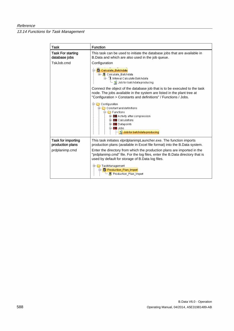
Reference 13.14 Functions for Task Management
B.Data V6.0 - Operation 588 Operating Manual, 04/2014, A5E31981489-AB
Task Function Task For starting database jobs TskJob.cmd
This task can be used to initiate the database jobs that are available in B.Data and which are also used in the job queue. Configuration
Connect the object of the database job that is to be executed to the task node. The jobs available in the system are listed in the plant tree at "Configuration > Constants and definitions" / Functions / Jobs.
Task for importing production plans prdplanimp.cmd
This task initiates xlprdplanimpLauncher.exe. The function imports production plans (available in Excel file format) into the B.Data system. Enter the directory from which the production plans are imported in the "prdplanimp.cmd" file. For the log files, enter the B.Data directory that is used by default for storage of B.Data log files.
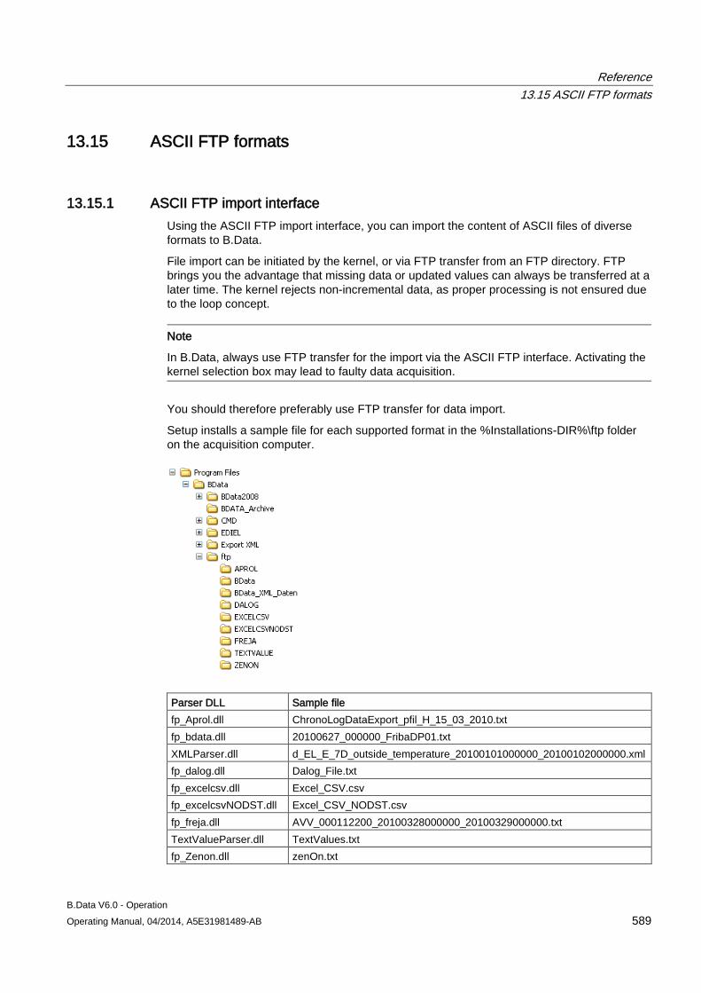
Reference 13.15 ASCII FTP formats
B.Data V6.0 - Operation Operating Manual, 04/2014, A5E31981489-AB 589
13.15 ASCII FTP formats
13.15.1 ASCII FTP import interface Using the ASCII FTP import interface, you can import the content of ASCII files of diverse formats to B.Data.
File import can be initiated by the kernel, or via FTP transfer from an FTP directory. FTP brings you the advantage that missing data or updated values can always be transferred at a later time. The kernel rejects non-incremental data, as proper processing is not ensured due to the loop concept.
Note
In B.Data, always use FTP transfer for the import via the ASCII FTP interface. Activating the kernel selection box may lead to faulty data acquisition.
You should therefore preferably use FTP transfer for data import.
Setup installs a sample file for each supported format in the %Installations-DIR%\ftp folder on the acquisition computer.
Parser DLL Sample file fp_Aprol.dll ChronoLogDataExport_pfil_H_15_03_2010.txt fp_bdata.dll 20100627_000000_FribaDP01.txt XMLParser.dll d_EL_E_7D_outside_temperature_20100101000000_20100102000000.xml fp_dalog.dll Dalog_File.txt fp_excelcsv.dll Excel_CSV.csv fp_excelcsvNODST.dll Excel_CSV_NODST.csv fp_freja.dll AVV_000112200_20100328000000_20100329000000.txt TextValueParser.dll TextValues.txt fp_Zenon.dll zenOn.txt
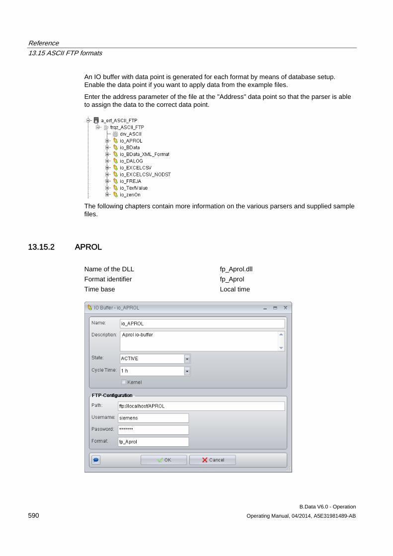
Reference 13.15 ASCII FTP formats
B.Data V6.0 - Operation 590 Operating Manual, 04/2014, A5E31981489-AB
An IO buffer with data point is generated for each format by means of database setup. Enable the data point if you want to apply data from the example files.
Enter the address parameter of the file at the "Address" data point so that the parser is able to assign the data to the correct data point.
The following chapters contain more information on the various parsers and supplied sample files.
13.15.2 APROL Name of the DLL fp_Aprol.dll Format identifier fp_Aprol Time base Local time
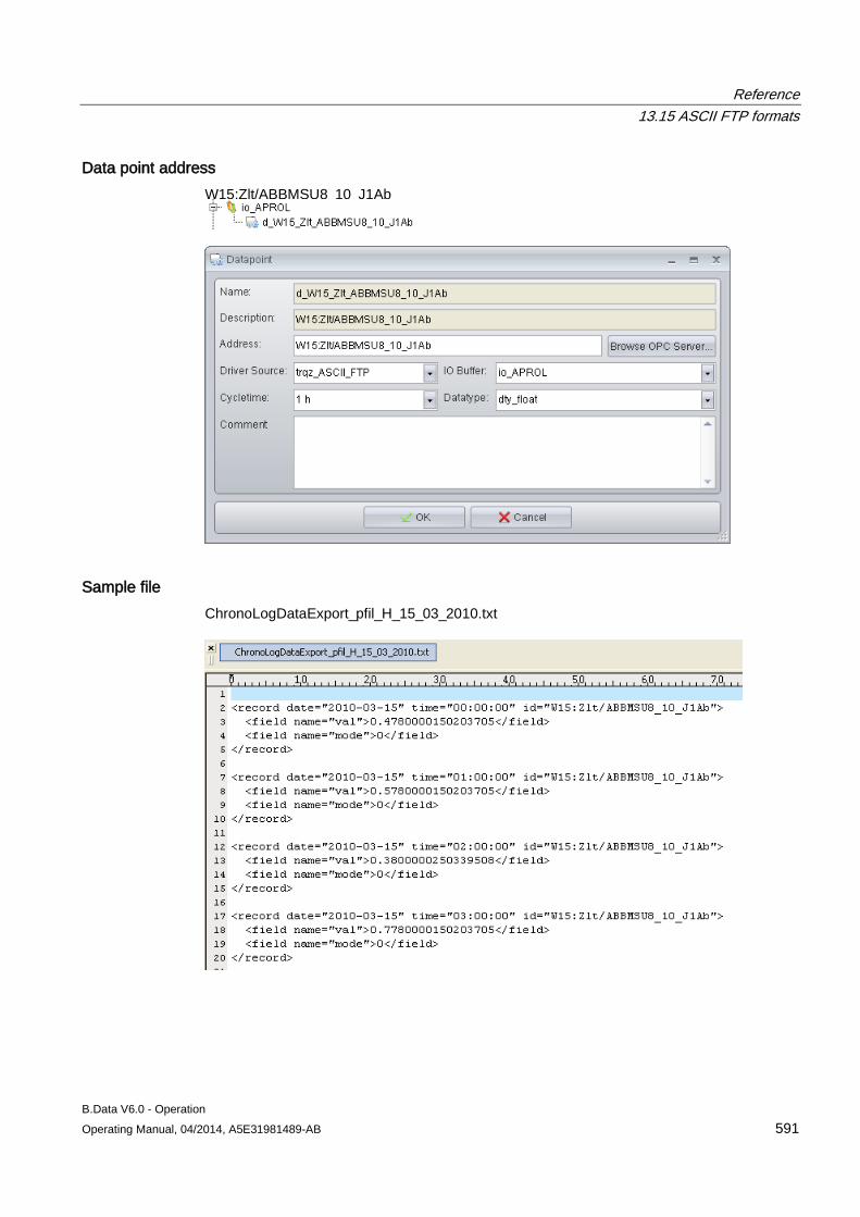
Reference 13.15 ASCII FTP formats
B.Data V6.0 - Operation Operating Manual, 04/2014, A5E31981489-AB 591
Data point address W15:Zlt/ABBMSU8_10_J1Ab
Sample file ChronoLogDataExport_pfil_H_15_03_2010.txt
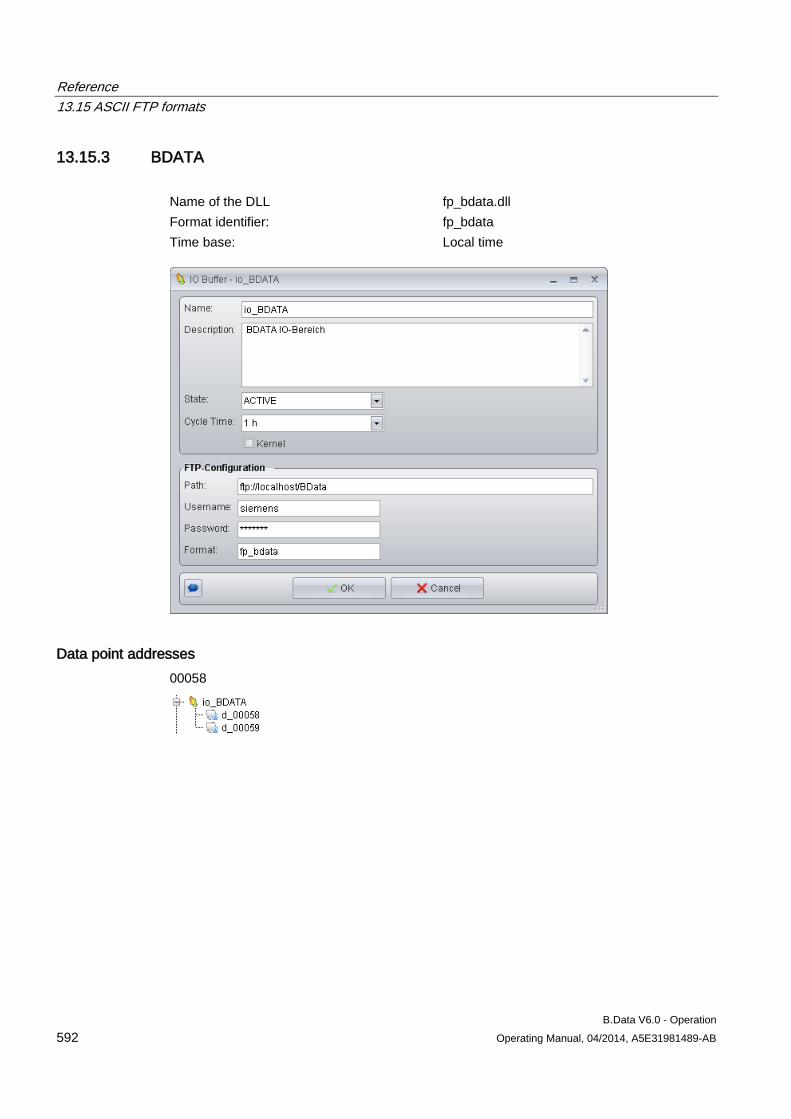
Reference 13.15 ASCII FTP formats
B.Data V6.0 - Operation 592 Operating Manual, 04/2014, A5E31981489-AB
13.15.3 BDATA Name of the DLL fp_bdata.dll Format identifier: fp_bdata Time base: Local time
Data point addresses 00058
00059
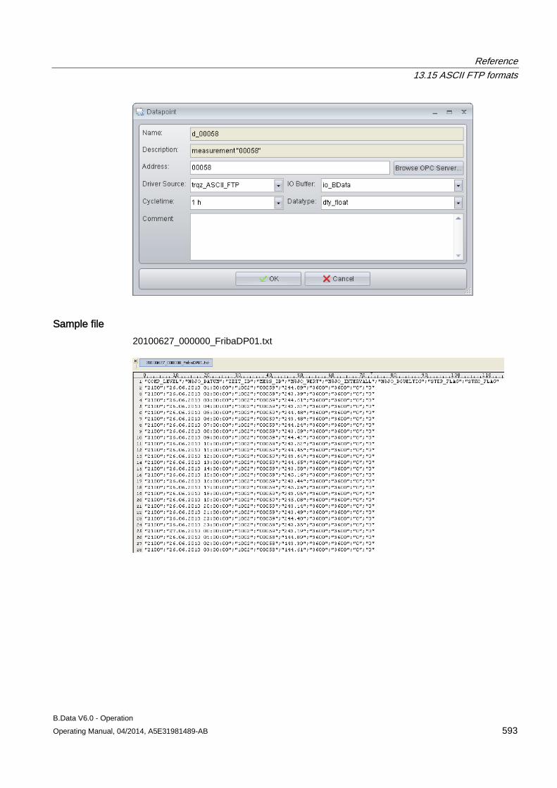
Reference 13.15 ASCII FTP formats
B.Data V6.0 - Operation Operating Manual, 04/2014, A5E31981489-AB 593
Sample file 20100627_000000_FribaDP01.txt
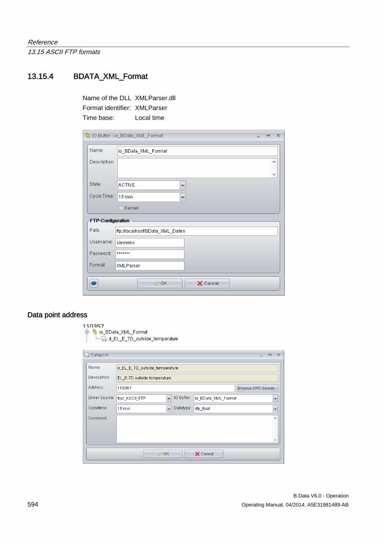
Reference 13.15 ASCII FTP formats
B.Data V6.0 - Operation 594 Operating Manual, 04/2014, A5E31981489-AB
13.15.4 BDATA_XML_Format Name of the DLL XMLParser.dll Format identifier: XMLParser Time base: Local time
Data point address 110357
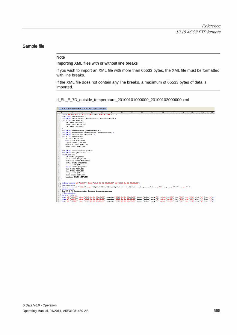
Reference 13.15 ASCII FTP formats
B.Data V6.0 - Operation Operating Manual, 04/2014, A5E31981489-AB 595
Sample file
Note Importing XML files with or without line breaks
If you wish to import an XML file with more than 65533 bytes, the XML file must be formatted with line breaks.
If the XML file does not contain any line breaks, a maximum of 65533 bytes of data is imported.
d_EL_E_7D_outside_temperature_20100101000000_20100102000000.xml
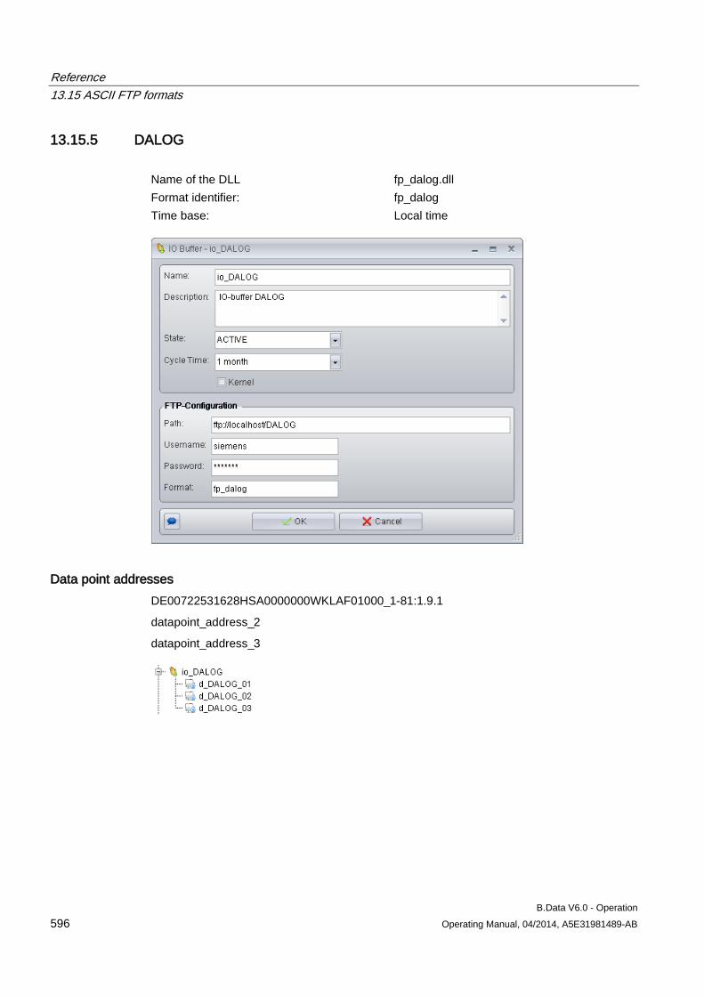
Reference 13.15 ASCII FTP formats
B.Data V6.0 - Operation 596 Operating Manual, 04/2014, A5E31981489-AB
13.15.5 DALOG Name of the DLL fp_dalog.dll Format identifier: fp_dalog Time base: Local time
Data point addresses DE00722531628HSA0000000WKLAF01000_1-81:1.9.1
datapoint_address_2
datapoint_address_3
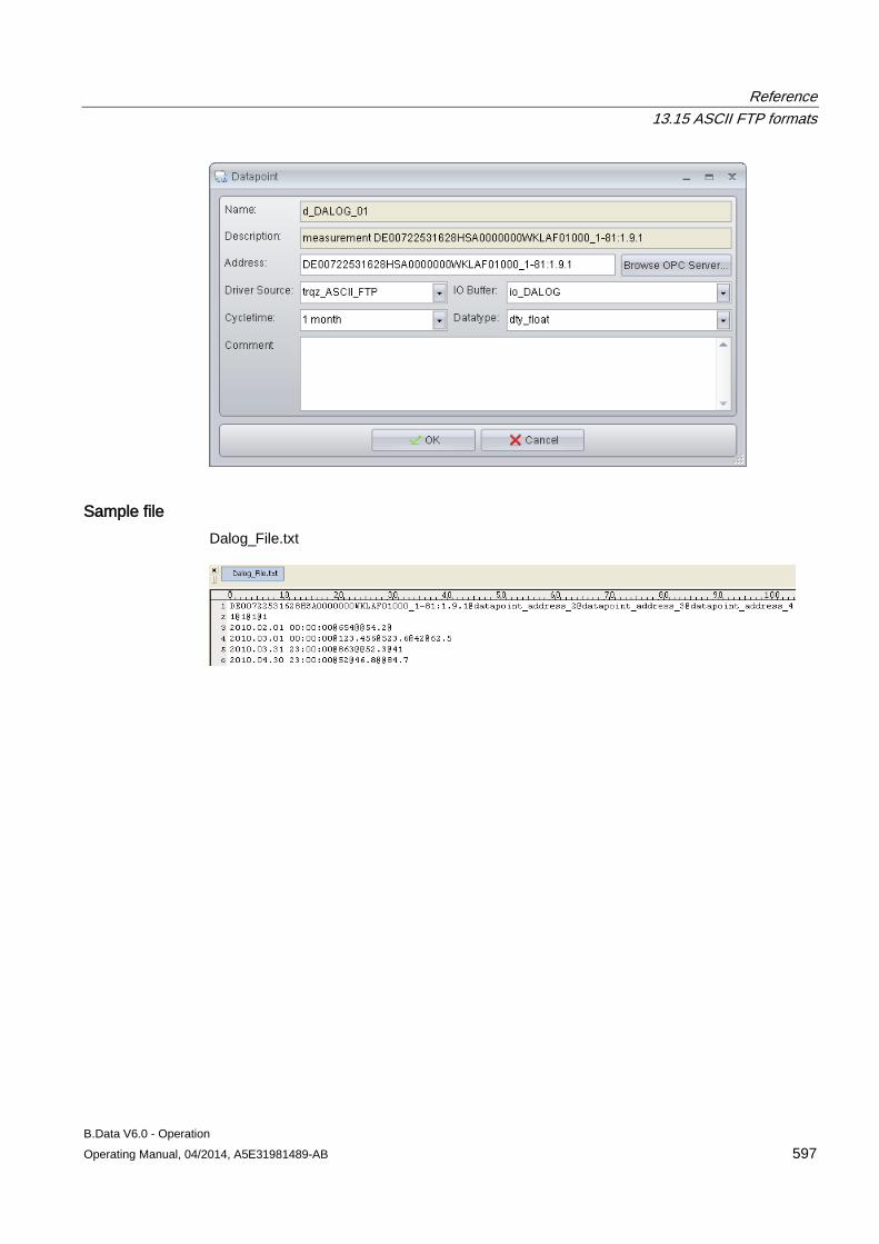
Reference 13.15 ASCII FTP formats
B.Data V6.0 - Operation Operating Manual, 04/2014, A5E31981489-AB 597
Sample file Dalog_File.txt
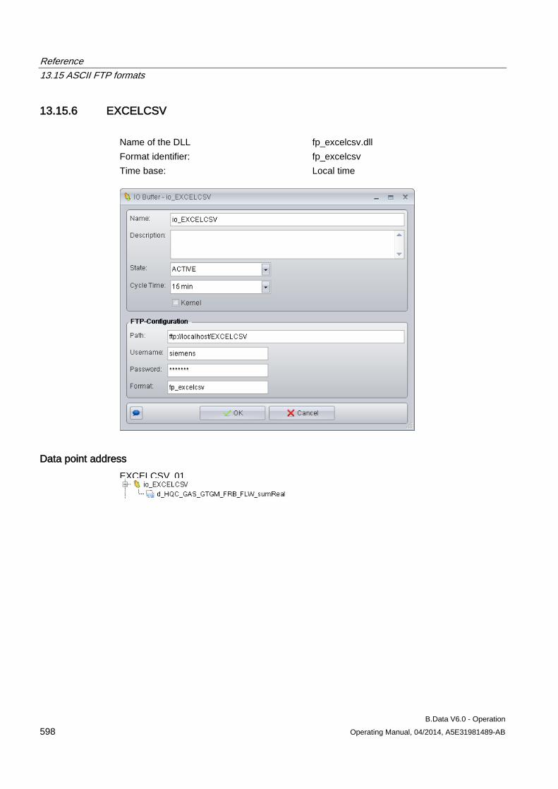
Reference 13.15 ASCII FTP formats
B.Data V6.0 - Operation 598 Operating Manual, 04/2014, A5E31981489-AB
13.15.6 EXCELCSV Name of the DLL fp_excelcsv.dll Format identifier: fp_excelcsv Time base: Local time
Data point address EXCELCSV_01
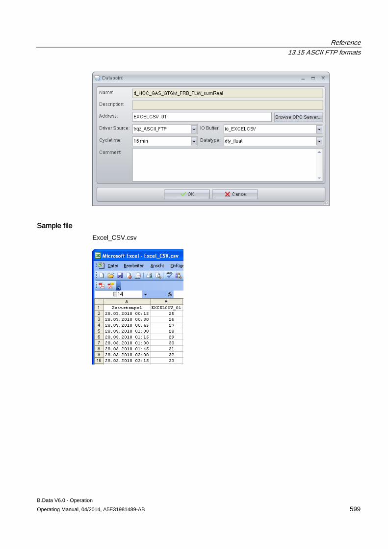
Reference 13.15 ASCII FTP formats
B.Data V6.0 - Operation Operating Manual, 04/2014, A5E31981489-AB 599
Sample file Excel_CSV.csv
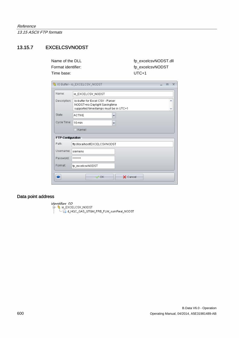
Reference 13.15 ASCII FTP formats
B.Data V6.0 - Operation 600 Operating Manual, 04/2014, A5E31981489-AB
13.15.7 EXCELCSVNODST Name of the DLL fp_excelcsvNODST.dll Format identifier: fp_excelcsvNODST Time base: UTC+1
Data point address identifier_02
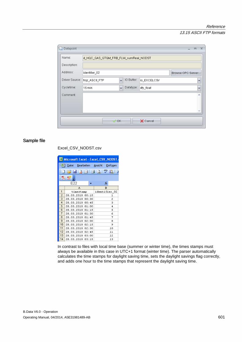
Reference 13.15 ASCII FTP formats
B.Data V6.0 - Operation Operating Manual, 04/2014, A5E31981489-AB 601
Sample file Excel_CSV_NODST.csv
In contrast to files with local time base (summer or winter time), the times stamps must always be available in this case in UTC+1 format (winter time). The parser automatically calculates the time stamps for daylight saving time, sets the daylight savings flag correctly, and adds one hour to the time stamps that represent the daylight saving time.
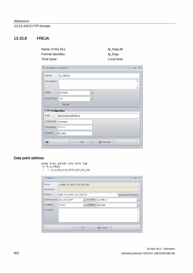
Reference 13.15 ASCII FTP formats
B.Data V6.0 - Operation 602 Operating Manual, 04/2014, A5E31981489-AB
13.15.8 FREJA Name of the DLL fp_freja.dll Format identifier: fp_freja Time base: Local time
Data point address HQK_FJV_ATOF_LEV_EGI_1M
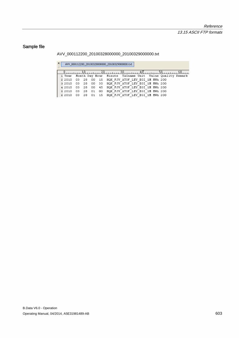
Reference 13.15 ASCII FTP formats
B.Data V6.0 - Operation Operating Manual, 04/2014, A5E31981489-AB 603
Sample file AVV_000112200_20100328000000_20100329000000.txt
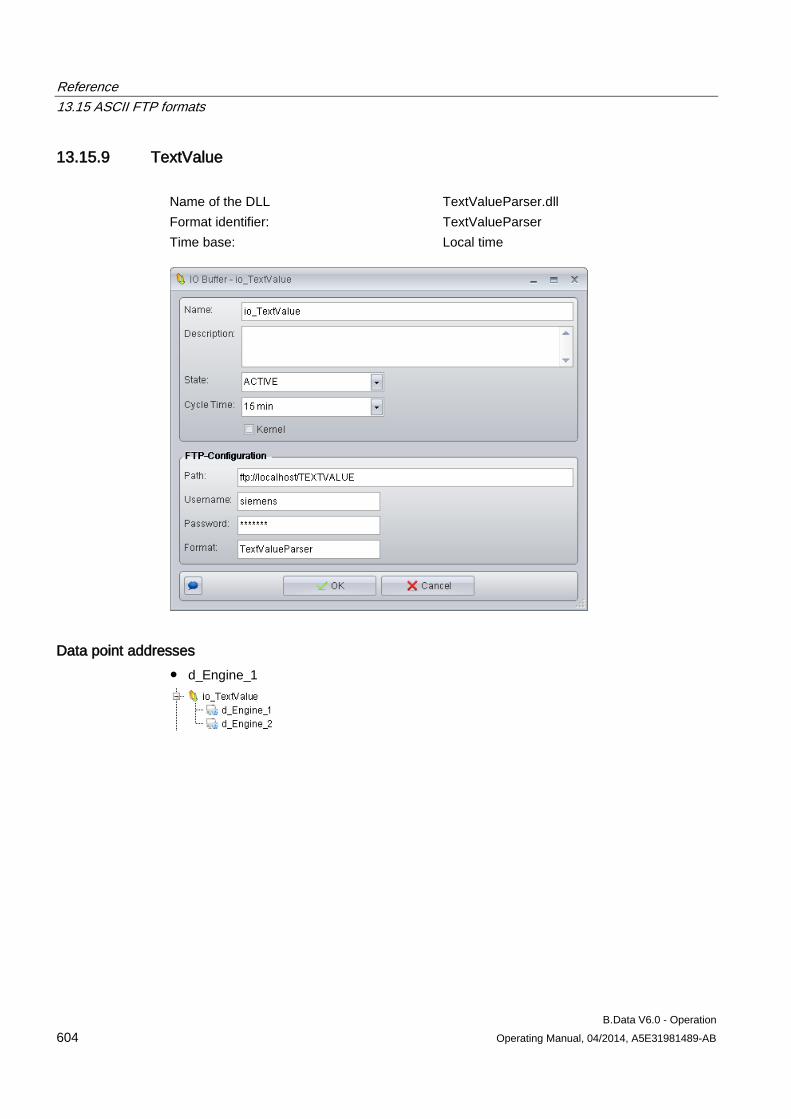
Reference 13.15 ASCII FTP formats
B.Data V6.0 - Operation 604 Operating Manual, 04/2014, A5E31981489-AB
13.15.9 TextValue Name of the DLL TextValueParser.dll Format identifier: TextValueParser Time base: Local time
Data point addresses ● d_Engine_1
● d_Engine_2
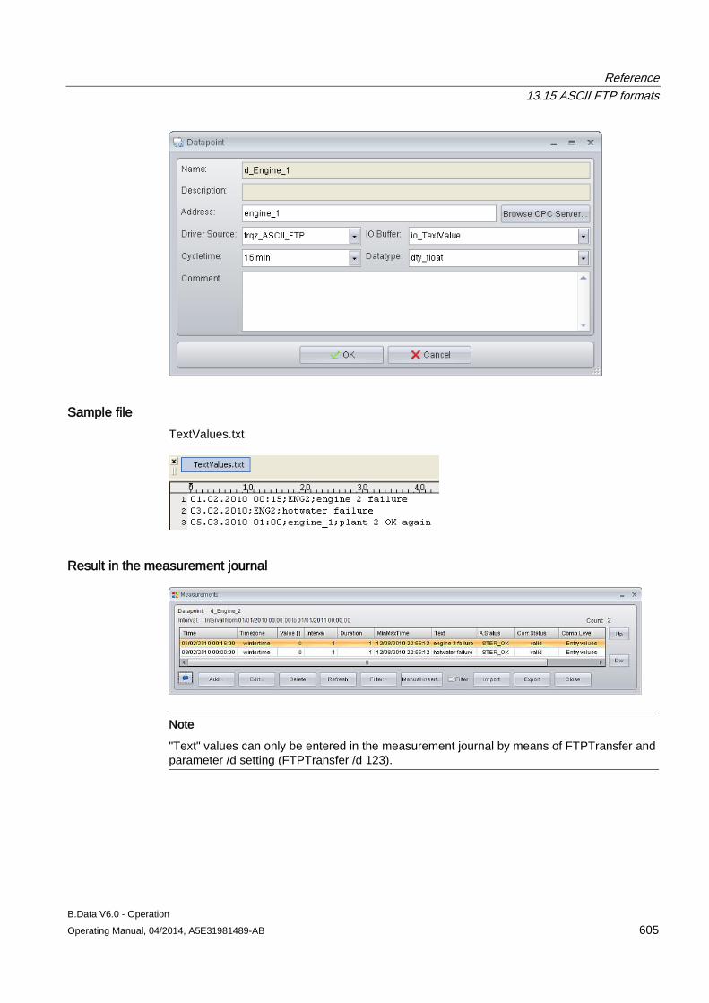
Reference 13.15 ASCII FTP formats
B.Data V6.0 - Operation Operating Manual, 04/2014, A5E31981489-AB 605
Sample file TextValues.txt
Result in the measurement journal
Note
"Text" values can only be entered in the measurement journal by means of FTPTransfer and parameter /d setting (FTPTransfer /d 123).
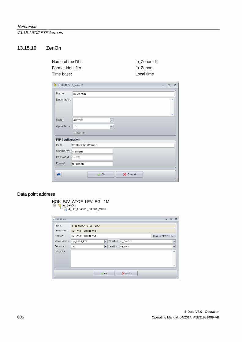
Reference 13.15 ASCII FTP formats
B.Data V6.0 - Operation 606 Operating Manual, 04/2014, A5E31981489-AB
13.15.10 ZenOn Name of the DLL fp_Zenon.dll Format identifier: fp_Zenon Time base: Local time
Data point address HQK_FJV_ATOF_LEV_EGI_1M
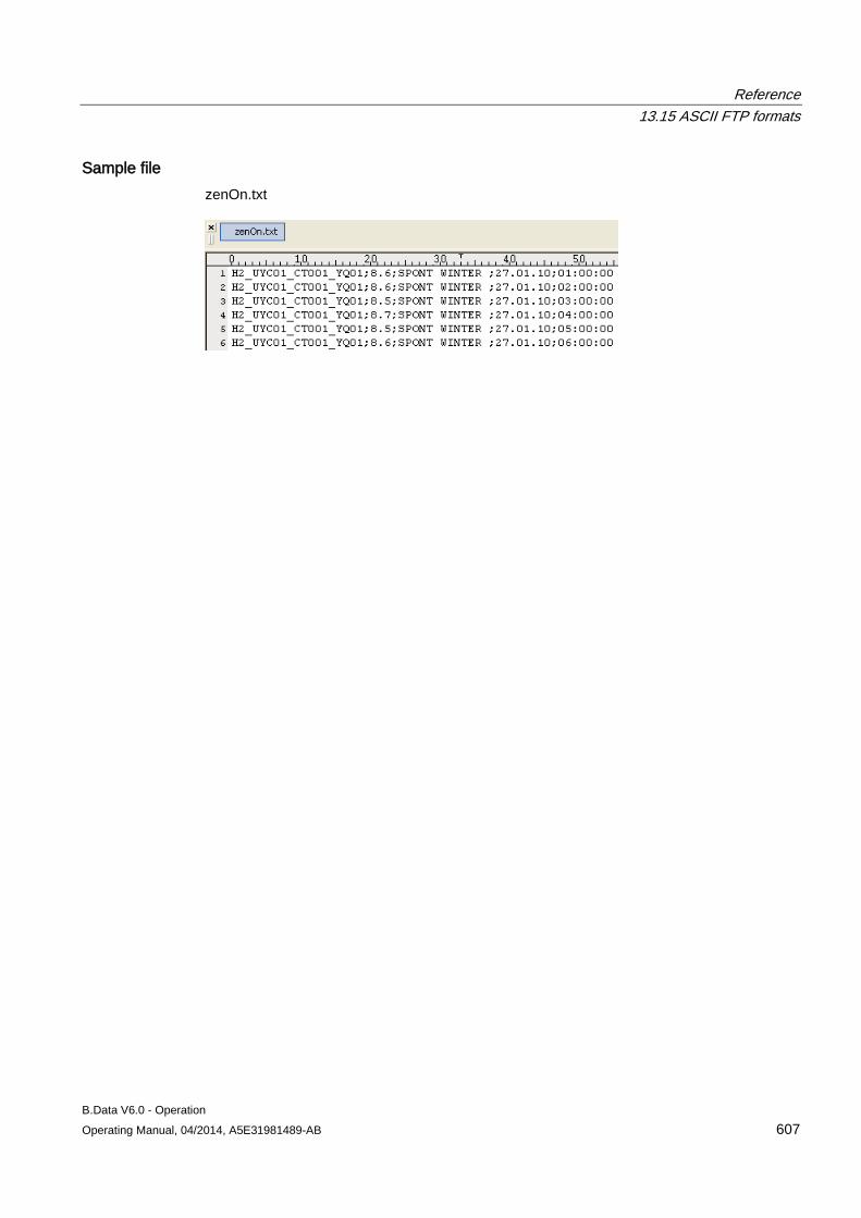
Reference 13.15 ASCII FTP formats
B.Data V6.0 - Operation Operating Manual, 04/2014, A5E31981489-AB 607
Sample file zenOn.txt
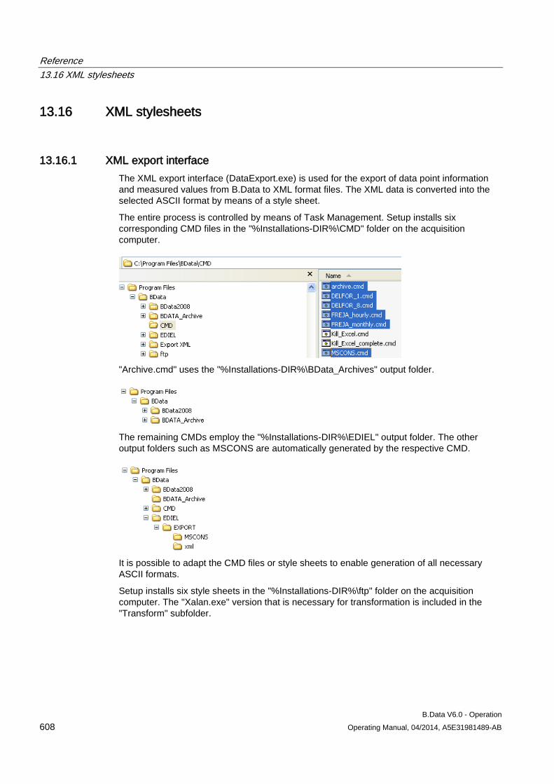
Reference 13.16 XML stylesheets
B.Data V6.0 - Operation 608 Operating Manual, 04/2014, A5E31981489-AB
13.16 XML stylesheets
13.16.1 XML export interface The XML export interface (DataExport.exe) is used for the export of data point information and measured values from B.Data to XML format files. The XML data is converted into the selected ASCII format by means of a style sheet.
The entire process is controlled by means of Task Management. Setup installs six corresponding CMD files in the "%Installations-DIR%\CMD" folder on the acquisition computer.
"Archive.cmd" uses the "%Installations-DIR%\BData_Archives" output folder.
The remaining CMDs employ the "%Installations-DIR%\EDIEL" output folder. The other output folders such as MSCONS are automatically generated by the respective CMD.
It is possible to adapt the CMD files or style sheets to enable generation of all necessary ASCII formats.
Setup installs six style sheets in the "%Installations-DIR%\ftp" folder on the acquisition computer. The "Xalan.exe" version that is necessary for transformation is included in the "Transform" subfolder.
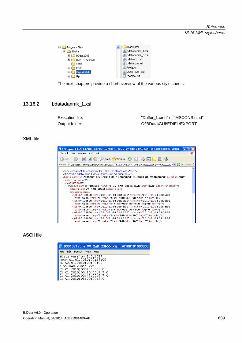
Reference 13.16 XML stylesheets
B.Data V6.0 - Operation Operating Manual, 04/2014, A5E31981489-AB 609
The next chapters provide a short overview of the various style sheets.
13.16.2 bdatadanmk_1.xsl Execution file: "Delfor_1.cmd" or "MSCONS.cmd" Output folder: C:\BData\GUI\EDIEL\EXPORT
XML file
ASCII file
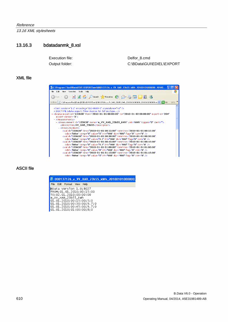
Reference 13.16 XML stylesheets
B.Data V6.0 - Operation 610 Operating Manual, 04/2014, A5E31981489-AB
13.16.3 bdatadanmk_8.xsl Execution file: Delfor_8.cmd Output folder: C:\BData\GUI\EDIEL\EXPORT
XML file
ASCII file
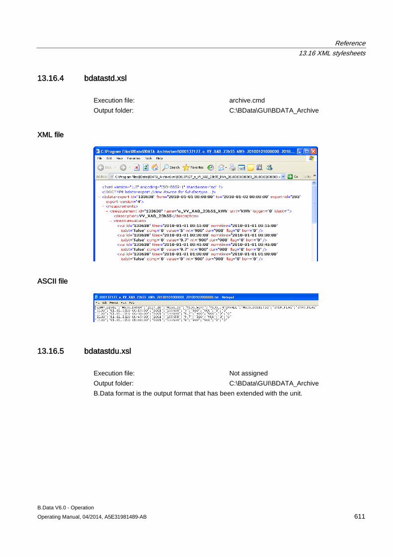
Reference 13.16 XML stylesheets
B.Data V6.0 - Operation Operating Manual, 04/2014, A5E31981489-AB 611
13.16.4 bdatastd.xsl Execution file: archive.cmd Output folder: C:\BData\GUI\BDATA_Archive
XML file
ASCII file
13.16.5 bdatastdu.xsl Execution file: Not assigned Output folder: C:\BData\GUI\BDATA_Archive B.Data format is the output format that has been extended with the unit.
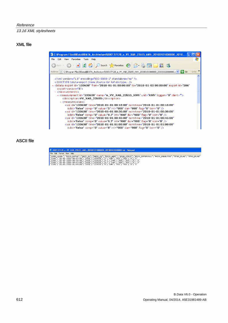
Reference 13.16 XML stylesheets
B.Data V6.0 - Operation 612 Operating Manual, 04/2014, A5E31981489-AB
XML file
ASCII file
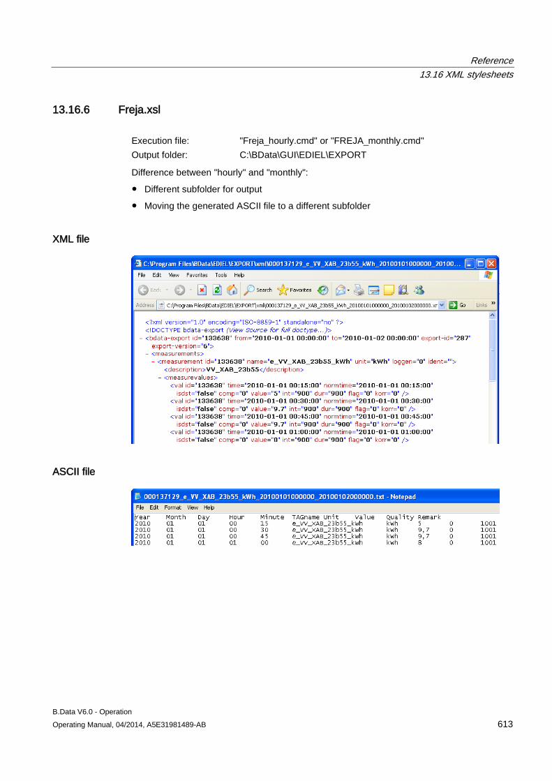
Reference 13.16 XML stylesheets
B.Data V6.0 - Operation Operating Manual, 04/2014, A5E31981489-AB 613
13.16.6 Freja.xsl Execution file: "Freja_hourly.cmd" or "FREJA_monthly.cmd" Output folder: C:\BData\GUI\EDIEL\EXPORT
Difference between "hourly" and "monthly":
● Different subfolder for output
● Moving the generated ASCII file to a different subfolder
XML file
ASCII file
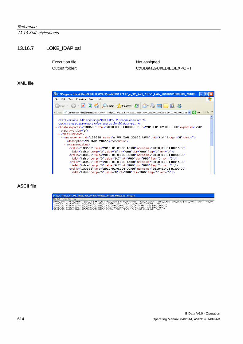
Reference 13.16 XML stylesheets
B.Data V6.0 - Operation 614 Operating Manual, 04/2014, A5E31981489-AB
13.16.7 LOKE_IDAP.xsl Execution file: Not assigned Output folder: C:\BData\GUI\EDIEL\EXPORT
XML file
ASCII file
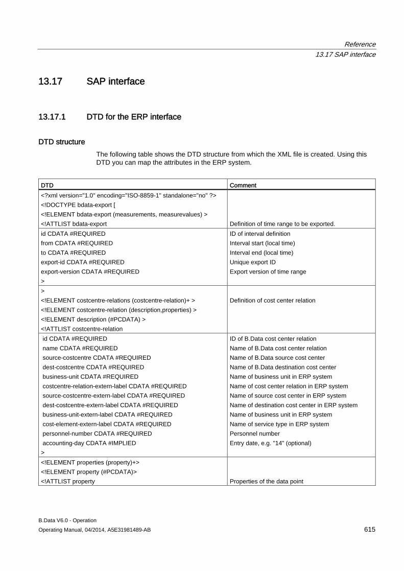
Reference 13.17 SAP interface
B.Data V6.0 - Operation Operating Manual, 04/2014, A5E31981489-AB 615
13.17 SAP interface
13.17.1 DTD for the ERP interface
DTD structure The following table shows the DTD structure from which the XML file is created. Using this DTD you can map the attributes in the ERP system.
DTD Comment <?xml version="1.0" encoding="ISO-8859-1" standalone="no" ?> <!DOCTYPE bdata-export [ <!ELEMENT bdata-export (measurements, measurevalues) > <!ATTLIST bdata-export
Definition of time range to be exported.
id CDATA #REQUIRED from CDATA #REQUIRED to CDATA #REQUIRED export-id CDATA #REQUIRED export-version CDATA #REQUIRED >
ID of interval definition Interval start (local time) Interval end (local time) Unique export ID Export version of time range
> <!ELEMENT costcentre-relations (costcentre-relation)+ > <!ELEMENT costcentre-relation (description,properties) > <!ELEMENT description (#PCDATA) > <!ATTLIST costcentre-relation
Definition of cost center relation
id CDATA #REQUIRED name CDATA #REQUIRED source-costcentre CDATA #REQUIRED dest-costcentre CDATA #REQUIRED business-unit CDATA #REQUIRED costcentre-relation-extern-label CDATA #REQUIRED source-costcentre-extern-label CDATA #REQUIRED dest-costcentre-extern-label CDATA #REQUIRED business-unit-extern-label CDATA #REQUIRED cost-element-extern-label CDATA #REQUIRED personnel-number CDATA #REQUIRED accounting-day CDATA #IMPLIED >
ID of B.Data cost center relation Name of B.Data cost center relation Name of B.Data source cost center Name of B.Data destination cost center Name of business unit in ERP system Name of cost center relation in ERP system Name of source cost center in ERP system Name of destination cost center in ERP system Name of business unit in ERP system Name of service type in ERP system Personnel number Entry date, e.g. "14" (optional)
<!ELEMENT properties (property)+> <!ELEMENT property (#PCDATA)> <!ATTLIST property
Properties of the data point
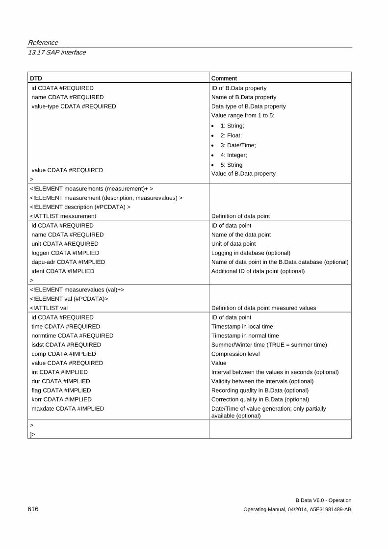
Reference 13.17 SAP interface
B.Data V6.0 - Operation 616 Operating Manual, 04/2014, A5E31981489-AB
DTD Comment id CDATA #REQUIRED name CDATA #REQUIRED value-type CDATA #REQUIRED value CDATA #REQUIRED >
ID of B.Data property Name of B.Data property Data type of B.Data property Value range from 1 to 5: • 1: String; • 2: Float; • 3: Date/Time; • 4: Integer; • 5: String Value of B.Data property
<!ELEMENT measurements (measurement)+ > <!ELEMENT measurement (description, measurevalues) > <!ELEMENT description (#PCDATA) > <!ATTLIST measurement
Definition of data point
id CDATA #REQUIRED name CDATA #REQUIRED unit CDATA #REQUIRED loggen CDATA #IMPLIED dapu-adr CDATA #IMPLIED ident CDATA #IMPLIED >
ID of data point Name of the data point Unit of data point Logging in database (optional) Name of data point in the B.Data database (optional) Additional ID of data point (optional)
<!ELEMENT measurevalues (val)+> <!ELEMENT val (#PCDATA)> <!ATTLIST val
Definition of data point measured values
id CDATA #REQUIRED time CDATA #REQUIRED normtime CDATA #REQUIRED isdst CDATA #REQUIRED comp CDATA #IMPLIED value CDATA #REQUIRED int CDATA #IMPLIED dur CDATA #IMPLIED flag CDATA #IMPLIED korr CDATA #IMPLIED maxdate CDATA #IMPLIED
ID of data point Timestamp in local time Timestamp in normal time Summer/Winter time (TRUE = summer time) Compression level Value Interval between the values in seconds (optional) Validity between the intervals (optional) Recording quality in B.Data (optional) Correction quality in B.Data (optional) Date/Time of value generation; only partially available (optional)
> ]>
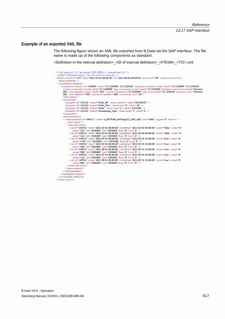
Reference 13.17 SAP interface
B.Data V6.0 - Operation Operating Manual, 04/2014, A5E31981489-AB 617
Example of an exported XML file The following figure shows an XML file exported from B.Data via the SAP interface. The file name is made up of the following components as standard:
<Definition in the interval definition>_<ID of interval definition>_<FROM>_<TO>.xml
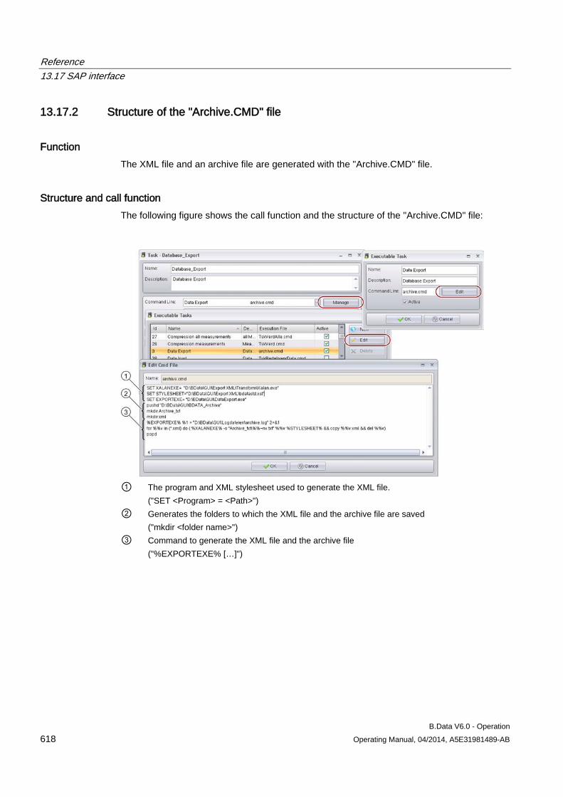
Reference 13.17 SAP interface
B.Data V6.0 - Operation 618 Operating Manual, 04/2014, A5E31981489-AB
13.17.2 Structure of the "Archive.CMD" file
Function The XML file and an archive file are generated with the "Archive.CMD" file.
Structure and call function The following figure shows the call function and the structure of the "Archive.CMD" file:
① The program and XML stylesheet used to generate the XML file.
("SET <Program> = <Path>") ② Generates the folders to which the XML file and the archive file are saved
("mkdir <folder name>") ③ Command to generate the XML file and the archive file
("%EXPORTEXE% […]")
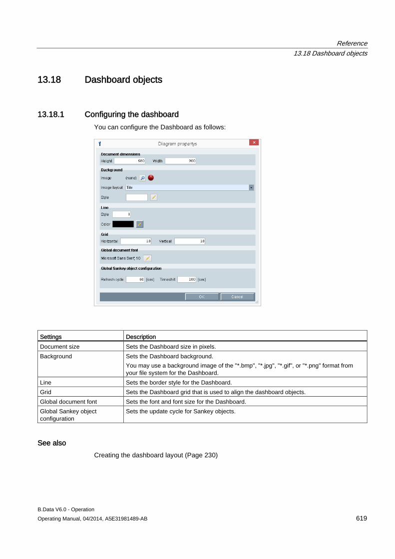
Reference 13.18 Dashboard objects
B.Data V6.0 - Operation Operating Manual, 04/2014, A5E31981489-AB 619
13.18 Dashboard objects
13.18.1 Configuring the dashboard You can configure the Dashboard as follows:
Settings Description Document size Sets the Dashboard size in pixels. Background Sets the Dashboard background.
You may use a background image of the "*.bmp", "*.jpg", "*.gif", or "*.png" format from your file system for the Dashboard.
Line Sets the border style for the Dashboard. Grid Sets the Dashboard grid that is used to align the dashboard objects. Global document font Sets the font and font size for the Dashboard. Global Sankey object configuration
Sets the update cycle for Sankey objects.
See also Creating the dashboard layout (Page 230)
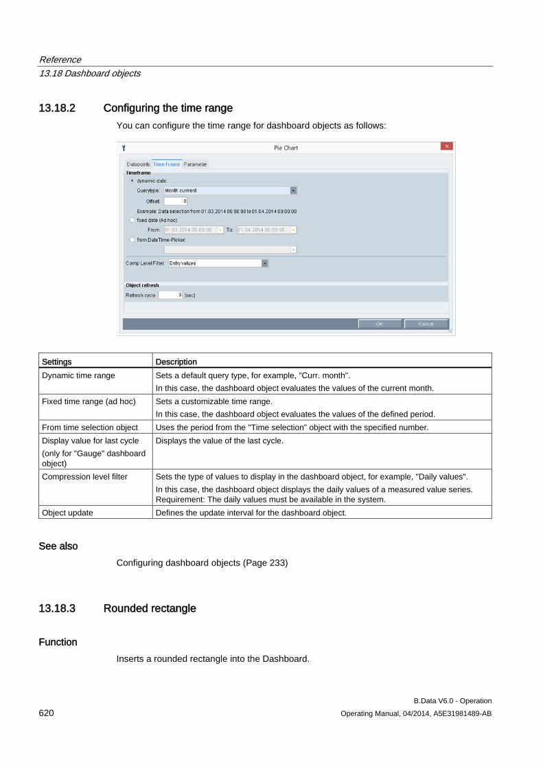
Reference 13.18 Dashboard objects
B.Data V6.0 - Operation 620 Operating Manual, 04/2014, A5E31981489-AB
13.18.2 Configuring the time range You can configure the time range for dashboard objects as follows:
Settings Description Dynamic time range Sets a default query type, for example, "Curr. month".
In this case, the dashboard object evaluates the values of the current month. Fixed time range (ad hoc) Sets a customizable time range.
In this case, the dashboard object evaluates the values of the defined period. From time selection object Uses the period from the "Time selection" object with the specified number. Display value for last cycle (only for "Gauge" dashboard object)
Displays the value of the last cycle.
Compression level filter Sets the type of values to display in the dashboard object, for example, "Daily values". In this case, the dashboard object displays the daily values of a measured value series. Requirement: The daily values must be available in the system.
Object update Defines the update interval for the dashboard object.
See also Configuring dashboard objects (Page 233)
13.18.3 Rounded rectangle
Function Inserts a rounded rectangle into the Dashboard.
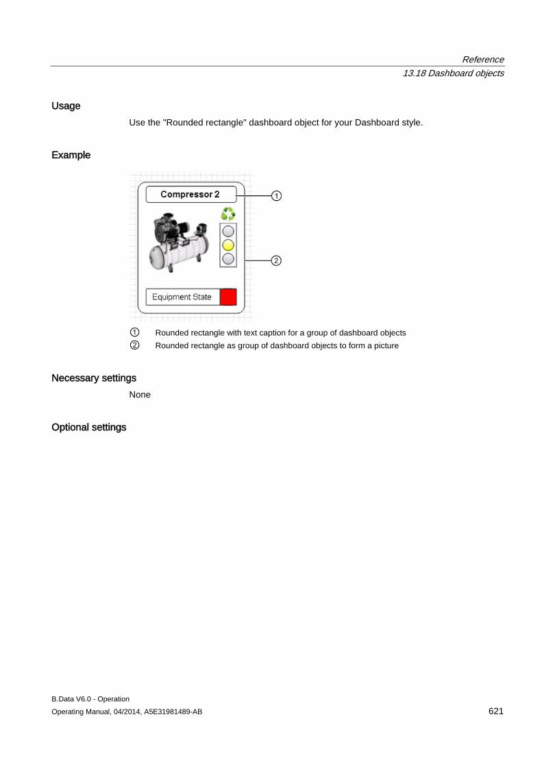
Reference 13.18 Dashboard objects
B.Data V6.0 - Operation Operating Manual, 04/2014, A5E31981489-AB 621
Usage Use the "Rounded rectangle" dashboard object for your Dashboard style.
Example
① Rounded rectangle with text caption for a group of dashboard objects ② Rounded rectangle as group of dashboard objects to form a picture
Necessary settings None
Optional settings
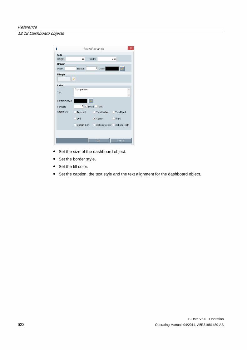
Reference 13.18 Dashboard objects
B.Data V6.0 - Operation 622 Operating Manual, 04/2014, A5E31981489-AB
● Set the size of the dashboard object.
● Set the border style.
● Set the fill color.
● Set the caption, the text style and the text alignment for the dashboard object.
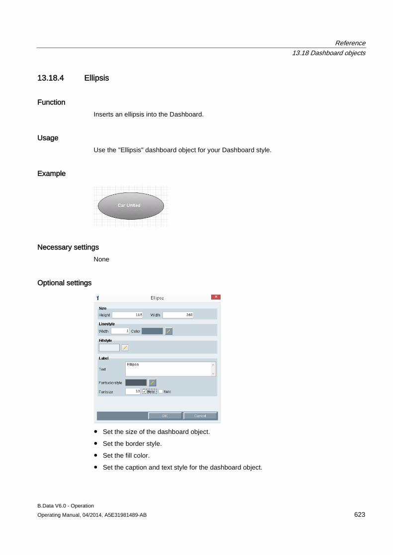
Reference 13.18 Dashboard objects
B.Data V6.0 - Operation Operating Manual, 04/2014, A5E31981489-AB 623
13.18.4 Ellipsis
Function Inserts an ellipsis into the Dashboard.
Usage Use the "Ellipsis" dashboard object for your Dashboard style.
Example
Necessary settings None
Optional settings
● Set the size of the dashboard object.
● Set the border style.
● Set the fill color.
● Set the caption and text style for the dashboard object.
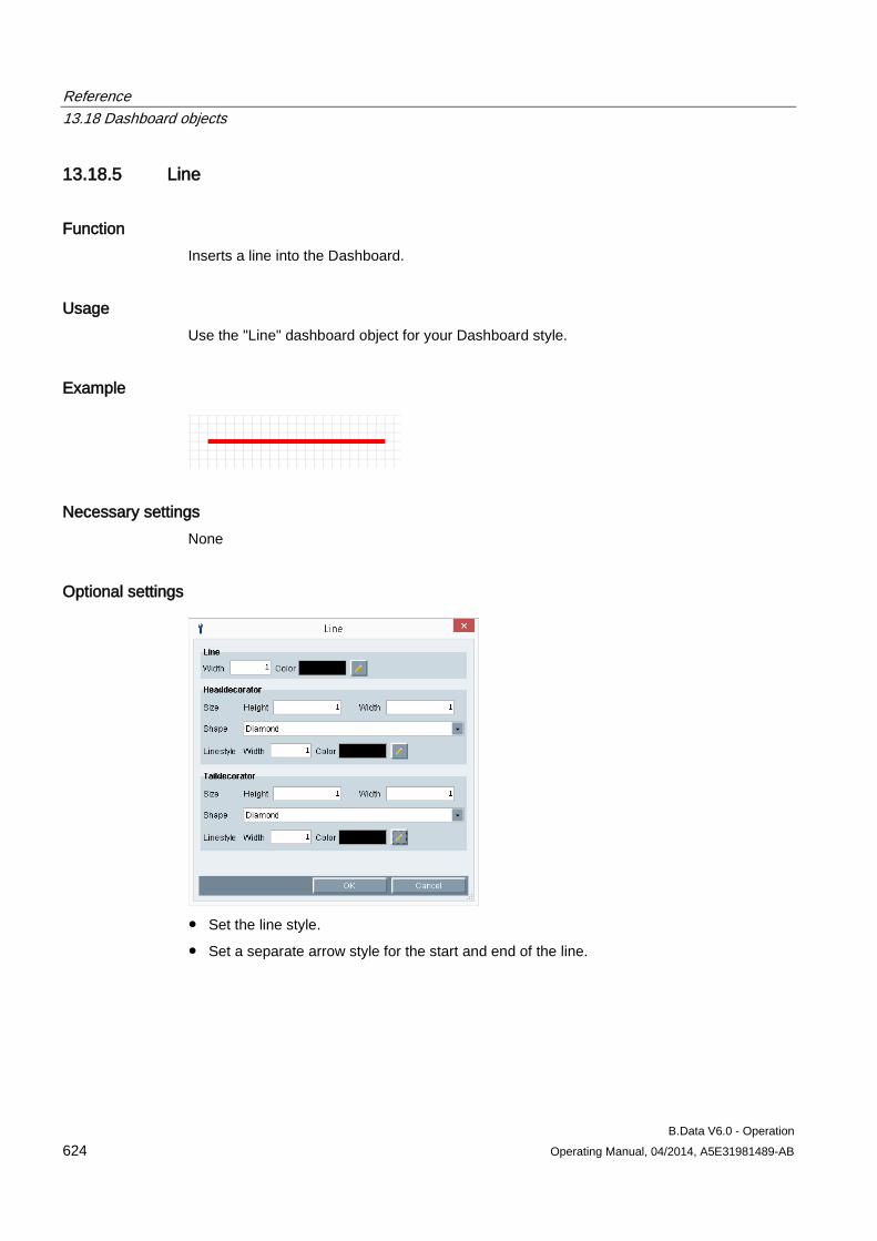
Reference 13.18 Dashboard objects
B.Data V6.0 - Operation 624 Operating Manual, 04/2014, A5E31981489-AB
13.18.5 Line
Function Inserts a line into the Dashboard.
Usage Use the "Line" dashboard object for your Dashboard style.
Example
Necessary settings None
Optional settings
● Set the line style.
● Set a separate arrow style for the start and end of the line.
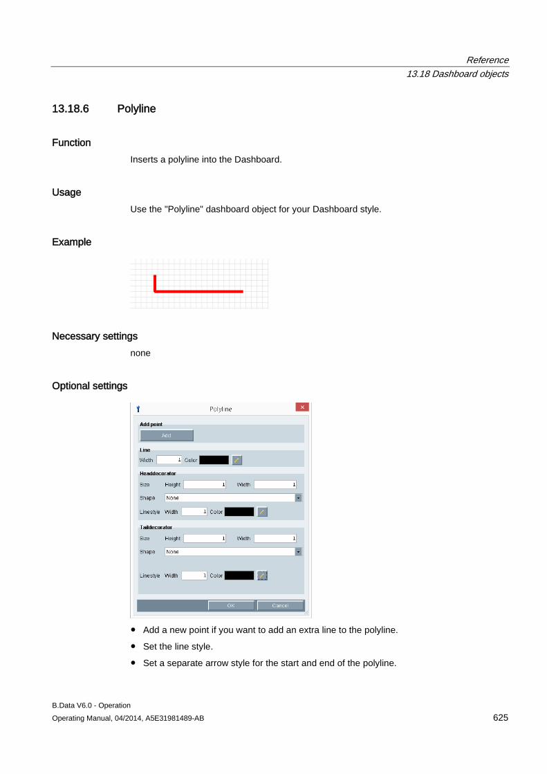
Reference 13.18 Dashboard objects
B.Data V6.0 - Operation Operating Manual, 04/2014, A5E31981489-AB 625
13.18.6 Polyline
Function Inserts a polyline into the Dashboard.
Usage Use the "Polyline" dashboard object for your Dashboard style.
Example
Necessary settings none
Optional settings
● Add a new point if you want to add an extra line to the polyline.
● Set the line style.
● Set a separate arrow style for the start and end of the polyline.
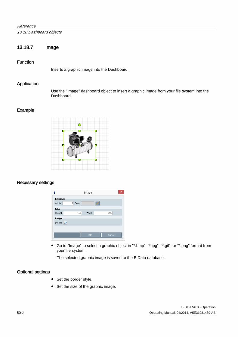
Reference 13.18 Dashboard objects
B.Data V6.0 - Operation 626 Operating Manual, 04/2014, A5E31981489-AB
13.18.7 Image
Function Inserts a graphic image into the Dashboard.
Application Use the "Image" dashboard object to insert a graphic image from your file system into the Dashboard.
Example
Necessary settings
● Go to "Image" to select a graphic object in "*.bmp", "*.jpg", "*.gif", or "*.png" format from
your file system.
The selected graphic image is saved to the B.Data database.
Optional settings ● Set the border style.
● Set the size of the graphic image.
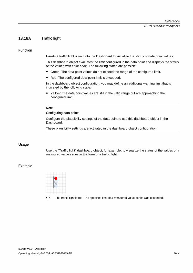
Reference 13.18 Dashboard objects
B.Data V6.0 - Operation Operating Manual, 04/2014, A5E31981489-AB 627
13.18.8 Traffic light
Function Inserts a traffic light object into the Dashboard to visualize the status of data point values.
This dashboard object evaluates the limit configured in the data point and displays the status of the values with color code. The following states are possible:
● Green: The data point values do not exceed the range of the configured limit.
● Red: The configured data point limit is exceeded.
In the dashboard object configuration, you may define an additional warning limit that is indicated by the following state:
● Yellow: The data point values are still in the valid range but are approaching the configured limit.
Note Configuring data points
Configure the plausibility settings of the data point to use this dashboard object in the Dashboard.
These plausibility settings are activated in the dashboard object configuration.
Usage Use the "Traffic light" dashboard object, for example, to visualize the status of the values of a measured value series in the form of a traffic light.
Example
① The traffic light is red: The specified limit of a measured value series was exceeded.
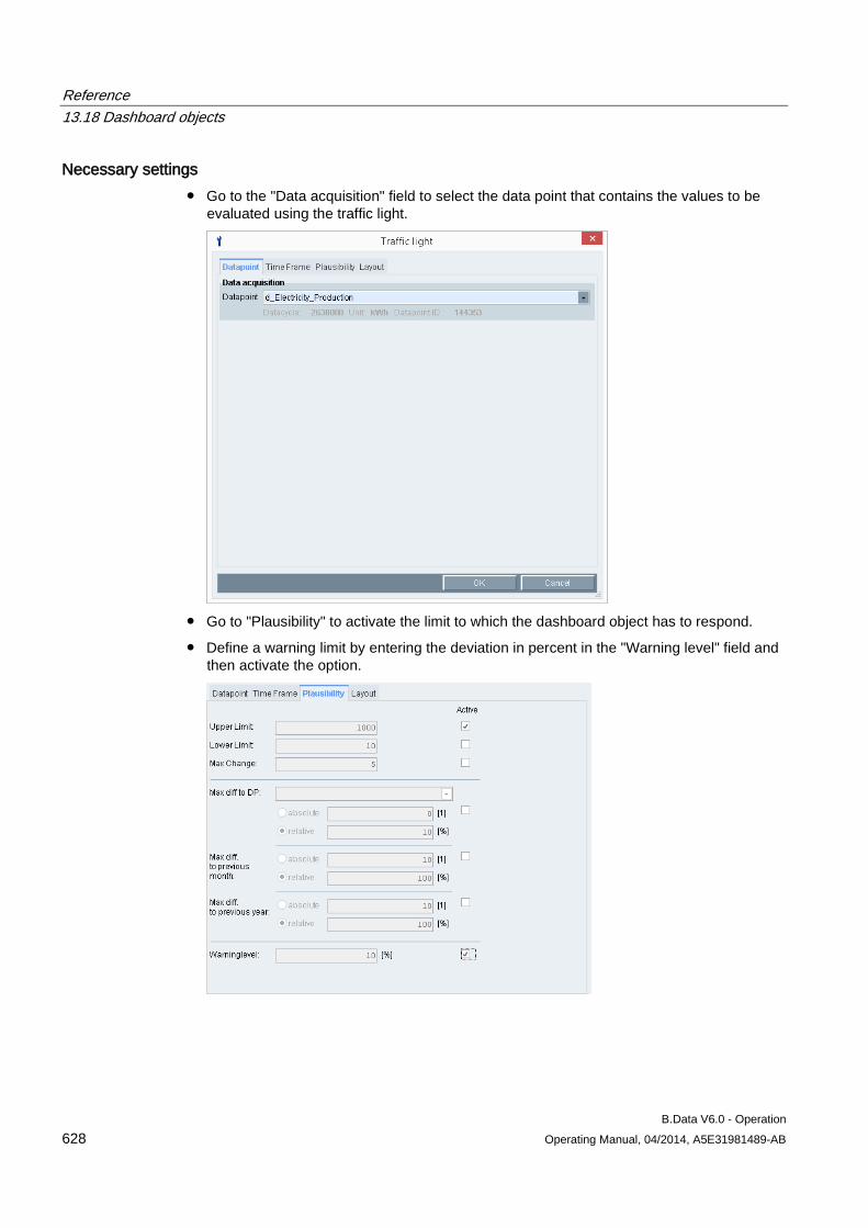
Reference 13.18 Dashboard objects
B.Data V6.0 - Operation 628 Operating Manual, 04/2014, A5E31981489-AB
Necessary settings ● Go to the "Data acquisition" field to select the data point that contains the values to be
evaluated using the traffic light.
● Go to "Plausibility" to activate the limit to which the dashboard object has to respond.
● Define a warning limit by entering the deviation in percent in the "Warning level" field and then activate the option.
Reference 13.18 Dashboard objects
B.Data V6.0 - Operation Operating Manual, 04/2014, A5E31981489-AB 629
Note
The dashboard object returns the "Red" status if only one of the limits you activated in the "Plausibility" setting is exceeded. The evaluation is not particularly helpful in this situation.
For this reason, evaluate only one limit per dashboard object. Create additional dashboard objects for further evaluations.
Optional settings Select the "Alignment" tab to set the size, border and background color for the dashboard object.
See also Configuring the time range (Page 620)
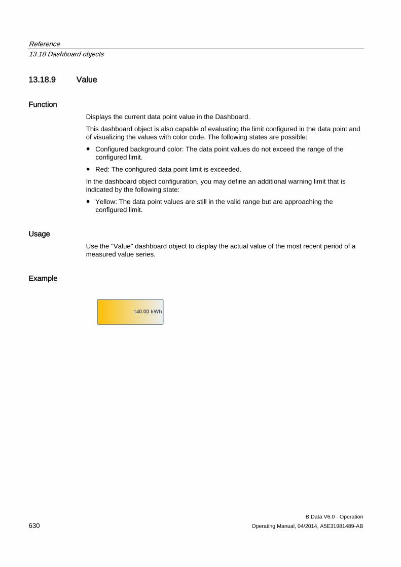
Reference 13.18 Dashboard objects
B.Data V6.0 - Operation 630 Operating Manual, 04/2014, A5E31981489-AB
13.18.9 Value
Function Displays the current data point value in the Dashboard.
This dashboard object is also capable of evaluating the limit configured in the data point and of visualizing the values with color code. The following states are possible:
● Configured background color: The data point values do not exceed the range of the configured limit.
● Red: The configured data point limit is exceeded.
In the dashboard object configuration, you may define an additional warning limit that is indicated by the following state:
● Yellow: The data point values are still in the valid range but are approaching the configured limit.
Usage Use the "Value" dashboard object to display the actual value of the most recent period of a measured value series.
Example
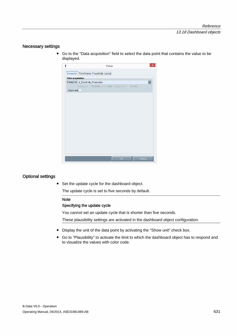
Reference 13.18 Dashboard objects
B.Data V6.0 - Operation Operating Manual, 04/2014, A5E31981489-AB 631
Necessary settings ● Go to the "Data acquisition" field to select the data point that contains the value to be
displayed.
Optional settings ● Set the update cycle for the dashboard object.
The update cycle is set to five seconds by default.
Note Specifying the update cycle
You cannot set an update cycle that is shorter than five seconds.
These plausibility settings are activated in the dashboard object configuration.
● Display the unit of the data point by activating the "Show unit" check box.
● Go to "Plausibility" to activate the limit to which the dashboard object has to respond and to visualize the values with color code.
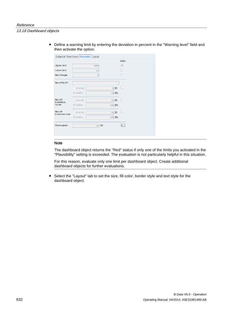
Reference 13.18 Dashboard objects
B.Data V6.0 - Operation 632 Operating Manual, 04/2014, A5E31981489-AB
● Define a warning limit by entering the deviation in percent in the "Warning level" field and then activate the option.
Note
The dashboard object returns the "Red" status if only one of the limits you activated in the "Plausibility" setting is exceeded. The evaluation is not particularly helpful in this situation.
For this reason, evaluate only one limit per dashboard object. Create additional dashboard objects for further evaluations.
● Select the "Layout" tab to set the size, fill color, border style and text style for the dashboard object.
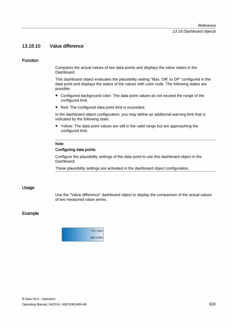
Reference 13.18 Dashboard objects
B.Data V6.0 - Operation Operating Manual, 04/2014, A5E31981489-AB 633
13.18.10 Value difference
Function Compares the actual values of two data points and displays the value states in the Dashboard.
This dashboard object evaluates the plausibility setting "Max. Diff. to DP" configured in the data point and displays the status of the values with color code. The following states are possible:
● Configured background color: The data point values do not exceed the range of the configured limit.
● Red: The configured data point limit is exceeded.
In the dashboard object configuration, you may define an additional warning limit that is indicated by the following state:
● Yellow: The data point values are still in the valid range but are approaching the configured limit.
Note Configuring data points
Configure the plausibility settings of the data point to use this dashboard object in the Dashboard.
These plausibility settings are activated in the dashboard object configuration.
Usage Use the "Value difference" dashboard object to display the comparison of the actual values of two measured value series.
Example
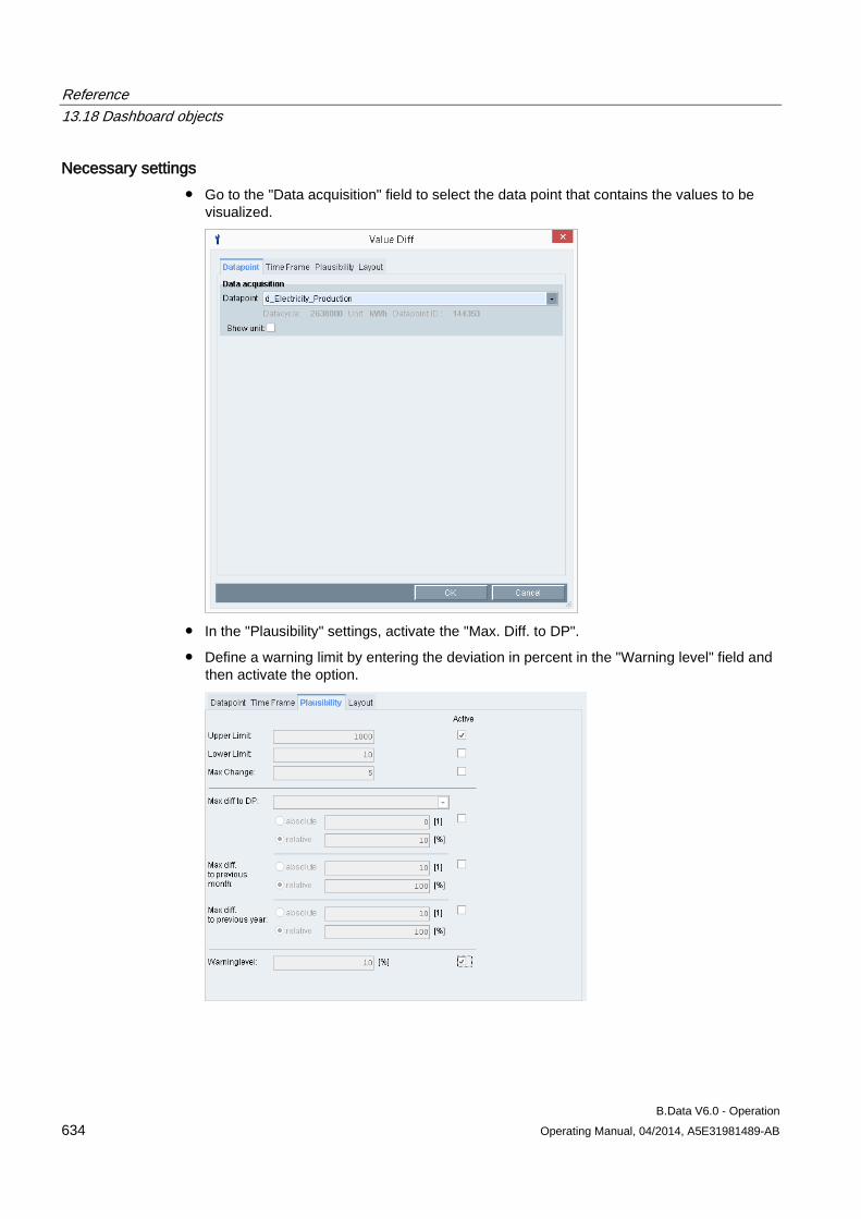
Reference 13.18 Dashboard objects
B.Data V6.0 - Operation 634 Operating Manual, 04/2014, A5E31981489-AB
Necessary settings ● Go to the "Data acquisition" field to select the data point that contains the values to be
visualized.
● In the "Plausibility" settings, activate the "Max. Diff. to DP".
● Define a warning limit by entering the deviation in percent in the "Warning level" field and then activate the option.

Reference 13.18 Dashboard objects
B.Data V6.0 - Operation Operating Manual, 04/2014, A5E31981489-AB 635
Optional settings ● Display the unit of the data point by activating the "Show unit" check box.
● Select the "Alignment" tab to set the size, fill color, border style and text style for the dashboard object.
See also Configuring the time range (Page 620)
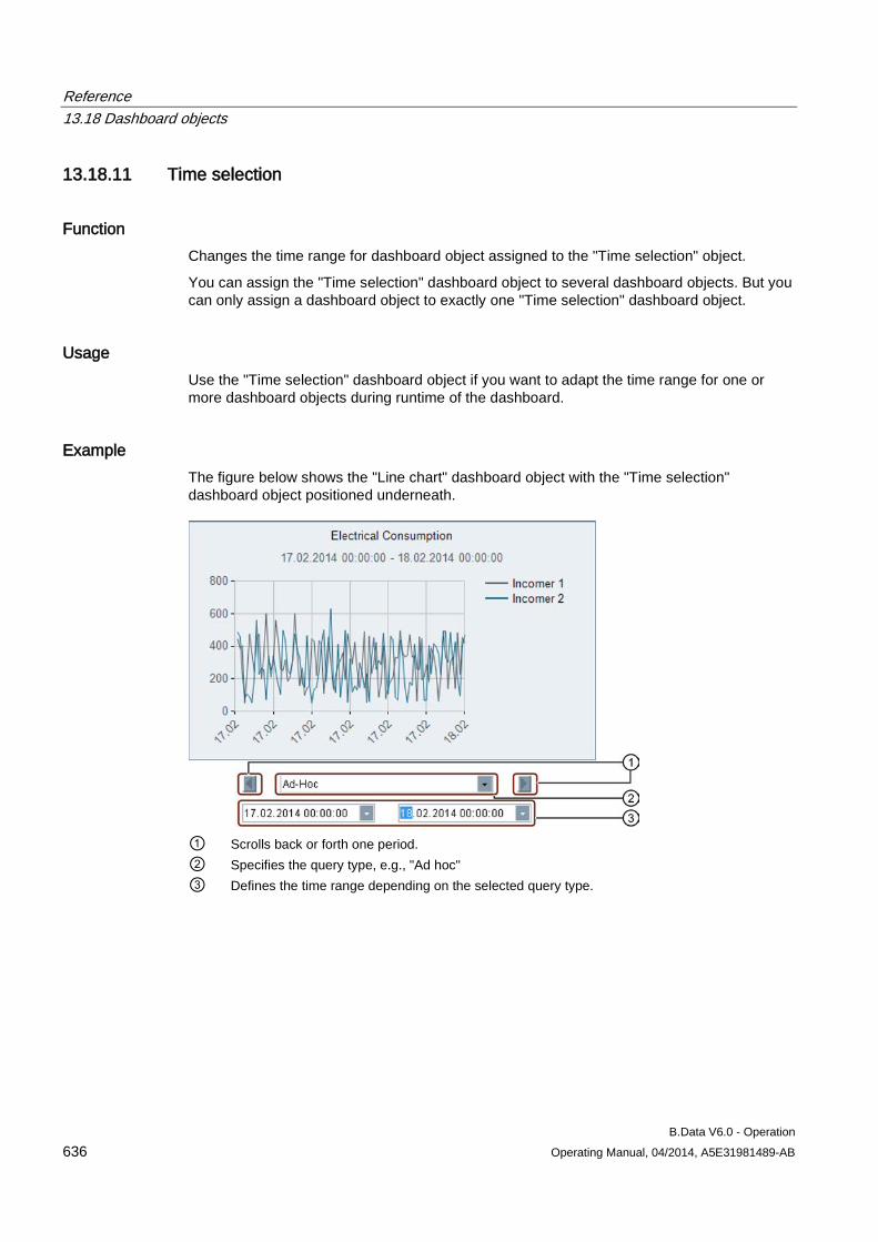
Reference 13.18 Dashboard objects
B.Data V6.0 - Operation 636 Operating Manual, 04/2014, A5E31981489-AB
13.18.11 Time selection
Function Changes the time range for dashboard object assigned to the "Time selection" object.
You can assign the "Time selection" dashboard object to several dashboard objects. But you can only assign a dashboard object to exactly one "Time selection" dashboard object.
Usage Use the "Time selection" dashboard object if you want to adapt the time range for one or more dashboard objects during runtime of the dashboard.
Example The figure below shows the "Line chart" dashboard object with the "Time selection" dashboard object positioned underneath.
① Scrolls back or forth one period. ② Specifies the query type, e.g., "Ad hoc" ③ Defines the time range depending on the selected query type.
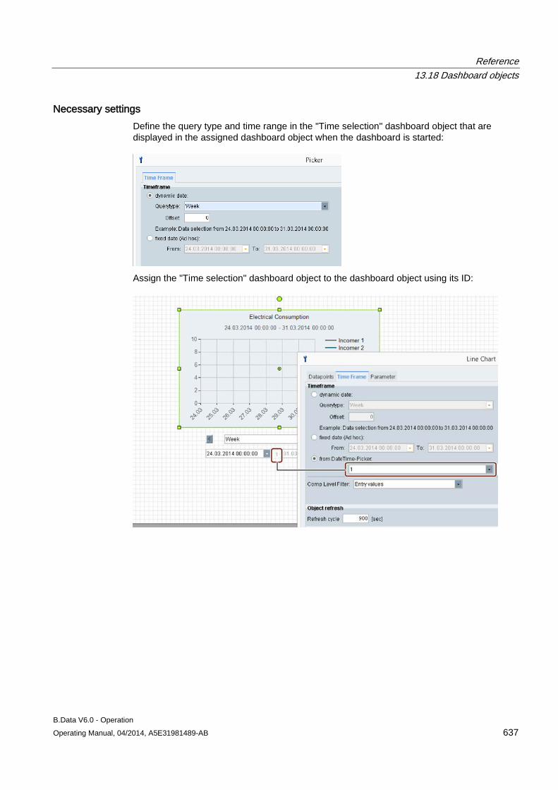
Reference 13.18 Dashboard objects
B.Data V6.0 - Operation Operating Manual, 04/2014, A5E31981489-AB 637
Necessary settings Define the query type and time range in the "Time selection" dashboard object that are displayed in the assigned dashboard object when the dashboard is started:
Assign the "Time selection" dashboard object to the dashboard object using its ID:
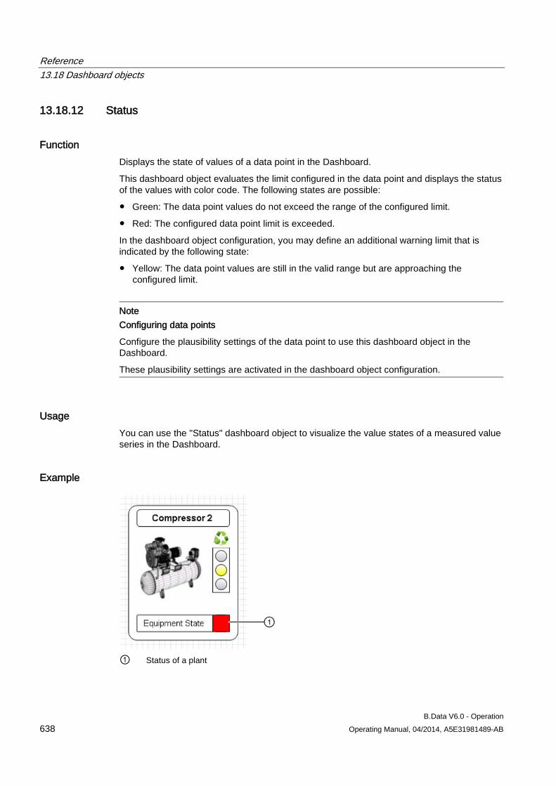
Reference 13.18 Dashboard objects
B.Data V6.0 - Operation 638 Operating Manual, 04/2014, A5E31981489-AB
13.18.12 Status
Function Displays the state of values of a data point in the Dashboard.
This dashboard object evaluates the limit configured in the data point and displays the status of the values with color code. The following states are possible:
● Green: The data point values do not exceed the range of the configured limit.
● Red: The configured data point limit is exceeded.
In the dashboard object configuration, you may define an additional warning limit that is indicated by the following state:
● Yellow: The data point values are still in the valid range but are approaching the configured limit.
Note Configuring data points
Configure the plausibility settings of the data point to use this dashboard object in the Dashboard.
These plausibility settings are activated in the dashboard object configuration.
Usage You can use the "Status" dashboard object to visualize the value states of a measured value series in the Dashboard.
Example
① Status of a plant
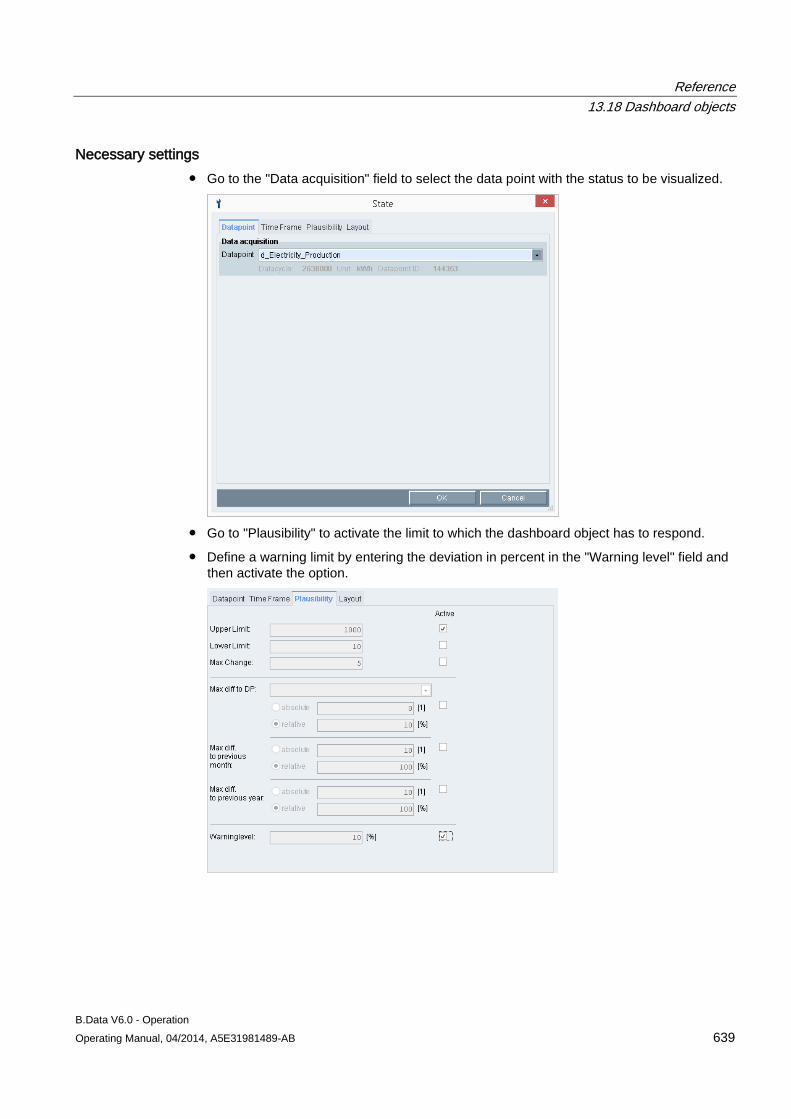
Reference 13.18 Dashboard objects
B.Data V6.0 - Operation Operating Manual, 04/2014, A5E31981489-AB 639
Necessary settings ● Go to the "Data acquisition" field to select the data point with the status to be visualized.
● Go to "Plausibility" to activate the limit to which the dashboard object has to respond.
● Define a warning limit by entering the deviation in percent in the "Warning level" field and then activate the option.
Reference 13.18 Dashboard objects
B.Data V6.0 - Operation 640 Operating Manual, 04/2014, A5E31981489-AB
Note
The dashboard object returns the "Red" status if only one of the limits you activated in the "Plausibility" setting is exceeded. The evaluation is not particularly helpful in this situation.
For this reason, evaluate only one limit per dashboard object. Create additional dashboard objects for further evaluations.
Optional settings Select the "Alignment" tab to set the size and border style for the dashboard object.
See also Configuring the time range (Page 620)
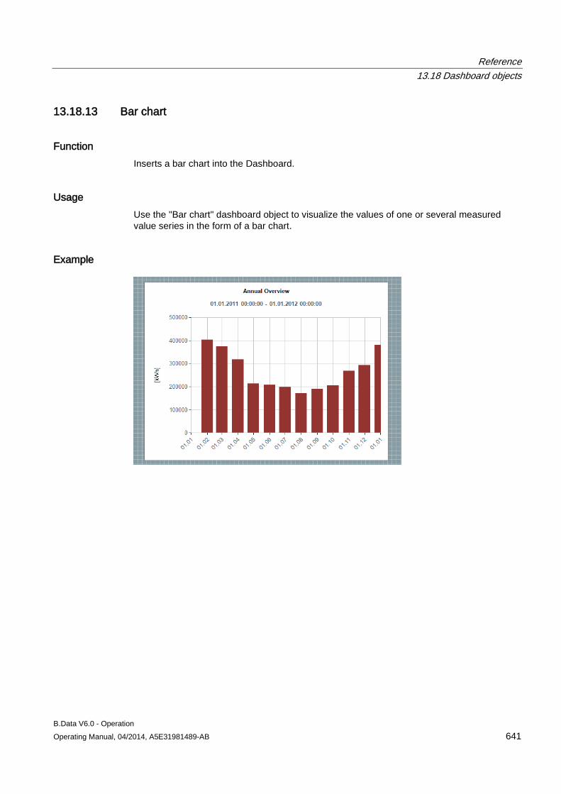
Reference 13.18 Dashboard objects
B.Data V6.0 - Operation Operating Manual, 04/2014, A5E31981489-AB 641
13.18.13 Bar chart
Function Inserts a bar chart into the Dashboard.
Usage Use the "Bar chart" dashboard object to visualize the values of one or several measured value series in the form of a bar chart.
Example
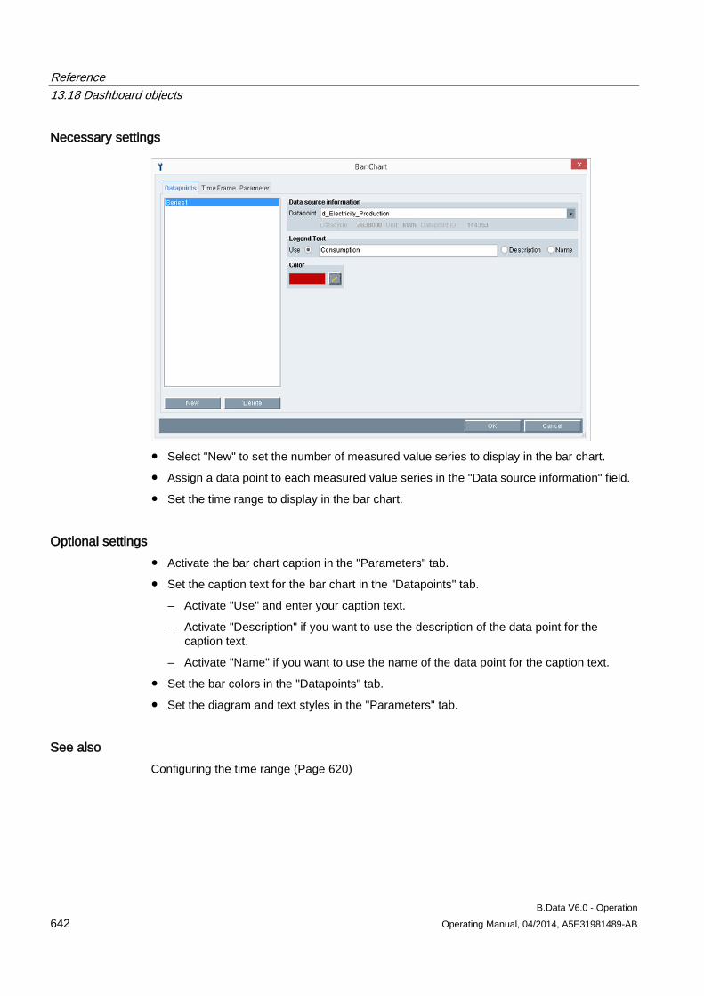
Reference 13.18 Dashboard objects
B.Data V6.0 - Operation 642 Operating Manual, 04/2014, A5E31981489-AB
Necessary settings
● Select "New" to set the number of measured value series to display in the bar chart.
● Assign a data point to each measured value series in the "Data source information" field.
● Set the time range to display in the bar chart.
Optional settings ● Activate the bar chart caption in the "Parameters" tab.
● Set the caption text for the bar chart in the "Datapoints" tab.
– Activate "Use" and enter your caption text.
– Activate "Description" if you want to use the description of the data point for the caption text.
– Activate "Name" if you want to use the name of the data point for the caption text.
● Set the bar colors in the "Datapoints" tab.
● Set the diagram and text styles in the "Parameters" tab.
See also Configuring the time range (Page 620)
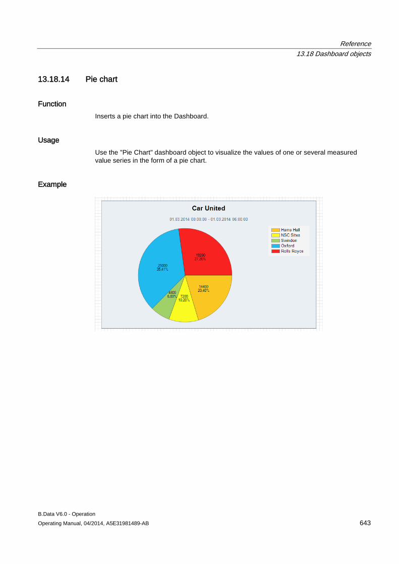
Reference 13.18 Dashboard objects
B.Data V6.0 - Operation Operating Manual, 04/2014, A5E31981489-AB 643
13.18.14 Pie chart
Function Inserts a pie chart into the Dashboard.
Usage Use the "Pie Chart" dashboard object to visualize the values of one or several measured value series in the form of a pie chart.
Example
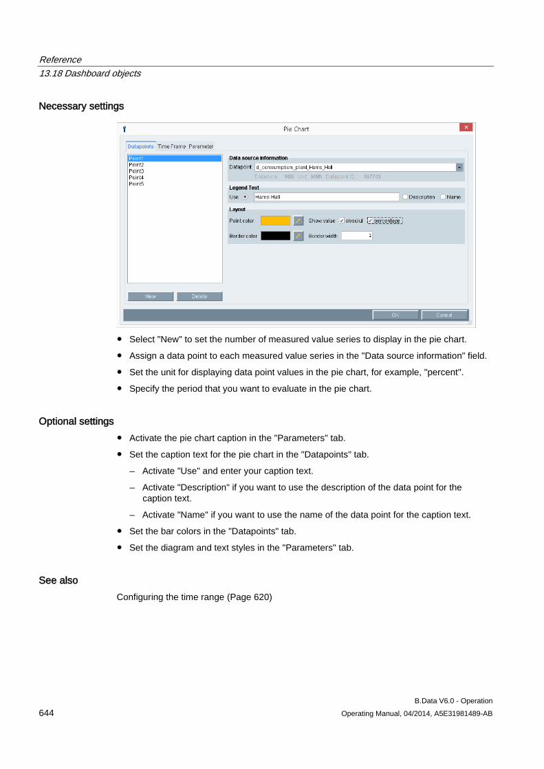
Reference 13.18 Dashboard objects
B.Data V6.0 - Operation 644 Operating Manual, 04/2014, A5E31981489-AB
Necessary settings
● Select "New" to set the number of measured value series to display in the pie chart.
● Assign a data point to each measured value series in the "Data source information" field.
● Set the unit for displaying data point values in the pie chart, for example, "percent".
● Specify the period that you want to evaluate in the pie chart.
Optional settings ● Activate the pie chart caption in the "Parameters" tab.
● Set the caption text for the pie chart in the "Datapoints" tab.
– Activate "Use" and enter your caption text.
– Activate "Description" if you want to use the description of the data point for the caption text.
– Activate "Name" if you want to use the name of the data point for the caption text.
● Set the bar colors in the "Datapoints" tab.
● Set the diagram and text styles in the "Parameters" tab.
See also Configuring the time range (Page 620)
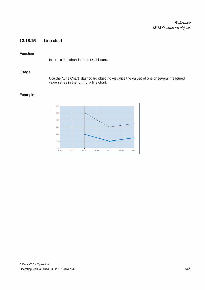
Reference 13.18 Dashboard objects
B.Data V6.0 - Operation Operating Manual, 04/2014, A5E31981489-AB 645
13.18.15 Line chart
Function Inserts a line chart into the Dashboard.
Usage Use the "Line Chart" dashboard object to visualize the values of one or several measured value series in the form of a line chart.
Example
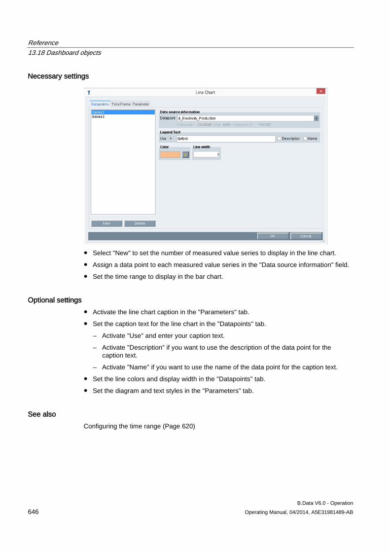
Reference 13.18 Dashboard objects
B.Data V6.0 - Operation 646 Operating Manual, 04/2014, A5E31981489-AB
Necessary settings
● Select "New" to set the number of measured value series to display in the line chart.
● Assign a data point to each measured value series in the "Data source information" field.
● Set the time range to display in the bar chart.
Optional settings ● Activate the line chart caption in the "Parameters" tab.
● Set the caption text for the line chart in the "Datapoints" tab.
– Activate "Use" and enter your caption text.
– Activate "Description" if you want to use the description of the data point for the caption text.
– Activate "Name" if you want to use the name of the data point for the caption text.
● Set the line colors and display width in the "Datapoints" tab.
● Set the diagram and text styles in the "Parameters" tab.
See also Configuring the time range (Page 620)
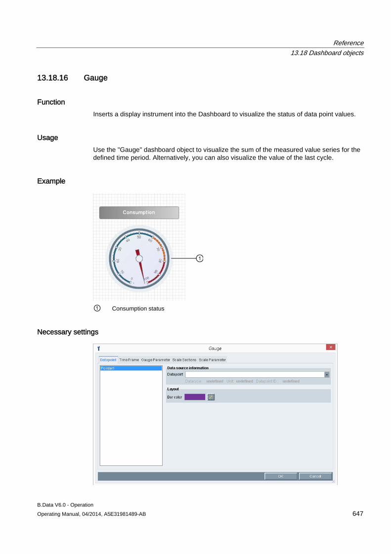
Reference 13.18 Dashboard objects
B.Data V6.0 - Operation Operating Manual, 04/2014, A5E31981489-AB 647
13.18.16 Gauge
Function Inserts a display instrument into the Dashboard to visualize the status of data point values.
Usage Use the "Gauge" dashboard object to visualize the sum of the measured value series for the defined time period. Alternatively, you can also visualize the value of the last cycle.
Example
① Consumption status
Necessary settings
Reference 13.18 Dashboard objects
B.Data V6.0 - Operation 648 Operating Manual, 04/2014, A5E31981489-AB
● Go to the "Data source information" field to select the data point that contains the values to be evaluated.
● Specify the period that you want to evaluate.
Optional settings ● Set the pointer color.
● Set the fill color and border style in the "Parameters" tab.
● Set the scale for the display instrument in the "Scale Parameter" section.
● Set the scale range in the "Scale Sections" section.
See also Configuring the time range (Page 620)

Reference 13.18 Dashboard objects
B.Data V6.0 - Operation Operating Manual, 04/2014, A5E31981489-AB 649
13.18.17 Panel switch
Function Inserts a button into the Dashboard that you can use to switch to another Dashboard .
Usage Use the "Panel switch" dashboard object to distribute selected data to several dashboards. Use the new button to switch between these dashboards.
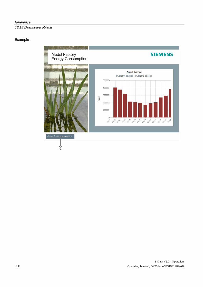
Reference 13.18 Dashboard objects
B.Data V6.0 - Operation 650 Operating Manual, 04/2014, A5E31981489-AB
Example
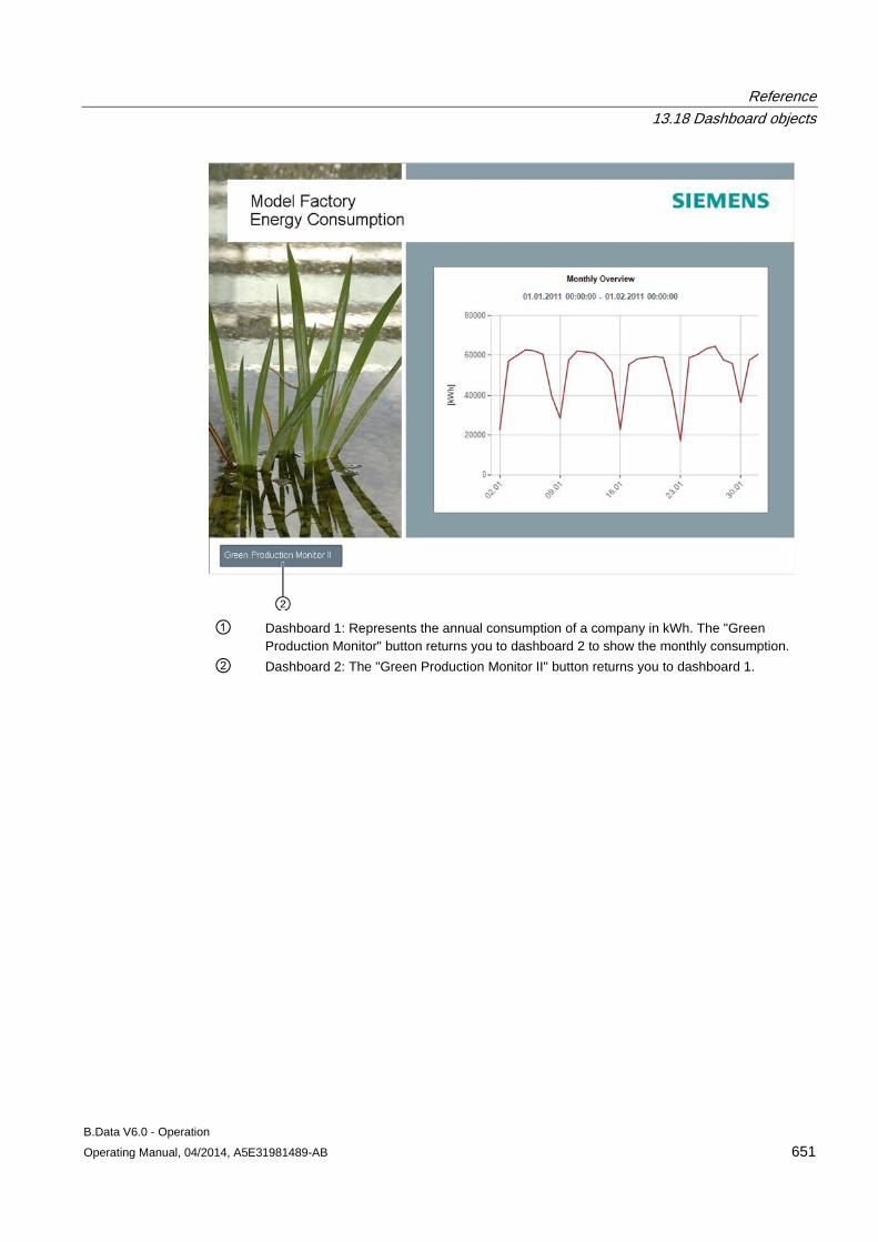
Reference 13.18 Dashboard objects
B.Data V6.0 - Operation Operating Manual, 04/2014, A5E31981489-AB 651
① Dashboard 1: Represents the annual consumption of a company in kWh. The "Green
Production Monitor" button returns you to dashboard 2 to show the monthly consumption. ② Dashboard 2: The "Green Production Monitor II" button returns you to dashboard 1.
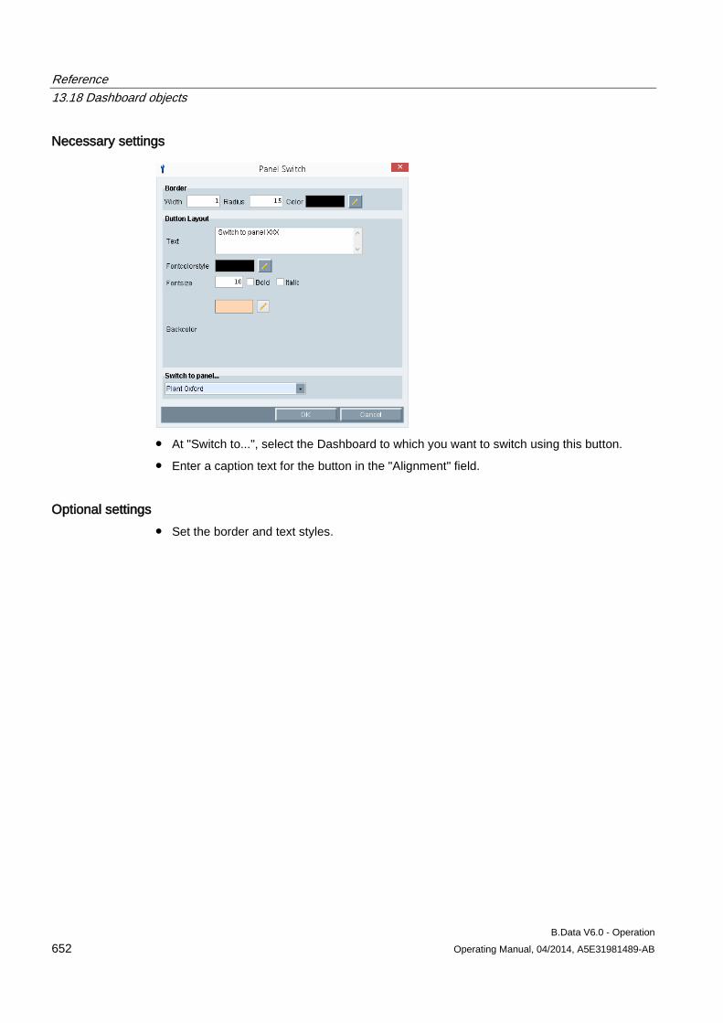
Reference 13.18 Dashboard objects
B.Data V6.0 - Operation 652 Operating Manual, 04/2014, A5E31981489-AB
Necessary settings
● At "Switch to...", select the Dashboard to which you want to switch using this button.
● Enter a caption text for the button in the "Alignment" field.
Optional settings ● Set the border and text styles.
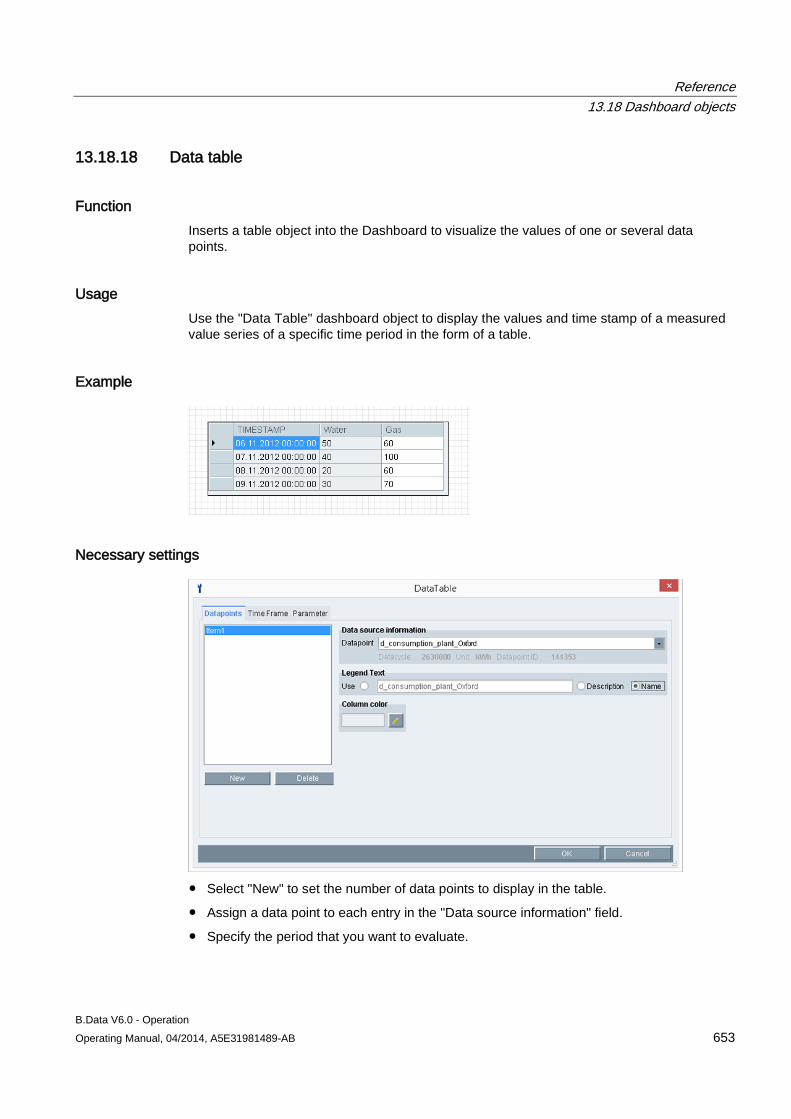
Reference 13.18 Dashboard objects
B.Data V6.0 - Operation Operating Manual, 04/2014, A5E31981489-AB 653
13.18.18 Data table
Function Inserts a table object into the Dashboard to visualize the values of one or several data points.
Usage Use the "Data Table" dashboard object to display the values and time stamp of a measured value series of a specific time period in the form of a table.
Example
Necessary settings
● Select "New" to set the number of data points to display in the table.
● Assign a data point to each entry in the "Data source information" field.
● Specify the period that you want to evaluate.
Reference 13.18 Dashboard objects
B.Data V6.0 - Operation 654 Operating Manual, 04/2014, A5E31981489-AB
Optional settings ● Create the "Legend name".
– Enter a text for the table header if you activate "Description".
– The data point name is used for the table header if you activate "Name".
● Set the column color.
● Set the table style in the "Parameters" tab.
See also Configuring the time range (Page 620)
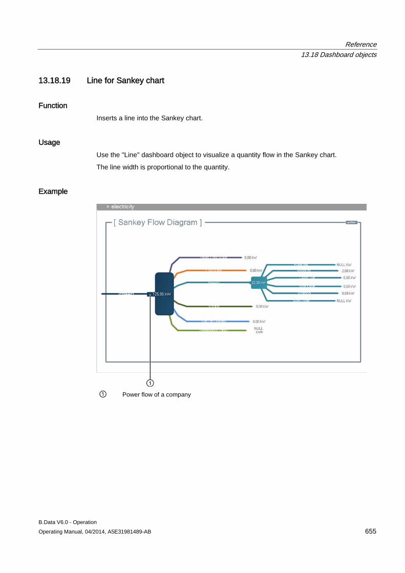
Reference 13.18 Dashboard objects
B.Data V6.0 - Operation Operating Manual, 04/2014, A5E31981489-AB 655
13.18.19 Line for Sankey chart
Function Inserts a line into the Sankey chart.
Usage Use the "Line" dashboard object to visualize a quantity flow in the Sankey chart.
The line width is proportional to the quantity.
Example
① Power flow of a company
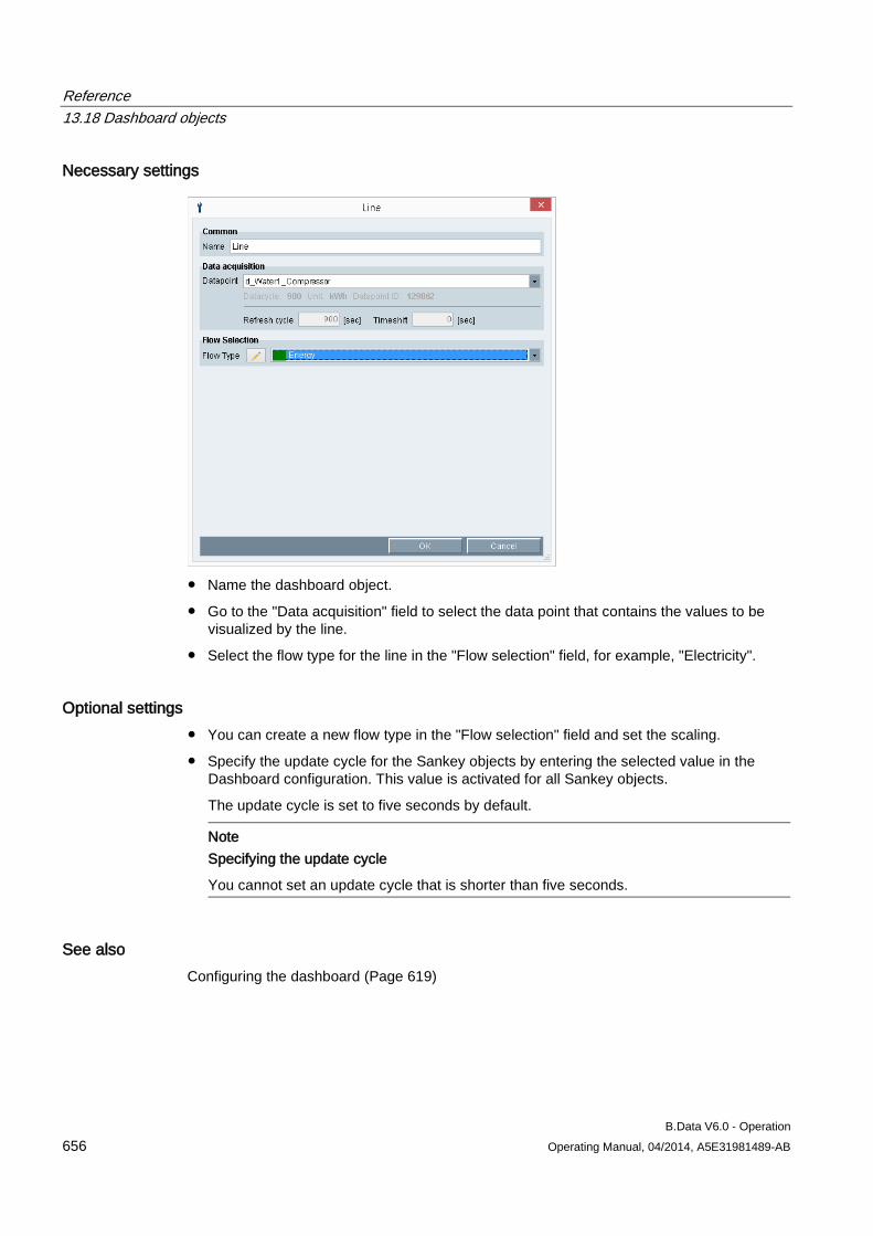
Reference 13.18 Dashboard objects
B.Data V6.0 - Operation 656 Operating Manual, 04/2014, A5E31981489-AB
Necessary settings
● Name the dashboard object.
● Go to the "Data acquisition" field to select the data point that contains the values to be visualized by the line.
● Select the flow type for the line in the "Flow selection" field, for example, "Electricity".
Optional settings ● You can create a new flow type in the "Flow selection" field and set the scaling.
● Specify the update cycle for the Sankey objects by entering the selected value in the Dashboard configuration. This value is activated for all Sankey objects.
The update cycle is set to five seconds by default.
Note Specifying the update cycle
You cannot set an update cycle that is shorter than five seconds.
See also Configuring the dashboard (Page 619)
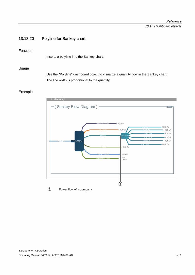
Reference 13.18 Dashboard objects
B.Data V6.0 - Operation Operating Manual, 04/2014, A5E31981489-AB 657
13.18.20 Polyline for Sankey chart
Function Inserts a polyline into the Sankey chart.
Usage Use the "Polyline" dashboard object to visualize a quantity flow in the Sankey chart.
The line width is proportional to the quantity.
Example
① Power flow of a company
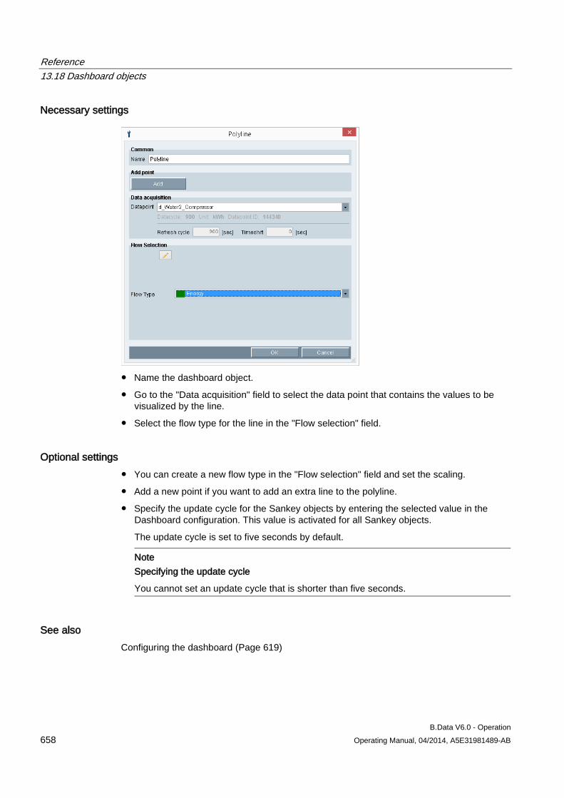
Reference 13.18 Dashboard objects
B.Data V6.0 - Operation 658 Operating Manual, 04/2014, A5E31981489-AB
Necessary settings
● Name the dashboard object.
● Go to the "Data acquisition" field to select the data point that contains the values to be visualized by the line.
● Select the flow type for the line in the "Flow selection" field.
Optional settings ● You can create a new flow type in the "Flow selection" field and set the scaling.
● Add a new point if you want to add an extra line to the polyline.
● Specify the update cycle for the Sankey objects by entering the selected value in the Dashboard configuration. This value is activated for all Sankey objects.
The update cycle is set to five seconds by default.
Note Specifying the update cycle
You cannot set an update cycle that is shorter than five seconds.
See also Configuring the dashboard (Page 619)
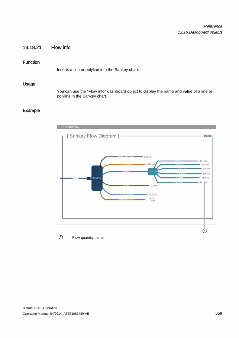
Reference 13.18 Dashboard objects
B.Data V6.0 - Operation Operating Manual, 04/2014, A5E31981489-AB 659
13.18.21 Flow info
Function Inserts a line or polyline into the Sankey chart.
Usage You can use the "Flow info" dashboard object to display the name and value of a line or polyline in the Sankey chart.
Example
① Flow quantity name
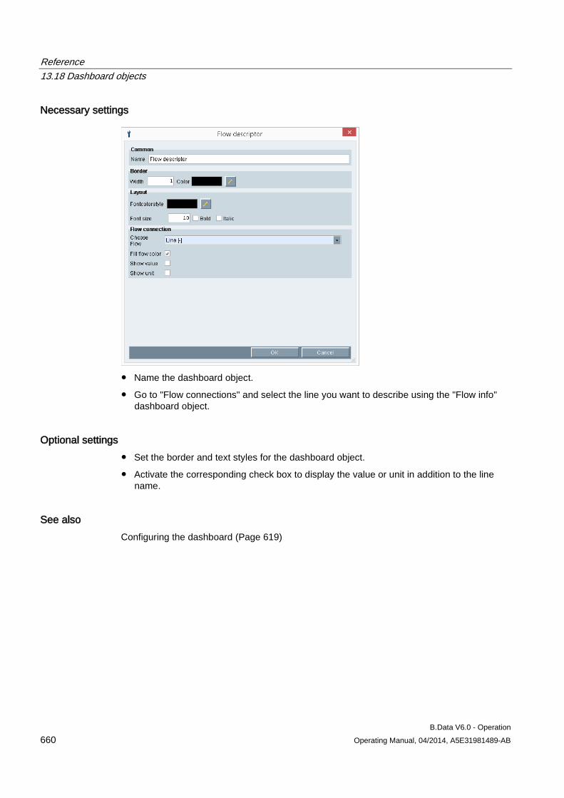
Reference 13.18 Dashboard objects
B.Data V6.0 - Operation 660 Operating Manual, 04/2014, A5E31981489-AB
Necessary settings
● Name the dashboard object.
● Go to "Flow connections" and select the line you want to describe using the "Flow info" dashboard object.
Optional settings ● Set the border and text styles for the dashboard object.
● Activate the corresponding check box to display the value or unit in addition to the line name.
See also Configuring the dashboard (Page 619)
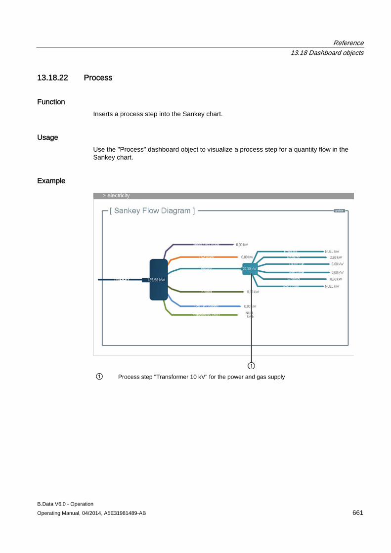
Reference 13.18 Dashboard objects
B.Data V6.0 - Operation Operating Manual, 04/2014, A5E31981489-AB 661
13.18.22 Process
Function Inserts a process step into the Sankey chart.
Usage Use the "Process" dashboard object to visualize a process step for a quantity flow in the Sankey chart.
Example
① Process step "Transformer 10 kV" for the power and gas supply
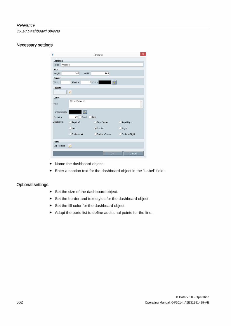
Reference 13.18 Dashboard objects
B.Data V6.0 - Operation 662 Operating Manual, 04/2014, A5E31981489-AB
Necessary settings
● Name the dashboard object.
● Enter a caption text for the dashboard object in the "Label" field.
Optional settings ● Set the size of the dashboard object.
● Set the border and text styles for the dashboard object.
● Set the fill color for the dashboard object.
● Adapt the ports list to define additional points for the line.
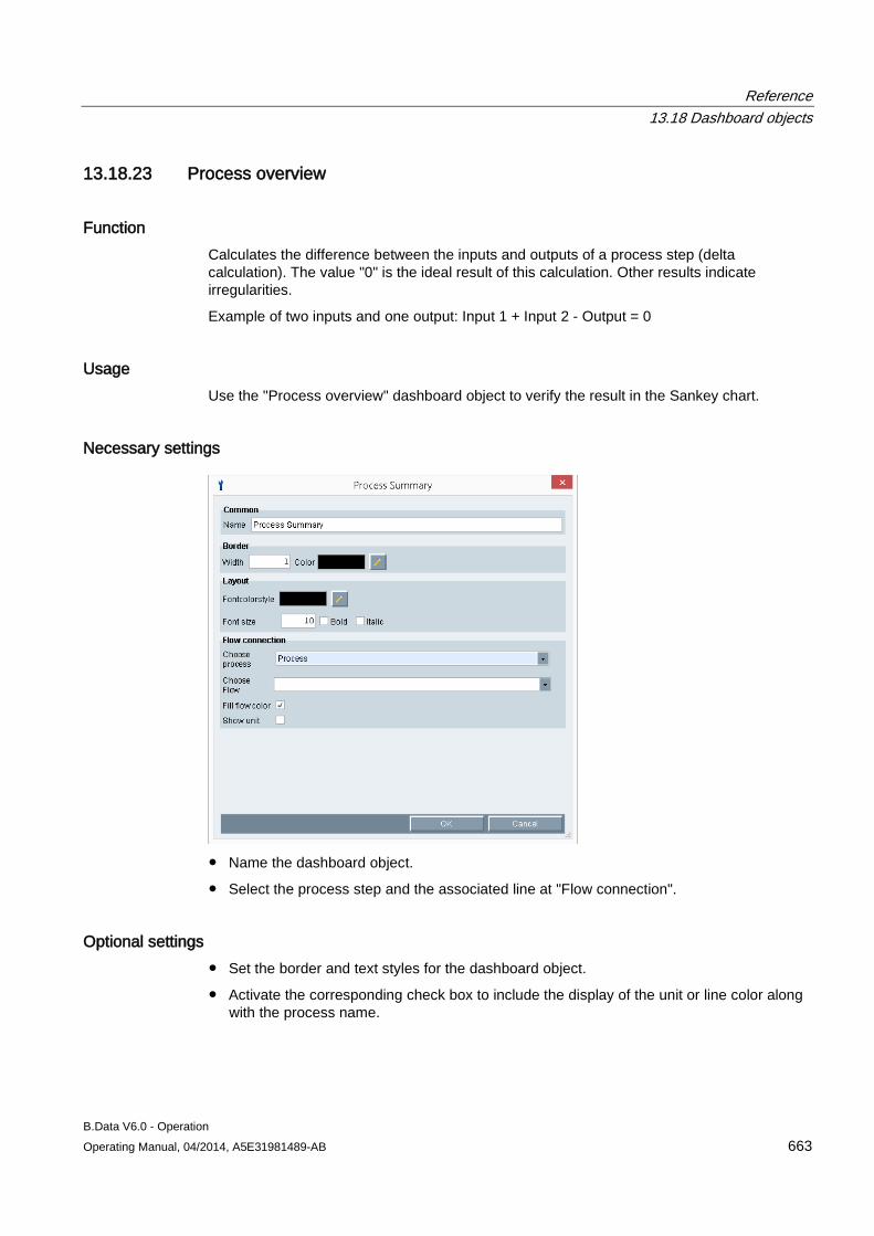
Reference 13.18 Dashboard objects
B.Data V6.0 - Operation Operating Manual, 04/2014, A5E31981489-AB 663
13.18.23 Process overview
Function Calculates the difference between the inputs and outputs of a process step (delta calculation). The value "0" is the ideal result of this calculation. Other results indicate irregularities.
Example of two inputs and one output: Input 1 + Input 2 - Output = 0
Usage Use the "Process overview" dashboard object to verify the result in the Sankey chart.
Necessary settings
● Name the dashboard object.
● Select the process step and the associated line at "Flow connection".
Optional settings ● Set the border and text styles for the dashboard object.
● Activate the corresponding check box to include the display of the unit or line color along with the process name.

Reference 13.18 Dashboard objects
B.Data V6.0 - Operation 664 Operating Manual, 04/2014, A5E31981489-AB
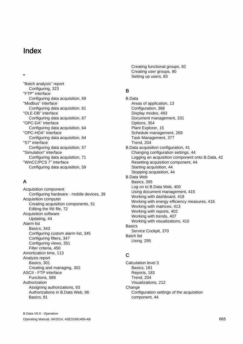
B.Data V6.0 - Operation Operating Manual, 04/2014, A5E31981489-AB 665
Index
" "Batch analysis" report
Configuring, 323 "FTP" interface
Configuring data acquisition, 69 "Modbus" interface
Configuring data acquisition, 61 "OLE-DB" interface
Configuring data acquisition, 67 "OPC-DA" interface
Configuring data acquisition, 64 "OPC-HDA" interface
Configuring data acquisition, 64 "S7" interface
Configuring data acquisition, 57 "Simulation" interface
Configuring data acquisition, 71 "WinCC/PCS 7" interface
Configuring data acquisition, 59
A Acquisition component
Configuring hardware - mobile devices, 39 Acquisition computer
Creating acquisition components, 51 Editing the INI file, 72
Acquisition software Updating, 44
Alarm list Basics, 343 Configuring custom alarm list, 345 Configuring filters, 347 Configuring views, 351 Filter criteria, 450
Amortization time, 113 Analysis report
Basics, 301 Creating and managing, 302
ASCII - FTP interface Functions, 589
Authorization Assigning authorizations, 93 Authorizations in B.Data Web, 96 Basics, 81
Creating functional groups, 92 Creating user groups, 90 Setting up users, 83
B B.Data
Areas of application, 13 Configuration, 368 Display modes, 493 Document management, 331 Options, 354 Plant Explorer, 15 Schedule management, 269 Task Management, 377 Trend, 204
B.Data acquisition configuration, 41 Changing configuration settings, 44 Logging an acquisition component onto B.Data, 42 Resetting acquisition component, 44 Starting acquisition, 44 Stopping acquisition, 44
B.Data Web Basics, 395 Log on to B.Data Web, 400 Using document management, 415 Working with dashboard, 418 Working with energy efficiency measures, 416 Working with matrices, 413 Working with reports, 402 Working with trends, 407 Working with visualizations, 410
Basics Service Cockpit, 370
Batch list Using, 295
C Calculation level 3
Basics, 181 Reports, 183 Trend, 204 Visualizations, 212
Change Configuration settings of the acquisition component, 44
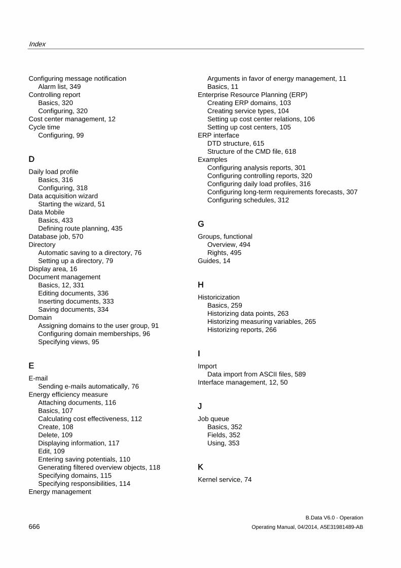
Index
B.Data V6.0 - Operation 666 Operating Manual, 04/2014, A5E31981489-AB
Configuring message notification Alarm list, 349
Controlling report Basics, 320 Configuring, 320
Cost center management, 12 Cycle time
Configuring, 99
D Daily load profile
Basics, 316 Configuring, 318
Data acquisition wizard Starting the wizard, 51
Data Mobile Basics, 433 Defining route planning, 435
Database job, 570 Directory
Automatic saving to a directory, 76 Setting up a directory, 79
Display area, 16 Document management
Basics, 12, 331 Editing documents, 336 Inserting documents, 333 Saving documents, 334
Domain Assigning domains to the user group, 91 Configuring domain memberships, 96 Specifying views, 95
E E-mail
Sending e-mails automatically, 76 Energy efficiency measure
Attaching documents, 116 Basics, 107 Calculating cost effectiveness, 112 Create, 108 Delete, 109 Displaying information, 117 Edit, 109 Entering saving potentials, 110 Generating filtered overview objects, 118 Specifying domains, 115 Specifying responsibilities, 114
Energy management
Arguments in favor of energy management, 11 Basics, 11
Enterprise Resource Planning (ERP) Creating ERP domains, 103 Creating service types, 104 Setting up cost center relations, 106 Setting up cost centers, 105
ERP interface DTD structure, 615 Structure of the CMD file, 618
Examples Configuring analysis reports, 301 Configuring controlling reports, 320 Configuring daily load profiles, 316 Configuring long-term requirements forecasts, 307 Configuring schedules, 312
G Groups, functional
Overview, 494 Rights, 495
Guides, 14
H Historicization
Basics, 259 Historizing data points, 263 Historizing measuring variables, 265 Historizing reports, 266
I Import
Data import from ASCII files, 589 Interface management, 12, 50
J Job queue
Basics, 352 Fields, 352 Using, 353
K Kernel service, 74
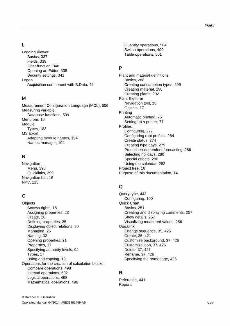
Index
B.Data V6.0 - Operation Operating Manual, 04/2014, A5E31981489-AB 667
L Logging Viewer
Basics, 337 Fields, 339 Filter function, 340 Opening an Editor, 338 Security settings, 341
Logon Acquisition component with B.Data, 42
M Measurement Configuration Language (MCL), 506 Measuring variable
Database functions, 509 Menu bar, 16 Module
Types, 183 MS Excel
Adapting module names, 194 Names manager, 194
N Navigation
Menu, 398 Quicklinks, 399
Navigation bar, 16 NPV, 113
O Objects
Access rights, 18 Assigning properties, 23 Create, 20 Defining properties, 25 Displaying object relations, 30 Managing, 26 Naming, 32 Opening properties, 21 Properties, 17 Specifying authority levels, 94 Types, 17 Using and copying, 18
Operations for the creation of calculation blocks Compare operations, 498 Interval operations, 502 Logical operations, 498 Mathematical operations, 496
Quantity operations, 504 Switch operations, 499 Table operations, 501
P Plant and material definitions
Basics, 288 Creating consumption types, 299 Creating material, 290 Creating plants, 292
Plant Explorer Navigation tool, 15 Objects, 17
Printing Automatic printing, 76 Setting up a printer, 77
Profiles Configuring, 277 Configuring root profiles, 284 Create status, 274 Creating type days, 275 Production-dependent forecasting, 286 Selecting holidays, 280 Special effects, 286 Using the calendar, 282
Project tree, 16 Purpose of this documentation, 14
Q Query type, 443
Configuring, 100 Quick Chart
Basics, 251 Creating and displaying comments, 257 Show details, 257 Visualizing measured values, 256
Quicklink Change sequence, 35, 425 Create, 35, 421 Customize background, 37, 426 Customize icon, 37, 426 Delete, 37, 427 Rename, 37, 426 Specifying the homepage, 426
R Reference, 441 Reports
Index
B.Data V6.0 - Operation 668 Operating Manual, 04/2014, A5E31981489-AB
Basics, 183 Configuring modules, 190 Configuring query types, 187 Configuring report templates in MS Excel, 193 Configuring templates, 195 Create, 185 Entering values, 197 Historizing, 266 Opening results, 202
Required basic knowledge, 14 Requirements forecast, long-term
Basics, 307 Configuring reports, 309 Creating derived data points, 307 Creating measuring variables, 308
Reset Acquisition component, 44
ROI, 113
S SAT interface, 51 Schedule
Basics, 312 Configuring, 314
Schedule management Basics, 12, 269 Examples, 301 Plant and material definitions, 288 Profiles, 273
Scope of validity, 14 Service Cockpit
Using, 373 Starting
Acquisition on acquisition component, 44 Stopping
Acquisition on acquisition component, 44
T Task Management
Basics, 12, 377 Creating the interval definition, 380 Creating the task, 379 Creating the Task Manager, 378 Functions, 584
Time unit abbreviations, 451 Trend
Assigning data points, 205 Basics, 12, 204 Configuring Trender objects, 206
Creating Trender objects, 205 Exporting data to an MS Office environment, 210 Generating, 205, 208 Operating the Trender, 549 Trender configuration dialog, 553 Trender legend, 552 Trender menu bar, 549 Trender status bar, 552 Trender toolbar, 551
U Unit configuration, 97 UNL notation, 79 Update
Acquisition software, 44 User
Assigning user name, 84 Editing logon information, 86 Entering contact information, 85
V Value
Acquisition status, 441 Correction status, 442
Visualizations Basics, 212 Configuring, 213 Generating, 221
X XLS report servers
Connection settings, 368 XML - ASCII interface
Basics, 608 Style sheets, 609
Related Documents