Battle of Water Networks DMAs (BWNDMA) Water Distribution Systems Analysis Conference 2016 Cartagena de Indias, Colombia, July 24 – 28, 2016 Problem Description and Rules Updated: 15/02/2016 Updated: 22/02/2016 Updated: 26/02/2016 Updated: 05/03/2016 Updated: 11/03/2016 Updated: 04/04/2016 Updated: 27/05/2016 1. Introduction The Battle of Water Networks District Meter Areas (BWNDMA) is the sixth Battle Competition since the beginning of the Water Distribution Systems Analysis Conference. The first one, known as Battle of Water Networks (BWN) was developed in 1985. Subsequent Battles included the Battle of the Water Sensor Networks (BWSN) in 2006, the Battle of the Calibration Networks (BWCN) in 2010, the Battle of the Water Networks Design (BWN-II) in 2012 and the Battle of Background Leakage Assessment for Water Networks (BBLAWN) in 2014. The BWNDMA invites either individuals or teams from academia, utilities, and consulting firms to propose a solution for the operation of a real water distribution system. The results of the BWNDMA will be presented at a special session of the upcoming 18 th Water Distribution Systems Analysis Conference in Cartagena, Colombia in July 2016. It is important to note that none of the members of the BWNDMA organizing committee will be taking part in the BWNDMA as participants. The responsibility of this committee is to gather the methodologies and results, propose an objective method of assessment, organize the session at the WDSA2016 event, and write a manuscript (as warranted) to be submitted to the Journal of Water Resources Planning and Management Division, ASCE, to summarize the outcomes and results of the competition.

Welcome message from author
This document is posted to help you gain knowledge. Please leave a comment to let me know what you think about it! Share it to your friends and learn new things together.
Transcript

Battle of Water Networks DMAs (BWNDMA)
Water Distribution Systems Analysis Conference 2016
Cartagena de Indias, Colombia, July 24 – 28, 2016
Problem Description and Rules
Updated: 15/02/2016
Updated: 22/02/2016
Updated: 26/02/2016
Updated: 05/03/2016
Updated: 11/03/2016
Updated: 04/04/2016
Updated: 27/05/2016
1. Introduction
The Battle of Water Networks District Meter Areas (BWNDMA) is the sixth Battle
Competition since the beginning of the Water Distribution Systems Analysis
Conference. The first one, known as Battle of Water Networks (BWN) was developed
in 1985. Subsequent Battles included the Battle of the Water Sensor Networks
(BWSN) in 2006, the Battle of the Calibration Networks (BWCN) in 2010, the Battle of
the Water Networks Design (BWN-II) in 2012 and the Battle of Background Leakage
Assessment for Water Networks (BBLAWN) in 2014.
The BWNDMA invites either individuals or teams from academia, utilities, and
consulting firms to propose a solution for the operation of a real water distribution
system. The results of the BWNDMA will be presented at a special session of the
upcoming 18th Water Distribution Systems Analysis Conference in Cartagena,
Colombia in July 2016.
It is important to note that none of the members of the BWNDMA organizing
committee will be taking part in the BWNDMA as participants. The responsibility of
this committee is to gather the methodologies and results, propose an objective
method of assessment, organize the session at the WDSA2016 event, and write a
manuscript (as warranted) to be submitted to the Journal of Water Resources
Planning and Management Division, ASCE, to summarize the outcomes and results of
the competition.
This document outlines the BWNDMA competition description, framework and rules.
2. How to participate
Each team/individual must submit an abstract for the WDSA2016 conference on-line
by March 7th 2016, briefly describing the proposed solution approach (e.g., trial and
error with simulation, evolutionary computation, heuristics, expert judgement, etc.).
In the conference Web page's Abstract Submission section, the author must tick the
box “Battle of Water Networks DMAs” in order to identify the abstract as a team in the
BWNDMA. Upon submission, please forward a copy of the submitted abstract to the
BWNDMA organizers at [email protected].
Notifications of accepted/rejected abstracts will be made by March 18th and each
successful team must summarize their results in a conference paper which must be
uploaded to the WDSA2016 website by June 22nd. All the received solutions will be
included in the special session for the presentation of the summary results at the
conference and will be published as part of the conference proceedings; a selected
participant of each team will present their results in this session.
Submitted papers, describing the final solution from each team, should be brief and to
the point. It is not necessary to describe the BWNDMA background. These papers
should include the following sections: Abstract, Introduction, Methodology, Summary
of results, Discussion of results, Conclusions and References.
In addition to the submission of the paper through the conference webpage,
participants are requested to email to the BWNDMA organizers the conference paper
and the following supporting material at [email protected]:
1. An EPANET (version 2.00.12) *.inp file of the solution proposed for the rainy
season (see further details below) with an Extended Period Simulation (EPS) of
168 hrs.
2. An EPANET (version 2.00.12) *.inp file of the solution proposed for the dry
season (see further details below) with an Extended Period Simulation (EPS) of
168 hrs.
3. An Excel file reporting the options adopted in the network for the solution
proposed.
4. A map of the resulting DMA configuration for the rainy season in E-Town (this
map can be delivered in a *.jpg, *.dwg, *.shp or any other).
The original EPANET file and the template for the Excel file for reporting the solution
options can be downloaded from:
https://wdsa2016.uniandes.edu.co/index.php/battle-of-water-networks

The BWNDMA organizers suggest that the Discussion of Results section should
emphasize the generality of the proposed strategy and the technical reasoning
focusing on the benefits of the adopted strategy. Results submitted with incomplete
information may be excluded from the competition.
3. Important BWNDMA dates
The following table (Table 1) lists important dates for the BWNDMA:
Table 1. BNWS Important Dates.
Problem Description Publication February 5th Abstract Deadline March 8th Notification of Abstract Acceptance March 18th Full paper and solution Deadline June 22nd Special Session at WDSA2016 July 28th
The winner(s) of the BWNDMA will be announced during the prepared special session
of the conference on July 28th.
4. Problem description
The municipality of E-Town, an important city in Colombia, is looking to change its
current infrastructure due to some problems related to water distribution. This town
has promising growth opportunities due to its touristic potential and overall macro-
economic growth of Colombia. However, it is having some issues with the operation
configuration of its water distribution system mainly due to the available sources of
water.
The water utility is interested in modifying the current DMA configuration in order to
make efficient use of available water in coordination with a number of infrastructure
changes proposed for 2022. To accomplish this task, the town has already developed a
calibrated hydraulic model of the current network and has included some of the
proposed interventions for the future (E-Town_05022016.inp). The network model
includes the forecasted demands, demand patterns, existing pump and tank
characteristics, and the actual controls of valves. The model shows that the existing
DMA configuration is not able to deliver water efficiently because there are
considerable differences in the pressure conditions of the city, some of the tanks are
empty and the water use is not efficient.
The main objective of this project is to develop a new DMA configuration that allows
the water utility to service with a minimal number of DMAs, each with a similar
number of users (similar demand); to guarantee pressure uniformity across the

municipality; to meet water quality goals and to ensure efficient system operation
during a variety of weather conditions throughout the year.
The E-Town water distribution system is supplied by three Water Treatment Plants
(WTPs): Bachue, Cuza and Bochica. During the rainy season (March, April, May,
September, October and November) these WTP are able to supply all the water
demanded by E-Town; however, during the dry season (December, January, February,
June, July and August) the water utility is forced to use a subsurface aquifer, which can
be directed, to two pump stations: Mohan and Fagua.
The new DMA configuration is to be designed for the rainy season, which is the most
common weather pattern in E-town. Nevertheless, proposals should provide a list of
the operational changes implemented in the system for the dry season to fulfill the
hydraulic requirements listed previously.
The current distribution of the DMAs in E-Town corresponds to a supply system that
was installed in 2014. By that year, the city was supplied by several pump stations
that distributed water from a subsurface aquifer and Poporo WTP provided 40% of
the water from superficial sources. However, with this supply configuration the city
had serious problems ensuring reliable water distribution. The delivered hydraulic
model includes the different DMAs that existed in 2014.
The supply configuration that will work from 2022 eliminates the Poporo WTP (which
in the future will work only as a storage tank_1). This is because a substantial portion
of new developments in the city have been built at higher elevation than the old city
and cannot longer by serviced by Poporo WTP.
The specific criteria required by the water utility to assess the solution proposed is
outlined below.
4.1. Solution Requirements
4.1.1. DMA Configuration
A DMA is considered as an isolated area with one or at most two entrances (in normal
operation conditions) regulated by one or two Pressure Reduction Valves (PRV). A
PRV simulates a flow measurement device; therefore, it must be installed at the
entrance of the DMA. The status of the PRV can be OPEN to simulate a valve that does
not have a regulation function in the system.
The water utility considers 15 DMAs to be manageable and convenient; therefore,
solutions that approach this number from the top will be favored. The minimum
number of DMAs must be 15 and this requirement will be assessed through the
following equation:
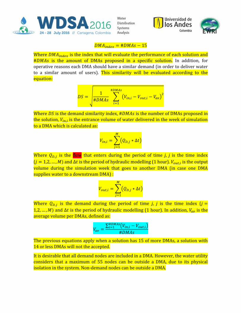
𝐷𝑀𝐴𝑖𝑛𝑑𝑒𝑥 = #𝐷𝑀𝐴𝑠 − 15
Where 𝐷𝑀𝐴𝑖𝑛𝑑𝑒𝑥 is the index that will evaluate the performance of each solution and
#𝐷𝑀𝐴𝑠 is the amount of DMAs proposed in a specific solution. In addition, for
operative reasons each DMA should have a similar demand (in order to deliver water
to a similar amount of users). This similarity will be evaluated according to the
equation:
𝐷𝑆 = √1
#𝐷𝑀𝐴𝑠 ∑ (𝑉𝑖𝑛,𝑖 − 𝑉𝑜𝑢𝑡,𝑖 − 𝑉𝑎𝑣)
2#𝐷𝑀𝐴𝑠
𝑖=1
Where 𝐷𝑆 is the demand similarity index, #𝐷𝑀𝐴𝑠 is the number of DMAs proposed in
the solution, 𝑉𝑖𝑛,𝑖 is the entrance volume of water delivered in the week of simulation
to a DMA which is calculated as:
𝑉𝑖𝑛,𝑖 = ∑(𝑄𝐷,𝑗 ∗ ∆𝑡)
𝑀
𝑗=1
Where 𝑄𝐷,𝑗 is the flow that enters during the period of time j, j is the time index
(𝑗 = 1,2, … ,𝑀) and ∆𝑡 is the period of hydraulic modelling (1 hour). 𝑉𝑜𝑢𝑡,𝑖 is the output
volume during the simulation week that goes to another DMA (in case one DMA
supplies water to a downstream DMA) :
𝑉𝑜𝑢𝑡,𝑖 = ∑(𝑄𝐷,𝑗 ∗ ∆𝑡)
𝑀
𝑗=1
Where 𝑄𝐷,𝑗 is the demand during the period of time j, j is the time index (𝑗 =
1,2, … ,𝑀) and ∆𝑡 is the period of hydraulic modelling (1 hour). In addition, 𝑉𝑎𝑣 is the
average volume per DMAs, defined as:
𝑉𝑎𝑣 =∑ (𝑉𝑖𝑛,𝑖 − 𝑉𝑜𝑢𝑡,𝑖)
#𝐷𝑀𝐴𝑠𝑖=1
#𝐷𝑀𝐴𝑠
The previous equations apply when a solution has 15 of more DMAs, a solution with
14 or less DMAs will not the accepted.
It is desirable that all demand nodes are included in a DMA. However, the water utility
considers that a maximum of 55 nodes can be outside a DMA, due to its physical
isolation in the system. Non-demand nodes can be outside a DMA.
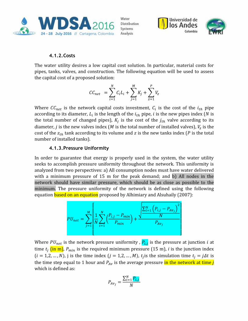
4.1.2. Costs
The water utility desires a low capital cost solution. In particular, material costs for
pipes, tanks, valves, and construction. The following equation will be used to assess
the capital cost of a proposed solution:
𝐶𝐶𝑛𝑒𝑡 = ∑𝐶𝑖𝐿𝑖
𝑁
𝑖=1
+ ∑𝐾𝑗
𝑀
𝑗=1
+ ∑𝑉𝑧
𝑃
𝑧=1
Where 𝐶𝐶𝑛𝑒𝑡 is the network capital costs investment, 𝐶𝑖 is the cost of the 𝑖𝑡ℎ pipe
according to its diameter, 𝐿𝑖 is the length of the 𝑖𝑡ℎ pipe, 𝑖 is the new pipes index (𝑁 is
the total number of changed pipes), 𝐾𝑗 is the cost of the 𝑗𝑡ℎ valve according to its
diameter, 𝑗 is the new valves index (𝑀 is the total number of installed valves), 𝑉𝑧 is the
cost of the 𝑧𝑡ℎ tank according to its volume and 𝑧 is the new tanks index (𝑃 is the total
number of installed tanks).
4.1.3. Pressure Uniformity
In order to guarantee that energy is properly used in the system, the water utility
seeks to accomplish pressure uniformity throughout the network. This uniformity is
analyzed from two perspectives: a) All consumption nodes must have water delivered
with a minimum pressure of 15 m for the peak demand; and b) All nodes in the
network should have similar pressure, which should be as close as possible to the
minimum. The pressure uniformity of the network is defined using the following
equation based on an equation proposed by Alhimiary and Alsuhaily (2007):
𝑃𝑈𝑛𝑒𝑡 = ∑
[
1
𝑁∑(
𝑃𝑖,𝑗 − 𝑃𝑚𝑖𝑛
𝑃𝑚𝑖𝑛)
𝑁
𝑖=1
+
√∑ (𝑃𝑖,𝑗 − 𝑃𝐴𝑣𝑗)2
𝑁𝑖=1
𝑁
𝑃𝐴𝑣𝑗
]
𝑀
𝑗=1
Where 𝑃𝑈𝑛𝑒𝑡 is the network pressure uniformity , 𝑃𝑖,𝑗 is the pressure at junction 𝑖 at
time 𝑡𝑗 (in m), 𝑃𝑚𝑖𝑛 is the required minimum pressure (15 m), i is the junction index
(𝑖 = 1,2, … ,𝑁), j is the time index (𝑗 = 1,2, … ,𝑀), 𝑡𝑗is the simulation time 𝑡𝑗 = 𝑗𝛥𝑡 is
the time step equal to 1 hour and 𝑃𝐴𝑣 is the average pressure in the network at time j
which is defined as:
𝑃𝐴𝑣𝑗=
∑ 𝑃𝑖,𝑗 𝑁𝑖=1
𝑁

The pressure uniformity is calculated only for demand nodes.
An additional condition is desired by the water utility regarding the pressure in the
system. While in the main pipe system of the municipality there are no restriction in
the maximum pressure, no pipes can have a pressure above 60 m at any moment of
the week. This restriction is valid only in the pipes within the DMAs.
4.1.4. Water Quality
Water quality is evaluated by the utility through the computation of water age in the
nodes of the network. Currently the preferred water age is exceeded in some parts of
the network and in the future, it should be minimized. The utility has defined the
measure of network water age as it was implemented in BWN-II:
𝑊𝐴𝑛𝑒𝑡 =∑ ∑ 𝑘𝑖
(𝑗)𝑄𝑑,𝑖(𝑗)(𝑊𝐴𝑖
(𝑗) − 𝑊𝐴𝐿𝑖𝑚)𝑀𝑗=1
𝑁𝑖=1
∑ ∑ 𝑄𝑑,𝑖(𝑗)𝑀
𝑗=1𝑁𝑖=1
Where 𝑊𝐴𝑛𝑒𝑡 is the network water age (in hours), 𝑊𝐴𝑖𝑗 is the water age at junction i
(excluding tanks and reservoirs) at time𝑡𝑗 , 𝑄𝑑,𝑖𝑗 is the demand at junction i and time 𝑡𝑗 ,
i is the junction index (𝑖 = 1,2, … ,𝑁), j is the time index (𝑗 = 1,2, … ,𝑀), 𝑡𝑗is the
simulation time 𝑡𝑗 = 𝑗𝛥𝑡 is the time step equal to 1 minute, 𝑊𝐴𝐿𝑖𝑚 is the limit water age
(in hours) allowed by the regulation of Colombia (60 hours) and 𝑘𝑖𝑗 is a variable defined
as:
𝑘𝑖𝑗 = {1,𝑊𝐴𝑖𝑗 ≥ 𝑊𝐴𝐿𝑖𝑚
0,𝑊𝐴𝑖𝑗 < 𝑊𝐴𝐿𝑖𝑚
The above network water age considers this variable only at non-zero demand nodes
and gives more importance to nodes with larger demands; it also only takes into
account the water age at junctions (excluding tanks and water sources). Finally, the
threshold from which the water age is considered was defined using the existing
regulation in Colombia.
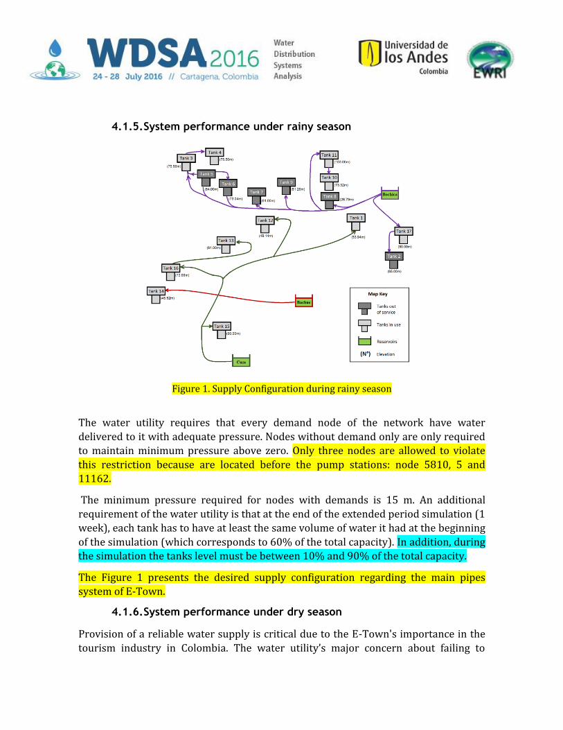
4.1.5. System performance under rainy season
Figure 1. Supply Configuration during rainy season
The water utility requires that every demand node of the network have water
delivered to it with adequate pressure. Nodes without demand only are only required
to maintain minimum pressure above zero. Only three nodes are allowed to violate
this restriction because are located before the pump stations: node 5810, 5 and
11162.
The minimum pressure required for nodes with demands is 15 m. An additional
requirement of the water utility is that at the end of the extended period simulation (1
week), each tank has to have at least the same volume of water it had at the beginning
of the simulation (which corresponds to 60% of the total capacity). In addition, during
the simulation the tanks level must be between 10% and 90% of the total capacity.
The Figure 1 presents the desired supply configuration regarding the main pipes
system of E-Town.
4.1.6. System performance under dry season
Provision of a reliable water supply is critical due to the E-Town's importance in the
tourism industry in Colombia. The water utility’s major concern about failing to
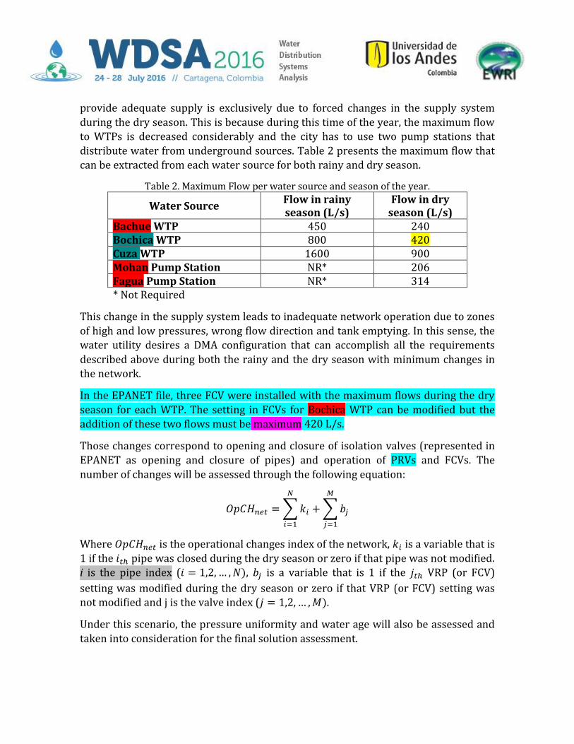
provide adequate supply is exclusively due to forced changes in the supply system
during the dry season. This is because during this time of the year, the maximum flow
to WTPs is decreased considerably and the city has to use two pump stations that
distribute water from underground sources. Table 2 presents the maximum flow that
can be extracted from each water source for both rainy and dry season.
Table 2. Maximum Flow per water source and season of the year.
Water Source Flow in rainy season (L/s)
Flow in dry season (L/s)
Bachue WTP 450 240 Bochica WTP 800 420 Cuza WTP 1600 900 Mohan Pump Station NR* 206 Fagua Pump Station NR* 314 * Not Required
This change in the supply system leads to inadequate network operation due to zones
of high and low pressures, wrong flow direction and tank emptying. In this sense, the
water utility desires a DMA configuration that can accomplish all the requirements
described above during both the rainy and the dry season with minimum changes in
the network.
In the EPANET file, three FCV were installed with the maximum flows during the dry
season for each WTP. The setting in FCVs for Bochica WTP can be modified but the
addition of these two flows must be maximum 420 L/s.
Those changes correspond to opening and closure of isolation valves (represented in
EPANET as opening and closure of pipes) and operation of PRVs and FCVs. The
number of changes will be assessed through the following equation:
𝑂𝑝𝐶𝐻𝑛𝑒𝑡 = ∑𝑘𝑖
𝑁
𝑖=1
+ ∑𝑏𝑗
𝑀
𝑗=1
Where 𝑂𝑝𝐶𝐻𝑛𝑒𝑡 is the operational changes index of the network, 𝑘𝑖 is a variable that is
1 if the 𝑖𝑡ℎ pipe was closed during the dry season or zero if that pipe was not modified.
i is the pipe index (𝑖 = 1,2, … ,𝑁), 𝑏𝑗 is a variable that is 1 if the 𝑗𝑡ℎ VRP (or FCV)
setting was modified during the dry season or zero if that VRP (or FCV) setting was not modified and j is the valve index (𝑗 = 1,2, … ,𝑀).
Under this scenario, the pressure uniformity and water age will also be assessed and
taken into consideration for the final solution assessment.

4.2. Intervention Options
4.2.1. Pipes
Pipe diameter options and costs for the network intervention are given in Table 3. The
costs shown include pipe construction, transport and installation. According to the
water utility, pipes can also be placed in parallel to existing pipes but as this implies
the disruption and reconstruction of pavement roads, the cost of duplicating existing
pipes is given by costs in Table 3 with and additional cost premium of 20%. The
absolute roughness (𝑘𝑠 𝑜𝑟 𝜀) for every diameter is 0.01 mm and the Minor Loss
Coefficient per length unit must be 0.02/m.
As an additional requirement, the water utility does not desire to disrupt city
operations to make changes in small pipes; therefore, the replacement of pipes is
restricted to pipes with diameters larger than 152 mm.
Table 3. Pipe annual costs.
Diameter (mm)
Cost New Pipe ($/m)
Cost Parallel Pipe ($/m)
203 23.31 27.97
254 26.09 31.30
305 29.86 35.83 356 32.56 39.07 406 35.35 42.42
457 38.56 46.27 508 41.87 50.25
610 62.18 74.62
711 69.96 83.95 762 73.46 88.15
4.2.2. Valves
The water utility considers the installation of Pressure Control Valves (PRVs) to
accomplish the desired system DMA configuration. The PRV costs are reported in
Table 4 and it is assumed that each one has a diameter equal to the diameter of the
pipe in which it is installed. The pressure setting on controlled nodes cannot be
variable over time; it can only change between seasons.

Table 4. PRV annual costs.
Diameter (mm)
Installation Cost ($)
102 315 152 695
203 1501 254 2240 305 3711 356 4470
406 7400
457 7733
508 7750 610 9211
711 10685 762 11708
The main objective of installing PRVs in the system is to define different DMAs. For
this reason, one or maximum two PRVs are allowed to be installed per DMA, at the
entrance(s).
E-Town system has installed Flow Control Valves (FCVs). The status and setting of
these elements can be changed with no additional costs but they can only be modified
between rainy and dry season. The status and setting of the FCVs cannot be changed
during the simulation.
4.2.3. Tanks
Because of the increased demands, the water utility is also allowing for the addition of
new tanks, but only adjacent to existing tanks where the water utility already owns
sufficient land. New tanks are assumed to have the same height and bottom elevation
as adjacent existing tanks (because the water utility does not want to introduce new
valves to control the system). All new tanks are cylindrical and come in pre-specified
standard sizes shown in Table 5, together with the installation costs. The construction
of non-standard tanks is discarded by the water utility because they are regarded as
too expensive.
Table 5. Tank annual costs.
Volume (m3)
Annual Cost ($/yr)
500 38827 1000 53387 2000 63093 3750 100258

5000 133467
10000 186667 15000 628075
Note that the costs shown in Table 4 already include the connectivity costs to link the
new tanks to the network. Therefore, the addition of new tanks can be modelled in
EPANET simply by increasing the tank diameters so that the resulting volume is equal
to the existing tank volume plus the new tank volume.
E-Town water distribution system has several tanks that are currently out of service
(in the hydraulic model its control valve is closed). The water utility has decided that
those tanks can be used without any additional costs (each team can install a FCV with
no costs in these tanks).
4.2.4. Pumps
E-Town water distribution system is supplied mainly by surface sources except
during the dry season when it is necessary to use the subsurface aquifer. The three
pump stations included in the model correspond to the two sites where water is
extracted (Mohan Pump Station has two pumps). These pump stations can work all
day during the dry season and it is allowed to add hydraulic controls in the model as
well (attached to any element of the system). Is not possible to add time controlled
pumps or variable speed pumps. It is not allowed to modify the pump curves.
The minimum flow that can be extracted is 100 L/s and the maximum flow was shown
in Table 2.
5. Solution Evaluation
Each team is required to submit only one solution regardless of the methodology used.
The solutions received will be assessed considering the following criteria:
1. DMA Configuration: number of DMAs
2. DMA Configuration: demand similarity index
3. Solution implementation cost
4. Pressure Uniformity during the rainy season
5. Water Age during the rainy season
6. Operation changes for the dry season
7. Pressure Uniformity during the dry season
8. Water Age during the dry season
9. Committee Score during the conference
10. Survey results during the conference

The final score of each team will be calculated considering the obtained range among
all participants of each criteria with the following equation:
𝐹𝑆𝑗 = ∑(𝑆𝑖𝑚𝑎𝑥 − 𝑆𝑖𝑗)
(𝑆𝑖𝑚𝑎𝑥 − 𝑆𝑖𝑚𝑖𝑛)
8
𝑖=1
+ ∑
(1
𝑆𝑖𝑚𝑎𝑥−
1𝑆𝑖𝑗
)
(1
𝑆𝑖𝑚𝑎𝑥−
1𝑆𝑖𝑚𝑖𝑛
)
10
𝑖=9
Where 𝐹𝑆𝑗 is the Final score of team j, 𝑆𝑖𝑚𝑎𝑥 is the maximum score in each criterion
accomplished by the worst team, 𝑆𝑖𝑗 is the score of the team j in the criterion i and
𝑆𝑚𝑖𝑛 is the minimum score in each criterion accomplished by the best team. The
solution with the highest overall rank will be selected as the winner.
If a team delivers a solution that violated any restriction of the problem (minimum,
maximum pressures, tanks levels or pump operation), they results will not be taken
into account in the final score.
Finally, during the special session at the conference, the groups will be ranked by the
committee taking into account the methodology and survey results from the attendees
at the special session.
6. Final Recommendations
Note that, as outlined earlier, to be eligible to participate, participants are required to
submit:
i) a paper describing the approach adopted
ii) an EPANET input file (*.inp) of the network solution selected (for the rainy
season)
iii) an EPANET input file (*.inp) of the network solution selected (for the dry
season)
iv) the completed Excel file outlining the solution decisions made by the team.
v) a map with the resulting DMA configuration for rainy season.
Note also that the delivered solution will be independently checked and evaluated
using the hydraulic solver EPANET to verify the authors’ results.
Groups from the same university are allowed if they are using different
methodologies, but no person can participate in more than one group.
7. Questions about the competition
If you have any question regarding the BWNDMA, please send us an email to

8. References
Alhimiary, H. and Alsuhaily, R. (2007) Minimizing Leakage Rates in Water Distribution
Networks through Optimal Valves Settings. World Environmental and Water
Resources Congress 2007: pp. 1-13. doi: 10.1061/40927(243)495
Marchi, A., Salomons, E., Ostfeld, A., Kapelan, Z., Simpson, A., Zecchin, A., Maier, H., Wu,
Z., Elsayed, S., Song, Y., Walski, T., Stokes, C., Wu, W., Dandy, G., Alvisi, S., Creaco, E.,
Franchini, M., Saldarriaga, J., Páez, D., Hernández, D., Bohórquez, J., Bent, R., Coffrin, C.,
Judi, D., McPherson, T., van Hentenryck, P., Matos, J., Monteiro, A., Matias, N., Yoo, D.,
Lee, H., Kim, J., Iglesias-Rey, P., Martínez-Solano, F., Mora-Meliá, D., Ribelles-Aguilar, J.,
Guidolin, M., Fu, G., Reed, P., Wang, Q., Liu, H., McClymont, K., Johns, M., Keedwell, E.,
Kandiah, V., Jasper, M., Drake, K., Shafiee, E., Barandouzi, M., Berglund, A., Brill, D.,
Mahinthakumar, G., Ranjithan, R., Zechman, E., Morley, M., Tricarico, C., de Marinis, G.,
Tolson, B., Khedr, A., and Asadzadeh, M. (2014). "Battle of the Water Networks II." J.
Water Resour. Plann. Manage., 10.1061/(ASCE)WR.1943-5452.0000378, 04014009.
Related Documents