aquatic products monitoring system in cold chain logistics

1

Applying CS and WSN methods for improving efficiency of frozen and chilled 1

aquatic products monitoring system in cold chain logistics 2

3

XIAO Xinqinga, b, HE Qile c, FU Zetiana, b, XU Markd, ZHANG Xiaoshuana, b* 4

a China Agricultural University, Beijing, 100083, China 5

b Beijing Laboratory of Food Quality and Safety, Beijing 100083, China 6

c Coventry University , Coventry, CV1 5FB,United Kingdom 7

d University of Portsmouth，Portsmouth, Hampshire，PO13DE，United Kingdom 8

* Corresponding author. China Agricultural University, Beijing 100083, P .R. China. Tel.: +86(0)1062736717. 9

E-mail addresses: [email protected] (Zhang. X) 10

11

12

Abstract: Wireless Sensor Network (WSN) is applied widely in food cold chain logistics. However, traditional 13

monitoring systems require significant real-time sensor data transmission which will result in heavy data traffic and 14

communication systems overloading, and thus reduce the data collection and transmission efficiency. This research 15

aims to develop a temperature Monitoring System for Frozen and Chilled Aquatic Products (MS-FCAP) based on 16

WSN integrated with Compressed Sending (CS) to improve the efficiency of MS-FCAP. Through understanding the 17

temperature and related information requirements of frozen and chilled aquatic products cold chain logistics, this 18

paper illustrates the design of the CS model which consists of sparse sampling and data reconstruction, and shelf-life 19

prediction. The system was implemented and evaluated in cold chain logistics between Hainan and Beijing in China. 20

The evaluation result suggests that MS-FCAP has a high accuracy in reconstructing temperature data under variable 21

temperature condition as well as under constant temperature condition. The result shows that MS-FCAP is capable of 22

recovering the sampled sensor data accurately and efficiently, reflecting the real-time temperature change in the 23

refrigerated truck during cold chain logistics, and providing effective decision support traceability for quality and 24

safety assurance of frozen and chilled aquatic products. 25

26

Keywords: Food safety and traceability; Cold chain logistics; Monitoring system; Wireless Sensor Network; 27

Compressed Sensing 28

29

1. Introduction 30

Wireless Sensor Network (WSN) has been adopted in many sectors, such as food cold chain logistics and 31

agriculture (e.g., Coates et al., 2013; Qi et al., 2014; Myo & Yoon, 2014), environmental monitoring (e.g., Weimer et 32

al., 2012; Guobao et al.,2014), and heavy industry (e.g., Wei et al., 2013; Xiao et al., 2014). WSN is a new 33

technology that combines sensor technology, embedded computing, networking, and wireless communication, and 34

distributed processing. It senses and collects information of monitoring objects and sends information to the end-user 35

via wireless and multi-hop network. Wireless transmission has many advantages over traditional wire transmission in 36

terms of low maintenance cost, higher mobility, better flexibility, and fast deployment in special occasions (Qi et al., 37

2011; Alayev et al., 2014; Suryadevara et al., 2015). However, a significant amount of real-time sensor data 38

transmission will result in heavy data traffic and overload the communication bandwidth in WSN, and thus reduce 39

the data collection and transmission efficiency (Qi et al., 2011; Li et al., 2012). 40

2

Compressed Sensing (CS) is a new signal acquisition method which recovers a sparse signal efficiently, accurately 41

with a relative small number of samples and overcomes some of the limitations of the classical compression schemes 42

(Candes and Tao, 2006; Donoho, 2006; Tsaig and Donoho, 2006; Haupt et al., 2008; Baraniuk et al., 2010). The 43

traditional signal processing maintains that a signal must be sampled at a Nyquist rate at least twice its bandwidth in 44

order to be represented without error. CS provides a low complexity approximation to the signal reconstruction, 45

which benefits storage, transmission and processing of natural signals, without restricting the Nyquist sampling 46

criterion. It also brings the benefits of simple compression in WSN without introducing excessive control overheads, 47

which meets the limited resource constraint of WSN (Chen et al., 2012; Xiao et al., 2013; Yunhe et al., 2013; Caione 48

et al., 2014). 49

Quality and safety of fresh food have attracted increasing attention from around the world, especially in emerging 50

economies, such as China thanks to the quickly rising living standards (Jiehong et al, 2013; Chuan-Heng et al., 2014). 51

For example, fish consumption per head in China is now 36.4 kg, which is twice the international average for fish 52

consumption. However, the official data show that the inspection pass rate of aquatic products in China is less than 53

95% (China Catfish Institute, 2012), putting serious threat to the health of consumers. 54

Fresh foods, such as aquatic products, are typically perishable, with the rate of deterioration accelerating when 55

temperature increases owing to a number of factors, such as microbial metabolism, oxidative reaction, and enzymatic 56

activity (Raven et al., 2014; Kotta et al., 2014; Pack et al., 2014). Unless appropriately packaged, transported and 57

stored, aquatic products will spoil in very short time. Therefore, an important aspect of aquatic products distribution 58

management is the effective monitoring of time-temperature conditions and effective temperature management, 59

which affect both safety and quality of aquatic products (Bytnerowicz et al., 2014). 60

Typical aquatic products cold chain logistics utilizes artificial refrigeration technology to meet low-temperature 61

requirements through temperature control. Traditional temperature measurement and monitoring system, such as 62

temperature chart recording system, is the most popular, reliable and accurate method to control and document 63

temperature condition in the cold chain storage and transportation (Chen et al., 2014). However, such systems have 64

high management costs while the data collection is time consuming. Moreover, each recorder of those systems needs 65

to be connected physically to a PC and the data collection is manually processed, thus resulting in highly complicated 66

system structure and high rate of inaccurate data monitoring (Trebar et al., 2013; Asadi et al., 2014). Therefore, 67

automated and efficient monitoring system and effective information management system are needed for effective 68

cold chain logistics. 69

In consideration of the benefits of WSN and CS, this research aim to adopt WSN integrated with CS as the 70

network infrastructure, and develops a temperature Monitoring System for Frozen and Chilled Aquatic Products 71

(MS-FCAP) in cold chain logistics. The system was designed to monitor the real-time temperature fluctuation and the 72

quality of frozen and chilled aquatic products by integrating the aquatic shelf-life prediction model. Moreover, the 73

system was implemented and evaluated in cold chain logistics between Hainan and Beijing in China. 74

This research contributes to the field of study in the following ways. First, the implementation of the MS-FCAP 75

helps to improve the transparency and traceability of the cold chain logistics and enables more effective control of the 76

quality and safety of the frozen and chilled aquatic products. Second, the MS-FCAP pilots the seamless integration of 77

WSN and CS for more effective temperature monitoring in cold chain logistics. Third, the successful implementation 78

of the MS-FCAP proves the feasibility of adopting WSN integrated with CS and paves the way for much wider 79

application in the areas of cold chain logistics monitoring. 80

The next section discusses the system analysis and architecture. This is followed by the system models discussion 81

and design. The paper then discusses the system implementation and evaluation. Finally, the discussion and 82

conclusion about this research as well as implications for future work are presented. 83

84

3

85

2. System analysis and architecture design 86

Multiple methods proposed Cortes et al. (2014) and Xiao et al. (2014) were followed to make sure that temperature 87

monitoring system would be designed to meet the need of potential users: a) Field observation for frozen and chilled 88

aquatic products in cold chain logistics; b) Field survey and interviews. 89

2.1. Field observation for frozen and chilled aquatic products in cold chain logistics 90

A field observation for frozen and chilled aquatic products in cold chain logistics was conducted in 2013, in 91

Hainan province, China. The purpose is to understand the actual process of cold chain logistics, including any factors 92

that may affect the safety and quality of aquatic products. As illustrated in Figure1, the typical cold chain logistics 93

process consists of the following basic steps: 94

Step 1: Catching the fresh fish from the farm. 95

Step 2: After the catching, fresh aquatic products are transported immediately via live or refrigerated 96

transportation to processing plants for further processing. 97

Step 3: Aquatic products processing and storage. Aquatic products are normally divided into two categories 98

for processing, either segmentation (with fish scales, cheek and viscera cast off) or whole fish. 99

Processed aquatic products are stored in cold storage or freezer maintained in -18℃ or lower. 100

Step 4: Transporting the frozen and chilled aquatic products from processing plants to retail stores. In this 101

process, temperature fluctuations, such as the variation from ambient temperature of about 20℃ to 102

-18℃ or lower, may cause safety and quality problems during the cold chain logistics process. 103

Step 5: Display and sale of frozen and chilled aquatic products by wholesalers and retailers. A large number of 104

refrigerated and frozen shelves are used to keep the appropriate temperature on -10℃ or lower. 105

Throughout the cold chain logistics, the chilled or refrigerated transportation has significantly impacted on 106

products safety. Pathogens, such as Listeria monocytogenes, can grow as low as -0.4°C (Fallah et al., 2013). 107

Clostridium botulinum type E and non-proteolytic type B and F can grow at temperatures as low as 3.3°C (Smelt et 108

al., 2013). Therefore, the ideal storage temperature of the frozen and chilled aquatic products should be maintained in 109

-18℃ or lower to ensure the products quality and safety. 110

Fig.1. Process of frozen and chilled aquatic products in cold chain logistics 111

2.2. Field survey and interview 112

To find out more about the needs of potential users, an interview based semi-structured survey was conducted to 113

explore and identify the potential users’ functional and information requirements. 6 senior managers and 20 first-line 114

managers working in the cold-chain logistics were involved in the survey. The interviewees were asked to describe 115

their routine work process, how they normally record the temperature information in the cold chain, how they get the 116

shelf-life information of the frozen and chilled aquatic products, and whether they knew about wireless monitoring or 117

if they have ever used it, what kind of information requirements are the most concerned or expected of such systems. 118

The interview survey lasted for one week. The results of the survey also helped the researcher to identify functional 119

and information requirements and system module divisions of MS-FCAP, which is discussed in the system 120

architecture below. 121

2.3. System architecture 122

In consideration of the functional and information requirements identified from the field observation and field 123

survey, the MS-FCAP architecture is developed consisting of three basic layers, namely wireless temperature sensor 124

4

nodes, the aggregation node, and the Aquatic Cold-chain Management System (ACMS) (see Figure 2). 125

A sensor node is a ZigBee wireless temperature sensor node. It is deployed at the refrigerated truck or storage 126

to sense the real-time temperature data and then send them to the network coordinator via ZigBee network 127

during cold chain logistics. A number of sensor nodes and a network coordinator will make up of a WSN. The 128

sensor nodes acquire and send the temperature data after the successful network synchronization and fall into 129

sleep after the successful data sending at regular intervals. 130

The aggregation node consists of a network coordinator and an Advanced RISC Machines (ARM) controller. 131

The network coordinator not only creates and controls the entire network, but also aggregates the sensor data 132

from the sensor nodes and sends them to the ARM controller to sparse sampling. The sparse sampling aims to 133

sample the sensor data and represents the original sensor data by a relative small number of samples. The 134

sampled data will be sent to the ACMS via General Packet Radio Service (GPRS) module for reconstruction 135

and generating predictions of the product shelf-life. 136

The ACMS is responsible for data receiving, reconstruction, and processing at the remote terminals. It 137

includes two layers: one is the server layer, which is responsible for data receiving/storage, sampled data 138

reconstruction, aquatic products shelf-life prediction via the data warehouse. The server layer serves as the 139

pipeline to connect the users and the sensor nodes, and also serves as the knowledge base and the model base. 140

The other one is the client layer, which provides not only the real-time and shelf-life information for the users, 141

but also the user-friendly operation and configuration interface for system managers. 142

Fig.2. Architecture diagram of the MS-FCAP 143

The temperature data is transmitted to the remote monitoring center via WSN integrated with CS, which includes 144

data sparse sampling and data reconstruction. The aquatic products shelf-life was then predicted via the shelf-life 145

prediction model (see Figure 3). The next section discusses in more detail about the system models of the MS-FCAP. 146

3. System models of MS-FCAP 147

3.1. Compressed sensing 148

Compressed Sensing (CS) ensures that the temperature signals can be acquired the global measurements with a 149

low sampling rate and reconstructed with a much smaller number of samples than those required by the Nysquist 150

theorem. This is possible only if the signals can be sparse represented under certain appropriate orthogonal basis 151

(Candes et al., 2006; Candes and Wakin, 2008; Chen and Wassell, 2012). 152

The sensor data NT RNxxx )](,),2(),1([ x are sparse transformed by the equation (1) as follows: 153

Ψsxx ori

N

i

is (1)

where N ,,, 21 Ψ , N

i R is the NN sparse matrix which is built according to the signal 154

characteristic, and T

Nsss ],,[ 21 s , N

i Rs , where s is the sparse representation of original signal x under 155

the basis of Ψ . 156

Vector y denotes the sampled data by calculating the inner product M

jj 1}{ as in equation (2). 157

5

ΘsΦΨsΦxy (2)

where TM ,, 21Φ is the NM observation matrix. 158

The sensor nodes are deployed at the refrigerated truck or storage to acquire the temperature data. The 159

biorthogonal wavelet transform matrix is built as the sparse matrixΨ , and the Gaussian random matrix Φ is built 160

as the signal observation matrix according to the temperature signal’s space-time characteristic to realize the sparse 161

sampling of the sensor data (see Figure 3). The sparse sampled data are sent via the GPRS module to the ACMS for 162

data reconstruction, data storage and processing, and for aquatic products shelf-life prediction. 163

The sparse sampled data y are reconstructed by choosing the Orthogonal Matching Pursuit (OMP) algorithm 164

model (Tropp and Gilbert, 2007; Donoho et al., 2012; Zhao et al., 2015) as described in equation (3) and (4): 165

Φxyxs ..minargˆ2

2ts

s

(3)

sΨx1ˆˆ (4)

where x is the accuracy or approximation value reconstructed by the 2-norm optimization method. Vector s is an 166

optimization sparse representation after the signal reconstruction. 167

The OMP is an efficient method to solve the data reconstruction problem. It is considered to be faster and easier to 168

implement for signal recovery problems (Tropp and Gilbert, 2007; Donoho et al., 2012; Zhao et al., 2015). The OMP 169

follows 5 steps as below: 170

Step 1: Initializing the model parameters. Setting I to be a null set and matrix q to be null to store the 171

suffix and the basis vectors of the recovery matrix respectively. Setting the initial residual yr , the sparse 172

coefficient 0s , the recovery matrix ΦΨΤ and iterations 0n . 173

Step 2: Choosing the basis vectors. To choose the maximum inner product value within the residual r from 174

the recovery matrix Τ as the basis vectors. Setting i to be the suffix of basis vectors, then it can get the 175

suffix value via the equation (5) as follows: 176

iii

tri ,maxˆ (5)

After the calculating, updating the set iII ˆ, , the matrix ],[ itqq and the basis vectors to be zero. 177

Step 3: Finding the sparse representation coefficient 2

2minargˆ qsys s

by the chosen basis vectors. 178

Step 4: Updating the residual sqyr ˆ . 179

Step 5: Stopping the iteration when the iterations get the maximum sparse value or the sparse coefficient equal 180

or less than reconstruction error. If not, then return to the step 2 to continue the iteration. 181

182

Fig.3. Flow chart of the system data transmission 183

184

3.2. Shelf-life prediction model 185

The frozen and chilled aquatic products shelf-life is the length of time aquatic products may be stored without 186

becoming unsuitable for use or consumption. Accurate shelf-life prediction can provide aid for the managers to 187

improve cold chain logistics processes and ensure aquatic products quality and safety. However, since temperature 188

6

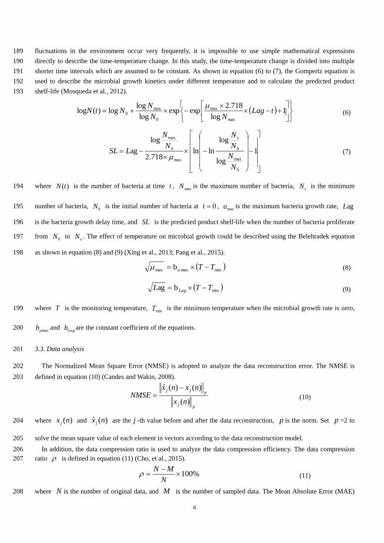
fluctuations in the environment occur very frequently, it is impossible to use simple mathematical expressions 189

directly to describe the time-temperature change. In this study, the time-temperature change is divided into multiple 190

shorter time intervals which are assumed to be constant. As shown in equation (6) to (7), the Gompertz equation is 191

used to describe the microbial growth kinetics under different temperature and to calculate the predicted product 192

shelf-life (Mosqueda et al., 2012). 193

1

log

718.2expexp

log

loglog)(log

max

max

0

max0 tLag

NN

NNtN

(6)

1

log

log

lnln718.2

log

ag

0

max

0

max

0

max

N

N

N

N

N

N

LSL

s

(7)

where )(tN is the number of bacteria at time t , maxN is the maximum number of bacteria,

sN is the minimum 194

number of bacteria, 0N is the initial number of bacteria at 0t ,

maxu is the maximum bacteria growth rate, agL 195

is the bacteria growth delay time, and SL is the predicted product shelf-life when the number of bacteria proliferate 196

from 0N to

sN . The effect of temperature on microbial growth could be described using the Belehradek equation 197

as shown in equation (8) and (9) (Xing et al., 2013; Pang et al., 2015). 198

minmaxmax b TTu (8)

minbag TTL Lag (9)

where T is the monitoring temperature, minT is the minimum temperature when the microbial growth rate is zero, 199

maxb and Lagb are the constant coefficient of the equations. 200

3.3. Data analysis 201

The Normalized Mean Square Error (NMSE) is adopted to analyze the data reconstruction error. The NMSE is 202

defined in equation (10) (Candes and Wakin, 2008). 203

pj

pjj

nx

nxnxNMSE

)(

)()(ˆ (10)

where )(nx j and )(ˆ nx j are the j -th value before and after the data reconstruction, p is the norm. Set p =2 to 204

solve the mean square value of each element in vectors according to the data reconstruction model. 205

In addition, the data compression ratio is used to analyze the data compression efficiency. The data compression 206

ratio is defined in equation (11) (Cho, et al., 2015). 207

%100

N

MN (11)

where N is the number of original data, and M is the number of sampled data. The Mean Absolute Error (MAE) 208

7

and Mean Relative Error (MRE) are adopted to measure the accuracy of the recovered data by comparing with the 209

original sensor data. 210

4. System design and implementation 211

This section discusses in more detailed in the system design and implementation of the MS-FCAP, which includes 212

the ACMS and the system hardware. 213

4.1. Hardware design and implementation 214

As shown in Figure 4, the system hardware mainly consists of the hardware of the sensor nodes and the 215

aggregation node. A sensor node is an integration of a microcontroller, a temperature sensor, and a battery power 216

supply. The aggregation node consists of the network coordinator, the ARM controller, and the GPRS remote 217

transmission module. The sensor node and the network coordinator adopt the CC2530 wireless sensor system on a 218

chip, which integrates a radio frequency transceiver with an enhanced 8051 microcontroller to improve the 219

integration and optimization of the hardware design. The sensor node and the network coordinator apply the CC2591 220

as the radio frequency front end to increase the transmission distance. 221

A sensor node adopts the DS18B20 as the temperature sensor, of which the temperature range is between -55°C 222

and +125°C and the temperature accuracy is ±0.5°C. The aggregation node adopts the S3C2440 as the ARM 223

controller to process the sparse sampling of data and to send the sampled data to the GPRS module. The network 224

coordinator and the GPRS module are all communicated with the ARM controller via the RS232 bus. The physical 225

implementation of the system hardware is illustrated in Figure 5. Each sensor node with an external antenna is 226

integrated in a plastic case. 227

228

Fig.4. Block diagram of the system hardware 229

Fig.5. Physical implementation of the sensor node hardware 230

4.2. ACMS design and implementation 231

ACMS serves as the management system for end-users. It is also responsible for maintaining the database of the 232

data received from the WSN, the reconstructed data of the sampled data, and data of aquatic products shelf-life 233

prediction during the cold chain logistics. The ACMS provides the function to add or edit the raw data from daily 234

operation and to search or review monitoring records. 235

ACMS adopts a 3-tier architecture, which includes the User Interface tier, the Functional Logic tier and the 236

Database tier (see Figure 6). 237

(1) User Interface tier provides a user interface for checking input data integrity and displaying information. For 238

example, cold chain managers can inquire the real-time temperature and the remaining products shelf-life in the cold 239

chain. Inquiry results can be displayed in the form of numerical temperature data or graphs and charts. The User 240

Interface tier also performs the data transmission between users and business logics. 241

(2) Business Logic tier consists of two components, is responsible for a variety of processing logics: 242

System management logic component consists of 5 modules of authorization management, communication 243

management, data management, model management and knowledge management. The authorization 244

management and communication management modules exchange data with the basic database in the database 245

tier. The data management module, the model management module, and the knowledge management module 246

exchange data with the data warehouse, the model base, and the knowledge base respectively. 247

Data processing logic component is the system core to realize the system real-time monitoring, data 248

reconstruction, and shelf-life prediction. The real-time temperature information is exchanged between the 249

8

temperature monitoring module and data management module within the system management component. 250

Data processing component reconstructs the sampled data and predicts the aquatic products shelf-life based 251

on the model management module and knowledge management module in the system management 252

component. After data reconstruction and shelf-life prediction, the data processing component sends the 253

real-time temperature monitoring and products shelf-life information based on model determined to user 254

interface tier. 255

Fig.6. Architecture of the ACMS 256

(3) Database tier consists of the following 4 independent databases, which communicate with each other and are 257

driven by the corresponding database management modules in the Business Logic tier: 258

The basic base is responsible for storing the authority and communication configuration information. 259

The data warehouse is responsible for storing the real-time temperature data which include the sampled and 260

reconstructed temperature data. 261

The knowledge base is responsible for storing knowledge models used for data analysis and decision making. 262

The model base is responsible for storing the parameters and equations of system models. 263

SQL Server 2008 database management system is applied to manage all the databases. ACMS is developed using 264

C# in Microsoft Visual Studio 2008 which is integrated with the real-time monitoring chart and shelf-life prediction 265

model powered by the Matlab M-language dynamic link library. 266

5. System test and evaluation 267

The MS-FCAP system is designed to improve the transparency of the cold chain logistics by better understanding 268

the temperature characteristics of cold chain process, and hence to ensure the quality and safety of the frozen and 269

chilled aquatic products. To evaluate the performance of the MS-FCAP system, system test and evaluation was 270

carried out, which is discussed in this section. The evaluation results were analyzed using Origin 8.1 software 271

(OriginLab Corporation, Northampton, MA) and SPSS 20.0 software (IBM Corporation, New York, NY, USA). 272

5.1. Experiment scenario 273

The MS-FCAP system was implemented in a Chinese aquatic products company to monitor the cold chain logistics 274

of frozen tilapia. The frozen products were kept in a refrigerated truck in 15-day transportation from Hainan, China to 275

Beijing, China. The transportation distance is around 2760 km. The length, width and height of the refrigerated truck 276

container are 3.0m×2.5m×2.4m. 27 sensor nodes were installed in the truck. Figure 7 indicates the sensor nodes 277

deployment in the refrigerated truck. Each sensor node was put into a box containing frozen and chilled tilapia before 278

loading. One aggregation node was installed in the driver’s cabin and the ACMS was installed in a remote control 279

center located in the company’s office. 280

To satisfy the low temperature storage requirements, the frozen tilapia transported should be kept in the container at 281

-18°C during the transportation and cold chain logistics (Qi et al., 2012; Calil et al., 2013). Real-time monitor and 282

control of the temperature in the refrigerated truck was carried out. The sensor nodes were calibrated using the 283

Resistance Temperature Detector calibrator (Fluke, Washington, USA) before deployed. 284

The temperature sample interval of the sensor nodes was set to 1 second, and the data sending interval of the 285

aggregation node was set to 1 minute. The length of data sending packet was 9 Bytes, which included the sensor ID 286

(1 Byte), the temperature data (4 Bytes) and the battery voltage (4 Bytes). The aggregation node aggregates and 287

sparse sampling the temperature data acquired from the 27 sensor nodes for every sample interval (1 second), and 288

transmits the sampled data to the ACMS for data reconstruction, and products shelf-life prediction via the GPRS 289

9

module for every data sending interval (1 minute). The aggregation node also stores the original temperature data to 290

test and evaluate the data reconstruction error while the sparse sampling of temperature data is being carried out. 291

Fig.7. Wireless temperature sensor nodes deployment in the refrigerated truck 292

The temperature distribution acquired from the MS-FCAP was analyzed to improve the transparency of the 293

temperature in the cold chain logistics and the aquatic products shelf-life predictions were also analyzed according to 294

the experiment scenario. 295

5.2. Data reconstruction error analysis 296

The cold chain for the frozen and chilled tilapia needs the pre-cooling step after loading to cool the temperature 297

down to -18°C from the ambient temperature, which takes around 2 hours. After pre-cooling, the temperature stays 298

constant at -18°C, which is referred to as the constant temperature condition, and then unloading (Wang et al., 2011). 299

The pre-cooling and unloading steps are referred to as the variable temperature condition. The data reconstruction 300

model was run at the ACMS to recover the sampled data. One of the sensor nodes, located nearby the door to reflect 301

the worst case temperature condition in refrigerated truck, was dedicated to analyze the temperature reconstruction 302

error in the cold chain. The absolute error with fitting surface between reconstructed and original temperature is 303

shown as Figure 8. 304

Fig.8. The absolute error between reconstructed and original temperature data in the cold chain 305

During the experiment, N is about 1620 and M is 256 (see also equation (1) and (2)). The NMSE, Mean 306

Absolute Error (MAE), Mean Relative Error (MRE) of reconstructed temperature data, and data compression ratio 307

under variable and constant temperature conditions are described in Table 1. 308

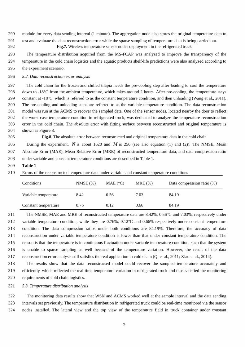
Table 1 309

Errors of the reconstructed temperature data under variable and constant temperature conditions 310

Conditions NMSE (%) MAE (°C) MRE (%) Data compression ratio (%)

Variable temperature 8.42 0.56 7.03 84.19

Constant temperature 0.76 0.12 0.66 84.19

The NMSE, MAE and MRE of reconstructed temperature data are 8.42%, 0.56°C and 7.03%, respectively under 311

variable temperature condition, while they are 0.76%, 0.12°C and 0.66% respectively under constant temperature 312

condition. The data compression ratios under both conditions are 84.19%. Therefore, the accuracy of data 313

reconstruction under variable temperature condition is lower than that under constant temperature condition. The 314

reason is that the temperature is in continuous fluctuation under variable temperature condition, such that the system 315

is unable to sparse sampling as well because of the temperature variation. However, the result of the data 316

reconstruction error analysis still satisfies the real application in cold chain (Qi et al., 2011; Xiao et al., 2014). 317

The results show that the data reconstructed model could recover the sampled temperature accurately and 318

efficiently, which reflected the real-time temperature variation in refrigerated truck and thus satisfied the monitoring 319

requirements of cold chain logistics. 320

5.3. Temperature distribution analysis 321

The monitoring data results show that WSN and ACMS worked well at the sample interval and the data sending 322

intervals set previously. The temperature distribution in refrigerated truck could be real-time monitored via the sensor 323

nodes installed. The lateral view and the top view of the temperature field in truck container under constant 324

10

temperature condition are illustrated in Figure 9. 325

Fig.9. The lateral view (a) and top view (b) of the temperature field in refrigerated truck 326

Specifically, the temperature near the container door is about -16.4°C and inside the container is about -18.5°C. 327

After evaluating the truck container, it was found that the temperature near the door being higher than that on the 328

inside because the refrigerator is installed inside of the container, and the cold winds are unevenly distributed, and 329

thus result in spatial differences in the temperature distribution (Cruz et al., 2009; Tarrega et al., 2011; Liu et al., 330

2014). The results show that the MS-FCAP could provide complete and accurate temperature monitoring information 331

in cold chain, so that to provide the more effective safety and quality assurance for the frozen and chilled aquatic 332

products in the cold chain. 333

5.4. Shelf-life prediction 334

The shelf-life of aquatic products was predicted according the determination of spoilage organism and the results 335

of fitting curve. The Total Viable Count (TVC) and Pseudomonas spp. spoilage organism for tilapia were determined 336

at the laboratory in Beijing between the year of 2012 and 2013 according to the literatures (Gram & Huss, 1996; 337

Boari et al, 2008; Xing et al., 2013). 338

Tilapias, which were almost the same size about 300-400g, were put into constant temperature incubators 339

(DPJ-100, Shanghai, China) with 0℃, 5℃, 10℃, 15℃, 20℃ and the variable temperature respectively for about 25 340

days. The Total Viable Count (TVC) and Pseudomonas spp. were determined from the samples every 48 hours. The 341

determination was composed of the following steps: 342

Step 1: Weighing tilapias for about 25g from each incubator by aseptic operation every time. 343

Step 2: Mincing by the meat grinder (TS-22, Beijing, China) with sterilization. 344

Step 3: Putting minced tilapia into 225mL conical flask within sterile physiological saline and several glass pearls. 345

Step 4: Shaking fully on the shaker (VS-10, Beijing, China). 346

Step 5: Diluting with 10 times volume. 347

Step 6: Determining the TVC using the pour method on plate count agar (Oxoid CM463, Hampshire, UK). 348

Step 7: Determining Pseudomonas counts using the spread plate method on agar base (Oxoid CM733, Hampshire, 349

UK) with CFC (cetrimide fucidin cephalosporin) selective supplement (Oxoid SR103, Hampshire, UK). 350

The TVC growth kinetics at various temperatures is shown as Figure 10. The fitting coefficients of determination 351

are about 0.996, 0.974, 0.994, 0.996 and 0.993 under 0℃, 5℃, 10℃, 15℃ and 20℃ temperature respectively. The 352

initial bacteria number is 5.12 log CFU/g and the maximum number is 20.12 log CFU/g. It can be seen that the 353

number of TVC increases with the storage time generally. However, the maximum growth rate is larger and the lag 354

phase is shorter when the temperature is higher (Xing et al., 2013). The initial TVC number under various 355

temperature conditions are almost identical because that’s the same amount of samples were weighed. The effect of 356

temperature on maxu and agL at various temperatures is shown as Figure 11. The temperature has a good linear 357

relation with the maximum Pseudomonas growth rate maxu and growth delay time agL , whose coefficient of 358

determination is about 0.973. 359

The TVC growth kinetics at variable temperature is shown as Figure 12. The variable temperature was controlled 360

according to the actual aquatic products cold chain, and the TVC and Pseudomonas counts were determined as the 361

same steps mentioned above. The coefficient of determination is about 0.956. It can be seen that the number of TVC 362

also increases with the storage time, but slower than that above 0℃. The calculated minimum Pseudomonas growth 363

11

temperature minT is about -0.112℃ according to the equation (8) and (9). This is may affect of the psychrophilic 364

bacteria. The psychrophilic bacteria will increase activity at below 0℃, but be inhibited at the normal temperature. 365

However, it has little impact on the quality of aquatic products because of the slower psychrophilic bacteria growth 366

rate compared with the Pseudomonas spp. (Farag et al. 2009). 367

The shelf-life prediction model, integrated the determined kinetic parameters, was performed by ACMS. The 368

calculated results interface is shown in Figure 13.The evaluation results show that the aquatic products shelf-life 369

prediction model built on the MS-FACP could be used to predict the remaining shelf-life of the aquatic products 370

during cold chain logistics and provide the effective decision support for the frozen and chilled aquatic products 371

managers in cold chain. 372

373

Fig.10. The TVC growth curve at various temperatures 374

Fig.11. The effect curve of temperature on maxu and agL at various temperatures 375

Fig.12. The TVC growth curve at variable temperature 376

Fig.13. The calculated results interface of aquatic products shelf-life prediction 377

5.5. System evaluation 378

System evaluation measures the current performance and provides the basis for the improvements of cold chain 379

management for frozen and chilled aquatic products on technological capacity, performance and system utilization 380

which brought by the MS-FCAP as well as the defects of this system prototype. 381

Managers and workers from the enterprise were invited to take part in a committee to evaluate the system and 382

discuss the system performance and form a consistent view on how this system should be perfected to improve 383

management efficiency of frozen and chilled aquatic products. 384

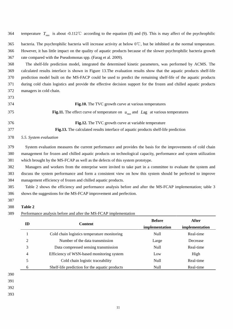
Table 2 shows the efficiency and performance analysis before and after the MS-FCAP implementation; table 3 385

shows the suggestions for the MS-FCAP improvement and perfection. 386

387

Table 2 388

Performance analysis before and after the MS-FCAP implementation 389

ID Content Before

implementation

After

implementation

1 Cold chain logistics temperature monitoring Null Real-time

2 Number of the data transmission Large Decrease

3 Data compressed sensing transmission Null Real-time

4 Efficiency of WSN-based monitoring system Low High

5 Cold chain logistic traceability Null Real-time

6 Shelf-life prediction for the aquatic products Null Real-time

390

391

392

393

12

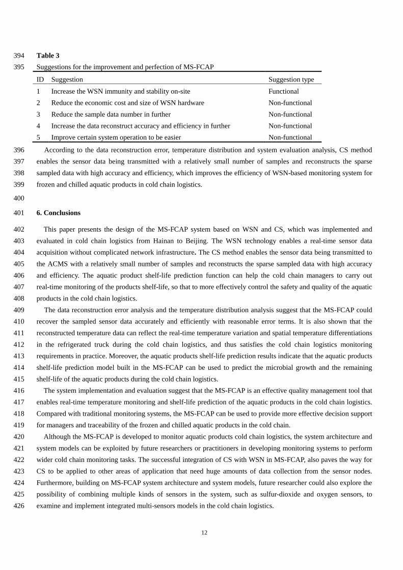
Table 3 394

Suggestions for the improvement and perfection of MS-FCAP 395

ID Suggestion Suggestion type

1 Increase the WSN immunity and stability on-site Functional

2 Reduce the economic cost and size of WSN hardware Non-functional

3 Reduce the sample data number in further Non-functional

4 Increase the data reconstruct accuracy and efficiency in further Non-functional

5 Improve certain system operation to be easier Non-functional

According to the data reconstruction error, temperature distribution and system evaluation analysis, CS method 396

enables the sensor data being transmitted with a relatively small number of samples and reconstructs the sparse 397

sampled data with high accuracy and efficiency, which improves the efficiency of WSN-based monitoring system for 398

frozen and chilled aquatic products in cold chain logistics. 399

400

6. Conclusions 401

This paper presents the design of the MS-FCAP system based on WSN and CS, which was implemented and 402

evaluated in cold chain logistics from Hainan to Beijing. The WSN technology enables a real-time sensor data 403

acquisition without complicated network infrastructure. The CS method enables the sensor data being transmitted to 404

the ACMS with a relatively small number of samples and reconstructs the sparse sampled data with high accuracy 405

and efficiency. The aquatic product shelf-life prediction function can help the cold chain managers to carry out 406

real-time monitoring of the products shelf-life, so that to more effectively control the safety and quality of the aquatic 407

products in the cold chain logistics. 408

The data reconstruction error analysis and the temperature distribution analysis suggest that the MS-FCAP could 409

recover the sampled sensor data accurately and efficiently with reasonable error terms. It is also shown that the 410

reconstructed temperature data can reflect the real-time temperature variation and spatial temperature differentiations 411

in the refrigerated truck during the cold chain logistics, and thus satisfies the cold chain logistics monitoring 412

requirements in practice. Moreover, the aquatic products shelf-life prediction results indicate that the aquatic products 413

shelf-life prediction model built in the MS-FCAP can be used to predict the microbial growth and the remaining 414

shelf-life of the aquatic products during the cold chain logistics. 415

The system implementation and evaluation suggest that the MS-FCAP is an effective quality management tool that 416

enables real-time temperature monitoring and shelf-life prediction of the aquatic products in the cold chain logistics. 417

Compared with traditional monitoring systems, the MS-FCAP can be used to provide more effective decision support 418

for managers and traceability of the frozen and chilled aquatic products in the cold chain. 419

Although the MS-FCAP is developed to monitor aquatic products cold chain logistics, the system architecture and 420

system models can be exploited by future researchers or practitioners in developing monitoring systems to perform 421

wider cold chain monitoring tasks. The successful integration of CS with WSN in MS-FCAP, also paves the way for 422

CS to be applied to other areas of application that need huge amounts of data collection from the sensor nodes. 423

Furthermore, building on MS-FCAP system architecture and system models, future researcher could also explore the 424

possibility of combining multiple kinds of sensors in the system, such as sulfur-dioxide and oxygen sensors, to 425

examine and implement integrated multi-sensors models in the cold chain logistics. 426

13

Acknowledgment 427

This research is funded by the ‘Special Fund for Agro-scientific Research in the Public Interest’ (201203017) from 428

the Ministry of Agriculture of China and the ‘China Spark Program’ (2013GA610002). 429

430

References 431

Alayev, Y., Chen, F., Hou, Y., Johnson, M. P., Bar-Noy, A., La Porta, T. F., & Leung, K. K. (2014). Throughput Maximization in 432

Mobile WSN Scheduling With Power Control and Rate Selection. Ieee Transactions on Wireless Communications, 433

13(7), 4066-4079. 434

Asadi, G., & Hosseini, E. (2014). Cold supply chain management in processing of food and agricultural products. 435

Scientific Papers, Series D. Animal Science, 57, 223-227. 436

Baraniuk, R. G., Candes, E., Elad, M., & Ma, Y. (2010). Applications of Sparse Representation and Compressive Sensing. 437

Proceedings of the Ieee, 98(6), 906-909. 438

Boari, C. A., Pereira, G. I., Valeriano, C., Silva, B. C., de Morais, V. M., Pereira Figueiredo, H. C., & Piccoli, R. H. (2008). Bacterial 439

ecology of tilapia fresh fillets and some factors that can influence their microbial quality. Ciencia E Tecnologia De 440

Alimentos, 28(4), 863-867. 441

Bytnerowicz, T. A., & Carruthers, R. I. (2014). Temperature-dependent models of Zannichellia palustris seed germination for 442

application in aquatic systems. Environmental and Experimental Botany, 104, 44-53. 443

Caione, C., Brunelli, D., & Benini, L. (2014). Compressive Sensing Optimization for Signal Ensembles in WSNs. Ieee 444

Transactions on Industrial Informatics, 10(1), 382-392. 445

Calil Angelini, M. F., Galvao, J. A., Vieira, A. d. F., Savay-da-Silva, L. K., Shirahigue, L. D., Ribeiro Cabral, I. S., Della Modesta, R. 446

C., Gallo, C. R., & Oetterer, M. (2013). Shelf-life and sensory assessment of tilapia quenelle during frozen storage. 447

Pesquisa Agropecuaria Brasileira, 48(8), 1080-1087. 448

Candes, E. J., Romberg, J., & Tao, T. (2006). Robust uncertainty principles: Exact signal reconstruction from highly 449

incomplete frequency information. Ieee Transactions on Information Theory, 52(2), 489-509. 450

Candes, E. J., & Tao, T. (2006). Near-optimal signal recovery from random projections: Universal encoding strategies? Ieee 451

Transactions on Information Theory, 52(12), 5406-5425. 452

Candes, E. J., & Wakin, M. B. (2008). An introduction to compressive sampling. Ieee Signal Processing Magazine25(2), 21-30. 453

Chen, F., Chandrakasan, A. P., & Stojanovic, V. M. (2012). Design and Analysis of a Hardware-Efficient Compressed Sensing 454

Architecture for Data Compression in Wireless Sensors. Ieee Journal of Solid-State Circuits, 47(3), 744-756. 455

Chen, W., & Wassell, I. J. (2012). Energy-efficient signal acquisition in wireless sensor networks: A compressive sensing 456

framework. IET Wireless Sensor Systems, 2(1), 1-8. 457

Chen, Y.-Y., Wang, Y.-J., & Jan, J.-K. (2014). A novel deployment of smart cold chain system using 2G-RFID-Sys. Journal of 458

Food Engineering, 141, 113-121. 459

China Catfish Institute.(2012). China Aquaculture Industry Report (2011–2012). Market Publisher, Beijing 460

[Online].Available:http://pdf.marketpublishers.com/researchinchina/china_aquaculture_industry_report_2011_2012.pdf 461

[05 December 2014]. 462

Cho, G.-Y., Lee, S.-J., & Lee, T.-R. (2015). An optimized compression algorithm for real-time ECG data transmission in wireless 463

network of medical information systems. Journal of medical systems, 39(1), 161-161. 464

Chuan-Heng, S., Wen-Yong, L., Chao, Z., Ming, L., Zeng-Tao, J., & Xin-Ting, Y. (2014). Anti-counterfeit code for aquatic product 465

identification for traceability and supervision in China. Food Control, 37, 126-134. 466

Coates, R. W., Delwiche, M. J., Broad, A., & Holler, M. (2013). Wireless sensor network with irrigation valve control. Computers 467

and Electronics in Agriculture, 96, 13-22. 468

Cortes, P., Badillo, G., Segura, L., & Bouchon, P. (2014). Experimental evidence of water loss and oil uptake during simulated 469

14

deep-fat frying using glass micromodels. Journal of Food Engineering, 140, 19-27. 470

Cruz, R. M. S., Vieira, M. C., & Silva, C. L. M. (2009). Effect of cold chain temperature abuses on the quality of frozen watercress 471

(Nasturtium offcinale R. Br.). Journal of Food Engineering, 94 (1), 90-97. 472

Donoho, D. L. (2006). Compressed sensing. Ieee Transactions on Information Theory, 52(4), 1289-1306. 473

Donoho, D. L., Tsaig, Y., Drori, I., & Starck, J.-L. (2012). Sparse Solution of Underdetermined Systems of Linear Equations by 474

Stagewise Orthogonal Matching Pursuit. Ieee Transactions on Information Theory, 58(2), 1094-1121. 475

Fallah, A. A., Saei-Dehkordi, S. S., & Mahzounieh, M. (2013). Occurrence and antibiotic resistance profiles of Listeria 476

monocytogenes isolated from seafood products and market and processing environments in Iran. Food Control, 34 (2), 477

630-636. 478

Farag, H., & Korashy, N. (2009). Prevalence of hydrogen sulfide producing psychrophilic bacteria in chilled Mugil cephalus" 479

Mullet" fish and their public health significance. Assiut Veterinary Medical Journal, 55(122), 156-168. 480

Gram, L., & Huss, H. H. (1996). Microbiological spoilage of fish and fish products. International journal of food microbiology, 481

33(1), 121-137. 482

Guobao, X., Weiming, S., & Xianbin, W. (2014). Applications of Wireless Sensor Networks in Marine Environment Monitoring: 483

A Survey. Sensors, 14(9), 16932-16952. 484

Haupt, J., Bajwa, W. U., Rabbat, M., & Nowak, R. (2008). Compressed sensing for networked data. Ieee Signal Processing 485

Magazine, 25(2), 92-101. 486

Jiehong, Z., Zhen, Y., & Yuan, W. (2013). Improving quality and safety of aquatic products: A case study of self-inspection 487

behavior from export-oriented aquatic enterprises in Zhejiang Province, China. Food Control,33(2), 528-535. 488

Kotta, J., Moeller, T., Orav-Kotta, H., & Paernoja, M. (2014). Realized niche width of a brackish water submerged aquatic 489

vegetation under current environmental conditions and projected influences of climate change. Marine Environmental 490

Research, 102, 88-101. 491

Li, X., Zhang, X.-y., & Wang, Z.-j. (2012). Study on Data Compression for TDOA Estimation in WSN Application. Signal 492

Processing, 28(9), 1226-1234. 493

Liu, J., Zhang, X., Xiao, X., & Fu, Z. (2014). Optimal sensor layout in refrigerator car based on multi-objective fuzzy matter 494

element method. Nongye Jixie Xuebao = Transactions of the Chinese Society for Agricultural Machinery, 45 (10), 214-219. 495

Mosqueda-Melgar, J., Raybaudi-Massilia, R. M., & Martin-Belloso, O. (2012). Microbiological shelf-life and sensory evaluation 496

of fruit juices treated by high-intensity pulsed electric fields and antimicrobials. Food and Bioproducts Processing, 90(C2), 497

205-214. 498

Myo Min, A., & Yoon Seok, C. (2014). Temperature management for the quality assurance of a perishable food supply chain. 499

Food Control, 40, 198-207. 500

Pack, E. C., Lee, S. H., Kim, C. H., Lim, C. H., Sung, D. G., Kim, M. H., Park, K. H., Lim, K. M., Choi, D. W., & Kim, S. W. (2014). Effects 501

of Environmental Temperature Change on Mercury Absorption in Aquatic Organisms with Respect to Climate Warming. 502

Journal of Toxicology and Environmental Health-Part a-Current Issues, 77(22-24), 1477-1490. 503

Pang, Y.-H., Zhang, L., Zhou, S., Yam, K. L., Liu, L., & Sheen, S. (2015). Growth behavior prediction of fresh catfish fillet with 504

Pseudomonas aeruginosa under stresses of allyl isothiocyanate, temperature and modified atmosphere. Food Control, 505

47, 326-333. 506

Qi, L., Han, Y., Zhang, X., Xing, S., & Fu, Z. (2012). Real-time monitoring system for aquatic cold-chain logistics based on WSN. 507

Nongye Jixie Xuebao = Transactions of the Chinese Society for Agricultural Machinery, 43(8), 134-140. 508

Qi, L., Tian, D., Zhang, J., Zhang, X., & Fu, Z. (2011). Sensing data compression method based on SPC for agri-food cold-chain 509

logistics. Nongye Jixie Xuebao = Transactions of the Chinese Society for Agricultural Machinery, 42(10), 129-134. 510

Qi, L., Xu, M., Fu, Z., Mira, T., & Zhang, X. (2014). (CSLDS)-S-2: A WSN-based perishable food shelf-life prediction and LSFO 511

strategy decision support system in cold chain logistics. Food Control, 38, 19-29. 512

Qi, L., Zhang, J., Mark, X., Fu, Z., Chen, W., & Zhang, X. (2011). Developing WSN-based traceability system for recirculation 513

15

aquaculture. Mathematical and Computer Modelling, 53(11-12), 2162-2172. 514

Raven, J. A., Beardall, J., & Giordano, M. (2014). Energy costs of carbon dioxide concentrating mechanisms in aquatic 515

organisms. Photosynthesis Research, 121(2-3), 111-124. 516

Smelt, J. P., Stringer, S. C., & Brul, S. (2013). Behaviour of individual spores of non proteolytic Clostridium botulinum as an 517

element in quantitative risk assessment. Food Control, 29 (2), 358-363. 518

Suryadevara, N. K., Mukhopadhyay, S. C., Kelly, S. D. T., & Gill, S. P. S. (2015). WSN-based smart sensors and actuator for power 519

management in intelligent buildings. IEEE/ASME Transactions on Mechatronics, 20(2), 564-571. 520

Tarrega, A., Torres, J. D., & Costell, E. (2011). Influence of the chain-length distribution of inulin on the rheology and 521

microstructure of prebiotic dairy desserts. Journal of Food Engineering, 104 (3), 356-363. 522

Trebar, M., Lotric, M., Fonda, I., Pletersek, A., & Kovacic, K. (2013). RFID Data Loggers in Fish Supply Chain Traceability. 523

International Journal of Antennas and Propagation. 524

Tropp, J. A., & Gilbert, A. C. (2007). Signal recovery from random measurements via orthogonal matching pursuit. Ieee 525

Transactions on Information Theory, 53(12), 4655-4666. 526

Tsaig, Y., & Donoho, D. L. (2006). Extensions of compressed sensing. Signal Processing, 86(3), 549-571. 527

Wang, T., Zhang, X., Chen, W., Fu, Z., & Peng, Z. (2011). RFID-based temperature monitoring system of frozen and chilled 528

tilapia in cold chain logistics. Transactions of the Chinese Society of Agricultural Engineering, 27(9), 141-146. 529

Wei, S., Tingting, Z., Gidlund, M., & Dobslaw, F. (2013). SAS-TDMA: a source aware scheduling algorithm for real-time 530

communication in industrial wireless sensor networks. Wireless Networks, 19(6), 1155-1170. 531

Weimer, J., Krogh, B. H., Small, M. J., & Sinopoli, B. (2012). An approach to leak detection using wireless sensor networks at 532

carbon sequestration sites. International Journal of Greenhouse Gas Control, 9, 243-253. 533

Xiao, X., Qi, L., Fu, Z., & Zhang, X. (2013). Monitoring method for cold chain logistics of table grape based on compressive 534

sensing. Transactions of the Chinese Society of Agricultural Engineering, 29(22), 259-266. 535

Xiao, X., Zhu, T., Qi, L., Moga, L. M., & Zhang, X. (2014). MS-BWME: A Wireless Real-Time Monitoring System for Brine Well 536

Mining Equipment. Sensors, 14(10), 19877-19896. 537

Xing, S., Zhang, X., Ma, C., & Fu, Z. (2013). Microbial growth kinetics model of tilapia under variable temperatures. Nongye 538

Jixie Xuebao = Transactions of the Chinese Society for Agricultural Machinery, 44(7), 194-198. 539

Yunhe, L., Qinyu, Z., Shaohua, W., & Ruofei, Z. (2013). Efficient Data Gathering with Network Coding Coupled Compressed 540

Sensing for Wireless Sensor Networks. Information Technology Journal, 12(9), 1737-1745. 541

Zhao, J., Song, R., Zhao, J., & Zhu, W.-P. (2015). New conditions for uniformly recovering sparse signals via orthogonal 542

matching pursuit. Signal Processing, 106, 106-113. 543