Applying Data Preparation Methods to Optimize Preterm Birth ...

Applying Data Preparation Methods to Optimize Preterm Birth

Prediction

by

Alana Esty, B. Eng.

A thesis submitted to the Faculty of Graduate and Postdoctoral

Affairs in partial fulfillment of the requirements for the degree of

Master of Applied Science

in

Biomedical Engineering

Ottawa - Carleton Institute for Biomedical Engineering (OCIBME)

Carleton University

Ottawa, Ontario

July 2018

© 2018

Alana Esty

ii

Abstract

The purpose of this work was to develop an accurate prediction model which can process

information contained in antenatal databases to determine whether a baby will be born

prematurely. The focus was on improved data preprocessing to add to methods developed by

previous students in the Carleton MIRG (Medical Information technology Research Group)

lab.

The machine learning classifiers used included Decision Tree (DT) classifiers (for feature

reduction) and the Artificial Neural Network (ANN) classifier (for model evaluation).

Missing values and class imbalance was dealt with by applying software packages in the R

statistical programming language.

This research has shown a marked improvement in the accuracy of predicting preterm births.

The final sensitivity and specificity results for the BORN (Better Outcomes Registry and

Network) database were: Parous 89.2%, and 67.8%, Nulliparous 89.0% and 71.5%, and for

PRAMS (Pregnancy Risk Assessment Monitoring System) database: Parous 84.1% and

71.4%, Nulliparous 83.8% and 76.0%. These improved results are promising. An accurate

predictive tool will allow caregivers to implement preventative treatment strategies or to

ensure delivery occurs in a tertiary health care Centre.

iii

Acknowledgements

I would like to thank my thesis supervisor, Dr. Monique Frize, for her support, advice

and guidance throughout my degree. Thank you for the opportunity to be exposed to and work

on a variety of enriching projects and workshops.

Thank you to my co-supervisor, Dr. Jeff Gilchrist who provided exceptional feedback

and mentorship throughout my degree.

Thank you to my co-supervisor, Dr. Erika Bariciak at the Children’s Hospital of Eastern

Ontario who was always available for questions and provided detailed and relevant feedback and

support.

I am also thankful for my parents who have consistently supported me through both the

highs and lows of my graduate degree and have always encouraged me to strive for the best I

can.

I would also like to thank Guy Kouamou Ntonfo, Carole Love, everyone at the Carleton

GSA and of course, Dawn Patrice Collins Gregory, I am very grateful for their support and

encouragement.

iv

Table of Contents Abstract .............................................................................................................................. ii

Acknowledgements ........................................................................................................... iii

Table of Contents .............................................................................................................. iv

List of Tables ................................................................................................................... vii

List of Figures .................................................................................................................. ix

List of Appendices ............................................................................................................ x

List of Acronyms .............................................................................................................. xi

1 Chapter: Introduction .................................................................................................... 1

1.1. Motivation .................................................................................................................................1

1.1.1. Healthcare Perspective ...............................................................................................2

1.1.2. Engineering Perspective.............................................................................................2

1.2. Problem Statement ....................................................................................................................2

1.3. Clinical Environment ................................................................................................................3

1.4. Defining Preterm Birth .............................................................................................................4

1.5. Databases ..................................................................................................................................5

1.5.1. Segmenting the databases .........................................................................................6

1.6. Thesis Objectives ......................................................................................................................6

1.7. Thesis Outline ...........................................................................................................................8

2 Chapter: Literature Review .......................................................................................... 9

2.1. Common Factors of Preterm Birth ............................................................................................9

2.1.1. Social Stress and Race ...............................................................................................9

2.1.2. Infection and Inflammation......................................................................................10

2.1.3. Genetics....................................................................................................................10

2.2. Cost of Preterm Birth ..............................................................................................................10

2.3. Health of Preterm Infants .......................................................................................................11

2.4. Current Prediction Models .....................................................................................................11

2.4.1. Cervical Length .......................................................................................................11

2.4.2. Uterine Electromyography ......................................................................................12

2.4.3. Fetal Fibronectin Test .............................................................................................12

2.4.4. Physician-Parent Decision Support (PPADS) ........................................................13

v

2.4.5. Ontario Perinatal Record .........................................................................................13

2.4.6. Predictive Tools ......................................................................................................14

2.5. Summary of Previous Work....................................................................................................14

2.6. Review of Data Preparation ....................................................................................................16

2.6.1. Missing Values ........................................................................................................16

2.6.2. Discussion of Alternative Imputation Methods ......................................................18

2.6.3. Simple Imputation Methods ....................................................................................18

2.6.4. k-NN Algorithm ......................................................................................................18

2.6.5. mice Algorithm .......................................................................................................19

2.6.6. Chosen Method: missForest Algorithm ..................................................................20

2.6.7. Class Imbalance ......................................................................................................21

2.6.8. Discussion of Alternative Class Imbalance Methods .............................................21

2.6.9. Get more training cases ...........................................................................................21

2.6.10. Oversampling the minority class ..........................................................................22

2.6.11. Chosen Method: Undersampling the majority class .............................................22

2.7. Performance Metrics ...............................................................................................................22

2.7.1. Confusion Matrix (Contingency Table) ..................................................................23

2.7.2. Correct Classification Rate (CCR) ..........................................................................23

2.7.3. Misclassification Rate .............................................................................................23

2.7.4. Sensitivity ...............................................................................................................23

2.7.5. Specificity ...............................................................................................................24

2.7.6. F1-Score .................................................................................................................24

2.7.7. Prevalence ...............................................................................................................24

2.7.8. Positive Predictive Value & Negative Predictive Value..........................................25

2.7.9. Receiver Operating Characteristic (ROC) Curve ....................................................25

2.7.10. Area Under the Curve ...........................................................................................26

2.7.11. Mathews Correlation Coefficient ...........................................................................27

2.7.12. Normalization .......................................................................................................28

2.8. Pattern Classification Methods ...............................................................................................28

2.8.1. Supervised Learning ...............................................................................................28

2.8.2. Unsupervised Learning ...........................................................................................28

2.8.3 Semi-Supervised Learning .......................................................................................28

vi

2.9. Feature Reduction ...................................................................................................................29

2.10. Machine Learning Tools .......................................................................................................31

2.10.1. Decision Tree Classifier .........................................................................................31

2.10.2. Random Forest Classifier .......................................................................................32

2.10.3. Artificial Neural Networks ....................................................................................33

2.11. Software Tools Used in this Research ..................................................................................35

2.11.1. R .............................................................................................................................35

2.11.2. Tableau ...................................................................................................................35

2.11.3. Cygwin Terminal ...................................................................................................35

2.11.4. See5/C5.0 Decision Tree Classifier .......................................................................36

2.11.5. Fast Artificial Neural Network Library .................................................................36

3 Chapter: Methodology ................................................................................................. 40

3.1. Preliminary step: Ethics Clearance .........................................................................................42

3.2. Step 1: Data Visualization ......................................................................................................42

3.3. Step 2: Eliminating cases and features ...................................................................................43

3.4. Step 3: Choosing features with greater than 50% importance using the

C5.0 DT classifier ....................................................................................................44

3.5. Step 4: Balancing the classes .................................................................................................46

3.6. Step 5: Input missing values ..................................................................................................47

3.7. Step 6: Normalizing the data ..................................................................................................48

3.8. Step 7: Divide into test, train and verification sets ................................................................50

3.8.1. 5-by-2 Cross Validation ..........................................................................................50

3.9. Step 8: Execution of the ANN Builder ..................................................................................53

4 Chapter: Results and Discussion ................................................................................. 57

4.1. Step 1: Data Visualization .....................................................................................................58

4.2. Step 2: Eliminating cases and features ...................................................................................61

4.3. Step 3: Choosing features with greater than 50% importance using the

C5.0 DT classifier ....................................................................................................62

4.4. Step 4: Balancing the classes .................................................................................................74

4.5. Step 5: Input missing values ..................................................................................................75

4.6. Step 6: Normalizing the data ..................................................................................................76

4.7. Step 7: Divide into test, train and verification sets ................................................................76

vii

4.8. Step 8: Execution of the ANN Builder ..................................................................................76

4.9. Comparison to Past Results ...................................................................................................86

4.10. Results and Discussion Summary ........................................................................................88

5 Chapter: Conclusion..................................................................................................... 90

5.1. Final Remarks and Conclusion ..............................................................................................90

5.2. Contributions to Knowledge ..................................................................................................90

5.3. Future Work ...........................................................................................................................93

References ......................................................................................................................... 95

List of Tables ....................................................................................................................................

Table 2.1 2-by-2 Confusion Matrix ..............................................................................................23

Table 2.2 AUC Index and its Effectiveness labels .......................................................................27

Table 3.1 Methodology for the development and evaluation of the predictive tool .....................41

Table 3.2 Description of parameters for package in R (ubBalance) ..............................................46

Table 3.3 Description of parameters for package in R (missForest) .............................................48

Table 3.4 Division of train, test and verification sets ...................................................................50

Table 4.1 Results for the development and evaluation of the predictive tool ...............................57

Table 4.2 Number of features prior to and after feature and case elimination .............................61

Table 4.3 Comparison of the two methodologies .........................................................................63

Table 4.4 Increased feature size to include ≥ 30% feature importance (BORN) ..........................64

Table 4.5 Reduced feature size to include ≥ 65% feature importance (BORN) ...........................65

Table 4.6 Increased feature size to include ≥ 30% feature importance (PRAMS) ........................65

Table 4.7 Reduced feature size to include ≥ 65% feature importance (PRAMS) .........................65

Table 4.8 Feature reduction result after applying the C5.0 DT classifier to the BORN and

PRAMS datasets ...........................................................................................................................67

Table 4.9 20 Features: Parous BORN ...........................................................................................67

Table 4.10 17 Features: Nulliparous BORN .................................................................................68

Table 4.11 22 Features: Parous PRAMS ......................................................................................68

Table 4.12 19 Features: Nulliparous PRAMS ...............................................................................69

Table 4.13 Similar features chosen in current and earlier research work: Parous_BORN ...........72

Table 4.14 Similar features chosen in current and earlier research work: Nulliparous_BORN ...72

viii

Table 4.15 Similar features chosen in current work and earlier research work: Parous_PRAMS

........................................................................................................................................................73

Table 4.16 Similar feature chosen in current work and earlier research work:

Nulliparous_PRAMS ....................................................................................................................74

Table 4.17 Case reduction results after applying package in R (ubBalance) to the BORN and

PRAMS datasets ...........................................................................................................................75

Table 4.18 OOB error estimate for Nulliparous_PRAMS dataset ................................................75

Table 4.19 Performance Metrics for the PRAMS_Parous classifier ............................................77

Table 4.20 Confusion Matrix: Parous _BORN Verification Results at 7.9% Prevalence Unseen

Data ...............................................................................................................................................80

Table 4.21 Performance Metrics Parous _BORN Verification results at 7.9% Prevalence Unseen

Data ...............................................................................................................................................80

Table 4.22 Confusion Matrix: Nulliparous_ BORN Verification Results at 7.9% Prevalence

Unseen Data ..................................................................................................................................81

Table 4.23 Performance Metrics: Nulliparous_ BORN Results at 7.9% Prevalence Unseen Data

........................................................................................................................................................81

Table 4.24 Confusion Matrix: Parous_ PRAMS Verification Results at 7.9% Prevalence Unseen

Data ...............................................................................................................................................82

Table 4.25 Performance Metrics: Parous_ PRAMS Verification Results at 7.9% Prevalence

Unseen Data ..................................................................................................................................82

Table 4.26 Confusion Matrix: Nulliparous _PRAMS Verification Results at 7.9% Prevalence

Unseen Data ..................................................................................................................................83

Table 4.27 Performance Metrics: Nulliparous _PRAMS Verification Results at 7.9% Prevalence

Unseen Data ..................................................................................................................................83

Table 4.28 Display of the Artificial Neural Network results for BORN and PRAMS datasets ...86

Table 4.29 Display of the Artificial Neural Network results for past results (2015) .....................87

Table 4.30 Display of the Artificial Neural Network results for past results (2009) .....................87

Table 4.31 Display of the Artificial Neural Network results for past results (2007) .....................87

ix

List of Figures ...................................................................................................................................

Figure 2.1 Regression methods in the mice algorithm to impute missing values .........................19

Figure 2.2 ROC curve and the different points of significance ....................................................26

Figure 2.3 Depiction of the Decision Tree Classifier Framework ................................................31

Figure 2.4 Depiction of the Random Forest Classifier Framework ..............................................33

Figure 2.5 Depiction of the Activation Function and Artificial Neural Network Framework .....34

Figure 3.1 Schematic representation of the methodology used for the preterm birth classification

tool. ................................................................................................................................................40

Figure 3.2 Script files representing the DT classifiers ..................................................................45

Figure 3.3 Feature percentage usage displayed ............................................................................45

Figure 3.4 5-by-2 Cross Validation to create train, test and verification sets ...............................52

Figure 3.5 Parameters for the BORN_Nulliparous dataset ...........................................................54

Figure 4.1 Bar Chart in Tableau comparing Parous_PRAMS features ........................................59

Figure 4.2 Missingness Map for the BORN_Nulliparous features ...............................................60

Figure 4.3 Missingness Map for the PRAMS_Nulliparous features ............................................61

Figure 4.4 List of abbreviations used for highly ranked features which occurred in both the

BORN and PRAMS data sets, used in this study to assess risk of preterm birth

........................................................................................................................................................71

Figure 4.5 Results of data normalization ......................................................................................76

Figure 4.6 Results of 5-by-2 Cross Validation (test set) ...............................................................76

Figure 4.7 Division of the BORN and PRAMS dataset: training, testing, verification and

validation data ...............................................................................................................................78

Figure 4.8 ROC Curve Performance for BORN_Parous Dataset .................................................84

Figure 4.9 ROC Curve Performance for BORN_Nulliparous Dataset .........................................85

Figure 4.10 ROC Curve Performance for PRAMS_Parous Dataset .............................................85

Figure 4.11 ROC Curve Performance for PRAMS_Nulliparous Dataset .....................................86

x

List of Appendices ...............................................................................................................

Appendix A- Ethics Approval Form ................................................................................101

Appendix B- Description of BORN and PRAMS Features .............................................102

BORN Parous Features ........................................................................................102

BORN Nulliparous Features ................................................................................106

PRAMS Parous Features......................................................................................110

PRAMS Nulliparous Features..............................................................................112

Appendix C- Description of ANN Final Network Parameters ........................................114

BORN Parous Method .........................................................................................114

BORN Nulliparous Method .................................................................................117

PRAMS Parous Method .......................................................................................121

PRAMS Nulliparous Method ...............................................................................124

xi

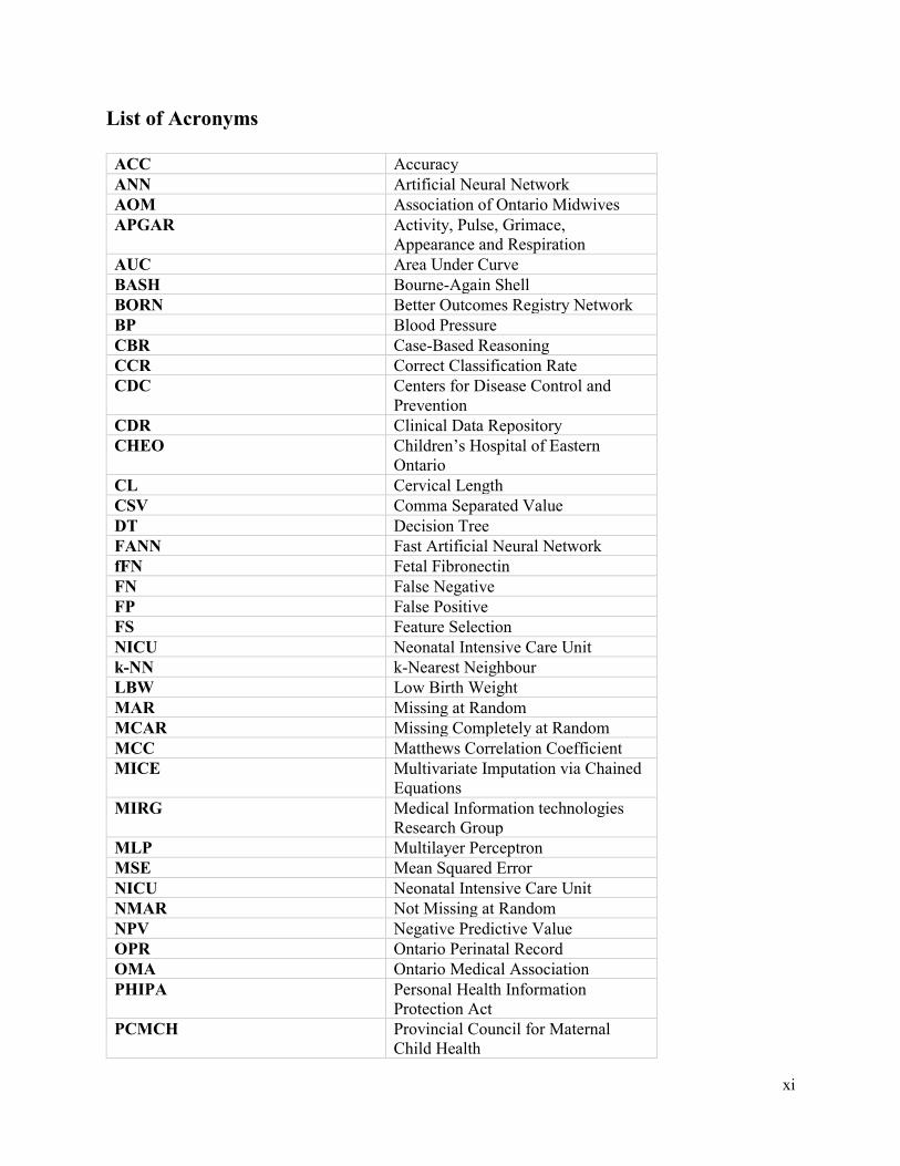
List of Acronyms

ACC Accuracy

ANN Artificial Neural Network

AOM Association of Ontario Midwives

APGAR Activity, Pulse, Grimace,

Appearance and Respiration

AUC Area Under Curve

BASH Bourne-Again Shell

BORN Better Outcomes Registry Network

BP Blood Pressure

CBR Case-Based Reasoning

CCR Correct Classification Rate

CDC Centers for Disease Control and

Prevention

CDR Clinical Data Repository

CHEO Children’s Hospital of Eastern

Ontario

CL Cervical Length

CSV Comma Separated Value

DT Decision Tree

FANN Fast Artificial Neural Network

fFN Fetal Fibronectin

FN False Negative

FP False Positive

FS Feature Selection

NICU Neonatal Intensive Care Unit

k-NN k-Nearest Neighbour

LBW Low Birth Weight

MAR Missing at Random

MCAR Missing Completely at Random

MCC Matthews Correlation Coefficient

MICE Multivariate Imputation via Chained

Equations

MIRG Medical Information technologies

Research Group

MLP Multilayer Perceptron

MSE Mean Squared Error

NICU Neonatal Intensive Care Unit

NMAR Not Missing at Random

NPV Negative Predictive Value

OPR Ontario Perinatal Record

OMA Ontario Medical Association

PHIPA Personal Health Information

Protection Act

PCMCH Provincial Council for Maternal

Child Health

xii

PBNN Pruning Based Neural Network

PPADS Physician-PArent Decision Support

PPV Positive Predictive Value

PRAMS Pregnancy Risk Assessment

Monitoring System

PTB Preterm Birth

RFW Research Framework

ROC Receiver Operating Curve

SQL Structured Query Language

TN True Negative

TP True Positive

EMG Uterine Electromyography

1

1. Chapter: Introduction

The purpose of this introductory chapter is to provide a framework for this thesis, including the

motivation for the research from both a healthcare and engineering perspective. In addition, an

overview of the problem statement, a description of the clinical environment, preterm birth, the

databases used, and the thesis objectives and outline are addressed.

1.1. Motivation

1.1.1. Healthcare Perspective

In the current healthcare environment data is constantly being collected by clinical and hospital

equipment. The ability to access massive amounts of healthcare data is a gold mine for predicting

future health outcomes [1]. Large companies such as Google, GE Health, and IBM have

recognized the potential of these massive datasets and have developed algorithms for recognizing

patterns in health data [2]. For instance, Google has developed machine learning algorithms to

quickly identify health conditions [3].

This work analyzes two large clinical datasets containing antenatal health information: the Better

Outcomes Registry and Network (BORN) Database [4] and the Pregnancy Risk Assessment

Monitoring System (PRAMS) Database [5]. Premature birth can have critical long-term effects

on the patient, the family and on the clinical environment. From a healthcare perspective, there

can be a huge benefit in being able to flag women who might be at risk for preterm birth; this

enables the health care team to apply preventative care and to decide how best to manage the

delivery. Currently methods used by healthcare teams to try to predict preterm birth are invasive,

not very accurate or reliable, and are only used once the patients presents with symptoms of

potential preterm [6].

2

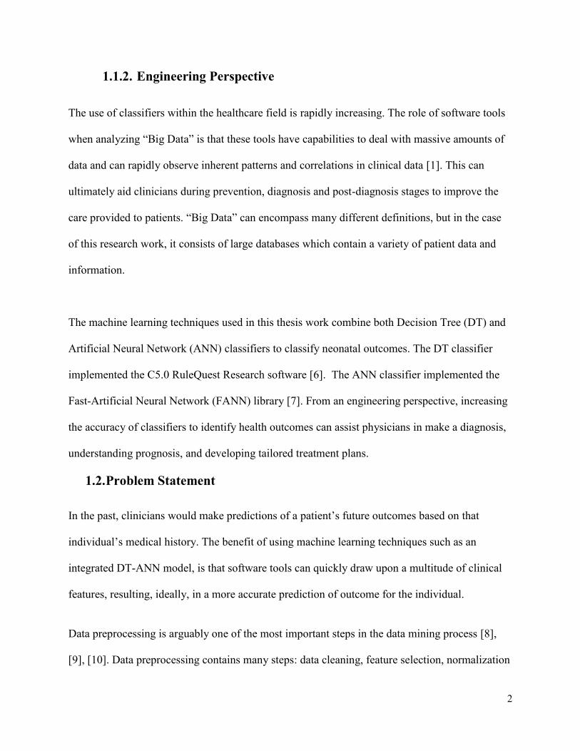
1.1.2. Engineering Perspective

The use of classifiers within the healthcare field is rapidly increasing. The role of software tools

when analyzing “Big Data” is that these tools have capabilities to deal with massive amounts of

data and can rapidly observe inherent patterns and correlations in clinical data [1]. This can

ultimately aid clinicians during prevention, diagnosis and post-diagnosis stages to improve the

care provided to patients. “Big Data” can encompass many different definitions, but in the case

of this research work, it consists of large databases which contain a variety of patient data and

information.

The machine learning techniques used in this thesis work combine both Decision Tree (DT) and

Artificial Neural Network (ANN) classifiers to classify neonatal outcomes. The DT classifier

implemented the C5.0 RuleQuest Research software [6]. The ANN classifier implemented the

Fast-Artificial Neural Network (FANN) library [7]. From an engineering perspective, increasing

the accuracy of classifiers to identify health outcomes can assist physicians in make a diagnosis,

understanding prognosis, and developing tailored treatment plans.

1.2. Problem Statement

In the past, clinicians would make predictions of a patient’s future outcomes based on that

individual’s medical history. The benefit of using machine learning techniques such as an

integrated DT-ANN model, is that software tools can quickly draw upon a multitude of clinical

features, resulting, ideally, in a more accurate prediction of outcome for the individual.

Data preprocessing is arguably one of the most important steps in the data mining process [8],

[9], [10]. Data preprocessing contains many steps: data cleaning, feature selection, normalization

3

and transformation of the data. Without this data preprocessing step, model evaluation can result

in misleading and inaccurate results [10]. The two datasets analyzed for this research work

contain raw, noisy, real-life data which needs to be preprocessed before entering the data into the

ANN model.

This thesis represents continuation of work done by previous MIRG students including:

Catley, Yu and Ong. Catley developed an early prediction model which used a combination of

Multilayer Perceptron Artificial Neural Networks and a decision tree voting algorithm [11]. This

hybrid machine learning classifier was then further developed by Yu, who used the decision tree

classifier to eliminate variables and then applied an artificial neural network with weight-

elimination, with improved sensitivity and specificity results [12]. Finally, Ong’s work

introduced a new neural network classifier using the Fast-Artificial Neural Network Library [13].

Compared to past research, which focused on the machine learning models, the primary focus of

this work is on data preparation to improve the sensitivity metric. The emphasis is on sensitivity,

as this performance metric describes the probability of the classifier correctly predicting preterm

cases. A prediction model with a high sensitivity will also help to ensure positive cases are not

missed. This is important, since the eventual integration of the classifier into a clinical setting

will necessitate identification of the risk of preterm birth as early as possible in the pregnancy

while not missing any positive cases.

1.3. Clinical Environment

Obstetrics is the area of medicine focused on childbirth and maternal health during childbirth.

Preventing and predicting preterm birth is an important area in the field of obstetrics, since

preterm birth is associated with decreased infant survival, increased risk for short term and long-

term health complications, and an increased use of health care technology and expenses [14].

4

Tocolytic drugs are medications used to delay the onset of labour [14]. Research shows that there

is no evidence that these drugs improve neonatal outcomes and can result in adverse effects for

both the mother and baby [14]. Frequently, these drugs are used as a last resort before a preterm

birth occurs. The focus of this research work is on predicting preterm birth, because with

accurate, non-invasive prediction methods, physicians can apply antenatal interventions as early

as possible and potentially improve birth outcome for infants.

1.4. Defining Preterm Birth

Preterm birth is defined as birth which takes place before 37 weeks of gestation [15]. In Ontario,

the preterm birth rate is 7.9% [16]. In the US, the frequency of preterm birth is around 8-12%

and in other developed nations in Europe the rate is around 5-9% [17]. Often there is no definite

identified cause of preterm birth; however, there are several socioeconomic, physiological and

environmental factors which can contribute to the risk of a preterm birth [17]. Some of these

factors include smoking, having previous children who were premature, and bacterial vaginosis

[17]. In addition, the risk of infant mortality with a premature birth is generally quite high [18].

These infants at birth are still in the early stages of development and this can leave them more

susceptible to illness and disease. For instance, premature infants often require mechanical

ventilation, as their lungs have not fully developed. Many of these infants experience several

chronic illnesses such as chronic lung disease and respiratory distress syndrome [19].These high-

risk situations can be damaging for the long-term health of the infant and can result in short and

long-term costs for hospitals.

The fetal fibronectin test is considered the current gold standard for predicting preterm birth,

specifically for women with a history of preterm birth; however, the test is expensive and

5

invasive [20], [21], [22]. In addition, the sensitivity of the test varies depending on the

gestational week and the test can only be used once the patient presents with symptoms which

are indicative of potential impending preterm birth [23]. Therefore, a less expensive method

which can either meet or exceed the accuracy and timing of the current standard is desired.

1.5. Databases

The PRAMS database contains over 100,000 cases with over 300 general clinical features of

state-specific population-based maternal and infant data [5]. This database was first developed in

1987, and although this questionnaire has been updated throughout the years, no major revisions

have occurred since Phase 4 (2000-2003). In order to compare these results to those obtained in

past thesis work, [24], the same database was used: Phase 6 (2009-2011). The PRAMS database

covers around 83% of all U.S. births. This database collects standardized data in survey form

from volunteers across 47 states. PRAMS is administered by the Centers for Disease Control and

Prevention (CDC), Division of Reproductive Health, National Center for Chronic Disease

Prevention and Health Promotion. It is mainly focused on data before, during, and after

pregnancy, and its purpose is to collect data to identify groups who might be at risk for high-risk

pregnancies and to prevent these occurrences in the future [5]. Around 20% of the dataset

analyzed in this research contained preterm cases.

The BORN database contains over 600,000 patient cases with over 200 general clinical features

of Ontario maternal and newborn data [4]. The BORN database is a prescribed registry which

has the authority to automatically collect and track health data under the Personal Health

Information Protection Act [25]. The BORN database is funded by the Ontario Ministry of

Health and Long-Term Care and is administered by the Children’s Hospital of Eastern Ontario

6

(CHEO). Some of the areas of focus of the BORN database include: maternal newborn outcomes

/ midwifery, congenital anomalies surveillance, newborn screening, and prenatal screening [26].

This database focuses on cases solely from Ontario with data on pregnancy, birth, and childhood

factors [4]. Around 8% of the dataset analyzed in this research contained preterm cases.

1.5.1. Segmenting the databases

The PRAMS and BORN database were further divided between Parous and Nulliparous cases.

Parous women are women who have had previous births, whereas Nulliparous women are

women who have not given birth previously. Therefore, specific features will only be applicable

to Parous women (i.e. previous premature birth) and thus, will affect the performance metrics of

the predictive tool. Features related to Parous and Nulliparous cases were selected with

consultation from our clinical partner. This is important since certain parous features, such as

previous premature birth, are known to be highly predictive of future preterm birth [17].

Although it is helpful to see how the predictive model performs for both of these case types, this

predictive model should be applicable to the general population and be inclusive of all women,

including those who have no prior history of preterm birth. Therefore, four datasets were

modelled throughout this research: BORN_Parous, BORN_Nulliparous, PRAMS_Parous and

PRAMS_Nulliparous, where the nulliparous group included both.

1.6. Thesis Objectives

The overall goal of this thesis was to develop a predictive tool which has improved sensitivity

results when compared to past work done by our research group. To accurately make this

comparison, the same methodology steps will be followed from Ong’s work [24], except for the

data preparation stage. The final goal is to be able to apply this tool prospectively at obstetrical

clinics that log patient data electronically to help clinicians and provide information for families.

7

To fulfill this goal, three objectives must first be addressed. The first objective was to evaluate

the processed data for feature reduction. There were a multitude of features in both the BORN

and PRAMS database; many of these were not related to predicting preterm birth. The C5.0

Decision Tree classifier was applied to create a subset of features most important for predicting

preterm birth. Utilizing this subset of features enhances the accuracy of the Artificial Neural

Network during training and testing.

The second objective of this thesis is to apply data mining techniques to the BORN and PRAMS

databases, with a focus on data preparation. Addressing the presence of missing values and class

imbalance were the two main areas of focus in the data preparation stage. The hypothesis was

that the greatest improvement in sensitivity results would be achieved by focusing on these two

areas.

The third objective was to evaluate the above hypothesis; by comparing the sensitivity metrics

obtained in this work with those obtained from past research (Ong [24], Yu [27] and Catley

[11]). The same machine learning tools were used (DT and ANN) in past work performed [24]

and the results obtained were compared to the current prediction performance, when applying

new data preparation methods. In addition, the 5-by-2 cross validation technique introduced in

past research [24] was applied to reduce bias and overfitting of the Artificial Neural Network

Classifier. This comparison was done to observe the differences in classification results, when

there is a focus on improving data quality, prior to training and testing the predictive model.

8

The final results should provide an assessment of the level of improvement provided by the new

methodology; this approach could be followed when implementing a predictive tool at clinics

collecting prenatal data, to ensure high accuracy of predicting preterm outcomes.

1.7. Thesis Outline

The outline of this thesis is as follows:

Chapter 1 outlines the motivation for this work, gives a general overview of the problem and

a description on how this research work contributes to improving past research results.

Chapter 2 provides a background and detailed literature review of preterm birth. This

chapter also provides a summary of past work done by researchers at the MIRG group and on

data preparation methods; this section also explains, in depth, the performance metrics

addressed in this research work. In addition, the machine learning classifiers and software

tools used to evaluate the datasets analyzed in this work are addressed.

Chapter 3 describes the methodology of the research work: it focuses on the software tools

and models used to analyze and test the clinical datasets.

Chapter 4 presents the results of the data preparation steps, model evaluation and contains a

discussion on the performance metrics achieved in predicting outcomes for preterm birth,

compared with previous results of other models.

Chapter 5 summarizes the final models and presents concluding remarks and the thesis

contribution. In addition, this section provides suggestions for future work.

9

2. Chapter: Literature Review

This chapter encompasses a review of the literature based on risk factors associated with preterm

birth. It includes a review of past work done by students within the MIRG lab, data preparation

methods and current prediction models. This chapter describes pertinent performance metrics

that will appear in later chapters and summarizes the machine learning and software tools used in

this research.

2.1. Common Factors of Preterm Birth

There is often no known cause of spontaneous preterm birth but there are a multitude of factors

which can lead to birth occurring at less than 37 weeks. Some of the medical factors can be

preeclampsia and fetal distress, while some of the social factors can be stress and physical abuse.

These factors can be grouped into three major areas leading to preterm birth: social stress and

race, infection and inflammation, and genetics [28], [29]

2.1.1. Social Stress and Race

Several studies have shown a correlation between high rates of poverty and increasing rates of

preterm birth [30]. Lack of access to healthcare and poor nutrition, as well as high rates of

domestic abuse can be linked to poverty-stricken areas and these factors can negatively affect the

health of both the baby and the mother. The rate of preterm birth amongst black women is

generally higher in comparison to other races. In the United States, the rate of preterm birth in

black women is twice as high as it is for white women [30]. Racial disparity in social situation

and discrimination, which may lead to social stressors such as poverty and lack of access to

proper healthcare, have been some of the reasons cited for this gap.

10

2.1.2. Infection and Inflammation

Another key factor linked to high rates of preterm birth is intrauterine infection and

inflammation. Bacterial infection can be widespread and can be found between the maternal

tissues and fetal membranes, within the fetal membranes, within the placenta, within the

amniotic fluid, within the umbilical cord, and within the fetus [30]. Bacterial infection often

results in inflammation of the tissues and this response can trigger a premature labour and

subsequent birth.

2.1.3. Genetics

There is some evidence that maternal genes have a large influence on the risk of preterm birth

[30]. Therefore, one could review the family history of the mother to determine if relatives have

had preterm births and this might be indicative of a predisposition to preterm birth. In addition,

women who have had previous preterm births are at a higher risk for subsequent births to also

occur prematurely [17].

2.2. Cost of Preterm Birth

The burden of premature births on health-care costs is significant. Patients born prematurely are

hospitalized for longer, need to be monitored more regularly, and use more hospital equipment

than full-term birth patients, as they are susceptible to a host of diseases and illnesses. Some of

the medical devices often used patients born prematurely are incubators, multiple infusion

pumps, invasive and non-invasive monitors, and ventilators. After discharge from hospital,

premature infants are more likely to be re-hospitalized than full-term babies. It is estimated in

Canada that the average hospital care cost for a preterm baby is nine times greater than a full-

term baby [31]. For full-term babies, it is estimated that they will remain in the hospital for

around two days, whereas with preterm babies, the hospital stay may be as long as 104 days [31].

11

Due to these factors, it is estimated that the hospital care cost of a preterm baby in Canada may

extend upwards to $117,000 [31].

2.3. Health of Preterm Infants

Preterm delivery can result in the infant having several long-lasting disabilities. Premature

infants have underdeveloped organs, specifically the lungs and heart. This can lead to severe

neurological and cardiovascular problems. For instance, some infants can have respiratory

distress, apnea and feeding problems; these illnesses all result in a longer hospitalization for the

patient. One study showed that children at age eight who were born prematurely had more

behavioural problems than their peers born full term [32]. Premature birth will likely impact the

individual’s life in the long term, with chronic lung disease and intellectual and developmental

handicaps occurring commonly in those patients born most prematurely.

2.4. Current Prediction Models

2.4.1. Cervical Length

As previously stated, there is not one identifiable factor known to predict preterm birth; however,

a correlation between the rate of shortening of the cervix and the prevalence of preterm birth has

been observed. For instance, in one study, [33] researchers focused on women whose cervixes

were shortening between 16-20 and 21-25 weeks and regularly observed the progression of their

pregnancy. They found that if the cervical length was stable for periods of time and then would

suddenly and rapidly decrease, this would often result in a preterm birth. Although this is an

interesting finding, in practice it is difficult to observe patients sufficiently regularly to detect

these changes and the detection methods are invasive and so a more realistic prediction model

would be helpful in clinical work.

12

2.4.2. Uterine Electromyography

Uterine Electromyography (EMG) is the practice of monitoring uterine contractility using

electrodes placed on the uterus and can detect when there is increased contractility signaling the

possible onset of preterm birth [34] With this method, the patient has to remain as still as

possible when collecting these signals; if not, this can result in noisy signals which have to be

filtered. In addition, the accuracy of this prediction model tends to be most accurate within a

short window of labour (24 hrs to 4 days), similar to the fetal fibronectin test [34]. However, the

focus of this thesis is to detect a preterm birth accurately, many weeks prior to labour, so that

preventative care can be administered.

2.4.3. Fetal Fibronectin Test

The fetal fibronectin test has become the gold standard for predicting preterm birth. However,

this test is expensive, invasive, and it is best designed as a short-term marker for preterm birth, as

the sensitivity decreases from 71%, 67% and 59% within 7,14 and 21 days of delivery [35]. It is

typically only measured after the membranes lining the uterus have ruptured, which is often the

sign of impending preterm labour. Fetal fibronectin is a protein produced by fetal cells which

forms a major portion of the maternal-fetal extracellular matrix [35]. Cervicovaginal leakage of

this protein in the late second and early third trimester has been an indicator in many cases of

spontaneous preterm birth [35]. The goal of this work, however, is to develop a tool that can be

applied non-invasively and throughout the early stages of pregnancy, before any signs of preterm

labour develop.

13

2.4.4. Physician-Parent Decision Support (PPADS)

The PPADS tool was developed in the MIRG lab at Carleton University and is a tool which

provides shared decision-making between physicians and parents, concerning infants in the

NICU [36]. The PPADS tool consists of two platforms: a clinician and a parent interface. The

parent interface provides information about the infant with mortality risk estimations and

provides a decision support module, allowing parents to communicate and understand the

options available to them. The clinician interface contains the list of all patients, admission files

and various medical details including outcome predictions. The PPADS system is currently

being remodeled and a dictionary of medical terms will also help to enhance parents

understanding of their child’s condition.

2.4.5. Ontario Perinatal Record

Since 1997, The Ontario Antenatal Record consisted of a form which collected pregnancy data,

and was administered by maternal care providers in Ontario. The Ontario Medical Association

(OMA) had been the primary driver of distributing and updating this form. Recently a new

partnership has arisen between the Provincial Council for Maternal Child Health (PCMCH), The

Better Outcomes Registry & Network (BORN) Ontario, the OMA and the Association of Ontario

Midwives (AOM), to create an expanded scope of these forms called the Ontario Perinatal

Record [37]. The questions within this form pertain to pregnancy, birth, and the early newborn

period [37]. There are clinics in Ontario where this information is being entered electronically

and one future method of monitoring patients for early risk of preterm birth would be to embed

the tool developed in this research to be used in conjunction with the Ontario Perinatal Record to

14

automatically screen the data as it is being collected and flag patients who are deemed to be at

risk of preterm birth.

2.4.6. Predictive Tools

A preterm risk scoring tool is a means of risk assessment which contains many major or minor

factors (previous preterm delivery, smoking/alcohol intake during pregnancy, etc...) and it

estimates the likelihood of the outcome of a preterm birth [38]. Preterm risk scoring, and

screening tools have been administered since the 1980s; however, the accuracy of these tests

remains quite low, at around 17-38% [38]. This can lead to a waste of hospital resources and

therefore, a more effective and accurate system is needed that balances both high sensitivity and

specificity metrics. One of the problems with current risk scoring tools is that they are often

limited in their capabilities. This is related to the fact that currently there is no specific cause of

spontaneous premature birth—just a multitude of factors which can contribute to a premature

birth occurring. The advantage of using machine learning tools over risk scoring methods is the

ability to easily analyze hundreds of possible preterm birth factors. The benefit of risk scoring

systems is that they do identify the complex social and environmental factors which surround the

risks of preterm births

2.5. Summary of Previous Work

Catley

The objective of Catley’s thesis work was to develop an integrated hybrid classifier which

combined ANNs (artificial neural networks) and MLP (multilayer perceptron)-ANNs with risk

stratification. She also used case-based reasoning and a DT (decision tree) voting algorithm to

predict preterm birth using an older version of the PRAMS database and the Perinatal

Partnership Program of Eastern and Southerneastern Ontario (PPPESO) database (1999-2001).

15

The results from this classifier yielded a sensitivity of 65% and a specificity of 84% and was

validated with 9701 new patient cases. The data preparation methods used in this thesis work

were to remove features with greater than 20% missing values and the k-NN (k-nearest neighbor)

CBR (case-based reasoning) algorithm, for imputing missing values [39].

Yu

The objective of Yu’s thesis was to combine an Artificial Neural Network and Decision Tree

classifier: C4.5 DT Classifier [40] to output an integrated classifier to reduce the number of

features and to increase the overall accuracy of the classifier. The model was validated using the

PRAMS database and this integrated classifier could predict mortality rates with a sensitivity of

65% and a specificity of 84%. The data preparation methods used in this thesis work were

similar to Catley’s: deletion of features with greater than 50% missing values, and the use of the

k-NN CBR for imputation of missing values [27].

Ong

The objective of Ong’s thesis was to improve the integrated classifier and to apply this classifier

to two recently updated databases, (PRAMS and BORN) to predict mortality rates. This thesis

also uses 5-by-2 cross validation to both ensure the model is trained with sufficient data and

reduce overfitting. In addition, many more features were analyzed than in Yu’s work, with

factors obtained from four different types of cases: Parous, Nulliparous, Parous without Obvious

clinical features, and Nulliparous without Obvious clinical features. The best performance

metrics achieved was the PRAMS Parous dataset: 50% for sensitivity and 92% for specificity

when analyzing around 53 clinical features. The data preparation methods used in this thesis

work were to remove outliers, deletion of features with greater than 50% missing values, deletion

16

of cases with no outcome feature, and the use of the k-NN CBR as an imputation method for

missing values [24].

Other Research

Research concerning predictive tools which use obstetrical data/devices and machine learning

algorithms have been investigated. In work done by [41], this work consists of using uterine

EMG data and artificial neural networks to classify preterm or term cases. The results were

promising, the ANN was able to classify preterm cases with an accuracy of 92% and was able to

classify term cases with an accuracy of 79%. Also, in [42], the focus of this research was to

document factors of importance by studying high-risk women from their first antenatal visit

straight through to delivery. Researchers used logistic regression and artificial neural networks to

identify significant risk factors (i.e. biochemical markers) which are associated with preterm

birth. Finally, [43], also made use of the C5.0 DT classifier and ANN as machine learning tools,

yet, the focus was on determining the top risk factors of preterm birth, in comparison to

improving the sensitivity in this research. Factors such as maternal age, multiple births and

maternal hypertension were just some of the factors which were identified to be of importance in

predicting preterm birth. Predictive methods using machine learning algorithms are being studied

extensively within the field of obstetrics, in search of faster, more accurate methods of predicting

preterm birth.

2.6. Review of Data Preparation

There were two main areas to address in the data preparation stage; the presence of missing

values and class imbalance in BORN and PRAMS.

2.6.1. Missing Values

There are three general categories of missing values [44]:

17

1) Missing Completely at Random (MCAR)

2) Missing at Random (MAR)

3) Not Missing at Random (NMAR)

MCAR refers to random experimental error which affects the presence of an attribute; MAR

refers to features which are not missing at random, but whose value depends on other measured

features; NMAR refers to features not missing at random; the probability of this missing attribute

depends on unavailable features. It is easier to impute missing values for MCAR and MAR

variables, than NMAR [45].

When the probability that the data is missing, is the same for all features in the dataset (e.g. no

blood pressure equipment to measure heart rate), this would fall under the category of MCAR.

When the probability that the data that is missing is dependent on observed data (e.g. study on

blood pressure, data on young people are less likely to be recorded, in comparison to older

individuals because they do not attend clinics as often); this would fall under the category of

MAR. Finally, when the probability that the data that is missing is dependent on data that has not

been observed (e.g. individuals with lower incomes are often less likely to fill out information

related to income), this represents NMAR [46]. As detailed in these examples, first-hand

knowledge of the observed data is a key to making assumptions about features and which

category the data falls under. The PRAMS dataset consists of survey data and BORN consists of

automatically obtained data. Thus, there is little room for researchers to make assumptions

because this data is obtained from external sources.

18

2.6.2. Discussion of Alternative Imputation Methods

There are several methods for imputing missing values. Some of these methods have been

analyzed below, to determine the best method of addressing missing values within the BORN

and PRAMS datasets.

2.6.3. Simple Imputation Methods

There are simple imputation methods such as calculating the mean or mode of the feature to fill

in missing values. However, calculating the mean or mode does not translate well for categorical

features and ignores correlations between features within the clinical datasets [47].

2.6.4. k-NN Algorithm

In previous work [24], a k-NN algorithm was used for imputing missing values through a CBR

tool developed in Microsoft Access. The k-NN algorithm makes two assumptions which make

this algorithm ineffective for this research when compared to other imputation methods. The first

assumption is that the data in the feature space are continuous [48]. Both the BORN and PRAMS

datasets contain mixed type features (both categorical and nominal). Usually Euclidean distance

is used as the distance function to measure differences between continuous features [48]. The

second assumption is that the user must choose the k-value; this is usually done through cross

validation [47]. The “k” value represents the number of neighbours which influence the

classification. Difficulties related to these two assumptions were crucial in the decision to adopt

another imputation method in this current research. There is a delicate balance between

increasing the k-value, improving the accuracy and increasing the computational time. This is

exemplified with Ong [24], where it was reported that it took up to three days to analyze these

19

clinical datasets using this algorithm and the CBR tool. In addition, there are software programs

(R) which drastically reduce the processing time from three days to hours.

2.6.5. mice Algorithm

The mice (Multivariate Imputation via Chained Equations) algorithm, as the name suggests,

creates multiple imputations to reduce bias of results [49]. This algorithm was developed by Stef

van Buuren and is a package in R. In the first step of the mice process, each missing value is

temporarily set to the mean value within that feature. Then using one of the regression methods

from the mice function (see Figure 2.1), which matches the data type of the feature, a missing

value is obtained. This process is repeated as specified by the user; usually this cycle is repeated

ten times [50]. The mice algorithm uses linear regression to predict nominal missing values and

logistic regression for categorical missing values. The methods for the mice function are

displayed below.

Figure 2.1. Regression methods in the mice algorithm to impute missing values [49]

20

2.6.6. Chosen Method: missForest Algorithm

The missForest algorithm is a function which uses random forest classifiers to train each feature,

and then this model is used to make predictions about missing values [48]. This algorithm was

developed by Daniel Stekhoven and is a package in R. This function also provides an imputation

error estimate for both the categorical and nominal data. Some papers show that missForest

outperforms mice with a lower imputation error [47], [48]. In addition, with the mice algorithm,

even though this algorithm has the capability to handle multiple types of data, one must make

this explicit, coding in R. For instance, if one of the features in the dataset is numeric, then this

had to be defined in the code as ‘pmm’ (predictive mean matching when using the mice

algorithm). Similarly, when one of the features had two factors (i.e. “Yes” or “No”) with two

levels, this was defined to be ‘logreg’ for logistic regression, and if another feature had more

than two levels, then this would be defined as ‘polyreg’ or multinomial logistic regression model.

With many mixed types in the dataset, this process can become tedious. Similarly, to the k-NN

algorithm, the number of imputed datasets with the mice model is controlled by the user.

Although the value of 10 seems to be the most widely chosen option, research has seen

improvements in accuracy when this value is chosen to be anywhere up to 40 [50]. Therefore,

again a trade-off between accuracy and computation time exists. The computation time using

missForest in this research work was significantly faster than using mice, when the number of

imputed datasets was chosen to be 10. For instance, using missForest, the processing time took

around 16 hours, while with mice repeating the process 10 times took around four days to

complete. Also, as the mice algorithm is a multiple imputation method, this algorithm operates

under the assumption of MAR (missing at random) [51]. However, there is a risk of biasing the

results if this assumption is made without strong justification [51]. Since, missForest is a non-

21

parametric algorithm, this removes the researcher from having to make incorrect assumptions

about missing values within features.

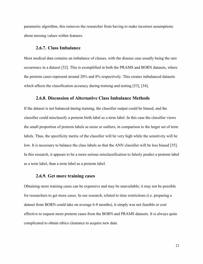
2.6.7. Class Imbalance

Most medical data contains an imbalance of classes, with the disease case usually being the rare

occurrence in a dataset [52]. This is exemplified in both the PRAMS and BORN datasets, where

the preterm cases represent around 20% and 8% respectively. This creates imbalanced datasets

which affects the classification accuracy during training and testing [53], [54].

2.6.8. Discussion of Alternative Class Imbalance Methods

If the dataset is not balanced during training, the classifier output could be biased, and the

classifier could misclassify a preterm birth label as a term label. In this case the classifier views

the small proportion of preterm labels as noise or outliers, in comparison to the larger set of term

labels. Thus, the specificity metric of the classifier will be very high while the sensitivity will be

low. It is necessary to balance the class labels so that the ANN classifier will be less biased [55].

In this research, it appears to be a more serious misclassification to falsely predict a preterm label

as a term label, than a term label as a preterm label.

2.6.9. Get more training cases

Obtaining more training cases can be expensive and may be unavailable; it may not be possible

for researchers to get more cases. In our research, related to time restrictions (i.e. preparing a

dataset from BORN could take on average 6-8 months), it simply was not feasible or cost

effective to request more preterm cases from the BORN and PRAMS datasets. It is always quite

complicated to obtain ethics clearance to acquire new data.

22

2.6.10. Oversampling the minority class

Oversampling the minority class would entail replicating the preterm cases. The disadvantage of

this method lies in possible overfitting of the minority class, as there are many more samples

created from replicating the minority cases [56], [57]. Also, with over 600,000 cases in the

BORN dataset and over 100,000 cases in the PRAMS dataset, oversampling would significantly

increase the size of these datasets; leading to increased computational time for training and

testing the Artificial Neural Network classifier.

2.6.11. Chosen Method: Undersampling the majority class

Several papers have reported the benefit of undersampling over oversampling when dealing with

class imbalances. Oversampling may result in over-fitting of the classifier and will result in

longer training times due to the increase in the sample size [56]. Although the disadvantage with

undersampling is the loss of “valuable” information, the focus of this research is on accurately

predicting preterm cases. The most “valuable” information lies in the preterm cases. Reducing

the number of term cases, greatly improved computational time and sensitivity results during the

training and testing of the neural network classifier.

2.7. Performance Metrics

2.7.1. Confusion Matrix (Contingency Table)

The purpose of a confusion matrix is to showcase the predictions from a classification model

versus the accurate predictions, to determine the efficiency of the model in predicting an

outcome [58]. For instance, in Table 2.1., the positive column displays both the true predictions

from the model output and the number of predictions the model “classified” as false predictions,

but which were true.

23

Table 2.1 2-by-2 Confusion Matrix

Actual Value

Predicted Value

Positive Negative

Positive True Positive

(TP)

False Positive

(FP)

Negative False Negative

(FN)

True Negative

(TN)

2.7.2. Correct Classification Rate (CCR)

This metric is a measure of the accuracy of the model in being able to predict cases [59].

𝐴𝑐𝑐𝑢𝑟𝑎𝑐𝑦 = 𝑇𝑃 + 𝑇𝑁

𝑇𝑃 + 𝑇𝑁 + 𝐹𝑃 + 𝐹𝑁

2.7.3. Misclassification Rate

This metric is a measure of how often the model makes an incorrect prediction [59].

𝑀𝑖𝑠𝑠𝑐𝑙𝑎𝑠𝑠𝑖𝑓𝑖𝑐𝑎𝑡𝑖𝑜𝑛 𝑅𝑎𝑡𝑒 = 𝐹𝑃 + 𝐹𝑁

𝑇𝑃 + 𝑇𝑁 + 𝐹𝑃 + 𝐹𝑁

2.7.4. Sensitivity

Sensitivity (True Positive Rate) is a specific parameter focusing on the ability of the classifier to

accurately classify a case which is defined as positive [58]. For instance, a positive case can be

defined as a patient having a preterm birth (or a specific disease). Therefore, if the sensitivity of

your test is 100%, this means the test will correctly label all patients who have preterm birth as

preterm births.

24

𝑆𝑒𝑛𝑠𝑖𝑡𝑖𝑣𝑖𝑡𝑦 = 𝑇𝑃𝑅 = 𝑇𝑃

𝑇𝑃 + 𝐹𝑁

2.7.5. Specificity

Specificity is a specific parameter focusing on the ability of the classifier to accurately classify a

case which is defined as negative [58]. Continuing with the same above example, if the negative

case is defined as the patient having a full-term outcome, a specificity of 100% means that the

test would correctly label all patients who have births to term as full-term outcomes.

𝑆𝑝𝑒𝑐𝑖𝑓𝑖𝑐𝑖𝑡𝑦 = 𝑇𝑁𝑅 = 𝑇𝑁

𝑇𝑁 + 𝐹𝑃= 1 − 𝐹𝑎𝑙𝑠𝑒 𝑃𝑜𝑠𝑖𝑡𝑖𝑣𝑒 𝑅𝑎𝑡𝑒 (𝐹𝑃𝑅)

2.7.6. F1-Score

This score functions as a weighted average of the precision and recall. The closer the classifier’s

F1-score is to 1, the higher the precision and recall values will be [60].

𝐹1 = 2𝑇𝑃

2𝑇𝑃 + 𝐹𝑃 + 𝐹𝑁

2.7.7. Prevalence

Prevalence is a measure of the prior probability of the individual having the disease before the

model is tested given the population size [61]. It is an important measure for the MIRG group as

it ensures clinical relevance and acts as a threshold. In the context of this research, prevalence

would relate to the proportion of the population who have had a preterm birth. In Ontario, the

prevalence of preterm birth is around 7.9% [16]. As a result, during the final testing stage, the

test sets evaluated by the ANN will use the prevalence in the population.

25

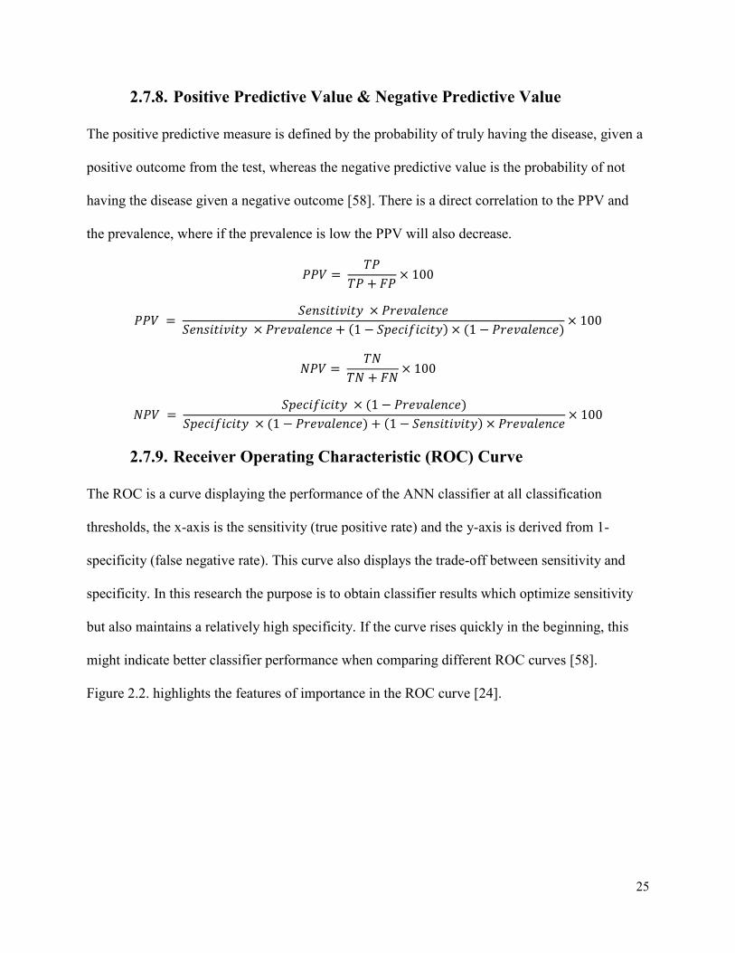
2.7.8. Positive Predictive Value & Negative Predictive Value

The positive predictive measure is defined by the probability of truly having the disease, given a

positive outcome from the test, whereas the negative predictive value is the probability of not

having the disease given a negative outcome [58]. There is a direct correlation to the PPV and

the prevalence, where if the prevalence is low the PPV will also decrease.

𝑃𝑃𝑉 = 𝑇𝑃

𝑇𝑃 + 𝐹𝑃× 100

𝑃𝑃𝑉 = 𝑆𝑒𝑛𝑠𝑖𝑡𝑖𝑣𝑖𝑡𝑦 × 𝑃𝑟𝑒𝑣𝑎𝑙𝑒𝑛𝑐𝑒

𝑆𝑒𝑛𝑠𝑖𝑡𝑖𝑣𝑖𝑡𝑦 × 𝑃𝑟𝑒𝑣𝑎𝑙𝑒𝑛𝑐𝑒 + (1 − 𝑆𝑝𝑒𝑐𝑖𝑓𝑖𝑐𝑖𝑡𝑦) × (1 − 𝑃𝑟𝑒𝑣𝑎𝑙𝑒𝑛𝑐𝑒)× 100

𝑁𝑃𝑉 = 𝑇𝑁

𝑇𝑁 + 𝐹𝑁× 100

𝑁𝑃𝑉 = 𝑆𝑝𝑒𝑐𝑖𝑓𝑖𝑐𝑖𝑡𝑦 × (1 − 𝑃𝑟𝑒𝑣𝑎𝑙𝑒𝑛𝑐𝑒)

𝑆𝑝𝑒𝑐𝑖𝑓𝑖𝑐𝑖𝑡𝑦 × (1 − 𝑃𝑟𝑒𝑣𝑎𝑙𝑒𝑛𝑐𝑒) + (1 − 𝑆𝑒𝑛𝑠𝑖𝑡𝑖𝑣𝑖𝑡𝑦) × 𝑃𝑟𝑒𝑣𝑎𝑙𝑒𝑛𝑐𝑒× 100

2.7.9. Receiver Operating Characteristic (ROC) Curve

The ROC is a curve displaying the performance of the ANN classifier at all classification

thresholds, the x-axis is the sensitivity (true positive rate) and the y-axis is derived from 1-

specificity (false negative rate). This curve also displays the trade-off between sensitivity and

specificity. In this research the purpose is to obtain classifier results which optimize sensitivity

but also maintains a relatively high specificity. If the curve rises quickly in the beginning, this

might indicate better classifier performance when comparing different ROC curves [58].

Figure 2.2. highlights the features of importance in the ROC curve [24].

26

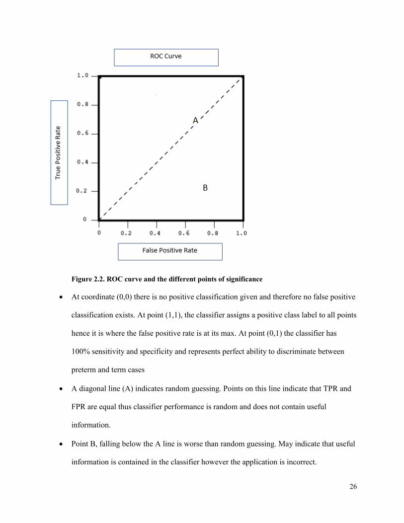
Figure 2.2. ROC curve and the different points of significance

• At coordinate (0,0) there is no positive classification given and therefore no false positive

classification exists. At point (1,1), the classifier assigns a positive class label to all points

hence it is where the false positive rate is at its max. At point (0,1) the classifier has

100% sensitivity and specificity and represents perfect ability to discriminate between

preterm and term cases

• A diagonal line (A) indicates random guessing. Points on this line indicate that TPR and

FPR are equal thus classifier performance is random and does not contain useful

information.

• Point B, falling below the A line is worse than random guessing. May indicate that useful

information is contained in the classifier however the application is incorrect.

27

2.7.10. Area Under the Curve (AUC)

The AUC is a measure of how accurate the classifiers predictions are. An AUC value of 1

represents 100% accuracy in predicting preterm births, while an AUC accuracy of 0 represents

0% accuracy in predicting preterm births. An AUC value should strive to be above 0.5, as 0.5

represents a classifier which is as good as random guessing. The effectiveness of this value is

summarized in Table 2.2. [62].

Table 2.2 AUC Index and its Effectiveness labels

Min Max Effectiveness

≤ 0.5 No discrimination

0.5 < 0.7 Poor discrimination

0.7 0.8 Acceptable

0.8 0.9 Excellent

0.9 1.0 Outstanding

2.7.11. Mathews Correlation Coefficient

The Mathews Correlation Coefficient (MCC): is a correlation coefficient between the observed

and predicted classifications. This metric varies between -1 and 1, -1 indicates a completely

wrong binary classifier, 0 represents an uncorrelated classifier (as good as random guessing) and

1 indicates a completely correct binary classifier [63].

𝑀𝐶𝐶 = (𝑇𝑃 × 𝑇𝑁) − (𝐹𝑃 × 𝐹𝑁)

√(𝑇𝑃 + 𝐹𝑃)(𝑇𝑃 + 𝐹𝑁)(𝑇𝑁 + 𝐹𝑃)(𝑇𝑁 + 𝐹𝑁)

28

2.7.12. Normalization

Normalization was an important preprocessing step before evaluating the data with the Artificial

Neural Network, this was done using the modified Z-score transformation. Normalizing refers to

scaling the data to fall within a certain range. The ANN deals with nominal data and the BORN

and PRAMS data contains categorical and nominal data. Therefore, it was important to

normalize the dataset so that all the features were in the same range and no specific feature was

given more weight than others during the training stage. There are several methods to

normalizing the data. Options include centering the data to have a mean of 0 or scaling the data

by the standard deviation [64]. Past work has shown that the neural network works best when

normalized between the range of [-1,1], [13]. The normalization process will be expanded on in

greater detail in Chapter 3.

2.8. Pattern Classification Methods

Pattern classification methods have been used with fields such as, medical informatics, to

classify and categorize large amounts of medical data and output clinical outcomes when faced

with medical problems. The two types of pattern classification tools used within this thesis are:

Decision Tree (DT) and Artificial Neural Network (ANN) classifiers. Specifically, a hybrid

classifier which uses both elements from the DT (feature reduction) and the ANN classifier

(model evaluation) are used to classify the preterm and term cases.

2.8.1. Supervised Learning

Supervised learning is a type of machine learning process which contains labels in the output

variable and this differentiates this type of learning from unsupervised learning. Furthermore,

supervised learning can be classified into two categories: regression and classification [65], [66].

29

A regression problem is described as having a numerical real value label such as “weight” and a

classification problem is described as having a categorical output label such as “preterm”. This

work deals with supervised learning, as the main objective is to determine an accurate preterm

birth outcome label, using an Artificial Neural Network classifier.

2.8.2. Unsupervised Learning

Conversely, unsupervised learning is a type of machine learning process which contains no

output labels. Unsupervised learning can also be classified into two categories: clustering and

associations. As the name suggests clustering refers to understanding how groups (clusters)

respond to certain features in a given dataset. Association refers to what rules or relations one

can make based on similarities between groups [65], [67].

2.8.3. Semi-supervised Learning

Semi-supervised learning takes aspects from both supervised and unsupervised learning. Semi-

supervised learning contains labeled and mostly unlabeled data. Given this mix of labels, one

could approach the problem with both an unsupervised or supervised approach. For instance, if

one wanted to learn about patterns and structure of the data, an unsupervised learning algorithm

could be one option [68]. However, in this work, the method used on the data would be a

supervised learning approach for the dataset, as the objective is to accurately predict the

unlabeled data with the labeled data provided [69].

2.9. Feature Reduction

Data reduction is a large section of data preprocessing [70]. The “curse of dimensionality” refers

to the situation where it is often beneficial to limit the number of features to maintain classifier

performance [71], [70]. A decrease in classifier performance might be related to overfitting,

30

when the classifier is provided with too many features. When the classifier sees new data that it

previously has not been trained on, the classifier performs poorly. Thus, appropriate feature

selection (FS) is important to maintaining a high accuracy for the ANN, (especially since this

classifier has a non-linear decision boundary prone to overfitting, in comparison to other

classifiers [72]). Currently there are hundreds of features in both the BORN and PRAMS

datasets and, by pruning these features down to an optimal subset, one can obtain improved

classifier performance; it makes sense not to use all the clinical features provided during training.

There are many FS (feature selection) methods to draw from, and these are the three main

categories [10]:

1) Filter FS methods

2) Wrapper FS methods

3) Embedded FS methods.

In Method 1, the features selected are independent of the classifier; the features are ranked

based on a specific statistical measure (i.e. entropy) and chosen based on rank; in Method 2 the

features are dependent on the classifier; a subset of feature is chosen and evaluated on the

classifier, and the subset of features with the best classifier performance is chosen. The final

method is akin to Method 2; however, these methods are much faster than the wrapper methods.

This feature selection method occurs during the learning process.

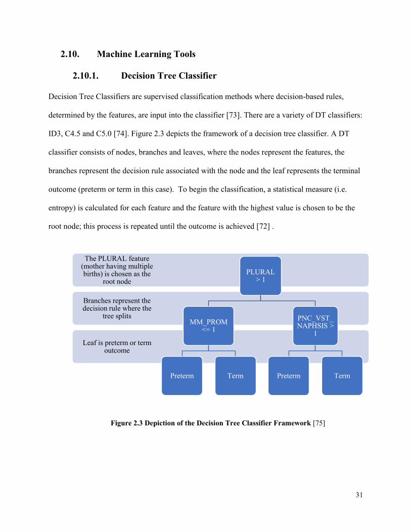
31

2.10. Machine Learning Tools

2.10.1. Decision Tree Classifier

Decision Tree Classifiers are supervised classification methods where decision-based rules,

determined by the features, are input into the classifier [73]. There are a variety of DT classifiers:

ID3, C4.5 and C5.0 [74]. Figure 2.3 depicts the framework of a decision tree classifier. A DT

classifier consists of nodes, branches and leaves, where the nodes represent the features, the

branches represent the decision rule associated with the node and the leaf represents the terminal

outcome (preterm or term in this case). To begin the classification, a statistical measure (i.e.

entropy) is calculated for each feature and the feature with the highest value is chosen to be the

root node; this process is repeated until the outcome is achieved [72] .

Figure 2.3 Depiction of the Decision Tree Classifier Framework [75]

Leaf is preterm or term outcome

Branches represent the decision rule where the

tree splits

The PLURAL feature (mother having multiple births) is chosen as the

root node

PLURAL > 1

MM_PROM <= 1

Preterm Term

PNC_VST_NAPHSIS >

1

Preterm Term

32

Some advantages to using DT classifiers include:

• The model is intuitive

• Data preprocessing is minimal (Decision Tree C5.0 can handle missing values)

Some disadvantages to using DT classifiers include:

• Risk of overfitting results

• In cases where the dataset has class imbalance, a biased tree can be produced

The disadvantages to using DT classifiers have been dealt with throughout this thesis work by

firstly using cross validation, and secondly, by separating the validation set from the original

dataset. This was done when testing the Artificial Neural Network (ANN) classifier, to reduce

the risk of overfitting results. The second disadvantage of creating a biased tree was reduced by

under-sampling the majority class of term cases by using the undersampling package in R [76];

these details will be expanded on later in the thesis.

2.10.2. Random Forest Classifier

The random forest classifiers can be described as a randomized ensemble of decision trees, as

observed in Figure 2.4. The random forest classifier is a type of supervised learning algorithm

which differs from decision tree classifiers. The DT classifier splits the features based on the

most important statistical measure (i.e. entropy) in the feature subset; the random forest classifier

splits features based on the most important statistical measure, derived from a random subset of

features; this adds randomness to the model and reduces the correlation between trees. This

creates a separate classification outcome for each tree, which is then aggregated, and a final vote

is done [48], [77], [78].

33

Figure 2.4. Depiction of the Random Forest Classifier Framework [79]

2.10.3. Artificial Neural Networks

Artificial Neural Networks were modeled to mimic processes within the brain. Artificial Neural

Networks consist of mathematical algorithms which have a similar basic framework (see Figure

2.5): inputs are multiplied by a weight (this is assigned based on relative importance in

comparison to other inputs) in the Input layer and passes into an activation function in the

Hidden layer which produces an output (preterm or term) in the Output layer. Then, Input 1 is

multiplied by the weight (-0.14) along with the other inputs and weights, is summed and the

activation function is present in the Hidden layer, resulting in an Output value of 1. There are

several types of ANNs; some of the formulations include multilayer perceptron (MLP) and

Radial Basis Function Networks (RBFNs) [70]. The specific activation function used in this

research work was a sigmoid symmetric function (also known as the tanh function) which gives

an output between [-1, 1] (see Figure 2.5), this is one of the most widely used functions for

layered feed-forward networks [7], [80]. Other non-linear functions are the ReLU (Rectified

Linear Unit) activation function which thresholds the output at 0 and replaces negative values

34

with 0. The output from the classifier is compared to known cases and adjusted by repeating this

entire process again until a minimum error rate is achieved [70].

Figure 2.5. Depiction of the Activation Function and Artificial Neural Network Framework [81]

Some advantages of using ANN classifiers include:

• Performs well with regards to non-linear models

• Ability to learn models in real time

Some disadvantages of using ANN classifiers include:

• Sensitive to scaling features

• Does not do well with missing values

The disadvantages of using ANN classifiers have been addressed throughout this thesis work

by normalizing the dataset before applying the ANN classifier and using the missForest package

in R [48], to deal with missing values in both the BORN and PRAMS datasets.

35

2.11. Software Tools Used in This Research

2.11.1. R

R (1993) is a statistical programming language which was created by Ross Ihaka and Robert

Gentleman at the University of Auckland, New Zealand. R is a versatile program which is open

source and can be integrated into several different platforms. R also contains several packages

produced by academics and data scientists, some of which have been used for data cleaning in

this research work to deal with missing values and class imbalance. Packages (missForest and

ubUnder) were tested to determine which one offered the best fit with the clinical data provided

[48], [76].

2.11.2. Tableau

Tableau software (2003) is a tool developed by Pat Hanrahan, Christian Chabot and Chris Stolte,

which allows for data visualization [82]. This program was instrumental in transforming the raw

data into informative graphics. The benefit of this approach was to be able to see which of the

over 100 clinical features present in these two clinical datasets, (BORN and PRAMS), were

strongly correlated with a preterm or a term outcome, so that further statistical analysis could be

carried out in R. Tableau offers many different charts and diagrams such as: pie charts,

geographical maps and bar charts. The ability in Tableau to easily display plots and graphs was

important in communicating project goals.

2.11.3. Cygwin Terminal

The Cygwin terminal was used in this research to run several Bourne-Again-Shell (BASH)

scripts for the C5.0 DT classifier and ANN classifier. This software provides a Unix-like

environment and is an open source platform [83].

36

2.11.4. See5/C5.0 Decision Tree Classifier

See5/C5.0 is a data mining tool developed by © Rulequest Research 1997 [84]. The C5.0

decision tree classifier is an updated version of the popular C4.5 decision tree classifier [74].

Some of the improvements in the latest version are the ability to deal with noisy or missing data,

boosting (that is using multiple decision tree classifiers for improved accuracy) and the ability to

predict which features are important. The last point was of great significance to this research

work. There are over 200 features in the PRAMS dataset and over 300 features in the BORN

dataset; these datasets are focused primarily on maternal health factors; thus, there are many

factors which are not directly related to predicting premature birth. Obtaining a set of features

which contains only those features that are relevant to preterm birth reduces computational time,

noise, the “curse of dimensionality” and subsequently increases the accuracy of the ANN.

Decision trees are often used for feature selection because they display a good balance of high

computational speed and high performance of the selected feature subset [10]. Removing

irrelevant features will improve the accuracy and speed of predicting premature births when this

adjusted data is inputted into the Artificial Neural Network (ANN) model. The C5.0 algorithm

can handle missing values and displays the percentage attribute usage. This tells the user how

important some features are in predicting a preterm birth outcome. In addition, this algorithm

incorporates adaptive boosting. In this research, ten DT classifiers were generated instead of one,

and each classifier voted for the predicted class (preterm or term); the votes were counted to

determine the final class. This feature incorporated into the C5.0 algorithm, reduces the error rate

significantly, instead of relying on one single classifier.

37

2.11.5. Fast Artificial Neural Network Library

In previous work done by Catley [39] and Yu [27] the ANN was created using MATLAB

software; however, MATLAB’s Neural Network Toolbox is not open source software and there

was difficulty in integrating it manually into the real time PPADS system. Previous work [85]

focused on implementing a multilayer feed-forward-backpropagation ANN. Previous students

have improved the ANN architecture through the years. The ANN-RFW (Artificial Neural

Network Research Framework) developed by Rybchynski [86] was intended to improve

automation and increase the prediction ability of ANNs. The problem with the use of this ANN

is that it is difficult to integrate this classifier into the clinical environment; we wanted to use an

ANN classifier which could quickly analyze large sets of clinical data.

The solution was to use the FANN (Fast Artificial Neural Network) Library to develop an ANN

for classification purposes [7]. The advantage of using this library is that it has access to feed-

forward ANNs and the library is based on the C language which makes the FANN library easy to

integrate with many different software environments. Also, the FANN library allows the user to

easily manipulate the same ANN parameters used in past work [86]. In addition, the FANN

library has access to feed-forward networks and these networks have superior computation

abilities—which is critical for processing large amounts of medical data. Neural networks are

also beneficial in identifying patterns and in identifying which trends deviate from these patterns.

Articles have reported the benefits of using neural networks focused on classification problems

and more specifically in the medical industry, such as with medical imaging [87], [88].

The ANN Builder can be run in several different modes: FAST, MEDIUM and SLOW. The

FAST mode analyzes around 0.5% of all neural network combinations, MEDIUM mode

38

analyzes around 7% of all options, and SLOW runs through all possible combinations. This feed-

forward artificial neural network is also multilayer, indicating an initial input phase, a defined

number of hidden layers, and ending with an output layer. There are three phases for these neural

networks (NN): a training, testing, and validation phase. The training and testing phases consist

of feeding the NN both preterm and term cases, so it can learn to differentiate between these two

classifications. The validation phase consists of inputting the NN cases that it has not previously

seen (unlabeled data) and it outputs final classification labels as either preterm or term. There is

user flexibility involved with this software; factors such as the learning rate, the activation

function, the steepness value of the activation function and the values of the initial weight of the

neural network can be manipulated by the user.

15 network parameters available through the FANN library [7] are listed below:

1. Connection rate

2. Number of hidden layers

3. Number of hidden nodes: Defines the number of nodes in each hidden layer

4. Connection weights: Two options available- randomly assign values to weights or

initialize weights (Widrow-Nguyen algorithm)

5. Activation functions: There are six activation functions available- Sigmoid

symmetric, Gaussian symmetric, Elliot symmetric, Linear piece symmetric, Sine

symmetric, Cosine symmetric; all these functions output a value between -1 to 1.

6. Activation steepness: Determines the speed at which the activation function goes

from the minimum to the maximum.

7. Training algorithms: Four training algorithms available- Incremental training,

Batch training, Quickprop training, Rprop training

39

8. Learning rate: Determines the speed at which the network attains a minimum in

the criterion function.

9. Training error function: Two error functions are available: A standard linear

function or a hyperbolic tangent error function.

10. Incremental training momentum: This parameter speeds up the training y adding a

proportion of the previous weight-change value to the new value

11. Quickprop training weight decay factor: Determines how much the weights need

to be penalized to make sure they do not become too high during training.

12. Quickprop training maximum growth factor: Restricts the size of weights’ growth

13. Rprop intial step-size: Determines the initial step-size for weights

14. Rprop step-increase: Determines how much the step size can increase during

training.

15. Rprop step-decrease: Determines how much the step size can decrease during

training.

40

3. Chapter: Methodology

The main goal of this thesis is to improve the accuracy of the prediction tool in classifying

preterm birth. Specifically, this thesis focuses on data preprocessing methods, to ensure the data

is of the highest quality, before applying the Artificial Neural Network classifier for model

evaluation. This chapter outlines the steps taken to achieve this goal.

The 8-step methodology for this work is outlined in Figure 3.1. Excluding Step 1, 4 and 5, this

methodology followed closely with the work done by Ong [24]. This was done to accurately

measure the effectiveness of the application of these data preparation tools, (Step 4 & 5) with the

overall improvement of the classifier’s ability to predict preterm birth.

Figure 3.1. Schematic representation of the methodology used for the preterm birth classification

tool

Step 1: Data visualization

Step 2: Eliminated cases and features

Step 3: Choosing features with

greater than 50% importance

Step 4: Balanced the classes

Step 5: Impute missing values

Step 6: Normalized the data

Step 7: Divided into test, train and validation sets

Step 8: Execution of the ANN Builder

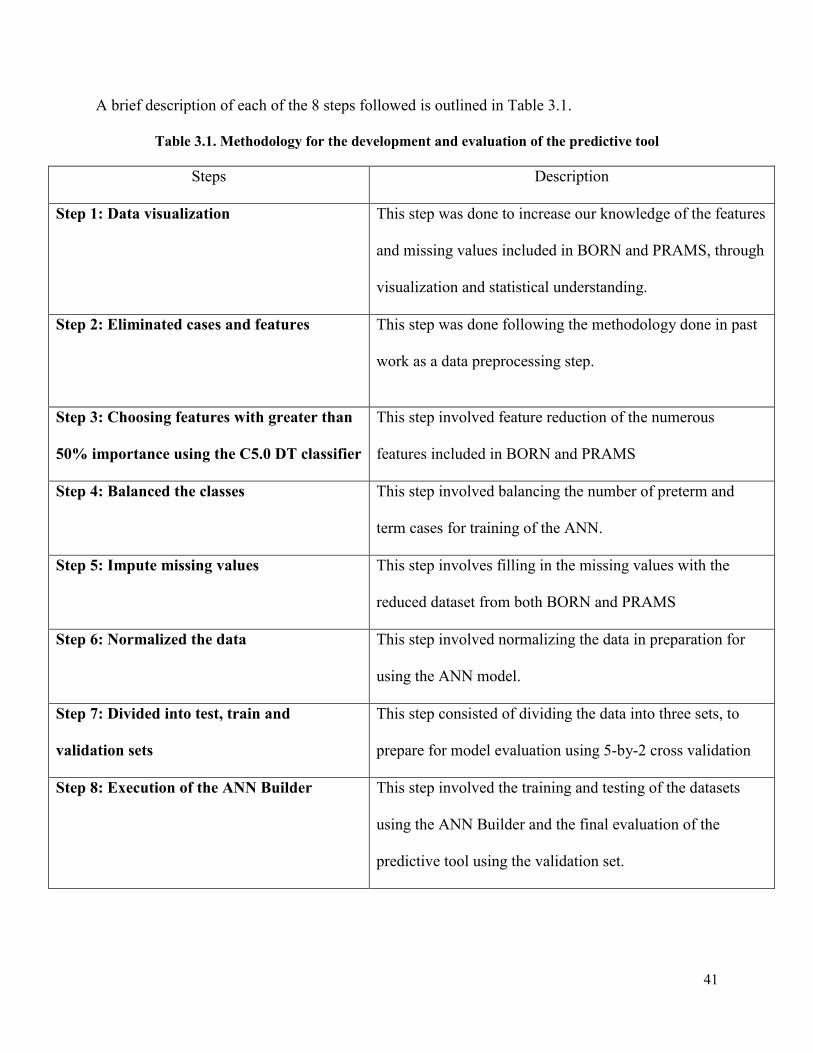
41

A brief description of each of the 8 steps followed is outlined in Table 3.1.

Table 3.1. Methodology for the development and evaluation of the predictive tool

Steps Description

Step 1: Data visualization This step was done to increase our knowledge of the features

and missing values included in BORN and PRAMS, through

visualization and statistical understanding.

Step 2: Eliminated cases and features

This step was done following the methodology done in past

work as a data preprocessing step.

Step 3: Choosing features with greater than

50% importance using the C5.0 DT classifier

This step involved feature reduction of the numerous

features included in BORN and PRAMS

Step 4: Balanced the classes This step involved balancing the number of preterm and

term cases for training of the ANN.

Step 5: Impute missing values This step involves filling in the missing values with the

reduced dataset from both BORN and PRAMS

Step 6: Normalized the data This step involved normalizing the data in preparation for

using the ANN model.

Step 7: Divided into test, train and

validation sets

This step consisted of dividing the data into three sets, to

prepare for model evaluation using 5-by-2 cross validation

Step 8: Execution of the ANN Builder

This step involved the training and testing of the datasets

using the ANN Builder and the final evaluation of the

predictive tool using the validation set.

42

3.1. Preliminary step: Ethics Clearance

This thesis work was approved by the Carleton University Research Ethics Committee and by

the CHEO Research Ethics Board. The databases used in this thesis work were: (1) Better

Outcomes Registry & Network (2010 - 2012) database (BORN) and the (2) Pregnancy Risk

Assessment Monitoring System (2009-2011) (PRAMS). A contract was signed protecting the

intellectual property of the data and their confidentiality before accessing both databases for this

thesis.

3.2. Step 1: Data Visualization

As noted in Chapter 2, data visualizations can be useful in determining possible relationships

between attributes and can provide information about individual attributes. Data visualization

can also reveal noisy aspects of the data such as outliers and show clusters in the data which

might indicate which is the best classifier to model the data.

The benefit of using Tableau as an analytic tool is that you can transform your data from raw

values to informative graphs, such as bar charts. Bar charts were widely used for data analysis in

this work because bar charts are good for showing comparisons. R was also used to visualize the

missing values present in BORN and PRAMS. Before applying complex algorithms, it is

important to understand the data and features present.

3.3. Step 2: Eliminating cases and features

The first step in the removal of features was to load the raw clinical data into Excel. Any missing

values were denoted as ‘N/A’. Then the ‘COUNTIF’ formula was used in Excel to count the

number of cells which contain missing values; from this, one could determine the percentage of

missing values for each feature. All features which contained greater than 50% of missing

values were removed. This followed steps taken in the theses of Ong [24] and Yu [27]. Applying

43

the Artificial Neural Network classifier in the final stage would require the datasets to have no

missing values; the focus was to not introduce too much imputed data into the dataset, to reduce

bias of the data. In addition, any cases which had a missing outcome (preterm or term) were

deleted. A more detailed description of the removed features can be found in Appendix B.

It was important to only included Parous and Nulliparous features which could be known at 23

weeks gestation so that preventative treatment could be applied, and patients could be monitored

to improve clinical outcomes. Both the BORN and PRAMS dataset were further divided into

BORN_Parous, BORN_Nulliparous, PRAMS_Parous and PRAMS_Nulliparous datasets based

on features selected by our clinical supervisor. Features which were only specific to mothers,

who have had previous births, fell under the Parous category (i.e. previous premature birth).

After feature and case elimination steps were applied to the raw BORN and PRAMS data,

divisions between BORN_Nulliparous, BORN_Parous, PRAMS_Nulliparous and

PRAMS_Parous were applied in the subsequent steps.

3.4. Step 3: Choosing features with greater than 50% importance using the

C5.0 DT classifier

The C5.0 DT classifier has the capability to deal with missing values. Therefore, two options

needed to be investigated:

1. Balance the data (using the ubBalance package in R), impute the missing values

(using the missForest package in R), and then apply the C5.0 DT classifier for feature

reduction

44

2. Apply the C5.0 DT classifier for feature reduction with the missing values present in

BORN and PRAMS, and then carry out the preprocessing steps (balance the data and

fill in missing values)

The results are summarized in the next chapter.

1. The first step in creating the C5.0 DT classifiers was to modify a file called

“mortality.names” this file contained information about the features and classes (files are

labeled as mortality/nonmortality throughout this research, due to past work done by

Hasmik on the ANN Builder [13], her work was focused on neonatal mortality risk

estimation models using Artificial Neural Networks)

2. In the mortality.names file the OUTCOME feature represented the target attribute, the

CASE ID was the label attribute and the rest of the features in: PRAMS_Parous,

PRAMS_Nulliparous, BORN_Parous or BORN_Nulliparous were defined to be

continuous (numeric) or discrete (nominal).

3. The next step was to create two csv files, one labeled mortality.csv and the other labeled

nonmortality.csv. The first file contained all the cases with a preterm label and the other

file contained all the cases with a term label.

4. After this was done, a script called ./create_5by2_folds.sh along with the mortality and

nonmortality files were executed in the Cygwin terminal. This script automatically

created 10, 5-by-2 cross validation sets.

5. The next step to create the DTs is the bash script ./run_dt_5by2.sh. This is a command

which calls C5.0 to create DTs for each of the 10 previously created sets. This produced

10 output files. The decision trees can be viewed in the mortality_fold_1_a.out and the

mortality_fold_1_a.out.boost (boosting enabled) files (see Figure 3.2).

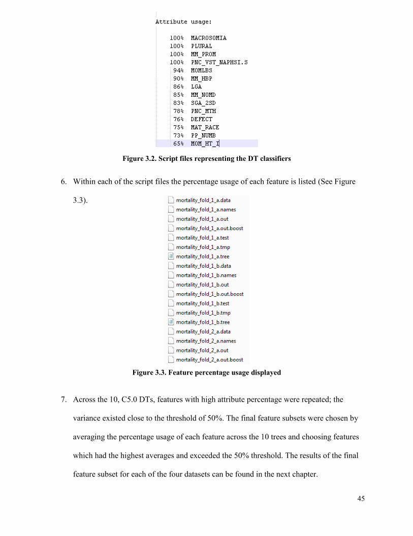
45

Figure 3.2. Script files representing the DT classifiers

6. Within each of the script files the percentage usage of each feature is listed (See Figure

3.3).

Figure 3.3. Feature percentage usage displayed

7. Across the 10, C5.0 DTs, features with high attribute percentage were repeated; the

variance existed close to the threshold of 50%. The final feature subsets were chosen by

averaging the percentage usage of each feature across the 10 trees and choosing features

which had the highest averages and exceeded the 50% threshold. The results of the final

feature subset for each of the four datasets can be found in the next chapter.

46

3.5. Step 4: Balancing the classes

In this research work, the unbalanced algorithm was used to apply the random undersampling

technique to the clinical datasets, in R [76]. The undersampling sub-function randomly removes

instances of the majority class while leaving all instances of the minority class (ubUnder

package). The ubUnder type has to be selected because the ubBalance package contains both

undersampling and oversampling methods. This function allows the user to determine which

percentage of the majority class will be left after sampling. In this work, 50% preterm cases and

50% term cases remained in the training dataset, so the classifier could be trained with an equal

proportion of both classes. The code below describes the BORN or PRAMS dataset represented

as X, with the Y variable representing the final OUTCOME feature (preterm or term cases) as

well as the type of balancing method (ubUnder) and the sampling parameters. The description of

which parameters were selected from this function are described in Table 3.2.

balance_dataset ubBalance (X, Y, type="ubUnder", positive= 0,

perc=50, method="percPos", w=NULL, verbose=FALSE)

Table 3.2. Description of parameters for package in R (ubBalance)

X represents the BORN or PRAMS

Y represents the OUTCOME feature (preterm or term) in BORN or PRAMS, which must be a

binary factor

type represents the balancing technique, in this research ubUnder was used, to remove

instances of the majority class (term)

positive represents the majority class (term cases), all term labels were changed from -1 to 0,

when using this function

47

perc represents the sampling percentage which was set to 50

method represents setting the percentage of positives to 50% after undersampling

w represents sampling the majority instances with equal weights, when w is set to NULL

verbose represents not printing extra information, when set to FALSE

3.6. Step 5: Input missing values

Before applying the ANN classifier, it was necessary to impute the missing values found within

the BORN and PRAMS dataset. Random forest classifiers were used to make predictions on

missing values in the BORN and PRAMS datasets. This was done by initially replacing the

missing values with the mean of the non-missing values within each feature. All features were

then sorted from lowest to highest, according to the amount of missing values. Then each feature

was trained with a random forest algorithm and predictions were made on the missing values.

This process was iterated until the difference between the previous and the new imputed matrix

increased for the first time. The package used to impute the missing values was missForest [48].

The code below described inputting the BORN or PRAMS dataset with missing values (noNAs

file) with the missForest algorithm applied. Then the filled in data was written to a text file once

the process ended. The description of which parameters were selected from this function are

described in Table 3.3.

tempData_noNAs <- missForest (noNAs,verbose = TRUE)

# writing the data to a text file

tempData_missF <- tempData_noNAs$ximp

48

write.table(tempData_missF,

"c:/MIRG/Thesis2017/missForestResults.txt", sep="\t")

Table 3.3. Description of parameters for package in R (missForest)

noNAs represents the BORN or PRAMS dataset with missing values

verbose represents additional output between iterations: estimated imputation error and

runtime, when TRUE

3.7. Step 6: Normalizing the data

Once the above preprocessing steps were applied, the four datasets were prepared for model

evaluation using the MIRG ANN classifier. Before applying this classifier, normalizing the data

was done, as the ANN tends to perform better when large range differences amongst features are

minimized [89]. In this work, the modified Z-score transformation equation was used to

transform the values between the range of -1 and 1, based on the MIRG ANN Guide [24].

The data was normalized to fall between [-1, 1] so that the activation function in the ANN treats

all features weighted equally during training. Normalization of the training, testing and

validation data was automated using BASH scripts. For scaling and normalization purposes, the

modified z-score transformation has been used previously in the MIRG lab [90], which scales the

data between -1 and 1 is:

𝑥𝑖𝑛 =

𝑥𝑖𝑛−𝑢𝑖

3𝜎𝑖

Where 𝑥𝑖 is the feature of interest, 𝑢𝑖 is defined as the population mean for each feature and 𝜎𝑖 is

defined as the population standard deviation for each feature.

This automation was done using the following steps:

49

a. Using SQL queries, the mean and standard deviation was obtained for all

attributes in the BORN Parous, BORN Nulliparous, PRAMS Parous and

PRAMS Nulliparous features. The mean and standard deviation values

were written to a file named “normalization.csv”.

b. Each dataset (BORN_Parous, BORN_Nulliparous, PRAMS_Parous and

PRAMS_Nulliparous) was divided into files called “mortality” and

“nonmortality” csv files

c. The mortality.csv file contained the balanced preterm cases with missing

values imputed and the nonmortality.csv files contained the balanced term

cases with missing values imputed.

d. Most of the values within each feature fell between the ranges of 1 to 5 as

many of the features within these datasets were categorical, however,

some of the continuous features such as maternal age had values of greater

than 40. When looking at the dataset as a whole these values might be

considered as outliers, however, the information within these features is

valuable for predicting preterm birth. Therefore, normalization was done

column-wise for each feature to ensure that the values fit the range of -1 to

1 and all values were included and not dropped.

e. A temporary file was created for both the mortality and the nonmortality

cases. The modified z-score was calculated for each attribute column in

mortality and nonmortality. This was done by obtaining the mean in the

first row of the attribute column and then the second row contained the

standard deviation for that attribute column. Once these two statistics were

50

obtained, using equation (1) above, the column data was normalized. In

these temporary files, both the Case ID and Outcome features were

excluded because these values should not be normalized.

f. Once all the feature columns were normalized, the data were combined

into a single csv file with the untouched Case ID and Outcome features.

3.8. Step 7: Divide into train, test and verification sets

There are three divisions of the data which are defined. First, the training set is the data that

trains the classifier, to improve the overall accuracy of classifying preterm and term cases. The

test set is the data which is not a part of the training set and is tested by the classifier during

model evaluation. Lastly, the verification set is the data which is unseen before inputting the data

into the neural network model (data preprocessing is still applied to these cases). The purpose of

this verification set is to output the true performance of the classifier, with data that it has not

been trained or tested on, to minimize overfitting. These three sets were created using 5-by-2

Cross Validation which is described below in Table 3.4. Separate from these three divisions, a

final test of the neural networks was evaluated on validation sets which consisted of unlabeled

data and contained 7.9% prevalence to match the population.

Table 3.4. Division of train, test and verification sets

Training Set Testing Set Verification Set

50% of the dataset 25% of the dataset 25% of the dataset

3.8.1. 5-by-2 Cross Validation

This work used 5-by-2 Cross Validation, to reduce overfitting of the classifier during the training

stage. Also, creating 10 sets of training, test and verification data with an equal number of

51

preterm and term cases; to ensure sufficient data was being verified by the ANN model. Before

using the ANN classifier, the clinical datasets were first normalized using the modified z-score

formula. BASH files have been developed by Gilchrist [91] to carry out 5-by-2 cross validation.

A BASH script file called create_5_by_2.sh carried out the following steps:

PHASE 1: There are two files one which contains the preterm cases and another file which

contains the term cases.

PHASE 2: Preterm and term cases are randomized and divided between Set A and Set B. At this

point the preterm and term cases remain separate.

PHASE 3: Set A which contains both preterm and term cases is further divided between two

cases (A1 and A2) while Set B remained unchanged. At this point A1, A2 and B contain preterm

and term cases. The subset of data is now 50% training, 25% test and 25% verification.

PHASE 4: The above process is reversed where Set B (containing preterm and term cases) is

further divided between two cases (B1 and B2) while Set A remains unchanged and the same

ratio is present.

PHASE 5: As a result of PHASE 3, Set #1 is produced which consists of B, A1, and A2 for the

training, test and the verification set respectively. While PHASE 4 results in Set #2 which

consists of A, B1 and B2. This process is repeated five times to create a total of 10 sets of

training, test and verification data

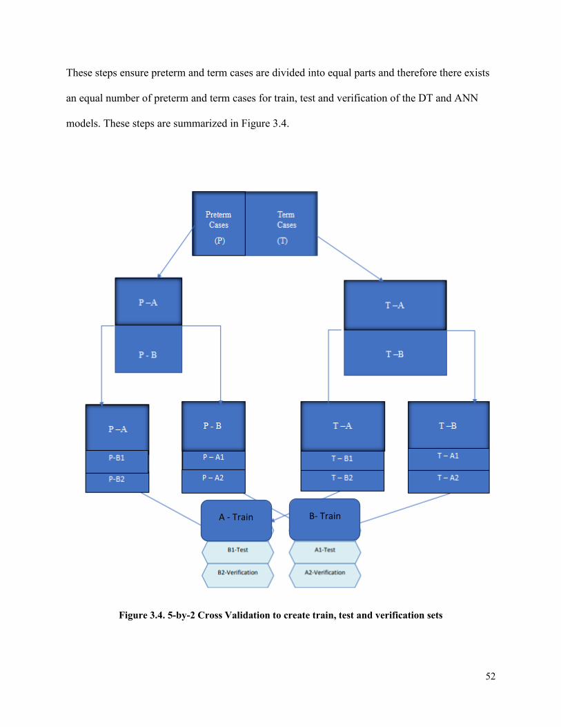
52

These steps ensure preterm and term cases are divided into equal parts and therefore there exists

an equal number of preterm and term cases for train, test and verification of the DT and ANN

models. These steps are summarized in Figure 3.4.

Figure 3.4. 5-by-2 Cross Validation to create train, test and verification sets

A - Train B- Train

53

3.9. Step 8: Execution of the ANN Builder

The purpose of this research was to follow similar steps applied, in the methodology of previous

work, to compare the difference in sensitivity results for preterm birth predictions when focusing

on data preparation. Therefore, the same ANN Builder using the FANN library, was used from

past research [7].

1. These steps were repeated for all four datasets.

2. The ANN Builder software was used to run the ANN Classifier and carried out training

and testing of the data.

3. The following network structures were automatically detected by the software for

training (see Figure 3.5): the number of hidden layers, the number of inputs (this is

dependent on the number of features determined by the C5.0 Decision Tree Classifier)

and the number of outputs is 1 (term or preterm).

54

Figure 3.5. Parameters for the BORN_Nulliparous dataset

4. After balancing the classes there were 102,187 cases in the BORN dataset and 46,867

cases in the PRAMS dataset. From this, 20,001 cases from BORN, and 10,001 cases

from PRAMS were put aside for the final testing stage of the validation set. Therefore,

the BORN dataset had around 82,186 cases to be trained and the PRAMS dataset had

around 36,866 cases to be trained with the ANN model.

5. The threshold to save the networks was chosen to be 60-85% for sensitivity and 70-

75% for specificity; these were the tested highest thresholds which would save the

networks in the result files.

55

6. The choice to optimize sensitivity over specificity was selected when selecting the best

networks and the performance metrics from the results were saved in a separate CSV

file (classifier_stats_final.csv).

7. The ANN Builder will create 10 networks which optimize the sensitivity metric

8. This final validation set is separate from the training, testing and verification sets

created from 5-by-2 cross validation. The validation set consisted of 5,000 cases (4605

term and 395 preterm) for PRAMS_Parous and PRAMS_Nulliparous and 10,000 (9210

term and 790 preterm) cases for BORN_Parous and BORN_Nulliparous. This

validation set had the labels removed before inputting the data into the ANN model for

final classification of the output labels. These cases were aggregated by randomly

sorting rows in Excel and selecting 790 or 395 preterm cases.

9. The performance metrics were calculated (sensitivity and specificity) for these four

datasets and are described in detail in the next section

Execution of the ANN Builder software was used with the following parameters: FAST mode

(tests around 0.5% of all possible combinations, excluding the number of hidden nodes), 3

hidden layers and the reported above network thresholds (see Step 5).

Another script was created: The Performance Measures Calculation Tool [13] for outputting the

performance metrics of the best network. These metrics include the Positive Predictive Value

(PPV), Negative Predictive Value (NPV), Accuracy (ACC), Matthews Correlation Coefficient

(MCC), Receiver Operating Curve (ROC), F1-Score and Area Under the Curve (AUC). These

statistical metrics were saved in the classifier_stats_final.csv.

The ANN Model Selection Tool [13] is a script which was used to select the best performing

network based on the highest sensitivity. This selection script is applied to 10 result files (after 5-

56

by-2 cross validation) and sorts through to find the final network with the highest sensitivity,

within the verification and test sets. This final network was tested against the validation set

(which is separate from the three datasets created from 5-by-2 Cross Validation and consists of

10,000 BORN or 5,000 PRAMS cases). More details regarding the network parameters can be

found in Appendix C.

57

4. Chapter: Results and Discussion

This chapter outlines the results of this thesis using data preparation methods and machine

learning classifiers. The results stem from the C5.0 DT Classifier for feature reduction and the

Artificial Neural Network Classifier for model evaluation.

Table 4.1. Results for the development and evaluation of the predictive tool

Steps Results

Step 1: Data Visualization Bar charts and plots showing the missing values within the data

Step 2: Eliminated cases and features

Removed cases with greater than 50% missing values and no

outcome label

Step 3: Choosing features with greater

than 50% importance using the C5.0 DT

classifier

Justified the 50% threshold and reduced feature subsets were

output across the 4 datasets.

Step 4: Balanced the classes Created an equal number of preterm and term cases for training

of the ANN using ubBalance.

Step 5: Impute missing values Filled in missing values using missForest

Step 6: Normalized the data Normalized the data in preparation for using the ANN model.

Step 7: Divided into test, train and

verification sets

Training, testing and verification sets for the ANN model.

Step 8: Execution of the ANN Builder

Created optimal networks for the final testing stage and

performance metric results outputted

58

4.1. Step 1: Data Visualization

The bar chart in Figure 4.1 compares a variety of clinical features: OTH_Term (Pregnancy

history: other terminations?), Plural (Plurality births), Preghx (Pregnancy history: calculated

from calculated from Previous Live Birth, Previous Low Birth Weight birth, and Previous

Preterm birth), Prev_Lb (Previous live births) plotted against the Outcome feature (1 for a

preterm outcome and -1 for a term outcome).

The small average difference between the Parous features reveals that there might not be a

significant difference between these Parous clinical features and a preterm or term outcome.

Therefore, more advanced algorithms are needed such as the C5.0 DT classifier to determine

features of importance. However, the benefit of using Tableau is that it provides a visual basis to

have conversations about features with our clinical partner, instead of looking at raw data from

Excel.

59

Figure 4.1. Bar Chart in Tableau comparing Parous_PRAMS features

Missing values were quite prevalent within both the BORN and PRAMS dataset. The below

Missingness Maps (Figure 4.2 & 4.3) were created to quickly see the presence of missing values

within the clinical features using the Amelia package in R [92]. The x-axis lists the features from

the BORN or PRAMS dataset and the y-axis is the CASE ID. Comparing the same number of

cases (50) the BORN dataset seems to have more missing values present than the PRAMS

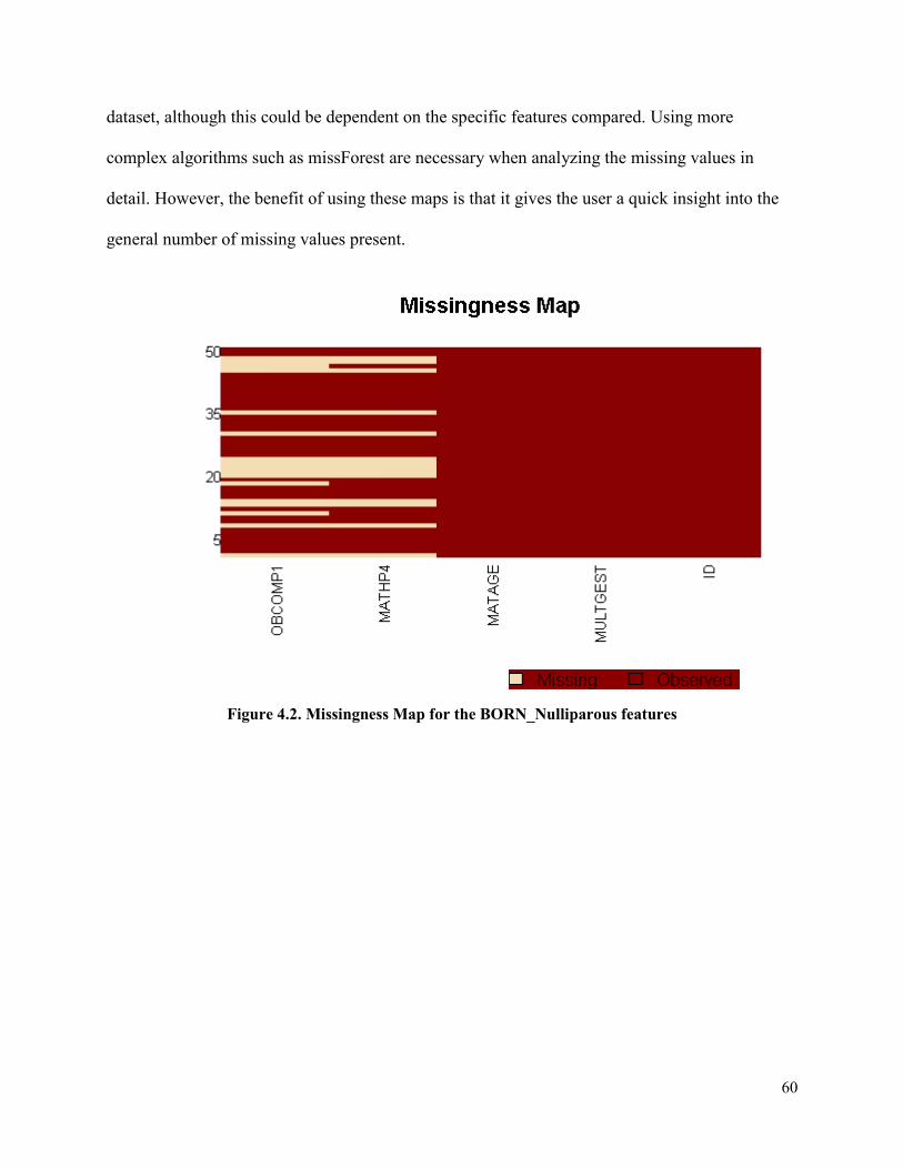
60

dataset, although this could be dependent on the specific features compared. Using more

complex algorithms such as missForest are necessary when analyzing the missing values in

detail. However, the benefit of using these maps is that it gives the user a quick insight into the

general number of missing values present.

Figure 4.2. Missingness Map for the BORN_Nulliparous features

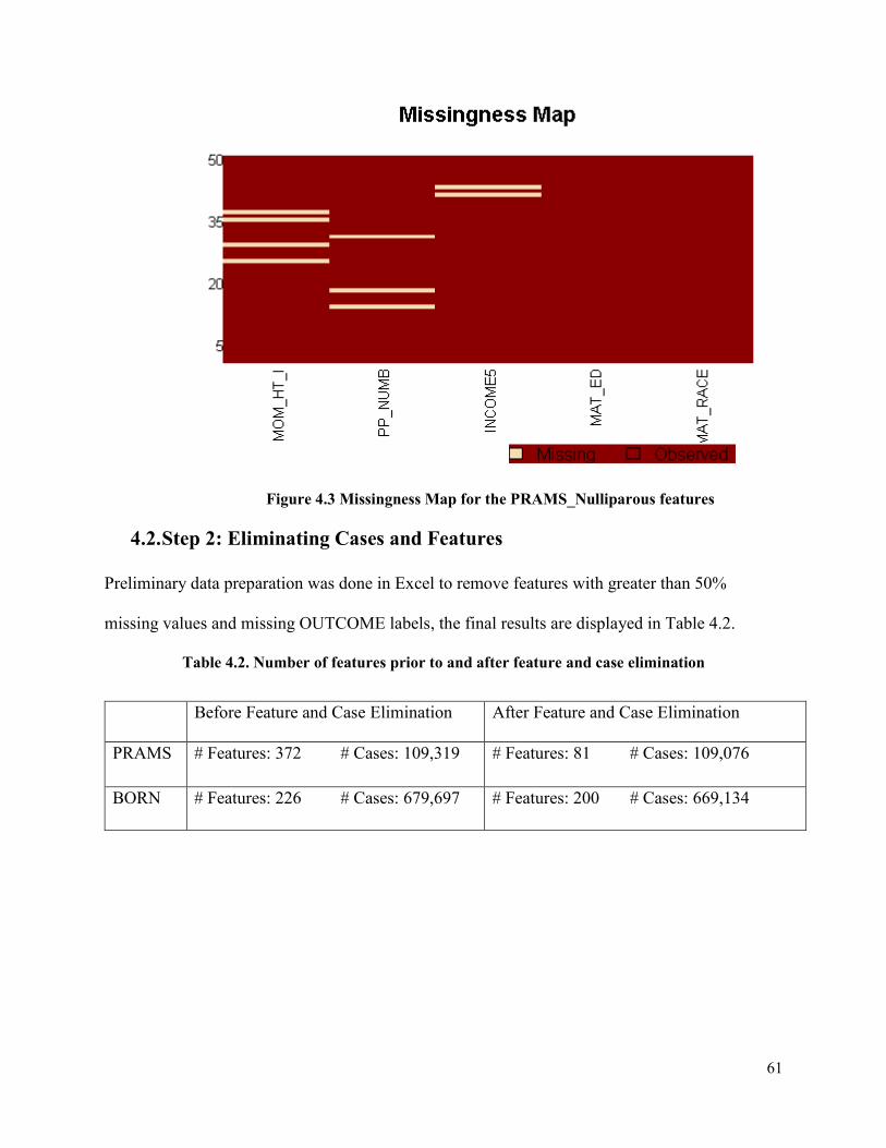
61

Figure 4.3 Missingness Map for the PRAMS_Nulliparous features

4.2. Step 2: Eliminating Cases and Features

Preliminary data preparation was done in Excel to remove features with greater than 50%

missing values and missing OUTCOME labels, the final results are displayed in Table 4.2.

Table 4.2. Number of features prior to and after feature and case elimination

Before Feature and Case Elimination After Feature and Case Elimination

PRAMS # Features: 372 # Cases: 109,319 # Features: 81 # Cases: 109,076

BORN # Features: 226 # Cases: 679,697 # Features: 200 # Cases: 669,134

62

4.3. Step 3: Choosing features with greater than 50% importance using the

C5.0 DT classifier

As previously stated, the C5.0 DT classifier has the capability to deal with missing values. This

led to investigating whether one should fill in missing values before or after feature reduction.

Although the sensitivity results were initially higher during training with the imputed values, (see

Table 4.3), the final results show that when testing the classifier, the classifier performed

generally worse. Therefore, it was decided to determine the features of importance prior to

imputing the missing values, to reduce possible overfitting of the results.

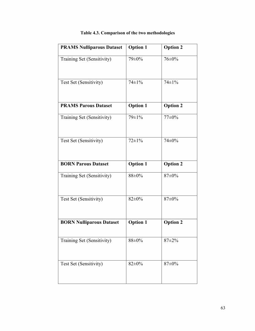
63

Table 4.3. Comparison of the two methodologies

PRAMS Nulliparous Dataset Option 1 Option 2

Training Set (Sensitivity) 79±0%

76±0%

Test Set (Sensitivity) 74±1%

74±1%

PRAMS Parous Dataset Option 1 Option 2

Training Set (Sensitivity) 79±1%

77±0%

Test Set (Sensitivity) 72±1%

74±0%

BORN Parous Dataset Option 1 Option 2

Training Set (Sensitivity)

88±0%

87±0%

Test Set (Sensitivity) 82±0% 87±0%

BORN Nulliparous Dataset Option 1 Option 2

Training Set (Sensitivity)

88±0%

87±2%

Test Set (Sensitivity) 82±0% 87±0%

64

The 50% threshold was determined experimentally by testing different feature subset sizes using

the C5.0 DT classifier. It was found that including features with greater than 30% feature

importance, sometimes resulted in slightly lower classification performance and greater

computational time (see Table 4.4. & 4.6.). Another test included features with greater than 65%

importance (see Table 4.5 & 4.7.). This resulted in a slight increase in accuracy, but this

threshold resulted in the removal of clinical features deemed important by our clinician

supervisor for predicting preterm birth, such as the feature, SGA_10 (small for gestation age) in

the PRAMS dataset and INTBF (intention to breastfeed) in the BORN dataset. Therefore, to

maintain a good balance, between including key clinical features and high accuracy, a feature

importance threshold of ≥ 50% was selected.

Table 4.4. Increased feature size to include ≥ 30% feature importance (BORN)

Performance Metric Train Test Standard

Deviation

Accuracy: 0.85 0.84 ±0.00

Sensitivity/Recall: 0.91 0.90 ±0.01

Specificity: 0.78 0.78 ±0.01

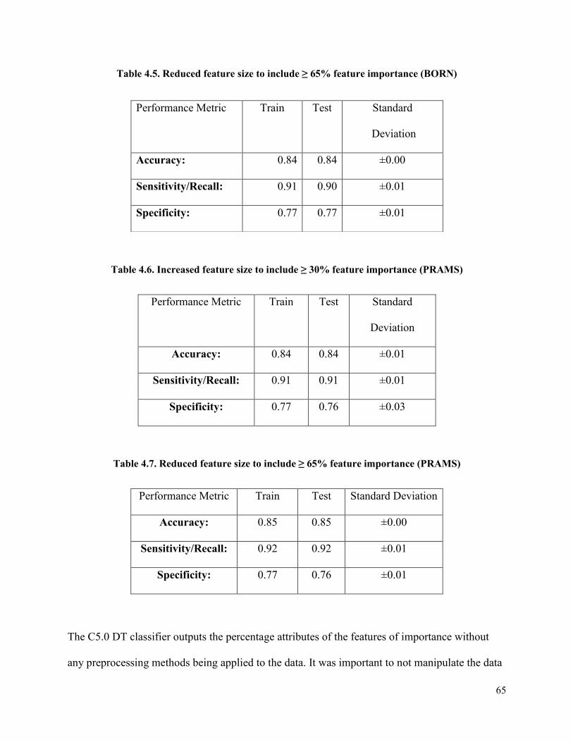
65

Table 4.5. Reduced feature size to include ≥ 65% feature importance (BORN)

Table 4.6. Increased feature size to include ≥ 30% feature importance (PRAMS)

Performance Metric Train Test Standard

Deviation

Accuracy: 0.84 0.84 ±0.01

Sensitivity/Recall: 0.91 0.91 ±0.01

Specificity: 0.77 0.76 ±0.03

Table 4.7. Reduced feature size to include ≥ 65% feature importance (PRAMS)

Performance Metric Train Test Standard Deviation

Accuracy: 0.85 0.85 ±0.00

Sensitivity/Recall: 0.92 0.92 ±0.01

Specificity: 0.77 0.76 ±0.01

The C5.0 DT classifier outputs the percentage attributes of the features of importance without

any preprocessing methods being applied to the data. It was important to not manipulate the data

Performance Metric Train Test Standard

Deviation

Accuracy: 0.84 0.84 ±0.00

Sensitivity/Recall: 0.91 0.90 ±0.01

Specificity: 0.77 0.77 ±0.01

66

so that, when the ANN classifier encounters new test data, this does not result in the classifier

overfitting the data.

The C5.0 DT classifier outputs ten trees and displays the feature importance for each tree. To

maintain a good balance between the importance and the quantity of features chosen for each

dataset, only features which had ≥50% feature importance were kept. Although most features

had the same percentage attribute across all ten of the trees such as the features: PLURAL and

MULTGEST (100%), there were some features that differed among the ten trees which were

close to the 50% threshold. In these cases, features were averaged across the ten trees and the

feature with the highest percentage average was chosen.

There were some obvious features that were selected by the classifier such as GENDER (baby’s

sex) and PPRETERM (number of previous preterm babies) in the BORN dataset and

MAT_AGE_NAPHSIS (maternal age grouped) and MAT_RACE (maternal race) in the PRAMS

dataset. These features have been documented to be increased risk factors for a preterm birth

outcome [30]. Some non-obvious features that were selected included PRENCLAS (number of

prenatal classes in weeks) and INTBF (intention to breastfeed) in the BORN dataset and

MAT_ED (maternal education) and PP_NUMB (# sources of payment for prenatal classes) in

the PRAMS dataset, these non-obvious features might allude to a certain socioeconomic status,

leading to an increased/decreased risk of preterm birth.

Once these features were reduced from over 300 features in PRAMS and over 200 features in

BORN (Table 4.8), this significantly decreased processing time and more importantly increased

the sensitivity results; as the subset of features chosen, were directly important to predicting a

preterm birth outcome.

67

Table 4.8. Feature reduction results after applying the C5.0 DT classifier to the BORN and

PRAMS datasets

Datasets Before Feature Reduction After Feature Reduction

BORN_Parous # Features: 200 # Features: 20

BORN_Nulliparous # Features: 180 # Features: 17

PRAMS_Parous # Features: 81 # Features: 22

PRAMS_Nulliparous # Features: 75 # Features: 20

The following Tables 4.9- 4.12 display the reduced features subsets (threshold of ≥ 50%) output by the

C5.0 DT classifier for BORN and PRAMS

Table 4.9: 20 Features: Parous BORN

100% MULTGEST: multiple gestation 95% PRENCLAS: Prenatal class

95% CONGAN55: Anomalies unclassified

elsewhere - Other syndromes

80% GENDER: Baby’s sex

82% OBCOMP12: Preterm premature rupture of

membranes (PPROM)

74% OBCOMP1: Obstetrical complications

(Eclampsia)

76% PREVCS: Previous cesarean Section 74% OBCOMP9: Pre-eclampsia

74% OBCOMP8: Obstetrical complications

(Placental abruption)

70% OBCOMP7: Obstetrical complications

(Placenta previa)

71% OBCOMP4: IUGR/SGA (Small for

gestational age)

69% OBCOMP10: Premature rupture of

membranes (PROM)

69% PPRETERM: Number of previous preterm

babies

64% OBCOMP3: Hypertension (gestational or

transient)

64% MATAGE: Mother’s age (years) 61% MATHP27: Other Maternal Health Problem

68

62% MATHP4: Maternal health problem

(Diabetes insulin)

60% MATHP3: Chronic hypertension

55% OBCOMP5: Obstetrical complications

(Large for Gestational Age)

50% INTBF: Intention to Breastfeed

Table 4.10: 17 Features: Nulliparous BORN

100% MULTGEST 80% GENDER

80% PRENCLAS 79% OBCOMP12

77% CONGAN55 76% MATAGE

74% OBCOMP1 74% OBCOMP8

74% OBCOMP9 70% OBCOMP4

69% OBCOMP7 68% OBCOMP10

65% MATHP27 62% OBCOMP3

62% MATHP3 57% MATHP4

58% OBCOMP5: LGA (large for gestational age)

Table 4.11: 22 Features: Parous PRAMS

100% PLURAL: plurality 100% MM_PROM: rupture membrane?

99% PNC_VST_NAPHSIS: number of

prenatal care visits grouped

93% MM_HBP: hypertension?

87% PREGHX: pregnancy history 84% MOMLBS: maternal weight gain

84% SGA_2SD: small for gestational age

based on 2SD from mean

83% LGA: large for gestational age based on

90th percentile

69

83% PNC_MTH: month of first prenatal care

visit

79% DEFECT: defect present? (this can be

detected during an antenatal ultrasound)

82% MM_FEVER: fever (mother)? 76% MAT_RACE: maternal race

77% OTH_TERM: pregnancy history (other

terminations?)

72% MOM_HT_I: mom total height (inches)

73% BC_YRLLB: years since last live birth 67% PNC_WKS: weeks 1st prenatal care

visit

71% INCOME5: 12 months before, total

income

64% MM_NOMD: no medical risk factors?

66% PRE_LB_NAPHSIS: number of

previous live births grouped

61% SGA_10: small for gestational age

based on 10th percentile

54% PP_NUMB: # sources of payment for

prenatal care

51% MAT_ED: maternal education

Table 4.12: 19 Features: Nulliparous PRAMS

100% PLURAL 100% MM_PROM

100% MACROSOMIA: Macrosomia:

≥ 4500 gram birth weight

100% PNC_VST_NAPHSIS

90% MM_HBP 88% LGA

87% MOMLBS 85% SGA_2SD

81% INCOME5 81% MM_NOMD:

79% PNC_MTH 79% DEFECT

70

78% MM_FEVER 78% MAT_RACE

77% MAT_ED: maternal education 78% MOM_HT_I

67% PP_NUMB: # sources of payment for

prenatal care

56% MAT_AGE_NAPHSIS: maternal age

grouped

51% SURE_WKS: weeks when sure pregnant

There are several similar features chosen by the C5.0 DT classifier between the PRAMS and

BORN datasets (see Figure 4.4.) Despite the differences, which include how the data has been

obtained, the features which have been measured, and the location of the clinical datasets, this

classifier has determined key features of importance when predicting a premature birth. These

features are important to record if one wants to build their own preterm birth dataset specific to a

clinical site. By inputting these features into the neural network, there is a high probability of

improved sensitivity results. Some of these features include: maternal age, if the mother has high

blood pressure, presence of previous premature births etc.… There are also similar features

chosen between Ong’s research work [24] (see Table 4.13-4.16). These features are of

importance when predicting preterm birth, as they tend to appear across various research reports

on preterm birth.

71

BORN PRAMS

MULTGEST: multiple gestation PLURAL: plurality

OBCOMP10 & OBCOMP12: premature

rupture of membranes (PROM) & Preterm

premature rupture of membranes (PPOM)

MM_PROM: ruptured membranes?

OBCOMP4: Small for gestational age SGA_2SD & SGA_10: Small for gestational

age based on 2 standard deviation from the

mean & Small for gestational age based on

10th percentile

OBCOMP5: Large for gestational age LGA: Large for gestational age based on the

90th percentile

MATAGE: Mother’s age in years MAT_AGE_NAPHSIS: Maternal age

grouped

PPRETERM: Number of previous preterm

babies

PREGHX: Pregnancy history (calculated

from Previous Live Birth, Previous Low Birth

Weight birth, and Previous Preterm birth)

OBCOMP3 & MATHP3 (Hypertension

gestational or transien & Chronic

hypertension

MM_HBP: Hypertension?

Figure 4.4. List of abbreviations used for highly ranked features which occurred in both the

BORN and PRAMS data sets, used in this study to assess risk of preterm birth

72

Table 4.13: Similar features chosen in current and earlier research work: Parous_BORN

100% MULTGEST 95% PRENCLAS

95% CONGAN55 80% GENDER

82% OBCOMP12 74% OBCOMP1

76% PREVCS 74% OBCOMP9

74% OBCOMP8 70% OBCOMP7

71% OBCOMP4 69% OBCOMP10

69% PPRETERM 64% OBCOMP3

64% MATAGE 61% MATHP27

62% MATHP4 60% MATHP3

55% OBCOMP5 50% INTBF

These features were also present in past work

Table 4.14: Similar features chosen in current and earlier research work: Nulliparous_BORN

100% MULTGEST 80% GENDER

80% PRENCLAS 79% OBCOMP12

77% CONGAN55 76% MATAGE

74% OBCOMP1 74% OBCOMP8

74% OBCOMP9 70% OBCOMP4

69% OBCOMP7 68% OBCOMP10

65% MATHP27 62% OBCOMP3

62% MATHP3 57% MATHP4

58% OBCOMP5

These features were also present in past work

73

Table 4.15: Similar features chosen in current and earlier research work: Parous_PRAMS

100% PLURAL: plurality 100% MM_PROM: rupture membrane?

99% PNC_VST_NAPHSIS: number of

prenatal care visits grouped

93% MM_HBP: hypertension?

87% PREGHX: pregnancy history 84% MOMLBS: maternal weight gain

84% SGA_2SD: small for gestational age

based on 2SD from mean

83% LGA: large for gestational age based on

90th percentile

83% PNC_MTH: month of first prenatal care

visit

79% DEFECT: defect present? (this can be

detected during an antenatal ultrasound)

82% MM_FEVER: fever (mother)? 76% MAT_RACE: maternal race

77% OTH_TERM: pregnancy history (other

terminations?)

72% MOM_HT_I: mom total height (inches)

73% BC_YRLLB: years since last live birth 67% PNC_WKS: weeks 1st prenatal care

visit

71% INCOME5: 12 months before, total

income

64% MM_NOMD: no medical risk factors?

66% PRE_LB_NAPHSIS: number of

previous live births grouped

61% SGA_10: small for gestational age

based on 10th percentile

54% PP_NUMB: # sources of payment for

prenatal care

51% MAT_ED: maternal education

These features were also present in past work

74

Table 4.16: Similar features chosen in current and earlier research work: Nulliparous_PRAMS

100% PLURAL 100% MM_PROM

100% MACROSOMIA: Macrosomia:

≥ 4500 gram birth weight

100% PNC_VST_NAPHSIS

90% MM_HBP 88% LGA

87% MOMLBS 85% SGA_2SD

81% INCOME5 81% MM_NOMD:

79% PNC_MTH 79% DEFECT

78% MM_FEVER 78% MAT_RACE

77% MAT_ED: maternal education 78% MOM_HT_I

67% PP_NUMB: # sources of payment for

prenatal care

56% MAT_AGE_NAPHSIS: maternal age

grouped

51% SURE_WKS: weeks when sure pregnant

These features were also present in past work

4.4. Step 4: Balancing the Classes

When applying this function, this greatly reduced the number of cases in the training dataset (See

Table 4.17.) and improved the computational training time of the neural network. For instance, in

work done by Ong [24], the BORN_Parous and BORN_Nulliparous datasets took around 634

hours and 186 hours respectively to train, whereas the PRAMS_Parous and PRAMS_Nulliparous

took 73 and 36 hours respectively to train. In this work, with the reduction of the dataset, the

BORN_Parous and BORN_Nulliparous datasets took around 10 and 9 hours respectively to

train, whereas the PRAMS_Parous and PRAMS_Nulliparous took around 4 hours each to train.

The hardware specifications of the computers on which the models were trained on were similar.

75

All simulations in this current work were run on BME-12 lab computers: Intel Core i5 760

(2.80GHz) processor, 8GB RAM, Windows 7 64bit. Where Ong [24], ran her models on the

BME-12 and BME-14 lab computer: Intel Core i7-3770 (3.4GHz) processor, 8 GB RAM,

Windows 7 64bit.

Table 4.17. Case reduction results after applying package in R (ubBalance) to the BORN and

PRAMS datasets

Before Class Balance After Class Balance

BORN # Cases: 679,697 # Cases: 102,187

PRAMS # Cases: 109,079 # Cases: 46,867

4.5. Step 5: Input missing values

As stated previously, missForest uses random forest classifiers. These classifiers do not need to

perform 5-by-2 cross validation to create a test set such as with the DT classifier or with the

ANN classifier because random forests contain internal test sets to estimate the error. During the

random forest run around 1/3 of cases are not used during training and are instead used as a test

set. The out of bag (OOB) imputation error supplied two values for the categorical and nominal

features and the results are displayed in Table 4.18. The proportion of falsely classified (PFC)

cases represents the error for the categorical features and the normalized mean square error

(NMSE) represents the error for the nominal features [48].

Table 4.18 OOB error estimate for Nulliparous_PRAMS dataset

NRMSE: 0.2353279 PFC: 0.3191449

76

4.6. Step 6: Normalizing the data

Results from normalizing the data using the modified Z-score transformation are displayed in

Figure 4.5., saved in a .data file. The data is scaled between a range of -1 to 1.

Figure 4.5. Results of data normalization

4.7. Step 7: Divide into test, train and verification sets

The results from applying the BASH file ./create_5_by_2.sh are displayed in the below Figure

4.6. Once these files have been created, then the training of the neural networks using the ANN

builder [13] can commence.

Figure 4.6. Results of 5-by-2 Cross Validation (test set)

4.8. Step 8: Execution of the ANN Builder

After 5-by-2 cross validation was applied to create train, test and verification sets for the ANN,

around 100 neural networks were saved in the network folders and the best neural network which

optimized sensitivity was selected. An example of the performance metrics for the

PRAMS_Parous classifier is displayed below in Table 4.19. This neural network was then tested

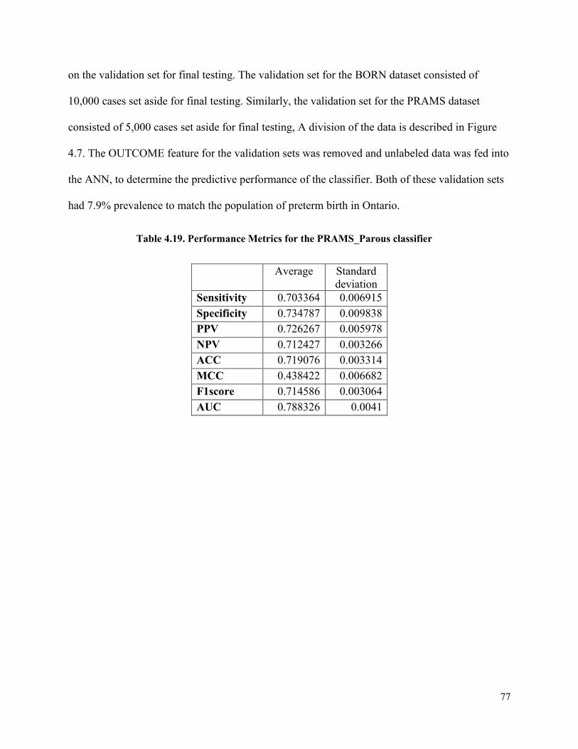
77

on the validation set for final testing. The validation set for the BORN dataset consisted of

10,000 cases set aside for final testing. Similarly, the validation set for the PRAMS dataset

consisted of 5,000 cases set aside for final testing, A division of the data is described in Figure

4.7. The OUTCOME feature for the validation sets was removed and unlabeled data was fed into

the ANN, to determine the predictive performance of the classifier. Both of these validation sets

had 7.9% prevalence to match the population of preterm birth in Ontario.

Table 4.19. Performance Metrics for the PRAMS_Parous classifier

Average Standard

deviation

Sensitivity 0.703364 0.006915

Specificity 0.734787 0.009838

PPV 0.726267 0.005978

NPV 0.712427 0.003266

ACC 0.719076 0.003314

MCC 0.438422 0.006682

F1score 0.714586 0.003064

AUC 0.788326 0.0041

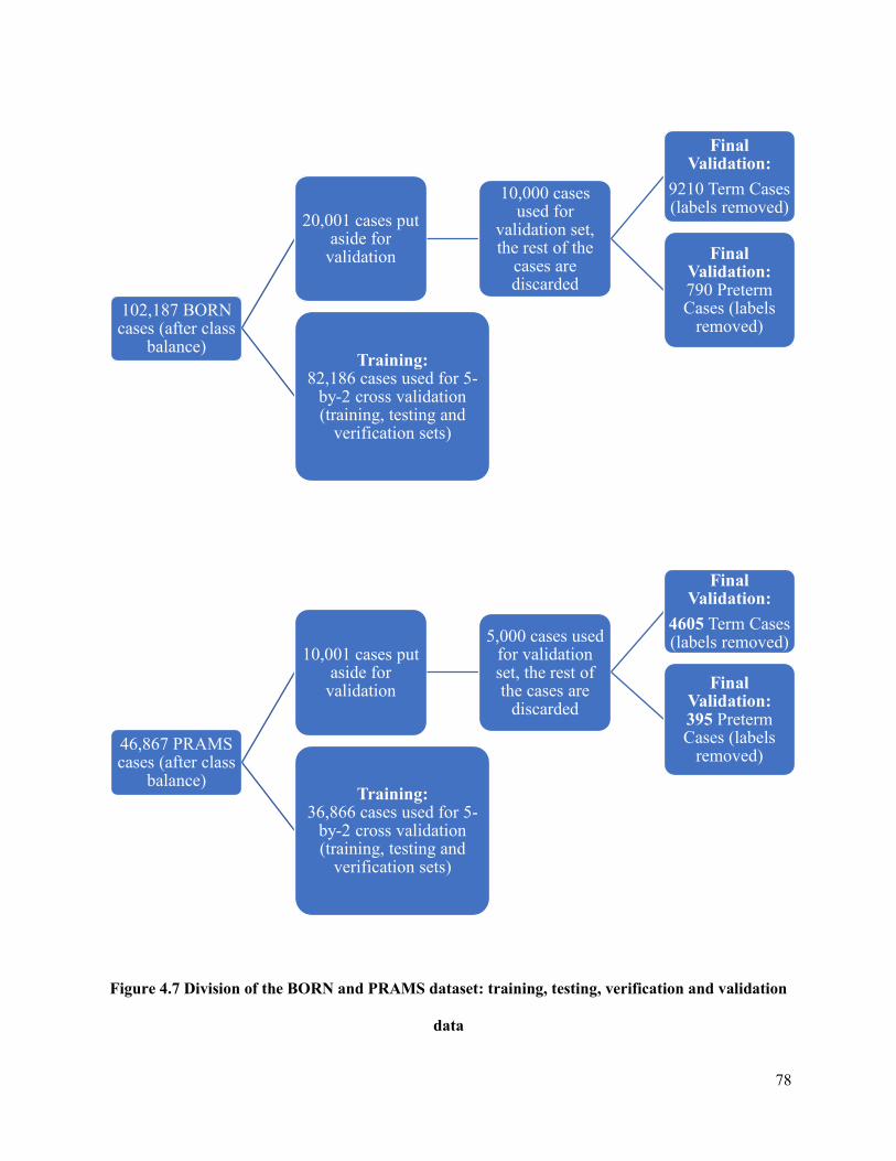
78

Figure 4.7 Division of the BORN and PRAMS dataset: training, testing, verification and validation

data

102,187 BORN cases (after class

balance)

20,001 cases put aside for

validation

10,000 cases used for

validation set, the rest of the

cases are discarded

Final Validation:

9210 Term Cases (labels removed)

Final Validation: 790 Preterm Cases (labels

removed)

Training: 82,186 cases used for 5-

by-2 cross validation (training, testing and

verification sets)

46,867 PRAMS cases (after class

balance)

10,001 cases put aside for

validation

5,000 cases used for validation set, the rest of the cases are

discarded

Final Validation:

4605 Term Cases (labels removed)

Final Validation: 395 Preterm Cases (labels

removed)

Training: 36,866 cases used for 5-

by-2 cross validation (training, testing and

verification sets)

79

The confusion matrix was calculated for each of the four datasets which were tested against the

final validation set (10,000 for BORN and 5,000 for PRAMS) the confusion matrix, sensitivity

and specificity metrics are displayed below (Table 4.20-4.27). In an imbalanced dataset which is

what the ANN is tested on with 7.9% prevalence, the accuracy metric is not the most effective

measure for determining the performance of the classifier. Since there is such a small proportion

of preterm cases, the classifier might not be able to distinguish between the preterm cases (low

true positive rate) but could instead classify the term cases with a high accuracy (high true

negative rate) leading to an overall high accuracy metric. A better metric to compare the

classifier’s performance is the AUC (area under the curve) which aggregates the classifier

performance at a variety of thresholds. In addition, due to this class imbalance there are many

term cases which could be classified as false positives (falsely classified as preterm), this

contributes to the low precision value (1) reported in the below tables. Conversely, due to the

high number of term cases, there are few preterm cases which could be classified as term, the

focus of this research is to limit this occurrence and contributes to the high negative predictive

value (2) reported in the below tables.

𝑃𝑃𝑉 = 𝑇𝑃

𝑇𝑃+𝐹𝑃× 100 (1)

𝑁𝑃𝑉 = 𝑇𝑁

𝑇𝑁+𝐹𝑁× 100 (2)

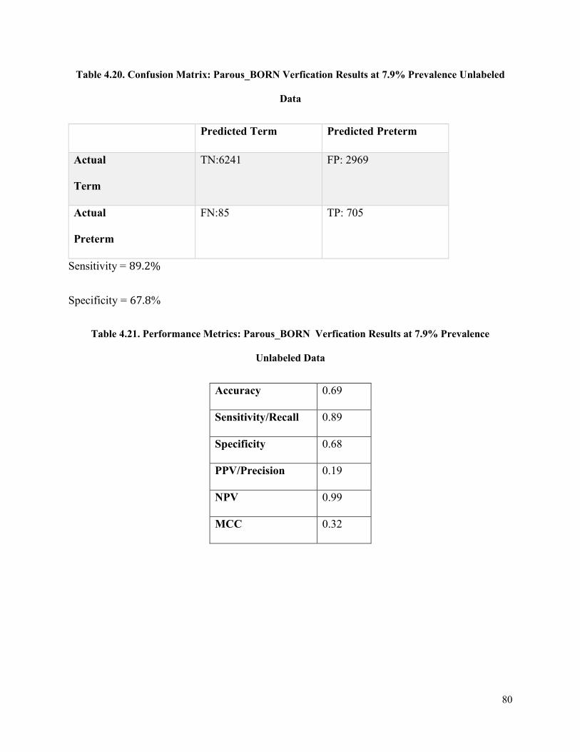
80

Table 4.20. Confusion Matrix: Parous_BORN Verfication Results at 7.9% Prevalence Unlabeled

Data

Predicted Term Predicted Preterm

Actual

Term

TN:6241 FP: 2969

Actual

Preterm

FN:85 TP: 705

Sensitivity = 89.2%

Specificity = 67.8%

Table 4.21. Performance Metrics: Parous_BORN Verfication Results at 7.9% Prevalence

Unlabeled Data

Accuracy 0.69

Sensitivity/Recall 0.89

Specificity 0.68

PPV/Precision 0.19

NPV 0.99

MCC 0.32

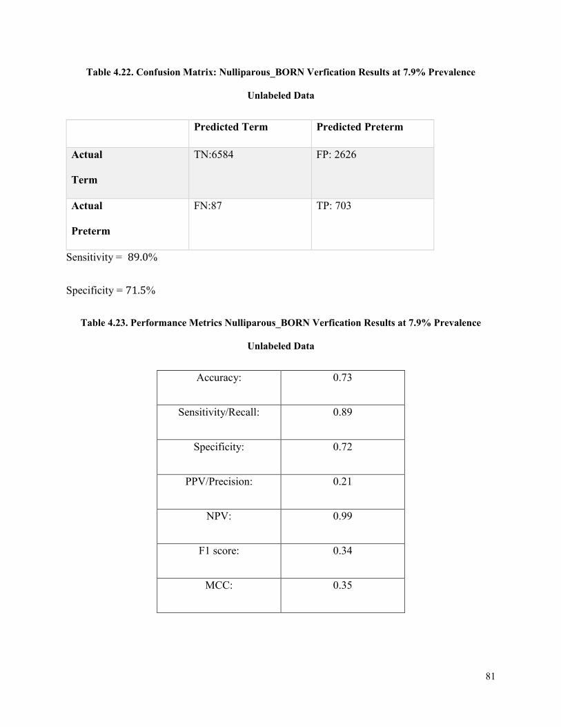
81

Table 4.22. Confusion Matrix: Nulliparous_BORN Verfication Results at 7.9% Prevalence

Unlabeled Data

Predicted Term Predicted Preterm

Actual

Term

TN:6584 FP: 2626

Actual

Preterm

FN:87 TP: 703

Sensitivity = 89.0%

Specificity = 71.5%

Table 4.23. Performance Metrics Nulliparous_BORN Verfication Results at 7.9% Prevalence

Unlabeled Data

Accuracy: 0.73

Sensitivity/Recall: 0.89

Specificity: 0.72

PPV/Precision: 0.21

NPV: 0.99

F1 score: 0.34

MCC: 0.35

82

Table 4.24. Confusion Matrix: Parous_PRAMS Verfication Results at 7.9% Prevalence Unlabeled

Data

Predicted Term Predicted Preterm

Actual

Term

TN:3288 FP: 1317

Actual

Preterm

FN:63 TP: 332

Sensitivity = 84.1%

Specificity = 71.4%

Table 4.25. Performance Metrics: Parous_PRAMS Verfication Results at 7.9% Prevalence Unseen

Data

Accuracy: 0.73

Sensitivity/Recall: 0.84

Specificity: 0.71

PPV/Precision: 0.21

NPV: 0.99

F1 score: 0.34

MCC: 0.35

83

Table 4.26. Confusion Matrix: Nulliparous_PRAMS Verfication Results at 7.9% Prevalence

Unseen Data

Predicted Term Predicted Preterm

Actual

Term

TN:3501 FP: 1104

Actual

Preterm

FN:64 TP: 331

Sensitivity = 83.8%

Specificity = 76.0%

Table 4.27. Performance Metrics: Nulliparous_PRAMS Verfication Results at 7.9% Prevalence

Unseen Data

Accuracy: 0.77

Sensitivity/Recall: 0.84

Specificity: 0.76

PPV/Precision: 0.23

NPV: 0.98

F1 score: 0.37

MCC: 0.36

The ROC Curves for each dataset (Figure 4.8 – 4.11) are displayed below. The True Positive

Rate (Sensitivity) is displayed on the y-axis and the False Positive Rate (1-Specificity) is

displayed on the x-axis. Each point on the ROC curves represents the Sensitivity versus 1-

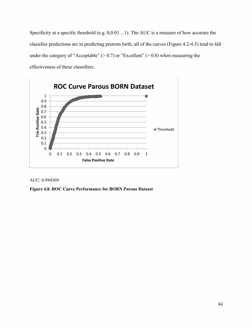
84

Specificity at a specific threshold (e.g. 0,0.01…1). The AUC is a measure of how accurate the

classifier predictions are in predicting preterm birth, all of the curves (Figure 4.2-4.5) tend to fall

under the category of “Acceptable” (> 0.7) or “Excellent” (> 0.8) when measuring the

effectiveness of these classifiers.

AUC: 0.894369

Figure 4.8. ROC Curve Performance for BORN Parous Dataset

0

0.1

0.2

0.3

0.4

0.5

0.6

0.7

0.8

0.9

1

0 0.1 0.2 0.3 0.4 0.5 0.6 0.7 0.8 0.9 1

Trie

Po

siti

ve R

ate

False Positive Rate

ROC Curve Parous BORN Dataset

Threshold

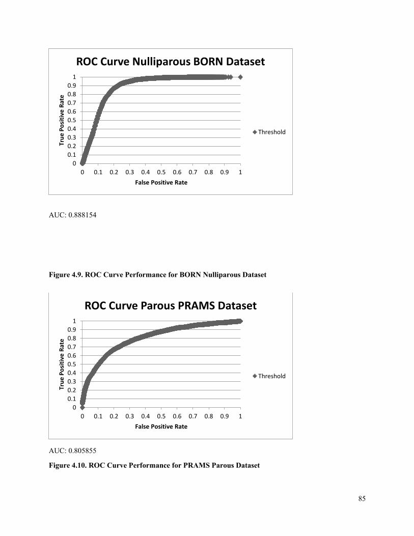
85

AUC: 0.888154

Figure 4.9. ROC Curve Performance for BORN Nulliparous Dataset

AUC: 0.805855

Figure 4.10. ROC Curve Performance for PRAMS Parous Dataset

0

0.1

0.2

0.3

0.4

0.5

0.6

0.7

0.8

0.9

1

0 0.1 0.2 0.3 0.4 0.5 0.6 0.7 0.8 0.9 1

Tru

e P

osi

tive

Rat

e

False Positive Rate

ROC Curve Nulliparous BORN Dataset

Threshold

0

0.1

0.2

0.3

0.4

0.5

0.6

0.7

0.8

0.9

1

0 0.1 0.2 0.3 0.4 0.5 0.6 0.7 0.8 0.9 1

Tru

e P

osi

tive

Rat

e

False Positive Rate

ROC Curve Parous PRAMS Dataset

Threshold

86

AUC: 0.788409

Figure 4.11. ROC Curve Performance for PRAMS Nulliparous Dataset

The parameters of the best final networks, which optimize sensitivity, for the BORN and

PRAMS Dataset at 7.9% Prevalence can be found in Appendix C. The final results of this

research are summarized below in Tables 4.28-4.31.

4.9. Comparison to Past Results

Table 4.28. Display of the Artificial Neural Network results for BORN and PRAMS datasets

Datasets Current Research (2018)

Sensitivity Specificity AUC

PRAMS_Parous 84.1% 71.4% 0.8059

PRAMS_Nulliparous 83.8% 76.0% 0.7884

BORN_Parous 89.2% 67.8% 0.8944

BORN_Nulliparous 89.0% 71.5% 0.8882

0

0.1

0.2

0.3

0.4

0.5

0.6

0.7

0.8

0.9

1

0 0.1 0.2 0.3 0.4 0.5 0.6 0.7 0.8 0.9 1

Tru

e P

osi

tive

Rat

e

False Positive Rate

ROC Nulliparous PRAMS Dataset

Threshold

87

Table 4.29. Displays the Artificial Neural Network results for past results (2015)

Datasets Past Research [24]

Sensitivity Specificity AUC

PRAMS_Parous 68.15% 64.17% 0.7256

PRAMS_Nulliparous 40.35% 94.75% 0.7064

BORN_Parous 50.53% 91.61% 0.7721

BORN_Nulliparous 53.96% 95.40% 0.7970

Table 4.30. Displays the Artificial Neural Network results for past results (2009)

Datasets Past Research [27]

Sensitivity Specificity AUC

PRAMS_Parous 65.13% 84.07% 0.8195

PRAMS_Nulliparous 61.08% 71.14% 0.7195

Table 4.31. Displays the Artificial Neural Network results for past results (2007)

Datasets Past Research [39]

Sensitivity Specificity

PRAMS 65% 84%

88

4.10. Results and Discussion Summary

This research focused on data preparation methods in comparison to past research which focused

on the machine learning algorithms. The first step dealt with class imbalance (ubBalance [76])

reducing the dataset from 679,697 (BORN) and 109,079 (PRAMS) cases to 102,187 (BORN)

and 46,867 (PRAMS) cases. This was a major change from past research [24], [27], [11], and

resulted in faster computational time building the ANN models and improved accuracy of the

classifier during training and testing. In addition, the second step of filling in missing values

using a package in R (missForest [48]), proved faster than a case-based reasoning approach to fill

in missing values. Ong remarked difficulty with comparing past results with her current

methodology, due to a variety of changes: a new ANN tool, introducing 5-by-2 cross validation

to reduce bias of results, prevalence to simulate real world conditions and the use of an updated

version of the PRAMS database. Therefore, effectiveness of these two data preparation methods

were reflected in the improved sensitivity results, when following the methodology of Ong [24]

closely. In addition, this research used significantly fewer variables (17-22) than past research

(34-45 for Ong [24] and 48 for Catley [39]). This addressed an area of improvement discussed

by Ong, who suggested fewer variables might result in better results.

There were promising results when evaluating the BORN and PRAMS dataset. Out of all the

datasets, the BORN_Parous dataset had the best results when considering classifier performance

(AUC) and sensitivity values. The Parous datasets had higher sensitivity metrics in comparison

to the Nulliparous datasets, these datasets contain features with prior medical history (i.e.

previous premature birth) and this seems to have a positive affect on the classifier’s ability to

classify preterm birth. There was an overall increase in sensitivity when comparing to past

89

results: 68.15% [24], 65% [27], 65% [39], meaning there are more accurate predictions when

predicting preterm birth. Since, the objective of the thesis is to obtain the most accurate results

when it comes to predicting preterm births, the specificity value is also important when referring

to clinical costs and resources; however, it is not as critical as correctly predicting a premature

birth outcome.

The aim was to exceed past sensitivity results and compare results to past performance metrics.

The performance of the BORN and PRAMS database using the ANN Builder, did exceed past

sensitivity results of prior students but did not surpass previous specificity metrics for all four

datasets. One of the advantages of the ANN builder is its ability to optimize sensitivity or

specificity; therefore, the model could be tailored specifically to fit the physician’s needs,

depending on which performance metric is desired. To be considered clinically useful in the

context of this research a sensitivity of 65% and a specificity of 85% was recommended by our

clinical partner [39], [24]. The sensitivity metric has been met and surpassed by all four datasets

and future work will consist of improving the specificity metric to meet the clinical standards.

This chapter outlined the results obtained with this research work. The results of the

methodology which focused on data preparation methods, showed an overall improvement in the

sensitivity results of the Artificial Neural Network classifier. The reduced feature subsets for

each of the four datasets were presented using the C5.0 DT Classifier. In addition, the

performance metrics of the ANN classifier were displayed and compared to past work done in

the MIRG lab. The contribution of this thesis work and future areas of improvement are

discussed in the next chapter.

90

5. Chapter: Conclusion

5.1 Final Remarks and Conclusion

This thesis work was focused on improving the sensitivity results of predicting a preterm birth

outcome using existing machine learning tools, applied to two large population-based datasets.

The method of improving the sensitivity results focused on preprocessing methods, primarily

addressing missing values and class imbalances found in the clinical datasets. In addition, with

the use of the C5.0 DT classifier, similar important features were identified between these widely

different datasets. This is a positive result as it shows some congruence between various

databases; these features will be necessary to include when implementing a similar database

system in a clinical environment. By addressing these common data preprocessing concerns, this

thesis work contributed to a higher accuracy and faster computational time when generating the

ANN models.

5.2 Contributions to Knowledge

1. This work demonstrated that the predictive system described in this thesis could

potentially be used in both an American (PRAMS) and a Canadian environment (BORN).

This provides further evidence that this algorithm could be further developed to someday

be incorporated into obstetrical clinics in Canada where prenatal data is collected

prospectively.

2. New tools were used in this research work: R, (missForest and ubBalance) and Tableau

which have not been used previously by students in the MIRG lab for data preprocessing

methods. Using R for imputing missing values has greatly improved computational time,

91

in comparison to previous methods (k-NN Algorithm). Tableau was an effective tool to

visualize real-world data. In addition, this tool provided insight into the importance of

some features over others, even before feature selection methods were applied. R and

Tableau were chosen over other software tools such as SAS because these software tools

needed to be open source to allow functionality within a clinical environment.

3. Similarly to previous students’ work, the ANN classifier performed better with the

BORN data than the PRAMS data [26], [29]. This may indicate that the variables

collected by BORN may be more helpful to predict preterm births.

4. Previous work highlighted a need to attempt to reduce the number of variables used. This

work has greatly reduced the number of features analyzed in the BORN (20 features for

Parous and 17 features for Nulliparous) and PRAMS (22 features for Parous and 19

features for Nulliparous) in comparison to past work by Ong [24]: BORN (45 features for

Parous and 38 features for Nulliparous) and PRAMS (48 features for Parous and 32

features for Nulliparous). This reduced feature subset maintained high sensitivity with

reduced computational time.

5. These data preprocessing steps can be applied to variety of fields outside of the clinical

sphere such as financial or environmental datasets with missing values; this is because

these libraries in R are not specific to clinical data, are open-source and can handle large

datasets.

6. Through data preprocessing methods described in the thesis, the sensitivity metric has

surpassed previous methods, critical for predicting preterm births effectively; and the

specificity metric has also remained sufficiently high. During the testing stage the

92

prevalence was set to 7.9%, to ensure that the data reflected an accurate population of

preterm to term cases.

7. This work identified several similar features chosen by the DT classifier between both the

PRAMS and BORN dataset:

a. Multiple gestation

b. Premature rupture of membranes

c. Small gestation age

d. Large gestational age

e. Mother’s age in years

f. Number of previous preterm babies

g. Hypertension

h. Obstetrical complications (yes or no?)

These features might be important to maintaining high sensitivity results when moving the

system to a real clinical environment.

8. During the feature selection methods, there were several features in the BORN dataset

which were restricted from access due to data privacy concerns, such as geographical

data; access to this data could result in an even higher sensitivity and specificity results

for the classifier. As well as including shared features between BORN and PRAMS such

as features including: hypertension, multiple gestation and maternal age. Given that the

plan is to eventually integrate this classifier into a clinical environment in Canada, access

to this data would be a great resource for future work. One option would be to anonymize

the data so that researchers would have access to important information while still

upholding the privacy of patients

93

9. This developed system is non-invasive and has the capability to predict a preterm birth

prior to 23 weeks, using only data; it surpasses the accuracy of the current gold standard-

fetal fibronectin.

5.3 Future Work

1. Future work should focus on improving the specificity performance metric (specifically

dealing with the high number of false positives). There is an important trade-off between

a high sensitivity and a high specificity. Although this work surpassed previous

sensitivity results, the same was not true for the specificity metric. Specificity results

were generally higher across the PRAMS datasets in comparison to BORN, therefore,

certain features in PRAMS, were likely central to an increase in the specificity results.

However, the specificity metric did not meet the clinical standard of 85%. Including

similar features to those reported in the PRAMS dataset might be a solution to increasing

this specificity metric.

2. Future work will include testing and validating the results from the use of these data

preprocessing software. Data will be removed and then added back into the dataset, to

test the validity of using the missForest package in R for imputing missing values.

Similarly, for ubUnder this can be tested by removing different percentages of the data

(using this package left 50% preterm and 50% term cases in the dataset) to ensure this

50% split between preterm and term cases represents the highest accuracy for predicting

preterm birth; further work can be tested by observing how 60% preterm and 40% term

cases affects the overall accuracy.

3. Future works consist of building a dataset of clinical features collected at obstetrical

clinics from past neonatal cases with known labels of preterm or term cases. To build this

94

dataset, the similar features identified between the BORN and PRAMS dataset could be

used to ensure high accuracy of the ANN classifier. Therefore, with future cases which

contain unlabeled data, physicians will be able to make an accurate prediction on whether

an individual may be at risk for a premature birth before 23 weeks gestation and then

apply preventative care.

4. Investigate the effect of increasing the size of the testing set and see how the classifier

performs. The classifier was tested in the final stage with 9210 term and 790 preterm

cases from the BORN dataset. This testing set should be increased to test the stability of

the performance of the classifier, with the same ratio between term and preterm cases.

This can be done by randomly resampling the original 10,000 test set for an increased test

set and then applying the classifier.

5. Eventually there will be a need to implement this system nationwide if it performs well in

local clinics. Therefore, greater insight is needed into how this classifier will perform

with data from populations in Canada, which have higher than normal preterm birth rates

(rural and remote areas).

6. Future work could include integrating this predictive tool at a clinical site in conjunction

with the prospective collection of data inputted into the Ontario Perinatal Record [37],

through a secure web service. Preterm birth predictions made by the system could then be

compared to the eventual pregnancy outcome, to determine the real-world accuracy of the

prediction tool.

95

References

[1] H. C. Koh and G. Tan, "Data mining applications in healthcare," Journal of healthcare

information management, vol. 19, no 2, pp. 65-71, 2011.

[2] J. Engel, "GE, IBM Race to Deliver on A.I. Hype in Healthcare," Xconomy Boston , 26 June

2017. [Online]. Available: https://www.xconomy.com/boston/2017/06/26/ge-ibm-race-to-

deliver-on-a-i-hype-in-healthcare/. [Accessed 2018].

[3] S. Armstrong, "The computer will assess you now," BMJ, London, vol. 355, no. 1, pp. 5680,

2016.

[4] BORN, "BORN Information System," Better Outcomes and Registry & Network, 2013.

[Online]. Available: https://www.bornontario.ca/en/born-information-system/. [Accessed

2017].

[5] CDC, "Premature Birth," Center for Disease Control and Prevention, 2014. [Online]. Available:

https://www.cdc.gov/prams/questionnaire.htm. [Accessed 2017].

[6] J. R. Quinlan, " C5. 0 Data Mining Tool. RuleQuest Research.," 1997. [Online]. Available:

https://www.rulequest.com/see5-info.html [Accessed 2017].

[7] S. Nissen, "Implementation of a fast artificial neural network library (fann)," Department of

Computer Science University of Copenhagen, Copenhagen, pp.1-92, 2003.

[8] J. Wang, "Data mining: opportunities and challenges,". IGI Global, pp. 85-105, 2003.

[9] N. Zhang and W. F. Lu, "An efficient data preprocessing method for mining customer survey

data," Industrial Informatics, 2007 5th IEEE International Conference, vol. 1, pp. 573-578,

2007.

[10] S. García, J. Luengo and F. Herrera, "Data preprocessing in data mining," Switzerland.

Springer International Publishing, pp. 195-243, 2015.

[11] C. Catley, M. Frize, R. C. Walker and D. C. Petriu, "Predicting high-risk preterm birth using

artificial neural networks," IEEE transactions on information technology in biomedicine, vol.

10, no. 3, pp. 540-549, 2006.

[12] M. Frize, N. Yu and S. Weyand, "Effectiveness of a hybrid pattern classifier for medical

applications," International Journal of Hybrid Intelligent Systems, vol. 8, no. 2, pp. 71-79,

2011.

[13] H. Martirosyan, M. Frize, D. E. Ong, J. Gilchrist and E. Bariciak, "A Decision-Support System

for Expecting Mothers and Obstetricians," 6th European Conference of the International

Federation for Medical and Biological Engineering. IFMBE Proceedings, vol. 45, pp. 703-706,

2015.

[14] K. M. Groom and P. R. Bennett, "Tocolysis for the treatment of preterm labour‐a clinically

based review.," The Obstetrician & Gynaecologist, London, vol. 6, no. 1, pp. 4-11, 2004.

[15] S. Beck, D. Wojdyla, L. Say, A. P. Betran, M. Merialdi, J. H. Requejo and P. F. Van Look,

"The worldwide incidence of preterm birth: a systematic review of maternal mortality and

morbidity," Bulletin of the World Health Organization,vol. 88, pp. 31-38, 2010.

[16] BORN Ontario, "Perinatal Health Indicators for Ontario 2012," 2012. [Online]. Available:

https://www.bornontario.ca/assets/documents/specialreports/Perinatal%20Health%20Indicators

%20for%20Ontario%202012.pdf.[Accessed 2018].

[17] R. L. Goldenberg, J. F. Culhane, J. D. Iams and R. Romero, "Epidemiology and causes of

preterm birth," The lancet, vol. 371, no. 9606, pp. 75-84, 2008.

96

[18] S. A. Leonard, C. M. Crespi, D. C. Gee, Y. Zhu and S. E. Whaley, "Prepregnancy risk factors

for preterm birth and the role of maternal nativity in a low-income, hispanic population.,"

Maternal and child health journal, vol. 19, no. 10, pp. 2295-2302, 2015.

[19] P. J. Meis, R. L. Goldenberg, B. M. Mercer, J. D. Iams, A. H. Moawad, M. Miodovnik and A.

Das, "The preterm prediction study: risk factors for indicated preterm births," American journal

of obstetrics and gynecology, vol. 178, no. 3, pp. 562-567, 1998.

[20] M. Parisaei, J. Currie, N. O’Gorman, S. Morris and A. L. David, "Implementation of foetal

fibronectin testing: Admissions, maternal interventions and costs at 1 year," Journal of

Obstetrics and Gynaecology, vol. 36, no. 7, pp. 888-892, 2016.

[21] S. N. Deshpande, A. D. I. Van Asselt, F. Tomini, N. Armstrong, A. Allen, C. Noake and M. E.

Westwood, "Rapid fetal fibronectin testing to predict preterm birth in women with symptoms

of premature labour: a systematic review and cost analysis.," NIHR Journals Library,

Southampton, vol. 40, no. 17, pp. 1-8, 2013.

[22] N. L. Hezelgrave and A. H. Shennan, "Quantitative fetal fibronectin to predict spontaneous

preterm birth: a review.," Women’s Health, vol. 12, no. 1, pp. 121-128, 2016.

[23] T. M. Malak, F. Sizmur, S. C. Bell and D. J. Taylor, "Fetal fibronectin in cervicovaginal

secretions as a predictor of preterm birth," BJOG: An International Journal of Obstetrics &

Gynaecology, vol. 103, no. 7, pp. 648-653, 1996.

[24] D. E. Ong, "An Integrated Machine Learning Approach to Optimize the Estimation of Preterm

Birth,". Carleton University, Ottawa, 2015.

[25] PHIP, " Personal Health Information Protection Act,"November 2014 [Online]. Available:

https://www.ontario.ca/laws/statute/04p03?search=phipa.[Accessed 2017].

[26] T. M. Program, "BORN — Better Outcomes Registry and Network," 2013. [Online].

Available: https://www.themothersprogram.ca/resources-and-information/born-better-

outcomes-registry-and-network.[Accessed 2018].

[27] N. Yu, An integrated decision tree-artificial neural network hybrid to estimate clinical

outcomes: ICU mortality and pre-term birth. Carleton University, Ottawa, 2009.

[28] G. S. Berkowitz, C. Blackmore-Prince, R. H. Lapinski and D. A. Savitz, "Risk factors for

preterm birth subtypes.," Epidemiology, vol. 9, no. 3, pp. 279-285, 1998.

[29] P. J. Meis, R. L. Goldenberg, B. M. Mercer, J. D. Iams, A. H. Moawad, M. Miodovnik and A.

Das, "The preterm prediction study: risk factors for indicated preterm births," American journal

of obstetrics and gynecology, vol. 178, no. 3, pp. 562-567, 1998.

[30] L. J. Muglia and M. Katz, "The enigma of spontaneous preterm birth," New England Journal of

Medicine, vol. 362, no. 6, pp. 529-535, 2010.

[31] G. Lim, J. Tracey, N. Boom, S. Karmakar, J. Wang, J. M. Berthelot and C. Heick, "CIHI

survey: Hospital costs for preterm and small-for-gestational age babies in Canada," Healthcare

Quarterly, vol. 12, no. 4, pp. 20-24, 2009.

[32] S. Saigal and L. W. Doyle, "An overview of mortality and sequelae of preterm birth from

infancy to adulthood," The Lancet, vol. 371, no. 9608, pp. 261-269, 2008.

[33] T. Yoshizato, H. Obama, T. Nojiri, Y. Miyake, S. Miyamoto and T. Kawarabayashi, "Clinical

significance of cervical length shortening before 31 weeks' gestation assessed by longitudinal

observation using transvaginal ultrasonography," Journal of Obstetrics and Gynaecology

Research, vol. 34, no. 5, pp. 805-811, 2008.

[34] W. L. Maner, R. E. Garfield, H. Maul, G. Olson and G. Saade, "Predicting term and preterm

delivery with transabdominal uterine electromyography.," Obstetrics & Gynecology,vol. 101,

no.6, pp. 1254-1260, 2003.

[35] H. Leitich and A. Kaider, "Fetal fibronectin—how useful is it in the prediction of preterm

birth?," BJOG: An International Journal of Obstetrics & Gynaecology, vol. 110, no .20, pp. 66-

70, 2003.

97

[36] M. Frize, E. Bariciak, S. Dunn, S. Weyand, J. Gilchrist and S. Tozer, "Combined Physician-

Parent Decision Support tool for the neonatal intensive care unit.," medical measurements and

applications proceedings (MeMeA), vol. 197, pp. 59-64, 2011.

[37] Provincial Council for Maternal and Child Health, "A User Guide to the Ontario Perinatal

Record.," 2017. [Online]. Available: http://www.pcmch.on.ca/wp-

content/uploads/2017/11/OPR_UserGuide_2017OCT26.pdf. [Accessed 2017].

[38] P. H. Shiono and M. A. Klebanoff, "A review of risk scoring for preterm birth," Clinics in

perinatology, vol. 20, no. 1, pp. 107-125, 1993.

[39] C. Catley, An Integrated Hybrid Data Mining System for Preterm Birth Risk Assessment Based

on a Semantic Web Servcies for Healthcare Framework, Carleton University, Ottawa, 2007.

[40] J. R. Quinlan, "Bagging, boosting, and C4. 5.," AAAI/IAAI, vol. 1, pp. 725-730, 1996.

[41] W. L. Maner and R. E. Garfield, "Identification of human term and preterm labor using

artificial neural networks on uterine electromyography data," Annals of biomedical

engineering, vol. 35, no. 3, pp. 465-473, 2007.

[42] C. J. Lockwood and E. Kuczynski, "Risk stratification and pathological mechanisms in preterm

delivery," Paediatric and perinatal epidemiology, vol. 15, pp. 78-89, 2001.

[43] H. Y. Chen, C. H. Chuang, Y. J. Yang and T. P. Wu, "Exploring the risk factors of preterm

birth using data mining.," Expert systems with applications, vol. 38, no. 5, pp. 5384-5387,

2011.

[44] H. Kang, "The prevention and handling of the missing data," Korean journal of anesthesiology,

vol. 64, no. 5, pp. 402-406, 2013.

[45] G. Doquire and M. Verleysen, "Feature selection with missing data using mutual information

estimators," Neurocomputing, vol. 90, pp. 3-11, 2012.

[46] A. B. Pedersen, E. M. Mikkelsen, D. Cronin-Fenton, N. R. Kristensen, T. M. Pham, L.

Pedersen and I. Petersen, "Missing data and multiple imputation in clinical epidemiological

research," Clinical epidemiology, vol. 9, pp. 157-166, 2017.

[47] A. K. Waljee, A. Mukherjee, A. G. Singal, Y. Zhang, J. Warren, U. Balis and P. D. Higgins,

"Comparison of imputation methods for missing laboratory data in medicine," BMJ open, vol.

3, no. 8, pp.1-7, 2013.

[48] D. J. Stekhoven and P. Bühlmann, "MissForest—non-parametric missing value imputation for

mixed-type data.," Bioinformatics, vol. 28, no. 1, pp. 112-118, 2011.

[49] S. V. Buuren and K. Groothuis-Oudshoorn, "mice: Multivariate imputation by chained

equations in R," Journal of statistical software, vol. 10, no. 2, pp. 1-68, 2010.

[50] M. J. Azur, E. A. Stuart, C. Frangakis and P. J. Leaf, "Multiple imputation by chained

equations: what is it and how does it work?," International journal of methods in psychiatric

research, vol. 20, no. 1, pp. 40-49, 2011.

[51] J. A. Sterne, I. R. White, J. B. Carlin, M. Spratt, P. Royston, M. G. Kenward and J. R.

Carpenter, "Multiple imputation for missing data in epidemiological and clinical research:

potential and pitfalls," vol. 339, no. 7713, pp. 157-160, Bmj, 2009.

[52] D. C. Li, C. W. Liu and S. C. Hu, "A learning method for the class imbalance problem with

medical data sets.," Computers in biology and medicine, vol. 40, no. 5, pp. 509-518, 2010.

[53] R. Longadge and S. Dongre, "Class imbalance problem in data mining review," vol. 2, no .1,

pp. 1-6, 2013.

[54] M. A. Mazurowski, P. A. Habas, J. M. Zurada, J. Y. Lo, J. A. Baker and G. D. Tourassi,

"Training neural network classifiers for medical decision making: The effects of imbalanced

datasets on classification performance," Neural networks,vol. 21, no. 2-3, pp. 427-436, 2008.

[55] R. Longadge and S. Dongre, "Class imbalance problem in data mining review," International

Journal of Computer Science and Network ,vol. 2, no.1, pp. 1-6, 2013.

98

[56] M. M. Rahman and D. N. Davis, "Addressing the class imbalance problem in medical

datasets.," International Journal of Machine Learning and Computing, vol. 3, no. 2, pp. 224,

2013.

[57] V. Ganganwar, "An overview of classification algorithms for imbalanced datasets.,"

International Journal of Emerging Technology and Advanced Engineering, vol. 2. no. 4, pp. 42-

47, 2012.

[58] M. Vihinen, "How to evaluate performance of prediction methods? Measures and their

interpretation in variation effect analysis," BMC genomics, vol 13. no. 4, pp. 1-10, 2012.

[59] A. H. Fielding and J. F. Bell, "A review of methods for the assessment of prediction errors in

conservation presence/absence models," Environmental conservation, vol. 24, no. 1, pp. 38-49,

1997.

[60] J. Gilchrist, C. M. Ennett, M. Frize and E. Bariciak, "Neonatal mortality prediction using real-

time medical measurements," medical measurements and applications proceedings (MeMeA),

pp. 65-70, 2011.

[61] B. Vidakovic, "Statistics for bioengineering sciences: with MATLAB and WinBUGS support,"

Springer Science & Business Media., pp. 471-472. 2011.

[62] J. N. Mandrekar, "Receiver operating characteristic curve in diagnostic test assessment,"

Journal of Thoracic Oncology, vol. 5, no. 9, pp. 1315-1316, 2010.

[63] S. Boughorbel, F. Jarray and M. El-Anbari, "Optimal classifier for imbalanced data using

Matthews Correlation Coefficient metric," PloS one, vol 12. no. 6, pp.1-17, 2017.

[64] MathWorks, "Normalize," R2015b. 2015 [Online]. Available:

https://www.mathworks.com/help/matlab/ref/normalize.html#d119e785470.[Accessed 2017]

[65] S. R. Maetschke, P. B. Madhamshettiwar, M. J. Davis and M. A. Ragan, "Supervised, semi-

supervised and unsupervised inference of gene regulatory networks," Briefings in

bioinformatics, vol. 15, no. 2, pp. 195-211, 2013.

[66] S. B. Kotsiantis, I. Zaharakis and P. Pintelas, "Supervised machine learning: A review of

classification techniques," Emerging artificial intelligence applications in computer

engineering, vol. 160, pp. 3-24, 2007.

[67] A. Abraham, F. Pedregosa, M. Eickenberg, P. Gervais, A. Mueller, J. Kossaifi and G.

Varoquaux, "Machine learning for neuroimaging with scikit-learn," Frontiers in

neuroinformatics, vol. 8, pp. 1-10, 2014.

[68] Z. Ghahramani, "Unsupervised learning," Advanced lectures on machine learning , pp. 72-112,

2004.

[69] J. H. Krijthe, "RSSL: Semi-supervised Learning in R," International Workshop on

Reproducible Research in Pattern Recognition, pp. 104-115, 2016.

[70] S. García, J. Luengo and F. Herrera, Data preprocessing in data mining, Granada: Springer

International Publishing, pp. 195-243, 2015.

[71] G. P. Zhang, "Neural networks for classification: a survey," IEEE Transactions on Systems,

Man, and Cybernetics, Part C (Applications and Reviews), vol. 30, no. 4, pp. 451-462, 2000.

[72] A. S. Galathiya, A. P. Ganatra and C. K. Bhensdadia, "Improved decision tree induction

algorithm with feature selection, cross validation, model complexity and reduced error

pruning.," International Journal of Computer Science and Information Technologies, vol. 3, no.

2, pp. 3427-3431, 2012.

[73] I. G. Maglogiannis, Emerging artificial intelligence applications in computer engineering: real

word ai systems with applications in ehealth, hci, information retrieval and pervasive

technologies, Amsterdam: IOS Press, vol. 160, pp. 3-25, 2007.

[74] R. Pandya and J. Pandya, "C5. 0 algorithm to improved decision tree with feature selection and

reduced error pruning.," International Journal of Computer Applications, vol. 117, no. 16, pp.

18-21, 2015.

99

[75] P. H. Swain and H. Hauska, "The decision tree classifier: Design and potential," IEEE

Transactions on Geoscience Electronics, vol. 15, no. 3, pp. 142-147, 1977.

[76] D. Pozzolo, O. Caelen and B. Gianluca, "Package ‘unbalanced," 26 June 2015. [Online].

Available: https://cran.r-project.org/web/packages/unbalanced/unbalanced.pdf.[Accessed

2018].

[77] M. Misztal, "Some Remarks on the Data Imputation Using “missForest” Method.,"pp. 1-11,

2013.

[78] A. T. Azar, H. I. Elshazly, A. E. Hassanien and A. M. Elkorany, "A random forest classifier for

lymph diseases.," Computer methods and programs in biomedicine, vol. 2, no. 113, pp. 465-

473, 2014.

[79] C. Nguyen, Y. Wang and H. N. Nguyen, "). Random forest classifier combined with feature

selection for breast cancer diagnosis and prognostic," Journal of Biomedical Science and

Engineering, vol. 5, no. 6, p. 551, 2013.

[80] B. L. Kalman and S. C. Kwasny, "Why tanh: choosing a sigmoidal function," Neural Networks,

vol. 4, pp. 578-581, 1992.

[81] J. V. Tu, "Advantages and disadvantages of using artificial neural networks versus logistic

regression for predicting medical outcomes," Journal of clinical epidemiology, vol. 11, no. 49,

pp. 1225-1231, 1996.

[82] Tableau, "Tableau Server 10.3.6," 12 December 2017. [Online]. Available:

https://www.tableau.com/support/releases/server/10.3.6.[Accessed 2018].

[83] Cygwin. [Online]. Available: https://www.cygwin.com/.[Accessed 2017].

[84] J. R. Quinlan, "C5.0: An Informal Tutorial," RULEQUEST RESEARCH 2017, [Online].

Available: https://www.rulequest.com/see5-unix.html.[Accessed 2018].

[85] C. M. Ennett, M. Frize and E. Charette, "Improvement and automation of artificial neural

networks to estimate medical outcomes.," Medical engineering & physics, vol. 26, no. 4, pp.

321-328, 2004.

[86] D. Rybchynski, "Design of an artificial neural network research framework to enhance the

development of clinical prediction models," University of Ottawa, Ottawa, 2005.

[87] A. S. Miller and B. H. Blott, "Review of neural network applications in medical imaging and

signal processing.," Medical and Biological Engineering and Computing, vol. 30, no. 5, pp.

449-464, 1992.

[88] J. Jiang, P. Trundle and J. Ren, "Medical image analysis with artificial neural networks,"

Computerized Medical Imaging and Graphics, vol. 34, no. 8, pp. 617-631, 2010.

[89] S. A. Durai and E. A. Saro, "Image compression with back-propagation neural network using

cumulative distribution function," World Academy of Science, Engineering and Technology,

vol. 17, pp. 60-64, 2006.

[90] M. Frize, J. Gilchrist, H. Martirosyan and E. Bariciak, "Integration of outcome estimations with

a clinical decision support system: Application in the neonatal intensive care unit (NICU),"

MeMeA, pp. 175-179, 2015.

[91] J. Honaker, G. King, M. Blackwell and M. M. Blackwell, "Package ‘Amelia’.," 2010. [Online].

Available: http://kambing.ui.ac.id/cran/web/packages/Amelia/Amelia.pdf.[Accessed 2018].

100

Appendices

Appendix A-Ethics Approval Form

Appendix B- Description of BORN and PRAMS Features

Appendix C- Description of ANN Final Network Parameters

101

Appendix A-Ethics Approval Form

102

Appendix B – BORN and PRAMS Features

BORN Parous Features

1. MULTGEST 2. MATAGE

3. PPRETERM 4. PTERM

5. PARITY 6. PRESENT

7. DELTYPE 8. PREVCS

9. ANTESTER 10. GENDER

11. APGAR1 12. APGAR5

13. INTBF 14. SMOKING

15. MATHP0 16. MATHP1

17. MATHP2 18. MATHP3

19. MATHP4 20. MATHP5

21. MATHP16 22. MATHP17

23. MATHP18 24. MATHP19

25. MATHP26 26. MATHP27

27. OBCOMP0 28. OBCOMP1

29. OBCOMP2 30. OBCOMP3

31. OBCOMP4 32. OBCOMP5

33. OBCOMP6 34. OBCOMP7

35. OBCOMP8 36. OBCOMP9

37. OBCOMP10 38. OBCOMP11

39. OBCOMP12 40. OBCOMP13

103

41. OBCOMP14 42. OBCOMP15

43. REPASS 44. FIRSTVIS

45. CONGAN0 46. CONGAN52

47. CONGAN54 48. CONGAN55

49. DISCHTO 50. PRENCLAS

51. GBSRES 52. FISCALYEAR

53. LANGUAGE_up 54. MATHP_sub

55. MATHP_ment 56. CONGAN_CNS

57. CONGAN_EYE 58. CONGAN_OROFACIAL

59. CONGAN_CARDIAC 60. CONGAN_RES

61. CONGAN_GAS 62. CONGAN_GEN

63. CONGAN_MUS 64. CONGAN_CHR

65. Total_15_marital 66. Single

67. not_separated 68. separated

69. divorced 70. widowed

71. Total_15_common_law 72. Not_common_law

73. In_common_law 74. Total_families_1

75. Size_2_person 76. Size_3_person

77. Size_4_person 78. Size_5_or_more

79. Total_families_2 80. Total_couple_families

81. Married_couples 82. Without_children_at_home

83. With_children_at_home 84. child_1

85. children_2 86. children_3_over

104

87. Common_law_couples 88. Without_children_at_home1

89. With_children_at_home1 90. child1_1

91. children1_2 92. children1_3_over

93. Total_lone_parent_families 94. Female_parent

95. child2_1 96. children2_2

97. children2_3_over 98. Male_parent

99. child3_1 100. children3_2

101. children3_3_over 102. Average_number_children

103. Total_family_by_type 104. One_family

105. Multiple_family 106. Non_family

107. Total_by_mother_tongue 108. Single_responses

109. English 110. French

111. Non_official_languages 112. Total_by_immigrant

113. Non_immigrants 114. Immigrants

115. Total_by_Aboriginal 116. Total_Aboriginal

117. North_American_single 118. Metis_single_response

119. Inuit_single_response 120. Multiple_Aboriginal

121. Aboriginal_responses 122. Non_Aboriginal

123. Total_by_labour 124. In_labour_force

125. Employed 126. Unemployed

127. Not_in_labour_force 128. Total_by_class

129. Class_worker_NA 130. All_classes__worker

131. Paid_workers 132. Employees

105

133. Self_employed 134. Without_paid_help

135. With_paid_help 136. Self_employed_unco

137. Without_paid_help2 138. With_paid_help2

139. Unpaid_family_workers 140. Total_15_24_diploma

141. No_diploma 142. Certificate__diploma

143. High_school 144. Apprenticeship

145. College__CEGEP_ 146. University_diploma

147. diploma_or_below 148. degree

149. Bachelor_degree 150. above_bachelor

151. Degree_in_medicine 152. Master_degree

153. Doctorate 154. Total_25_to_64_diploma

155. No_diploma_degree 156. Certi_diploma_degree

157. High_school_certi 158. Apprenticeship_diploma

159. College_CEGEP_or_other 160. University_dipoma

161. diploma_below_bachelor 162. University_certificate

163. Bachelor_s_degree 164. above_bachelor_degree

165. Degree_medicine 166. Master_s_degree

167. Earned_doctorate 168. Total_minority

169. Total_visible_minority 170. Total_by_ethnic

171. British_Isles_origins 172. French_origins

173. Aboriginal_origins 174. Other_American_origins

175. Caribbean_origins 176. Latin_Central

177. European_origins 178. African_origins

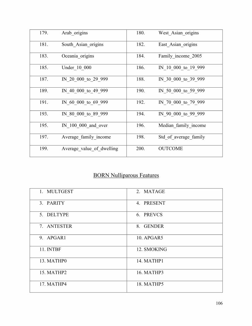
106

179. Arab_origins 180. West_Asian_origins

181. South_Asian_origins 182. East_Asian_origins

183. Oceania_origins 184. Family_income_2005

185. Under_10_000 186. IN_10_000_to_19_999

187. IN_20_000_to_29_999 188. IN_30_000_to_39_999

189. IN_40_000_to_49_999 190. IN_50_000_to_59_999

191. IN_60_000_to_69_999 192. IN_70_000_to_79_999

193. IN_80_000_to_89_999 194. IN_90_000_to_99_999

195. IN_100_000_and_over 196. Median_family_income

197. Average_family_income 198. Std_of_average_family

199. Average_value_of_dwelling 200. OUTCOME

BORN Nulliparous Features

1. MULTGEST 2. MATAGE

3. PARITY 4. PRESENT

5. DELTYPE 6. PREVCS

7. ANTESTER 8. GENDER

9. APGAR1 10. APGAR5

11. INTBF 12. SMOKING

13. MATHP0 14. MATHP1

15. MATHP2 16. MATHP3

17. MATHP4 18. MATHP5

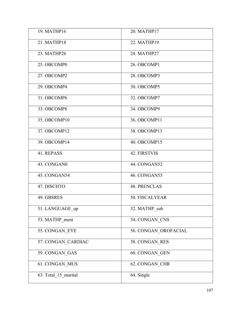
107

19. MATHP16 20. MATHP17

21. MATHP18 22. MATHP19

23. MATHP26 24. MATHP27

25. OBCOMP0 26. OBCOMP1

27. OBCOMP2 28. OBCOMP3

29. OBCOMP4 30. OBCOMP5

31. OBCOMP6 32. OBCOMP7

33. OBCOMP8 34. OBCOMP9

35. OBCOMP10 36. OBCOMP11

37. OBCOMP12 38. OBCOMP13

39. OBCOMP14 40. OBCOMP15

41. REPASS 42. FIRSTVIS

43. CONGAN0 44. CONGAN52

45. CONGAN54 46. CONGAN55

47. DISCHTO 48. PRENCLAS

49. GBSRES 50. FISCALYEAR

51. LANGUAGE_up 52. MATHP_sub

53. MATHP_ment 54. CONGAN_CNS

55. CONGAN_EYE 56. CONGAN_OROFACIAL

57. CONGAN_CARDIAC 58. CONGAN_RES

59. CONGAN_GAS 60. CONGAN_GEN

61. CONGAN_MUS 62. CONGAN_CHR

63. Total_15_marital 64. Single

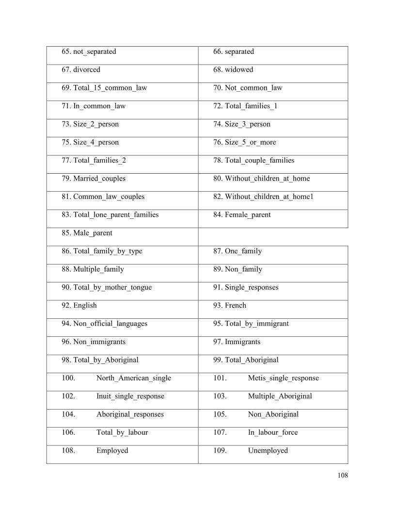
108

65. not_separated 66. separated

67. divorced 68. widowed

69. Total_15_common_law 70. Not_common_law

71. In_common_law 72. Total_families_1

73. Size_2_person 74. Size_3_person

75. Size_4_person 76. Size_5_or_more

77. Total_families_2 78. Total_couple_families

79. Married_couples 80. Without_children_at_home

81. Common_law_couples 82. Without_children_at_home1

83. Total_lone_parent_families 84. Female_parent

85. Male_parent

86. Total_family_by_type 87. One_family

88. Multiple_family 89. Non_family

90. Total_by_mother_tongue 91. Single_responses

92. English 93. French

94. Non_official_languages 95. Total_by_immigrant

96. Non_immigrants 97. Immigrants

98. Total_by_Aboriginal 99. Total_Aboriginal

100. North_American_single 101. Metis_single_response

102. Inuit_single_response 103. Multiple_Aboriginal

104. Aboriginal_responses 105. Non_Aboriginal

106. Total_by_labour 107. In_labour_force

108. Employed 109. Unemployed

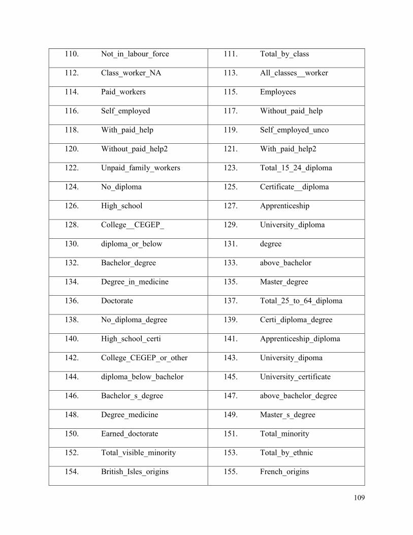
109

110. Not_in_labour_force 111. Total_by_class

112. Class_worker_NA 113. All_classes__worker

114. Paid_workers 115. Employees

116. Self_employed 117. Without_paid_help

118. With_paid_help 119. Self_employed_unco

120. Without_paid_help2 121. With_paid_help2

122. Unpaid_family_workers 123. Total_15_24_diploma

124. No_diploma 125. Certificate__diploma

126. High_school 127. Apprenticeship

128. College__CEGEP_ 129. University_diploma

130. diploma_or_below 131. degree

132. Bachelor_degree 133. above_bachelor

134. Degree_in_medicine 135. Master_degree

136. Doctorate 137. Total_25_to_64_diploma

138. No_diploma_degree 139. Certi_diploma_degree

140. High_school_certi 141. Apprenticeship_diploma

142. College_CEGEP_or_other 143. University_dipoma

144. diploma_below_bachelor 145. University_certificate

146. Bachelor_s_degree 147. above_bachelor_degree

148. Degree_medicine 149. Master_s_degree

150. Earned_doctorate 151. Total_minority

152. Total_visible_minority 153. Total_by_ethnic

154. British_Isles_origins 155. French_origins

110

156. Aboriginal_origins 157. Other_American_origins

158. Caribbean_origins 159. Latin_Central

160. European_origins 161. African_origins

162. Arab_origins 163. West_Asian_origins

164. South_Asian_origins 165. East_Asian_origins

166. Oceania_origins 167. Family_income_2005

168. Under_10_000 169. IN_10_000_to_19_999

170. IN_20_000_to_29_999 171. IN_30_000_to_39_999

172. IN_40_000_to_49_999 173. IN_50_000_to_59_999

174. IN_60_000_to_69_999 175. IN_70_000_to_79_999

176. IN_80_000_to_89_999 177. IN_90_000_to_99_999

178. IN_100_000_and_over 179. Median_family_income

180. Average_family_income 181. Std_of_average_family

182. Average_value_of_dwelling 183. OUTCOME

PRAMS Parous Features

1. ID 2. B_ORDER

3. CIG_1TRI 4. CIG_2TRI

5. CIG_3TRI 6. CIG_PRIOR

7. DEFECT 8. FRACE_AMI

9. FRACE_ASN_NAPHSIS 10. FRACE_BLK

111

11. FRACE_CHN 12. FRACE_FLP

13. FRACE_JPN 14. FRACE_NHW

15. FRACE_WHT 16. HISP_BC

17. INFER_TR 18. KESSNER

19. LGA 20. MACROSOMIA

21. MARRIED 22. MAT_AGE_NAPHSIS

23. MAT_ED 24. MAT_RACE

25. MAT_TRAN 26. MAT_WIC

27. MM_DIAB 28. MM_FEVER

29. MM_HBP 30. MM_LMP

31. MM_NOMD 32. MM_PCV

33. MM_PROM 34. MOMCIG

35. MOMLBS 36. MOMSMOKE

37. MRACE_AMI 38. MRACE_ASN_NAPHSIS

39. MRACE_BLK 40. MRACE_CHN

41. MRACE_FLP 42. MRACE_JPN

43. MRACE_NHW 44. MRACE_OTH

45. MRACE_WHT 46. OTH_TERM

47. PAT_ED 48. PAY

49. PLURAL 50. PNC_MTH

51. PNC_VST_NAPHSI.S 52. PRE_LB_NAPHSIS

53. P_PRTERM 54. SEX

55. SGA_10 56. SGA_2SD

112

57. YY4_LMP 58. YY4_PCV

59. YY_LMP 60. HISPANIC

61. URB_RUR 62. BC_YRLLB

63. DRK63B_A 64. DRK63L_A

65. DRK6C_PG 66. INCOME5

67. MOM_BMI 68. MOM_BMIG

69. MOM_HT_I 70. MOM_WT

71. PNCNO 72. PNC_1TRM

73. PNC_WKS 74. PP_NUMB

75. PREGHX 76. SMK6C_PG

77. SMK6C_PP 78. STRS_TT3

79. STRS_T_G 80. SURE_WKS

81. OUTCOME

PRAMS Nulliparous Features

1. ID 2. CIG_1TRI

3. CIG_2TRI 4. CIG_3TRI

5. CIG_PRIOR 6. DEFECT

7. FRACE_AMI 8. FRACE_ASN_NAPHSIS

9. FRACE_BLK 10. FRACE_CHN

11. FRACE_FLP 12. FRACE_JPN

113

13. FRACE_NHW 14. FRACE_WHT

15. HISP_BC 16. INFER_TR

17. KESSNER 18. LGA

19. MACROSOMIA 20. MARRIED

21. MAT_AGE_NAPHSIS 22. MAT_ED

23. MAT_RACE 24. MAT_TRAN

25. MAT_WIC 26. MM_DIAB

27. MM_FEVER 28. MM_HBP

29. MM_LMP 30. MM_NOMD

31. MM_PCV 32. MM_PROM

33. MOMCIG 34. MOMLBS

35. MOMSMOKE 36. MRACE_AMI

37. MRACE_ASN_NAPHSIS 38. MRACE_BLK

39. MRACE_CHN 40. MRACE_FLP

41. MRACE_JPN 42. MRACE_NHW

43. MRACE_OTH 44. MRACE_WHT

45. PAT_ED 46. PAY

47. PLURAL 48. PNC_MTH

49. PNC_VST_NAPHSI.S 50. SEX

51. SGA_10 52. SGA_2SD

53. YY4_LMP 54. YY4_PCV

55. YY_LMP 56. HISPANIC

57. URB_RUR 58. DRK63B_A

114

59. DRK63L_A 60. DRK6C_PG

61. INCOME5 62. MOM_BMI

63. MOM_BMIG 64. MOM_HT_I

65. MOM_WT 66. POB

67. PNCNO 68. PNC_1TRM

69. PNC_WKS 70. PP_NUMB

71. SMK6C_PG 72. SMK6C_PP

73. STRS_TT3 74. STRS_T_G

75. SURE_WKS 76. OUTCOME

Appendix C- Description of ANN Final Network Parameters

BORN Parous Method

FANN_FLO_2.1

num_layers=3

learning_rate=0.100000

connection_rate=0.100000

network_type=0

learning_momentum=0.000000

training_algorithm=3

train_error_function=0

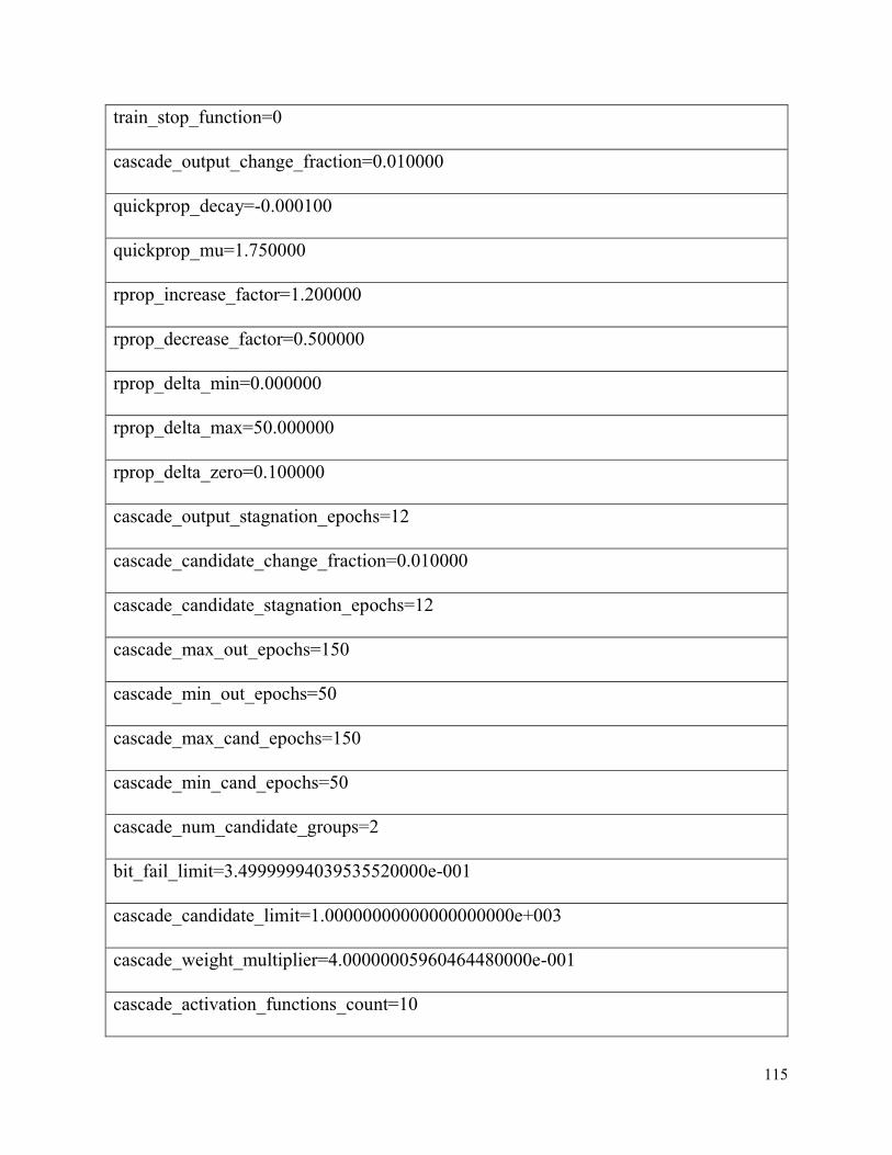
115

train_stop_function=0

cascade_output_change_fraction=0.010000

quickprop_decay=-0.000100

quickprop_mu=1.750000

rprop_increase_factor=1.200000

rprop_decrease_factor=0.500000

rprop_delta_min=0.000000

rprop_delta_max=50.000000

rprop_delta_zero=0.100000

cascade_output_stagnation_epochs=12

cascade_candidate_change_fraction=0.010000

cascade_candidate_stagnation_epochs=12

cascade_max_out_epochs=150

cascade_min_out_epochs=50

cascade_max_cand_epochs=150

cascade_min_cand_epochs=50

cascade_num_candidate_groups=2

bit_fail_limit=3.49999994039535520000e-001

cascade_candidate_limit=1.00000000000000000000e+003

cascade_weight_multiplier=4.00000005960464480000e-001

cascade_activation_functions_count=10

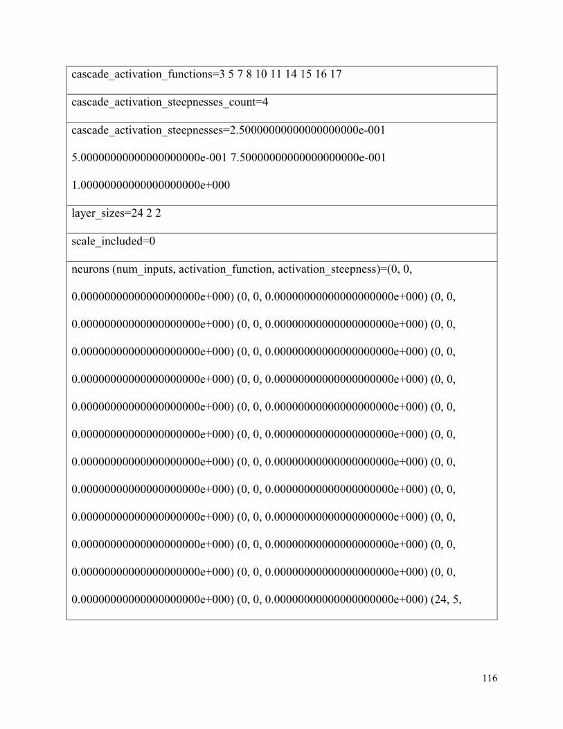
116

cascade_activation_functions=3 5 7 8 10 11 14 15 16 17

cascade_activation_steepnesses_count=4

cascade_activation_steepnesses=2.50000000000000000000e-001

5.00000000000000000000e-001 7.50000000000000000000e-001

1.00000000000000000000e+000

layer_sizes=24 2 2

scale_included=0

neurons (num_inputs, activation_function, activation_steepness)=(0, 0,

0.00000000000000000000e+000) (0, 0, 0.00000000000000000000e+000) (0, 0,

0.00000000000000000000e+000) (0, 0, 0.00000000000000000000e+000) (0, 0,

0.00000000000000000000e+000) (0, 0, 0.00000000000000000000e+000) (0, 0,

0.00000000000000000000e+000) (0, 0, 0.00000000000000000000e+000) (0, 0,

0.00000000000000000000e+000) (0, 0, 0.00000000000000000000e+000) (0, 0,

0.00000000000000000000e+000) (0, 0, 0.00000000000000000000e+000) (0, 0,

0.00000000000000000000e+000) (0, 0, 0.00000000000000000000e+000) (0, 0,

0.00000000000000000000e+000) (0, 0, 0.00000000000000000000e+000) (0, 0,

0.00000000000000000000e+000) (0, 0, 0.00000000000000000000e+000) (0, 0,

0.00000000000000000000e+000) (0, 0, 0.00000000000000000000e+000) (0, 0,

0.00000000000000000000e+000) (0, 0, 0.00000000000000000000e+000) (0, 0,

0.00000000000000000000e+000) (0, 0, 0.00000000000000000000e+000) (24, 5,

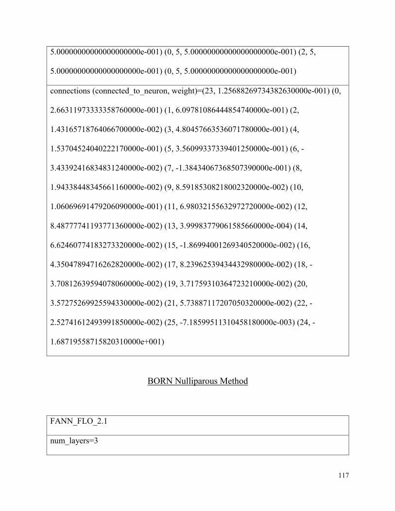
117

5.00000000000000000000e-001) (0, 5, 5.00000000000000000000e-001) (2, 5,

5.00000000000000000000e-001) (0, 5, 5.00000000000000000000e-001)

connections (connected_to_neuron, weight)=(23, 1.25688269734382630000e-001) (0,

2.66311973333358760000e-001) (1, 6.09781086444854740000e-001) (2,

1.43165718764066700000e-002) (3, 4.80457663536071780000e-001) (4,

1.53704524040222170000e-001) (5, 3.56099337339401250000e-001) (6, -

3.43392416834831240000e-002) (7, -1.38434067368507390000e-001) (8,

1.94338448345661160000e-002) (9, 8.59185308218002320000e-002) (10,

1.06069691479206090000e-001) (11, 6.98032155632972720000e-002) (12,

8.48777741193771360000e-002) (13, 3.99983779061585660000e-004) (14,

6.62460774183273320000e-002) (15, -1.86994001269340520000e-002) (16,

4.35047894716262820000e-002) (17, 8.23962539434432980000e-002) (18, -

3.70812639594078060000e-002) (19, 3.71759310364723210000e-002) (20,

3.57275269925594330000e-002) (21, 5.73887117207050320000e-002) (22, -

2.52741612493991850000e-002) (25, -7.18599511310458180000e-003) (24, -

1.68719558715820310000e+001)

BORN Nulliparous Method

FANN_FLO_2.1

num_layers=3

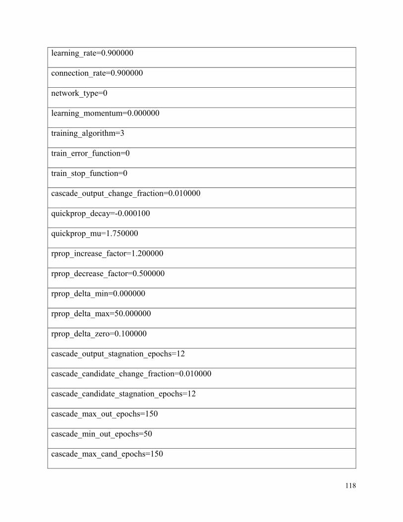
118

learning_rate=0.900000

connection_rate=0.900000

network_type=0

learning_momentum=0.000000

training_algorithm=3

train_error_function=0

train_stop_function=0

cascade_output_change_fraction=0.010000

quickprop_decay=-0.000100

quickprop_mu=1.750000

rprop_increase_factor=1.200000

rprop_decrease_factor=0.500000

rprop_delta_min=0.000000

rprop_delta_max=50.000000

rprop_delta_zero=0.100000

cascade_output_stagnation_epochs=12

cascade_candidate_change_fraction=0.010000

cascade_candidate_stagnation_epochs=12

cascade_max_out_epochs=150

cascade_min_out_epochs=50

cascade_max_cand_epochs=150

119

cascade_min_cand_epochs=50

cascade_num_candidate_groups=2

bit_fail_limit=3.49999994039535520000e-001

cascade_candidate_limit=1.00000000000000000000e+003

cascade_weight_multiplier=4.00000005960464480000e-001

cascade_activation_functions_count=10

cascade_activation_functions=3 5 7 8 10 11 14 15 16 17

cascade_activation_steepnesses_count=4

cascade_activation_steepnesses=2.50000000000000000000e-001

5.00000000000000000000e-001 7.50000000000000000000e-001

1.00000000000000000000e+000

layer_sizes=22 2 2

scale_included=0

neurons (num_inputs, activation_function, activation_steepness)=(0, 0,

0.00000000000000000000e+000) (0, 0, 0.00000000000000000000e+000) (0, 0,

0.00000000000000000000e+000) (0, 0, 0.00000000000000000000e+000) (0, 0,

0.00000000000000000000e+000) (0, 0, 0.00000000000000000000e+000) (0, 0,

0.00000000000000000000e+000) (0, 0, 0.00000000000000000000e+000) (0, 0,

0.00000000000000000000e+000) (0, 0, 0.00000000000000000000e+000) (0, 0,

0.00000000000000000000e+000) (0, 0, 0.00000000000000000000e+000) (0, 0,

0.00000000000000000000e+000) (0, 0, 0.00000000000000000000e+000) (0, 0,

120

0.00000000000000000000e+000) (0, 0, 0.00000000000000000000e+000) (0, 0,

0.00000000000000000000e+000) (0, 0, 0.00000000000000000000e+000) (0, 0,

0.00000000000000000000e+000) (0, 0, 0.00000000000000000000e+000) (0, 0,

0.00000000000000000000e+000) (0, 0, 0.00000000000000000000e+000) (22, 13,

1.00000001490116120000e-001) (0, 13, 1.00000001490116120000e-001) (2, 13,

1.00000001490116120000e-001) (0, 13, 1.00000001490116120000e-001)

connections (connected_to_neuron, weight)=(21, -2.67026305198669430000e-001) (0,

-8.52863311767578130000e-001) (1, -1.68956208229064940000e+000) (2, -

5.95090351998806000000e-002) (3, -1.32812857627868650000e+000) (4, -

5.02927422523498540000e-001) (5, -1.13625288009643550000e+000) (6,

1.10775783658027650000e-001) (7, 3.71086090803146360000e-001) (8, -

7.68902972340583800000e-002) (9, -2.61429905891418460000e-001) (10, -

3.40900719165802000000e-001) (11, -2.45855316519737240000e-001) (12, -

3.01536351442337040000e-001) (13, -1.50970257818698880000e-002) (14, -

1.59091368317604060000e-001) (15, -2.95506596565246580000e-001) (16,

8.50619897246360780000e-002) (17, -1.35745197534561160000e-001) (18, -

9.54492390155792240000e-002) (19, -1.71354278922080990000e-001) (20,

7.79731199145317080000e-002) (23, -4.08418588340282440000e-002) (22,

9.58872451782226560000e+001)

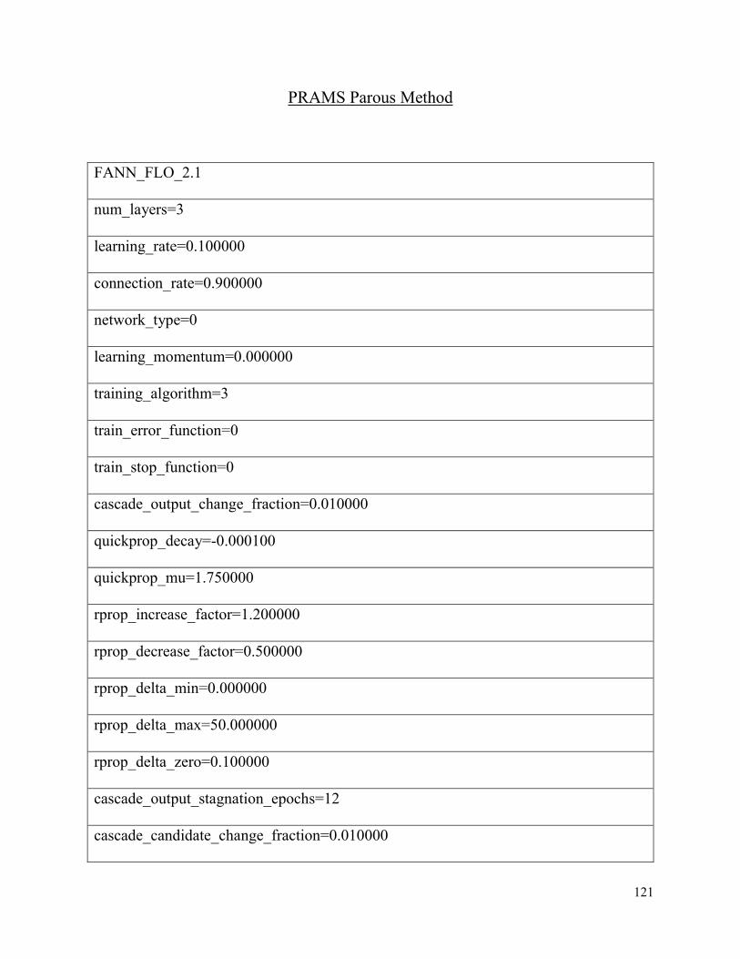
121

PRAMS Parous Method

FANN_FLO_2.1

num_layers=3

learning_rate=0.100000

connection_rate=0.900000

network_type=0

learning_momentum=0.000000

training_algorithm=3

train_error_function=0

train_stop_function=0

cascade_output_change_fraction=0.010000

quickprop_decay=-0.000100

quickprop_mu=1.750000

rprop_increase_factor=1.200000

rprop_decrease_factor=0.500000

rprop_delta_min=0.000000

rprop_delta_max=50.000000

rprop_delta_zero=0.100000

cascade_output_stagnation_epochs=12

cascade_candidate_change_fraction=0.010000

122

cascade_candidate_stagnation_epochs=12

cascade_max_out_epochs=150

cascade_min_out_epochs=50

cascade_max_cand_epochs=150

cascade_min_cand_epochs=50

cascade_num_candidate_groups=2

bit_fail_limit=3.49999994039535520000e-001

cascade_candidate_limit=1.00000000000000000000e+003

cascade_weight_multiplier=4.00000005960464480000e-001

cascade_activation_functions_count=10

cascade_activation_functions=3 5 7 8 10 11 14 15 16 17

cascade_activation_steepnesses_count=4

cascade_activation_steepnesses=2.50000000000000000000e-001

5.00000000000000000000e-001 7.50000000000000000000e-001

1.00000000000000000000e+000

layer_sizes=22 2 2

scale_included=0

neurons (num_inputs, activation_function, activation_steepness)=(0, 0,

0.00000000000000000000e+000) (0, 0, 0.00000000000000000000e+000) (0, 0,

0.00000000000000000000e+000) (0, 0, 0.00000000000000000000e+000) (0, 0,

0.00000000000000000000e+000) (0, 0, 0.00000000000000000000e+000) (0, 0,

123

0.00000000000000000000e+000) (0, 0, 0.00000000000000000000e+000) (0, 0,

0.00000000000000000000e+000) (0, 0, 0.00000000000000000000e+000) (0, 0,

0.00000000000000000000e+000) (0, 0, 0.00000000000000000000e+000) (0, 0,

0.00000000000000000000e+000) (0, 0, 0.00000000000000000000e+000) (0, 0,

0.00000000000000000000e+000) (0, 0, 0.00000000000000000000e+000) (0, 0,

0.00000000000000000000e+000) (0, 0, 0.00000000000000000000e+000) (0, 0,

0.00000000000000000000e+000) (0, 0, 0.00000000000000000000e+000) (0, 0,

0.00000000000000000000e+000) (0, 0, 0.00000000000000000000e+000) (22, 13,

5.00000000000000000000e-001) (0, 13, 5.00000000000000000000e-001) (2, 13,

5.00000000000000000000e-001) (0, 13, 5.00000000000000000000e-001)

connections (connected_to_neuron, weight)=(21, -4.81621362268924710000e-003) (0,

-3.77618372440338130000e-001) (1, 2.71326005458831790000e-001) (2,

2.01477393507957460000e-001) (3, 3.89230191707611080000e-001) (4,

1.80385738611221310000e-001) (5, 1.81966885924339290000e-001) (6, -

6.72936737537384030000e-002) (7, 6.26910030841827390000e-002) (8, -

1.07730038464069370000e-001) (9, -2.16764673590660100000e-001) (10, -

2.86051910370588300000e-002) (11, -1.92716140300035480000e-002) (12, -

3.67171764373779300000e-002) (13, 8.91868695616722110000e-002) (14,

6.25061318278312680000e-002) (15, 4.32300828397274020000e-002) (16,

4.19008620083332060000e-002) (17, -4.29477244615554810000e-002) (18,

1.59060545265674590000e-002) (19, 1.50518894195556640000e-001) (20, -

124

9.95577126741409300000e-002) (23, 2.02126815915107730000e-001) (22, -

8.73242187500000000000e+000)

PRAMS Nulliparous Method

FANN_FLO_2.1

num_layers=3

learning_rate=0.100000

connection_rate=0.100000

network_type=0

learning_momentum=0.000000

training_algorithm=3

train_error_function=0

train_stop_function=0

cascade_output_change_fraction=0.010000

quickprop_decay=-0.000100

quickprop_mu=1.750000

rprop_increase_factor=1.200000

rprop_decrease_factor=0.500000

rprop_delta_min=0.000000

125

rprop_delta_max=50.000000

rprop_delta_zero=0.100000

cascade_output_stagnation_epochs=12

cascade_candidate_change_fraction=0.010000

cascade_candidate_stagnation_epochs=12

cascade_max_out_epochs=150

cascade_min_out_epochs=50

cascade_max_cand_epochs=150

cascade_min_cand_epochs=50

cascade_num_candidate_groups=2

bit_fail_limit=3.49999994039535520000e-001

cascade_candidate_limit=1.00000000000000000000e+003

cascade_weight_multiplier=4.00000005960464480000e-001

cascade_activation_functions_count=10

cascade_activation_functions=3 5 7 8 10 11 14 15 16 17

cascade_activation_steepnesses_count=4

cascade_activation_steepnesses=2.50000000000000000000e-001

5.00000000000000000000e-001 7.50000000000000000000e-001

1.00000000000000000000e+000

layer_sizes=20 2 2

scale_included=0

126

neurons (num_inputs, activation_function, activation_steepness)=(0, 0,

0.00000000000000000000e+000) (0, 0, 0.00000000000000000000e+000) (0, 0,

0.00000000000000000000e+000) (0, 0, 0.00000000000000000000e+000) (0, 0,

0.00000000000000000000e+000) (0, 0, 0.00000000000000000000e+000) (0, 0,

0.00000000000000000000e+000) (0, 0, 0.00000000000000000000e+000) (0, 0,

0.00000000000000000000e+000) (0, 0, 0.00000000000000000000e+000) (0, 0,

0.00000000000000000000e+000) (0, 0, 0.00000000000000000000e+000) (0, 0,

0.00000000000000000000e+000) (0, 0, 0.00000000000000000000e+000) (0, 0,

0.00000000000000000000e+000) (0, 0, 0.00000000000000000000e+000) (0, 0,

0.00000000000000000000e+000) (0, 0, 0.00000000000000000000e+000) (0, 0,

0.00000000000000000000e+000) (0, 0, 0.00000000000000000000e+000) (20, 13,

5.00000000000000000000e-001) (0, 13, 5.00000000000000000000e-001) (2, 13,

5.00000000000000000000e-001) (0, 13, 5.00000000000000000000e-001)

connections (connected_to_neuron, weight)=(19, 1.87676306813955310000e-002) (0,

3.46589267253875730000e-001) (1, -2.97859013080596920000e-001) (2, -

3.89916002750396730000e-001) (3, -2.26215943694114690000e-001) (4,

7.55250155925750730000e-002) (5, -1.93298980593681340000e-001) (6,

7.11965858936309810000e-002) (7, -1.62846028804779050000e-001) (8,

8.92773196101188660000e-002) (9, -3.60125824809074400000e-002) (10,

7.41084944456815720000e-003) (11, -7.02089443802833560000e-002) (12,

1.44820913672447200000e-001) (13, 2.34051253646612170000e-002) (14, -

127

7.23048374056816100000e-002) (15, -7.50005841255187990000e-002) (16,

4.46150936186313630000e-002) (17, 8.22790618985891340000e-003) (18, -

2.57767923176288600000e-002) (21, -3.70220951735973360000e-002) (20,

8.20150947570800780000e+000)