Application of Sensitive API-Based Indicators and Numerical Simulation Tools to Advance Hot-Melt Extrusion Process Understanding Dissertation zur Erlangung des Doktorgrades (Dr. rer. nat.) der Mathematisch-Naturwissenschaftlichen Fakultät der Rheinischen Friedrich-Wilhelms-Universität Bonn vorgelegt von Rachel Catherine Evans aus Salt Lake City, Utah, USA Bonn 2019

Welcome message from author
This document is posted to help you gain knowledge. Please leave a comment to let me know what you think about it! Share it to your friends and learn new things together.
Transcript
Application of Sensitive API-Based
Indicators and Numerical Simulation Tools
to Advance Hot-Melt Extrusion Process
Understanding
Dissertation
zur
Erlangung des Doktorgrades (Dr. rer. nat.)
der
Mathematisch-Naturwissenschaftlichen Fakultät
der
Rheinischen Friedrich-Wilhelms-Universität Bonn
vorgelegt von
Rachel Catherine Evans
aus
Salt Lake City, Utah, USA
Bonn 2019
Angefertigt mit Genehmigung der Mathematisch-Naturwissenschaftlichen
Fakultät der Rheinischen Friedrich-Wilhelms-Universität Bonn
Promotionskommission:
Erstgutachter: Prof. Dr. Karl-Gerhard Wagner
Zweitgutachter: Prof. Dr. Alf Lamprecht
Fachnaher Gutachter: Prof. Dr. Gerd Bendas
Fachfremder Gutachter: Prof. Dr. Robert Glaum
Tag der Promotion: 17. Juli 2019
Erscheinungsjahr: 2019
Significant portions of Chapter 4 were previously published in an article entitled “Development and Performance of a Highly Sensitive Model Formulation Based on Torasemide to Enhance Hot-Melt Extrusion Process Understanding and Process Development”, Evans, et.al., AAPS PharmSciTech, 2018. Significant portions of Chapters 2 and 5 were submitted for publication in an article entitled “Holistic QbD Approach for Hot-Melt Extrusion Process Design Space Evaluation: Linking Materials Science, Experimentation and Process Modeling”, Evans, et.al. to the European Journal of Pharmaceutics and Biopharmaceutics.
Acknowledgements
I would first like to thank Prof. Dr. Karl G. Wagner for both his scientific advice as well
as for his carefully considered and unwavering support and guidance throughout the
supervision of my PhD thesis. From the AbbVie side, I would like to thank Dr. Samuel
Kyeremateng and Andreas Gryczke for their scientific mentorship, enthusiastically
sharing their knowledge and expertise and for always being available for technical
discussions. Also invaluable, I would like to thank Esther Bochmann for generously
sharing her knowledge and expertise in melt rheology and for being an eager and
engaging research partner.
I would also like to acknowledge and thank many AbbVie colleagues for helpful and
productive conversations over the last few years. I greatly appreciate the early input
and advice from Dr. Jörg Rosenberg and Dr. Geoff Zhang which shaped my
approach to the research, especially in the selection of model compounds and
polymers. Mirko Pauli, Constanze Schmidt and Norbert Steiger introduced me to
small-scale extrusion and formulation considerations and were helpful discussion
partners throughout. Ute Lander generously taught me large-scale extrusion and was
a vital partner during the last stage of experiments. Thomas Keßler was always
available to discuss the complexities of hot-melt extrusion, advising extruder and
screw configuration design, and pointing out aspects of my results that would be
interesting for further study. I greatly enjoyed productive discussions with Dr. Kristin
Lehmkemper about extrusion theory and collaborating with her on the sensitivity
analysis, especially the impact of material properties. Both Dr. Mario Hirth and Dr.
Frank Theil helped me to reason through various aspects of the research and to, on
occasion, keep me grounded.
I very much appreciate the experimental assistance and support of Teresa
Dagenbach, Amelie Wirth, Max Frentzel and Alex Castillo with material property
analysis and sample characterization. For their analytical expertise and advice, I
would like to recognize and thank David Geßner, Stefan Weber, Karlheinz Rauwolf,
Dirk Remmler, Dr. Benjamin-Luca Keller and Dr. Christian Schley. I would also like to
thank Ines Mittenzwei, Michael Preiß, Michael Gali and Jannik Mohr for their
experimental assistance with large-scale extrusion.

Support for my PhD research would not have been possible without the initiation of
the collaboration between AbbVie and the University of Bonn by Dr. Martin Bultmann,
Dr. Matthias Degenhardt and Dr. Gunther Berndl. In addition, I greatly appreciate my
AbbVie managers, Dr. Lutz Asmus, Dr. Matthias Degenhardt, Dr. Mike Hoffman and
Andreas Gryczke, for supporting my research activities while also arranging my part-
time AbbVie responsibilities so that I could both focus on the scientific aspects of
research while still contributing to AbbVie’s business objectives. I would especially
like to thank Andreas Gryczke for supporting my goal in the last year and aligning my
AbbVie and PhD work around one topic; both mutually benefitted from this.
Experimental facilities and infrastructure support and were provided by AbbVie, NCE-
Formulation Sciences and Maintenance and Engineering departments, and particular
thanks go to the teams of mechanics and electricians and Zija Islamovic for pilot-
plant equipment setup and cleanup. Special thanks go to Roger Kubitschek and Ralf
Heilmann, as well as Rainer van Deursen from Schneider Electric / Eurotherm, for
prioritization and realization of extruder upgrades.
From Sciences Computers Consultants, I wish to thank the entire team for training,
support, helpful discussions and upgrades to the Ludovic® software, especially Batch
Mode.
I would also like to thank Chrissi Lekić, Dr. Sheetal Pai-Wechsung, Esther
Bochmann, Dr. Ariana Low, Karola Rau, Dijana Trajkovic and Ekaterina Sobich for
friendships begun in Germany, in particular for frequent chats, sometimes daily and
sometimes after hours. I also wish to thank my parents, brother, sister-in-law and
nieces, and long-time friends Dr. Nihan Yönet-Tanyeri, Kate Ferrario, Dan Ferrario,
Dr. Noelle Patno, Dr. Dorothea Sauer, Millán Díaz-Aguado and Mihaela Iordanova for
their moral support from across the ocean.
I wish to express tremendous gratitude to Ingrid Hölig and her family for welcoming
me and a very special little dog named Cherry into their lives and making us feel at
home in Wächtersbach. And last but definitely not least, I would like to thank my dear
Peter for sharing the best of his homeland, keeping me culturally entertained as well
as physically fit with hikes and bike trips to visit our favorite fields of wild flowers.

For my friends and family, both near and far
The highest reward for a person’s toil is not what they get for it,
but what they become by it.
John Ruskin
I
TABLE OF CONTENTS
NOMENCLATURE .................................................................................................... IV
Symbols ............................................................................................................... IV
Abbreviations ....................................................................................................... VI
1 INTRODUCTION ................................................................................................... 1
2 THEORETICAL BACKGROUND .......................................................................... 5
2.1 Application of the Materials Science Tetrahedron to HME ............................. 5
2.2 Process Parameters ....................................................................................... 6
2.3 Material Properties ......................................................................................... 8
2.4 Process Performance ................................................................................... 12
2.4.1 Melt Temperature and Melt Viscosity ..................................................... 12
2.4.2 Residence Time Distribution .................................................................. 13
2.4.3 Mechanical Energy Input ....................................................................... 13
2.4.4 Conducted Energy Input ........................................................................ 15
2.4.5 Measures of Fill ..................................................................................... 15
2.4.6 Critical Quality Attributes ....................................................................... 16
2.5 Process Modeling and Simulation ................................................................ 18
3 AIMS AND SCOPE OF WORK ........................................................................... 20
4 DEVELOPMENT AND PERFORMANCE OF A HIGHLY SENSITIVE MODEL
FORMULATION BASED ON TORASEMIDE TO ENHANCE HOT-MELT
EXTRUSION PROCESS UNDERSTANDING AND PROCESS DEVELOPMENT ... 21
4.1 Introduction .................................................................................................. 21
4.2 Aims of Work ................................................................................................ 22
4.3 Experiment Design ....................................................................................... 23
4.4 Results ......................................................................................................... 25
4.4.1 Thermal Characterization of Torasemide and Physical Mixtures ........... 25
4.4.2 Selection of Matrix Composition for Optimal Extrusion Processing Space
and Observation of CQAs.................................................................................... 29
4.4.3 Performance of Torasemide-Based Indicator System with 10 %w/w
PEG 1500 Formulation ........................................................................................ 36
4.4.4 Chemical Composition of Torasemide-Containing Extrudates ............... 40
II
4.4.5 Numerical Simulation and Correlation of CQAs with Dimulation-Derived
Process Characteristic......................................................................................... 42
4.5 Discussion .................................................................................................... 47
4.6 Conclusions .................................................................................................. 52
5 MELT VISCOSITY DESIGN SPACE EVALUATION USING TELMISARTAN AS
A LOW-SOLUBILITY API-IN-POLYMER INDICATOR AND PROCESS MODELING54
5.1 Introduction .................................................................................................. 54
5.2 Aims of Work ................................................................................................ 55
5.3 Experiment Design ....................................................................................... 56
5.4 Results ......................................................................................................... 59
5.4.1 Selection of Model System – Material Properties .................................. 59
5.4.2 Experimental Extrusion – Produce Data to Build and Validate Ludovic®
Model 63
5.4.3 Deeper Insight via Process Modeling .................................................... 65
5.5 Discussion .................................................................................................... 74
5.6 Conclusions .................................................................................................. 82
6 APPLICATION OF TELMISARTAN INDICATOR SYSTEM AND PROCESS
MODELING TO STUDY SCALING OF A QUASI-ADIABATIC PHARMACEUTICAL
HME PROCESS ........................................................................................................ 84
6.1 Introduction .................................................................................................. 84
6.1.1 Simplified Criteria for Assessing Quasi-Adiabatic Processing ............... 86
6.1.2 Twin-Screw Extrusion Scaling Approaches ........................................... 91
6.2 Aims of Work ................................................................................................ 94
6.3 Experiment Design ....................................................................................... 95
6.3.1 Formulation Compositions ..................................................................... 96
6.3.2 Laboratory Experiment Design .............................................................. 96
6.3.3 Simulation Experiment Design ............................................................. 105
6.4 Results & Discussion .................................................................................. 105
6.4.1 Selection of Formulation and Barrel Temperatures for Laboratory
Experiments via Supportive Simulation ............................................................. 105
6.4.2 Process Analysis and Assessment of Energy Balance ........................ 109
6.4.3 Assessment of Scaling via CQA Indicator Substance .......................... 121
III
6.5 Conclusions ................................................................................................ 128
7 MATERIALS AND METHODS .......................................................................... 129
7.1 Materials ..................................................................................................... 129
7.2 Methods ..................................................................................................... 131
7.2.1 Equipment and Software ..................................................................... 131
7.2.2 Sample Preparation ............................................................................. 132
7.2.3 Process Characterization ..................................................................... 138
7.2.4 Analytical Sample Preparation ............................................................. 139
7.2.5 Sample Characterization/Analysis ....................................................... 139
7.2.6 Process Simulation .............................................................................. 146
8 SUMMARY AND OUTLOOK ............................................................................ 159
9 PUBLICATIONS ............................................................................................... 164
10 APPENDIX ................................................................................................... 165
10.1 Mass Spectrometry Characterization for Torasemide Study ................... 165
10.2 Determination of Telmisartan Degradation.............................................. 167
10.2.1 Sample Preparation ............................................................................. 167
10.2.2 HPLC Analysis ..................................................................................... 167
10.2.3 Results ................................................................................................. 168
11 REFERENCES ............................................................................................. 169
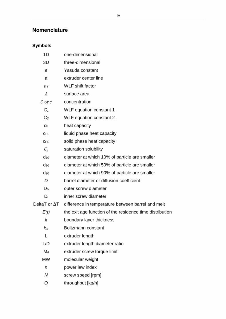
IV
Nomenclature
Symbols
1D one-dimensional
3D three-dimensional
a Yasuda constant
a extruder center line
aT WLF shift factor
𝐴 surface area
𝐶 or 𝑐 concentration
C1 WLF equation constant 1
C2 WLF equation constant 2
cP heat capacity
cPL liquid phase heat capacity
cPS solid phase heat capacity
𝐶𝑠 saturation solubility
d10 diameter at which 10% of particle are smaller
d50 diameter at which 50% of particle are smaller
d90 diameter at which 90% of particle are smaller
D barrel diameter or diffusion coefficient
Do outer screw diameter
Di inner screw diameter
DeltaT or ΔT difference in temperature between barrel and melt
E(t) the exit age function of the residence time distribution
ℎ boundary layer thickness
𝑘𝐵 Boltzmann constant
L extruder length
L/D extruder length:diameter ratio
Md extruder screw torque limit
MW molecular weight
n power law index
N screw speed [rpm]
Q throughput [kg/h]
V
r radius
t time
t > 115 °C time that melt temperature is greater than 115 °C
T temperature
Td degradation onset temperature
Tg glass transition temperature
Tm melting temperature
Tmax maximum simulated melt temperature, typically at end of 2nd BW
kneading block
ΔTmax Tmax at high screw speed minus Tmax at low screw speed
Tp processing temperature (melt temperature, not barrel)
Ts solubility temperature
T0 reference temperature
𝑉 volume
Vfree extruder free volume [dm3]
�̇� shear rate
�̇�𝐶 shear rate in the screw channel
�̇�𝑂 shear rate in the overflight region
𝛿𝐶 channel depth
𝛿𝐶𝐿 screw clearance (or leakage)
𝜂 shear melt viscosity
𝜂0 zero-shear rate viscosity
𝜂∞ infinite-shear rate viscosity
𝜂𝑇 shear viscosity at extrapolated temperature
|η*| complex viscosity
𝜆 characteristic time
𝜆𝑇 characteristic time at extrapolated temperature
𝜆0 characteristic time at reference temperature
𝜏 torque [N∙m] or shear stress [Pa]
𝜏𝐹 filled torque (when process is running) [N∙m]
𝜏𝐸 empty torque (but screws turning) [N∙m]
VI
Abbreviations
API active pharmaceutical ingredient
ASD amorphous solid dispersion
BW backward
COP copovidone
CQA critical quality attribute
C-Y Carreau-Yasuda (equation)
DoE design of experiments
DPD dipyridamole
DSC dynamic scanning calorimetry
f(t) function of time
FW forward
f(x) function of position
HME hot-melt extrusion
HPLC high-performance liquid chromatography
HPLC-MS high-performance liquid chromatography – mass spectrometry
HSS high screw speed
IR infrared
KB kneading block
LCE local conducted energy
LOD loss-on-drying
LSS low screw speed
MRT mean residence time
MST materials science tetrahedron
NoR average number of revolutions experienced by a unit of material
PA% peak area percent
PAT process analytical technology
PEG polyethylene glycol
PID proportional–integral–derivative control
PLM polarized light microscopy
PSD particle size distribution
QbD quality by design
RT retention time
VII
RTD residence time distribution
SA:V surface area to volume ratio
SAOS small angle oscillatory shear
SFL specific feed load
SME specific mechanical energy
SOL Soluplus®
Span® 20 sorbitan monolaurate
TCE total conducted energy
TEC triethyl citrate or thermal exchange coefficient
TEL telmisartan
TGA thermogravimetric analysis
TOR torasemide
TPE total product energy
TSE twin-screw extruder
TW80 Tween® 80 (polysorbate 80)
VSFL volume-specific feed load
WLF Williams-Landel-Ferry (equation)
wt% weight percent
XRPD x-ray powder diffraction
ZSK18 18 mm extruder
ZSK26 26 mm extruder
ZSK40 40 mm extruder
1
1. Introduction and theoretical background
1 Introduction
The process of hot-melt extrusion (HME) in the pharmaceutical industry via a twin-
screw extruder (TSE) was adapted from the plastics industry more than 35 years ago
for the purpose of generating amorphous solid dispersions (ASDs) of poorly water-
soluble active pharmaceutical ingredients (APIs) in polymeric matrices (1–5). It has
since become an established unit operation for more than 10 APIs in commercial
amorphous drug products (6–8). HME is efficient in that TSEs have a relatively small
physical footprint and can potentially be run continuously (9,10). The process is
primarily performed to enhance the bioavailability of poorly-water soluble drug
substances (2,11). By imparting thermal and mechanical energy to material being
processed, the crystalline API is transformed into a high-energy amorphous state,
dissolved or melted and dispersed in the surrounding stabilizing polymer matrix (8).
As a result, the energetic barrier for dissolving into aqueous fluids is overcome.
Over the years, HME using various polymer matrices has been used to produce a
wide range of commercial medicinal products such as oral tablets and has extended
to parenteral implants (3,6,7). It has also been used to show the feasibility of
production of films, granules and pellets (2,5,11). For such a widely-used process as
HME, both in the development of new drug products as well as in the production of
commercial products, it is imperative that pharmaceutical scientists and engineers
possess a solid understanding of the process and its relationship to critical quality
attributes (CQAs) such as degradation and residual crystallinity. Despite many years
and much effort spent to research HME, even at present, there are many gaps in
HME process understanding.
Generally, the process involves a number of inter-related steps which can be
considered sub-unit operations within the extruder barrels (Figure 1.1). Typically a
co-rotating TSE is used for pharmaceutical applications (12). A powder-based
mixture composed of at least API and polymer matrix are fed at constant feed rate
into the TSE onto rotating screws containing at least one section of mixing elements.
Melting or softening of the matrix occurs due to heat rise resulting from conduction
from the barrel housing or by viscous dissipation from the shear imparted by
conveying and mixing screw elements. Ideally, through this mixing and temperature
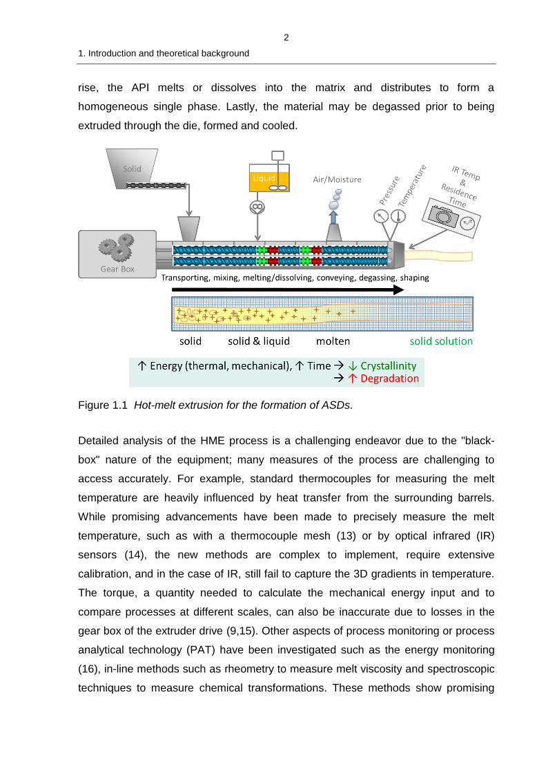
2
1. Introduction and theoretical background
rise, the API melts or dissolves into the matrix and distributes to form a
homogeneous single phase. Lastly, the material may be degassed prior to being
extruded through the die, formed and cooled.
Figure 1.1 Hot-melt extrusion for the formation of ASDs.
Detailed analysis of the HME process is a challenging endeavor due to the "black-
box" nature of the equipment; many measures of the process are challenging to
access accurately. For example, standard thermocouples for measuring the melt
temperature are heavily influenced by heat transfer from the surrounding barrels.
While promising advancements have been made to precisely measure the melt
temperature, such as with a thermocouple mesh (13) or by optical infrared (IR)
sensors (14), the new methods are complex to implement, require extensive
calibration, and in the case of IR, still fail to capture the 3D gradients in temperature.
The torque, a quantity needed to calculate the mechanical energy input and to
compare processes at different scales, can also be inaccurate due to losses in the
gear box of the extruder drive (9,15). Other aspects of process monitoring or process
analytical technology (PAT) have been investigated such as the energy monitoring
(16), in-line methods such as rheometry to measure melt viscosity and spectroscopic
techniques to measure chemical transformations. These methods show promising
3
1. Introduction and theoretical background
results but are not yet routinely implemented in the pharmaceutical industry
(9,10,17,18).
The materials being processed have complex properties and behavior which are both
intrinsic but also dependent upon the process conditions and extent of processing.
Typical matrix polymers used for HME often exhibit non-Newtonian viscoelastic flow
behavior, meaning that the melt viscosity is a function of both temperature and shear
rate. APIs often plasticize the matrix, and additives such as surfactants may also
impact the rheology (19,20). Further, because the purpose of HME is to form a single
phase from multiple discrete starting materials, the structure and therefore properties
of the material inside the extruder evolve along the screw, a type of reactive
extrusion (21).
Although HME can be run continuously, scaling is required at different stages during
product and process development. For example, in early stages or for research or
troubleshooting purposes, small scales may be used, while larger scales are used
when larger quantities of API are available and for commercial production. Despite
approaches to maintain geometric similarity across scales, differences in
performance arise due to the inherent and fundamental difference of the ratio
between barrel surface area and volume and different barrel heating and cooling
designs among vendors, even within scale (22). Many guidelines and
recommendations have been written regarding scaling of pharmaceutical HME (23–
26), but few scholarly investigations have been published studying relevant scaling
approaches or evaluating the success of the approaches.
Process modeling in multiple dimensions, not just 1D but also 3D, can supplement
the lack of accurate experimental data (15). One-dimensional simulation can
compute global mechanical and conducted energy values, residence time distribution
values, local temperature, pressure, melt viscosity, shear stress, residence time and
viscous dissipation (27). Three-dimensional approaches such as computational fluid
dynamics and smoothed particle hydrodynamics can compute gradients in many of
these local values, but high computational burden limits the study of the entire
extruder (28,29). However, a challenge for validating these models exists in the form
of quantitative correlations of the process with critical quality attributes. While residual
4
1. Introduction and theoretical background
crystallinity, for example, can be quantified and correlated, degradation of the API
resulting from excess thermal energy is often negligible or overshadowed by
analytical method error. The reason for this is that most poorly-water soluble APIs are
screened for suitability, primarily thermal stability, long before an API is available in
large enough quantities for a hot-melt extrusion experiment. As a result, and as is
also the case for attempts to understand the process through purely empirical
approaches, there is little way of measuring the success of the process; it has a
certain level of robustness built-in. For these reasons there is a need for correlating
the experimental results with simulated results. One way to address this is through
measurement of the sum total outcome of the process via an indirect method, namely
with a process indicator. The focus of this thesis is the use of both simulation
approaches and the use of APIs as sensitive process indicators to gain deeper
insights into the HME process.
5
2. Theoretical Background
2 Theoretical Background
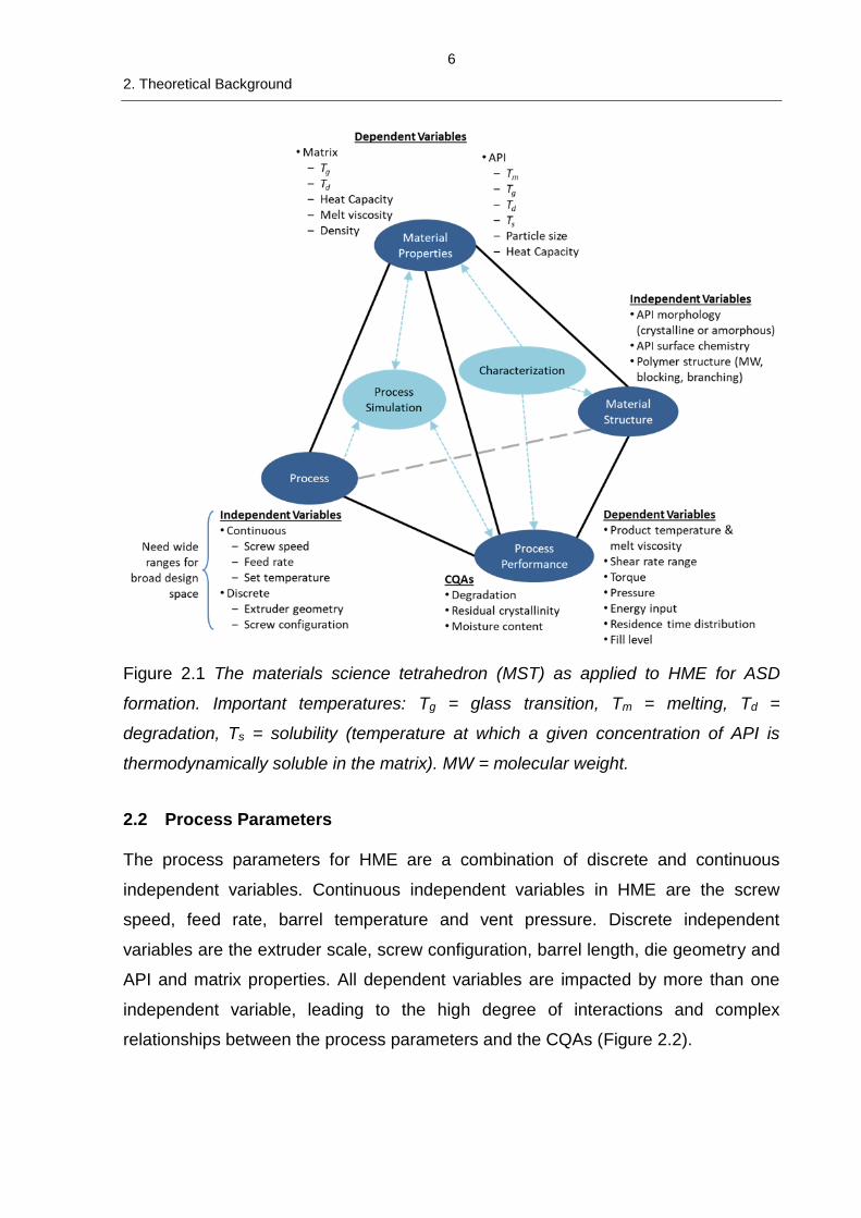
2.1 Application of the Materials Science Tetrahedron to HME
The complex nature of HME and the transformation of the input material through
extrusion can be captured by the application of the materials science tetrahedron
(MST). Its origin and applicability to drug product development was explained with
several examples by Sun, primarily focusing on tablet compression (30). This
concept is interpreted and applied for HME and presented in Figure 2.1. The corners
of the tetrahedron are represented by the material structure, material properties,
process parameters and process performance. Similar to interstitial sites in a crystal
lattice, characterization and process simulation are placed at the core of the
tetrahedron. The value in describing a process using the MST is that all of the inter-
dependent relationships can be holistically described and analyzed.
Inherent to any process, variation of a number of independent and dependent
variables influence the final material produced by the process. In HME, the
independent variables are both continuous and discrete. When an HME process is
analyzed via a design of experiment (DoE), a regression equation describing the
relationship between a given response and the independent variables typically
contains terms with not only main effects but also interactions (31). The existence of
these interactions suggests that the more important factors in the process may be
dependent variables. Process performance responses are typically defined by the
critical quality attributes, the most important of which for HME are the residual
crystallinity and degradation as they determine the amount and form of solubilized
API available to contribute to enhanced bio-performance. Other important CQAs also
include assay and uniformity, as well as moisture content, which is important for
physical and potentially chemical stability of the ASD.
6
2. Theoretical Background
Figure 2.1 The materials science tetrahedron (MST) as applied to HME for ASD
formation. Important temperatures: Tg = glass transition, Tm = melting, Td =
degradation, Ts = solubility (temperature at which a given concentration of API is
thermodynamically soluble in the matrix). MW = molecular weight.
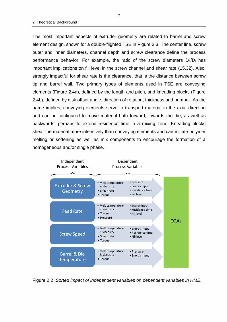
2.2 Process Parameters
The process parameters for HME are a combination of discrete and continuous
independent variables. Continuous independent variables in HME are the screw
speed, feed rate, barrel temperature and vent pressure. Discrete independent
variables are the extruder scale, screw configuration, barrel length, die geometry and
API and matrix properties. All dependent variables are impacted by more than one
independent variable, leading to the high degree of interactions and complex
relationships between the process parameters and the CQAs (Figure 2.2).
7
2. Theoretical Background
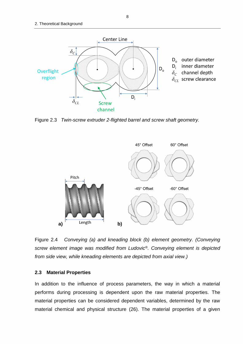
The most important aspects of extruder geometry are related to barrel and screw
element design, shown for a double-flighted TSE in Figure 2.3. The center line, screw
outer and inner diameters, channel depth and screw clearance define the process
performance behavior. For example, the ratio of the screw diameters Do/Di has
important implications on fill level in the screw channel and shear rate (15,32). Also,
strongly impactful for shear rate is the clearance, that is the distance between screw
tip and barrel wall. Two primary types of elements used in TSE are conveying
elements (Figure 2.4a), defined by the length and pitch, and kneading blocks (Figure
2.4b), defined by disk offset angle, direction of rotation, thickness and number. As the
name implies, conveying elements serve to transport material in the axial direction
and can be configured to move material both forward, towards the die, as well as
backwards, perhaps to extend residence time in a mixing zone. Kneading blocks
shear the material more intensively than conveying elements and can initiate polymer
melting or softening as well as mix components to encourage the formation of a
homogeneous and/or single phase.
Figure 2.2 Sorted impact of independent variables on dependent variables in HME.
8
2. Theoretical Background
Figure 2.3 Twin-screw extruder 2-flighted barrel and screw shaft geometry.
a) b)
Figure 2.4 Conveying (a) and kneading block (b) element geometry. (Conveying
screw element image was modified from Ludovic®. Conveying element is depicted
from side view, while kneading elements are depicted from axial view.)
2.3 Material Properties
In addition to the influence of process parameters, the way in which a material
performs during processing is dependent upon the raw material properties. The
material properties can be considered dependent variables, determined by the raw
material chemical and physical structure (26). The material properties of a given
9
2. Theoretical Background
formulation, especially their thermal properties, determine processing behavior and
potentially also the product’s final quality. The appropriate material properties will
enable optimal processing with a broad design space and optimal product quality and
vice versa. Knowledge and understanding of the material properties and their
significance can facilitate working with and not against the natural behavior of the
formulation. For HME, understanding the thermal properties and the role of the matrix
rheological properties is essential to designing and controlling the process and the
resulting product quality. Specifically, some of the most important material properties
are the API particle size, matrix polymer and API glass transition temperatures (Tg),
the API melting and solubility temperatures (Tm and Ts), the API and matrix
degradation temperatures (Td), and the matrix melt viscosity as a function of
temperature and shear rate. Smaller API particle size will increase the dissolution
rate due to greater surface area (33). Characterization of the matrix Tg and melt
viscosity can be used to identify the minimum processing temperature and extruder
torque limitation (34–41). Because the formation of an ASD via HME involves
physical transformation of the raw materials, sometimes considered to be a type of
reactive extrusion (21), the material properties of the product being processed can
change as a function of the position along the length of the extruder. For example, an
API, which is soluble in the polymer matrix and has Tg much lower than that of the
matrix, will plasticize the matrix upon dissolution and mixing (19). This effect will
reduce the melt viscosity and therefore reduce viscous dissipation. However, an API
can also anti-plasticize the matrix if its Tg is higher than that of the matrix, leading to
potentially more viscous dissipation (42).
Any rise in product temperature can result in degradation of the constituent materials,
depending on their degradation temperatures and the respective temperature
realized by the process. This potential for thermal degradation is one of the most
commonly cited concerns in the HME process. It is commonly assumed that HME
cannot be used to process high melting point APIs for the formation of ASDs (43,44).
This assumption leads to the thinking that the product temperature must exceed the
melting point of the crystalline API in order to form an ASD (6,45). For high melting
point APIs, this temperature can exceed the thermal stability of the API or even the
matrix. Further, as a remedy, the common thinking is that a plasticizer should be
10
2. Theoretical Background
added to the formulation to reduce the viscosity and consequently shift the
temperature processing window to lower values, below the degradation temperature
of the thermo-labile species (46,47).
However, this rationale is flawed primarily due to a lack of wide-spread
understanding of the relevant material properties such as the influence of
intermolecular interactions between API and polymer which affect the phase diagram
of the ASD system. An ASD can be produced below the melting point of the pure API
if the solubility temperature for a given drug loading is within an accessible
temperature range (26,48). This temperature may be substantially lower than the
melting point and well within a range in which no degradation occurs. In addition, too
much plasticization and reduction in processing temperature could lead to incomplete
formation of the ASD, aka presence of residually crystalline API in the matrix. In this
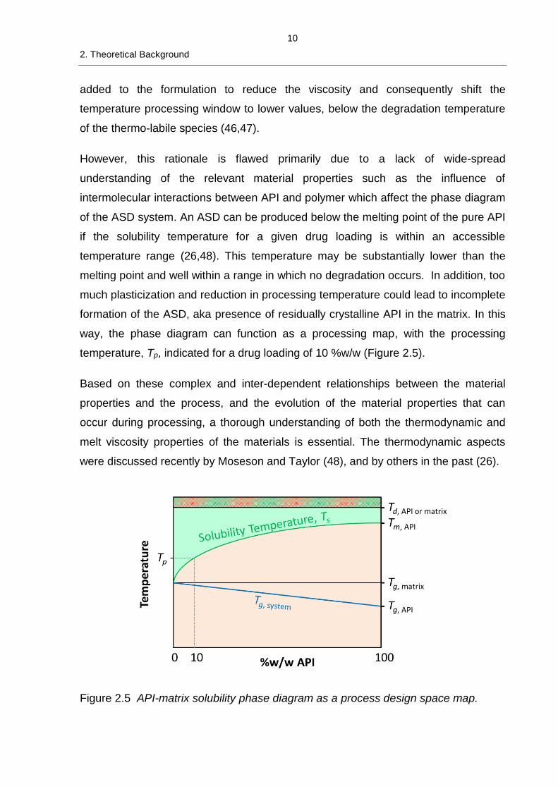
way, the phase diagram can function as a processing map, with the processing
temperature, Tp, indicated for a drug loading of 10 %w/w (Figure 2.5).
Based on these complex and inter-dependent relationships between the material
properties and the process, and the evolution of the material properties that can
occur during processing, a thorough understanding of both the thermodynamic and
melt viscosity properties of the materials is essential. The thermodynamic aspects
were discussed recently by Moseson and Taylor (48), and by others in the past (26).
Figure 2.5 API-matrix solubility phase diagram as a process design space map.
11
2. Theoretical Background
The complex non-Newtonian behavior, specifically the temperature and shear-rate
dependency, can be described by a number of empirical models, for example the
Cross model (49) or, in these studies, the Carreau-Yasuda (C-Y) model (50,51). The
Carreau-Yasuda (C-Y) model in combination with the with temperature dependency
described by the Williams-Landel-Ferry (WLF) equation (52) can account for both
Newtonian and non-Newtonian rheological behavior. The basic form of the C-Y
equation expressing the melt viscosity as a function of shear rate is shown in
equation 2.1:
𝜂 = 𝜂∞ + (𝜂0 − 𝜂∞) ∙ [1 + (𝜆�̇�)𝑎]𝑛−1
𝑎 (2.1)
where η is the viscosity as a function of temperature and shear rate, �̇�, η0 is the melt
viscosity at zero shear rate, η∞ is the melt viscosity at infinite shear rate, λ is the
characteristic time, n is the Power law index and a is the Yasuda constant. The
characteristic time is related to the relaxation behavior of the specimen over time.
Both the zero-shear rate viscosity and the characteristic time are functions of
temperature. If η∞ is assumed zero, the equation simplifies to equation 2.2:
𝜂 = 𝜂0 ∙ [1 + (𝜆�̇�)𝑎]𝑛−1
𝑎 (2.2)
Both the zero-shear rate viscosity, η0, and the characteristic time, λ, are strong
functions of temperature for amorphous pharmaceutical polymers, especially near
the Tg of the polymer, roughly Tg < T < Tg+100 °C (15,52,53). This temperature
dependency can be accounted for by use of the WLF equation, equation 2.3:
log(𝑎𝑇) =−𝐶1 (𝑇−𝑇0)
𝐶2+(𝑇−𝑇0) (2.3)
where aT is a shift factor resulting from time-temperature superposition processing of
rheological data, T is the target temperature, T0 is the reference temperature, and C1
and C2 are constants. Equations 2.4 and 2.5 are used to calculate the melt viscosity
and characteristic time at temperatures other than the reference temperature:
𝑎𝑇 =𝜂𝑇
𝜂0 (2.4)
12
2. Theoretical Background
𝑎𝑇 =𝜆𝑇
𝜆0 (2.5)
where η and λ are the viscosity and characteristic time from the Carreau-Yasuda
equation, and the subscripts T and 0 refer to the desired and reference temperatures,
respectively.
2.4 Process Performance
Process performance can be characterized by two categories of measures of the
process: the dependent variables and the product CQAs. Dependent variables for
HME have been identified as the melt temperature, residence time, energy input, and
fill level (9,54,55). Additional measures of the process not considered to be
dependent variables are the product CQAs, namely degradation, residual crystallinity
and moisture content. These aspects of process performance are discussed in more
detail below, as well as how they are measured or calculated.
2.4.1 Melt Temperature and Melt Viscosity
The temperature of the melt is a measure of the amount of energy input into the
processed material resulting from either conductive heat transfer or mechanical
energy. The most common method to measure the melt temperature is via
thermocouples inserted into the extruder barrel and die. They are flush mounted to
prevent melt flow disruption and, due to insufficient insulation of the thermocouple
junction, the measured values are known to be highly influenced by the barrel itself
and therefore inaccurate (14). An alternative is infrared thermography in which an IR
camera is used to measure the radiation emitted by the melt exiting an extruder die.
The IR intensity is material dependent, characterized by the thermal emissivity, which
itself varies as a function of wavelength and temperature. The emissivity for
polymeric materials can be approximated with a value of 0.9 (56). While the
measurement is limited by the fact that it takes place at the end of the extruder and at
the surface of the melt, and therefore may be influenced by heat loss to the
environment, it has proved to be more informative and relevant than measurements
by thermocouples. This means that IR thermography cannot measure the
temperature of the melt along the screw. Traditional thermocouples can be inserted
into bores placed at any point along the screw, but again, the measurement is highly
13
2. Theoretical Background
influenced by the barrel temperature. As discussed in section 2.3, the material melt
viscosity is a strong function of temperature and will change as the temperature of
the melt changes.
2.4.2 Residence Time Distribution
The residence time distribution (RTD) is a measure of the time a unit of material
spends inside the extruder. It provides valuable information about the degree of axial
mixing and is also an input for reaction kinetics related to dissolution and
degradation. Measurements are performed at steady state with the addition of a low
concentration pulse of tracer substance added to the feed stream. The concentration
of the tracer substance, typically a pigment, is measured or monitored at the extruder
die exit over time. The concentration can be characterized by the exit age distribution
(57) given by equations 2.6 and 2.7:
∫ 𝐸(𝑡)𝑑𝑡∞
0 = 1 (2.6)
𝐸(𝑡) = 𝑐
∫ 𝑐𝑑𝑡∞
0
= 𝑐
∑ 𝑐∆𝑡∞0
(2.7)
where c is the tracer concentration at a given time t and E(t), the exit age function,
has units of 1/s or %.
The mean residence time (MRT), defined as the time that a unit of material which
was added at time t = 0 leaves the process with a 50% probability, can be calculated
by equation 2.8.
𝑡𝑚𝑒𝑎𝑛 =∫ 𝑡𝑐𝑑𝑡
∞0
∫ 𝑐𝑑𝑡∞
0
=∑ 𝑡𝑐∆∞
0 𝑡
∑ 𝑐∆𝑡∞0
(2.8)
2.4.3 Mechanical Energy Input
2.4.3.1 Shear Rate and Shear Stress
The average shear rate in an extruder can be calculated using a simple relationship
considering the extruder geometry, screw geometry and the screw speed (15,58,59).
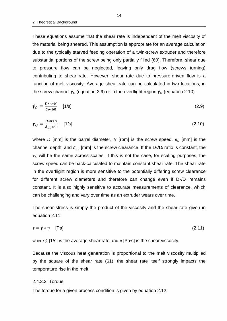
14
2. Theoretical Background
These equations assume that the shear rate is independent of the melt viscosity of
the material being sheared. This assumption is appropriate for an average calculation
due to the typically starved feeding operation of a twin-screw extruder and therefore
substantial portions of the screw being only partially filled (60). Therefore, shear due
to pressure flow can be neglected, leaving only drag flow (screws turning)
contributing to shear rate. However, shear rate due to pressure-driven flow is a
function of melt viscosity. Average shear rate can be calculated in two locations, in
the screw channel �̇�𝐶 (equation 2.9) or in the overflight region �̇�𝑂 (equation 2.10):
�̇�𝐶 =𝐷∗𝜋∗𝑁
𝛿𝐶∗60 [1/s] (2.9)
�̇�𝑂 =𝐷∗𝜋∗𝑁
𝛿𝐶𝐿∗60 [1/s] (2.10)
where D [mm] is the barrel diameter, N [rpm] is the screw speed, 𝛿𝐶 [mm] is the
channel depth, and 𝛿𝐶𝐿 [mm] is the screw clearance. If the Do/Di ratio is constant, the
�̇�𝐶 will be the same across scales. If this is not the case, for scaling purposes, the
screw speed can be back-calculated to maintain constant shear rate. The shear rate
in the overflight region is more sensitive to the potentially differing screw clearance
for different screw diameters and therefore can change even if Do/Di remains
constant. It is also highly sensitive to accurate measurements of clearance, which
can be challenging and vary over time as an extruder wears over time.
The shear stress is simply the product of the viscosity and the shear rate given in
equation 2.11:
𝜏 = �̇� ∗ 𝜂 [Pa] (2.11)
where �̇� [1/s] is the average shear rate and η [Pa∙s] is the shear viscosity.
Because the viscous heat generation is proportional to the melt viscosity multiplied
by the square of the shear rate (61), the shear rate itself strongly impacts the
temperature rise in the melt.
2.4.3.2 Torque
The torque for a given process condition is given by equation 2.12:
15
2. Theoretical Background
𝜏 = 𝜏𝐹 − 𝜏𝐸 [N∙m] (2.12)
where 𝜏𝐹 [N∙m] is the torque reading from the extruder when the process is running
minus 𝜏𝐸 [N∙m] the empty torque, or the torque reading from the extruder when no
material is in the extruder, at the identical screw speed.
2.4.3.3 SME
The specific mechanical energy can be calculated using multiple equations, but the
one selected for use in this thesis is given by equation 2.13 (62):
𝑆𝑀𝐸 = 2∗𝜋∗𝑁∗𝜏
𝑄 [
𝑘𝑊ℎ
𝑘𝑔] (2.13)
where N [rpm] is the screw speed, τ [N∙m] is the torque and Q [kg/h] is the throughput.
2.4.4 Conducted Energy Input
The conducted energy describes the thermal energy that is transferred between the
extruded material and the temperature regulated barrel housing. Conducted energy
can be approximated by measuring the heating and cooling activity occurring in the
various barrel segments in an extruder. The heating and cooling activity is recorded
by logging the occurrence and duration of heating element activity and water valve
opening. Additional aspects of this topic are discussed in Chapter 6.
2.4.5 Measures of Fill
2.4.5.1 Specific Feed Load and Volume Specific Feed Load
The rate of feeding an extruder screw can be calculated and somewhat visualized by
using the equation for the specific feed load, equation 2.14:
𝑆𝐹𝐿 = 𝑄∗1000
𝑁∗60 [
𝑔
𝑟𝑒𝑣] (2.14)
where Q [kg/h] is the throughput and N [rpm] is the screw speed. The SFL can be
normalized by the extruder free volume, known as the volume specific feed load (62),
equation 2.15:
16
2. Theoretical Background
𝑉𝑆𝐹𝐿 =𝑄∗1000
𝑁 ∗60∗ 𝑉𝑓𝑟𝑒𝑒 [
𝑔
𝑟𝑒𝑣∙𝑑𝑚3] (2.15)
where Vfree [dm3] is the extruder free volume not including the die. This equation is
useful for scaling purposes or when the extruder free volume varies within scale.
2.4.5.2 Fill Level
The fill level of the extruder, meaning total amount of material present in the extruder,
neglecting the die, can be estimated by equation 2.16:
𝐹𝑖𝑙𝑙 𝐿𝑒𝑣𝑒𝑙 = 𝑉𝑆𝐹𝐿 ∗ 𝑁𝑜𝑅 =𝑄∗𝑀𝑅𝑇∗1000
3600∗𝑉𝑓𝑟𝑒𝑒 [
𝑔
𝑑𝑚3] (2.16)
where the NoR is the average number of revolutions experienced by a unit of material
and can be estimated by equation 2.17:
𝑁𝑜𝑅 =𝑁∗𝑀𝑅𝑇
60 [𝑟𝑒𝑣] (2.17)
where N [rpm] is the screw speed and MRT [s] is the mean residence time. The
simplified form of the equation for fill level is similar to equations found in the
literature (63,64) and is sometimes normalized by material melt density.
2.4.5.3 Pressure
Pressure is typically measured in the die by a pressure transducer as a safety
mechanism (61). Rise in pressure can be related to high water content, but in
pharmaceutical extrusion, material is often degassed in the barrel segment prior to
the die. In the case of starved-fed extruders in pharmaceutical extrusion, the
pressure rarely exceeds 1 bar and has not been observed to vary as a function of
processing conditions in these studies. Therefore, pressure was not considered to be
an important measure of the process.
2.4.6 Critical Quality Attributes
2.4.6.1 Degradation
Degradation of both the API and the matrix components are undesirable results for
an HME process. Thermal degradation is a primarily concern for the API because
17
2. Theoretical Background
most polymer matrices are thermoplastic in nature and require processing
temperatures to be set above the Tg at which the material will flow, typically with melt
viscosity between 100 to 10,000 Pa∙s (22). Other degradation reactions such as
hydrolysis can also occur during HME processing. Corrective measures to reduce the
melt temperature include reduction of the mechanical energy input, e.g. decreasing
melt viscosity or decreasing screw speed, or reduction of conductive energy from the
barrels, e.g. reducing barrel temperature. However, below a certain barrel
temperature, the melt will be highly viscous, leading to heat generation by viscous
dissipation. The degradation of API can be quantified by chromatographic techniques
such as HPLC.
2.4.6.2 Residual Crystallinity
Residual crystallinity is a measure of the success of the formation of the ASD. It can
be quantified by peak height and/or area in x-ray powder diffraction (XRPD) or by
integration of the melting endotherm in differential scanning calorimetry (DSC), if the
API does not recrystallize upon heating or dissolve before melting. Another aspect of
crystallinity present in an ASD is that of recrystallization but was outside the scope of
this work. It can occur over time or at elevated temperatures and moisture content at
which the molecular mobility within the matrix enables API molecules to reconfigure
and crystallize.
2.4.6.3 Moisture content
The moisture content is an important CQA because it can impact physical stability,
most importantly the presence of crystallinity (65). Often the starting materials contain
moisture or may be somewhat hygroscopic, especially the matrix polymers. The
resulting moisture content can be variable based on heat exposure and vacuum
pressure applied during processing. It can be measured by common loss-on-drying
for a quick readout or by Karl Fischer titration for more accuracy. However, because
the physical stability of the materials was not considered in this thesis, the resulting
moisture content was not measured.
18
2. Theoretical Background
2.5 Process Modeling and Simulation
In addition to building relationships via laboratory experiments, process modeling can
help to establish the relationships within the tetrahedron and provide deeper insight.
Process models take into account the relevant properties of the material being
processed in relation to the process parameters and equipment geometries, even
accounting for evolution of the properties as a function of location in the process and
feeding that back into the computation by way of numerical methods. Upon variation
of any input parameter, process models are particularly useful for the generation of
qualitative estimates and rank ordering, identifying the most influential variables. In
this way, better experiments can be designed upfront, with perhaps a reduced
number of variables to be tested. In addition, a synergistic approach utilizing both
process modeling and relevant experimentation can yield answers to the gaps in
understanding on both sides (66). With a validated model, gaps in experimental data
can be supplemented with simulated data or design spaces can be supported.
However, because not all experimental factors can be modeled, at least not at the
present, quantitative predictions are not always feasible for every scenario. In the
end, the requirements of quality by design (QbD) can be fulfilled by a combination of
experimentation and modeling to rationally select formulation components based on
their material properties to ensure product performance, quality, and even processing
performance.
Process modeling has been applied to twin-screw extrusion through the development
of a number of 1D simulation software programs (27,67–69) and a number of studies
in the polymer and food industries have been reported (15,70–79). However,
scholarly articles applying it to pharmaceutical HME are still limited. Studies with 1-
dimensional simulation of the twin-screw extrusion process have shown agreement
with the main effects of process parameters, that it can be used to optimize screw
configurations during process scaling, as well as provide insight into the energetics of
the process and study and optimize sources of heat generation during scaling
(22,38). More recently, advancements to ease the use of HME simulation in early-
stage formulation development have been made with the development of a model for
ASD melt viscosity based on simpler measurements of the matrix melt viscosity and
the Tg of the ASD (80,81). Other researchers have focused on performing 3D

19
2. Theoretical Background
simulations based on smoothed particle hydrodynamics, reducing them to 1D models
with the goal of applying them to pharmaceutical HME (28,29,82–84). Studies
specifically related to the modeling of pharmaceutical HME include, for example, the
development of a new model of the residence time distribution and the time to
dissolution (85,86).
20
3. Aims and Scope of Work
3 Aims and Scope of Work
The aim of this work was to gain deeper insight into the process of hot-melt extrusion
by use of sensitive indicator substances and process simulation. Specifically, the
work should establish links between material properties, process parameters,
process performance and scaling behavior. Particular emphasis should be placed on
relevant CQAs for the HME process as well as the process energetics.
In order to do this, indicator substances would need to be identified and fit-for-
purpose formulations developed. Ideally, at least in the scope of this work, the
indicator substances should not modify the formulation material properties, e.g. Tg or
melt viscosity, so as to simplify description of the system to the simulation model.
Specifically, two APIs, torasemide and telmisartan, were selected for use as the
indicator substances because it was found that as a function of processing, due to
their physicochemical properties, they could yield measurable and relevant CQA
responses, i.e. degradation and/or residual crystallinity. The formulations were
developed and selected for their processing performance to exhibit the desired
material properties such as processing window or melt viscosity characteristics. The
formulations were not designed to be viable in terms of bioavailability enhancement
or chemical and physical stability. Accordingly, neither the drug release / bio-
performance nor the product stability was analyzed.
In terms of the HME process, in-scope was the study and characterization of the
HME process from extruder inlet to die, including design of the extruder, process and
measurements in-line and at-line. Reasons for this decision were based on 1) the
ASD is formed within the extruder and not after exiting the die and 2) because the
chosen simulation software, Ludovic®, only considers the process in this zone. As a
result, any aspects of the process after the melt exits the die, aside from melt
temperature measurement, or downstream processing were not considered.
Samples were of course cooled quickly and stored in a controlled humidity and
temperature environment so as to preserve their physical and chemical state at die
exit.
21
4. Torasemide-as-Indicator for HME Process Understanding
4 Development and Performance of a Highly Sensitive Model
Formulation Based on Torasemide to Enhance Hot-Melt
Extrusion Process Understanding and Process Development
4.1 Introduction
Process understanding of HME can be defined in several ways, and includes the
knowledge of the design and functional aspects of processing equipment, the impact
of process parameters and process conditions on the final product attributes, material
properties that may impact certain process conditions, accurately scaling the
process, and the value and application of models or simulation tools to optimize a
design space, just to name a few. A recent review discussed the basic impact of
common process parameters and the use of design of experiments to identify critical
formulation and process factors as well as define design spaces, and basic strategies
for scale-up of the HME process (64). However, fully understanding and simulating
the HME process is a challenging task due to the known complexities of the twin-
screw extruder, such as heat-transfer, heat-generation and variable geometry
(32,82).
Nevertheless, generation of an amorphous solid dispersion (ASD) via the process of
HME involves a complex series of inter-related unit operations within one piece of
equipment (1,87,88). The process is further complicated by the dynamic aspect of
the chemical and physical composition of the material being processed. In the case
of pharmaceutical HME, which can be considered a type of reactive extrusion, an
amorphous or semi-crystalline polymer serves as a matrix, sometimes in combination
with a plasticizer or surfactant, into which a solid drug substance melts or dissolves
into a molecularly dispersed state throughout the process (2,21,33). This means that
the phase-composition of the material, and potentially its bulk material properties,
evolves over the length of the extruder. The successful formation of an ASD, as
determined primarily by drug substance degradation and residual crystallinity CQAs,
is thus dependent on many factors such as the properties of the materials and their
interactions with one another, as well as the interplay between process conditions
such as temperature, time and shear.
22
4. Torasemide-as-Indicator for HME Process Understanding
On the one hand, the above-mentioned process variables enable the formation of an
ASD, but on the other hand, they can also induce degradation of thermo-labile APIs.
When the processing of thermo-labile APIs via HME is discussed in the literature,
strategies for mitigating this challenge are usually presented. Such examples include
plasticization of the melt (89), drug-polymer interactions (90), formation of an
amorphous form prior to extrusion (91), co-crystal formation (92), adjusting the
process parameters or setup (93–95), adjusting the chemical microenvironment (95),
or utilizing alternative approaches such as melt fusion (25,96), solvent-based
approaches (97) or spray congealing (98). Residual crystallinity, as a measure of the
success of ASD formation, has been discussed in a similar fashion; strategies related
to process setup, namely screw configuration, have been presented to fully melt or
dissolve the API (33,99). Alternatively, two studies have been reported utilizing the
degradation of model substances to better understand the process, one to
investigate the thermal history of material processed and another to calibrate in-line
Raman spectroscopy as a prediction tool for the final product properties (31,100).
This work builds on and adds to the idea of using a sensitive indicator substance and
allows for correlation of the degradation and residual crystallinity, two of the most
important CQAs for hot-melt extrusion, with processing conditions.
4.2 Aims of Work
The aim of this work was to investigate the use of torasemide as a highly sensitive
indicator substance, develop a formulation suitable for studying the effect of a wide
range of process parameters on typical HME CQAs, specifically drug substance
degradation and residual crystallinity, and to identify links between the observed
relationships and HME simulation-derived results. It was not the goal to produce a
viable ASD formulation of torasemide in which the substance is completely dissolved
and not degraded. In fact, in preliminary unpublished experiments, torasemide
showed a rather pronounced level of degradation, even up to 100% of the initial drug
substance, depending on the processing conditions. It was also observed that at
lower main barrel and die temperatures, extrudates with both residual crystallinity
and degradation could be produced. Based on these findings, the idea of utilizing
torasemide as a process indicator was conceived.
23
4. Torasemide-as-Indicator for HME Process Understanding
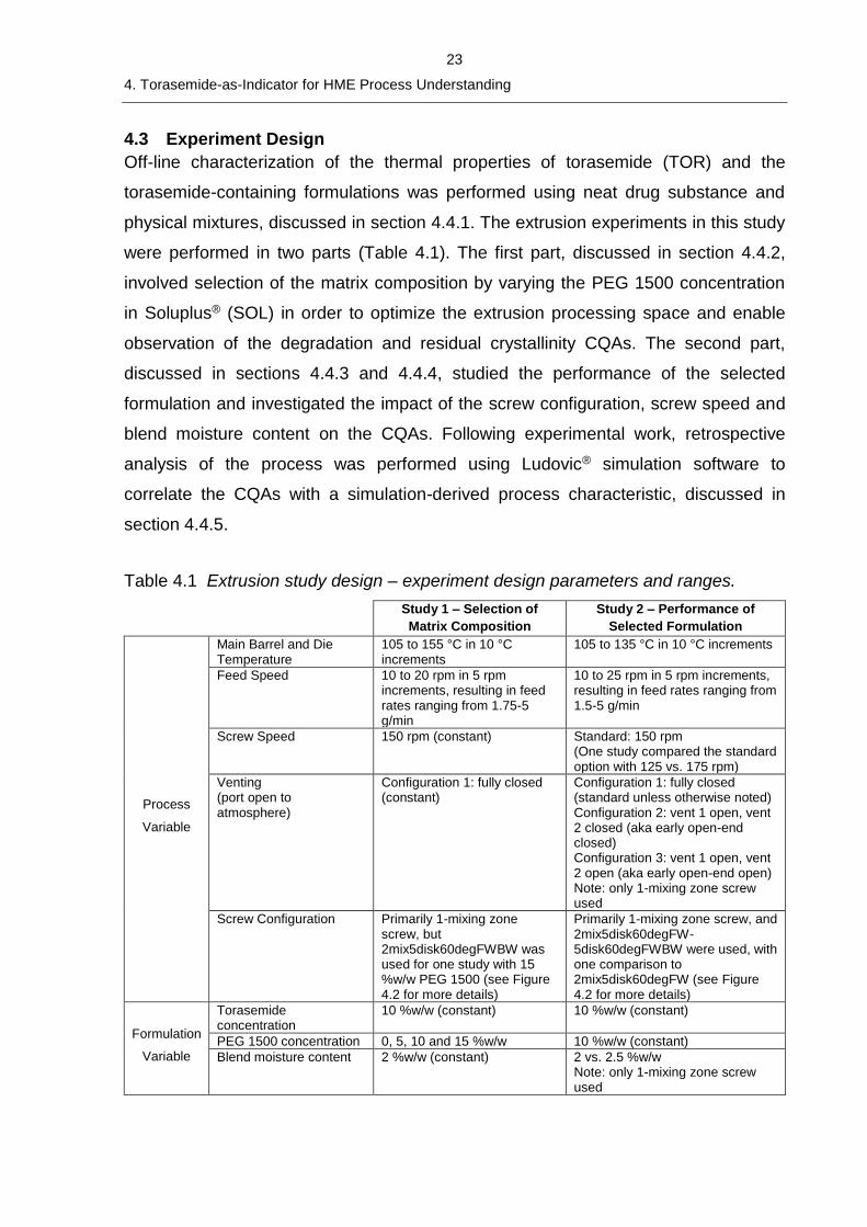
4.3 Experiment Design
Off-line characterization of the thermal properties of torasemide (TOR) and the
torasemide-containing formulations was performed using neat drug substance and
physical mixtures, discussed in section 4.4.1. The extrusion experiments in this study
were performed in two parts (Table 4.1). The first part, discussed in section 4.4.2,
involved selection of the matrix composition by varying the PEG 1500 concentration
in Soluplus® (SOL) in order to optimize the extrusion processing space and enable
observation of the degradation and residual crystallinity CQAs. The second part,
discussed in sections 4.4.3 and 4.4.4, studied the performance of the selected
formulation and investigated the impact of the screw configuration, screw speed and
blend moisture content on the CQAs. Following experimental work, retrospective
analysis of the process was performed using Ludovic® simulation software to
correlate the CQAs with a simulation-derived process characteristic, discussed in
section 4.4.5.
Table 4.1 Extrusion study design – experiment design parameters and ranges.
Study 1 – Selection of
Matrix Composition
Study 2 – Performance of
Selected Formulation
Process
Variable
Main Barrel and Die Temperature
105 to 155 °C in 10 °C increments
105 to 135 °C in 10 °C increments
Feed Speed 10 to 20 rpm in 5 rpm increments, resulting in feed rates ranging from 1.75-5 g/min
10 to 25 rpm in 5 rpm increments, resulting in feed rates ranging from 1.5-5 g/min
Screw Speed 150 rpm (constant)
Standard: 150 rpm (One study compared the standard option with 125 vs. 175 rpm)
Venting (port open to atmosphere)
Configuration 1: fully closed (constant)
Configuration 1: fully closed (standard unless otherwise noted) Configuration 2: vent 1 open, vent 2 closed (aka early open-end closed) Configuration 3: vent 1 open, vent 2 open (aka early open-end open) Note: only 1-mixing zone screw used
Screw Configuration Primarily 1-mixing zone screw, but 2mix5disk60degFWBW was used for one study with 15 %w/w PEG 1500 (see Figure 4.2 for more details)
Primarily 1-mixing zone screw, and 2mix5disk60degFW-5disk60degFWBW were used, with one comparison to 2mix5disk60degFW (see Figure 4.2 for more details)
Formulation
Variable
Torasemide concentration
10 %w/w (constant) 10 %w/w (constant)
PEG 1500 concentration 0, 5, 10 and 15 %w/w 10 %w/w (constant)
Blend moisture content 2 %w/w (constant) 2 vs. 2.5 %w/w Note: only 1-mixing zone screw used
24
4. Torasemide-as-Indicator for HME Process Understanding
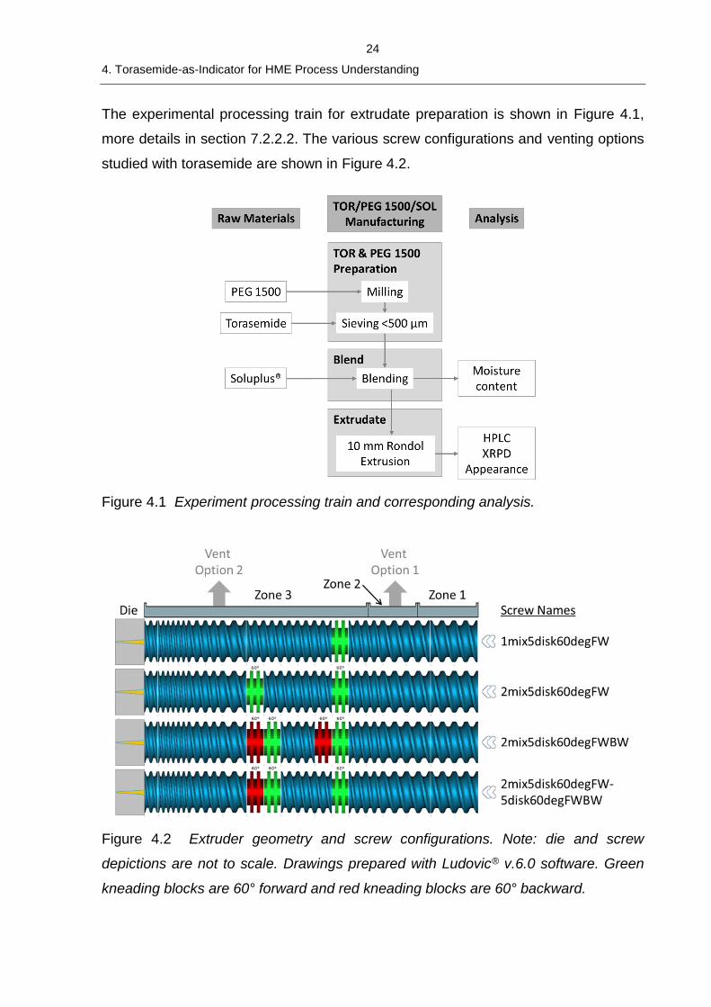
The experimental processing train for extrudate preparation is shown in Figure 4.1,
more details in section 7.2.2.2. The various screw configurations and venting options
studied with torasemide are shown in Figure 4.2.
Figure 4.1 Experiment processing train and corresponding analysis.
Figure 4.2 Extruder geometry and screw configurations. Note: die and screw
depictions are not to scale. Drawings prepared with Ludovic® v.6.0 software. Green
kneading blocks are 60° forward and red kneading blocks are 60° backward.
25
4. Torasemide-as-Indicator for HME Process Understanding
4.4 Results
4.4.1 Thermal Characterization of Torasemide and Physical Mixtures
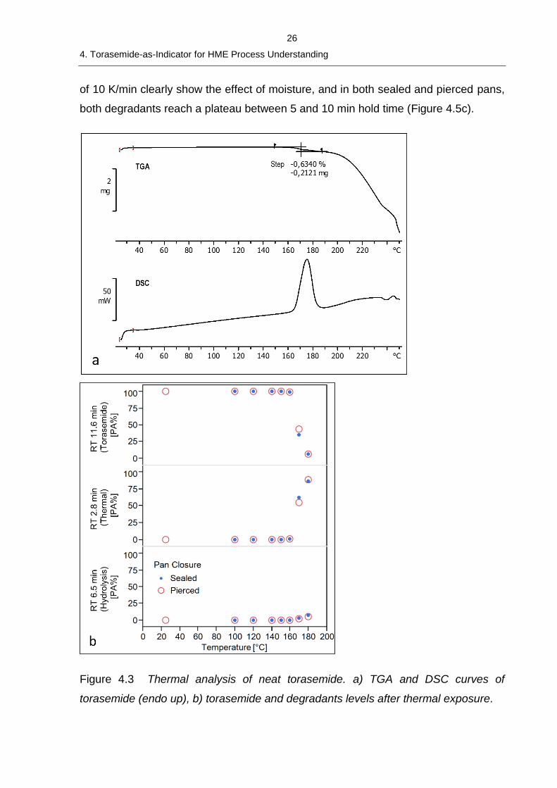
Heating studies via TGA and DSC with neat torasemide were performed to better
understand its degradation behavior. Melting of torasemide begins at approximately
160 °C and a weight loss of ~0.6 wt% is observed throughout this transition (Figure
4.3a). HPLC analysis of samples heated to intermediate temperatures between 100
to 180 °C showed that degradation began only upon melting (Figure 4.3b). Two
degradants were observed, and less than 10 PA% of torasemide was remaining at
180 °C. The primary degradant was the thermal degradant, confirmed by HPLC-MS
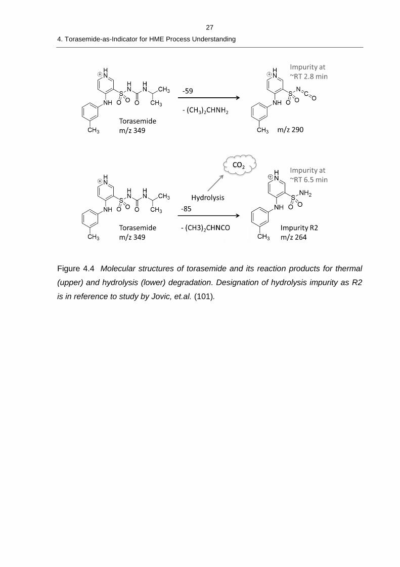
(Appendix 10.1), and the second was the hydrolysis degradant (Figure 4.4). A
comparison of pierced and hermetically sealed pans showed little difference in the
formation of the thermal versus hydrolysis degradants.
Preliminary extrusion experiments showed substantial degradation at main barrel and
die temperatures below the melting point of torasemide (data not shown). Therefore,
DSC experiments similar to those with neat torasemide were conducted to
investigate the degradation process in physical mixtures. HPLC analysis showed that
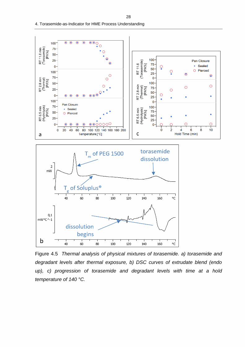
in the case of sealed pans, both the thermal and hydrolysis degradants start to form
at temperatures between 110-120 °C (Figure 4.5a). In the case of pierced pans, only
the thermal degradant is formed. The DSC thermogram in Figure 4.5b for a pre-dried
extrusion blend shows 3 thermal events. The first is melting of the PEG 1500 at
45 °C. The second is glass transition of the mixture formed up to that point,
dominated by SOL softening at ~70 °C. The third is a dissolution endotherm of the
torasemide dissolving into the matrix. The dissolution process begins at ~115 °C, as
clearly seen in the first derivative of the thermogram (Figure 4.5b). Control
experiments of binary mixtures of TOR and PEG 1500 showed degradation occurring
at similar temperatures (data not shown). Moreover, when extrudates with a
substantial amount of residual crystallinity were heated on a hot-stage polarized light
microscope (PLM), crystals were visually observed to lose birefringence also at
~115 °C, indicating onset dissolution of the crystals (data not included). The
progression of degradation over time for samples heated to 140 °C at a heating rate
26
4. Torasemide-as-Indicator for HME Process Understanding
of 10 K/min clearly show the effect of moisture, and in both sealed and pierced pans,
both degradants reach a plateau between 5 and 10 min hold time (Figure 4.5c).
Figure 4.3 Thermal analysis of neat torasemide. a) TGA and DSC curves of
torasemide (endo up), b) torasemide and degradants levels after thermal exposure.
27
4. Torasemide-as-Indicator for HME Process Understanding
Figure 4.4 Molecular structures of torasemide and its reaction products for thermal
(upper) and hydrolysis (lower) degradation. Designation of hydrolysis impurity as R2
is in reference to study by Jovic, et.al. (101).
28
4. Torasemide-as-Indicator for HME Process Understanding
Figure 4.5 Thermal analysis of physical mixtures of torasemide. a) torasemide and
degradant levels after thermal exposure, b) DSC curves of extrudate blend (endo
up), c) progression of torasemide and degradant levels with time at a hold
temperature of 140 °C.
29
4. Torasemide-as-Indicator for HME Process Understanding
4.4.2 Selection of Matrix Composition for Optimal Extrusion Processing Space
and Observation of CQAs
For studies exploring matrix composition, the process parameters were chosen such
that the primary independent variables were main barrel and die temperature and
feed rate. However, because the screw speed was held constant and only the 1-
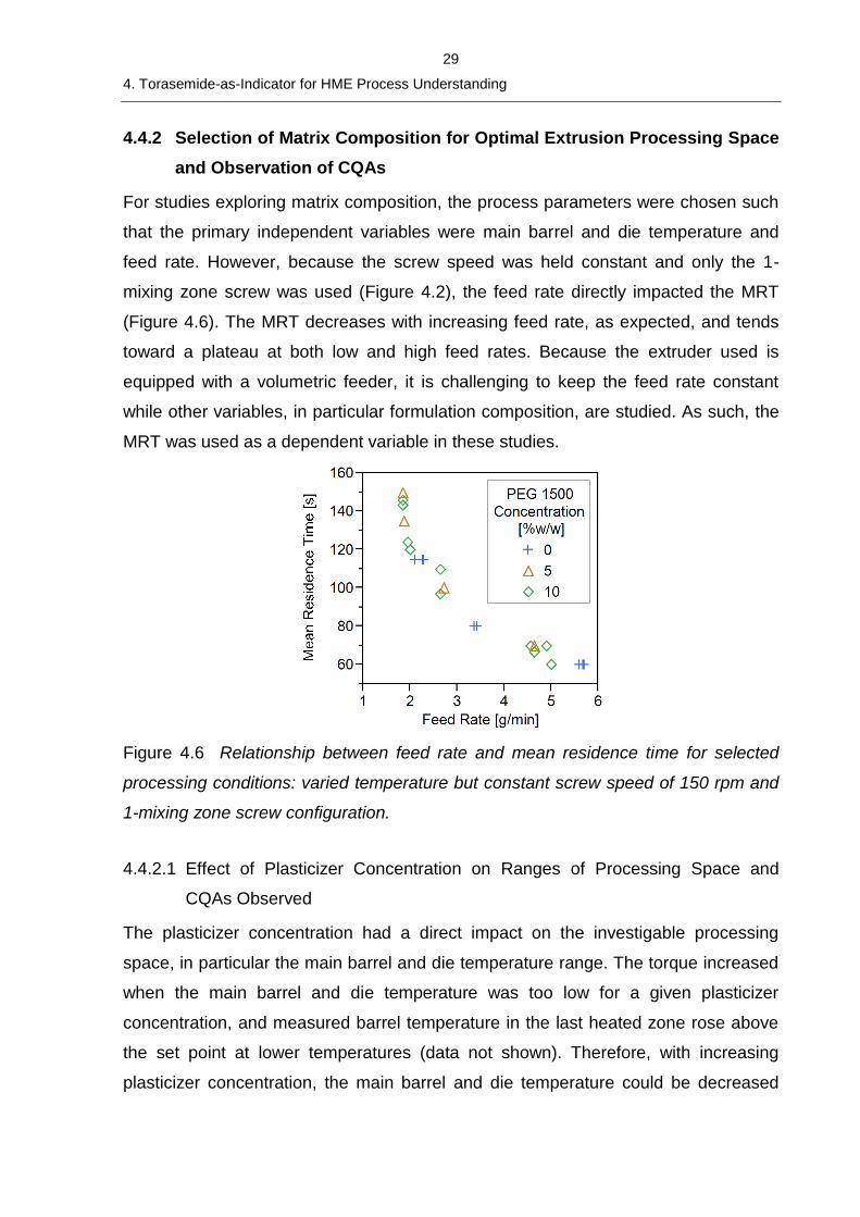
mixing zone screw was used (Figure 4.2), the feed rate directly impacted the MRT
(Figure 4.6). The MRT decreases with increasing feed rate, as expected, and tends
toward a plateau at both low and high feed rates. Because the extruder used is
equipped with a volumetric feeder, it is challenging to keep the feed rate constant
while other variables, in particular formulation composition, are studied. As such, the
MRT was used as a dependent variable in these studies.
Figure 4.6 Relationship between feed rate and mean residence time for selected
processing conditions: varied temperature but constant screw speed of 150 rpm and
1-mixing zone screw configuration.
4.4.2.1 Effect of Plasticizer Concentration on Ranges of Processing Space and
CQAs Observed
The plasticizer concentration had a direct impact on the investigable processing
space, in particular the main barrel and die temperature range. The torque increased
when the main barrel and die temperature was too low for a given plasticizer
concentration, and measured barrel temperature in the last heated zone rose above
the set point at lower temperatures (data not shown). Therefore, with increasing
plasticizer concentration, the main barrel and die temperature could be decreased
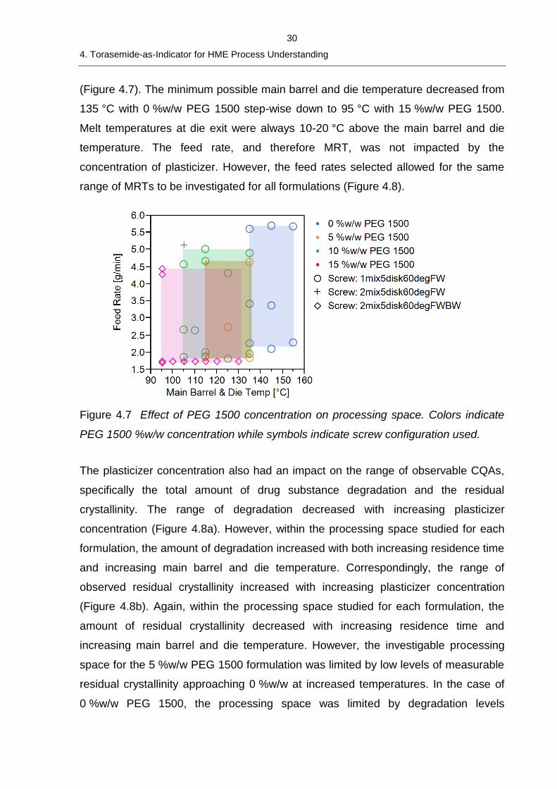
30
4. Torasemide-as-Indicator for HME Process Understanding
(Figure 4.7). The minimum possible main barrel and die temperature decreased from
135 °C with 0 %w/w PEG 1500 step-wise down to 95 °C with 15 %w/w PEG 1500.
Melt temperatures at die exit were always 10-20 °C above the main barrel and die
temperature. The feed rate, and therefore MRT, was not impacted by the
concentration of plasticizer. However, the feed rates selected allowed for the same
range of MRTs to be investigated for all formulations (Figure 4.8).
Figure 4.7 Effect of PEG 1500 concentration on processing space. Colors indicate
PEG 1500 %w/w concentration while symbols indicate screw configuration used.
The plasticizer concentration also had an impact on the range of observable CQAs,
specifically the total amount of drug substance degradation and the residual
crystallinity. The range of degradation decreased with increasing plasticizer
concentration (Figure 4.8a). However, within the processing space studied for each
formulation, the amount of degradation increased with both increasing residence time
and increasing main barrel and die temperature. Correspondingly, the range of
observed residual crystallinity increased with increasing plasticizer concentration
(Figure 4.8b). Again, within the processing space studied for each formulation, the
amount of residual crystallinity decreased with increasing residence time and
increasing main barrel and die temperature. However, the investigable processing
space for the 5 %w/w PEG 1500 formulation was limited by low levels of measurable
residual crystallinity approaching 0 %w/w at increased temperatures. In the case of
0 %w/w PEG 1500, the processing space was limited by degradation levels
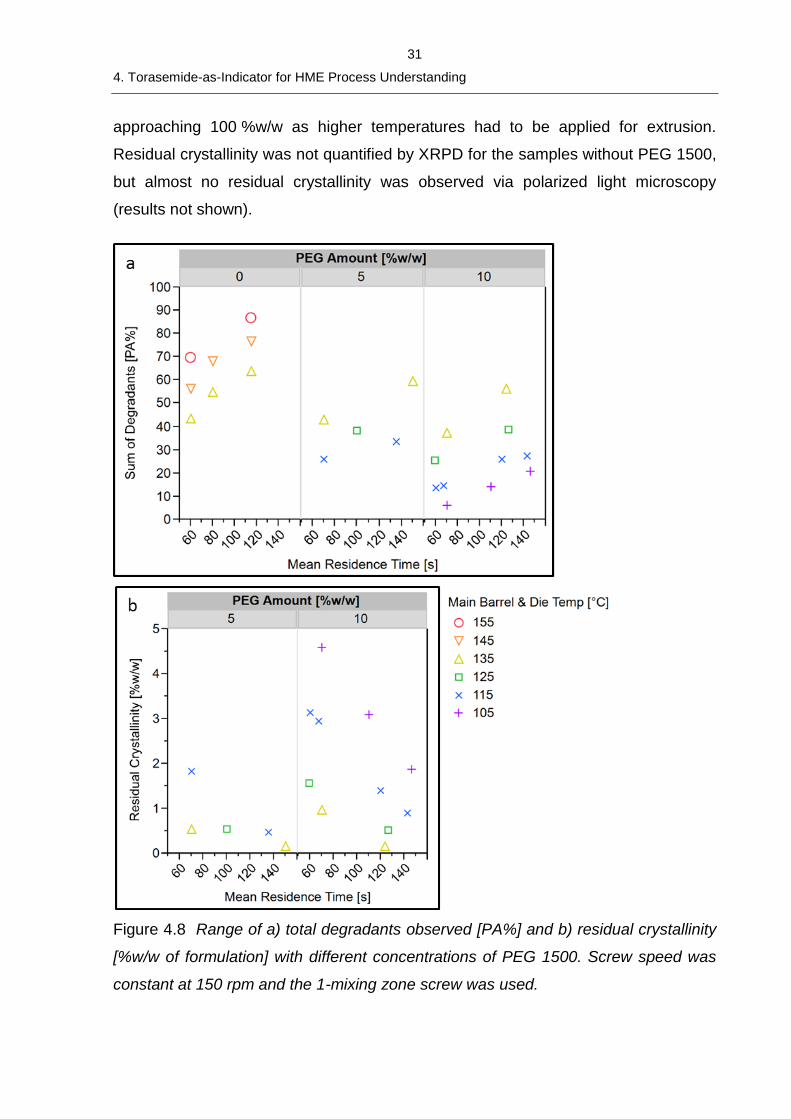
31
4. Torasemide-as-Indicator for HME Process Understanding
approaching 100 %w/w as higher temperatures had to be applied for extrusion.
Residual crystallinity was not quantified by XRPD for the samples without PEG 1500,
but almost no residual crystallinity was observed via polarized light microscopy
(results not shown).
Figure 4.8 Range of a) total degradants observed [PA%] and b) residual crystallinity
[%w/w of formulation] with different concentrations of PEG 1500. Screw speed was
constant at 150 rpm and the 1-mixing zone screw was used.
32
4. Torasemide-as-Indicator for HME Process Understanding
The amount of degradation and residual crystallinity also showed a dependency on
PEG 1500 concentration, even when similar processing conditions were used (Figure
4.8). At main barrel and die temperatures between 115 and 135 °C, the amount of
degradation decreased slightly with increasing PEG 1500 concentration. Within the
same temperature range, the amount of residual crystallinity was higher with
10 %w/w PEG 1500 than with 5 %w/w PEG 1500.
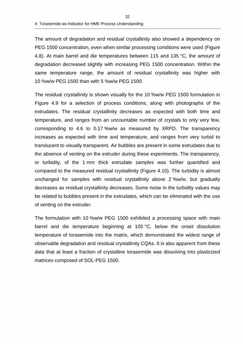
The residual crystallinity is shown visually for the 10 %w/w PEG 1500 formulation in
Figure 4.9 for a selection of process conditions, along with photographs of the
extrudates. The residual crystallinity decreases as expected with both time and
temperature, and ranges from an uncountable number of crystals to only very few,
corresponding to 4.6 to 0.17 %w/w as measured by XRPD. The transparency
increases as expected with time and temperature, and ranges from very turbid to
translucent to visually transparent. Air bubbles are present in some extrudates due to
the absence of venting on the extruder during these experiments. The transparency,
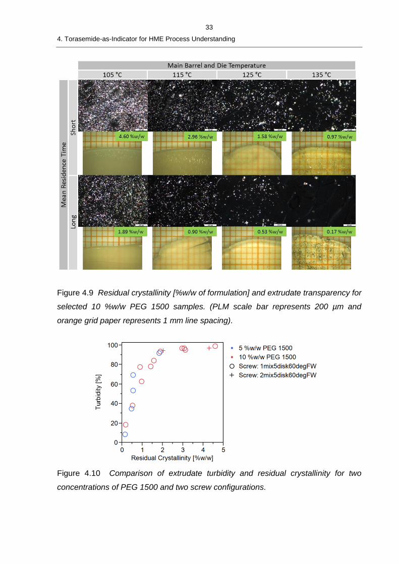
or turbidity, of the 1 mm thick extrudate samples was further quantified and
compared to the measured residual crystallinity (Figure 4.10). The turbidity is almost
unchanged for samples with residual crystallinity above 2 %w/w, but gradually
decreases as residual crystallinity decreases. Some noise in the turbidity values may
be related to bubbles present in the extrudates, which can be eliminated with the use
of venting on the extruder.
The formulation with 10 %w/w PEG 1500 exhibited a processing space with main
barrel and die temperature beginning at 105 °C, below the onset dissolution
temperature of torasemide into the matrix, which demonstrated the widest range of
observable degradation and residual crystallinity CQAs. It is also apparent from these
data that at least a fraction of crystalline torasemide was dissolving into plasticized
matrices composed of SOL-PEG 1500.
33
4. Torasemide-as-Indicator for HME Process Understanding
Figure 4.9 Residual crystallinity [%w/w of formulation] and extrudate transparency for
selected 10 %w/w PEG 1500 samples. (PLM scale bar represents 200 µm and
orange grid paper represents 1 mm line spacing).
Figure 4.10 Comparison of extrudate turbidity and residual crystallinity for two
concentrations of PEG 1500 and two screw configurations.
34
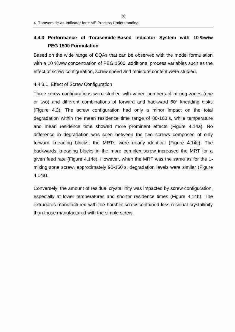
4. Torasemide-as-Indicator for HME Process Understanding
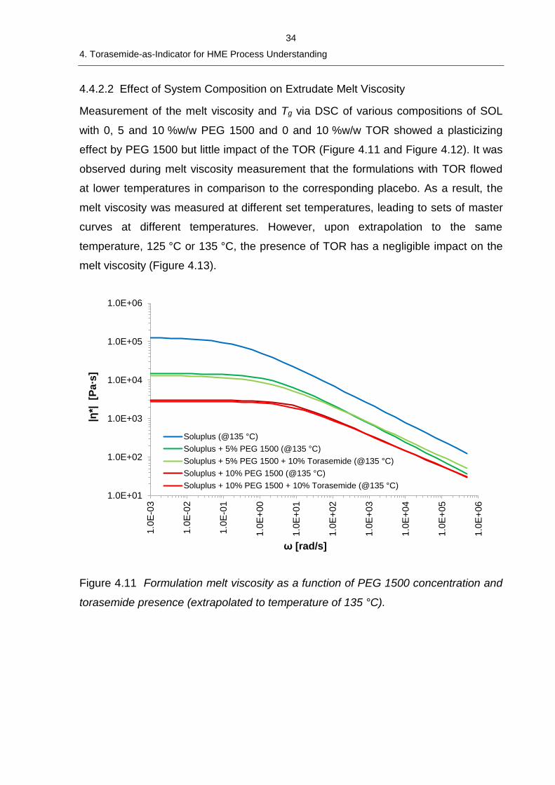
4.4.2.2 Effect of System Composition on Extrudate Melt Viscosity
Measurement of the melt viscosity and Tg via DSC of various compositions of SOL
with 0, 5 and 10 %w/w PEG 1500 and 0 and 10 %w/w TOR showed a plasticizing
effect by PEG 1500 but little impact of the TOR (Figure 4.11 and Figure 4.12). It was
observed during melt viscosity measurement that the formulations with TOR flowed
at lower temperatures in comparison to the corresponding placebo. As a result, the
melt viscosity was measured at different set temperatures, leading to sets of master
curves at different temperatures. However, upon extrapolation to the same
temperature, 125 °C or 135 °C, the presence of TOR has a negligible impact on the
melt viscosity (Figure 4.13).
Figure 4.11 Formulation melt viscosity as a function of PEG 1500 concentration and
torasemide presence (extrapolated to temperature of 135 °C).
1.0E+01
1.0E+02
1.0E+03
1.0E+04
1.0E+05
1.0E+06
1.0
E-0
3
1.0
E-0
2
1.0
E-0
1
1.0
E+
00
1.0
E+
01
1.0
E+
02
1.0
E+
03
1.0
E+
04
1.0
E+
05
1.0
E+
06
|η*|
[P
a∙s
]
ω [rad/s]
Soluplus (@135 °C)
Soluplus + 5% PEG 1500 (@135 °C)
Soluplus + 5% PEG 1500 + 10% Torasemide (@135 °C)
Soluplus + 10% PEG 1500 (@135 °C)
Soluplus + 10% PEG 1500 + 10% Torasemide (@135 °C)
35
4. Torasemide-as-Indicator for HME Process Understanding
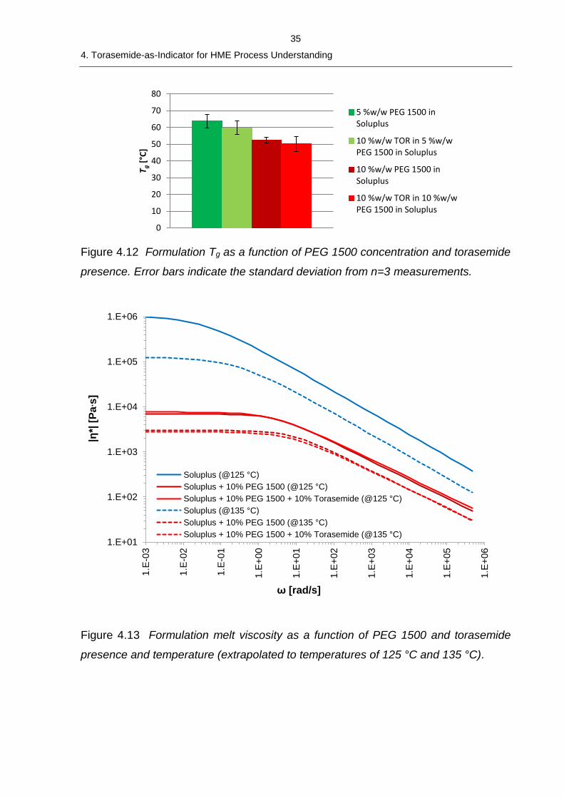
Figure 4.12 Formulation Tg as a function of PEG 1500 concentration and torasemide
presence. Error bars indicate the standard deviation from n=3 measurements.
Figure 4.13 Formulation melt viscosity as a function of PEG 1500 and torasemide
presence and temperature (extrapolated to temperatures of 125 °C and 135 °C).
0
10
20
30
40
50
60
70
80
T g[°C]
5 %w/w PEG 1500 inSoluplus
10 %w/w TOR in 5 %w/wPEG 1500 in Soluplus
10 %w/w PEG 1500 inSoluplus
10 %w/w TOR in 10 %w/wPEG 1500 in Soluplus
1.E+01
1.E+02
1.E+03
1.E+04
1.E+05
1.E+06
1.E
-03
1.E
-02
1.E
-01
1.E
+00
1.E
+01
1.E
+02
1.E
+03
1.E
+04
1.E
+05
1.E
+06
|η*|
[P
a∙s
]
ω [rad/s]
Soluplus (@125 °C)
Soluplus + 10% PEG 1500 (@125 °C)
Soluplus + 10% PEG 1500 + 10% Torasemide (@125 °C)
Soluplus (@135 °C)
Soluplus + 10% PEG 1500 (@135 °C)
Soluplus + 10% PEG 1500 + 10% Torasemide (@135 °C)
36
4. Torasemide-as-Indicator for HME Process Understanding
4.4.3 Performance of Torasemide-Based Indicator System with 10 %w/w
PEG 1500 Formulation
Based on the wide range of CQAs that can be observed with the model formulation
with a 10 %w/w concentration of PEG 1500, additional process variables such as the
effect of screw configuration, screw speed and moisture content were studied.
4.4.3.1 Effect of Screw Configuration
Three screw configurations were studied with varied numbers of mixing zones (one
or two) and different combinations of forward and backward 60° kneading disks
(Figure 4.2). The screw configuration had only a minor impact on the total
degradation within the mean residence time range of 80-160 s, while temperature
and mean residence time showed more prominent effects (Figure 4.14a). No
difference in degradation was seen between the two screws composed of only
forward kneading blocks; the MRTs were nearly identical (Figure 4.14c). The
backwards kneading blocks in the more complex screw increased the MRT for a
given feed rate (Figure 4.14c). However, when the MRT was the same as for the 1-
mixing zone screw, approximately 90-160 s, degradation levels were similar (Figure
4.14a).
Conversely, the amount of residual crystallinity was impacted by screw configuration,
especially at lower temperatures and shorter residence times (Figure 4.14b). The
extrudates manufactured with the harsher screw contained less residual crystallinity
than those manufactured with the simple screw.
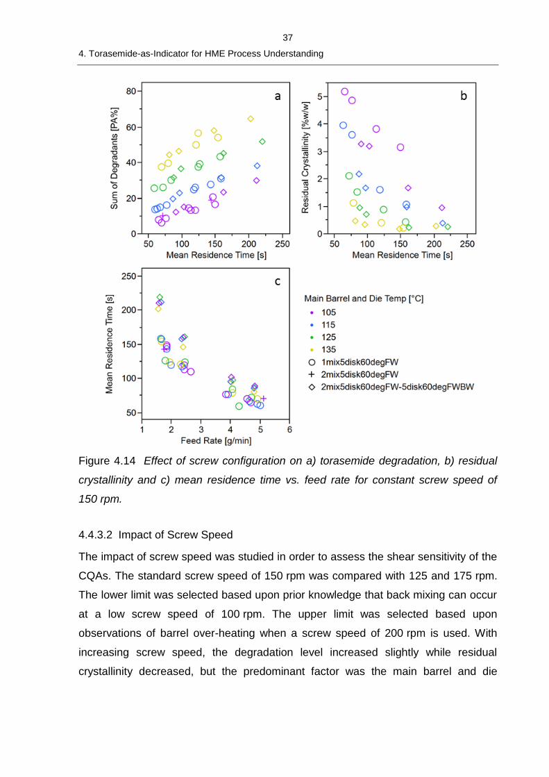
37
4. Torasemide-as-Indicator for HME Process Understanding
Figure 4.14 Effect of screw configuration on a) torasemide degradation, b) residual
crystallinity and c) mean residence time vs. feed rate for constant screw speed of
150 rpm.
4.4.3.2 Impact of Screw Speed
The impact of screw speed was studied in order to assess the shear sensitivity of the
CQAs. The standard screw speed of 150 rpm was compared with 125 and 175 rpm.
The lower limit was selected based upon prior knowledge that back mixing can occur
at a low screw speed of 100 rpm. The upper limit was selected based upon
observations of barrel over-heating when a screw speed of 200 rpm is used. With
increasing screw speed, the degradation level increased slightly while residual
crystallinity decreased, but the predominant factor was the main barrel and die
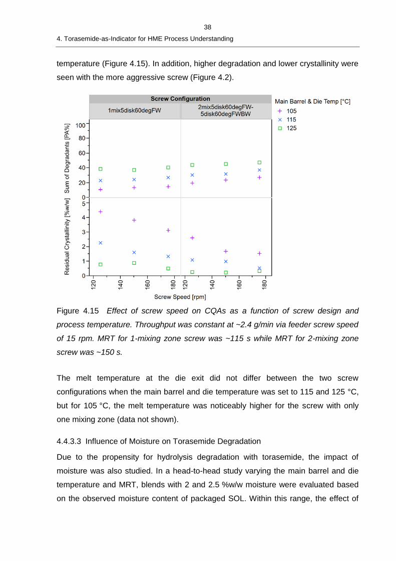
38
4. Torasemide-as-Indicator for HME Process Understanding
temperature (Figure 4.15). In addition, higher degradation and lower crystallinity were
seen with the more aggressive screw (Figure 4.2).
Figure 4.15 Effect of screw speed on CQAs as a function of screw design and
process temperature. Throughput was constant at ~2.4 g/min via feeder screw speed
of 15 rpm. MRT for 1-mixing zone screw was ~115 s while MRT for 2-mixing zone
screw was ~150 s.
The melt temperature at the die exit did not differ between the two screw
configurations when the main barrel and die temperature was set to 115 and 125 °C,
but for 105 °C, the melt temperature was noticeably higher for the screw with only
one mixing zone (data not shown).
4.4.3.3 Influence of Moisture on Torasemide Degradation
Due to the propensity for hydrolysis degradation with torasemide, the impact of
moisture was also studied. In a head-to-head study varying the main barrel and die
temperature and MRT, blends with 2 and 2.5 %w/w moisture were evaluated based
on the observed moisture content of packaged SOL. Within this range, the effect of
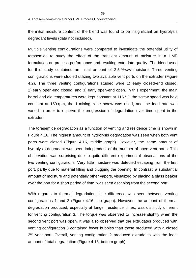
39
4. Torasemide-as-Indicator for HME Process Understanding
the initial moisture content of the blend was found to be insignificant on hydrolysis
degradant levels (data not included).
Multiple venting configurations were compared to investigate the potential utility of
torasemide to study the effect of the transient amount of moisture in a HME
formulation on process performance and resulting extrudate quality. The blend used
for this study contained an initial amount of 2.5 %w/w moisture. Three venting
configurations were studied utilizing two available vent ports on the extruder (Figure
4.2). The three venting configurations studied were 1) early closed-end closed,
2) early open-end closed, and 3) early open-end open. In this experiment, the main
barrel and die temperatures were kept constant at 115 °C, the screw speed was held
constant at 150 rpm, the 1-mixing zone screw was used, and the feed rate was
varied in order to observe the progression of degradation over time spent in the
extruder.
The torasemide degradation as a function of venting and residence time is shown in
Figure 4.16. The highest amount of hydrolysis degradation was seen when both vent
ports were closed (Figure 4.16, middle graph). However, the same amount of
hydrolysis degradant was seen independent of the number of open vent ports. This
observation was surprising due to quite different experimental observations of the
two venting configurations. Very little moisture was detected escaping from the first
port, partly due to material filling and plugging the opening. In contrast, a substantial
amount of moisture and potentially other vapors, visualized by placing a glass beaker
over the port for a short period of time, was seen escaping from the second port.
With regards to thermal degradation, little difference was seen between venting
configurations 1 and 2 (Figure 4.16, top graph). However, the amount of thermal
degradation produced, especially at longer residence times, was distinctly different
for venting configuration 3. The torque was observed to increase slightly when the
second vent port was open. It was also observed that the extrudates produced with
venting configuration 3 contained fewer bubbles than those produced with a closed
2nd vent port. Overall, venting configuration 2 produced extrudates with the least
amount of total degradation (Figure 4.16, bottom graph).
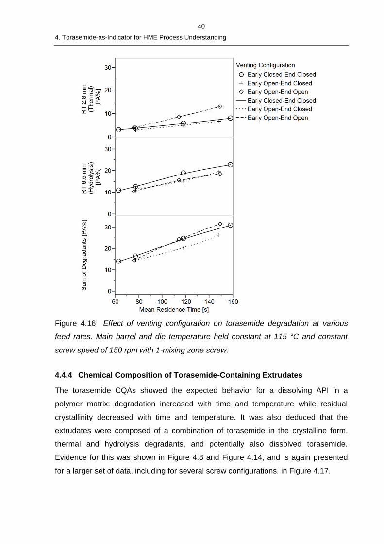
40
4. Torasemide-as-Indicator for HME Process Understanding
Figure 4.16 Effect of venting configuration on torasemide degradation at various
feed rates. Main barrel and die temperature held constant at 115 °C and constant
screw speed of 150 rpm with 1-mixing zone screw.
4.4.4 Chemical Composition of Torasemide-Containing Extrudates
The torasemide CQAs showed the expected behavior for a dissolving API in a
polymer matrix: degradation increased with time and temperature while residual
crystallinity decreased with time and temperature. It was also deduced that the
extrudates were composed of a combination of torasemide in the crystalline form,
thermal and hydrolysis degradants, and potentially also dissolved torasemide.
Evidence for this was shown in Figure 4.8 and Figure 4.14, and is again presented
for a larger set of data, including for several screw configurations, in Figure 4.17.
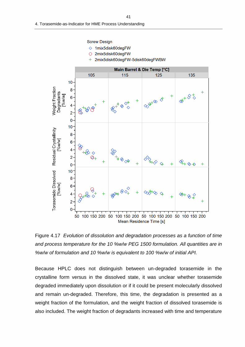
41
4. Torasemide-as-Indicator for HME Process Understanding
Figure 4.17 Evolution of dissolution and degradation processes as a function of time
and process temperature for the 10 %w/w PEG 1500 formulation. All quantities are in
%w/w of formulation and 10 %w/w is equivalent to 100 %w/w of initial API.
Because HPLC does not distinguish between un-degraded torasemide in the
crystalline form versus in the dissolved state, it was unclear whether torasemide
degraded immediately upon dissolution or if it could be present molecularly dissolved
and remain un-degraded. Therefore, this time, the degradation is presented as a
weight fraction of the formulation, and the weight fraction of dissolved torasemide is
also included. The weight fraction of degradants increased with time and temperature
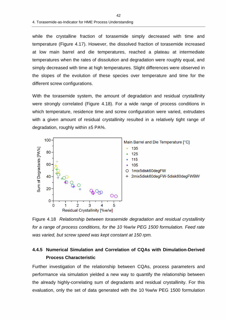
42
4. Torasemide-as-Indicator for HME Process Understanding
while the crystalline fraction of torasemide simply decreased with time and
temperature (Figure 4.17). However, the dissolved fraction of torasemide increased
at low main barrel and die temperatures, reached a plateau at intermediate
temperatures when the rates of dissolution and degradation were roughly equal, and
simply decreased with time at high temperatures. Slight differences were observed in
the slopes of the evolution of these species over temperature and time for the
different screw configurations.
With the torasemide system, the amount of degradation and residual crystallinity
were strongly correlated (Figure 4.18). For a wide range of process conditions in
which temperature, residence time and screw configuration were varied, extrudates
with a given amount of residual crystallinity resulted in a relatively tight range of
degradation, roughly within ±5 PA%.
Figure 4.18 Relationship between torasemide degradation and residual crystallinity
for a range of process conditions, for the 10 %w/w PEG 1500 formulation. Feed rate
was varied, but screw speed was kept constant at 150 rpm.
4.4.5 Numerical Simulation and Correlation of CQAs with Dimulation-Derived
Process Characteristic
Further investigation of the relationship between CQAs, process parameters and
performance via simulation yielded a new way to quantify the relationship between
the already highly-correlating sum of degradants and residual crystallinity. For this
evaluation, only the set of data generated with the 10 %w/w PEG 1500 formulation
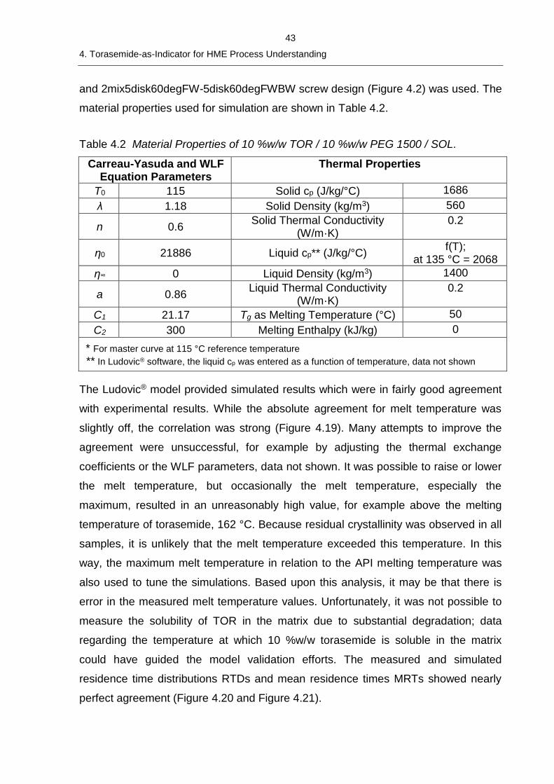
43
4. Torasemide-as-Indicator for HME Process Understanding
and 2mix5disk60degFW-5disk60degFWBW screw design (Figure 4.2) was used. The
material properties used for simulation are shown in Table 4.2.
Table 4.2 Material Properties of 10 %w/w TOR / 10 %w/w PEG 1500 / SOL.
Carreau-Yasuda and WLF Equation Parameters
Thermal Properties
T0 115 Solid cp (J/kg/°C) 1686
λ 1.18 Solid Density (kg/m3) 560
n 0.6 Solid Thermal Conductivity
(W/m·K) 0.2
η0 21886 Liquid cp** (J/kg/°C) f(T);
at 135 °C = 2068
η∞ 0 Liquid Density (kg/m3) 1400
a 0.86 Liquid Thermal Conductivity
(W/m·K) 0.2
C1 21.17 Tg as Melting Temperature (°C) 50
C2 300 Melting Enthalpy (kJ/kg) 0
* For master curve at 115 °C reference temperature ** In Ludovic® software, the liquid cp was entered as a function of temperature, data not shown
The Ludovic® model provided simulated results which were in fairly good agreement
with experimental results. While the absolute agreement for melt temperature was
slightly off, the correlation was strong (Figure 4.19). Many attempts to improve the
agreement were unsuccessful, for example by adjusting the thermal exchange
coefficients or the WLF parameters, data not shown. It was possible to raise or lower
the melt temperature, but occasionally the melt temperature, especially the
maximum, resulted in an unreasonably high value, for example above the melting
temperature of torasemide, 162 °C. Because residual crystallinity was observed in all
samples, it is unlikely that the melt temperature exceeded this temperature. In this
way, the maximum melt temperature in relation to the API melting temperature was
also used to tune the simulations. Based upon this analysis, it may be that there is
error in the measured melt temperature values. Unfortunately, it was not possible to
measure the solubility of TOR in the matrix due to substantial degradation; data
regarding the temperature at which 10 %w/w torasemide is soluble in the matrix
could have guided the model validation efforts. The measured and simulated
residence time distributions RTDs and mean residence times MRTs showed nearly
perfect agreement (Figure 4.20 and Figure 4.21).
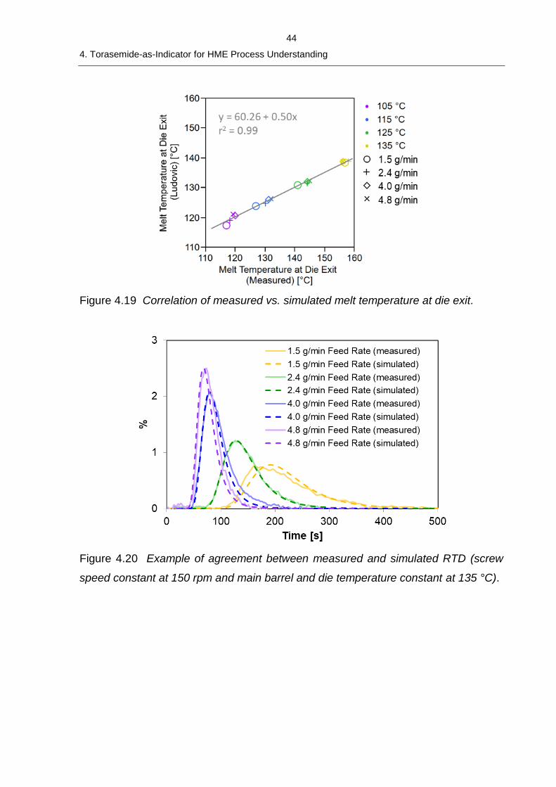
44
4. Torasemide-as-Indicator for HME Process Understanding
Figure 4.19 Correlation of measured vs. simulated melt temperature at die exit.
Figure 4.20 Example of agreement between measured and simulated RTD (screw
speed constant at 150 rpm and main barrel and die temperature constant at 135 °C).
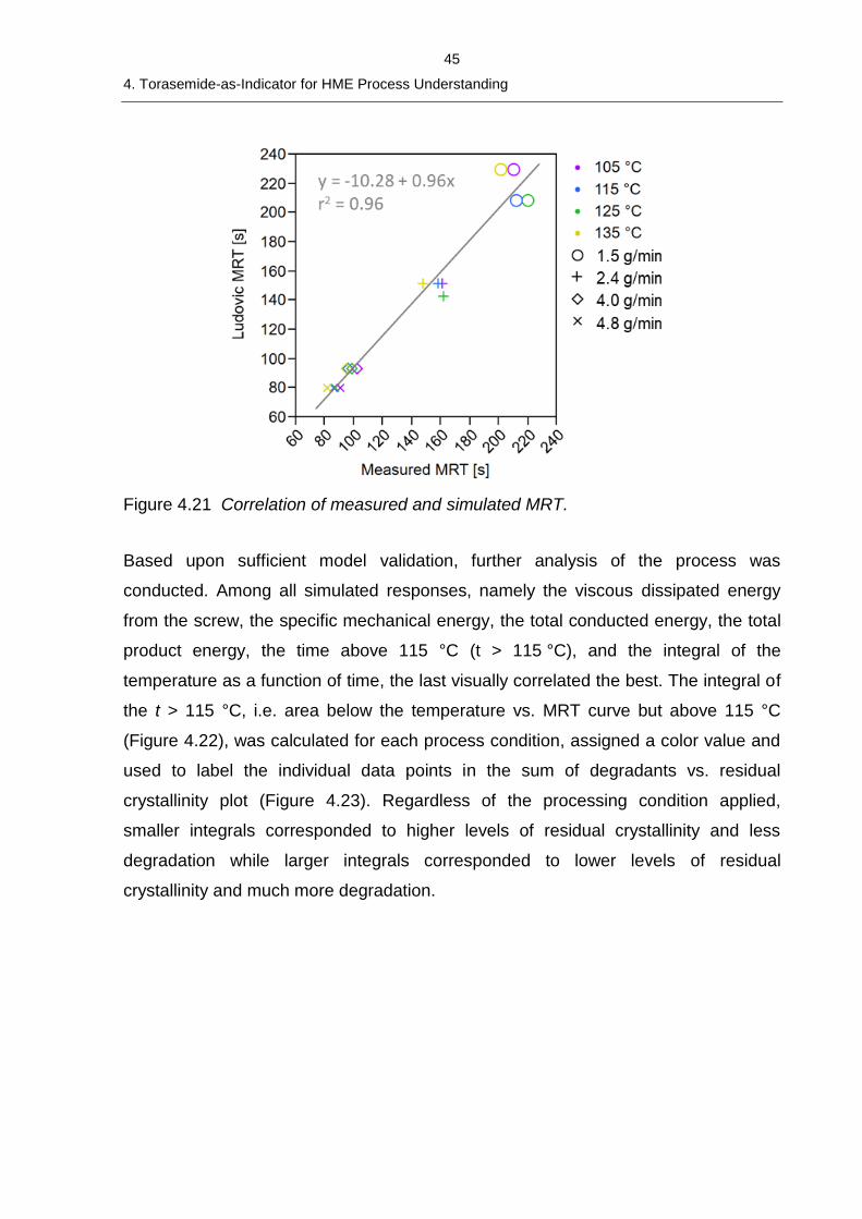
45
4. Torasemide-as-Indicator for HME Process Understanding
Figure 4.21 Correlation of measured and simulated MRT.
Based upon sufficient model validation, further analysis of the process was
conducted. Among all simulated responses, namely the viscous dissipated energy
from the screw, the specific mechanical energy, the total conducted energy, the total
product energy, the time above 115 °C (t > 115 °C), and the integral of the
temperature as a function of time, the last visually correlated the best. The integral of
the t > 115 °C, i.e. area below the temperature vs. MRT curve but above 115 °C
(Figure 4.22), was calculated for each process condition, assigned a color value and
used to label the individual data points in the sum of degradants vs. residual
crystallinity plot (Figure 4.23). Regardless of the processing condition applied,
smaller integrals corresponded to higher levels of residual crystallinity and less
degradation while larger integrals corresponded to lower levels of residual
crystallinity and much more degradation.
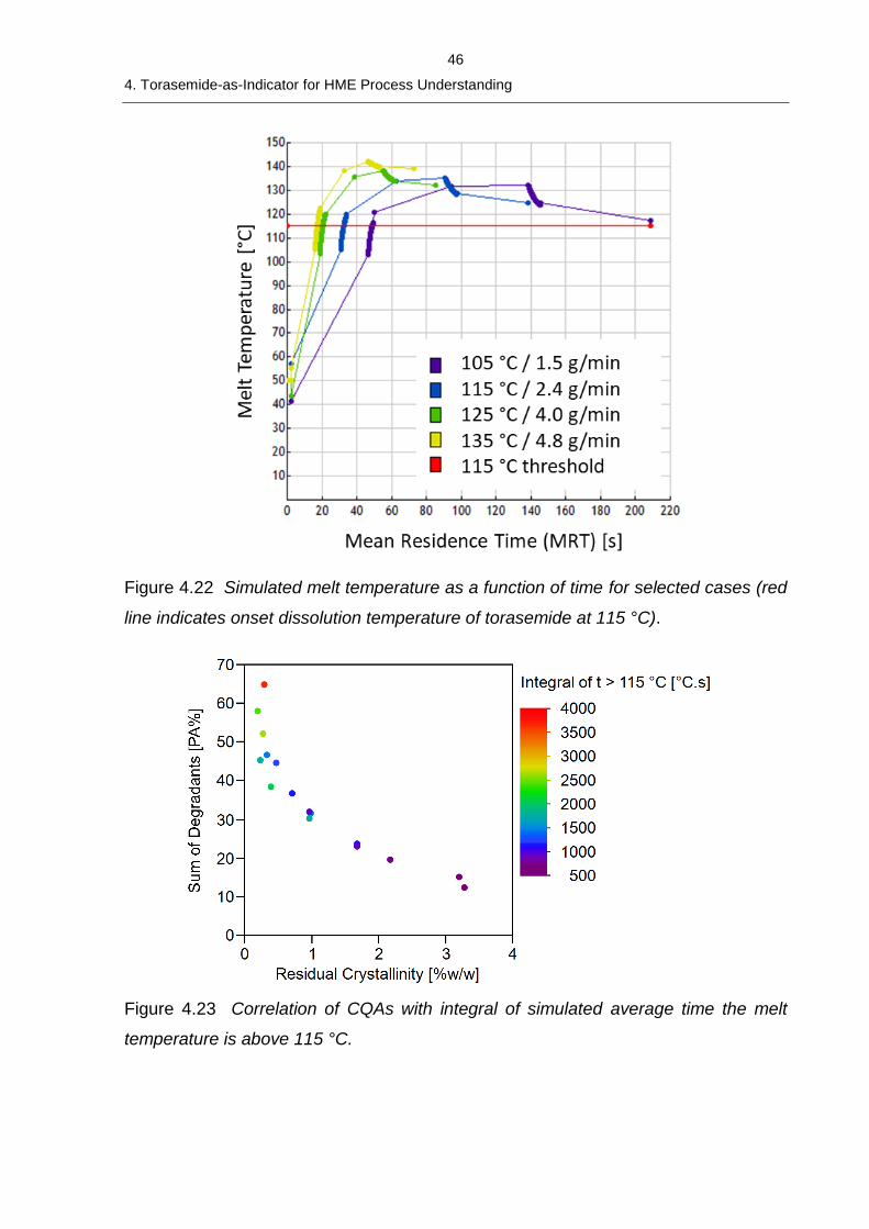
46
4. Torasemide-as-Indicator for HME Process Understanding
Figure 4.22 Simulated melt temperature as a function of time for selected cases (red
line indicates onset dissolution temperature of torasemide at 115 °C).
Figure 4.23 Correlation of CQAs with integral of simulated average time the melt
temperature is above 115 °C.
47
4. Torasemide-as-Indicator for HME Process Understanding
4.5 Discussion
HME, as a process technology with a long history of use in the formation of ASDs,
brings thermal and mechanical energy to the material being processed. However,
determining the specific impact of the process on the final product CQAs is
challenging due to the fact that most APIs are screened for thermal stability, as well
as their likelihood of forming a solid solution via molecular interactions or solubility in
the polymer matrix (45,102). Therefore, most products have an inherently wide
process design space. Nevertheless, in a regulated industry, pharmaceutical
scientists must demonstrate the impact of the process on the final product (103).
These studies with torasemide and the development of a formulation with a tailored
processing window indicate potential for deeper understanding of the HME process.
With one system, two CQAs, degradation and residual crystallinity, can be related to
process conditions such as the thermal and shear environment, as well as the
residence time.
The torasemide formulation based on SOL and PEG 1500 enables the study of both
degradation and residual crystallinity due to its dissolve-then-degrade mechanism.
Thermal characterization of neat torasemide via weight lost during TGA alone did not
explain the substantial amount of degradation observed when torasemide was
extruded at main barrel and die temperatures well below its melting point (Figure
4.3). However, when combined with HPLC-MS analysis, the degradation products
were revealed to be very similar in molecular weight to torasemide itself and
therefore not likely to be volatile (Figure 4.4 and Appendix 10.1). In addition,
torasemide underwent no degradation until melting was initiated but was nearly
100% degraded by the time it had completely melted (Figure 4.3), or 20 °C above the
initial melting temperature and after only 2 minutes of additional heating. This
observation indicated rapid degradation kinetics and that melt quenching attempts to
prepare an amorphous form of torasemide are futile. It also indicated that torasemide
is highly susceptible to degradation, specifically thermal and hydrolysis, when not
stabilized by a crystalline lattice. This instability at elevated temperatures in the non-
crystalline state was confirmed by controlled heating of the physical mixture and the
correlation between onset dissolution temperature and by the temperature at which
degradation products were detected (Figure 4.5).
48
4. Torasemide-as-Indicator for HME Process Understanding
Extrusion experiments (Figure 4.8, Figure 4.14 and Figure 4.15) and the high degree
of correlation between degradation and residual crystallinity (Figure 4.17 and Figure
4.18) also confirmed the dissolve-then-degrade mechanism. The torasemide system,
as already demonstrated in this study on a standard design twin-screw extruder with
various kneading block screw configurations, showed a wide and measurable range
of degradation and residual crystallinity within typical residence times for twin-screw
extrusion. This rate of dissolution and degradation occurring within a more
representative range of residence time in the torasemide system is an advantage
over the spironolactone system studied by Vigh, et.al. For that system, materials
were extruded in recirculation mode on a Haake® Mini-lab extruder in which
processing times of up to 25 min were required to see the evolution of degradation
and residual crystallinity (31). In fact, the residence time data in this TOR study, for a
given screw speed and configuration, showed that the MRT was a strong function of
feed rate and reached both maximum and minimum limits (Figure 4.6), which agrees
with the literature (104). The MRT reached a maximum limit of about 150 s at low
feed rates and a minimum limit of about 60 s at high feed rates, which can be
explained by the MRT’s dependency on extruder free volume and fill ratio (104).
Given this dependency and the practical desire for process efficiency enabled by
high throughputs, an indicator system like torasemide which shows sensitivity within
practical and realistic process boundaries is advantageous. The MRT, as well as the
residence time distribution, could be increased and/or adjusted by introducing more
mixing or backwards conveying elements to the screw configuration, but not without
causing considerable changes to other process conditions.
Measurement and quantification of the residual crystallinity in this TOR system was
only feasible by XRPD. Utilization of the melting endotherm via DSC was not
possible because none was detected (data not included), indicating that torasemide
fully dissolved before melting. This observation has been described previously and
the present work corroborates this finding (3,31).
The high degree of correlation shown between torasemide degradation and residual
crystallinity over a wide range of different process parameter combinations (Figure
4.18) also indicates that a more general process condition, rather than several
independent process variables, is responsible for the evolution of the CQAs. In this
49
4. Torasemide-as-Indicator for HME Process Understanding
case, the integral of the time > 115 °C correlated well with the relationship between
residual crystallinity and sum of degradants (Figure 4.23). This approach neglects the
kinetics of the reaction, namely that the API will both dissolve and degrade at a faster
rate at higher temperatures. In fact, due to the dissolve-then-degrade mechanism of
TOR in this system, and absent of a method to quantify the dissolution rate of TOR
into the matrix, development of a coupled dissolution and degradation kinetics
relationship is at present not feasible. However, the integral approach is a preliminary
attempt to identify a general process characteristic which correlates with multiple
CQAs which could also guide scaling. If confirmed for other systems, it could be
highly efficient to design extrusion development and scale-up studies around varying
this type of general process characteristic, or perhaps another type of imparted
energy and residence time distribution, for example. This concept has been
discussed in the literature, and the present data confirms and supports this approach
towards process understanding and development (9).
The plasticizing effects of torasemide and the presence of its degradants on the
overall system melt viscosity are not fully understood. Due to the high concentration
of degradants and potentially yet-to-be degraded torasemide present in the extrudate
samples, it was important to investigate the impact of their presence on the melt
viscosity of the system. Pure un-extruded Soluplus® was compared to extruded
placebo and active-containing extrudates with 5 and 10 %w/w PEG 1500 (Figure
4.11). The placebos and active formulations were extruded to ensure mixing of the
matrix components as well as to ensure the presence of dissolved and degraded
torasemide. These formulations were considered to be extremes in sample
composition and should indicate the maximum extent that plasticization by dissolved
and degraded torasemide could have on the system, if indeed there were to be an
observable difference in melt viscosity. The extremes in sample composition were
tested, rather than for example low, middle and high amounts of degradation, due to
the time-dependent nature of rheological experiments. It is impossible to eliminate
the time component from such testing because samples must be thermally
equilibrated, and the frequency sweeps also last at least a few minutes. This is an
important consideration for measuring the rheology of reactive systems. Although
feasible temperature windows for rheological measurements differed for placebo vs.
50
4. Torasemide-as-Indicator for HME Process Understanding
active, the melt viscosity data and Tg analysis indicate that the concentration of PEG
1500 strongly plasticized the SOL, while the presence of torasemide and its
degradants had a minor impact (Figure 4.11, Figure 4.12 and Figure 4.13). Further,
the glass transition temperature of SOL, approximately 70 °C (62) is similar to that of
torasemide, approximately 80 °C (105). Therefore, it is expected that torasemide will
modify the melt viscosity of the system to a lesser extent than PEG 1500 as the
torasemide dissolves into the surrounding matrix, assuming no specific interaction,
and hence the Gordon-Taylor law would apply. SOL as a matrix polymer was chosen
in part for this exact reason, to avoid a reactively-plasticizing effect of the API on the
matrix. Moreover, the similarity of the degradants’ molecular structures to that of
torasemide might also result in a non-plasticizing effect. If this is the case, the extent
of reaction of torasemide dissolving and then degrading may not substantially impact
the overall melt viscosity of the system. These attributes lend the system well to the
study of melt viscosity as a function of plasticizer content as well as the study of
shear in the extruder.
The effect of plasticization was seen as the processing space was adjusted
exclusively via the PEG 1500 concentration (Figure 4.7). The minimum main barrel
and die temperature for each formulation was limited by high torque due to higher
material melt viscosity at lower temperatures. However, when processed at the same
temperature, formulations with varying PEG 1500 concentration showed almost the
same amount of degradation, indicating that in this small extruder, material
temperature was controlled more by barrel heat conduction than viscous dissipation
(Figure 4.8). This conduction-dominated heating was also apparent when two
different screw configurations were compared (Figure 4.14) as well as when screw
speed was varied, although the screw speed range was limited by equipment
constraints (Figure 4.15). On the other hand, residual crystallinity levels varied both
with PEG 1500 concentration and screw configuration (Figure 4.8 and Figure 4.14).
Lower residual crystallinity levels at lower PEG 1500 concentration can be explained
by a higher level of viscous dissipation. For screw configuration, more shear simply
led to fresh surfaces of the torasemide crystals which could more readily dissolve into
the surrounding matrix. However, some of these relationships, particularly the
conduction dominated heating, may not be the case at larger scales when shear
51
4. Torasemide-as-Indicator for HME Process Understanding
rates are higher, especially at the outer diameter of the screws near the barrel wall,
and as the surface area to volume ratio decreases. Lastly, the fact that a difference in
residual crystallinity is observed but little difference in degradation corroborates the
finding that torasemide does not immediately degrade once dissolved, as shown in
Figure 4.17.
Overall, the loss in crystallinity and degradation at main barrel and die temperatures
lower than the onset dissolution temperature of torasemide (115 °C) is indicative of at
least some viscous dissipation, regardless of the plasticizer concentration. The
presence of viscous dissipation is also supported by two observations: 1) melt
temperatures at die exit were higher than the main barrel and die temperatures for all
process conditions and 2) the measured barrel temperature in the last heated zone of
the extruder rose above the set temperature at the lowest temperature settings.
However, comparison of the melt temperature at die exit to barrel and die set
temperatures does not reveal the melt’s complete thermal history. On the other hand,
the use of torasemide as an indicator can support process understanding and
provide an indirect view of the effect of processing conditions, since the degradation
is a function of the entire thermal history. In addition, the highly plasticized 15 %w/w
PEG 1500 formulation offered no advantage in terms of minimizing the main barrel
and die temperature to limit degradation due to the fact that processing at a
temperature, for example 95 °C, below the onset dissolution temperature of
torasemide (115 °C; note: not melting point) would lead to no dissolution. Therefore,
before processing a new API via HME which exhibits a dissolving mechanism for
ASD formation, it is useful to know its onset dissolution temperature, in addition to
other material characteristics such as melt viscosity and degradation temperatures.
The combination of both thermal and hydrolytic degradation mechanisms in the
torasemide system offers a unique opportunity to study the impact of moisture as well
as transient plasticization via moisture on the extrusion process. The fact that the
most thermal degradation was observed when the extruder was fully vented (Figure
4.16) indicates that moisture was serving as a plasticizer. Removing the moisture
near to the exit of the extruder resulted in a strong increase in melt viscosity, which
lead to increased viscous dissipation, increased melt temperature and therefore
thermal degradation. The expected rise in torque also supported this conclusion.
52
4. Torasemide-as-Indicator for HME Process Understanding
These findings are in agreement with the observations regarding torque and
extrudate appearance, namely the presence of bubbles, reported previously
(95,106). Furthermore, the present data links these observations to important
degradation CQAs by adjusting the process setup to limit hydrolysis degradation. In
addition, the effect of moisture, in particular residual moisture in a finished product, is
important to understand as it could result in reduced physical stability, due to the
reduction in glass transition temperature and elevated molecular mobility favoring
recrystallization (65,102).
In these studies, the blend moisture content within the range of 2-2.5 %w/w resulted
in negligible differences in thermal and hydrolysis degradation levels. However, in
preliminary studies (data not included), 10 %w/w drug load torasemide in SOL blends
prepared with SOL artificially equilibrated to contain 0.5 and 6 %w/w moisture did
show considerable differences. In this case, the ratio of thermal to hydrolysis
degradants was reversed, similar to in the DSC study (Figure 4.5). The presence of a
hydrolysis degradation mechanism is certainly a complicating aspect of this model
formulation, especially in terms of normal processing. However, open-pan controlled
heating DSC experiments showed that it is possible to eliminate the hydrolysis
degradation pathway, if water is removed. Further, isolated feeding systems capable
of drying feed material and controlling ambient moisture are available on the market.
Such systems are used in the extrusion of polyethylene terephthalate and poly(lactic
acid), for example, which are highly hygroscopic and hydrolysis in the melt phase can
lead to a reduction in molecular weight (107–109).
4.6 Conclusions
In this work, a highly sensitive indicator, crystalline torasemide modification I was
identified and studied. Torasemide degrades not only as a function of heat but also
moisture content, and the degradation level is a function of the extent to which the
indicator substance has dissolved into the surrounding matrix. This means that both
degradation and residual crystallinity, two common CQAs in HME products, can be
monitored with the same system.
The degradation mechanism of torasemide was described and the development of
the complete model formulation as well as its performance under different processing
53
4. Torasemide-as-Indicator for HME Process Understanding
conditions was discussed. Torasemide in a PEG 1500-plasticized SOL matrix was
found to be a highly sensitive model to show the impact of thermal and temporal
process events in the HME process. Crystalline torasemide begins dissolving into the
polymer matrix at approximately 115 °C and subsequently decomposes into thermal
and hydrolysis degradants. Depending on the process conditions, varying amounts of
residual crystalline torasemide, dissolved but un-degraded torasemide, thermal
degradant and hydrolysis degradant are present. Depending on the amount of
plasticizer present, the feasible processing window can be shifted, resulting in
measurable quantities of residual crystallinity and degradants. Furthermore, a wide
range of degradation and residual crystallinity levels are observable within typical
processing ranges, especially with respect to processing times. In addition, the
hydrolysis-sensitivity of torasemide was exploited to study the effectiveness of
venting systems. Correlations between the CQAs and process parameters and
conditions reflect the current understanding of the HME process, justifying this model
system as highly relevant and informative for further studies of the HME process and
optimizing process development.
Despite the unique insights the torasemide indicator system delivered, there are a
few drawbacks as well. In particular, torasemide is unsuitable for correlating the
degradation kinetics with simulation due to the dependency of degradation on
dissolution into the matrix. If a method could be developed which accurately
measures the dissolution kinetics of API in the matrix polymer, a coupled kinetic
relationship could be generated. In addition, although the API and matrix polymer
were selected to have similar Tg, there was some uncertainty in the melt viscosity
characterization of the system, primarily due to its reactive nature. Due to the
similarity between the time-scale of rheological experiments and reactions occurring
within the formulation, it is challenging to identify the precise material properties as a
function of time or extent of reaction. This aspect of HME, though, can be important
because the material properties evolve as a function of the process.
However, the idea of identifying a process design space within which substantial
levels of CQAs can be generated, facilitated by a sensitive indicator such as the API
itself, can be applied to other systems. The telmisartan-copovidone system is one
such system and is the subject of the remainder of this thesis.
54
5. Telmisartan-as-Indicator for HME Melt Viscosity Design Space Evaluation
5 Melt Viscosity Design Space Evaluation using Telmisartan as a
Low-Solubility API-in-Polymer Indicator and Process Modeling
5.1 Introduction
Knowledge of the material properties and their relationship to processing
characteristics is fundamental to successful development of broad design spaces
and implementation of Quality-by-Design (QbD) (103). In particular, the formulation
melt viscosity has a substantial impact on HME process performance, especially the
melt temperature evolution (Figure 7.3). The rheological behavior of polymer melts
and the importance of their relationship to some of the critical aspects of HME
process performance was the subject of a review by Aho, et.al. (37). In addition,
there has been interest in recent years to utilize rheological data to estimate or even
predict starting process parameters (34–36,40,41). Further, pharmaceutical systems
tend to exhibit well-described viscoelastic behavior and can be modeled. For
example, the complex non-Newtonian behavior, specifically the temperature and
shear-rate dependency, can be described by a number of empirical models. In this
study, the Carreau-Yasuda equation (equation 2.2) with WLF temperature
dependency (equation 2.3) was used to model the melt viscosity.
A schematic representation of the melt viscosity as a function of shear rate is shown
in Figure 5.1. The effects of both the zero-shear rate viscosity η0 and the power law
index n are depicted. The η0 is both a function of the composition and the
temperature of the material, and has been shown to correlate with Tg (110). The n
describes the extent of shear thinning that can occur for a particular material
(111,112), with a value of 1 for Newtonian behavior and a value between 0 and 1 for
materials exhibiting shear thinning behavior. Both of these parameters can vary from
polymer-to-polymer and from formulation-to-formulation (41,110,113). Depending on
the shear rate range of the process, with range typically between 100 to 10,000 1/s
(15), either or both of these parameters can influence the resulting melt viscosity. In
addition to being a function of temperature and shear rate, the matrix melt viscosity
can also be a function of additional components incorporated within it, such as
moisture content, undissolved and dissolved API, surfactant, plasticizer, depending
on relative concentrations (19,20,37,39,110,112,114–127).
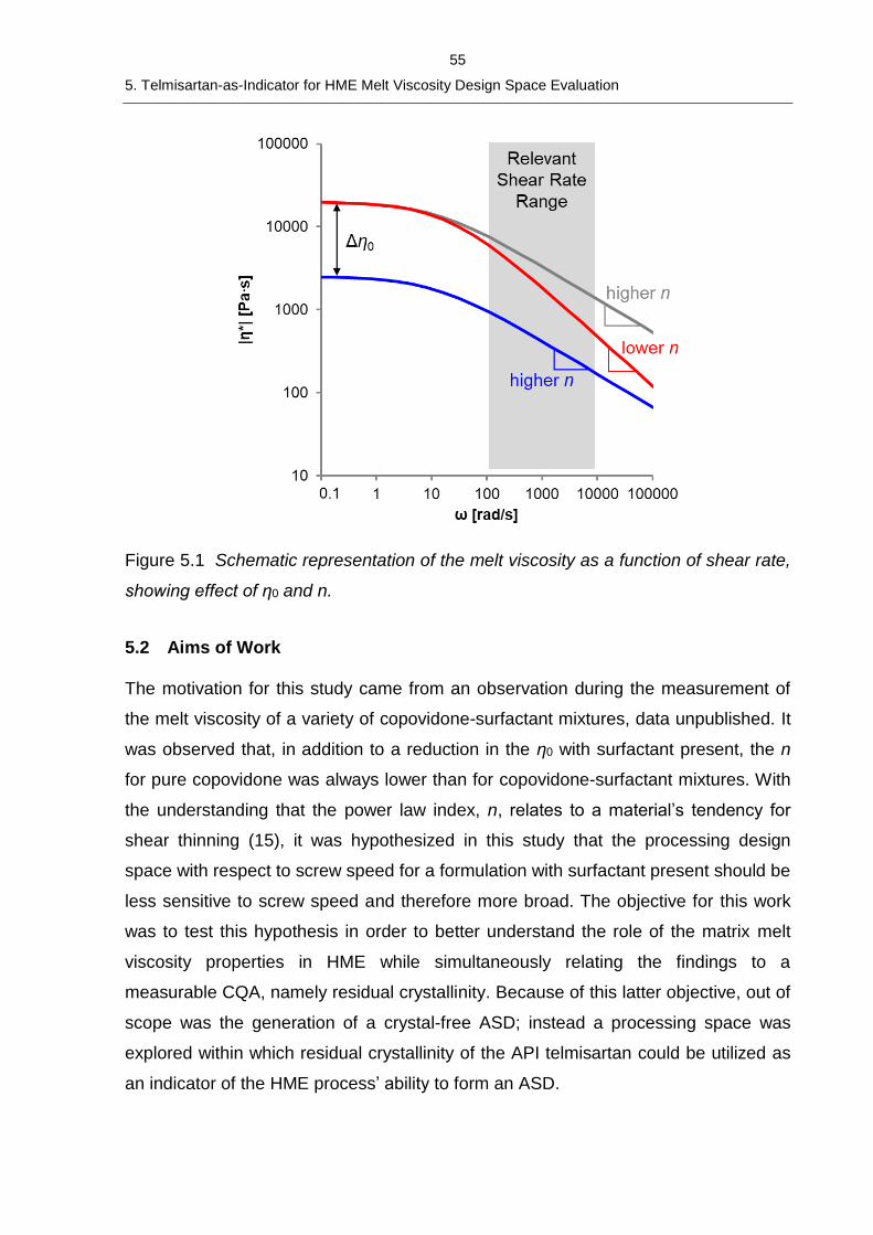
55
5. Telmisartan-as-Indicator for HME Melt Viscosity Design Space Evaluation
Figure 5.1 Schematic representation of the melt viscosity as a function of shear rate,
showing effect of η0 and n.
5.2 Aims of Work
The motivation for this study came from an observation during the measurement of
the melt viscosity of a variety of copovidone-surfactant mixtures, data unpublished. It
was observed that, in addition to a reduction in the η0 with surfactant present, the n
for pure copovidone was always lower than for copovidone-surfactant mixtures. With
the understanding that the power law index, n, relates to a material’s tendency for
shear thinning (15), it was hypothesized in this study that the processing design
space with respect to screw speed for a formulation with surfactant present should be
less sensitive to screw speed and therefore more broad. The objective for this work
was to test this hypothesis in order to better understand the role of the matrix melt
viscosity properties in HME while simultaneously relating the findings to a
measurable CQA, namely residual crystallinity. Because of this latter objective, out of
scope was the generation of a crystal-free ASD; instead a processing space was
explored within which residual crystallinity of the API telmisartan could be utilized as
an indicator of the HME process’ ability to form an ASD.
56
5. Telmisartan-as-Indicator for HME Melt Viscosity Design Space Evaluation
The reasons for focusing on residual crystallinity are two-fold. First, the primary
objective of solubility enhancement via the formation of an ASD is to break down the
crystal lattice and transform the crystalline API into an amorphous form. Second,
degradation of the API is also an important CQA, but as has been observed in a few
cases, this may not occur until the API has first dissolved (31,128). In addition, any
analysis of the solubility enhancement of the model API as a result of formation of an
amorphous form, as an ASD or not, was also out of scope, as this has already been
demonstrated (42,129,130). Along with the analysis of the rheological properties of
the model system, and in order to fully interpret the findings, the CQA results were
related back to the thermodynamic properties, that is, the temperature-dependent
API solubility phase diagram. Lastly, process simulation was used to gain access to
non-measurable processing characteristics for additional interpretation of the
findings.
5.3 Experiment Design
Two formulations containing 10 %w/w telmisartan, 0 or 5 %w/w polysorbate 80
(Tween® 80 or TW80), and copovidone (COP) were compared in these studies. The
experimental processing train is shown in Figure 5.2, more details in 7.2.2.2, with the
primary difference being pre-extrusion of the TW80 / COP matrix. Process
parameters for the laboratory extrusion experiment are listed in Table 5.1 and they
were also used for simulations for executing and validating the corresponding
Ludovic® model according to the method outlined in Figure 7.7. An expanded set of
processing conditions was simulated using the validated model (Table 5.2) to further
evaluate and compare the process design space as a function of formulation. To
supplement the study, a simulated sensitivity analysis of the effect of the rheological
parameters, n and η0 in the Carreau-Yasuda equation, on melt temperature as a
function of barrel temperature and screw speed was also performed (see section
7.2.6.3 for more details).
In all simulations in this chapter, the effect of screw speed on melt temperature
evolution was quantified by calculating the difference in maximum melt temperature,
ΔTmax, in this case corresponding with a position in the reverse kneading block, in red
color (Figure 5.3), between high and low screw speeds.
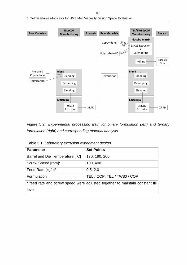
57
5. Telmisartan-as-Indicator for HME Melt Viscosity Design Space Evaluation
Figure 5.2 Experimental processing train for binary formulation (left) and ternary
formulation (right) and corresponding material analysis.
Table 5.1 Laboratory extrusion experiment design.
Parameter Set Points
Barrel and Die Temperature [°C] 170, 190, 200
Screw Speed [rpm]* 100, 400
Feed Rate [kg/h]* 0.5, 2.0
Formulation TEL / COP, TEL / TW80 / COP
* feed rate and screw speed were adjusted together to maintain constant fill
level
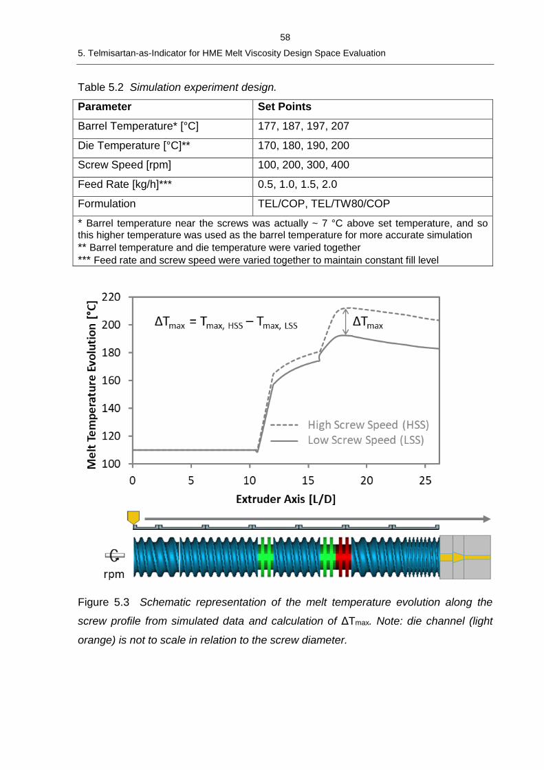
58
5. Telmisartan-as-Indicator for HME Melt Viscosity Design Space Evaluation
Table 5.2 Simulation experiment design.
Parameter Set Points
Barrel Temperature* [°C] 177, 187, 197, 207
Die Temperature [°C]** 170, 180, 190, 200
Screw Speed [rpm] 100, 200, 300, 400
Feed Rate [kg/h]*** 0.5, 1.0, 1.5, 2.0
Formulation TEL/COP, TEL/TW80/COP
* Barrel temperature near the screws was actually ~ 7 °C above set temperature, and so this higher temperature was used as the barrel temperature for more accurate simulation ** Barrel temperature and die temperature were varied together
*** Feed rate and screw speed were varied together to maintain constant fill level
Figure 5.3 Schematic representation of the melt temperature evolution along the
screw profile from simulated data and calculation of ΔTmax. Note: die channel (light
orange) is not to scale in relation to the screw diameter.
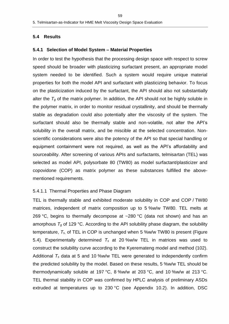
59
5. Telmisartan-as-Indicator for HME Melt Viscosity Design Space Evaluation
5.4 Results
5.4.1 Selection of Model System – Material Properties
In order to test the hypothesis that the processing design space with respect to screw
speed should be broader with plasticizing surfactant present, an appropriate model
system needed to be identified. Such a system would require unique material
properties for both the model API and surfactant with plasticizing behavior. To focus
on the plasticization induced by the surfactant, the API should also not substantially
alter the Tg of the matrix polymer. In addition, the API should not be highly soluble in
the polymer matrix, in order to monitor residual crystallinity, and should be thermally
stable as degradation could also potentially alter the viscosity of the system. The
surfactant should also be thermally stable and non-volatile, not alter the API’s
solubility in the overall matrix, and be miscible at the selected concentration. Non-
scientific considerations were also the potency of the API so that special handling or
equipment containment were not required, as well as the API’s affordability and
sourceability. After screening of various APIs and surfactants, telmisartan (TEL) was
selected as model API, polysorbate 80 (TW80) as model surfactant/plasticizer and
copovidone (COP) as matrix polymer as these substances fulfilled the above-
mentioned requirements.
5.4.1.1 Thermal Properties and Phase Diagram
TEL is thermally stable and exhibited moderate solubility in COP and COP / TW80
matrices, independent of matrix composition up to 5 %w/w TW80. TEL melts at
269 °C, begins to thermally decompose at ~280 °C (data not shown) and has an
amorphous Tg of 129 °C. According to the API solubility phase diagram, the solubility
temperature, Ts, of TEL in COP is unchanged when 5 %w/w TW80 is present (Figure
5.4). Experimentally determined Ts at 20 %w/w TEL in matrices was used to
construct the solubility curve according to the Kyeremateng model and method (102).
Additional Ts data at 5 and 10 %w/w TEL were generated to independently confirm
the predicted solubility by the model. Based on these results, 5 %w/w TEL should be
thermodynamically soluble at 197 °C, 8 %w/w at 203 °C, and 10 %w/w at 213 °C.
TEL thermal stability in COP was confirmed by HPLC analysis of preliminary ASDs
extruded at temperatures up to 230 °C (see Appendix 10.2). In addition, DSC
60
5. Telmisartan-as-Indicator for HME Melt Viscosity Design Space Evaluation
analysis of the extrudates with residual crystallinity shows the onset of the dissolution
process to initiate between 170-180 °C, indicated by the dissolution endotherm, data
not shown.
TEL had the tendency to anti-plasticize the COP or TW80 / COP matrix, but at the
10 %w/w concentration used, the effect is minimal or even negligible. The matrix
polymer, COP, had a dry Tg of 107 °C while the Tg of TEL was 129 °C. The
measured Tg of a 20 %w/w of TEL in COP was 108.5 °C. TEL exhibited a slight anti-
plasticizing effect on COP, however, at 10 %w/w drug load, this effect was negligible
as the Tg (107.8 °C) is close to that of COP. The Tg of the ternary system 20 %w/w
TEL / 5 %w/w TW80 / COP was 95 °C, slightly lower than the binary mixture,
indicating a plasticizing effect of the TW80. The Tg of the ternary system with
10 %w/w TEL / 5 %w/w TW80 / COP was 92 °C.
Figure 5.4. Phase diagram of telmisartan in copovidone with and without TW80. The
black line is the solubility curve and indicates the temperature at which a given
concentration of TEL is soluble in the polymer matrix. The red and blue lines indicate
the glass transition temperature as a function of the concentration of TEL in a COP
matrix or a 5 %w/w TW80 / COP matrix, respectively.
5.4.1.2 Blend Powder Properties
The blends were designed to be as identical as possible in terms of powder
properties so as to provide a similar environment into which the TEL could
incorporate and dissolve, albeit with different melt rheological properties. The
61
5. Telmisartan-as-Indicator for HME Melt Viscosity Design Space Evaluation
properties of the matrix considered were the bulk density, the particle size distribution
(PSD) and the moisture content and were kept constant (Table 5.3).
Table 5.3 Blend Powder Properties.
Formulation Blend Bulk
Density
[g/mL]
Matrix PSD Blend
Loss-on-Drying
[%]
d10 [µm] d50 [µm] d90 [µm]
10 %w/w TEL / COP 0.36 24.0 ± 0.4 79.3 ± 1.2 184 ± 1 0.86
10 %w/w TEL /
5 %w/w TW80 / COP
0.42 22.1 ± 0.3 81.3 ± 1.1 181 ± 0 1.26
5.4.1.3 Rheological Properties
Model Formulations
The melt viscosity as a function of angular frequency at a reference temperature of
170 °C of the two formulations, 10 %w/w TEL / COP and 10 %w/w TEL / 5 %w/w
TW80 / COP, shows the plasticizing effect of the TW80 in the TEL / TW80 / COP
formulation (Figure 5.5a), described and captured by the difference in η0, the zero-
shear rate viscosity (Table 5.4). For comparison, the melt viscosity profiles of pure
COP and a plasticizer / COP mixture (3 %w/w TEC / COP) are included. The Tg of
the 3 %w/w TEC / COP system was measured to be 95 °C, and this value was used
as an input value into the melt viscosity prediction model (110). The plasticization
effect by the surfactant TW80 was similar to that of a common plasticizer, TEC. The
melt viscosity for both TEL formulations is also a function of temperature (Figure
5.5b). The expected reduction in melt viscosity as temperature increases is seen for
three reference temperatures, 150 °C, 160 °C, and 170 °C.
Another potentially interesting behavior is the slight difference in shear-thinning
tendency, seen as the slope in the power law region of the melt viscosity profile and
described by the power law index, n. The power law index is higher for the
formulation with TW80 (Table 5.4), potentially indicating that this formulation is less
susceptible to shear thinning than the TEL / COP binary mixture. This observation
and its effect on melt temperature evolution is further explored via a sensitivity
analysis simulation study (see next sub-section). Other differences include the
variation of the Yasuda constant, a, and the characteristic time, λ, which is related to
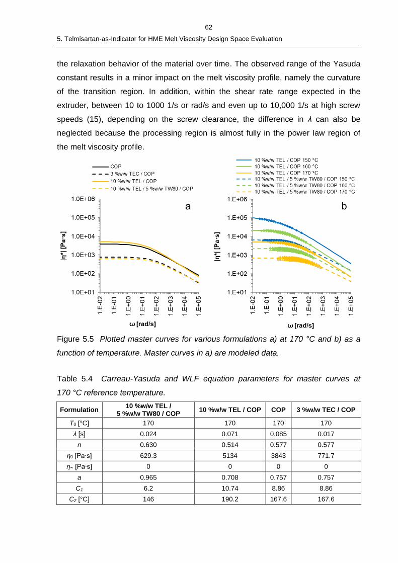
62
5. Telmisartan-as-Indicator for HME Melt Viscosity Design Space Evaluation
the relaxation behavior of the material over time. The observed range of the Yasuda
constant results in a minor impact on the melt viscosity profile, namely the curvature
of the transition region. In addition, within the shear rate range expected in the
extruder, between 10 to 1000 1/s or rad/s and even up to 10,000 1/s at high screw
speeds (15), depending on the screw clearance, the difference in λ can also be
neglected because the processing region is almost fully in the power law region of
the melt viscosity profile.
Figure 5.5 Plotted master curves for various formulations a) at 170 °C and b) as a
function of temperature. Master curves in a) are modeled data.
Table 5.4 Carreau-Yasuda and WLF equation parameters for master curves at
170 °C reference temperature.
Formulation 10 %w/w TEL /
5 %w/w TW80 / COP 10 %w/w TEL / COP COP 3 %w/w TEC / COP
T0 [°C] 170 170 170 170
λ [s] 0.024 0.071 0.085 0.017
n 0.630 0.514 0.577 0.577
η0 [Pa∙s] 629.3 5134 3843 771.7
η∞ [Pa∙s] 0 0 0 0
a 0.965 0.708 0.757 0.757
C1 6.2 10.74 8.86 8.86
C2 [°C] 146 190.2 167.6 167.6
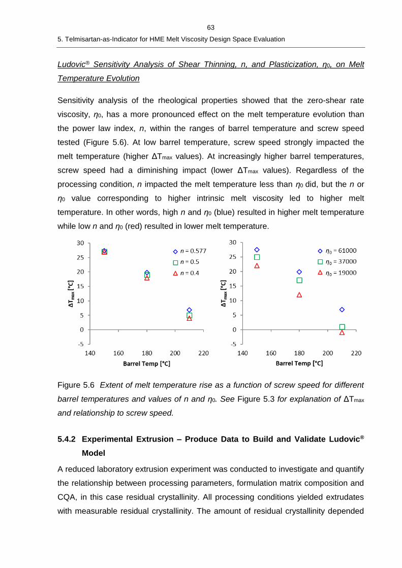
63
5. Telmisartan-as-Indicator for HME Melt Viscosity Design Space Evaluation
Ludovic® Sensitivity Analysis of Shear Thinning, n, and Plasticization, η0, on Melt
Temperature Evolution
Sensitivity analysis of the rheological properties showed that the zero-shear rate
viscosity, η0, has a more pronounced effect on the melt temperature evolution than
the power law index, n, within the ranges of barrel temperature and screw speed
tested (Figure 5.6). At low barrel temperature, screw speed strongly impacted the
melt temperature (higher ΔTmax values). At increasingly higher barrel temperatures,
screw speed had a diminishing impact (lower ΔTmax values). Regardless of the
processing condition, n impacted the melt temperature less than η0 did, but the n or
η0 value corresponding to higher intrinsic melt viscosity led to higher melt
temperature. In other words, high n and η0 (blue) resulted in higher melt temperature
while low n and η0 (red) resulted in lower melt temperature.
Figure 5.6 Extent of melt temperature rise as a function of screw speed for different
barrel temperatures and values of n and η0. See Figure 5.3 for explanation of ΔTmax
and relationship to screw speed.
5.4.2 Experimental Extrusion – Produce Data to Build and Validate Ludovic®
Model
A reduced laboratory extrusion experiment was conducted to investigate and quantify
the relationship between processing parameters, formulation matrix composition and
CQA, in this case residual crystallinity. All processing conditions yielded extrudates
with measurable residual crystallinity. The amount of residual crystallinity depended
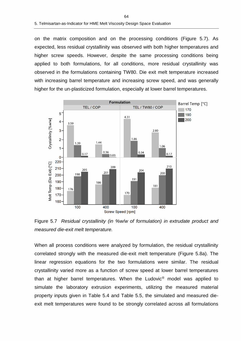
64
5. Telmisartan-as-Indicator for HME Melt Viscosity Design Space Evaluation
on the matrix composition and on the processing conditions (Figure 5.7). As
expected, less residual crystallinity was observed with both higher temperatures and
higher screw speeds. However, despite the same processing conditions being
applied to both formulations, for all conditions, more residual crystallinity was
observed in the formulations containing TW80. Die exit melt temperature increased
with increasing barrel temperature and increasing screw speed, and was generally
higher for the un-plasticized formulation, especially at lower barrel temperatures.
Figure 5.7 Residual crystallinity (in %w/w of formulation) in extrudate product and
measured die-exit melt temperature.
When all process conditions were analyzed by formulation, the residual crystallinity
correlated strongly with the measured die-exit melt temperature (Figure 5.8a). The
linear regression equations for the two formulations were similar. The residual
crystallinity varied more as a function of screw speed at lower barrel temperatures
than at higher barrel temperatures. When the Ludovic® model was applied to
simulate the laboratory extrusion experiments, utilizing the measured material
property inputs given in Table 5.4 and Table 5.5, the simulated and measured die-
exit melt temperatures were found to be strongly correlated across all formulations
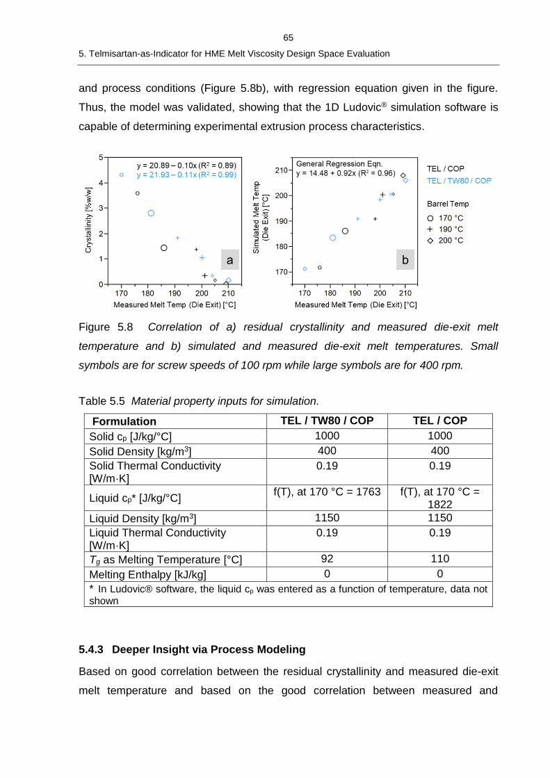
65
5. Telmisartan-as-Indicator for HME Melt Viscosity Design Space Evaluation
and process conditions (Figure 5.8b), with regression equation given in the figure.
Thus, the model was validated, showing that the 1D Ludovic® simulation software is
capable of determining experimental extrusion process characteristics.
Figure 5.8 Correlation of a) residual crystallinity and measured die-exit melt
temperature and b) simulated and measured die-exit melt temperatures. Small
symbols are for screw speeds of 100 rpm while large symbols are for 400 rpm.
Table 5.5 Material property inputs for simulation.
Formulation TEL / TW80 / COP TEL / COP
Solid cp [J/kg/°C] 1000 1000
Solid Density [kg/m3] 400 400
Solid Thermal Conductivity [W/m·K]
0.19 0.19
Liquid cp* [J/kg/°C] f(T), at 170 °C = 1763 f(T), at 170 °C =
1822
Liquid Density [kg/m3] 1150 1150
Liquid Thermal Conductivity [W/m·K]
0.19 0.19
Tg as Melting Temperature [°C] 92 110
Melting Enthalpy [kJ/kg] 0 0
* In Ludovic® software, the liquid cp was entered as a function of temperature, data not shown
5.4.3 Deeper Insight via Process Modeling
Based on good correlation between the residual crystallinity and measured die-exit
melt temperature and based on the good correlation between measured and
66
5. Telmisartan-as-Indicator for HME Melt Viscosity Design Space Evaluation
simulated die-exit melt temperatures, the validated Ludovic® model was used for
further process analysis. In addition, the model was applied to conduct a simulated
full-factorial experiment in order to fill in gaps in laboratory experimental data and
confirm observations about the design space.
5.4.3.1 Impact of Matrix Melt Viscosity on Maximum Melt Temperature
Process modeling enabled analysis of the melt temperature inside the extruder, in
particular the maximum melt temperature, which is a difficult quantity to measure via
typical temperature sensing methods (Figure 5.3). As was seen for the experimental
melt temperature at die exit, the simulated maximum melt temperature increased with
both increasing screw speed and increasing barrel temperature (Figure 5.9a). At a
screw speed of 400 rpm and barrel temperature of 200 °C, both formulations reached
simulated max temperatures greater than the solubility temperature of 10 %w/w TEL
in the matrix, 213 °C. It was at these same processing conditions that almost no
residual crystallinity was observed (Figure 5.7 and symbols marked with an
asterisk, *, Figure 5.9a). Little residual crystallinity, namely less than 0.5 %w/w, was
also observed for the TEL / COP formulation processed at barrel temperature of
190 °C and screw speed of 400 rpm as well as for both formulations processed at
barrel temperature of 200 °C but only 100 rpm screw speed. For the two formulations
extruded at 200 °C and 100 rpm, the maximum melt temperature was slightly below
the API solubility temperature. In comparison to the melt temperature measured at
die exit (Figure 5.7), a greater distinction can be made between the two formulations
in the maximum melt temperature in the extruder. Namely, for a given processing
condition, a higher maximum melt temperature was always observed for the un-
plasticized TEL / COP formulation. Furthermore, as was seen with the melt viscosity
parameter sensitivity analysis, the higher intrinsic melt viscosity formulation,
TEL / COP, reached higher melt temperatures within the same range of screw
speeds, independent of barrel temperature setting (Figure 5.9b). In addition, the
screw speed sensitivity ΔTmax was decreased for both formulations as barrel
temperature was increased, corroborating the observations that residual crystallinity
was less sensitive to changes in screw speed at higher temperatures.

67
5. Telmisartan-as-Indicator for HME Melt Viscosity Design Space Evaluation
Figure 5.9 Simulated maximum melt temperature (a) and extent of melt temperature
rise as a function of screw speed ΔTmax (b) for different barrel temperatures and
formulations. The API solubility temperature, Ts, for 10 %w/w TEL in the matrices is
designated in (a) and extrudates with less than 0.5 %w/w residual crystallinity are
indicated with an asterisk (*).
5.4.3.2 Simulated Full-Factorial Experiment and Impact of Rheology on Design
Space
The findings from the reduced laboratory extrusion experiment were supplemented
by a full-factorial simulated experiment. The melt temperature evolution, in particular
the range of maximum melt temperature as a function of screw speed, differs more
for the TEL / COP formulation than for the TEL / TW80 / COP formulation (Figure
5.10). The range of maximum melt temperature is broader for lower barrel
temperatures than higher barrel temperatures. In addition, the melt temperature
approaches the set barrel temperature at higher barrel temperatures, especially at
lower screw speeds and for the TEL / TW80 / COP formulation, e.g. at 200 °C.
According to the approach described in Figure 5.3, these effects were further
quantified by calculating the difference in maximum melt temperature between high
and low screw speeds, ΔTmax (Figure 5.11). As barrel temperature is increased, the

68
5. Telmisartan-as-Indicator for HME Melt Viscosity Design Space Evaluation
screw speed had less and less of an impact on temperature rise (Figure 5.11), as
also observed in the rheology sensitivity analysis study (Figure 5.6) and for the
simulations of the reduced experimental data set (Figure 5.9b). Especially in
comparison to the experimental data set, the results are the same except for the
addition of data simulated for barrel temperatures of 180 °C. In this representation, it
is clearly seen that the melt temperature rise is more sensitive to screw speed for the
TEL / COP formulation than for the TEL / TW80 / COP formulation.
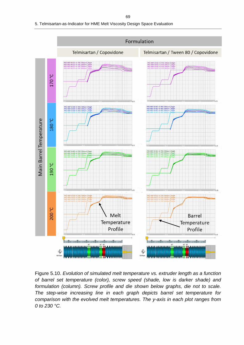
69
5. Telmisartan-as-Indicator for HME Melt Viscosity Design Space Evaluation
Figure 5.10. Evolution of simulated melt temperature vs. extruder length as a function
of barrel set temperature (color), screw speed (shade, low is darker shade) and
formulation (column). Screw profile and die shown below graphs, die not to scale.
The step-wise increasing line in each graph depicts barrel set temperature for
comparison with the evolved melt temperatures. The y-axis in each plot ranges from
0 to 230 °C.
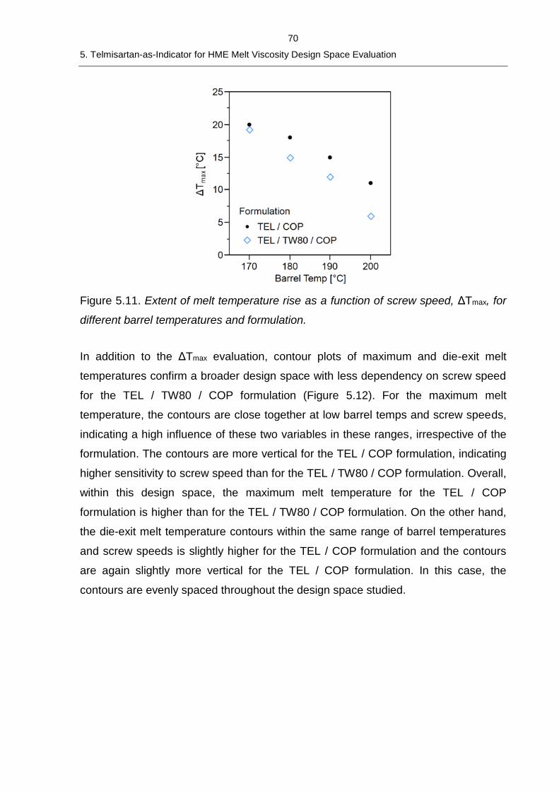
70
5. Telmisartan-as-Indicator for HME Melt Viscosity Design Space Evaluation
Figure 5.11. Extent of melt temperature rise as a function of screw speed, ΔTmax, for
different barrel temperatures and formulation.
In addition to the ΔTmax evaluation, contour plots of maximum and die-exit melt
temperatures confirm a broader design space with less dependency on screw speed
for the TEL / TW80 / COP formulation (Figure 5.12). For the maximum melt
temperature, the contours are close together at low barrel temps and screw speeds,
indicating a high influence of these two variables in these ranges, irrespective of the
formulation. The contours are more vertical for the TEL / COP formulation, indicating
higher sensitivity to screw speed than for the TEL / TW80 / COP formulation. Overall,
within this design space, the maximum melt temperature for the TEL / COP
formulation is higher than for the TEL / TW80 / COP formulation. On the other hand,
the die-exit melt temperature contours within the same range of barrel temperatures
and screw speeds is slightly higher for the TEL / COP formulation and the contours
are again slightly more vertical for the TEL / COP formulation. In this case, the
contours are evenly spaced throughout the design space studied.
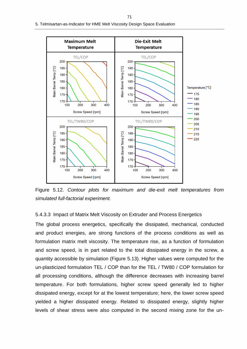
71
5. Telmisartan-as-Indicator for HME Melt Viscosity Design Space Evaluation
Figure 5.12. Contour plots for maximum and die-exit melt temperatures from
simulated full-factorial experiment.
5.4.3.3 Impact of Matrix Melt Viscosity on Extruder and Process Energetics
The global process energetics, specifically the dissipated, mechanical, conducted
and product energies, are strong functions of the process conditions as well as
formulation matrix melt viscosity. The temperature rise, as a function of formulation
and screw speed, is in part related to the total dissipated energy in the screw, a
quantity accessible by simulation (Figure 5.13). Higher values were computed for the
un-plasticized formulation TEL / COP than for the TEL / TW80 / COP formulation for
all processing conditions, although the difference decreases with increasing barrel
temperature. For both formulations, higher screw speed generally led to higher
dissipated energy, except for at the lowest temperature; here, the lower screw speed
yielded a higher dissipated energy. Related to dissipated energy, slightly higher
levels of shear stress were also computed in the second mixing zone for the un-
72
5. Telmisartan-as-Indicator for HME Melt Viscosity Design Space Evaluation
plasticized formulation (data not shown). The specific mechanical energy showed the
same relationships to the processing conditions and formulations as the total
dissipated energy and was generally higher for the TEL / COP formulation.
For both formulations, the total conducted energy became more positive with
increasing barrel temperatures. For a given processing condition, the total conducted
energy was much lower for the TEL / COP formulation than for the
TEL / TW80 / COP formulation. At roughly 200 °C barrel temperature, the total
conducted energy for the TEL / COP formulation approached 0 kJ/kg, indicated by a
darker gray horizontal line in the third row of plots, while the total conducted energy
approached 0 kJ/kg at lower barrel temperature for the TEL / TW80 / COP
formulation (180 to 190 °C). Negative values for the total conducted energy indicate
barrel cooling will be required while positive values indicate that the barrels will need
to heat the product. The total conducted energy for the TEL / COP formulation also
showed a temperature-dependent effect for screw speed, as indicated by the cross-
over point around 180 °C in the plots for total dissipated energy, specific mechanical
energy and again total conducted energy. Within the temperature range studied, the
TEL / TW80 / COP formulation showed a straightforward relationship with screw
speed: higher screw speeds lead to more negative values of total conducted energy.
The total product energy (TPE), a global value equivalent to the sum of the specific
mechanical energy and the total conducted energy, was nearly the same for both
formulations, increasing with increasing barrel temperature and increasing screw
speed (4th row of plots in Figure 5.13). When the two formulations were considered
independently, the total product energy correlated well with the residual crystallinity,
with both regression equations yielding high r2 values (0.89 for un-plasticized and
0.98 for plasticized) (Figure 5.14). The residual crystallinity decreased as more
energy was applied. However, for the same level of TPE, the amount of residual
crystallinity was slightly higher for the TEL / TW80 / COP formulation.
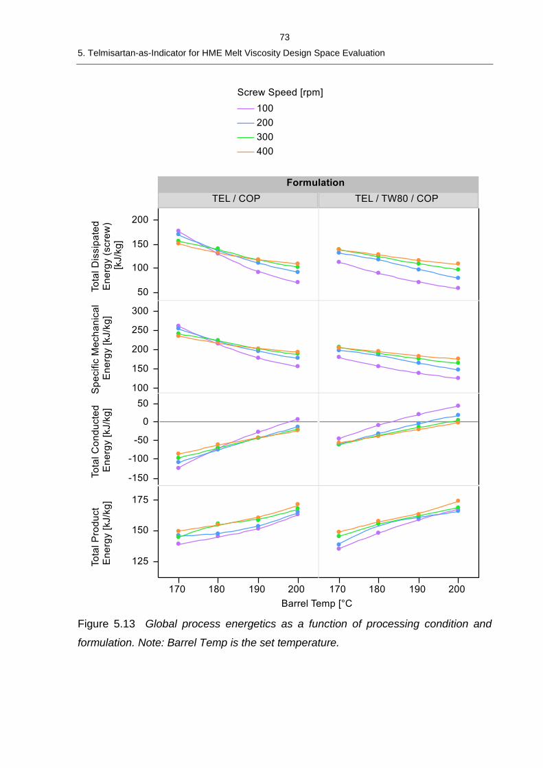
73
5. Telmisartan-as-Indicator for HME Melt Viscosity Design Space Evaluation
Figure 5.13 Global process energetics as a function of processing condition and
formulation. Note: Barrel Temp is the set temperature.
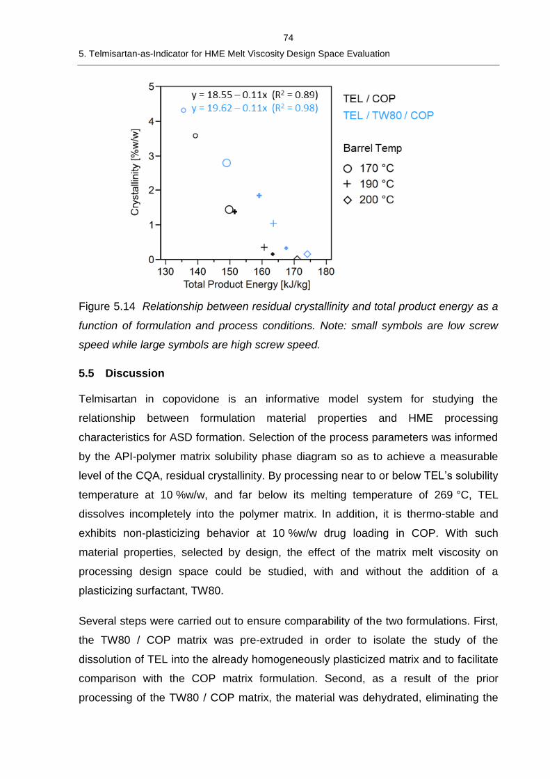
74
5. Telmisartan-as-Indicator for HME Melt Viscosity Design Space Evaluation
Figure 5.14 Relationship between residual crystallinity and total product energy as a
function of formulation and process conditions. Note: small symbols are low screw
speed while large symbols are high screw speed.
5.5 Discussion
Telmisartan in copovidone is an informative model system for studying the
relationship between formulation material properties and HME processing
characteristics for ASD formation. Selection of the process parameters was informed
by the API-polymer matrix solubility phase diagram so as to achieve a measurable
level of the CQA, residual crystallinity. By processing near to or below TEL’s solubility
temperature at 10 %w/w, and far below its melting temperature of 269 °C, TEL
dissolves incompletely into the polymer matrix. In addition, it is thermo-stable and
exhibits non-plasticizing behavior at 10 %w/w drug loading in COP. With such
material properties, selected by design, the effect of the matrix melt viscosity on
processing design space could be studied, with and without the addition of a
plasticizing surfactant, TW80.
Several steps were carried out to ensure comparability of the two formulations. First,
the TW80 / COP matrix was pre-extruded in order to isolate the study of the
dissolution of TEL into the already homogeneously plasticized matrix and to facilitate
comparison with the COP matrix formulation. Second, as a result of the prior
processing of the TW80 / COP matrix, the material was dehydrated, eliminating the
75
5. Telmisartan-as-Indicator for HME Melt Viscosity Design Space Evaluation
plasticizing effect of moisture. Correspondingly, the COP raw material was also
dehydrated. By dehydrating both matrices, the melt rheological behavior was
simplified and made to be more similar with the material measured with the
rheometer; in fact, rheological studies are most reliable when performed in the
absence of water, especially in the temperature regions of interest here. Third, the
pre-extruded TW80 / COP matrix was milled to similar particle size distribution as the
raw COP material with the intention of maintaining blend bulk density and therefore
fill volume in the extruder constant. Further studies are needed to determine if these
precautions were absolutely necessary.
One of the goals of this study was to evaluate the significance of melt rheology, in
particular the plasticization and apparent shear thinning behavior of a surfactant, on
ASD formation. The formation of the ASD, namely the dissolution of the API, as
measured by residual crystallinity, is a function of the independent process
parameters, e.g. barrel temperature, screw speed, feed rate, as well as the resultant
process performance, e.g. product temperature, melt viscosity, shear rate. However,
the process performance is in turn dependent on the properties of the material being
processed, e.g. matrix melt viscosity. These inter-dependent relationships were
simultaneously considered using process simulation.
First, simulation was used to investigate the sensitivity of the melt temperature rise as
a function of screw speed and barrel temperature for materials with different
rheological characteristics, η0 and n. As mentioned in the introduction to this chapter,
these parameters can vary for different material compositions and, depending on the
shear rate range of the process, either or both of these parameters can influence the
resulting melt viscosity. However, the results indicated that the overall plasticization
described by η0 is the dominating factor (Figure 5.6). Within the shear rate range
explored, the melt viscosity profile essentially shifts vertically along the melt viscosity
axis, with η0 exhibiting a greater shift than n (Figure 5.1, Figure 5.5). While intrinsic
shear thinning behavior described by n does contribute to melt viscosity reduction,
decreased viscous dissipation and therefore lower heat rise, it was less substantial in
this case. However, HME process simulations can and should be used to evaluate
the relative significance of the melt viscosity parameters in other systems as well.
This example also highlights the applicability of the model developed by the working
76
5. Telmisartan-as-Indicator for HME Melt Viscosity Design Space Evaluation
group of K.G. Wagner to estimate melt viscosity by a straightforward Tg
measurement (80,81,110), but also that further work is needed to extend the model
for matrices which exhibit different non-Newtonian behavior.
Second, simulation was used to retrospectively gain insight into the experimental
results. After validating the model by obtaining correlation between the measured
and simulated die-exit melt temperatures, the additional results that only simulation
can produce, maximum melt temperature and the process energetics, were
correlated with the CQA, residual crystallinity. In this way, process conditions and
material properties were again simultaneously taken into consideration. Through
analysis of the ΔTmax and contour diagrams, melt temperature rise as a function of
formulation melt viscosity, barrel temperature and screw speed showed that the
design space as a function of screw speed is broader for the plasticized formulation.
In this study, this behavior was shown with TW80 as a surfactant in COP, and in a
related publication, the same behavior with a sorbitan monolaurate (Span® 20)-COP
system was observed (119). Further, the narrow spacing of the maximum melt
temperature contours in the low temperature and low screw speed region (Figure
5.12) corroborates the finding that the residual crystallinity is a strong function of
screw speed at low temperatures (Figure 5.8a). Additional analysis of the die-exit
melt temperature contour diagrams, along with the measured melt temperature
(Figure 5.7 & Figure 5.8), highlights the insufficiency of correlating the absolute
residual crystallinity with die-exit melt temperature. The total product energy, which
along with the die-exit melt temperature, showed strong correlation with residual
crystallinity, was also insufficient for explaining the difference in residual crystallinity
between the two formulations. By the time that the melt reaches the die-exit, it may
experience heat loss to the barrels if they are set to lower values. Albeit the use of
this value for validating the model, this method, although imperfect, was the most
feasible option and utilized the most accessible experimentally measurable value, the
melt temperature via IR sensor. Additional work to develop better methods for
measuring the melt temperature, perhaps in a highly-filled zone such as a mixing
element, are certainly justified and would improve model validation.
Despite the method of validation of the model using the die-exit melt temperature,
simulation further revealed that the maximum melt temperature within the extruder
77
5. Telmisartan-as-Indicator for HME Melt Viscosity Design Space Evaluation
was found to strongly correlate with residual crystallinity. Residual crystallinity
approached zero as the simulated maximum melt temperature was close to the
solubility temperature given by the API solubility phase diagram for the given drug
loading, differentiating between the formulations with differing intrinsic melt viscosity
(Figure 5.9). As Moseson and Taylor recently described theoretically and
demonstrated practically using a small conical twin-screw extruder, the
thermodynamics and use of API-polymer matrix phase diagrams clearly and
scientifically explain the requirement of reaching the solubility temperature for
achieving a crystal-free ASD (48). This argumentation of thermodynamic driving force
for dissolution, the API solubility temperature, also explains the strong correlation
between residual crystallinity, maximum melt temperature and the greater degree of
TEL dissolution into the matrix for the un-plasticized TEL / COP formulation.
However, it is not the only possible explanation, as kinetics is also a driving force for
dissolution. As several authors have discussed previously, application of the Noyes-
Whitney equation, equation 5.1, can phenomonologically elucidate the impact of
temperature, screw speed and melt viscosity on the rate of API dissolution into a
polymer matrix (7,26,48,131–133):
𝑑𝐶
𝑑𝑡=
𝐷𝐴(𝐶𝑠−𝐶)
ℎ𝑉 (5.1)
where C is the concentration of the API dissolved in the polymer matrix at a given
time t, D is the diffusion coefficient, A is the surface area of API particles suspended
in the polymer matrix, Cs is the saturation solubility of the drug at a given
temperature, h is the diffusion boundary layer thickness, and V is the volume of the
molten polymer phase. The diffusion coefficient can be expressed by equation 5.2,
the Stokes-Einstein equation (134):
𝐷 = 𝑘𝐵𝑇
6𝜋𝜂𝑟 (5.2)
where kB is the Boltzmann constant, T is the temperature, η is the melt viscosity and r
is the particle radius.
78
5. Telmisartan-as-Indicator for HME Melt Viscosity Design Space Evaluation
An increase in matrix temperature, regardless of the source, e.g. conduction from
barrels warmer than the melt or from viscous dissipation, will increase the saturation
solubility of the API and therefore the dissolution rate; this saturation solubility value
is equivalent to the solubility temperature given in the phase diagram. In this study,
the temperature rise, locally in the 2nd mixing zone, was higher for the formulation
with higher intrinsic melt viscosity due to pronounced viscous dissipation. This heat
rise was enough to increase the saturation solubility and induce more dissolution of
the API in the un-plasticized system. However, at increasingly high barrel
temperatures, the differences observed between the two formulations in maximum
melt temperature and viscous dissipation diminished. These results were a direct
reflection of the increasing similarity of the measured melt temperature and residual
crystallinity between the two formulations at higher barrel temperatures. In addition,
an increase in matrix temperature, either by conduction from the barrels or melt
temperature rise from viscous dissipation will lead to an increase in the diffusion
coefficient.
Further, a decrease in melt viscosity, from higher process set temperatures,
increased shear rate, intrinsic matrix melt viscosity by incorporation of a plasticizer, or
over time as a plasticizing API dissolves into the matrix (19,39,41,135) will also lead
to a higher diffusion coefficient. Changing melt viscosity as a function of API
dissolution was not a factor in this study because the API and matrix properties, as
well as drug loading, were selected to minimize this potential effect. Conversely, an
increase in melt viscosity, perhaps from the use of lower process set temperatures,
lower shear rate or even anti-plasticization by APIs with amorphous Tg greater than
that of the matrix, will decrease the diffusion coefficient, but can also lead to an
increase in viscous dissipation, and therefore temperature rise and increased
diffusion coefficient. Interestingly, this phenomenon is exemplified by the discrepancy
in dissipated energy for the un-plasticized formulation at 100 rpm and 170 °C (Figure
5.13) in which the highest dissipated energy condition did not directly translate into
the highest melt temperature or lowest observed residual crystallinity. Here, the shear
rate and melt temperature were so low that insufficient shear thinning occurred,
resulting in a high value for melt viscosity, leading to higher dissipated energy.
However, this high viscous dissipation was not enough to overcome the predominant
79
5. Telmisartan-as-Indicator for HME Melt Viscosity Design Space Evaluation
effect of temperature control by conduction from the barrels at this temperature
setting. In addition, at this processing setting, the feed rate was relatively low, leading
to longer residence times and correspondingly more time for melt temperature to
equilibrate with that of the barrel wall. This type of result, highlighting different heat
generation phenomena in different processing regimes, proves the value of process
simulation due to consideration of all relationships between relevant material property
and process parameter inputs simultaneously. Despite these inter-dependent
relationships, the simulated maximum melt temperature still correlated with the CQA
residual crystallinity. Furthermore, a low barrel temperature setting of 170 °C was not
able to reduce the risk of temperature rise of the melt due to viscous dissipation,
especially in the non-plasticized formulation. Not only was the melt temperature too
low to dissolve the API, the amount dissolved was more dependent on screw speed
at this low temperature, narrowing the design space. Therefore, it is more desirable
to operate at low melt viscosities so as to widen the design space with respect to
screw speed.
Higher shear rate can reduce the boundary layer thickness, inherently a function of
melt viscosity, decrease the melt viscosity due to shear thinning, and decrease the
local concentration of dissolved API near a particle surface via distributive mixing,
leading to a higher local concentration gradient at the particle surface, all of which will
increase the diffusion coefficient. Some of these effects are supported by the
experimental results, in particular the variation of screw speed. In addition, higher
shear rate, especially at high melt viscosity, can lead to higher shear stress and
greater dispersive mixing (99). In this study, slightly higher levels of shear stress
computed for the un-plasticized formulation may have contributed to breaking up
potential aggregates of the fine TEL primary particles, which would have increased
the area of contact between API particles and polymer matrix, and therefore
increasing the dissolution rate (99,133). Alternatively, increased distributive mixing
can homogenize the melt temperature, caused simply by a higher number of
expansion and contraction events at higher screw speeds (15,99). This effect can
lead to either increasing or decreasing local temperature gradients within the melt,
which could both increase or decrease the dissolution rate.
80
5. Telmisartan-as-Indicator for HME Melt Viscosity Design Space Evaluation
A large specific surface area of the API and smaller particle size will lead to
increased dissolution rates. This effect was shown by Li, et.al., in which the smaller of
two acetaminophen API batches led to overall more API dissolved via faster
dissolution rates (33).
The impact of the overall process time, that is residence time, and another aspect of
the kinetics, can be inferred, as it was not independently varied. Longer residence
time in the extruder can also lead to more observed dissolution. In this study, for a
given combination of feed rate and screw speed, the residence time should not be a
strong function of formulation due to similar bulk density and therefore fill level. On
the other hand, the residence time would have been shorter as a consequence of
increasing feed rate proportionally to screw speed in order to maintain fill ratio for all
conditions, consistent with published RTD characteristics for TSEs (136,137).
However, more residual crystallinity was observed with low feed rates, i.e. long
residence times, and therefore this cannot be the dominating factor for dissolution of
TEL. Of course, a separate study in which the temperature and residence time are
independently varied could be performed to confirm this inference.
Despite the complex interdependent and simultaneously evolving relationships
between all of the independent process and formulation parameters (e.g. screw
speed, barrel temperature, feed rate, screw configuration, material properties) and
process variables (e.g. melt temperature, shear rate, melt viscosity, residence time),
which can in part be accounted for by use of process simulation, the strongest
evidence for less observed residual crystallinity in the un-plasticized formulation is
the generally higher material temperature. After all, the residual crystallinity
approached 0 %w/w when the simulated maximum melt temperature reached the
solubility temperature. For more dramatically evolving systems, for example when the
API itself is a strong plasticizer for the matrix, process modeling may help to explain
complex processing behavior. However, the same challenges as those mentioned by
Vergnes and Berzin for modeling reactive extrusion will also apply to pharmaceutical
HME (138) and will need to be addressed.
While the TW80 certainly exhibited the typical behavior of a plasticizer, that is
decreasing the Tg and therefore overall melt viscosity profile, it also widened the
81
5. Telmisartan-as-Indicator for HME Melt Viscosity Design Space Evaluation
design space with respect to screw speed. This behavior offers an additional
justification for including a surfactant in an ASD formulation; beyond improving
bioavailability enhancement (45), the surfactant can improve processability. Of
course, traditional plasticizers are typically advised for decreasing the processing
temperature to avoid high temperatures which could lead to API or polymer
degradation. However, this study shows that this would not help to achieve complete
dissolution due to lack of a thermodynamic driving force, as has also been suggested
by others (26,48). Instead, process conditions must induce a melt temperature which
reaches the solubility temperature for the given drug load.
Any plasticization must also be considered in the context of the impact it can have on
product stability. Reduction in the Tg will lead to greater molecular mobility which can
induce recrystallization (65,139–141). On the other hand, rather than having a
destabilizing effect, Ghebremeskel, et.al., showed that plasticizing surfactants can
increase the physical stability (121). They reasoned that the solubility of API in the
polymer matrix could increase due to positive intermolecular interactions or that
greater homogeneity was achieved via better mixing in the extruder in a plasticized
matrix. However, by design, this was not the case in this system as TEL’s solubility in
COP was unaffected by 5 %w/w TW80. In addition, the reduced Tg of the TW80
formulation in this study does not indicate an explanation for higher residual
crystallinity. The potential for recrystallization at 10 %w/w TEL is low because the
formulation Tg is 92 °C, well above the recommended 50 °C above room temperature
(142). In addition, the pure drug substance does not recrystallize from the amorphous
state upon re-heating (data not included, see Lepek, et.al. (129)).
Last but not least, the simulated global process energetics generated insightful
results which are difficult to obtain experimentally. While the specific mechanical
energy can be measured, it is highly reliant on accurate measurement of torque,
which can be error-prone due to energy loss between the gear box and the shafts.
The conducted energy can also be estimated for a process, but it is again
challenging as not all extruders are configured to access relevant heating and cooling
signals and due to inaccessible measures of melt surface area contact with the
barrels, for example. Therefore, there are advantages to using process simulation to
obtain a comprehensive picture of the process energetics. The viscous dissipated
82
5. Telmisartan-as-Indicator for HME Melt Viscosity Design Space Evaluation
energy, specific mechanical energy and total conducted energy all accounted for the
differences between the two formulations, especially as a function of process
conditions. According to the analysis by Zecevic, et.al., a total conducted energy of
zero is a predictor of a quasi-adiabatic process (22). By comparing formulation
matrices with differing degrees of plasticization, it is apparent that the processing
conditions at which a given formulation will produce a quasi-adiabatic state are highly
dependent on the matrix melt viscosity, as suggested in the literature (143). The
results indicate that the quasi-adiabatic point can be achieved at lower temperatures
for the plasticized formulation, and a quantitative, rather than qualitative, estimate is
provided by simulation. In this study, because the extruder was not yet configured to
collect and record heating and cooling events, it was not possible to confirm this
observation experimentally. The lower-temperature quasi-adiabatic point could be
beneficial for formulations in which thermal degradation is a concern and for which
scaling needs to be performed. The advantage of an adiabatic process is that if little
or no cooling or heating is required, scaling should be more straightforward and less
dependent on the differing conducting surface area to volume ratio, which decreases
with increasing extruder diameter. This idea is explored further in Chapter 6. In
addition, as mentioned previously, the global total product energy, although it
correlated with the residual crystallinity, was not sufficient to explain the difference
between the two formulations; only analysis of the maximum melt temperature fully
explained the difference in the extent of telmisartan dissolution.
5.6 Conclusions
Like the torasemide indicator system, telmisartan in copovidone is an informative
model system for the study of HME QbD. It enabled the comprehensive evaluation of
the relationship between formulation material properties and HME processing
characteristics for ASD formation. Due to its high solubility temperature and non-
plasticizing characteristic in copovidone-based polymer matrices at a concentration
of 10 %w/w, the plasticizing effect of a common surfactant on the HME process and
the residual crystallinity CQA could be isolated and studied. While surfactants are
commonly selected to enhance the bioavailability of a drug substance, it was found
that the plasticizing behavior of polysorbate 80 broadened the processing design
space with respect to screw speed. Also, while plasticizers are commonly
83
5. Telmisartan-as-Indicator for HME Melt Viscosity Design Space Evaluation
incorporated to reduce the processing temperature, it was also found that by doing
so in the case of TEL with a high API solubility temperature, the complete formation
of the ASD is hindered; complete reduction of residual crystallinity is only possible if
the melt temperature reaches the thermodynamic solubility temperature. Therefore, a
temperature increase in kneading blocks due to viscous dissipation generated by a
highly viscous melt was required to achieve a fully amorphous system. Process
simulations, in which matrix melt viscosity, screw speed and barrel temperature were
varied, enabled simultaneous consideration of the complex inter-dependent
relationships inherent to HME, namely those between formulation material properties,
independent process parameters, and process dependent variables such as melt
temperature and melt viscosity and their impact on the CQA residual crystallinity. In
this way, the measured melt temperature and simulated maximum melt temperature
were correlated with residual crystallinity, differentiating the process behavior
between plasticized and un-plasticized matrices.
84
6. Quasi-Adiabatic Scaling with Telmisartan Indicator System and Process Modeling
6 Application of Telmisartan Indicator System and Process
Modeling to Study Scaling of a Quasi-Adiabatic Pharmaceutical
HME Process
6.1 Introduction
The optimization of the energy usage of an extrusion process, particularly in plastics
compounding, but also food extrusion, has been the subject of research for many
years. Due to the emerging importance of single screw extrusion for plastics
processing in the middle of the 20th century, and following the development of models
to better understand the process, the first theoretical analysis of adiabatic extrusion
for a single screw extruder was published in 1954 (143). Plastics processing by
extrusion is typically performed at large scale, e.g. up to 420 mm diameter extruders
with throughputs of up to 125,000 kg/h for a twin-screw extruder. At such large
scales, energy conservation is of high interest and improvements can be achieved
following simple guidelines (144,145). Despite commercial pharmaceutical products
being manufactured on much smaller extruders ranging in diameter from 27 to
70 mm, it is of interest to study the applicability to pharmaceutical extrusion, in
particular if it is feasible for common pharmaceutical materials and if the required
product quality can still be achieved given the reactive nature of the formation of an
ASD.
Extruder operation, in terms of heat generation and heat transfer, has been
categorized as either autogenous or isothermal (146). Autogenous or near adiabatic
operation takes place when no heating or cooling of the barrels occurs because
enough thermal energy is generated by mechanical work from the screws turning and
shearing the processed material. Isothermal operation denotes that heating or
cooling from the barrels maintains the temperature of the product.
Isothermal operation can be appropriate for low melt viscosity materials, if a material
is fed pre-molten, or if the fill volume is low. However, isothermal processing of
viscous materials is not practical, especially when high throughput is desired for
which a high screw speed is needed in order to maintain a suitable fill level in the
extruder barrel. Due to the viscous nature of polymeric materials, polymers will
85
6. Quasi-Adiabatic Scaling with Telmisartan Indicator System and Process Modeling
generate heat from the mechanical energy imparted by turning of the screws,
referred to as viscous dissipation (143). Further, because polymers are thermally
insulating materials, heating or cooling them in temperature-jacketed containers is
also not practical due to low thermal conductivity (16,145).
For pharmaceutical production, as in other types of polymer processing (143), the
material is fed as a solid, and therefore a certain amount of thermal conduction from
the barrels helps to facilitate the transition from solid to melt. As a result, the process
combines both isothermal and autogenous characteristics, and therefore the term
quasi-adiabatic is used. The exact quasi-adiabatic point depends on formulation melt
viscosity, extruder design and screw speed (143). Depending on the material
rheological properties and the thermal and energy efficiency requirements for a given
product and process, the ideal combination of all factors may be difficult to identify,
as was noted for single screw extrusion of pure polymers (147,148). It may also be
challenging to identify the exact adiabatic point if a formulation’s melt viscosity is
changing as a function of composition, for example if an API highly-plasticizes the
surrounding matrix.
In addition to achieving an energetically optimized process, scaling of a process
which is also energetically balanced is of interest. If quasi-adiabatic extrusion can be
achieved for a given formulation, it may be advantageous or easier to scale the
process. For example, if the mechanical energy per amount of material remains
constant across scales, the product temperature may also remain constant, and if the
barrel temperatures are simply selected to be similar to the temperature profile of the
melt along the screw, then key geometric differences between scales such as the
difference in surface area to volume ratio may not be important. On the other hand,
an energetically unbalanced situation may be one in which the melt temperature is
higher than the barrel temperature due to considerably higher mechanical energy on
the larger scale and the reduced barrel surface area may not be sufficient to cool the
melt. Further, heat transfer between melt and barrel, particularly in the screw
channel, is inefficient due to the insulating nature of the polymeric material as well as
short contact time (149). Alternatively, regardless of scale, if the melt temperature is
lower than the barrel temperature, local hot spots may form high thermal gradients
near the barrel walls (143). Both types of energetically unbalanced situations could
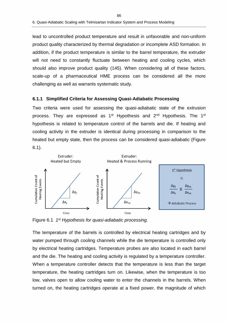
86
6. Quasi-Adiabatic Scaling with Telmisartan Indicator System and Process Modeling
lead to uncontrolled product temperature and result in unfavorable and non-uniform
product quality characterized by thermal degradation or incomplete ASD formation. In
addition, if the product temperature is similar to the barrel temperature, the extruder
will not need to constantly fluctuate between heating and cooling cycles, which
should also improve product quality (145). When considering all of these factors,
scale-up of a pharmaceutical HME process can be considered all the more
challenging as well as warrants systematic study.
6.1.1 Simplified Criteria for Assessing Quasi-Adiabatic Processing
Two criteria were used for assessing the quasi-adiabatic state of the extrusion
process. They are expressed as 1st Hypothesis and 2nd Hypothesis. The 1st
hypothesis is related to temperature control of the barrels and die. If heating and
cooling activity in the extruder is identical during processing in comparison to the
heated but empty state, then the process can be considered quasi-adiabatic (Figure
6.1).
Figure 6.1 1st Hypothesis for quasi-adiabatic processing.
The temperature of the barrels is controlled by electrical heating cartridges and by
water pumped through cooling channels while the die temperature is controlled only
by electrical heating cartridges. Temperature probes are also located in each barrel
and the die. The heating and cooling activity is regulated by a temperature controller.
When a temperature controller detects that the temperature is less than the target
temperature, the heating cartridges turn on. Likewise, when the temperature is too
low, valves open to allow cooling water to enter the channels in the barrels. When
turned on, the heating cartridges operate at a fixed power, the magnitude of which
87
6. Quasi-Adiabatic Scaling with Telmisartan Indicator System and Process Modeling
can depend on the scale and vendor. For cooling power, the temperature of the
water can be adjusted, as well as frequency and duration of valve opening. The
primary control, however, of heating and cooling is the length of time, also called the
impulse, for which the cartridges are on or the valves are open. These times are
regulated by the temperature controller, typically operating under PID logic (150).
This type of signal has been used successfully to monitor the energetics of single
screw extrusion (16).
Heating and cooling activity is described by the controller output, expressed either as
a percentage value in the range of -100% to 100%, with positive values indicating
heating and negative values indicating cooling, or as the slope of the cumulative
count of heating or cooling events over time. Actually, the former is in fact derived
from the latter. A value of 100% or -100% indicates that the heating cartridges are on
at all times or that the water valves are open at all times, respectively. Intermediate
controller output values indicate periodic turning on and off or opening and closing.
When expressed as a slope, a slope of zero indicates no activity while a steeper
slope indicates many impulses of activity and for long periods of time. For the
extruders used in this study, the 40 mm extruder (ZSK40) controller output was
expressed as a percentage while the 18 mm extruder (ZSK18) controller output was
expressed as a slope. For the ZSK18, separate signals were produced for heating
and cooling. As an approximation, when both were active, the slope of cooling line
was subtracted from the slope of the heating line. In summary, the process is
considered quasi-adiabatic if the percentage value of the controller output or the
slope of the controller output is identical between the “heated but empty” and “heated
and process running” states.
A notable complicating factor is that extruders are composed of many independently
temperature-controlled zones, all of which ideally should meet the 1st Hypothesis
criteria. In addition, in the “heated and process running” state, heat is generated by
viscous dissipation inside the screw channel, leading to an additional heat source. In
reality, it is challenging to achieve a quasi-adiabatic state because of the many
channels of heat flow. For example, heat can flow between the barrel segment or die
and the surrounding environment, between melt and barrel segment or die, and
between barrel segment-to-barrel segment and barrel segment-to-die. Considerable
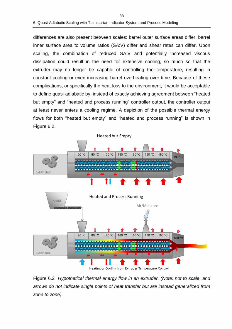
88
6. Quasi-Adiabatic Scaling with Telmisartan Indicator System and Process Modeling
differences are also present between scales: barrel outer surface areas differ, barrel
inner surface area to volume ratios (SA:V) differ and shear rates can differ. Upon
scaling, the combination of reduced SA:V and potentially increased viscous
dissipation could result in the need for extensive cooling, so much so that the
extruder may no longer be capable of controlling the temperature, resulting in
constant cooling or even increasing barrel overheating over time. Because of these
complications, or specifically the heat loss to the environment, it would be acceptable
to define quasi-adiabatic by, instead of exactly achieving agreement between “heated
but empty” and “heated and process running” controller output, the controller output
at least never enters a cooling regime. A depiction of the possible thermal energy
flows for both “heated but empty” and “heated and process running” is shown in
Figure 6.2.
Figure 6.2 Hypothetical thermal energy flow in an extruder. (Note: not to scale, and
arrows do not indicate single points of heat transfer but are instead generalized from
zone to zone).
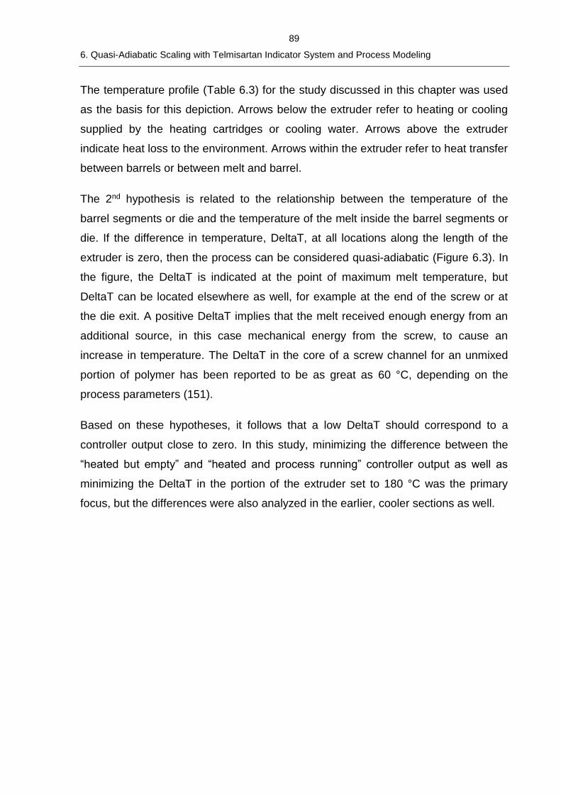
89
6. Quasi-Adiabatic Scaling with Telmisartan Indicator System and Process Modeling
The temperature profile (Table 6.3) for the study discussed in this chapter was used
as the basis for this depiction. Arrows below the extruder refer to heating or cooling
supplied by the heating cartridges or cooling water. Arrows above the extruder
indicate heat loss to the environment. Arrows within the extruder refer to heat transfer
between barrels or between melt and barrel.
The 2nd hypothesis is related to the relationship between the temperature of the
barrel segments or die and the temperature of the melt inside the barrel segments or
die. If the difference in temperature, DeltaT, at all locations along the length of the
extruder is zero, then the process can be considered quasi-adiabatic (Figure 6.3). In
the figure, the DeltaT is indicated at the point of maximum melt temperature, but
DeltaT can be located elsewhere as well, for example at the end of the screw or at
the die exit. A positive DeltaT implies that the melt received enough energy from an
additional source, in this case mechanical energy from the screw, to cause an
increase in temperature. The DeltaT in the core of a screw channel for an unmixed
portion of polymer has been reported to be as great as 60 °C, depending on the
process parameters (151).
Based on these hypotheses, it follows that a low DeltaT should correspond to a
controller output close to zero. In this study, minimizing the difference between the
“heated but empty” and “heated and process running” controller output as well as
minimizing the DeltaT in the portion of the extruder set to 180 °C was the primary
focus, but the differences were also analyzed in the earlier, cooler sections as well.
90
6. Quasi-Adiabatic Scaling with Telmisartan Indicator System and Process Modeling
Figure 6.3 2nd Hypothesis for quasi-adiabatic processing (note: die not to scale).
An additional hypothesis was related to use of the results from the Ludovic® model.
The question posed was: could Ludovic® guide the selection of process parameters
to achieve a quasi-adiabatic state? For example, the total conducted energy (TCE), a
global result and measure of how much heating or cooling occurs during steady state
(Figure 7.2), could directly relate to the controller output. Evidence for this idea was
present in the study performed by Zecevic, et.al., in which minimal TCE
corresponded with low measured DeltaT, although controller output was not
monitored (22). Further, and possibly even better, the local conduction energy (LCE)
as a function of extruder length could relate to the individual barrel and die controller
output. In addition, the estimated difference between melt and barrel temperature can
be calculated from the temperature evolution as a function of the length of the
extruder, f(x), plot in Ludovic®. One uncertainty, however, is that these results are
also a function of the thermal exchange coefficient (TEC), an input value in Ludovic®
(Figure 7.6). Therefore, any result is always only an estimate for the real process

91
6. Quasi-Adiabatic Scaling with Telmisartan Indicator System and Process Modeling
unless the model is tuned or validated with experimental data. Such validation is
challenging if not impossible because of measurement limitations, such as
temperature at all locations in the extruder.
6.1.2 Twin-Screw Extrusion Scaling Approaches
Transfer of a process from one scale to another, known generally as scaling, or
specifically as scale-up or scale-down, aims to maintain product quality while
adapting scale-specific process parameters. Scale-up may be performed to increase
the overall throughput of the process or to develop a commercial-scale process while
scale-down may be performed to study the large-scale process at development-scale
and reduce quantities of costly raw materials while developing or troubleshooting a
process.
Several important variables in TSE differ as a function of scale: barrel diameter and
cross-sectional area, barrel volume and inner surface area per unit length, screw tip
speed, drive power, and barrel heating and cooling capacity (146). As the diameter
increases, the barrel inner surface area increases by the power of 2 while the barrel
inner volume increases by the power of 3. This results in the dramatic decrease in
the surface area to volume ratio as the diameter increases (22). Reduced surface
area results in a decrease in the area available for heat exchange between melt and
barrel. At the same time, as the diameter increases, the screw tip speed will also
increase, leading to higher potential for shear heating; however, the propensity for
shear heating is also a function of the screw-barrel clearance and screw-screw
clearance. As a result, upon scale-up, these geometrical differences can result in
reduced heat transfer and increased amount of viscous dissipated energy. The
independent process parameters such as screw speed, feed rate, barrel temperature
and screw configuration can be adapted in order to compensate for these
fundamental differences and to obtain comparable operating conditions. Along with
geometric similarity (see next paragraph), such operating conditions to keep
consistent include average shear rate, fill level in the screw channels, discharge
pressure, specific heating and cooling power, residence time and the heat exchange
surface (15).
92
6. Quasi-Adiabatic Scaling with Telmisartan Indicator System and Process Modeling
Numerous strategies for scaling of the extrusion process, originally intended for
single-screw extruders, have been published (32,152). The strategies can be
adapted to twin-screw extrusion, but the added geometric complexity and the
presence of both filled and partially-filled sections along the screw channel should not
be disregarded (60). In both single- and twin-screw extrusion, one typically begins
with the assumption that geometric similarity exists between the two extruder scales.
Geometric similarity is defined by similar extruder length:diameter ratio L/D, Do/Di,
number of flights and screw helix angle (15). If geometric similarity criteria are met,
the screw speed is typically maintained and the feed rate, Q, is calculated for the new
scale based upon a selected scaling exponent, x, using equation 6.1.
𝑄2
𝑄1= (
𝐷2
𝐷1)
𝑥 (6.1)
where D refers to the barrel diameter and the subscripts 1 and 2 refer to the initial
and second scales, respectively. The origin and derivation of this equation is outlined
nicely in Dryer, et.al., in particular its applicability to twin-screw extrusion and
geometrically similar extruders based on the assumption that flow from pressure or
leakage are negligible in comparison to drag flow (60). The exponent x is selected
from a range between 1.5 to 3 with 1.5-2 typically for comparable heat transfer and 3
for comparable mixing (32,146). Rauwendaal states that scaling for heat transfer
typically results in nearly constant specific energy consumption and therefore
comparable melt temperature, while the output is significantly lower and therefore the
residence time much longer. On the other hand, scaling for mixing again results in
constant specific energy consumption and high throughput upon scale-up, which can
be detrimental if melting is required. In this case, these problems can be
compensated for by altering the screw configuration, but then the geometric similarity
would no longer be present. As mentioned by Dryer, et.al., for both single- and twin-
screw extrusion, compromises must be made, and the scaling factor should be
selected based on which characteristic should be kept more constant for the
particular formulation being processed.
In both scaling scenarios, the shear rate remains constant with constant screw
speed, again as long as geometric similarity is maintained, in particular the Do/Di and
93
6. Quasi-Adiabatic Scaling with Telmisartan Indicator System and Process Modeling
leakage (15,58). If this is not the case, the shear rate can be adapted by adjusting
the screw speed using equation 2.9 for shear rate in the screw channel and equation
2.10 in the screw overflight region.
Specifically in the case of adiabatic extrusion, two approaches have been suggested.
The first approach outlined by Frame seeks to maintain the same viscous dissipation
energy by linking the residence time, the power and screw tip speed, given that the
residence time is determined in large part by the feed rate as long as the screw
speed and profile are comparable (146). Since an adiabatic process is limited by the
extent of viscous dissipated energy, the first approach recommends an exponent of 3
in equation 6.1 so as to increase the feed rate in accordance with increasing volume.
Screw tip speed should be maintained with the assumption that it maintains constant
shear rate. Equivalent power can be achieved with comparable power density or
specific torque Md/a3, where Md is the torque limit of the screws and ‘a’ is the center
line (15). It is therefore assumed that adiabatic conditions can be realized on both
scales if these three parameters are kept constant. The second approach developed
by Nakatani strives to maintain melt temperature upon scaling (153). Several unique
parameters were included to account for heat-removal, an adiabatic index which
should fall between 0 and 1, and the non-Newtonian index from modeling of
rheological data. The approach acknowledges that additional work is needed to
account for situations in which the barrels are heating and cooling, in which case the
adiabatic index would be greater than 1 or negative, respectively. The adiabatic index
can be calculated via simulation software and the resulting scale up index for
throughput, x, in equation 6.1, can be determined.
Alternatively, scale-independent parameters such as specific energy, residence time
distribution and product temperature can be held constant during scaling (24,58).
However, identification of process parameters to obtain consistency in these scale-
independent parameters is not straightforward due to the inter-dependent
relationship between independent and dependent variables and the process
responses (Figure 2.1). For example, specific mechanical energy increases with
screw speed and torque, but decreases with increasing feed rate (equation 2.13).
However, the torque can increase with increasing feed rate but can also decrease
with increasing screw speed due to the dependency of torque on material melt
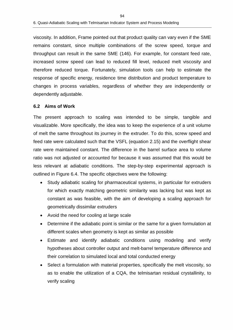
94
6. Quasi-Adiabatic Scaling with Telmisartan Indicator System and Process Modeling
viscosity. In addition, Frame pointed out that product quality can vary even if the SME
remains constant, since multiple combinations of the screw speed, torque and
throughput can result in the same SME (146). For example, for constant feed rate,
increased screw speed can lead to reduced fill level, reduced melt viscosity and
therefore reduced torque. Fortunately, simulation tools can help to estimate the
response of specific energy, residence time distribution and product temperature to
changes in process variables, regardless of whether they are independently or
dependently adjustable.
6.2 Aims of Work
The present approach to scaling was intended to be simple, tangible and
visualizable. More specifically, the idea was to keep the experience of a unit volume
of melt the same throughout its journey in the extruder. To do this, screw speed and
feed rate were calculated such that the VSFL (equation 2.15) and the overflight shear
rate were maintained constant. The difference in the barrel surface area to volume
ratio was not adjusted or accounted for because it was assumed that this would be
less relevant at adiabatic conditions. The step-by-step experimental approach is
outlined in Figure 6.4. The specific objectives were the following:
• Study adiabatic scaling for pharmaceutical systems, in particular for extruders
for which exactly matching geometric similarity was lacking but was kept as
constant as was feasible, with the aim of developing a scaling approach for
geometrically dissimilar extruders
• Avoid the need for cooling at large scale
• Determine if the adiabatic point is similar or the same for a given formulation at
different scales when geometry is kept as similar as possible
• Estimate and identify adiabatic conditions using modeling and verify
hypotheses about controller output and melt-barrel temperature difference and
their correlation to simulated local and total conducted energy
• Select a formulation with material properties, specifically the melt viscosity, so
as to enable the utilization of a CQA, the telmisartan residual crystallinity, to
verify scaling
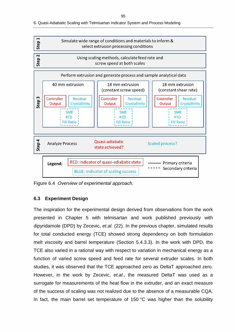
95
6. Quasi-Adiabatic Scaling with Telmisartan Indicator System and Process Modeling
Figure 6.4 Overview of experimental approach.
6.3 Experiment Design
The inspiration for the experimental design derived from observations from the work
presented in Chapter 5 with telmisartan and work published previously with
dipyridamole (DPD) by Zecevic, et.al. (22). In the previous chapter, simulated results
for total conducted energy (TCE) showed strong dependency on both formulation
melt viscosity and barrel temperature (Section 5.4.3.3). In the work with DPD, the
TCE also varied in a rational way with respect to variation in mechanical energy as a
function of varied screw speed and feed rate for several extruder scales. In both
studies, it was observed that the TCE approached zero as DeltaT approached zero.
However, in the work by Zecevic, et.al., the measured DeltaT was used as a
surrogate for measurements of the heat flow in the extruder, and an exact measure
of the success of scaling was not realized due to the absence of a measurable CQA.
In fact, the main barrel set temperature of 150 °C was higher than the solubility
96
6. Quasi-Adiabatic Scaling with Telmisartan Indicator System and Process Modeling
temperature of ~120 °C for 30 %w/w DPD in copovidone, and DPD strongly
plasticizes COP (135). The focus of this work was to build upon the prior work and to
connect the behavior of residual crystallinity as a CQA to better understand quasi-
adiabatic extrusion processing in a pharmaceutical scaling application.
6.3.1 Formulation Compositions
The two formulations investigated in Chapter 5, 10 %w/w TEL in COP and 10 %w/w
TEL in a 5 %w/w TW80 in COP matrix, were also investigated in the simulation study
in this chapter, while only the ternary mixture was evaluated experimentally.
6.3.2 Laboratory Experiment Design
6.3.2.1 Extruder Design
Two extruders were used in the study, with nominal diameters of 18 and 40 mm, and
were relatively geometrically similar. The design characteristics of the two extruders
are listed in Table 6.1. Included in the list are the make and model, geometric
dimensions, heating and cooling capabilities, and motor capabilities. While the
absolute screw lengths were different, the relative length in units of length divided by
diameter, or L/D, was similar at 28 L/D and 25.725 L/D for the 18 mm (ZSK18) and
40 mm (ZSK40) extruders, respectively. Both extruders had an identical diameter
ratio of 1.55, which is important for geometrical similarity, especially with respect to
the shear rate in the screw channel (see discussion in section 6.3.2.2).
One design difference was the number of barrel segments, with the ZSK18 extruder
consisting of 7 barrel segments while the ZSK40 only 6 barrel segments. Because
the individual barrel segments had nearly the same length ratio of 4 L/D, the ZSK18
extruder essentially had one additional heating zone. This difference was
compensated for by slightly lengthening the distance between the two mixing zones
and by keeping the barrel set temperature constant in this region.
97
6. Quasi-Adiabatic Scaling with Telmisartan Indicator System and Process Modeling
Table 6.1 Comparison of extruder characteristics – ZSK18 vs. ZSK40.
18 mm Extruder 40 mm Extruder
Vendor Coperion Coperion
Model ZSK18 MegaCompounder
ZSK40 MegaCompounder
Screw Diameter [mm] 18 40
Diameter Ratio Do/Di 1.55 1.55
Total Screw Length [mm] 504 1029
Total Screw Length [L/D] 28 25.725
Number of Barrels 7 (plus a passively-heated die plate)
6 (plus a passively-heated die plate)
Barrel Length [mm] 72 162
Barrel Length [L/D] 4 4.05
Die Plate Length [mm] 25 57
Barrel Diameter [mm] 18.25 40.3
Center Line [mm] 15.0 33.4
Screw-Barrel Clearance [mm] 0.1 0.2
Free Cross-Sectional Area [mm2] 188 872
Barrel Free Volume without Die [dm3] 0.095 0.8865
Barrel Surface Area to Volume Ratio [1/cm] 4.79 2.38
Die Plate Length [mm] 58 25
Die Free Volume [cm3] 9.1 116
Die Outlet Dimensions 10 mm diameter 5 mm x 60 mm
Heating Cartridges per Barrel 4 x 200 W 4 x 800 W
Maximum Barrel Temperature [°C] 250 270
Barrel Cooling Medium water water
Heating Cartridges per Die and Power 1 x 160 W 4 x 550 W
Location of Heating Cartridges adjacent to die lip, near surface of die
2 internal near melt flow
2 adjacent to die lip
Location of Die Thermocouples adjacent to die lip, near surface of die
(upper, middle, lower)
Power Drive [kW] 10 64
Maximum Screw Speed [rpm] 1024 250
Max Torque/shaft [N∙m] 38 500
The screw configurations were designed such that the functional zones remained
constant (Figure 6.5). Considerations included the number and type of mixing zones,
the barrel temperature profile, use and placement of the vacuum port, and placement
of the mixing zones with respect to the temperature profile, vacuum port, and die exit.
For example, the first mixing element was placed within the temperature transition
region between 120 °C and 180 °C, while the second mixing section was placed just
before the vacuum port. The kneading blocks used at both scales were identically
geometrically scaled, meaning that the number of disks per element, the element
length in L/D, the disk L/D, and offset angle were the same (Table 6.2).The pitch of
conveying elements was also kept constant as much as was feasible. For example,
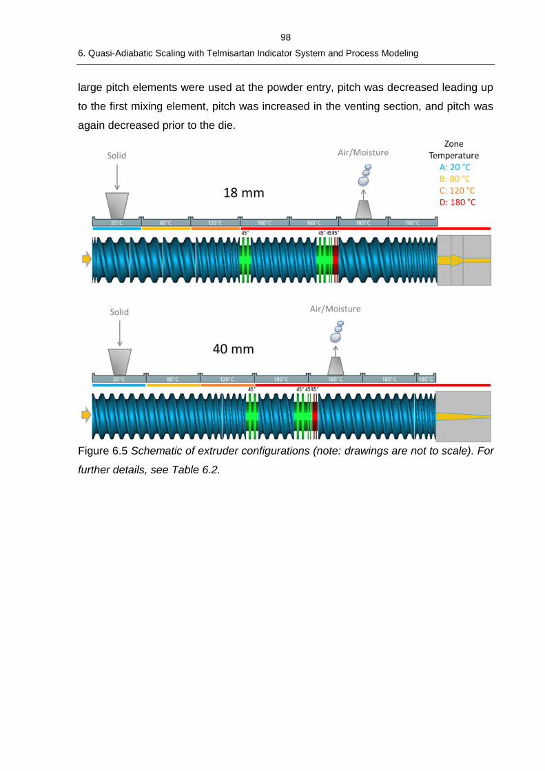
98
6. Quasi-Adiabatic Scaling with Telmisartan Indicator System and Process Modeling
large pitch elements were used at the powder entry, pitch was decreased leading up
to the first mixing element, pitch was increased in the venting section, and pitch was
again decreased prior to the die.
Figure 6.5 Schematic of extruder configurations (note: drawings are not to scale). For
further details, see Table 6.2.
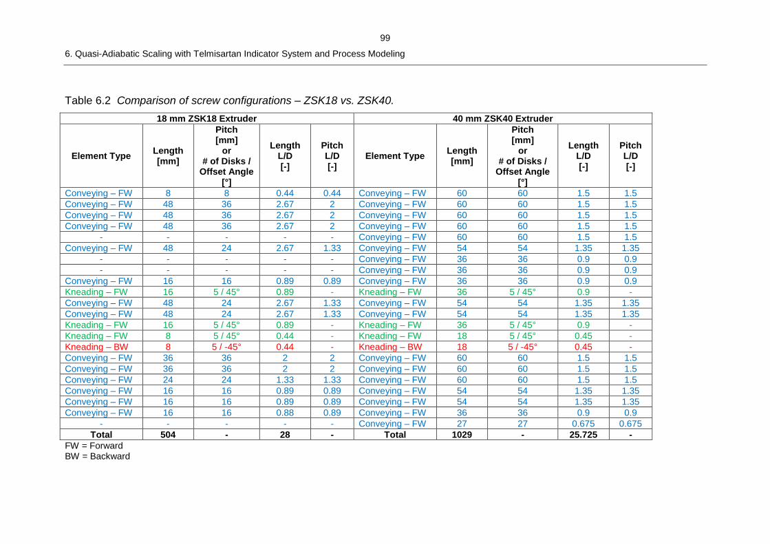
99
6. Quasi-Adiabatic Scaling with Telmisartan Indicator System and Process Modeling
Table 6.2 Comparison of screw configurations – ZSK18 vs. ZSK40.
18 mm ZSK18 Extruder 40 mm ZSK40 Extruder
Element Type Length [mm]
Pitch [mm]
or # of Disks /
Offset Angle [°]
Length L/D [-]
Pitch L/D [-]
Element Type Length [mm]
Pitch [mm]
or # of Disks /
Offset Angle [°]
Length L/D [-]
Pitch L/D [-]
Conveying – FW 8 8 0.44 0.44 Conveying – FW 60 60 1.5 1.5
Conveying – FW 48 36 2.67 2 Conveying – FW 60 60 1.5 1.5
Conveying – FW 48 36 2.67 2 Conveying – FW 60 60 1.5 1.5
Conveying – FW 48 36 2.67 2 Conveying – FW 60 60 1.5 1.5
- - - - - Conveying – FW 60 60 1.5 1.5
Conveying – FW 48 24 2.67 1.33 Conveying – FW 54 54 1.35 1.35
- - - - - Conveying – FW 36 36 0.9 0.9
- - - - - Conveying – FW 36 36 0.9 0.9
Conveying – FW 16 16 0.89 0.89 Conveying – FW 36 36 0.9 0.9
Kneading – FW 16 5 / 45° 0.89 - Kneading – FW 36 5 / 45° 0.9 -
Conveying – FW 48 24 2.67 1.33 Conveying – FW 54 54 1.35 1.35
Conveying – FW 48 24 2.67 1.33 Conveying – FW 54 54 1.35 1.35
Kneading – FW 16 5 / 45° 0.89 - Kneading – FW 36 5 / 45° 0.9 -
Kneading – FW 8 5 / 45° 0.44 - Kneading – FW 18 5 / 45° 0.45 -
Kneading – BW 8 5 / -45° 0.44 - Kneading – BW 18 5 / -45° 0.45 -
Conveying – FW 36 36 2 2 Conveying – FW 60 60 1.5 1.5
Conveying – FW 36 36 2 2 Conveying – FW 60 60 1.5 1.5
Conveying – FW 24 24 1.33 1.33 Conveying – FW 60 60 1.5 1.5
Conveying – FW 16 16 0.89 0.89 Conveying – FW 54 54 1.35 1.35
Conveying – FW 16 16 0.89 0.89 Conveying – FW 54 54 1.35 1.35
Conveying – FW 16 16 0.88 0.89 Conveying – FW 36 36 0.9 0.9
- - - - - Conveying – FW 27 27 0.675 0.675
Total 504 - 28 - Total 1029 - 25.725 -
FW = Forward BW = Backward
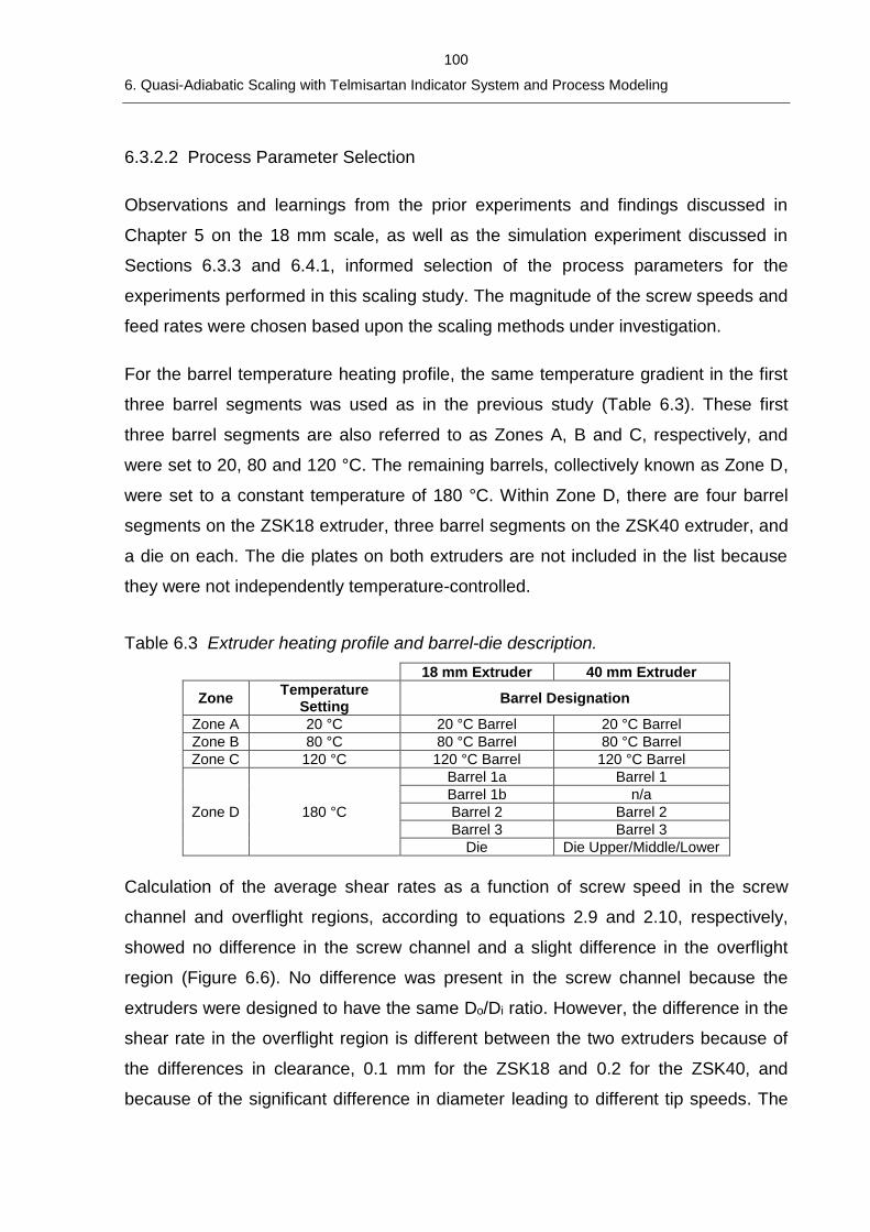
100
6. Quasi-Adiabatic Scaling with Telmisartan Indicator System and Process Modeling
6.3.2.2 Process Parameter Selection
Observations and learnings from the prior experiments and findings discussed in
Chapter 5 on the 18 mm scale, as well as the simulation experiment discussed in
Sections 6.3.3 and 6.4.1, informed selection of the process parameters for the
experiments performed in this scaling study. The magnitude of the screw speeds and
feed rates were chosen based upon the scaling methods under investigation.
For the barrel temperature heating profile, the same temperature gradient in the first
three barrel segments was used as in the previous study (Table 6.3). These first
three barrel segments are also referred to as Zones A, B and C, respectively, and
were set to 20, 80 and 120 °C. The remaining barrels, collectively known as Zone D,
were set to a constant temperature of 180 °C. Within Zone D, there are four barrel
segments on the ZSK18 extruder, three barrel segments on the ZSK40 extruder, and
a die on each. The die plates on both extruders are not included in the list because
they were not independently temperature-controlled.
Table 6.3 Extruder heating profile and barrel-die description.
18 mm Extruder 40 mm Extruder
Zone Temperature
Setting Barrel Designation
Zone A 20 °C 20 °C Barrel 20 °C Barrel
Zone B 80 °C 80 °C Barrel 80 °C Barrel
Zone C 120 °C 120 °C Barrel 120 °C Barrel
Zone D 180 °C
Barrel 1a Barrel 1
Barrel 1b n/a
Barrel 2 Barrel 2
Barrel 3 Barrel 3
Die Die Upper/Middle/Lower
Calculation of the average shear rates as a function of screw speed in the screw
channel and overflight regions, according to equations 2.9 and 2.10, respectively,
showed no difference in the screw channel and a slight difference in the overflight
region (Figure 6.6). No difference was present in the screw channel because the
extruders were designed to have the same Do/Di ratio. However, the difference in the
shear rate in the overflight region is different between the two extruders because of
the differences in clearance, 0.1 mm for the ZSK18 and 0.2 for the ZSK40, and
because of the significant difference in diameter leading to different tip speeds. The
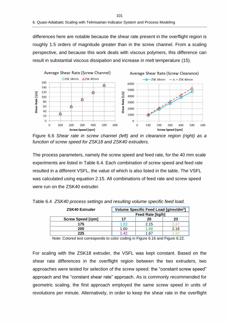
101
6. Quasi-Adiabatic Scaling with Telmisartan Indicator System and Process Modeling
differences here are notable because the shear rate present in the overflight region is
roughly 1.5 orders of magnitude greater than in the screw channel. From a scaling
perspective, and because this work deals with viscous polymers, this difference can
result in substantial viscous dissipation and increase in melt temperature (15).
Figure 6.6 Shear rate in screw channel (left) and in clearance region (right) as a
function of screw speed for ZSK18 and ZSK40 extruders.
The process parameters, namely the screw speed and feed rate, for the 40 mm scale
experiments are listed in Table 6.4. Each combination of screw speed and feed rate
resulted in a different VSFL, the value of which is also listed in the table. The VSFL
was calculated using equation 2.15. All combinations of feed rate and screw speed
were run on the ZSK40 extruder.
Table 6.4 ZSK40 process settings and resulting volume specific feed load.
ZSK40 Extruder Volume Specific Feed Load [g/rev/dm3]
Feed Rate [kg/h]
Screw Speed [rpm] 17 20 23
175 1.83 2.15 2.47
200 1.60 1.88 2.16
225 1.42 1.67 1.92
Note: Colored text corresponds to color coding in Figure 6.16 and Figure 6.22.
For scaling with the ZSK18 extruder, the VSFL was kept constant. Based on the
shear rate differences in the overflight region between the two extruders, two
approaches were tested for selection of the screw speed: the “constant screw speed”
approach and the “constant shear rate” approach. As is commonly recommended for
geometric scaling, the first approach employed the same screw speed in units of
revolutions per minute. Alternatively, in order to keep the shear rate in the overflight
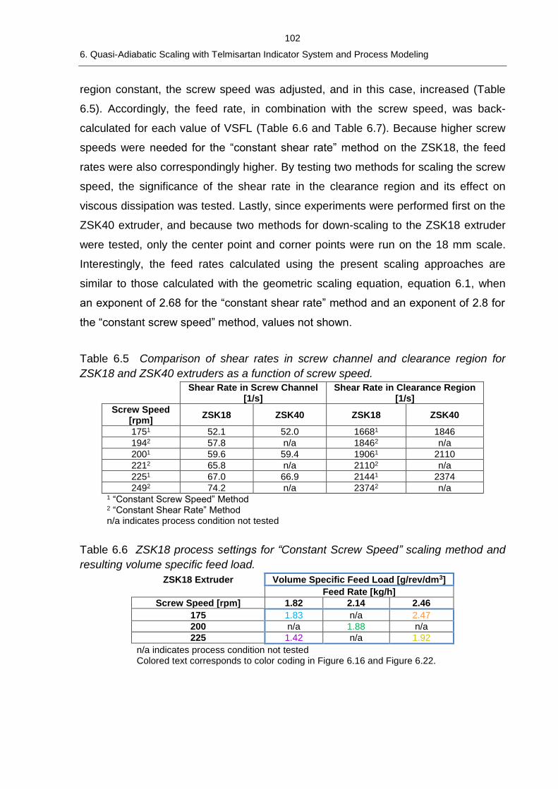
102
6. Quasi-Adiabatic Scaling with Telmisartan Indicator System and Process Modeling
region constant, the screw speed was adjusted, and in this case, increased (Table
6.5). Accordingly, the feed rate, in combination with the screw speed, was back-
calculated for each value of VSFL (Table 6.6 and Table 6.7). Because higher screw
speeds were needed for the “constant shear rate” method on the ZSK18, the feed
rates were also correspondingly higher. By testing two methods for scaling the screw
speed, the significance of the shear rate in the clearance region and its effect on
viscous dissipation was tested. Lastly, since experiments were performed first on the
ZSK40 extruder, and because two methods for down-scaling to the ZSK18 extruder
were tested, only the center point and corner points were run on the 18 mm scale.
Interestingly, the feed rates calculated using the present scaling approaches are
similar to those calculated with the geometric scaling equation, equation 6.1, when
an exponent of 2.68 for the “constant shear rate” method and an exponent of 2.8 for
the “constant screw speed” method, values not shown.
Table 6.5 Comparison of shear rates in screw channel and clearance region for
ZSK18 and ZSK40 extruders as a function of screw speed.
Shear Rate in Screw Channel
[1/s] Shear Rate in Clearance Region
[1/s]
Screw Speed [rpm]
ZSK18 ZSK40 ZSK18 ZSK40
1751 52.1 52.0 16681 1846
1942 57.8 n/a 18462 n/a
2001 59.6 59.4 19061 2110
2212 65.8 n/a 21102 n/a
2251 67.0 66.9 21441 2374
2492 74.2 n/a 23742 n/a 1 “Constant Screw Speed” Method 2 “Constant Shear Rate” Method n/a indicates process condition not tested
Table 6.6 ZSK18 process settings for “Constant Screw Speed” scaling method and
resulting volume specific feed load.
ZSK18 Extruder Volume Specific Feed Load [g/rev/dm3]
Feed Rate [kg/h]
Screw Speed [rpm] 1.82 2.14 2.46
175 1.83 n/a 2.47
200 n/a 1.88 n/a
225 1.42 n/a 1.92
n/a indicates process condition not tested Colored text corresponds to color coding in Figure 6.16 and Figure 6.22.
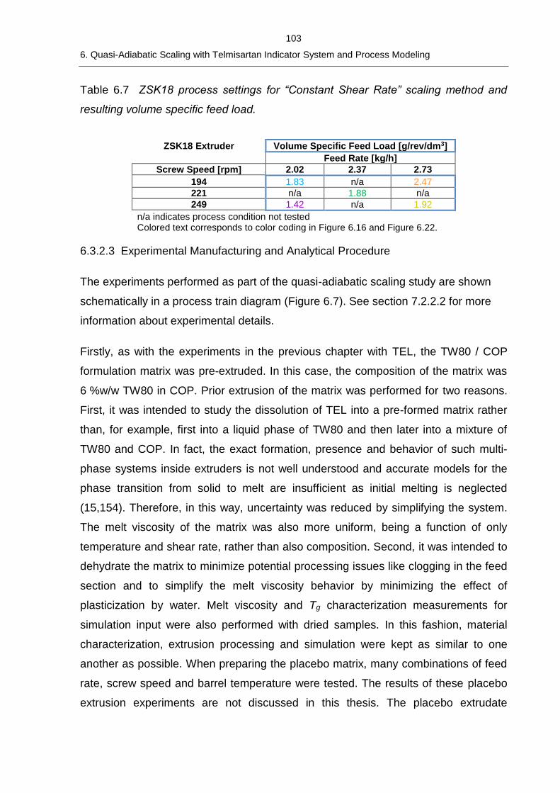
103
6. Quasi-Adiabatic Scaling with Telmisartan Indicator System and Process Modeling
Table 6.7 ZSK18 process settings for “Constant Shear Rate” scaling method and
resulting volume specific feed load.
ZSK18 Extruder Volume Specific Feed Load [g/rev/dm3]
Feed Rate [kg/h]
Screw Speed [rpm] 2.02 2.37 2.73
194 1.83 n/a 2.47
221 n/a 1.88 n/a
249 1.42 n/a 1.92
n/a indicates process condition not tested Colored text corresponds to color coding in Figure 6.16 and Figure 6.22.
6.3.2.3 Experimental Manufacturing and Analytical Procedure
The experiments performed as part of the quasi-adiabatic scaling study are shown
schematically in a process train diagram (Figure 6.7). See section 7.2.2.2 for more
information about experimental details.
Firstly, as with the experiments in the previous chapter with TEL, the TW80 / COP
formulation matrix was pre-extruded. In this case, the composition of the matrix was
6 %w/w TW80 in COP. Prior extrusion of the matrix was performed for two reasons.
First, it was intended to study the dissolution of TEL into a pre-formed matrix rather
than, for example, first into a liquid phase of TW80 and then later into a mixture of
TW80 and COP. In fact, the exact formation, presence and behavior of such multi-
phase systems inside extruders is not well understood and accurate models for the
phase transition from solid to melt are insufficient as initial melting is neglected
(15,154). Therefore, in this way, uncertainty was reduced by simplifying the system.
The melt viscosity of the matrix was also more uniform, being a function of only
temperature and shear rate, rather than also composition. Second, it was intended to
dehydrate the matrix to minimize potential processing issues like clogging in the feed
section and to simplify the melt viscosity behavior by minimizing the effect of
plasticization by water. Melt viscosity and Tg characterization measurements for
simulation input were also performed with dried samples. In this fashion, material
characterization, extrusion processing and simulation were kept as similar to one
another as possible. When preparing the placebo matrix, many combinations of feed
rate, screw speed and barrel temperature were tested. The results of these placebo
extrusion experiments are not discussed in this thesis. The placebo extrudate
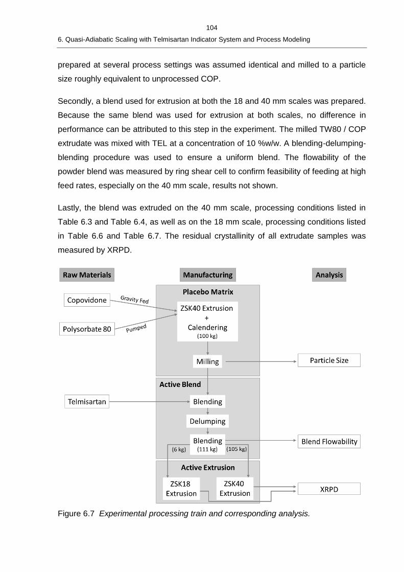
104
6. Quasi-Adiabatic Scaling with Telmisartan Indicator System and Process Modeling
prepared at several process settings was assumed identical and milled to a particle
size roughly equivalent to unprocessed COP.
Secondly, a blend used for extrusion at both the 18 and 40 mm scales was prepared.
Because the same blend was used for extrusion at both scales, no difference in
performance can be attributed to this step in the experiment. The milled TW80 / COP
extrudate was mixed with TEL at a concentration of 10 %w/w. A blending-delumping-
blending procedure was used to ensure a uniform blend. The flowability of the
powder blend was measured by ring shear cell to confirm feasibility of feeding at high
feed rates, especially on the 40 mm scale, results not shown.
Lastly, the blend was extruded on the 40 mm scale, processing conditions listed in
Table 6.3 and Table 6.4, as well as on the 18 mm scale, processing conditions listed
in Table 6.6 and Table 6.7. The residual crystallinity of all extrudate samples was
measured by XRPD.
Figure 6.7 Experimental processing train and corresponding analysis.
105
6. Quasi-Adiabatic Scaling with Telmisartan Indicator System and Process Modeling
6.3.3 Simulation Experiment Design
A full factorial design of simulation experiments was performed to guide the selection
of barrel temperatures (Table 6.8). Ranges of feed rate and screw speed were
chosen based on prior experiments with placebo, the results of which are not
discussed. Both extruders, ZSK18 and ZSK40, were included in the experiment. Two
formulations, identical to those processed in the previous study, with differing zero-
shear rate viscosity were also included (Figure 5.5b). As always, the extruders were
represented geometrically as similarly to the laboratory extruders as was possible.
Table 6.8 Variables for simulated full factorial DOE.
Extruder Scale 18 mm Extruder 40 mm Extruder
Screw Speed [mm] 175, 200, 225
Feed Rate [kg/h] 1.8, 2.15, 2.5 17, 20, 23
Zone A Temperature [°C] 20 °C
Zone B Temperature [°C] 80 °C
Zone C Temperature [°C] 120 °C
Zone D Temperature [°C] 160, 170, 180, 190, 200
Formulation TEL-COP, TEL-TW80-COP
6.4 Results & Discussion
6.4.1 Selection of Formulation and Barrel Temperatures for Laboratory
Experiments via Supportive Simulation
In addition to learnings from numerous process settings tested empirically with
placebo (results not presented), findings from simulation discussed in this section
informed and supported the selection of the process parameters for extrusion
experiments with TEL. The findings from simulation also confirmed the decision to
select the TEL / TW80 / COP formulation for empirical scaling.
Based on the assumption that the 1st and 2nd Hypotheses would lead to a quasi-
adiabatic state, and also that zero TCE would be related to this, process conditions
were virtually identified that exhibited these characteristics. The simulations were
performed for both formulations, namely with and without TW80, so as to confirm the
findings from section 5.4.3.3 on both the 18 mm and 40 mm scales. Independent of
extruder scale and with less substantial influence from screw speed and feed rate,
simulation results showed that the TCE was near to zero when the TW80 formulation
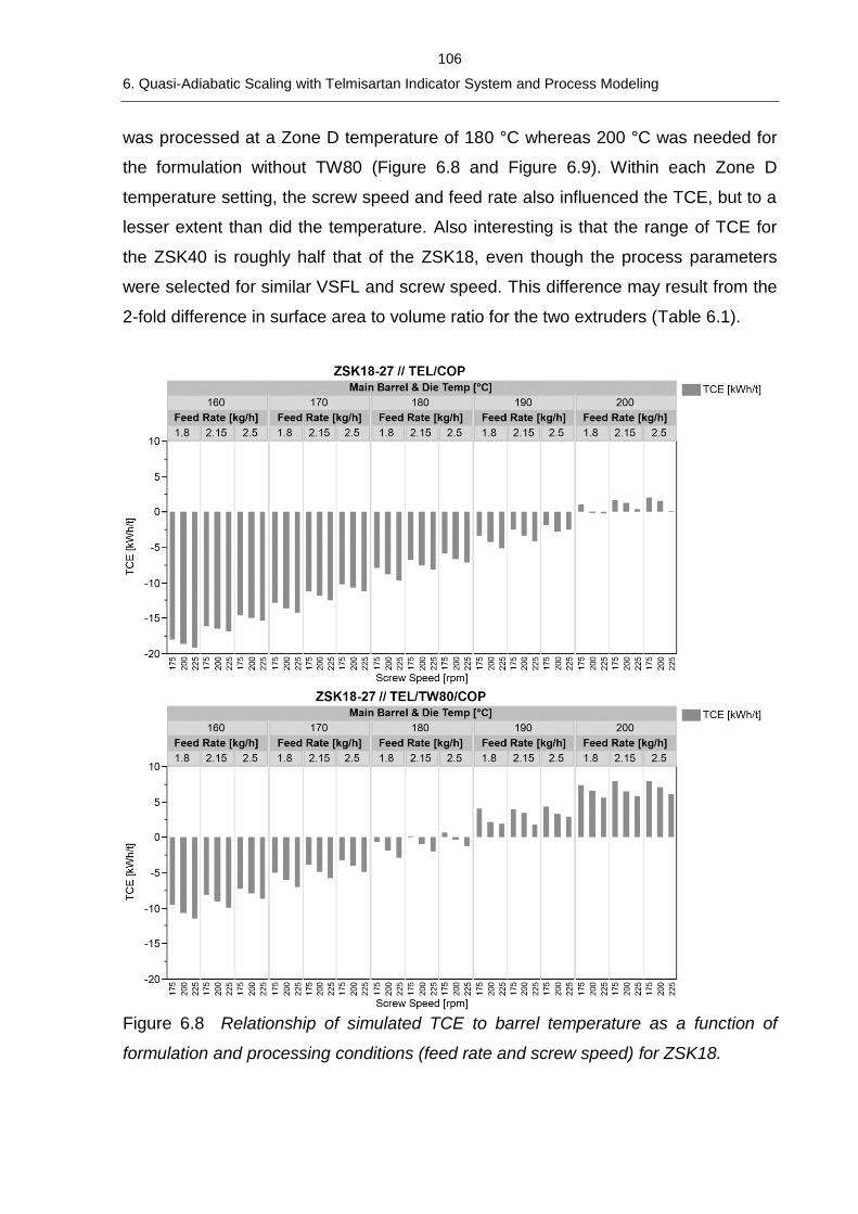
106
6. Quasi-Adiabatic Scaling with Telmisartan Indicator System and Process Modeling
was processed at a Zone D temperature of 180 °C whereas 200 °C was needed for
the formulation without TW80 (Figure 6.8 and Figure 6.9). Within each Zone D
temperature setting, the screw speed and feed rate also influenced the TCE, but to a
lesser extent than did the temperature. Also interesting is that the range of TCE for
the ZSK40 is roughly half that of the ZSK18, even though the process parameters
were selected for similar VSFL and screw speed. This difference may result from the
2-fold difference in surface area to volume ratio for the two extruders (Table 6.1).
Figure 6.8 Relationship of simulated TCE to barrel temperature as a function of
formulation and processing conditions (feed rate and screw speed) for ZSK18.
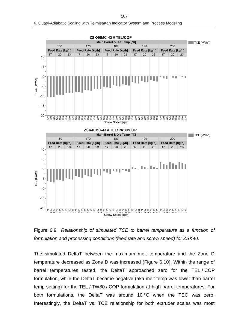
107
6. Quasi-Adiabatic Scaling with Telmisartan Indicator System and Process Modeling
Figure 6.9 Relationship of simulated TCE to barrel temperature as a function of
formulation and processing conditions (feed rate and screw speed) for ZSK40.
The simulated DeltaT between the maximum melt temperature and the Zone D
temperature decreased as Zone D was increased (Figure 6.10). Within the range of
barrel temperatures tested, the DeltaT approached zero for the TEL / COP
formulation, while the DeltaT became negative (aka melt temp was lower than barrel
temp setting) for the TEL / TW80 / COP formulation at high barrel temperatures. For
both formulations, the DeltaT was around 10 °C when the TEC was zero.
Interestingly, the DeltaT vs. TCE relationship for both extruder scales was most
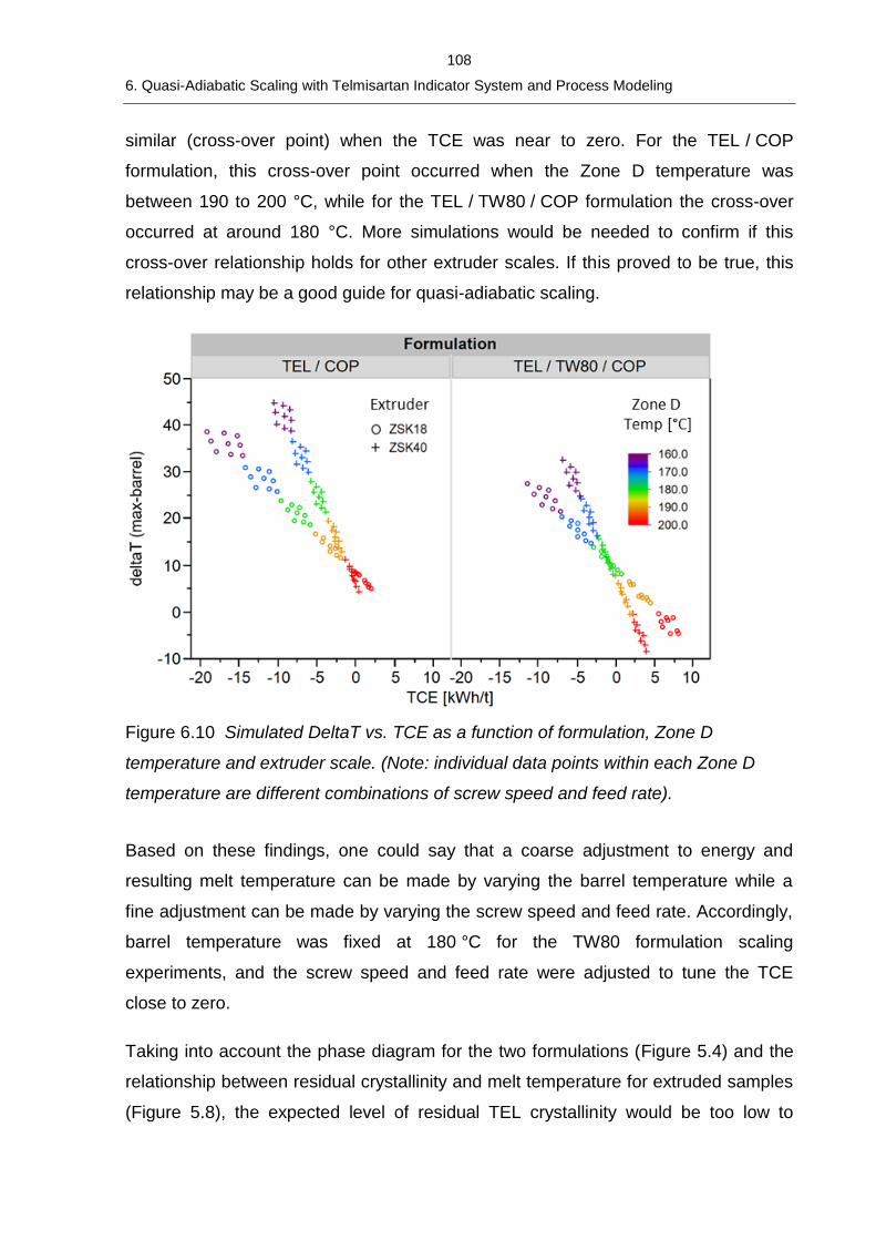
108
6. Quasi-Adiabatic Scaling with Telmisartan Indicator System and Process Modeling
similar (cross-over point) when the TCE was near to zero. For the TEL / COP
formulation, this cross-over point occurred when the Zone D temperature was
between 190 to 200 °C, while for the TEL / TW80 / COP formulation the cross-over
occurred at around 180 °C. More simulations would be needed to confirm if this
cross-over relationship holds for other extruder scales. If this proved to be true, this
relationship may be a good guide for quasi-adiabatic scaling.
Figure 6.10 Simulated DeltaT vs. TCE as a function of formulation, Zone D
temperature and extruder scale. (Note: individual data points within each Zone D
temperature are different combinations of screw speed and feed rate).
Based on these findings, one could say that a coarse adjustment to energy and
resulting melt temperature can be made by varying the barrel temperature while a
fine adjustment can be made by varying the screw speed and feed rate. Accordingly,
barrel temperature was fixed at 180 °C for the TW80 formulation scaling
experiments, and the screw speed and feed rate were adjusted to tune the TCE
close to zero.
Taking into account the phase diagram for the two formulations (Figure 5.4) and the
relationship between residual crystallinity and melt temperature for extruded samples
(Figure 5.8), the expected level of residual TEL crystallinity would be too low to
109
6. Quasi-Adiabatic Scaling with Telmisartan Indicator System and Process Modeling
potentially distinguish between process settings in the TEL / COP formulation at
barrel temp of 200 °C. Therefore, the TEL / TW80 / COP formulation was selected for
scaling studies so as to enable both use of TEL as an indicator substance as well as
study adiabatic scaling.
6.4.2 Process Analysis and Assessment of Energy Balance
6.4.2.1 Baseline Controller Output for Heated but Empty ZSK18 and ZSK40
The controller output of each temperature-controlled barrel and die zone, measured
for a heated but empty extruder, was similar for both extruder scales due to selection
of the same set points in the temperature profile. The temperature profile used was
similar to that listed in Table 6.3, except that Zone D was varied from 150 to 210 °C
for the ZSK18 and from 140 to 180 °C for the ZSK40. The temperature of Zones A, B
and C was held constant. Zone D was varied in order to assess the impact of its
magnitude on heating and cooling requirements in other zones. In addition, the data
was generated in order to have the baseline values in case, during the experiments
with the process running, adjustment of the Zone D temperature was required in
order to achieve a more acceptable quasi-adiabatic state. The results obtained did
not vary as a function of room temperature within the range of 20-28 °C.
The controller output for the heated but empty ZSK18 extruder, expressed in units of
counts/s, for each barrel segment and the die was plotted as a function of Zone D
temperature (Figure 6.11). No heating or cooling was required to hold Zone A at
20 °C. As for the other zones, the most heating took place in the die due to probe
placement, followed by the first barrel segment in Zone D. Zone B also required a
considerable amount of heating, while Zone C fluctuated between heating and
cooling, especially as the Zone D temperature was increased, due to barrel segment-
to-segment heat transfer from the adjacent cooler and warmer segments. As the
temperature of Zone D was increased, cooling activity in Zone C increased. At the
same time, most of the individual barrel segments within Zone D needed increasingly
more heating activity to hold their temperature due to the temperature differential
between the barrel and the environment and resulting heat loss over time.
Interestingly, both the first barrel segment in Zone D and the die exhibited maxima in
their heating requirements as a function of Zone D temperature.
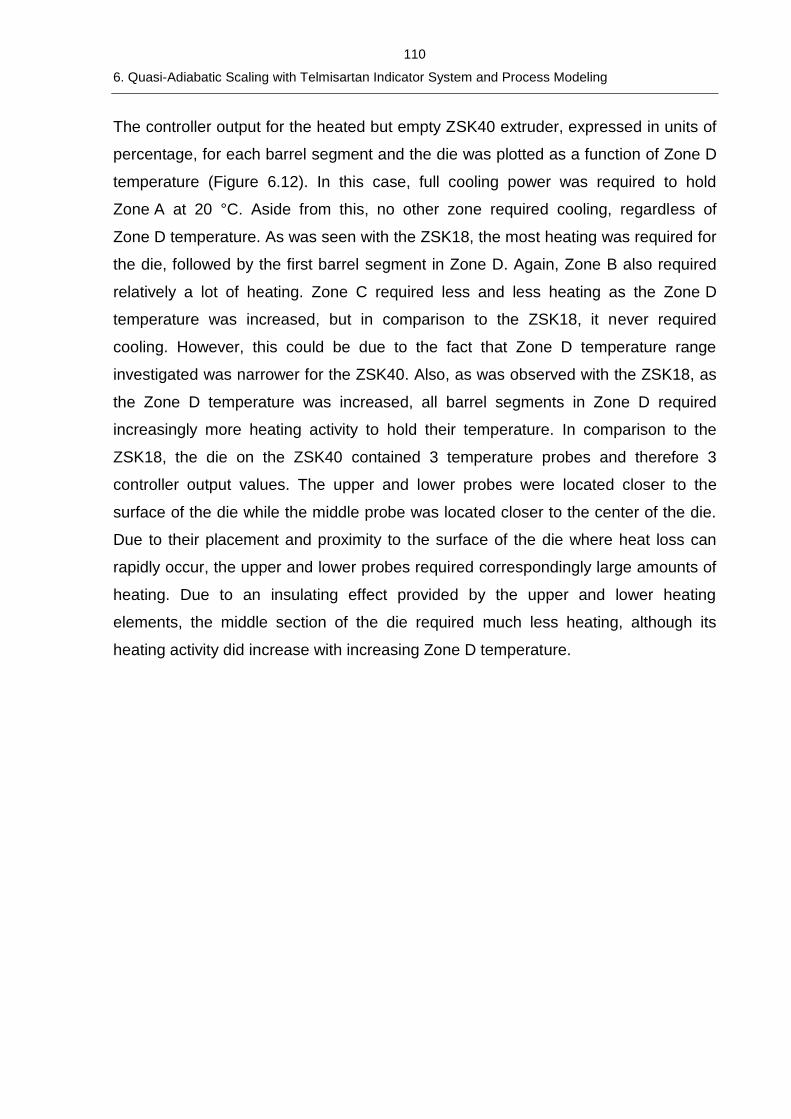
110
6. Quasi-Adiabatic Scaling with Telmisartan Indicator System and Process Modeling
The controller output for the heated but empty ZSK40 extruder, expressed in units of
percentage, for each barrel segment and the die was plotted as a function of Zone D
temperature (Figure 6.12). In this case, full cooling power was required to hold
Zone A at 20 °C. Aside from this, no other zone required cooling, regardless of
Zone D temperature. As was seen with the ZSK18, the most heating was required for
the die, followed by the first barrel segment in Zone D. Again, Zone B also required
relatively a lot of heating. Zone C required less and less heating as the Zone D
temperature was increased, but in comparison to the ZSK18, it never required
cooling. However, this could be due to the fact that Zone D temperature range
investigated was narrower for the ZSK40. Also, as was observed with the ZSK18, as
the Zone D temperature was increased, all barrel segments in Zone D required
increasingly more heating activity to hold their temperature. In comparison to the
ZSK18, the die on the ZSK40 contained 3 temperature probes and therefore 3
controller output values. The upper and lower probes were located closer to the
surface of the die while the middle probe was located closer to the center of the die.
Due to their placement and proximity to the surface of the die where heat loss can
rapidly occur, the upper and lower probes required correspondingly large amounts of
heating. Due to an insulating effect provided by the upper and lower heating
elements, the middle section of the die required much less heating, although its
heating activity did increase with increasing Zone D temperature.
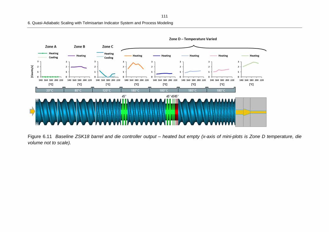
111
6. Quasi-Adiabatic Scaling with Telmisartan Indicator System and Process Modeling
Figure 6.11 Baseline ZSK18 barrel and die controller output – heated but empty (x-axis of mini-plots is Zone D temperature, die
volume not to scale).
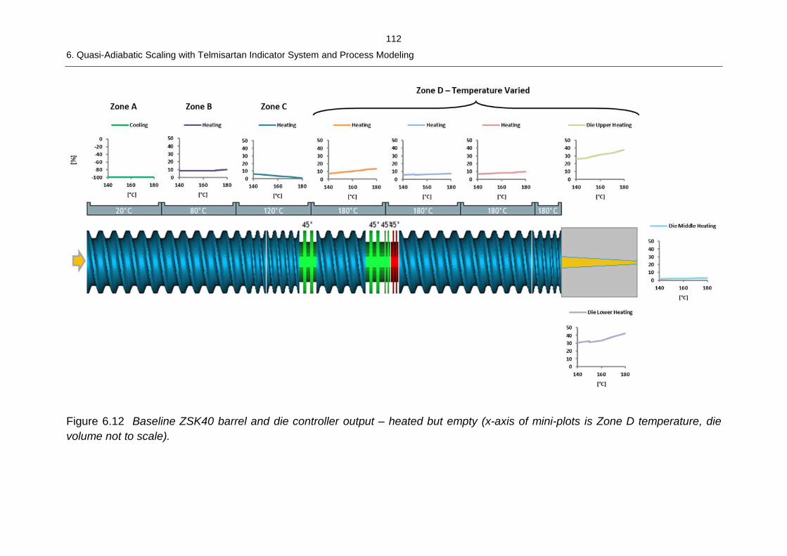
112
6. Quasi-Adiabatic Scaling with Telmisartan Indicator System and Process Modeling
Figure 6.12 Baseline ZSK40 barrel and die controller output – heated but empty (x-axis of mini-plots is Zone D temperature, die
volume not to scale).
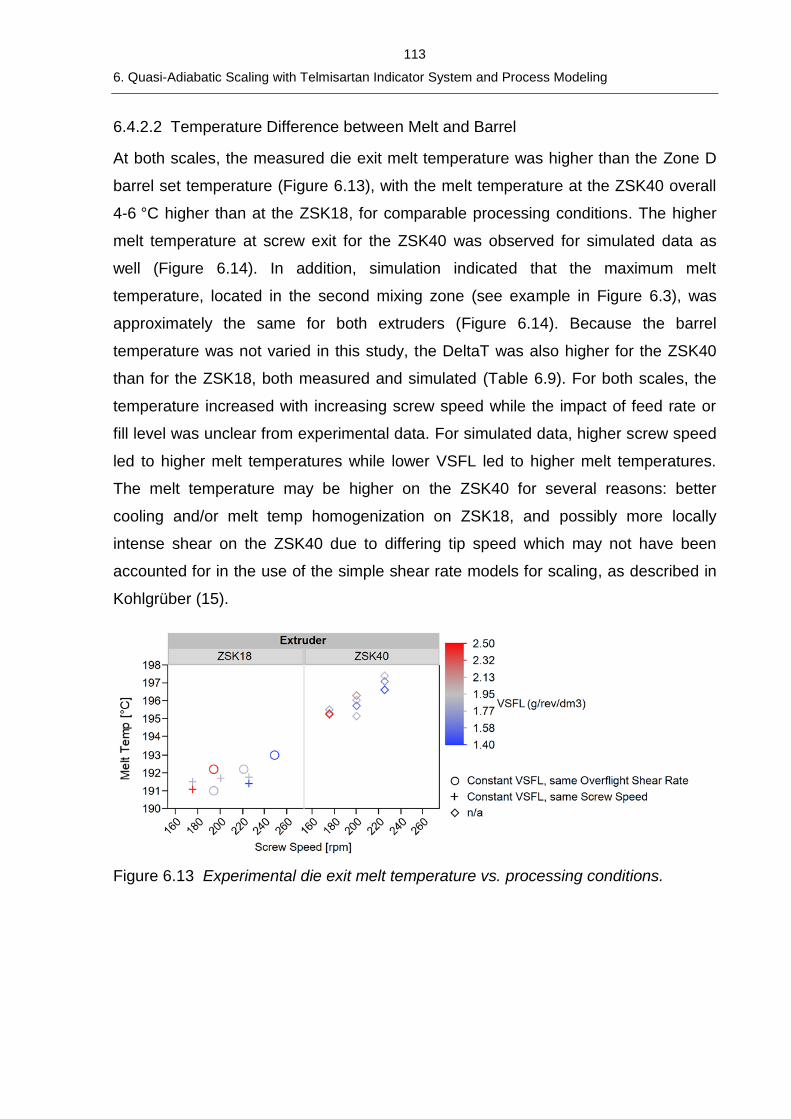
113
6. Quasi-Adiabatic Scaling with Telmisartan Indicator System and Process Modeling
6.4.2.2 Temperature Difference between Melt and Barrel
At both scales, the measured die exit melt temperature was higher than the Zone D
barrel set temperature (Figure 6.13), with the melt temperature at the ZSK40 overall
4-6 °C higher than at the ZSK18, for comparable processing conditions. The higher
melt temperature at screw exit for the ZSK40 was observed for simulated data as
well (Figure 6.14). In addition, simulation indicated that the maximum melt
temperature, located in the second mixing zone (see example in Figure 6.3), was
approximately the same for both extruders (Figure 6.14). Because the barrel
temperature was not varied in this study, the DeltaT was also higher for the ZSK40
than for the ZSK18, both measured and simulated (Table 6.9). For both scales, the
temperature increased with increasing screw speed while the impact of feed rate or
fill level was unclear from experimental data. For simulated data, higher screw speed
led to higher melt temperatures while lower VSFL led to higher melt temperatures.
The melt temperature may be higher on the ZSK40 for several reasons: better
cooling and/or melt temp homogenization on ZSK18, and possibly more locally
intense shear on the ZSK40 due to differing tip speed which may not have been
accounted for in the use of the simple shear rate models for scaling, as described in
Kohlgrüber (15).
Figure 6.13 Experimental die exit melt temperature vs. processing conditions.
114
6. Quasi-Adiabatic Scaling with Telmisartan Indicator System and Process Modeling
Figure 6.14 Simulated maximum melt temperature and melt temperature at screw
exit vs. processing conditions.
Table 6.9. Range of experimental and simulated DeltaT.
Extruder Scale
Range of DeltaT [°C]
Measured (Die Exit) Simulated (Screw Exit)
ZSK18 11-13 6-12
ZSK40 15-17 10-18
6.4.2.3 Controller Output when Heated and Process Running
The controller output behaved similarly for both extruder scales due to similar barrel
temperature profile. In addition, the Zone D for both extruders required less heating
than in the empty state. The controller output was found to correlate with simulated
total conducted energy and simulated local conducted energy, and all of these
tended to correlate with variation in SME via changes in screw speed and feed rate.
As was observed in the “heated but empty” state, similarities were also observed
when comparing the controller output between scales when the extruder was heated
and the process was running (Figure 6.15). In the figure, individual data points
indicate the controller output for a given screw speed and VSFL. In the array of plots,
the controller output for the “heated but empty” extruder state, with temperature
115
6. Quasi-Adiabatic Scaling with Telmisartan Indicator System and Process Modeling
profile listed in Table 6.3, is indicated by a thin horizontal line. The bold horizontal
lines serve to differentiate between each temperature zone and to guide the eye.
Overall, the screw speed had the predominant effect on controller output in each
zone. In comparison, the feed rate or corresponding fill level had little effect, within
the range tested. In addition, if the zone needed cooling or less heating than when
empty, less heating was required with higher screw speeds. This agrees with the
relationships described by the equation to calculate SME (equation 2.13), namely
that SME increases with increasing screw speed and decreasing feed rate.
Cooling was required to keep Zone A at 20 °C. Both extruders required less heating
than in the “heated but empty” state to keep Zone B at 80 °C, possibly due to a high
level of powder friction or the powder beginning to melt in this region. Depending on
the processing conditions, heating or cooling was required in Zone C to hold the
120 °C temperature. Interestingly, more heating was required at higher screw speeds
on the ZSK18 while the opposite was true for the ZSK40. In fact, the highest SME
process condition with high screw speed and low feed rate resulted in the first
instance of cooling (red dot at about ‒8% encircled and indicated with an asterisk *).
The other two gray dots between ‒4% and ‒8% were run after the extruder entered
the cooling state in this zone, and because material was limited, the extruder could
not overcome this transition and reach a new steady state within the allocated
processing time. However, with the last set of low SME process conditions at low
screw speed and high feed rate, Zone C recovered and no longer needed cooling
(data not explicitly shown). This observation reinforced the critical influence that
mechanical energy from varied screw speed and feed rate can have on heating and
cooling requirements. In addition, it is notable that the first mixing zone is located in
or near to Zone C, potentially adding substantial mechanical energy, especially
because this is where the polymer will undergo a solid-to-liquid phase transition,
contributing thermal energy to the overall system due to more intensive shear than in
conveying elements. This aspect of plasticating extrusion is noted in the analysis by
McKelvey, in which he hypothesized that adiabatic operation in the early zones in the
extruder may not be feasible (143).
116
6. Quasi-Adiabatic Scaling with Telmisartan Indicator System and Process Modeling
The first barrel segment in Zone D, designated Barrel 1a, required either a slight bit
of heating or cooling depending on the processing parameters. Again, as in Zone C,
more heating was required at higher screw speeds on the ZSK18 while the opposite
was true for the ZSK40. However, within the ranges tested, and considering the
theory of SME, the observation on the ZSK18 is likely negligible while the
observation on the ZSK40 is likely true. For all remaining barrel segments in Zone D,
less heating was required to hold the temperature of 180 °C than in the empty state.
Lastly, it was observed that the controller output for Barrel 2 in Zone D on the ZSK40
fluctuated substantially under the same processing conditions as when Zone C
began to require cooling. Barrel 2 remained in this unstable state until the processing
conditions were returned to the lowest SME state.
As for the die, the upper section of the ZSK40 die required either more or less
heating than in the empty state, depending on the processing condition. Less heating
was required when higher screw speeds were used. The lower section of the ZSK40
die always required less heating than in the empty state. Interestingly, more heating
than in the empty state was required to hold the die at the set temperature of 180 °C
for the ZSK18. The same was observed for the middle section of the die on the
ZSK40. Given the fact that the melt is warmer than the barrel set temperature and
given that the middle of the die on the ZSK40 extruder was insulated by the other two
zones, this result is counterintuitive.
These observations of controller output agree with the dependency of the SME on
the terms in the equation for its calculation (equation 2.13). Higher screw speeds and
lower feed rates lead to higher SME. The higher the SME, the higher will be the
viscous dissipation, leading to higher melt temperature and a higher contribution of
heat coming from the melt. Thus, at high SME conditions, there will be a lower
requirement for heating the barrel segments, and in extreme cases of very high SME,
the barrel segments may need to cool.
The controller output values for each individual temperature zone also correlate well
with the Ludovic® simulated local conduction energy (LCE) (Figure 6.16) given in
units of energy per mass per unit length. A positive LCE, indicating heating is
required, located in Zone C and at the beginning of Zone D, corresponded with
117
6. Quasi-Adiabatic Scaling with Telmisartan Indicator System and Process Modeling
observations of controller output with values near the “heated but empty” controller
output. Likewise, a negative LCE, indicating either cooling or perhaps heating less
than when empty because Ludovic® does not consider heat loss to the environment,
occurring in the majority of Zone D, corresponded with observations of controller
output less than values needed when empty. The rank ordering with respect to SME
is also in agreement with experimental values. The magnitude of local conducted
energy corresponding to cooling is greater for the ZSK18 than for the ZSK40. To
compare the absolute values of the LCE between scales, one must correct for the
length of the extruder. When this correction is made, and the resulting cumulated
conduction energy is compared, the values at each scale are more comparable
although still indicative of more cooling occurring on the ZSK18 (results not shown).
Note that Ludovic® calculates the LCE only where it assumes melt is located, in this
case beginning at the first kneading block.
A more precise minimization of DeltaT and LCE along the length of the extruder
might be obtained by further adjustment of each zone temperature. Depending on the
screw design, especially near the mixing zones, the Zone D temperature could be
broken down further into multiple temperature steps, instead of using one constant
temperature for all barrel segments. If possible, a detailed energy or mass balance
could be performed on each section of the extruder, taking into consideration the
potential endothermic and exothermic processes occurring along the screw (146).
The dependency of total conducted energy on VSFL and screw speed is in
agreement with that of the controller output (Figure 6.17). In addition, as reasoned
above, the TCE decreases as SME increases (Figure 6.18), confirming experimental
observations. Although the TCE values for this study are negative, they may actually
account for the energy lost to the environment at the barrel-air interface. Exact
calibration of this “gray-zone” could be an area of future research and would be
highly dependent on extruder scale and model. Also of note in Figure 6.18 is the
similarity in magnitude of the SME and TCE for both scales and between experiment
and simulation.
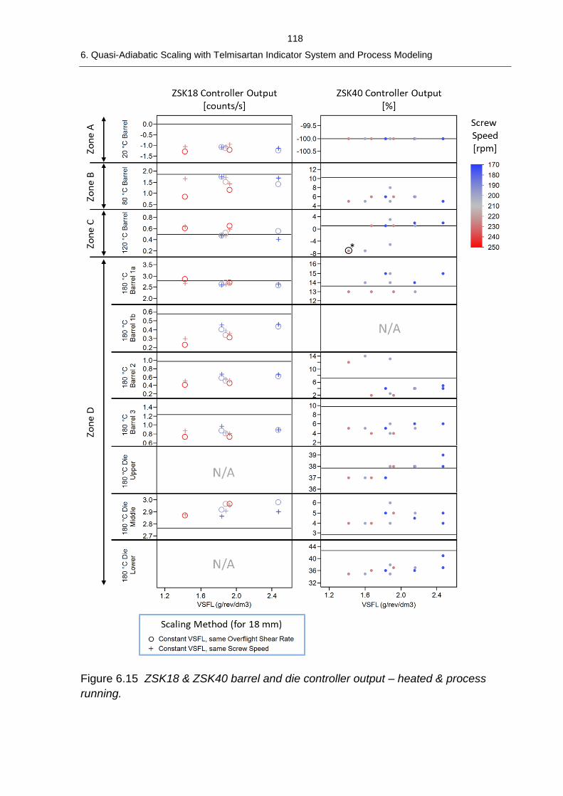
118
6. Quasi-Adiabatic Scaling with Telmisartan Indicator System and Process Modeling
Figure 6.15 ZSK18 & ZSK40 barrel and die controller output – heated & process
running.
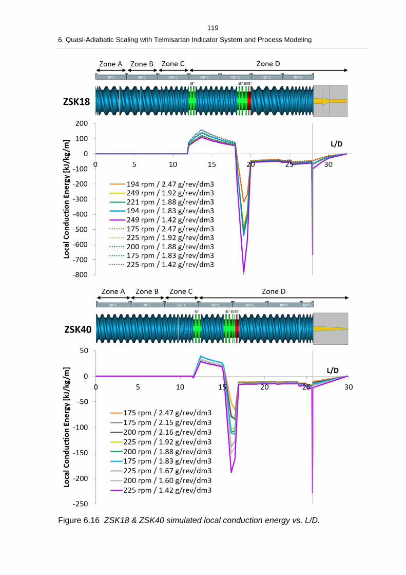
119
6. Quasi-Adiabatic Scaling with Telmisartan Indicator System and Process Modeling
Figure 6.16 ZSK18 & ZSK40 simulated local conduction energy vs. L/D.
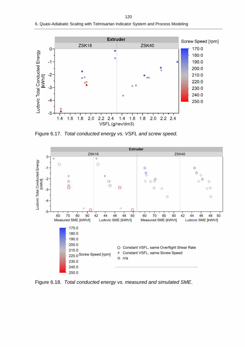
120
6. Quasi-Adiabatic Scaling with Telmisartan Indicator System and Process Modeling
Figure 6.17. Total conducted energy vs. VSFL and screw speed.
Figure 6.18. Total conducted energy vs. measured and simulated SME.
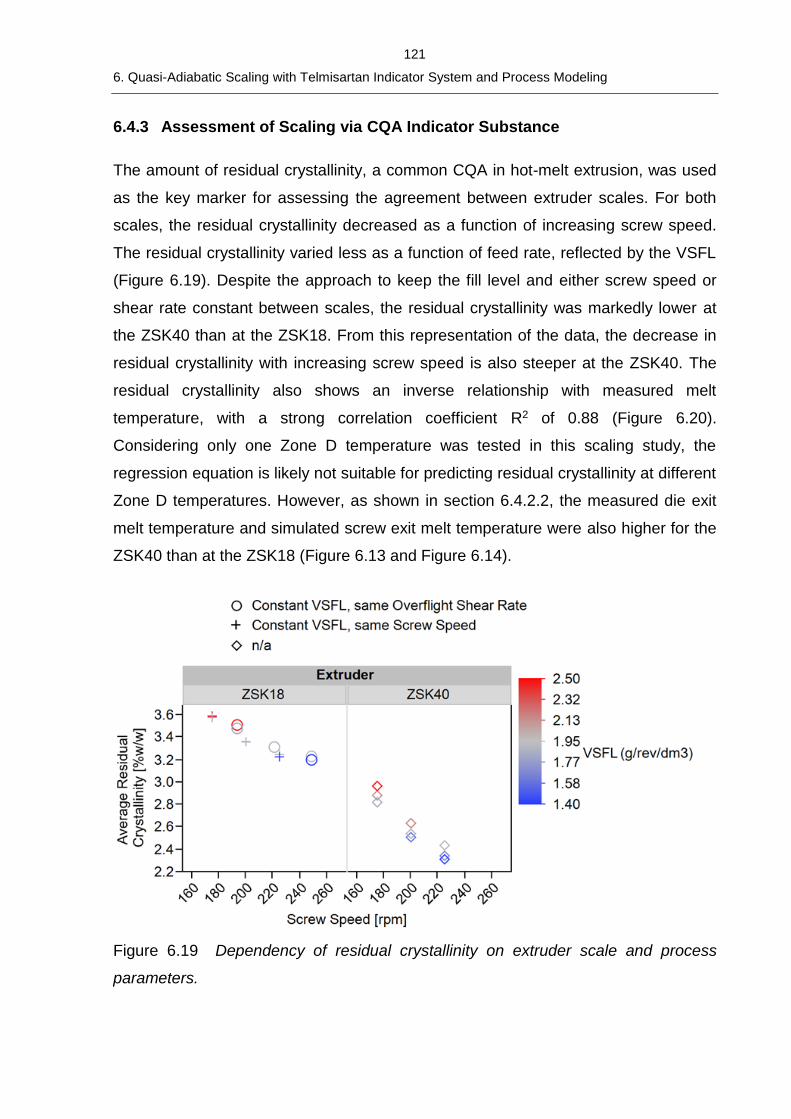
121
6. Quasi-Adiabatic Scaling with Telmisartan Indicator System and Process Modeling
6.4.3 Assessment of Scaling via CQA Indicator Substance
The amount of residual crystallinity, a common CQA in hot-melt extrusion, was used
as the key marker for assessing the agreement between extruder scales. For both
scales, the residual crystallinity decreased as a function of increasing screw speed.
The residual crystallinity varied less as a function of feed rate, reflected by the VSFL
(Figure 6.19). Despite the approach to keep the fill level and either screw speed or
shear rate constant between scales, the residual crystallinity was markedly lower at
the ZSK40 than at the ZSK18. From this representation of the data, the decrease in
residual crystallinity with increasing screw speed is also steeper at the ZSK40. The
residual crystallinity also shows an inverse relationship with measured melt
temperature, with a strong correlation coefficient R2 of 0.88 (Figure 6.20).
Considering only one Zone D temperature was tested in this scaling study, the
regression equation is likely not suitable for predicting residual crystallinity at different
Zone D temperatures. However, as shown in section 6.4.2.2, the measured die exit
melt temperature and simulated screw exit melt temperature were also higher for the
ZSK40 than at the ZSK18 (Figure 6.13 and Figure 6.14).
Figure 6.19 Dependency of residual crystallinity on extruder scale and process
parameters.
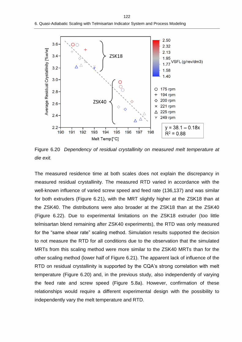
122
6. Quasi-Adiabatic Scaling with Telmisartan Indicator System and Process Modeling
Figure 6.20 Dependency of residual crystallinity on measured melt temperature at
die exit.
The measured residence time at both scales does not explain the discrepancy in
measured residual crystallinity. The measured RTD varied in accordance with the
well-known influence of varied screw speed and feed rate (136,137) and was similar
for both extruders (Figure 6.21), with the MRT slightly higher at the ZSK18 than at
the ZSK40. The distributions were also broader at the ZSK18 than at the ZSK40
(Figure 6.22). Due to experimental limitations on the ZSK18 extruder (too little
telmisartan blend remaining after ZSK40 experiments), the RTD was only measured
for the “same shear rate” scaling method. Simulation results supported the decision
to not measure the RTD for all conditions due to the observation that the simulated
MRTs from this scaling method were more similar to the ZSK40 MRTs than for the
other scaling method (lower half of Figure 6.21). The apparent lack of influence of the
RTD on residual crystallinity is supported by the CQA’s strong correlation with melt
temperature (Figure 6.20) and, in the previous study, also independently of varying
the feed rate and screw speed (Figure 5.8a). However, confirmation of these
relationships would require a different experimental design with the possibility to
independently vary the melt temperature and RTD.
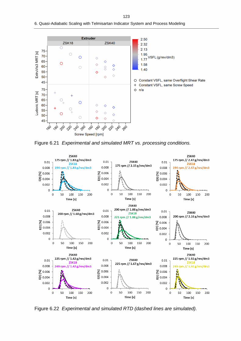
123
6. Quasi-Adiabatic Scaling with Telmisartan Indicator System and Process Modeling
Figure 6.21 Experimental and simulated MRT vs. processing conditions.
Figure 6.22 Experimental and simulated RTD (dashed lines are simulated).
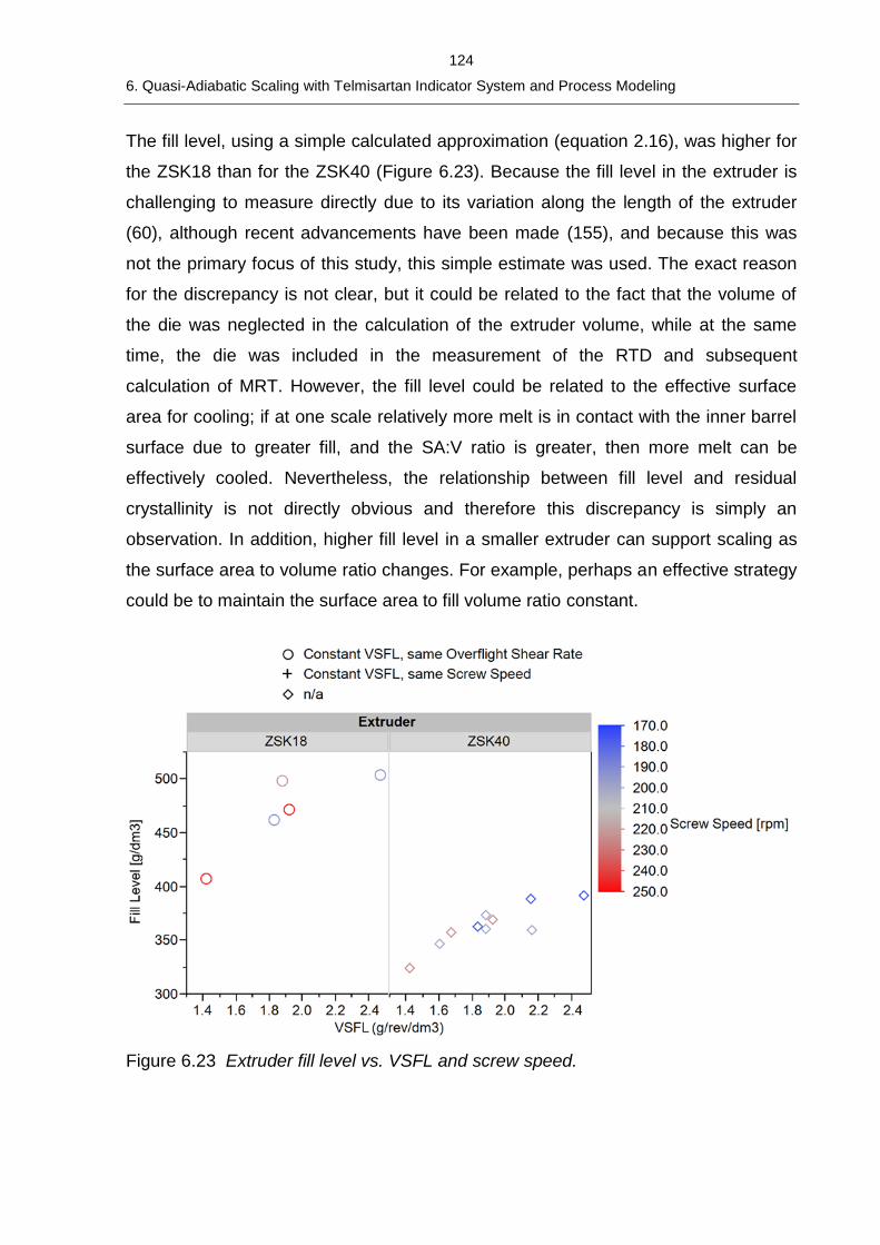
124
6. Quasi-Adiabatic Scaling with Telmisartan Indicator System and Process Modeling
The fill level, using a simple calculated approximation (equation 2.16), was higher for
the ZSK18 than for the ZSK40 (Figure 6.23). Because the fill level in the extruder is
challenging to measure directly due to its variation along the length of the extruder
(60), although recent advancements have been made (155), and because this was
not the primary focus of this study, this simple estimate was used. The exact reason
for the discrepancy is not clear, but it could be related to the fact that the volume of
the die was neglected in the calculation of the extruder volume, while at the same
time, the die was included in the measurement of the RTD and subsequent
calculation of MRT. However, the fill level could be related to the effective surface
area for cooling; if at one scale relatively more melt is in contact with the inner barrel
surface due to greater fill, and the SA:V ratio is greater, then more melt can be
effectively cooled. Nevertheless, the relationship between fill level and residual
crystallinity is not directly obvious and therefore this discrepancy is simply an
observation. In addition, higher fill level in a smaller extruder can support scaling as
the surface area to volume ratio changes. For example, perhaps an effective strategy
could be to maintain the surface area to fill volume ratio constant.
Figure 6.23 Extruder fill level vs. VSFL and screw speed.
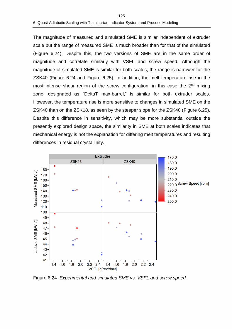
125
6. Quasi-Adiabatic Scaling with Telmisartan Indicator System and Process Modeling
The magnitude of measured and simulated SME is similar independent of extruder
scale but the range of measured SME is much broader than for that of the simulated
(Figure 6.24). Despite this, the two versions of SME are in the same order of
magnitude and correlate similarly with VSFL and screw speed. Although the
magnitude of simulated SME is similar for both scales, the range is narrower for the
ZSK40 (Figure 6.24 and Figure 6.25). In addition, the melt temperature rise in the
most intense shear region of the screw configuration, in this case the 2nd mixing
zone, designated as “DeltaT max-barrel,” is similar for both extruder scales.
However, the temperature rise is more sensitive to changes in simulated SME on the
ZSK40 than on the ZSK18, as seen by the steeper slope for the ZSK40 (Figure 6.25).
Despite this difference in sensitivity, which may be more substantial outside the
presently explored design space, the similarity in SME at both scales indicates that
mechanical energy is not the explanation for differing melt temperatures and resulting
differences in residual crystallinity.
Figure 6.24 Experimental and simulated SME vs. VSFL and screw speed.
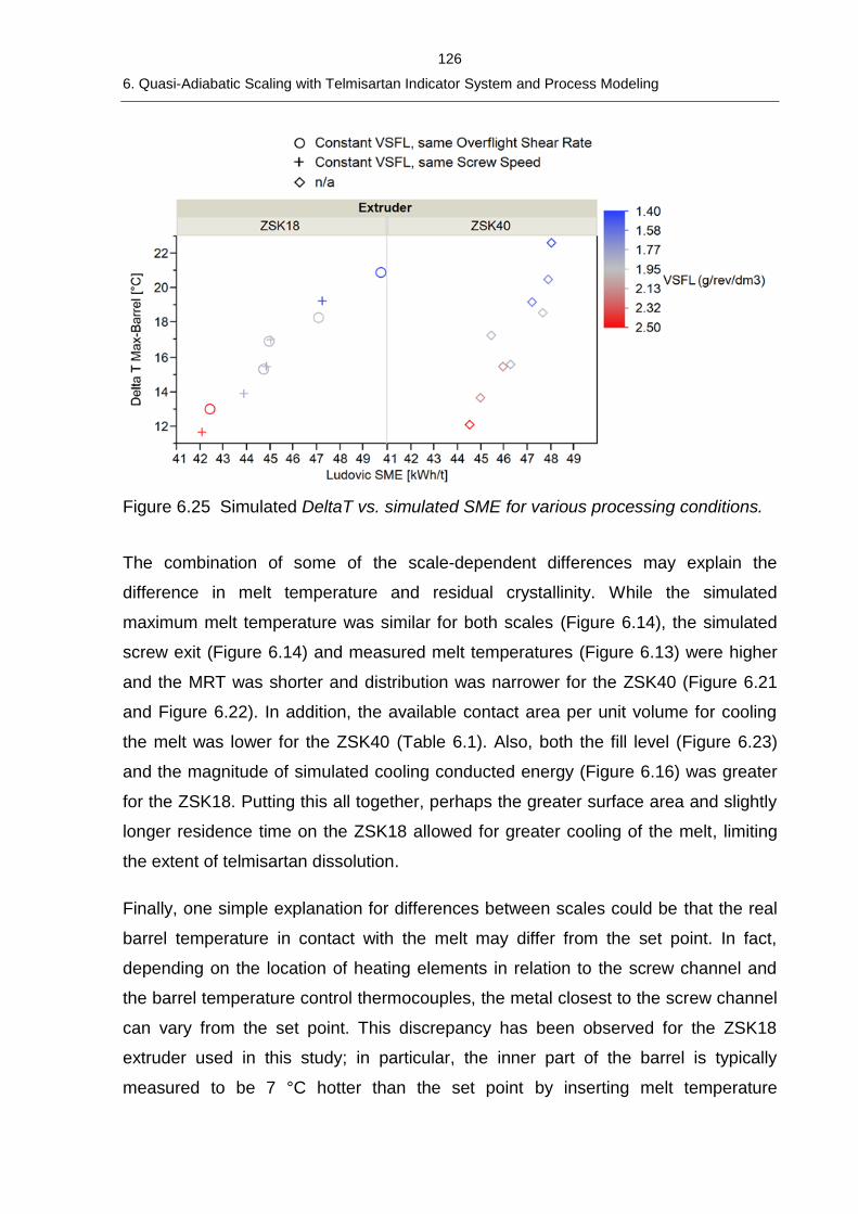
126
6. Quasi-Adiabatic Scaling with Telmisartan Indicator System and Process Modeling
Figure 6.25 Simulated DeltaT vs. simulated SME for various processing conditions.
The combination of some of the scale-dependent differences may explain the
difference in melt temperature and residual crystallinity. While the simulated
maximum melt temperature was similar for both scales (Figure 6.14), the simulated
screw exit (Figure 6.14) and measured melt temperatures (Figure 6.13) were higher
and the MRT was shorter and distribution was narrower for the ZSK40 (Figure 6.21
and Figure 6.22). In addition, the available contact area per unit volume for cooling
the melt was lower for the ZSK40 (Table 6.1). Also, both the fill level (Figure 6.23)
and the magnitude of simulated cooling conducted energy (Figure 6.16) was greater
for the ZSK18. Putting this all together, perhaps the greater surface area and slightly
longer residence time on the ZSK18 allowed for greater cooling of the melt, limiting
the extent of telmisartan dissolution.
Finally, one simple explanation for differences between scales could be that the real
barrel temperature in contact with the melt may differ from the set point. In fact,
depending on the location of heating elements in relation to the screw channel and
the barrel temperature control thermocouples, the metal closest to the screw channel
can vary from the set point. This discrepancy has been observed for the ZSK18
extruder used in this study; in particular, the inner part of the barrel is typically
measured to be 7 °C hotter than the set point by inserting melt temperature
127
6. Quasi-Adiabatic Scaling with Telmisartan Indicator System and Process Modeling
thermocouples into the sensor bores. Because of this, the barrel set point was
adjusted accordingly, although slight offsets of this type could potentially lead to
experimental error. On the other hand, this is again likely not the explanation for the
temperature discrepancy because the simulated temperature was also different for
both scales.
Depending on the sensitivity of a given CQA to melt temperature in a given
formulation, the observed difference of 4-6 °C in melt temperature upon scaling may
or may not be problematic. In the case of telmisartan, this temperature difference
was great enough to result in a measurable difference in residual crystallinity.
However, at process settings intense enough to eliminate residual crystallinity, such
as higher barrel temperatures and higher mechanical energy, the design space may
be broader, as was seen in Chapter 5. On the other hand, if a system is thermo-labile
or exhibits fast degradation kinetics following dissolution, as was seen with
torasemide and other systems (31,128,156), this difference in temperature may not
be tolerable. If a narrow temperature range is required for a particular pharmaceutical
product, for example one prone to thermal degradation, some options for adjusting
the melt temperature could be to adjust the barrel temperature, the screw speed
(146), or the volume of material in the extruder, for example, in accordance with the
change in surface area available for conduction, as suggested earlier.
The methodology employed here for identifying the quasi-adiabatic point for a
formulation for a given hardware setup, i.e. screw configuration, using simulation,
and then and using simple scaling approaches coupled with simulation to select
ranges for screw speed and feed rate to more precisely inform experimental design
could be used to guide scaling approaches in other systems which seek to maintain
constant CQAs and simultaneously balance the extruder thermal energy. The two
ideas are not mutually exclusive and the relationships between all factors should still
hold. Use of a phase diagram plus knowledge of the degradation propensity can
support identification of the target melt temperature which will enable meeting the
CQA ranges. Simulation can then be used to identify and build a process around the
quasi-adiabatic point. Due to all of the inter-dependent and related factors which can
affect the melt temperature, and because simulation accounts for these factors,
simulation is a promising and useful tool to design a scale-up or -down study. If the

128
6. Quasi-Adiabatic Scaling with Telmisartan Indicator System and Process Modeling
quasi-adiabatic point is too high, or too low, to achieve the required CQAs for a given
drug substance, the formulation can be adjusted by addition of a plasticizer or anti-
plasticizer, or the screw configuration could be adapted. The feed rate and screw
speed, considering their individual impact on the SME, can then be adjusted to tune
the process to the quasi-adiabatic point. As was highlighted in Chapter 5, the
formulation is not just critical for bio-performance; formulation material properties are
also critical to achieve ideal processing performance.
6.5 Conclusions
This investigation aimed to study the scaling of adiabatic processes using an
indicator substance, the API itself, with support from simulation, and to avoid the
need for cooling at large scale. Simulation helped to identify the best formulation for
processing to both achieve adiabatic state and have a measurable CQA. Simulation
also helped to identify the target barrel temperature that would result in an adiabatic
state.
Quasi-adiabatic states were observed for both scales. In particular, a balance was
achieved in which the DeltaT was positive due to some viscous dissipation but, on
the whole, the extruder required less heating than in the empty state to maintain
barrel set temperatures. Cooling in one barrel was required on the 40 mm scale in
only one extreme high SME condition. The controller output correlated with both
simulated total and local conducted energy, indicating that this simulated value is a
good predictor of an adiabatic state. Use of the simplified scaling approaches of
maintaining VSFL and shear rate resulted in slightly higher melt temperature and
slightly less residual crystallinity at large scale. The telmisartan indicator system was
sensitive enough to indicate that the slight difference in melt temperature between
the two scales was too substantial. However, this melt temperature difference
between scales may be insignificant in other cases in which the CQA is less sensitive
to temperature. The agreement across scale in extruder conducted energy profile,
melt temperature, residence time and SME indicate that the approach investigated in
this study is appropriate for scaling an adiabatic process.
129
7. Materials and Methods
7 Materials and Methods
7.1 Materials
The materials used in the experiments are listed in Table 7.1. All materials were used
as supplied unless otherwise noted. All materials were purchased except for
Soluplus® which was kindly donated by BASF.
Torasemide API particle size was d90 < 36 µm according to the material certificate of
analysis. SOL was chosen for its relatively low processing temperature, beginning at
135 °C on the 10 mm diameter extruder based on torque limitations. PEG 1500 was
chosen as a plasticizer for SOL based on its chemical similarity to the side chains of
the SOL polymer as well as for its waxy-solid state at room temperature for ease of
processing.
Telmisartan API displayed needle shaped morphology with primary particle size less
than 50 µm. Agglomerates were present in the bulk API powder. COP and TW80
were chosen for their thermal stability and melt viscosity properties.
Table 7.1 Material utilization.
Material Name Abbreviation Function Supplier Modification prior to use
Torasemide, anhydrous, polymorphic form I
TOR API indicator substance
Arevipharma GmbH, Radebeul, Germany
none
Telmisartan, polymorphic form A
TEL API indicator substance
Molekula GmbH, Munich, Germany
none
Polyvinyl caprolactam-polyvinyl acetate-polyethylene glycol graft copolymer (Soluplus®)
SOL Matrix polymer BASF Chemical Co., Ludwigshafen, Germany (donated)
none
vinylpyrrolidone-vinyl acetate copolymer (copovidone, Kollidon® VA 64)
COP Matrix polymer BASF SE, Ludwigshafen, Germany
dried or as received
Polyethylene glycol 1500 PEG 1500 Plasticizer Carl Roth GmbH & Co. KG, Karlsruhe, Germany
milled and screened to <500 µm
polysorbate 80 Ph.Eur./NF (Tween® 80)
TW80 Surfactant / plasticizer
Merck KGaA, Darmstadt, Germany
none
triethyl citrate TEC plasticizer Merck KGaA, Darmstadt, Germany
none
Red iron(III) oxide Sicovit® Red 30 E172
n/a RTD tracer substance
BASF Chemical Co., Ludwigshafen, Germany
none
Two-component adhesive n/a Embedding matrix for microtome
Stanger PV GmbH & Co. KG, Espelkamp, Germany
none
Wacker® AK 10000 silicone fluid
n/a Refractive index-matching fluid
Wacker Chemie AG, Munich, Germany
none
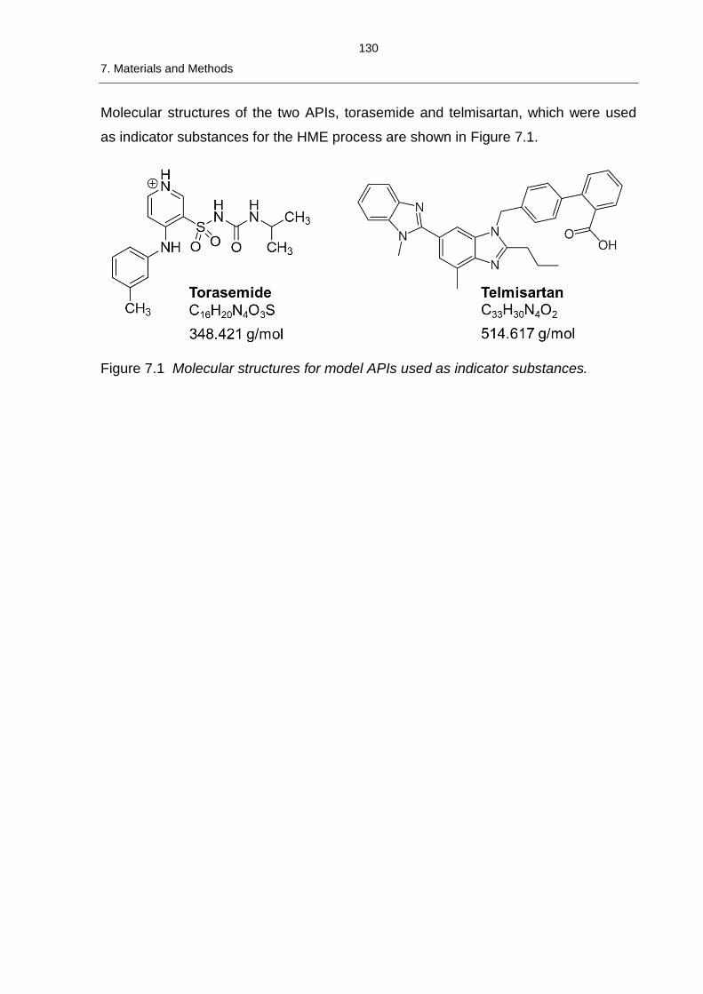
130
7. Materials and Methods
Molecular structures of the two APIs, torasemide and telmisartan, which were used
as indicator substances for the HME process are shown in Figure 7.1.
Figure 7.1 Molecular structures for model APIs used as indicator substances.
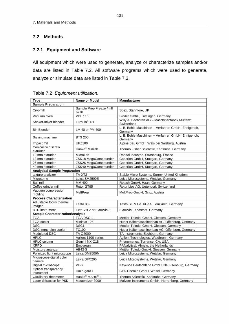
131
7. Materials and Methods
7.2 Methods
7.2.1 Equipment and Software
All equipment which were used to generate, analyze or characterize samples and/or
data are listed in Table 7.2. All software programs which were used to generate,
analyze or simulate data are listed in Table 7.3.
Table 7.2 Equipment utilization.
Type Name or Model Manufacturer
Sample Preparation
Cryomill Sample Prep Freezer/mill 6770
Spex, Stanmore, UK
Vacuum oven VDL 115 Binder GmbH, Tuttlingen, Germany
Shaker-mixer blender Turbula® T2F Willy A. Bachofen AG – Maschinenfabrik Muttenz, Switzerland
Bin Blender LM 40 or PM 400 L. B. Bohle Maschinen + Verfahren GmbH, Ennigerloh, Germany
Sieving machine BTS 200 L. B. Bohle Maschinen + Verfahren GmbH, Ennigerloh, Germany
Impact mill UPZ100 Alpine Bau GmbH, Wals bei Salzburg, Austria
Conical twin screw extruder
Haake® Minilab Thermo Fisher Scientific, Karlsruhe, Germany
10 mm extruder MicroLab Rondol Industrie, Strasbourg, France
18 mm extruder ZSK18 MegaCompounder Coperion GmbH, Stuttgart, Germany
26 mm extruder ZSK26 MegaCompounder Coperion GmbH, Stuttgart, Germany
40 mm extruder ZSK40 MegaCompounder Coperion GmbH, Stuttgart, Germany
Analytical Sample Preparation
texture analyzer TA-XT2 Stable Micro Systems, Surrey, United Kingdom
Microtome Leica SM2500E Leica Microsystems, Wetzlar, Germany
Ball mill MM 400 Retsch GmbH, Haan, Germany
Coffee grinder mill Rotor GT95 Rotor Lips AG, Uetendorf, Switzerland
Vacuum compression molding
MeltPrep MeltPrep GmbH, Graz, Austria
Process Characterization
Adjustable focus thermal imager
Testo 882 Testo SE & Co. KGaA, Lenzkirch, Germany
RTD instrument ExtruVis 2 or ExtruVis 3 ExtruVis, Riedstadt, Germany
Sample Characterization/Analysis
TGA TGA/DSC 1 Mettler-Toledo, GmbH, Giessen, Germany
TGA cooler Ministat 125 Huber Kältemaschinenbau AG, Offenburg, Germany
DSC DSC1 Mettler-Toledo, GmbH, Giessen, Germany
DSC immersion cooler TC100 Huber Kältemaschinenbau AG, Offenburg, Germany
Modulated DSC TA Q2000 TA Instruments, Eschborn, Germany
HPLC Agilent 1100 series Agilent Technologies, Waldbronn, Germany
HPLC column Gemini NX-C18 Phenomenex, Torrence, CA, USA
XRPD Empyrean PANalytical, Almelo, the Netherlands
Moisture analyzer HB43-S Mettler-Toledo GmbH, Giessen, Germany
Polarized light microscope Leica DM2500M Leica Microsystems, Wetzlar, Germany
Microscope digital color camera
Leica DFC295 Leica Microsystems, Wetzlar, Germany
Digital microscope VH-X Keyence Deutschland GmbH, Neu-Isenburg, Germany
Optical transparency instrument
Haze-gard i BYK-Chemie GmbH, Wesel, Germany
Oscillatory rheometer Haake® MARS® II Thermo Scientific, Karlsruhe, Germany
Laser diffraction for PSD Mastersizer 3000 Malvern Instruments GmbH, Herrenberg, Germany
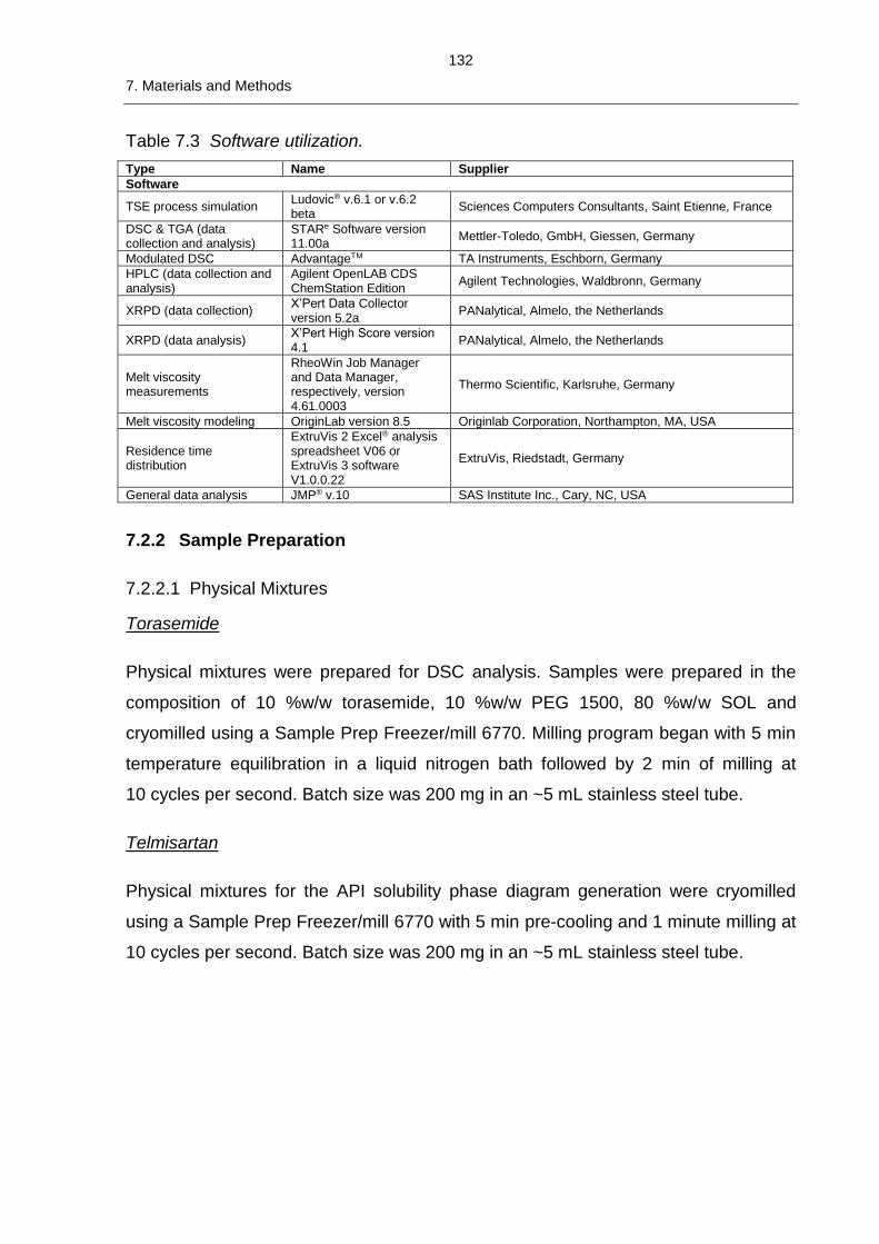
132
7. Materials and Methods
Table 7.3 Software utilization.
Type Name Supplier
Software
TSE process simulation Ludovic® v.6.1 or v.6.2 beta
Sciences Computers Consultants, Saint Etienne, France
DSC & TGA (data collection and analysis)
STARe Software version 11.00a
Mettler-Toledo, GmbH, Giessen, Germany
Modulated DSC AdvantageTM TA Instruments, Eschborn, Germany
HPLC (data collection and analysis)
Agilent OpenLAB CDS ChemStation Edition
Agilent Technologies, Waldbronn, Germany
XRPD (data collection) X’Pert Data Collector version 5.2a
PANalytical, Almelo, the Netherlands
XRPD (data analysis) X’Pert High Score version 4.1
PANalytical, Almelo, the Netherlands
Melt viscosity measurements
RheoWin Job Manager and Data Manager, respectively, version 4.61.0003
Thermo Scientific, Karlsruhe, Germany
Melt viscosity modeling OriginLab version 8.5 Originlab Corporation, Northampton, MA, USA
Residence time distribution
ExtruVis 2 Excel® analysis spreadsheet V06 or ExtruVis 3 software V1.0.0.22
ExtruVis, Riedstadt, Germany
General data analysis JMP® v.10 SAS Institute Inc., Cary, NC, USA
7.2.2 Sample Preparation
7.2.2.1 Physical Mixtures
Torasemide
Physical mixtures were prepared for DSC analysis. Samples were prepared in the
composition of 10 %w/w torasemide, 10 %w/w PEG 1500, 80 %w/w SOL and
cryomilled using a Sample Prep Freezer/mill 6770. Milling program began with 5 min
temperature equilibration in a liquid nitrogen bath followed by 2 min of milling at
10 cycles per second. Batch size was 200 mg in an ~5 mL stainless steel tube.
Telmisartan
Physical mixtures for the API solubility phase diagram generation were cryomilled
using a Sample Prep Freezer/mill 6770 with 5 min pre-cooling and 1 minute milling at
10 cycles per second. Batch size was 200 mg in an ~5 mL stainless steel tube.
133
7. Materials and Methods
7.2.2.2 Extrudates
Torasemide
Extrudate production involved preparation of blends, extrusion, and ball milling of
extrudates for analysis. Blending involved de-lumping the torasemide by passing it
through a 500 µm screen followed by blending it with the PEG 1500 and SOL
(dispensed amount was adjusted for moisture) in a Turbula® blender for 5 min.
Blends and extrudates were stored refrigerated at 5 °C. Blends were prepared in
500 g quantities in 2 L containers.
Extrusion experiments were conducted with a 10 mm (actual 10.9 mm) co-rotating
twin-screw extruder. The extruder was fed via a volumetric feeder with two co-
rotating feeding screws with adjustable speed; feed rate was controlled in this way
and throughput was measured as mass exiting the die per time. Samples of
extrudate were collected only during steady state, defined by a constant torque
reading. The processing zone of the extruder contained 4 temperature zones: zone 1
was cooled by recirculating water set to 10 °C, zone 2 was set to 80 °C, and zone 3,
composed of the last two temperature-controlled regions, was varied. The die was
also heated and was set to the same temperature as zone 3; collectively they are
referred to as “main barrel and die temperature” (Figure 4.2). The die geometry is
known as an 8-0 shape with the following dimensions: 22.9 mm length, 11 mm inlet
diameter, 2 mm outlet diameter, and 9 mm centerline for inlet portion. Four screw
configurations were used (Figure 4.2, Table 7.4). Note that die geometry, designated
in yellow, is not to scale. Extrusion experiments were conducted in 2 separate
studies, details explained in Table 4.1).
The three venting configurations listed in Table 4.1 were selected to produce
extremes in moisture removal from the extruder. The early closed-end closed
configuration enabled a high-moisture process while the two early open
configurations enabled lower-moisture containing processes, and especially with
moisture removal prior to intense mixing. A fourth option, early closed-end open, was
not included in the study because it represents an intermediate moisture-level
condition. In this way, high and low moisture content environments were created to
look at the effect on the evolution of the different degradant species.
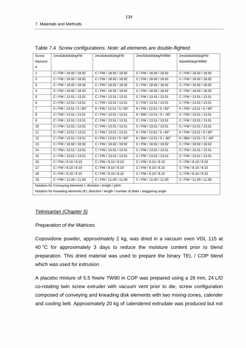
134
7. Materials and Methods
Table 7.4 Screw configurations. Note: all elements are double-flighted.
Screw
Element
#
1mix5disk60degFW 2mix5disk60degFW 2mix5disk60degFWBW 2mix5disk60degFW-
5disk60degFWBW
1 C / FW / 18.92 / 18.92 C / FW / 18.92 / 18.92 C / FW / 18.92 / 18.92 C / FW / 18.92 / 18.92
2 C / FW / 18.92 / 18.92 C / FW / 18.92 / 18.92 C / FW / 18.92 / 18.92 C / FW / 18.92 / 18.92
3 C / FW / 18.92 / 18.92 C / FW / 18.92 / 18.92 C / FW / 18.92 / 18.92 C / FW / 18.92 / 18.92
4 C / FW / 18.92 / 18.92 C / FW / 18.92 / 18.92 C / FW / 18.92 / 18.92 C / FW / 18.92 / 18.92
5 C / FW / 13.51 / 13.51 C / FW / 13.51 / 13.51 C / FW / 13.51 / 13.51 C / FW / 13.51 / 13.51
6 C / FW / 13.51 / 13.51 C / FW / 13.51 / 13.51 C / FW / 13.51 / 13.51 C / FW / 13.51 / 13.51
7 K / FW / 13.51 / 5 / 60° K / FW / 13.51 / 5 / 60° K / FW / 13.51 / 5 / 60° K / FW / 13.51 / 5 / 60°
8 C / FW / 13.51 / 13.51 C / FW / 13.51 / 13.51 K / BW / 13.51 / 5 / -60° C / FW / 13.51 / 13.51
9 C / FW / 13.51 / 13.51 C / FW / 13.51 / 13.51 C / FW / 13.51 / 13.51 C / FW / 13.51 / 13.51
10 C / FW / 13.51 / 13.51 C / FW / 13.51 / 13.51 C / FW / 13.51 / 13.51 C / FW / 13.51 / 13.51
11 C / FW / 13.51 / 13.51 C / FW / 13.51 / 13.51 K / FW / 13.51 / 5 / 60° K / FW / 13.51 / 5 / 60°
12 C / FW / 13.51 / 13.51 K / FW / 13.51 / 5 / 60° K / BW / 13.51 / 5 / -60° K / BW / 13.51 / 5 / -60°
13 C / FW / 18.92 / 18.92 C / FW / 18.92 / 18.92 C / FW / 18.92 / 18.92 C / FW / 18.92 / 18.92
14 C / FW / 13.51 / 13.51 C / FW / 13.51 / 13.51 C / FW / 13.51 / 13.51 C / FW / 13.51 / 13.51
15 C / FW / 13.51 / 13.51 C / FW / 13.51 / 13.51 C / FW / 13.51 / 13.51 C / FW / 13.51 / 13.51
16 C / FW / 8.10 / 8.10 C / FW / 8.10 / 8.10 C / FW / 8.10 / 8.10 C / FW / 8.10 / 8.10
17 C / FW / 8.10 / 8.10 C / FW / 8.10 / 8.10 C / FW / 8.10 / 8.10 C / FW / 8.10 / 8.10
18 C / FW / 8.10 / 8.10 C / FW / 8.10 / 8.10 C / FW / 8.10 / 8.10 C / FW / 8.10 / 8.10
19 C / FW / 11.00 / 11.00 C / FW / 11.00 / 11.00 C / FW / 11.00 / 11.00 C / FW / 11.00 / 11.00
Notation for Conveying elements I: direction / length / pitch
Notation for Kneading elements (K): direction / length / number of disks / staggering angle
Telmisartan (Chapter 5)
Preparation of the Matrices
Copovidone powder, approximately 2 kg, was dried in a vacuum oven VDL 115 at
40 °C for approximately 3 days to reduce the moisture content prior to blend
preparation. This dried material was used to prepare the binary TEL / COP blend
which was used for extrusion.
A placebo mixture of 5.5 %w/w TW80 in COP was prepared using a 26 mm, 24 L/D
co-rotating twin screw extruder with vacuum vent prior to die, screw configuration
composed of conveying and kneading disk elements with two mixing-zones, calender
and cooling belt. Approximately 20 kg of calendered extrudate was produced but not
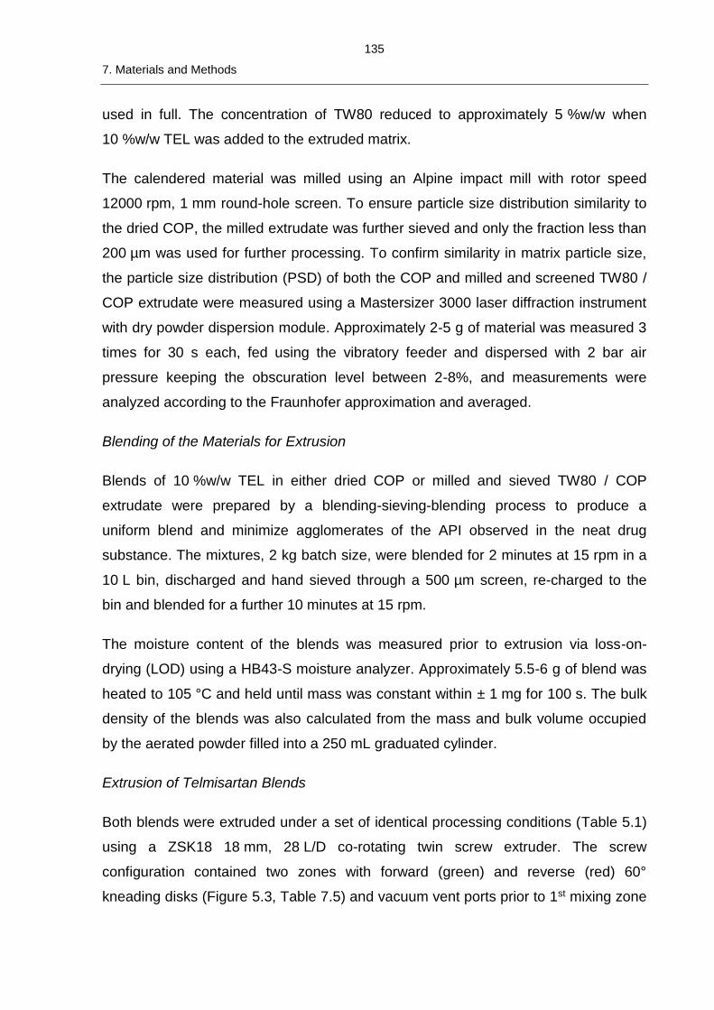
135
7. Materials and Methods
used in full. The concentration of TW80 reduced to approximately 5 %w/w when
10 %w/w TEL was added to the extruded matrix.
The calendered material was milled using an Alpine impact mill with rotor speed
12000 rpm, 1 mm round-hole screen. To ensure particle size distribution similarity to
the dried COP, the milled extrudate was further sieved and only the fraction less than
200 µm was used for further processing. To confirm similarity in matrix particle size,
the particle size distribution (PSD) of both the COP and milled and screened TW80 /
COP extrudate were measured using a Mastersizer 3000 laser diffraction instrument
with dry powder dispersion module. Approximately 2-5 g of material was measured 3
times for 30 s each, fed using the vibratory feeder and dispersed with 2 bar air
pressure keeping the obscuration level between 2-8%, and measurements were
analyzed according to the Fraunhofer approximation and averaged.
Blending of the Materials for Extrusion
Blends of 10 %w/w TEL in either dried COP or milled and sieved TW80 / COP
extrudate were prepared by a blending-sieving-blending process to produce a
uniform blend and minimize agglomerates of the API observed in the neat drug
substance. The mixtures, 2 kg batch size, were blended for 2 minutes at 15 rpm in a
10 L bin, discharged and hand sieved through a 500 µm screen, re-charged to the
bin and blended for a further 10 minutes at 15 rpm.
The moisture content of the blends was measured prior to extrusion via loss-on-
drying (LOD) using a HB43-S moisture analyzer. Approximately 5.5-6 g of blend was
heated to 105 °C and held until mass was constant within ± 1 mg for 100 s. The bulk
density of the blends was also calculated from the mass and bulk volume occupied
by the aerated powder filled into a 250 mL graduated cylinder.
Extrusion of Telmisartan Blends
Both blends were extruded under a set of identical processing conditions (Table 5.1)
using a ZSK18 18 mm, 28 L/D co-rotating twin screw extruder. The screw
configuration contained two zones with forward (green) and reverse (red) 60°
kneading disks (Figure 5.3, Table 7.5) and vacuum vent ports prior to 1st mixing zone
136
7. Materials and Methods
and prior to the die. The second vacuum port pressure was set to 900 mbar. The
extruder barrel was composed of 7 barrel segments or temperature zones plus die
set to 20/80/120/T/T/T/T/T °C, with T meaning target temperature. The target
temperature was varied together in the experiment and is referred to as “barrel
temperature.” The screw speed and feed rate were varied together in order to
maintain the same degree of fill in the extruder barrel using the simple specific feed
load equation, equation 2.14 of mass flow rate divided by screw speed (62).
Thin strands of extrudate were collected, separated from one another, and allowed to
cool to room temperature before storage in air tight bottles. Samples were stored at
room temperature prior to further processing.
Table 7.5 Screw configurations. Note: all elements are double-flighted.
Screw
Element #
Screw Element Description Screw
Element #
Screw Element Description
1 C / FW / 8.00 / 8.00 (spacer element) 11 C / FW / 24.00 / 24.00
2 C / FW / 48.00 / 36.00 12 K / FW / 24.00 / 5 / 60°
3 C / FW / 48.00 / 36.00 13 K / BW / 24.00 / 5 / -60°
4 C / FW / 36.00 / 24.00 14 C / FW / 36.00 / 36.00
5 C / FW / 36.00 / 24.00 15 C / FW / 24.00 / 24.00
6 C / FW / 24.00 / 24.00 16 C / FW / 24.00 / 24.00
7 C / FW / 24.00 / 24.00 17 C / FW / 12.00 / 12.00
8 K / FW / 24.00 / 5 / 60° 18 C / FW / 12.00 / 12.00
9 C / FW / 24.00 / 24.00 19 C / FW / 12.00 / 12.00
10 C / FW / 24.00 / 24.00 20 C / FW / 16.00 / 16.00
Notation for Conveying elements I: direction / length / pitch
Notation for Kneading elements (K): direction / length / number of disks / staggering angle
3 %w/w Triethyl Citrate in COP
A mixture of 3 %w/w triethyl citrate in COP was prepared in a coffee grinder type mill
and extruded at 160 °C and 100 rpm using a Minilab co-rotating conical screw
extruder. The extrudates were milled again in a coffee grinder type mill and stored at
ambient conditions prior to further testing.
Telmisartan (Chapter 6)
The process flow diagram for sample preparation is shown in Figure 6.7.
137
7. Materials and Methods
Preparation of the Matrix
A mixture of 6 %w/w TW80 in COP was prepared using a 40 mm, 25.725 L/D co-
rotating twin screw extruder with vacuum vent prior to die at 500 mbar, 2 mixing-zone
screw composed of conveying and kneading disk elements (Figure 6.5, Table 6.2),
calender and cooling belt. Approximately 100 kg was prepared.
The calendered material was milled using an impact mill using a 2-step procedure.
First the calendered material was milled with rotor speed 12000 rpm, 1.3 mm conidur
screen to form a coarse granulate. Second, the granulate was milled with rotor speed
11000 rpm and 0.8 mm conidur screen to ensure similarity to the dried COP and
milled placebo extrudate used in Chapter 5. To confirm similarity in matrix particle
size, the extrudate was measured identically as described in methods for Chapter 5.
Blending of the Materials for Extrusion
A blend of 10 %w/w TEL in milled TW80/COP extrudate were prepared by a
blending-sieving-blending process to produce a uniform blend and minimize
agglomerates of the API observed in the neat drug substance. The blend, about
110 kg in two portions due to blender container fill volume, was blended for
10 minutes at 6 rpm in a Bohle MCL 200 L container, discharged and de-lumped
through a 1.5 mm screen installed in a Bohle BTS 200 sieving machine, collected in
a second Bohle MCL 200 L container and blended for a further 10 minutes at 6 rpm.
Blending was performed using a Bohle PM 400 machine.
Extrusion with Telmisartan
The blend was extruded according to scaled conditions using both 18 mm and 40
mm extruders. The extruder characteristics are listed in Table 6.1, schematics of the
extruder configurations are shown in Figure 6.5, the screw configurations are listed
and compared in Table 6.2, and the barrel and die temperature profile is listed in
Table 6.3. The feed rate and screw speed process parameters for the 40 mm scale
are listed in Table 6.4, while those for the two scaling methods run on the 18 mm
scale are listed in Table 6.6 and Table 6.7. The vacuum port pressure was set to 500
mbar. The experiment design is explained in section 6.3 and selection of the process
138
7. Materials and Methods
parameters is explained in section 6.3.2.2. Approximately 100 kg of blend was
extruded at the 40 mm scale while less than 10 kg remained for the 18 mm scale.
Thin strands of extrudate were collected, separated from one another in metal bowls,
and allowed to cool to room temperature before collection in air tight bottles. Samples
were stored at room temperature prior to further processing.
7.2.3 Process Characterization
7.2.3.1 Melt Temperature
The melt temperature of the extrudate was measured at the exit of the die using a
Testo 882 adjustable focus thermal imager. The hottest temperature recorded on the
extrudate strand in the focused image was taken as the melt temperature. A literature
value of 0.9 was used for the thermal emissivity (56).
7.2.3.2 Residence Time Distribution (RTD)
Experiments discussed in section 4.4.2 were measured with the ExtruVis 2 and
accompanying analysis spreadsheet. Experiments discussed in section 4.4.3 and in
Chapter 6 were measured using the ExtruVis 3 and accompanying software. Mean
residence times (MRT) were determined using the algorithms described in the
equipment documentation literature. Red iron(III) oxide was used as a tracer
substance and added as a pulse in quantities <1/100 of the throughput.
7.2.3.3 Controller Output
The controller output on the ZSK18 consisted of a cumulative count of heating or
cooling events at least 150 ms in duration. This accumulation was plotted over time
and the slope was taken as the controller output signal. When both heating and
cooling events were occurring in a given temperature zone, aka barrel segment or
die, during steady state, both slopes were calculated and summed. For the ZSK40,
the controller output, expressed as either a positive or negative percentage, was
used directly.
139
7. Materials and Methods
7.2.4 Analytical Sample Preparation
Torasemide extrudates were ball milled using 50 mL jars and 20 mm diameter balls
for 10 s at 30 Hz, followed by collection of powder <500 µm via sieving. Milled
extrudates were stored refrigerated at 5 °C prior to further analysis and
characterization.
Telmisartan extrudates were milled in a coffee grinder type mill and sieved <500 µm.
Powder was stored at room temperature in air-tight bottles prior to further analysis
and characterization.
7.2.5 Sample Characterization/Analysis
TGA experiments for all samples were performed using a TGA/DSC 1 with a Ministat
125 under nitrogen gas flow. All conventional DSC experiments were performed
using a DSC 1 with auto-sampler with a TC100 immersion cooler under nitrogen gas
flow. Calibration of the DSC was performed with zinc and indium standards.
7.2.5.1 Torasemide
TGA
TGA was used to characterize the degradation temperature of a neat unprocessed
torasemide sample. A sample mass of 33.5 mg was filled in a 100 µL aluminum pan
and was heated from 25 to 250 °C at a heating rate of 10 K/min under nitrogen gas
flow.
DSC
A DSC was used as an oven for controlled heating studies on the micro-scale as well
as for heat flow characterization. Measurements were conducted under nitrogen gas
flow.
Controlled Heating of Neat Torasemide and Physical Mixtures
DSC pans, 40 µL aluminum, containing approximately 5 mg of sample were heated
from room temperature to various end temperatures at a heating rate of 10 K/min.
140
7. Materials and Methods
The end temperature range for neat torasemide was 100-180 °C while a range of 40-
160 °C was used for physical mixtures. Both lid-pierced, with 3 large vent holes, and
hermetically sealed pans were prepared for each end temperature to study the effect
of moisture. Samples were removed from the DSC via the auto-sampler and were
allowed to cool at ambient conditions.
Determination of Torasemide Dissolution Starting Temperature in Soluplus® / PEG
1500 Matrix
An 8.5 mg sample of extrusion blend, dried in a vacuum oven to remove moisture,
was heated in a 40 µL aluminum pan with pierced lid from 25-180 °C at a heating
rate of 10 K/min. The dissolution endotherm was visible from the thermogram, but the
exact point of dissolution onset was identified via the first derivative of the original
curve.
HPLC
HPLC was conducted to identify the presence and relative amounts of degradation
products of torasemide formed during DSC studies and extrusion processing, as well
as to quantify the total amount of torasemide in the extrudates, i.e. crystalline plus
dissolved. Analysis was performed using an Agilent 1100 series. The
chromatographic separation was performed on a Gemini NX-C18 analytical column
(150 mm long, 2.1 mm diameter, 3 µm particle size, 110 Å pore size). The mobile
phase was water with 0.1 %v/v trifluoroacetic acid (85%) (mobile phase A) and
acetonitrile with 0.05 %v/v trifluoroacetic acid (85%) (mobile phase B) with linear
gradient elution: 0 min, B 10%; 5 min, B 15%; 15 min, B 65%; 17 min, B 80%;
18 min, B 10% (total time 25 min). The flow rate was 0.4 mL/min, the injection volume
was 2 µL, and the detection was performed at 280 nm. All reagents were of HPLC
grade.
Standard solutions of neat torasemide in 1+1 (v/v) acetonitrile (I) + water were
prepared at 0.1 mg/mL. Ball-milled extrudate samples were dissolved at
concentrations of approximately 5 mg of extrudate per 50 mL 1+1 (v/v) acetonitrile +
water. Samples prepared in DSC pans containing approximately 5 mg of analyte
were dissolved in 50 mL 1+1 (v/v) I + water.
141
7. Materials and Methods
Typical chromatograms showed 1-3 peaks, depending on their composition and how
they were processed. The molecular structure of the species present in each peak
was investigated by mass spectrometry. For details, please see Appendix 10.1. The
first eluent at retention time (RT) 2.8 min is a thermal degradant, m/z 290, the second
at RT 6.5 min is a hydrolysis degradant, m/z 264, identical to R2 described in (101),
and the third at RT 11.6 min is torasemide, m/z 349. Most results are reported as
sum of degradants in units of peak area percent (PA%), and in extrudate samples,
this value is the sum of the thermal and hydrolysis degradant PA%. Total torasemide
as %w/w of the original extrusion blend was calculated via a calibration standard
curve. The amount of dissolved torasemide as %w/w was calculated by subtracting
the residual crystallinity in %w/w measured by XRPD from the total torasemide. An
estimate of the weight fraction of degradants was calculated by subtracting the total
torasemide from the theoretical extrusion blend concentration of 10 %w/w. Note that
10 %w/w is the maximum value that these values can have based upon the 10 %w/w
drug loading of the original extrusion blend.
X-ray Powder Diffraction (XRPD)
Residual crystallinity was quantified using X-ray powder diffraction (XRPD). Samples
were measured using an Empyrean system using Cu Kα radiation (45 kV and 40 mA),
a step size of 0.026° 2θ over an angular range of 24-26° 2θ. Background subtraction
was performed on all diffraction patterns. Calibration was performed with samples
ranging from 0.1 to 10 %w/w spiked crystalline torasemide in extruded placebo, and
the reflex height at 24.5° 2θ was used for back calculation of the %w/w crystalline
torasemide in extruded samples. Residual crystallinity is reported as %w/w of
sample, and all formulations contained a nominal or initial concentration of 10 %w/w
crystalline torasemide.
Blend Moisture Content
The moisture content of SOL and extrusion blends was measured via loss-on-drying
using a HB43-S moisture analyzer. Samples were heated to 105 °C and held until the
mass was constant within +/- 1 mg for 100 seconds. The typical SOL moisture
content was 2.5-3 %w/w and for blends was 2-2.5 %w/w.
142
7. Materials and Methods
Polarized Light Microscopy (PLM)
Residual crystallinity present in extrudates was qualitatively visualized in the form of
thin sections. Extrudates were prepared by embedding them in two-component
adhesive for support. The two-component adhesive was prepared in a 1:1 mass ratio
of resin to accelerator, which produced a non-brittle matrix suitable for cutting. This
composite sample was sliced to 50 µm thick using a Leica SM2500E microtome. The
thin sections were submerged in silicone fluid between glass slide and cover slip to
minimize the presence of cut marks and then imaged using a Leica DM2500M
microscope equipped with a Leica DFC295 color digital camera. The samples were
imaged using crossed polars and Koehler illumination.
Extrudate Optical Appearance
Extrudate strands were flattened between two slides to a thickness of 1 mm using a
TA-XT2 texture analyzer equipped with an oven set to 100 °C. These extrudates
were placed on 1 mm grid paper and photographed using a digital microscope VH-X.
The turbidity of the samples was quantified using the haze value reported by the
Haze-gard i optical transparency instrument. The haze value is a measure of the
diffuse scattering of transmitted light in all directions, and this is detected by an
integrating sphere with the forward directed light being excluded by a light trap.
Melt Rheology
The melt viscosity of pure Soluplus® and selected extrudates was measured and
fitted to the Carreau-Yasuda equation with WLF temperature dependency, as
described previously (135), with slight modifications: a Haake® MARS® II oscillatory
rheometer was used with a gap height of 1.5 mm and amplitude of 5%. Temperature
ranged from 110 to 170 °C, depending on formulation.
Thermal Properties for Simulation
The heat capacity of milled TOR extrudates with less than 1 %w/w residual
crystallinity was measured by modulated DSC TA Q2000. Approximately 4 mg was
placed in a pierced Tzero hermetic aluminum pan and heated to 100 °C, held for
2 min, cooled to 10 °C, held for 5 min, and then heated to 170 °C with a heating rate
143
7. Materials and Methods
of 2 K/min with modulation ±1 °C every 120 s. The instrument was temperature
calibrated with gallium, indium, tin and bismuth standards. Calibration of the heat
capacity was performed with a sapphire calibration standard. The thermal
conductivity for both solid and liquid phases was assumed to be temperature
independent and a literature value similar to other amorphous polymers was used
(157). The Tg of the respective formulation was used at the input value for melt
temperature.
Density Characterization for Simulation
The solid density input parameter required for simulation was taken to be the bulk
density of the starting blend, method described in section 7.2.2.2. The melt density
was taken as the room temperature density calculated from cylindrically shaped
pieces of cooled extrudate of uniform diameter.
7.2.5.2 Telmisartan
DSC Experiments
Basic thermal analysis such as melting temperature (Tm) and glass transition
temperature, (Tg), were performed. The Tm of TEL, taken as the peak of the melting
endotherm, was confirmed using DSC by heating 4 mg of substance in 20 µL pierced
aluminum pans and heated from room temperature to 280 °C at 10 K/min under
nitrogen gas flow. The Tg, taken as the midpoint in the transition, was measured in
the second heating after the Tm determination, holding the sample above the melting
point for 1 minute, then rapidly cooling at 50 K/min to -40 °C, and re-heating to the
melting temperature at 10 K/min.
In addition, the solubility phase diagram of TEL in binary and ternary mixtures of
COP and TW80 according to method in Kyeremateng, et.al., was also generated
(102). The Tg of various mixtures was calculated using the Fox equation (158). The
onset dissolution temperature of TEL into the two matrices was measured using DSC
and extrudates with > 3 %w/w residual crystallinity by heating the milled extrudates to
120 °C at 10 K/min, holding for 2 minutes to dehydrate the sample, cooling to -40 °C
at 50K/min, and finally heating to 220 °C at 10 K/min.
144
7. Materials and Methods
The Tg of a 3 %w/w TEC in COP milled extrudate sample was measured using the
DSC1 by heating the sample to 150 °C at 10 K/min, holding for 2 minutes to remove
moisture, cooling rapidly at 50 K/min to -40 °C and heating again to 150 °C at
10 K/min.
TGA Experiments
Thermal decomposition of TEL and TW80 was determined by thermogravimetric
analysis (TGA) in 40 µL aluminum pans with 5-20 mg of substance, heating from
room temperature to 300 °C with a heating rate of 10 K/min under nitrogen gas flow.
X-Ray Powder Diffraction (XRPD)
The residual crystalline TEL in milled extrudate samples was measured using an
Empyrean system using Cu Kα (45 kV and 40 mA), over an angular range of 5-8° 2θ
with a step size of 0.026° 2θ. Data was analyzed using X’Pert High Score v4.1,
including background subtraction on all diffraction patterns. Peak intensities at
6.75° 2θ were compared to those measured in a calibration set of samples with
spiked crystallinity concentrations ranging between 0-10 %w/w. The residual
crystallinity is reported as %w/w of sample, and aside from the calibration samples, a
nominal concentration of 10 %w/w TEL was used in all samples.
Thermal Properties for Simulation
The heat capacity, cp, of milled TEL extrudates with less than 1 %w/w residual
crystallinity was measured by modulated DSC TA Q2000. Approximately 4 mg was
placed in a pierced Tzero hermetic aluminum pan and heated to 100 °C, held for
2 min, cooled to 10 °C, held for 5 min, and then heated to 230 °C with a heating rate
of 2 K/min with modulation ±1 °C every 120 s. The instrument was temperature
calibrated with gallium, indium, tin and bismuth standards. Calibration of the heat
capacity was performed with a sapphire calibration standard. The thermal
conductivity for both solid and liquid phases was assumed to be temperature
independent and a literature value similar to other amorphous polymers was used
(157). The Tg of the respective formulation taken from the phase diagram was used
as the input value for melt temperature in the Ludovic® simulation.
145
7. Materials and Methods
Density Characterization for Simulation
The solid density input parameter required for simulation was taken to be the bulk
density of the starting blend, method described in section 7.2.2.2. The melt density
was taken as the room temperature density calculated from disks made with a 20 mm
diameter vacuum compression molding device (159).
Melt Rheology
Melt viscosity of copovidone and the two TEL-containing formulations was measured
using small angle oscillatory shear (SAOS) rheometry according to the method
described by Bochmann, et.al., with minor modifications (135) noted here for the
TEL-containing formulations. Using milled extrudates with less than 1 %w/w residual
crystallinity, sample disks were prepared using the 20 mm diameter vacuum
compression molding device to a thickness of 2 mm. An oscillatory rheometer was
used with a 20 mm diameter plate-plate geometry and gap height of 2 mm. The melt
viscosity was measured over a range of 150-180 °C, frequency sweep data was
subsequently processed by time temperature superposition (TTS) to generate master
curves. The master curves and obtained TTS data were fitted using the Carreau-
Yasuda (C-Y) and Williams-Landel-Ferry (WLF) equations. The parameters from the
fit to the reference temperature of 170 °C were then used as inputs to the Ludovic®
simulation software. The master curves are presented as a function of angular
frequency, which is equivalent to shear rate because the Cox-Merz relation has been
found to apply to particle-free COP-based melts (135,160)
The melt viscosity of the 3 %w/w triethyl citrate in COP mixture was modeled using
the equation developed by Bochmann, et.al. (110) based on the free-volume theory
relating Tg and melt viscosity (52,161). The modeling procedure is as follows. One
begins with the C-Y equation coefficients n, a, η0 and λ for COP at a certain
reference temperature, here 170 °C. The zero-shear rate viscosity for the new
formulation, η0,new, is calculated using equation 7.1 by inserting the Tg, measured by
DSC:
𝜂0,𝑛𝑒𝑤 = 4.91𝐸−5𝑒0.17351𝑇𝑔 (7.1)
146
7. Materials and Methods
Please note that this equation is valid only for COP and at a reference temperature of
170 °C. A shift factor, SF is then calculated from the η0 and the η0,new in order to also
adjust the characteristic time λ for the new formulation, λnew. They are calculated
using equations 7.2 and 7.3:
𝑆𝐹 = 𝜂0,𝑛𝑒𝑤
𝜂0 (7.2)
𝜆𝑛𝑒𝑤 = 𝑆𝐹 ∗ 𝜆 (7.3)
The WLF equation coefficients C1 and C2 of COP are used un-changed.
7.2.6 Process Simulation
7.2.6.1 Numerical Simulation
The Ludovic® Model
Ludovic® is a 1D numerical simulation software representing the polymer flow in a
hot-melt co-rotating twin-screw extrusion process. The extruder geometry, polymer
material properties and extrusion process parameters are all inputs for the
computation. The Ludovic® model, its development and working principles have been
summarized elsewhere (22,27,80). Briefly, computation of the temperature and
pressure occurs locally in discretized c-shaped chambers and proceeds backward
from the die until the convergence criteria of product temperature equals the defined
melting or softening temperature, the pressure is equal to zero, and no further
restrictive elements are present upstream. The numerical computations are
performed iteratively, beginning at the exit because the fill volume is unknown for
starve-fed extruders. The iteration begins with a user-defined exit temperature, in this
case chosen to be that of the die temperature. Melting or softening of the matrix is
assumed by default to occur at the first restrictive element, although this position can
be adjusted by the user.
Results are computed and categorized according to global values, residence time
distribution, f(x) results, and f(t) results (Table 7.6). Global values are either averages
or summations of local values for the entire process, but which are in some cases
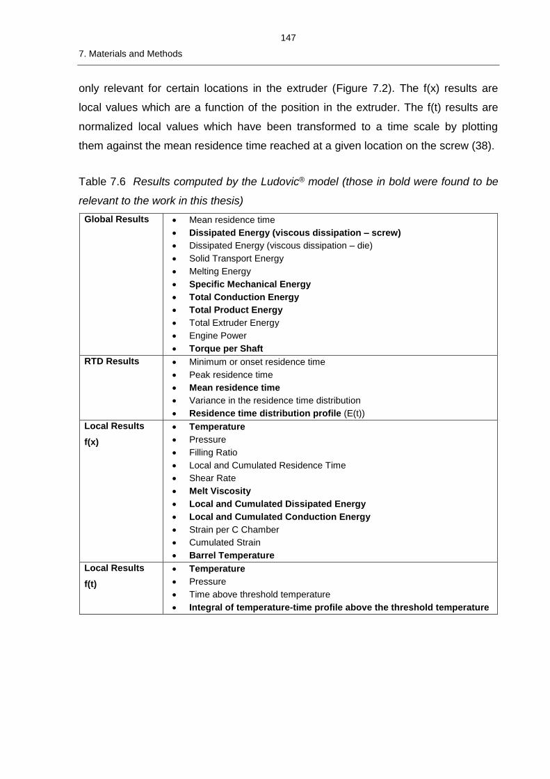
147
7. Materials and Methods
only relevant for certain locations in the extruder (Figure 7.2). The f(x) results are
local values which are a function of the position in the extruder. The f(t) results are
normalized local values which have been transformed to a time scale by plotting
them against the mean residence time reached at a given location on the screw (38).
Table 7.6 Results computed by the Ludovic® model (those in bold were found to be
relevant to the work in this thesis)
Global Results • Mean residence time
• Dissipated Energy (viscous dissipation – screw)
• Dissipated Energy (viscous dissipation – die)
• Solid Transport Energy
• Melting Energy
• Specific Mechanical Energy
• Total Conduction Energy
• Total Product Energy
• Total Extruder Energy
• Engine Power
• Torque per Shaft
RTD Results • Minimum or onset residence time
• Peak residence time
• Mean residence time
• Variance in the residence time distribution
• Residence time distribution profile (E(t))
Local Results
f(x)
• Temperature
• Pressure
• Filling Ratio
• Local and Cumulated Residence Time
• Shear Rate
• Melt Viscosity
• Local and Cumulated Dissipated Energy
• Local and Cumulated Conduction Energy
• Strain per C Chamber
• Cumulated Strain
• Barrel Temperature
Local Results
f(t)
• Temperature
• Pressure
• Time above threshold temperature
• Integral of temperature-time profile above the threshold temperature
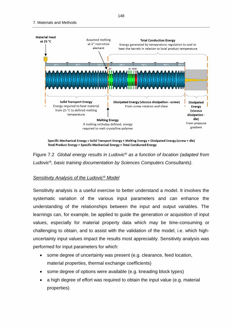
148
7. Materials and Methods
Figure 7.2 Global energy results in Ludovic® as a function of location (adapted from
Ludovic®, basic training documentation by Sciences Computers Consultants).
Sensitivity Analysis of the Ludovic® Model
Sensitivity analysis is a useful exercise to better understand a model. It involves the
systematic variation of the various input parameters and can enhance the
understanding of the relationships between the input and output variables. The
learnings can, for example, be applied to guide the generation or acquisition of input
values, especially for material property data which may be time-consuming or
challenging to obtain, and to assist with the validation of the model, i.e. which high-
uncertainty input values impact the results most appreciably. Sensitivity analysis was
performed for input parameters for which:
• some degree of uncertainty was present (e.g. clearance, feed location,
material properties, thermal exchange coefficients)
• some degree of options were available (e.g. kneading block types)
• a high degree of effort was required to obtain the input value (e.g. material
properties)
149
7. Materials and Methods
• perceived variation in the value could greatly impact the process (e.g. barrel or
die temperature, screw speed, feed rate).
If an input parameter had little impact on the simulation results, then an estimate was
used for real simulation purposes. A high-level summary is shown in Table 7.7.
The most informative sensitivity analysis studies were the ones in which material
properties, process parameters and thermal exchange coefficients were varied and
results are presented in greater detail. In the presentation of the results, primary
focus is placed on the melt temperature evolution along the screw; any change in
energy will manifest itself in product temperature change. The ranges selected for
analysis are based upon a survey of typical and reasonable expected variation
(Table 7.8 and Table 7.9).
The material Tm or Tg and the melt viscosity show direct relationships and strong
impact on the melt temperature while the liquid phase heat capacity and density have
lesser impact as well as inverse relationships with melt temperature (Figure 7.3). The
other properties had no impact on the melt temperature. Among the values for the
material properties tested, only the melt density affected the residence time (data not
shown).
Not surprisingly, the process parameters also have a strong influence on the melt
temperature and residence time distribution. The Ludovic® model shows the
expected relationships that melt temperature increases with increasing screw speed
and decreases to a lesser extent with increasing feed rate Figure 7.4. The residence
time decreases and becomes a narrower distribution with increasing feed rate at
constant screw speed, while the screw speed, at constant feed rate, simply shifts the
time to earlier or later. An increase in barrel temperature generally leads to an
increase in melt temperature (Figure 7.5), with no impact on residence time (data not
shown).
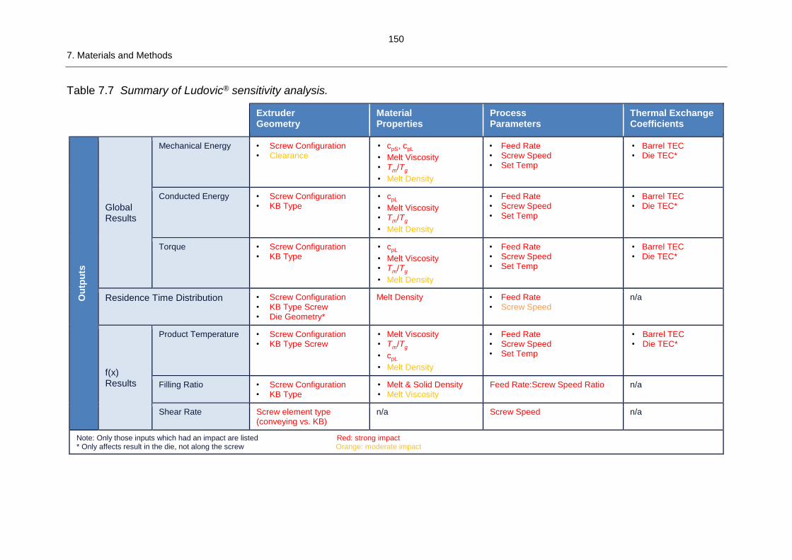
150
7. Materials and Methods
Table 7.7 Summary of Ludovic® sensitivity analysis.
Extruder Geometry
Material Properties
Process Parameters
Thermal Exchange Coefficients
Ou
tpu
ts
Global Results
Mechanical Energy • Screw Configuration • Clearance
• cpS, cpL
• Melt Viscosity • Tm/Tg
• Melt Density
• Feed Rate • Screw Speed • Set Temp
• Barrel TEC • Die TEC*
Conducted Energy • Screw Configuration • KB Type
• cpL
• Melt Viscosity • Tm/Tg
• Melt Density
• Feed Rate • Screw Speed • Set Temp
• Barrel TEC • Die TEC*
Torque • Screw Configuration • KB Type
• cpL
• Melt Viscosity • Tm/Tg
• Melt Density
• Feed Rate • Screw Speed • Set Temp
• Barrel TEC • Die TEC*
Residence Time Distribution • Screw Configuration • KB Type Screw • Die Geometry*
Melt Density • Feed Rate • Screw Speed
n/a
f(x) Results
Product Temperature • Screw Configuration • KB Type Screw
• Melt Viscosity • Tm/Tg
• cpL
• Melt Density
• Feed Rate • Screw Speed • Set Temp
• Barrel TEC • Die TEC*
Filling Ratio • Screw Configuration • KB Type
• Melt & Solid Density • Melt Viscosity
Feed Rate:Screw Speed Ratio n/a
Shear Rate Screw element type (conveying vs. KB)
n/a Screw Speed n/a
Note: Only those inputs which had an impact are listed Red: strong impact * Only affects result in the die, not along the screw Orange: moderate impact
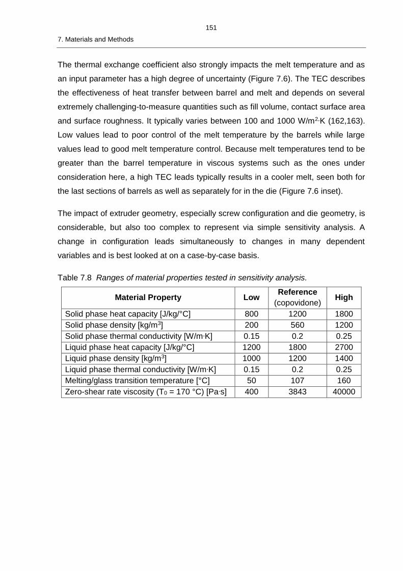
151
7. Materials and Methods
The thermal exchange coefficient also strongly impacts the melt temperature and as
an input parameter has a high degree of uncertainty (Figure 7.6). The TEC describes
the effectiveness of heat transfer between barrel and melt and depends on several
extremely challenging-to-measure quantities such as fill volume, contact surface area
and surface roughness. It typically varies between 100 and 1000 W/m2∙K (162,163).
Low values lead to poor control of the melt temperature by the barrels while large
values lead to good melt temperature control. Because melt temperatures tend to be
greater than the barrel temperature in viscous systems such as the ones under
consideration here, a high TEC leads typically results in a cooler melt, seen both for
the last sections of barrels as well as separately for in the die (Figure 7.6 inset).
The impact of extruder geometry, especially screw configuration and die geometry, is
considerable, but also too complex to represent via simple sensitivity analysis. A
change in configuration leads simultaneously to changes in many dependent
variables and is best looked at on a case-by-case basis.
Table 7.8 Ranges of material properties tested in sensitivity analysis.
Material Property Low Reference
(copovidone) High
Solid phase heat capacity [J/kg/°C] 800 1200 1800
Solid phase density [kg/m3] 200 560 1200
Solid phase thermal conductivity [W/m∙K] 0.15 0.2 0.25
Liquid phase heat capacity [J/kg/°C] 1200 1800 2700
Liquid phase density [kg/m3] 1000 1200 1400
Liquid phase thermal conductivity [W/m∙K] 0.15 0.2 0.25
Melting/glass transition temperature [°C] 50 107 160
Zero-shear rate viscosity (T0 = 170 °C) [Pa∙s] 400 3843 40000
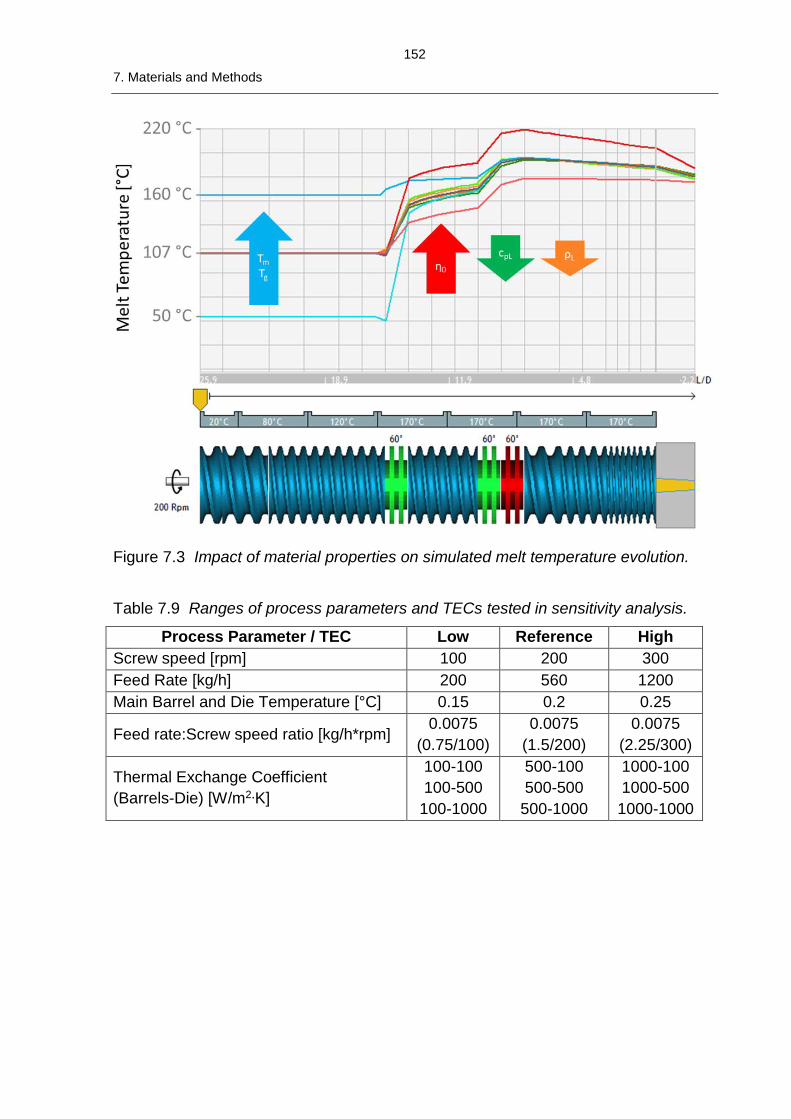
152
7. Materials and Methods
Figure 7.3 Impact of material properties on simulated melt temperature evolution.
Table 7.9 Ranges of process parameters and TECs tested in sensitivity analysis.
Process Parameter / TEC Low Reference High
Screw speed [rpm] 100 200 300
Feed Rate [kg/h] 200 560 1200
Main Barrel and Die Temperature [°C] 0.15 0.2 0.25
Feed rate:Screw speed ratio [kg/h*rpm] 0.0075
(0.75/100)
0.0075
(1.5/200)
0.0075
(2.25/300)
Thermal Exchange Coefficient
(Barrels-Die) [W/m2∙K]
100-100
100-500
100-1000
500-100
500-500
500-1000
1000-100
1000-500
1000-1000
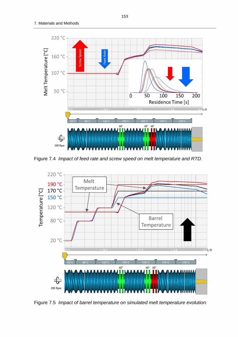
153
7. Materials and Methods
Figure 7.4 Impact of feed rate and screw speed on melt temperature and RTD.
Figure 7.5 Impact of barrel temperature on simulated melt temperature evolution.
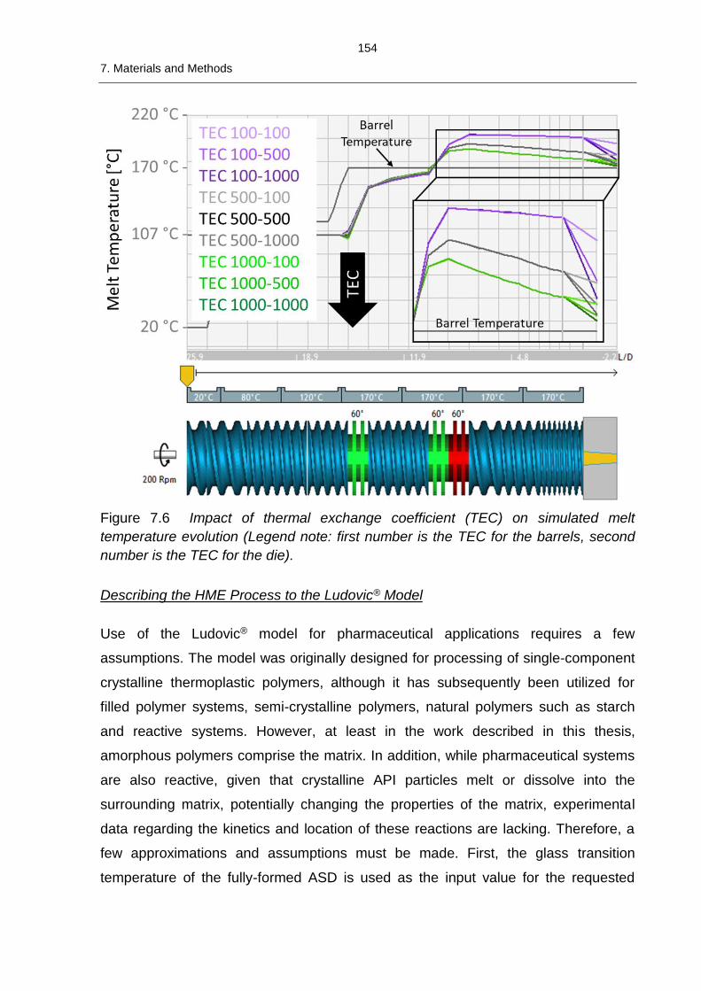
154
7. Materials and Methods
Figure 7.6 Impact of thermal exchange coefficient (TEC) on simulated melt
temperature evolution (Legend note: first number is the TEC for the barrels, second
number is the TEC for the die).
Describing the HME Process to the Ludovic® Model
Use of the Ludovic® model for pharmaceutical applications requires a few
assumptions. The model was originally designed for processing of single-component
crystalline thermoplastic polymers, although it has subsequently been utilized for
filled polymer systems, semi-crystalline polymers, natural polymers such as starch
and reactive systems. However, at least in the work described in this thesis,
amorphous polymers comprise the matrix. In addition, while pharmaceutical systems
are also reactive, given that crystalline API particles melt or dissolve into the
surrounding matrix, potentially changing the properties of the matrix, experimental
data regarding the kinetics and location of these reactions are lacking. Therefore, a
few approximations and assumptions must be made. First, the glass transition
temperature of the fully-formed ASD is used as the input value for the requested
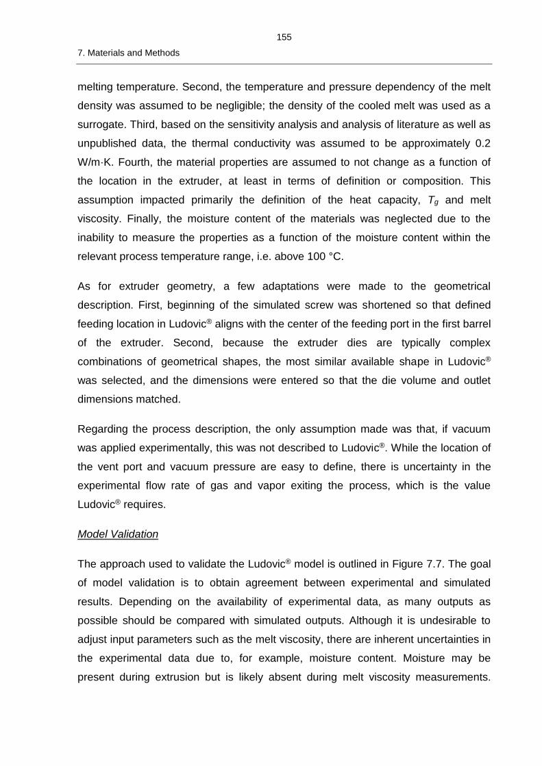
155
7. Materials and Methods
melting temperature. Second, the temperature and pressure dependency of the melt
density was assumed to be negligible; the density of the cooled melt was used as a
surrogate. Third, based on the sensitivity analysis and analysis of literature as well as
unpublished data, the thermal conductivity was assumed to be approximately 0.2
W/m·K. Fourth, the material properties are assumed to not change as a function of
the location in the extruder, at least in terms of definition or composition. This
assumption impacted primarily the definition of the heat capacity, Tg and melt
viscosity. Finally, the moisture content of the materials was neglected due to the
inability to measure the properties as a function of the moisture content within the
relevant process temperature range, i.e. above 100 °C.
As for extruder geometry, a few adaptations were made to the geometrical
description. First, beginning of the simulated screw was shortened so that defined
feeding location in Ludovic® aligns with the center of the feeding port in the first barrel
of the extruder. Second, because the extruder dies are typically complex
combinations of geometrical shapes, the most similar available shape in Ludovic®
was selected, and the dimensions were entered so that the die volume and outlet
dimensions matched.
Regarding the process description, the only assumption made was that, if vacuum
was applied experimentally, this was not described to Ludovic®. While the location of
the vent port and vacuum pressure are easy to define, there is uncertainty in the
experimental flow rate of gas and vapor exiting the process, which is the value
Ludovic® requires.
Model Validation
The approach used to validate the Ludovic® model is outlined in Figure 7.7. The goal
of model validation is to obtain agreement between experimental and simulated
results. Depending on the availability of experimental data, as many outputs as
possible should be compared with simulated outputs. Although it is undesirable to
adjust input parameters such as the melt viscosity, there are inherent uncertainties in
the experimental data due to, for example, moisture content. Moisture may be
present during extrusion but is likely absent during melt viscosity measurements.
156
7. Materials and Methods
Uncertainties in extruder geometrical definition may also occur due to wear and tear,
e.g. clearance could be larger than specification, or the die geometry may be
complex and challenging to describe to the model.
Figure 7.7 General method and decision tree for model validation.
7.2.6.2 Torasemide Simulation
Process simulations were performed using Ludovic® v.6.2 beta. This version is a test
version based on v.6.1 with the additional feature of automatic integration of the
temperature vs. time curve when a threshold temperature is given to the software.
The model is described in section 7.2.6.1.
Additional parameters describing the extruder needed for simulation are: center line
of 9 mm, screw/barrel leakage of 0.35 mm, and 2 mm diameter die opening. The
screw configuration 2mix5disk60degFW-5disk60degFWBW, composed of conveying
elements of various pitch, forward 60 degree kneading blocks shown in green and
reverse kneading block shown in red, is displayed at the bottom of Figure 4.2 and all
elements are listed in Table 7.4.
157
7. Materials and Methods
Process simulations at conditions identical to the experimental extrusion conditions
were performed to validate the model for torasemide-containing formulations. The
model was validated by correlating 1) the measured and simulated melt temperature
at die exit and 2) the measured and simulated residence time distribution and mean
residence time. The thermal exchange coefficients used were 500 W/m2∙K in the first
two barrels, 300 W/m2∙K in the last two barrels, and 50 W/m2∙K in the die.
7.2.6.3 Telmisartan Simulation
Chapter 5
Process simulations of the laboratory experiments on the ZSK18 were performed
using Ludovic® v.6.1 software. The model is described in section 7.2.6.1.
Additional parameters describing the ZSK18 extruder needed for simulation are:
center line of 15 mm, screw/barrel leakage of 0.14 mm, and 10 mm diameter die
opening. The screw configuration, composed of conveying elements of various pitch,
forward 60° kneading blocks shown in green and reverse kneading block shown in
red, is displayed at the bottom of Figure 5.3 and elements listed in Table 7.5.
Sensitivity analysis of the Ludovic® model with varied rheological parameters, n and
η0 in the Carreau-Yasuda equation, were performed to determine the relative impact
of n and η0 on melt temperature evolution. Copovidone was used as the baseline
material with n and η0 ranges selected within that of previously measured values
when the formulation was varied by addition of surfactant. Copovidone at a reference
temperature of 150 °C has n = 0.577 and η0 = 61000 Pa∙s. The extruder and screw
geometry used for this study was the same as for all other simulations of the ZSK18
extruder. The barrel temperature was varied along with the screw speed, and the
feed rate was adjusted in combination with the screw speed to maintain constant fill
level. The thermal exchange coefficients used were 500 W/m2∙K in the barrels and
500 W/m2∙K in the die.
Process simulations at conditions identical to the TEL experimental extrusion
conditions were performed to validate the model for TEL-containing formulations. The
model was validated by correlating the melt temperature at die exit, measured
158
7. Materials and Methods
experimentally, with that of the simulated value. The thermal exchange coefficients
used were 300 W/m2∙K in the barrels and 100 W/m2∙K in the die.
Thereafter, a full factorial simulated experimental design was employed thanks to the
resource-sparing nature of simulation work. The parameters varied in the simulation
experiment are listed in Table 5.2. The thermal exchange coefficients used were
300 W/m2∙K in the barrels and 100 W/m2∙K in the die. Contour plots of resulting
simulated data were generated using JMP® v.10 software.
In addition to the simulated melt temperature at die exit, the maximum melt
temperature along the screw, the total viscous dissipated energy from the screw, the
specific mechanical energy, the total conducted energy, the total product energy
(Figure 7.2) and local shear stress were analyzed. The total viscous dissipated
energy in the screw is calculated by Ludovic® as the sum of the viscous dissipated
energy computed in each c-shaped chamber, utilizing the local values of computed
shear rate, melt viscosity, discretized volume and local residence time for
computation. The local shear stress can be calculated by multiplying the local values
for melt viscosity and shear rate in each c-shaped chamber.
Chapter 6
Process simulations were performed using Ludovic® v.6.2 beta. The model is
described in section 7.2.6.1.
Two sets of simulations were performed: 1) pre-experiment full factorial design to
select the best formulation and also the barrel temperature and 2) post-experiment to
analyze the process. The simulation parameters for the first set are listed in Table 6.8
while the simulation parameters for the second set were identical to the experimental
parameters described in section 7.2.2.2. Material property inputs were identical to
those used in Chapter 5 simulations. Thermal exchange coefficients were
500/300/50 W/m2∙K for zones A-C/zone D/die for the both extruder scales. The
Ludovic® model was validated by comparing the empirically measured temperature
with the simulated melt temperature at screw exit in this study.
159
8. Summary and Outlook
8 Summary and Outlook
Hot-melt extrusion is a well-established process for the production of pharmaceutical
products. Nevertheless, some aspects of process development are not
straightforward to ascertain and are poorly understood, such as assessing the
correlation of CQAs with process performance or achieving a scaled and energy-
balanced process. These challenges are primarily due to the lack of accurate
measures of the process. In order to gain deeper process understanding, a surrogate
approach combining the use of indicator substances with process simulation can be
used.
In this work, two APIs, torasemide and telmisartan, were identified which, when
combined with the appropriate matrix and processed at appropriate conditions,
behaved like highly sensitive indicator substances. With these indicator substances,
two relevant CQAs for the HME process, degradation and residual crystallinity, were
correlated with both empirical and simulated process performance. Customized
formulations were developed for both APIs in order to target the relevant process and
CQA design spaces. Formulations were developed to minimize the impact of the API
dissolution into the matrix on melt viscosity or thermal properties by minimizing the
difference between the Tg of the API and that of the matrix.
Both APIs were processed below their single-component melting points as well as
below their solubility temperatures in the matrix system. By doing so, the APIs were
forced to dissolve into the surrounding matrix rather than first melt and then disperse
and distribute. As a result, for the given drug loading, dissolution was never complete
and residually crystalline material was always present after extrusion. The amount of
residually crystalline material present was correlated to both melt temperature and
residence time in the case of torasemide while for telmisartan was highly correlated
with melt temperature.
In order to realize the full benefit of torasemide as an indicator substance, a
formulation with 10 %w/w TOR, 10 %w/w PEG 1500 in Soluplus® was used.
Soluplus® was chosen for its relatively low temperature processing window and
because its Tg of 70 °C was similar to that of TOR, 80 °C. PEG 1500 was chosen as
160
8. Summary and Outlook
a plasticizer for the system because PEG was already present in the Soluplus®
polymer side chains. Addition of the plasticizer allowed processing at barrel
temperatures below the onset temperature of dissolution of TOR in Soluplus®,
115 °C. Solid-state characterization tools and a 10 mm diameter lab-scale co-rotating
TSE were used to study the system. It was found that TOR first dissolved into the
matrix and then degraded. Based on this mechanism, within the processing space of
varied barrel temperatures and residence times explored, both degradation and
residual crystallinity were observed and were highly correlated to both time and
temperature. In addition, because torasemide is sensitive to both thermal- and
hydrolysis-induced degradation, the indicator system was used to study the effect of
moisture on the process by way of various venting conditions. Also, because of the
dissolve-then-degrade mechanism, the residual crystallinity and total degradation
were highly correlated, independent of the processing conditions applied. This
relationship was further quantified by use of simulated results, namely the integral of
the melt temperature evolution over time for which the melt temperature was greater
than the onset dissolution temperature of the API in the polymer, 115 °C. In this way,
utilization of torasemide as a highly-sensitive process indicator enhanced the
understanding of the dynamic thermal environment inside an extruder and elucidated
the inter-dependent yet cumulative thermal and hydrolysis effects of the processes
occurring within HME.
The telmisartan indicator system was developed specifically with the intention of
studying the relationship between melt viscosity and processing performance and its
relevance for pharmaceutical extrusion coupled with process simulation. Two
formulations containing 10 %w/w TEL in either a pure COP matrix or one containing
5.5 %w/w polysorbate 80 were extruded at various barrel temperatures and screw
speeds, keeping fill volume in the barrel constant, on an 18 mm screw diameter
extruder. The polysorbate 80 was included as a plasticizing component, while the
presence of dissolved telmisartan had a negligible effect on Tg at the investigated
drug loading. The presence of polysorbate 80 did not impact the solubility of TEL in
the matrix. It was hypothesized and also confirmed by process simulation that the
design space with respect to screw speed was broader for the plasticized
formulation. In addition, the amount of residual crystallinity was more sensitive to
161
8. Summary and Outlook
screw speed at low barrel temperatures than at higher barrel temperatures. The
residual crystallinity was found to be highly correlated with melt temperature but
differed for the two formulations. Uniquely, the simulated maximum melt temperature
at which residual crystallinity approached zero was very similar to the solubility
temperature of telmisartan in the matrix determined by DSC, therefore explaining the
difference in residual crystallinity between the two formulations. In this way,
simulation enabled a deeper understanding of the relationship between process
performance and CQAs.
Based on these results with telmisartan and a surfactant acting as a plasticizer, the
conventionally proposed recommendation for using a plasticizer should be
reconsidered. While the decision to use a plasticizer is typically centered around
lowering the processing temperature to avoid thermal degradation, consideration
should be made in relation to the inherent need to achieve an ASD, which can only
be done by processing above the solubility temperature for a given drug
concentration. Use of a plasticizer to simply process below an API’s degradation
temperature is only one factor for consideration. While it will enable processing at a
lower barrel temperature, doing so may prevent the full dissolution of the API into the
polymeric matrix for high solubility temperature APIs. Alternatively, the benefit in
broadening the design space with respect to shear rate is a rational reason to
introduce a plasticizer. The decision to use a surfactant in an ASD formulation can
also be based not only on bioavailability enhancement but also on process
performance. If the API’s in-vitro or in-vivo release behavior benefits from the
inclusion of a surfactant in the formulation, a surfactant’s plasticizing behavior will
also broaden the design space.
Use of the telmisartan indicator system and process simulations also enabled
quantitative analysis of scaling and adiabatic conditions between two twin-screw
extruders 18 mm and 40 mm in diameter. The scaling approach of maintaining VSFL
and either the screw speed or the overflight shear rate resulted in almost identical
quantitative energetic states, namely same SME, same conduction energy profile,
same quasi-adiabatic state, and melt temperature was also similar. However, the
TEL system is so sensitive that the difference in melt temperature, measured at die
exit, resulted in a different amount of residual crystallinity between the two scales.
162
8. Summary and Outlook
For some systems, this degree of similarity in melt temperature and process
energetics may be sufficient for scaling, while in others not.
Despite the reasonable findings and correlations between simulated results and
CQAs obtained, validation of the Ludovic® model in this work was dependent on an
imperfect measure of the process, namely the melt temperature at the die exit. Even
better models could be developed with the help of enhanced measures of the
process such as the melt temperature measurement in a maximum temperature
zone, for example in a mixing element with high or complete degree of fill. If
temperature could be measured more accurately, especially maximum temperature
and not just the die-exit temperature, then the thermal exchange coefficients could be
more precisely adjusted to obtain a greater degree of confidence in experiment-
simulation agreement.
Further work is also needed to calibrate the Ludovic® model with respect to the “gray-
zone” of total conducted energy because the model does not consider heat loss to
the environment in the energy balance. This heat loss would differ from extruder to
extruder, and therefore would need to be analyzed on a case-by-case basis. One
way to investigate this could be to extrude a matrix polymer and vary the melt
viscosity by either gradually adjusting barrel temperature or plasticizer content to
quantitatively identify the threshold of total conducted energy magnitude which
correlates to real cooling, aka a negative controller output.
Additional experiments are also needed to confirm some of the findings, those for
which slight indications or tendencies were observed. Because the present
experiments were designed to study other hypotheses, perhaps a screening DOE to
determine main effects would be useful, for example to confirm observation of the
temperature dependency of TEL, seen both Chapters 5 and 6, and rule out the
observation that the residual crystallinity is independent of residence time. On the
other hand, it may be tricky to design such an experiment due to the extent of
interactions between the independent variables in an extrusion process.
An additional aspect of the process which was not fully explored in these studies is
kinetics, both that of dissolution of the API into the polymer and that of API
163
8. Summary and Outlook
degradation. Study of the dissolution kinetics of an API into the molten polymer would
require development of either new methods and/or sensors. For example, an off-line
device to replicate in a controlled fashion the thermal-temporal-mechanical
environment of molten polymer in an extruder with off-line sample analysis could be
used to study the kinetics of dissolution. Alternatively, on-line sensors could be used
to quantify the rate of dissolution if a signal could be identified as specific to the
dissolved or undissolved state of the API. Further, if dissolution and degradation
kinetics could be quantified, the Ludovic® model could be used to simulate and
estimate the CQAs for a given process setting as has been done for polymerization
reactions.
Lastly, the use of these or other indicator substances could be used to study other
aspects of the HME process such as the impact of screw configuration or mixing
element design, die geometry, moisture as a plasticizer or other plasticizers on the
outcome of the process. In addition, new models could be developed and validated
based on the use of indicator substances. The benefit of using the API as the
indicator substance for pharmaceutical applications is that the response is directly
related to relevant CQAs for the given unit operation.
164
9. Publications
9 Publications
Parts of this work are already published or submitted as:
Articles:
• Evans, R.C., Kyeremateng, S.O., Asmus, L., Degenhardt, M., Rosenberg, J.,
Wagner, K.G.; Development and Performance of a Highly Sensitive Model
Formulation Based on Torasemide to Enhance Hot-Melt Extrusion Process
Understanding and Process Development; AAPS PharmSciTech 2018;
doi:10.1208/s12249-018-0970-y
• Evans, R.C., Bochmann, E.S., Kyeremateng, S.O., Gryczke, A., Wagner, K.G.;
Holistic QbD Approach for Hot-Melt Extrusion Process Design Space
Evaluation: Linking Materials Science, Experimentation and Process
Modeling; submitted.
Abstracts/Posters (Conference participation):
• Evans, R.C., Kyeremateng, S., Asmus, L., Degenhardt, M., Rosenberg, J.,
Wagner, K.G.; Improved HME Process Understanding Facilitated by API-as-
Indicator Substance and Simulation; AAPS Annual Meeting, San Diego,
California, USA, November 2017.
• Evans, R.C., Kyeremateng, S., Degenhardt, M., Wagner, K.G.; Influence of
Surfactant+Polymer Rheological Properties on Hot-Melt Extrusion Design
Space – Investigation via Process Simulation; 11th PBP World Meeting,
Granada, Spain, March 2018.
AbbVie Poster Sessions
• Rachel C. Evans, Lutz Asmus, Samuel Kyeremateng, Matthias Degenhardt,
Jörg Rosenberg, Karl G. Wagner Enhancing Hot Melt Extrusion Process
Understanding – Development of a Highly Sensitive Model to Facilitate
Rational Process Understanding (Ludwigshafen – AbbVie Celebration of
Science 2015)
• John Strong, Rachel C. Evans, Maxx Capece, Sean Garner, David O’Brien,
Divya Sunkara, Connie Skoug, Ping Gao, Samuel Kyeremateng, Lutz Asmus,
Matthias Degenhardt, Jörg Rosenberg, Karl G. Wagner Formulation
Development and Process Understanding Facilitated by Simulation and
Modeling (Lake County – AbbVie Celebration of Science 2016)
165
10. Appendix
10 Appendix
10.1 Mass Spectrometry Characterization for Torasemide Study
HPLC mass spectrometry (HPLC-MS) was conducted to identify the chemical
structure of the three peaks observed in standard HPLC sample analysis. HPLC-MS
was performed with an Agilent 1260 series (Agilent Technologies, Germany) HPLC
with a binary pump (G1313B), column compartment (G1316C), DAD detector
(G4212B), and HIP sampler (G1367E) coupled to a Bruker AmaZon x ion trap mass
spectrometer (Brucker, USA). The amaZon x was controlled by ESI Compass 1.7
trapControl software Version 7.2, data were collected using HyStar software, version
3.2, and data were processed using Bruker Compass DataAnalysis Version 4.2
(Bruker Daltonik GmbH, Bremen, Germany).
The chromatographic separation was performed using the same column as standard
HPLC-UV and with column temperature of 25 °C. The mobile phase was water with
0.1 %v/v trifluoroacetic acid (85%) (mobile phase A) and acetonitrile with 0.05 %v/v
trifluoroacetic acid (85%) (mobile phase B). Chromatographic separation was
conducted using gradient elution: 0 min, B 5%; 5 min, B 10%; 15 min, B 40%; 17 min,
B 80%; 18 min, B 5%; 25 min, B 5%. The flow rate was 0.4 mL/min and the injection
volume was 5 µL for both LC-DAD and LC-MS analysis. UV-detection was performed
at 249 nm and 279 nm.
LC-MS analysis utilized electrospray ionization (ESI) operating in positive ionization
mode. The following MS parameters, optimized for the corresponding analysis, were
applied: flow rate drying gas (N2) = 8.0 mL/min, nebulizer gas pressure = 20 psig,
temperature drying gas (N2) = 220 °C, capillary voltage = 4500 V, collision gas =
Helium. The mass spectrometer was operated in full scan mode in the range from
100 to 1000 m/z. Tuning of the ion trap mass spectrometer was performed with
Agilent ESI tune mix (G2431A). The tune solution was infused with a syringe pump at
a flow rate of 180 µL/h. A torasemide standard solution at a concentration of 500
µg/mL was used as control standard to verify the collision energy. The target mass
was 350 m/z and the compound stability 100% for SPS tune.
Mass spectrometry data for the three peaks observed in torasemide physical mixture
and extrudate samples, along with a corresponding UV chromatogram, are shown in
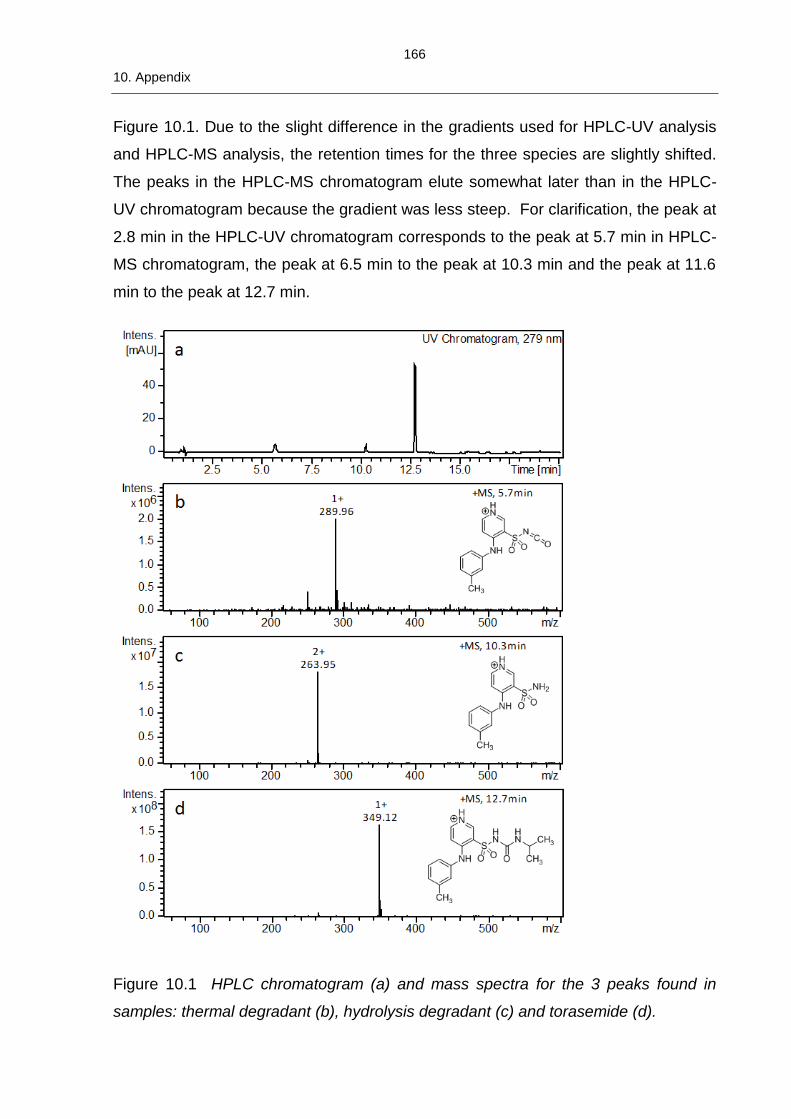
166
10. Appendix
Figure 10.1. Due to the slight difference in the gradients used for HPLC-UV analysis
and HPLC-MS analysis, the retention times for the three species are slightly shifted.
The peaks in the HPLC-MS chromatogram elute somewhat later than in the HPLC-
UV chromatogram because the gradient was less steep. For clarification, the peak at
2.8 min in the HPLC-UV chromatogram corresponds to the peak at 5.7 min in HPLC-
MS chromatogram, the peak at 6.5 min to the peak at 10.3 min and the peak at 11.6
min to the peak at 12.7 min.
Figure 10.1 HPLC chromatogram (a) and mass spectra for the 3 peaks found in
samples: thermal degradant (b), hydrolysis degradant (c) and torasemide (d).
167
10. Appendix
10.2 Determination of Telmisartan Degradation
The extent of degradation of telmisartan within the extrusion processing range was
determined by lab-scale extrusion and HPLC analysis.
10.2.1 Sample Preparation
A blend of 10 %w/w TEL in COP was prepared via mixing in a Turbula® blender for 5
min (Willy A. Bachofen AG - Maschinenfabrik Muttenz, Switzerland). Extrudates were
prepared by extruding using a Haake® MiniLab conical twin-screw extruder (Thermo
Fisher Scientific, Karlsruhe, Germany) at 100 rpm and barrel temperatures of 180 °C
and 220 °C. The extrudates were milled to <500 µm using a coffee grinder type mill.
10.2.2 HPLC Analysis
HPLC was conducted to identify the presence and relative amounts of degradation
products of telmisartan formed during extrusion feasibility studies.
Analysis was performed using an Agilent 1100 series (Agilent Technologies,
Waldbronn, Germany). The chromatographic separation was performed on an
Agilent Poroshell 120 SB-C18 analytical column (100 mm long, 3 mm diameter, 2.7
µm particle size, 120 Å pore size) with column temperature of 40 °C. The mobile
phase was 10 mM ammonium acetate in water (mobile phase A) and acetonitrile
(mobile phase B) with linear gradient elution: 0 min, B 15%; 5 min, B 20%; 25 min, B
100%; 30 min, B 100%; 30.1 min, B 15%; 35 min, B 15%. The flow rate was 1.0
mL/min, the injection volume was 10 µL, and the detection was performed at 292 nm,
slit 4 nm. Agilent OpenLAB CDS ChemStation Edition software was used for data
collection and analysis. All reagents were of HPLC grade. Results are presented as
peak area percent.
Diluent for both neat telmisartan standard and milled extrudate samples was
composed of 1+1 (v/v) methanol + water. Both the standard and sample solutions
were prepared at 200 µg/mL concentration.
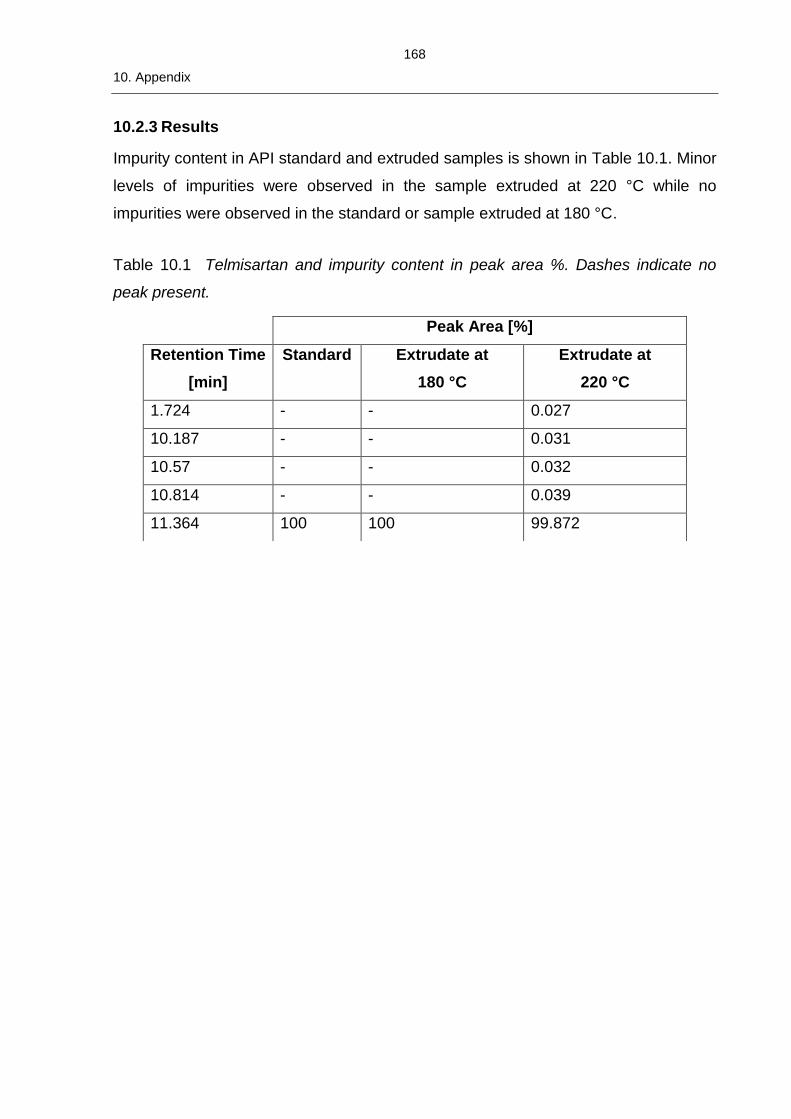
168
10. Appendix
10.2.3 Results
Impurity content in API standard and extruded samples is shown in Table 10.1. Minor
levels of impurities were observed in the sample extruded at 220 °C while no
impurities were observed in the standard or sample extruded at 180 °C.
Table 10.1 Telmisartan and impurity content in peak area %. Dashes indicate no
peak present.
Peak Area [%]
Retention Time
[min]
Standard Extrudate at
180 °C
Extrudate at
220 °C
1.724 - - 0.027
10.187 - - 0.031
10.57 - - 0.032
10.814 - - 0.039
11.364 100 100 99.872
169
11. References
11 References
1. Breitenbach J. Melt extrusion: from process to drug delivery technology. Eur J Pharm Biopharm. 2002 Sep;54(2):107–17.
2. Crowley MM, Zhang F, Repka MA, Thumma S, Upadhye SB, Kumar Battu S, et al. Pharmaceutical Applications of Hot-Melt Extrusion: Part I. Drug Dev Ind Pharm. 2007 Jan 1;33(9):909–26.
3. Stanković M, Frijlink HW, Hinrichs WLJ. Polymeric formulations for drug release prepared by hot melt extrusion: application and characterization. Drug Discov Today. 2015 Jul;20(7):812–23.
4. Theil F, Anantharaman S, Kyeremateng SO, van Lishaut H, Dreis-Kühne SH, Rosenberg J, et al. Frozen in Time: Kinetically Stabilized Amorphous Solid Dispersions of Nifedipine Stable after a Quarter Century of Storage. Mol Pharm. 2017 Jan 3;14(1):183–92.
5. Patil H, Tiwari RV, Repka MA. Hot-Melt Extrusion: from Theory to Application in Pharmaceutical Formulation. AAPS PharmSciTech. 2016;17(1):20–42.
6. Jermain SV, Brough C, Williams RO. Amorphous solid dispersions and nanocrystal technologies for poorly water-soluble drug delivery – An update. Int J Pharm. 2018 Jan 15;535(1):379–92.
7. Repka MA, Bandari S, Kallakunta VR, Vo AQ, McFall H, Pimparade MB, et al. Melt extrusion with poorly soluble drugs – An integrated review. Int J Pharm. 2018 Jan 15;535(1):68–85.
8. Newman A, editor. Pharmaceutical Amorphous Solid Dispersions. New Jersey: John Wiley & Sons, Inc.; 2015.
9. Gryczke A. Hot-Melt Extrusion Process Design Using Process Analytical Technology. In: Melt Extrusion. 1st ed. New York: Springer-Verlag; 2013. (AAPS Advances in the Pharmaceutical Sciences; vol. 9).
10. Treffer D, Wahl P, Markl D, Koscher G, Roblegg E, Khinast J. Hot Melt Extrusion as a Continuous Pharmaceutical Manufacturing Process. In: Repka MA, Langley N, DiNunzio J, editors. Melt Extrusion. 1st ed. New York: Springer-Verlag; 2013. (AAPS Advances in the Pharmaceutical Sciences; vol. 9).
11. Lang B, McGinity JW, Williams RO. Hot-melt extrusion – basic principles and pharmaceutical applications. Drug Dev Ind Pharm. 2014 Sep 1;40(9):1133–55.
12. Repka MA, Langley N, DiNunzio J. Melt Extrusion. 1st ed. New York: Springer-Verlag; 2013. 474 p. (AAPS Advances in the Pharmaceutical Sciences; vol. 9).
13. Brown EC, Kelly AL, Coates PD. Melt temperature field measurement in single screw extrusion using thermocouple meshes. Rev Sci Instrum. 2004 Nov 1;75(11):4742–8.
170
11. References
14. Emin MA, Teumer T, Schmitt W, Rädle M, Schuchmann HP. Measurement of the true melt temperature in a twin-screw extrusion processing of starch based matrices via infrared sensor. J Food Eng. 2016 Feb;170:119–24.
15. Kohlgrüber K. Co-Rotating Twin-Screw Extruders - Fundamentals, Technology and Applications. Munich: Carl Hanser Verlag; 2008.
16. Deng J, Li K, Harkin-Jones E, Price M, Karnachi N, Kelly A, et al. Energy monitoring and quality control of a single screw extruder. Appl Energy. 2014;113:1775–85.
17. Heil C, Hirsch J. Improved process understanding and control of a hot-melt extrusion process with near-infrared spectroscopy. In: Hot-Melt Extrusion: Pharmaceutical Applications. John Wiley & Sons, Ltd; 2012. p. 333–52.
18. Hitzer P, Bäuerle T, Drieschner T, Ostertag E, Paulsen K, van Lishaut H, et al. Process analytical techniques for hot-melt extrusion and their application to amorphous solid dispersions. Anal Bioanal Chem. 2017 Jul 1;409(18):4321–33.
19. Siepmann F, Le Brun V, Siepmann J. Drugs acting as plasticizers in polymeric systems: A quantitative treatment. J Controlled Release. 2006 Oct 27;115(3):298–306.
20. Ghebremeskel AN, Vemavarapu C, Lodaya M. Use of surfactants as plasticizers in preparing solid dispersions of poorly soluble API: Selection of polymer–surfactant combinations using solubility parameters and testing the processability. Int J Pharm. 2007 Jan 10;328(2):119–29.
21. Gogos CG, Liu H, Wang P. Laminar Dispersive and Distributive Mixing with Dissolution and Applications to Hot-Melt Extrusion. In: Hot-Melt Extrusion: Pharmaceutical Applications [Internet]. John Wiley & Sons, Ltd; 2012. p. 261–84. Available from: http://dx.doi.org/10.1002/9780470711415.ch12
22. Zecevic DE, Evans RC, Paulsen K, Wagner KG. From benchtop to pilot scale–experimental study and computational assessment of a hot-melt extrusion scale-up of a solid dispersion of dipyridamole and copovidone. Int J Pharm. 2018 Feb 15;537(1):132–9.
23. Dreiblatt A. Technological Considerations Related to Scale-Up of Hot-Melt Extrusion Processes. In: Hot-Melt Extrusion: Pharmaceutical Applications [Internet]. John Wiley & Sons, Ltd; 2012. p. 285–300. Available from: https://doi.org/10.1002/9780470711415.ch13
24. Lowinger M. Process Development: Scaling a Melt Extrusion Process from Conception to Commercialization. Am Parmaceutical Rev. 2011 Mar 1;
25. Hughey JR, DiNunzio JC, Bennett RC, Brough C, Miller DA, Ma H, et al. Dissolution Enhancement of a Drug Exhibiting Thermal and Acidic Decomposition Characteristics by Fusion Processing: A Comparative Study of Hot Melt Extrusion and KinetiSol® Dispersing. AAPS PharmSciTech. 2010;11(2):760–74.
171
11. References
26. Boersen N, Brown C, DiNunzio J, Johnson D, Marsac P, Meyer R, et al. Hot-Melt Extrusion: The Process-Product-Performance Interplay. In: Templeton AC, Byrn SR, Haskell RJ, Prisinzano TE, editors. Discovering and Developing Molecules with Optimal Drug-Like Properties [Internet]. New York, NY: Springer New York; 2015. p. 345–81. Available from: https://doi.org/10.1007/978-1-4939-1399-2_11
27. Vergnes B, Valle GD, Delamare L. A global computer software for polymer flows in corotating twin screw extruders. Polym Eng Sci. 1998 Nov 1;38(11):1781–92.
28. Eitzlmayr A, Khinast J. Co-rotating twin-screw extruders: Detailed analysis of conveying elements based on smoothed particle hydrodynamics. Part 1: Hydrodynamics. Chem Eng Sci. 2015 Sep 29;134:861–79.
29. Eitzlmayr A, Khinast J. Co-rotating twin-screw extruders: Detailed analysis of conveying elements based on smoothed particle hydrodynamics. Part 2: Mixing. Chem Eng Sci. 2015 Sep 29;134:880–6.
30. Sun Changquan Calvin. Materials science tetrahedron—A useful tool for pharmaceutical research and development. J Pharm Sci. 2008 Sep 9;98(5):1671–87.
31. Vigh T, Drávavölgyi G, Sóti PL, Pataki H, Igricz T, Wagner I, et al. Predicting final product properties of melt extruded solid dispersions from process parameters using Raman spectrometry. J Pharm Biomed Anal. 2014 Sep;98:166–77.
32. Rauwendaal C. Polymer Extrusion [Internet]. Hanser; 2001. (SPE books). Available from: https://books.google.de/books?id=pT3MIAAACAAJ
33. Li M, Gogos CG, Ioannidis N. Improving the API dissolution rate during pharmaceutical hot-melt extrusion I: Effect of the API particle size, and the co-rotating, twin-screw extruder screw configuration on the API dissolution rate. Int J Pharm. 2015 Jan 15;478(1):103–12.
34. Chokshi RJ, Sandhu HK, Iyer RM, Shah NH, Malick AW, Zia H. Characterization of physico-mechanical properties of indomethacin and polymers to assess their suitability for hot-melt extrusion processs as a means to manufacture solid dispersion/solution. J Pharm Sci. 2005 Nov 1;94(11):2463–74.
35. Dudhedia Mayur S., Agrawal Anjali M. Rheological study of copovidone and solid dispersion blend used for hot melt extrusion. J Appl Polym Sci [Internet]. 2015 Dec 24 [cited 2018 Apr 30];133(14). Available from: https://doi.org/10.1002/app.43278
36. Yang F, Su Y, Zhang J, DiNunzio J, Leone A, Huang C, et al. Rheology Guided Rational Selection of Processing Temperature To Prepare Copovidone–Nifedipine Amorphous Solid Dispersions via Hot Melt Extrusion (HME). Mol Pharm. 2016 Oct 3;13(10):3494–505.
172
11. References
37. Aho J, Boetker JP, Baldursdottir S, Rantanen J. Rheology as a tool for evaluation of melt processability of innovative dosage forms. Potential 2D 3D Print Pharm Dev. 2015 Oct 30;494(2):623–42.
38. Zecevic DE, Wagner KG. Rational development of solid dispersions via hot-melt extrusion using screening, material characterization, and numeric simulation tools. J Pharm Sci. 2013 Jul 1;102(7):2297–310.
39. Chan S-Y, Qi S, Craig DQM. An investigation into the influence of drug–polymer interactions on the miscibility, processability and structure of polyvinylpyrrolidone-based hot melt extrusion formulations. Spec Issue Contin Manuf Process Anal Tools”. 2015 Dec 30;496(1):95–106.
40. Solanki N, Gupta SS, Serajuddin ATM. Rheological analysis of itraconazole-polymer mixtures to determine optimal melt extrusion temperature for development of amorphous solid dispersion. Eur J Pharm Sci. 2018 Jan 1;111:482–91.
41. Sarode AL, Sandhu H, Shah N, Malick W, Zia H. Hot melt extrusion (HME) for amorphous solid dispersions: Predictive tools for processing and impact of drug–polymer interactions on supersaturation. Eur J Pharm Sci. 2013 Feb 14;48(3):371–84.
42. Dukeck R, Sieger P, Karmwar P. Investigation and correlation of physical stability, dissolution behaviour and interaction parameter of amorphous solid dispersions of telmisartan: A drug development perspective. Eur J Pharm Sci. 2013 Jul 16;49(4):723–31.
43. Williams III RO. Technologies to enhance the delivery of poorly water soluble drugs. 11th PBP World Meeting; 2018 Mar 20; Granada, Spain.
44. Williams III RO. Formulating Poorly Water Soluble Drugs - Importance of Process Selection. AAPS PharmSci360; 2018 Nov 7; Washington D.C.
45. DiNunzio JC, Miller DA. Formulation Development of Amorphous Solid Dispersions Prepared by Melt Extrusion. In: Melt Extrusion. 1st ed. New York: Springer-Verlag; 2013. (AAPS Advances in the Pharmaceutical Sciences; vol. 9).
46. Verreck G. The Influence of Plasticizers in Hot-melt Extrusion. In: Hot-Melt Extrusion: Pharmaceutical Applications [Internet]. John Wiley & Sons, Ltd; 2012. p. 93–112. Available from: https://onlinelibrary.wiley.com/doi/abs/10.1002/9780470711415.ch5
47. LaFountaine JS, McGinity JW, Williams RO. Challenges and Strategies in Thermal Processing of Amorphous Solid Dispersions: A Review. AAPS PharmSciTech. 2016;17(1):43–55.
48. Moseson DE, Taylor LS. The application of temperature-composition phase diagrams for hot melt extrusion processing of amorphous solid dispersions to prevent residual crystallinity. Int J Pharm. 2018 Dec 20;553(1):454–66.
173
11. References
49. Cross MM. Rheology of non-Newtonian fluids: A new flow equation for pseudoplastic systems. J Colloid Sci. 1965 Jun 1;20(5):417–37.
50. Carreau PJ. Rheological Equations from Molecular Network Theories [Ph.D. thesis]. [Madison, Wisconsin]: University of Wisconsin, Madison; 1968.
51. Yasuda K. Investigation of the analogies between viscometric and linear viscoelastic properties of polystyrene fluids [Ph.D. thesis]. [Cambridge]: MIT; 1979.
52. Williams ML, Landel RF, Ferry JD. The temperature dependence of relaxation mechanisms in amorphous polymers and other glass-forming liquids. J Am Chem Soc. 1955;77:3701–7.
53. Fried JR. Polymer Science and Technology. 2nd ed. New Jersey: Prentice Hall; 2003.
54. Brown C, DiNunzio J, Eglesia M, Forster S, Lamm M, Lowinger M, et al. HME for Solid Dispersions: Scale-Up and Late-Stage Development. In: Shah N, Sandhu H, Choi DS, Chokshi H, Malick AW, editors. Amorphous Solid Dispersions: Theory and Practice [Internet]. New York, NY: Springer New York; 2014. p. 231–60. Available from: https://doi.org/10.1007/978-1-4939-1598-9_7
55. Brown C, DiNunzio J, Eglesia M, Forster S, Lamm M, Lowinger M, et al. Hot-Melt Extrusion for Solid Dispersions: Composition and Design Considerations. In: Shah N, Sandhu H, Choi DS, Chokshi H, Malick AW, editors. Amorphous Solid Dispersions: Theory and Practice [Internet]. New York, NY: Springer New York; 2014. p. 197–230. Available from: https://doi.org/10.1007/978-1-4939-1598-9_6
56. Gay FP. Polymer emissivity. J Polym Sci Polym Phys Ed. 1973 Nov;11(11):2227–35.
57. Levenspiel O. Chemical Reaction Engineering. 3rd ed. New York: John Wiley & Sons, Inc.; 1999.
58. Hughey JR. A Practical Guide to Hot-Melt Extrusion Scale-Up for Pharmaceutical Applications. Pharmaceutical Technology. 2014 Apr 15;2014(1):24–9.
59. Maniruzzaman M, Nokhodchi A. Continuous manufacturing via hot-melt extrusion and scale up: regulatory matters. Drug Discov Today. 2017 Feb 1;22(2):340–51.
60. Dryer B, Fukuda G, Webb J, Montemayor K, Bigio DI, Andersen P, et al. Comparison of scale-up methods for dispersive mixing in twin-screw extruders. Polym Eng Sci. 2017 Mar 1;57(3):345–54.
61. Rauwendaal C. Understanding Extrusion. In: Understanding Extrusion [Internet]. Carl Hanser Verlag GmbH & Co. KG; 2018 [cited 2018 Nov 27]. p. I–XII. Available from: https://doi.org/10.3139/9781569906996.fm
174
11. References
62. Kolter K, Karl M, Gryczke A. Hot-Melt Extrusion with BASF Pharma Polymers. 2nd ed. Ludwigshafen, Germany: BASF SE; 2012.
63. Swanborough A. A Practical Approach to Scale-up from Bench-top Twin-screw Extruders. 2006; ThermoFisher Scientific.
64. Thiry J, Krier F, Evrard B. A review of pharmaceutical extrusion: Critical process parameters and scaling-up. Int J Pharm. 2015 Feb 1;479(1):227–40.
65. Lehmkemper K, Kyeremateng SO, Heinzerling O, Degenhardt M, Sadowski G. Long-Term Physical Stability of PVP- and PVPVA-Amorphous Solid Dispersions. Mol Pharm. 2017 Jan 3;14(1):157–71.
66. Kremer DM, Hancock BC. Process simulation in the pharmaceutical industry: A review of some basic physical models. J Pharm Sci. 2006 Mar 1;95(3):517–29.
67. Markarian J. Compounders look to simulation software for savings in time and costs. Plast Addit Compd. 2005 Mar 1;7(2):34–7.
68. Potente H., Bastian M., Flecke J. Design of a compounding extruder by means of the SIGMA simulation software. Adv Polym Technol. 1999 Apr 20;18(2):147–70.
69. White JL, Keum J, Jung H, Ban K, Bumm S. Corotating Twin-Screw Extrusion Reactive Extrusion-Devolatilization Model and Software. Polym-Plast Technol Eng. 2006 May 1;45(4):539–48.
70. Banu I, Puaux J-P, Bozga G, Nagy I. Modeling of L-lactide Polymerization by Reactive Extrusion. Macromol Symp. 2010 Mar 26;289(1):108–18.
71. Farahanchi A, Sobkowicz MJ. Kinetic and process modeling of thermal and mechanical degradation in ultrahigh speed twin screw extrusion. Polym Degrad Stab. 2017 Apr 1;138:40–6.
72. Dubey PS, Abhyankar AH, Marchante V, Brighton LJ, Blackburn K, Temple C, et al. Modelling and Validation of Synthesis of Poly Lactic Acid Using an Alternative Energy Source through a Continuous Reactive Extrusion Process. Polymers. 2016;8(4).
73. Carneiro OS, Covas JA, Vergnes B. Experimental and theoretical study of twin-screw extrusion of polypropylene. J Appl Polym Sci. 2000;78(7):1419–30.
74. Berzin F, Tara A, Tighzert L, Vergnes B. Importance of coupling between specific energy and viscosity in the modeling of twin screw extrusion of starchy products. Polym Eng Sci. 2010 Aug 16;50(9):1758–66.
75. Berzin F, Tara A, Tighzert L, Vergnes B. Computation of starch cationization performances by twin-screw extrusion. Polym Eng Sci. 2007 Jan 17;47(2):112–9.
76. Balakrishnan N. Validation of residence stress distribution methodology using 1-D computer simulations [Master of Science]. [College Park]: University of Maryland;
175
11. References
77. Emin MA. Modeling extrusion processes. In: Bakalis S, Knoerzer K, Fryer PJ, editors. Modeling Food Processing Operations [Internet]. Woodhead Publishing; 2015. p. 235–53. Available from: http://www.sciencedirect.com/science/article/pii/B978178242284600009X
78. Redl A, Morel MH, Bonicel J, Vergnes B, Guilbert S. Extrusion of Wheat Gluten Plasticized with Glycerol: Influence of Process Conditions on Flow Behavior, Rheological Properties, and Molecular Size Distribution. Cereal Chem. 1999 May 15;76(3):361–70.
79. Domenech T, Peuvrel-Disdier E, Vergnes B. The importance of specific mechanical energy during twin screw extrusion of organoclay based polypropylene nanocomposites. Compos Sci Technol. 2013 Feb 11;75:7–14.
80. Bochmann ES, Steffens KE, Gryczke A, Wagner KG. Numerical simulation of hot-melt extrusion processes for amorphous solid dispersions using model-based melt viscosity. Eur J Pharm Biopharm. 2018 Mar 1;124:34–42.
81. Bochmann ES, Gryczke A, Wagner KG. Validation of Model-Based Melt Viscosity in Hot-Melt Extrusion Numerical Simulation. Pharmaceutics. 2018;10(3).
82. Eitzlmayr A, Koscher G, Reynolds G, Huang Z, Booth J, Shering P, et al. Mechanistic modeling of modular co-rotating twin-screw extruders. Int J Pharm. 2014 Oct 20;474(1–2):157–76.
83. Eitzlmayr A, Khinast J, Hörl G, Koscher G, Reynolds G, Huang Z, et al. Experimental characterization and modeling of twin-screw extruder elements for pharmaceutical hot melt extrusion. AIChE J. 2013 Jun 27;59(11):4440–50.
84. Eitzlmayr A, Matić J, Khinast J. Analysis of flow and mixing in screw elements of corotating twin-screw extruders via SPH. AIChE J. 2016 Dec 10;63(6):2451–63.
85. Reitz E, Podhaisky H, Ely D, Thommes M. Residence time modeling of hot melt extrusion processes. Eur J Pharm Biopharm. 2013 Nov 1;85(3, Part B):1200–5.
86. Schittny A, Ogawa H, Huwyler J, Puchkov M. A combined mathematical model linking the formation of amorphous solid dispersions with hot-melt-extrusion process parameters. Eur J Pharm Biopharm. 2018 Nov 1;132:127–45.
87. Chokshi R, Zia H. Hot-Melt Extrusion Technique: A Review. Iran J Pharm Res. 2010;Volume 3(Number 1):3–16.
88. Tadmor Z, Gogos CG. Principles of Polymer Processing. 2nd ed. New Jersey: Wiley; 2006.
89. Verreck G, Decorte A, Heymans K, Adriaensen J, Liu D, Tomasko D, et al. Hot stage extrusion of p-amino salicylic acid with EC using CO2 as a temporary plasticizer. Int J Pharm. 2006 Dec 11;327(1–2):45–50.
176
11. References
90. Guo Z, Lu M, Li Y, Pang H, Lin L, Liu X, et al. The utilization of drug–polymer interactions for improving the chemical stability of hot-melt extruded solid dispersions. J Pharm Pharmacol. 2014 Feb 1;66(2):285–96.
91. Lakshman JP, Cao Y, Kowalski J, Serajuddin ATM. Application of Melt Extrusion in the Development of a Physically and Chemically Stable High-Energy Amorphous Solid Dispersion of a Poorly Water-Soluble Drug. Mol Pharm. 2008 Dec 1;5(6):994–1002.
92. Liu X, Lu M, Guo Z, Huang L, Feng X, Wu C. Improving the Chemical Stability of Amorphous Solid Dispersion with Cocrystal Technique by Hot Melt Extrusion. Pharm Res. 2012;29(3):806–17.
93. Ghosh I, Vippagunta R, Li S, Vippagunta S. Key considerations for optimization of formulation and melt-extrusion process parameters for developing thermosensitive compound. Pharm Dev Technol. 2012 Aug 1;17(4):502–10.
94. Munjal M, Stodghill SP, ElSohly MA, Repka MA. Polymeric systems for amorphous Δ9-tetrahydrocannabinol produced by a hot-melt method. Part I: Chemical and thermal stability during processing. J Pharm Sci. 2006 Aug 1;95(8):1841–53.
95. Haser A, Huang S, Listro T, White D, Zhang F. An approach for chemical stability during melt extrusion of a drug substance with a high melting point. Int J Pharm. 2017 May 30;524(1–2):55–64.
96. DiNunzio JC, Brough C, Hughey JR, Miller DA, Williams III RO, McGinity JW. Fusion production of solid dispersions containing a heat-sensitive active ingredient by hot melt extrusion and Kinetisol® dispersing. Eur J Pharm Biopharm. 2010 Feb;74(2):340–51.
97. Surasarang SH, Keen JM, Huang S, Zhang F, McGinity JW, Williams RO. Hot melt extrusion versus spray drying: hot melt extrusion degrades albendazole. Drug Dev Ind Pharm. 2016 Sep 12;1–15.
98. Kulthe VV, Chaudhari PD. Effectiveness of Spray Congealing to Obtain Physically Stabilized Amorphous Dispersions of a Poorly Soluble Thermosensitive API. AAPS PharmSciTech. 2014;15(6):1370–7.
99. Liu H, Zhu L, Wang P, Zhang X, Gogos CG. Effects of screw configuration on indomethacin dissolution behavior in Eudragit E PO. Adv Polym Technol. 2012 Dec 1;31(4):331–42.
100. Flanagan F, Hein E, Choi R, Yang F, McQuade M, Neu C, et al. Measurement of hot melt extrusion thermal residence distributions. In Indianapolis, Indiana, USA: Society of Plastics Engineers; 2016. p. 806–11. Available from: www.4spe.org
177
11. References
101. Jovic Z, Zivanovic L, Protic A, Radisic M, Lausevic M, Malesevic M, et al. Forced Degradation Study of Torasemide: Characterization of its Degradation Products. J Liq Chromatogr Relat Technol. 2013 May 1;36(15):2082–94.
102. Kyeremateng SO, Pudlas M, Woehrle GH. A Fast and Reliable Empirical Approach for Estimating Solubility of Crystalline Drugs in Polymers for Hot Melt Extrusion Formulations. J Pharm Sci. 2014 Sep 1;103(9):2847–58.
103. Pharmaceutical Development Annex to Q8(R2) [Internet]. ICH; 2009. Available from: http://www.ich.org/fileadmin/Public_Web_Site/ICH_Products/Guidelines/Quality/Q8_R1/Step4/Q8_R2_Guideline.pdf
104. Unlu E, Faller JF. RTD in twin-screw food extrusion. J Food Eng. 2002 Jun;53(2):115–31.
105. Filić D, Dumić M, Klepić B, Danilovski A, Tudja M. Amorphous torasemide modification. US 6,767,917, 2004.
106. Alshahrani SM, Morott JT, Alshetaili AS, Tiwari RV, Majumdar S, Repka MA. Influence of degassing on hot-melt extrusion process. Eur J Pharm Sci. 2015 Dec 1;80:43–52.
107. Wagner, Jr JR, Mount III EM, Giles, Jr. HF. Extrusion: The Definitive Processing Guide and Handbook. 2nd. ed. Waltham, MA: William Andrew; 2014. (Plastics Design Series).
108. Yalçinyuva T, Kamal MR, Lai-Fook RA, Özgümüs S. Hydrolytic Depolymerization of Polyethylene Terephthalate by Reactive Extrusion. Int Polym Process. 2000 May 1;15(2):137–46.
109. Lim L-T, Auras R, Rubino M. Processing technologies for poly(lactic acid). Prog Polym Sci. 2008 Aug;33(8):820–52.
110. Bochmann ES, Üstüner EE, Gryczke A, Wagner KG. Predicting melt rheology for hot-melt extrusion by means of a simple Tg-measurement. Eur J Pharm Biopharm. 2017 Oct;119:47–55.
111. Vlachopoulos J, Polychronopoulos N. Basic concepts in polymer melt rheology and their importance in processing. In: Applied Polymer Rheology: Polymeric Fluids with Industrial Applications. 1st ed. John Wiley & Sons, Ltd; 2012. p. 1–26.
112. Kachrimanis K, Nikolakakis I. Polymers as Formulation Excipients for Hot-Melt Extrusion Processing of Pharmaceuticals. In: Handbook of Polymers for Pharmaceutical Technologies. Scrivener Publishing LLC; 2015. p. 121–50.
113. Maru SM, de Matas M, Kelly A, Paradkar A. Characterization of thermal and rheological properties of zidovidine, lamivudine and plasticizer blends with ethyl cellulose to assess their suitability for hot melt extrusion. Eur J Pharm Sci. 2011 Nov 20;44(4):471–8.
178
11. References
114. Gupta SS, Parikh T, Meena AK, Mahajan N, Vitez I, Serajuddin ATM. Effect of carbamazepine on viscoelastic properties and hot melt extrudability of Soluplus®. Int J Pharm. 2015 Jan 15;478(1):232–9.
115. Yang F, Su Y, Zhu L, Brown CD, Rosen LA, Rosenberg KJ. Rheological and solid-state NMR assessments of copovidone/clotrimazole model solid dispersions. Int J Pharm. 2016 Mar 16;500(1):20–31.
116. Repka MA, Gerding TG, Repka SL, McGinity JW. Influence of Plasticizers and Drugs on the Physical-Mechanical Properties of Hydroxypropylcellulose Films Prepared by Hot Melt Extrusion. Drug Dev Ind Pharm. 1999 Jan 1;25(5):625–33.
117. Desai D, Sandhu H, Shah N, Malick W, Zia H, Phuapradit W, et al. Selection of Solid-State Plasticizers as Processing Aids for Hot-Melt Extrusion. J Pharm Sci. 2018 Jan 1;107(1):372–9.
118. Aho J, Van Renterghem J, Arnfast L, De Beer T, Rantanen J. The flow properties and presence of crystals in drug-polymer mixtures: Rheological investigation combined with light microscopy. Int J Pharm. 2017 Aug 7;528(1):383–94.
119. Evans RC, Kyeremateng SO, Degenhardt M, Wagner KG. Influence of Surfactant+Polymer Rheological Properties on Hot-Melt Extrusion Design Space - Investigation via Process Simulation. In Granada, Spain: APV International Association for Pharmaceutical Technology; 2018.
120. Verreck G, Decorte A, Li H, Tomasko D, Arien A, Peeters J, et al. The effect of pressurized carbon dioxide as a plasticizer and foaming agent on the hot melt extrusion process and extrudate properties of pharmaceutical polymers. J Supercrit Fluids. 2006 Oct 1;38(3):383–91.
121. Ghebremeskel AN, Vemavarapu C, Lodaya M. Use of Surfactants as Plasticizers in Preparing Solid Dispersions of Poorly Soluble API: Stability Testing of Selected Solid Dispersions. Pharm Res. 2006 Aug 1;23(8):1928–36.
122. De Brabander C, van den Mooter G, Vervaet C, Remon JP. Characterization of Ibuprofen as a Nontraditional Plasticizer of Ethyl Cellulose. J Pharm Sci. 2002 Jul 1;91(7):1678–85.
123. Repka MA, McGinity JW. Influence of Vitamin E TPGS on the properties of hydrophilic films produced by hot-melt extrusion. Int J Pharm. 2000 Jul 20;202(1):63–70.
124. Wu C, McGinity JW. Non-traditional plasticization of polymeric films. Int J Pharm. 1999 Jan 15;177(1):15–27.
125. Yang M, Wang P, Suwardie H, Gogos C. Determination of acetaminophen’s solubility in poly(ethylene oxide) by rheological, thermal and microscopic methods. Int J Pharm. 2011 Jan 17;403(1–2):83–9.
179
11. References
126. Wu C, McGinity JW. Influence of ibuprofen as a solid-state plasticizer in eudragit® RS 30 D on the physicochemical properties of coated beads. AAPS PharmSciTech. 2001 Dec 1;2(4):35–43.
127. Zhu Y, Shah NH, Malick AW, Infeld MH, McGinity JW. Solid-state plasticization of an acrylic polymer with chlorpheniramine maleate and triethyl citrate. Int J Pharm. 2002 Jul 25;241(2):301–10.
128. Evans RC, Kyeremateng SO, Asmus L, Degenhardt M, Rosenberg J, Wagner KG. Development and Performance of a Highly Sensitive Model Formulation Based on Torasemide to Enhance Hot-Melt Extrusion Process Understanding and Process Development. AAPS PharmSciTech [Internet]. 2018 Feb 27; Available from: https://doi.org/10.1208/s12249-018-0970-y
129. Lepek P, Sawicki W, Wlodarski K, Wojnarowska Z, Paluch M, Guzik L. Effect of amorphization method on telmisartan solubility and the tableting process. Eur J Pharm Biopharm. 2013 Jan 1;83(1):114–21.
130. Jamadar S, Pore Y, Sayyad F. Formation of Amorphous Telmisartan Polymeric Microparticles for Improvement of Physicochemical Characteristics. Part Sci Technol. 2014 Sep 3;32(5):512–9.
131. Noyes AA, Whitney WR. THE RATE OF SOLUTION OF SOLID SUBSTANCES IN THEIR OWN SOLUTIONS. J Am Chem Soc. 1897 Dec 1;19(12):930–4.
132. Wurster DE, Taylor PW. Dissolution rates. J Pharm Sci. 1965 Feb;54(2):169–75.
133. Liu H, Wang P, Zhang X, Shen F, Gogos CG. Effects of extrusion process parameters on the dissolution behavior of indomethacin in Eudragit® E PO solid dispersions. Int J Pharm. 2010 Jan 4;383(1):161–9.
134. Bird RB, Stewart WE, Lightfoot EN. Transport Phenomena. New York: John Wiley & Sons, Inc.; 1960.
135. Bochmann ES, Neumann D, Gryczke A, Wagner KG. Micro-scale prediction method for API-solubility in polymeric matrices and process model for forming amorphous solid dispersion by hot-melt extrusion. Eur J Pharm Biopharm. 2016 Oct;107:40–8.
136. Poulesquen A, Vergnes B. A study of residence time distribution in co-rotating twin-screw extruders. Part I: Theoretical modeling. Polym Eng Sci. 2004 Apr 7;43(12):1841–8.
137. Puaux J., Bozga G, Ainser A. Residence time distribution in a corotating twin-screw extruder. Chem Eng Sci. 2000 May;55(9):1641–51.
138. Vergnes B, Berzin F. Modeling of reactive systems in twin-screw extrusion: challenges and applications. Modif Dégrad Stabilisation PolymèresPolymer Modif Degrad Stabilisation. 2006 Nov;9(11–12):1409–18.
180
11. References
139. Kothari K, Ragoonanan V, Suryanarayanan R. Influence of Molecular Mobility on the Physical Stability of Amorphous Pharmaceuticals in the Supercooled and Glassy States. Mol Pharm. 2014 Sep 2;11(9):3048–55.
140. Matsumoto T, Zografi G. Physical Properties of Solid Molecular Dispersions of Indomethacin with Poly(vinylpyrrolidone) and Poly(vinylpyrrolidone-co-vinyl-acetate) in Relation to Indomethacin Crystallization. Pharm Res. 1999 Nov 1;16(11):1722–8.
141. Lauer EM, Maurer R, De Paepe TA, Stillhart C, Jacob L, James R, et al. A Miniaturized Extruder to Prototype Amorphous Solid Dispersions: Selection of Plasticizers for Hot Melt Extrusion. Pharmaceutics. 2018;10(2).
142. Hancock BC, Shamblin SL, Zografi G. Molecular Mobility of Amorphous Pharmaceutical Solids Below Their Glass Transition Temperatures. Pharm Res. 1995 Jun 1;12(6):799–806.
143. McKelvey JM. Theory of Adiabatic Extruder Operation. Ind Eng Chem. 1954;46(4):660–4.
144. Frankland J. Extrusion: Run Your Chevy Volt with Extruder Energy Savings - Part 1 [Internet]. Plastics Technology - Columns - Extrusion. 2011 [cited 2018 Nov 4]. Available from: https://www.ptonline.com/columns/extrusion-run-your-chevy-volt-with-extruder-energy-savingspart-i
145. Frankland J. Extrusion: Reducing Energy, Part II: “Adiabatic” Extrusion [Internet]. Plastics Technology - Columns - Extrusion. 2011 [cited 2018 Nov 4]. Available from: https://www.ptonline.com/columns/extrusion-reducing-energy-part-ii-adiabatic-extrusion
146. Frame ND. Operational characteristics of the co-rotating twin-screw extruder. In: Frame ND, editor. The Technology of Extrusion Cooking [Internet]. Boston, MA: Springer US; 1994. p. 1–51. Available from: http://dx.doi.org/10.1007/978-1-4615-2135-8_1
147. Vera-Sorroche J, Kelly AL, Brown EC, Gough T, Abeykoon C, Coates PD, et al. The effect of melt viscosity on thermal efficiency for single screw extrusion of HDPE. Chem Eng Res Des. 2014 Nov 1;92(11):2404–12.
148. Abeykoon C, Kelly AL, Vera-Sorroche J, Brown EC, Coates PD, Deng J, et al. Process efficiency in polymer extrusion: Correlation between the energy demand and melt thermal stability. Appl Energy. 2014 Dec 15;135:560–71.
149. Rauwendaal C. Heat transfer in twin screw compounding extruders. AIP Conf Proc. 2016 Oct 31;1779(1):030014.
150. Rauwendaal C. Instrumentation and Control. In: Understanding Extrusion [Internet]. Carl Hanser Verlag GmbH & Co. KG; 2018 [cited 2018 Nov 27]. p. 19–52. Available from: https://doi.org/10.3139/9781569906996.002
181
11. References
151. Rauwendaal C. How an Extruder Works. In: Understanding Extrusion [Internet]. Carl Hanser Verlag GmbH & Co. KG; 2018 [cited 2018 Nov 27]. p. 77–121. Available from: https://doi.org/10.3139/9781569906996.005
152. Carley JF, McKelvey JM. Extruder Scale-Up Theory and Experiments. Ind Eng Chem. 1953 May 1;45(5):989–92.
153. Nakatani M. Scale-Up Theory for Twin-Screw Extruder, Keeping the Resin Temperature Unchanged. Adv Polym Technol. 1998;17(1):19–22.
154. Knieper A, Beinert C. Plastification of polymers in twin-screw-extruders: New visualization technic using high-speed imaging. AIP Conf Proc. 2014 May 15;1593(1):48–51.
155. Taki K, Sugiyama T, Ohara M, Umemoto S, Tanifuji S, Murata J, et al. Online Monitoring of the Degree of Fill in a Rotating Full-Flight Screw of a Corotating Twin-Screw Extruder. AIChE J [Internet]. 2018 Aug 16 [cited 2018 Oct 28];0(0). Available from: https://doi.org/10.1002/aic.16382
156. Huang S, O’Donnell KP, Delpon de Vaux SM, O’Brien J, Stutzman J, Williams RO. Processing thermally labile drugs by hot-melt extrusion: The lesson with gliclazide. Eur J Pharm Biopharm. 2017 Oct 1;119:56–67.
157. Mark JE. Physical Properties of Polymers Handbook. 2nd ed. New York: Springer Science+Business Media, LLC; 2007.
158. Fox TG. Influence of Diluent and of Copolymer Composition on the Glass Temperature of a Polymer System. In: Bulletin of the American Physical Society. New York City: American Physical Society; 1956.
159. Treffer D, Troiss A, Khinast J. A novel tool to standardize rheology testing of molten polymers for pharmaceutical applications. Int J Pharm. 2015 Nov 10;495(1):474–81.
160. Cox WP, Merz EH. Rheology of polymer melts - A correlation of dynamic and steady flow measurements. In: Committee D-20, editor. Int Symp Plast Test Stand [Internet]. 100 Barr Harbor Drive, PO Box C700, West Conshohocken, PA 19428-2959: ASTM International; Available from: http://dx.doi.org/10.1520/STP44206S
161. Doolittle AK. Studies in newtonian flow. II. The dependence of the viscosity of liquids on free-space. J Appl Phys. 1951;22(12):1471–5.
162. White JL, Kim EK, Keum JM, Jung HC, Bang DS. Modeling heat transfer in screw extrusion with special application to modular self-wiping co-rotating twin-screw extrusion. Polym Eng Sci. 2001 Aug 1;41(8):1448–55.
163. Derezinski SJ. Heat Transfer Coefficients in Extruder Melt Sections. In: SPE Conference Papers. Indianapolis, Indiana, USA: Society of Plastics Engineers; 1996. p. 417–21.
Related Documents