APA 2007/2008 Lecture 13 (Sec. 4.3-4.4) - cs.uu.nl fileDepartment of Information and Computing Sciences, Universiteit Utrecht March 25, 2009 Center for Software Technology Jurriaan

APA 2007/2008 Lecture 13 (Sec. 4.3-4.4) 1 / 26

APA 2007/2008Lecture 13 (Sec. 4.3-4.4)

Jurriaan Hagee-mail: [email protected]

homepage: http://www.cs.uu.nl/people/jur/

Department of Information and Computing Sciences, Universiteit Utrecht

March 25, 2009

Center for Software Technology Jurriaan Hage

APA 2007/2008 Lecture 13 (Sec. 4.3-4.4) 2 / 26

Overview

1 Galois Connections and Galois Insertions

2 Constructing Galois Connections

3 Other useful combinators


APA 2007/2008 Lecture 13 (Sec. 4.3-4.4) > Galois Connections and Galois Insertions 3 / 26

Abstraction and concretization

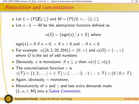
Let L = (P(Z),⊆) and M = (P({0,+,−}),⊆).

Let α : L→ M be the abstraction function defined as

α(S) = {sign(z) | z ∈ S} where

sign(x) = 0 if x = 0, + if x > 0 and − if x < 0.

For example: α({0, 2, 20, 204}) = {0,+} and α(O) = {−,+}where O is the set of odd numbers.

Obviously, α is monotone: if x ⊆ y then α(x) ⊆ α(y).

The concretization function γ isγ(T ) = {1, 2, . . . | + ∈ T} ∪ {. . . ,−2,−1 | − ∈ T} ∪ {0 | 0 ∈ T}Again, obviously, γ monotone.

Monotonicity of α and γ and two extra demands make(L, α, γ,M) into a Galois Connection.



Demand number 1

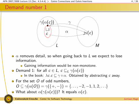
γ

v

γ(α(c))

αc

L M

α(c)

α removes detail, so when going back to L we expect to loseinformation.

Gaining information would be non-monotone.

Demand 1: for all c ∈ L, c vL γ(α(c))In the book: λc .c v γ ◦ α. Obtained by abstracting c away.

For the set O of odd numbers,O ⊆ γ(α(O)) = γ({+,−}) = {. . . ,−2,−1, 1, 2, . . .}What about α(γ(α(c)))? It equals α(c).



Demand number 2

γγ(a)

L M

v

a

αα(γ(a))

Demand 2: for all a ∈ M, α(γ(a)) vM a

In the book formulated as α ◦ γ v λa.a. Same thing.

Dual version of demand 1.

Abstracting the concrete value of an abstract values gives a lowerbound of the abstract value

For a = {+, 0} ∈ M, α(γ(a)) = α({0, 1, 2, . . .}) = {0,+}What about γ(α(γ(a)))? It equals γ(a).



Galois Insertions

Sometimes Demand 2 becomesDemand 2’: for all a ∈ M, α(γ(a)) = a.

It is then called a Galois Insertion.

Often an Insertion is a Connection, but not always.



A Connection that is not an Insertion

Consider the complete lattice M = P({0,+,−} × {odd, even})with the obvious α and γ from L = (P(Z),⊆) to M.

Is γ so obvious? What is γ({(0, odd), (−, even)})?

What happens to (0, odd)? We ignore it!

Abstracting back gives

α(γ({(0, odd), (−, even)})) = {(−, even)} ⊂ {(0, odd), (−, even)} .



A Connection that is not an Insertion

Consider the complete lattice M = P({0,+,−} × {odd, even})with the obvious α and γ from L = (P(Z),⊆) to M.

Is γ so obvious? What is γ({(0, odd), (−, even)})?

What happens to (0, odd)? We ignore it!

Abstracting back gives

α(γ({(0, odd), (−, even)})) = {(−, even)} ⊂ {(0, odd), (−, even)} .



Every Connection can be made into an Insertion

How?

Remove superfluous elements from M.

Often, Galois Connections are easier to specify:

In the example we would be forced to enumerate the five caseswhich are allowed.

In the book, reduncancy removal by reduction function:ς(a) = a− {(0, odd)}.



Adjoints

Mα

γ

v v

a

α(c)c

γ(a)

L

An equivalent way of phrasing the demands.

Now α and γ are total functions between L and M.

Abstraction of less gives less: c v γ(a) implies α(c) v a.

Concretization of more gives more: α(c) v a implies c v γ(a).

The above restrictions define when (L, α, γ,M) is an adjoint.

Proposition 4.20: adjoints are Galois Connections and vice versa.



Some example abstractions

Reachability: M = Lab∗ → {⊥,>}. ⊥ describes “not reachable”,> describes “might be reachable”.

Undefined variable analysis: M = Var∗ → {⊥,>} where >describes “might get a value”, ⊥ describes “never gets a value”.

Possibly add program points to find out which variables might beused, before they get their value: M = Lab∗ → Var∗ → {⊥,>}Detection of Signs Analysis: we have seen it already

Detection of Parity Analysis: see the chapter of Nielson and Joneson the APA website.


APA 2007/2008 Lecture 13 (Sec. 4.3-4.4) > Constructing Galois Connections 11 / 26

Building a better Galois Connection

From Galois Connections, other Galois Connections can be built.

Allows reuse of different Galois Connections, both in proofs andimplementations.

We look at the following constructions:

composition of Galois Connections,total function space,independent attribute combination,relational method, anddirect product.



A large example

Construct a Galois Connection from the collecting semantics

L = Lab∗ → P(Var∗ → Z)

toM = Lab∗ → Var∗ → Interval

M can be used for Array Bound Analysis:

Of interest are only the minimal and maximal values.

First we abstract L to T = Lab∗ → Var∗ → P(Z), and then T toM.

The abstraction α from L to M is the composition of these two.

The intermediate Galois Connections are built using the totalfunction space combinator.



First from L to T

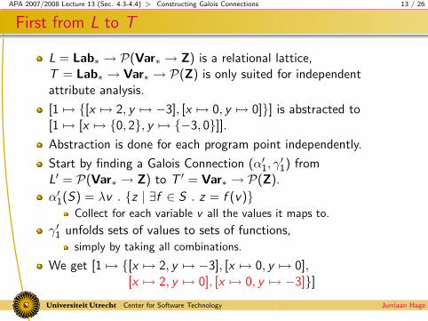
L = Lab∗ → P(Var∗ → Z) is a relational lattice,T = Lab∗ → Var∗ → P(Z) is only suited for independentattribute analysis.

[1 7→ {[x 7→ 2, y 7→ −3], [x 7→ 0, y 7→ 0]}] is abstracted to[1 7→ [x 7→ {0, 2}, y 7→ {−3, 0}]].Abstraction is done for each program point independently.

Start by finding a Galois Connection (α′1, γ′1) from

L′ = P(Var∗ → Z) to T ′ = Var∗ → P(Z).

α′1(S) = λv . {z | ∃f ∈ S . z = f (v)}Collect for each variable v all the values it maps to.

γ′1 unfolds sets of values to sets of functions,simply by taking all combinations.

We get [1 7→ {[x 7→ 2, y 7→ −3], [x 7→ 0, y 7→ 0],[x 7→ 2, y 7→ 0], [x 7→ 0, y 7→ −3]}]



The total function space combinator

Let (L′, α′1, γ′1,T

′) be the Galois Connection of the previous slide.

How can we obtain a Galois Connection (L, α1, γ1,T )?

Use the total function space combinator.

For a fixed set, say S = Lab∗, (L′, α′1, γ′1,T

′) is transformed intoa Galois Connection between L = S → L′ to T = S → T ′.

Appendix A: L and T are complete lattices if L′ and T ′ are.

Cf. adding context in Chapter 2.

The construction tells us how to build α1 and γ1 out of α′1 and γ1.

For each φ ∈ L: α1(φ) = α′1 ◦ φ (see also p. 96)

Similarly, for each ψ ∈ T : γ1(ψ) = γ′1 ◦ ψ.



The general result

Assume (L′, α′, γ′,M ′) is a Galois Insertion and prove that

(S → L′, α, γ,S → M ′) is a Galois Insertion:

S → L′ and S → M ′ are complete lattices,α and γ are monotone.For all a ∈ S → M ′: α(γ(a)) = a.And for all c ∈ S → L′: c v γ(α(c)).

Sketch:

Appendix A: elementwise comparison of function values:f vL g iff ∀x ∈ S : f (x) vL′ g(x).Composition preserves monotonicityα inherits from α′

Same here (see next slide).

Can also be proved for Galois Connections.



Part of the proof

Consider the following statement:

For all c ∈ S → L′: c v γ(α(c)).

Remember: L = S → L′ in this particular case.

Recall

For each φ ∈ L: α(φ) = α′ ◦ φ.For each ψ ∈ T : γ(ψ) = γ′ ◦ ψ.

Let c ∈ S → L′, s ∈ S , so that c(s) ∈ L′.

Then

c(s) v γ′(α′(c(s)))= γ′((α′ ◦ c)(s))= γ′(α(c)(s))= (γ′ ◦ α(c))(s)= γ(α(c))(s).



The next step

We have a Galois Connection from the relational latticeL = Lab∗ → P(Var∗ → Z) to the independent attribute latticeT = Lab∗ → Var∗ → P(Z).

Is it a Galois Insertion?

We now abstract further to M = Lab∗ → Var∗ → Interval, whereInterval is the complete lattice of intervals.

The two Galois Connections (from L to T and from T to M) canbe composed to form a direct one.

The Galois Connection from L to T can be reused, for instancewhen we want to abstract from L toLab∗ → Var∗ → P({0,+,−}).

The first abstraction already does quite a bit of the work.



The lattice of intervals

Interval = (Interval,v) withInterval = {⊥} ∪ {[z1, z2] | z1 ≤ z2, z1, z2 ∈ Z ∪ {−∞,∞}}

⊥ could be written [ ] = [∞,−∞] and > = [−∞,∞].

The operator t works like expected:

⊥ t X = X = X t ⊥ and[i1, j1] t [i2, j2] = [min(i1, i2),max(j1, j2)],where min(−∞, a) = −∞ and max(∞, a) =∞ and so on.

Define inf(X ) =∞ if X = ⊥ and inf(X ) = i if X = [i , j ].

Define sup(X ) = −∞ if X = ⊥ and sup(X ) = j if X = [i , j ].

X v Y if inf(Y ) ≤ inf(X ) and sup(X ) ≤ sup(Y ).

Interval is a complete lattice, but does not have ACC.

The lattice can abstract sets of integers that a variable may takeduring execution of a program (at a given point `).



A Galois Insertion from T to M

T = Lab∗ → Var∗ → P(Z) and M = Lab∗ → Var∗ → Interval.

First abstract P(Z) to Interval, then apply total function spacecombinator twice.

Abstraction from P(Z) to Interval is relatively easy:S ⊆ P(Z) abstracts to α′′2(S) = [inf ′(S), sup′(S)] whereinf ′(∅) =∞, and inf ′(S) = −∞ if S has no smallest element.

sup′ can be similarly defined.

Concretization is easier: γ′′2 (I ) = {x | x ≥ inf(I ) ∧ x ≤ sup(I )}.Applying the total function space combinator twice in successionfirst adds Var∗, then Lab∗.

The resulting Galois Insertion is (T , α2, γ2,M).



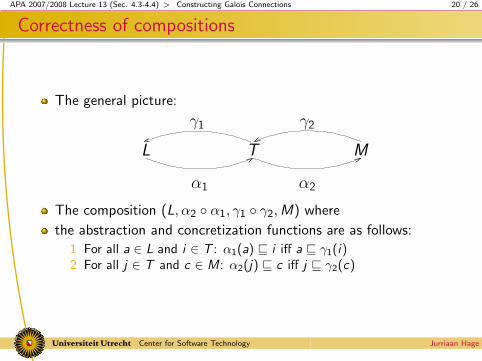
Correctness of compositions

The general picture:

γ2

L T M

γ1

α2α1

The composition (L, α2 ◦ α1, γ1 ◦ γ2,M) where

the abstraction and concretization functions are as follows:

1 For all a ∈ L and i ∈ T : α1(a) v i iff a v γ1(i)2 For all j ∈ T and c ∈ M: α2(j) v c iff j v γ2(c)



Proof of correctness of compositions

We prove that (L, α2 ◦ α1, γ1 ◦ γ2,M) is a Galois Connection.

Recall:

1 For all a ∈ L and i ∈ T : α1(a) v i iff a v γ1(i)2 For all j ∈ T and c ∈ M: α2(j) v c iff j v γ2(c)

Via the defining adjoint property: α(c) v a iff c v γ(a).

To prove:(α2 ◦ α1)(a) v c iff a v (γ1 ◦ γ2)(c)

(α2 ◦ α1)(a) v c⇐⇒ α2(α1(a)) v c

2⇐⇒ α1(a) v γ2(c)1⇐⇒ a v γ1(γ2(c))⇐⇒ a v (γ1 ◦ γ2)(c)



Summarizing

To obtain a Galois Connection from

L = Lab∗ → P(Var∗ → Z) to M = Lab∗ → Var∗ → Interval

we constructed two Galois Connections by handfrom P(Var∗ → Z) to Var∗ → P(Z), andfrom P(Z) to Interval.Proofs that these are Galois Connections/adjoints should be made.

Usually, easy but tedious.

The remainder of the work was done by application of generalresults:

lifting a Galois Connection between two lattices to one where acertain amount of context was added,composing Galois Connections sequentially.

Further abstraction to Lab∗ → Var∗ → P({−, 0,+}) is perfectlypossible.


APA 2007/2008 Lecture 13 (Sec. 4.3-4.4) > Other useful combinators 23 / 26

Direct product

Starting from the lattice P(Z) we can obtain separate GaloisConnections to M1 = P({odd, even}) and M2 = P({−, 0,+}).

Combine the two into one Galois Insertion betweenL = P(Z) and M = P({odd, even})× P({−, 0,+}).

Given that we have (L, α1, γ1,M1) and (L, α2, γ2,M2) we obtain(L, α, γ,M1 ×M2) where

α(c) = (α1(c), α2(c)) andγ(a1, a2) = γ1(a1) u γ2(a2)

Why take the meet (greatest lower bound)?

It enables us to ignore combinations (a1, a2) that cannot occur.

γ({odd}, {0}) = γ1({odd})∩γ2({0}) = {. . . ,−1, 1, . . .}∩{0} = ∅.One can prove that (L, α, γ,M1 ×M2) is an adjoint.

Verify that for all c ∈ L, (a1, a2) ∈ M1 ×M2:

α(c) v (a1, a2) iff c v γ(a1, a2)



Direct product

Starting from the lattice P(Z) we can obtain separate GaloisConnections to M1 = P({odd, even}) and M2 = P({−, 0,+}).

Combine the two into one Galois Insertion betweenL = P(Z) and M = P({odd, even})× P({−, 0,+}).

Given that we have (L, α1, γ1,M1) and (L, α2, γ2,M2) we obtain(L, α, γ,M1 ×M2) where

α(c) = (α1(c), α2(c)) andγ(a1, a2) = γ1(a1) u γ2(a2)

Why take the meet (greatest lower bound)?It enables us to ignore combinations (a1, a2) that cannot occur.

γ({odd}, {0}) = γ1({odd})∩γ2({0}) = {. . . ,−1, 1, . . .}∩{0} = ∅.One can prove that (L, α, γ,M1 ×M2) is an adjoint.

Verify that for all c ∈ L, (a1, a2) ∈ M1 ×M2:

α(c) v (a1, a2) iff c v γ(a1, a2)



The independent attribute method

γ1

γ2

L2 M2

L1 × L2=⇒ M1 ×M2

(γ1, γ2)

(α1, α2)α2

α1

M1L1

Example: L1 = L and M1 = M, and M2 is some abstraction of L2

which describes the state of the heap at different program points.

We can define α and γ between L1 × L2 and M1 ×M2 as follows:

α(c1, c2) = (α1(c1), α2(c2))γ(a1, a2) = (γ1(a1), γ2(a2)).

The two abstractions are done in parallel and independently:

no cross-over, no helping each other.



The relational method

The independent attribute method demands that the twocomponents be unrelated.

The relational method may obtain a more precise lattice,

but only works for powersets, so less generally usable.

Consider (P(C1), α1, γ1,P(A1)) and (P(C2), α2, γ2,P(A2)).

Build a new Galois Connection: (P(C1 × C2), α, γ,P(A1 × A2)).

α(CC ) =⋃{(α1({c1}), α2({c2})) | (c1, c2) ∈ CC}.

Related pairs (c1, c2) are mapped to sets of related pairs.

Example: {(z ,−z) | z ∈ Z}.Relational method maps pair of integers to pair of signs:{(+,−), (0, 0), (−,+)}.

The ’inverse’ relation between the two elements is preserved

Independent method abstracts to P({−, 0,+})× P({−, 0,+}).

The example maps to ({−, 0,+}, {−, 0,+}), which is less precise.



Inducing operators

Replacing a complete lattice for the collecting semantics L with asimpler one like M might take a lot of work.

Operators which worked on elements of L now should work onabstract values.

Example for intervals: I1 + I2 = [inf(I1) + inf(I2), sup(I1) + sup(I2)]where −∞+ 2 = −∞ and so on.

One basic rule: a1 opM a2 w α(γ(a1) opL γ(a2))

Computing α(γ(a1) opL γ(a2)) is often too costly: add all pairs ofvalues from two (possibly infinite) intervals.

It is also fine to define I1 +I I2 = > for all intervals (but not wise).

Modularity in development Galois Insertions also leads to modularabstract operators:

Once we know how to add intervals, we also know how to addfunctions from Lab∗ → Var∗ → Interval.


APA 2007/2008 Lecture 13 (Sec. 4.3-4.4) - cs.uu.nl fileDepartment of Information and Computing Sciences, Universiteit Utrecht March 25, 2009 Center for Software Technology Jurriaan

Documents