RENATO LEONI Another Approach to Simple Principal Component Analysis (version January, 2014) Florence, Italy

Welcome message from author
This document is posted to help you gain knowledge. Please leave a comment to let me know what you think about it! Share it to your friends and learn new things together.
Transcript

RENATO LEONI
Another Approach to Simple PrincipalComponent Analysis
(version January, 2014)
Florence, Italy

Università di Firenze
Dipartimento di Statistica, Informatica, Applicazioni
"Giuseppe Parenti" (DiSIA)
Italia
ANOTHER APPROACH TO SIMPLE PRINCIPAL COMPONENT ANALYSIS 3
0 INTRODUCTION
Researchers are frequently faced with the task of analysing a data
collection concerning a large number of quantitative variables measured on
many individuals (units) and usually displayed in matrix form.
The aim of the analysis is often to find out patterns of relationships which
can exist among variables.
The problem is that, given the data volume, this aim is not readily
achieved.
A way to solve this problem is to perform a principal component analy-
sis (PCA) of the data at hand.
Yet, since principal components are linear combinations of the variables
with coefficients generally all different from zero, they can sometimes be
difficult to interpret.
Attempts to overcome this drawback − which can be collected under the
label simple principal component analysis (S_PCA) − are numerous.
In this paper, we will present another approach to S_PCA.
Essentially, the method we propose lies in forcing the first few principal
vectors to be sparse and orthonormal and the corresponding sparse prin-
cipal components to be uncorrelated.
The contents of the paper can be summarized as follows.
In Section 1, some preliminary concepts and notation are introduced. In
Section 2, the approach to S_PCA we suggest is outlined. In Section 3,
rules for building up and interpreting graphical representation of variables
are given. In Section 4, a further remark is set out. Finally, in Appendix, the
Matlab code for performing the necessary calculations and graphics is
presented and results of a numerical example are shown.
1 SOME PRELIMINARY CONCEPTS AND NOTATION
Consider the raw data matrix (1)
(1) Uppercase and lowercase boldface letters represent, respectively, matrices and column vectors.A prime denotes transposition.
4 RENATO LEONI
X = x1 1 x1 p
xn 1 xn p
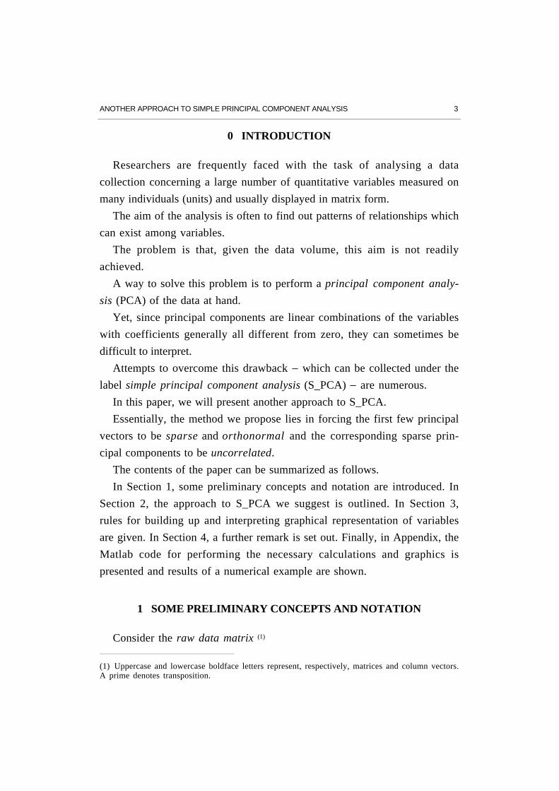
where xi j (j = 1, ... , p; i = 1, ... , n) denotes the value of the jth quantitative
variable observed on the ith individual.
Notice that, setting (j = 1, ... , p)
x j = x1 j
xn j
and (i = 1, ... , n)
x i = x i 1
x i p
,
we can write
X = x1 xp
and
X' = x1 xn .
Considering the notation just introduced, we say that x1 , ... , xp and
x1 , ... , xn represent, respectively, the p variables and the n individuals.
Regarding x1 , ... , xp and x1 , ... , xn as elements of Rn and Rp, respectively,
Rn (variable space) and Rp (individual space) are equipped with a Euclid-
ean metric.
In Rn the matrix (symmetric and positive definite) of the Euclidean metric
− with respect to the basis formed by the n canonical vectors u 1 , ... , u n − is
M = diag ( 1n , ... , 1n ) .
In Rp the matrix (symmetric and positive definite) of the Euclidean metric
ANOTHER APPROACH TO SIMPLE PRINCIPAL COMPONENT ANALYSIS 5
− with respect to the basis formed by the p canonical vectors u1 , ... , up − is
Q = diag ( 1σ 1
2 , ... , 1
σ p2)
where σ j2 (j = 1, ... , p) represents the variance of the jth variable.
Now, let
g' = x 1 x p
where x j = Σ i m ixi j is the (weighted) arithmetic mean of the variable x j .
The vector g is called the mean vector of the p variables x1 , ... , xp or the
barycentre (centroid) of the n individuals x1 , ... , xn .
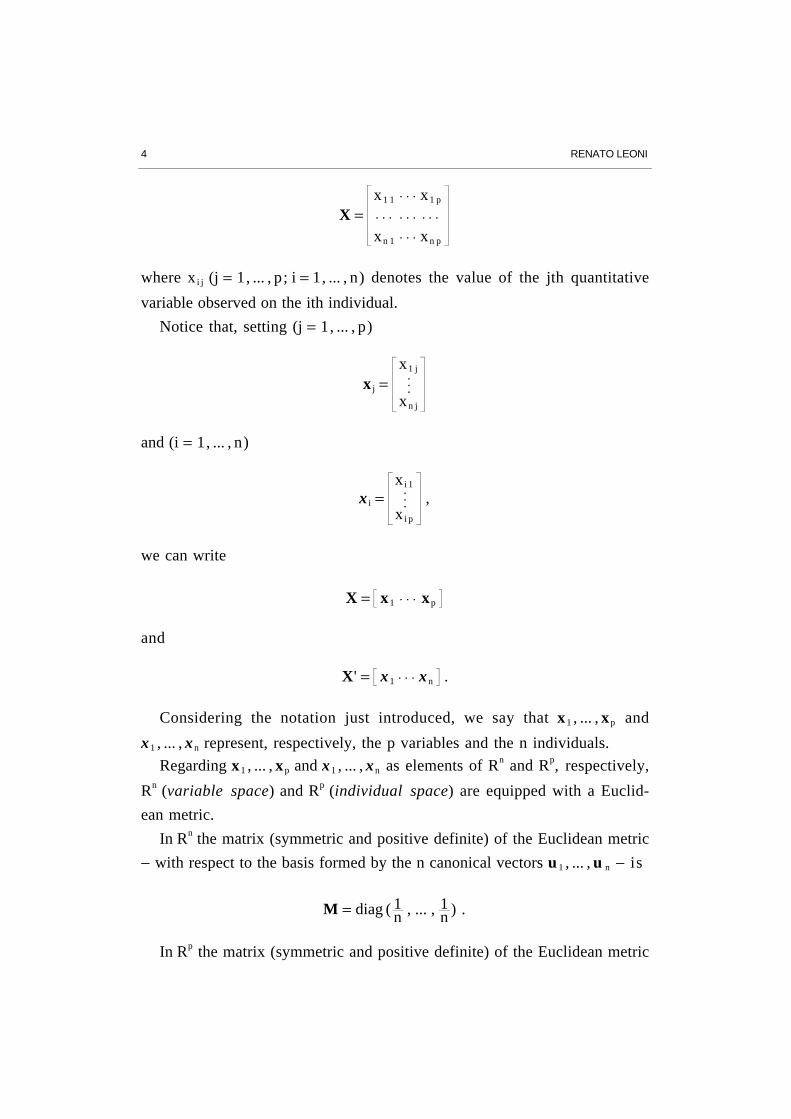
Next, assuming that u is a column vector of order n with elements all
equal to 1, consider the column centred data matrix
Y = X − u g ' = x1 1 x1 p
xn 1 xn p
− x 1 x p
x 1 x p
= x1 1 − x1 x1 p − xp
xn 1 − x1 xn 1 − xp
.
Then, setting (j = 1, ... , p)
y j = x1 j − x j
xn j − x j
and (i = 1, ... , n)
y i = x i 1 − x1
xi p − xp
we can write
Y = y1 yp
and
Y' = y 1 y n .
6 RENATO LEONI
Taking into account the notation just introduced, we say that y1 , ... , yp
and y1 , ... , y n represent, respectively, the p variables and the n individuals
(measured in terms of deviations from the means).
Of course, the (weighted) arthmetic mean of y j (j = 1, ... , p) is zero.
2 AN APPROACH TO S_PCA
Assuming that rank(Y) > 2, suppose we have performed a PCA of the
matrix Y obtaining the (first two) principal components (2)
(1) y1 = YQ c1 = Y w1 , y2 = YQ c2 = Y w2
where
• c1 and c2 are the (first two) principal vectors ;
• w1 = Q c1 and w2 = Q c2 are the (first two) principal factors or loadings.
It should be remembered that
• c1 and c2 are orthonormal with respect to the metric represented by the
matrix Q;
• w1 and w2 are orthonormal with respect to the metric represented by the
matrix Q -1;
• y1 and y2 are uncorrelated with variances given by the (first two) eigen-
values λ 1 and λ 2 .
The method we propose lies in forcing principal vectors to be sparse and
orthonormal (which implies that principal factors are sparse and ortho-
normal too), and the corresponding principal components to be sparse and
uncorrelated.
(2) We limit ourselves to consider the first two principal components, but the approach wepropose can be exended to three or more proncipal components.
ANOTHER APPROACH TO SIMPLE PRINCIPAL COMPONENT ANALYSIS 7
The procedure we suggest consists of two steps.
Step 1. Notice that the first relationship in (1) can be rewritten as
(2) y1 = YQ C (1) u
where
C (1) = diag(c1) .
Notice also that if we replace u with a sparsity vector s 1 the relatonship
(2) is generally no more exact but becomes
(3) y1 = YQ C (1) s 1 + e 1
where e 1 is a vector of residuals.
Suppose that we choose
(4) s 1 = argmin s1
(y1 − YQ C (1) s 1)'M(y1 − YQ C (1) s 1)
under the constraints
(5) s 1 ≥ 0 , u' s 1 ≤ t < p .
As the tuning parameter t decreasis, some elements of s 1 are forced to
zero, while the remaining elements are shrunken.
Hence, setting c1 = C (1) s 1 ,
(6) c1 = c1 /(c1' Qc1)1 2 , y1 = YQ c1
represent, respectively, the first normalized sparse principal vector and
the first sparse principal component.
Step 2. This step is similar to the previous one but, in order to achieve
orthogonality of sparse principal vectors and lack of correlation of sparse
principal components, more constraints are taken into account.
8 RENATO LEONI
In details, notice that the second relationship in (1) can be rewritten as
(7) y2 = YQ C (2) u
where
C (2) = diag(c2) .
Notice also that if we replace u with a sparsity vector s 2 the relatonship
(7) is generally no more exact but becomes
(8) y2 = YQ C (2) s 2 + e 2
where e 2 is a vector of residuals.
Suppose we choose
(9) s 2 = argmin s2
(y2 − YQ C (2) s 2)'M(y2 − YQ C (2) s 2)
under the constraints
(10) s 2 ≥ 0 , u' s 2 ≤ t < p , c1' Q C (2) s 2 = 0 , y1' M YQ C (2) s 2 = 0 .
Again, as the tuning parameter t decreasis, some elements of s 2 are
forced to zero, while the remaining elements are shrunken.
Hence, setting c2 = C (2) s 2 ,
(11) c2 = c2 /(c2' Qc2)1 2 , y2 = YQ c2
represent, respectively, the second normalized sparse principal vector,
orthogonal to c1 , and the second sparse principal component, uncorrelated
with y1 .
REMARK 1. The problems (4)-(5) and (9)-(10) are classical least squares
problems under linear constraints for which exist efficient numerical algo-
rithms to solve them.
ANOTHER APPROACH TO SIMPLE PRINCIPAL COMPONENT ANALYSIS 9
REMARK 2. We have assumed that the tuning parameter t is the same in
Step 1 and Step 2, but this is not necessary.
REMARK 3. Like any other approach to S_PCA, our approach is sub-optimal
with respect to PCA, in the sense that sparse principal components have
variances (depending on the tuning parameter t) less than those of ordinary
principal components.
Besides orthonormality of sparse principal vectors and lack of correlation
between sparse principal components, two more properties should be noted.
1. It results (h = 1 , 2)
(12) u' M yh = u' M Y Q ch = 0
namely the (weighted) arthmetic mean of yh is zero.
2. The orthogonal projection of y j (j = 1 , ... , p) on the subspace spanned by
yh (h = 1 , 2) is
(13) yh (y h' Myh)
- 1 y h' My j =
yh
(y h' Myh)-1 2
σ j y h
' My j
(y h' Myh)-1 2 σ j
= yh* σ j r j h
where yh* denotes the hth standardized sparse principal component and
rj h is the linear correlation coefficient between y j and yh .
3 GRAPHICAL REPRESENTATION OF VARIABLES
A graphical representation of the p variables y1 , ... , yp is usually obtained
by their orthogonal projections on the subspace S (y1* , y2
*) spanned by the
first two standardized sparse principal components y1* , y2
* .
Taking into account of (13) and denoting by y j the orthogonal projection of
y j (j = 1, ... , p) on S (y1* , y2
*), we have
y j = y1* σ j r j 1 + y2
* σ j r j 2 .
10 RENATO LEONI
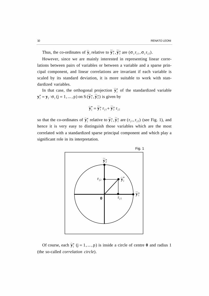
Thus, the co-ordinates of y j relative to y1
* , y2* are (σ j r j 1 , σ j r j 2) .
However, since we are mainly interested in representing linear corre-
lations between pairs of variables or between a variable and a sparse prin-
cipal component, and linear correlations are invariant if each variable is
scaled by its standard deviation, it is more suitable to work with stan-
dardized variables.
In that case, the orthogonal projection y j* of the standardized variable
y j* = y j σ j (j = 1, ... , p) on S (y1
* , y2*) is given by
y j* = y1
* r j 1 + y2* r j 2
so that the co-ordinates of y j* relative to y1
* , y2* are (r j 1 , r j 2) (see Fig. 1), and
hence it is very easy to distinguish those variables which are the most
correlated with a standardized sparse principal component and which play a
significant role in its interpretation.
y j*
0 r j 1
r j 2
y1*
y2*
Fig. 1
Of course, each y j* (j = 1, ... , p) is inside a circle of centre 0 and radius 1
(the so-called correlation circle).
ANOTHER APPROACH TO SIMPLE PRINCIPAL COMPONENT ANALYSIS 11
Moreover, the quality of representation of each variable on S (y1* , y2
*) can
be judged by means of the square cosine of the angle formed by y j* and y j
*
which is given by ((y j*)'M(y j
*) = 1)
QR(j ; y1* , y2
*) = [(y j
*)'M( y j*)]2
[(y j*)'M(y j
*) ] [ (y j*)'M( y j
*) ] =
[(y j*)'M( y j
*)]2
( y j*)'M( y j
*) .
A high QR(j ; y1* , y2
*) − for example, QR(j ; y1* , y2
*) ≥ 0.7 − means that y j* is
well represented by y j*; on the contrary, a low QR(j ; y1
* , y2*) means that the
representation of y j* by y j
* is poor.
Notice that a more explicit expression of QR(j ; y1* , y2
*) can be obtained
taking into account that ( (yh*)'M(yh
*) = 1; (yh*)'M(yh*
* ) = 0 for h ≠ h*)
( y j*)'M( y j
*) = (y1* r j 1 + y2
* r j 2)'M(y1* r j 1 + y2
* r j 2) = r j 12 + r j 2
2
and
(y j*)'M( y j
*) = (y j*)'M(y1
* r j 1 + y2* r j 2) = r j 1
2 + r j 22 .
Thus,
QR(j ; y1* , y2
*) = r j 12 + r j 2
2 .
On the other hand, since QR(j ; y1* , y2
*) also denotes the square distance
of y j* from the correlation circle centre, we can see that well-represented
points lie near the circumference of the correlation circle.
Concluding, for well-represented variables we can visualize on the corre-
lation circle:
• which variables are correlated among themselves and with each
principal component;
• which variables are uncorrelated (orthogonal) among themselves and
with each principal component.
12 RENATO LEONI
4 A FURTHER REMARK
As mentioned in the Introduction, the literature on S_PCA is somewhat
extensive (3). It can be added that such literature is rather heterogeneous for
what concerns the formulation of the problem and/or the way to solve it.
Any how, suppose that the aht (a = 1 , ... , A) approach to S_PCA has
produced the principal components y1(a) , y2
(a) (not necessarily uncorrelated)
spanning the subspace S (y1(a) , y2
(a)).
On the other hand, an ordinary PCA also produces the principal compo-
nents y1 , y2 (uncorrelated) spanning the subspace S (y1 , y2).
It seems quite natural to evaluate the performance of each approach to
S_PCA comparing the subspaces S (y1(a) , y2
(a)) and S (y1 , y2).
Setting
Y(a)
= y1(a) y2
(a) , Y = y1 y2
an index (among many others) which can serve the purpose − lying in the
interval [0 , 1) − is
corr2 ( Y(a)
, Y) = trace( Y
(a) 'M Y)
2
trace( Y(a) '
M Y(a)
) trace( Y 'M Y) .
It should be noted that, when applyed to our approach, this index depends
on the tuning parameter t and, as t increases, the index increases too.
(3) A partial list of contibutions to the theme is given below.
ANOTHER APPROACH TO SIMPLE PRINCIPAL COMPONENT ANALYSIS 13
BIBLIOGRAPHY
Anaya-Izquierdo, K., Critchley, F. and Vines, K. (2008): Orthogonal simplecomponent analysis. The Open University.
Cadima, J. F. C. L. and Jolliffe, I. T. (1995): Loading and correlations in theinterpretation of principle components. Journal of Applied Statistics.
Cadima, J. F. C. L. and Jolliffe I. T. (2001): Variable selection and theinterpretation of principal subspaces. Journal of Agricultural, Biological, andEnvironmental Statistics.
Chipman, H. A. and Gu, H. (2005): Interpretable dimension reduction.Journal of Applied Statistics.
Choulakian, V., D'Ambra, L. and Simonetti, B. (2006): Hausman principalcomponent analysis. From Data and Information Analysis to KnowledgeEngineering.
d'Aspremont, A., Ghaoui, L. E., Jordan, M. I. and Lanckriet, G. R. (2004): Adirect formulation for sparse PCA using semidefinite programming. SIAMReview.
DeSarbo, W. S. and Hausman, R. E. (2005): An efficient branch and boundprocedure for restricted principal components analysis. Data Analysis andDecision Support.
Gervini, D. and Rousson, V. (2004): Criteria for evaluating dimension-reducing components for multivariate data. The American Statistician.
Gragn, D. and Trendafilov, N. T. (2010): Sparse principal componentsbased on clustering. The Open University.
Hausman, R. (1982): Constrained multivariate analysis. Studies in theManagement Sciences.
Johnstone, I. M. and Lu, A. Y. (2009): On consistency and sparsity forprincipal components analysis in high dimensions (with discussion).Journal of the American Statistical Association.
Jolliffe, I. T. (1995): Rotation of principal components: choice of norma-lization constraints. Journal of Applied Statistics.
Jolliffe, I. T. (2002). Principal component analysis. Springer Verlag.
Jolliffe, I. T., Trendafilov, N. T. and Uddin, M. (2003): A modified principalcomponent technique based on the LASSO. Journal of Computational andGraphical Statistics.
Jolliffe, I. T. and Uddin, M. (2000): The simplified component technique: An
14 RENATO LEONI
alternative to rotated principal components. Journal of Computational andGraphical Statistics.
Journèe, M., Nesterov, Y., Richtàrik, P. and Sepulchre, R. (2010): Gen-eralized power method for sparse principal component analysis, Journal ofMachine Learning Research.
Rousson, V. and Gasser, T. (2004): Simple component analysis. Journal ofthe Royal Statistical Society, Series C (Applied Statistics).
Vines, S. K. (2000): Simple principal components. Applied Statistics.
Witten, D. M., Hastie, T. and Tibshirani, R. (2009): A penalized matrixdecomposition, with applications to sparse principal components andcanonical correlation analysis. Biostatistics.
Zou, H., Hastie, T. and Tibshirani, R. (2006): Sparse principal componentanalysis. Journal of Computational and Graphical Statistics.

Appendix

• Matlab Code
• A numerical example: 1992 Olimpic Games (decathlon)
Matlab Code 17
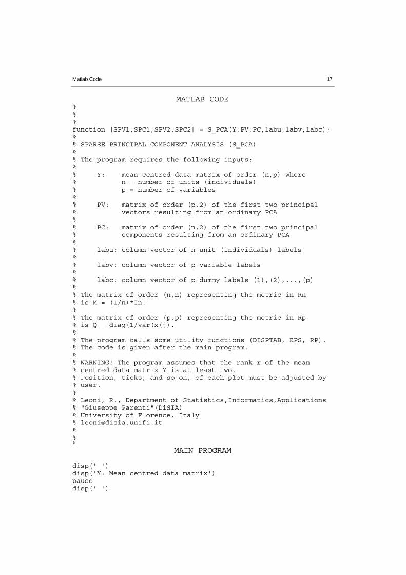
MATLAB CODE%%%function [SPV1,SPC1,SPV2,SPC2] = S_PCA(Y,PV,PC,labu,labv,labc);%% SPARSE PRINCIPAL COMPONENT ANALYSIS (S_PCA)%% The program requires the following inputs:%% Y: mean centred data matrix of order (n,p) where% n = number of units (individuals)% p = number of variables%% PV: matrix of order (p,2) of the first two principal% vectors resulting from an ordinary PCA%% PC: matrix of order (n,2) of the first two principal% components resulting from an ordinary PCA%% labu: column vector of n unit (individuals) labels%% labv: column vector of p variable labels%% labc: column vector of p dummy labels (1),(2),...,(p)%% The matrix of order (n,n) representing the metric in Rn% is M = (1/n)*In.%% The matrix of order (p,p) representing the metric in Rp% is Q = diag(1/var(x(j).%% The program calls some utility functions (DISPTAB, RPS, RP).% The code is given after the main program.%% WARNING! The program assumes that the rank r of the mean% centred data matrix Y is at least two.% Position, ticks, and so on, of each plot must be adjusted by% user.%% Leoni, R., Department of Statistics,Informatics,Applications% "Giuseppe Parenti"(DiSIA)% University of Florence, Italy% [email protected]%%%
MAIN PROGRAM
disp(' ')disp('Y: Mean centred data matrix')pausedisp(' ')
18 RENATO LEONI
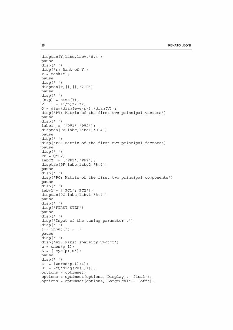
disptab(Y,labu,labv,'8.4')pausedisp(' ')disp('r: Rank of Y')r = rank(Y);pausedisp(' ')disptab(r,[],[],'2.0')pausedisp(' ')[n,p] = size(Y);V = (1/n)*Y'*Y;Q = diag(diag(eye(p))./diag(V));disp('PV: Matrix of the first two principal vectors')pausedisp(' ')labc1 = ['PV1';'PV2'];disptab(PV,labc,labc1,'8.4')pausedisp(' ')disp('PF: Matrix of the first two principal factors')pausedisp(' ')PF = Q*PV;labc2 = ['PF1';'PF2'];disptab(PF,labc,labc2,'8.4')pausedisp(' ')disp('PC: Matrix of the first two principal components')pausedisp(' ')labv1 = ['PC1';'PC2'];disptab(PC,labu,labv1,'8.4')pausedisp(' ')disp('FIRST STEP')pausedisp(' ')disp('Input of the tuning parameter t')disp(' ')t = input('t = ')pausedisp(' ')disp('s1: First sparsity vector')u = ones(p,1);A = [-eye(p);u'];pausedisp(' ')a = [zeros(p,1);t];H1 = Y*Q*diag(PV(:,1));options = optimset;options = optimset(options,'Display', 'final');options = optimset(options,'LargeScale', 'off');
Matlab Code 19
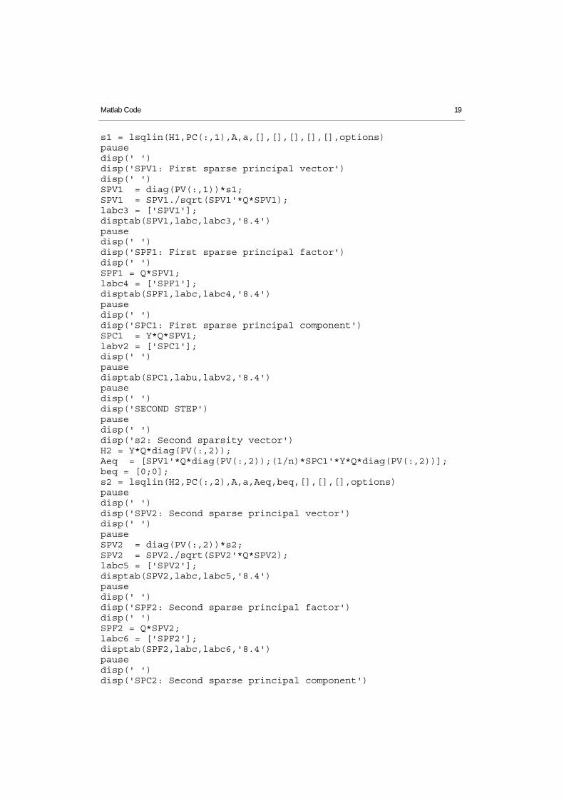
s1 = lsqlin(H1,PC(:,1),A,a,[],[],[],[],[],options)pausedisp(' ')disp('SPV1: First sparse principal vector')disp(' ')SPV1 = diag(PV(:,1))*s1;SPV1 = SPV1./sqrt(SPV1'*Q*SPV1);labc3 = ['SPV1'];disptab(SPV1,labc,labc3,'8.4')pausedisp(' ')disp('SPF1: First sparse principal factor')disp(' ')SPF1 = Q*SPV1;labc4 = ['SPF1'];disptab(SPF1,labc,labc4,'8.4')pausedisp(' ')disp('SPC1: First sparse principal component')SPC1 = Y*Q*SPV1;labv2 = ['SPC1'];disp(' ')pausedisptab(SPC1,labu,labv2,'8.4')pausedisp(' ')disp('SECOND STEP')pausedisp(' ')disp('s2: Second sparsity vector')H2 = Y*Q*diag(PV(:,2));Aeq = [SPV1'*Q*diag(PV(:,2));(1/n)*SPC1'*Y*Q*diag(PV(:,2))];beq = [0;0];s2 = lsqlin(H2,PC(:,2),A,a,Aeq,beq,[],[],[],options)pausedisp(' ')disp('SPV2: Second sparse principal vector')disp(' ')pauseSPV2 = diag(PV(:,2))*s2;SPV2 = SPV2./sqrt(SPV2'*Q*SPV2);labc5 = ['SPV2'];disptab(SPV2,labc,labc5,'8.4')pausedisp(' ')disp('SPF2: Second sparse principal factor')disp(' ')SPF2 = Q*SPV2;labc6 = ['SPF2'];disptab(SPF2,labc,labc6,'8.4')pausedisp(' ')disp('SPC2: Second sparse principal component')
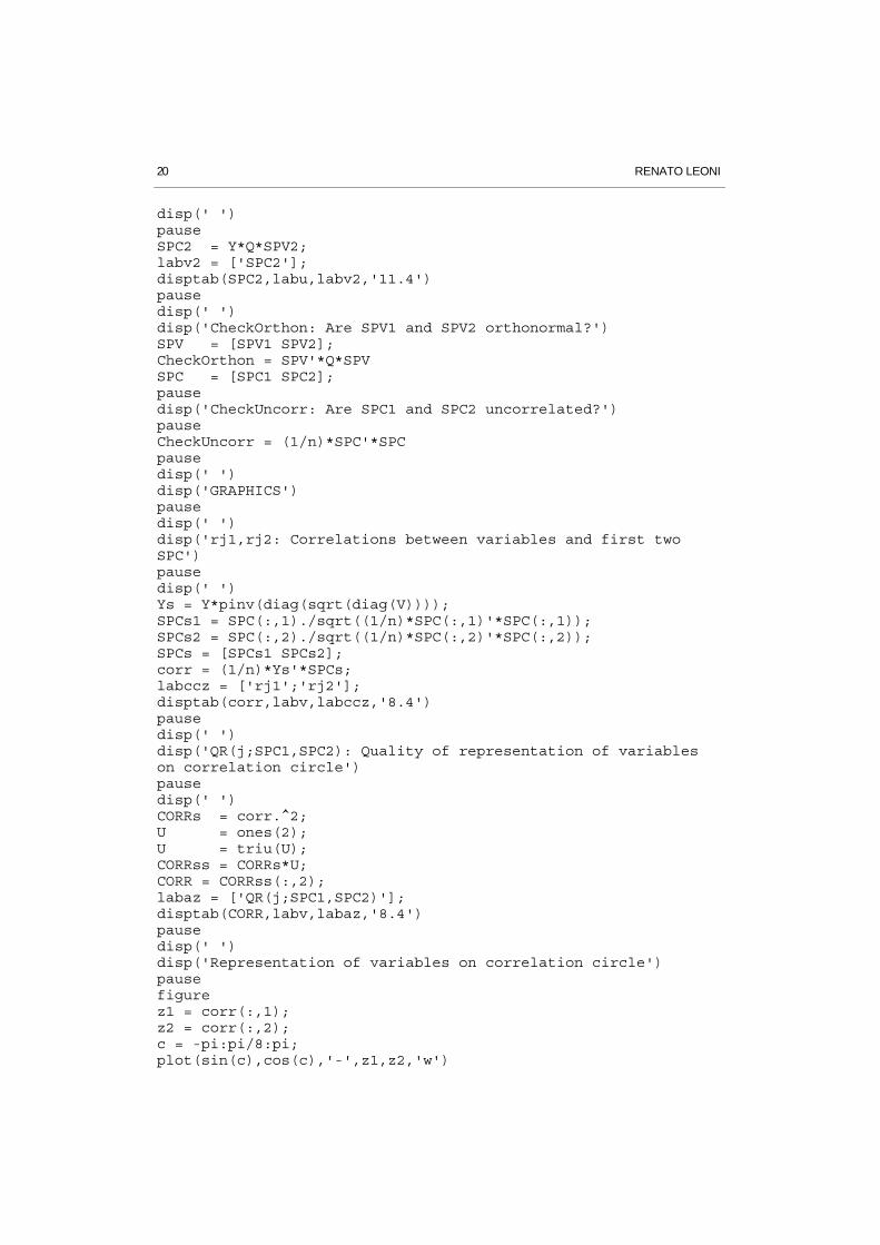
20 RENATO LEONI
disp(' ')pauseSPC2 = Y*Q*SPV2;labv2 = ['SPC2'];disptab(SPC2,labu,labv2,'11.4')pausedisp(' ')disp('CheckOrthon: Are SPV1 and SPV2 orthonormal?')SPV = [SPV1 SPV2];CheckOrthon = SPV'*Q*SPVSPC = [SPC1 SPC2];pausedisp('CheckUncorr: Are SPC1 and SPC2 uncorrelated?')pauseCheckUncorr = (1/n)*SPC'*SPCpausedisp(' ')disp('GRAPHICS')pausedisp(' ')disp('rj1,rj2: Correlations between variables and first twoSPC')pausedisp(' ')Ys = Y*pinv(diag(sqrt(diag(V))));SPCs1 = SPC(:,1)./sqrt((1/n)*SPC(:,1)'*SPC(:,1));SPCs2 = SPC(:,2)./sqrt((1/n)*SPC(:,2)'*SPC(:,2));SPCs = [SPCs1 SPCs2];corr = (1/n)*Ys'*SPCs;labccz = ['rj1';'rj2'];disptab(corr,labv,labccz,'8.4')pausedisp(' ')disp('QR(j;SPC1,SPC2): Quality of representation of variableson correlation circle')pausedisp(' ')CORRs = corr.^2;U = ones(2);U = triu(U);CORRss = CORRs*U;CORR = CORRss(:,2);labaz = ['QR(j;SPC1,SPC2)'];disptab(CORR,labv,labaz,'8.4')pausedisp(' ')disp('Representation of variables on correlation circle')pausefigurez1 = corr(:,1);z2 = corr(:,2);c = -pi:pi/8:pi;plot(sin(c),cos(c),'-',z1,z2,'w')
Matlab Code 21
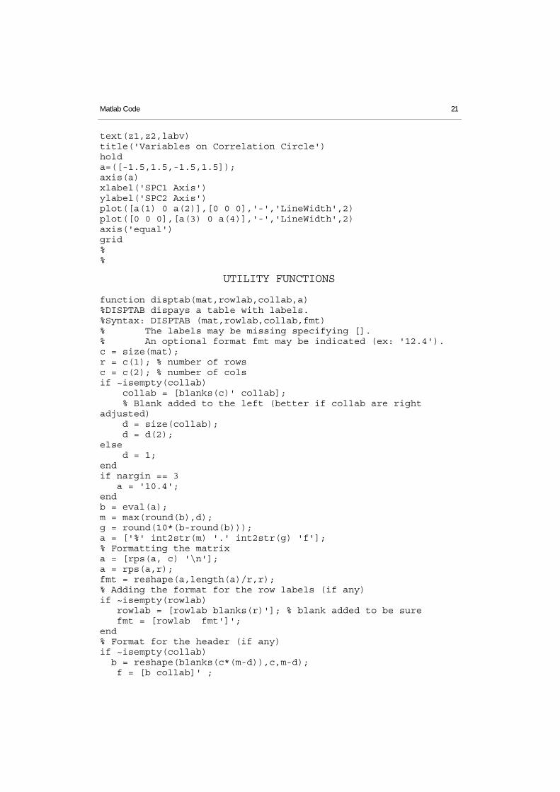
text(z1,z2,labv)title('Variables on Correlation Circle')holda=([-1.5,1.5,-1.5,1.5]);axis(a)xlabel('SPC1 Axis')ylabel('SPC2 Axis')plot([a(1) 0 a(2)],[0 0 0],'-','LineWidth',2)plot([0 0 0],[a(3) 0 a(4)],'-','LineWidth',2)axis('equal')grid%%
UTILITY FUNCTIONS
function disptab(mat,rowlab,collab,a)%DISPTAB dispays a table with labels.%Syntax: DISPTAB (mat,rowlab,collab,fmt)% The labels may be missing specifying [].% An optional format fmt may be indicated (ex: '12.4').c = size(mat);r = c(1); % number of rowsc = c(2); % number of colsif ~isempty(collab) collab = [blanks(c)' collab]; % Blank added to the left (better if collab are rightadjusted) d = size(collab); d = d(2);else d = 1;endif nargin == 3 a = '10.4';endb = eval(a);m = max(round(b),d);g = round(10*(b-round(b)));a = ['%' int2str(m) '.' int2str(g) 'f'];% Formatting the matrixa = [rps(a, c) '\n'];a = rps(a,r);fmt = reshape(a,length(a)/r,r);% Adding the format for the row labels (if any)if ~isempty(rowlab) rowlab = [rowlab blanks(r)']; % blank added to be sure fmt = [rowlab fmt']';end% Format for the header (if any)if ~isempty(collab) b = reshape(blanks(c*(m-d)),c,m-d); f = [b collab]' ;
22 RENATO LEONI
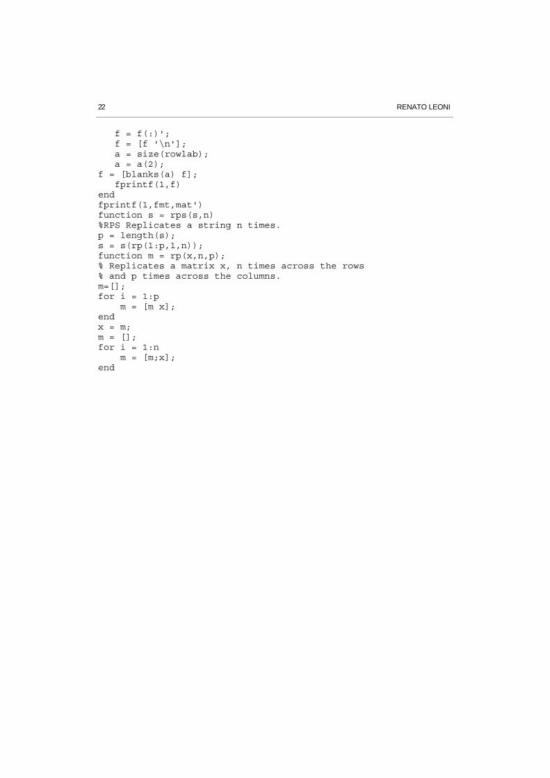
f = f(:)'; f = [f '\n']; a = size(rowlab); a = a(2);f = [blanks(a) f]; fprintf(1,f)endfprintf(1,fmt,mat')function s = rps(s,n)%RPS Replicates a string n times.p = length(s);s = s(rp(1:p,1,n));function m = rp(x,n,p);% Replicates a matrix x, n times across the rows% and p times across the columns.m=[];for i = 1:p m = [m x];endx = m;m = [];for i = 1:n m = [m;x];end
1992 Olimpic Games (decathlon) 23
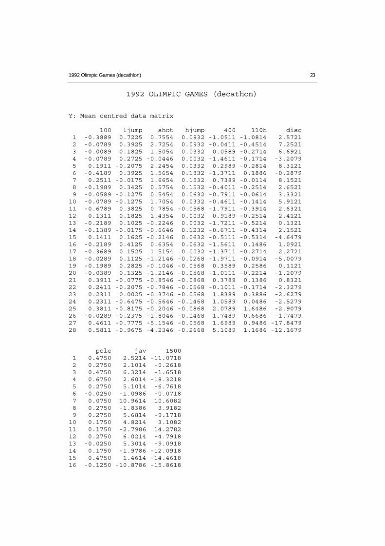
1992 OLIMPIC GAMES (decathon)
Y: Mean centred data matrix
100 ljump shot hjump 400 110h disc 1 -0.3889 0.7225 0.7554 0.0932 -1.0511 -1.0814 2.5721 2 -0.0789 0.3925 2.7254 0.0932 -0.0411 -0.4514 7.2521 3 -0.0089 0.1825 1.5054 0.0332 0.0589 -0.2714 6.6921 4 -0.0789 0.2725 -0.0446 0.0032 -1.4611 -0.1714 -3.2079 5 0.1911 -0.2075 2.2454 0.0332 0.2989 -0.2814 8.3121 6 -0.4189 0.3925 1.5654 0.1832 -1.3711 0.1886 -0.2879 7 0.2511 -0.0175 1.6654 0.1532 0.7389 -0.0114 8.1521 8 -0.1989 0.3425 0.5754 0.1532 -0.4011 -0.2514 2.6521 9 -0.0589 -0.1275 0.5454 0.0632 -0.7911 -0.0614 3.332110 -0.0789 -0.1275 1.7054 0.0332 -0.4611 -0.1414 5.912111 -0.6789 0.3825 0.7854 -0.0568 -1.7911 -0.3914 2.632112 0.1311 0.1825 1.4354 0.0032 0.9189 -0.2514 2.412113 -0.2189 0.1025 -0.2246 0.0032 -1.7211 -0.5214 0.132114 -0.1389 -0.0175 -0.6646 0.1232 -0.6711 -0.4314 2.152115 0.1411 0.1625 -0.2146 0.0632 -0.5111 -0.5314 -4.647916 -0.2189 0.4125 0.6354 0.0632 -1.5611 0.1486 1.092117 -0.3689 0.1525 1.5154 0.0032 -1.3711 -0.2714 2.272118 -0.0289 0.1125 -1.2146 -0.0268 -1.9711 -0.0914 -5.007919 -0.1989 0.2825 -0.1046 -0.0568 0.3589 0.2586 0.112120 -0.0389 0.1325 -1.2146 -0.0568 -1.0111 -0.2214 -1.207921 0.3911 -0.0775 -0.8546 -0.0868 0.3789 0.1386 0.832122 0.2411 -0.2075 -0.7846 -0.0568 -0.1011 -0.1714 -2.327923 0.2311 0.0025 -0.3746 -0.0568 1.8389 0.3886 -2.627924 0.2311 -0.6475 -0.5646 -0.1468 1.0589 0.0486 -2.527925 0.3811 -0.8175 -0.2046 -0.0868 2.0789 1.6486 -2.907926 -0.0289 -0.2375 -1.8046 -0.1468 1.7489 0.6686 -1.747927 0.4611 -0.7775 -5.1546 -0.0568 1.6989 0.9486 -17.847928 0.5811 -0.9675 -4.2346 -0.2668 5.1089 1.1686 -12.1679
pole jav 1500 1 0.4750 2.5214 -11.0718 2 0.2750 2.1014 -0.2618 3 0.4750 6.3214 -1.6518 4 0.6750 2.6014 -18.3218 5 0.2750 5.1014 -6.7618 6 -0.0250 -1.0986 -0.0718 7 0.0750 10.9614 10.6082 8 0.2750 -1.8386 3.9182 9 0.2750 5.6814 -9.171810 0.1750 4.8214 3.108211 0.1750 -2.7986 14.278212 0.2750 6.0214 -4.791813 -0.0250 5.3014 -9.091814 0.1750 -1.9786 -12.091815 0.4750 1.4614 -14.461816 -0.1250 -10.8786 -15.8618
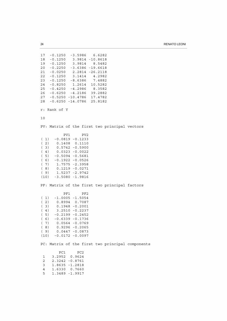
24 RENATO LEONI
17 -0.1250 -3.5986 6.628218 -0.1250 3.9814 -10.861819 -0.1250 3.9814 8.548220 -0.2250 -3.6386 -19.661821 -0.0250 2.2814 -26.211822 -0.1250 3.1414 4.298223 -0.1250 -8.6386 7.488224 -0.8250 1.2614 10.528225 -0.4250 -4.2986 8.358226 -0.6250 -4.2186 39.288227 -0.5250 -10.4786 17.478228 -0.6250 -14.0786 25.8182
r: Rank of Y
10
PV: Matrix of the first two principal vectors
PV1 PV2( 1) -0.0819 -0.1233( 2) 0.1408 0.1110( 3) 0.5742 -0.5900( 4) 0.0323 -0.0022( 5) -0.5094 -0.5681( 6) -0.1922 -0.0526( 7) 1.7575 -2.3958( 8) 0.1219 -0.0271( 9) 1.5237 -2.9742(10) -3.5080 -1.9816
PF: Matrix of the first two principal factors
PF1 PF2( 1) -1.0005 -1.5054( 2) 0.8994 0.7087( 3) 0.1948 -0.2001( 4) 3.2510 -0.2237( 5) -0.2199 -0.2452( 6) -0.6339 -0.1736( 7) 0.0564 -0.0769( 8) 0.9296 -0.2065( 9) 0.0447 -0.0873(10) -0.0172 -0.0097
PC: Matrix of the first two principal components
PC1 PC2 1 3.2952 0.9624 2 2.3242 -0.8761 3 1.8635 -1.2818 4 1.6330 0.7660 5 1.3489 -1.9917
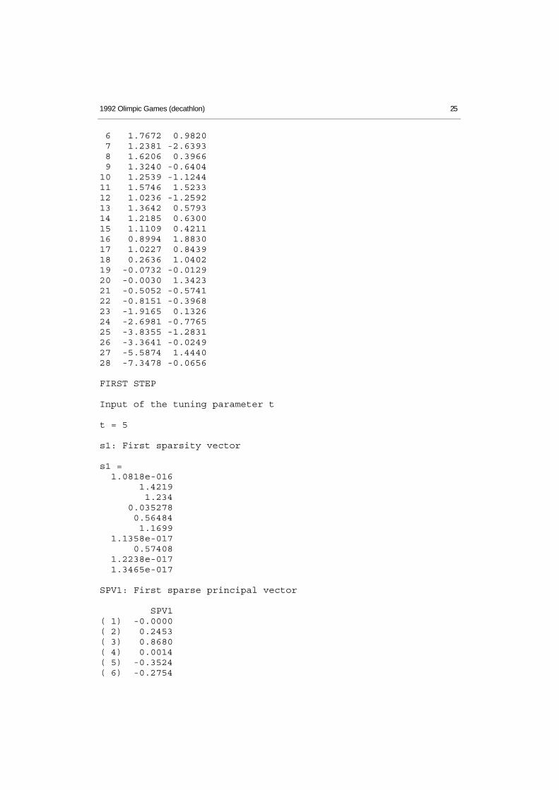
1992 Olimpic Games (decathlon) 25
6 1.7672 0.9820 7 1.2381 -2.6393 8 1.6206 0.3966 9 1.3240 -0.640410 1.2539 -1.124411 1.5746 1.523312 1.0236 -1.259213 1.3642 0.579314 1.2185 0.630015 1.1109 0.421116 0.8994 1.883017 1.0227 0.843918 0.2636 1.040219 -0.0732 -0.012920 -0.0030 1.342321 -0.5052 -0.574122 -0.8151 -0.396823 -1.9165 0.132624 -2.6981 -0.776525 -3.8355 -1.283126 -3.3641 -0.024927 -5.5874 1.444028 -7.3478 -0.0656
FIRST STEP
Input of the tuning parameter t
t = 5
s1: First sparsity vector
s1 = 1.0818e-016 1.4219 1.234 0.035278 0.56484 1.1699 1.1358e-017 0.57408 1.2238e-017 1.3465e-017
SPV1: First sparse principal vector
SPV1( 1) -0.0000( 2) 0.2453( 3) 0.8680( 4) 0.0014( 5) -0.3524( 6) -0.2754
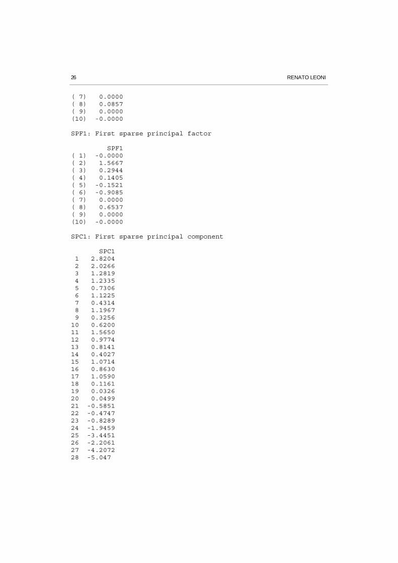
26 RENATO LEONI
( 7) 0.0000( 8) 0.0857( 9) 0.0000(10) -0.0000
SPF1: First sparse principal factor
SPF1( 1) -0.0000( 2) 1.5667( 3) 0.2944( 4) 0.1405( 5) -0.1521( 6) -0.9085( 7) 0.0000( 8) 0.6537( 9) 0.0000(10) -0.0000
SPC1: First sparse principal component
SPC1 1 2.8204 2 2.0266 3 1.2819 4 1.2335 5 0.7306 6 1.1225 7 0.4314 8 1.1967 9 0.325610 0.620011 1.565012 0.977413 0.814114 0.402715 1.071416 0.863017 1.059018 0.116119 0.032620 0.049921 -0.585122 -0.474723 -0.828924 -1.945925 -3.445126 -2.206127 -4.207228 -5.047
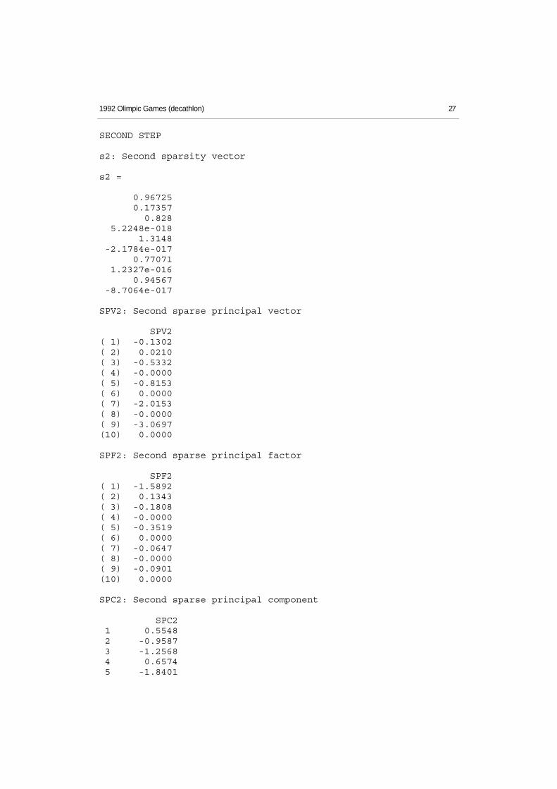
1992 Olimpic Games (decathlon) 27
SECOND STEP
s2: Second sparsity vector
s2 =
0.96725 0.17357 0.828 5.2248e-018 1.3148 -2.1784e-017 0.77071 1.2327e-016 0.94567 -8.7064e-017
SPV2: Second sparse principal vector
SPV2( 1) -0.1302( 2) 0.0210( 3) -0.5332( 4) -0.0000( 5) -0.8153( 6) 0.0000( 7) -2.0153( 8) -0.0000( 9) -3.0697(10) 0.0000
SPF2: Second sparse principal factor
SPF2( 1) -1.5892( 2) 0.1343( 3) -0.1808( 4) -0.0000( 5) -0.3519( 6) 0.0000( 7) -0.0647( 8) -0.0000( 9) -0.0901(10) 0.0000
SPC2: Second sparse principal component
SPC2 1 0.5548 2 -0.9587 3 -1.2568 4 0.6574 5 -1.8401
28 RENATO LEONI
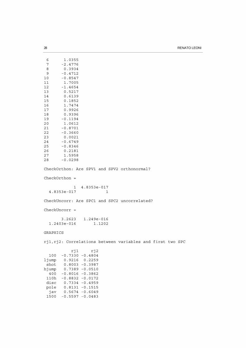
6 1.0355 7 -2.4776 8 0.3934 9 -0.471210 -0.854711 1.700512 -1.465413 0.521714 0.613915 0.185216 1.747417 0.992618 0.939619 -0.119420 1.061221 -0.870122 -0.366023 0.002124 -0.674925 -0.834626 0.218127 1.595828 -0.0298
CheckOrthon: Are SPV1 and SPV2 orthonormal?
CheckOrthon =
1 4.8353e-017 4.8353e-017 1
CheckUncorr: Are SPC1 and SPC2 uncorrelated?
CheckUncorr =
3.2623 1.249e-016 1.2403e-016 1.1202
GRAPHICS
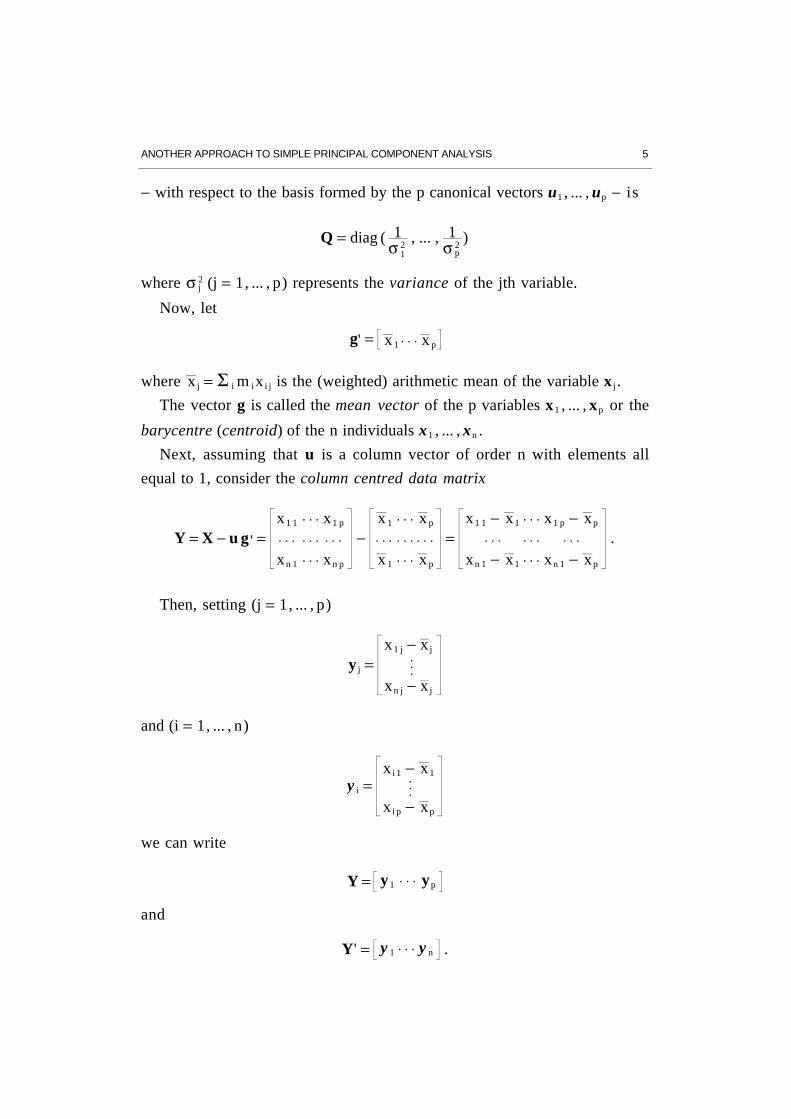
rj1,rj2: Correlations between variables and first two SPC
rj1 rj2 100 -0.7330 -0.4804ljump 0.9216 0.2259 shot 0.8003 -0.3987hjump 0.7389 -0.0510 400 -0.8016 -0.3862 110h -0.8832 -0.0172 disc 0.7334 -0.4959 pole 0.8131 -0.1515 jav 0.5674 -0.6049 1500 -0.5597 -0.0483
1992 Olimpic Games (decathlon) 29
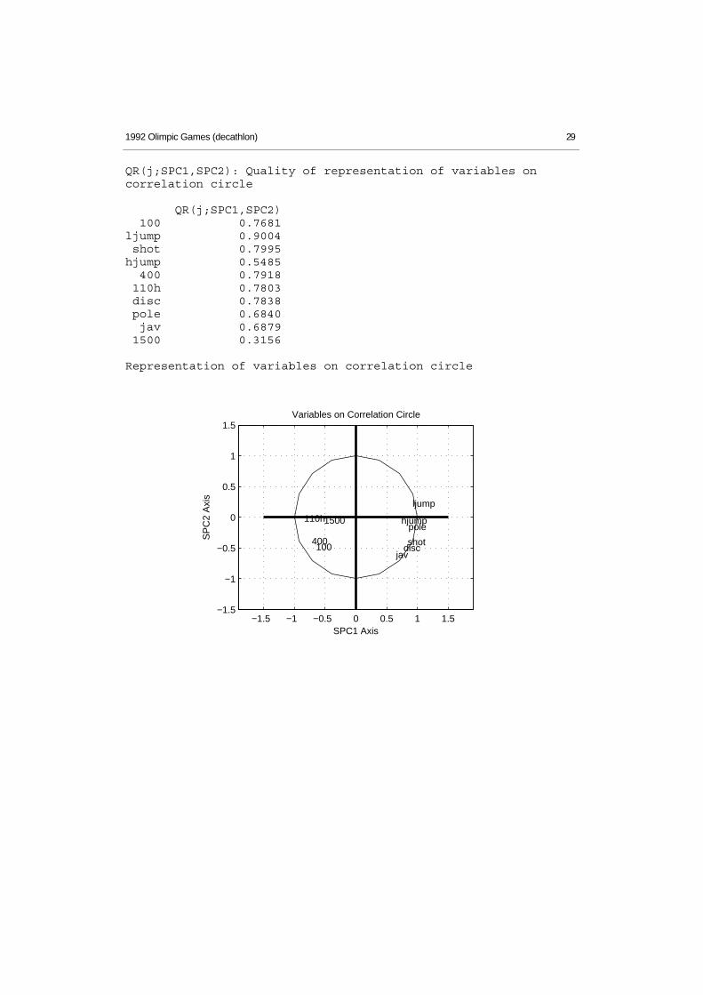
QR(j;SPC1,SPC2): Quality of representation of variables oncorrelation circle
QR(j;SPC1,SPC2) 100 0.7681ljump 0.9004 shot 0.7995hjump 0.5485 400 0.7918 110h 0.7803 disc 0.7838 pole 0.6840 jav 0.6879 1500 0.3156
Representation of variables on correlation circle
−1.5 −1 −0.5 0 0.5 1 1.5−1.5
−1
−0.5
0
0.5
1
1.5
100
ljump
shot
hjump
400
110h
disc
pole
jav
1500
Variables on Correlation Circle
SPC1 Axis
SP
C2
Axi
s
Related Documents