Principal Component Analysis Aryan Mokhtari, Santiago Paternain, and Alejandro Ribeiro Dept. of Electrical and Systems Engineering University of Pennsylvania [email protected] http://www.seas.upenn.edu/users/ ~ aribeiro/ March 28, 2018 Signal and Information Processing Principal Component Analysis 1

Welcome message from author
This document is posted to help you gain knowledge. Please leave a comment to let me know what you think about it! Share it to your friends and learn new things together.
Transcript

Principal Component Analysis
Aryan Mokhtari, Santiago Paternain, and Alejandro RibeiroDept. of Electrical and Systems Engineering
University of [email protected]
http://www.seas.upenn.edu/users/~aribeiro/
March 28, 2018
Signal and Information Processing Principal Component Analysis 1
The DFT and iDFT with unitary matrices
The discrete Fourier transform with unitary matrices
Stochastic signals
Principal Component Analysis (PCA) transform
Dimensionality reduction
Principal Components
Face recognition
Signal and Information Processing Principal Component Analysis 2
The discrete Fourier transform, again
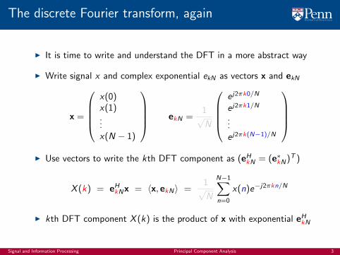
I It is time to write and understand the DFT in a more abstract way
I Write signal x and complex exponential ekN as vectors x and ekN
x =
x(0)x(1)...x(N − 1)
ekN =1√N
e j2πk0/N
e j2πk1/N
...e j2πk(N−1)/N
I Use vectors to write the kth DFT component as (eH
kN = (e∗kN)T )
X (k) = eHkNx = 〈x, ekN〉 =
1√N
N−1∑n=0
x(n)e−j2πkn/N
I kth DFT component X (k) is the product of x with exponential eHkN
Signal and Information Processing Principal Component Analysis 3
DFT in matrix notation
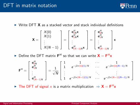
I Write DFT X as a stacked vector and stack individual definitions
X =
X (0)X (1)...X (N − 1)
=
eH
0NxeH
1Nx...eH
(N−1)Nx
=
eH
0N
eH1N
...eH
(N−1)N
x
I Define the DFT matrix FH so that we can write X = FHx
FH =
eH
0N
eH1N
...eH
(N−1)N
=1√N
1 1 · · · 1
1 e−j2π(1)(1)/N · · · e−j2π(1)(N−1)/N
......
. . ....
1 e−j2π(N−1)(1)/N · · · e−j2π(N−1)(N−1)/N
I The DFT of signal x is a matrix multiplication ⇒ X = FHx
Signal and Information Processing Principal Component Analysis 4
The DFT as a matrix product
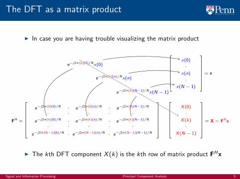
I In case you are having trouble visualizing the matrix product
e−j2π(0)(0)/N · e−j2π(0)(n)/N · e−j2π(0)(N−1)/N
· · · · ·e−j2π(k)(0)/N · e−j2π(k)(n)/N · e−j2π(k)(N−1)/N
· · · · ·e−j2π(N−1)(0)/N · e−j2π(N−1)(n)/N · e−j2π(N−1)(N−1)/N
x(0)
·x(n)
·x(N − 1)
X (0)
·X (k)
·X (N − 1)
FH =
= x
= X = FHx
e−j2π(k)(0)/Nx(0)
e−j2π(k)(n)/Nx(n)
e−j2π(k)(N−1)/Nx(N − 1)
I The kth DFT component X (k) is the kth row of matrix product FHx
Signal and Information Processing Principal Component Analysis 5

Some properties of the DFT matrix FH
I The (k , n)th element of the matrix FH is the complex exponential
((FH))
kn= e−j2π(k)(n)/N =
(e−j2π(k)/N
)(n)
I Since elements of rows are indexed powers we say FH is Vandermonde
I Also observe that since e−j2π(k)(n)/N = e−j2π(n)(k)/N we have((FH))
kn= e−j2π(k)(n)/N = e−j2π(n)(k)/N =
((FH))
nk
I The DFT matrix F is symmetric ⇒ (FH)T = FH
I Can write FH as ⇒ FH = (FH)T =[
e∗0N e∗1N · · · e∗(N−1)N
]
Signal and Information Processing Principal Component Analysis 6

The Hermitian of the DFT matrix FH
I Let F =(FH)H
be conjugate transpose of FH . We can write F as
F =
eT
0N
eT1N
...eT
(N−1)N
⇐ FH =[
e∗0N e∗
1N · · · e∗(N−1)N
]
I We say that FH and F are Hermitians of each other (that’s why FH)
I The nth row of F is the nth complex exponential eTnN
I The kth column of FH is the kth conjugate complex exponential e∗kN
Signal and Information Processing Principal Component Analysis 7
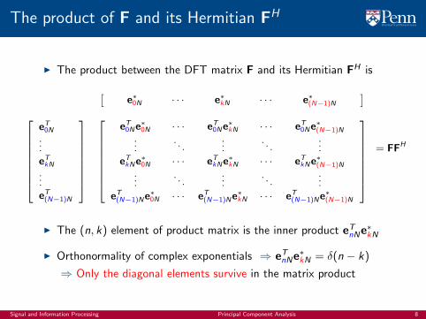
The product of F and its Hermitian FH
I The product between the DFT matrix F and its Hermitian FH is
[e∗
0N · · · e∗kN · · · e∗
(N−1)N
]
eT0N
...eTkN
...eT
(N−1)N
eT0Ne∗
0N · · · eT0Ne∗
kN · · · eT0Ne∗
(N−1)N
.... . .
.... . .
...eTkNe∗
0N · · · eTkNe∗
kN · · · eTkNe∗
(N−1)N
.... . .
.... . .
...eT
(N−1)Ne∗0N · · · eT
(N−1)Ne∗kN · · · eT
(N−1)Ne∗(N−1)N
= FFH
I The (n, k) element of product matrix is the inner product eTnNe∗kN
I Orthonormality of complex exponentials ⇒ eTnNe∗kN = δ(n − k)
⇒ Only the diagonal elements survive in the matrix product
Signal and Information Processing Principal Component Analysis 8
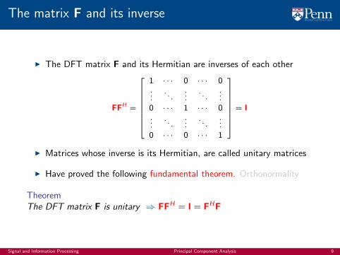
The matrix F and its inverse
I The DFT matrix F and its Hermitian are inverses of each other
FFH =
1 · · · 0 · · · 0...
. . ....
. . ....
0 · · · 1 · · · 0...
. . ....
. . ....
0 · · · 0 · · · 1
= I
I Matrices whose inverse is its Hermitian, are called unitary matrices
I Have proved the following fundamental theorem. Orthonormality
TheoremThe DFT matrix F is unitary ⇒ FFH = I = FHF
Signal and Information Processing Principal Component Analysis 9
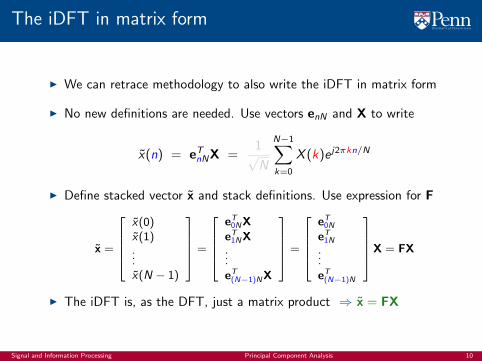
The iDFT in matrix form
I We can retrace methodology to also write the iDFT in matrix form
I No new definitions are needed. Use vectors enN and X to write
x(n) = eTnNX =
1√N
N−1∑k=0
X (k)e j2πkn/N
I Define stacked vector x and stack definitions. Use expression for F
x =
x(0)x(1)...x(N − 1)
=
eT
0NXeT
1NX...eT
(N−1)NX
=
eT
0N
eT1N
...eT
(N−1)N
X = FX
I The iDFT is, as the DFT, just a matrix product ⇒ x = FX
Signal and Information Processing Principal Component Analysis 10
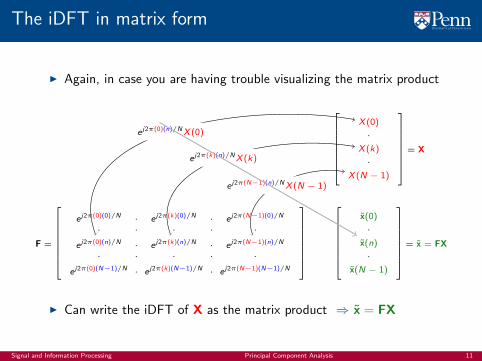
The iDFT in matrix form
I Again, in case you are having trouble visualizing the matrix product
e j2π(0)(0)/N · e j2π(k)(0)/N · e j2π(N−1)(0)/N
· · · · ·e j2π(0)(n)/N · e j2π(k)(n)/N · e j2π(N−1)(n)/N
· · · · ·e j2π(0)(N−1)/N · e j2π(k)(N−1)/N · e j2π(N−1)(N−1)/N
X (0)
·X (k)
·X (N − 1)
x(0)
·x(n)
·x(N − 1)
F =
= X
= x = FX
e j2π(0)(n)/NX (0)
e j2π(k)(n)/NX (k)
e j2π(N−1)(n)/NX (N − 1)
I Can write the iDFT of X as the matrix product ⇒ x = FX
Signal and Information Processing Principal Component Analysis 11
Inverse theorem, like a pro
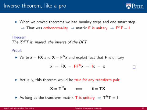
I When we proved theorems we had monkey steps and one smart step
⇒ That was orthonormality ⇒ matrix F is unitary ⇒ FHF = I
TheoremThe iDFT is, indeed, the inverse of the DFT
Proof.
I Write x = FX and X = FHx and exploit fact that F is unitary
x = FX = FFHx = Ix = x
I Actually, this theorem would be true for any transform pair
X = THx ⇐⇒ x = TX
I As long as the transform matrix T is unitary ⇒ THT = I
Signal and Information Processing Principal Component Analysis 12
Energy conservation (Parseval) theorem, like a pro
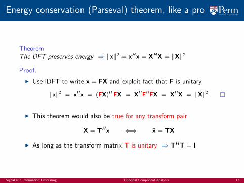
TheoremThe DFT preserves energy ⇒ ‖x‖2 = xHx = XHX = ‖X‖2
Proof.
I Use iDFT to write x = FX and exploit fact that F is unitary
‖x‖2 = xHx = (FX)H FX = XHFHFX = XHX = ‖X‖2
I This theorem would also be true for any transform pair
X = THx ⇐⇒ x = TX
I As long as the transform matrix T is unitary ⇒ THT = I
Signal and Information Processing Principal Component Analysis 13
The discrete cosine transform
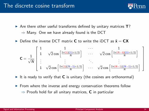
I Are there other useful transforms defined by unitary matrices T?
⇒ Many. One we have already found is the DCT
I Define the inverse DCT matrix C to write the iDCT as x = CX
C =1√N
1 1 · · · 1
1√
2 cos[
2π(1)((1)+1/2)N
]· · ·
√2 cos
[2π(N−1)((1)+1/2)
N
]...
.... . .
...
1√
2 cos[
2π(1)((N−1)+1/2)N
]· · ·
√2 cos
[2π(N−1)((N−1)+1/2)
N
]
I It is ready to verify that C is unitary (the cosines are orthonormal)
I From where the inverse and energy conservation theorems follow
⇒ Proofs hold for all unitary matrices, C in particular
Signal and Information Processing Principal Component Analysis 14

Designing transformations adapted to signals
I A basic information processing theory can be built for any T
I Then, why do we specifically choose the DFT? Or the DCT?
⇒ Oscillations represent different rates of change
⇒ Different rates of change represent different aspects of a signal
I Not a panacea, though. E.g., FH is independent of the signal
I If we know something about signal, we should use it to build betterT
I A way of “knowing something” is a stochastic model of the signal
I PCA: Principal component analysis
⇒ Use the eigenvectors of the covariance matrix to build T
Signal and Information Processing Principal Component Analysis 15

Stochastic signals
The discrete Fourier transform with unitary matrices
Stochastic signals
Principal Component Analysis (PCA) transform
Dimensionality reduction
Principal Components
Face recognition
Signal and Information Processing Principal Component Analysis 16
Random Variables
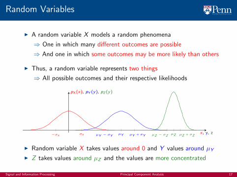
I A random variable X models a random phenomena
⇒ One in which many different outcomes are possible
⇒ And one in which some outcomes may be more likely than others
I Thus, a random variable represents two things
⇒ All possible outcomes and their respective likelihoods
−σx σx µYµY − σY µY + σYµZµZ − σZ µZ + σZ
x , y, z
pX (x), pY (y), pZ (y)
I Random variable X takes values around 0 and Y values around µY
I Z takes values around µZ and the values are more concentrated
Signal and Information Processing Principal Component Analysis 17
Probabilities
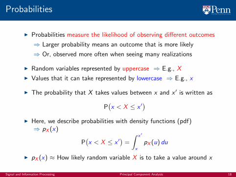
I Probabilities measure the likelihood of observing different outcomes
⇒ Larger probability means an outcome that is more likely
⇒ Or, observed more often when seeing many realizations
I Random variables represented by uppercase ⇒ E.g., X
I Values that it can take represented by lowercase ⇒ E.g., x
I The probability that X takes values between x and x ′ is written as
P(x < X ≤ x ′
)I Here, we describe probabilities with density functions (pdf)⇒ pX (x)
P(x < X ≤ x ′
)=
∫ x′
x
pX (u) du
I pX (x) ≈ How likely random variable X is to take a value around x
Signal and Information Processing Principal Component Analysis 18
Gaussian random variables
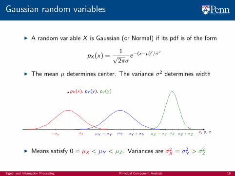
I A random variable X is Gaussian (or Normal) if its pdf is of the form
pX (x) =1√2πσ
e−(x−µ)2/σ2
I The mean µ determines center. The variance σ2 determines width
−σx σx µYµY − σY µY + σYµZµZ − σZ µZ + σZ
x , y, z
pX (x), pY (y), pZ (y)
I Means satisfy 0 = µX < µY < µZ . Variances are σ2X = σ2
Y > σ2Z
Signal and Information Processing Principal Component Analysis 19
Expectation
I Expectation of random variable is an average weighted by likelihoods
E [X ] =
∫ ∞−∞
xpX (x) dx
I Regular average ⇒ Sum all values and divide by number of values
I Expectation ⇒ Weight values x by their relative likelihoods pX (x)
I For a Gaussian random variable X the expectation is the mean µ
E [X ] =
∫ ∞−∞
x1√2πσ
e−(x−µ)2/σ2
dx = µ
I Not difficult to evaluate integral, but besides the point to do so here
Signal and Information Processing Principal Component Analysis 20
Variance
I Measure of variability around the mean weighted by likelihoods
var [X ] = E[(X − E [X ]
)2]
=
∫ ∞−∞
(x − E [X ]
)2pX (x) dx
I Large variance ≡ likely values are spread out around the mean
I Small variance ≡ likely values are concentrated around the mean
I For a Gaussian random variable X the variance is the variance σ2
var [X ] =
∫ ∞−∞
(x − E [X ]
)2 1√2πσ
e−(x−µ)2/σ2
dx = σ2
I Not difficult to evaluate either. But also besides the point here
Signal and Information Processing Principal Component Analysis 21
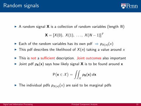
Random signals
I A random signal X is a collection of random variables (length N)
X = [X (0), X (1), . . . , X (N − 1)]T
I Each of the random variables has its own pdf ⇒ pX (n)(x)
I This pdf describes the likelihood of X (n) taking a value around x
I This is not a sufficient description. Joint outcomes also important
I Joint pdf pX(x) says how likely signal X is to be found around x
P(x ∈ X
)=
∫∫XpX(x) dx
I The individual pdfs pX (n)(x) are said to be marginal pdfs
Signal and Information Processing Principal Component Analysis 22

Face images
I Random signal X ⇒ All possible images of human faces
I More manageable ⇒ X is a collection of 400 face images
⇒ The random variable represents all the images
⇒ The likelihood of each of them being chosen. E.g., 1/400 each
I Random variable specified by all outcomes and respective probabilities
Signal and Information Processing Principal Component Analysis 23

Vectorization
I Do observe that the dataset consists of images ≡ matrices
I Each image is stored in a matrix of size 112× 92
Mi =
m1,1 m1,2 . . . m1,92
m2,1 m2,2 . . . m2,92
......
. . ....
m112,1 m112,2 . . . m112,92
I Stack columns of image Mi into the vector xi with length 10, 304
xi =[m1,1, m21, . . ., m112,1, m1,2, m2,2, . . ., m112,2,
..., m1,92, m2,92, . . ., m112,92
]TI Images are matrices Mi ∈ R112×92. Signals are vectors xi ∈ R10,304
Signal and Information Processing Principal Component Analysis 24
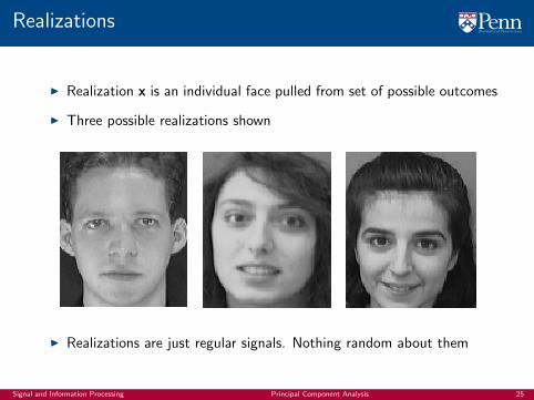
Realizations
I Realization x is an individual face pulled from set of possible outcomes
I Three possible realizations shown
I Realizations are just regular signals. Nothing random about them
Signal and Information Processing Principal Component Analysis 25
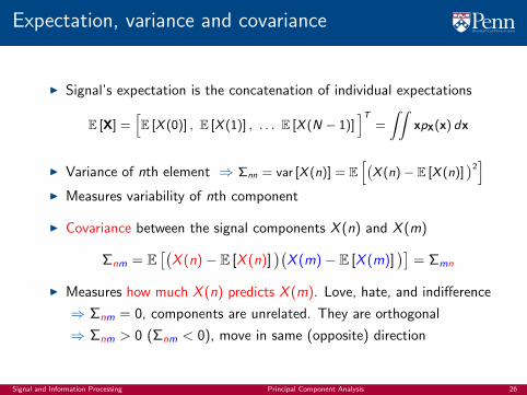
Expectation, variance and covariance
I Signal’s expectation is the concatenation of individual expectations
E [X] =[E [X (0)] , E [X (1)] , . . . E [X (N − 1)]
]T=
∫∫xpX(x) dx
I Variance of nth element ⇒ Σnn = var [X (n)] = E[(X (n)− E [X (n)]
)2]
I Measures variability of nth component
I Covariance between the signal components X (n) and X (m)
Σnm = E[(X (n)− E [X (n)]
)(X (m)− E [X (m)]
)]= Σmn
I Measures how much X (n) predicts X (m). Love, hate, and indifference
⇒ Σnm = 0, components are unrelated. They are orthogonal
⇒ Σnm > 0 (Σnm < 0), move in same (opposite) direction
Signal and Information Processing Principal Component Analysis 26
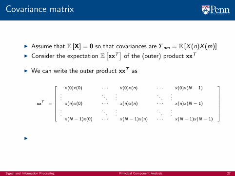
Covariance matrix
I Assume that E [X] = 0 so that covariances are Σnm = E [X (n)X (m)]
I Consider the expectation E[xxT
]of the (outer) product xxT
I We can write the outer product xxT as
xxT =
x(0)x(0) · · · x(0)x(n) · · · x(0)x(N − 1)...
. . ....
. . ....
x(n)x(0) · · · x(n)x(n) · · · x(n)x(N − 1)...
. . ....
. . ....
x(N − 1)x(0) · · · x(N − 1)x(n) · · · x(N − 1)x(N − 1)
I
Signal and Information Processing Principal Component Analysis 27

Covariance matrix
I Assume that E [X] = 0 so that covariances are Σnm = E [X (n)X (m)]
I Consider the expectation E[xxT
]of the (outer) product xxT
I Expectation E[xxT
]implies expectation of each individual element
E[
xxT]
=
E[x(0)x(0)] · · · E[x(0)x(n)] · · · E[x(0)x(N − 1)]...
. . ....
. . ....
E[x(n)x(0)] · · · E[x(n)x(n)] · · · E[x(n)x(N − 1)]...
. . ....
. . ....
E[x(N − 1)x(0)] · · · E[x(N − 1)x(n)] · · · E[x(N − 1)x(N − 1)]
I
Signal and Information Processing Principal Component Analysis 28
Covariance matrix
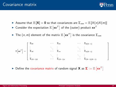
I Assume that E [X] = 0 so that covariances are Σnm = E [X (n)X (m)]
I Consider the expectation E[xxT
]of the (outer) product xxT
I The (n,m) element of the matrix E[xxT
]is the covariance Σnm
E[
xxT]
=
Σ00 · · · Σ0n · · · Σ0(N−1)
.
.
.. . .
.
.
.. . .
.
.
.Σn0 · · · Σnn · · · Σn(N−1)
.
.
.. . .
.
.
.. . .
.
.
.Σ(N−1)0 · · · Σ(N−1)n · · · Σ(N−1)(N−1)
I Define the covariance matrix of random signal X as Σ := E[xxT
]
Signal and Information Processing Principal Component Analysis 29
Definition of covariance matrix
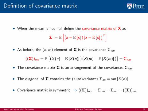
I When the mean is not null define the covariance matrix of X as
Σ := E[(
x− E [x])(
x− E [x])T ]
I As before, the (n,m) element of Σ is the covariance Σnm
((Σ))nm = E[(X (n)− E [X (n)]
)(X (m)− E [X (m)]
)]= Σnm
I The covariance matrix Σ is an arrangement of the covariances Σnm
I The diagonal of Σ contains the (auto)variances Σnn = var [X (n)]
I Covariance matrix is symmetric ⇒ ((Σ))nm = Σnm = Σmn = ((Σ))mn
Signal and Information Processing Principal Component Analysis 30
Mean of face images
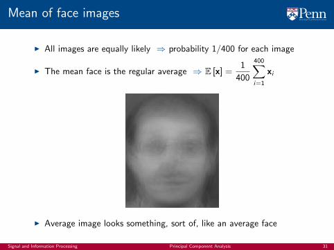
I All images are equally likely ⇒ probability 1/400 for each image
I The mean face is the regular average ⇒ E [x] =1
400
400∑i=1
xi
I Average image looks something, sort of, like an average face
Signal and Information Processing Principal Component Analysis 31

Covariance matrix of face images
I Covariance matrix ⇒ Σ =1
400
400∑i=1
(xi − E [x]
)(xi − E [x]
)T
I Heat map of covariancematrix Σ shown on left
I Large correlation valuesaround diagonal
I Large correlation valuesevery 112 elements (jump arow on matrix)
Signal and Information Processing Principal Component Analysis 32

Principal Component Analysis (PCA) transform
The discrete Fourier transform with unitary matrices
Stochastic signals
Principal Component Analysis (PCA) transform
Dimensionality reduction
Principal Components
Face recognition
Signal and Information Processing Principal Component Analysis 33
Eigenvectors and eigenvalues of covariance matrix
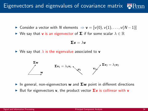
I Consider a vector with N elements ⇒ v = [v(0), v(1), . . . , v(N − 1)]
I We say that v is an eigenvector of Σ if for some scalar λ ∈ R
Σv = λv
I We say that λ is the eigenvalue associated to v
w
Σw
v1
Σv1 = λ1v1 v2
Σv2 = λ2v2
I In general, non-eigenvectors w and Σw point in different directions
I But for eigenvectors v, the product vector Σv is collinear with v
Signal and Information Processing Principal Component Analysis 34
Normalization
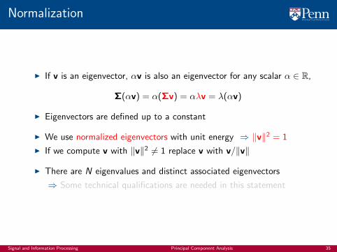
I If v is an eigenvector, αv is also an eigenvector for any scalar α ∈ R,
Σ(αv) = α(Σv) = αλv = λ(αv)
I Eigenvectors are defined up to a constant
I We use normalized eigenvectors with unit energy ⇒ ‖v‖2 = 1
I If we compute v with ‖v‖2 6= 1 replace v with v/‖v‖
I There are N eigenvalues and distinct associated eigenvectors
⇒ Some technical qualifications are needed in this statement
Signal and Information Processing Principal Component Analysis 35

Ordering
TheoremThe eigenvalues of Σ are real and nonnegative ⇒ λ ∈ R and λ ≥ 0
Proof.
I Begin by observing that we can write λ = vHΣv/‖v‖2. Indeed
vHΣv = vH (Σv) = vH (λv) = λvHv = λ‖v‖2
I Complete by showing that vTΣv is nonnegative. Indeed (assume E [x] = 0)
vHΣv = vHE[xxH]
v = E[vHxxHv
]= E
[(vHx)(
xHv)]
= E[(
vHx)2]≥ 0
I Order eigenvalues from largest to smallest ⇒ λ0 ≥ λ1 ≥ . . . ≥ λN−1
I Eigenvectors inherit order ⇒ v0, v1, . . . , vN−1
I The nth eigenvector of Σ is associated with its nth largest eigenvalue
Signal and Information Processing Principal Component Analysis 36
Eigenvectors are orthonormal
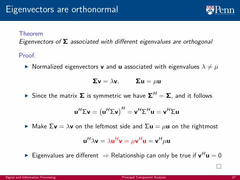
TheoremEigenvectors of Σ associated with different eigenvalues are orthogonal
Proof.
I Normalized eigenvectors v and u associated with eigenvalues λ 6= µ
Σv = λv, Σu = µu
I Since the matrix Σ is symmetric we have ΣH = Σ, and it follows
uHΣv =(uHΣv
)H= vHΣHu = vHΣu
I Make Σv = λv on the leftmost side and Σu = µu on the rightmost
uHλv = λuHv = µvHu = vHµu
I Eigenvalues are different ⇒ Relationship can only be true if vHu = 0
Signal and Information Processing Principal Component Analysis 37
Eigenvectors of face images (1D)
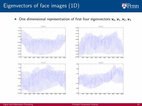
I One dimensional representation of first four eigenvectors v0, v1, v2, v3
0 1000 2000 3000 4000 5000 6000 7000 8000 9000 10000−0.03
−0.025
−0.02
−0.015
−0.01
−0.005
0
0.005
0.01
0.015
0.02
v0(n)
0 1000 2000 3000 4000 5000 6000 7000 8000 9000 10000−0.025
−0.02
−0.015
−0.01
−0.005
0
0.005
0.01
0.015
0.02
0.025
v2(n)
0 1000 2000 3000 4000 5000 6000 7000 8000 9000 10000−0.015
−0.01
−0.005
0
0.005
0.01
0.015
0.02
0.025
v1(n)
0 1000 2000 3000 4000 5000 6000 7000 8000 9000 10000−0.03
−0.02
−0.01
0
0.01
0.02
0.03
v3(n)
Signal and Information Processing Principal Component Analysis 38

Eigenvectors of face images (2D)
I Two dimensional representation of first four eigenvectors v0, v1, v2, v3
10 20 30 40 50 60 70 80 90
10
20
30
40
50
60
70
80
90
100
110
10 20 30 40 50 60 70 80 90
10
20
30
40
50
60
70
80
90
100
110
10 20 30 40 50 60 70 80 90
10
20
30
40
50
60
70
80
90
100
110
10 20 30 40 50 60 70 80 90
10
20
30
40
50
60
70
80
90
100
110
Signal and Information Processing Principal Component Analysis 39

Eigenvector matrix
I Define the matrix T whose kth column is the kth eigenvector of Σ
T = [v0, v1, . . . , vN−1]
I Since the eigenvectors vk are orthonormal, the product THT is
THT =
[v0 · · · vk · · · vN−1
]
vH0
...vHk
...vHN−1
vH0 v0 · · · vH
1 vk · · · vH0 vN−1
.... . .
.... . .
...vHk v0 · · · vH
k vk · · · vHk vN−1
.... . .
.... . .
...vHN−1vN−1 · · · vH
N−1vk · · · vHN−1vN−1
=
1 · · · 0 · · · 0...
. . ....
. . ....
0 · · · 1 · · · 0...
. . ....
. . ....
0 · · · 0 · · · 1
I The eigenvector matrix T is Hermitian ⇒ THT = I
Signal and Information Processing Principal Component Analysis 40

Principal component analysis transform
I Any Hermitian T can be used to define an info processing transform
I Define principal component analysis (PCA) transform ⇒ y = THx
I And the inverse (i)PCA transform ⇒ x = Ty
I Since T is Hermitian, iPCA is, indeed, the inverse of the PCA
x = Ty = T(THx
)= TTHx = Ix = x
I Thus y is an equivalent representation of x ⇒ Back and forth
I And, also because T is Hermitian, Parseval’s theorem holds
‖x‖2 = xHx = (Ty)H Ty = yHTHTy = yHy = ‖y‖2
I Modifying elements yk means altering energy composition of signal
Signal and Information Processing Principal Component Analysis 41
Discussions
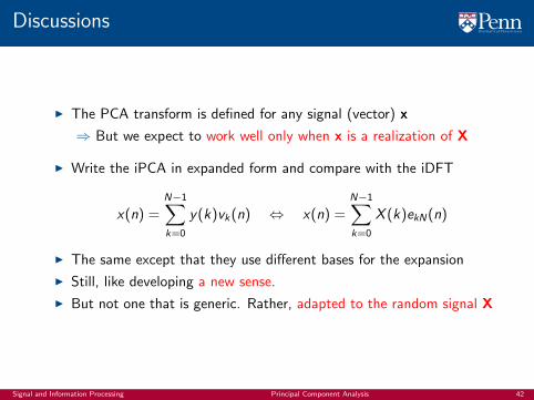
I The PCA transform is defined for any signal (vector) x
⇒ But we expect to work well only when x is a realization of X
I Write the iPCA in expanded form and compare with the iDFT
x(n) =N−1∑k=0
y(k)vk(n) ⇔ x(n) =N−1∑k=0
X (k)ekN(n)
I The same except that they use different bases for the expansion
I Still, like developing a new sense.
I But not one that is generic. Rather, adapted to the random signal X
Signal and Information Processing Principal Component Analysis 42

Coefficients of a projected face image
I PCA transform coefficients for given face image with 10,304 pixels
I Substantial energy in the first 15 PCA coefficients y(k) with k ≤ 15
I Almost all energy in the first 50 PCA coefficients y(k) with k ≤ 50
⇒ This is a compression factor of more than 200
10 20 30 40 50 60 70 80 90
10
20
30
40
50
60
70
80
90
100
110
0 5 10 15 20 25 30 35 40 45 50−8000
−6000
−4000
−2000
0
2000
4000
Coefficients for the first 50 eigenvectors
Signal and Information Processing Principal Component Analysis 43
Reconstructed face images
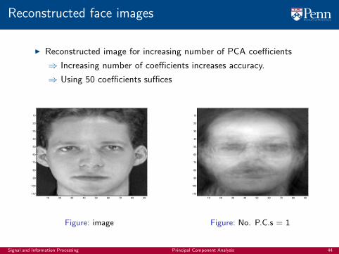
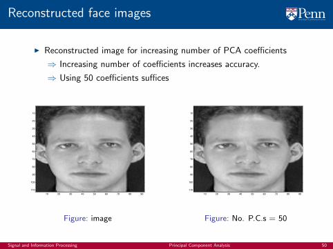
I Reconstructed image for increasing number of PCA coefficients
⇒ Increasing number of coefficients increases accuracy.
⇒ Using 50 coefficients suffices
10 20 30 40 50 60 70 80 90
10
20
30
40
50
60
70
80
90
100
110
Figure: image
10 20 30 40 50 60 70 80 90
10
20
30
40
50
60
70
80
90
100
110
Figure: No. P.C.s = 1
Signal and Information Processing Principal Component Analysis 44

Reconstructed face images
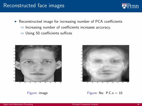
I Reconstructed image for increasing number of PCA coefficients
⇒ Increasing number of coefficients increases accuracy.
⇒ Using 50 coefficients suffices
10 20 30 40 50 60 70 80 90
10
20
30
40
50
60
70
80
90
100
110
Figure: image
10 20 30 40 50 60 70 80 90
10
20
30
40
50
60
70
80
90
100
110
Figure: No. P.C.s = 5
Signal and Information Processing Principal Component Analysis 45
Reconstructed face images
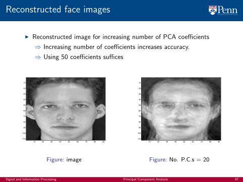
I Reconstructed image for increasing number of PCA coefficients
⇒ Increasing number of coefficients increases accuracy.
⇒ Using 50 coefficients suffices
10 20 30 40 50 60 70 80 90
10
20
30
40
50
60
70
80
90
100
110
Figure: image
10 20 30 40 50 60 70 80 90
10
20
30
40
50
60
70
80
90
100
110
Figure: No. P.C.s = 10
Signal and Information Processing Principal Component Analysis 46
Reconstructed face images
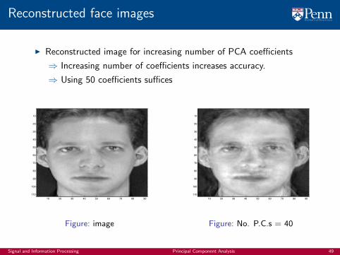
I Reconstructed image for increasing number of PCA coefficients
⇒ Increasing number of coefficients increases accuracy.
⇒ Using 50 coefficients suffices
10 20 30 40 50 60 70 80 90
10
20
30
40
50
60
70
80
90
100
110
Figure: image
10 20 30 40 50 60 70 80 90
10
20
30
40
50
60
70
80
90
100
110
Figure: No. P.C.s = 20
Signal and Information Processing Principal Component Analysis 47

Reconstructed face images
I Reconstructed image for increasing number of PCA coefficients
⇒ Increasing number of coefficients increases accuracy.
⇒ Using 50 coefficients suffices
10 20 30 40 50 60 70 80 90
10
20
30
40
50
60
70
80
90
100
110
Figure: image
10 20 30 40 50 60 70 80 90
10
20
30
40
50
60
70
80
90
100
110
Figure: No. P.C.s = 30
Signal and Information Processing Principal Component Analysis 48
Reconstructed face images
I Reconstructed image for increasing number of PCA coefficients
⇒ Increasing number of coefficients increases accuracy.
⇒ Using 50 coefficients suffices
10 20 30 40 50 60 70 80 90
10
20
30
40
50
60
70
80
90
100
110
Figure: image
10 20 30 40 50 60 70 80 90
10
20
30
40
50
60
70
80
90
100
110
Figure: No. P.C.s = 40
Signal and Information Processing Principal Component Analysis 49
Reconstructed face images
I Reconstructed image for increasing number of PCA coefficients
⇒ Increasing number of coefficients increases accuracy.
⇒ Using 50 coefficients suffices
10 20 30 40 50 60 70 80 90
10
20
30
40
50
60
70
80
90
100
110
Figure: image
10 20 30 40 50 60 70 80 90
10
20
30
40
50
60
70
80
90
100
110
Figure: No. P.C.s = 50
Signal and Information Processing Principal Component Analysis 50
Coefficients of the same person
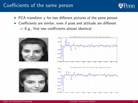
I PCA transform y for two different pictures of the same person
I Coefficients are similar, even if pose and attitude are different
⇒ E.g., first two coefficients almost identical
10 20 30 40 50 60 70 80 90
10
20
30
40
50
60
70
80
90
100
110
0 5 10 15 20 25 30 35 40 45 50−8000
−6000
−4000
−2000
0
2000
4000
Coefficients for the first 50 eigenvectors
10 20 30 40 50 60 70 80 90
10
20
30
40
50
60
70
80
90
100
110
0 5 10 15 20 25 30 35 40 45 50−10000
−8000
−6000
−4000
−2000
0
2000
4000
Coefficients for the first 50 eigenvectors
Signal and Information Processing Principal Component Analysis 51

Coefficients of different persons
I PCA transform y for pictures of different persons
I Similar pose and attitude, but PCA coefficients are still different
⇒ Can be used to perform face recognition. More later
10 20 30 40 50 60 70 80 90
10
20
30
40
50
60
70
80
90
100
110
0 5 10 15 20 25 30 35 40 45 50−8000
−6000
−4000
−2000
0
2000
4000
Coefficients for the first 50 eigenvectors
10 20 30 40 50 60 70 80 90
10
20
30
40
50
60
70
80
90
100
110
0 5 10 15 20 25 30 35 40 45 50−10000
−8000
−6000
−4000
−2000
0
2000
Coefficients for the first 50 eigenvectors
Signal and Information Processing Principal Component Analysis 52

Dimensionality reduction
The discrete Fourier transform with unitary matrices
Stochastic signals
Principal Component Analysis (PCA) transform
Dimensionality reduction
Principal Components
Face recognition
Signal and Information Processing Principal Component Analysis 53
Compression with the DFT
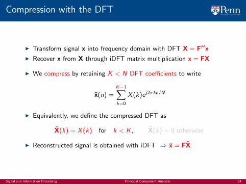
I Transform signal x into frequency domain with DFT X = FHx
I Recover x from X through iDFT matrix multiplication x = FX
I We compress by retaining K < N DFT coefficients to write
x(n) =K−1∑k=0
X (k)e j2πkn/N
I Equivalently, we define the compressed DFT as
X(k) = X (k) for k < K , X(k) = 0 otherwise
I Reconstructed signal is obtained with iDFT ⇒ x = FX
Signal and Information Processing Principal Component Analysis 54

Compression with the PCA
I Transform signal x into eigenvector domain with PCA y = THx
I Recover x from y through iPCA matrix multiplication x = Ty
I We compress by retaining K < N PCA coefficients to write
x(n) =K−1∑k=0
y(k)vk(n)
I Equivalently, we define the compressed PCA as
y(k) = y(k) for k < K , y(k) = 0 otherwise
I Reconstructed signal is obtained with iPCA ⇒ x = Ty
Signal and Information Processing Principal Component Analysis 55

Why keeping the first K coefficients?
I Why do we keep the first K DFT coefficients?
⇒ Because faster oscillations tend to represent faster variation
⇒ Also, not always, sometimes we keep the largest coefficients
I Why do we keep the first K PCA coefficients?
⇒ Eigenvectors with lower ordinality have larger eigenvalues
⇒ Larger eigenvalues entail more variability
⇒ And more variability signifies more dominant features
I Eigenvectors with large ordinality represent finer signal features
⇒ And can often be omitted
Signal and Information Processing Principal Component Analysis 56
Dimensionality reduction
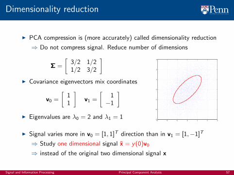
I PCA compression is (more accurately) called dimensionality reduction
⇒ Do not compress signal. Reduce number of dimensions
Σ =
[3/2 1/21/2 3/2
]I Covariance eigenvectors mix coordinates
v0 =
[11
]v1 =
[1−1
]I Eigenvalues are λ0 = 2 and λ1 = 1
−3 −2 −1 0 1 2 3−3
−2
−1
0
1
2
3
I Signal varies more in v0 = [1, 1]T direction than in v1 = [1,−1]T
⇒ Study one dimensional signal x = y(0)v0
⇒ instead of the original two dimensional signal x
Signal and Information Processing Principal Component Analysis 57

Expected reconstruction error
I PCA dimensionality reduction minimizes the expected error energy
I To see that this is true, define the error signal as ⇒ e := x− x
I The energy of the error signal is ⇒ ‖e‖2 = ‖x− x‖2
I The expected value of the energy of the error signal is
E[‖e‖2
]= E
[‖x− x‖2
]I Keeping the first K PCA coefficients minimizes E
[‖e‖2
]⇒ Among all reconstructions that use, at most, K coefficients
Signal and Information Processing Principal Component Analysis 58

Dimensionality reduction expected error
TheoremThe expectation of the reconstruction error is the sum of the eigenvaluescorresponding to the eigenvectors of the coefficients that are discarded
E[‖e‖2
]=
N−1∑k=K
λk
I It follows that keeping the first K PCA coefficients is optimal
⇒ In the sense that it minimizes the Expected error energy
I Good on average. Across realizations of the stochastic signal X
I Need not be good for given realization (but we expect it to be good)
Signal and Information Processing Principal Component Analysis 59

Proof of expected error expression
Proof.
I Error signal signal is e := x− x. Define error PCA transform as f = THx
I Using Parseval’s (energy conservation) we can write the energy of e as
‖e‖2 = ‖f‖2 =N−1∑k=K
y 2(k)
I In the last equality we used that f = y− y = [0, . . . , 0,y(K), . . . , y(N − 1)]
I Here, we are interested in the expected value of the error’s energy
I Take expectation on both sides of equality ⇒ E[‖e‖2
]=
N−1∑k=K
E[y 2(k)
]I Used the fact that expectations are linear operators
Signal and Information Processing Principal Component Analysis 60

Proof of expected error expression
Proof.
I Compute expected value E[y 2(k)
]of the squared PCA coefficient y(k)
I As per PCA transform definition y(k) = vHx, which implies
E[y 2(k)
]= E
[(vH
k x)2]
= E[vHk xxTvk
]= vH
k E[xxT
]vk
I Covariance matrix: Σ := E[xxT
]. Eigenvector definition Σvk = λk . Thus
E[y 2(k)
]= vH
k Σvk = vHk λkvk = λk‖vk‖2
I Substitute into expression for E[‖e‖2
]to write ⇒ E
[‖e‖2
]=
N−1∑k=K
λk
Signal and Information Processing Principal Component Analysis 61

Principal eigenvalues for face dataset
I Covariance matrix eigenvalues for faces dataset.
I Expected approximation error ⇒ Tail sum of eigenvalue distribution
⇒ Average across all realizations. Not the same as actual error
0 10 20 30 40 50 60 70 80 90 1000
0.05
0.1
0.15
0.2
0.25
0.3
0.35
0.4
0.45
0.5
Index of eigenvalue
Normalized
Energy
ofeige
nvalue:=
λ2 i
∑N
−1
i=0λ2 i
I First 10 coefficients have 98% of energy.
I Eigenvectors with index k > 50 have 10−3% of energy on average
Signal and Information Processing Principal Component Analysis 62
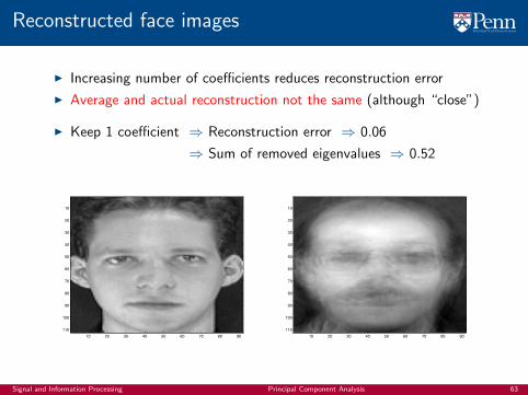
Reconstructed face images
I Increasing number of coefficients reduces reconstruction error
I Average and actual reconstruction not the same (although “close”)
I Keep 1 coefficient ⇒ Reconstruction error ⇒ 0.06
⇒ Sum of removed eigenvalues ⇒ 0.52
10 20 30 40 50 60 70 80 90
10
20
30
40
50
60
70
80
90
100
110
10 20 30 40 50 60 70 80 90
10
20
30
40
50
60
70
80
90
100
110
Signal and Information Processing Principal Component Analysis 63

Reconstructed face images
I Increasing number of coefficients reduces reconstruction error
I Average and actual reconstruction not the same (although “close”)
I Keep 5 coefficients ⇒ Reconstruction error ⇒ 0.03
⇒ Sum of removed eigenvalues ⇒ 0.11
10 20 30 40 50 60 70 80 90
10
20
30
40
50
60
70
80
90
100
110
10 20 30 40 50 60 70 80 90
10
20
30
40
50
60
70
80
90
100
110
Signal and Information Processing Principal Component Analysis 64
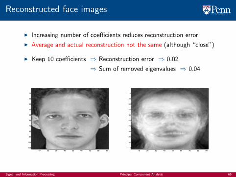
Reconstructed face images
I Increasing number of coefficients reduces reconstruction error
I Average and actual reconstruction not the same (although “close”)
I Keep 10 coefficients ⇒ Reconstruction error ⇒ 0.02
⇒ Sum of removed eigenvalues ⇒ 0.04
10 20 30 40 50 60 70 80 90
10
20
30
40
50
60
70
80
90
100
110
10 20 30 40 50 60 70 80 90
10
20
30
40
50
60
70
80
90
100
110
Signal and Information Processing Principal Component Analysis 65
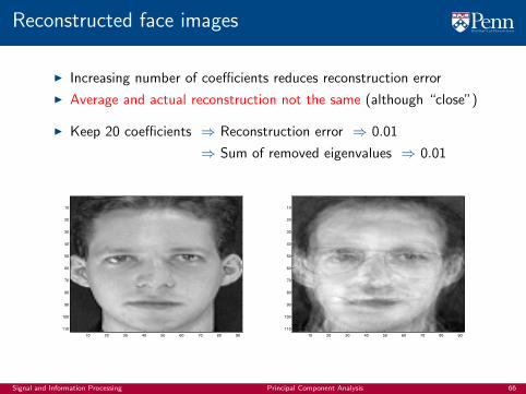
Reconstructed face images
I Increasing number of coefficients reduces reconstruction error
I Average and actual reconstruction not the same (although “close”)
I Keep 20 coefficients ⇒ Reconstruction error ⇒ 0.01
⇒ Sum of removed eigenvalues ⇒ 0.01
10 20 30 40 50 60 70 80 90
10
20
30
40
50
60
70
80
90
100
110
10 20 30 40 50 60 70 80 90
10
20
30
40
50
60
70
80
90
100
110
Signal and Information Processing Principal Component Analysis 66
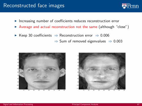
Reconstructed face images
I Increasing number of coefficients reduces reconstruction error
I Average and actual reconstruction not the same (although “close”)
I Keep 30 coefficients ⇒ Reconstruction error ⇒ 0.006
⇒ Sum of removed eigenvalues ⇒ 0.003
10 20 30 40 50 60 70 80 90
10
20
30
40
50
60
70
80
90
100
110
10 20 30 40 50 60 70 80 90
10
20
30
40
50
60
70
80
90
100
110
Signal and Information Processing Principal Component Analysis 67

Reconstructed face images
I Increasing number of coefficients reduces reconstruction error
I Average and actual reconstruction not the same (although “close”)
I Keep 40 coefficients ⇒ Reconstruction error ⇒ 0
⇒ Sum of removed eigenvalues ⇒ 0
10 20 30 40 50 60 70 80 90
10
20
30
40
50
60
70
80
90
100
110
10 20 30 40 50 60 70 80 90
10
20
30
40
50
60
70
80
90
100
110
Signal and Information Processing Principal Component Analysis 68

Reconstructed face images
I Increasing number of coefficients reduces reconstruction error
I Average and actual reconstruction not the same (although “close”)
I Keep 50 coefficients ⇒ Reconstruction error ⇒ 0
⇒ Sum of removed eigenvalues ⇒ 0
10 20 30 40 50 60 70 80 90
10
20
30
40
50
60
70
80
90
100
110
10 20 30 40 50 60 70 80 90
10
20
30
40
50
60
70
80
90
100
110
Signal and Information Processing Principal Component Analysis 69

Evolution of reconstruction error
I Error for reconstruction process
I one realization (red), energy of removed eigenvalues (blue)
0 5 10 15 20 25 30 35 40 45 500
0.1
0.2
0.3
0.4
0.5
0.6
Number of Principal Components
Signal and Information Processing Principal Component Analysis 70
Principal Components
The discrete Fourier transform with unitary matrices
Stochastic signals
Principal Component Analysis (PCA) transform
Dimensionality reduction
Principal Components
Face recognition
Signal and Information Processing Principal Component Analysis 71

Signals with uncorrelated components
I A random signal X with uncorrelated components is one with
Σnm = E[(X (n)− E [X (n)]
)(X (m)− E [X (m)]
)]= 0
I Different components are unrelated to each other.
I They represent different (orthogonal) aspects of signal
I Components uncorrelated ⇒ The covariance matrix is diagonal
Σ = E[(
x − E [x])(
x − E [x])T ]
=
Σ00 · · · Σ0n · · · Σ0(N−1)
.... . .
.... . .
...Σn0 · · · Σnn · · · Σn(N−1)
.... . .
.... . .
...Σ(N−1)0 · · · Σ(N−1)n · · · Σ(N−1)(N−1)
I How do eigenvectors (principal components) of uncorrelated signalslook?
Signal and Information Processing Principal Component Analysis 72
Uncorrelated signal with 2 components
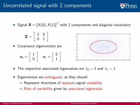
I Signal X = [X (0),X (1)]T with 2 components and diagonal covariance
Σ =
[2 00 1
]I Covariance eigenvectors are
v0 =
[10
]v1 =
[01
]−4 −3 −2 −1 0 1 2 3 4
−2
−1.5
−1
−0.5
0
0.5
1
1.5
2
I The respective associated eigenvalues are λ0 = 2 and λ1 = 1
I Eigenvectors are orthogonal, as they should.
⇒ Represent directions of separate signal variability
⇒ Rate of variability given by associated eigenvalue
Signal and Information Processing Principal Component Analysis 73

Another uncorrelated signal with 2 components
I Signal X = [X (0),X (1)]T with 2 components and diagonal covariance
Σ =
[1 00 2
]I Covariance eigenvectors reverse order
v0 =
[01
]v1 =
[10
]I Associated eigenvalues are λ0 = 2 and λ1 = 1
I Eigenvectors still orthogonal, as they should.
⇒ Directions of separate signal variability
⇒ Rate given by associated eigenvalue−2 −1.5 −1 −0.5 0 0.5 1 1.5 2
−4
−3
−2
−1
0
1
2
3
4
Signal and Information Processing Principal Component Analysis 74

Signal with correlated components
I Signal X = [X (0),X (1)]T with 2 components and diagonal covariance
Σ =
[3/2 1/21/2 3/2
]I Covariance eigenvectors mix coordinates
v0 =
[11
]v1 =
[1−1
]I Eigenvalues are λ0 = 2 and λ1 = 1
−3 −2 −1 0 1 2 3−3
−2
−1
0
1
2
3
I The eigenvalues are orthogonal. This is true for any covariance matrix
⇒ Mix coordinates but still represent directions of separate variability
⇒ Rate of change also given by associated eigenvalue
Signal and Information Processing Principal Component Analysis 75

Eigenvectors in uncorrelated signals
I Uncorrelated components means diagonal covariance matrix
Σ =
Σ00 · · · Σ0n · · · Σ0(N−1)
.... . .
.... . .
...Σn0 · · · Σnn · · · Σn(N−1)
.... . .
.... . .
...Σ(N−1)0 · · · Σ(N−1)n · · · Σ(N−1)(N−1)
I If variances are ordered, kth eigenvector is k-shifted delta δ(n − k)
I The corresponding variance Σkk is the associated eigenvalue
I Eigenvectors represent directions of orthogonal variability
I Rate of variability given by associated eigenvalue
Signal and Information Processing Principal Component Analysis 76

Eigenvectors in correlated signals
I Correlated components means a full covariance matrix
Σ =
Σ00 · · · Σ0n · · · Σ0(N−1)
.... . .
.... . .
...Σn0 · · · Σnn · · · Σn(N−1)
.... . .
.... . .
...Σ(N−1)0 · · · Σ(N−1)n · · · Σ(N−1)(N−1)
I The eigenvectors vk now mix different components
⇒ But they still represent directions of orthogonal variability
⇒ With the rate of variability given by associated eigenvalue
I PCA transform represents a signal as a sum of orthonormal vectors
⇒ Each of which represents independent variability
I Principal components (eigenvectors) with larger eigenvalues representdirections in which the signal has more variability
Signal and Information Processing Principal Component Analysis 77
Face recognization
The discrete Fourier transform with unitary matrices
Stochastic signals
Principal Component Analysis (PCA) transform
Dimensionality reduction
Principal Components
Face recognition
Signal and Information Processing Principal Component Analysis 78
Face Recognition
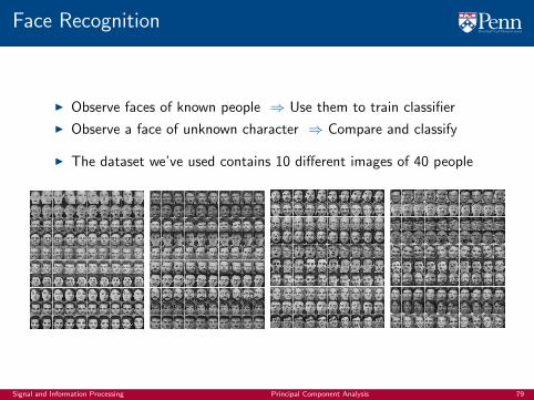
I Observe faces of known people ⇒ Use them to train classifier
I Observe a face of unknown character ⇒ Compare and classify
I The dataset we’ve used contains 10 different images of 40 people
Signal and Information Processing Principal Component Analysis 79
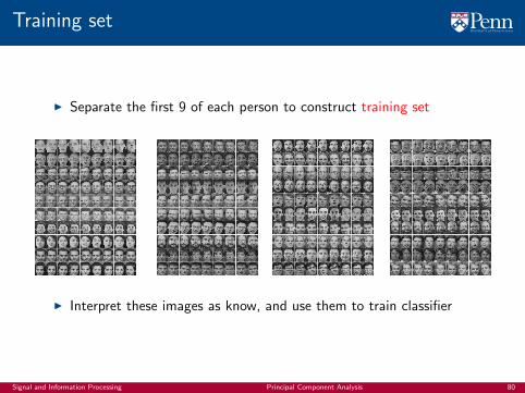
Training set
I Separate the first 9 of each person to construct training set
I Interpret these images as know, and use them to train classifier
Signal and Information Processing Principal Component Analysis 80
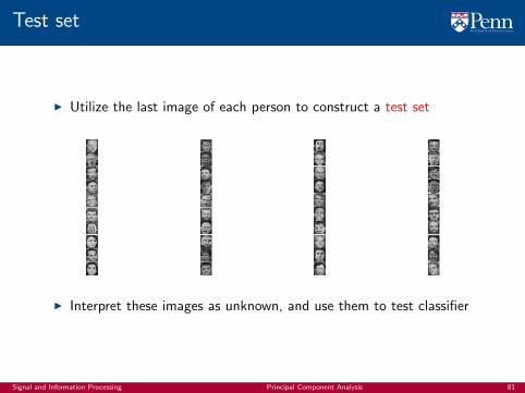
Test set
I Utilize the last image of each person to construct a test set
I Interpret these images as unknown, and use them to test classifier
Signal and Information Processing Principal Component Analysis 81

Nearest neighbor classification
I Training set contains (signal, label) pairs ⇒ T = {(xi , zi )}Ni=1
I Signal x is the face image. Label z is the person’s “name”
I Given (unknown) signals x, we want to assign a label
I Nearest neighbor classification rule
⇒ Find nearest neighbor signal in the training set
xNN := argminxi∈T
‖xi − x‖2
⇒ Assign the label associated with the nearest neighbor
xNN ⇒ (xi , zi ) ⇒ z = zi
I Reasonable enough. It should work. But it doesn’t
Signal and Information Processing Principal Component Analysis 82
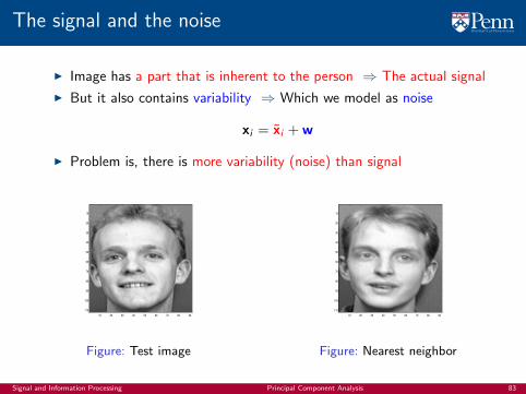
The signal and the noise
I Image has a part that is inherent to the person ⇒ The actual signal
I But it also contains variability ⇒ Which we model as noise
xi = xi + w
I Problem is, there is more variability (noise) than signal
10 20 30 40 50 60 70 80 90
10
20
30
40
50
60
70
80
90
100
110
Figure: Test image
10 20 30 40 50 60 70 80 90
10
20
30
40
50
60
70
80
90
100
110
Figure: Nearest neighbor
Signal and Information Processing Principal Component Analysis 83
PCA nearest neighbor classification
I Compute PCA for all elements of training set ⇒ yi = THxiI Redefine training set as one with PCA transforms ⇒ T = {(yi , zi )}Ni=1
I Compute PCA transform of (unknown) signal x ⇒ y = THx
I PCA nearest neighbor classification rule
⇒ Find nearest neighbor signal in training set with PCA transforms
yNN := argminyi∈T
‖yi − y‖2
⇒ Assign the label associated with the nearest neighbor
yNN ⇒ (yi , zi ) ⇒ z = zi
I Reasonable enough. It should work. And it does
Signal and Information Processing Principal Component Analysis 84
Why does PCA work for face recognition?
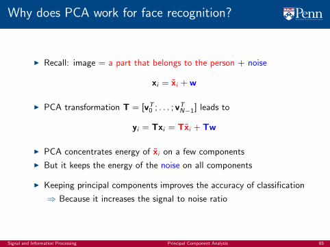
I Recall: image = a part that belongs to the person + noise
xi = xi + w
I PCA transformation T = [vT0 ; . . . ; vT
N−1] leads to
yi = Txi = Txi + Tw
I PCA concentrates energy of xi on a few components
I But it keeps the energy of the noise on all components
I Keeping principal components improves the accuracy of classification
⇒ Because it increases the signal to noise ratio
Signal and Information Processing Principal Component Analysis 85
PCA on the training set
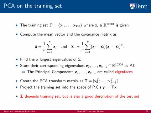
I The training set D = {x1, . . . , x360} where xi ∈ R10304 is given
I Compute the mean vector and the covariance matrix as
x =1
n
n∑i=1
xi and Σ :=1
n
n∑i=1
(xi − xi )(xi − xi )T .
I Find the k largest eigenvalues of Σ
I Store their corresponding eigenvalues v0, . . . , vk−1 ∈ R10304 as P.C.
⇒ The Principal Components v0, . . . , vk−1 are called eigenfaces
I Create the PCA transform matrix as T = [vT0 ; . . . ; vT
k−1]
I Project the training set into the space of P.C.s yi = Txi
I Σ depends training set, but is also a good description of the test set
Signal and Information Processing Principal Component Analysis 86

Average face of the training set
I The average face of the training set
10 20 30 40 50 60 70 80 90
10
20
30
40
50
60
70
80
90
100
110
Signal and Information Processing Principal Component Analysis 87
PCA on the training set
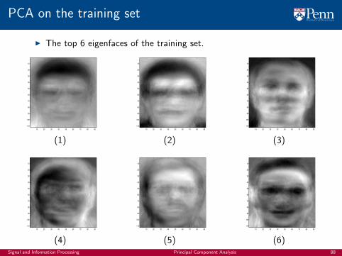
I The top 6 eigenfaces of the training set.
10 20 30 40 50 60 70 80 90
10
20
30
40
50
60
70
80
90
100
110
(1)
10 20 30 40 50 60 70 80 90
10
20
30
40
50
60
70
80
90
100
110
(2)
10 20 30 40 50 60 70 80 90
10
20
30
40
50
60
70
80
90
100
110
(3)
10 20 30 40 50 60 70 80 90
10
20
30
40
50
60
70
80
90
100
110
(4)
10 20 30 40 50 60 70 80 90
10
20
30
40
50
60
70
80
90
100
110
(5)
10 20 30 40 50 60 70 80 90
10
20
30
40
50
60
70
80
90
100
110
(6)Signal and Information Processing Principal Component Analysis 88
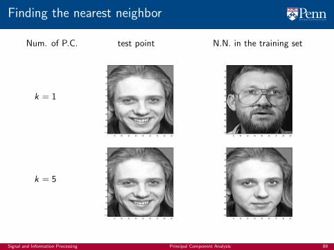
Finding the nearest neighbor
Num. of P.C. test point N.N. in the training set
k = 1
10 20 30 40 50 60 70 80 90
10
20
30
40
50
60
70
80
90
100
110
10 20 30 40 50 60 70 80 90
10
20
30
40
50
60
70
80
90
100
110
k = 5
10 20 30 40 50 60 70 80 90
10
20
30
40
50
60
70
80
90
100
110
10 20 30 40 50 60 70 80 90
10
20
30
40
50
60
70
80
90
100
110
Signal and Information Processing Principal Component Analysis 89

PCA improves classification accuracy
Classification method test point result of classification
Naive N.N.
10 20 30 40 50 60 70 80 90
10
20
30
40
50
60
70
80
90
100
110
10 20 30 40 50 60 70 80 90
10
20
30
40
50
60
70
80
90
100
110
PCA-ed(k = 5) N.N.
10 20 30 40 50 60 70 80 90
10
20
30
40
50
60
70
80
90
100
110
10 20 30 40 50 60 70 80 90
10
20
30
40
50
60
70
80
90
100
110
Signal and Information Processing Principal Component Analysis 90
Related Documents


![Multivariate Statistics [1em]Principal Component Analysis ...meier/teaching/cheming/4_multivariate.pdf · Principal Component Analysis (PCA) Goal: Dimensionality reduction. We have](https://static.cupdf.com/doc/110x72/5e80b49cd82bd2127764cf4d/multivariate-statistics-1emprincipal-component-analysis-meierteachingcheming4.jpg)


![Compressive Online Robust Principal Component Analysis Via ... · PRINCIPAL component analysis (PCA) [3] forms the crux of dimensionality reduction for high-dimensional data analysis.](https://static.cupdf.com/doc/110x72/5f81c7d5913e1f66f56c76c3/compressive-online-robust-principal-component-analysis-via-principal-component.jpg)