PCA Principal Component Analysis

EE-214/2011

PCA

Principal Component Analysis

EE-214/2011

Sensor 3

Sensor 4

Medida 9

Medida 14

x =

1.8196 5.6843 6.8238 4.7767 1.0397 4.1195 6.0911 4.2638 1.1126 4.6507 7.8633 5.5043 1.3735 6.0801 8.0462 5.6324 2.4124 3.6608 7.1652 5.0156 3.2898 4.7301 6.0169 4.2119 2.9436 4.2940 7.4612 5.2228 1.6561 3.1509 5.2104 3.6473 0.4757 1.4661 6.6255 4.6379 2.1659 1.6211 9.2418 6.4692 1.4852 3.6537 7.3074 5.1152 0.7544 3.3891 6.1951 4.3365 2.3136 3.5918 7.6207 5.3345 2.4068 2.5844 6.8016 4.7611 2.5996 4.2271 7.7247 5.4073 1.8136 4.2080 6.7446 4.7212

m

N

EE-214/2011

-4 -3 -2 -1 0 1 2 3 4-4

-3

-2

-1

0

1

2

3

4

x1

x2

x=

0.5632 0.0525

0.1992 0.9442

-1.4904 0.0169

0.5112 0.2334

2.3856 0.4861

0.5951 0.0604

0.6180 1.5972

-0.5145 -0.6150

1.7430 1.4551

-1.0344 -0.9598

1.5369 1.3969

0.1178 -0.5428

0.8500 0.9795

-1.4907 -0.7346

-0.0970 -0.7409

-0.9971 -0.8030

-0.1868 -0.2996

-0.5746 -0.8211

1.2367 2.3720

0.3793 0.1620

0.0675 -0.3321

1.3183 0.7651

-0.8986 -0.5059

-0.1140 1.3910

-0.6703 0.1073

2.3948 1.4875

1.0090 1.2579

0.0914 -0.3765

-0.1388 -0.7678

-2.3396 -1.2983

0.9069 1.4772

-0.3849 -0.0941

-0.3874 -0.4512

0.0444 -0.1314

-0.2293 -0.6040

0.4161 0.5944

-3.0050 -1.9646

-1.1580 -0.1741

-0.6379 -1.7942

1.0003 -0.4333

0.2530 -0.1742

1.8173 1.5607

-1.7688 -2.0968

0.1575 -0.1781

-0.5782 0.0264

-2.5254 -1.8191

0.5193 0.9366

1.7935 1.6216

-1.7429 -1.9603

0.4392 -0.3092]

EE-214/2011

-4 -3 -2 -1 0 1 2 3 4-4

-3

-2

-1

0

1

2

3

4

x1

x2

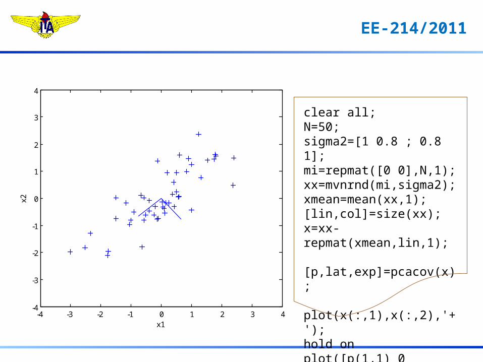
clear all;N=50;sigma2=[1 0.8 ; 0.8 1];mi=repmat([0 0],N,1);xx=mvnrnd(mi,sigma2);xmean=mean(xx,1);[lin,col]=size(xx);x=xx-repmat(xmean,lin,1);

[p,lat,exp]=pcacov(x);

plot(x(:,1),x(:,2),'+');hold onplot([p(1,1) 0 p(1,2)],[p(2,1) 0 p(2,2)])

EE-214/2011

-4 -3 -2 -1 0 1 2 3 4-4

-3

-2

-1

0

1

2

3

4

xnew1

xnew

2

-4 -3 -2 -1 0 1 2 3 4-4

-3

-2

-1

0

1

2

3

4

x1

x2

EE-214/2011

-4 -3 -2 -1 0 1 2 3 4-4

-3

-2

-1

0

1

2

3

4

xnew1

xnew

2

EE-214/2011

-4 -3 -2 -1 0 1 2 3 4-4

-3

-2

-1

0

1

2

3

4

x1

x2

Como determinar?

EE-214/2011

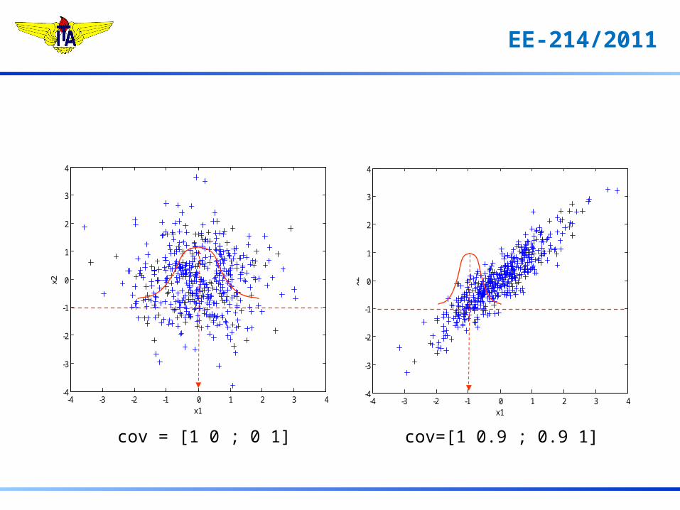
cov = [1 0 ; 0 1]

-4 -3 -2 -1 0 1 2 3 4-4

-3

-2

-1

0

1

2

3

4

x1

x2

-4 -3 -2 -1 0 1 2 3 4-4

-3

-2

-1

0

1

2

3

4

x1

x2

cov=[1 0.9 ; 0.9 1]

EE-214/2011

-4 -3 -2 -1 0 1 2 3 4-4

-3

-2

-1

0

1

2

3

4

x1

x2

-4 -3 -2 -1 0 1 2 3 4-4

-3

-2

-1

0

1

2

3

4

x1

x2

cov = [1 0 ; 0 1] cov=[1 0.9 ; 0.9 1]

EE-214/2011

-4 -3 -2 -1 0 1 2 3 4-4

-3

-2

-1

0

1

2

3

4

x1

x2

-4 -3 -2 -1 0 1 2 3 4-4

-3

-2

-1

0

1

2

3

4

x1

x2

cov = [1 0 ; 0 1] cov=[1 0.9 ; 0.9 1]

EE-214/2011

cov = [1 0 ; 0 1]

-4 -3 -2 -1 0 1 2 3 4-4

-3

-2

-1

0

1

2

3

4

x1

x2

Para Gaussianas:

Não Correlacionados Independentes

Matriz de Covariança Diagonal

EE-214/2011

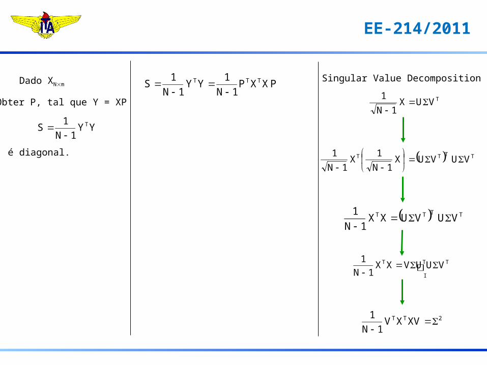
Dado XNm

Obter P, tal que Y = XP

YY1N

1S T

é diagonal.

Dada uma matriz Amm , os auto-valores e os auto-vetores v são caracterizados por

vvA ou seja,

0AIdet

Como (s) é um polinômio de grau m, (s) =0 possuim raízes, 1, 2, ... , m associados a v1, v2, ... , vm

m

2

P

m21

P

m21

00

0000

vvvvvvA

No caso de e-valores distintos:

P-1 A P =

EE-214/2011

PXXP1N

1YY1N

1S TTT

A = XTX

P-1 = PT

P é simétrica

Dado XNm


YY1N

1S T

é diagonal.P-1 A P =

m21 vvvP

vi e-vetores de XTX

PXXP T1

( normalizados vi = 1)

PTP = vivjT

1vvvPP ijTiij

T

i = j

EE-214/2011

PXXP1N

1YY1N

1S TTT

A = XTX

P-1 A P = m21 vvvP

vi e-vetores de XTX

PXXP T1

P-1 = PT

P é simétrica

Dado XNm


YY1N

1S T

é diagonal.

PTP = vivjT

jTiiij

Ti vvPP

vvP

jTT

ijTii vPvvv

PT = P

jTij

Tii vPvvv

vvP

jTijj

Tii vvvv

0vv jTi

0

ji


i j

EE-214/2011

PXXP1N

1YY1N

1S TTT

A = XTX

P-1 A P = m21 vvvP

vi e-vetores de XTX

PXXP T1

P-1 = PT

P é simétrica

Dado XNm


YY1N

1S T

é diagonal.

PTP = vivjT


ji0ji1

PP ijT

PTP = I

EE-214/2011

PXXP1N

1YY1N

1S TTT

A = XTX

P-1 A P = m21 vvvP

vi e-vetores de XTX

PXXP T1

P-1 = PT

P é simétrica

P é ortogonal

Dado XNm


YY1N

1S T

é diagonal.


jivv ki

EE-214/2011

PXXP1N

1YY1N

1S TTT

Dado XNm


YY1N

1S T

é diagonal.

Singular Value Decomposition

TVUX1N

1

TTTT VUVUX1N

1X

1N1

TTTT VUVUXX1N

1

2TT XVXV1N

1

T

I

TT VUUVXX1N

1

EE-214/2011

PXXP1N

1YY1N

1S TTT

Dado XNm


YY1N

1S T

é diagonal.

P = Matriz de e-vec de (XTX)V = Matriz à direita no SVD

2T1 PXXP

2TT XVXV1N

1

EE-214/2011

-4 -3 -2 -1 0 1 2 3 4-4

-3

-2

-1

0

1

2

3

4

x1

x2

x=

0.5632 0.0525

0.1992 0.9442

-1.4904 0.0169

0.5112 0.2334

2.3856 0.4861

0.5951 0.0604

0.6180 1.5972

-0.5145 -0.6150

1.7430 1.4551

-1.0344 -0.9598

1.5369 1.3969

0.1178 -0.5428

0.8500 0.9795

-1.4907 -0.7346

-0.0970 -0.7409

-0.9971 -0.8030

-0.1868 -0.2996

-0.5746 -0.8211

1.2367 2.3720

0.3793 0.1620

0.0675 -0.3321

1.3183 0.7651

-0.8986 -0.5059

-0.1140 1.3910

-0.6703 0.1073

2.3948 1.4875

1.0090 1.2579

0.0914 -0.3765

-0.1388 -0.7678

-2.3396 -1.2983

0.9069 1.4772

-0.3849 -0.0941

-0.3874 -0.4512

0.0444 -0.1314

-0.2293 -0.6040

0.4161 0.5944

-3.0050 -1.9646

-1.1580 -0.1741

-0.6379 -1.7942

1.0003 -0.4333

0.2530 -0.1742

1.8173 1.5607

-1.7688 -2.0968

0.1575 -0.1781

-0.5782 0.0264

-2.5254 -1.8191

0.5193 0.9366

1.7935 1.6216

-1.7429 -1.9603

0.4392 -0.3092]

EE-214/2011

x=

0.5632 0.0525

0.1992 0.9442

-1.4904 0.0169

0.5112 0.2334

2.3856 0.4861

0.5951 0.0604

0.6180 1.5972

-0.5145 -0.6150

1.7430 1.4551

-1.0344 -0.9598

1.5369 1.3969

0.1178 -0.5428

0.8500 0.9795

-1.4907 -0.7346

-0.0970 -0.7409

-0.9971 -0.8030

-0.1868 -0.2996

-0.5746 -0.8211

1.2367 2.3720

0.3793 0.1620

0.0675 -0.3321

1.3183 0.7651

-0.8986 -0.5059

-0.1140 1.3910

-0.6703 0.1073

2.3948 1.4875

1.0090 1.2579

0.0914 -0.3765

-0.1388 -0.7678

-2.3396 -1.2983

0.9069 1.4772

-0.3849 -0.0941

-0.3874 -0.4512

0.0444 -0.1314

-0.2293 -0.6040

0.4161 0.5944

-3.0050 -1.9646

-1.1580 -0.1741

-0.6379 -1.7942

1.0003 -0.4333

0.2530 -0.1742

1.8173 1.5607

-1.7688 -2.0968

0.1575 -0.1781

-0.5782 0.0264

-2.5254 -1.8191

0.5193 0.9366

1.7935 1.6216

-1.7429 -1.9603

0.4392 -0.3092]

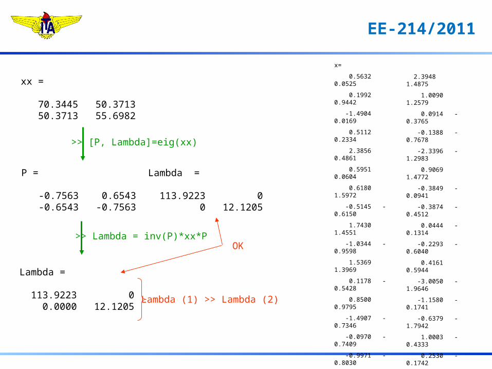
xx =

70.3445 50.3713 50.3713 55.6982

>> [P, Lambda]=eig(xx)

Lambda =

113.9223 0 0 12.1205

P =

-0.7563 0.6543 -0.6543 -0.7563

>> Lambda = inv(P)*xx*P

Lambda =

113.9223 0 0.0000 12.1205

Lambda (1) >> Lambda (2)

OK

EE-214/2011

-4 -3 -2 -1 0 1 2 3 4-4

-3

-2

-1

0

1

2

3

4

xnew1

xnew

2

P =

-0.7563 0.6543 -0.6543 -0.7563

>> xnew = x * P

Pelim =

-0.7563 0.0 -0.6543 0.0 >> xelim = x * Pelim

EE-214/2011

x=

0.5632 0.0525

0.1992 0.9442

-1.4904 0.0169

0.5112 0.2334

2.3856 0.4861

0.5951 0.0604

0.6180 1.5972

-0.5145 -0.6150

1.7430 1.4551

-1.0344 -0.9598

1.5369 1.3969

0.1178 -0.5428

0.8500 0.9795

-1.4907 -0.7346

-0.0970 -0.7409

-0.9971 -0.8030

-0.1868 -0.2996

-0.5746 -0.8211

1.2367 2.3720

0.3793 0.1620

0.0675 -0.3321

1.3183 0.7651

-0.8986 -0.5059

-0.1140 1.3910

-0.6703 0.1073

2.3948 1.4875

1.0090 1.2579

0.0914 -0.3765

-0.1388 -0.7678

-2.3396 -1.2983

0.9069 1.4772

-0.3849 -0.0941

-0.3874 -0.4512

0.0444 -0.1314

-0.2293 -0.6040

0.4161 0.5944

-3.0050 -1.9646

-1.1580 -0.1741

-0.6379 -1.7942

1.0003 -0.4333

0.2530 -0.1742

1.8173 1.5607

-1.7688 -2.0968

0.1575 -0.1781

-0.5782 0.0264

-2.5254 -1.8191

0.5193 0.9366

1.7935 1.6216

-1.7429 -1.9603

0.4392 -0.3092]

OK

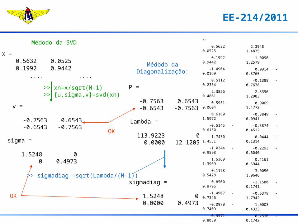
x = 0.5632 0.0525 0.1992 0.9442 .... ....

>> xn=x/sqrt(N-1)>> [u,sigma,v]=svd(xn)

v =

-0.7563 0.6543 -0.6543 -0.7563

sigma =

1.5248 0 0 0.4973

>> sigmadiag =sqrt(Lambda/(N-1))

Lambda =

113.9223 0 0.0000 12.1205

sigmadiag =

1.5248 0 0.0000 0.4973

Médodo da SVD

P =

-0.7563 0.6543 -0.6543 -0.7563

Médodo daDiagonalização:

OK

EE-214/2011

>> help pcacov

PCACOV Principal Component Analysis using the covariance matrix. [PC, LATENT, EXPLAINED] = PCACOV(X) takes a the covariance matrix, X, and returns the principal components in PC, the eigenvalues of the covariance matrix of X in LATENT, and the percentage of the total variance in the observations explained by each eigenvector in EXPLAINED.

>> [pc,latent,explained]=pcacov(x)

pc =

-0.7563 0.6543 -0.6543 -0.7563

latent =

10.6734 3.4814

explained =

75.4046 24.5954

EE-214/2011

>> help pcacov


P =

-0.7563 0.6543 -0.6543 -0.7563

v =

-0.7563 0.6543 -0.6543 -0.7563


pc =

-0.7563 0.6543 -0.6543 -0.7563

latent =

10.6734 3.4814

explained =

75.4046 24.5954

OK

EE-214/2011

>> help pcacov



pc =

-0.7563 0.6543 -0.6543 -0.7563

latent =

10.6734 3.4814

>> sqrlamb=sqrt(evalor)

Lambda =

113.9223 0 0 12.1205

sqrlamb =

10.6734 0 0 3.4814

explained =

75.4046 24.5954

EE-214/2011

>> help pcacov



pc =

-0.7563 0.6543 -0.6543 -0.7563

latent =

10.6734 3.4814

sqrlamb =

10.6734 0 0 3.4814

explained =

75.4046 24.5954

>> e=[Lambda(1,1) ; Lambda(2,2)]>> soma=sum(e)>> percent=e*100/soma

percent =

75.4046 24.5954

EE-214/2011

>> help princomp

PRINCOMP Principal Component Analysis (centered and scaled data). [PC, SCORE, LATENT, TSQUARE] = PRINCOMP(X) takes a data matrix X and returns the principal components in PC, the so-called Z-scores in SCORES, the eigenvalues of the covariance matrix of X in LATENT, and Hotelling's T-squared statistic for each data point in TSQUARE.

>> [pc,score,latent1,tsquare]=princomp(x)

pc =

-0.7563 0.6543 -0.6543 -0.7563

score =

-0.4603 0.3288 -0.7684 -0.5837 1.1161 -0.9879 -0.5393 0.1579 -2.1222 1.1932 -0.4896 0.3437 ..... .....

latent1 =

2.3249 0.2474

tsquare =

0.5281 1.6315 4.4813 0.2260 7.6929 0.5806 .....

EE-214/2011

>> help princomp



pc =

-0.7563 0.6543 -0.6543 -0.7563

score =

-0.4603 0.3288 -0.7684 -0.5837 1.1161 -0.9879 -0.5393 0.1579 -2.1222 1.1932 -0.4896 0.3437 ..... .....

latent1 =

2.3249 0.2474

tsquare =

0.5281 1.6315 4.4813 0.2260 7.6929 0.5806 .....P =

-0.7563 0.6543 -0.6543 -0.7563

EE-214/2011

>> help princomp



score =

-0.4603 0.3288 -0.7684 -0.5837 1.1161 -0.9879 -0.5393 0.1579 -2.1222 1.1932 -0.4896 0.3437 ..... .....

sco =

-0.4603 0.3288 -0.7684 -0.5838 1.1161 -0.9880 -0.5393 0.1580 -2.1223 1.1933 -0.4896 0.3437

>> sco=x*P

EE-214/2011

>> help princomp



latent1 =

2.3249 0.2474

tsquare =

0.5281 1.6315 4.4813 0.2260 7.6929 0.5806 .....

>> eig( x'*x /(N-1))

ans =

0.2474 2.3249

pc =

-0.7563 0.6543 -0.6543 -0.7563

score =

-0.4603 0.3288 -0.7684 -0.5837 1.1161 -0.9879 -0.5393 0.1579 -2.1222 1.1932 -0.4896 0.3437 ..... .....

EE-214/2011

>> help princomp



latent1 =

2.3249 0.2474

tsquare =

0.5281 1.6315 4.4813 0.2260 7.6929 0.5806 .....

pc =

-0.7563 0.6543 -0.6543 -0.7563

score =

-0.4603 0.3288 -0.7684 -0.5837 1.1161 -0.9879 -0.5393 0.1579 -2.1222 1.1932 -0.4896 0.3437 ..... .....

22 TT

mN,mFmNN

1N1NmT2

caracteriza a região de confiança 100

EE-214/2011

-0.6 -0.4 -0.2 0 0.2 0.4 0.6

-0.6

-0.4

-0.2

0

0.2

0.4

0.6

xnew1

xnew

2

-0.6 -0.4 -0.2 0 0.2 0.4 0.6

-0.6

-0.4

-0.2

0

0.2

0.4

0.6

x1

x2

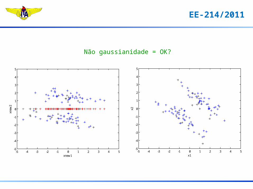
Não gaussianidade = OK?

EE-214/2011

-5 -4 -3 -2 -1 0 1 2 3 4 5-5

-4

-3

-2

-1

0

1

2

3

4

5

xnew1

xnew

2

-5 -4 -3 -2 -1 0 1 2 3 4 5-5

-4

-3

-2

-1

0

1

2

3

4

5

x1

x2


EE-214/2011

-5 -4 -3 -2 -1 0 1 2 3 4 5-5

-4

-3

-2

-1

0

1

2

3

4

5

xnew1

xnew

2

-5 -4 -3 -2 -1 0 1 2 3 4 5-5

-4

-3

-2

-1

0

1

2

3

4

5

x1

x2


EE-214/2011

-5 -4 -3 -2 -1 0 1 2 3 4 5-5

-4

-3

-2

-1

0

1

2

3

4

5

x1

x2

>> xm=mean(xx);>> [lin,col]=size(xx);>> xm=repmat(xm,lin,1);>> xx=xx-xm;

-5 -4 -3 -2 -1 0 1 2 3 4 5-5

-4

-3

-2

-1

0

1

2

3

4

5

x1

x2

EE-214/2011

-3 -2 -1 0 1 2 3-3

-2

-1

0

1

2

3

x1

x2

0 20 40 60 80 100 120 140 160 180 2000

1

2

3

4

5

6

7

8

9

10

11

k

x1

0 20 40 60 80 100 120 140 160 180 2000

1

2

3

4

5

6

7

8

9

10

11

k

x2

EE-214/2011

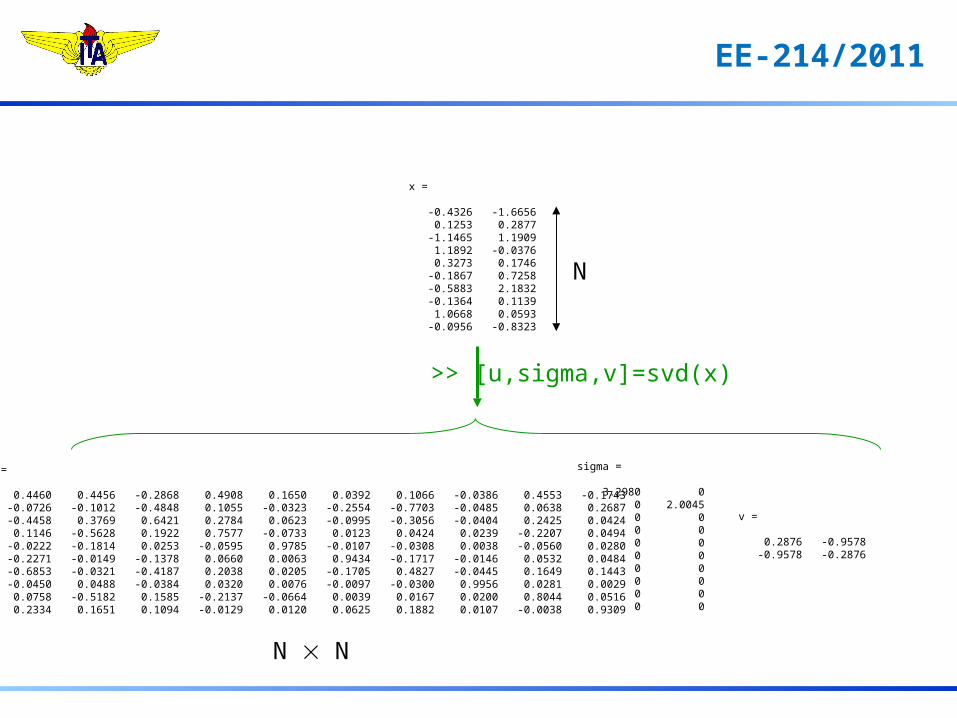
x =

-0.4326 -1.6656 0.1253 0.2877 -1.1465 1.1909 1.1892 -0.0376 0.3273 0.1746 -0.1867 0.7258 -0.5883 2.1832 -0.1364 0.1139 1.0668 0.0593 -0.0956 -0.8323

>> [u,sigma,v]=svd(x)

u =

0.4460 0.4456 -0.2868 0.4908 0.1650 0.0392 0.1066 -0.0386 0.4553 -0.1743 -0.0726 -0.1012 -0.4848 0.1055 -0.0323 -0.2554 -0.7703 -0.0485 0.0638 0.2687 -0.4458 0.3769 0.6421 0.2784 0.0623 -0.0995 -0.3056 -0.0404 0.2425 0.0424 0.1146 -0.5628 0.1922 0.7577 -0.0733 0.0123 0.0424 0.0239 -0.2207 0.0494 -0.0222 -0.1814 0.0253 -0.0595 0.9785 -0.0107 -0.0308 0.0038 -0.0560 0.0280 -0.2271 -0.0149 -0.1378 0.0660 0.0063 0.9434 -0.1717 -0.0146 0.0532 0.0484 -0.6853 -0.0321 -0.4187 0.2038 0.0205 -0.1705 0.4827 -0.0445 0.1649 0.1443 -0.0450 0.0488 -0.0384 0.0320 0.0076 -0.0097 -0.0300 0.9956 0.0281 0.0029 0.0758 -0.5182 0.1585 -0.2137 -0.0664 0.0039 0.0167 0.0200 0.8044 0.0516 0.2334 0.1651 0.1094 -0.0129 0.0120 0.0625 0.1882 0.0107 -0.0038 0.9309

sigma =

3.2980 0 0 2.0045 0 0 0 0 0 0 0 0 0 0 0 0 0 0 0 0

v =

0.2876 -0.9578 -0.9578 -0.2876

N

N N

EE-214/2011

Muito Obrigado!

PCA Principal Component Analysis

Documents