An Open Innovation Intraday Implied Volatility for Pricing ...

Journal of Open Innovation:

Technology, Market, and Complexity

Article

An Open Innovation Intraday Implied Volatility for PricingAustralian Dollar Options

Thi Le , Ariful Hoque * and Kamrul Hassan

�����������������

Citation: Le, T.; Hoque, A.; Hassan,

K. An Open Innovation Intraday

Implied Volatility for Pricing

Australian Dollar Options. J. Open

Innov. Technol. Mark. Complex. 2021, 7,

23. https://doi.org/10.3390/

joitmc7010023

Received: 10 December 2020

Accepted: 5 January 2021

Published: 9 January 2021

Publisher’s Note: MDPI stays neu-

tral with regard to jurisdictional clai-

ms in published maps and institutio-

nal affiliations.

Copyright: © 2021 by the authors. Li-

censee MDPI, Basel, Switzerland.

This article is an open access article

distributed under the terms and con-

ditions of the Creative Commons At-

tribution (CC BY) license (https://

creativecommons.org/licenses/by/

4.0/).

Murdoch Business School, Murdoch University, Perth 6150, Australia; [email protected] (T.L.);[email protected] (K.H.)* Correspondence: [email protected]

Abstract: This study introduces the intraday implied volatility (IV) for pricing the Australian dollar(AUD) options. The IV is estimated using the at-the-money one-month, two-month, and three-month maturity AUD options traded in the opening, midday, and closing period of a trading day.The Mincer-Zarnowitz regression test evaluates the predictive power of IV to forecast the foreignexchange volatility for the within-week, one-week, and one-month horizon. The mean absolute error,mean squared error, and root mean squared error measures are employed to assess the performanceof IV in estimating the price of currency options for the within-week, one-week, and one-monthhorizon. This study reveals four critical findings. First, a three-month maturity IV does not containvital information for pricing options. Second, IV incorporated information is not relevant to computethe value of options for a horizon of less than a week. Third, IV in the closing period of Monday orTuesday subsumes most of the essential information to estimate options price. Fourth, the shorter(longer) maturity IV provides critical information to price options for the shorter (longer) horizon.The intraday IV is a new dimension of unobservable volatility in accurately pricing currency optionsfor researchers and practitioners.

Keywords: intraday implied volatility; realised volatility; Australian dollar options; Mincer–Zarnowitzregression

1. Introduction

This study introduces intraday implied volatility (IV) which is an innovative approachto estimate the volatility of underlying currency for pricing currency options accurately.The intraday IV captures the market information at the opening, midday, and closing periodof a trading day for pricing options with higher accuracy. If the options are mispriced,particularly overpriced options, it will increase the cost for hedging using currency options.The 2019 Bank for International Settlement (BIS) Triennial Survey results reveal that theturnover in Australian dollar (AUD) options increased by 58 percent between April 2016and April 2019 [1], which is significant compared to other currency options. Therefore,Australian dollar options are considered to assess the capability of intraday IV to holdingappropriate market information for pricing options precisely.

Foreign exchange (FX) risks are reported as one of the major risks related to foreign in-vestments and international assets pricing [2]. Most portfolio managers have been using FXoptions as their primary hedging tools to manage these risks [3]. The flexibility of currencyoptions in creating a customised risk/return profile to achieve a specific investment objec-tive has led to the significant growth of the FX options market. Holding currency optionsfor various investment decisions such as hedging or speculation can be costly if the optionsare mispriced. Options mispricing affects the selection of hedge ratio, hedging efficiency, aswell as expected hedging costs [4]. For this reason, the accuracy of currency options pricinghas been attracting the attention of market participants [5]. Currently, the most commonlyused model to calculate European options prices is known as the Black–Scholes [6] (BS)

J. Open Innov. Technol. Mark. Complex. 2021, 7, 23. https://doi.org/10.3390/joitmc7010023 https://www.mdpi.com/journal/joitmc

J. Open Innov. Technol. Mark. Complex. 2021, 7, 23 2 of 14

model [7]. The BS model assumes constant volatility. If true, this assumption would leadto a flat implied volatility curve. Observed implied volatility in practice differs acrossoption contracts, depending on both moneyness and time to maturity. However, due tothe theoretical approximation between the stochastic volatility and conditional volatilitymodels to BS for at-the-money (ATM) options and nearest to expiration [8,9] and the richinformational content, implied volatility is still of interest [10–13] and the BS model is stillwidely applied [14]. Using the Merton [15] version of the BS model (BSM) to calculateprices of European currency options, all components are observable except the volatilityof the underlying currency. Errors in the estimation of volatility result in the options mis-pricing [16–18]. The improvement of volatility estimation leads to lower errors of optionprices [19]. Hence, forecasts of future volatility of underlying assets are vital for estimatingand forecasting the currency options price accurately.

The literature has explored the volatility intensively. As the options prices reflect themarket’s expectation about the future movements of the prices of the underlying asset overthe remaining life of the option contract, more research concentrates on volatility implied inoptions prices [20]. The implied volatility (IV) contains all available information, includinghistorical data [10,20–25]. It is widely accepted that the IV from the market options priceis a reasonable measure of the market’s opinion of the volatility of the underlying asset.The forward-looking IV subsumes relevant information in terms of future volatility, andit often outperforms historical volatility in predicting future realised volatility (RV). Suchsuperior performance was recognised in different types of assets [26]. For currency options,the majority of both previous and more current research found that IV was a reliablepredictor of future volatility. IV contained valuable information for volatility forecastingand captured approximately 50 per cent of actual currency volatility [27].

However, most of the previous research used the conventional approach that wasbased on daily IV obtained from daily closing options prices. As the operation of financialmarkets during their opening trading hour are based on a continuous, high-frequency basis,the conventional method using a discrete sample of datasets on markets at a significantlylower frequency with the majority of data being extracted per day, or per week to forecastvolatility is no longer relevant [28]. New technologies have been creating opportunitiesto obtain better, faster, and more efficient datasets to explore financial market phenomenaat the finest levels of data [29]. It provides reliable intraday data to supporting financialinvestment decisions across different assets classes and instruments consisting of commodi-ties, derivatives, equities, fixed income, and foreign exchange [30]. The purpose of thispaper is to investigate the performance of the intraday implied volatility (IV) for pricingthe Australian dollar (AUD) options. This study has three major contributions.

First, this study introduces an intraday IV approach based on the one-month, two-month, and three-month maturity options traded in the opening, midday, and closingperiod of a trading day, which captures the most relevant information of the FX in es-timating options prices. Second, the research findings indicate that the one-month andtwo-month maturity intraday IV holds vital information to predict the volatility of theunderlying currency of options for the one-week and one-month forecast horizon, respec-tively. Third, this research confirms that the information content embedded in the IV basedon the one-month and two-month maturity options is appropriate to estimate the value ofcurrency options for the one-week and one-month horizon, respectively.

The rest of the paper proceeds as follows. Section 2 discusses the literature review. Thenext section describes the methodology and data used in this study. Section 4 conducts theempirical analysis, followed by the discussion of the findings. The last section concludesthe paper.

2. Literature Review

Xu and Taylor [31] examined the informational efficiency of the four currency options(British pound (GBP), Deutsche mark (DEM), Japanese yen (JPY), and Swiss franc (CHF)against the US dollar (USD)) from January 1985 to January 1992 and concluded that

J. Open Innov. Technol. Mark. Complex. 2021, 7, 23 3 of 14

option prices subsumed useful information about future volatilities. Likewise, Jorion [32]tested the predictive power of DEM, JPY, and CHF against the USD and found that IVcontained more information content compared to statistical time-series models. Kazantzisand Tessaromatis [33] analysed the information content and predictive power of IV usingsix currency options (JPY, DEM, GBP, CHF, Canadian dollar (CAD), and AUD againstthe USD) from December 1989 to April 1997. The findings indicated that IV was moreinformative than historical and GARCH-based volatilities for horizons ranging from oneday to three months. Kim and Kim [34] showed that the IV of the CAD, CHF, DEM, GBP,and JPY options tended to be low in the early part of the week but remain high in the lastpart of the week beginning on Wednesdays. Chang and Tabak [35] produced evidence thatthe IV of Brazilian options contained vital information that was missing in the econometricmodels and it provided superior foreign exchange (FX) forecasts. Busch et al. [23] exploredthe role of IV in predicting future volatility and found that IV was an unbiased predictorand provided helpful information for volatility forecasting in the FX market. Pilbeam andLangeland [36] recognised that the IV of CHF, EUR, GBP, and JPY provided a superiorperformance compared to the GARCH model in both the low and high volatility periods ofthe FX market. Sahoo and Trivedi [37] showed that IV outperformed historical volatilitiesin forecasting future RV. Wong and Heaney [38] found the knowledge of the volatility smile,which were implied from the one-month maturity of GBP/USD, EUR/USD, AUD/USD,and USD/JPY options, improved FX volatility forecast accuracy. Covrig and Low [39]used over-the-counter (OTC) data for USD per GBP, JPY per USD, and USD per AUD toexamine the information of IV for different forecast horizons. They suggested that quotedIV subsumed the information content of historically based forecasts at shorter horizons(one-month and two-month horizon). Pong et al. [40] found that the IV of the DEM, GBP,and JPY options incorporated most of the relevant information for the forecast horizon ofeither one-month or three-month. Christoffersen and Mazzotta [41] revealed that the IV ofat-the-money (ATM) options for the EUR, GBP, and JPY mostly provided the unbiased andreasonably accurate forecasts of actual volatility one month and three months out.

Until the late 1970s, using monthly data played an essential role in empirical researchdue to the unavailability of and access problems to higher frequency data, such as daily orintraday data. However, the development of information technology in the 1990s providedaccess to time-stamped observations on all quotes and transactions. These tick-by-tickdata, termed as ultra-high-frequency data by Engle [42], are usually referred to as high-frequency data in current studies. High-frequency data indicated that many financial assetsexperienced the particular intraday patterns [20] and these patterns were significantlyassociated with intraday returns variations, volatility, volume, and bid-ask spreads [43]. Alarge number of studies suggested that intraday trading activities exhibited a U-shapedpattern with the trading volumes being extremely high at the market’s opening and closingperiods, such as Wood et al. [44], Gerety and Mulherin [45], Brock and Kleidon [46] for theNew York Stock Exchange (NYSE); Mclnish and Wood [47] for the Toronto Stock Exchange;and Hamao and Hasbrouck [48] for the Tokyo stock exchange. Several studies reportedthe M-shaped [29,49] or J-shaped patterns [50] for the UK stock exchange. Most of theresearch found the importance of intraday data in improving volatility predicting. Therewas a significant amount of information in the five-minute returns when estimating hourlyvariances [51–53]. Wang and Wang [20] explored the capability of intraday IV informationcontent using the S&P500 Index as a sample from 2005 to 2010. Their study recognised thatthe IV around noon contains more useful information regarding future volatility than IVat the market’s closing period, which has been frequently used in the previous literature.Trading at a specific time of the trading day is motivated by specific information andrisk factors, which do not remain during other times. Hence, our paper investigates theperformance of IV in estimating and forecasting options prices at three different tradingtime periods of the trading day (opening, midday, and closing) using the AUD currencyoptions datasets covering the period from 2010 to 2017.

J. Open Innov. Technol. Mark. Complex. 2021, 7, 23 4 of 14

Previous studies focused on the daily IV of currency options to forecast the volatilityof FX. There are not many pieces of research utilising the high-frequency data and intradayIV in estimating and forecasting volatility. Furthermore, IV incorporated information hasnot been used for pricing options. Therefore, this paper will examine the capability ofintraday IV with different time to maturity in forecasting future volatility and estimatingcurrency options price.

3. Materials and Methods3.1. Data Description

This study used AUD currency options provided by the Options Price ReportingAuthority (OPRA) as the last-sale options quotations. We obtained data from ThomsonReuters’ database through the Securities Industry Research Centre of Asia-Pacific (SIRCA).The sample period began on 01 January 2010 and ended on 31 December 2017. The optionswere traded on Monday to Friday, excluding public holidays from 9:30 to 16:00 (US Easternstandard time), and expired on the third Friday of each month. The options were Europeanstyle, with the contract size of sample currency options being AUD 10,000 and settledin USD. The time to maturity of an option was assumed to be the number of calendardays remaining until the option matured. The sample options expired in one-month (2 to30 days), two-month (31 to 60 days), and three-month (61 to 90 days) periods. The IVwas calculated for the opening-period (9:30 to 10:00), midday-period (12:30 to 13:00), andclosing-period (15:30 to 16:00) of a trading day. The time difference between “opening-period” and “midday-period” and between “midday period” and “closing period” wasequal (two and half hours) enough to position them evenly in a trading day. The BSMmodel assumed the volatility as constant, which introduced a bias into the IV estimation.Hull and White [54] stated that the magnitude of the bias in the BS model was the smallestfor near-the-money options. Therefore, the IV was calculated based on the ATM one-month,two-month, and three-month maturity options traded during the opening, midday, andclosing periods of a trading day.

We followed the ATM criteria in Xing et al. [55]; the ratio of the strike price to the stockprice was considered between 0.95 and 1.05. The average of the close bid/ask quote ofeach five-minute interval was computed for each options price to mitigate problems due tobid/ask bounce [56]. The one-month, two-month, and three-month AUD and USD depositinterest rate were used as the proxy of the risk-free interest rate.

3.2. Methodology

The research methodology consists of five sub-sections, (i) calculating IV, (ii) comput-ing realised volatility (RV), (iii) IV forecasting RV, (iv) IV estimating options model price,and (v) estimating the options pricing error.

3.2.1. Implied Volatility Calculation

The BSM model replaces the stock price with foreign currency and considers theinterest gained on holding foreign currency to be equivalent to a continuously paid stockdividend. The notation of the BSM model and its descriptions are as follows:

Ct = price of call in domestic currency at time tPt = price of put in domestic currency at time tSt = spot price at time tXt = exercise price in domestic currency at time tRd

t = interest rate of domestic currency at time tRf

t = foreign currency interest rate at time tT = options expiration timeσt = volatility of underlying currencyN = cumulative normal distribution function

J. Open Innov. Technol. Mark. Complex. 2021, 7, 23 5 of 14

In the BSM model, the European type call and put options are priced as:

Ct = Ste−R ft T N(d1,t)− Xte−Rd

t N(d2,t) (1)

Pt = Xte−Rdt T N(−d2,t)− Ste−R f

t N(−d1,t) (2)

where,

d1,t =ln(

StXt

)+(

Rdt − R f

t +σ2

t2

)T

σt√

T, (3)

And

d2,t =ln(

StXt

)+(

Rdt − R f

t −σ2

t2

)T

σt√

T= d1,t − σt

√T (4)

For notation convenience, let ξt = e−R ft T and ηt = e−Rd

t T so that Equations (1) and (2)can be written as follows:

Cmkt,k,lt = StξtN

[d1,t

(σk,l

c,t

)]− XtηtN

[d2,t

(σk,l

c,t

)](5)

Pmkt,k,lt = XtηtN

[−d2,t

(σk,l

p,t

)]− StξtN

[−d1,t

(σk,l

p,t

)](6)

where ∀mkt = call and put market price; ∀k = one-month, two-month, three-month maturityoptions; ∀l = opening period, midday period, closing period. Now we calculate the impliedvolatility

(σk,l

c,t

)for the ATM call options market price (Cmkt,k,l

t ) and implied volatility(σk,l

p,t

)for the ATM put options market price (Pmkt,k,l

t ) through the Newton–Raphson [57]iterative search procedure.

Despite the numerous suggestions about weighted-average techniques for calculatingIV, there is no theoretically appropriate weighting scheme in the literature to estimate IV.We used the method suggested by Jorion [32] that computes IV as the average of the calloptions price IV and the put options’ price IV. This study estimates IV as:

σ̂k,lt =

σ̂k,lc,t + σ̂k,l

p,t

2, (7)

3.2.2. Realised Volatility Calculation

The actual market volatility is unobservable, so in evaluating volatility estimating andforecasting, the usual proxy for “true volatility” is the so-called realised volatility (RV). TheRV sums the squared intraday returns sampled at a particular rate of recurrence [52,58]. Theoptimal interval to construct the RV is not known. Based on standard practice and previousliterature, there is evidence that the five-minute RV as the benchmark outperformed othermeasures, and it is difficult to significantly surpass the five-minute (5 min) data frequencyfor RV [53]. Consequently, this study used daily RV series constructed from five-minuteintraday spot prices as a proxy for the unobservable variance. If Si is the spot rate fora five-minute sampling frequency, the underlying exchange rate return in a five-minuteinterval was estimated as:

ri,t = ln(

SiSi−1

)(8)

where ri,t represents the return in interval i on day t. Equation (7) computed the realisedvariance of day t,

vt =n

∑i=1

r2t,i, (9)

J. Open Innov. Technol. Mark. Complex. 2021, 7, 23 6 of 14

where n denotes the total number of data points from 9:30 to 16:00 for Monday to Friday.Further, the RV is the standard deviation of the realised variance. Therefore, the RV pertrading day is calculated as:

σ̂RVt =

√vt, (10)

As intraday data of trading days estimate the RV, when the exchange is closed, daysare ignored and the RV per annum is:

σ̂RVt =

√Dvt, (11)

where D is considered 252 trading days per year consistent with the normal assumption ofthe options market.

3.2.3. Implied Volatility Forecasting Realised Volatility

For IV from different maturities of options, the forecasting evaluation was imple-mented using the regression test introduced by Mincer and Zarnowitz [59], known as theMincer–Zarnowitz (MZ) regression. In the MZ regression analysis, the RV is regressed on aconstant and IV as in Equation (12):

σ̂RVt = β0 + β1σ̂k,l

t−j + εt, (12)

where ∀j = within-week, one-week, and one-month horizon. The within-week horizonindicates that the IV is calculated one to four days before the date of RV is computed.Similarly, the one-week and one-month horizon imply that the IV is estimated one weekand one month before the date of RV is obtained. The MZ regression allowed the evaluationof two different aspects to predict the volatility. First, the unbiasedness and efficiency ofthe forecast were evaluated by testing the intercept and slope through the joint hypothesis(H0: β0 = 0 and β1 = 1) [60]. Second, the accuracy of the forecast was evaluated by thehigh goodness of fit value, R-squared (R2). The R2 is a statistical measure that representsthe percentage of the variance for RV explained by IV. The value of R2 compares thepredictive power of IV to forecast RV for different horizons; such as, the R2 of IV for theone-week horizon being higher than that of the one-month horizon implies that the RV canbe explained well by the IV for the one-week horizon; that is, IV forecast of RV for one-week horizon outperforms its performance for the one-month horizon. The MZ regressionanalysis uses the OLS (ordinary least squared) method with Newey–West corrected errorsfor heteroscedasticity and serial correlation.

3.2.4. Implied Volatility Estimating Options Model Price

This study calculated the call options and put options model price using the estimatedvalue of IV as the input for the BSM options pricing model. The Cmkt,k

t and Pmkt,kt in

Equations (5) and (6) were substituted with call options model price(

Π̂mod,kc,t

)and put

options model price(

Π̂mod,kp,t

)as in Equations (13) and (14), respectively.

Π̂mod,kc,t = StξtN

[d1,t

(σ̂k,l

t−i

)]− XtηtN

[d2,t

(σ̂k,l

t−i

)](13)

Π̂mod,kp,t = XtηtN

[−d2,t

(σ̂k,l

t−i

)]− StξtN

[−d1,t

(σ̂k,l

t−i

)](14)

3.2.5. Options Pricing Error Estimation

The options pricing error (OPE) is the difference between the ATM options marketprice and the estimated options model price. The OPE is measured using standard statistical

J. Open Innov. Technol. Mark. Complex. 2021, 7, 23 7 of 14

accuracy criteria, including mean absolute error (MAE), mean squared error (MSE), andthe root mean squared error (RMSE), as in Equations (15)–(17), respectively.

MAEm,k,lu =

1n

n

∑t=1

∣∣∣ΠATM,k,lu,t − Π̂mod,k,l

u,t

∣∣∣ (15)

MSEm,k,lu =

1n

n

∑t=1

(ΠATM,k,l

u,t − Π̂mod,k,lu,t

)2(16)

RMSEm,k,lu =

√1n

n

∑t=1

(ΠATM,k,l

u,t − Π̂mod,k,lu,t

)2(17)

where ∀u = call price, put price.

4. Results

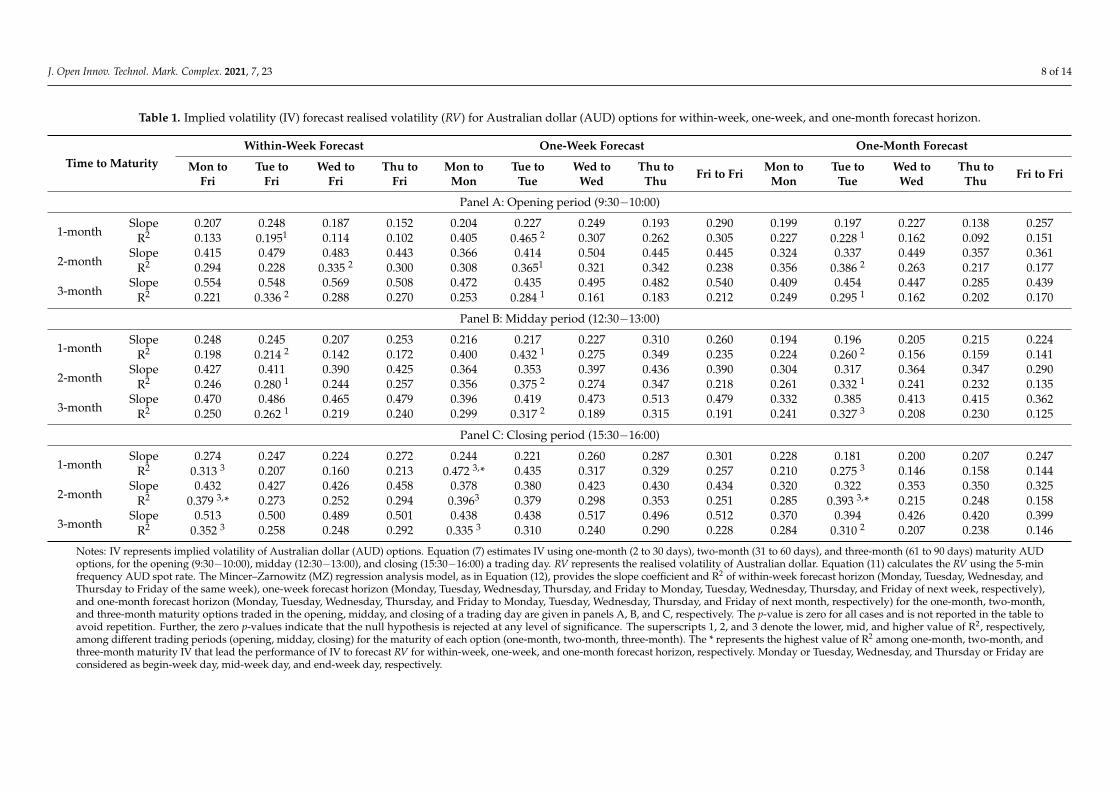
Table 1 describes the performance of IV to forecast RV for the within-week forecasthorizon, one-week forecast horizon, and one-month forecast horizon. R2 values from theforecasting regression in Equation (12) are reported. The IV with the highest R2 is preferred.

For the within-week forecast horizon, in the opening of Tuesday, three-month (R2 = 0.336)maturity IV outperformed in forecasting the RV. In the midday of Wednesday, two-month(R2 = 0.335) maturity IV outperformed in forecasting the RV. In the closing period of Monday,two-month (R2 = 0.379) maturity IV performed better when predicting the RV. Overall findingsfor the within-week horizon indicated that the two-month maturity IV (R2 = 0.379) in theclosing period of Monday (begin-week day) were the most superior to the forecast of RV.

For the one-week forecast horizon, in the opening period of Tuesday, one-month(R2 = 0.465) maturity IV performed better in forecasting RV. Likewise, in the middayperiod of Tuesday, one-month (R2 = 0.432) maturity IV showed better performance whenpredicting RV. Next, in the closing period of Monday, one-month (R2 = 0.472) maturity IVwas superior in predicting RV. Overall findings for the one-week horizon revealed thatone-month maturity IV (R2 = 0.472) in the closing period of Monday (begin-week day) heldbetter predictive power when forecasting RV.

For the one-month forecast horizon, in the opening period of Tuesday, two-month(R2 = 0.386) maturity IV performed better when forecasting RV. In the midday periodof Tuesday, two-month (R2 = 0.332) maturity IV held higher predictive power whenpredicting RV. Finally, in the closing period of Tuesday, two-month (R2 = 0.393) maturity IVwas superior when predicting RV. Overall findings for the one-month horizon suggestedthat the two-month maturity IV (R2 = 0.393) in the closing periods of Tuesday (begin-weekday) held higher forecasting capabilities in predicting RV.

The closing period IV better performed in forecasting RV for within-week, one-week,and one-month forecast horizons. Therefore, this study estimated the currency optionsprice using IV based on options traded only during closing periods with a one-month,two-month, and three-month maturity. The closing period IV were used as inputs forthe Equations (13) and (14) to estimate the call and put options model price, respectively.The MAE, MSE, and RMSE methods were employed in Equation (15), Equation (16) andEquation (17), respectively, to measure the options pricing error (OPE).

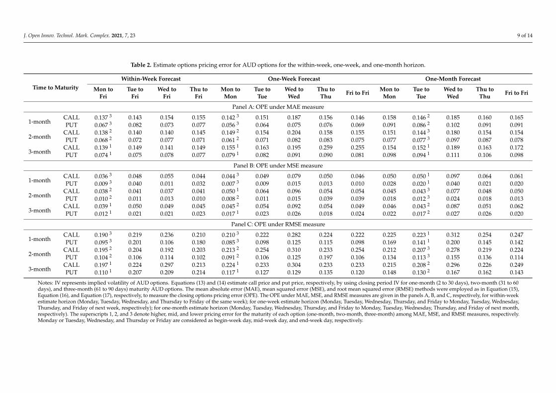
Table 2 describes the performance of IV to price the AUD options for the within-weekforecast horizon, one-week forecast horizon, and one-month forecast horizon.

J. Open Innov. Technol. Mark. Complex. 2021, 7, 23 8 of 14

Table 1. Implied volatility (IV) forecast realised volatility (RV) for Australian dollar (AUD) options for within-week, one-week, and one-month forecast horizon.

Time to MaturityWithin-Week Forecast One-Week Forecast One-Month Forecast

Mon toFri

Tue toFri

Wed toFri

Thu toFri

Mon toMon

Tue toTue

Wed toWed

Thu toThu Fri to Fri Mon to

MonTue to

TueWed to

WedThu to

Thu Fri to Fri

Panel A: Opening period (9:30−10:00)

1-monthSlope 0.207 0.248 0.187 0.152 0.204 0.227 0.249 0.193 0.290 0.199 0.197 0.227 0.138 0.257

R2 0.133 0.1951 0.114 0.102 0.405 0.465 2 0.307 0.262 0.305 0.227 0.228 1 0.162 0.092 0.151

2-monthSlope 0.415 0.479 0.483 0.443 0.366 0.414 0.504 0.445 0.445 0.324 0.337 0.449 0.357 0.361

R2 0.294 0.228 0.335 2 0.300 0.308 0.3651 0.321 0.342 0.238 0.356 0.386 2 0.263 0.217 0.177

3-monthSlope 0.554 0.548 0.569 0.508 0.472 0.435 0.495 0.482 0.540 0.409 0.454 0.447 0.285 0.439

R2 0.221 0.336 2 0.288 0.270 0.253 0.284 1 0.161 0.183 0.212 0.249 0.295 1 0.162 0.202 0.170

Panel B: Midday period (12:30−13:00)

1-monthSlope 0.248 0.245 0.207 0.253 0.216 0.217 0.227 0.310 0.260 0.194 0.196 0.205 0.215 0.224

R2 0.198 0.214 2 0.142 0.172 0.400 0.432 1 0.275 0.349 0.235 0.224 0.260 2 0.156 0.159 0.141

2-monthSlope 0.427 0.411 0.390 0.425 0.364 0.353 0.397 0.436 0.390 0.304 0.317 0.364 0.347 0.290

R2 0.246 0.280 1 0.244 0.257 0.356 0.375 2 0.274 0.347 0.218 0.261 0.332 1 0.241 0.232 0.135

3-monthSlope 0.470 0.486 0.465 0.479 0.396 0.419 0.473 0.513 0.479 0.332 0.385 0.413 0.415 0.362

R2 0.250 0.262 1 0.219 0.240 0.299 0.317 2 0.189 0.315 0.191 0.241 0.327 3 0.208 0.230 0.125

Panel C: Closing period (15:30−16:00)

1-monthSlope 0.274 0.247 0.224 0.272 0.244 0.221 0.260 0.287 0.301 0.228 0.181 0.200 0.207 0.247

R2 0.313 3 0.207 0.160 0.213 0.472 3,* 0.435 0.317 0.329 0.257 0.210 0.275 3 0.146 0.158 0.144

2-monthSlope 0.432 0.427 0.426 0.458 0.378 0.380 0.423 0.430 0.434 0.320 0.322 0.353 0.350 0.325

R2 0.379 3,* 0.273 0.252 0.294 0.3963 0.379 0.298 0.353 0.251 0.285 0.393 3,* 0.215 0.248 0.158

3-monthSlope 0.513 0.500 0.489 0.501 0.438 0.438 0.517 0.496 0.512 0.370 0.394 0.426 0.420 0.399

R2 0.352 3 0.258 0.248 0.292 0.335 3 0.310 0.240 0.290 0.228 0.284 0.310 2 0.207 0.238 0.146

Notes: IV represents implied volatility of Australian dollar (AUD) options. Equation (7) estimates IV using one-month (2 to 30 days), two-month (31 to 60 days), and three-month (61 to 90 days) maturity AUDoptions, for the opening (9:30−10:00), midday (12:30−13:00), and closing (15:30−16:00) a trading day. RV represents the realised volatility of Australian dollar. Equation (11) calculates the RV using the 5-minfrequency AUD spot rate. The Mincer–Zarnowitz (MZ) regression analysis model, as in Equation (12), provides the slope coefficient and R2 of within-week forecast horizon (Monday, Tuesday, Wednesday, andThursday to Friday of the same week), one-week forecast horizon (Monday, Tuesday, Wednesday, Thursday, and Friday to Monday, Tuesday, Wednesday, Thursday, and Friday of next week, respectively),and one-month forecast horizon (Monday, Tuesday, Wednesday, Thursday, and Friday to Monday, Tuesday, Wednesday, Thursday, and Friday of next month, respectively) for the one-month, two-month,and three-month maturity options traded in the opening, midday, and closing of a trading day are given in panels A, B, and C, respectively. The p-value is zero for all cases and is not reported in the table toavoid repetition. Further, the zero p-values indicate that the null hypothesis is rejected at any level of significance. The superscripts 1, 2, and 3 denote the lower, mid, and higher value of R2, respectively,among different trading periods (opening, midday, closing) for the maturity of each option (one-month, two-month, three-month). The * represents the highest value of R2 among one-month, two-month, andthree-month maturity IV that lead the performance of IV to forecast RV for within-week, one-week, and one-month forecast horizon, respectively. Monday or Tuesday, Wednesday, and Thursday or Friday areconsidered as begin-week day, mid-week day, and end-week day, respectively.

J. Open Innov. Technol. Mark. Complex. 2021, 7, 23 9 of 14

Table 2. Estimate options pricing error for AUD options for the within-week, one-week, and one-month horizon.

Time to MaturityWithin-Week Forecast One-Week Forecast One-Month Forecast

Mon toFri

Tue toFri

Wed toFri

Thu toFri

Mon toMon

Tue toTue

Wed toWed

Thu toThu Fri to Fri Mon to

MonTue to

TueWed to

WedThu to

Thu Fri to Fri

Panel A: OPE under MAE measure

1-monthCALL 0.137 3 0.143 0.154 0.155 0.142 3 0.151 0.187 0.156 0.146 0.158 0.146 2 0.185 0.160 0.165PUT 0.067 3 0.082 0.073 0.077 0.056 3 0.064 0.075 0.076 0.069 0.091 0.086 2 0.102 0.091 0.091

2-monthCALL 0.138 2 0.140 0.140 0.145 0.149 2 0.154 0.204 0.158 0.155 0.151 0.144 3 0.180 0.154 0.154PUT 0.068 2 0.072 0.077 0.071 0.061 2 0.071 0.082 0.083 0.075 0.077 0.077 3 0.097 0.087 0.078

3-monthCALL 0.139 1 0.149 0.141 0.149 0.155 1 0.163 0.195 0.259 0.255 0.154 0.152 1 0.189 0.163 0.172PUT 0.074 1 0.075 0.078 0.077 0.079 1 0.082 0.091 0.090 0.081 0.098 0.094 1 0.111 0.106 0.098

Panel B: OPE under MSE measure

1-monthCALL 0.036 3 0.048 0.055 0.044 0.044 3 0.049 0.079 0.050 0.046 0.050 0.050 1 0.097 0.064 0.061PUT 0.009 3 0.040 0.011 0.032 0.007 3 0.009 0.015 0.013 0.010 0.028 0.020 1 0.040 0.021 0.020

2-monthCALL 0.038 2 0.041 0.037 0.041 0.050 1 0.064 0.096 0.054 0.054 0.045 0.043 3 0.077 0.048 0.050PUT 0.010 2 0.011 0.013 0.010 0.008 2 0.011 0.015 0.039 0.039 0.018 0.012 3 0.024 0.018 0.013

3-monthCALL 0.039 1 0.050 0.049 0.045 0.045 2 0.054 0.092 0.054 0.049 0.046 0.043 2 0.087 0.051 0.062PUT 0.012 1 0.021 0.021 0.023 0.017 1 0.023 0.026 0.018 0.024 0.022 0.017 2 0.027 0.026 0.020

Panel C: OPE under RMSE measure

1-monthCALL 0.190 3 0.219 0.236 0.210 0.210 3 0.222 0.282 0.224 0.222 0.225 0.223 1 0.312 0.254 0.247PUT 0.095 3 0.201 0.106 0.180 0.085 3 0.098 0.125 0.115 0.098 0.169 0.141 1 0.200 0.145 0.142

2-monthCALL 0.195 2 0.204 0.192 0.203 0.213 2 0.254 0.310 0.233 0.254 0.212 0.207 3 0.278 0.219 0.224PUT 0.104 2 0.106 0.114 0.102 0.091 2 0.106 0.125 0.197 0.106 0.134 0.113 3 0.155 0.136 0.114

3-monthCALL 0.197 1 0.224 0.297 0.213 0.224 1 0.233 0.304 0.233 0.233 0.215 0.208 2 0.296 0.226 0.249PUT 0.110 1 0.207 0.209 0.214 0.117 1 0.127 0.129 0.135 0.120 0.148 0.130 2 0.167 0.162 0.143

Notes: IV represents implied volatility of AUD options. Equations (13) and (14) estimate call price and put price, respectively, by using closing period IV for one-month (2 to 30 days), two-month (31 to 60days), and three-month (61 to 90 days) maturity AUD options. The mean absolute error (MAE), mean squared error (MSE), and root mean squared error (RMSE) methods were employed as in Equation (15),Equation (16), and Equation (17), respectively, to measure the closing options pricing error (OPE). The OPE under MAE, MSE, and RMSE measures are given in the panels A, B, and C, respectively, for within-weekestimate horizon (Monday, Tuesday, Wednesday, and Thursday to Friday of the same week); for one-week estimate horizon (Monday, Tuesday, Wednesday, Thursday, and Friday to Monday, Tuesday, Wednesday,Thursday, and Friday of next week, respectively); for one-month estimate horizon (Monday, Tuesday, Wednesday, Thursday, and Friday to Monday, Tuesday, Wednesday, Thursday, and Friday of next month,respectively). The superscripts 1, 2, and 3 denote higher, mid, and lower pricing error for the maturity of each option (one-month, two-month, three-month) among MAE, MSE, and RMSE measures, respectively.Monday or Tuesday, Wednesday, and Thursday or Friday are considered as begin-week day, mid-week day, and end-week day, respectively.

J. Open Innov. Technol. Mark. Complex. 2021, 7, 23 10 of 14

For the within-week forecast horizon, under the MAE measure, one-month (call pric-ing error = 0.137 and put pricing error = 0.067) maturity IV of Monday outperformed whenestimating AUD call and put options. Next, for the MSE measure, one-month (call pric-ing error = 0.036 and put pricing error = 0.009) maturity IV of Monday was superior toprice AUD call and put options. Finally, under the RMSE measure of Monday, one-month(call pricing error = 0.190 and put pricing error = 0.095) maturity IV held appropriateinformation to compute AUD call and put options. Overall, the one-month maturity ofMonday (begin-week day) IV contained vital information to price AUD options.

For the one-week horizon, under the MAE measure, one-month (call pricing error =0.142 and put pricing error = 0.056) maturity IV of Monday held appropriate information toestimate the AUD call and put options. Next, for the MSE measure, one-month (call pricingerror = 0.044 and put pricing error = 0.007) maturity IV of Monday was superior to price theAUD call and put options. Finally, under the RMSE measure, one-month (call pricing error= 0.210 and put pricing error = 0.085) maturity IV of Monday contained vital informationto compute the AUD call and put options. Overall, the one-month maturity of Monday(begin-week day) IV held critical information to estimate the price of the AUD options.

For the one-month horizon, under the MAE measure, two-month (call pricing er-ror = 0.144 and put pricing error = 0.077) maturity IV of Tuesday provided appropriateinformation to estimate the AUD call and put options. Next, for the MSE measure, two-month (call pricing error = 0.043 and put pricing error = 0.012) maturity IV of Tuesdayoutperformed when pricing AUD call and put options. Finally, under the RMSE measure,two-month (call pricing error = 0.207 and put pricing error = 0.113) maturity IV of Tuesdaycontained vital information to compute the AUD call and put options. Overall, two-monthmaturity of Tuesday (begin-week day) IV held critical information to estimate the price ofthe AUD options.

5. Discussion

Our paper employed the tick data obtained from Thomson Reuters’ database, anarchive of historical every-minute data drawn from the real-time content. The use of bigdata would enable efficiency and speed to innovation. Financial innovation, such as venturecapital, equity funds, and exchange-traded funds contributed positively to the financialdeepening and economic growth [61,62]. The application of the information in portfoliomanagement also allows the generation of high-frequency trading, which is considered afinancial innovation, concentrating on order flow and rapidly evolving information [63].In the derivatives market, millions of calculations need to be conducted daily to pricederivative instruments to manage the risks and to determine hedge positions. However,information obtained from these computations is useful for only a limited period and willbe outdated when the market moves. De Spiegeleer et al. [64] indicated that the use ofreal-time data and market information was mandatory in successfully running a derivativebusiness in the present era of information explosion. As technology is increasing and theworld overwhelmed by numbers and digits [65], forecasting volatility and options pricebased on the intraday data is crucial for the immediate investment decision making.

The empirical analysis indicated that the IV at the closing period performed better inpredicting RV for all forecast horizons. As more intensive trading occurred at the end ofthe trading day, more valuable information to forecast future volatility can be extractedfrom the options price at the market close [66]. The within-week horizon provides a mixedpicture for IV in terms of holding information to forecast RV. It suggests that the IV doesnot contain relevant information to predict the volatility of the underlying currency ofoptions for a one- to four-day forecast horizon. Therefore, the intraday IV is not appropriateto estimate the currency options price for the within-week horizon. The one-month andtwo-month maturity; begin-week day and closing period of IV hold relevant information toforecast RV for the one-week and one-month forecast horizon, respectively. It reveals thatthe information content embedded in one-month and two-month maturity IV is significantin predicting the volatility of the underlying currency of options for the one-week and

J. Open Innov. Technol. Mark. Complex. 2021, 7, 23 11 of 14

one-month forecast horizon, respectively. Consequently, a one-month and two-monthmaturity IV is appropriate to estimate the currency options price for the one-week and one-month estimate horizon, respectively. These findings are in line with the research of Garveyand Gallagher [10] that examined the forecastability of IV using a sample of 16 FTSE-100stocks and found that IV provided a useful volatility forecasting method, especially for themedium forecasting horizons between ten and thirty days. Although most of the previousresearch using data from stock market showed that the optimal forecast horizon of IV wasfrom one day to less than thirty days [22,56], our results showed that the IV did not workwell for the short forecast horizons from one day to four days, but it performed superiorlyfor the medium forecast horizons from one week to one month.

6. Conclusions

The accuracy of currency options pricing plays a crucial role in managing financial risk,providing a source of financial leverage for speculators, and preventing the opportunityfor abnormal arbitrage profit. To calculate prices of currency options using the Merton [15]version of the BSM model, only the volatility of the underlying currency is not observablein the market. As volatility estimation errors lead to options mispricing, accurate forecastsof future volatility of underlying assets are essential for estimating and forecasting thecurrency options price. The IV is widely used to estimate the volatility of FX. The majorityof the studies involving IV often find that the most relevant information for predicting anunderlying asset’s volatility can be found in the options price. Therefore, this paper wasparticularly interested in FX volatility prediction for pricing currency options. However,it is argued that the daily IV holds discrete information regarding the FX movement ata specific time of the trading day, which is not sufficient for estimating options pricesaccurately [67]. This study, therefore, introduces intraday IV through estimating IV for theprice of options with different maturity during the opening, midday, and closing period ofa trading day. The intraday IV approach will add a new dimension in the literature for thepricing currency option with higher accuracy.

Overall, the results suggest four key insights. First, three-month maturity IV doesnot hold vital information about future volatility of the underlying currency and pricingcurrency options. It happens because the shorter period information of one-month andtwo-month maturity options are useful compared to the longer period information ofthree-month maturity options. Second, IV incorporating all information is not relevantin computing the value of currency options for a horizon estimate that is less than aweek. This is due to FX volatility following clustering, and both information contentday (e.g., Monday) and forecasting day (i.e., Friday) lying in the same cluster. Third,IV for the closing period on Monday or Tuesday includes the most useful informationcompared to other periods of trading day and other days of the week when forecastingthe volatility of the underlying currency and estimating the price of currency options.This occurs as all weekdays do not hold equally relevant information or critical informationdiminishes gradually from the middle of the week. Fourth, the shorter (longer) maturityIV provides essential information when pricing currency options for the shorter (longer)horizon. If the currency options are overpriced, the hedgers and speculators experiencethe higher cost for buying or holding currency options. However, the options becomeprofitable for the options seller or writer. Further, the cost of hedging and speculationis less when options are underpriced. This also makes an opportunity cost loss for theoptions seller. The paper’s results can provide valuable information to fund managersto hedge extreme risk and allow policy makers to construct a comprehensive strategy toprevent the opportunity for abnormal arbitrage profit. High-frequency traders can referto these results to select valuable and useful intraday information for their immediatedecision marking. The sample data obtained for this research from the exchange-tradedmarket is not as big as the OTC market. BIS (2019) reported that the currency options aretraded not only in the exchanges, but a considerable volume of currency options are alsotraded in the interbank market due to the customisation benefit of OTC currency options

J. Open Innov. Technol. Mark. Complex. 2021, 7, 23 12 of 14

over options traded in exchanges. Moreover, the study limits the data sample in the AUDcurrency options that represent the developed market. The research findings may notbe appropriate to apply to the other FX markets that experience different characteristicssuch as currency markets of emerging countries. The covered period of the dataset is from1 January 2010 to 31 December 2017 due to the large volume of high-frequency data thatneeds to be collected. Therefore, our research captures particular economic circumstancesin the context of the post Global Financial crisis period. The research results may benot suitable to apply for different economic circumstances such as before and during thecrisis period. However, the information content of the IV during a crisis period is alsopeculiarly relevant [68,69] as it provides incremental and valuable information to hedgefinancial risk and to bring us a better understanding of market sentiment and behaviour.Hence, the avenue for potential further research concerns extending this research to theemerging currency options, using data from the OTC market, or testing the research resultsin different economic circumstances. As each type and each period of FX market containspeculiar characteristics, the investigations of intraday IV in other market conditions arenecessary to provide a fully comprehensive view of its performance in forecasting thevolatility of the underlying currency and estimating the value of currency options.

Author Contributions: Conceptualization, T.L. and A.H.; methodology, T.L. and A.H.; software, T.L.and A.H.; validation, T.L., A.H., and K.H.; formal analysis, T.L.; investigation, T.L.; resources, T.L.and A.H.; data curation, T.L. and A.H.; writing—original draft preparation, T.L., A.H., and K.H.;writing—review and editing, T.L., A.H., and K.H.; visualization, T.L.; supervision, A.H. and K.H.;project administration, A.H.; funding acquisition, A.H. All authors have read and agreed to thepublished version of the manuscript.

Funding: This research received no external funding.

Data Availability Statement: Data is available on request.

Conflicts of Interest: For this study, the authors declare no conflict of interest.

References1. Reserve Bank of Australia. Available online: https://www.rba.gov.au/media-releases/2019/mr-19-25-tables.html (accessed on

9 December 2020).2. Vohra, S.; Fabozzi, F.J. Effectiveness of developed and emerging market FX options in active currency risk management. J. Int.

Money Financ. 2019, 96, 130–146. [CrossRef]3. Beer, S.; Fink, H. Dynamics of foreign exchange implied volatility and implied correlation surfaces. Quant. Financ. 2019, 19,

1293–1320. [CrossRef]4. Lai, Y.-W.; Lin, C.-F.; Tang, M.-L. Mispricing and trader positions in the S&P 500 index futures market. N. Am. J. Econ. Financ.

2017, 42, 250–265. [CrossRef]5. Becker, R.; Clements, A.E.; White, S.I. On the informational efficiency of S&P500 implied volatility. N. Am. J. Econ. Financ. 2006,

17, 139–153. [CrossRef]6. Black, F.; Scholes, M. The Pricing of Options and Corporate Liabilities. World Sci. Ref. Conting. Claims Anal. Corp. Financ. 2019, 83,

3–21. [CrossRef]7. Yang, S.-H.; Lee, J. Predicting a distribution of implied volatilities for option pricing. Expert Syst. Appl. 2011, 38, 1702–1708. [CrossRef]8. Fleming, J. The quality of market volatility forecasts implied by S&P 100 index option prices. J. Empir. Financ. 1998, 5, 317–345. [CrossRef]9. Nelson, D.B. Conditional Heteroskedasticity in Asset Returns: A New Approach. Econometrica 1991, 59, 347. [CrossRef]10. Garvey, J.; Gallagher, L.A. The Realised-Implied Volatility Relationship: Recent Empirical Evidence from FTSE-100 Stocks.

J. Forecast. 2011, 31, 639–660. [CrossRef]11. Kearney, F.; Cummins, M.; Murphy, F. Forecasting implied volatility in foreign exchange markets: A functional time series

approach. Eur. J. Financ. 2017, 24, 1–18. [CrossRef]12. Muzzioli, S. Option-based forecasts of volatility: An empirical study in the DAX-index options market. Eur. J. Financ. 2010, 16,

561–586. [CrossRef]13. Taylor, S.J.; Yadav, P.K.; Zhang, Y. The information content of implied volatilities and model-free volatility expectations: Evidence

from options written on individual stocks. J. Bank. Financ. 2010, 34, 871–881. [CrossRef]14. Corredor, P.; Santamaria, R. Forecasting volatility in the Spanish option market. Appl. Financ. Econ. 2004, 14, 1–11. [CrossRef]15. Merton, R.C. Theory of Rational Option Pricing. Bell J. Econ. Manag. Sci. 1973, 4, 141. [CrossRef]16. Cruz, M.G. Modeling, Measuring and Hedging Operational Risk, 1st ed.; John Wiley & Sons Ltd.: New York, NY, USA, 2008; pp. 1–346.17. Singh, S. Performance of Black-Scholes model with TSRV estimates. Manag. Financ. 2015, 41, 857–870. [CrossRef]

J. Open Innov. Technol. Mark. Complex. 2021, 7, 23 13 of 14

18. Tu, A.H.; Hsieh, W.-L.G.; Wu, W.-S. Market uncertainty, expected volatility and the mispricing of S&P 500 index futures. J. Empir.Financ. 2016, 35, 78–98. [CrossRef]

19. Byun, S.J.; Hyun, J.; Sung, W.J. Estimation of stochastic volatility and option prices. J. Futur. Mark. 2020, 1–12. [CrossRef]20. Wang, Y.-H.; Wang, Y.-Y. The Information Content of Intraday Implied Volatility for Volatility Forecasting. J. Forecast. 2015, 35,

167–178. [CrossRef]21. Beckers, S. Standard deviations implied in option prices as predictors of future stock price variability. J. Bank. Financ. 1981, 5,

363–381. [CrossRef]22. Brous, P.; Ince, U.; Popova, I. Volatility forecasting and liquidity: Evidence from individual stocks. J. Deriv. Hedge Funds 2010, 16,

144–159. [CrossRef]23. Busch, T.; Christensen, B.J.; Nielsen, M.Ø. The role of implied volatility in forecasting future realized volatility and jumps in

foreign exchange, stock, and bond markets. J. Econ. 2011, 160, 48–57. [CrossRef]24. Latane, H.A.; Rendleman, R.J. Standard Deviations of Stock Price Ratios Implied in Option Prices. J. Financ. 1976, 31, 369. [CrossRef]25. Schmalensee, R.; Trippi, R.R. Common stock volatility expectations implied by option premia. J. Financ. 1978, 33, 129–147. [CrossRef]26. Andersen, T.G.; Bollerslev, T.; Diebold, F.X.; Labys, P. Exchange Rate Returns Standardised by Realised Volatility Are (Nearly)

Gaussian. Multinatl. Financ. J. 2000, 4, 159–179. [CrossRef]27. Scott, E.; Tucker, A.L. Predicting currency return volatility. J. Bank. Financ. 1989, 13, 839–851. [CrossRef]28. Goodhart, C.A.; O’Hara, M. High frequency data in financial markets: Issues and applications. J. Empir. Financ. 1997, 4, 73–114.

[CrossRef]29. Cai, C.X.; Hudson, R.; Keasey, K. Intra Day Bid-Ask Spreads, Trading Volume and Volatility: Recent Empirical Evidence from the

London Stock Exchange. J. Bus. Financ. Account. 2004, 31, 647–676. [CrossRef]30. Bank for International Settlements. Available online: https://www.bis.org/publ/bppdf/bispap109.pdf (accessed on 9 December 2020).31. Xu, X.; Taylor, S.J. The Term Structure of Volatility Implied by Foreign Exchange Options. J. Financ. Quant. Anal. 1994, 29, 57. [CrossRef]32. Jorion, P. Predicting Volatility in the Foreign Exchange Market. J. Financ. 1995, 50, 507–528. [CrossRef]33. Kazantzis, C.; Tessaromatis, N. Volatility in currency markets. Manag. Financ. 2001, 27, 1–22. [CrossRef]34. Kim, M.; Kim, M. Implied volatility dynamics in the foreign exchange markets. J. Int. Money Financ. 2003, 22, 511–528. [CrossRef]35. Chang, E.J.; Tabak, B.M. Are implied volatilities more informative? The Brazilian real exchange rate case. Appl. Financ. Econ.

2007, 17, 569–576. [CrossRef]36. Pılbeam, K.; Langeland, K.N. Forecasting exchange rate volatility: GARCH models versus implied volatility forecasts. Int. Econ.

Econ. Policy 2014, 12, 127–142. [CrossRef]37. Sahoo, S.; Trivedi, P. The Interrelationship Between Implied and Realized Exchange Rate Volatility in India †. IUP J. Appl. Econ.

2018, 17, 7–26.38. Wong, A.H.-S.; Heaney, R. Volatility Smile and One-Month Foreign Currency Volatility Forecasts. J. Future Mark. 2016, 37, 286–312.

[CrossRef]39. Covrig, V.; Low, B.S. The quality of volatility traded on the over-the-counter currency market: A multiple horizons study. J. Future

Mark. 2003, 23, 261–285. [CrossRef]40. Pong, S.; Shackleton, M.B.; Taylor, S.J.; Xu, X. Forecasting currency volatility: A comparison of implied volatilities and AR(FI)MA

models. J. Bank. Financ. 2004, 28, 2541–2563. [CrossRef]41. Christoffersen, P.; Mazzotta, S. The Accuracy of Density Forecasts from Foreign Exchange Options. J. Financ. Econ. 2005, 3,

578–605. [CrossRef]42. Engle, R.F. The Econometrics of Ultra-high-frequency Data. Econometrica 2000, 68, 1–22. [CrossRef]43. Batten, J.A.; Lucey, B.; McGroarty, F.; Peat, M.; Urquhart, A. Stylized facts of intraday precious metals. PLoS ONE 2017, 12,

e0174232. [CrossRef] [PubMed]44. Wood, R.A.; McInish, T.H.; Ord, J.K. An Investigation of Transactions Data for NYSE Stocks. J. Financ. 1985, 40, 723–739.

[CrossRef]45. Gerety, M.S.; Mulherin, J.H. Trading Halts and Market Activity: An Analysis of Volume at the Open and the Close. J. Financ. 1992,

47, 1765–1784. [CrossRef]46. Brock, W.A.; Kleidon, A.W. Periodic market closure and trading volume. J. Econ. Dyn. Control. 1992, 16, 451–489. [CrossRef]47. McInish, T.H.; Wood, R.A. An analysis of transactions data for the Toronto Stock Exchange. J. Bank. Financ. 1990, 14, 441–458. [CrossRef]48. Hamao, Y.; Hasbrouck, J. Securities Trading in the Absence of Dealers: Trades and Quotes on the Tokyo Stock Exchange.

Rev. Financ. Stud. 1995, 8, 849–878. [CrossRef]49. Ellul, A.; Shin, H.S.; Tonks, I. Towards Deep and Liquid Markets: Lessons from Open and Close at the London Stock Exchange;

LSE Financial Markets Group Working Paper: London, UK, 2002.50. Naik, N.Y.; Yadav, P.K. The Effects of Market Reform on Trading Costs of Public Investors: Evidence from the London Stock

Exchange. Ssrn Electron. J. 1999. [CrossRef]51. Taylor, S.J.; Xu, X. The incremental volatility information in one million foreign exchange quotations. J. Empir. Financ. 1997, 4,

317–340. [CrossRef]52. Barndorff-Nielsen, O.E.; Shephard, N. Econometric Analysis of Realised Volatility and Its Use in Estimating Stochastic Volatility

Models. Journal of the Royal Statistical Society. J. R. Stat. Soc. Ser. B Stat. Methodol. 2002, 64, 253–280. [CrossRef]

J. Open Innov. Technol. Mark. Complex. 2021, 7, 23 14 of 14

53. Liu, L.Y.; Patton, A.J.; Sheppard, K. Does anything beat 5-minute RV? A comparison of realized measures across multiple assetclasses. J. Econ. 2015, 187, 293–311. [CrossRef]

54. Hull, J.; White, A. The Pricing of Options on Assets with Stochastic Volatilities. J. Financ. 1987, 42, 281–300. [CrossRef]55. Xing, Y.; Zhang, X.; Zhao, R. What Does the Individual Option Volatility Smirk Tell Us About Future Equity Returns? J. Financ.

Quant. Anal. 2010, 45, 641–662. [CrossRef]56. Blair, B.J.; Poon, S.-H.; Taylor, S.J. Forecasting S&P 100 volatility: The incremental information content of implied volatilities and

high-frequency index returns. J. Econ. 2001, 105, 5–26. [CrossRef]57. Press, W.H.; Flannery, B.P.; Vetterling, W.T. Numerical Recipes in C: The Art of Scientific Computing, 2nd ed.; Cambridge University

Press: Cambridge, UK, 1992; ISBN 0-521-43108-5.58. Andersen, T.G.; Bollerslev, T. Answering the Skeptics: Yes, Standard Volatility Models do Provide Accurate Forecasts. Int. Econ.

Rev. 1998, 39, 885. [CrossRef]59. Mincer, J.; Zarnowitz, V. The evaluation of economic forecasts. In Economic Forecasts and Expectations; Zarnowitz, J., Ed.; National

Bureau of Economic Research: New York, NY, USA, 1969; pp. 3–46.60. Guler, K.; Ng, P.T.; Xiao, Z. Mincer-Zarnowitz quantile and expectile regressions for forecast evaluations under aysmmetric loss

functions. J. Forecast. 2017, 36, 651–679. [CrossRef]61. Lerner, J.; Tufano, P. The Consequences of Financial Innovation: A Counterfactual Research Agenda. Annu. Rev. Financ. Econ.

2011, 3, 41–85. [CrossRef]62. Beck, T.; Chen, T.; Lin, C.; Song, F. Financial innovation: The bright and the dark sides. J. Bank. Financ. 2016, 72, 28–51. [CrossRef]63. Dalko, V.; Wang, M.H. High-frequency trading: Order-based innovation or manipulation? J. Bank. Regul. 2020, 21, 289–298. [CrossRef]64. De Spiegeleer, J.; Madan, D.B.; Reyners, S.; Schoutens, W. Machine learning for quantitative finance: Fast derivative pricing,

hedging and fitting. Quant. Financ. 2018, 18, 1635–1643. [CrossRef]65. Ye, M.; Li, G. Internet big data and capital markets: A literature review. Financ. Innov. 2017, 3, 6. [CrossRef]66. Caporale, G.M.; Gil-Alana, L.; Plastun, A.; Makarenko, I. Intraday Anomalies and Market Efficiency: A Trading Robot Analysis.

Comput. Econ. 2015, 47, 275–295. [CrossRef]67. Baillie, R.T.; Bollerslev, T. Intra-Day and Inter-Market Volatility in Foreign Exchange Rates. Rev. Econ. Stud. 1991, 58, 565–585. [CrossRef]68. Bates, D.S. U.S. stock market crash risk, 1926–2010. J. Financ. Econ. 2012, 105, 229–259. [CrossRef]69. Hilal, S.; Poon, S.-H.; Tawn, J.A. Hedging the black swan: Conditional heteroskedasticity and tail dependence in S&P500 and VIX.

J. Bank. Financ. 2011, 35, 2374–2387. [CrossRef]