Selected chapters from draft of An Introduction to Game Theory by Martin J. Osborne Please send comments to Martin J. Osborne Department of Economics 150 St. George Street University of Toronto Toronto, Canada M5S 3G7 email: [email protected] This version: 2000/11/6

Welcome message from author
This document is posted to help you gain knowledge. Please leave a comment to let me know what you think about it! Share it to your friends and learn new things together.
Transcript
Selected chapters from draft of
An Introduction to Game TheorybyMartin J. Osborne
Please send comments to
Martin J. Osborne
Department of Economics150 St. George Street
University of Toronto
Toronto, Canada M5S 3G7
email: [email protected]
This version: 2000/11/6
Copyright c© 1995–2000 by Martin J. Osborne
All rights reserved. No part of this book may be reproduced by any electronic or mechanical means(including photocopying, recording, or information storage and retrieval) without permission inwriting from Oxford University Press.
Contents
Preface xiii
1 Introduction 1
1.1 What is game theory? 1
An outline of the history of game theory 3John von Neumann 3
1.2 The theory of rational choice 4
1.3 Coming attractions 7
Notes 8
I Games with Perfect Information 9
2 Nash Equilibrium: Theory 11
2.1 Strategic games 11
2.2 Example: the Prisoner’s Dilemma 12
2.3 Example: Bach or Stravinsky? 16
2.4 Example: Matching Pennies 17
2.5 Example: the Stag Hunt 18
2.6 Nash equilibrium 19
John F. Nash, Jr. 20Studying Nash equilibrium experimentally 22
2.7 Examples of Nash equilibrium 24
Experimental evidence on the Prisoner’s Dilemma 26Focal points 30
2.8 Best response functions 33
2.9 Dominated actions 43
2.10 Equilibrium in a single population: symmetric games and symmetric
equilibria 49
Notes 51
v
vi Contents
3 Nash Equilibrium: Illustrations 53
3.1 Cournot’s model of oligopoly 53
3.2 Bertrand’s model of oligopoly 61
Cournot, Bertrand, and Nash: some historical notes 673.3 Electoral competition 68
3.4 The War of Attrition 75
3.5 Auctions 79
Auctions from Babylonia to eBay 793.6 Accident law 89
Notes 94
4 Mixed Strategy Equilibrium 97
4.1 Introduction 97
Some evidence on expected payoff functions 1024.2 Strategic games in which players may randomize 103
4.3 Mixed strategy Nash equilibrium 105
4.4 Dominated actions 117
4.5 Pure equilibria when randomization is allowed 119
4.6 Illustration: expert diagnosis 120
4.7 Equilibrium in a single population 125
4.8 Illustration: reporting a crime 128
Reporting a crime: social psychology and game theory 1304.9 The formation of players’ beliefs 131
4.10 Extension: Finding all mixed strategy Nash equilibria 135
4.11 Extension: Mixed strategy Nash equilibria of games in which each player
has a continuum of actions 139
4.12 Appendix: Representing preferences over lotteries by the expected value of
a payoff function 143
Notes 148
5 Extensive Games with Perfect Information: Theory 151
5.1 Introduction 151
5.2 Extensive games with perfect information 151
5.3 Strategies and outcomes 157
5.4 Nash equilibrium 159
5.5 Subgame perfect equilibrium 162
5.6 Finding subgame perfect equilibria of finite horizon games: backward
induction 167
Ticktacktoe, chess, and related games 176Notes 177
Contents vii
6 Extensive Games with Perfect Information: Illustrations 179
6.1 Introduction 179
6.2 The ultimatum game and the holdup game 179
Experiments on the ultimatum game 1816.3 Stackelberg’s model of duopoly 184
6.4 Buying votes 189
6.5 A race 194
Notes 200
7 Extensive Games with Perfect Information: Extensions and Discussion 201
7.1 Allowing for simultaneous moves 201
More experimental evidence on subgame perfect equilibrium 2077.2 Illustration: entry into a monopolized industry 209
7.3 Illustration: electoral competition with strategic voters 211
7.4 Illustration: committee decision-making 213
7.5 Illustration: exit from a declining industry 217
7.6 Allowing for exogenous uncertainty 222
7.7 Discussion: subgame perfect equilibrium and backward induction 226
Experimental evidence on the centipede game 230Notes 232
8 Coalitional Games and the Core 235
8.1 Coalitional games 235
8.2 The core 239
8.3 Illustration: ownership and the distribution of wealth 243
8.4 Illustration: exchanging homogeneous horses 247
8.5 Illustration: exchanging heterogeneous houses 252
8.6 Illustration: voting 256
8.7 Illustration: matching 259
Matching doctors with hospitals 2648.8 Discussion: other solution concepts 265
Notes 266
viii Contents
II Games with Imperfect Information 269
9 Bayesian Games 271
9.1 Introduction 271
9.2 Motivational examples 271
9.3 General definitions 276
9.4 Two examples concerning information 281
9.5 Illustration: Cournot’s duopoly game with imperfect information 283
9.6 Illustration: providing a public good 287
9.7 Illustration: auctions 290
Auctions of the radio spectrum 2989.8 Illustration: juries 299
9.9 Appendix: Analysis of auctions for an arbitrary distribution of
valuations 306
Notes 309
10 Extensive games with imperfect information 311
10.1 To be written 311
Notes 312
III Variants and Extensions 333
11 Strictly Competitive Games and Maxminimization 335
11.1 Introduction 335
11.2 Definitions and examples 335
11.3 Strictly competitive games 338
Maxminimization: some history 344Testing the theory of Nash equilibrium in strictly competitive
games 347Notes 348
12 Rationalizability 349
12.1 Introduction 349
12.2 Iterated elimination of strictly dominated actions 355
12.3 Iterated elimination of weakly dominated actions 359
Notes 361
Contents ix
13 Evolutionary Equilibrium 363
13.1 Introduction 363
13.2 Monomorphic pure strategy equilibrium 364
Evolutionary game theory: some history 36913.3 Mixed strategies and polymorphic equilibrium 370
13.4 Asymmetric equilibria 377
Explaining the outcomes of contests in nature 37913.5 Variation on a theme: sibling behavior 380
13.6 Variation on a theme: nesting behavior of wasps 386
Notes 388
14 Repeated games: The Prisoner’s Dilemma 389
14.1 The main idea 389
14.2 Preferences 391
14.3 Infinitely repeated games 393
14.4 Strategies 394
14.5 Some Nash equilibria of the infinitely repeated Prisoner’s Dilemma 396
14.6 Nash equilibrium payoffs of the infinitely repeated Prisoner’s Dilemma when
the players are patient 398
14.7 Subgame perfect equilibria and the one-deviation property 402
14.8 Some subgame perfect equilibria of the infinitely repeated Prisoner’s
Dilemma 404
Notes 409
15 Repeated games: General Results 411
15.1 Nash equilibria of general infinitely repeated games 411
15.2 Subgame perfect equilibria of general infinitely repeated games 414
Axelrod’s experiments 418Reciprocal altruism among sticklebacks 419
15.3 Finitely repeated games 420
Notes 420
16 Bargaining 421
16.1 To be written 421
16.2 Repeated ultimatum game 421
16.3 Holdup game 421
x Contents
17 Appendix: Mathematics 443
17.1 Introduction 443
17.2 Numbers 443
17.3 Sets 444
17.4 Functions 445
17.5 Profiles 448
17.6 Sequences 449
17.7 Probability 449
17.8 Proofs 454
References 457
Preface
Game theoretic reasoning pervades economic theory and is used widely in othersocial and behavioral sciences. This book presents the main ideas of game theoryand shows how they can be used to understand economic, social, political, and bi-ological phenomena. It assumes no knowledge of economics, political science, orany other social or behavioral science. It emphasizes the ideas behind the theoryrather than their mathematical expression, and assumes no specific mathematicalknowledge beyond that typically taught in US and Canadian high schools. (Chap-ter 17 reviews the mathematical concepts used in the book.) In particular, calculusis not used, except in the appendix of Chapter 9 (Section 9.7). Nevertheless, allconcepts are defined precisely, and logical reasoning is used extensively. The morecomfortable you are with tight logical analysis, the easier you will find the argu-ments. In brief, my aim is to explain the main ideas of game theory as simply aspossible while maintaining complete precision.
The only way to appreciate the theory is to see it in action, or better still to putit into action. So the book includes a wide variety of illustrations from the socialand behavioral sciences, and over 200 exercises.
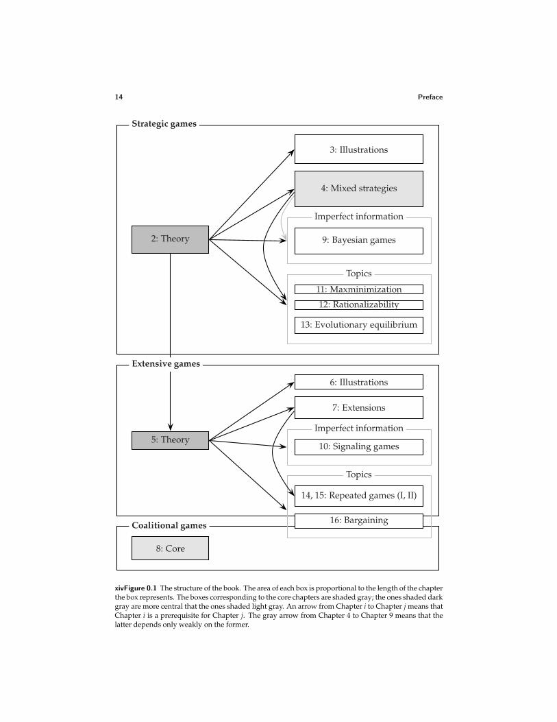
The structure of the book is illustrated in the figure on the next page. Thegray boxes indicate core chapters (the darker gray, the more important). An blackarrow from Chapter i to Chapter j means that Chapter j depends on Chapter i.The gray arrow from Chapter 4 to Chapter 9 means that the latter depends weaklyon the former; for all but Section 9.8 only an understanding of expected payoffs(Section 4.1.3) is required, not a knowledge of mixed strategy Nash equilibrium.(Two chapters are not included in this figure: Chapter 1 reviews the theory of asingle rational decision-maker, and Chapter 17 reviews the mathematical conceptsused in the book.)
Each topic is presented with the aid of “Examples”, which highlight theoreti-cal points, and “Illustrations”, which demonstrate how the theory may be used tounderstand social, economic, political, and biological phenomena. The “Illustra-tions” for the key models of strategic and extensive games are grouped in separatechapters (3 and 6), whereas those for the other models occupy the same chaptersas the theory. The “Illustrations” introduce no new theoretical points, and any orall of them may be skipped without loss of continuity.
The limited dependencies between chapters mean that several routes may betaken through the book.
• At a minimum, you should study Chapters 2 (Nash Equilibrium: Theory)and 5 (Extensive Games with Perfect Information: Theory).
• Optionally you may sample some sections of Chapters 3 (Nash Equilibrium:
14 Preface
Strategic games
2: Theory
3: Illustrations
4: Mixed strategies
9: Bayesian games
Imperfect information
11: Maxminimization
12: Rationalizability
13: Evolutionary equilibrium
Topics
Extensive games
5: Theory
6: Illustrations
7: Extensions
10: Signaling games
Imperfect information
14, 15: Repeated games (I, II)
Coalitional games
8: Core
16: Bargaining
Topics
xivFigure 0.1 The structure of the book. The area of each box is proportional to the length of the chapterthe box represents. The boxes corresponding to the core chapters are shaded gray; the ones shaded darkgray are more central that the ones shaded light gray. An arrow from Chapter i to Chapter j means thatChapter i is a prerequisite for Chapter j. The gray arrow from Chapter 4 to Chapter 9 means that thelatter depends only weakly on the former.

Preface 15
Illustrations) and 6 (Extensive Games with Perfect Information: Illustrations).
• You may add to this plan any combination of Chapters 4 (Mixed StrategyEquilibrium), 9 (Bayesian Games, except Section 9.8), 7 (Extensive Gameswith Perfect Information: Extensions and Discussion), 8 (Coalitional Gamesand the Core), and 16 (Bargaining).
• If you read Chapter 4 (Mixed Strategy Equilibrium) then you may in additionstudy any combination of the remaining chapters covering strategic games,and if you study Chapter 7 (Extensive Games with Perfect Information: Ex-tensions and Discussion) then you are ready to tackle Chapters 14 and 15(Repeated Games).
All the material should be accessible to undergraduate students. A one-semestercourse for third or fourth year North American economics majors (who have beenexposed to a few of the main ideas in first and second year courses) could coverup to about half the material in the book in moderate detail.
Personal pronouns
The lack of a sex-neutral third person singular pronoun in English has led manywriters of formal English to use “he” for this purpose. Such usage conflicts withthat of everyday speech. People may say “when an airplane pilot is working, heneeds to concentrate”, but they do not usually say “when a flight attendant isworking, he needs to concentrate” or “when a secretary is working, he needs toconcetrate”. The use of “he” only for roles in which men traditionally predomi-nate in Western societies suggests that women may not play such roles; I find thisinsinuation unacceptable.
To quote the New Oxford Dictionary of English, “[the use of he to refer to refer toa person of unspecified sex] has become . . . a hallmark of old-fashioned languageor sexism in language.” Writers have become sensitive to this issue in the last halfcentury, but the lack of a sex-neutral pronoun “has been felt since at least as farback as Middle English” (Webster’s Dictionary of English Usage, Merriam-WebsterInc., 1989, p. 499). A common solution has been to use “they”, a usage that theNew Oxford Dictionary of English endorses (and employs). This solution can createambiguity when the pronoun follows references to more than one person; it alsodoes not always sound natural. I choose a different solution: I use “she” exclu-sively. Obviously this usage, like that of “he”, is not sex-neutral; but its use maydo something to counterbalance the widespread use of “he”, and does not seemlikely to do any harm.
Acknowledgements
I owe a huge debt to Ariel Rubinstein. I have learned, and continue to learn, vastlyfrom him about game theory. His influence on this book will be clear to anyone
16 Preface
familiar with our jointly-authored book A course in game theory. Had we not writtenthat book and our previous book Bargaining and markets, I doubt that I would haveembarked on this project.
Discussions over the years with Jean-Pierre Benoıt, Vijay Krishna, Michael Pe-ters, and Carolyn Pitchik have improved my understanding of many game theo-retic topics.
Many people have generously commented on all or parts of drafts of the book.I am particularly grateful to Jeffrey Banks, Nikolaos Benos, Ted Bergstrom, TilmanBorgers, Randy Calvert, Vu Cao, Rachel Croson, Eddie Dekel, Marina De Vos, Lau-rie Duke, Patrick Elias, Mukesh Eswaran, Xinhua Gu, Costas Halatsis, Joe Har-rington, Hiroyuki Kawakatsu, Lewis Kornhauser, Jack Leach, Simon Link, BartLipman, Kin Chung Lo, Massimo Marinacci, Peter McCabe, Barry O’Neill, RobinG. Osborne, Marco Ottaviani, Marie Rekkas, Bob Rosenthal, Al Roth, MatthewShum, Giora Slutzki, Michael Smart, Nick Vriend, and Chuck Wilson.
I thank also the anonymous reviewers consulted by Oxford University Pressand several other presses; the suggestions in their reviews greatly improved thebook.
The book has its origins in a course I taught at Columbia University in the early1980s. My experience in that course, and in courses at McMaster University, whereI taught from early drafts, and at the University of Toronto, brought the book toits current form. The Kyoto Institute of Economic Research at Kyoto Universityprovided me with a splendid environment in which to work on the book duringtwo months in 1999.
References
The “Notes” section at the end of each chapter attempts to assign credit for theideas in the chapter. Several cases present difficulties. In some cases, ideas evolvedover a long period of time, with contributions by many people, making their ori-gins hard to summarize in a sentence or two. In a few cases, my research has ledto a conclusion about the origins of an idea different from the standard one. In allcases, I cite the relevant papers without regard to their difficulty.
Over the years, I have taken exercises from many sources. I have attemptedto remember where I got them from, and have given credit, but I have probablymissed some.
Examples addressing economic, political, and biological issues
The following tables list examples that address economic, political, and biologicalissues. [SO FAR CHECKED ONLY THROUGH CHAPTER 7.]
Games related to economic issues (THROUGH CHAPTER 7)
Preface 17
Exercise 31.1,Section 2.8.4,Exercise 42.1
Provision of a public good
Section 2.9.4 Collective decision-making
Section 3.1,Exercise 133.1
Cournot’s model of oligopoly
Section 3.1.5 Common property
Section 3.2,Exercise 133.2,Exercise 143.2,Exercise 189.1,Exercise 210.1
Bertrand’s model of oligopoly
Exercise 75.1 Competition in product characteristics
Section 3.5 Auctions with perfect information
Section 3.6 Accident law
Section 4.6 Expert diagnosis
Exercise 125.2,Exercise 208.1
Price competition between sellers
Section 4.8 Reporting a crime (private provision of a public good)
Example 141.1 All-pay auction with perfect information
Exercise 172.2 Entry into an industry by a financially-constrained challenger
Exercise 175.1 The “rotten kid theorem”
Section 6.2.2 The holdup game
Section 6.3 Stackelberg’s model of duopoly
Exercise 207.2 A market game
Section 7.2 Entry into a monopolized industry
Section 7.5 Exit from a declining industry
Example 227.1 Chain-store game
Games related to political issues (THROUGH CHAPTER 7)
Exercise 32.2 Voter participation
Section 2.9.3 Voting
Exercise 47.3 Approval voting
Section 2.9.4 Collective decision-making
Section 3.3,Exercise 193.3,Exercise 193.4,Section 7.3
Hotelling’s model of electoral competition
18 Preface
Exercise 73.1 Electoral competition between policy-motivated candidates
Exercise 73.2 Electoral competition between citizen-candidates
Exercise 88.3 Lobbying as an auction
Exercise 115.3 Voter participation
Exercise 139.1 Allocating resources in election campaigns
Section 6.4 Buying votes in a legislature
Section 7.4 Committee decision-making
Exercise 224.1 Cohesion of governing coalitions
Games related to biological issues (THROUGH CHAPTER 7)
Exercise 16.1 Hermaphroditic fish
Section 3.4 War of attrition
Typographic conventions, numbering, and nomenclature
In formal definitions, the terms being defined are set in boldface. Terms are set initalics when they are defined informally.
Definitions, propositions, examples, and exercises are numbered according tothe page on which they appear. If the first such object on page z is an exercise, forexample, it is called Exercise z.1; if the next object on that page is a definition, it iscalled Definition z.2. For example, the definition of a strategic game with ordinalpreferences on page 11 is Definition 11.1. This scheme allows numbered items tofound rapidly, and also facilitates precise index entries.
Symbol/term Meaning
? Exercise
?? Hard exercise
Definition
Proposition
Example: a game that illustrates a game-theoretic point
Illustration A game, or family of games, that shows how the theory can illu-minate observed phenomena
I maintain a website for the book. The current URL ishttp://www.economics.utoronto.ca/osborne/igt/.
Draft chapter from An introduction to game theory by Martin J. [email protected]; www.economics.utoronto.ca/osborneVersion: 00/11/6.Copyright c© 1995–2000 by Martin J. Osborne. All rights reserved. No part of this book may be re-produced by any electronic or mechanical means (including photocopying, recording, or informationstorage and retrieval) without permission in writing from Oxford University Press, except that onecopy of up to six chapters may be made by any individual for private study.
1 Introduction
What is game theory? 1The theory of rational choice 4
1.1 What is game theory?
GAME THEORY aims to help us understand situations in which decision-makersinteract. A game in the everyday sense—“a competitive activity . . . in which
players contend with each other according to a set of rules”, in the words of mydictionary—is an example of such a situation, but the scope of game theory isvastly larger. Indeed, I devote very little space to games in the everyday sense;my main focus is the use of game theory to illuminate economic, political, andbiological phenomena.
A list of some of the applications I discuss will give you an idea of the rangeof situations to which game theory can be applied: firms competing for business,political candidates competing for votes, jury members deciding on a verdict, ani-mals fighting over prey, bidders competing in an auction, the evolution of siblings’behavior towards each other, competing experts’ incentives to provide correct di-agnoses, legislators’ voting behavior under pressure from interest groups, and therole of threats and punishment in long-term relationships.
Like other sciences, game theory consists of a collection of models. A modelis an abstraction we use to understand our observations and experiences. What“understanding” entails is not clear-cut. Partly, at least, it entails our perceivingrelationships between situations, isolating principles that apply to a range of prob-lems, so that we can fit into our thinking new situations that we encounter. Forexample, we may fit our observation of the path taken by a lobbed tennis ball intoa model that assumes the ball moves forward at a constant velocity and is pulledtowards the ground by the constant force of “gravity”. This model enhances ourunderstanding because it fits well no matter how hard or in which direction theball is hit, and applies also to the paths taken by baseballs, cricket balls, and awide variety of other missiles, launched in any direction.
A model is unlikely to help us understand a phenomenon if its assumptions arewildly at odds with our observations. At the same time, a model derives powerfrom its simplicity; the assumptions upon which it rests should capture the essence
1
2 Chapter 1. Introduction
of the situation, not irrelevant details. For example, when considering the pathtaken by a lobbed tennis ball we should ignore the dependence of the force ofgravity on the distance of the ball from the surface of the earth.
Models cannot be judged by an absolute criterion: they are neither “right” nor“wrong”. Whether a model is useful or not depends, in part, on the purpose forwhich we use it. For example, when I determine the shortest route from Florenceto Venice, I do not worry about the projection of the map I am using; I work underthe assumption that the earth is flat. When I determine the shortest route fromBeijing to Havana, however, I pay close attention to the projection—I assume thatthe earth is spherical. And were I to climb the Matterhorn I would assume that theearth is neither flat nor spherical!
One reason for improving our understanding of the world is to enhance ourability to mold it to our desires. The understanding that game theoretic modelsgive is particularly relevant in the social, political, and economic arenas. Studyinggame theoretic models (or other models that apply to human interaction) may alsosuggest ways in which our behavior may be modified to improve our own welfare.By analyzing the incentives faced by negotiators locked in battle, for example, wemay see the advantages and disadvantages of various strategies.
The models of game theory are precise expressions of ideas that can be pre-sented verbally. However, verbal descriptions tend to be long and imprecise; inthe interest of conciseness and precision, I frequently use mathematical symbolswhen describing models. Although I use the language of mathematics, I use fewof its concepts; the ones I use are described in Chapter 17. My aim is to take ad-vantage of the precision and conciseness of a mathematical formulation withoutlosing sight of the underlying ideas.
Game-theoretic modeling starts with an idea related to some aspect of the inter-action of decision-makers. We express this idea precisely in a model, incorporatingfeatures of the situation that appear to be relevant. This step is an art. We wish toput enough ingredients into the model to obtain nontrivial insights, but not somany that we are lead into irrelevant complications; we wish to lay bare the un-derlying structure of the situation as opposed to describe its every detail. The nextstep is to analyze the model—to discover its implications. At this stage we need toadhere to the rigors of logic; we must not introduce extraneous considerations ab-sent from the model. Our analysis may yield results that confirm our idea, or thatsuggest it is wrong. If it is wrong, the analysis should help us to understand whyit is wrong. We may see that an assumption is inappropriate, or that an importantelement is missing from the model; we may conclude that our idea is invalid, orthat we need to investigate it further by studying a different model. Thus, the in-teraction between our ideas and models designed to shed light on them runs intwo directions: the implications of models help us determine whether our ideasmake sense, and these ideas, in the light of the implications of the models, mayshow us how the assumptions of our models are inappropriate. In either case, theprocess of formulating and analyzing a model should improve our understandingof the situation we are considering.
1.1 What is game theory? 3
AN OUTLINE OF THE HISTORY OF GAME THEORY
Some game-theoretic ideas can be traced to the 18th century, but the major de-velopment of the theory began in the 1920s with the work of the mathematicianEmile Borel (1871–1956) and the polymath John von Neumann (1903–57). A de-cisive event in the development of the theory was the publication in 1944 of thebook Theory of games and economic behavior by von Neumann and Oskar Morgen-stern. In the 1950s game-theoretic models began to be used in economic theoryand political science, and psychologists began studying how human subjects be-have in experimental games. In the 1970s game theory was first used as a tool inevolutionary biology. Subsequently, game theoretic methods have come to dom-inate microeconomic theory and are used also in many other fields of economicsand a wide range of other social and behavioral sciences. The 1994 Nobel prize ineconomics was awarded to the game theorists John C. Harsanyi (1920–2000), JohnF. Nash (1928–), and Reinhard Selten (1930–).
JOHN VON NEUMANN
John von Neumann, the most important figure in the early development of gametheory, was born in Budapest, Hungary, in 1903. He displayed exceptional math-ematical ability as a child (he had mastered calculus by the age of 8), but his fa-ther, concerned about his son’s financial prospects, did not want him to become amathematician. As a compromise he enrolled in mathematics at the University ofBudapest in 1921, but immediately left to study chemistry, first at the Universityof Berlin and subsequently at the Swiss Federal Institute of Technology in Zurich,from which he earned a degree in chemical engineering in 1925. During his time inGermany and Switzerland he returned to Budapest to write examinations, and in1926 obtained a PhD in mathematics from the University of Budapest. He taughtin Berlin and Hamburg, and, from 1930 to 1933, at Princeton University. In 1933 hebecame the youngest of the first six professors of the School of Mathematics at theInstitute for Advanced Study in Princeton (Einstein was another).
Von Neumann’s first published scientific paper appeared in 1922, when he was19 years old. In 1928 he published a paper that establishes a key result on strictlycompetitive games (a result that had eluded Borel). He made many major contribu-tions in pure and applied mathematics and in physics—enough, according to Hal-mos (1973), “for about three ordinary careers, in pure mathematics alone”. Whileat the Institute for Advanced Study he collaborated with the Princeton economistOskar Morgenstern in writing Theory of games and economic behavior, the book thatestablished game theory as a field. In the 1940s he became increasingly involvedin applied work. In 1943 he became a consultant to the Manhattan project, whichwas developing an atomic bomb. In 1944 he became involved with the develop-ment of the first electronic computer, to which he made major contributions. He
4 Chapter 1. Introduction
stayed at Princeton until 1954, when he became a member of the US Atomic EnergyCommission. He died in 1957.
1.2 The theory of rational choice
The theory of rational choice is a component of many models in game theory.Briefly, this theory is that a decision-maker chooses the best action according toher preferences, among all the actions available to her. No qualitative restrictionis placed on the decision-maker’s preferences; her “rationality” lies in the consis-tency of her decisions when faced with different sets of available actions, not in thenature of her likes and dislikes.
1.2.1 Actions
The theory is based on a model with two components: a set A consisting of allthe actions that, under some circumstances, are available to the decision-maker,and a specification of the decision-maker’s preferences. In any given situationthe decision-maker is faced with a subset1 of A, from which she must choose asingle element. The decision-maker knows this subset of available choices, andtakes it as given; in particular, the subset is not influenced by the decision-maker’spreferences. The set A could, for example, be the set of bundles of goods thatthe decision-maker can possibly consume; given her income at any time, she isrestricted to choose from the subset of A containing the bundles she can afford.
1.2.2 Preferences and payoff functions
As to preferences, we assume that the decision-maker, when presented with anypair of actions, knows which of the pair she prefers, or knows that she regardsboth actions as equally desirable (is “indifferent between the actions”). We assumefurther that these preferences are consistent in the sense that if the decision-makerprefers the action a to the action b, and the action b to the action c, then she prefersthe action a to the action c. No other restriction is imposed on preferences. In par-ticular, we do not rule out the possibility that a person’s preferences are altruisticin the sense that how much she likes an outcome depends on some other person’swelfare. Theories that use the model of rational choice aim to derive implicationsthat do not depend on any qualitative characteristic of preferences.
How can we describe a decision-maker’s preferences? One way is to specify,for each possible pair of actions, the action the decision-maker prefers, or to notethat the decision-maker is indifferent between the actions. Alternatively we can“represent” the preferences by a payoff function, which associates a number witheach action in such a way that actions with higher numbers are preferred. More
1See Chapter 17 for a description of mathematical terminology.
1.2 The theory of rational choice 5
precisely, the payoff function u represents a decision-maker’s preferences if, forany actions a in A and b in A,
u(a) > u(b) if and only if the decision-maker prefers a to b. (5.1)
(A better name than payoff function might be “preference indicator function”;in economic theory a payoff function that represents a consumer’s preferences isoften referred to as a “utility function”.)
EXAMPLE 5.2 (Payoff function representing preferences) A person is faced withthe choice of three vacation packages, to Havana, Paris, and Venice. She prefersthe package to Havana to the other two, which she regards as equivalent. Herpreferences between the three packages are represented by any payoff functionthat assigns the same number to both Paris and Venice and a higher number toHavana. For example, we can set u(Havana) = 1 and u(Paris) = u(Venice) =0, or u(Havana) = 10 and u(Paris) = u(Venice) = 1, or u(Havana) = 0 andu(Paris) = u(Venice) = −2.
? EXERCISE 5.3 (Altruistic preferences) Person 1 cares both about her income andabout person 2’s income. Precisely, the value she attaches to each unit of her ownincome is the same as the value she attaches to any two units of person 2’s income.How do her preferences order the outcomes (1, 4), (2, 1), and (3, 0), where thefirst component in each case is person 1’s income and the second component isperson 2’s income? Give a payoff function consistent with these preferences.
A decision-maker’s preferences, in the sense used here, convey only ordinalinformation. They may tell us that the decision-maker prefers the action a to theaction b to the action c, for example, but they do not tell us “how much” she prefersa to b, or whether she prefers a to b “more” than she prefers b to c. Consequentlya payoff function that represents a decision-maker’s preferences also conveys onlyordinal information. It may be tempting to think that the payoff numbers attachedto actions by a payoff function convey intensity of preference—that if, for example,a decision-maker’s preferences are represented by a payoff function u for whichu(a) = 0, u(b) = 1, and u(c) = 100, then the decision-maker likes c a lot more thanb but finds little difference between a and b. But a payoff function contains no suchinformation! The only conclusion we can draw from the fact that u(a) = 0, u(b) = 1,and u(c) = 100 is that the decision-maker prefers c to b to a; her preferences arerepresented equally well by the payoff function v for which v(a) = 0, v(b) = 100,and v(c) = 101, for example, or any other function w for which w(a) < w(b) <
w(c).From this discussion we see that a decision-maker’s preferences are represented
by many different payoff functions. Looking at the condition (5.1) under which thepayoff function u represents a decision-maker’s preferences, we see that if u rep-resents a decision-maker’s preferences and the payoff function v assigns a highernumber to the action a than to the action b if and only if the payoff function u does
6 Chapter 1. Introduction
so, then v also represents these preferences. Stated more compactly, if u representsa decision-maker’s preferences and v is another payoff function for which
v(a) > v(b) if and only if u(a) > u(b)
then v also represents the decision-maker’s preferences. Or, more succinctly, if urepresents a decision-maker’s preferences then any increasing function of u alsorepresents these preferences.
? EXERCISE 6.1 (Alternative representations of preferences) A decision-maker’s pref-erences over the set A = a, b, c are represented by the payoff function u for whichu(a) = 0, u(b) = 1, and u(c) = 4. Are they also represented by the function v forwhich v(a) = −1, v(b) = 0, and v(c) = 2? How about the function w for whichw(a) = w(b) = 0 and w(c) = 8?
Sometimes it is natural to formulate a model in terms of preferences and thenfind payoff functions that represent these preferences. In other cases it is naturalto start with payoff functions, even if the analysis depends only on the underlyingpreferences, not on the specific representation we choose.
1.2.3 The theory of rational choice
The theory of rational choice is that in any given situation the decision-makerchooses the member of the available subset of A that is best according to her pref-erences. Allowing for the possibility that there are several equally attractive bestactions, the theory of rational choice is:
the action chosen by a decision-maker is at least as good, according to herpreferences, as every other available action.
For any action, we can design preferences with the property that no other actionis preferred. Thus if we have no information about a decision-maker’s preferences,and make no assumptions about their character, any single action is consistent withthe theory. However, if we assume that a decision-maker who is indifferent be-tween two actions sometimes chooses one action and sometimes the other, not ev-ery collection of choices for different sets of available actions is consistent with thetheory. Suppose, for example, we observe that a decision-maker chooses a when-ever she faces the set a, b, but sometimes chooses b when facing the set a, b, c.The fact that she always chooses a when faced with a, b means that she prefersa to b (if she were indifferent then she would sometimes choose b). But then whenshe faces the set a, b, c she must choose either a or c, never b. Thus her choicesare inconsistent with the theory. (More concretely, if you choose the same dishfrom the menu of your favorite lunch spot whenever there are no specials then,regardless of your preferences, it is inconsistent for you to choose some other itemfrom the menu on a day when there is an off-menu special.)
If you have studied the standard economic theories of the consumer and thefirm, you have encountered the theory of rational choice before. In the economic

1.3 Coming attractions 7
theory of the consumer, for example, the set of available actions is the set of allbundles of goods that the consumer can afford. In the theory of the firm, the set ofavailable actions is the set of all input-output vectors, and the action a is preferredto the action b if and only if a yields a higher profit than does b.
1.2.4 Discussion
The theory of rational choice is enormously successful; it is a component of count-less models that enhance our understanding of social phenomena. It pervadeseconomic theory to such an extent that arguments are classified as “economic” asmuch because they apply the theory of rational choice as because they involveparticularly “economic” variables.
Nevertheless, under some circumstances its implications are at variance withobservations of human decision-making. To take a small example, adding an un-desirable action to a set of actions sometimes significantly changes the action cho-sen (see Rabin 1998, 38). The significance of such discordance with the theorydepends upon the phenomenon being studied. If we are considering how themarkup of price over cost in an industry depends on the number of firms, forexample, this sort of weakness in the theory may be unimportant. But if we arestudying how advertising, designed specifically to influence peoples’ preferences,affects consumers’ choices, then the inadequacies of the model of rational choicemay be crucial.
No general theory currently challenges the supremacy of rational choice the-ory. But you should bear in mind as you read this book that the model of choicethat underlies most of the theories has its limits; some of the phenomena that youmay think of explaining using a game theoretic model may lie beyond these lim-its. As always, the proof of the pudding is in the eating: if a model enhances ourunderstanding of the world, then it serves its purpose.
1.3 Coming attractions
Part I presents the main models in game theory: a strategic game, an extensivegame, and a coalitional game. These models differ in two dimensions. A strategicgame and an extensive game focus on the actions of individuals, whereas a coali-tional game focuses on the outcomes that can be achieved by groups of individ-uals; a strategic game and a coalitional game consider situations in which actionsare chosen once and for all, whereas an extensive game allows for the possibilitythat plans may be revised as they are carried out.
The model, consisting of actions and preferences, to which rational choice the-ory is applied is tailor-made for the theory; if we want to develop another theory,we need to add elements to the model in addition to actions and preferences. Thesame is not true of most models in game theory: strategic interaction is sufficientlycomplex that even a relatively simple model can admit more than one theory ofthe outcome. We refer to a theory that specifies a set of outcomes for a model as a
8 Chapter 1. Introduction
“solution”. Chapter 2 describes the model of a strategic game and the solution ofNash equilibrium for such games. The theory of Nash equilibrium in a strategicgame has been applied to a vast variety of situations; a handful of some of the mostsignificant applications are discussed in Chapter 3.
Chapter 4 extends the notion of Nash equilibrium in a strategic game to al-low for the possibility that a decision-maker, when indifferent between actions,may not always choose the same action, or, alternatively, identical decision-makersfacing the same set of actions may choose different actions if more than one is best.
The model of an extensive game, which adds a temporal dimension to the de-scription of strategic interaction captured by a strategic game, is studied in Chap-ters 5, 6, and 7. Part I concludes with Chapter 8, which discusses the model of acoalitional game and a solution concept for such a game, the core.
Part II extends the models of a strategic game and an extensive game to situ-ations in which the players do not know the other players’ characteristics or pastactions. Chapter 9 extends the model of a strategic game, and Chapter 10 extendsthe model of an extensive game.
The chapters in Part III cover topics outside the basic theory. Chapters 11 and12 examine two theories of the outcome in a strategic game that are alternatives tothe theory of Nash equilibrium. Chapter 13 discusses how a variant of the notionof Nash equilibrium in a strategic game can be used to model behavior that is theoutcome of evolutionary pressure rather than conscious choice. Chapters 14 and15 use the model of an extensive game to study long-term relationships, in whichthe same group of players repeatedly interact. Finally, Chapter 16 uses strate-gic, extensive, and coalitional models to gain an understanding of the outcomeof bargaining.
Notes
Von Neumann and Morgenstern (1944) established game theory as a field. The in-formation about John von Neumann in the box on page 3 is drawn from Ulam (1958),Halmos (1973), Thompson (1987), Poundstone (1992), and Leonard (1995). Au-mann (1985), on which I draw in the opening section, contains a very readablediscussion of the aims and achievements of game theory. Two papers that discussthe limitations of rational choice theory are Rabin (1998) and Elster (1998).
Draft chapter from An introduction to game theory by Martin J. [email protected]; www.economics.utoronto.ca/osborneVersion: 00/11/6.Copyright c© 1995–2000 by Martin J. Osborne. All rights reserved. No part of this book may be re-produced by any electronic or mechanical means (including photocopying, recording, or informationstorage and retrieval) without permission in writing from Oxford University Press, except that onecopy of up to six chapters may be made by any individual for private study.
2 Nash Equilibrium: Theory
Strategic games 11Example: the Prisoner’s Dilemma 12Example: Bach of Stravinsky? 16Example: Matching Pennies 17Example: the Stag Hunt 18Nash equilibrium 19Examples of Nash equilibrium 24Best response functions 33Dominated actions 43Symmetric games and symmetric equilibria 49Prerequisite: Chapter 1.
2.1 Strategic games
ASTRATEGIC GAME is a model of interacting decision-makers. In recognitionof the interaction, we refer to the decision-makers as players. Each player
has a set of possible actions. The model captures interaction between the playersby allowing each player to be affected by the actions of all players, not only herown action. Specifically, each player has preferences about the action profile—thelist of all the players’ actions. (See Section 17.5, in the mathematical appendix, fora discussion of profiles.)
More precisely, a strategic game is defined as follows. (The qualification “withordinal preferences” distinguishes this notion of a strategic game from a moregeneral notion studied in Chapter 4.)
DEFINITION 11.1 (Strategic game with ordinal preferences) A strategic game (withordinal preferences) consists of
• a set of players
• for each player, a set of actions
• for each player, preferences over the set of action profiles.
A very wide range of situations may be modeled as strategic games. For exam-ple, the players may be firms, the actions prices, and the preferences a reflection ofthe firms’ profits. Or the players may be candidates for political office, the actions
11
12 Chapter 2. Nash Equilibrium: Theory
campaign expenditures, and the preferences a reflection of the candidates’ proba-bilities of winning. Or the players may be animals fighting over some prey, the ac-tions concession times, and the preferences a reflection of whether an animal winsor loses. In this chapter I describe some simple games designed to capture funda-mental conflicts present in a variety of situations. The next chapter is devoted tomore detailed applications to specific phenomena.
As in the model of rational choice by a single decision-maker (Section 1.2), it isfrequently convenient to specify the players’ preferences by giving payoff functionsthat represent them. Bear in mind that these payoffs have only ordinal significance.If a player’s payoffs to the action profiles a, b, and c are 1, 2, and 10, for example,the only conclusion we can draw is that the player prefers c to b and b to a; thenumbers do not imply that the player’s preference between c and b is strongerthan her preference between a and b.
Time is absent from the model. The idea is that each player chooses her ac-tion once and for all, and the players choose their actions “simultaneously” in thesense that no player is informed, when she chooses her action, of the action chosenby any other player. (For this reason, a strategic game is sometimes referred toas a “simultaneous move game”.) Nevertheless, an action may involve activitiesthat extend over time, and may take into account an unlimited number of contin-gencies. An action might specify, for example, “if company X’s stock falls below$10, buy 100 shares; otherwise, do not buy any shares”. (For this reason, an actionis sometimes called a “strategy”.) However, the fact that time is absent from themodel means that when analyzing a situation as a strategic game, we abstract fromthe complications that may arise if a player is allowed to change her plan as eventsunfold: we assume that actions are chosen once and for all.
2.2 Example: the Prisoner’s Dilemma
One of the most well-known strategic games is the Prisoner’s Dilemma. Its namecomes from a story involving suspects in a crime; its importance comes from thehuge variety of situations in which the participants face incentives similar to thosefaced by the suspects in the story.
EXAMPLE 12.1 (Prisoner’s Dilemma) Two suspects in a major crime are held inseparate cells. There is enough evidence to convict each of them of a minor offense,but not enough evidence to convict either of them of the major crime unless one ofthem acts as an informer against the other (finks). If they both stay quiet, each willbe convicted of the minor offense and spend one year in prison. If one and onlyone of them finks, she will be freed and used as a witness against the other, whowill spend four years in prison. If they both fink, each will spend three years inprison.
This situation may be modeled as a strategic game:
Players The two suspects.
Actions Each player’s set of actions is Quiet, Fink.
2.2 Example: the Prisoner’s Dilemma 13
Preferences Suspect 1’s ordering of the action profiles, from best to worst, is(Fink, Quiet) (she finks and suspect 2 remains quiet, so she is freed), (Quiet,Quiet) (she gets one year in prison), (Fink, Fink) (she gets three years in prison),(Quiet, Fink) (she gets four years in prison). Suspect 2’s ordering is (Quiet, Fink),(Quiet, Quiet), (Fink, Fink), (Fink, Quiet).
We can represent the game compactly in a table. First choose payoff functionsthat represent the suspects’ preference orderings. For suspect 1 we need a functionu1 for which
u1(Fink, Quiet) > u1(Quiet, Quiet) > u1(Fink, Fink) > u1(Quiet, Fink).
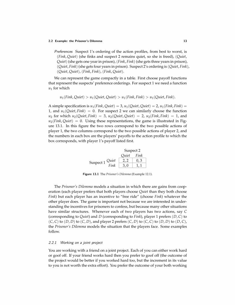
A simple specification is u1(Fink, Quiet) = 3, u1(Quiet, Quiet) = 2, u1(Fink, Fink) =1, and u1(Quiet, Fink) = 0. For suspect 2 we can similarly choose the functionu2 for which u2(Quiet, Fink) = 3, u2(Quiet, Quiet) = 2, u2(Fink, Fink) = 1, andu2(Fink, Quiet) = 0. Using these representations, the game is illustrated in Fig-ure 13.1. In this figure the two rows correspond to the two possible actions ofplayer 1, the two columns correspond to the two possible actions of player 2, andthe numbers in each box are the players’ payoffs to the action profile to which thebox corresponds, with player 1’s payoff listed first.
Suspect 1
Suspect 2Quiet Fink
Quiet 2, 2 0, 3Fink 3, 0 1, 1
Figure 13.1 The Prisoner’s Dilemma (Example 12.1).
The Prisoner’s Dilemma models a situation in which there are gains from coop-eration (each player prefers that both players choose Quiet than they both chooseFink) but each player has an incentive to “free ride” (choose Fink) whatever theother player does. The game is important not because we are interested in under-standing the incentives for prisoners to confess, but because many other situationshave similar structures. Whenever each of two players has two actions, say C(corresponding to Quiet) and D (corresponding to Fink), player 1 prefers (D, C) to(C, C) to (D, D) to (C, D), and player 2 prefers (C, D) to (C, C) to (D, D) to (D, C),the Prisoner’s Dilemma models the situation that the players face. Some examplesfollow.
2.2.1 Working on a joint project
You are working with a friend on a joint project. Each of you can either work hardor goof off. If your friend works hard then you prefer to goof off (the outcome ofthe project would be better if you worked hard too, but the increment in its valueto you is not worth the extra effort). You prefer the outcome of your both working
14 Chapter 2. Nash Equilibrium: Theory
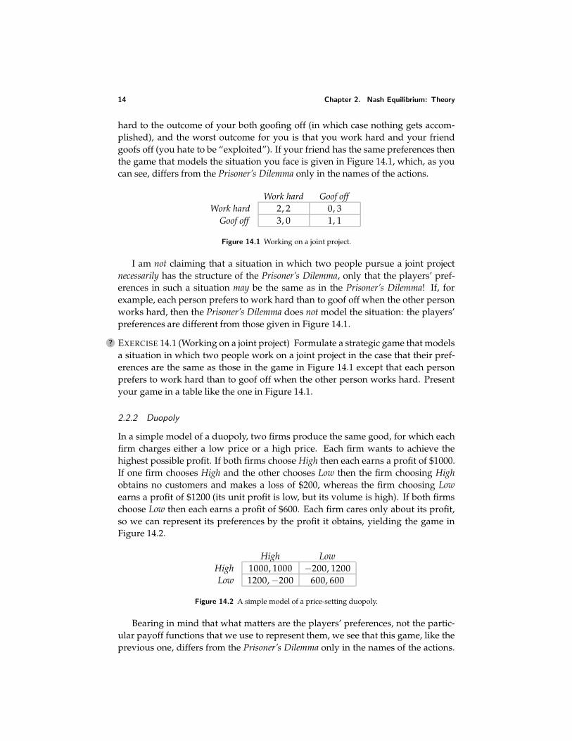
hard to the outcome of your both goofing off (in which case nothing gets accom-plished), and the worst outcome for you is that you work hard and your friendgoofs off (you hate to be “exploited”). If your friend has the same preferences thenthe game that models the situation you face is given in Figure 14.1, which, as youcan see, differs from the Prisoner’s Dilemma only in the names of the actions.
Work hard Goof offWork hard 2, 2 0, 3
Goof off 3, 0 1, 1
Figure 14.1 Working on a joint project.
I am not claiming that a situation in which two people pursue a joint projectnecessarily has the structure of the Prisoner’s Dilemma, only that the players’ pref-erences in such a situation may be the same as in the Prisoner’s Dilemma! If, forexample, each person prefers to work hard than to goof off when the other personworks hard, then the Prisoner’s Dilemma does not model the situation: the players’preferences are different from those given in Figure 14.1.
? EXERCISE 14.1 (Working on a joint project) Formulate a strategic game that modelsa situation in which two people work on a joint project in the case that their pref-erences are the same as those in the game in Figure 14.1 except that each personprefers to work hard than to goof off when the other person works hard. Presentyour game in a table like the one in Figure 14.1.
2.2.2 Duopoly
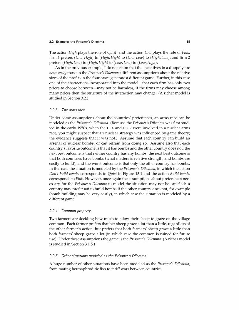
In a simple model of a duopoly, two firms produce the same good, for which eachfirm charges either a low price or a high price. Each firm wants to achieve thehighest possible profit. If both firms choose High then each earns a profit of $1000.If one firm chooses High and the other chooses Low then the firm choosing Highobtains no customers and makes a loss of $200, whereas the firm choosing Lowearns a profit of $1200 (its unit profit is low, but its volume is high). If both firmschoose Low then each earns a profit of $600. Each firm cares only about its profit,so we can represent its preferences by the profit it obtains, yielding the game inFigure 14.2.
High LowHigh 1000, 1000 −200, 1200Low 1200, −200 600, 600
Figure 14.2 A simple model of a price-setting duopoly.
Bearing in mind that what matters are the players’ preferences, not the partic-ular payoff functions that we use to represent them, we see that this game, like theprevious one, differs from the Prisoner’s Dilemma only in the names of the actions.
2.2 Example: the Prisoner’s Dilemma 15
The action High plays the role of Quiet, and the action Low plays the role of Fink;firm 1 prefers (Low, High) to (High, High) to (Low, Low) to (High, Low), and firm 2prefers (High, Low) to (High, High) to (Low, Low) to (Low, High).
As in the previous example, I do not claim that the incentives in a duopoly arenecessarily those in the Prisoner’s Dilemma; different assumptions about the relativesizes of the profits in the four cases generate a different game. Further, in this caseone of the abstractions incorporated into the model—that each firm has only twoprices to choose between—may not be harmless; if the firms may choose amongmany prices then the structure of the interaction may change. (A richer model isstudied in Section 3.2.)
2.2.3 The arms race
Under some assumptions about the countries’ preferences, an arms race can bemodeled as the Prisoner’s Dilemma. (Because the Prisoner’s Dilemma was first stud-ied in the early 1950s, when the USA and USSR were involved in a nuclear armsrace, you might suspect that US nuclear strategy was influenced by game theory;the evidence suggests that it was not.) Assume that each country can build anarsenal of nuclear bombs, or can refrain from doing so. Assume also that eachcountry’s favorite outcome is that it has bombs and the other country does not; thenext best outcome is that neither country has any bombs; the next best outcome isthat both countries have bombs (what matters is relative strength, and bombs arecostly to build); and the worst outcome is that only the other country has bombs.In this case the situation is modeled by the Prisoner’s Dilemma, in which the actionDon’t build bombs corresponds to Quiet in Figure 13.1 and the action Build bombscorresponds to Fink. However, once again the assumptions about preferences nec-essary for the Prisoner’s Dilemma to model the situation may not be satisfied: acountry may prefer not to build bombs if the other country does not, for example(bomb-building may be very costly), in which case the situation is modeled by adifferent game.
2.2.4 Common property
Two farmers are deciding how much to allow their sheep to graze on the villagecommon. Each farmer prefers that her sheep graze a lot than a little, regardless ofthe other farmer’s action, but prefers that both farmers’ sheep graze a little thanboth farmers’ sheep graze a lot (in which case the common is ruined for futureuse). Under these assumptions the game is the Prisoner’s Dilemma. (A richer modelis studied in Section 3.1.5.)
2.2.5 Other situations modeled as the Prisoner’s Dilemma
A huge number of other situations have been modeled as the Prisoner’s Dilemma,from mating hermaphroditic fish to tariff wars between countries.
16 Chapter 2. Nash Equilibrium: Theory
? EXERCISE 16.1 (Hermaphroditic fish) Members of some species of hermaphroditicfish choose, in each mating encounter, whether to play the role of a male or afemale. Each fish has a preferred role, which uses up fewer resources and henceallows more future mating. A fish obtains a payoff of H if it mates in its preferredrole and L if it mates in the other role, where H > L. (Payoffs are measured interms of number of offspring, which fish are evolved to maximize.) Consider anencounter between two fish whose preferred roles are the same. Each fish has twopossible actions: mate in either role, and insist on its preferred role. If both fishoffer to mate in either role, the roles are assigned randomly, and each fish’s payoffis 1
2 (H + L) (the average of H and L). If each fish insists on its preferred role, thefish do not mate; each goes off in search of another partner, and obtains the payoffS. The higher the chance of meeting another partner, the larger is S. Formulate thissituation as a strategic game and determine the range of values of S, for any givenvalues of H and L, for which the game differs from the Prisoner’s Dilemma only inthe names of the actions.
2.3 Example: Bach or Stravinsky?
In the Prisoner’s Dilemma the main issue is whether or not the players will cooperate(choose Quiet). In the following game the players agree that it is better to cooperatethan not to cooperate, but disagree about the best outcome.
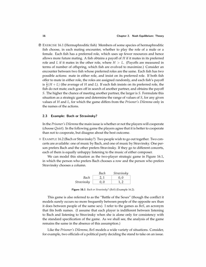
EXAMPLE 16.2 (Bach or Stravinsky?) Two people wish to go out together. Two con-certs are available: one of music by Bach, and one of music by Stravinsky. One per-son prefers Bach and the other prefers Stravinsky. If they go to different concerts,each of them is equally unhappy listening to the music of either composer.
We can model this situation as the two-player strategic game in Figure 16.1,in which the person who prefers Bach chooses a row and the person who prefersStravinsky chooses a column.
Bach StravinskyBach 2, 1 0, 0
Stravinsky 0, 0 1, 2
Figure 16.1 Bach or Stravinsky? (BoS) (Example 16.2).
This game is also referred to as the “Battle of the Sexes” (though the conflict itmodels surely occurs no more frequently between people of the opposite sex thanit does between people of the same sex). I refer to the games as BoS, an acronymthat fits both names. (I assume that each player is indifferent between listeningto Bach and listening to Stravinsky when she is alone only for consistency withthe standard specification of the game. As we shall see, the analysis of the gameremains the same in the absence of this assumption.)
Like the Prisoner’s Dilemma, BoS models a wide variety of situations. Consider,for example, two officials of a political party deciding the stand to take on an issue.
2.4 Example: Matching Pennies 17
Suppose that they disagree about the best stand, but are both better off if they takethe same stand than if they take different stands; both cases in which they takedifferent stands, in which case voters do not know what to think, are equally bad.Then BoS captures the situation they face. Or consider two merging firms thatcurrently use different computer technologies. As two divisions of a single firmthey will both be better off if they both use the same technology; each firm prefersthat the common technology be the one it used in the past. BoS models the choicesthe firms face.
2.4 Example: Matching Pennies
Aspects of both conflict and cooperation are present in both the Prisoner’s Dilemmaand BoS. The next game is purely conflictual.
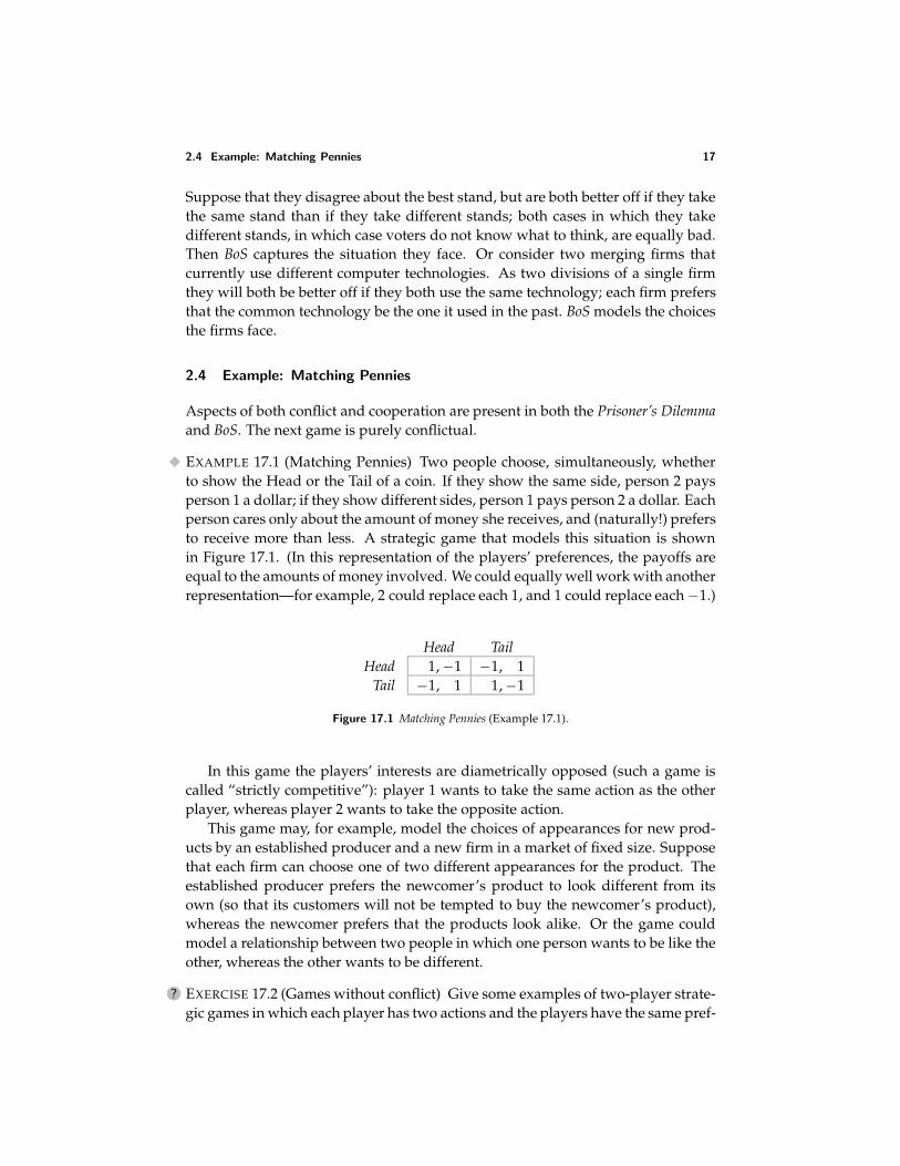
EXAMPLE 17.1 (Matching Pennies) Two people choose, simultaneously, whetherto show the Head or the Tail of a coin. If they show the same side, person 2 paysperson 1 a dollar; if they show different sides, person 1 pays person 2 a dollar. Eachperson cares only about the amount of money she receives, and (naturally!) prefersto receive more than less. A strategic game that models this situation is shownin Figure 17.1. (In this representation of the players’ preferences, the payoffs areequal to the amounts of money involved. We could equally well work with anotherrepresentation—for example, 2 could replace each 1, and 1 could replace each −1.)
Head TailHead 1, −1 −1, 1
Tail −1, 1 1, −1
Figure 17.1 Matching Pennies (Example 17.1).
In this game the players’ interests are diametrically opposed (such a game iscalled “strictly competitive”): player 1 wants to take the same action as the otherplayer, whereas player 2 wants to take the opposite action.
This game may, for example, model the choices of appearances for new prod-ucts by an established producer and a new firm in a market of fixed size. Supposethat each firm can choose one of two different appearances for the product. Theestablished producer prefers the newcomer’s product to look different from itsown (so that its customers will not be tempted to buy the newcomer’s product),whereas the newcomer prefers that the products look alike. Or the game couldmodel a relationship between two people in which one person wants to be like theother, whereas the other wants to be different.
? EXERCISE 17.2 (Games without conflict) Give some examples of two-player strate-gic games in which each player has two actions and the players have the same pref-
18 Chapter 2. Nash Equilibrium: Theory
erences, so that there is no conflict between their interests. (Present your games astables like the one in Figure 17.1.)
2.5 Example: the Stag Hunt
A sentence in Discourse on the origin and foundations of inequality among men (1755)by the philosopher Jean-Jacques Rousseau discusses a group of hunters who wishto catch a stag. They will succeed if they all remain sufficiently attentive, but eachis tempted to desert her post and catch a hare. One interpretation of the sentence isthat the interaction between the hunters may be modeled as the following strategicgame.
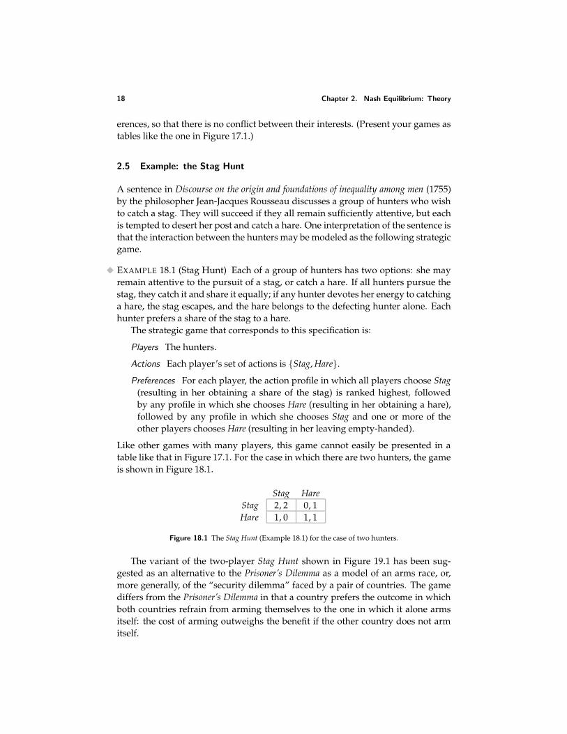
EXAMPLE 18.1 (Stag Hunt) Each of a group of hunters has two options: she mayremain attentive to the pursuit of a stag, or catch a hare. If all hunters pursue thestag, they catch it and share it equally; if any hunter devotes her energy to catchinga hare, the stag escapes, and the hare belongs to the defecting hunter alone. Eachhunter prefers a share of the stag to a hare.
The strategic game that corresponds to this specification is:
Players The hunters.
Actions Each player’s set of actions is Stag, Hare.
Preferences For each player, the action profile in which all players choose Stag(resulting in her obtaining a share of the stag) is ranked highest, followedby any profile in which she chooses Hare (resulting in her obtaining a hare),followed by any profile in which she chooses Stag and one or more of theother players chooses Hare (resulting in her leaving empty-handed).
Like other games with many players, this game cannot easily be presented in atable like that in Figure 17.1. For the case in which there are two hunters, the gameis shown in Figure 18.1.
Stag HareStag 2, 2 0, 1Hare 1, 0 1, 1
Figure 18.1 The Stag Hunt (Example 18.1) for the case of two hunters.
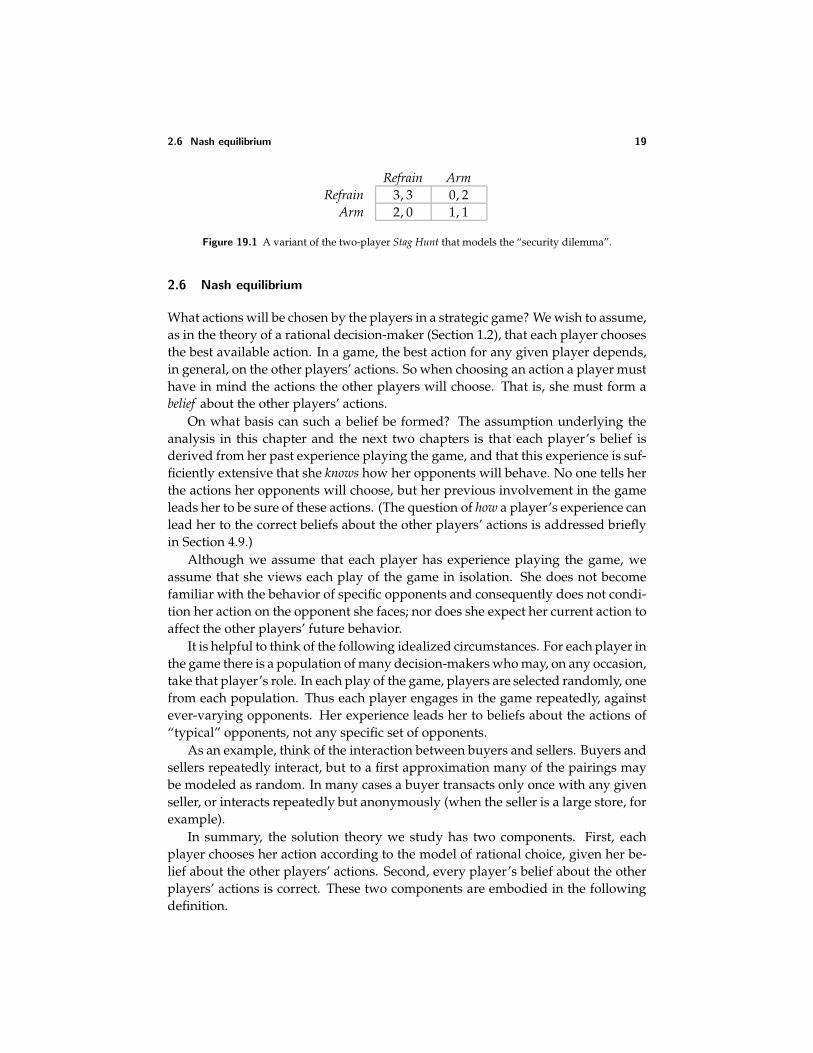
The variant of the two-player Stag Hunt shown in Figure 19.1 has been sug-gested as an alternative to the Prisoner’s Dilemma as a model of an arms race, or,more generally, of the “security dilemma” faced by a pair of countries. The gamediffers from the Prisoner’s Dilemma in that a country prefers the outcome in whichboth countries refrain from arming themselves to the one in which it alone armsitself: the cost of arming outweighs the benefit if the other country does not armitself.
2.6 Nash equilibrium 19
Refrain ArmRefrain 3, 3 0, 2
Arm 2, 0 1, 1
Figure 19.1 A variant of the two-player Stag Hunt that models the “security dilemma”.
2.6 Nash equilibrium
What actions will be chosen by the players in a strategic game? We wish to assume,as in the theory of a rational decision-maker (Section 1.2), that each player choosesthe best available action. In a game, the best action for any given player depends,in general, on the other players’ actions. So when choosing an action a player musthave in mind the actions the other players will choose. That is, she must form abelief about the other players’ actions.
On what basis can such a belief be formed? The assumption underlying theanalysis in this chapter and the next two chapters is that each player’s belief isderived from her past experience playing the game, and that this experience is suf-ficiently extensive that she knows how her opponents will behave. No one tells herthe actions her opponents will choose, but her previous involvement in the gameleads her to be sure of these actions. (The question of how a player’s experience canlead her to the correct beliefs about the other players’ actions is addressed brieflyin Section 4.9.)
Although we assume that each player has experience playing the game, weassume that she views each play of the game in isolation. She does not becomefamiliar with the behavior of specific opponents and consequently does not condi-tion her action on the opponent she faces; nor does she expect her current action toaffect the other players’ future behavior.
It is helpful to think of the following idealized circumstances. For each player inthe game there is a population of many decision-makers who may, on any occasion,take that player’s role. In each play of the game, players are selected randomly, onefrom each population. Thus each player engages in the game repeatedly, againstever-varying opponents. Her experience leads her to beliefs about the actions of“typical” opponents, not any specific set of opponents.
As an example, think of the interaction between buyers and sellers. Buyers andsellers repeatedly interact, but to a first approximation many of the pairings maybe modeled as random. In many cases a buyer transacts only once with any givenseller, or interacts repeatedly but anonymously (when the seller is a large store, forexample).
In summary, the solution theory we study has two components. First, eachplayer chooses her action according to the model of rational choice, given her be-lief about the other players’ actions. Second, every player’s belief about the otherplayers’ actions is correct. These two components are embodied in the followingdefinition.
20 Chapter 2. Nash Equilibrium: Theory
JOHN F. NASH, JR.
A few of the ideas of John F. Nash Jr., developed while he was a graduate studentat Princeton from 1948 to 1950, transformed game theory. Nash was born in 1928 inBluefield, West Virginia, USA, where he grew up. He was an undergraduate math-ematics major at Carnegie Institute of Technology from 1945 to 1948. In 1948 heobtained both a B.S. and an M.S., and began graduate work in the Department ofMathematics at Princeton University. (One of his letters of recommendation, froma professor at Carnegie Institute of Technology, was a single sentence: “This man isa genius” (Kuhn et al. 1995, 282).) A paper containing the main result of his thesiswas submitted to the Proceedings of the National Academy of Sciences in November1949, fourteen months after he started his graduate work. (“A fine goal to set . . .graduate students”, to quote Kuhn! (See Kuhn et al. 1995, 282.)) He completed hisPhD the following year, graduating on his 22nd birthday. His thesis, 28 pages inlength, introduces the equilibrium notion now known as “Nash equilibrium” anddelineates a class of strategic games that have Nash equilibria (Proposition 116.1in this book). The notion of Nash equilibrium vastly expanded the scope of gametheory, which had previously focussed on two-player “strictly competitive” games(in which the players’ interests are directly opposed). While a graduate student atPrinceton, Nash also wrote the seminal paper in bargaining theory, Nash (1950b)(the ideas of which originated in an elective class in international economics hetook as an undergraduate). He went on to take an academic position in the Depart-ment of Mathematics at MIT, where he produced “a remarkable series of papers”(Milnor 1995, 15); he has been described as “one of the most original mathematicalminds of [the twentieth] century” (Kuhn 1996). He shared the 1994 Nobel prize ineconomics with the game theorists John C. Harsanyi and Reinhard Selten.
A Nash equilibrium is an action profile a∗ with the property that noplayer i can do better by choosing an action different from a∗i , giventhat every other player j adheres to a∗j .
In the idealized setting in which the players in any given play of the game aredrawn randomly from a collection of populations, a Nash equilibrium correspondsto a steady state. If, whenever the game is played, the action profile is the same Nashequilibrium a∗, then no player has a reason to choose any action different from hercomponent of a∗; there is no pressure on the action profile to change. Expresseddifferently, a Nash equilibrium embodies a stable “social norm”: if everyone elseadheres to it, no individual wishes to deviate from it.
The second component of the theory of Nash equilibrium—that the players’ be-liefs about each other’s actions are correct—implies, in particular, that two players’beliefs about a third player’s action are the same. For this reason, the condition issometimes said to be that the players’ “expectations are coordinated”.
The situations to which we wish to apply the theory of Nash equilibrium do
2.6 Nash equilibrium 21
not in general correspond exactly to the idealized setting described above. Forexample, in some cases the players do not have much experience with the game;in others they do not view each play of the game in isolation. Whether or notthe notion of Nash equilibrium is appropriate in any given situation is a matter ofjudgment. In some cases, a poor fit with the idealized setting may be mitigatedby other considerations. For example, inexperienced players may be able to drawconclusions about their opponents’ likely actions from their experience in othersituations, or from other sources. (One aspect of such reasoning is discussed in thebox on page 30). Ultimately, the test of the appropriateness of the notion of Nashequilibrium is whether it gives us insights into the problem at hand.
With the aid of an additional piece of notation, we can state the definition ofa Nash equilibrium precisely. Let a be an action profile, in which the action ofeach player i is ai. Let a′i be any action of player i (either equal to ai, or differentfrom it). Then (a′i , a−i) denotes the action profile in which every player j excepti chooses her action aj as specified by a, whereas player i chooses a′i. (The −isubscript on a stands for “except i”.) That is, (a′i , a−i) is the action profile in whichall the players other than i adhere to a while i “deviates” to a′i. (If a′i = ai thenof course (a′i , a−i) = (ai, a−i) = a.) If there are three players, for example, then(a′2, a−2) is the action profile in which players 1 and 3 adhere to a (player 1 choosesa1, player 3 chooses a3) and player 2 deviates to a′2.
Using this notation, we can restate the condition for an action profile a∗ to be aNash equilibrium: no player i has any action ai for which she prefers (ai, a∗−i) to a∗.Equivalently, for every player i and every action ai of player i, the action profile a∗
is at least as good for player i as the action profile (ai , a∗−i).
DEFINITION 21.1 (Nash equilibrium of strategic game with ordinal preferences) Theaction profile a∗ in a strategic game with ordinal preferences is a Nash equilibriumif, for every player i and every action ai of player i, a∗ is at least as good accordingto player i’s preferences as the action profile (ai , a∗−i) in which player i chooses aiwhile every other player j chooses a∗j . Equivalently, for every player i,
ui(a∗) ≥ ui(ai , a∗−i) for every action ai of player i, (21.2)
where ui is a payoff function that represents player i’s preferences.
This definition implies neither that a strategic game necessarily has a Nashequilibrium, nor that it has at most one. Examples in the next section show thatsome games have a single Nash equilibrium, some possess no Nash equilibrium,and others have many Nash equilibria.
The definition of a Nash equilibrium is designed to model a steady state amongexperienced players. An alternative approach to understanding players’ actions instrategic games assumes that the players know each others’ preferences, and con-siders what each player can deduce about the other players’ actions from theirrationality and their knowledge of each other’s rationality. This approach is stud-ied in Chapter 12. For many games, it leads to a conclusion different from that of
22 Chapter 2. Nash Equilibrium: Theory
Nash equilibrium. For games in which the conclusion is the same the approachoffers us an alternative interpretation of a Nash equilibrium, as the outcome of ra-tional calculations by players who do not necessarily have any experience playingthe game.
STUDYING NASH EQUILIBRIUM EXPERIMENTALLY
The theory of strategic games lends itself to experimental study: arranging for sub-jects to play games and observing their choices is relatively straightforward. A fewyears after game theory was launched by von Neumann and Morgenstern’s (1944)book, reports of laboratory experiments began to appear. Subsequently a hugenumber of experiments have been conducted, illuminating many issues relevantto the theory. I discuss selected experimental evidence throughout the book.
The theory of Nash equilibrium, as we have seen, has two components: theplayers act in accordance with the theory of rational choice, given their beliefsabout the other players’ actions, and these beliefs are correct. If every subjectunderstands the game she is playing and faces incentives that correspond to thepreferences of the player whose role she is taking, then a divergence between theobserved outcome and a Nash equilibrium can be blamed on a failure of one orboth of these two components. Experimental evidence has the potential of indi-cating the types of games for which the theory works well and, for those in whichthe theory does not work well, of pointing to the faulty component and giving ushints about the characteristics of a better theory. In designing an experiment thatcleanly tests the theory, however, we need to confront several issues.
The model of rational choice takes preferences as given. Thus to test the theoryof Nash equilibrium experimentally, we need to ensure that each subject’s prefer-ences are those of the player whose role she is taking in the game we are exam-ining. The standard way of inducing the appropriate preferences is to pay eachsubject an amount of money directly related to the payoff given by a payoff func-tion that represents the preferences of the player whose role the subject is taking.Such remuneration works if each subject likes money and cares only about theamount of money she receives, ignoring the amounts received by her opponents.The assumption that people like receiving money is reasonable in many cultures,but the assumption that people care only about their own monetary rewards—are “selfish”—may, in some contexts at least, not be reasonable. Unless we checkwhether our subjects are selfish in the context of our experiment, we will jointly testtwo hypotheses: that humans are selfish—a hypothesis not part of game theory—and that the notion of Nash equilibrium models their behavior. In some cases wemay indeed wish to test these hypotheses jointly. But in order to test the theory ofNash equilibrium alone we need to ensure that we induce the preferences we wishto study.
Assuming that better decisions require more effort, we need also to ensure that
2.6 Nash equilibrium 23
each subject finds it worthwhile to put in the extra effort required to obtain a higherpayoff. If we rely on monetary payments to provide incentives, the amount ofmoney a subject can obtain must be sufficiently sensitive to the quality of her deci-sions to compensate her for the effort she expends (paying a flat fee, for example,is inappropriate). In some cases, monetary payments may not be necessary: undersome circumstances, subjects drawn from a highly competitive culture like that ofthe USA may be sufficiently motivated by the possibility of obtaining a high score,even if that score does not translate into a monetary payoff.
The notion of Nash equilibrium models action profiles compatible with steadystates. Thus to study the theory experimentally we need to collect observations ofsubjects’ behavior when they have experience playing the game. But they shouldnot have obtained that experience while knowingly facing the same opponentsrepeatedly, for the theory assumes that the players consider each play of the gamein isolation, not as part of an ongoing relationship. One option is to have eachsubject play the game against many different opponents, gaining experience abouthow the other subjects on average play the game, but not about the choices of anyother given player. Another option is to describe the game in terms that relate toa situation in which the subjects already have experience. A difficulty with thissecond approach is that the description we give may connote more than simplythe payoff numbers of our game. If we describe the Prisoner’s Dilemma in termsof cooperation on a joint project, for example, a subject may be biased towardchoosing the action she has found appropriate when involved in joint projects,even if the structures of those interactions were significantly different from that ofthe Prisoner’s Dilemma. As she plays the experimental game repeatedly she maycome to appreciate how it differs from the games in which she has been involvedpreviously, but her biases may disappear only slowly.
Whatever route we take to collect data on the choices of subjects experiencedin playing the game, we confront a difficult issue: how do we know when theoutcome has converged? Nash’s theory concerns only equilibria; it has nothing tosay about the path players’ choices will take on the way to an equilibrium, and sogives us no guide as to whether 10, 100, or 1,000 plays of the game are enough togive a chance for the subjects’ expectations to become coordinated.
Finally, we can expect the theory of Nash equilibrium to correspond to realityonly approximately: like all useful theories, it definitely is not exactly correct. Howdo we tell whether the data are close enough to the theory to support it? One pos-sibility is to compare the theory of Nash equilibrium with some other theory. Butfor many games there is no obvious alternative theory—and certainly not one withthe generality of Nash equilibrium. Statistical tests can sometimes aid in decidingwhether the data is consistent with the theory, though ultimately we remain thejudge of whether or not our observations persuade us that the theory enhancesour understanding of human behavior in the game.
24 Chapter 2. Nash Equilibrium: Theory
2.7 Examples of Nash equilibrium
2.7.1 Prisoner’s Dilemma
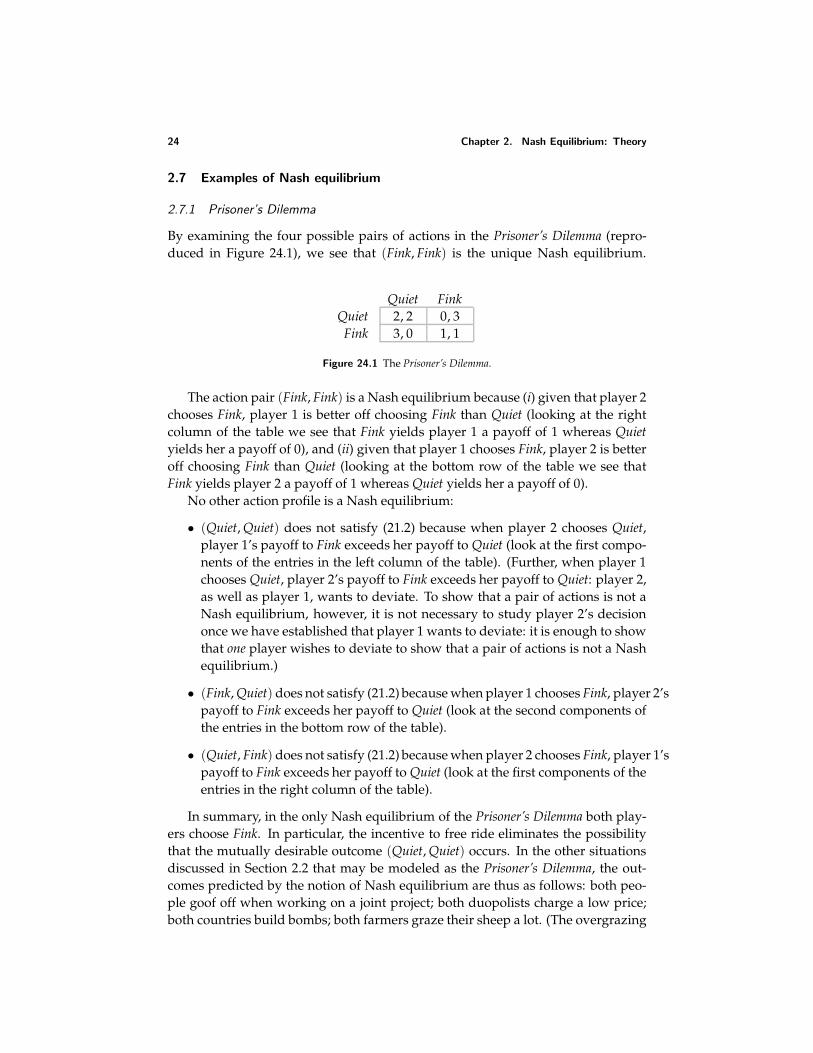
By examining the four possible pairs of actions in the Prisoner’s Dilemma (repro-duced in Figure 24.1), we see that (Fink, Fink) is the unique Nash equilibrium.
Quiet FinkQuiet 2, 2 0, 3Fink 3, 0 1, 1
Figure 24.1 The Prisoner’s Dilemma.
The action pair (Fink, Fink) is a Nash equilibrium because (i) given that player 2chooses Fink, player 1 is better off choosing Fink than Quiet (looking at the rightcolumn of the table we see that Fink yields player 1 a payoff of 1 whereas Quietyields her a payoff of 0), and (ii) given that player 1 chooses Fink, player 2 is betteroff choosing Fink than Quiet (looking at the bottom row of the table we see thatFink yields player 2 a payoff of 1 whereas Quiet yields her a payoff of 0).
No other action profile is a Nash equilibrium:
• (Quiet, Quiet) does not satisfy (21.2) because when player 2 chooses Quiet,player 1’s payoff to Fink exceeds her payoff to Quiet (look at the first compo-nents of the entries in the left column of the table). (Further, when player 1chooses Quiet, player 2’s payoff to Fink exceeds her payoff to Quiet: player 2,as well as player 1, wants to deviate. To show that a pair of actions is not aNash equilibrium, however, it is not necessary to study player 2’s decisiononce we have established that player 1 wants to deviate: it is enough to showthat one player wishes to deviate to show that a pair of actions is not a Nashequilibrium.)
• (Fink, Quiet) does not satisfy (21.2) because when player 1 chooses Fink, player 2’spayoff to Fink exceeds her payoff to Quiet (look at the second components ofthe entries in the bottom row of the table).
• (Quiet, Fink) does not satisfy (21.2) because when player 2 chooses Fink, player 1’spayoff to Fink exceeds her payoff to Quiet (look at the first components of theentries in the right column of the table).
In summary, in the only Nash equilibrium of the Prisoner’s Dilemma both play-ers choose Fink. In particular, the incentive to free ride eliminates the possibilitythat the mutually desirable outcome (Quiet, Quiet) occurs. In the other situationsdiscussed in Section 2.2 that may be modeled as the Prisoner’s Dilemma, the out-comes predicted by the notion of Nash equilibrium are thus as follows: both peo-ple goof off when working on a joint project; both duopolists charge a low price;both countries build bombs; both farmers graze their sheep a lot. (The overgrazing
2.7 Examples of Nash equilibrium 25
of a common thus predicted is sometimes called the “tragedy of the commons”.The intuition that some of these dismal outcomes may be avoided if the same pairof people play the game repeatedly is explored in Chapter 14.)
In the Prisoner’s Dilemma, the Nash equilibrium action of each player (Fink) isthe best action for each player not only if the other player chooses her equilib-rium action (Fink), but also if she chooses her other action (Quiet). The action pair(Fink, Fink) is a Nash equilibrium because if a player believes that her opponentwill choose Fink then it is optimal for her to choose Fink. But in fact it is optimal fora player to choose Fink regardless of the action she expects her opponent to choose.In most of the games we study, a player’s Nash equilibrium action does not sat-isfy this condition: the action is optimal if the other players choose their Nashequilibrium actions, but some other action is optimal if the other players choosenon-equilibrium actions.
? EXERCISE 25.1 (Altruistic players in the Prisoner’s Dilemma) Each of two playershas two possible actions, Quiet and Fink; each action pair results in the players’receiving amounts of money equal to the numbers corresponding to that actionpair in Figure 24.1. (For example, if player 1 chooses Quiet and player 2 choosesFink, then player 1 receives nothing, whereas player 2 receives $3.) The players arenot “selfish”; rather, the preferences of each player i are represented by the payofffunction mi(a) + αmj(a), where mi(a) is the amount of money received by player iwhen the action profile is a, j is the other player, and α is a given nonnegativenumber. Player 1’s payoff to the action pair (Quiet, Quiet), for example, is 2 + 2α.
a. Formulate a strategic game that models this situation in the case α = 1. Is thisgame the Prisoner’s Dilemma?
b. Find the range of values of α for which the resulting game is the Prisoner’sDilemma. For values of α for which the game is not the Prisoner’s Dilemma,find its Nash equilibria.
? EXERCISE 25.2 (Selfish and altruistic social behavior) Two people enter a bus. Twoadjacent cramped seats are free. Each person must decide whether to sit or stand.Sitting alone is more comfortable than sitting next to the other person, which ismore comfortable than standing.
a. Suppose that each person cares only about her own comfort. Model the situ-ation as a strategic game. Is this game the Prisoner’s Dilemma? Find its Nashequilibrium (equilibria?).
b. Suppose that each person is altruistic, ranking the outcomes according to theother person’s comfort, and, out of politeness, prefers to stand than to sit if theother person stands. Model the situation as a strategic game. Is this game thePrisoner’s Dilemma? Find its Nash equilibrium (equilibria?).
c. Compare the people’s comfort in the equilibria of the two games.
26 Chapter 2. Nash Equilibrium: Theory
EXPERIMENTAL EVIDENCE ON THE Prisoner’s Dilemma
The Prisoner’s Dilemma has attracted a great deal of attention by economists, psy-chologists, sociologists, and biologists. A huge number of experiments have beenconducted with the aim of discovering how people behave when playing the game.Almost all these experiments involve each subject’s playing the game repeatedlyagainst an unchanging opponent, a situation that calls for an analysis significantlydifferent from the one in this chapter (see Chapter 14).
The evidence on the outcome of isolated plays of the game is inconclusive. Noexperiment of which I am aware carefully induces the appropriate preferences andis specifically designed to elicit a steady state action profile (see the box on page 22).Thus in each case the choice of Quiet by a player could indicate that she is not“selfish” or that she is not experienced in playing the game, rather than providingevidence against the notion of Nash equilibrium.
In two experiments with very low payoffs, each subject played the game a smallnumber of times against different opponents; between 50% and 94% of subjectschose Fink, depending on the relative sizes of the payoffs and some details ofthe design (Rapoport, Guyer, and Gordon 1976, 135–137, 211–213, and 223-226).A more recent experiment finds that in the last 10 of 20 rounds of play againstdifferent opponents, 78% of subjects choose Fink (Cooper, DeJong, Forsythe, andRoss 1996). In face-to-face games in which communication is allowed, the inci-dence of the choice of Fink tends to be lower: from 29% to 70% depending on thenature of the communication allowed (Deutsch 1958, and Frank, Gilovich, and Re-gan 1993, 163–167). (In all these experiments, the subjects were college students inthe USA or Canada.)
One source of the variation in the results seems to be that some designs in-duce preferences that differ from those of the Prisoner’s Dilemma; no clear answeremerges to the question of whether the notion of Nash equilibrium is relevant tothe Prisoner’s Dilemma. If, nevertheless, one interprets the evidence as showing thatsome subjects in the Prisoner’s Dilemma systematically choose Quiet rather thanFink, one must fault the rational choice component of Nash equilibrium, not thecoordinated expectations component. Why? Because, as noted in the text, Fink isoptimal no matter what a player thinks her opponent will choose, so that any modelin which the players act according to the model of rational choice, whether or nottheir expectations are coordinated, predicts that each player chooses Fink.
2.7.2 BoS
To find the Nash equilibria of BoS (Figure 16.1), we can examine each pair of actionsin turn:
• (Bach, Bach): If player 1 switches to Stravinsky then her payoff decreases from2 to 0; if player 2 switches to Stravinsky then her payoff decreases from 1 to 0.
2.7 Examples of Nash equilibrium 27
Thus a deviation by either player decreases her payoff. Thus (Bach, Bach) isa Nash equilibrium.
• (Bach, Stravinsky): If player 1 switches to Stravinsky then her payoff increasesfrom 0 to 1. Thus (Bach, Stravinsky) is not a Nash equilibrium. (Player 2can increase her payoff by deviating, too, but to show the pair is not a Nashequilibrium it suffices to show that one player can increase her payoff bydeviating.)
• (Stravinsky, Bach): If player 1 switches to Bach then her payoff increases from0 to 2. Thus (Stravinsky, Bach) is not a Nash equilibrium.
• (Stravinsky, Stravinsky): If player 1 switches to Bach then her payoff decreasesfrom 1 to 0; if player 2 switches to Bach then her payoff decreases from 2 to 0.Thus a deviation by either player decreases her payoff. Thus (Stravinsky, Stravinsky)is a Nash equilibrium.
We conclude that the game has two Nash equilibria: (Bach, Bach) and (Stravinsky,Stravinsky). That is, both of these outcomes are compatible with a steady state;both outcomes are stable social norms. If, in every encounter, both players chooseBach, then no player has an incentive to deviate; if, in every encounter, both play-ers choose Stravinsky, then no player has an incentive to deviate. If we use thegame to model the choices of men when matched with women, for example, thenthe notion of Nash equilibrium shows that two social norms are stable: both play-ers choose the action associated with the outcome preferred by women, and bothplayers choose the action associated with the outcome preferred by men.
2.7.3 Matching Pennies
By checking each of the four pairs of actions in Matching Pennies (Figure 17.1) wesee that the game has no Nash equilibrium. For the pairs of actions (Head, Head)and (Tail, Tail), player 2 is better off deviating; for the pairs of actions (Head, Tail)and (Tail, Head), player 1 is better off deviating. Thus for this game the notion ofNash equilibrium isolates no steady state. In Chapter 4 we return to this game;an extension of the notion of a Nash equilibrium gives us an understanding of thelikely outcome.
2.7.4 The Stag Hunt
Inspection of Figure 18.1 shows that the two-player Stag Hunt has two Nash equi-libria: (Stag, Stag) and (Hare, Hare). If one player remains attentive to the pursuitof the stag, then the other player prefers to remain attentive; if one player chasesa hare, the other one prefers to chase a hare (she cannot catch a stag alone). (Theequilibria of the variant of the game in Figure 19.1 are analogous: (Refrain, Refrain)and (Arm, Arm).)
28 Chapter 2. Nash Equilibrium: Theory
Unlike the Nash equilibria of BoS, one of these equilibria is better for both play-ers than the other: each player prefers (Stag, Stag) to (Hare, Hare). This fact has nobearing on the equilibrium status of (Hare, Hare), since the condition for an equi-librium is that a single player cannot gain by deviating, given the other player’s be-havior. Put differently, an equilibrium is immune to any unilateral deviation; coor-dinated deviations by groups of players are not contemplated. However, the exis-tence of two equilibria raises the possibility that one equilibrium might more likelybe the outcome of the game than the other. I return to this issue in Section 2.7.6.
I argue that the many-player Stag Hunt (Example 18.1) also has two Nash equi-libria: the action profile (Stag, . . . , Stag) in which every players joins in the pursuitof the stag, and the profile (Hare, . . . , Hare) in which every player catches a hare.
• (Stag, . . . , Stag) is a Nash equilibrium because each player prefers this profileto that in which she alone chooses Hare. (A player is better off remainingattentive to the pursuit of the stag than running after a hare if all the otherplayers remain attentive.)
• (Hare, . . . , Hare) is a Nash equilibrium because each player prefers this profileto that in which she alone pursues the stag. (A player is better off catching ahare than pursuing the stag if no one else pursues the stag.)
• No other profile is a Nash equilibrium, because in any other profile at leastone player chooses Stag and at least one player chooses Hare, so that anyplayer choosing Stag is better off switching to Hare. (A player is better offcatching a hare than pursing the stag if at least one other person chases ahare, since the stag can be caught only if everyone pursues it.)
? EXERCISE 28.1 (Variants of the Stag Hunt) Consider two variants of the n-hunterStag Hunt in which only m hunters, with 2 ≤ m < n, need to pursue the stag inorder to catch it. (Continue to assume that there is a single stag.) Assume that acaptured stag is shared only by the hunters that catch it.
a. Assume, as before, that each hunter prefers the fraction 1/n of the stag to ahare. Find the Nash equilibria of the strategic game that models this situation.
b. Assume that each hunter prefers the fraction 1/k of the stag to a hare, butprefers the hare to any smaller fraction of the stag, where k is an integer withm ≤ k ≤ n. Find the Nash equilibria of the strategic game that models thissituation.
The following more difficult exercise enriches the hunters’ choices in the StagHunt. This extended game has been proposed as a model that captures Keynes’ ba-sic insight about the possibility of multiple economic equilibria, some undesirable(Bryant 1983, 1994).
?? EXERCISE 28.2 (Extension of the Stag hunt) Extend the n-hunter Stag Hunt by giv-ing each hunter K (a positive integer) units of effort, which she can allocate be-tween pursuing the stag and catching hares. Denote the effort hunter i devotes
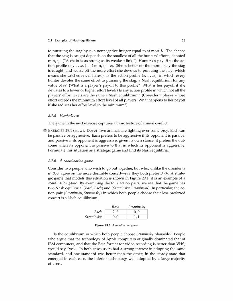
2.7 Examples of Nash equilibrium 29
to pursuing the stag by ei, a nonnegative integer equal to at most K. The chancethat the stag is caught depends on the smallest of all the hunters’ efforts, denotedminj ej. (“A chain is as strong as its weakest link.”) Hunter i’s payoff to the ac-tion profile (e1, . . . , en) is 2 minj ej − ei. (She is better off the more likely the stagis caught, and worse off the more effort she devotes to pursuing the stag, whichmeans she catches fewer hares.) Is the action profile (e, . . . , e), in which everyhunter devotes the same effort to pursuing the stag, a Nash equilibrium for anyvalue of e? (What is a player’s payoff to this profile? What is her payoff if shedeviates to a lower or higher effort level?) Is any action profile in which not all theplayers’ effort levels are the same a Nash equilibrium? (Consider a player whoseeffort exceeds the minimum effort level of all players. What happens to her payoffif she reduces her effort level to the minimum?)
2.7.5 Hawk–Dove
The game in the next exercise captures a basic feature of animal conflict.
? EXERCISE 29.1 (Hawk–Dove) Two animals are fighting over some prey. Each canbe passive or aggressive. Each prefers to be aggressive if its opponent is passive,and passive if its opponent is aggressive; given its own stance, it prefers the out-come when its opponent is passive to that in which its opponent is aggressive.Formulate this situation as a strategic game and find its Nash equilibria.
2.7.6 A coordination game
Consider two people who wish to go out together, but who, unlike the dissidentsin BoS, agree on the more desirable concert—say they both prefer Bach. A strate-gic game that models this situation is shown in Figure 29.1; it is an example of acoordination game. By examining the four action pairs, we see that the game hastwo Nash equilibria: (Bach, Bach) and (Stravinsky, Stravinsky). In particular, the ac-tion pair (Stravinsky, Stravinsky) in which both people choose their less-preferredconcert is a Nash equilibrium.
Bach StravinskyBach 2, 2 0, 0
Stravinsky 0, 0 1, 1
Figure 29.1 A coordination game.
Is the equilibrium in which both people choose Stravinsky plausible? Peoplewho argue that the technology of Apple computers originally dominated that ofIBM computers, and that the Beta format for video recording is better than VHS,would say “yes”. In both cases users had a strong interest in adopting the samestandard, and one standard was better than the other; in the steady state thatemerged in each case, the inferior technology was adopted by a large majorityof users.
30 Chapter 2. Nash Equilibrium: Theory
FOCAL POINTS
In games with many Nash equilibria, the theory isolates more than one pattern ofbehavior compatible with a steady state. In some games, some of these equilibriaseem more likely to attract the players’ attentions than others. To use the termi-nology of Schelling (1960), some equilibria are focal. In the coordination game inFigure 29.1, where the players agree on the more desirable Nash equilibrium andobtain the same payoff to every nonequilibrium action pair, the preferable equi-librium seems more likely to be focal (though two examples are given in the textof steady states involving the inferior equilibrium). In the variant of this game inwhich the two equilibria are equally good (i.e. (2, 2) is replaced by (1, 1)), nothingin the structure of the game gives any clue as to which steady state might occur.In such a game, the names or nature of the actions, or other information, maypredispose the players to one equilibrium rather than the other.
Consider, for example, voters in an election. Pre-election polls may give them in-formation about each other’s intended actions, pointing them to one of many Nashequilibria. Or consider a situation in which two players independently divide $100into two piles, each receiving $10 if they choose the same divisions and nothingotherwise. The strategic game that models this situation has many Nash equilib-ria, in each of which both players choose the same division. But the equilibriumin which both players choose the ($50, $50) division seems likely to command theplayers’ attentions, possibly for esthetic reasons (it is an appealing division), andpossibly because it is a steady state in an unrelated game in which the chosendivision determines the players’ payoffs.
The theory of Nash equilibrium is neutral about the equilibrium that will occurin a game with many equilibria. If features of the situation not modeled by thenotion of a strategic game make some equilibria focal then those equilibria maybe more likely to emerge as steady states, and the rate at which a steady state isreached may be higher than it otherwise would have been.
If two people played this game in a laboratory it seems likely that the outcomewould be (Bach, Bach). Nevertheless, (Stravinsky, Stravinsky) also corresponds to asteady state: if either action pair is reached, there is no reason for either player todeviate from it.
2.7.7 Provision of a public good
The model in the next exercise captures an aspect of the provision of a “publicgood”, like a park or a swimming pool, whose use by one person does not diminishits value to another person (at least, not until it is overcrowded). (Other aspects ofpublic good provision are studied in Section 2.8.4.)
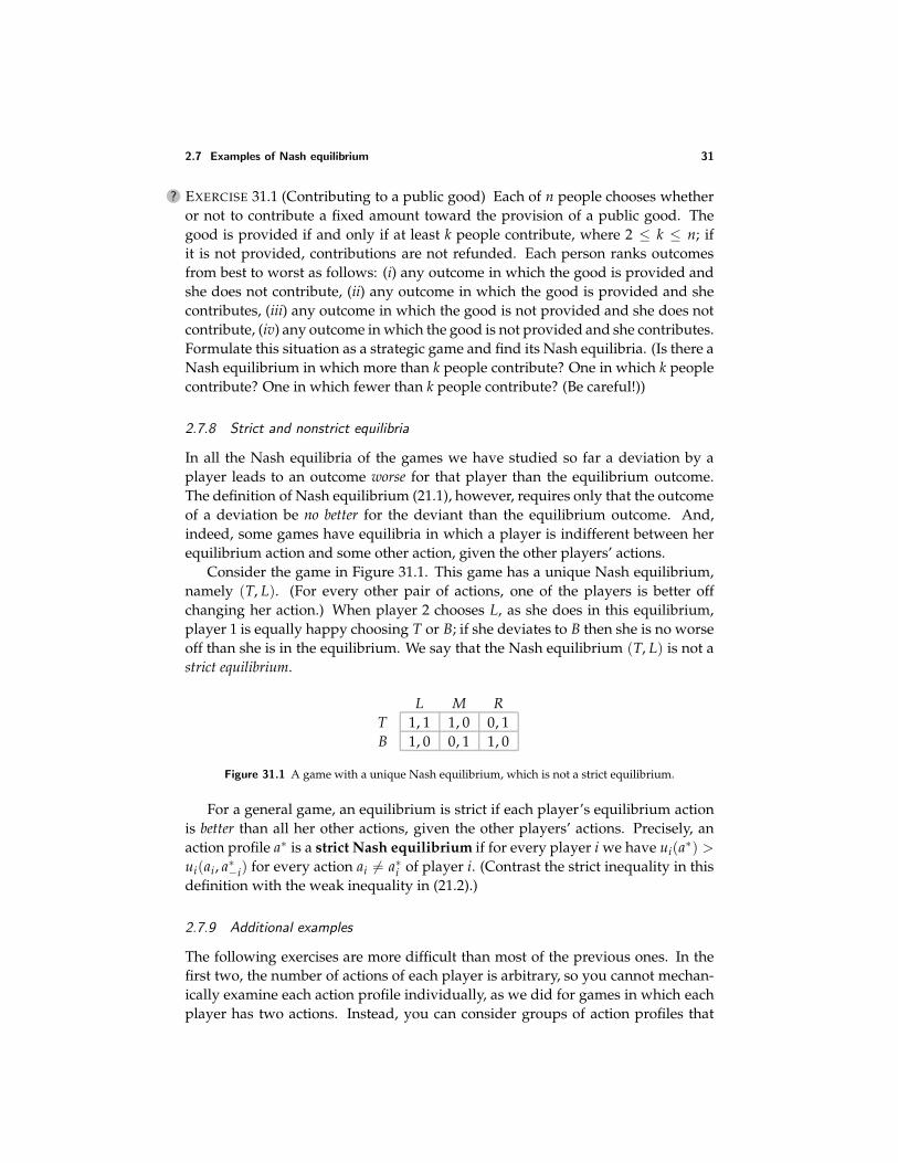
2.7 Examples of Nash equilibrium 31
? EXERCISE 31.1 (Contributing to a public good) Each of n people chooses whetheror not to contribute a fixed amount toward the provision of a public good. Thegood is provided if and only if at least k people contribute, where 2 ≤ k ≤ n; ifit is not provided, contributions are not refunded. Each person ranks outcomesfrom best to worst as follows: (i) any outcome in which the good is provided andshe does not contribute, (ii) any outcome in which the good is provided and shecontributes, (iii) any outcome in which the good is not provided and she does notcontribute, (iv) any outcome in which the good is not provided and she contributes.Formulate this situation as a strategic game and find its Nash equilibria. (Is there aNash equilibrium in which more than k people contribute? One in which k peoplecontribute? One in which fewer than k people contribute? (Be careful!))
2.7.8 Strict and nonstrict equilibria
In all the Nash equilibria of the games we have studied so far a deviation by aplayer leads to an outcome worse for that player than the equilibrium outcome.The definition of Nash equilibrium (21.1), however, requires only that the outcomeof a deviation be no better for the deviant than the equilibrium outcome. And,indeed, some games have equilibria in which a player is indifferent between herequilibrium action and some other action, given the other players’ actions.
Consider the game in Figure 31.1. This game has a unique Nash equilibrium,namely (T, L). (For every other pair of actions, one of the players is better offchanging her action.) When player 2 chooses L, as she does in this equilibrium,player 1 is equally happy choosing T or B; if she deviates to B then she is no worseoff than she is in the equilibrium. We say that the Nash equilibrium (T, L) is not astrict equilibrium.
L M RT 1, 1 1, 0 0, 1B 1, 0 0, 1 1, 0
Figure 31.1 A game with a unique Nash equilibrium, which is not a strict equilibrium.
For a general game, an equilibrium is strict if each player’s equilibrium actionis better than all her other actions, given the other players’ actions. Precisely, anaction profile a∗ is a strict Nash equilibrium if for every player i we have ui(a∗) >
ui(ai, a∗−i) for every action ai = a∗i of player i. (Contrast the strict inequality in thisdefinition with the weak inequality in (21.2).)
2.7.9 Additional examples
The following exercises are more difficult than most of the previous ones. In thefirst two, the number of actions of each player is arbitrary, so you cannot mechan-ically examine each action profile individually, as we did for games in which eachplayer has two actions. Instead, you can consider groups of action profiles that
32 Chapter 2. Nash Equilibrium: Theory
have features in common, and show that all action profiles in any given group areor are not equilibria. Deciding how best to group the profiles into types calls forsome intuition about the character of a likely equilibrium; the exercises containsuggestions on how to proceed.
?? EXERCISE 32.1 (Guessing two-thirds of the average) Each of three people announcesan integer from 1 to K. If the three integers are different, the person whose integeris closest to 2
3 of the average of the three integers wins $1. If two or more integersare the same, $1 is split equally between the people whose integer is closest to 2
3of the average integer. Is there any integer k such that the action profile (k, k, k), inwhich every person announces the same integer k, is a Nash equilibrium? (If k ≥ 2,what happens if a person announces a smaller number?) Is any other action profilea Nash equilibrium? (What is the payoff of a person whose number is the highestof the three? Can she increase this payoff by announcing a different number?)
Game theory is used widely in political science, especially in the study of elec-tions. The game in the following exercise explores citizens’ costly decisions tovote.
?? EXERCISE 32.2 (Voter participation) Two candidates, A and B, compete in an elec-tion. Of the n citizens, k support candidate A and m (= n − k) support candidate B.Each citizen decides whether to vote, at a cost, for the candidate she supports, orto abstain. A citizen who abstains receives the payoff of 2 if the candidate shesupports wins, 1 if this candidate ties for first place, and 0 if this candidate loses.A citizen who votes receives the payoffs 2 − c, 1 − c, and −c in these three cases,where 0 < c < 1.
a. For k = m = 1, is the game the same (except for the names of the actions) asany considered so far in this chapter?
b. For k = m, find the set of Nash equilibria. (Is the action profile in whicheveryone votes a Nash equilibrium? Is there any Nash equilibrium in whichthe candidates tie and not everyone votes? Is there any Nash equilibrium inwhich one of the candidates wins by one vote? Is there any Nash equilibriumin which one of the candidates wins by two or more votes?)
c. What is the set of Nash equilibria for k < m?
If, when sitting in a traffic jam, you have ever thought about the time you mightsave if another road were built, the next exercise may lead you to think again.
?? EXERCISE 32.3 (Choosing a route) Four people must drive from A to B at the sametime. Two routes are available, one via X and one via Y. (Refer to the left panel ofFigure 33.1.) The roads from A to X, and from Y to B are both short and narrow;in each case, one car takes 6 minutes, and each additional car increases the traveltime per car by 3 minutes. (If two cars drive from A to X, for example, each car takes9 minutes.) The roads from A to Y, and from X to B are long and wide; on A to Yone car takes 20 minutes, and each additional car increases the travel time per car
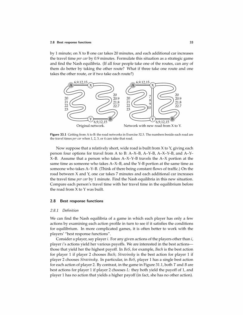
2.8 Best response functions 33
by 1 minute; on X to B one car takes 20 minutes, and each additional car increasesthe travel time per car by 0.9 minutes. Formulate this situation as a strategic gameand find the Nash equilibria. (If all four people take one of the routes, can any ofthem do better by taking the other route? What if three take one route and onetakes the other route, or if two take each route?)
6,9,12,15
20212223
6,9,12,15
2020.921.822.7
A X
BY
Original network.
6,9,12,15
20212223
6,9,12,15
2020.921.822.7
789
10
A X
BY
Network with new road from X to Y.
Figure 33.1 Getting from A to B: the road networks in Exercise 32.3. The numbers beside each road arethe travel times per car when 1, 2, 3, or 4 cars take that road.
Now suppose that a relatively short, wide road is built from X to Y, giving eachperson four options for travel from A to B: A–X–B, A–Y–B, A–X–Y–B, and A–Y–X–B. Assume that a person who takes A–X–Y–B travels the A–X portion at thesame time as someone who takes A–X–B, and the Y–B portion at the same time assomeone who takes A–Y–B. (Think of there being constant flows of traffic.) On theroad between X and Y, one car takes 7 minutes and each additional car increasesthe travel time per car by 1 minute. Find the Nash equilibria in this new situation.Compare each person’s travel time with her travel time in the equilibrium beforethe road from X to Y was built.
2.8 Best response functions
2.8.1 Definition
We can find the Nash equilibria of a game in which each player has only a fewactions by examining each action profile in turn to see if it satisfies the conditionsfor equilibrium. In more complicated games, it is often better to work with theplayers’ “best response functions”.
Consider a player, say player i. For any given actions of the players other than i,player i’s actions yield her various payoffs. We are interested in the best actions—those that yield her the highest payoff. In BoS, for example, Bach is the best actionfor player 1 if player 2 chooses Bach; Stravinsky is the best action for player 1 ifplayer 2 chooses Stravinsky. In particular, in BoS, player 1 has a single best actionfor each action of player 2. By contrast, in the game in Figure 31.1, both T and B arebest actions for player 1 if player 2 chooses L: they both yield the payoff of 1, andplayer 1 has no action that yields a higher payoff (in fact, she has no other action).
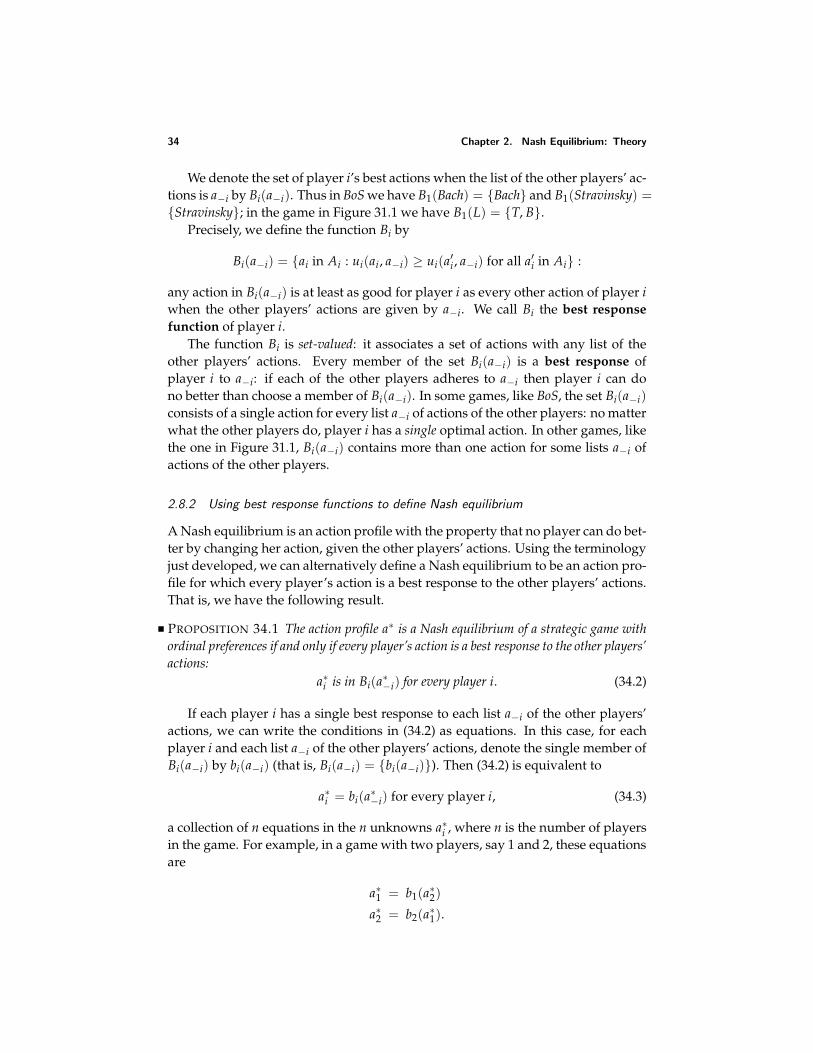
34 Chapter 2. Nash Equilibrium: Theory
We denote the set of player i’s best actions when the list of the other players’ ac-tions is a−i by Bi(a−i). Thus in BoS we have B1(Bach) = Bach and B1(Stravinsky) =Stravinsky; in the game in Figure 31.1 we have B1(L) = T, B.
Precisely, we define the function Bi by
Bi(a−i) = ai in Ai : ui(ai , a−i) ≥ ui(a′i , a−i) for all a′i in Ai :
any action in Bi(a−i) is at least as good for player i as every other action of player iwhen the other players’ actions are given by a−i. We call Bi the best responsefunction of player i.
The function Bi is set-valued: it associates a set of actions with any list of theother players’ actions. Every member of the set Bi(a−i) is a best response ofplayer i to a−i: if each of the other players adheres to a−i then player i can dono better than choose a member of Bi(a−i). In some games, like BoS, the set Bi(a−i)consists of a single action for every list a−i of actions of the other players: no matterwhat the other players do, player i has a single optimal action. In other games, likethe one in Figure 31.1, Bi(a−i) contains more than one action for some lists a−i ofactions of the other players.
2.8.2 Using best response functions to define Nash equilibrium
A Nash equilibrium is an action profile with the property that no player can do bet-ter by changing her action, given the other players’ actions. Using the terminologyjust developed, we can alternatively define a Nash equilibrium to be an action pro-file for which every player’s action is a best response to the other players’ actions.That is, we have the following result.
PROPOSITION 34.1 The action profile a∗ is a Nash equilibrium of a strategic game withordinal preferences if and only if every player’s action is a best response to the other players’actions:
a∗i is in Bi(a∗−i) for every player i. (34.2)
If each player i has a single best response to each list a−i of the other players’actions, we can write the conditions in (34.2) as equations. In this case, for eachplayer i and each list a−i of the other players’ actions, denote the single member ofBi(a−i) by bi(a−i) (that is, Bi(a−i) = bi(a−i)). Then (34.2) is equivalent to
a∗i = bi(a∗−i) for every player i, (34.3)
a collection of n equations in the n unknowns a∗i , where n is the number of playersin the game. For example, in a game with two players, say 1 and 2, these equationsare
a∗1 = b1(a∗2)a∗2 = b2(a∗1).
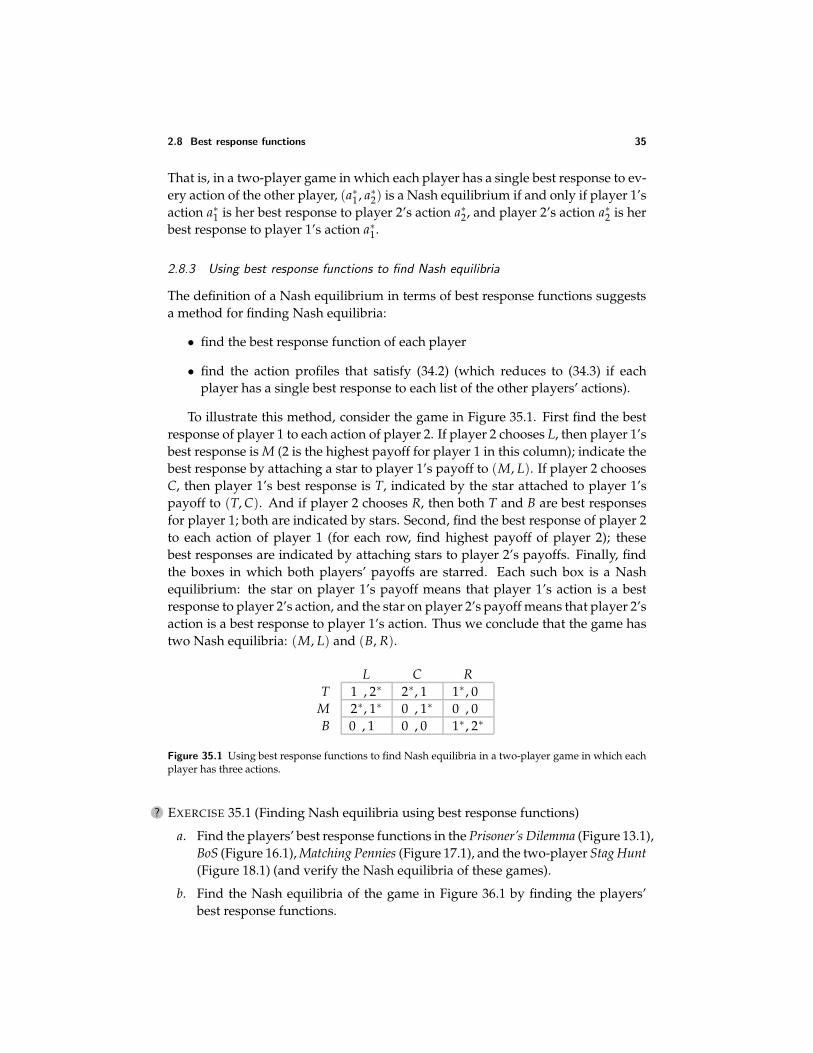
2.8 Best response functions 35
That is, in a two-player game in which each player has a single best response to ev-ery action of the other player, (a∗1, a∗2) is a Nash equilibrium if and only if player 1’saction a∗1 is her best response to player 2’s action a∗2, and player 2’s action a∗2 is herbest response to player 1’s action a∗1.
2.8.3 Using best response functions to find Nash equilibria
The definition of a Nash equilibrium in terms of best response functions suggestsa method for finding Nash equilibria:
• find the best response function of each player
• find the action profiles that satisfy (34.2) (which reduces to (34.3) if eachplayer has a single best response to each list of the other players’ actions).
To illustrate this method, consider the game in Figure 35.1. First find the bestresponse of player 1 to each action of player 2. If player 2 chooses L, then player 1’sbest response is M (2 is the highest payoff for player 1 in this column); indicate thebest response by attaching a star to player 1’s payoff to (M, L). If player 2 choosesC, then player 1’s best response is T, indicated by the star attached to player 1’spayoff to (T, C). And if player 2 chooses R, then both T and B are best responsesfor player 1; both are indicated by stars. Second, find the best response of player 2to each action of player 1 (for each row, find highest payoff of player 2); thesebest responses are indicated by attaching stars to player 2’s payoffs. Finally, findthe boxes in which both players’ payoffs are starred. Each such box is a Nashequilibrium: the star on player 1’s payoff means that player 1’s action is a bestresponse to player 2’s action, and the star on player 2’s payoff means that player 2’saction is a best response to player 1’s action. Thus we conclude that the game hastwo Nash equilibria: (M, L) and (B, R).
L C RT 1 , 2∗ 2∗, 1 1∗ , 0
M 2∗, 1∗ 0 , 1∗ 0 , 0B 0 , 1 0 , 0 1∗ , 2∗
Figure 35.1 Using best response functions to find Nash equilibria in a two-player game in which eachplayer has three actions.
? EXERCISE 35.1 (Finding Nash equilibria using best response functions)
a. Find the players’ best response functions in the Prisoner’s Dilemma (Figure 13.1),BoS (Figure 16.1), Matching Pennies (Figure 17.1), and the two-player Stag Hunt(Figure 18.1) (and verify the Nash equilibria of these games).
b. Find the Nash equilibria of the game in Figure 36.1 by finding the players’best response functions.
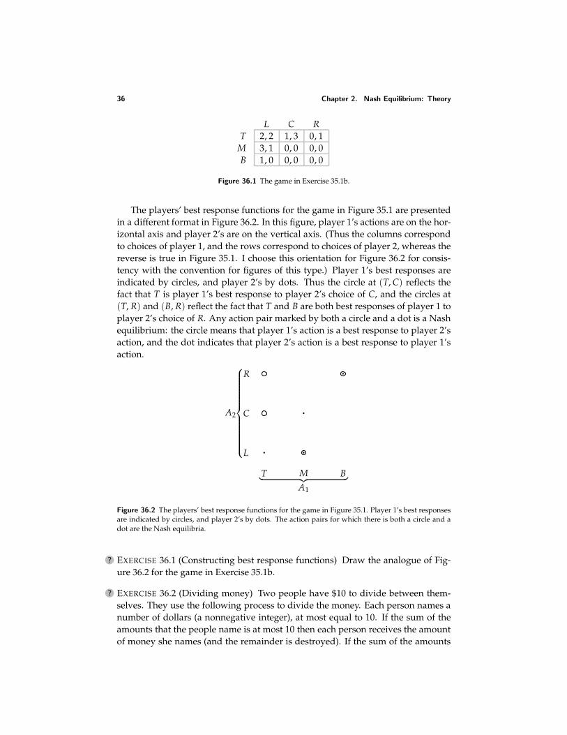
36 Chapter 2. Nash Equilibrium: Theory
L C RT 2, 2 1, 3 0, 1
M 3, 1 0, 0 0, 0B 1, 0 0, 0 0, 0
Figure 36.1 The game in Exercise 35.1b.
The players’ best response functions for the game in Figure 35.1 are presentedin a different format in Figure 36.2. In this figure, player 1’s actions are on the hor-izontal axis and player 2’s are on the vertical axis. (Thus the columns correspondto choices of player 1, and the rows correspond to choices of player 2, whereas thereverse is true in Figure 35.1. I choose this orientation for Figure 36.2 for consis-tency with the convention for figures of this type.) Player 1’s best responses areindicated by circles, and player 2’s by dots. Thus the circle at (T, C) reflects thefact that T is player 1’s best response to player 2’s choice of C, and the circles at(T, R) and (B, R) reflect the fact that T and B are both best responses of player 1 toplayer 2’s choice of R. Any action pair marked by both a circle and a dot is a Nashequilibrium: the circle means that player 1’s action is a best response to player 2’saction, and the dot indicates that player 2’s action is a best response to player 1’saction.
A1
︸ ︷︷ ︸T M B
A2
L
C
R
Figure 36.2 The players’ best response functions for the game in Figure 35.1. Player 1’s best responsesare indicated by circles, and player 2’s by dots. The action pairs for which there is both a circle and adot are the Nash equilibria.
? EXERCISE 36.1 (Constructing best response functions) Draw the analogue of Fig-ure 36.2 for the game in Exercise 35.1b.
? EXERCISE 36.2 (Dividing money) Two people have $10 to divide between them-selves. They use the following process to divide the money. Each person names anumber of dollars (a nonnegative integer), at most equal to 10. If the sum of theamounts that the people name is at most 10 then each person receives the amountof money she names (and the remainder is destroyed). If the sum of the amounts
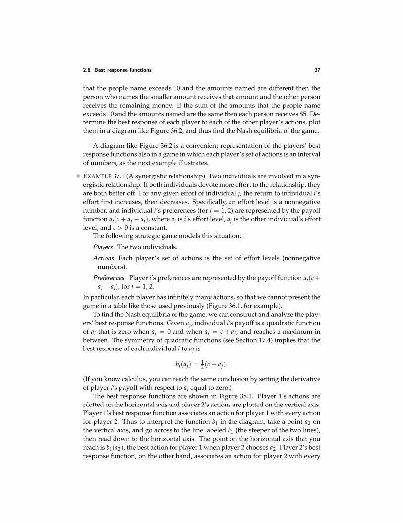
2.8 Best response functions 37
that the people name exceeds 10 and the amounts named are different then theperson who names the smaller amount receives that amount and the other personreceives the remaining money. If the sum of the amounts that the people nameexceeds 10 and the amounts named are the same then each person receives $5. De-termine the best response of each player to each of the other player’s actions, plotthem in a diagram like Figure 36.2, and thus find the Nash equilibria of the game.
A diagram like Figure 36.2 is a convenient representation of the players’ bestresponse functions also in a game in which each player’s set of actions is an intervalof numbers, as the next example illustrates.
EXAMPLE 37.1 (A synergistic relationship) Two individuals are involved in a syn-ergistic relationship. If both individuals devote more effort to the relationship, theyare both better off. For any given effort of individual j, the return to individual i’seffort first increases, then decreases. Specifically, an effort level is a nonnegativenumber, and individual i’s preferences (for i = 1, 2) are represented by the payofffunction ai(c + aj − ai), where ai is i’s effort level, aj is the other individual’s effortlevel, and c > 0 is a constant.
The following strategic game models this situation.
Players The two individuals.
Actions Each player’s set of actions is the set of effort levels (nonnegativenumbers).
Preferences Player i’s preferences are represented by the payoff function ai(c +aj − ai), for i = 1, 2.
In particular, each player has infinitely many actions, so that we cannot present thegame in a table like those used previously (Figure 36.1, for example).
To find the Nash equilibria of the game, we can construct and analyze the play-ers’ best response functions. Given aj, individual i’s payoff is a quadratic functionof ai that is zero when ai = 0 and when ai = c + aj, and reaches a maximum inbetween. The symmetry of quadratic functions (see Section 17.4) implies that thebest response of each individual i to aj is
bi(aj) = 12 (c + aj).
(If you know calculus, you can reach the same conclusion by setting the derivativeof player i’s payoff with respect to ai equal to zero.)
The best response functions are shown in Figure 38.1. Player 1’s actions areplotted on the horizontal axis and player 2’s actions are plotted on the vertical axis.Player 1’s best response function associates an action for player 1 with every actionfor player 2. Thus to interpret the function b1 in the diagram, take a point a2 onthe vertical axis, and go across to the line labeled b1 (the steeper of the two lines),then read down to the horizontal axis. The point on the horizontal axis that youreach is b1(a2), the best action for player 1 when player 2 chooses a2. Player 2’s bestresponse function, on the other hand, associates an action for player 2 with every
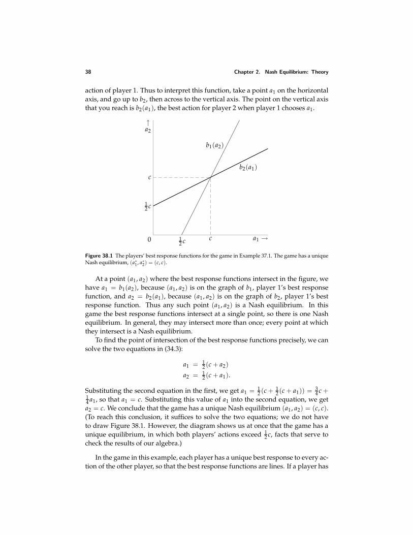
38 Chapter 2. Nash Equilibrium: Theory
action of player 1. Thus to interpret this function, take a point a1 on the horizontalaxis, and go up to b2, then across to the vertical axis. The point on the vertical axisthat you reach is b2(a1), the best action for player 2 when player 1 chooses a1.
0 a1 →
↑a2
12 c
12 c
c
cb2(a1)
b1(a2)
Figure 38.1 The players’ best response functions for the game in Example 37.1. The game has a uniqueNash equilibrium, (a∗1, a∗2) = (c, c).
At a point (a1, a2) where the best response functions intersect in the figure, wehave a1 = b1(a2), because (a1, a2) is on the graph of b1, player 1’s best responsefunction, and a2 = b2(a1), because (a1, a2) is on the graph of b2, player 1’s bestresponse function. Thus any such point (a1, a2) is a Nash equilibrium. In thisgame the best response functions intersect at a single point, so there is one Nashequilibrium. In general, they may intersect more than once; every point at whichthey intersect is a Nash equilibrium.
To find the point of intersection of the best response functions precisely, we cansolve the two equations in (34.3):
a1 = 12 (c + a2)
a2 = 12 (c + a1).
Substituting the second equation in the first, we get a1 = 12 (c + 1
2 (c + a1)) = 34 c +
14 a1, so that a1 = c. Substituting this value of a1 into the second equation, we geta2 = c. We conclude that the game has a unique Nash equilibrium (a1, a2) = (c, c).(To reach this conclusion, it suffices to solve the two equations; we do not haveto draw Figure 38.1. However, the diagram shows us at once that the game has aunique equilibrium, in which both players’ actions exceed 1
2 c, facts that serve tocheck the results of our algebra.)
In the game in this example, each player has a unique best response to every ac-tion of the other player, so that the best response functions are lines. If a player has
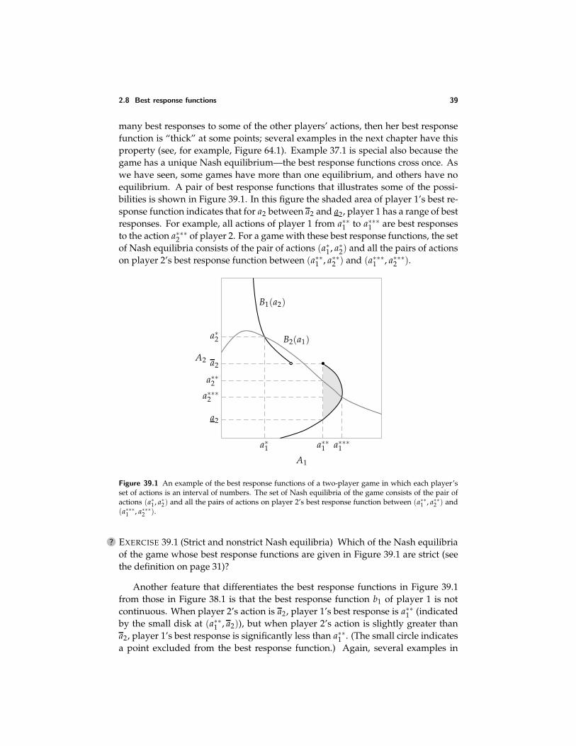
2.8 Best response functions 39
many best responses to some of the other players’ actions, then her best responsefunction is “thick” at some points; several examples in the next chapter have thisproperty (see, for example, Figure 64.1). Example 37.1 is special also because thegame has a unique Nash equilibrium—the best response functions cross once. Aswe have seen, some games have more than one equilibrium, and others have noequilibrium. A pair of best response functions that illustrates some of the possi-bilities is shown in Figure 39.1. In this figure the shaded area of player 1’s best re-sponse function indicates that for a2 between a2 and a2, player 1 has a range of bestresponses. For example, all actions of player 1 from a∗∗1 to a∗∗∗1 are best responsesto the action a∗∗∗2 of player 2. For a game with these best response functions, the setof Nash equilibria consists of the pair of actions (a∗1, a∗2) and all the pairs of actionson player 2’s best response function between (a∗∗1 , a∗∗2 ) and (a∗∗∗1 , a∗∗∗2 ).
a∗1
a∗2
a2
a∗∗1
a∗∗2
a∗∗∗2
a∗∗∗1
a2
B1(a2)
B2(a1)
A1
A2
Figure 39.1 An example of the best response functions of a two-player game in which each player’sset of actions is an interval of numbers. The set of Nash equilibria of the game consists of the pair ofactions (a∗1, a∗2) and all the pairs of actions on player 2’s best response function between (a∗∗1 , a∗∗2 ) and(a∗∗∗1 , a∗∗∗2 ).
? EXERCISE 39.1 (Strict and nonstrict Nash equilibria) Which of the Nash equilibriaof the game whose best response functions are given in Figure 39.1 are strict (seethe definition on page 31)?
Another feature that differentiates the best response functions in Figure 39.1from those in Figure 38.1 is that the best response function b1 of player 1 is notcontinuous. When player 2’s action is a2, player 1’s best response is a∗∗1 (indicatedby the small disk at (a∗∗1 , a2)), but when player 2’s action is slightly greater thana2, player 1’s best response is significantly less than a∗∗1 . (The small circle indicatesa point excluded from the best response function.) Again, several examples in
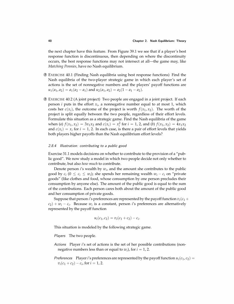
40 Chapter 2. Nash Equilibrium: Theory
the next chapter have this feature. From Figure 39.1 we see that if a player’s bestresponse function is discontinuous, then depending on where the discontinuityoccurs, the best response functions may not intersect at all—the game may, likeMatching Pennies, have no Nash equilibrium.
? EXERCISE 40.1 (Finding Nash equilibria using best response functions) Find theNash equilibria of the two-player strategic game in which each player’s set ofactions is the set of nonnegative numbers and the players’ payoff functions areu1(a1, a2) = a1(a2 − a1) and u2(a1, a2) = a2(1 − a1 − a2).
? EXERCISE 40.2 (A joint project) Two people are engaged in a joint project. If eachperson i puts in the effort xi, a nonnegative number equal to at most 1, whichcosts her c(xi), the outcome of the project is worth f (x1, x2). The worth of theproject is split equally between the two people, regardless of their effort levels.Formulate this situation as a strategic game. Find the Nash equilibria of the gamewhen (a) f (x1, x2) = 3x1x2 and c(xi) = x2
i for i = 1, 2, and (b) f (x1, x2) = 4x1x2and c(xi) = xi for i = 1, 2. In each case, is there a pair of effort levels that yieldsboth players higher payoffs than the Nash equilibrium effort levels?
2.8.4 Illustration: contributing to a public good
Exercise 31.1 models decisions on whether to contribute to the provision of a “pub-lic good”. We now study a model in which two people decide not only whether tocontribute, but also how much to contribute.
Denote person i’s wealth by wi, and the amount she contributes to the publicgood by ci (0 ≤ ci ≤ wi); she spends her remaining wealth wi − ci on “privategoods” (like clothes and food, whose consumption by one person precludes theirconsumption by anyone else). The amount of the public good is equal to the sumof the contributions. Each person cares both about the amount of the public goodand her consumption of private goods.
Suppose that person i’s preferences are represented by the payoff function vi(c1 +c2) + wi − ci. Because wi is a constant, person i’s preferences are alternativelyrepresented by the payoff function
ui(c1, c2) = vi(c1 + c2) − ci.
This situation is modeled by the following strategic game.
Players The two people.
Actions Player i’s set of actions is the set of her possible contributions (non-negative numbers less than or equal to wi), for i = 1, 2.
Preferences Player i’s preferences are represented by the payoff function ui(c1, c2) =vi(c1 + c2) − ci, for i = 1, 2.
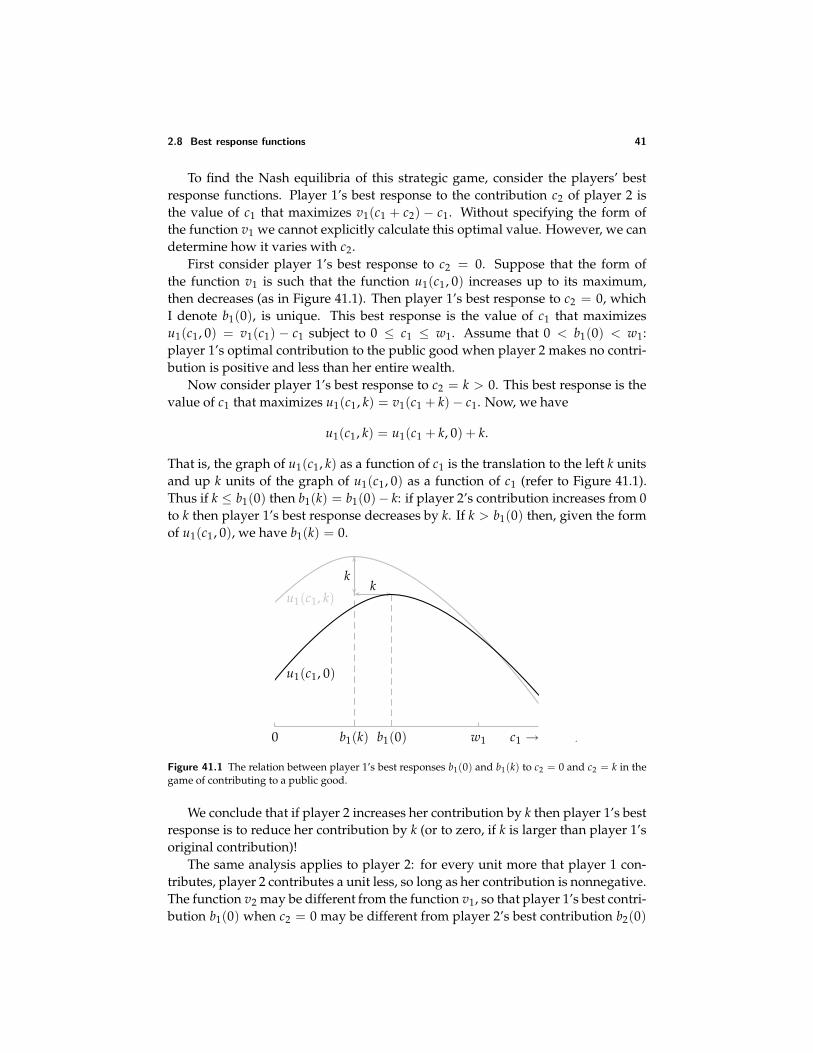
2.8 Best response functions 41
To find the Nash equilibria of this strategic game, consider the players’ bestresponse functions. Player 1’s best response to the contribution c2 of player 2 isthe value of c1 that maximizes v1(c1 + c2) − c1. Without specifying the form ofthe function v1 we cannot explicitly calculate this optimal value. However, we candetermine how it varies with c2.
First consider player 1’s best response to c2 = 0. Suppose that the form ofthe function v1 is such that the function u1(c1, 0) increases up to its maximum,then decreases (as in Figure 41.1). Then player 1’s best response to c2 = 0, whichI denote b1(0), is unique. This best response is the value of c1 that maximizesu1(c1, 0) = v1(c1) − c1 subject to 0 ≤ c1 ≤ w1. Assume that 0 < b1(0) < w1:player 1’s optimal contribution to the public good when player 2 makes no contri-bution is positive and less than her entire wealth.
Now consider player 1’s best response to c2 = k > 0. This best response is thevalue of c1 that maximizes u1(c1, k) = v1(c1 + k) − c1. Now, we have
u1(c1, k) = u1(c1 + k, 0) + k.
That is, the graph of u1(c1, k) as a function of c1 is the translation to the left k unitsand up k units of the graph of u1(c1, 0) as a function of c1 (refer to Figure 41.1).Thus if k ≤ b1(0) then b1(k) = b1(0)− k: if player 2’s contribution increases from 0to k then player 1’s best response decreases by k. If k > b1(0) then, given the formof u1(c1, 0), we have b1(k) = 0.
kk
0 w1b1(0)b1(k) c1 →
u1(c1, k)
u1(c1, 0)
Figure 41.1 The relation between player 1’s best responses b1(0) and b1(k) to c2 = 0 and c2 = k in thegame of contributing to a public good.
We conclude that if player 2 increases her contribution by k then player 1’s bestresponse is to reduce her contribution by k (or to zero, if k is larger than player 1’soriginal contribution)!
The same analysis applies to player 2: for every unit more that player 1 con-tributes, player 2 contributes a unit less, so long as her contribution is nonnegative.The function v2 may be different from the function v1, so that player 1’s best contri-bution b1(0) when c2 = 0 may be different from player 2’s best contribution b2(0)
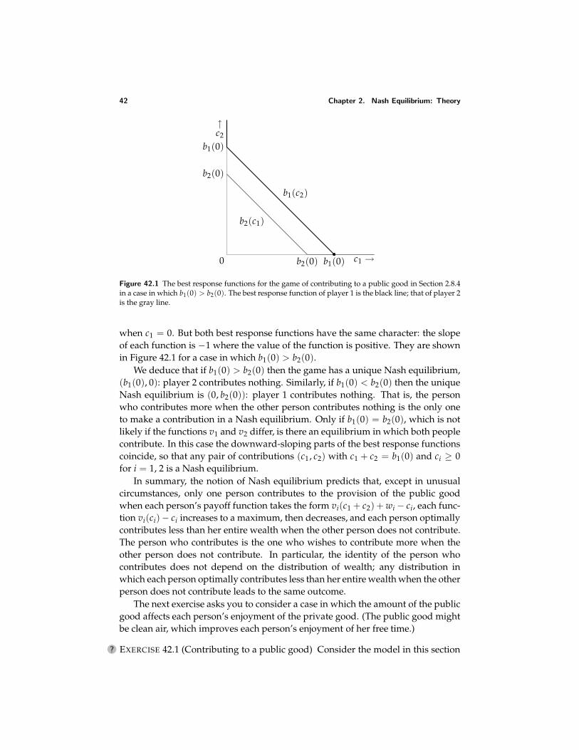
42 Chapter 2. Nash Equilibrium: Theory
0 c1 →
↑c2
b1(0)
b1(0)
b2(0)
b2(0)
b1(c2)
b2(c1)
Figure 42.1 The best response functions for the game of contributing to a public good in Section 2.8.4in a case in which b1(0) > b2(0). The best response function of player 1 is the black line; that of player 2is the gray line.
when c1 = 0. But both best response functions have the same character: the slopeof each function is −1 where the value of the function is positive. They are shownin Figure 42.1 for a case in which b1(0) > b2(0).
We deduce that if b1(0) > b2(0) then the game has a unique Nash equilibrium,(b1(0), 0): player 2 contributes nothing. Similarly, if b1(0) < b2(0) then the uniqueNash equilibrium is (0, b2(0)): player 1 contributes nothing. That is, the personwho contributes more when the other person contributes nothing is the only oneto make a contribution in a Nash equilibrium. Only if b1(0) = b2(0), which is notlikely if the functions v1 and v2 differ, is there an equilibrium in which both peoplecontribute. In this case the downward-sloping parts of the best response functionscoincide, so that any pair of contributions (c1, c2) with c1 + c2 = b1(0) and ci ≥ 0for i = 1, 2 is a Nash equilibrium.
In summary, the notion of Nash equilibrium predicts that, except in unusualcircumstances, only one person contributes to the provision of the public goodwhen each person’s payoff function takes the form vi(c1 + c2) + wi − ci, each func-tion vi(ci)− ci increases to a maximum, then decreases, and each person optimallycontributes less than her entire wealth when the other person does not contribute.The person who contributes is the one who wishes to contribute more when theother person does not contribute. In particular, the identity of the person whocontributes does not depend on the distribution of wealth; any distribution inwhich each person optimally contributes less than her entire wealth when the otherperson does not contribute leads to the same outcome.
The next exercise asks you to consider a case in which the amount of the publicgood affects each person’s enjoyment of the private good. (The public good mightbe clean air, which improves each person’s enjoyment of her free time.)
? EXERCISE 42.1 (Contributing to a public good) Consider the model in this section
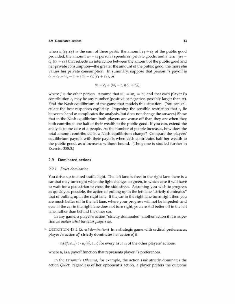
2.9 Dominated actions 43
when ui(c1, c2) is the sum of three parts: the amount c1 + c2 of the public goodprovided, the amount wi − ci person i spends on private goods, and a term (wi −ci)(c1 + c2) that reflects an interaction between the amount of the public good andher private consumption—the greater the amount of the public good, the more shevalues her private consumption. In summary, suppose that person i’s payoff isc1 + c2 + wi − ci + (wi − ci)(c1 + c2), or
wi + cj + (wi − ci)(c1 + c2),
where j is the other person. Assume that w1 = w2 = w, and that each player i’scontribution ci may be any number (positive or negative, possibly larger than w).Find the Nash equilibrium of the game that models this situation. (You can cal-culate the best responses explicitly. Imposing the sensible restriction that ci liebetween 0 and w complicates the analysis, but does not change the answer.) Showthat in the Nash equilibrium both players are worse off than they are when theyboth contribute one half of their wealth to the public good. If you can, extend theanalysis to the case of n people. As the number of people increases, how does thetotal amount contributed in a Nash equilibrium change? Compare the players’equilibrium payoffs with their payoffs when each contributes half her wealth tothe public good, as n increases without bound. (The game is studied further inExercise 358.3.)
2.9 Dominated actions
2.9.1 Strict domination
You drive up to a red traffic light. The left lane is free; in the right lane there is acar that may turn right when the light changes to green, in which case it will haveto wait for a pedestrian to cross the side street. Assuming you wish to progressas quickly as possible, the action of pulling up in the left lane “strictly dominates”that of pulling up in the right lane. If the car in the right lane turns right then youare much better off in the left lane, where your progress will not be impeded; andeven if the car in the right lane does not turn right, you are still better off in the leftlane, rather than behind the other car.
In any game, a player’s action “strictly dominates” another action if it is supe-rior, no matter what the other players do.
DEFINITION 43.1 (Strict domination) In a strategic game with ordinal preferences,player i’s action a′′i strictly dominates her action a′i if
ui(a′′i , a−i) > ui(a′i , a−i) for every list a−i of the other players’ actions,
where ui is a payoff function that represents player i’s preferences.
In the Prisoner’s Dilemma, for example, the action Fink strictly dominates theaction Quiet: regardless of her opponent’s action, a player prefers the outcome
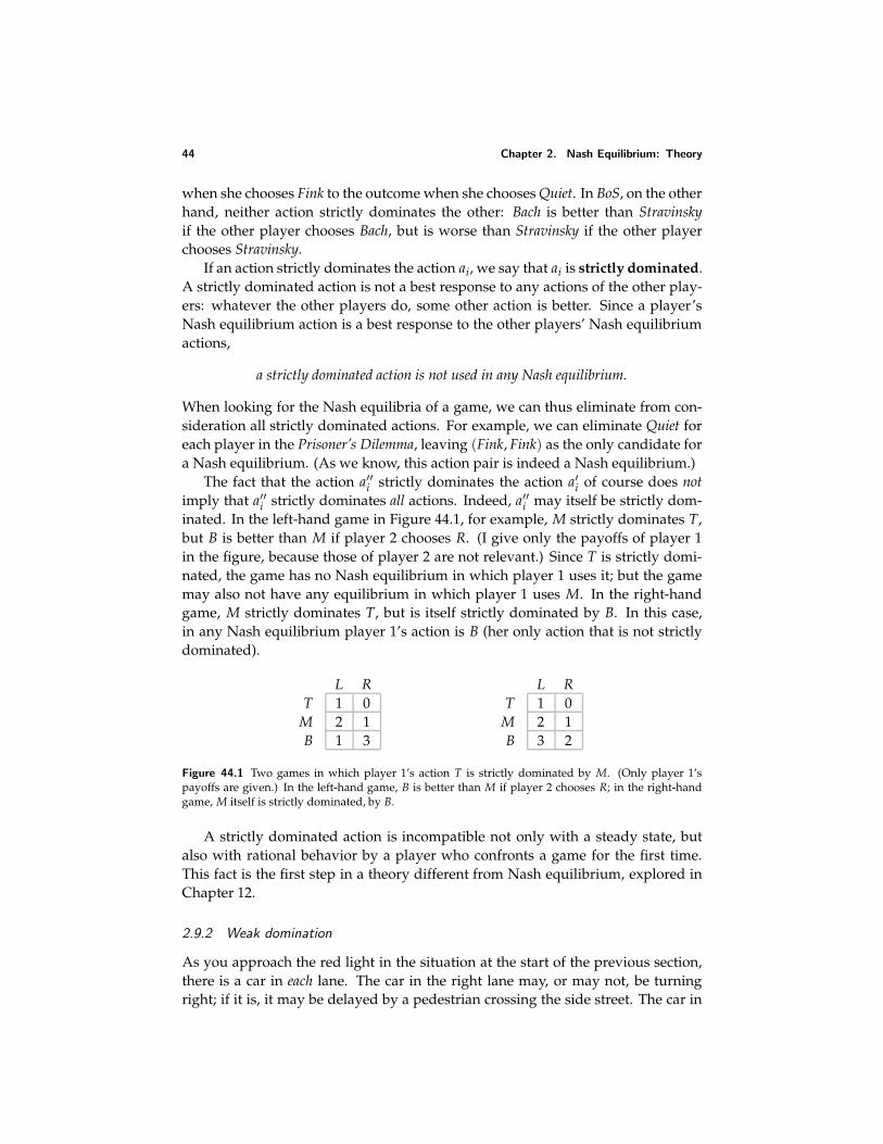
44 Chapter 2. Nash Equilibrium: Theory
when she chooses Fink to the outcome when she chooses Quiet. In BoS, on the otherhand, neither action strictly dominates the other: Bach is better than Stravinskyif the other player chooses Bach, but is worse than Stravinsky if the other playerchooses Stravinsky.
If an action strictly dominates the action ai, we say that ai is strictly dominated.A strictly dominated action is not a best response to any actions of the other play-ers: whatever the other players do, some other action is better. Since a player’sNash equilibrium action is a best response to the other players’ Nash equilibriumactions,
a strictly dominated action is not used in any Nash equilibrium.
When looking for the Nash equilibria of a game, we can thus eliminate from con-sideration all strictly dominated actions. For example, we can eliminate Quiet foreach player in the Prisoner’s Dilemma, leaving (Fink, Fink) as the only candidate fora Nash equilibrium. (As we know, this action pair is indeed a Nash equilibrium.)
The fact that the action a′′i strictly dominates the action a′i of course does notimply that a′′i strictly dominates all actions. Indeed, a′′i may itself be strictly dom-inated. In the left-hand game in Figure 44.1, for example, M strictly dominates T,but B is better than M if player 2 chooses R. (I give only the payoffs of player 1in the figure, because those of player 2 are not relevant.) Since T is strictly domi-nated, the game has no Nash equilibrium in which player 1 uses it; but the gamemay also not have any equilibrium in which player 1 uses M. In the right-handgame, M strictly dominates T, but is itself strictly dominated by B. In this case,in any Nash equilibrium player 1’s action is B (her only action that is not strictlydominated).
L RT 1 0
M 2 1B 1 3
L RT 1 0
M 2 1B 3 2
Figure 44.1 Two games in which player 1’s action T is strictly dominated by M. (Only player 1’spayoffs are given.) In the left-hand game, B is better than M if player 2 chooses R; in the right-handgame, M itself is strictly dominated, by B.
A strictly dominated action is incompatible not only with a steady state, butalso with rational behavior by a player who confronts a game for the first time.This fact is the first step in a theory different from Nash equilibrium, explored inChapter 12.
2.9.2 Weak domination
As you approach the red light in the situation at the start of the previous section,there is a car in each lane. The car in the right lane may, or may not, be turningright; if it is, it may be delayed by a pedestrian crossing the side street. The car in
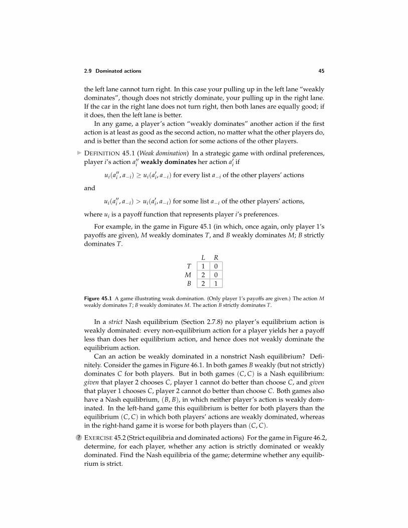
2.9 Dominated actions 45
the left lane cannot turn right. In this case your pulling up in the left lane “weaklydominates”, though does not strictly dominate, your pulling up in the right lane.If the car in the right lane does not turn right, then both lanes are equally good; ifit does, then the left lane is better.
In any game, a player’s action “weakly dominates” another action if the firstaction is at least as good as the second action, no matter what the other players do,and is better than the second action for some actions of the other players.
DEFINITION 45.1 (Weak domination) In a strategic game with ordinal preferences,player i’s action a′′i weakly dominates her action a′i if
ui(a′′i , a−i) ≥ ui(a′i, a−i) for every list a−i of the other players’ actions
and
ui(a′′i , a−i) > ui(a′i , a−i) for some list a−i of the other players’ actions,
where ui is a payoff function that represents player i’s preferences.
For example, in the game in Figure 45.1 (in which, once again, only player 1’spayoffs are given), M weakly dominates T, and B weakly dominates M; B strictlydominates T.
L RT 1 0
M 2 0B 2 1
Figure 45.1 A game illustrating weak domination. (Only player 1’s payoffs are given.) The action Mweakly dominates T; B weakly dominates M. The action B strictly dominates T.
In a strict Nash equilibrium (Section 2.7.8) no player’s equilibrium action isweakly dominated: every non-equilibrium action for a player yields her a payoffless than does her equilibrium action, and hence does not weakly dominate theequilibrium action.
Can an action be weakly dominated in a nonstrict Nash equilibrium? Defi-nitely. Consider the games in Figure 46.1. In both games B weakly (but not strictly)dominates C for both players. But in both games (C, C) is a Nash equilibrium:given that player 2 chooses C, player 1 cannot do better than choose C, and giventhat player 1 chooses C, player 2 cannot do better than choose C. Both games alsohave a Nash equilibrium, (B, B), in which neither player’s action is weakly dom-inated. In the left-hand game this equilibrium is better for both players than theequilibrium (C, C) in which both players’ actions are weakly dominated, whereasin the right-hand game it is worse for both players than (C, C).
? EXERCISE 45.2 (Strict equilibria and dominated actions) For the game in Figure 46.2,determine, for each player, whether any action is strictly dominated or weaklydominated. Find the Nash equilibria of the game; determine whether any equilib-rium is strict.
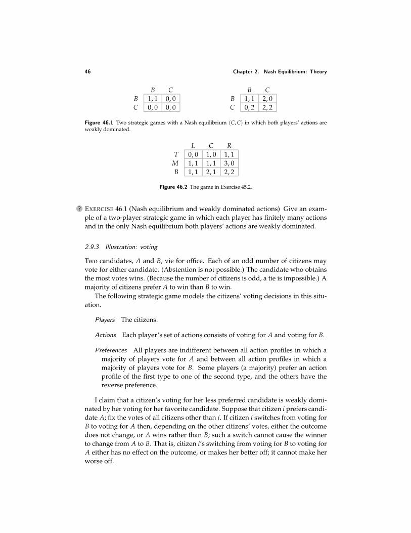
46 Chapter 2. Nash Equilibrium: Theory
B CB 1, 1 0, 0C 0, 0 0, 0
B CB 1, 1 2, 0C 0, 2 2, 2
Figure 46.1 Two strategic games with a Nash equilibrium (C, C) in which both players’ actions areweakly dominated.
L C RT 0, 0 1, 0 1, 1
M 1, 1 1, 1 3, 0B 1, 1 2, 1 2, 2
Figure 46.2 The game in Exercise 45.2.
? EXERCISE 46.1 (Nash equilibrium and weakly dominated actions) Give an exam-ple of a two-player strategic game in which each player has finitely many actionsand in the only Nash equilibrium both players’ actions are weakly dominated.
2.9.3 Illustration: voting
Two candidates, A and B, vie for office. Each of an odd number of citizens mayvote for either candidate. (Abstention is not possible.) The candidate who obtainsthe most votes wins. (Because the number of citizens is odd, a tie is impossible.) Amajority of citizens prefer A to win than B to win.
The following strategic game models the citizens’ voting decisions in this situ-ation.
Players The citizens.
Actions Each player’s set of actions consists of voting for A and voting for B.
Preferences All players are indifferent between all action profiles in which amajority of players vote for A and between all action profiles in which amajority of players vote for B. Some players (a majority) prefer an actionprofile of the first type to one of the second type, and the others have thereverse preference.
I claim that a citizen’s voting for her less preferred candidate is weakly domi-nated by her voting for her favorite candidate. Suppose that citizen i prefers candi-date A; fix the votes of all citizens other than i. If citizen i switches from voting forB to voting for A then, depending on the other citizens’ votes, either the outcomedoes not change, or A wins rather than B; such a switch cannot cause the winnerto change from A to B. That is, citizen i’s switching from voting for B to voting forA either has no effect on the outcome, or makes her better off; it cannot make herworse off.
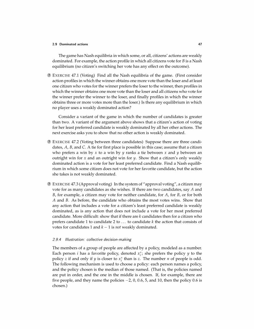
2.9 Dominated actions 47
The game has Nash equilibria in which some, or all, citizens’ actions are weaklydominated. For example, the action profile in which all citizens vote for B is a Nashequilibrium (no citizen’s switching her vote has any effect on the outcome).
? EXERCISE 47.1 (Voting) Find all the Nash equilibria of the game. (First consideraction profiles in which the winner obtains one more vote than the loser and at leastone citizen who votes for the winner prefers the loser to the winner, then profiles inwhich the winner obtains one more vote than the loser and all citizens who vote forthe winner prefer the winner to the loser, and finally profiles in which the winnerobtains three or more votes more than the loser.) Is there any equilibrium in whichno player uses a weakly dominated action?
Consider a variant of the game in which the number of candidates is greaterthan two. A variant of the argument above shows that a citizen’s action of votingfor her least preferred candidate is weakly dominated by all her other actions. Thenext exercise asks you to show that no other action is weakly dominated.
? EXERCISE 47.2 (Voting between three candidates) Suppose there are three candi-dates, A, B, and C. A tie for first place is possible in this case; assume that a citizenwho prefers a win by x to a win by y ranks a tie between x and y between anoutright win for x and an outright win for y. Show that a citizen’s only weaklydominated action is a vote for her least preferred candidate. Find a Nash equilib-rium in which some citizen does not vote for her favorite candidate, but the actionshe takes is not weakly dominated.
? EXERCISE 47.3 (Approval voting) In the system of “approval voting”, a citizen mayvote for as many candidates as she wishes. If there are two candidates, say A andB, for example, a citizen may vote for neither candidate, for A, for B, or for bothA and B. As before, the candidate who obtains the most votes wins. Show thatany action that includes a vote for a citizen’s least preferred candidate is weaklydominated, as is any action that does not include a vote for her most preferredcandidate. More difficult: show that if there are k candidates then for a citizen whoprefers candidate 1 to candidate 2 to . . . to candidate k the action that consists ofvotes for candidates 1 and k − 1 is not weakly dominated.
2.9.4 Illustration: collective decision-making
The members of a group of people are affected by a policy, modeled as a number.Each person i has a favorite policy, denoted x∗
i ; she prefers the policy y to thepolicy z if and only if y is closer to x∗
i than is z. The number n of people is odd.The following mechanism is used to choose a policy: each person names a policy,and the policy chosen is the median of those named. (That is, the policies namedare put in order, and the one in the middle is chosen. If, for example, there arefive people, and they name the policies −2, 0, 0.6, 5, and 10, then the policy 0.6 ischosen.)
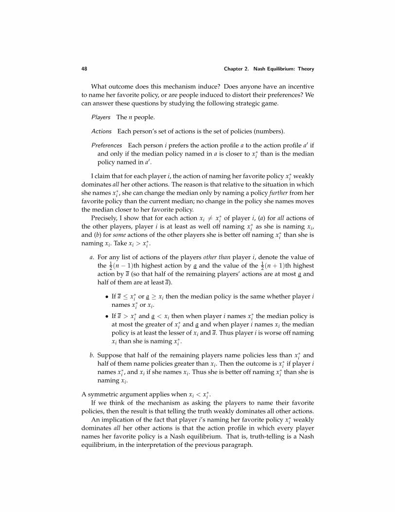
48 Chapter 2. Nash Equilibrium: Theory
What outcome does this mechanism induce? Does anyone have an incentiveto name her favorite policy, or are people induced to distort their preferences? Wecan answer these questions by studying the following strategic game.
Players The n people.
Actions Each person’s set of actions is the set of policies (numbers).
Preferences Each person i prefers the action profile a to the action profile a′ ifand only if the median policy named in a is closer to x∗
i than is the medianpolicy named in a′.
I claim that for each player i, the action of naming her favorite policy x∗i weakly
dominates all her other actions. The reason is that relative to the situation in whichshe names x∗
i , she can change the median only by naming a policy further from herfavorite policy than the current median; no change in the policy she names movesthe median closer to her favorite policy.
Precisely, I show that for each action xi = x∗i of player i, (a) for all actions of
the other players, player i is at least as well off naming x∗i as she is naming xi,
and (b) for some actions of the other players she is better off naming x∗i than she is
naming xi. Take xi > x∗i .
a. For any list of actions of the players other than player i, denote the value ofthe 1
2 (n − 1)th highest action by a and the value of the 12 (n + 1)th highest
action by a (so that half of the remaining players’ actions are at most a andhalf of them are at least a).
• If a ≤ x∗i or a ≥ xi then the median policy is the same whether player i
names x∗i or xi.
• If a > x∗i and a < xi then when player i names x∗
i the median policy isat most the greater of x∗
i and a and when player i names xi the medianpolicy is at least the lesser of xi and a. Thus player i is worse off namingxi than she is naming x∗
i .
b. Suppose that half of the remaining players name policies less than x∗i and
half of them name policies greater than xi. Then the outcome is x∗i if player i
names x∗i , and xi if she names xi. Thus she is better off naming x∗
i than she isnaming xi.
A symmetric argument applies when xi < x∗i .
If we think of the mechanism as asking the players to name their favoritepolicies, then the result is that telling the truth weakly dominates all other actions.
An implication of the fact that player i’s naming her favorite policy x∗i weakly
dominates all her other actions is that the action profile in which every playernames her favorite policy is a Nash equilibrium. That is, truth-telling is a Nashequilibrium, in the interpretation of the previous paragraph.
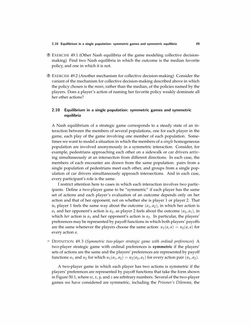
2.10 Equilibrium in a single population: symmetric games and symmetric equilibria 49
? EXERCISE 49.1 (Other Nash equilibria of the game modeling collective decision-making) Find two Nash equilibria in which the outcome is the median favoritepolicy, and one in which it is not.
? EXERCISE 49.2 (Another mechanism for collective decision-making) Consider thevariant of the mechanism for collective decision-making described above in whichthe policy chosen is the mean, rather than the median, of the policies named by theplayers. Does a player’s action of naming her favorite policy weakly dominate allher other actions?
2.10 Equilibrium in a single population: symmetric games and symmetric
equilibria
A Nash equilibrium of a strategic game corresponds to a steady state of an in-teraction between the members of several populations, one for each player in thegame, each play of the game involving one member of each population. Some-times we want to model a situation in which the members of a single homogeneouspopulation are involved anonymously in a symmetric interaction. Consider, forexample, pedestrians approaching each other on a sidewalk or car drivers arriv-ing simultaneously at an intersection from different directions. In each case, themembers of each encounter are drawn from the same population: pairs from asingle population of pedestrians meet each other, and groups from a single pop-ulation of car drivers simultaneously approach intersections. And in each case,every participant’s role is the same.
I restrict attention here to cases in which each interaction involves two partic-ipants. Define a two-player game to be “symmetric” if each player has the sameset of actions and each player’s evaluation of an outcome depends only on heraction and that of her opponent, not on whether she is player 1 or player 2. Thatis, player 1 feels the same way about the outcome (a1, a2), in which her action isa1 and her opponent’s action is a2, as player 2 feels about the outcome (a2, a1), inwhich her action is a1 and her opponent’s action is a2. In particular, the players’preferences may be represented by payoff functions in which both players’ payoffsare the same whenever the players choose the same action: u1(a, a) = u2(a, a) forevery action a.
DEFINITION 49.3 (Symmetric two-player strategic game with ordinal preferences) Atwo-player strategic game with ordinal preferences is symmetric if the players’sets of actions are the same and the players’ preferences are represented by payofffunctions u1 and u2 for which u1(a1, a2) = u2(a2, a1) for every action pair (a1, a2).
A two-player game in which each player has two actions is symmetric if theplayers’ preferences are represented by payoff functions that take the form shownin Figure 50.1, where w, x, y, and z are arbitrary numbers. Several of the two-playergames we have considered are symmetric, including the Prisoner’s Dilemma, the
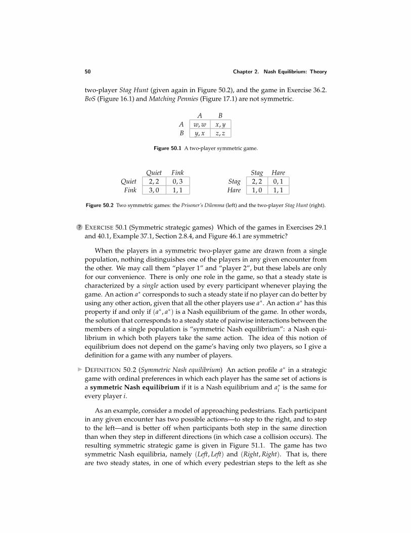
50 Chapter 2. Nash Equilibrium: Theory
two-player Stag Hunt (given again in Figure 50.2), and the game in Exercise 36.2.BoS (Figure 16.1) and Matching Pennies (Figure 17.1) are not symmetric.
A BA w, w x, yB y, x z, z
Figure 50.1 A two-player symmetric game.
Quiet FinkQuiet 2, 2 0, 3Fink 3, 0 1, 1
Stag HareStag 2, 2 0, 1Hare 1, 0 1, 1
Figure 50.2 Two symmetric games: the Prisoner’s Dilemma (left) and the two-player Stag Hunt (right).
? EXERCISE 50.1 (Symmetric strategic games) Which of the games in Exercises 29.1and 40.1, Example 37.1, Section 2.8.4, and Figure 46.1 are symmetric?
When the players in a symmetric two-player game are drawn from a singlepopulation, nothing distinguishes one of the players in any given encounter fromthe other. We may call them “player 1” and “player 2”, but these labels are onlyfor our convenience. There is only one role in the game, so that a steady state ischaracterized by a single action used by every participant whenever playing thegame. An action a∗ corresponds to such a steady state if no player can do better byusing any other action, given that all the other players use a∗. An action a∗ has thisproperty if and only if (a∗ , a∗) is a Nash equilibrium of the game. In other words,the solution that corresponds to a steady state of pairwise interactions between themembers of a single population is “symmetric Nash equilibrium”: a Nash equi-librium in which both players take the same action. The idea of this notion ofequilibrium does not depend on the game’s having only two players, so I give adefinition for a game with any number of players.
DEFINITION 50.2 (Symmetric Nash equilibrium) An action profile a∗ in a strategicgame with ordinal preferences in which each player has the same set of actions isa symmetric Nash equilibrium if it is a Nash equilibrium and a∗i is the same forevery player i.
As an example, consider a model of approaching pedestrians. Each participantin any given encounter has two possible actions—to step to the right, and to stepto the left—and is better off when participants both step in the same directionthan when they step in different directions (in which case a collision occurs). Theresulting symmetric strategic game is given in Figure 51.1. The game has twosymmetric Nash equilibria, namely (Left, Left) and (Right, Right). That is, thereare two steady states, in one of which every pedestrian steps to the left as she
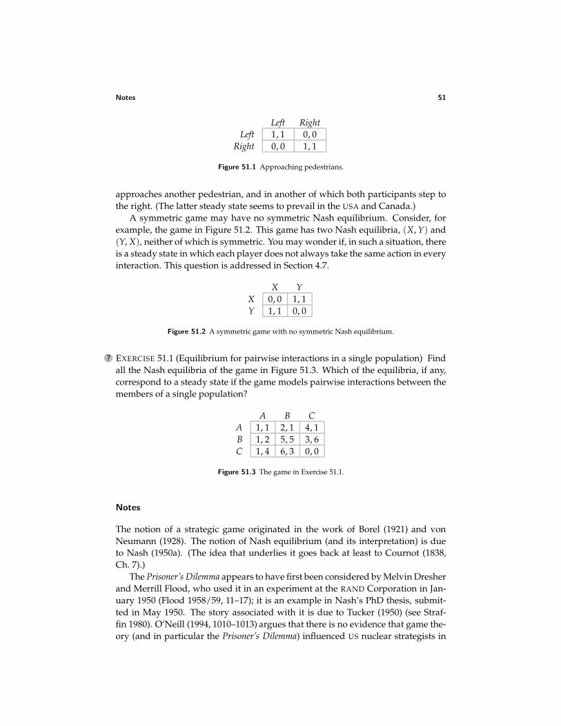
Notes 51
Left RightLeft 1, 1 0, 0
Right 0, 0 1, 1
Figure 51.1 Approaching pedestrians.
approaches another pedestrian, and in another of which both participants step tothe right. (The latter steady state seems to prevail in the USA and Canada.)
A symmetric game may have no symmetric Nash equilibrium. Consider, forexample, the game in Figure 51.2. This game has two Nash equilibria, (X, Y) and(Y, X), neither of which is symmetric. You may wonder if, in such a situation, thereis a steady state in which each player does not always take the same action in everyinteraction. This question is addressed in Section 4.7.
X YX 0, 0 1, 1Y 1, 1 0, 0
Figure 51.2 A symmetric game with no symmetric Nash equilibrium.
? EXERCISE 51.1 (Equilibrium for pairwise interactions in a single population) Findall the Nash equilibria of the game in Figure 51.3. Which of the equilibria, if any,correspond to a steady state if the game models pairwise interactions between themembers of a single population?
A B CA 1, 1 2, 1 4, 1B 1, 2 5, 5 3, 6C 1, 4 6, 3 0, 0
Figure 51.3 The game in Exercise 51.1.
Notes
The notion of a strategic game originated in the work of Borel (1921) and vonNeumann (1928). The notion of Nash equilibrium (and its interpretation) is dueto Nash (1950a). (The idea that underlies it goes back at least to Cournot (1838,Ch. 7).)
The Prisoner’s Dilemma appears to have first been considered by Melvin Dresherand Merrill Flood, who used it in an experiment at the RAND Corporation in Jan-uary 1950 (Flood 1958/59, 11–17); it is an example in Nash’s PhD thesis, submit-ted in May 1950. The story associated with it is due to Tucker (1950) (see Straf-fin 1980). O’Neill (1994, 1010–1013) argues that there is no evidence that game the-ory (and in particular the Prisoner’s Dilemma) influenced US nuclear strategists in
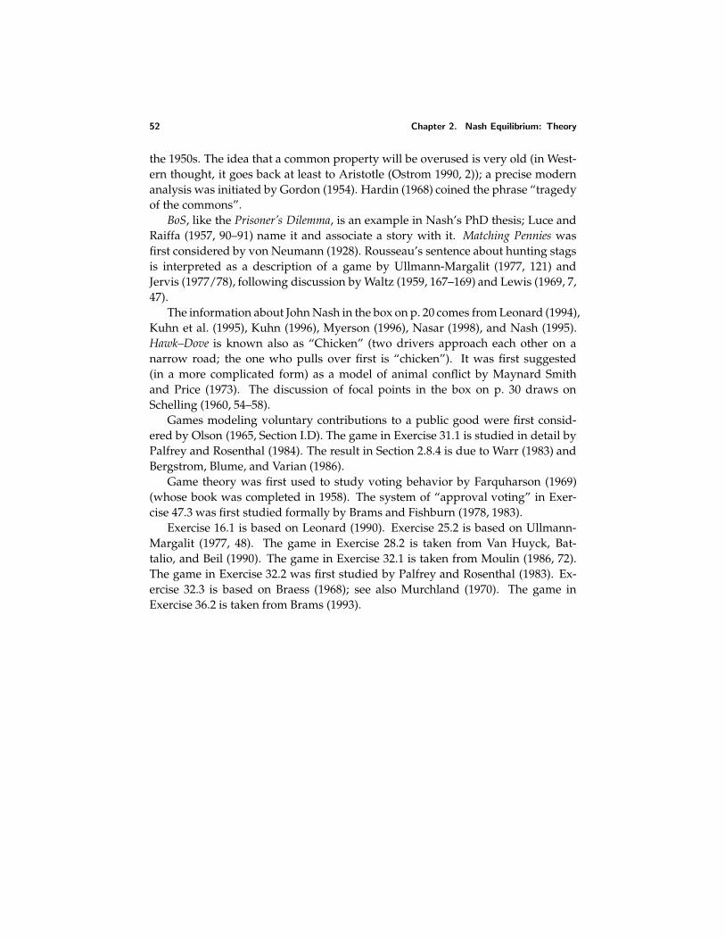
52 Chapter 2. Nash Equilibrium: Theory
the 1950s. The idea that a common property will be overused is very old (in West-ern thought, it goes back at least to Aristotle (Ostrom 1990, 2)); a precise modernanalysis was initiated by Gordon (1954). Hardin (1968) coined the phrase “tragedyof the commons”.
BoS, like the Prisoner’s Dilemma, is an example in Nash’s PhD thesis; Luce andRaiffa (1957, 90–91) name it and associate a story with it. Matching Pennies wasfirst considered by von Neumann (1928). Rousseau’s sentence about hunting stagsis interpreted as a description of a game by Ullmann-Margalit (1977, 121) andJervis (1977/78), following discussion by Waltz (1959, 167–169) and Lewis (1969, 7,47).
The information about John Nash in the box on p. 20 comes from Leonard (1994),Kuhn et al. (1995), Kuhn (1996), Myerson (1996), Nasar (1998), and Nash (1995).Hawk–Dove is known also as “Chicken” (two drivers approach each other on anarrow road; the one who pulls over first is “chicken”). It was first suggested(in a more complicated form) as a model of animal conflict by Maynard Smithand Price (1973). The discussion of focal points in the box on p. 30 draws onSchelling (1960, 54–58).
Games modeling voluntary contributions to a public good were first consid-ered by Olson (1965, Section I.D). The game in Exercise 31.1 is studied in detail byPalfrey and Rosenthal (1984). The result in Section 2.8.4 is due to Warr (1983) andBergstrom, Blume, and Varian (1986).
Game theory was first used to study voting behavior by Farquharson (1969)(whose book was completed in 1958). The system of “approval voting” in Exer-cise 47.3 was first studied formally by Brams and Fishburn (1978, 1983).
Exercise 16.1 is based on Leonard (1990). Exercise 25.2 is based on Ullmann-Margalit (1977, 48). The game in Exercise 28.2 is taken from Van Huyck, Bat-talio, and Beil (1990). The game in Exercise 32.1 is taken from Moulin (1986, 72).The game in Exercise 32.2 was first studied by Palfrey and Rosenthal (1983). Ex-ercise 32.3 is based on Braess (1968); see also Murchland (1970). The game inExercise 36.2 is taken from Brams (1993).
Draft chapter from An introduction to game theory by Martin J. [email protected]; www.economics.utoronto.ca/osborneVersion: 00/11/6.Copyright c© 1995–2000 by Martin J. Osborne. All rights reserved. No part of this book may be re-produced by any electronic or mechanical means (including photocopying, recording, or informationstorage and retrieval) without permission in writing from Oxford University Press, except that onecopy of up to six chapters may be made by any individual for private study.
3 Nash Equilibrium: Illustrations
Cournot’s model of oligopoly 53Bertrand’s model of oligopoly 61Electoral competition 68The War of Attrition 75Auctions 79Accident law 89Prerequisite: Chapter 2.
IN THIS CHAPTER I discuss in detail a few key models that use the notion of Nashequilibrium to study economic, political, and biological phenomena. The dis-
cussion shows how the notion of Nash equilibrium improves our understanding ofa wide variety of phenomena. It also illustrates some of the many forms strategicgames and their Nash equilibria can take. The models in Sections 3.1 and 3.2 arerelated to each other, whereas those in each of the other sections are independentof each other.
3.1 Cournot’s model of oligopoly
3.1.1 Introduction
How does the outcome of competition among the firms in an industry depend onthe characteristics of the demand for the firms’ output, the nature of the firms’ costfunctions, and the number of firms? Will the benefits of technological improve-ments be passed on to consumers? Will a reduction in the number of firms gener-ate a less desirable outcome? To answer these questions we need a model of theinteraction between firms competing for the business of consumers. In this sectionand the next I analyze two such models. Economists refer to them as models of“oligopoly” (competition between a small number of sellers), though they involveno restriction on the number of firms; the label reflects the strategic interactionthey capture. Both models were studied first in the nineteenth century, before thenotion of Nash equilibrium was formalized for a general strategic game. The firstis due to the economist Cournot (1838).
53
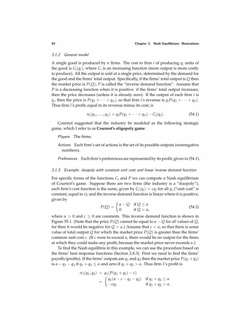
54 Chapter 3. Nash Equilibrium: Illustrations
3.1.2 General model
A single good is produced by n firms. The cost to firm i of producing qi units ofthe good is Ci(qi), where Ci is an increasing function (more output is more costlyto produce). All the output is sold at a single price, determined by the demand forthe good and the firms’ total output. Specifically, if the firms’ total output is Q thenthe market price is P(Q); P is called the “inverse demand function”. Assume thatP is a decreasing function when it is positive: if the firms’ total output increases,then the price decreases (unless it is already zero). If the output of each firm i isqi, then the price is P(q1 + · · · + qn), so that firm i’s revenue is qiP(q1 + · · · + qn).Thus firm i’s profit, equal to its revenue minus its cost, is
πi(q1, . . . , qn) = qiP(q1 + · · · + qn) − Ci(qi). (54.1)
Cournot suggested that the industry be modeled as the following strategicgame, which I refer to as Cournot’s oligopoly game.
Players The firms.
Actions Each firm’s set of actions is the set of its possible outputs (nonnegativenumbers).
Preferences Each firm’s preferences are represented by its profit, given in (54.1).
3.1.3 Example: duopoly with constant unit cost and linear inverse demand function
For specific forms of the functions Ci and P we can compute a Nash equilibriumof Cournot’s game. Suppose there are two firms (the industry is a “duopoly”),each firm’s cost function is the same, given by Ci(qi) = cqi for all qi (“unit cost” isconstant, equal to c), and the inverse demand function is linear where it is positive,given by
P(Q) =
α − Q if Q ≤ α
0 if Q > α,(54.2)
where α > 0 and c ≥ 0 are constants. This inverse demand function is shown inFigure 55.1. (Note that the price P(Q) cannot be equal to α − Q for all values of Q,for then it would be negative for Q > α.) Assume that c < α, so that there is somevalue of total output Q for which the market price P(Q) is greater than the firms’common unit cost c. (If c were to exceed α, there would be no output for the firmsat which they could make any profit, because the market price never exceeds α.)
To find the Nash equilibria in this example, we can use the procedure based onthe firms’ best response functions (Section 2.8.3). First we need to find the firms’payoffs (profits). If the firms’ outputs are q1 and q2 then the market price P(q1 + q2)is α − q1 − q2 if q1 + q2 ≤ α and zero if q1 + q2 > α. Thus firm 1’s profit is
π1(q1, q2) = q1(P(q1 + q2) − c)
=
q1(α − c − q1 − q2) if q1 + q2 ≤ α
−cq1 if q1 + q2 > α.
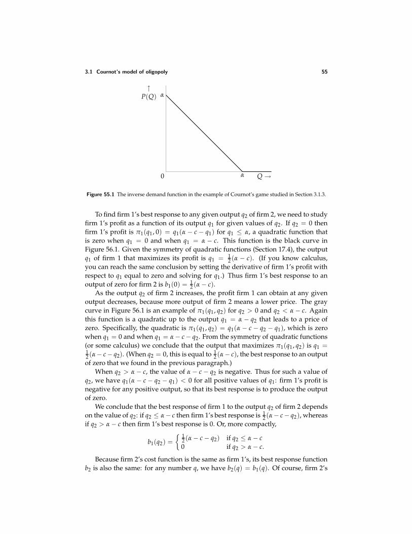
3.1 Cournot’s model of oligopoly 55
0 Q →
↑P(Q) α
α
Figure 55.1 The inverse demand function in the example of Cournot’s game studied in Section 3.1.3.
To find firm 1’s best response to any given output q2 of firm 2, we need to studyfirm 1’s profit as a function of its output q1 for given values of q2. If q2 = 0 thenfirm 1’s profit is π1(q1, 0) = q1(α − c − q1) for q1 ≤ α, a quadratic function thatis zero when q1 = 0 and when q1 = α − c. This function is the black curve inFigure 56.1. Given the symmetry of quadratic functions (Section 17.4), the outputq1 of firm 1 that maximizes its profit is q1 = 1
2 (α − c). (If you know calculus,you can reach the same conclusion by setting the derivative of firm 1’s profit withrespect to q1 equal to zero and solving for q1.) Thus firm 1’s best response to anoutput of zero for firm 2 is b1(0) = 1
2 (α − c).As the output q2 of firm 2 increases, the profit firm 1 can obtain at any given
output decreases, because more output of firm 2 means a lower price. The graycurve in Figure 56.1 is an example of π1(q1, q2) for q2 > 0 and q2 < α − c. Againthis function is a quadratic up to the output q1 = α − q2 that leads to a price ofzero. Specifically, the quadratic is π1(q1, q2) = q1(α − c − q2 − q1), which is zerowhen q1 = 0 and when q1 = α − c − q2. From the symmetry of quadratic functions(or some calculus) we conclude that the output that maximizes π1(q1, q2) is q1 =12 (α− c− q2). (When q2 = 0, this is equal to 1
2 (α− c), the best response to an outputof zero that we found in the previous paragraph.)
When q2 > α − c, the value of α − c − q2 is negative. Thus for such a value ofq2, we have q1(α − c − q2 − q1) < 0 for all positive values of q1: firm 1’s profit isnegative for any positive output, so that its best response is to produce the outputof zero.
We conclude that the best response of firm 1 to the output q2 of firm 2 dependson the value of q2: if q2 ≤ α− c then firm 1’s best response is 1
2 (α− c− q2), whereasif q2 > α − c then firm 1’s best response is 0. Or, more compactly,
b1(q2) = 1
2 (α − c − q2) if q2 ≤ α − c0 if q2 > α − c.
Because firm 2’s cost function is the same as firm 1’s, its best response functionb2 is also the same: for any number q, we have b2(q) = b1(q). Of course, firm 2’s
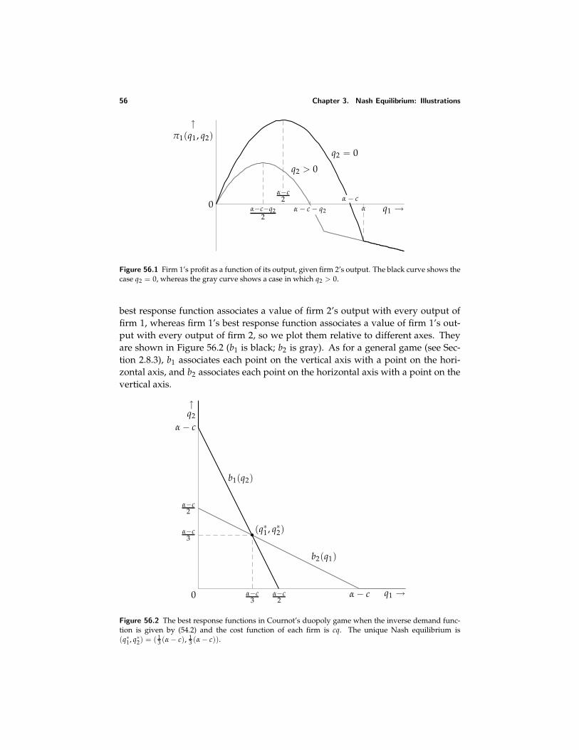
56 Chapter 3. Nash Equilibrium: Illustrations
0
↑π1(q1, q2)
q1 →
q2 = 0
q2 > 0
α
α − cα − c − q2
α−c2
α−c−q22
Figure 56.1 Firm 1’s profit as a function of its output, given firm 2’s output. The black curve shows thecase q2 = 0, whereas the gray curve shows a case in which q2 > 0.
best response function associates a value of firm 2’s output with every output offirm 1, whereas firm 1’s best response function associates a value of firm 1’s out-put with every output of firm 2, so we plot them relative to different axes. Theyare shown in Figure 56.2 (b1 is black; b2 is gray). As for a general game (see Sec-tion 2.8.3), b1 associates each point on the vertical axis with a point on the hori-zontal axis, and b2 associates each point on the horizontal axis with a point on thevertical axis.
0 α−c3
α−c2
α − c
α−c3
α−c2
α − c
↑q2
q1 →
b1(q2)
b2(q1)
(q∗1, q∗2)
Figure 56.2 The best response functions in Cournot’s duopoly game when the inverse demand func-tion is given by (54.2) and the cost function of each firm is cq. The unique Nash equilibrium is(q∗1, q∗2) = ( 1
3 (α − c), 13 (α − c)).
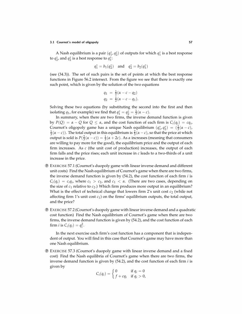
3.1 Cournot’s model of oligopoly 57
A Nash equilibrium is a pair (q∗1, q∗2) of outputs for which q∗1 is a best responseto q∗2, and q∗2 is a best response to q∗1:
q∗1 = b1(q∗2) and q∗2 = b2(q∗1)
(see (34.3)). The set of such pairs is the set of points at which the best responsefunctions in Figure 56.2 intersect. From the figure we see that there is exactly onesuch point, which is given by the solution of the two equations
q1 = 12 (α − c − q2)
q2 = 12 (α − c − q1).
Solving these two equations (by substituting the second into the first and thenisolating q1, for example) we find that q∗1 = q∗2 = 1
3 (α − c).In summary, when there are two firms, the inverse demand function is given
by P(Q) = α − Q for Q ≤ α, and the cost function of each firm is Ci(qi) = cqi,Cournot’s oligopoly game has a unique Nash equilibrium (q∗1, q∗2) = ( 1
3 (α − c),13 (α − c)). The total output in this equilibrium is 2
3 (α− c), so that the price at whichoutput is sold is P( 2
3 (α − c)) = 13 (α + 2c). As α increases (meaning that consumers
are willing to pay more for the good), the equilibrium price and the output of eachfirm increases. As c (the unit cost of production) increases, the output of eachfirm falls and the price rises; each unit increase in c leads to a two-thirds of a unitincrease in the price.
? EXERCISE 57.1 (Cournot’s duopoly game with linear inverse demand and differentunit costs) Find the Nash equilibrium of Cournot’s game when there are two firms,the inverse demand function is given by (54.2), the cost function of each firm i isCi(qi) = ciqi, where c1 > c2, and c1 < α. (There are two cases, depending onthe size of c1 relative to c2.) Which firm produces more output in an equilibrium?What is the effect of technical change that lowers firm 2’s unit cost c2 (while notaffecting firm 1’s unit cost c1) on the firms’ equilibrium outputs, the total output,and the price?
? EXERCISE 57.2 (Cournot’s duopoly game with linear inverse demand and a quadraticcost function) Find the Nash equilibrium of Cournot’s game when there are twofirms, the inverse demand function is given by (54.2), and the cost function of eachfirm i is Ci(qi) = q2
i .
In the next exercise each firm’s cost function has a component that is indepen-dent of output. You will find in this case that Cournot’s game may have more thanone Nash equilibrium.
? EXERCISE 57.3 (Cournot’s duopoly game with linear inverse demand and a fixedcost) Find the Nash equilibria of Cournot’s game when there are two firms, theinverse demand function is given by (54.2), and the cost function of each firm i isgiven by
Ci(qi) =
0 if qi = 0f + cqi if qi > 0,
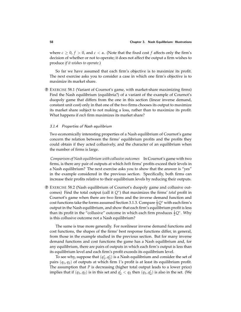
58 Chapter 3. Nash Equilibrium: Illustrations
where c ≥ 0, f > 0, and c < α. (Note that the fixed cost f affects only the firm’sdecision of whether or not to operate; it does not affect the output a firm wishes toproduce if it wishes to operate.)
So far we have assumed that each firm’s objective is to maximize its profit.The next exercise asks you to consider a case in which one firm’s objective is tomaximize its market share.
? EXERCISE 58.1 (Variant of Cournot’s game, with market-share maximizing firms)Find the Nash equilibrium (equilibria?) of a variant of the example of Cournot’sduopoly game that differs from the one in this section (linear inverse demand,constant unit cost) only in that one of the two firms chooses its output to maximizeits market share subject to not making a loss, rather than to maximize its profit.What happens if each firm maximizes its market share?
3.1.4 Properties of Nash equilibrium
Two economically interesting properties of a Nash equilibrium of Cournot’s gameconcern the relation between the firms’ equilibrium profits and the profits theycould obtain if they acted collusively, and the character of an equilibrium whenthe number of firms is large.
Comparison of Nash equilibrium with collusive outcomes In Cournot’s game with twofirms, is there any pair of outputs at which both firms’ profits exceed their levels ina Nash equilibrium? The next exercise asks you to show that the answer is “yes”in the example considered in the previous section. Specifically, both firms canincrease their profits relative to their equilibrium levels by reducing their outputs.
? EXERCISE 58.2 (Nash equilibrium of Cournot’s duopoly game and collusive out-comes) Find the total output (call it Q∗) that maximizes the firms’ total profit inCournot’s game when there are two firms and the inverse demand function andcost functions take the forms assumed Section 3.1.3. Compare 1
2 Q∗ with each firm’soutput in the Nash equilibrium, and show that each firm’s equilibrium profit is lessthan its profit in the “collusive” outcome in which each firm produces 1
2 Q∗. Whyis this collusive outcome not a Nash equilibrium?
The same is true more generally. For nonlinear inverse demand functions andcost functions, the shapes of the firms’ best response functions differ, in general,from those in the example studied in the previous section. But for many inversedemand functions and cost functions the game has a Nash equilibrium and, forany equilibrium, there are pairs of outputs in which each firm’s output is less thanits equilibrium level and each firm’s profit exceeds its equilibrium level.
To see why, suppose that (q∗1, q∗2) is a Nash equilibrium and consider the set ofpairs (q1, q2) of outputs at which firm 1’s profit is at least its equilibrium profit.The assumption that P is decreasing (higher total output leads to a lower price)implies that if (q1, q2) is in this set and q′2 < q2 then (q1, q′2) is also in the set. (We
3.1 Cournot’s model of oligopoly 59
have q1 + q′2 < q1 + q2, and hence P(q1 + q′2) > P(q1 + q2), so that firm 1’s profit at(q1, q′2) exceeds its profit at (q1, q2).) Thus in Figure 59.1 the set of pairs of outputsat which firm 1’s profit is at least its equilibrium profit lies on or below the lineq2 = q∗2; an example of such a set is shaded light gray. Similarly, the set of pairs ofoutputs at which firm 2’s profit is at least its equilibrium profit lies on or to the leftof the line q1 = q∗1, and an example is shaded light gray.
Nash equilibrium
q1 →
↑q2
q∗10
q∗2
Firm 1’s profit exceedsits equilibrium level
Firm 2’s profitexceeds its
equilibriumlevel
Figure 59.1 The pair (q∗1, q∗2) is a Nash equilibrium; along each gray curve one of the firm’s profits isconstant, equal to its profit at the equilibrium. The area shaded dark gray is the set of pairs of outputsat which both firms’ profits exceed their equilibrium levels.
We see that if the parts of the boundaries of these sets indicated by the graylines in the figure are smooth then the two sets must intersect; in the figure theintersection is shaded dark gray. At every pair of outputs in this area each firm’soutput is less than its equilibrium level (qi < q∗i for i = 1, 2) and each firm’s profitis higher than its equilibrium profit. That is, both firms are better off by restrictingtheir outputs.
Dependence of Nash equilibrium on number of firms How does the equilibrium out-come in Cournot’s game depend on the number of firms? If each firm’s cost func-tion has the same constant unit cost c, the best outcome for consumers compatiblewith no firm’s making a loss has a price of c and a total output of α− c. The next ex-ercise asks you to show that if, for this cost function, the inverse demand functionis linear (as in Section 3.1.3), then the price in the Nash equilibrium of Cournot’sgame decreases as the number of firms increases, approaching c. That is, fromthe viewpoint of consumers, the outcome is better the larger the number of firms,and when the number of firms is very large, the outcome is close to the best onecompatible with nonnegative profits for the firms.
? EXERCISE 59.1 (Cournot’s game with many firms) Consider Cournot’s game inthe case of an arbitrary number n of firms; retain the assumptions that the in-
60 Chapter 3. Nash Equilibrium: Illustrations
verse demand function takes the form (54.2) and the cost function of each firm i isCi(qi) = cqi for all qi, with c < α. Find the best response function of each firm andset up the conditions for (q∗1, . . . , q∗n) to be a Nash equilibrium (see (34.3)), assum-ing that there is a Nash equilibrium in which all firms’ outputs are positive. Solvethese equations to find the Nash equilibrium. (For n = 2 your answer should be( 1
3 (α − c), 13 (α − c)), the equilibrium found in the previous section. First show that
in an equilibrium all firms produce the same output, then solve for that output. Ifyou cannot show that all firms produce the same output, simply assume that theydo.) Find the price at which output is sold in a Nash equilibrium and show thatthis price decreases as n increases, approaching c as the number of firms increaseswithout bound.
The main idea behind this result does not depend on the assumptions on theinverse demand function and the firms’ cost functions. Suppose, more generally,that the inverse demand function is any decreasing function, that each firm’s costfunction is the same, denoted by C, and that there is a single output, say q, at whichthe average cost of production C(q)/q is minimal. In this case, any given totaloutput is produced most efficiently by each firm’s producing q, and the lowestprice compatible with the firms’ not making losses is the minimal value of theaverage cost. The next exercise asks you to show that in a Nash equilibrium ofCournot’s game in which the firms’ total output is large relative to q, this is theprice at which the output is sold.
?? EXERCISE 60.1 (Nash equilibrium of Cournot’s game with small firms) Supposethat there are infinitely many firms, all of which have the same cost function C.Assume that C(0) = 0, and for q > 0 the function C(q)/q has a unique minimizerq; denote the minimum of C(q)/q by p. Assume that the inverse demand functionP is decreasing. Show that in any Nash equilibrium the firms’ total output Q∗
satisfiesP(Q∗ + q) ≤ p ≤ P(Q∗).
(That is, the price is at least the minimal value p of the average cost, but is closeenough to this minimum that increasing the total output of the firms by q would re-duce the price to at most p.) To establish these inequalities, show that if P(Q∗) < por P(Q∗ + q) > p then Q∗ is not the total output of the firms in a Nash equilibrium,because in each case at least one firm can deviate and increase its profit.
3.1.5 A generalization of Cournot’s game: using common property
In Cournot’s game, the payoff function of each firm i is qiP(q1 + · · · + qn) − Ci(qi).In particular, each firm’s payoff depends only on its output and the sum of allthe firm’s outputs, not on the distribution of the total output among the firms,and decreases when this sum increases (given that P is decreasing). That is, thepayoff of each firm i may be written as fi(qi , q1 + · · ·+ qn), where the function fi isdecreasing in its second argument (given the value of its first argument, qi).
3.2 Bertrand’s model of oligopoly 61
This general payoff function captures many situations in which players com-pete in using a piece of common property whose value to any one player dimin-ishes as total use increases. The property might be a village green, for example; thehigher the total number of sheep grazed there, the less valuable the green is to anygiven farmer.
The first property of a Nash equilibrium in Cournot’s model discussed in theprevious section applies to this general model: common property is “overused” ina Nash equilibrium in the sense that every player’s payoff increases when everyplayer reduces her use of the property from its equilibrium level. For example, allfarmers’ payoffs increase if each farmer reduces her use of the village green fromits equilibrium level: in an equilibrium the green is “overgrazed”. The argument isthe same as the one illustrated in Figure 59.1 in the case of two players, because thisargument depends only on the fact that each player’s payoff function is smoothand is decreasing in the other player’s action. (In Cournot’s model, the “commonproperty” that is overused is the demand for the good.)
? EXERCISE 61.1 (Interaction among resource-users) A group of n firms uses a com-mon resource (a river or a forest, for example) to produce output. As more of theresource is used, any given firm can produce less output. Denote by xi the amountof the resource used by firm i (= 1, . . . , n). Assume specifically that firm i’s out-put is xi(1 − (x1 + · · · + xn)) if x1 + · · · + xn ≤ 1, and zero otherwise. Each firm ichooses xi to maximize its output. Formulate this situation as a strategic game.Find values of α and c such that the game is the same as the one studied in Exer-cise 59.1, and hence find its Nash equilibria. Find an action profile (x1, . . . , xn) atwhich each firm’s output is higher than it is at the Nash equilibrium.
3.2 Bertrand’s model of oligopoly
3.2.1 General model
In Cournot’s game, each firm chooses an output; the price is determined by thedemand for the good in relation to the total output produced. In an alternativemodel of oligopoly, associated with a review of Cournot’s book by Bertrand (1883),each firm chooses a price, and produces enough output to meet the demand itfaces, given the prices chosen by all the firms. The model is designed to shed lighton the same questions that Cournot’s game addresses; as we shall see, some of theanswers it gives are different.
The economic setting for the model is similar to that for Cournot’s game. Asingle good is produced by n firms; each firm can produce qi units of the good ata cost of Ci(qi). It is convenient to specify demand by giving a “demand function”D, rather than an inverse demand function as we did for Cournot’s game. The in-terpretation of D is that if the good is available at the price p then the total amountdemanded is D(p).
Assume that if the firms set different prices then all consumers purchase thegood from the firm with the lowest price, which produces enough output to meet
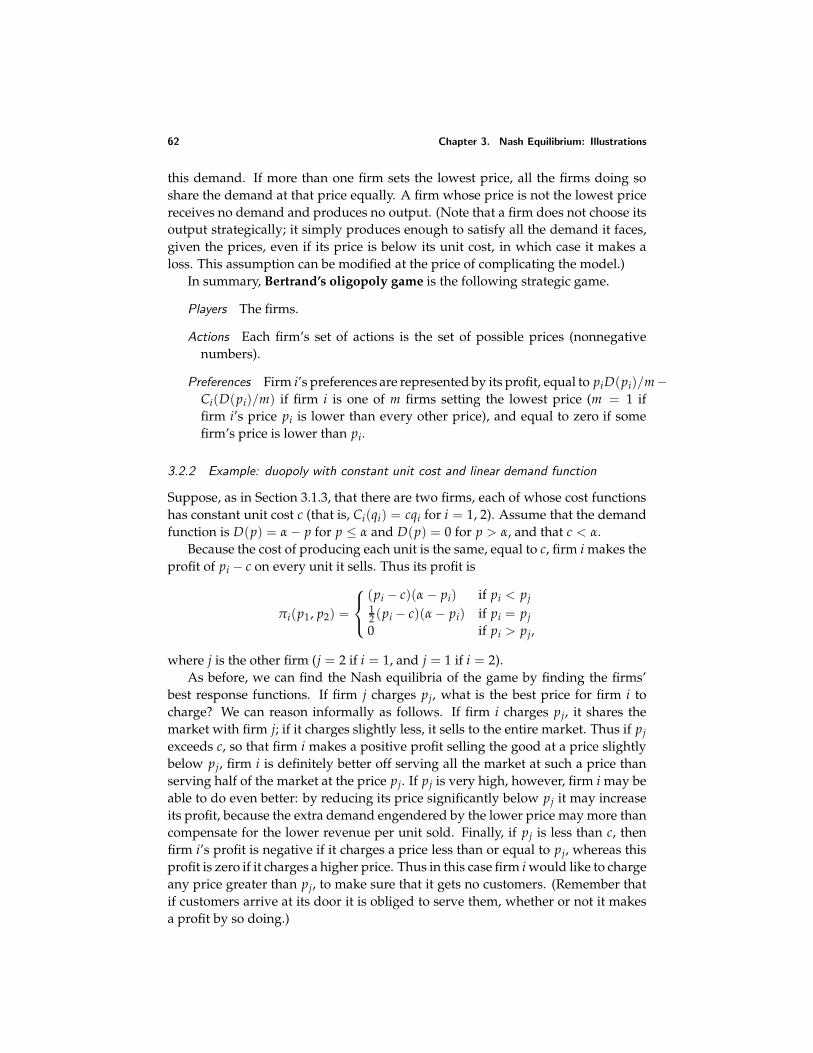
62 Chapter 3. Nash Equilibrium: Illustrations
this demand. If more than one firm sets the lowest price, all the firms doing soshare the demand at that price equally. A firm whose price is not the lowest pricereceives no demand and produces no output. (Note that a firm does not choose itsoutput strategically; it simply produces enough to satisfy all the demand it faces,given the prices, even if its price is below its unit cost, in which case it makes aloss. This assumption can be modified at the price of complicating the model.)
In summary, Bertrand’s oligopoly game is the following strategic game.
Players The firms.
Actions Each firm’s set of actions is the set of possible prices (nonnegativenumbers).
Preferences Firm i’s preferences are represented by its profit, equal to piD(pi)/m−Ci(D(pi)/m) if firm i is one of m firms setting the lowest price (m = 1 iffirm i’s price pi is lower than every other price), and equal to zero if somefirm’s price is lower than pi.
3.2.2 Example: duopoly with constant unit cost and linear demand function
Suppose, as in Section 3.1.3, that there are two firms, each of whose cost functionshas constant unit cost c (that is, Ci(qi) = cqi for i = 1, 2). Assume that the demandfunction is D(p) = α − p for p ≤ α and D(p) = 0 for p > α, and that c < α.
Because the cost of producing each unit is the same, equal to c, firm i makes theprofit of pi − c on every unit it sells. Thus its profit is
πi(p1, p2) =
(pi − c)(α − pi) if pi < pj12 (pi − c)(α − pi) if pi = pj0 if pi > pj,
where j is the other firm (j = 2 if i = 1, and j = 1 if i = 2).As before, we can find the Nash equilibria of the game by finding the firms’
best response functions. If firm j charges pj, what is the best price for firm i tocharge? We can reason informally as follows. If firm i charges pj, it shares themarket with firm j; if it charges slightly less, it sells to the entire market. Thus if pjexceeds c, so that firm i makes a positive profit selling the good at a price slightlybelow pj, firm i is definitely better off serving all the market at such a price thanserving half of the market at the price pj. If pj is very high, however, firm i may beable to do even better: by reducing its price significantly below pj it may increaseits profit, because the extra demand engendered by the lower price may more thancompensate for the lower revenue per unit sold. Finally, if pj is less than c, thenfirm i’s profit is negative if it charges a price less than or equal to pj, whereas thisprofit is zero if it charges a higher price. Thus in this case firm i would like to chargeany price greater than pj, to make sure that it gets no customers. (Remember thatif customers arrive at its door it is obliged to serve them, whether or not it makesa profit by so doing.)
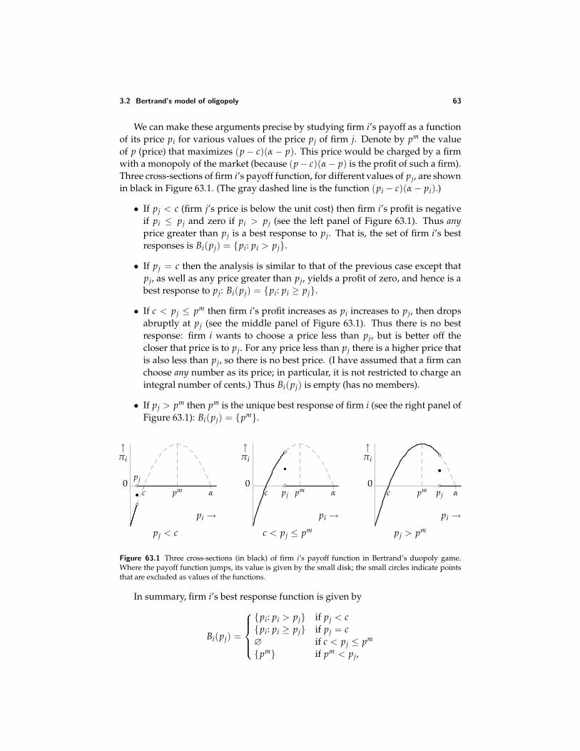
3.2 Bertrand’s model of oligopoly 63
We can make these arguments precise by studying firm i’s payoff as a functionof its price pi for various values of the price pj of firm j. Denote by pm the valueof p (price) that maximizes (p − c)(α − p). This price would be charged by a firmwith a monopoly of the market (because (p − c)(α − p) is the profit of such a firm).Three cross-sections of firm i’s payoff function, for different values of pj, are shownin black in Figure 63.1. (The gray dashed line is the function (pi − c)(α − pi).)
• If pj < c (firm j’s price is below the unit cost) then firm i’s profit is negativeif pi ≤ pj and zero if pi > pj (see the left panel of Figure 63.1). Thus anyprice greater than pj is a best response to pj. That is, the set of firm i’s bestresponses is Bi(pj) = pi: pi > pj.
• If pj = c then the analysis is similar to that of the previous case except thatpj, as well as any price greater than pj, yields a profit of zero, and hence is abest response to pj: Bi(pj) = pi: pi ≥ pj.
• If c < pj ≤ pm then firm i’s profit increases as pi increases to pj, then dropsabruptly at pj (see the middle panel of Figure 63.1). Thus there is no bestresponse: firm i wants to choose a price less than pj, but is better off thecloser that price is to pj. For any price less than pj there is a higher price thatis also less than pj, so there is no best price. (I have assumed that a firm canchoose any number as its price; in particular, it is not restricted to charge anintegral number of cents.) Thus Bi(pj) is empty (has no members).
• If pj > pm then pm is the unique best response of firm i (see the right panel ofFigure 63.1): Bi(pj) = pm.
0
↑πi
pi →pj < c
c
pj
pm α0
↑πi
pi →c < pj ≤ pm
c pj pm α0
↑πi
pi →pj > pm
c pjpm α
Figure 63.1 Three cross-sections (in black) of firm i’s payoff function in Bertrand’s duopoly game.Where the payoff function jumps, its value is given by the small disk; the small circles indicate pointsthat are excluded as values of the functions.
In summary, firm i’s best response function is given by
Bi(pj) =
pi: pi > pj if pj < cpi: pi ≥ pj if pj = c∅ if c < pj ≤ pm
pm if pm < pj,
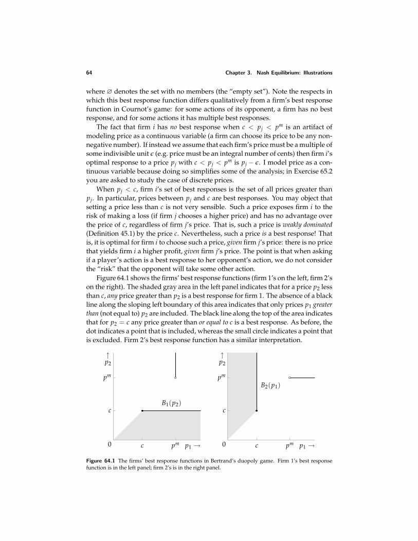
64 Chapter 3. Nash Equilibrium: Illustrations
where ∅ denotes the set with no members (the “empty set”). Note the respects inwhich this best response function differs qualitatively from a firm’s best responsefunction in Cournot’s game: for some actions of its opponent, a firm has no bestresponse, and for some actions it has multiple best responses.
The fact that firm i has no best response when c < pj < pm is an artifact ofmodeling price as a continuous variable (a firm can choose its price to be any non-negative number). If instead we assume that each firm’s price must be a multiple ofsome indivisible unit ε (e.g. price must be an integral number of cents) then firm i’soptimal response to a price pj with c < pj < pm is pj − ε. I model price as a con-tinuous variable because doing so simplifies some of the analysis; in Exercise 65.2you are asked to study the case of discrete prices.
When pj < c, firm i’s set of best responses is the set of all prices greater thanpj. In particular, prices between pj and c are best responses. You may object thatsetting a price less than c is not very sensible. Such a price exposes firm i to therisk of making a loss (if firm j chooses a higher price) and has no advantage overthe price of c, regardless of firm j’s price. That is, such a price is weakly dominated(Definition 45.1) by the price c. Nevertheless, such a price is a best response! Thatis, it is optimal for firm i to choose such a price, given firm j’s price: there is no pricethat yields firm i a higher profit, given firm j’s price. The point is that when askingif a player’s action is a best response to her opponent’s action, we do not considerthe “risk” that the opponent will take some other action.
Figure 64.1 shows the firms’ best response functions (firm 1’s on the left, firm 2’son the right). The shaded gray area in the left panel indicates that for a price p2 lessthan c, any price greater than p2 is a best response for firm 1. The absence of a blackline along the sloping left boundary of this area indicates that only prices p1 greaterthan (not equal to) p2 are included. The black line along the top of the area indicatesthat for p2 = c any price greater than or equal to c is a best response. As before, thedot indicates a point that is included, whereas the small circle indicates a point thatis excluded. Firm 2’s best response function has a similar interpretation.
c pm
c
pm
0
↑p2
p1 →
B1(p2)
c pm
c
pm
0
↑p2
p1 →
B2(p1)
Figure 64.1 The firms’ best response functions in Bertrand’s duopoly game. Firm 1’s best responsefunction is in the left panel; firm 2’s is in the right panel.
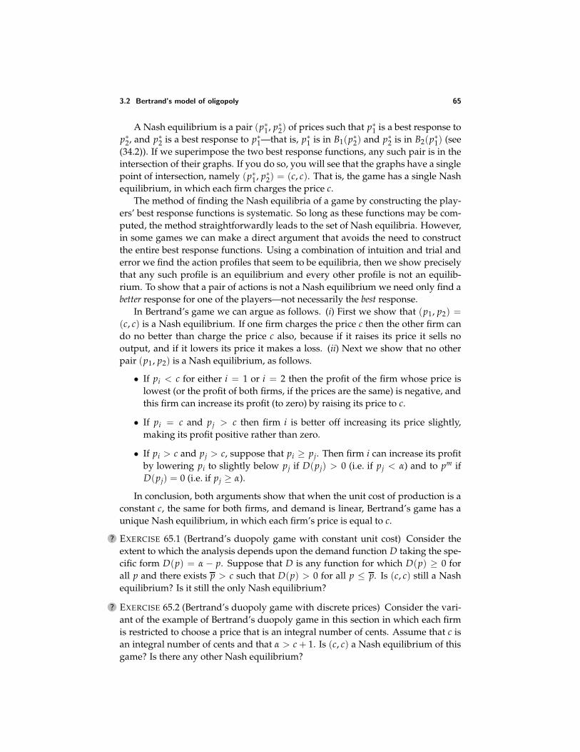
3.2 Bertrand’s model of oligopoly 65
A Nash equilibrium is a pair (p∗1, p∗2) of prices such that p∗1 is a best response top∗2, and p∗2 is a best response to p∗1—that is, p∗1 is in B1(p∗2) and p∗2 is in B2(p∗1) (see(34.2)). If we superimpose the two best response functions, any such pair is in theintersection of their graphs. If you do so, you will see that the graphs have a singlepoint of intersection, namely (p∗1, p∗2) = (c, c). That is, the game has a single Nashequilibrium, in which each firm charges the price c.
The method of finding the Nash equilibria of a game by constructing the play-ers’ best response functions is systematic. So long as these functions may be com-puted, the method straightforwardly leads to the set of Nash equilibria. However,in some games we can make a direct argument that avoids the need to constructthe entire best response functions. Using a combination of intuition and trial anderror we find the action profiles that seem to be equilibria, then we show preciselythat any such profile is an equilibrium and every other profile is not an equilib-rium. To show that a pair of actions is not a Nash equilibrium we need only find abetter response for one of the players—not necessarily the best response.
In Bertrand’s game we can argue as follows. (i) First we show that (p1, p2) =(c, c) is a Nash equilibrium. If one firm charges the price c then the other firm cando no better than charge the price c also, because if it raises its price it sells nooutput, and if it lowers its price it makes a loss. (ii) Next we show that no otherpair (p1, p2) is a Nash equilibrium, as follows.
• If pi < c for either i = 1 or i = 2 then the profit of the firm whose price islowest (or the profit of both firms, if the prices are the same) is negative, andthis firm can increase its profit (to zero) by raising its price to c.
• If pi = c and pj > c then firm i is better off increasing its price slightly,making its profit positive rather than zero.
• If pi > c and pj > c, suppose that pi ≥ pj. Then firm i can increase its profitby lowering pi to slightly below pj if D(pj) > 0 (i.e. if pj < α) and to pm ifD(pj) = 0 (i.e. if pj ≥ α).
In conclusion, both arguments show that when the unit cost of production is aconstant c, the same for both firms, and demand is linear, Bertrand’s game has aunique Nash equilibrium, in which each firm’s price is equal to c.
? EXERCISE 65.1 (Bertrand’s duopoly game with constant unit cost) Consider theextent to which the analysis depends upon the demand function D taking the spe-cific form D(p) = α − p. Suppose that D is any function for which D(p) ≥ 0 forall p and there exists p > c such that D(p) > 0 for all p ≤ p. Is (c, c) still a Nashequilibrium? Is it still the only Nash equilibrium?
? EXERCISE 65.2 (Bertrand’s duopoly game with discrete prices) Consider the vari-ant of the example of Bertrand’s duopoly game in this section in which each firmis restricted to choose a price that is an integral number of cents. Assume that c isan integral number of cents and that α > c + 1. Is (c, c) a Nash equilibrium of thisgame? Is there any other Nash equilibrium?
66 Chapter 3. Nash Equilibrium: Illustrations
3.2.3 Discussion
For a duopoly in which both firms have the same constant unit cost and the de-mand function is linear, the Nash equilibria of Cournot’s and Bertrand’s gamesgenerate different economic outcomes. The equilibrium price in Bertrand’s gameis equal to the common unit cost c, whereas the price associated with the equilib-rium of Cournot’s game is 1
3 (α + 2c), which exceeds c because c < α. In particular,the equilibrium price in Bertrand’s game is the lowest price compatible with thefirms’ not making losses, whereas the price at the equilibrium of Cournot’s gameis higher. In Cournot’s game, the price decreases towards c as the number of firmsincreases (Exercise 59.1), whereas in Bertrand’s game it is c even if there are onlytwo firms. In the next exercise you are asked to show that as the number of firmsincreases in Bertrand’s game, the price remains c.
? EXERCISE 66.1 (Bertrand’s oligopoly game) Consider Bertrand’s oligopoly gamewhen the cost and demand functions satisfy the conditions in Section 3.2.2 andthere are n firms, with n ≥ 3. Show that the set of Nash equilibria is the set ofprofiles (p1, . . . , pn) of prices for which pi ≥ c for all i and at least two prices areequal to c. (Show that any such profile is a Nash equilibrium, and that every otherprofile is not a Nash equilibrium.)
What accounts for the difference between the Nash equilibria of Cournot’s andBertrand’s games? The key point is that different strategic variables (output inCournot’s game, price in Bertrand’s game) imply different strategic reasoning bythe firms. In Cournot’s game a firm changes its behavior if it can increase its profitby changing its output, on the assumption that the other firms’ outputs will re-main the same and the price will adjust to clear the market. In Bertrand’s gamea firm changes its behavior if it can increase its profit by changing its price, onthe assumption that the other firms’ prices will remain the same and their outputswill adjust to clear the market. Which assumption makes more sense depends onthe context. For example, the wholesale market for agricultural produce may fitCournot’s game better, whereas the retail market for food may fit Bertrand’s gamebetter.
Under some variants of the assumptions in the previous section, Bertrand’sgame has no Nash equilibrium. In one case the firms’ cost functions have constantunit costs, and these costs are different; in another case the cost functions have afixed component. In both these cases, as well as in some other cases, an equilib-rium is restored if we modify the way in which consumers are divided betweenthe firms when the prices are the same, as the following exercises show. (We canthink of the division of consumers between firms charging the same price as beingdetermined as part of the equilibrium. Note that we retain the assumption that ifthe firms charge different prices then the one charging the lower price receives allthe demand.)
? EXERCISE 66.2 (Bertrand’s duopoly game with different unit costs) Consider Ber-trand’s duopoly game under a variant of the assumptions of Section 3.2.2 in which
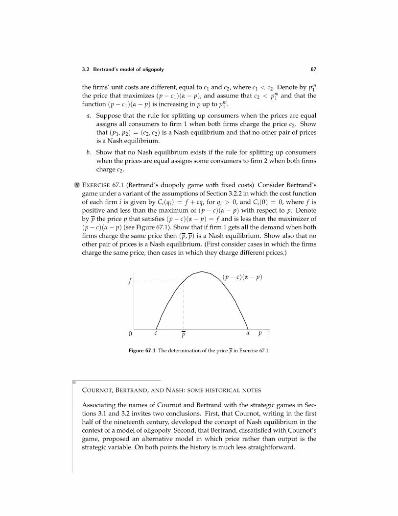
3.2 Bertrand’s model of oligopoly 67
the firms’ unit costs are different, equal to c1 and c2, where c1 < c2. Denote by pm1
the price that maximizes (p − c1)(α − p), and assume that c2 < pm1 and that the
function (p − c1)(α − p) is increasing in p up to pm1 .
a. Suppose that the rule for splitting up consumers when the prices are equalassigns all consumers to firm 1 when both firms charge the price c2. Showthat (p1, p2) = (c2, c2) is a Nash equilibrium and that no other pair of pricesis a Nash equilibrium.
b. Show that no Nash equilibrium exists if the rule for splitting up consumerswhen the prices are equal assigns some consumers to firm 2 when both firmscharge c2.
?? EXERCISE 67.1 (Bertrand’s duopoly game with fixed costs) Consider Bertrand’sgame under a variant of the assumptions of Section 3.2.2 in which the cost functionof each firm i is given by Ci(qi) = f + cqi for qi > 0, and Ci(0) = 0, where f ispositive and less than the maximum of (p − c)(α − p) with respect to p. Denoteby p the price p that satisfies (p − c)(α − p) = f and is less than the maximizer of(p − c)(α − p) (see Figure 67.1). Show that if firm 1 gets all the demand when bothfirms charge the same price then (p, p) is a Nash equilibrium. Show also that noother pair of prices is a Nash equilibrium. (First consider cases in which the firmscharge the same price, then cases in which they charge different prices.)
0 p →
(p − c)(α − p)f
αc p
Figure 67.1 The determination of the price p in Exercise 67.1.
COURNOT, BERTRAND, AND NASH: SOME HISTORICAL NOTES
Associating the names of Cournot and Bertrand with the strategic games in Sec-tions 3.1 and 3.2 invites two conclusions. First, that Cournot, writing in the firsthalf of the nineteenth century, developed the concept of Nash equilibrium in thecontext of a model of oligopoly. Second, that Bertrand, dissatisfied with Cournot’sgame, proposed an alternative model in which price rather than output is thestrategic variable. On both points the history is much less straightforward.
68 Chapter 3. Nash Equilibrium: Illustrations
Cournot presented his “equilibrium” as the outcome of a dynamic adjustmentprocess in which, in the case of two firms, the firms alternately choose best re-sponses to each other’s outputs. During such an adjustment process, each firm,when choosing an output, acts on the assumption that the other firm’s output willremain the same, an assumption shown to be incorrect when the other firm subse-quently adjusts its output. The fact that the adjustment process rests on the firms’acting on assumptions constantly shown to be false was the subject of criticism in aleading presentation of Cournot’s model (Fellner 1949) available at the time Nashwas developing his idea.
Certainly Nash did not literally generalize Cournot’s idea: the evidence sug-gests that he was completely unaware of Cournot’s work when developing thenotion of Nash equilibrium (Leonard 1994, 502–503). In fact, only gradually, asNash’s work was absorbed into mainstream economic theory, was Cournot’s solu-tion interpreted as a Nash equilibrium (Leonard 1994, 507–509).
The association of the price-setting model with Bertrand (a mathematician)rests on a paragraph in a review of Cournot’s book written by Bertrand in 1883.(Cournot’s book, published in 1838, had previously been largely ignored.) Thereview is confused. Bertrand is under the impression that in Cournot’s model thefirms compete in prices, undercutting each other to attract more business! He ar-gues that there is “no solution” because there is no limit to the fall in prices, aresult he says that Cournot’s formulation conceals (Bertrand 1883, 503). In brief,Bertrand’s understanding of Cournot’s work is flawed; he sees that price competi-tion leads each firm to undercut the other, but his conclusion about the outcome isincorrect.
Through the lens of modern game theory we see that the models associatedwith Cournot and Bertrand are strategic games that differ only in the strategicvariable, the solution in both cases being a Nash equilibrium. Until Nash’s work,the picture was much murkier.
3.3 Electoral competition
What factors determine the number of political parties and the policies they pro-pose? How is the outcome of an election affected by the electoral system and thevoters’ preferences among policies? A model that is the foundation for many the-ories of political phenomena addresses these questions. In the model, each of sev-eral candidates chooses a policy; each citizen has preferences over policies andvotes for one of the candidates.
A simple version of this model is a strategic game in which the players are thecandidates and a policy is a number, referred to as a “position”. (The compressionof all policy differences into one dimension is a major abstraction, though politi-cal positions are often categorized on a left–right axis.) After the candidates havechosen positions, each of a set of citizens votes (nonstrategically) for the candidate
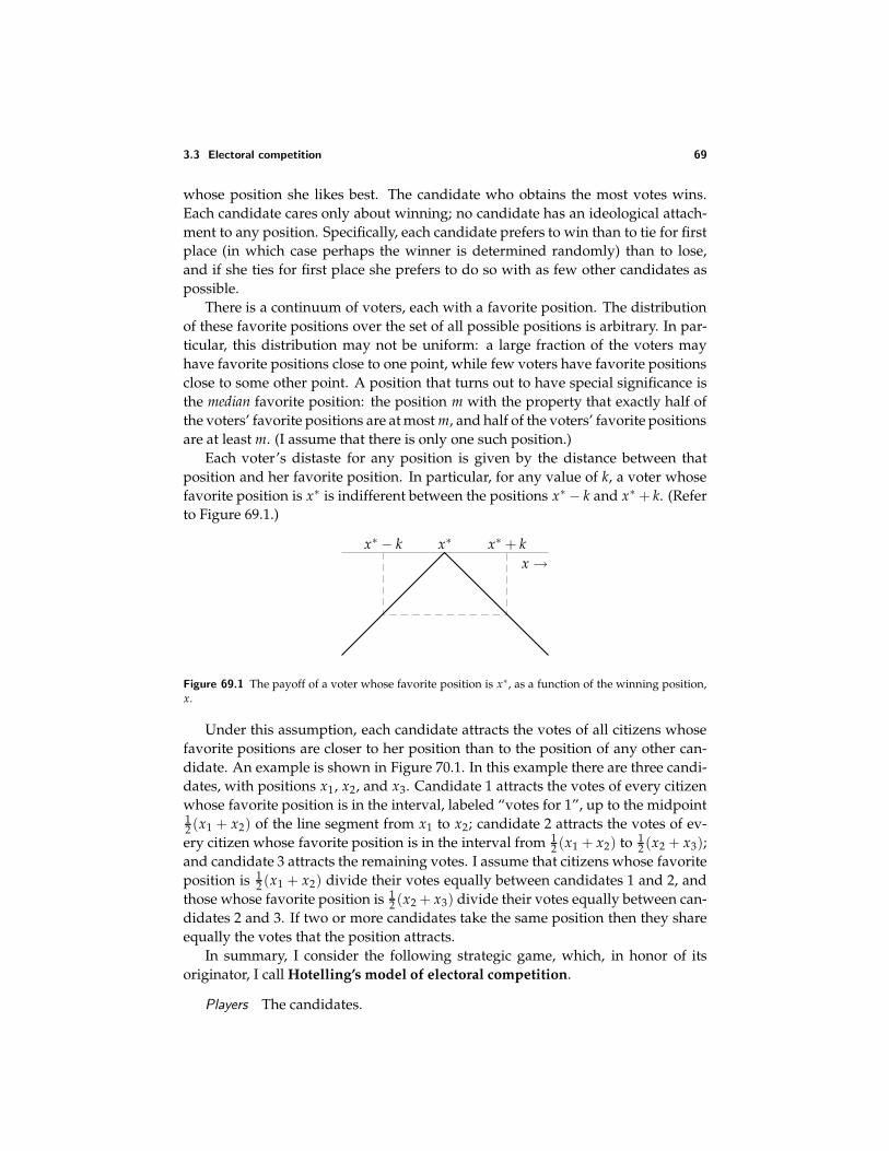
3.3 Electoral competition 69
whose position she likes best. The candidate who obtains the most votes wins.Each candidate cares only about winning; no candidate has an ideological attach-ment to any position. Specifically, each candidate prefers to win than to tie for firstplace (in which case perhaps the winner is determined randomly) than to lose,and if she ties for first place she prefers to do so with as few other candidates aspossible.
There is a continuum of voters, each with a favorite position. The distributionof these favorite positions over the set of all possible positions is arbitrary. In par-ticular, this distribution may not be uniform: a large fraction of the voters mayhave favorite positions close to one point, while few voters have favorite positionsclose to some other point. A position that turns out to have special significance isthe median favorite position: the position m with the property that exactly half ofthe voters’ favorite positions are at most m, and half of the voters’ favorite positionsare at least m. (I assume that there is only one such position.)
Each voter’s distaste for any position is given by the distance between thatposition and her favorite position. In particular, for any value of k, a voter whosefavorite position is x∗ is indifferent between the positions x∗ − k and x∗ + k. (Referto Figure 69.1.)
x∗x∗ − k x∗ + kx →
Figure 69.1 The payoff of a voter whose favorite position is x∗, as a function of the winning position,x.
Under this assumption, each candidate attracts the votes of all citizens whosefavorite positions are closer to her position than to the position of any other can-didate. An example is shown in Figure 70.1. In this example there are three candi-dates, with positions x1, x2, and x3. Candidate 1 attracts the votes of every citizenwhose favorite position is in the interval, labeled “votes for 1”, up to the midpoint12 (x1 + x2) of the line segment from x1 to x2; candidate 2 attracts the votes of ev-ery citizen whose favorite position is in the interval from 1
2 (x1 + x2) to 12 (x2 + x3);
and candidate 3 attracts the remaining votes. I assume that citizens whose favoriteposition is 1
2 (x1 + x2) divide their votes equally between candidates 1 and 2, andthose whose favorite position is 1
2 (x2 + x3) divide their votes equally between can-didates 2 and 3. If two or more candidates take the same position then they shareequally the votes that the position attracts.
In summary, I consider the following strategic game, which, in honor of itsoriginator, I call Hotelling’s model of electoral competition.
Players The candidates.
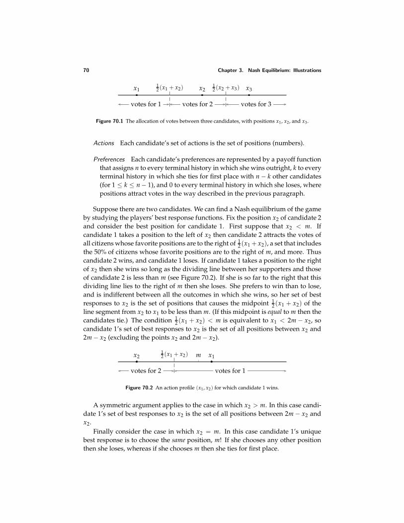
70 Chapter 3. Nash Equilibrium: Illustrations
x1 x2 x312 (x1 + x2) 1
2 (x2 + x3)
votes for 1 votes for 2 votes for 3
Figure 70.1 The allocation of votes between three candidates, with positions x1, x2, and x3.
Actions Each candidate’s set of actions is the set of positions (numbers).
Preferences Each candidate’s preferences are represented by a payoff functionthat assigns n to every terminal history in which she wins outright, k to everyterminal history in which she ties for first place with n − k other candidates(for 1 ≤ k ≤ n − 1), and 0 to every terminal history in which she loses, wherepositions attract votes in the way described in the previous paragraph.
Suppose there are two candidates. We can find a Nash equilibrium of the gameby studying the players’ best response functions. Fix the position x2 of candidate 2and consider the best position for candidate 1. First suppose that x2 < m. Ifcandidate 1 takes a position to the left of x2 then candidate 2 attracts the votes ofall citizens whose favorite positions are to the right of 1
2 (x1 + x2), a set that includesthe 50% of citizens whose favorite positions are to the right of m, and more. Thuscandidate 2 wins, and candidate 1 loses. If candidate 1 takes a position to the rightof x2 then she wins so long as the dividing line between her supporters and thoseof candidate 2 is less than m (see Figure 70.2). If she is so far to the right that thisdividing line lies to the right of m then she loses. She prefers to win than to lose,and is indifferent between all the outcomes in which she wins, so her set of bestresponses to x2 is the set of positions that causes the midpoint 1
2 (x1 + x2) of theline segment from x2 to x1 to be less than m. (If this midpoint is equal to m then thecandidates tie.) The condition 1
2 (x1 + x2) < m is equivalent to x1 < 2m − x2, socandidate 1’s set of best responses to x2 is the set of all positions between x2 and2m − x2 (excluding the points x2 and 2m − x2).
x2 x112 (x1 + x2) m
votes for 2 votes for 1
Figure 70.2 An action profile (x1, x2) for which candidate 1 wins.
A symmetric argument applies to the case in which x2 > m. In this case candi-date 1’s set of best responses to x2 is the set of all positions between 2m − x2 andx2.
Finally consider the case in which x2 = m. In this case candidate 1’s uniquebest response is to choose the same position, m! If she chooses any other positionthen she loses, whereas if she chooses m then she ties for first place.
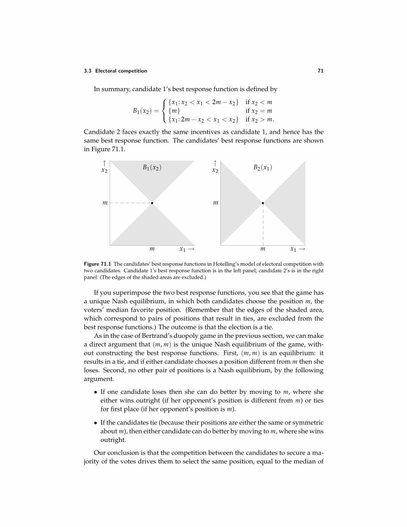
3.3 Electoral competition 71
In summary, candidate 1’s best response function is defined by
B1(x2) =
x1: x2 < x1 < 2m − x2 if x2 < mm if x2 = mx1: 2m − x2 < x1 < x2 if x2 > m.
Candidate 2 faces exactly the same incentives as candidate 1, and hence has thesame best response function. The candidates’ best response functions are shownin Figure 71.1.
↑x2
x1 →m
m
B1(x2)↑x2
x1 →m
m
B2(x1)
Figure 71.1 The candidates’ best response functions in Hotelling’s model of electoral competition withtwo candidates. Candidate 1’s best response function is in the left panel; candidate 2’s is in the rightpanel. (The edges of the shaded areas are excluded.)
If you superimpose the two best response functions, you see that the game hasa unique Nash equilibrium, in which both candidates choose the position m, thevoters’ median favorite position. (Remember that the edges of the shaded area,which correspond to pairs of positions that result in ties, are excluded from thebest response functions.) The outcome is that the election is a tie.
As in the case of Bertrand’s duopoly game in the previous section, we can makea direct argument that (m, m) is the unique Nash equilibrium of the game, with-out constructing the best response functions. First, (m, m) is an equilibrium: itresults in a tie, and if either candidate chooses a position different from m then sheloses. Second, no other pair of positions is a Nash equilibrium, by the followingargument.
• If one candidate loses then she can do better by moving to m, where sheeither wins outright (if her opponent’s position is different from m) or tiesfor first place (if her opponent’s position is m).
• If the candidates tie (because their positions are either the same or symmetricabout m), then either candidate can do better by moving to m, where she winsoutright.
Our conclusion is that the competition between the candidates to secure a ma-jority of the votes drives them to select the same position, equal to the median of
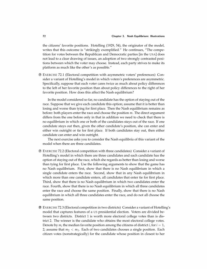
72 Chapter 3. Nash Equilibrium: Illustrations
the citizens’ favorite positions. Hotelling (1929, 54), the originator of the model,writes that this outcome is “strikingly exemplified.” He continues, “The compe-tition for votes between the Republican and Democratic parties [in the USA] doesnot lead to a clear drawing of issues, an adoption of two strongly contrasted posi-tions between which the voter may choose. Instead, each party strives to make itsplatform as much like the other’s as possible.”
? EXERCISE 72.1 (Electoral competition with asymmetric voters’ preferences) Con-sider a variant of Hotelling’s model in which voters’s preferences are asymmetric.Specifically, suppose that each voter cares twice as much about policy differencesto the left of her favorite position than about policy differences to the right of herfavorite position. How does this affect the Nash equilibrium?
In the model considered so far, no candidate has the option of staying out of therace. Suppose that we give each candidate this option; assume that it is better thanlosing and worse than tying for first place. Then the Nash equilibrium remains asbefore: both players enter the race and choose the position m. The direct argumentdiffers from the one before only in that in addition we need to check that there isno equilibrium in which one or both of the candidates stays out of the race. If onecandidate stays out then, given the other candidate’s position, she can enter andeither win outright or tie for first place. If both candidates stay out, then eithercandidate can enter and win outright.
The next exercise asks you to consider the Nash equilibria of this variant of themodel when there are three candidates.
? EXERCISE 72.2 (Electoral competition with three candidates) Consider a variant ofHotelling’s model in which there are three candidates and each candidate has theoption of staying out of the race, which she regards as better than losing and worsethan tying for first place. Use the following arguments to show that the game hasno Nash equilibrium. First, show that there is no Nash equilibrium in which asingle candidate enters the race. Second, show that in any Nash equilibrium inwhich more than one candidate enters, all candidates that enter tie for first place.Third, show that there is no Nash equilibrium in which two candidates enter therace. Fourth, show that there is no Nash equilibrium in which all three candidatesenter the race and choose the same position. Finally, show that there is no Nashequilibrium in which all three candidates enter the race, and do not all choose thesame position.
?? EXERCISE 72.3 (Electoral competition in two districts) Consider a variant of Hotelling’smodel that captures features of a US presidential election. Voters are divided be-tween two districts. District 1 is worth more electoral college votes than is dis-trict 2. The winner is the candidate who obtains the most electoral college votes.Denote by mi the median favorite position among the citizens of district i, for i = 1,2; assume that m2 < m1. Each of two candidates chooses a single position. Eachcitizen votes (nonstrategically) for the candidate whose position in closest to her
3.3 Electoral competition 73
favorite position. The candidate who wins a majority of the votes in a district ob-tains all the electoral college votes of that district; if the candidates obtain the samenumber of votes in a district, they each obtain half of the electoral college votesof that district. Find the Nash equilibrium (equilibria?) of the strategic game thatmodels this situation.
So far we have assumed that the candidates care only about winning; they arenot at all concerned with the winner’s position. The next exercise asks you toconsider the case in which each candidate cares only about the winner’s position,and not at all about winning. (You may be surprised by the equilibrium.)
?? EXERCISE 73.1 (Electoral competition between candidates who care only about thewinning position) Consider the variant of Hotelling’s model in which the can-didates (like the citizens) care about the winner’s position, and not at all aboutwinning per se. There are two candidates. Each candidate has a favorite position;her dislike for other positions increases with their distance from her favorite po-sition. Assume that the favorite position of one candidate is less than m and thefavorite position of the other candidate is greater than m. Assume also that if thecandidates tie when they take the positions x1 and x2 then the outcome is the com-promise policy 1
2 (x1 + x2). Find the set of Nash equilibria of the strategic gamethat models this situation. (First consider pairs (x1, x2) of positions for which ei-ther x1 < m and x2 < m, or x1 > m and x2 > m. Next consider pairs (x1, x2) forwhich either x1 < m < x2, or x2 < m < x1, then those for which x1 = m andx2 = m, or x1 = m and x2 = m. Finally consider the pair (m, m).)
The set of candidates in Hotelling’s model is given. The next exercise asksyou to analyze a model in which the set of candidates is generated as part of anequilibrium.
?? EXERCISE 73.2 (Citizen-candidates) Consider a game in which the players are thecitizens. Any citizen may, at some cost c > 0, become a candidate. Assume thatthe only position a citizen can espouse is her favorite position, so that a citizen’sonly decision is whether to stand as a candidate. After all citizens have (simulta-neously) decided whether to become candidates, each citizen votes for her favoritecandidate, as in Hotelling’s model. Citizens care about the position of the winningcandidate; a citizen whose favorite position is x loses |x − x∗| if the winning candi-date’s position is x∗. (For any number z, |z| denotes the absolute value of z: |z| = zif z > 0 and |z| = −z if z < 0.) Winning confers the benefit b. Thus a citizen whobecomes a candidate and ties with k − 1 other candidates for first place obtains thepayoff b/k − c; a citizen with favorite position x who becomes a candidate and isnot one of the candidates tied for first place obtains the payoff −|x − x∗| − c, wherex∗ is the winner’s position; and a citizen with favorite position x who does notbecome a candidate obtains the payoff −|x − x∗|, where x∗ is the winner’s posi-tion. Assume that for every position x there is a citizen for whom x is the favoriteposition. Show that if b ≤ 2c then the game has a Nash equilibrium in which one
74 Chapter 3. Nash Equilibrium: Illustrations
citizen becomes a candidate. Is there an equilibrium (for any values of b and c) inwhich two citizens, each with favorite position m, become candidates? Is there anequilibrium in which two citizens with favorite positions different from m becomecandidates?
Hotelling’s model assumes a basic agreement among the voters about the or-dering of the positions. For example, if one voter prefers x to y to z and anothervoter prefers y to z to x, no voter prefers z to x to y. The next exercise asks you tostudy a model that does not so restrict the voters’ preferences.
? EXERCISE 74.1 (Electoral competition for more general preferences) There is a fi-nite number of positions and a finite, odd, number of voters. For any positions xand y, each voter either prefers x to y or prefers y to x. (No voter regards any twopositions as equally desirable.) We say that a position x∗ is a Condorcet winner if forevery position y different from x∗, a majority of voters prefer x∗ to y.
a. Show that for any configuration of preferences there is at most one Condorcetwinner.
b. Give an example in which no Condorcet winner exists. (Suppose there arethree positions (x, y, and z) and three voters. Assume that voter 1 prefers xto y to z. Construct preferences for the other two voters such that one voterprefers x to y and the other prefers y to x, one prefers x to z and the otherprefers z to x, and one prefers y to z and the other prefers z to y. The pref-erences you construct must, of course, satisfy the condition that a voter whoprefers a to b and b to c also prefers a to c, where a, b, and c are any positions.)
c. Consider the strategic game in which two candidates simultaneously choosepositions, as in Hotelling’s model. If the candidates choose different posi-tions, each voter endorses the candidate whose position she prefers, and thecandidate who receives the most votes wins. If the candidates choose thesame position, they tie. Show that this game has a unique Nash equilibriumif the voters’ preferences are such that there is a Condorcet winner, and has noNash equilibrium if the voters’ preferences are such that there is no Condorcetwinner.
A variant of Hotelling’s model of electoral competition can be used to analyzethe choices of product characteristics by competing firms in situations in whichprice is not a significant variable. (Think of radio stations that offer different stylesof music, for example.) The set of positions is the range of possible characteristicsfor the product, and the citizens are consumers rather than voters. Consumers’tastes differ; each consumer buys (at a fixed price, possibly zero) one unit of theproduct she likes best. The model differs substantially from Hotelling’s model ofelectoral competition in that each firm’s objective is to maximize its market share,rather than to obtain a market share larger than that of any other firm. In thenext exercise you are asked to show that the Nash equilibria of this game in thecase of two or three firms are the same as those in Hotelling’s model of electoralcompetition.
3.4 The War of Attrition 75
? EXERCISE 75.1 (Competition in product characteristics) In the variant of Hotelling’smodel that captures competing firms’ choices of product characteristics, show thatwhen there are two firms the unique Nash equilibrium is (m, m) (both firms offerthe consumers’ median favorite product) and when there are three firms there is noNash equilibrium. (Start by arguing that when there are two firms whose productsdiffer, either firm is better off making its product more similar to that of its rival.)
3.4 The War of Attrition
The game known as the War of Attrition elaborates on the ideas captured by thegame Hawk–Dove (Exercise 29.1). It was originally posed as a model of a conflictbetween two animals fighting over prey. Each animal chooses the time at whichit intends to give up. When an animal gives up, its opponent obtains all the prey(and the time at which the winner intended to give up is irrelevant). If both animalsgive up at the same time then they each have an equal chance of obtaining the prey.Fighting is costly: each animal prefers as short a fight as possible.
The game models not only such a conflict between animals, but also many otherdisputes. The “prey” can be any indivisible object, and “fighting” can be any costlyactivity—for example, simply waiting.
To define the game precisely, let time be a continuous variable that starts at0 and runs indefinitely. Assume that the value party i attaches to the object indispute is vi > 0 and the value it attaches to a 50% chance of obtaining the objectis vi/2. Each unit of time that passes before the dispute is settled (i.e. one of theparties concedes) costs each party one unit of payoff. Thus if player i concedesfirst, at time ti, her payoff is −ti (she spends ti units of time and does not obtainthe object). If the other player concedes first, at time tj, player i’s payoff is vi − tj(she obtains the object after tj units of time). If both players concede at the sametime, player i’s payoff is 1
2 vi − ti, where ti is the common concession time. The Warof Attrition is the following strategic game.
Players The two parties to a dispute.
Actions Each player’s set of actions is the set of possible concession times(nonnegative numbers).
Preferences Player i’s preferences are represented by the payoff function
ui(t1, t2) =
−ti if ti < tj12 vi − ti if ti = tjvi − tj if ti > tj,
where j is the other player.
To find the Nash equilibria of this game, we start, as before, by finding theplayers’ best response functions. Intuitively, if player j’s intended concession timeis early enough (tj is small) then it is optimal for player i to wait for player j to
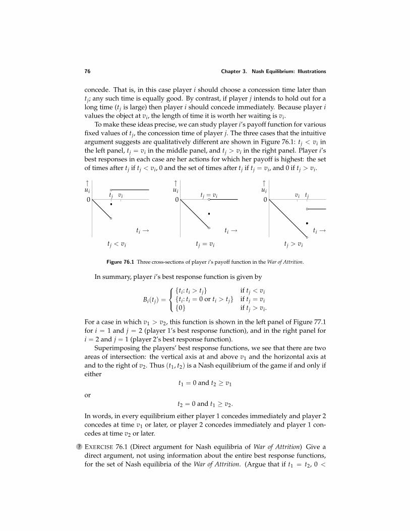
76 Chapter 3. Nash Equilibrium: Illustrations
concede. That is, in this case player i should choose a concession time later thantj; any such time is equally good. By contrast, if player j intends to hold out for along time (tj is large) then player i should concede immediately. Because player ivalues the object at vi, the length of time it is worth her waiting is vi.
To make these ideas precise, we can study player i’s payoff function for variousfixed values of tj, the concession time of player j. The three cases that the intuitiveargument suggests are qualitatively different are shown in Figure 76.1: tj < vi inthe left panel, tj = vi in the middle panel, and tj > vi in the right panel. Player i’sbest responses in each case are her actions for which her payoff is highest: the setof times after tj if tj < vi, 0 and the set of times after tj if tj = vi, and 0 if tj > vi.
0
↑ui
ti →tj < vi
tj vi 0
↑ui
ti →tj = vi
tj = vi 0
↑ui
ti →tj > vi
tjvi
Figure 76.1 Three cross-sections of player i’s payoff function in the War of Attrition.
In summary, player i’s best response function is given by
Bi(tj) =
ti: ti > tj if tj < viti: ti = 0 or ti > tj if tj = vi0 if tj > vi.
For a case in which v1 > v2, this function is shown in the left panel of Figure 77.1for i = 1 and j = 2 (player 1’s best response function), and in the right panel fori = 2 and j = 1 (player 2’s best response function).
Superimposing the players’ best response functions, we see that there are twoareas of intersection: the vertical axis at and above v1 and the horizontal axis atand to the right of v2. Thus (t1, t2) is a Nash equilibrium of the game if and only ifeither
t1 = 0 and t2 ≥ v1
ort2 = 0 and t1 ≥ v2.
In words, in every equilibrium either player 1 concedes immediately and player 2concedes at time v1 or later, or player 2 concedes immediately and player 1 con-cedes at time v2 or later.
? EXERCISE 76.1 (Direct argument for Nash equilibria of War of Attrition) Give adirect argument, not using information about the entire best response functions,for the set of Nash equilibria of the War of Attrition. (Argue that if t1 = t2, 0 <
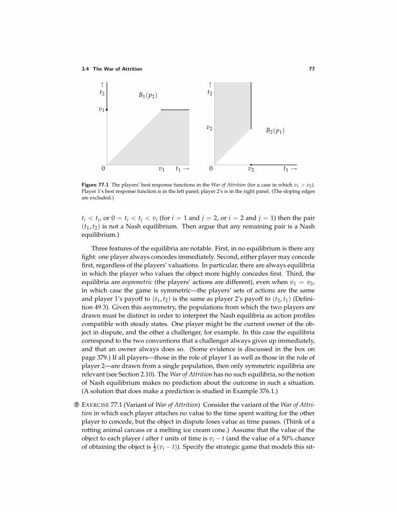
3.4 The War of Attrition 77
↑t2
t1 →
v1
v1
B1(p2)
0
↑t2
t1 →v2
v2 B2(p1)
0
Figure 77.1 The players’ best response functions in the War of Attrition (for a case in which v1 > v2).Player 1’s best response function is in the left panel; player 2’s is in the right panel. (The sloping edgesare excluded.)
ti < tj, or 0 = ti < tj < vi (for i = 1 and j = 2, or i = 2 and j = 1) then the pair(t1, t2) is not a Nash equilibrium. Then argue that any remaining pair is a Nashequilibrium.)
Three features of the equilibria are notable. First, in no equilibrium is there anyfight: one player always concedes immediately. Second, either player may concedefirst, regardless of the players’ valuations. In particular, there are always equilibriain which the player who values the object more highly concedes first. Third, theequilibria are asymmetric (the players’ actions are different), even when v1 = v2,in which case the game is symmetric—the players’ sets of actions are the sameand player 1’s payoff to (t1, t2) is the same as player 2’s payoff to (t2, t1) (Defini-tion 49.3). Given this asymmetry, the populations from which the two players aredrawn must be distinct in order to interpret the Nash equilibria as action profilescompatible with steady states. One player might be the current owner of the ob-ject in dispute, and the other a challenger, for example. In this case the equilibriacorrespond to the two conventions that a challenger always gives up immediately,and that an owner always does so. (Some evidence is discussed in the box onpage 379.) If all players—those in the role of player 1 as well as those in the role ofplayer 2—are drawn from a single population, then only symmetric equilibria arerelevant (see Section 2.10). The War of Attrition has no such equilibria, so the notionof Nash equilibrium makes no prediction about the outcome in such a situation.(A solution that does make a prediction is studied in Example 376.1.)
? EXERCISE 77.1 (Variant of War of Attrition) Consider the variant of the War of Attri-tion in which each player attaches no value to the time spent waiting for the otherplayer to concede, but the object in dispute loses value as time passes. (Think of arotting animal carcass or a melting ice cream cone.) Assume that the value of theobject to each player i after t units of time is vi − t (and the value of a 50% chanceof obtaining the object is 1
2 (vi − t)). Specify the strategic game that models this sit-
78 Chapter 3. Nash Equilibrium: Illustrations
uation (take care with the payoff functions). Construct the analogue of Figure 76.1,find the players’ best response functions, and hence find the Nash equilibria of thegame.
The War of Attrition is an example of a “game of timing”, in which each player’saction is a number and each player’s payoff depends sensitively on whether heraction is greater or less than the other player’s action. In many such games, eachplayer’s strategic variable is the time at which to act, hence the name “game oftiming”. The next two exercises are further examples of such games. (In the firstthe strategic variable is time, whereas in the second it is not.)
? EXERCISE 78.1 (Timing product release) Two firms are developing competing prod-ucts for a market of fixed size. The longer a firm spends on development, the betterits product. But the first firm to release its product has an advantage: the customersit obtains will not subsequently switch to its rival. (Once a person starts using aproduct, the cost of switching to an alternative, even one significantly better, is toohigh to make a switch worthwhile.) A firm that releases its product first, at time t,captures the share h(t) of the market, where h is a function that increases fromtime 0 to time T, with h(0) = 0 and h(T) = 1. The remaining market share is leftfor the other firm. If the firms release their products at the same time, each obtainshalf of the market. Each firm wishes to obtain the highest possible market share.Model this situation as a strategic game and find its Nash equilibrium (equilibria?).(When finding firm i’s best response to firm j’s release time tj, there are three cases:that in which h(tj) < 1
2 (firm j gets less than half of the market if it is the first torelease its product), that in which h(tj) = 1
2 , and that in which h(tj) > 12 .)
? EXERCISE 78.2 (A fight) Each of two people has one unit of a resource. Each personchooses how much of the resource to use in fighting the other individual and howmuch to use productively. If each person i devotes yi to fighting then the totaloutput is f (y1, y2) ≥ 0 and person i obtains the fraction pi(y1, y2) of the output,where
pi(y1, y2) =
1 if yi > yj12 if yi = yj0 if yi < yj.
The function f is continuous (small changes in y1 and y2 cause small changes inf (y1, y2)), is decreasing in both y1 and y2 (the more each player devotes to fighting,the less output is produced), and satisfies f (1, 1) = 0 (if each player devotes all herresource to fighting then no output is produced). (If you prefer to deal with aspecific function f , take f (y1, y2) = 2 − y1 − y2.) Each person cares only about theamount of output she receives, and prefers to receive as much as possible. Specifythis situation as a strategic game and find its Nash equilibrium (equilibria?). (Usea direct argument: first consider pairs (y1, y2) with y1 = y2, then those with y1 =y2 < 1, then those with y1 = y2 = 1.)
3.5 Auctions 79
3.5 Auctions
3.5.1 Introduction
In an “auction”, a good is sold to the party who submits the highest bid. Auctions,broadly defined, are used to allocate significant economic resources, from works ofart to short-term government bonds to offshore tracts for oil and gas explorationto the radio spectrum. They take many forms. For example, bids may be calledout sequentially (as in auctions for works of art) or may be submitted in sealedenvelopes; the price paid may be the highest bid, or some other price; if more thanone unit of a good is being sold, bids may be taken on all units simultaneously,or the units may be sold sequentially. A game-theoretic analysis helps us to un-derstand the consequences of various auction designs; it suggests, for example,the design likely to be the most effective at allocating resources, and the one likelyto raise the most revenue. In this section I discuss auctions in which every buyerknows her own valuation and every other buyer’s valuation of the item being sold.Chapter 9 develops tools that allow us to study, in Section 9.7, auctions in whichbuyers are not perfectly informed of each other’s valuations.
AUCTIONS FROM BABYLONIA TO EBAY
Auctioning has a very long history. Herodotus, a Greek writer of the fifth cen-tury BC who, together with Thucydides, created the intellectual field of history,describes auctions in Babylonia. He writes that the Babylonians’ “most sensible”custom was an annual auction in each village of the women of marriageable age.The women most attractive to the men were sold first; they commanded positiveprices, whereas men were paid to be matched with the least desirable women. Ineach auction, bids appear to have been called out sequentially, the man who bidthe most winning and paying the price he bid.
Auctions were also used in Athens in the fifth and fourth centuries BC to sellthe rights to collect taxes, to dispose of confiscated property, and to lease land andmines. The evidence on the nature of the auctions is slim, but some interestingaccounts survive. For example, the Athenian politician Andocides (c. 440–391 BC)reports collusive behavior in an auction of tax-collection rights (see Langdon 1994,260).
Auctions were frequent in ancient Rome, and continued to be used in medievalEurope after the end of the Roman empire (tax-collection rights were annuallyauctioned by the towns of the medieval and early modern Low Countries, for ex-ample). The earliest use of the English word “auction” given by the Oxford EnglishDictionary dates from 1595, and concerns an auction “when will be sold Slaves,household goods, etc.”. Rules surviving from the auctions of this era show that insome cases, at least, bids were called out sequentially, with the bidder remainingat the end obtaining the object at the price she bid (Cassady 1967, 30–31). A variant
80 Chapter 3. Nash Equilibrium: Illustrations
of this mechanism, in which a time limit is imposed on the bids, is reported by theEnglish diarist and naval administrator Samuel Pepys (1633–1703). The auction-eer lit a short candle, and bids were valid only if made before the flame went out.Pepys reports that a flurry of bidding occurred at the last moment. At an auctionon September 3, 1662, a bidder “cunninger than the rest” told him that just as theflame goes out, “the smoke descends”, signaling the moment at which one shouldbid, an observation Pepys found “very pretty” (Pepys 1970, 185–186).
The auction houses of Sotheby’s and Christie’s were founded in the mid-18thcentury. At the beginning of the twenty-first century, they are being eclipsed, atleast in the value of the goods they sell, by online auction companies. For example,eBay, founded in September 1995, sold US$1.3 billion of merchandise in 62 millionauctions during the second quarter of 2000, roughly double the numbers for thesecond quarter of the previous year; Sotheby’s and Christie’s together sell aroundUS$1 billion of art and antiques each quarter.
The mechanism used by eBay shares a feature with the ones Pepys observed:all bids must be received before some fixed time. The way in which the price isdetermined differs. In an eBay auction, a bidder submits a “proxy bid” that is notrevealed; the prevailing price is a small increment above the second-highest proxybid. As in the 17th century auctions Pepys observed, many bidders on eBay act atthe last moment—a practice known as “sniping” in the argot of cyberspace. Otheronline auction houses use different termination rules. For example, Amazon waitsten minutes after a bid before closing an auction. The fact that last-minute biddingis much less common in Amazon auctions than it is in eBay auctions has attractedthe attention of game theorists, who have begun to explore models that explainit in terms of the difference in the auctions’ termination rules (see, for example,Ockenfels and Roth 2000).
In recent years, many countries have auctioned the rights to the radio spec-trum, used for wireless communication. These auctions have been much studiedby game theorists; they are discussed in the box on page 298.
3.5.2 Second-price sealed-bid auctions
In a common form of auction, people sequentially submit increasing bids for anobject. (The word “auction” comes from the Latin augere, meaning “to increase”.)When no one wishes to submit a bid higher than the current bid, the person mak-ing the current bid obtains the object at the price she bid.
Given that every person is certain of her valuation of the object before the bid-ding begins, during the bidding no one can learn anything relevant to her actions.Thus we can model the auction by assuming that each person decides, before bid-ding begins, the most she is willing to bid—her “maximal bid”. When the playerscarry out their plans, the winner is the person whose maximal bid is highest. Howmuch does she need to bid? Eventually only she and the person with the secondhighest maximal bid will be left competing against each other. In order to win,
3.5 Auctions 81
she therefore needs to bid slightly more than the second highest maximal bid. If thebidding increment is small, we can take the price the winner pays to be equal to thesecond highest maximal bid.
Thus we can model such an auction as a strategic game in which each playerchooses an amount of money, interpreted as the maximal amount she is willing tobid, and the player who chooses the highest amount obtains the object and pays aprice equal to the second highest amount.
This game models also a situation in which the people simultaneously put bidsin sealed envelopes, and the person who submits the highest bid wins and pays aprice equal to the second highest bid. For this reason the game is called a second-pricesealed-bid auction.
To define the game precisely, denote by vi the value player i attaches to theobject; if she obtains the object at the price p her payoff is vi − p. Assume thatthe players’ valuations of the object are all different and all positive; number theplayers 1 through n in such a way that v1 > v2 > · · · > vn > 0. Each player isubmits a (sealed) bid bi. If player i’s bid is higher than every other bid, she obtainsthe object at a price equal to the second-highest bid, say bj, and hence receives thepayoff vi − bj. If some other bid is higher than player i’s bid, player i does notobtain the object, and receives the payoff of zero. If player i is in a tie for the highestbid, her payoff depends on the way in which ties are broken. A simple (thougharbitrary) assumption is that the winner is the player among those submitting thehighest bid whose number is smallest (i.e. whose valuation of the object is highest).(If the highest bid is submitted by players 2, 5, and 7, for example, the winner isplayer 2.) Under this assumption, player i’s payoff when she bids bi and is in a tiefor the highest bid is vi − bi if her number is lower than that of any other playersubmitting the bid bi, and 0 otherwise.
In summary, a second-price sealed-bid auction (with perfect information) isthe following strategic game.
Players The n bidders, where n ≥ 2.
Actions The set of actions of each player is the set of possible bids (nonnega-tive numbers).
Preferences The payoff of any player i is vi − bj, where bj is the highest bidsubmitted by a player other than i if either bi is higher than every other bid,or bi is at least as high as every other bid and the number of every otherplayer who bids bi is greater than i. Otherwise player i’s payoff is 0.
This game has many Nash equilibria. One equilibrium is (b1, . . . , bn) = (v1, . . . ,vn): each player’s bid is equal to her valuation of the object. Because v1 > v2 >
· · · > vn, the outcome is that player 1 obtains the object at the price b2; her payoff isv1 − b2 and every other player’s payoff is zero. This profile is a Nash equilibriumby the following argument.
• If player 1 changes her bid to some other price at least equal to b2 then theoutcome does not change (recall that she pays the second highest bid, not the
82 Chapter 3. Nash Equilibrium: Illustrations
highest bid). If she changes her bid to a price less than b2 then she loses andobtains the payoff of zero.
• If some other player lowers her bid or raises it to some price at most equal tob1 then she remains a loser; if she raises her bid above b1 then she wins but,in paying the price b1, makes a loss (because her valuation is less than b1).
Another equilibrium is (b1, . . . , bn) = (v1, 0, . . . , 0). In this equilibrium, player 1obtains the object and pays the price of zero. The profile is an equilibrium becauseif player 1 changes her bid then the outcome remains the same, and if any of theremaining players raises her bid then either the outcome remains the same (if hernew bid is at most v1) or causes her to obtain the object at a price that exceeds hervaluation (if her bid exceeds v1). (The auctioneer obviously has an incentive forthe price to be bid up, but she is not a player in the game!)
In both of these equilibria, player 1 obtains the object. But there are also equilib-ria in which player 1 does not obtain the object. Consider, for example, the actionprofile (v2, v1, 0, . . . , 0), in which player 2 obtains the object at the price v2 and ev-ery player (including player 2) receives the payoff of zero. This action profile is aNash equilibrium by the following argument.
• If player 1 raises her bid to v1 or more, she wins the object but her payoffremains zero (she pays the price v1, bid by player 2). Any other change inher bid has no effect on the outcome.
• If player 2 changes her bid to some other price greater than v2, the outcomedoes not change. If she changes her bid to v2 or less she loses, and her payoffremains zero.
• If any other player raises her bid to at most v1, the outcome does not change.If she raises her bid above v1 then she wins, but in paying the price v1 (bidby player 2) she obtains a negative payoff.
? EXERCISE 82.1 (Nash equilibrium of second-price sealed-bid auction) Find a Nashequilibrium of a second-price sealed-bid auction in which player n obtains theobject.
Player 2’s bid in this equilibrium exceeds her valuation, and thus may seem alittle rash: if player 1 were to increase her bid to any value less than v1, player 2’spayoff would be negative (she would obtain the object at a price greater thanher valuation). This property of the action profile does not affect its status as anequilibrium, because in a Nash equilibrium a player does not consider the “risk”that another player will take an action different from her equilibrium action; eachplayer simply chooses an action that is optimal, given the other players’ actions.But the property does suggest that the equilibrium is less plausible as the outcomeof the auction than the equilibrium in which every player bids her valuation.
The same point takes a different form when we interpret the strategic game as amodel of events that unfold over time. Under this interpretation, player 2’s action
3.5 Auctions 83
v1 means that she will continue bidding until the price reaches v1. If player 1 is surethat player 2 will continue bidding until the price is v1, then player 1 rationallystops bidding when the price reaches v2 (or, indeed, when it reaches any otherlevel at most equal to v1). But there is little reason for player 1 to believe thatplayer 2 will in fact stay in the bidding if the price exceeds v2: player 2’s action isnot credible, because if the bidding were to go above v2, player 2 would rationallywithdraw.
The weakness of the equilibrium is reflected in the fact that player 2’s bid v1 isweakly dominated by the bid v2. More generally,
in a second-price sealed-bid auction (with perfect information), a player’s bidequal to her valuation weakly dominates all her other bids.
That is, for any bid bi = vi, player i’s bid vi is at least as good as bi, no matter whatthe other players bid, and is better than bi for some actions of the other players. (SeeDefinition 45.1.) A player who bids less than her valuation stands not to win insome cases in which she could profit by winning (when the highest of the otherbids is between her bid and her valuation), and never stands to gain relative tothe situation in which she bids her valuation; a player who bids more than hervaluation stands to win in some cases in which she obtains a negative payoff bydoing so (when the highest of the remaining bids is between her valuation andher bid), and never stands to gain relative to the situation in which she bids hervaluation. The key point is that in a second-price auction, a player who changesher bid does not lower the price she pays, but only possibly changes her statusfrom that of a winner into that of a loser, or vice versa.
A precise argument is shown in Figure 84.1, which compares player i’s payoffsto the bid vi with her payoffs to a bid bi < vi (top table), and to a bid bi < vi(bottom table), as a function of the highest of the other players’ bids, denoted b.In each case, for all bids of the other players, player i’s payoffs to vi are at least aslarge as her payoffs to the other bid, and for bids of the other players such that bis in the middle column of each table, player i’s payoffs to vi are greater than herpayoffs to the other bid. Thus player i’s bid vi weakly dominates all her other bids.
In summary, a second-price auction has many Nash equilibria, but the equilib-rium (b1, . . . , bn) = (v1, . . . , vn) in which every player’s bid is equal to her valu-ation of the object is distinguished by the fact that every player’s action weaklydominates all her other actions.
? EXERCISE 83.1 (Second-price sealed-bid auction with two bidders) Find all theNash equilibria of a second-price sealed-bid auction with two bidders. (Constructthe players’ best response functions. Apart from a difference in the tie-breakingrule, the game is the same as the one in Exercise 77.1.)
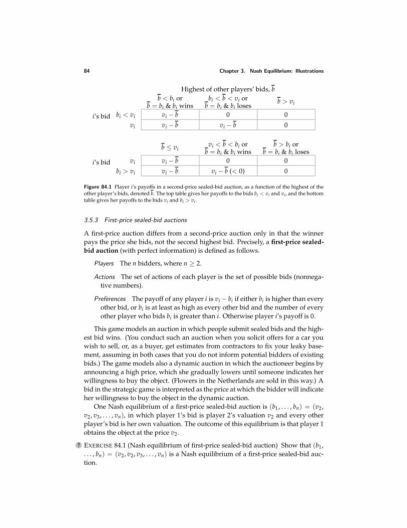
84 Chapter 3. Nash Equilibrium: Illustrations
i’s bid
Highest of other players’ bids, bb < bi or
b = bi & bi winsbi < b < vi or
b = bi & bi losesb > vi
bi < vi vi − b 0 0
vi vi − b vi − b 0
i’s bid
b ≤ vivi < b < bi or
b = bi & bi winsb > bi or
b = bi & bi losesvi vi − b 0 0
bi > vi vi − b vi − b (< 0) 0
Figure 84.1 Player i’s payoffs in a second-price sealed-bid auction, as a function of the highest of theother player’s bids, denoted b. The top table gives her payoffs to the bids bi < vi and vi, and the bottomtable gives her payoffs to the bids vi and bi > vi.
3.5.3 First-price sealed-bid auctions
A first-price auction differs from a second-price auction only in that the winnerpays the price she bids, not the second highest bid. Precisely, a first-price sealed-bid auction (with perfect information) is defined as follows.
Players The n bidders, where n ≥ 2.
Actions The set of actions of each player is the set of possible bids (nonnega-tive numbers).
Preferences The payoff of any player i is vi − bi if either bi is higher than everyother bid, or bi is at least as high as every other bid and the number of everyother player who bids bi is greater than i. Otherwise player i’s payoff is 0.
This game models an auction in which people submit sealed bids and the high-est bid wins. (You conduct such an auction when you solicit offers for a car youwish to sell, or, as a buyer, get estimates from contractors to fix your leaky base-ment, assuming in both cases that you do not inform potential bidders of existingbids.) The game models also a dynamic auction in which the auctioneer begins byannouncing a high price, which she gradually lowers until someone indicates herwillingness to buy the object. (Flowers in the Netherlands are sold in this way.) Abid in the strategic game is interpreted as the price at which the bidder will indicateher willingness to buy the object in the dynamic auction.
One Nash equilibrium of a first-price sealed-bid auction is (b1, . . . , bn) = (v2,v2, v3, . . . , vn), in which player 1’s bid is player 2’s valuation v2 and every otherplayer’s bid is her own valuation. The outcome of this equilibrium is that player 1obtains the object at the price v2.
? EXERCISE 84.1 (Nash equilibrium of first-price sealed-bid auction) Show that (b1,. . . , bn) = (v2, v2, v3, . . . , vn) is a Nash equilibrium of a first-price sealed-bid auc-tion.
3.5 Auctions 85
A first-price sealed-bid auction has many other equilibria, but in all equilibriathe winner is the player who values the object most highly (player 1), by the fol-lowing argument. In any action profile (b1, . . . , bn) in which some player i = 1wins, we have bi > b1. If bi > v2 then i’s payoff is negative, so that she can dobetter by reducing her bid to 0; if bi ≤ v2 then player 1 can increase her payofffrom 0 to v1 − bi by bidding bi, in which case she wins. Thus no such action profileis a Nash equilibrium.
? EXERCISE 85.1 (First-price sealed-bid auction) Show that in a Nash equilibrium ofa first-price sealed-bid auction the two highest bids are the same, one of these bidsis submitted by player 1, and the highest bid is at least v2 and at most v1. Showalso that any action profile satisfying these conditions is a Nash equilibrium.
In any equilibrium in which the winning bid exceeds v2, at least one player’sbid exceeds her valuation. As in a second-price sealed-bid auction, such a bidseems “risky”, because it would yield the bidder a negative payoff if it were to win.In the equilibrium there is no risk, because the bid does not win; but, as before, thefact that the bid has this property reduces the plausibility of the equilibrium.
As in a second-price sealed-bid auction, the potential “riskiness” to player i ofa bid bi > vi is reflected in the fact that it is weakly dominated by the bid vi, asshown by the following argument.
• If the other players’ bids are such that player i loses when she bids bi, thenthe outcome is the same whether she bids bi or vi.
• If the other players’ bids are such that player i wins when she bids bi, thenher payoff is negative when she bids bi and zero when she bids vi (whetheror not this bid wins).
However, in a first-price auction, unlike a second-price auction, a bid bi < viof player i is not weakly dominated by the bid vi. If fact, such a bid is not weaklydominated by any bid. It is not weakly dominated by a bid b′i < bi, because if theother players’ highest bid is between b′i and bi then b′i loses whereas bi wins andyields player i a positive payoff. And it is not weakly dominated by a bid b′i > bi,because if the other players’ highest bid is less than bi then both bi and b′i win andbi yields a lower price.
Further, even though the bid vi weakly dominates higher bids, this bid is itselfweakly dominated, by a lower bid! If player i bids vi her payoff is 0 regardless ofthe other players’ bids, whereas if she bids less than vi her payoff is either 0 (if sheloses) or positive (if she wins).
In summary,
in a first-price sealed-bid auction (with perfect information), a player’s bid ofat least her valuation is weakly dominated, and a bid of less than her valuationis not weakly dominated.
86 Chapter 3. Nash Equilibrium: Illustrations
An implication of this result is that in every Nash equilibrium of a first-pricesealed-bid auction at least one player’s action is weakly dominated. However,this property of the equilibria depends on the assumption that a bid may be anynumber. In the variant of the game in which bids and valuations are restrictedto be multiples of some discrete monetary unit ε (e.g. a cent), an action profile(v2 − ε, v2 − ε, b3, . . . , bn) for any bj ≤ vj − ε for j = 3, . . . , n is a Nash equilib-rium in which no player’s bid is weakly dominated. Further, every equilibriumin which no player’s bid is weakly dominated takes this form. When ε is small,each such equilibrium is close to an equilibrium (v2, v2, b3, . . . , bn) (with bj ≤ vjfor j = 3, . . . , n) of the game with unrestricted bids. On this (somewhat ad hoc)basis, I select action profiles (v2, v2, b3, . . . , bn) with bj ≤ vj for j = 3, . . . , n as“distinguished” equilibria of a first-price sealed-bid auction.
One conclusion of this analysis is that while both second-price and first-priceauctions have many Nash equilibria, yielding a variety of outcomes, their distin-guished equilibria yield the same outcome. (Recall that the distinguished equi-librium of a second-price sealed-bid auction is the action profile in which everyplayer bids her valuation.) In every distinguished equilibrium of each game, theobject is sold to player 1 at the price v2. In particular, the auctioneer’s revenue isthe same in both cases. Thus if we restrict attention to the distinguished equilibria,the two auction forms are “revenue equivalent”. The rules are different, but theplayers’ equilibrium bids adjust to the difference and lead to the same outcome:
the single Nash equilibrium in which no player’s bid is weakly dominated ina second-price auction yields the same outcome as the distinguished equilibriaof a first-price auction.
? EXERCISE 86.1 (Third-price auction) Consider a third-price sealed-bid auction, whichdiffers from a first- and a second-price auction only in that the winner (the personwho submits the highest bid) pays the third highest price. (Assume that there areat least three bidders.)
a. Show that for any player i the bid of vi weakly dominates any lower bid, butdoes not weakly dominate any higher bid. (To show the latter, for any bidbi > vi find bids for the other players such that player i is better off biddingbi than bidding vi.)
b. Show that the action profile in which each player bids her valuation is not aNash equilibrium.
c. Find a Nash equilibrium. (There are ones in which every player submits thesame bid.)
3.5.4 Variants
Uncertain valuations One respect in which the models in this section depart fromreality is in the assumption that each bidder is certain of both her own valuationand every other bidder’s valuation. In most, if not all, actual auctions, information
3.5 Auctions 87
is surely less perfect. The case in which the players are uncertain about each other’svaluations has been thoroughly explored, and is discussed in Section 9.7. The re-sult that a player’s bidding her valuation weakly dominates all her other actions ina second-price auction survives when players are uncertain about each other’s val-uations, as does the revenue-equivalence of first- and second-price auctions undersome conditions on the players’ preferences.
Common valuations In some auctions the main difference between the bidders isnot that the value the object differently but that they have different informationabout its value. For example, the bidders for an oil tract may put similar values onany given amount of oil, but have different information about how much oil is inthe tract. Such auctions involve informational considerations that do not arise inthe model we have studied in this section; they are studied in Section 9.7.3.
Multi-unit auctions In some auctions, like those for Treasury Bills (short-termgovernment bonds) in the USA, many units of an object are available, and eachbidder may value positively more than one unit. In each of the types of auctiondescribed below, each bidder submits a bid for each unit of the good. That is, anaction is a list of bids (b1, . . . , bk), where b1 is the player’s bid for the first unit ofthe good, b2 is her bid for the second unit, and so on. The player who submits thehighest bid for any given unit obtains that unit. The auctions differ in the pricespaid by the winners. (The first type of auction generalizes a first-price auction,whereas the next two generalize a second-price auction.)
Discriminatory auction The price paid for each unit is the winning bid for thatunit.
Uniform-price auction The price paid for each unit is the same, equal to thehighest rejected bid among all the bids for all units.
Vickrey auction A bidder who wins k objects pays the sum of the k highest re-jected bids submitted by the other bidders.
The next exercise asks you to study these auctions when two units of an object areavailable.
?? EXERCISE 87.1 (Multi-unit auctions) Two units of an object are available. Thereare n bidders. Bidder i values the first unit that she obtains at vi and the secondunit at wi, where vi > wi > 0. Each bidder submits two bids; the two highestbids win. Retain the tie-breaking rule in the text. Show that in discriminatory anduniform-price auctions, player i’s action of bidding vi and wi does not dominateall her other actions, whereas in a Vickrey auction it does. (In the case of a Vickreyauction, consider separately the cases in which the other players’ bids are such thatplayer i wins no units, one unit, and two units when her bids are vi and wi.)
Goods for which the demand exceeds the supply at the going price are some-times sold to the people who are willing to wait longest in line. We can model such
88 Chapter 3. Nash Equilibrium: Illustrations
situations as multi-unit auctions in which each person’s bid is the amount of timeshe is willing to wait.
?? EXERCISE 88.1 (Waiting in line) Two hundred people are willing to wait in line tosee a movie at a theater whose capacity is one hundred. Denote person i’s valu-ation of the movie in excess of the price of admission, expressed in terms of theamount of time she is willing to wait, by vi. That is, person i’s payoff if she waitsfor ti units of time is vi − ti. Each person attaches no value to a second ticket, andcannot buy tickets for other people. Assume that v1 > v2 > · · · > v200. Eachperson chooses an arrival time. If several people arrive at the same time then theirorder in line is determined by their index (lower-numbered people go first). If aperson arrives to find 100 or more people already in line, her payoff is zero. Modelthe situation as a variant of a discriminatory multi-unit auction, in which each per-son submits a bid for only one unit, and find its Nash equilibria. (Look at youranswer to Exercise 85.1 before seeking the Nash equilibria.) Arrival times for peo-ple at movies do not in general seem to conform with a Nash equilibrium. Whatfeature missing from the model could explain the pattern of arrivals?
The next exercise is another application of a multi-unit auction. As in the pre-vious exercise each person wants to buy only one unit, but in this case the pricepaid by the winners is the highest losing bid.
? EXERCISE 88.2 (Internet pricing) A proposal to deal with congestion on electronicmessage pathways is that each message should include a field stating an amountof money the sender is willing to pay for the message to be sent. Suppose thatduring some time interval, each of n people wants to send one message and thecapacity of the pathway is k messages, with k < n. The k messages whose bids arehighest are the ones sent, and each of the persons sending these messages pays aprice equal to the (k + 1)st highest bid. Model this situation as a multi-unit auction.(Use the same tie-breaking rule as the one in the text.) Does a person’s action ofbidding the value of her message weakly dominate all her other actions? (Notethat the auction differs from those considered in Exercise 87.1 because each personsubmits only one bid. Look at the argument in the text that in a second-pricesealed-bid auction a player’s action of bidding her value weakly dominates all herother actions.)
Lobbying as an auction Variants of the models in this section can be used to under-stand some situations that are not explicitly auctions. An example, illustrated inthe next exercise, is the competition between groups pressuring a government tofollow policies they favor. This exercise shows also that the outcome of an auctionmay depend significantly (and perhaps counterintuitively) on the form the auctiontakes.
? EXERCISE 88.3 (Lobbying as an auction) A government can pursue three poli-cies, x, y, and z. The monetary values attached to these policies by two interestgroups, A and B, are given in Figure 89.1. The government chooses a policy in
3.6 Accident law 89
response to the payments the interest groups make to it. Consider the followingtwo mechanisms.
First-price auction Each interest group chooses a policy and an amount of moneyit is willing to pay. The government chooses the policy proposed by the groupwilling to pay the most. This group makes its payment to the government,and the losing group makes no payment.
Menu auction Each interest group states, for each policy, the amount it is will-ing to pay to have the government implement that policy. The governmentchooses the policy for which the sum of the payments the groups are willingto make is the highest, and each group pays the government the amount ofmoney it is willing to pay for that policy.
In each case each interest group’s payoff is the value it attaches to the policyimplemented minus the payment it makes. Assume that a tie is broken by thegovernment’s choosing the policy, among those tied, whose name is first in thealphabet.
x y zInterest group A 0 3 −100Interest group B 0 −100 3
Figure 89.1 The values of the interest groups for the policies x, y, and z in Exercise 88.3.
Show that the first-price auction has a Nash equilibrium in which lobby A saysit will pay 103 for y, lobby B says it will pay 103 for z, and the government’s rev-enue is 103. Show that the menu auction has a Nash equilibrium in which lobby Aannounces that it will pay 3 for x, 6 for y, and 0 for z, and lobby B announcesthat it will pay 3 for x, 0 for y, and 6 for z, and the government chooses x, ob-taining a revenue of 6. (In each case the pair of actions given is in fact the uniqueequilibrium.)
3.6 Accident law
3.6.1 Introduction
In some situations, laws influence the participants’ payoffs and hence their actions.For example, a law may provide for the victim of an accident to be compensated bya party who was at fault, and the size of the compensation may affect the care thateach party takes. What laws can we expect to produce socially desirable outcomes?A game theoretic analysis is useful in addressing this question.
3.6.2 The game
Consider the interaction between an injurer (player 1) and a victim (player 2). Thevictim suffers a loss that depends on the amounts of care taken by both her and
90 Chapter 3. Nash Equilibrium: Illustrations
the injurer. (How badly you hurt yourself when you fall down on the sidewalkin front of my house depends on both how well I have cleared the ice and howcarefully you tread.) Denote by ai the amount of care player i takes, measuredin monetary terms, and by L(a1, a2) the loss, also measured in monetary terms,suffered by the victim, as a function of the amounts of care. (In many cases thevictim does not suffer a loss with certainty, but only with probability less thanone. In such cases we can interpret L(a1, a2) as the expected loss—the averageloss suffered over many occurrences.) Assume that L(a1, a2) > 0 for all values of(a1, a2), and that more care taken by either player reduces the loss: L is decreasingin a1 for any fixed value of a2, and decreasing in a2 for any fixed value of a1.
A legal rule determines the fraction of the loss borne by the injurer, as a functionof the amounts of care taken. Denote this fraction by ρ(a1, a2). If ρ(a1, a2) = 0 forall (a1, a2), for example, the victim bears the entire loss, regardless of how muchcare she takes or how little care the injurer takes. At the other extreme, ρ(a1, a2) = 1for all (a1, a2) means that the victim is fully compensated by the injurer no matterhow careless she is or how careful the injurer is.
If the amounts of care are (a1, a2) then the injurer bears the cost a1 of takingcare and suffers the loss of L(a1, a2), of which she bears the fraction ρ(a1, a2). Thusthe injurer’s payoff is
−a1 − ρ(a1, a2)L(a1, a2).
Similarly, the victim’s payoff is
−a2 − (1 − ρ(a1, a2))L(a1, a2).
For any given legal rule, embodied in ρ, we can model the interaction betweenthe injurer and victim as the following strategic game.
Players The injurer and the victim.
Actions The set of actions of each player is the set of possible levels of care(nonnegative numbers).
Preferences The injurer’s preferences are represented by the payoff function−a1 − ρ(a1, a2)L(a1, a2) and the victim’s preferences are represented by thepayoff function −a2 − (1 − ρ(a1, a2))L(a1, a2), where a1 is the injurer’s levelof care and a2 is the victim’s level of care.
How do the equilibria of this game depend upon the legal rule? Do any legalrules lead to socially desirable equilibrium outcomes?
I restrict attention to a class of legal rules known as negligence with contributorynegligence. (This class was established in the USA in the mid-nineteenth century,and prevailed until the mid-1970s.) Each rule in this class requires the injurer tocompensate the victim for a loss if and only if both the victim is sufficiently carefuland the injurer is sufficiently careless; the required compensation is the total loss.Rules in the class differ in the standards of care they specify for each party. Therule that specifies the standards of care X1 for the injurer and X2 for the victim
3.6 Accident law 91
requires the injurer to pay the victim the entire loss L(a1, a2) when a1 < X1 (theinjurer is insufficiently careful) and a2 ≥ X2 (the victim is sufficiently careful), andnothing otherwise. That is, under this rule the fraction ρ(a1, a2) of the loss borneby the injurer is
ρ(a1, a2) =
1 if a1 < X1 and a2 ≥ X20 if a1 ≥ X1 or a2 < X2.
Included in this class of rules are those for which X1 is a positive finite numberand X2 = 0 (the injurer has to pay if she is not sufficiently careful, even if thevictim takes no care at all), known as rules of pure negligence, and that for which X1is infinite and X2 = 0 (the injurer has to pay regardless of how careful she is andhow careless the victim is), known as the rule of strict liability.
3.6.3 Nash equilibrium
Suppose we decide that the pair (a1, a2) of actions is socially desirable. We wishto answer the question: are there values of X1 and X2 such that the game gen-erated by the rule of negligence with contributory negligence for (X1, X2) has(a1, a2) as its unique Nash equilibrium? If the answer is affirmative, then, as-suming the solution concept of Nash equilibrium is appropriate for the situationwe are considering, we have found a legal rule that induces the socially desirableoutcome.
Specifically, suppose that we select as socially desirable the pair (a1, a2) ofactions that maximizes the sum of the players’ payoffs. That is,
(a1, a2) maximizes −a1 − a2 − L(a1, a2).
(For some functions L, this pair (a1, a2) may be a reasonable candidate for a sociallydesirable outcome; in other cases it may induce a very inequitable distribution ofpayoff between the players, and thus be an unlikely candidate.)
I claim that the unique Nash equilibrium of the game induced by the legal ruleof negligence with contributory negligence for (X1, X2) = (a1, a2) is (a1, a2). Thatis, if the standards of care are equal to their socially desirable levels, then these arethe levels chosen by an injurer and a victim in the only equilibrium of the game.The outcome is that the injurer pays no compensation: her level of care is a1, justhigh enough that ρ(a1, a2) = 0. At the same time the victim’s level of care is a2,high enough that if the injurer reduces her level of care even slightly then she hasto pay full compensation.
I first argue that (a1, a2) is a Nash equilibrium of the game, then show that it isthe only equilibrium. To show that (a1, a2) is a Nash equilibrium, I need to showthat the injurer’s action a1 is a best response to the victim’s action a2 and vice versa.
Injurer’s action Given that the victim’s action is a2, the injurer has to pay com-pensation if and only if a1 < a1. Thus the injurer’s payoff is
u1(a1, a2) =−a1 − L(a1, a2) if a1 < a1−a1 if a1 ≥ a1.
(91.1)
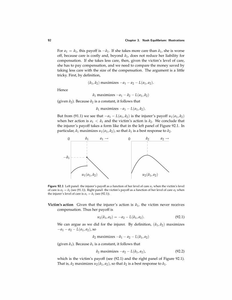
92 Chapter 3. Nash Equilibrium: Illustrations
For a1 = a1, this payoff is −a1. If she takes more care than a1, she is worseoff, because care is costly and, beyond a1, does not reduce her liability forcompensation. If she takes less care, then, given the victim’s level of care,she has to pay compensation, and we need to compare the money saved bytaking less care with the size of the compensation. The argument is a littletricky. First, by definition,
(a1, a2) maximizes −a1 − a2 − L(a1, a2).
Hencea1 maximizes −a1 − a2 − L(a1, a2)
(given a2). Because a2 is a constant, it follows that
a1 maximizes −a1 − L(a1, a2).
But from (91.1) we see that −a1 − L(a1, a2) is the injurer’s payoff u1(a1, a2)when her action is a1 < a1 and the victim’s action is a2. We conclude thatthe injurer’s payoff takes a form like that in the left panel of Figure 92.1. Inparticular, a1 maximizes u1(a1, a2), so that a1 is a best response to a2.
0 a1 a1 →
−a1
u1(a1, a2)
0 a2 a2 →
u2(a1, a2)
Figure 92.1 Left panel: the injurer’s payoff as a function of her level of care a1 when the victim’s levelof care is a2 = a2 (see (91.1)). Right panel: the victim’s payoff as a function of her level of care a2 whenthe injurer’s level of care is a1 = a1 (see (92.1)).
Victim’s action Given that the injurer’s action is a1, the victim never receivescompensation. Thus her payoff is
u2(a1, a2) = −a2 − L(a1, a2). (92.1)
We can argue as we did for the injurer. By definition, (a1, a2) maximizes−a1 − a2 − L(a1, a2), so
a2 maximizes −a1 − a2 − L(a1, a2)
(given a1). Because a1 is a constant, it follows that
a2 maximizes −a2 − L(a1, a2), (92.2)
which is the victim’s payoff (see (92.1) and the right panel of Figure 92.1).That is, a2 maximizes u2(a1, a2), so that a2 is a best response to a1.
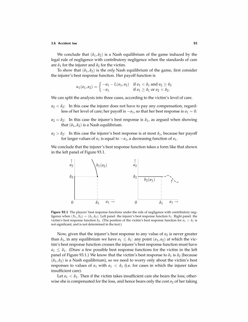
3.6 Accident law 93
We conclude that (a1, a2) is a Nash equilibrium of the game induced by thelegal rule of negligence with contributory negligence when the standards of careare a1 for the injurer and a2 for the victim.
To show that (a1, a2) is the only Nash equilibrium of the game, first considerthe injurer’s best response function. Her payoff function is
u1(a1, a2) =−a1 − L(a1, a2) if a1 < a1 and a2 ≥ a2−a1 if a1 ≥ a1 or a2 < a2.
We can split the analysis into three cases, according to the victim’s level of care.
a2 < a2: In this case the injurer does not have to pay any compensation, regard-less of her level of care; her payoff is −a1, so that her best response is a1 = 0.
a2 = a2: In this case the injurer’s best response is a1, as argued when showingthat (a1, a2) is a Nash equilibrium.
a2 > a2: In this case the injurer’s best response is at most a1, because her payofffor larger values of a1 is equal to −a1, a decreasing function of a1.
We conclude that the injurer’s best response function takes a form like that shownin the left panel of Figure 93.1.
0
a2
a1 a1 →
↑a2 b1(a2)
0
a2
a1 a1 →
↑a2
?b2(a1)
Figure 93.1 The players’ best response functions under the rule of negligence with contributory neg-ligence when (X1, X2) = (a1, a2). Left panel: the injurer’s best response function b1. Right panel: thevictim’s best response function b2. (The position of the victim’s best response function for a1 > a1 isnot significant, and is not determined in the text.)
Now, given that the injurer’s best response to any value of a2 is never greaterthan a1, in any equilibrium we have a1 ≤ a1: any point (a1, a2) at which the vic-tim’s best response function crosses the injurer’s best response function must havea1 ≤ a1. (Draw a few possible best response functions for the victim in the leftpanel of Figure 93.1.) We know that the victim’s best response to a1 is a2 (because(a1, a2) is a Nash equilibrium), so we need to worry only about the victim’s bestresponses to values of a1 with a1 < a1 (i.e. for cases in which the injurer takesinsufficient care).
Let a1 < a1. Then if the victim takes insufficient care she bears the loss; other-wise she is compensated for the loss, and hence bears only the cost a2 of her taking
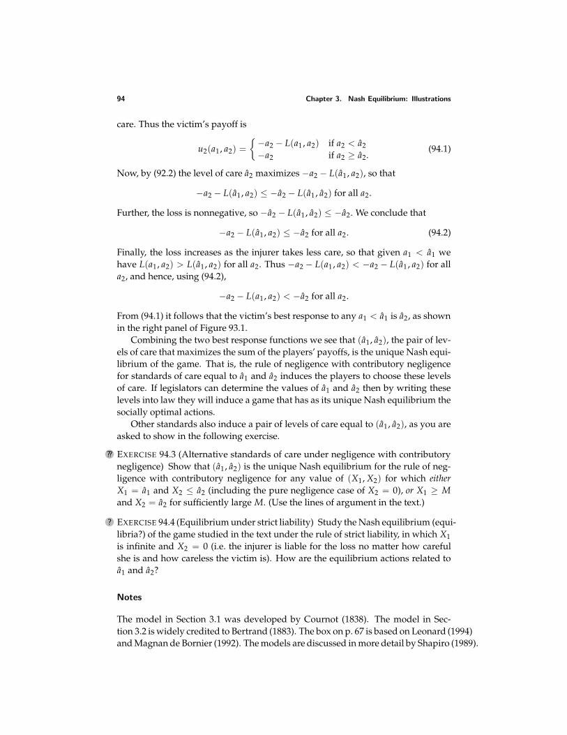
94 Chapter 3. Nash Equilibrium: Illustrations
care. Thus the victim’s payoff is
u2(a1, a2) =−a2 − L(a1, a2) if a2 < a2−a2 if a2 ≥ a2.
(94.1)
Now, by (92.2) the level of care a2 maximizes −a2 − L(a1, a2), so that
−a2 − L(a1, a2) ≤ −a2 − L(a1, a2) for all a2.
Further, the loss is nonnegative, so −a2 − L(a1, a2) ≤ −a2. We conclude that
−a2 − L(a1, a2) ≤ −a2 for all a2. (94.2)
Finally, the loss increases as the injurer takes less care, so that given a1 < a1 wehave L(a1, a2) > L(a1, a2) for all a2. Thus −a2 − L(a1, a2) < −a2 − L(a1, a2) for alla2, and hence, using (94.2),
−a2 − L(a1, a2) < −a2 for all a2.
From (94.1) it follows that the victim’s best response to any a1 < a1 is a2, as shownin the right panel of Figure 93.1.
Combining the two best response functions we see that (a1, a2), the pair of lev-els of care that maximizes the sum of the players’ payoffs, is the unique Nash equi-librium of the game. That is, the rule of negligence with contributory negligencefor standards of care equal to a1 and a2 induces the players to choose these levelsof care. If legislators can determine the values of a1 and a2 then by writing theselevels into law they will induce a game that has as its unique Nash equilibrium thesocially optimal actions.
Other standards also induce a pair of levels of care equal to (a1, a2), as you areasked to show in the following exercise.
?? EXERCISE 94.3 (Alternative standards of care under negligence with contributorynegligence) Show that (a1, a2) is the unique Nash equilibrium for the rule of neg-ligence with contributory negligence for any value of (X1, X2) for which eitherX1 = a1 and X2 ≤ a2 (including the pure negligence case of X2 = 0), or X1 ≥ Mand X2 = a2 for sufficiently large M. (Use the lines of argument in the text.)
? EXERCISE 94.4 (Equilibrium under strict liability) Study the Nash equilibrium (equi-libria?) of the game studied in the text under the rule of strict liability, in which X1is infinite and X2 = 0 (i.e. the injurer is liable for the loss no matter how carefulshe is and how careless the victim is). How are the equilibrium actions related toa1 and a2?
Notes
The model in Section 3.1 was developed by Cournot (1838). The model in Sec-tion 3.2 is widely credited to Bertrand (1883). The box on p. 67 is based on Leonard (1994)and Magnan de Bornier (1992). The models are discussed in more detail by Shapiro (1989).
Notes 95
The model in Section 3.3 is due to Hotelling (1929) (though the focus of hispaper is a model in which the players are firms that choose not only locations, butalso prices). Downs (1957, especially Ch. 8) popularized Hotelling’s model, usingit to gain insights about electoral competition. Shepsle (1991) and Osborne (1995)survey work in the field.
The War of Attrition studied in Section 3.4 is due to Maynard Smith (1974); it isa variant of the Dollar Auction presented by Shubik (1971).
Vickrey (1961) initiated the formal modeling of auctions, as studied in Sec-tion 3.5. The literature is surveyed by Wilson (1992). The box on page 79 drawson Herodotus’ Histories (Book 1, paragraph 196; see for example Herodotus 1998,86), Langdon (1994), Cassady (1967, Ch. 3), Shubik (1983), Andreau (1999, 38–39),the website www.eBay.com, Ockenfels and Roth (2000), and personal correspon-dence with Robin G. Osborne (on ancient Greece and Rome) and John H. Munro(on medieval Europe).
The model of accident law discussed in Section 94.3 originated with Brown (1973)and Diamond (1974); the result about negligence with contributory negligence isdue to Brown (1973, 340–341). The literature is surveyed by Benoıt and Korn-hauser (1995).
Novshek and Sonnenschein (1978) study, in a general setting, the issue ad-dressed in Exercise 60.1. A brief summary of the early work on common propertyis given in the Notes to Chapter 2. The idea of the tie-breaking rule being deter-mined by the equilibrium, used in Exercises 66.2 and 67.1, is due to Simon andZame (1990). The result in Exercise 73.1 is due to Wittman (1977). Exercise 73.2 isbased on Osborne and Slivinski (1996). The notion of a Condorcet winner definedin Exercise 74.1 is associated with Marie-Jean-Antoine-Nicolas de Caritat, marquisde Condorcet (1743–1794), an early student of voting procedures. The game inExercise 78.1 is a variant of a game studied by Blackwell and Girschick (1954, Ex-ample 5 in Ch. 2). It is an example of a noisy duel (which models the situationof duelists, each of whom chooses when to fire a single bullet, which her oppo-nent hears, as she gradually approaches her rival). Duels were first modeled asgames in the late 1940s by members of the RAND Corporation in the USA; see Kar-lin (1959b, Ch. 5). Exercise 88.3 is based on Boylan (1997). The situation consideredin Exercise 88.1, in which people decide when to join a queue, is studied by Holtand Sherman (1982). Exercise 88.2 is based on MacKie-Mason and Varian (1995).
Draft chapter from An introduction to game theory by Martin J. [email protected]; www.economics.utoronto.ca/osborneVersion: 00/11/6.Copyright c© 1995–2000 by Martin J. Osborne. All rights reserved. No part of this book may be re-produced by any electronic or mechanical means (including photocopying, recording, or informationstorage and retrieval) without permission in writing from Oxford University Press, except that onecopy of up to six chapters may be made by any individual for private study.
4 Mixed Strategy Equilibrium
Games in which players may randomize 103Mixed strategy Nash equilibrium 105Illustration: expert diagnosis 120Equilibrium in a single population 125Illustration: reporting a crime 128Prerequisite: Chapter 2.
4.1 Introduction
4.1.1 Stochastic steady states
ANASH EQUILIBRIUM of a strategic game is an action profile in which everyplayer’s action is optimal given every other player’s action (Definition 21.1).
Such an action profile corresponds to a steady state of the idealized situation inwhich for each player in the game there is a population of individuals, and when-ever the game is played, one player is drawn randomly from each population (seeSection 2.6). In a steady state, every player’s behavior is the same whenever sheplays the game, and no player wishes to change her behavior, knowing (from herexperience) the other players’ behavior. In a steady state in which each player’s“behavior” is simply an action and within each population all players choose thesame action, the outcome of every play of the game is the same Nash equilibrium.
More general notions of a steady state allow the players’ choices to vary, aslong as the pattern of choices remains constant. For example, different membersof a given population may choose different actions, each player choosing the sameaction whenever she plays the game. Or each individual may, on each occasionshe plays the game, choose her action probabilistically according to the same, un-changing distribution. These two more general notions of a steady state are equiv-alent: a steady state of the first type in which the fraction p of the population rep-resenting player i chooses the action a corresponds to a steady state of the secondtype in which each member of the population representing player i chooses a withprobability p. In both cases, in each play of the game the probability that the indi-vidual in the role of player i chooses a is p. Both these notions of steady state aremodeled by a mixed strategy Nash equilibrium, a generalization of the notion ofNash equilibrium. For expository convenience, in most of this chapter I interpretsuch an equilibrium as a model of the second type of steady state, in which each
97
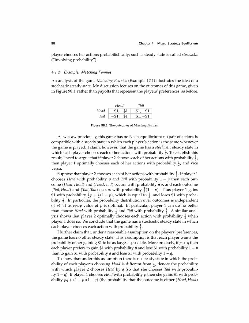
98 Chapter 4. Mixed Strategy Equilibrium
player chooses her actions probabilistically; such a steady state is called stochastic(“involving probability”).
4.1.2 Example: Matching Pennies
An analysis of the game Matching Pennies (Example 17.1) illustrates the idea of astochastic steady state. My discussion focuses on the outcomes of this game, givenin Figure 98.1, rather than payoffs that represent the players’ preferences, as before.
Head TailHead $1, −$1 −$1, $1
Tail −$1, $1 $1, −$1
Figure 98.1 The outcomes of Matching Pennies.
As we saw previously, this game has no Nash equilibrium: no pair of actions iscompatible with a steady state in which each player’s action is the same wheneverthe game is played. I claim, however, that the game has a stochastic steady state inwhich each player chooses each of her actions with probability 1
2 . To establish thisresult, I need to argue that if player 2 chooses each of her actions with probability 1
2 ,then player 1 optimally chooses each of her actions with probability 1
2 , and viceversa.
Suppose that player 2 chooses each of her actions with probability 12 . If player 1
chooses Head with probability p and Tail with probability 1 − p then each out-come (Head, Head) and (Head, Tail) occurs with probability 1
2 p, and each outcome(Tail, Head) and (Tail, Tail) occurs with probability 1
2 (1 − p). Thus player 1 gains$1 with probability 1
2 p + 12 (1 − p), which is equal to 1
2 , and loses $1 with proba-bility 1
2 . In particular, the probability distribution over outcomes is independentof p! Thus every value of p is optimal. In particular, player 1 can do no betterthan choose Head with probability 1
2 and Tail with probability 12 . A similar anal-
ysis shows that player 2 optimally chooses each action with probability 12 when
player 1 does so. We conclude that the game has a stochastic steady state in whicheach player chooses each action with probability 1
2 .I further claim that, under a reasonable assumption on the players’ preferences,
the game has no other steady state. This assumption is that each player wants theprobability of her gaining $1 to be as large as possible. More precisely, if p > q theneach player prefers to gain $1 with probability p and lose $1 with probability 1 − pthan to gain $1 with probability q and lose $1 with probability 1 − q.
To show that under this assumption there is no steady state in which the prob-ability of each player’s choosing Head is different from 1
2 , denote the probabilitywith which player 2 chooses Head by q (so that she chooses Tail with probabil-ity 1 − q). If player 1 chooses Head with probability p then she gains $1 with prob-ability pq + (1 − p)(1 − q) (the probability that the outcome is either (Head, Head)
4.1 Introduction 99
or (Tail, Tail)) and loses $1 with probability (1 − p)q + p(1 − q). The first probabil-ity is equal to 1 − q + p(2q − 1) and the second is equal to q + p(1 − 2q). Thus ifq < 1
2 (player 2 chooses Head with probability less than 12 ), the first probability is
decreasing in p and the second is increasing in p, so that the lower is p, the betteris the outcome for player 1; the value of p that induces the best probability dis-tribution over outcomes for player 1 is 0. That is, if player 2 chooses Head withprobability less than 1
2 , then the uniquely best policy for player 1 is to choose Tailwith certainty. A similar argument shows that if player 2 chooses Head with prob-ability greater than 1
2 , the uniquely best policy for player 1 is to choose Head withcertainty.
Now, if player 1 chooses one of her actions with certainty, an analysis like that inthe previous paragraph leads to the conclusion that the optimal policy of player 2is to choose one of her actions with certainty (Head if player 1 chooses Tail and Tailif player 1 chooses Head).
We conclude that there is no steady state in which the probability that player 2chooses Head is different from 1
2 . A symmetric argument leads to the conclusionthat there is no steady state in which the probability that player 1 chooses Head isdifferent from 1
2 . Thus the only stochastic steady state is that in which each playerchooses each of her actions with probability 1
2 .As discussed in the first section, the stable pattern of behavior we have found
can be alternatively interpreted as a steady state in which no player randomizes.Instead, half the players in the population of individuals who take the role ofplayer 1 in the game choose Head whenever they play the game and half of themchoose Tail whenever they play the game; similarly half of those who take therole of player 2 choose Head and half choose Tail. Given that the individuals in-volved in any given play of the game are chosen randomly from the populations,in each play of the game each individual faces with probability 1
2 an opponent whochooses Head, and with probability 1
2 an opponent who chooses Tail.
? EXERCISE 99.1 (Variant of Matching Pennies) Find the steady state(s) of the gamethat differs from Matching Pennies only in that the outcomes of (Head,Head) and of(Tail,Tail) are that player 1 gains $2 and player 2 loses $1.
4.1.3 Generalizing the analysis: expected payoffs
The fact that Matching Pennies has only two outcomes for each player (gain $1, lose$1) makes the analysis of a stochastic steady state particularly simple, because itallows us to deduce, under a weak assumption, the players’ preferences regardinglotteries (probability distributions) over outcomes from their preferences regardingdeterministic outcomes (outcomes that occur with certainty). If a player prefersthe deterministic outcome a to the deterministic outcome b, it is very plausible thatif p > q then she prefers the lottery in which a occurs with probability p (and boccurs with probability 1 − p) to the lottery in which a occurs with probability q(and b occurs with probability 1 − q).
100 Chapter 4. Mixed Strategy Equilibrium
In a game with more than two outcomes for some player, we cannot extrapo-late in this way from preferences regarding deterministic outcomes to preferencesregarding lotteries over outcomes. Suppose, for example, that a game has threepossible outcomes, a, b, and c, and that a player prefers a to b to c. Does she preferthe deterministic outcome b to the lottery in which a and c each occur with prob-ability 1
2 , or vice versa? The information about her preferences over deterministicoutcomes gives us no clue about the answer to this question. She may prefer bto the lottery in which a and c each occur with probability 1
2 , or she may preferthis lottery to b; both preferences are consistent with her preferring a to b to c. Inorder to study her behavior when she is faced with choices between lotteries, weneed to add to the model a description of her preferences regarding lotteries overoutcomes.
A standard assumption in game theory restricts attention to preferences regard-ing lotteries over outcomes that may be represented by the expected value of a pay-off function over deterministic outcomes. (See Section 17.7.3 if you are unfamiliarwith the notion of “expected value”.) That is, for every player i there is a payofffunction ui with the property that player i prefers one lottery over outcomes to an-other if and only if, according to ui, the expected value of the first lottery exceedsthe expected value of the second lottery.
For example, suppose that there are three outcomes, a, b, and c, and lottery Pyields a with probability pa, b with probability pb, and c with probability pc, whereaslottery Q yields these three outcomes with probabilities qa, qb, and qc. Then the as-sumption is that for each player i there are numbers ui(a), ui(b), and ui(c) such thatplayer i prefers lottery P to lottery Q if and only if paui(a) + pbui(b) + pcui(c) >
qaui(a) + qbui(b) + qcui(c). (I discuss the representation of preferences by the ex-pected value of a payoff function in more detail in Section 4.12, an appendix to thischapter.)
The first systematic investigation of preferences regarding lotteries representedby the expected value of a payoff function over deterministic outcomes was un-dertaken by von Neumann and Morgenstern (1944). Accordingly such preferencesare called vNM preferences. A payoff function over deterministic outcomes (uiin the previous paragraph) whose expected value represents such preferences iscalled a Bernoulli payoff function (in honor of Daniel Bernoulli (1700–1782), whoappears to have been one of the first persons to use such a function to representpreferences).
The restrictions on preferences regarding deterministic outcomes required forthem to be represented by a payoff function are relatively innocuous (see Sec-tion 1.2.2). The same is not true of the restrictions on preferences regarding lot-teries over outcomes required for them to be represented by the expected value ofa payoff function. (I do not discuss these restrictions, but the box at the end of thissection gives an example of preferences that violate them.) Nevertheless, we ob-tain many insights from models that assume preferences take this form; followingstandard game theory (and standard economic theory), I maintain the assumptionthroughout the book.
4.1 Introduction 101
The assumption that a player’s preferences be represented by the expectedvalue of a payoff function does not restrict her attitudes to risk: a person whosepreferences are represented by such a function may have an arbitrarily strong likeor dislike for risk. Suppose, for example, that a, b, and c are three outcomes, and aperson prefers a to b to c. A person who is very averse to risky outcomes prefers toobtain b for sure rather than to face the lottery in which a occurs with probability pand c occurs with probability 1 − p, even if p is relatively large. Such preferencesmay be represented by the expected value of a payoff function u for which u(a) isclose to u(b), which is much larger than u(c). A person who is not at all averse torisky outcomes prefers the lottery to the certain outcome b, even if p is relativelysmall. Such preferences are represented by the expected value of a payoff functionu for which u(a) is much larger than u(b), which is close to u(c). If u(a) = 10,u(b) = 9, and u(c) = 0, for example, then the person prefers the certain outcomeb to any lottery between a and c that yields a with probability less than 9
10 . But ifu(a) = 10, u(b) = 1, and u(c) = 0, she prefers any lottery between a and c thatyields a with probability greater than 1
10 to the certain outcome b.Suppose that the outcomes are amounts of money and a person’s preferences
are represented by the expected value of a payoff function in which the payoff ofeach outcome is equal to the amount of money involved. Then we say the person isrisk neutral. Such a person compares lotteries according to the expected amount ofmoney involved. (For example, she is indifferent between receiving $100 for sureand the lottery that yields $0 with probability 9
10 and $1000 with probability 110 .)
On the one hand, the fact that people buy insurance suggests that in some circum-stances preferences are risk averse: people prefer to obtain $z with certainty thanto receive the outcome of a lottery that yields $z on average. On the other hand,the fact that people buy lottery tickets that pay, on average, much less than theirpurchase price, suggests that in other circumstances preferences are risk preferring.In both cases, preferences over lotteries are not represented by expected monetaryvalues, though they still may be represented by the expected value of a payoff func-tion (in which the payoffs to outcome are different from the monetary values of theoutcomes).
Any given preferences over deterministic outcomes are represented by manydifferent payoff functions (see Section 1.2.2). The same is true of preferences overlotteries; the relation between payoff functions whose expected values representthe same preferences is discussed in Section 4.12.2 in the appendix to this chap-ter. In particular, we may choose arbitrary payoffs for the outcomes that are bestand worst according to the preferences, as long as the payoff to the best outcomeexceeds the payoff to the worst outcome. For example, suppose there are threeoutcomes, a, b, and c, and a person prefers a to b to c, and is indifferent between band the lottery that yields a with probability 1
2 and c with probability 12 . Then we
may choose u(a) = 3 and u(c) = 1, in which case u(b) = 2; or, for example, wemay choose u(a) = 10 and u(c) = 0, in which case u(b) = 5.
102 Chapter 4. Mixed Strategy Equilibrium
SOME EVIDENCE ON EXPECTED PAYOFF FUNCTIONS
Consider the following two lotteries (the first of which is, in fact, deterministic):
Lottery 1 You receive $2 million with certainty
Lottery 2 You receive $10 million with probability 0.1, $2 million with probabil-ity 0.89, and nothing with probability 0.01.
Which do you prefer? Now consider two more lotteries:
Lottery 3 You receive $2 million with probability 0.11 and nothing with probabil-ity 0.89
Lottery 4 You receive $10 million with probability 0.1 and nothing with probabil-ity 0.9.
Which do you prefer? A significant fraction of experimental subjects say they pre-fer lottery 1 to lottery 2, and lottery 4 to lottery 3. (See, for example, Conlisk (1989)and Camerer (1995, 622–623).)
These preferences cannot be represented by an expected payoff function! Ifthey could be, there would exist a payoff function u for which the expected payoffof lottery 1 exceeds that of lottery 2:
u(2) > 0.1u(10) + 0.89u(2) + 0.01u(0),
where the amounts of money are expressed in millions. Subtracting 0.89u(2) andadding 0.89u(0) to each side we obtain
0.11u(2) + 0.89u(0) > 0.1u(10) + 0.9u(0).
But this inequality says that the expected payoff of lottery 3 exceeds that of lot-tery 4! Thus preferences represented by an expected payoff function that yield apreference for lottery 1 over lottery 2 must also yield a preference for lottery 3 overlottery 4.
Preferences represented by the expected value of a payoff function are, how-ever, consistent with a person’s being indifferent between lotteries 1 and 2, andbetween lotteries 3 and 4. Suppose we assume that when a person is almost in-different between two lotteries, she may make a “mistake”. Then a person’s ex-pressed preference for lottery 1 over lottery 2 and for lottery 4 over lottery 3 is notdirectly inconsistent with her preferences being represented by the expected valueof a payoff function in which she is almost indifferent between lotteries 1 and 2 andbetween lotteries 3 and 4. If, however, we add the assumption that mistakes aredistributed symmetrically, then the frequency with which people express a prefer-ence for lottery 2 over lottery 1 and for lottery 4 over lottery 3 (also inconsistentwith preferences represented by the expected value of a payoff function) should be
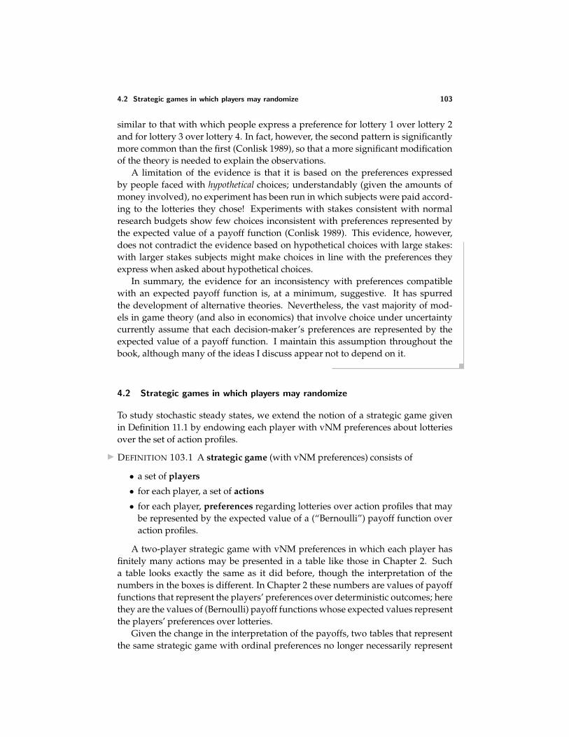
4.2 Strategic games in which players may randomize 103
similar to that with which people express a preference for lottery 1 over lottery 2and for lottery 3 over lottery 4. In fact, however, the second pattern is significantlymore common than the first (Conlisk 1989), so that a more significant modificationof the theory is needed to explain the observations.
A limitation of the evidence is that it is based on the preferences expressedby people faced with hypothetical choices; understandably (given the amounts ofmoney involved), no experiment has been run in which subjects were paid accord-ing to the lotteries they chose! Experiments with stakes consistent with normalresearch budgets show few choices inconsistent with preferences represented bythe expected value of a payoff function (Conlisk 1989). This evidence, however,does not contradict the evidence based on hypothetical choices with large stakes:with larger stakes subjects might make choices in line with the preferences theyexpress when asked about hypothetical choices.
In summary, the evidence for an inconsistency with preferences compatiblewith an expected payoff function is, at a minimum, suggestive. It has spurredthe development of alternative theories. Nevertheless, the vast majority of mod-els in game theory (and also in economics) that involve choice under uncertaintycurrently assume that each decision-maker’s preferences are represented by theexpected value of a payoff function. I maintain this assumption throughout thebook, although many of the ideas I discuss appear not to depend on it.
4.2 Strategic games in which players may randomize
To study stochastic steady states, we extend the notion of a strategic game givenin Definition 11.1 by endowing each player with vNM preferences about lotteriesover the set of action profiles.
DEFINITION 103.1 A strategic game (with vNM preferences) consists of
• a set of players
• for each player, a set of actions
• for each player, preferences regarding lotteries over action profiles that maybe represented by the expected value of a (“Bernoulli”) payoff function overaction profiles.
A two-player strategic game with vNM preferences in which each player hasfinitely many actions may be presented in a table like those in Chapter 2. Sucha table looks exactly the same as it did before, though the interpretation of thenumbers in the boxes is different. In Chapter 2 these numbers are values of payofffunctions that represent the players’ preferences over deterministic outcomes; herethey are the values of (Bernoulli) payoff functions whose expected values representthe players’ preferences over lotteries.
Given the change in the interpretation of the payoffs, two tables that representthe same strategic game with ordinal preferences no longer necessarily represent
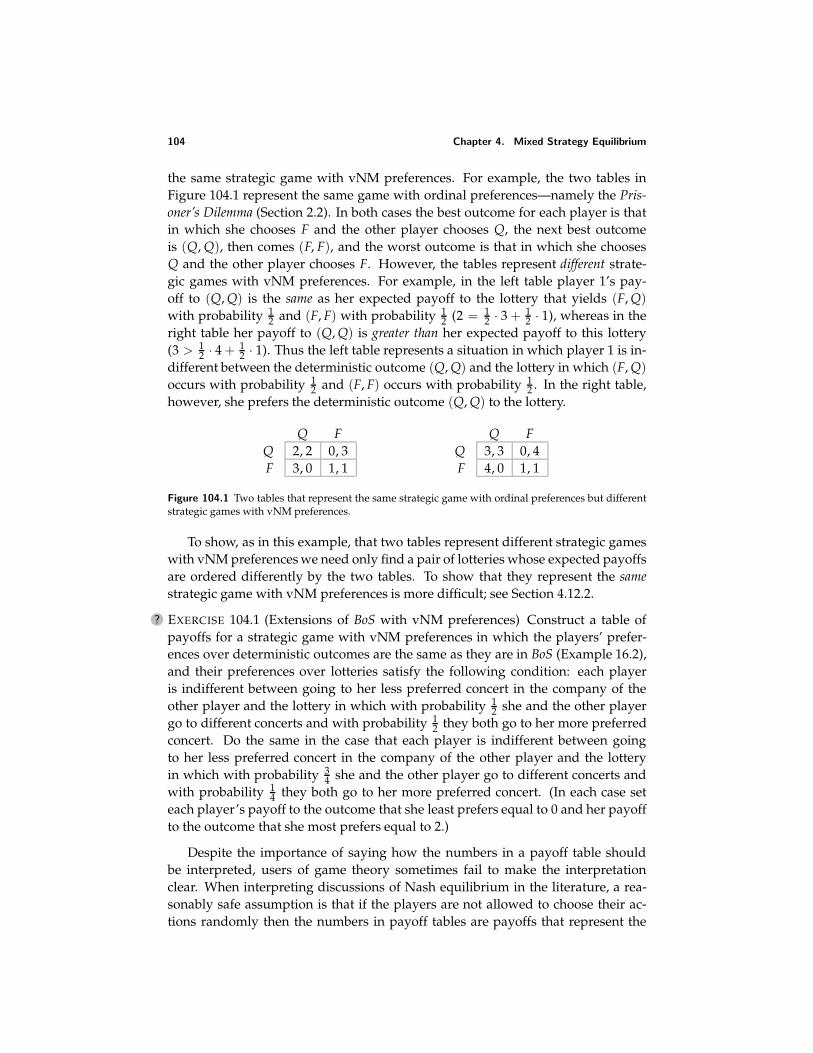
104 Chapter 4. Mixed Strategy Equilibrium
the same strategic game with vNM preferences. For example, the two tables inFigure 104.1 represent the same game with ordinal preferences—namely the Pris-oner’s Dilemma (Section 2.2). In both cases the best outcome for each player is thatin which she chooses F and the other player chooses Q, the next best outcomeis (Q, Q), then comes (F, F), and the worst outcome is that in which she choosesQ and the other player chooses F. However, the tables represent different strate-gic games with vNM preferences. For example, in the left table player 1’s pay-off to (Q, Q) is the same as her expected payoff to the lottery that yields (F, Q)with probability 1
2 and (F, F) with probability 12 (2 = 1
2 · 3 + 12 · 1), whereas in the
right table her payoff to (Q, Q) is greater than her expected payoff to this lottery(3 > 1
2 · 4 + 12 · 1). Thus the left table represents a situation in which player 1 is in-
different between the deterministic outcome (Q, Q) and the lottery in which (F, Q)occurs with probability 1
2 and (F, F) occurs with probability 12 . In the right table,
however, she prefers the deterministic outcome (Q, Q) to the lottery.
Q FQ 2, 2 0, 3F 3, 0 1, 1
Q FQ 3, 3 0, 4F 4, 0 1, 1
Figure 104.1 Two tables that represent the same strategic game with ordinal preferences but differentstrategic games with vNM preferences.
To show, as in this example, that two tables represent different strategic gameswith vNM preferences we need only find a pair of lotteries whose expected payoffsare ordered differently by the two tables. To show that they represent the samestrategic game with vNM preferences is more difficult; see Section 4.12.2.
? EXERCISE 104.1 (Extensions of BoS with vNM preferences) Construct a table ofpayoffs for a strategic game with vNM preferences in which the players’ prefer-ences over deterministic outcomes are the same as they are in BoS (Example 16.2),and their preferences over lotteries satisfy the following condition: each playeris indifferent between going to her less preferred concert in the company of theother player and the lottery in which with probability 1
2 she and the other playergo to different concerts and with probability 1
2 they both go to her more preferredconcert. Do the same in the case that each player is indifferent between goingto her less preferred concert in the company of the other player and the lotteryin which with probability 3
4 she and the other player go to different concerts andwith probability 1
4 they both go to her more preferred concert. (In each case seteach player’s payoff to the outcome that she least prefers equal to 0 and her payoffto the outcome that she most prefers equal to 2.)
Despite the importance of saying how the numbers in a payoff table shouldbe interpreted, users of game theory sometimes fail to make the interpretationclear. When interpreting discussions of Nash equilibrium in the literature, a rea-sonably safe assumption is that if the players are not allowed to choose their ac-tions randomly then the numbers in payoff tables are payoffs that represent the

4.3 Mixed strategy Nash equilibrium 105
players’ ordinal preferences, whereas if the players are allowed to randomize thenthe numbers are payoffs whose expected values represent the players’ preferencesregarding lotteries over outcomes.
4.3 Mixed strategy Nash equilibrium
4.3.1 Mixed strategies
In the generalization of the notion of Nash equilibrium that models a stochasticsteady state of a strategic game with vNM preferences, we allow each player tochoose a probability distribution over her set of actions rather than restricting herto choose a single deterministic action. We refer to such a probability distributionas a mixed strategy.
I usually use α to denote a profile of mixed strategies; αi(ai) is the probabilityassigned by player i’s mixed strategy αi to her action ai. To specify a mixed strategyof player i we need to give the probability it assigns to each of player i’s actions.For example, the strategy of player 1 in Matching Pennies that assigns probability 1
2to each action is the strategy α1 for which α1(Head) = 1
2 and α1(Tail) = 12 . Because
this way of describing a mixed strategy is cumbersome, I often use a shorthandfor a game that is presented in a table like those in Figure 104.1: I write a mixedstrategy as a list of probabilities, one for each action, in the order the actions are givenin the table. For example, the mixed strategy ( 1
3 , 23 ) for player 1 in either of the
games in Figure 104.1 assigns probability 13 to Q and probability 2
3 to F.A mixed strategy may assign probability 1 to a single action: by allowing a
player to choose probability distributions, we do not prohibit her from choos-ing deterministic actions. We refer to such a mixed strategy as a pure strategy.Player i’s choosing the pure strategy that assigns probability 1 to the action ai isequivalent to her simply choosing the action ai, and I denote this strategy simplyby ai.
4.3.2 Equilibrium
The notion of equilibrium that we study is called “mixed strategy Nash equilib-rium”. The idea behind it is the same as the idea behind the notion of Nash equi-librium for a game with ordinal preferences: a mixed strategy Nash equilibrium isa mixed strategy profile α∗ with the property that no player i has a mixed strategyαi such that she prefers the lottery over outcomes generated by the strategy pro-file (αi, α∗
−i) to the lottery over outcomes generated by the strategy profile α∗. Thefollowing definition gives this condition using payoff functions whose expectedvalues represent the players’ preferences.
DEFINITION 105.1 (Mixed strategy Nash equilibrium of strategic game with vNM pref-erences) The mixed strategy profile α∗ in a strategic game with vNM preferences isa (mixed strategy) Nash equilibrium if, for each player i and every mixed strategyαi of player i, the expected payoff to player i of α∗ is at least as large as the expected
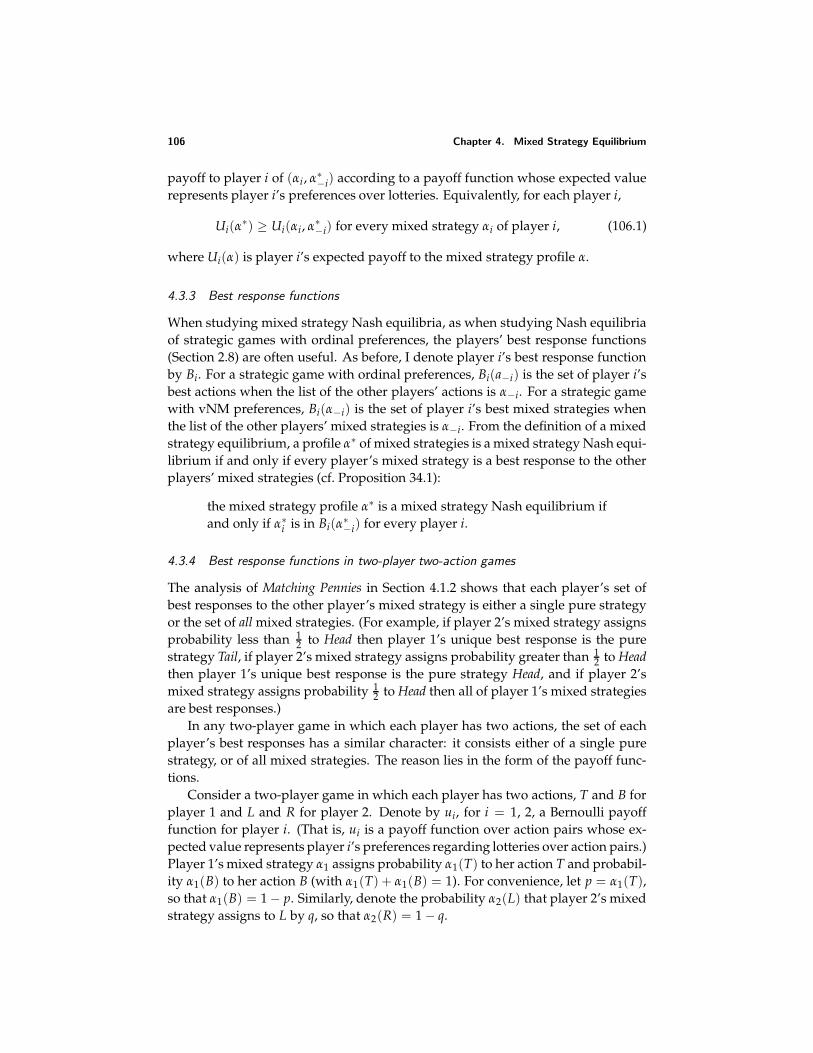
106 Chapter 4. Mixed Strategy Equilibrium
payoff to player i of (αi , α∗−i) according to a payoff function whose expected value
represents player i’s preferences over lotteries. Equivalently, for each player i,
Ui(α∗) ≥ Ui(αi, α∗−i) for every mixed strategy αi of player i, (106.1)
where Ui(α) is player i’s expected payoff to the mixed strategy profile α.
4.3.3 Best response functions
When studying mixed strategy Nash equilibria, as when studying Nash equilibriaof strategic games with ordinal preferences, the players’ best response functions(Section 2.8) are often useful. As before, I denote player i’s best response functionby Bi. For a strategic game with ordinal preferences, Bi(a−i) is the set of player i’sbest actions when the list of the other players’ actions is α−i. For a strategic gamewith vNM preferences, Bi(α−i) is the set of player i’s best mixed strategies whenthe list of the other players’ mixed strategies is α−i. From the definition of a mixedstrategy equilibrium, a profile α∗ of mixed strategies is a mixed strategy Nash equi-librium if and only if every player’s mixed strategy is a best response to the otherplayers’ mixed strategies (cf. Proposition 34.1):
the mixed strategy profile α∗ is a mixed strategy Nash equilibrium ifand only if α∗
i is in Bi(α∗−i) for every player i.
4.3.4 Best response functions in two-player two-action games
The analysis of Matching Pennies in Section 4.1.2 shows that each player’s set ofbest responses to the other player’s mixed strategy is either a single pure strategyor the set of all mixed strategies. (For example, if player 2’s mixed strategy assignsprobability less than 1
2 to Head then player 1’s unique best response is the purestrategy Tail, if player 2’s mixed strategy assigns probability greater than 1
2 to Headthen player 1’s unique best response is the pure strategy Head, and if player 2’smixed strategy assigns probability 1
2 to Head then all of player 1’s mixed strategiesare best responses.)
In any two-player game in which each player has two actions, the set of eachplayer’s best responses has a similar character: it consists either of a single purestrategy, or of all mixed strategies. The reason lies in the form of the payoff func-tions.
Consider a two-player game in which each player has two actions, T and B forplayer 1 and L and R for player 2. Denote by ui, for i = 1, 2, a Bernoulli payofffunction for player i. (That is, ui is a payoff function over action pairs whose ex-pected value represents player i’s preferences regarding lotteries over action pairs.)Player 1’s mixed strategy α1 assigns probability α1(T) to her action T and probabil-ity α1(B) to her action B (with α1(T) + α1(B) = 1). For convenience, let p = α1(T),so that α1(B) = 1 − p. Similarly, denote the probability α2(L) that player 2’s mixedstrategy assigns to L by q, so that α2(R) = 1 − q.
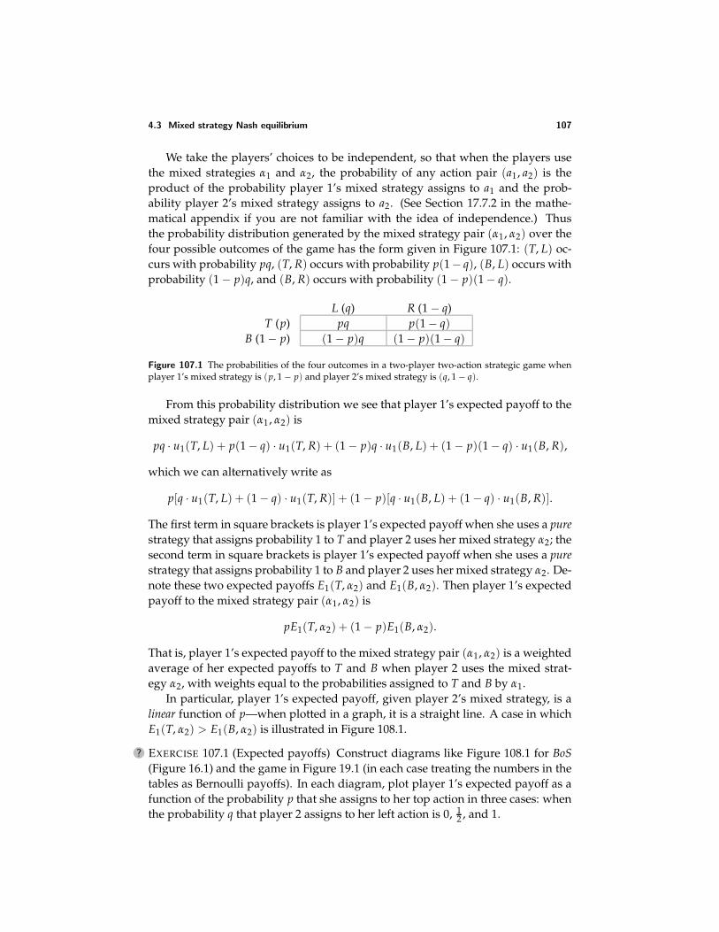
4.3 Mixed strategy Nash equilibrium 107
We take the players’ choices to be independent, so that when the players usethe mixed strategies α1 and α2, the probability of any action pair (a1, a2) is theproduct of the probability player 1’s mixed strategy assigns to a1 and the prob-ability player 2’s mixed strategy assigns to a2. (See Section 17.7.2 in the mathe-matical appendix if you are not familiar with the idea of independence.) Thusthe probability distribution generated by the mixed strategy pair (α1, α2) over thefour possible outcomes of the game has the form given in Figure 107.1: (T, L) oc-curs with probability pq, (T, R) occurs with probability p(1− q), (B, L) occurs withprobability (1 − p)q, and (B, R) occurs with probability (1 − p)(1 − q).
L (q) R (1 − q)T (p) pq p(1 − q)
B (1 − p) (1 − p)q (1 − p)(1 − q)
Figure 107.1 The probabilities of the four outcomes in a two-player two-action strategic game whenplayer 1’s mixed strategy is (p, 1 − p) and player 2’s mixed strategy is (q, 1 − q).
From this probability distribution we see that player 1’s expected payoff to themixed strategy pair (α1, α2) is
pq · u1(T, L) + p(1 − q) · u1(T, R) + (1 − p)q · u1(B, L) + (1 − p)(1 − q) · u1(B, R),
which we can alternatively write as
p[q · u1(T, L) + (1 − q) · u1(T, R)] + (1 − p)[q · u1(B, L) + (1 − q) · u1(B, R)].
The first term in square brackets is player 1’s expected payoff when she uses a purestrategy that assigns probability 1 to T and player 2 uses her mixed strategy α2; thesecond term in square brackets is player 1’s expected payoff when she uses a purestrategy that assigns probability 1 to B and player 2 uses her mixed strategy α2. De-note these two expected payoffs E1(T, α2) and E1(B, α2). Then player 1’s expectedpayoff to the mixed strategy pair (α1, α2) is
pE1(T, α2) + (1 − p)E1(B, α2).
That is, player 1’s expected payoff to the mixed strategy pair (α1, α2) is a weightedaverage of her expected payoffs to T and B when player 2 uses the mixed strat-egy α2, with weights equal to the probabilities assigned to T and B by α1.
In particular, player 1’s expected payoff, given player 2’s mixed strategy, is alinear function of p—when plotted in a graph, it is a straight line. A case in whichE1(T, α2) > E1(B, α2) is illustrated in Figure 108.1.
? EXERCISE 107.1 (Expected payoffs) Construct diagrams like Figure 108.1 for BoS(Figure 16.1) and the game in Figure 19.1 (in each case treating the numbers in thetables as Bernoulli payoffs). In each diagram, plot player 1’s expected payoff as afunction of the probability p that she assigns to her top action in three cases: whenthe probability q that player 2 assigns to her left action is 0, 1
2 , and 1.
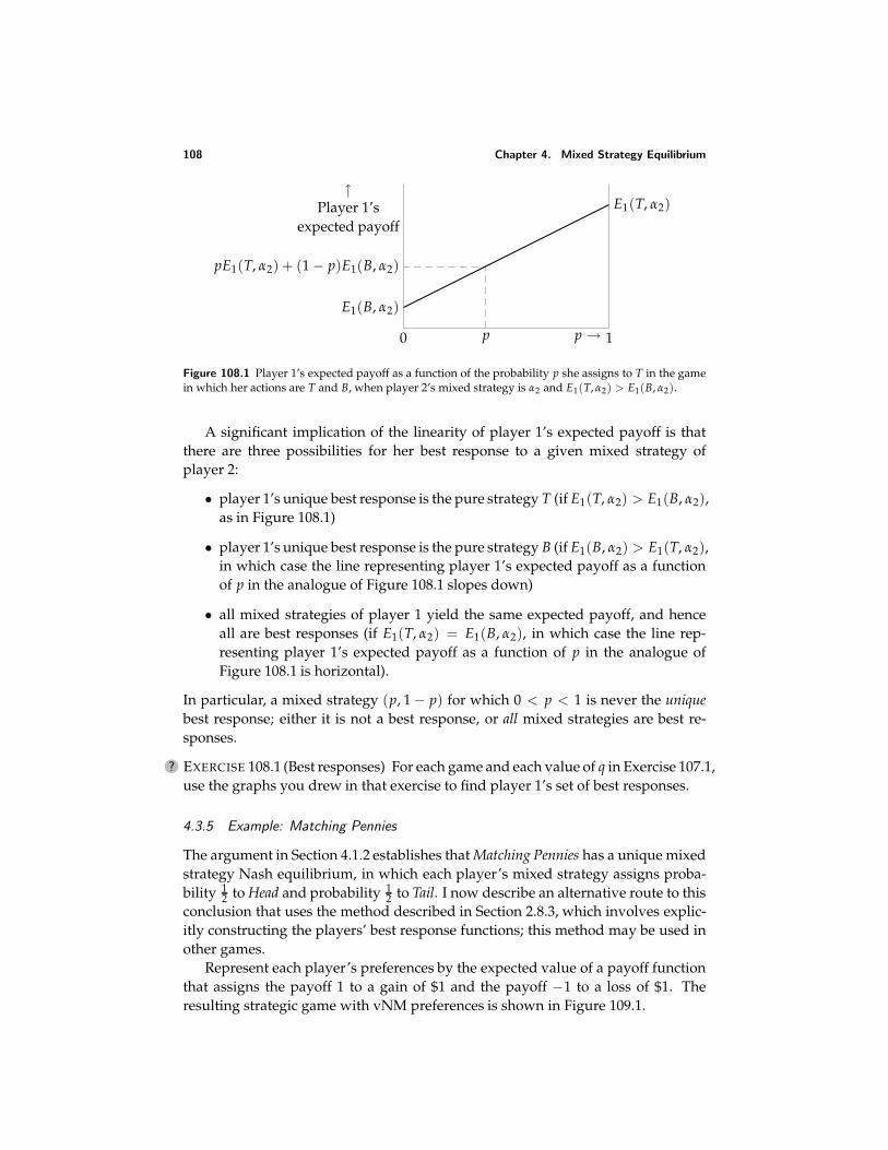
108 Chapter 4. Mixed Strategy Equilibrium
↑Player 1’s
expected payoff
E1(B, α2)
E1(T, α2)
0 1p →
pE1(T, α2) + (1 − p)E1(B, α2)
p
Figure 108.1 Player 1’s expected payoff as a function of the probability p she assigns to T in the gamein which her actions are T and B, when player 2’s mixed strategy is α2 and E1(T, α2) > E1(B, α2).
A significant implication of the linearity of player 1’s expected payoff is thatthere are three possibilities for her best response to a given mixed strategy ofplayer 2:
• player 1’s unique best response is the pure strategy T (if E1(T, α2) > E1(B, α2),as in Figure 108.1)
• player 1’s unique best response is the pure strategy B (if E1(B, α2) > E1(T, α2),in which case the line representing player 1’s expected payoff as a functionof p in the analogue of Figure 108.1 slopes down)
• all mixed strategies of player 1 yield the same expected payoff, and henceall are best responses (if E1(T, α2) = E1(B, α2), in which case the line rep-resenting player 1’s expected payoff as a function of p in the analogue ofFigure 108.1 is horizontal).
In particular, a mixed strategy (p, 1 − p) for which 0 < p < 1 is never the uniquebest response; either it is not a best response, or all mixed strategies are best re-sponses.
? EXERCISE 108.1 (Best responses) For each game and each value of q in Exercise 107.1,use the graphs you drew in that exercise to find player 1’s set of best responses.
4.3.5 Example: Matching Pennies
The argument in Section 4.1.2 establishes that Matching Pennies has a unique mixedstrategy Nash equilibrium, in which each player’s mixed strategy assigns proba-bility 1
2 to Head and probability 12 to Tail. I now describe an alternative route to this
conclusion that uses the method described in Section 2.8.3, which involves explic-itly constructing the players’ best response functions; this method may be used inother games.
Represent each player’s preferences by the expected value of a payoff functionthat assigns the payoff 1 to a gain of $1 and the payoff −1 to a loss of $1. Theresulting strategic game with vNM preferences is shown in Figure 109.1.
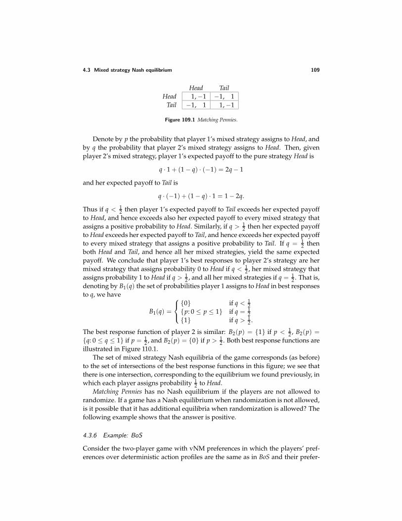
4.3 Mixed strategy Nash equilibrium 109
Head TailHead 1, −1 −1, 1
Tail −1, 1 1, −1
Figure 109.1 Matching Pennies.
Denote by p the probability that player 1’s mixed strategy assigns to Head, andby q the probability that player 2’s mixed strategy assigns to Head. Then, givenplayer 2’s mixed strategy, player 1’s expected payoff to the pure strategy Head is
q · 1 + (1 − q) · (−1) = 2q − 1
and her expected payoff to Tail is
q · (−1) + (1 − q) · 1 = 1 − 2q.
Thus if q < 12 then player 1’s expected payoff to Tail exceeds her expected payoff
to Head, and hence exceeds also her expected payoff to every mixed strategy thatassigns a positive probability to Head. Similarly, if q > 1
2 then her expected payoffto Head exceeds her expected payoff to Tail, and hence exceeds her expected payoffto every mixed strategy that assigns a positive probability to Tail. If q = 1
2 thenboth Head and Tail, and hence all her mixed strategies, yield the same expectedpayoff. We conclude that player 1’s best responses to player 2’s strategy are hermixed strategy that assigns probability 0 to Head if q < 1
2 , her mixed strategy thatassigns probability 1 to Head if q > 1
2 , and all her mixed strategies if q = 12 . That is,
denoting by B1(q) the set of probabilities player 1 assigns to Head in best responsesto q, we have
B1(q) =
0 if q < 12
p: 0 ≤ p ≤ 1 if q = 12
1 if q > 12 .
The best response function of player 2 is similar: B2(p) = 1 if p < 12 , B2(p) =
q: 0 ≤ q ≤ 1 if p = 12 , and B2(p) = 0 if p > 1
2 . Both best response functions areillustrated in Figure 110.1.
The set of mixed strategy Nash equilibria of the game corresponds (as before)to the set of intersections of the best response functions in this figure; we see thatthere is one intersection, corresponding to the equilibrium we found previously, inwhich each player assigns probability 1
2 to Head.Matching Pennies has no Nash equilibrium if the players are not allowed to
randomize. If a game has a Nash equilibrium when randomization is not allowed,is it possible that it has additional equilibria when randomization is allowed? Thefollowing example shows that the answer is positive.
4.3.6 Example: BoS
Consider the two-player game with vNM preferences in which the players’ pref-erences over deterministic action profiles are the same as in BoS and their prefer-
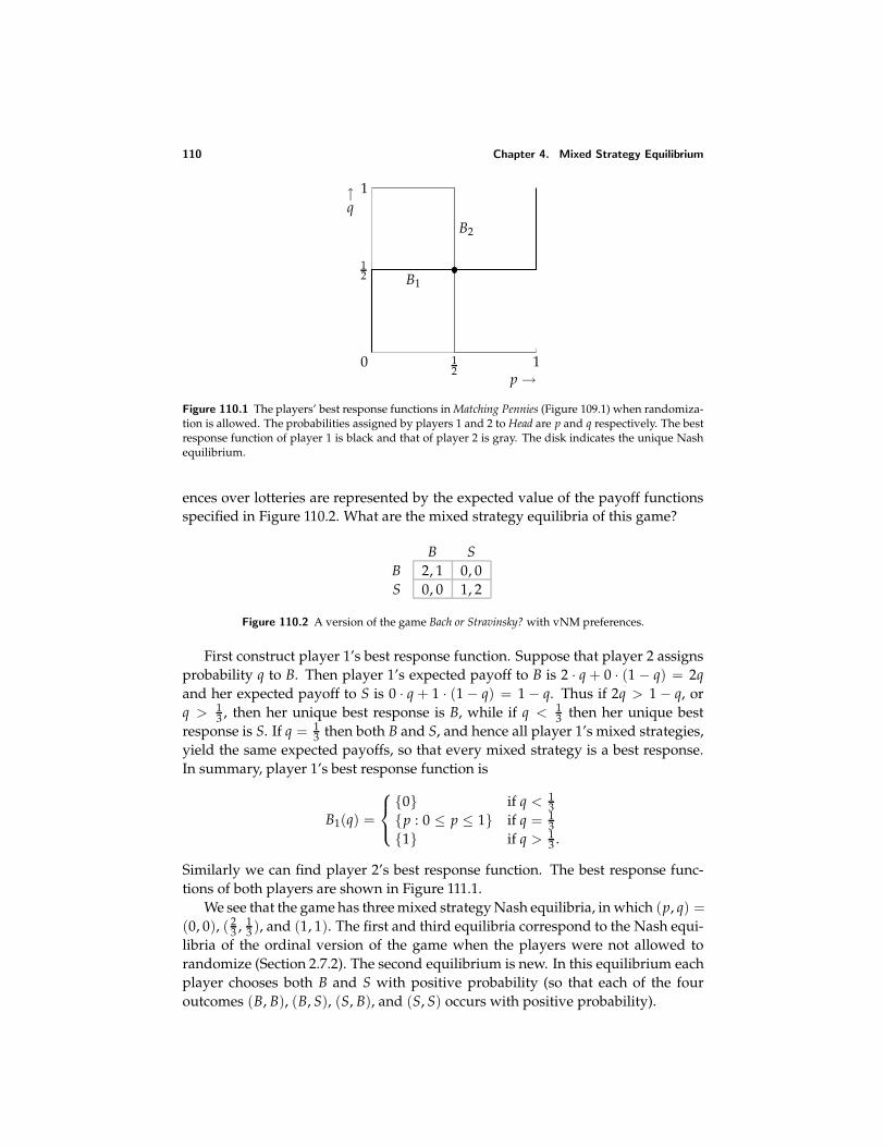
110 Chapter 4. Mixed Strategy Equilibrium
0 12
1p →
12
1↑q
B1
B2
Figure 110.1 The players’ best response functions in Matching Pennies (Figure 109.1) when randomiza-tion is allowed. The probabilities assigned by players 1 and 2 to Head are p and q respectively. The bestresponse function of player 1 is black and that of player 2 is gray. The disk indicates the unique Nashequilibrium.
ences over lotteries are represented by the expected value of the payoff functionsspecified in Figure 110.2. What are the mixed strategy equilibria of this game?
B SB 2, 1 0, 0S 0, 0 1, 2
Figure 110.2 A version of the game Bach or Stravinsky? with vNM preferences.
First construct player 1’s best response function. Suppose that player 2 assignsprobability q to B. Then player 1’s expected payoff to B is 2 · q + 0 · (1 − q) = 2qand her expected payoff to S is 0 · q + 1 · (1 − q) = 1 − q. Thus if 2q > 1 − q, orq > 1
3 , then her unique best response is B, while if q < 13 then her unique best
response is S. If q = 13 then both B and S, and hence all player 1’s mixed strategies,
yield the same expected payoffs, so that every mixed strategy is a best response.In summary, player 1’s best response function is
B1(q) =
0 if q < 13
p : 0 ≤ p ≤ 1 if q = 13
1 if q > 13 .
Similarly we can find player 2’s best response function. The best response func-tions of both players are shown in Figure 111.1.
We see that the game has three mixed strategy Nash equilibria, in which (p, q) =(0, 0), ( 2
3 , 13 ), and (1, 1). The first and third equilibria correspond to the Nash equi-
libria of the ordinal version of the game when the players were not allowed torandomize (Section 2.7.2). The second equilibrium is new. In this equilibrium eachplayer chooses both B and S with positive probability (so that each of the fouroutcomes (B, B), (B, S), (S, B), and (S, S) occurs with positive probability).
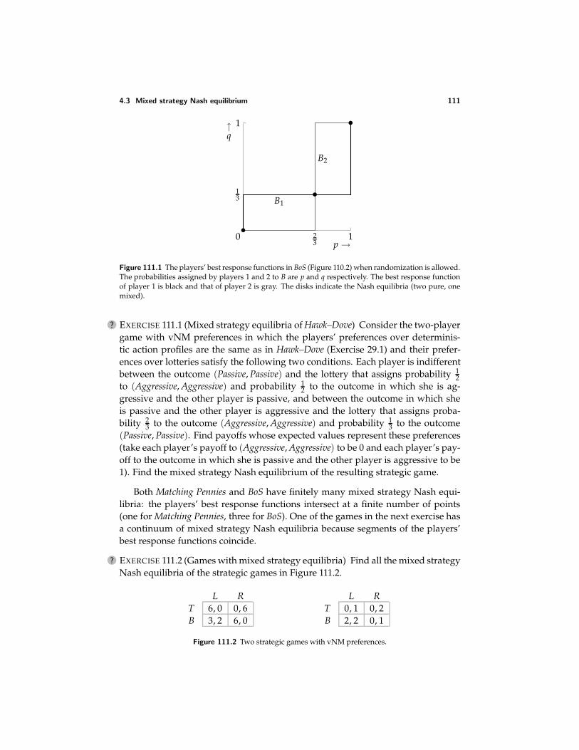
4.3 Mixed strategy Nash equilibrium 111
0 23
1p →
13
1↑q
B1
B2
Figure 111.1 The players’ best response functions in BoS (Figure 110.2) when randomization is allowed.The probabilities assigned by players 1 and 2 to B are p and q respectively. The best response functionof player 1 is black and that of player 2 is gray. The disks indicate the Nash equilibria (two pure, onemixed).
? EXERCISE 111.1 (Mixed strategy equilibria of Hawk–Dove) Consider the two-playergame with vNM preferences in which the players’ preferences over determinis-tic action profiles are the same as in Hawk–Dove (Exercise 29.1) and their prefer-ences over lotteries satisfy the following two conditions. Each player is indifferentbetween the outcome (Passive, Passive) and the lottery that assigns probability 1
2to (Aggressive, Aggressive) and probability 1
2 to the outcome in which she is ag-gressive and the other player is passive, and between the outcome in which sheis passive and the other player is aggressive and the lottery that assigns proba-bility 2
3 to the outcome (Aggressive, Aggressive) and probability 13 to the outcome
(Passive, Passive). Find payoffs whose expected values represent these preferences(take each player’s payoff to (Aggressive, Aggressive) to be 0 and each player’s pay-off to the outcome in which she is passive and the other player is aggressive to be1). Find the mixed strategy Nash equilibrium of the resulting strategic game.
Both Matching Pennies and BoS have finitely many mixed strategy Nash equi-libria: the players’ best response functions intersect at a finite number of points(one for Matching Pennies, three for BoS). One of the games in the next exercise hasa continuum of mixed strategy Nash equilibria because segments of the players’best response functions coincide.
? EXERCISE 111.2 (Games with mixed strategy equilibria) Find all the mixed strategyNash equilibria of the strategic games in Figure 111.2.
L RT 6, 0 0, 6B 3, 2 6, 0
L RT 0, 1 0, 2B 2, 2 0, 1
Figure 111.2 Two strategic games with vNM preferences.
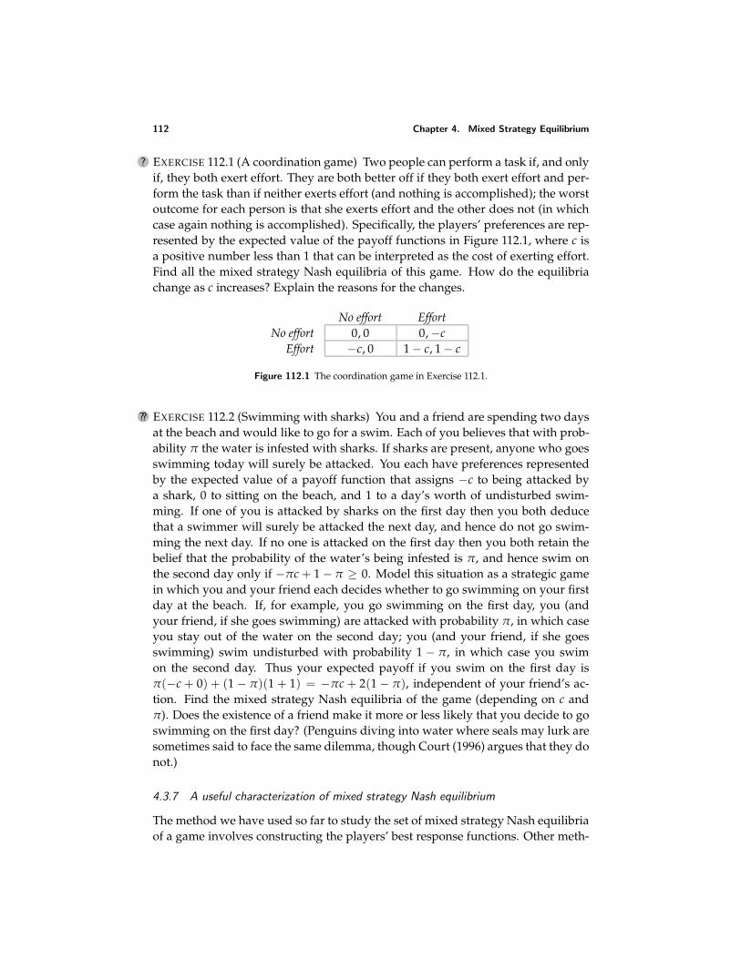
112 Chapter 4. Mixed Strategy Equilibrium
? EXERCISE 112.1 (A coordination game) Two people can perform a task if, and onlyif, they both exert effort. They are both better off if they both exert effort and per-form the task than if neither exerts effort (and nothing is accomplished); the worstoutcome for each person is that she exerts effort and the other does not (in whichcase again nothing is accomplished). Specifically, the players’ preferences are rep-resented by the expected value of the payoff functions in Figure 112.1, where c isa positive number less than 1 that can be interpreted as the cost of exerting effort.Find all the mixed strategy Nash equilibria of this game. How do the equilibriachange as c increases? Explain the reasons for the changes.
No effort EffortNo effort 0, 0 0, −c
Effort −c, 0 1 − c, 1 − c
Figure 112.1 The coordination game in Exercise 112.1.
?? EXERCISE 112.2 (Swimming with sharks) You and a friend are spending two daysat the beach and would like to go for a swim. Each of you believes that with prob-ability π the water is infested with sharks. If sharks are present, anyone who goesswimming today will surely be attacked. You each have preferences representedby the expected value of a payoff function that assigns −c to being attacked bya shark, 0 to sitting on the beach, and 1 to a day’s worth of undisturbed swim-ming. If one of you is attacked by sharks on the first day then you both deducethat a swimmer will surely be attacked the next day, and hence do not go swim-ming the next day. If no one is attacked on the first day then you both retain thebelief that the probability of the water’s being infested is π, and hence swim onthe second day only if −πc + 1 − π ≥ 0. Model this situation as a strategic gamein which you and your friend each decides whether to go swimming on your firstday at the beach. If, for example, you go swimming on the first day, you (andyour friend, if she goes swimming) are attacked with probability π, in which caseyou stay out of the water on the second day; you (and your friend, if she goesswimming) swim undisturbed with probability 1 − π, in which case you swimon the second day. Thus your expected payoff if you swim on the first day isπ(−c + 0) + (1 − π)(1 + 1) = −πc + 2(1 − π), independent of your friend’s ac-tion. Find the mixed strategy Nash equilibria of the game (depending on c andπ). Does the existence of a friend make it more or less likely that you decide to goswimming on the first day? (Penguins diving into water where seals may lurk aresometimes said to face the same dilemma, though Court (1996) argues that they donot.)
4.3.7 A useful characterization of mixed strategy Nash equilibrium
The method we have used so far to study the set of mixed strategy Nash equilibriaof a game involves constructing the players’ best response functions. Other meth-
4.3 Mixed strategy Nash equilibrium 113
ods are sometimes useful. I now present a characterization of mixed strategy Nashequilibrium that gives us an easy way to check whether a mixed strategy profileis an equilibrium, and is the basis of a procedure (described in Section 4.10) forfinding all equilibria of a game.
The key point is an observation made in Section 4.3.4 for two-player two-actiongames: a player’s expected payoff to a mixed strategy profile is a weighted averageof her expected payoffs to her pure strategies, where the weight attached to eachpure strategy is the probability assigned to that strategy by the player’s mixedstrategy. This property holds for any game (with any number of players) in whicheach player has finitely many actions. We can state it more precisely as follows.
A player’s expected payoff to the mixed strategy profile α is aweighted average of her expected payoffs to all mixed strategy pro-files of the type (ai , α−i), where the weight attached to (ai , α−i) is theprobability αi(ai) assigned to ai by player i’s mixed strategy αi.
(113.1)
Symbolically we have
Ui(α) = ∑ai∈Ai
αi(ai)Ui(ai , α−i),
where Ai is player i’s set of actions (pure strategies) and Ui(ai , α−i) is her expectedpayoff when she uses the pure strategy that assigns probability 1 to ai and ev-ery other player j uses her mixed strategy αj. (See the end of Section 17.3 in theappendix on mathematics for an explanation of the ∑ notation.)
This property leads to a useful characterization of mixed strategy Nash equi-librium. Let α∗ be a mixed strategy Nash equilibrium and denote by E∗
i player i’sexpected payoff in the equilibrium (i.e. E∗
i = Ui(α∗)). Because α∗ is an equilibrium,player i’s expected payoff, given α∗
−i, to each of her pure strategies is at most E∗i .
Now, by (113.1), E∗i is a weighted average of player i’s expected payoffs to the pure
strategies to which α∗i assigns positive probability. Thus player i’s expected payoffs
to these pure strategies are all equal to E∗i . (If any were smaller then the weighted
average would be smaller.) We conclude that the expected payoff to each action towhich α∗
i assigns positive probability is E∗i and the expected payoff to every other
action is at most E∗i . Conversely, if these conditions are satisfied for every player i
then α∗ is a mixed strategy Nash equilibrium: the expected payoff to α∗i is E∗
i , andthe expected payoff to any other mixed strategy is at most E∗
i , because by (113.1) itis a weighted average of E∗
i and numbers that are at most E∗i .
This argument establishes the following result.
PROPOSITION 113.2 (Characterization of mixed strategy Nash equilibrium of finitegame) A mixed strategy profile α∗ in a strategic game with vNM preferences in whicheach player has finitely many actions is a mixed strategy Nash equilibrium if and only if,for each player i,
• the expected payoff, given α∗−i, to every action to which α∗
i assigns positive probabilityis the same
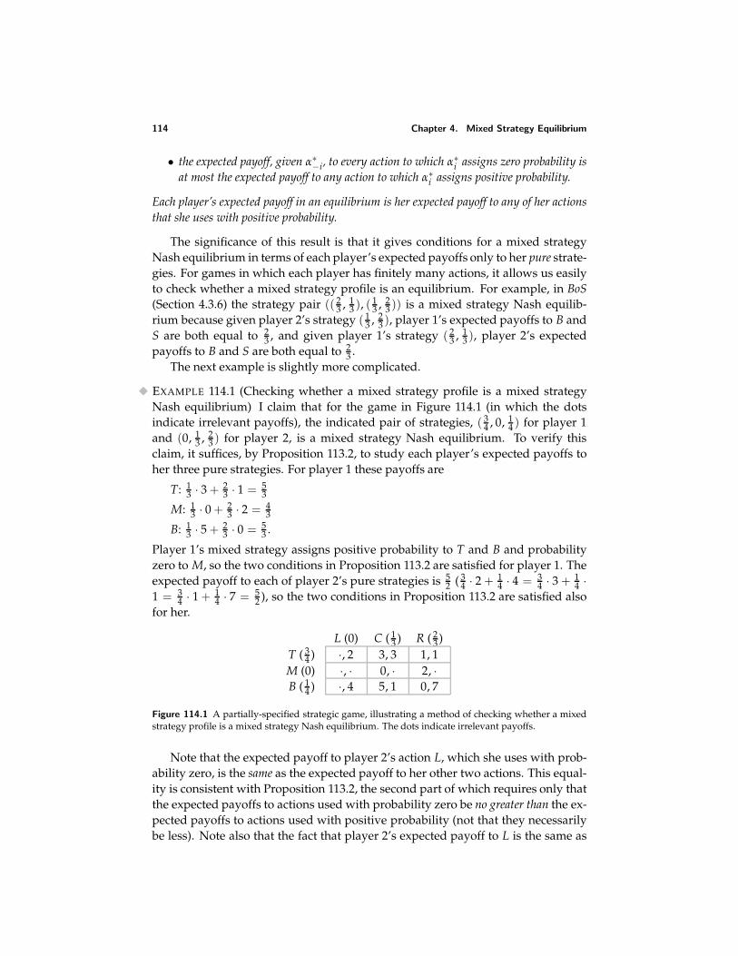
114 Chapter 4. Mixed Strategy Equilibrium
• the expected payoff, given α∗−i, to every action to which α∗
i assigns zero probability isat most the expected payoff to any action to which α∗
i assigns positive probability.
Each player’s expected payoff in an equilibrium is her expected payoff to any of her actionsthat she uses with positive probability.
The significance of this result is that it gives conditions for a mixed strategyNash equilibrium in terms of each player’s expected payoffs only to her pure strate-gies. For games in which each player has finitely many actions, it allows us easilyto check whether a mixed strategy profile is an equilibrium. For example, in BoS(Section 4.3.6) the strategy pair (( 2
3 , 13 ), ( 1
3 , 23 )) is a mixed strategy Nash equilib-
rium because given player 2’s strategy ( 13 , 2
3 ), player 1’s expected payoffs to B andS are both equal to 2
3 , and given player 1’s strategy ( 23 , 1
3 ), player 2’s expectedpayoffs to B and S are both equal to 2
3 .The next example is slightly more complicated.
EXAMPLE 114.1 (Checking whether a mixed strategy profile is a mixed strategyNash equilibrium) I claim that for the game in Figure 114.1 (in which the dotsindicate irrelevant payoffs), the indicated pair of strategies, ( 3
4 , 0, 14 ) for player 1
and (0, 13 , 2
3 ) for player 2, is a mixed strategy Nash equilibrium. To verify thisclaim, it suffices, by Proposition 113.2, to study each player’s expected payoffs toher three pure strategies. For player 1 these payoffs are
T: 13 · 3 + 2
3 · 1 = 53
M: 13 · 0 + 2
3 · 2 = 43
B: 13 · 5 + 2
3 · 0 = 53 .
Player 1’s mixed strategy assigns positive probability to T and B and probabilityzero to M, so the two conditions in Proposition 113.2 are satisfied for player 1. Theexpected payoff to each of player 2’s pure strategies is 5
2 ( 34 · 2 + 1
4 · 4 = 34 · 3 + 1
4 ·1 = 3
4 · 1 + 14 · 7 = 5
2 ), so the two conditions in Proposition 113.2 are satisfied alsofor her.
L (0) C ( 13 ) R ( 2
3 )T ( 3
4 ) ·, 2 3, 3 1, 1M (0) ·, · 0, · 2, ·B ( 1
4 ) ·, 4 5, 1 0, 7
Figure 114.1 A partially-specified strategic game, illustrating a method of checking whether a mixedstrategy profile is a mixed strategy Nash equilibrium. The dots indicate irrelevant payoffs.
Note that the expected payoff to player 2’s action L, which she uses with prob-ability zero, is the same as the expected payoff to her other two actions. This equal-ity is consistent with Proposition 113.2, the second part of which requires only thatthe expected payoffs to actions used with probability zero be no greater than the ex-pected payoffs to actions used with positive probability (not that they necessarilybe less). Note also that the fact that player 2’s expected payoff to L is the same as
4.3 Mixed strategy Nash equilibrium 115
her expected payoffs to C and R does not imply that the game has a mixed strategyNash equilibrium in which player 2 uses L with positive probability—it may, or itmay not, depending on the unspecified payoffs.
? EXERCISE 115.1 (Choosing numbers) Players 1 and 2 each choose a positive integerup to K. If the players choose the same number then player 2 pays $1 to player 1;otherwise no payment is made. Each player’s preferences are represented by herexpected monetary payoff.
a. Show that the game has a mixed strategy Nash equilibrium in which eachplayer chooses each positive integer up to K with probability 1/K.
b. (More difficult.) Show that the game has no other mixed strategy Nash equi-libria. (Deduce from the fact that player 1 assigns positive probability tosome action k that player 2 must do so; then look at the implied restrictionon player 1’s equilibrium strategy.)
? EXERCISE 115.2 (Silverman’s game) Each of two players chooses a positive inte-ger. If player i’s integer is greater than player j’s integer and less than three timesthis integer then player j pays $1 to player i. If player i’s integer is at least threetimes player j’s integer then player i pays $1 to player j. If the integers are equal,no payment is made. Each player’s preferences are represented by her expectedmonetary payoff. Show that the game has no Nash equilibrium in pure strategies,and that the pair of mixed strategies in which each player chooses 1, 2, and 5 eachwith probability 1
3 is a mixed strategy Nash equilibrium. (In fact, this pair of mixedstrategies is the unique mixed strategy Nash equilibrium.)
?? EXERCISE 115.3 (Voter participation) Consider the game of voter participation inExercise 32.2. Assume that k ≤ m and that each player’s preferences are repre-sented by the expectation of her payoffs given in Exercise 32.2. Show that thereis a value of p between 0 and 1 such that the game has a mixed strategy Nashequilibrium in which every supporter of candidate A votes with probability p, ksupporters of candidate B vote with certainty, and the remaining m − k supportersof candidate B abstain. How do the probability p that a supporter of candidate Avotes and the expected number of voters (“turnout”) depend upon c? (Note that ifevery supporter of candidate A votes with probability p then the probability thatexactly k − 1 of them vote is kpk−1(1 − p).)
?? EXERCISE 115.4 (Defending territory) General A is defending territory accessibleby two mountain passes against an attack by general B. General A has three di-visions at her disposal, and general B has two divisions. Each general allocatesher divisions between the two passes. General A wins the battle at a pass if andonly if she assigns at least as many divisions to the pass as does general B; shesuccessfully defends her territory if and only if she wins the battle at both passes.Formulate this situation as a strategic game and find all its mixed strategy equilib-ria. (First argue that in every equilibrium B assigns probability zero to the action
116 Chapter 4. Mixed Strategy Equilibrium
of allocating one division to each pass. Then argue that in any equilibrium sheassigns probability 1
2 to each of her other actions. Finally, find A’s equilibriumstrategies.) In an equilibrium do the generals concentrate all their forces at onepass, or spread them out?
An implication of Proposition 113.2 is that a nondegenerate mixed strategyequilibrium (a mixed strategy equilibrium that is not also a pure strategy equi-librium) is never a strict Nash equilibrium: every player whose mixed strategyassigns positive probability to more than one action is indifferent between herequilibrium mixed strategy and every action to which this mixed strategy assignspositive probability.
Any equilibrium that is not strict, whether in mixed strategies or not, has lessappeal than a strict equilibrium because some (or all) of the players lack a positiveincentive to choose their equilibrium strategies, given the other players’ behavior.There is no reason for them not to choose their equilibrium strategies, but at thesame time there is no reason for them not to choose another strategy that is equallygood. Many pure strategy equilibria—especially in complex games—are also notstrict, but among mixed strategy equilibria the problem is pervasive.
Given that in a mixed strategy equilibrium no player has a positive incentive tochoose her equilibrium strategy, what determines how she randomizes in equilib-rium? From the examples above we see that a player’s equilibrium mixed strategyin a two-player game keeps the other player indifferent between a set of her actions,so that she is willing to randomize. In the mixed strategy equilibrium of BoS, forexample, player 1 chooses B with probability 2
3 so that player 2 is indifferent be-tween B and S, and hence is willing to choose each with positive probability. Note,however, that the theory is not that the players consciously choose their strategieswith this goal in mind! Rather, the conditions for equilibrium are designed to en-sure that it is consistent with a steady state. In BoS, for example, if player 1 choosesB with probability 2
3 and player 2 chooses B with probability 13 then neither player
has any reason to change her action. We have not yet studied how a steady statemight come about, but have rather simply looked for strategy profiles consistentwith steady states. In Section 4.9 I briefly discuss some theories of how a steadystate might be reached.
4.3.8 Existence of equilibrium in finite games
Every game we have examined has at least one mixed strategy Nash equilibrium.In fact, every game in which each player has finitely many actions has at least onesuch equilibrium.
PROPOSITION 116.1 (Existence of mixed strategy Nash equilibrium in finite games)Every strategic game with vNM preferences in which each player has finitely many actionshas a mixed strategy Nash equilibrium.
This result is of no help in finding equilibria. But it is a useful fact to know: yourquest for an equilibrium of a game in which each player has finitely many actions
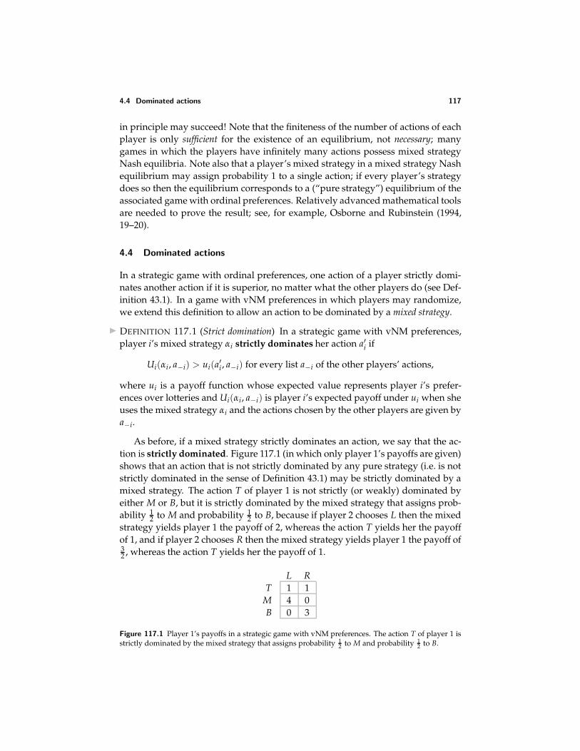
4.4 Dominated actions 117
in principle may succeed! Note that the finiteness of the number of actions of eachplayer is only sufficient for the existence of an equilibrium, not necessary; manygames in which the players have infinitely many actions possess mixed strategyNash equilibria. Note also that a player’s mixed strategy in a mixed strategy Nashequilibrium may assign probability 1 to a single action; if every player’s strategydoes so then the equilibrium corresponds to a (“pure strategy”) equilibrium of theassociated game with ordinal preferences. Relatively advanced mathematical toolsare needed to prove the result; see, for example, Osborne and Rubinstein (1994,19–20).
4.4 Dominated actions
In a strategic game with ordinal preferences, one action of a player strictly domi-nates another action if it is superior, no matter what the other players do (see Def-inition 43.1). In a game with vNM preferences in which players may randomize,we extend this definition to allow an action to be dominated by a mixed strategy.
DEFINITION 117.1 (Strict domination) In a strategic game with vNM preferences,player i’s mixed strategy αi strictly dominates her action a′i if
Ui(αi, a−i) > ui(a′i , a−i) for every list a−i of the other players’ actions,
where ui is a payoff function whose expected value represents player i’s prefer-ences over lotteries and Ui(αi, a−i) is player i’s expected payoff under ui when sheuses the mixed strategy αi and the actions chosen by the other players are given bya−i.
As before, if a mixed strategy strictly dominates an action, we say that the ac-tion is strictly dominated. Figure 117.1 (in which only player 1’s payoffs are given)shows that an action that is not strictly dominated by any pure strategy (i.e. is notstrictly dominated in the sense of Definition 43.1) may be strictly dominated by amixed strategy. The action T of player 1 is not strictly (or weakly) dominated byeither M or B, but it is strictly dominated by the mixed strategy that assigns prob-ability 1
2 to M and probability 12 to B, because if player 2 chooses L then the mixed
strategy yields player 1 the payoff of 2, whereas the action T yields her the payoffof 1, and if player 2 chooses R then the mixed strategy yields player 1 the payoff of32 , whereas the action T yields her the payoff of 1.
L RT 1 1
M 4 0B 0 3
Figure 117.1 Player 1’s payoffs in a strategic game with vNM preferences. The action T of player 1 isstrictly dominated by the mixed strategy that assigns probability 1
2 to M and probability 12 to B.
118 Chapter 4. Mixed Strategy Equilibrium
? EXERCISE 118.1 (Strictly dominated actions) In Figure 117.1, the mixed strategythat assigns probability 1
2 to M and probability 12 to B is not the only mixed strategy
that strictly dominates T. Find all the mixed strategies that do so.
In a Nash equilibrium of a strategic game with ordinal preferences no playeruses a strictly dominated action (Section 2.9.1). I now argue that the same is true ofa mixed strategy Nash equilibrium of a strategic game with vNM preferences. Infact, I argue that a strictly dominated action is not a best response to any collectionof mixed strategies of the other players. Suppose that player i’s action a′i is strictlydominated by her mixed strategy αi, and the other players’ mixed strategies aregiven by α−i. Player i’s expected payoff Ui(αi , α−i) when she uses the mixed strat-egy αi and the other players use the mixed strategies α−i is a weighted averageof her payoffs Ui(αi , a−i) as a−i varies over all the collections of actions for theother players, with the weight on each a−i equal to the probability with which itoccurs when the other players’ mixed strategies are α−i. Player i’s expected payoffwhen she uses the action a′i and the other players use the mixed strategies α−i isa similar weighted average; the weights are the same, but the terms take the formui(a′i, a−i) rather than Ui(αi , a−i). The fact that a′i is strictly dominated by αi meansthat Ui(αi, a−i) > ui(a′i , a−i) for every collection a−i of the other players’ actions.Hence player i’s expected payoff when she uses the mixed strategy αi exceeds herexpected payoff when she uses the action a′i, given α−i. Consequently,
a strictly dominated action is not used with positive probability in any mixedstrategy equilibrium.
Thus when looking for mixed strategy equilibria we can eliminate from consider-ation every strictly dominated action.
As before, we can define the notion of weak domination (see Definition 45.1).
DEFINITION 118.2 (Weak domination) In a strategic game with vNM preferences,player i’s mixed strategy αi weakly dominates her action a′i if
Ui(αi , a−i) ≥ ui(a′i, a−i) for every list a−i of the other players’ actions
and
Ui(αi, a−i) > ui(a′i , a−i) for some list a−i of the other players’ actions,
where ui is a payoff function whose expected value represents player i’s prefer-ences over lotteries and Ui(αi, a−i) is player i’s expected payoff under ui when sheuses the mixed strategy αi and the actions chosen by the other players are given bya−i.
We saw that a weakly dominated action may be used in a Nash equilibrium(see Figure 46.1). Thus a weakly dominated action may be used with positiveprobability in a mixed strategy equilibrium, so that we cannot eliminate weaklydominated actions from consideration when finding mixed strategy equilibria!
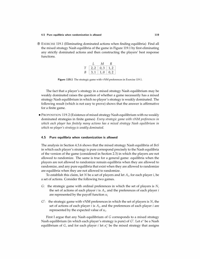
4.5 Pure equilibria when randomization is allowed 119
? EXERCISE 119.1 (Eliminating dominated actions when finding equilibria) Find allthe mixed strategy Nash equilibria of the game in Figure 119.1 by first eliminatingany strictly dominated actions and then constructing the players’ best responsefunctions.
L M RT 2, 2 0, 3 1, 2B 3, 1 1, 0 0, 2
Figure 119.1 The strategic game with vNM preferences in Exercise 119.1.
The fact that a player’s strategy in a mixed strategy Nash equilibrium may beweakly dominated raises the question of whether a game necessarily has a mixedstrategy Nash equilibrium in which no player’s strategy is weakly dominated. Thefollowing result (which is not easy to prove) shows that the answer is affirmativefor a finite game.
PROPOSITION 119.2 (Existence of mixed strategy Nash equilibrium with no weaklydominated strategies in finite games) Every strategic game with vNM preferences inwhich each player has finitely many actions has a mixed strategy Nash equilibrium inwhich no player’s strategy is weakly dominated.
4.5 Pure equilibria when randomization is allowed
The analysis in Section 4.3.6 shows that the mixed strategy Nash equilibria of BoSin which each player’s strategy is pure correspond precisely to the Nash equilibriaof the version of the game (considered in Section 2.3) in which the players are notallowed to randomize. The same is true for a general game: equilibria when theplayers are not allowed to randomize remain equilibria when they are allowed torandomize, and any pure equilibria that exist when they are allowed to randomizeare equilibria when they are not allowed to randomize.
To establish this claim, let N be a set of players and let Ai, for each player i, bea set of actions. Consider the following two games.
G: the strategic game with ordinal preferences in which the set of players is N,the set of actions of each player i is Ai, and the preferences of each player iare represented by the payoff function ui
G′: the strategic game with vNM preferences in which the set of players is N, theset of actions of each player i is Ai, and the preferences of each player i arerepresented by the expected value of ui.
First I argue that any Nash equilibrium of G corresponds to a mixed strategyNash equilibrium (in which each player’s strategy is pure) of G′. Let a∗ be a Nashequilibrium of G, and for each player i let α∗
i be the mixed strategy that assigns
120 Chapter 4. Mixed Strategy Equilibrium
probability 1 to a∗i . Since a∗ is a Nash equilibrium of G we know that in G′ noplayer i has an action that yields her a payoff higher than does a∗i when all the otherplayers adhere to α∗
−i. Thus α∗ satisfies the two conditions in Proposition 113.2, sothat it is a mixed strategy equilibrium of G′, establishing the following result.
PROPOSITION 120.1 (Pure strategy equilibria survive when randomization is al-lowed) Let a∗ be a Nash equilibrium of G and for each player i let α∗
i be the mixed strategyof player i that assigns probability one to the action a∗i . Then α∗ is a mixed strategy Nashequilibrium of G′.
Next I argue that any mixed strategy Nash equilibrium of G′ in which eachplayer’s strategy is pure corresponds to a Nash equilibrium of G. Let α∗ be a mixedstrategy Nash equilibrium of G′ in which every player’s mixed strategy is pure; foreach player i, denote by a∗i the action to which αi assigns probability one. Then nomixed strategy of player i yields her a payoff higher than does α∗
i when the otherplayers’ mixed strategies are given by α∗
−i. Hence, in particular, no pure strategyof player i yields her a payoff higher than does α∗
i . Thus a∗ is a Nash equilibriumof G. In words, if a pure strategy is optimal for a player when she is allowedto randomize then it remains optimal when she is prohibited from randomizing.(More generally, prohibiting a decision-maker from taking an action that is notoptimal does not change the set of actions that are optimal.)
PROPOSITION 120.2 (Pure strategy equilibria survive when randomization is pro-hibited) Let α∗ be a mixed strategy Nash equilibrium of G′ in which the mixed strategy ofeach player i assigns probability one to the single action a∗i . Then a∗ is a Nash equilibriumof G.
4.6 Illustration: expert diagnosis
I seem to confront the following predicament all too frequently. Something aboutwhich I am relatively ill-informed (my car, my computer, my body) stops workingproperly. I consult an expert, who makes a diagnosis and recommends an action.I am not sure if the diagnosis is correct—the expert, after all, has an interest inselling her services. I have to decide whether to follow the expert’s advice or to tryto fix the problem myself, put up with it, or consult another expert.
4.6.1 Model
A simple model that captures the main features of this situation starts with the as-sumption that there are two types of problem, major and minor. Denote the fractionof problems that are major by r, and assume that 0 < r < 1. An expert knows, onseeing a problem, whether it is major or minor; a consumer knows only the prob-ability r. (The diagnosis is costly neither to the expert nor to the consumer.) Anexpert may recommend either a major or a minor repair (regardless of the true
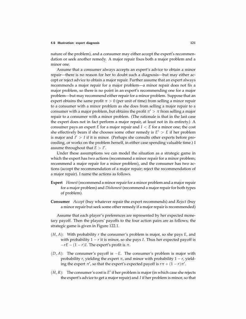
4.6 Illustration: expert diagnosis 121
nature of the problem), and a consumer may either accept the expert’s recommen-dation or seek another remedy. A major repair fixes both a major problem and aminor one.
Assume that a consumer always accepts an expert’s advice to obtain a minorrepair—there is no reason for her to doubt such a diagnosis—but may either ac-cept or reject advice to obtain a major repair. Further assume that an expert alwaysrecommends a major repair for a major problem—a minor repair does not fix amajor problem, so there is no point in an expert’s recommending one for a majorproblem—but may recommend either repair for a minor problem. Suppose that anexpert obtains the same profit π > 0 (per unit of time) from selling a minor repairto a consumer with a minor problem as she does from selling a major repair to aconsumer with a major problem, but obtains the profit π′ > π from selling a majorrepair to a consumer with a minor problem. (The rationale is that in the last casethe expert does not in fact perform a major repair, at least not in its entirety.) Aconsumer pays an expert E for a major repair and I < E for a minor one; the costshe effectively bears if she chooses some other remedy is E′ > E if her problemis major and I ′ > I if it is minor. (Perhaps she consults other experts before pro-ceeding, or works on the problem herself, in either case spending valuable time.) Iassume throughout that E > I ′.
Under these assumptions we can model the situation as a strategic game inwhich the expert has two actions (recommend a minor repair for a minor problem;recommend a major repair for a minor problem), and the consumer has two ac-tions (accept the recommendation of a major repair; reject the recommendation ofa major repair). I name the actions as follows.
Expert Honest (recommend a minor repair for a minor problem and a major repairfor a major problem) and Dishonest (recommend a major repair for both typesof problem).
Consumer Accept (buy whatever repair the expert recommends) and Reject (buya minor repair but seek some other remedy if a major repair is recommended)
Assume that each player’s preferences are represented by her expected mone-tary payoff. Then the players’ payoffs to the four action pairs are as follows; thestrategic game is given in Figure 122.1.
(H, A): With probability r the consumer’s problem is major, so she pays E, andwith probability 1 − r it is minor, so she pays I. Thus her expected payoff is−rE − (1 − r)I. The expert’s profit is π.
(D, A): The consumer’s payoff is −E. The consumer’s problem is major withprobability r, yielding the expert π, and minor with probability 1 − r, yield-ing the expert π′, so that the expert’s expected payoff is rπ + (1 − r)π′.
(H, R): The consumer’s cost is E′ if her problem is major (in which case she rejectsthe expert’s advice to get a major repair) and I if her problem is minor, so that
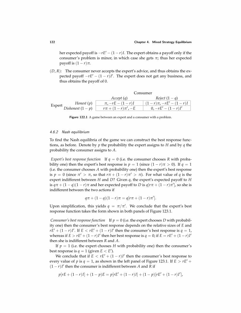
122 Chapter 4. Mixed Strategy Equilibrium
her expected payoff is −rE′ − (1 − r)I. The expert obtains a payoff only if theconsumer’s problem is minor, in which case she gets π; thus her expectedpayoff is (1 − r)π.
(D, R): The consumer never accepts the expert’s advice, and thus obtains the ex-pected payoff −rE′ − (1 − r)I ′. The expert does not get any business, andthus obtains the payoff of 0.
Expert
ConsumerAccept (q) Reject (1 − q)
Honest (p) π, −rE − (1 − r)I (1 − r)π, −rE′ − (1 − r)IDishonest (1 − p) rπ + (1 − r)π′ , −E 0, −rE′ − (1 − r)I ′
Figure 122.1 A game between an expert and a consumer with a problem.
4.6.2 Nash equilibrium
To find the Nash equilibria of the game we can construct the best response func-tions, as before. Denote by p the probability the expert assigns to H and by q theprobability the consumer assigns to A.
Expert’s best response function If q = 0 (i.e. the consumer chooses R with proba-bility one) then the expert’s best response is p = 1 (since (1 − r)π > 0). If q = 1(i.e. the consumer chooses A with probability one) then the expert’s best responseis p = 0 (since π′ > π, so that rπ + (1 − r)π′ > π). For what value of q is theexpert indifferent between H and D? Given q, the expert’s expected payoff to His qπ + (1 − q)(1 − r)π and her expected payoff to D is q[rπ + (1 − r)π′], so she isindifferent between the two actions if
qπ + (1 − q)(1 − r)π = q[rπ + (1 − r)π′].
Upon simplification, this yields q = π/π′. We conclude that the expert’s bestresponse function takes the form shown in both panels of Figure 123.1.
Consumer’s best response function If p = 0 (i.e. the expert chooses D with probabil-ity one) then the consumer’s best response depends on the relative sizes of E andrE′ + (1 − r)I ′. If E < rE′ + (1 − r)I ′ then the consumer’s best response is q = 1,whereas if E > rE′ + (1 − r)I ′ then her best response is q = 0; if E = rE′ + (1 − r)I ′
then she is indifferent between R and A.If p = 1 (i.e. the expert chooses H with probability one) then the consumer’s
best response is q = 1 (given E < E′).We conclude that if E < rE′ + (1 − r)I ′ then the consumer’s best response to
every value of p is q = 1, as shown in the left panel of Figure 123.1. If E > rE′ +(1 − r)I ′ then the consumer is indifferent between A and R if
p[rE + (1 − r)I] + (1 − p)E = p[rE′ + (1 − r)I] + (1 − p)[rE′ + (1 − r)I ′],
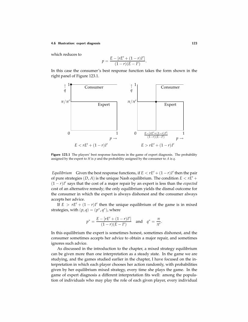
4.6 Illustration: expert diagnosis 123
which reduces to
p =E − [rE′ + (1 − r)I ′]
(1 − r)(E − I ′).
In this case the consumer’s best response function takes the form shown in theright panel of Figure 123.1.
0 1p →
π/π′
1↑q
Expert
Consumer
E < rE′ + (1 − r)I ′
0 E−[rE′+(1−r)I′](1−r)(E−I′)
1p →
π/π′
1↑q
Expert
Consumer
E > rE′ + (1 − r)I ′
Figure 123.1 The players’ best response functions in the game of expert diagnosis. The probabilityassigned by the expert to H is p and the probability assigned by the consumer to A is q.
Equilibrium Given the best response functions, if E < rE′ + (1 − r)I ′ then the pairof pure strategies (D, A) is the unique Nash equilibrium. The condition E < rE′ +(1 − r)I ′ says that the cost of a major repair by an expert is less than the expectedcost of an alternative remedy; the only equilibrium yields the dismal outcome forthe consumer in which the expert is always dishonest and the consumer alwaysaccepts her advice.
If E > rE′ + (1 − r)I ′ then the unique equilibrium of the game is in mixedstrategies, with (p, q) = (p∗, q∗), where
p∗ =E − [rE′ + (1 − r)I ′]
(1 − r)(E − I ′)and q∗ =
π
π′ .
In this equilibrium the expert is sometimes honest, sometimes dishonest, and theconsumer sometimes accepts her advice to obtain a major repair, and sometimesignores such advice.
As discussed in the introduction to the chapter, a mixed strategy equilibriumcan be given more than one interpretation as a steady state. In the game we arestudying, and the games studied earlier in the chapter, I have focused on the in-terpretation in which each player chooses her action randomly, with probabilitiesgiven by her equilibrium mixed strategy, every time she plays the game. In thegame of expert diagnosis a different interpretation fits well: among the popula-tion of individuals who may play the role of each given player, every individual
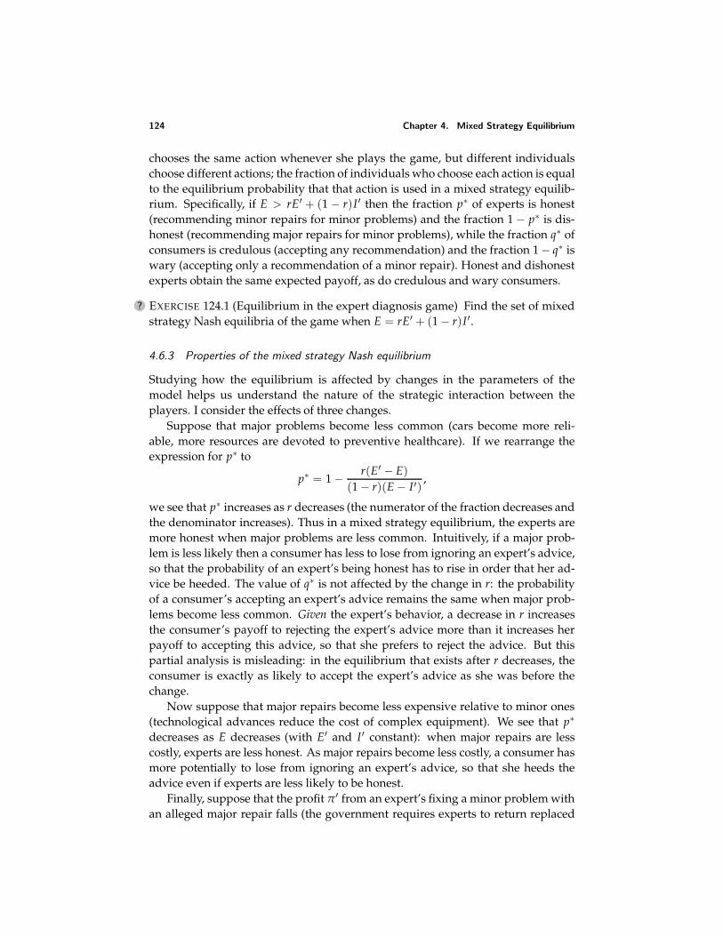
124 Chapter 4. Mixed Strategy Equilibrium
chooses the same action whenever she plays the game, but different individualschoose different actions; the fraction of individuals who choose each action is equalto the equilibrium probability that that action is used in a mixed strategy equilib-rium. Specifically, if E > rE′ + (1 − r)I ′ then the fraction p∗ of experts is honest(recommending minor repairs for minor problems) and the fraction 1 − p∗ is dis-honest (recommending major repairs for minor problems), while the fraction q∗ ofconsumers is credulous (accepting any recommendation) and the fraction 1 − q∗ iswary (accepting only a recommendation of a minor repair). Honest and dishonestexperts obtain the same expected payoff, as do credulous and wary consumers.
? EXERCISE 124.1 (Equilibrium in the expert diagnosis game) Find the set of mixedstrategy Nash equilibria of the game when E = rE′ + (1 − r)I ′.
4.6.3 Properties of the mixed strategy Nash equilibrium
Studying how the equilibrium is affected by changes in the parameters of themodel helps us understand the nature of the strategic interaction between theplayers. I consider the effects of three changes.
Suppose that major problems become less common (cars become more reli-able, more resources are devoted to preventive healthcare). If we rearrange theexpression for p∗ to
p∗ = 1 − r(E′ − E)(1 − r)(E − I ′)
,
we see that p∗ increases as r decreases (the numerator of the fraction decreases andthe denominator increases). Thus in a mixed strategy equilibrium, the experts aremore honest when major problems are less common. Intuitively, if a major prob-lem is less likely then a consumer has less to lose from ignoring an expert’s advice,so that the probability of an expert’s being honest has to rise in order that her ad-vice be heeded. The value of q∗ is not affected by the change in r: the probabilityof a consumer’s accepting an expert’s advice remains the same when major prob-lems become less common. Given the expert’s behavior, a decrease in r increasesthe consumer’s payoff to rejecting the expert’s advice more than it increases herpayoff to accepting this advice, so that she prefers to reject the advice. But thispartial analysis is misleading: in the equilibrium that exists after r decreases, theconsumer is exactly as likely to accept the expert’s advice as she was before thechange.
Now suppose that major repairs become less expensive relative to minor ones(technological advances reduce the cost of complex equipment). We see that p∗
decreases as E decreases (with E′ and I ′ constant): when major repairs are lesscostly, experts are less honest. As major repairs become less costly, a consumer hasmore potentially to lose from ignoring an expert’s advice, so that she heeds theadvice even if experts are less likely to be honest.
Finally, suppose that the profit π′ from an expert’s fixing a minor problem withan alleged major repair falls (the government requires experts to return replaced
4.7 Equilibrium in a single population 125
parts to the consumer, making it more difficult for an expert to fraudulently claimto have performed a major repair). Then q∗ increases—consumers become lesswary. Experts have less to gain from acting dishonestly, so that consumers can bemore confident of their advice.
? EXERCISE 125.1 (Incompetent experts) Consider a (realistic?) variant of the model,in which the experts are not entirely competent. Assume that each expert alwayscorrectly recognizes a major problem but correctly recognizes a minor problemwith probability s < 1: with probability 1 − s she mistakenly thinks that a minorproblem is major, and, if the consumer accepts her advice, performs a major repairand obtains the profit π. Maintain the assumption that each consumer believes(correctly) that the probability her problem is major is r. As before, a consumerwho does not give the job of fixing her problem to an expert bears the cost E′ if itis major and I ′ if it is minor.
Suppose, for example, that an expert is honest and a consumer rejects advice toobtain a major repair. With probability r the consumer’s problem is major, so thatthe expert recommends a major repair, which the consumer rejects; the consumerbears the cost E′. With probability 1 − r the consumer’s problem is minor. In thiscase with probability s the expert correctly diagnoses it as minor, and the consumeraccepts her advice and pays I; with probability 1 − s the expert diagnoses it as ma-jor, and the consumer rejects her advice and bears the cost I ′. Thus the consumer’sexpected payoff in this case is −rE′ − (1 − r)[sI + (1 − s)I ′].
Construct the payoffs for every pair of actions and find the mixed strategy equi-librium in the case E > rE′ + (1− r)I ′. Does incompetence breed dishonesty? Morewary consumers?
? EXERCISE 125.2 (Choosing a seller) Each of two sellers has available one indivisibleunit of a good. Seller 1 posts the price p1 and seller 2 posts the price p2. Each oftwo buyers would like to obtain one unit of the good; they simultaneously decidewhich seller to approach. If both buyers approach the same seller, each trades withprobability 1
2 ; the disappointed buyer does not subsequently have the option totrade with the other seller. (This assumption models the risk faced by a buyer thata good is sold out when she patronizes a seller with a low price.) Each buyer’spreferences are represented by the expected value of a payoff function that assignsthe payoff 0 to not trading and the payoff 1 − p to purchasing one unit of the goodat the price p. (Neither buyer values more than one unit.) For any pair (p1, p2) ofprices with 0 ≤ pi ≤ 1 for i = 1, 2, find the Nash equilibria (in pure and in mixedstrategies) of the strategic game that models this situation. (There are three maincases: p2 < 2p1 − 1, 2p1 − 1 < p2 < 1
2 (1 + p1), and p2 > 12 (1 + p1).)
4.7 Equilibrium in a single population
In Section 2.10 I discussed deterministic steady states in situations in which themembers of a single population interact. I now discuss stochastic steady states insuch situations.
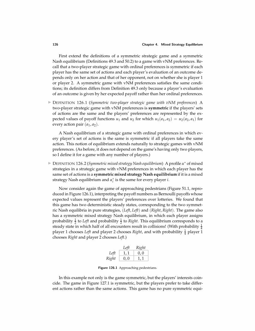
126 Chapter 4. Mixed Strategy Equilibrium
First extend the definitions of a symmetric strategic game and a symmetricNash equilibrium (Definitions 49.3 and 50.2) to a game with vNM preferences. Re-call that a two-player strategic game with ordinal preferences is symmetric if eachplayer has the same set of actions and each player’s evaluation of an outcome de-pends only on her action and that of her opponent, not on whether she is player 1or player 2. A symmetric game with vNM preferences satisfies the same condi-tions; its definition differs from Definition 49.3 only because a player’s evaluationof an outcome is given by her expected payoff rather than her ordinal preferences.
DEFINITION 126.1 (Symmetric two-player strategic game with vNM preferences) Atwo-player strategic game with vNM preferences is symmetric if the players’ setsof actions are the same and the players’ preferences are represented by the ex-pected values of payoff functions u1 and u2 for which u1(a1, a2) = u2(a2, a1) forevery action pair (a1, a2).
A Nash equilibrium of a strategic game with ordinal preferences in which ev-ery player’s set of actions is the same is symmetric if all players take the sameaction. This notion of equilibrium extends naturally to strategic games with vNMpreferences. (As before, it does not depend on the game’s having only two players,so I define it for a game with any number of players.)
DEFINITION 126.2 (Symmetric mixed strategy Nash equilibrium) A profile α∗ of mixedstrategies in a strategic game with vNM preferences in which each player has thesame set of actions is a symmetric mixed strategy Nash equilibrium if it is a mixedstrategy Nash equilibrium and α∗
i is the same for every player i.
Now consider again the game of approaching pedestrians (Figure 51.1, repro-duced in Figure 126.1), interpreting the payoff numbers as Bernoulli payoffs whoseexpected values represent the players’ preferences over lotteries. We found thatthis game has two deterministic steady states, corresponding to the two symmet-ric Nash equilibria in pure strategies, (Left, Left) and (Right, Right). The game alsohas a symmetric mixed strategy Nash equilibrium, in which each player assignsprobability 1
2 to Left and probability 12 to Right. This equilibrium corresponds to a
steady state in which half of all encounters result in collisions! (With probability 14
player 1 chooses Left and player 2 chooses Right, and with probability 14 player 1
chooses Right and player 2 chooses Left.)
Left RightLeft 1, 1 0, 0
Right 0, 0 1, 1
Figure 126.1 Approaching pedestrians.
In this example not only is the game symmetric, but the players’ interests coin-cide. The game in Figure 127.1 is symmetric, but the players prefer to take differ-ent actions rather than the same actions. This game has no pure symmetric equi-
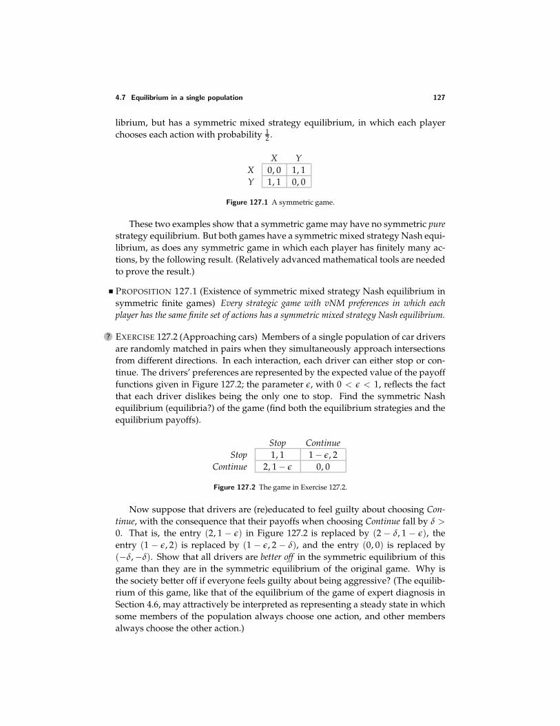
4.7 Equilibrium in a single population 127
librium, but has a symmetric mixed strategy equilibrium, in which each playerchooses each action with probability 1
2 .
X YX 0, 0 1, 1Y 1, 1 0, 0
Figure 127.1 A symmetric game.
These two examples show that a symmetric game may have no symmetric purestrategy equilibrium. But both games have a symmetric mixed strategy Nash equi-librium, as does any symmetric game in which each player has finitely many ac-tions, by the following result. (Relatively advanced mathematical tools are neededto prove the result.)
PROPOSITION 127.1 (Existence of symmetric mixed strategy Nash equilibrium insymmetric finite games) Every strategic game with vNM preferences in which eachplayer has the same finite set of actions has a symmetric mixed strategy Nash equilibrium.
? EXERCISE 127.2 (Approaching cars) Members of a single population of car driversare randomly matched in pairs when they simultaneously approach intersectionsfrom different directions. In each interaction, each driver can either stop or con-tinue. The drivers’ preferences are represented by the expected value of the payofffunctions given in Figure 127.2; the parameter ε, with 0 < ε < 1, reflects the factthat each driver dislikes being the only one to stop. Find the symmetric Nashequilibrium (equilibria?) of the game (find both the equilibrium strategies and theequilibrium payoffs).
Stop ContinueStop 1, 1 1 − ε, 2
Continue 2, 1 − ε 0, 0
Figure 127.2 The game in Exercise 127.2.
Now suppose that drivers are (re)educated to feel guilty about choosing Con-tinue, with the consequence that their payoffs when choosing Continue fall by δ >
0. That is, the entry (2, 1 − ε) in Figure 127.2 is replaced by (2 − δ, 1 − ε), theentry (1 − ε, 2) is replaced by (1 − ε, 2 − δ), and the entry (0, 0) is replaced by(−δ, −δ). Show that all drivers are better off in the symmetric equilibrium of thisgame than they are in the symmetric equilibrium of the original game. Why isthe society better off if everyone feels guilty about being aggressive? (The equilib-rium of this game, like that of the equilibrium of the game of expert diagnosis inSection 4.6, may attractively be interpreted as representing a steady state in whichsome members of the population always choose one action, and other membersalways choose the other action.)
128 Chapter 4. Mixed Strategy Equilibrium
? EXERCISE 128.1 (Bargaining) Pairs of players from a single population bargainover the division of a pie of size 10. The members of a pair simultaneously makedemands; the possible demands are the nonnegative even integers up to 10. If thedemands sum to 10 then each player receives her demand; if the demands sumto less than 10 then each player receives her demand plus half of the pie that re-mains after both demands have been satisfied; if the demands sum to more than10 then neither player receives any payoff. Find all the symmetric mixed strategyNash equilibria in which each player assigns positive probability to at most twodemands. (Many situations in which each player assigns positive probability totwo actions, say a′ and a′′, can be ruled out as equilibria because when one playeruses such a strategy, some action a′′′ yields the other player a payoff higher thandoes a′ and/or a′′.)
4.8 Illustration: reporting a crime
A crime is observed by a group of n people. Each person would like the policeto be informed, but prefers that someone else make the phone call. Specifically,suppose that each person attaches the value v to the police being informed andbears the cost c if she makes the phone call, where v > c > 0. Then the situation ismodeled by the following strategic game with vNM preferences.
Players The n people.
Actions Each player’s set of actions is Call, Don’t call.
Preferences Each player’s preferences are represented by the expected valueof a payoff function that assigns 0 to the profile in which no one calls, v − cto any profile in which she calls, and v to any profile in which at least oneperson calls, but she does not.
This game is a variant of the one in Exercise 31.1, with k = 1. It has n pure Nashequilibria, in each of which exactly one person calls. (If that person switches to notcalling, her payoff falls from v − c to 0; if any other person switches to calling, herpayoff falls from v to v− c.) If the members of the group differ in some respect, thenthese asymmetric equilibria may be compelling as steady states. For example, thesocial norm in which the oldest person in the group makes the phone call is stable.
If the members of the group either do not differ significantly or are not awareof any differences among themselves—if they are drawn from a single homoge-neous population—then there is no way for them to coordinate, and a symmetricequilibrium, in which every player uses the same strategy, is more compelling.
The game has no symmetric pure Nash equilibrium. (If everyone calls, thenany person is better off switching to not calling. If no one calls, then any person isbetter off switching to calling.)
However, it has a symmetric mixed strategy equilibrium in which each personcalls with positive probability less than one. In any such equilibrium, each per-son’s expected payoff to calling is equal to her expected payoff to not calling. Each
4.8 Illustration: reporting a crime 129
person’s payoff to calling is v − c, and her payoff to not calling is 0 if no one elsecalls and v if at least one other person calls, so the equilibrium condition is
v − c = 0 · Prno one else calls + v · Prat least one other person calls,
orv − c = v · (1 − Prno one else calls),
orc/v = Prno one else calls. (129.1)
Denote by p the probability with which each person calls. The probability thatno one else calls is the probability that every one of the other n − 1 people does notcall, namely (1 − p)n−1. Thus the equilibrium condition is c/v = (1 − p)n−1, or
p = 1 − (c/v)1/(n−1).
This number p is between 0 and 1, so we conclude that the game has a uniquesymmetric mixed strategy equilibrium, in which each person calls with probability1 − (c/v)1/(n−1). That is, there is a steady state in which whenever a person isin a group of n people facing the situation modeled by the game, she calls withprobability 1 − (c/v)1/(n−1).
How does this equilibrium change as the size of the group increases? We seethat as n increases, the probability p that any given person calls decreases. (Asn increases, 1/(n − 1) decreases, so that (c/v)1/(n−1) increases.) What about theprobability that at least one person calls? Fix any player i. Then the event “no onecalls” is the same as the event “i does not call and no one other than i calls”. Thus
Prno one calls = Pri does not call Prno one else calls. (129.2)
Now, the probability that any given person calls decreases as n increases, or equiv-alently the probability that she does not call increases as n increases. Further, fromthe equilibrium condition (129.1), Prno one else calls is equal to c/v, independentof n. We conclude that the probability that no one calls increases as n increases.That is, the larger the group, the less likely the police are informed of the crime!
The condition defining a mixed strategy equilibrium is responsible for this re-sult. For any given person to be indifferent between calling and not calling thiscondition requires that the probability that no one else calls be independent of thesize of the group. Thus each person’s probability of not calling is larger in a largergroup, and hence, by the laws of probability reflected in (129.2), the probabilitythat no one calls is larger in a larger group.
The result that the larger the group, the less likely any given person calls is notsurprising. The result that the larger the group, the less likely at least one personcalls is a more subtle implication of the notion of equilibrium. In a larger group noindividual is any less concerned that the police should be called, but in a steadystate the behavior of the group drives down the chance that the police are notifiedof the crime.
130 Chapter 4. Mixed Strategy Equilibrium
? EXERCISE 130.1 (Contributing to a public good) Consider an extension of the anal-ysis above to the game in Exercise 31.1 for k ≥ 2. (In this case a player may con-tribute even though the good is not provided; the player’s payoff in this case is −c.)Denote by Qn−1,m(p) the probability that exactly m of a group of n − 1 players con-tribute when each player contributes with probability p. What condition must besatisfied by Qn−1,k−1(p) in a symmetric mixed strategy equilibrium (in which eachplayer contributes with the same probability)? (When does a player’s contributionmake a difference to the outcome?) For the case v = 1, n = 4, k = 2, and c = 3
8 findthe equilibria explicitly. (You need to use the fact that Q3,1(p) = 3p(1 − p)2, anddo a bit of algebra.)
REPORTING A CRIME: SOCIAL PSYCHOLOGY AND GAME THEORY
Thirty-eight people witnessed the brutal murder of Catherine (“Kitty”) Genoveseover a period of half an hour in New York City in March 1964. During this period,none of them significantly responded to her screams for help; none even called thepolice. Journalists, psychiatrists, sociologists, and others subsequently struggledto understand the witnesses’ inaction. Some ascribed it to apathy engendered bylife in a large city: “Indifference to one’s neighbor and his troubles is a conditionedreflex of life in New York as it is in other big cities” (Rosenthal 1964, 81–82).
The event particularly interested social psychologists. It led them to try to un-derstand the circumstances under which a bystander would help someone in trou-ble. Experiments quickly suggested that, contrary to the popular theory, people—even those living in large cities—are not in general apathetic to others’ plights. Anexperimental subject who is the lone witness of a person in distress is very likelyto try to help. But as the size of the group of witnesses increases, there is a declinenot only in the probability that any given one of them offers assistance, but alsoin the probability that at least one of them offers assistance. Social psychologistshypothesize that three factors explain these experimental findings. First, “diffu-sion of responsibility”: the larger the group, the lower the psychological cost ofnot helping. Second, “audience inhibition”: the larger the group, the greater theembarrassment suffered by a helper in case the event turns out to be one in whichhelp is inappropriate (because, for example, it is not in fact an emergency). Third,“social influence”: a person infers the appropriateness of helping from others’ be-havior, so that in a large group everyone else’s lack of intervention leads any givenperson to think intervention is less likely to be appropriate.
In terms of the model in Section 4.8, these three factors raise the expected costand/or reduce the expected benefit of a person’s intervening. They all seem plausi-ble. However, they are not needed to explain the phenomenon: our game-theoreticanalysis shows that even if the cost and benefit are independent of group size, adecrease in the probability that at least one person intervenes is an implicationof equilibrium. This game-theoretic analysis has an advantage over the socio-
4.9 The formation of players’ beliefs 131
psychological one: it derives the conclusion from the same principles that underlieall the other models studied so far (oligopoly, auctions, voting, and elections, forexample), rather than positing special features of the specific environment in whicha group of bystanders may come to the aid of a person in distress.
The critical element missing from the socio-psychological analysis is the notionof an equilibrium. Whether any given person intervenes depends on the probabilityshe assigns to some other person’s intervening. In an equilibrium each personmust be indifferent between intervening and not intervening, and as we have seenthis condition leads inexorably to the conclusion that an increase in group sizereduces the probability that at least one person intervenes.
4.9 The formation of players’ beliefs
In a Nash equilibrium, each player chooses a strategy that maximizes her expectedpayoff, knowing the other players’ strategies. So far we have not considered howplayers may acquire such information. Informally, the idea underlying the pre-vious analysis is that the players have learned each other’s strategies from theirexperience playing the game. In the idealized situation to which the analysis cor-responds, for each player in the game there is a large population of individualswho may take the role of that player; in any play of the game, one participant isdrawn randomly from each population. In this situation, a new individual whojoins a population that is in a steady state (i.e. is using a Nash equilibrium strategyprofile) can learn the other players’ strategies by observing their actions over manyplays of the game. As long as the turnover in players is small enough, existingplayers’ encounters with neophytes (who may use nonequilibrium strategies) willbe sufficiently rare that their beliefs about the steady state will not be disturbed, sothat a new player’s problem is simply to learn the other players’ actions.
This analysis leaves open the question of what might happen if new playerssimultaneously join more than one population in sufficient numbers that they havea significant chance of facing opponents who are themselves new. In particular,can we expect a steady state to be reached when no one has experience playing thegame?
4.9.1 Eliminating dominated actions
In some games the players may reasonably be expected to choose their Nash equi-librium actions from an introspective analysis of the game. At an extreme, eachplayer’s best action may be independent of the other players’ actions, as in thePrisoner’s Dilemma (Example 12.1). In such a game no player needs to worry aboutthe other players’ actions. In a less extreme case, some player’s best action maydepend on the other players’ actions, but the actions the other players will choosemay be clear because each of these players has an action that strictly dominatesall others. For example, in the game in Figure 132.1, player 2’s action R strictly
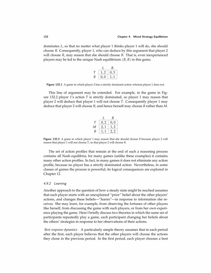
132 Chapter 4. Mixed Strategy Equilibrium
dominates L, so that no matter what player 1 thinks player 1 will do, she shouldchoose R. Consequently, player 1, who can deduce by this argument that player 2will choose R, may reason that she should choose B. That is, even inexperiencedplayers may be led to the unique Nash equilibrium (B, R) in this game.
L RT 1, 2 0, 3B 0, 0 1, 1
Figure 132.1 A game in which player 2 has a strictly dominant action whereas player 1 does not.
This line of argument may be extended. For example, in the game in Fig-ure 132.2 player 1’s action T is strictly dominated, so player 1 may reason thatplayer 2 will deduce that player 1 will not choose T. Consequently player 1 maydeduce that player 2 will choose R, and hence herself may choose B rather than M.
L RT 0, 2 0, 0
M 2, 1 1, 2B 1, 1 2, 2
Figure 132.2 A game in which player 1 may reason that she should choose B because player 2 willreason that player 1 will not choose T, so that player 2 will choose R.
The set of action profiles that remain at the end of such a reasoning processcontains all Nash equilibria; for many games (unlike these examples) it containsmany other action profiles. In fact, in many games it does not eliminate any actionprofile, because no player has a strictly dominated action. Nevertheless, in someclasses of games the process is powerful; its logical consequences are explored inChapter 12.
4.9.2 Learning
Another approach to the question of how a steady state might be reached assumesthat each player starts with an unexplained “prior” belief about the other players’actions, and changes these beliefs—“learns”—in response to information she re-ceives. She may learn, for example, from observing the fortunes of other playerslike herself, from discussing the game with such players, or from her own experi-ence playing the game. Here I briefly discuss two theories in which the same set ofparticipants repeatedly play a game, each participant changing her beliefs aboutthe others’ strategies in response to her observations of their actions.
Best response dynamics A particularly simple theory assumes that in each periodafter the first, each player believes that the other players will choose the actionsthey chose in the previous period. In the first period, each player chooses a best
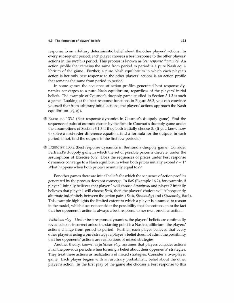
4.9 The formation of players’ beliefs 133
response to an arbitrary deterministic belief about the other players’ actions. Inevery subsequent period, each player chooses a best response to the other players’actions in the previous period. This process is known as best response dynamics. Anaction profile that remains the same from period to period is a pure Nash equi-librium of the game. Further, a pure Nash equilibrium in which each player’saction is her only best response to the other players’ actions is an action profilethat remains the same from period to period.
In some games the sequence of action profiles generated best response dy-namics converges to a pure Nash equilibrium, regardless of the players’ initialbeliefs. The example of Cournot’s duopoly game studied in Section 3.1.3 is sucha game. Looking at the best response functions in Figure 56.2, you can convinceyourself that from arbitrary initial actions, the players’ actions approach the Nashequilibrium (q∗1, q∗2).
? EXERCISE 133.1 (Best response dynamics in Cournot’s duopoly game) Find thesequence of pairs of outputs chosen by the firms in Cournot’s duopoly game underthe assumptions of Section 3.1.3 if they both initially choose 0. (If you know howto solve a first-order difference equation, find a formula for the outputs in eachperiod; if not, find the outputs in the first few periods.)
? EXERCISE 133.2 (Best response dynamics in Bertrand’s duopoly game) ConsiderBertrand’s duopoly game in which the set of possible prices is discrete, under theassumptions of Exercise 65.2. Does the sequences of prices under best responsedynamics converge to a Nash equilibrium when both prices initially exceed c + 1?What happens when both prices are initially equal to c?
For other games there are initial beliefs for which the sequence of action profilesgenerated by the process does not converge. In BoS (Example 16.2), for example, ifplayer 1 initially believes that player 2 will choose Stravinsky and player 2 initiallybelieves that player 1 will choose Bach, then the players’ choices will subsequentlyalternate indefinitely between the action pairs (Bach, Stravinsky) and (Stravinsky, Bach).This example highlights the limited extent to which a player is assumed to reasonin the model, which does not consider the possibility that she cottons on to the factthat her opponent’s action is always a best response to her own previous action.
Fictitious play Under best response dynamics, the players’ beliefs are continuallyrevealed to be incorrect unless the starting point is a Nash equilibrium: the players’actions change from period to period. Further, each player believes that everyother player is using a pure strategy: a player’s belief does not admit the possibilitythat her opponents’ actions are realizations of mixed strategies.
Another theory, known as fictitious play, assumes that players consider actionsin all the previous periods when forming a belief about their opponents’ strategies.They treat these actions as realizations of mixed strategies. Consider a two-playergame. Each player begins with an arbitrary probabilistic belief about the otherplayer’s action. In the first play of the game she chooses a best response to this
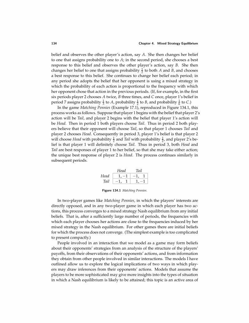
134 Chapter 4. Mixed Strategy Equilibrium
belief and observes the other player’s action, say A. She then changes her beliefto one that assigns probability one to A; in the second period, she chooses a bestresponse to this belief and observes the other player’s action, say B. She thenchanges her belief to one that assigns probability 1
2 to both A and B, and choosesa best response to this belief. She continues to change her belief each period; inany period she adopts the belief that her opponent is using a mixed strategy inwhich the probability of each action is proportional to the frequency with whichher opponent chose that action in the previous periods. (If, for example, in the firstsix periods player 2 chooses A twice, B three times, and C once, player 1’s belief inperiod 7 assigns probability 1
3 to A, probability 12 to B, and probability 1
6 to C.)In the game Matching Pennies (Example 17.1), reproduced in Figure 134.1, this
process works as follows. Suppose that player 1 begins with the belief that player 2’saction will be Tail, and player 2 begins with the belief that player 1’s action willbe Head. Then in period 1 both players choose Tail. Thus in period 2 both play-ers believe that their opponent will choose Tail, so that player 1 chooses Tail andplayer 2 chooses Head. Consequently in period 3, player 1’s belief is that player 2will choose Head with probability 1
2 and Tail with probability 12 , and player 2’s be-
lief is that player 1 will definitely choose Tail. Thus in period 3, both Head andTail are best responses of player 1 to her belief, so that she may take either action;the unique best response of player 2 is Head. The process continues similarly insubsequent periods.
Head TailHead 1, −1 −1, 1
Tail −1, 1 1, −1
Figure 134.1 Matching Pennies.
In two-player games like Matching Pennies, in which the players’ interests aredirectly opposed, and in any two-player game in which each player has two ac-tions, this process converges to a mixed strategy Nash equilibrium from any initialbeliefs. That is, after a sufficiently large number of periods, the frequencies withwhich each player chooses her actions are close to the frequencies induced by hermixed strategy in the Nash equilibrium. For other games there are initial beliefsfor which the process does not converge. (The simplest example is too complicatedto present compactly.)
People involved in an interaction that we model as a game may form beliefsabout their opponents’ strategies from an analysis of the structure of the players’payoffs, from their observations of their opponents’ actions, and from informationthey obtain from other people involved in similar interactions. The models I haveoutlined allow us to explore the logical implications of two ways in which play-ers may draw inferences from their opponents’ actions. Models that assume theplayers to be more sophisticated may give more insights into the types of situationin which a Nash equilibrium is likely to be attained; this topic is an active area of
4.10 Extension: Finding all mixed strategy Nash equilibria 135
current research.
4.10 Extension: Finding all mixed strategy Nash equilibria
We can find all the mixed strategy Nash equilibria of a two-player game in whicheach player has two actions by constructing the players’ best response functions,as we have seen. In more complicated games, this method is usually not practical.
The following systematic method of finding all mixed strategy Nash equilib-ria of a game is suggested by the characterization of an equilibrium in Proposi-tion 113.2.
• For each player i, choose a subset Si of her set Ai of actions.
• Check whether there exists a mixed strategy profile α such that (i) the set ofactions to which each strategy αi assigns positive probability is Si and (ii) α
satisfies the conditions in Proposition 113.2.
• Repeat the analysis for every collection of subsets of the players’ sets ofactions.
The following example illustrates this method for a two-player game in whicheach player has two actions.
EXAMPLE 135.1 (Finding all mixed strategy equilibria of a two-player game inwhich each player has two actions) Consider a two-player game in which eachplayer has two actions. Denote the actions and payoffs as in Figure 136.1. Eachplayer’s set of actions has three nonempty subsets: two each consisting of a sin-gle action, and one consisting of both actions. Thus there are nine (3 × 3) pairs ofsubsets of the players’ action sets. For each pair (S1, S2), we check if there is a pair(α1, α2) of mixed strategies such that each strategy αi assigns positive probabilityonly to actions in Si and the conditions in Proposition 113.2 are satisfied.
• Checking the four pairs of subsets in which each player’s subset consists of asingle action amounts to checking whether any of the four pairs of actions isa pure strategy equilibrium. (For each player, the first condition in Proposi-tion 113.2 is automatically satisfied, because there is only one action in eachsubset.)
• Consider the pair of subsets T, B for player 1 and L for player 2. Thesecond condition in Proposition 113.2 is automatically satisfied for player 1,who has no actions to which she assigns probability 0, and the first conditionis automatically satisfied for player 2, because she assigns positive probabilityto only one action. Thus for there to be a mixed strategy equilibrium in whichplayer 1’s probability of using T is p we need u11 = u21 (player 1’s payoffs toher two actions must be equal) and
pv11 + (1 − p)v21 ≥ pv12 + (1 − p)v22
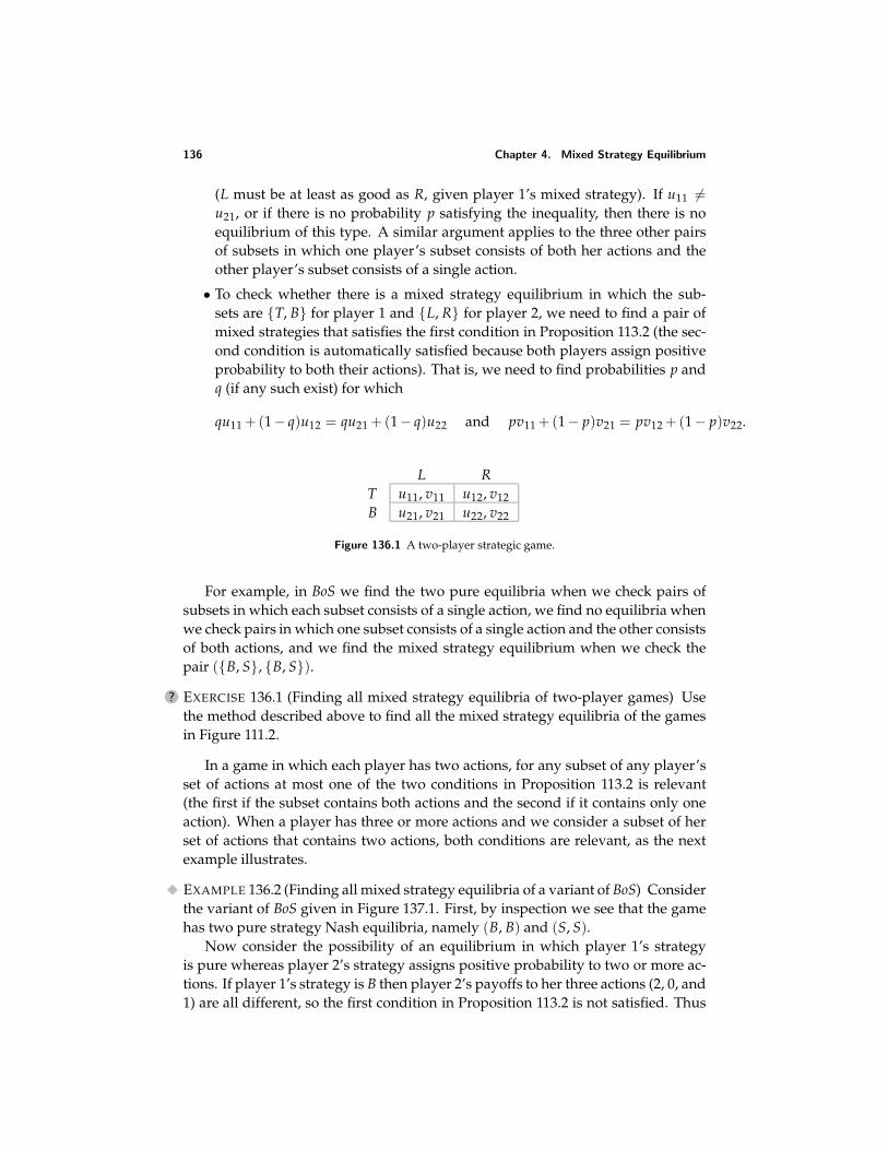
136 Chapter 4. Mixed Strategy Equilibrium
(L must be at least as good as R, given player 1’s mixed strategy). If u11 =u21, or if there is no probability p satisfying the inequality, then there is noequilibrium of this type. A similar argument applies to the three other pairsof subsets in which one player’s subset consists of both her actions and theother player’s subset consists of a single action.
• To check whether there is a mixed strategy equilibrium in which the sub-sets are T, B for player 1 and L, R for player 2, we need to find a pair ofmixed strategies that satisfies the first condition in Proposition 113.2 (the sec-ond condition is automatically satisfied because both players assign positiveprobability to both their actions). That is, we need to find probabilities p andq (if any such exist) for which
qu11 + (1− q)u12 = qu21 + (1− q)u22 and pv11 + (1− p)v21 = pv12 + (1− p)v22.
L RT u11, v11 u12, v12B u21, v21 u22, v22
Figure 136.1 A two-player strategic game.
For example, in BoS we find the two pure equilibria when we check pairs ofsubsets in which each subset consists of a single action, we find no equilibria whenwe check pairs in which one subset consists of a single action and the other consistsof both actions, and we find the mixed strategy equilibrium when we check thepair (B, S, B, S).
? EXERCISE 136.1 (Finding all mixed strategy equilibria of two-player games) Usethe method described above to find all the mixed strategy equilibria of the gamesin Figure 111.2.
In a game in which each player has two actions, for any subset of any player’sset of actions at most one of the two conditions in Proposition 113.2 is relevant(the first if the subset contains both actions and the second if it contains only oneaction). When a player has three or more actions and we consider a subset of herset of actions that contains two actions, both conditions are relevant, as the nextexample illustrates.
EXAMPLE 136.2 (Finding all mixed strategy equilibria of a variant of BoS) Considerthe variant of BoS given in Figure 137.1. First, by inspection we see that the gamehas two pure strategy Nash equilibria, namely (B, B) and (S, S).
Now consider the possibility of an equilibrium in which player 1’s strategyis pure whereas player 2’s strategy assigns positive probability to two or more ac-tions. If player 1’s strategy is B then player 2’s payoffs to her three actions (2, 0, and1) are all different, so the first condition in Proposition 113.2 is not satisfied. Thus
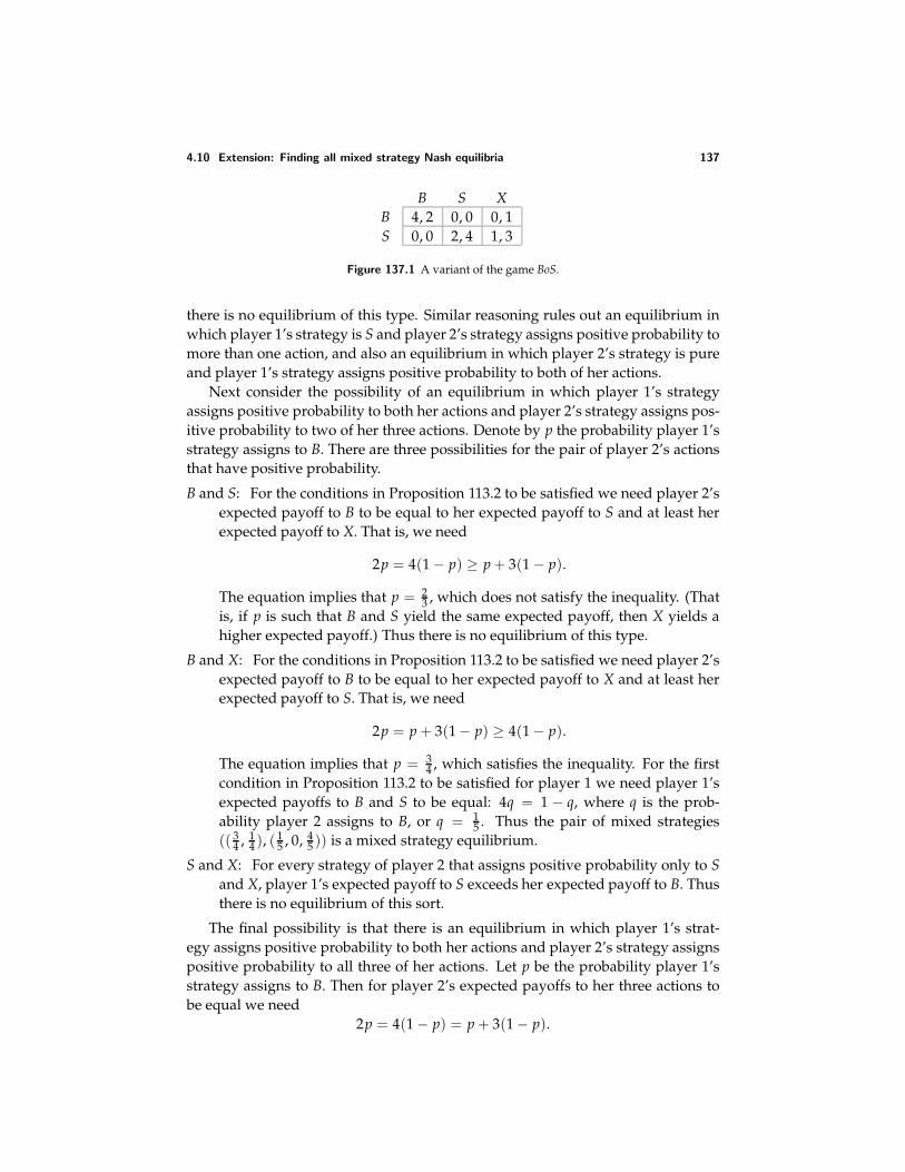
4.10 Extension: Finding all mixed strategy Nash equilibria 137
B S XB 4, 2 0, 0 0, 1S 0, 0 2, 4 1, 3
Figure 137.1 A variant of the game BoS.
there is no equilibrium of this type. Similar reasoning rules out an equilibrium inwhich player 1’s strategy is S and player 2’s strategy assigns positive probability tomore than one action, and also an equilibrium in which player 2’s strategy is pureand player 1’s strategy assigns positive probability to both of her actions.
Next consider the possibility of an equilibrium in which player 1’s strategyassigns positive probability to both her actions and player 2’s strategy assigns pos-itive probability to two of her three actions. Denote by p the probability player 1’sstrategy assigns to B. There are three possibilities for the pair of player 2’s actionsthat have positive probability.
B and S: For the conditions in Proposition 113.2 to be satisfied we need player 2’sexpected payoff to B to be equal to her expected payoff to S and at least herexpected payoff to X. That is, we need
2p = 4(1 − p) ≥ p + 3(1 − p).
The equation implies that p = 23 , which does not satisfy the inequality. (That
is, if p is such that B and S yield the same expected payoff, then X yields ahigher expected payoff.) Thus there is no equilibrium of this type.
B and X: For the conditions in Proposition 113.2 to be satisfied we need player 2’sexpected payoff to B to be equal to her expected payoff to X and at least herexpected payoff to S. That is, we need
2p = p + 3(1 − p) ≥ 4(1 − p).
The equation implies that p = 34 , which satisfies the inequality. For the first
condition in Proposition 113.2 to be satisfied for player 1 we need player 1’sexpected payoffs to B and S to be equal: 4q = 1 − q, where q is the prob-ability player 2 assigns to B, or q = 1
5 . Thus the pair of mixed strategies(( 3
4 , 14 ), ( 1
5 , 0, 45 )) is a mixed strategy equilibrium.
S and X: For every strategy of player 2 that assigns positive probability only to Sand X, player 1’s expected payoff to S exceeds her expected payoff to B. Thusthere is no equilibrium of this sort.
The final possibility is that there is an equilibrium in which player 1’s strat-egy assigns positive probability to both her actions and player 2’s strategy assignspositive probability to all three of her actions. Let p be the probability player 1’sstrategy assigns to B. Then for player 2’s expected payoffs to her three actions tobe equal we need
2p = 4(1 − p) = p + 3(1 − p).
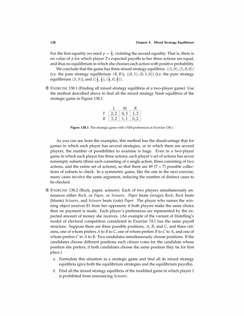
138 Chapter 4. Mixed Strategy Equilibrium
For the first equality we need p = 23 , violating the second equality. That is, there is
no value of p for which player 2’s expected payoffs to her three actions are equal,and thus no equilibrium in which she chooses each action with positive probability.
We conclude that the game has three mixed strategy equilibria: ((1, 0), (1, 0, 0))(i.e. the pure strategy equilibrium (B, B)), ((0, 1), (0, 1, 0)) (i.e. the pure strategyequilibrium (S, S)), and (( 3
4 , 14 ), ( 1
5 , 0, 45 )).
? EXERCISE 138.1 (Finding all mixed strategy equilibria of a two-player game) Usethe method described above to find all the mixed strategy Nash equilibria of thestrategic game in Figure 138.1.
L M RT 2, 2 0, 3 1, 3B 3, 2 1, 1 0, 2
Figure 138.1 The strategic game with vNM preferences in Exercise 138.1.
As you can see from the examples, this method has the disadvantage that forgames in which each player has several strategies, or in which there are severalplayers, the number of possibilities to examine is huge. Even in a two-playergame in which each player has three actions, each player’s set of actions has sevennonempty subsets (three each consisting of a single action, three consisting of twoactions, and the entire set of actions), so that there are 49 (7 × 7) possible collec-tions of subsets to check. In a symmetric game, like the one in the next exercise,many cases involve the same argument, reducing the number of distinct cases tobe checked.
? EXERCISE 138.2 (Rock, paper, scissors) Each of two players simultaneously an-nounces either Rock, or Paper, or Scissors. Paper beats (wraps) Rock, Rock beats(blunts) Scissors, and Scissors beats (cuts) Paper. The player who names the win-ning object receives $1 from her opponent; if both players make the same choicethen no payment is made. Each player’s preferences are represented by the ex-pected amount of money she receives. (An example of the variant of Hotelling’smodel of electoral competition considered in Exercise 74.1 has the same payoffstructure. Suppose there are three possible positions, A, B, and C, and three citi-zens, one of whom prefers A to B to C, one of whom prefers B to C to A, and one ofwhom prefers C to A to B. Two candidates simultaneously choose positions. If thecandidates choose different positions each citizen votes for the candidate whoseposition she prefers; if both candidates choose the same position they tie for firstplace.)
a. Formulate this situation as a strategic game and find all its mixed strategyequilibria (give both the equilibrium strategies and the equilibrium payoffs).
b. Find all the mixed strategy equilibria of the modified game in which player 1is prohibited from announcing Scissors.
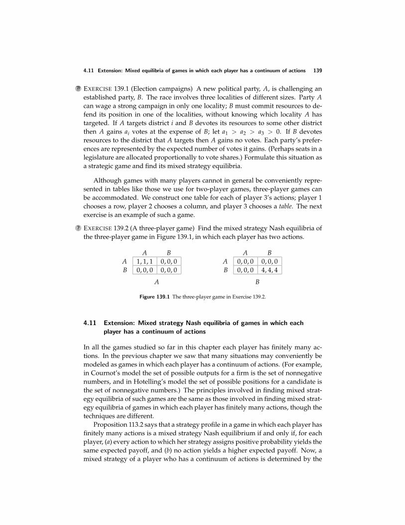
4.11 Extension: Mixed equilibria of games in which each player has a continuum of actions 139
?? EXERCISE 139.1 (Election campaigns) A new political party, A, is challenging anestablished party, B. The race involves three localities of different sizes. Party Acan wage a strong campaign in only one locality; B must commit resources to de-fend its position in one of the localities, without knowing which locality A hastargeted. If A targets district i and B devotes its resources to some other districtthen A gains ai votes at the expense of B; let a1 > a2 > a3 > 0. If B devotesresources to the district that A targets then A gains no votes. Each party’s prefer-ences are represented by the expected number of votes it gains. (Perhaps seats in alegislature are allocated proportionally to vote shares.) Formulate this situation asa strategic game and find its mixed strategy equilibria.
Although games with many players cannot in general be conveniently repre-sented in tables like those we use for two-player games, three-player games canbe accommodated. We construct one table for each of player 3’s actions; player 1chooses a row, player 2 chooses a column, and player 3 chooses a table. The nextexercise is an example of such a game.
? EXERCISE 139.2 (A three-player game) Find the mixed strategy Nash equilibria ofthe three-player game in Figure 139.1, in which each player has two actions.
A BA 1, 1, 1 0, 0, 0B 0, 0, 0 0, 0, 0
A
A BA 0, 0, 0 0, 0, 0B 0, 0, 0 4, 4, 4
B
Figure 139.1 The three-player game in Exercise 139.2.
4.11 Extension: Mixed strategy Nash equilibria of games in which each
player has a continuum of actions
In all the games studied so far in this chapter each player has finitely many ac-tions. In the previous chapter we saw that many situations may conveniently bemodeled as games in which each player has a continuum of actions. (For example,in Cournot’s model the set of possible outputs for a firm is the set of nonnegativenumbers, and in Hotelling’s model the set of possible positions for a candidate isthe set of nonnegative numbers.) The principles involved in finding mixed strat-egy equilibria of such games are the same as those involved in finding mixed strat-egy equilibria of games in which each player has finitely many actions, though thetechniques are different.
Proposition 113.2 says that a strategy profile in a game in which each player hasfinitely many actions is a mixed strategy Nash equilibrium if and only if, for eachplayer, (a) every action to which her strategy assigns positive probability yields thesame expected payoff, and (b) no action yields a higher expected payoff. Now, amixed strategy of a player who has a continuum of actions is determined by the
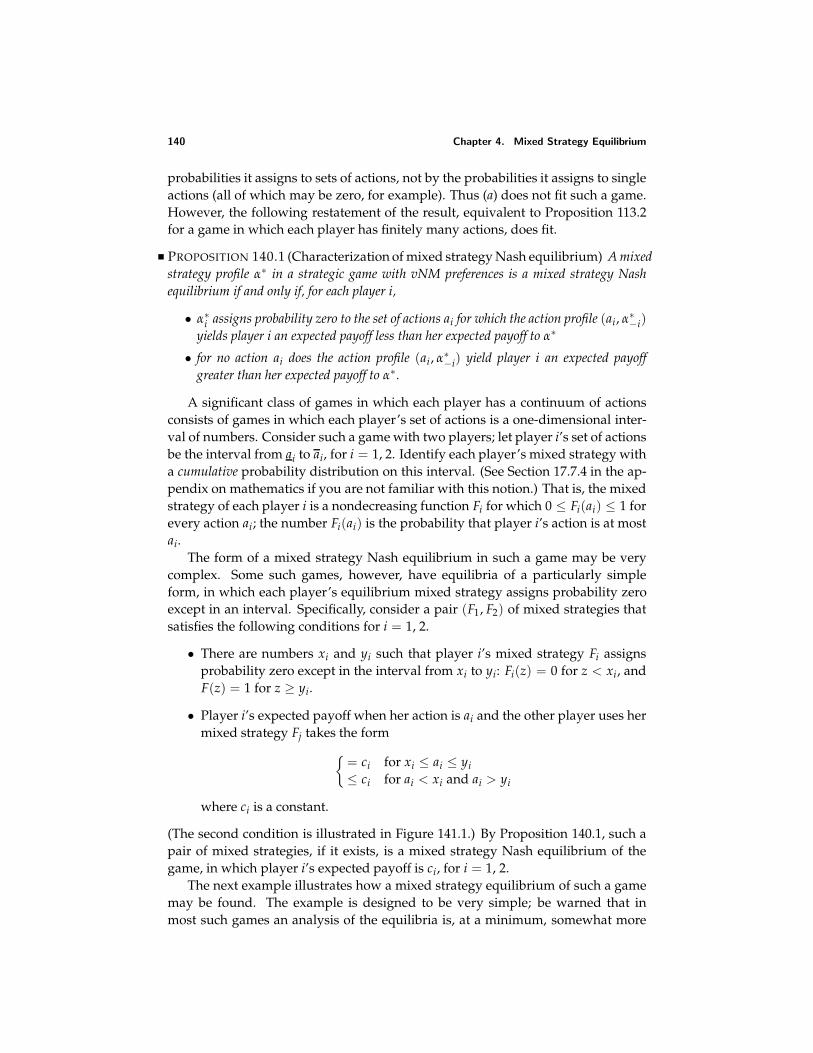
140 Chapter 4. Mixed Strategy Equilibrium
probabilities it assigns to sets of actions, not by the probabilities it assigns to singleactions (all of which may be zero, for example). Thus (a) does not fit such a game.However, the following restatement of the result, equivalent to Proposition 113.2for a game in which each player has finitely many actions, does fit.
PROPOSITION 140.1 (Characterization of mixed strategy Nash equilibrium) A mixedstrategy profile α∗ in a strategic game with vNM preferences is a mixed strategy Nashequilibrium if and only if, for each player i,
• α∗i assigns probability zero to the set of actions ai for which the action profile (ai, α∗
−i)yields player i an expected payoff less than her expected payoff to α∗
• for no action ai does the action profile (ai , α∗−i) yield player i an expected payoff
greater than her expected payoff to α∗.
A significant class of games in which each player has a continuum of actionsconsists of games in which each player’s set of actions is a one-dimensional inter-val of numbers. Consider such a game with two players; let player i’s set of actionsbe the interval from ai to ai, for i = 1, 2. Identify each player’s mixed strategy witha cumulative probability distribution on this interval. (See Section 17.7.4 in the ap-pendix on mathematics if you are not familiar with this notion.) That is, the mixedstrategy of each player i is a nondecreasing function Fi for which 0 ≤ Fi(ai) ≤ 1 forevery action ai; the number Fi(ai) is the probability that player i’s action is at mostai.
The form of a mixed strategy Nash equilibrium in such a game may be verycomplex. Some such games, however, have equilibria of a particularly simpleform, in which each player’s equilibrium mixed strategy assigns probability zeroexcept in an interval. Specifically, consider a pair (F1, F2) of mixed strategies thatsatisfies the following conditions for i = 1, 2.
• There are numbers xi and yi such that player i’s mixed strategy Fi assignsprobability zero except in the interval from xi to yi: Fi(z) = 0 for z < xi, andF(z) = 1 for z ≥ yi.
• Player i’s expected payoff when her action is ai and the other player uses hermixed strategy Fj takes the form
= ci for xi ≤ ai ≤ yi≤ ci for ai < xi and ai > yi
where ci is a constant.
(The second condition is illustrated in Figure 141.1.) By Proposition 140.1, such apair of mixed strategies, if it exists, is a mixed strategy Nash equilibrium of thegame, in which player i’s expected payoff is ci, for i = 1, 2.
The next example illustrates how a mixed strategy equilibrium of such a gamemay be found. The example is designed to be very simple; be warned that inmost such games an analysis of the equilibria is, at a minimum, somewhat more
4.11 Extension: Mixed equilibria of games in which each player has a continuum of actions 141
a1 x1 y1 a1a1 →
c1
Player 1’s expected payoff given F2
a2 x2 y2 a2a2 →
c2
Player 2’s expected payoff given F1
Figure 141.1 If (i) F1 assigns positive probability only to actions in the interval from x1 to y1, (ii) F2assigns positive probability only to the actions in the interval from x2 to y2, (iii) given player 2’s mixedstrategy F2, player 1’s expected payoff takes the form shown in the left panel, and (iv) given player 1’smixed strategy F1, player 2’s expected payoff takes the form shown in the right panel, then (F1, F2) is amixed strategy equilibrium.
complex. Further, my analysis is not complete: I merely find an equilibrium, ratherthan studying all equilibria. (In fact, the game has no other equilibria.)
EXAMPLE 141.1 (All-pay auction) Two people submit sealed bids for an objectworth $K to each of them. Each person’s bid may be any nonnegative numberup to $K. The winner is the person whose bid is higher; in the event of a tie eachperson receives half of the object, which she values at $K/2. Each person paysher bid, whether or not she wins, and has preferences represented by the expectedamount of money she receives.
This situation may be modeled by the following strategic game, known as anall-pay auction.
Players The two bidders.
Actions Each player’s set of actions is the set of possible bids (nonnegativenumbers up to K)
Payoff functions Each player i’s preferences are represented by the expectedvalue of the payoff function given by
ui(a1, a2) =
−ai if ai < ajK/2 − ai if ai = ajK − ai if ai > aj,
where j is the other player.
One situation that may be modeled as such an auction is a lobbying process inwhich each of two interest groups spends resources to persuade a government tocarry out the policy it prefers, and the group that spends the most wins. Anothersituation that may be modeled as such an auction is the competition between twofirms to develop a new product by some deadline, where the firm that spends themost develops a better product, which captures the entire market.
An all-pay auction has no pure strategy Nash equilibrium, by the followingargument.
142 Chapter 4. Mixed Strategy Equilibrium
• No pair of actions (x, x) with x < K is a Nash equilibrium, because eitherplayer can increase her payoff by slightly increasing her bid.
• (K, K) is not a Nash equilibrium, because either player can increase her payofffrom −K/2 to 0 by reducing her bid to 0.
• No pair of actions (a1, a2) with a1 = a2 is a Nash equilibrium because theplayer whose bid is higher can increase her payoff by reducing her bid (andthe player whose bid is lower can, if her bid is positive, increase her payoff byreducing her bid to 0).
Consider the possibility that the game has a mixed strategy Nash equilibrium.Denote by Fi the mixed strategy (i.e. cumulative probability distribution over theinterval of possible bids) of player i. I look for an equilibrium in which neithermixed strategy assigns positive probability to any single bid. (Remember that thereare infinitely many possible bids.) In this case Fi(ai) is both the probability thatplayer i bids at most ai and the probability that she bids less than ai. I furtherrestrict attention to strategy pairs (F1, F2) for which, for i = 1, 2, there are numbersxi and yi such that Fi assigns positive probability only to the interval from xi to yi.
To investigate the possibility of such an equilibrium, consider player 1’s ex-pected payoff when she uses the action a1, given player 2’s mixed strategy F2.
• If a1 < x2 then a1 is less than player 2’s bid with probability one, so thatplayer 1’s payoff is −a1.
• If a1 > y2 then a1 exceeds player 2’s bid with probability one, so that player 1’spayoff is K − a1.
• If x2 ≤ a1 ≤ y2 then player 1’s expected payoff is calculated as follows. Withprobability F2(a1) player 2’s bid is less than a1, in which case player 1’s payoffis K − a1; with probability 1 − F2(a1) player 2’s bid exceeds a1, in which caseplayer 1’s payoff is −a1; and, by assumption, the probability that player 2’sbid is exactly equal to a1 is zero. Thus player 1’s expected payoff is
(K − a1)F2(a1) + (−a1)(1 − F2(a1)) = KF2(a1) − a1.
We need to find values of x2 and y2 and a strategy F2 such that player 1’s ex-pected payoff satisfies the condition illustrated in the left panel of Figure 141.1: itis constant on the interval from x1 to y1, and less than this constant for a1 < x1 anda1 > y1. The constancy of the payoff on the interval from x1 to y1 requires thatKF2(a1) − a1 = c1 for x1 ≤ a1 ≤ y1, for some constant c1. We also need F2(x2) = 0and F2(y2) = 1 (because I am restricting attention to equilibria in which neitherplayer’s strategy assigns positive probability to any single action), and F2 mustbe nondecreasing (so that it is a cumulative probability distribution). Analogousconditions must be satisfied by x2, y2, and F1.
We see that if x1 = x2 = 0, y1 = y2 = K, and F1(z) = F2(z) = z/K for all z with0 ≤ z ≤ K then all these conditions are satisfied. Each player’s expected payoff isconstant, equal to 0 for all her actions a1.
4.12 Appendix: Representing preferences by expected payoffs 143
Thus the game has a mixed strategy Nash equilibrium in which each playerrandomizes “uniformly” over all her actions. In this equilibrium each player’sexpected payoff is 0: on average, the amount a player spends is exactly equal tothe value of the object. (A more involved argument shows that this equilibrium isthe only mixed strategy Nash equilibrium of the game.)
?? EXERCISE 143.1 (All-pay auction with many bidders) Consider the generalizationof the game considered in the previous example in which there are n ≥ 2 bidders.Find a mixed strategy Nash equilibrium in which each player uses the same mixedstrategy. (If you know how, find each player’s mean bid in the equilibrium.)
?? EXERCISE 143.2 (Bertrand’s duopoly game) Consider Bertrand’s oligopoly game(Section 3.2) when there are two firms. Assume that each firm’s preferences arerepresented by its expected profit. Show that if the function (p − c)D(p) is increas-ing in p, and increases without bound as p increases without bound, then for everyp > c, the game has a mixed strategy Nash equilibrium in which each firm usesthe same mixed strategy F, with F(p) = 0 and F(p) > 0 for p > p.
In the games in the example and exercises each player’s payoff depends onlyon her action and whether this action is greater than, equal to, or less than the otherplayers’ actions. The limited dependence of each player’s payoff on the other play-ers’ actions makes the calculation of a player’s expected payoff straightforward.In many games, each player’s payoff is affected more substantially by the otherplayers’ actions, making the calculation of expected payoff more complex; moresophisticated mathematical tools are required to analyze such games.
4.12 Appendix: Representing preferences over lotteries by the expected value
of a payoff function
4.12.1 Expected payoffs
Suppose that a decision-maker has preferences over a set of deterministic out-comes, and that each of her actions results in a lottery (probability distribution)over these outcomes. In order to determine the action she chooses, we need toknow her preferences over these lotteries. As argued in Section 4.1.3, we cannot de-rive these preferences from her preferences over deterministic outcomes, but haveto specify them as part of the model.
So assume that we are given the decision-maker’s preferences over lotteries.As in the case of preferences over deterministic outcomes, under some fairly weakassumptions we can represent these preferences by a payoff function. (Refer toSection 1.2.2.) That is, when there are K deterministic outcomes we can find afunction, say U, over lotteries such that
U(p1, . . . , pK) > U(p′1, . . . , p′K)
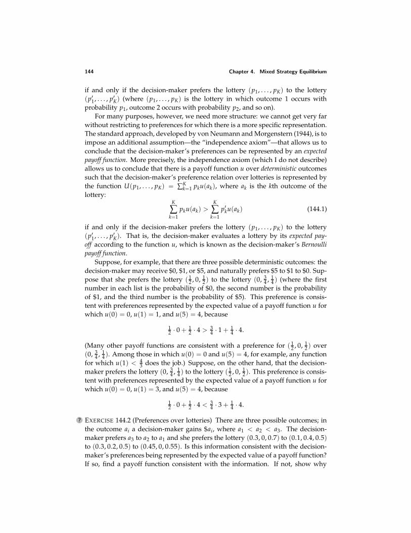
144 Chapter 4. Mixed Strategy Equilibrium
if and only if the decision-maker prefers the lottery (p1, . . . , pK) to the lottery(p′1, . . . , p′K) (where (p1, . . . , pK) is the lottery in which outcome 1 occurs withprobability p1, outcome 2 occurs with probability p2, and so on).
For many purposes, however, we need more structure: we cannot get very farwithout restricting to preferences for which there is a more specific representation.The standard approach, developed by von Neumann and Morgenstern (1944), is toimpose an additional assumption—the “independence axiom”—that allows us toconclude that the decision-maker’s preferences can be represented by an expectedpayoff function. More precisely, the independence axiom (which I do not describe)allows us to conclude that there is a payoff function u over deterministic outcomessuch that the decision-maker’s preference relation over lotteries is represented bythe function U(p1, . . . , pK) = ∑K
k=1 pku(ak), where ak is the kth outcome of thelottery:
K
∑k=1
pku(ak) >K
∑k=1
p′ku(ak) (144.1)
if and only if the decision-maker prefers the lottery (p1, . . . , pK) to the lottery(p′1, . . . , p′K). That is, the decision-maker evaluates a lottery by its expected pay-off according to the function u, which is known as the decision-maker’s Bernoullipayoff function.
Suppose, for example, that there are three possible deterministic outcomes: thedecision-maker may receive $0, $1, or $5, and naturally prefers $5 to $1 to $0. Sup-pose that she prefers the lottery ( 1
2 , 0, 12 ) to the lottery (0, 3
4 , 14 ) (where the first
number in each list is the probability of $0, the second number is the probabilityof $1, and the third number is the probability of $5). This preference is consis-tent with preferences represented by the expected value of a payoff function u forwhich u(0) = 0, u(1) = 1, and u(5) = 4, because
12 · 0 + 1
2 · 4 > 34 · 1 + 1
4 · 4.
(Many other payoff functions are consistent with a preference for ( 12 , 0, 1
2 ) over(0, 3
4 , 14 ). Among those in which u(0) = 0 and u(5) = 4, for example, any function
for which u(1) < 43 does the job.) Suppose, on the other hand, that the decision-
maker prefers the lottery (0, 34 , 1
4 ) to the lottery ( 12 , 0, 1
2 ). This preference is consis-tent with preferences represented by the expected value of a payoff function u forwhich u(0) = 0, u(1) = 3, and u(5) = 4, because
12 · 0 + 1
2 · 4 < 34 · 3 + 1
4 · 4.
? EXERCISE 144.2 (Preferences over lotteries) There are three possible outcomes; inthe outcome ai a decision-maker gains $ai, where a1 < a2 < a3. The decision-maker prefers a3 to a2 to a1 and she prefers the lottery (0.3, 0, 0.7) to (0.1, 0.4, 0.5)to (0.3, 0.2, 0.5) to (0.45, 0, 0.55). Is this information consistent with the decision-maker’s preferences being represented by the expected value of a payoff function?If so, find a payoff function consistent with the information. If not, show why
4.12 Appendix: Representing preferences by expected payoffs 145
not. Answer the same questions when, alternatively, the decision-maker prefersthe lottery (0.4, 0, 0.6) to (0, 0.5, 0.5) to (0.3, 0.2, 0.5) to (0.45, 0, 0.55).
Preferences represented by the expected value of a (Bernoulli) payoff functionhave the great advantage that they are completely specified by that payoff func-tion. Once we know u(ak) for each possible outcome ak we know the decision-maker’s preferences among all lotteries. This significant advantage does, how-ever, carry with it a small price: it is very easy to confuse a Bernoulli payoff func-tion with a payoff function that represents the decision-maker’s preferences overdeterministic outcomes.
To describe the relation between the two, suppose that a decision-maker’s pref-erences over lotteries are represented by the expected value of the Bernoulli pay-off function u. Then certainly u is a payoff function that represents the decision-maker’s preferences over deterministic outcomes (which are special cases of lotter-ies, in which a single outcome is assigned probability 1). However, the converse isnot true: if the decision-maker’s preferences over deterministic outcomes are repre-sented by the payoff function u (i.e. the decision-maker prefers a to a′ if and only ifu(a) > u(a′)), then u is not necessarily a Bernoulli payoff function whose expectedvalue represents the decision-maker’s preferences over lotteries. For instance, sup-pose that the decision-maker prefers $5 to $1 to $0, and prefers the lottery ( 1
2 , 0, 12 )
to the lottery (0, 34 , 1
4 ). Then her preferences over deterministic outcomes are con-sistent with the payoff function u for which u(0) = 0, u(1) = 3, and u(5) = 4.However, her preferences over lotteries are not consistent with the expected valueof this function (since 1
2 · 0 + 12 · 4 < 3
4 · 3 + 14 · 4). The moral is that you should be
careful to determine the type of payoff function you are dealing with.
4.12.2 Equivalent Bernoulli payoff functions
If a decision-maker’s preferences in a deterministic environment are representedby the payoff function u then they are represented also by any payoff function thatis an increasing function of u (see Section 1.2.2). The analogous property is notsatisfied by Bernoulli payoff functions. Consider the example discussed above. ABernoulli payoff function u for which u(0) = 0, u(1) = 1, and u(5) = 4 is consistentwith a preference for the lottery ( 1
2 , 0, 12 ) over (0, 3
4 , 14 ), but the function
√u, for
which u(0) = 0, u(1) = 1, and u(5) = 2, is not consistent with such a preference( 1
2 · 0 + 12 · 2 < 3
4 · 1 + 14 · 2), though the square root function is increasing (larger
numbers have larger square roots).Under what circumstances do the expected values of two Bernoulli payoff func-
tions represent the same preferences? The next result shows that they do so if andonly if one payoff function is an increasing linear function of the other.
LEMMA 145.1 (Equivalence of Bernoulli payoff functions) Suppose there are at leastthree possible outcomes. The expected values of the Bernoulli payoff functions u and vrepresent the same preferences over lotteries if and only if there exist numbers η and θ withθ > 0 such that u(x) = η + θv(x) for all x.
146 Chapter 4. Mixed Strategy Equilibrium
If the expected value of u represents a decision-maker’s preferences over lot-teries then so, for example, do the expected values of 2u, 1 + u, and −1 + 4u; butthe expected values of u2 and of
√u do not.
Part of the lemma is easy to establish. Let u be a Bernoulli payoff functionwhose expected value represents a decision-maker’s preferences, and let v(x) =η + θu(x) for all x, where η and θ are constants with θ > 0. I argue that the expectedvalues of u and of v represent the same preferences. Suppose that the decision-maker prefers the lottery (p1, . . . , pK) to the lottery (p′1, . . . , p′K). Then her expectedpayoff to (p1, . . . , pK) exceeds her expected payoff to (p′1, . . . , p′K), or
K
∑k=1
pku(ak) >K
∑k=1
p′ku(ak) (146.1)
(see (144.1)). Now,
K
∑k=1
pkv(ak) =K
∑k=1
pkη +K
∑k=1
pkθu(ak) = η + θK
∑k=1
pku(ak),
using the fact that the sum of the probabilities pk is 1. Similarly,
K
∑k=1
p′kv(ak) = η + θK
∑k=1
p′ku(ak).
Substituting for u in (146.1) we obtain(
K
∑k=1
pkv(ak) − η
)/θ >
(K
∑k=1
p′kv(ak) − η
)/θ,
which, given θ > 0, is equivalent to
K
∑k=1
pkv(ak) >K
∑k=1
p′kv(ak) :
according to v, the expected payoff of (p1, . . . , pK) exceeds the expected payoff of(p′1, . . . , p′K). We conclude that if u represents the decision-maker’s preferencesthen so does the function v defined by v(x) = η + θu(x).
I omit the more difficult argument that if the expected values of the Bernoullipayoff functions u and v represent the same preferences over lotteries then v(x) =η + θu(x) for some constants η and θ > 0.
? EXERCISE 146.2 (Normalized Bernoulli payoff functions) Suppose that a decision-maker’s preferences can be represented by the expected value of the Bernoulli pay-off function u. Find a Bernoulli payoff function whose expected value representsthe decision-maker’s preferences and that assigns a payoff of 1 to the best outcomeand a payoff of 0 to the worst outcome.

4.12 Appendix: Representing preferences by expected payoffs 147
4.12.3 Equivalent strategic games with vNM preferences
Turning to games, consider the three payoff tables in Figure 147.1. All three tablesrepresent the same strategic game with deterministic preferences: in each case,player 1 prefers (B, B) to (S, S) to (B, S), which she regards as indifferent to (S, B),and player 2 prefers (S, S) to (B, B) to (B, S), which she regards as indifferent to(S, B). However, only the left and middle tables represent the same strategic gamewith vNM preferences. The reason is that the payoff functions in the middle ta-ble are linear functions of the payoff functions in the left table, whereas the pay-off functions in the right table are not. Specifically, denote the Bernoulli payofffunctions of player i in the three games by ui, vi, and wi. Then
v1(a) = 2u1(a) and v2(a) = −3 + 3u2(a),
so that the left and middle tables represent the same strategic game with vNMpreferences. However, w1 is not a linear function of u1. If it were, there wouldexist constants η and θ > 0 such that w1(a) = η + θu1(a) for each action pair a, or
0 = η + θ · 0
1 = η + θ · 1
3 = η + θ · 2,
but these three equations have no solution. Thus the left and right tables representdifferent strategic games with vNM preferences. (As you can check, w2 is not alinear function of u2 either; but for the games not to be equivalent it is sufficientthat one player’s preferences be different.) Another way to see that player 1’s vNMpreferences in the left and right games are different is to note that in the left tableplayer 1 is indifferent between the certain outcome (S, S) and the lottery in which(B, B) occurs with probability 1
2 and (S, B) occurs with probability 12 (each yields
an expected payoff of 1), whereas in the right table she prefers the latter (since ityields an expected payoff of 1.5).
B SB 2, 1 0, 0S 0, 0 1, 2
B SB 4, 0 0, −3S 0, −3 2, 3
B SB 3, 2 0, 1S 0, 1 1, 4
Figure 147.1 All three tables represent the same strategic game with ordinal preferences, but only theleft and middle games, not the right one, represent the same strategic game with vNM preferences.
? EXERCISE 147.1 (Games equivalent to the Prisoner’s Dilemma) Which of the tablesin Figure 148.1 represents the same strategic game with vNM preferences as thePrisoner’s Dilemma as specified in the left panel of Figure 104.1, when the numbersare interpreted as Bernoulli payoffs?
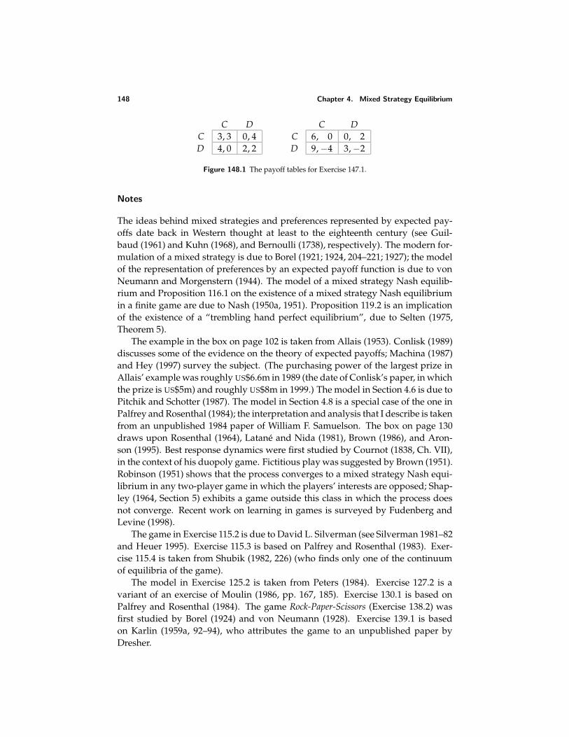
148 Chapter 4. Mixed Strategy Equilibrium
C DC 3, 3 0, 4D 4, 0 2, 2
C DC 6, 0 0, 2D 9, −4 3, −2
Figure 148.1 The payoff tables for Exercise 147.1.
Notes
The ideas behind mixed strategies and preferences represented by expected pay-offs date back in Western thought at least to the eighteenth century (see Guil-baud (1961) and Kuhn (1968), and Bernoulli (1738), respectively). The modern for-mulation of a mixed strategy is due to Borel (1921; 1924, 204–221; 1927); the modelof the representation of preferences by an expected payoff function is due to vonNeumann and Morgenstern (1944). The model of a mixed strategy Nash equilib-rium and Proposition 116.1 on the existence of a mixed strategy Nash equilibriumin a finite game are due to Nash (1950a, 1951). Proposition 119.2 is an implicationof the existence of a “trembling hand perfect equilibrium”, due to Selten (1975,Theorem 5).
The example in the box on page 102 is taken from Allais (1953). Conlisk (1989)discusses some of the evidence on the theory of expected payoffs; Machina (1987)and Hey (1997) survey the subject. (The purchasing power of the largest prize inAllais’ example was roughly US$6.6m in 1989 (the date of Conlisk’s paper, in whichthe prize is US$5m) and roughly US$8m in 1999.) The model in Section 4.6 is due toPitchik and Schotter (1987). The model in Section 4.8 is a special case of the one inPalfrey and Rosenthal (1984); the interpretation and analysis that I describe is takenfrom an unpublished 1984 paper of William F. Samuelson. The box on page 130draws upon Rosenthal (1964), Latane and Nida (1981), Brown (1986), and Aron-son (1995). Best response dynamics were first studied by Cournot (1838, Ch. VII),in the context of his duopoly game. Fictitious play was suggested by Brown (1951).Robinson (1951) shows that the process converges to a mixed strategy Nash equi-librium in any two-player game in which the players’ interests are opposed; Shap-ley (1964, Section 5) exhibits a game outside this class in which the process doesnot converge. Recent work on learning in games is surveyed by Fudenberg andLevine (1998).
The game in Exercise 115.2 is due to David L. Silverman (see Silverman 1981–82and Heuer 1995). Exercise 115.3 is based on Palfrey and Rosenthal (1983). Exer-cise 115.4 is taken from Shubik (1982, 226) (who finds only one of the continuumof equilibria of the game).
The model in Exercise 125.2 is taken from Peters (1984). Exercise 127.2 is avariant of an exercise of Moulin (1986, pp. 167, 185). Exercise 130.1 is based onPalfrey and Rosenthal (1984). The game Rock-Paper-Scissors (Exercise 138.2) wasfirst studied by Borel (1924) and von Neumann (1928). Exercise 139.1 is basedon Karlin (1959a, 92–94), who attributes the game to an unpublished paper byDresher.
Notes 149
Exercise 143.1 is based on a result in Baye, Kovenock, and de Vries (1996). Themixed strategy Nash equilibria of Bertrand’s model of duopoly (Exercise 143.2) arestudied in detail by Baye and Morgan (1996).
The method of finding all mixed strategy equilibrium described in Section 4.10is computationally very intense in all but the simplest games. Some computation-ally more efficient methods are implemented in the computer program GAMBIT,located at http://www.hss.caltech.edu/\symbol126gambit/Gambit.html.
Draft chapter from An introduction to game theory by Martin J. [email protected]; www.economics.utoronto.ca/osborneVersion: 00/11/6.Copyright c© 1995–2000 by Martin J. Osborne. All rights reserved. No part of this book may be re-produced by any electronic or mechanical means (including photocopying, recording, or informationstorage and retrieval) without permission in writing from Oxford University Press, except that onecopy of up to six chapters may be made by any individual for private study.
5 Extensive Games with Perfect Information:Theory
Extensive games with perfect information 151Nash equilibrium 159Subgame perfect equilibrium 162Prerequisite: Chapters 1 and 2.
5.1 Introduction
THE model of a strategic game suppresses the sequential structure of decision-making. When applying the model to situations in which decision-makers
move sequentially, we assume that each decision-maker chooses her plan of actiononce and for all; she is committed to this plan, which she cannot modify as eventsunfold. The model of an extensive game, by contrast, describes the sequentialstructure of decision-making explicitly, allowing us to study situations in whicheach decision-maker is free to change her mind as events unfold.
In this chapter and the next two we study a model in which each decision-maker is always fully informed about all previous actions. In Chapter 10 we studya more general model, which allows each decision-maker, when taking an action,to be imperfectly informed about previous actions.
5.2 Extensive games with perfect information
5.2.1 Definition
To describe an extensive game with perfect information, we need to specify theset of players and their preferences, as for a strategic game (Definition 11.1). Inaddition, we need to specify the order of the players’ moves and the actions eachplayer may take at each point. We do so by specifying the set of all sequences ofactions that can possibly occur, together with the player who moves at each pointin each sequence. We refer to each possible sequence of actions as a terminal historyand to the function that gives the player who moves at each point in each terminalhistory as the player function. That is, an extensive game has four components:
• players
• terminal histories
151
152 Chapter 5. Extensive Games with Perfect Information: Theory
• player function
• preferences for the players.
Before giving precise definitions of these components, I give an example that illus-trates them informally.
EXAMPLE 152.1 (Entry game) An incumbent faces the possibility of entry by achallenger. (The challenger may, for example, be a firm considering entry intoan industry currently occupied by a monopolist, a politician competing for theleadership of a party, or an animal considering competing for the right to matewith a congener of the opposite sex.) The challenger may enter or not. If it enters,the incumbent may either acquiesce or fight.
We may model this situation as an extensive game with perfect information inwhich the terminal histories are (In, Acquiesce), (In, Fight), and Out, and the playerfunction assigns the challenger to the start of the game and the incumbent to thehistory In.
At the start of an extensive game, and after any sequence of events, a playerchooses an action. The sets of actions available to the players are not, however,given explicitly in the description of the game. Instead, the description of the gamespecifies the set of terminal histories and the player function, from which we candeduce the available sets of actions.
In the entry game, for example, the actions available to the challenger at thestart of the game are In and Out, because these actions (and no others) begin ter-minal histories, and the actions available to the incumbent are Acquiesce and Fight,because these actions (and no others) follow In in terminal histories. More gener-ally, suppose that (C, D) and (C, E) are terminal histories and the player functionassigns player 1 to the start of the game and player 2 to the history C. Then twoof the actions available to player 2 after player 1 chooses C at the start of the gameare D and E.
The terminal histories of a game are specified as a set of sequences. But notevery set of sequences is a legitimate set of terminal histories. If (C, D) is a terminalhistory, for example, there is no sense in specifying C as a terminal history: the factthat (C, D) is terminal implies that after C is chosen at the start of the game, someplayer may choose D, so that the action C does not end the game. More generally,a sequence that is a proper subhistory of a terminal history cannot itself be a terminalhistory. This restriction is the only one we need to impose on a set of sequences inorder that the set be interpretable as a set of terminal histories.
To state the restriction precisely, define the subhistories of a finite sequence(a1, a2, . . . , ak) of actions to be the empty sequence consisting of no actions, de-noted ∅ (representing the start of the game), and all sequences of the form (a1, a2, . . . , am)where 1 ≤ m ≤ k. (In particular, the entire sequence is a subhistory of itself.) Sim-ilarly, define the subhistories of an infinite sequence (a1, a2, . . .) of actions to bethe empty sequence ∅, every sequence of the form (a1, a2, . . . , am) where m is apositive integer, and the entire sequence (a1, a2, . . .). A subhistory not equal to
5.2 Extensive games with perfect information 153
the entire sequence is called a proper subhistory. A sequence of actions that is asubhistory of some terminal history is called simply a history.
In the entry game in Example 152.1, the subhistories of (In, Acquiesce) are theempty history ∅ and the sequences In and (In, Acquiesce); the proper subhistoriesare the empty history and the sequence In.
DEFINITION 153.1 (Extensive game with perfect information) An extensive gamewith perfect information consists of
• a set of players
• a set of sequences (terminal histories) with the property that no sequence isa proper subhistory of any other sequence
• a function (the player function) that assigns a player to every sequence thatis a proper subhistory of some terminal history
• for each player, preferences over the set of terminal histories.
The set of terminal histories is the set of all sequences of actions that may occur;the player assigned by the player function to any history h is the player who takesan action after h.
As for a strategic game, we may specify a player’s preferences by giving a pay-off function that represents them (see Section 1.2.2). In some situations an outcomeis associated with each terminal history, and the players’ preferences are naturallydefined over these outcomes, rather than directly over the terminal histories. Forexample, if we are modeling firms choosing prices then we may think in terms ofeach firm’s caring about its profit—the outcome of a profile of prices—rather thandirectly about the profile of prices. However, any preferences over outcomes (e.g.profits) may be translated into preferences over terminal histories (e.g. sequencesof prices). In the general definition, outcomes are conveniently identified with ter-minal histories and preferences are defined directly over these histories, avoidingthe need for an additional element in the specification of the game.
EXAMPLE 153.2 (Entry game) In the situation described in Example 152.1, supposethat the best outcome for the challenger is that it enters and the incumbent acqui-esces, and the worst outcome is that it enters and the incumbent fights, whereasthe best outcome for the incumbent is that the challenger stays out, and the worstoutcome is that it enters and there is a fight. Then the situation may be modeled asthe following extensive game with perfect information.
Players The challenger and the incumbent.
Terminal histories (In, Acquiesce), (In, Fight), and Out.
Player function P(∅) = Challenger and P(In) = Incumbent.
Preferences The challenger’s preferences are represented by the payoff func-tion u1 for which u1(In, Acquiesce) = 2, u1(Out) = 1, and u1(In, Fight) = 0,and the incumbent’s preferences are represented by the payoff function u2 forwhich u2(Out) = 2, u2(In, Acquiesce) = 1, and u2(In, Fight) = 0.
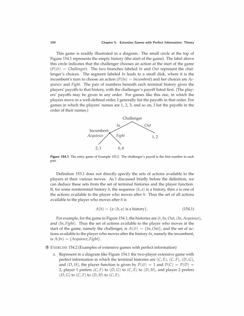
154 Chapter 5. Extensive Games with Perfect Information: Theory
This game is readily illustrated in a diagram. The small circle at the top ofFigure 154.1 represents the empty history (the start of the game). The label abovethis circle indicates that the challenger chooses an action at the start of the game(P(∅) = Challenger). The two branches labeled In and Out represent the chal-lenger’s choices. The segment labeled In leads to a small disk, where it is theincumbent’s turn to choose an action (P(In) = Incumbent) and her choices are Ac-quiesce and Fight. The pair of numbers beneath each terminal history gives theplayers’ payoffs to that history, with the challenger’s payoff listed first. (The play-ers’ payoffs may be given in any order. For games like this one, in which theplayers move in a well-defined order, I generally list the payoffs in that order. Forgames in which the players’ names are 1, 2, 3, and so on, I list the payoffs in theorder of their names.)
Challenger
In Out
1, 2
IncumbentAcquiesce Fight
2, 1 0, 0
Figure 154.1 The entry game of Example 153.2. The challenger’s payoff is the first number in eachpair.
Definition 153.1 does not directly specify the sets of actions available to theplayers at their various moves. As I discussed briefly before the definition, wecan deduce these sets from the set of terminal histories and the player function.If, for some nonterminal history h, the sequence (h, a) is a history, then a is one ofthe actions available to the player who moves after h. Thus the set of all actionsavailable to the player who moves after h is
A(h) = a: (h, a) is a history. (154.1)
For example, for the game in Figure 154.1, the histories are ∅, In, Out, (In, Acquiesce),and (In, Fight). Thus the set of actions available to the player who moves at thestart of the game, namely the challenger, is A(∅) = In, Out, and the set of ac-tions available to the player who moves after the history In, namely the incumbent,is A(In) = Acquiesce, Fight.
? EXERCISE 154.2 (Examples of extensive games with perfect information)
a. Represent in a diagram like Figure 154.1 the two-player extensive game withperfect information in which the terminal histories are (C, E), (C, F), (D, G),and (D, H), the player function is given by P(∅) = 1 and P(C) = P(D) =2, player 1 prefers (C, F) to (D, G) to (C, E) to (D, H), and player 2 prefers(D, G) to (C, F) to (D, H) to (C, E).
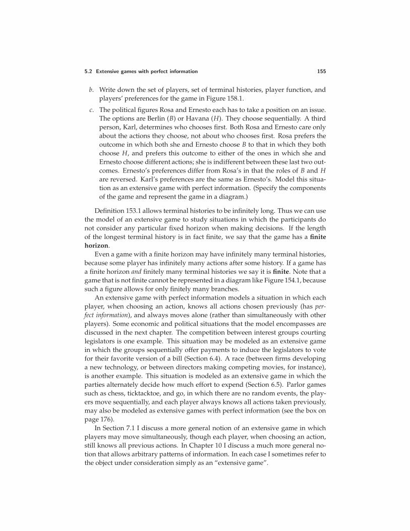
5.2 Extensive games with perfect information 155
b. Write down the set of players, set of terminal histories, player function, andplayers’ preferences for the game in Figure 158.1.
c. The political figures Rosa and Ernesto each has to take a position on an issue.The options are Berlin (B) or Havana (H). They choose sequentially. A thirdperson, Karl, determines who chooses first. Both Rosa and Ernesto care onlyabout the actions they choose, not about who chooses first. Rosa prefers theoutcome in which both she and Ernesto choose B to that in which they bothchoose H, and prefers this outcome to either of the ones in which she andErnesto choose different actions; she is indifferent between these last two out-comes. Ernesto’s preferences differ from Rosa’s in that the roles of B and Hare reversed. Karl’s preferences are the same as Ernesto’s. Model this situa-tion as an extensive game with perfect information. (Specify the componentsof the game and represent the game in a diagram.)
Definition 153.1 allows terminal histories to be infinitely long. Thus we can usethe model of an extensive game to study situations in which the participants donot consider any particular fixed horizon when making decisions. If the lengthof the longest terminal history is in fact finite, we say that the game has a finitehorizon.
Even a game with a finite horizon may have infinitely many terminal histories,because some player has infinitely many actions after some history. If a game hasa finite horizon and finitely many terminal histories we say it is finite. Note that agame that is not finite cannot be represented in a diagram like Figure 154.1, becausesuch a figure allows for only finitely many branches.
An extensive game with perfect information models a situation in which eachplayer, when choosing an action, knows all actions chosen previously (has per-fect information), and always moves alone (rather than simultaneously with otherplayers). Some economic and political situations that the model encompasses arediscussed in the next chapter. The competition between interest groups courtinglegislators is one example. This situation may be modeled as an extensive gamein which the groups sequentially offer payments to induce the legislators to votefor their favorite version of a bill (Section 6.4). A race (between firms developinga new technology, or between directors making competing movies, for instance),is another example. This situation is modeled as an extensive game in which theparties alternately decide how much effort to expend (Section 6.5). Parlor gamessuch as chess, ticktacktoe, and go, in which there are no random events, the play-ers move sequentially, and each player always knows all actions taken previously,may also be modeled as extensive games with perfect information (see the box onpage 176).
In Section 7.1 I discuss a more general notion of an extensive game in whichplayers may move simultaneously, though each player, when choosing an action,still knows all previous actions. In Chapter 10 I discuss a much more general no-tion that allows arbitrary patterns of information. In each case I sometimes refer tothe object under consideration simply as an “extensive game”.
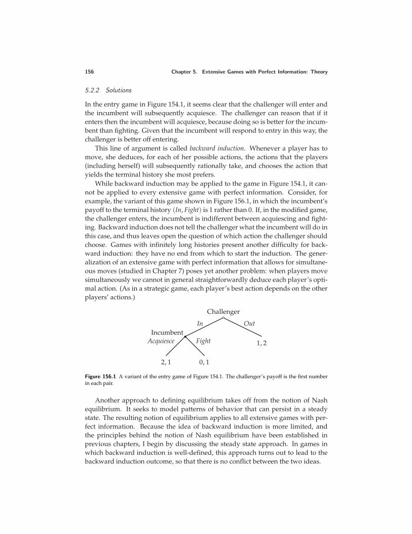
156 Chapter 5. Extensive Games with Perfect Information: Theory
5.2.2 Solutions
In the entry game in Figure 154.1, it seems clear that the challenger will enter andthe incumbent will subsequently acquiesce. The challenger can reason that if itenters then the incumbent will acquiesce, because doing so is better for the incum-bent than fighting. Given that the incumbent will respond to entry in this way, thechallenger is better off entering.
This line of argument is called backward induction. Whenever a player has tomove, she deduces, for each of her possible actions, the actions that the players(including herself) will subsequently rationally take, and chooses the action thatyields the terminal history she most prefers.
While backward induction may be applied to the game in Figure 154.1, it can-not be applied to every extensive game with perfect information. Consider, forexample, the variant of this game shown in Figure 156.1, in which the incumbent’spayoff to the terminal history (In, Fight) is 1 rather than 0. If, in the modified game,the challenger enters, the incumbent is indifferent between acquiescing and fight-ing. Backward induction does not tell the challenger what the incumbent will do inthis case, and thus leaves open the question of which action the challenger shouldchoose. Games with infinitely long histories present another difficulty for back-ward induction: they have no end from which to start the induction. The gener-alization of an extensive game with perfect information that allows for simultane-ous moves (studied in Chapter 7) poses yet another problem: when players movesimultaneously we cannot in general straightforwardly deduce each player’s opti-mal action. (As in a strategic game, each player’s best action depends on the otherplayers’ actions.)
Challenger
In Out
1, 2
IncumbentAcquiesce Fight
2, 1 0, 1
Figure 156.1 A variant of the entry game of Figure 154.1. The challenger’s payoff is the first numberin each pair.
Another approach to defining equilibrium takes off from the notion of Nashequilibrium. It seeks to model patterns of behavior that can persist in a steadystate. The resulting notion of equilibrium applies to all extensive games with per-fect information. Because the idea of backward induction is more limited, andthe principles behind the notion of Nash equilibrium have been established inprevious chapters, I begin by discussing the steady state approach. In games inwhich backward induction is well-defined, this approach turns out to lead to thebackward induction outcome, so that there is no conflict between the two ideas.
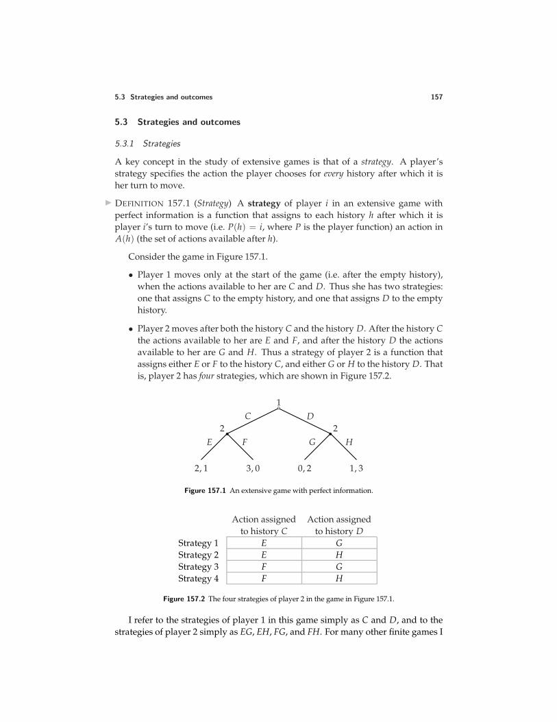
5.3 Strategies and outcomes 157
5.3 Strategies and outcomes
5.3.1 Strategies
A key concept in the study of extensive games is that of a strategy. A player’sstrategy specifies the action the player chooses for every history after which it isher turn to move.
DEFINITION 157.1 (Strategy) A strategy of player i in an extensive game withperfect information is a function that assigns to each history h after which it isplayer i’s turn to move (i.e. P(h) = i, where P is the player function) an action inA(h) (the set of actions available after h).
Consider the game in Figure 157.1.
• Player 1 moves only at the start of the game (i.e. after the empty history),when the actions available to her are C and D. Thus she has two strategies:one that assigns C to the empty history, and one that assigns D to the emptyhistory.
• Player 2 moves after both the history C and the history D. After the history Cthe actions available to her are E and F, and after the history D the actionsavailable to her are G and H. Thus a strategy of player 2 is a function thatassigns either E or F to the history C, and either G or H to the history D. Thatis, player 2 has four strategies, which are shown in Figure 157.2.
1C D
2E F
2, 1 3, 0
2G H
0, 2 1, 3
Figure 157.1 An extensive game with perfect information.
Action assignedto history C
Action assignedto history D
Strategy 1 E GStrategy 2 E HStrategy 3 F GStrategy 4 F H
Figure 157.2 The four strategies of player 2 in the game in Figure 157.1.
I refer to the strategies of player 1 in this game simply as C and D, and to thestrategies of player 2 simply as EG, EH, FG, and FH. For many other finite games I
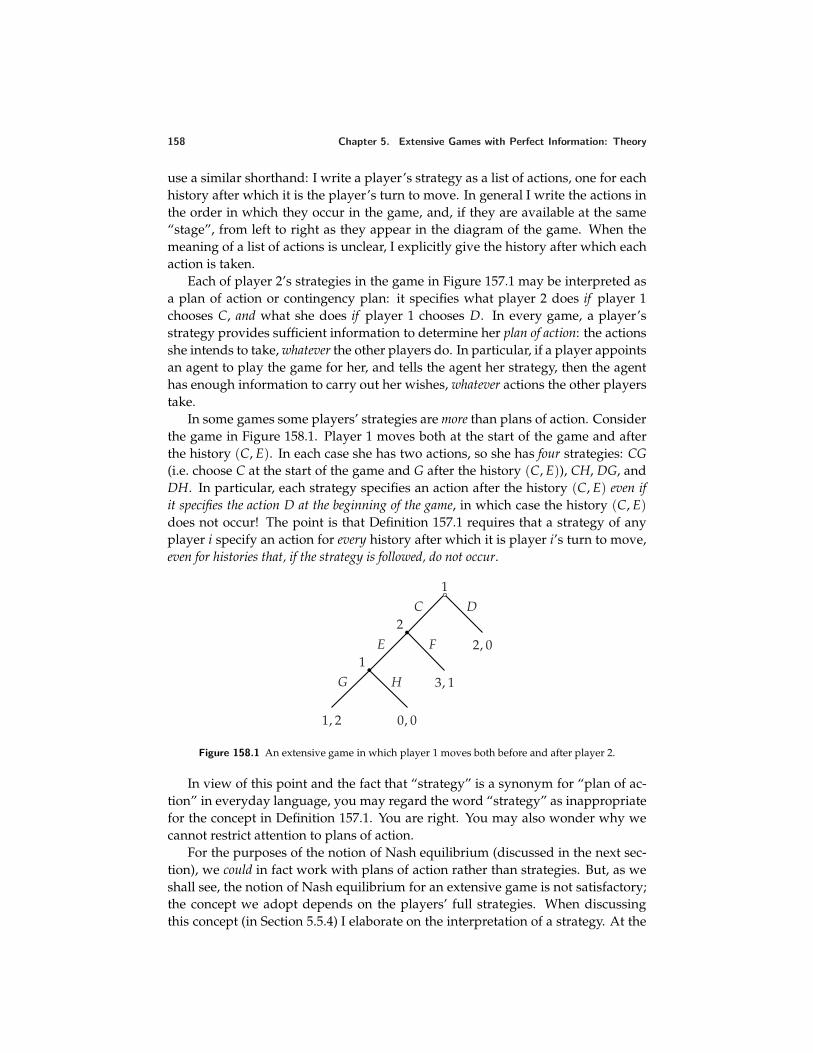
158 Chapter 5. Extensive Games with Perfect Information: Theory
use a similar shorthand: I write a player’s strategy as a list of actions, one for eachhistory after which it is the player’s turn to move. In general I write the actions inthe order in which they occur in the game, and, if they are available at the same“stage”, from left to right as they appear in the diagram of the game. When themeaning of a list of actions is unclear, I explicitly give the history after which eachaction is taken.
Each of player 2’s strategies in the game in Figure 157.1 may be interpreted asa plan of action or contingency plan: it specifies what player 2 does if player 1chooses C, and what she does if player 1 chooses D. In every game, a player’sstrategy provides sufficient information to determine her plan of action: the actionsshe intends to take, whatever the other players do. In particular, if a player appointsan agent to play the game for her, and tells the agent her strategy, then the agenthas enough information to carry out her wishes, whatever actions the other playerstake.
In some games some players’ strategies are more than plans of action. Considerthe game in Figure 158.1. Player 1 moves both at the start of the game and afterthe history (C, E). In each case she has two actions, so she has four strategies: CG(i.e. choose C at the start of the game and G after the history (C, E)), CH, DG, andDH. In particular, each strategy specifies an action after the history (C, E) even ifit specifies the action D at the beginning of the game, in which case the history (C, E)does not occur! The point is that Definition 157.1 requires that a strategy of anyplayer i specify an action for every history after which it is player i’s turn to move,even for histories that, if the strategy is followed, do not occur.
1C D
2, 0
2E F
3, 1
1G H
1, 2 0, 0
Figure 158.1 An extensive game in which player 1 moves both before and after player 2.
In view of this point and the fact that “strategy” is a synonym for “plan of ac-tion” in everyday language, you may regard the word “strategy” as inappropriatefor the concept in Definition 157.1. You are right. You may also wonder why wecannot restrict attention to plans of action.
For the purposes of the notion of Nash equilibrium (discussed in the next sec-tion), we could in fact work with plans of action rather than strategies. But, as weshall see, the notion of Nash equilibrium for an extensive game is not satisfactory;the concept we adopt depends on the players’ full strategies. When discussingthis concept (in Section 5.5.4) I elaborate on the interpretation of a strategy. At the
5.4 Nash equilibrium 159
moment, you may think of a player’s strategy as a plan of what to do, whateverthe other players do, both if the player carries out her intended actions, and alsoif she makes mistakes. For example, we can interpret the strategy DG of player 1in the game in Figure 158.1 to mean “I intend to choose D, but if I make a mistakeand choose C instead then I will subsequently choose G”. (Because the notion ofNash equilibrium depends only on plans of action, I could delay the definition of astrategy to the start of Section 5.5. I do not do so because the notion of a strategy iscentral to the study of extensive games, and its precise definition is much simplerthan that of a plan of action.)
? EXERCISE 159.1 (Strategies in extensive games) What are the strategies of the play-ers in the entry game (Example 153.2)? What are Rosa’s strategies in the game inExercise 154.2c?
5.3.2 Outcomes
A strategy profile determines the terminal history that occurs. Denote the strategyprofile by s and the player function by P. At the start of the game player P(∅)moves. Her strategy is sP(∅), and she chooses the action sP(∅)(∅). Denote this ac-tion by a1. If the history a1 is not terminal, player P(a1) moves next. Her strategyis sP(a1), and she chooses the action sP(a1)(a1). Denote this action by a2. If the his-tory (a1, a2) is not terminal, then again the player function specifies whose turn itis to move, and that player’s strategy specifies the action she chooses. The processcontinues until a terminal history is constructed. We refer to this terminal historyas the outcome of s, and denote it O(s).
In the game in Figure 158.1, for example, the outcome of the strategy pair(DG, E) is the terminal history D, and the outcome of (CH, E) is the terminalhistory (C, E, H).
Note that the outcome O(s) of the strategy profile s depends only on the play-ers’ plans of action, not their full strategies. That is, to determine O(s) we do notneed to refer to any component of any player’s strategy that specifies her actionsafter histories precluded by that strategy.
5.4 Nash equilibrium
As for strategic games, we are interested in notions of equilibrium that model theplayers’ behavior in a steady state. That is, we look for patterns of behavior withthe property that if every player knows every other player’s behavior, she has noreason to change her own behavior. I start by defining a Nash equilibrium: a strat-egy profile from which no player wishes to deviate, given the other players’ strate-gies. The definition is an adaptation of that of a Nash equilibrium in a strategicgame (21.1).
DEFINITION 159.2 (Nash equilibrium of extensive game with perfect information) Thestrategy profile s∗ in an extensive game with perfect information is a Nash equi-
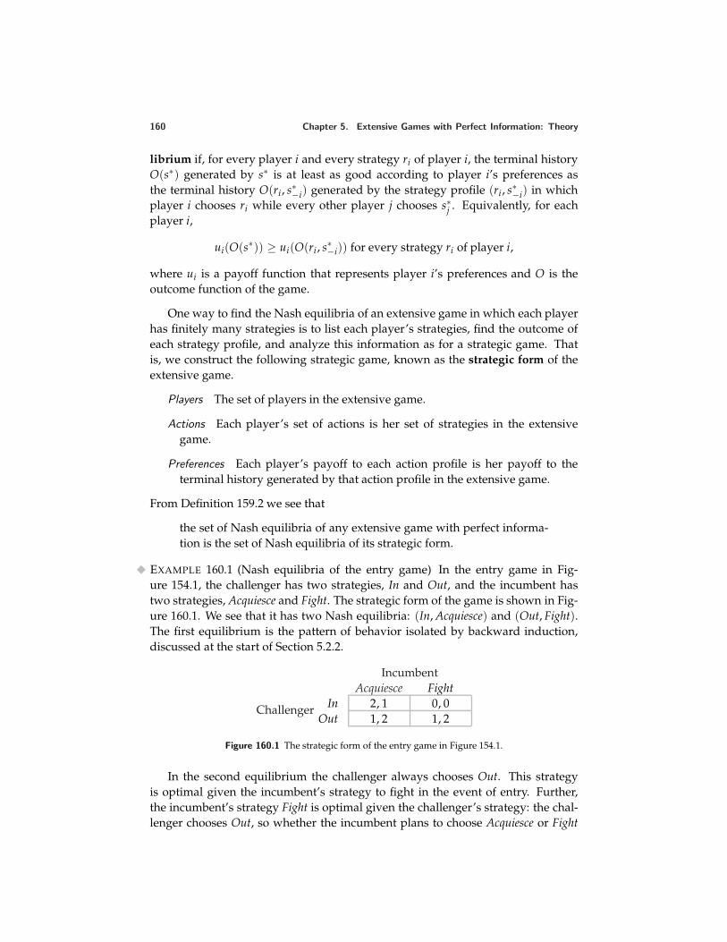
160 Chapter 5. Extensive Games with Perfect Information: Theory
librium if, for every player i and every strategy ri of player i, the terminal historyO(s∗) generated by s∗ is at least as good according to player i’s preferences asthe terminal history O(ri , s∗−i) generated by the strategy profile (ri , s∗−i) in whichplayer i chooses ri while every other player j chooses s∗j . Equivalently, for eachplayer i,
ui(O(s∗)) ≥ ui(O(ri , s∗−i)) for every strategy ri of player i,
where ui is a payoff function that represents player i’s preferences and O is theoutcome function of the game.
One way to find the Nash equilibria of an extensive game in which each playerhas finitely many strategies is to list each player’s strategies, find the outcome ofeach strategy profile, and analyze this information as for a strategic game. Thatis, we construct the following strategic game, known as the strategic form of theextensive game.
Players The set of players in the extensive game.
Actions Each player’s set of actions is her set of strategies in the extensivegame.
Preferences Each player’s payoff to each action profile is her payoff to theterminal history generated by that action profile in the extensive game.
From Definition 159.2 we see that
the set of Nash equilibria of any extensive game with perfect informa-tion is the set of Nash equilibria of its strategic form.
EXAMPLE 160.1 (Nash equilibria of the entry game) In the entry game in Fig-ure 154.1, the challenger has two strategies, In and Out, and the incumbent hastwo strategies, Acquiesce and Fight. The strategic form of the game is shown in Fig-ure 160.1. We see that it has two Nash equilibria: (In, Acquiesce) and (Out, Fight).The first equilibrium is the pattern of behavior isolated by backward induction,discussed at the start of Section 5.2.2.
Challenger
IncumbentAcquiesce Fight
In 2, 1 0, 0Out 1, 2 1, 2
Figure 160.1 The strategic form of the entry game in Figure 154.1.
In the second equilibrium the challenger always chooses Out. This strategyis optimal given the incumbent’s strategy to fight in the event of entry. Further,the incumbent’s strategy Fight is optimal given the challenger’s strategy: the chal-lenger chooses Out, so whether the incumbent plans to choose Acquiesce or Fight
5.4 Nash equilibrium 161
makes no difference to its payoff. Thus neither player can increase its payoff bychoosing a different strategy, given the other player’s strategy.
Thinking about the extensive game in this example raises a question about theNash equilibrium (Out, Fight) that does not arise when thinking about the strategicform: how does the challenger know that the incumbent will choose Fight if it en-ters? We interpret the strategic game to model a situation in which, whenever thechallenger plays the game, it observes the incumbent’s action, even if it choosesOut. By contrast, we interpret the extensive game to model a situation in whicha challenger that always chooses Out never observes the incumbent’s action, be-cause the incumbent never moves. In a strategic game, the rationale for the Nashequilibrium condition that each player’s strategy be optimal given the other play-ers’ strategies is that in a steady state, each player’s experience playing the gameleads her belief about the other players’ actions to be correct. This rationale doesnot apply to the Nash equilibrium (Out, Fight) of the (extensive) entry game, be-cause a challenger who always chooses Out never observes the incumbent’s actionafter the history In.
We can escape from this difficulty in interpreting a Nash equilibrium of anextensive game by considering a slightly perturbed steady state in which, on rareoccasions, nonequilibrium actions are taken (perhaps players make mistakes, ordeliberately experiment), and the perturbations allow each player eventually toobserve every other player’s action after every history. Given such perturbations,each player eventually learns the other players’ entire strategies.
Interpreting the Nash equilibrium (Out, Fight) as such a perturbed steady state,however, we run into another problem. On those (rare) occasions when the chal-lenger enters, the subsequent behavior of the incumbent to fight is not a steadystate in the remainder of the game: if the challenger enters, the incumbent is betteroff acquiescing than fighting. That is, the Nash equilibrium (Out, Fight) does notcorrespond to a robust steady state of the extensive game.
Note that the extensive game embodies the assumption that the incumbent can-not commit, at the beginning of the game, to fight if the challenger enters; it is freeto choose either Acquiesce or Fight in this event. If the incumbent could commit tofight in the event of entry then the analysis would be different. Such a commitmentwould induce the challenger to stay out, an outcome that the incumbent prefers. Inthe absence of the possibility of the incumbent’s making a commitment, we mightthink of the its announcing at the start of the game that it intends to fight; but sucha threat is not credible, because after the challenger enters the incumbent’s onlyincentive is to acquiesce.
? EXERCISE 161.1 (Nash equilibria of extensive games) Find the Nash equilibria ofthe games in Exercise 154.2a and Figure 158.1. (When constructing the strategicform of each game, be sure to include all the strategies of each player.)
? EXERCISE 161.2 (Voting by alternating veto) Two people select a policy that affectsthem both by alternately vetoing policies until only one remains. First person 1
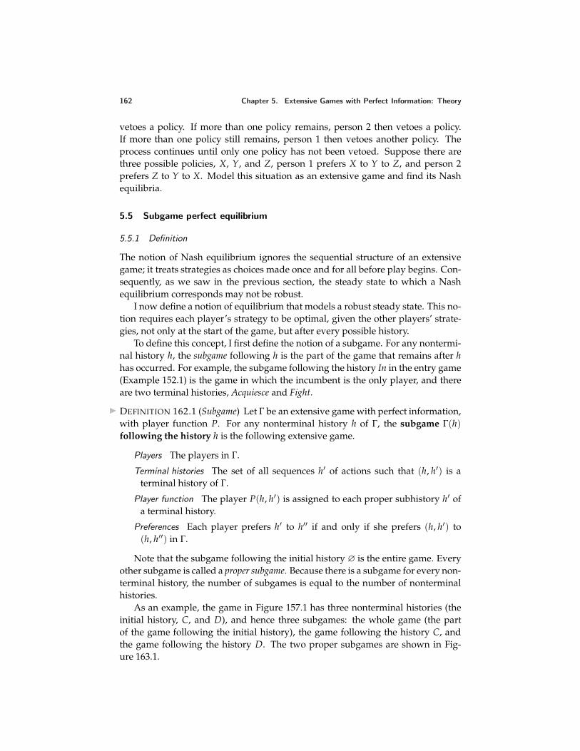
162 Chapter 5. Extensive Games with Perfect Information: Theory
vetoes a policy. If more than one policy remains, person 2 then vetoes a policy.If more than one policy still remains, person 1 then vetoes another policy. Theprocess continues until only one policy has not been vetoed. Suppose there arethree possible policies, X, Y, and Z, person 1 prefers X to Y to Z, and person 2prefers Z to Y to X. Model this situation as an extensive game and find its Nashequilibria.
5.5 Subgame perfect equilibrium
5.5.1 Definition
The notion of Nash equilibrium ignores the sequential structure of an extensivegame; it treats strategies as choices made once and for all before play begins. Con-sequently, as we saw in the previous section, the steady state to which a Nashequilibrium corresponds may not be robust.
I now define a notion of equilibrium that models a robust steady state. This no-tion requires each player’s strategy to be optimal, given the other players’ strate-gies, not only at the start of the game, but after every possible history.
To define this concept, I first define the notion of a subgame. For any nontermi-nal history h, the subgame following h is the part of the game that remains after hhas occurred. For example, the subgame following the history In in the entry game(Example 152.1) is the game in which the incumbent is the only player, and thereare two terminal histories, Acquiesce and Fight.
DEFINITION 162.1 (Subgame) Let Γ be an extensive game with perfect information,with player function P. For any nonterminal history h of Γ, the subgame Γ(h)following the history h is the following extensive game.
Players The players in Γ.
Terminal histories The set of all sequences h′ of actions such that (h, h′) is aterminal history of Γ.
Player function The player P(h, h′) is assigned to each proper subhistory h′ ofa terminal history.
Preferences Each player prefers h′ to h′′ if and only if she prefers (h, h′) to(h, h′′) in Γ.
Note that the subgame following the initial history ∅ is the entire game. Everyother subgame is called a proper subgame. Because there is a subgame for every non-terminal history, the number of subgames is equal to the number of nonterminalhistories.
As an example, the game in Figure 157.1 has three nonterminal histories (theinitial history, C, and D), and hence three subgames: the whole game (the partof the game following the initial history), the game following the history C, andthe game following the history D. The two proper subgames are shown in Fig-ure 163.1.
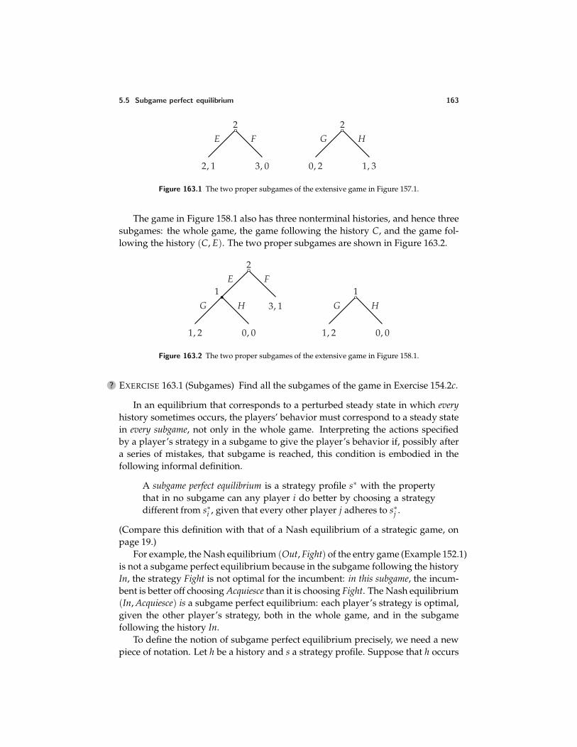
5.5 Subgame perfect equilibrium 163
2E F
2, 1 3, 0
2G H
0, 2 1, 3
Figure 163.1 The two proper subgames of the extensive game in Figure 157.1.
The game in Figure 158.1 also has three nonterminal histories, and hence threesubgames: the whole game, the game following the history C, and the game fol-lowing the history (C, E). The two proper subgames are shown in Figure 163.2.
2E F
3, 1
1G H
1, 2 0, 0
1G H
1, 2 0, 0
Figure 163.2 The two proper subgames of the extensive game in Figure 158.1.
? EXERCISE 163.1 (Subgames) Find all the subgames of the game in Exercise 154.2c.
In an equilibrium that corresponds to a perturbed steady state in which everyhistory sometimes occurs, the players’ behavior must correspond to a steady statein every subgame, not only in the whole game. Interpreting the actions specifiedby a player’s strategy in a subgame to give the player’s behavior if, possibly aftera series of mistakes, that subgame is reached, this condition is embodied in thefollowing informal definition.
A subgame perfect equilibrium is a strategy profile s∗ with the propertythat in no subgame can any player i do better by choosing a strategydifferent from s∗i , given that every other player j adheres to s∗j .
(Compare this definition with that of a Nash equilibrium of a strategic game, onpage 19.)
For example, the Nash equilibrium (Out, Fight) of the entry game (Example 152.1)is not a subgame perfect equilibrium because in the subgame following the historyIn, the strategy Fight is not optimal for the incumbent: in this subgame, the incum-bent is better off choosing Acquiesce than it is choosing Fight. The Nash equilibrium(In, Acquiesce) is a subgame perfect equilibrium: each player’s strategy is optimal,given the other player’s strategy, both in the whole game, and in the subgamefollowing the history In.
To define the notion of subgame perfect equilibrium precisely, we need a newpiece of notation. Let h be a history and s a strategy profile. Suppose that h occurs
164 Chapter 5. Extensive Games with Perfect Information: Theory
(even though it is not necessarily consistent with s), and afterwards the players ad-here to the strategy profile s. Denote the resulting terminal history by Oh(s). Thatis, Oh(s) is the terminal history consisting of h followed by the outcome generatedin the subgame following h by the strategy profile induced by s in the subgame.Note that for any strategy profile s, we have O∅(s) = O(s) (where ∅, as always,denotes the initial history).
As an example, consider again the entry game. Let s be the strategy profile(Out, Fight) and let h be the history In. If h occurs, and afterwards the players adhereto s, the resulting terminal history is Oh(s) = (In, Fight).
DEFINITION 164.1 (Subgame perfect equilibrium) The strategy profile s∗ in an exten-sive game with perfect information is a subgame perfect equilibrium if, for everyplayer i, every history h after which it is player i’s turn to move (i.e. P(h) = i), andevery strategy ri of player i, the terminal history Oh(s∗) generated by s∗ after thehistory h is at least as good according to player i’s preferences as the terminal his-tory Oh(ri , s∗−i) generated by the strategy profile (ri , s∗−i) in which player i choosesri while every other player j chooses s∗j . Equivalently, for every player i and everyhistory h after which it is player i’s turn to move,
ui(Oh(s∗)) ≥ ui(Oh(ri , s∗−i)) for every strategy ri of player i,
where ui is a payoff function that represents player i’s preferences and Oh(s) is theterminal history consisting of h followed by the sequence of actions generated bys after h.
The important point in this definition is that each player’s strategy is requiredto be optimal for every history after which it is the player’s turn to move, not onlyat the start of the game as in the definition of a Nash equilibrium (159.2).
5.5.2 Subgame perfect equilibrium and Nash equilibrium
In a subgame perfect equilibrium every player’s strategy is optimal, in particular,after the initial history (put h = ∅ in the definition, and remember that O∅(s) =O(s)). Thus:
Every subgame perfect equilibrium is a Nash equilibrium.
In fact, a subgame perfect equilibrium generates a Nash equilibrium in everysubgame: if s∗ is a subgame perfect equilibrium then, for any history h and player i,the strategy induced by s∗i in the subgame following h is optimal given the strate-gies induced by s∗−i in the subgame. Further, any strategy profile that generates aNash equilibrium in every subgame is a subgame perfect equilibrium, so that wecan give the following alternative definition.
A subgame perfect equilibrium is a strategy profile that induces a Nashequilibrium in every subgame.
5.5 Subgame perfect equilibrium 165
In a Nash equilibrium every player’s strategy is optimal, given the other play-ers’ strategies, in the whole game. As we have seen, it may not be optimal in somesubgames. I claim, however, that it is optimal in any subgame that is reachedwhen the players follow their strategies. Given this claim, the significance of therequirement in the definition of a subgame perfect equilibrium that each player’sstrategy be optimal after every history, relative to the requirement in the defini-tion of a Nash equilibrium, is that each player’s strategy be optimal after historiesthat do not occur if the players follow their strategies (like the history In when thechallenger’s action is Out at the beginning of the entry game).
To show my claim, suppose that s∗ is a Nash equilibrium of a game in whichyou are player i. Then your strategy s∗i is optimal given the other players’ strategiess∗−i. When the other players follow their strategies, there comes a point (possiblythe start of the game) when you have to move for the first time. Suppose that atthis point you follow your strategy s∗i ; denote the action you choose by C. Now,after having chosen C, should you change your strategy in the rest of the game,given that the other players will continue to adhere to their strategies? No! If youcould do better by changing your strategy after choosing C—say by switching tothe strategy s′i in the subgame—then you could have done better at the start of thegame by choosing the strategy that chooses C and then follows s′i. That is, if yourplan is optimal, given the other players’ strategies, at the start of the game, andyou stick to it, then you never want to change your mind after play begins, as longas the other players stick to their strategies. (The general principle is known as thePrinciple of Optimality in dynamic programming.)
5.5.3 Examples
EXAMPLE 165.1 (Entry game) Consider again the entry game of Example 152.1,which has two Nash equilibria, (In, Acquiesce) and (Out, Fight). The fact that theNash equilibrium (Out, Fight) is not a subgame perfect equilibrium follows fromthe formal definition as follows. For s∗ = (Out, Fight), i = Incumbent, ri =Acquiesce, and h = In, we have Oh(s∗) = (In, Fight) and Oh(ri , s∗−i) = (In, Acquiesce),so that the inequality in the definition is violated: ui(Oh(s∗)) = 0 and ui(Oh(ri , s∗−i)) =1.
The Nash equilibrium (In, Acquiesce) is a subgame perfect equilibrium because(a) it is a Nash equilibrium, so that at the start of the game the challenger’s strategyIn is optimal, given the incumbent’s strategy Acquiesce, and (b) after the history In,the incumbent’s strategy Acquiesce in the subgame is optimal. In the language ofthe formal definition, let s∗ = (In, Acquiesce).
• The challenger moves after one history, namely h = ∅. We have Oh(s∗) =(In, Acquiesce) and hence for i = challenger we have ui(Oh(s∗)) = 2, whereasfor the only other strategy of the challenger, ri = Out, we have ui(Oh(ri , s∗−i)) =1.
166 Chapter 5. Extensive Games with Perfect Information: Theory
• The incumbent moves after one history, namely h = In. We have Oh(s∗) =(In, Acquiesce) and hence for i = incumbent we have ui(Oh(s∗)) = 1, whereasfor the only other strategy of the incumbent, ri = Fight, we have ui(Oh(ri , s∗−i)) =0.
Every subgame perfect equilibrium is a Nash equilibrium, so we conclude thatthe game has a unique subgame perfect equilibrium, (In, Acquiesce).
EXAMPLE 166.1 (Variant of entry game) Consider the variant of the entry game inwhich the incumbent is indifferent between fighting and acquiescing if the chal-lenger enters (see Figure 156.1). This game, like the original game, has two Nashequilibria, (In, Acquiesce) and (Out, Fight). But now both of these equilibria are sub-game perfect equilibria, because after the history In both Fight and Acquiesce areoptimal for the incumbent.
In particular, the game has a steady state in which every challenger alwayschooses In and every incumbent always chooses Acquiesce. If you, as the chal-lenger, were playing the game for the first time, you would probably regard theaction In as “risky”, because after the history In the incumbent is indifferent be-tween Acquiesce and Fight, and you prefer the terminal history Out to the termi-nal history (In, Fight). Indeed, as discussed in Section 5.2.2, backward inductiondoes not yield a clear solution of this game. But the subgame perfect equilibrium(In, Acquiesce) corresponds to a perfectly reasonable steady state. If you had playedthe game hundreds of times against opponents drawn from the same population,and on every occasion your opponent had chosen Acquiesce, you could reasonablyexpect your next opponent to choose Acquiesce, and thus optimally choose In.
? EXERCISE 166.2 (Checking for subgame perfect equilibria) Which of the Nash equi-libria of the game in Figure 158.1 are subgame perfect?
5.5.4 Interpretation
A Nash equilibrium of a strategic game corresponds to a steady state in an ide-alized setting in which the participants in each play of the game are drawn ran-domly from a collection of populations (see Section 2.6). The idea is that eachplayer’s long experience playing the game leads her to correct beliefs about theother players’ actions; given these beliefs her equilibrium action is optimal.
A subgame perfect equilibrium of an extensive game corresponds to a slightlyperturbed steady state, in which all players, on rare occasions, take nonequilib-rium actions, so that after long experience each player forms correct beliefs aboutthe other players’ entire strategies, and thus knows how the other players will be-have in every subgame. Given these beliefs, no player wishes to deviate from herstrategy either at the start of the game or after any history.
This interpretation of a subgame perfect equilibrium, like the interpretationof a Nash equilibrium as a steady state, does not require a player to know theother players’ preferences, or to think about the other players’ rationality. It en-tails interpreting a strategy as a plan specifying a player’s actions not only after
5.6 Finding subgame perfect equilibria of finite horizon games: backward induction 167
histories consistent with the strategy, but also after histories that result when theplayer chooses arbitrary alternative actions, perhaps because she makes mistakesor deliberately experiments.
The subgame perfect equilibria of some extensive game can be given other in-terpretations. In some cases, one alternative interpretation is particularly attrac-tive. Consider an extensive game with perfect information in which each playerhas a unique best action at every history after which it is her turn to move, and thehorizon is finite. In such a game, a player who knows the other players’ prefer-ences and knows that the other players are rational can use backward induction todeduce her optimal strategy, as discussed in Section 5.2.2. Thus we can interpreta subgame perfect equilibrium as the outcome of the players’ rational calculationsabout each other’s strategies.
This interpretation of a subgame perfect equilibrium entails an interpretation ofa strategy different from the one that fits the steady state interpretation. Consider,for example, the game in Figure 158.1. When analyzing this game, player 1 mustconsider the consequences of choosing C. Thus she must think about player 2’saction after the history C, and hence must form a belief about what player 2 thinksshe (player 1) will do after the history (C, E). The component of her strategy thatspecifies her action after this history reflects this belief. For instance, the strategyDG means that player 1 chooses D at the start of the game and believes that wereshe to choose C, player 2 would believe that after the history (C, E) she wouldchoose G. In an arbitrary game, the interpretation of a subgame perfect equilib-rium as the outcome of the players’ rational calculations about each other’s strate-gies entails interpreting the components of a player’s strategy that assign actionsto histories inconsistent with other parts of the strategy as specifying the player’sbelief about the other players’ beliefs about what the player will do if one of thesehistories occurs.
This interpretation of a subgame perfect equilibrium is not free of difficulties,which are discussed in Section 7.7. Further, the interpretation is not tenable ingames in which some player has more than one optimal action after some history,or in the more general extensive games considered in Section 7.1 and Chapter 10.Nevertheless, in some of the games studied in this chapter and the next it is anappealing alternative to the steady state interpretation. Further, an extension of theprocedure of backward induction can be used to find all subgame perfect equilibriaof finite horizon games, as we shall see in the next section. (This extension cannotbe given an appealing behavioral interpretation in games in which some playerhas more than one optimal action after some history.)
5.6 Finding subgame perfect equilibria of finite horizon games: backward
induction
We found the subgame perfect equilibria of the games in Examples 165.1 and 166.1by finding the Nash equilibria of the games and checking whether each of these
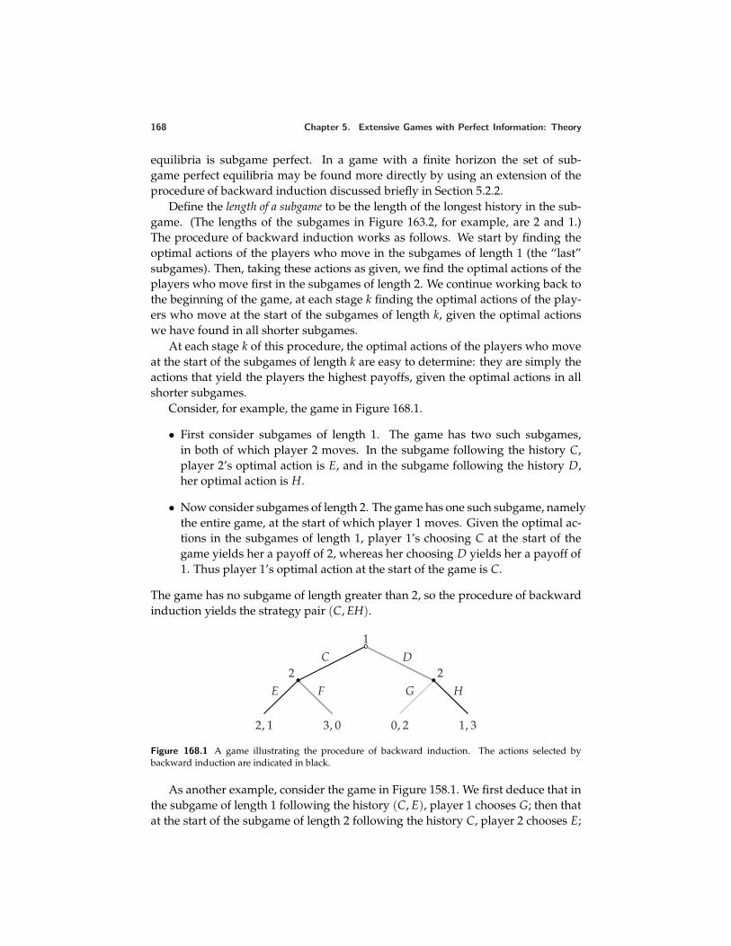
168 Chapter 5. Extensive Games with Perfect Information: Theory
equilibria is subgame perfect. In a game with a finite horizon the set of sub-game perfect equilibria may be found more directly by using an extension of theprocedure of backward induction discussed briefly in Section 5.2.2.
Define the length of a subgame to be the length of the longest history in the sub-game. (The lengths of the subgames in Figure 163.2, for example, are 2 and 1.)The procedure of backward induction works as follows. We start by finding theoptimal actions of the players who move in the subgames of length 1 (the “last”subgames). Then, taking these actions as given, we find the optimal actions of theplayers who move first in the subgames of length 2. We continue working back tothe beginning of the game, at each stage k finding the optimal actions of the play-ers who move at the start of the subgames of length k, given the optimal actionswe have found in all shorter subgames.
At each stage k of this procedure, the optimal actions of the players who moveat the start of the subgames of length k are easy to determine: they are simply theactions that yield the players the highest payoffs, given the optimal actions in allshorter subgames.
Consider, for example, the game in Figure 168.1.
• First consider subgames of length 1. The game has two such subgames,in both of which player 2 moves. In the subgame following the history C,player 2’s optimal action is E, and in the subgame following the history D,her optimal action is H.
• Now consider subgames of length 2. The game has one such subgame, namelythe entire game, at the start of which player 1 moves. Given the optimal ac-tions in the subgames of length 1, player 1’s choosing C at the start of thegame yields her a payoff of 2, whereas her choosing D yields her a payoff of1. Thus player 1’s optimal action at the start of the game is C.
The game has no subgame of length greater than 2, so the procedure of backwardinduction yields the strategy pair (C, EH).
1C D
2E F
2, 1 3, 0
2G H
0, 2 1, 3
Figure 168.1 A game illustrating the procedure of backward induction. The actions selected bybackward induction are indicated in black.
As another example, consider the game in Figure 158.1. We first deduce that inthe subgame of length 1 following the history (C, E), player 1 chooses G; then thatat the start of the subgame of length 2 following the history C, player 2 chooses E;
5.6 Finding subgame perfect equilibria of finite horizon games: backward induction 169
then that at the start of the whole game, player 1 chooses D. Thus the procedureof backward induction in this game yields the strategy pair (DG, E).
In any game in which this procedure selects a single action for the player whomoves at the start of each subgame, the strategy profile thus selected is the uniquesubgame perfect equilibrium of the game. (You should find this result very plau-sible, though a complete proof is not trivial.)
What happens in a game in which at the start of some subgames more thanone action is optimal? In such a game an extension of the procedure of backwardinduction locates all subgame perfect equilibrium. This extension traces back sep-arately the implications for behavior in the longer subgames of every combination ofoptimal actions in the shorter subgames.
Consider, for example, the game in Figure 170.1.
• The game has three subgames of length one, in each of which player 2 moves.In the subgames following the histories C and D, player 2 is indifferent be-tween her two actions. In the subgame following the history E, player 2’sunique optimal action is K. Thus there are four combinations of player 2’soptimal actions in the subgames of length 1: FHK, FIK, GHK, and GIK (wherethe first component in each case is player 2’s action after the history C, thesecond component is her action after the history D, and the third componentis her action after the history E).
• The game has a single subgame of length two, namely the whole game, inwhich player 1 moves first. We now consider player 1’s optimal action in thisgame for every combination of the optimal actions of player 2 in the subgamesof length 1.
– For the combinations FHK and FIK of optimal actions of player 2, player 1’soptimal action at the start of the game is C.
– For the combination GHK of optimal actions of player 2, the actions C,D, and E are all optimal for player 1.
– For the combination GIK of optimal actions of player, player 1’s optimalaction at the start of the game is D.
Thus the strategy pairs isolated by the procedure are (C, FHK), (C, FIK), (C, GHK),(D, GHK), (E, GHK), and (D, GIK).
The procedure, which for simplicity I refer to simply as backward induction,may be described compactly for an arbitrary game as follows.
• Find, for each subgame of length 1, the set of optimal actions of the playerwho moves first. Index the subgames by j, and denote by S∗
j (1) the set ofoptimal actions in subgame j. (If the player who moves first in subgame jhas a unique optimal action, then S∗
j (1) contains a single action.)
• For each combination of actions consisting of one from each set S∗j (1), find,
for each subgame of length two, the set of optimal actions of the player who
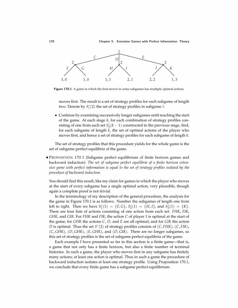
170 Chapter 5. Extensive Games with Perfect Information: Theory
1C D E
2F G
3, 0 1, 0
2H I
1, 1 2, 1
2J K
2, 2 1, 3
Figure 170.1 A game in which the first-mover in some subgames has multiple optimal actions.
moves first. The result is a set of strategy profiles for each subgame of lengthtwo. Denote by S∗
(2) the set of strategy profiles in subgame .
• Continue by examining successively longer subgames until reaching the startof the game. At each stage k, for each combination of strategy profiles con-sisting of one from each set S∗
p(k − 1) constructed in the previous stage, find,for each subgame of length k, the set of optimal actions of the player whomoves first, and hence a set of strategy profiles for each subgame of length k.
The set of strategy profiles that this procedure yields for the whole game is theset of subgame perfect equilibria of the game.
PROPOSITION 170.1 (Subgame perfect equilibrium of finite horizon games andbackward induction) The set of subgame perfect equilibria of a finite horizon exten-sive game with perfect information is equal to the set of strategy profiles isolated by theprocedure of backward induction.
You should find this result, like my claim for games in which the player who movesat the start of every subgame has a single optimal action, very plausible, thoughagain a complete proof is not trivial.
In the terminology of my description of the general procedure, the analysis forthe game in Figure 170.1 is as follows. Number the subgames of length one fromleft to right. Then we have S∗
1(1) = F, G, S∗2(1) = H, I, and S∗
3(1) = K.There are four lists of actions consisting of one action from each set: FHK, FIK,GHK, and GIK. For FHK and FIK, the action C of player 1 is optimal at the start ofthe game; for GHK the actions C, D, and E are all optimal; and for GIK the actionD is optimal. Thus the set S∗(2) of strategy profiles consists of (C, FHK), (C, FIK),(C, GHK), (D, GHK), (E, GHK), and (D, GIK). There are no longer subgames, sothis set of strategy profiles is the set of subgame perfect equilibria of the game.
Each example I have presented so far in this section is a finite game—that is,a game that not only has a finite horizon, but also a finite number of terminalhistories. In such a game, the player who moves first in any subgame has finitelymany actions; at least one action is optimal. Thus in such a game the procedure ofbackward induction isolates at least one strategy profile. Using Proposition 170.1,we conclude that every finite game has a subgame perfect equilibrium.
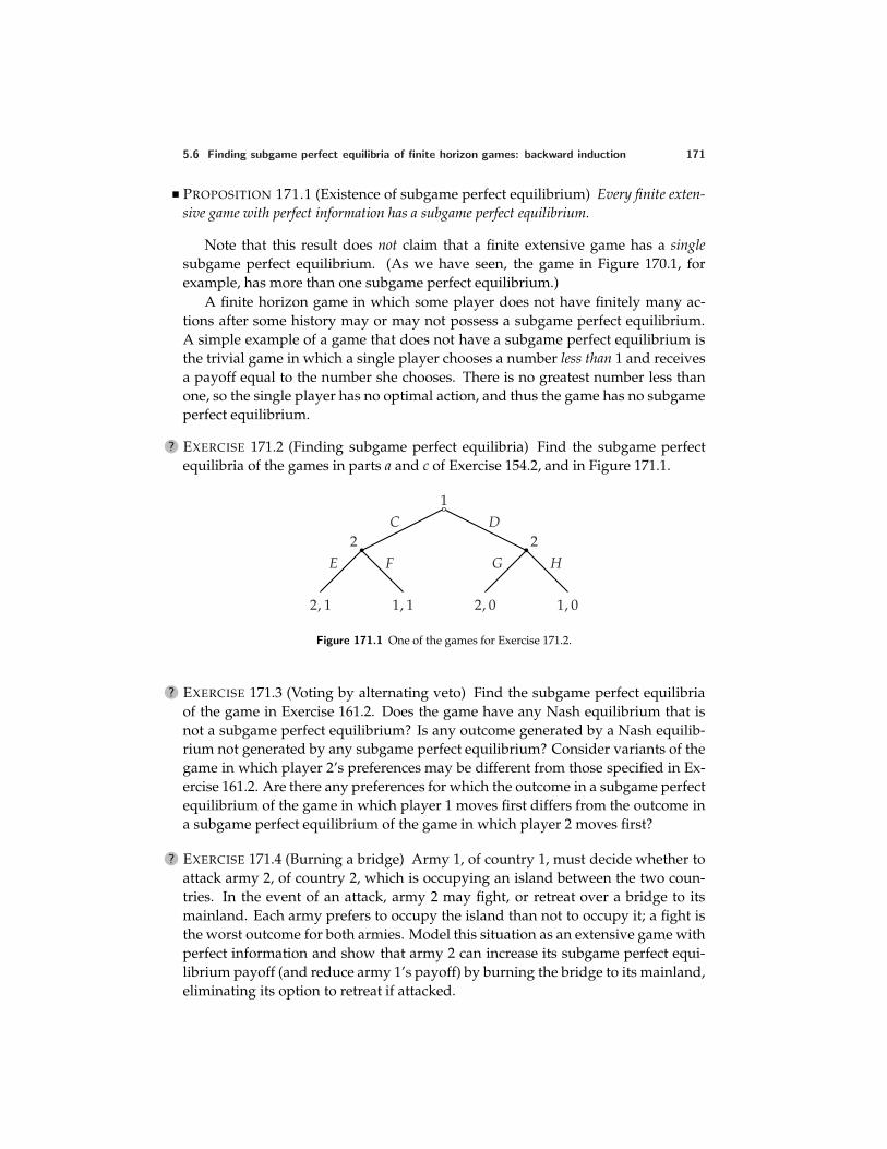
5.6 Finding subgame perfect equilibria of finite horizon games: backward induction 171
PROPOSITION 171.1 (Existence of subgame perfect equilibrium) Every finite exten-sive game with perfect information has a subgame perfect equilibrium.
Note that this result does not claim that a finite extensive game has a singlesubgame perfect equilibrium. (As we have seen, the game in Figure 170.1, forexample, has more than one subgame perfect equilibrium.)
A finite horizon game in which some player does not have finitely many ac-tions after some history may or may not possess a subgame perfect equilibrium.A simple example of a game that does not have a subgame perfect equilibrium isthe trivial game in which a single player chooses a number less than 1 and receivesa payoff equal to the number she chooses. There is no greatest number less thanone, so the single player has no optimal action, and thus the game has no subgameperfect equilibrium.
? EXERCISE 171.2 (Finding subgame perfect equilibria) Find the subgame perfectequilibria of the games in parts a and c of Exercise 154.2, and in Figure 171.1.
1C D
2E F
2, 1 1, 1
2G H
2, 0 1, 0
Figure 171.1 One of the games for Exercise 171.2.
? EXERCISE 171.3 (Voting by alternating veto) Find the subgame perfect equilibriaof the game in Exercise 161.2. Does the game have any Nash equilibrium that isnot a subgame perfect equilibrium? Is any outcome generated by a Nash equilib-rium not generated by any subgame perfect equilibrium? Consider variants of thegame in which player 2’s preferences may be different from those specified in Ex-ercise 161.2. Are there any preferences for which the outcome in a subgame perfectequilibrium of the game in which player 1 moves first differs from the outcome ina subgame perfect equilibrium of the game in which player 2 moves first?
? EXERCISE 171.4 (Burning a bridge) Army 1, of country 1, must decide whether toattack army 2, of country 2, which is occupying an island between the two coun-tries. In the event of an attack, army 2 may fight, or retreat over a bridge to itsmainland. Each army prefers to occupy the island than not to occupy it; a fight isthe worst outcome for both armies. Model this situation as an extensive game withperfect information and show that army 2 can increase its subgame perfect equi-librium payoff (and reduce army 1’s payoff) by burning the bridge to its mainland,eliminating its option to retreat if attacked.
172 Chapter 5. Extensive Games with Perfect Information: Theory
? EXERCISE 172.1 (Sharing heterogeneous objects) A group of n people have to sharek objects that the value differently. Each person assigns values to the objects; noone assigns the same value to two different objects. Each person evaluates a setof objects according to the sum of the values she assigns to the objects in the set.The following procedure is used to share the objects. The players are ordered 1through n. Person 1 chooses an object, then person 2 does so, and so on; if k > n,then after person n chooses an object, person 1 chooses a second object, then per-son 2 chooses a second object, and so on. Objects are chosen until none remain. (InCanada and the USA professional sports teams use a similar procedure to choosenew players.) Denote by G(n, k) the extensive game that models this procedure.If k ≤ n then obviously G(n, k) has a subgame perfect equilibrium in which eachplayer’s strategy is to choose her favorite object among those remaining when herturn comes. Show that if k > n then G(n, k) may have no subgame perfect equi-librium in which person 1 chooses her favorite object on the first round. (You cangive an example in which n = 2 and k = 3.) Now fix n = 2. Define xk to bethe object least preferred by the person who does not choose at stage k (i.e. whodoes not choose the last object); define xk−1 to be the object, among all those ex-cept xk, least preferred by the person who does not choose at stage k − 1. Similarly,for any j with 2 ≤ j ≤ k, given xj, . . . , xk, define xj−1 to be the object, among allthose excluding xj, . . . , xk, least preferred by the person who does not chooseat stage j − 1. Show that the game G(2, 3) has a subgame perfect equilibrium inwhich for every j = 1, . . . , k the object xj is chosen at stage j. (This result is true forG(2, k) for all values of k.) If n ≥ 3 then interestingly a person may be better off inall subgame perfect equilibria of G(n, k) when she comes later in the ordering ofplayers. (An example, however, is difficult to construct; one is given in Brams andStraffin (1979).)
The next exercise shows how backward induction can cause a relatively minorchange in the way in which a game ends to reverberate to the start of the game,leading to a very different action for the first-mover.
?? EXERCISE 172.2 (An entry game with a financially-constrained firm) An incum-bent in an industry faces the possibility of entry by a challenger. First the chal-lenger chooses whether or not to enter. If it does not enter, neither firm has anyfurther action; the incumbent’s payoff is TM (it obtains the profit M in each of thefollowing T ≥ 1 periods) and the challenger’s payoff is 0. If the challenger enters,it pays the entry cost f > 0, and in each of T periods the incumbent first commitsto fight or cooperate with the challenger in that period, then the challenger chooseswhether to stay in the industry or to exit. (Note that the order of the firms’ moveswithin a period differs from that in the game in Example 152.1.) If, in any period,the challenger stays in, each firm obtains in that period the profit −F < 0 if the in-cumbent fights and C > maxF, f if it cooperates. If, in any period, the challengerexits, both firms obtain the profit zero in that period (regardless of the incumbent’saction); the incumbent obtains the profit M > 2C and the challenger the profit
5.6 Finding subgame perfect equilibria of finite horizon games: backward induction 173
0 in every subsequent period. Once the challenger exits, it cannot subsequentlyre-enter. Each firm cares about the sum of its profits.
a. Find the subgame perfect equilibria of the extensive game that models thissituation.
b. Consider a variant of the situation, in which the challenger is constrained byits financial war chest, which allows it to survive at most T − 2 fights. Specif-ically, consider the game that differs from the one in part a only in that thehistory in which the challenger enters, in each of the following T − 2 periodsthe incumbent fights and the challenger stays in, and in period T − 1 the in-cumbent fights, is a terminal history (the challenger has to exit), in which theincumbent’s payoff is M (it is the only firm in the industry in the last period)and the challenger’s payoff is − f . Find the subgame perfect equilibria of thisgame.
EXAMPLE 173.1 (Dollar auction) Consider an auction in which an object is sold tothe highest bidder, but both the highest bidder and the second highest bidder paytheir bids to the auctioneer. When such an auction is conducted and the object is adollar, the outcome is sometimes that the object is sold at a price greater than a dol-lar. (Shubik writes that “A total of payments between three and five dollars is notuncommon” (1971, 110).) Obviously such an outcome is inconsistent with a sub-game perfect equilibrium of an extensive game that models the auction: every par-ticipant has the option of not bidding, so that in no subgame perfect equilibriumcan anyone’s payoff be negative.
Why, then, do such outcomes occur? Suppose that there are two participants,and that both start bidding. If the player making the lower bid thinks that makinga bid above the other player’s bid will induce the other player to quit, she may bebetter off doing so than stopping bidding. For example, if the bids are currently$0.50 and $0.51, the player bidding $0.50 is better off bidding $0.52 if doing soinduces the other bidder to quit, because she then wins the dollar and obtains apayoff of $0.48, rather than losing $0.50. The same logic applies even if the bids aregreater than $1.00, as long as they do not differ by more than $1.00. If, for example,they are currently $2.00 and $2.01, then the player bidding $2.00 loses only $1.02 ifa bid of $2.02 induces her opponent to quit, whereas she loses $2.00 if she herselfquits. That is, in subgames in which bids have been made, the player making thesecond highest bid may optimally beat a bid that exceeds $1.00, depending on theother players’ strategies and the difference between the top two bids. (When dis-cussing outcomes in which the total payment to the auctioneer exceeds $1, Shubikremarks that “In playing this game, a large crowd is desirable . . . the best time isduring a party when spirits are high and the propensity to calculate does not settlein until at least two bids have been made” (1971, 109).)
In the next exercise you are asked to find the subgame perfect equilibria of anextensive game that models a simple example of such an auction.
? EXERCISE 173.2 (Dollar auction) An object that two people each value at v (a pos-itive integer) is sold in an auction. In the auction, the people alternately have
174 Chapter 5. Extensive Games with Perfect Information: Theory
the opportunity to bid; a bid must be a positive integer greater than the previousbid. (In the situation that gives the game its name, v is 100 cents.) On her turn, aplayer may pass rather than bid, in which case the game ends and the other playerreceives the object; both players pay their last bids (if any). (If player 1 passes ini-tially, for example, player 2 receives the object and makes no payment; if player 1bids 1, player 2 bids 3, and then player 1 passes, player 2 obtains the object andpays 3, and player 1 pays 1.) Each person’s wealth is w, which exceeds v; neitherplayer may bid more than her wealth. For v = 2 and w = 3 model the auction as anextensive game and find its subgame perfect equilibria. (A much more ambitiousproject is to find all subgame perfect equilibria for arbitrary values of v and w.)
In all the extensive games studied so far in this chapter, each player has avail-able finitely many actions whenever she moves. The next example shows how theprocedure of backward induction may be used to find the subgame perfect equi-libria of games in which a continuum of actions is available after some histories.
EXAMPLE 174.1 (A synergistic relationship) Consider a variant of the situation inExample 37.1, in which two individuals are involved in a synergistic relationship.Suppose that the players choose their effort levels sequentially, rather than simul-taneously. First individual 1 chooses her effort level a1, then individual 2 choosesher effort level a2. An effort level is a nonnegative number, and individual i’s pref-erences (for i = 1, 2) are represented by the payoff function ai(c + aj − ai), where jis the other individual and c > 0 is a constant.
To find the subgame perfect equilibria, we first consider the subgames of length 1,in which individual 2 chooses a value of a2. Individual 2’s optimal action after thehistory a1 is her best response to a1, which we found to be 1
2 (c + a1) in Exam-ple 37.1. Thus individual 2’s strategy in any subgame perfect equilibrium is thefunction that associates with each history a1 the action 1
2 (c + a1).Now consider individual 1’s action at the start of the game. Given individ-
ual 2’s strategy, individual 1’s payoff if she chooses a1 is a1(c + 12 (c + a1) − a1),
or 12 a1(3c − a1). This function is a quadratic that is zero when a1 = 0 and when
a1 = 3c, and reaches a maximum in between. Thus individual 1’s optimal actionat the start of the game is a1 = 3
2 c.We conclude that the game has a unique subgame perfect equilibrium, in which
individual 1’s strategy is a1 = 32 c and individual 2’s strategy is the function that
associates with each history a1 the action 12 (c + a1). The outcome of the equilibrium
is that individual 1 chooses a1 = 32 c and individual 2 chooses a2 = 5
4 c.
? EXERCISE 174.2 (Firm–union bargaining) A firm’s output is L(100 − L) when ituses L ≤ 50 units of labor, and 2500 when it uses L > 50 units of labor. Theprice of output is 1. A union that represents workers presents a wage demand (anonnegative number w), which the firm either accepts or rejects. If the firm acceptsthe demand, it chooses the number L of workers to employ (which you should taketo be a continuous variable, not an integer); if it rejects the demand, no production
5.6 Finding subgame perfect equilibria of finite horizon games: backward induction 175
takes place (L = 0). The firm’s preferences are represented by its profit; the union’spreferences are represented by the value of wL.
a. Formulate this situation as an extensive game with perfect information.
b. Find the subgame perfect equilibrium (equilibria?) of the game.
c. Is there an outcome of the game that both parties prefer to any subgameperfect equilibrium outcome?
d. Find a Nash equilibrium for which the outcome differs from any subgameperfect equilibrium outcome.
? EXERCISE 175.1 (The “rotten kid theorem”) A child’s action a (a number) affectsboth her own private income c(a) and her parent’s income p(a); for all values ofa we have c(a) < p(a). The child is selfish: she cares only about the amount ofmoney she has. Her loving parent cares both about how much money she has andhow much her child has. Specifically, her preferences are represented by a payoffequal to the smaller of the amount of money she has and the amount of money herchild has. The parent may transfer money to the child. First the child takes an ac-tion, then the parent decides how much money to transfer. Model this situation asan extensive game and show that in a subgame perfect equilibrium the child takesan action that maximizes the sum of her private income and her parent’s income.(In particular, the child’s action does not maximize her own private income. Theresult is not limited to the specific form of the parent’s preferences, but holds forany preferences with the property that a parent who is allocating a fixed amount xof money between herself and her child wishes to give more to the child when x islarger.)
? EXERCISE 175.2 (Comparing simultaneous and sequential games) The set of ac-tions available to player 1 is A1; the set available to player 2 is A2. Player 1’s pref-erences over pairs (a1, a2) are represented by the payoff u1(a1, a2), and player 2’spreferences are represented by the payoff u2(a1, a2). Compare the Nash equilibria(in pure strategies) of the strategic game in which the players choose actions si-multaneously with the subgame perfect equilibria of the extensive game in whichplayer 1 chooses an action, then player 2 does so. (For each history a1 in theextensive game, the set of actions available to player 2 is A2.)
a. Show that if, for every value of a1, there is a unique member of A2 that max-imizes u2(a1, a2), then in every subgame perfect equilibrium of the extensivegame, player 1’s payoff is at least equal to her highest payoff in any Nashequilibrium of the strategic game.
b. Show that player 2’s payoff in every subgame perfect equilibrium of the ex-tensive game may be higher than her highest payoff in any Nash equilibriumof the strategic game.
c. Show that if for some values of a1 more than one member of A2 maximizesu2(a1, a2), then the extensive game may have a subgame perfect equilibrium
176 Chapter 5. Extensive Games with Perfect Information: Theory
in which player 1’s payoff is less than her payoff in all Nash equilibria of thestrategic game.
(For parts b and c you can give examples in which both A1 and A2 contain twoactions.)
TICKTACKTOE, CHESS, AND RELATED GAMES
Ticktacktoe, chess, and related games may be modeled as extensive games withperfect information. (A history is a sequence of moves and each player prefersto win than to tie than to lose.) Both ticktacktoe and chess may be modeled asfinite games, so by Proposition 171.1 each game has a subgame perfect equilibrium.(The official rules of chess allow indefinitely long sequences of moves, but thegame seems to be well modeled by an extensive game in which a draw is declaredautomatically if a position is repeated three times, rather than a player having theoption of declaring a draw in this case, as in the official rules.) The subgame perfectequilibria of ticktacktoe are of course known, whereas those of chess are not (yet).
Ticktacktoe and chess are “strictly competitive” games (Definition 339.1): inevery outcome, either one player loses and the other wins, or the players draw.A result in a later chapter implies that for such a game all Nash equilibria yieldthe same outcome (Corollary 342.1). Further, a player’s Nash equilibrium strategyyields at least her equilibrium payoff, regardless of the other players’ strategies(Proposition 341.1a). (The same is definitely not true for an arbitrary game that isnot strictly competitive: look, for example, at the game in Figure 29.1.) Because anysubgame perfect equilibrium is a Nash equilibrium, the same is true for subgameperfect equilibrium strategies.
We conclude that in ticktacktoe and chess, either (a) one of the players has astrategy that guarantees she wins, or (b) each player has a strategy that guaranteesat worst a draw.
In ticktacktoe, of course, we know that (b) is true. Chess is more subtle. Inparticular, it is not known whether White has a strategy that guarantees it wins,or Black has a strategy that guarantees it wins, or each player has a strategy thatguarantees at worst a draw. The empirical evidence suggests that Black does nothave a winning strategy, but this result has not been proved. When will a sub-game perfect equilibrium of chess be found? (The answer “never” underestimateshuman ingenuity!)
? EXERCISE 176.1 (Subgame perfect equilibria of ticktacktoe) Ticktacktoe has sub-game perfect equilibria in which the first player puts her first X in a corner. Thesecond player’s move is the same in all these equilibria. What is it?
? EXERCISE 176.2 (Toetacktick) Toetacktick is a variant of ticktacktoe in which aplayer who puts three marks in a line loses (rather than wins). Find a strategy
Notes 177
of the first-mover that guarantees that she does not lose. (If fact, in all subgameperfect equilibria the game is a draw.)
? EXERCISE 177.1 (Three Men’s Morris, or Mill) The ancient game of “Three Men’sMorris” is played on a ticktacktoe board. Each player has three counters. The play-ers move alternately. On each of her first three turns, a player places a counter onan unoccupied square. On each subsequent move, a player may move a counter toan adjacent square (vertically or horizontally, but not diagonally). The first playerwhose counters are in a row (vertically, horizontally, or diagonally) wins. Find asubgame perfect equilibrium strategy of player 1, and the equilibrium outcome.
Notes
The notion of an extensive game is due to von Neumann and Morgenstern (1944).Kuhn (1950, 1953) suggested the formulation described in this chapter. The de-scription of an extensive game in terms of histories was suggested by Ariel Rubin-stein. The notion of subgame perfect equilibrium is due to Selten (1965). Proposi-tion 171.1 is due to Kuhn (1953). The interpretation of a strategy when a subgameperfect equilibrium is interpreted as the outcome of the players’ reasoning abouteach others’ rational actions is due to Rubinstein (1991). The principle of optimalityin dynamic programming is discussed by Bellman (1957, 83), for example.
The procedure in Exercises 161.2 and 171.3 was first studied by Mueller (1978)and Moulin (1981). The idea in Exercise 171.4 goes back at least to Sun-tzu, who,in The art of warfare (probably written between 500BC and 300BC), advises “in sur-rounding the enemy, leave him a way out; do not press an enemy that is cornered”(end of Ch. 7; see, for example, Sun-tzu (1993, 132)). (That is, if no bridge exists inthe situation described in the exercise, army 1 should build one.) Schelling (1966,45) quotes Sun-tzu and gives examples of the strategy’s being used in antiquity.My formulation of the exercise comes from Tirole (1988, 316). The model in Exer-cise 172.1 is studied by Kohler and Chandrasekaran (1971) and Brams and Straf-fin (1979). The game in Exercise 172.2 is based on Benoıt (1984, Section 1). Thedollar auction (Exercise 173.2) was introduced into the literature by Shubik (1971).Some of its subgame perfect equilibria, for arbitrary values of v and w, are studiedby O’Neill (1986) and Leininger (1989); see also Taylor (1995, Chs. 1 and 6). Pound-stone (1992, 257–272) writes informally about the game and its possible applica-tions. The result in Exercise 175.1 is due to Becker (1974); see also Bergstrom (1989).The first formal study of chess is Zermelo (1913); see Schwalbe and Walker (2000)for a discussion of this paper and related work. Exercises 176.1, 176.2, and 177.1are taken from Gardner (1959, Ch. 4), which includes several other intriguingexamples.
Draft chapter from An introduction to game theory by Martin J. [email protected]; www.economics.utoronto.ca/osborneVersion: 00/11/6.Copyright c© 1995–2000 by Martin J. Osborne. All rights reserved. No part of this book may be re-produced by any electronic or mechanical means (including photocopying, recording, or informationstorage and retrieval) without permission in writing from Oxford University Press, except that onecopy of up to six chapters may be made by any individual for private study.
6 Extensive Games with Perfect Information:Illustrations
Ultimatum game and holdup game 179Stackelberg’s model of duopoly 184Buying votes 189A race 194Prerequisite: Chapter 5.
6.1 Introduction
THE first three sections of this chapter illustrate the notion of subgame per-fect equilibrium in games in which the longest history has length two or
three. The last section studies a game with an arbitrary finite horizon. Games withinfinite horizons are studied in Chapters 16 and 14.
6.2 The ultimatum game and the holdup game
6.2.1 The ultimatum game
Bargaining over the division of a pie may naturally be modeled as an extensivegame. Chapter 16 studies several such models. Here I analyze a very simple gamethat is the basis of one of the richer models studied in the later chapter. The game isso simple, in fact, that you may not initially think of it as a model of “bargaining”.
Two people use the following procedure to split $c. Person 1 offers person 2an amount of money up to $c. If 2 accepts this offer then 1 receives the remainderof the $c. If 2 rejects the offer then neither person receives any payoff. Each per-son cares only about the amount of money she receives, and (naturally!) prefers toreceive as much as possible.
Assume that the amount person 1 offers can be any number, not necessarilyan integral number of cents. Then the following extensive game, known as theultimatum game, models the procedure.
Players The two people.
Terminal histories The set of sequences (x, Z), where x is a number with 0 ≤x ≤ c (the amount of money that person 1 offers to person 2) and Z is eitherY (“yes, I accept”) or N (“no, I reject”).
179
180 Chapter 6. Extensive Games with Perfect Information: Illustrations
Player function P(∅) = 1 and P(x) = 2 for all x.
Preferences Each person’s preferences are represented by payoffs equal to theamounts of money she receives. For the terminal history (x, Y) person 1receives c − x and person 2 receives x; for the terminal history (x, N) eachperson receives 0.
This game has a finite horizon, so we can use backward induction to find itssubgame perfect equilibria. First consider the subgames of length 1, in which per-son 2 either accepts or rejects an offer of person 1. For every possible offer ofperson 1, there is such a subgame. In the subgame that follows an offer x of per-son 1 for which x > 0, person 2’s optimal action is to accept (if she rejects, she getsnothing). In the subgame that follows the offer x = 0, person 2 is indifferent be-tween accepting and rejecting. Thus in a subgame perfect equilibrium person 2’sstrategy either accepts all offers (including 0), or accepts all offers x > 0 and rejectsthe offer x = 0.
Now consider the whole game. For each possible subgame perfect equilibriumstrategy of person 2, we need to find the optimal strategy of person 1.
• If person 2 accepts all offers (including 0), then person 1’s optimal offer is 0(which yields her the payoff $c).
• If person 2 accepts all offers except zero, then no offer of person 1 is optimal!No offer x > 0 is optimal, because the offer x/2 (for example) is better, giventhat person 2 accept both offers. And an offer of 0 is not optimal becauseperson 2 rejects it, leading to a payoff of 0 for person 1, who is thus better offoffering any positive amount less than $c.
We conclude that the only subgame perfect equilibrium of the game is thestrategy pair in which person 1 offers 0 and person 2 accepts all offers. In thisequilibrium, person 1’s payoff is $c and person 2’s payoff is zero.
This one-sided outcome is a consequence of the one-sided structure of the game.If we allow person 2 to make a counteroffer after rejecting person 1’s opening offer(and possibly allow further responses by both players), so that the model corre-sponds more closely to a “bargaining” situation, then under some circumstancesthe outcome is less one-sided. (An extension of this type is explored in Chapter 16.)
? EXERCISE 180.1 (Nash equilibria of the ultimatum game) Find the values of xfor which there is a Nash equilibrium of the ultimatum game in which person 1offers x.
? EXERCISE 180.2 (Subgame perfect equilibria of the ultimatum game with indivis-ible units) Find the subgame perfect equilibria of the variant of the ultimatumgame in which the amount of money is available only in multiples of a cent.
? EXERCISE 180.3 (Dictator game and impunity game) The “dictator game” differsfrom the ultimatum game only in that person 2 does not have the option to reject
6.2 The ultimatum game and the holdup game 181
person 1’s offer (and thus has no strategic role in the game). The “impunity game”differs from the ultimatum game only in that person 1’s payoff when person 2rejects any offer x is c − x, rather than 0. (The game is named for the fact thatperson 2 is unable to “punish” person 1 for making a low offer.) Find the subgameperfect equilibria of each game.
?? EXERCISE 181.1 (Variants of ultimatum game and impunity game with equity-conscious players) Consider variants of the ultimatum game and impunity gamein which each person cares not only about the amount of money she receives, butalso about the equity of the allocation. Specifically, suppose that person i’s prefer-ences are represented by the payoff function given by ui(x1, x2) = xi − βi|x1 − x2|,where xi is the amount of money person i receives, βi > 0, and, for any numberz, |z| denotes the absolute value of z (i.e. |z| = z if z > 0 and |z| = −z if z < 0).Find the set of subgame perfect equilibria of each game and compare them. Arethere any values of β1 and β2 for which an offer is rejected in equilibrium? (Aninteresting further variant of the ultimatum game in which person 1 is uncertainabout the value of β2 is considered in Exercise 222.2.)
EXPERIMENTS ON THE ULTIMATUM GAME
The sharp prediction of the notion of subgame perfect equilibrium in the ultima-tum game lends itself to experimental testing. The first test was conducted in thelate 1970s among graduate students of economics in a class at the University ofCologne (in what was then West Germany). The amount c available varied amongthe games played; it ranged from 4 DM to 10 DM (around US$2 to US$5 at the time).A group of 42 students was split into two groups and seated on different sides ofa room. Each member of one subgroup played the role of player 1 in an ultima-tum game. She wrote down on a form the amount (up to c) that she demanded.Her form was then given to a randomly determined member of the other group,who, playing the role of player 2, either accepted what remained of the amount cor rejected it (in which case neither player received any payoff). Each player had10 minutes to make her decision. The entire experiment was repeated a week later.(Guth, Schmittberger, and Schwarze 1982.)
In the first experiment the average demand by people playing the role of player 1was 0.65c, and in the second experiment it was 0.69c, much less than the amountc or c − 0.01 predicted by the notion of subgame perfect equilibrium (0.01DM wasthe smallest monetary unit; see Exercise 180.2). Almost 20% of offers were rejectedover the two experiments, including one of 3DM (out of a pie of 7DM) and fiveof around 1DM (out of pies of between 4DM and 6DM). Many other experiments,including one in which the amount of money to be divided was much larger (Hoff-man, McCabe, and Smith 1996), have produced similar results. In brief, the resultsdo not accord well with the predictions of subgame perfect equilibrium.
182 Chapter 6. Extensive Games with Perfect Information: Illustrations
Or do they? Each player in the ultimatum game cares only about the amount ofmoney she receives. But an experimental subject may care also about the amount ofmoney her opponent receives. Further, a variant of the ultimatum game in whichthe players are equity-conscious has subgame perfect equilibria in which offers aresignificant (as you will have discovered if you did Exercise 181.1).
However, if people are equity-conscious in the strategic environment of theultimatum game, they should be equity-conscious also in related environments; anexplanation of the experimental results in the ultimatum game based on the natureof preferences is not convincing if it applies only to that environment. Severalrelated games have been studied, among them the dictator game and the impunitygame (Exercise 180.3). In the subgame perfect equilibria of these games, player 1offers 0; in a variant in which the players are equity-conscious, player 1’s offersare no higher than they are in the analogous variant of the ultimatum game, and,for moderate degrees of equity-conscience, are lower (see Exercise 181.1). Thesefeatures of the equilibria are broadly consistent with the experimental evidence ondictator, impunity, and ultimatum games (see, for example, Forsythe, Horowitz,Savin, and Sefton 1994, Bolton and Zwick 1995, and Guth and Huck 1997).
One feature of the experimental results is inconsistent with subgame perfectequilibrium even when players are equity-conscious (at least given the form ofthe payoff functions in Exercise 181.1): positive offers are sometimes rejected. Theequilibrium strategy of an equity-conscious player 2 in the ultimatum game re-jects inequitable offers, but, knowing this, player 1 does not, in equilibrium, makesuch an offer. To generate rejections in equilibrium we need to further modifythe model by assuming that people differ in their degree of equity-conscience,and that player 1 does not know the degree of equity-conscience of player 2 (seeExercise 222.2).
An alternative explanation of the experimental results focuses on player 2’s be-havior. The evidence is consistent with player 1’s significant offers in the ultima-tum game being driven by a fear that player 2 will reject small offers—a fear that isrational, because small offers are often rejected. Why does player 2 behave in thisway? One argument is that in our daily lives, we use “rules of thumb” that workwell in the situations in which we are typically involved; we do not calculate ourrational actions in each situation. Further, we are not typically involved in one-shotsituations with the structure of the ultimatum game. Instead, we usually engage inrepeated interactions, where it is advantageous to “punish” a player who makes apaltry offer, and to build a reputation for not accepting such offers. Experimentalsubjects may apply such rules of thumb rather than carefully thinking through thelogic of the game, and thus reject low offers in an ultimatum game, but accept themin an impunity game, where rejection does not affect the proposer. The experimen-tal evidence so far collected is broadly consistent with both this explanation andthe explanation based on the nature of players’ preferences.
6.2 The ultimatum game and the holdup game 183
? EXERCISE 183.1 (Bargaining over two indivisible objects) Consider a variant of theultimatum game, with indivisible units. Two people use the following procedureto allocate two desirable identical indivisible objects. One person proposes an al-location (both objects go to person 1, both go to person 2, one goes to each person),which the other person then either accepts or rejects. In the event of rejection,neither person receives either object. Each person cares only about the numberof objects she obtains. Construct an extensive game that models this situation andfind its subgame perfect equilibria. Does the game have any Nash equilibrium thatis not a subgame perfect equilibrium? Is there any outcome that is generated by aNash equilibrium but not by any subgame perfect equilibrium?
?? EXERCISE 183.2 (Dividing a cake fairly) Two players use the following procedureto divide a cake. Player 1 divides the cake into two pieces, and then player 2chooses one of the pieces; player 1 obtains the remaining piece. The cake is contin-uously divisible (no lumps!), and each player likes all parts of it.
a. Suppose that the cake is perfectly homogeneous, so that each player caresonly about the size of the piece of cake she obtains. How is the cake dividedin a subgame perfect equilibrium?
b. Suppose that the cake is not homogeneous: the players evaluate differentparts of it differently. Represent the cake by the set C, so that a piece of thecake is a subset P of C. Assume that if P is a subset of P′ not equal to P′
(smaller than P′) then each player prefers P′ to P. Assume also that the play-ers’ preferences are continuous: if player i prefers P to P′ then there is a subsetof P not equal to P that player i also prefers to P′. Let (P1, P2) (where P1 andP2 together constitute the whole cake C) be the division chosen by player 1 ina subgame perfect equilibrium of the divide-and-choose game, P2 being thepiece chosen by player 2. Show that player 2 is indifferent between P1 andP2, and player 1 likes P1 at least as much as P2. Give an example in whichplayer 1 prefers P1 to P2.
6.2.2 The holdup game
Before engaging in an ultimatum game in which she may accept or reject an offer ofperson 1, person 2 takes an action that affects the size c of the pie to be divided. Shemay exert little effort, resulting in a small pie, of size cL, or great effort, resultingin a large pie, of size cH. She dislikes exerting effort. Specifically, assume that herpayoff is x − E if her share of the pie is x, where E = L if she exerts little effort andE = H > L if she exerts great effort. The extensive game that models this situationis known as the holdup game.
? EXERCISE 183.3 (Holdup game) Formulate the holdup game precisely. (Writedown the set of players, set of terminal histories, player function, and the players’preferences.)
184 Chapter 6. Extensive Games with Perfect Information: Illustrations
What is the subgame perfect equilibrium of the holdup game? Each subgamethat follows person 2’s choice of effort is an ultimatum game, and thus has a uniquesubgame perfect equilibrium, in which person 1 offers 0 and person 2 accepts alloffers. Now consider person 2’s choice of effort at the start of the game. If shechooses L then her payoff, given the outcome in the following subgame, is −L,whereas if she chooses H then her payoff is −H. Consequently she chooses L. Thusthe game has a unique subgame perfect equilibrium, in which person 2 exerts littleeffort and person 1 obtains all of the resulting small pie.
This equilibrium does not depend on the values of cL, cH , L, and H (given thatH > L). In particular, even if cH is much larger than cL, but H is only slightly largerthan L, person 2 exerts little effort in the equilibrium, although both players couldbe much better off if person 2 were to exert great effort (which, in this case, is notvery great) and person 2 were to obtain some of the extra pie. No such superioroutcome is sustainable in an equilibrium because person 2, having exerted greateffort, may be “held up” for the entire pie by person 1.
This result does not depend sensitively on the extreme subgame perfect equilib-rium outcome of the ultimatum game. In Section 16.3 I analyze a model in whicha similar result may emerge when the bargaining following person 2’s choice ofeffort generates a more equal division of the pie.
6.3 Stackelberg’s model of duopoly
6.3.1 General model
In the models of oligopoly studied in Sections 3.1 and 3.2, each firm chooses itsaction not knowing the other firms’ actions. How do the conclusions change whenthe firms move sequentially? Is a firm better off moving before or after the otherfirms?
In this section I consider a market in which there are two firms, both producingthe same good. Firm i’s cost of producing qi units of the good is Ci(qi); the price atwhich output is sold when the total output is Q is Pd(Q). (In Section 3.1 I denotethis function P; here I add a d subscript to avoid a conflict with the player functionof the extensive game.) Each firm’s strategic variable is output, as in Cournot’smodel (Section 3.1), but the firms make their decisions sequentially, rather thansimultaneously: one firm chooses its output, then the other firm does so, knowingthe output chosen by the first firm.
We can model this situation by the following extensive game, known as Stack-elberg’s duopoly game (after its originator).
Players The two firms.
Terminal histories The set of all sequences (q1, q2) of outputs for the firms (whereeach qi, the output of firm i, is a nonnegative number).
Player function P(∅) = 1 and P(q1) = 2 for all q1.
6.3 Stackelberg’s model of duopoly 185
Preferences The payoff of firm i to the terminal history (q1, q2) is its profitqiP(q1 + q2) − Ci(qi), for i = 1, 2.
Firm 1 moves at the start of the game. Thus a strategy of firm 1 is simply anoutput. Firm 2 moves after every history in which firm 1 chooses an output. Thus astrategy of firm 2 is a function that associates an output for firm 2 with each possibleoutput of firm 1.
The game has a finite horizon, so we may use backward induction to find itssubgame perfect equilibria.
• First, for any output of firm 1, we find the outputs of firm 2 that maximizeits profit. Suppose that for each output q1 of firm 1 there is one such outputof firm 2; denote it b2(q1). Then in any subgame perfect equilibrium, firm 2’sstrategy is b2.
• Next, we find the outputs of firm 1 that maximize its profit, given the strategyof firm 2. When firm 1 chooses the output q1, firm 2 chooses the output b2(q1),resulting in a total output of q1 + b2(q1), and hence a price of Pd(q1 + b2(q1)).Thus firm 1’s output in a subgame perfect equilibrium is a value of q1 thatmaximizes
q1Pd(q1 + b2(q1)) − C1(q1). (185.1)
Suppose that there is one such value of q1; denote it q∗1.
We conclude that if firm 2 has a unique best response b2(q1) to each output q1 offirm 1, and firm 1 has a unique best action q∗1, given firm 2’s best responses, then thesubgame perfect equilibrium of the game is (q∗1, b2): firm 1’s equilibrium strategyis q∗1 and firm 2’s equilibrium strategy is the function b2. The output chosen byfirm 2, given firm 1’s equilibrium strategy, is b2(q∗1); denote this output q∗2.
When firm 1 chooses any output q1, the outcome, given that firm 2 uses itsequilibrium strategy, is the pair of outputs (q1, b2(q1)). That is, as firm 1 variesits output, the outcome varies along firm 2’s best response function b2. Thus wecan characterize the subgame perfect equilibrium outcome (q∗1, q∗2) as the point onfirm 2’s best response function that maximizes firm 1’s profit.
6.3.2 Example: constant unit cost and linear inverse demand
Suppose that Ci(qi) = cqi for i = 1, 2, and
Pd(Q) =
α − Q if Q ≤ α
0 if Q > α,(185.2)
where c > 0 and c < α (as in the example of Cournot’s duopoly game in Sec-tion 3.1.3). We found that under these assumptions firm 2 has a unique best re-sponse to each output q1 of firm 1, given by
b2(q1) = 1
2 (α − c − q1) if q1 ≤ α − c0 if q1 > α − c.
186 Chapter 6. Extensive Games with Perfect Information: Illustrations
Thus in a subgame perfect equilibrium of Stackelberg’s game firm 2’s strategy isthis function b2 and firm 1’s strategy is the output q1 that maximizes
q1(α − c − (q1 + 12 (α − c − q1))) = 1
2 q1(α − c − q1)
(refer to (185.1)). This function is a quadratic in q1 that is zero when q1 = 0 andwhen q1 = α − c. Thus its maximizer is q1 = 1
2 (α − c).We conclude that the game has a unique subgame perfect equilibrium, in which
firm 1’s strategy is the output 12 (α − c) and firm 2’s strategy is b2. The outcome of
the equilibrium is that firm 1 produces the output q∗1 = 12 (α − c) and firm 2 pro-
duces the output q∗2 = b2(q∗1) = b2( 12 (α − c)) = 1
2 (α − c − 12 (α − c)) = 1
4 (α − c).Firm 1’s profit is q∗1(P(q∗1 + q∗2) − c) = 1
8 (α − c)2, and firm 2’s profit is q∗1(P(q∗1 +q∗2) − c) = 1
16 (α − c)2. By contrast, in the unique Nash equilibrium of Cournot’s(simultaneous-move) game under the same assumptions, each firm produces 1
3 (α−c) units of output and obtains the profit 1
9 (α − c)2. Thus under our assumptionsfirm 1 produces more output and obtains more profit in the subgame perfect equi-librium of the sequential game in which it moves first than it does in the Nashequilibrium of Cournot’s game, and firm 2 produces less output and obtains lessprofit.
? EXERCISE 186.1 (Stackelberg’s duopoly game with quadratic costs) Find the sub-game perfect equilibrium of Stackelberg’s duopoly game when Ci(qi) = q2
i fori = 1, 2, and Pd(Q) = α − Q for all Q ≤ α (with Pd(Q) = 0 for Q > α). Comparethe equilibrium outcome with the Nash equilibrium of Cournot’s game under thesame assumptions (Exercise 57.2).
6.3.3 Properties of subgame perfect equilibrium
First-mover’s equilibrium profit In the example just studied, the first-mover is bet-ter off in the subgame perfect equilibrium of Stackelberg’s game than it is in theNash equilibrium of Cournot’s game. A weak version of this result holds undervery general conditions: for any cost and inverse demand functions for whichfirm 2 has a unique best response to each output of firm 1, firm 1 is at least aswell off in any subgame perfect equilibrium of Stackelberg’s game as it is in anyNash equilibrium of Cournot’s game. This result follows from the general resultin Exercise 175.2a. The argument is simple. One of firm 1’s options in Stackel-berg’s game is to choose its output in some Nash equilibrium of Cournot’s game.If it chooses such an output then firm 2’s best action is to choose its output in thesame Nash equilibrium, given the assumption that it has a unique best responseto each output of firm 1. Thus by choosing such an output, firm 1 obtains its profitat a Nash equilibrium of Cournot’s game; by choosing a different output it maypossibly obtain a higher payoff.
Equilibrium outputs In the example in the previous section, firm 1 produces moreoutput in the subgame perfect equilibrium of Stackelberg’s game than it does in
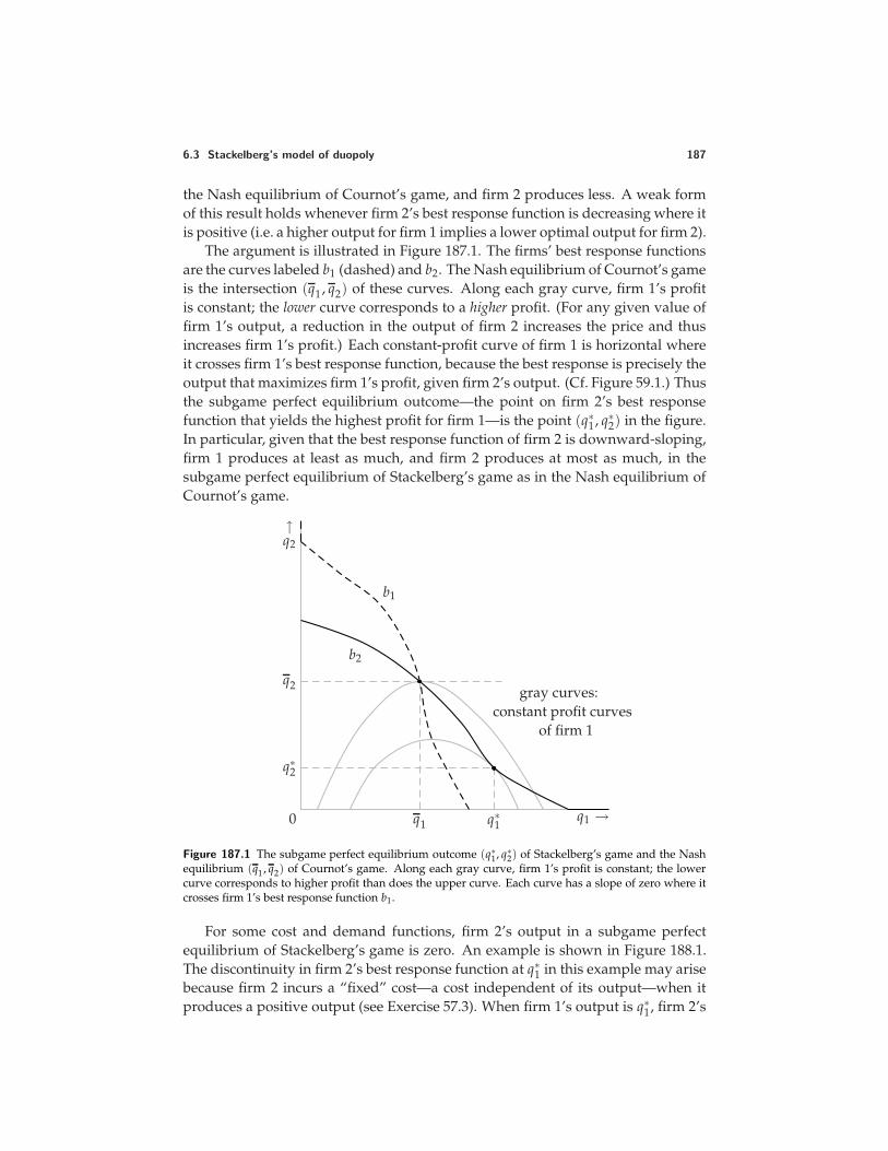
6.3 Stackelberg’s model of duopoly 187
the Nash equilibrium of Cournot’s game, and firm 2 produces less. A weak formof this result holds whenever firm 2’s best response function is decreasing where itis positive (i.e. a higher output for firm 1 implies a lower optimal output for firm 2).
The argument is illustrated in Figure 187.1. The firms’ best response functionsare the curves labeled b1 (dashed) and b2. The Nash equilibrium of Cournot’s gameis the intersection (q1, q2) of these curves. Along each gray curve, firm 1’s profitis constant; the lower curve corresponds to a higher profit. (For any given value offirm 1’s output, a reduction in the output of firm 2 increases the price and thusincreases firm 1’s profit.) Each constant-profit curve of firm 1 is horizontal whereit crosses firm 1’s best response function, because the best response is precisely theoutput that maximizes firm 1’s profit, given firm 2’s output. (Cf. Figure 59.1.) Thusthe subgame perfect equilibrium outcome—the point on firm 2’s best responsefunction that yields the highest profit for firm 1—is the point (q∗1, q∗2) in the figure.In particular, given that the best response function of firm 2 is downward-sloping,firm 1 produces at least as much, and firm 2 produces at most as much, in thesubgame perfect equilibrium of Stackelberg’s game as in the Nash equilibrium ofCournot’s game.
q1 →
↑q2
q∗1q10
q∗2
q2
b1
b2
gray curves:constant profit curves
of firm 1
Figure 187.1 The subgame perfect equilibrium outcome (q∗1, q∗2) of Stackelberg’s game and the Nashequilibrium (q1, q2) of Cournot’s game. Along each gray curve, firm 1’s profit is constant; the lowercurve corresponds to higher profit than does the upper curve. Each curve has a slope of zero where itcrosses firm 1’s best response function b1.
For some cost and demand functions, firm 2’s output in a subgame perfectequilibrium of Stackelberg’s game is zero. An example is shown in Figure 188.1.The discontinuity in firm 2’s best response function at q∗1 in this example may arisebecause firm 2 incurs a “fixed” cost—a cost independent of its output—when itproduces a positive output (see Exercise 57.3). When firm 1’s output is q∗1, firm 2’s
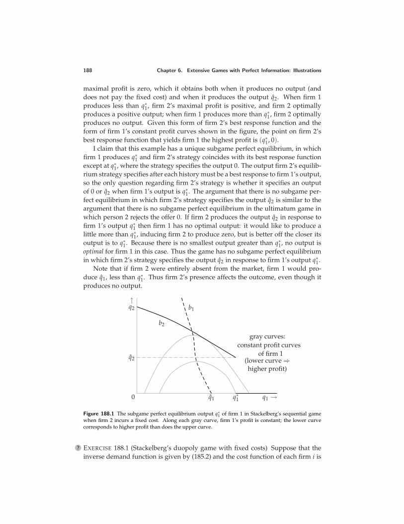
188 Chapter 6. Extensive Games with Perfect Information: Illustrations
maximal profit is zero, which it obtains both when it produces no output (anddoes not pay the fixed cost) and when it produces the output q2. When firm 1produces less than q∗1, firm 2’s maximal profit is positive, and firm 2 optimallyproduces a positive output; when firm 1 produces more than q∗1, firm 2 optimallyproduces no output. Given this form of firm 2’s best response function and theform of firm 1’s constant profit curves shown in the figure, the point on firm 2’sbest response function that yields firm 1 the highest profit is (q∗1, 0).
I claim that this example has a unique subgame perfect equilibrium, in whichfirm 1 produces q∗1 and firm 2’s strategy coincides with its best response functionexcept at q∗1, where the strategy specifies the output 0. The output firm 2’s equilib-rium strategy specifies after each history must be a best response to firm 1’s output,so the only question regarding firm 2’s strategy is whether it specifies an outputof 0 or q2 when firm 1’s output is q∗1. The argument that there is no subgame per-fect equilibrium in which firm 2’s strategy specifies the output q2 is similar to theargument that there is no subgame perfect equilibrium in the ultimatum game inwhich person 2 rejects the offer 0. If firm 2 produces the output q2 in response tofirm 1’s output q∗1 then firm 1 has no optimal output: it would like to produce alittle more than q∗1, inducing firm 2 to produce zero, but is better off the closer itsoutput is to q∗1. Because there is no smallest output greater than q∗1, no output isoptimal for firm 1 in this case. Thus the game has no subgame perfect equilibriumin which firm 2’s strategy specifies the output q2 in response to firm 1’s output q∗1.
Note that if firm 2 were entirely absent from the market, firm 1 would pro-duce q1, less than q∗1. Thus firm 2’s presence affects the outcome, even though itproduces no output.
q1 →
↑q2
q2
q∗1q10
b2
b1
gray curves:constant profit curves
of firm 1(lower curve ⇒higher profit)
Figure 188.1 The subgame perfect equilibrium output q∗1 of firm 1 in Stackelberg’s sequential gamewhen firm 2 incurs a fixed cost. Along each gray curve, firm 1’s profit is constant; the lower curvecorresponds to higher profit than does the upper curve.
? EXERCISE 188.1 (Stackelberg’s duopoly game with fixed costs) Suppose that theinverse demand function is given by (185.2) and the cost function of each firm i is
6.4 Buying votes 189
given by
Ci(qi) =
0 if qi = 0f + cqi if qi > 0,
where c ≥ 0, f > 0, and c < α, as in Exercise 57.3. Show that if c = 0, α =12, and f = 4, Stackelberg’s game has a unique subgame perfect equilibrium, inwhich firm 1’s output is 8 and firm 2’s output is zero. (Use your results fromExercise 57.3).
The value of commitment Firm 1’s output in a subgame perfect equilibrium ofStackelberg’s game is not in general a best response to firm 2’s output: if firm 1could adjust its output after firm 2 has chosen its output, then it would do so! (Inthe case shown in Figure 187.1, it would reduce its output.) However, if firm 1 hadthis opportunity, and firm 2 knew that it had the opportunity, then firm 2 wouldchoose a different output. Indeed, if we simply add a third stage to the game,in which firm 1 chooses an output, then the first stage is irrelevant, and firm 2 iseffectively the first-mover; in the subgame perfect equilibrium firm 1 is worse offthan it is in the Nash equilibrium of the simultaneous-move game. (In the examplein the previous section, the unique subgame perfect equilibrium has firm 2 choosethe output (α − c)/2 and firm 1 choose the output (α − c)/4.) In summary, eventhough firm 1 can increase its profit by changing its output after firm 2 has chosenits output, in the game in which it has this opportunity it is worse off than it is inthe game in which it must choose its output before firm 2 and cannot subsequentlymodify this output. That is, firm 1 prefers to be committed not to change its mind.
? EXERCISE 189.1 (Sequential variant of Bertrand’s duopoly game) Consider thevariant of Bertrand’s duopoly game (Section 3.2) in which first firm 1 chooses aprice, then firm 2 chooses a price. Assume that each firm is restricted to choose aprice that is an integral number of cents (as in Exercise 65.2), that each firm’s unitcost is constant, equal to c (an integral number of cents), and that the monopolyprofit is positive.
a. Specify an extensive game with perfect information that models this situation.
b. Give an example of a strategy of firm 1 and an example of a strategy of firm 2.
c. Find the subgame perfect equilibria of the game.
6.4 Buying votes
A legislature has k members, where k is an odd number. Two rival bills, X andY, are being considered. The bill that attracts the votes of a majority of legislatorswill pass. Interest group X favors bill X, whereas interest group Y favors bill Y.Each group wishes to entice a majority of legislators to vote for its favorite bill.First interest group X gives an amount of money (possibly zero) to each legislator,then interest group Y does so. Each interest group wishes to spend as little aspossible. Group X values the passing of bill X at $VX > 0 and the passing of bill Y
190 Chapter 6. Extensive Games with Perfect Information: Illustrations
at zero, and group Y values the passing of bill Y at $VY > 0 and the passing ofbill X at zero. (For example, group X is indifferent between an outcome in whichit spends VX and bill X is passed and one in which it spends nothing and bill Y ispassed.) Each legislator votes for the favored bill of the interest group that offersher the most money; a legislator to whom both groups offer the same amount ofmoney votes for bill Y (an arbitrary assumption that simplifies the analysis withoutqualitatively changing the outcome). For example, if k = 3, the amounts offered tothe legislators by group X are x = (100, 50, 0), and the amounts offered by group Yare y = (100, 0, 50), then legislators 1 and 3 vote for Y and legislator 2 votes for X,so that Y passes. (In some legislatures the inducements offered to legislators aremore subtle than cash transfers.)
We can model this situation as the following extensive game.
Players The two interest groups, X and Y.
Terminal histories The set of all sequences (x, y), where x is a list of paymentsto legislators made by interest group X and y is a list of payments to legisla-tors made by interest group Y. (That is, both x and y are lists of k nonnegativeintegers.)
Player function P(∅) = X and P(x) = Y for all x.
Preferences The preferences of interest group X are represented by the payofffunction
VX − (x1 + · · · + xk) if bill X passes−(x1 + · · · + xk) if bill Y passes,
where bill Y passes after the terminal history (x, y) if and only if the numberof components of y that are at least equal to the corresponding componentsof x is at least 1
2 (k + 1) (a bare majority of the k legislators). The prefer-ences of interest group Y are represented by the analogous function (whereVY replaces VX , y replaces x, and Y replaces X).
Before studying the subgame perfect equilibria of this game for arbitrary valuesof the parameters, consider two examples. First suppose that k = 3 and VX =VY = 300. Under these assumptions, the most group X is willing to pay to getbill X passed is 300. For any payments it makes to the three legislators that sum toat most 300, two of the payments sum to at most 200, so that if group Y matchesthese payments it spends less than VY (= 300) and gets bill Y passed. Thus inany subgame perfect equilibrium group X makes no payments, group Y makes nopayments, and (given the tie-breaking rule) bill Y is passed.
Now suppose that k = 3, VX = 300, and VY = 100. In this case by payingeach legislator more than 50, group X makes matching payments by group Y un-profitable: only by spending more than VY (= 100) can group Y cause bill Y tobe passed. However, there is no subgame perfect equilibrium in which group Xpays each legislator more than 50, because it can always pay a little less (as long
6.4 Buying votes 191
as the payments still exceed 50) and still prevent group Y from profitably match-ing. In the only subgame perfect equilibrium group X pays each legislator ex-actly 50, and group Y makes no payments. Given group X’s action, group Y isindifferent between matching X’s payments (so that bill Y is passed), and mak-ing no payments. However, there is no subgame perfect equilibrium in whichgroup Y matches group X’s payments, because if this were group Y’s responsethen group X could increase its payments a little, making matching payments bygroup Y unprofitable.
For arbitrary values of the parameters the subgame perfect equilibrium out-come takes one of the forms in these two examples: either no payments are madeand bill Y is passed, or group X makes payments that group Y does not wish tomatch, group Y makes no payments, and bill X is passed.
To find the subgame perfect equilibria in general, we may use backward induc-tion. First consider group Y’s best response to an arbitrary strategy x of group X.Let µ = 1
2 (k + 1), a bare majority of k legislators, and denote by mx the sum of thesmallest µ components of x—the total payments Y needs to make to buy off a baremajority of legislators.
• If mx < VY then group Y can buy off a bare majority of legislators for lessthan VY, so that its best response to x is to match group X’s payments to theµ legislators to whom group X’s payments are smallest; the outcome is thatbill Y is passed.
• If mx > VY then the cost to group Y of buying off any majority of legislatorsexceeds VY , so that group Y’s best response to x is to make no payments; theoutcome is that bill X is passed.
• If mx = VY then both the actions in the previous two cases are best responsesby group Y to x.
We conclude that group Y’s strategy in a subgame perfect equilibrium has thefollowing properties.
• After a history x for which mx < VY , group Y matches group X’s paymentsto the µ legislators to whom X’s payments are smallest.
• After a history x for which mx > VY , group Y makes no payments.
• After a history x for which mx = VY , group Y either makes no payments ormatches group X’s payments to the µ legislators to whom X’s payments aresmallest.
Given that group Y’s subgame perfect equilibrium strategy has these proper-ties, what should group X do? If it chooses a list of payments x for which mx < VYthen group Y matches its payments to a bare majority of legislators, and bill Ypasses. If it reduces all its payments, the same bill is passed. Thus the only list ofpayments x with mx < VY that may be optimal is (0, . . . , 0). If it chooses a list of
192 Chapter 6. Extensive Games with Perfect Information: Illustrations
payments x with mx > VY then group Y makes no payments, and bill X passes.If it reduces all its payments a little (keeping the payments to every bare majoritygreater than VY), the outcome is the same. Thus no list of payments x for whichmx > VY is optimal.
We conclude that in any subgame perfect equilibrium we have either x =(0, . . . , 0) (group X makes no payments) or mx = VY (the smallest sum of group X’spayments to a bare majority of legislators is VY). Under what conditions does eachcase occur? If group X needs to spend more than VX to deter group Y from match-ing its payments to a bare majority of legislators, then its best strategy is to makeno payments (x = (0, . . . , 0)). How much does it need to spend to deter group Y?It needs to pay more than VY to every bare majority of legislators, so it needs topay each legislator more than VY/µ, in which case its total payment is more thankVY/µ. Thus if VX < kVY/µ, group X is better off making no payments than gettingbill X passed by making payments large enough to deter group Y from matchingits payments to a bare majority of legislators.
If VX > kVY/µ, on the other hand, group X can afford to make payments largeenough to deter group Y from matching. In this case its best strategy is to payeach legislator VY/µ, so that its total payment to every bare majority of legislatorsis VY . Given this strategy, group Y is indifferent between matching group X’spayments to a bare majority of legislators and making no payments. I claim thatthe game has no subgame perfect equilibrium in which group Y matches. Theargument is similar to the argument that the ultimatum game has no subgameperfect equilibrium in which person 2 rejects the offer 0. Suppose that group Ymatches. Then group X can increase its payoff by increasing its payments a little(keeping the total less than VX), thereby deterring group Y from matching, andensuring that bill X passes. Thus in any subgame perfect equilibrium group Ymakes no payments in response to group X’s strategy.
In conclusion, if VX = kVY/µ then the game has a unique subgame perfectequilibrium, in which group Y’s strategy is
• match group X’s payments to the µ legislators to whom X’s payments aresmallest after a history x for which mx < VY
• make no payments after a history x for which mx ≥ VY
and group X’s strategy depends on the relative sizes of VX and VY:
• if VX < kVY/µ then group X makes no payments;
• if VX > kVY/µ then group X pays each legislator VY/µ.
If VX < kVY/µ then the outcome is that neither group makes any payment, andbill Y is passed; if VX > kVY/µ then the outcome is that group X pays each legisla-tor VY/µ, group Y makes no payments, and bill X is passed. (If VX = kVY/µ thenthe analysis is more complex.)
Three features of the subgame perfect equilibrium are significant. First, the out-come favors the second-mover in the game (group Y): only if VX > kVY/µ, which
6.4 Buying votes 193
is close to 2VY when k is large, does group X manage to get bill X passed. Second,group Y never makes any payments! According to its equilibrium strategy it isprepared to make payments in response to certain strategies of group X, but givengroup X’s equilibrium strategy it spends not a cent. Third, if group X makes anypayments (as it does in the equilibrium for VX > kVY/µ) then it makes a paymentto every legislator. If there were no competing interest group but nonetheless eachlegislator would vote for bill X only if she were paid at least some amount, thengroup X would make payments to only a bare majority of legislators; if it were toact in this way in the presence of group Y it would supply group Y with almost amajority of legislators who could be induced to vote for bill Y at no cost.
? EXERCISE 193.1 (Three interest groups buying votes) Consider a variant of themodel in which there are three bills, X, Y, and Z, and three interest groups, X, Y,and Z, who choose lists of payments sequentially. Ties are broken in favor of thegroup moving later. Find the bill that is passed in any subgame perfect equilibriumwhen k = 3 and (a) VX = VY = VZ = 300, (b) VX = 300, VY = VZ = 100, and(c) VX = 300, VY = 202, VZ = 100. (You may assume that in each case a subgameperfect equilibrium exists; note that you are not asked to find the subgame perfectequilibria themselves.)
? EXERCISE 193.2 (Interest groups buying votes under supermajority rule) Consideran alternative variant of the model in which a supermajority is required to pass abill. There are two bills, X and Y, and a “default outcome”. A bill passes if andonly if it receives at least k∗ > 1
2 (k + 1) votes; if neither bill passes the defaultoutcome occurs. There are two interest groups. Both groups attach value 0 to thedefault outcome. Find the bill that is passed in any subgame perfect equilibriumwhen k = 7, k∗ = 5, and (a) VX = VY = 700 and (b) VX = 750, VY = 400. In eachcase, would the legislators be better off or worse off if a simple majority of voteswere required to pass a bill?
? EXERCISE 193.3 (Sequential positioning by two political candidates) Consider thevariant of Hotelling’s model of electoral competition in Section 3.3 in which the ncandidates choose their positions sequentially, rather than simultaneously. Modelthis situation as an extensive game. Find the subgame perfect equilibrium (equi-libria?) when n = 2.
?? EXERCISE 193.4 (Sequential positioning by three political candidates) Consider afurther variant of Hotelling’s model of electoral competition in which the n can-didates choose their positions sequentially and each candidate has the option ofstaying out of the race. Assume that each candidate prefers to stay out than toenter and lose, prefers to enter and tie with any number of candidates than to stayout, and prefers to tie with as few other candidates as possible. Model the situ-ation as an extensive game and find the subgame perfect equilibrium outcomeswhen n = 2 (easy) and when n = 3 and the voters’ favorite positions are dis-tributed uniformly from 0 to 1 (i.e. the fraction of the voters’ favorite positions lessthan x is x) (hard).
194 Chapter 6. Extensive Games with Perfect Information: Illustrations
6.5 A race
6.5.1 General model
Firms compete with each other to develop new technologies; authors compete witheach other to write books and film scripts about momentous current events; scien-tists compete with each other to make discoveries. In each case the winner enjoysa significant advantage over the losers, and each competitor can, at a cost, increaseher pace of activity. How do the presence of competitors and size of the prize affectthe pace of activity? How does the identity of the winner of the race depend onthe each competitor’s initial distance from the finish line?
We can model a race as an extensive game with perfect information in whichthe players alternately choose how many “steps” to take. Here I study a simpleexample of such a game, with two players.
Player i is initially ki > 0 steps from the finish line, for i = 1, 2. On each of herturns, a player can either not take any steps (at a cost of 0), or can take one step, ata cost of c(1), or two steps, at a cost of c(2). The first player to reach the finish linewins a prize, worth vi > 0 to player i; the losing player’s payoff is 0. To make thegame finite, I assume that if, on successive turns, neither player takes any step, thegame ends and neither player obtains the prize.
I denote the game in which player i moves first by Gi(k1, k2). The game G1(k1, k2)is defined precisely as follows.
Players The two parties.
Terminal histories The set of sequences of the form (x1, y1, x2, y2, . . . , xT) or(x1, y1, x2, y2, . . . , yT) for some integer T, where each xt (the number of stepstaken by player 1 on her tth turn) and each yt (the number of steps takenby player 2 on her tth turn) is 0, 1, or 2, there are never two successive 0’sexcept possibly at the end of a sequence, and either x1 + · · · + xT = k1 andy1 + · · ·+ yT < k2 (player 1 reaches the finish line first), or x1 + · · ·+ xT < k1and y1 + · · · + yT = k2 (player 2 reaches the finish line first).
Player function P(∅) = 1, P(x1) = 2 for all x1, P(x1, y1) = 1 for all (x1, y1),P(x1, y1, x2) = 2 for all (x1, y1, x2), and so on.
Preferences For a terminal history in which player i loses, her payoff is thenegative of the sum of the costs of all her moves; for a terminal history inwhich she wins it is vi minus the sum of these costs.
6.5.2 Subgame perfect equilibria of an example
A simple example illustrates the features of the subgame perfect equilibria of thisgame. Suppose that both v1 and v2 are between 6 and 7 (their exact values do notaffect the equilibria), the cost c(1) of a single step is 1, and the cost c(2) of two steps
6.5 A race 195
is 4. (Given that c(2) > 2c(1), each player, in the absence of a competitor, wouldlike to take one step at a time.)
The game has a finite horizon, so we may use backward induction to find itssubgame perfect equilibria. Each of its subgames is either a game Gi(m1, m2) withi = 1 or i = 2 and 0 < m1 ≤ k1 and 0 < m2 ≤ k2, or, if the last player to movebefore the subgame took no steps, a game that differs from Gi(m1, m2) only in thatit ends if player i initially takes no steps (i.e. the only terminal history starting with0 consists only of 0).
First consider the very simplest game, G1(1, 1), in which each player is initiallyone step from the finish line. If player 1 takes one step, she wins; if she does notmove then player 2 optimally takes one step (if she does not, the game ends) andwins. We conclude that the game has a unique subgame perfect equilibrium, inwhich player 1 initially takes one step and wins.
A similar argument applies to the game G1(1, 2). If player 1 does not movethen player 2 has the option of taking one or two steps. If she takes one step thenplay moves to a subgame identical G1(1, 1), in which we have just concluded thatplayer 1 wins. Thus player 2 takes two steps, and wins, if player 1 does not moveat the start of G1(1, 2). We conclude that the game has a unique subgame perfectequilibrium, in which player 1 initially takes one step and wins.
Now consider player 1’s options in the game G1(2, 1).
Player 1 takes two steps: She wins, and obtains a payoff of at least 6 − 4 = 2(her valuation is more than 6, and the cost of two steps is 4).
Player 1 take one step: Play moves to a subgame identical to G2(1, 1); we knowthat in the equilibrium of this subgame player 2 initially takes one step andwins.
Player 1 does not move: Play moves to a subgame in which player 2 is the first-mover and is one step from the finish line, and, if player 2 does not move, thegame ends. In an equilibrium of this subgame player 2 takes one step andwins.
We conclude that the game G1(2, 1) has a unique subgame perfect equilibrium, inwhich player 1 initially takes two steps and wins.
I have spelled out the details of the analysis of these cases to show how weuse the result for the game G1(1, 1) to find the equilibria of the games G1(1, 2) andG1(2, 1). In general, the equilibria of the games Gi(k1, k2) for all values of k1 and k2up to k tell us the consequences of player 1’s taking one or two steps in the gameG1(k + 1, k).
? EXERCISE 195.1 (The race G1(2, 2)) Show that the game G1(2, 2) has a unique sub-game perfect equilibrium outcome, in which player 1 initially takes two steps, andwins.
196 Chapter 6. Extensive Games with Perfect Information: Illustrations
So far we have concluded that in any game in which each player is initially atmost two steps from the finish line, the first-mover takes enough steps to reach thefinish line, and wins.
Now suppose that player 1 is at most two steps from the finish line, but player 2is three steps away. Suppose that player 1 takes only one step (even if she is initiallytwo steps from the finish line). Then if player 2 takes either one or two steps, playmoves to a subgame in which player 1 (the first-mover) wins. Thus player 2 isbetter off not moving (and not incurring any cost), in which case player 1 takesone step on her next turn, and wins. (Player 1 prefers to move one step at a timethan to move two steps initially, because the former costs her 2 whereas the lattercosts her 4.) We conclude that the outcome of a subgame perfect equilibrium in thegame G1(2, 3) is that player 1 takes one step on her first turn, then player 2 doesnot move, and then player 1 takes another step, and wins.
By a similar argument, in a subgame perfect equilibrium of any game in whichplayer 1 is at most two steps from the finish line and player 2 is three or more stepsaway, player 1 moves one step at a time, and player 2 does not move; player 1 wins.Symmetrically, in a subgame perfect equilibrium of any game in which player 1 isthree or more steps from the finish line and player 2 is at most two steps away,player 1 does not move, and player 2 moves one step at a time, and wins.
Our conclusions so far are illustrated in Figure 197.1. In this figure, player 1moves to the left, and player 2 moves down. The values of (k1, k2) for which thesubgame perfect equilibrium outcome has been determined so far are labeled. Thelabel “1” means that, regardless of who moves first, in a subgame perfect equilib-rium player 1 moves one step on each turn, and player 2 does not move; player 1wins. Similarly, the label “2” means that, regardless of who moves first, player 2moves one step on each turn, and player 1 does not move; player 2 wins. The label“f” means that the first player to move takes enough steps to reach the finish line,and wins.
Now consider the game G1(3, 3). If player 1 takes one step, we reach the gameG2(2, 3). From Figure 197.1 we see that in the subgame perfect equilibrium of thisgame player 1 wins, and does so by taking one step at a time (the point (2, 3) islabeled “1”). If player 1 takes two steps, we reach the game G2(1, 3), in whichplayer 1 also wins. Player 1 prefers not to take two steps unless she has to, soin the subgame perfect equilibrium of G1(3, 3) she takes one step at a time, andwins, and player 2 does not move. Similarly, in a subgame perfect equilibrium ofG2(3, 3), player 2 takes one step at a time, and wins, and player 1 does not move.
A similar argument applies to each of the games Gi(3, 4), Gi(4, 3), and Gi(4, 4)for i = 1, 2. The argument differs only if the first-mover is four steps from thefinish line, in which case she initially takes two steps in order to reach a game inwhich she wins. (If she initially takes only one step, the other player wins.)
Now consider the game Gi(3, 5) for i = 1, 2. By taking one step in G1(3, 5),player 1 reaches a game in which she wins by taking one step at a time. Thecost of her taking three steps is less than v1, so in a subgame perfect equilibriumof G1(3, 5) she takes one step at a time, and wins, and player 2 does not move.
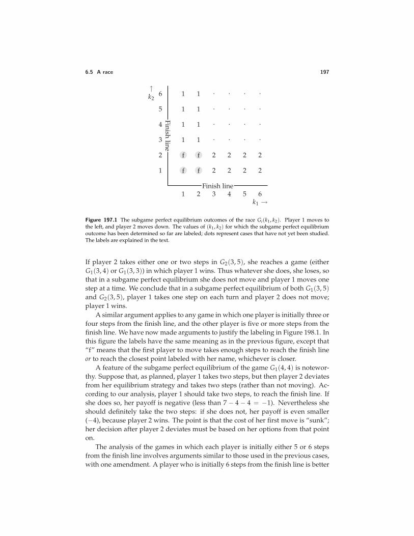
6.5 A race 197
f f
f f
2 2 2 2
2 2 2 2
1
1
1
1
1
1
1
1 . . . .
. . . .
. . . .
. . . .
Finish line
Finishline
k1 →1 2 3 4 5 6
1
2
3
4
5
6↑k2
Figure 197.1 The subgame perfect equilibrium outcomes of the race Gi(k1, k2). Player 1 moves tothe left, and player 2 moves down. The values of (k1, k2) for which the subgame perfect equilibriumoutcome has been determined so far are labeled; dots represent cases that have not yet been studied.The labels are explained in the text.
If player 2 takes either one or two steps in G2(3, 5), she reaches a game (eitherG1(3, 4) or G1(3, 3)) in which player 1 wins. Thus whatever she does, she loses, sothat in a subgame perfect equilibrium she does not move and player 1 moves onestep at a time. We conclude that in a subgame perfect equilibrium of both G1(3, 5)and G2(3, 5), player 1 takes one step on each turn and player 2 does not move;player 1 wins.
A similar argument applies to any game in which one player is initially three orfour steps from the finish line, and the other player is five or more steps from thefinish line. We have now made arguments to justify the labeling in Figure 198.1. Inthis figure the labels have the same meaning as in the previous figure, except that“f” means that the first player to move takes enough steps to reach the finish lineor to reach the closest point labeled with her name, whichever is closer.
A feature of the subgame perfect equilibrium of the game G1(4, 4) is notewor-thy. Suppose that, as planned, player 1 takes two steps, but then player 2 deviatesfrom her equilibrium strategy and takes two steps (rather than not moving). Ac-cording to our analysis, player 1 should take two steps, to reach the finish line. Ifshe does so, her payoff is negative (less than 7 − 4 − 4 = −1). Nevertheless sheshould definitely take the two steps: if she does not, her payoff is even smaller(−4), because player 2 wins. The point is that the cost of her first move is “sunk”;her decision after player 2 deviates must be based on her options from that pointon.
The analysis of the games in which each player is initially either 5 or 6 stepsfrom the finish line involves arguments similar to those used in the previous cases,with one amendment. A player who is initially 6 steps from the finish line is better
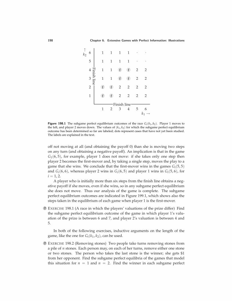
198 Chapter 6. Extensive Games with Perfect Information: Illustrations
f f
f f
f f
f f
2 2 2 2
2 2 2 2
2 2
2 2
1
1
1
1
1
1
1
1
1
1
1
1
. .
. .
Finish line
Finishline
k1 →1 2 3 4 5 6
1
2
3
4
5
6↑k2
Figure 198.1 The subgame perfect equilibrium outcomes of the race Gi(k1, k2). Player 1 moves tothe left, and player 2 moves down. The values of (k1, k2) for which the subgame perfect equilibriumoutcome has been determined so far are labeled; dots represent cases that have not yet been studied.The labels are explained in the text.
off not moving at all (and obtaining the payoff 0) than she is moving two stepson any turn (and obtaining a negative payoff). An implication is that in the gameG1(6, 5), for example, player 1 does not move: if she takes only one step thenplayer 2 becomes the first-mover and, by taking a single step, moves the play to agame that she wins. We conclude that the first-mover wins in the games Gi(5, 5)and Gi(6, 6), whereas player 2 wins in Gi(6, 5) and player 1 wins in Gi(5, 6), fori = 1, 2.
A player who is initially more than six steps from the finish line obtains a neg-ative payoff if she moves, even if she wins, so in any subgame perfect equilibriumshe does not move. Thus our analysis of the game is complete. The subgameperfect equilibrium outcomes are indicated in Figure 199.1, which shows also thesteps taken in the equilibrium of each game when player 1 is the first-mover.
? EXERCISE 198.1 (A race in which the players’ valuations of the prize differ) Findthe subgame perfect equilibrium outcome of the game in which player 1’s valu-ation of the prize is between 6 and 7, and player 2’s valuation is between 4 and5.
In both of the following exercises, inductive arguments on the length of thegame, like the one for Gi(k1, k2), can be used.
? EXERCISE 198.2 (Removing stones) Two people take turns removing stones froma pile of n stones. Each person may, on each of her turns, remove either one stoneor two stones. The person who takes the last stone is the winner; she gets $1from her opponent. Find the subgame perfect equilibria of the games that modelthis situation for n = 1 and n = 2. Find the winner in each subgame perfect
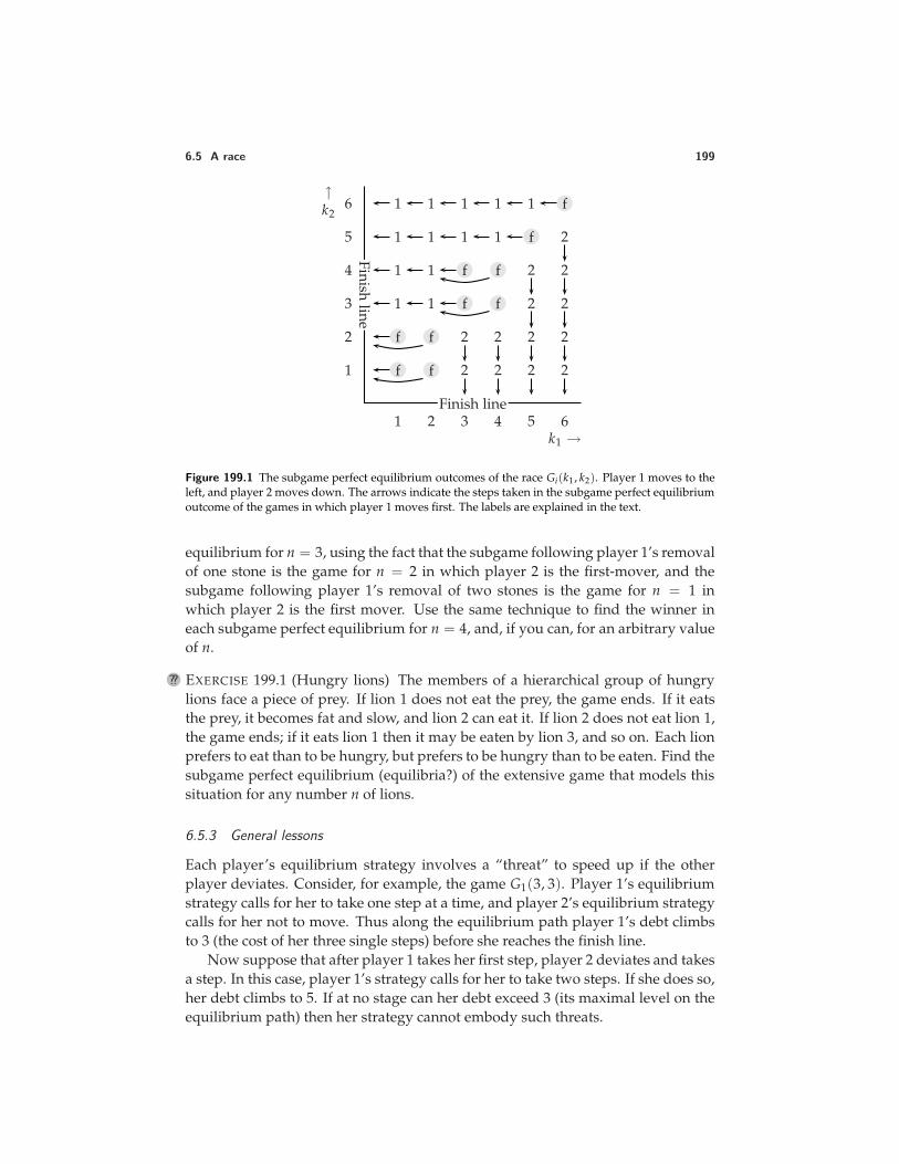
6.5 A race 199
f f
f f
f f
f f
2 2 2 2
2 2 2 2
2 2
2 2
2
1 1
1 1
1 1 1 1
1 1 1 1 1
f
f
Finish line
Finishline
k1 →1 2 3 4 5 6
1
2
3
4
5
6↑k2
Figure 199.1 The subgame perfect equilibrium outcomes of the race Gi(k1, k2). Player 1 moves to theleft, and player 2 moves down. The arrows indicate the steps taken in the subgame perfect equilibriumoutcome of the games in which player 1 moves first. The labels are explained in the text.
equilibrium for n = 3, using the fact that the subgame following player 1’s removalof one stone is the game for n = 2 in which player 2 is the first-mover, and thesubgame following player 1’s removal of two stones is the game for n = 1 inwhich player 2 is the first mover. Use the same technique to find the winner ineach subgame perfect equilibrium for n = 4, and, if you can, for an arbitrary valueof n.
?? EXERCISE 199.1 (Hungry lions) The members of a hierarchical group of hungrylions face a piece of prey. If lion 1 does not eat the prey, the game ends. If it eatsthe prey, it becomes fat and slow, and lion 2 can eat it. If lion 2 does not eat lion 1,the game ends; if it eats lion 1 then it may be eaten by lion 3, and so on. Each lionprefers to eat than to be hungry, but prefers to be hungry than to be eaten. Find thesubgame perfect equilibrium (equilibria?) of the extensive game that models thissituation for any number n of lions.
6.5.3 General lessons
Each player’s equilibrium strategy involves a “threat” to speed up if the otherplayer deviates. Consider, for example, the game G1(3, 3). Player 1’s equilibriumstrategy calls for her to take one step at a time, and player 2’s equilibrium strategycalls for her not to move. Thus along the equilibrium path player 1’s debt climbsto 3 (the cost of her three single steps) before she reaches the finish line.
Now suppose that after player 1 takes her first step, player 2 deviates and takesa step. In this case, player 1’s strategy calls for her to take two steps. If she does so,her debt climbs to 5. If at no stage can her debt exceed 3 (its maximal level on theequilibrium path) then her strategy cannot embody such threats.
200 Chapter 6. Extensive Games with Perfect Information: Illustrations
The general point is that a limit on the debt a player can accumulate may affectthe outcome even if it exceeds the player’s debt along the equilibrium path in theabsence of any limits. You are asked to study an example in the next exercise.
? EXERCISE 200.1 (A race with a liquidity constraint) Find the subgame perfect equi-librium of the variant of the game G1(3, 3) in which player 1’s debt may neverexceed 3.
In the subgame perfect equilibrium of every game Gi(k1, k2), only one playermoves; her opponent “gives up”. This property of equilibrium holds in more gen-eral games. What added ingredient might lead to an equilibrium in which bothplayers are active? A player’s uncertainty about the other’s characteristics wouldseem to be such an ingredient: if a player does not know the cost of its opponent’smoves, it may assign a positive probability less than one to its winning, at leastuntil it has accumulated some evidence of its opponent’s behavior, and while it isoptimistic it may be active even though its rival is also active. To build such con-siderations into the model we need to generalize the model of an extensive gameto encompass imperfect information, as we do in Chapter 10.
Another feature of the subgame perfect equilibrium of Gi(k1, k2) that holds inmore general games is that the presence of a competitor has little effect on thespeed of the player who moves. A lone player would move one step at a time.When there are two players, for most starting points the one that moves does so atthe same leisurely pace. Only for a small number of starting points, in all of whichthe players’ initial distances from the starting line are similar, does the presence ofa competitor induce the active player to hasten its progress, and then only in thefirst period.
Notes
The first experiment on the ultimatum game is reported in Guth, Schmittberger,and Schwarze (1982). Grout (1984) is an early analysis of a holdup game. Themodel in Section 6.3 is due to von Stackelberg (1934). The vote-buying game inSection 6.4 is taken from Groseclose and Snyder (1996). The model of a race inSection 6.5 is a simplification suggested by Vijay Krishna of a model of Harris andVickers (1985).
For more discussion of the experimental evidence on the ultimatum game (dis-cussed in the box on page 181), see Roth (1995). Bolton and Ockenfels (2000) studythe implications of assuming that players are equity-conscious, and relate theseimplications to the experimental outcomes in various games. The explanation ofthe experimental results in terms of rules of thumb is discussed by Aumann (1997,7–8). The problem of fair division, an example of which is given in Exercise 183.2,is studied in detail by Brams and Taylor (1996), who trace the idea of divide-and-choose back to antiquity (p. 10). I have been unable to find the origin of the idea inExercise 199.1; Barton Lipman suggested the formulation in the exercise.
Draft chapter from An introduction to game theory by Martin J. [email protected]; www.economics.utoronto.ca/osborneVersion: 00/11/6.Copyright c© 1995–2000 by Martin J. Osborne. All rights reserved. No part of this book may be re-produced by any electronic or mechanical means (including photocopying, recording, or informationstorage and retrieval) without permission in writing from Oxford University Press, except that onecopy of up to six chapters may be made by any individual for private study.
7 Extensive Games with Perfect Information:Extensions and Discussion
Extensive games with perfect information and simultaneous moves 201Illustration: entry into a monopolized industry 209Illustration: electoral competition with strategic voters 211Illustration: committee decision-making 213Illustration: exit from a declining industry 217Allowing for exogenous uncertainty 222Discussion: subgame perfect equilibrium and backward induction 226Prerequisite: Chapter 5.
7.1 Allowing for simultaneous moves
7.1.1 Definition
THE model of an extensive game with perfect information (Definition 153.1) as-sumes that after every sequences of events, a single decision-maker takes an
action, knowing every decision-maker’s previous actions. I now describe a moregeneral model that allows us to study situations in which, after some sequences ofevents, the members of a group of decision-makers choose their actions “simulta-neously”, each member knowing every decision-maker’s previous actions, but notthe contemporaneous actions of the other members of the group.
In the more general model, a terminal history is a sequence of lists of actions,each list specifying the actions of a set of players. (A game in which each set con-tains a single player is an extensive game with perfect information as defined pre-viously.) For example, consider a situation in which player 1 chooses either C orD, then players 2 and 3 simultaneously take actions, each choosing either E or F.In the extensive game that models this situation, (C, (E, E)) is a terminal history, inwhich first player 1 chooses C, and then players 2 and 3 both choose E. In the gen-eral model, the player function assigns a set of players to each nonterminal history.In the example just described, this set consists of the single player 1 for the initialhistory, and consists of players 2 and 3 for the history C.
An extensive game with perfect information (Definition 153.1) does not specifyexplicitly the sets of actions available to the players. However, we may derivethe set of actions of the player who moves after any nonterminal history fromthe set of terminal histories and the player function (see (154.1)). When we allowsimultaneous moves, the players’ sets of actions are conveniently specified in the
201
202 Chapter 7. Extensive Games with Perfect Information: Extensions and Discussion
definition of a game. In the example of the previous paragraph, for instance, wespecify the game by giving the eight possible terminal histories (C or D followedby one of the four pairs (E, E), (E, F), (F, E), and (F, F)), the player function definedby P(∅) = 1 and P(C) = P(D) = 2, 3, the sets of actions C, D for player 1 atthe start of the game and E, F for both player 2 and player 3 after the histories Cand D, and each player’s preferences over terminal histories.
In any game, the set of terminal histories, player function, and sets of actionsfor the players must be consistent: the list of actions that follows a subhistory ofany terminal history must be a list of actions of the players assigned by the playerfunction to that subhistory. In the game described above, for example, the listof actions following the subhistory C of the terminal history (C, (E, E)) is (E, E),which is a pair of actions for the players (2 and 3) assigned by the player functionto the history C.
Precisely, an extensive game with perfect information and simultaneous movesis defined as follows.
DEFINITION 202.1 An extensive game with perfect information and simultane-ous moves consists of
• a set of players
• a set of sequences (terminal histories) with the property that no sequence isa proper subhistory of any other sequence
• a function (the player function) that assigns a set of players to every sequencethat is a proper subhistory of some terminal history
• for each proper subhistory h of each terminal history and each player i thatis a member of the set of players assigned to h by the player function, a setAi(h) (the set of actions available to player i after the history h)
• for each player, preferences over the set of terminal histories
such that the set of terminal histories, player function, and sets of actions are con-sistent in the sense that h is a terminal history if and only if either (i) h takes theform (a1, . . . , ak) for some integer k, the player function is not defined at h, andfor every = 0, . . . , k − 1, a+1 is a list of actions of the players assigned by theplayer function to (a1, . . . , a) (the empty history if = 0), or (ii) h takes the form(a1, a2, . . .) and for every = 0, 1, . . ., a+1 is a list of actions of the players assignedby the player function to (a1, . . . , a) (the empty history if = 0).
This definition encompasses both extensive games with perfect information asin Definition 153.1 and, in a sense, strategic games. An extensive game with per-fect information is an extensive game with perfect information and simultaneousmoves in which the set of players assigned to each history consists of exactly onemember. (The definition of an extensive game with perfect information and simul-taneous moves includes the players’ actions, whereas the definition of an extensivegame with perfect information does not. However, actions may be derived fromthe terminal histories and player function of the latter.)
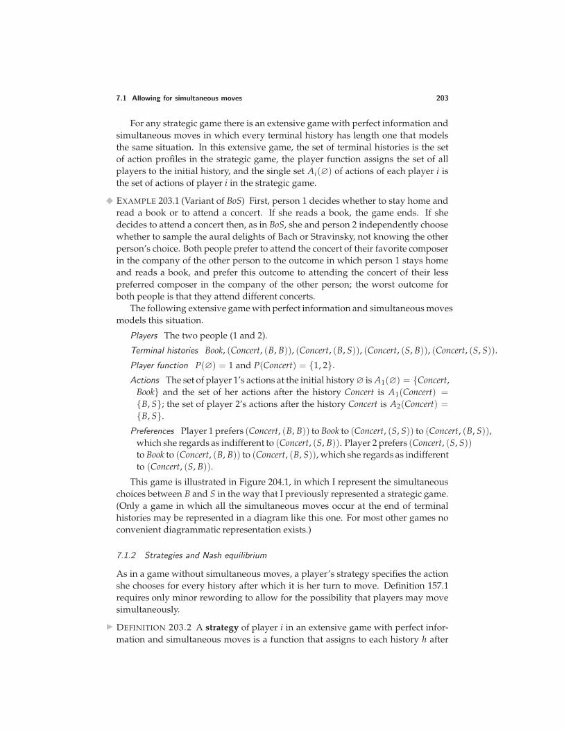
7.1 Allowing for simultaneous moves 203
For any strategic game there is an extensive game with perfect information andsimultaneous moves in which every terminal history has length one that modelsthe same situation. In this extensive game, the set of terminal histories is the setof action profiles in the strategic game, the player function assigns the set of allplayers to the initial history, and the single set Ai(∅) of actions of each player i isthe set of actions of player i in the strategic game.
EXAMPLE 203.1 (Variant of BoS) First, person 1 decides whether to stay home andread a book or to attend a concert. If she reads a book, the game ends. If shedecides to attend a concert then, as in BoS, she and person 2 independently choosewhether to sample the aural delights of Bach or Stravinsky, not knowing the otherperson’s choice. Both people prefer to attend the concert of their favorite composerin the company of the other person to the outcome in which person 1 stays homeand reads a book, and prefer this outcome to attending the concert of their lesspreferred composer in the company of the other person; the worst outcome forboth people is that they attend different concerts.
The following extensive game with perfect information and simultaneous movesmodels this situation.
Players The two people (1 and 2).
Terminal histories Book, (Concert, (B, B)), (Concert, (B, S)), (Concert, (S, B)), (Concert, (S, S)).
Player function P(∅) = 1 and P(Concert) = 1, 2.
Actions The set of player 1’s actions at the initial history ∅ is A1(∅) = Concert,Book and the set of her actions after the history Concert is A1(Concert) =B, S; the set of player 2’s actions after the history Concert is A2(Concert) =B, S.
Preferences Player 1 prefers (Concert, (B, B)) to Book to (Concert, (S, S)) to (Concert, (B, S)),which she regards as indifferent to (Concert, (S, B)). Player 2 prefers (Concert, (S, S))to Book to (Concert, (B, B)) to (Concert, (B, S)), which she regards as indifferentto (Concert, (S, B)).
This game is illustrated in Figure 204.1, in which I represent the simultaneouschoices between B and S in the way that I previously represented a strategic game.(Only a game in which all the simultaneous moves occur at the end of terminalhistories may be represented in a diagram like this one. For most other games noconvenient diagrammatic representation exists.)
7.1.2 Strategies and Nash equilibrium
As in a game without simultaneous moves, a player’s strategy specifies the actionshe chooses for every history after which it is her turn to move. Definition 157.1requires only minor rewording to allow for the possibility that players may movesimultaneously.
DEFINITION 203.2 A strategy of player i in an extensive game with perfect infor-mation and simultaneous moves is a function that assigns to each history h after
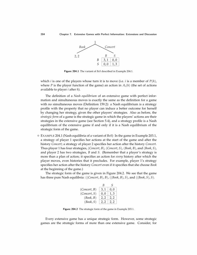
204 Chapter 7. Extensive Games with Perfect Information: Extensions and Discussion
1Book Concert
2, 2 B SB 3, 1 0, 0S 0, 0 1, 3
Figure 204.1 The variant of BoS described in Example 204.1.
which i is one of the players whose turn it is to move (i.e. i is a member of P(h),where P is the player function of the game) an action in Ai(h) (the set of actionsavailable to player i after h).
The definition of a Nash equilibrium of an extensive game with perfect infor-mation and simultaneous moves is exactly the same as the definition for a gamewith no simultaneous moves (Definition 159.2): a Nash equilibrium is a strategyprofile with the property that no player can induce a better outcome for herselfby changing her strategy, given the other players’ strategies. Also as before, thestrategic form of a game is the strategic game in which the players’ actions are theirstrategies in the extensive game (see Section 5.4), and a strategy profile is a Nashequilibrium of the extensive game if and only if it is a Nash equilibrium of thestrategic form of the game.
EXAMPLE 204.1 (Nash equilibria of a variant of BoS) In the game in Example 203.1,a strategy of player 1 specifies her actions at the start of the game and after thehistory Concert; a strategy of player 2 specifies her action after the history Concert.Thus player 1 has four strategies, (Concert, B), (Concert, S), (Book, B), and (Book, S),and player 2 has two strategies, B and S. (Remember that a player’s strategy ismore than a plan of action; it specifies an action for every history after which theplayer moves, even histories that it precludes. For example, player 1’s strategyspecifies her action after the history Concert even if it specifies that she choose Bookat the beginning of the game.)
The strategic form of the game is given in Figure 204.2. We see that the gamehas three pure Nash equilibria: ((Concert, B), B), ((Book, B), S), and ((Book, S), S).
B S(Concert, B) 3, 1 0, 0(Concert, S) 0, 0 1, 3
(Book, B) 2, 2 2, 2(Book, S) 2, 2 2, 2
Figure 204.2 The strategic form of the game in Example 203.1.
Every extensive game has a unique strategic form. However, some strategicgames are the strategic forms of more than one extensive game. Consider, for
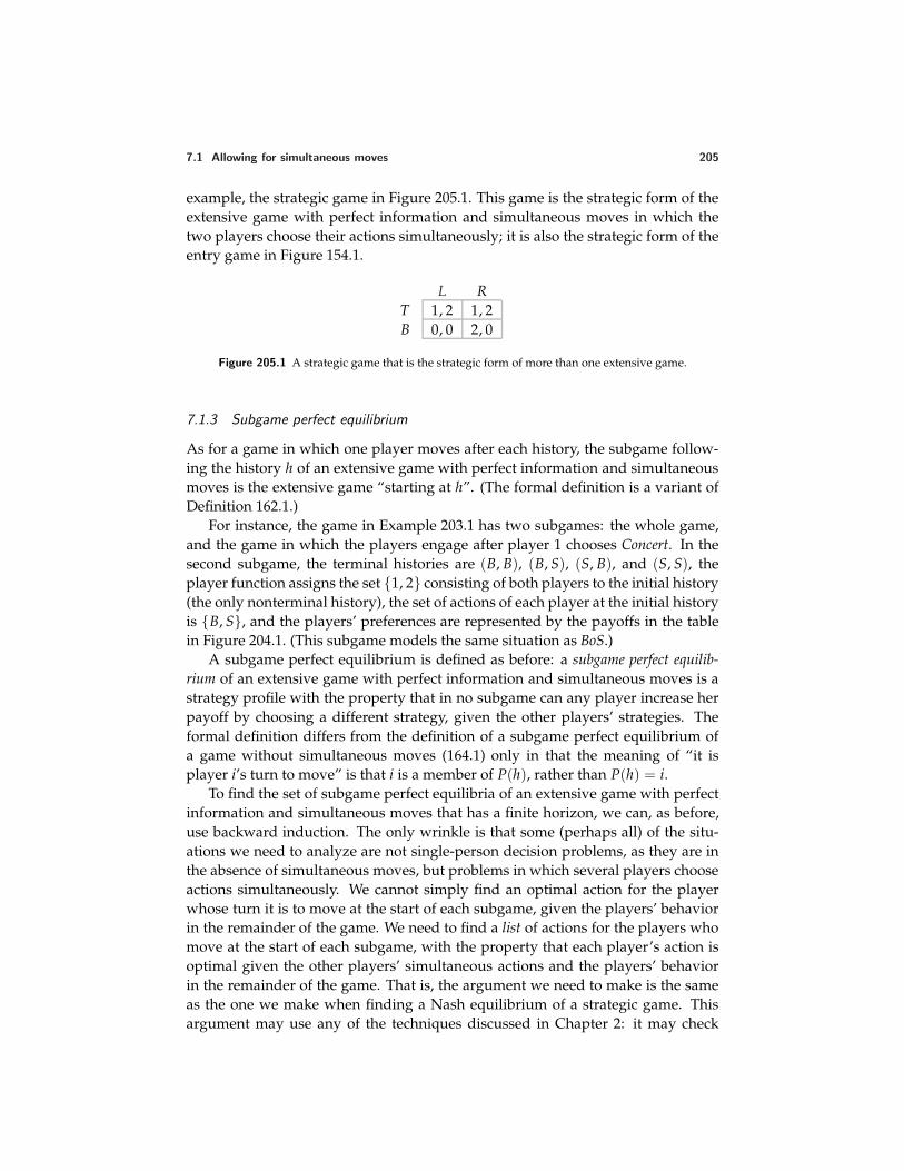
7.1 Allowing for simultaneous moves 205
example, the strategic game in Figure 205.1. This game is the strategic form of theextensive game with perfect information and simultaneous moves in which thetwo players choose their actions simultaneously; it is also the strategic form of theentry game in Figure 154.1.
L RT 1, 2 1, 2B 0, 0 2, 0
Figure 205.1 A strategic game that is the strategic form of more than one extensive game.
7.1.3 Subgame perfect equilibrium
As for a game in which one player moves after each history, the subgame follow-ing the history h of an extensive game with perfect information and simultaneousmoves is the extensive game “starting at h”. (The formal definition is a variant ofDefinition 162.1.)
For instance, the game in Example 203.1 has two subgames: the whole game,and the game in which the players engage after player 1 chooses Concert. In thesecond subgame, the terminal histories are (B, B), (B, S), (S, B), and (S, S), theplayer function assigns the set 1, 2 consisting of both players to the initial history(the only nonterminal history), the set of actions of each player at the initial historyis B, S, and the players’ preferences are represented by the payoffs in the tablein Figure 204.1. (This subgame models the same situation as BoS.)
A subgame perfect equilibrium is defined as before: a subgame perfect equilib-rium of an extensive game with perfect information and simultaneous moves is astrategy profile with the property that in no subgame can any player increase herpayoff by choosing a different strategy, given the other players’ strategies. Theformal definition differs from the definition of a subgame perfect equilibrium ofa game without simultaneous moves (164.1) only in that the meaning of “it isplayer i’s turn to move” is that i is a member of P(h), rather than P(h) = i.
To find the set of subgame perfect equilibria of an extensive game with perfectinformation and simultaneous moves that has a finite horizon, we can, as before,use backward induction. The only wrinkle is that some (perhaps all) of the situ-ations we need to analyze are not single-person decision problems, as they are inthe absence of simultaneous moves, but problems in which several players chooseactions simultaneously. We cannot simply find an optimal action for the playerwhose turn it is to move at the start of each subgame, given the players’ behaviorin the remainder of the game. We need to find a list of actions for the players whomove at the start of each subgame, with the property that each player’s action isoptimal given the other players’ simultaneous actions and the players’ behaviorin the remainder of the game. That is, the argument we need to make is the sameas the one we make when finding a Nash equilibrium of a strategic game. Thisargument may use any of the techniques discussed in Chapter 2: it may check
206 Chapter 7. Extensive Games with Perfect Information: Extensions and Discussion
each action profile in turn, it may construct and study the players’ best responsefunctions, or it may show directly that an action profile we have obtained by acombination of intuition and trial and error is an equilibrium.
EXAMPLE 206.1 (Subgame perfect equilibria of a variant of BoS) Consider the gamein Figure 204.1. Backward induction proceeds as follows.
• In the subgame that follows the history Concert, there are two Nash equilibria(in pure strategies), namely (S, S) and (B, B), as we found in Section 2.7.2.
• If the outcome in the subgame that follows Concert is (S, S) then the optimalchoice of player 1 at the start of the game is Book.
• If the outcome in the subgame that follows Concert is (B, B) then the optimalchoice of player 1 at the start of the game is Concert.
We conclude that the game has two subgame perfect equilibria: ((Book, S), S) and((Concert, B), B).
Every finite extensive game with perfect information has a (pure) subgame per-fect equilibrium (Proposition 171.1). The same is not true of a finite extensivegame with perfect information and simultaneous moves because, as we know, afinite strategic game (which corresponds to an extensive game with perfect in-formation and simultaneous moves of length one) may not possess a pure strat-egy Nash equilibrium. (Consider Matching pennies (Example 17.1).) If you havestudied Chapter 4, you know that some strategic games that lack a pure strat-egy Nash equilibrium have a “mixed strategy Nash equilibrium”, in which eachplayer randomizes. The same is true of extensive games with perfect informationand simultaneous moves. However, in this chapter I restrict attention almost ex-clusively to pure strategy equilibria; the only occasion on which mixed strategyNash equilibrium appears is Exercise 208.1.
? EXERCISE 206.2 (Extensive game with simultaneous moves) Find the subgameperfect equilibria of the following game. First player 1 chooses either A or B.After either choice, she and player 2 simultaneously choose actions. If player 1initially chooses A then she and player 2 subsequently each choose either C or D;if player 1 chooses B initially then she and player 2 subsequently each choose eitherE or F. Among the terminal histories, player 1 prefers (A, (C, C)) to (B, (E, E)) to(A, (D, D)) to (B, (F, F)), and prefers all these to (A, (C, D)), (A, (D, C)), (B, (E, F)),and (B, (F, E)), between which she is indifferent. Player 2 prefers (A, (D, D)) to(B, (F, F)) to (A, (C, C)) to (B, (E, E)), and prefers all these to (A, (C, D)), (A, (D, C)),(B, (E, F)), and (B, (F, E)), between which she is indifferent.
? EXERCISE 206.3 (Two-period Prisoner’s Dilemma) Two people simultaneously chooseactions; each person chooses either Q or F (as in the Prisoner’s Dilemma). Thenthey simultaneously choose actions again, once again each choosing either Q orF. Each person’s preferences are represented by the payoff function that assignsto the terminal history ((W, X), (Y, Z)) (where each component is either Q or F)
7.1 Allowing for simultaneous moves 207
a payoff equal to the sum of the person’s payoffs to (W, X) and to (Y, Z) in thePrisoner’s Dilemma given in Figure 13.1. Specify this situation as an extensive gamewith perfect information and simultaneous moves and find its subgame perfectequilibria.
? EXERCISE 207.1 (Timing claims on an investment) An amount of money is accu-mulating; in period t (= 1, 2, . . . , T) its size is $2t. In each period two peoplesimultaneously decide whether to claim the money. If only one person does so,she gets all the money; if both people do so, they split the money equally; andif neither person does so, both people have the opportunity to do so in the nextperiod. If neither person claims the money in period T, each person obtains $T.Each person cares only about the amount of money she obtains. Formulate thissituation as an extensive game with perfect information and simultaneous moves,and find its subgame perfect equilibria). (Start by considering the cases T = 1 andT = 2.)
? EXERCISE 207.2 (A market game) A seller owns one indivisible unit of a good,which she does not value. Several potential buyers, each of whom attaches thesame positive value v to the good, simultaneously offer prices they are willing topay for the good. After receiving the offers, the seller decides which, if any, toaccept. If she does not accept any offer, then no transaction takes place, and allpayoffs are 0. Otherwise, the buyer whose offer the seller accepts pays the amountp she offered and receives the good; the payoff of the seller is p, the payoff ofthe buyer who obtained the good is v − p, and the payoff of every other buyer is 0.Model this situation as an extensive game with perfect information and simultane-ous moves and find its subgame perfect equilibria. (Use a combination of intuitionand trial and error to find a strategy profile that appears to be an equilibrium, thenargue directly that it is. The incentives in the game are closely related to those inBertrand’s oligopoly game (see Exercise 66.1), with the roles of buyers and sellersreversed.) Show, in particular, that in every subgame perfect equilibrium everybuyer’s payoff is zero.
MORE EXPERIMENTAL EVIDENCE ON SUBGAME PERFECT EQUILIBRIUM
Experiments conducted in 1989 and 1990 among college students (mainly takingeconomics classes) show that the subgame perfect equilibria of the game in Exer-cise 207.2 correspond closely to experimental outcomes (Roth, Prasnikar, Okuno-Fujiwara, and Zamir 1991), in contrast to the subgame perfect equilibrium of theultimatum game (see the box on page 181).
In experiments conducted at four locations (Jerusalem, Ljubljana, Pittsburgh,and Tokyo), nine “buyers” simultaneously bid for the rough equivalent (in termsof local purchasing power) of US$10, held by a “seller”. Each experiment involveda group of 20 participants, which was divided into two markets, each with one
208 Chapter 7. Extensive Games with Perfect Information: Extensions and Discussion
seller and nine buyers. Each participant was involved in ten rounds of the market;in each round the sellers and buyers were assigned anew, and in any given roundno participant knew who, among the other participants, were sellers and buyers,and who was involved in her market. In every session of the experiment the maxi-mum proposed price was accepted by the seller, and by the seventh round of everyexperiment the highest bid was at least (the equivalent of) US$9.95.
Experiments involving the ultimatum game, run in the same locations using asimilar design, yielded results similar to those of previous experiments (see the boxon page 181): proposers kept considerably less than 100% of the pie, and nontrivialoffers were rejected.
The box on page 181 discusses two explanations for the experimental results inthe ultimatum game. Both explanations are consistent with the results in the mar-ket game. One explanation is that people are concerned not only with their ownmonetary payoffs, but also with other people’s payoffs. At least some specifica-tions of such preferences do not affect the subgame perfect equilibria of a marketgame with many buyers, which still all yield every buyer the payoff of zero. (Whenthere are many buyers, even a seller who cares about the other players’ payoffs ac-cepts the highest price offered, because accepting a lower price has little impact onthe distribution of monetary payoffs, all but two of which remain zero.) Thus suchpreferences are consistent with both sets of experimental outcomes. Another ex-planation is that people incorrectly recognize the ultimatum game as one in whichthe rule of thumb “don’t be a sucker” is advantageously invoked, and thus reject apoor offer, “punishing” the person who makes such an offer. In the market game,the players treated poorly in the subgame perfect equilibrium are the buyers, whohave no opportunity to punish any other player, because they move first. Thus therule of thumb is not relevant in this game, so that this explanation is also consistentwith both sets of experimental outcomes.
In the next exercise you are asked to investigate subgame perfect equilibria inwhich some players use mixed strategies (discussed in Chapter 4).
?? EXERCISE 208.1 (Price competition) Extend the model in Exercise 125.2 by havingthe sellers simultaneously choose their prices before the buyers simultaneouslychoose which seller to approach. Assume that each seller’s preferences are repre-sented by the expected value of a Bernoulli payoff function in which the payoffto not trading is 0 the payoff to trading at the price p is p. Formulate this modelprecisely as an extensive game with perfect information and simultaneous moves.Show that for every p ≥ 1
2 the game has a subgame perfect equilibrium in whicheach seller announces the price p. (You may use the fact that if seller j’s price isat least 1
2 , seller i’s payoff in the mixed strategy equilibrium of the subgame inwhich the buyers choose which seller to approach is decreasing in her price piwhen pi > pj.)
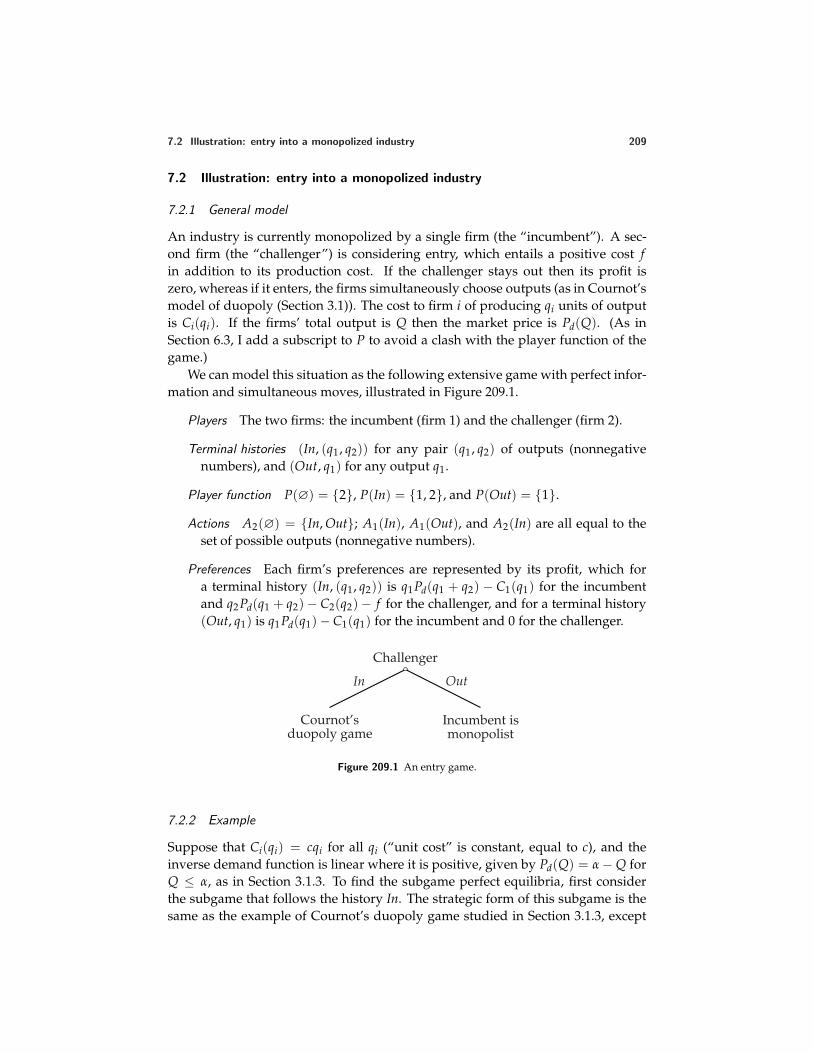
7.2 Illustration: entry into a monopolized industry 209
7.2 Illustration: entry into a monopolized industry
7.2.1 General model
An industry is currently monopolized by a single firm (the “incumbent”). A sec-ond firm (the “challenger”) is considering entry, which entails a positive cost fin addition to its production cost. If the challenger stays out then its profit iszero, whereas if it enters, the firms simultaneously choose outputs (as in Cournot’smodel of duopoly (Section 3.1)). The cost to firm i of producing qi units of outputis Ci(qi). If the firms’ total output is Q then the market price is Pd(Q). (As inSection 6.3, I add a subscript to P to avoid a clash with the player function of thegame.)
We can model this situation as the following extensive game with perfect infor-mation and simultaneous moves, illustrated in Figure 209.1.
Players The two firms: the incumbent (firm 1) and the challenger (firm 2).
Terminal histories (In, (q1, q2)) for any pair (q1, q2) of outputs (nonnegativenumbers), and (Out, q1) for any output q1.
Player function P(∅) = 2, P(In) = 1, 2, and P(Out) = 1.
Actions A2(∅) = In, Out; A1(In), A1(Out), and A2(In) are all equal to theset of possible outputs (nonnegative numbers).
Preferences Each firm’s preferences are represented by its profit, which fora terminal history (In, (q1, q2)) is q1Pd(q1 + q2) − C1(q1) for the incumbentand q2Pd(q1 + q2) − C2(q2) − f for the challenger, and for a terminal history(Out, q1) is q1Pd(q1) − C1(q1) for the incumbent and 0 for the challenger.
Challenger
In Out
Cournot’sduopoly game
Incumbent ismonopolist
Figure 209.1 An entry game.
7.2.2 Example
Suppose that Ci(qi) = cqi for all qi (“unit cost” is constant, equal to c), and theinverse demand function is linear where it is positive, given by Pd(Q) = α − Q forQ ≤ α, as in Section 3.1.3. To find the subgame perfect equilibria, first considerthe subgame that follows the history In. The strategic form of this subgame is thesame as the example of Cournot’s duopoly game studied in Section 3.1.3, except
210 Chapter 7. Extensive Games with Perfect Information: Extensions and Discussion
that the payoff of the challenger is reduced by f (the fixed cost of entry) regardlessof the challenger’s output. Thus the subgame has a unique Nash equilibrium, inwhich the output of each firm is 1
3 (α − c); the incumbent’s profit is 19 (α − c)2, and
the challenger’s profit is 19 (α − c)2 − f .
Now consider the subgame that follows the history Out. In this subgame theincumbent chooses an output. The incumbent’s profit when it chooses the outputq1 is q1(α − q1) − cq1 = q1(α − c − q1). This function is a quadratic that increasesand then decreases as q1 increases, and is zero when q1 = 0 and when q1 = α − c.Thus the function is maximized when q1 = 1
2 (α − c). We conclude that in anysubgame perfect equilibrium the incumbent chooses q1 = 1
2 (α − c) in the subgamefollowing the history Out.
Finally, consider the challenger’s action at the start of the game. If the chal-lenger stays out then its profit is 0, whereas if it enters then, given the actionschosen in the resulting subgame, its profit is 1
9 (α − c)2 − f . Thus in any sub-game perfect equilibrium the challenger enters if 1
9 (α − c)2 > f and stays out if19 (α − c)2 < f . If 1
9 (α − c)2 = f then the game has two subgame perfect equilibria,in one of which the challenger enters and in the other of which it does not.
In summary, the set of subgame perfect equilibria depend on the value of f . Inall equilibria the incumbent’s strategy is to produce 1
3 (α− c) if the challenger entersand 1
2 (α − c) if it does not, and the challenger’s strategy involves its producing13 (α − c) if it enters.
• If f < 19 (α − c)2 there is a unique subgame perfect equilibrium, in which the
challenger enters. The outcome is that the challenger enters and each firmproduces the output 1
3 (α − c).
• If f > 19 (α − c)2 there is a unique subgame perfect equilibrium, in which the
challenger stays out. The outcome is that the challenger stays out and theincumbent produces 1
2 (α − c).
• If f = 19 (α − c)2 the game has two subgame perfect equilibria: the one for the
case f < 19 (α − c)2 and the one for the case f > 1
9 (α − c)2.
Why, if f is small, does the game have no subgame perfect equilibrium in whichthe incumbent floods the market if the challenger enters, so that the challengeroptimally stays out and the incumbent obtains a profit higher than its profit if thechallenger enters? Because the action this strategy prescribes after the history inwhich the challenger enters is not the incumbent’s action in a Nash equilibriumof the subgame: the subgame has a unique Nash equilibrium, in which each firmproduces 1
3 (α − c). Put differently, the incumbent’s “threat” to flood the market ifthe challenger enters is not credible.
? EXERCISE 210.1 (Bertrand’s duopoly game with entry) Find the subgame perfectequilibria of the variant of the game studied in this section in which the post-entrycompetition is a game in which each firm chooses a price, as in the example ofBertrand’s duopoly game studied in Section 3.2.2, rather than an output.
7.3 Illustration: electoral competition with strategic voters 211
7.3 Illustration: electoral competition with strategic voters
The voters in Hotelling’s model of electoral competition (Section 3.3) are not play-ers in the game: each citizen is assumed simply to vote for the candidate whoseposition she most prefers. How do the conclusions of the model change if weassume that each citizen chooses the candidate for whom to vote?
Consider the extensive game in which the candidates first simultaneously chooseactions, then the citizens simultaneously choose how to vote. As in the variant ofHotelling’s game considered on page 72, assume that each candidate may eitherchoose a position (as in Hotelling’s original model) or choose to stay out of the race,an option she is assumed to rank between losing and tying for first place with allthe other candidates.
Players The candidates and the citizens.
Terminal histories All sequences (x, v) where x is a list of the candidates’ ac-tions, each component of which is either a position (a number) or Out, andv is a list of voting decisions for the citizens (i.e. a list of candidates, one foreach citizen).
Player function P(∅) is the set of all the candidates, and P(x), for any list x ofpositions for the candidates, is the set of all citizens.
Actions The set of actions available to each candidate at the start of the gameconsists of Out and the set of possible positions. The set of actions availableto each citizen after a history x is the set of candidates.
Preferences Each candidate’s preferences are represented by a payoff functionthat assigns n to every terminal history in which she wins outright, k to everyterminal history in which she ties for first place with n − k other candidates(for 1 ≤ k ≤ n − 1), 0 to every terminal history in which she stays out ofthe race, and −1 to every terminal history in which she loses, where n is thenumber of candidates. Each citizen’s preferences are represented by a payofffunction that assigns to each terminal history the average distance from thecitizen’s favorite position of the set of winning candidates in that history.
First consider the game in which there are two candidates (and an arbitrarynumber of citizens). Every subgame following choices of positions by the candi-dates has many Nash equilibria (as you know if you solved Exercise 47.1). Forexample, any action profile in which all citizens vote for the same candidate isa Nash equilibrium. (A citizen’s switching her vote to another candidate has noeffect on the outcome.)
This plethora of Nash equilibria allows us to construct, for every pair of posi-tions, a subgame perfect equilibrium in which the candidates choose those posi-tions! Consider the strategy profile in which the candidates choose the positionsx1 and x2, and
212 Chapter 7. Extensive Games with Perfect Information: Extensions and Discussion
• all citizens vote for candidate 1 after a history (x′1, x′
2) in which x′1 = x1
• all citizens vote for candidate 2 after a history (x′1, x′
2) in which x′1 = x1.
The outcome is that the candidates choose the positions x1 and x2 and candi-date 1 wins. The strategy profile is a subgame perfect equilibrium because forevery history (x1, x2) the profile of the citizens’ actions is a Nash equilibrium, andneither candidate can induce an outcome she prefers by deviating: a deviation bycandidate 1 to a position different from x1 leads her to lose, and a deviation bycandidate 2 has no effect on the outcome.
However, most of the Nash equilibria of the voting subgames are fragile (as youknow if you solved Exercise 47.1): a citizen’s voting for her less preferred candidateis weakly dominated (Definition 45.1) by her voting for her favorite candidate. (Acitizen who switches from voting for her less preferred candidate to voting for herfavorite candidate either does not affect the outcome (if her favorite candidate wasthree or more votes behind) or causes her favorite candidate either to tie for firstplace rather than lose, or to win rather than tie.) Thus in the only Nash equilibriumof a voting subgame in which no citizen uses a weakly dominated action, eachcitizen votes for the candidate whose position is closest to her favorite position.
Hotelling’s model (Section 3.3) assumes that each citizen votes for the candidatewhose position is closest to her favorite position; in its unique Nash equilibrium,each candidate’s position is the median of the citizens’ favorite positions. Combin-ing this result with the result of the previous paragraph, we conclude that the gamewe are studying has only one subgame perfect equilibrium in which no player’sstrategy is weakly dominated: each candidate chooses the median of the citizens’favorite positions, and for every pair of the candidates’ positions, each citizen votesfor her favorite candidate.
In the game with three or more candidates, not only do many of the votingsubgames have many Nash equilibria, with a variety of outcomes, but restrictingto voting strategies that are not weakly dominated does not dramatically affect theset of equilibria: a citizen’s only weakly dominated strategy is a vote for her leastpreferred candidate (see Exercise 47.2).
However, the set of equilibrium outcomes is dramatically restricted by the as-sumption that each candidate prefers to stay out of the race than to enter and lose,as the next two exercises show. The result in the first exercise is that the game hasa subgame perfect equilibrium in which no citizen’s strategy is weakly dominatedand every candidate enters and chooses as her position the median of the citizens’favorite positions. The result in the second exercise is that under an assumptionthat makes the citizens averse to ties and an assumption that there exist citizenswith extreme preferences, in every subgame perfect equilibrium all candidates whoenter do so at the median of the citizens’ favorite positions. The additional as-sumptions about the citizens’ preferences are much stronger that necessary; theyare designed to make the argument relatively easy.
? EXERCISE 212.1 (Electoral competition with strategic voters) Assume that there
7.4 Illustration: committee decision-making 213
are n ≥ 3 candidates and q citizens, where q ≥ 2n is odd (so that the median ofthe voters’ favorite positions is well-defined) and divisible by n. Show that thegame has a subgame perfect equilibrium in which no citizen’s strategy is weaklydominated and every candidate enters the race and chooses the median of thecitizens’ favorite positions. (You may use the fact that every voting subgame has a(pure) Nash equilibrium in which no citizen’s action is weakly dominated.)
?? EXERCISE 213.1 (Electoral competition with strategic voters) Consider the variantof the game in this section in which (i) the set of possible positions is the set ofnumbers x with 0 ≤ x ≤ 1, (ii) the favorite position of at least one citizen is 0and the favorite position of at least one citizen is 1, and (iii) each citizen’s pref-erences are represented by a payoff function that assigns to each terminal historythe distance from the citizen’s favorite position to the position of the candidate inthe set of winners whose position is furthest from her favorite position. Under theother assumptions of the previous exercise, show that in every subgame perfectequilibrium in which no citizen’s action is weakly dominated, the position chosenby every candidate who enters is the median of the citizens’ favorite positions. Todo so, first show that in any equilibrium each candidate that enters is in the setof winners. Then show that in any Nash equilibrium of any voting subgame inwhich there are more than two candidates and not all candidates’ positions are thesame, some candidate loses. (Argue that if all candidates tie for first place, somecitizen can increase her payoff by changing her vote.) Finally, show that in anysubgame perfect equilibrium in which either only two candidates enter, or all can-didates who enter choose the same position, every entering candidates chooses themedian of the citizens’ favorite positions.
7.4 Illustration: committee decision-making
How does the procedure used by a committee affect the decision it makes? One ap-proach to this question models a decision-making procedure as an extensive gamewith perfect information and simultaneous moves in which a sequence of ballotsare taken, in each of which the committee members vote simultaneously, and theresult of each ballot determines the choices on the next ballot, or, eventually, thedecision to be made.
Fix a set of committee members and a set of alternatives over which each mem-ber has strict preferences (no member is indifferent between any two alternatives).Assume that the number of committee members is odd, to avoid ties in votes. Ifthere are two alternatives, the simplest committee procedure is that in which themembers vote simultaneously for one of the alternatives. (We may interpret thegame in Section 2.9.3 as a model of this procedure.) In the procedure illustratedin Figure 214.1, there are three alternatives, x, y, and z. The committee first voteswhether to choose x (option “a”) or to eliminate it from consideration (option “b”).If it votes to eliminate x, it subsequently votes between y and z.
In these procedures, each vote is between two options. Such procedures are
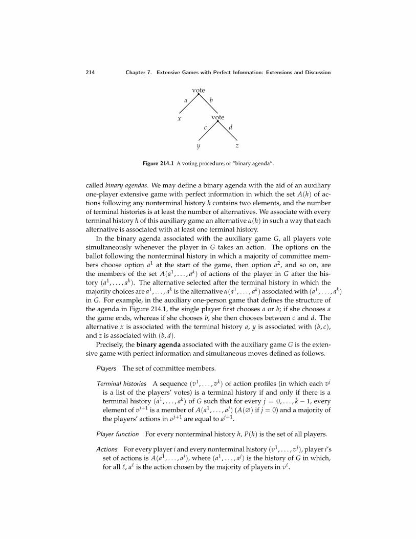
214 Chapter 7. Extensive Games with Perfect Information: Extensions and Discussion
votea b
x votec d
y z
Figure 214.1 A voting procedure, or “binary agenda”.
called binary agendas. We may define a binary agenda with the aid of an auxiliaryone-player extensive game with perfect information in which the set A(h) of ac-tions following any nonterminal history h contains two elements, and the numberof terminal histories is at least the number of alternatives. We associate with everyterminal history h of this auxiliary game an alternative α(h) in such a way that eachalternative is associated with at least one terminal history.
In the binary agenda associated with the auxiliary game G, all players votesimultaneously whenever the player in G takes an action. The options on theballot following the nonterminal history in which a majority of committee mem-bers choose option a1 at the start of the game, then option a2, and so on, arethe members of the set A(a1, . . . , ak) of actions of the player in G after the his-tory (a1, . . . , ak). The alternative selected after the terminal history in which themajority choices are a1, . . . , ak is the alternative α(a1, . . . , ak) associated with (a1, . . . , ak)in G. For example, in the auxiliary one-person game that defines the structure ofthe agenda in Figure 214.1, the single player first chooses a or b; if she chooses athe game ends, whereas if she chooses b, she then chooses between c and d. Thealternative x is associated with the terminal history a, y is associated with (b, c),and z is associated with (b, d).
Precisely, the binary agenda associated with the auxiliary game G is the exten-sive game with perfect information and simultaneous moves defined as follows.
Players The set of committee members.
Terminal histories A sequence (v1, . . . , vk) of action profiles (in which each vj
is a list of the players’ votes) is a terminal history if and only if there is aterminal history (a1, . . . , ak) of G such that for every j = 0, . . . , k − 1, everyelement of vj+1 is a member of A(a1, . . . , aj) (A(∅) if j = 0) and a majority ofthe players’ actions in vj+1 are equal to aj+1.
Player function For every nonterminal history h, P(h) is the set of all players.
Actions For every player i and every nonterminal history (v1, . . . , vj), player i’sset of actions is A(a1, . . . , aj), where (a1, . . . , aj) is the history of G in which,for all , a is the action chosen by the majority of players in v.
7.4 Illustration: committee decision-making 215
Preferences The rank each player assigns to the terminal history (v1, . . . , vk) isequal to the rank she assigns to the alternative α(a1, . . . , ak) associated withthe terminal history (a1, . . . , ak) of G in which, for all j, aj is the action chosenby a majority of players in vj.
Every binary agenda, like every voting subgame of the model in the previoussection, has many subgame perfect equilibria. In fact, in any binary agenda, everyalternative is the outcome of some subgame perfect equilibrium, because if, in ev-ery vote, every player votes for the same option, no player can affect the outcomeby changing her strategy. However, if we restrict attention to weakly undominatedstrategies, we greatly reduce the set of equilibria. As we saw before (Section 2.9.3),in a ballot with two options, a player’s action of voting for the option she prefersweakly dominates the action of voting for the other option. Thus in a subgame per-fect equilibrium of a binary agenda in which every player’s vote on every ballot isweakly undominated, on each ballot every player votes for the option that leads,ultimately (given the outcomes of the later ballots), to the alternative she prefers.The alternative associated with the terminal history generated by such a subgameperfect equilibrium is said to be the outcome of sophisticated voting.
Which alternatives are the outcomes of sophisticated voting in binary agendas?Say that alternative x beats alternative y if a majority of committee members preferx to y. An alternative that beats every other alternative is called a Condorcet winner.For any preferences, there is either one Condorcet winner or no Condorcet winner(see Exercise 74.1).
First suppose that the players’ preferences are such that some alternative, sayx∗, is a Condorcet winner. I claim that x∗ is the outcome of sophisticated votingin every binary agenda. The argument, using backward induction, is simple. Firstconsider a subgame of length 1 in which one option leads to the alternative x∗. Inthis subgame a majority of the players vote for the option that leads to x∗, becausea majority prefers x∗ to every other alternative, and each player’s only weakly un-dominated strategy is to vote for the option that leads to the alternative she prefers.Thus in at least one subgame of length 2, at least one option leads ultimately to thedecision x∗ (given the players’ votes in the subgames of length 1). In this subgame,by the same argument as before, the winning option leads to x∗. Continuing back-wards, we conclude that at least one option on the first ballot leads ultimately tox∗, and that consequently the winning option on this ballot leads to x∗.
Thus if the players’ preferences are such that a Condorcet winner exists, theagenda does not matter: the outcome of sophisticated voting is always the Con-dorcet winner. If the players’ preferences are such that no alternative is a Con-dorcet winner, the outcome of sophisticated voting depends on the agenda. Con-sider, for example, a committee with three members facing three alternatives. Sup-pose that one member prefers x to y to z, another prefers y to z to x, and the thirdprefers z to x to y. For these preferences, no alternative is a Condorcet winner. Theoutcome of sophisticated voting in the binary agenda in Figure 214.1 is the alter-native x. (Use backward induction: y beats z, and x beats y.) If the positions of x
216 Chapter 7. Extensive Games with Perfect Information: Extensions and Discussion
and y are interchanged then the outcome is y, and if the positions of x and z areinterchanged then the outcome is z. Thus in this case, for every alternative there isa binary agenda for which that alternative is the outcome of sophisticated voting.
Which alternatives are the outcomes of sophisticated voting in binary agendaswhen no alternative is a Condorcet winner? Consider a committee with arbitrarypreferences (not necessarily the ones considered in the previous paragraph), usingthe agenda in Figure 214.1. In order for x to be the outcome of sophisticated votingit must beat the winner of y and z. It may not beat both y and z directly, but it mustbeat them both at least “indirectly”: either x beats y beats x, or x beats z beats y.Similarly, if y or z is the outcome of sophisticated voting then it must beat both ofthe other alternatives at least indirectly.
Precisely, say that alternative x indirectly beats alternative y if for some k ≥ 1there are alternatives u1, . . . , uk such that x beats u1, uj beats uj+1 for j = 1, . . . , k −1, and uk beats y. The set of alternatives x such that x beats every other alternativeeither directly or indirectly is called the top cycle set. (Note that if alternative xbeats any alternative indirectly, it beats at least one alternative directly.) If there isa Condorcet winner, then the top cycle set consists of this single alternative. If thereis no Condorcet winner, then the top cycle set contains more than one alternative.
? EXERCISE 216.1 (Top cycle set) A committee has three members.
a. Suppose that there are three alternatives, x, y, and z, and that one memberprefers x to y to z, another prefers y to z to x, and the third prefers z to x to y.Find the top cycle set.
b. Suppose that there are four alternatives, w, x, y, and z, and that one memberprefers w to z to x to y, one member prefers y to w to z to x, and one memberprefers x to y to w to z. Find the top cycle set. Show, in particular, that z is inthe top cycle set even though all committee members prefer w.
Rephrasing my conclusion for the agenda in Figure 214.1, if an alternative is theoutcome of sophisticated voting, then it is in the top cycle set. The argument forthis conclusion extends to any binary agenda. In every subgame, the outcome ofsophisticated voting must beat the alternative that will be selected if it is rejected.Thus by backward induction, the outcome of sophisticated voting in the wholegame must beat every other alternative either directly or indirectly: the outcomeof sophisticated voting in any binary agenda is in the top cycle set.
Now consider a converse question: for any given alternative x in the top cycleset, is there a binary agenda for which x is the outcome of sophisticated voting?The answer is affirmative. The idea behind the construction of an appropriateagenda is illustrated by a simple example. Suppose that there are three alterna-tives, x, y, and z, and x beats y beats z. Then the agenda in Figure 214.1 is onefor which x is the outcome of sophisticated voting. Now suppose there are twoadditional alternatives, u and w, and x beats u beats w. Then we can construct alarger agenda in which x is the outcome of sophisticated voting by replacing thealternative x in Figure 214.1 with a subgame in which a vote is taken for or against
7.5 Illustration: exit from a declining industry 217
x, and, if x is rejected, a vote is subsequently taken between u and w. If there areother chains through which x beats other alternatives, we can similarly add furthersubgames.
? EXERCISE 217.1 (Designing agendas) A committee has three members; there arefive alternatives. One member prefers x to y to v to w to z, another prefers z to x tov to w to y, and the third prefers y to z to w to v to x. Find the top cycle set, and foreach alternative a in the set design a binary agenda for which a is the outcome ofsophisticated voting. Convince yourself that for no binary agenda is the outcomeof sophisticated voting outside the top cycle set.
? EXERCISE 217.2 (An agenda that yields an undesirable outcome) Design a binaryagenda for the committee in Exercise 216.1 for which the outcome of sophisticatedvoting is z (which is worse for all committee members than w).
In summary, (i) for any binary agenda, the alternative generated by the sub-game perfect equilibrium in which no citizen’s action in any ballot is weakly dom-inated is in the top cycle set, and (ii) for every alternative in the top cycle set, thereis a binary agenda for which that alternative is generated by the subgame perfectequilibrium in which no citizen’s action in any ballot is weakly dominated. In par-ticular, the extent to which the procedure used by a committee affects its decisiondepends on the nature of the members’ preferences. At one extreme, for prefer-ences such that some alternative is a Condorcet winner, the agenda is irrelevant.At another extreme, for preferences for which every alternative is in the top cy-cle set, the agenda is instrumental in determining the decision. Further, for somepreferences there are agendas for which the subgame perfect equilibrium yieldsan alternative that is unambiguously undesirable in the sense that there is anotheralternative that all committee members prefer.
7.5 Illustration: exit from a declining industry
An industry currently consists of two firms, one with a large capacity, and onewith a small capacity. Demand for the firms’ output is declining steadily overtime. When will the firms leave the industry? Which firm will leave first? Do thefirms’ financial resources affect the outcome? The analysis of a model that answersthese questions illustrates a use of backward induction more sophisticated thanthat in the previous sections of this chapter.
7.5.1 A model
Take time to be a discrete variable, starting in period 1. Denote by Pt(Q) the marketprice in period t when the firms’ total output is Q, and assume that this price isdeclining over time: for every value of Q, we have Pt+1(Q) < Pt(Q) for all t ≥ 1.(See Figure 219.1.) We are interested in the firms’ decisions to exit, rather thantheir decisions of how much to produce in the event they stay in the market, so
218 Chapter 7. Extensive Games with Perfect Information: Extensions and Discussion
we assume that firm i’s only decision is whether to produce some fixed output,denoted ki, or to produce no output. (You may think of ki as firm i’s capacity.)Once a firm stops production, it cannot start up again. Assume that k2 < k1 (firm 2is smaller than firm 1) and that each firm’s cost of producing q units of output iscq.
The following extensive game with simultaneous moves models this situation.
Players The two firms.
Terminal histories All sequences (X1, . . . , Xt) for some t ≥ 1, where Xs =(Stay, Stay) for 1 ≤ s ≤ t− 1 and Xt = (Exit, Exit) (both firms exit in period t),or Xs = (Stay, Stay) for all s with 1 ≤ s ≤ r − 1 for some r, Xr = (Stay, Exit)or (Exit, Stay), Xs = Stay for all s with r + 1 ≤ s ≤ t − 1, and Xt = Exit(one firm exits in period r and the other exits in period t), and all infinitesequences (X1, X2, . . .) where Xr = (Stay, Stay) for all r (neither firm everexits).
Player function P(h) = 1, 2 after any history h in which neither firm hasexited; P(h) = 1 after any history h in which only firm 2 has exited; andP(h) = 2 after any history h in which only firm 1 has exited.
Actions Whenever a firm moves, its set of actions is Stay, Exit).
Preferences Each firm’s preferences are represented by a payoff function thatassociates with each terminal history the firm’s total profit, where the profitof firm i (= 1, 2) in period t is (Pt(ki) − c)ki if the other firm has exited and(Pt(k1 + k2) − c)ki if the other firm has not exited.
7.5.2 Subgame perfect equilibrium
In a period in which Pt(ki) < c, firm i makes a loss even if it is the only firmremaining (the market price for its output is less than its unit cost). Denote by tithe last period in which firm i is profitable if it is the only firm in the market. Thatis, ti is the largest value of t for which Pt(ki) ≥ c. (Refer to Figure 219.1.) Becausek1 > k2, we have t1 ≤ t2: the time at which the large firm becomes unprofitable asa loner is no later than the time at which the small firm becomes unprofitable as aloner.
The game has an infinite horizon, but after period ti firm i’s profit is negativeeven if it is the only firm remaining in the market. Thus if firm i is in the marketin any period after ti, it chooses Exit in that period in every subgame perfect equi-librium. In particular, both firms choose Exit in every period after t2. We can usebackward induction from period t2 to find the firms’ subgame perfect equilibriumactions in earlier periods.
If firm 1 (the larger firm) is in the market in any period from t1 on, it shouldexit, whether or not firm 2 is still operating. As a consequence, if firm 2 is still
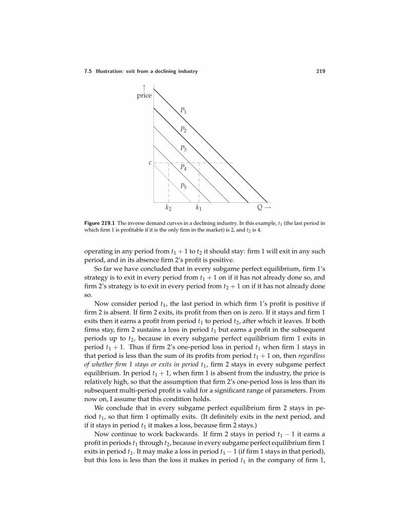
7.5 Illustration: exit from a declining industry 219
Q →
↑price
c
k2 k1
P1
P2
P3
P4
P5
Figure 219.1 The inverse demand curves in a declining industry. In this example, t1 (the last period inwhich firm 1 is profitable if it is the only firm in the market) is 2, and t2 is 4.
operating in any period from t1 + 1 to t2 it should stay: firm 1 will exit in any suchperiod, and in its absence firm 2’s profit is positive.
So far we have concluded that in every subgame perfect equilibrium, firm 1’sstrategy is to exit in every period from t1 + 1 on if it has not already done so, andfirm 2’s strategy is to exit in every period from t2 + 1 on if it has not already doneso.
Now consider period t1, the last period in which firm 1’s profit is positive iffirm 2 is absent. If firm 2 exits, its profit from then on is zero. If it stays and firm 1exits then it earns a profit from period t1 to period t2, after which it leaves. If bothfirms stay, firm 2 sustains a loss in period t1 but earns a profit in the subsequentperiods up to t2, because in every subgame perfect equilibrium firm 1 exits inperiod t1 + 1. Thus if firm 2’s one-period loss in period t1 when firm 1 stays inthat period is less than the sum of its profits from period t1 + 1 on, then regardlessof whether firm 1 stays or exits in period t1, firm 2 stays in every subgame perfectequilibrium. In period t1 + 1, when firm 1 is absent from the industry, the price isrelatively high, so that the assumption that firm 2’s one-period loss is less than itssubsequent multi-period profit is valid for a significant range of parameters. Fromnow on, I assume that this condition holds.
We conclude that in every subgame perfect equilibrium firm 2 stays in pe-riod t1, so that firm 1 optimally exits. (It definitely exits in the next period, andif it stays in period t1 it makes a loss, because firm 2 stays.)
Now continue to work backwards. If firm 2 stays in period t1 − 1 it earns aprofit in periods t1 through t2, because in every subgame perfect equilibrium firm 1exits in period t1. It may make a loss in period t1 − 1 (if firm 1 stays in that period),but this loss is less than the loss it makes in period t1 in the company of firm 1,
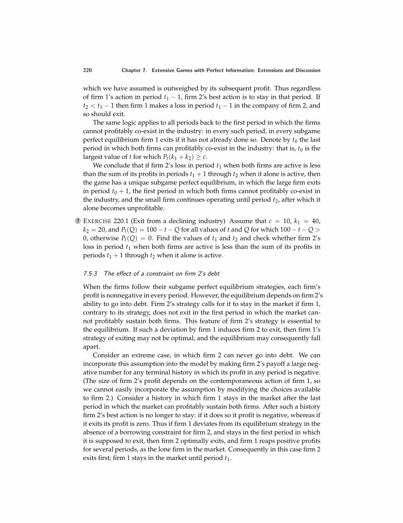
220 Chapter 7. Extensive Games with Perfect Information: Extensions and Discussion
which we have assumed is outweighed by its subsequent profit. Thus regardlessof firm 1’s action in period t1 − 1, firm 2’s best action is to stay in that period. Ift2 < t1 − 1 then firm 1 makes a loss in period t1 − 1 in the company of firm 2, andso should exit.
The same logic applies to all periods back to the first period in which the firmscannot profitably co-exist in the industry: in every such period, in every subgameperfect equilibrium firm 1 exits if it has not already done so. Denote by t0 the lastperiod in which both firms can profitably co-exist in the industry: that is, t0 is thelargest value of t for which Pt(k1 + k2) ≥ c.
We conclude that if firm 2’s loss in period t1 when both firms are active is lessthan the sum of its profits in periods t1 + 1 through t2 when it alone is active, thenthe game has a unique subgame perfect equilibrium, in which the large firm exitsin period t0 + 1, the first period in which both firms cannot profitably co-exist inthe industry, and the small firm continues operating until period t2, after which italone becomes unprofitable.
? EXERCISE 220.1 (Exit from a declining industry) Assume that c = 10, k1 = 40,k2 = 20, and Pt(Q) = 100 − t − Q for all values of t and Q for which 100− t − Q >
0, otherwise Pt(Q) = 0. Find the values of t1 and t2 and check whether firm 2’sloss in period t1 when both firms are active is less than the sum of its profits inperiods t1 + 1 through t2 when it alone is active.
7.5.3 The effect of a constraint on firm 2’s debt
When the firms follow their subgame perfect equilibrium strategies, each firm’sprofit is nonnegative in every period. However, the equilibrium depends on firm 2’sability to go into debt. Firm 2’s strategy calls for it to stay in the market if firm 1,contrary to its strategy, does not exit in the first period in which the market can-not profitably sustain both firms. This feature of firm 2’s strategy is essential tothe equilibrium. If such a deviation by firm 1 induces firm 2 to exit, then firm 1’sstrategy of exiting may not be optimal, and the equilibrium may consequently fallapart.
Consider an extreme case, in which firm 2 can never go into debt. We canincorporate this assumption into the model by making firm 2’s payoff a large neg-ative number for any terminal history in which its profit in any period is negative.(The size of firm 2’s profit depends on the contemporaneous action of firm 1, sowe cannot easily incorporate the assumption by modifying the choices availableto firm 2.) Consider a history in which firm 1 stays in the market after the lastperiod in which the market can profitably sustain both firms. After such a historyfirm 2’s best action is no longer to stay: if it does so it profit is negative, whereas ifit exits its profit is zero. Thus if firm 1 deviates from its equilibrium strategy in theabsence of a borrowing constraint for firm 2, and stays in the first period in whichit is supposed to exit, then firm 2 optimally exits, and firm 1 reaps positive profitsfor several periods, as the lone firm in the market. Consequently in this case firm 2exits first; firm 1 stays in the market until period t1.
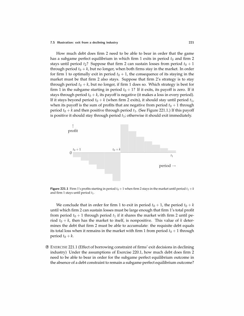
7.5 Illustration: exit from a declining industry 221
How much debt does firm 2 need to be able to bear in order that the gamehas a subgame perfect equilibrium in which firm 1 exits in period t0 and firm 2stays until period t2? Suppose that firm 2 can sustain losses from period t0 + 1through period t0 + k, but no longer, when both firms stay in the market. In orderfor firm 1 to optimally exit in period t0 + 1, the consequence of its staying in themarket must be that firm 2 also stays. Suppose that firm 2’s strategy is to staythrough period t0 + k, but no longer, if firm 1 does so. Which strategy is best forfirm 1 in the subgame starting in period t0 + 1? If it exits, its payoff is zero. If itstays through period t0 + k, its payoff is negative (it makes a loss in every period).If it stays beyond period t0 + k (when firm 2 exits), it should stay until period t1,when its payoff is the sum of profits that are negative from period t0 + 1 throughperiod t0 + k and then positive through period t1. (See Figure 221.1.) If this payoffis positive it should stay through period t1; otherwise it should exit immediately.
0t0 + 1 t0 + k
t1
↑profit
period →
Figure 221.1 Firm 1’s profits starting in period t0 + 1 when firm 2 stays in the market until period t1 + kand firm 1 stays until period t1.
We conclude that in order for firm 1 to exit in period t0 + 1, the period t0 + kuntil which firm 2 can sustain losses must be large enough that firm 1’s total profitfrom period t0 + 1 through period t1 if it shares the market with firm 2 until pe-riod t0 + k, then has the market to itself, is nonpositive. This value of k deter-mines the debt that firm 2 must be able to accumulate: the requisite debt equalsits total loss when it remains in the market with firm 1 from period t0 + 1 throughperiod t0 + k.
? EXERCISE 221.1 (Effect of borrowing constraint of firms’ exit decisions in decliningindustry) Under the assumptions of Exercise 220.1, how much debt does firm 2need to be able to bear in order for the subgame perfect equilibrium outcome inthe absence of a debt constraint to remain a subgame perfect equilibrium outcome?
222 Chapter 7. Extensive Games with Perfect Information: Extensions and Discussion
7.6 Allowing for exogenous uncertainty
7.6.1 General model
The model of an extensive game with perfect information (with or without simul-taneous moves) does not allow random events to occur during the course of play.However, we can easily extend the model to cover such situations. The definitionof an extensive game with perfect information and chance moves is a variant ofthe definition of an extensive game with perfect information (153.1) in which
• the player function assigns “chance”, rather than a set of players, to somehistories
• the probabilities that chance uses after any such history are specified
• the players’ preferences are defined over the set of lotteries over terminalhistories (rather than simply over the set of terminal histories).
(We may similarly add chance moves to an extensive game with perfect informa-tion and simultaneous moves by modifying Definition 202.1.) To keep the analysissimple, assume that the random event after any given history is independent ofthe random event after any other history. (That is, the realization of any randomevent is not affected by the realization of any other random event.)
The definition of a player’s strategy remains the same as before. The outcomeof a strategy profile is now a probability distribution over terminal histories. Thedefinition of subgame perfect equilibrium remains the same as before.
EXAMPLE 222.1 (Extensive game with chance moves) Consider a situation involv-ing two players in which player 1 first chooses A or B. If she chooses A the gameends, with (Bernoulli) payoffs (1, 1). If she chooses B then with probability 1
2 thegame ends, with payoffs (3, 0), and with probability 1
2 player 2 gets to choose be-tween C, which yields payoffs (0, 1) and D, which yields payoffs (1, 0). An exten-sive game with perfect information and chance moves that models this situation isshown in Figure 223.1. The label c denotes chance; the number beside each actionof chance is the probability with which that action is chosen.
We may use backward induction to find the subgame perfect equilibria of thisgame. In any equilibrium, player 2 chooses C. Now consider the consequences ofplayer 1’s actions. If she chooses A then she obtains the payoff 1. If she chooses Bthen she obtains 3 with probability 1
2 and 0 with probability 12 , yielding an expected
payoff of 32 . Thus the game has a unique subgame perfect equilibrium, in which
player 1 choose B and player 2 chooses C.
? EXERCISE 222.2 (Variant of ultimatum game with equity-conscious players) Con-sider a variant of the game in Exercise 181.1 in which β1 = 0, and the person 2whom person 1 faces is drawn randomly from a population in which the fractionp have β2 = 0 and the remaining fraction 1 − p have β2 = 1. When making her
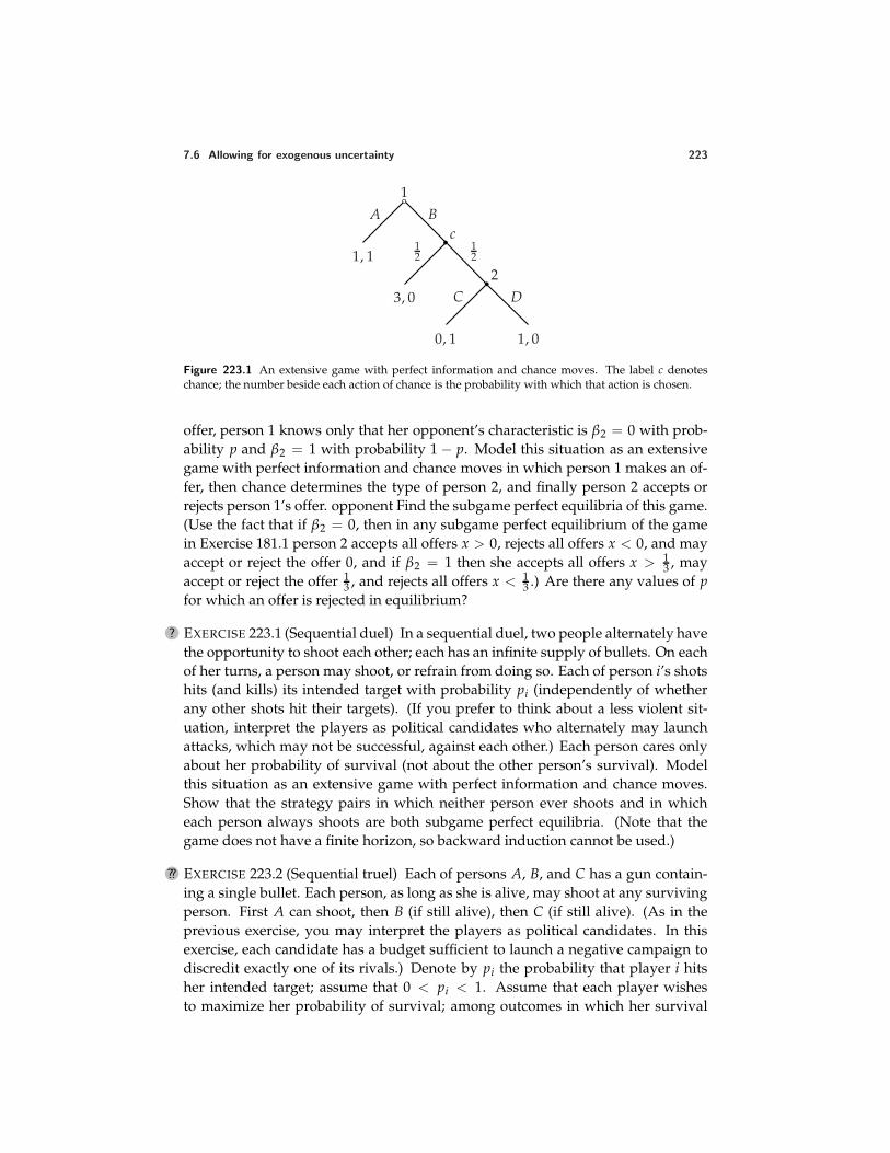
7.6 Allowing for exogenous uncertainty 223
1A B
1, 1
c12
12
3, 0
2C D
0, 1 1, 0
Figure 223.1 An extensive game with perfect information and chance moves. The label c denoteschance; the number beside each action of chance is the probability with which that action is chosen.
offer, person 1 knows only that her opponent’s characteristic is β2 = 0 with prob-ability p and β2 = 1 with probability 1 − p. Model this situation as an extensivegame with perfect information and chance moves in which person 1 makes an of-fer, then chance determines the type of person 2, and finally person 2 accepts orrejects person 1’s offer. opponent Find the subgame perfect equilibria of this game.(Use the fact that if β2 = 0, then in any subgame perfect equilibrium of the gamein Exercise 181.1 person 2 accepts all offers x > 0, rejects all offers x < 0, and mayaccept or reject the offer 0, and if β2 = 1 then she accepts all offers x > 1
3 , mayaccept or reject the offer 1
3 , and rejects all offers x < 13 .) Are there any values of p
for which an offer is rejected in equilibrium?
? EXERCISE 223.1 (Sequential duel) In a sequential duel, two people alternately havethe opportunity to shoot each other; each has an infinite supply of bullets. On eachof her turns, a person may shoot, or refrain from doing so. Each of person i’s shotshits (and kills) its intended target with probability pi (independently of whetherany other shots hit their targets). (If you prefer to think about a less violent sit-uation, interpret the players as political candidates who alternately may launchattacks, which may not be successful, against each other.) Each person cares onlyabout her probability of survival (not about the other person’s survival). Modelthis situation as an extensive game with perfect information and chance moves.Show that the strategy pairs in which neither person ever shoots and in whicheach person always shoots are both subgame perfect equilibria. (Note that thegame does not have a finite horizon, so backward induction cannot be used.)
?? EXERCISE 223.2 (Sequential truel) Each of persons A, B, and C has a gun contain-ing a single bullet. Each person, as long as she is alive, may shoot at any survivingperson. First A can shoot, then B (if still alive), then C (if still alive). (As in theprevious exercise, you may interpret the players as political candidates. In thisexercise, each candidate has a budget sufficient to launch a negative campaign todiscredit exactly one of its rivals.) Denote by pi the probability that player i hitsher intended target; assume that 0 < pi < 1. Assume that each player wishesto maximize her probability of survival; among outcomes in which her survival
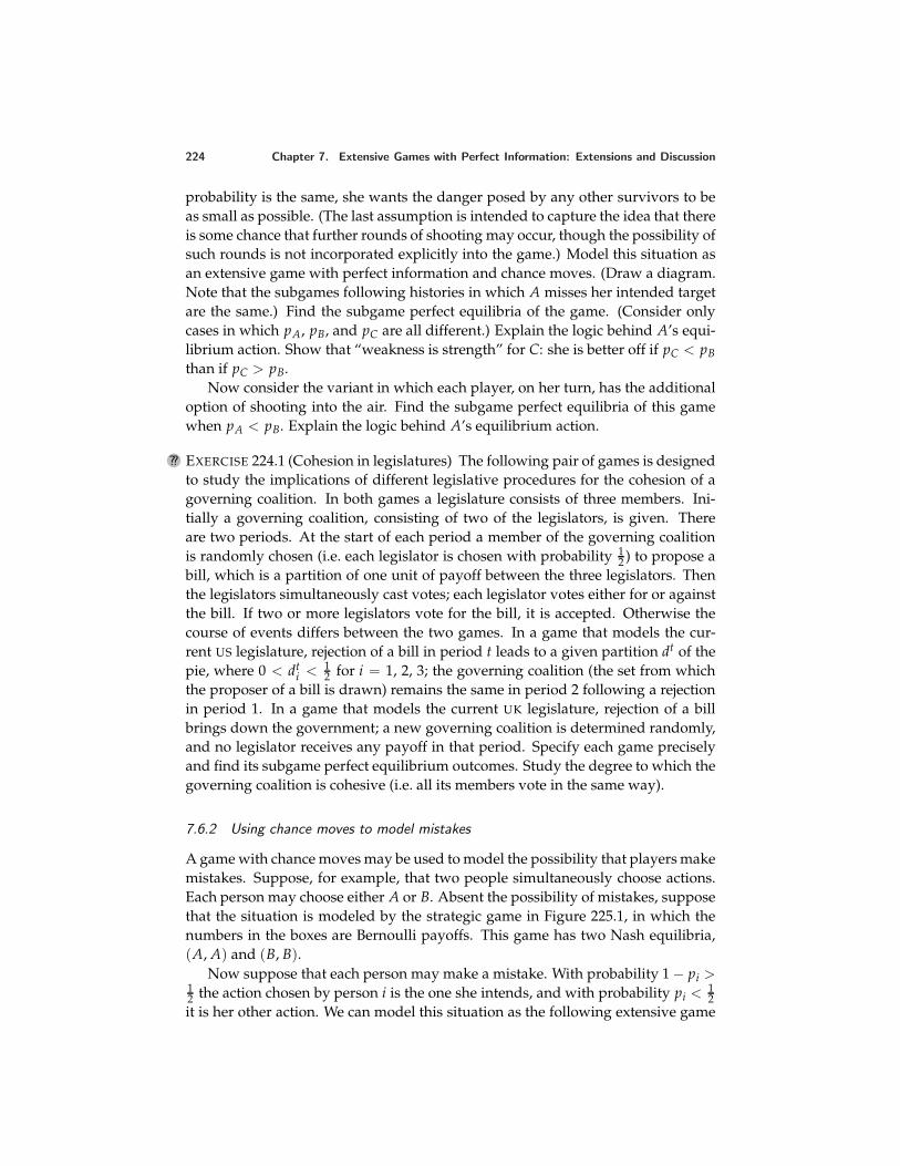
224 Chapter 7. Extensive Games with Perfect Information: Extensions and Discussion
probability is the same, she wants the danger posed by any other survivors to beas small as possible. (The last assumption is intended to capture the idea that thereis some chance that further rounds of shooting may occur, though the possibility ofsuch rounds is not incorporated explicitly into the game.) Model this situation asan extensive game with perfect information and chance moves. (Draw a diagram.Note that the subgames following histories in which A misses her intended targetare the same.) Find the subgame perfect equilibria of the game. (Consider onlycases in which pA, pB, and pC are all different.) Explain the logic behind A’s equi-librium action. Show that “weakness is strength” for C: she is better off if pC < pBthan if pC > pB.
Now consider the variant in which each player, on her turn, has the additionaloption of shooting into the air. Find the subgame perfect equilibria of this gamewhen pA < pB. Explain the logic behind A’s equilibrium action.
?? EXERCISE 224.1 (Cohesion in legislatures) The following pair of games is designedto study the implications of different legislative procedures for the cohesion of agoverning coalition. In both games a legislature consists of three members. Ini-tially a governing coalition, consisting of two of the legislators, is given. Thereare two periods. At the start of each period a member of the governing coalitionis randomly chosen (i.e. each legislator is chosen with probability 1
2 ) to propose abill, which is a partition of one unit of payoff between the three legislators. Thenthe legislators simultaneously cast votes; each legislator votes either for or againstthe bill. If two or more legislators vote for the bill, it is accepted. Otherwise thecourse of events differs between the two games. In a game that models the cur-rent US legislature, rejection of a bill in period t leads to a given partition dt of thepie, where 0 < dt
i < 12 for i = 1, 2, 3; the governing coalition (the set from which
the proposer of a bill is drawn) remains the same in period 2 following a rejectionin period 1. In a game that models the current UK legislature, rejection of a billbrings down the government; a new governing coalition is determined randomly,and no legislator receives any payoff in that period. Specify each game preciselyand find its subgame perfect equilibrium outcomes. Study the degree to which thegoverning coalition is cohesive (i.e. all its members vote in the same way).
7.6.2 Using chance moves to model mistakes
A game with chance moves may be used to model the possibility that players makemistakes. Suppose, for example, that two people simultaneously choose actions.Each person may choose either A or B. Absent the possibility of mistakes, supposethat the situation is modeled by the strategic game in Figure 225.1, in which thenumbers in the boxes are Bernoulli payoffs. This game has two Nash equilibria,(A, A) and (B, B).
Now suppose that each person may make a mistake. With probability 1 − pi >12 the action chosen by person i is the one she intends, and with probability pi < 1
2it is her other action. We can model this situation as the following extensive game
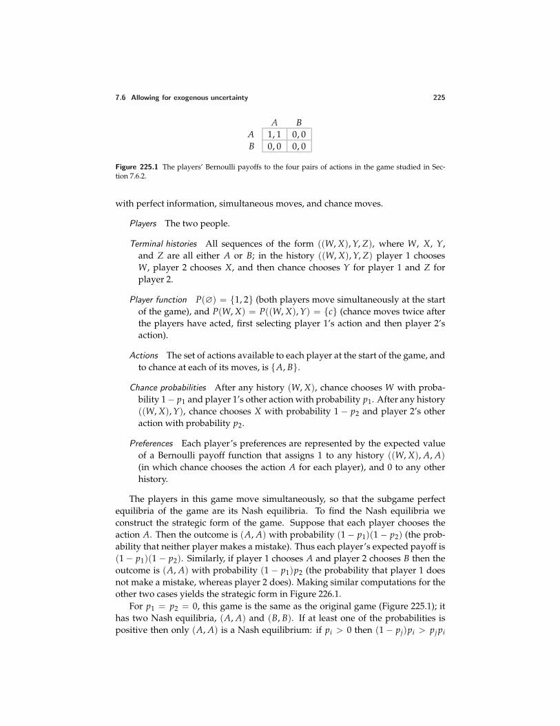
7.6 Allowing for exogenous uncertainty 225
A BA 1, 1 0, 0B 0, 0 0, 0
Figure 225.1 The players’ Bernoulli payoffs to the four pairs of actions in the game studied in Sec-tion 7.6.2.
with perfect information, simultaneous moves, and chance moves.
Players The two people.
Terminal histories All sequences of the form ((W, X), Y, Z), where W, X, Y,and Z are all either A or B; in the history ((W, X), Y, Z) player 1 choosesW, player 2 chooses X, and then chance chooses Y for player 1 and Z forplayer 2.
Player function P(∅) = 1, 2 (both players move simultaneously at the startof the game), and P(W, X) = P((W, X), Y) = c (chance moves twice afterthe players have acted, first selecting player 1’s action and then player 2’saction).
Actions The set of actions available to each player at the start of the game, andto chance at each of its moves, is A, B.
Chance probabilities After any history (W, X), chance chooses W with proba-bility 1− p1 and player 1’s other action with probability p1. After any history((W, X), Y), chance chooses X with probability 1 − p2 and player 2’s otheraction with probability p2.
Preferences Each player’s preferences are represented by the expected valueof a Bernoulli payoff function that assigns 1 to any history ((W, X), A, A)(in which chance chooses the action A for each player), and 0 to any otherhistory.
The players in this game move simultaneously, so that the subgame perfectequilibria of the game are its Nash equilibria. To find the Nash equilibria weconstruct the strategic form of the game. Suppose that each player chooses theaction A. Then the outcome is (A, A) with probability (1 − p1)(1 − p2) (the prob-ability that neither player makes a mistake). Thus each player’s expected payoff is(1 − p1)(1 − p2). Similarly, if player 1 chooses A and player 2 chooses B then theoutcome is (A, A) with probability (1 − p1)p2 (the probability that player 1 doesnot make a mistake, whereas player 2 does). Making similar computations for theother two cases yields the strategic form in Figure 226.1.
For p1 = p2 = 0, this game is the same as the original game (Figure 225.1); ithas two Nash equilibria, (A, A) and (B, B). If at least one of the probabilities ispositive then only (A, A) is a Nash equilibrium: if pi > 0 then (1 − pj)pi > pj pi
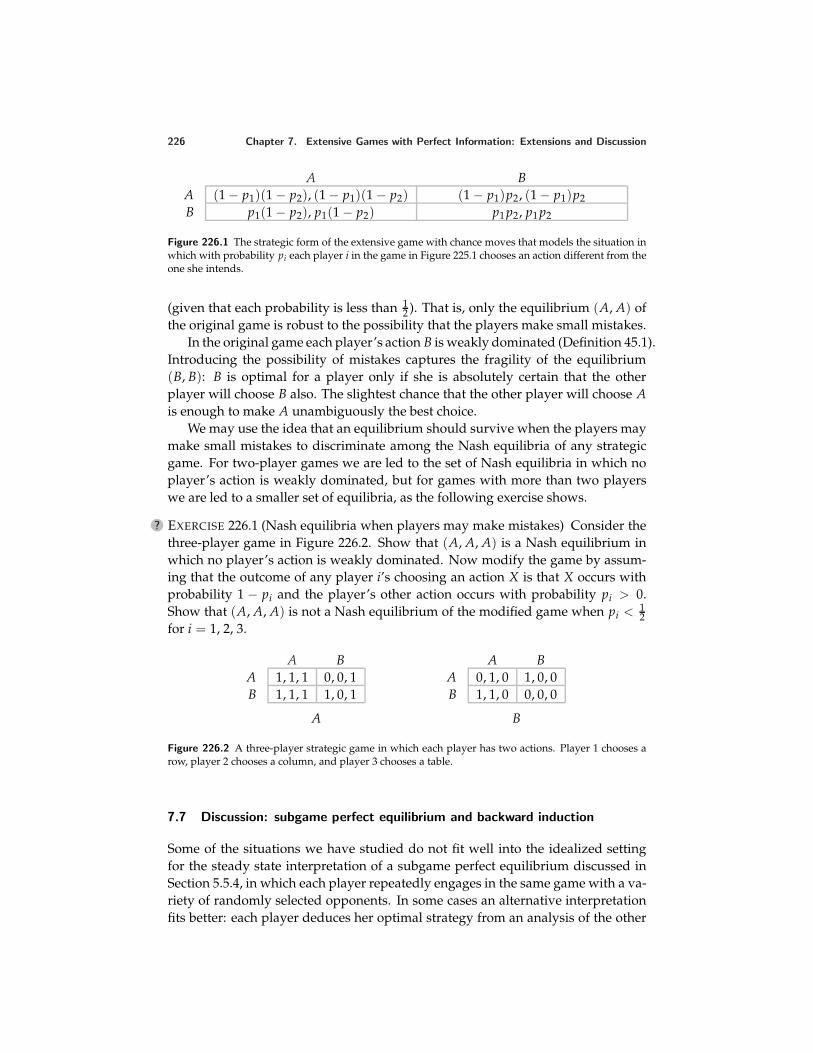
226 Chapter 7. Extensive Games with Perfect Information: Extensions and Discussion
A BA (1 − p1)(1 − p2), (1 − p1)(1 − p2) (1 − p1)p2, (1 − p1)p2B p1(1 − p2), p1(1 − p2) p1 p2, p1 p2
Figure 226.1 The strategic form of the extensive game with chance moves that models the situation inwhich with probability pi each player i in the game in Figure 225.1 chooses an action different from theone she intends.
(given that each probability is less than 12 ). That is, only the equilibrium (A, A) of
the original game is robust to the possibility that the players make small mistakes.In the original game each player’s action B is weakly dominated (Definition 45.1).
Introducing the possibility of mistakes captures the fragility of the equilibrium(B, B): B is optimal for a player only if she is absolutely certain that the otherplayer will choose B also. The slightest chance that the other player will choose Ais enough to make A unambiguously the best choice.
We may use the idea that an equilibrium should survive when the players maymake small mistakes to discriminate among the Nash equilibria of any strategicgame. For two-player games we are led to the set of Nash equilibria in which noplayer’s action is weakly dominated, but for games with more than two playerswe are led to a smaller set of equilibria, as the following exercise shows.
? EXERCISE 226.1 (Nash equilibria when players may make mistakes) Consider thethree-player game in Figure 226.2. Show that (A, A, A) is a Nash equilibrium inwhich no player’s action is weakly dominated. Now modify the game by assum-ing that the outcome of any player i’s choosing an action X is that X occurs withprobability 1 − pi and the player’s other action occurs with probability pi > 0.Show that (A, A, A) is not a Nash equilibrium of the modified game when pi < 1
2for i = 1, 2, 3.
A BA 1, 1, 1 0, 0, 1B 1, 1, 1 1, 0, 1
A
A BA 0, 1, 0 1, 0, 0B 1, 1, 0 0, 0, 0
B
Figure 226.2 A three-player strategic game in which each player has two actions. Player 1 chooses arow, player 2 chooses a column, and player 3 chooses a table.
7.7 Discussion: subgame perfect equilibrium and backward induction
Some of the situations we have studied do not fit well into the idealized settingfor the steady state interpretation of a subgame perfect equilibrium discussed inSection 5.5.4, in which each player repeatedly engages in the same game with a va-riety of randomly selected opponents. In some cases an alternative interpretationfits better: each player deduces her optimal strategy from an analysis of the other
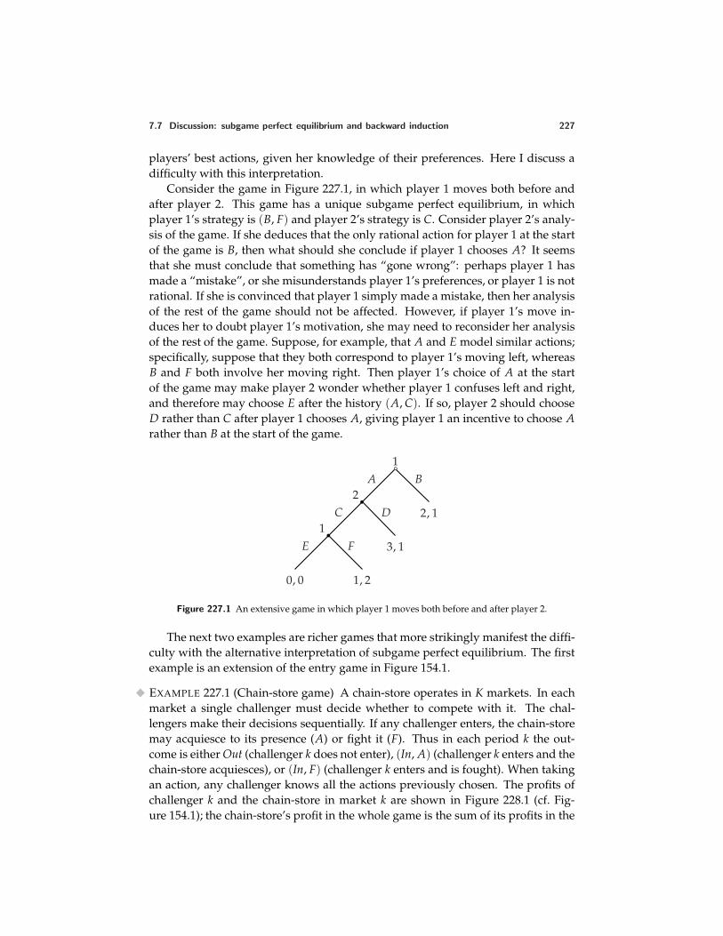
7.7 Discussion: subgame perfect equilibrium and backward induction 227
players’ best actions, given her knowledge of their preferences. Here I discuss adifficulty with this interpretation.
Consider the game in Figure 227.1, in which player 1 moves both before andafter player 2. This game has a unique subgame perfect equilibrium, in whichplayer 1’s strategy is (B, F) and player 2’s strategy is C. Consider player 2’s analy-sis of the game. If she deduces that the only rational action for player 1 at the startof the game is B, then what should she conclude if player 1 chooses A? It seemsthat she must conclude that something has “gone wrong”: perhaps player 1 hasmade a “mistake”, or she misunderstands player 1’s preferences, or player 1 is notrational. If she is convinced that player 1 simply made a mistake, then her analysisof the rest of the game should not be affected. However, if player 1’s move in-duces her to doubt player 1’s motivation, she may need to reconsider her analysisof the rest of the game. Suppose, for example, that A and E model similar actions;specifically, suppose that they both correspond to player 1’s moving left, whereasB and F both involve her moving right. Then player 1’s choice of A at the startof the game may make player 2 wonder whether player 1 confuses left and right,and therefore may choose E after the history (A, C). If so, player 2 should chooseD rather than C after player 1 chooses A, giving player 1 an incentive to choose Arather than B at the start of the game.
1A B
2, 1
2C D
3, 1
1E F
0, 0 1, 2
Figure 227.1 An extensive game in which player 1 moves both before and after player 2.
The next two examples are richer games that more strikingly manifest the diffi-culty with the alternative interpretation of subgame perfect equilibrium. The firstexample is an extension of the entry game in Figure 154.1.
EXAMPLE 227.1 (Chain-store game) A chain-store operates in K markets. In eachmarket a single challenger must decide whether to compete with it. The chal-lengers make their decisions sequentially. If any challenger enters, the chain-storemay acquiesce to its presence (A) or fight it (F). Thus in each period k the out-come is either Out (challenger k does not enter), (In, A) (challenger k enters and thechain-store acquiesces), or (In, F) (challenger k enters and is fought). When takingan action, any challenger knows all the actions previously chosen. The profits ofchallenger k and the chain-store in market k are shown in Figure 228.1 (cf. Fig-ure 154.1); the chain-store’s profit in the whole game is the sum of its profits in the
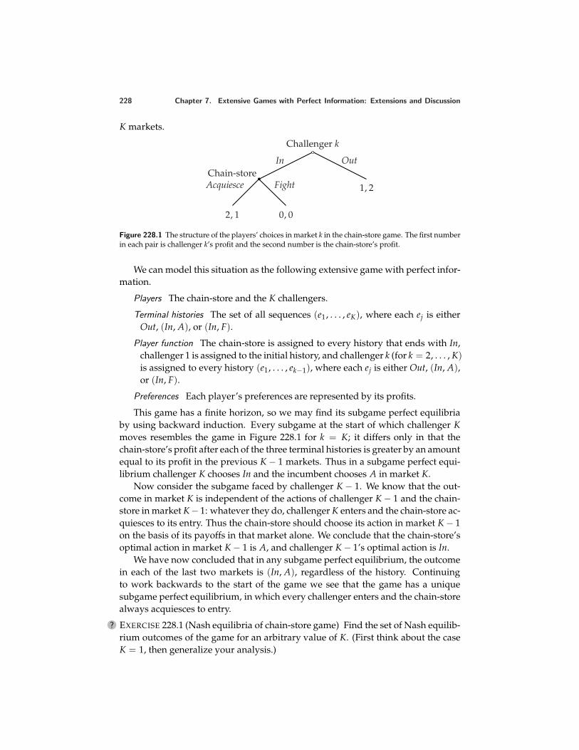
228 Chapter 7. Extensive Games with Perfect Information: Extensions and Discussion
K markets.
Challenger k
In Out
1, 2
Chain-storeAcquiesce Fight
2, 1 0, 0
Figure 228.1 The structure of the players’ choices in market k in the chain-store game. The first numberin each pair is challenger k’s profit and the second number is the chain-store’s profit.
We can model this situation as the following extensive game with perfect infor-mation.
Players The chain-store and the K challengers.
Terminal histories The set of all sequences (e1, . . . , eK), where each ej is eitherOut, (In, A), or (In, F).
Player function The chain-store is assigned to every history that ends with In,challenger 1 is assigned to the initial history, and challenger k (for k = 2, . . . , K)is assigned to every history (e1, . . . , ek−1), where each ej is either Out, (In, A),or (In, F).
Preferences Each player’s preferences are represented by its profits.
This game has a finite horizon, so we may find its subgame perfect equilibriaby using backward induction. Every subgame at the start of which challenger Kmoves resembles the game in Figure 228.1 for k = K; it differs only in that thechain-store’s profit after each of the three terminal histories is greater by an amountequal to its profit in the previous K − 1 markets. Thus in a subgame perfect equi-librium challenger K chooses In and the incumbent chooses A in market K.
Now consider the subgame faced by challenger K − 1. We know that the out-come in market K is independent of the actions of challenger K − 1 and the chain-store in market K − 1: whatever they do, challenger K enters and the chain-store ac-quiesces to its entry. Thus the chain-store should choose its action in market K − 1on the basis of its payoffs in that market alone. We conclude that the chain-store’soptimal action in market K − 1 is A, and challenger K − 1’s optimal action is In.
We have now concluded that in any subgame perfect equilibrium, the outcomein each of the last two markets is (In, A), regardless of the history. Continuingto work backwards to the start of the game we see that the game has a uniquesubgame perfect equilibrium, in which every challenger enters and the chain-storealways acquiesces to entry.
? EXERCISE 228.1 (Nash equilibria of chain-store game) Find the set of Nash equilib-rium outcomes of the game for an arbitrary value of K. (First think about the caseK = 1, then generalize your analysis.)

7.7 Discussion: subgame perfect equilibrium and backward induction 229
? EXERCISE 229.1 (Subgame perfect equilibrium of chain-store game) Consider thefollowing strategy pair in the game for K = 100. For k = 1, . . . , 90, challenger kstays out after any history in which every previous challenger that entered wasfought (or no challenger entered), and otherwise enters; challengers 91 through100 enter. The chain-store fights every challenger up to challenger 90 that entersafter a history in which it fought every challenger that entered (or no challengerentered), acquiesces to any of these challengers that enters after any other history,and acquiesces to challengers 91 through 100 regardless of the history. Find theplayers’ payoffs in this strategy pair. Show that the strategy pair is not a subgameperfect equilibrium: find a player who can increase her payoff in some subgame.How much can the deviant increase its payoff?
Suppose that K = 100. You are in charge of challenger 21. You observe, con-trary to the subgame perfect equilibrium, that every previous challenger enteredand that the chain-store fought each one. What should you do? According tothe subgame perfect equilibrium, the chain-store will acquiesce to your entry. Butshould you really regard the chain-store’s 19 previous decisions as “mistakes”?You might instead read some logic into the chain-store’s deliberately fighting thefirst 20 entrants: if, by doing so, it persuades more than 20 of the remaining chal-lengers to stay out, then its profit will be higher than it is in the subgame perfectequilibrium. That is, you may imagine that the chain-store’s aggressive behaviorin the earlier markets is an attempt to establish a reputation for being a fighter,which, if successful, will make it better off. By such reasoning you may concludethat your best strategy is to stay out.
Thus, a deviation from the subgame perfect equilibrium by the chain-store inwhich it engages in a long series of fights may not be dismissed by challengers asa series of mistakes, but rather may cause them to doubt the chain-store’s futurebehavior. This doubt may lead a challenger who is followed by enough futurechallengers to stay out.
EXAMPLE 229.2 (Centipede game) The two-player game in Figure 230.1 is knownas a “centipede game” because of its shape. (The game, like the arthropod, mayhave fewer than 100 legs.) The players move alternately; on each move a playercan stop the game (S) or continue (C). On any move, a player is better off stoppingthe game than continuing if the other player stops immediately afterwards, but isworse off stopping than continuing if the other player continues, regardless of thesubsequent actions. After k periods, the game ends.
This game has a finite horizon, so we may find its subgame perfect equilibriaby using backward induction. The last player to move prefers to stop the gamethan to continue. Given this player’s action, the player who moves before heralso prefers to stop the game than to continue. Working backwards, we concludethat the game has a unique subgame perfect equilibrium, in which each player’sstrategy is to stop the game whenever it is her turn to move. The outcome is thatplayer 1 stops the game immediately.
? EXERCISE 229.3 (Nash equilibria of the centipede game) Show that the outcome
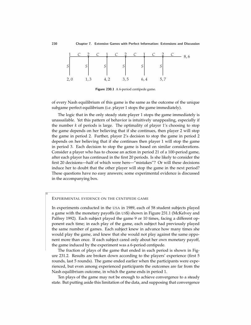
230 Chapter 7. Extensive Games with Perfect Information: Extensions and Discussion
1
S
C
2, 0
2
S
C
1, 3
1
S
C
4, 2
2
S
C
3, 5
1
S
C
6, 4
2
S
C
5, 7
8, 6
Figure 230.1 A 6-period centipede game.
of every Nash equilibrium of this game is the same as the outcome of the uniquesubgame perfect equilibrium (i.e. player 1 stops the game immediately).
The logic that in the only steady state player 1 stops the game immediately isunassailable. Yet this pattern of behavior is intuitively unappealing, especially ifthe number k of periods is large. The optimality of player 1’s choosing to stopthe game depends on her believing that if she continues, then player 2 will stopthe game in period 2. Further, player 2’s decision to stop the game in period 2depends on her believing that if she continues then player 1 will stop the gamein period 3. Each decision to stop the game is based on similar considerations.Consider a player who has to choose an action in period 21 of a 100-period game,after each player has continued in the first 20 periods. Is she likely to consider thefirst 20 decisions—half of which were hers—“mistakes”? Or will these decisionsinduce her to doubt that the other player will stop the game in the next period?These questions have no easy answers; some experimental evidence is discussedin the accompanying box.
EXPERIMENTAL EVIDENCE ON THE CENTIPEDE GAME
In experiments conducted in the USA in 1989, each of 58 student subjects playeda game with the monetary payoffs (in US$) shown in Figure 231.1 (McKelvey andPalfrey 1992). Each subject played the game 9 or 10 times, facing a different op-ponent each time; in each play of the game, each subject had previously playedthe same number of games. Each subject knew in advance how many times shewould play the game, and knew that she would not play against the same oppo-nent more than once. If each subject cared only about her own monetary payoff,the game induced by the experiment was a 6-period centipede.
The fraction of plays of the game that ended in each period is shown in Fig-ure 231.2. Results are broken down according to the players’ experience (first 5rounds, last 5 rounds). The game ended earlier when the participants were expe-rienced, but even among experienced participants the outcomes are far from theNash equilibrium outcome, in which the game ends in period 1.
Ten plays of the game may not be enough to achieve convergence to a steadystate. But putting aside this limitation of the data, and supposing that convergence

7.7 Discussion: subgame perfect equilibrium and backward induction 231
1
S
C
$0.40$0.10
2
S
C
$0.20$0.80
1
S
C
$1.60$0.40
2
S
C
$0.80$3.20
1
S
C
$6.40$1.60
2
S
C
$3.20$12.80
$25.60$6.40
Figure 231.1 The game in McKelvey and Palfrey’s (1992) experiment. The payoff of player 1 is writtenabove the payoff of player 2.
First 5 rounds
Last 5 rounds
period1 2 3 4 5 6 7
0.1
0.2
0.3
0.4
Figure 231.2 Fraction of games ending in each period of McKelvey and Palfrey’s experiments on thesix-period centipede game. (A game is counted as ending in period 7 if the last player to move choseC.) Computed from McKelvey and Palfrey (1992, Table IIIA).
was in fact achieved at the end of 10 rounds, how far does the observed behaviordiffer from a Nash equilibrium (maintaining the assumption that each player caresonly about her own monetary payoff)?
The theory of Nash equilibrium has two components: each player optimizes,given her beliefs about the other players, and these beliefs are correct. Some deci-sions in McKelvey and Palfrey’s experiment were patently suboptimal, regardlessof the subjects’ beliefs: a few subjects in the role of player 2 chose to continue in pe-riod 6, obtaining $6.40 with certainty instead of $12.80 with certainty. To assess thedeparture of the other decisions from optimality we need to assign the subjects be-liefs (which were not directly observed). An assumption consistent with the steadystate interpretation of Nash equilibrium is that a player’s belief is based on her ob-servations of the other players’ actions. Even in round 10 of the experiment eachplayer had only 9 observations on which to base her belief, and could have usedthese data in various ways. But suppose that, somehow, at the end of round 4, eachplayer correctly inferred the distribution of her opponents’ strategies in the next 5rounds. What strategy should she subsequently have used? From Palfrey andMcKelvey (1992, Table IIIB) we may deduce that the optimal strategy of player 1
232 Chapter 7. Extensive Games with Perfect Information: Extensions and Discussion
stops in period 5 and that of player 2 stops in period 6. That is, each player’sbest response to the empirical distribution of the other players’ strategies differsdramatically from her subgame perfect equilibrium strategy. Other assumptionsabout the subjects’ beliefs rationalize other strategies; the data seem too limited toconclude that the subjects were not optimizing given beliefs they might reasonablyhave held, given their experience. That is, the experimental data are not stronglyinconsistent with the theory of Nash equilibrium as a steady state.
Are the data inconsistent with the theory that rational players, even those withno experience playing the game, will deduce their opponents’ rational actions froman analysis of the game using backward induction? This theory predicts that thefirst player immediately stops the game, so certainly the data are inconsistent withit. How inconsistent? One way to approach this question is to consider the impli-cations of each player’s thinking that the others are likely to be rational, but are notcertainly so. If, in any period, player 1 thinks that the probability that player 2 willstop the game in the next period is less than 6
7 , continuing yields a higher expectedpayoff than stopping. Given the limited time the subjects had to analyze the game(and the likelihood that they had never before thought about any related game),even those who understood the implications of backward induction may reason-ably have entertained the relatively small doubt about the other players’ cognitiveabilities required to make stopping the game immediately an unattractive option.Or, alternatively, a player confident of her opponents’ logical abilities may havedoubted her opponents’ assessment of her own analytical skills. If player 1 believesthat player 2 thinks that the probability that player 1 will continue in period 3 isgreater than 1
7 , then she should continue in period 1, because player 2 will continuein period 2. That is, relatively minor departures from the theory yield outcomesclose to those observed.
Notes
The idea of regarding games with simultaneous moves as games with perfectinformation is due to Dubey and Kaneko (1984).
The model in Section 7.3 was first studied by Ledyard (1981, 1984). The ap-proach to voting in committees in Section 7.4 was initiated by Farquharson (1969).(The publication of Farquharson’s book was delayed; the book was completed in1958.) The top cycle set was first defined by Ward (1961) (who called it the “ma-jority set”). The characterization of the outcomes of sophisticated voting in binaryagendas in terms of the top cycle set is due to Miller (1977) (who calls the top cycleset the “Condorcet set”) and McKelvey and Niemi (1978). Miller (1995) surveys thefield. The model in Section 7.5 is taken from Nalebuff and Ghemawat (1985); theidea is closely related to that of Benoıt (1984, Section 1) (see Exercise 172.2). My dis-cussion draws on an unpublished exposition of the model by Vijay Krishna. Theidea of discriminating among Nash equilibria by considering the possibility that
Notes 233
players make mistakes, briefly discussed in Section 7.6.2, is due to Selten (1975).The chain-store game in Example 227.1 is due to Selten (1978). The centipede gamein Example 229.2 is due to Rosenthal (1981).
The experimental results discussed in the box on page 207 are due to Roth,Prasnikar, Okuno-Fujiwara, and Zamir (1991). The subgame perfect equilibria ofa variant of the market game in which each player’s payoff depends on the otherplayers’ monetary payoffs are analyzed by Bolton and Ockenfels (2000). The modelin Exercise 208.1 is taken from Peters (1984). The results in Exercises 212.1 and213.1 are due to Feddersen, Sened, and Wright (1990). The game in Exercise 223.2is a simplification of an example due to Shubik (1954); the main idea appears inPhillips (1937, 159) and Kinnaird (1946, 246), both of which consist mainly of puz-zles previously published in newspapers. Exercise 224.1 is based on Diermeier andFeddersen (1996). The experiment discussed in the box on page 230 is reported inMcKelvey and Palfrey (1992).
Draft chapter from An introduction to game theory by Martin J. [email protected]; www.economics.utoronto.ca/osborneVersion: 00/11/6.Copyright c© 1995–2000 by Martin J. Osborne. All rights reserved. No part of this book may be re-produced by any electronic or mechanical means (including photocopying, recording, or informationstorage and retrieval) without permission in writing from Oxford University Press, except that onecopy of up to six chapters may be made by any individual for private study.
8 Coalitional Games and the Core
Coalitional games 235The core 239Illustration: ownership and the distribution of wealth 243Illustration: exchanging homogeneous horses 247Illustration: exchanging heterogeneous houses 252Illustration: voting 256Illustration: matching 259Discussion: other solution concepts 265Prerequisite: Chapter 1.
8.1 Coalitional games
ACOALITIONAL GAME is a model of interacting decision-makers that focuseson the behavior of groups of players. It associates a set of actions with every
group of players, not only with individual players, like the models of a strategicgame (Definition 11.1) and extensive game (Definition 153.1)). We call each groupof players a coalition, and the coalition of all the players the grand coalition.
An outcome of a coalitional game consists of a partition of the set of players intogroups, together with an action for each group in the partition. (See Section 17.3if you are not familiar with the notion of a “partition” of a set.) At one extreme,each group in the partition may consist of a single player, who acts on her own;at another extreme, the partition may consist of a single group containing all theplayers. The most general model of a coalitional game allows players to care aboutthe action chosen by each group in the partition that defines the outcome. I discussonly the widely-studied class of games in which each player cares only about theaction chosen by the member of the partition to which she belongs. In such games,each player’s preferences rank the actions of all possible groups of players thatcontain her.
DEFINITION 235.1 (Coalitional game) A coalitional game consists of
• a set of players
• for each coalition, a set of actions
• for each player, preferences over the set of all actions of all coalitions of whichshe is a member.
235
236 Chapter 8. Coalitional Games and the Core
I usually denote the grand coalition (the set of all the players) by N and an arbi-trary coalition by S. As before, we may conveniently specify a player’s preferencesby giving a payoff function that represents them.
In several of the examples that I present, each coalition controls some quantityof a good, which may be distributed among its members. Each action of a coalitionS in such a game is a distribution among the members of S of the good that Scontrols, which I refer to as an S-allocation of the good. I refer to an N-allocationsimply as an allocation.
Note that the definition of a coalitional game does not relate the actions of acoalition to the actions of the members of the coalition. The coalition’s actions aresimply taken as given; they are not derived from the individual players’ actions.
A coalitional game is designed to model situations in which players can bene-ficially form groups, rather than acting individually. Most of the theory is orientedto situations in which the incentive to coalesce is extreme, in the sense that thereis no disadvantage to the formation of the single group consisting of all the play-ers. In considering the action that this single group takes in such a situation, weneed to consider the possibility that smaller groups break away on their own; butwhen looking for “equilibria” we can restrict attention to outcomes in which all theplayers coalesce. Such situations are modeled as games in which the grand coali-tion can achieve outcomes at least as desirable for every player as those achievableby any partition of the players into subgroups. We call such games “cohesive”,defined precisely as follows.
DEFINITION 236.1 (Cohesive coalitional game) A coalitional game is cohesive if,for every partition S1, . . . , Sk of the set of all players and every combination(aS1 , . . . , aSk
) of actions, one for every coalition in the partition, the grand coali-tion N has an action that is at least as desirable for every player i as the action aSj
of the member Sj of the partition to she player i belongs.
The concepts I subsequently describe may be applied to any game, cohesive andnot, but have attractive interpretations only for cohesive games.
EXAMPLE 236.2 (Two-player unanimity game) Two people can together produceone unit of output, which they may share in any way they wish. Neither person byherself can produce any output. Each person cares only about the amount of out-put she receives, and prefers more to less. The following coalitional game modelsthis situation.
Players The two people (players 1 and 2).
Actions Each player by herself has a single action, which yields her no output.The set of actions of the coalition 1, 2 of both players is the set of all pairs(x1, x2) of nonnegative numbers such that x1 + x2 = 1 (the set of divisions ofone unit of output between the two players).
Preferences Each player’s preferences are represented by the amount of outputshe obtains.
8.1 Coalitional games 237
The possible partitions of the set of players are 1, 2, consisting of the singlecoalition of both players, and 1, 2, in which each player acts alone. The lat-ter has only one combination of actions available to it, which produces not output.Thus the game is cohesive.
In the next example the opportunities for producing output are richer and theparticipants are not all symmetric.
EXAMPLE 237.1 (Landowner and workers) A landowner’s estate, when used byk workers, produces the output f (k + 1) of food, where f is a increasing functionfor which f (0) = 0. The total number of workers is m. The landowner and eachworker care only about the amount of output she receives, and prefer more to less.The following coalitional game models this situation.
Players The landowner and the m workers.
Actions A coalition consisting solely of workers has a single action in whichno member receives any output. The set of actions of a coalition S consistingof the landowner and k workers is the set of all S-allocations of the outputf (k + 1) among the members of S.
Preferences Each player’s preferences are represented by the amount of outputshe obtains.
This game is cohesive because the grand coalition produces more output thanany other coalition, and, for any partition of the set of all the players, only onecoalition produces any output.
EXAMPLE 237.2 (Three-player majority game) Three people have access to one unitof output. Any majority—two or three people—may control the allocation of thisoutput. Each person cares only about the amount of output she obtains.
We may model this situation as the following coalitional game.
Players The three people.
Actions Each coalition consisting of a single player has a single action, whichyields the player no output. The set of actions of each coalition S with two orthree players is the set of S-allocations of one unit of output.
Preferences Each player’s preferences are represented by the amount of outputshe obtains.
This game is cohesive because every partition of the set of players contains atmost one majority coalition, and for every action of such a coalition there is anaction of the grand coalition that yields each player as least as much output.
In these examples the set of actions of each coalition S is the set of S-allocationsof the output that S can obtain, and each player’s preferences are represented bythe amount of output she obtains. Thus we can summarize each coalition’s set ofactions by a single number, equal to the total output it can obtain, and can interpretthis number as the total “payoff” that may be distributed among the members of
238 Chapter 8. Coalitional Games and the Core
the coalition. A coalitional game in which the set of payoff distributions result-ing from each coalition’s actions may be represented in this way is said to havetransferable payoff.
We refer to the total payoff of any coalition S in a game with transferable payoffas the worth of S, and denote it v(S). Such a game is thus specified by its set ofplayers N and its worth function.
For the two-player unanimity game, for example, we have N = 1, 2, v(1) =v(2) = 0, and v(1, 2) = 1. For the landlord–worker game we have N =1, . . . , m + 1 (where 1 is the landowner and 2, . . . , m are the workers) and
v(S) =
0 if 1 is not a member of Sf (k) if S consists of 1 and k workers.
For the three-player majority game we have N = 1, 2, 3, v(i) = 0 for i = 1, 2,3, and v(S) = 1 for every other coalition S.
In the next two examples, payoff is not transferable.
EXAMPLE 238.1 (House allocation) Each member of a group of n people has asingle house. Any subgroup may reallocate its members’ houses in any way itwishes (one house to each person). (Time-sharing and other devices to evade theindivisibility of a house are prohibited.) The values assigned to houses vary amongthe people; each person cares only about the house she obtains. The followingcoalitional game models this situation.
Players The n people.
Actions The set of actions of a coalition S is the set of all assignments to mem-bers of S of the houses originally owned by members of S.
Preferences Each player prefers one outcome to another according to the houseshe is assigned.
This game is cohesive because any allocation of the houses that can be achievedby the coalitions in any partition of the set of players can also be achieved by theset of all players. It does not have transferable payoff. For example, a coalition ofplayers 1 and 2 can achieve only the two payoff distributions (v1, w2) and (v2, w1),where vi is the payoff to player 1 of the house owned by player i and wi is thepayoff to player 2 of the house owned by player i.
EXAMPLE 238.2 (Marriage market) A group of men and a group of women may bematched in pairs. Each person cares about her partner. A matching of the membersof a coalition S is a partition of the members of S into male-female pairs and singles.The following coalitional game models this situation.
Players The set of all the men and all the women.
Actions The set of actions of a coalition S is the set of all matchings of themembers of S.
Preferences Each player prefers one outcome to another according to the part-ner she is assigned.
8.2 The core 239
This game is cohesive because the matching of the members of the grand coali-tion induced by any collection of actions of the coalitions in a partition can beachieved by some action of the grand coalition.
8.2 The core
Which action may we expect the grand coalition to choose? We seek an action com-patible with the pressures imposed by the opportunities of each coalition, ratherthan simply those of individual players as in the models of a strategic game (Chap-ter 2) and an extensive game (Chapter 5). We define an action of the grand coalitionto be “stable” if no coalition can break away and choose an action that all its mem-bers prefer. The set of all stable actions of the grand coalition is called the core,defined precisely as follows.
DEFINITION 239.1 (Core) The core of a coalitional game is the set of actions aNof the grand coalition N such that no coalition has an action that all its membersprefer to aN .
If a coalition S has an action that all its members prefer to some action aN of thegrand coalition, we say that S can improve upon aN . Thus we may alternativelydefine the core to be the set of all actions of the grand coalition upon which nocoalition can improve.
Note that the core is defined as a set of actions, so it always exists; a game cannotfail to have a core, though it may be the empty set, in which case no action of thegrand coalition is immune to deviations.
We have restricted attention to games in which, when evaluating an outcome,each player cares only about the action chosen by the coalition in the partition ofwhich she is a member. Thus the members of a coalition do not need to specu-late about the remaining players’ behavior when considering a deviation. Conse-quently an interpretation of the core does not require us to assume that the playersare experienced; the concept makes sense even for naıve players with no experi-ence in the game. (By contrast, the main interpretations of Nash equilibrium andsubgame perfect equilibrium require the players to have experience playing thegame.)
In a game with transferable payoff, a coalition S can improve upon an action aNof the grand coalition if and only if its worth v(S) (i.e. the total payoff it can achieveby itself) exceeds the total payoff of its members in aN . That is, aN is in the core ifand only if for every coalition S the total payoff xS(aN) it yields the members of Sis at least v(S):
xS(aN) ≥ v(S) for every coalition S.
To find the core of a coalitional game we need to find the set of all actions ofthe grand coalition upon which no coalition can improve. In the next example, nocoalition can improve upon any action of the grand coalition, so the core consistsof all actions of the grand coalition.
240 Chapter 8. Coalitional Games and the Core
EXAMPLE 240.1 (Two-player unanimity game) Consider the two-player unanimitygame in Example 236.2. An action of the grand coalition is a pair (x1, x2) withx1 + x2 = 1 and xi ≥ 0 for i = 1, 2 (a division of the one unit of output betweenthe two players). I claim that the core consists of all possible divisions:
(x1, x2) : x1 + x2 = 1 and xi ≥ 0 for i = 1, 2.
Any such division is in the core because if a single player deviates she obtains nooutput, and if the grand coalition chooses a different division then one player isworse off.
In this example no coalition has any action that imposes any restriction on theaction of the grand coalition. In most other games the coalitions’ opportunitiesconstrain the actions of the grand coalition.
One way to find the core is to check each action of the grand coalition in turn.For each action and each coalition S, we impose the condition that S cannot makeall its members better off; an action is a member of the core if and only if it satisfiesthese conditions.
Consider, for example, a variant of the two-player unanimity game in whichplayer 1, by herself, can obtain p units of output, and player 2, by herself, canobtain q units of output. Then the condition that the coalition consisting of player 1not be able to improve upon the action (x1, x2) of the grand coalition is x1 ≥ p, andthe condition that the coalition consisting of player 2 not be able to improve uponthis action is x2 ≥ q. As in the original game, the coalition of both players cannotimprove upon any action (x1, x2), so the core is
(x1, x2) : x1 + x2 = 1, x1 ≥ p, and x2 ≥ q.
(An implication is that if p + q > 1—in which case the game is not cohesive—thecore is empty.)
An example of the landowner–worker game further illustrates this method offinding the core.
EXAMPLE 240.2 (Landowner–worker game with two workers) Consider the gamein Example 237.1 in which there are two workers (k = 2). Let (x1, x2, x3) be anaction of the grand coalition. That is, let (x1, x2, x3) be an allocation of the outputf (3) among the three players. The only coalitions that can obtain a positive amountof output are that consisting of the landowner (player 1), which can obtain theoutput f (1), those consisting of the landowner and a worker, which can obtainf (2), and the grand coalition. Thus (x1, x2, x3) is in the core if and only if
x1 ≥ f (1)
x2 ≥ 0
x3 ≥ 0
x1 + x2 ≥ f (2)
x1 + x3 ≥ f (2)
x1 + x2 + x3 = f (3),
8.2 The core 241
where the last condition ensures that (x1, x2, x3) is an allocation of f (3).From the last condition we have x1 = f (3) − x2 − x3, so that we may rewrite
the conditions as
0 ≤ x2 ≤ f (3) − f (2)
0 ≤ x3 ≤ f (3) − f (2)
x2 + x3 ≤ f (3) − f (1)
x1 + x2 + x3 = f (3).
That is, in an action in the core, each worker obtains at most the extra output f (3)−f (2) produced by the third player, and the workers together obtain at most theextra output f (3) − f (1) produced by the second and third players together.
? EXERCISE 241.1 (Three-player majority game) Show that the core of the three-player majority game (Example 237.2) has an empty core. Find the core of thevariant of this game in which player 1 has three votes (and player 2 and player 3each has one vote, as in the original game).
The next example introduces a class of games that model the market for aneconomic good.
EXAMPLE 241.2 (Market with one owner and two buyers) A person holds one in-divisible unit of a good and each of two (potential) buyers has a large amount ofmoney. The owner values money but not the good; each buyer values both moneyand the good and regards the good as equivalent to one unit of money. Each coali-tion may assign the good (if owned by one of its members) to any of its membersand allocate its members’ money in any way it wishes among its members.
We may model this situation as the following coalitional game.
Players The owner and the two buyers.
Actions The set of actions of each coalition S is the set of S-allocations of themoney and good (if any) owned by S.
Preferences The owner’s preferences are represented by the amount of moneyshe obtains; each buyer’s preferences are represented by the amount of thegood (either 0 or 1) she obtains plus the amount of money she holds.
I claim that for any action in the core, the owner does not keep the good. LetaN be an action of the grand coalition in which the owner keeps the good, andlet mi be the amount of money transferred from potential buyer i to the owner inthis action. (Transfers of money from the buyers to the owner when the ownerkeeps the good may not sound sensible, but they are feasible, so that we need toconsider them.) Consider the alternative action a′N of the grand coalition in whichthe good is allocated to buyer 1, who transfers m1 + 2ε money to the owner, andbuyer 2 transfers m2 − ε money to the owner, where 0 < ε < 1
2 . We see that allthe players’ payoffs are higher in a′N than they are in aN . (The owner’s payoff is ε
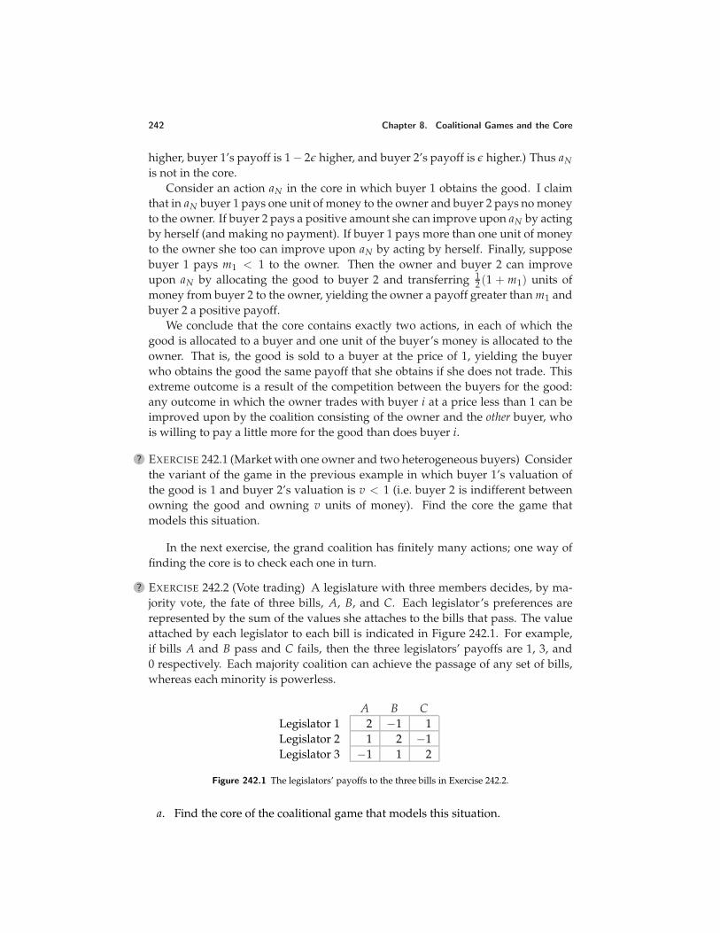
242 Chapter 8. Coalitional Games and the Core
higher, buyer 1’s payoff is 1 − 2ε higher, and buyer 2’s payoff is ε higher.) Thus aNis not in the core.
Consider an action aN in the core in which buyer 1 obtains the good. I claimthat in aN buyer 1 pays one unit of money to the owner and buyer 2 pays no moneyto the owner. If buyer 2 pays a positive amount she can improve upon aN by actingby herself (and making no payment). If buyer 1 pays more than one unit of moneyto the owner she too can improve upon aN by acting by herself. Finally, supposebuyer 1 pays m1 < 1 to the owner. Then the owner and buyer 2 can improveupon aN by allocating the good to buyer 2 and transferring 1
2 (1 + m1) units ofmoney from buyer 2 to the owner, yielding the owner a payoff greater than m1 andbuyer 2 a positive payoff.
We conclude that the core contains exactly two actions, in each of which thegood is allocated to a buyer and one unit of the buyer’s money is allocated to theowner. That is, the good is sold to a buyer at the price of 1, yielding the buyerwho obtains the good the same payoff that she obtains if she does not trade. Thisextreme outcome is a result of the competition between the buyers for the good:any outcome in which the owner trades with buyer i at a price less than 1 can beimproved upon by the coalition consisting of the owner and the other buyer, whois willing to pay a little more for the good than does buyer i.
? EXERCISE 242.1 (Market with one owner and two heterogeneous buyers) Considerthe variant of the game in the previous example in which buyer 1’s valuation ofthe good is 1 and buyer 2’s valuation is v < 1 (i.e. buyer 2 is indifferent betweenowning the good and owning v units of money). Find the core the game thatmodels this situation.
In the next exercise, the grand coalition has finitely many actions; one way offinding the core is to check each one in turn.
? EXERCISE 242.2 (Vote trading) A legislature with three members decides, by ma-jority vote, the fate of three bills, A, B, and C. Each legislator’s preferences arerepresented by the sum of the values she attaches to the bills that pass. The valueattached by each legislator to each bill is indicated in Figure 242.1. For example,if bills A and B pass and C fails, then the three legislators’ payoffs are 1, 3, and0 respectively. Each majority coalition can achieve the passage of any set of bills,whereas each minority is powerless.
A B CLegislator 1 2 −1 1Legislator 2 1 2 −1Legislator 3 −1 1 2
Figure 242.1 The legislators’ payoffs to the three bills in Exercise 242.2.
a. Find the core of the coalitional game that models this situation.
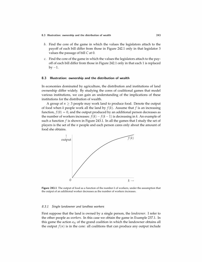
8.3 Illustration: ownership and the distribution of wealth 243
b. Find the core of the game in which the values the legislators attach to thepayoff of each bill differ from those in Figure 242.1 only in that legislator 3values the passage of bill C at 0.
c. Find the core of the game in which the values the legislators attach to the pay-off of each bill differ from those in Figure 242.1 only in that each 1 is replacedby −1.
8.3 Illustration: ownership and the distribution of wealth
In economies dominated by agriculture, the distribution and institutions of landownership differ widely. By studying the cores of coalitional games that modelvarious institutions, we can gain an understanding of the implications of theseinstitutions for the distribution of wealth.
A group of n ≥ 3 people may work land to produce food. Denote the outputof food when k people work all the land by f (k). Assume that f is an increasingfunction, f (0) = 0, and the output produced by an additional person decreases asthe number of workers increases: f (k) − f (k − 1) is decreasing in k. An example ofsuch a function f is shown in Figure 243.1. In all the games that I study the set ofplayers is the set of the n people and each person cares only about the amount offood she obtains.
0 k →
↑output f (k)
Figure 243.1 The output of food as a function of the number k of workers, under the assumption thatthe output of an additional worker decreases as the number of workers increases.
8.3.1 Single landowner and landless workers
First suppose that the land is owned by a single person, the landowner. I refer tothe other people as workers. In this case we obtain the game in Example 237.1. Inthis game the action aN of the grand coalition in which the landowner obtains allthe output f (n) is in the core: all coalitions that can produce any output include
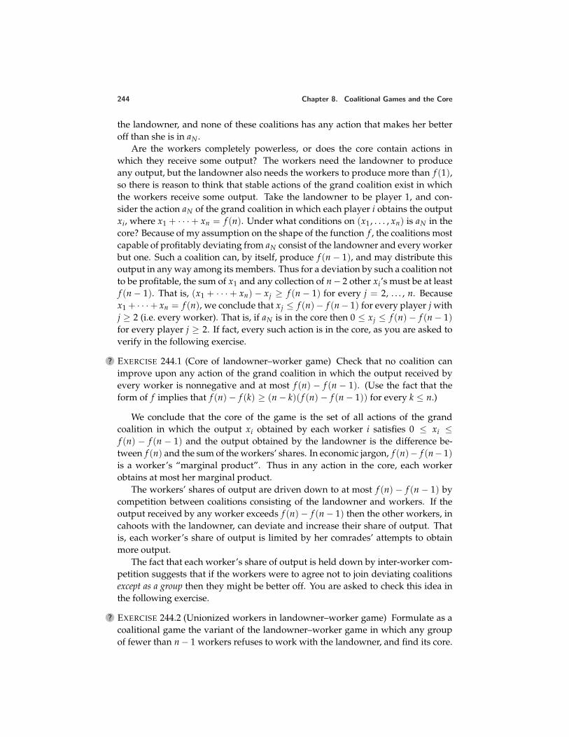
244 Chapter 8. Coalitional Games and the Core
the landowner, and none of these coalitions has any action that makes her betteroff than she is in aN .
Are the workers completely powerless, or does the core contain actions inwhich they receive some output? The workers need the landowner to produceany output, but the landowner also needs the workers to produce more than f (1),so there is reason to think that stable actions of the grand coalition exist in whichthe workers receive some output. Take the landowner to be player 1, and con-sider the action aN of the grand coalition in which each player i obtains the outputxi, where x1 + · · · + xn = f (n). Under what conditions on (x1, . . . , xn) is aN in thecore? Because of my assumption on the shape of the function f , the coalitions mostcapable of profitably deviating from aN consist of the landowner and every workerbut one. Such a coalition can, by itself, produce f (n − 1), and may distribute thisoutput in any way among its members. Thus for a deviation by such a coalition notto be profitable, the sum of x1 and any collection of n − 2 other xi’s must be at leastf (n − 1). That is, (x1 + · · · + xn) − xj ≥ f (n − 1) for every j = 2, . . . , n. Becausex1 + · · ·+ xn = f (n), we conclude that xj ≤ f (n)− f (n − 1) for every player j withj ≥ 2 (i.e. every worker). That is, if aN is in the core then 0 ≤ xj ≤ f (n) − f (n − 1)for every player j ≥ 2. If fact, every such action is in the core, as you are asked toverify in the following exercise.
? EXERCISE 244.1 (Core of landowner–worker game) Check that no coalition canimprove upon any action of the grand coalition in which the output received byevery worker is nonnegative and at most f (n) − f (n − 1). (Use the fact that theform of f implies that f (n) − f (k) ≥ (n − k)( f (n) − f (n − 1)) for every k ≤ n.)
We conclude that the core of the game is the set of all actions of the grandcoalition in which the output xi obtained by each worker i satisfies 0 ≤ xi ≤f (n) − f (n − 1) and the output obtained by the landowner is the difference be-tween f (n) and the sum of the workers’ shares. In economic jargon, f (n)− f (n− 1)is a worker’s “marginal product”. Thus in any action in the core, each workerobtains at most her marginal product.
The workers’ shares of output are driven down to at most f (n) − f (n − 1) bycompetition between coalitions consisting of the landowner and workers. If theoutput received by any worker exceeds f (n) − f (n − 1) then the other workers, incahoots with the landowner, can deviate and increase their share of output. Thatis, each worker’s share of output is limited by her comrades’ attempts to obtainmore output.
The fact that each worker’s share of output is held down by inter-worker com-petition suggests that if the workers were to agree not to join deviating coalitionsexcept as a group then they might be better off. You are asked to check this idea inthe following exercise.
? EXERCISE 244.2 (Unionized workers in landowner–worker game) Formulate as acoalitional game the variant of the landowner–worker game in which any groupof fewer than n − 1 workers refuses to work with the landowner, and find its core.
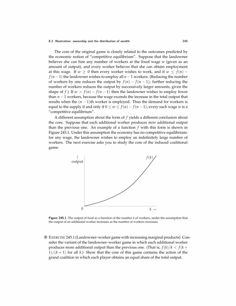
8.3 Illustration: ownership and the distribution of wealth 245
The core of the original game is closely related to the outcomes predicted bythe economic notion of “competitive equilibrium”. Suppose that the landownerbelieves she can hire any number of workers at the fixed wage w (given as anamount of output), and every worker believes that she can obtain employmentat this wage. If w ≥ 0 then every worker wishes to work, and if w ≤ f (n) −f (n− 1) the landowner wishes to employ all n− 1 workers. (Reducing the numberof workers by one reduces the output by f (n) − f (n − 1); further reducing thenumber of workers reduces the output by successively larger amounts, given theshape of f .) If w > f (n) − f (n − 1) then the landowner wishes to employ fewerthan n − 1 workers, because the wage exceeds the increase in the total output thatresults when the (n − 1)th worker is employed. Thus the demand for workers isequal to the supply if and only if 0 ≤ w ≤ f (n) − f (n − 1); every such wage w is a“competitive equilibrium”.
A different assumption about the form of f yields a different conclusion aboutthe core. Suppose that each additional worker produces more additional outputthan the previous one. An example of a function f with this form is shown inFigure 245.1. Under this assumption the economy has no competitive equilibrium:for any wage, the landowner wishes to employ an indefinitely large number ofworkers. The next exercise asks you to study the core of the induced coalitionalgame.
0 k →
↑output
f (k)
Figure 245.1 The output of food as a function of the number k of workers, under the assumption thatthe output of an additional worker increases as the number of workers increases.
? EXERCISE 245.1 (Landowner–worker game with increasing marginal products) Con-sider the variant of the landowner–worker game in which each additional workerproduces more additional output than the previous one. (That is, f (k)/k < f (k +1)/(k + 1) for all k.) Show that the core of this game contains the action of thegrand coalition in which each player obtains an equal share of the total output.
246 Chapter 8. Coalitional Games and the Core
8.3.2 Small landowners
Suppose that the land is distributed equally between all n people, rather than beingconcentrated in the hands of a single landowner. Assume that a group of k peoplewho pool their land and work together produce (k/n) f (n) units of output. (Theoutput produced by half the people working half the land, for example, is half theoutput produced by all the people working all the land.)
The following specification of the set of actions available to each coalition mod-els this situation.
Actions The set of actions of a coalition S consisting of k players is the set ofall S-allocations of the output (k/n) f (n) between the members of S.
As you might expect, one action in the core of this game is that in which everyplayer obtains an equal share of the total output—that is, f (n)/n units. Under thisaction, the total amount received by each coalition is precisely the total amountthe coalition produces. In fact, no other action is in the core. In any other action,some player receives less than f (n)/n, and hence can improve upon the actionalone (obtaining f (n)/n for herself). That is, the core consists of the single actionin which every player obtains f (n)/n units of output.
8.3.3 Collective ownership
Suppose that the land is owned collectively and the distribution of output is deter-mined by majority voting. Assume that any majority may distribute the output inany way it wishes; any majority may, in particular, take all the output for itself. Inthis case the set of actions available to each coalition are given as follows.
Actions The set of actions of a coalition S consisting of more than n/2 playersis the set of all S-allocations of the output f (n) between the members of S.The set of actions of a coalition S consisting of at most n/2 players is thesingle S-allocation in which no player in S receives any output.
The core of the coalitional game defined by this assumption is empty. For ev-ery action of the grand coalition, at least one player obtains a positive amountof output. But if player i obtains a positive amount of output then the coalitionof the remaining players, which is a majority, may improve upon the action, dis-tributing the output f (n) among its members (so that player i gets nothing). Thusevery action of the grand coalition may be improved upon by some coalition; nodistribution of output is “stable”.
The core of this game is empty because of the extreme power of every majoritycoalition. If any majority coalition may control how the land is used, but everyplayer owns a “share” that entitles her to the fraction 1/n of the output, then amajority coalition with k members can lay claim to only the fraction k/n of thetotal output, and a stable distribution of output may exist. This alternative own-ership institution, which tempers the power of majority coalitions, does not have
8.4 Illustration: exchanging homogeneous horses 247
interesting implications in the model in this section because the control of land usevested in a majority coalition is inconsequential—only one sensible pattern of useexists (all the players work!). If choices exist—if, for example, different crops maybe grown, and people differ in their preferences for these crops—then collectiveownership in which each player is entitled to an equal share of the output mayyield a different outcome from individual ownership.
8.4 Illustration: exchanging homogeneous horses
Markets may be modeled as coalitional games in which the set of actions of eachcoalition S is the set of S-allocations of the good initially owned by the membersof S. The core of such a game is the set of allocations of the goods available inthe economy that are robust to the trading opportunities of all possible groupsof participants: if aN is in the core then no group of agents can secede from theeconomy, trade among themselves, and produce an outcome they all prefer to aN .
In this section I describe a simple example of a market, in which there is moneyand a single homogeneous good (all units of which are identical). In the next sec-tion I describe a market in which there is a single heterogeneous good. In both casethe core makes a very precise prediction about the outcome.
8.4.1 Model
Some people own one unit of an indivisible good, whereas others possess onlymoney. Some non-owners value a unit of the good more highly than some owners,so that mutually beneficial trades exist. Which allocation of goods and money willresult?
We may address this question with the help of a coalitional game that gener-alizes the one in Example 241.2. I refer to the goods as “horses” (following theliterature on the model, which takes off from an analysis by Eugen von Bohm-Bawerk (1851–1914)). Call each person who owns a horse simply an owner, and ev-ery other person a nonowner. Assume that all horses are identical, and that no onewishes to own more than one. People value a horse differently; denote player i’svaluation by vi. Assume that there are at least two owners and two nonowners,and that some owner’s valuation is less than some nonowner’s valuation (i.e. forsome owner i and nonowner j have vi < vj), so that some trade is mutually desir-able. Assume also, to avoid some special cases, that some nonowner’s valuation isless than some owner’s valuation (i.e. for some nonowner i and owner j we havevi < vj) and that no two players have the same valuation. Further assume that ev-ery person has enough money to fully compensate the owner who values a horsemost highly, so that no one’s behavior is constrained by her cash balance.
As to preferences, assume that each person cares only about the amount ofmoney she has and whether or not she has a horse. (In particular, no one caresabout any other person’s holdings.) Specifically, assume that each player i’s pref-
248 Chapter 8. Coalitional Games and the Core
erences are represented by the payoff function
vi + r if she has a horse and $r more money than she had originallyr if she has no horse and $r more money than she had originally.
(This assumption does not mean that people do not value the money they haveinitially. Equivalently we could represent player i’s preferences by the functionsvi + r + mi if she has a horse and r + mi if she does not, where mi is the amount ofmoney she has initially.)
The following coalitional game models, which I call a horse trading game,models the situation.
Players The group of people (owners and nonowners).
Actions The set of actions of each coalition S is the set of S-allocations of thehorses and the total amount of money owned by S in which each playerobtains at most one horse.
Preferences Each player’s preferences are represented by the payoff functiondescribed above.
This game incorporates no restriction on the way in which a coalition may dis-tribute its money and horses. In particular, players are not restricted to bilateraltrades of money for horses. A coalition of two owners and two nonowners, forexample, may, if it wishes, allocate each of the owners’ horses to a nonowner andtransfer money from both nonowners to only one owner, or from one nonowner tothe other.
8.4.2 The core
Number the owners in ascending order and the nonowners in descending or-der of the valuations they attach to a horse. Figure 249.1 illustrates the valua-tions, ordered in this way. (This diagram should be familiar—perhaps it is a littletoo familiar—if you have studied economics.) Denote owner i’s valuation σi andnonowner i’s valuation βi. Denote by k∗ the largest number i such that βi > σi(so that among the owners and nonowners whose indices are k∗ or less, everynonowner’s valuation is greater than every owner’s valuation).
Let aN be an action in the core. Denote by L∗ the set of owners who have nohorse in aN (the set of sellers) and by B∗ the set of nonowners who have a horse inaN (the set of buyers). These two sets must have the same number of members (bythe law of conservation of horses). Denote by ri the amount of money received byowner i and by pj the amount paid by nonowner j in aN .
I claim that pj = 0 for every nonowner j not in B∗. (That is, no nonowner whodoes not acquire a horse either pays or receives any money.)
• If pj > 0 for some nonowner j not in B∗ then her payoff is negative, and shecan unilaterally improve upon aN by retaining her original money.
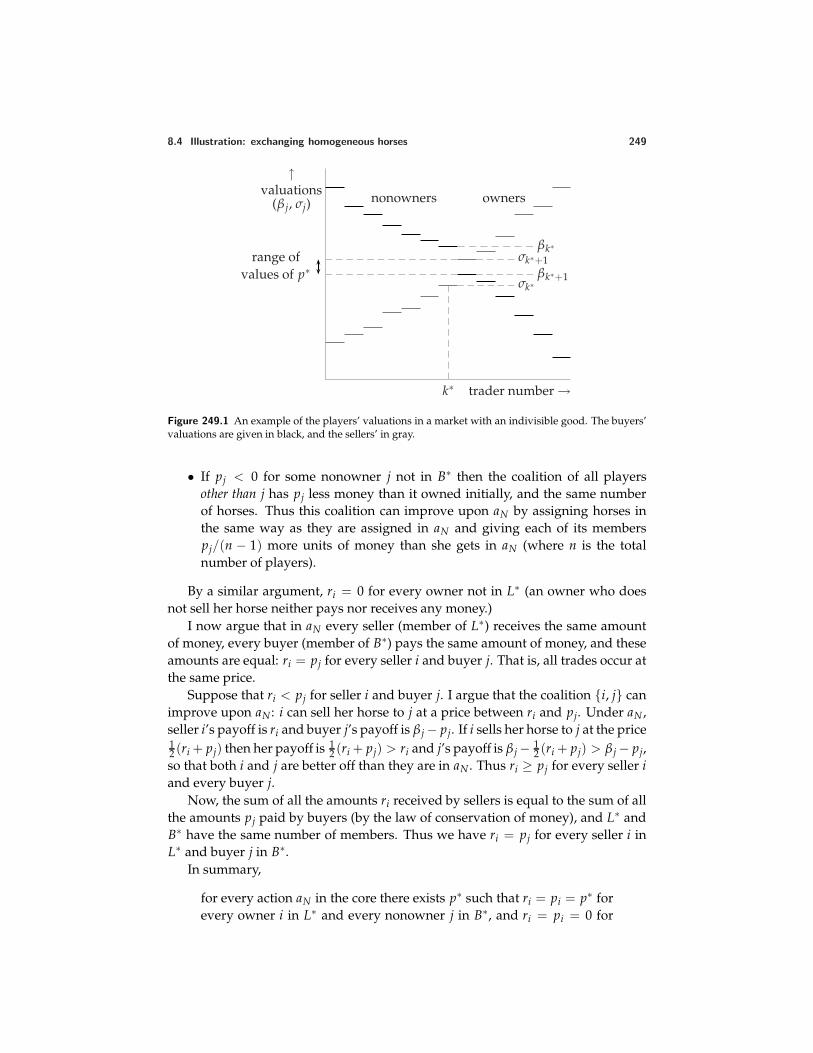
8.4 Illustration: exchanging homogeneous horses 249
βk∗
βk∗+1σk∗
σk∗+1range ofvalues of p∗
k∗ trader number →
↑valuations
(β j, σj)nonowners owners
Figure 249.1 An example of the players’ valuations in a market with an indivisible good. The buyers’valuations are given in black, and the sellers’ in gray.
• If pj < 0 for some nonowner j not in B∗ then the coalition of all playersother than j has pj less money than it owned initially, and the same numberof horses. Thus this coalition can improve upon aN by assigning horses inthe same way as they are assigned in aN and giving each of its memberspj/(n − 1) more units of money than she gets in aN (where n is the totalnumber of players).
By a similar argument, ri = 0 for every owner not in L∗ (an owner who doesnot sell her horse neither pays nor receives any money.)
I now argue that in aN every seller (member of L∗) receives the same amountof money, every buyer (member of B∗) pays the same amount of money, and theseamounts are equal: ri = pj for every seller i and buyer j. That is, all trades occur atthe same price.
Suppose that ri < pj for seller i and buyer j. I argue that the coalition i, j canimprove upon aN : i can sell her horse to j at a price between ri and pj. Under aN ,seller i’s payoff is ri and buyer j’s payoff is β j − pj. If i sells her horse to j at the price12 (ri + pj) then her payoff is 1
2 (ri + pj) > ri and j’s payoff is β j − 12 (ri + pj) > β j − pj,
so that both i and j are better off than they are in aN . Thus ri ≥ pj for every seller iand every buyer j.
Now, the sum of all the amounts ri received by sellers is equal to the sum of allthe amounts pj paid by buyers (by the law of conservation of money), and L∗ andB∗ have the same number of members. Thus we have ri = pj for every seller i inL∗ and buyer j in B∗.
In summary,
for every action aN in the core there exists p∗ such that ri = pi = p∗ forevery owner i in L∗ and every nonowner j in B∗, and ri = pi = 0 for
250 Chapter 8. Coalitional Games and the Core
every owner not in L∗ and every nonowner j not in B∗.
I now argue that the common price p∗ at which all trades take place lies in anarrow range.
In aN , every owner i whose valuation of a horse is less than p∗ must sell herhorse: if she did not then the coalition consisting of herself and any nonowner jwho buys a horse in aN could improve upon aN by taking the action in which jbuys i’s horse at a price between the owner’s valuation and p∗. Also, no ownerwhose valuation exceeds p∗ trades, because her payoff from doing so is negative.Similarly, every nonowner whose valuation is greater than p∗ buys a horse, and nononowner whose valuation is less than p∗ does so.
? EXERCISE 250.1 (Range of prices in horse market) Show that the requirement thatthe number of owners who sell their horses must equal the number of nonownerswho buy horses, together with the arguments above, implies that the commontrading price p∗ is at least σk∗ , at least βk∗+1, at most βk∗ , and at most σk∗+1. Thatis, p∗ ≥ maxσk∗ , βk∗+1 and p∗ ≤ minβk∗ , σk∗+1.
Finally, I argue that in any action in the core a player whose valuation is equal top∗ trades. Suppose nonowner i’s valuation is equal to p∗. Then owner i’s valuationis less than p∗ and owner i + 1’s valuation is greater than p∗ (given my assumptionthat no two players have the same valuation), so that exactly i owners trade. Thusexactly i nonowners must trade, implying that nonowner i trades. Symmetrically,a owner whose valuation is equal to p∗ trades.
In summary, in every action in the core of a horse trading game,
• every nonowner pays the same price for a horse
• the common price is at least maxσk∗ , βk∗+1 and at mostminβk∗ , σk∗+1
• every owner whose valuation is at most the price trades her horse
• every nonowner whose valuation is at least the price obtains ahorse.
(250.2)
The action satisfying these conditions for the price p∗ yields the payoffs
maxvi, p∗ for every owner imaxvi, p∗ − p∗ for every nonowner i.
The core does not impose any additional restrictions on the actions of the grandcoalition: every action that satisfies these conditions is in the core. To establish thisresult, I need to show that for any action aN that satisfies the conditions, no coali-tion has an action that is better for all its members. When a coalition deviates,which of its actions has the best chance of improving upon aN? The optimal actiondefinitely assigns the coalition’s horses to the members who value a horse mosthighly. (If vi < vj then the transfer of a horse from i to j, accompanied by the
8.4 Illustration: exchanging homogeneous horses 251
transfer from j to i of an amount of money between vi and vj makes both i and jbetter off.) No transfer of money makes anyone better off without making some-one worse off, so in order for a coalition to improve upon aN there must be somedistribution of the total amount of money it owns that, given the optimal distri-bution of horses, makes all its members better off than they are in aN . For everydistribution of a coalition’s money the total payoff of the members of the coalitionis the same. Thus a coalition can improve upon aN if and only if the total pay-off of its members under aN is less than its total payoff when it assigns its horsesoptimally.
Consider an arbitrary coalition S. Denote by the total number of owners in S,by b the total number of nonowners in S, and by S∗ the set of members of S whosevaluations are highest. Then S’s total payoff when it assigns its horses optimally is
∑i∈S∗
vi,
whereas its total payoff under aN is
∑i∈S
maxvi, p∗ − bp∗ = ∑i∈S∗
maxvi, p∗ + ∑i∈S\S∗
maxvi, p∗ − bp∗,
where S \ S∗ is the set of members of S not in S∗. The former is never higher thanthe latter because S \ S∗ has b members, so that ∑i∈S\S∗ maxvi, p∗ − bp∗ ≥ 0.
In summary, the core of a horse trading game is the set of actions of the grandcoalition that satisfies the four conditions in (250.2).
? EXERCISE 251.1 (Horse trading game with single seller) Find the core of the variantof the horse trading game in which there is a single owner, whose valuation is lessthan the highest valuation of the nonowners.
If you have studied economics you know that this outcome is the same as the“competitive equilibrium”. The theories differ, however. The theory of competi-tive equilibrium assumes that all trades take place at the same price. It defines anequilibrium price to be one at which “demand” (the total number of nonownerswhose valuations exceed the price) is equal to “supply” (the total number of own-ers whose valuations are less than the price). This equilibrium may be justified bythe argument that if demand exceeds supply then the price will tend to rise, and ifsupply exceeds demand it will tend to fall. Thus in this theory, “market pressures”generate an equilibrium price; no agent in the market chooses a price.
By contrast, the coalitional game we have studied models the players’ actionsexplicitly; each group may exchange its horses and money in any way it wishes.The core is the set of actions of all players that survives the pressures imposed bythe trading opportunities of each possible group of players. A uniform price is notassumed, but is shown to be a necessary property of any action in the core.
? EXERCISE 251.2 (Horse trading game with large seller) Consider the variant of thehorse trading game in which there is a single owner who has two horses. Assume
252 Chapter 8. Coalitional Games and the Core
that the owner’s payoff is σ1 + r if she keeps one of her horses and 2σ1 + r if shekeeps both of them, where r is the amount of money she receives. Assume thatthere are at least two nonowners, both of whose values of a horse exceed σ1. Findthe core of this game. (Do all trades take place at the same price, as they do in acompetitive equilibrium?)
8.5 Illustration: exchanging heterogeneous houses
8.5.1 Model
Each member of a group of n people owns an indivisible good—call it a house.Houses, unlike the horses of the previous section, differ. Any subgroup may re-allocate its members’ houses in any way it wishes (one house to each person).(Time-sharing and other devices to evade the indivisibility of a house are prohib-ited.) Each person cares only about the house she obtains, and has a strict rankingof the houses (she is not indifferent between any two houses).
Which assignments of houses to people are stable? You may think that withoutimposing any restrictions on the nature or diversity of preferences, this question ishard to answer, and that for some sufficiently conflicting configurations of prefer-ences no assignment is stable. If so, you are wrong on both counts, at least as far asthe core is concerned; remarkably, for any preferences, a slight variant of the coreyields a unique stable outcome.
The following coalitional game, which I call a house exchange game, modelsthe situation.
Players The n people.
Actions The set of actions of a coalition S is the set of all assignments to mem-bers of S of the houses originally owned by members of S.
Preferences Each player prefers one outcome to another according to the houseshe is assigned.
8.5.2 The top trading cycle procedure and the core
One property of an action in the core is immediate: any player who initially ownsher favorite house obtains that house in any assignment in the core, because everyplayer has the option of simply keeping the house she initially owns.
This property allows us to completely analyze the simplest nontrivial exampleof the game, with two people. Denote the person who initially owns player i’sfavorite house by o(i).
• If at least one person initially owns her favorite house (i.e. if o(1) = 1 oro(2) = 2), then the core contains the single assignment in which each personkeeps the house she owns.
8.5 Illustration: exchanging heterogeneous houses 253
• If each person prefers the house owned by the other person (i.e. if o(1) = 2and o(2) = 1), then the core contains the single assignment in which the twopeople exchange houses.
In the second case we say that “12 is a 2-cycle”. When there are more players,longer cycles are possible. For example, if there are three or more players ando(i) = j, o(j) = k, and o(k) = i, then we say that “ijk is a 3-cycle”. (If o(i) = i, wecan think of i as a “1-cycle”.)
The case in which there are three people raises some new possibilities.
• If at least two people initially own their favorite houses, then the core con-tains the single assignment in which each person keeps the house she initiallyowns.
• If exactly one person, say player i, initially owns her favorite house, thenin any assignment in the core, that person keeps her house. Whether theother two people exchange their houses depends on their preferences overthese houses, ignoring player i’s house (which has already been assigned);the analysis is the same as that for the two-player game.
• If no person initially owns her favorite house, there are two cases.
– If there is a 2-cycle (i.e. if there exist persons i and j such that j initiallyowns i’s favorite house and i initially owns j’s favorite house), then theonly assignment in the core is that in which i and j swap houses and theremaining player keeps the house she owns initially.
– Otherwise, suppose that o(i) = j. Then o(j) = k, where k is the thirdplayer (otherwise ij is a 2-cycle), and o(k) = i (otherwise kj is a 2-cycle.)That is, ijk is a 3-cycle. Consider the assignment in which i gets j’shouse, j gets k’s house, and k gets i’s house. Every player is assignedher favorite house, so the assignment is in the core. (This argumentdoes not show that the core contains no other assignments.)
This construction of an assignment in the core can be extended to games withany number of players. First we look for cycles among the houses at the top ofthe players’ rankings, and assign to each member of each cycle her favorite house.(If there are at most three players, only one cycle containing more than one playermay exist, but if there are more players, many cycles may exist.) Then we eliminatefrom consideration the players involved in these cycles and the houses they areallocated, look for any cycles at the top of the remains of the players’ rankings,and assign to each member of each of these cycles her favorite house among thoseremaining. We continue in the same manner until all players are assigned houses.This procedure is called the top trading cycle procedure.
To illustrate the procedure, consider the game with four players whose prefer-ences satisfy the specification in Figure 254.1. In this figure, hi denotes the houseowned by player i and the players’ rankings are listed from best to worst, starting
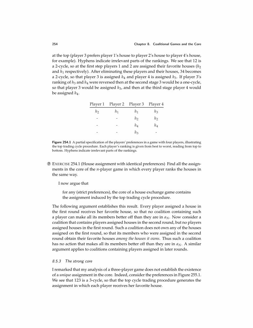
254 Chapter 8. Coalitional Games and the Core
at the top (player 3 prefers player 1’s house to player 2’s house to player 4’s house,for example). Hyphens indicate irrelevant parts of the rankings. We see that 12 isa 2-cycle, so at the first step players 1 and 2 are assigned their favorite houses (h2and h1 respectively). After eliminating these players and their houses, 34 becomesa 2-cycle, so that player 3 is assigned h4 and player 4 is assigned h3. If player 3’sranking of h3 and h4 were reversed then at the second stage 3 would be a one-cycle,so that player 3 would be assigned h3, and then at the third stage player 4 wouldbe assigned h4.
Player 1 Player 2 Player 3 Player 4
h2 h1 h1 h3
- - h2 h2
- - h4 h4
- - h3 -
Figure 254.1 A partial specification of the players’ preferences in a game with four players, illustratingthe top trading cycle procedure. Each player’s ranking is given from best to worst, reading from top tobottom. Hyphens indicate irrelevant parts of the rankings.
? EXERCISE 254.1 (House assignment with identical preferences) Find all the assign-ments in the core of the n-player game in which every player ranks the houses inthe same way.
I now argue that
for any (strict preferences), the core of a house exchange game containsthe assignment induced by the top trading cycle procedure.
The following argument establishes this result. Every player assigned a house inthe first round receives her favorite house, so that no coalition containing sucha player can make all its members better off than they are in aN . Now consider acoalition that contains players assigned houses in the second round, but no playersassigned houses in the first round. Such a coalition does not own any of the housesassigned on the first round, so that its members who were assigned in the secondround obtain their favorite houses among the houses it owns. Thus such a coalitionhas no action that makes all its members better off than they are in aN . A similarargument applies to coalitions containing players assigned in later rounds.
8.5.3 The strong core
I remarked that my analysis of a three-player game does not establish the existenceof a unique assignment in the core. Indeed, consider the preferences in Figure 255.1.We see that 123 is a 3-cycle, so that the top cycle trading procedure generates theassignment in which each player receives her favorite house.
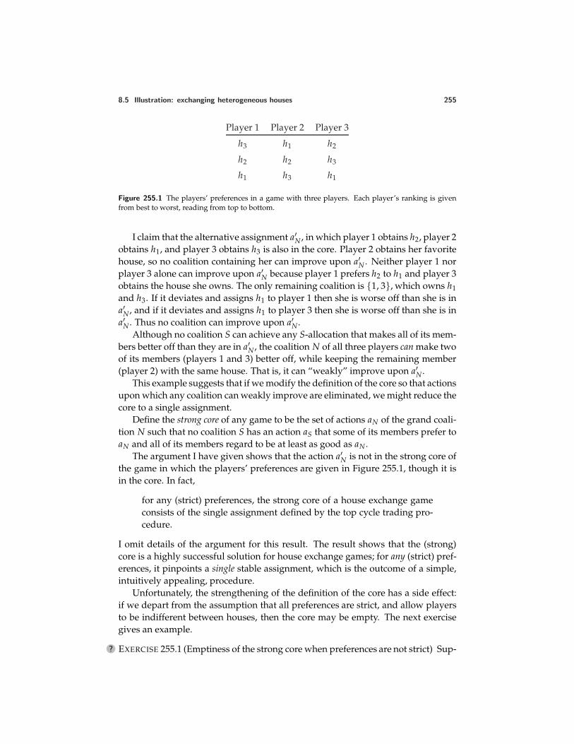
8.5 Illustration: exchanging heterogeneous houses 255
Player 1 Player 2 Player 3
h3 h1 h2
h2 h2 h3
h1 h3 h1
Figure 255.1 The players’ preferences in a game with three players. Each player’s ranking is givenfrom best to worst, reading from top to bottom.
I claim that the alternative assignment a′N , in which player 1 obtains h2, player 2obtains h1, and player 3 obtains h3 is also in the core. Player 2 obtains her favoritehouse, so no coalition containing her can improve upon a′N . Neither player 1 norplayer 3 alone can improve upon a′N because player 1 prefers h2 to h1 and player 3obtains the house she owns. The only remaining coalition is 1, 3, which owns h1and h3. If it deviates and assigns h1 to player 1 then she is worse off than she is ina′N , and if it deviates and assigns h1 to player 3 then she is worse off than she is ina′N . Thus no coalition can improve upon a′N .
Although no coalition S can achieve any S-allocation that makes all of its mem-bers better off than they are in a′N , the coalition N of all three players can make twoof its members (players 1 and 3) better off, while keeping the remaining member(player 2) with the same house. That is, it can “weakly” improve upon a′N .
This example suggests that if we modify the definition of the core so that actionsupon which any coalition can weakly improve are eliminated, we might reduce thecore to a single assignment.
Define the strong core of any game to be the set of actions aN of the grand coali-tion N such that no coalition S has an action aS that some of its members prefer toaN and all of its members regard to be at least as good as aN .
The argument I have given shows that the action a′N is not in the strong core ofthe game in which the players’ preferences are given in Figure 255.1, though it isin the core. In fact,
for any (strict) preferences, the strong core of a house exchange gameconsists of the single assignment defined by the top cycle trading pro-cedure.
I omit details of the argument for this result. The result shows that the (strong)core is a highly successful solution for house exchange games; for any (strict) pref-erences, it pinpoints a single stable assignment, which is the outcome of a simple,intuitively appealing, procedure.
Unfortunately, the strengthening of the definition of the core has a side effect:if we depart from the assumption that all preferences are strict, and allow playersto be indifferent between houses, then the core may be empty. The next exercisegives an example.
? EXERCISE 255.1 (Emptiness of the strong core when preferences are not strict) Sup-
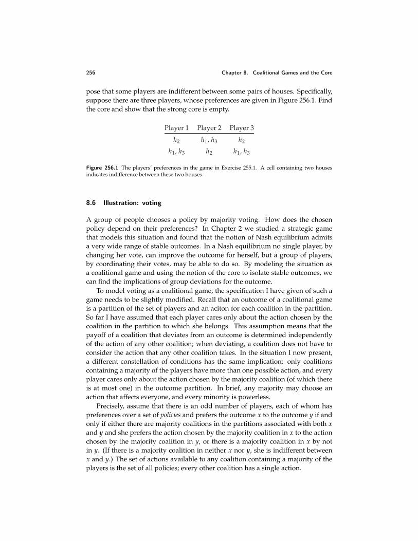
256 Chapter 8. Coalitional Games and the Core
pose that some players are indifferent between some pairs of houses. Specifically,suppose there are three players, whose preferences are given in Figure 256.1. Findthe core and show that the strong core is empty.
Player 1 Player 2 Player 3
h2 h1, h3 h2
h1, h3 h2 h1, h3
Figure 256.1 The players’ preferences in the game in Exercise 255.1. A cell containing two housesindicates indifference between these two houses.
8.6 Illustration: voting
A group of people chooses a policy by majority voting. How does the chosenpolicy depend on their preferences? In Chapter 2 we studied a strategic gamethat models this situation and found that the notion of Nash equilibrium admitsa very wide range of stable outcomes. In a Nash equilibrium no single player, bychanging her vote, can improve the outcome for herself, but a group of players,by coordinating their votes, may be able to do so. By modeling the situation asa coalitional game and using the notion of the core to isolate stable outcomes, wecan find the implications of group deviations for the outcome.
To model voting as a coalitional game, the specification I have given of such agame needs to be slightly modified. Recall that an outcome of a coalitional gameis a partition of the set of players and an aciton for each coalition in the partition.So far I have assumed that each player cares only about the action chosen by thecoalition in the partition to which she belongs. This assumption means that thepayoff of a coalition that deviates from an outcome is determined independentlyof the action of any other coalition; when deviating, a coalition does not have toconsider the action that any other coalition takes. In the situation I now present,a different constellation of conditions has the same implication: only coalitionscontaining a majority of the players have more than one possible action, and everyplayer cares only about the action chosen by the majority coalition (of which thereis at most one) in the outcome partition. In brief, any majority may choose anaction that affects everyone, and every minority is powerless.
Precisely, assume that there is an odd number of players, each of whom haspreferences over a set of policies and prefers the outcome x to the outcome y if andonly if either there are majority coalitions in the partitions associated with both xand y and she prefers the action chosen by the majority coalition in x to the actionchosen by the majority coalition in y, or there is a majority coalition in x by notin y. (If there is a majority coalition in neither x nor y, she is indifferent betweenx and y.) The set of actions available to any coalition containing a majority of theplayers is the set of all policies; every other coalition has a single action.
8.6 Illustration: voting 257
The definition of the core of this variant of a coalitional game is the naturalvariant of Definition 239.1: the set of actions aN of the grand coalition N such thatno majority coalition has an action that all its members prefer to aN .
Suppose that the policy x is in the core of this game. Then no policy is preferredto x by a coalition consisting of a majority of the players. Equivalently, for everypolicy y = x, the set of players who either prefer x to y or regard x and y to beequally good is a majority. If we assume that every player’s preferences are strict—no player is indifferent between any two policies—then for every policy y = x, theset of players who prefer x to y is a majority. That is, x is a Condorcet winner (seeExercise 74.1). For any preferences, there is at most one Condorcet winner, so wehave established that
if every player’s preferences are strict, the core of a majority votinggame is empty if there is no Condorcet winner, and otherwise is the setconsisting of the single Condorcet winner.
How does the existence and character of a Condorcet winner depend on theplayers’ preferences? First suppose that a policy is a number. Assume that eachplayer i has a favorite policy x∗
i , and that her preferences are single-peaked: if x andx′ are policies for which x < x′ < x∗
i or x∗i < x′ < x then she prefers x′ to x. Then
the median of the players’ favorite positions is the Condorcet winner, as you areasked to show in the next exercise, and hence the unique member of the core of thevoting game. (The median is well-defined because the number of players is odd.)
? EXERCISE 257.1 (Median voter theorem) Show that when the policy space is one-dimensional and the players’ preferences are single-peaked the unique Condorcetwinner is the median of the players’ favorite positions. (This result is known as themedian voter theorem.)
A one-dimensional space captures some policy choices, but in other situationsa higher dimensional space is needed. For example, a government has to choosethe amounts to spend on health care and defense, and not all citizens’ preferencesare aligned on these issues. Unfortunately, for most configurations of the players’preferences, a Condorcet winner does not exist in a policy space of two or moredimensions, so that the core is empty.
To see why this claim is plausible, suppose the policy space is two-dimensionaland there are three players. Place the players’ favorite positions at three arbitrarypoints, like x∗
1, x∗2, and x∗
3 in Figure 258.1. Assume that each player i’s distaste for aposition x different from her favorite position x∗
i is exactly the distance between xand x∗
i , so that for any value of r she is indifferent between all policies on the circlewith radius r centered at x∗
i .Now choose any policy and ask if it is a Condorcet winner. The policy x in the
figure is not, because any policy in the shaded area is preferred to x by players 1and 2, who constitute a majority. The policy x is also beaten in a majority vote byany policy in either of the other lens-shaped areas defined by the intersection of thecircles centered at x∗
1, x∗2, and x∗
3. Is there any policy for which no such lens-shaped
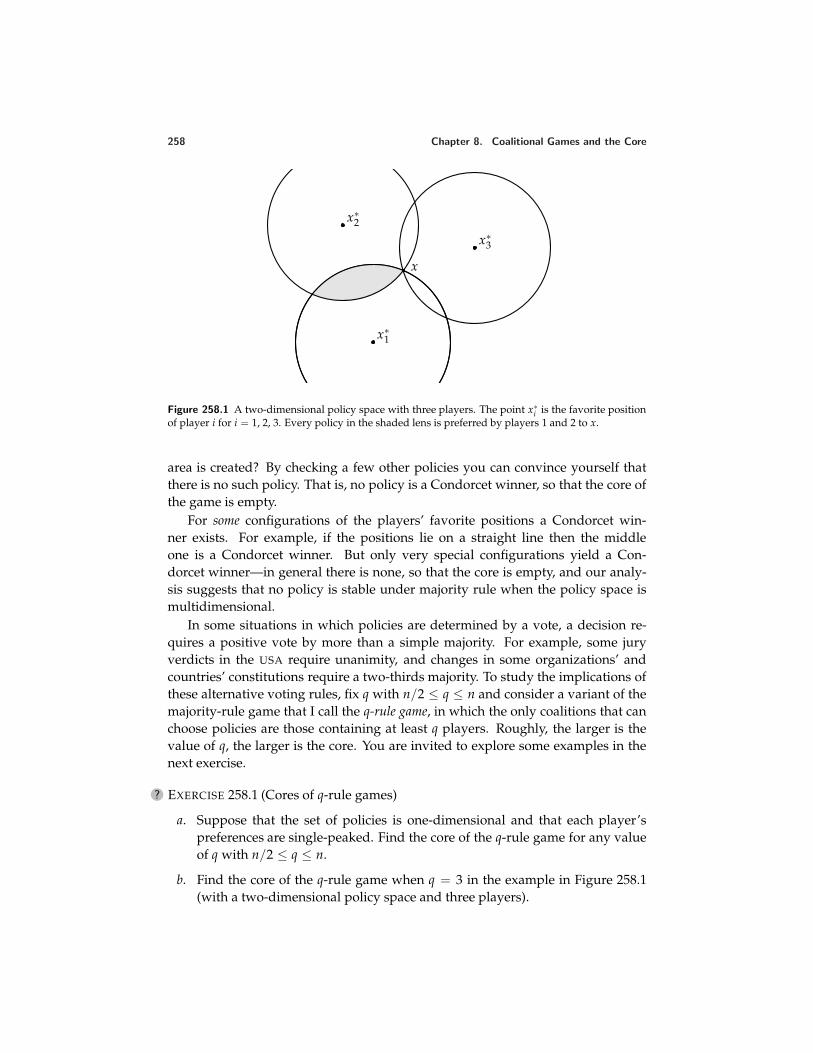
258 Chapter 8. Coalitional Games and the Core
x∗1
x∗2
x∗3
x
Figure 258.1 A two-dimensional policy space with three players. The point x∗i is the favorite position
of player i for i = 1, 2, 3. Every policy in the shaded lens is preferred by players 1 and 2 to x.
area is created? By checking a few other policies you can convince yourself thatthere is no such policy. That is, no policy is a Condorcet winner, so that the core ofthe game is empty.
For some configurations of the players’ favorite positions a Condorcet win-ner exists. For example, if the positions lie on a straight line then the middleone is a Condorcet winner. But only very special configurations yield a Con-dorcet winner—in general there is none, so that the core is empty, and our analy-sis suggests that no policy is stable under majority rule when the policy space ismultidimensional.
In some situations in which policies are determined by a vote, a decision re-quires a positive vote by more than a simple majority. For example, some juryverdicts in the USA require unanimity, and changes in some organizations’ andcountries’ constitutions require a two-thirds majority. To study the implications ofthese alternative voting rules, fix q with n/2 ≤ q ≤ n and consider a variant of themajority-rule game that I call the q-rule game, in which the only coalitions that canchoose policies are those containing at least q players. Roughly, the larger is thevalue of q, the larger is the core. You are invited to explore some examples in thenext exercise.
? EXERCISE 258.1 (Cores of q-rule games)
a. Suppose that the set of policies is one-dimensional and that each player’spreferences are single-peaked. Find the core of the q-rule game for any valueof q with n/2 ≤ q ≤ n.
b. Find the core of the q-rule game when q = 3 in the example in Figure 258.1(with a two-dimensional policy space and three players).
8.7 Illustration: matching 259
8.7 Illustration: matching
Applicants must be matched with universities, workers with firms, and footballplayers with teams. Do stable matchings exist? If so, what are their properties,and which institutions generate them?
In this section I analyze a model of two-sided one-to-one matching: each partyon one side must be matched with exactly one party on the other side. Most of themain ideas that emerge apply also to many-to-one matching problems.
The model I analyze is sometimes referred to as one of “marriage”, though ofcourse it captures only one dimension of matrimony. Some of the language I use istaken from this interpretation of the model.
8.7.1 Model
I refer to the two sides as X’s and Y’s. Each X may be matched with at most oneY, and each Y may be matched with at most one X; staying single is an option foreach individual. A matching of any set of individuals thus splits the set into pairs,each consisting of an X and a Y, and single individuals. I denote the partner of anyplayer i under the matching µ by µ(i). If i and j are matched, we thus have µ(i) = jand µ(j) = i; if i is single then µ(i) = i. Each person cares only about her partner,not about anyone else’s partner. Assume that every person’s preferences are strict:no person is indifferent between any two partners. I refer to the set of partners thati prefers to the option of remaining single as the set of i’s acceptable partners. Thefollowing coalitional game, which I refer to as a two-sided one-to-one matchinggame, models this situation.
Players The set of all X’s and all Y’s.
Actions The set of actions of a coalition S is the set of all matchings of themembers of S.
Preferences Each player prefers one outcome to another according to the part-ner she is assigned.
An example of possible preferences is given in Figure 260.1. For instance,player x1 ranks y2 first, then y1, and finds y3 unacceptable.
8.7.2 The core and the deferred acceptance procedure
A matching in the core of a two-sided one-to-one matching game has the propertythat no group of players may, by rearranging themselves, produce a matching thatthey all like better. I claim that when looking for matchings in the core, we mayrestrict attention to coalitions consisting either of a single individual or of one Xand one Y. Precisely, a matching is in the core if and only if
a. each player prefers her partner to being single
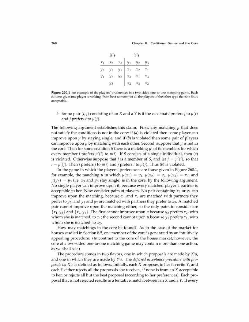
260 Chapter 8. Coalitional Games and the Core
X’s Y’s
x1 x2 x3 y1 y2 y3
y2 y1 y1 x1 x2 x1
y1 y2 y2 x3 x1 x3
y3 x2 x3 x2
Figure 260.1 An example of the players’ preferences in a two-sided one-to-one matching game. Eachcolumn gives one player’s ranking (from best to worst) of all the players of the other type that she findsacceptable.
b. for no pair (i, j) consisting of an X and a Y is it the case that i prefers j to µ(i)and j prefers i to µ(j).
The following argument establishes this claim. First, any matching µ that doesnot satisfy the conditions is not in the core: if (a) is violated then some player canimprove upon µ by staying single, and if (b) is violated then some pair of playerscan improve upon µ by matching with each other. Second, suppose that µ is not inthe core. Then for some coalition S there is a matching µ′ of its members for whichevery member i prefers µ′(i) to µ(i). If S consists of a single individual, then (a)is violated. Otherwise suppose that i is a member of S, and let j = µ′(i), so thati = µ′(j). Then i prefers j to µ(i) and j prefers i to µ(j). Thus (b) is violated.
In the game in which the players’ preferences are those given in Figure 260.1,for example, the matching µ in which µ(x1) = y1, µ(x2) = y2, µ(x3) = x3, andµ(y3) = y3 (i.e. x3 and y3 stay single) is in the core, by the following argument.No single player can improve upon it, because every matched player’s partner isacceptable to her. Now consider pairs of players. No pair containing x3 or y3 canimprove upon the matching, because x1 and x2 are matched with partners theyprefer to y3, and y1 and y2 are matched with partners they prefer to x3. A matchedpair cannot improve upon the matching either, so the only pairs to consider arex1, y2 and x2, y1. The first cannot improve upon µ because y2 prefers x2, withwhom she is matched, to x1; the second cannot upon µ because y1 prefers x1, withwhom she is matched, to x2.
How may matchings in the core be found? As in the case of the market forhouses studied in Section 8.5, one member of the core is generated by an intuitivelyappealing procedure. (In contrast to the core of the house market, however, thecore of a two-sided one-to-one matching game may contain more than one action,as we shall see.)
The procedure comes in two flavors, one in which proposals are made by X’s,and one in which they are made by Y’s. The deferred acceptance procedure with pro-posals by X’s is defined as follows. Initially, each X proposes to her favorite Y, andeach Y either rejects all the proposals she receives, if none is from an X acceptableto her, or rejects all but the best proposal (according to her preferences). Each pro-posal that is not rejected results in a tentative match between an X and a Y. If every
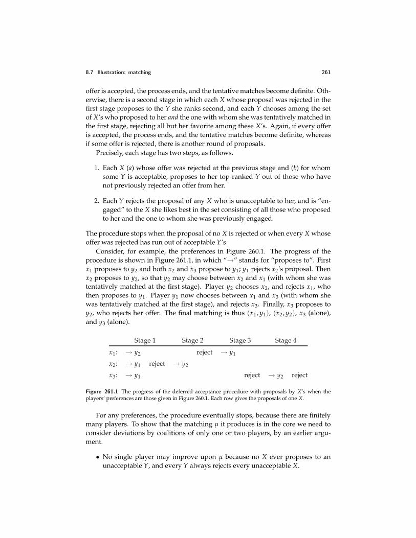
8.7 Illustration: matching 261
offer is accepted, the process ends, and the tentative matches become definite. Oth-erwise, there is a second stage in which each X whose proposal was rejected in thefirst stage proposes to the Y she ranks second, and each Y chooses among the setof X’s who proposed to her and the one with whom she was tentatively matched inthe first stage, rejecting all but her favorite among these X’s. Again, if every offeris accepted, the process ends, and the tentative matches become definite, whereasif some offer is rejected, there is another round of proposals.
Precisely, each stage has two steps, as follows.
1. Each X (a) whose offer was rejected at the previous stage and (b) for whomsome Y is acceptable, proposes to her top-ranked Y out of those who havenot previously rejected an offer from her.
2. Each Y rejects the proposal of any X who is unacceptable to her, and is “en-gaged” to the X she likes best in the set consisting of all those who proposedto her and the one to whom she was previously engaged.
The procedure stops when the proposal of no X is rejected or when every X whoseoffer was rejected has run out of acceptable Y’s.
Consider, for example, the preferences in Figure 260.1. The progress of theprocedure is shown in Figure 261.1, in which “→” stands for “proposes to”. Firstx1 proposes to y2 and both x2 and x3 propose to y1; y1 rejects x2’s proposal. Thenx2 proposes to y2, so that y2 may choose between x2 and x1 (with whom she wastentatively matched at the first stage). Player y2 chooses x2, and rejects x1, whothen proposes to y1. Player y1 now chooses between x1 and x3 (with whom shewas tentatively matched at the first stage), and rejects x3. Finally, x3 proposes toy2, who rejects her offer. The final matching is thus (x1, y1), (x2, y2), x3 (alone),and y3 (alone).
Stage 1 Stage 2 Stage 3 Stage 4
x1: → y2 reject → y1
x2: → y1 reject → y2
x3: → y1 reject → y2 reject
Figure 261.1 The progress of the deferred acceptance procedure with proposals by X’s when theplayers’ preferences are those given in Figure 260.1. Each row gives the proposals of one X.
For any preferences, the procedure eventually stops, because there are finitelymany players. To show that the matching µ it produces is in the core we need toconsider deviations by coalitions of only one or two players, by an earlier argu-ment.
• No single player may improve upon µ because no X ever proposes to anunacceptable Y, and every Y always rejects every unacceptable X.
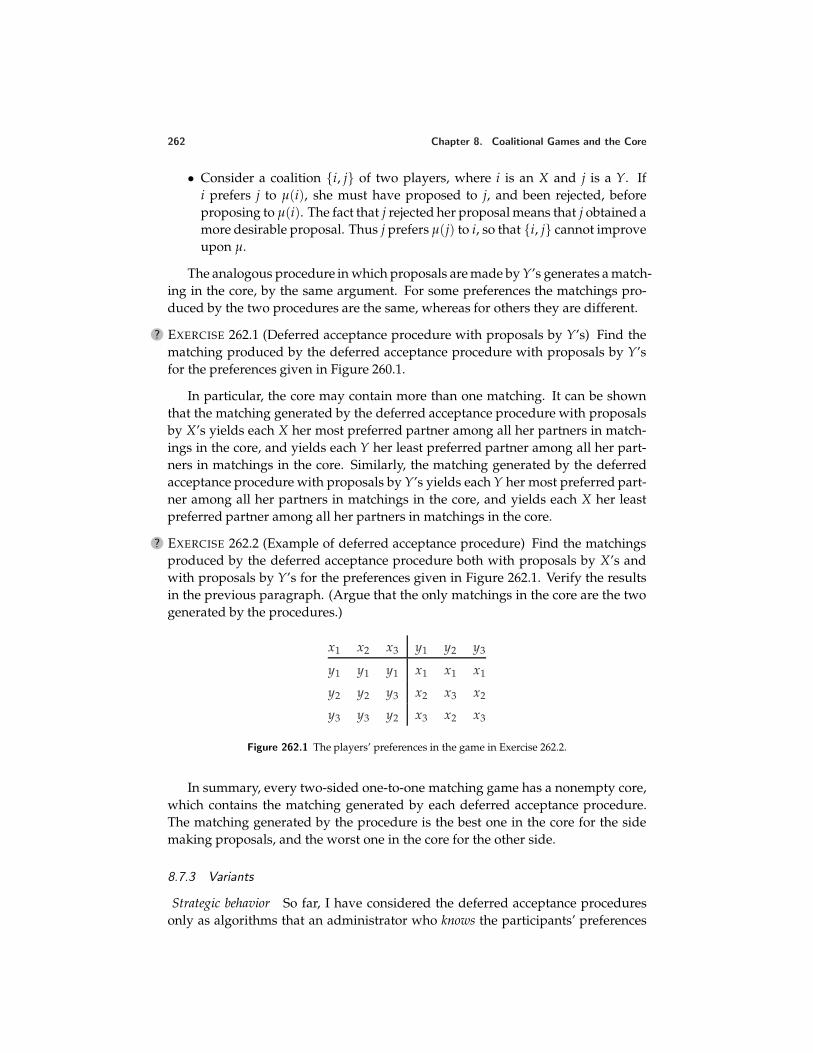
262 Chapter 8. Coalitional Games and the Core
• Consider a coalition i, j of two players, where i is an X and j is a Y. Ifi prefers j to µ(i), she must have proposed to j, and been rejected, beforeproposing to µ(i). The fact that j rejected her proposal means that j obtained amore desirable proposal. Thus j prefers µ(j) to i, so that i, j cannot improveupon µ.
The analogous procedure in which proposals are made by Y’s generates a match-ing in the core, by the same argument. For some preferences the matchings pro-duced by the two procedures are the same, whereas for others they are different.
? EXERCISE 262.1 (Deferred acceptance procedure with proposals by Y’s) Find thematching produced by the deferred acceptance procedure with proposals by Y’sfor the preferences given in Figure 260.1.
In particular, the core may contain more than one matching. It can be shownthat the matching generated by the deferred acceptance procedure with proposalsby X’s yields each X her most preferred partner among all her partners in match-ings in the core, and yields each Y her least preferred partner among all her part-ners in matchings in the core. Similarly, the matching generated by the deferredacceptance procedure with proposals by Y’s yields each Y her most preferred part-ner among all her partners in matchings in the core, and yields each X her leastpreferred partner among all her partners in matchings in the core.
? EXERCISE 262.2 (Example of deferred acceptance procedure) Find the matchingsproduced by the deferred acceptance procedure both with proposals by X’s andwith proposals by Y’s for the preferences given in Figure 262.1. Verify the resultsin the previous paragraph. (Argue that the only matchings in the core are the twogenerated by the procedures.)
x1 x2 x3 y1 y2 y3
y1 y1 y1 x1 x1 x1
y2 y2 y3 x2 x3 x2
y3 y3 y2 x3 x2 x3
Figure 262.1 The players’ preferences in the game in Exercise 262.2.
In summary, every two-sided one-to-one matching game has a nonempty core,which contains the matching generated by each deferred acceptance procedure.The matching generated by the procedure is the best one in the core for the sidemaking proposals, and the worst one in the core for the other side.
8.7.3 Variants
Strategic behavior So far, I have considered the deferred acceptance proceduresonly as algorithms that an administrator who knows the participants’ preferences
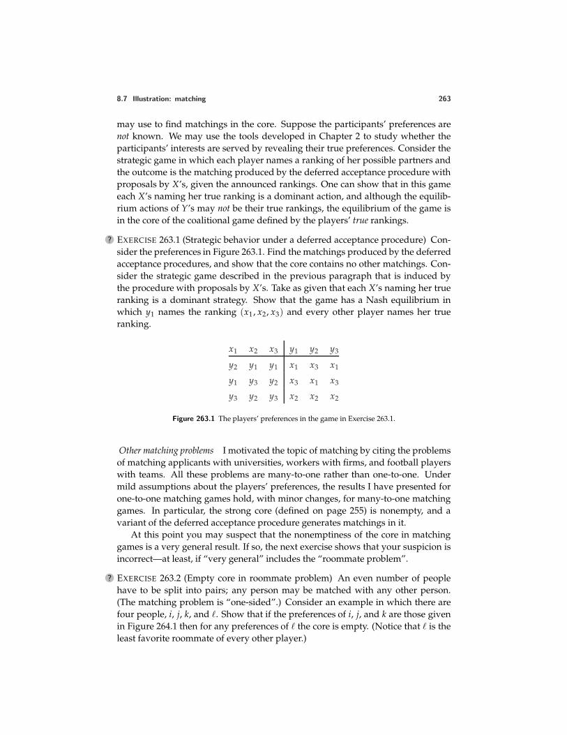
8.7 Illustration: matching 263
may use to find matchings in the core. Suppose the participants’ preferences arenot known. We may use the tools developed in Chapter 2 to study whether theparticipants’ interests are served by revealing their true preferences. Consider thestrategic game in which each player names a ranking of her possible partners andthe outcome is the matching produced by the deferred acceptance procedure withproposals by X’s, given the announced rankings. One can show that in this gameeach X’s naming her true ranking is a dominant action, and although the equilib-rium actions of Y’s may not be their true rankings, the equilibrium of the game isin the core of the coalitional game defined by the players’ true rankings.
? EXERCISE 263.1 (Strategic behavior under a deferred acceptance procedure) Con-sider the preferences in Figure 263.1. Find the matchings produced by the deferredacceptance procedures, and show that the core contains no other matchings. Con-sider the strategic game described in the previous paragraph that is induced bythe procedure with proposals by X’s. Take as given that each X’s naming her trueranking is a dominant strategy. Show that the game has a Nash equilibrium inwhich y1 names the ranking (x1, x2, x3) and every other player names her trueranking.
x1 x2 x3 y1 y2 y3
y2 y1 y1 x1 x3 x1
y1 y3 y2 x3 x1 x3
y3 y2 y3 x2 x2 x2
Figure 263.1 The players’ preferences in the game in Exercise 263.1.
Other matching problems I motivated the topic of matching by citing the problemsof matching applicants with universities, workers with firms, and football playerswith teams. All these problems are many-to-one rather than one-to-one. Undermild assumptions about the players’ preferences, the results I have presented forone-to-one matching games hold, with minor changes, for many-to-one matchinggames. In particular, the strong core (defined on page 255) is nonempty, and avariant of the deferred acceptance procedure generates matchings in it.
At this point you may suspect that the nonemptiness of the core in matchinggames is a very general result. If so, the next exercise shows that your suspicion isincorrect—at least, if “very general” includes the “roommate problem”.
? EXERCISE 263.2 (Empty core in roommate problem) An even number of peoplehave to be split into pairs; any person may be matched with any other person.(The matching problem is “one-sided”.) Consider an example in which there arefour people, i, j, k, and . Show that if the preferences of i, j, and k are those givenin Figure 264.1 then for any preferences of the core is empty. (Notice that is theleast favorite roommate of every other player.)
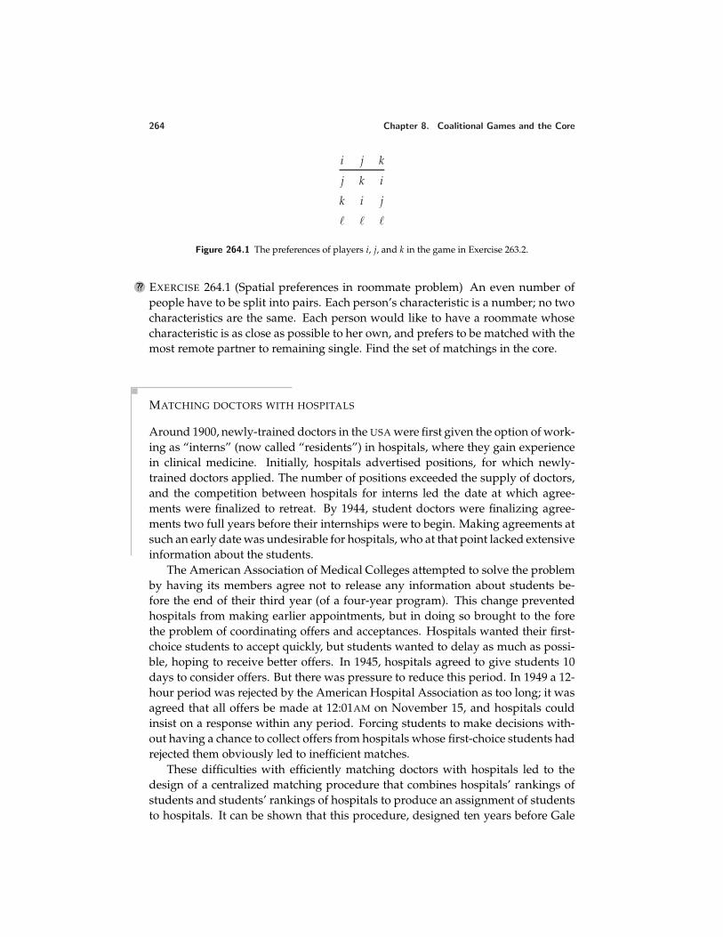
264 Chapter 8. Coalitional Games and the Core
i j k
j k i
k i j
Figure 264.1 The preferences of players i, j, and k in the game in Exercise 263.2.
?? EXERCISE 264.1 (Spatial preferences in roommate problem) An even number ofpeople have to be split into pairs. Each person’s characteristic is a number; no twocharacteristics are the same. Each person would like to have a roommate whosecharacteristic is as close as possible to her own, and prefers to be matched with themost remote partner to remaining single. Find the set of matchings in the core.
MATCHING DOCTORS WITH HOSPITALS
Around 1900, newly-trained doctors in the USA were first given the option of work-ing as “interns” (now called “residents”) in hospitals, where they gain experiencein clinical medicine. Initially, hospitals advertised positions, for which newly-trained doctors applied. The number of positions exceeded the supply of doctors,and the competition between hospitals for interns led the date at which agree-ments were finalized to retreat. By 1944, student doctors were finalizing agree-ments two full years before their internships were to begin. Making agreements atsuch an early date was undesirable for hospitals, who at that point lacked extensiveinformation about the students.
The American Association of Medical Colleges attempted to solve the problemby having its members agree not to release any information about students be-fore the end of their third year (of a four-year program). This change preventedhospitals from making earlier appointments, but in doing so brought to the forethe problem of coordinating offers and acceptances. Hospitals wanted their first-choice students to accept quickly, but students wanted to delay as much as possi-ble, hoping to receive better offers. In 1945, hospitals agreed to give students 10days to consider offers. But there was pressure to reduce this period. In 1949 a 12-hour period was rejected by the American Hospital Association as too long; it wasagreed that all offers be made at 12:01AM on November 15, and hospitals couldinsist on a response within any period. Forcing students to make decisions with-out having a chance to collect offers from hospitals whose first-choice students hadrejected them obviously led to inefficient matches.
These difficulties with efficiently matching doctors with hospitals led to thedesign of a centralized matching procedure that combines hospitals’ rankings ofstudents and students’ rankings of hospitals to produce an assignment of studentsto hospitals. It can be shown that this procedure, designed ten years before Gale
8.8 Discussion: other solution concepts 265
and Shapley’s work on the deferred acceptance procedure, generates a matchingin the core for any stated preferences! It differs from the natural generalizationof Gale and Shapley’s deferred acceptance procedure to a many-to-one matchingproblem, but generates precisely the same matching, namely the one in the corethat is best for the hospitals. (Gale and Shapley, and the designers of the student–hospital matching procedure were not aware of each other’s work until the mid-1970s, when a physician heard Gale speak on his work.)
In the early years of operation of the procedure, over 95% of students and hos-pitals participated. In the mid-1970s the participation rate fell to around 85%.Many nonparticipants were married couples both members of which wished toobtain positions in the same city. The matching procedure contained a mechanismfor dealing with married couples, but, unlike the mechanism for single students, itcould lead to a matching upon which some couple could improve. The difficulty isserious: when couples exist who restrict themselves to accept positions in the samecity, for some preferences the core of the resulting game is empty—no matching isstable.
Further problems arose. In the 1990s, associations of medical students beganto argue that changes were needed because the procedure was favorable to hos-pitals, and possibilities for strategic behavior on the part of students existed. Thegame theorist Alvin E. Roth was retained by the “National Resident Matching Pro-gram” to design a new procedure to generate stable matchings that are as favor-able as possible to applicants. The new procedure was first used in 1998; it matchesaround 20,000 new doctors with hospitals each year.
8.8 Discussion: other solution concepts
In replacing the requirement of a Nash equilibrium that no individual player mayprofitably deviate with the requirement that no group of players may profitablydeviate, the notion of the core makes an assumption that is unnecessary wheninterpreting a Nash equilibrium. A single player who deviates from an actionprofile in a strategic game can be sure of her deviant action, because she unilaterallychooses it. But a member of a group of players that chooses a deviant action mustassume that no subgroup of her comrades will deviate further, or, at least, she willremain better off if they do.
Consider, for example, the three-player majority game (Example 237.2 and Ex-ercise 241.1). The action ( 1
2 , 12 , 0) of the grand coalition in this game is not in the
core because, for example, the coalition consisting of players 1 and 3 can take anaction that gives player 1 an amount x with 1
2 < x < 1 and player 3 the amount1 − x, which leads to the payoff profile (x, 0, 1 − x). But this profile itself is notstable—the coalition consisting of players 2 and 3, for example, has an action thatgenerates the payoff profile (0, y, 1 − y), where 0 < y < x, in which both of themare better off than they are in (x, 0, 1 − x). The fact that player 3 will be tempted
266 Chapter 8. Coalitional Games and the Core
by an offer of player 2 to deviate from (x, 0, 1 − x) may dampen player 1’s en-thusiasm for joining player 3 in the deviation from ( 1
2 , 12 , 0). For similar reasons,
player 2 may be reluctant to join in a deviation from this action.Several solution concepts that take into account these considerations have been
suggested. None has so far had anything like the success of the core in illuminatingsocial and economic phenomena, however.
Notes
The notion of a coalitional game is due to von Neumann and Morgenstern (1944).Shapley and Shubik (1953), Luce and Raiffa (1957, 234–235), and Aumann andPeleg (1960) generalized von Numann and Morgenstern’s notion. The notion of thecore was introduced in the early 1950s by Gillies as a tool to study another solutionconcept (his work is published in Gillies 1959); Shapley and Shubik developed itas a solution concept.
Edgeworth (1881, 35–39) pointed out a connection between the competitiveequilibria of a market model and the set of outcomes we now call the core. von Neu-mann and Morgensten (1944, 583–584) first suggested modeling markets as coali-tional games; Shubik (1959a) recognized the game-theoretic content of Edgeworth’sarguments and, together with Shapley (1959), developed the analysis. Section 8.3is based on Shapley and Shubik (1967). The core of the market studied in Sec-tion 8.4 was first studied by Shapley and Shubik (1971/72). My discussion owes adebt to Moulin (1995, Section 2.3).
Voting behavior in committees was first studied formally by Black (1958) (writ-ten in the mid-1940s), Black and Newing (1951), and Arrow (1951). Black usedthe core as the solution (before it had been defined generally) and established themedian voter theorem (Exercise 257.1). He also noticed that in policy spaces of di-mension greater than 1 a Condorcet winner is not likely to exist, a result extendedby Plott (1967) and refined by Banks (1995) and others, who find conditions relat-ing the number of voters, the dimension of the policy space, and the value of qfor which the core of the q-rule game is generally empty; see Austen-Smith andBanks (1999, Secton 6.1) for details.
The model and result on the nonemptiness of the core in Section 8.5 are due toShapley and Scarf (1974), who credit David Gale with the top trading cycle pro-cedure. The result that the strong core contains a single action is due to Roth andPostlewaite (1977). The model is discussed in detail by Moulin (1995, Section 3.2).
The model and main results in Section 8.7 are due to Gale and Shapley (1962).The result about the strategic properties of the deferred acceptance proceduresat the end of the section is a combination of results due to Dubins and Freed-man (1981) and Roth (1982), and to Roth (1984a). Exercise 263.1 is based on anexample in Moulin (1995, 113 and 116). Exercise 263.2 is taken from Gale andShapley (1962, Example 3). For a comprehensive presentation of results on two-sided matching, see Roth and Sotomayor (1990). The box on page 264 is based
Notes 267
on Roth (1984b), Roth and Sotomayor (1990, Section 5.4), and Roth and Peran-son (1999).
Draft chapter from An introduction to game theory by Martin J. [email protected]; www.economics.utoronto.ca/osborneVersion: 00/11/6.Copyright c© 1995–2000 by Martin J. Osborne. All rights reserved. No part of this book may be re-produced by any electronic or mechanical means (including photocopying, recording, or informationstorage and retrieval) without permission in writing from Oxford University Press, except that onecopy of up to six chapters may be made by any individual for private study.
9 Bayesian Games
Motivational examples 271General definitions 276Two examples concerning information 281Illustration: Cournot’s duopoly game with imperfect information 283Illustration: providing a public good 287Illustration: auctions 290Illustration: juries 299Appendix: Analysis of auctions for an arbitrary distribution of valuations 306Prerequisite: Chapter 2 and Section 4.1.3; Section 9.8 requires Chapter 4.
9.1 Introduction
AN ASSUMPTION underlying the notion of Nash equilibrium is that each playerholds the correct belief about the other players’ actions. To do so, a player
must know the game she is playing; in particular, she must know the other players’preferences. In many situations the participants are not perfectly informed abouttheir opponents’ characteristics: bargainers may not know each others’ valuationsof the object of negotiation, firms may not know each others’ cost functions, com-batants may not know each others’ strengths, and jurors may not know their col-leagues’ interpretations of the evidence in a trial. In some situations, a participantmay be well informed about her opponents’ characteristics, but may not know howwell these opponents are informed about her own characteristics. In this chapter Idescribe the model of a “Bayesian game”, which generalizes the notion of a strate-gic game to allows us to analyze any situation in which each player is imperfectlyinformed about some aspect of her environment relevant to her choice of an action.
9.2 Motivational examples
I start with two examples that illustrate the main ideas in the model of a Bayesiangame. I define the notion of Nash equilibrium separately for each game. In thenext section I define the general model of a Bayesian game and the notion of Nashequilibrium for such a game.
EXAMPLE 271.1 (Variant of BoS with imperfect information) Consider a variant ofthe situation modeled by BoS (Figure 16.1) in which player 1 is unsure whether
271
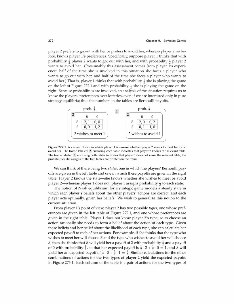
272 Chapter 9. Bayesian Games
player 2 prefers to go out with her or prefers to avoid her, whereas player 2, as be-fore, knows player 1’s preferences. Specifically, suppose player 1 thinks that withprobability 1
2 player 2 wants to got out with her, and with probability 12 player 2
wants to avoid her. (Presumably this assessment comes from player 1’s experi-ence: half of the time she is involved in this situation she faces a player whowants to go out with her, and half of the time she faces a player who wants toavoid her.) That is, player 1 thinks that with probability 1
2 she is playing the gameon the left of Figure 272.1 and with probability 1
2 she is playing the game on theright. Because probabilities are involved, an analysis of the situation requires us toknow the players’ preferences over lotteries, even if we are interested only in purestrategy equilibria; thus the numbers in the tables are Bernoulli payoffs.
B SB 2, 1 0, 0S 0, 0 1, 2
2 wishes to meet 1
B SB 2, 0 0, 2S 0, 1 1, 0
2 wishes to avoid 1
1prob. 1
2 prob. 12
2 2
Figure 272.1 A variant of BoS in which player 1 is unsure whether player 2 wants to meet her or toavoid her. The frame labeled 2 enclosing each table indicates that player 2 knows the relevant table.The frame labeled 1 enclosing both tables indicates that player 1 does not know the relevant table; theprobabilities she assigns to the two tables are printed on the frame.
We can think of there being two states, one in which the players’ Bernoulli pay-offs are given in the left table and one in which these payoffs are given in the righttable. Player 2 knows the state—she knows whether she wishes to meet or avoidplayer 2—whereas player 1 does not; player 1 assigns probability 1
2 to each state.The notion of Nash equilibrium for a strategic game models a steady state in
which each player’s beliefs about the other players’ actions are correct, and eachplayer acts optimally, given her beliefs. We wish to generalize this notion to thecurrent situation.
From player 1’s point of view, player 2 has two possible types, one whose pref-erences are given in the left table of Figure 272.1, and one whose preferences aregiven in the right table. Player 1 does not know player 2’s type, so to choose anaction rationally she needs to form a belief about the action of each type. Giventhese beliefs and her belief about the likelihood of each type, she can calculate herexpected payoff to each of her actions. For example, if she thinks that the type whowishes to meet her will choose B and the type who wishes to avoid her will chooseS, then she thinks that B will yield her a payoff of 2 with probability 1
2 and a payoffof 0 with probability 1
2 , so that her expected payoff is 12 · 2 + 1
2 · 0 = 1, and S willyield her an expected payoff of 1
2 · 0 + 12 · 1 = 1
2 . Similar calculations for the othercombinations of actions for the two types of player 2 yield the expected payoffsin Figure 273.1. Each column of the table is a pair of actions for the two types of
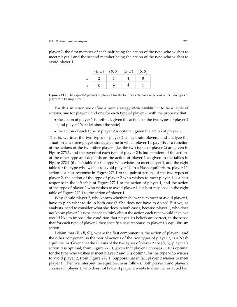
9.2 Motivational examples 273
player 2, the first member of each pair being the action of the type who wishes tomeet player 1 and the second member being the action of the type who wishes toavoid player 1.
(B, B) (B, S) (S, B) (S, S)
B 2 1 1 0
S 0 12
12 1
Figure 273.1 The expected payoffs of player 1 for the four possible pairs of actions of the two types ofplayer 2 in Example 271.1.
For this situation we define a pure strategy Nash equilibrium to be a triple ofactions, one for player 1 and one for each type of player 2, with the property that
• the action of player 1 is optimal, given the actions of the two types of player 2(and player 1’s belief about the state)
• the action of each type of player 2 is optimal, given the action of player 1.
That is, we treat the two types of player 2 as separate players, and analyze thesituation as a three-player strategic game in which player 1’s payoffs as a functionof the actions of the two other players (i.e. the two types of player 2) are given inFigure 273.1, and the payoff of each type of player 2 is independent of the actionsof the other type and depends on the action of player 1 as given in the tables inFigure 272.1 (the left table for the type who wishes to meet player 1, and the righttable for the type who wishes to avoid player 1). In a Nash equilibrium, player 1’saction is a best response in Figure 273.1 to the pair of actions of the two types ofplayer 2, the action of the type of player 2 who wishes to meet player 1 is a bestresponse in the left table of Figure 272.1 to the action of player 1, and the actionof the type of player 2 who wishes to avoid player 1 is a best response in the righttable of Figure 272.1 to the action of player 1.
Why should player 2, who knows whether she wants to meet or avoid player 1,have to plan what to do in both cases? She does not have to do so! But we, asanalysts, need to consider what she does in both cases, because player 1, who doesnot know player 2’s type, needs to think about the action each type would take; wewould like to impose the condition that player 1’s beliefs are correct, in the sensethat for each type of player 2 they specify a best response to player 1’s equilibriumaction.
I claim that (B, (B, S)), where the first component is the action of player 1 andthe other component is the pair of actions of the two types of player 2, is a Nashequilibrium. Given that the actions of the two types of player 2 are (B, S), player 1’saction B is optimal, from Figure 273.1; given that player 1 chooses B, B is optimalfor the type who wishes to meet player 2 and S is optimal for the type who wishesto avoid player 2, from Figure 272.1. Suppose that in fact player 2 wishes to meetplayer 1. Then we interpret the equilibrium as follows. Both player 1 and player 2chooses B; player 1, who does not know if player 2 wants to meet her or avoid her,
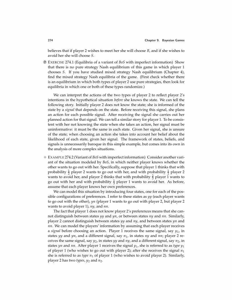
274 Chapter 9. Bayesian Games
believes that if player 2 wishes to meet her she will choose B, and if she wishes toavoid her she will choose S.
? EXERCISE 274.1 (Equilibria of a variant of BoS with imperfect information) Showthat there is no pure strategy Nash equilibrium of this game in which player 1chooses S. If you have studied mixed strategy Nash equilibrium (Chapter 4),find the mixed strategy Nash equilibria of the game. (First check whether thereis an equilibrium in which both types of player 2 use pure strategies, then look forequilibria in which one or both of these types randomize.)
We can interpret the actions of the two types of player 2 to reflect player 2’sintentions in the hypothetical situation before she knows the state. We can tell thefollowing story. Initially player 2 does not know the state; she is informed of thestate by a signal that depends on the state. Before receiving this signal, she plansan action for each possible signal. After receiving the signal she carries out herplanned action for that signal. We can tell a similar story for player 1. To be consis-tent with her not knowing the state when she takes an action, her signal must beuninformative: it must be the same in each state. Given her signal, she is unsureof the state; when choosing an action she takes into account her belief about thelikelihood of each state, given her signal. The framework of states, beliefs, andsignals is unnecessarily baroque in this simple example, but comes into its own inthe analysis of more complex situations.
EXAMPLE 274.2 (Variant of BoS with imperfect information) Consider another vari-ant of the situation modeled by BoS, in which neither player knows whether theother wants to go out with her. Specifically, suppose that player 1 thinks that withprobability 1
2 player 2 wants to go out with her, and with probability 12 player 2
wants to avoid her, and player 2 thinks that with probability 23 player 1 wants to
go out with her and with probability 13 player 1 wants to avoid her. As before,
assume that each player knows her own preferences.We can model this situation by introducing four states, one for each of the pos-
sible configurations of preferences. I refer to these states as yy (each player wantsto go out with the other), yn (player 1 wants to go out with player 2, but player 2wants to avoid player 1), ny, and nn.
The fact that player 1 does not know player 2’s preferences means that she can-not distinguish between states yy and yn, or between states ny and nn. Similarly,player 2 cannot distinguish between states yy and ny, and between states yn andnn. We can model the players’ information by assuming that each player receivesa signal before choosing an action. Player 1 receives the same signal, say y1, instates yy and yn, and a different signal, say n1, in states ny and nn; player 2 re-ceives the same signal, say y2, in states yy and ny, and a different signal, say n2, instates yn and nn. After player 1 receives the signal y1, she is referred to as type y1of player 1 (who wishes to go out with player 2); after she receives the signal n1she is referred to as type n1 of player 1 (who wishes to avoid player 2). Similarly,player 2 has two types, y2 and n2.
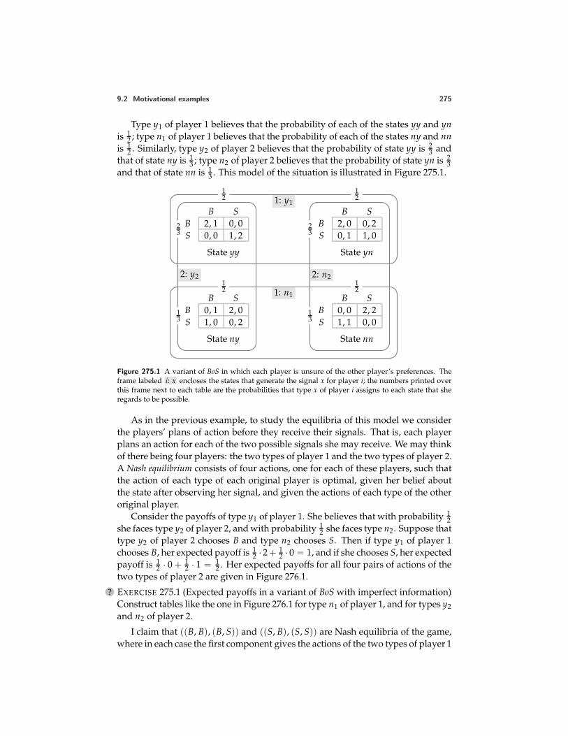
9.2 Motivational examples 275
Type y1 of player 1 believes that the probability of each of the states yy and ynis 1
2 ; type n1 of player 1 believes that the probability of each of the states ny and nnis 1
2 . Similarly, type y2 of player 2 believes that the probability of state yy is 23 and
that of state ny is 13 ; type n2 of player 2 believes that the probability of state yn is 2
3and that of state nn is 1
3 . This model of the situation is illustrated in Figure 275.1.
B SB 2, 1 0, 0S 0, 0 1, 2
State yy
B SB 2, 0 0, 2S 0, 1 1, 0
State yn
B SB 0, 1 2, 0S 1, 0 0, 2
State ny
B SB 0, 0 2, 2S 1, 1 0, 0
State nn
1: n1
1: y1
2: y2 2: n212
12
12
12
13
23
13
23
Figure 275.1 A variant of BoS in which each player is unsure of the other player’s preferences. Theframe labeled i: x encloses the states that generate the signal x for player i; the numbers printed overthis frame next to each table are the probabilities that type x of player i assigns to each state that sheregards to be possible.
As in the previous example, to study the equilibria of this model we considerthe players’ plans of action before they receive their signals. That is, each playerplans an action for each of the two possible signals she may receive. We may thinkof there being four players: the two types of player 1 and the two types of player 2.A Nash equilibrium consists of four actions, one for each of these players, such thatthe action of each type of each original player is optimal, given her belief aboutthe state after observing her signal, and given the actions of each type of the otheroriginal player.
Consider the payoffs of type y1 of player 1. She believes that with probability 12
she faces type y2 of player 2, and with probability 12 she faces type n2. Suppose that
type y2 of player 2 chooses B and type n2 chooses S. Then if type y1 of player 1chooses B, her expected payoff is 1
2 · 2 + 12 · 0 = 1, and if she chooses S, her expected
payoff is 12 · 0 + 1
2 · 1 = 12 . Her expected payoffs for all four pairs of actions of the
two types of player 2 are given in Figure 276.1.
? EXERCISE 275.1 (Expected payoffs in a variant of BoS with imperfect information)Construct tables like the one in Figure 276.1 for type n1 of player 1, and for types y2and n2 of player 2.
I claim that ((B, B), (B, S)) and ((S, B), (S, S)) are Nash equilibria of the game,where in each case the first component gives the actions of the two types of player 1
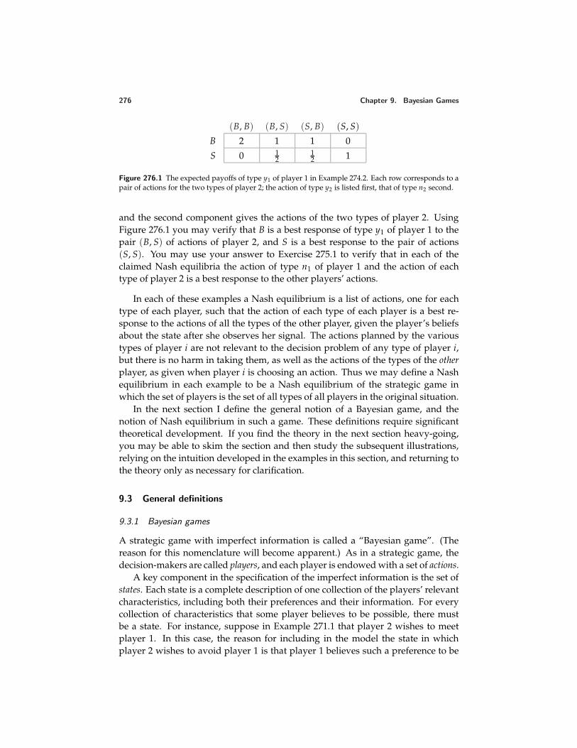
276 Chapter 9. Bayesian Games
(B, B) (B, S) (S, B) (S, S)
B 2 1 1 0
S 0 12
12 1
Figure 276.1 The expected payoffs of type y1 of player 1 in Example 274.2. Each row corresponds to apair of actions for the two types of player 2; the action of type y2 is listed first, that of type n2 second.
and the second component gives the actions of the two types of player 2. UsingFigure 276.1 you may verify that B is a best response of type y1 of player 1 to thepair (B, S) of actions of player 2, and S is a best response to the pair of actions(S, S). You may use your answer to Exercise 275.1 to verify that in each of theclaimed Nash equilibria the action of type n1 of player 1 and the action of eachtype of player 2 is a best response to the other players’ actions.
In each of these examples a Nash equilibrium is a list of actions, one for eachtype of each player, such that the action of each type of each player is a best re-sponse to the actions of all the types of the other player, given the player’s beliefsabout the state after she observes her signal. The actions planned by the varioustypes of player i are not relevant to the decision problem of any type of player i,but there is no harm in taking them, as well as the actions of the types of the otherplayer, as given when player i is choosing an action. Thus we may define a Nashequilibrium in each example to be a Nash equilibrium of the strategic game inwhich the set of players is the set of all types of all players in the original situation.
In the next section I define the general notion of a Bayesian game, and thenotion of Nash equilibrium in such a game. These definitions require significanttheoretical development. If you find the theory in the next section heavy-going,you may be able to skim the section and then study the subsequent illustrations,relying on the intuition developed in the examples in this section, and returning tothe theory only as necessary for clarification.
9.3 General definitions
9.3.1 Bayesian games
A strategic game with imperfect information is called a “Bayesian game”. (Thereason for this nomenclature will become apparent.) As in a strategic game, thedecision-makers are called players, and each player is endowed with a set of actions.
A key component in the specification of the imperfect information is the set ofstates. Each state is a complete description of one collection of the players’ relevantcharacteristics, including both their preferences and their information. For everycollection of characteristics that some player believes to be possible, there mustbe a state. For instance, suppose in Example 271.1 that player 2 wishes to meetplayer 1. In this case, the reason for including in the model the state in whichplayer 2 wishes to avoid player 1 is that player 1 believes such a preference to be
9.3 General definitions 277
possible.At the start of the game a state is realized. The players do not observe this state.
Rather, each player receives a signal that may give her some information about thestate. Denote the signal player i receives in state ω by τi(ω). The function τi iscalled player i’s signal function. (Note that the signal is a deterministic function ofthe state: for each state a definite signal is received.) The states that generate anygiven signal ti are said to be consistent with ti. The sizes of the sets of states con-sistent with each of player i’s signals reflect the quality of player i’s information.If, for example, τi(ω) is different for each value of ω, then player i knows, givenher signal, the state that has occurred; after receiving her signal, she is perfectlyinformed about all the players’ relevant characteristics. At the other extreme, ifτi(ω) is the same for all states, then player i’s signal conveys no information aboutthe state. If τi(ω) is constant over some subsets of the set of states, but is not thesame for all states, then player i’s signal conveys partial information. For example,if there are three states, ω1, ω2, and ω3, and τi(ω1) = τi(ω2) = τi(ω3), then whenthe state is ω1 player i knows that it is ω1, whereas when it is either ω2 or ω3 sheknows only that it is one of these two states.
We refer to player i in the event that she receives the signal ti as type ti ofplayer i. Each type of each player holds a belief about the likelihood of the statesconsistent with her signal. If, for example, ti = τi(ω1) = τi(ω2), then type tiof player i assigns probabilities to ω1 and ω2. (A player who receives a signalconsistent with only one state naturally assigns probability 1 to that state.)
Each player may care about the actions chosen by the other players, as in astrategic game with perfect information, and also about the state. The playersmay be uncertain about the state, so we need to specify their preferences regard-ing probability distributions over pairs (a, ω) consisting of an action profile a anda state ω. I assume that each player’s preferences over such probability distribu-tions are represented by the expected value of a Bernoulli payoff function. Thus Ispecify each player i’s preferences by giving a Bernoulli payoff function ui overpairs (a, ω). (Note that in both Example 271.1 and Example 274.2, both playerscare only about the other player’s action, not independently about the state.)
In summary, a Bayesian game is defined as follows.
DEFINITION 277.1 A Bayesian game consists of
• a set of players
• a set of states
and for each player
• a set of actions
• a set of signals that she may receive and a signal function that associates asignal with each state
278 Chapter 9. Bayesian Games
• for each signal that she may receive, a belief about the states consistent withthe signal (a probability distribution over the set of states with which thesignal is associated)
• a Bernoulli payoff function over pairs (a, ω), where a is an action profile andω is a state, the expected value of which represents the player’s preferencesamong lotteries over the set of such pairs.
The eponymous Thomas Bayes (1702–61) first showed how probabilities shouldbe changed in the light of new information. His formula (discussed in Section 17.7.5)is needed when working with a variant of Definition 277.1 in which each player isendowed with a “prior” belief about the states, from which the belief of each of hertypes is derived. For the purposes of this chapter, the belief of each type of eachplayer is more conveniently taken as a primitive, rather than being derived from aprior belief.
The game in Example 271.1 fits into this general definition as follows.
Players The pair of people.
States The set of states is meet, avoid.
Actions The set of actions of each player is B, S.
Signals Player 1 may receive a single signal, say z; her signal function τ1 satis-fies τ1(meet) = τ1(avoid) = z. Player 2 receives one of two signals, say m andv; her signal function τ2 satisfies τ2(meet) = m and τ2(avoid) = v.
Beliefs Player 1 assigns probability 12 to each state after receiving the signal z.
Player 2 assigns probability 1 to the state meet after receiving the signal m,and probability 1 to the state avoid after receiving the signal v.
Payoffs The payoffs ui(a, meet) of each player i for all possible action pairs aregiven in the left panel of Figure 272.1, and the payoffs ui(a, avoid) are givenin the right panel.
Similarly, the game in Example 274.2 fits into the definition as follows.
Players The pair of people.
States The set of states is yy, yn, ny, nn.
Actions The set of actions of each player is B, S.
Signals Player 1 receives one of two signals, y1 and n1; her signal functionτ1 satisfies τ1(yy) = τ1(yn) = y1 and τ1(ny) = τ1(nn) = n1. Player 2 re-ceives one of two signals, y2 and n2; her signal function τ2 satisfies τ2(yy) =τ2(ny) = y2 and τ2(yn) = τ2(nn) = n2.
9.3 General definitions 279
Beliefs Player 1 assigns probability 12 to each of the states yy and yn after re-
ceiving the signal y1 and probability 12 to each of the states ny and nn after
receiving the signal n1. Player 2 assigns probability 23 to the state yy and
probability 13 to the state ny after receiving the signal y2, and probability 2
3 tothe state yn and probability 1
3 to the state nn after receiving the signal n2.
Payoffs The payoffs ui(a, ω) of each player i for all possible action pairs andstates are given in Figure 275.1.
9.3.2 Nash equilibrium
In a strategic game, each player chooses an action. In a Bayesian game, each playerchooses a collection of actions, one for each signal she may receive. That is, in aBayesian game each type of each player chooses an action. In a Nash equilibriumof such a game, the action chosen by each type of each player is optimal, given theactions chosen by every type of every other player. (In a steady state, each player’sexperience teaches her these actions.) Any given type of player i is not affected bythe actions chosen by the other types of player i, so there is no harm in thinkingthat player i takes as given these actions, as well as those of the other players. Thuswe may define a Nash equilibrium of a Bayesian game to be a Nash equilibriumof a strategic game in which each player is one type of one of the players in theBayesian game. What is each player’s payoff function in this strategic game?
Consider type ti of player i. For each state ω she knows every other player’stype (i.e. she knows the signal received by every other player). This information,together with her belief about the states, allows her to calculate her expected pay-off for each of her actions and each collection of actions for the various types of theother players. For instance, in Example 271.1, player 1’s belief is that the probabil-ity of each state is 1
2 , and she knows that player 2 is type m in the state meet andtype v in the state avoid. Thus if type m of player 2 chooses B and type v of player 2chooses S, player 1 thinks that if she chooses B then her expected payoff is
12 u1(B, B, meet) + 1
2 u1(B, S, avoid),
where u1 is her payoff function in the Bayesian game. (In general her payoff maydepend on the state, though in this example it does not.) The top box of the secondcolumn in Figure 273.1 gives this payoff; the other boxes give player 1’s payoffs forher other action and the other combinations of actions for the two types of player 2.
In a general game, denote the probability assigned by the belief of type ti ofplayer i to state ω by Pr(ω|ti). Denote the action taken by each type tj of eachplayer j by a(j, tj). Player j’s signal in state ω is τj(ω), so her action in state ω
is a(j, τj(ω)). For each state ω, denote by a(ω) the action profile in which eachplayer j chooses the action a(j, τj(ω)). Then the expected payoff of type ti ofplayer i when she chooses the action ai is
∑ω∈Ω
Pr(ω | ti)ui((ai , a−i(ω)), ω), (279.1)
280 Chapter 9. Bayesian Games
where Ω is the set of states and (ai, a−i(ω)) is the action profile in which player ichooses the action ai and every other player j chooses aj(ω). (Note that this ex-pected payoff does not depend on the actions of any other types of player i, butonly on the actions of the various types of the other players.)
We may now define precisely a Nash equilibrium of a Bayesian game.
DEFINITION 280.1 A Nash equilibrium of a Bayesian game is a Nash equilibriumof the strategic game (with vNM preferences) defined as follows.
Players The set of all pairs (i, ti) where i is a player in the Bayesian game and ti isone of the signals that i may receive.
Actions The set of actions of each player (i, ti) is the set of actions of player i inthe Bayesian game.
Preferences The Bernoulli payoff function of each player (i, ti) is given by (279.1).
? EXERCISE 280.2 (A fight with imperfect information about strengths) Two peopleare involved in a dispute. Person 1 does not know whether person 2 is strongor weak; she assigns probability α to person 2’s being strong. Person 2 is fullyinformed. Each person can either fight or yield. Each person’s preferences arerepresented by the expected value of a Bernoulli payoff function that assigns thepayoff of 0 if she yields (regardless of the other person’s action) and a payoff of1 if she fights and her opponent yields; if both people fight then their payoffs are(−1, 1) if person 2 is strong and (1, −1) if person 2 is weak. Formulate this situationas a Bayesian game and find its Nash equilibria if α < 1
2 and if α > 12 .
? EXERCISE 280.3 (An exchange game) Each of two individuals receives a ticket onwhich there is an integer from 1 to m indicating the size of a prize she may receive.The individuals’ tickets are assigned randomly and independently; the probabil-ity of an individual’s receiving each possible number is positive. Each individ-ual is given the option to exchange her prize for the other individual’s prize; theindividuals are given this option simultaneously. If both individuals wish to ex-change then the prizes are exchanged; otherwise each individual receives her ownprize. Each individual’s objective is to maximize her expected monetary payoff.Model this situation as a Bayesian game and show that in any Nash equilibrium thehighest prize that either individual is willing to exchange is the smallest possibleprize.
? EXERCISE 280.4 (Adverse selection) Firm A (the “acquirer”) is considering takingover firm T (the “target”). It does not know firm T’s value; it believes that thisvalue, when firm T is controlled by its own management, is at least $0 and at most$100, and assigns equal probability to each of the 101 dollar values in this range.Firm T will be worth 50% more under firm A’s management than it is under itsown management. Suppose that firm A bids y to take over firm T, and firm T isworth x (under its own management). Then if T accepts A’s offer, A’s payoff is32 x − y and T’s payoff is y; if T rejects A’s offer, A’s payoff is 0 and T’s payoff is
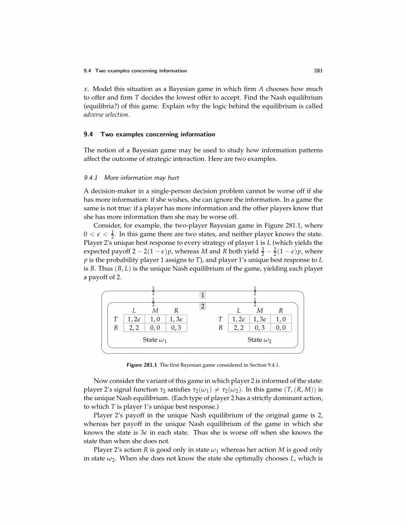
9.4 Two examples concerning information 281
x. Model this situation as a Bayesian game in which firm A chooses how muchto offer and firm T decides the lowest offer to accept. Find the Nash equilibrium(equilibria?) of this game. Explain why the logic behind the equilibrium is calledadverse selection.
9.4 Two examples concerning information
The notion of a Bayesian game may be used to study how information patternsaffect the outcome of strategic interaction. Here are two examples.
9.4.1 More information may hurt
A decision-maker in a single-person decision problem cannot be worse off if shehas more information: if she wishes, she can ignore the information. In a game thesame is not true: if a player has more information and the other players know thatshe has more information then she may be worse off.
Consider, for example, the two-player Bayesian game in Figure 281.1, where0 < ε < 1
2 . In this game there are two states, and neither player knows the state.Player 2’s unique best response to every strategy of player 1 is L (which yields theexpected payoff 2 − 2(1 − ε)p, whereas M and R both yield 3
2 − 32 (1 − ε)p, where
p is the probability player 1 assigns to T), and player 1’s unique best response to Lis B. Thus (B, L) is the unique Nash equilibrium of the game, yielding each playera payoff of 2.
L M RT 1, 2ε 1, 0 1, 3ε
B 2, 2 0, 0 0, 3
State ω1
L M RT 1, 2ε 1, 3ε 1, 0B 2, 2 0, 3 0, 0
State ω2
1
2
12
12
12
12
Figure 281.1 The first Bayesian game considered in Section 9.4.1.
Now consider the variant of this game in which player 2 is informed of the state:player 2’s signal function τ2 satisfies τ2(ω1) = τ2(ω2). In this game (T, (R, M)) isthe unique Nash equilibrium. (Each type of player 2 has a strictly dominant action,to which T is player 1’s unique best response.)
Player 2’s payoff in the unique Nash equilibrium of the original game is 2,whereas her payoff in the unique Nash equilibrium of the game in which sheknows the state is 3ε in each state. Thus she is worse off when she knows thestate than when she does not.
Player 2’s action R is good only in state ω1 whereas her action M is good onlyin state ω2. When she does not know the state she optimally chooses L, which is
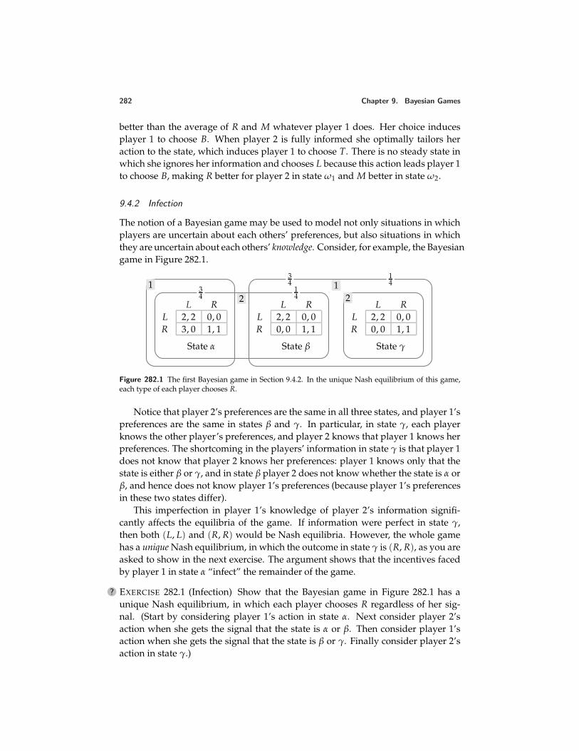
282 Chapter 9. Bayesian Games
better than the average of R and M whatever player 1 does. Her choice inducesplayer 1 to choose B. When player 2 is fully informed she optimally tailors heraction to the state, which induces player 1 to choose T. There is no steady state inwhich she ignores her information and chooses L because this action leads player 1to choose B, making R better for player 2 in state ω1 and M better in state ω2.
9.4.2 Infection
The notion of a Bayesian game may be used to model not only situations in whichplayers are uncertain about each others’ preferences, but also situations in whichthey are uncertain about each others’ knowledge. Consider, for example, the Bayesiangame in Figure 282.1.
L RL 2, 2 0, 0R 3, 0 1, 1
State α
L RL 2, 2 0, 0R 0, 0 1, 1
State β
L RL 2, 2 0, 0R 0, 0 1, 1
State γ
12
34
14
34
14
12
Figure 282.1 The first Bayesian game in Section 9.4.2. In the unique Nash equilibrium of this game,each type of each player chooses R.
Notice that player 2’s preferences are the same in all three states, and player 1’spreferences are the same in states β and γ. In particular, in state γ, each playerknows the other player’s preferences, and player 2 knows that player 1 knows herpreferences. The shortcoming in the players’ information in state γ is that player 1does not know that player 2 knows her preferences: player 1 knows only that thestate is either β or γ, and in state β player 2 does not know whether the state is α orβ, and hence does not know player 1’s preferences (because player 1’s preferencesin these two states differ).
This imperfection in player 1’s knowledge of player 2’s information signifi-cantly affects the equilibria of the game. If information were perfect in state γ,then both (L, L) and (R, R) would be Nash equilibria. However, the whole gamehas a unique Nash equilibrium, in which the outcome in state γ is (R, R), as you areasked to show in the next exercise. The argument shows that the incentives facedby player 1 in state α “infect” the remainder of the game.
? EXERCISE 282.1 (Infection) Show that the Bayesian game in Figure 282.1 has aunique Nash equilibrium, in which each player chooses R regardless of her sig-nal. (Start by considering player 1’s action in state α. Next consider player 2’saction when she gets the signal that the state is α or β. Then consider player 1’saction when she gets the signal that the state is β or γ. Finally consider player 2’saction in state γ.)
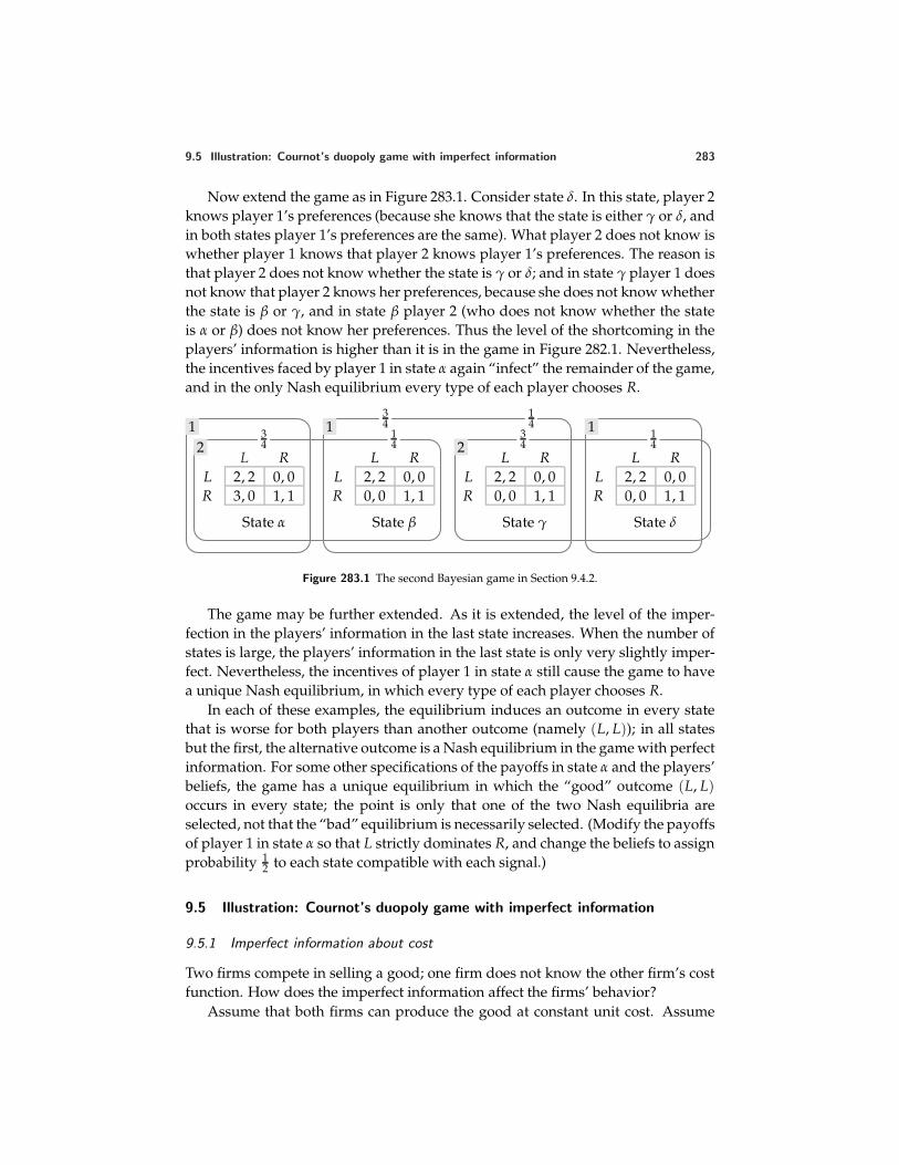
9.5 Illustration: Cournot’s duopoly game with imperfect information 283
Now extend the game as in Figure 283.1. Consider state δ. In this state, player 2knows player 1’s preferences (because she knows that the state is either γ or δ, andin both states player 1’s preferences are the same). What player 2 does not know iswhether player 1 knows that player 2 knows player 1’s preferences. The reason isthat player 2 does not know whether the state is γ or δ; and in state γ player 1 doesnot know that player 2 knows her preferences, because she does not know whetherthe state is β or γ, and in state β player 2 (who does not know whether the stateis α or β) does not know her preferences. Thus the level of the shortcoming in theplayers’ information is higher than it is in the game in Figure 282.1. Nevertheless,the incentives faced by player 1 in state α again “infect” the remainder of the game,and in the only Nash equilibrium every type of each player chooses R.
L RL 2, 2 0, 0R 3, 0 1, 1
State α
L RL 2, 2 0, 0R 0, 0 1, 1
State β
L RL 2, 2 0, 0R 0, 0 1, 1
State γ
L RL 2, 2 0, 0R 0, 0 1, 1
State δ
34
14
34
14
34
14
1 1 12 2
Figure 283.1 The second Bayesian game in Section 9.4.2.
The game may be further extended. As it is extended, the level of the imper-fection in the players’ information in the last state increases. When the number ofstates is large, the players’ information in the last state is only very slightly imper-fect. Nevertheless, the incentives of player 1 in state α still cause the game to havea unique Nash equilibrium, in which every type of each player chooses R.
In each of these examples, the equilibrium induces an outcome in every statethat is worse for both players than another outcome (namely (L, L)); in all statesbut the first, the alternative outcome is a Nash equilibrium in the game with perfectinformation. For some other specifications of the payoffs in state α and the players’beliefs, the game has a unique equilibrium in which the “good” outcome (L, L)occurs in every state; the point is only that one of the two Nash equilibria areselected, not that the “bad” equilibrium is necessarily selected. (Modify the payoffsof player 1 in state α so that L strictly dominates R, and change the beliefs to assignprobability 1
2 to each state compatible with each signal.)
9.5 Illustration: Cournot’s duopoly game with imperfect information
9.5.1 Imperfect information about cost
Two firms compete in selling a good; one firm does not know the other firm’s costfunction. How does the imperfect information affect the firms’ behavior?
Assume that both firms can produce the good at constant unit cost. Assume
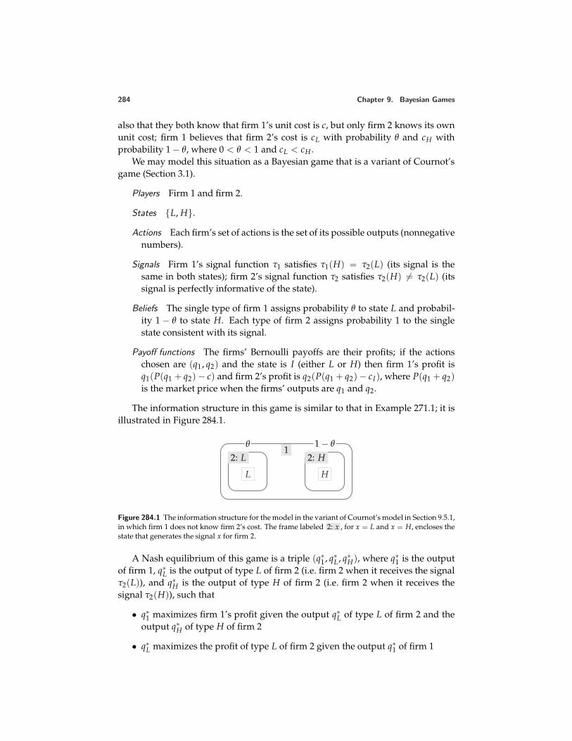
284 Chapter 9. Bayesian Games
also that they both know that firm 1’s unit cost is c, but only firm 2 knows its ownunit cost; firm 1 believes that firm 2’s cost is cL with probability θ and cH withprobability 1 − θ, where 0 < θ < 1 and cL < cH .
We may model this situation as a Bayesian game that is a variant of Cournot’sgame (Section 3.1).
Players Firm 1 and firm 2.
States L, H.
Actions Each firm’s set of actions is the set of its possible outputs (nonnegativenumbers).
Signals Firm 1’s signal function τ1 satisfies τ1(H) = τ2(L) (its signal is thesame in both states); firm 2’s signal function τ2 satisfies τ2(H) = τ2(L) (itssignal is perfectly informative of the state).
Beliefs The single type of firm 1 assigns probability θ to state L and probabil-ity 1 − θ to state H. Each type of firm 2 assigns probability 1 to the singlestate consistent with its signal.
Payoff functions The firms’ Bernoulli payoffs are their profits; if the actionschosen are (q1, q2) and the state is I (either L or H) then firm 1’s profit isq1(P(q1 + q2) − c) and firm 2’s profit is q2(P(q1 + q2) − cI), where P(q1 + q2)is the market price when the firms’ outputs are q1 and q2.
The information structure in this game is similar to that in Example 271.1; it isillustrated in Figure 284.1.
1θ 1 − θ
L H
2: L 2: H
Figure 284.1 The information structure for the model in the variant of Cournot’s model in Section 9.5.1,in which firm 1 does not know firm 2’s cost. The frame labeled 2: x , for x = L and x = H, encloses thestate that generates the signal x for firm 2.
A Nash equilibrium of this game is a triple (q∗1, q∗L, q∗H), where q∗1 is the outputof firm 1, q∗L is the output of type L of firm 2 (i.e. firm 2 when it receives the signalτ2(L)), and q∗H is the output of type H of firm 2 (i.e. firm 2 when it receives thesignal τ2(H)), such that
• q∗1 maximizes firm 1’s profit given the output q∗L of type L of firm 2 and theoutput q∗H of type H of firm 2
• q∗L maximizes the profit of type L of firm 2 given the output q∗1 of firm 1
9.5 Illustration: Cournot’s duopoly game with imperfect information 285
• q∗H maximizes the profit of type H of firm 2 given the output q∗1 of firm 1.
To find an equilibrium, we first find the firms’ best response functions. Givenfirm 1’s posterior beliefs, its best response b1(qL, qH) to (qL, qH) solves
maxq1
[θ(P(q1 + qL) − c)q1 + (1 − θ)(P(q1 + qH) − c)q1] .
Firm 2’s best response bL(q1) to q1 when its cost is cL solves
maxqL
[(P(q1 + qL) − cL)qL] ,
and its best response bH(q1) to q1 when its cost is cH solves
maxqH
[(P(q1 + qH) − cH)qH ] .
A Nash equilibrium is a triple (q∗1, q∗L, q∗H) such that
q∗1 = b1(q∗L, q∗H), q∗L = bL(q∗1), and q∗H = bH(q∗1).
? EXERCISE 285.1 (Cournot’s duopoly game with imperfect information) Considerthe game when the inverse demand function is given by P(Q) = α − Q for Q ≤ α
and P(Q) = 0 for Q > α (see (54.2)). For values of cH and cL close enough thatthere is a Nash equilibrium in which all outputs are positive, find this equilibrium.Compare this equilibrium with the Nash equilibrium of the game in which firm 1knows that firm 2’s unit cost is cL, and with the Nash equilibrium of the game inwhich firm 1 knows that firm 2’s unit cost is cH .
9.5.2 Imperfect information about both cost and information
Now suppose that firm 2 does not know whether firm 1 knows its cost. That is,suppose that one circumstance that firm 2 believes to be possible is that firm 1knows it cost (although in fact it does not). Because firm 2 thinks this circumstanceto be possible, we need four states to model the situation, which I call L0, H0, L1,and H1, with the following interpretations.
L0: firm 2’s cost is low and firm 1 does not know whether it is low or high
H0: firm 2’s cost is high and firm 1 does not know whether it is low or high
L1: firm 2’s cost is low and firm 1 knows it is low
H1: firm 2’s cost is high and firm 1 knows it is high.
Firm 1 receives one of three possible signals, 0, L, and H. The states L0 and H0generate the signal 0 (firm 1 does not know firm 2’s cost), the state L1 generatesthe signal L (firm 1 knows firm 2’s cost is low), and the state H1 generates thesignal H (firm 1 knows firm 2’s cost is high). Firm 2 receives one of two possiblesignals, L, in states L0 and L1, and H, in states H0 and H1. Denote by θ (as before)
286 Chapter 9. Bayesian Games
the probability assigned by type 0 of firm 1 to firm 2’s cost being cL, and by π theprobability assigned by each type of firm 2 to firm 1’s knowing firm 2’s cost. (Thecase π = 0 is equivalent to the one considered in the previous section.) A Bayesiangame that models the situation is defined as follows.
Players Firm 1 and firm 2.
States L0, L1, H0, H1, where the first letter in the name of the state indi-cates firm 2’s cost and the second letter indicates whether (1) or not (0) firm 1knows firm 2’s cost.
Actions Each firm’s set of actions is the set of its possible outputs (nonnegativenumbers).
Signals Firm 1 gets one of the signals 0, L, and H, and her signal function τ1satisfies τ1(L0) = τ1(H0) = 0, τ1(L1) = L, and τ1(H1) = H. Firm 2 gets thesignal L or H and her signal function τ2 satisfies τ2(L0) = τ2(L1) = L andτ2(H0) = τ2(H1) = H.
Beliefs Firm 1: type 0 assigns probability θ to state L0 and probability 1 − θ tostate H0; type L assigns probability 1 to state L1; type H assigns probability 1to state H. Firm 2: type L assigns probability π to state L1 and probability 1−π to state L0; type H assigns probability π to state H1 and probability 1 − π
to state H0.
Payoff functions The firms’ Bernoulli payoffs are their profits; if the actionschosen are (q1, q2), then firm 1’s profit is q1(P(q1 + q2)− c) and firm 2’s profitis q2(P(q1 + q2)− cL) in states L0 and L1, and q2(P(q1 + q2)− cL) in states H0and H1.
The information structure in this game is illustrated in Figure 287.1. You areasked to investigate its Nash equilibria in the following exercise.
? EXERCISE 286.1 (Cournot’s duopoly game with imperfect information) Write downthe maximization problems that determine the best response function each type ofeach player. (Denote by q0, q, and qh the outputs of types 0, , and h of firm 1,and by qL and qH the outputs of types L and H of firm 2.) Now suppose that theinverse demand function is given by P(Q) = α − Q for Q ≤ α and P(Q) = 0 forQ > α. For values of cH and cL close enough that there is a Nash equilibrium inwhich all outputs are positive, find this equilibrium. Check that when π = 0 theequilibrium output of type 0 of firm 1 is equal to the equilibrium output of firm 1you found in Exercise 285.1, and that the equilibrium outputs of the two types offirm 2 are the same as the ones you found in that exercise. Check also that whenπ = 1 the equilibrium outputs of type of firm 1 and type L of firm 2 are the sameas the equilibrium outputs when there is perfect information and the costs are cand cL, and that the equilibrium outputs of type h of firm 1 and type H of firm 2are the same as the equilibrium outputs when there is perfect information and the
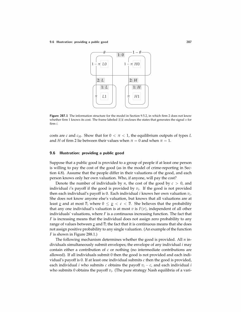
9.6 Illustration: providing a public good 287
1: 0
2: L 2: H
1: L 1: H
θ 1 − θ
π π
1 − π 1 − π
L1 H1
L0 H0
Figure 287.1 The information structure for the model in Section 9.5.2, in which firm 2 does not knowwhether firm 1 knows its cost. The frame labeled i: x encloses the states that generates the signal x forfirm i.
costs are c and cH . Show that for 0 < π < 1, the equilibrium outputs of types Land H of firm 2 lie between their values when π = 0 and when π = 1.
9.6 Illustration: providing a public good
Suppose that a public good is provided to a group of people if at least one personis willing to pay the cost of the good (as in the model of crime-reporting in Sec-tion 4.8). Assume that the people differ in their valuations of the good, and eachperson knows only her own valuation. Who, if anyone, will pay the cost?
Denote the number of individuals by n, the cost of the good by c > 0, andindividual i’s payoff if the good is provided by vi. If the good is not providedthen each individual’s payoff is 0. Each individual i knows her own valuation vi.She does not know anyone else’s valuation, but knows that all valuations are atleast v and at most v, where 0 ≤ v < c < v. She believes that the probabilitythat any one individual’s valuation is at most v is F(v), independent of all otherindividuals’ valuations, where F is a continuous increasing function. The fact thatF is increasing means that the individual does not assign zero probability to anyrange of values between v and v; the fact that it is continuous means that she doesnot assign positive probability to any single valuation. (An example of the functionF is shown in Figure 288.1.)
The following mechanism determines whether the good is provided. All n in-dividuals simultaneously submit envelopes; the envelope of any individual i maycontain either a contribution of c or nothing (no intermediate contributions areallowed). If all individuals submit 0 then the good is not provided and each indi-vidual’s payoff is 0. If at least one individual submits c then the good is provided,each individual i who submits c obtains the payoff vi − c, and each individual iwho submits 0 obtains the payoff vi. (The pure strategy Nash equilibria of a vari-
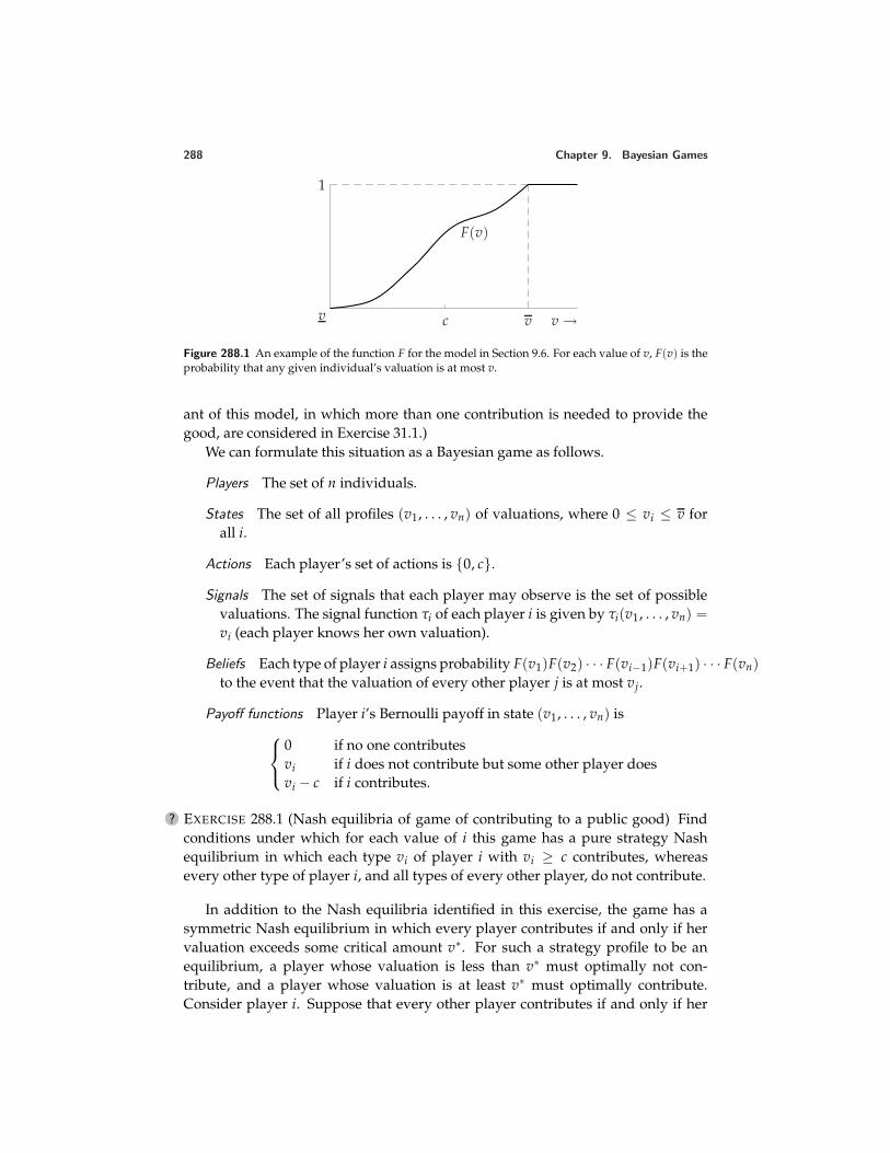
288 Chapter 9. Bayesian Games
v
1
F(v)
v →c v
Figure 288.1 An example of the function F for the model in Section 9.6. For each value of v, F(v) is theprobability that any given individual’s valuation is at most v.
ant of this model, in which more than one contribution is needed to provide thegood, are considered in Exercise 31.1.)
We can formulate this situation as a Bayesian game as follows.
Players The set of n individuals.
States The set of all profiles (v1, . . . , vn) of valuations, where 0 ≤ vi ≤ v forall i.
Actions Each player’s set of actions is 0, c.
Signals The set of signals that each player may observe is the set of possiblevaluations. The signal function τi of each player i is given by τi(v1, . . . , vn) =vi (each player knows her own valuation).
Beliefs Each type of player i assigns probability F(v1)F(v2) · · · F(vi−1)F(vi+1) · · · F(vn)to the event that the valuation of every other player j is at most vj.
Payoff functions Player i’s Bernoulli payoff in state (v1, . . . , vn) is
0 if no one contributesvi if i does not contribute but some other player doesvi − c if i contributes.
? EXERCISE 288.1 (Nash equilibria of game of contributing to a public good) Findconditions under which for each value of i this game has a pure strategy Nashequilibrium in which each type vi of player i with vi ≥ c contributes, whereasevery other type of player i, and all types of every other player, do not contribute.
In addition to the Nash equilibria identified in this exercise, the game has asymmetric Nash equilibrium in which every player contributes if and only if hervaluation exceeds some critical amount v∗. For such a strategy profile to be anequilibrium, a player whose valuation is less than v∗ must optimally not con-tribute, and a player whose valuation is at least v∗ must optimally contribute.Consider player i. Suppose that every other player contributes if and only if her
9.6 Illustration: providing a public good 289
valuation is at least v∗. The probability that at least one of the other players con-tributes is the probability that at least one of the other players’ valuations is atleast v∗, which is 1 − (F(v∗))n−1. (Note that (F(v∗))n−1 is the probability that allthe other valuations are at most v∗.) Thus if player i’s valuation is vi, her expectedpayoff is (1 − (F(v∗))n−1)vi if she does not contribute and vi − c if she does con-tribute. Hence the conditions for player i to optimally not contribute when vi < v∗
and optimally contribute when vi ≥ v∗ are (1 − (F(v∗))n−1)vi ≥ vi − c if vi < v∗,and (1 − (F(v∗))n−1)vi ≤ vi − c if vi ≥ v∗, or equivalently
vi(F(v∗))n−1 ≤ c if vi < v∗
vi(F(v∗))n−1 ≥ c if vi ≥ v∗.(289.1)
If these inequalities are satisfied then
v∗(F(v∗))n−1 = c. (289.2)
Conversely, if v∗ satisfies (289.2) then it satisfies the two equations in (289.1). Thusthe game has a Nash equilibrium in which every player contributes whenever hervaluation is at least v∗ if and only if v∗ satisfies (289.2).
Note that because F(v) = 1 only if v ≥ v, and v > c, we have v∗ > c. That is,every player’s cutoff for contributing exceeds the cost of the public good. Whenat least one player’s valuation exceeds c, all players are better off if the publicgood is provided and the high-valuation player contributes than if the good is notprovided. But in the equilibrium, the good is provided only if at least one player’svaluation exceeds v∗, which exceeds c.
As the number of individuals increases, is the good more or less likely to beprovided in this equilibrium? The probability that the good is provided is theprobability that at least one player’s valuation is at least v∗, which is equal to 1 −(F(v∗))n. (Note that (F(v∗))n is the probability that every player’s valuation isless than v∗.) From (289.2) this probability is equal to 1 − cF(v∗)/v∗. How doesv∗ vary with n? As n increases, for any given value of v∗ the value of (F(v∗))n−1
decreases, and thus the value of v∗(F(v∗))n−1 decreases. Thus to maintain theequality (289.2), the value of v∗ must increase as n increases. We conclude thatas n increases the change in the probability that the good is provided dependson the change in F(v∗)/v∗ as v∗ increases: the probability increases if F(v∗)/v∗ is adecreasing function of v∗, whereas it decreases if F(v∗)/v∗ is an increasing functionof v∗. If F is uniform and v > 0, for example, F(v∗)/v∗ is a decreasing function ofv∗, so that the probability that the good is provided increases as the populationsize increases.
The notion of a Bayesian game may be used to model a situation in which eachplayer is uncertain of the number of other players. In the next exercise you areasked to study another variant of the crime-reporting model of Section 4.8 in whicheach of the two players does not know whether she is the only witness or whetherthere is another witness (in which case she knows that witness’s valuation). (Theexercise requires a knowledge of mixed strategy Nash equilibrium (Chapter 4).)
290 Chapter 9. Bayesian Games
? EXERCISE 290.1 (Reporting a crime with an unknown number of witnesses) Con-sider the variant of the model of Section 4.8 in which each of two players does notknow whether she is the only witness, or whether there is another witness. De-note by π the probability each player assigns to being the sole witness. Model thissituation as a Bayesian game with three states: one in which player 1 is the onlywitness, one in which player 2 is the only witness, and one in which both playersare witnesses. Find a condition on π under which the game has a pure Nash equi-librium in which each player chooses Call (given the signal that she is a witness).When the condition is violated, find the symmetric mixed strategy Nash equilib-rium of the game, and check that when π = 0 this equilibrium coincides with theone found in Section 4.8 for n = 2.
9.7 Illustration: auctions
9.7.1 Introduction
In the analysis of auctions in Section 3.5, every bidder knows every other bidder’svaluation of the object for sale. Here I use the notion of a Bayesian game to analyzeauctions in which bidders are not perfectly informed about each others’ valuations.
Assume that a single object is for sale, and that each bidder independentlyreceives some information—a “signal”—about the value of the object to her. If eachbidder’s signal is simply her valuation of the object, as assumed in Section 3.5, wesay that the bidders’ valuations are private. If each bidder’s valuation depends onother bidders’ signals as well as her own, we say that the valuations are common.
The assumption of private values is appropriate, for example, for a work of artwhose beauty rather than resale value interests the buyers. Each bidder knowsher valuation of the object, but not that of any other bidder; the other bidders’ val-uations have no bearing on her valuation. The assumption of common values isappropriate, for example, for an oil tract containing unknown reserves on whicheach bidder has conducted a test. Each bidder i’s test result gives her some infor-mation about the size of the reserves, and hence her valuation of these reserves,but the other bidders’ test results, if known to bidder i, would typically improvethis information.
As in the analysis of auctions in which the bidders are perfectly informed abouteach others’ valuations, I study models in which bids for a single object are submit-ted simultaneously (bids are sealed), and the participant who submits the highestbid obtains the object. As before I consider both first-price auctions, in which thewinner pays the price she bid, and second-price auctions, in which the winner paysthe highest of the remaining bids.
(In Section 3.5 I argue that the first-price rule models an open descending (“Dutch”)auction, and the second-price rule models an open ascending (“English”) auc-tion. Note that the argument that the second-price rule corresponds to an openascending auction depends upon the bidders’ valuations being private. If a bid-der is uncertain of her valuation, which is related to that of other bidders, then in
9.7 Illustration: auctions 291
an open ascending auction she may obtain information about her valuation fromother participants’ bids, information not available in a sealed-bid auction.)
I first consider the case in which the bidders’ valuations are private, then thecase in which they are common.
9.7.2 Independent private values
In the case in which the bidders’ valuations are private, the assumptions aboutthese valuations are similar to those in the previous section (on the provision ofa public good). Each bidder knows that all other bidders’ valuations are at leastv, where v ≥ 0, and at most v. She believes that the probability that any givenbidder’s valuation is at most v is F(v), independent of all other bidders’ valuations,where F is a continuous increasing function (as in Figure 288.1).
The preferences of a bidder whose valuation is v are represented by the ex-pected value of the Bernoulli payoff function that assigns 0 to the outcome in whichshe does not win the object and v − p to the outcome in which she wins the objectand pays the price p. (That is, each bidder is risk neutral.) I assume that the ex-pected payoff of a bidder whose bid is tied for first place is (v − p)/m, where m isthe number of tied winning bids. (The assumption about the outcome when bidsare tied for first place has mainly “technical” significance; in Section 3.5, it wasconvenient to make an assumption different from the one here.)
Denote by P(b) the price paid by the winner of the auction when the pro-file of bids is b. For a first-price auction P(b) is the winning bid (the largest bi),whereas for a second-price auction it is the highest bid made by a bidder dif-ferent from the winner. Given the appropriate specification of P, the followingBayesian game models first- and second-price auctions with independent privatevaluations (and imperfect information about valuations).
Players The set of bidders, say 1, . . . , n.
States The set of all profiles (v1, . . . , vn) of valuations, where v ≤ vi ≤ v forall i.
Actions Each player’s set of actions is the set of possible bids (nonnegativenumbers).
Signals The set of signals that each player may observe is the set of possiblevaluations. The signal function τi of each player i is given by τi(v1, . . . , vn) =vi (each player knows her own valuation).
Beliefs Each type of player i assigns probability F(v1)F(v2) · · · F(vi−1)F(vi+1) · · · F(vn)to the event that the valuation of every other player j is at most vj.
Payoff functions Player i’s Bernoulli payoff in state (v1, . . . , vn) is 0 if her bidbi is not the highest bid, and (vi − P(b))/m if no bid is higher than bi and m
292 Chapter 9. Bayesian Games
bids (including bi) are equal to bi:
ui(b, (v1, . . . , vn)) =
(vi − P(b))/m if bj ≤ bi for all j = i andbj = bi for m players
0 if bj > bi for some j = i.
Nash equilibrium in a second-price sealed-bid auction As in a second-price sealed-bidauction in which every bidder knows every other bidder’s valuation,
in a second-price sealed-bid auction with imperfect information about valu-ations, a player’s bid equal to her valuation weakly dominates all her otherbids.
Precisely, consider some type vi of some player i, and let bi be a bid not equal to vi.Then for all bids by all types of all the other players, the expected payoff of type viof player i is at least as high when she bids vi as it is when she bids bi, and for somebids by the various types of the other players, her expected payoff is greater whenshe bids vi than it is when she bids bi.
The argument for this result is similar to the argument in Section 3.5.2 in thecase in which the players know each others’ valuations. The main difference be-tween the arguments arises because in the case in which the players do not knoweach others’ valuations, any given bids for every type of every player but i leaveplayer i uncertain about the highest of the remaining bids, because she is uncertainof the other players’ types. (The difference in the tie-breaking rules between thetwo cases also necessitates a small change in the argument.) In the next exerciseyou are asked to fill in the details.
? EXERCISE 292.1 (Weak domination in second-price sealed-bid action) Show thatfor each type vi of each player i in a second-price sealed-bid auction with imperfectinformation about valuations the bid vi weakly dominates all other bids.
We conclude, in particular, that a second-price sealed-bid auction with imper-fect information about valuations has a Nash equilibrium in which every type ofevery player bids her valuation. The game has also other equilibria, some of whichyou are asked to find in the next exercise.
? EXERCISE 292.2 (Nash equilibria of a second-price sealed-bid auction) For everyplayer i, find a Nash equilibrium of a second-price sealed-bid auction in whichplayer i wins. (Think about the Nash equilibria when the players know eachothers’ valuations, studied in Section 3.5.)
Nash equilibrium in a first-price sealed-bid auction As when the players are perfectlyinformed about each others’ valuations, the bid of vi by type vi of player i weaklydominates any bid greater than vi, but does not weakly dominate bids less than vi,and is itself weakly dominated by any such lower bid. (If type vi of player i bidsvi, her payoff is certainly 0 (either she wins and pays her valuation, or she loses),whereas if she bids less than vi, she may win and obtain a positive payoff.)
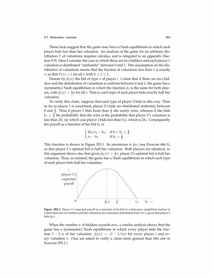
9.7 Illustration: auctions 293
These facts suggest that the game may have a Nash equilibrium in which eachplayer bids less than her valuation. An analysis of the game for an arbitrary dis-tribution F of valuations requires calculus, and is relegated to an appendix (Sec-tion 9.9). Here I consider the case in which there are two bidders and each player’svaluation is distributed “uniformly” between 0 and 1. This assumption on the dis-tribution of valuations means that the fraction of valuations less than v is exactlyv, so that F(v) = v for all v with 0 ≤ v ≤ 1.
Denote by βi(v) the bid of type v of player i. I claim that if there are two bid-ders and the distribution of valuations is uniform between 0 and 1, the game has a(symmetric) Nash equilibrium in which the function βi is the same for both play-ers, with βi(v) = 1
2 v for all v. That is, each type of each player bids exactly half hervaluation.
To verify this claim, suppose that each type of player 2 bids in this way. Thenas far as player 1 is concerned, player 2’s bids are distributed uniformly between0 and 1
2 . Thus if player 1 bids more than 12 she surely wins, whereas if she bids
b1 ≤ 12 the probability that she wins is the probability that player 2’s valuation is
less than 2b1 (in which case player 2 bids less than b1), which is 2b1. Consequentlyher payoff as a function of her bid b1 is
2b1(v1 − b1) if 0 ≤ b1 ≤ 1
2v1 − b1 if b1 > 1
2 .
This function is shown in Figure 293.1. Its maximizer is 12 v1 (see Exercise 446.1),
so that player 1’s optimal bid is half her valuation. Both players are identical, sothis argument shows also that given β1(v) = 1
2 v, player 2’s optimal bid is half hervaluation. Thus, as claimed, the game has a Nash equilibrium in which each typeof each player bids half her valuation.
↑player 1’sexpected
payoff
0 12 v1 v1
12 b1 →
Figure 293.1 Player 1’s expected payoff as a function of its bid in a first-price sealed-bid auction inwhich there are two bidders and the valuations are uniformly distributed from 0 to 1, given that player 2bids 1
2 v2.
When the number n of bidders exceeds two, a similar analysis shows that thegame has a (symmetric) Nash equilibrium in which every player bids the frac-tion 1 − 1/n of her valuation: βi(v) = (1 − 1/n)v for every player i and ev-ery valuation v. (You are asked to verify a claim more general than this one inExercise 295.1.)
294 Chapter 9. Bayesian Games
In this example—and, it turns out, for any distribution F satisfying the condi-tions in Section 9.7.2—the players’ common bidding function in a symmetric Nashequilibrium may be given an illuminating interpretation. Choose n − 1 valuationsrandomly and independently, each according to the cumulative distribution func-tion F. The highest of these n − 1 valuations is a “random variable”: its valuedepends on the n − 1 valuations that were chosen. Denote it by X. Fix a valua-tion v. Some values of X are less than v; others are greater than v. Consider thedistribution of X in those cases in which it is less than v. The expected value ofthis distribution is denoted E[X | X < v]: the expected value of X conditional onX being less than v. We may prove the following result. (A proof is given in theappendix, Section 9.9.)
For a distribution of valuations satisfying the conditions in Section 9.7.2,a first-price sealed-bid auction with imperfect information about valuationshas a (symmetric) Nash equilibrium in which each type v of each player bidsE[X | X < v], the expected value of the highest of the other players’ bids con-ditional on v being higher than all the other valuations.
Put differently, each bidder asks the following question: Over all the cases inwhich my valuation is the highest, what is the expectation of the highest of theother players’ valuations? This expectation is the amount she bids.
In the case considered above in which F is uniform from 0 to 1 and n = 2, wemay verify that indeed the equilibrium we found may be expressed in this way. Forany valuation v of player 1, the cases in which player 2’s valuation is less than v aredistributed uniformly from 0 to v, so that the expected value of player 2’s valuationconditional on its being less than v is 1
2 v, which is equal to the equilibrium biddingfunction that we found.
Comparing equilibria of first- and second-price auctions At the end of Section 3.5.3we saw that first- and second-price auctions are “revenue equivalent” when theplayers know each others’ valuations: their distinguished equilibria yield the sameoutcome. The same is true when the players are uncertain of each others’ valua-tions.
Consider the equilibrium of a second-price auction in which every player bidsher valuation. In this equilibrium, the expected price paid by a bidder with valua-tion v who wins is the expectation of the highest of the other n − 1 valuations, con-ditional on this maximum being less than v, or, in the notation above, E[X | X < v].We have just seen that a first-price auction has a symmetric Nash equilibrium inwhich this amount is precisely the bid of a player with valuation v, and hence theamount paid by such a player. Thus in the equilibria of both auctions the expectedprice paid by a winning bidder is the same. In both cases, the player with the high-est valuation submits the winning bid, so both auctions yield the same revenue forthe auctioneer:
if each bidder is risk neutral and the distribution of valuations satisfies the con-ditions in Section 9.7.2, then the Nash equilibrium of a second-price sealed-bid
9.7 Illustration: auctions 295
auction with independent private valuations (and imperfect information aboutvaluations) in which each player bids her valuation yields the same revenueas the symmetric Nash equilibrium of the corresponding first-price sealed-bidauction.
This result depends on the assumption that each player’s preferences are repre-sented by the expected value of a risk neutral Bernoulli payoff function. The nextexercise asks you to study an example in which each player is risk averse. (Seepage 101 for a discussion of risk neutrality and risk aversion.)
?? EXERCISE 295.1 (Auctions with risk averse bidders) Consider a variant of the Bayesiangame defined in Section 9.7.2 in which the players are risk averse. Specifically, sup-pose each of the n players’ preferences are represented by the expected value of theBernoulli payoff function x1/m, where x is the player’s monetary payoff and m > 1.Suppose also that each player’s valuation is distributed uniformly between 0 and1, as in the example in Section 9.7.2. Show that the Bayesian game that modelsa first-price sealed-bid auction under these assumptions has a (symmetric) Nashequilibrium in which each type vi of each player i bids (1 − 1/[m(n − 1) + 1])vi.(You need to use the mathematical fact that the solution of the problem maxb[bk(v−b)] is kv/(k + ).) Compare the auctioneer’s revenue in this equilibrium withher revenue in the symmetric Nash equilibrium of a second-price sealed-bid auc-tion in which each player bids her valuation. (Note that the equilibrium of thesecond-price auction does not depend on the players’ payoff functions.)
9.7.3 Common valuations
In an auction with common valuations, each player’s valuation depends on theother players’ signals as well as her own. (As before, I assume that the players’signals are independent.) I denote the function that gives player i’s valuation bygi, and assume that it is increasing in all the signals. Given the appropriate spec-ification of the function P that determines the price P(b) paid by the winner asa function of the profile b of bids, the following Bayesian game models first- andsecond-price auctions with common valuations (and imperfect information aboutvaluations).
Players The set of bidders, say 1, . . . , n.
States The set of all profiles (t1, . . . , tn) of signals that the players may receive.
Actions Each player’s set of actions is the set of possible bids (nonnegativenumbers).
Signals The signal function τi of each player i is given by τi(t1, . . . , tn) = ti(each player observes her own signal).
Beliefs Each type of each player believes that the signal of every type of everyother player is independent of all the other players’ signals.
296 Chapter 9. Bayesian Games
Payoff functions Player i’s Bernoulli payoff in state (t1, . . . , tn) is 0 if her bid biis not the highest bid, and (gi(t1, . . . , tn)− P(b))/m if no bid is higher than biand m bids (including bi) are equal to bi:
ui(b, (t1, . . . , tn)) =
(gi(t1, . . . , tn) − P(b))/m if bj ≤ bi for all j = i andbj = bi for m players
0 if bj > bi for some j = i.
Nash equilibrium in a second-price sealed-bid auction The main ideas in the analysisof sealed-bid common value auctions are illustrated by an example in which thereare two bidders, each bidder’s signal is uniformly distributed from 0 to 1, and thevaluation of each bidder i is given by vi = αti + γtj, where j is the other playerand α ≥ γ ≥ 0. The case in which α = 1 and γ = 0 is exactly the one studiedin Section 9.7.2: in this case, the bidders’ valuations are private. If α = γ then forany given signals, each bidder’s valuation is the same—a case of “pure commonvaluations”. If, for example, the signal ti is the number of barrels of oil in a tract,then the expected valuation of a bidder i who knows the signals ti and tj is p · 1
2 (ti +tj), where p is the monetary worth of a barrel of oil. Our assumption, of course,is that a bidder does not know any other player’s signal. However, a key point inthe analysis of common value auctions is that the other players’ bids contain someinformation about the other players’ signals—information that may profitably beused.
I claim that under these assumptions a second-price sealed-bid auction has aNash equilibrium in which each type ti of each player i bids (α + γ)ti.
To verify this claim, suppose that each type of player 2 bids in this way andtype t1 of player 1 bids b1. To determine the expected payoff of type t1 of player 1,we need to find the probability with which she wins, and both the expected priceshe pays and the expected value of player 2’s signal if she wins.
Probability that player 1 wins: Given that player 2’s bidding function is (α + γ)t2,player 1’s bid of b1 wins only if b1 ≥ (α + γ)t2, or if t2 ≤ b1/(α + γ).Now, t2 is distributed uniformly from 0 to 1, so the probability that it isat most b1/(α + γ) is b1/(α + γ). Thus a bid of b1 by player 1 wins withprobability b1/(α + γ).
Expected price player 1 pays if she wins: The price she pays is equal to player 2’sbid, which, conditional on its being less than b1, is distributed uniformly from 0to b1. Thus the expected value of player 2’s bid, given that it is less than b1, is12 b1.
Expected value of player 2’s signal if player 1 wins: Player 2’s bid, given her sig-nal t2, is (α + γ)t2, so that the expected value of signals that yield a bid of lessthan b1 is 1
2 b1/(α + γ) (because of the uniformity of the distribution of t2).
Now, player 1’s expected payoff if she bids b1 is the difference between her ex-pected valuation, given her signal t1 and the fact that she wins, and the expected
9.7 Illustration: auctions 297
price she pays, multiplied by her probability of winning. Combining the calcula-tions above, player 1’s expected payoff if she bids b1 is thus (αt1 + 1
2 γb1/(α + γ)−12 b1)b1/(α + γ), or
α
2(α + γ)2 · (2(α + γ)t1 − b1)b1.
This function is maximized at b1 = (α + γ)t1. That is, if each type t2 of player 2 bids(α + γ)t2, any type t1 of player 1 optimally bids (α + γ)t1. Symmetrically, if eachtype t1 of player 1 bids (α + γ)t1, any type t2 of player 2 optimally bids (α + γ)t2.Hence, as claimed, the game has a Nash equilibrium in which each type ti of eachplayer i bids (α + γ)ti.
? EXERCISE 297.1 (Asymmetric Nash equilibria of second-price sealed-bid commonvalue auctions) Show that when α = γ = 1, for any value of λ > 0 the game stud-ied above has an (asymmetric) Nash equilibrium in which each type t1 of player 1bids (1 + λ)t1 and each type t2 of player 2 bids (1 + 1/λ)t2.
Note that when player 1 calculates her expected value of the object, she findsthe expected value of player 2’s signal given that her bid wins. If her bid is low thenshe is unlikely to be the winner, but if she is the winner, player 2’s signal must below, and so she should impute a low value to the object. She should not base herbid simply on an estimate of the valuation derived from her own signal and the(unconditional) expectation of the other player’s signal. If she does so, then overall the cases in which she wins, she more likely than not overvalues the object.A bidder who incorrectly behaves in this way is said to suffer the winner’s curse.(Bidders in real auctions know this problem: when a contractor gives you a quo-tation to renovate your house, she does not base her price simply on an unbiasedestimate out how much it will cost her to do the job, but takes into account thatyou will select her only if her competitors’ estimates are all be higher than hers, inwhich case her estimate may be suspiciously low.)
Nash equilibrium in a first-price sealed-bid auction I claim that under the assump-tions on the players’ signals and valuations in the previous section, a first-pricesealed-bid auction has a Nash equilibrium in which each type ti of each player ibids 1
2 (α + γ)ti. This claim may be verified by arguments like those in the previoussection. In the next exercise, you are asked to supply the details.
? EXERCISE 297.2 (First-price sealed-bid auction with common valuations) Verifythat under the assumptions on signals and valuations in the previous section,a first-price sealed-bid auction has a Nash equilibrium in which the bid of eachtype ti of each player i is 1
2 (α + γ)ti.
Comparing equilibria of first- and second-price auctions We see that the revenueequivalence of first- and second-price auctions that holds when valuations are pri-vate hold also for the symmetric equilibria of the examples above in which thevaluations are common. That is, the expected price paid by a player of any given
298 Chapter 9. Bayesian Games
type is the same in the symmetric equilibrium of the first-price auction as it is in thesymmetric equilibrium of the second-price auction: in each case type ti of player ipays 1
2 (α + γ)ti if she wins, and wins with the same probability.In fact, the revenue equivalence principle holds much more generally. When-
ever each bidder is risk neutral and independently receives a signal that the samedistribution, which satisfies the conditions on the distribution of valuations in Sec-tion 9.7.2, the expected payment of a bidder of any given type is the same inthe symmetric Nash equilibrium of a second-price sealed-bid auction revenue-equivalent as it is in the symmetric Nash equilibrium of a first-price sealed-bidauction. Further, this revenue equivalence is not restricted to first- and second-price auctions; a general result, encompassing a wider range of auction forms, isstated at the end of the appendix (Section 9.9).
AUCTIONS OF THE RADIO SPECTRUM
In the 1990s several countries started auctioning the right to use parts of the radiospectrum used for wireless communication (by mobile telephones, for example).Spectrum licenses in the USA were originally allocated on the basis of hearingsby the Federal Communications Commission (FCC). This procedure was time-consuming, and a large backlog developed, prompting a switch to lotteries. Li-censes awarded by the lotteries could be re-sold at high prices, attracting manyparticipants. In one case that drew attention, the winner of a license to run cellu-lar telephones in Cape Cod sold it to Southwestern Bell for US$41.5 million (NewYork Times, May 30, 1991, p. A1). In the early 1990s, the US government was per-suaded that auctioning licenses would allocate them more efficiently and mightraise nontrivial revenue.
For each interval of the spectrum, many licenses were available, each coveringa geographic area. A buyer’s valuation of a license could be expected to dependon the other licenses it owned, so many interdependent goods were for sale. Indesigning an auction mechanism, the FCC had many choices: for example, the bid-ding could be open, or it could be sealed, with the price equal to either the highestbid or the second-highest bid; the licenses could be sold sequentially, or simulta-neously, in which case participants could submit bids for individual licenses, orfor combinations of licenses. Experts in auction theory were consulted on the de-sign of the mechanism. John McMillan (who advised the FCC), writes that “Whentheorists met the policy-makers, concepts like Bayes-Nash equilibrium, incentive-compatibility constraints, and order-statistic theorems came to be discussed in thecorridors of power” (1994, 146). No theoretical analysis fitted the environmentof the auction well, but the experts appealed to some principles from the existingtheory, the results of laboratory experiments, and experience in auctions held inNew Zealand and Australia in the early 1990s in making their recommendations.The mechanism adopted in 1994 was an open ascending auction for which bids
9.8 Illustration: juries 299
were accepted simultaneously for all licenses in each round. Experts argued thatthe open (as opposed to sealed-bid) format and the simultaneity of the auctionspromoted an efficient outcome because at each stage the bidders could see theirrivals’ previous bids for all licenses.
The FCC has conducted several auctions, starting with “narrowband” licenses(each covering a sliver of the spectrum, used by paging services) and continuingwith “broadband” licenses (used for voice and data communications). These auc-tions have provided more employment for game theorists, many of whom haveadvised the companies bidding for licenses. In response to growing congestionof the airwaves and the expectation that a significant part of the rapidly growingInternet traffic will move to wireless devices, in 2000 the US president Bill Clintonordered further auctions of large parts of the spectrum (New York Times, October 14,2000). Whether the auctions that have been held have allocated licenses efficientlyis hard to tell, though it appears that the winners were able to obtain the sets oflicenses they wanted. Certainly the auctions have been successful in generatingrevenue: the first four generated over US$18 billion.
9.8 Illustration: juries
9.8.1 Model
In a trial, jurors are presented with evidence concerning the guilt or innocence of adefendant. They may interpret the evidence differently. On the basis of her inter-pretation, each juror votes either to convict or acquit the defendant. Assume thata unanimous verdict is required for conviction: the defendant is convicted if andonly if every juror votes to convict her. (This rule is used in the USA and Canada,for example.) What can we say about the chances of an innocent defendant’s beingconvicted and a guilty defendant’s being acquitted?
In deciding how to vote, each juror must consider the costs of convicting aninnocent person and of acquitting a guilty person. She must consider also thelikely effect of her vote on the outcome, which depends on the other jurors’ votes.For example, a juror who thinks that at least one of her colleagues is likely to votefor acquittal may act differently from one who is sure that all her colleagues willvote for conviction. Thus an answer to the question requires us to consider thestrategic interaction between the jurors, which we may model as a Bayesian game.
Assume that each juror comes to the trial with the belief that the defendantis guilty with probability π (the same for every juror), a belief modified by theevidence presented. We model the possibility that jurors interpret the evidencedifferently by assuming that for each of the defendant’s true statuses (guilty andinnocent), each juror interprets the evidence to point to guilt with positive prob-ability, and to innocence with positive probability, and that the jurors’ interpreta-tions are independent (no juror’s interpretation depends on any other juror’s in-terpretation). I assume that the probabilities are the same for all jurors, and denote
300 Chapter 9. Bayesian Games
the probability of any given juror’s interpreting the evidence to point to guilt whenthe defendant is guilty by p, and the probability of her interpreting the evidence topoint to innocence when the defendant is innocent by q. I assume also that a juroris more likely than not to interpret the evidence correctly, so that p > 1
2 and q > 12 ,
and hence in particular p > 1 − q.Each juror wishes to convict a guilty defendant and acquit an innocent one.
She is indifferent between these two outcomes, and prefers each of them to onein which an innocent defendant is convicted or a guilty defendant is acquitted.Assume specifically that each juror’s Bernoulli payoffs are:
0 if guilty defendant convicted or innocent defendant acquitted−z if innocent defendant convicted−(1 − z) if guilty defendant acquitted.
(300.1)The parameter z may be given an appealing interpretation. Denote by r the prob-ability a juror assigns to the defendant’s being guilty, given all her information.Then her expected payoff if the defendant is acquitted is −r(1 − z) + (1 − r) · 0 =−r(1 − z) and her expected payoff if the defendant is convicted is r · 0 − (1 − r)z =−(1 − r)z. Thus she prefers the defendant to be acquitted if −r(1 − z) > −(1 − r)z,or r < z, and convicted if r > z. That is, z is equal to the probability of guilt re-quired for the juror to want the defendant to be convicted. Put differently, for anyjuror
acquittal is at least as good as conviction if and only ifPr(defendant is guilty, given juror’s information) ≤ z.
(300.2)
We may now formulate a Bayesian game that models the situation. The playersare the jurors, and each player’s action is a vote to convict (C) or to acquit (Q). Weneed one state for each configuration of the players’ preferences and information.Each player’s preferences depend on whether the defendant is guilty or innocent,and each player’s information consists of her interpretation of the evidence. Thuswe define a state to be a list (X, s1, . . . , sn), where X denotes the defendant’s truestatus, guilty (G) or innocent (I), and si represents player i’s interpretation of theevidence, which may point to guilt (g) or innocence (b). (I do not use i for “inno-cence” because I use it to index the players; b stands for “blameless”.) The signalthat each player i receives is her interpretation of the evidence, si. In any state inwhich X = G (i.e. the defendant is guilty), each player assigns the probability p toany other player’s receiving the signal g, and the probability 1 − p to her receiv-ing the signal b, independently of all other players’ signals. Similarly, in any statein which X = I (i.e. the defendant is innocent), each player assigns the probabil-ity q to any other player’s receiving the signal b, and the probability 1 − q to herreceiving the signal g, independently of all other players’ signals.
Each player cares about the verdict, which depends on the players’ actions, andthe defendant’s true status. Given the assumption that unanimity is required toconvict the defendant, only the action profile (C, . . . , C) leads to conviction. Thus(300.1) implies that player i’s payoff function in the Bayesian game is defined as
9.8 Illustration: juries 301
follows.
ui(a, ω) =
0 if a = (C, . . . , C) and ω1 = I orif a = (C, . . . , C) and ω1 = G
−z if a = (C, . . . , C) and ω1 = I−(1 − z) if a = (C, . . . , C) and ω1 = G,
(301.1)
where ω1 is the first component of the state, giving the defendant’s true status.In summary, the following Bayesian game models the situation.
Players A set of n jurors.
States The set of states is the set of all lists (X, s1, . . . , sn) where X ∈ G, Iand sj ∈ g, b for every juror j, where X = G if the defendant is guilty,X = I if she is innocent, sj = g if player j receives the signal that she is guilty,and sj = b if player j receives the signal that she is innocent.
Actions The set of actions of each player is C, Q, where C means vote toconvict, and Q means vote to acquit.
Signals The set of signals that each player may receive is g, b and player j’ssignal function is defined by τj(X, s1, . . . , sn) = sj (each juror is informedonly of her own signal).
Beliefs Type g of any player i believes that the state is (G, s1, . . . , sn) withprobability πpk−1(1 − p)n−k and (I, s1, . . . , sn) with probability (1 − π)(1 −q)k−1qn−k, where k is the number of players j (including i) for whom sj = g ineach case. Type b of any player i believes that the state is (G, s1, . . . , sn) withprobability πpk(1 − p)n−k−1 and (I, s1, . . . , sn) with probability (1 − π)(1 −q)k−1qn−k−1, where k is the number of players j for whom sj = g in each case.
Payoff functions The Bernoulli payoff function of each player i is given in (301.1).
9.8.2 Nash equilibrium
One juror Start by considering the very simplest case, in which there is a singlejuror. Suppose that her signal is b. To determine whether she prefers convictionor acquittal we need to find the probability she assigns to the defendant’s beingguilty, given her signal. We can find this probability, denoted Pr(G | b), by usingBayes’ Rule (see Section 17.7.5, in particular (454.2)), as follows.
Pr(G | b) =Pr(b | G) Pr(G)
Pr(b | G) Pr(G) + Pr(b | I) Pr(I)
=(1 − p)π
(1 − p)π + q(1 − π)
Thus by (300.2), acquittal yields an expected payoff at least as high as does convic-tion if and only if
z ≥ (1 − p)π
(1 − p)π + q(1 − π).
302 Chapter 9. Bayesian Games
That is, after getting the signal that the defendant is innocent, the juror choosesacquittal as long as z is not too small—as long as she is too concerned about ac-quitting a guilty defendant. If her signal is g then a similar calculation leads tothe conclusion that conviction yields an expected payoff at least as high as doesacquittal if
z ≤ pπ
pπ + (1 − q)(1 − π).
Thus if(1 − p)π
(1 − p)π + q(1 − π)≤ z ≤ pπ
pπ + (1 − q)(1 − π)(302.1)
then the juror optimally acts according to her signal, acquitting the defendantwhen her signal is b and convicting her when it is g. (A bit of algebra shows thatthe term on the left of (302.1) is less than the term on the right, given p > 1 − q.)
Two jurors Now suppose there are two jurors. Are there values for z such thatthe game has a Nash equilibrium in which each juror votes according to her sig-nal? Suppose that juror 2 acts in this way: type b votes to acquit, and type g votesto convict. Consider type b of juror 1. If juror 2’s signal is b, juror 1’s vote has noeffect on the outcome, because juror 2 votes to acquit and unanimity is required forconviction. Thus when deciding how to vote, juror 1 should ignore the possibilitythat juror 2’s signal is b, and assume it is g. That is, juror 1 should take as evidenceher signal and the fact that juror 2’s signal is g. Hence, given (300.2), for type b ofjuror 1 acquittal is at least as good as conviction if the probability that the defen-dant is guilty, given juror 1’s signal is b and juror 2’s signal is g, is at most z. Thisprobability is
Pr(G | b, g) =Pr(b, g | G) Pr(G)
Pr(b, g | G) Pr(G) + Pr(b, g | I) Pr(I)
=(1 − p)pπ
(1 − p)pπ + q(1 − q)(1 − π).
Thus type b of juror 1 optimally votes for acquittal if
z ≥ (1 − p)pπ
(1 − p)pπ + q(1 − q)(1 − π).
By a similar argument, for type g of juror 1 conviction is at least as good as acquittalif
z ≤ p2π
p2π + (1 − q)2(1 − π).
Thus when there are two jurors, the game has a Nash equilibrium in which eachjuror acts according to her signal, voting to acquit the defendant when her signalis b and to convict her when it is g, if
(1 − p)pπ
(1 − p)pπ + q(1 − q)(1 − π)≤ z ≤ p2π
p2π + (1 − q)2(1 − π). (302.2)
9.8 Illustration: juries 303
Consider the expressions on the left of (302.1) and (302.2). Divide the numer-ator and denominator of the expression on the left of (302.1) by 1 − p and the nu-merator and denominator of the expression on the left of (302.2) by (1− p)p. Then,given p > 1 − q, we see that the expression on the left of (302.2) is greater thanthe expression on the left of (302.1). That is, the lowest value of z for which anequilibrium exists in which each juror votes according to her signal is higher whenthere are two jurors than when there is only one juror. Why? Because a juror whoreceives the signal b, knowing that her vote makes a difference only if the otherjuror votes to convict, makes her decision on the assumption that the other juror’ssignal is g, and so is less worried about convicting an innocent defendant than is asingle juror in isolation.
Many jurors Now suppose the number of jurors is arbitrary, equal to n. Supposethat every juror other than juror 1 votes to acquit when her signal is b and to convictwhen her signal is g. Consider type b of juror 1. As in the case of two jurors,juror 1’s vote has no effect on the outcome unless every other juror’s signal is g.Thus when deciding how to vote, juror 1 should assume that all the other signalsare g. Hence, given (300.2), for type b of juror 1 acquittal is at least as good asconviction if the probability that the defendant is guilty, given juror 1’s signal is band every other juror’s signal is g, is at most z. This probability is
Pr(G | b, g, . . . , g) =Pr(b, g, . . . , g | G) Pr(G)
Pr(b, g, . . . , g | G) Pr(G) + Pr(b, g, . . . , g | I) Pr(I)
=(1 − p)pn−1π
(1 − p)pn−1π + q(1 − q)n−1(1 − π).
Thus type b of juror 1 optimally votes for acquittal if
z ≥ (1 − p)pn−1π
(1 − p)pn−1π + q(1 − q)n−1(1 − π)
=1
1 +q
1 − p
(1 − q
p
)n−1 1 − π
π
.
Now, given that p > 1 − q, the denominator decreases to 1 as n increases. Thusthe lower bound on z for which type b of juror 1 votes for acquittal approaches1 as n increases. (You may check that if p = q = 0.8, π = 0.5, and n = 12, thelower bound on z exceeds 0.999999.) In particular, in a large jury, if jurors careeven slightly about acquitting a guilty defendant then a juror who interprets theevidence to point to innocence will nevertheless vote for conviction. The reason isthat the vote of a juror who interprets the evidence to point to innocence makes adifference to the outcome only if every other juror interprets the evidence to pointto guilt, in which case the probability that the defendant is in fact guilty is veryhigh.
We conclude that the model of a large jury in which the jurors are concernedabout acquitting a guilty defendant has no Nash equilibrium in which every juror
304 Chapter 9. Bayesian Games
votes according to her signal. What are its equilibria? You are asked to find theconditions for two equilibria in the next exercise.
? EXERCISE 304.1 (Signal-independent equilibria in a model of a jury) Find con-ditions under which the game, for an arbitrary number of jurors, has a Nashequilibrium in which every juror votes for acquittal regardless of her signal, andconditions under which every juror votes for conviction regardless of her signal.
Under some conditions on z the game has in addition a symmetric mixed strat-egy Nash equilibrium in which each type g juror votes for conviction, and eachtype b juror votes for acquittal and conviction each with positive probability. De-note by β the mixed strategy of each juror of type b. As before, a juror’s vote affectsthe outcome only if all other jurors vote for conviction, so when choosing an actiona juror should assume that all other jurors vote for conviction.
Each type b juror must be indifferent between voting for conviction and votingfor acquittal, because she takes each action with positive probability. By (300.2) wethus need the mixed strategy β to be such that the probability that the defendant isguilty, given that all other jurors vote for conviction, is equal to z. Now, the proba-bility of any given juror’s voting for conviction is p + (1 − p)β(C) if the defendantis guilty and 1 − q + qβ(C) if she is innocent. Thus
Pr(G | signal b and n − 1 votes for C)
=Pr(b | G)(Pr(vote for C | G))n−1 Pr(G)
Pr(b | G)(Pr(vote for C | G))n−1 Pr(G) + Pr(b | I)(Pr(vote for C | I))n−1 Pr(I)
=(1 − p)(p + (1 − p)β(C))n−1π
(1 − p)(p + (1 − p)β(C))n−1π + q(1 − q + qβ(C))n−1(1 − π).
The condition that this probability equals z implies
(1 − p)(p + (1 − p)β(C))n−1π(1 − z) = q(1 − q + qβ(C))n−1(1 − π)z (304.2)
and hence
β(C) =pX − (1 − q)q − (1 − p)X
,
where X = [π(1 − p)(1 − z)/((1 − π)qz)]1/(n−1). For a range of parameter values,0 ≤ β(C) ≤ 1, so that β(C) is indeed a probability. Notice that when n is large, Xis close to 1, and hence β(C) is close to 1: a juror who interprets the evidence aspointing to innocence very likely nonetheless votes for conviction.
Each type g juror votes for conviction, and so must get an expected payoff atleast as high from conviction as from acquittal. From an analysis like that for eachtype b juror, this condition is
p(p + (1 − p)β(C))n−1π(1 − z) ≥ (1 − q)(1 − q + qβ(C))n−1(1 − π)z.
Given p > 12 and q > 1
2 , this condition follows from (304.2).
9.8 Illustration: juries 305
An interesting property of this equilibrium is that the probability that an in-nocent defendant is convicted increases as n increases: the larger the jury, the morelikely an innocent defendant is to be convicted. (The proof of this result is notsimple.)
Variants The key point behind the results is that under unanimity rule a juror’svote makes a difference to the outcome only if every other juror votes for convic-tion. Consequently, a juror, when deciding how to vote, rationally assesses thedefendant’s probability of guilt under the assumption that every other juror votesfor conviction. The fact that this implication of unanimity rule drives the resultssuggests that the Nash equilibria might be quite different if less than unanimitywere required for conviction. The analysis of such rules is difficult, but indeed theNash equilibria they generate differ significantly from the Nash equilibria underunanimity rule. In particular, the analog of the mixed strategy Nash equilibria con-sidered above generate a probability that an innocent defendant is convicted thatapproaches zero as the jury size increases, as Feddersen and Pesendorfer (1998)show.
The idea behind the equilibria of the model in the next exercise is related to theideas in this section, though the model is different.
? EXERCISE 305.1 (Swing voter’s curse) Whether candidate 1 or candidate 2 is electeddepends on the votes of two citizens. The economy may be in one of two states, Aand B. The citizens agree that candidate 1 is best if the state is A and candidate 2is best if the state is B. Each citizen’s preferences are represented by the expectedvalue of a Bernoulli payoff function that assigns a payoff of 1 if the best candidatefor the state wins (obtains more votes than the other candidate), a payoff of 0 if theother candidate wins, and payoff of 1
2 if the candidates tie. Citizen 1 is informed ofthe state, whereas citizen 2 believes it is A with probability 0.9 and B with proba-bility 0.1. Each citizen may either vote for candidate 1, vote for candidate 2, or notvote.
a. Formulate this situation as a Bayesian game. (Construct the table of payoffsfor each state.)
b. Show that the game has exactly two pure Nash equilibria, in one of whichcitizen 2 does not vote and in the other of which she votes for 1.
c. Show that one of the player’s actions in the second of these equilibria isweakly dominated.
d. Why is the “swing voter’s curse” an appropriate name for the determinant ofcitizen 2’s decision in the second equilibrium?
306 Chapter 9. Bayesian Games
9.9 Appendix: Analysis of auctions for an arbitrary distribution of valuations
9.9.1 First-price sealed-bid auctions
In this section I construct a symmetric equilibrium of a first-price sealed-bid auc-tion for an arbitrary distribution F of valuations that satisfies the assumptions inSection 9.7.2. (Unlike the remainder of the book, the section uses calculus.)
The method I use to find the equilibrium is the same as the one used previously:first I find conditions satisfied by the players’ best response functions, then imposethe equilibrium condition that the bid of each type of each player be a best responseto the bids of each type of every other player.
As before, denote the bid of type vi of player i (i.e. player i when her valuationis vi) by βi(vi). In a symmetric equilibrium we have βi = β for every player i.A reasonable guess is that in an equilibrium the common bidding function β isincreasing: bidders with higher valuations bid more. I start by making this as-sumption. After finding a possible equilibrium, I check that in fact the biddingfunction has this property.
Each player is uncertain about the other players’ valuations, and hence is uncer-tain about the bids they will make, even though she knows the bidding function β.Denote by Gβ(b) the probability that, given β, any given player’s bid is at most b.Under my assumption that β is increasing, a player’s bid is at most b if and only ifher valuation is at most β−1(b) (where β−1 is the inverse of β). Thus
Gβ(b) = Prv ≤ β−1(b) = F(β−1(b)).
Now, the expected payoff of a player with valuation v who bids b when all otherplayers act according to the bidding function β is
(v − b) PrHighest bid is b. (306.1)
The probability PrHighest bid is b is equal to the probability that all the valu-ations of the other n − 1 bidders are less than b, which is (Gβ(b))n−1. Thus theexpected payoff in (306.1) is
(v − b)(Gβ(b))n−1. (306.2)
Consider the best response function of each type of an arbitrary player. Denotethe optimal bid by a player with valuation v, given that all the other players use thebidding function β, by Bv(β). This bid maximizes the expected payoff in (306.2),and thus satisfies the condition that the derivative of this payoff with respect to bis zero:
−(Gβ(Bv(β)))n−1 + (v − Bv(β))(n − 1)(Gβ(Bv(β)))n−2G′β(Bv(β)) = 0. (306.3)
For (β∗ , . . . , β∗) to be a Nash equilibrium, we need
Bv(β∗) = β∗(v) for all v.
9.9 Appendix: Analysis of auctions for an arbitrary distribution of valuations 307
That is, for every valuation v, the best response of a player with valuation v whenevery other player acts according to β∗ must be precisely β∗(v).
Now, from the definition of Gβ we have Gβ∗(Bv(β∗)) = F(β∗−1(β∗(v)) = F(v),and, for any β,
G′β(b) = F′(β−1(b))(β−1)′(b) =
F′(β−1(b))β′(β−1(b))
.
Hence G′β∗(β∗(v)) = F′(v)/β∗′(v). Thus we deduce from (306.3) that an equilib-
rium bidding function β∗ satisfies
−(F(v))n−1 + (v − β∗(v))(n − 1)(F(v))n−2F′(v)/β∗′(v) = 0,
or
β∗′(v)(F(v))n−1 + (n − 1)β∗(v)(F(v))n−2F′(v) = (n − 1)v(F(v))n−2F′(v).
We may solve this differential equation by noting that the left-hand side is pre-cisely the derivative with respect to v of β∗(v)(F(v))n−1. Thus integrating bothsides we obtain
β∗(v)(F(v))n−1 =∫ v
v(n − 1)x(F(x))n−2F′(x) dx
= v(F(v))n−1 −∫ v
v(F(x))n−1 dx
(using integration by parts to obtain the second line). Hence
β∗(v) = v −∫ v
v (F(x))n−1 dx
(F(v))n−1 . (307.1)
?? EXERCISE 307.2 (Properties of the bidding function in a first-price auction) Showthat the bidding function defined in (307.1) is increasing in v for v > v. Showalso that a bidder with the lowest possible valuation bids her valuation, whereasa bidder with any other valuation bids less than her valuation: β∗(v) = v andβ∗(v) < v for all v > v (use L’Hopital’s rule).
? EXERCISE 307.3 (Example of Nash equilibrium in a first-price auction) Verify thatfor the distribution F uniform from 0 to 1 the bidding function defined by (307.1)is (1 − 1/n)v.
The alternative expression for the Nash equilibrium bidding function discussedin the text may be derived as follows. As before, denote by X the random variableequal to the highest of n − 1 independent valuations, each with cumulative dis-tribution function F. The cumulative distribution function of X is H defined byH(x) = (F(x))n−1. Thus the expected value of X, conditional on its being less thanv, is
E[X | X < v] =
∫ vv xH′(x) dx
H(v)
=
∫ vv (n − 1)x(F(x))n−2F′(x) dx
(F(v))n−1 ,
308 Chapter 9. Bayesian Games
which is precisely β∗(v). (Integrating the numerator by parts.) That is, β∗(v) =E[X | X < v].
9.9.2 Revenue equivalence of auctions
I argued in the text that the expected price paid by the winner of a first-price auc-tion is the same as the expected price paid by the winner of a second-price auction.A much more general result may be established.
Suppose that n risk neutral bidders are involved in a sealed-bid auction inwhich the price is an arbitrary function of the bids (not necessarily the highest, orsecond highest). Each player’s bid affects the probability p that she wins and theexpected amount e(p) that she pays. Thus we can think of each bidder’s choosinga value of p, and can formulate the problem of a bidder with valuation v as
maxp
(p · v − e(p)).
Denote the solution of this problem by p∗(v). Assuming that e is differentiable, thefirst-order condition for this problem implies that
v = e′(p∗(v)) for all v.
Integrating both sides of this equation we have
e(p∗(v)) = e(p∗(v)) +∫ v
vx dp∗(x). (308.1)
Now consider an equilibrium with the property that the object is sold to the bidderwith the highest valuation, so that p∗(v) = PrX < v, and the expected payoffe(p∗(v)) = 0 of a bidder with the lowest possible valuation is zero. In any suchequilibrium, (308.1) implies that the expected payment e(p∗(v)) of a bidder withany given valuation v is independent of the price-determination rule in the auction,equal to Pr(X < v)E[X | X < v].
This result generalizes the earlier observation that the expected payments ofbidders in the Nash equilibria of first- and second-price auctions in which the bid-ders’ valuations are independent and private are the same. It is a special case ofthe more general revenue equivalence principle, which applies to a class of commonvalue auctions, as well as private value auctions, and may be stated as follows.
Suppose that each bidder (i) is risk neutral, (ii) independently receives a signalfrom the same distribution, which satisfies the conditions on the distributionof valuations in Section 9.7.2, and (iii) has a valuation that may depend onall the bidders’ signals. Consider auction mechanisms in the symmetric Nashequilibria of which the object is sold to the bidder with the highest signal andthe expected payoff of a bidder with the lowest possible valuation is zero. Inthe symmetric Nash equilibrium of any such mechanism the expected paymentof a bidder of any given type is the same, and hence the auctioneer’s expectedrevenue is the same.
Notes 309
Notes
The notion of a general Bayesian game was defined and studied by Harsanyi (1967/68).The formulation I describe here is taken (with a minor change) from Osborne andRubinstein (1994, Section 2.6).
The origin of the observation that more information may hurt (Section 9.4.1)is unclear. The idea of “infection” in Section 9.4.2 was first studied by Rubin-stein (1989). The game in Figure 282.1 is a variant suggested by Eddie Dekel ofthe one analyzed by Morris, Rob, and Shin (1995).
Games modeling voluntary contributions to a public good were first consid-ered by Olson (1965, Section I.D), and have been subsequently much studied. Themodel in Section 9.6 is a variant of one in an unpublished paper of William F.Samuelson dated 1984.
Vickrey (1961) initiated the study of auctions described in Section 9.7. First-price common value auctions (Section 9.7.3) were first studied by Wilson (1967,1969, 1977). The “winner’s curse” appears to have been first articulated by Capen,Clapp, and Campbell (1971). The general revenue equivalence principle at the endof Section 9.9.2 is due to Myerson (1981) and Riley and Samuelson (1981); theirresults are generalized by Bulow and Klemperer (1996, Lemma 3). The equilibriain Exercise 297.1 are described by Milgrom (1981, Theorem 6.3). The literature issurveyed by Klemperer (1999). The box on spectrum auctions on page 298 is basedon McMillan (1994), Cramton (1995, 1997, 1998), and McAfee and McMillan (1996).
Section 9.8 is based on Austen-Smith and Banks (1996) and Feddersen andPesendorfer (1996).
Exercise 280.2 was suggested by Ariel Rubinstein. Exercise 280.3 is based onBrams, Kilgour, and Davis (1993). A model of adverse selection was first stud-ied by Akerlof (1974); the model in Exercise 280.4 is taken from Samuelson andBazerman (1985). Exercise 305.1 is based on Feddersen and Pesendorfer (1996).
Draft chapter from An introduction to game theory by Martin J. [email protected]; www.economics.utoronto.ca/osborneVersion: 00/11/6.Copyright c© 1995–2000 by Martin J. Osborne. All rights reserved. No part of this book may be re-produced by any electronic or mechanical means (including photocopying, recording, or informationstorage and retrieval) without permission in writing from Oxford University Press, except that onecopy of up to six chapters may be made by any individual for private study.
11 Strictly Competitive Games andMaxminimization
Definitions and examples 335Strictly competitive games 338Prerequisite: Chapters 2 and 4.
11.1 Introduction
THE NOTION of Nash equilibrium (studied in Chapters 2, 3, and 4) models asteady state. The idea is that each player, through her experience playing the
game against various opponents, knows the actions that the other players in thegame will take, and chooses her action in light of this knowledge.
In this chapter and the next, we study the likely outcome of a game from adifferent angle. We consider the implications of each player’s forming a beliefabout the other players’ actions not from her experience, but from her analysis ofthe game.
In this chapter we focus on two-player strictly competitive games, in whichthe players’ interests are diametrically opposed. In such games a simple decision-making procedure leads each player to choose a Nash equilibrium action.
11.2 Definitions and examples
You are confronted with a game for the first time; you have no idea what actionsyour opponents will take. How should you choose your action? A conservativecriterion entails your working under the assumption that whatever you do, youropponents will take the worst possible action for you. For each of your actions,you look at all the outcomes that can occur, as the other players choose differentactions, and find the one that gives you the lowest payoff. Then you choose theaction for which this lowest payoff is largest. This procedure for choosing an actionis called maxminimization.
Many of the interesting examples of this procedure involve mixed strategies,so from the beginning I define the concepts for a strategic game with vNM pref-erences (Definition 103.1), though the ideas do not depend upon the players’ ran-domizing. Let Ui be an expected payoff function that represents player i’s pref-erences on lotteries over action profiles in a strategic game. For any given mixedstrategy αi of player i, the lowest payoff that she obtains, for any possible vector α−i
335
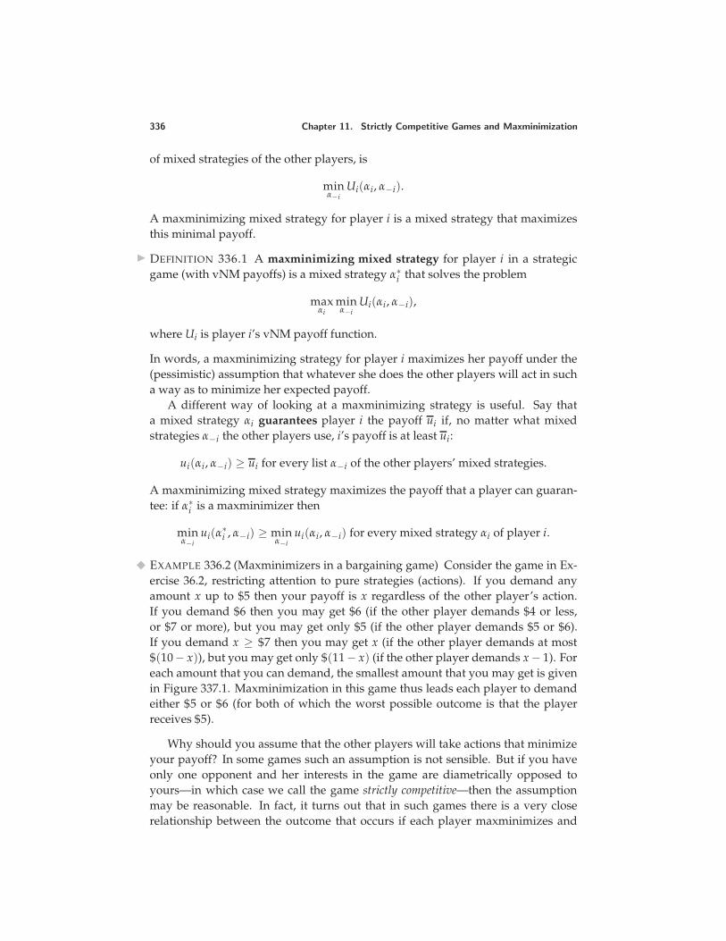
336 Chapter 11. Strictly Competitive Games and Maxminimization
of mixed strategies of the other players, is
minα−i
Ui(αi, α−i).
A maxminimizing mixed strategy for player i is a mixed strategy that maximizesthis minimal payoff.
DEFINITION 336.1 A maxminimizing mixed strategy for player i in a strategicgame (with vNM payoffs) is a mixed strategy α∗
i that solves the problem
maxαi
minα−i
Ui(αi, α−i),
where Ui is player i’s vNM payoff function.
In words, a maxminimizing strategy for player i maximizes her payoff under the(pessimistic) assumption that whatever she does the other players will act in sucha way as to minimize her expected payoff.
A different way of looking at a maxminimizing strategy is useful. Say thata mixed strategy αi guarantees player i the payoff ui if, no matter what mixedstrategies α−i the other players use, i’s payoff is at least ui:
ui(αi, α−i) ≥ ui for every list α−i of the other players’ mixed strategies.
A maxminimizing mixed strategy maximizes the payoff that a player can guaran-tee: if α∗
i is a maxminimizer then
minα−i
ui(α∗i , α−i) ≥ min
α−iui(αi, α−i) for every mixed strategy αi of player i.
EXAMPLE 336.2 (Maxminimizers in a bargaining game) Consider the game in Ex-ercise 36.2, restricting attention to pure strategies (actions). If you demand anyamount x up to $5 then your payoff is x regardless of the other player’s action.If you demand $6 then you may get $6 (if the other player demands $4 or less,or $7 or more), but you may get only $5 (if the other player demands $5 or $6).If you demand x ≥ $7 then you may get x (if the other player demands at most$(10− x)), but you may get only $(11− x) (if the other player demands x − 1). Foreach amount that you can demand, the smallest amount that you may get is givenin Figure 337.1. Maxminimization in this game thus leads each player to demandeither $5 or $6 (for both of which the worst possible outcome is that the playerreceives $5).
Why should you assume that the other players will take actions that minimizeyour payoff? In some games such an assumption is not sensible. But if you haveonly one opponent and her interests in the game are diametrically opposed toyours—in which case we call the game strictly competitive—then the assumptionmay be reasonable. In fact, it turns out that in such games there is a very closerelationship between the outcome that occurs if each player maxminimizes and
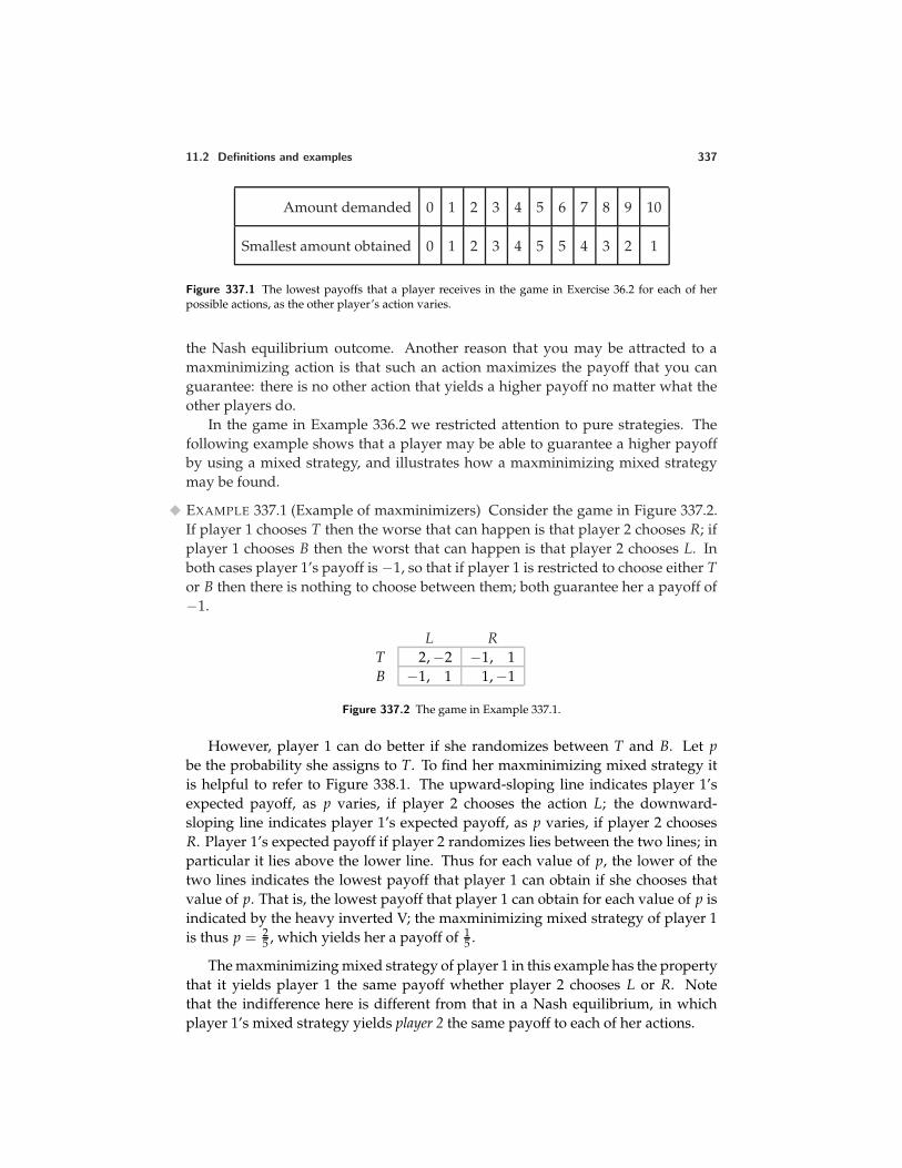
11.2 Definitions and examples 337
Amount demanded 0 1 2 3 4 5 6 7 8 9 10
Smallest amount obtained 0 1 2 3 4 5 5 4 3 2 1
Figure 337.1 The lowest payoffs that a player receives in the game in Exercise 36.2 for each of herpossible actions, as the other player’s action varies.
the Nash equilibrium outcome. Another reason that you may be attracted to amaxminimizing action is that such an action maximizes the payoff that you canguarantee: there is no other action that yields a higher payoff no matter what theother players do.
In the game in Example 336.2 we restricted attention to pure strategies. Thefollowing example shows that a player may be able to guarantee a higher payoffby using a mixed strategy, and illustrates how a maxminimizing mixed strategymay be found.
EXAMPLE 337.1 (Example of maxminimizers) Consider the game in Figure 337.2.If player 1 chooses T then the worse that can happen is that player 2 chooses R; ifplayer 1 chooses B then the worst that can happen is that player 2 chooses L. Inboth cases player 1’s payoff is −1, so that if player 1 is restricted to choose either Tor B then there is nothing to choose between them; both guarantee her a payoff of−1.
L RT 2, −2 −1, 1B −1, 1 1, −1
Figure 337.2 The game in Example 337.1.
However, player 1 can do better if she randomizes between T and B. Let pbe the probability she assigns to T. To find her maxminimizing mixed strategy itis helpful to refer to Figure 338.1. The upward-sloping line indicates player 1’sexpected payoff, as p varies, if player 2 chooses the action L; the downward-sloping line indicates player 1’s expected payoff, as p varies, if player 2 choosesR. Player 1’s expected payoff if player 2 randomizes lies between the two lines; inparticular it lies above the lower line. Thus for each value of p, the lower of thetwo lines indicates the lowest payoff that player 1 can obtain if she chooses thatvalue of p. That is, the lowest payoff that player 1 can obtain for each value of p isindicated by the heavy inverted V; the maxminimizing mixed strategy of player 1is thus p = 2
5 , which yields her a payoff of 15 .
The maxminimizing mixed strategy of player 1 in this example has the propertythat it yields player 1 the same payoff whether player 2 chooses L or R. Notethat the indifference here is different from that in a Nash equilibrium, in whichplayer 1’s mixed strategy yields player 2 the same payoff to each of her actions.
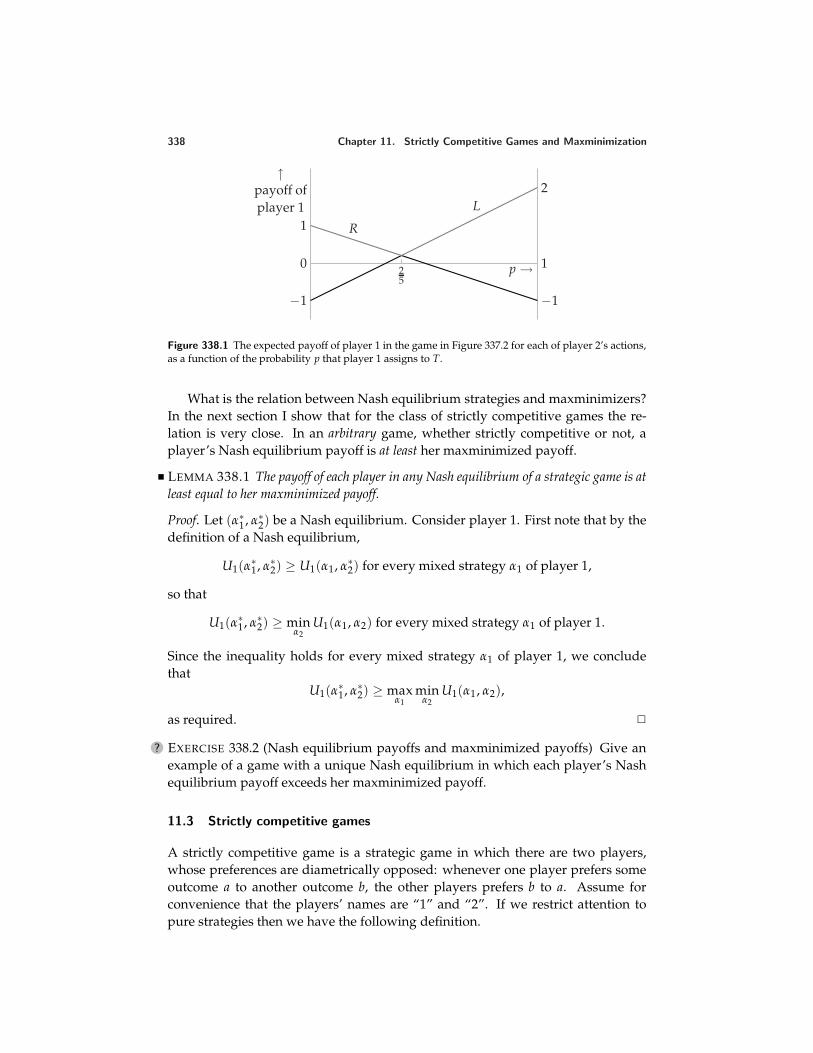
338 Chapter 11. Strictly Competitive Games and Maxminimization
↑payoff ofplayer 1
0
1
−1
1
2
−1
p →25
R
L
Figure 338.1 The expected payoff of player 1 in the game in Figure 337.2 for each of player 2’s actions,as a function of the probability p that player 1 assigns to T.
What is the relation between Nash equilibrium strategies and maxminimizers?In the next section I show that for the class of strictly competitive games the re-lation is very close. In an arbitrary game, whether strictly competitive or not, aplayer’s Nash equilibrium payoff is at least her maxminimized payoff.
LEMMA 338.1 The payoff of each player in any Nash equilibrium of a strategic game is atleast equal to her maxminimized payoff.
Proof. Let (α∗1, α∗
2) be a Nash equilibrium. Consider player 1. First note that by thedefinition of a Nash equilibrium,
U1(α∗1, α∗
2) ≥ U1(α1, α∗2) for every mixed strategy α1 of player 1,
so that
U1(α∗1, α∗
2) ≥ minα2
U1(α1, α2) for every mixed strategy α1 of player 1.
Since the inequality holds for every mixed strategy α1 of player 1, we concludethat
U1(α∗1, α∗
2) ≥ maxα1
minα2
U1(α1, α2),
as required.
? EXERCISE 338.2 (Nash equilibrium payoffs and maxminimized payoffs) Give anexample of a game with a unique Nash equilibrium in which each player’s Nashequilibrium payoff exceeds her maxminimized payoff.
11.3 Strictly competitive games
A strictly competitive game is a strategic game in which there are two players,whose preferences are diametrically opposed: whenever one player prefers someoutcome a to another outcome b, the other players prefers b to a. Assume forconvenience that the players’ names are “1” and “2”. If we restrict attention topure strategies then we have the following definition.
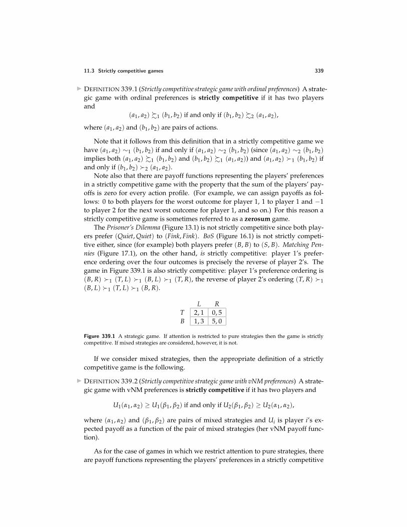
11.3 Strictly competitive games 339
DEFINITION 339.1 (Strictly competitive strategic game with ordinal preferences) A strate-gic game with ordinal preferences is strictly competitive if it has two playersand
(a1, a2) 1 (b1, b2) if and only if (b1, b2) 2 (a1, a2),
where (a1, a2) and (b1, b2) are pairs of actions.
Note that it follows from this definition that in a strictly competitive game wehave (a1, a2) ∼1 (b1, b2) if and only if (a1, a2) ∼2 (b1, b2) (since (a1, a2) ∼2 (b1, b2)implies both (a1, a2) 1 (b1, b2) and (b1, b2) 1 (a1, a2)) and (a1, a2) 1 (b1, b2) ifand only if (b1, b2) 2 (a1, a2).
Note also that there are payoff functions representing the players’ preferencesin a strictly competitive game with the property that the sum of the players’ pay-offs is zero for every action profile. (For example, we can assign payoffs as fol-lows: 0 to both players for the worst outcome for player 1, 1 to player 1 and −1to player 2 for the next worst outcome for player 1, and so on.) For this reason astrictly competitive game is sometimes referred to as a zerosum game.
The Prisoner’s Dilemma (Figure 13.1) is not strictly competitive since both play-ers prefer (Quiet, Quiet) to (Fink, Fink). BoS (Figure 16.1) is not strictly competi-tive either, since (for example) both players prefer (B, B) to (S, B). Matching Pen-nies (Figure 17.1), on the other hand, is strictly competitive: player 1’s prefer-ence ordering over the four outcomes is precisely the reverse of player 2’s. Thegame in Figure 339.1 is also strictly competitive: player 1’s preference ordering is(B, R) 1 (T, L) 1 (B, L) 1 (T, R), the reverse of player 2’s ordering (T, R) 1(B, L) 1 (T, L) 1 (B, R).
L RT 2, 1 0, 5B 1, 3 5, 0
Figure 339.1 A strategic game. If attention is restricted to pure strategies then the game is strictlycompetitive. If mixed strategies are considered, however, it is not.
If we consider mixed strategies, then the appropriate definition of a strictlycompetitive game is the following.
DEFINITION 339.2 (Strictly competitive strategic game with vNM preferences) A strate-gic game with vNM preferences is strictly competitive if it has two players and
U1(α1, α2) ≥ U1(β1, β2) if and only if U2(β1, β2) ≥ U2(α1, α2),
where (α1, α2) and (β1, β2) are pairs of mixed strategies and Ui is player i’s ex-pected payoff as a function of the pair of mixed strategies (her vNM payoff func-tion).
As for the case of games in which we restrict attention to pure strategies, thereare payoff functions representing the players’ preferences in a strictly competitive
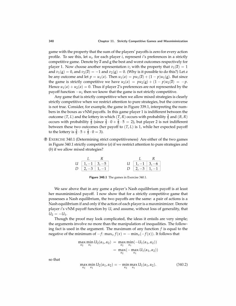
340 Chapter 11. Strictly Competitive Games and Maxminimization
game with the property that the sum of the players’ payoffs is zero for every actionprofile. To see this, let ui, for each player i, represent i’s preferences in a strictlycompetitive game. Denote by a and a the best and worst outcomes respectively forplayer 1. Now choose another representation vi with the property that v1(a) = 1and v1(a) = 0, and v2(a) = −1 and v2(a) = 0. (Why is it possible to do this?) Let abe any outcome and let p = u1(a). Then u1(a) = pu1(a) + (1 − p)u1(a). But sincethe game is strictly competitive we have u2(a) = pu2(a) + (1 − p)u2(a) = −p.Hence u1(a) + u2(a) = 0. Thus if player 2’s preferences are not represented by thepayoff function −u1 then we know that the game is not strictly competitive.
Any game that is strictly competitive when we allow mixed strategies is clearlystrictly competitive when we restrict attention to pure strategies, but the converseis not true. Consider, for example, the game in Figure 339.1, interpreting the num-bers in the boxes as vNM payoffs. In this game player 1 is indifferent between theoutcome (T, L) and the lottery in which (T, R) occurs with probability 3
5 and (B, R)occurs with probability 2
5 (since 35 · 0 + 2
5 · 5 = 2), but player 2 is not indifferentbetween these two outcomes (her payoff to (T, L) is 1, while her expected payoffto the lottery is 3
5 · 5 + 25 · 0 = 3).
? EXERCISE 340.1 (Determining strict competitiveness) Are either of the two gamesin Figure 340.1 strictly competitive (a) if we restrict attention to pure strategies and(b) if we allow mixed strategies?
L RU 1, −1 3, −5D 2, −3 1, −1
L RU 1, −1 3, −6D 2, −3 1, −1
Figure 340.1 The games in Exercise 340.1.
We saw above that in any game a player’s Nash equilibrium payoff is at leasther maxminimized payoff. I now show that for a strictly competitive game thatpossesses a Nash equilibrium, the two payoffs are the same: a pair of actions is aNash equilibrium if and only if the action of each player is a maxminimizer. Denoteplayer i’s vNM payoff function by Ui and assume, without loss of generality, thatU2 = −U1.
Though the proof may look complicated, the ideas it entails are very simple;the arguments involve no more than the manipulation of inequalities. The follow-ing fact is used in the argument. The maximum of any function f is equal to thenegative of the minimum of − f : maxx f (x) = − minx(− f (x)). It follows that
maxα2
minα1
U2(α1, α2) = maxα2
minα1
(−U1(α1, α2))
= maxα2
(− maxα1
U1(α1, α2))
so thatmax
α2min
α1U2(α1, α2) = − min
α2max
α1U1(α1, α2). (340.2)
11.3 Strictly competitive games 341
PROPOSITION 341.1 (Nash equilibrium strategies and maxminimizers of strictlycompetitive games) Consider a strictly competitive strategic game with vNM prefer-ences. Denote the vNM payoff function of each player i by Ui.
a. If (α∗1, α∗
2) is a Nash equilibrium then α∗1 is a maxminimizer for player 1, α∗
2 is amaxminimizer for player 2, and maxα1 minα2 U1(α1, α2) = minα2 maxα1 U1(α1, α2) =U1(α∗
1, α∗2).
b. If α∗1 is a maxminimizer for player 1, α∗
2 is a maxminimizer for player 2, and maxα1 minα2 U1(α1, α2) =minα2 maxα1 U1(α1, α2) (and thus, in particular, if the game has a Nash equilibrium(see part a)), then (α∗
1, α∗2) is a Nash equilibrium.
Proof. I first prove part a. By the definition of Nash equilibrium we have
U2(α∗1, α∗
2) ≥ U2(α∗1, α2) for every mixed strategy α2 of player 2
or, since U2 = −U1,
U1(α∗1, α∗
2) ≤ U1(α∗1, α2) for every mixed strategy α2 of player 2 .
HenceU1(α∗
1, α∗2) = min
α2U1(α∗
1, α2).
Now, the function on the right hand side of this equality is evaluated at the specificstrategy α∗
1, so that its value is not more than the maximum as we vary α1, namelymaxα1 minα2 U1(α1, α2). Thus we conclude that
U1(α∗1, α∗
2) ≤ maxα1
minα2
U1(α1, α2).
Now, from Lemma 338.1 we have the opposite inequality: a player’s Nash equi-librium payoff is at least her maxminimized payoff. Thus U1(α∗
1, α∗2) = maxα1 minα2 U1(α1, α2),
so that α∗1 is a maxminimizer for player 1.
An analogous argument for player 2 establishes that α∗2 is a maxminimizer for
player 2 and U2(α∗1, α∗
2) = maxα2 minα1 U2(α1, α2). From (340.2) we deduce thatU1(α∗
1, α∗2) = minα2 maxα1 U1(α1, α2), completing the proof of part a.
To prove part b, let
v∗ = maxα1
minα2
U1(α1, α2) = minα2
maxα1
U1(α1, α2).
From (340.2) we have maxα2 minα1 U2(α1, α2) = −v∗. Since α∗1 is a maxminimizer
for player 1 we have U1(α∗1, α2) ≥ v∗ for every mixed strategy a2 of player 2; since
α∗2 is a maxminimizer for player 2 we have U2(α1, α∗
2) ≥ −v∗ for every mixedstrategy α1 of player 1. Letting α2 = α∗
2 and α1 = α∗1 in these two inequalities
we obtain U1(α∗1, α∗
2) ≥ v∗ and U2(α∗1, α∗
2) ≥ −v∗, or U1(α∗1, α∗
2) ≤ v∗, so thatU1(α∗
1, α∗2) = v∗. Thus
U1(α∗1, α2) ≥ U1(α∗
1, α∗2) for every mixed strategy α2 of player 2,
342 Chapter 11. Strictly Competitive Games and Maxminimization
orU2(α∗
1, α2) ≤ U2(α∗1, α∗
2) for every mixed strategy α2 of player 2.
Similarly,
U2(α1, α∗2) ≥ U2(α∗
1, α∗2) for every mixed strategy α1 of player 1,
orU1(α1, α∗
2) ≤ U1(α∗1, α∗
2) for every mixed strategy α1 of player 1,
so that (α∗1, α∗
2) is a Nash equilibrium of the game.
This result is of interest not only because it shows the close relation betweenthe Nash equilibria and maxminimizers in a strictly competitive game, but alsobecause it reveals properties of Nash equilibria in a strictly competitive game thatare independent of the notion of maxminimization.
First, part a of the result implies that the Nash equilibrium payoff of each playerin a strictly competitive game is unique.
COROLLARY 342.1 Every Nash equilibrium of a strictly competitive game yields thesame pair of payoffs.
As we have seen, this property of Nash equilibria is not necessarily satisfied ingames that are not strictly competitive (consider BoS (Figure 16.1), for example).
Second, the result implies that a Nash equilibrium of a strictly competitivegame can be found by solving the problem maxα1 minα2 U1(α1, α2). Further, if weknow player 1’s equilibrium payoff then any mixed strategy that yields this payoffwhen player 2 uses any of her pure strategies solves the maxminimization prob-lem, and hence is an equilibrium mixed strategy of player 1. This fact is sometimesuseful when calculating the mixed strategy equilibria of a game when we knowthe equilibrium payoffs before we have found the equilibrium strategies (see, forexample, Exercise 344.2).
Third, suppose that (α1, α2) and (α′1, α′
2) are Nash equilibria of a strictly com-petitive game. Then by part a of the result the strategies α1 and α′
1 are maxmin-imizers for player 1, the strategies α2 and α′
2 are maxminimizers for player 2,and
maxα1
minα2
U1(α1, α2) = minα2
maxα1
U1(α1, α2) = U1(α1, α2) = U1(α′1, α′
2).
But then by part b of the result both (α1, α′2) and (α′
1, α2) are Nash equilibria of thegame. That is, the result implies that Nash equilibria of a strictly competitive gamehave the following property.
COROLLARY 342.2 The Nash equilibria of a strictly competitive game are interchange-able: if (α1, α2) and (α′
1, α′2) are Nash equilibria then so are (α1, α′
2) and (α′1, α2).
11.3 Strictly competitive games 343
The game BoS shows that the Nash equilibria of a game that is not strictly compet-itive are not necessarily interchangeable.
Part a of Proposition 341.1 shows that for any strictly competitive game thathas a Nash equilibrium we have
maxα1
minα2
U1(α1, α2) = minα2
maxα1
U1(α1, α2).
Note that the inequality
maxα1
minα2
U1(α1, α2) ≤ minα2
maxα1
U1(α1, α2)
holds more generally: for any α′1 we have U1(α′
1, α2) ≤ maxα1 U1(α1, α2) for allα2, so that minα2 U1(α′
1, α2) ≤ minα2 maxα1 U1(α1, α2). Thus in any game (whetheror not it is strictly competitive) the payoff that player 1 can guarantee herself is atmost the amount that player 2 can hold her down to.
If maxα1 minα2 U1(α1, α2) = minα2 maxα1 U1(α1, α2) then we say that this pay-off, the equilibrium payoff of player 1, is the value of the game. An implicationof Proposition 341.1 is that any equilibrium strategy of player 1 guarantees thather payoff is at least v∗, and any equilibrium strategy of player 2 guarantees thatplayer 1’s payoff is at most v∗.
COROLLARY 343.1 Any Nash equilibrium strategy of player 1 in a strictly competitivegame guarantees that her payoff is at least the value of the game, and any Nash equilibriumstrategy of player 2 guarantees that player 1’s payoff is at most the value.
Proof. For i = 1, 2, let α∗i be an equilibrium strategy of player i and let v∗ be
the value of the game. By Proposition 341.1a, α∗1 is a maxminimizer, so that it
guarantees that player 1’s payoff is at least v∗:
U1(α∗1, α2) ≥ min
α2U1(α∗
1, α2) = maxα1
minα2
U1(α∗1, α2) = v∗.
Similarly, any equilibrium strategy of player 2 guarantees that her payoff is at leasther equilibrium payoff −v∗; or, equivalently, any equilibrium strategy of player 2guarantees that player 1’s payoff is at most v∗.
In a game that is not strictly competitive a player’s equilibrium strategy doesnot in general have these properties, as the following exercise shows.
? EXERCISE 343.2 (Maxminimizers in BoS) For the game BoS (Figure 16.1) find themaxminimizer of each player. Show for each equilibrium, the strategy of neitherplayer guarantees her equilibrium payoff.
? EXERCISE 343.3 (Increasing payoffs and eliminating actions in strictly competitivegames) Let G be a strictly competitive game that has a Nash equilibrium.
a. Show that if some of player 1’s payoffs in G are increased in such a way thatthe resulting game G′ is strictly competitive then G′ has no equilibrium inwhich player 1 is worse off than she was in an equilibrium of G. (Note thatG′ may have no equilibrium at all.)
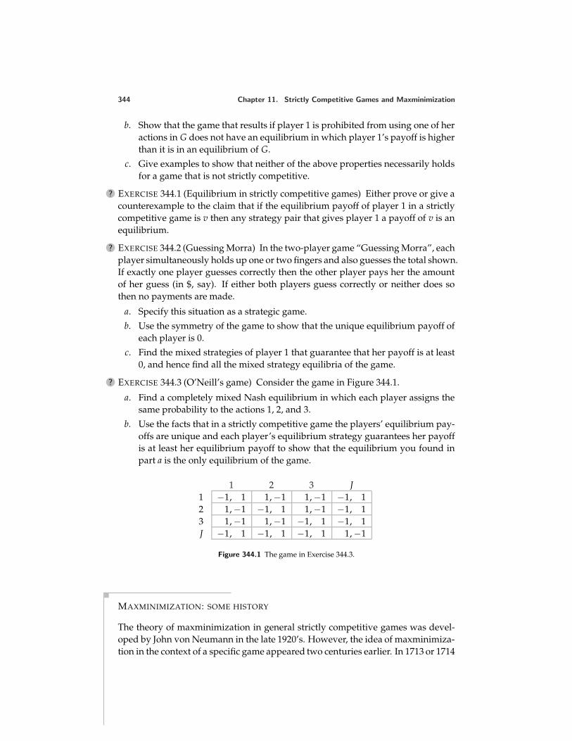
344 Chapter 11. Strictly Competitive Games and Maxminimization
b. Show that the game that results if player 1 is prohibited from using one of heractions in G does not have an equilibrium in which player 1’s payoff is higherthan it is in an equilibrium of G.
c. Give examples to show that neither of the above properties necessarily holdsfor a game that is not strictly competitive.
? EXERCISE 344.1 (Equilibrium in strictly competitive games) Either prove or give acounterexample to the claim that if the equilibrium payoff of player 1 in a strictlycompetitive game is v then any strategy pair that gives player 1 a payoff of v is anequilibrium.
? EXERCISE 344.2 (Guessing Morra) In the two-player game “Guessing Morra”, eachplayer simultaneously holds up one or two fingers and also guesses the total shown.If exactly one player guesses correctly then the other player pays her the amountof her guess (in $, say). If either both players guess correctly or neither does sothen no payments are made.
a. Specify this situation as a strategic game.
b. Use the symmetry of the game to show that the unique equilibrium payoff ofeach player is 0.
c. Find the mixed strategies of player 1 that guarantee that her payoff is at least0, and hence find all the mixed strategy equilibria of the game.
? EXERCISE 344.3 (O’Neill’s game) Consider the game in Figure 344.1.
a. Find a completely mixed Nash equilibrium in which each player assigns thesame probability to the actions 1, 2, and 3.
b. Use the facts that in a strictly competitive game the players’ equilibrium pay-offs are unique and each player’s equilibrium strategy guarantees her payoffis at least her equilibrium payoff to show that the equilibrium you found inpart a is the only equilibrium of the game.
1 2 3 J1 −1, 1 1, −1 1, −1 −1, 12 1, −1 −1, 1 1, −1 −1, 13 1, −1 1, −1 −1, 1 −1, 1J −1, 1 −1, 1 −1, 1 1, −1
Figure 344.1 The game in Exercise 344.3.
MAXMINIMIZATION: SOME HISTORY
The theory of maxminimization in general strictly competitive games was devel-oped by John von Neumann in the late 1920’s. However, the idea of maxminimiza-tion in the context of a specific game appeared two centuries earlier. In 1713 or 1714
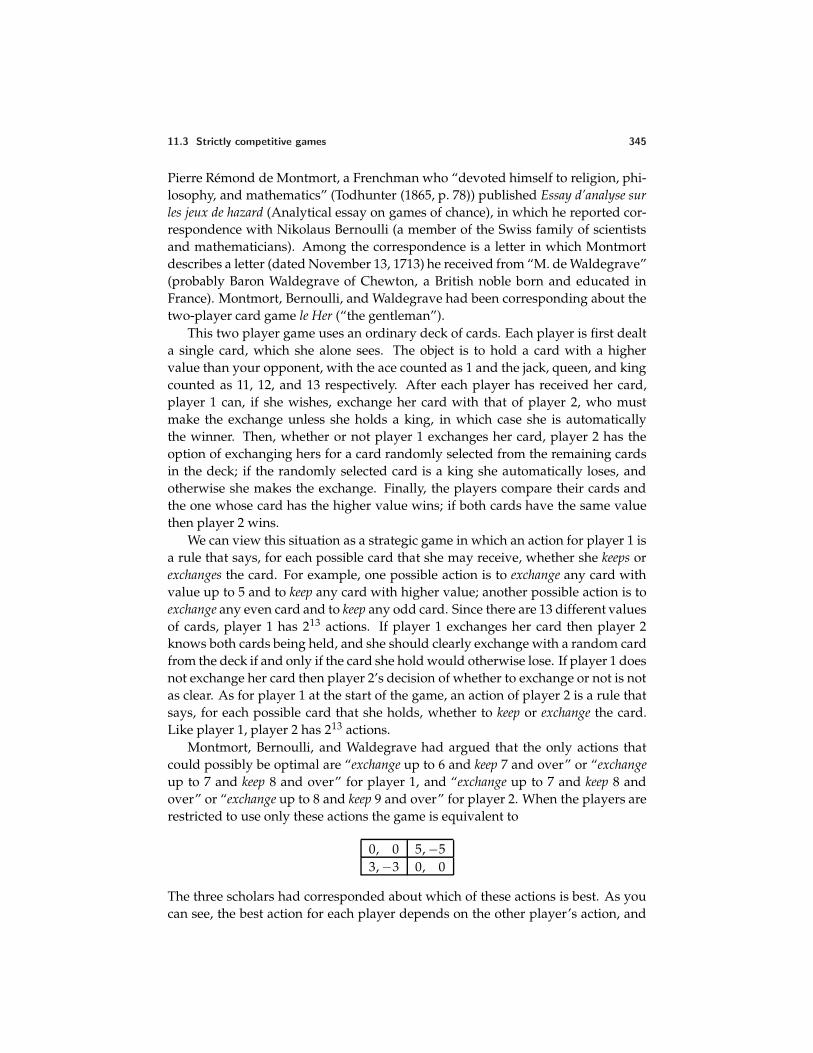
11.3 Strictly competitive games 345
Pierre Remond de Montmort, a Frenchman who “devoted himself to religion, phi-losophy, and mathematics” (Todhunter (1865, p. 78)) published Essay d’analyse surles jeux de hazard (Analytical essay on games of chance), in which he reported cor-respondence with Nikolaus Bernoulli (a member of the Swiss family of scientistsand mathematicians). Among the correspondence is a letter in which Montmortdescribes a letter (dated November 13, 1713) he received from “M. de Waldegrave”(probably Baron Waldegrave of Chewton, a British noble born and educated inFrance). Montmort, Bernoulli, and Waldegrave had been corresponding about thetwo-player card game le Her (“the gentleman”).
This two player game uses an ordinary deck of cards. Each player is first dealta single card, which she alone sees. The object is to hold a card with a highervalue than your opponent, with the ace counted as 1 and the jack, queen, and kingcounted as 11, 12, and 13 respectively. After each player has received her card,player 1 can, if she wishes, exchange her card with that of player 2, who mustmake the exchange unless she holds a king, in which case she is automaticallythe winner. Then, whether or not player 1 exchanges her card, player 2 has theoption of exchanging hers for a card randomly selected from the remaining cardsin the deck; if the randomly selected card is a king she automatically loses, andotherwise she makes the exchange. Finally, the players compare their cards andthe one whose card has the higher value wins; if both cards have the same valuethen player 2 wins.
We can view this situation as a strategic game in which an action for player 1 isa rule that says, for each possible card that she may receive, whether she keeps orexchanges the card. For example, one possible action is to exchange any card withvalue up to 5 and to keep any card with higher value; another possible action is toexchange any even card and to keep any odd card. Since there are 13 different valuesof cards, player 1 has 213 actions. If player 1 exchanges her card then player 2knows both cards being held, and she should clearly exchange with a random cardfrom the deck if and only if the card she hold would otherwise lose. If player 1 doesnot exchange her card then player 2’s decision of whether to exchange or not is notas clear. As for player 1 at the start of the game, an action of player 2 is a rule thatsays, for each possible card that she holds, whether to keep or exchange the card.Like player 1, player 2 has 213 actions.
Montmort, Bernoulli, and Waldegrave had argued that the only actions thatcould possibly be optimal are “exchange up to 6 and keep 7 and over” or “exchangeup to 7 and keep 8 and over” for player 1, and “exchange up to 7 and keep 8 andover” or “exchange up to 8 and keep 9 and over” for player 2. When the players arerestricted to use only these actions the game is equivalent to
0, 0 5, −53, −3 0, 0
The three scholars had corresponded about which of these actions is best. As youcan see, the best action for each player depends on the other player’s action, and
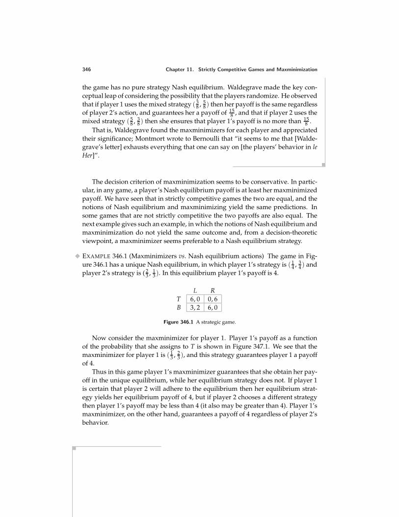
346 Chapter 11. Strictly Competitive Games and Maxminimization
the game has no pure strategy Nash equilibrium. Waldegrave made the key con-ceptual leap of considering the possibility that the players randomize. He observedthat if player 1 uses the mixed strategy ( 3
8 , 58 ) then her payoff is the same regardless
of player 2’s action, and guarantees her a payoff of 158 , and that if player 2 uses the
mixed strategy ( 58 , 3
8 ) then she ensures that player 1’s payoff is no more than 158 .
That is, Waldegrave found the maxminimizers for each player and appreciatedtheir significance; Montmort wrote to Bernoulli that “it seems to me that [Walde-grave’s letter] exhausts everything that one can say on [the players’ behavior in leHer]”.
The decision criterion of maxminimization seems to be conservative. In partic-ular, in any game, a player’s Nash equilibrium payoff is at least her maxminimizedpayoff. We have seen that in strictly competitive games the two are equal, and thenotions of Nash equilibrium and maxminimizing yield the same predictions. Insome games that are not strictly competitive the two payoffs are also equal. Thenext example gives such an example, in which the notions of Nash equilibrium andmaxminimization do not yield the same outcome and, from a decision-theoreticviewpoint, a maxminimizer seems preferable to a Nash equilibrium strategy.
EXAMPLE 346.1 (Maxminimizers vs. Nash equilibrium actions) The game in Fig-ure 346.1 has a unique Nash equilibrium, in which player 1’s strategy is ( 1
4 , 34 ) and
player 2’s strategy is ( 23 , 1
3 ). In this equilibrium player 1’s payoff is 4.
L RT 6, 0 0, 6B 3, 2 6, 0
Figure 346.1 A strategic game.
Now consider the maxminimizer for player 1. Player 1’s payoff as a functionof the probability that she assigns to T is shown in Figure 347.1. We see that themaxminimizer for player 1 is ( 1
3 , 23 ), and this strategy guarantees player 1 a payoff
of 4.Thus in this game player 1’s maxminimizer guarantees that she obtain her pay-
off in the unique equilibrium, while her equilibrium strategy does not. If player 1is certain that player 2 will adhere to the equilibrium then her equilibrium strat-egy yields her equilibrium payoff of 4, but if player 2 chooses a different strategythen player 1’s payoff may be less than 4 (it also may be greater than 4). Player 1’smaxminimizer, on the other hand, guarantees a payoff of 4 regardless of player 2’sbehavior.
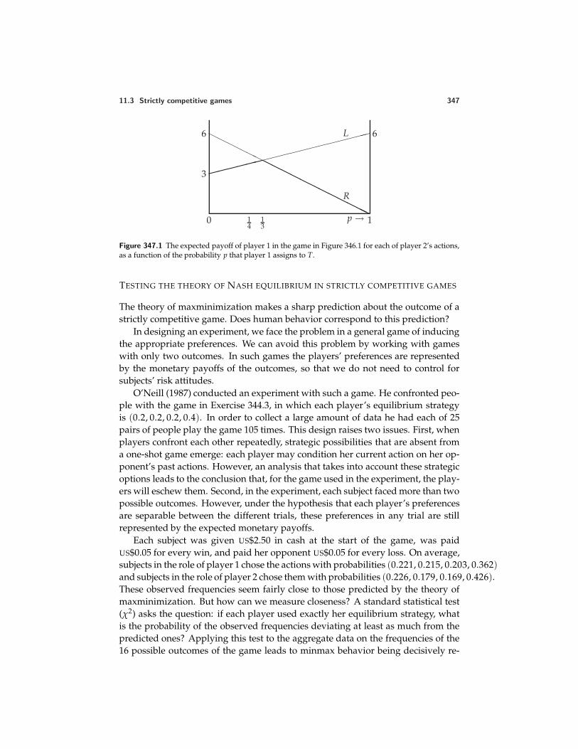
11.3 Strictly competitive games 347
3
6 6
0 1p →13
14
L
R
Figure 347.1 The expected payoff of player 1 in the game in Figure 346.1 for each of player 2’s actions,as a function of the probability p that player 1 assigns to T.
TESTING THE THEORY OF NASH EQUILIBRIUM IN STRICTLY COMPETITIVE GAMES
The theory of maxminimization makes a sharp prediction about the outcome of astrictly competitive game. Does human behavior correspond to this prediction?
In designing an experiment, we face the problem in a general game of inducingthe appropriate preferences. We can avoid this problem by working with gameswith only two outcomes. In such games the players’ preferences are representedby the monetary payoffs of the outcomes, so that we do not need to control forsubjects’ risk attitudes.
O’Neill (1987) conducted an experiment with such a game. He confronted peo-ple with the game in Exercise 344.3, in which each player’s equilibrium strategyis (0.2, 0.2, 0.2, 0.4). In order to collect a large amount of data he had each of 25pairs of people play the game 105 times. This design raises two issues. First, whenplayers confront each other repeatedly, strategic possibilities that are absent froma one-shot game emerge: each player may condition her current action on her op-ponent’s past actions. However, an analysis that takes into account these strategicoptions leads to the conclusion that, for the game used in the experiment, the play-ers will eschew them. Second, in the experiment, each subject faced more than twopossible outcomes. However, under the hypothesis that each player’s preferencesare separable between the different trials, these preferences in any trial are stillrepresented by the expected monetary payoffs.
Each subject was given US$2.50 in cash at the start of the game, was paidUS$0.05 for every win, and paid her opponent US$0.05 for every loss. On average,subjects in the role of player 1 chose the actions with probabilities (0.221, 0.215, 0.203, 0.362)and subjects in the role of player 2 chose them with probabilities (0.226, 0.179, 0.169, 0.426).These observed frequencies seem fairly close to those predicted by the theory ofmaxminimization. But how can we measure closeness? A standard statistical test(χ2) asks the question: if each player used exactly her equilibrium strategy, whatis the probability of the observed frequencies deviating at least as much from thepredicted ones? Applying this test to the aggregate data on the frequencies of the16 possible outcomes of the game leads to minmax behavior being decisively re-

348 Chapter 11. Strictly Competitive Games and Maxminimization
jected (the probability of a deviation from the prediction at least as large as that ob-served is less than 1 in 1,000). Other tests on O’Neill’s data also reject the minmaxhypothesis (Brown and Rosenthal (1990)).
In a variant of O’Neill’s experiment, with considerably higher stakes and asomewhat more complicated game, the evidence also does not support maxmini-mization, although maxminimization explains the data better than two alternativetheories (Rapoport and Boebel (1992)). (Of course, it’s relatively easy to designa theory that works well in one particular game; in order to “understand” behav-ior we want a theory that works well in a large class of games.) In summary, theevidence so far tends not to support the theory of maxminimization, although noother theory is systematically superior.
Notes
The material in the box on page 344 is based on Todhunter (1865) and Kuhn (1968).Guilbaud (1961) rediscovered Monmort’s report of Waldegrave’s work.
Draft chapter from An introduction to game theory by Martin J. [email protected]; www.economics.utoronto.ca/osborneVersion: 00/11/6.Copyright c© 1995–2000 by Martin J. Osborne. All rights reserved. No part of this book may be re-produced by any electronic or mechanical means (including photocopying, recording, or informationstorage and retrieval) without permission in writing from Oxford University Press, except that onecopy of up to six chapters may be made by any individual for private study.
12 Rationalizability
Iterated elimination of strictly dominated actions 355Iterated elimination of weakly dominated actions 359Prerequisite: Chapters 2 and 4.
12.1 Introduction
WHAT outcomes in a strategic game are consistent with the players’ analysesof each others’ rational behavior? The main solution notion we have stud-
ied so far, Nash equilibrium, is not designed to address this question, but rathermodels a steady state in which each player has learned the other players’ actionsfrom her long experience playing the game. In this chapter I discuss an approachto the question that considers players who carefully study a game, deducing theiropponents’ rational actions from their knowledge of their opponents’ preferencesand analyses of their opponents’ reasoning about their rational actions.
Suppose that we model each player’s decision problem as follows. She formsa probabilistic belief about the other players’ actions, and chooses her action (ormixed strategy) to maximize her expected payoff given this probabilistic belief.We say that a player who behaves in this way is rational. Precisely, suppose thatplayer i’s preferences are represented by the expected value of the Bernoulli payofffunction ui. Denote by µi her probabilistic belief about the other players’ actions:µi(a−i) is the probability she assigns to the collection a−i of the other players’ ac-tions. Denote by Ui(αi, a−i) player i’s expected payoff when she uses the mixedstrategy αi and the other players’ actions are given by a−i.
DEFINITION 349.1 A belief of player i about the other players’ actions is a proba-bility distribution over A−i. Player i is rational if she chooses her mixed strategy αito solve the problem
maxαi
∑a−i
µi(a−i)Ui(αi , a−i),
where µi is her belief about the other players’ actions.
Suppose that each player’s belief is correct—that is, the probability that it as-signs to each collection of actions of the other players is the probability impliedby their mixed strategies. Then a solution of each player’s maximization problemis her Nash equilibrium strategy. That is, if each player’s belief about the other
349
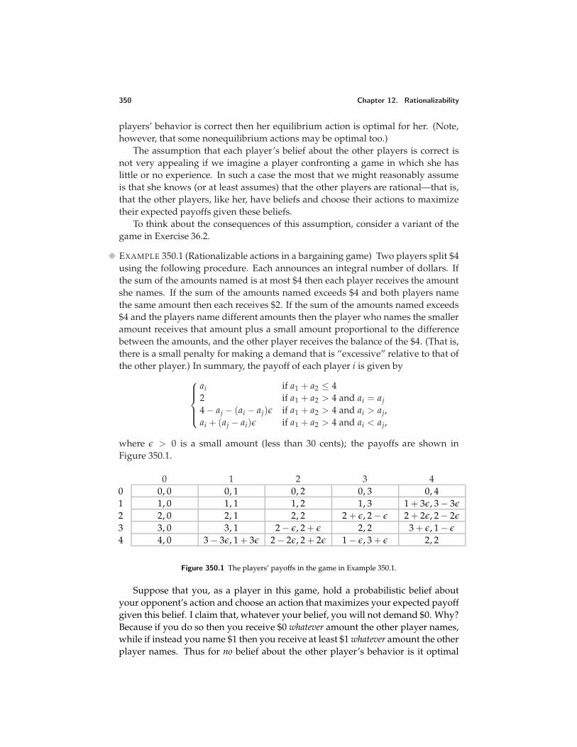
350 Chapter 12. Rationalizability
players’ behavior is correct then her equilibrium action is optimal for her. (Note,however, that some nonequilibrium actions may be optimal too.)
The assumption that each player’s belief about the other players is correct isnot very appealing if we imagine a player confronting a game in which she haslittle or no experience. In such a case the most that we might reasonably assumeis that she knows (or at least assumes) that the other players are rational—that is,that the other players, like her, have beliefs and choose their actions to maximizetheir expected payoffs given these beliefs.
To think about the consequences of this assumption, consider a variant of thegame in Exercise 36.2.
EXAMPLE 350.1 (Rationalizable actions in a bargaining game) Two players split $4using the following procedure. Each announces an integral number of dollars. Ifthe sum of the amounts named is at most $4 then each player receives the amountshe names. If the sum of the amounts named exceeds $4 and both players namethe same amount then each receives $2. If the sum of the amounts named exceeds$4 and the players name different amounts then the player who names the smalleramount receives that amount plus a small amount proportional to the differencebetween the amounts, and the other player receives the balance of the $4. (That is,there is a small penalty for making a demand that is “excessive” relative to that ofthe other player.) In summary, the payoff of each player i is given by
ai if a1 + a2 ≤ 42 if a1 + a2 > 4 and ai = aj4 − aj − (ai − aj)ε if a1 + a2 > 4 and ai > aj,ai + (aj − ai)ε if a1 + a2 > 4 and ai < aj,
where ε > 0 is a small amount (less than 30 cents); the payoffs are shown inFigure 350.1.
0 1 2 3 40 0, 0 0, 1 0, 2 0, 3 0, 41 1, 0 1, 1 1, 2 1, 3 1 + 3ε, 3 − 3ε
2 2, 0 2, 1 2, 2 2 + ε, 2 − ε 2 + 2ε, 2 − 2ε
3 3, 0 3, 1 2 − ε, 2 + ε 2, 2 3 + ε, 1 − ε
4 4, 0 3 − 3ε, 1 + 3ε 2 − 2ε, 2 + 2ε 1 − ε, 3 + ε 2, 2
Figure 350.1 The players’ payoffs in the game in Example 350.1.
Suppose that you, as a player in this game, hold a probabilistic belief aboutyour opponent’s action and choose an action that maximizes your expected payoffgiven this belief. I claim that, whatever your belief, you will not demand $0. Why?Because if you do so then you receive $0 whatever amount the other player names,while if instead you name $1 then you receive at least $1 whatever amount the otherplayer names. Thus for no belief about the other player’s behavior is it optimal
12.1 Introduction 351
for you to demand $0. Without considering whether your belief about the otherplayer’s behavior is consistent with her being rational, we can conclude that if youmaximize your payoff given some belief about the other player then you will notdemand $0. We say that a demand of $0 is a never best response.
By a similar argument we can conclude that you will not demand $1, whateveryour belief. But you might demand $2. Why? Because you might believe, forexample, that the other player is sure to demand $2 (that is, you might assignprobability 1 to the other player’s demanding $2), in which case your best actionis to demand $2 (if you demand more than $2 then you obtain less than $2, sinceyou pay a small penalty for making an excessive demand).
Is there any belief under which it is optimal for you to demand $3? Yes: if youare sure that the other player will demand $1 then it is optimal to demand $3 (ifyou demand less then the sum of the demands will be less than $4 and you willreceive what you demand, while if you demand more then the sum of the demandswill exceed $4 and you will receive $3 minus a small penalty). Similarly, if you aresure that the other player will demand $0 then it is optimal for you to demand $4.
In summary, any demand of at least $2 is consistent with your choosing anaction to maximize your expected payoff given some belief, while any smallerdemand is not. Or, more succinctly,
the only demands consistent with your being rational are $2, $3, and $4.
Now take the argument one step further. Suppose that you work under theassumption that your adversary is rational. Then you can conclude that she willnot demand less than $2: for any belief that she holds about you, it is not optimalfor her to demand less than $2 (just as it is not optimal for you to demand less than$2 if you are rational). But if she demands at least $2 then it is not optimal for youto demand $4, whatever belief you hold about her demand: you are better off de-manding $2 or $3 than you are demanding $4, whether you think your adversarywill demand $2, $3, or $4. On the other hand, the demands of $2 and $3 are bothoptimal for some belief that assigns positive probability only to your adversarydemanding $2, $3, or $4: if you are sure that the other player will demand $4, forexample, it is optimal for you to demand $3.
We have now argued that only the demands $2 and $3 are consistent with yourchoosing an action to maximize your expected payoff given some belief about theother player’s actions that is consistent with her being rational in the sense thatfor each action to which it assigns positive probability there is a belief that she canhold about your behavior that makes that action optimal for her:
only the demands $2 and $3 are consistent with your being rational and yourassuming that the other player is rational.
We can take the argument yet another step. What if you assume not only thatyour opponent is rational but that she assumes that you are rational? Then eachof the actions to which each of her beliefs about you assigns positive probabilityshould in turn be justified by a possible belief of yours about her. The only de-mands consistent with your rationality are those at least equal to $2, as we saw
352 Chapter 12. Rationalizability
above. Thus if she assumes that you are rational then each of her beliefs aboutyou must assign positive probability only to demands of at least $2. But then, bythe last argument above, the belief that you hold must assign positive probabilityonly to demands of $2 or $3. Finally, referring to Figure 350.1 you can see that ifyou hold such a belief you will not demand $3: a demand of $2 generates a higherpayoff for you, whether your opponent demands $2 or $3. To summarize:
only the demand of $2 is consistent with your rationality, your assuming thatyour opponent is rational, and your assuming that your opponent assumesthat you are rational.
The line of reasoning can be taken further: we can consider the consequence ofyour assuming that your opponent assumes that you assume that she is rational.However, such reasoning eliminates no more actions: a demand of $2 survivesevery additional level, since a demand of $2 is optimal for a player who is surethat her opponent will demand $2. (That is, ($2, $2) is a Nash equilibrium of thegame.)
In summary, in this game we conclude that
• if you are rational you will demand either $2, $3, or $4
• if you assume that your opponent is rational you will demand either $2 or $3
• if you assume that your opponent assumes that you are rational then you willdemand $2.
The general structure of this argument is illustrated in Figure 353.1. (I re-strict the informal discussion, though not the definitions and results, to two-playergames.) The rectangles represent the sets Ai and Aj of players i and j in the game.Assume that the action a∗i is consistent with player i’s acting rationally. Then thereis a belief of player i about player j’s actions under which a∗i is optimal. Let µ1
ibe one such belief, and let the set of actions to which this belief assigns positiveprobability be the shaded set on the right, which I denote X1
j . In the example, ifa∗1 = $0 or $1 then there is no such belief. If a∗1 = $2, $3, or $4 there are such beliefs;if a∗1 = $4, for example, then all such beliefs assign relatively high probability to$0.
Now further assume that a∗i is consistent with player i’s assuming that player jis rational. Then for some belief of player i about player j’s actions that makes a∗ioptimal—say µ1
i —each action in X1j (the set of actions to which µ1
i assigns positiveprobability) must be optimal for player j under some belief about player i’s action.For the two actions a′j and a′′j in X1
j the beliefs µ2j (a′j) and µ2
j (a′′j ) under which theactions are optimal are indicated in the figure, together with the sets of actions ofplayer i to which they assign positive probability. The shaded set on the left is theset of actions of player i to which some belief µ2
j (aj) of player j for aj in X1j assigns
positive probability. (The action a∗i may or may not be a member of X2i ; in the
figure it is not.)Note that we do not require that for every belief of player i under which a∗i is
optimal the actions of player j to which that belief assigns positive probability be
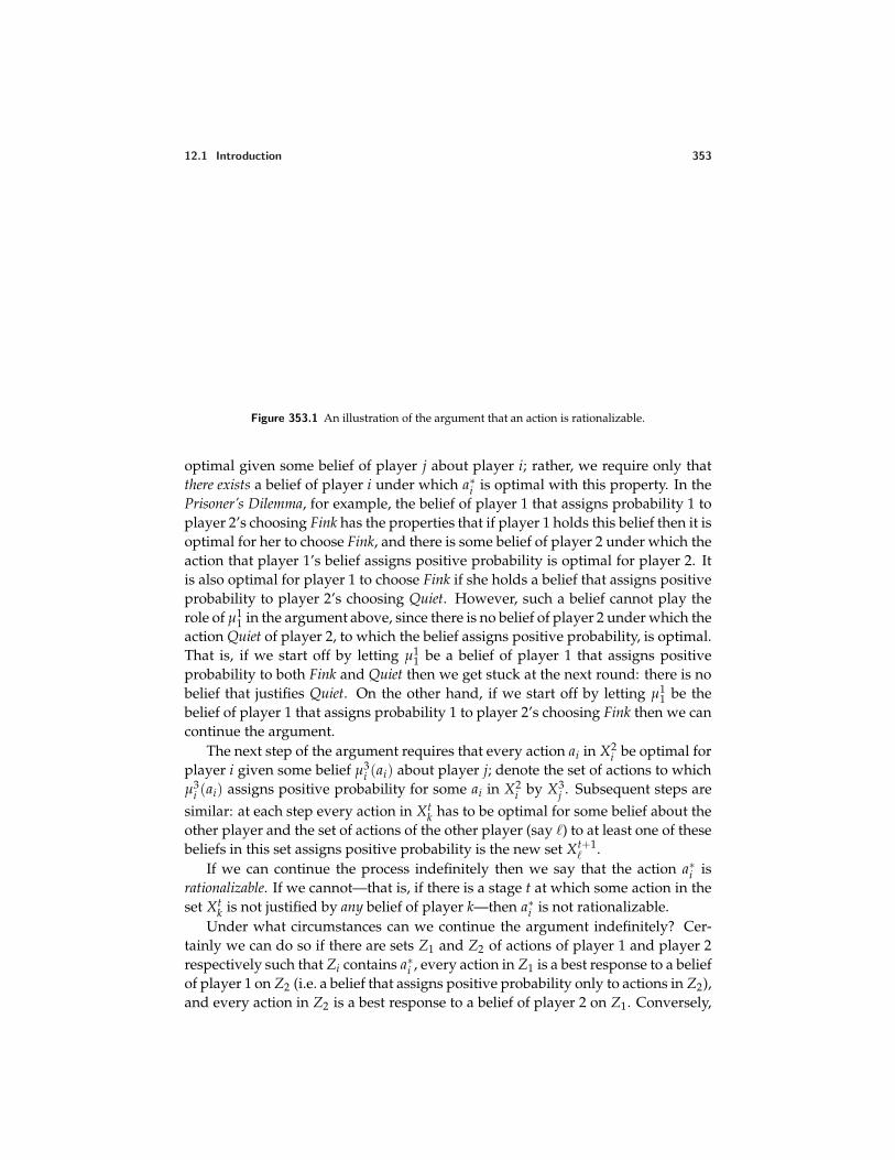
12.1 Introduction 353
Figure 353.1 An illustration of the argument that an action is rationalizable.
optimal given some belief of player j about player i; rather, we require only thatthere exists a belief of player i under which a∗i is optimal with this property. In thePrisoner’s Dilemma, for example, the belief of player 1 that assigns probability 1 toplayer 2’s choosing Fink has the properties that if player 1 holds this belief then it isoptimal for her to choose Fink, and there is some belief of player 2 under which theaction that player 1’s belief assigns positive probability is optimal for player 2. Itis also optimal for player 1 to choose Fink if she holds a belief that assigns positiveprobability to player 2’s choosing Quiet. However, such a belief cannot play therole of µ1
1 in the argument above, since there is no belief of player 2 under which theaction Quiet of player 2, to which the belief assigns positive probability, is optimal.That is, if we start off by letting µ1
1 be a belief of player 1 that assigns positiveprobability to both Fink and Quiet then we get stuck at the next round: there is nobelief that justifies Quiet. On the other hand, if we start off by letting µ1
1 be thebelief of player 1 that assigns probability 1 to player 2’s choosing Fink then we cancontinue the argument.
The next step of the argument requires that every action ai in X2i be optimal for
player i given some belief µ3i (ai) about player j; denote the set of actions to which
µ3i (ai) assigns positive probability for some ai in X2
i by X3j . Subsequent steps are
similar: at each step every action in Xtk has to be optimal for some belief about the
other player and the set of actions of the other player (say ) to at least one of thesebeliefs in this set assigns positive probability is the new set Xt+1
.If we can continue the process indefinitely then we say that the action a∗i is
rationalizable. If we cannot—that is, if there is a stage t at which some action in theset Xt
k is not justified by any belief of player k—then a∗i is not rationalizable.Under what circumstances can we continue the argument indefinitely? Cer-
tainly we can do so if there are sets Z1 and Z2 of actions of player 1 and player 2respectively such that Zi contains a∗i , every action in Z1 is a best response to a beliefof player 1 on Z2 (i.e. a belief that assigns positive probability only to actions in Z2),and every action in Z2 is a best response to a belief of player 2 on Z1. Conversely,
354 Chapter 12. Rationalizability
suppose that it can be continued indefinitely. For player i let Zi be the union ofa∗i with the union of the sets Xt
i for all even values of t and let Zj be the unionof the sets Xt
j for all odd values of t. Then for i = 1, 2, every action in Zi is a bestresponse to a belief on Zj. Thus we can define an action to be rationalizable asfollows, where Z−i denotes the set of all collections a−i of actions for the playersother than i for which aj ∈ Zj for all j.
DEFINITION 354.1 The action a∗i of player i in a strategic game is rationalizable iffor each player j there exists a set Zj of actions such that
• Zi contains a∗i• for every player j, every action aj in Zj is a best response to a belief of player j
on Z−j.
Suppose that a∗ is a pure strategy Nash equilibrium. Then for each player ithe action a∗i is a best response to a belief that assigns probability one to the otherplayers’ choosing a∗−i. Setting Zi = a∗i for each i, we see that a∗ is rationalizable.In fact, we have the following stronger result.
PROPOSITION 354.2 Every action used with positive probability in some mixed strategyNash equilibrium is rationalizable.
Proof. For each player i, let Zi be the set of actions to which player i’s equilibriummixed strategy assigns positive probability. Then every action in Zi is a best re-sponse to the belief of player i that coincides with the probability distribution overthe other players’ actions that is generated by their mixed strategies (which bydefinition assigns positive probability only to collections of actions in Z−i). Henceevery action in Zi is rationalizable.
In many games, actions not used with positive probability in some Nash equi-librium are rationalizable. Consider, for example, the game in Figure 355.1, whichhas a unique Nash equilibrium (M, C).
? EXERCISE 354.3 (Mixed strategy equilibrium of game in Figure 355.1) Show thatthe game in Figure 355.1 has no nondegenerate mixed strategy equilibrium.
Each action of each player is a best response to some action of the other player (forexample, T is a best response of player 1 to R, M is a best response to C, and B isa best response to L). Thus, setting Z1 = T, M, B and Z2 = L, C, R we see thatevery action of each player is rationalizable. In particular the actions T and B ofplayer 1 are rationalizable, even though they are not used with positive probabilityin any Nash equilibrium. The argument for player 1’s choosing T, for example, isthat player 2 might choose R, which is rational for her if she thinks player 1 willchoose B, and it is reasonable for player 2 to so think since B is optimal for player 1if she thinks that player 2 will choose L, which in turn is rational for player 2 if shethinks that player 1 will choose T, and so on.
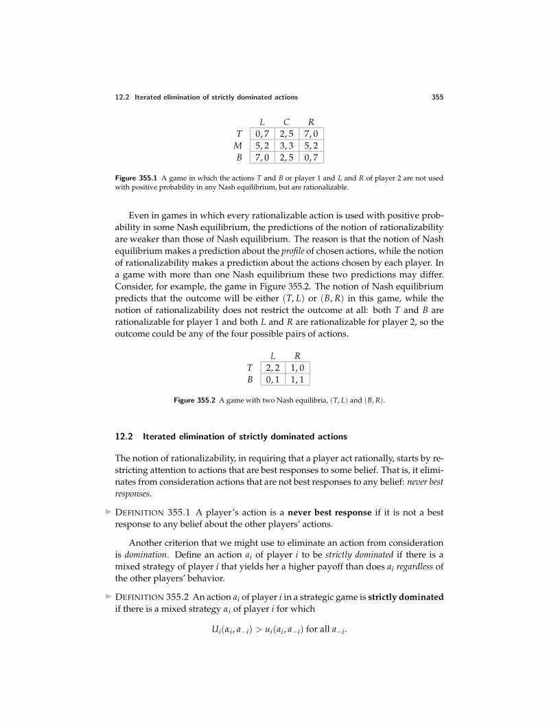
12.2 Iterated elimination of strictly dominated actions 355
L C RT 0, 7 2, 5 7, 0
M 5, 2 3, 3 5, 2B 7, 0 2, 5 0, 7
Figure 355.1 A game in which the actions T and B or player 1 and L and R of player 2 are not usedwith positive probability in any Nash equilibrium, but are rationalizable.
Even in games in which every rationalizable action is used with positive prob-ability in some Nash equilibrium, the predictions of the notion of rationalizabilityare weaker than those of Nash equilibrium. The reason is that the notion of Nashequilibrium makes a prediction about the profile of chosen actions, while the notionof rationalizability makes a prediction about the actions chosen by each player. Ina game with more than one Nash equilibrium these two predictions may differ.Consider, for example, the game in Figure 355.2. The notion of Nash equilibriumpredicts that the outcome will be either (T, L) or (B, R) in this game, while thenotion of rationalizability does not restrict the outcome at all: both T and B arerationalizable for player 1 and both L and R are rationalizable for player 2, so theoutcome could be any of the four possible pairs of actions.
L RT 2, 2 1, 0B 0, 1 1, 1
Figure 355.2 A game with two Nash equilibria, (T, L) and (B, R).
12.2 Iterated elimination of strictly dominated actions
The notion of rationalizability, in requiring that a player act rationally, starts by re-stricting attention to actions that are best responses to some belief. That is, it elimi-nates from consideration actions that are not best responses to any belief: never bestresponses.
DEFINITION 355.1 A player’s action is a never best response if it is not a bestresponse to any belief about the other players’ actions.
Another criterion that we might use to eliminate an action from considerationis domination. Define an action ai of player i to be strictly dominated if there is amixed strategy of player i that yields her a higher payoff than does ai regardless ofthe other players’ behavior.
DEFINITION 355.2 An action ai of player i in a strategic game is strictly dominatedif there is a mixed strategy αi of player i for which
Ui(αi , a−i) > ui(ai , a−i) for all a−i .
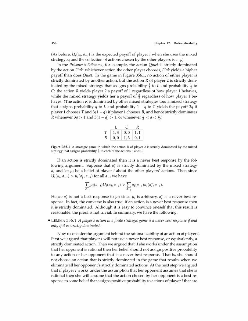
356 Chapter 12. Rationalizability
(As before, Ui(αi, a−i) is the expected payoff of player i when she uses the mixedstrategy αi and the collection of actions chosen by the other players is a−i.)
In the Prisoner’s Dilemma, for example, the action Quiet is strictly dominatedby the action Fink: whichever action the other player chooses, Fink yields a higherpayoff than does Quiet. In the game in Figure 356.1, no action of either player isstrictly dominated by another action, but the action R of player 2 is strictly dom-inated by the mixed strategy that assigns probability 1
2 to L and probability 12 to
C: the action R yields player 2 a payoff of 1 regardless of how player 1 behaves,while the mixed strategy yields her a payoff of 3
2 regardless of how player 1 be-haves. (The action R is dominated by other mixed strategies too: a mixed strategythat assigns probability q to L and probability 1 − q to C yields the payoff 3q ifplayer 1 chooses T and 3(1 − q) if player 1 chooses B, and hence strictly dominatesR whenever 3q > 1 and 3(1 − q) > 1, or whenever 1
3 < q < 23 .)
L C RT 1, 3 0, 0 1, 1B 0, 0 1, 3 0, 1
Figure 356.1 A strategic game in which the action R of player 2 is strictly dominated by the mixedstrategy that assigns probability 1
2 to each of the actions L and C.
If an action is strictly dominated then it is a never best response by the fol-lowing argument. Suppose that a∗i is strictly dominated by the mixed strategyαi and let µi be a belief of player i about the other players’ actions. Then sinceUi(αi, a−i) > ui(a∗i , a−i) for all a−i we have
∑a−i
µi(a−i)Ui(αi , a−i) > ∑a−i
µi(a−i)ui(a∗i , a−i).
Hence a∗i is not a best response to µi; since µi is arbitrary, a∗i is a never best re-sponse. In fact, the converse is also true: if an action is a never best response thenit is strictly dominated. Although it is easy to convince oneself that this result isreasonable, the proof is not trivial. In summary, we have the following.
LEMMA 356.1 A player’s action in a finite strategic game is a never best response if andonly if it is strictly dominated.
Now reconsider the argument behind the rationalizability of an action of player i.First we argued that player i will not use a never best response, or equivalently, astrictly dominated action. Then we argued that if she works under the assumptionthat her opponent is rational then her belief should not assign positive probabilityto any action of her opponent that is a never best response. That is, she shouldnot choose an action that is strictly dominated in the game that results when weeliminate all her opponent’s strictly dominated actions. At the next step we arguedthat if player i works under the assumption that her opponent assumes that she isrational then she will assume that the action chosen by her opponent is a best re-sponse to some belief that assigns positive probability to actions of player i that are
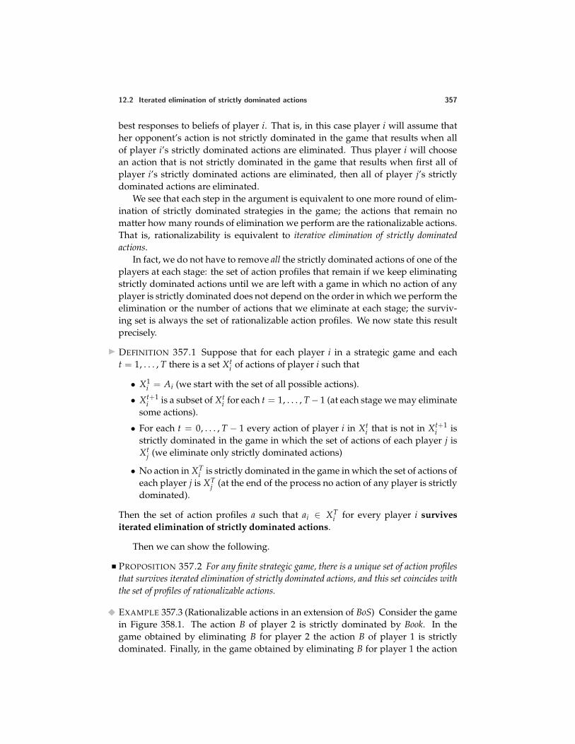
12.2 Iterated elimination of strictly dominated actions 357
best responses to beliefs of player i. That is, in this case player i will assume thather opponent’s action is not strictly dominated in the game that results when allof player i’s strictly dominated actions are eliminated. Thus player i will choosean action that is not strictly dominated in the game that results when first all ofplayer i’s strictly dominated actions are eliminated, then all of player j’s strictlydominated actions are eliminated.
We see that each step in the argument is equivalent to one more round of elim-ination of strictly dominated strategies in the game; the actions that remain nomatter how many rounds of elimination we perform are the rationalizable actions.That is, rationalizability is equivalent to iterative elimination of strictly dominatedactions.
In fact, we do not have to remove all the strictly dominated actions of one of theplayers at each stage: the set of action profiles that remain if we keep eliminatingstrictly dominated actions until we are left with a game in which no action of anyplayer is strictly dominated does not depend on the order in which we perform theelimination or the number of actions that we eliminate at each stage; the surviv-ing set is always the set of rationalizable action profiles. We now state this resultprecisely.
DEFINITION 357.1 Suppose that for each player i in a strategic game and eacht = 1, . . . , T there is a set Xt
i of actions of player i such that
• X1i = Ai (we start with the set of all possible actions).
• Xt+1i is a subset of Xt
i for each t = 1, . . . , T − 1 (at each stage we may eliminatesome actions).
• For each t = 0, . . . , T − 1 every action of player i in Xti that is not in Xt+1
i isstrictly dominated in the game in which the set of actions of each player j isXt
j (we eliminate only strictly dominated actions)
• No action in XTi is strictly dominated in the game in which the set of actions of
each player j is XTj (at the end of the process no action of any player is strictly
dominated).
Then the set of action profiles a such that ai ∈ XTi for every player i survives
iterated elimination of strictly dominated actions.
Then we can show the following.
PROPOSITION 357.2 For any finite strategic game, there is a unique set of action profilesthat survives iterated elimination of strictly dominated actions, and this set coincides withthe set of profiles of rationalizable actions.
EXAMPLE 357.3 (Rationalizable actions in an extension of BoS) Consider the gamein Figure 358.1. The action B of player 2 is strictly dominated by Book. In thegame obtained by eliminating B for player 2 the action B of player 1 is strictlydominated. Finally, in the game obtained by eliminating B for player 1 the action
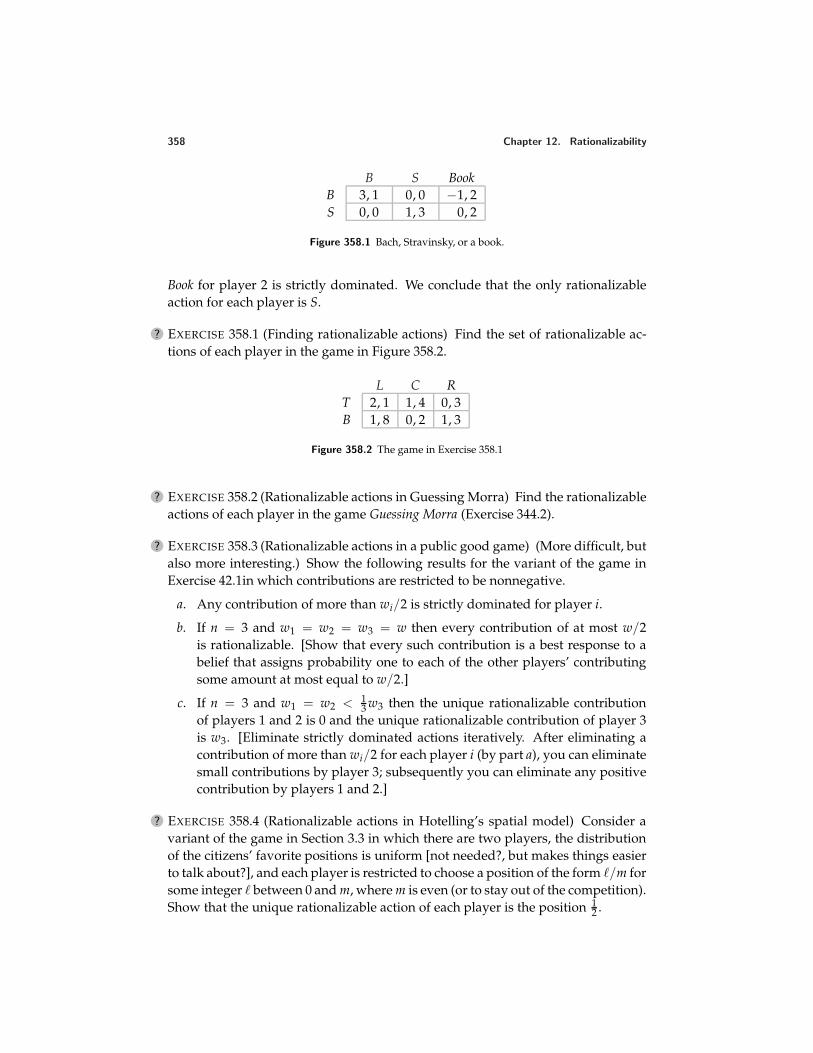
358 Chapter 12. Rationalizability
B S BookB 3, 1 0, 0 −1, 2S 0, 0 1, 3 0, 2
Figure 358.1 Bach, Stravinsky, or a book.
Book for player 2 is strictly dominated. We conclude that the only rationalizableaction for each player is S.
? EXERCISE 358.1 (Finding rationalizable actions) Find the set of rationalizable ac-tions of each player in the game in Figure 358.2.
L C RT 2, 1 1, 4 0, 3B 1, 8 0, 2 1, 3
Figure 358.2 The game in Exercise 358.1
? EXERCISE 358.2 (Rationalizable actions in Guessing Morra) Find the rationalizableactions of each player in the game Guessing Morra (Exercise 344.2).
? EXERCISE 358.3 (Rationalizable actions in a public good game) (More difficult, butalso more interesting.) Show the following results for the variant of the game inExercise 42.1in which contributions are restricted to be nonnegative.
a. Any contribution of more than wi/2 is strictly dominated for player i.
b. If n = 3 and w1 = w2 = w3 = w then every contribution of at most w/2is rationalizable. [Show that every such contribution is a best response to abelief that assigns probability one to each of the other players’ contributingsome amount at most equal to w/2.]
c. If n = 3 and w1 = w2 < 13 w3 then the unique rationalizable contribution
of players 1 and 2 is 0 and the unique rationalizable contribution of player 3is w3. [Eliminate strictly dominated actions iteratively. After eliminating acontribution of more than wi/2 for each player i (by part a), you can eliminatesmall contributions by player 3; subsequently you can eliminate any positivecontribution by players 1 and 2.]
? EXERCISE 358.4 (Rationalizable actions in Hotelling’s spatial model) Consider avariant of the game in Section 3.3 in which there are two players, the distributionof the citizens’ favorite positions is uniform [not needed?, but makes things easierto talk about?], and each player is restricted to choose a position of the form /m forsome integer between 0 and m, where m is even (or to stay out of the competition).Show that the unique rationalizable action of each player is the position 1
2 .
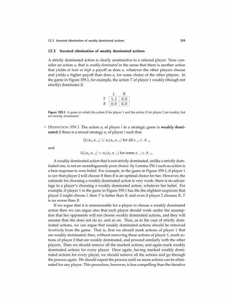
12.3 Iterated elimination of weakly dominated actions 359
12.3 Iterated elimination of weakly dominated actions
A strictly dominated action is clearly unattractive to a rational player. Now con-sider an action ai that is weakly dominated in the sense that there is another actionthat yields at least as high a payoff as does ai whatever the other players chooseand yields a higher payoff than does ai for some choice of the other players. Inthe game in Figure 359.1, for example, the action T of player 1 weakly (though notstrictly) dominates B.
L RT 1, 1 0, 0B 0, 0 0, 0
Figure 359.1 A game in which the action B for player 1 and the action R for player 2 are weakly, butnot strictly, dominated.
DEFINITION 359.1 The action ai of player i in a strategic game is weakly domi-nated if there is a mixed strategy αi of player i such that
Ui(αi, a−i) ≥ ui(ai, a−i) for all a−i ∈ A−i
andUi(αi, a−i) > ui(ai , a−i) for some a−i ∈ A−i.
A weakly dominated action that is not strictly dominated, unlike a strictly dom-inated one, is not an unambiguously poor choice: by Lemma 356.1 such an action isa best response to some belief. For example, in the game in Figure 359.1, if player 1is sure that player 2 will choose R then B is an optimal choice for her. However, therationale for choosing a weakly dominated action is very weak: there is no advan-tage to a player’s choosing a weakly dominated action, whatever her belief. Forexample, if player 1 in the game in Figure 359.1 has the the slightest suspicion thatplayer 2 might choose L then T is better than B, and even if player 2 chooses R, Tis no worse than B.
If we argue that it is unreasonable for a player to choose a weakly dominatedaction then we can argue also that each player should work under the assump-tion that her opponents will not choose weakly dominated actions, and they willassume that she does not do so, and so on. Thus, as in the case of strictly dom-inated actions, we can argue that weakly dominated actions should be removediteratively from the game. That is, first we should mark actions of player 1 thatare weakly dominated; then, without removing these actions of player 1, mark ac-tions of player 2 that are weakly dominated, and proceed similarly with the otherplayers. Then we should remove all the marked actions, and again mark weaklydominated actions for every player. Once again, having marked weakly domi-nated actions for every player, we should remove all the actions and go throughthe process again. We should repeat the process until no more actions can be elimi-nated for any player. This procedure, however, is less compelling than the iterative
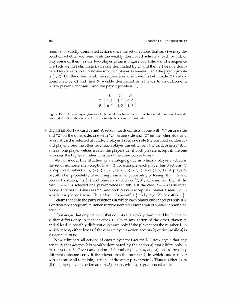
360 Chapter 12. Rationalizability
removal of strictly dominated actions since the set of actions that survive may de-pend on whether we remove all the weakly dominated actions at each round, oronly some of them, as the two-player game in Figure 360.1 shows. The sequencein which we first eliminate L (weakly dominated by C) and then T (weakly domi-nated by B) leads to an outcome in which player 1 chooses B and the payoff profileis (1, 2). On the other hand, the sequence in which we first eliminate R (weaklydominated by C) and then B (weakly dominated by T) leads to an outcome inwhich player 1 chooses T and the payoff profile is (1, 1).
L C RT 1, 1 1, 1 0, 0B 0, 0 1, 2 1, 2
Figure 360.1 A two-player game in which the set of actions that survive iterated elimination of weaklydominated actions depends on the order in which actions are eliminated.
EXAMPLE 360.1 (A card game) A set of n cards consists of one with “1” on one sideand “2” on the other side, one with “2” on one side and “3” on the other side, andso on. A card is selected at random; player 1 sees one side (determined randomly)and player 2 sees the other side. Each player can either veto the card, or accept it. Ifat least one player vetoes a card, the players tie; if both players accept it, the onewho sees the higher number wins (and the other player loses).
We can model this situation as a strategic game in which a player’s action isthe set of numbers she accepts. If n = 2, for example, each player has 8 actions: ∅
(accept no number), 1, 2, 3, 1, 2, 1, 3, 2, 3, and 1, 2, 3. A player’spayoff is her probability of winning minus her probability of losing. If n = 2 andplayer 1’s strategy is 3 and player 2’s action is 2, 3, for example, then if thecard 1 − −2 is selected one player vetoes it, while if the card 2 − −3 is selectedplayer 1 vetoes it if she sees “2” and both players accept it if player 1 sees “3”, inwhich case player 1 wins. Thus player 1’s payoff is 1
4 and player 2’s payoff is − 14 .
I claim that only the pairs of actions in which each player either accepts only n +1 or does not accept any number survive iterated elimination of weakly dominatedactions.
I first argue that any action ai that accepts 1 is weakly dominated by the actiona′i that differs only in that it vetoes 1. Given any action of the other player, aiand a′i lead to possibly different outcomes only if the player sees the number 1, inwhich case ai either loses (if the other player’s action accepts 2) or ties, while a′i isguaranteed to tie.
Now eliminate all actions of each player that accept 1. I now argue that anyaction ai that accepts 2 is weakly dominated by the action a′i that differs only inthat it vetoes 2. Given any action of the other player, ai and a′i lead to possiblydifferent outcomes only if the player sees the number 2, in which case ai neverwins, because all remaining actions of the other player veto 1. Thus ai either loses(if the other player’s action accepts 3) or ties, while a′i is guaranteed to tie.
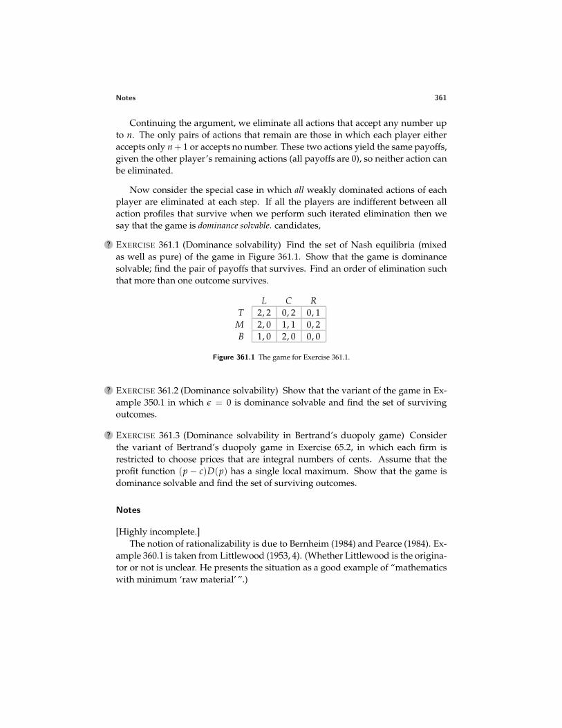
Notes 361
Continuing the argument, we eliminate all actions that accept any number upto n. The only pairs of actions that remain are those in which each player eitheraccepts only n + 1 or accepts no number. These two actions yield the same payoffs,given the other player’s remaining actions (all payoffs are 0), so neither action canbe eliminated.
Now consider the special case in which all weakly dominated actions of eachplayer are eliminated at each step. If all the players are indifferent between allaction profiles that survive when we perform such iterated elimination then wesay that the game is dominance solvable. candidates,
? EXERCISE 361.1 (Dominance solvability) Find the set of Nash equilibria (mixedas well as pure) of the game in Figure 361.1. Show that the game is dominancesolvable; find the pair of payoffs that survives. Find an order of elimination suchthat more than one outcome survives.
L C RT 2, 2 0, 2 0, 1
M 2, 0 1, 1 0, 2B 1, 0 2, 0 0, 0
Figure 361.1 The game for Exercise 361.1.
? EXERCISE 361.2 (Dominance solvability) Show that the variant of the game in Ex-ample 350.1 in which ε = 0 is dominance solvable and find the set of survivingoutcomes.
? EXERCISE 361.3 (Dominance solvability in Bertrand’s duopoly game) Considerthe variant of Bertrand’s duopoly game in Exercise 65.2, in which each firm isrestricted to choose prices that are integral numbers of cents. Assume that theprofit function (p − c)D(p) has a single local maximum. Show that the game isdominance solvable and find the set of surviving outcomes.
Notes
[Highly incomplete.]The notion of rationalizability is due to Bernheim (1984) and Pearce (1984). Ex-
ample 360.1 is taken from Littlewood (1953, 4). (Whether Littlewood is the origina-tor or not is unclear. He presents the situation as a good example of “mathematicswith minimum ‘raw material’ ”.)
Draft chapter from An introduction to game theory by Martin J. [email protected]; www.chass.utoronto.ca/~osborne
Version: 99/11/19.Copyright c© 1995–1999 by Martin J. Osborne. All rights reserved. No part of this book may bereproduced by any electronic or mechanical means (including photocopying, recording, or infor-mation storage and retrieval) without permission in writing from Oxford University Press, exceptthat one copy of up to six chapters may be made by any individual for private study.
13 Evolutionary equilibrium
Monomorphic pure strategy equilibrium · Mixed strategies and polymor-phic equilibrium · Asymmetric equilibria · Extensive games · Illustrations:sibling behavior; nesting behavior of wasps. Prerequisite: Chapters 2, 4,and 5.
13.1 Introduction
According to the Darwinian theory of evolution the modes of behavior thatsurvive are those that are most successful in producing offspring. In an envi-
ronment in which organisms interact, the reproductive success of a mode of behaviormay depend on the modes of behavior followed by all the organisms in the popula-tion. For example, if all organisms act aggressively, then an organism may be ableto survive only if it is aggressive; if all organisms are passive, then an organism’sreproductive success may be greater if the organism acts passively than if it actsaggressively. Game theory provides tools with which to study evolution in such anenvironment.
In the games studied in this chapter, the players are representatives from anevolving population of organisms (humans, animals, plants, bacteria, . . . ). Eachplayer’s payoffs measure the increments in the player’s biological fitness, or repro-ductive success (e.g. expected number of healthy offspring), associated with the pos-sible outcomes, rather than indicating the player’s subjective feelings about the out-comes. Each player’s actions are modes of behavior that the player is programmedto follow.
The players do not make conscious choices. Rather, each player’s mode of be-havior comes from one of two sources: with high probability it is inherited from theplayer’s parent (or parents), and with low (but positive) probability it is assigned tothe player as the result of a mutation. For most of the models in this chapter, inher-itance is conceived very simply: each player has a single parent, and, unless it is amutant, simply takes the same action as does its parent. This model of inheritancecaptures the essential features of both genetic inheritance and social inheritance:players either follow the programs encoded in their genes, which come from theirparents, or learn how to behave by imitating their parents. The distinction betweengenetic and social evolution may be significant if we wish to change society, but isinsignificant for most of the models considered in this chapter.
We choose each player’s set of actions to consist of all the modes of behavior that
279
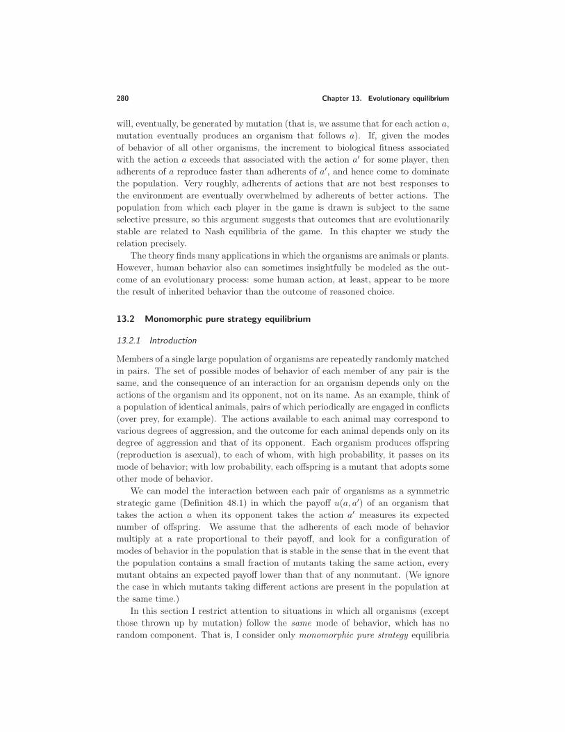
280 Chapter 13. Evolutionary equilibrium
will, eventually, be generated by mutation (that is, we assume that for each action a,mutation eventually produces an organism that follows a). If, given the modesof behavior of all other organisms, the increment to biological fitness associatedwith the action a exceeds that associated with the action a′ for some player, thenadherents of a reproduce faster than adherents of a′, and hence come to dominatethe population. Very roughly, adherents of actions that are not best responses tothe environment are eventually overwhelmed by adherents of better actions. Thepopulation from which each player in the game is drawn is subject to the sameselective pressure, so this argument suggests that outcomes that are evolutionarilystable are related to Nash equilibria of the game. In this chapter we study therelation precisely.
The theory finds many applications in which the organisms are animals or plants.However, human behavior also can sometimes insightfully be modeled as the out-come of an evolutionary process: some human action, at least, appear to be morethe result of inherited behavior than the outcome of reasoned choice.
13.2 Monomorphic pure strategy equilibrium
13.2.1 Introduction
Members of a single large population of organisms are repeatedly randomly matchedin pairs. The set of possible modes of behavior of each member of any pair is thesame, and the consequence of an interaction for an organism depends only on theactions of the organism and its opponent, not on its name. As an example, think ofa population of identical animals, pairs of which periodically are engaged in conflicts(over prey, for example). The actions available to each animal may correspond tovarious degrees of aggression, and the outcome for each animal depends only on itsdegree of aggression and that of its opponent. Each organism produces offspring(reproduction is asexual), to each of whom, with high probability, it passes on itsmode of behavior; with low probability, each offspring is a mutant that adopts someother mode of behavior.
We can model the interaction between each pair of organisms as a symmetricstrategic game (Definition 48.1) in which the payoff u(a, a′) of an organism thattakes the action a when its opponent takes the action a′ measures its expectednumber of offspring. We assume that the adherents of each mode of behaviormultiply at a rate proportional to their payoff, and look for a configuration ofmodes of behavior in the population that is stable in the sense that in the event thatthe population contains a small fraction of mutants taking the same action, everymutant obtains an expected payoff lower than that of any nonmutant. (We ignorethe case in which mutants taking different actions are present in the population atthe same time.)
In this section I restrict attention to situations in which all organisms (exceptthose thrown up by mutation) follow the same mode of behavior, which has norandom component. That is, I consider only monomorphic pure strategy equilibria
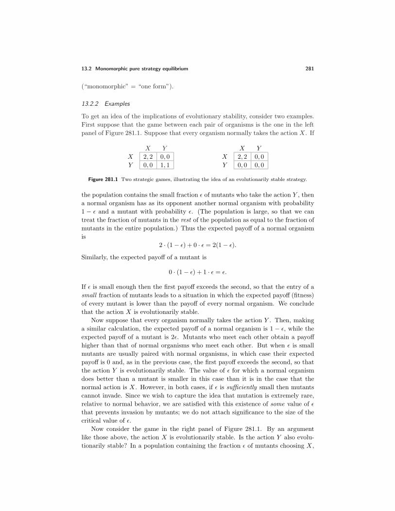
13.2 Monomorphic pure strategy equilibrium 281
(“monomorphic” = “one form”).
13.2.2 Examples
To get an idea of the implications of evolutionary stability, consider two examples.First suppose that the game between each pair of organisms is the one in the leftpanel of Figure 281.1. Suppose that every organism normally takes the action X . If
X Y
X 2, 2 0, 0Y 0, 0 1, 1
X Y
X 2, 2 0, 0Y 0, 0 0, 0
Figure 281.1 Two strategic games, illustrating the idea of an evolutionarily stable strategy.
the population contains the small fraction ε of mutants who take the action Y , thena normal organism has as its opponent another normal organism with probability1 − ε and a mutant with probability ε. (The population is large, so that we cantreat the fraction of mutants in the rest of the population as equal to the fraction ofmutants in the entire population.) Thus the expected payoff of a normal organismis
2 · (1− ε) + 0 · ε = 2(1− ε).
Similarly, the expected payoff of a mutant is
0 · (1− ε) + 1 · ε = ε.
If ε is small enough then the first payoff exceeds the second, so that the entry of asmall fraction of mutants leads to a situation in which the expected payoff (fitness)of every mutant is lower than the payoff of every normal organism. We concludethat the action X is evolutionarily stable.
Now suppose that every organism normally takes the action Y . Then, makinga similar calculation, the expected payoff of a normal organism is 1 − ε, while theexpected payoff of a mutant is 2ε. Mutants who meet each other obtain a payoffhigher than that of normal organisms who meet each other. But when ε is smallmutants are usually paired with normal organisms, in which case their expectedpayoff is 0 and, as in the previous case, the first payoff exceeds the second, so thatthe action Y is evolutionarily stable. The value of ε for which a normal organismdoes better than a mutant is smaller in this case than it is in the case that thenormal action is X . However, in both cases, if ε is sufficiently small then mutantscannot invade. Since we wish to capture the idea that mutation is extremely rare,relative to normal behavior, we are satisfied with this existence of some value of εthat prevents invasion by mutants; we do not attach significance to the size of thecritical value of ε.
Now consider the game in the right panel of Figure 281.1. By an argumentlike those above, the action X is evolutionarily stable. Is the action Y also evolu-tionarily stable? In a population containing the fraction ε of mutants choosing X ,
282 Chapter 13. Evolutionary equilibrium
the expected payoff of a normal organism is 0 (it obtains 0 whether its opponentis normal or a mutant) while the expected payoff of a mutant is 2ε (it obtains 2against another mutant and 0 against a normal organism). Thus the action Y isnot evolutionarily stable: for any value of ε the expected payoff of a mutant exceedsthat of a normal organism.
In both games, both (X,X) and (Y, Y ) are Nash equilibria, but while X is anevolutionarily stable action in both games, Y is evolutionarily stable only in theleft game. What is the essential difference between the games? If the normal actionis Y then in the left game a mutant who chooses X is worse off than a normalorganism in encounters with normal organisms, while in the right game a mutantthat chooses X obtains the same expected payoff as does a normal organism inencounters with normal organisms. In the left game, there is always a value of εsmall enough that the gain (relative to the payoff of a normal organism) that amutant obtains with probability ε when it faces another mutant does not cancel outthe loss it obtains with probability 1 − ε when it faces a normal organism. In theright game, however, a mutant loses nothing relative to a normal organism, so nomatter how small ε is, a mutant is better off than a normal organism. That is, theessential difference between the games is that u(X,Y ) < u(Y, Y ) in the left game,but u(X,Y ) = u(Y, Y ) in the right game.
13.2.3 General definitions
Consider now an arbitrary symmetric strategic game in which each player hasfinitely many actions. Under what circumstances is the action a∗ evolutionarilystable?
Suppose that a small group of mutants choosing the action b different from a∗
enters the population. The notion of stability that we consider requires that eachsuch mutant obtain an expected payoff less than that of each normal organism, sothat the mutants die out. (If the mutants obtained a payoff higher than that of thenormal organisms then they would eventually come to dominate the population; ifthey obtained the same payoff as that of the normal organisms then they wouldneither multiply nor decline. Our notion of stability excludes the latter case: it isa strong notion that requires that mutants be driven out of the population.)
Denote the fraction of mutants in the population by ε. First consider a mutant,which adopts the action b. In a random encounter, the probability that it facesan organism that adopts the action a∗ is approximately 1 − ε (the population islarge, so that the fraction in the rest of the population is close to the fraction inthe entire population), while the probability that it faces a mutant, which adoptsb, is approximately ε. Thus its expected payoff is
(1− ε)u(b, a∗) + εu(b, b).
Similarly, the expected payoff of an organism that adopts the action a∗ is
(1 − ε)u(a∗, a∗) + εu(a∗, b).
13.2 Monomorphic pure strategy equilibrium 283
In order that any mutation be driven out of the population, we need the expectedpayoff of any mutant to be less than the expected payoff of a normal organism:
(1 − ε)u(a∗, a∗) + εu(a∗, b) > (1− ε)u(b, a∗) + εu(b, b) for all b = a∗. (283.1)
To capture the idea that mutation is extremely rare, the notion of evolutionarystability requires only that there is some (small) number ε such that the inequalityholds whenever ε < ε. That is, we can make the following definition:
The action a∗ is evolutionarily stable if there exists ε > 0 such that a∗
satisfies (283.1) for all ε < ε.
Intuitively, the larger is ε, the “more stable” is the action a∗, since larger mutationsare resisted. However, in the current discussion we do not attach any significanceto the value of ε; in order that a∗ be evolutionarily stable we require only that thereis some size for ε such that all smaller mutations are resisted.
The condition in this definition of evolutionary stability is a little awkwardto work with, since whenever we apply it we need to check whether we can find asuitable value of ε. I now reformulate the condition in a way that avoids the variableε.
I first claim that
if there exists ε > 0 such that a∗ satisfies (283.1) for all ε < ε then(a∗, a∗) is a Nash equilibrium.
To reach this conclusion, suppose that (a∗, a∗) is not a Nash equilibrium. Then thereexists an action b such that u(b, a∗) > u(a∗, a∗). Hence (283.1) is strictly violatedwhen ε = 0, and thus remains violated for all sufficiently small positive values of ε.(If w < x and y and z are any numbers, then (1− ε)w+ εy < (1− ε)x+ εz wheneverε is small enough.) Thus there is no ε such that the inequality holds whenever ε < ε.Our conclusion is that a necessary condition for an action a∗ to be evolutionarilystable is that (a∗, a∗) be a Nash equilibrium.
Similar considerations lead to the conclusion that
if (a∗, a∗) is a strict Nash equilibrium then there exists ε > 0 such thata∗ satisfies (283.1) for all ε < ε.
The argument is that if (a∗, a∗) is a strict Nash equilibrium then u(b, a∗) < u(a∗, a∗)for all b, so that the strict inequality in (283.1) is satisfied for ε = 0; hence it isalso satisfied for sufficiently small positive values of ε. That is, we conclude thata sufficient condition for a∗ to be evolutionarily stable is that (a∗, a∗) be a strictNash equilibrium.
What happens if (a∗, a∗) is a Nash equilibrium, but is not strict? Suppose thatb = a∗ is a best response to a∗: u(b, a∗) = u(a∗, a∗). Then (283.1) reduces to thecondition u(a∗, b) > u(b, b), so that a∗ is evolutionarily stable if and only if thiscondition is satisfied.
284 Chapter 13. Evolutionary equilibrium
We conclude that necessary and sufficient conditions for the action a∗ to beevolutionarily stable are that (i) (a∗, a∗) is a Nash equilibrium, and (ii) u(a∗, b) >u(b, b) for every b = a∗ that is a best response to a∗. Intuitively, in order thatmutant behavior die out it must be that (i) no mutant does better than a∗ inencounters with organisms using a∗ and (ii) any mutant that does as well as a∗ insuch encounters must do worse than a∗ in encounters with mutants.
To summarize, the definition of evolutionary stability given above is equivalentto the following definition (which is much easier to work with).
Definition 284.1 An action a∗ of a player in a symmetric two-player game isevolutionarily stable with respect to mutants using pure strategies if
• (a∗, a∗) is a Nash equilibrium, and• u(b, b) < u(a∗, b) for every best response b to a∗ for which b = a∗,
where u is each player’s payoff function.
As I argued above, if (a∗, a∗) is a strict Nash equilibrium then a∗ is evolution-arily stable. This fact follows from the definition, since if (a∗, a∗) is a strict Nashequilibrium then the only best response to a∗ is a∗, so that the second condition inthe definition is vacuously satisfied.
Note that the inequality in the second condition is strict. If it were an equalitythen we would include as stable situations in which mutants neither multiply nordie out, but reproduce at the same rate as the normal population.
13.2.4 Examples
Both of the symmetric pure Nash equilibria of the left game in Figure 281.1 arestrict, so that both X and Y are evolutionarily stable (confirming our previousanalysis). In the right game in Figure 281.1, (X,X) and (Y, Y ) are symmetric pureNash equilibria also. But in this case (X,X) is strict while (Y, Y ) is not. Further,since u(X,X) > u(Y,X), the second condition in the definition of evolutionarystability is not satisfied by Y . Thus in this game only X is evolutionarily stable(again confirming our previous analysis).
The Prisoner’s Dilemma (Figure 13.1) has a unique symmetric Nash equilibrium(D,D), and this Nash equilibrium is strict. Thus the action D is the only evolu-tionarily stable action. The game BoS (Figure 16.1) has no symmetric pure Nashequilibrium, and hence no evolutionarily stable action. (I consider mixed strategiesin the next section.)
The following game, which generalizes the ideas on the game in Exercise 28.3,presents a richer range of possibilities for evolutionarily stable actions.
Example 284.2 (Hawk–Dove) Two animals of the same species compete for a re-source (e.g. food, or a good nesting site) whose value (in units of “fitness”) is v > 0.(That is, v measures the increase in the expected number of offspring brought bycontrol of the resource.) Each animal can be either aggressive or passive. If both
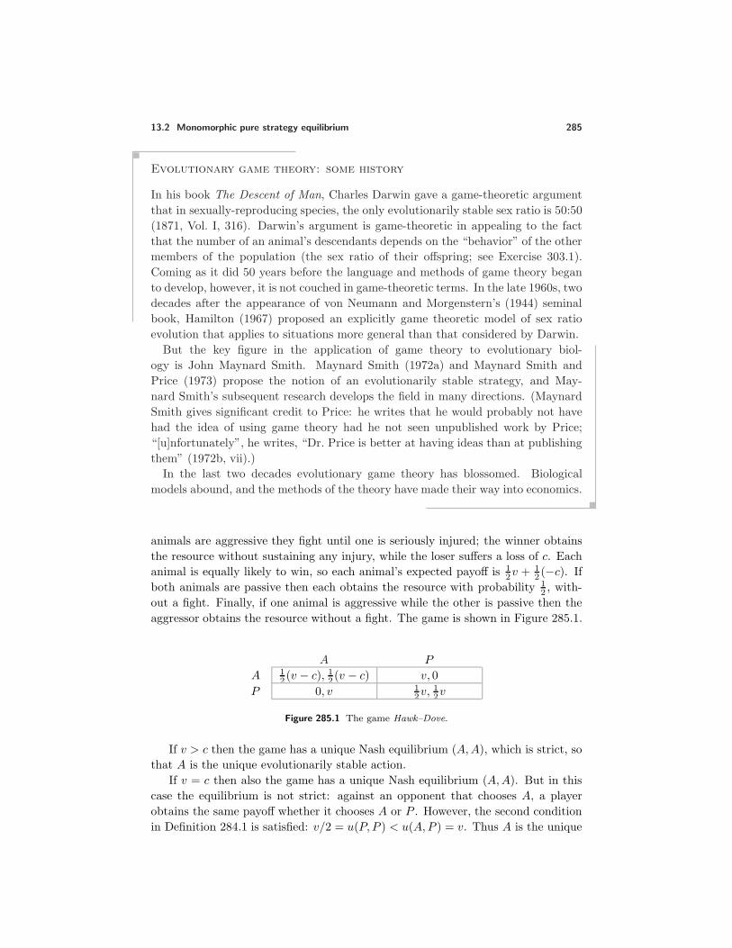
13.2 Monomorphic pure strategy equilibrium 285
Evolutionary game theory: some history
In his book The Descent of Man, Charles Darwin gave a game-theoretic argumentthat in sexually-reproducing species, the only evolutionarily stable sex ratio is 50:50(1871, Vol. I, 316). Darwin’s argument is game-theoretic in appealing to the factthat the number of an animal’s descendants depends on the “behavior” of the othermembers of the population (the sex ratio of their offspring; see Exercise 303.1).Coming as it did 50 years before the language and methods of game theory beganto develop, however, it is not couched in game-theoretic terms. In the late 1960s, twodecades after the appearance of von Neumann and Morgenstern’s (1944) seminalbook, Hamilton (1967) proposed an explicitly game theoretic model of sex ratioevolution that applies to situations more general than that considered by Darwin.But the key figure in the application of game theory to evolutionary biol-
ogy is John Maynard Smith. Maynard Smith (1972a) and Maynard Smith andPrice (1973) propose the notion of an evolutionarily stable strategy, and May-nard Smith’s subsequent research develops the field in many directions. (MaynardSmith gives significant credit to Price: he writes that he would probably not havehad the idea of using game theory had he not seen unpublished work by Price;“[u]nfortunately”, he writes, “Dr. Price is better at having ideas than at publishingthem” (1972b, vii).)In the last two decades evolutionary game theory has blossomed. Biological
models abound, and the methods of the theory have made their way into economics.
animals are aggressive they fight until one is seriously injured; the winner obtainsthe resource without sustaining any injury, while the loser suffers a loss of c. Eachanimal is equally likely to win, so each animal’s expected payoff is 1
2v +12 (−c). If
both animals are passive then each obtains the resource with probability 12 , with-
out a fight. Finally, if one animal is aggressive while the other is passive then theaggressor obtains the resource without a fight. The game is shown in Figure 285.1.
A P
A 12 (v − c), 1
2 (v − c) v, 0P 0, v 1
2v,12v
Figure 285.1 The game Hawk–Dove.
If v > c then the game has a unique Nash equilibrium (A,A), which is strict, sothat A is the unique evolutionarily stable action.
If v = c then also the game has a unique Nash equilibrium (A,A). But in thiscase the equilibrium is not strict: against an opponent that chooses A, a playerobtains the same payoff whether it chooses A or P . However, the second conditionin Definition 284.1 is satisfied: v/2 = u(P, P ) < u(A,P ) = v. Thus A is the unique
286 Chapter 13. Evolutionary equilibrium
evolutionarily stable action in this case also.In both of these cases, a population of passive players can be invaded by ag-
gressive players: an aggressive mutant does better than a passive player when itsopponent is passive, and at least as well as a passive player when its opponent isaggressive.
If v < c then the game has no symmetric Nash equilibrium in pure strategies:neither (A,A) nor (P, P ) is a Nash equilibrium. Thus in this case the game hasno evolutionarily stable action. (The game has only asymmetric Nash equilibria inthis case.)
? Exercise 286.1 (Evolutionary stability and weak domination) Let a∗ be an evolu-tionarily stable action. Does a∗ necessarily weakly dominate every other action? Isit possible that some other action weakly dominates a∗?
? Exercise 286.2 (Example of evolutionarily stable actions) Pairs of members ofa single population engage in the following game. Each player has three actions,corresponding to demands of 1, 2, or 3 units of payoff. If both players in a pairmake the same demand, each player obtains her demand. Otherwise the player whodemands less obtains the amount demanded by her opponent, while the player whodemands more obtains aδ, where a is her demand and δ is a number less than 1
3 .Find the set of pure strategy symmetric Nash equilibria of the game, and the setof pure evolutionarily stable strategies. What happens if each player has n actions,corresponding to demands of 1, 2, . . . , n units of payoff (and δ < 1/n)?
To gain an understanding of the outcome that evolutionary pressure might in-duce in games that have no evolutionarily stable action (e.g. BoS, and Hawk–Dovewhen v < c) we can take several routes. One is to consider mixed strategies as wellas pure strategies; another is to allow for the possibility of several types of behaviorcoexisting in the population; a third is to consider interpretations of the asymmetricequilibria. I begin by discussing the first two approaches; in the following section Iconsider the third approach.
13.3 Mixed strategies and polymorphic equilibrium
13.3.1 Definition
So far we have considered only situations in which both “normal” organisms andmutants use pure strategies. If we assume that mixed strategies, as well as purestrategies, are passed on from parents to offspring, and may be thrown up by mu-tation, then an argument analogous to the one in the previous section leads tothe conclusion that an evolutionarily stable mixed strategy satisfies conditions likethose in Definition 284.1. Precisely, we can define an evolutionarily stable (mixed)strategy, known briefly as an ESS, as follows.
Definition 286.3 An evolutionarily stable strategy (ESS) in a symmetrictwo-player game is a mixed strategy α∗ such that
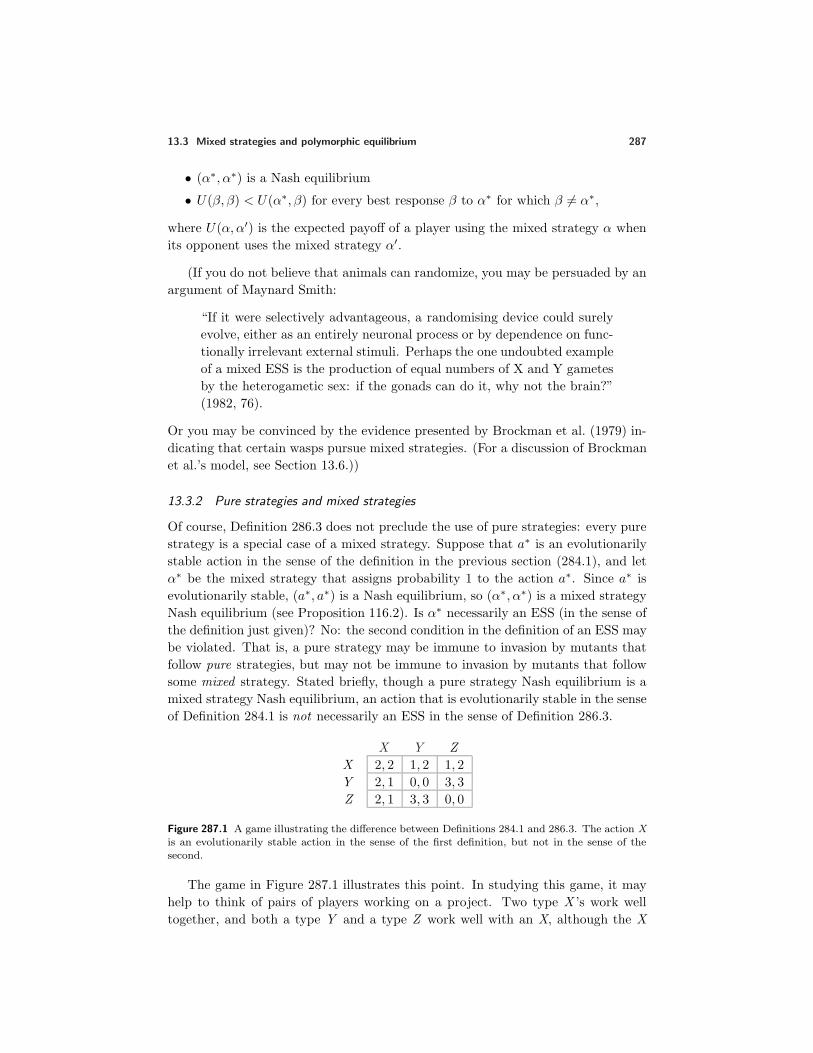
13.3 Mixed strategies and polymorphic equilibrium 287
• (α∗, α∗) is a Nash equilibrium
• U(β, β) < U(α∗, β) for every best response β to α∗ for which β = α∗,
where U(α, α′) is the expected payoff of a player using the mixed strategy α whenits opponent uses the mixed strategy α′.
(If you do not believe that animals can randomize, you may be persuaded by anargument of Maynard Smith:
“If it were selectively advantageous, a randomising device could surelyevolve, either as an entirely neuronal process or by dependence on func-tionally irrelevant external stimuli. Perhaps the one undoubted exampleof a mixed ESS is the production of equal numbers of X and Y gametesby the heterogametic sex: if the gonads can do it, why not the brain?”(1982, 76).
Or you may be convinced by the evidence presented by Brockman et al. (1979) in-dicating that certain wasps pursue mixed strategies. (For a discussion of Brockmanet al.’s model, see Section 13.6.))
13.3.2 Pure strategies and mixed strategies
Of course, Definition 286.3 does not preclude the use of pure strategies: every purestrategy is a special case of a mixed strategy. Suppose that a∗ is an evolutionarilystable action in the sense of the definition in the previous section (284.1), and letα∗ be the mixed strategy that assigns probability 1 to the action a∗. Since a∗ isevolutionarily stable, (a∗, a∗) is a Nash equilibrium, so (α∗, α∗) is a mixed strategyNash equilibrium (see Proposition 116.2). Is α∗ necessarily an ESS (in the sense ofthe definition just given)? No: the second condition in the definition of an ESS maybe violated. That is, a pure strategy may be immune to invasion by mutants thatfollow pure strategies, but may not be immune to invasion by mutants that followsome mixed strategy. Stated briefly, though a pure strategy Nash equilibrium is amixed strategy Nash equilibrium, an action that is evolutionarily stable in the senseof Definition 284.1 is not necessarily an ESS in the sense of Definition 286.3.
X Y ZX 2, 2 1, 2 1, 2Y 2, 1 0, 0 3, 3Z 2, 1 3, 3 0, 0
Figure 287.1 A game illustrating the difference between Definitions 284.1 and 286.3. The action Xis an evolutionarily stable action in the sense of the first definition, but not in the sense of thesecond.
The game in Figure 287.1 illustrates this point. In studying this game, it mayhelp to think of pairs of players working on a project. Two type X ’s work welltogether, and both a type Y and a type Z work well with an X, although the X
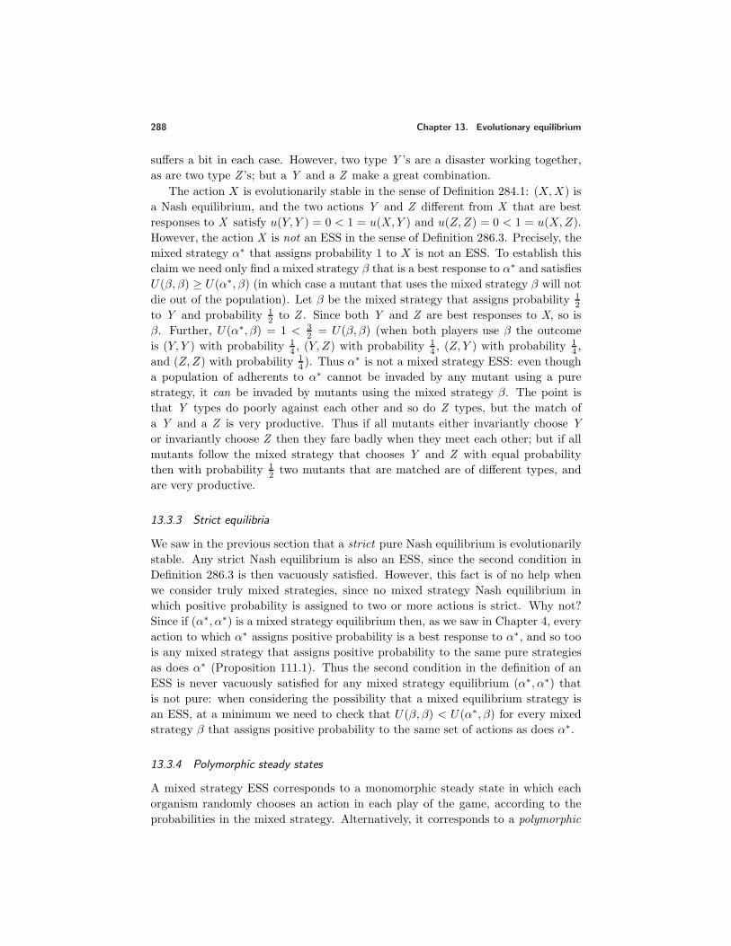
288 Chapter 13. Evolutionary equilibrium
suffers a bit in each case. However, two type Y ’s are a disaster working together,as are two type Z ’s; but a Y and a Z make a great combination.
The action X is evolutionarily stable in the sense of Definition 284.1: (X,X) isa Nash equilibrium, and the two actions Y and Z different from X that are bestresponses to X satisfy u(Y, Y ) = 0 < 1 = u(X,Y ) and u(Z,Z) = 0 < 1 = u(X,Z).However, the action X is not an ESS in the sense of Definition 286.3. Precisely, themixed strategy α∗ that assigns probability 1 to X is not an ESS. To establish thisclaim we need only find a mixed strategy β that is a best response to α∗ and satisfiesU(β, β) ≥ U(α∗, β) (in which case a mutant that uses the mixed strategy β will notdie out of the population). Let β be the mixed strategy that assigns probability 1
2
to Y and probability 12 to Z . Since both Y and Z are best responses to X, so is
β. Further, U(α∗, β) = 1 < 32 = U(β, β) (when both players use β the outcome
is (Y, Y ) with probability 14 , (Y, Z) with probability
14 , (Z, Y ) with probability
14 ,
and (Z,Z) with probability 14 ). Thus α
∗ is not a mixed strategy ESS: even thougha population of adherents to α∗ cannot be invaded by any mutant using a purestrategy, it can be invaded by mutants using the mixed strategy β. The point isthat Y types do poorly against each other and so do Z types, but the match ofa Y and a Z is very productive. Thus if all mutants either invariantly choose Yor invariantly choose Z then they fare badly when they meet each other; but if allmutants follow the mixed strategy that chooses Y and Z with equal probabilitythen with probability 1
2 two mutants that are matched are of different types, andare very productive.
13.3.3 Strict equilibria
We saw in the previous section that a strict pure Nash equilibrium is evolutionarilystable. Any strict Nash equilibrium is also an ESS, since the second condition inDefinition 286.3 is then vacuously satisfied. However, this fact is of no help whenwe consider truly mixed strategies, since no mixed strategy Nash equilibrium inwhich positive probability is assigned to two or more actions is strict. Why not?Since if (α∗, α∗) is a mixed strategy equilibrium then, as we saw in Chapter 4, everyaction to which α∗ assigns positive probability is a best response to α∗, and so toois any mixed strategy that assigns positive probability to the same pure strategiesas does α∗ (Proposition 111.1). Thus the second condition in the definition of anESS is never vacuously satisfied for any mixed strategy equilibrium (α∗, α∗) thatis not pure: when considering the possibility that a mixed equilibrium strategy isan ESS, at a minimum we need to check that U(β, β) < U(α∗, β) for every mixedstrategy β that assigns positive probability to the same set of actions as does α∗.
13.3.4 Polymorphic steady states
A mixed strategy ESS corresponds to a monomorphic steady state in which eachorganism randomly chooses an action in each play of the game, according to theprobabilities in the mixed strategy. Alternatively, it corresponds to a polymorphic
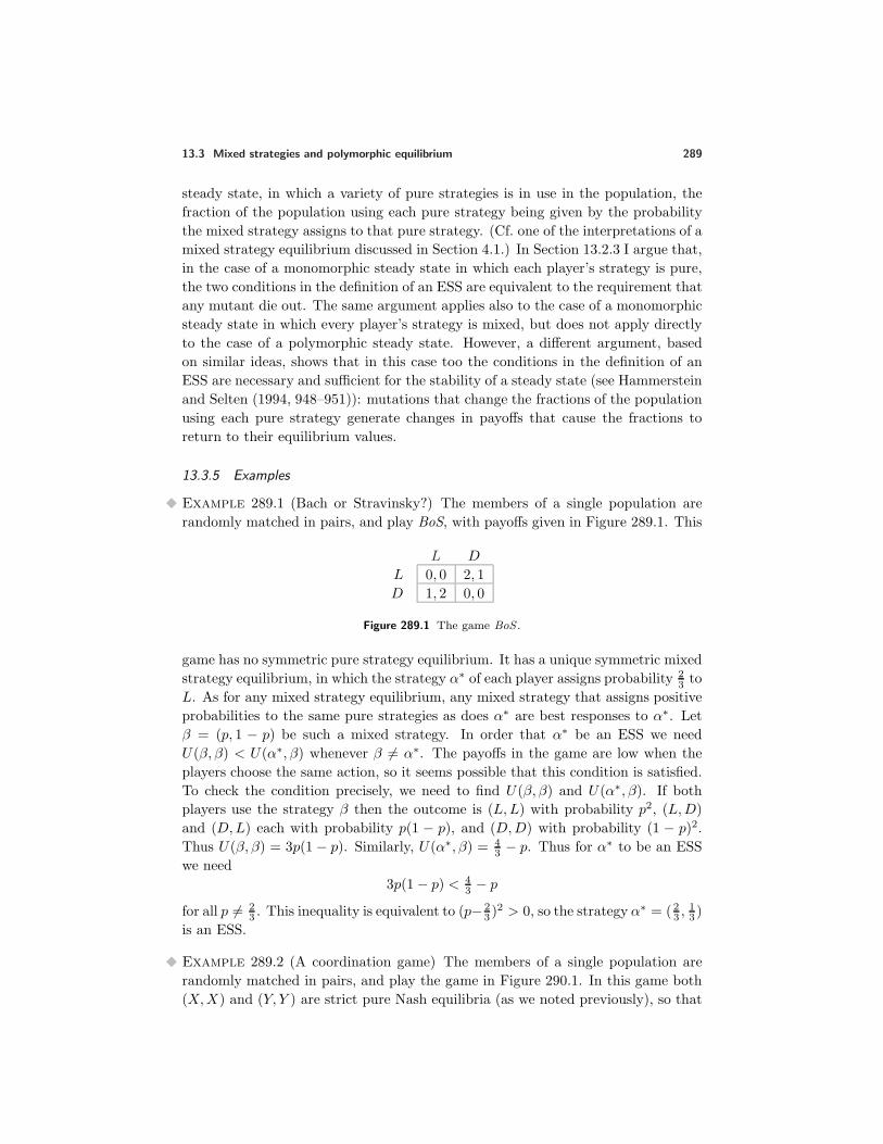
13.3 Mixed strategies and polymorphic equilibrium 289
steady state, in which a variety of pure strategies is in use in the population, thefraction of the population using each pure strategy being given by the probabilitythe mixed strategy assigns to that pure strategy. (Cf. one of the interpretations of amixed strategy equilibrium discussed in Section 4.1.) In Section 13.2.3 I argue that,in the case of a monomorphic steady state in which each player’s strategy is pure,the two conditions in the definition of an ESS are equivalent to the requirement thatany mutant die out. The same argument applies also to the case of a monomorphicsteady state in which every player’s strategy is mixed, but does not apply directlyto the case of a polymorphic steady state. However, a different argument, basedon similar ideas, shows that in this case too the conditions in the definition of anESS are necessary and sufficient for the stability of a steady state (see Hammersteinand Selten (1994, 948–951)): mutations that change the fractions of the populationusing each pure strategy generate changes in payoffs that cause the fractions toreturn to their equilibrium values.
13.3.5 Examples
Example 289.1 (Bach or Stravinsky?) The members of a single population arerandomly matched in pairs, and play BoS, with payoffs given in Figure 289.1. This
L D
L 0, 0 2, 1D 1, 2 0, 0
Figure 289.1 The game BoS .
game has no symmetric pure strategy equilibrium. It has a unique symmetric mixedstrategy equilibrium, in which the strategy α∗ of each player assigns probability 2
3 toL. As for any mixed strategy equilibrium, any mixed strategy that assigns positiveprobabilities to the same pure strategies as does α∗ are best responses to α∗. Letβ = (p, 1 − p) be such a mixed strategy. In order that α∗ be an ESS we needU(β, β) < U(α∗, β) whenever β = α∗. The payoffs in the game are low when theplayers choose the same action, so it seems possible that this condition is satisfied.To check the condition precisely, we need to find U(β, β) and U(α∗, β). If bothplayers use the strategy β then the outcome is (L,L) with probability p2, (L,D)and (D,L) each with probability p(1 − p), and (D,D) with probability (1 − p)2.Thus U(β, β) = 3p(1 − p). Similarly, U(α∗, β) = 4
3 − p. Thus for α∗ to be an ESSwe need
3p(1− p) < 43 − p
for all p = 23 . This inequality is equivalent to (p− 2
3 )2 > 0, so the strategy α∗ = (23 ,
13 )
is an ESS.
Example 289.2 (A coordination game) The members of a single population arerandomly matched in pairs, and play the game in Figure 290.1. In this game both(X,X) and (Y, Y ) are strict pure Nash equilibria (as we noted previously), so that
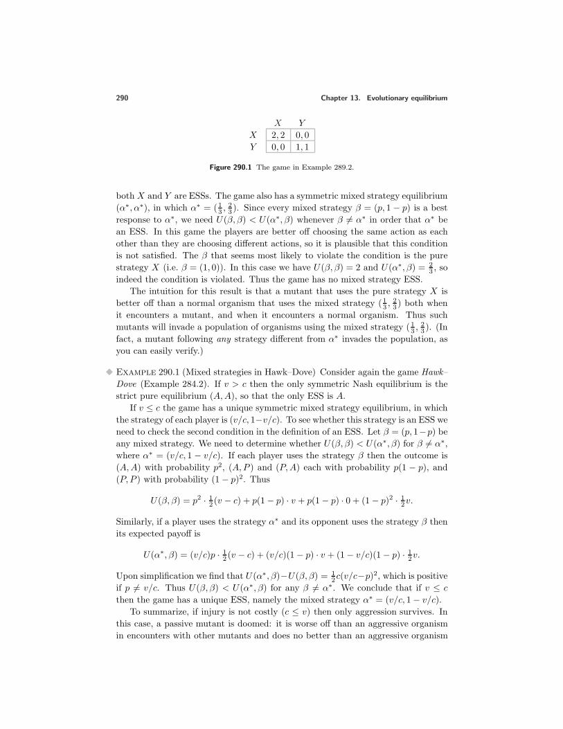
290 Chapter 13. Evolutionary equilibrium
X Y
X 2, 2 0, 0Y 0, 0 1, 1
Figure 290.1 The game in Example 289.2.
both X and Y are ESSs. The game also has a symmetric mixed strategy equilibrium(α∗, α∗), in which α∗ = (13 ,
23 ). Since every mixed strategy β = (p, 1 − p) is a best
response to α∗, we need U(β, β) < U(α∗, β) whenever β = α∗ in order that α∗ bean ESS. In this game the players are better off choosing the same action as eachother than they are choosing different actions, so it is plausible that this conditionis not satisfied. The β that seems most likely to violate the condition is the purestrategy X (i.e. β = (1, 0)). In this case we have U(β, β) = 2 and U(α∗, β) = 2
3 , soindeed the condition is violated. Thus the game has no mixed strategy ESS.
The intuition for this result is that a mutant that uses the pure strategy X isbetter off than a normal organism that uses the mixed strategy (13 ,
23 ) both when
it encounters a mutant, and when it encounters a normal organism. Thus suchmutants will invade a population of organisms using the mixed strategy (13 ,
23 ). (In
fact, a mutant following any strategy different from α∗ invades the population, asyou can easily verify.)
Example 290.1 (Mixed strategies in Hawk–Dove) Consider again the game Hawk–Dove (Example 284.2). If v > c then the only symmetric Nash equilibrium is thestrict pure equilibrium (A,A), so that the only ESS is A.
If v ≤ c the game has a unique symmetric mixed strategy equilibrium, in whichthe strategy of each player is (v/c, 1−v/c). To see whether this strategy is an ESS weneed to check the second condition in the definition of an ESS. Let β = (p, 1−p) beany mixed strategy. We need to determine whether U(β, β) < U(α∗, β) for β = α∗,where α∗ = (v/c, 1 − v/c). If each player uses the strategy β then the outcome is(A,A) with probability p2, (A,P ) and (P,A) each with probability p(1 − p), and(P, P ) with probability (1− p)2. Thus
U(β, β) = p2 · 12 (v − c) + p(1− p) · v + p(1− p) · 0 + (1− p)2 · 1
2v.
Similarly, if a player uses the strategy α∗ and its opponent uses the strategy β thenits expected payoff is
U(α∗, β) = (v/c)p · 12 (v − c) + (v/c)(1− p) · v + (1− v/c)(1− p) · 1
2v.
Upon simplification we find that U(α∗, β)−U(β, β) = 12c(v/c−p)2, which is positive
if p = v/c. Thus U(β, β) < U(α∗, β) for any β = α∗. We conclude that if v ≤ c
then the game has a unique ESS, namely the mixed strategy α∗ = (v/c, 1− v/c).To summarize, if injury is not costly (c ≤ v) then only aggression survives. In
this case, a passive mutant is doomed: it is worse off than an aggressive organismin encounters with other mutants and does no better than an aggressive organism
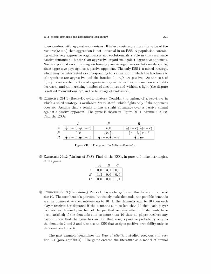
13.3 Mixed strategies and polymorphic equilibrium 291
in encounters with aggressive organisms. If injury costs more than the value of theresource (c > v) then aggression is not universal in an ESS. A population contain-ing exclusively aggressive organisms is not evolutionarily stable in this case, sincepassive mutants do better than aggressive organisms against aggressive opponent.Nor is a population containing exclusively passive organisms evolutionarily stable,since aggressive pays against a passive opponent. The only ESS is a mixed strategy,which may be interpreted as corresponding to a situation in which the fraction v/cof organisms are aggressive and the fraction 1 − v/c are passive. As the cost ofinjury increases the fraction of aggressive organisms declines; the incidence of fightsdecreases, and an increasing number of encounters end without a fight (the disputeis settled “conventionally”, in the language of biologists).
? Exercise 291.1 (Hawk–Dove–Retaliator) Consider the variant of Hawk–Dove inwhich a third strategy is available: “retaliator”, which fights only if the opponentdoes so. Assume that a retaliator has a slight advantage over a passive animalagainst a passive opponent. The game is shown in Figure 291.1; assume δ < 1
2v.Find the ESSs.
A P R
A 12 (v − c), 1
2 (v − c) v, 0 12 (v − c), 1
2 (v − c)P 0, v 1
2v,12v
12v − δ, 1
2v + δ
R 12 (v − c), 1
2 (v − c) 12v + δ, 1
2v − δ 12v,
12v
Figure 291.1 The game Hawk–Dove–Retaliator.
? Exercise 291.2 (Variant of BoS ) Find all the ESSs, in pure and mixed strategies,of the game
A B C
A 0, 0 3, 1 0, 0B 1, 3 0, 0 0, 0C 0, 0 0, 0 1, 1
? Exercise 291.3 (Bargaining) Pairs of players bargain over the division of a pie ofsize 10. The members of a pair simultaneously make demands; the possible demandsare the nonnegative even integers up to 10. If the demands sum to 10 then eachplayer receives her demand; if the demands sum to less than 10 then each playerreceives her demand plus half of the pie that remains after both demands havebeen satisfied; if the demands sum to more than 10 then no player receives anypayoff. Show that the game has an ESS that assigns positive probability only tothe demands 2 and 8 and also has an ESS that assigns positive probability only tothe demands 4 and 6.
The next example reexamines the War of attrition, studied previously in Sec-tion 3.4 (pure equilibria). The game entered the literature as a model of animal
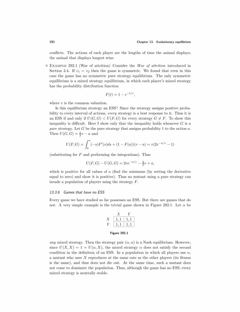
292 Chapter 13. Evolutionary equilibrium
conflicts. The actions of each player are the lengths of time the animal displays;the animal that displays longest wins.
Example 292.1 (War of attrition) Consider the War of attrition introduced inSection 3.4. If v1 = v2 then the game is symmetric. We found that even in thiscase the game has no symmetric pure strategy equilibrium. The only symmetricequilibrium is a mixed strategy equilibrium, in which each player’s mixed strategyhas the probability distribution function
F (t) = 1− e−t/v,
where v is the common valuation.Is this equilibrium strategy an ESS? Since the strategy assigns positive proba-
bility to every interval of actions, every strategy is a best response to it. Thus it isan ESS if and only if U(G,G) < U(F,G) for every strategy G = F . To show thisinequality is difficult. Here I show only that the inequality holds whenever G is apure strategy. Let G be the pure strategy that assigns probability 1 to the action a.Then U(G,G) = 1
2v − a and
U(F,G) =∫ a
0
(−s)F ′(s)ds+ (1− F (a))(v − a) = v(2e−a/v − 1)
(substituting for F and performing the integrations). Thus
U(F,G)− U(G,G) = 2ve−a/v − 32v + a,
which is positive for all values of a (find the minimum (by setting the derivativeequal to zero) and show it is positive). Thus no mutant using a pure strategy caninvade a population of players using the strategy F .
13.3.6 Games that have no ESS
Every game we have studied so far possesses an ESS. But there are games that donot. A very simple example is the trivial game shown in Figure 292.1. Let α be
X YX 1, 1 1, 1Y 1, 1 1, 1
Figure 292.1
any mixed strategy. Then the strategy pair (α, α) is a Nash equilibrium. However,since U(X,X) = 1 = U(α,X), the mixed strategy α does not satisfy the secondcondition in the definition of an ESS. In a population in which all players use α,a mutant who uses X reproduces at the same rate as the other players (its fitnessis the same), and thus does not die out. At the same time, such a mutant doesnot come to dominate the population. Thus, although the game has no ESS, everymixed strategy is neutrally stable.
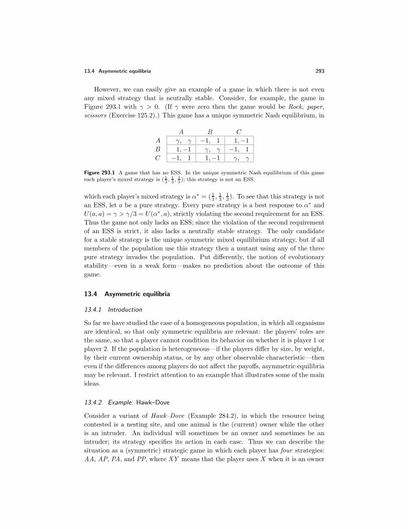
13.4 Asymmetric equilibria 293
However, we can easily give an example of a game in which there is not evenany mixed strategy that is neutrally stable. Consider, for example, the game inFigure 293.1 with γ > 0. (If γ were zero then the game would be Rock, paper,scissors (Exercise 125.2).) This game has a unique symmetric Nash equilibrium, in
A B C
A γ, γ −1, 1 1,−1B 1,−1 γ, γ −1, 1C −1, 1 1,−1 γ, γ
Figure 293.1 A game that has no ESS. In the unique symmetric Nash equilibrium of this gameeach player’s mixed strategy is ( 1
3, 1
3, 1
3); this strategy is not an ESS.
which each player’s mixed strategy is α∗ = (13 ,13 ,
13 ). To see that this strategy is not
an ESS, let a be a pure strategy. Every pure strategy is a best response to α∗ andU(a, a) = γ > γ/3 = U(α∗, a), strictly violating the second requirement for an ESS.Thus the game not only lacks an ESS; since the violation of the second requirementof an ESS is strict, it also lacks a neutrally stable strategy. The only candidatefor a stable strategy is the unique symmetric mixed equilibrium strategy, but if allmembers of the population use this strategy then a mutant using any of the threepure strategy invades the population. Put differently, the notion of evolutionarystability—even in a weak form—makes no prediction about the outcome of thisgame.
13.4 Asymmetric equilibria
13.4.1 Introduction
So far we have studied the case of a homogeneous population, in which all organismsare identical, so that only symmetric equilibria are relevant: the players’ roles arethe same, so that a player cannot condition its behavior on whether it is player 1 orplayer 2. If the population is heterogeneous—if the players differ by size, by weight,by their current ownership status, or by any other observable characteristic—theneven if the differences among players do not affect the payoffs, asymmetric equilibriamay be relevant. I restrict attention to an example that illustrates some of the mainideas.
13.4.2 Example: Hawk–Dove
Consider a variant of Hawk–Dove (Example 284.2), in which the resource beingcontested is a nesting site, and one animal is the (current) owner while the otheris an intruder. An individual will sometimes be an owner and sometimes be anintruder; its strategy specifies its action in each case. Thus we can describe thesituation as a (symmetric) strategic game in which each player has four strategies:AA, AP, PA, and PP, where XY means that the player uses X when it is an owner
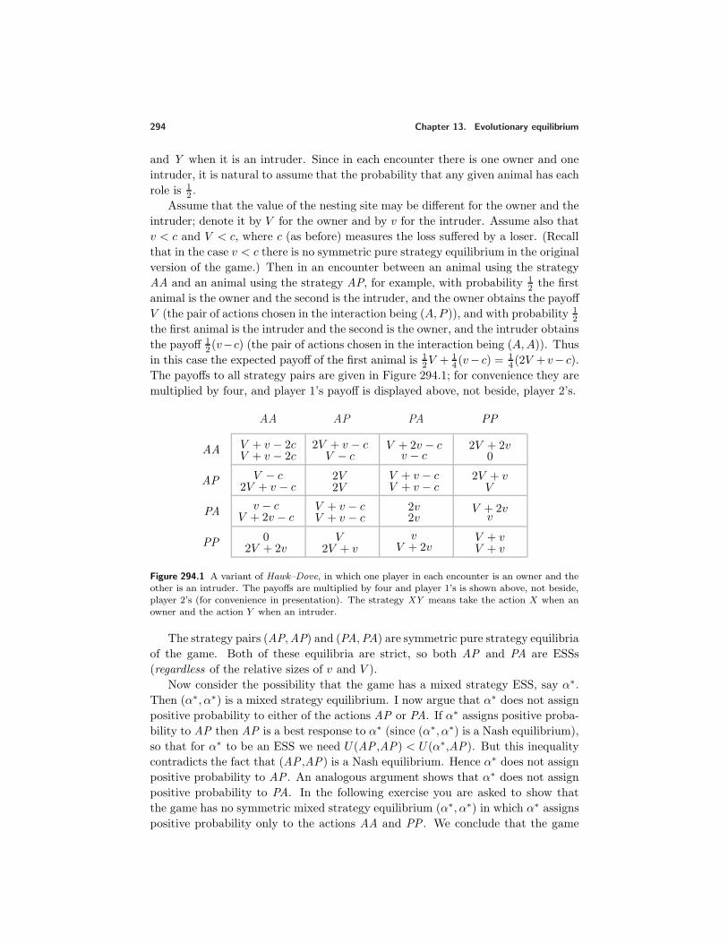
294 Chapter 13. Evolutionary equilibrium
and Y when it is an intruder. Since in each encounter there is one owner and oneintruder, it is natural to assume that the probability that any given animal has eachrole is 1
2 .Assume that the value of the nesting site may be different for the owner and the
intruder; denote it by V for the owner and by v for the intruder. Assume also thatv < c and V < c, where c (as before) measures the loss suffered by a loser. (Recallthat in the case v < c there is no symmetric pure strategy equilibrium in the originalversion of the game.) Then in an encounter between an animal using the strategyAA and an animal using the strategy AP, for example, with probability 1
2 the firstanimal is the owner and the second is the intruder, and the owner obtains the payoffV (the pair of actions chosen in the interaction being (A,P )), and with probability 1
2
the first animal is the intruder and the second is the owner, and the intruder obtainsthe payoff 1
2 (v−c) (the pair of actions chosen in the interaction being (A,A)). Thusin this case the expected payoff of the first animal is 1
2V +14 (v− c) = 1
4 (2V + v− c).The payoffs to all strategy pairs are given in Figure 294.1; for convenience they aremultiplied by four, and player 1’s payoff is displayed above, not beside, player 2’s.
AA AP PA PP
AA V + v − 2cV + v − 2c
2V + v − cV − c
V + 2v − cv − c
2V + 2v0
AP V − c2V + v − c
2V2V
V + v − cV + v − c
2V + vV
PA v − cV + 2v − c
V + v − cV + v − c
2v2v
V + 2vv
PP 02V + 2v
V2V + v
vV + 2v
V + vV + v
Figure 294.1 A variant of Hawk–Dove, in which one player in each encounter is an owner and theother is an intruder. The payoffs are multiplied by four and player 1’s is shown above, not beside,player 2’s (for convenience in presentation). The strategy XY means take the action X when anowner and the action Y when an intruder.
The strategy pairs (AP,AP) and (PA,PA) are symmetric pure strategy equilibriaof the game. Both of these equilibria are strict, so both AP and PA are ESSs(regardless of the relative sizes of v and V ).
Now consider the possibility that the game has a mixed strategy ESS, say α∗.Then (α∗, α∗) is a mixed strategy equilibrium. I now argue that α∗ does not assignpositive probability to either of the actions AP or PA. If α∗ assigns positive proba-bility to AP then AP is a best response to α∗ (since (α∗, α∗) is a Nash equilibrium),so that for α∗ to be an ESS we need U(AP ,AP) < U(α∗,AP). But this inequalitycontradicts the fact that (AP ,AP) is a Nash equilibrium. Hence α∗ does not assignpositive probability to AP . An analogous argument shows that α∗ does not assignpositive probability to PA. In the following exercise you are asked to show thatthe game has no symmetric mixed strategy equilibrium (α∗, α∗) in which α∗ assignspositive probability only to the actions AA and PP . We conclude that the game
13.4 Asymmetric equilibria 295
has no mixed ESS.
? Exercise 295.1 (Nash equilibrium in an asymmetric variant of Hawk–Dove) Letβ be a mixed strategy that assigns positive probability only to the actions AA andPP in the game in Figure 294.1. Show that in order that AA and PP yield a playerthe same expected payoff when her opponent uses the strategy β, we need β toassign probability (V + v)/2c to AA. Show further that when her opponent usesthis strategy β, a player obtains a higher expected payoff from the action AP thanshe does from the action AA, so that (β, β) is not a Nash equilibrium.
? Exercise 295.2 (ESSs and mixed strategy equilibria) Generalize the argument thatno ESS in the game in Figure 294.1 assigns positive probability to AP or to PA,to show the following result. Let (α∗, α∗) be a mixed strategy equilibrium; denotethe set of actions to which α∗ assigns positive probability by A∗. Then the onlystrategy assigning positive probability to every action in A∗ that can be an ESS isα∗.
In summary, this analysis of Hawk–Dove for the case in which v < c and V < c
leads to the conclusion that there are two evolutionarily stable strategies. In one,a player is aggressive when it is an owner and passive when it is an intruder, andin the other a player is passive when it is an owner and aggressive when it is anintruder. In both cases the dispute is resolved without a fight. The first strategy, inwhich an intruder concedes to an owner without a fight, is known as the bourgeoisstrategy; the second, in which the owner concedes to an intruder, is known as theparadoxical strategy. There are many examples in nature of the bourgeois strategy.The paradoxical strategy gets its name from the fact that it leads the members of apopulation to constantly change roles: whenever there is an encounter, the intruderbecomes the owner, and the owner becomes a potential intruder. One example ofthis convention is described in the box on p. 295.
Explaining the outcomes of contests in nature
[Note: this box is rough.] Hawk–Dove and its variants give us insights into the wayin which animal conflicts are resolved. Before the development of evolutionary gametheory, one explanation of the observation that conflicts are often settled withouta fight was that it is not in the interest of a species for its members to be killed orinjured. This theory is not explicit about how evolution could generate a situationin which individual members of a species act in a way that benefits the species asa whole. Further, by no means all animal conflicts are resolved peacefully, and thetheory has nothing to say about the conditions under which peaceful resolution islikely to be the norm. As we have seen, a game theoretic analysis in which the unit ofanalysis is the individual member of the species suggests that in a symmetric contestthe relation between the value of the resource under contention and the cost of anescalated contest determines the incidence of escalation. In an asymmetric contest
296 Chapter 13. Evolutionary equilibrium
the theory predicts that no escalation will occur, regardless of the value of theresource and the cost of injury. In particular, the convention that the owner alwayswins (the bourgeois strategy) is evolutionarily stable. (Classical theory appealed toan unexplained bias towards the owner, or to behavior that, in the context of thegame theoretic models, is not rational.)
Biologists have studied behavior in many species in order to determine whetherthe predictions of the theory correspond to observed outcomes. Maynard Smithmotivated his models by facts about conflicts between baboons. An example of morerecent work concerns the behavior of the funnel web spider Agelenopsis aperta inNew Mexico. Spiders differ in weight and web sites differ greatly in their desirability(some offer much more prey). At an average web site a confrontation usually endswithout a fight. If the weights of the owner and intruder are similar, the disputeis usually settled in favor of the owner; if the weights are significantly differentthen the heavier spider wins. Hammerstein and Riechert (1988) estimate from fieldobservations the fitness associated with various events and conclude that the ESSyields good predictions.
? Exercise 296.1 (Variant of BoS ) Members of a population are randomly matchedand play the game BoS . Each player in any given match can condition her actionon whether she was the first to suggest getting together. Assume that for any givenplayer the probability of being the first is one half. Find the ESSs of this game.
13.5 Variation on a theme: sibling behavior
The models of the previous sections are simple examples illustrating the main ideasof evolutionary game theory. In this section and the next I describe more detailedmodels that illustrate how these ideas may be applied in specific contexts.
Consider the interaction of siblings. The models in the previous sections as-sume that each player is equally likely to encounter any other player in the popu-lation. If we wish to study siblings’ behavior toward each other we need to modifythis assumption. I retain the other assumptions made previously: players interactpairwise, and payoffs measure fitness (reproductive success). I restrict attentionthroughout to pure strategies.
13.5.1 Asexual reproduction
The analysis in the previous sections rests on a simple model of reproduction, inwhich each organism, on its own, produces offspring. Before elaborating upon thismodel, consider its implications for the evolution of intrasibling behavior. Supposethat every organism in the population originally uses the action a∗ when interactingwith its siblings, obtaining the payoff u(a∗, a∗). If a mutant using the action b
appears, then, assuming that it has some offspring, all these offspring inherit thesame behavior (ignoring further mutations). Thus the payoff (fitness) of each of
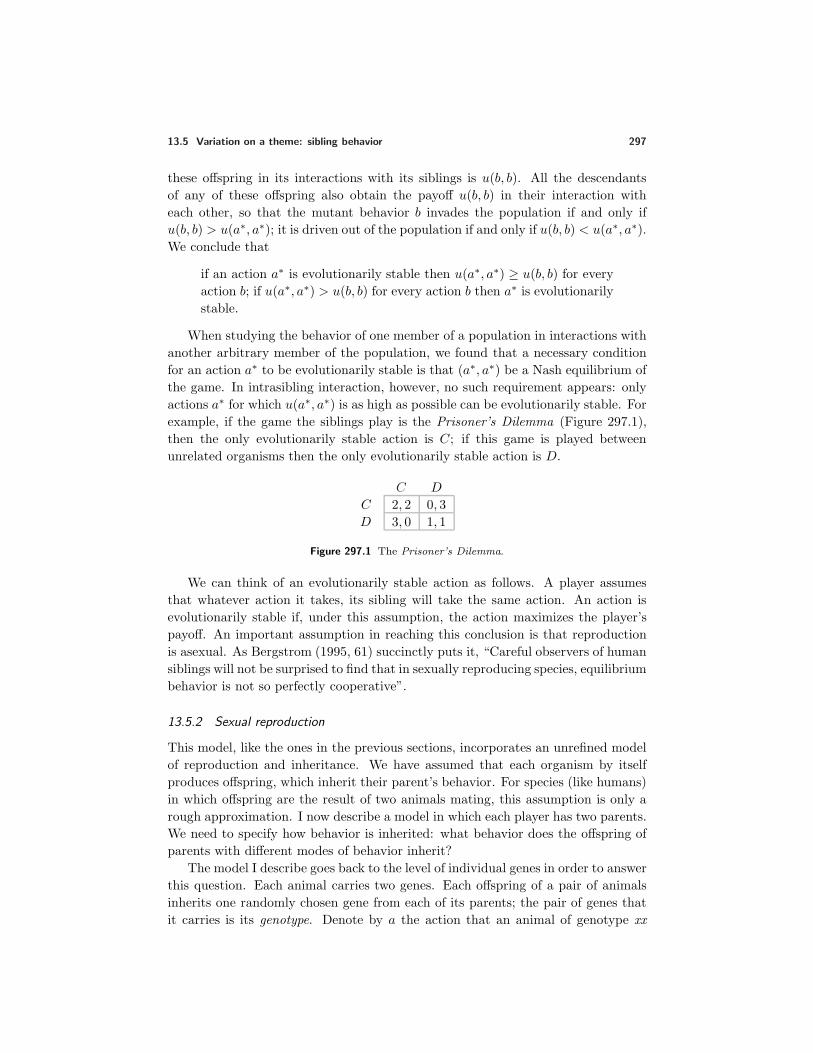
13.5 Variation on a theme: sibling behavior 297
these offspring in its interactions with its siblings is u(b, b). All the descendantsof any of these offspring also obtain the payoff u(b, b) in their interaction witheach other, so that the mutant behavior b invades the population if and only ifu(b, b) > u(a∗, a∗); it is driven out of the population if and only if u(b, b) < u(a∗, a∗).We conclude that
if an action a∗ is evolutionarily stable then u(a∗, a∗) ≥ u(b, b) for everyaction b; if u(a∗, a∗) > u(b, b) for every action b then a∗ is evolutionarilystable.
When studying the behavior of one member of a population in interactions withanother arbitrary member of the population, we found that a necessary conditionfor an action a∗ to be evolutionarily stable is that (a∗, a∗) be a Nash equilibrium ofthe game. In intrasibling interaction, however, no such requirement appears: onlyactions a∗ for which u(a∗, a∗) is as high as possible can be evolutionarily stable. Forexample, if the game the siblings play is the Prisoner’s Dilemma (Figure 297.1),then the only evolutionarily stable action is C; if this game is played betweenunrelated organisms then the only evolutionarily stable action is D.
C D
C 2, 2 0, 3D 3, 0 1, 1
Figure 297.1 The Prisoner’s Dilemma.
We can think of an evolutionarily stable action as follows. A player assumesthat whatever action it takes, its sibling will take the same action. An action isevolutionarily stable if, under this assumption, the action maximizes the player’spayoff. An important assumption in reaching this conclusion is that reproductionis asexual. As Bergstrom (1995, 61) succinctly puts it, “Careful observers of humansiblings will not be surprised to find that in sexually reproducing species, equilibriumbehavior is not so perfectly cooperative”.
13.5.2 Sexual reproduction
This model, like the ones in the previous sections, incorporates an unrefined modelof reproduction and inheritance. We have assumed that each organism by itselfproduces offspring, which inherit their parent’s behavior. For species (like humans)in which offspring are the result of two animals mating, this assumption is only arough approximation. I now describe a model in which each player has two parents.We need to specify how behavior is inherited: what behavior does the offspring ofparents with different modes of behavior inherit?
The model I describe goes back to the level of individual genes in order to answerthis question. Each animal carries two genes. Each offspring of a pair of animalsinherits one randomly chosen gene from each of its parents; the pair of genes thatit carries is its genotype. Denote by a the action that an animal of genotype xx
298 Chapter 13. Evolutionary equilibrium
(i.e. with two x genes) is programmed to take and denote by b the action that ananimal of genotype XX is programmed to take. Suppose that a = b, and that ananimal of genotype xx mates with an animal of genotype XX. All the offspring havegenotype Xx, and there are two possibilities for the action taken by these offspring:a and b. If the offspring are programmed to take the action b, we say that X isdominant and x is recessive, and if they are programmed to take the action a thenX is recessive and x is dominant.
Assume that all mating is monogamous: all siblings share the same two parents.Reproductive success depends on both parents’ characteristics; it simplifies thediscussion to assume that animals differ not in their fecundity, but in their chanceof surviving to adulthood (the age at which they start reproducing).
Under what circumstances is a population of animals of genotype xx, each choos-ing the action a∗, evolutionarily stable? Genes are now the basic unit of analysis,from which behavior is derived, so we need to consider whether any mutant gene,say X , can invade the population. That is, we need to consider the consequencesof an animal of genotype Xx being produced. There are two cases to consider: Xmay be dominant or recessive.
Invasion by dominant genes
First consider the case in which X is dominant. Denote the action taken by animalsof genotype XX and Xx by b, and assume that b = a∗. (If b = a∗ then the mutationis inconsequential for behavior.) Since almost all animals have genotype xx, almostevery mutant (of genotype Xx ) mates with an animal of genotype xx. Each of theoffspring of such a pair inherits an x gene from her xx parent, and a second genefrom her genotype Xx parent that is x with probability 1
2 and X with probability 12 .
Thus each offspring has genotype xx with probability 12 and genotype Xx with
probability 12 .
We now need to compare the payoffs of mutants and normal animals. We areassuming that the mutation is rare, so every mutant Xx has one Xx parent and onexx parent. Thus in its random matchings with its siblings, such a mutant faces anXx with probability 1
2 and an xx with probability12 . Hence its expected payoff is
12u(b, a
∗) + 12u(b, b).
Normal xx animals are present both in (“normal”) families with two xx parents andin families with one xx parent and one Xx parent; the vast majority are in normalfamilies. Thus to determine whether Xx ’s come to dominate the population we needto consider only the payoff (survival probability) of an Xx relative to that of an xxin a normal family. All the siblings of an xx in a normal family have genotype xx,and hence obtain the payoff
u(a∗, a∗).
We conclude that no dominant mutant gene can invade the population if
12u(b, a
∗) + 12u(b, b) < u(a∗, a∗) for every action b.
13.5 Variation on a theme: sibling behavior 299
Conversely, a dominant mutant gene can invade if the inequality is reversed for anyaction b.
If we define the function v by
v(b, a) = 12u(b, a) +
12u(b, b),
then, noting that v(a, a) = u(a, a) for any action a, we can rewrite the sufficientcondition for a∗ to be evolutionarily stable as
v(b, a∗) < v(a∗, a∗) for every action b.
That is, (a∗, a∗) is a strict Nash equilibrium of the game with payoff function v. Ifthe inequality is reversed for any action b then a∗ is not evolutionarily stable, sothat a necessary condition for a∗ to be evolutionarily stable is that (a∗, a∗) be aNash equilibrium of the game with payoff function v.
In summary, a sufficient condition for a∗ to be evolutionarily stable is that(a∗, a∗) be a strict Nash equilibrium of the game with payoff function v, in whicha player’s payoff is the average of its payoff in the original game and the payoff itobtains if its sibling mimics its behavior; a necessary condition is that (a∗, a∗) be aNash equilibrium of this game.
Invasion by recessive genes
Now consider the case in which X is recessive. An animal of genotype Xx choosethe same action a∗ as does an animal of genotype xx in this case. In a family inwhich one parent has genotype xx and the other has genotype Xx, half the offspringhave genotype xx and half have genotype Xx, and hence all take the action a∗ andreceive the payoff u(a∗, a∗) in interactions with each other. Thus on this accountthe X gene neither invades the population nor is eliminated from it. To determinethe fate of mutants, we need to consider the outcome of the interaction betweensiblings in families that constitute an even smaller fraction of the population.
The next smallest group of families are those in which the genotype of bothparents is Xx, in which case one fourth of the offspring have genotype XX . Supposethat an animal of genotype XX takes the action b = a∗. If, in interactions withits siblings, such an animal is more successful than animals of genotypes xx or Xxthen the mutant gene X , though starting from a very small base, can invade thepopulation.
In families with two Xx parents, the genotypes of the offspring are distributedas follows: one fourth are xx, one half are Xx, and one fourth are XX . To find theexpected payoff of an X gene in the offspring of such families, we need to considereach possible pair of siblings in turn. The analysis is somewhat complicated; I omitthe details. The conclusion is that the expected payoff to an X gene is
18u(b, b) +
18u(a
∗, b) + 38u(b, a
∗) + 38u(a
∗, a∗).
The expected payoff of the “normal” gene x (which initially dominates the popu-lation, in families in which both parents are xx ) is u(a∗, a∗), so the mutant gene
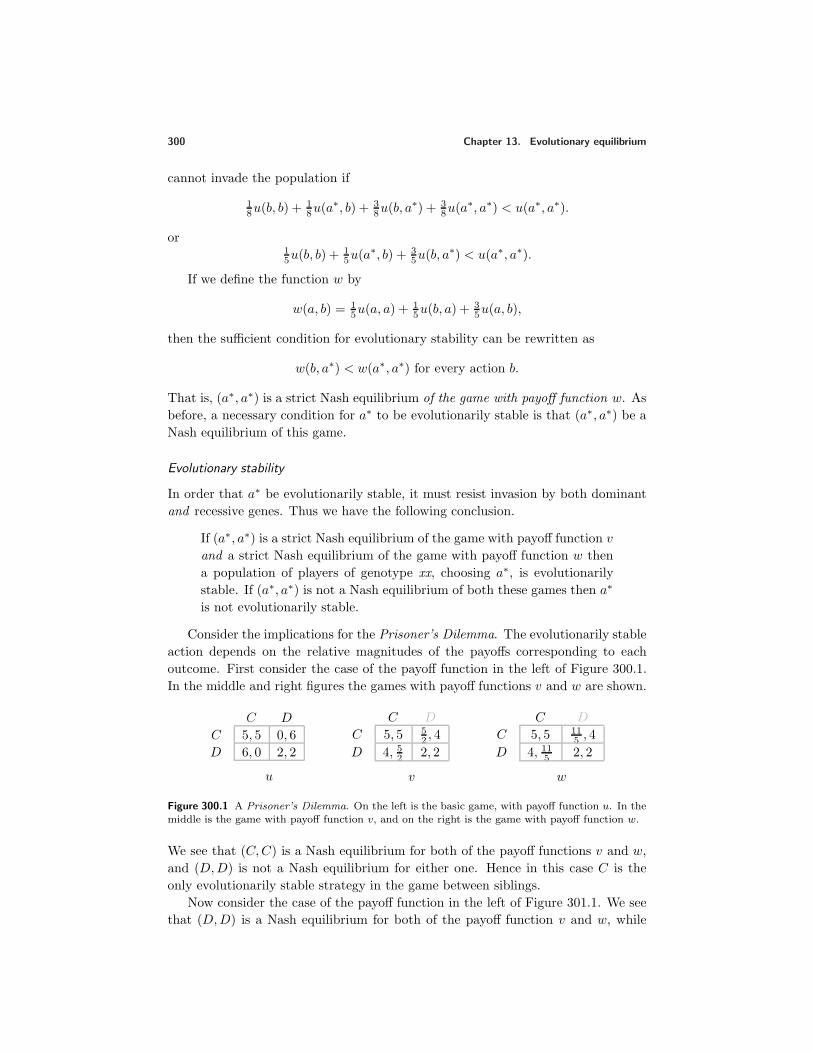
300 Chapter 13. Evolutionary equilibrium
cannot invade the population if
18u(b, b) +
18u(a
∗, b) + 38u(b, a
∗) + 38u(a
∗, a∗) < u(a∗, a∗).
or15u(b, b) +
15u(a
∗, b) + 35u(b, a
∗) < u(a∗, a∗).
If we define the function w by
w(a, b) = 15u(a, a) +
15u(b, a) +
35u(a, b),
then the sufficient condition for evolutionary stability can be rewritten as
w(b, a∗) < w(a∗, a∗) for every action b.
That is, (a∗, a∗) is a strict Nash equilibrium of the game with payoff function w. Asbefore, a necessary condition for a∗ to be evolutionarily stable is that (a∗, a∗) be aNash equilibrium of this game.
Evolutionary stability
In order that a∗ be evolutionarily stable, it must resist invasion by both dominantand recessive genes. Thus we have the following conclusion.
If (a∗, a∗) is a strict Nash equilibrium of the game with payoff function vand a strict Nash equilibrium of the game with payoff function w thena population of players of genotype xx, choosing a∗, is evolutionarilystable. If (a∗, a∗) is not a Nash equilibrium of both these games then a∗
is not evolutionarily stable.
Consider the implications for the Prisoner’s Dilemma. The evolutionarily stableaction depends on the relative magnitudes of the payoffs corresponding to eachoutcome. First consider the case of the payoff function in the left of Figure 300.1.In the middle and right figures the games with payoff functions v and w are shown.
C D
C 5, 5 0, 6D 6, 0 2, 2
u
C D
C 5, 5 52 , 4
D 4, 52 2, 2
v
C D
C 5, 5 115 , 4
D 4, 115 2, 2
w
Figure 300.1 A Prisoner’s Dilemma. On the left is the basic game, with payoff function u. In themiddle is the game with payoff function v, and on the right is the game with payoff function w.
We see that (C,C) is a Nash equilibrium for both of the payoff functions v and w,and (D,D) is not a Nash equilibrium for either one. Hence in this case C is theonly evolutionarily stable strategy in the game between siblings.
Now consider the case of the payoff function in the left of Figure 301.1. We seethat (D,D) is a Nash equilibrium for both of the payoff function v and w, while
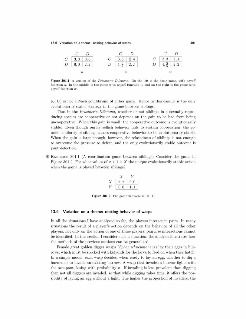
13.6 Variation on a theme: nesting behavior of wasps 301
C D
C 3, 3 0, 6D 6, 0 2, 2
u
C D
C 3, 3 32 , 4
D 4, 32 2, 2
v
C D
C 3, 3 95 , 4
D 4, 95 2, 2
w
Figure 301.1 A version of the Prisoner’s Dilemma. On the left is the basic game, with payofffunction u. In the middle is the game with payoff function v, and on the right is the game withpayoff function w.
(C,C) is not a Nash equilibrium of either game. Hence in this case D is the onlyevolutionarily stable strategy in the game between siblings.
Thus in the Prisoner’s Dilemma, whether or not siblings in a sexually repro-ducing species are cooperative or not depends on the gain to be had from beinguncooperative. When this gain is small, the cooperative outcome is evolutionarilystable. Even though purely selfish behavior fails to sustain cooperation, the ge-netic similarity of siblings causes cooperative behavior to be evolutionarily stable.When the gain is large enough, however, the relatedness of siblings is not enoughto overcome the pressure to defect, and the only evolutionarily stable outcome isjoint defection.
? Exercise 301.1 (A coordination game between siblings) Consider the game inFigure 301.2. For what values of x > 1 is X the unique evolutionarily stable actionwhen the game is played between siblings?
X Y
X x, x 0, 0Y 0, 0 1, 1
Figure 301.2 The game in Exercise 301.1.
13.6 Variation on a theme: nesting behavior of wasps
In all the situations I have analyzed so far, the players interact in pairs. In manysituations the result of a player’s action depends on the behavior of all the otherplayers, not only on the action of one of these players; pairwise interactions cannotbe identified. In this section I consider such a situation; the analysis illustrates howthe methods of the previous sections can be generalized.
Female great golden digger wasps (Sphex ichneumoneus) lay their eggs in bur-rows, which must be stocked with katydids for the larva to feed on when they hatch.In a simple model, each wasp decides, when ready to lay an egg, whether to dig aburrow or to invade an existing burrow. A wasp that invades a burrow fights withthe occupant, losing with probability π. If invading is less prevalent than diggingthen not all diggers are invaded, so that while digging takes time, it offers the pos-sibility of laying an egg without a fight. The higher the proportion of invaders, the
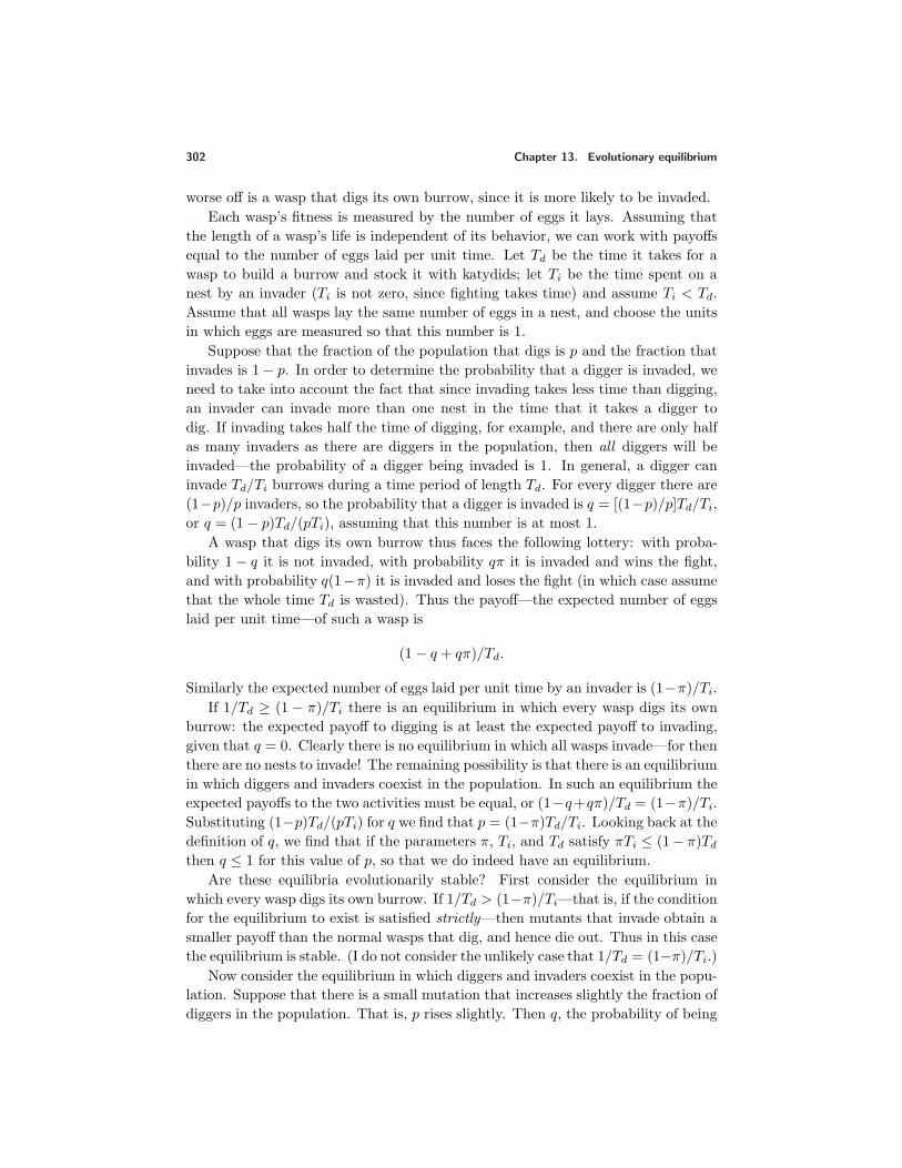
302 Chapter 13. Evolutionary equilibrium
worse off is a wasp that digs its own burrow, since it is more likely to be invaded.Each wasp’s fitness is measured by the number of eggs it lays. Assuming that
the length of a wasp’s life is independent of its behavior, we can work with payoffsequal to the number of eggs laid per unit time. Let Td be the time it takes for awasp to build a burrow and stock it with katydids; let Ti be the time spent on anest by an invader (Ti is not zero, since fighting takes time) and assume Ti < Td.Assume that all wasps lay the same number of eggs in a nest, and choose the unitsin which eggs are measured so that this number is 1.
Suppose that the fraction of the population that digs is p and the fraction thatinvades is 1− p. In order to determine the probability that a digger is invaded, weneed to take into account the fact that since invading takes less time than digging,an invader can invade more than one nest in the time that it takes a digger todig. If invading takes half the time of digging, for example, and there are only halfas many invaders as there are diggers in the population, then all diggers will beinvaded—the probability of a digger being invaded is 1. In general, a digger caninvade Td/Ti burrows during a time period of length Td. For every digger there are(1−p)/p invaders, so the probability that a digger is invaded is q = [(1−p)/p]Td/Ti,or q = (1 − p)Td/(pTi), assuming that this number is at most 1.
A wasp that digs its own burrow thus faces the following lottery: with proba-bility 1 − q it is not invaded, with probability qπ it is invaded and wins the fight,and with probability q(1−π) it is invaded and loses the fight (in which case assumethat the whole time Td is wasted). Thus the payoff—the expected number of eggslaid per unit time—of such a wasp is
(1 − q + qπ)/Td.
Similarly the expected number of eggs laid per unit time by an invader is (1−π)/Ti.If 1/Td ≥ (1 − π)/Ti there is an equilibrium in which every wasp digs its own
burrow: the expected payoff to digging is at least the expected payoff to invading,given that q = 0. Clearly there is no equilibrium in which all wasps invade—for thenthere are no nests to invade! The remaining possibility is that there is an equilibriumin which diggers and invaders coexist in the population. In such an equilibrium theexpected payoffs to the two activities must be equal, or (1−q+qπ)/Td = (1−π)/Ti.Substituting (1−p)Td/(pTi) for q we find that p = (1−π)Td/Ti. Looking back at thedefinition of q, we find that if the parameters π, Ti, and Td satisfy πTi ≤ (1− π)Td
then q ≤ 1 for this value of p, so that we do indeed have an equilibrium.Are these equilibria evolutionarily stable? First consider the equilibrium in
which every wasp digs its own burrow. If 1/Td > (1−π)/Ti—that is, if the conditionfor the equilibrium to exist is satisfied strictly—then mutants that invade obtain asmaller payoff than the normal wasps that dig, and hence die out. Thus in this casethe equilibrium is stable. (I do not consider the unlikely case that 1/Td = (1−π)/Ti.)
Now consider the equilibrium in which diggers and invaders coexist in the popu-lation. Suppose that there is a small mutation that increases slightly the fraction ofdiggers in the population. That is, p rises slightly. Then q, the probability of being
Notes 303
invaded, falls, and the expected payoff to digging increases; the expected payoffto invading does not change. Thus a slight increase in p leads to an increase inthe relative attractiveness of digging; diggers prosper relative to invaders, furtherincreasing the value of p. We conclude that the equilibrium is not evolutionarilystable.
The polymorphic equilibrium I have analyzed can alternatively be interpretedas a mixed strategy equilibrium, in which each individual wasp randomizes betweendigging and invading, choosing to dig with probability p. In the populations thatBrockmann et al. (1979) observe, digging and invading do coexist, and in factindividual wasps pursue mixed strategies—sometimes they dig and sometimes theyinvade. This evidence raises the question of how the model could be modified so thatthe mixed strategy equilibrium is evolutionarily stable. Brockman et al. suggest twosuch variants. In one case, for example, they assume that a wasp who digs a nest isbetter off if she is invaded and wins the fight than she is if she is not invaded (theinvader may have helped to stock the nest with katydids before it got into a fightwith the digger). The data Brockman et al. collected in one site generates a valueof p that fits their observations very well; the data from another site does not fitwell.
The following exercise illustrates another application of the main ideas of evo-lutionary game theory.
? Exercise 303.1 (Darwin’s theory of the sex ratio) A population of males and fe-males mate pairwise to produce offspring. Suppose that each offspring is male withprobability p and female with probability 1 − p. Then there is a steady state inwhich the fraction p of the population is male and the fraction 1 − p is female. Ifp = 1
2 then males and females have different numbers of offspring (on average). Issuch an equilibrium evolutionarily stable? Denote the number of children born toeach female by n, so that the number of children born to each male is (p/(1− p))n.Suppose a mutation occurs that produces boys and girls each with probability 1
2 .Assume for simplicity that the mutant trait is dominant: if one partner in a couplehas it, then all the offspring of the couple have it. Assume also that the number ofchildren produced by a female with the trait is n, the same as for “normal” mem-bers of the population. Since both normal and mutant females produce the samenumber of children, it might seem that the fitness of a mutant is the same as thatof a normal organism. But compare the number of grandchildren of mutants andnormal organisms. How many female offspring does a normal organism produce?How many male offspring? Use your answers to find the number of grandchildrenborn to each mutant and to each normal organism. Does the mutant invade thepopulation? Which value (values?) of p is evolutionarily stable?
Notes
[Incomplete.]The main ideas in this chapter are due to Maynard Smith.
304 Chapter 13. Evolutionary equilibrium
The chapter draws on the expositions of Hammerstein and Selten (1994) andvan Damme (1987, Chapter 9).
Darwin’s theory of sex ratio evolution (see the box on page 285) was indepen-dently discovered by Ronald A. Fisher (1930, 141–143), and is often referred to as“Fisher’s theory”. In the second edition of Darwin’s book (1874, 256), he retractedhis theory for reasons that are not apparent, and Fisher appears to have been awareonly of the retraction, not of the original theory. Bulmer (1994, 207–208) appearsto have been the first to notice that “Fisher’s theory” was given by Darwin.
Hawk–Dove (Example 284.2) is due to Maynard Smith and Price (1973).The discussion in Section 13.4 is based on van Damme (1987, Section 9.5).Exercise 295.2 is a slightly less general version of Lemma 9.2.4 of van Damme (1987).The material in Section 13.5 is taken from Bergstrom (1995).The model in Section 13.6 is taken from Brockmann, Grafen, and Dawkins (1979),
simplified along the lines of Bergstrom and Varian (1987, 324–327).
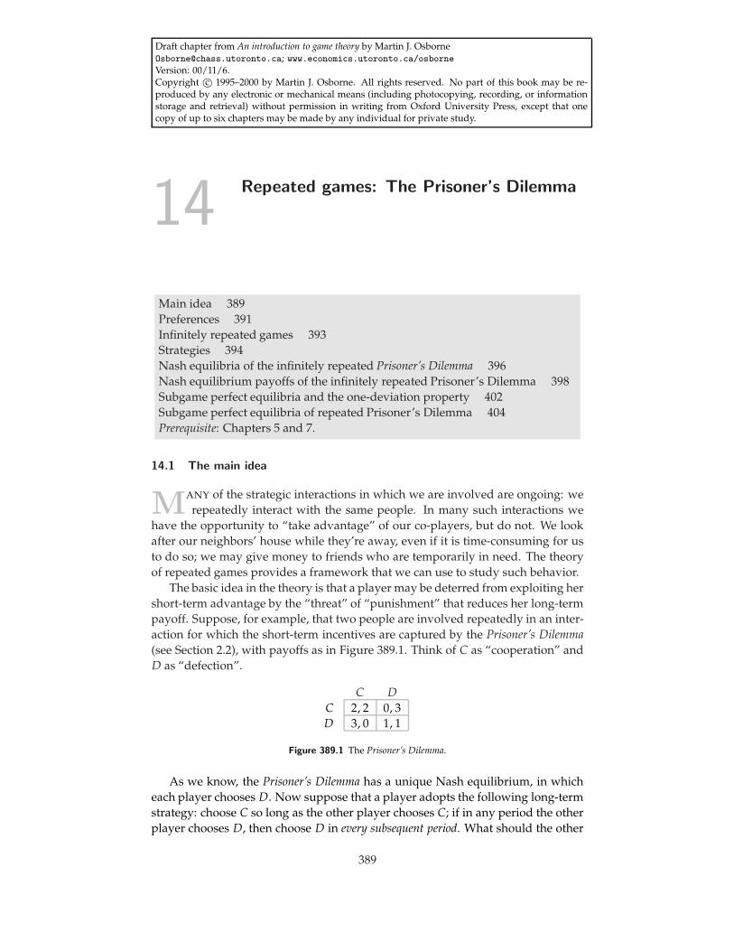
Draft chapter from An introduction to game theory by Martin J. [email protected]; www.economics.utoronto.ca/osborneVersion: 00/11/6.Copyright c© 1995–2000 by Martin J. Osborne. All rights reserved. No part of this book may be re-produced by any electronic or mechanical means (including photocopying, recording, or informationstorage and retrieval) without permission in writing from Oxford University Press, except that onecopy of up to six chapters may be made by any individual for private study.
14 Repeated games: The Prisoner’s Dilemma
Main idea 389Preferences 391Infinitely repeated games 393Strategies 394Nash equilibria of the infinitely repeated Prisoner’s Dilemma 396Nash equilibrium payoffs of the infinitely repeated Prisoner’s Dilemma 398Subgame perfect equilibria and the one-deviation property 402Subgame perfect equilibria of repeated Prisoner’s Dilemma 404Prerequisite: Chapters 5 and 7.
14.1 The main idea
MANY of the strategic interactions in which we are involved are ongoing: werepeatedly interact with the same people. In many such interactions we
have the opportunity to “take advantage” of our co-players, but do not. We lookafter our neighbors’ house while they’re away, even if it is time-consuming for usto do so; we may give money to friends who are temporarily in need. The theoryof repeated games provides a framework that we can use to study such behavior.
The basic idea in the theory is that a player may be deterred from exploiting hershort-term advantage by the “threat” of “punishment” that reduces her long-termpayoff. Suppose, for example, that two people are involved repeatedly in an inter-action for which the short-term incentives are captured by the Prisoner’s Dilemma(see Section 2.2), with payoffs as in Figure 389.1. Think of C as “cooperation” andD as “defection”.
C DC 2, 2 0, 3D 3, 0 1, 1
Figure 389.1 The Prisoner’s Dilemma.
As we know, the Prisoner’s Dilemma has a unique Nash equilibrium, in whicheach player chooses D. Now suppose that a player adopts the following long-termstrategy: choose C so long as the other player chooses C; if in any period the otherplayer chooses D, then choose D in every subsequent period. What should the other
389
390 Chapter 14. Repeated games: The Prisoner’s Dilemma
player do? If she chooses C in every period then the outcome is (C, C) in everyperiod and she obtains a payoff of 2 in every period. If she switches to D in someperiod then she obtains a payoff of 3 in that period and a payoff of 1 in everysubsequent period. She may value the present more highly than the future—shemay be impatient—but as long as the value she attaches to future payoffs is nottoo small compared with the value she attaches to her current payoff, the streamof payoffs (3, 1, 1, . . .) is worse for her than the stream (2, 2, 2, . . .), so that she isbetter off choosing C in every period.
This argument shows that if a player is sufficiently patient, the strategy thatchooses C after every history is a best response to the strategy that starts off choos-ing C and “punishes” any defection by switching to D. Clearly another best re-sponse is this same punishment strategy: if your opponent is using this punish-ment strategy then the outcome is the same if you use the strategy that chooses Cafter every history, or the same punishment strategy as your opponent is using. Inboth cases, the outcome in every period is (C, C) (the other player never defects,so if you use the punishment strategy you are never induced to switch to punish-ment). Thus the strategy pair in which both players use the punishment strategy isa Nash equilibrium of the game: neither player can do better by adopting anotherlong-term strategy.
The conclusion that the repeated Prisoner’s Dilemma has a Nash equilibriumin which the outcome is (C, C) in every period accords with our intuition that inlong-term relationships there is scope for mutually supportive strategies that donot relentlessly exploit short-term gain. However, this strategy pair is not the onlyNash equilibrium of the game. Another Nash equilibrium is the strategy pair inwhich each player chooses D after every history: if one player adopts this strategythen the other player can do no better than to adopt the strategy herself, regardlessof how she values the future, since whatever she does has no effect on the otherplayer’s behavior.
This analysis leaves open many questions.
• We have seen that the outcome in which (C, C) occurs in every period is sup-ported as a Nash equilibrium if the players are sufficiently patient. Exactlyhow patient do they have to be?
• We have seen also that the outcome in which (D, D) occurs in every periodis supported as a Nash equilibrium. What other outcomes are supported?
• We saw in Chapter 5 that Nash equilibria of extensive games are not alwaysintuitively appealing, since the actions they prescribe after histories that re-sult from deviations may not be optimal. The notion of subgame perfectequilibrium, which requires actions to be optimal after every possible his-tory, not only those that are reached if the players adhere to their strategies,may be more appealing. Is the strategy pair in which each player uses thepunishment strategy I have described a subgame perfect equilibrium? Thatis, is it optimal for each player to punish the other player for deviating? If
14.2 Preferences 391
not, is there any other strategy pair that supports desirable outcomes and isa subgame perfect equilibrium?
• The punishment strategy studied above is rather severe; in switching per-manently to D in response to a deviation it leaves no room for error. Arethere any Nash equilibria or subgame perfect equilibria in which the players’strategies punish deviations less severely?
• The arguments above are restricted to the Prisoner’s Dilemma. To what othergames do they apply?
I now formulate the model of a repeated game more precisely in order to answerthese questions.
14.2 Preferences
14.2.1 Discounting
The outcome of a repeated game is a sequence of outcomes of a strategic game.How does each player evaluate such sequences? I assume that she associates apayoff with each outcome of the strategic game, and evaluates each sequence ofoutcomes by the discounted sum of the associated sequence of payoffs. More pre-cisely, each player i has a payoff function ui for the strategic game and a discountfactor δ between 0 and 1 such that she evaluates the sequence (a1, a2, . . . , aT) ofoutcomes of the strategic game by the sum
ui(a1) + δui(a2) + δ2ui(a3) + · · · + δT−1ui(aT) =T
∑t=1
δt−1ui(at).
(Note that in this expression superscripts are used for two purposes: at is the ac-tion profile in period t, while δt is the discount factor δ raised to the power t.)I assume throughout that all players have the same discount factor δ. A playerwhose discount factor is close to zero cares very little about the future—she is veryimpatient; a player whose discount factor is close to one is very patient.
Why should a person value future payoffs less than current ones? Possibly sheis simply impatient. Or, possibly, her underlying preferences do not display impa-tience, but in comparing streams of outcomes she takes into account the positiveprobability with which she may die in any given period.1 Or, if the outcome in eachperiod involves the payment to her of some amount of money, possibly impatienceis induced by the fact that she can borrow and lend at a positive interest rate. Forexample, suppose her underlying preferences over streams of monetary payoffsdo not display impatience. Then if she can borrow and lend at the interest rate rshe is indifferent between the sequence ($100, $100, 0, 0, . . .) of amounts of money
1Alternatively, the hazard of death may have favored those who reproduce early, leading to theevolution of people who are “impatient”.
392 Chapter 14. Repeated games: The Prisoner’s Dilemma
and the sequence ($100 + $100/(1 + r), 0, 0, . . .), since by lending $100/(1 + r) ofthe amount she obtains in the first period she obtains $100 in the second period.In fact, under these assumptions her preferences are represented precisely by thediscounted sum of her payoffs with a discount factor of 1/(1 + r): any stream canbe obtained from any other stream with the same discounted sum by borrowingand lending. (If you win one of the North American lotteries that promises $1myou will quickly learn about discounted values: you will receive a stream of 20yearly payments each of $50,000, which at an interest rate of 7% is equivalent toreceiving about $567,000 as a lump sum.)
Obviously the assumption that everyone’s preferences over sequences of out-comes are represented by a discounted sum of payoffs is restrictive: people’s pref-erences do not necessarily take this form. However, a discounted sum capturessimply the idea that people may value the present more highly than the future andappears not to obscure any other feature of preferences significant to the problemwe are considering.
14.2.2 Equivalent payoff functions
When we considered preferences over atemporal outcomes and atemporal lotter-ies, we found that many payoff functions represent the same preferences. Specifi-cally, if u is a payoff function that represents a person’s preferences over determin-istic outcomes, then any increasing function of u also represents her preferences. Ifu is a Bernoulli payoff function whose expected value represents a person’s pref-erences over lotteries, then the expected value of any increasing affine function ofu also represents her preferences.
Consider the same question for preferences over sequences of outcomes. Sup-pose that a person’s preferences are represented by the discounted sum of pay-offs with payoff function u and discount factor δ. Then if the two sequences ofoutcomes (x1, x2, . . .) and (y1, y2, . . .) are indifferent, we have
∞
∑t=0
δt−1u(xt) =∞
∑t=0
δt−1u(yt).
Now let v be an increasing affine function of u: v(x) = α + βu(x) with β > 0. Then
∞
∑t=0
δt−1v(xt) =∞
∑t=0
δt−1[α + βu(xt)] =∞
∑t=0
δt−1α + β∞
∑t=0
δt−1u(xt)
and similarly
∞
∑t=0
δt−1v(yt) =∞
∑t=0
δt−1[α + βu(yt)] =∞
∑t=0
δt−1α + β∞
∑t=0
δt−1u(yt),
so that∞
∑t=0
δt−1v(xt) =∞
∑t=0
δt−1v(yt).
14.3 Infinitely repeated games 393
Thus the person’s preferences are represented also by the discounted sum of pay-offs with payoff function v and discount factor δ. That is, if a person’s preferencesare represented by the discounted sum of payoffs with payoff function u and dis-count factor δ then they are also represented by the discounted sum of payoffs withpayoff function α + βu and discount factor δ, for any α and any β > 0.
In fact, as in the case of payoff representations of preferences over lotteries (seeLemma 145.1), the converse is also true: if preferences over a stream of outcomesare represented by the discounted sum of payoffs with payoff function u and dis-count factor δ, and also by the discounted sum of payoffs with payoff function vand discount factor δ, then v must be an increasing affine function of u.
LEMMA 393.1 (Equivalence of payoff functions under discounting) Suppose thereare at least three possible outcomes. The discounted sum of payoffs with the payoff func-tion u and discount factor δ represents the same preferences over streams of payoffs as thediscounted sum of payoffs with the payoff function v and discount factor δ if and only ifthere exist α and β > 0 such that u(x) = α + βv(x) for all x.
The significance of this result is that the payoffs in the strategic games that gen-erate the repeated games we now study are no longer simply ordinal, even if werestrict attention to deterministic outcomes. For example, the players’ preferencesin the repeated game based on a Prisoner’s Dilemma with the payoffs given in Fig-ure 389.1 are different from the players’ preferences in the repeated game basedon the variant of this game in which the payoff pairs (0, 3) and (3, 0) are replacedby (0, 5) and (5, 0). (When the discount factor is close enough to 1, for instance,each player prefers the sequence of outcomes ((C, C), (C, C)) to the sequence ofoutcomes ((D, C), (C, D)) in the first case, but not in the second case.) Thus I re-fer to a repeated Prisoner’s Dilemma, rather than the repeated Prisoner’s Dilemma.More generally, throughout the remainder of this chapter I define strategic gamesin terms of payoff functions rather than preferences: a strategic game consists of aset of players, and, for each player, a set of actions and a payoff function.
If a player’s preferences over streams (w1, w2, . . .) of payoffs are representedby the discounted sum ∑∞
t=1 δt−1wt of these payoffs, where δ < 1, then they arealso represented by the discounted average (1 − δ) ∑∞
t=1 δt−1wt of these payoffs(since this discounted average is simply a constant times the discounted sum).The discounted average has the advantage that its values are directly comparableto the payoffs in a single period. Specifically, for any discount factor δ between 0and 1 the constant stream of payoffs (c, c, . . .) has discounted average (1 − δ)(c +δc + δ2c + · · ·) = c (see (449.2)). For this reason I subsequently work with thediscounted average rather than the discounted sum.
14.3 Infinitely repeated games
I start by studying a model of a repeated interaction in which play may continueindefinitely—there is no fixed final period. In many situations play cannot con-tinue indefinitely. But the assumption that it can may nevertheless capture well
394 Chapter 14. Repeated games: The Prisoner’s Dilemma
the players’ perceptions. The players may be aware that play cannot go on forever,but, especially if the termination date is very far in the future, may ignore this factin their strategic reasoning. (I consider a model in which there is a definite finalperiod in Section 15.3.)
A repeated game is an extensive game with perfect information and simultane-ous moves. A history is a sequence of action profiles in the strategic game. Afterevery nonterminal history, every player i chooses an action from the set of actionsavailable to her in the strategic game.
DEFINITION 394.1 Let G be a strategic game. Denote the set of players by N andthe set of actions and payoff function of each player i by Ai and ui respectively.The infinitely repeated game of G for the discount factor δ is the extensive gamewith perfect information and simultaneous moves in which
• the set of players is N
• the set of terminal histories is the set of infinite sequences (a1, a2, . . .) of actionprofiles in G
• the player function assigns the set of all players to every proper subhistory ofevery terminal history
• the set of actions available to player i after any history is Ai
• each player i evaluates each terminal history (a1, a2, . . .) according to its dis-counted average (1 − δ) ∑∞
t=1 δt−1ui(at).
14.4 Strategies
A player’s strategy in an extensive game specifies her action after all possible his-tories after which it is her turn to move, including histories that are inconsistentwith her strategy (Definition 203.2). Thus a strategy of player i in an infinitely re-peated game of the strategic game G specifies an action of player i (a member ofAi) for every sequence (a1, . . . , aT) of outcomes of G.
For example, if player i’s strategy si is the one discussed at the beginning of thischapter, it is defined as follows: si(∅) = C and
si(a1, . . . , at) =
C if aτj = C for τ = 1, . . . , t
D otherwise.(394.2)
That is, player i chooses C at the start of the game (after the initial history ∅) andafter any history in which every previous action of player j was C; she chooses Dafter every other history. We refer to this strategy as a grim trigger strategy, since itis a mode of behavior in which a defection by the other player triggers relentless(“grim”) punishment.
We can think of the strategy as having two states: one, call it C , in which C ischosen, and another, call it D, in which D is chosen. Initially the state is C ; if theother player chooses D in any period then the state changes to D, where it stays
14.4 Strategies 395
C : C (·, D)
D: D
Figure 395.1 A grim trigger strategy for an infinitely repeated Prisoner’s Dilemma.
forever. Figure 395.1 gives a natural representation of the strategy when we thinkof it in these terms. The box with a bold outline is the initial state, C , in whichthe player chooses the action C. If the other player chooses D (indicated by the(·, D) under the arrow) then the state changes to D, in which the player choosesD. If the other player does not choose D (i.e. chooses C) then the state remains C .(The convention in the diagrams is that the state remains the same unless an eventoccurs that is a label for one of the arrows emanating from the state.) Once D isreached it is never left: there is no arrow leaving the box for state D.
Any strategy can be represented in a diagram like Figure 395.1. In many cases,such a diagram is easier to interpret than a symbolic specification of the actiontaken after each history like (394.2). Note that since a player’s strategy must specifyher action after all histories, including those that do not occur if she follows herstrategy, the diagram that represents a strategy must include, for every state, atransition for each of the possible outcomes in the game. In particular, if in somestate the strategy calls for the player to choose the action B, then there must beone transition from the state for each of the cases in which the player chooses anaction different from B. Figure 395.1 obscures this fact, since the event that triggers achange in the player’s action is an action of her opponent; none of her own actionstrigger a change in the state, so that the (null) transitions that her own actionsinduce are not indicated explicitly in the diagram.
A strategy that entails less draconian punishment is shown in Figure 395.2.This strategy punishes deviations for only three periods: it responds to a deviationby choosing the action D for three periods, then reverting to C, no matter how theother player behaved during her punishment.
P0: C (·, D)
P1: D all
outcomes
P2: D all
outcomes
P3: D
all outcomes
Figure 395.2 A strategy in an infinitely repeated Prisoner’s Dilemma that punishes deviations for threeperiods.
In the strategy tit-for-tat the length of the punishment depends on the behaviorof the player being punished. If she continues to choose D then tit-for-tat continuesto do so; if she reverts to C then tit-for-tat reverts to C also. The strategy can begiven a very compact description: do whatever the other player did in the previousperiod. It is illustrated in Figure 396.1.
? EXERCISE 395.1 (Strategies in the infinitely repeated Prisoner’s dilemma) Representeach of the following strategies s in an infinitely repeated Prisoner’s Dilemma in a
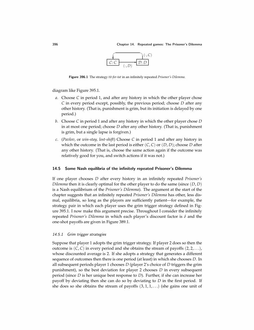
396 Chapter 14. Repeated games: The Prisoner’s Dilemma
C : C D: D(·, D)
(·, C)
Figure 396.1 The strategy tit-for-tat in an infinitely repeated Prisoner’s Dilemma.
diagram like Figure 395.1.
a. Choose C in period 1, and after any history in which the other player choseC in every period except, possibly, the previous period; choose D after anyother history. (That is, punishment is grim, but its initiation is delayed by oneperiod.)
b. Choose C in period 1 and after any history in which the other player chose Din at most one period; choose D after any other history. (That is, punishmentis grim, but a single lapse is forgiven.)
c. (Pavlov, or win-stay, lost-shift) Choose C in period 1 and after any history inwhich the outcome in the last period is either (C, C) or (D, D); choose D afterany other history. (That is, choose the same action again if the outcome wasrelatively good for you, and switch actions if it was not.)
14.5 Some Nash equilibria of the infinitely repeated Prisoner’s Dilemma
If one player chooses D after every history in an infinitely repeated Prisoner’sDilemma then it is clearly optimal for the other player to do the same (since (D, D)is a Nash equilibrium of the Prisoner’s Dilemma). The argument at the start of thechapter suggests that an infinitely repeated Prisoner’s Dilemma has other, less dis-mal, equilibria, so long as the players are sufficiently patient—for example, thestrategy pair in which each player uses the grim trigger strategy defined in Fig-ure 395.1. I now make this argument precise. Throughout I consider the infinitelyrepeated Prisoner’s Dilemma in which each player’s discount factor is δ and theone-shot payoffs are given in Figure 389.1.
14.5.1 Grim trigger strategies
Suppose that player 1 adopts the grim trigger strategy. If player 2 does so then theoutcome is (C, C) in every period and she obtains the stream of payoffs (2, 2, . . .),whose discounted average is 2. If she adopts a strategy that generates a differentsequence of outcomes then there is one period (at least) in which she chooses D. Inall subsequent periods player 1 chooses D (player 2’s choice of D triggers the grimpunishment), so the best deviation for player 2 chooses D in every subsequentperiod (since D is her unique best response to D). Further, if she can increase herpayoff by deviating then she can do so by deviating to D in the first period. Ifshe does so she obtains the stream of payoffs (3, 1, 1, . . .) (she gains one unit of
14.5 Nash equilibria of the infinitely repeated Prisoner’s Dilemma 397
payoff in the first period, then loses one unit in every subsequent period), whosediscounted average is
(1 − δ)[3 + δ + δ2 + δ3 + · · ·] = 3(1 − δ) + δ.
Thus she cannot increase her payoff by deviating if and only if
2 ≥ 3(1 − δ) + δ,
or δ ≥ 12 . We conclude that if δ ≥ 1
2 then the strategy pair in which each player’sstrategy is the grim trigger strategy defined in Figure 395.1 is a Nash equilibrium ofthe infinitely repeated Prisoner’s Dilemma with one-shot payoffs as in Figure 389.1.
14.5.2 Limited punishment
Now consider a generalization of the limited punishment strategy in Figure 395.2in which a player who chooses D is punished for k periods. (The strategy in Fig-ure 395.2 has k = 3; the grim punishment strategy corresponds to k = ∞.) Ifone player adopts this strategy, is it optimal for the other to do so? Suppose thatplayer 1 does so. As in the argument for the grim trigger strategy, if player 2can increase her payoff by deviating then she can increase her payoff by deviatingin the first period. So suppose she chooses D in the first period. Then player 1chooses D in each of the next k periods, regardless of player 2’s choices, so player 2also should choose D in these periods. In the (k + 1)st period after the devia-tion player 1 switches back to C (regardless of player 2’s behavior in the previousperiod), and player 2 faces precisely the same situation that she faced at the begin-ning of the game. Thus if her deviation increases her payoff, it increases her payoffduring the first k + 1 periods. If she adheres to her strategy then her discountedaverage payoff during these periods is
(1 − δ)[2 + 2δ + 2δ2 + · · · + 2δk] = 2(1 − δk+1)
(see (449.1)), whereas if she deviates as described above then her payoff duringthese periods is
(1 − δ)[3 + δ + δ2 + · · · + δk] = 3(1 − δ) + δ(1 − δk).
Thus she cannot increase her payoff by deviating if and only if
2(1 − δk+1) ≥ 3(1 − δ) + δ(1 − δk),
or δk+1 − 2δ + 1 ≤ 0. If k = 1 then no value of δ less than 1 satisfies the inequality:one period of punishment is not severe enough to discourage a deviation, howeverpatient the players are. If k = 2 then the inequality is satisfied for δ ≥ 0.62, and ifk = 3 it is satisfied for δ ≥ 0.55. As k increases the lower bound on δ approaches12 , the lower bound for the grim strategy.
398 Chapter 14. Repeated games: The Prisoner’s Dilemma
We conclude that the strategy pair in which each player punishes the other for kperiods in the event of a deviation is a Nash equilibrium of the infinitely repeatedgame so long as k ≥ 2 and δ is large enough; the larger is k, the smaller is thelower bound on δ. Thus short punishment is effective in sustaining the mutuallydesirable outcome (C, C) only if the players are very patient.
14.5.3 Tit-for-tat
Now consider the conditions under which the strategy pair in which each playeruses the strategy tit-for-tat is a Nash equilibrium. Suppose that player 1 adheresto this strategy. Then, as above, if player 2 can gain by deviating then she cangain by choosing D in the first period. If she does so, then player 1 chooses D inthe second period, and continues to choose D until player 2 reverts to C. Thusplayer 2 has two options: she can revert to C, in which case in the next period shefaces the same situation as she did at the start of the game, or she can continue tochoose D, in which case player 1 will continue to do so too. We conclude that ifplayer 2 can increase her payoff by deviating then she can do so either by alternat-ing between D and C or by choosing D in every period. If she alternates betweenD and C then her stream of payoffs is (3, 0, 3, 0, . . .), with a discounted average of(1− δ) · 3/(1− δ2) = 3/(1 + δ), while if she chooses D in every period her stream ofpayoffs is (3, 1, 1, . . .), with a discounted average of 3(1− δ) + δ = 3− 2δ. Since herdiscounted average payoff to adhering to the strategy tit-for-tat is 2, we concludethat tit-for-tat is a best response to tit-for-tat if and only if
2 ≥ 31 + δ
and 2 ≥ 3 − 2δ.
Both of these conditions are equivalent to δ ≥ 12 .
Thus if δ ≥ 12 then the strategy pair in which the strategy of each player is
tit-for-tat is a Nash equilibrium of the infinitely repeated Prisoner’s Dilemma withpayoffs as in Figure 389.1.
? EXERCISE 398.1 (Nash equilibria of the infinitely repeated Prisoner’s Dilemma) Foreach of the three strategies s in Exercise 395.1 determine the values of δ, if any,for which the strategy pair (s, s) is a Nash equilibrium of an infinitely repeatedPrisoner’s Dilemma with discount factor δ and the one-shot payoffs given in Fig-ure 389.1. For each strategy s for which there is no value of δ such that (s, s) isa Nash equilibrium of this game, determine whether there are any payoffs for thePrisoner’s Dilemma such that for some δ the strategy pair (s, s) is a Nash equilibriumof the infinitely repeated game with discount factor δ.
14.6 Nash equilibrium payoffs of the infinitely repeated Prisoner’s Dilemma
when the players are patient
All the Nash equilibria of the infinitely repeated Prisoner’s Dilemma that I have dis-cussed so far generate either the outcome (C, C) in every period or the outcome
14.6 Nash equilibria of the infinitely repeated Prisoner’s Dilemma 399
(D, D) in every period. The first outcome path yields the discounted average pay-off of 2 to each player, while the second outcome path yields the discounted aver-age payoff of 1 to each player. What other discounted average payoffs are consis-tent with Nash equilibrium? It turns out that this question is hard to answer foran arbitrary discount factor. The question is relatively straightforward to answer,however, in the case that the discount factor is close to 1 (the players are very pa-tient). Before tackling it, we need to determine the set of discounted average pairsof payoffs that are feasible—i.e. can be achieved by outcome paths.
14.6.1 Feasible discounted average payoffs
If the outcome is (X, Y) in every period then the discounted average payoff is(u1(X, Y), u2(X, Y)), for any X and Y. Thus (2, 2), (3, 0), (0, 3), and (1, 1) can allbe achieved as pairs of discounted average payoffs.
Now consider the path in which the outcome alternates between (C, C) and(C, D). Along this path player 1’s payoff alternates between 2 and 0 while player 2’salternates between 2 and 3. Thus the players’ average payoffs along the path are1 and 5
2 respectively. Since player 1 receives more of her payoff in the first periodof each two-period cycle than in the second period (in fact, she obtains nothingin the second period), her discounted average payoff exceeds 1, whatever the dis-count factor. But if the discount factor is close to 1 then her discounted averagepayoff is close to 1: the fact that more payoff is obtained in the first period of eachtwo-period cycle is insignificant if the discount factor is close to 1. Similarly, sinceplayer 2 receives most of her payoff in the second period of each two-period cycle,her discounted average payoff is less than 5
2 , whatever the discount factor, but isclose to 5
2 when the discount factor is close to 1. Thus (1, 52 ) can approximately be
achieved as a pair of discounted average payoffs when the discount factor is closeto 1.
This argument can be extended to any outcome path in which a sequence ofoutcomes is repeated. If the discount factor is close to 1 then a player’s discountedaverage payoff on such a path is close to her average payoff in the sequence. For ex-ample, the outcome path that consists of repetitions of the sequence ((C, C), (D, C), (D, C))yields player 1 a discounted average payoff close to 1
3 (2 + 3 + 3) = 83 and player 2
a discounted average payoff close to 13 (2 + 0 + 0) = 2
3 .We conclude that the average of the payoffs to any sequence of outcomes can
approximately be achieved as the discounted average payoff if the discount factoris close to 1. Further, if the discount factor is close to 1 then only such discountedaverage payoffs can be achieved. Thus if the discount factor is close to 1, the set offeasible discounted average payoff pairs in the infinitely repeated game is approxi-mately the set of all pairs of weighted averages of payoffs in the component game.The same argument applies to any strategic game, and for convenience I make thefollowing definition.
DEFINITION 399.1 The set of feasible payoff profiles of a strategic game is the setof all weighted averages of payoff profiles in the game.
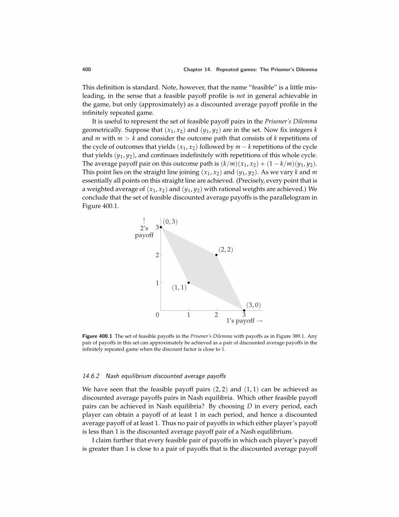
400 Chapter 14. Repeated games: The Prisoner’s Dilemma
This definition is standard. Note, however, that the name “feasible” is a little mis-leading, in the sense that a feasible payoff profile is not in general achievable inthe game, but only (approximately) as a discounted average payoff profile in theinfinitely repeated game.
It is useful to represent the set of feasible payoff pairs in the Prisoner’s Dilemmageometrically. Suppose that (x1, x2) and (y1, y2) are in the set. Now fix integers kand m with m > k and consider the outcome path that consists of k repetitions ofthe cycle of outcomes that yields (x1, x2) followed by m − k repetitions of the cyclethat yields (y1, y2), and continues indefinitely with repetitions of this whole cycle.The average payoff pair on this outcome path is (k/m)(x1, x2) + (1 − k/m)(y1, y2).This point lies on the straight line joining (x1, x2) and (y1, y2). As we vary k and messentially all points on this straight line are achieved. (Precisely, every point that isa weighted average of (x1, x2) and (y1, y2) with rational weights are achieved.) Weconclude that the set of feasible discounted average payoffs is the parallelogram inFigure 400.1.
0 1 2 3
1
2
3(0, 3)
(1, 1)
(2, 2)
(3, 0)
1’s payoff →
↑2’s
payoff
Figure 400.1 The set of feasible payoffs in the Prisoner’s Dilemma with payoffs as in Figure 389.1. Anypair of payoffs in this set can approximately be achieved as a pair of discounted average payoffs in theinfinitely repeated game when the discount factor is close to 1.
14.6.2 Nash equilibrium discounted average payoffs
We have seen that the feasible payoff pairs (2, 2) and (1, 1) can be achieved asdiscounted average payoffs pairs in Nash equilibria. Which other feasible payoffpairs can be achieved in Nash equilibria? By choosing D in every period, eachplayer can obtain a payoff of at least 1 in each period, and hence a discountedaverage payoff of at least 1. Thus no pair of payoffs in which either player’s payoffis less than 1 is the discounted average payoff pair of a Nash equilibrium.
I claim further that every feasible pair of payoffs in which each player’s payoffis greater than 1 is close to a pair of payoffs that is the discounted average payoff
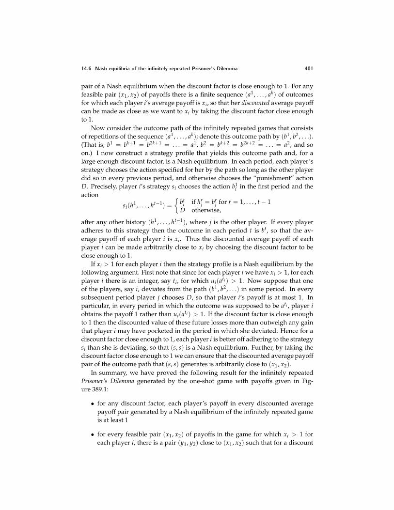
14.6 Nash equilibria of the infinitely repeated Prisoner’s Dilemma 401
pair of a Nash equilibrium when the discount factor is close enough to 1. For anyfeasible pair (x1, x2) of payoffs there is a finite sequence (a1, . . . , ak) of outcomesfor which each player i’s average payoff is xi, so that her discounted average payoffcan be made as close as we want to xi by taking the discount factor close enoughto 1.
Now consider the outcome path of the infinitely repeated games that consistsof repetitions of the sequence (a1, . . . , ak); denote this outcome path by (b1, b2, . . .).(That is, b1 = bk+1 = b2k+1 = . . . = a1, b2 = bk+2 = b2k+2 = . . . = a2, and soon.) I now construct a strategy profile that yields this outcome path and, for alarge enough discount factor, is a Nash equilibrium. In each period, each player’sstrategy chooses the action specified for her by the path so long as the other playerdid so in every previous period, and otherwise chooses the “punishment” actionD. Precisely, player i’s strategy si chooses the action b1
i in the first period and theaction
si(h1, . . . , ht−1) =
bti if hr
j = brj for r = 1, . . . , t − 1
D otherwise,
after any other history (h1, . . . , ht−1), where j is the other player. If every playeradheres to this strategy then the outcome in each period t is bt, so that the av-erage payoff of each player i is xi. Thus the discounted average payoff of eachplayer i can be made arbitrarily close to xi by choosing the discount factor to beclose enough to 1.
If xi > 1 for each player i then the strategy profile is a Nash equilibrium by thefollowing argument. First note that since for each player i we have xi > 1, for eachplayer i there is an integer, say ti, for which ui(ati) > 1. Now suppose that oneof the players, say i, deviates from the path (b1, b2, . . .) in some period. In everysubsequent period player j chooses D, so that player i’s payoff is at most 1. Inparticular, in every period in which the outcome was supposed to be ati , player iobtains the payoff 1 rather than ui(ati ) > 1. If the discount factor is close enoughto 1 then the discounted value of these future losses more than outweigh any gainthat player i may have pocketed in the period in which she deviated. Hence for adiscount factor close enough to 1, each player i is better off adhering to the strategysi than she is deviating, so that (s, s) is a Nash equilibrium. Further, by taking thediscount factor close enough to 1 we can ensure that the discounted average payoffpair of the outcome path that (s, s) generates is arbitrarily close to (x1, x2).
In summary, we have proved the following result for the infinitely repeatedPrisoner’s Dilemma generated by the one-shot game with payoffs given in Fig-ure 389.1:
• for any discount factor, each player’s payoff in every discounted averagepayoff pair generated by a Nash equilibrium of the infinitely repeated gameis at least 1
• for every feasible pair (x1, x2) of payoffs in the game for which xi > 1 foreach player i, there is a pair (y1, y2) close to (x1, x2) such that for a discount
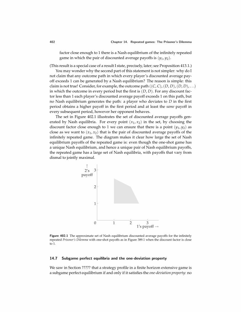
402 Chapter 14. Repeated games: The Prisoner’s Dilemma
factor close enough to 1 there is a Nash equilibrium of the infinitely repeatedgame in which the pair of discounted average payoffs is (y1, y2).
(This result is a special case of a result I state, precisely, later; see Proposition 413.1.)You may wonder why the second part of this statement is not simpler: why do I
not claim that any outcome path in which every player’s discounted average pay-off exceeds 1 can be generated by a Nash equilibrium? The reason is simple: thisclaim is not true! Consider, for example, the outcome path ((C, C), (D, D), (D, D), . . .)in which the outcome in every period but the first is (D, D). For any discount fac-tor less than 1 each player’s discounted average payoff exceeds 1 on this path, butno Nash equilibrium generates the path: a player who deviates to D in the firstperiod obtains a higher payoff in the first period and at least the same payoff inevery subsequent period, however her opponent behaves.
The set in Figure 402.1 illustrates the set of discounted average payoffs gen-erated by Nash equilibria. For every point (x1, x2) in the set, by choosing thediscount factor close enough to 1 we can ensure that there is a point (y1, y2) asclose as we want to (x1, x2) that is the pair of discounted average payoffs of theinfinitely repeated game. The diagram makes it clear how large the set of Nashequilibrium payoffs of the repeated game is: even though the one-shot game hasa unique Nash equilibrium, and hence a unique pair of Nash equilibrium payoffs,the repeated game has a large set of Nash equilibria, with payoffs that vary fromdismal to jointly maximal.
0 1 2 3
1
2
3
1’s payoff →
↑2’s
payoff
Figure 402.1 The approximate set of Nash equilibrium discounted average payoffs for the infinitelyrepeated Prisoner’s Dilemma with one-shot payoffs as in Figure 389.1 when the discount factor is closeto 1.
14.7 Subgame perfect equilibria and the one-deviation property
We saw in Section ????? that a strategy profile in a finite horizon extensive game isa subgame perfect equilibrium if and only if it satisfies the one-deviation property: no
14.7 Subgame perfect equilibria and the one-deviation property 403
player can increase her payoff by changing her action at the start of any subgamein which she is the first mover, given the other player’s strategies and the rest of herown strategy. I now argue that the same is true in an infinitely repeated game, afact that can greatly simplify the process of determining whether or not a strategyprofile is a subgame perfect equilibrium.
As in the case of a finite horizon game, if a strategy profile is a subgame perfectequilibrium then certainly it satisfies the one-deviation property, since no playermust be able to increase her payoff by any change in her strategy. What we needto show is the converse: if a strategy profile is not a subgame perfect equilibriumthen there is some subgame in which the first-mover can increase her payoff bychanging only her initial action.
Let s be a strategy profile that is not a subgame perfect equilibrium. Specifically,suppose that in the subgame following the nonterminal history h, player i canincrease her payoff by using the strategy s′i rather than si. Now, since payoffs in thedistant future are worth very little, there is some period T such that any strategythat coincides with s′i through period T is better than any strategy that coincideswith si through period T: T can be chosen to be sufficiently large that the firststrategy yields a higher discounted average payoff than the second one even if thefirst strategy induces the best possible outcome for player i in every period after T,and the second strategy induces the worst possible outcome in every such period.In particular, the strategy s′′i that coincides with s′i through period T and with siafter period T is better for player i than si.
But now by the same argument as for finite horizon games (Proposition ????),we can find a strategy for player i and a subgame such that in the subgame thestrategy differs from si only in its first action and yields a payoff higher than thatyielded by si (given that the other players adhere to s−i). A more precise statementof the result and proof follows.
PROPOSITION 403.1 (One-deviation property of subgame perfect equilibria of in-finitely repeated games) A strategy profile in an infinitely repeated game is a subgameperfect equilibrium if and only if no player can gain by changing her action after anyhistory, given both the strategies of the other players and the remainder of her own strategy.
Proof. If the strategy profile s is a subgame perfect equilibrium then no player cangain by any deviation, so that if some player can gain by a one-period deviationthen s is definitely not a subgame perfect equilibrium.
I now need to show that if s is not a subgame perfect equilibrium then in thesubgame that follows some history h, some player, say i, can gain by a one-perioddeviation from si. Without loss of generality, assume that h is the initial history.
Now, since payoffs in the sufficiently distant future have an arbitrarily smallvalue from today’s point of view, there is some period T such that the payoff toany strategy that follows s′i through period T exceeds the payoff to any strategythat follows by si through period T (given that the other players adhere to s−i).(The integer T can be chosen to be sufficiently large that the first strategy yields a
404 Chapter 14. Repeated games: The Prisoner’s Dilemma
higher discounted average payoff than the second one even if the first strategy in-duces the best possible outcome for player i in every period after T, and the secondstrategy induces the worst possible outcome in every such period.) In particular,the strategy s′′i that coincides with s′i through period T and with si subsequently isbetter for player i than the strategy si.
Now, si and s′′i differ only in the actions they prescribe after finitely many histo-ries, so we can apply the argument in the proof of Proposition ??? to find a strategyof player i and a history such that in the subgame that follows the history, the strat-egy differs from si only in the action it prescribes initially, and player i is better offfollowing the strategy than following si.
Thus we have shown that if s is not a subgame perfect equilibrium then someplayer can increase her payoff by making a one-period deviation after some history.
14.8 Some subgame perfect equilibria of the infinitely repeated Prisoner’s
Dilemma
The notion of Nash equilibrium requires only that each player’s strategy be opti-mal in the whole game, given the other players’ strategies; after histories that donot occur if the players follow their strategies, the actions specified by a player’sNash equilibrium strategy may not be optimal. In some cases we can think of theactions prescribed by a strategy for histories that will not occur if the players fol-low their strategies as “threats”; the notion of Nash equilibrium does not requirethat it be optimal for a player to carry out these threats if called upon to do so. Inthe previous chapter we studied the notion of subgame perfect equilibrium, whichdoes impose such a requirement: a strategy profile is a subgame perfect equilib-rium if every player’s strategy is optimal not only in the whole game, but afterevery history (including histories that do not occur if the players adhere to theirstrategies).
Are the Nash equilibria we considered in the previous section subgame per-fect equilibria of the infinitely repeated Prisoner’s Dilemma with payoffs as in Fig-ure 389.1? Clearly the Nash equilibrium in which each player chooses D afterevery history is a subgame perfect equilibrium: whatever happens, each playerchooses D, so it is optimal for the other player to do likewise. Now consider theother Nash equilibria we studied.
14.8.1 Grim trigger strategies
Suppose that the outcome in the first period is (C, D). Is it optimal for each playerto subsequently adhere to the grim trigger strategy, given that the other playerdoes so? In particular, is it optimal for player 1 to carry out the punishment thatthe grim trigger strategy prescribes? If both players adhere to the strategy thenplayer 1 chooses D in every subsequent period while player 2 chooses C in period 2
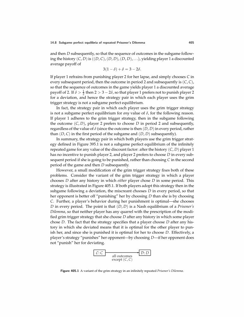
14.8 Subgame perfect equilibria of repeated Prisoner’s Dilemma 405
and then D subsequently, so that the sequence of outcomes in the subgame follow-ing the history (C, D) is ((D, C), (D, D), (D, D), . . .), yielding player 1 a discountedaverage payoff of
3(1 − δ) + δ = 3 − 2δ.
If player 1 refrains from punishing player 2 for her lapse, and simply chooses C inevery subsequent period, then the outcome in period 2 and subsequently is (C, C),so that the sequence of outcomes in the game yields player 1 a discounted averagepayoff of 2. If δ > 1
2 then 2 > 3 − 2δ, so that player 1 prefers not to punish player 2for a deviation, and hence the strategy pair in which each player uses the grimtrigger strategy is not a subgame perfect equilibrium.
In fact, the strategy pair in which each player uses the grim trigger strategyis not a subgame perfect equilibrium for any value of δ, for the following reason.If player 1 adheres to the grim trigger strategy, then in the subgame followingthe outcome (C, D), player 2 prefers to choose D in period 2 and subsequently,regardless of the value of δ (since the outcome is then (D, D) in every period, ratherthan (D, C) in the first period of the subgame and (D, D) subsequently).
In summary, the strategy pair in which both players use the grim trigger strat-egy defined in Figure 395.1 is not a subgame perfect equilibrium of the infinitelyrepeated game for any value of the discount factor: after the history (C, D) player 1has no incentive to punish player 2, and player 2 prefers to choose D in every sub-sequent period if she is going to be punished, rather than choosing C in the secondperiod of the game and then D subsequently.
However, a small modification of the grim trigger strategy fixes both of theseproblems. Consider the variant of the grim trigger strategy in which a playerchooses D after any history in which either player chose D in some period. Thisstrategy is illustrated in Figure 405.1. If both players adopt this strategy then in thesubgame following a deviation, the miscreant chooses D in every period, so thather opponent is better off “punishing” her by choosing D than she is by choosingC. Further, a player’s behavior during her punishment is optimal—she choosesD in every period. The point is that (D, D) is a Nash equilibrium of a Prisoner’sDilemma, so that neither player has any quarrel with the prescription of the modi-fied grim trigger strategy that she choose D after any history in which some playerchose D. The fact that the strategy specifies that a player choose D after any his-tory in which she deviated means that it is optimal for the other player to pun-ish her, and since she is punished it is optimal for her to choose D. Effectively, aplayer’s strategy “punishes” her opponent—by choosing D—if her opponent doesnot “punish” her for deviating.
C : C all outcomesexcept (C, C)
D: D
Figure 405.1 A variant of the grim strategy in an infinitely repeated Prisoner’s Dilemma.
406 Chapter 14. Repeated games: The Prisoner’s Dilemma
14.8.2 Limited punishment
The pair of strategies (s, s) in which s is the limited punishment strategy studiedin Section 14.5.2 is not a subgame perfect equilibrium of the infinitely repeatedPrisoner’s Dilemma for the same reason that a pair of grim trigger strategies is nota subgame perfect equilibrium. However, as in the case of grim trigger strategies,we can modify the limited punishment strategy in order to obtain a subgame per-fect equilibrium. Specifically, we need the transition from state P0 to state P1 inFigure 395.2 to occur whenever either player chooses D (not just if the other playerchooses D). A player using this modified strategy chooses D during her punish-ment, which both is optimal for her and makes the other player’s choice to punishoptimal. When the punishment ends she, like her punisher, reverts to C.
? EXERCISE 406.1 (Lengths of punishment in subgame perfect equilibrium) Is thereany subgame perfect equilibrium of an infinitely repeated Prisoner’s Dilemma (withpayoffs as in Figure 389.1), for any value of δ, in which each player’s strategyinvolves limited punishment, but the lengths of the punishment are different foreach player? If so, describe such a subgame perfect equilibrium; if not, argue whynot.
14.8.3 Tit-for-tat
The behavior in a subgame of a player who uses the strategy tit-for-tat dependsonly on the last outcome in the history that preceded the subgame. Thus to ex-amine whether the strategy pair in which both players use the strategy tit-for-tat is a subgame perfect equilibrium we need to consider four types of subgame,following histories in which the last outcome is (C, C), (C, D), (D, C), and (D, D).
The optimality of tit-for-tat in a subgame following a history ending in (C, C),given that the other player uses tit-for-tat, is covered by our analysis of Nash equi-librium: if δ ≥ 1
2 then tit-for-tat is a best response to tit-for-tat in such a subgame.In studying subgames following histories ending in other outcomes, I appeal
to the fact that a strategy profile is a subgame perfect equilibrium if and only if itsatisfies the one-deviation property (Propostion ???).
Consider the subgame following a history ending in the outcome (C, D). Sup-pose that player 2 adheres to tit-for-tat. If player 1 also adheres to tit-for-tat then theoutcome alternates between (D, C) and (C, D), and player 1’s discounted averagepayoff in the subgame is
(1 − δ)(3 + 3δ2 + · · ·) =3
1 + δ.
If player 1 instead chooses C in the first period of the subgame, and subsequentlyadheres to tit-for-tat, then the outcome is (C, C) in every period of the subgame,so that player 1’s discounted average payoff is 2. Thus in order that tit-for-tat beoptimal in such a subgame we need
31 + δ
≥ 2, or δ ≤ 12 .
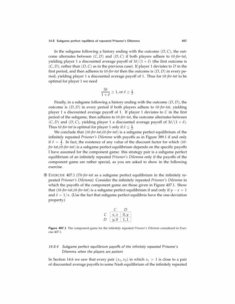
14.8 Subgame perfect equilibria of repeated Prisoner’s Dilemma 407
In the subgame following a history ending with the outcome (D, C), the out-come alternates between (C, D) and (D, C) if both players adhere to tit-for-tat,yielding player 1 a discounted average payoff of 3δ/(1 + δ) (the first outcome is(C, D), rather than (D, C) as in the previous case). If player 1 deviates to D in thefirst period, and then adheres to tit-for-tat then the outcome is (D, D) in every pe-riod, yielding player 1 a discounted average payoff of 1. Thus for tit-for-tat to beoptimal for player 1 we need
3δ
1 + δ≥ 1, or δ ≥ 1
2 .
Finally, in a subgame following a history ending with the outcome (D, D), theoutcome is (D, D) in every period if both players adhere to tit-for-tat, yieldingplayer 1 a discounted average payoff of 1. If player 1 deviates to C in the firstperiod of the subgame, then adheres to tit-for-tat, the outcome alternates between(C, D) and (D, C), yielding player 1 a discounted average payoff of 3δ/(1 + δ).Thus tit-for-tat is optimal for player 1 only if δ ≤ 1
2 .We conclude that (tit-for-tat,tit-for-tat) is a subgame perfect equilibrium of the
infinitely repeated Prisoner’s Dilemma with payoffs as in Figure 389.1 if and onlyif δ = 1
2 . In fact, the existence of any value of the discount factor for which (tit-for-tat,tit-for-tat) is a subgame perfect equilibrium depends on the specific payoffsI have assumed for the component game: this strategy pair is a subgame perfectequilibrium of an infinitely repeated Prisoner’s Dilemma only if the payoffs of thecomponent game are rather special, as you are asked to show in the followingexercise.
? EXERCISE 407.1 (Tit-for-tat as a subgame perfect equilibrium in the infinitely re-peated Prisoner’s Dilemma) Consider the infinitely repeated Prisoner’s Dilemma inwhich the payoffs of the component game are those given in Figure 407.1. Showthat (tit-for-tat,tit-for-tat) is a subgame perfect equilibrium if and only if y − x = 1and δ = 1/x. (Use the fact that subgame perfect equilibria have the one-deviationproperty.)
C DC x, x 0, yD y, 0 1, 1
Figure 407.1 The component game for the infinitely repeated Prisoner’s Dilemma considered in Exer-cise 407.1.
14.8.4 Subgame perfect equilibrium payoffs of the infinitely repeated Prisoner’s
Dilemma when the players are patient
In Section 14.6 we saw that every pair (x1, x2) in which xi > 1 is close to a pairof discounted average payoffs to some Nash equilibrium of the infinitely repeated
408 Chapter 14. Repeated games: The Prisoner’s Dilemma
Prisoner’s Dilemma with payoffs as in Figure 389.1 when the players are sufficientlypatient. Since every subgame perfect equilibrium is a Nash equilibrium, the set ofsubgame perfect equilibrium payoff pairs is a subset of the set of Nash equilibriumpayoff pairs. I now argue that, in fact, the two sets are the same. The strategy pairthat I used in the argument of Section 14.6 is not a subgame perfect equilibrium,but can be modified, along the lines we considered in the previous section, to turnit into such an equilibrium.
Let (x1, x2) be a pair of feasible payoffs in the Prisoner’s Dilemma for whichxi > 1 for each player i. Let (a1, . . . , ak) be a sequence of outcomes of the gamefor which each player i’s average payoff is xi, and let (b1, b2, . . .) be the outcomepath of the infinitely repeated game that consists of repetitions of the sequence(a1, . . . , ak). I claim that the strategy pair in which each player follows the path(b1, b2, . . .) so long as both she and the other player have done so in the past, andotherwise chooses D, is a subgame perfect equilibrium. If one player deviatesthen subsequent to her deviation she continues to choose D, making it optimal forher opponent to “punish” her by choosing D. Precisely, the strategy si of player ichooses the action b1
i in the first period and the action
si(h1, . . . , ht−1) =
bti if hr = br for r = 1, . . . , t − 1
D otherwise,
after any other history (h1, . . . , ht−1).I claim that (s, s) is a subgame perfect equilibrium of the infinitely repeated
game. There are two types of subgame to consider. First, consider a history inwhich the outcome was br in every period r. The argument that if one player actsaccording to s in the subgame that follows such a history then it is optimal for theother to do so is the same as the argument that the strategy pair defined in Sec-tion 14.6 is a Nash equilibrium. Briefly, if both players adhere to the strategy sin the subgame, the outcome is bt in every period t, yielding each player i a dis-counted average payoff close to xi when the discount factor is close to 1. If oneplayer deviates from s, then she may gain in the period in which she deviates, buther deviation will trigger her opponent to choose D in every subsequent period,so that given xi > 1 for each i, her deviation makes her worse off if her discountfactor is close enough to 1.
Now consider a history in which the outcome was different from br in someperiod r. If, in the subgame following this history, the players both use the strat-egy s, then they both choose D regardless of the outcomes in the subgame. Sincethe strategy pair in which both players always choose D regardless of history isa Nash equilibrium of the infinitely repeated game, the strategy pair that (s, s)induces in such a subgame is a Nash equilibrium.
We conclude that the strategy pair (s, s) is a subgame perfect equilibrium. Thepoint is that after any deviation the players’ strategies lead them to choose Nashequilibrium actions of the component game in every subsequent period, so thatneither player has any incentive to deviate.
Notes 409
Since no player’s discounted average payoff can be less than 1 in any Nashequilibrium of the infinitely repeated game, we conclude that the set of discountedaverage payoffs possible in subgame perfect equilibria is exactly the same as theset of discounted average payoffs possible in Nash equilibria:
• for any discount factor, each player’s payoff in every discounted averagepayoff pair generated by a subgame perfect equilibrium of the infinitely re-peated game is at least 1
• for every pair (x1, x2) of feasible payoffs in the game for which xi > 1 for eachplayer i, there is a pair (y1, y2) close to (x1, x2) such that for a discount factorclose enough to 1 there is a subgame perfect equilibrium of the infinitelyrepeated game in which the pair of discounted average payoffs is (y1, y2).
Notes
Draft chapter from An introduction to game theory by Martin J. [email protected]; www.economics.utoronto.ca/osborneVersion: 00/11/9.Copyright c© 1995–2000 by Martin J. Osborne. All rights reserved. No part of this book may be re-produced by any electronic or mechanical means (including photocopying, recording, or informationstorage and retrieval) without permission in writing from Oxford University Press, except that onecopy of up to six chapters may be made by any individual for private study.
15 Repeated games: General Results
Nash equilibria of general infinitely repeated games 411Subgame perfect equilibria of infinitely repeated games 414Finitely repeated games 420Prerequisite: Chapter 14
15.1 Nash equilibria of general infinitely repeated games
THE IDEA behind the analysis of an infinitely repeated Prisoner’s Dilemma ap-plies to any infinitely repeated game: every feasible payoff profile in the one
shot game in which each player’s payoff exceeds some minimum is close (at least)to the discounted average payoff profile of a Nash equilibrium in which a deviationtriggers each player to begin an indefinite “punishment” of the deviant.
For the Prisoner’s Dilemma the minimum payoff of player i that is supported bya Nash equilibrium is ui(D, D). The significance of this payoff is that player j canensure (by choosing D) that player i’s payoff does not exceed ui(D, D), and thereis no lower payoff with this property. That is, ui(D, D) is the lowest payoff thatplayer j can force upon player i.
How can we find this minimum payoff in an arbitrary strategic game? Supposethat the deviant is player i. For any collection a−i of the other players’ actions,player i’s highest possible payoff is her payoff when she chooses a best responseto a−i, namely
maxai∈Ai
ui(ai , a−i).
As a−i varies, this maximal payoff varies. We seek a collection a−i of “punishment”actions that make this maximum as small as possible. That is, we seek a solutionto the problem
mina−i∈A−i
(maxai∈Ai
ui(ai , a−i))
.
This payoff is known, not surprisingly, as player i’s minmax payoff.
DEFINITION 411.1 Player i’s minmax payoff in a strategic game in which theaction set and payoff function of each player i are Ai and ui respectively is
mina−i∈A−i
(maxai∈Ai
ui(ai , a−i))
. (411.2)
411
412 Chapter 15. Repeated games: General Results
(Note that I am restricting attention to pure strategies in the strategic game; aplayer’s minmax payoff is different if we consider mixed strategies.)
For example, in the Prisoner’s Dilemma with the payoffs in Figure 389.1, eachplayer’s minmax payoff is 1; in BoS (Example 16.2) each player’s minmax payoff isalso 1.
? EXERCISE 412.1 (Minmax payoffs) Find each player’s minmax payoff in each ofthe following games.
a. The game of dividing money in Exercise 36.2.
b. Cournot’s oligopoly game (Section 3.1) when Ci(0) = 0 for each firm i andP(Q) = 0 for some sufficiently large value of Q.
c. Hotelling’s model of electoral competition (Section 3.3) when (i) there are twocandidates and (ii) there are three candidates, under the assumptions that theset of possible positions is the interval [0, 1], the distribution of the candidates’ideal positions has a unique median, a tie results in each candidate’s winningwith probability 1
2 , and each candidate’s payoff is her probability of winning.
Whatever the other players’ strategies, any player can obtain at least her min-max payoff in every period, and hence a discounted average payoff at least equalto her minmax payoff, by choosing in each period a best response to the other play-ers’ actions. More precisely, player i can ensure that her payoff in every period isat least her minmax payoff by using a strategy that, after every history h, choosesa best response to s−i(h), the collection of actions prescribed for the other players’strategies after the history h. Thus in no Nash equilibrium of the infinitely repeatedgame is player i’s discounted average payoff less than her minmax payoff.
We saw that in the Prisoner’s Dilemma, a converse of this result holds: for everyfeasible payoff profile x in the game in which xi exceeds player i’s minmax payofffor i = 1, 2, for a discount factor sufficiently close to 1 there is a Nash equilibriumof the infinitely repeated game in which the discounted average payoff of player iis close to xi for i = 1, 2.
An analogous result holds in general. The simplest case to consider is that inwhich x is a payoff profile of the game. Let x be the payoff profile generated by theaction profile a; assume that each xi exceeds player i’s minmax payoff. For eachplayer i, let p−i be a collection of actions for the players other than i that holdsplayer i down to her minmax payoff. (That is, p−i is a solution of the minimizationproblem (411.2).) Define a strategy for each player as follows. In each period, thestrategy of each player i chooses ai as long as every other player j chose aj in everyprevious period, and otherwise chooses the action (p−j)i, where j is the player whodeviated in the first period in which exactly one player deviated. Precisely, let H∗
be the set of histories in which there is at least one period in which exactly oneplayer j chose an action different from aj. Refer to such a player as a lone deviant.The strategy of player i is defined by si(∅) = ai (her action at the start of the game
15.1 Nash equilibria of general infinitely repeated games 413
is ai) and
si(h) =
ai if h is not in H∗
(p−j)i if h ∈ H∗ and j is the first lone deviant in h.
The strategy profile s is a Nash equilibrium by the following argument. Ifplayer i adheres to si then, given that every other player j adheres to sj, her payoffis xi in every period. If player i deviates from si, while every other player j adheresto sj, then she may gain in the period in which she deviates, but she loses in everysubsequent period, obtaining at most her minmax payoff, rather than xi. Thus fora discount factor close enough to 1, si is a best response to s−i for every player i, sothat s is a Nash equilibrium.
(Note that the strategies I have defined do not react when more than one playerdeviates in any one period. They do not need to, since the notion of Nash equilib-rium requires only that no single player has an incentive to deviate.)
This argument can be extended to deal with the case in which x is a feasible pay-off profile that is not the payoff profile of a single action profile in the componentgame, along the same lines as the argument in the case of the Prisoner’s Dilemma inthe previous section. The result we obtain is known as a “folk theorem”, since thebasic form of the result was known long before it was written down precisely.1
PROPOSITION 413.1 (Nash folk theorem) Let G be a strategic game.
• For any discount factor δ with 0 < δ < 1, the discounted average payoff of everyplayer in any Nash equilibrium of the infinitely repeated game of G is at least herminmax payoff.
• Let w be a feasible payoff profile of G for which each player’s payoff exceeds her min-max payoff. Then for all ε > 0 there exists δ < 1 such that if the discount fac-tor exceeds δ then the infinitely repeated game of G has a Nash equilibrium whosediscounted average payoff profile w′ satisfies|w − w′| < ε.
? EXERCISE 413.2 (Nash equilibrium payoffs in infinitely repeated games) For theinfinitely repeated games for which each of the following strategic games is thecomponent game, find the set of discounted average payoffs to Nash equilibria ofthese infinitely repeated games when the discount factor is close to 1. (Parts b andc of Exercise 412.1 are relevant to parts b and c.)
a. BoS (Example 16.2).
b. Cournot’s oligopoly game (Section 3.1) when there are two firms, Ci(qi) = qifor all qi for each firm i, and P(Q) = max0, α − βQ.
c. Hotelling’s model of electoral competition (Section 3.3) when there are twocandidates, under the assumptions that the set of possible positions is theinterval [0, 1], the distribution of the citizens’ ideal positions has a uniquemedian, a tie results in each candidate’s winning with probability 1
2 , and eachcandidate’s payoff is her probability of winning.
1If x = (x1, . . . , xn) is a vector then |x| is the norm of x, namely (x21 + · · · + x2
n)1/2. If x and y arevectors and |x − y| is small then the components of x and y are close to each other.
414 Chapter 15. Repeated games: General Results
The strategies in the Nash equilibrium used to prove Proposition 413.1 are grimtrigger strategies: any transgression leads to interminable punishment. As in thecase of the Prisoner’s Dilemma, less draconian punishment is sufficient to deter de-viations; grim trigger strategies are simply easy to work with. The punishmentembedded in a strategy has only to be severe enough that any deviation ultimatelyresults in a net loss for its perpetrator.
? EXERCISE 414.1 (Repeated Bertrand duopoly) Consider Bertrand’s model of duopoly(Section 3.2) in the case that each firm’s unit cost is constant, equal to c. LetΠ(p) = (p − c)D(p) for any price p, and assume that Π is continuous and isuniquely maximized at the price pm (the “monopoly price”).
a. Let s be the strategy for the infinitely repeated game that charges pm in thefirst period and subsequently as long as the other firm continues to charge pm,and punishes any deviation from pm by the other firm by choosing the price cfor k periods, then reverting to pm. Given any value of δ, for what values of kis the strategy pair (s, s) a Nash equilibrium of the infinitely repeated game?
b. Let s be the strategy for the infinitely repeated game defined as follows:
• in the first period charge the price pm
• in every subsequent period charge the lowest of all the prices charged bythe other firm in all previous periods.
Is the strategy pair (s, s) a Nash equilibrium of the infinitely repeated gamefor any discount factor less than 1?
15.2 Subgame perfect equilibria of general infinitely repeated games
The Prisoner’s Dilemma has a feature that makes it easy to construct a subgame per-fect equilibrium of the infinitely repeated game to prove the result in the previoussection: it has a Nash equilibrium in which each player’s payoff is her minmaxpayoff. In any game, each player’s payoff is at least her minmax payoff, but ingeneral there is no Nash equilibrium in which the payoffs are exactly the min-max payoffs. It may be clear how to generalize the arguments above to define asubgame perfect equilibrium of any infinitely repeated game in which both play-ers’ discounted average payoffs exceed their payoffs in some Nash equilibrium ofthe component game. However, it is not clear whether there are subgame perfectequilibrium payoff pairs in which the players’ payoffs are between their minmaxpayoffs and their payoffs in the worst Nash equilibrium of the component game.
Consider the game in Figure 415.1. Each player’s minmax payoff is 1: by choos-ing C, each player can ensure that the other player’s payoff does not exceed 1, andthere is no action that ensures that the other player’s payoff is less than 1. In theunique Nash equilibrium (A, A), on the other hand, each player’s payoff is 4. Pay-offs between 1 and 4 cannot be achieved by strategies that react to deviations bychoosing A, since one player’s choosing A allows the other to obtain a payoff of 4(by choosing A also), which exceeds her payoff if she does not deviate.
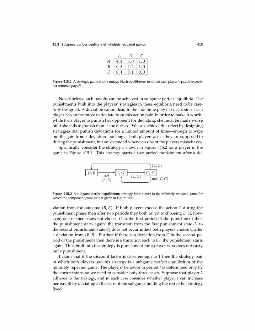
15.2 Subgame perfect equilibria of infinitely repeated games 415
A B CA 4, 4 3, 0 1, 0B 0, 3 2, 2 1, 0C 0, 1 0, 1 0, 0
Figure 415.1 A strategic game with a unique Nash equilibrium in which each player’s payoff exceedsher minmax payoff.
Nevertheless, such payoffs can be achieved in subgame perfect equilibria. Thepunishments built into the players’ strategies in these equilibria need to be care-fully designed. A deviation cannot lead to the indefinite play of (C, C), since eachplayer has an incentive to deviate from this action pair. In order to make it worth-while for a player to punish her opponent for deviating, she must be made worseoff if she fails to punish than if she does so. We can achieve this effect by designingstrategies that punish deviations for a limited amount of time—enough to wipeout the gain from a deviation—so long as both players act as they are supposed toduring the punishment, but are extended whenever one of the players misbehaves.
Specifically, consider the strategy s shown in Figure 415.2 for a player in thegame in Figure 415.1. This strategy starts a two-period punishment after a de-
B: B not
(B, B)
C1: C (C, C)
C2: C
(C, C)
not (C, C)
Figure 415.2 A subgame perfect equilibrium strategy for a player in the infinitely repeated game forwhich the component game is that given in Figure 415.1.
viation from the outcome (B, B). If both players choose the action C during thepunishment phase then after two periods they both revert to choosing B. If, how-ever, one of them does not choose C in the first period of the punishment thenthe punishment starts again: the transition from the first punishment state C1 tothe second punishment state C2 does not occur unless both players choose C aftera deviation from (B, B). Further, if there is a deviation from C in the second pe-riod of the punishment then there is a transition back to C1: the punishment startsagain. Thus built into the strategy is punishment for a player who does not carryout a punishment.
I claim that if the discount factor is close enough to 1 then the strategy pairin which both players use this strategy is a subgame perfect equilibrium of theinfinitely repeated game. The players’ behavior in period t is determined only bythe current state, so we need to consider only three cases. Suppose that player 2adheres to the strategy, and in each case consider whether player 1 can increaseher payoff by deviating at the start of the subgame, holding the rest of her strategyfixed.
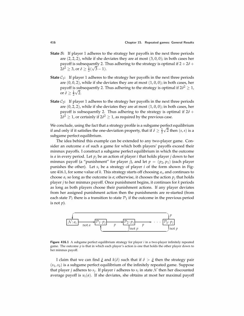
416 Chapter 15. Repeated games: General Results
State B: If player 1 adheres to the strategy her payoffs in the next three periodsare (2, 2, 2), while if she deviates they are at most (3, 0, 0); in both cases herpayoff is subsequently 2. Thus adhering to the strategy is optimal if 2 + 2δ +2δ2 ≥ 3, or δ ≥ 1
2 (√
3 − 1).
State C1: If player 1 adheres to the strategy her payoffs in the next three periodsare (0, 0, 2), while if she deviates they are at most (1, 0, 0); in both cases, herpayoff is subsequently 2. Thus adhering to the strategy is optimal if 2δ2 ≥ 1,or δ ≥ 1
2
√2.
State C2: If player 1 adheres to the strategy her payoffs in the next three periodsare (0, 2, 2), while if she deviates they are at most (1, 0, 0); in both cases, herpayoff is subsequently 2. Thus adhering to the strategy is optimal if 2δ +2δ2 ≥ 1, or certainly if 2δ2 ≥ 1, as required by the previous case.
We conclude, using the fact that a strategy profile is a subgame perfect equilibriumif and only if it satisfies the one-deviation property, that if δ ≥ 1
2
√2 then (s, s) is a
subgame perfect equilibrium.The idea behind this example can be extended to any two-player game. Con-
sider an outcome a of such a game for which both players’ payoffs exceed theirminmax payoffs. I construct a subgame perfect equilibrium in which the outcomeis a in every period. Let pj be an action of player i that holds player j down to herminmax payoff (a “punishment” for player j), and let p = (p2, p1) (each playerpunishes the other). Let si be a strategy of player i of the form shown in Fig-ure 416.1, for some value of k. This strategy starts off choosing ai, and continues tochoose ai so long as the outcome is a; otherwise, it chooses the action pj that holdsplayer j to her minmax payoff. Once punishment begins, it continues for k periodsas long as both players choose their punishment actions. If any player deviatesfrom her assigned punishment action then the punishments are re-started (fromeach state P there is a transition to state P1 if the outcome in the previous periodis not p).
N : ai
not aP1: pj
pP2: pj
p. . . Pk: pj
p
not p
not p
Figure 416.1 A subgame perfect equilibrium strategy for player i in a two-player infinitely repeatedgame. The outcome p is that in which each player’s action is one that holds the other player down toher minmax payoff.
I claim that we can find δ and k(δ) such that if δ > δ then the strategy pair(s1, s2) is a subgame perfect equilibrium of the infinitely repeated game. Supposethat player j adheres to sj. If player i adheres to si in state N then her discountedaverage payoff is ui(a). If she deviates, she obtains at most her maximal payoff
15.2 Subgame perfect equilibria of infinitely repeated games 417
in the game, say ui, in the period of her deviation, then ui(p) for k periods, andsubsequently ui(a) in the future. Thus her discounted average payoff from thedeviation is at most
(1 − δ)[ui + δui(p) + · · · + δkui(p)] + δk+1ui(a) =
(1 − δ)ui + δ(1 − δk)ui(p) + δk+1ui(a).
In order for her not to want to deviate it is thus sufficient that
ui(a) ≥ (1 − δ)ui + δ(1 − δk)ui(p) + δk+1ui(a). (417.1)
If player i adheres to si in any state P then she obtains ui(p) for at most kperiods, then ui(a) in every subsequent period, which yields a discounted averagepayoff of at least
(1 − δk)ui(p) + δkui(a)
(since ui(p) is at most player i’s minmax payoff and ui(a) exceeds this minmaxpayoff). If she deviates from si, she obtains at most her minmax payoff in theperiod of her deviation, then ui(p) for k periods, then ui(a) in the future, whichyields a discounted average payoff of at most
(1 − δ)mi + δ(1 − δk)ui(p) + δk+1ui(a),
where mi is her minmax payoff. Thus in order that she not want to deviate it issufficient that
(1 − δk)ui(p) + δkui(a) ≥ (1 − δ)mi + δ(1 − δk)ui(p) + δk+1ui(a)
or(1 − δk)ui(p) + δkui(a) ≥ mi. (417.2)
Thus if for each value of δ sufficiently close to 1 we can find k(δ) such that(δ, k(δ)) satisfies (417.1) and (417.2) then the strategy pair (s1, s2) is a subgameperfect equilibrium. [Need to make this argument.]
This argument shows that for any outcome of the component game in whicheach player’s payoff exceeds her minmax payoff there is a subgame perfect equi-librium that yields this outcome path. More generally, for any two-player strategicgame and any feasible payoff pair (x1, x2) in which each player’s payoff exceedsher minmax payoff, we can construct a Nash equilibrium strategy pair that gener-ates an outcome path for which the discounted average payoff of each player i isxi. A precise statement of this result follows.
PROPOSITION 417.3 (Subgame perfect folk theorem for two-player games) Let Gbe a two-player strategic game.
• For any discount factor δ with 0 < δ < 1, the discounted average payoff of everyplayer in any subgame perfect equilibrium of the infinitely repeated game of G is atleast her minmax payoff.
418 Chapter 15. Repeated games: General Results
• Let w be a feasible payoff profile of G for which each player’s payoff exceeds her min-max payoff. Then for all ε > 0 there exists δ < 1 such that if the discount factorexceeds δ then the infinitely repeated game of G has a subgame perfect equilibriumwhose discounted average payoff profile w′ satisfies |w − w′| < ε.
The conclusion of this result does not hold for all multi-player games.
AXELROD’S EXPERIMENTS
In the late 1970s, Robert Axelrod (a political scientist at the University of Michigan)invited some economists, psychologists, mathematicians, and sociologists famil-iar with the repeated Prisoner’s Dilemma to submit strategies (written in computercode) for a finitely repeated Prisoner’s Dilemma with payoffs of (3, 3) for (C, C),(5, 0) for (D, C), (0, 5) for (C, D), and (1, 1) for (D, D). He received 14 entries,which he pitted against each other, and against a strategy that randomly choosesC and D each with probability 1
2 , in 200-fold repetitions of the game. Each strategywas paired against each other five times. (Strategies could involve random choices,so a pair of strategies could generate different outcomes when paired repeatedly.)The strategy with the highest payoff was tit-for-tat (submitted by Anatol Rapoport,then a member of the Psychology Department of the University of Toronto). (SeeAxelrod (1980a, 1984).)
Axelrod, intrigued by the result, subsequently ran a second tournament. Heinvited the participants in the first tournament to compete again, and also re-cruited entrants by advertising in journals read by microcomputer users (a rela-tively small crowd in the early 1980s); contestants were informed of the results ofthe first round. Sixty-two strategies were submitted. The contest was run slightlydifferently from the previous one: the length of each game was determined prob-abilistically. Again tit-for-tat (again submitted by Anatol Rapoport) won. (SeeAxelrod (1980b, 1984).
Using the strategies submitted in his second tournament, Axelrod simulated anenvironment in which strategies that do well reproduce faster than other strategies.He repeatedly matched the strategies against each other, increasing the number ofrepresentatives of strategies that achieved high payoffs. A strategy that obtained ahigh payoff initially might, under these conditions, obtain a low one later on if theopponents against which it did well become much less numerous relative to theothers. Axelrod found that after a large number of “generations” tit-for-tat had themost representatives in the population.
However, tit-for-tat’s supremacy has been subsequently shown to be fragile.[Discussion to be added.]
Axelrod’s simulations are limited by the set of strategies that were submittedto him. Other simulations have included all strategies of a particular type. Onetype of strategy that has been examined is the class of “reactive strategies”, inwhich a player’s action in any period depends only on the other player’s action in
15.2 Subgame perfect equilibria of infinitely repeated games 419
the previous period (Nowak and Sigmund (1992)). In evolutionary simulations inwhich the initial population consists of randomly selected reactive strategies, thestrategy that chooses D in every period, regardless of the history, is found to cometo dominate. However, if tit-for-tat is included in the set of strategies initially inthe population, a strategy known as generous tit-for-tat, which differs from tit-for-tat only in that after its opponent chooses D it chooses D with probability 1
3 (giventhe payoffs for the Prisoner’s Dilemma used by Axelrod), XXXXXXXXXXXXX.
The results are different when the larger class of strategies in which the actionchosen in any period depends on both actions chosen in the previous period isstudied. In this case the strategy Pavlov (also known as win–stay, lose–shift; seeExercise 398.1), which chooses C when the outcome in the previous period waseither (C, C) or (D, D) and otherwise chooses D, tends to come to dominate thepopulation.
In summary, simulations show that a variety of strategies may emerge as “win-ners” in the repeated Prisoner’s Dilemma; Axelrod’s conclusions about the robust-ness of tit-for-tat appear to have been premature.
Given these results, it is natural to ask if the theory of evolutionary games(Chapter 13) can offer insights into the strategies that might be expected to survive.Unfortunately, the existing results are negative: depending on how one defines anevolutionarily stable strategy (ESS) in an extensive game, an infinitely repeatedPrisoner’s Dilemma either has no ESS, or the only ESS is the strategy that choosesD in every period regardless of history, or every feasible pair of payoffs can besustained by some pair of ESSs (Kim (1994)).
RECIPROCAL ALTRUISM AMONG STICKLEBACKS
The idea that a population of animals repeatedly involved in a conflict with thestructure of a Prisoner’s Dilemma might evolve a mode of behavior involving recip-rocal altruism (as in the strategy tit-for-tat), was suggested by Trivers (1971) andled biologists to look for examples of such behavior.
One much-discussed example involves predator inspection by sticklebacks. Stick-lebacks often approach a predator in pairs, the members of a pair taking turns tobe the first to move forward a few centimeters. (It is advantageous for them toapproach the predator closely, since they thereby obtain more information aboutit.) The process can be modeled as a repeated Prisoner’s Dilemma, in which movingforward is analogous to cooperating and holding back is like defecting. Milin-ski (1987) reports an experiment in which he put a stickleback into one compart-ment of a tank and a cichlid, which resembles a perch, a common predator of stick-lebacks, in another compartment, separated by glass. In one condition he placeda mirror along one side of the tank (a “cooperating mirror”), so that as the stickle-back approached the predator is had the impression that there was another stickle-
420 Chapter 15. Repeated games: General Results
back mimicking its actions, as if following the strategy tit-for-tat. In a second con-dition he placed the mirror at an angle (a “defecting mirror”), so that a sticklebackthat approached the cichlid had the impression that there was another sticklebackthat was increasingly holding back. He found that the stickleback approached thecichlid much more closely with a cooperating mirror than with a defecting mirror.With a defecting mirror, the apparent second stickleback held back when the realone moved forward, and disappeared entirely when the real stickleback movedinto the front half of the tank—that is, it tended to defect. Milinski interpretedthe behavior of the real stickleback as consistent with its following the strategy tit-for-tat. (The same behavior was subsequently observed in guppies approaching apumpkinseed sunfish (Dugatkin (1988, 1991)).)
Other explanations have been offered for the observed behavior of the fish. Forexample, one stickleback might simply be attracted to another, since sticklebacksshoal, or a stickleback might be bolder if in the company of another one, since itschances of being captured by the predator are lower (Lazarus and Metcalfe (1990)).Milinski (1990) argues that neither of these alternative theories fits the evidence; inMilinski (1993) he suggests that further evidence indicates that the strategy thathis sticklebacks follow may not be tit-for-tat but rather Pavlov (see Exercise 398.1).
15.3 Finitely repeated games
To be written.
Notes
Early discussions of the notion of a repeated game and the ideas behind the Nashfolk theorem (Proposition 413.1) appear in Luce and Raiffa (1957, pp. 97–105 (es-pecially p. 102) and Appendix 8), Shubik (1959b, Ch. 10 (especially p. 226)), andFriedman (1971). Proposition 417.3 (a perfect folk theorem) is due to Fudenbergand Maskin (1986); related results were established earlier (see Aumann and Shap-ley (1994), Rubinstein (1994), and Rubinstein (1979)).
Draft chapter from An introduction to game theory by Martin J. [email protected]; www.economics.utoronto.ca/osborneVersion: 00/11/6.Copyright c© 1995–2000 by Martin J. Osborne. All rights reserved. No part of this book may be re-produced by any electronic or mechanical means (including photocopying, recording, or informationstorage and retrieval) without permission in writing from Oxford University Press, except that onecopy of up to six chapters may be made by any individual for private study.
17 Appendix: Mathematics
Numbers 443Sets 444Functions 445Profiles 448Sequences 449Probability 449Proofs 454
17.1 Introduction
THIS CHAPTER presents informal definitions and discussions of the mathemati-cal concepts used in the text. Much of the material should be familiar to you,
though a few concepts may be new.
17.2 Numbers
I take the concept of a number as basic; 3, −7.4, 12 , and
√2 are all numbers. The
whole numbers . . . , −3, −2, −1, 0, 1, 2, 3, . . . are called integers. Let x be a number.If x > 0 then x is positive; if x ≥ 0 then x is nonnegative; if x < 0 then x isnegative; and if x ≤ 0 then x is nonpositive. Note that 0 is both nonnegative andnonpositive, but neither positive nor negative.
When working with sums of numbers, a shorthand that uses the symbol ∑ (alarge uppercase Greek sigma) is handy. Instead of writing x1 + x2 + x3 + x4, forexample, where x1, x2, x3, and x4 are numbers, we can write
4
∑i=1
xi.
This expression is read as “the sum from i = 1 to i = 4 of xi”. The name we givethe indexing variable is arbitrary; we frequently use i or j, but can alternatively useany other letter. If the number of items in the sum is a variable, say n, the notationis even more useful. Instead of writing xk + · · · + xn, which leaves in doubt the
443
444 Chapter 17. Appendix: Mathematics
variables indicated by the ellipsis, we can write
n
∑i=k
xi,
which has a precise meaning: first set i = k and take xi; then increase i by one andadd the new xi; continue increasing i by one at a time and adding xi to the sum ateach step, until i = n.
17.3 Sets
A set is a collection of objects. If we can count the members of a set, and, whenwe do so, we eventually exhaust the members of the set, then the set is finite.We can specify a finite set by listing the names of its members within braces:Paris, Venice, Havana is a set of (beautiful) cities, for example. Neither the orderin which the members of the set are listed nor the number of times each one ap-pears has any significance: Paris, Venice, Havana is the same set as Venice, Paris, Havana,which is the same set as Paris, Venice, Paris, Havana (and has three members).
The symbol ∈ is used to denote set membership: for example, Havana ∈ Paris,Venice, Havana. We read the statement “a ∈ A” as “a is in A”.
If every member of the set B is a member of the set A, we say that B is a sub-set of A. For example, the set Paris consisting of the single city Paris is a sub-set of the set Paris, Venice, Havana, since Paris is a member of this set. The setParis, Havana is also a subset of Paris, Venice, Havana, since both Paris andHavana are members of the set. Further, the set Paris, Venice, Havana is a subsetof itself: saying that A is a subset of B does not rule out the possibility that A andB are equal.
A partition of a set A is a collection A1, . . . , Ak of subsets of A such that everymember of A is in exactly one of the sets Aj. The set Paris, Venice, Havana, forexample, has five partitions: Paris, Venice, Havana, Paris, Venice, Havana,Paris, Havana, Venice, Paris, Venice, Havana, and Paris, Venice, Havana.
Some sets are not finite. We can divide such sets into two groups. The mem-bers of some sets can be counted, but if we count them then we go on countingforever. The set of positive integers is a set of this type. The members of other setscannot be counted. For example, the set of all numbers between 0 and 1 cannotbe counted. (Of course, one can arbitrarily choose one number in this set, thenarbitrarily choose another number, and so on. But there is no systematic way ofcounting all the numbers.) We say that both types of sets have infinitely manymembers.
A set with infinitely many members obviously cannot be described by listing allits members! One way to describe such a set is to state a property that characterizesits members. For example, if a person’s set of actions is a set of numbers A thenwe can describe the subset of her actions that exceed 1 as
a ∈ A: a > 1.
17.4 Functions 445
We read this as “the set of a in A such that a exceeds 1”. If the set from which theobjects come—in this case, the set A—is the set of all numbers, I do not include itexplicitly. Thus
p: 0 ≤ p ≤ 1is the set of all nonnegative numbers that are at most 1.
Sometimes we wish to calculate the sum of the numbers xi for every i in someset S. If S is a set of consecutive numbers of the form 1, . . . , k then we can writethis sum as
k
∑i=1
xi,
as described at the end of the previous section. If S is not a set of consecutivenumbers then we can use a variant of the previous notation to denote the sum
∑i∈S
xi,
which means “the sum of all values of xi for i in the set S”.For example, if S is the set of cities Paris, Venice, Havana and the population
of city i is xi then the total population of the cities in S is
∑i∈S
xi.
17.4 Functions
A function is a rule defining a relationship between two variables. We usuallyspecify a function by giving the formula that defines it. For example, the function,say f , that associates with every number twice that number is defined by f (x) = 2xfor each number x; the function, say g, that associates with every number its squareis defined by g(x) = x2.
If the variables that a function relates are both numbers then the function canbe represented in a graph, like the one in Figure 446.1. We usually put the inde-pendent variable (denoted x in the examples above) on the horizontal axis, andthe value of the function, f (x), on the vertical axis. To read the graph, find a valueof x on the horizontal axis, go vertically up to the graph, then horizontally to thevertical axis; the number on this axis is the value f (x) of the function at x.
Two classes of functions figure prominently in the examples in this book. Afunction f defining a relationship between two numbers is affine if it takes theform f (x) = ax + b, where a and b are constants. For example, the functions −3x +1 and 4x are both affine. (Sometimes such functions are called “linear”, ratherthan “affine”; I follow the convention that a linear function is an affine function forwhich b = 0.) The graph of a general affine function ax + b is a straight line withslope a that goes through the points (0, b) and (−b/a, 0) (since a · 0 + b = b anda · (−b/a) + b = 0). In particular, if a > 0 then the slope is positive and if a < 0then the slope is negative. An example is given in Figure 446.2.
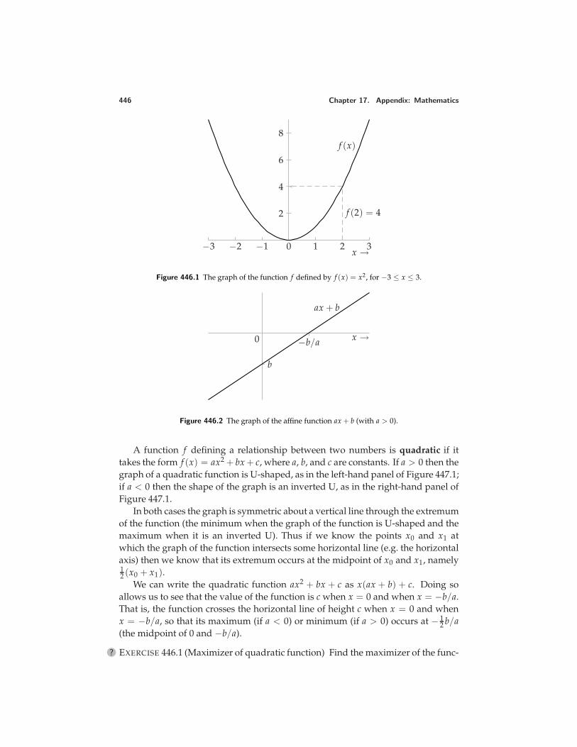
446 Chapter 17. Appendix: Mathematics
−3 −2 −1 0 1 2 3
2
4
6
8
x →
f (x)
f (2) = 4
Figure 446.1 The graph of the function f defined by f (x) = x2, for −3 ≤ x ≤ 3.
b
−b/a0
ax + b
x →
Figure 446.2 The graph of the affine function ax + b (with a > 0).
A function f defining a relationship between two numbers is quadratic if ittakes the form f (x) = ax2 + bx + c, where a, b, and c are constants. If a > 0 then thegraph of a quadratic function is U-shaped, as in the left-hand panel of Figure 447.1;if a < 0 then the shape of the graph is an inverted U, as in the right-hand panel ofFigure 447.1.
In both cases the graph is symmetric about a vertical line through the extremumof the function (the minimum when the graph of the function is U-shaped and themaximum when it is an inverted U). Thus if we know the points x0 and x1 atwhich the graph of the function intersects some horizontal line (e.g. the horizontalaxis) then we know that its extremum occurs at the midpoint of x0 and x1, namely12 (x0 + x1).
We can write the quadratic function ax2 + bx + c as x(ax + b) + c. Doing soallows us to see that the value of the function is c when x = 0 and when x = −b/a.That is, the function crosses the horizontal line of height c when x = 0 and whenx = −b/a, so that its maximum (if a < 0) or minimum (if a > 0) occurs at − 1
2 b/a(the midpoint of 0 and −b/a).
? EXERCISE 446.1 (Maximizer of quadratic function) Find the maximizer of the func-
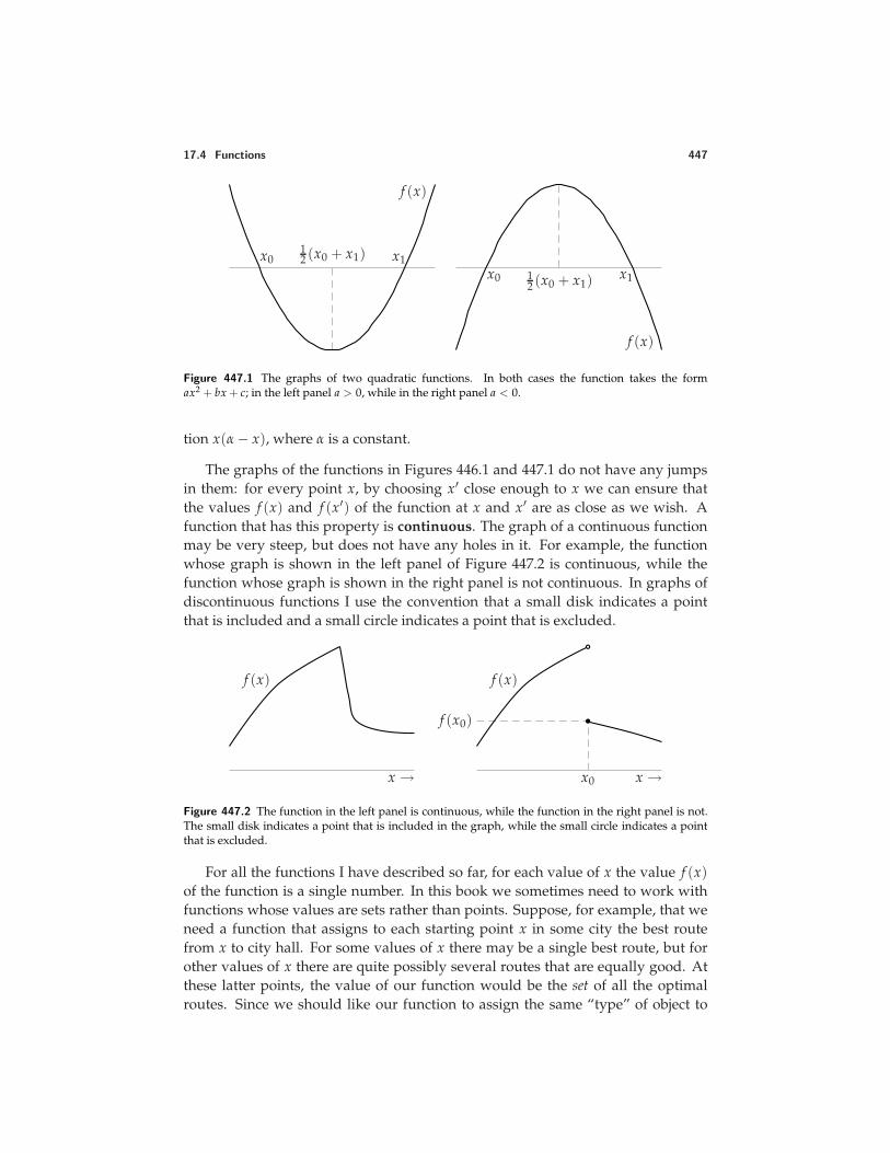
17.4 Functions 447
x0 x112 (x0 + x1)
f (x)
x0 x112 (x0 + x1)
f (x)
Figure 447.1 The graphs of two quadratic functions. In both cases the function takes the formax2 + bx + c; in the left panel a > 0, while in the right panel a < 0.
tion x(α − x), where α is a constant.
The graphs of the functions in Figures 446.1 and 447.1 do not have any jumpsin them: for every point x, by choosing x′ close enough to x we can ensure thatthe values f (x) and f (x′) of the function at x and x′ are as close as we wish. Afunction that has this property is continuous. The graph of a continuous functionmay be very steep, but does not have any holes in it. For example, the functionwhose graph is shown in the left panel of Figure 447.2 is continuous, while thefunction whose graph is shown in the right panel is not continuous. In graphs ofdiscontinuous functions I use the convention that a small disk indicates a pointthat is included and a small circle indicates a point that is excluded.
x →
f (x)
f (x0)
x0 x →
f (x)
Figure 447.2 The function in the left panel is continuous, while the function in the right panel is not.The small disk indicates a point that is included in the graph, while the small circle indicates a pointthat is excluded.
For all the functions I have described so far, for each value of x the value f (x)of the function is a single number. In this book we sometimes need to work withfunctions whose values are sets rather than points. Suppose, for example, that weneed a function that assigns to each starting point x in some city the best routefrom x to city hall. For some values of x there may be a single best route, but forother values of x there are quite possibly several routes that are equally good. Atthese latter points, the value of our function would be the set of all the optimalroutes. Since we should like our function to assign the same “type” of object to
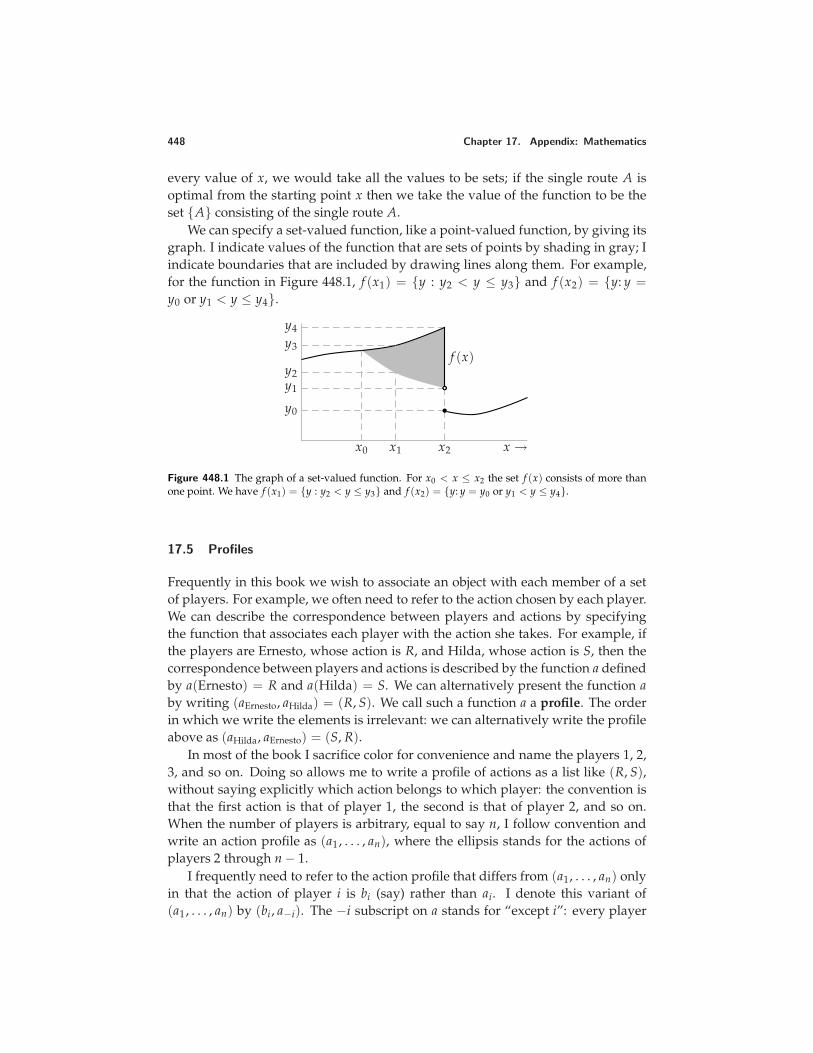
448 Chapter 17. Appendix: Mathematics
every value of x, we would take all the values to be sets; if the single route A isoptimal from the starting point x then we take the value of the function to be theset A consisting of the single route A.
We can specify a set-valued function, like a point-valued function, by giving itsgraph. I indicate values of the function that are sets of points by shading in gray; Iindicate boundaries that are included by drawing lines along them. For example,for the function in Figure 448.1, f (x1) = y : y2 < y ≤ y3 and f (x2) = y: y =y0 or y1 < y ≤ y4.
f (x)
x0 x1 x2
y0
y1
y2
y3
y4
x →
Figure 448.1 The graph of a set-valued function. For x0 < x ≤ x2 the set f (x) consists of more thanone point. We have f (x1) = y : y2 < y ≤ y3 and f (x2) = y: y = y0 or y1 < y ≤ y4.
17.5 Profiles
Frequently in this book we wish to associate an object with each member of a setof players. For example, we often need to refer to the action chosen by each player.We can describe the correspondence between players and actions by specifyingthe function that associates each player with the action she takes. For example, ifthe players are Ernesto, whose action is R, and Hilda, whose action is S, then thecorrespondence between players and actions is described by the function a definedby a(Ernesto) = R and a(Hilda) = S. We can alternatively present the function aby writing (aErnesto, aHilda) = (R, S). We call such a function a a profile. The orderin which we write the elements is irrelevant: we can alternatively write the profileabove as (aHilda, aErnesto) = (S, R).
In most of the book I sacrifice color for convenience and name the players 1, 2,3, and so on. Doing so allows me to write a profile of actions as a list like (R, S),without saying explicitly which action belongs to which player: the convention isthat the first action is that of player 1, the second is that of player 2, and so on.When the number of players is arbitrary, equal to say n, I follow convention andwrite an action profile as (a1, . . . , an), where the ellipsis stands for the actions ofplayers 2 through n − 1.
I frequently need to refer to the action profile that differs from (a1, . . . , an) onlyin that the action of player i is bi (say) rather than ai. I denote this variant of(a1, . . . , an) by (bi , a−i). The −i subscript on a stands for “except i”: every player
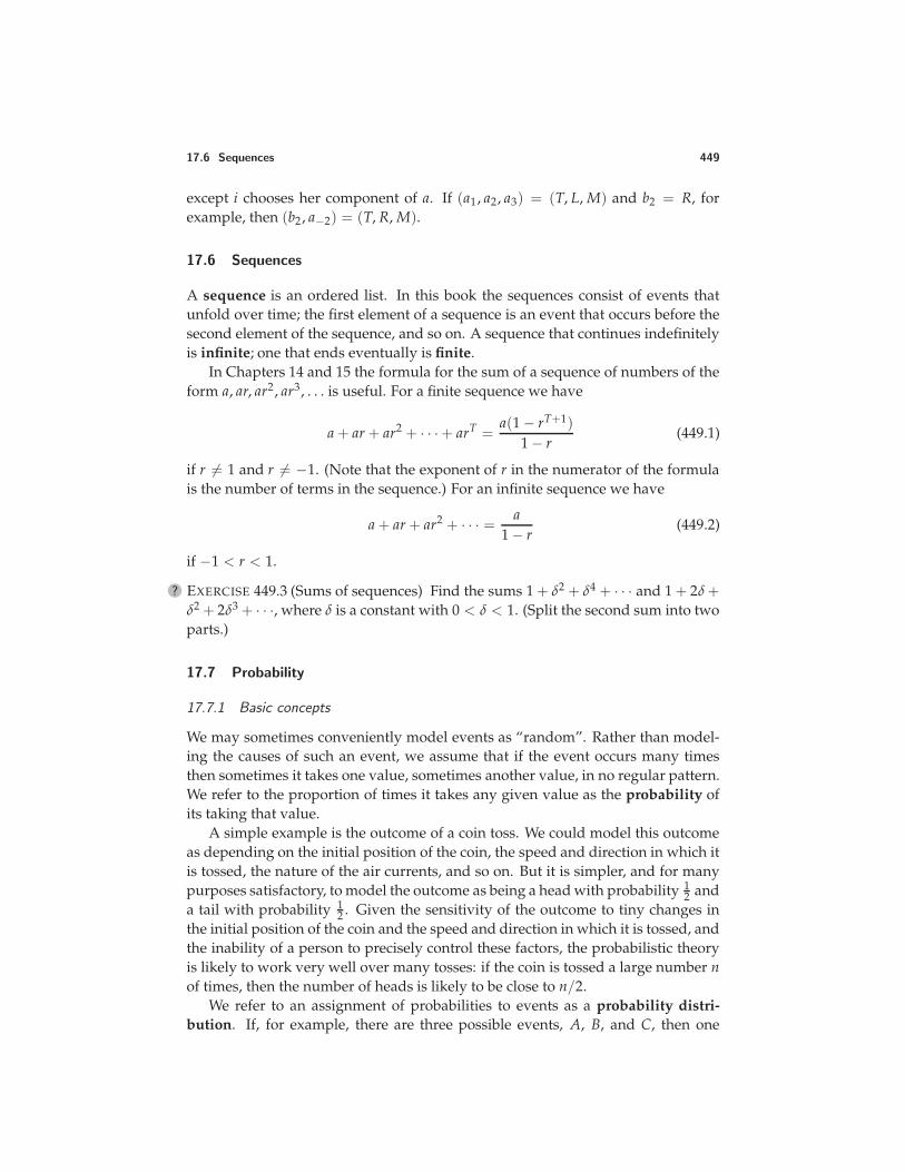
17.6 Sequences 449
except i chooses her component of a. If (a1, a2, a3) = (T, L, M) and b2 = R, forexample, then (b2, a−2) = (T, R, M).
17.6 Sequences
A sequence is an ordered list. In this book the sequences consist of events thatunfold over time; the first element of a sequence is an event that occurs before thesecond element of the sequence, and so on. A sequence that continues indefinitelyis infinite; one that ends eventually is finite.
In Chapters 14 and 15 the formula for the sum of a sequence of numbers of theform a, ar, ar2, ar3, . . . is useful. For a finite sequence we have
a + ar + ar2 + · · · + arT =a(1 − rT+1)
1 − r(449.1)
if r = 1 and r = −1. (Note that the exponent of r in the numerator of the formulais the number of terms in the sequence.) For an infinite sequence we have
a + ar + ar2 + · · · =a
1 − r(449.2)
if −1 < r < 1.
? EXERCISE 449.3 (Sums of sequences) Find the sums 1 + δ2 + δ4 + · · · and 1 + 2δ +δ2 + 2δ3 + · · ·, where δ is a constant with 0 < δ < 1. (Split the second sum into twoparts.)
17.7 Probability
17.7.1 Basic concepts
We may sometimes conveniently model events as “random”. Rather than model-ing the causes of such an event, we assume that if the event occurs many timesthen sometimes it takes one value, sometimes another value, in no regular pattern.We refer to the proportion of times it takes any given value as the probability ofits taking that value.
A simple example is the outcome of a coin toss. We could model this outcomeas depending on the initial position of the coin, the speed and direction in which itis tossed, the nature of the air currents, and so on. But it is simpler, and for manypurposes satisfactory, to model the outcome as being a head with probability 1
2 anda tail with probability 1
2 . Given the sensitivity of the outcome to tiny changes inthe initial position of the coin and the speed and direction in which it is tossed, andthe inability of a person to precisely control these factors, the probabilistic theoryis likely to work very well over many tosses: if the coin is tossed a large number nof times, then the number of heads is likely to be close to n/2.
We refer to an assignment of probabilities to events as a probability distri-bution. If, for example, there are three possible events, A, B, and C, then one
450 Chapter 17. Appendix: Mathematics
probability distribution assigns probability 13 to A, probability 1
2 to B, and prob-ability 1
6 to C. In any probability distribution the sum of the probabilities of allpossible events is 1 (on any given occasion, one of the events must occur), and eachprobability is nonnegative and at most 1. Saying that an event occurs with posi-tive probability is equivalent to saying that there is some chance that it may occur;saying that an event occurs with probability zero is equivalent to saying that it willnever occur. Similarly, saying that an event occurs with probability less than one isequivalent to saying that there is some chance that it may not occur; saying that anevent occurs with probability one is equivalent to saying that it is certain to occur.We sometimes denote the probability of an event E by Pr(E).
If the events E and F cannot both occur, then the probability that either E or Foccurs is the sum Pr(E) + Pr(F). For example, suppose we model the outcome ofthe toss of a die as random, with the probability of each side equal to 1
6 . Then theprobability that the side is either 3 or 4 is Pr(3) + Pr(4) = 1
6 + 16 = 1
3 .
17.7.2 Independence
Two events E and F are independent if the probability Pr(E and F) that they bothoccur is the product Pr(E) Pr(F) of the probabilities that each occurs. Events maysensibly be modeled as independent if the occurrence of one has no bearing onthe occurrence of the other. For example, the outcome of an election may sensiblybe modeled as independent of the outcome of a coin toss, but not independentof the weather on the polling day (which may affect the candidates’ supportersdifferently). In a strategic game, we model the players’ choices of actions as in-dependent: the probability that player 1 chooses action a1 and player 2 choosesaction a2 is assumed to be the product of the probability that player 1 chooses a1and the probability that player 2 chooses a2.
17.7.3 Lotteries and expected values
The material in this section is used only in Chapter 4 (Mixed strategy equilibrium), Sec-tion 7.6 (Extensive games with perfect information, simultaneous moves, and chance moves),Chapter 9 (Bayesian Games), Chapter 10 (Extensive games with imperfect information),Chapter 11 (Strictly competitive games and maxminimization), and Chapter 12 (Rational-izability).
Consider a decision-maker who faces a situation in which there are probabilisticelements. Each action that she chooses induces a probability distribution over out-comes. If you make an offer for an item in a classified advertisement, for example,then given the behavior of other potential buyers, your offer may be accepted withprobability 1
3 and rejected with probability 23 . We refer to a probability distribution
over outcomes as a lottery over outcomes.If the outcomes of a lottery are numerical (for example, amounts of money), we
may be interested in their average value—the value we should expect to get if wefound the total of the values on a large number n of trials and divided by n. For the
17.7 Probability 451
lottery that yields the amount xi with probability pi, for i = 1, . . . , n, this averagevalue is
p1x1 + · · · + pnxn
or, more compactly, ∑ni=1 pnxn. It is called the expected value of the lottery. A
lottery that yields $12 with probability 13 , $4 with probability 1
2 , and $6 with prob-ability 1
6 , for example, has an expected value of 13 · 12 + 1
2 · 4 + 16 · 6 = 7. On no
single occasion does the lottery yield $7, but over a large number of occasions theaverage amount that it yields is likely to be close to $7 (the more likely, the largerthe number of occasions).
17.7.4 Cumulative probability distributions
The material in this section is used only in Section 4.11 (Mixed strategy equilibrium ingames in which each player has a continuum of actions) and Chapter 9 (Bayesian Games).
If the events in our model are associated with numbers, we can describe theprobabilities assigned to them by giving the cumulative probability distribution,which assigns to each number x the total of the probabilities of all numbers at mostequal to x. The cumulative probability distribution of the number of dots on theexposed side of a die, for example, is the function F for which F(1) = 1
6 , F(2) = 13 ,
F(3) = 12 , and so on. Given a cumulative probability distribution we can recover
the probabilities of the events by calculating the differences between values of F:the probability of x is F(x) − F(x′), where x′ is the next smaller event.
When the number of events is finite, we can represent the assignment of proba-bilities to events either by a probability distribution or by a cumulative probabilitydistribution. When the number of events is infinite, we can usefully represent theprobabilities only by a cumulative probability distribution, because the probabilityof any single event is typically zero. If the set of events is the set of numbers froma to a then a cumulative probability distribution is a nondecreasing function, sayF, for which F(x) = 0 if x < a (the probability of a number less than a is 0) andF(a) = 1 (the probability of a number at most equal to a is 1). The number F(x) isthe probability of an event at most equal to x.
For example, if a = 0 and a = 1 then the function F(x) = x is a cumulativeprobability distribution. This distribution represents uniform randomization overthe interval (sets of the same size have the same probability). Another cumulativeprobability distribution is given by the function F(x) = x2. In this distribution theprobabilities of sets of numbers close to 0 are lower than the probabilities of sets ofnumbers close to 1.
17.7.5 Conditional probability and Bayes’ rule
The material in this section is used only in Section 9.8 (Juries) and Chapter 10 (ExtensiveGames with Imperfect Information).
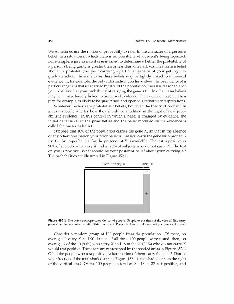
452 Chapter 17. Appendix: Mathematics
We sometimes use the notion of probability to refer to the character of a person’sbelief, in a situation in which there is no possibility of an event’s being repeated.For example, a jury in a civil case is asked to determine whether the probability ofa person’s being guilty is greater than or less than one half; you may form a beliefabout the probability of your carrying a particular gene or of your getting intograduate school. In some cases these beliefs may be tightly linked to numericalevidence. If, for example, the only information you have about the prevalence of aparticular gene is that it is carried by 10% of the population, then it is reasonable foryou to believe that your probability of carrying the gene is 0.1. In other cases beliefsmay be at most loosely linked to numerical evidence. The evidence presented to ajury, for example, is likely to be qualitative, and open to alternative interpretations.
Whatever the basis for probabilistic beliefs, however, the theory of probabilitygives a specific rule for how they should be modified in the light of new prob-abilistic evidence. In this context in which a belief is changed by evidence, theinitial belief is called the prior belief and the belief modified by the evidence iscalled the posterior belief.
Suppose that 10% of the population carries the gene X, so that in the absenceof any other information your prior belief is that you carry the gene with probabil-ity 0.1. An imperfect test for the presence of X is available. The test is positive in90% of subjects who carry X and in 20% of subjects who do not carry X. The teston you is positive. What should be your posterior belief about your carrying X?The probabilities are illustrated in Figure 452.1.
Don’t carry X Carry X
+
−+
−
Figure 452.1 The outer box represents the set of people. People to the right of the vertical line carrygene X, while people to the left of this line do not. People in the shaded areas test positive for the gene.
Consider a random group of 100 people from the population. Of these, onaverage 10 carry X and 90 do not. If all these 100 people were tested, then, onaverage, 9 of the 10 (90%) who carry X and 18 of the 90 (20%) who do not carry Xwould test positive. These sets are represented by the shaded areas in Figure 452.1.Of all the people who test positive, what fraction of them carry the gene? That is,what fraction of the total shaded area in Figure 452.1 is the shaded area to the rightof the vertical line? Of the 100 people, a total of 9 + 18 = 27 test positive, and
17.7 Probability 453
one-third of these (9/27) carry the gene. Thus after testing positive, your posteriorbelief that you carry the gene is 1
3 : the positive test raises the probability you assignto your carrying X from 1
10 to 13 .
To generalize the analysis in this example, we introduce the concept of con-ditional probability. Let E and F be two events that may be related; assume thatPr(F) > 0. Suppose that F is true. Define the probability Pr(E | F) of E condi-tional on F by
Pr(E | F) =Pr(E and F)
Pr(F). (453.1)
This number makes sense as the probability that E is true given that F is true. Oneway to see that it makes sense is to consider Figure 452.1 again. Let E be the eventthat you carry X and let F be the event that you test positive. If you test posi-tive then we know you lie in the shaded area. Given you lie in this area, what isthe probability Pr(E | F) that you lie to the right of the vertical line? This prob-ability is the ratio of the shaded area to the right of the vertical line—the proba-bility Pr(E and F) that you carry the gene and test positive—to the total shadedarea—the probability Pr(F) that you test positive.
If the events E and F are independent then
Pr(E | F) = Pr(E) and Pr(F) > 0
or, alternatively,Pr(F | E) = Pr(F) and Pr(E) > 0.
These conditions express directly the idea that the occurrence of one event has nobearing on the occurrence of the other event.
In using the expression for conditional probability to find the posterior beliefin this case, we needed to calculate Pr(E and F) and Pr(F), which were not givendirectly as data in the problem. The data we were given were the prior belief Pr(E),the probability Pr(F | E) of a person who carries the gene testing positive, and theprobability Pr(F | not E) of a person who does not carry the gene testing positive.
Bayes’ rule expresses the conditional probability Pr(E | F) directly in terms ofPr(E), Pr(F | E), and Pr(F | not E):
Pr(E | F) =Pr(E) Pr(F | E)
Pr(E) Pr(F | E) + Pr(not E) Pr(F | not E). (453.2)
(The probability Pr(not E) is of course equal to 1 − Pr(E); recall that I have as-sumed that Pr(F) > 0.) This formula follows from the definition of conditionalprobability (453.1) and the properties of probabilities. First, interchanging E and Fin (453.1) we deduce Pr(E) Pr(F | E) = Pr(E and F). Thus the numerator of (453.2)is equal to Pr(E and F). Second, again using (453.1) we see that the denominator of(453.2) is equal to Pr(E and F) + Pr((not E) and F). Now, either the event E or theevent not E occurs, but not both. Thus Pr(E and F) + Pr((not E) and F) = Pr(F).(The probability that either “it rains and you carry an umbrella” or “it rains andyou do not carry an umbrella” is equal to the probability that “it rains”!)
454 Chapter 17. Appendix: Mathematics
? EXERCISE 454.1 (Bayes’ rule) Consider a generalization of the example of testingpositive for a gene in which the fraction p of the population carry the gene. Ver-ify that as p decreases, the posterior probability that you carry X given that youtest positive decreases. What value does this posterior probability take when p is0.001? What value does the posterior probability take when p is 0.001 and the testis positive for 99% of those who carry X and is negative for 99% of those who donot carry X? (Are you surprised?)
In the cases I have described so far, the event about which we form a belief takestwo possible values (E, or not E). In a more general setting, this event may takemany values. For example, we may form a belief about the quality of an item—avariable that may take many values—on its price. In general, let F be an event andlet E1, . . . , En be a collection of events, exactly one of which must occur. (In theexample above, F is the event that you test positive, n = 2, E1 is the event youcarry the gene, and E2 is the event you do not carry the gene.) Then the probabilityof Ek conditional on F is
Pr(Ek | F) =Pr(F | Ek) Pr(Ek)
∑nj=1 Pr(F | Ej) Pr(Ej)
. (454.2)
This general formula is known as Bayes’ rule, after Thomas Bayes (1702–61). Inthe context in which we use this rule in a Bayesian game to find the probability ofa state given the observed signal, the events E1, . . . , En are the states and the eventF is a signal. Thus every probability Pr(F | Ek) is either one or zero, depending onwhether the state Ek generates the signal F or not.
17.8 Proofs
This book focuses on concepts, but contains precise arguments, and, in some cases,proofs of results. The results are given three names: Lemma, Proposition, andCorollary. These names have no formal significance—they do not have any impli-cations for the type of logic used—but are intended to convey the role of the resultin the analysis. Lemmas are results whose importance lies mainly in their beingsteps on the way to proving further results. Propositions are the main results.Corollaries are more or less direct implications of the main results.
A result consists of a series of statements of the form “if A is true then B istrue”. Frequently the series contains only one such statement, which may not beexplicitly rendered as “if A then B”. For example, “all prime numbers are odd” is aresult; it can be transformed into the “if . . . then” form: “if a number is prime thenit is odd”. A result that makes the two claims “if A is true then B is true” and “if Bis true then A is true” is sometimes stated compactly as “A is true if and only if Bis true”.
A proof of the result “if A then B” is a series of arguments that lead from Ato B, each of which follows from a known fact (including an earlier member ofthe series). Except for the proofs of very simple results, most proofs are not, and
17.8 Proofs 455
should not sensibly be, “complete”. To spell out how each step follows from thebasic principles of mathematics would make a proof extremely long and very dif-ficult to read. Some facts must be taken for granted; judging which to put in andwhich to leave out is an art. A good proof convinces readers that the result is trueand gives them some understanding of why it is true (the features of A that aresignificant, and those that are not significant).
References
Akerlof, George A. (1974?), “The market for ’lemons”’, Quarterly Journal of Eco-nomics ??, 488–500.
Allais, Maurice (1953), “Le comportement de l’homme rationnel devant le risque:critique des postulats et axiomes de l’ecole Americaine”, Econometrica 21,503–546.
Andreau, Jean (1999), Banking and business in the Roman world. Cambridge: Cam-bridge University Press.
Aronson, Elliot (1995), The social animal (7th edition). New York: W. H. Freeman.Arrow, Kenneth J. (1951), Social choice and individual values. New York: Wiley.Aumann, Robert J. (1985), “What is game theory trying to accomplish?”, pp. 28–76
in Frontiers of economics (Kenneth J. Arrow and Seppo Honkapohja, eds.),Oxford: Basil Blackwell.
Aumann, Robert J. (1997), “Rationality and bounded rationality”, Games and Eco-nomic Behavior 21, 2–14.
Aumann, Robert J., and Bezalel Peleg (1960), “Von Neumann–Morgenstern solu-tions to cooperative games without side payments”, Bulletin of the AmericanMathematical Society 66, 173–179.
Aumann, Robert J., and Lloyd S. Shapley (1994), “Long-term competition—a game-theoretic analysis”, pp. 1–15 in Essays in game theory (Nimrod Megiddo, ed.),New York: Springer-Verlag.
Austen-Smith, David, and Jeffrey S. Banks (1996), “Information aggregation, ratio-nality, and the Condorcet Jury Theorem”, American Political Science Review90, 34–45.
Austen-Smith, David, and Jeffrey S. Banks (1999), Positive political theory I. AnnArbor: University of Michigan Press.
Axelrod, Robert (1980a), “Effective choice in the Prisoner’s Dilemma”, Journal ofConflict Resolution 24, 3–25.
Axelrod, Robert (1980b), “More effective choice in the Prisoner’s Dilemma”, Jour-nal of Conflict Resolution 24, 379–403.
Axelrod, Robert (1984), The evolution of cooperation. New York: Basic Books.Banks, Jeffrey S. (1995), “Singularity theory and core existence in the spatial model”,
Journal of Mathematical Economics 24, 523–536.Baye, Michael R., Dan Kovenock, and Casper G. de Vries (1996), “The all-pay
auction with complete information”, Economic Theory 8, 291–305.Baye, Michael R., and John Morgan (1996), “Revisiting Bertrand’s competition:
paradox lost or paradox found?”, unpublished paper.Becker, Gary S. (1974), “A theory of social interactions”, Journal of Political Economy
82, 1063–1091.
458 References
Bellman, Richard (1957), Dynamic programming. Princeton: Princeton UniversityPress.
Benoıt, Jean-Pierre (1984), “Financially constrained entry in a game of incompleteinformation”, Rand Journal of Economics 15, 490–499.
Benoıt, Jean-Pierre, and Lewis A. Kornhauser (1996), “Game theoretic analysis oflegal rules and institutions”, pp. ???–??? in Handbook of Game Theory withEconomic Applications (Robert J. Aumann and Sergiu Hart, eds.), Amster-dam: North-Holland.
Bergstrom, Theodore C. (1989), “A fresh look at the rotten kid theorem—and otherhousehold mysteries”, Journal of Political Economy 97, 1138–1159.
Bergstrom, Theodore C. (1995), “On the evolution of altruistic ethical rules forsiblings”, American Economic Review 85, 58–81.
Bergstrom, Theodore C., Lawrence E. Blume, and Hal R. Varian (1986), “On theprivate provision of public goods”, Journal of Public Economics 29, 25–49.
Bergstrom, Theodore C., and Hal R. Varian (1987), Workouts in intermediate microe-conomics, 3rd edition. New York: Norton.
Bernheim, B. Douglas (1984), “Rationalizable strategic behavior”, Econometrica 52,1007–1028.
Bernoulli, Daniel (1738), “Specimen theoriae novae de mensura sortis”, translatedas “Exposition of a new theory on the measurement of risk” by LouiseSommer, Econometrica 22 (1954), 23-36.
Bertrand, Joseph (1883), “Review of ‘Theorie mathematique de la richesse sociale’by Leon Walras and ‘Recherches sur les principes mathematiques de la theoriedes richesses’ by Augustin Cournot”, Journal des Savants, September, 499-508. (Translated as “Review by Joseph Bertrand of two books”, History ofPolitical Economy 24 (1992), 646–653.)
Black, Duncan (1958), The theory of committees and elections. Cambridge: CambridgeUniversity Press.
Black, Duncan, and R. A. Newing (1951), Committee decisions with complementaryvaluation. London: William Hodge.
Blackwell, David, and M. A. Girshick (1954), Theory of games and statistical decisions.New York: Wiley.
Bolton, Gary E, and Axel Ockenfels (2000), “ERC: a theory of equity, reciprocity,and competition”, American Economic Review 90, 166–193.
Bolton, Gary E, and Rami Zwick (1995), “Anonymity versus punishment in ulti-matum bargaining”, Games and Economic Behavior 10, 95–121.
Borel, Emile (1921), “La theorie du jeu et les equations integrales a noyau symetrique”,Comptes Rendus Hebdomadaires des Seances de l’Academie des Sciences (Paris)173, 1304–1308. (Translated as “The theory of play and integral equationswith skew symmetric kernels”, Econometrica 21 (1953), pp. 97–100.)
Borel, Emile (1924), Elements de la theorie des probabilites (third edition). Paris: Li-brairie Scientifique, J. Hermann. (Pp. 204–221 translated as “On GamesThat Involve Chance and the Skill of the Players”, Econometrica 21 (1953),101–115.)
References 459
Borel, Emile (1927), “Sur les systemes de formes lineaires a determinant symetriquegauche et la theorie generale du jeu”, Comptes Rendus Hebdomadaires desSeances de l’Academie des Sciences (Paris) 184, 52–54. (Translated as “On sys-tems of linear forms of skew symmetric determinant and the general theoryof play”, Econometrica 21 (1953), 116–117.)
Boylan, Richard T. (2000), “An optimal auction perspective on lobbying”, SocialChoice and Welfare 17, 55–68.
Braess, Dietrich (1968), “’Uber ein Paradoxon der Verkehrsplanung”, Unternehmensforschung12, 258–268.
Brams, Steven J., and Peter C. Fishburn (1978), “Approval voting”, American Polit-ical Science Review 72, 831–847.
Brams, Steven J., and Peter C. Fishburn (1983), Approval voting. Boston: Birkhauser.Brams, Steven J., D. Marc Kilgour, and Morton D. Davis (1993), “Unraveling in
games of sharing and exchange”, pp. 195–212 in Frontiers of Game Theory(Kenneth G. Binmore, Alan Kirman, and Piero Tani, eds.), Cambridge, Mass.:MIT Press.
Brams, Steven J., and Philip D. Straffin, Jr. (1979), “Prisoners’ dilemma and profes-sional sports drafts”, American Mathematical Monthly 86, 80–88.
Brams, Steven J., and Alan D. Taylor (1996), Fair division. Cambridge UniversityPress: Cambridge.
Brockmann, H. Jane, Alan Grafen, and Richard Dawkins (1979), “Evolutionarilystable nesting strategy in a digger wasp”, Journal of Theoretical Biology 77,473–496.
Brown, George W. (1951), “Iterative solution of games by fictitious play”, pp. 374–376 in Activity analysis of production and allocation (Tjalling C. Koopmans,ed.), New York: Wiley.
Brown, James N., and Robert W. Rosenthal (1990), “Testing the minimax hypothe-sis: a re-examination of O’Neill’s game experiment”, Econometrica 58, 1065–1081.
Brown, John P. (1973), “Toward an economic theory of liability”, Journal of LegalStudies 2, 323–349.
Brown, Roger (1986), Social psychology, the second edition. New York: Free Press.Bryant, John (1983), “A simple rational expectations Keynes-type model”, Quar-
terly Journal of Economics 98, 525–528.Bryant, John (1994), “Coordination theory, the stag hunt and macroeconomics”,
pp. 207–225 in Problems of coordination in economic activity (James W. Fried-man, ed.), Boston: Kluwer.
Bulmer, Michael G. (1994), Theoretical evolutionary ecology. Sunderland, Massachusetts:Sinauer Associates.
Bulow, Jeremy, and Paul Klemperer (1996), “Auctions versus negotiations”, Amer-ican Economic Review 86, 180–194.
Camerer, Colin (1995), “Individual decision making”, pp. 587–703 in The handbookof experimental economics (John H. Kagel and Alvin E. Roth, eds.), Princeton:Princeton University Press.
460 References
Capen, E. C., R. V. Clapp, and W. M. Campbell (1971), “Competitive bidding inhigh-risk situations”, Journal of Petroleum Technology 23, 641–653.
Cassady, Ralph, Jr. (1967), Auctions and auctioneering. Berkeley: University ofCalifornia Press.
Conlisk, John (1989), “Three variants on the Allais example”, American EconomicReview 79, 392–407.
Cooper, Russell, Douglas V. DeJong, Robert Forsythe, and Thomas W. Ross (1996),“Cooperation without reputation: experimental evidence from Prisoner’sDilemma games”, Games and Economic Behavior 12, 187–218.
Cournot, Antoine A. (1838), Recherches sur les principes mathematiques de la theoriedes richesses. Paris: Hachette. (English translation: “Researches into themathematical principles of the theory of wealth”, New York: Macmillan,1897.)
Court, Gordon S. (1996), “The seal’s own skin game”, Natural History 105.8, 36–41.Cramton, Peter C. (1995), “Money out of thin air: the nationwide narrowband PCS
auction”, Journal of Economics and Management Strategy 4, 267–343.Cramton, Peter C. (1997), “The FCC spectrum auctions: an early assessment”,
Journal of Economics and Management Strategy 6, 431–495.Cramton, Peter C. (1998), “The efficiency of the FCC spectrum auctions”, Journal of
Law and Economics 41, 727–736.Darwin, Charles (1871), The descent of man, and selection in relation to sex. London:
John Murray.Darwin, Charles (1874), The descent of man, and selection in relation to sex (Second
edition, revised and augmented). London: John Murray.Deutsch, Morton (1958), “Trust and suspicion”, Journal of Conflict Resolution 2, 265–
279.Diamond, Peter A. (1974), “Accident law and resource allocation”, Bell Journal of
Economics and Management Science 5, 366–405.Diermeier, Daniel, and Timothy J. Feddersen (1996), “Voting cohesion in presiden-
tial and parliamentary legislatures”, unpublished paper.Dixit, Avinash, and Barry Nalebuff (1991), Thinking strategically. New York: Nor-
ton.Downs, Anthony (1957), An economic theory of democracy. New York: Harper and
Row.Dubey, Pradeep, and Mamoru Kaneko (1984), “Information patterns and Nash
equilibria in extensive games: I”, Mathematical Social Sciences 8, 111–139.Dubins, Lester E., and David A. Freedman (1981), “Machiavelli and the Gale-
Shapley algorithm”, American Mathematical Monthly 88, 485–494.Dugatkin, Lee Alan (1991), “Dynamics of the tit for tat strategy during predator
inspection in the guppy (Poecilia reticulata)”, Behavioral Ecology and Sociobi-ology 29, 127–132.
Edgeworth, Francis Y. (1881), Mathematical psychics. London: Kegan Paul.Elster, Jon (1998), “Emotions and economic theory”, Journal of Economic Literature
36, 47–74.
References 461
Farquharson, Robin (1969), Theory of voting. New Haven: Yale University Press.(See also Niemi (1983).)
Feddersen, Timothy J., and Wolfgang Pesendorfer (1996), “The swing voter’s curse”,American Economic Review 86, 408–424.
Feddersen, Timothy J., and Wolfgang Pesendorfer (1998), “Convicting the inno-cent: the inferiority of unanimous jury verdicts under strategic voting”,American Political Science Review 92, 23–35.
Feddersen, Timothy J., Itai Sened, and Stephen G. Wright (1990), “Rational vot-ing and candidate entry under plurality rule”, American Journal of PoliticalScience 34, 1005–1016.
Fellner, William (1949), Competition among the few. New York: Alfred A. Knopf.Fiorina, Morris P., and Charles R. Plott (1978), “Committee decisions under ma-
jority rule: an experimental study”, American Political Science Review 72,575–598.
Fisher, Ronald A. (1930), The genetical theory of natural selection. Oxford: ClarendonPress.
Flood, Merrill M. (1958/59), “Some experimental games”, Management Science 5,5–26.
Forsythe, Robert, Joel L. Horowitz, N. E. Savin, and Martin Sefton (1994), “Fairnessin simple bargaining experiments”, Games and Economic Behavior 6, 347–369.
Frank, Robert H., Thomas Gilovich, and Dennis T. Regan (1993), “Does studyingeconomics inhibit cooperation?”, Journal of Economic Perspectives 7 (2), 159–171.
Friedman, James W. (1971), “A non-cooperative equilibrium for supergames”, Re-view of Economic Studies 38, 1–12.
Fudenberg, Drew, and David K. Levine (1998), The theory of learning in games.Cambridge, Massachusetts: MIT Press.
Fudenberg, Drew, and Eric S. Maskin (1986), “The folk theorem in repeated gameswith discounting or with incomplete information”, Econometrica 54, 533–554.
Gale, David, and Lloyd S. Shapley (1962), “College admissions and the stability ofmarriage”, American Mathematical Monthly 69, 9–15.
Gardner, Martin (1959), The Scientific American book of mathematical puzzles and di-versions. New York: Simon and Schuster.
Ghemawat, Pankaj, and Barry Nalebuff (1985), “Exit”, Rand Journal of Economics 16,184–194.
Gordon, H. Scott (1954), “The economic theory of a common-property resource:the fishery”, Journal of Political Economy 62, 124–142.
Groseclose, Tim, and James M. Snyder, Jr. (1996), “Buying supermajorities”, Amer-ican Political Science Review 90, 303–315.
Grout, Paul A. (1984), “Investment and wages in the absence of binding contracts:a Nash bargaining approach”, Econometrica 52, 449–460.
Guilbaud, Georges T. (1961), “Faut-il jouer au plus fin? (notes sur l’histoire dela theorie des jeux)”, pp. 171–182 in La decision, Paris: Editions du Centre
462 References
National de la Recherce Scientifique.Guth, Werner, and Steffen Huck (1997), “From ultimatum bargaining to dictatorship—
an experimental study of four games varying in veto power”, Metroeconom-ica 48, 262–279.
Guth, Werner, Rolf Schmittberger, and Bernd Schwarze (1982), “An experimentalanalysis of ultimatum bargaining”, Journal of Economic Behavior and Organi-zation 3, 367–388.
Halmos, Paul R. (1973), “The legend of John von Neumann”, American Mathemati-cal Monthly 80, 382–394.
Hamilton, W. D. (1967), “Extraordinary sex ratios”, Science 156, 477–488.Hammerstein, Peter, and Susan E. Riechert (1988), “Payoffs and strategies in ter-
ritorial contests: ESS analyses of two ecotypes of the spider Agelenopsisaperta”, Evolutionary Ecology 2, 115–138.
Hammerstein, Peter, and Reinhard Selten (1994), “Game theory and evolution-ary biology”, pp. 929–993 in Handbook of Game Theory, Volume 2 (Robert J.Aumann and Sergiu Hart, eds.), Amsterdam: Elsevier.
Hardin, Garrett (1968), “The tragedy of the commons”, Science 162, 1243–1248.Harris, Christopher, and John Vickers (1985), “Perfect equilibrium in a model of a
race”, Review of Economic Studies 52, 193–209.Harsanyi, John C. (1967/68), “Games with incomplete information played by ‘Bayesian’
players, Parts I, II, and III”, Management Science 14, 159–182, 320–334, and486–502.
Herodotus (1998), The histories (translated by Robin Waterfield). Oxford: OxfordUniversity Press.
Heuer, Gerald A. (1995), “Solution to problem 1069”, Journal of Recreational Math-ematics 27, 146–158. [Author’s middle initial incorrectly given as “N” injournal.]
Hey, John D. (1997), “Experiments and the economics of individual decision mak-ing under risk and uncertainty”, pp. 173–205 in Advances in economics andeconometrics: theory and applications (Seventh world congress), Volume I (DavidM. Kreps and Kenneth F. Wallis, eds.), Cambridge: Cambridge UniversityPress.
Hoffman, Elizabeth, Kevin A. McCabe, and Vernon L. Smith (1996), “On expecta-tions and the monetary stakes in ultimatum games”, International Journal ofGame Theory 25, 289–301.
Holt, Charles A., Jr., and Roger Sherman (1982), “Waiting-line auctions”, Journal ofEconomic Perspectives 90, 280–294.
Hotelling, Harold (1929), “Stability in competition”, Economic Journal 39, 41–57.Jervis, Robert (1977/78), “Cooperation under the security dilemma”, World Politics
30, 167–214.Kaneko, Mamoru, and Shubhashis Raychaudhuri (1993), “Segregation, discrimi-
natory behaviors, and fallacious utility functions in the Festival Game withMerrymakers”, unpublished paper.
Karlin, Samuel (1959a), Mathematical methods and theory in games, programming, and
References 463
economics, Volume I. Reading, Massachusetts: Addison-Wesley.Karlin, Samuel (1959b), Mathematical methods and theory in games, programming, and
economics, Volume II. Reading, Massachusetts: Addison-Wesley.Kim, Yong-Gwan (1994), “Evolutionarily stable strategies in the repeated pris-
oner’s dilemma”, Mathematical Social Sciences 28, 167–197.Kinnaird, Clark (1946), Encyclopedia of puzzles and pastimes. New York: Citadel
Press.Klemperer, Paul (1999), “Auction theory: a guide to the literature”, Journal of Eco-
nomic Surveys 13, 227–286.Kohler, David A., and R. Chandrasekaran (1971), “A class of sequential games”,
Operations Research 19, 270–277.Kuhn, Harold W. (1950), “Extensive games”, Proceedings of the National Academy of
Sciences of the United States of America 36, 570–576.Kuhn, Harold W. (1953), “Extensive games and the problem of information”, pp. 193–
216 in Contributions to the theory of games, Volume II (Annals of MathematicsStudies, 28) (Harold W. Kuhn and A. W Tucker, eds.), Princeton: PrincetonUniversity Press.
Kuhn, Harold W. (1968), “Preface” and translation of excerpt from a letter fromPierre Remond de Monmort to Nicholas Bernoulli”, pp. 3–9 in Precursors inmathematical economics: an anthology (Series of Reprints of Scarce Works onPolitical Economy, 19) (William J. Baumol and Stephen M. Goldfeld, eds.),London: London School of Economics and Political Science.
Kuhn, Harold W. (1996), “Introduction”, Duke Mathematical Journal 81, i–v.Kuhn, Harold W., John C. Harsanyi, Reinhard Selten, Jorgen W. Weibull, Eric van
Damme, John F. Nash, Jr., and Peter Hammerstein (1995), “The work ofJohn Nash in game theory”, pp. 280–310 in Les prix Nobel 1994, Stockholm:Almqvist and Wiksell. (Reprinted in Journal of Economic Theory 69 (1996),153–185.)
Langdon, Merle (1994), “Public auctions in ancient Athens”, pp. 253–265 in Rit-ual, finance, politics (Robin Osborne and Simon Hornblower, eds.), Oxford:Clarendon Press.
Latane, Bibb, and Steve Nida (1981), “Ten years of research on group size andhelping”, Psychological Bulletin 89, 308–324.
Lazarus, John, and Neil B. Metcalfe (1990), “Tit-for-tat cooperation in sticklebacks:a critique of Milinski”, Animal Behaviour 39, 987–988.
Ledyard, John O. (1981), “The paradox of voting and candidate competition: a gen-eral equilibrium analysis”, pp. 54–80 in Essays in contemporary fields of eco-nomics (George Horwich and James P. Quirk, eds.), West Lafayette, Indiana:Purdue University Press.
Ledyard, John O. (1984), “The pure theory of large two-candidate elections”, PublicChoice 44, 7–41.
Leininger, Wolfgang (1989), “Escalation and cooperation in conflict situations: thedollar auction revisited”, Journal of Conflict Resolution 33, 231–254.
Leonard, Janet L. (1990), “The hermaphrodite’s dilemma”, Journal of Theoretical
464 References
Biology 147, 361–371.Leonard, Robert J. (1994), “Reading Cournot, reading Nash: the creation and sta-
bilisation of the Nash equilibrium”, Economic Journal 104, 492–511.Leonard, Robert J. (1995), “From parlor games to social science: von Neumann,
Morgenstern, and the creation of game theory 1928–1944”, Journal of Eco-nomic Literature 33, 730–761.
Lewis, David K. (1969), Convention. Cambridge: Harvard University Press.Littlewood, John E. (1953), A mathematician’s miscellany. London: Methuen.Luce, R. Duncan, and Howard Raiffa (1957), Games and decisions. New York: John
Wiley and Sons.Machina, Mark J. (1987), “Choice under uncertainty: problems solved and un-
solved”, Journal of Economic Perspectives 1(1), 121–154.MacKie-Mason, Jeffrey K., and Hal R. Varian (1995), “Pricing the internet”, pp. 269–
314 in Public access to the internet (Brian Kahin and James Keller, eds.), Cam-bridge, Massachusetts: MIT Press.
Magnan de Bornier, Jean (1992), “The “Cournot-Bertrand debate”: a historicalperspective”, History of Political Economy 24, 623–656.
Maynard Smith, John (1972a), “Game theory and the evolution of fighting”, pp. 8–28 in On evolution (John Maynard Smith), Edinburgh: Edinburgh UniversityPress.
Maynard Smith, John (1972b), On evolution. Edinburgh: Edinburgh UniversityPress.
Maynard Smith, John (1974), “The theory of games and the evolution of animalconflicts”, Journal of Theoretical Biology 47, 209–221.
Maynard Smith, John (1982), Evolution and the theory of games. Cambridge: Cam-bridge University Press.
Maynard Smith, John, and G. R. Price (1973), “The logic of animal conflict”, Nature246, 15–18.
McAfee, R. Preston, and John McMillan (1996), “Analyzing the airwaves auction”,Journal of Economic Perspectives 10 (1), 159–175.
McKelvey, Richard D., and Richard G. Niemi (1978), “A multistage game represen-tation of sophisticated voting and binary procedures”, Journal of EconomicTheory 18, 1–22.
McMillan, John (1994), “Selling spectrum rights”, Journal of Economic Perspectives 8(3), 145–162.
Milgrom, Paul R. (1981), “Rational expectations, information acquisition, and com-petitive bidding”, Econometrica 49, 921–943.
Milinski, Manfred (1987), “Tit for tat in sticklebacks and the evolution of coopera-tion”, Nature 325, 433–435.
Milinski, Manfred (1990), “No alternative to tit-for-tat cooperation in sticklebacks”,Animal Behaviour 39, 989–991.
Milinski, Manfred (1993), “Cooperation wins and stays”, Nature 364, 12–13.Miller, Nicholas R. (1977), “Graph-theoretical approaches to the theory of voting”,
American Journal of Political Science 21, 769–803.
References 465
Miller, Nicholas R. (1995), Committees, agendas, and voting. Chur, Switzerland:Harwood Academic Publishers.
Milnor, John W. (1995), “A Nobel prize for John Nash”, Mathematical Intelligencer17 (3), 11–17.
Morris, Stephen, Rafael Rob, and Hyun Song Shin (1995), “p-dominance and beliefpotential”, Econometrica 63, 145–157.
Moulin, Herve (1981), “Prudence versus sophistication in voting strategy”, Journalof Economic Theory 24, 398–412.
Moulin, Herve (1986), Game theory for the social sciences (Second Edition). New York:New York University Press.
Moulin, Herve (1995), Cooperative microeconomics. Princeton: Princeton UniversityPress.
Mueller, Dennis C. (1978), “Voting by veto”, Journal of Public Economics 10, 57–75.Murchland, J. D. (1970), “Braess’s paradox of traffic flow”, Transportation Research
4, 391–394.Myerson, Roger B. (1981), “Optimal auction design”, Mathematics of Operations
Research 6, 58–73.Myerson, Roger B. (1996), “John Nash’s contribution to economics”, Games and
Economic Behavior 14, 287–295.Nasar, Sylvia (1998), A beautiful mind. New York: Simon and Schuster.Nash, John F. (1950a), “Equilibrium points in N-person games”, Proceedings of the
National Academy of Sciences of the United States of America 36, 48–49.Nash, John F. (1950b), “The bargaining problem”, Econometrica 18, 155–162.Nash, John F. (1951), “Non-cooperative games”, Annals of Mathematics 54, 286–295.Nash, John F., Jr. (1995), “John F. Nash, Jr.”, pp. 275–279 in Les prix Nobel 1994,
Stockholm: Almqvist and Wiksell.Novshek, William, and Hugo Sonnenschein (1978), “Cournot and Walras equilib-
rium”, Journal of Economic Theory 19, 223–266.Nowak, Martin A., and Karl Sigmund (1992), “Tit for tat in heterogeneous popula-
tions”, Nature 355, 250–253.Nowak, Martin A., and Karl Sigmund (1993), “A strategy of win-stay, lose-shift
that outperforms tit-for-tat in the Prisoner’s Dilemma”, Nature 364, 56–58.Olson, Mancur, Jr. (1965), The logic of collective action. Cambridge: Harvard Univer-
sity Press.O’Neill, Barry (1986), “International escalation and the dollar auction”, Journal of
Conflict Resolution 30, 33–50.O’Neill, Barry (1987), “Nonmetric test of the minimax theory of two-person ze-
rosum games”, Proceedings of the National Academy of Sciences of the UnitedStates of America 84, 2106–2109.
O’Neill, Barry (1994), “Game theory models of peace and war”, pp. 995–1053 inHandbook of Game Theory with Economic Applications, Vol. 2 (Robert J. Au-mann and Sergiu Hart, eds.), Amsterdam: Elsevier.
Osborne, Martin J. (1995), “Spatial models of political competition under pluralityrule: a survey of some explanations of the number of candidates and the
466 References
positions they take”, Canadian Journal of Economics 28, 261–301.Osborne, Martin J., and Ariel Rubinstein (1994), A course in game theory. Cam-
bridge: MIT Press.Osborne, Martin J., and Al Slivinski (1996), “A model of political competition with
citizen-candidates”, Quarterly Journal of Economics 111, 65–96.Ostrom, Elinor (1990), Governing the commons. Cambridge: Cambridge University
Press.Palfrey, Thomas R., and Richard D. McKelvey (1992), “An experimental study of
the centipede game”, Econometrica 60, 830–836.Palfrey, Thomas R., and Howard Rosenthal (1983), “A strategic calculus of voting”,
Public Choice 41, 7–53.Palfrey, Thomas R., and Howard Rosenthal (1984), “Participation and the provi-
sion of discrete public goods: a strategic analysis”, Journal of Public Eco-nomics 24, 171–193.
Pepys, Samuel (1970), The diary of Samuel Pepys, Volume III (Robert Latham andWilliam Matthews, editors). Berkeley: University of California Press.
Peters, Michael (1984), “Bertrand equilibrium with capacity constraints and re-stricted mobility”, Econometrica 52, 1117–1127.
Phillips, Hubert (1937), Question time. London: J. M. Dent and Sons.Pitchik, Carolyn, and Andrew Schotter (1987), “Honesty in a model of strategic in-
formation transmission”, American Economic Review 77, 1032–1036 (see also78, 1164).
Plott, Charles R. (1967), “A notion of equilibrium and its possibility under majorityrule”, American Economic Review 57, 787–806.
Poundstone, William (1992), Prisoner’s dilemma. New York: Doubleday.Rabin, Matthew (1998), “Psychology and economics”, Journal of Economic Literature
36, 11–46.Rapoport, Amnon, and Richard B. Boebel (1992), “Mixed strategies in strictly com-
petitive games: a further test of the minimax hypothesis”, Games and Eco-nomic Behavior 4, 261–283.
Rapoport, Anatol, Melvin J. Guyer, and David G. Gordon (1976), The 2 × 2 game.Ann Arbor: University of Michigan Press.
Riley, John G., and William F. Samuelson (1981), “Optimal auctions”, AmericanEconomic Review 71, 381–392.
Robinson, Julia (1951), “An iterative method of solving a game”, Annals of Mathe-matics 54, 296–301.
Rosenthal, A. M. (1964), Thirty-eight witnesses. New York: McGraw-Hill.Rosenthal, Robert W. (1981), “Games of perfect information, predatory pricing and
the chain-store paradox”, Journal of Economic Theory 25, 92–100.Roth, Alvin E. (1982), “The economics of matching: stability and incentives”, Math-
ematics of Operations Research 7, 617–628.Roth, Alvin E. (1984a), “Misrepresentation and stability in the marriage problem”,
Journal of Economic Theory 34, 383–387.Roth, Alvin E. (1984b), “The evolution of the labor market for medical interns and
References 467
residents: a case study in game theory”, Journal of Political Economy 92, 991–1016.
Roth, Alvin E. (1995), “Bargaining experiments”, pp. 253–348 in The handbook ofexperimental economics (John H. Kagel and Alvin E. Roth, eds.), Princeton:Princeton University Press.
Roth, Alvin E., and Axel Ockenfels (2000), “Last minute bidding and the rules forending second-price auctions: theory and evidence from a natural experi-ment on the Internet”, Working Paper 7729, National Bureau of EconomicResearch, Cambridge, Massachusetts.
Roth, Alvin E., and Elliott Peranson (1999), “The redesign of the matching marketfor American physicians: some engineering aspects of economic design”,American Economic Review 89, 748–780.
Roth, Alvin E., and Andrew Postlewaite (1977), “Weak versus strong dominationin a market with indivisible goods”, Journal of Mathematical Economics 4, 131–137.
Roth, Alvin E., Vesna Prasnikar, Masahiro Okuno-Fujiwara, and Shmuel Zamir(1991), “Bargaining and market behavior in Jerusalem, Ljubljana, Pittsburgh,and Tokyo: an experimental study”, American Economic Review 81, 1068–1095.
Roth, Alvin E., and Marilda A. Oliveira Sotomayor (1990), Two-sided matching.Cambridge: Cambridge University Press.
Rubinstein, Ariel (1979), “Equilibrium in supergames with the overtaking crite-rion”, Journal of Economic Theory 21, 1–9.
Rubinstein, Ariel (1989), “The electronic mail game: strategic behavior under ‘al-most common knowledge’ ”, American Economic Review 79, 385–391.
Rubinstein, Ariel (1991), “Comments on the interpretation of game theory”, Econo-metrica 59, 909–924.
Rubinstein, Ariel (1994), “Equilibrium in supergames”, pp. 17–27 in Essays in gametheory (Nimrod Megiddo, ed.), New York: Springer-Verlag.
Samuelson, William F., and Max H. Bazerman (1985), “The winner’s curse in bilat-eral negotiations”, pp. 105–137 in Research in experimental economics, Volume3 (Vernon L. Smith, ed.), Greenwich, Connecticut: JAI Press.
Schelling, Thomas C. (1960), The strategy of conflict. Cambridge, Mass.: HarvardUniversity.
Schelling, Thomas C. (1966), Arms and influence. New Haven: Yale UniversityPress.
Schwalbe, Ulrich, and Paul Walker (1999), “Zermelo and the early history of gametheory”, unpublished paper.
Selten, Reinhard (1965), “Spieltheoretische Behandlung eines Oligopolmodells mitNachfragetragheit”, Zeitschrift fur die gesamte Staatswissenschaft 121, 301–324and 667–689.
Selten, Reinhard (1975), “Reexamination of the perfectness concept for equilibriumpoints in extensive games”, International Journal of Game Theory 4, 25–55.
Selten, Reinhard (1978), “The chain store paradox”, Theory and Decision 9, 127–159.
468 References
Shapiro, Carl (1989), “Theories of oligopoly behavior”, pp. 329–414 in Handbook ofindustrial organization, Volume 1 (Richard Schmalensee and Robert D. Willig,eds.), Amsterdam: North-Holland.
Shapley, Lloyd S. (1959), “The solutions of a symmetric market game”, pp. 145–162 in Contributions to the theory of games, Volume IV (Annals of Mathemat-ics Studies, 40) (A. W. Tucker and R. D. Luce, eds.), Princeton: PrincetonUniversity Press.
Shapley, Lloyd S. (1964), “Some topics in two-person games”, pp. 1–28 in Advancesin game theory (Annals of Mathematics Studies, 52) (M. Dresher, Lloyd S.Shapley, and A. W. Tucker, eds.), Princeton: Princeton University Press.
Shapley, Lloyd S., and Herbert Scarf (1974), “On cores and indivisibility”, Journalof Mathematical Economics 1, 23–37.
Shapley, Lloyd S., and Martin Shubik (1953), “Solutions of N-person games withordinal utilities”, Econometrica 21, 348–349. (Abstract of a paper presentedat a conference.)
Shapley, Lloyd S., and Martin Shubik (1967), “Ownership and the production func-tion”, Quarterly Journal of Economics 81, 88–111.
Shapley, Lloyd S., and Martin Shubik (1971/72), “The assignment game I: thecore”, International Journal of Game Theory 1, 111–130.
Shepsle, Kenneth A. (1991), Models of multiparty electoral competition. Chur: Har-wood Academic Publishers.
Shubik, Martin (1954), “Does the fittest necessarily survive?”, pp. 43–46 in Readingsin game theory and political behavior (Martin Shubik, ed.), Garden City, NewYork: Doubleday.
Shubik, Martin (1959a), “Edgeworth market games”, pp. 267–278 in Contributionsto the theory of games, Volume IV (Annals of Mathematics Studies, 40) (A. W.Tucker and R. D. Luce, eds.), Princeton: Princeton University Press.
Shubik, Martin (1959b), Strategy and market structure. New York: Wiley.Shubik, Martin (1971), “The dollar auction game: a paradox in noncooperative
behavior and escalation”, Journal of Conflict Resolution 15, 109–111.Shubik, Martin (1982), Game theory in the social sciences. Cambridge, Mass.: MIT
Press.Shubik, Martin (1983), “Auctions, bidding, and markets: an historical sketch”,
pp. 33–52 in Auctions, bidding, and contracting (Richard Engelbrecht-Wiggans,Martin Shubik, and Robert M. Stark, eds.), New York: New York UniversityPress.
Silverman, David L. (1981–82), “N-gumbo (Problem 1069)”, Journal of RecreationalMathematics 14, 139.
Simon, Leo K., and William R. Zame (1990), “Discontinuous games and endoge-nous sharing rules”, Econometrica 58, 861–872.
Straffin, Philip D., Jr. (1980), “The Prisoner’s Dilemma”, UMAP Journal 1, 102–103.Sun-tzu (1993), The art of warfare (translated, with an introduction and commentary,
by Roger T. Ames). New York: Ballantine Books.Thompson, Gerald L. (1987), “John von Neumann”, pp. 242–252 in The new Pal-
References 469
grave (John Eatwell, Murray Milgate, and Peter Newman, eds.), New York:Norton.
Tirole, Jean (1988), The theory of industrial organization. Cambridge, Massachusetts:MIT Press.
Todhunter, Isaac (1865), A history of the mathematical theory of probability from the timeof Pascal to that of Laplace. Cambridge: Macmillan.
Trivers, Robert L. (1971), “The evolution of reciprocal altruism”, Quarterly Reviewof Biology 46, 35–57.
Tucker, Albert W. (1950), “A two-person dilemma”, unpublished paper, StanfordUniversity. (Reprinted in UMAP Journal 1 (1980), 101.)
Ulam, S. (1958), “John von Neumann, 1903–1957”, Bulletin of the American Mathe-matical Society 64, 1–49 of special issue on von Neumann.
Ullmann-Margalit, Edna (1977), The emergence of norms. Oxford: Clarendon Press.van Damme, Eric (1987), Stability and perfection of Nash equilibria. Berlin: Springer-
Verlag.Van Huyck, John B., Raymond C. Battalio, and Richard O. Beil (1990), “Tacit coor-
dination games, strategic uncertainty, and coordination failure”, AmericanEconomic Review 80, 234–248.
Vickrey, William (1961), “Counterspeculation, auctions, and competitive sealedtenders”, Journal of Finance 16, 8–37.
von Neumann, John (1928), “Zur Theorie der Gesellschaftsspiele”, MathematischeAnnalen 100, 295–320. (Translated as “On the theory of games of strategy”,pp. 13–42 in Contributions to the theory of games, Volume IV (Annals of Mathe-matics Studies, 40) (A. W. Tucker and R. D. Luce, eds.), Princeton UniversityPress, Princeton, 1959.)
von Neumann, John, and Oskar Morgenstern (1944), Theory of games and economicbehavior. New York: John Wiley and Sons.
von Stackelberg, Heinrich (1934), Marktform und Gleichgewicht. Vienna: Julius Springer.Waltz, Kenneth N. (1959), Man, the state and war. New York: Columbia University
Press.Ward, Benjamin (1961), “Majority rule and allocation”, Journal of Conflict Resolution
5, 379–389.Warr, Peter G. (1983), “The private provision of a public good is independent of
the distribution of income”, Economic Letters 13, 207–211.Wilson, Robert B. (1967), “Competitive bidding with asymmetric information”,
Management Science (Series A) 13, 816–820.Wilson, Robert B. (1969), “Competitive bidding with disparate information”, Man-
agement Science (Theory) 15, 446–448.Wilson, Robert B. (1977), “A bidding model of perfect competition”, Review of
Economic Studies 44, 511–518.Wilson, Robert B. (1992), “Strategic analysis of auctions”, pp. 227–279 in Handbook
of game theory with economic applications, Volume 1 (Robert J. Aumann andSergiu Hart, eds.), Amsterdam: North-Holland.
470 References
Wittman, Donald (1977), “Candidates with policy preferences: a dynamic model”,Journal of Economic Theory 14, 180–189.
Zermelo, Ernst (1913), “Uber eine Anwendung der Mengenlehre auf die Theoriedes Schachspiels”, pp. 501–504 in Proceedings of the fifth international congressof mathematicians (Volume II) (E. W. Hobson and A. E. H. Love, eds.), Cam-bridge: Cambridge University Press. (English translation by Ulrich Schwalbeand Paul Walker, ...)
Draft of solutions to exercises in chapter of An introduction to game theory by Martin J. [email protected]; www.chass.utoronto.ca/~osborne/index.htmlVersion: 00/11/6.Copyright c© 1995–2000 by Martin J. Osborne. All rights reserved. No part of this book may be re-produced in any form by any electronic or mechanical means (including photocopying, recording, orinformation storage and retrieval) without permission in writing from Martin J. Osborne. On request,permission to make one copy for each student will be granted to instructors who wish to use the bookin a course, on condition that copies be sold at a price not more than the cost of duplication.
1 Introduction
5.3 Altruistic preferences
Person 1 is indifferent between (1, 4) and (3, 0), and prefers both of these to (2, 1).Any function that assigns the same number to (1, 4) and to (3, 0), and a lowernumber to (2, 1) is a payoff function that represents her preferences.
6.1 Alternative representations of preferences
The function v represents the same preferences as does u (since u(a) < u(b) <
u(c) and v(a) < v(b) < v(c)), but the function w does not represent the samepreferences, since w(a) = w(b) while u(a) < u(b).
1
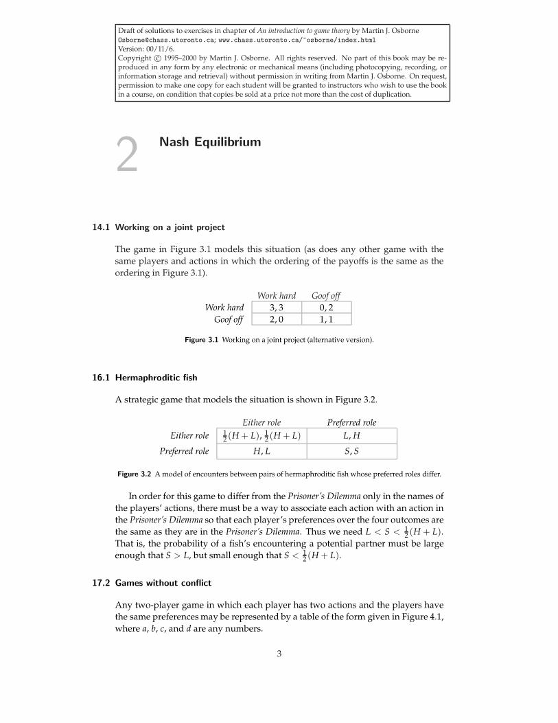
Draft of solutions to exercises in chapter of An introduction to game theory by Martin J. [email protected]; www.chass.utoronto.ca/~osborne/index.htmlVersion: 00/11/6.Copyright c© 1995–2000 by Martin J. Osborne. All rights reserved. No part of this book may be re-produced in any form by any electronic or mechanical means (including photocopying, recording, orinformation storage and retrieval) without permission in writing from Martin J. Osborne. On request,permission to make one copy for each student will be granted to instructors who wish to use the bookin a course, on condition that copies be sold at a price not more than the cost of duplication.
2 Nash Equilibrium
14.1 Working on a joint project
The game in Figure 3.1 models this situation (as does any other game with thesame players and actions in which the ordering of the payoffs is the same as theordering in Figure 3.1).
Work hard Goof offWork hard 3, 3 0, 2
Goof off 2, 0 1, 1
Figure 3.1 Working on a joint project (alternative version).
16.1 Hermaphroditic fish
A strategic game that models the situation is shown in Figure 3.2.
Either role Preferred roleEither role 1
2 (H + L), 12 (H + L) L, H
Preferred role H, L S, S
Figure 3.2 A model of encounters between pairs of hermaphroditic fish whose preferred roles differ.
In order for this game to differ from the Prisoner’s Dilemma only in the names ofthe players’ actions, there must be a way to associate each action with an action inthe Prisoner’s Dilemma so that each player’s preferences over the four outcomes arethe same as they are in the Prisoner’s Dilemma. Thus we need L < S < 1
2 (H + L).That is, the probability of a fish’s encountering a potential partner must be largeenough that S > L, but small enough that S < 1
2 (H + L).
17.2 Games without conflict
Any two-player game in which each player has two actions and the players havethe same preferences may be represented by a table of the form given in Figure 4.1,where a, b, c, and d are any numbers.
3
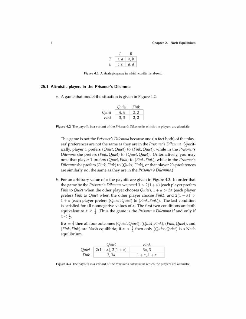
4 Chapter 2. Nash Equilibrium
L RT a, a b, bB c, c d, d
Figure 4.1 A strategic game in which conflict is absent.
25.1 Altruistic players in the Prisoner’s Dilemma
a. A game that model the situation is given in Figure 4.2.
Quiet FinkQuiet 4, 4 3, 3Fink 3, 3 2, 2
Figure 4.2 The payoffs in a variant of the Prisoner’s Dilemma in which the players are altruistic.
This game is not the Prisoner’s Dilemma because one (in fact both) of the play-ers’ preferences are not the same as they are in the Prisoner’s Dilemma. Specif-ically, player 1 prefers (Quiet, Quiet) to (Fink, Quiet), while in the Prisoner’sDilemma she prefers (Fink, Quiet) to (Quiet, Quiet). (Alternatively, you maynote that player 1 prefers (Quiet, Fink) to (Fink, Fink), while in the Prisoner’sDilemma she prefers (Fink, Fink) to (Quiet, Fink), or that player 2’s preferencesare similarly not the same as they are in the Prisoner’s Dilemma.)
b. For an arbitrary value of α the payoffs are given in Figure 4.3. In order thatthe game be the Prisoner’s Dilemma we need 3 > 2(1 + α) (each player prefersFink to Quiet when the other player chooses Quiet), 1 + α > 3α (each playerprefers Fink to Quiet when the other player choose Fink), and 2(1 + α) >
1 + α (each player prefers (Quiet, Quiet) to (Fink, Fink)). The last conditionis satisfied for all nonnegative values of α. The first two conditions are bothequivalent to α < 1
2 . Thus the game is the Prisoner’s Dilemma if and only ifα < 1
2 .
If α = 12 then all four outcomes (Quiet, Quiet), (Quiet, Fink), (Fink, Quiet), and
(Fink, Fink) are Nash equilibria; if α > 12 then only (Quiet, Quiet) is a Nash
equilibrium.
Quiet FinkQuiet 2(1 + α), 2(1 + α) 3α, 3Fink 3, 3α 1 + α, 1 + α
Figure 4.3 The payoffs in a variant of the Prisoner’s Dilemma in which the players are altruistic.
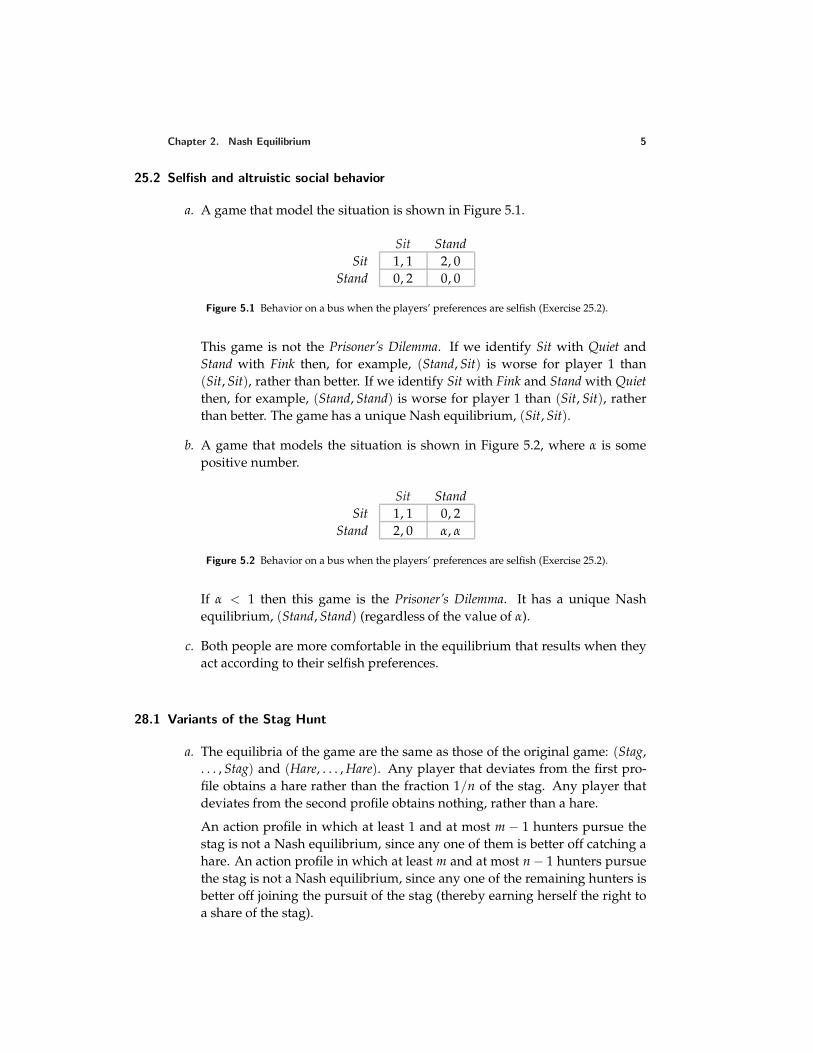
Chapter 2. Nash Equilibrium 5
25.2 Selfish and altruistic social behavior
a. A game that model the situation is shown in Figure 5.1.
Sit StandSit 1, 1 2, 0
Stand 0, 2 0, 0
Figure 5.1 Behavior on a bus when the players’ preferences are selfish (Exercise 25.2).
This game is not the Prisoner’s Dilemma. If we identify Sit with Quiet andStand with Fink then, for example, (Stand, Sit) is worse for player 1 than(Sit, Sit), rather than better. If we identify Sit with Fink and Stand with Quietthen, for example, (Stand, Stand) is worse for player 1 than (Sit, Sit), ratherthan better. The game has a unique Nash equilibrium, (Sit, Sit).
b. A game that models the situation is shown in Figure 5.2, where α is somepositive number.
Sit StandSit 1, 1 0, 2
Stand 2, 0 α, α
Figure 5.2 Behavior on a bus when the players’ preferences are selfish (Exercise 25.2).
If α < 1 then this game is the Prisoner’s Dilemma. It has a unique Nashequilibrium, (Stand, Stand) (regardless of the value of α).
c. Both people are more comfortable in the equilibrium that results when theyact according to their selfish preferences.
28.1 Variants of the Stag Hunt
a. The equilibria of the game are the same as those of the original game: (Stag,. . . , Stag) and (Hare, . . . , Hare). Any player that deviates from the first pro-file obtains a hare rather than the fraction 1/n of the stag. Any player thatdeviates from the second profile obtains nothing, rather than a hare.
An action profile in which at least 1 and at most m − 1 hunters pursue thestag is not a Nash equilibrium, since any one of them is better off catching ahare. An action profile in which at least m and at most n − 1 hunters pursuethe stag is not a Nash equilibrium, since any one of the remaining hunters isbetter off joining the pursuit of the stag (thereby earning herself the right toa share of the stag).
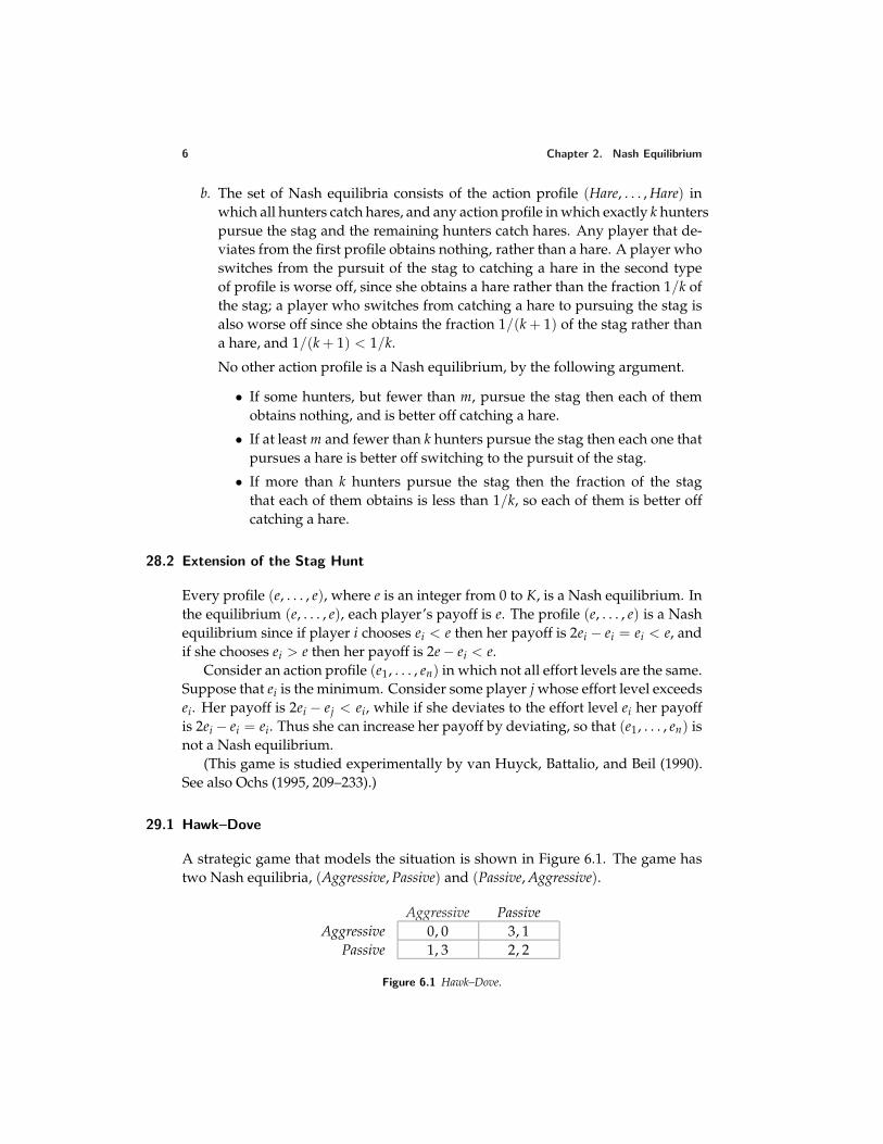
6 Chapter 2. Nash Equilibrium
b. The set of Nash equilibria consists of the action profile (Hare, . . . , Hare) inwhich all hunters catch hares, and any action profile in which exactly k hunterspursue the stag and the remaining hunters catch hares. Any player that de-viates from the first profile obtains nothing, rather than a hare. A player whoswitches from the pursuit of the stag to catching a hare in the second typeof profile is worse off, since she obtains a hare rather than the fraction 1/k ofthe stag; a player who switches from catching a hare to pursuing the stag isalso worse off since she obtains the fraction 1/(k + 1) of the stag rather thana hare, and 1/(k + 1) < 1/k.
No other action profile is a Nash equilibrium, by the following argument.
• If some hunters, but fewer than m, pursue the stag then each of themobtains nothing, and is better off catching a hare.
• If at least m and fewer than k hunters pursue the stag then each one thatpursues a hare is better off switching to the pursuit of the stag.
• If more than k hunters pursue the stag then the fraction of the stagthat each of them obtains is less than 1/k, so each of them is better offcatching a hare.
28.2 Extension of the Stag Hunt
Every profile (e, . . . , e), where e is an integer from 0 to K, is a Nash equilibrium. Inthe equilibrium (e, . . . , e), each player’s payoff is e. The profile (e, . . . , e) is a Nashequilibrium since if player i chooses ei < e then her payoff is 2ei − ei = ei < e, andif she chooses ei > e then her payoff is 2e − ei < e.
Consider an action profile (e1, . . . , en) in which not all effort levels are the same.Suppose that ei is the minimum. Consider some player j whose effort level exceedsei. Her payoff is 2ei − ej < ei, while if she deviates to the effort level ei her payoffis 2ei − ei = ei. Thus she can increase her payoff by deviating, so that (e1, . . . , en) isnot a Nash equilibrium.
(This game is studied experimentally by van Huyck, Battalio, and Beil (1990).See also Ochs (1995, 209–233).)
29.1 Hawk–Dove
A strategic game that models the situation is shown in Figure 6.1. The game hastwo Nash equilibria, (Aggressive, Passive) and (Passive, Aggressive).
Aggressive PassiveAggressive 0, 0 3, 1
Passive 1, 3 2, 2
Figure 6.1 Hawk–Dove.
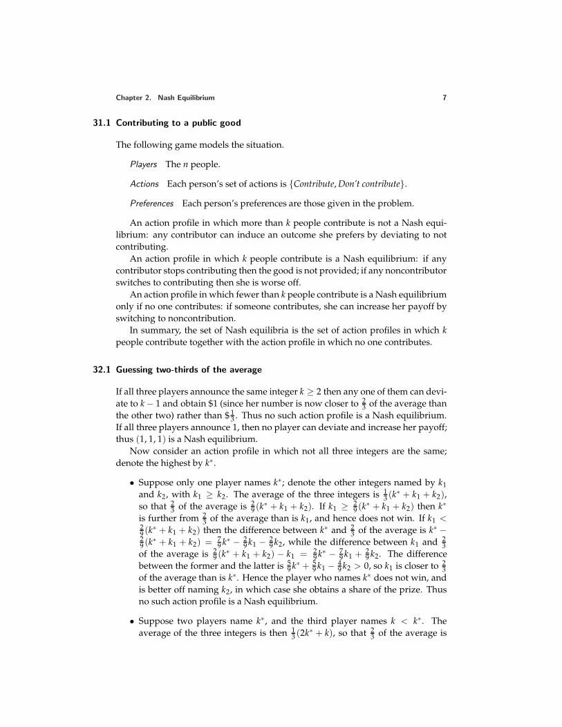
Chapter 2. Nash Equilibrium 7
31.1 Contributing to a public good
The following game models the situation.
Players The n people.
Actions Each person’s set of actions is Contribute, Don’t contribute.
Preferences Each person’s preferences are those given in the problem.
An action profile in which more than k people contribute is not a Nash equi-librium: any contributor can induce an outcome she prefers by deviating to notcontributing.
An action profile in which k people contribute is a Nash equilibrium: if anycontributor stops contributing then the good is not provided; if any noncontributorswitches to contributing then she is worse off.
An action profile in which fewer than k people contribute is a Nash equilibriumonly if no one contributes: if someone contributes, she can increase her payoff byswitching to noncontribution.
In summary, the set of Nash equilibria is the set of action profiles in which kpeople contribute together with the action profile in which no one contributes.
32.1 Guessing two-thirds of the average
If all three players announce the same integer k ≥ 2 then any one of them can devi-ate to k − 1 and obtain $1 (since her number is now closer to 2
3 of the average thanthe other two) rather than $ 1
3 . Thus no such action profile is a Nash equilibrium.If all three players announce 1, then no player can deviate and increase her payoff;thus (1, 1, 1) is a Nash equilibrium.
Now consider an action profile in which not all three integers are the same;denote the highest by k∗.
• Suppose only one player names k∗; denote the other integers named by k1and k2, with k1 ≥ k2. The average of the three integers is 1
3 (k∗ + k1 + k2),so that 2
3 of the average is 29 (k∗ + k1 + k2). If k1 ≥ 2
9 (k∗ + k1 + k2) then k∗
is further from 23 of the average than is k1, and hence does not win. If k1 <
29 (k∗ + k1 + k2) then the difference between k∗ and 2
3 of the average is k∗ −29 (k∗ + k1 + k2) = 7
9 k∗ − 29 k1 − 2
9 k2, while the difference between k1 and 23
of the average is 29 (k∗ + k1 + k2) − k1 = 2
9 k∗ − 79 k1 + 2
9 k2. The differencebetween the former and the latter is 5
9 k∗ + 59 k1 − 4
9 k2 > 0, so k1 is closer to 23
of the average than is k∗. Hence the player who names k∗ does not win, andis better off naming k2, in which case she obtains a share of the prize. Thusno such action profile is a Nash equilibrium.
• Suppose two players name k∗, and the third player names k < k∗. Theaverage of the three integers is then 1
3 (2k∗ + k), so that 23 of the average is
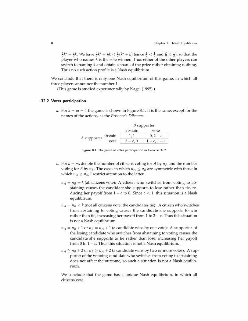
8 Chapter 2. Nash Equilibrium
49 k∗ + 2
9 k. We have 49 k∗ + 2
9 k < 12 (k∗ + k) (since 4
9 < 12 and 2
9 < 12 ), so that the
player who names k is the sole winner. Thus either of the other players canswitch to naming k and obtain a share of the prize rather obtaining nothing.Thus no such action profile is a Nash equilibrium.
We conclude that there is only one Nash equilibrium of this game, in which allthree players announce the number 1.
(This game is studied experimentally by Nagel (1995).)
32.2 Voter participation
a. For k = m = 1 the game is shown in Figure 8.1. It is the same, except for thenames of the actions, as the Prisoner’s Dilemma.
A supporter
B supporterabstain vote
abstain 1, 1 0, 2 − cvote 2 − c, 0 1 − c, 1 − c
Figure 8.1 The game of voter participation in Exercise 32.2.
b. For k = m, denote the number of citizens voting for A by nA and the numbervoting for B by nB. The cases in which nA ≤ nB are symmetric with those inwhich nA ≥ nB; I restrict attention to the latter.
nA = nB = k (all citizens vote): A citizen who switches from voting to ab-staining causes the candidate she supports to lose rather than tie, re-ducing her payoff from 1 − c to 0. Since c < 1, this situation is a Nashequilibrium.
nA = nB < k (not all citizens vote; the candidates tie): A citizen who switchesfrom abstaining to voting causes the candidate she supports to winrather than tie, increasing her payoff from 1 to 2 − c. Thus this situationis not a Nash equilibrium.
nA = nB + 1 or nB = nA + 1 (a candidate wins by one vote): A supporter ofthe losing candidate who switches from abstaining to voting causes thecandidate she supports to tie rather than lose, increasing her payofffrom 0 to 1 − c. Thus this situation is not a Nash equilibrium.
nA ≥ nB + 2 or nB ≥ nA + 2 (a candidate wins by two or more votes): A sup-porter of the winning candidate who switches from voting to abstainingdoes not affect the outcome, so such a situation is not a Nash equilib-rium.
We conclude that the game has a unique Nash equilibrium, in which allcitizens vote.
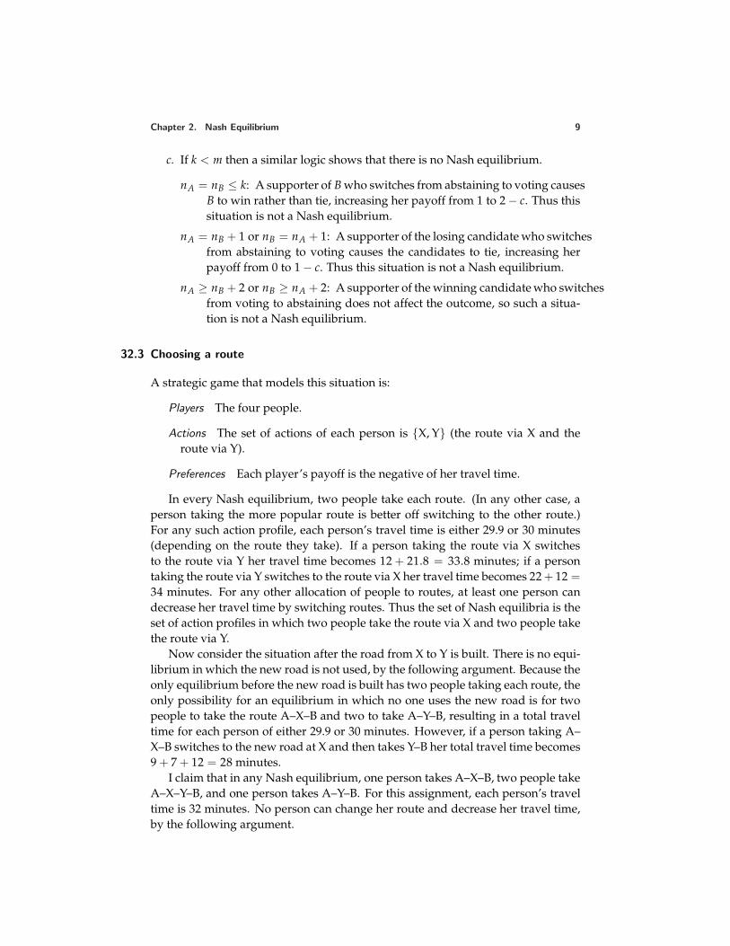
Chapter 2. Nash Equilibrium 9
c. If k < m then a similar logic shows that there is no Nash equilibrium.
nA = nB ≤ k: A supporter of B who switches from abstaining to voting causesB to win rather than tie, increasing her payoff from 1 to 2 − c. Thus thissituation is not a Nash equilibrium.
nA = nB + 1 or nB = nA + 1: A supporter of the losing candidate who switchesfrom abstaining to voting causes the candidates to tie, increasing herpayoff from 0 to 1 − c. Thus this situation is not a Nash equilibrium.
nA ≥ nB + 2 or nB ≥ nA + 2: A supporter of the winning candidate who switchesfrom voting to abstaining does not affect the outcome, so such a situa-tion is not a Nash equilibrium.
32.3 Choosing a route
A strategic game that models this situation is:
Players The four people.
Actions The set of actions of each person is X, Y (the route via X and theroute via Y).
Preferences Each player’s payoff is the negative of her travel time.
In every Nash equilibrium, two people take each route. (In any other case, aperson taking the more popular route is better off switching to the other route.)For any such action profile, each person’s travel time is either 29.9 or 30 minutes(depending on the route they take). If a person taking the route via X switchesto the route via Y her travel time becomes 12 + 21.8 = 33.8 minutes; if a persontaking the route via Y switches to the route via X her travel time becomes 22 + 12 =34 minutes. For any other allocation of people to routes, at least one person candecrease her travel time by switching routes. Thus the set of Nash equilibria is theset of action profiles in which two people take the route via X and two people takethe route via Y.
Now consider the situation after the road from X to Y is built. There is no equi-librium in which the new road is not used, by the following argument. Because theonly equilibrium before the new road is built has two people taking each route, theonly possibility for an equilibrium in which no one uses the new road is for twopeople to take the route A–X–B and two to take A–Y–B, resulting in a total traveltime for each person of either 29.9 or 30 minutes. However, if a person taking A–X–B switches to the new road at X and then takes Y–B her total travel time becomes9 + 7 + 12 = 28 minutes.
I claim that in any Nash equilibrium, one person takes A–X–B, two people takeA–X–Y–B, and one person takes A–Y–B. For this assignment, each person’s traveltime is 32 minutes. No person can change her route and decrease her travel time,by the following argument.
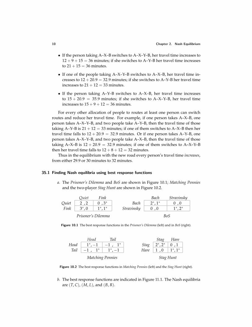
10 Chapter 2. Nash Equilibrium
• If the person taking A–X–B switches to A–X–Y–B, her travel time increases to12 + 9 + 15 = 36 minutes; if she switches to A–Y–B her travel time increasesto 21 + 15 = 36 minutes.
• If one of the people taking A–X–Y–B switches to A–X–B, her travel time in-creases to 12 + 20.9 = 32.9 minutes; if she switches to A–Y–B her travel timeincreases to 21 + 12 = 33 minutes.
• If the person taking A–Y–B switches to A–X–B, her travel time increasesto 15 + 20.9 = 35.9 minutes; if she switches to A–X–Y–B, her travel timeincreases to 15 + 9 + 12 = 36 minutes.
For every other allocation of people to routes at least one person can switchroutes and reduce her travel time. For example, if one person takes A–X–B, oneperson takes A–X–Y–B, and two people take A–Y–B, then the travel time of thosetaking A–Y–B is 21 + 12 = 33 minutes; if one of them switches to A–X–B then hertravel time falls to 12 + 20.9 = 32.9 minutes. Or if one person takes A–Y–B, oneperson takes A–X–Y–B, and two people take A–X–B, then the travel time of thosetaking A–X–B is 12 + 20.9 = 32.9 minutes; if one of them switches to A–X–Y–Bthen her travel time falls to 12 + 8 + 12 = 32 minutes.
Thus in the equilibrium with the new road every person’s travel time increases,from either 29.9 or 30 minutes to 32 minutes.
35.1 Finding Nash equilibria using best response functions
a. The Prisoner’s Dilemma and BoS are shown in Figure 10.1; Matching Penniesand the two-player Stag Hunt are shown in Figure 10.2.
Quiet FinkQuiet 2 , 2 0 , 3∗
Fink 3∗, 0 1∗, 1∗
Prisoner’s Dilemma
Bach StravinskyBach 2∗, 1∗ 0 , 0
Stravinsky 0 , 0 1∗, 2∗
BoS
Figure 10.1 The best response functions in the Prisoner’s Dilemma (left) and in BoS (right).
Head TailHead 1∗, −1 −1 , 1∗
Tail −1 , 1∗ 1∗, −1
Matching Pennies
Stag HareStag 2∗, 2∗ 0 , 1Hare 1 , 0 1∗, 1∗
Stag Hunt
Figure 10.2 The best response functions in Matching Pennies (left) and the Stag Hunt (right).
b. The best response functions are indicated in Figure 11.1. The Nash equilibriaare (T, C), (M, L), and (B, R).

Chapter 2. Nash Equilibrium 11
L C RT 2 , 2 1∗, 3∗ 0∗, 1
M 3∗, 1∗ 0 , 0 0∗, 0B 1 , 0∗ 0 , 0∗ 0∗, 0∗
Figure 11.1 The game in Exercise 35.1.
36.1 Constructing best response functions
The analogue of Figure 36.2 is given in Figure 11.2.
A1
︸ ︷︷ ︸T M B
A2
L
C
R
Figure 11.2 The players’ best response functions for the game in Exercise 36.1b. Player 1’s best re-sponses are indicated by circles, and player 2’s by dots. The action pairs for which there is both a circleand a dot are the Nash equilibria.
36.2 Dividing money
For each amount named by one of the players, the other player’s best responsesare given in the following table.
Other player’s action Sets of best responses0 101 9, 102 8, 9, 103 7, 8, 9, 104 6, 7, 8, 9, 105 5, 6, 7, 8, 9, 106 5, 67 68 79 8
10 9
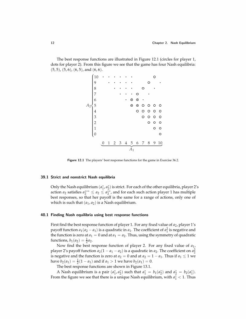
12 Chapter 2. Nash Equilibrium
The best response functions are illustrated in Figure 12.1 (circles for player 1,dots for player 2). From this figure we see that the game has four Nash equilibria:(5, 5), (5, 6), (6, 5), and (6, 6).
A1
︸ ︷︷ ︸0 1 2 3 4 5 6 7 8 9 10
A2
0
12345678910
Figure 12.1 The players’ best response functions for the game in Exercise 36.2.
39.1 Strict and nonstrict Nash equilibria
Only the Nash equilibrium (a∗1, a∗2) is strict. For each of the other equilibria, player 2’saction a2 satisfies a∗∗∗2 ≤ a2 ≤ a∗∗2 , and for each such action player 1 has multiplebest responses, so that her payoff is the same for a range of actions, only one ofwhich is such that (a1, a2) is a Nash equilibrium.
40.1 Finding Nash equilibria using best response functions
First find the best response function of player 1. For any fixed value of a2, player 1’spayoff function a1(a2 − a1) is a quadratic in a1. The coefficient of a2
1 is negative andthe function is zero at a1 = 0 and at a1 = a2. Thus, using the symmetry of quadraticfunctions, b1(a2) = 1
2 a2.Now find the best response function of player 2. For any fixed value of a1,
player 2’s payoff function a2(1 − a1 − a2) is a quadratic in a2. The coefficient on a22
is negative and the function is zero at a2 = 0 and at a2 = 1 − a1. Thus if a1 ≤ 1 wehave b2(a1) = 1
2 (1 − a1) and if a1 > 1 we have b2(a1) = 0.The best response functions are shown in Figure 13.1.A Nash equilibrium is a pair (a∗1, a∗2) such that a∗1 = b1(a∗2) and a∗2 = b2(a∗1).
From the figure we see that there is a unique Nash equilibrium, with a∗1 < 1. Thus
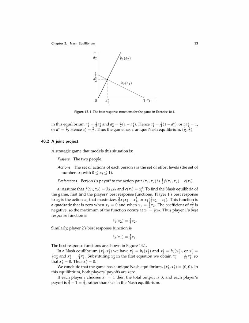
Chapter 2. Nash Equilibrium 13
0 a1 →
↑a2
1a∗1
12
a∗2
b1(a2)
b2(a1)
Figure 13.1 The best response functions for the game in Exercise 40.1.
in this equilibrium a∗1 = 12 a∗2 and a∗2 = 1
2 (1 − a∗1). Hence a∗1 = 14 (1 − a∗1), or 5a∗1 = 1,
or a∗1 = 15 . Hence a∗2 = 2
5 . Thus the game has a unique Nash equilibrium, ( 15 , 2
5 ).
40.2 A joint project
A strategic game that models this situation is:
Players The two people.
Actions The set of actions of each person i is the set of effort levels (the set ofnumbers xi with 0 ≤ xi ≤ 1).
Preferences Person i’s payoff to the action pair (x1, x2) is 12 f (x1, x2) − c(xi).
a. Assume that f (x1, x2) = 3x1x2 and c(xi) = x2i . To find the Nash equilibria of
the game, first find the players’ best response functions. Player 1’s best responseto x2 is the action x1 that maximizes 3
2 x1x2 − x21, or x1( 3
2 x2 − x1). This function isa quadratic that is zero when x1 = 0 and when x1 = 3
2 x2. The coefficient of x21 is
negative, so the maximum of the function occurs at x1 = 34 x2. Thus player 1’s best
response function isb1(x2) = 3
4 x2.
Similarly, player 2’s best response function is
b2(x1) = 34 x1.
The best response functions are shown in Figure 14.1.In a Nash equilibrium (x∗
1, x∗2) we have x∗
1 = b1(x∗2) and x∗
2 = b2(x∗1), or x∗
1 =34 x∗
2 and x∗2 = 3
4 x∗1. Substituting x∗
2 in the first equation we obtain x∗1 = 9
16 x∗1, so
that x∗1 = 0. Thus x∗
2 = 0.We conclude that the game has a unique Nash equilibrium, (x∗
1, x∗2) = (0, 0). In
this equilibrium, both players’ payoffs are zero.If each player i chooses xi = 1 then the total output is 3, and each player’s
payoff is 32 − 1 = 1
2 , rather than 0 as in the Nash equilibrium.
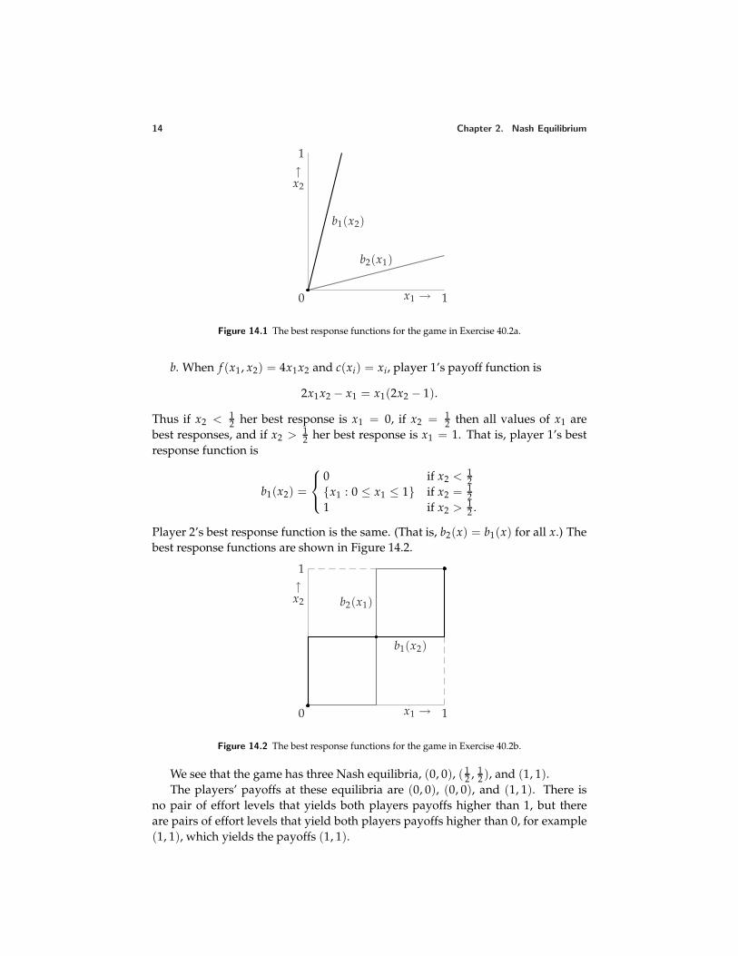
14 Chapter 2. Nash Equilibrium
0 x1 →
↑x2
1
1
b1(x2)
b2(x1)
Figure 14.1 The best response functions for the game in Exercise 40.2a.
b. When f (x1, x2) = 4x1x2 and c(xi) = xi, player 1’s payoff function is
2x1x2 − x1 = x1(2x2 − 1).
Thus if x2 < 12 her best response is x1 = 0, if x2 = 1
2 then all values of x1 arebest responses, and if x2 > 1
2 her best response is x1 = 1. That is, player 1’s bestresponse function is
b1(x2) =
0 if x2 < 12
x1 : 0 ≤ x1 ≤ 1 if x2 = 12
1 if x2 > 12 .
Player 2’s best response function is the same. (That is, b2(x) = b1(x) for all x.) Thebest response functions are shown in Figure 14.2.
0 x1 →
↑x2
1
1
b2(x1)
b1(x2)
Figure 14.2 The best response functions for the game in Exercise 40.2b.
We see that the game has three Nash equilibria, (0, 0), ( 12 , 1
2 ), and (1, 1).The players’ payoffs at these equilibria are (0, 0), (0, 0), and (1, 1). There is
no pair of effort levels that yields both players payoffs higher than 1, but thereare pairs of effort levels that yield both players payoffs higher than 0, for example(1, 1), which yields the payoffs (1, 1).
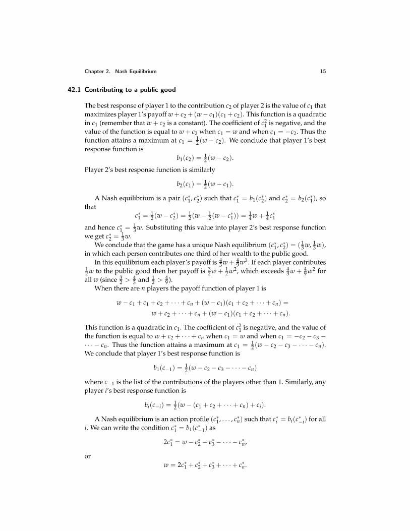
Chapter 2. Nash Equilibrium 15
42.1 Contributing to a public good
The best response of player 1 to the contribution c2 of player 2 is the value of c1 thatmaximizes player 1’s payoff w + c2 + (w − c1)(c1 + c2). This function is a quadraticin c1 (remember that w + c2 is a constant). The coefficient of c2
1 is negative, and thevalue of the function is equal to w + c2 when c1 = w and when c1 = −c2. Thus thefunction attains a maximum at c1 = 1
2 (w − c2). We conclude that player 1’s bestresponse function is
b1(c2) = 12 (w − c2).
Player 2’s best response function is similarly
b2(c1) = 12 (w − c1).
A Nash equilibrium is a pair (c∗1, c∗2) such that c∗1 = b1(c∗2) and c∗2 = b2(c∗1), sothat
c∗1 = 12 (w − c∗2) = 1
2 (w − 12 (w − c∗1)) = 1
4 w + 14 c∗1
and hence c∗1 = 13 w. Substituting this value into player 2’s best response function
we get c∗2 = 13 w.
We conclude that the game has a unique Nash equilibrium (c∗1, c∗2) = ( 13 w, 1
3 w),in which each person contributes one third of her wealth to the public good.
In this equilibrium each player’s payoff is 43 w + 4
9 w2. If each player contributes12 w to the public good then her payoff is 3
2 w + 12 w2, which exceeds 4
3 w + 49 w2 for
all w (since 32 > 4
3 and 12 > 4
9 ).When there are n players the payoff function of player 1 is
w − c1 + c1 + c2 + · · · + cn + (w − c1)(c1 + c2 + · · · + cn) =
w + c2 + · · · + cn + (w − c1)(c1 + c2 + · · · + cn).
This function is a quadratic in c1. The coefficient of c21 is negative, and the value of
the function is equal to w + c2 + · · · + cn when c1 = w and when c1 = −c2 − c3 −· · · − cn. Thus the function attains a maximum at c1 = 1
2 (w − c2 − c3 − · · · − cn).We conclude that player 1’s best response function is
b1(c−1) = 12 (w − c2 − c3 − · · · − cn)
where c−1 is the list of the contributions of the players other than 1. Similarly, anyplayer i’s best response function is
bi(c−i) = 12 (w − (c1 + c2 + · · · + cn) + ci).
A Nash equilibrium is an action profile (c∗1, . . . , c∗n) such that c∗i = bi(c∗−i) for alli. We can write the condition c∗1 = b1(c∗−1) as
2c∗1 = w − c∗2 − c∗3 − · · · − c∗n,
orw = 2c∗1 + c∗2 + c∗3 + · · · + c∗n.
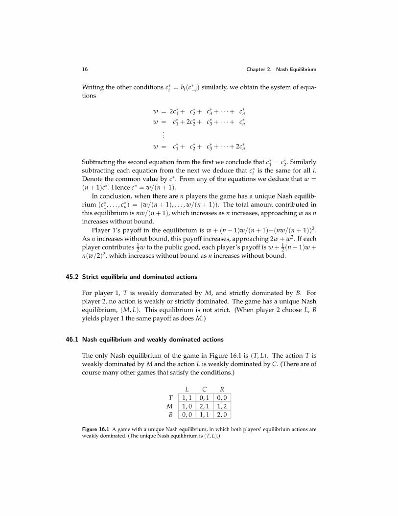
16 Chapter 2. Nash Equilibrium
Writing the other conditions c∗i = bi(c∗−i) similarly, we obtain the system of equa-tions
w = 2c∗1 + c∗2 + c∗3 + · · · + c∗nw = c∗1 + 2c∗2 + c∗3 + · · · + c∗n
...
w = c∗1 + c∗2 + c∗3 + · · · + 2c∗n
Subtracting the second equation from the first we conclude that c∗1 = c∗2. Similarlysubtracting each equation from the next we deduce that c∗i is the same for all i.Denote the common value by c∗. From any of the equations we deduce that w =(n + 1)c∗. Hence c∗ = w/(n + 1).
In conclusion, when there are n players the game has a unique Nash equilib-rium (c∗1, . . . , c∗n) = (w/(n + 1), . . . , w/(n + 1)). The total amount contributed inthis equilibrium is nw/(n + 1), which increases as n increases, approaching w as nincreases without bound.
Player 1’s payoff in the equilibrium is w + (n − 1)w/(n + 1)+(nw/(n + 1))2.As n increases without bound, this payoff increases, approaching 2w + w2. If eachplayer contributes 1
2 w to the public good, each player’s payoff is w + 12 (n − 1)w +
n(w/2)2, which increases without bound as n increases without bound.
45.2 Strict equilibria and dominated actions
For player 1, T is weakly dominated by M, and strictly dominated by B. Forplayer 2, no action is weakly or strictly dominated. The game has a unique Nashequilibrium, (M, L). This equilibrium is not strict. (When player 2 choose L, Byields player 1 the same payoff as does M.)
46.1 Nash equilibrium and weakly dominated actions
The only Nash equilibrium of the game in Figure 16.1 is (T, L). The action T isweakly dominated by M and the action L is weakly dominated by C. (There are ofcourse many other games that satisfy the conditions.)
L C RT 1, 1 0, 1 0, 0
M 1, 0 2, 1 1, 2B 0, 0 1, 1 2, 0
Figure 16.1 A game with a unique Nash equilibrium, in which both players’ equilibrium actions areweakly dominated. (The unique Nash equilibrium is (T, L).)
Chapter 2. Nash Equilibrium 17
47.1 Voting
First consider an action profile in which the winner receives one more vote thanthe loser and at least one citizen who votes for the winner prefers the loser to thewinner. Any citizen who votes for the winner and prefers the loser to the winnercan, by switching her vote, cause her favorite candidate to win rather than lose.Thus no such action profile is a Nash equilibrium.
Next consider an action profile in which the winner receives one more votethan the loser and all citizens who vote for the winner prefer the winner to theloser. Because a majority of citizens prefer A to B, the winner in any such case mustbe A. No citizen who prefers A to B can induce a better outcome by changing hervote, since her favorite candidate wins. Now consider a citizen who prefers B to A.By assumption, every such citizen votes for B; a change in her vote has no effect onthe outcome (A still wins). Thus every such action profile is a Nash equilibrium.
Finally consider an action profile in which the winner receives at least threemore votes than the loser. In this case no change in any citizen’s vote has any effecton the outcome. Thus every such profile is a Nash equilibrium.
In summary, the Nash equilibria are: any action profile in which A receives onemore vote than B and all the citizens who vote for A prefer A to B, and any actionprofile in which the winner receives at least three more votes than the loser.
The only equilibrium in which no citizen uses a weakly dominated action isthat in which every citizen votes for her favorite candidate.
47.2 Voting between three candidates
Fix some citizen, say i; suppose she prefers A to B to C. By the argument in thetext, citizen i’s voting for C is weakly dominated by her voting for A (and by hervoting for B). Her voting for B is clearly not weakly dominated by her voting forC. I now argue that her voting for B is not weakly dominated by her voting forA. Suppose that the other citizens’ votes are equally divided between B and C; noone votes for A. Then if citizen i votes for A the outcome is a tie between B and C,while if she votes for B the outcome is that B wins. Thus for this configuration ofthe other citizens’ votes, citizen i is better off voting for B than she is voting for A.Thus her voting for B is not weakly dominated by her voting for A.
Now fix some citizen, say i, and consider the candidate she ranks in the mid-dle, say candidate B. The action profile in which all citizens vote for B is a Nashequilibrium. (No citizen’s changing her vote affects the outcome.) In this equilib-rium, citizen i does not vote for her favorite candidate, but the action she takes isnot weakly dominated. (Other Nash equilibria also satisfy the conditions in theexercise.)
18 Chapter 2. Nash Equilibrium
47.3 Approval voting
First I argue that any action ai of player i that includes a vote for i’s least preferredcandidate, say candidate k, is weakly dominated by the action a′i that differs fromai only in that candidate k does not receive a vote in a′i. For any list a−i of theother players’ actions, the outcome of (a′i , a−i) differs from that of (ai , a−i) onlyin that the total number of votes received by candidate k is one less in (a′i , a−i)than it is in (ai , a−i). There are two possible implications for the winners of theelection, depending on a−i: either the set of winners is the same in (ai , a−i) as itis in (a′i , a−i), or candidate k is a winner in (ai , a−i) but not in (a′i , a−i). Becausecandidate k is player i’s least preferred candidate, a′i thus weakly dominates ai.
I now argue that any action ai of player i that excludes a vote for i’s most pre-ferred candidate, say candidate 1, is weakly dominated by the action a′i that differsfrom ai only in that candidate 1 receives a vote in a′i. The argument is symmet-ric with the one in the previous paragraph. For any list a−i of the other players’actions, the outcome of (a′i, a−i) differs from that of (ai , a−i) only in that the to-tal number of votes received by candidate 1 is one more in (a′i , a−i) than it is in(ai , a−i). There are two possible implications for the winners of the election, de-pending on a−i: either the set of winners is the same in (ai, a−i) as it is in (a′i , a−i),or candidate 1 is a winner in (a′i , a−i) but not in (ai , a−i). Because candidate 1 isplayer i’s most preferred candidate, a′i thus weakly dominates ai.
Finally I argue that if citizen i prefers candidate 1 to candidate 2 to . . . to can-didate k then the action ai that consists of votes for candidates 1 and k − 1 is notweakly dominated.
• The action ai is not weakly dominated by any action that excludes votes foreither candidate 1 or candidate k − 1 (or both). Suppose a′i excludes a vote forcandidate 1. Then if the total votes by the other citizens for candidates 1 and2 are equal, and the total votes for all other candidates are less, then citizen i’staking the action ai leads candidate 1 to win, while the action a′i leads to atbest (from the point of view of citizen i) a tie between candidates 1 and 2.Thus a′i does not weakly dominate ai. Similarly, suppose that a′i excludesa vote for candidate k − 1. Then if the total votes by the other citizens forcandidates k − 1 and k are equal, while the total votes for all other candidatesare less, then citizen i’s taking the action ai leads candidate k− 1 to win, whilethe action a′i leads to at best (from the point of view of citizen i) a tie betweencandidates k − 1 and k.
• Now let a′i be an action that includes votes for both candidate 1 and candi-date k − 1, and also for at least one other candidate, say candidate j. Supposethat the total votes by the other citizens for candidates 1 and j are equal, andthe total votes for all other candidates are less. Then citizen i’s taking theaction ai leads candidate 1 to win, while the action a′i leads to at best (fromthe point of view of citizen i) a tie between candidates 1 and j. Thus a′i doesnot weakly dominate ai.
Chapter 2. Nash Equilibrium 19
49.1 Other Nash equilibria of the game modeling collective decision-making
Denote by i the player whose favorite policy is the median favorite policy. Theset of Nash equilibria includes every action profile in which (i) i’s action is herfavorite policy x∗
i , (ii) every player whose favorite policy is less than x∗i names a
policy equal to at most x∗i , and (iii) every player whose favorite policy is greater
than x∗i names a policy equal to at least x∗
i .To show this, first note that the outcome is x∗
i , so player i cannot induce a bet-ter outcome for herself by changing her action. Now, if a player whose favoriteposition is less than x∗
i changes her action to some x < x∗i , the outcome does not
change; if such a player changes her action to some x > x∗i then the outcome either
remains the same (if some player whose favorite position exceeds x∗i names x∗
i ) orincreases, so that the player is not better off. A similar argument applies to a playerwhose favorite position is greater than x∗
i .The set of Nash equilibria also includes, for any positive integer k ≤ n, every
action profile in which k players name the median favorite policy x∗i , at most 1
2 (n −3) players name policies less than x∗
i , and at most 12 (n − 3) players name policies
greater than x∗i . (In these equilibria, the favorite policy of a player who names a
policy less than x∗i may be greater than x∗
i , and vice versa. The conditions on thenumbers of players who name policies less than x∗
i and greater than x∗i ensure that
no such player can, by naming instead her favorite policy, move the median policycloser to her favorite policy.)
Any action profile in which all players name the same, arbitrary, policy is alsoa Nash equilibrium; the outcome is the common policy named.
More generally, any profile in which at least three players name the same, ar-bitrary, policy x, at most (n − 3)/2 players name a policy less than x, and at most(n − 3)/2 players name a policy greater than x is a Nash equilibrium. (In bothcases, no change in any player’s action has any effect on the outcome.)
49.2 Another mechanism for collective decision-making
When the policy chosen is the mean of the announced policies, player i’s announc-ing her favorite policy does not weakly dominate all her other actions. For exam-ple, if there are three players, the favorite policy of player 1 is 0.3, and the otherplayers both announce the policy 0, then player 1 should announce the policy 0.9,which leads to the policy 0.3 (= (0 + 0 + 0.9)/3) being chosen, rather than 0.3,which leads to the policy 0.1.
50.1 Symmetric strategic game
The games in Exercise 29.1, Example 37.1, and Figure 46.1 (both games) are sym-metric. The game in Exercise 40.1 is not symmetric. The game in Section 2.8.4 issymmetric if and only if u1 = u2.
20 Chapter 2. Nash Equilibrium
51.1 Equilibrium for pairwise interactions in a single population
The Nash equilibria are (A, A), (A, C), and (C, A). Only the equilibrium (A, A) isrelevant if the game is played between the members of a single population—thisequilibrium is the only symmetric equilibrium.
Draft of solutions to exercises in chapter of An introduction to game theory by Martin J. [email protected]; www.chass.utoronto.ca/~osborne/index.htmlVersion: 00/11/6.Copyright c© 1995–2000 by Martin J. Osborne. All rights reserved. No part of this book may be re-produced in any form by any electronic or mechanical means (including photocopying, recording, orinformation storage and retrieval) without permission in writing from Martin J. Osborne. On request,permission to make one copy for each student will be granted to instructors who wish to use the bookin a course, on condition that copies be sold at a price not more than the cost of duplication.
3 Nash Equilibrium: Illustrations
57.1 Cournot’s duopoly game with linear inverse demand and different unit costs
Following the analysis in the text, the best response function of firm 1 is
b1(q2) =
12 (α − c1 − q2) if q2 ≤ α − c10 otherwise
while that of firm 2 is
b2(q1) =
12 (α − c2 − q1) if q1 ≤ α − c20 otherwise.
To find the Nash equilibrium, first plot these two functions. Each function hasthe same general form as the best response function of either firm in the case stud-ied in the text. However, the fact that c1 = c2 leads to two qualitatively differentcases when we combine the two functions to find a Nash equilibrium. If c1 and c2do not differ very much then the functions in the analogue of Figure 56.2 intersectat a pair of outputs that are both positive. If c1 and c2 differ a lot, however, thefunctions intersect at a pair of outputs in which q1 = 0.
Precisely, if c1 ≤ 12 (α + c2) then the downward-sloping parts of the best re-
sponse functions intersect (as in Figure 56.2), and the game has a unique Nashequilibrium, given by the solution of the two equations
q1 = 12 (α − c1 − q2)
q2 = 12 (α − c2 − q1).
This solution is
(q∗1, q∗2) =(
13 (α − 2c1 + c2), 1
3 (α − 2c2 + c1))
.
If c1 > 12 (α + c2) then the downward-sloping part of firm 1’s best response func-
tion lies below the downward-sloping part of firm 2’s best response function (as inFigure 22.1), and the game has a unique Nash equilibrium, (q∗1, q∗2) = (0, 1
2 (α− c2)).
In summary, the game always has a unique Nash equilibrium, defined as fol-lows:
(13 (α − 2c1 + c2), 1
3 (α − 2c2 + c1))
if c1 ≤ 12 (α + c2)(
0, 12 (α − c2)
)if c1 > 1
2 (α + c2).
21
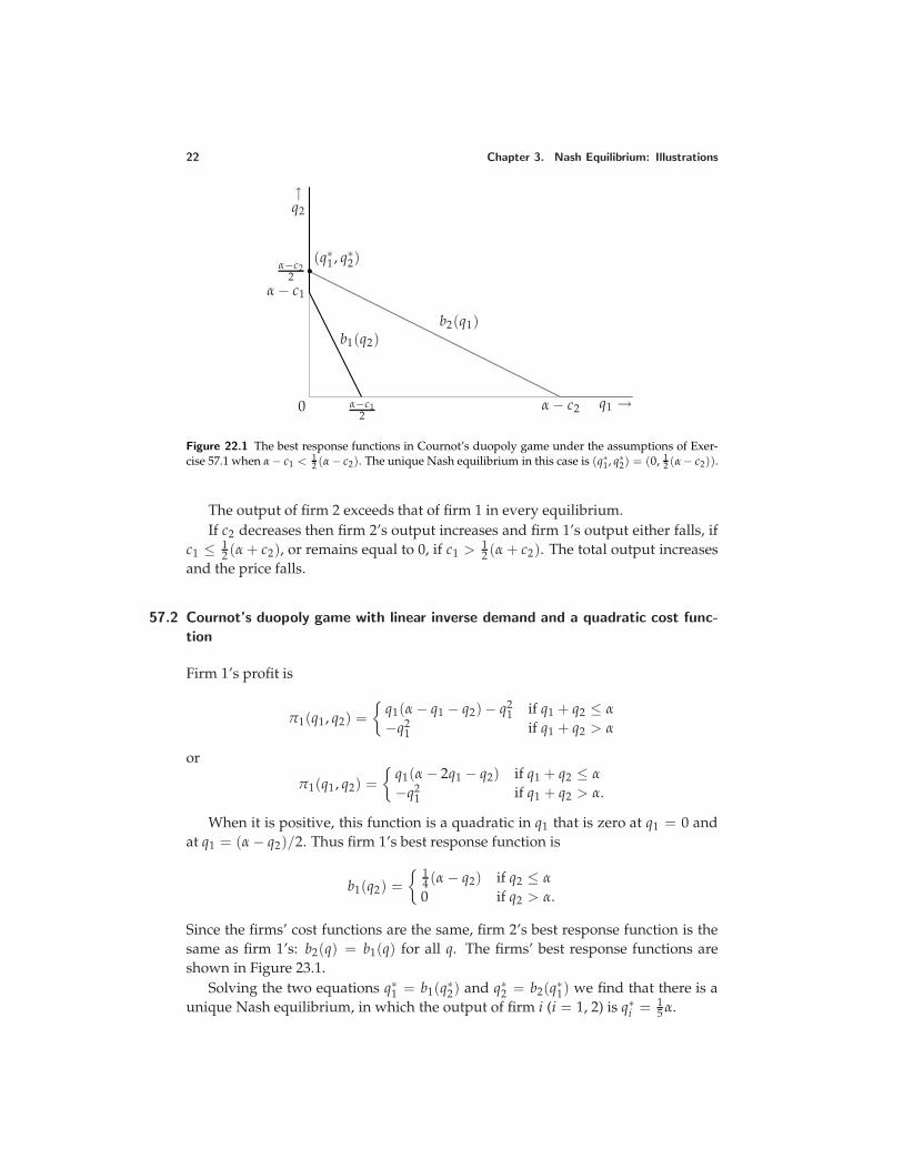
22 Chapter 3. Nash Equilibrium: Illustrations
0 α−c12
α − c2
α−c22
α − c1
↑q2
q1 →
b1(q2)b2(q1)
(q∗1, q∗2)
Figure 22.1 The best response functions in Cournot’s duopoly game under the assumptions of Exer-cise 57.1 when α − c1 < 1
2 (α − c2). The unique Nash equilibrium in this case is (q∗1, q∗2) = (0, 12 (α − c2)).
The output of firm 2 exceeds that of firm 1 in every equilibrium.If c2 decreases then firm 2’s output increases and firm 1’s output either falls, if
c1 ≤ 12 (α + c2), or remains equal to 0, if c1 > 1
2 (α + c2). The total output increasesand the price falls.
57.2 Cournot’s duopoly game with linear inverse demand and a quadratic cost func-
tion
Firm 1’s profit is
π1(q1, q2) =
q1(α − q1 − q2) − q21 if q1 + q2 ≤ α
−q21 if q1 + q2 > α
or
π1(q1, q2) =
q1(α − 2q1 − q2) if q1 + q2 ≤ α
−q21 if q1 + q2 > α.
When it is positive, this function is a quadratic in q1 that is zero at q1 = 0 andat q1 = (α − q2)/2. Thus firm 1’s best response function is
b1(q2) = 1
4 (α − q2) if q2 ≤ α
0 if q2 > α.
Since the firms’ cost functions are the same, firm 2’s best response function is thesame as firm 1’s: b2(q) = b1(q) for all q. The firms’ best response functions areshown in Figure 23.1.
Solving the two equations q∗1 = b1(q∗2) and q∗2 = b2(q∗1) we find that there is aunique Nash equilibrium, in which the output of firm i (i = 1, 2) is q∗i = 1
5 α.
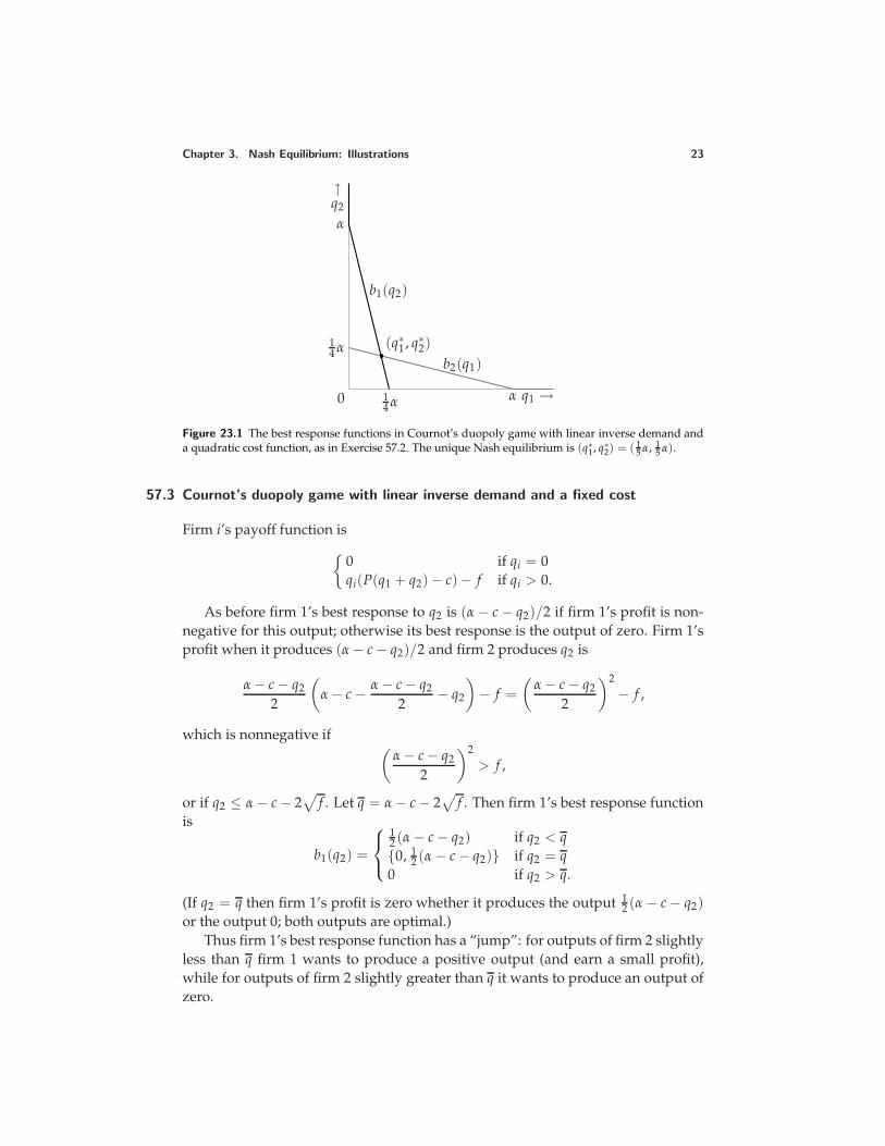
Chapter 3. Nash Equilibrium: Illustrations 23
0 14 α
14 α
α
α
↑q2
q1 →
b1(q2)
b2(q1)(q∗1, q∗2)
Figure 23.1 The best response functions in Cournot’s duopoly game with linear inverse demand anda quadratic cost function, as in Exercise 57.2. The unique Nash equilibrium is (q∗1, q∗2) = ( 1
5 α, 15 α).
57.3 Cournot’s duopoly game with linear inverse demand and a fixed cost
Firm i’s payoff function is
0 if qi = 0qi(P(q1 + q2) − c) − f if qi > 0.
As before firm 1’s best response to q2 is (α − c − q2)/2 if firm 1’s profit is non-negative for this output; otherwise its best response is the output of zero. Firm 1’sprofit when it produces (α − c − q2)/2 and firm 2 produces q2 is
α − c − q2
2
(α − c − α − c − q2
2− q2
)− f =
(α − c − q2
2
)2− f ,
which is nonnegative if (α − c − q2
2
)2> f ,
or if q2 ≤ α − c − 2√
f . Let q = α − c − 2√
f . Then firm 1’s best response functionis
b1(q2) =
12 (α − c − q2) if q2 < q0, 1
2 (α − c − q2) if q2 = q0 if q2 > q.
(If q2 = q then firm 1’s profit is zero whether it produces the output 12 (α − c − q2)
or the output 0; both outputs are optimal.)Thus firm 1’s best response function has a “jump”: for outputs of firm 2 slightly
less than q firm 1 wants to produce a positive output (and earn a small profit),while for outputs of firm 2 slightly greater than q it wants to produce an output ofzero.
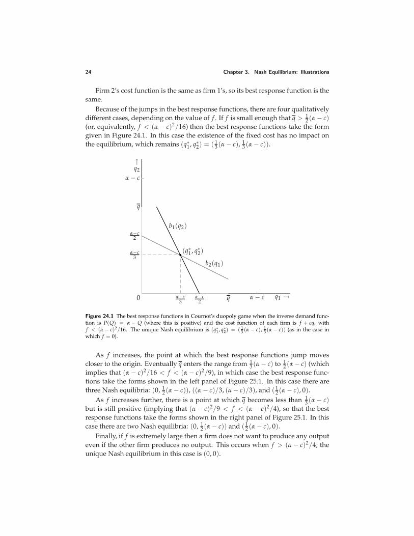
24 Chapter 3. Nash Equilibrium: Illustrations
Firm 2’s cost function is the same as firm 1’s, so its best response function is thesame.
Because of the jumps in the best response functions, there are four qualitativelydifferent cases, depending on the value of f . If f is small enough that q > 1
2 (α − c)(or, equivalently, f < (α − c)2/16) then the best response functions take the formgiven in Figure 24.1. In this case the existence of the fixed cost has no impact onthe equilibrium, which remains (q∗1, q∗2) = ( 1
3 (α − c), 13 (α − c)).
0 α−c3
α−c2
q α − c
α−c3
α−c2
q
α − c
↑q2
q1 →
b1(q2)
b2(q1)
(q∗1, q∗2)
Figure 24.1 The best response functions in Cournot’s duopoly game when the inverse demand func-tion is P(Q) = α − Q (where this is positive) and the cost function of each firm is f + cq, withf < (α − c)2/16. The unique Nash equilibrium is (q∗1, q∗2) = ( 1
3 (α − c), 13 (α − c)) (as in the case in
which f = 0).
As f increases, the point at which the best response functions jump movescloser to the origin. Eventually q enters the range from 1
3 (α − c) to 12 (α − c) (which
implies that (α − c)2/16 < f < (α − c)2/9), in which case the best response func-tions take the forms shown in the left panel of Figure 25.1. In this case there arethree Nash equilibria: (0, 1
2 (α − c)), ((α − c)/3, (α − c)/3), and ( 12 (α − c), 0).
As f increases further, there is a point at which q becomes less than 13 (α − c)
but is still positive (implying that (α − c)2/9 < f < (α − c)2/4), so that the bestresponse functions take the forms shown in the right panel of Figure 25.1. In thiscase there are two Nash equilibria: (0, 1
2 (α − c)) and ( 12 (α − c), 0).
Finally, if f is extremely large then a firm does not want to produce any outputeven if the other firm produces no output. This occurs when f > (α − c)2/4; theunique Nash equilibrium in this case is (0, 0).
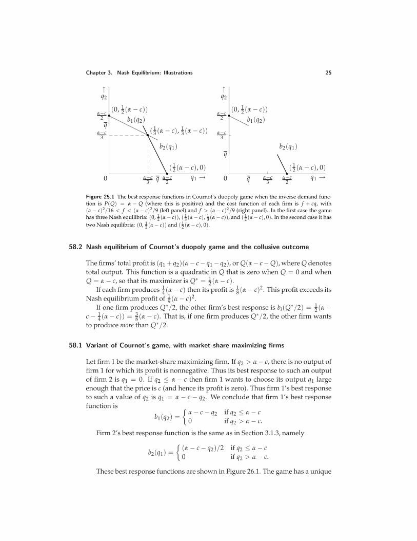
Chapter 3. Nash Equilibrium: Illustrations 25
0 α−c3
α−c2
q
α−c3
α−c2
q
↑q2
q1 →
b1(q2)
b2(q1)
( 13 (α − c), 1
3 (α − c))
(0, 12 (α − c))
( 12 (α − c), 0)
0 α−c3
α−c2
q
α−c3
α−c2
q
↑q2
q1 →
b1(q2)
b2(q1)
(0, 12 (α − c))
( 12 (α − c), 0)
Figure 25.1 The best response functions in Cournot’s duopoly game when the inverse demand func-tion is P(Q) = α − Q (where this is positive) and the cost function of each firm is f + cq, with(α − c)2/16 < f < (α − c)2/9 (left panel) and f > (α − c)2/9 (right panel). In the first case the gamehas three Nash equilibria: (0, 1
2 (α − c)), ( 13 (α − c), 1
3 (α − c)), and ( 12 (α − c), 0). In the second case it has
two Nash equilibria: (0, 12 (α − c)) and ( 1
2 (α − c), 0).
58.2 Nash equilibrium of Cournot’s duopoly game and the collusive outcome
The firms’ total profit is (q1 + q2)(α− c− q1 − q2), or Q(α− c−Q), where Q denotestotal output. This function is a quadratic in Q that is zero when Q = 0 and whenQ = α − c, so that its maximizer is Q∗ = 1
2 (α − c).If each firm produces 1
4 (α − c) then its profit is 18 (α − c)2. This profit exceeds its
Nash equilibrium profit of 19 (α − c)2.
If one firm produces Q∗/2, the other firm’s best response is bi(Q∗/2) = 12 (α −
c − 14 (α − c)) = 3
8 (α − c). That is, if one firm produces Q∗/2, the other firm wantsto produce more than Q∗/2.
58.1 Variant of Cournot’s game, with market-share maximizing firms
Let firm 1 be the market-share maximizing firm. If q2 > α − c, there is no output offirm 1 for which its profit is nonnegative. Thus its best response to such an outputof firm 2 is q1 = 0. If q2 ≤ α − c then firm 1 wants to choose its output q1 largeenough that the price is c (and hence its profit is zero). Thus firm 1’s best responseto such a value of q2 is q1 = α − c − q2. We conclude that firm 1’s best responsefunction is
b1(q2) =
α − c − q2 if q2 ≤ α − c0 if q2 > α − c.
Firm 2’s best response function is the same as in Section 3.1.3, namely
b2(q1) =
(α − c − q2)/2 if q2 ≤ α − c0 if q2 > α − c.
These best response functions are shown in Figure 26.1. The game has a unique
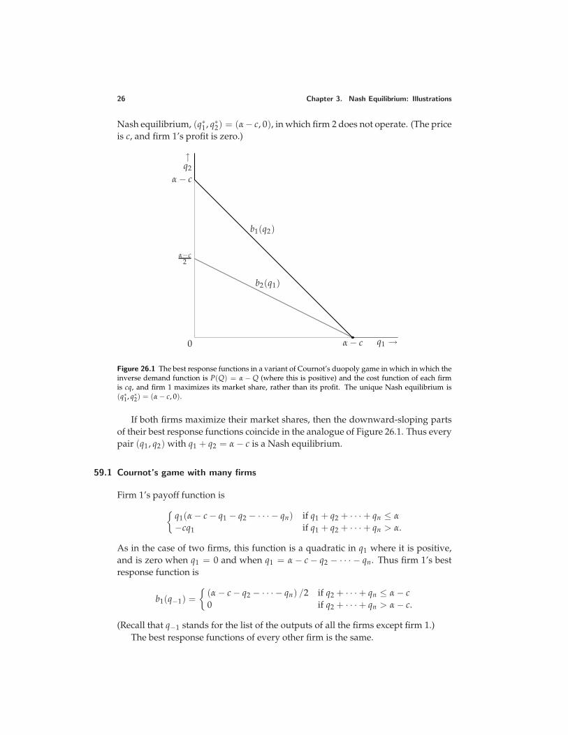
26 Chapter 3. Nash Equilibrium: Illustrations
Nash equilibrium, (q∗1, q∗2) = (α− c, 0), in which firm 2 does not operate. (The priceis c, and firm 1’s profit is zero.)
0 α − c
α−c2
α − c
↑q2
q1 →
b1(q2)
b2(q1)
Figure 26.1 The best response functions in a variant of Cournot’s duopoly game in which in which theinverse demand function is P(Q) = α − Q (where this is positive) and the cost function of each firmis cq, and firm 1 maximizes its market share, rather than its profit. The unique Nash equilibrium is(q∗1, q∗2) = (α − c, 0).
If both firms maximize their market shares, then the downward-sloping partsof their best response functions coincide in the analogue of Figure 26.1. Thus everypair (q1, q2) with q1 + q2 = α − c is a Nash equilibrium.
59.1 Cournot’s game with many firms
Firm 1’s payoff function is
q1(α − c − q1 − q2 − · · · − qn) if q1 + q2 + · · · + qn ≤ α
−cq1 if q1 + q2 + · · · + qn > α.
As in the case of two firms, this function is a quadratic in q1 where it is positive,and is zero when q1 = 0 and when q1 = α − c − q2 − · · · − qn. Thus firm 1’s bestresponse function is
b1(q−1) =
(α − c − q2 − · · · − qn) /2 if q2 + · · · + qn ≤ α − c0 if q2 + · · · + qn > α − c.
(Recall that q−1 stands for the list of the outputs of all the firms except firm 1.)The best response functions of every other firm is the same.
Chapter 3. Nash Equilibrium: Illustrations 27
The conditions for (q∗1, . . . , q∗n) to be a Nash equilibrium are
q∗1 = b1(q∗−1)
q∗2 = b2(q∗−2)...
q∗n = b2(q∗−n)
or, in an equilibrium in which all the firms’ outputs are positive,
q∗1 = 12 (α − c − q∗2 − q∗3 − · · · − q∗n)
q∗2 = 12 (α − c − q∗1 − q∗3 − · · · − q∗n)
...
q∗n = 12 (α − c − q∗1 − q∗2 − · · · − q∗n−1).
We can write these equations as
0 = α − c − 2q∗1 − q∗2 − · · · − q∗n−1 − q∗n0 = α − c − q∗1 − 2q∗2 − · · · − q∗n−1 − q∗n
...
0 = α − c − q∗1 − q∗2 − · · · − q∗n−1 − 2q∗n.
If we subtract the second equation from the first we obtain 0 = −q∗1 + q∗2, or q∗1 = q∗2.Similarly subtracting the third equation from the second we conclude that q∗2 = q∗3,and continuing with all pairs of equations we deduce that q∗1 = q∗2 = · · · = q∗n.Let the common value of the firms’ outputs be q∗. Then each equation is 0 =α − c − (n + 1)q∗, so that q∗ = (α − c)/(n + 1).
In summary, the game has a unique Nash equilibrium, in which the output ofevery firm i is (α − c)/(n + 1).
The price at this equilibrium is α − n(α − c)/(n + 1), or (α + nc)/(n + 1). As nincreases this price decreases, approaching c as n increases without bound: α/(n +1) decreases to 0 and nc/(n + 1) decreases to c.
60.1 Nash equilibrium of Cournot’s game with small firms
• If P(Q∗) < p then every firm producing a positive output makes a negativeprofit, and can increase its profit (to 0) by deviating and producing zero.
• If P(Q∗ + q) > p, take a firm that is either producing no output, or an ar-bitrarily small output. (Such a firm exists, since demand is finite.) Such afirm earns a profit of either zero or arbitrarily close to zero. If it deviatesand chooses the output q then total output changes to at most Q∗ + q, so thatthe price still exceeds p (since P(Q∗ + q) > p). Hence the deviant makes apositive profit.
28 Chapter 3. Nash Equilibrium: Illustrations
61.1 Interaction among resource-users
The game is given as follows.
Players The firms.
Actions Each firm’s set of actions is the set of all nonnegative numbers (repre-senting the amount of input it uses).
Preferences The payoff of each firm i is
xi(1 − (x1 + · · · + xn)) if x1 + · · · + xn ≤ 10 if x1 + · · · + xn > 1.
This game is the same as that in Exercise 59.1 for c = 0 and α = 1. Thus it has aunique Nash equilibrium, (x1, . . . , xn) = (1/(n + 1), . . . , 1/(n + 1)).
In this Nash equilibrium, each firm’s output is (1/(n + 1))(1 − n/(n + 1)) =1/(n + 1)2. If xi = 1/(2n) for i = 1, . . . , n then each firm’s output is 1/(4n), whichexceeds 1/(n + 1)2 for n ≥ 2. (We have 1/(4n) − 1/(n + 1)2 = (n − 1)2/(4n(n +1)2) > 0 for n ≥ 2.)
65.1 Bertrand’s duopoly game with constant unit cost
The pair (c, c) of prices remains a Nash equilibrium; the argument is the sameas before. Further, as before, there is no other Nash equilibrium. The argumentneeds only very minor modification. For an arbitrary function D there may existno monopoly price pm; in this case, if pi > c, pj > c, pi ≥ pj, and D(pj) = 0 thenfirm i can increase its profit by reducing its price slightly below p (for example).
65.2 Bertrand’s duopoly game with discrete prices
Yes, (c, c) is still a Nash equilibrium, by the same argument as before.In addition, (c + 1, c + 1) is a Nash equilibrium (where c is given in cents). In
this equilibrium both firms’ profits are positive. If either firm raises its price orlowers it to c, its profit becomes zero. If either firm lowers its price below c, itsprofit becomes negative.
No other pair of prices is a Nash equilibrium, by the following argument, simi-lar to the argument in the text for the case in which a price can be any nonnegativenumber.
• If pi < c then the firm whose price is lowest (or either firm, if the prices arethe same) can increase its profit (to zero) by raising its price to c.
• If pi = c and pj ≥ c + 1 then firm i can increase its profit from zero to apositive amount by increasing its price to c + 1.
Chapter 3. Nash Equilibrium: Illustrations 29
• If pi > pj ≥ c + 1 then firm i can increase its profit (from zero) by loweringits price to c + 1.
• If pi = pj ≥ c + 2 and pj < α then either firm can increase its profit bylowering its price by one cent. (If firm i does so, its profit changes from12 (pi − c)(α − pi) to (pi − 1 − c)(α − pi + 1) = (pi − 1 − c)(α − pi) + pi − 1 − c.We have pi − 1 − c ≥ 1
2 (pi − c) and pi − 1 − c > 0, since pi ≥ c + 2.)
• If pi = pj ≥ c + 2 and pj ≥ α then either firm can increase its profit bylowering its price to pm.
66.1 Bertrand’s oligopoly game
Consider a profile (p1, . . . , pn) of prices in which pi ≥ c for all i and at least twoprices are equal to c. Every firm’s profit is zero. If any firm raises its price its profitremains zero. If a firm charging more than c lowers its price, but not below c, itsprofit also remains zero. If a firm lowers its price below c then its profit is negative.Thus any such profile is a Nash equilibrium.
To show that no other profile is a Nash equilibrium, we can argue as follows.
• If some price is less than c then the firm charging the lowest price can increaseits profit (to zero) by increasing its price to c.
• If exactly one firm’s price is equal to c then that firm can increase its profit byraising its price a little (keeping it less than the next highest price).
• If all firms’ prices exceed c then the firm charging the highest price can in-crease its profit by lowering its price to some price between c and the lowestprice being charged.
66.2 Bertrand’s duopoly game with different unit costs
a. If all consumers buy from firm 1 when both firms charge the price c2, then(p1, p2) = (c2, c2) is a Nash equilibrium by the following argument. Firm 1’s profitis positive, while firm 2’s profit is zero (since it serves no customers).
• If firm 1 increases its price, its profit falls to zero.
• If firm 1 reduces its price, say to p, then its profit changes from (c2 − c1)(α −c2) to (p − c1)(α − p). Since c2 is less than the maximizer of (p − c1)(α − p),firm 1’s profit falls.
• If firm 2 increases its price, its profit remains zero.
• If firm 2 decreases its price, its profit becomes negative (since its price is lessthan its unit cost).
30 Chapter 3. Nash Equilibrium: Illustrations
Under this rule no other pair of prices is a Nash equilibrium, by the followingargument.
• If pi < c1 for i = 1, 2 then the firm with the lower price (or either firm, if theprices are the same) can increase its profit (to zero) by raising its price abovethat of the other firm.
• If p1 > p2 ≥ c2 then firm 2 can increase its profit by raising its price a little.
• If p2 > p1 ≥ c1 then firm 1 can increase its profit by raising its price a little.
• If p2 ≤ p1 and p2 < c2 then firm 2’s profit is negative, so that it can increaseits profit by raising its price.
• If p1 = p2 > c2 then at least one of the firms is not receiving all of thedemand, and that firm can increase its profit by lowering its price a little.
b. Now suppose that the rule for splitting up the customers when the prices areequal specifies that firm 2 receives some customers when both prices are c2. By theargument for part a, the only possible Nash equilibrium is (p1, p2) = (c2, c2). (Theargument in part a that every other pair of prices is not a Nash equilibrium doesnot use the fact that customers are split equally when (p1, p2) = (c2, c2).) But if(p1, p2) = (c2, c2) and firm 2 receives some customers, firm 1 can increase its profitby reducing its price a little and capturing the entire market.
67.1 Bertrand’s duopoly game with fixed costs
At the pair of prices (p, p), both firms’ profits are zero. (Firm 1 receives all thedemand and obtains the profit (p − c)(α − p) − f = 0, and firm 2 receives nodemand.) This pair of prices is a Nash equilibrium by the following argument.
• If either firm raises its price its profit remains zero (it receives no customers).
• If either firm lowers its price then it receives all the demand and earns anegative profit (since f is less than the maximum of (p − c)(α − p)).
No other pair of prices (p1, p2) is a Nash equilibrium, by the following argu-ment.
• If p1 = p2 < p then firm 1’s profit is negative; firm 1 can increase its profit byraising its price.
• If p1 = p2 > p then firm 2’s profit is zero; firm 2 can obtain a positive profitby lowering its price a little.
• If pi < pj and firm i’s profit is positive then firm j can increase its profit fromzero to almost the current level of i’s profit by changing its price to be slightlyless than pi.
Chapter 3. Nash Equilibrium: Illustrations 31
• If pi < pj and firm i’s profit is zero then firm i can earn a positive profit byraising its price a little.
• If pi < pj and firm i’s profit is negative then firm i can increase its profit tozero by raising its price above pj.
72.1 Electoral competition with asymmetric voters’ preferences
The unique Nash equilibrium remains (m, m); the direct argument is exactly thesame as before. (The dividing line between the supporters of two candidates withdifferent positions changes. If xi < xj, for example, the dividing line is 1
3 xi + 23 xj
rather than 12 (xi + xj). The resulting change in the best response functions does
not affect the Nash equilibrium.)
72.2 Electoral competition with three candidates
If a single candidate enters, then either of the remaining candidates can enter andeither win outright or tie for first place. Thus there is no Nash equilibrium in whicha single candidate enters.
In any Nash equilibrium in which more than one candidate enters, all the can-didates that enter tie for first place, since if they do not then some candidate loses,and hence can do better by staying out of the race.
If two candidates enter, then by the argument in the text for the case in whichthere are two candidates, each takes the position m. But then the third candi-date can enter and win outright. Thus there is no Nash equilibrium in which twocandidates enter.
If all three candidates enter and choose the same position, each candidate re-ceives one third of the votes. If the common position is equal to m then any candi-date can win outright (obtaining close to one-half of the votes) by moving slightlyto one side of m. If the common position is different from m then any candidatecan win outright (obtaining more than one-half of the votes) by moving to m. Thusthere is no Nash equilibrium in which all three candidates enter and choose thesame position.
If all three candidates enter and do not all choose the same position then they alltie for first place, by the second argument. At least one candidate (i) does not shareher position with any other candidate and (ii) is an extremist (her position is notbetween the positions of the other candidates). This candidate can move slightlycloser to the other candidates and win outright. Thus there is no Nash equilibriumin which all three candidates enter and not all of them choose the same position.
We conclude that the game has no Nash equilibrium.
32 Chapter 3. Nash Equilibrium: Illustrations
72.3 Electoral competition in two districts
The game has a unique equilibrium, in which the both candidates choose the posi-tion m1 (the median favorite position in the district with the most electoral collegevotes). The outcome is a tie.
The following argument shows that this pair of positions is a Nash equilibrium.If a candidate deviates to a position less than m1, she loses in district 1 and wins indistrict 2, and thus loses overall. If a candidate deviates to a position greater thanm1, she loses in both districts.
To see that there is no other Nash equilibrium, first consider a pair of positionsfor which candidate 1 loses in district 1, and hence loses overall. By deviating tom1, she either wins in district 1, and hence wins overall, or, if candidate 2’s positionis m1, ties in district 1, and ties overall. Thus her deviation induces an outcome sheprefers. The same argument applies to candidate 2, so that in any equilibrium thecandidates tie in district 1. Now, if the candidates’ positions are either different,or the same and different from m1, either candidate can win outright rather thantying for first place by moving to m1. Thus there is a single equilibrium, in whichboth candidates’ positions are m1.
73.1 Electoral competition between candidates who care only about the winning
position
First consider a pair (x1, x2) of positions for which either x1 < m and x2 < m, orx1 > m and x2 > m.
• If x1 = x2 and the winner’s position is different from her favorite positionthen the winner can move slightly closer to her favorite position and stillwin.
• If x1 = x2 and the winner’s position is equal to her favorite position then theother candidate can move to m, which is closer to her favorite position thanthe winner’s position, and win.
• If x1 = x2 < m then the candidate whose favorite position exceeds m canmove to m and cause the winning position to be m rather than x1 = x2.
• If x1 = x2 > m then the candidate whose favorite position is less than m canmove to m and cause the winning position to be m rather than x1 = x2.
Now suppose the candidates’ positions are on opposite sides of m: either x1 <
m < x2, or x2 < m < x1.
• If each candidate’s position is on the same side of m as her favorite positionand one candidate wins outright, then the loser can win outright by movingto m, which she prefers to the position of the other candidate.
Chapter 3. Nash Equilibrium: Illustrations 33
• If each candidate’s position is on the same side of m as her favorite positionand the candidates tie for first place, then by moving slightly closer to meither candidate can win. If her movement is small enough she prefers hernew position to the previous compromise 1
2 (x1 + x2) (= m).
• If each candidate’s position is on the opposite side of m to her favorite po-sition then the winner, or either player in the case of a tie, can move to herfavorite position and either win outright or cause the winning position to bethe other candidate’s position, in both cases improving the outcome from herpoint of view.
Now suppose that x1 = m and x2 < m. If x∗1 < m then candidate 1 is better off
choosing a slightly smaller value of x1 (in which case she still wins). If x∗1 > m then
candidate 1 is better off choosing a slightly larger value of x1 (in which case shestill wins). Thus (x1, x2) is not a Nash equilibrium. A similar argument applies topairs (x1, x2) for which x1 = m and x2 > m, and for which x1 = m and x2 = m.
Finally, if (x1, x2) = (m, m), then the candidates tie. If either candidate changesher position then she loses, and the winning position does not change. Thus thispair of positions is a Nash equilibrium.
73.2 Citizen-candidates
If b ≤ 2c then the game has a Nash equilibrium in which a single citizen, withfavorite position m, stands as a candidate. Another citizen with the same favoriteposition who stands obtains the payoff 1
2 b − c, as opposed to the payoff of 0 if shedoes not stand. Given b ≤ 2c, it is optimal for any such citizen not to stand. Acitizen with any other favorite position who stands loses, and hence is worse offthan if she does not stand.
If two citizens with favorite position m become candidates, each candidate’spayoff is 1
2 b − c; if one withdraws then she obtains the payoff of 0, so for equilib-rium we require b ≥ 2c. Now consider a citizen whose favorite position is closeto m. If she enters she wins outright, obtaining the payoff b − c. Since b ≥ 2c, thispayoff is positive, and hence exceeds her payoff if she does not stand (which isnegative, since the winner’s position is then different from her favorite position).Thus there is no equilibrium in which two citizens with favorite position m standas candidates.
Now consider the possibility of an equilibrium in which two citizens with fa-vorite positions different from m stand as candidates. For an equilibrium the can-didates must tie, otherwise one loses, and can do better by withdrawing. Thus thepositions, say x1 and x2, must satisfy 1
2 (x1 + x2) = m. If x1 and x2 are close enoughto m then any other citizen loses if she becomes a candidate. Thus there are equilib-ria in which two citizens with positions symmetric about m, and sufficiently closeto m, become candidates.
34 Chapter 3. Nash Equilibrium: Illustrations
74.1 Electoral competition for more general preferences
a. If x∗ is a Condorcet winner then for any y = x∗ a majority of voters preferx∗ to y, so y is not a Condorcet winner. Thus there is no more than oneCondorcet winner.
b. Suppose that one of the remaining voters prefers y to z to x, and the otherprefers z to x to y. For each position there is another position preferred by amajority of voters, so no position is a Condorcet winner.
c. Now suppose that x∗ is a Condorcet winner. Then the strategic game de-scribed the exercise has a unique Nash equilibrium in which both candidateschoose x∗. This pair of actions is a Nash equilibrium because if either can-didate chooses a different position she loses. For any other pair of actionseither one candidate loses, in which case that candidate can deviate to theposition x∗ and at least tie, or the candidates tie at a position different fromx∗, in which case either of them can deviate to x∗ and win.
If there is no Condorcet winner then for every position there is another posi-tion preferred by a majority of voters. Thus for every pair of distinct positionsthe loser can deviate and win, and for every pair of identical positions eithercandidate can deviate and win. Thus there is no Nash equilibrium.
75.1 Competition in product characteristics
Suppose there are two firms. If the products are different, then either firm increasesits market share by making its product more similar to that of its rival. Thus inevery possible equilibrium the products are the same. But if x1 = x2 = m then eachfirm’s market share is 50%, while if it changes its product to be closer to m then itsmarket share rises above 50%. Thus the only possible equilibrium is (x1, x2) =(m, m). This pair of positions is an equilibrium, since each firm’s market share is50%, and if either firm changes its product its market share falls below 50%.
Now suppose there are three firms. If all firms’ products are the same, eachobtains one-third of the market. If x1 = x2 = x3 = m then any firm, by changingits product a little, can obtain close to one-half of the market. If x1 = x2 = x3 = mthen any firm, by changing its product a little, can obtain more than one-half of themarket. If the firms’ products are not all the same, then at least one of the extremeproducts is different from the other two products, and the firm that produces it canincrease its market share by making it more similar to the other products. Thuswhen there are three firms there is no Nash equilibrium.
76.1 Direct argument for Nash equilibria of War of Attrition
• If t1 = t2 then either player can increase her payoff by conceding slightlylater (in which case she obtains the object for sure, rather than getting it with
Chapter 3. Nash Equilibrium: Illustrations 35
probability 12 ).
• If 0 < ti < tj then player i can increase her payoff by conceding at 0.
• If 0 = ti < tj < vi then player i can increase her payoff (from 0 to almostvi − tj > 0) by conceding slightly after tj.
Thus there is no Nash equilibrium in which t1 = t2, 0 < ti < tj, or 0 = ti <
tj < vi (for i = 1 and j = 2, or i = 2 and j = 1). The remaining possibility is that0 = ti < tj and tj ≥ vi for i = 1 and j = 2, or i = 2 and j = 1. In this case player i’spayoff is 0, while if she concedes later her payoff is negative; player j’s payoff is vj,her highest possible payoff in the game.
77.1 Variant of War of Attrition
The game is
Players The two parties to the dispute.
Actions Each player’s set of actions is the set of possible concession times(nonnegative numbers).
Preferences Player i’s preferences are represented by the payoff function
ui(t1, t2) =
0 if ti < tj12 (vi − ti) if ti = tjvi − tj if ti > tj.
where j is the other player.
Three representative cross-sections of player i’s payoff function are shown inFigure 35.1.
0
↑ui
ti →tj < vi
tj vi 0
↑ui
ti →tj = vi
tj = vi 0
↑ui
ti →tj > vi
tjvi
Figure 35.1 Three cross-sections of player i’s payoff function in the variant of the War of Attrition inExercise 77.1.
From this figure we deduce that the best response function of player i is
Bi(tj) =
ti: ti > tj if tj < viti: ti ≥ 0 if tj = viti: 0 ≤ ti < tj if tj > vi.
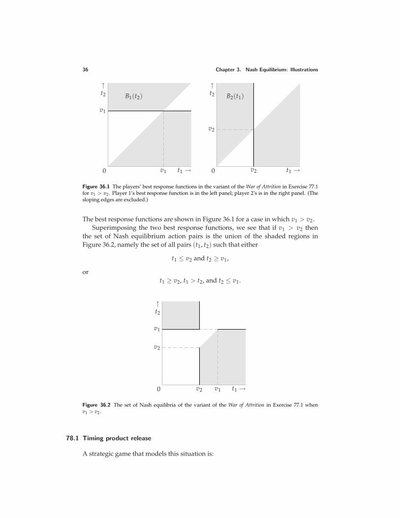
36 Chapter 3. Nash Equilibrium: Illustrations
↑t2
t1 →
v1
v1
B1(t2)
0
↑t2
t1 →v2
v2
B2(t1)
0
Figure 36.1 The players’ best response functions in the variant of the War of Attrition in Exercise 77.1for v1 > v2. Player 1’s best response function is in the left panel; player 2’s is in the right panel. (Thesloping edges are excluded.)
The best response functions are shown in Figure 36.1 for a case in which v1 > v2.Superimposing the two best response functions, we see that if v1 > v2 then
the set of Nash equilibrium action pairs is the union of the shaded regions inFigure 36.2, namely the set of all pairs (t1, t2) such that either
t1 ≤ v2 and t2 ≥ v1,
ort1 ≥ v2, t1 > t2, and t2 ≤ v1.
↑t2
t1 →
v1
v1
v2
v20
Figure 36.2 The set of Nash equilibria of the variant of the War of Attrition in Exercise 77.1 whenv1 > v2.
78.1 Timing product release
A strategic game that models this situation is:
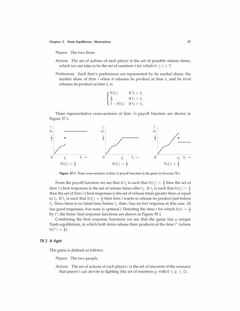
Chapter 3. Nash Equilibrium: Illustrations 37
Players The two firms
Actions The set of actions of each player is the set of possible release times,which we can take to be the set of numbers t for which 0 ≤ t ≤ T.
Preferences Each firm’s preferences are represented by its market share; themarket share of firm i when it releases its product at time ti and its rivalreleases its product at time tj is
h(ti) if ti < tj12 if ti = tj1 − h(tj) if ti > tj.
Three representative cross-sections of firm i’s payoff function are shown inFigure 37.1.
0
↑ui
ti →h(tj) < 1
2
tj
12
0
↑ui
ti →h(tj) = 1
2
12
tj 0
↑ui
ti →h(tj) > 1
2
12
tj
Figure 37.1 Three cross-sections of firm i’s payoff function in the game in Exercise 78.1.
From the payoff function we see that if tj is such that h(tj) < 12 then the set of
firm i’s best responses is the set of release times after tj. If tj is such that h(tj) = 12
then the set of firm i’s best responses is the set of release times greater than or equalto tj. If tj is such that h(tj) > 1
2 then firm i wants to release its product just beforetj. Since there is no latest time before tj, firm i has no best response in this case. (Ithas good responses, but none is optimal.) Denoting the time t for which h(t) = 1
2by t∗, the firms’ best response functions are shown in Figure 38.1.
Combining the best response functions we see that the game has a uniqueNash equilibrium, in which both firms release their products at the time t∗ (whereh(t∗) = 1
2 ).
78.2 A fight
The game is defined as follows.
Players The two people.
Actions The set of actions of each player i is the set of amounts of the resourcethat player i can devote to fighting (the set of numbers yi with 0 ≤ yi ≤ 1).
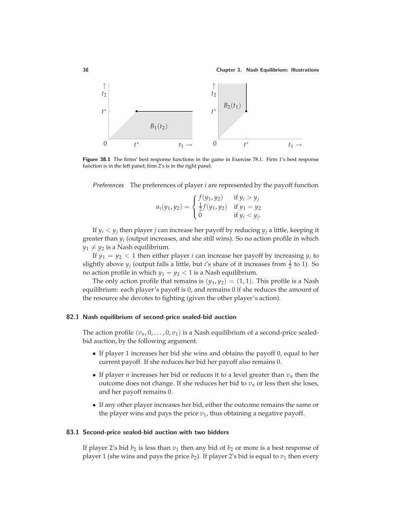
38 Chapter 3. Nash Equilibrium: Illustrations
t∗
t∗
0
↑t2
t1 →
B1(t2)
t∗
t∗
0
↑t2
t1 →
B2(t1)
Figure 38.1 The firms’ best response functions in the game in Exercise 78.1. Firm 1’s best responsefunction is in the left panel; firm 2’s is in the right panel.
Preferences The preferences of player i are represented by the payoff function
ui(y1, y2) =
f (y1, y2) if yi > yj12 f (y1, y2) if y1 = y20 if yi < yj.
If yi < yj then player j can increase her payoff by reducing yj a little, keeping itgreater than yi (output increases, and she still wins). So no action profile in whichy1 = y2 is a Nash equilibrium.
If y1 = y2 < 1 then either player i can increase her payoff by increasing yi toslightly above yj (output falls a little, but i’s share of it increases from 1
2 to 1). Sono action profile in which y1 = y2 < 1 is a Nash equilibrium.
The only action profile that remains is (y1, y2) = (1, 1). This profile is a Nashequilibrium: each player’s payoff is 0, and remains 0 if she reduces the amount ofthe resource she devotes to fighting (given the other player’s action).
82.1 Nash equilibrium of second-price sealed-bid auction
The action profile (vn, 0, . . . , 0, v1) is a Nash equilibrium of a second-price sealed-bid auction, by the following argument.
• If player 1 increases her bid she wins and obtains the payoff 0, equal to hercurrent payoff. If she reduces her bid her payoff also remains 0.
• If player n increases her bid or reduces it to a level greater than vn then theoutcome does not change. If she reduces her bid to vn or less then she loses,and her payoff remains 0.
• If any other player increases her bid, either the outcome remains the same orthe player wins and pays the price v1, thus obtaining a negative payoff.
83.1 Second-price sealed-bid auction with two bidders
If player 2’s bid b2 is less than v1 then any bid of b2 or more is a best response ofplayer 1 (she wins and pays the price b2). If player 2’s bid is equal to v1 then every
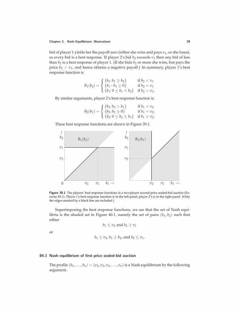
Chapter 3. Nash Equilibrium: Illustrations 39
bid of player 1 yields her the payoff zero (either she wins and pays v1, or she loses),so every bid is a best response. If player 2’s bid b2 exceeds v1 then any bid of lessthan b2 is a best response of player 1. (If she bids b2 or more she wins, but pays theprice b2 > v1, and hence obtains a negative payoff.) In summary, player 1’s bestresponse function is
B1(b2) =
b1: b1 ≥ b2 if b2 < v1b1 : b1 ≥ 0 if b2 = v1b1: 0 ≤ b1 < b2 if b2 > v1.
By similar arguments, player 2’s best response function is
B2(b1) =
b2: b2 > b1 if b1 < v2b2: b2 ≥ 0 if b1 = v2.b2: 0 ≤ b2 ≤ b1 if b1 > v2.
These best response functions are shown in Figure 39.1.
↑b2
b1 →
v1
v2
v1v2
B1(b2)
0
↑b2
b1 →
v1
v2
v1v2
B2(b1)
Figure 39.1 The players’ best response functions in a two-player second-price sealed-bid auction (Ex-ercise 83.1). Player 1’s best response function is in the left panel; player 2’s is in the right panel. (Onlythe edges marked by a black line are included.)
Superimposing the best response functions, we see that the set of Nash equi-libria is the shaded set in Figure 40.1, namely the set of pairs (b1, b2) such thateither
b1 ≤ v2 and b2 ≥ v1
orb1 ≥ v2, b1 ≥ b2, and b2 ≤ v1.
84.1 Nash equilibrium of first-price sealed-bid auction
The profile (b1, . . . , bn) = (v2, v2, v3, . . . , vn) is a Nash equilibrium by the followingargument.
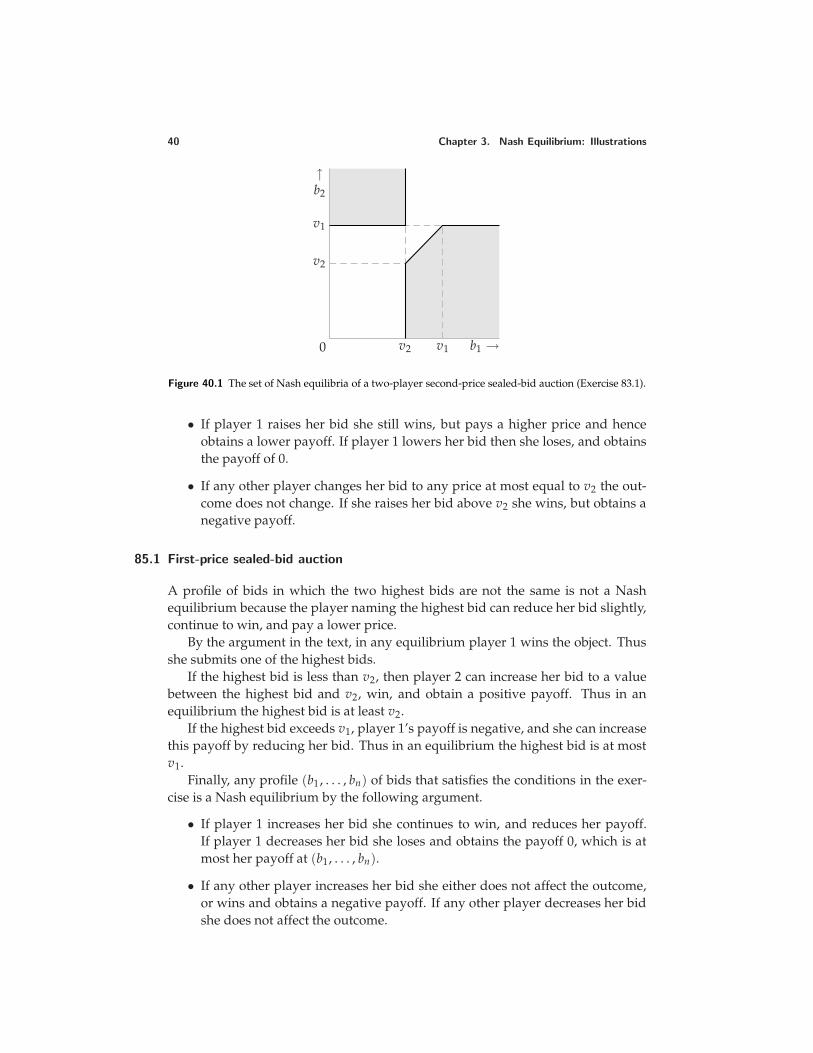
40 Chapter 3. Nash Equilibrium: Illustrations
↑b2
b1 →
v1
v1
v2
v20
Figure 40.1 The set of Nash equilibria of a two-player second-price sealed-bid auction (Exercise 83.1).
• If player 1 raises her bid she still wins, but pays a higher price and henceobtains a lower payoff. If player 1 lowers her bid then she loses, and obtainsthe payoff of 0.
• If any other player changes her bid to any price at most equal to v2 the out-come does not change. If she raises her bid above v2 she wins, but obtains anegative payoff.
85.1 First-price sealed-bid auction
A profile of bids in which the two highest bids are not the same is not a Nashequilibrium because the player naming the highest bid can reduce her bid slightly,continue to win, and pay a lower price.
By the argument in the text, in any equilibrium player 1 wins the object. Thusshe submits one of the highest bids.
If the highest bid is less than v2, then player 2 can increase her bid to a valuebetween the highest bid and v2, win, and obtain a positive payoff. Thus in anequilibrium the highest bid is at least v2.
If the highest bid exceeds v1, player 1’s payoff is negative, and she can increasethis payoff by reducing her bid. Thus in an equilibrium the highest bid is at mostv1.
Finally, any profile (b1, . . . , bn) of bids that satisfies the conditions in the exer-cise is a Nash equilibrium by the following argument.
• If player 1 increases her bid she continues to win, and reduces her payoff.If player 1 decreases her bid she loses and obtains the payoff 0, which is atmost her payoff at (b1, . . . , bn).
• If any other player increases her bid she either does not affect the outcome,or wins and obtains a negative payoff. If any other player decreases her bidshe does not affect the outcome.
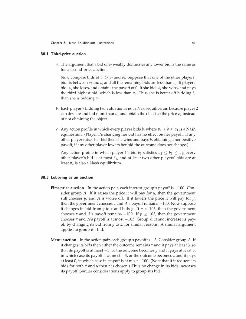
Chapter 3. Nash Equilibrium: Illustrations 41
86.1 Third-price auction
a. The argument that a bid of vi weakly dominates any lower bid is the same asfor a second-price auction.
Now compare bids of bi > vi and vi. Suppose that one of the other players’bids is between vi and bi and all the remaining bids are less than vi. If player ibids vi she loses, and obtains the payoff of 0. If she bids bi she wins, and paysthe third highest bid, which is less than vi. Thus she is better off bidding bithan she is bidding vi.
b. Each player’s bidding her valuation is not a Nash equilibrium because player 2can deviate and bid more than v1 and obtain the object at the price v3 insteadof not obtaining the object.
c. Any action profile in which every player bids b, where v2 ≤ b ≤ v1 is a Nashequilibrium. (Player 1’s changing her bid has no effect on her payoff. If anyother player raises her bid then she wins and pays b, obtaining a nonpositivepayoff; if any other player lowers her bid the outcome does not change.)
Any action profile in which player 1’s bid b1 satisfies v2 ≤ b1 ≤ v1, everyother player’s bid is at most b1, and at least two other players’ bids are atleast v2 is also a Nash equilibrium.
88.3 Lobbying as an auction
First-price auction In the action pair, each interest group’s payoff is −100. Con-sider group A. If it raises the price it will pay for y, then the governmentstill chooses y, and A is worse off. If it lowers the price it will pay for y,then the government chooses z and A’s payoff remains −100. Now supposeit changes its bid from y to x and bids p. If p < 103, then the governmentchooses z and A’s payoff remains −100. If p ≥ 103, then the governmentchooses x and A’s payoff is at most −103. Group A cannot increase its pay-off by changing its bid from y to z, for similar reasons. A similar argumentapplies to group B’s bid.
Menu auction In the action pair, each group’s payoff is −3. Consider group A. Ifit changes its bids then either the outcome remains x and it pays at least 3, sothat its payoff is at most −3, or the outcome becomes y and it pays at least 6,in which case its payoff is at most −3, or the outcome becomes z and it paysat least 0, in which case its payoff is at most −100. (Note that if it reduces itsbids for both x and y then z is chosen.) Thus no change in its bids increasesits payoff. Similar considerations apply to group B’s bid.
42 Chapter 3. Nash Equilibrium: Illustrations
87.1 Multi-unit auctions
Discriminatory auction To show that the action of bidding vi and wi is not domi-nant for player i, we need only find actions for the other players and alterna-tive bids for player i such that player i’s payoff is higher under the alternativebids than it is under the vi and wi, given the other players’ actions. Supposethat each of the other players submits two bids of 0. Then if player i submitsone bid between 0 and vi and one bid between 0 and wi she still wins twounits, and pays less than when she bids vi and wi.
Uniform-price auction Suppose that some bidder other than i submits one bidbetween wi and vi and one bid of 0, and all the remaining bidders submittwo bids of 0. Then bidder i wins one unit, and pays the price wi. If shereplaces her bid of wi with a bid between 0 and wi then she pays a lowerprice, and hence is better off.
Vickrey auction Suppose that player i bids vi and wi. Consider separately thecases in which the bids of the players other than i are such that player i wins0, 1, and 2 units.
Player i wins 0 units: In this case the second highest of the other players’bids is at least vi, so that if player i changes her bids so that she winsone or more units, for any unit she wins she pays at least vi. Thus nochange in her bids increases her payoff from its current value of 0 (andsome changes lower her payoff).
Player i wins 1 unit: If player i raises her bid of vi then she still wins one unitand the price remains the same. If she lowers this bid then either she stillwins and pays the same price, or she does not win any units. If she raisesher bid of wi then either the outcome does not change, or she wins a sec-ond unit. In the latter case the price she pays is the previously-winningbid she beat, which is at least wi, so that her payoff either remains zeroor becomes negative.
Player i wins 2 units: Player i’s raising either of her bids has no effect on theoutcome; her lowering a bid either has no effect on the outcome or leadsher to lose rather than to win, leading her to obtain the payoff of zero.
88.1 Waiting in line
The situation is modeled by a variant of a discriminatory multi-unit auction inwhich 100 units are available, and each person attaches a positive value only toone unit and submits a bid for only one unit.
We can argue along the lines of Exercise 85.1.
• The first 100 people to arrive must do so at the same time. If not, at least oneof them could arrive a little later and still be in the first 100.

Chapter 3. Nash Equilibrium: Illustrations 43
• The first 100 people to arrive must be persons 1 through 100. Suppose, to thecontrary, that one of these people is person i with i ≥ 101, and person j withj ≤ 100 is not in the group that arrives first. Then the common waiting timeof the first 100 must be at most v101, otherwise person i obtains a negativepayoff. But then person j can deviate and arrive slightly earlier than thegroup of 100, and obtain a positive payoff.
• The common waiting time of the first 100 people must be at least v101. If not,then person 101 could arrive slightly before the first 100 and obtain a positivepayoff.
• The common waiting time of the first 100 people must be at most v100. If not,then person 100 obtains a negative payoff, while by arriving later her payoffis zero.
• At least one person i with i ≥ 101 arrives at the same time as the first 100people. If not, then any person i with i ≤ 100 can arrive slightly later andstill be one of the first 100 to arrive.
This argument shows that in a Nash equilibrium persons 1 through 100 choosethe same waiting time t∗ with v101 ≤ t∗ ≤ v100, all the remaining people choosewaiting times of at most t∗, and at least one of the remaining people chooses awaiting time equal to t∗. Any such action profile is a Nash equilibrium: any per-son i with i ≤ 100 obtains a smaller payoff if she arrives earlier and a payoff ofzero if she arrives later. Any person i with i ≥ 101 obtains a negative payoff if shearrives before the first 100 people and a payoff of zero if she arrives at or after thefirst 100 people.
Thus the set of Nash equilibria is the set of action profiles (t1, . . . , t200) in whicht1 = · · · = t100, this common waiting time, say t∗, satisfies v101 ≤ t∗ ≤ v100, ti ≥ t∗
for all i ≥ 101, and tj = t∗ for some j ≥ 101.When goods are rationed by line-ups in the world, people in general do not all
arrive at the same time. The feature missing from the model that seems to explainthe dispersion in arrival times is uncertainty on the part of each player about theother players’ valuations.
88.2 Internet pricing
The situation may be modeled as a multi-unit auction in which k units are avail-able, and each player attaches a positive value to only one unit and submits a bidfor only one unit. The k highest bids win, and each winner pays the (k + 1)sthighest bid.
By a variant of the argument for a second-price auction, in which “highest ofthe other players’ bids” is replaced by “highest rejected bid”, each player’s actionof bidding her value is weakly dominates all her other actions.
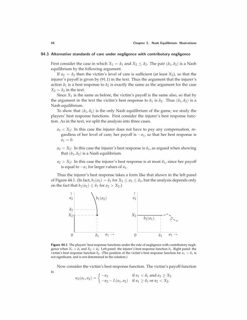
44 Chapter 3. Nash Equilibrium: Illustrations
94.3 Alternative standards of care under negligence with contributory negligence
First consider the case in which X1 = a1 and X2 ≤ a2. The pair (a1, a2) is a Nashequilibrium by the following argument.
If a2 = a2 then the victim’s level of care is sufficient (at least X2), so that theinjurer’s payoff is given by (91.1) in the text. Thus the argument that the injurer’saction a1 is a best response to a2 is exactly the same as the argument for the caseX2 = a2 in the text.
Since X1 is the same as before, the victim’s payoff is the same also, so that bythe argument in the text the victim’s best response to a1 is a2. Thus (a1, a2) is aNash equilibrium.
To show that (a1, a2) is the only Nash equilibrium of the game, we study theplayers’ best response functions. First consider the injurer’s best response func-tion. As in the text, we split the analysis into three cases.
a2 < X2: In this case the injurer does not have to pay any compensation, re-gardless of her level of care; her payoff is −a1, so that her best response isa1 = 0.
a2 = X2: In this case the injurer’s best response is a1, as argued when showingthat (a1, a2) is a Nash equilibrium.
a2 > X2: In this case the injurer’s best response is at most a1, since her payoffis equal to −a1 for larger values of a1.
Thus the injurer’s best response takes a form like that shown in the left panelof Figure 44.1. (In fact, b1(a2) = a1 for X2 ≤ a2 ≤ a2, but the analysis depends onlyon the fact that b1(a2) ≤ a1 for a2 > X2.)
0
a2
X2
a1 a1 →
↑a2 b1(a2)
0
X2
a1 a1 →
↑a2
?b2(a1)
Figure 44.1 The players’ best response functions under the rule of negligence with contributory negli-gence when X1 = a1 and X2 = a2. Left panel: the injurer’s best response function b1. Right panel: thevictim’s best response function b2. (The position of the victim’s best response function for a1 > a1 isnot significant, and is not determined in the solution.)
Now consider the victim’s best response function. The victim’s payoff functionis
u2(a1, a2) =−a2 if a1 < a1 and a2 ≥ X2−a2 − L(a1, a2) if a1 ≥ a1 or a2 < X2.
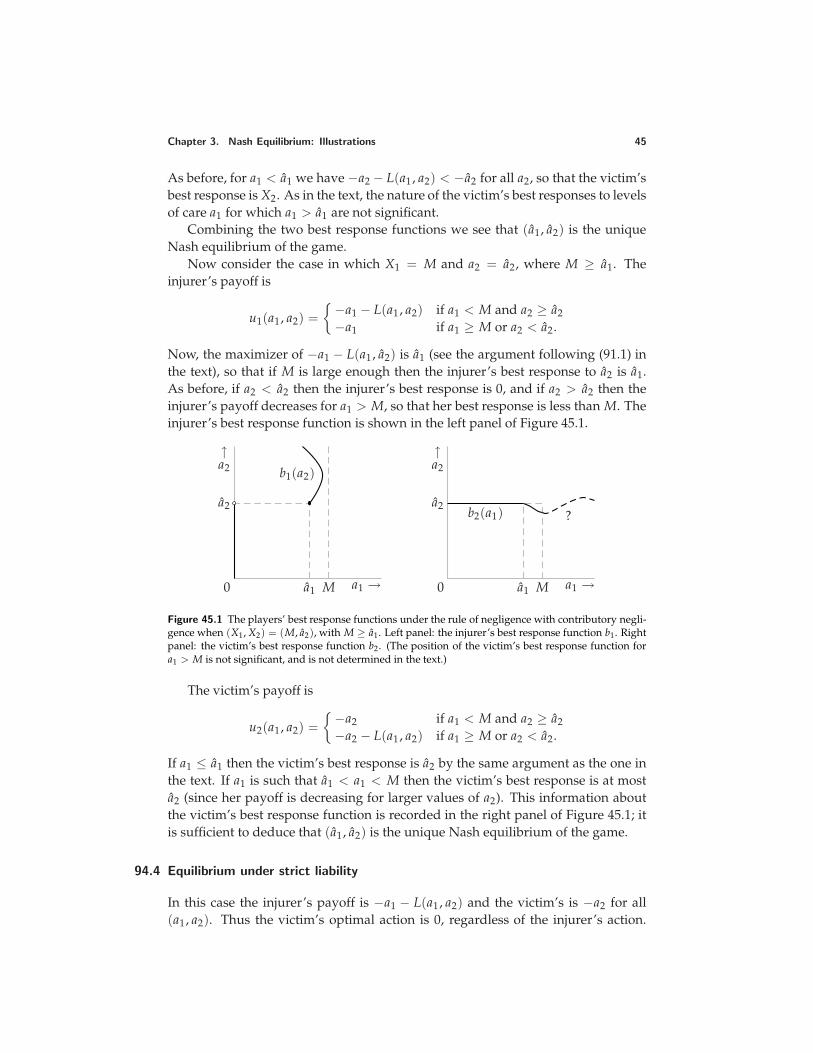
Chapter 3. Nash Equilibrium: Illustrations 45
As before, for a1 < a1 we have −a2 − L(a1, a2) < −a2 for all a2, so that the victim’sbest response is X2. As in the text, the nature of the victim’s best responses to levelsof care a1 for which a1 > a1 are not significant.
Combining the two best response functions we see that (a1, a2) is the uniqueNash equilibrium of the game.
Now consider the case in which X1 = M and a2 = a2, where M ≥ a1. Theinjurer’s payoff is
u1(a1, a2) =−a1 − L(a1, a2) if a1 < M and a2 ≥ a2−a1 if a1 ≥ M or a2 < a2.
Now, the maximizer of −a1 − L(a1, a2) is a1 (see the argument following (91.1) inthe text), so that if M is large enough then the injurer’s best response to a2 is a1.As before, if a2 < a2 then the injurer’s best response is 0, and if a2 > a2 then theinjurer’s payoff decreases for a1 > M, so that her best response is less than M. Theinjurer’s best response function is shown in the left panel of Figure 45.1.
0
a2
a1 M a1 →
↑a2 b1(a2)
0
a2
a1 M a1 →
↑a2
?b2(a1)
Figure 45.1 The players’ best response functions under the rule of negligence with contributory negli-gence when (X1, X2) = (M, a2), with M ≥ a1. Left panel: the injurer’s best response function b1. Rightpanel: the victim’s best response function b2. (The position of the victim’s best response function fora1 > M is not significant, and is not determined in the text.)
The victim’s payoff is
u2(a1, a2) =−a2 if a1 < M and a2 ≥ a2−a2 − L(a1, a2) if a1 ≥ M or a2 < a2.
If a1 ≤ a1 then the victim’s best response is a2 by the same argument as the one inthe text. If a1 is such that a1 < a1 < M then the victim’s best response is at mosta2 (since her payoff is decreasing for larger values of a2). This information aboutthe victim’s best response function is recorded in the right panel of Figure 45.1; itis sufficient to deduce that (a1, a2) is the unique Nash equilibrium of the game.
94.4 Equilibrium under strict liability
In this case the injurer’s payoff is −a1 − L(a1, a2) and the victim’s is −a2 for all(a1, a2). Thus the victim’s optimal action is 0, regardless of the injurer’s action.
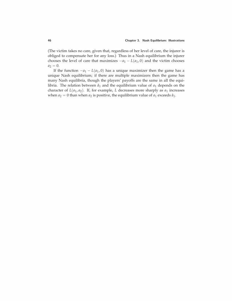
46 Chapter 3. Nash Equilibrium: Illustrations
(The victim takes no care, given that, regardless of her level of care, the injurer isobliged to compensate her for any loss.) Thus in a Nash equilibrium the injurerchooses the level of care that maximizes −a1 − L(a1, 0) and the victim choosesa2 = 0.
If the function −a1 − L(a1, 0) has a unique maximizer then the game has aunique Nash equilibrium; if there are multiple maximizers then the game hasmany Nash equilibria, though the players’ payoffs are the same in all the equi-libria. The relation between a1 and the equilibrium value of a1 depends on thecharacter of L(a1, a2). If, for example, L decreases more sharply as a1 increaseswhen a2 = 0 than when a2 is positive, the equilibrium value of a1 exceeds a1.
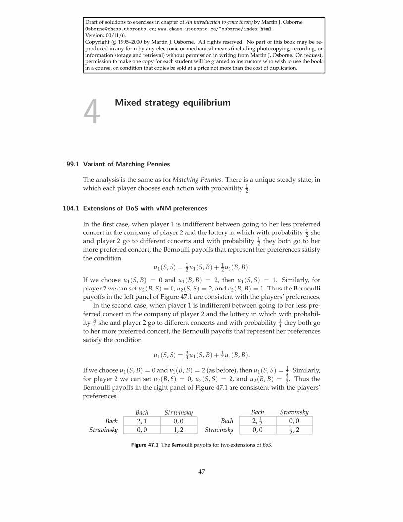
Draft of solutions to exercises in chapter of An introduction to game theory by Martin J. [email protected]; www.chass.utoronto.ca/~osborne/index.htmlVersion: 00/11/6.Copyright c© 1995–2000 by Martin J. Osborne. All rights reserved. No part of this book may be re-produced in any form by any electronic or mechanical means (including photocopying, recording, orinformation storage and retrieval) without permission in writing from Martin J. Osborne. On request,permission to make one copy for each student will be granted to instructors who wish to use the bookin a course, on condition that copies be sold at a price not more than the cost of duplication.
4 Mixed strategy equilibrium
99.1 Variant of Matching Pennies
The analysis is the same as for Matching Pennies. There is a unique steady state, inwhich each player chooses each action with probability 1
2 .
104.1 Extensions of BoS with vNM preferences
In the first case, when player 1 is indifferent between going to her less preferredconcert in the company of player 2 and the lottery in which with probability 1
2 sheand player 2 go to different concerts and with probability 1
2 they both go to hermore preferred concert, the Bernoulli payoffs that represent her preferences satisfythe condition
u1(S, S) = 12 u1(S, B) + 1
2 u1(B, B).
If we choose u1(S, B) = 0 and u1(B, B) = 2, then u1(S, S) = 1. Similarly, forplayer 2 we can set u2(B, S) = 0, u2(S, S) = 2, and u2(B, B) = 1. Thus the Bernoullipayoffs in the left panel of Figure 47.1 are consistent with the players’ preferences.
In the second case, when player 1 is indifferent between going to her less pre-ferred concert in the company of player 2 and the lottery in which with probabil-ity 3
4 she and player 2 go to different concerts and with probability 14 they both go
to her more preferred concert, the Bernoulli payoffs that represent her preferencessatisfy the condition
u1(S, S) = 34 u1(S, B) + 1
4 u1(B, B).
If we choose u1(S, B) = 0 and u1(B, B) = 2 (as before), then u1(S, S) = 12 . Similarly,
for player 2 we can set u2(B, S) = 0, u2(S, S) = 2, and u2(B, B) = 12 . Thus the
Bernoulli payoffs in the right panel of Figure 47.1 are consistent with the players’preferences.
Bach StravinskyBach 2, 1 0, 0
Stravinsky 0, 0 1, 2
Bach StravinskyBach 2, 1
2 0, 0Stravinsky 0, 0 1
2 , 2
Figure 47.1 The Bernoulli payoffs for two extensions of BoS.
47
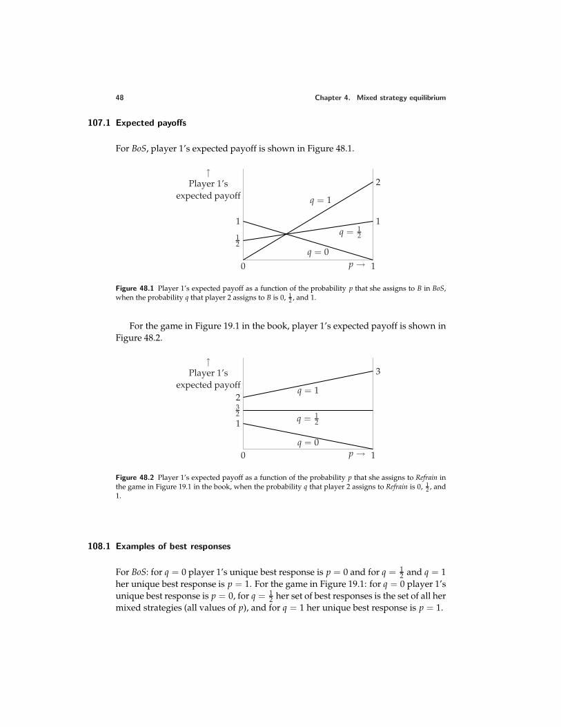
48 Chapter 4. Mixed strategy equilibrium
107.1 Expected payoffs
For BoS, player 1’s expected payoff is shown in Figure 48.1.
↑Player 1’s
expected payoff2
q = 1
12
1q = 1
2
1
q = 0
0 1p →
Figure 48.1 Player 1’s expected payoff as a function of the probability p that she assigns to B in BoS,when the probability q that player 2 assigns to B is 0, 1
2 , and 1.
For the game in Figure 19.1 in the book, player 1’s expected payoff is shown inFigure 48.2.
↑Player 1’s
expected payoff3
2q = 1
32 q = 1
21
q = 00 1p →
Figure 48.2 Player 1’s expected payoff as a function of the probability p that she assigns to Refrain inthe game in Figure 19.1 in the book, when the probability q that player 2 assigns to Refrain is 0, 1
2 , and1.
108.1 Examples of best responses
For BoS: for q = 0 player 1’s unique best response is p = 0 and for q = 12 and q = 1
her unique best response is p = 1. For the game in Figure 19.1: for q = 0 player 1’sunique best response is p = 0, for q = 1
2 her set of best responses is the set of all hermixed strategies (all values of p), and for q = 1 her unique best response is p = 1.
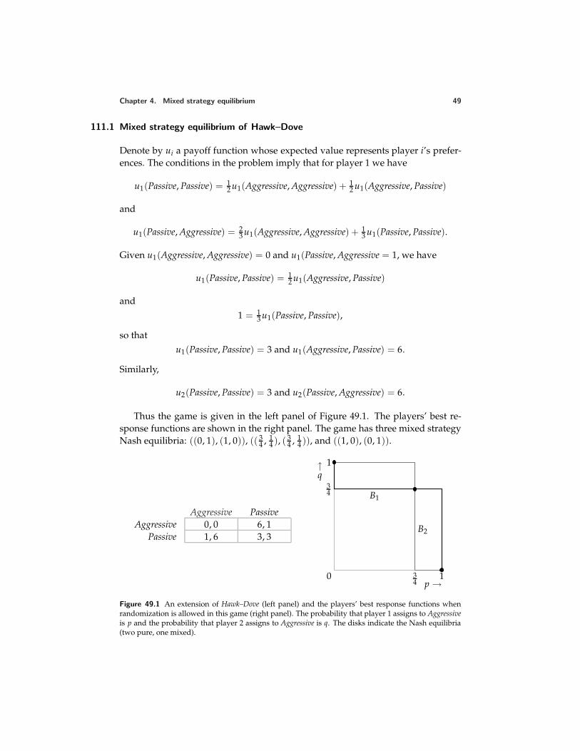
Chapter 4. Mixed strategy equilibrium 49
111.1 Mixed strategy equilibrium of Hawk–Dove
Denote by ui a payoff function whose expected value represents player i’s prefer-ences. The conditions in the problem imply that for player 1 we have
u1(Passive, Passive) = 12 u1(Aggressive, Aggressive) + 1
2 u1(Aggressive, Passive)
and
u1(Passive, Aggressive) = 23 u1(Aggressive, Aggressive) + 1
3 u1(Passive, Passive).
Given u1(Aggressive, Aggressive) = 0 and u1(Passive, Aggressive = 1, we have
u1(Passive, Passive) = 12 u1(Aggressive, Passive)
and1 = 1
3 u1(Passive, Passive),
so thatu1(Passive, Passive) = 3 and u1(Aggressive, Passive) = 6.
Similarly,
u2(Passive, Passive) = 3 and u2(Passive, Aggressive) = 6.
Thus the game is given in the left panel of Figure 49.1. The players’ best re-sponse functions are shown in the right panel. The game has three mixed strategyNash equilibria: ((0, 1), (1, 0)), (( 3
4 , 14 ), ( 3
4 , 14 )), and ((1, 0), (0, 1)).
Aggressive PassiveAggressive 0, 0 6, 1
Passive 1, 6 3, 3
0 34
1p →
34
1↑q
B1
B2
Figure 49.1 An extension of Hawk–Dove (left panel) and the players’ best response functions whenrandomization is allowed in this game (right panel). The probability that player 1 assigns to Aggressiveis p and the probability that player 2 assigns to Aggressive is q. The disks indicate the Nash equilibria(two pure, one mixed).
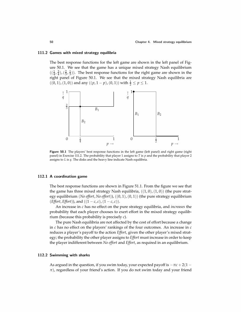
50 Chapter 4. Mixed strategy equilibrium
111.2 Games with mixed strategy equilibria
The best response functions for the left game are shown in the left panel of Fig-ure 50.1. We see that the game has a unique mixed strategy Nash equilibrium(( 1
4 , 34 ), ( 2
3 , 13 )). The best response functions for the right game are shown in the
right panel of Figure 50.1. We see that the mixed strategy Nash equilibria are((0, 1), (1, 0)) and any ((p, 1 − p), (0, 1)) with 1
2 ≤ p ≤ 1.
0 14
1p →
23
1↑q
B1
B2
0 12
1p →
1↑q
B1 B2
Figure 50.1 The players’ best response functions in the left game (left panel) and right game (rightpanel) in Exercise 111.2. The probability that player 1 assigns to T is p and the probability that player 2assigns to L is q. The disks and the heavy line indicate Nash equilibria.
112.1 A coordination game
The best response functions are shown in Figure 51.1. From the figure we see thatthe game has three mixed strategy Nash equilibria, ((1, 0), (1, 0)) (the pure strat-egy equilibrium (No effort, No effort)), ((0, 1), (0, 1)) (the pure strategy equilibrium(Effort, Effort)), and ((1 − c, c), (1 − c, c)).
An increase in c has no effect on the pure strategy equilibria, and increases theprobability that each player chooses to exert effort in the mixed strategy equilib-rium (because this probability is precisely c).
The pure Nash equilibria are not affected by the cost of effort because a changein c has no effect on the players’ rankings of the four outcomes. An increase in creduces a player’s payoff to the action Effort, given the other player’s mixed strat-egy; the probability the other player assigns to Effort must increase in order to keepthe player indifferent between No effort and Effort, as required in an equilibrium.
112.2 Swimming with sharks
As argued in the question, if you swim today, your expected payoff is −πc + 2(1−π), regardless of your friend’s action. If you do not swim today and your friend
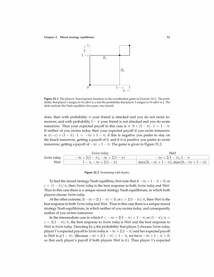
Chapter 4. Mixed strategy equilibrium 51
0 1 − c 1p →
1 − c
1↑q
B1
B2
Figure 51.1 The players’ best response functions in the coordination game in Exercise 112.1. The prob-ability that player 1 assigns to No effort is p and the probability that player 2 assigns to No effort is q. Thedisks indicate the Nash equilibria (two pure, one mixed).
does, then with probability π your friend is attacked and you do not swim to-morrow, and with probability 1 − π your friend is not attacked and you do swimtomorrow. Thus your expected payoff in this case is π · 0 + (1 − π) · 1 = 1 − π.If neither of you swims today then your expected payoff if you swim tomorrowis π(−c) + (1 − π) · 1 = −πc + 1 − π; if this is negative you prefer to stay onthe beach tomorrow, getting a payoff of 0, and if it is positive you prefer to swimtomorrow, getting a payoff of −πc + 1 − π. The game is given in Figure 51.2.
Swim today WaitSwim today −πc + 2(1 − π), −πc + 2(1 − π) −πc + 2(1 − π), 1 − π
Wait 1 − π, −πc + 2(1 − π) max0, −πc + 1 − π, max0, −πc + 1 − π
Figure 51.2 Swimming with sharks.
To find the mixed strategy Nash equilibria, first note that if −πc + 1 − π > 0, orc < (1 − π)/π, then Swim today is the best response to both Swim today and Wait.Thus in this case there is a unique mixed strategy Nash equilibrium, in which bothplayers choose Swim today.
At the other extreme, if −πc + 2(1 − π) < 0, or c > 2(1 − π)/π, then Wait is thebest response to both Swim today and Wait. Thus in this case there is a unique mixedstrategy Nash equilibrium, in which neither of you swims today, and consequentlyneither of you swims tomorrow.
In the intermediate case in which 0 < −πc + 2(1 − π) < 1 − π, or (1 − π)/π <
c < 2(1 − π)/π, the best response to Swim today is Wait and the best response toWait is Swim today. Denoting by q the probability that player 2 chooses Swim today,player 1’s expected payoff to Swim today is −πc + 2(1−π) and her expected payoffto Wait is q(1 − π). (Because −πc + 2(1 − π) < 1 − π, we have −πc + 1 − π < 0,so that each player’s payoff if both players Wait is 0.) Thus player 1’s expected
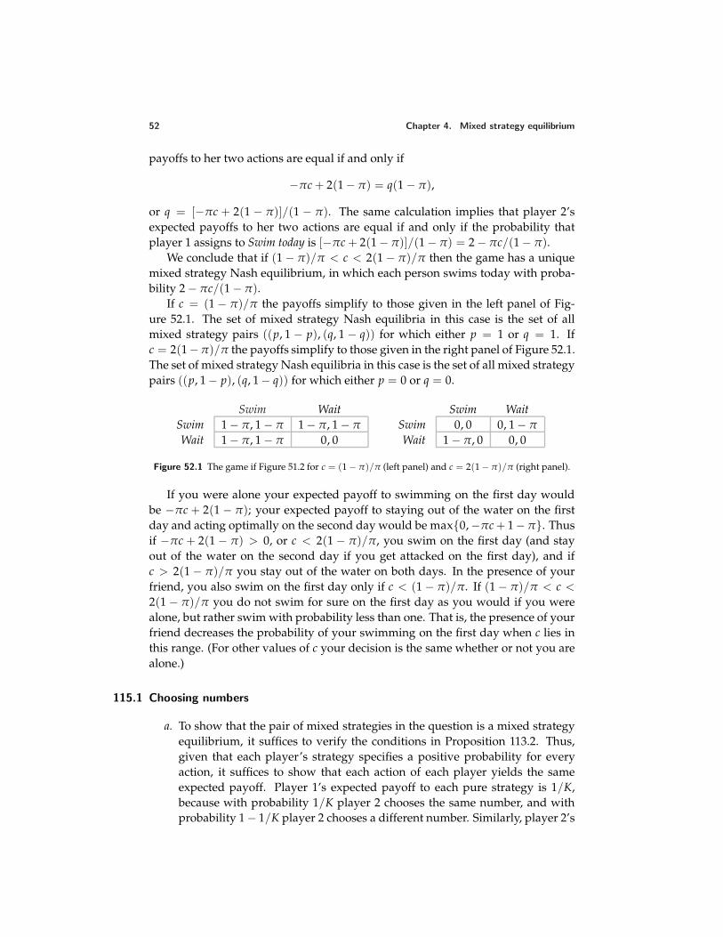
52 Chapter 4. Mixed strategy equilibrium
payoffs to her two actions are equal if and only if
−πc + 2(1 − π) = q(1 − π),
or q = [−πc + 2(1 − π)]/(1 − π). The same calculation implies that player 2’sexpected payoffs to her two actions are equal if and only if the probability thatplayer 1 assigns to Swim today is [−πc + 2(1 − π)]/(1 − π) = 2 − πc/(1 − π).
We conclude that if (1 − π)/π < c < 2(1 − π)/π then the game has a uniquemixed strategy Nash equilibrium, in which each person swims today with proba-bility 2 − πc/(1 − π).
If c = (1 − π)/π the payoffs simplify to those given in the left panel of Fig-ure 52.1. The set of mixed strategy Nash equilibria in this case is the set of allmixed strategy pairs ((p, 1 − p), (q, 1 − q)) for which either p = 1 or q = 1. Ifc = 2(1−π)/π the payoffs simplify to those given in the right panel of Figure 52.1.The set of mixed strategy Nash equilibria in this case is the set of all mixed strategypairs ((p, 1 − p), (q, 1 − q)) for which either p = 0 or q = 0.
Swim WaitSwim 1 − π, 1 − π 1 − π, 1 − π
Wait 1 − π, 1 − π 0, 0
Swim WaitSwim 0, 0 0, 1 − π
Wait 1 − π, 0 0, 0
Figure 52.1 The game if Figure 51.2 for c = (1 − π)/π (left panel) and c = 2(1 − π)/π (right panel).
If you were alone your expected payoff to swimming on the first day wouldbe −πc + 2(1 − π); your expected payoff to staying out of the water on the firstday and acting optimally on the second day would be max0, −πc + 1 − π. Thusif −πc + 2(1 − π) > 0, or c < 2(1 − π)/π, you swim on the first day (and stayout of the water on the second day if you get attacked on the first day), and ifc > 2(1 − π)/π you stay out of the water on both days. In the presence of yourfriend, you also swim on the first day only if c < (1 − π)/π. If (1 − π)/π < c <
2(1 − π)/π you do not swim for sure on the first day as you would if you werealone, but rather swim with probability less than one. That is, the presence of yourfriend decreases the probability of your swimming on the first day when c lies inthis range. (For other values of c your decision is the same whether or not you arealone.)
115.1 Choosing numbers
a. To show that the pair of mixed strategies in the question is a mixed strategyequilibrium, it suffices to verify the conditions in Proposition 113.2. Thus,given that each player’s strategy specifies a positive probability for everyaction, it suffices to show that each action of each player yields the sameexpected payoff. Player 1’s expected payoff to each pure strategy is 1/K,because with probability 1/K player 2 chooses the same number, and withprobability 1 − 1/K player 2 chooses a different number. Similarly, player 2’s
Chapter 4. Mixed strategy equilibrium 53
expected payoff to each pure strategy is −1/K, because with probability 1/Kplayer 1 chooses the same number, and with probability 1 − 1/K player 2chooses a different number. Thus the pair of strategies is a mixed strategyNash equilibrium.
b. Let (p∗, q∗) be a mixed strategy equilibrium, where p∗ and q∗ are vectors,the jth components of which are the probabilities assigned to the integer jby each player. Given that player 2 uses the mixed strategy q∗, player 1’sexpected payoff if she chooses the number k is q∗k . Hence if p∗k > 0 then (bythe first condition in Proposition 113.2) we need q∗k ≥ q∗j for all j, so that, inparticular, q∗k > 0 (q∗j cannot be zero for all j!). But player 2’s expected payoffif she chooses the number k is −pk, so given q∗k > 0 we need p∗k ≤ p∗j for all j(again by the first condition in Proposition 113.2), and, in particular, p∗k ≤ 1/K(p∗j cannot exceed 1/K for all j!). We conclude that any probability p∗k that ispositive must be at most 1/K. The only possibility is that p∗k = 1/K for all k.A similar argument implies that q∗k = 1/K for all k.
115.2 Silverman’s game
The game has no pure strategy Nash equilibrium in which the players’ integers arethe same because either player can increase her payoff from 0 to 1 by naming thenext higher integer. It has no Nash equilibrium in which the players’ integers aredifferent because the losing player (the player whose payoff is −1) can increase herpayoff to 1 by changing her integer to be one more than the other player’s integer.Thus the game has no pure strategy Nash equilibrium.
To show that the pair of mixed strategies in the question is a mixed strategyequilibrium, it suffices to verify the conditions in Proposition 113.2. That is, it suf-fices to show that for each player, each action to which the player’s mixed strategyassigns positive probability yields the player the same expected payoff, and everyother action yields her a payoff at most as large. The game is symmetric and theplayers’ strategies are the same, so we need to make an argument only for oneplayer.
Suppose player 2 uses the mixed strategy in the question. Player 1’s expectedpayoffs to her actions are as follows:
1: 13 · 0 + 1
3 · (−1) + 13 · 1 = 0.
2: 13 · 1 + 1
3 · 0 + 13 · (−1) = 0.
3 or 4: 13 · (−1) + 1
3 · 1 + 13 · (−1) = − 1
3 .
5: 13 · (−1) + 1
3 · 1 + 13 · 0 = 0.
6–14: 13 · (−1) + 1
3 · (−1) + 13 · 1 = − 1
3 .
15 or more: 13 · (−1) + 1
3 · (−1) + 13 · (−1) = −1.
Thus the pair of strategies is a mixed strategy equilibrium.
54 Chapter 4. Mixed strategy equilibrium
115.3 Voter participation
I verify that the conditions in Proposition 113.2 are satisfied.First consider a supporter of candidate A. If she votes then candidate A ties
if all k − 1 of her comrades vote, an event with probability pk−1, and otherwisecandidate A loses. Thus her expected payoff is
pk−1 − c.
If she abstains, then candidate A surely loses, so her payoff is 0. Thus in an equi-librium in which 0 < p < 1 the first condition in Proposition 113.2 implies thatpk−1 = c, or
p = c1/(k−1).
Now consider a supporter of candidate B who votes. With probability pk all ofthe supporters of candidate A vote, in which case the election is a tie; with proba-bility 1 − pk at least one of the supporters of candidate A does not vote, in whichcase candidate B wins. Thus the expected payoff of a supporter of candidate Bwho votes is
pk + 2(1 − pk) − c.
If the supporter of candidate B switches to abstaining, then
• candidate B loses if all supporters of candidate A vote, an event with proba-bility pk
• candidate B ties if exactly k− 1 supporters of candidate A vote, an event withprobability kpk−1(1 − p)
• candidate B wins if fewer than k− 1 supporters of candidate A vote, an eventwith probability 1 − pk − kpk−1(1 − p).
Thus a supporter of candidate B who switches from voting to abstaining obtainsan expected payoff of
kpk−1(1 − p) + 2(1 − pk − kpk−1(1 − p)) = 2 − (2 − k)pk − kpk−1.
Hence in order for it to be optimal for such a citizen to vote (i.e. in order for thesecond condition in Proposition 113.2 to be satisfied), we need
pk + 2(1 − pk) − c ≥ 2 − (2 − k)pk − kpk−1,
orkpk−1(1 − p) + pk ≥ c.
Finally, consider a supporter of candidate B who abstains. With probability pk
all the supporters of candidate A vote, in which case the candidates tie; with prob-ability 1 − pk at least one of the supporters of candidate A does not vote, in which
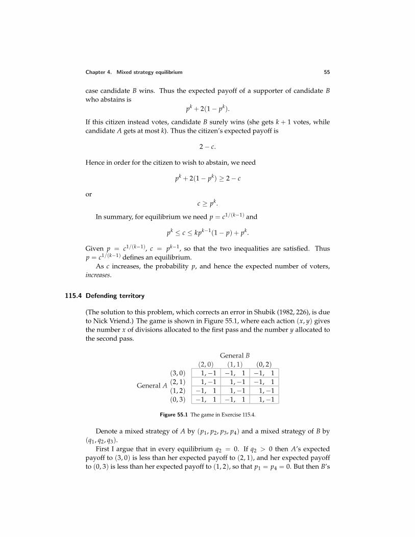
Chapter 4. Mixed strategy equilibrium 55
case candidate B wins. Thus the expected payoff of a supporter of candidate Bwho abstains is
pk + 2(1 − pk).
If this citizen instead votes, candidate B surely wins (she gets k + 1 votes, whilecandidate A gets at most k). Thus the citizen’s expected payoff is
2 − c.
Hence in order for the citizen to wish to abstain, we need
pk + 2(1 − pk) ≥ 2 − c
orc ≥ pk.
In summary, for equilibrium we need p = c1/(k−1) and
pk ≤ c ≤ kpk−1(1 − p) + pk.
Given p = c1/(k−1), c = pk−1, so that the two inequalities are satisfied. Thusp = c1/(k−1) defines an equilibrium.
As c increases, the probability p, and hence the expected number of voters,increases.
115.4 Defending territory
(The solution to this problem, which corrects an error in Shubik (1982, 226), is dueto Nick Vriend.) The game is shown in Figure 55.1, where each action (x, y) givesthe number x of divisions allocated to the first pass and the number y allocated tothe second pass.
General A
General B(2, 0) (1, 1) (0, 2)
(3, 0) 1, −1 −1, 1 −1, 1(2, 1) 1, −1 1, −1 −1, 1(1, 2) −1, 1 1, −1 1, −1(0, 3) −1, 1 −1, 1 1, −1
Figure 55.1 The game in Exercise 115.4.
Denote a mixed strategy of A by (p1, p2, p3, p4) and a mixed strategy of B by(q1, q2, q3).
First I argue that in every equilibrium q2 = 0. If q2 > 0 then A’s expectedpayoff to (3, 0) is less than her expected payoff to (2, 1), and her expected payoffto (0, 3) is less than her expected payoff to (1, 2), so that p1 = p4 = 0. But then B’s
56 Chapter 4. Mixed strategy equilibrium
expected payoff to at least one of her actions (2, 0) and (0, 2) exceeds her expectedpayoff to (1, 1), contradicting q2 > 0.
Now I argue that in every equilibrium q1 = q3 = 0. Given q2 = 0 we haveq3 = 1 − q1, and A’s payoffs are 2q1 − 1 to (3, 0) and to (2, 1), and 1 − 2q1 to (1, 2)and (0, 3). Thus if q1 < 1
2 then in any equilibrium we have p1 = p2 = 0. Then B’saction (2, 0) yields her a higher payoff than does (0, 2), so that in any equilibriumq1 = 1. But then A’s actions (3, 0) and (2, 1) both yield higher payoffs than do(1, 2) and (0, 3), contradicting p1 = p2 = 0. Similarly, q1 > 1
2 is inconsistent withequilibrium. Hence in any equilibrium q1 = q3 = 1
2 .Now, given q1 = q3 = 1
2 , A’s payoffs to her four actions are all equal. Thus((p1, p2, p3, p4), (q1, q2, q3)) is a Nash equilibrium if and only if B’s payoff to (2, 0)is the same as her payoff to (0, 2), and this payoff is at least her payoff to (1, 1).The first condition is −p1 − p2 + p3 + p4 = p1 + p2 − p3 − p4, or p1 + p2 = p3 +p4 = 1
2 . Thus B’s payoff to (2, 0) and to (0, 2) is zero, and the second condition isp1 − p2 − p3 + p4 ≤ 0, or p1 + p4 ≤ 1
2 (using p1 + p2 + p3 + p4 = 1).We conclude that the set of mixed strategy Nash equilibria of the game is the
set of strategy pairs ((p1, 12 − p1, 1
2 − p4, p4), ( 12 , 0, 1
2 )) with p1 + p4 ≤ 12 .
In this equilibrium general A splits her resources between the two passes withprobability at least 1
2 (p2 + p3 = 12 − p1 + 1
2 − p4 = 1 − (p1 + p4) ≥ 12 ) while
general B concentrates all of her resources in one or other of the passes (with equalprobability).
118.1 Strictly dominated actions
Denote the probability that player 1 assigns to T by p and the probability she as-signs to M by r (so that the probability she assigns to B is 1 − p − r). A mixedstrategy of player 1 strictly dominates T if and only if
p + 4r > 1 and p + 3(1 − p − r) > 1,
or if and only if 1 − 4r < p < 1 − 32 r. For example, the mixed strategies ( 1
4 , 14 , 1
2 )and (0, 1
4 , 34 ) both strictly dominate T.
119.1 Eliminating dominated actions when finding equilibria
Player 2’s action L is strictly dominated by the mixed strategy that assigns proba-bility 1
4 to M and probability 34 to R (for example), so that we can ignore the action
L. The players’ best response functions in the reduced game in which player 2’sactions are M and R are shown in Figure 57.1. We see that the game has a singlemixed strategy Nash equilibrium, namely (( 2
3 , 13 ), (0, 1
2 , 12 )).
124.1 Equilibrium in the expert diagnosis game
When E = rE′ + (1 − r)I ′ the consumer is indifferent between her two actionswhen p = 0, so that her best response function has a vertical segment at p = 0.
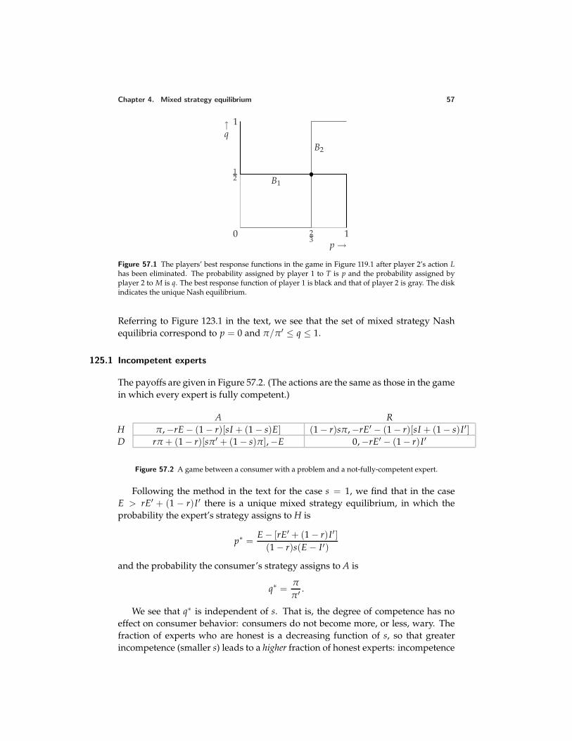
Chapter 4. Mixed strategy equilibrium 57
0 23
1p →
12
1↑q
B1
B2
Figure 57.1 The players’ best response functions in the game in Figure 119.1 after player 2’s action Lhas been eliminated. The probability assigned by player 1 to T is p and the probability assigned byplayer 2 to M is q. The best response function of player 1 is black and that of player 2 is gray. The diskindicates the unique Nash equilibrium.
Referring to Figure 123.1 in the text, we see that the set of mixed strategy Nashequilibria correspond to p = 0 and π/π′ ≤ q ≤ 1.
125.1 Incompetent experts
The payoffs are given in Figure 57.2. (The actions are the same as those in the gamein which every expert is fully competent.)
A RH π, −rE − (1 − r)[sI + (1 − s)E] (1 − r)sπ, −rE′ − (1 − r)[sI + (1 − s)I ′]D rπ + (1 − r)[sπ′ + (1 − s)π], −E 0, −rE′ − (1 − r)I ′
Figure 57.2 A game between a consumer with a problem and a not-fully-competent expert.
Following the method in the text for the case s = 1, we find that in the caseE > rE′ + (1 − r)I ′ there is a unique mixed strategy equilibrium, in which theprobability the expert’s strategy assigns to H is
p∗ =E − [rE′ + (1 − r)I ′]
(1 − r)s(E − I ′)
and the probability the consumer’s strategy assigns to A is
q∗ =π
π′ .
We see that q∗ is independent of s. That is, the degree of competence has noeffect on consumer behavior: consumers do not become more, or less, wary. Thefraction of experts who are honest is a decreasing function of s, so that greaterincompetence (smaller s) leads to a higher fraction of honest experts: incompetence
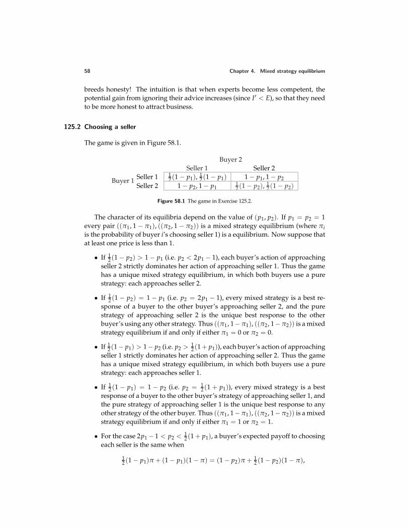
58 Chapter 4. Mixed strategy equilibrium
breeds honesty! The intuition is that when experts become less competent, thepotential gain from ignoring their advice increases (since I ′ < E), so that they needto be more honest to attract business.
125.2 Choosing a seller
The game is given in Figure 58.1.
Buyer 1
Buyer 2Seller 1 Seller 2
Seller 1 12 (1 − p1), 1
2 (1 − p1) 1 − p1, 1 − p2
Seller 2 1 − p2, 1 − p112 (1 − p2), 1
2 (1 − p2)
Figure 58.1 The game in Exercise 125.2.
The character of its equilibria depend on the value of (p1, p2). If p1 = p2 = 1every pair ((π1, 1 − π1), ((π2, 1 − π2)) is a mixed strategy equilibrium (where πiis the probability of buyer i’s choosing seller 1) is a equilibrium. Now suppose thatat least one price is less than 1.
• If 12 (1 − p2) > 1 − p1 (i.e. p2 < 2p1 − 1), each buyer’s action of approaching
seller 2 strictly dominates her action of approaching seller 1. Thus the gamehas a unique mixed strategy equilibrium, in which both buyers use a purestrategy: each approaches seller 2.
• If 12 (1 − p2) = 1 − p1 (i.e. p2 = 2p1 − 1), every mixed strategy is a best re-
sponse of a buyer to the other buyer’s approaching seller 2, and the purestrategy of approaching seller 2 is the unique best response to the otherbuyer’s using any other strategy. Thus ((π1, 1−π1), ((π2, 1−π2)) is a mixedstrategy equilibrium if and only if either π1 = 0 or π2 = 0.
• If 12 (1− p1) > 1− p2 (i.e. p2 > 1
2 (1 + p1)), each buyer’s action of approachingseller 1 strictly dominates her action of approaching seller 2. Thus the gamehas a unique mixed strategy equilibrium, in which both buyers use a purestrategy: each approaches seller 1.
• If 12 (1 − p1) = 1 − p2 (i.e. p2 = 1
2 (1 + p1)), every mixed strategy is a bestresponse of a buyer to the other buyer’s strategy of approaching seller 1, andthe pure strategy of approaching seller 1 is the unique best response to anyother strategy of the other buyer. Thus ((π1, 1−π1), ((π2, 1−π2)) is a mixedstrategy equilibrium if and only if either π1 = 1 or π2 = 1.
• For the case 2p1 − 1 < p2 < 12 (1 + p1), a buyer’s expected payoff to choosing
each seller is the same when
12 (1 − p1)π + (1 − p1)(1 − π) = (1 − p2)π + 1
2 (1 − p2)(1 − π),
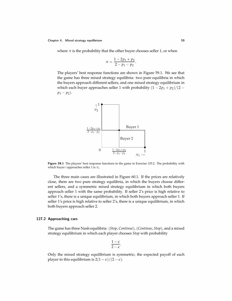
Chapter 4. Mixed strategy equilibrium 59
where π is the probability that the other buyer chooses seller 1, or when
π =1 − 2p1 + p2
2 − p1 − p2.
The players’ best response functions are shown in Figure 59.1. We see thatthe game has three mixed strategy equilibria: two pure equilibria in whichthe buyers approach different sellers, and one mixed strategy equilibrium inwhich each buyer approaches seller 1 with probability (1 − 2p1 + p2)/(2 −p1 − p2).
0 1−2p1+p22−p1−p2
1π1 →
1−2p1+p22−p1−p2
1↑π2
Buyer 1
Buyer 2
Figure 59.1 The players’ best response functions in the game in Exercise 125.2. The probability withwhich buyer i approaches seller 1 is πi.
The three main cases are illustrated in Figure 60.1. If the prices are relativelyclose, there are two pure strategy equilibria, in which the buyers choose differ-ent sellers, and a symmetric mixed strategy equilibrium in which both buyersapproach seller 1 with the same probability. If seller 2’s price is high relative toseller 1’s, there is a unique equilibrium, in which both buyers approach seller 1. Ifseller 1’s price is high relative to seller 2’s, there is a unique equilibrium, in whichboth buyers approach seller 2.
127.2 Approaching cars
The game has three Nash equilibria: (Stop, Continue), (Continue, Stop), and a mixedstrategy equilibrium in which each player chooses Stop with probability
1 − ε
2 − ε.
Only the mixed strategy equilibrium is symmetric; the expected payoff of eachplayer in this equilibrium is 2(1 − ε)/(2 − ε).
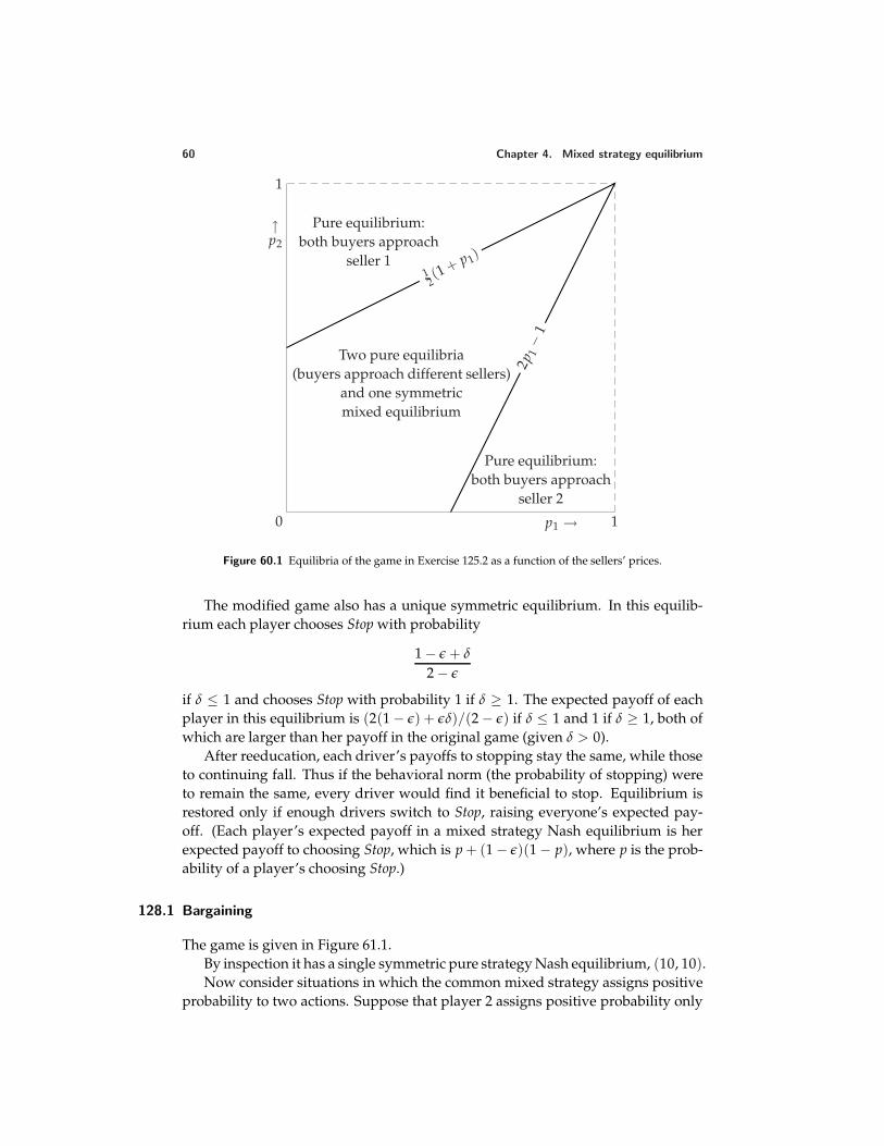
60 Chapter 4. Mixed strategy equilibrium
0
1
1p1 →
↑p2
Pure equilibrium:both buyers approach
seller 1
Pure equilibrium:both buyers approach
seller 2
Two pure equilibria(buyers approach different sellers)
and one symmetricmixed equilibrium
2p1−
1
12(1 + p 1)
Figure 60.1 Equilibria of the game in Exercise 125.2 as a function of the sellers’ prices.
The modified game also has a unique symmetric equilibrium. In this equilib-rium each player chooses Stop with probability
1 − ε + δ
2 − ε
if δ ≤ 1 and chooses Stop with probability 1 if δ ≥ 1. The expected payoff of eachplayer in this equilibrium is (2(1 − ε) + εδ)/(2 − ε) if δ ≤ 1 and 1 if δ ≥ 1, both ofwhich are larger than her payoff in the original game (given δ > 0).
After reeducation, each driver’s payoffs to stopping stay the same, while thoseto continuing fall. Thus if the behavioral norm (the probability of stopping) wereto remain the same, every driver would find it beneficial to stop. Equilibrium isrestored only if enough drivers switch to Stop, raising everyone’s expected pay-off. (Each player’s expected payoff in a mixed strategy Nash equilibrium is herexpected payoff to choosing Stop, which is p + (1 − ε)(1 − p), where p is the prob-ability of a player’s choosing Stop.)
128.1 Bargaining
The game is given in Figure 61.1.By inspection it has a single symmetric pure strategy Nash equilibrium, (10, 10).Now consider situations in which the common mixed strategy assigns positive
probability to two actions. Suppose that player 2 assigns positive probability only
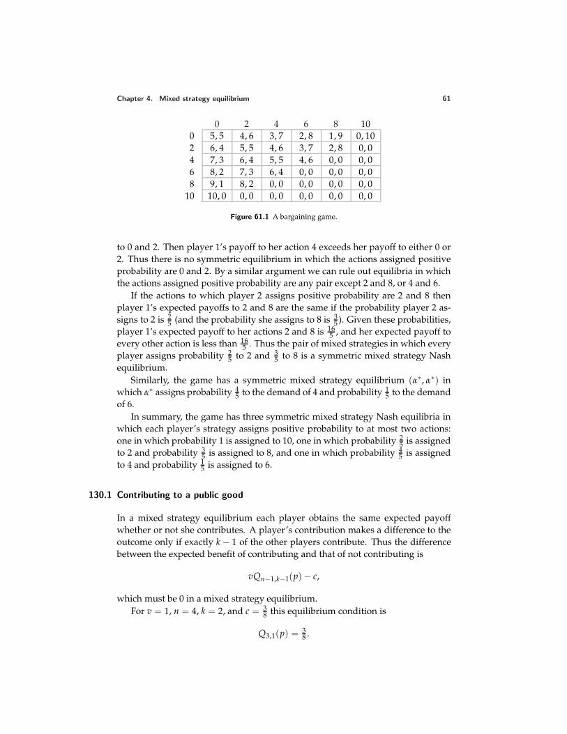
Chapter 4. Mixed strategy equilibrium 61
0 2 4 6 8 100 5, 5 4, 6 3, 7 2, 8 1, 9 0, 102 6, 4 5, 5 4, 6 3, 7 2, 8 0, 04 7, 3 6, 4 5, 5 4, 6 0, 0 0, 06 8, 2 7, 3 6, 4 0, 0 0, 0 0, 08 9, 1 8, 2 0, 0 0, 0 0, 0 0, 0
10 10, 0 0, 0 0, 0 0, 0 0, 0 0, 0
Figure 61.1 A bargaining game.
to 0 and 2. Then player 1’s payoff to her action 4 exceeds her payoff to either 0 or2. Thus there is no symmetric equilibrium in which the actions assigned positiveprobability are 0 and 2. By a similar argument we can rule out equilibria in whichthe actions assigned positive probability are any pair except 2 and 8, or 4 and 6.
If the actions to which player 2 assigns positive probability are 2 and 8 thenplayer 1’s expected payoffs to 2 and 8 are the same if the probability player 2 as-signs to 2 is 2
5 (and the probability she assigns to 8 is 35 ). Given these probabilities,
player 1’s expected payoff to her actions 2 and 8 is 165 , and her expected payoff to
every other action is less than 165 . Thus the pair of mixed strategies in which every
player assigns probability 25 to 2 and 3
5 to 8 is a symmetric mixed strategy Nashequilibrium.
Similarly, the game has a symmetric mixed strategy equilibrium (α∗, α∗) inwhich α∗ assigns probability 4
5 to the demand of 4 and probability 15 to the demand
of 6.In summary, the game has three symmetric mixed strategy Nash equilibria in
which each player’s strategy assigns positive probability to at most two actions:one in which probability 1 is assigned to 10, one in which probability 2
5 is assignedto 2 and probability 3
5 is assigned to 8, and one in which probability 45 is assigned
to 4 and probability 15 is assigned to 6.
130.1 Contributing to a public good
In a mixed strategy equilibrium each player obtains the same expected payoffwhether or not she contributes. A player’s contribution makes a difference to theoutcome only if exactly k − 1 of the other players contribute. Thus the differencebetween the expected benefit of contributing and that of not contributing is
vQn−1,k−1(p) − c,
which must be 0 in a mixed strategy equilibrium.For v = 1, n = 4, k = 2, and c = 3
8 this equilibrium condition is
Q3,1(p) = 38 .
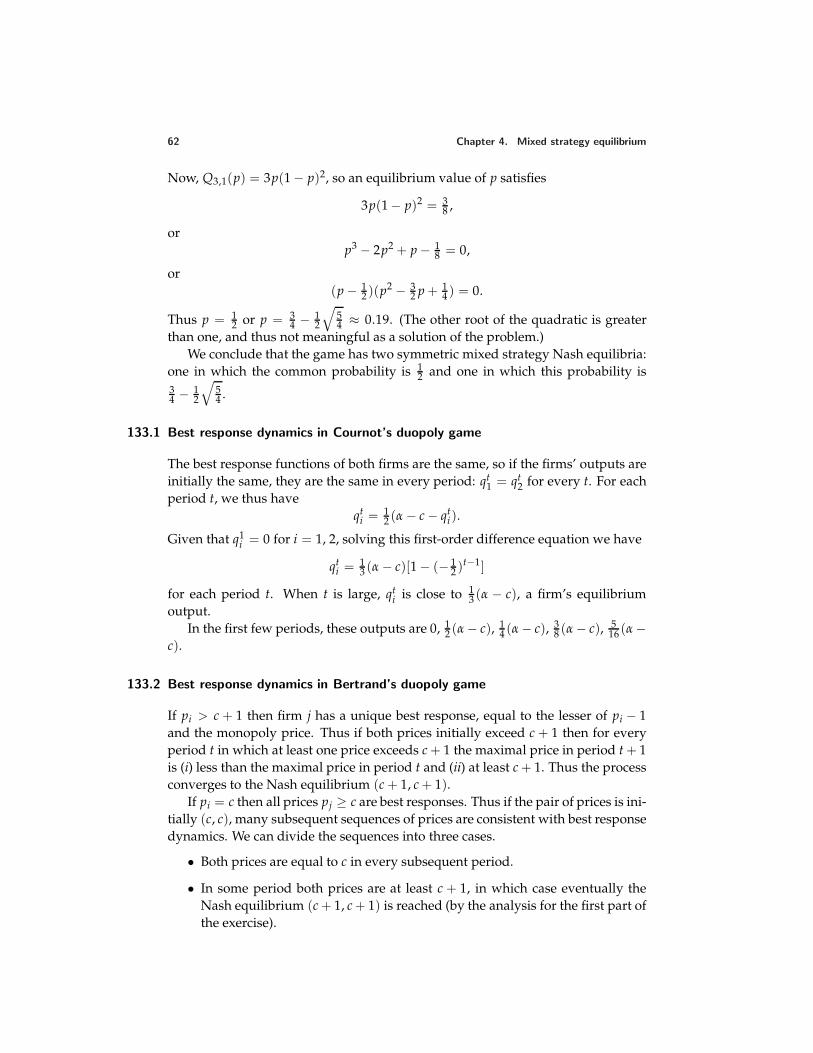
62 Chapter 4. Mixed strategy equilibrium
Now, Q3,1(p) = 3p(1 − p)2, so an equilibrium value of p satisfies
3p(1 − p)2 = 38 ,
orp3 − 2p2 + p − 1
8 = 0,
or(p − 1
2 )(p2 − 32 p + 1
4 ) = 0.
Thus p = 12 or p = 3
4 − 12
√54 ≈ 0.19. (The other root of the quadratic is greater
than one, and thus not meaningful as a solution of the problem.)We conclude that the game has two symmetric mixed strategy Nash equilibria:
one in which the common probability is 12 and one in which this probability is
34 − 1
2
√54 .
133.1 Best response dynamics in Cournot’s duopoly game
The best response functions of both firms are the same, so if the firms’ outputs areinitially the same, they are the same in every period: qt
1 = qt2 for every t. For each
period t, we thus haveqt
i = 12 (α − c − qt
i).
Given that q1i = 0 for i = 1, 2, solving this first-order difference equation we have
qti = 1
3 (α − c)[1 − (− 12 )t−1]
for each period t. When t is large, qti is close to 1
3 (α − c), a firm’s equilibriumoutput.
In the first few periods, these outputs are 0, 12 (α − c), 1
4 (α − c), 38 (α − c), 5
16 (α −c).
133.2 Best response dynamics in Bertrand’s duopoly game
If pi > c + 1 then firm j has a unique best response, equal to the lesser of pi − 1and the monopoly price. Thus if both prices initially exceed c + 1 then for everyperiod t in which at least one price exceeds c + 1 the maximal price in period t + 1is (i) less than the maximal price in period t and (ii) at least c + 1. Thus the processconverges to the Nash equilibrium (c + 1, c + 1).
If pi = c then all prices pj ≥ c are best responses. Thus if the pair of prices is ini-tially (c, c), many subsequent sequences of prices are consistent with best responsedynamics. We can divide the sequences into three cases.
• Both prices are equal to c in every subsequent period.
• In some period both prices are at least c + 1, in which case eventually theNash equilibrium (c + 1, c + 1) is reached (by the analysis for the first part ofthe exercise).
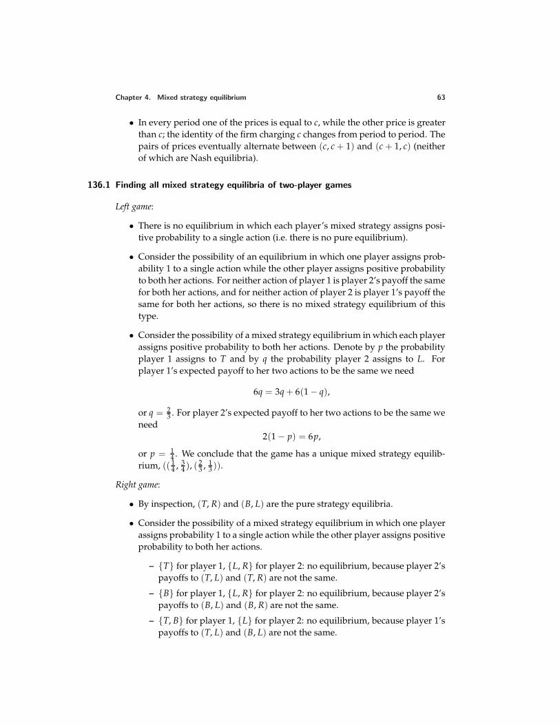
Chapter 4. Mixed strategy equilibrium 63
• In every period one of the prices is equal to c, while the other price is greaterthan c; the identity of the firm charging c changes from period to period. Thepairs of prices eventually alternate between (c, c + 1) and (c + 1, c) (neitherof which are Nash equilibria).
136.1 Finding all mixed strategy equilibria of two-player games
Left game:
• There is no equilibrium in which each player’s mixed strategy assigns posi-tive probability to a single action (i.e. there is no pure equilibrium).
• Consider the possibility of an equilibrium in which one player assigns prob-ability 1 to a single action while the other player assigns positive probabilityto both her actions. For neither action of player 1 is player 2’s payoff the samefor both her actions, and for neither action of player 2 is player 1’s payoff thesame for both her actions, so there is no mixed strategy equilibrium of thistype.
• Consider the possibility of a mixed strategy equilibrium in which each playerassigns positive probability to both her actions. Denote by p the probabilityplayer 1 assigns to T and by q the probability player 2 assigns to L. Forplayer 1’s expected payoff to her two actions to be the same we need
6q = 3q + 6(1 − q),
or q = 23 . For player 2’s expected payoff to her two actions to be the same we
need2(1 − p) = 6p,
or p = 14 . We conclude that the game has a unique mixed strategy equilib-
rium, (( 14 , 3
4 ), ( 23 , 1
3 )).
Right game:
• By inspection, (T, R) and (B, L) are the pure strategy equilibria.
• Consider the possibility of a mixed strategy equilibrium in which one playerassigns probability 1 to a single action while the other player assigns positiveprobability to both her actions.
– T for player 1, L, R for player 2: no equilibrium, because player 2’spayoffs to (T, L) and (T, R) are not the same.
– B for player 1, L, R for player 2: no equilibrium, because player 2’spayoffs to (B, L) and (B, R) are not the same.
– T, B for player 1, L for player 2: no equilibrium, because player 1’spayoffs to (T, L) and (B, L) are not the same.
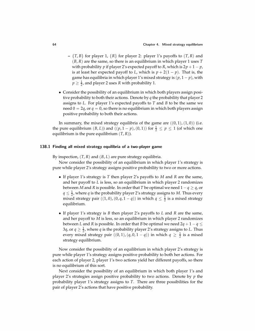
64 Chapter 4. Mixed strategy equilibrium
– T, B for player 1, R for player 2: player 1’s payoffs to (T, R) and(B, R) are the same, so there is an equilibrium in which player 1 uses Twith probability p if player 2’s expected payoff to R, which is 2p + 1− p,is at least her expected payoff to L, which is p + 2(1 − p). That is, thegame has equilibria in which player 1’s mixed strategy is (p, 1− p), withp ≥ 1
2 , and player 2 uses R with probability 1.
• Consider the possibility of an equilibrium in which both players assign posi-tive probability to both their actions. Denote by q the probability that player 2assigns to L. For player 1’s expected payoffs to T and B to be the same weneed 0 = 2q, or q = 0, so there is no equilibrium in which both players assignpositive probability to both their actions.
In summary, the mixed strategy equilibria of the game are ((0, 1), (1, 0)) (i.e.the pure equilibrium (B, L)) and ((p, 1 − p), (0, 1)) for 1
2 ≤ p ≤ 1 (of which oneequilibrium is the pure equilibrium (T, R)).
138.1 Finding all mixed strategy equilibria of a two-player game
By inspection, (T, R) and (B, L) are pure strategy equilibria.Now consider the possibility of an equilibrium in which player 1’s strategy is
pure while player 2’s strategy assigns positive probability to two or more actions.
• If player 1’s strategy is T then player 2’s payoffs to M and R are the same,and her payoff to L is less, so an equilibrium in which player 2 randomizesbetween M and R is possible. In order that T be optimal we need 1− q ≥ q, orq ≤ 1
2 , where q is the probability player 2’s strategy assigns to M. Thus everymixed strategy pair ((1, 0), (0, q, 1 − q)) in which q ≤ 1
2 is a mixed strategyequilibrium.
• If player 1’s strategy is B then player 2’s payoffs to L and R are the same,and her payoff to M is less, so an equilibrium in which player 2 randomizesbetween L and R is possible. In order that B be optimal we need 2q + 1 − q ≤3q, or q ≥ 1
2 , where q is the probability player 2’s strategy assigns to L. Thusevery mixed strategy pair ((0, 1), (q, 0, 1 − q)) in which q ≥ 1
2 is a mixedstrategy equilibrium.
Now consider the possibility of an equilibrium in which player 2’s strategy ispure while player 1’s strategy assigns positive probability to both her actions. Foreach action of player 2, player 1’s two actions yield her different payoffs, so thereis no equilibrium of this sort.
Next consider the possibility of an equilibrium in which both player 1’s andplayer 2’s strategies assign positive probability to two actions. Denote by p theprobability player 1’s strategy assigns to T. There are three possibilities for thepair of player 2’s actions that have positive probability.
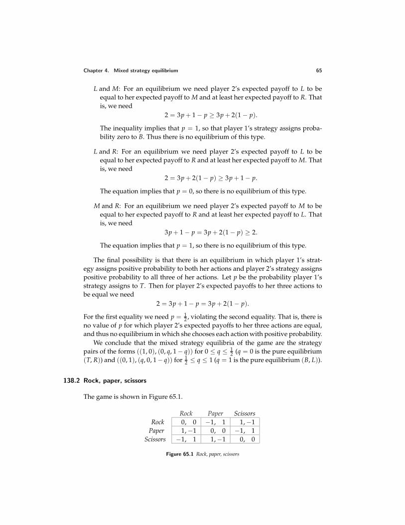
Chapter 4. Mixed strategy equilibrium 65
L and M: For an equilibrium we need player 2’s expected payoff to L to beequal to her expected payoff to M and at least her expected payoff to R. Thatis, we need
2 = 3p + 1 − p ≥ 3p + 2(1 − p).
The inequality implies that p = 1, so that player 1’s strategy assigns proba-bility zero to B. Thus there is no equilibrium of this type.
L and R: For an equilibrium we need player 2’s expected payoff to L to beequal to her expected payoff to R and at least her expected payoff to M. Thatis, we need
2 = 3p + 2(1 − p) ≥ 3p + 1 − p.
The equation implies that p = 0, so there is no equilibrium of this type.
M and R: For an equilibrium we need player 2’s expected payoff to M to beequal to her expected payoff to R and at least her expected payoff to L. Thatis, we need
3p + 1 − p = 3p + 2(1 − p) ≥ 2.
The equation implies that p = 1, so there is no equilibrium of this type.
The final possibility is that there is an equilibrium in which player 1’s strat-egy assigns positive probability to both her actions and player 2’s strategy assignspositive probability to all three of her actions. Let p be the probability player 1’sstrategy assigns to T. Then for player 2’s expected payoffs to her three actions tobe equal we need
2 = 3p + 1 − p = 3p + 2(1 − p).
For the first equality we need p = 12 , violating the second equality. That is, there is
no value of p for which player 2’s expected payoffs to her three actions are equal,and thus no equilibrium in which she chooses each action with positive probability.
We conclude that the mixed strategy equilibria of the game are the strategypairs of the forms ((1, 0), (0, q, 1 − q)) for 0 ≤ q ≤ 1
2 (q = 0 is the pure equilibrium(T, R)) and ((0, 1), (q, 0, 1− q)) for 1
2 ≤ q ≤ 1 (q = 1 is the pure equilibrium (B, L)).
138.2 Rock, paper, scissors
The game is shown in Figure 65.1.
Rock Paper ScissorsRock 0, 0 −1, 1 1, −1
Paper 1, −1 0, 0 −1, 1Scissors −1, 1 1, −1 0, 0
Figure 65.1 Rock, paper, scissors
66 Chapter 4. Mixed strategy equilibrium
By inspection the game has no pure strategy equilibrium, and no mixed strat-egy equilibrium in which one player’s strategy is pure and the other’s is strictlymixed.
In the remaining possibilities both players use at least two actions with positiveprobability. Suppose that player 1’s mixed strategy assigns positive probability toRock and to Paper. Then player 2’s expected payoff to Paper exceeds her expectedpayoff to Rock, so in any such equilibrium player 2 must assign positive probabilityonly to Paper and Scissors. Player 1’s expected payoffs to Rock and Paper are equalonly if player 2 assigns probability 2
3 to Paper and probability 13 to Scissors. But
then player 1’s expected payoff to Scissors exceeds her expected payoffs to Rockand Paper. So there is no mixed strategy equilibrium in which player 1 assignspositive probability only to Rock and to Paper.
Given the symmetry of the game, the same argument implies that there is noequilibrium in which player 1 assigns positive probability to only two actions, norany equilibrium in which player 2 assigns positive probability to only two actions.
The remaining possibility is that each player assigns positive probability to allthree of her actions. Denote the probabilities player 1 assigns to her three actions by(p1, p2, p3) and the probabilities player 2 assigns to her three actions by (q1, q2, q3).Player 1’s actions all yield her the same expected payoff if and only if there is avalue of c for which
−q2 + q3 = c
q1 − q3 = c
−q1 + q2 = c.
Adding the three equations we deduce c = 0, and hence q1 = q2 = q3 = 13 . A
similar calculation for player 2 yields p1 = p2 = p3 = 13 .
In conclusion, the game has a unique mixed strategy equilibrium, in whicheach player uses the strategy ( 1
3 , 13 , 1
3 ). Each player’s equilibrium payoff is 0.In the modified game in which player 1 is prohibited from using the action Scis-
sors, player 2’s action Rock is strictly dominated. The remaining game has a uniquemixed strategy equilibrium, in which player 1 chooses Rock with probability 1
3 andPaper with probability 2
3 , and player 2 chooses Paper with probability 23 and Scissors
with probability 13 . The equilibrium payoff of player 1 is − 1
3 and that of player 2 is13 .
139.1 Election campaigns
A strategic game that models the situation is shown in Figure 67.1, where action kmeans devote resources to locality k.
By inspection the game has no pure strategy equilibrium and no equilibrium inwhich one player’s strategy is pure and the other is strictly mixed. (For each actionof each player, the other player has a single best action.)
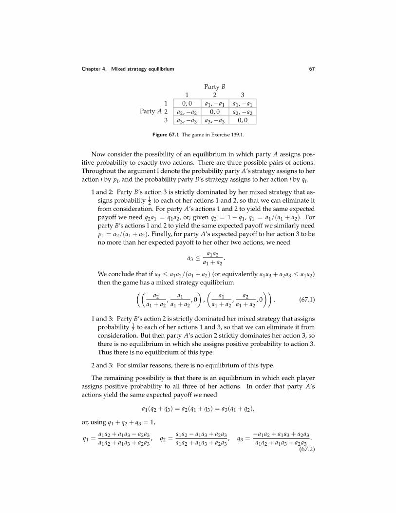
Chapter 4. Mixed strategy equilibrium 67
Party A
Party B1 2 3
1 0, 0 a1, −a1 a1, −a12 a2, −a2 0, 0 a2, −a23 a3, −a3 a3, −a3 0, 0
Figure 67.1 The game in Exercise 139.1.
Now consider the possibility of an equilibrium in which party A assigns pos-itive probability to exactly two actions. There are three possible pairs of actions.Throughout the argument I denote the probability party A’s strategy assigns to heraction i by pi, and the probability party B’s strategy assigns to her action i by qi.
1 and 2: Party B’s action 3 is strictly dominated by her mixed strategy that as-signs probability 1
2 to each of her actions 1 and 2, so that we can eliminate itfrom consideration. For party A’s actions 1 and 2 to yield the same expectedpayoff we need q2a1 = q1a2, or, given q2 = 1 − q1, q1 = a1/(a1 + a2). Forparty B’s actions 1 and 2 to yield the same expected payoff we similarly needp1 = a2/(a1 + a2). Finally, for party A’s expected payoff to her action 3 to beno more than her expected payoff to her other two actions, we need
a3 ≤ a1a2
a1 + a2.
We conclude that if a3 ≤ a1a2/(a1 + a2) (or equivalently a1a3 + a2a3 ≤ a1a2)then the game has a mixed strategy equilibrium
((a2
a1 + a2,
a1
a1 + a2, 0)
,(
a1
a1 + a2,
a2
a1 + a2, 0))
. (67.1)
1 and 3: Party B’s action 2 is strictly dominated her mixed strategy that assignsprobability 1
2 to each of her actions 1 and 3, so that we can eliminate it fromconsideration. But then party A’s action 2 strictly dominates her action 3, sothere is no equilibrium in which she assigns positive probability to action 3.Thus there is no equilibrium of this type.
2 and 3: For similar reasons, there is no equilibrium of this type.
The remaining possibility is that there is an equilibrium in which each playerassigns positive probability to all three of her actions. In order that party A’sactions yield the same expected payoff we need
a1(q2 + q3) = a2(q1 + q3) = a3(q1 + q2),
or, using q1 + q2 + q3 = 1,
q1 =a1a2 + a1a3 − a2a3
a1a2 + a1a3 + a2a3, q2 =
a1a2 − a1a3 + a2a3
a1a2 + a1a3 + a2a3, q3 =
−a1a2 + a1a3 + a2a3
a1a2 + a1a3 + a2a3.
(67.2)
68 Chapter 4. Mixed strategy equilibrium
For these three numbers to be positive we need
a1a2 + a1a3 − a2a3 > 0, a1a2 − a1a3 + a2a3 > 0, −a1a2 + a1a3 + a2a3 > 0.
Since a1 > a2 > a3, these inequalities are satisfied if and only if a1a3 + a2a3 > a1a2.Similarly, in order that party B’s actions yield the same expected payoff we
need
p1 =a2a3
a1a2 + a1a3 + a2a3, p2 =
a1a3
a1a2 + a1a3 + a2a3, p3 =
a1a2
a1a2 + a1a3 + a2a3.
(68.1)These three numbers are positive, given ai > 0 for all i.
Thus if a1a3 + a2a3 > a1a2 there is an equilibrium in which player 1’s mixedstrategy is (p1, p2, p3) and player 2’s mixed strategy is (q1, q2, q3).
In summary,
• if (a1 + a2)a3 ≤ a1a2 then the game has a unique mixed strategy equilibriumgiven by (67.1)
• if (a1 + a2)a3 > a1a2 then the game has a unique mixed strategy equilibriumgiven by (67.2) and (68.1).
That is, if the first two localities are sufficiently more valuable than the thirdthen both parties concentrate all their efforts on these two localities, while other-wise they both randomize between all three localities.
139.2 A three-player game
By inspection the game has two pure strategy equilibria, namely (A, A, A) and(B, B, B).
Now consider the possibility of an equilibrium in which one or more of theplayers’ strategies is pure, and at least one is strictly mixed. If player 1 uses theaction A and player 2 uses a strictly mixed strategy then player 3’s uniquely bestaction is A, in which case player 2’s uniquely best action is A. Thus there is noequilibrium in which player 1 uses the action A and at least one of the other play-ers randomizes. By similar arguments, there is no equilibrium in which player 1uses the action B and at least one of the other players randomizes, or indeed anyequilibrium in which some player’s strategy is pure while some other player’sstrategy is mixed.
The remaining possibility is that there is an equilibrium in which each player’sstrategy assigns positive probability to each of her actions. Denote the probabili-ties that players 1, 2, and 3 assign to A by p, q, and r respectively. In order thatplayer 1’s expected payoffs to her two actions be the same we need
qr = 4(1 − q)(1 − r).
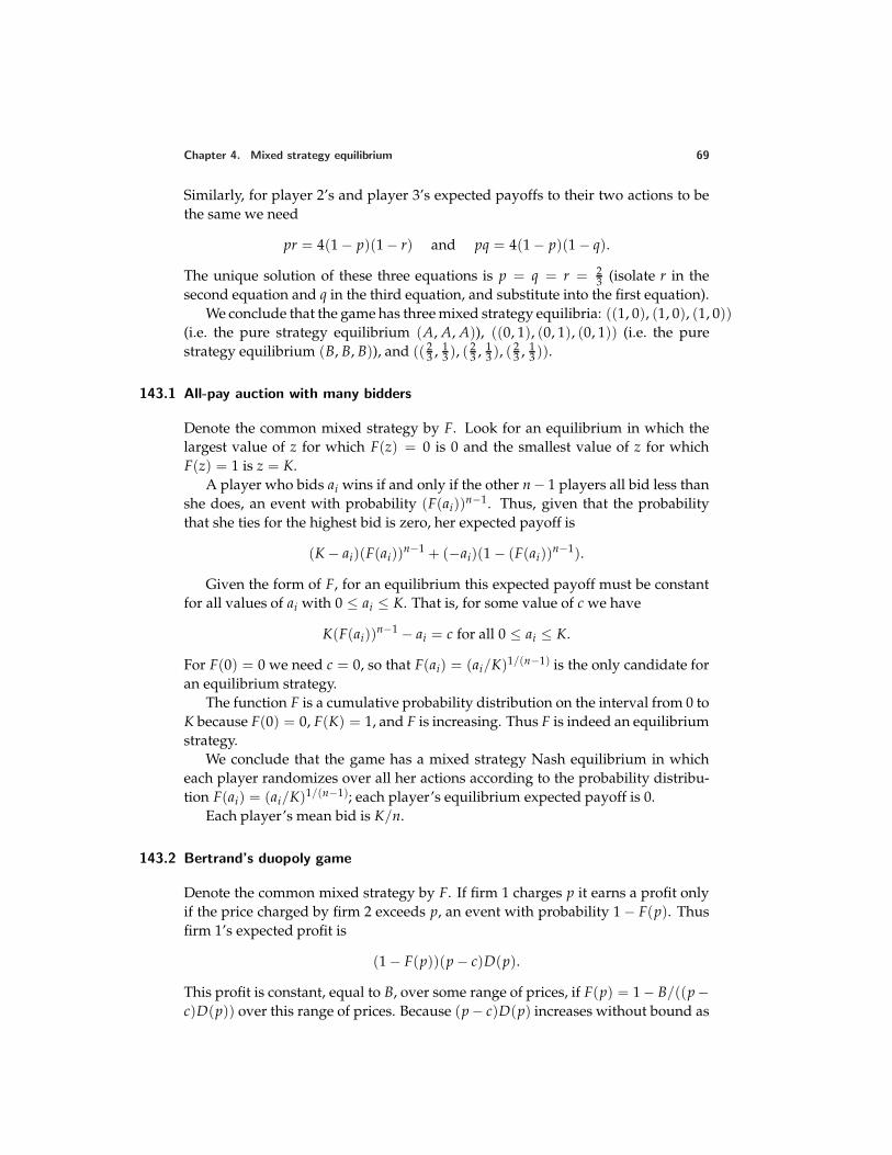
Chapter 4. Mixed strategy equilibrium 69
Similarly, for player 2’s and player 3’s expected payoffs to their two actions to bethe same we need
pr = 4(1 − p)(1 − r) and pq = 4(1 − p)(1 − q).
The unique solution of these three equations is p = q = r = 23 (isolate r in the
second equation and q in the third equation, and substitute into the first equation).We conclude that the game has three mixed strategy equilibria: ((1, 0), (1, 0), (1, 0))
(i.e. the pure strategy equilibrium (A, A, A)), ((0, 1), (0, 1), (0, 1)) (i.e. the purestrategy equilibrium (B, B, B)), and (( 2
3 , 13 ), ( 2
3 , 13 ), ( 2
3 , 13 )).
143.1 All-pay auction with many bidders
Denote the common mixed strategy by F. Look for an equilibrium in which thelargest value of z for which F(z) = 0 is 0 and the smallest value of z for whichF(z) = 1 is z = K.
A player who bids ai wins if and only if the other n − 1 players all bid less thanshe does, an event with probability (F(ai))n−1. Thus, given that the probabilitythat she ties for the highest bid is zero, her expected payoff is
(K − ai)(F(ai))n−1 + (−ai)(1 − (F(ai))
n−1).
Given the form of F, for an equilibrium this expected payoff must be constantfor all values of ai with 0 ≤ ai ≤ K. That is, for some value of c we have
K(F(ai))n−1 − ai = c for all 0 ≤ ai ≤ K.
For F(0) = 0 we need c = 0, so that F(ai) = (ai/K)1/(n−1) is the only candidate foran equilibrium strategy.
The function F is a cumulative probability distribution on the interval from 0 toK because F(0) = 0, F(K) = 1, and F is increasing. Thus F is indeed an equilibriumstrategy.
We conclude that the game has a mixed strategy Nash equilibrium in whicheach player randomizes over all her actions according to the probability distribu-tion F(ai) = (ai/K)1/(n−1); each player’s equilibrium expected payoff is 0.
Each player’s mean bid is K/n.
143.2 Bertrand’s duopoly game
Denote the common mixed strategy by F. If firm 1 charges p it earns a profit onlyif the price charged by firm 2 exceeds p, an event with probability 1 − F(p). Thusfirm 1’s expected profit is
(1 − F(p))(p − c)D(p).
This profit is constant, equal to B, over some range of prices, if F(p) = 1 − B/((p−c)D(p)) over this range of prices. Because (p − c)D(p) increases without bound as
70 Chapter 4. Mixed strategy equilibrium
p increases without bound, for any value of B the number F(p) approaches 1 as pincreases without bound. Further, for any B > 0, there exists some p > c such that(p − c)D(p) = B, so that F(p) = 0. Finally, because (p − c)D(p) is an increasingfunction, so is F. Thus F is a cumulative probability distribution function.
We conclude that for any p > c, the game has a mixed strategy equilibrium inwhich each firm’s mixed strategy is given by
F(p) =
0 if p < p
1 − (p − c)D(p)(p − c)D(p) if p ≥ p.
144.2 Preferences over lotteries
The first piece of information about the decision-maker’s preferences among lot-teries is consistent with her preferences being represented by the expected valueof a payoff function. For example, set u(a1) = 0, u(a2) = 1, and u(a3) = 1
3 (or anynumber between 1
2 and 14 ).
The second piece of information about the decision-maker’s preferences is notconsistent with these preferences being represented by the expected value of a pay-off function, by the following argument. For consistency with the informationabout the decision-maker’s preferences among the four lotteries, we need
0.4u(a1) + 0.6u(a3) > 0.5u(a2) + 0.5u(a3) >
0.3u(a1) + 0.2u(a2) + 0.5u(a3) > 0.45u(a1) + 0.55u(a3).
The first inequality implies u(a2) < 0.8u(a1) + 0.2u(a3) and the last inequality im-plies u(a2) > 0.75u(a1) + 0.25u(a3). Because u(a1) < u(a3), we have 0.75u(a1) +0.25u(a3) > 0.8u(a1) + 0.2u(a3), so that the two inequalities are incompatible.
146.2 Normalized vNM payoff functions
Let a be the best outcome according to her preferences and let a be the worse out-come. Let η = −u(a)/(u(a) − u(a)) and θ = 1/(u(a) − u(a)) > 0. Lemma 145.1implies that the function v defined by v(x) = η + θu(x) represents the same pref-erences as does u; we have v(a) = 0 and v(a) = 1.
147.1 Games equivalent to the Prisoner’s Dilemma
The left-hand game is not equivalent, by the following argument. Using eitherplayer’s payoffs, for equivalence we need η and θ > 0 such that
0 = η + θ · 0, 2 = η + θ · 1, 3 = η + θ · 2, and 4 = η + θ · 3.
From the first equation we have η = 0 and hence from the second we have θ = 2.But these values do not satisfy the last two equations. (Alternatively, note that in
Chapter 4. Mixed strategy equilibrium 71
the game in the left panel of Figure 104.1, player 1 is indifferent between (D, D)and the lottery in which (C, D) occurs with probability 1
2 and (D, C) occurs withprobability 1
2 , while in the left-hand game in Figure 148.1 she is not.)The right-hand game is equivalent, by the following argument. For the equiv-
alence of player 1’s payoffs, we need η and θ > 0 such that
0 = η + θ · 0, 3 = η + θ · 1, 6 = η + θ · 2, and 9 = η + θ · 3.
The first two equations yield η = 0 and θ = 3; these values satisfy the second twoequations. A similar argument for player 2’s payoffs yields η = −4 and θ = 2.
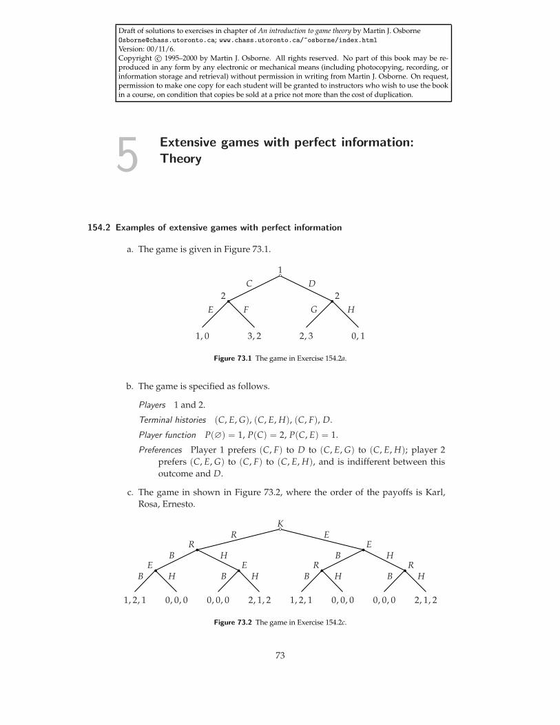
Draft of solutions to exercises in chapter of An introduction to game theory by Martin J. [email protected]; www.chass.utoronto.ca/~osborne/index.htmlVersion: 00/11/6.Copyright c© 1995–2000 by Martin J. Osborne. All rights reserved. No part of this book may be re-produced in any form by any electronic or mechanical means (including photocopying, recording, orinformation storage and retrieval) without permission in writing from Martin J. Osborne. On request,permission to make one copy for each student will be granted to instructors who wish to use the bookin a course, on condition that copies be sold at a price not more than the cost of duplication.
5 Extensive games with perfect information:Theory
154.2 Examples of extensive games with perfect information
a. The game is given in Figure 73.1.
1C D
2E F
1, 0 3, 2
2G H
2, 3 0, 1
Figure 73.1 The game in Exercise 154.2a.
b. The game is specified as follows.
Players 1 and 2.
Terminal histories (C, E, G), (C, E, H), (C, F), D.
Player function P(∅) = 1, P(C) = 2, P(C, E) = 1.
Preferences Player 1 prefers (C, F) to D to (C, E, G) to (C, E, H); player 2prefers (C, E, G) to (C, F) to (C, E, H), and is indifferent between thisoutcome and D.
c. The game in shown in Figure 73.2, where the order of the payoffs is Karl,Rosa, Ernesto.
KR E
RB H
EB H
1, 2, 1 0, 0, 0
EB H
0, 0, 0 2, 1, 2
EB H
RB H
1, 2, 1 0, 0, 0
RB H
0, 0, 0 2, 1, 2
Figure 73.2 The game in Exercise 154.2c.
73
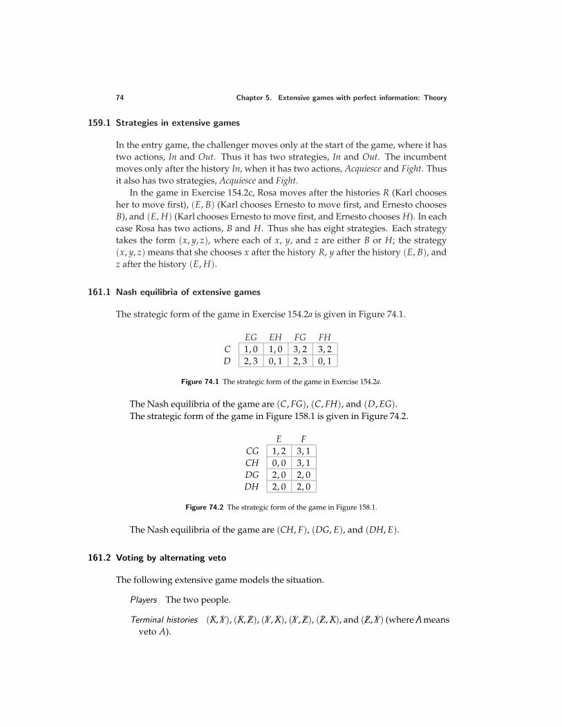
74 Chapter 5. Extensive games with perfect information: Theory
159.1 Strategies in extensive games
In the entry game, the challenger moves only at the start of the game, where it hastwo actions, In and Out. Thus it has two strategies, In and Out. The incumbentmoves only after the history In, when it has two actions, Acquiesce and Fight. Thusit also has two strategies, Acquiesce and Fight.
In the game in Exercise 154.2c, Rosa moves after the histories R (Karl choosesher to move first), (E, B) (Karl chooses Ernesto to move first, and Ernesto choosesB), and (E, H) (Karl chooses Ernesto to move first, and Ernesto chooses H). In eachcase Rosa has two actions, B and H. Thus she has eight strategies. Each strategytakes the form (x, y, z), where each of x, y, and z are either B or H; the strategy(x, y, z) means that she chooses x after the history R, y after the history (E, B), andz after the history (E, H).
161.1 Nash equilibria of extensive games
The strategic form of the game in Exercise 154.2a is given in Figure 74.1.
EG EH FG FHC 1, 0 1, 0 3, 2 3, 2D 2, 3 0, 1 2, 3 0, 1
Figure 74.1 The strategic form of the game in Exercise 154.2a.
The Nash equilibria of the game are (C, FG), (C, FH), and (D, EG).The strategic form of the game in Figure 158.1 is given in Figure 74.2.
E FCG 1, 2 3, 1CH 0, 0 3, 1DG 2, 0 2, 0DH 2, 0 2, 0
Figure 74.2 The strategic form of the game in Figure 158.1.
The Nash equilibria of the game are (CH, F), (DG, E), and (DH, E).
161.2 Voting by alternating veto
The following extensive game models the situation.
Players The two people.
Terminal histories (X/ , Y/ ), (X/ , Z/ ), (Y/ , X/ ), (Y/ , Z/ ), (Z/ , X/ ), and (Z/ , Y/ ) (where A/ meansveto A).
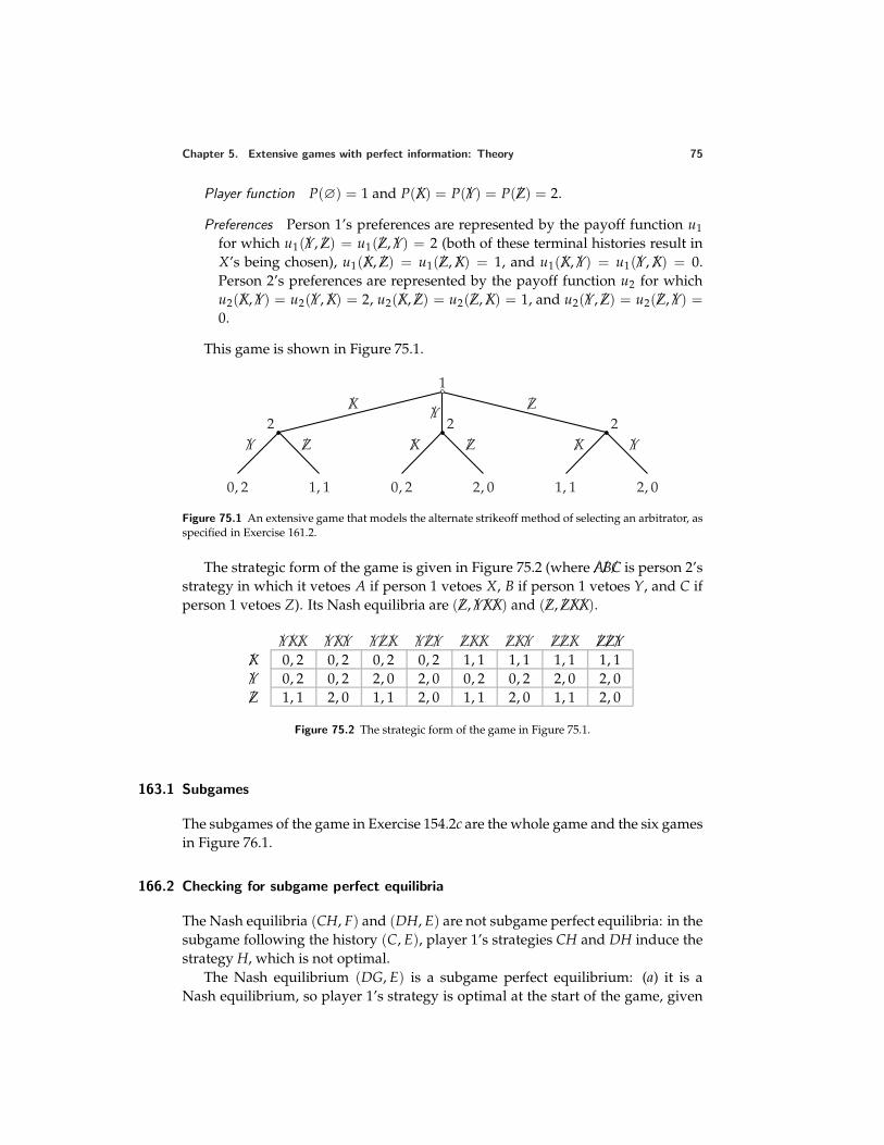
Chapter 5. Extensive games with perfect information: Theory 75
Player function P(∅) = 1 and P(X/ ) = P(Y/ ) = P(Z/ ) = 2.
Preferences Person 1’s preferences are represented by the payoff function u1for which u1(Y/ , Z/ ) = u1(Z/ , Y/ ) = 2 (both of these terminal histories result inX’s being chosen), u1(X/ , Z/ ) = u1(Z/ , X/ ) = 1, and u1(X/ , Y/ ) = u1(Y/ , X/ ) = 0.Person 2’s preferences are represented by the payoff function u2 for whichu2(X/ , Y/ ) = u2(Y/ , X/ ) = 2, u2(X/ , Z/ ) = u2(Z/ , X/ ) = 1, and u2(Y/ , Z/ ) = u2(Z/ , Y/ ) =0.
This game is shown in Figure 75.1.
1X/
Y/Z/
2Y/ Z/
0, 2 1, 1
2X/ Z/
0, 2 2, 0
2X/ Y/
1, 1 2, 0
Figure 75.1 An extensive game that models the alternate strikeoff method of selecting an arbitrator, asspecified in Exercise 161.2.
The strategic form of the game is given in Figure 75.2 (where A/ B/ C/ is person 2’sstrategy in which it vetoes A if person 1 vetoes X, B if person 1 vetoes Y, and C ifperson 1 vetoes Z). Its Nash equilibria are (Z/ , Y/ X/ X/ ) and (Z/ , Z/ X/ X/ ).
Y/ X/ X/ Y/ X/ Y/ Y/ Z/ X/ Y/ Z/ Y/ Z/ X/ X/ Z/ X/ Y/ Z/ Z/ X/ Z/ Z/ Y/X/ 0, 2 0, 2 0, 2 0, 2 1, 1 1, 1 1, 1 1, 1Y/ 0, 2 0, 2 2, 0 2, 0 0, 2 0, 2 2, 0 2, 0Z/ 1, 1 2, 0 1, 1 2, 0 1, 1 2, 0 1, 1 2, 0
Figure 75.2 The strategic form of the game in Figure 75.1.
163.1 Subgames
The subgames of the game in Exercise 154.2c are the whole game and the six gamesin Figure 76.1.
166.2 Checking for subgame perfect equilibria
The Nash equilibria (CH, F) and (DH, E) are not subgame perfect equilibria: in thesubgame following the history (C, E), player 1’s strategies CH and DH induce thestrategy H, which is not optimal.
The Nash equilibrium (DG, E) is a subgame perfect equilibrium: (a) it is aNash equilibrium, so player 1’s strategy is optimal at the start of the game, given
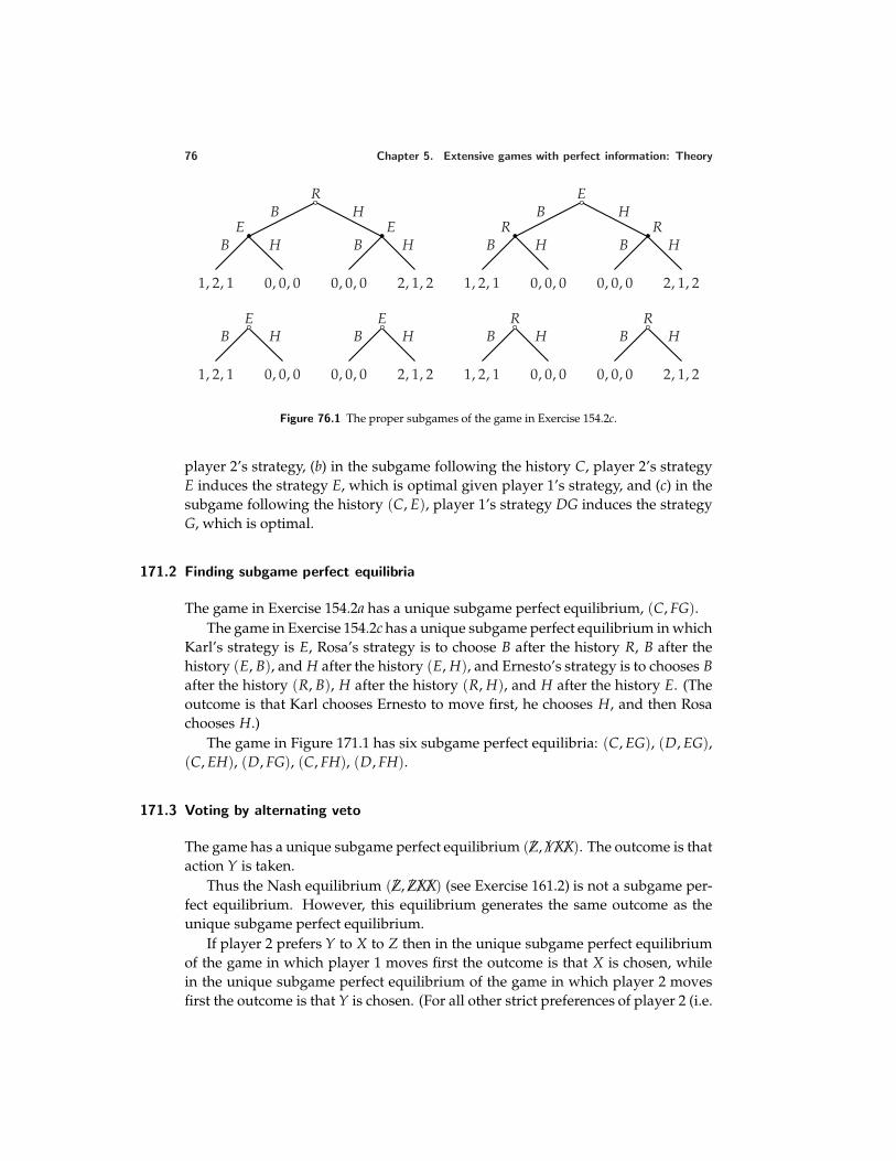
76 Chapter 5. Extensive games with perfect information: Theory
RB H
EB H
1, 2, 1 0, 0, 0
EB H
0, 0, 0 2, 1, 2
EB H
RB H
1, 2, 1 0, 0, 0
RB H
0, 0, 0 2, 1, 2
EB H
1, 2, 1 0, 0, 0
EB H
0, 0, 0 2, 1, 2
RB H
1, 2, 1 0, 0, 0
RB H
0, 0, 0 2, 1, 2
Figure 76.1 The proper subgames of the game in Exercise 154.2c.
player 2’s strategy, (b) in the subgame following the history C, player 2’s strategyE induces the strategy E, which is optimal given player 1’s strategy, and (c) in thesubgame following the history (C, E), player 1’s strategy DG induces the strategyG, which is optimal.
171.2 Finding subgame perfect equilibria
The game in Exercise 154.2a has a unique subgame perfect equilibrium, (C, FG).The game in Exercise 154.2c has a unique subgame perfect equilibrium in which
Karl’s strategy is E, Rosa’s strategy is to choose B after the history R, B after thehistory (E, B), and H after the history (E, H), and Ernesto’s strategy is to chooses Bafter the history (R, B), H after the history (R, H), and H after the history E. (Theoutcome is that Karl chooses Ernesto to move first, he chooses H, and then Rosachooses H.)
The game in Figure 171.1 has six subgame perfect equilibria: (C, EG), (D, EG),(C, EH), (D, FG), (C, FH), (D, FH).
171.3 Voting by alternating veto
The game has a unique subgame perfect equilibrium (Z/ , Y/ X/ X/ ). The outcome is thataction Y is taken.
Thus the Nash equilibrium (Z/ , Z/ X/ X/ ) (see Exercise 161.2) is not a subgame per-fect equilibrium. However, this equilibrium generates the same outcome as theunique subgame perfect equilibrium.
If player 2 prefers Y to X to Z then in the unique subgame perfect equilibriumof the game in which player 1 moves first the outcome is that X is chosen, whilein the unique subgame perfect equilibrium of the game in which player 2 movesfirst the outcome is that Y is chosen. (For all other strict preferences of player 2 (i.e.
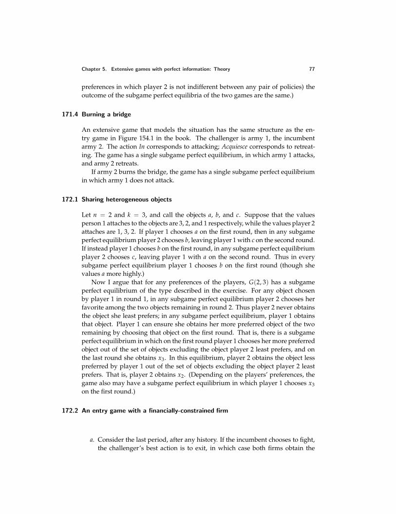
Chapter 5. Extensive games with perfect information: Theory 77
preferences in which player 2 is not indifferent between any pair of policies) theoutcome of the subgame perfect equilibria of the two games are the same.)
171.4 Burning a bridge
An extensive game that models the situation has the same structure as the en-try game in Figure 154.1 in the book. The challenger is army 1, the incumbentarmy 2. The action In corresponds to attacking; Acquiesce corresponds to retreat-ing. The game has a single subgame perfect equilibrium, in which army 1 attacks,and army 2 retreats.
If army 2 burns the bridge, the game has a single subgame perfect equilibriumin which army 1 does not attack.
172.1 Sharing heterogeneous objects
Let n = 2 and k = 3, and call the objects a, b, and c. Suppose that the valuesperson 1 attaches to the objects are 3, 2, and 1 respectively, while the values player 2attaches are 1, 3, 2. If player 1 chooses a on the first round, then in any subgameperfect equilibrium player 2 chooses b, leaving player 1 with c on the second round.If instead player 1 chooses b on the first round, in any subgame perfect equilibriumplayer 2 chooses c, leaving player 1 with a on the second round. Thus in everysubgame perfect equilibrium player 1 chooses b on the first round (though shevalues a more highly.)
Now I argue that for any preferences of the players, G(2, 3) has a subgameperfect equilibrium of the type described in the exercise. For any object chosenby player 1 in round 1, in any subgame perfect equilibrium player 2 chooses herfavorite among the two objects remaining in round 2. Thus player 2 never obtainsthe object she least prefers; in any subgame perfect equilibrium, player 1 obtainsthat object. Player 1 can ensure she obtains her more preferred object of the tworemaining by choosing that object on the first round. That is, there is a subgameperfect equilibrium in which on the first round player 1 chooses her more preferredobject out of the set of objects excluding the object player 2 least prefers, and onthe last round she obtains x3. In this equilibrium, player 2 obtains the object lesspreferred by player 1 out of the set of objects excluding the object player 2 leastprefers. That is, player 2 obtains x2. (Depending on the players’ preferences, thegame also may have a subgame perfect equilibrium in which player 1 chooses x3on the first round.)
172.2 An entry game with a financially-constrained firm
a. Consider the last period, after any history. If the incumbent chooses to fight,the challenger’s best action is to exit, in which case both firms obtain the
78 Chapter 5. Extensive games with perfect information: Theory
profit zero. If the incumbent chooses to cooperate, the challenger’s best ac-tion is to stay in, in which case both firms obtain the profit C > 0. Thus theincumbent’s best action at the start of the period is to cooperate.
Now consider period T − 1. Regardless of the outcome in this period, the in-cumbent will cooperate in the last period, and the challenger will stay in (aswe have just argued). Thus each player’s action in the period affects its pay-off only because it affects its profit in the period. Thus by the same argumentas for the last period, in period T − 1 the incumbent optimally cooperates,and the challenger optimally stays in if the incumbent cooperates. If, in pe-riod T − 1, the incumbent fights, then the challenger also optimally stays in,because in the last period it obtains C > F.
Working back to the start of the game, using the same argument in each pe-riod, we conclude that in every period before the last the incumbent cooper-ates and the challenger stays in regardless of the incumbent’s action. GivenC > f , the challenger optimally enters at the start of the game.
That is, the game has a unique subgame perfect equilibrium, in which
• the challenger enters at the start of the game, exits in the last period ifthe challenger fights in that period, and stays in after every other historyafter which it moves
• the incumbent cooperates after every history after which it moves.
The incumbent’s payoff in this equilibrium is TC and the challenger’s payoffis TC − f .
b. First consider the incumbent’s action after the history in which the challengerenters, the incumbent fights in the first T − 2 periods, and in each of theseperiods the challenger stays in. Denote this history hT−2. If the incumbentfights after hT−2, the challenger exits (it has no alternative), and the incum-bent’s profit in the last period is M. If the incumbent cooperates after hT−2then by the argument for the game in part a, the challenger stays in, and in thelast period the incumbent also cooperates and the challenger stays in. Thusthe incumbent’s payoff if it cooperates after the history hT−2 is 2C. BecauseM > 2C, we conclude that the incumbent fights after the history hT−2.
Now consider the incumbent’s action after the history in which the chal-lenger enters, the incumbent fights in the first T − 3 periods, and in eachperiod the challenger stays in. Denote this history hT−3. If the incumbentfights after hT−3, we know, by the previous paragraph, that if the challengerstays in then the incumbent will fight in the next period, driving the chal-lenger out. Thus the challenger will obtain an additional profit of −F if itstays in and 0 if it exits. Consequently the challenger exits if the incum-bent fights after hT−3, making a fight by the incumbent optimal (it yields theincumbent the additional profit 2M).
Chapter 5. Extensive games with perfect information: Theory 79
Working back to the first period we conclude that the incumbent fights andthe challenger exits. Thus the challenger’s optimal action at the start of thegame is to stay out.
In summary, the game has a unique subgame perfect equilibrium, in which
• the challenger stays out at the start of the game, exits after any historyin which the incumbent fought in every period, exits in the last periodif the incumbent fights in that period, and stays in after every otherhistory.
• the incumbent fights after the challenger enters and after any history inwhich it has fought in every period, and cooperates after every otherhistory.
The incumbent’s payoff in this equilibrium is TM and the challenger’s payoffis 0.
173.2 Dollar auction
The game is shown in Figure 80.1. It has four subgame perfect equilibria. In all theequilibria player 2 passes after player 1 bids $2. After other histories the actions inthe equilibria are as follows.
• Player 1 bids $3 after the history ($1, $2), player 2 passes after the history $1,and player 1 bids $1 at the start of the game.
• Player 1 passes after the history ($1, $2), player 2 passes after the history $1,and player 1 bids $1 at the start of the game.
• Player 1 passes after the history ($1, $2), player 2 bids $2 after the history $1,and player 1 passes at the start of the game.
• Player 1 passes after the history ($1, $2), player 2 bids $2 after the history $1,and player 1 bids $2 at the start of the game.
There are three subgame perfect equilibrium outcomes: player 1 passes at thestart of the game (player 2 gets the object without making any payment), player 1bids $1 and then player 2 passes (player 1 gets the object for $1), and player 1 bids$2 and then player 2 passes (player 1 gets the object for $2).
174.2 Firm–union bargaining
a. The following extensive game models the situation.
Players The firm and the union.
Terminal histories All sequences of the form (w, Y, L) and (w, N) for nonneg-ative numbers w and L (where w is a wage, Y means accept, N meansreject, and L is the number of workers hired).
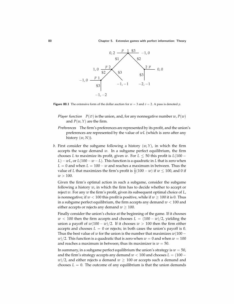
80 Chapter 5. Extensive games with perfect information: Theory
1
$1 $2
p0, 2 $3 −1, 0
2$2 $3
−1, −1
p1, 0
1p−1, 0$3
−1, −2
2
$3
p
−2, −1
0, 0
Figure 80.1 The extensive form of the dollar auction for w = 3 and v = 2. A pass is denoted p.
Player function P(∅) is the union, and, for any nonnegative number w, P(w)and P(w, Y) are the firm.
Preferences The firm’s preferences are represented by its profit, and the union’spreferences are represented by the value of wL (which is zero after anyhistory (w, N)).
b. First consider the subgame following a history (w, Y), in which the firmaccepts the wage demand w. In a subgame perfect equilibrium, the firmchooses L to maximize its profit, given w. For L ≤ 50 this profit is L(100 −L)−wL, or L(100−w− L). This function is a quadratic in L that is zero whenL = 0 and when L = 100 − w and reaches a maximum in between. Thus thevalue of L that maximizes the firm’s profit is 1
2 (100 − w) if w ≤ 100, and 0 ifw > 100.
Given the firm’s optimal action in such a subgame, consider the subgamefollowing a history w, in which the firm has to decide whether to accept orreject w. For any w the firm’s profit, given its subsequent optimal choice of L,is nonnegative; if w < 100 this profit is positive, while if w ≥ 100 it is 0. Thusin a subgame perfect equilibrium, the firm accepts any demand w < 100 andeither accepts or rejects any demand w ≥ 100.
Finally consider the union’s choice at the beginning of the game. If it choosesw < 100 then the firm accepts and chooses L = (100 − w)/2, yielding theunion a payoff of w(100 − w)/2. If it chooses w > 100 then the firm eitheraccepts and chooses L = 0 or rejects; in both cases the union’s payoff is 0.Thus the best value of w for the union is the number that maximizes w(100−w)/2. This function is a quadratic that is zero when w = 0 and when w = 100and reaches a maximum in between; thus its maximizer is w = 50.
In summary, in a subgame perfect equilibrium the union’s strategy is w = 50,and the firm’s strategy accepts any demand w < 100 and chooses L = (100−w)/2, and either rejects a demand w ≥ 100 or accepts such a demand andchooses L = 0. The outcome of any equilibrium is that the union demands
Chapter 5. Extensive games with perfect information: Theory 81
w = 50 and the firm chooses L = 25.
c. Yes. In any subgame perfect equilibrium the union’s payoff is (50)(25) =1250 and the firm’s payoff is (25)(75) − (50)(25) = 625. Thus both par-ties are better off at the outcome (w, L) than they are in the unique subgameperfect equilibrium if and only if L ≤ 50 and
wL > 1250
L(100 − L) − wL > 625
or L ≥ 50 and
wL > 1250
2500 − wL > 625.
These conditions are satisfied for a nonempty set of pairs (w, L). For example,if L = 50 the conditions are satisfied by 25 < w < 37.5; if L = 100 they aresatisfied by 12.5 < w < 18.75.
d. There are many Nash equilibria in which the firm “threatens” to reject highwage demands. In one such Nash equilibrium the firm threatens to rejectany positive wage demand. In this equilibrium the union’s strategy is w = 0,and the firm’s strategy rejects any demand w > 0, and accepts the demandw = 0 and chooses L = 50. (The union’s payoff is 0 no matter what demandit makes; given w = 0, the firm’s optimal action is L = 50.)
175.1 The “rotten kid theorem”
The situation is modeled by the following extensive game.
Players The parent and the child.
Terminal histories The set of sequences (a, t), where a (an action of the child)and t (a transfer from the parent to the child) are numbers.
Player function P(∅) is the child, P(a) is the parent for every value of a.
Preferences The child’s preferences are represented by the payoff function c(a)+t and the parent’s preferences are represented by the payoff function minp(a)−t, c(a) + t.
To find the subgame perfect equilibria of this game, first consider the parent’soptimal actions in the subgames of length 1. Consider the subgame following thechoice of a by the child. We have p(a) > c(a) (by assumption), so if the parentmakes no transfer her payoff is c(a). If she transfers $1 to the child then her payoffincreases to c(a) + 1. As she increases the transfer her payoff increases until p(a)−t = c(a) + t; that is, until t = 1
2 (p(a) − c(a)). (If she increases the transfer any
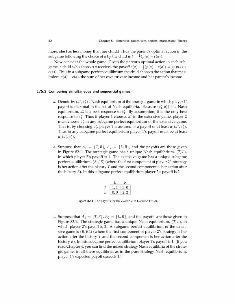
82 Chapter 5. Extensive games with perfect information: Theory
more, she has less money than her child.) Thus the parent’s optimal action in thesubgame following the choice of a by the child is t = 1
2 (p(a) − c(a)).Now consider the whole game. Given the parent’s optimal action in each sub-
game, a child who chooses a receives the payoff c(a) + 12 (p(a) − c(a)) = 1
2 (p(a) +c(a)). Thus in a subgame perfect equilibrium the child chooses the action that max-imizes p(a) + c(a), the sum of her own private income and her parent’s income.
175.2 Comparing simultaneous and sequential games
a. Denote by (a∗1, a∗2) a Nash equilibrium of the strategic game in which player 1’spayoff is maximal in the set of Nash equilibria. Because (a∗1, a∗2) is a Nashequilibrium, a∗2 is a best response to a∗1. By assumption, it is the only bestresponse to a∗1. Thus if player 1 chooses a∗1 in the extensive game, player 2must choose a∗2 in any subgame perfect equilibrium of the extensive game.That is, by choosing a∗1, player 1 is assured of a payoff of at least u1(a∗1, a∗2).Thus in any subgame perfect equilibrium player 1’s payoff must be at leastu1(a∗1, a∗2).
b. Suppose that A1 = T, B, A2 = L, R, and the payoffs are those givenin Figure 82.1. The strategic game has a unique Nash equilibrium, (T, L),in which player 2’s payoff is 1. The extensive game has a unique subgameperfect equilibrium, (B, LR) (where the first component of player 2’s strategyis her action after the history T and the second component is her action afterthe history B). In this subgame perfect equilibrium player 2’s payoff is 2.
L RT 1, 1 3, 0B 0, 0 2, 2
Figure 82.1 The payoffs for the example in Exercise 175.2a.
c. Suppose that A1 = T, B, A2 = L, R, and the payoffs are those given inFigure 83.1. The strategic game has a unique Nash equilibrium, (T, L), inwhich player 2’s payoff is 2. A subgame perfect equilibrium of the exten-sive game is (B, RL) (where the first component of player 2’s strategy is heraction after the history T and the second component is her action after thehistory B). In this subgame perfect equilibrium player 1’s payoff is 1. (If youread Chapter 4, you can find the mixed strategy Nash equilibria of the strate-gic game; in all these equilibria, as in the pure strategy Nash equilibrium,player 1’s expected payoff exceeds 1.)
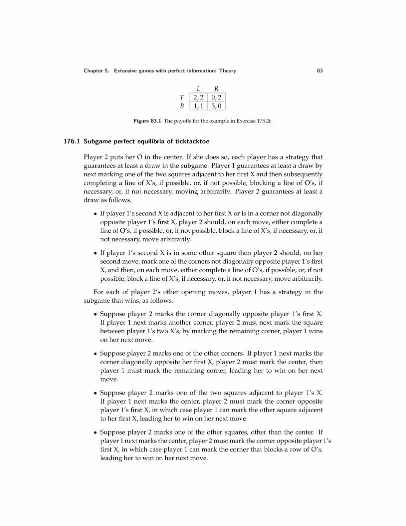
Chapter 5. Extensive games with perfect information: Theory 83
L RT 2, 2 0, 2B 1, 1 3, 0
Figure 83.1 The payoffs for the example in Exercise 175.2b.
176.1 Subgame perfect equilibria of ticktacktoe
Player 2 puts her O in the center. If she does so, each player has a strategy thatguarantees at least a draw in the subgame. Player 1 guarantees at least a draw bynext marking one of the two squares adjacent to her first X and then subsequentlycompleting a line of X’s, if possible, or, if not possible, blocking a line of O’s, ifnecessary, or, if not necessary, moving arbitrarily. Player 2 guarantees at least adraw as follows.
• If player 1’s second X is adjacent to her first X or is in a corner not diagonallyopposite player 1’s first X, player 2 should, on each move, either complete aline of O’s, if possible, or, if not possible, block a line of X’s, if necessary, or, ifnot necessary, move arbitrarily.
• If player 1’s second X is in some other square then player 2 should, on hersecond move, mark one of the corners not diagonally opposite player 1’s firstX, and then, on each move, either complete a line of O’s, if possible, or, if notpossible, block a line of X’s, if necessary, or, if not necessary, move arbitrarily.
For each of player 2’s other opening moves, player 1 has a strategy in thesubgame that wins, as follows.
• Suppose player 2 marks the corner diagonally opposite player 1’s first X.If player 1 next marks another corner, player 2 must next mark the squarebetween player 1’s two X’s; by marking the remaining corner, player 1 winson her next move.
• Suppose player 2 marks one of the other corners. If player 1 next marks thecorner diagonally opposite her first X, player 2 must mark the center, thenplayer 1 must mark the remaining corner, leading her to win on her nextmove.
• Suppose player 2 marks one of the two squares adjacent to player 1’s X.If player 1 next marks the center, player 2 must mark the corner oppositeplayer 1’s first X, in which case player 1 can mark the other square adjacentto her first X, leading her to win on her next move.
• Suppose player 2 marks one of the other squares, other than the center. Ifplayer 1 next marks the center, player 2 must mark the corner opposite player 1’sfirst X, in which case player 1 can mark the corner that blocks a row of O’s,leading her to win on her next move.
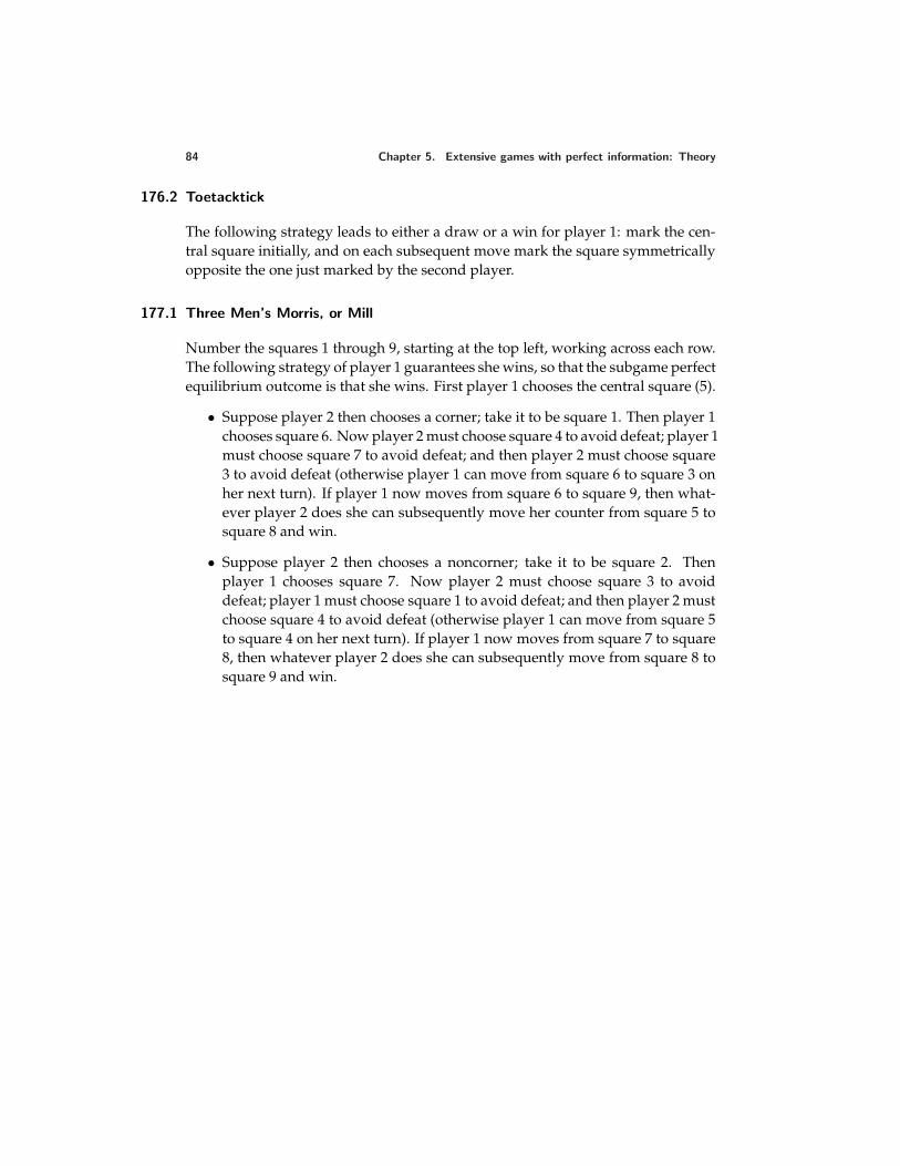
84 Chapter 5. Extensive games with perfect information: Theory
176.2 Toetacktick
The following strategy leads to either a draw or a win for player 1: mark the cen-tral square initially, and on each subsequent move mark the square symmetricallyopposite the one just marked by the second player.
177.1 Three Men’s Morris, or Mill
Number the squares 1 through 9, starting at the top left, working across each row.The following strategy of player 1 guarantees she wins, so that the subgame perfectequilibrium outcome is that she wins. First player 1 chooses the central square (5).
• Suppose player 2 then chooses a corner; take it to be square 1. Then player 1chooses square 6. Now player 2 must choose square 4 to avoid defeat; player 1must choose square 7 to avoid defeat; and then player 2 must choose square3 to avoid defeat (otherwise player 1 can move from square 6 to square 3 onher next turn). If player 1 now moves from square 6 to square 9, then what-ever player 2 does she can subsequently move her counter from square 5 tosquare 8 and win.
• Suppose player 2 then chooses a noncorner; take it to be square 2. Thenplayer 1 chooses square 7. Now player 2 must choose square 3 to avoiddefeat; player 1 must choose square 1 to avoid defeat; and then player 2 mustchoose square 4 to avoid defeat (otherwise player 1 can move from square 5to square 4 on her next turn). If player 1 now moves from square 7 to square8, then whatever player 2 does she can subsequently move from square 8 tosquare 9 and win.
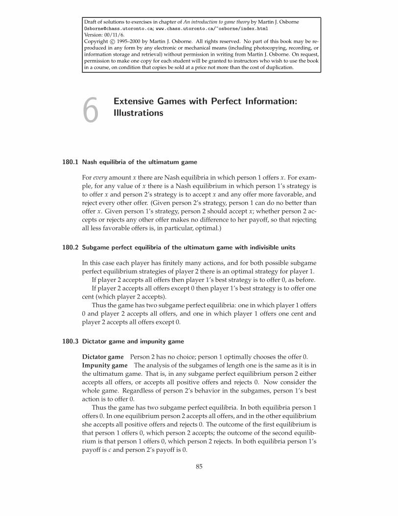
Draft of solutions to exercises in chapter of An introduction to game theory by Martin J. [email protected]; www.chass.utoronto.ca/~osborne/index.htmlVersion: 00/11/6.Copyright c© 1995–2000 by Martin J. Osborne. All rights reserved. No part of this book may be re-produced in any form by any electronic or mechanical means (including photocopying, recording, orinformation storage and retrieval) without permission in writing from Martin J. Osborne. On request,permission to make one copy for each student will be granted to instructors who wish to use the bookin a course, on condition that copies be sold at a price not more than the cost of duplication.
6 Extensive Games with Perfect Information:Illustrations
180.1 Nash equilibria of the ultimatum game
For every amount x there are Nash equilibria in which person 1 offers x. For exam-ple, for any value of x there is a Nash equilibrium in which person 1’s strategy isto offer x and person 2’s strategy is to accept x and any offer more favorable, andreject every other offer. (Given person 2’s strategy, person 1 can do no better thanoffer x. Given person 1’s strategy, person 2 should accept x; whether person 2 ac-cepts or rejects any other offer makes no difference to her payoff, so that rejectingall less favorable offers is, in particular, optimal.)
180.2 Subgame perfect equilibria of the ultimatum game with indivisible units
In this case each player has finitely many actions, and for both possible subgameperfect equilibrium strategies of player 2 there is an optimal strategy for player 1.
If player 2 accepts all offers then player 1’s best strategy is to offer 0, as before.If player 2 accepts all offers except 0 then player 1’s best strategy is to offer one
cent (which player 2 accepts).Thus the game has two subgame perfect equilibria: one in which player 1 offers
0 and player 2 accepts all offers, and one in which player 1 offers one cent andplayer 2 accepts all offers except 0.
180.3 Dictator game and impunity game
Dictator game Person 2 has no choice; person 1 optimally chooses the offer 0.Impunity game The analysis of the subgames of length one is the same as it is inthe ultimatum game. That is, in any subgame perfect equilibrium person 2 eitheraccepts all offers, or accepts all positive offers and rejects 0. Now consider thewhole game. Regardless of person 2’s behavior in the subgames, person 1’s bestaction is to offer 0.
Thus the game has two subgame perfect equilibria. In both equilibria person 1offers 0. In one equilibrium person 2 accepts all offers, and in the other equilibriumshe accepts all positive offers and rejects 0. The outcome of the first equilibrium isthat person 1 offers 0, which person 2 accepts; the outcome of the second equilib-rium is that person 1 offers 0, which person 2 rejects. In both equilibria person 1’spayoff is c and person 2’s payoff is 0.
85
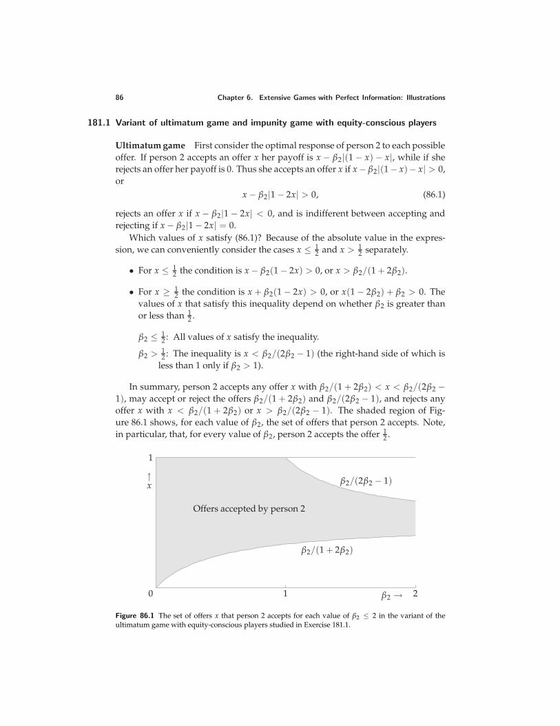
86 Chapter 6. Extensive Games with Perfect Information: Illustrations
181.1 Variant of ultimatum game and impunity game with equity-conscious players
Ultimatum game First consider the optimal response of person 2 to each possibleoffer. If person 2 accepts an offer x her payoff is x − β2|(1 − x) − x|, while if sherejects an offer her payoff is 0. Thus she accepts an offer x if x − β2|(1− x)− x| > 0,or
x − β2|1 − 2x| > 0, (86.1)
rejects an offer x if x − β2|1 − 2x| < 0, and is indifferent between accepting andrejecting if x − β2|1 − 2x| = 0.
Which values of x satisfy (86.1)? Because of the absolute value in the expres-sion, we can conveniently consider the cases x ≤ 1
2 and x > 12 separately.
• For x ≤ 12 the condition is x − β2(1 − 2x) > 0, or x > β2/(1 + 2β2).
• For x ≥ 12 the condition is x + β2(1 − 2x) > 0, or x(1 − 2β2) + β2 > 0. The
values of x that satisfy this inequality depend on whether β2 is greater thanor less than 1
2 .
β2 ≤ 12 : All values of x satisfy the inequality.
β2 > 12 : The inequality is x < β2/(2β2 − 1) (the right-hand side of which is
less than 1 only if β2 > 1).
In summary, person 2 accepts any offer x with β2/(1 + 2β2) < x < β2/(2β2 −1), may accept or reject the offers β2/(1 + 2β2) and β2/(2β2 − 1), and rejects anyoffer x with x < β2/(1 + 2β2) or x > β2/(2β2 − 1). The shaded region of Fig-ure 86.1 shows, for each value of β2, the set of offers that person 2 accepts. Note,in particular, that, for every value of β2, person 2 accepts the offer 1
2 .
1
0 1 2β2 →
↑x
Offers accepted by person 2
β2/(1 + 2β2)
β2/(2β2 − 1)
Figure 86.1 The set of offers x that person 2 accepts for each value of β2 ≤ 2 in the variant of theultimatum game with equity-conscious players studied in Exercise 181.1.
Chapter 6. Extensive Games with Perfect Information: Illustrations 87
Now consider person 1’s decision. Her payoff is 0 if her offer is rejected and1 − x − β1|(1 − x) − x| = 1 − x − β1|1 − 2x| if it is accepted. We can convenientlyseparate the analysis into three cases.
β1 < 12 : Person 1’s payoff when her offer x is accepted is positive for 0 ≤ x < 1
and is decreasing in x. Thus person 1’s optimal offer is the smallest one thatperson 2 accepts. If person 2’s strategy rejects the offer β2/(1 + 2β2), thenas in the analysis of the original game when person 2’s strategy rejects 0,person 1 has no optimal response. Thus in any subgame perfect equilibriumperson 2 accepts β2/(1 + 2β2), and person 1 offers this amount.
β1 = 12 : Person 1’s payoff to an offer that is accepted is positive and constant
from x = 0 to x = 12 , then decreasing. Thus if person 2 accepts the offer
β2/(1 + 2β2) then every offer x with β2/(1 + 2β2) ≤ x ≤ 12 is optimal, while if
person 2 rejects the offer β2/(1 + 2β2) then every offer x with β2/(1 + 2β2) <
x ≤ 12 is optimal.
β1 > 12 : Person 1’s payoff to an offer that is accepted is increasing up to x = 1
2and then decreasing, and is positive at x = 1
2 , so that her optimal offer is 12
(which person 2 accepts).
We conclude that the set of subgame perfect equilibria depends on the valuesof β1 and β2, as follows.
β1 < 12 : the set of subgame perfect equilibria is the set of all strategy pairs for
which
• person 1 offers β2/(1 + 2β2)
• person 2 accepts all offers x with β2/(1 + 2β2) ≤ x < β2/(2β2 − 1),rejects all offers x with x < β2/(1 + 2β2) or x > β2/(2β2 − 1), andeither accepts or rejects the offer β2/(2β2 − 1).
β1 = 12 : the set of subgame perfect equilibria is the set of all strategy pairs for
which
• person 1’s offer x satisfies β2/(1 + 2β2) ≤ x ≤ 12
• person 2 accepts all offers x with β2/(1 + 2β2) < x < β2/(2β2 − 1),rejects all offers x with x < β2/(1 + 2β2) or x > β2/(2β2 − 1), eitheraccepts or rejects the offer β2/(2β2 − 1), and either accepts or rejectsthe offer β2/(1 + 2β2) unless person 1 makes this offer, in which caseperson 2 definitely accepts it.
β1 > 12 : the set of subgame perfect equilibria is the set of all strategy pairs for
which
• person 1 offers 12
88 Chapter 6. Extensive Games with Perfect Information: Illustrations
• person 2 accepts all offers x with β2/(1 + 2β2) < x < β2/(2β2 − 1),rejects all offers x with x < β2/(1 + 2β2) or x > β2/(2β2 − 1), and eitheraccepts or rejects the offer β2/(2β2 − 1) and the offer β2/(1 + 2β2).
The subgame perfect equilibrium outcomes are:
β1 < 12 : person 1 offers β2/(1 + 2β2), which person 2 accepts
β1 = 12 : person 1 makes an offer x that satisfies β2/(1 + 2β2) ≤ x ≤ 1
2 , andperson 2 accepts this offer
β1 > 12 : person 1 offers 1
2 , which person 2 accepts.
In particular, in all cases the offer made by person 1 in equilibrium is accepted byperson 2.Impunity game First consider the optimal response of person 2 to each possibleoffer. If person 2 accepts an offer x her payoff is x − β2|(1 − x) − x|, while if sherejects an offer her payoff is −β2(1 − x). Thus she accepts an offer x if x − β2|(1 −x) − x| > −β2(1 − x), or
x(1 − β2) + β2(1 − |1 − 2x|) > 0, (88.1)
rejects an offer x if x(1 − β2) + β2(1 − |1 − 2x|) < 0, and is indifferent betweenaccepting and rejecting if x(1 − β2) + β2(1 − |1 − 2x|) = 0.
As before, we can conveniently consider the cases x ≤ 12 and x > 1
2 separately.
• For x ≤ 12 the condition is x(1 + β2) > 0, or x > 0.
• For x ≥ 12 the condition is x(1 − 3β2) + 2β2 > 0, which is satisfied by all
values of x if β2 ≤ 13 , and for all x with x < 2β2/(3β2 − 1) if β2 > 1
3 .
In summary, person 2 accepts any offer x with 0 < x < 2β2/(3β2 − 1), mayaccept or reject the offers 0 and 2β2/(3β2 − 1), and rejects any offer x with x >
2β2/(3β2 − 1).Now consider person 1. If she offers x, her payoff is
1 − x − β1|1 − 2x| if person 1 accepts x1 − x − β1(1 − x) if person 1 rejects x.
If β1 < 12 then in both cases person 1’s payoff is decreasing in x; for x = 0 the
payoffs are equal. Thus, given person 2’s optimal strategy, in any subgame perfectequilibrium person 1’s optimal offer is 0, which person 2 may accept or reject.
If β1 = 12 then person 1’s payoff when person 2 accepts x is constant from 0 to
12 , then decreases. Her payoff when person 2 rejects x is decreasing in x, and thetwo payoffs are equal when x = 0. Thus the optimal offers of person 1 are 0, whichperson 2 may accept or reject, and any x with 0 < x ≤ 1
2 , which person 2 accepts.If β1 > 1
2 then person 1’s highest payoff is obtained when x = 12 , which
person 2 accepts. Thus x = 12 is her optimal offer.
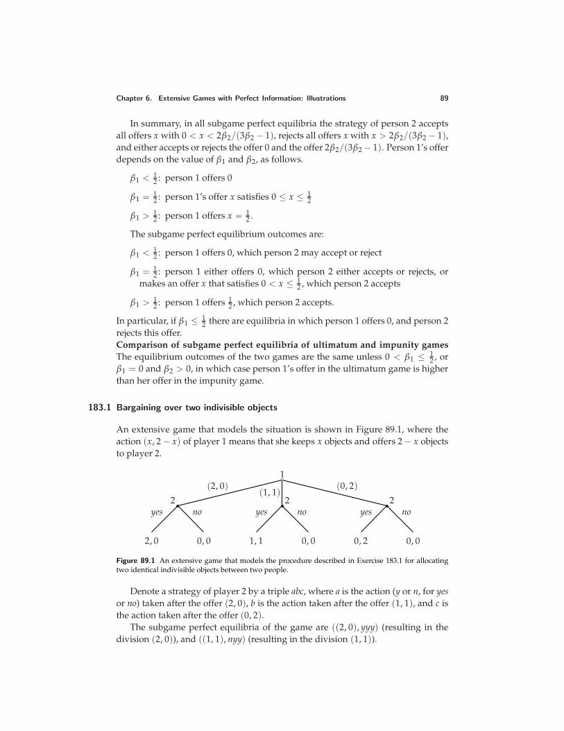
Chapter 6. Extensive Games with Perfect Information: Illustrations 89
In summary, in all subgame perfect equilibria the strategy of person 2 acceptsall offers x with 0 < x < 2β2/(3β2 − 1), rejects all offers x with x > 2β2/(3β2 − 1),and either accepts or rejects the offer 0 and the offer 2β2/(3β2 − 1). Person 1’s offerdepends on the value of β1 and β2, as follows.
β1 < 12 : person 1 offers 0
β1 = 12 : person 1’s offer x satisfies 0 ≤ x ≤ 1
2
β1 > 12 : person 1 offers x = 1
2 .
The subgame perfect equilibrium outcomes are:
β1 < 12 : person 1 offers 0, which person 2 may accept or reject
β1 = 12 : person 1 either offers 0, which person 2 either accepts or rejects, or
makes an offer x that satisfies 0 < x ≤ 12 , which person 2 accepts
β1 > 12 : person 1 offers 1
2 , which person 2 accepts.
In particular, if β1 ≤ 12 there are equilibria in which person 1 offers 0, and person 2
rejects this offer.Comparison of subgame perfect equilibria of ultimatum and impunity gamesThe equilibrium outcomes of the two games are the same unless 0 < β1 ≤ 1
2 , orβ1 = 0 and β2 > 0, in which case person 1’s offer in the ultimatum game is higherthan her offer in the impunity game.
183.1 Bargaining over two indivisible objects
An extensive game that models the situation is shown in Figure 89.1, where theaction (x, 2 − x) of player 1 means that she keeps x objects and offers 2 − x objectsto player 2.
1(2, 0)
(1, 1)(0, 2)
2yes no
2, 0 0, 0
2yes no
1, 1 0, 0
2yes no
0, 2 0, 0
Figure 89.1 An extensive game that models the procedure described in Exercise 183.1 for allocatingtwo identical indivisible objects between two people.
Denote a strategy of player 2 by a triple abc, where a is the action (y or n, for yesor no) taken after the offer (2, 0), b is the action taken after the offer (1, 1), and c isthe action taken after the offer (0, 2).
The subgame perfect equilibria of the game are ((2, 0), yyy) (resulting in thedivision (2, 0)), and ((1, 1), nyy) (resulting in the division (1, 1)).
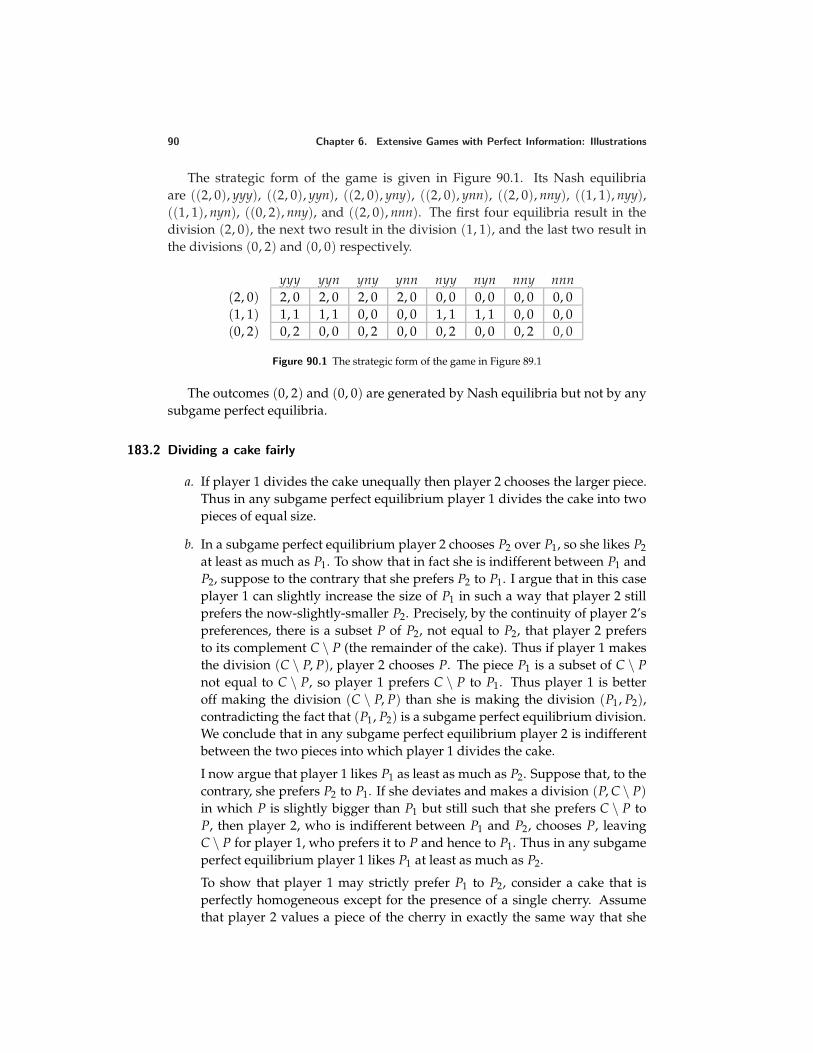
90 Chapter 6. Extensive Games with Perfect Information: Illustrations
The strategic form of the game is given in Figure 90.1. Its Nash equilibriaare ((2, 0), yyy), ((2, 0), yyn), ((2, 0), yny), ((2, 0), ynn), ((2, 0), nny), ((1, 1), nyy),((1, 1), nyn), ((0, 2), nny), and ((2, 0), nnn). The first four equilibria result in thedivision (2, 0), the next two result in the division (1, 1), and the last two result inthe divisions (0, 2) and (0, 0) respectively.
yyy yyn yny ynn nyy nyn nny nnn(2, 0) 2, 0 2, 0 2, 0 2, 0 0, 0 0, 0 0, 0 0, 0(1, 1) 1, 1 1, 1 0, 0 0, 0 1, 1 1, 1 0, 0 0, 0(0, 2) 0, 2 0, 0 0, 2 0, 0 0, 2 0, 0 0, 2 0, 0
Figure 90.1 The strategic form of the game in Figure 89.1
The outcomes (0, 2) and (0, 0) are generated by Nash equilibria but not by anysubgame perfect equilibria.
183.2 Dividing a cake fairly
a. If player 1 divides the cake unequally then player 2 chooses the larger piece.Thus in any subgame perfect equilibrium player 1 divides the cake into twopieces of equal size.
b. In a subgame perfect equilibrium player 2 chooses P2 over P1, so she likes P2at least as much as P1. To show that in fact she is indifferent between P1 andP2, suppose to the contrary that she prefers P2 to P1. I argue that in this caseplayer 1 can slightly increase the size of P1 in such a way that player 2 stillprefers the now-slightly-smaller P2. Precisely, by the continuity of player 2’spreferences, there is a subset P of P2, not equal to P2, that player 2 prefersto its complement C \ P (the remainder of the cake). Thus if player 1 makesthe division (C \ P, P), player 2 chooses P. The piece P1 is a subset of C \ Pnot equal to C \ P, so player 1 prefers C \ P to P1. Thus player 1 is betteroff making the division (C \ P, P) than she is making the division (P1, P2),contradicting the fact that (P1, P2) is a subgame perfect equilibrium division.We conclude that in any subgame perfect equilibrium player 2 is indifferentbetween the two pieces into which player 1 divides the cake.
I now argue that player 1 likes P1 as least as much as P2. Suppose that, to thecontrary, she prefers P2 to P1. If she deviates and makes a division (P, C \ P)in which P is slightly bigger than P1 but still such that she prefers C \ P toP, then player 2, who is indifferent between P1 and P2, chooses P, leavingC \ P for player 1, who prefers it to P and hence to P1. Thus in any subgameperfect equilibrium player 1 likes P1 at least as much as P2.
To show that player 1 may strictly prefer P1 to P2, consider a cake that isperfectly homogeneous except for the presence of a single cherry. Assumethat player 2 values a piece of the cherry in exactly the same way that she
Chapter 6. Extensive Games with Perfect Information: Illustrations 91
values a piece of the cake of the same size, while player 1 prefers a piece ofthe cherry to a piece of the cake of the same size. Then there is a subgameperfect equilibrium in which player 1 divides the cake equally, with one piececontaining all of the cherry, and player 2 chooses the piece without the cherry.(In this equilibrium, as in all equilibria, player 2 is indifferent between thetwo pieces—but note that there is no subgame perfect equilibrium in whichshe chooses the piece with the cherry in it. A strategy pair in which she actsin this way is not an equilibrium, because player 1 can deviate and increaseslightly the size of the cherryless piece of cake, inducing player 2 to choosethat piece.)
183.3 Holdup game
The game is defined as follows.
Players Two people, person 1 and person 2.
Terminal histories The set of all sequences (low, x, Z), where x is a number with0 ≤ x ≤ cL (the amount of money that person 1 offers to person 2 when thepie is small), and (high, x, Z), where x is a number with 0 ≤ x ≤ cH (theamount of money that person 1 offers to person 2 when the pie is large) andZ is either Y (“yes, I accept”) or N (“no, I reject”).
Player function P(∅) = 2, P(low) = P(high) = 1, and P(low, x) = P(high, x) =2 for all x.
Preferences Person 1’s preferences are represented by payoffs equal to the amountsof money she receives, equal to cL − x for any terminal history (low, x, Y)with 0 ≤ x ≤ cL, equal to cH − x for any terminal history (high, x, Y) with0 ≤ x ≤ cH , and equal to 0 for any terminal history (low, x, N) with 0 ≤x ≤ cL and for any terminal history (high, x, N) with 0 ≤ x ≤ cH . Person 2’spreferences are represented by payoffs equal to x − L for the terminal history(low, x, Y), x − H for the terminal history (high, x, Y), −L for the terminalhistory (low, x, N), and −H for the terminal history (high, x, N).
186.1 Stackelberg’s duopoly game with quadratic costs
From Exercise 57.2, the best response function of firm 2 is the function b2 definedby
b2(q1) = 1
4 (α − q1) if q1 ≤ α
0 if q1 > α.
Firm 1’s subgame perfect equilibrium strategy is the value of q1 that maxi-mizes q1(α − q1 − b2(q1)) − q2
1, or q1(α − q1 − 14 (α − q1)) − q2
1, or 14 q1(3α − 7q1).
The maximizer is q1 = 314 α.
92 Chapter 6. Extensive Games with Perfect Information: Illustrations
We conclude that the game has a unique subgame perfect equilibrium, in whichfirm 1’s strategy is the output 3
14 α and firm 2’s strategy is its best response functionb2.
The outcome of the subgame perfect equilibrium is that firm 1 produces q∗1 =3
14 α units of output and firm 2 produces q∗2 = b2( 314 α) = 11
56 α units. In a Nashequilibrium of Cournot’s (simultaneous-move) game each firm produces 1
5 α (seeExercise 57.2). Thus firm 1 produces more in the subgame perfect equilibrium ofthe sequential game than it does in the Nash equilibrium of Cournot’s game, andfirm 2 produces less.
188.1 Stackelberg’s duopoly game with fixed costs
We have f < (α − c)2/16 ( f = 4; (α − c)2/16 = 9), so the best response function offirm 2 takes the form shown in Figure 24.1 (in the solution to Exercise 57.3). To de-termine the subgame perfect equilibrium we need to compare firm 1’s profit whenit produces q = 8 units of output, so that firm 2 produces 0, with its profit when itproduces the output that maximizes its profit on the positive part of firm 2’s bestresponse function.
If firm 1 produces 8 units of output and firm 2 produces 0, firm 1’s profit is8(12 − 8) = 32. Firm 1’s best output on the positive part of firm 2’s best responsefunction is 1
2 (α − c) = 6. If it produces this output then firm 2 produces 12 (α − c −
q1) = 12 (12 − 6) = 3, and firm 1’s profit is 6(12 − 9) = 18. Thus firm 1’s profit is
higher when it produces enough to induce firm 2 to produce zero. We concludethat the game has a unique subgame perfect equilibrium, in which firm 1’s strategyis to produce 8 units, and firm 2’s strategy is to produce 1
2 (α − c − q1) = 12 (12− q1)
units if firm 1 produces q1 < 8 and 0 if firm 1 produces q1 ≥ 8 units.
189.1 Sequential variant of Bertrand’s duopoly game
a. Players The two firms.
Terminal histories The set of all sequences (p1, p2) of prices (where each piis a nonnegative number).
Player function P(∅) = 1 and P(p1) = 2 for all p1.
Preferences The payoff of each firm i to the terminal history (p1, p2) is itsprofit
(pi − c)D(pi) if pi < pj12 (pi − c)D(pi) if pi = pj0 if pi > pj,
where j is the other firm.
b. A strategy of firm 1 is a price (e.g. the price c). A strategy of firm 2 isa function that associates a price with every price chosen by firm 1 (e.g.
Chapter 6. Extensive Games with Perfect Information: Illustrations 93
s2(p1) = p1 − 1, the strategy in which firm 2 always charges 1 cent less thanfirm 1).
c. First consider firm 2’s best responses to each price p1 chosen by firm 1.
• If p1 < c, any price greater than p1 is a best response for firm 2.
• If p1 = c, any price at least equal to c is a best response for firm 2.
• If p1 = c + 1, firm 2’s unique best response is to set the same price.
• If p1 > c + 1, firm 2’s unique best response is to set the price minpm, p1 −1 (where pm is the monopoly price).
Now consider the optimal action of firm 1. Given firm 2’s best responses,
• if p1 < c, firm 1’s profit is positive
• if p1 = c, firm 1’s profit is zero
• if p1 = c + 1, firm 1’s profit is positive
• if p1 > c + 1, firm 1’s profit is zero.
Thus the only price p1 for which there is a best response of firm 2 that leadsto a positive profit for firm 1 is c + 1.
We conclude that in every subgame perfect equilibrium firm 1’s strategy isp1 = c + 1, and firm 2’s strategy assigns to each price chosen by firm 1 oneof its best responses, so that firm 2’s strategy takes the form
s2(p1) =
k(p1) if p1 < ck′ if p1 = cc + 1 if p1 = c + 1minpm, p1 − 1 if p1 > c + 1
where k(p1) > p1 for all p1 and k′ ≥ c.
The outcome of every subgame perfect equilibrium is that both firms choosethe price c + 1.
193.1 Three interest groups buying votes
a. Consider the possibility of a subgame perfect equilibrium in which bill Xpasses. In any such equilibrium, groups Y and Z make no payments. Butnow given that Y makes no payments and that VX = VZ, group Z can matchX’s payments to the two legislators to whom X’s payments are smallest, andgain the passage of bill Z. Thus there is no subgame perfect equilibriumin which bill X passes. Similarly there is no subgame perfect equilibrium inwhich bill Y passes. Thus in every subgame perfect equilibrium bill Z passes.
94 Chapter 6. Extensive Games with Perfect Information: Illustrations
b. By making payments of more than 50 to each legislator, group X ensures thatneither group Y nor group Z can profitably buy the passage of its favorite bill.(In any subgame perfect equilibrium, group X’s payments to each legislatorare exactly 50.) Thus in every subgame perfect equilibrium the outcome isthat bill X is passed.
c. For any payments of group X that sum to at most 300, group Y can makepayments that are (i) at least as high to at least two legislators and (ii) highenough that group Z cannot buy off more than one legislator. (Take thetwo legislators to whom group X pays the least. Let them be legislators 1and 2, and denote group X’s payments x1 and x2; suppose that x1 ≥ x2.Group Y pays x1 + 1 to legislator 1 and 200 − x1 to legislator 2.) Thus inevery subgame perfect equilibrium the outcome is that bill Y is passed.
193.2 Interest groups buying votes under supermajority rule
a. However group X allocates payments summing to 700, group Y can buy offfive legislators for at most 500. Thus in any subgame perfect equilibriumneither group makes any payment, and bill Y is passed.
b. If group X pays each legislator 80 then group Y is indifferent between buyingoff five legislators, in which case bill Y is passed, and in making no payments,in which case bill X is passed. If group Y makes no payments then X is se-lected, and group X is better off than it is if it makes no payments. There isno subgame perfect equilibrium in which group Y buys off five legislators,because if it were to do so group X could pay each legislator slightly morethan 80 to ensure the passage of bill X. Thus in every subgame perfect equi-librium group X pays each legislator 80, group Y makes no payments, andbill X is passed.
c. If only a simple majority is required to pass a bill, in case a the outcome undermajority rule is the same as it is when five votes are required.
In case b, group X needs to pay each legislator 100 in order to prevent group Yfrom winning. If it does so, its total payments are less than VX , so doing sois optimal. Thus in this case the payment to each legislator is higher undermajority rule.
193.3 Sequential positioning by two political candidates
The following extensive game models the situation.
Players The candidates.
Terminal histories The set of all sequences (x1, . . . , xn), where xi is a positionof candidate i (a number) for i = 1, . . . , n.
Chapter 6. Extensive Games with Perfect Information: Illustrations 95
Player function P(∅) = 1, P(x1) = 2 for all x1, P(x1, x2) = 3 for all (x1, x2),. . . , P(x1, . . . , xn−1) = n for all (x1, . . . , xn−1).
Preferences Each candidate’s preferences are represented by a payoff functionthat assigns n to every terminal history in which she wins outright, k to ev-ery terminal history in which she ties for first place with n − k other candi-dates, for 1 ≤ k ≤ n − 1, and 0 to every terminal history in which she loses,where positions attract votes as in Hotelling’s model of electoral competition(Section 3.3).
This game has a finite horizon, so we may use backward induction to find itssubgame perfect equilibria. Suppose there are two candidates. First consider can-didate 2’s best response to each strategy of candidate 1. Suppose candidate 1’sstrategy is m. Then candidate 2 loses if she chooses any position different from mand ties with candidate 1 if she chooses m. Thus candidate 2’s best response to mis m. Now suppose candidate 1’s strategy is x1 = m. Then candidate 2 wins if shechooses any position between x1 and 2m − x1; thus every such position is a bestresponse.
Given candidate 2’s best responses, the best strategy for candidate 1 is m, lead-ing to a tie. (Every other strategy of candidate 1 leads her to lose.)
We conclude that in every subgame perfect equilibrium candidate 1’s strat-egy is m; candidate 2’s strategy chooses m after the history m and some positionbetween x1 and 2m − x1 after any other history x1.
193.4 Sequential positioning by three political candidates
The following extensive game models the situation.
Players The candidates.
Terminal histories The set of all sequences (x1, . . . , xn), where xi is either Outor a position of candidate i (a number) for i = 1, . . . , n.
Player function P(∅) = 1, P(x1) = 2 for all x1, P(x1, x2) = 3 for all (x1, x2),. . . , P(x1, . . . , xn−1) = n for all (x1, . . . , xn−1).
Preferences Each candidate’s preferences are represented by a payoff functionthat assigns n to every terminal history in which she wins, k to every terminalhistory in which she ties for first place with n − k other candidates, for 1 ≤k ≤ n − 1, 0 to every terminal history in which she stays out, and −1 toevery terminal history in which she loses, where positions attract votes as inHotelling’s model of electoral competition (Section 3.3).
When there are two candidates the analysis of the subgame perfect equilibriais similar to that in the previous exercise. In every subgame perfect equilibriumcandidate 1’s strategy is m; candidate 2’s strategy chooses m after the history m,
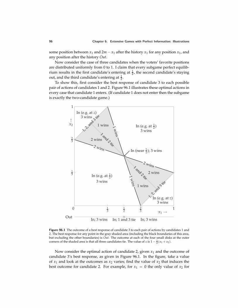
96 Chapter 6. Extensive Games with Perfect Information: Illustrations
some position between x1 and 2m − x1 after the history x1 for any position x1, andany position after the history Out.
Now consider the case of three candidates when the voters’ favorite positionsare distributed uniformly from 0 to 1. I claim that every subgame perfect equilib-rium results in the first candidate’s entering at 1
2 , the second candidate’s stayingout, and the third candidate’s entering at 1
2 .To show this, first consider the best response of candidate 3 to each possible
pair of actions of candidates 1 and 2. Figure 96.1 illustrates these optimal actions inevery case that candidate 1 enters. (If candidate 1 does not enter then the subgameis exactly the two-candidate game.)
23
23
12
13
13 In (e.g. at 1
2 )3 wins
In (e.g. at 12 )
3 wins
In (e.g. at z)3 wins
In (e.g. at z)3 wins
In (near 12 ); 3 wins
1,2,
and
3 tie
1,2,
and 3 tie
2 wins
1 wins
1 and2 tie
1 wins
2 wins
1 and 2 tie
2 wins
2 wins
1w
ins
1w
ins
0
1
1x1 →
↑x2
OutIn; 3 wins In; 1 and 3 tie In; 3 wins
Figure 96.1 The outcome of a best response of candidate 3 to each pair of actions by candidates 1 and2. The best response for any point in the gray shaded area (including the black boundaries of this area,but excluding the other boundaries) is Out. The outcome at each of the four small disks at the outercorners of the shaded area is that all three candidates tie. The value of z is 1 − 1
2 (x1 + x2).
Now consider the optimal action of candidate 2, given x1 and the outcome ofcandidate 3’s best response, as given in Figure 96.1. In the figure, take a valueof x1 and look at the outcomes as x2 varies; find the value of x2 that induces thebest outcome for candidate 2. For example, for x1 = 0 the only value of x2 for
Chapter 6. Extensive Games with Perfect Information: Illustrations 97
which candidate 2 does not lose is 23 , at which point she ties with the other two
candidates. Thus when candidate 1’s strategy is x1 = 0, candidate 2’s best action,given candidate 3’s best response, is x2 = 2
3 , which leads to a three-way tie. Wefind that the outcome of the optimal value of x2, for each value of x1, is given asfollows.
1, 2, and 3 tie (x2 = 23 ) if x1 = 0
2 wins if 0 < x1 < 12
1 and 3 tie (2 stays out) if x1 = 12
2 wins if 12 < x1 < 1
1, 2, and 3 tie (x2 = 13 ) if x1 = 1.
Finally, consider candidate 1’s best strategy, given the responses of candidates 2and 3. If she stays out then candidates 2 and 3 enter at m and tie. If she enters thenthe best position at which to do so is x1 = 1
2 , where she ties with candidate 3. (Forevery other position she either loses or ties with both of the other candidates.)
We conclude that in every subgame perfect equilibrium the outcome is thatcandidate 1 enters at 1
2 , candidate 2 stays out, and candidate 3 enters at 12 . (There
are many subgame perfect equilibria, because after many histories candidate 3’soptimal action is not unique.)
(If you’re interested in what may happen when there are many potential candi-dates, look at http://www.economics.utoronto.ca/osborne/research/CONJECT.HTM.)
195.1 The race G1(2, 2)
The consequences of player 1’s actions at the start of the game are as follows.
Take two steps: Player 1 wins.
Take one step: Go to the game G2(1, 2), in which player 2 initially takes twosteps and wins.
Do not move: If player 2 does not move, the game ends. If she takes one stepwe go to the game G1(2, 1), in which player 1 takes two steps and wins. If shetakes two steps, she wins. Thus in a subgame perfect equilibrium player 2takes two steps, and wins.
We conclude that in a subgame perfect equilibrium of G1(2, 2) player 1 initiallytakes two steps, and wins.
198.1 A race in which the players’ valuations of the prize differ
By the arguments in the text for the case in which both players’ valuations of theprize are between 6 and 7, the subgame perfect equilibrium outcomes of all gamesin which k1 ≤ 2 or k2 ≤ 3 are the same as they are when both players’ valuations ofthe prize are between 6 and 7. If k2 ≥ 5 then player 1 is the winner in all subgame
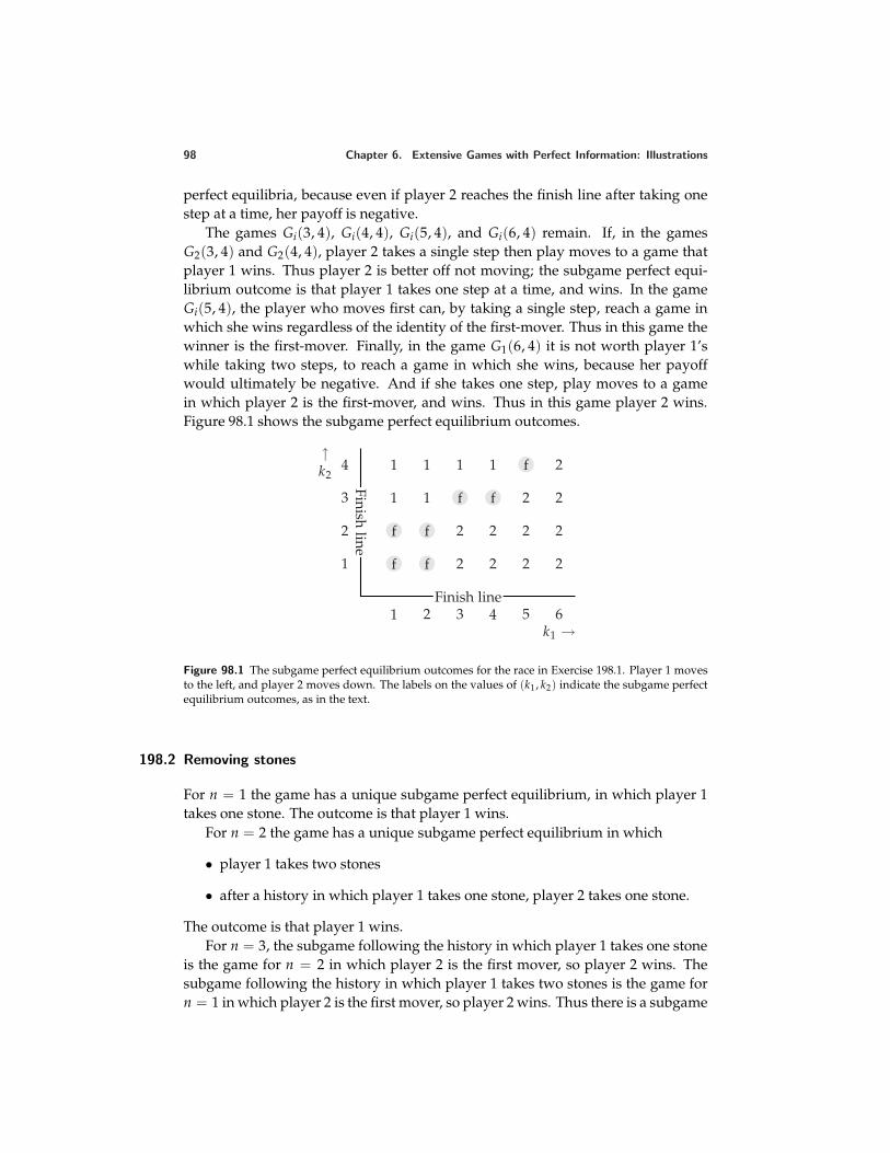
98 Chapter 6. Extensive Games with Perfect Information: Illustrations
perfect equilibria, because even if player 2 reaches the finish line after taking onestep at a time, her payoff is negative.
The games Gi(3, 4), Gi(4, 4), Gi(5, 4), and Gi(6, 4) remain. If, in the gamesG2(3, 4) and G2(4, 4), player 2 takes a single step then play moves to a game thatplayer 1 wins. Thus player 2 is better off not moving; the subgame perfect equi-librium outcome is that player 1 takes one step at a time, and wins. In the gameGi(5, 4), the player who moves first can, by taking a single step, reach a game inwhich she wins regardless of the identity of the first-mover. Thus in this game thewinner is the first-mover. Finally, in the game G1(6, 4) it is not worth player 1’swhile taking two steps, to reach a game in which she wins, because her payoffwould ultimately be negative. And if she takes one step, play moves to a gamein which player 2 is the first-mover, and wins. Thus in this game player 2 wins.Figure 98.1 shows the subgame perfect equilibrium outcomes.
f f
f f
f f
f
2 2 2 2
2 2 2 2
2 2
2
1 1
1 1 1 1
Finish line
Finishline
k1 →1 2 3 4 5 6
1
2
3
4↑k2
Figure 98.1 The subgame perfect equilibrium outcomes for the race in Exercise 198.1. Player 1 movesto the left, and player 2 moves down. The labels on the values of (k1, k2) indicate the subgame perfectequilibrium outcomes, as in the text.
198.2 Removing stones
For n = 1 the game has a unique subgame perfect equilibrium, in which player 1takes one stone. The outcome is that player 1 wins.
For n = 2 the game has a unique subgame perfect equilibrium in which
• player 1 takes two stones
• after a history in which player 1 takes one stone, player 2 takes one stone.
The outcome is that player 1 wins.For n = 3, the subgame following the history in which player 1 takes one stone
is the game for n = 2 in which player 2 is the first mover, so player 2 wins. Thesubgame following the history in which player 1 takes two stones is the game forn = 1 in which player 2 is the first mover, so player 2 wins. Thus there is a subgame
Chapter 6. Extensive Games with Perfect Information: Illustrations 99
perfect equilibrium in which player 1 takes one stone initially, and one in whichshe takes two stones initially. In both subgame perfect equilibria player 2 wins.
For n = 4, the subgame following the history in which player 1 takes one stoneis the game for n = 3 in which player 2 is the first-mover, so player 1 wins. Thesubgame following the history in which player 1 takes two stones is the game forn = 2 in which player 2 is the first-mover, so player 2 wins. Thus in every subgameperfect equilibrium player 1 takes one stone initially, and wins.
Continuing this argument for larger values of n, we see that if n is a multipleof 3 then in every subgame perfect equilibrium player 2 wins, while if n is not amultiple of 3 then in every subgame perfect equilibrium player 1 wins. We canprove this claim by induction on n. The claim is correct for n = 1, 2, and 3, by thearguments above. Now suppose it is correct for all integers through n − 1. I willargue that it is correct for n.
First suppose that n is divisible by 3. The subgames following player 1’s re-moval of one or two stones are the games for n − 1 and n − 2 in which player 2 isthe first-mover. Neither n − 1 nor n − 2 is divisible by 3, so by hypothesis player 2is the winner in every subgame perfect equilibrium of both of these subgames.Thus player 2 is the winner in every subgame perfect equilibrium of the wholegame.
Now suppose that n is not divisible by 3. As before, the subgames followingplayer 1’s removal of one or two stones are the games for n − 1 and n − 2 in whichplayer 2 is the first-mover. Either n − 1 or n − 2 is divisible by 3, so in one ofthese subgames player 1 is the winner in every subgame perfect equilibrium. Thusplayer 1 is the winner in every subgame perfect equilibrium of the whole game.
199.1 Hungry lions
Denote by G(n) the game in which there are n lions.The game G(1) has a unique subgame perfect equilibrium, in which the single
lion eats the prey.Consider the game G(2). If lion 1 does not eat, it remains hungry. If it eats, we
reach a subgame identical to G(1), which we know has a unique subgame perfectequilibrium, in which lion 2 eats lion 1. Thus G(2) has a unique subgame perfectequilibrium, in which lion 1 does not eat the prey.
In G(3), lion 1’s eating the prey leads to G(2), in which we have just concludedthat the first mover (lion 2) does not eat the prey (lion 1). Thus G(3) has a uniquesubgame perfect equilibrium, in which lion 1 eats the prey.
For an arbitrary value of n, lion 1’s eating the prey in G(n) leads to G(n − 1).If G(n − 1) has a unique subgame perfect equilibrium, in which the prey is eaten,then G(n) has a unique subgame perfect equilibrium, in which the prey is noteaten; if G(n − 1) has a unique subgame perfect equilibrium, in which the prey isnot eaten, then G(n) has a unique subgame perfect equilibrium, in which the preyis eaten. Given that G(1) has a unique subgame perfect equilibrium, in which the
100 Chapter 6. Extensive Games with Perfect Information: Illustrations
prey is eaten, we conclude that if n is odd then G(n) has a unique subgame perfectequilibrium, in which lion 1 eats the prey, and if n is even it has a unique subgameperfect equilibrium, in which lion 1 does not eat the prey.
200.1 A race with a liquidity constraint
In the absence of the constraint, player 1 initially takes one step. Suppose she doesso in the game with the constraint. Consider player 2’s options after player 1’smove.
Player 2 takes two steps: Because of the liquidity constraint, player 1 can takeat most one step. If she takes one step, player 2’s optimal action is to take onestep, and win. Thus player 1’s best action is not to move; player 2’s payoffexceeds 1 (her steps cost 5, and the prize is worth more than 6).
Player 2 moves one step: Again because of the liquidity constraint, player 1can take at most one step. If she takes one step, player 2 can take two stepsand win, obtaining a payoff of more than 1 (as in the previous case).
Player 2 does not move: Player 1, as before, can take one step on each turn, andwin; player 2’s payoff is 0.
We conclude that after player 1 moves one step, player 2 should take eitherone or two steps, and ultimately win; player 1’s payoff is −1. A better option forplayer 1 is not to move, in which case player 2 can move one step at a time, andwin; player 1’s payoff is zero.
Thus the subgame perfect equilibrium outcome is that player 1 does not move,and player 2 takes one step at a time and wins.
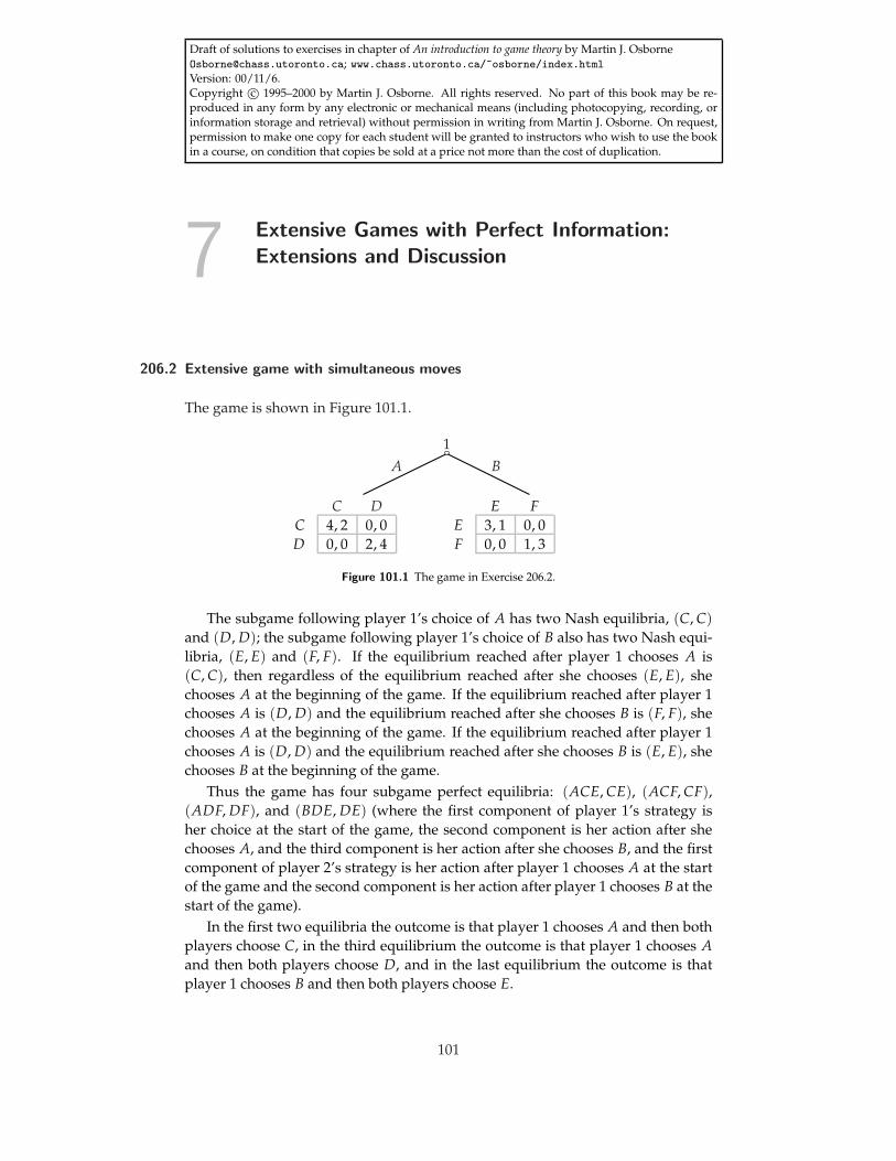
Draft of solutions to exercises in chapter of An introduction to game theory by Martin J. [email protected]; www.chass.utoronto.ca/~osborne/index.htmlVersion: 00/11/6.Copyright c© 1995–2000 by Martin J. Osborne. All rights reserved. No part of this book may be re-produced in any form by any electronic or mechanical means (including photocopying, recording, orinformation storage and retrieval) without permission in writing from Martin J. Osborne. On request,permission to make one copy for each student will be granted to instructors who wish to use the bookin a course, on condition that copies be sold at a price not more than the cost of duplication.
7 Extensive Games with Perfect Information:Extensions and Discussion
206.2 Extensive game with simultaneous moves
The game is shown in Figure 101.1.
1A B
C DC 4, 2 0, 0D 0, 0 2, 4
E FE 3, 1 0, 0F 0, 0 1, 3
Figure 101.1 The game in Exercise 206.2.
The subgame following player 1’s choice of A has two Nash equilibria, (C, C)and (D, D); the subgame following player 1’s choice of B also has two Nash equi-libria, (E, E) and (F, F). If the equilibrium reached after player 1 chooses A is(C, C), then regardless of the equilibrium reached after she chooses (E, E), shechooses A at the beginning of the game. If the equilibrium reached after player 1chooses A is (D, D) and the equilibrium reached after she chooses B is (F, F), shechooses A at the beginning of the game. If the equilibrium reached after player 1chooses A is (D, D) and the equilibrium reached after she chooses B is (E, E), shechooses B at the beginning of the game.
Thus the game has four subgame perfect equilibria: (ACE, CE), (ACF, CF),(ADF, DF), and (BDE, DE) (where the first component of player 1’s strategy isher choice at the start of the game, the second component is her action after shechooses A, and the third component is her action after she chooses B, and the firstcomponent of player 2’s strategy is her action after player 1 chooses A at the startof the game and the second component is her action after player 1 chooses B at thestart of the game).
In the first two equilibria the outcome is that player 1 chooses A and then bothplayers choose C, in the third equilibrium the outcome is that player 1 chooses Aand then both players choose D, and in the last equilibrium the outcome is thatplayer 1 chooses B and then both players choose E.
101
102 Chapter 7. Extensive Games with Perfect Information: Extensions and Discussion
206.3 Two-period Prisoner’s Dilemma
The extensive game is specified as follows.
Players The two people.
Terminal histories The set of pairs ((W, X), (Y, Z)), where each component iseither Q or F.
Player function P(∅) = 1, 2 and P(W, X) = 1, 2 for any pair (W, X) inwhich both W and X are either Q or F.
Actions The set Ai(∅) of player i’s actions at the initial history is Q, F, fori = 1, 2; the set Ai(W, X) of player i’s actions after any history (W, X) inwhich both W and X are either Q or F is Q, F, for i = 1, 2.
Preferences Each player’s preferences are represented by the payoffs describedin the problem.
Consider the subgame following some history (W, X) (where W and X are botheither Q or F). In this subgame each player chooses either Q or F, and her payoff toeach resulting terminal history is the sum of her payoff to (W, X) in the Prisoner’sDilemma given in Figure 13.1 and her payoff to the pair of actions chosen in thesubgame, again as in the Prisoner’s Dilemma. Thus the subgame differs from thePrisoner’s Dilemma given in Figure 13.1 only in that every payoff to a given playeris increased by her payoff to the pair of actions (W, X). Thus the subgame has aunique Nash equilibrium, in which both players choose F.
Now consider the whole game. Regardless of the actions chosen at the startof the game, the outcome in the second period is (F, F). Thus the payoffs to thepairs of actions chosen in the first period are the payoffs in the Prisoner’s Dilemmaplus the payoff to (F, F). We conclude that the game has a unique subgame perfectequilibrium, in which each player chooses F after every history.
207.1 Timing claims on an investment
The following extensive game models the situation.
Players The two people.
Terminal histories The sequences of the form ((N, N), (N, N), . . . , (N, N), xt),where 1 ≤ t ≤ T, xt is (C, C), (C, N), or (N, C) if t ≤ T − 1 and (C, C),(C, N), (N, C), or (N, N) if t = T, C means “claim”, and N means “do notclaim”.
Player function The set of players assigned to every nonterminal history is1, 2 (the two people).
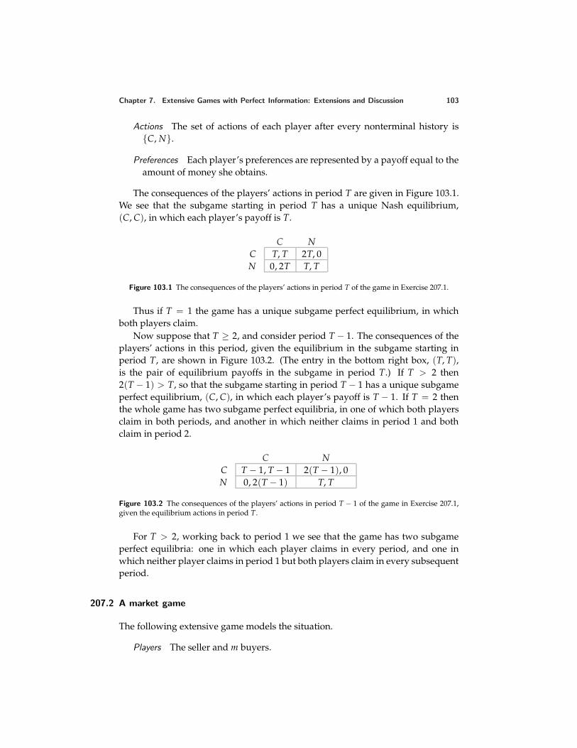
Chapter 7. Extensive Games with Perfect Information: Extensions and Discussion 103
Actions The set of actions of each player after every nonterminal history isC, N.
Preferences Each player’s preferences are represented by a payoff equal to theamount of money she obtains.
The consequences of the players’ actions in period T are given in Figure 103.1.We see that the subgame starting in period T has a unique Nash equilibrium,(C, C), in which each player’s payoff is T.
C NC T, T 2T, 0N 0, 2T T, T
Figure 103.1 The consequences of the players’ actions in period T of the game in Exercise 207.1.
Thus if T = 1 the game has a unique subgame perfect equilibrium, in whichboth players claim.
Now suppose that T ≥ 2, and consider period T − 1. The consequences of theplayers’ actions in this period, given the equilibrium in the subgame starting inperiod T, are shown in Figure 103.2. (The entry in the bottom right box, (T, T),is the pair of equilibrium payoffs in the subgame in period T.) If T > 2 then2(T − 1) > T, so that the subgame starting in period T − 1 has a unique subgameperfect equilibrium, (C, C), in which each player’s payoff is T − 1. If T = 2 thenthe whole game has two subgame perfect equilibria, in one of which both playersclaim in both periods, and another in which neither claims in period 1 and bothclaim in period 2.
C NC T − 1, T − 1 2(T − 1), 0N 0, 2(T − 1) T, T
Figure 103.2 The consequences of the players’ actions in period T − 1 of the game in Exercise 207.1,given the equilibrium actions in period T.
For T > 2, working back to period 1 we see that the game has two subgameperfect equilibria: one in which each player claims in every period, and one inwhich neither player claims in period 1 but both players claim in every subsequentperiod.
207.2 A market game
The following extensive game models the situation.
Players The seller and m buyers.
104 Chapter 7. Extensive Games with Perfect Information: Extensions and Discussion
Terminal histories The set of sequences of the form ((p1, . . . , pm), j), where eachpi is a price (nonnegative number) and j is either 0 or one of the sellers (aninteger from 1 to m), with the interpretation that pi is the offer of buyer i,j = 0 means that the seller accepts no offer, and j ≥ 1 means that the selleraccepts buyer j’s offer.
Player function P(∅) is the set of buyers and P(p1, . . . , pm) is the seller forevery history (p1, . . . , pm).
Actions The set Ai(∅) of actions of buyer i at the start of the game is the set ofprices (nonnegative numbers). The set As(p1, . . . , pm) of actions of the sellerafter the buyers have made offers is the set of integers from 0 to m.
Preferences Each player’s preferences are represented by the payoffs given inthe question.
To find the subgame perfect equilibria of the game, first consider the subgamefollowing a history (p1, . . . , pm) of offers. The seller’s best action is to accept thehighest price, or one of the highest prices in the case of a tie.
I claim that a strategy profile is a subgame perfect equilibrium of the wholegame if and only if the seller’s strategy is the one just described, and among thebuyers’ strategies (p1, . . . , pm), every offer pi is at most v and at least two offers areequal to v.
Such a strategy profile is a subgame perfect equilibrium by the following ar-gument. If the buyer with whom the seller trades raises her offer then her payoffbecomes negative, while if she lowers her offer she no longer trades and her payoffremains zero. If any other buyer raises her offer then either she still does not trade,or she trades at a price greater than v and hence receives a negative payoff.
No other profile of actions for the buyers at the start of the game is part of asubgame perfect equilibrium by the following argument.
• If some offer exceeds v then the buyer who submits the highest offer caninduce a better outcome by reducing her offer to a value below v, so thateither the seller does not trade with her, or, if the seller does trade with her,she trades at a lower price.
• If all offers are at most v and only one is equal to v, the buyer who offers vcan increase her payoff by reducing her offer a little.
• If all offers are less than v then one of the buyers whose offer is not acceptedcan increase her offer to some value between the winning offer and v, inducethe seller to trade with her, and obtain a positive payoff.
In any equilibrium the buyer who trades with the seller does so at the price v.Thus her payoff is zero. The other buyers do not trade, and hence also obtain thepayoff of zero.
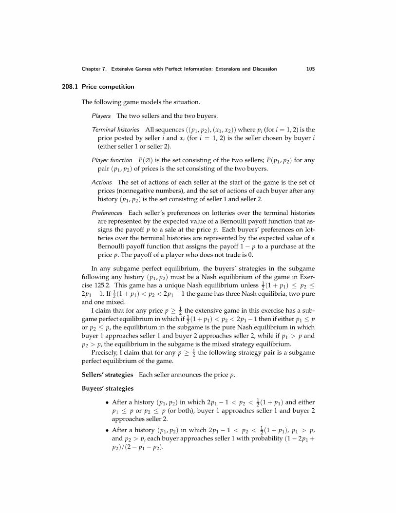
Chapter 7. Extensive Games with Perfect Information: Extensions and Discussion 105
208.1 Price competition
The following game models the situation.
Players The two sellers and the two buyers.
Terminal histories All sequences ((p1, p2), (x1, x2)) where pi (for i = 1, 2) is theprice posted by seller i and xi (for i = 1, 2) is the seller chosen by buyer i(either seller 1 or seller 2).
Player function P(∅) is the set consisting of the two sellers; P(p1, p2) for anypair (p1, p2) of prices is the set consisting of the two buyers.
Actions The set of actions of each seller at the start of the game is the set ofprices (nonnegative numbers), and the set of actions of each buyer after anyhistory (p1, p2) is the set consisting of seller 1 and seller 2.
Preferences Each seller’s preferences on lotteries over the terminal historiesare represented by the expected value of a Bernoulli payoff function that as-signs the payoff p to a sale at the price p. Each buyers’ preferences on lot-teries over the terminal histories are represented by the expected value of aBernoulli payoff function that assigns the payoff 1 − p to a purchase at theprice p. The payoff of a player who does not trade is 0.
In any subgame perfect equilibrium, the buyers’ strategies in the subgamefollowing any history (p1, p2) must be a Nash equilibrium of the game in Exer-cise 125.2. This game has a unique Nash equilibrium unless 1
2 (1 + p1) ≤ p2 ≤2p1 − 1. If 1
2 (1 + p1) < p2 < 2p1 − 1 the game has three Nash equilibria, two pureand one mixed.
I claim that for any price p ≥ 12 the extensive game in this exercise has a sub-
game perfect equilibrium in which if 12 (1 + p1) < p2 < 2p1 − 1 then if either p1 ≤ p
or p2 ≤ p, the equilibrium in the subgame is the pure Nash equilibrium in whichbuyer 1 approaches seller 1 and buyer 2 approaches seller 2, while if p1 > p andp2 > p, the equilibrium in the subgame is the mixed strategy equilibrium.
Precisely, I claim that for any p ≥ 12 the following strategy pair is a subgame
perfect equilibrium of the game.
Sellers’ strategies Each seller announces the price p.
Buyers’ strategies
• After a history (p1, p2) in which 2p1 − 1 < p2 < 12 (1 + p1) and either
p1 ≤ p or p2 ≤ p (or both), buyer 1 approaches seller 1 and buyer 2approaches seller 2.
• After a history (p1, p2) in which 2p1 − 1 < p2 < 12 (1 + p1), p1 > p,
and p2 > p, each buyer approaches seller 1 with probability (1 − 2p1 +p2)/(2 − p1 − p2).
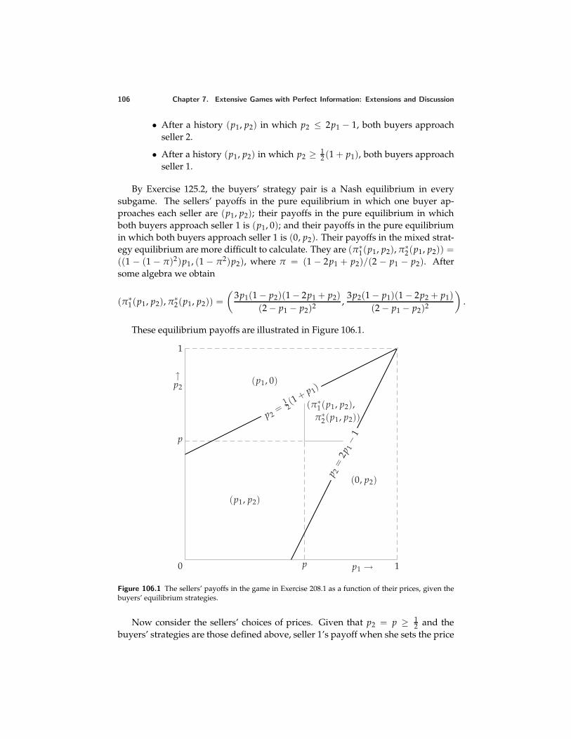
106 Chapter 7. Extensive Games with Perfect Information: Extensions and Discussion
• After a history (p1, p2) in which p2 ≤ 2p1 − 1, both buyers approachseller 2.
• After a history (p1, p2) in which p2 ≥ 12 (1 + p1), both buyers approach
seller 1.
By Exercise 125.2, the buyers’ strategy pair is a Nash equilibrium in everysubgame. The sellers’ payoffs in the pure equilibrium in which one buyer ap-proaches each seller are (p1, p2); their payoffs in the pure equilibrium in whichboth buyers approach seller 1 is (p1, 0); and their payoffs in the pure equilibriumin which both buyers approach seller 1 is (0, p2). Their payoffs in the mixed strat-egy equilibrium are more difficult to calculate. They are (π∗
1(p1, p2), π∗2(p1, p2)) =
((1 − (1 − π)2)p1, (1 − π2)p2), where π = (1 − 2p1 + p2)/(2 − p1 − p2). Aftersome algebra we obtain
(π∗1(p1, p2), π∗
2(p1, p2)) =(
3p1(1 − p2)(1 − 2p1 + p2)(2 − p1 − p2)2 ,
3p2(1 − p1)(1 − 2p2 + p1)(2 − p1 − p2)2
).
These equilibrium payoffs are illustrated in Figure 106.1.
p
p
0
1
1p1 →
↑p2
(p1, 0)
(0, p2)
(π∗1(p1, p2),
π∗2(p1, p2))
(p1, p2)
p 2=
2p1− 1
p 2=
12(1 + p 1)
Figure 106.1 The sellers’ payoffs in the game in Exercise 208.1 as a function of their prices, given thebuyers’ equilibrium strategies.
Now consider the sellers’ choices of prices. Given that p2 = p ≥ 12 and the
buyers’ strategies are those defined above, seller 1’s payoff when she sets the price
Chapter 7. Extensive Games with Perfect Information: Extensions and Discussion 107
p1 is
p1 if p1 ≤ pπ∗
1(p1, p) if p < p1 ≤ 12 (1 + p)
0 if p > 12 (1 + p).
By the claim in the question (verified at the end of this solution), π∗1(p1, p2) is
decreasing in p1 for p1 ≥ p2, so that seller 1’s best response to p is p. An analogousargument shows that seller 2’s best response to p is p.
We conclude that the strategy pair defined above is a subgame perfect equilib-rium.
The verification of the last claim of the question (not required as part of ananswer) follows. We have
π∗1(p1, p2) =
3p1(1 − p2)(1 − 2p1 + p2)(2 − p1 − p2)2 .
The derivative of this function with respect to p1 is
3(1 − p2)[(2 − p1 − p2)2(1 − 2p1 + p2 − 2p1) + 2(2 − p1 − p2)p1(1 − 2p1 + p2)
](2 − p1 − p2)4
or
3(1 − p2)(2 − p1 − p2) [(2 − p1 − p2)(1 − 4p1 + p2) + 2p1(1 − 2p1 + p2)](2 − p1 − p2)4 .
This expression is negative if
(2 − p1 − p2)(1 − 4p1 + p2) + 2p1(1 − 2p1 + p2) < 0,
or
p1 >(2 − p2)(1 + p2)
7 − 5p2.
The right-hand side is less than p2 if
(2p2 − 1)(p2 − 1) < 0,
which is true if 12 < p2 < 1, so that seller 1’s equilibrium payoff is decreasing in p1
whenever p1 > p2 > 12 .
210.1 Bertrand’s duopoly game with entry
The unique Nash equilibrium of the subgame that follows the challenger’s entryis (c, c), as we found in Section 3.2.2. The challenger’s profit is − f < 0 in thisequilibrium. By choosing to stay out the challenger obtains the profit of 0, so inany subgame perfect equilibrium the challenger stays out. After the history inwhich the challenger stays out, the incumbent chooses its price p1 to maximize itsprofit (p1 − c)(α − p1).
Thus for any value of f > 0 the whole game has a unique subgame perfectequilibrium, in which the strategies are:
108 Chapter 7. Extensive Games with Perfect Information: Extensions and Discussion
Challenger
• at the start of the game: stay out
• after the history in which the challenger enters: choose the price c
Incumbent
• after the history in which the challenger enters: choose the price c
• after the history in which the challenger stays out: choose the price p1that maximizes (p1 − c)(α − p1).
212.1 Electoral competition with strategic voters
Consider the strategy profile in which each candidate chooses the median m of thecitizens’ favorite positions and the citizens’ strategies are defined as follows.
• After a history in which every candidate chooses m, each citizen i votes forcandidate j, where j is the smallest integer greater than or equal to in/q. (Thatis, the citizens split their votes equally among the n candidates. If there are 3candidates and 15 citizens, for example, citizens 1 through 5 vote for candi-date 1, citizens 6 through 10 vote for candidate 2, and citizens 11 through 15vote for candidate 3.)
• After a history in which all candidates enter and every candidate but j choosesm, each citizen votes for candidate j if her favorite position is closer to j’s po-sition than it is to m, and for some candidate whose position is m otherwise.(All citizens who do not vote for j vote for the same candidate .)
• After any other history, the citizens’ action profile is any Nash equilibrium ofthe voting subgame in which no citizen’s action is weakly dominated.
The outcome induced by this strategy profile is that all candidates enter andchoose the median of the citizens’ favorite positions, and tie for first place. Afterevery history of one of the first two types, every citizen votes for one of the candi-dates who is closest to her favorite position, so no citizen’s strategy is weakly dom-inated. After a history of the third type, no citizen’s strategy is weakly dominatedby construction.
The strategy profile is a subgame perfect equilibrium by the following argu-ment.
In each voting subgame the citizens’ strategy profile is a Nash equilibrium:
• after the history in which the candidates’ positions are the same, equal to m,no citizen’s vote affects the outcome
• after a history in which all candidates enter and every candidate but j choosesm, a change in any citizen’s vote either has no effect on the outcome or makesit worse for her
Chapter 7. Extensive Games with Perfect Information: Extensions and Discussion 109
• after any other history the citizens’ strategy profile is a Nash equilibrium byconstruction.
Now consider the candidates’ choices at the start of the game. If any candidatedeviates by choosing a position different from that of the other candidates, sheloses, rather than tying for first place. If any candidate deviates by staying out ofthe race, the outcome is worse for her than adhering to the equilibrium, and tyingfor first place. Thus each candidate’s strategy is optimal given the other players’strategies.
[The claim that every voting subgame has a (pure) Nash equilibrium in whichno citizen’s action is weakly dominated, which you are not asked to prove, may bedemonstrated as follows. Given the candidates’ positions, choose the candidate,say j, ranked last by the smallest number of citizens. Suppose that all citizensexcept those who rank j last vote for j; distribute the votes of the citizens whorank j last as equally as possible among the other candidates. Each citizen’s actionis not weakly dominated (no citizen votes for the candidate she ranks last) and,given q ≥ 2n, no change in any citizen’s vote affects the outcome, so that the list ofcitizens’ actions is a Nash equilibrium of the voting subgame.]
213.1 Electoral competition with strategic voters
I first argue that in any equilibrium each candidate that enters is in the set of win-ners. If some candidate that enters is not a winner, she can increase her payoff bydeviating to Out.
Now consider the voting subgame in which there are more than two candidatesand not all candidates’ positions are the same. Suppose that the citizens’ votes areequally divided among the candidates. I argue that this list of citizens’ strategiesis not a Nash equilibrium of the voting subgame.
For either the citizen whose favorite position is 0 or the citizen whose favoriteposition is 1 (or both), at least two candidates’ positions are better than the positionof the candidate furthest from the citizen’s favorite position. Denote a citizen forwhom this condition holds by i. (The claim that citizen i exists is immediate if thecandidates occupy at least three distinct positions, or they occupy two distinct po-sitions and at least two candidates occupy each position. If the candidates occupyonly two positions and one position is occupied by a single candidate, then takethe citizen whose favorite position is 0 if the lone candidate’s position exceeds theother candidates’ position; otherwise take the citizen whose favorite position is 1.)
Now, given that each candidate obtains the same number of votes, if citizen iswitches her vote to one of the candidates whose position is better for her thanthat of the candidate whose position is furthest from her favorite position, thenthis candidate wins outright. (If citizen i originally votes for one of these superiorcandidates, she can switch her vote to the other superior candidate; if she originallyvotes for neither of the superior candidates, she can switch her vote to either one
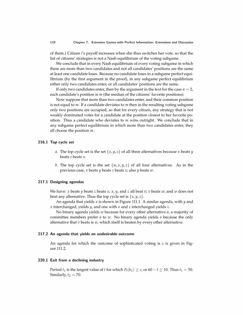
110 Chapter 7. Extensive Games with Perfect Information: Extensions and Discussion
of them.) Citizen i’s payoff increases when she thus switches her vote, so that thelist of citizens’ strategies is not a Nash equilibrium of the voting subgame.
We conclude that in every Nash equilibrium of every voting subgame in whichthere are more than two candidates and not all candidates’ positions are the sameat least one candidate loses. Because no candidate loses in a subgame perfect equi-librium (by the first argument in the proof), in any subgame perfect equilibriumeither only two candidates enter, or all candidates’ positions are the same.
If only two candidates enter, then by the argument in the text for the case n = 2,each candidate’s position is m (the median of the citizens’ favorite positions).
Now suppose that more than two candidates enter, and their common positionis not equal to m. If a candidate deviates to m then in the resulting voting subgameonly two positions are occupied, so that for every citizen, any strategy that is notweakly dominated votes for a candidate at the position closest to her favorite po-sition. Thus a candidate who deviates to m wins outright. We conclude that inany subgame perfect equilibrium in which more than two candidates enter, theyall choose the position m.
216.1 Top cycle set
a. The top cycle set is the set x, y, z of all three alternatives because x beats ybeats z beats x.
b. The top cycle set is the set w, x, y, z of all four alternatives. As in theprevious case, x beats y beats z beats x; also y beats w.
217.1 Designing agendas
We have: x beats y beats z beats x; x, y, and z all beat v; v beats w; and w does notbeat any alternative. Thus the top cycle set is x, y, z.
An agenda that yields x is shown in Figure 111.1. A similar agenda, with y andx interchanged, yields y, and one with x and z interchanged yields z.
No binary agenda yields w because for every other alternative a, a majority ofcommittee members prefer a to w. No binary agenda yields v because the onlyalternative that v beats is w, which itself is beaten by every other alternative.
217.2 An agenda that yields an undesirable outcome
An agenda for which the outcome of sophisticated voting is z is given in Fig-ure 111.2.
220.1 Exit from a declining industry
Period t1 is the largest value of t for which Pt(k1) ≥ c, or 60 − t ≥ 10. Thus t1 = 50.Similarly, t2 = 70.
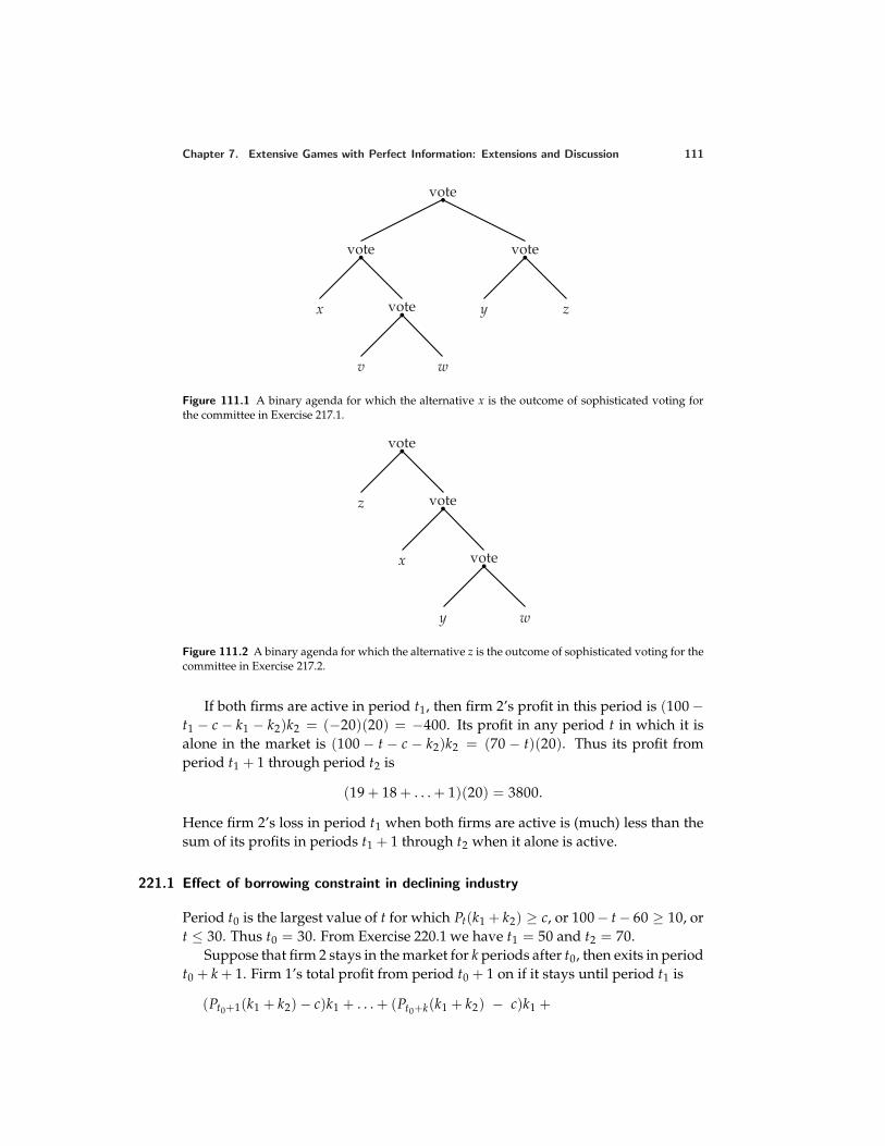
Chapter 7. Extensive Games with Perfect Information: Extensions and Discussion 111
vote
vote
x vote
v w
vote
y z
Figure 111.1 A binary agenda for which the alternative x is the outcome of sophisticated voting forthe committee in Exercise 217.1.
vote
z vote
x vote
y w
Figure 111.2 A binary agenda for which the alternative z is the outcome of sophisticated voting for thecommittee in Exercise 217.2.
If both firms are active in period t1, then firm 2’s profit in this period is (100 −t1 − c − k1 − k2)k2 = (−20)(20) = −400. Its profit in any period t in which it isalone in the market is (100 − t − c − k2)k2 = (70 − t)(20). Thus its profit fromperiod t1 + 1 through period t2 is
(19 + 18 + . . . + 1)(20) = 3800.
Hence firm 2’s loss in period t1 when both firms are active is (much) less than thesum of its profits in periods t1 + 1 through t2 when it alone is active.
221.1 Effect of borrowing constraint in declining industry
Period t0 is the largest value of t for which Pt(k1 + k2) ≥ c, or 100 − t − 60 ≥ 10, ort ≤ 30. Thus t0 = 30. From Exercise 220.1 we have t1 = 50 and t2 = 70.
Suppose that firm 2 stays in the market for k periods after t0, then exits in periodt0 + k + 1. Firm 1’s total profit from period t0 + 1 on if it stays until period t1 is
(Pt0+1(k1 + k2) − c)k1 + . . . + (Pt0+k(k1 + k2) − c)k1 +
112 Chapter 7. Extensive Games with Perfect Information: Extensions and Discussion
(Pt0+k+1(k1) − c)k1 + . . . + (Pt1(k1) − c)k1,
or
40[(100 − 30 − 1 − 60 − 10) + . . . + (100 − 30 − k − 60 − 10) +
(100 − 30 − k − 1 − 40 − 10) + . . . + (100 − 50 − 40 − 10)],
or40[−1 − . . . − k + (19 − k) + . . . + 0],
or40[− 1
2 k(k + 1) + 12 (19 − k)(20 − k)]
(using the fact that the sum of the first n positive integers is 12 n(n + 1)), or
20(380 − 40k).
In order that this profit be nonpositive we need 40k ≥ 380, or k ≥ 9.5. Thus firm 2needs to survive until at least period 40 (30 + 10) in order to make firm 1’s exit inperiod t0 + 1 optimal.
Firm 2’s total loss from period 31 through period 40 when both firms are in themarket is
(P31(k1 + k2) − c)k2 + . . . + (P40(k1 + k2) − c)k2,
or20[(100 − 31 − 60 − 10) + . . . + (100 − 40 − 60 − 10)],
or20(−1 + . . . + −10),
or 1100.Thus firm 2 needs to be able to bear a debt of at least 1100 in order for there to
be a subgame perfect equilibrium in which firm 1 exits in period t0 + 1.
222.2 Variant of ultimatum game with equity-conscious players
The game is defined as follows.
Players The two people.
Terminal histories The set of sequences (x, β2, Z), where x is a number with0 ≤ x ≤ c (the amount of money that person 1 offers to person 2), β2 is 0 or 1(the value of β2 selected by chance), and Z is either Y (“yes, I accept”) or N(“no, I reject”).
Player function P(∅) = 1, P(x) = c for all x, and P(x, β2) = 2 for all x and allβ2.
Chance probabilities For every history x, chance chooses 0 with probability pand 1 with probability 1 − p.
Chapter 7. Extensive Games with Perfect Information: Extensions and Discussion 113
Preferences Each person’s preferences are represented by the expected valueof a payoff equal to the amount of money she receives. For any terminalhistory (x, β2, Y) person 1 receives c − x and person 2 receives x; for anyterminal history (x, β2, N) each person receives 0.
Given the result from Exercise 181.1 given in the question, if person 1’s offer xsatisfies 0 < x < 1
3 then the offer is rejected with probability 1 − p, so that per-son 1’s expected payoff is p(1 − x), while if x > 1
3 the offer is certainly accepted,independent of the type of person 2. Thus person 1’s optimal offer is
13 if p < 2
30 if p > 2
3 ;
if p = 23 then both offers are optimal.
If p > 23 we see that in a subgame perfect equilibrium person 1’s offers are
rejected by every person 2 with whom she is matched for whom β2 = 1 (that is,with probability 1 − p).
223.1 Sequential duel
The following game models the situation.
Players The two people.
Terminal histories All sequences of the form (X1, X2, . . . , Xk, S, H), where eachXi is either N (“don’t shoot”) or (S, M) (“shoot”, “miss”), and H means “hit”,together with the infinite sequence (S, M, S, M, S, M, . . .).
Player function P(h) = 1 for any history h in which the total number of S’s andN’s is even and P(h) = 2 for any history h in which the total number of S’sand N’s is odd.
Chance probabilities Whenever chance moves after a move of player 1 it choosesH with probability p1 and M with probability 1− p1; whenever chance movesafter a move of player 2 it chooses H with probability p2 and M with proba-bility 1 − p2;
Preferences Each player’s preferences are represented by the expected value ofa Bernoulli payoff function that assigns 1 to any history in which she survivesand 0 to any history in which she is killed.
If neither player ever shoots, both players survive. No outcome is better foreither player, so in particular neither player has a strategy that leads to a betteroutcome for her, given the other player’s strategy.
Now suppose that player 2 shoots whenever it is her turn to move. I claim thata best response for player 1 is to shoot whenever it is her turn to move. Denoteplayer 1’s probability of survival when she follows this strategy by π1.
114 Chapter 7. Extensive Games with Perfect Information: Extensions and Discussion
Suppose that player 1 deviates to not shooting at the start of the game (butdoes not change the remainder of her strategy). If player 2 hits her in the nextround, she does not survive. If player 2 misses her, an event with probability1− p2, then we reach a subgame identical to the whole game in which both playersalways shoot, so that in this subgame player 1’s survival probability is π1. Thus ifplayer 1 deviates to not shooting at the start of the game her survival probabilityis (1 − p2)π1. We conclude that player 1 is not better off (and worse off if p2 > 0)by deviating at the start of the game.
The same argument shows that, given player 2’s strategy, player 1 is not betteroff deviating after any history that ends with player 2’s shooting and missing, orafter any collection of such histories. A change in player 1’s strategy after a his-tory that ends with player 2’s not shooting has no effect on the outcome (becauseplayer 2’s is to shoot whenever it is her turn to move). Thus no change in player 1’sstrategy increases her expected payoff.
A symmetric argument shows that player 2 is not better off changing her strat-egy. Thus the strategy pair in which each player always shoots is a subgame perfectequilibrium.
223.2 Sequential truel
The games are shown in Figure 115.1. (The action marked “0” is that of shootinginto the air, which is available only in the second version of the game.)
To find the subgame perfect equilibria, first consider the subgame Γ′ in Fig-ure 115.1. Whomever player C aims at, if she misses then she survives in the com-pany of both A and B. If she aims at B and hits her, then she survives in thecompany of A; if she aims at A and hits her then she survives in the company ofB. Thus C aims at B if pA < pB and at A if pA > pB.
Now consider the subgame Γ. Whomever B aims at, the outcome is the sameif she misses (because Γ′ has a unique subgame perfect equilibrium). If B aims atA and hits her, then she survives with probability 1 − pC; if she aims at C and hitsher, then she survives with probability 1. Thus (given pC > 0), the subgame Γ thushas a unique subgame perfect equilibrium, in which B aims at C.
Finally, consider the whole game. Whomever A aims at, the outcome is thesame if she misses (because Γ has a unique subgame perfect equilibrium). If sheaims at B and hits her, then she survives with probability 1 − pC; if she aims at Cand hits her, then she survives with probability 1− pB. Thus A aims at C if pB < pCand at B if pB > pC.
In summary, the game in which no player has the option of shooting into theair has the following unique subgame perfect equilibrium.
• At the start of the game, A aims at C if pB < pC and at B if pB > pC.
• After a history in which A misses, B aims at C.
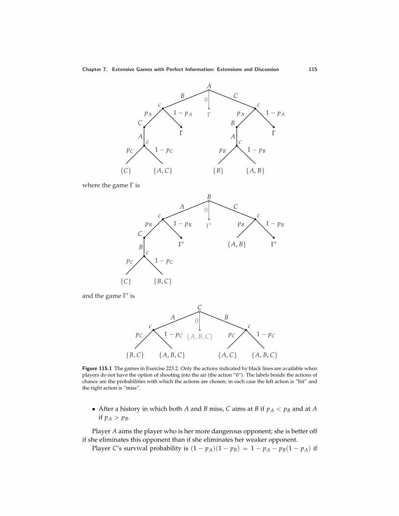
Chapter 7. Extensive Games with Perfect Information: Extensions and Discussion 115
0
Γ
AB C
cpA 1 − pA
Γ
C
Ac
pC 1 − pC
C A, C
cpA 1 − pA
Γ
B
Ac
pB 1 − pB
B A, B
where the game Γ is
0
Γ′
B
A Cc
pB 1 − pB
Γ′C
Bc
pC 1 − pC
C B, C
cpB 1 − pB
A, B Γ′
and the game Γ′ is
0
A, B, C
C
A Bc
pC 1 − pC
B, C A, B, C
cpC 1 − pC
A, C A, B, CFigure 115.1 The games in Exercise 223.2. Only the actions indicated by black lines are available whenplayers do not have the option of shooting into the air (the action “0”). The labels beside the actions ofchance are the probabilities with which the actions are chosen; in each case the left action is “hit” andthe right action is “miss”.
• After a history in which both A and B miss, C aims at B if pA < pB and at Aif pA > pB.
Player A aims the player who is her more dangerous opponent; she is better offif she eliminates this opponent than if she eliminates her weaker opponent.
Player C’s survival probability is (1 − pA)(1 − pB) = 1 − pA − pB(1 − pA) if
116 Chapter 7. Extensive Games with Perfect Information: Extensions and Discussion
pC > pB, and 1 − pB(1 − pA) if pC < pB. Thus she is better off if pC < pB than ifpC > pB.
Now consider the game in which each player has the option of shooting intothe air. In the subgame Γ′, player C’s best action is to aim at B (given pA < pB). (Ifshe shoots into the air then the set of survivors is A, B, C; if she aims at B she hassome chance of eliminating her.)
In the subgame Γ we know that if B shoots, her target should be C. If shedoes so her probability of survival is 1 − (1 − pB)pC. If she shoots into the air herprobability of survival is 1 − pC. The former exceeds the latter, so in the subgame Γplayer B aims at C.
Finally, given the equilibrium actions in the subgames, at the start of the gamewe know that if A fires she aims at C if pB < pC and at B if pB > pC. GivenpA < pB, her shooting into the air results in her certain survival, while her aimingat B or C results in her surviving with probability less than 1. Thus she shoots intothe air.
We conclude that if pA < pB then the game in which each player has the optionof shooting into the air has a unique subgame perfect equilibrium, which differsfrom the subgame perfect equilibrium in which this option is absent only in that Ashoots into the air at the beginning of the game.
Player A fires into the air because when she does so B and C fight betweenthemselves; if she shoots at one of them she may eliminate her from the game,giving the remaining player an incentive to shoot at her.
224.1 Cohesion in legislatures
Let the initial governing coalition consist of legislators 1 and 2. The US game isdefined as follows.
Players The three legislators.
Terminal histories All sequences (i, (x1, x2, x3), (A, B, C), j, (y1, y2, y3), (A′ , B′, C′)),where i and j are members of the governing coalition (possibly i = j), (x1, x2, x3)and (y1, y2, y3) are partitions of one unit of payoff (x1 + x2 + x3 = y1 + y2 +y3 = 1, xi ≥ 0, and yi ≥ 0 for i = 1, 2, 3), and A, B, C, A′, B′, and C′ are eitheryes (vote for bill) or no (vote against bill).
Player function
• P(∅) = c (chance)
• P(i) = i
• P(i, (x1, x2, x3)) = 1, 2, 3• P(i, (x1, x2, x3), (A, B, C)) = c
• P(i, (x1, x2, x3), (A, B, C), j) = j
• P(i, (x1, x2, x3), (A, B, C), j, (y1, y2, y3)) = 1, 2, 3.
Chapter 7. Extensive Games with Perfect Information: Extensions and Discussion 117
Chance probabilities Chance assigns probability 12 to 1 and probability 1
2 to 2whenever it moves.
Actions
• A(∅) = 1, 2• A(i) = (x1, x2, x3) : x1 + x2 + x3 = 1, xi ≥ 0 for all i for i = 1, 2
• Ak(i, (x1, x2, x3)) = yes, no for all k, i = 1, 2, and all (x1, x2, x3)
• A(i, (x1, x2, x3), (A, B, C)) = 1, 2 for all i, all (x1, x2, x3), and all triples(A, B, C) in which A, B, and C are all either yes or no
• A(i, (x1, x2, x3), (A, B, C), j) = (x1, x2, x3) : x1 + x2 + x3 = 1, xi ≥0 for all i for i = 1, 2, all (x1, x2, x3), all triples (A, B, C) in which A,B, and C are all either yes or no, and j = 1, 2
• Ak(i, (x1, x2, x3), (A, B, C), j, (y1, y2, y3)) = yes, no for all k, i = 1, 2, all(x1, x2, x3), all triples (A, B, C) in which A, B, and C are all either yes orno, j = 1, 2, and all (y1, y2, y3).
Preferences Each legislator i ranks the terminal histories by the amount ofmoney she receives: xi + yi if both bills are passed, xi + d2
i if only the firstbill is passed, d1
i + yi if only the second bill is passed, and d1i + d2
i if neitherbill is passed.
We find a subgame perfect equilibrium as follows. Refer to dti as legislator i’s
reservation value in period t. In the second period, denote by k the legislator whosereservation value is lower between the two who do not propose a bill. Each leg-islator i gets dt
i if a bill does not pass, and hence votes for a bill only if it givesher a payoff of at least dt
i . The proposer needs one vote in addition to her ownto pass a bill, and can obtain it most cheaply by proposing a bill that gives k thepayoff d2
k and gives herself the remaining payoff 1 − d2k (which exceeds her reser-
vation value, because all reservation values are less than 12 ). Legislator k and the
proposer vote for the bill, which thus passes. (Legislator k is indifferent betweenvoting for or against the bill, but there is no subgame perfect equilibrium in whichshe votes against the bill, because relative if she uses such a strategy the proposercan increase her offer to k a little, leading k to strictly prefer voting for the bill.) Thethird player may vote for or against the bill (her vote has no effect on the outcome).
In the first period, the pattern of behavior is the same: the bill proposed givesthe non-proposer with the lower reservation value that value.
In summary, in every subgame perfect equilibrium of the US game the strategyof each member i of the governing coalition has the following properties:
• after the move of chance in either period, propose the bill that gives the leg-islator with the smallest reservation value in the that period her reservationvalue and gives i the remaining payoff
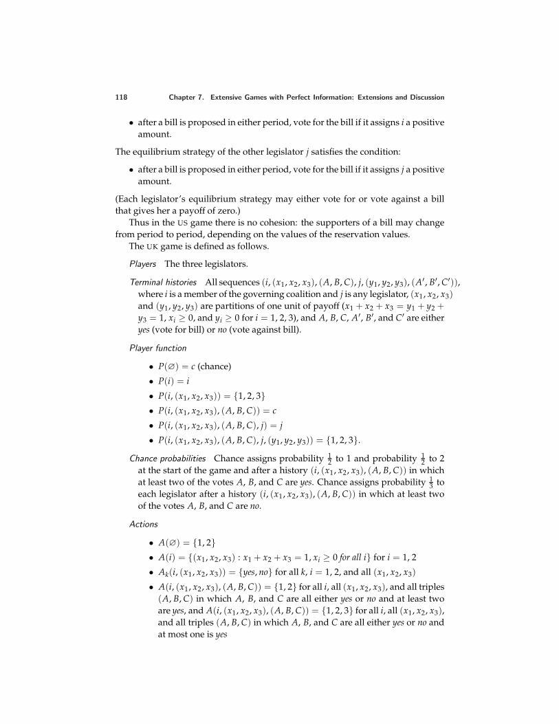
118 Chapter 7. Extensive Games with Perfect Information: Extensions and Discussion
• after a bill is proposed in either period, vote for the bill if it assigns i a positiveamount.
The equilibrium strategy of the other legislator j satisfies the condition:
• after a bill is proposed in either period, vote for the bill if it assigns j a positiveamount.
(Each legislator’s equilibrium strategy may either vote for or vote against a billthat gives her a payoff of zero.)
Thus in the US game there is no cohesion: the supporters of a bill may changefrom period to period, depending on the values of the reservation values.
The UK game is defined as follows.
Players The three legislators.
Terminal histories All sequences (i, (x1, x2, x3), (A, B, C), j, (y1, y2, y3), (A′ , B′, C′)),where i is a member of the governing coalition and j is any legislator, (x1, x2, x3)and (y1, y2, y3) are partitions of one unit of payoff (x1 + x2 + x3 = y1 + y2 +y3 = 1, xi ≥ 0, and yi ≥ 0 for i = 1, 2, 3), and A, B, C, A′, B′, and C′ are eitheryes (vote for bill) or no (vote against bill).
Player function
• P(∅) = c (chance)
• P(i) = i
• P(i, (x1, x2, x3)) = 1, 2, 3• P(i, (x1, x2, x3), (A, B, C)) = c
• P(i, (x1, x2, x3), (A, B, C), j) = j
• P(i, (x1, x2, x3), (A, B, C), j, (y1, y2, y3)) = 1, 2, 3.
Chance probabilities Chance assigns probability 12 to 1 and probability 1
2 to 2at the start of the game and after a history (i, (x1, x2, x3), (A, B, C)) in whichat least two of the votes A, B, and C are yes. Chance assigns probability 1
3 toeach legislator after a history (i, (x1, x2, x3), (A, B, C)) in which at least twoof the votes A, B, and C are no.
Actions
• A(∅) = 1, 2• A(i) = (x1, x2, x3) : x1 + x2 + x3 = 1, xi ≥ 0 for all i for i = 1, 2
• Ak(i, (x1, x2, x3)) = yes, no for all k, i = 1, 2, and all (x1, x2, x3)
• A(i, (x1, x2, x3), (A, B, C)) = 1, 2 for all i, all (x1, x2, x3), and all triples(A, B, C) in which A, B, and C are all either yes or no and at least twoare yes, and A(i, (x1, x2, x3), (A, B, C)) = 1, 2, 3 for all i, all (x1, x2, x3),and all triples (A, B, C) in which A, B, and C are all either yes or no andat most one is yes
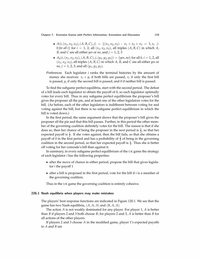
Chapter 7. Extensive Games with Perfect Information: Extensions and Discussion 119
• A(i, (x1, x2, x3), (A, B, C), j) = (x1, x2, x3) : x1 + x2 + x3 = 1, xi ≥0 for all i for i = 1, 2, all (x1, x2, x3), all triples (A, B, C) in which A,B, and C are all either yes or no, and j = 1, 2, 3
• Ak(i, (x1, x2, x3), (A, B, C), j, (y1, y2, y3)) = yes, no for all k, i = 1, 2, all(x1, x2, x3), all triples (A, B, C) in which A, B, and C are all either yes orno, j = 1, 2, 3, and all (y1, y2, y3).
Preferences Each legislator i ranks the terminal histories by the amount ofmoney she receives: xi + yi if both bills are passed, xi if only the first billis passed, yi if only the second bill is passed, and 0 if neither bill is passed.
To find the subgame perfect equilibria, start with the second period. The defeatof a bill leads each legislator to obtain the payoff of 0, so each legislator optimallyvotes for every bill. Thus in any subgame perfect equilibrium the proposer’s billgives the proposer all the pie, and at least one of the other legislators votes for thebill. (As before, each of the other legislators is indifferent between voting for andvoting against the bill, but there is no subgame perfect equilibrium in which thebill is voted down.)
In the first period, the same argument shows that the proposer’s bill gives theproposer all the pie and that this bill passes. Further, in this period the other mem-ber of the governing coalition definitely votes for the bill. The reason is that if shedoes so, then her chance of being the proposer in the next period is 1
2 , so that herexpected payoff is 1
2 . If she votes against, then the bill fails, so that she obtains apayoff of 0 in the first period and has a probability of 2
3 of being in the governingcoalition in the second period, so that her expected payoff is 1
3 . Thus she is betteroff voting for her comrade’s bill than against it.
In summary, in every subgame perfect equilibrium of the UK game the strategyof each legislator i has the following properties:
• after the move of chance in either period, propose the bill that gives legisla-tor i the payoff 1
• after a bill is proposed in the first period, vote for the bill if i is a member ofthe governing coalition.
Thus in the UK game the governing coalition is entirely cohesive.
226.1 Nash equilibria when players may make mistakes
The players’ best response functions are indicated in Figure 120.1. We see that thegame has two Nash equilibria, (A, A, A) and (B, A, A).
The action A is not weakly dominated for any player. For player 1, A is betterthan B if players 2 and 3 both choose B; for players 2 and 3, A is better than B forall actions of the other players.
If players 2 and 3 choose A in the modified game, player 1’s expected payoffsto A and B are
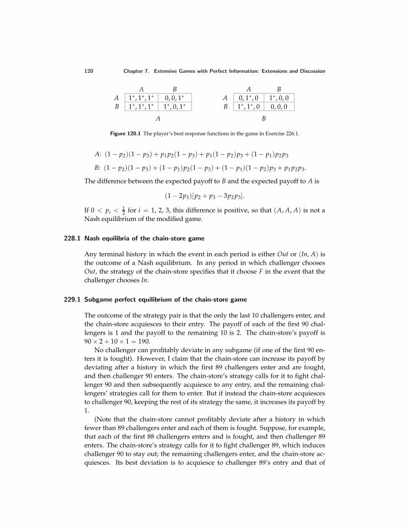
120 Chapter 7. Extensive Games with Perfect Information: Extensions and Discussion
A BA 1∗, 1∗, 1∗ 0, 0, 1∗
B 1∗, 1∗, 1∗ 1∗, 0, 1∗
A
A BA 0, 1∗, 0 1∗, 0, 0B 1∗, 1∗, 0 0, 0, 0
B
Figure 120.1 The player’s best response functions in the game in Exercise 226.1.
A: (1 − p2)(1 − p3) + p1 p2(1 − p3) + p1(1 − p2)p3 + (1 − p1)p2 p3
B: (1 − p2)(1 − p3) + (1 − p1)p2(1 − p3) + (1 − p1)(1 − p2)p3 + p1 p2 p3.
The difference between the expected payoff to B and the expected payoff to A is
(1 − 2p1)[p2 + p3 − 3p2 p3].
If 0 < pi < 12 for i = 1, 2, 3, this difference is positive, so that (A, A, A) is not a
Nash equilibrium of the modified game.
228.1 Nash equilibria of the chain-store game
Any terminal history in which the event in each period is either Out or (In, A) isthe outcome of a Nash equilibrium. In any period in which challenger choosesOut, the strategy of the chain-store specifies that it choose F in the event that thechallenger chooses In.
229.1 Subgame perfect equilibrium of the chain-store game
The outcome of the strategy pair is that the only the last 10 challengers enter, andthe chain-store acquiesces to their entry. The payoff of each of the first 90 chal-lengers is 1 and the payoff to the remaining 10 is 2. The chain-store’s payoff is90 × 2 + 10 × 1 = 190.
No challenger can profitably deviate in any subgame (if one of the first 90 en-ters it is fought). However, I claim that the chain-store can increase its payoff bydeviating after a history in which the first 89 challengers enter and are fought,and then challenger 90 enters. The chain-store’s strategy calls for it to fight chal-lenger 90 and then subsequently acquiesce to any entry, and the remaining chal-lengers’ strategies call for them to enter. But if instead the chain-store acquiescesto challenger 90, keeping the rest of its strategy the same, it increases its payoff by1.
(Note that the chain-store cannot profitably deviate after a history in whichfewer than 89 challengers enter and each of them is fought. Suppose, for example,that each of the first 88 challengers enters and is fought, and then challenger 89enters. The chain-store’s strategy calls for it to fight challenger 89, which induceschallenger 90 to stay out; the remaining challengers enter, and the chain-store ac-quiesces. Its best deviation is to acquiesce to challenger 89’s entry and that of
Chapter 7. Extensive Games with Perfect Information: Extensions and Discussion 121
all subsequent entrants, in which case all remaining challengers, including chal-lenger 90, enter. The outcomes of the two strategies differ in periods 89 and 90.If the challenger sticks to its original strategy it obtains 0 in period 89 and 2 inperiod 90; if it deviates it obtains 1 in each period.)
229.3 Nash equilibria of the centipede game
Consider a strategy pair that results in an outcome in which player 1 stops thegame in period k ≥ 2. (That is, each player chooses C through period k − 1 and theplayer who moves in period k chooses S.) Such a pair is not a Nash equilibriumbecause the player who moves in period k− 1 can do better (in the whole game, notonly the subgame) by choosing S rather than C, given the other player’s strategy.Similarly the strategy pair in which each player always chooses C is not a Nashequilibrium. Thus in every Nash equilibrium player 1 chooses S at the start of thegame.
Draft of solutions to exercises in chapter of An introduction to game theory by Martin J. [email protected]; www.chass.utoronto.ca/~osborne/index.htmlVersion: 00/11/6.Copyright c© 1995–2000 by Martin J. Osborne. All rights reserved. No part of this book may be re-produced in any form by any electronic or mechanical means (including photocopying, recording, orinformation storage and retrieval) without permission in writing from Martin J. Osborne. On request,permission to make one copy for each student will be granted to instructors who wish to use the bookin a course, on condition that copies be sold at a price not more than the cost of duplication.
8 Coalitional Games and the Core
241.1 Three-player majority game
Let (x1, x2, x3) be an action of the grand coalition. Every coalition consisting oftwo players can obtain one unit of output, so for (x1, x2, x3) to be in the core weneed
x1 + x2 ≥ 1
x1 + x3 ≥ 1
x2 + x3 ≥ 1
x1 + x2 + x3 = 1.
Adding the first three conditions we conclude that
2x1 + 2x2 + 2x3 ≥ 3,
or x1 + x2 + x3 ≥ 32 , contradicting the last condition. Thus no action of the grand
coalition satisfies all the conditions, so that the core of the game is empty.In the variant in which player 1 has three votes, a coalition can obtain one unit
of output if and only if it contains player 1. (Note that players 2 and 3 together donot have a majority of the votes.) Thus for (x1, x2, x3) to be in the core we need
x1 ≥ 1
x1 + x2 ≥ 1
x1 + x3 ≥ 1
x1 + x2 + x3 = 1.
The first and last conditions (and the restriction that amounts of output must benonnegative) imply that (x1, x2, x3) = (1, 0, 0), which satisfies the other two condi-tions. Thus the core consists of the single action (1, 0, 0) in which player 1 obtainsall the output.
242.1 Market with one owner and two heterogeneous buyers
By the arguments in Example 241.2, in any action in the core the owner does notkeep the good, the buyer who obtains the good pays at most her valuation, and
123

124 Chapter 8. Coalitional Games and the Core
the other buyer makes no payment. Let aN be an action of the grand coalitionin which buyer 2 obtains the good and pays the owner p, and buyer 1 makes nopayment. Then p ≤ v < 1, so that the coalition consisting of the owner and buyer 1can improve upon aN : if the owner transfers the good to buyer 1 in exchange for12 (1 + p) units of money, both the owner and buyer 1 are better off than they arein aN . Thus in any action in the core, buyer 1 obtains the good. The price shepays is at least v (otherwise the coalition consisting of the owner and buyer 2 canimprove upon the action). No coalition can improve upon any action in whichbuyer 1 obtains the good and pays the owner at least v and at most 1 (and buyer 2makes no payment), so the core consists of all such actions.
242.2 Vote trading
a. The core consists of the single action in which all three bills pass, yieldingeach legislator a payoff of 2. This action cannot be improved upon by anycoalition because no single bill or pair of bills gives every member of anymajority coalition a payoff of more than 2.
No other action is in the core, by the following argument.
• The action in which no bill passes (so that each legislator’s payoff is 0)can be improved upon by the coalition of all three legislators, which bypassing all three bills raises the payoff of each legislator to 2.
• The action in which only A passes can be improved upon by the coali-tion of legislators 2 and 3, who by passing bills A and B raise both oftheir payoffs.
• Similarly the action in which only B passes can be improved upon bythe coalition of legislators 1 and 3, and the action in which only C passescan be improved upon by the coalition of legislators 1 and 2.
• The action in which bills A and B pass can be improved upon by thecoalition of legislators 1 and 3, who by passing all three bills raise boththeir payoffs.
• Similarly the action in which bills A and C pass can be improved uponby the coalition of legislators 2 and 3, and the action in which bills B andC pass can be improved upon by the coalition of legislators 1 and 2.
b. The core consists of two actions: all three bills pass, and bills A and B pass.As in part a, the action in which all three bills pass cannot be improved uponby any coalition. The action in which bills A and B cannot be improved uponeither: for no other set of bills are at least two legislators better off.
No other action is in the core, by the following argument.
• The action in which A passes can be improved upon by the coalitionconsisting of legislators 2 and 3, who can pass B instead.
Chapter 8. Coalitional Games and the Core 125
• The action in which B passes can be improved upon by the coalitionconsisting of legislators 1 and 2, who can pass A and B instead.
• The action in which C passes can be improved upon by the coalitionconsisting of legislators 2 and 3, who can pass B instead.
• The action in which A and C pass can be improved upon by the coalitionconsisting of legislators 2 and 3, who can pass A and B instead.
• The action in which B and C pass can be improved upon by the coalitionconsisting of legislators 1 and 2, who can pass A and B instead.
c. The core is empty.
• The action in which no bill passes can be improved upon by the coalitionconsisting of legislators 1 and 2, who can pass A and B instead.
• The action in which any single bill passes can be improved upon by thecoalition consisting of the two legislators whose payoffs are −1 if thisbill passes; this coalition can do better by passing the other two bills.
• The action in which bills A and B pass can be improved upon by thecoalition consisting of legislators 2 and 3, who can pass B instead.
• Similarly the action in which A and C pass can be improved upon by thecoalition consisting of legislators 1 and 2, who can pass A instead, andthe action in which B and C pass can be improved upon by the coalitionconsisting of legislators 1 and 2, who can pass B instead.
• The action in which all three bills pass can be improved upon by thecoalition consisting of legislators 1 and 2, who can pass A and B instead.
244.1 Core of landowner–worker game
Let aN be an action of the grand coalition in which the output received by eachworker is at most f (n) − f (n − 1). No coalition consisting solely of workers canobtain any output, so no such coalition can improve upon aN . Let S be a coalitionof the landowner and k − 1 workers. The total output received by the members ofS in aN is at least
f (n) − (n − k)( f (n) − f (n − 1))
(because the total output is f (n), and every other worker receives at most f (n) −f (n − 1)). Now, the output that S can obtain is f (k), so for S to improve upon aNwe need
f (k) > f (n) − (n − k)( f (n) − f (n − 1)),
which contradicts the inequality given in the exercise.
126 Chapter 8. Coalitional Games and the Core
244.2 Unionized workers in landowner–worker game
The following game models the situation.
Players The landowner and the workers.
Actions The set of actions of the grand coalition is the set of all allocations ofthe output f (n). Every other coalition has a single action, which yields theoutput 0.
Preferences Each player’s preferences are represented by the amount of outputshe obtains.
The core of this game consists of every allocation of the output f (n) amongthe players. The grand coalition cannot improve upon any allocation x becausefor every other allocation x′ there is at least one player whose payoff is lower inx′ than it is in x. No other coalition can improve upon any allocation because noother coalition can obtain any output.
245.1 Landowner–worker game with increasing marginal products
We need to show that no coalition can improve upon the action aN of the grandcoalition in which every player receives the output f (n)/n. No coalition of work-ers can obtain any output, so we need to consider only coalitions containing thelandowner. Consider a coalition consisting of the landowner and k workers, whichcan obtain f (k + 1) units of output by itself. Under aN this coalition obtains the out-put (k + 1) f (n)/n, and we have f (k + 1)/(k + 1) < f (n)/n because k < n. Thus nocoalition can improve upon aN .
250.1 Range of prices in horse market
The equality of the number of owners who sell their horses and the number ofnonowners who buy horses implies that the common trading price p∗
• is not less than σk∗ , otherwise at most k∗ − 1 owners’ valuations would beless than p∗ and at least k∗ nonowners’ valuations would be greater than p∗,so that the number of buyers would exceed the number of sellers
• is not less than βk∗+1, otherwise at most k∗ owners’ valuations would be lessthan p∗ and at least k∗ + 1 nonowners’ valuations would be greater than p∗,so that the number of buyers would exceed the number of sellers
• is not greater than βk∗ , otherwise at least k∗ owners’ valuations would be lessthan p∗ and at most k∗ − 1 nonowners’ valuations would be greater than p∗,so that the number of sellers would exceed the number of buyers
Chapter 8. Coalitional Games and the Core 127
• is not greater than σk∗+1, otherwise at least k∗ + 1 owners’ valuations wouldbe less than p∗ and at most k∗ nonowners’ valuations would be greater thanp∗, so that the number of sellers would exceed the number of buyers.
That is, p∗ ≥ maxσk∗ , βk∗+1 and p∗ ≤ minβk∗ , σk∗+1.
251.1 Horse trading game with single seller
The core consists of the set of actions of the grand coalition in which the owner sellsher horse to the nonowner with the highest valuation (nonowner 1) at a price p∗
for which maxβ2, σ1 ≤ p∗ ≤ β1. (The coalition consisting of the owner and non-woner 2 can improve any action in which the price is less than β2, the owner alonecan improve upon any action in which the price is less than σ1, and nonowner 1alone can improve upon any action in which the price is greater than β1.)
251.2 Horse trading game with large seller
In every action in the core, the owner sells one horse to buyer 1 and one horse tobuyer 2. The prices at which the trades occur are not necessarily the same. Theprice p1 paid by buyer 1 satisfies maxβ3, σ1 ≤ p1 ≤ β1 and the price p2 paid bybuyer 2 satisfies maxβ3, σ1 ≤ p1 ≤ β2.
254.1 House assignment with identical preferences
Because the players rank the houses in the same way, we can refer to the “besthouse”, the “second best house”, and so on. In any assignment in the core, theplayer who owns the best house is assigned this house (because she has the optionof keeping it). Among the remaining players, the one who owns the second besthouse must be assigned this house (again, because she has the option of keepingit). Continuing to argue in the same way, we see that there is a single assignmentin the core, in which every player is assigned the house she owns initially.
255.1 Emptiness of the strong core when preferences are not strict
Of the six possible assignments, h1h2h3 (i.e. every player keeps the house sheowns) and h3h2h1 can both be improved upon by 1, 2 (and by 2, 3). All four ofthe other assignments are in the core.
None of the assignments in the core is in the strong core. The assignmentsh1h3h2 and h3h1h2 can both be weakly improved upon by 1, 2, and h2h1h3 andh2h3h1 can both be weakly improved upon by 2, 3.
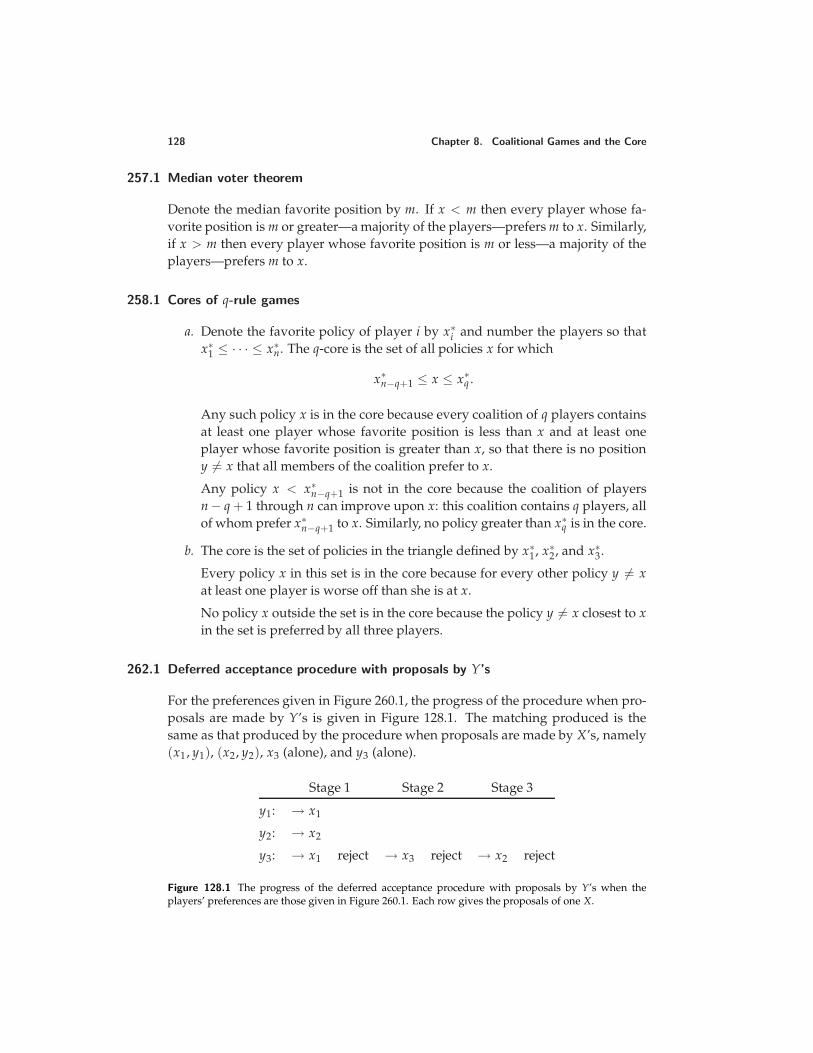
128 Chapter 8. Coalitional Games and the Core
257.1 Median voter theorem
Denote the median favorite position by m. If x < m then every player whose fa-vorite position is m or greater—a majority of the players—prefers m to x. Similarly,if x > m then every player whose favorite position is m or less—a majority of theplayers—prefers m to x.
258.1 Cores of q-rule games
a. Denote the favorite policy of player i by x∗i and number the players so that
x∗1 ≤ · · · ≤ x∗
n. The q-core is the set of all policies x for which
x∗n−q+1 ≤ x ≤ x∗
q .
Any such policy x is in the core because every coalition of q players containsat least one player whose favorite position is less than x and at least oneplayer whose favorite position is greater than x, so that there is no positiony = x that all members of the coalition prefer to x.
Any policy x < x∗n−q+1 is not in the core because the coalition of players
n − q + 1 through n can improve upon x: this coalition contains q players, allof whom prefer x∗
n−q+1 to x. Similarly, no policy greater than x∗q is in the core.
b. The core is the set of policies in the triangle defined by x∗1, x∗
2, and x∗3.
Every policy x in this set is in the core because for every other policy y = xat least one player is worse off than she is at x.
No policy x outside the set is in the core because the policy y = x closest to xin the set is preferred by all three players.
262.1 Deferred acceptance procedure with proposals by Y’s
For the preferences given in Figure 260.1, the progress of the procedure when pro-posals are made by Y’s is given in Figure 128.1. The matching produced is thesame as that produced by the procedure when proposals are made by X’s, namely(x1, y1), (x2, y2), x3 (alone), and y3 (alone).
Stage 1 Stage 2 Stage 3
y1: → x1
y2: → x2
y3: → x1 reject → x3 reject → x2 reject
Figure 128.1 The progress of the deferred acceptance procedure with proposals by Y’s when theplayers’ preferences are those given in Figure 260.1. Each row gives the proposals of one X.
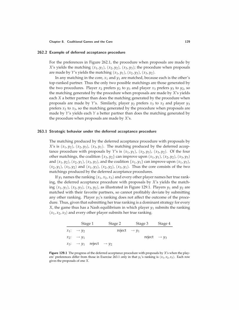
Chapter 8. Coalitional Games and the Core 129
262.2 Example of deferred acceptance procedure
For the preferences in Figure 262.1, the procedure when proposals are made byX’s yields the matching (x1, y1), (x2, y2), (x3, y3); the procedure when proposalsare made by Y’s yields the matching (x1, y1), (x2, y3), (x3, y2).
In any matching in the core, x1 and y1 are matched, because each is the other’stop-ranked partner. Thus the only two possible matchings are those generated bythe two procedures. Player x2 prefers y2 to y3 and player x3 prefers y3 to y2, sothe matching generated by the procedure when proposals are made by X’s yieldseach X a better partner than does the matching generated by the procedure whenproposals are made by Y’s. Similarly, player y2 prefers x3 to x2 and player y3prefers x2 to x3, so the matching generated by the procedure when proposals aremade by Y’s yields each Y a better partner than does the matching generated bythe procedure when proposals are made by X’s.
263.1 Strategic behavior under the deferred acceptance procedure
The matching produced by the deferred acceptance procedure with proposals byX’s is (x1, y2), (x2, y3), (x3, y1). The matching produced by the deferred accep-tance procedure with proposals by Y’s is (x1, y1), (x2, y3), (x3, y2). Of the fourother matchings, the coalition x3, y2 can improve upon (x1, y1), (x2, y2), (x3, y3)and (x1, y2), (x2, y1), (x3, y3), and the coalition x1, y1 can improve upon (x1, y3),(x2, y1), (x3, y2) and (x1, y3), (x2, y2), (x3, y1). Thus the core consists of the twomatchings produced by the deferred acceptance procedures.
If y1 names the ranking (x1, x2, x3) and every other player names her true rank-ing, the deferred acceptance procedure with proposals by X’s yields the match-ing (x1, y1), (x2, y3), (x3, y2), as illustrated in Figure 129.1. Players y1 and y2 arematched with their favorite partners, so cannot profitably deviate by submittingany other ranking. Player y3’s ranking does not affect the outcome of the proce-dure. Thus, given that submitting her true ranking is a dominant strategy for everyX, the game thus has a Nash equilibrium in which player y1 submits the ranking(x1, x2, x3) and every other player submits her true ranking.
Stage 1 Stage 2 Stage 3 Stage 4
x1: → y2 reject → y1
x2: → y1 reject → y3
x3: → y1 reject → y2
Figure 129.1 The progress of the deferred acceptance procedure with proposals by X’s when the play-ers’ preferences differ from those in Exercise 263.1 only in that y1’s ranking is (x1, x2, x3). Each rowgives the proposals of one X.
130 Chapter 8. Coalitional Games and the Core
263.2 Empty core in roommate problem
Notice that is at the bottom of each of the other players’ preferences. Supposethat she is matched with i. Then j and k are matched, and i, k can improve uponthe matching. Similarly, if is matched with j then i, j can improve upon thematching, and if is matched with k then j, k can improve upon the matching.Thus the core is empty ( has to be matched with someone!).
264.1 Spatial preferences in roommate problem
The core consists of the single matching µ∗ defined as follows. First match thepair of players whose characteristics are closest. Then match the pair of players inthe remaining set whose characteristics are closest. Continue until all players arematched.
Number the matches in the order they are made according to this procedure. Ifa coalition can improve upon µ∗, then a coalition consisting of two players can doso. Now, neither member of match k is better off being matched with a member ofmatch for any > k, so no two-player coalition can improve upon the matching.Thus µ∗ is in the core.
For any other matching µ′, at least one of the members of some match k definedby the procedure is matched with a different partner. If she is matched with amember of some match < k then the coalition consisting of the two members ofmatch can improve µ′; if she is matched with a member of some match > k thenthe coalition consisting of the two member of match k can improve upon µ′. Thusno matching µ′ = µ∗ is in the core.
Draft of solutions to exercises in chapter of An introduction to game theory by Martin J. [email protected]; www.chass.utoronto.ca/~osborne/index.htmlVersion: 00/11/6.Copyright c© 1995–2000 by Martin J. Osborne. All rights reserved. No part of this book may be re-produced in any form by any electronic or mechanical means (including photocopying, recording, orinformation storage and retrieval) without permission in writing from Martin J. Osborne. On request,permission to make one copy for each student will be granted to instructors who wish to use the bookin a course, on condition that copies be sold at a price not more than the cost of duplication.
9 Bayesian games
274.1 Equilibria of a variant of BoS with imperfect information
If player 1 chooses S then type 1 of player 2 chooses S and type 2 chooses B. Butif the two types of player 2 make these choices then player 1 is better off choosingB (which yields her an expected payoff of 1) than choosing S (which yields her anexpected payoff of 1
2 ). Thus there is no Nash equilibrium in which player 1 choosesS.
Now consider the mixed strategy Nash equilibria. If both types of player 2 usea pure strategy then player 1’s two actions yield her different payoffs. Thus thereis no equilibrium in which both types of player 2 use pure strategies and player 1randomizes.
Now consider an equilibrium in which type 1 of player 2 randomizes. Denoteby p the probability that player 1’s mixed strategy assigns to B. In order for type 1of player 2 to obtain the same expected payoff to B and S we need p = 2
3 . For thisvalue of p the best action of type 2 of player 2 is S. Denote by q the probability thattype 1 of player 2 assigns to B. Given these strategies for the two types of player 2,player 1’s expected payoff if she chooses B is
12 · 2q = q
and her expected payoff if she chooses S is
12 · (1 − q) + 1
2 · 1 = 1 − 12 q.
These expected payoffs are equal if and only if q = 23 . Thus the game has a mixed
strategy equilibrium in which the mixed strategy of player 1 is ( 23 , 1
3 ), that of type 1of player 2 is ( 2
3 , 13 ), and that of type 2 of player 2 is (0, 1) (that is, type 2 of player 2
uses the pure strategy that assigns probability 1 to S).Similarly the game has a mixed strategy equilibrium in which the strategy of
player 1 is ( 13 , 2
3 ), that of type 1 of player 2 is (0, 1), and that of type 2 of player 2 is( 2
3 , 13 ).For no mixed strategy of player 1 are both types of player 2 indifferent between
their two actions, so there is no equilibrium in which both types randomize.
275.1 Expected payoffs in a variant of BoS with imperfect information
The expected payoffs are given in Figure 132.1.
131
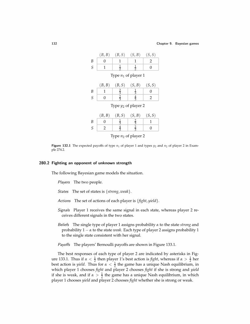
132 Chapter 9. Bayesian games
(B, B) (B, S) (S, B) (S, S)
B 0 1 1 2
S 1 12
12 0
Type n1 of player 1
(B, B) (B, S) (S, B) (S, S)
B 1 23
13 0
S 0 23
43 2
Type y2 of player 2
(B, B) (B, S) (S, B) (S, S)
B 0 13
23 1
S 2 43
23 0
Type n2 of player 2
Figure 132.1 The expected payoffs of type n1 of player 1 and types y2 and n2 of player 2 in Exam-ple 274.2.
280.2 Fighting an opponent of unknown strength
The following Bayesian game models the situation.
Players The two people.
States The set of states is strong, weak.
Actions The set of actions of each player is fight, yield.
Signals Player 1 receives the same signal in each state, whereas player 2 re-ceives different signals in the two states.
Beliefs The single type of player 1 assigns probability α to the state strong andprobability 1 − α to the state weak. Each type of player 2 assigns probability 1to the single state consistent with her signal.
Payoffs The players’ Bernoulli payoffs are shown in Figure 133.1.
The best responses of each type of player 2 are indicated by asterisks in Fig-ure 133.1. Thus if α < 1
2 then player 1’s best action is fight, whereas if α > 12 her
best action is yield. Thus for α < 12 the game has a unique Nash equilibrium, in
which player 1 chooses fight and player 2 chooses fight if she is strong and yieldif she is weak, and if α > 1
2 the game has a unique Nash equilibrium, in whichplayer 1 chooses yield and player 2 chooses fight whether she is strong or weak.
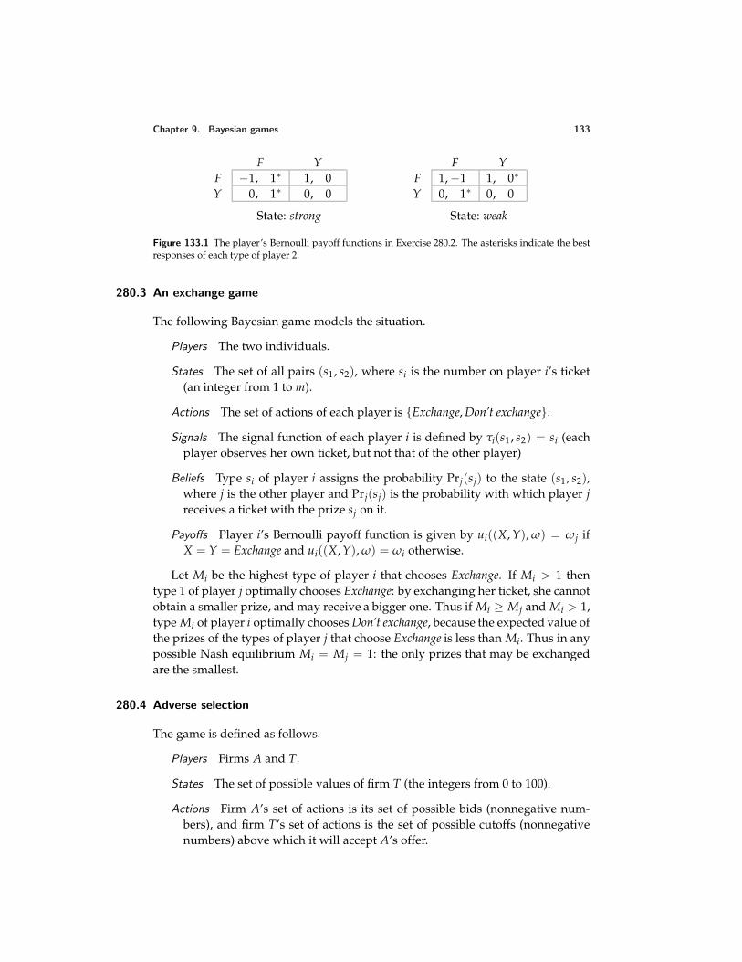
Chapter 9. Bayesian games 133
F YF −1, 1∗ 1, 0Y 0, 1∗ 0, 0
State: strong
F YF 1, −1 1, 0∗
Y 0, 1∗ 0, 0
State: weak
Figure 133.1 The player’s Bernoulli payoff functions in Exercise 280.2. The asterisks indicate the bestresponses of each type of player 2.
280.3 An exchange game
The following Bayesian game models the situation.
Players The two individuals.
States The set of all pairs (s1, s2), where si is the number on player i’s ticket(an integer from 1 to m).
Actions The set of actions of each player is Exchange, Don’t exchange.
Signals The signal function of each player i is defined by τi(s1, s2) = si (eachplayer observes her own ticket, but not that of the other player)
Beliefs Type si of player i assigns the probability Prj(sj) to the state (s1, s2),where j is the other player and Prj(sj) is the probability with which player jreceives a ticket with the prize sj on it.
Payoffs Player i’s Bernoulli payoff function is given by ui((X, Y), ω) = ωj ifX = Y = Exchange and ui((X, Y), ω) = ωi otherwise.
Let Mi be the highest type of player i that chooses Exchange. If Mi > 1 thentype 1 of player j optimally chooses Exchange: by exchanging her ticket, she cannotobtain a smaller prize, and may receive a bigger one. Thus if Mi ≥ Mj and Mi > 1,type Mi of player i optimally chooses Don’t exchange, because the expected value ofthe prizes of the types of player j that choose Exchange is less than Mi. Thus in anypossible Nash equilibrium Mi = Mj = 1: the only prizes that may be exchangedare the smallest.
280.4 Adverse selection
The game is defined as follows.
Players Firms A and T.
States The set of possible values of firm T (the integers from 0 to 100).
Actions Firm A’s set of actions is its set of possible bids (nonnegative num-bers), and firm T’s set of actions is the set of possible cutoffs (nonnegativenumbers) above which it will accept A’s offer.
134 Chapter 9. Bayesian games
Signals Firm A receives the same signal in every state; firm T receives a differ-ent signal in every state.
Beliefs The single type of firm A assigns an equal probability to each state;each type of firm T assigns probability 1 to the single state consistent with itssignal.
Payoff functions If firm A bids y, firm T’s cutoff is at most y, and the state is x,then A’s payoff is 3
2 x − y and T’s payoff is y. If firm A bids y, firm T’s cutoffis greater than y, and the state is x, then A’s payoff is 0 and T’s payoff is x.
To find the Nash equilibria of this game, first consider the behavior of each typeof firm T. Type x is at least as well off accepting the offer y than it is rejecting it ifand only if y ≥ x. Thus type x’s optimal cutoff for accepting offers is x, regardlessof firm A’s action.
Now consider firm A. If it bids y then each type x of T with x < y accepts itsoffer, and each type x of T with x > y rejects the offer. Thus the expected value ofthe type that accepts an offer y ≤ 100 is 1
2 y, and the expected value of the type thataccepts an offer y > 100 is 50. If the offer y is accepted then A’s payoff is 3
2 x − y,so that its expected payoff is 3
2 ( 12 y) − y = − 1
4 y if y ≤ 100 and 32 (50) − y = 75 − y
if y > 100. Thus firm A’s optimal bid is 0!We conclude that the game has a unique Nash equilibrium, in which firm A
bids 0 and the cutoff for accepting an offer for each type x of firm T is x.Even though firm A can increase firm T’s value, it is not willing to make a
positive bid in equilibrium because firm T’s interest is in accepting only offers thatexceed its value, so that the average type that accepts an offer has a value of onlyhalf the offer. As A decreases its offer, the value of the average firm that accepts theoffer decreases: the selection of firms that accept the offer is adverse to A’s interest.
282.1 Infection argument
In any Nash equilibrium, the action of player 1 when she receives the signal τ1(α)is R, because R strictly dominates L.
Now suppose that player 2’s signal is τ2(α) = τ2(β). I claim that her best actionis R, regardless of player 1’s action in state β. If player 1 chooses L in state β thenplayer 2’s expected payoff to L is 3
4 · 0 + 14 · 2 = 1
2 , and her expected payoff to R is34 · 1 + 1
4 · 0 = 34 . If player 1 chooses R in state β then player 2’s expected payoff to
L is 0, and her expected payoff to R is 1. Thus in any Nash equilibrium player 2’saction when her signal is τ2(α) = τ2(β) is R.
Now suppose that player 1’s signal is τ1(β) = τ1(γ). By the same argumentas in the previous paragraph, player 1’s best action is R, regardless of player 2’saction in state γ. Thus in any Nash equilibrium player 1’s action in this case is R.
Finally, given that player 1’s action in state γ is R, player 2’s best action in thisstate is also R.
Chapter 9. Bayesian games 135
285.1 Cournot’s duopoly game with imperfect information
We have
b1(qL , qH) =
12 (α − c − (θqL + (1 − θ)qH)) if θqL + (1 − θ)qH ≤ α − c0 otherwise.
The best response function of each type of player 2 is similar:
bI(q1) =
12 (α − cI − q1) if q1 ≤ α − cI0 otherwise
for I = L, H.The three equations that define a Nash equilibrium are
q∗1 = b1(q∗L, q∗H), q∗L = bL(q∗1), and q∗H = bH(q∗1).
Solving these equations under the assumption that they have a solution in whichall three outputs are positive, we obtain
q∗1 = 13 (α − 2c + θcL + (1 − θ)cH)
q∗L = 13 (α − 2cL + c) − 1
6 (1 − θ)(cH − cL)
q∗H = 13 (α − 2cH + c) + 1
6 θ(cH − cL)
If both firms know that the unit costs of the two firms are c1 and c2 then ina Nash equilibrium the output of firm i is 1
3 (α − 2ci + cj) (see Exercise 57.1). Inthe case of imperfect information considered here, firm 2’s output is less than13 (α − 2cL + c) if its cost is cL and is greater than 1
3 (α − 2cH + c) if its cost is cH .Intuitively, the reason is as follows. If firm 1 knew that firm 2’s cost were highthen it would produce a relatively large output; if it knew this cost were low thenit would produce a relatively small output. Given that it does not know whetherthe cost is high or low it produces a moderate output, less than it would if it knewfirm 2’s cost were high. Thus if firm 2’s cost is in fact high, firm 2 benefits fromfirm 1’s lack of knowledge and optimally produces more than it would if firm 1knew its cost.
286.1 Cournot’s duopoly game with imperfect information
The best response b0(qL, qH) of type 0 of firm 1 is the solution of
maxq0
[θ(P(q0 + qL) − c)q0 + (1 − θ)(P(q0 + qH) − c)q0].
The best response b(qL , qH) of type of firm 1 is the solution of
maxq
(P(q + qL) − c)q
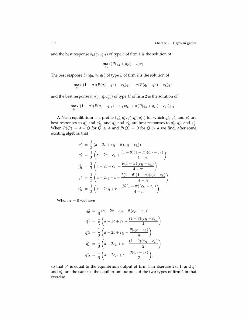
136 Chapter 9. Bayesian games
and the best response bh(qL , qH) of type h of firm 1 is the solution of
maxqh
(P(qh + qH) − c)qh .
The best response bL(q0, q, qh) of type L of firm 2 is the solution of
maxqL
[(1 − π)(P(q0 + qL) − cL)qL + π(P(q + qL) − cL)qL]
and the best response bH(q0, q, qh) of type H of firm 2 is the solution of
maxqH
[(1 − π)(P(q0 + qH) − cH)qH + π(P(qh + qH) − cH)qH ].
A Nash equilibrium is a profile (q∗0, q∗ , q∗h , q∗L, q∗H) for which q∗0, q∗ , and q∗h arebest responses to q∗L and q∗H , and q∗L and q∗H are best responses to q∗0, q∗ , and q∗h.When P(Q) = α − Q for Q ≤ α and P(Q) = 0 for Q > α we find, after someexciting algebra, that
q∗0 =13
(α − 2c + cH − θ (cH − cL))
q∗ =13
(α − 2c + cL +
(1 − θ)(1 − π)(cH − cL)4 − π
)
q∗H =13
(α − 2c + cH − θ(1 − π)(cH − cL)
4 − π
)
q∗L =13
(α − 2cL + c − 2(1 − θ)(1 − π)(cH − cL)
4 − π
)
q∗H =13
(α − 2cH + c +
2θ(1 − π)(cH − cL)4 − π
).
When π = 0 we have
q∗0 =13
(α − 2c + cH − θ (cH − cL))
q∗ =13
(α − 2c + cL +
(1 − θ)(cH − cL)4
)
q∗H =13
(α − 2c + cH − θ(cH − cL)
4
)
q∗L =13
(α − 2cL + c − (1 − θ)(cH − cL)
2
)
q∗H =13
(α − 2cH + c +
θ(cH − cL)2
),
so that q∗0 is equal to the equilibrium output of firm 1 in Exercise 285.1, and q∗Land q∗H are the same as the equilibrium outputs of the two types of firm 2 in thatexercise.
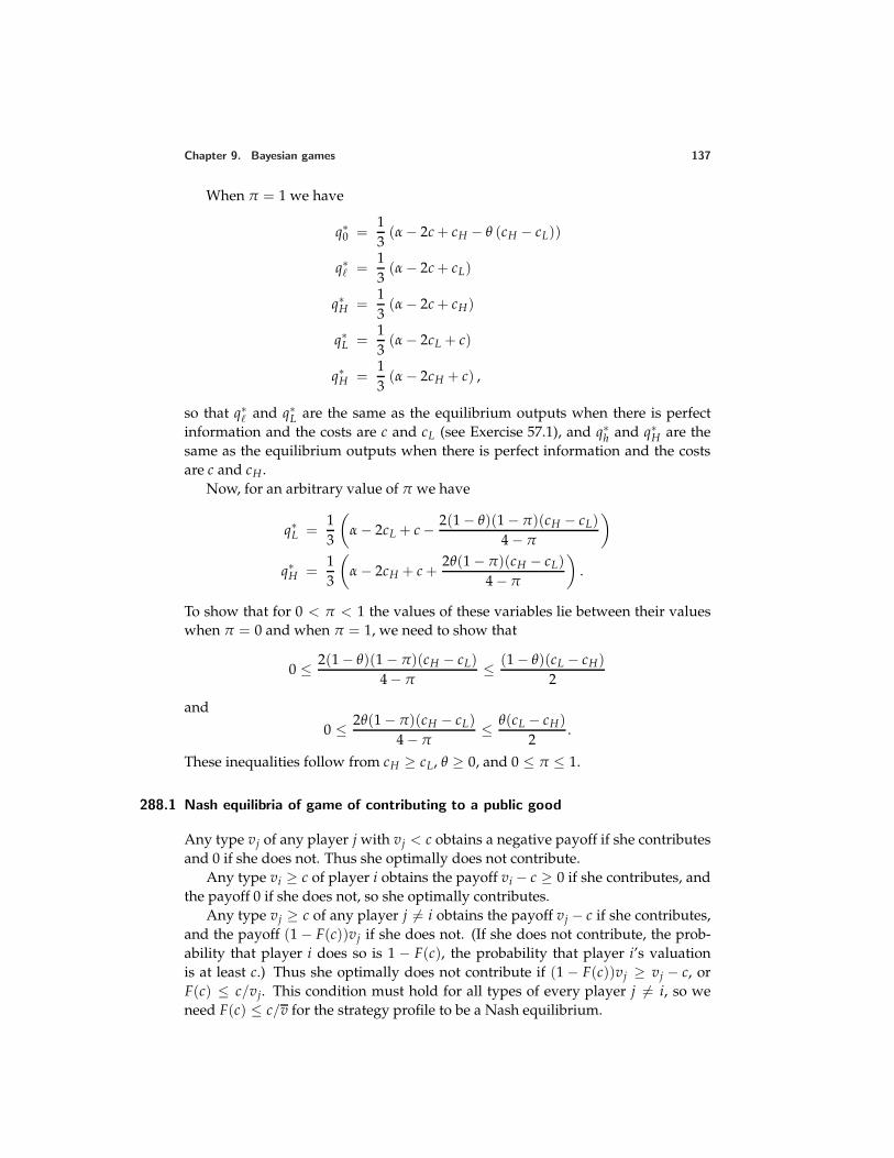
Chapter 9. Bayesian games 137
When π = 1 we have
q∗0 =13
(α − 2c + cH − θ (cH − cL))
q∗ =13
(α − 2c + cL)
q∗H =13
(α − 2c + cH)
q∗L =13
(α − 2cL + c)
q∗H =13
(α − 2cH + c) ,
so that q∗ and q∗L are the same as the equilibrium outputs when there is perfectinformation and the costs are c and cL (see Exercise 57.1), and q∗h and q∗H are thesame as the equilibrium outputs when there is perfect information and the costsare c and cH .
Now, for an arbitrary value of π we have
q∗L =13
(α − 2cL + c − 2(1 − θ)(1 − π)(cH − cL)
4 − π
)
q∗H =13
(α − 2cH + c +
2θ(1 − π)(cH − cL)4 − π
).
To show that for 0 < π < 1 the values of these variables lie between their valueswhen π = 0 and when π = 1, we need to show that
0 ≤ 2(1 − θ)(1 − π)(cH − cL)4 − π
≤ (1 − θ)(cL − cH)2
and
0 ≤ 2θ(1 − π)(cH − cL)4 − π
≤ θ(cL − cH)2
.
These inequalities follow from cH ≥ cL, θ ≥ 0, and 0 ≤ π ≤ 1.
288.1 Nash equilibria of game of contributing to a public good
Any type vj of any player j with vj < c obtains a negative payoff if she contributesand 0 if she does not. Thus she optimally does not contribute.
Any type vi ≥ c of player i obtains the payoff vi − c ≥ 0 if she contributes, andthe payoff 0 if she does not, so she optimally contributes.
Any type vj ≥ c of any player j = i obtains the payoff vj − c if she contributes,and the payoff (1 − F(c))vj if she does not. (If she does not contribute, the prob-ability that player i does so is 1 − F(c), the probability that player i’s valuationis at least c.) Thus she optimally does not contribute if (1 − F(c))vj ≥ vj − c, orF(c) ≤ c/vj. This condition must hold for all types of every player j = i, so weneed F(c) ≤ c/v for the strategy profile to be a Nash equilibrium.
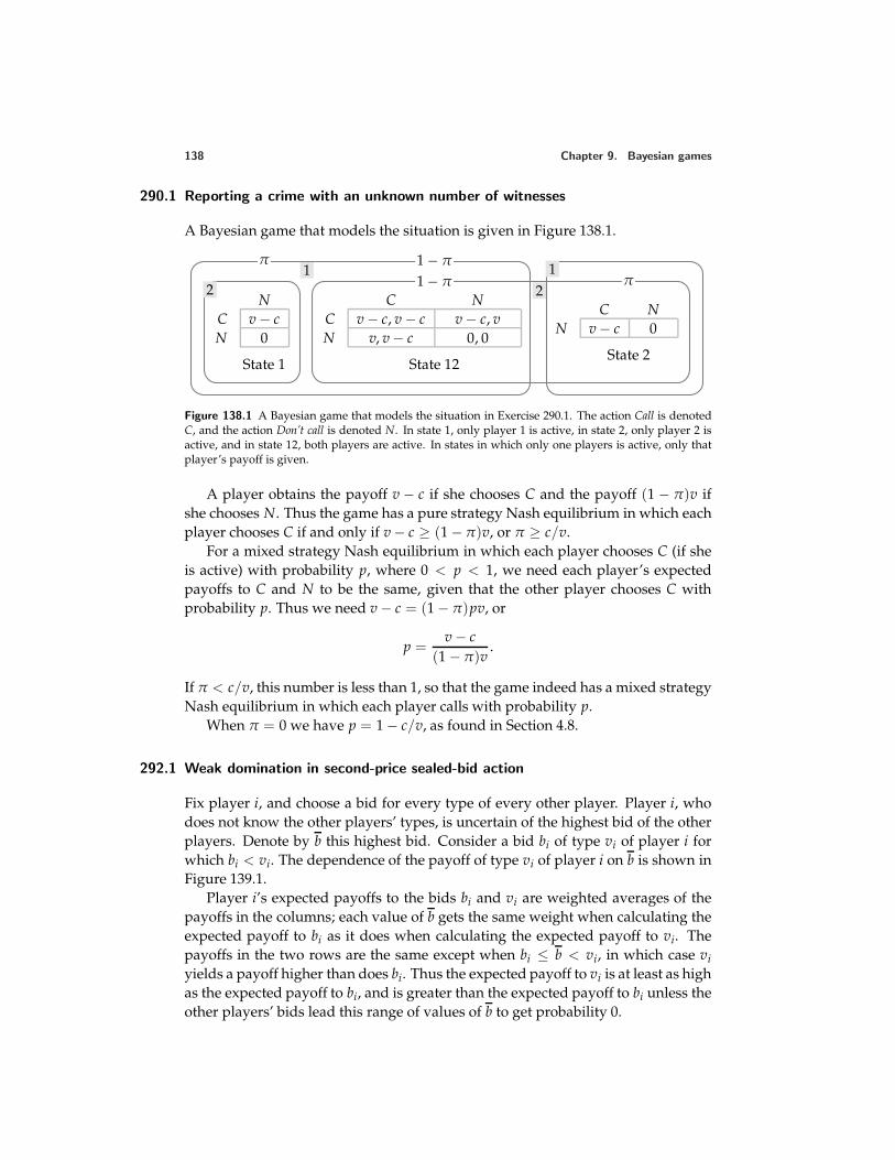
138 Chapter 9. Bayesian games
290.1 Reporting a crime with an unknown number of witnesses
A Bayesian game that models the situation is given in Figure 138.1.
NC v − cN 0
State 1
C NC v − c, v − c v − c, vN v, v − c 0, 0
State 12
C NN v − c 0
State 2
12
π 1 − π
1 − π π1
2
Figure 138.1 A Bayesian game that models the situation in Exercise 290.1. The action Call is denotedC, and the action Don’t call is denoted N. In state 1, only player 1 is active, in state 2, only player 2 isactive, and in state 12, both players are active. In states in which only one players is active, only thatplayer’s payoff is given.
A player obtains the payoff v − c if she chooses C and the payoff (1 − π)v ifshe chooses N. Thus the game has a pure strategy Nash equilibrium in which eachplayer chooses C if and only if v − c ≥ (1 − π)v, or π ≥ c/v.
For a mixed strategy Nash equilibrium in which each player chooses C (if sheis active) with probability p, where 0 < p < 1, we need each player’s expectedpayoffs to C and N to be the same, given that the other player chooses C withprobability p. Thus we need v − c = (1 − π)pv, or
p =v − c
(1 − π)v.
If π < c/v, this number is less than 1, so that the game indeed has a mixed strategyNash equilibrium in which each player calls with probability p.
When π = 0 we have p = 1 − c/v, as found in Section 4.8.
292.1 Weak domination in second-price sealed-bid action
Fix player i, and choose a bid for every type of every other player. Player i, whodoes not know the other players’ types, is uncertain of the highest bid of the otherplayers. Denote by b this highest bid. Consider a bid bi of type vi of player i forwhich bi < vi. The dependence of the payoff of type vi of player i on b is shown inFigure 139.1.
Player i’s expected payoffs to the bids bi and vi are weighted averages of thepayoffs in the columns; each value of b gets the same weight when calculating theexpected payoff to bi as it does when calculating the expected payoff to vi. Thepayoffs in the two rows are the same except when bi ≤ b < vi, in which case viyields a payoff higher than does bi. Thus the expected payoff to vi is at least as highas the expected payoff to bi, and is greater than the expected payoff to bi unless theother players’ bids lead this range of values of b to get probability 0.
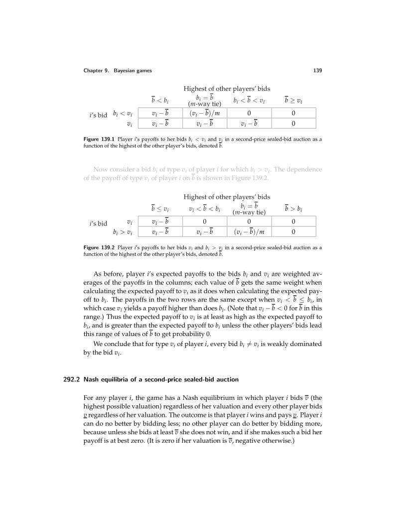
Chapter 9. Bayesian games 139
i’s bid
Highest of other players’ bids
b < bibi = b
(m-way tie) bi < b < vi b ≥ vi
bi < vi vi − b (vi − b)/m 0 0
vi vi − b vi − b vi − b 0
Figure 139.1 Player i’s payoffs to her bids bi < vi and vi in a second-price sealed-bid auction as afunction of the highest of the other player’s bids, denoted b.
Now consider a bid bi of type vi of player i for which bi > vi. The dependenceof the payoff of type vi of player i on b is shown in Figure 139.2.
i’s bid
Highest of other players’ bids
b ≤ vi vi < b < bibi = b
(m-way tie) b > bi
vi vi − b 0 0 0
bi > vi vi − b vi − b (vi − b)/m 0
Figure 139.2 Player i’s payoffs to her bids vi and bi > vi in a second-price sealed-bid auction as afunction of the highest of the other player’s bids, denoted b.
As before, player i’s expected payoffs to the bids bi and vi are weighted av-erages of the payoffs in the columns; each value of b gets the same weight whencalculating the expected payoff to vi as it does when calculating the expected pay-off to bi. The payoffs in the two rows are the same except when vi < b ≤ bi, inwhich case vi yields a payoff higher than does bi. (Note that vi − b < 0 for b in thisrange.) Thus the expected payoff to vi is at least as high as the expected payoff tobi, and is greater than the expected payoff to bi unless the other players’ bids leadthis range of values of b to get probability 0.
We conclude that for type vi of player i, every bid bi = vi is weakly dominatedby the bid vi.
292.2 Nash equilibria of a second-price sealed-bid auction
For any player i, the game has a Nash equilibrium in which player i bids v (thehighest possible valuation) regardless of her valuation and every other player bidsv regardless of her valuation. The outcome is that player i wins and pays v. Player ican do no better by bidding less; no other player can do better by bidding more,because unless she bids at least v she does not win, and if she makes such a bid herpayoff is at best zero. (It is zero if her valuation is v, negative otherwise.)
140 Chapter 9. Bayesian games
295.1 Auctions with risk-averse bidders
Consider player i. Suppose that the bid of each type vj of player j is given byβ j(vj) = (1 − 1/[m(n − 1) + 1])vj. Then as far as player i is concerned, the bids ofevery other player are distributed uniformly between 0 and 1 − 1/[m(n − 1) + 1].Thus for 0 ≤ x ≤ 1 − 1/[m(n − 1) + 1], the probability that any given player’sbid is less than x is (1 + 1/[m(n + 1)])x (1 + 1/[m(n + 1)] being the reciprocal of1 − 1/[m(n − 1) + 1]), and hence the probability that all the bids of the other n − 1players are less than x is [(1 + 1/[m(n + 1)])x]n−1. Consequently, if player i bidsmore than 1 − 1/[m(n − 1) + 1] then she surely wins, whereas if she bids bi ≤1 − 1/[m(n − 1) + 1] she wins with probability [(1 + 1/[m(n + 1)])bi]n−1. Thusplayer i’s payoff as a function of her bid bi is
(vi − bi)1/m(
1 +1
m(n + 1)
)bi
n−1if 0 ≤ bi ≤ 1 − 1
m(n − 1) + 1
(vi − bi)1/m if bi > 1 − 1m(n − 1) + 1
.(140.1)
Now, the value of bi that maximizes the function
(vi − bi)1/m(
1 +1
m(n + 1)
)bi
n−1
is the same as the value of bi that maximizes the function
(vi − bi)1/m(bi)
n−1,
which is (n − 1)vi/(n − 1 + 1/m) (by the mathematical fact stated in the exercise),or (
1 − 1m(n − 1) + 1
)vi.
We have (1 − 1
m(n − 1) + 1
)vi ≤ 1 − 1
m(n − 1) + 1
(because vi ≤ 1), and the function in (140.1) is decreasing in bi for bi > 1− 1/[m(n−1) + 1], so 1− 1/[m(n− 1) + 1] is the bid that maximizes player i’s expected payoff,given that the bid of each type vj of player j is (1 − 1/[m(n − 1) + 1])vj.
We conclude that, as claimed, the game has a Nash equilibrium in which eachtype vi of each player i bids (1 − 1/[m(n − 1) + 1])vi.
In this equilibrium, the price paid by a bidder with valuation v who wins is(1 − 1/[m(n − 1) + 1])v (the amount she bids). The expected price paid by a bidderin a second-price auction does not depend on the players’ payoff functions. Thusthis payoff is equal, by the revenue equivalence result, to the expected price paidby a bidder with valuation v who wins in a first-price auction in which each bidderis risk-neutral, namely (1 − 1/n)v. We have
(1 − 1
m(n − 1) + 1
)−(
1 − 1n
)=
(m − 1)(n − 1)n(m(n − 1) + 1)
,
Chapter 9. Bayesian games 141
which is positive because m > 1. Thus the expected price paid by a bidder withvaluation v who wins is greater in a first-price auction than it is in a second-priceauction. The probability that a bidder with any given valuation wins is the samein both auctions, so the auctioneer’s expected revenue is greater in a first-priceauction than it is in a second-price auction.
297.1 Asymmetric Nash equilibria of second-price sealed-bid common value auctions
Suppose that each type t2 of player 2 bids (1 + 1/λ)t2 and that type t1 of player 1bids b1. Then by the calculations in the text, with α = 1 and γ = 1/λ,
• a bid of b1 by player 1 wins with probability b1/(1 + 1/λ)
• the expected value of player 2’s bid, given that it is less than b1, is 12 b1
• the expected value of signals that yield a bid of less than b1 is 12 b1/(1 + 1/λ)
(because of the uniformity of the distribution of t2).
Thus player 1’s expected payoff if she bids b1 is (t1 + 12 b1/(1 + 1/λ)− 1
2 b1)b1/(1 +1/λ), or
λ
2(1 + λ)2 · (2(1 + λ)t1 − b1)b1.
This function is maximized at b1 = (1 + λ)t1. That is, if each type t2 of player 2bids (1 + 1/λ)t2, any type t1 of player 1 optimally bids (1 + λ)t1. Symmetrically,if each type t1 of player 1 bids (1 + λ)t1, any type t2 of player 2 optimally bids(1 + 1/λ)t2. Hence the game has the claimed Nash equilibrium.
297.2 First-price sealed-bid auction with common valuations
Suppose that each type t2 of player 2 bids 12 (α + γ)t2 and type t1 of player 1 bids
b1. To determine the expected payoff of type t1 of player 1, we need to find theprobability with which she wins, and the expected value of player 2’s signal ifplayer 1 wins. (The price she pays is her bid, b1.)
Probability of player 1’s winning: Given that player 2’s bidding function is12 (α + γ)t2, player 1’s bid of b1 wins only if b1 ≥ 1
2 (α + γ)t2, or if t2 ≤ 2b1/(α + γ).Now, t2 is distributed uniformly from 0 to 1, so the probability that it is at most2b1/(α + γ) is 2b1/(α + γ). Thus a bid of b1 by player 1 wins with probabil-ity 2b1/(α + γ).
Expected value of player 2’s signal if player 1 wins: Player 2’s bid, given hersignal t2, is 1
2 (α + γ)t2, so that the expected value of signals that yield a bid of lessthan b1 is b1/(α + γ) (because of the uniformity of the distribution of t2).
Thus player 1’s expected payoff if she bids b1 is 2(αt1 + γb1/(α + γ)− b1)b1/(α +γ), or
2α
(α + γ)2 ((α + γ)t1 − b1)b1.
142 Chapter 9. Bayesian games
This function is maximized at b1 = 12 (α + γ)t1. That is, if each type t2 of player 2
bids 12 (α + γ)t2, any type t1 of player 1 optimally bids 1
2 (α + γ)t1. Hence, asclaimed, the game has a Nash equilibrium in which each type ti of player i bids12 (α + γ)ti.
304.1 Signal-independent equilibria in a model of a jury
If every juror votes for acquittal regardless of her signal then the action of anysingle juror has no effect on the outcome. Thus the strategy profile in which everyjuror votes for acquittal regardless of her signal is always a Nash equilibrium.
Now consider the possibility of a Nash equilibrium in which every juror votesfor conviction regaredless of her signal. Suppose that every juror other than juror 1votes for conviction independently of her signal. Then juror 1’s vote determinesthe outcome, exactly as in the case in which there is a single juror. Thus from thecalculations in Section 9.8.2, type b of juror 1 optimally votes for conviction if andonly if
z ≤ (1 − p)π
(1 − p)π + q(1 − π)
and type g of juror 1 optimally votes for conviction if and only if
z ≤ pπ
pπ + (1 − q)(1 − π).
The assumption that p > 1 − q implies that the term on the right side of the secondinequality is greater than the term on the right side of the first inequality, so that weconclude that there is a Nash equilibrium in which every juror votes for convictionregardless of her signal if and only if
(1 − p)π
(1 − p)π + q(1 − π)≤ z ≤ pπ
pπ + (1 − q)(1 − π).
305.1 Swing voter’s curse
a. The Bayesian game is defined as follows.
Players Citizens 1 and 2.
States A, B.
Actions The set of actions of each player is 0, 1, 2 (where 0 means do notvote).
Signals Citizen 1 receives different signals in states A and B, whereas citi-zen 2 receives the same signal in both states.
Beliefs Each type of citizen 1 assigns probability 1 to the single state consis-tent with her signal. The single type of citizen 2 assigns probability 0.9to state A and probability 0.1 to state B.
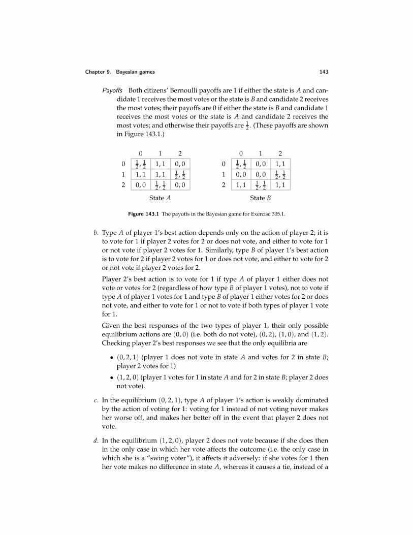
Chapter 9. Bayesian games 143
Payoffs Both citizens’ Bernoulli payoffs are 1 if either the state is A and can-didate 1 receives the most votes or the state is B and candidate 2 receivesthe most votes; their payoffs are 0 if either the state is B and candidate 1receives the most votes or the state is A and candidate 2 receives themost votes; and otherwise their payoffs are 1
2 . (These payoffs are shownin Figure 143.1.)
0 1 2
0 12 , 1
2 1, 1 0, 0
1 1, 1 1, 1 12 , 1
2
2 0, 0 12 , 1
2 0, 0
State A
0 1 2
0 12 , 1
2 0, 0 1, 1
1 0, 0 0, 0 12 , 1
2
2 1, 1 12 , 1
2 1, 1
State B
Figure 143.1 The payoffs in the Bayesian game for Exercise 305.1.
b. Type A of player 1’s best action depends only on the action of player 2; it isto vote for 1 if player 2 votes for 2 or does not vote, and either to vote for 1or not vote if player 2 votes for 1. Similarly, type B of player 1’s best actionis to vote for 2 if player 2 votes for 1 or does not vote, and either to vote for 2or not vote if player 2 votes for 2.
Player 2’s best action is to vote for 1 if type A of player 1 either does notvote or votes for 2 (regardless of how type B of player 1 votes), not to vote iftype A of player 1 votes for 1 and type B of player 1 either votes for 2 or doesnot vote, and either to vote for 1 or not to vote if both types of player 1 votefor 1.
Given the best responses of the two types of player 1, their only possibleequilibrium actions are (0, 0) (i.e. both do not vote), (0, 2), (1, 0), and (1, 2).Checking player 2’s best responses we see that the only equilibria are
• (0, 2, 1) (player 1 does not vote in state A and votes for 2 in state B;player 2 votes for 1)
• (1, 2, 0) (player 1 votes for 1 in state A and for 2 in state B; player 2 doesnot vote).
c. In the equilibrium (0, 2, 1), type A of player 1’s action is weakly dominatedby the action of voting for 1: voting for 1 instead of not voting never makesher worse off, and makes her better off in the event that player 2 does notvote.
d. In the equilibrium (1, 2, 0), player 2 does not vote because if she does thenin the only case in which her vote affects the outcome (i.e. the only case inwhich she is a “swing voter”), it affects it adversely: if she votes for 1 thenher vote makes no difference in state A, whereas it causes a tie, instead of a
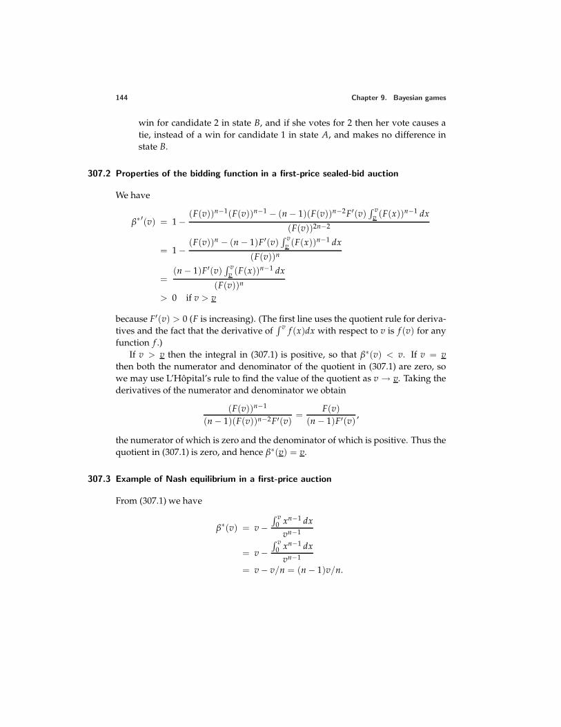
144 Chapter 9. Bayesian games
win for candidate 2 in state B, and if she votes for 2 then her vote causes atie, instead of a win for candidate 1 in state A, and makes no difference instate B.
307.2 Properties of the bidding function in a first-price sealed-bid auction
We have
β∗′(v) = 1 −(F(v))n−1(F(v))n−1 − (n − 1)(F(v))n−2F′(v)
∫ vv (F(x))n−1 dx
(F(v))2n−2
= 1 −(F(v))n − (n − 1)F′(v)
∫ vv (F(x))n−1 dx
(F(v))n
=(n − 1)F′(v)
∫ vv (F(x))n−1 dx
(F(v))n
> 0 if v > v
because F′(v) > 0 (F is increasing). (The first line uses the quotient rule for deriva-tives and the fact that the derivative of
∫ v f (x)dx with respect to v is f (v) for anyfunction f .)
If v > v then the integral in (307.1) is positive, so that β∗(v) < v. If v = vthen both the numerator and denominator of the quotient in (307.1) are zero, sowe may use L’Hopital’s rule to find the value of the quotient as v → v. Taking thederivatives of the numerator and denominator we obtain
(F(v))n−1
(n − 1)(F(v))n−2F′(v)=
F(v)(n − 1)F′(v)
,
the numerator of which is zero and the denominator of which is positive. Thus thequotient in (307.1) is zero, and hence β∗(v) = v.
307.3 Example of Nash equilibrium in a first-price auction
From (307.1) we have
β∗(v) = v −∫ v
0 xn−1 dxvn−1
= v −∫ v
0 xn−1 dxvn−1
= v − v/n = (n − 1)v/n.
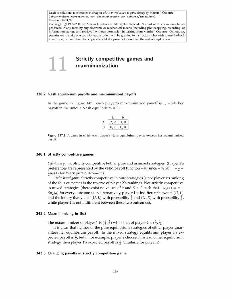
Draft of solutions to exercises in chapter of An introduction to game theory by Martin J. [email protected]; www.chass.utoronto.ca/~osborne/index.htmlVersion: 00/11/6.Copyright c© 1995–2000 by Martin J. Osborne. All rights reserved. No part of this book may be re-produced in any form by any electronic or mechanical means (including photocopying, recording, orinformation storage and retrieval) without permission in writing from Martin J. Osborne. On request,permission to make one copy for each student will be granted to instructors who wish to use the bookin a course, on condition that copies be sold at a price not more than the cost of duplication.
11 Strictly competitive games andmaxminimization
338.2 Nash equilibrium payoffs and maxminimized payoffs
In the game in Figure 147.1 each player’s maxminimized payoff is 1, while herpayoff in the unique Nash equilibrium is 2.
L RT 2, 2 1, 0B 0, 1 0, 0
Figure 147.1 A game in which each player’s Nash equilibrium payoff exceeds her maxminimizedpayoff.
340.1 Strictly competitive games
Left-hand game: Strictly competitive both in pure and in mixed strategies. (Player 2’spreferences are represented by the vNM payoff function −u1 since −u1(a) = − 1
2 +12 u2(a) for every pure outcome a.)
Right-hand game: Strictly competitive in pure strategies (since player 1’s rankingof the four outcomes is the reverse of player 2’s ranking). Not strictly competitivein mixed strategies (there exist no values of α and β > 0 such that −u1(a) = α +βu2(a) for every outcome a; or, alternatively, player 1 is indifferent between (D, L)and the lottery that yields (U, L) with probability 1
2 and (U, R) with probability 12 ,
while player 2 is not indifferent between these two outcomes).
343.2 Maxminimizing in BoS
The maxminimizer of player 1 is ( 13 , 2
3 ) while that of player 2 is ( 23 , 1
3 ).It is clear that neither of the pure equilibrium strategies of either player guar-
antees her equilibrium payoff. In the mixed strategy equilibrium player 1’s ex-pected payoff is 2
3 ; but if, for example, player 2 choose S instead of her equilibriumstrategy, then player 1’s expected payoff is 1
3 . Similarly for player 2.
343.3 Changing payoffs in strictly competitive game
147
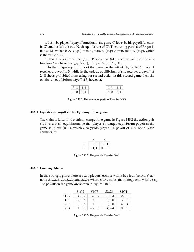
148 Chapter 11. Strictly competitive games and maxminimization
a. Let ui be player i’s payoff function in the game G, let wi be his payoff functionin G′, and let (x∗ , y∗) be a Nash equilibrium of G′. Then, using part (a) of Proposi-tion 341.1, we have w1(x∗, y∗) = miny maxx w1(x, y) ≥ miny maxx u1(x, y), whichis the value of G.
b. This follows from part (a) of Proposition 341.1 and the fact that for anyfunction f we have maxx∈X f (x) ≥ maxx∈Y f (x) if Y ⊆ X.
c. In the unique equilibrium of the game on the left of Figure 148.1 player 1receives a payoff of 3, while in the unique equilibrium of she receives a payoff of2. If she is prohibited from using her second action in this second game then sheobtains an equilibrium payoff of 3, however.
3, 3 1, 11, 0 0, 1
3, 3 1, 14, 0 2, 1
Figure 148.1 The games for part c of Exercise 343.3.
344.1 Equilibrium payoff in strictly competitive game
The claim is false. In the strictly competitive game in Figure 148.2 the action pair(T, L) is a Nash equilibrium, so that player 1’s unique equilibrium payoff in thegame is 0; but (B, R), which also yields player 1 a payoff of 0, is not a Nashequilibrium.
L RT 0, 0 1, −1B −1, 1 0, 0
Figure 148.2 The game in Exercise 344.1.
344.2 Guessing Morra
In the strategic game there are two players, each of whom has four (relevant) ac-tions, S1G2, S1G3, S2G3, and S2G4, where SiGj denotes the strategy (Show i, Guess j).The payoffs in the game are shown in Figure 148.3.
S1G2 S1G3 S2G3 S2G4S1G2 0, 0 2, −2 −3, 3 0, 0S1G3 −2, 2 0, 0 0, 0 3, −3S2G3 3, −3 0, 0 0, 0 −4, 4S2G4 0, 0 −3, 3 4, −4 0, 0
Figure 148.3 The game in Exercise 344.2.
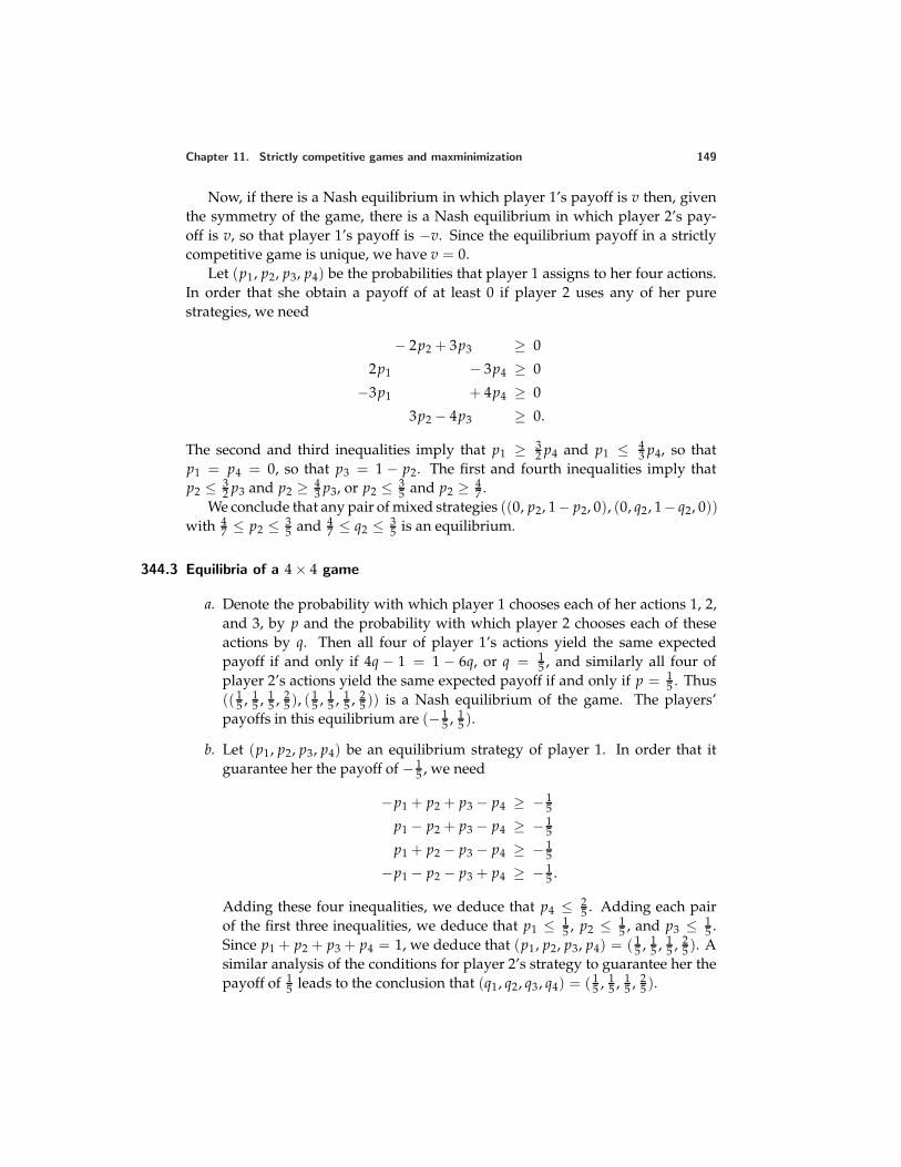
Chapter 11. Strictly competitive games and maxminimization 149
Now, if there is a Nash equilibrium in which player 1’s payoff is v then, giventhe symmetry of the game, there is a Nash equilibrium in which player 2’s pay-off is v, so that player 1’s payoff is −v. Since the equilibrium payoff in a strictlycompetitive game is unique, we have v = 0.
Let (p1, p2, p3, p4) be the probabilities that player 1 assigns to her four actions.In order that she obtain a payoff of at least 0 if player 2 uses any of her purestrategies, we need
− 2p2 + 3p3 ≥ 0
2p1 − 3p4 ≥ 0
−3p1 + 4p4 ≥ 0
3p2 − 4p3 ≥ 0.
The second and third inequalities imply that p1 ≥ 32 p4 and p1 ≤ 4
3 p4, so thatp1 = p4 = 0, so that p3 = 1 − p2. The first and fourth inequalities imply thatp2 ≤ 3
2 p3 and p2 ≥ 43 p3, or p2 ≤ 3
5 and p2 ≥ 47 .
We conclude that any pair of mixed strategies ((0, p2, 1− p2, 0), (0, q2, 1− q2, 0))with 4
7 ≤ p2 ≤ 35 and 4
7 ≤ q2 ≤ 35 is an equilibrium.
344.3 Equilibria of a 4 × 4 game
a. Denote the probability with which player 1 chooses each of her actions 1, 2,and 3, by p and the probability with which player 2 chooses each of theseactions by q. Then all four of player 1’s actions yield the same expectedpayoff if and only if 4q − 1 = 1 − 6q, or q = 1
5 , and similarly all four ofplayer 2’s actions yield the same expected payoff if and only if p = 1
5 . Thus(( 1
5 , 15 , 1
5 , 25 ), ( 1
5 , 15 , 1
5 , 25 )) is a Nash equilibrium of the game. The players’
payoffs in this equilibrium are (− 15 , 1
5 ).
b. Let (p1, p2, p3, p4) be an equilibrium strategy of player 1. In order that itguarantee her the payoff of − 1
5 , we need
−p1 + p2 + p3 − p4 ≥ − 15
p1 − p2 + p3 − p4 ≥ − 15
p1 + p2 − p3 − p4 ≥ − 15
−p1 − p2 − p3 + p4 ≥ − 15 .
Adding these four inequalities, we deduce that p4 ≤ 25 . Adding each pair
of the first three inequalities, we deduce that p1 ≤ 15 , p2 ≤ 1
5 , and p3 ≤ 15 .
Since p1 + p2 + p3 + p4 = 1, we deduce that (p1, p2, p3, p4) = ( 15 , 1
5 , 15 , 2
5 ). Asimilar analysis of the conditions for player 2’s strategy to guarantee her thepayoff of 1
5 leads to the conclusion that (q1, q2, q3, q4) = ( 15 , 1
5 , 15 , 2
5 ).
Draft of solutions to exercises in chapter of An introduction to game theory by Martin J. [email protected]; www.chass.utoronto.ca/~osborne/index.htmlVersion: 00/11/6.Copyright c© 1995–2000 by Martin J. Osborne. All rights reserved. No part of this book may be re-produced in any form by any electronic or mechanical means (including photocopying, recording, orinformation storage and retrieval) without permission in writing from Martin J. Osborne. On request,permission to make one copy for each student will be granted to instructors who wish to use the bookin a course, on condition that copies be sold at a price not more than the cost of duplication.
12 Rationalizability
354.3 Mixed strategy equilibria of game
There is no equilibrium in which player 2 assigns positive probability only to Land C, since if she does so then only M and B are possible best responses forplayer 1, but if player 1 assigns positive probability only to these actions then Lis not optimal for player 2.
By a similar argument there is no equilibrium in which player 2 assigns positiveprobability only to C and R.
Assume that player 2 assigns positive probability only to L and R. There areno probabilities for L and R under which player 1 is indifferent between all threeof her actions, so player 1 must assign positive probability to at most two actions.If these two actions are T and M then player 2 prefers L to R, while if the twoactions are M and B then player 2 prefers R to L. The only possibility is thus thatthe two actions are T and B. In this case we need player 2 to assign probability 1
2to L and R (in order that player 1 be indifferent between T and B); but then M isbetter for player 1. Thus there is no equilibrium in which player 2 assigns positiveprobability only to L and R.
Finally, if player 2 assigns positive probability to all three of her actions thenplayer 1’s mixed strategy must be such that each of these three actions yields thesame payoff. A calculation shows that there is no mixed strategy of player 1 withthis property.
We conclude that the game has no mixed strategy equilibrium in which eitherplayer assigns positive probability to more than one action.
358.1 Example of rationalizable actions
I claim that the action R of player 2 is strictly dominated by some mixed strategiesthat assign positive probability to L and C. Consider such a mixed strategy thatassigns probability p to L. In order for this mixed strategy to strictly dominate Rwe need p + 4(1 − p) > 3 and 8p + 2(1 − p) > 3, or 1
6 < p < 13 . That is, any
such value of p is associated with a mixed strategy that strictly dominated R. Inthe reduced game (i.e. after R is eliminated), B is dominated by T. Finally, L isdominated by C. Hence the only rationalizable action of player 1 is T and the onlyrationalizable action of player 2 is C.
151
152 Chapter 12. Rationalizability
358.2 Guessing Morra
Take Zi to be all the actions of player i, for i = 1, 2. Then (Z1, Z2) satisfies Defini-tion 354.1. (The action S1G2 is a best response to a belief that assigns probability 1to S1G3, the action S1G3 is a best response to the belief that assigns probabilityone to S2G4, the action S2G3 is a best response to the belief that assigns probabil-ity one to S1G2, and the action S2G4 is a best response to the belief that assignsprobability one to S2G3.)
358.3 Contributing to a public good
a. The derivative to player i’s payoff with respect to ci is
−2ci − ∑j =i
cj + wi,
which, for every possible value of ∑j =i cj, is negative if ci > 12 wi. Thus the
contribution wi/2 yields player i a payoff higher than does any larger contri-bution, regardless of the other players’ contributions. (Note that this resultdepends on the sum of the other players’ contributions being nonnegative.)
b. The best response function of player i is given by
max0, 12 (w − ∑
j =icj).
Let c ≤ w/2 and suppose that each of the other players contributes 12 w − c
(which is nonnegative). Then the other players’ total contribution is w − 2c,so that player i’s best response is to contribute c. That is, any contribution c ofat most w/2 is a best response to the belief that assigns probability one to eachof the other player’s contributing 1
2 w − c ≤ 12 w. Thus if we set Zi = [0, w/2]
for all i in Definition 354.1 we see that any action of player i in [0, w/2] isrationalizable for player i. [Note: This argument does not show that actionsoutside [0, w/2] are not rationalizable.]
c. Denote w1 = w2 = w. First eliminate contributions of more than wi/2 byeach player i.
In the reduced game the most that players 1 and 2 together contribute isw (since each contributes at most w/2). Now consider player 3. Given thederivative of her payoff function found in part a, her payoff is increasingin her contribution for every remaining possible value of c1 + c2 so long asc3 < 1
2 (w3 − (c1 + c2)). Since c1 + c2 ≤ w, player 3’s payoff is thus definitelyincreasing for c3 < 1
2 (w3 − w). But w3 ≥ 3w, so player 3’s payoff is definitelyincreasing for c3 < w. We conclude that in the reduced game every contribu-tion of player 3 of less than w is strictly dominated. Eliminate all such actionsof player 3.
Chapter 12. Rationalizability 153
In the newly reduced game every contribution of player 3 is in the interval[w, w3/2]. Now consider player 1. Her payoff is decreasing in her contribu-tion if c1 > 1
2 (w − (c2 + c3)). We have c2 ≥ 0 and c3 ≥ w, so player 1’s payoffis decreasing if c1 > 0. Thus every action of player 1 is strictly dominated bya contribution of 0. The same analysis applies to player 2. Eliminate all suchactions of player 1 and player 2.
Finally, in the game we now have, players 1 and 2 both contribute 0; it followsthat all actions of player 3 are dominated except for a contribution of w3/2,which is her best response to a total contribution of 0 by players 1 and 2.
We conclude that the unique action profile that survives iterated eliminationof strictly dominated actions is (0, 0, w3/2).
358.4 Iterated elimination in location game
In the first round Out is strictly dominated by the position 12 (since the position 1
2guarantees at least a draw, which each player prefers to staying out of the com-petition). In the next round the positions 0 and 1 are strictly dominated by theposition 1
2 : a player who chooses 12 rather than either 0 or 1 ties rather than loses
if her opponent also chooses 12 , and wins outright rather than ties or loses if her
opponent chooses any other position. In every subsequent round the two remain-ing extreme positions are strictly dominated by 1
2 . The only action that remainsis 1
2 . [Note that under the procedure of iterated elimination of weakly dominatedactions, discussed in the next section of the text, there is only one round of elimina-tion: all actions other than 1
2 are weakly dominated by 12 . (In particular, the game
is dominance solvable.)]
361.1 Example of dominance solvability
The Nash equilibria of the game are (T, L), any ((0, 0, 1), (0, q, 1 − q)) with 0 ≤q ≤ 1, and any ((0, p, 1 − p), (0, 0, 1)) with 0 ≤ p ≤ 1. The game is dominancesolvable, because T and L are the only weakly dominated actions, and in they areeliminated the only weakly dominated actions are M and C, leaving (B, R), withpayoffs (0, 0).
If T is eliminated, then L and C, no remaining action is weakly dominated;(M, R) and (B, R) both remain.
361.2 Dominance solvability in demand game
In the first round the demands 0, 1, and 2 are eliminated for each player and inthe second round the demand 4 is eliminated, leaving the outcome in which eachplayer demands 3 (and receives 2).
154 Chapter 12. Rationalizability
361.3 Dominance solvability in Bertrand’s duopoly game
In the first round every price in excess of the monopoly price is weakly dominatedby the monopoly price and every price equal to at most c is weakly dominated bythe price c + 0.01. At each subsequent round the highest remaining price is weaklydominated by the next highest price. (Note that for any p ≥ c + 0.01 it is betterto obtain all the demand at the price p than obtain half of the demand at the pricep + 0.01.) The pair of prices that remains is (c + 0.01, c + 0.01).
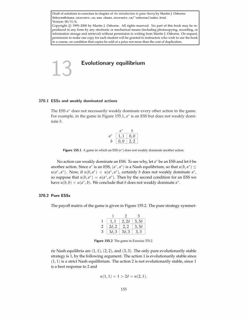
Draft of solutions to exercises in chapter of An introduction to game theory by Martin J. [email protected]; www.chass.utoronto.ca/~osborne/index.htmlVersion: 00/11/6.Copyright c© 1995–2000 by Martin J. Osborne. All rights reserved. No part of this book may be re-produced in any form by any electronic or mechanical means (including photocopying, recording, orinformation storage and retrieval) without permission in writing from Martin J. Osborne. On request,permission to make one copy for each student will be granted to instructors who wish to use the bookin a course, on condition that copies be sold at a price not more than the cost of duplication.
13 Evolutionary equilibrium
370.1 ESSs and weakly dominated actions
The ESS a∗ does not necessarily weakly dominate every other action in the game.For example, in the game in Figure 155.1, a∗ is an ESS but does not weakly domi-nate b.
a∗ ba∗ 1, 1 0, 0b 0, 0 2, 2
Figure 155.1 A game in which an ESS (a∗) does not weakly dominate another action.
No action can weakly dominate an ESS. To see why, let a∗ be an ESS and let b beanother action. Since a∗ is an ESS, (a∗ , a∗) is a Nash equilibrium, so that u(b, a∗) ≤u(a∗ , a∗). Now, if u(b, a∗) < u(a∗ , a∗), certainly b does not weakly dominate a∗,so suppose that u(b, a∗) = u(a∗ , a∗). Then by the second condition for an ESS wehave u(b, b) < u(a∗ , b). We conclude that b does not weakly dominate a∗.
370.2 Pure ESSs
The payoff matrix of the game is given in Figure 155.2. The pure strategy symmet-
1 2 31 1, 1 2, 2δ 3, 3δ
2 2δ, 2 2, 2 3, 3δ
3 3δ, 3 3δ, 3 3, 3
Figure 155.2 The game in Exercise 370.2.
ric Nash equilibria are (1, 1), (2, 2), and (3, 3). The only pure evolutionarily stablestrategy is 1, by the following argument. The action 1 is evolutionarily stable since(1, 1) is a strict Nash equilibrium. The action 2 is not evolutionarily stable, since 1is a best response to 2 and
u(1, 1) = 1 > 2δ = u(2, 1).
155
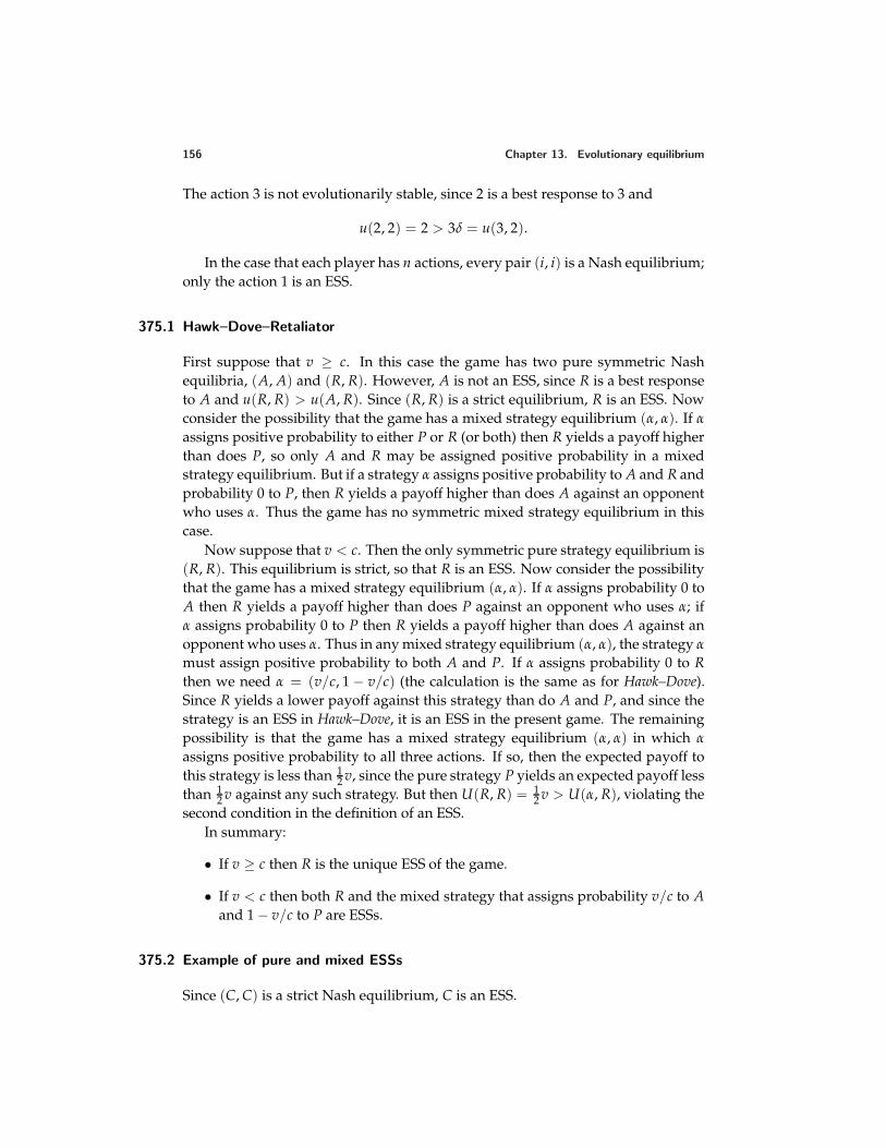
156 Chapter 13. Evolutionary equilibrium
The action 3 is not evolutionarily stable, since 2 is a best response to 3 and
u(2, 2) = 2 > 3δ = u(3, 2).
In the case that each player has n actions, every pair (i, i) is a Nash equilibrium;only the action 1 is an ESS.
375.1 Hawk–Dove–Retaliator
First suppose that v ≥ c. In this case the game has two pure symmetric Nashequilibria, (A, A) and (R, R). However, A is not an ESS, since R is a best responseto A and u(R, R) > u(A, R). Since (R, R) is a strict equilibrium, R is an ESS. Nowconsider the possibility that the game has a mixed strategy equilibrium (α, α). If α
assigns positive probability to either P or R (or both) then R yields a payoff higherthan does P, so only A and R may be assigned positive probability in a mixedstrategy equilibrium. But if a strategy α assigns positive probability to A and R andprobability 0 to P, then R yields a payoff higher than does A against an opponentwho uses α. Thus the game has no symmetric mixed strategy equilibrium in thiscase.
Now suppose that v < c. Then the only symmetric pure strategy equilibrium is(R, R). This equilibrium is strict, so that R is an ESS. Now consider the possibilitythat the game has a mixed strategy equilibrium (α, α). If α assigns probability 0 toA then R yields a payoff higher than does P against an opponent who uses α; ifα assigns probability 0 to P then R yields a payoff higher than does A against anopponent who uses α. Thus in any mixed strategy equilibrium (α, α), the strategy α
must assign positive probability to both A and P. If α assigns probability 0 to Rthen we need α = (v/c, 1 − v/c) (the calculation is the same as for Hawk–Dove).Since R yields a lower payoff against this strategy than do A and P, and since thestrategy is an ESS in Hawk–Dove, it is an ESS in the present game. The remainingpossibility is that the game has a mixed strategy equilibrium (α, α) in which α
assigns positive probability to all three actions. If so, then the expected payoff tothis strategy is less than 1
2 v, since the pure strategy P yields an expected payoff lessthan 1
2 v against any such strategy. But then U(R, R) = 12 v > U(α, R), violating the
second condition in the definition of an ESS.In summary:
• If v ≥ c then R is the unique ESS of the game.
• If v < c then both R and the mixed strategy that assigns probability v/c to Aand 1 − v/c to P are ESSs.
375.2 Example of pure and mixed ESSs
Since (C, C) is a strict Nash equilibrium, C is an ESS.
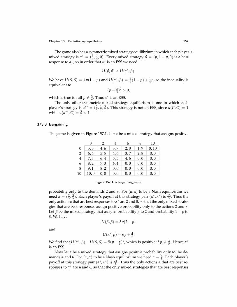
Chapter 13. Evolutionary equilibrium 157
The game also has a symmetric mixed strategy equilibrium in which each player’smixed strategy is α∗ = ( 3
4 , 14 , 0). Every mixed strategy β = (p, 1 − p, 0) is a best
response to α∗, so in order that α∗ is an ESS we need
U(β, β) < U(α∗, β).
We have U(β, β) = 4p(1 − p) and U(α∗, β) = 94 (1 − p) + 1
4 p, so the inequality isequivalent to
(p − 34 )2 > 0,
which is true for all p = 34 . Thus α∗ is an ESS.
The only other symmetric mixed strategy equilibrium is one in which eachplayer’s strategy is α∗∗ = ( 3
7 , 17 , 3
7 ). This strategy is not an ESS, since u(C, C) = 1while u(α∗∗, C) = 3
7 < 1.
375.3 Bargaining
The game is given in Figure 157.1. Let α be a mixed strategy that assigns positive
0 2 4 6 8 100 5, 5 4, 6 3, 7 2, 8 1, 9 0, 102 6, 4 5, 5 4, 6 3, 7 2, 8 0, 04 7, 3 6, 4 5, 5 4, 6 0, 0 0, 06 8, 2 7, 3 6, 4 0, 0 0, 0 0, 08 9, 1 8, 2 0, 0 0, 0 0, 0 0, 0
10 10, 0 0, 0 0, 0 0, 0 0, 0 0, 0
Figure 157.1 A bargaining game.
probability only to the demands 2 and 8. For (α, α) to be a Nash equilibrium weneed α = ( 2
5 , 35 ). Each player’s payoff at this strategy pair (α∗ , α∗) is 16
5 . Thus theonly actions a that are best responses to α∗ are 2 and 8, so that the only mixed strate-gies that are best responses assign positive probability only to the actions 2 and 8.Let β be the mixed strategy that assigns probability p to 2 and probability 1 − p to8. We have
U(β, β) = 5p(2 − p)
andU(α∗, β) = 6p + 4
5 .
We find that U(α∗, β) − U(β, β) = 5(p − 25 )2, which is positive if p = 2
5 . Hence α∗
is an ESS.Now let α be a mixed strategy that assigns positive probability only to the de-
mands 4 and 6. For (α, α) to be a Nash equilibrium we need α = 45 . Each player’s
payoff at this strategy pair (α∗, α∗) is 245 . Thus the only actions a that are best re-
sponses to α∗ are 4 and 6, so that the only mixed strategies that are best responses
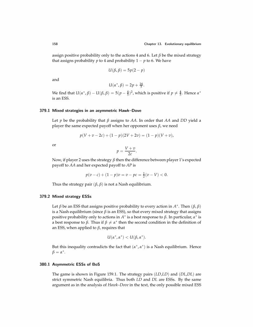
158 Chapter 13. Evolutionary equilibrium
assign positive probability only to the actions 4 and 6. Let β be the mixed strategythat assigns probability p to 4 and probability 1 − p to 6. We have
U(β, β) = 5p(2 − p)
andU(α∗, β) = 2p + 16
5 .
We find that U(α∗, β) − U(β, β) = 5(p − 45 )2, which is positive if p = 4
5 . Hence α∗
is an ESS.
379.1 Mixed strategies in an asymmetric Hawk–Dove
Let p be the probability that β assigns to AA. In order that AA and DD yield aplayer the same expected payoff when her opponent uses β, we need
p(V + v − 2c) + (1 − p)(2V + 2v) = (1 − p)(V + v),
orp =
V + v2c
.
Now, if player 2 uses the strategy β then the difference between player 1’s expectedpayoff to AA and her expected payoff to AP is
p(v − c) + (1 − p)v = v − pc = 12 (v − V) < 0.
Thus the strategy pair (β, β) is not a Nash equilibrium.
379.2 Mixed strategy ESSs
Let β be an ESS that assigns positive probability to every action in A∗. Then (β, β)is a Nash equilibrium (since β is an ESS), so that every mixed strategy that assignspositive probability only to actions in A∗ is a best response to β. In particular, α∗ isa best response to β. Thus if β = α∗ then the second condition in the definition ofan ESS, when applied to β, requires that
U(α∗, α∗) < U(β, α∗).
But this inequality contradicts the fact that (α∗ , α∗) is a Nash equilibrium. Henceβ = α∗.
380.1 Asymmetric ESSs of BoS
The game is shown in Figure 159.1. The strategy pairs (LD,LD) and (DL,DL) arestrict symmetric Nash equilibria. Thus both LD and DL are ESSs. By the sameargument as in the analysis of Hawk–Dove in the text, the only possible mixed ESS
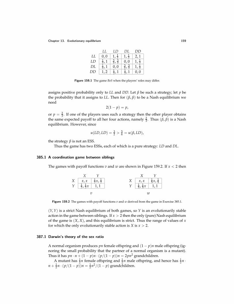
Chapter 13. Evolutionary equilibrium 159
LL LD DL DDLL 0, 0 1, 1
2 1, 12 2, 1
LD 12 , 1 3
2 , 32 0, 0 1, 1
2DL 1
2 , 1 0, 0 32 , 3
2 1, 12
DD 1, 2 12 , 1 1
2 , 1 0, 0
Figure 159.1 The game BoS when the players’ roles may differ.
assigns positive probability only to LL and DD. Let β be such a strategy; let p bethe probability that it assigns to LL. Then for (β, β) to be a Nash equilibrium weneed
2(1 − p) = p,
or p = 23 . If one of the players uses such a strategy then the other player obtains
the same expected payoff to all her four actions, namely 23 . Thus (β, β) is a Nash
equilibrium. However, since
u(LD, LD) = 32 > 5
6 = u(β, LD),
the strategy β is not an ESS.Thus the game has two ESSs, each of which is a pure strategy: LD and DL.
385.1 A coordination game between siblings
The games with payoff functions v and w are shown in Figure 159.2. If x < 2 then
X YX x, x 1
2 x, 12
Y 12 , 1
2 x 1, 1
v
X YX x, x 1
5 x, 15
Y 15 , 1
5 x 1, 1
w
Figure 159.2 The games with payoff functions v and w derived from the game in Exercise 385.1.
(Y, Y) is a strict Nash equilibrium of both games, so Y is an evolutionarily stableaction in the game between siblings. If x > 2 then the only (pure) Nash equilibriumof the game is (X, X), and this equilibrium is strict. Thus the range of values of xfor which the only evolutionarily stable action is X is x > 2.
387.1 Darwin’s theory of the sex ratio
A normal organism produces pn female offspring and (1 − p)n male offspring (ig-noring the small probability that the partner of a normal organism is a mutant).Thus it has pn · n + (1 − p)n · (p/(1 − p))n = 2pn2 grandchildren.
A mutant has 12 n female offspring and 1
2 n male offspring, and hence has 12 n ·
n + 12 n · (p/(1 − p))n = 1
2 n2/(1 − p) grandchildren.
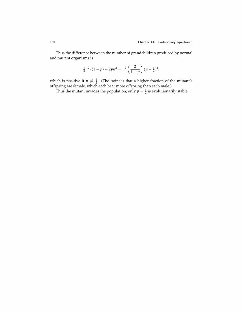
160 Chapter 13. Evolutionary equilibrium
Thus the difference between the number of grandchildren produced by normaland mutant organisms is
12 n2/(1 − p) − 2pn2 = n2
(2
1 − p
)(p − 1
2 )2,
which is positive if p = 12 . (The point is that a higher fraction of the mutant’s
offspring are female, which each bear more offspring than each male.)Thus the mutant invades the population; only p = 1
2 is evolutionarily stable.
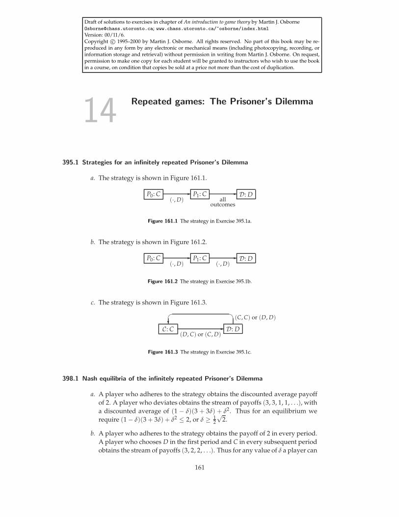
Draft of solutions to exercises in chapter of An introduction to game theory by Martin J. [email protected]; www.chass.utoronto.ca/~osborne/index.htmlVersion: 00/11/6.Copyright c© 1995–2000 by Martin J. Osborne. All rights reserved. No part of this book may be re-produced in any form by any electronic or mechanical means (including photocopying, recording, orinformation storage and retrieval) without permission in writing from Martin J. Osborne. On request,permission to make one copy for each student will be granted to instructors who wish to use the bookin a course, on condition that copies be sold at a price not more than the cost of duplication.
14 Repeated games: The Prisoner’s Dilemma
395.1 Strategies for an infinitely repeated Prisoner’s Dilemma
a. The strategy is shown in Figure 161.1.
P0: C (·, D)
P1: C all
outcomes
D: D
Figure 161.1 The strategy in Exercise 395.1a.
b. The strategy is shown in Figure 161.2.
P0: C (·, D)
P1: C (·, D)
D: D
Figure 161.2 The strategy in Exercise 395.1b.
c. The strategy is shown in Figure 161.3.
C : C D: D(D, C) or (C, D)
(C, C) or (D, D)
Figure 161.3 The strategy in Exercise 395.1c.
398.1 Nash equilibria of the infinitely repeated Prisoner’s Dilemma
a. A player who adheres to the strategy obtains the discounted average payoffof 2. A player who deviates obtains the stream of payoffs (3, 3, 1, 1, . . .), witha discounted average of (1 − δ)(3 + 3δ) + δ2. Thus for an equilibrium werequire (1 − δ)(3 + 3δ) + δ2 ≤ 2, or δ ≥ 1
2
√2.
b. A player who adheres to the strategy obtains the payoff of 2 in every period.A player who chooses D in the first period and C in every subsequent periodobtains the stream of payoffs (3, 2, 2, . . .). Thus for any value of δ a player can
161
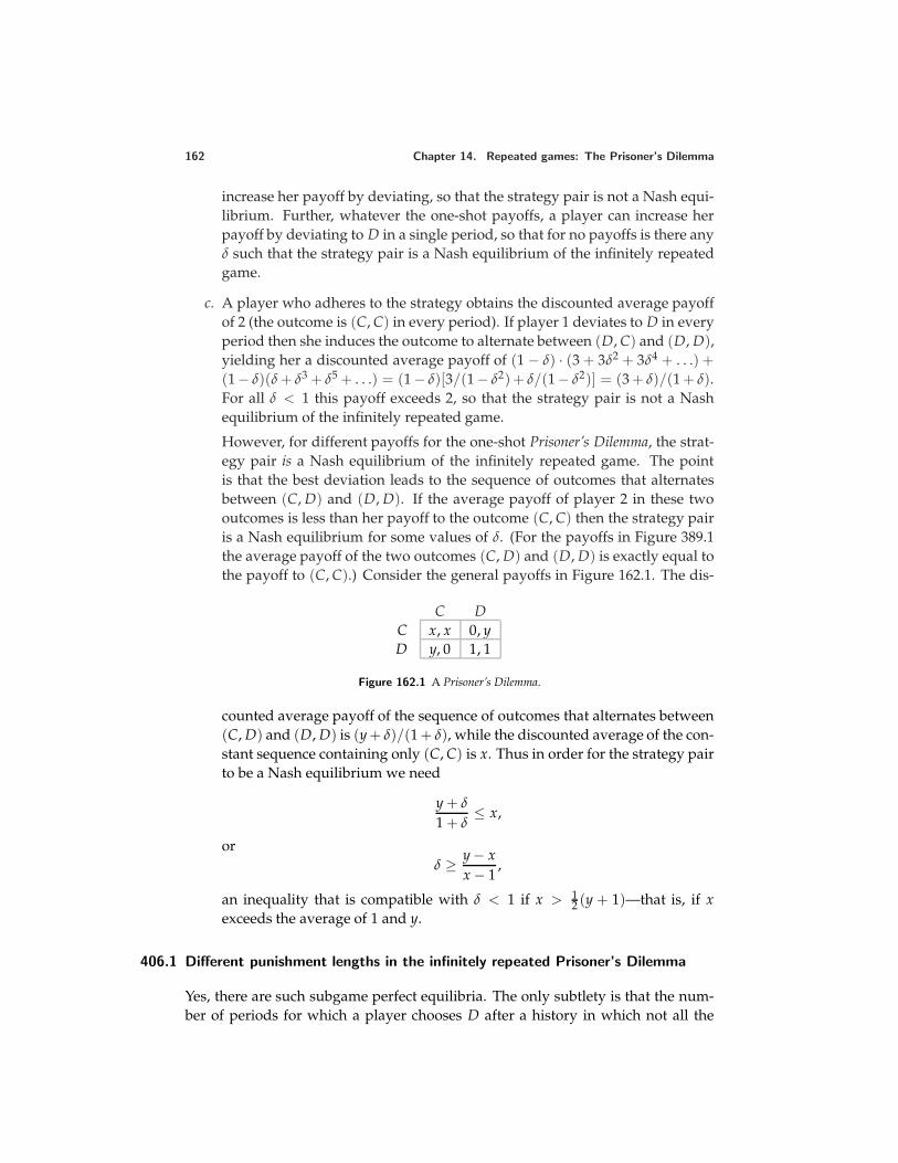
162 Chapter 14. Repeated games: The Prisoner’s Dilemma
increase her payoff by deviating, so that the strategy pair is not a Nash equi-librium. Further, whatever the one-shot payoffs, a player can increase herpayoff by deviating to D in a single period, so that for no payoffs is there anyδ such that the strategy pair is a Nash equilibrium of the infinitely repeatedgame.
c. A player who adheres to the strategy obtains the discounted average payoffof 2 (the outcome is (C, C) in every period). If player 1 deviates to D in everyperiod then she induces the outcome to alternate between (D, C) and (D, D),yielding her a discounted average payoff of (1 − δ) · (3 + 3δ2 + 3δ4 + . . .) +(1− δ)(δ + δ3 + δ5 + . . .) = (1− δ)[3/(1− δ2) + δ/(1− δ2)] = (3 + δ)/(1 + δ).For all δ < 1 this payoff exceeds 2, so that the strategy pair is not a Nashequilibrium of the infinitely repeated game.
However, for different payoffs for the one-shot Prisoner’s Dilemma, the strat-egy pair is a Nash equilibrium of the infinitely repeated game. The pointis that the best deviation leads to the sequence of outcomes that alternatesbetween (C, D) and (D, D). If the average payoff of player 2 in these twooutcomes is less than her payoff to the outcome (C, C) then the strategy pairis a Nash equilibrium for some values of δ. (For the payoffs in Figure 389.1the average payoff of the two outcomes (C, D) and (D, D) is exactly equal tothe payoff to (C, C).) Consider the general payoffs in Figure 162.1. The dis-
C DC x, x 0, yD y, 0 1, 1
Figure 162.1 A Prisoner’s Dilemma.
counted average payoff of the sequence of outcomes that alternates between(C, D) and (D, D) is (y + δ)/(1 + δ), while the discounted average of the con-stant sequence containing only (C, C) is x. Thus in order for the strategy pairto be a Nash equilibrium we need
y + δ
1 + δ≤ x,
orδ ≥ y − x
x − 1,
an inequality that is compatible with δ < 1 if x > 12 (y + 1)—that is, if x
exceeds the average of 1 and y.
406.1 Different punishment lengths in the infinitely repeated Prisoner’s Dilemma
Yes, there are such subgame perfect equilibria. The only subtlety is that the num-ber of periods for which a player chooses D after a history in which not all the
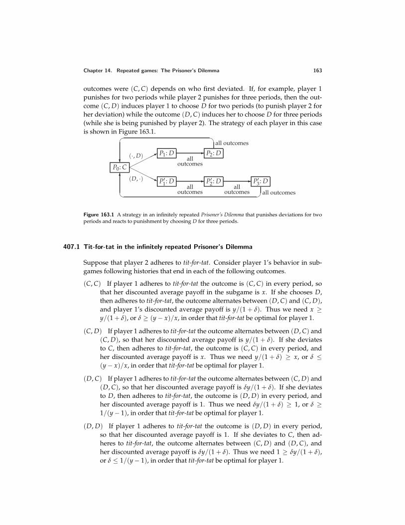
Chapter 14. Repeated games: The Prisoner’s Dilemma 163
outcomes were (C, C) depends on who first deviated. If, for example, player 1punishes for two periods while player 2 punishes for three periods, then the out-come (C, D) induces player 1 to choose D for two periods (to punish player 2 forher deviation) while the outcome (D, C) induces her to choose D for three periods(while she is being punished by player 2). The strategy of each player in this caseis shown in Figure 163.1.
P0: C (·, D) P1: D all
outcomes
P2: D
all outcomes
(D, ·) P′1: D
alloutcomes
P′2: D
alloutcomes
P′3: D
all outcomes
Figure 163.1 A strategy in an infinitely repeated Prisoner’s Dilemma that punishes deviations for twoperiods and reacts to punishment by choosing D for three periods.
407.1 Tit-for-tat in the infinitely repeated Prisoner’s Dilemma
Suppose that player 2 adheres to tit-for-tat. Consider player 1’s behavior in sub-games following histories that end in each of the following outcomes.
(C, C) If player 1 adheres to tit-for-tat the outcome is (C, C) in every period, sothat her discounted average payoff in the subgame is x. If she chooses D,then adheres to tit-for-tat, the outcome alternates between (D, C) and (C, D),and player 1’s discounted average payoff is y/(1 + δ). Thus we need x ≥y/(1 + δ), or δ ≥ (y − x)/x, in order that tit-for-tat be optimal for player 1.
(C, D) If player 1 adheres to tit-for-tat the outcome alternates between (D, C) and(C, D), so that her discounted average payoff is y/(1 + δ). If she deviatesto C, then adheres to tit-for-tat, the outcome is (C, C) in every period, andher discounted average payoff is x. Thus we need y/(1 + δ) ≥ x, or δ ≤(y − x)/x, in order that tit-for-tat be optimal for player 1.
(D, C) If player 1 adheres to tit-for-tat the outcome alternates between (C, D) and(D, C), so that her discounted average payoff is δy/(1 + δ). If she deviatesto D, then adheres to tit-for-tat, the outcome is (D, D) in every period, andher discounted average payoff is 1. Thus we need δy/(1 + δ) ≥ 1, or δ ≥1/(y − 1), in order that tit-for-tat be optimal for player 1.
(D, D) If player 1 adheres to tit-for-tat the outcome is (D, D) in every period,so that her discounted average payoff is 1. If she deviates to C, then ad-heres to tit-for-tat, the outcome alternates between (C, D) and (D, C), andher discounted average payoff is δy/(1 + δ). Thus we need 1 ≥ δy/(1 + δ),or δ ≤ 1/(y − 1), in order that tit-for-tat be optimal for player 1.
164 Chapter 14. Repeated games: The Prisoner’s Dilemma
We conclude that for (tit-for-tat,tit-for-tat) to be a subgame perfect equilibriumwe need δ = (y − x)/x and δ = 1/(y − 1). Thus only if (y − x)/x = 1/(y − 1),or y − x = 1, is the strategy pair a subgame perfect equilibrium. Given that asubgame perfect equilibrium satisfies the one-deviation property, the strategy pairis indeed a subgame perfect equilibrium in this case when δ = 1/x.
Draft of solutions to exercises in chapter of An introduction to game theory by Martin J. [email protected]; www.chass.utoronto.ca/~osborne/index.htmlVersion: 00/11/6.Copyright c© 1995–2000 by Martin J. Osborne. All rights reserved. No part of this book may be re-produced in any form by any electronic or mechanical means (including photocopying, recording, orinformation storage and retrieval) without permission in writing from Martin J. Osborne. On request,permission to make one copy for each student will be granted to instructors who wish to use the bookin a course, on condition that copies be sold at a price not more than the cost of duplication.
17 Mathematical appendix
446.1 Maximizer of quadratic function
We can write the function as −x(x − α). Thus r1 = 0 and r2 = α, and hence themaximizer is α/2.
449.3 Sums of sequences
In the first case set r = δ2 to transform the sum into 1 + r + r2 + · · ·, which is equalto 1/(1 − r) = 1/(1 − δ2).
In the second case split the sum into (1 + δ2 + δ4 + · · ·) + (2δ + 2δ3 + 2δ5 + · · ·);the first part is equal to 1/(1 − δ2) and the second part is equal to 2δ(1 + δ2 + δ4 +· · ·), or 2δ/(1 − δ2). Thus the complete sum is
1 + 2δ
1 − δ2 .
454.1 Bayes’ law
Your posterior probability of carrying X given that you test positive is
Pr(positive test|X) Pr(X)Pr(positive test|X) Pr(X) + Pr(positive test|¬X) Pr(¬X)
where ¬X means “not X”. This probability is equal to 0.9p/(0.9p + 0.2(1 − p)) =0.9p/(0.2 + 0.7p), which is increasing in p (i.e. a smaller value of p gives a smallervalue of the probability). If p = 0.001 then the probability is approximately 0.004.(That is, if 1 in 1,000 people carry the gene then if you test positive on a test thatis 90% accurate for people who carry the gene and 80% accurate for people whodo not carry the gene, then you should assign probability 0.004 to your carryingthe gene.) If the test is 99% accurate in both cases then the posterior probability is(0.99 · 0.001)/[0.99 · 0.001 + 0.01 · 0.999] ≈ 0.09.
171
Corrections and updates for first printing ofOsborne’s “An Introduction to Game Theory”
(Oxford University Press, 2003)
2004/5/4
I thank the following people for pointing out errors and improvements: T. K.Ahn, Kyung Hwan Baik, Richard Boylan, Hao-Chen Liu, Nathan Nunn, DavidA. Malueg, Ahmer Tarar, Debraj Ray, Kaouthar Souki.
Corrections
Page, Line Correction4 The first letter of the text in Section 1.2 should be upper case.6 Add a space after the period on the last line.
31 The “A” in the caption of Figure 31.1 should be upright, not italic.78 In Figure 78.2, replace “B1(p2)” with “B1(t2)” and replace “B2(p1)”
with “B2(t1)”.83 In the first line of the second paragraph, change “complete” to “per-
fect” (for consistency with other terminology).83 The first sentence of the item “Preferences” just below the middle of
the page is hard to follow. A better version is: “Denote by bi the bid of
player i and by b the highest bid submitted by a player other than i. If
either (a) bi > b or (b) bi = b and the number of every other player who
bids b is greater than i, then player i’s payoff is vi − b.”85–87 In the third line of the text on page 85, in the third line of Section 3.5.3
on page 86, and in the fifth line from the bottom of page 87, change“complete” to “perfect” (for consistency with other terminology).
94 The fourth word of the caption of Figure 94.1 should be “shows”.110 Replace “an” at the end of line 16 with “a”.143 Replace F(z) on line 21 with Fi(z).145 Replace “x2 and y2” on the line below the display with “x1 and y1”.145 Delete “a1” at the end of line −8.187 Replace “in” with “is” on line 2.
202–203 The term “equilibrium path” is used without explanation. It is syn-onymous with “equilibrium outcome”. (That is, the equilibrium pathis the terminal history generated by the equilibrium strategies.)
216 The word “that” on the fourth line from the bottom of the page shouldbe “than”.
1
289 In the description of the states above the figure, replace “0 ≤ vi ≤ v”with “v ≤ vi ≤ v”.
291 Replace “a decreasing” with “an increasing” on line 16 and “increases”with “decreases” on line 17.
295 The claim in the last sentence on the page is too strong: the appendixcontains only suggestive arguments, not a proof.
303 In the description of the beliefs in the middle of the page, replace theπ near the start of the second line with Pr(G | g), the 1 − π near theend of the second line with Pr(I | g), the π near the middle of the fifthline with Pr(G | b), and the expression involving 1 − π near the startof the sixth line with Pr(I | b)(1 − q)kqn−k−1.
307 In part c of Exercise 307.1, replace “one of the player’s actions” with“an action of one of the players”. In part d, replace “second” with“first”.
308–309 To deduce the solution of the differential equation near the bottom ofpage 308, the initial condition β(v) = v is needed. Given that thisinitial condition is needed to find the equilibrium bidding function, thepart of Exercise 309.2 asking for a proof that the equilibrium biddingfunction satisfies the condition should be removed. See the website forthe book for a version of Section 9.8.1 that corrects these two points,treats more carefully the boundary cases in which v = v and v = v,and explains the argument more clearly.
310 Two lines below (310.1), replace PrX < v with Pr(X < v). On thefollowing line, delete “= 0”.
319 Change the weak inequality on the next to last line to a strict inequality.321 In the bottom row of the right-hand table in the bottom panel of Fig-
ure 321.1, interchange the entries in the columns headed XY and YX,so that 1/(2 − 4ε) is in the column headed XY and 0 is in the columnheaded YX.
330 In the 7th line of Example 330.1, replace “the history is Acquiesce” with“the history is Unready”.
331 Add a period to the end of the caption of Figure 331.2.331 Replace Exercise 331.2 (which is incorrect) with the following exercise.
EXERCISE 331.2 (Weak sequential equilibrium and Nash equilibriumin subgames) Consider the variant of the game in Figure 331.1 shownin Figure 332.1, in which the challenger’s initial move is broken intotwo steps. Show that this game has a weak sequential equilibrium inwhich the players’ actions in the subgame following the history In donot constitute a Nash equilibrium of the subgame.
2
332–333 Replace the last word on page 332 and the first word on page 333with “a weak”, and replace the penultimate word of the sentence with“strong”.
344 Replace each of the seven occurrences of the string t − b with t + b.389 On line 11, the outcomes that survive are (T, L) and (T, C) (not (T, L)
and (T, R)).415 Add a period to the end of the caption of Figure 415.1.457 Change k − ` to k − ` + 1 on line −2.
Updates
Dhillon and Lockwood (2003) is now
Dhillon, Amrita, and Ben Lockwood (2004), “When are plurality rulevoting games dominance-solvable?”, Games and Economic Behav-ior 46, 55–75.
3
Publiclyavailable solutions for
AN INTRODUCTION TO
GAME THEORY

Publiclyavailable solutions for
AN INTRODUCTION TO
GAME THEORY
MARTIN J. OSBORNE
University of Toronto

Copyright © 2004 by Martin J. Osborne
All rights reserved. No part of this publication may be reproduced, stored in a
retrieval system, or transmitted, in any form or by any means, electronic,
mechanical, photocopying, recording, or otherwise, without the prior permission
of Martin J. Osborne.
This manual was typeset by the author, who is greatly indebted to Donald Knuth
(TEX), Leslie Lamport (LATEX), Diego Puga (mathpazo), Christian Schenk
(MiKTEX), Ed Sznyter (ppctr), Timothy van Zandt (PSTricks), and others, for
generously making superlative software freely available. The main font is 10pt
Palatino.
Version 2: 2004-4-27
Contents
Preface xi
1 Introduction 1
Exercise 5.3 (Altruistic preferences) 1
Exercise 6.1 (Alternative representations of preferences) 1
2 Nash Equilibrium 3
Exercise 16.1 (Working on a joint project) 3
Exercise 17.1 (Games equivalent to the Prisoner’s Dilemma) 3
Exercise 20.1 (Games without conflict) 3
Exercise 31.1 (Extension of the Stag Hunt) 4
Exercise 34.1 (Guessing two-thirds of the average) 4
Exercise 34.3 (Choosing a route) 5
Exercise 37.1 (Finding Nash equilibria using best response functions) 6
Exercise 38.1 (Constructing best response functions) 6
Exercise 38.2 (Dividing money) 7
Exercise 41.1 (Strict and nonstrict Nash equilibria) 7
Exercise 47.1 (Strict equilibria and dominated actions) 8
Exercise 47.2 (Nash equilibrium and weakly dominated actions) 8
Exercise 50.1 (Other Nash equilibria of the game modeling collective
decision-making) 8
Exercise 51.2 (Symmetric strategic games) 9
Exercise 52.2 (Equilibrium for pairwise interactions in a single population) 9
3 Nash Equilibrium: Illustrations 11
Exercise 58.1 (Cournot’s duopoly game with linear inverse demand and different
unit costs) 11
Exercise 60.2 (Nash equilibrium of Cournot’s duopoly game and the collusive
outcome) 12
Exercise 63.1 (Interaction among resource-users) 12
Exercise 67.1 (Bertrand’s duopoly game with constant unit cost) 13
Exercise 68.1 (Bertrand’s oligopoly game) 13
Exercise 68.2 (Bertrand’s duopoly game with different unit costs) 13
Exercise 73.1 (Electoral competition with asymmetric voters’ preferences) 14
Exercise 75.3 (Electoral competition for more general preferences) 14
Exercise 76.1 (Competition in product characteristics) 15
Exercise 79.1 (Direct argument for Nash equilibria of War of Attrition) 15
Exercise 85.1 (Second-price sealed-bid auction with two bidders) 16
v
vi Contents
Exercise 86.2 (Nash equilibrium of first-price sealed-bid auction) 17
Exercise 87.1 (First-price sealed-bid auction) 17
Exercise 89.1 (All-pay auctions) 18
Exercise 90.1 (Multiunit auctions) 18
Exercise 90.3 (Internet pricing) 19
Exercise 96.2 (Alternative standards of care under negligence with contributory
negligence) 19
4 Mixed Strategy Equilibrium 23
Exercise 101.1 (Variant of Matching Pennies) 23
Exercise 106.2 (Extensions of BoS with vNM preferences) 23
Exercise 110.1 (Expected payoffs) 24
Exercise 111.1 (Examples of best responses) 24
Exercise 114.1 (Mixed strategy equilibrium of Hawk–Dove) 25
Exercise 117.2 (Choosing numbers) 26
Exercise 120.2 (Strictly dominating mixed strategies) 26
Exercise 120.3 (Strict domination for mixed strategies) 26
Exercise 127.1 (Equilibrium in the expert diagnosis game) 27
Exercise 130.3 (Bargaining) 27
Exercise 132.2 (Reporting a crime when the witnesses are heterogeneous) 28
Exercise 136.1 (Best response dynamics in Cournot’s duopoly game) 29
Exercise 139.1 (Finding all mixed strategy equilibria of two-player games) 29
Exercise 145.1 (All-pay auction with many bidders) 30
Exercise 147.2 (Preferences over lotteries) 31
Exercise 149.2 (Normalized vNM payoff functions) 31
5 Extensive Games with Perfect Information: Theory 33
Exercise 163.1 (Nash equilibria of extensive games) 33
Exercise 164.2 (Subgames) 33
Exercise 168.1 (Checking for subgame perfect equilibria) 33
Exercise 174.1 (Sharing heterogeneous objects) 34
Exercise 177.3 (Comparing simultaneous and sequential games) 34
Exercise 179.3 (Three Men’s Morris, or Mill) 35
6 Extensive Games with Perfect Information: Illustrations 37
Exercise 183.1 (Nash equilibria of the ultimatum game) 37
Exercise 183.2 (Subgame perfect equilibria of the ultimatum game with indivisible
units) 37
Exercise 186.1 (Holdup game) 37
Exercise 189.1 (Stackelberg’s duopoly game with quadratic costs) 38
Exercise 196.4 (Sequential positioning by three political candidates) 38
Exercise 198.1 (The race G1(2, 2)) 40
Exercise 203.1 (A race with a liquidity constraint) 40
Contents vii
7 Extensive Games with Perfect Information: Extensions and Discussion 43
Exercise 210.2 (Extensive game with simultaneous moves) 43
Exercise 217.1 (Electoral competition with strategic voters) 43
Exercise 220.1 (Top cycle set) 44
Exercise 224.1 (Exit from a declining industry) 45
Exercise 227.1 (Variant of ultimatum game with equity-conscious players) 45
Exercise 230.1 (Nash equilibria when players may make mistakes) 46
Exercise 233.1 (Nash equilibria of the chain-store game) 46
8 Coalitional Games and the Core 47
Exercise 245.1 (Three-player majority game) 47
Exercise 248.1 (Core of landowner–worker game) 47
Exercise 249.1 (Unionized workers in landowner–worker game) 47
Exercise 249.2 (Landowner–worker game with increasing marginal products) 48
Exercise 254.1 (Range of prices in horse market) 48
Exercise 258.1 (House assignment with identical preferences) 49
Exercise 261.1 (Median voter theorem) 49
Exercise 267.2 (Empty core in roommate problem) 49
9 Bayesian Games 51
Exercise 276.1 (Equilibria of a variant of BoS with imperfect information) 51
Exercise 277.1 (Expected payoffs in a variant of BoS with imperfect
information) 51
Exercise 282.2 (An exchange game) 52
Exercise 287.1 (Cournot’s duopoly game with imperfect information) 53
Exercise 288.1 (Cournot’s duopoly game with imperfect information) 53
Exercise 290.1 (Nash equilibria of game of contributing to a public good) 55
Exercise 294.1 (Weak domination in second-price sealed-bid action) 56
Exercise 299.1 (Asymmetric Nash equilibria of second-price sealed-bid common
value auctions) 57
Exercise 299.2 (First-price sealed-bid auction with common valuations) 57
Exercise 309.2 (Properties of the bidding function in a first-price sealed-bid
auction) 58
Exercise 309.3 (Example of Nash equilibrium in a first-price auction) 58
10 Extensive Games with Imperfect Information 59
Exercise 316.1 (Variant of card game) 59
Exercise 318.2 (Strategies in variants of card game and entry game) 59
Exercise 331.2 (Weak sequential equilibrium and Nash equilibrium in
subgames) 60
Exercise 340.1 (Pooling equilibria of game in which expenditure signals quality) 60
Exercise 346.1 (Comparing the receiver’s expected payoff in two equilibria) 61
Exercise 350.1 (Variant of model with piecewise linear payoff functions) 61
viii Contents
11 Strictly Competitive Games and Maxminimization 63
Exercise 363.1 (Maxminimizers in a bargaining game) 63
Exercise 363.3 (Finding a maxminimizer) 63
Exercise 366.2 (Determining strictly competitiveness) 64
Exercise 370.2 (Maxminimizing in BoS) 64
Exercise 372.2 (Equilibrium in strictly competitive game) 64
Exercise 372.4 (O’Neill’s game) 64
12 Rationalizability 67
Exercise 379.2 (Best responses to beliefs) 67
Exercise 384.1 (Mixed strategy equilibria of game in Figure 384.1) 67
Exercise 387.2 (Finding rationalizable actions) 68
Exercise 387.5 (Hotelling’s model of electoral competition) 68
Exercise 388.2 (Cournot’s duopoly game) 68
Exercise 391.1 (Example of dominance-solvable game) 69
Exercise 391.2 (Dividing money) 69
Exercise 392.2 (Strictly competitive extensive games with perfect information) 69
13 Evolutionary Equilibrium 71
Exercise 400.1 (Evolutionary stability and weak domination) 71
Exercise 405.1 (Hawk–Dove–Retaliator) 71
Exercise 405.3 (Bargaining) 72
Exercise 408.1 (Equilibria of C and of G) 72
Exercise 414.1 (A coordination game between siblings) 73
Exercise 414.2 (Assortative mating) 73
Exercise 416.1 (Darwin’s theory of the sex ratio) 74
14 Repeated Games: The Prisoner’s Dilemma 75
Exercise 423.1 (Equivalence of payoff functions) 75
Exercise 426.1 (Subgame perfect equilibrium of finitely repeated Prisoner’s
Dilemma) 75
Exercise 428.1 (Strategies in an infinitely repeated Prisoner’s Dilemma) 76
Exercise 439.1 (Finitely repeated Prisoner’s Dilemma with switching cost) 76
Exercise 442.1 (Deviations from grim trigger strategy) 78
Exercise 443.2 (Different punishment lengths in subgame perfect equilibrium) 78
Exercise 445.1 (Tit-for-tat as a subgame perfect equilibrium) 79
15 Repeated Games: General Results 81
Exercise 454.3 (Repeated Bertrand duopoly) 81
Exercise 459.2 (Detection lags) 82
16 Bargaining 83
Exercise 468.1 (Two-period bargaining with constant cost of delay) 83
Exercise 468.2 (Three-period bargaining with constant cost of delay) 83
Contents ix
17 Appendix: Mathematics 85
Exercise 497.1 (Maximizer of quadratic function) 85
Exercise 499.3 (Sums of sequences) 85
Exercise 504.2 (Bayes’ law) 85
References 87

Preface
This manual contains all publicly-available solutions to exercises in my book An
Introduction to Game Theory (Oxford University Press, 2004). The sources of the
problems are given in the section entitled “Notes” at the end of each chapter of the
book. Please alert me to errors.
MARTIN J. OSBORNE
[email protected] of Economics, 150 St. George Street,University of Toronto, Toronto, Canada M5S 3G7
xi
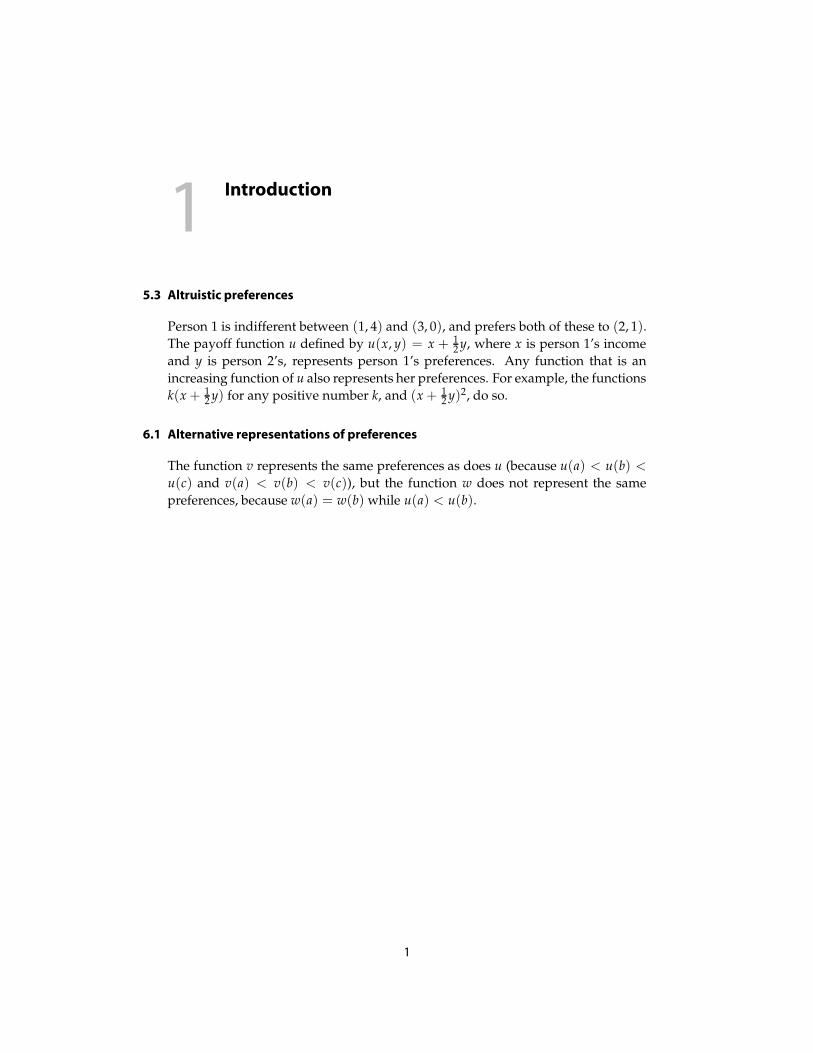
1Introduction
5.3 Altruistic preferences
Person 1 is indifferent between (1, 4) and (3, 0), and prefers both of these to (2, 1).
The payoff function u defined by u(x, y) = x + 12 y, where x is person 1’s income
and y is person 2’s, represents person 1’s preferences. Any function that is an
increasing function of u also represents her preferences. For example, the functions
k(x + 12 y) for any positive number k, and (x + 1
2 y)2, do so.
6.1 Alternative representations of preferences
The function v represents the same preferences as does u (because u(a) < u(b) <
u(c) and v(a) < v(b) < v(c)), but the function w does not represent the same
preferences, because w(a) = w(b) while u(a) < u(b).
1

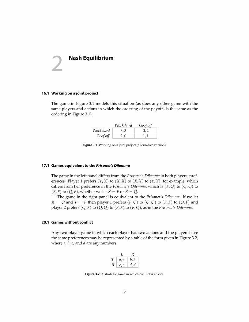
2Nash Equilibrium
16.1 Working on a joint project
The game in Figure 3.1 models this situation (as does any other game with the
same players and actions in which the ordering of the payoffs is the same as the
ordering in Figure 3.1).
Work hard Goof off
Work hard 3, 3 0, 2
Goof off 2, 0 1, 1
Figure 3.1 Working on a joint project (alternative version).
17.1 Games equivalent to the Prisoner’s Dilemma
The game in the left panel differs from the Prisoner’s Dilemma in both players’ pref-
erences. Player 1 prefers (Y, X) to (X, X) to (X, Y) to (Y, Y), for example, which
differs from her preference in the Prisoner’s Dilemma, which is (F, Q) to (Q, Q) to
(F, F) to (Q, F), whether we let X = F or X = Q.
The game in the right panel is equivalent to the Prisoner’s Dilemma. If we let
X = Q and Y = F then player 1 prefers (F, Q) to (Q, Q) to (F, F) to (Q, F) and
player 2 prefers (Q, F) to (Q, Q) to (F, F) to (F, Q), as in the Prisoner’s Dilemma.
20.1 Games without conflict
Any two-player game in which each player has two actions and the players have
the same preferences may be represented by a table of the form given in Figure 3.2,
where a, b, c, and d are any numbers.
L R
T a, a b, b
B c, c d, d
Figure 3.2 A strategic game in which conflict is absent.
3
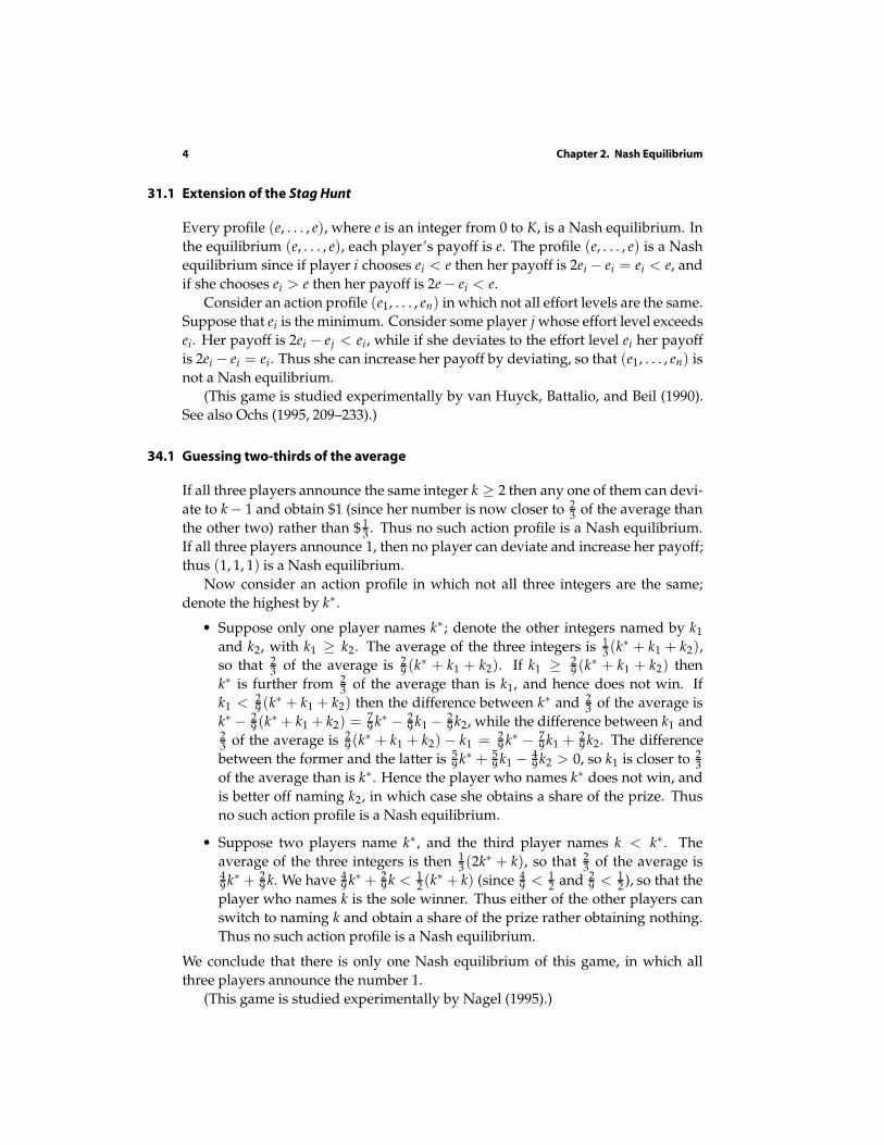
4 Chapter 2. Nash Equilibrium
31.1 Extension of the Stag Hunt
Every profile (e, . . . , e), where e is an integer from 0 to K, is a Nash equilibrium. In
the equilibrium (e, . . . , e), each player’s payoff is e. The profile (e, . . . , e) is a Nash
equilibrium since if player i chooses ei < e then her payoff is 2ei − ei = ei < e, and
if she chooses ei > e then her payoff is 2e − ei < e.
Consider an action profile (e1, . . . , en) in which not all effort levels are the same.
Suppose that ei is the minimum. Consider some player j whose effort level exceeds
ei. Her payoff is 2ei − ej < ei, while if she deviates to the effort level ei her payoff
is 2ei − ei = ei. Thus she can increase her payoff by deviating, so that (e1, . . . , en) is
not a Nash equilibrium.
(This game is studied experimentally by van Huyck, Battalio, and Beil (1990).
See also Ochs (1995, 209–233).)
34.1 Guessing twothirds of the average
If all three players announce the same integer k ≥ 2 then any one of them can devi-
ate to k − 1 and obtain $1 (since her number is now closer to 23 of the average than
the other two) rather than $ 13 . Thus no such action profile is a Nash equilibrium.
If all three players announce 1, then no player can deviate and increase her payoff;
thus (1, 1, 1) is a Nash equilibrium.
Now consider an action profile in which not all three integers are the same;
denote the highest by k∗.
• Suppose only one player names k∗; denote the other integers named by k1
and k2, with k1 ≥ k2. The average of the three integers is 13 (k∗ + k1 + k2),
so that 23 of the average is 2
9 (k∗ + k1 + k2). If k1 ≥ 29 (k∗ + k1 + k2) then
k∗ is further from 23 of the average than is k1, and hence does not win. If
k1 < 29 (k∗ + k1 + k2) then the difference between k∗ and 2
3 of the average is
k∗ − 29 (k∗ + k1 + k2) = 7
9 k∗ − 29 k1 −
29 k2, while the difference between k1 and
23 of the average is 2
9 (k∗ + k1 + k2) − k1 = 29 k∗ − 7
9 k1 + 29 k2. The difference
between the former and the latter is 59 k∗ + 5
9 k1 −49 k2 > 0, so k1 is closer to 2
3of the average than is k∗. Hence the player who names k∗ does not win, and
is better off naming k2, in which case she obtains a share of the prize. Thus
no such action profile is a Nash equilibrium.
• Suppose two players name k∗, and the third player names k < k∗. The
average of the three integers is then 13 (2k∗ + k), so that 2
3 of the average is49 k∗ + 2
9 k. We have 49 k∗ + 2
9 k <12 (k∗ + k) (since 4
9 <12 and 2
9 <12 ), so that the
player who names k is the sole winner. Thus either of the other players can
switch to naming k and obtain a share of the prize rather obtaining nothing.
Thus no such action profile is a Nash equilibrium.
We conclude that there is only one Nash equilibrium of this game, in which all
three players announce the number 1.
(This game is studied experimentally by Nagel (1995).)
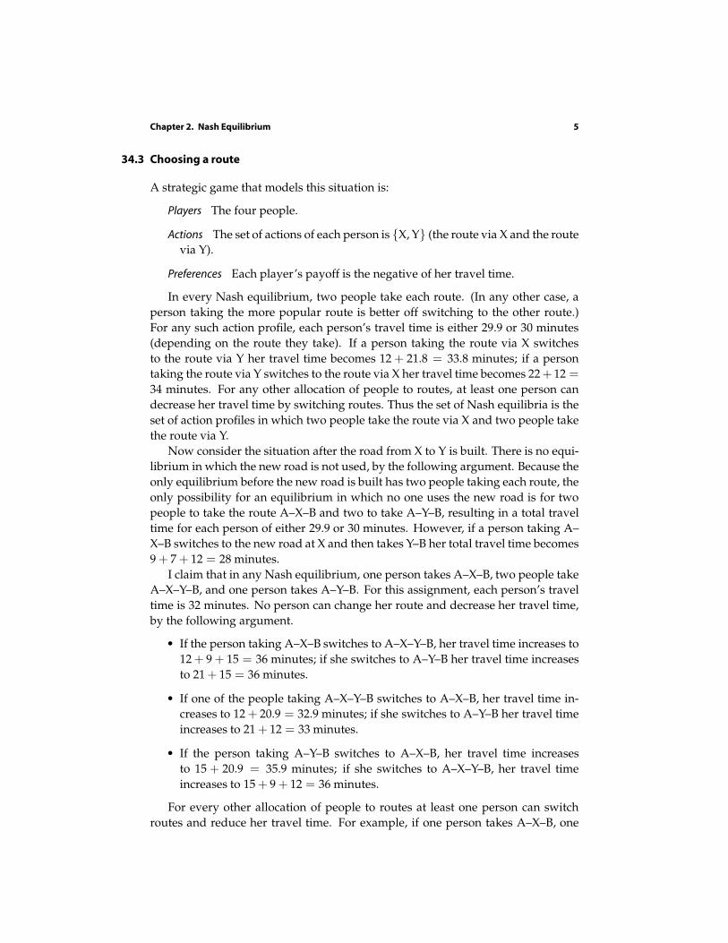
Chapter 2. Nash Equilibrium 5
34.3 Choosing a route
A strategic game that models this situation is:
Players The four people.
Actions The set of actions of each person is X, Y (the route via X and the route
via Y).
Preferences Each player’s payoff is the negative of her travel time.
In every Nash equilibrium, two people take each route. (In any other case, a
person taking the more popular route is better off switching to the other route.)
For any such action profile, each person’s travel time is either 29.9 or 30 minutes
(depending on the route they take). If a person taking the route via X switches
to the route via Y her travel time becomes 12 + 21.8 = 33.8 minutes; if a person
taking the route via Y switches to the route via X her travel time becomes 22 + 12 =34 minutes. For any other allocation of people to routes, at least one person can
decrease her travel time by switching routes. Thus the set of Nash equilibria is the
set of action profiles in which two people take the route via X and two people take
the route via Y.
Now consider the situation after the road from X to Y is built. There is no equi-
librium in which the new road is not used, by the following argument. Because the
only equilibrium before the new road is built has two people taking each route, the
only possibility for an equilibrium in which no one uses the new road is for two
people to take the route A–X–B and two to take A–Y–B, resulting in a total travel
time for each person of either 29.9 or 30 minutes. However, if a person taking A–
X–B switches to the new road at X and then takes Y–B her total travel time becomes
9 + 7 + 12 = 28 minutes.
I claim that in any Nash equilibrium, one person takes A–X–B, two people take
A–X–Y–B, and one person takes A–Y–B. For this assignment, each person’s travel
time is 32 minutes. No person can change her route and decrease her travel time,
by the following argument.
• If the person taking A–X–B switches to A–X–Y–B, her travel time increases to
12 + 9 + 15 = 36 minutes; if she switches to A–Y–B her travel time increases
to 21 + 15 = 36 minutes.
• If one of the people taking A–X–Y–B switches to A–X–B, her travel time in-
creases to 12 + 20.9 = 32.9 minutes; if she switches to A–Y–B her travel time
increases to 21 + 12 = 33 minutes.
• If the person taking A–Y–B switches to A–X–B, her travel time increases
to 15 + 20.9 = 35.9 minutes; if she switches to A–X–Y–B, her travel time
increases to 15 + 9 + 12 = 36 minutes.
For every other allocation of people to routes at least one person can switch
routes and reduce her travel time. For example, if one person takes A–X–B, one
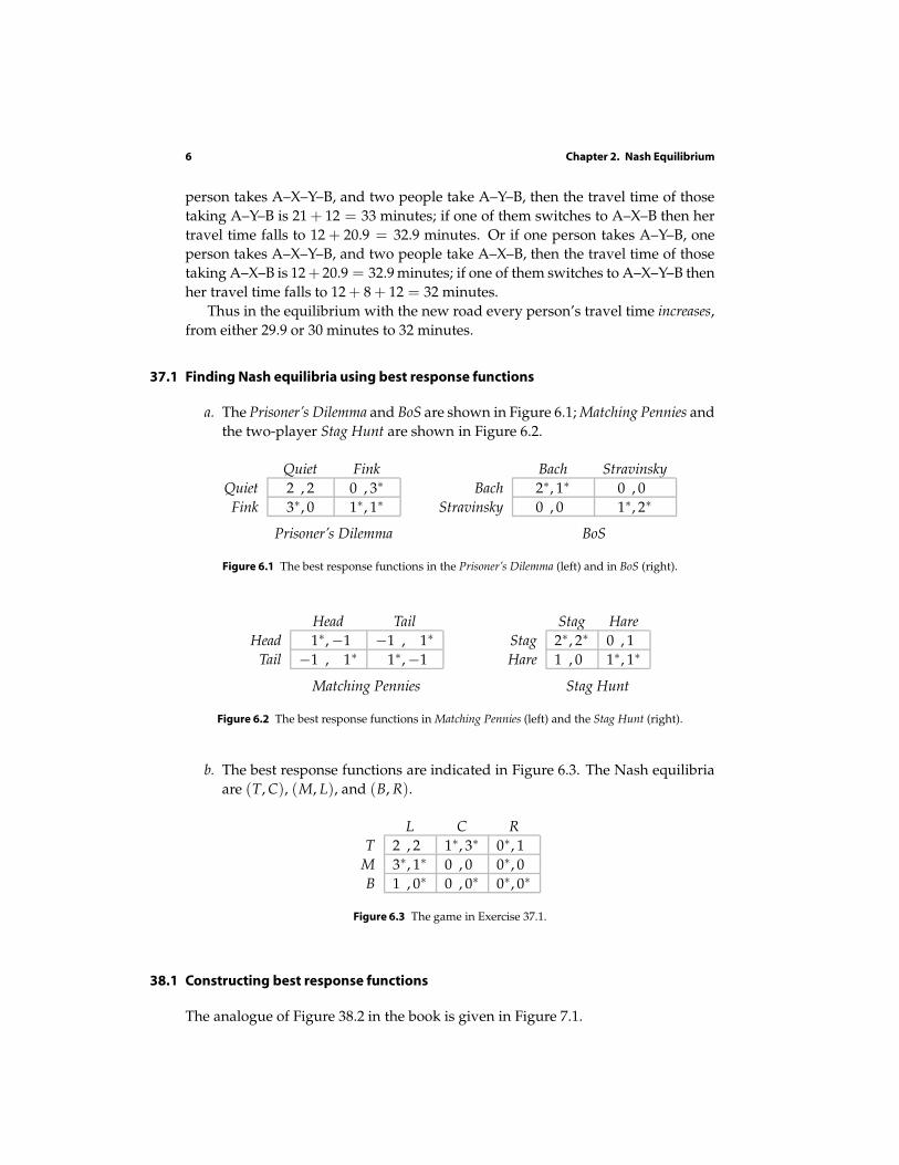
6 Chapter 2. Nash Equilibrium
person takes A–X–Y–B, and two people take A–Y–B, then the travel time of those
taking A–Y–B is 21 + 12 = 33 minutes; if one of them switches to A–X–B then her
travel time falls to 12 + 20.9 = 32.9 minutes. Or if one person takes A–Y–B, one
person takes A–X–Y–B, and two people take A–X–B, then the travel time of those
taking A–X–B is 12 + 20.9 = 32.9 minutes; if one of them switches to A–X–Y–B then
her travel time falls to 12 + 8 + 12 = 32 minutes.
Thus in the equilibrium with the new road every person’s travel time increases,
from either 29.9 or 30 minutes to 32 minutes.
37.1 Finding Nash equilibria using best response functions
a. The Prisoner’s Dilemma and BoS are shown in Figure 6.1; Matching Pennies and
the two-player Stag Hunt are shown in Figure 6.2.
Quiet Fink
Quiet 2 , 2 0 , 3∗
Fink 3∗, 0 1∗, 1∗
Prisoner’s Dilemma
Bach Stravinsky
Bach 2∗, 1∗ 0 , 0
Stravinsky 0 , 0 1∗, 2∗
BoS
Figure 6.1 The best response functions in the Prisoner’s Dilemma (left) and in BoS (right).
Head Tail
Head 1∗,−1 −1 , 1∗
Tail −1 , 1∗ 1∗,−1
Matching Pennies
Stag Hare
Stag 2∗, 2∗ 0 , 1
Hare 1 , 0 1∗, 1∗
Stag Hunt
Figure 6.2 The best response functions in Matching Pennies (left) and the Stag Hunt (right).
b. The best response functions are indicated in Figure 6.3. The Nash equilibria
are (T, C), (M, L), and (B, R).
L C R
T 2 , 2 1∗, 3∗ 0∗, 1
M 3∗, 1∗ 0 , 0 0∗, 0
B 1 , 0∗ 0 , 0∗ 0∗, 0∗
Figure 6.3 The game in Exercise 37.1.
38.1 Constructing best response functions
The analogue of Figure 38.2 in the book is given in Figure 7.1.
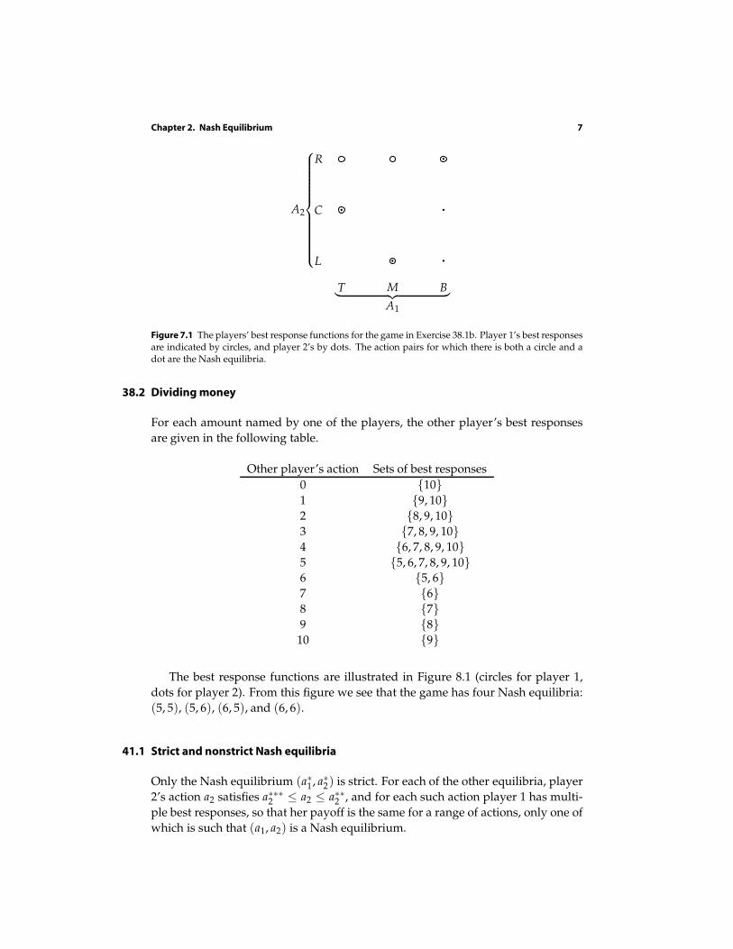
Chapter 2. Nash Equilibrium 7
A1
︸ ︷︷ ︸T M B
A2
L
C
R
Figure 7.1 The players’ best response functions for the game in Exercise 38.1b. Player 1’s best responsesare indicated by circles, and player 2’s by dots. The action pairs for which there is both a circle and adot are the Nash equilibria.
38.2 Dividing money
For each amount named by one of the players, the other player’s best responses
are given in the following table.
Other player’s action Sets of best responses
0 101 9, 102 8, 9, 103 7, 8, 9, 104 6, 7, 8, 9, 105 5, 6, 7, 8, 9, 106 5, 67 68 79 8
10 9
The best response functions are illustrated in Figure 8.1 (circles for player 1,
dots for player 2). From this figure we see that the game has four Nash equilibria:
(5, 5), (5, 6), (6, 5), and (6, 6).
41.1 Strict and nonstrict Nash equilibria
Only the Nash equilibrium (a∗1 , a∗2) is strict. For each of the other equilibria, player
2’s action a2 satisfies a∗∗∗2 ≤ a2 ≤ a∗∗2 , and for each such action player 1 has multi-
ple best responses, so that her payoff is the same for a range of actions, only one of
which is such that (a1, a2) is a Nash equilibrium.
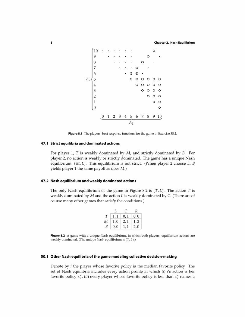
8 Chapter 2. Nash Equilibrium
A1
︸ ︷︷ ︸0 1 2 3 4 5 6 7 8 9 10
A2
0
1
2
3
4
5
6
7
8
9
10
Figure 8.1 The players’ best response functions for the game in Exercise 38.2.
47.1 Strict equilibria and dominated actions
For player 1, T is weakly dominated by M, and strictly dominated by B. For
player 2, no action is weakly or strictly dominated. The game has a unique Nash
equilibrium, (M, L). This equilibrium is not strict. (When player 2 choose L, B
yields player 1 the same payoff as does M.)
47.2 Nash equilibrium and weakly dominated actions
The only Nash equilibrium of the game in Figure 8.2 is (T, L). The action T is
weakly dominated by M and the action L is weakly dominated by C. (There are of
course many other games that satisfy the conditions.)
L C R
T 1, 1 0, 1 0, 0
M 1, 0 2, 1 1, 2
B 0, 0 1, 1 2, 0
Figure 8.2 A game with a unique Nash equilibrium, in which both players’ equilibrium actions areweakly dominated. (The unique Nash equilibrium is (T, L).)
50.1 Other Nash equilibria of the game modeling collective decisionmaking
Denote by i the player whose favorite policy is the median favorite policy. The
set of Nash equilibria includes every action profile in which (i) i’s action is her
favorite policy x∗i , (ii) every player whose favorite policy is less than x∗i names a
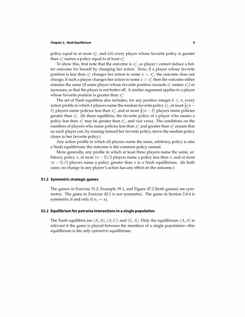
Chapter 2. Nash Equilibrium 9
policy equal to at most x∗i , and (iii) every player whose favorite policy is greater
than x∗i names a policy equal to at least x∗i .
To show this, first note that the outcome is x∗i , so player i cannot induce a bet-
ter outcome for herself by changing her action. Now, if a player whose favorite
position is less than x∗i changes her action to some x < x∗i , the outcome does not
change; if such a player changes her action to some x > x∗i then the outcome either
remains the same (if some player whose favorite position exceeds x∗i names x∗i ) or
increases, so that the player is not better off. A similar argument applies to a player
whose favorite position is greater than x∗i .
The set of Nash equilibria also includes, for any positive integer k ≤ n, every
action profile in which k players name the median favorite policy x∗i , at most 12 (n−
3) players name policies less than x∗i , and at most 12 (n − 3) players name policies
greater than x∗i . (In these equilibria, the favorite policy of a player who names a
policy less than x∗i may be greater than x∗i , and vice versa. The conditions on the
numbers of players who name policies less than x∗i and greater than x∗i ensure that
no such player can, by naming instead her favorite policy, move the median policy
closer to her favorite policy.)
Any action profile in which all players name the same, arbitrary, policy is also
a Nash equilibrium; the outcome is the common policy named.
More generally, any profile in which at least three players name the same, ar-
bitrary, policy x, at most (n − 3)/2 players name a policy less than x, and at most
(n − 3)/2 players name a policy greater than x is a Nash equilibrium. (In both
cases, no change in any player’s action has any effect on the outcome.)
51.2 Symmetric strategic games
The games in Exercise 31.2, Example 39.1, and Figure 47.2 (both games) are sym-
metric. The game in Exercise 42.1 is not symmetric. The game in Section 2.8.4 is
symmetric if and only if u1 = u2.
52.2 Equilibrium for pairwise interactions in a single population
The Nash equilibria are (A, A), (A, C), and (C, A). Only the equilibrium (A, A) is
relevant if the game is played between the members of a single population—this
equilibrium is the only symmetric equilibrium.

3Nash Equilibrium: Illustrations
58.1 Cournot’s duopoly game with linear inverse demand and different unit costs
Following the analysis in the text, the best response function of firm 1 is
b1(q2) =
12 (α − c1 − q2) if q2 ≤ α − c1
0 otherwise
while that of firm 2 is
b2(q1) =
12 (α − c2 − q1) if q1 ≤ α − c2
0 otherwise.
To find the Nash equilibrium, first plot these two functions. Each function has
the same general form as the best response function of either firm in the case stud-
ied in the text. However, the fact that c1 6= c2 leads to two qualitatively different
cases when we combine the two functions to find a Nash equilibrium. If c1 and c2
do not differ very much then the functions in the analogue of Figure 59.1 intersect
at a pair of outputs that are both positive. If c1 and c2 differ a lot, however, the
functions intersect at a pair of outputs in which q1 = 0.
Precisely, if c1 ≤ 12 (α + c2) then the downward-sloping parts of the best re-
sponse functions intersect (as in Figure 59.1), and the game has a unique Nash
equilibrium, given by the solution of the two equations
q1 = 12 (α − c1 − q2)
q2 = 12 (α − c2 − q1).
This solution is
(q∗1 , q∗2) =(
13 (α − 2c1 + c2), 1
3 (α − 2c2 + c1))
.
If c1 >12 (α + c2) then the downward-sloping part of firm 1’s best response
function lies below the downward-sloping part of firm 2’s best response func-
tion (as in Figure 12.1), and the game has a unique Nash equilibrium, (q∗1 , q∗2) =(0, 1
2 (α − c2)).
In summary, the game always has a unique Nash equilibrium, defined as fol-
lows:
(13 (α − 2c1 + c2), 1
3 (α − 2c2 + c1))
if c1 ≤ 12 (α + c2)
(
0, 12 (α − c2)
)
if c1 > 12 (α + c2).
The output of firm 2 exceeds that of firm 1 in every equilibrium.
11
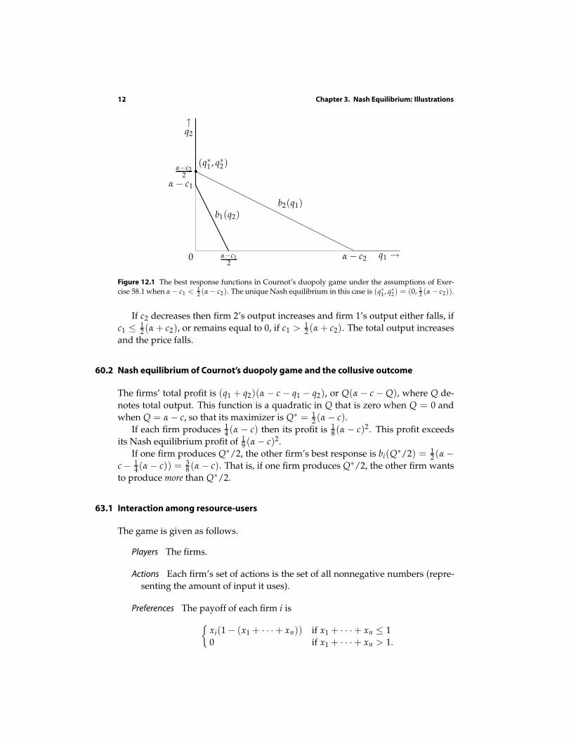
12 Chapter 3. Nash Equilibrium: Illustrations
0 α−c12
α − c2
α−c22
α − c1
↑q2
q1 →
b1(q2)b2(q1)
(q∗1 , q∗2)
Figure 12.1 The best response functions in Cournot’s duopoly game under the assumptions of Exer-cise 58.1 when α − c1 <
12 (α− c2). The unique Nash equilibrium in this case is (q∗1 , q∗2) = (0, 1
2 (α − c2)).
If c2 decreases then firm 2’s output increases and firm 1’s output either falls, if
c1 ≤ 12 (α + c2), or remains equal to 0, if c1 >
12 (α + c2). The total output increases
and the price falls.
60.2 Nash equilibrium of Cournot’s duopoly game and the collusive outcome
The firms’ total profit is (q1 + q2)(α − c − q1 − q2), or Q(α − c − Q), where Q de-
notes total output. This function is a quadratic in Q that is zero when Q = 0 and
when Q = α − c, so that its maximizer is Q∗ = 12 (α − c).
If each firm produces 14 (α − c) then its profit is 1
8 (α − c)2. This profit exceeds
its Nash equilibrium profit of 19 (α − c)2.
If one firm produces Q∗/2, the other firm’s best response is bi(Q∗/2) = 12 (α −
c − 14 (α − c)) = 3
8 (α − c). That is, if one firm produces Q∗/2, the other firm wants
to produce more than Q∗/2.
63.1 Interaction among resourceusers
The game is given as follows.
Players The firms.
Actions Each firm’s set of actions is the set of all nonnegative numbers (repre-
senting the amount of input it uses).
Preferences The payoff of each firm i is
xi(1 − (x1 + · · ·+ xn)) if x1 + · · ·+ xn ≤ 1
0 if x1 + · · ·+ xn > 1.
Chapter 3. Nash Equilibrium: Illustrations 13
This game is the same as that in Exercise 61.1 for c = 0 and α = 1. Thus it has a
unique Nash equilibrium, (x1, . . . , xn) = (1/(n + 1), . . . , 1/(n + 1)).
In this Nash equilibrium, each firm’s output is (1/(n + 1))(1 − n/(n + 1)) =1/(n + 1)2. If xi = 1/(2n) for i = 1, . . . , n then each firm’s output is 1/(4n), which
exceeds 1/(n + 1)2 for n ≥ 2. (We have 1/(4n) − 1/(n + 1)2 = (n − 1)2/(4n(n +1)2) > 0 for n ≥ 2.)
67.1 Bertrand’s duopoly game with constant unit cost
The pair (c, c) of prices remains a Nash equilibrium; the argument is the same
as before. Further, as before, there is no other Nash equilibrium. The argument
needs only very minor modification. For an arbitrary function D there may exist
no monopoly price pm; in this case, if pi > c, pj > c, pi ≥ pj, and D(pj) = 0 then
firm i can increase its profit by reducing its price slightly below p (for example).
68.1 Bertrand’s oligopoly game
Consider a profile (p1, . . . , pn) of prices in which pi ≥ c for all i and at least two
prices are equal to c. Every firm’s profit is zero. If any firm raises its price its profit
remains zero. If a firm charging more than c lowers its price, but not below c, its
profit also remains zero. If a firm lowers its price below c then its profit is negative.
Thus any such profile is a Nash equilibrium.
To show that no other profile is a Nash equilibrium, we can argue as follows.
• If some price is less than c then the firm charging the lowest price can increase
its profit (to zero) by increasing its price to c.
• If exactly one firm’s price is equal to c then that firm can increase its profit by
raising its price a little (keeping it less than the next highest price).
• If all firms’ prices exceed c then the firm charging the highest price can in-
crease its profit by lowering its price to some price between c and the lowest
price being charged.
68.2 Bertrand’s duopoly game with different unit costs
a. If all consumers buy from firm 1 when both firms charge the price c2, then
(p1, p2) = (c2, c2) is a Nash equilibrium by the following argument. Firm 1’s profit
is positive, while firm 2’s profit is zero (since it serves no customers).
• If firm 1 increases its price, its profit falls to zero.
• If firm 1 reduces its price, say to p, then its profit changes from (c2 − c1)(α −c2) to (p − c1)(α − p). Since c2 is less than the maximizer of (p − c1)(α − p),
firm 1’s profit falls.
14 Chapter 3. Nash Equilibrium: Illustrations
• If firm 2 increases its price, its profit remains zero.
• If firm 2 decreases its price, its profit becomes negative (since its price is less
than its unit cost).
Under this rule no other pair of prices is a Nash equilibrium, by the following
argument.
• If pi < c1 for i = 1, 2 then the firm with the lower price (or either firm, if the
prices are the same) can increase its profit (to zero) by raising its price above
that of the other firm.
• If p1 > p2 ≥ c2 then firm 2 can increase its profit by raising its price a little.
• If p2 > p1 ≥ c1 then firm 1 can increase its profit by raising its price a little.
• If p2 ≤ p1 and p2 < c2 then firm 2’s profit is negative, so that it can increase
its profit by raising its price.
• If p1 = p2 > c2 then at least one of the firms is not receiving all of the
demand, and that firm can increase its profit by lowering its price a little.
b. Now suppose that the rule for splitting up the customers when the prices are
equal specifies that firm 2 receives some customers when both prices are c2. By the
argument for part a, the only possible Nash equilibrium is (p1, p2) = (c2, c2). (The
argument in part a that every other pair of prices is not a Nash equilibrium does
not use the fact that customers are split equally when (p1, p2) = (c2, c2).) But if
(p1, p2) = (c2, c2) and firm 2 receives some customers, firm 1 can increase its profit
by reducing its price a little and capturing the entire market.
73.1 Electoral competition with asymmetric voters’ preferences
The unique Nash equilibrium remains (m, m); the direct argument is exactly the
same as before. (The dividing line between the supporters of two candidates with
different positions changes. If xi < xj, for example, the dividing line is 13 xi + 2
3 xj
rather than 12 (xi + xj). The resulting change in the best response functions does
not affect the Nash equilibrium.)
75.3 Electoral competition for more general preferences
a. If x∗ is a Condorcet winner then for any y 6= x∗ a majority of voters prefer
x∗ to y, so y is not a Condorcet winner. Thus there is no more than one
Condorcet winner.
b. Suppose that one of the remaining voters prefers y to z to x, and the other
prefers z to x to y. For each position there is another position preferred by a
majority of voters, so no position is a Condorcet winner.
Chapter 3. Nash Equilibrium: Illustrations 15
c. Now suppose that x∗ is a Condorcet winner. Then the strategic game de-
scribed the exercise has a unique Nash equilibrium in which both candidates
choose x∗. This pair of actions is a Nash equilibrium because if either can-
didate chooses a different position she loses. For any other pair of actions
either one candidate loses, in which case that candidate can deviate to the
position x∗ and at least tie, or the candidates tie at a position different from
x∗, in which case either of them can deviate to x∗ and win.
If there is no Condorcet winner then for every position there is another posi-
tion preferred by a majority of voters. Thus for every pair of distinct positions
the loser can deviate and win, and for every pair of identical positions either
candidate can deviate and win. Thus there is no Nash equilibrium.
76.1 Competition in product characteristics
Suppose there are two firms. If the products are different, then either firm increases
its market share by making its product more similar to that of its rival. Thus in
every possible equilibrium the products are the same. But if x1 = x2 6= m then each
firm’s market share is 50%, while if it changes its product to be closer to m then its
market share rises above 50%. Thus the only possible equilibrium is (x1, x2) =(m, m). This pair of positions is an equilibrium, since each firm’s market share is
50%, and if either firm changes its product its market share falls below 50%.
Now suppose there are three firms. If all firms’ products are the same, each
obtains one-third of the market. If x1 = x2 = x3 = m then any firm, by changing
its product a little, can obtain close to one-half of the market. If x1 = x2 = x3 6= m
then any firm, by changing its product a little, can obtain more than one-half of the
market. If the firms’ products are not all the same, then at least one of the extreme
products is different from the other two products, and the firm that produces it can
increase its market share by making it more similar to the other products. Thus
when there are three firms there is no Nash equilibrium.
79.1 Direct argument for Nash equilibria of War of Attrition
• If t1 = t2 then either player can increase her payoff by conceding slightly
later (in which case she obtains the object for sure, rather than getting it with
probability 12 ).
• If 0 < ti < tj then player i can increase her payoff by conceding at 0.
• If 0 = ti < tj < vi then player i can increase her payoff (from 0 to almost
vi − tj > 0) by conceding slightly after tj.
Thus there is no Nash equilibrium in which t1 = t2, 0 < ti < tj, or 0 = ti <
tj < vi (for i = 1 and j = 2, or i = 2 and j = 1). The remaining possibility is that
0 = ti < tj and tj ≥ vi for i = 1 and j = 2, or i = 2 and j = 1. In this case player i’s
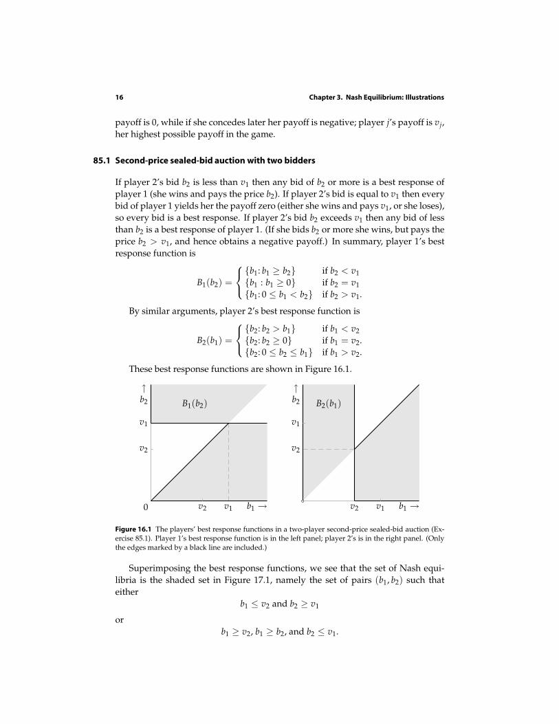
16 Chapter 3. Nash Equilibrium: Illustrations
payoff is 0, while if she concedes later her payoff is negative; player j’s payoff is vj,
her highest possible payoff in the game.
85.1 Secondprice sealedbid auction with two bidders
If player 2’s bid b2 is less than v1 then any bid of b2 or more is a best response of
player 1 (she wins and pays the price b2). If player 2’s bid is equal to v1 then every
bid of player 1 yields her the payoff zero (either she wins and pays v1, or she loses),
so every bid is a best response. If player 2’s bid b2 exceeds v1 then any bid of less
than b2 is a best response of player 1. (If she bids b2 or more she wins, but pays the
price b2 > v1, and hence obtains a negative payoff.) In summary, player 1’s best
response function is
B1(b2) =
b1: b1 ≥ b2 if b2 < v1
b1 : b1 ≥ 0 if b2 = v1
b1: 0 ≤ b1 < b2 if b2 > v1.
By similar arguments, player 2’s best response function is
B2(b1) =
b2: b2 > b1 if b1 < v2
b2: b2 ≥ 0 if b1 = v2.
b2: 0 ≤ b2 ≤ b1 if b1 > v2.
These best response functions are shown in Figure 16.1.
↑b2
b1 →
v1
v2
v1v2
B1(b2)
0
↑b2
b1 →
v1
v2
v1v2
B2(b1)
Figure 16.1 The players’ best response functions in a two-player second-price sealed-bid auction (Ex-ercise 85.1). Player 1’s best response function is in the left panel; player 2’s is in the right panel. (Onlythe edges marked by a black line are included.)
Superimposing the best response functions, we see that the set of Nash equi-
libria is the shaded set in Figure 17.1, namely the set of pairs (b1, b2) such that
either
b1 ≤ v2 and b2 ≥ v1
or
b1 ≥ v2, b1 ≥ b2, and b2 ≤ v1.
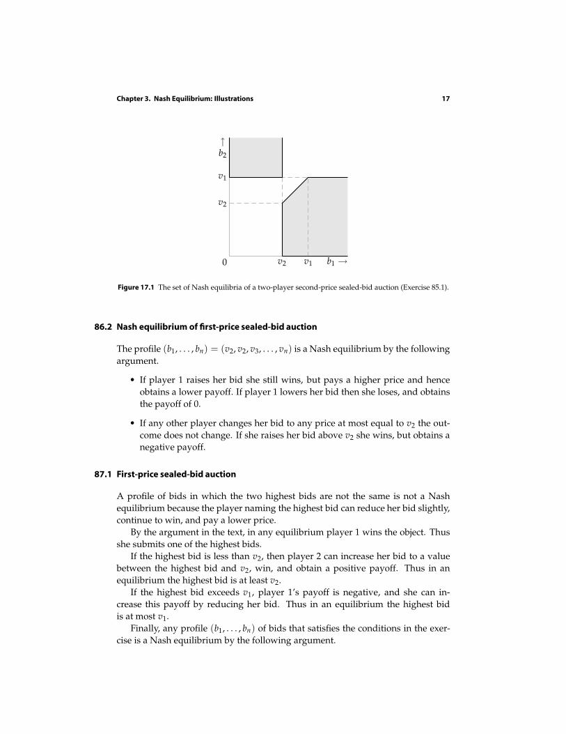
Chapter 3. Nash Equilibrium: Illustrations 17
↑b2
b1 →
v1
v1
v2
v20
Figure 17.1 The set of Nash equilibria of a two-player second-price sealed-bid auction (Exercise 85.1).
86.2 Nash equilibrium of firstprice sealedbid auction
The profile (b1, . . . , bn) = (v2, v2, v3, . . . , vn) is a Nash equilibrium by the following
argument.
• If player 1 raises her bid she still wins, but pays a higher price and hence
obtains a lower payoff. If player 1 lowers her bid then she loses, and obtains
the payoff of 0.
• If any other player changes her bid to any price at most equal to v2 the out-
come does not change. If she raises her bid above v2 she wins, but obtains a
negative payoff.
87.1 Firstprice sealedbid auction
A profile of bids in which the two highest bids are not the same is not a Nash
equilibrium because the player naming the highest bid can reduce her bid slightly,
continue to win, and pay a lower price.
By the argument in the text, in any equilibrium player 1 wins the object. Thus
she submits one of the highest bids.
If the highest bid is less than v2, then player 2 can increase her bid to a value
between the highest bid and v2, win, and obtain a positive payoff. Thus in an
equilibrium the highest bid is at least v2.
If the highest bid exceeds v1, player 1’s payoff is negative, and she can in-
crease this payoff by reducing her bid. Thus in an equilibrium the highest bid
is at most v1.
Finally, any profile (b1, . . . , bn) of bids that satisfies the conditions in the exer-
cise is a Nash equilibrium by the following argument.
18 Chapter 3. Nash Equilibrium: Illustrations
• If player 1 increases her bid she continues to win, and reduces her payoff.
If player 1 decreases her bid she loses and obtains the payoff 0, which is at
most her payoff at (b1, . . . , bn).
• If any other player increases her bid she either does not affect the outcome,
or wins and obtains a negative payoff. If any other player decreases her bid
she does not affect the outcome.
89.1 Allpay auctions
Second-price all-pay auction with two bidders: The payoff function of bidder i is
ui(b1, b2) =
−bi if bi < bj
vi − bj if bi > bj,
with u1(b, b) = v1 − b and u2(b, b) = −b for all b. This payoff function differs from
that of player i in the War of Attrition only in the payoffs when the bids are equal.
The set of Nash equilibria of the game is the same as that for the War of Attrition:
the set of all pairs (0, b2) where b2 ≥ v1 and (b1, 0) where b1 ≥ v2. (The pair (b, b)of actions is not a Nash equilibrium for any value of b because player 2 can increase
her payoff by either increasing her bid slightly or by reducing it to 0.)
First-price all-pay auction with two bidders: In any Nash equilibrium the two
highest bids are equal, otherwise the player with the higher bid can increase her
payoff by reducing her bid a little (keeping it larger than the other player’s bid).
But no profile of bids in which the two highest bids are equal is a Nash equilibrium,
because the player with the higher index who submits this bid can increase her
payoff by slightly increasing her bid, so that she wins rather than loses.
90.1 Multiunit auctions
Discriminatory auction To show that the action of bidding vi and wi is not domi-
nant for player i, we need only find actions for the other players and alterna-
tive bids for player i such that player i’s payoff is higher under the alternative
bids than it is under the vi and wi, given the other players’ actions. Suppose
that each of the other players submits two bids of 0. Then if player i submits
one bid between 0 and vi and one bid between 0 and wi she still wins two
units, and pays less than when she bids vi and wi.
Uniform-price auction Suppose that some bidder other than i submits one bid
between wi and vi and one bid of 0, and all the remaining bidders submit
two bids of 0. Then bidder i wins one unit, and pays the price wi. If she
replaces her bid of wi with a bid between 0 and wi then she pays a lower
price, and hence is better off.
Chapter 3. Nash Equilibrium: Illustrations 19
Vickrey auction Suppose that player i bids vi and wi. Consider separately the
cases in which the bids of the players other than i are such that player i wins
0, 1, and 2 units.
Player i wins 0 units: In this case the second highest of the other players’
bids is at least vi, so that if player i changes her bids so that she wins
one or more units, for any unit she wins she pays at least vi. Thus no
change in her bids increases her payoff from its current value of 0 (and
some changes lower her payoff).
Player i wins 1 unit: If player i raises her bid of vi then she still wins one unit
and the price remains the same. If she lowers this bid then either she still
wins and pays the same price, or she does not win any units. If she raises
her bid of wi then either the outcome does not change, or she wins a sec-
ond unit. In the latter case the price she pays is the previously-winning
bid she beat, which is at least wi, so that her payoff either remains zero
or becomes negative.
Player i wins 2 units: Player i’s raising either of her bids has no effect on the
outcome; her lowering a bid either has no effect on the outcome or leads
her to lose rather than to win, leading her to obtain the payoff of zero.
90.3 Internet pricing
The situation may be modeled as a multiunit auction in which k units are available,
and each player attaches a positive value to only one unit and submits a bid for
only one unit. The k highest bids win, and each winner pays the (k + 1)st highest
bid.
By a variant of the argument for a second-price auction, in which “highest of
the other players’ bids” is replaced by “highest rejected bid”, each player’s action
of bidding her value is weakly dominates all her other actions.
96.2 Alternative standards of care under negligence with contributory negligence
First consider the case in which X1 = a1 and X2 ≤ a2. The pair (a1, a2) is a Nash
equilibrium by the following argument.
If a2 = a2 then the victim’s level of care is sufficient (at least X2), so that the
injurer’s payoff is given by (94.1) in the text. Thus the argument that the injurer’s
action a1 is a best response to a2 is exactly the same as the argument for the case
X2 = a2 in the text.
Since X1 is the same as before, the victim’s payoff is the same also, so that by
the argument in the text the victim’s best response to a1 is a2. Thus (a1, a2) is a
Nash equilibrium.
To show that (a1, a2) is the only Nash equilibrium of the game, we study the
players’ best response functions. First consider the injurer’s best response func-
tion. As in the text, we split the analysis into three cases.
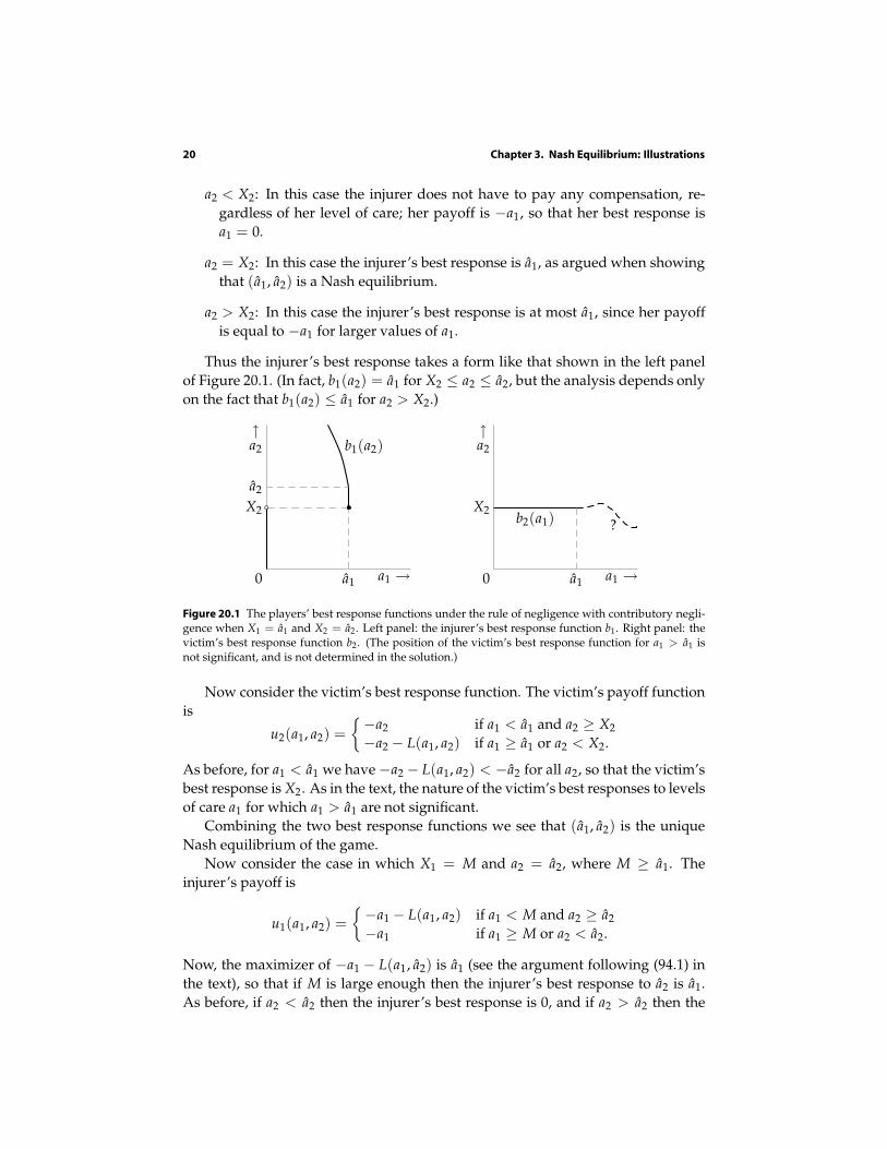
20 Chapter 3. Nash Equilibrium: Illustrations
a2 < X2: In this case the injurer does not have to pay any compensation, re-
gardless of her level of care; her payoff is −a1, so that her best response is
a1 = 0.
a2 = X2: In this case the injurer’s best response is a1, as argued when showing
that (a1, a2) is a Nash equilibrium.
a2 > X2: In this case the injurer’s best response is at most a1, since her payoff
is equal to −a1 for larger values of a1.
Thus the injurer’s best response takes a form like that shown in the left panel
of Figure 20.1. (In fact, b1(a2) = a1 for X2 ≤ a2 ≤ a2, but the analysis depends only
on the fact that b1(a2) ≤ a1 for a2 > X2.)
0
a2
X2
a1a1 →
↑a2 b1(a2)
0
X2
a1a1 →
↑a2
?b2(a1)
Figure 20.1 The players’ best response functions under the rule of negligence with contributory negli-gence when X1 = a1 and X2 = a2. Left panel: the injurer’s best response function b1. Right panel: thevictim’s best response function b2. (The position of the victim’s best response function for a1 > a1 isnot significant, and is not determined in the solution.)
Now consider the victim’s best response function. The victim’s payoff function
is
u2(a1, a2) =
−a2 if a1 < a1 and a2 ≥ X2
−a2 − L(a1, a2) if a1 ≥ a1 or a2 < X2.
As before, for a1 < a1 we have −a2 − L(a1, a2) < −a2 for all a2, so that the victim’s
best response is X2. As in the text, the nature of the victim’s best responses to levels
of care a1 for which a1 > a1 are not significant.
Combining the two best response functions we see that (a1, a2) is the unique
Nash equilibrium of the game.
Now consider the case in which X1 = M and a2 = a2, where M ≥ a1. The
injurer’s payoff is
u1(a1, a2) =
−a1 − L(a1, a2) if a1 < M and a2 ≥ a2
−a1 if a1 ≥ M or a2 < a2.
Now, the maximizer of −a1 − L(a1, a2) is a1 (see the argument following (94.1) in
the text), so that if M is large enough then the injurer’s best response to a2 is a1.
As before, if a2 < a2 then the injurer’s best response is 0, and if a2 > a2 then the
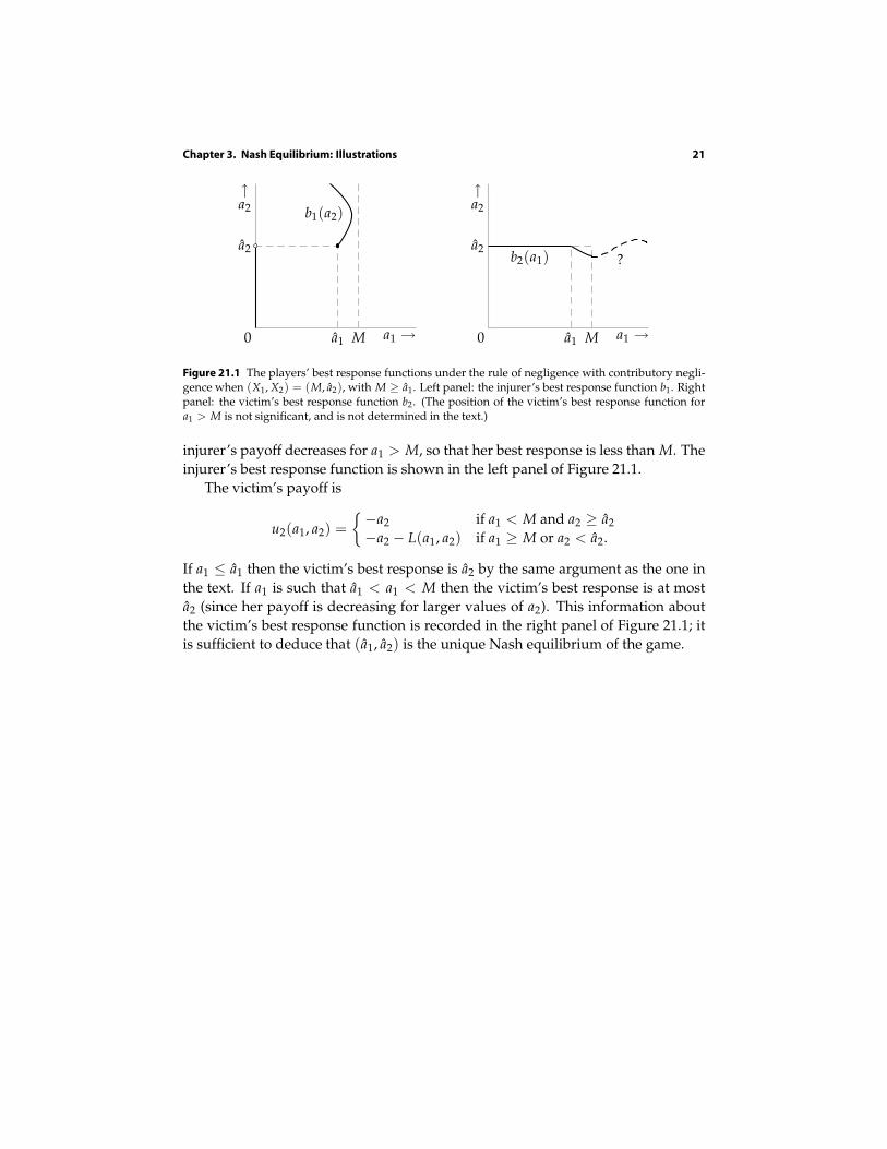
Chapter 3. Nash Equilibrium: Illustrations 21
0
a2
a1 M a1 →
↑a2 b1(a2)
0
a2
a1 M a1 →
↑a2
?b2(a1)
Figure 21.1 The players’ best response functions under the rule of negligence with contributory negli-gence when (X1, X2) = (M, a2), with M ≥ a1. Left panel: the injurer’s best response function b1. Rightpanel: the victim’s best response function b2. (The position of the victim’s best response function fora1 > M is not significant, and is not determined in the text.)
injurer’s payoff decreases for a1 > M, so that her best response is less than M. The
injurer’s best response function is shown in the left panel of Figure 21.1.
The victim’s payoff is
u2(a1, a2) =
−a2 if a1 < M and a2 ≥ a2
−a2 − L(a1, a2) if a1 ≥ M or a2 < a2.
If a1 ≤ a1 then the victim’s best response is a2 by the same argument as the one in
the text. If a1 is such that a1 < a1 < M then the victim’s best response is at most
a2 (since her payoff is decreasing for larger values of a2). This information about
the victim’s best response function is recorded in the right panel of Figure 21.1; it
is sufficient to deduce that (a1, a2) is the unique Nash equilibrium of the game.

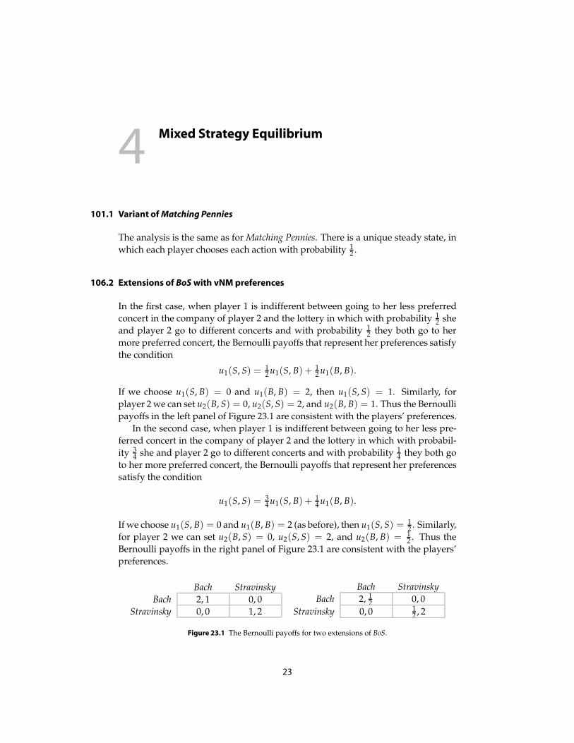
4Mixed Strategy Equilibrium
101.1 Variant of Matching Pennies
The analysis is the same as for Matching Pennies. There is a unique steady state, in
which each player chooses each action with probability 12 .
106.2 Extensions of BoS with vNM preferences
In the first case, when player 1 is indifferent between going to her less preferred
concert in the company of player 2 and the lottery in which with probability 12 she
and player 2 go to different concerts and with probability 12 they both go to her
more preferred concert, the Bernoulli payoffs that represent her preferences satisfy
the condition
u1(S, S) = 12 u1(S, B) + 1
2 u1(B, B).
If we choose u1(S, B) = 0 and u1(B, B) = 2, then u1(S, S) = 1. Similarly, for
player 2 we can set u2(B, S) = 0, u2(S, S) = 2, and u2(B, B) = 1. Thus the Bernoulli
payoffs in the left panel of Figure 23.1 are consistent with the players’ preferences.
In the second case, when player 1 is indifferent between going to her less pre-
ferred concert in the company of player 2 and the lottery in which with probabil-
ity 34 she and player 2 go to different concerts and with probability 1
4 they both go
to her more preferred concert, the Bernoulli payoffs that represent her preferences
satisfy the condition
u1(S, S) = 34 u1(S, B) + 1
4 u1(B, B).
If we choose u1(S, B) = 0 and u1(B, B) = 2 (as before), then u1(S, S) = 12 . Similarly,
for player 2 we can set u2(B, S) = 0, u2(S, S) = 2, and u2(B, B) = 12 . Thus the
Bernoulli payoffs in the right panel of Figure 23.1 are consistent with the players’
preferences.
Bach Stravinsky
Bach 2, 1 0, 0
Stravinsky 0, 0 1, 2
Bach Stravinsky
Bach 2, 12 0, 0
Stravinsky 0, 0 12 , 2
Figure 23.1 The Bernoulli payoffs for two extensions of BoS.
23
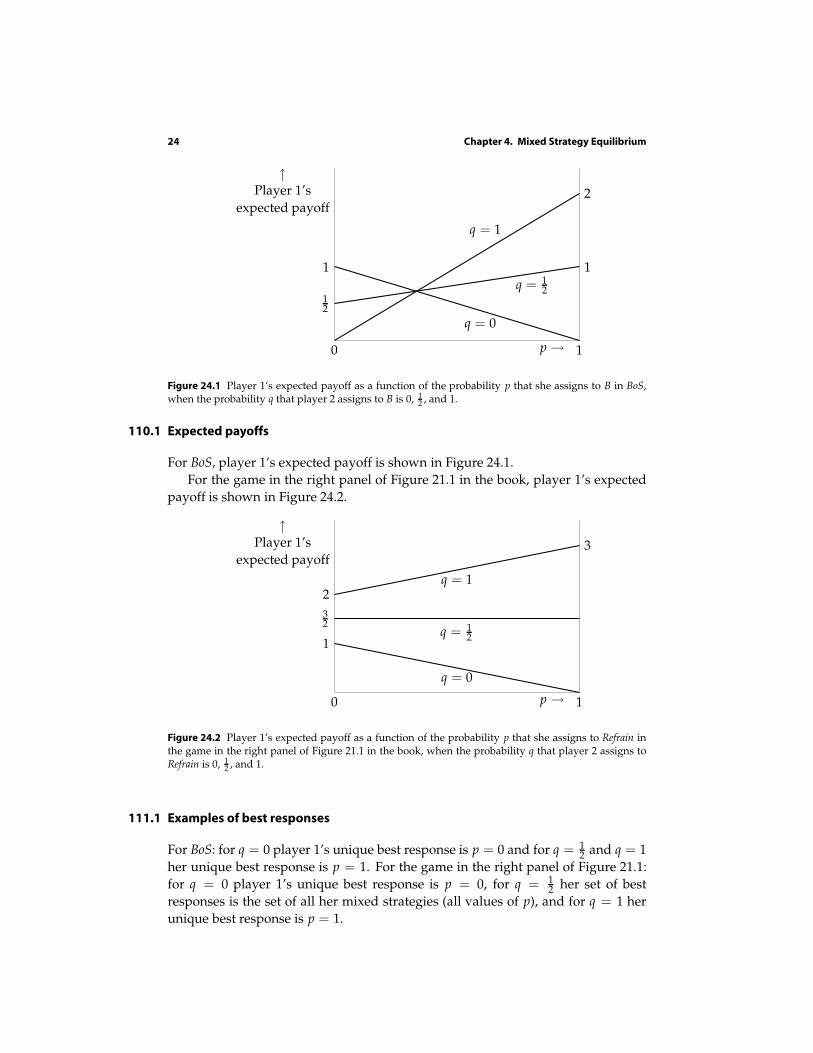
24 Chapter 4. Mixed Strategy Equilibrium
↑Player 1’s
expected payoff2
q = 1
12
1
q = 12
1
q = 0
0 1p →
Figure 24.1 Player 1’s expected payoff as a function of the probability p that she assigns to B in BoS,when the probability q that player 2 assigns to B is 0, 1
2 , and 1.
110.1 Expected payoffs
For BoS, player 1’s expected payoff is shown in Figure 24.1.
For the game in the right panel of Figure 21.1 in the book, player 1’s expected
payoff is shown in Figure 24.2.
↑Player 1’s
expected payoff3
2q = 1
32
q = 12
1
q = 0
0 1p →
Figure 24.2 Player 1’s expected payoff as a function of the probability p that she assigns to Refrain inthe game in the right panel of Figure 21.1 in the book, when the probability q that player 2 assigns toRefrain is 0, 1
2 , and 1.
111.1 Examples of best responses
For BoS: for q = 0 player 1’s unique best response is p = 0 and for q = 12 and q = 1
her unique best response is p = 1. For the game in the right panel of Figure 21.1:
for q = 0 player 1’s unique best response is p = 0, for q = 12 her set of best
responses is the set of all her mixed strategies (all values of p), and for q = 1 her
unique best response is p = 1.
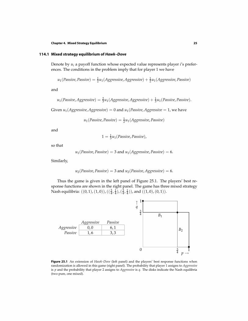
Chapter 4. Mixed Strategy Equilibrium 25
114.1 Mixed strategy equilibrium of Hawk–Dove
Denote by ui a payoff function whose expected value represents player i’s prefer-
ences. The conditions in the problem imply that for player 1 we have
u1(Passive, Passive) = 12 u1(Aggressive, Aggressive) + 1
2 u1(Aggressive, Passive)
and
u1(Passive, Aggressive) = 23 u1(Aggressive, Aggressive) + 1
3 u1(Passive, Passive).
Given u1(Aggressive, Aggressive) = 0 and u1(Passive, Aggressive = 1, we have
u1(Passive, Passive) = 12 u1(Aggressive, Passive)
and
1 = 13 u1(Passive, Passive),
so that
u1(Passive, Passive) = 3 and u1(Aggressive, Passive) = 6.
Similarly,
u2(Passive, Passive) = 3 and u2(Passive, Aggressive) = 6.
Thus the game is given in the left panel of Figure 25.1. The players’ best re-
sponse functions are shown in the right panel. The game has three mixed strategy
Nash equilibria: ((0, 1), (1, 0)), (( 34 , 1
4 ), ( 34 , 1
4 )), and ((1, 0), (0, 1)).
Aggressive Passive
Aggressive 0, 0 6, 1
Passive 1, 6 3, 3
0 34
1p →
34
1↑q
B1
B2
Figure 25.1 An extension of Hawk–Dove (left panel) and the players’ best response functions whenrandomization is allowed in this game (right panel). The probability that player 1 assigns to Aggressive
is p and the probability that player 2 assigns to Aggressive is q. The disks indicate the Nash equilibria(two pure, one mixed).
26 Chapter 4. Mixed Strategy Equilibrium
117.2 Choosing numbers
a. To show that the pair of mixed strategies in the question is a mixed strategy
equilibrium, it suffices to verify the conditions in Proposition 116.2. Thus,
given that each player’s strategy specifies a positive probability for every
action, it suffices to show that each action of each player yields the same
expected payoff. Player 1’s expected payoff to each pure strategy is 1/K,
because with probability 1/K player 2 chooses the same number, and with
probability 1− 1/K player 2 chooses a different number. Similarly, player 2’s
expected payoff to each pure strategy is −1/K, because with probability 1/K
player 1 chooses the same number, and with probability 1 − 1/K player 2
chooses a different number. Thus the pair of strategies is a mixed strategy
Nash equilibrium.
b. Let (p∗, q∗) be a mixed strategy equilibrium, where p∗ and q∗ are vectors,
the jth components of which are the probabilities assigned to the integer j
by each player. Given that player 2 uses the mixed strategy q∗, player 1’s
expected payoff if she chooses the number k is q∗k . Hence if p∗k > 0 then (by
the first condition in Proposition 116.2) we need q∗k ≥ q∗j for all j, so that, in
particular, q∗k > 0 (q∗j cannot be zero for all j!). But player 2’s expected payoff
if she chooses the number k is −p∗k , so given q∗k > 0 we need p∗k ≤ p∗j for all
j (again by the first condition in Proposition 116.2), and, in particular, p∗k ≤1/K (p∗j cannot exceed 1/K for all j!). We conclude that any probability p∗kthat is positive must be at most 1/K. The only possibility is that p∗k = 1/K
for all k. A similar argument implies that q∗k = 1/K for all k.
120.2 Strictly dominating mixed strategies
Denote the probability that player 1 assigns to T by p and the probability she as-
signs to M by r (so that the probability she assigns to B is 1 − p − r). A mixed
strategy of player 1 strictly dominates T if and only if
p + 4r > 1 and p + 3(1− p − r) > 1,
or if and only if 1 − 4r < p < 1 − 32 r. For example, the mixed strategies ( 1
4 , 14 , 1
2 )and (0, 1
4 , 34 ) both strictly dominate T.
120.3 Strict domination for mixed strategies
(a) True. Suppose that the mixed strategy α′i assigns positive probability to the
action a′i, which is strictly dominated by the action ai. Then ui(ai, a−i) > ui(a′i, a−i)for all a−i. Let αi be the mixed strategy that differs from α′i only in the weight that α′iassigns to a′i is transferred to ai. That is, αi is defined by αi(a′i) = 0, αi(ai) = α′i(a′i)+α′i(ai), and αi(bi) = α′i(bi) for every other action bi. Then αi strictly dominates α′i:
for any a−i we have U(αi, a−i)− U(α′i, a−i) = α′i(a′i)(u(ai, a−i) − ui(a′i, a−i)) > 0.
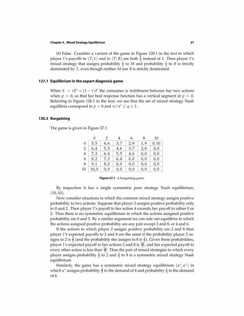
Chapter 4. Mixed Strategy Equilibrium 27
(b) False. Consider a variant of the game in Figure 120.1 in the text in which
player 1’s payoffs to (T, L) and to (T, R) are both 52 instead of 1. Then player 1’s
mixed strategy that assigns probability 12 to M and probability 1
2 to B is strictly
dominated by T, even though neither M nor B is strictly dominated.
127.1 Equilibrium in the expert diagnosis game
When E = rE′ + (1 − r)I′ the consumer is indifferent between her two actions
when p = 0, so that her best response function has a vertical segment at p = 0.
Referring to Figure 126.1 in the text, we see that the set of mixed strategy Nash
equilibria correspond to p = 0 and π/π′ ≤ q ≤ 1.
130.3 Bargaining
The game is given in Figure 27.1.
0 2 4 6 8 10
0 5, 5 4, 6 3, 7 2, 8 1, 9 0, 10
2 6, 4 5, 5 4, 6 3, 7 2, 8 0, 0
4 7, 3 6, 4 5, 5 4, 6 0, 0 0, 0
6 8, 2 7, 3 6, 4 0, 0 0, 0 0, 0
8 9, 1 8, 2 0, 0 0, 0 0, 0 0, 0
10 10, 0 0, 0 0, 0 0, 0 0, 0 0, 0
Figure 27.1 A bargaining game.
By inspection it has a single symmetric pure strategy Nash equilibrium,
(10, 10).
Now consider situations in which the common mixed strategy assigns positive
probability to two actions. Suppose that player 2 assigns positive probability only
to 0 and 2. Then player 1’s payoff to her action 4 exceeds her payoff to either 0 or
2. Thus there is no symmetric equilibrium in which the actions assigned positive
probability are 0 and 2. By a similar argument we can rule out equilibria in which
the actions assigned positive probability are any pair except 2 and 8, or 4 and 6.
If the actions to which player 2 assigns positive probability are 2 and 8 then
player 1’s expected payoffs to 2 and 8 are the same if the probability player 2 as-
signs to 2 is 25 (and the probability she assigns to 8 is 3
5 ). Given these probabilities,
player 1’s expected payoff to her actions 2 and 8 is 165 , and her expected payoff to
every other action is less than 165 . Thus the pair of mixed strategies in which every
player assigns probability 25 to 2 and 3
5 to 8 is a symmetric mixed strategy Nash
equilibrium.
Similarly, the game has a symmetric mixed strategy equilibrium (α∗, α∗) in
which α∗ assigns probability 45 to the demand of 4 and probability 1
5 to the demand
of 6.
28 Chapter 4. Mixed Strategy Equilibrium
In summary, the game has three symmetric mixed strategy Nash equilibria in
which each player’s strategy assigns positive probability to at most two actions:
one in which probability 1 is assigned to 10, one in which probability 25 is assigned
to 2 and probability 35 is assigned to 8, and one in which probability 4
5 is assigned
to 4 and probability 15 is assigned to 6.
132.2 Reporting a crime when the witnesses are heterogeneous
Denote by pi the probability with which each witness with cost ci reports the crime,
for i = 1, 2. For each witness with cost c1 to report with positive probability less
than one, we need
v − c1 = v · Prat least one other person calls
= v(
1 − (1 − p1)n1−1(1 − p2)
n2
)
,
or
c1 = v(1 − p1)n1−1(1 − p2)
n2 . (28.1)
Similarly, for each witness with cost c2 to report with positive probability less than
one, we need
v − c2 = v · Prat least one other person calls
= v(
1 − (1 − p1)n1(1 − p2)
n2−1)
,
or
c2 = v(1 − p1)n1(1 − p2)
n2−1. (28.2)
Dividing (28.1) by (28.2) we obtain
1 − p2 = c1(1 − p1)/c2.
Substituting this expression for 1 − p2 into (28.1) we get
p1 = 1 −
(c1
v·
(c2
c1
)n2)1/(n−1)
.
Similarly,
p2 = 1 −
(c2
v·
(c1
c2
)n1)1/(n−1)
.
For these two numbers to be probabilities, we need each of them to be nonnegative
and at most one, which requires
(
cn22
v
)1/(n2−1)
< c1 <
(
vcn1−12
)1/n1.
Chapter 4. Mixed Strategy Equilibrium 29
136.1 Best response dynamics in Cournot’s duopoly game
The best response functions of both firms are the same, so if the firms’ outputs are
initially the same, they are the same in every period: qt1 = qt
2 for every t. For each
period t, we thus have
qti = 1
2 (α − c − qti).
Given that q1i = 0 for i = 1, 2, solving this first-order difference equation we have
qti = 1
3 (α − c)[1 − (− 12 )t−1]
for each period t. When t is large, qti is close to 1
3 (α − c), a firm’s equilibrium
output.
In the first few periods, these outputs are 0, 12 (α − c), 1
4 (α − c), 38 (α − c), 5
16 (α −c).
139.1 Finding all mixed strategy equilibria of twoplayer games
Left game:
• There is no equilibrium in which each player’s mixed strategy assigns posi-
tive probability to a single action (i.e. there is no pure equilibrium).
• Consider the possibility of an equilibrium in which one player assigns prob-
ability 1 to a single action while the other player assigns positive probability
to both her actions. For neither action of player 1 is player 2’s payoff the same
for both her actions, and for neither action of player 2 is player 1’s payoff the
same for both her actions, so there is no mixed strategy equilibrium of this
type.
• Consider the possibility of a mixed strategy equilibrium in which each player
assigns positive probability to both her actions. Denote by p the probability
player 1 assigns to T and by q the probability player 2 assigns to L. For
player 1’s expected payoff to her two actions to be the same we need
6q = 3q + 6(1 − q),
or q = 23 . For player 2’s expected payoff to her two actions to be the same we
need
2(1 − p) = 6p,
or p = 14 . We conclude that the game has a unique mixed strategy equilib-
rium, (( 14 , 3
4 ), ( 23 , 1
3 )).
Right game:
• By inspection, (T, R) and (B, L) are the pure strategy equilibria.
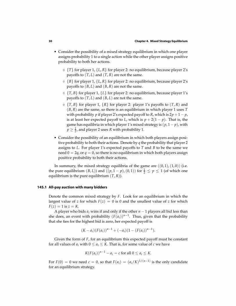
30 Chapter 4. Mixed Strategy Equilibrium
• Consider the possibility of a mixed strategy equilibrium in which one player
assigns probability 1 to a single action while the other player assigns positive
probability to both her actions.
T for player 1, L, R for player 2: no equilibrium, because player 2’s
payoffs to (T, L) and (T, R) are not the same.
B for player 1, L, R for player 2: no equilibrium, because player 2’s
payoffs to (B, L) and (B, R) are not the same.
T, B for player 1, L for player 2: no equilibrium, because player 1’s
payoffs to (T, L) and (B, L) are not the same.
T, B for player 1, R for player 2: player 1’s payoffs to (T, R) and
(B, R) are the same, so there is an equilibrium in which player 1 uses T
with probability p if player 2’s expected payoff to R, which is 2p + 1− p,
is at least her expected payoff to L, which is p + 2(1 − p). That is, the
game has equilibria in which player 1’s mixed strategy is (p, 1− p), with
p ≥ 12 , and player 2 uses R with probability 1.
• Consider the possibility of an equilibrium in which both players assign posi-
tive probability to both their actions. Denote by q the probability that player 2
assigns to L. For player 1’s expected payoffs to T and B to be the same we
need 0 = 2q, or q = 0, so there is no equilibrium in which both players assign
positive probability to both their actions.
In summary, the mixed strategy equilibria of the game are ((0, 1), (1, 0)) (i.e.
the pure equilibrium (B, L)) and ((p, 1 − p), (0, 1)) for 12 ≤ p ≤ 1 (of which one
equilibrium is the pure equilibrium (T, R)).
145.1 Allpay auction with many bidders
Denote the common mixed strategy by F. Look for an equilibrium in which the
largest value of z for which F(z) = 0 is 0 and the smallest value of z for which
F(z) = 1 is z = K.
A player who bids ai wins if and only if the other n − 1 players all bid less than
she does, an event with probability (F(ai))n−1. Thus, given that the probability
that she ties for the highest bid is zero, her expected payoff is
(K − ai)(F(ai))n−1 + (−ai)(1 − (F(ai))
n−1).
Given the form of F, for an equilibrium this expected payoff must be constant
for all values of ai with 0 ≤ ai ≤ K. That is, for some value of c we have
K(F(ai))n−1 − ai = c for all 0 ≤ ai ≤ K.
For F(0) = 0 we need c = 0, so that F(ai) = (ai/K)1/(n−1) is the only candidate
for an equilibrium strategy.
Chapter 4. Mixed Strategy Equilibrium 31
The function F is a cumulative probability distribution on the interval from 0 to
K because F(0) = 0, F(K) = 1, and F is increasing. Thus F is indeed an equilibrium
strategy.
We conclude that the game has a mixed strategy Nash equilibrium in which
each player randomizes over all her actions according to the probability distribu-
tion F(ai) = (ai/K)1/(n−1); each player’s equilibrium expected payoff is 0.
Each player’s mean bid is K/n.
147.2 Preferences over lotteries
The first piece of information about the decision-maker’s preferences among lot-
teries is consistent with her preferences being represented by the expected value
of a payoff function: set u(a1) = 0, u(a2) equal to any number between 12 and 1
4 ,
and u(a3) = 1.
The second piece of information about the decision-maker’s preferences is not
consistent with these preferences being represented by the expected value of a pay-
off function, by the following argument. For consistency with the information
about the decision-maker’s preferences among the four lotteries, we need
0.4u(a1) + 0.6u(a3) > 0.5u(a2) + 0.5u(a3) >
0.3u(a1) + 0.2u(a2) + 0.5u(a3) > 0.45u(a1) + 0.55u(a3).
The first inequality implies u(a2) < 0.8u(a1) + 0.2u(a3) and the last inequality im-
plies u(a2) > 0.75u(a1) + 0.25u(a3). Because u(a1) < u(a3), we have 0.75u(a1) +0.25u(a3) > 0.8u(a1) + 0.2u(a3), so that the two inequalities are incompatible.
149.2 Normalized vNM payoff functions
Let a be the best outcome according to her preferences and let a be the worse out-
come. Let η = −u(a)/(u(a) − u(a)) and θ = 1/(u(a) − u(a)) > 0. Lemma 148.1
implies that the function v defined by v(x) = η + θu(x) represents the same
preferences as does u; we have v(a) = 0 and v(a) = 1.

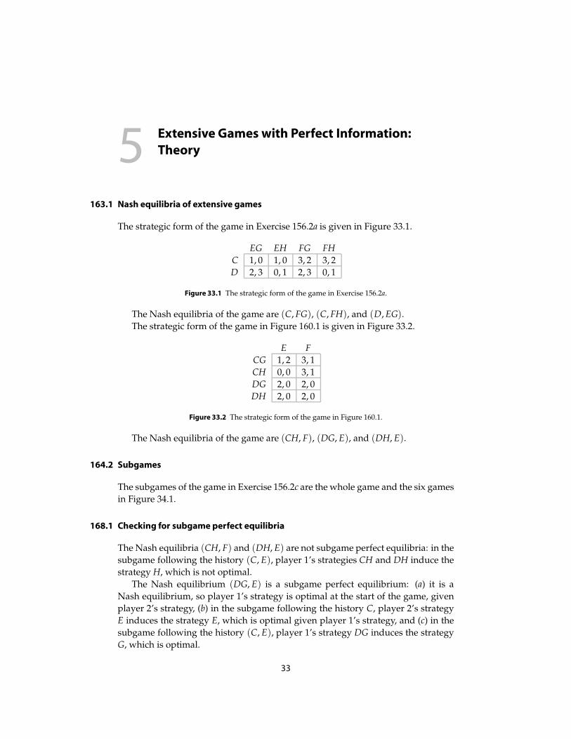
5Extensive Games with Perfect Information:
Theory
163.1 Nash equilibria of extensive games
The strategic form of the game in Exercise 156.2a is given in Figure 33.1.
EG EH FG FH
C 1, 0 1, 0 3, 2 3, 2
D 2, 3 0, 1 2, 3 0, 1
Figure 33.1 The strategic form of the game in Exercise 156.2a.
The Nash equilibria of the game are (C, FG), (C, FH), and (D, EG).
The strategic form of the game in Figure 160.1 is given in Figure 33.2.
E F
CG 1, 2 3, 1
CH 0, 0 3, 1
DG 2, 0 2, 0
DH 2, 0 2, 0
Figure 33.2 The strategic form of the game in Figure 160.1.
The Nash equilibria of the game are (CH, F), (DG, E), and (DH, E).
164.2 Subgames
The subgames of the game in Exercise 156.2c are the whole game and the six games
in Figure 34.1.
168.1 Checking for subgame perfect equilibria
The Nash equilibria (CH, F) and (DH, E) are not subgame perfect equilibria: in the
subgame following the history (C, E), player 1’s strategies CH and DH induce the
strategy H, which is not optimal.
The Nash equilibrium (DG, E) is a subgame perfect equilibrium: (a) it is a
Nash equilibrium, so player 1’s strategy is optimal at the start of the game, given
player 2’s strategy, (b) in the subgame following the history C, player 2’s strategy
E induces the strategy E, which is optimal given player 1’s strategy, and (c) in the
subgame following the history (C, E), player 1’s strategy DG induces the strategy
G, which is optimal.
33
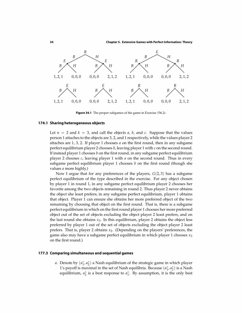
34 Chapter 5. Extensive Games with Perfect Information: Theory
HBR
H
0, 0, 0
B
1, 2, 1
EH
2, 1, 2
B
0, 0, 0
EHB
E
H
0, 0, 0
B
1, 2, 1
RH
2, 1, 2
B
0, 0, 0
R
H
0, 0, 0
B
1, 2, 1
EH
2, 1, 2
B
0, 0, 0
EH
0, 0, 0
B
1, 2, 1
RH
2, 1, 2
B
0, 0, 0
R
Figure 34.1 The proper subgames of the game in Exercise 156.2c.
174.1 Sharing heterogeneous objects
Let n = 2 and k = 3, and call the objects a, b, and c. Suppose that the values
person 1 attaches to the objects are 3, 2, and 1 respectively, while the values player 2
attaches are 1, 3, 2. If player 1 chooses a on the first round, then in any subgame
perfect equilibrium player 2 chooses b, leaving player 1 with c on the second round.
If instead player 1 chooses b on the first round, in any subgame perfect equilibrium
player 2 chooses c, leaving player 1 with a on the second round. Thus in every
subgame perfect equilibrium player 1 chooses b on the first round (though she
values a more highly.)
Now I argue that for any preferences of the players, G(2, 3) has a subgame
perfect equilibrium of the type described in the exercise. For any object chosen
by player 1 in round 1, in any subgame perfect equilibrium player 2 chooses her
favorite among the two objects remaining in round 2. Thus player 2 never obtains
the object she least prefers; in any subgame perfect equilibrium, player 1 obtains
that object. Player 1 can ensure she obtains her more preferred object of the two
remaining by choosing that object on the first round. That is, there is a subgame
perfect equilibrium in which on the first round player 1 chooses her more preferred
object out of the set of objects excluding the object player 2 least prefers, and on
the last round she obtains x3. In this equilibrium, player 2 obtains the object less
preferred by player 1 out of the set of objects excluding the object player 2 least
prefers. That is, player 2 obtains x2. (Depending on the players’ preferences, the
game also may have a subgame perfect equilibrium in which player 1 chooses x3
on the first round.)
177.3 Comparing simultaneous and sequential games
a. Denote by (a∗1 , a∗2) a Nash equilibrium of the strategic game in which player
1’s payoff is maximal in the set of Nash equilibria. Because (a∗1 , a∗2) is a Nash
equilibrium, a∗2 is a best response to a∗1 . By assumption, it is the only best
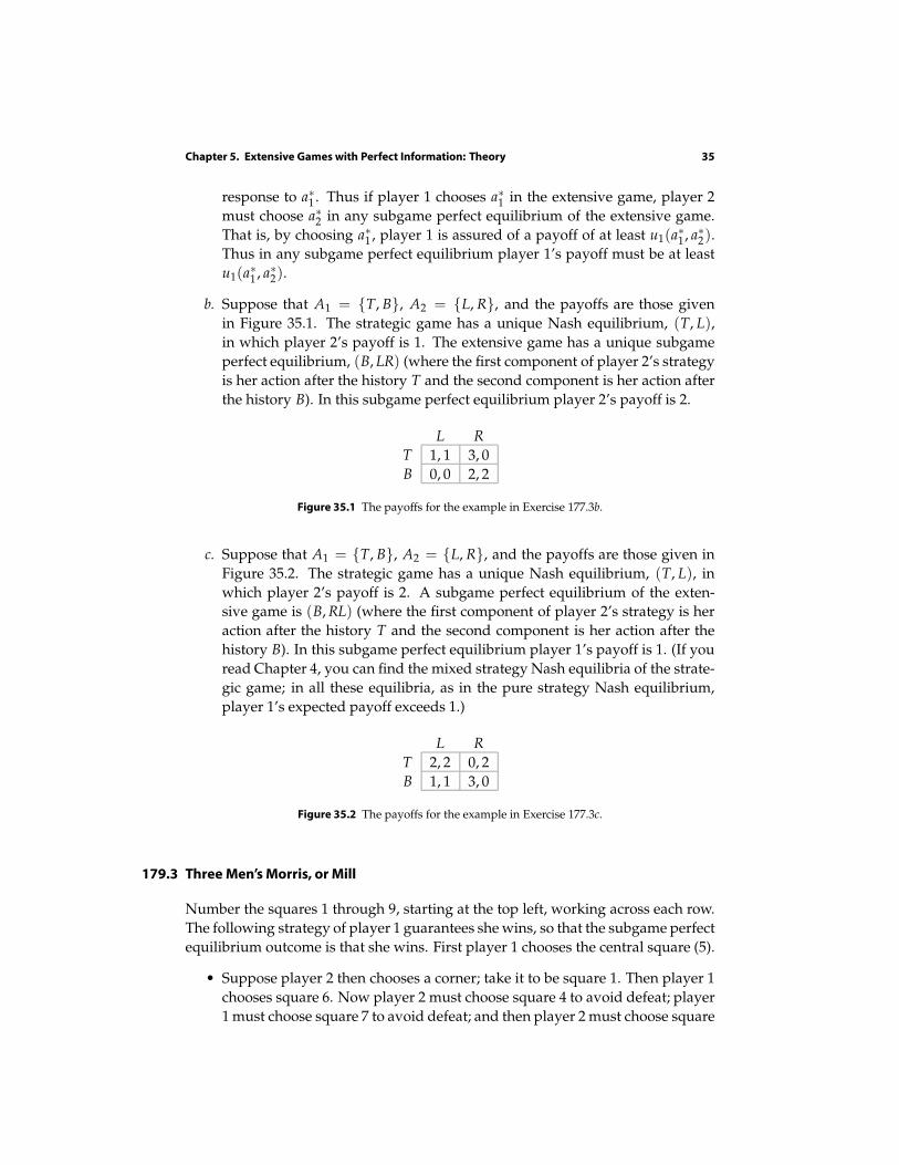
Chapter 5. Extensive Games with Perfect Information: Theory 35
response to a∗1 . Thus if player 1 chooses a∗1 in the extensive game, player 2
must choose a∗2 in any subgame perfect equilibrium of the extensive game.
That is, by choosing a∗1 , player 1 is assured of a payoff of at least u1(a∗1 , a∗2).
Thus in any subgame perfect equilibrium player 1’s payoff must be at least
u1(a∗1 , a∗2).
b. Suppose that A1 = T, B, A2 = L, R, and the payoffs are those given
in Figure 35.1. The strategic game has a unique Nash equilibrium, (T, L),
in which player 2’s payoff is 1. The extensive game has a unique subgame
perfect equilibrium, (B, LR) (where the first component of player 2’s strategy
is her action after the history T and the second component is her action after
the history B). In this subgame perfect equilibrium player 2’s payoff is 2.
L R
T 1, 1 3, 0
B 0, 0 2, 2
Figure 35.1 The payoffs for the example in Exercise 177.3b.
c. Suppose that A1 = T, B, A2 = L, R, and the payoffs are those given in
Figure 35.2. The strategic game has a unique Nash equilibrium, (T, L), in
which player 2’s payoff is 2. A subgame perfect equilibrium of the exten-
sive game is (B, RL) (where the first component of player 2’s strategy is her
action after the history T and the second component is her action after the
history B). In this subgame perfect equilibrium player 1’s payoff is 1. (If you
read Chapter 4, you can find the mixed strategy Nash equilibria of the strate-
gic game; in all these equilibria, as in the pure strategy Nash equilibrium,
player 1’s expected payoff exceeds 1.)
L R
T 2, 2 0, 2
B 1, 1 3, 0
Figure 35.2 The payoffs for the example in Exercise 177.3c.
179.3 Three Men’s Morris, or Mill
Number the squares 1 through 9, starting at the top left, working across each row.
The following strategy of player 1 guarantees she wins, so that the subgame perfect
equilibrium outcome is that she wins. First player 1 chooses the central square (5).
• Suppose player 2 then chooses a corner; take it to be square 1. Then player 1
chooses square 6. Now player 2 must choose square 4 to avoid defeat; player
1 must choose square 7 to avoid defeat; and then player 2 must choose square
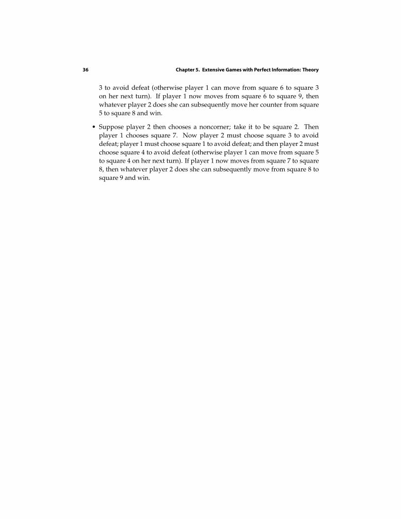
36 Chapter 5. Extensive Games with Perfect Information: Theory
3 to avoid defeat (otherwise player 1 can move from square 6 to square 3
on her next turn). If player 1 now moves from square 6 to square 9, then
whatever player 2 does she can subsequently move her counter from square
5 to square 8 and win.
• Suppose player 2 then chooses a noncorner; take it to be square 2. Then
player 1 chooses square 7. Now player 2 must choose square 3 to avoid
defeat; player 1 must choose square 1 to avoid defeat; and then player 2 must
choose square 4 to avoid defeat (otherwise player 1 can move from square 5
to square 4 on her next turn). If player 1 now moves from square 7 to square
8, then whatever player 2 does she can subsequently move from square 8 to
square 9 and win.
6Extensive Games with Perfect Information:
Illustrations
183.1 Nash equilibria of the ultimatum game
For every amount x there are Nash equilibria in which person 1 offers x. For exam-
ple, for any value of x there is a Nash equilibrium in which person 1’s strategy is
to offer x and person 2’s strategy is to accept x and any offer more favorable, and
reject every other offer. (Given person 2’s strategy, person 1 can do no better than
offer x. Given person 1’s strategy, person 2 should accept x; whether person 2 ac-
cepts or rejects any other offer makes no difference to her payoff, so that rejecting
all less favorable offers is, in particular, optimal.)
183.2 Subgame perfect equilibria of the ultimatum game with indivisible units
In this case each player has finitely many actions, and for both possible subgame
perfect equilibrium strategies of player 2 there is an optimal strategy for player 1.
If player 2 accepts all offers then player 1’s best strategy is to offer 0, as before.
If player 2 accepts all offers except 0 then player 1’s best strategy is to offer one
cent (which player 2 accepts).
Thus the game has two subgame perfect equilibria: one in which player 1 offers
0 and player 2 accepts all offers, and one in which player 1 offers one cent and
player 2 accepts all offers except 0.
186.1 Holdup game
The game is defined as follows.
Players Two people, person 1 and person 2.
Terminal histories The set of all sequences (low, x, Z), where x is a number with
0 ≤ x ≤ cL (the amount of money that person 1 offers to person 2 when the
pie is small), and (high, x, Z), where x is a number with 0 ≤ x ≤ cH (the
amount of money that person 1 offers to person 2 when the pie is large) and
Z is either Y (“yes, I accept”) or N (“no, I reject”).
Player function P(∅) = 2, P(low) = P(high) = 1, and P(low, x) = P(high, x) =2 for all x.
Preferences Person 1’s preferences are represented by payoffs equal to the
amounts of money she receives, equal to cL − x for any terminal history
(low, x, Y) with 0 ≤ x ≤ cL, equal to cH − x for any terminal history
37
38 Chapter 6. Extensive Games with Perfect Information: Illustrations
(high, x, Y) with 0 ≤ x ≤ cH , and equal to 0 for any terminal history
(low, x, N) with 0 ≤ x ≤ cL and for any terminal history (high, x, N) with
0 ≤ x ≤ cH . Person 2’s preferences are represented by payoffs equal to x − L
for the terminal history (low, x, Y), x − H for the terminal history (high, x, Y),
−L for the terminal history (low, x, N), and −H for the terminal history
(high, x, N).
189.1 Stackelberg’s duopoly game with quadratic costs
From Exercise 59.1, the best response function of firm 2 is the function b2 defined
by
b2(q1) =
14 (α − q1) if q1 ≤ α
0 if q1 > α.
Firm 1’s subgame perfect equilibrium strategy is the value of q1 that maximizes
q1(α − q1 − b2(q1)) − q21, or q1(α − q1 −
14 (α − q1)) − q2
1, or 14 q1(3α − 7q1). The
maximizer is q1 = 314 α.
We conclude that the game has a unique subgame perfect equilibrium, in which
firm 1’s strategy is the output 314 α and firm 2’s strategy is its best response function
b2.
The outcome of the subgame perfect equilibrium is that firm 1 produces q∗1 =3
14 α units of output and firm 2 produces q∗2 = b2(314 α) = 11
56 α units. In a Nash
equilibrium of Cournot’s (simultaneous-move) game each firm produces 15 α (see
Exercise 59.1). Thus firm 1 produces more in the subgame perfect equilibrium of
the sequential game than it does in the Nash equilibrium of Cournot’s game, and
firm 2 produces less.
196.4 Sequential positioning by three political candidates
The following extensive game models the situation.
Players The candidates.
Terminal histories The set of all sequences (x1, . . . , xn), where xi is either Out or
a position of candidate i (a number) for i = 1, . . . , n.
Player function P(∅) = 1, P(x1) = 2 for all x1, P(x1, x2) = 3 for all (x1, x2), . . . ,
P(x1, . . . , xn−1) = n for all (x1, . . . , xn−1).
Preferences Each candidate’s preferences are represented by a payoff function
that assigns n to every terminal history in which she wins, k to every terminal
history in which she ties for first place with n − k other candidates, for 1 ≤k ≤ n − 1, 0 to every terminal history in which she stays out, and −1 to
every terminal history in which she loses, where positions attract votes as in
Hotelling’s model of electoral competition (Section 3.3).
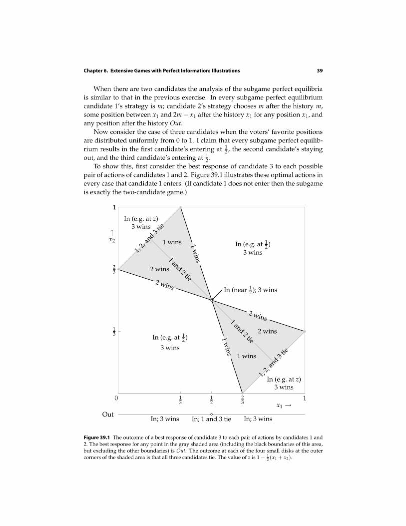
Chapter 6. Extensive Games with Perfect Information: Illustrations 39
When there are two candidates the analysis of the subgame perfect equilibria
is similar to that in the previous exercise. In every subgame perfect equilibrium
candidate 1’s strategy is m; candidate 2’s strategy chooses m after the history m,
some position between x1 and 2m − x1 after the history x1 for any position x1, and
any position after the history Out.
Now consider the case of three candidates when the voters’ favorite positions
are distributed uniformly from 0 to 1. I claim that every subgame perfect equilib-
rium results in the first candidate’s entering at 12 , the second candidate’s staying
out, and the third candidate’s entering at 12 .
To show this, first consider the best response of candidate 3 to each possible
pair of actions of candidates 1 and 2. Figure 39.1 illustrates these optimal actions in
every case that candidate 1 enters. (If candidate 1 does not enter then the subgame
is exactly the two-candidate game.)
23
23
12
13
13
In (e.g. at 12 )
3 wins
In (e.g. at 12 )
3 wins
In (e.g. at z)3 wins
In (e.g. at z)3 wins
In (near 12 ); 3 wins
1,2,
and
3tie
1,2,
and
3tie
2 wins
1 wins
1and
2tie
1 wins
2 wins
1and
2tie
2 wins
2 wins
1w
ins
1w
ins
0
1
1x1 →
↑x2
OutIn; 3 wins In; 1 and 3 tie In; 3 wins
Figure 39.1 The outcome of a best response of candidate 3 to each pair of actions by candidates 1 and2. The best response for any point in the gray shaded area (including the black boundaries of this area,but excluding the other boundaries) is Out. The outcome at each of the four small disks at the outercorners of the shaded area is that all three candidates tie. The value of z is 1 − 1
2 (x1 + x2).
40 Chapter 6. Extensive Games with Perfect Information: Illustrations
Now consider the optimal action of candidate 2, given x1 and the outcome of
candidate 3’s best response, as given in Figure 39.1. In the figure, take a value
of x1 and look at the outcomes as x2 varies; find the value of x2 that induces the
best outcome for candidate 2. For example, for x1 = 0 the only value of x2 for
which candidate 2 does not lose is 23 , at which point she ties with the other two
candidates. Thus when candidate 1’s strategy is x1 = 0, candidate 2’s best action,
given candidate 3’s best response, is x2 = 23 , which leads to a three-way tie. We
find that the outcome of the optimal value of x2, for each value of x1, is given as
follows.
1, 2, and 3 tie (x2 = 23 ) if x1 = 0
2 wins if 0 < x1 <12
1 and 3 tie (2 stays out) if x1 = 12
2 wins if 12 < x1 < 1
1, 2, and 3 tie (x2 = 13 ) if x1 = 1.
Finally, consider candidate 1’s best strategy, given the responses of candidates 2
and 3. If she stays out then candidates 2 and 3 enter at m and tie. If she enters then
the best position at which to do so is x1 = 12 , where she ties with candidate 3. (For
every other position she either loses or ties with both of the other candidates.)
We conclude that in every subgame perfect equilibrium the outcome is that
candidate 1 enters at 12 , candidate 2 stays out, and candidate 3 enters at 1
2 . (There
are many subgame perfect equilibria, because after many histories candidate 3’s
optimal action is not unique.)
(The case in which there are many potential candidates, is discussed on the
page http://www.economics.utoronto.ca/osborne/research/CONJECT.HTM.)
198.1 The race G1(2, 2)
The consequences of player 1’s actions at the start of the game are as follows.
Take two steps: Player 1 wins.
Take one step: Go to the game G2(1, 2), in which player 2 initially takes two
steps and wins.
Do not move: If player 2 does not move, the game ends. If she takes one step
we go to the game G1(2, 1), in which player 1 takes two steps and wins. If she
takes two steps, she wins. Thus in a subgame perfect equilibrium player 2
takes two steps, and wins.
We conclude that in a subgame perfect equilibrium of G1(2, 2) player 1 initially
takes two steps, and wins.
203.1 A race with a liquidity constraint
In the absence of the constraint, player 1 initially takes one step. Suppose she does
so in the game with the constraint. Consider player 2’s options after player 1’s
move.
Chapter 6. Extensive Games with Perfect Information: Illustrations 41
Player 2 takes two steps: Because of the liquidity constraint, player 1 can take
at most one step. If she takes one step, player 2’s optimal action is to take one
step, and win. Thus player 1’s best action is not to move; player 2’s payoff
exceeds 1 (her steps cost 5, and the prize is worth more than 6).
Player 2 moves one step: Again because of the liquidity constraint, player 1
can take at most one step. If she takes one step, player 2 can take two steps
and win, obtaining a payoff of more than 1 (as in the previous case).
Player 2 does not move: Player 1, as before, can take one step on each turn, and
win; player 2’s payoff is 0.
We conclude that after player 1 moves one step, player 2 should take either
one or two steps, and ultimately win; player 1’s payoff is −1. A better option for
player 1 is not to move, in which case player 2 can move one step at a time, and
win; player 1’s payoff is zero.
Thus the subgame perfect equilibrium outcome is that player 1 does not move,
and player 2 takes one step at a time and wins.

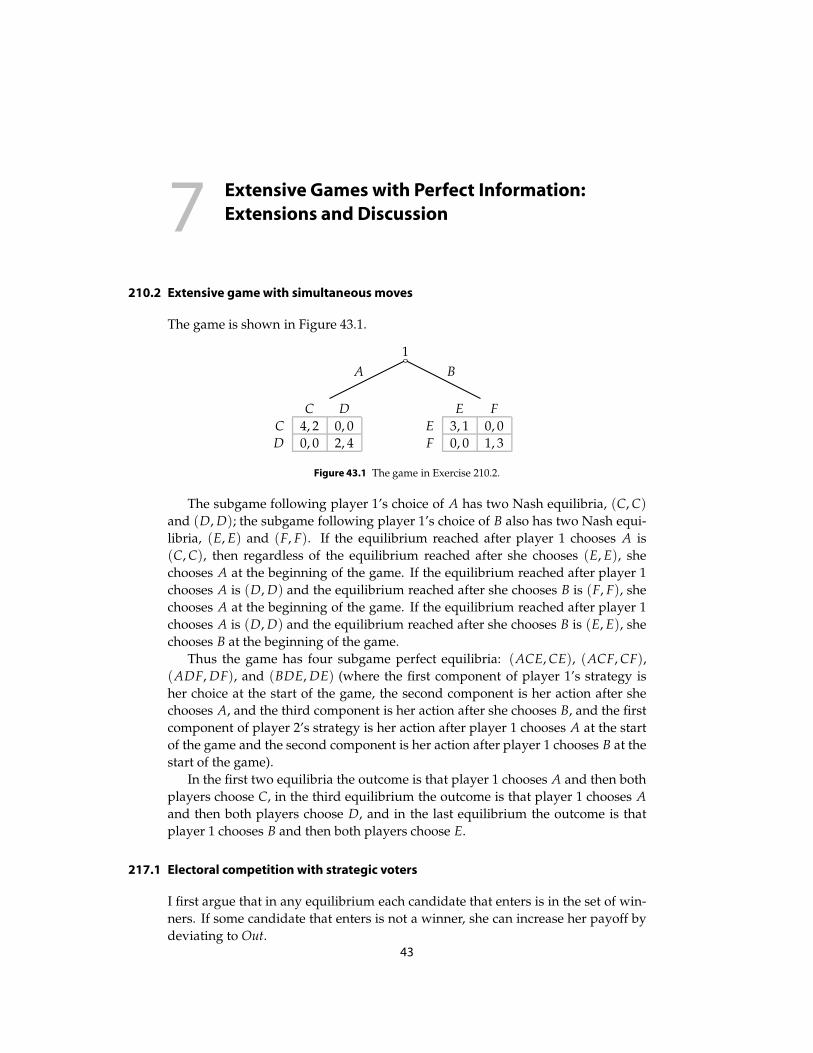
7Extensive Games with Perfect Information:
Extensions and Discussion
210.2 Extensive game with simultaneous moves
The game is shown in Figure 43.1.
BA
1
C D
C 4, 2 0, 0
D 0, 0 2, 4
E F
E 3, 1 0, 0
F 0, 0 1, 3
Figure 43.1 The game in Exercise 210.2.
The subgame following player 1’s choice of A has two Nash equilibria, (C, C)and (D, D); the subgame following player 1’s choice of B also has two Nash equi-
libria, (E, E) and (F, F). If the equilibrium reached after player 1 chooses A is
(C, C), then regardless of the equilibrium reached after she chooses (E, E), she
chooses A at the beginning of the game. If the equilibrium reached after player 1
chooses A is (D, D) and the equilibrium reached after she chooses B is (F, F), she
chooses A at the beginning of the game. If the equilibrium reached after player 1
chooses A is (D, D) and the equilibrium reached after she chooses B is (E, E), she
chooses B at the beginning of the game.
Thus the game has four subgame perfect equilibria: (ACE, CE), (ACF, CF),
(ADF, DF), and (BDE, DE) (where the first component of player 1’s strategy is
her choice at the start of the game, the second component is her action after she
chooses A, and the third component is her action after she chooses B, and the first
component of player 2’s strategy is her action after player 1 chooses A at the start
of the game and the second component is her action after player 1 chooses B at the
start of the game).
In the first two equilibria the outcome is that player 1 chooses A and then both
players choose C, in the third equilibrium the outcome is that player 1 chooses A
and then both players choose D, and in the last equilibrium the outcome is that
player 1 chooses B and then both players choose E.
217.1 Electoral competition with strategic voters
I first argue that in any equilibrium each candidate that enters is in the set of win-
ners. If some candidate that enters is not a winner, she can increase her payoff by
deviating to Out.43
44 Chapter 7. Extensive Games with Perfect Information: Extensions and Discussion
Now consider the voting subgame in which there are more than two candidates
and not all candidates’ positions are the same. Suppose that the citizens’ votes are
equally divided among the candidates. I argue that this list of citizens’ strategies
is not a Nash equilibrium of the voting subgame.
For either the citizen whose favorite position is 0 or the citizen whose favorite
position is 1 (or both), at least two candidates’ positions are better than the position
of the candidate furthest from the citizen’s favorite position. Denote a citizen for
whom this condition holds by i. (The claim that citizen i exists is immediate if the
candidates occupy at least three distinct positions, or they occupy two distinct po-
sitions and at least two candidates occupy each position. If the candidates occupy
only two positions and one position is occupied by a single candidate, then take
the citizen whose favorite position is 0 if the lone candidate’s position exceeds the
other candidates’ position; otherwise take the citizen whose favorite position is 1.)
Now, given that each candidate obtains the same number of votes, if citizen i
switches her vote to one of the candidates whose position is better for her than
that of the candidate whose position is furthest from her favorite position, then
this candidate wins outright. (If citizen i originally votes for one of these superior
candidates, she can switch her vote to the other superior candidate; if she originally
votes for neither of the superior candidates, she can switch her vote to either one
of them.) Citizen i’s payoff increases when she thus switches her vote, so that the
list of citizens’ strategies is not a Nash equilibrium of the voting subgame.
We conclude that in every Nash equilibrium of every voting subgame in which
there are more than two candidates and not all candidates’ positions are the same
at least one candidate loses. Because no candidate loses in a subgame perfect equi-
librium (by the first argument in the proof), in any subgame perfect equilibrium
either only two candidates enter, or all candidates’ positions are the same.
If only two candidates enter, then by the argument in the text for the case n = 2,
each candidate’s position is m (the median of the citizens’ favorite positions).
Now suppose that more than two candidates enter, and their common position
is not equal to m. If a candidate deviates to m then in the resulting voting subgame
only two positions are occupied, so that for every citizen, any strategy that is not
weakly dominated votes for a candidate at the position closest to her favorite po-
sition. Thus a candidate who deviates to m wins outright. We conclude that in
any subgame perfect equilibrium in which more than two candidates enter, they
all choose the position m.
220.1 Top cycle set
a. The top cycle set is the set x, y, z of all three alternatives because x beats y
beats z beats x.
b. The top cycle set is the set w, x, y, z of all four alternatives. As in the
previous case, x beats y beats z beats x; also y beats w.
Chapter 7. Extensive Games with Perfect Information: Extensions and Discussion 45
224.1 Exit from a declining industry
Period t1 is the largest value of t for which Pt(k1) ≥ c, or 60− t ≥ 10. Thus t1 = 50.
Similarly, t2 = 70.
If both firms are active in period t1, then firm 2’s profit in this period is (100 −t1 − c − k1 − k2)k2 = (−20)(20) = −400. Its profit in any period t in which it is
alone in the market is (100 − t − c − k2)k2 = (70 − t)(20). Thus its profit from
period t1 + 1 through period t2 is
(19 + 18 + . . . + 1)(20) = 3800.
Hence firm 2’s loss in period t1 when both firms are active is (much) less than the
sum of its profits in periods t1 + 1 through t2 when it alone is active.
227.1 Variant of ultimatum game with equityconscious players
The game is defined as follows.
Players The two people.
Terminal histories The set of sequences (x, β2, Z), where x is a number with 0 ≤x ≤ c (the amount of money that person 1 offers to person 2), β2 is 0 or 1 (the
value of β2 selected by chance), and Z is either Y (“yes, I accept”) or N (“no,
I reject”).
Player function P(∅) = 1, P(x) = c for all x, and P(x, β2) = 2 for all x and all
β2.
Chance probabilities For every history x, chance chooses 0 with probability p
and 1 with probability 1 − p.
Preferences Each person’s preferences are represented by the expected value of
a payoff equal to the amount of money she receives. For any terminal history
(x, β2, Y) person 1 receives c − x and person 2 receives x; for any terminal
history (x, β2, N) each person receives 0.
Given the result from Exercise 183.4 given in the question, if person 1’s offer x
satisfies 0 < x <13 then the offer is rejected with probability 1 − p, so that per-
son 1’s expected payoff is p(1 − x), while if x >13 the offer is certainly accepted,
independent of the type of person 2. Thus person 1’s optimal offer is
13 if p <
23
0 if p >23 ;
if p = 23 then both offers are optimal.
If p >23 we see that in a subgame perfect equilibrium person 1’s offers are
rejected by every person 2 with whom she is matched for whom β2 = 1 (that is,
with probability 1 − p).
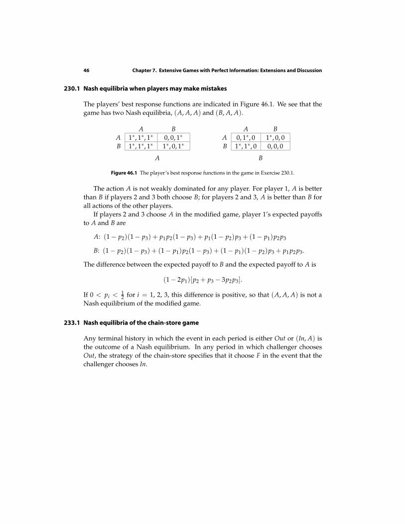
46 Chapter 7. Extensive Games with Perfect Information: Extensions and Discussion
230.1 Nash equilibria when players may make mistakes
The players’ best response functions are indicated in Figure 46.1. We see that the
game has two Nash equilibria, (A, A, A) and (B, A, A).
A B
A 1∗, 1∗, 1∗ 0, 0, 1∗
B 1∗, 1∗, 1∗ 1∗, 0, 1∗
A
A B
A 0, 1∗, 0 1∗, 0, 0
B 1∗, 1∗, 0 0, 0, 0
B
Figure 46.1 The player’s best response functions in the game in Exercise 230.1.
The action A is not weakly dominated for any player. For player 1, A is better
than B if players 2 and 3 both choose B; for players 2 and 3, A is better than B for
all actions of the other players.
If players 2 and 3 choose A in the modified game, player 1’s expected payoffs
to A and B are
A: (1 − p2)(1− p3) + p1 p2(1 − p3) + p1(1 − p2)p3 + (1 − p1)p2p3
B: (1 − p2)(1 − p3) + (1 − p1)p2(1 − p3) + (1 − p1)(1 − p2)p3 + p1 p2 p3.
The difference between the expected payoff to B and the expected payoff to A is
(1 − 2p1)[p2 + p3 − 3p2 p3].
If 0 < pi <12 for i = 1, 2, 3, this difference is positive, so that (A, A, A) is not a
Nash equilibrium of the modified game.
233.1 Nash equilibria of the chainstore game
Any terminal history in which the event in each period is either Out or (In, A) is
the outcome of a Nash equilibrium. In any period in which challenger chooses
Out, the strategy of the chain-store specifies that it choose F in the event that the
challenger chooses In.
8Coalitional Games and the Core
245.1 Threeplayer majority game
Let (x1, x2, x3) be an action of the grand coalition. Every coalition consisting of two
players can obtain one unit of output, so for (x1, x2, x3) to be in the core we need
x1 + x2 ≥ 1
x1 + x3 ≥ 1
x2 + x3 ≥ 1
x1 + x2 + x3 = 1.
Adding the first three conditions we conclude that
2x1 + 2x2 + 2x3 ≥ 3,
or x1 + x2 + x3 ≥ 32 , contradicting the last condition. Thus no action of the grand
coalition satisfies all the conditions, so that the core of the game is empty.
248.1 Core of landowner–worker game
Let aN be an action of the grand coalition in which the output received by each
worker is at most f (n) − f (n − 1). No coalition consisting solely of workers can
obtain any output, so no such coalition can improve upon aN . Let S be a coalition
of the landowner and k − 1 workers. The total output received by the members of
S in aN is at least
f (n) − (n − k)( f (n)− f (n − 1))
(because the total output is f (n), and every other worker receives at most f (n) −f (n − 1)). Now, the output that S can obtain is f (k), so for S to improve upon aN
we need
f (k) > f (n) − (n − k)( f (n)− f (n − 1)),
which contradicts the inequality given in the exercise.
249.1 Unionized workers in landowner–worker game
The following game models the situation.
Players The landowner and the workers.
47
48 Chapter 8. Coalitional Games and the Core
Actions The set of actions of the grand coalition is the set of all allocations of
the output f (n). Every other coalition has a single action, which yields the
output 0.
Preferences Each player’s preferences are represented by the amount of output
she obtains.
The core of this game consists of every allocation of the output f (n) among
the players. The grand coalition cannot improve upon any allocation x because
for every other allocation x′ there is at least one player whose payoff is lower in
x′ than it is in x. No other coalition can improve upon any allocation because no
other coalition can obtain any output.
249.2 Landowner–worker game with increasing marginal products
We need to show that no coalition can improve upon the action aN of the grand
coalition in which every player receives the output f (n)/n. No coalition of work-
ers can obtain any output, so we need to consider only coalitions containing the
landowner. Consider a coalition consisting of the landowner and k workers, which
can obtain f (k + 1) units of output by itself. Under aN this coalition obtains the
output (k + 1) f (n)/n, and we have f (k + 1)/(k + 1) < f (n)/n because k < n.
Thus no coalition can improve upon aN .
254.1 Range of prices in horse market
The equality of the number of owners who sell their horses and the number of
nonowners who buy horses implies that the common trading price p∗
• is not less than σk∗ , otherwise at most k∗ − 1 owners’ valuations would be
less than p∗ and at least k∗ nonowners’ valuations would be greater than p∗,
so that the number of buyers would exceed the number of sellers
• is not less than βk∗+1, otherwise at most k∗ owners’ valuations would be less
than p∗ and at least k∗ + 1 nonowners’ valuations would be greater than p∗,
so that the number of buyers would exceed the number of sellers
• is not greater than βk∗ , otherwise at least k∗ owners’ valuations would be less
than p∗ and at most k∗ − 1 nonowners’ valuations would be greater than p∗,
so that the number of sellers would exceed the number of buyers
• is not greater than σk∗+1, otherwise at least k∗ + 1 owners’ valuations would
be less than p∗ and at most k∗ nonowners’ valuations would be greater than
p∗, so that the number of sellers would exceed the number of buyers.
That is, p∗ ≥ maxσk∗ , βk∗+1 and p∗ ≤ minβk∗ , σk∗+1.
Chapter 8. Coalitional Games and the Core 49
258.1 House assignment with identical preferences
Because the players rank the houses in the same way, we can refer to the “best
house”, the “second best house”, and so on. In any assignment in the core, the
player who owns the best house is assigned this house (because she has the option
of keeping it). Among the remaining players, the one who owns the second best
house must be assigned this house (again, because she has the option of keeping
it). Continuing to argue in the same way, we see that there is a single assignment
in the core, in which every player is assigned the house she owns initially.
261.1 Median voter theorem
Denote the median favorite position by m. If x < m then every player whose fa-
vorite position is m or greater—a majority of the players—prefers m to x. Similarly,
if x > m then every player whose favorite position is m or less—a majority of the
players—prefers m to x.
267.2 Empty core in roommate problem
Notice that ` is at the bottom of each of the other players’ preferences. Suppose
that she is matched with i. Then j and k are matched, and i, k can improve upon
the matching. Similarly, if ` is matched with j then i, j can improve upon the
matching, and if ` is matched with k then j, k can improve upon the matching.
Thus the core is empty (` has to be matched with someone!).

9Bayesian Games
276.1 Equilibria of a variant of BoS with imperfect information
If player 1 chooses S then type 1 of player 2 chooses S and type 2 chooses B. But
if the two types of player 2 make these choices then player 1 is better off choosing
B (which yields her an expected payoff of 1) than choosing S (which yields her an
expected payoff of 12 ). Thus there is no Nash equilibrium in which player 1 chooses
S.
Now consider the mixed strategy Nash equilibria. If both types of player 2 use
a pure strategy then player 1’s two actions yield her different payoffs. Thus there
is no equilibrium in which both types of player 2 use pure strategies and player 1
randomizes.
Now consider an equilibrium in which type 1 of player 2 randomizes. Denote
by p the probability that player 1’s mixed strategy assigns to B. In order for type 1
of player 2 to obtain the same expected payoff to B and S we need p = 23 . For this
value of p the best action of type 2 of player 2 is S. Denote by q the probability that
type 1 of player 2 assigns to B. Given these strategies for the two types of player 2,
player 1’s expected payoff if she chooses B is
12 · 2q = q
and her expected payoff if she chooses S is
12 · (1 − q) + 1
2 · 1 = 1 − 12 q.
These expected payoffs are equal if and only if q = 23 . Thus the game has a mixed
strategy equilibrium in which the mixed strategy of player 1 is ( 23 , 1
3 ), that of type 1
of player 2 is ( 23 , 1
3 ), and that of type 2 of player 2 is (0, 1) (that is, type 2 of player 2
uses the pure strategy that assigns probability 1 to S).
Similarly the game has a mixed strategy equilibrium in which the strategy of
player 1 is ( 13 , 2
3 ), that of type 1 of player 2 is (0, 1), and that of type 2 of player 2 is
( 23 , 1
3 ).
For no mixed strategy of player 1 are both types of player 2 indifferent between
their two actions, so there is no equilibrium in which both types randomize.
277.1 Expected payoffs in a variant of BoS with imperfect information
The expected payoffs are given in Figure 52.1.
51
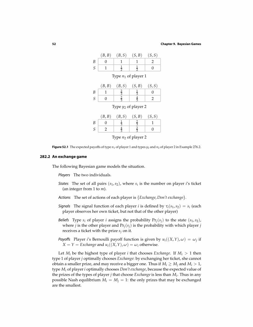
52 Chapter 9. Bayesian Games
(B, B) (B, S) (S, B) (S, S)
B 0 1 1 2
S 1 12
12 0
Type n1 of player 1
(B, B) (B, S) (S, B) (S, S)
B 1 23
13 0
S 0 23
43 2
Type y2 of player 2
(B, B) (B, S) (S, B) (S, S)
B 0 13
23 1
S 2 43
23 0
Type n2 of player 2
Figure 52.1 The expected payoffs of type n1 of player 1 and types y2 and n2 of player 2 in Example 276.2.
282.2 An exchange game
The following Bayesian game models the situation.
Players The two individuals.
States The set of all pairs (s1, s2), where si is the number on player i’s ticket
(an integer from 1 to m).
Actions The set of actions of each player is Exchange, Don’t exchange.
Signals The signal function of each player i is defined by τi(s1, s2) = si (each
player observes her own ticket, but not that of the other player)
Beliefs Type si of player i assigns the probability Prj(sj) to the state (s1, s2),
where j is the other player and Prj(sj) is the probability with which player j
receives a ticket with the prize sj on it.
Payoffs Player i’s Bernoulli payoff function is given by ui((X, Y), ω) = ωj if
X = Y = Exchange and ui((X, Y), ω) = ωi otherwise.
Let Mi be the highest type of player i that chooses Exchange. If Mi > 1 then
type 1 of player j optimally chooses Exchange: by exchanging her ticket, she cannot
obtain a smaller prize, and may receive a bigger one. Thus if Mi ≥ Mj and Mi > 1,
type Mi of player i optimally chooses Don’t exchange, because the expected value of
the prizes of the types of player j that choose Exchange is less than Mi. Thus in any
possible Nash equilibrium Mi = Mj = 1: the only prizes that may be exchanged
are the smallest.
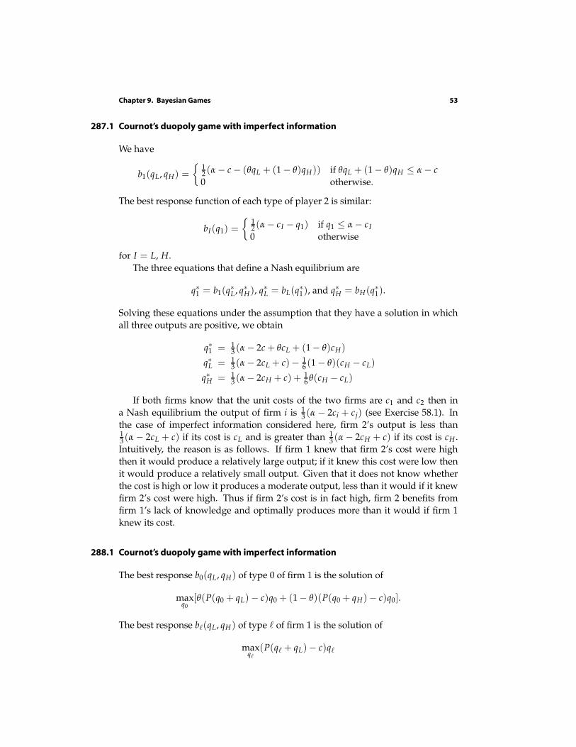
Chapter 9. Bayesian Games 53
287.1 Cournot’s duopoly game with imperfect information
We have
b1(qL, qH) =
12 (α − c − (θqL + (1 − θ)qH)) if θqL + (1 − θ)qH ≤ α − c
0 otherwise.
The best response function of each type of player 2 is similar:
bI(q1) =
12 (α − cI − q1) if q1 ≤ α − cI
0 otherwise
for I = L, H.
The three equations that define a Nash equilibrium are
q∗1 = b1(q∗L, q∗H), q∗L = bL(q∗1), and q∗H = bH(q∗1).
Solving these equations under the assumption that they have a solution in which
all three outputs are positive, we obtain
q∗1 = 13 (α − 2c + θcL + (1 − θ)cH)
q∗L = 13 (α − 2cL + c)− 1
6 (1 − θ)(cH − cL)
q∗H = 13 (α − 2cH + c) + 1
6 θ(cH − cL)
If both firms know that the unit costs of the two firms are c1 and c2 then in
a Nash equilibrium the output of firm i is 13 (α − 2ci + cj) (see Exercise 58.1). In
the case of imperfect information considered here, firm 2’s output is less than13 (α − 2cL + c) if its cost is cL and is greater than 1
3 (α − 2cH + c) if its cost is cH .
Intuitively, the reason is as follows. If firm 1 knew that firm 2’s cost were high
then it would produce a relatively large output; if it knew this cost were low then
it would produce a relatively small output. Given that it does not know whether
the cost is high or low it produces a moderate output, less than it would if it knew
firm 2’s cost were high. Thus if firm 2’s cost is in fact high, firm 2 benefits from
firm 1’s lack of knowledge and optimally produces more than it would if firm 1
knew its cost.
288.1 Cournot’s duopoly game with imperfect information
The best response b0(qL, qH) of type 0 of firm 1 is the solution of
maxq0
[θ(P(q0 + qL) − c)q0 + (1 − θ)(P(q0 + qH)− c)q0].
The best response b`(qL, qH) of type ` of firm 1 is the solution of
maxq`
(P(q` + qL)− c)q`
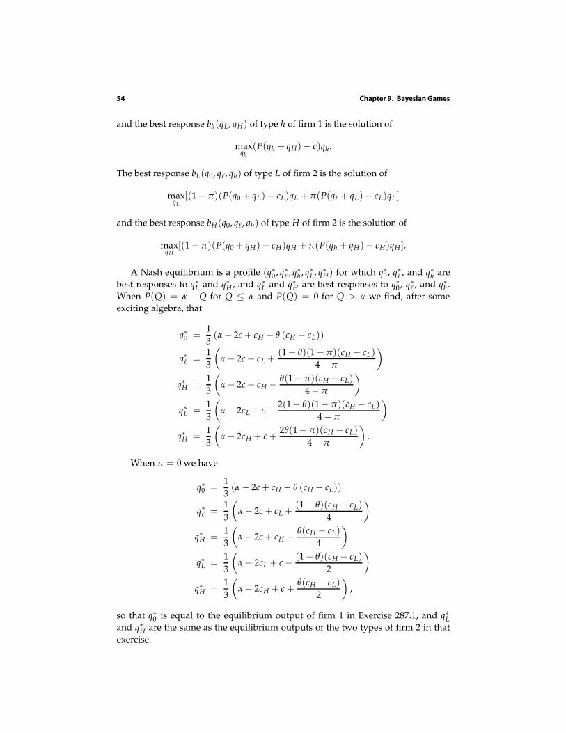
54 Chapter 9. Bayesian Games
and the best response bh(qL, qH) of type h of firm 1 is the solution of
maxqh
(P(qh + qH) − c)qh.
The best response bL(q0, q`, qh) of type L of firm 2 is the solution of
maxqL
[(1 − π)(P(q0 + qL) − cL)qL + π(P(q` + qL)− cL)qL]
and the best response bH(q0, q`, qh) of type H of firm 2 is the solution of
maxqH
[(1 − π)(P(q0 + qH) − cH)qH + π(P(qh + qH) − cH)qH ].
A Nash equilibrium is a profile (q∗0 , q∗`, q∗h, q∗L, q∗H) for which q∗0 , q∗
`, and q∗h are
best responses to q∗L and q∗H , and q∗L and q∗H are best responses to q∗0 , q∗`, and q∗h .
When P(Q) = α − Q for Q ≤ α and P(Q) = 0 for Q > α we find, after some
exciting algebra, that
q∗0 =1
3(α − 2c + cH − θ (cH − cL))
q∗` =1
3
(
α − 2c + cL +(1 − θ)(1 − π)(cH − cL)
4 − π
)
q∗H =1
3
(
α − 2c + cH −θ(1 − π)(cH − cL)
4 − π
)
q∗L =1
3
(
α − 2cL + c −2(1 − θ)(1 − π)(cH − cL)
4 − π
)
q∗H =1
3
(
α − 2cH + c +2θ(1 − π)(cH − cL)
4 − π
)
.
When π = 0 we have
q∗0 =1
3(α − 2c + cH − θ (cH − cL))
q∗`
=1
3
(
α − 2c + cL +(1 − θ)(cH − cL)
4
)
q∗H =1
3
(
α − 2c + cH −θ(cH − cL)
4
)
q∗L =1
3
(
α − 2cL + c −(1 − θ)(cH − cL)
2
)
q∗H =1
3
(
α − 2cH + c +θ(cH − cL)
2
)
,
so that q∗0 is equal to the equilibrium output of firm 1 in Exercise 287.1, and q∗Land q∗H are the same as the equilibrium outputs of the two types of firm 2 in that
exercise.

Chapter 9. Bayesian Games 55
When π = 1 we have
q∗0 =1
3(α − 2c + cH − θ (cH − cL))
q∗`
=1
3(α − 2c + cL)
q∗H =1
3(α − 2c + cH)
q∗L =1
3(α − 2cL + c)
q∗H =1
3(α − 2cH + c) ,
so that q∗`
and q∗L are the same as the equilibrium outputs when there is perfect
information and the costs are c and cL (see Exercise 58.1), and q∗h and q∗H are the
same as the equilibrium outputs when there is perfect information and the costs
are c and cH .
Now, for an arbitrary value of π we have
q∗L =1
3
(
α − 2cL + c −2(1 − θ)(1 − π)(cH − cL)
4 − π
)
q∗H =1
3
(
α − 2cH + c +2θ(1 − π)(cH − cL)
4 − π
)
.
To show that for 0 < π < 1 the values of these variables lie between their values
when π = 0 and when π = 1, we need to show that
0 ≤2(1− θ)(1 − π)(cH − cL)
4 − π≤
(1 − θ)(cL − cH)
2
and
0 ≤2θ(1 − π)(cH − cL)
4 − π≤
θ(cL − cH)
2.
These inequalities follow from cH ≥ cL, θ ≥ 0, and 0 ≤ π ≤ 1.
290.1 Nash equilibria of game of contributing to a public good
Any type vj of any player j with vj < c obtains a negative payoff if she contributes
and 0 if she does not. Thus she optimally does not contribute.
Any type vi ≥ c of player i obtains the payoff vi − c ≥ 0 if she contributes, and
the payoff 0 if she does not, so she optimally contributes.
Any type vj ≥ c of any player j 6= i obtains the payoff vj − c if she contributes,
and the payoff (1 − F(c))vj if she does not. (If she does not contribute, the prob-
ability that player i does so is 1 − F(c), the probability that player i’s valuation
is at least c.) Thus she optimally does not contribute if (1 − F(c))vj ≥ vj − c, or
F(c) ≤ c/vj. This condition must hold for all types of every player j 6= i, so we
need F(c) ≤ c/v for the strategy profile to be a Nash equilibrium.
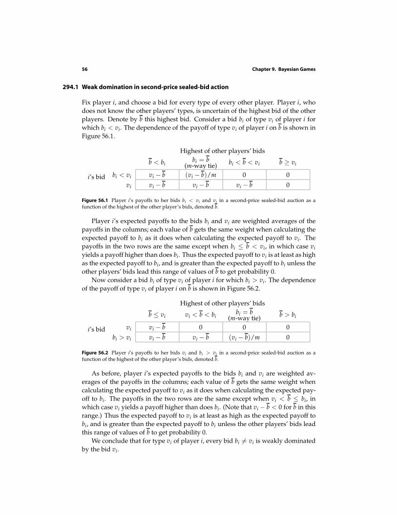
56 Chapter 9. Bayesian Games
294.1 Weak domination in secondprice sealedbid action
Fix player i, and choose a bid for every type of every other player. Player i, who
does not know the other players’ types, is uncertain of the highest bid of the other
players. Denote by b this highest bid. Consider a bid bi of type vi of player i for
which bi < vi. The dependence of the payoff of type vi of player i on b is shown in
Figure 56.1.
i’s bid
Highest of other players’ bids
b < bibi = b
(m-way tie)bi < b < vi b ≥ vi
bi < vi vi − b (vi − b)/m 0 0
vi vi − b vi − b vi − b 0
Figure 56.1 Player i’s payoffs to her bids bi < vi and vi in a second-price sealed-bid auction as afunction of the highest of the other player’s bids, denoted b.
Player i’s expected payoffs to the bids bi and vi are weighted averages of the
payoffs in the columns; each value of b gets the same weight when calculating the
expected payoff to bi as it does when calculating the expected payoff to vi. The
payoffs in the two rows are the same except when bi ≤ b < vi, in which case vi
yields a payoff higher than does bi. Thus the expected payoff to vi is at least as high
as the expected payoff to bi, and is greater than the expected payoff to bi unless the
other players’ bids lead this range of values of b to get probability 0.
Now consider a bid bi of type vi of player i for which bi > vi. The dependence
of the payoff of type vi of player i on b is shown in Figure 56.2.
i’s bid
Highest of other players’ bids
b ≤ vi vi < b < bibi = b
(m-way tie)b > bi
vi vi − b 0 0 0
bi > vi vi − b vi − b (vi − b)/m 0
Figure 56.2 Player i’s payoffs to her bids vi and bi > vi in a second-price sealed-bid auction as afunction of the highest of the other player’s bids, denoted b.
As before, player i’s expected payoffs to the bids bi and vi are weighted av-
erages of the payoffs in the columns; each value of b gets the same weight when
calculating the expected payoff to vi as it does when calculating the expected pay-
off to bi. The payoffs in the two rows are the same except when vi < b ≤ bi, in
which case vi yields a payoff higher than does bi. (Note that vi − b < 0 for b in this
range.) Thus the expected payoff to vi is at least as high as the expected payoff to
bi, and is greater than the expected payoff to bi unless the other players’ bids lead
this range of values of b to get probability 0.
We conclude that for type vi of player i, every bid bi 6= vi is weakly dominated
by the bid vi.
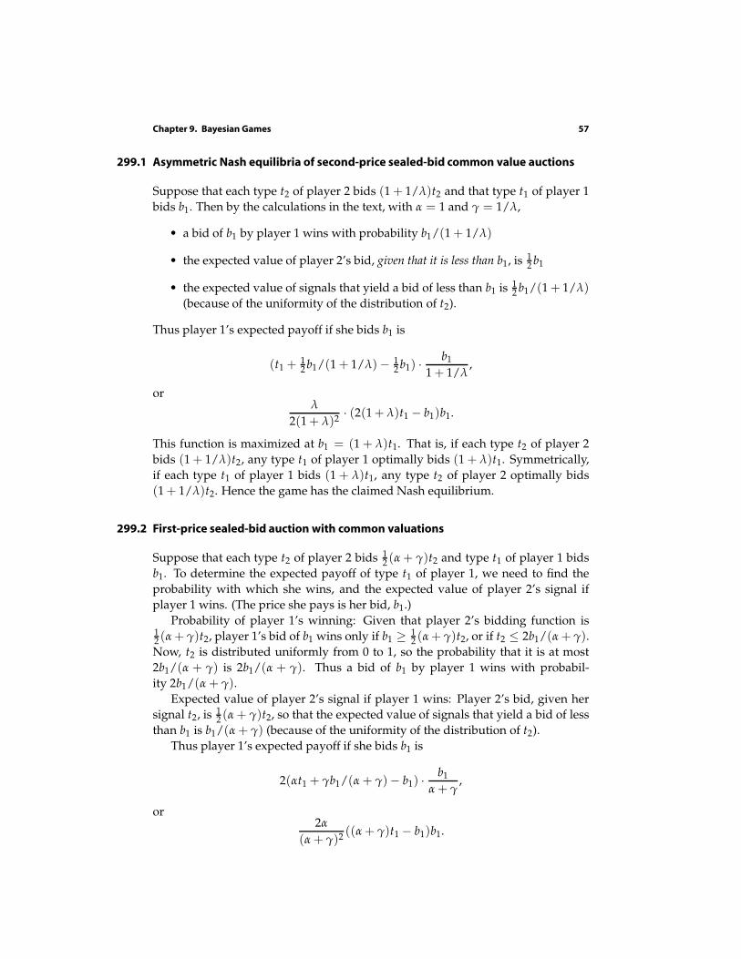
Chapter 9. Bayesian Games 57
299.1 Asymmetric Nash equilibria of secondprice sealedbid common value auctions
Suppose that each type t2 of player 2 bids (1 + 1/λ)t2 and that type t1 of player 1
bids b1. Then by the calculations in the text, with α = 1 and γ = 1/λ,
• a bid of b1 by player 1 wins with probability b1/(1 + 1/λ)
• the expected value of player 2’s bid, given that it is less than b1, is 12 b1
• the expected value of signals that yield a bid of less than b1 is 12 b1/(1 + 1/λ)
(because of the uniformity of the distribution of t2).
Thus player 1’s expected payoff if she bids b1 is
(t1 + 12 b1/(1 + 1/λ) − 1
2 b1) ·b1
1 + 1/λ,
orλ
2(1 + λ)2· (2(1 + λ)t1 − b1)b1.
This function is maximized at b1 = (1 + λ)t1. That is, if each type t2 of player 2
bids (1 + 1/λ)t2, any type t1 of player 1 optimally bids (1 + λ)t1. Symmetrically,
if each type t1 of player 1 bids (1 + λ)t1, any type t2 of player 2 optimally bids
(1 + 1/λ)t2. Hence the game has the claimed Nash equilibrium.
299.2 Firstprice sealedbid auction with common valuations
Suppose that each type t2 of player 2 bids 12 (α + γ)t2 and type t1 of player 1 bids
b1. To determine the expected payoff of type t1 of player 1, we need to find the
probability with which she wins, and the expected value of player 2’s signal if
player 1 wins. (The price she pays is her bid, b1.)
Probability of player 1’s winning: Given that player 2’s bidding function is12 (α + γ)t2, player 1’s bid of b1 wins only if b1 ≥ 1
2 (α + γ)t2, or if t2 ≤ 2b1/(α + γ).
Now, t2 is distributed uniformly from 0 to 1, so the probability that it is at most
2b1/(α + γ) is 2b1/(α + γ). Thus a bid of b1 by player 1 wins with probabil-
ity 2b1/(α + γ).
Expected value of player 2’s signal if player 1 wins: Player 2’s bid, given her
signal t2, is 12 (α + γ)t2, so that the expected value of signals that yield a bid of less
than b1 is b1/(α + γ) (because of the uniformity of the distribution of t2).
Thus player 1’s expected payoff if she bids b1 is
2(αt1 + γb1/(α + γ)− b1) ·b1
α + γ,
or2α
(α + γ)2((α + γ)t1 − b1)b1.
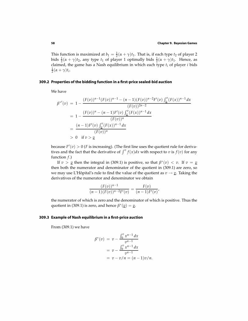
58 Chapter 9. Bayesian Games
This function is maximized at b1 = 12 (α + γ)t1. That is, if each type t2 of player 2
bids 12 (α + γ)t2, any type t1 of player 1 optimally bids 1
2 (α + γ)t1. Hence, as
claimed, the game has a Nash equilibrium in which each type ti of player i bids12 (α + γ)ti.
309.2 Properties of the bidding function in a firstprice sealedbid auction
We have
β∗′(v) = 1 −(F(v))n−1(F(v))n−1 − (n − 1)(F(v))n−2F′(v)
∫ vv (F(x))n−1 dx
(F(v))2n−2
= 1 −(F(v))n − (n − 1)F′(v)
∫ vv (F(x))n−1 dx
(F(v))n
=(n − 1)F′(v)
∫ vv (F(x))n−1 dx
(F(v))n
> 0 if v > v
because F′(v) > 0 (F is increasing). (The first line uses the quotient rule for deriva-
tives and the fact that the derivative of∫ v
f (x)dx with respect to v is f (v) for any
function f .)
If v > v then the integral in (309.1) is positive, so that β∗(v) < v. If v = v
then both the numerator and denominator of the quotient in (309.1) are zero, so
we may use L’Hôpital’s rule to find the value of the quotient as v → v. Taking the
derivatives of the numerator and denominator we obtain
(F(v))n−1
(n − 1)(F(v))n−2F′(v)=
F(v)
(n − 1)F′(v),
the numerator of which is zero and the denominator of which is positive. Thus the
quotient in (309.1) is zero, and hence β∗(v) = v.
309.3 Example of Nash equilibrium in a firstprice auction
From (309.1) we have
β∗(v) = v −
∫ v0 xn−1 dx
vn−1
= v −
∫ v0 xn−1 dx
vn−1
= v − v/n = (n − 1)v/n.
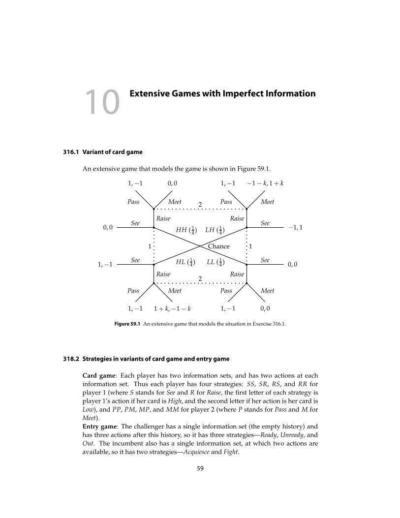
10Extensive Games with Imperfect Information
316.1 Variant of card game
An extensive game that models the game is shown in Figure 59.1.
HL ( 14 )
HH ( 14 )
Chance
LL ( 14 )
LH ( 14 )
1 1
RaiseSee
0, 0
RaiseSee
−1, 1
Meet
0, 0
Pass
1,−1
Meet
−1 − k, 1 + k
Pass
1,−1
2
Raise
See1,−1
Raise
See0, 0
Meet
1 + k,−1 − k
Pass
1,−1
Meet
0, 0
Pass
1,−1
2
Figure 59.1 An extensive game that models the situation in Exercise 316.1.
318.2 Strategies in variants of card game and entry game
Card game: Each player has two information sets, and has two actions at each
information set. Thus each player has four strategies: SS, SR, RS, and RR for
player 1 (where S stands for See and R for Raise, the first letter of each strategy is
player 1’s action if her card is High, and the second letter if her action is her card is
Low), and PP, PM, MP, and MM for player 2 (where P stands for Pass and M for
Meet).
Entry game: The challenger has a single information set (the empty history) and
has three actions after this history, so it has three strategies—Ready, Unready, and
Out. The incumbent also has a single information set, at which two actions are
available, so it has two strategies—Acquiesce and Fight.
59
60 Chapter 10. Extensive Games with Imperfect Information
331.2 Weak sequential equilibrium and Nash equilibrium in subgames
Consider the assessment in which the Challenger’s strategy is (Out, R), the In-
cumbent’s strategy is F, and the Incumbent’s belief assigns probability 1 to the
history (In, U) at her information set. Each player’s strategy is sequentially ratio-
nal. The Incumbent’s belief satisfies the condition of weak consistency because her
information set is not reached when the Challenger follows her strategy. Thus the
assessment is a weak sequential equilibrium.
The players’ actions in the subgame following the history In do not constitute a
Nash equilibrium of the subgame because the Incumbent’s action F is not optimal
when the Challenger chooses R. (The Incumbent’s action F is optimal given her
belief that the history is (In, U), as it is in the weak sequential equilibrium. In a
Nash equilibrium she acts as if she has a belief that coincides with the Challenger’s
action in the subgame.)
340.1 Pooling equilibria of game in which expenditure signals quality
We know that in the second period the high-quality firm charges the price H and
the low-quality firm charges any nonnegative price, and the consumer buys the
good from a high-quality firm, does not buy the good from a low-quality firm that
charges a positive price, and may or may not buy from a low-quality firm that
charges a price of 0.
Consider an assessment in which each type of firm chooses (p∗, E∗) in the first
period, the consumer believes the firm is high-quality with probability π if it ob-
serves (p∗, E∗) and low quality if it observes any other (price, expenditure) pair,
and buys the good if and only if it observes (p∗, E∗).
The payoff of a high-quality firm under this assessment is p∗ + H − E∗ − 2cH,
that of a low-quality firm is p∗ − E∗, and that of the consumer is π(H − p∗) + (1 −π)(−p∗) = πH − p∗.
This assessment is consistent—the only first-period action of the firm observed
in equilibrium is (p∗, E∗), and after observing this pair the consumer believes,
correctly, that the firm is high-quality with probability π.
Under what conditions is the assessment sequentially rational?
Firm If the firm chooses a (price, expenditure) pair different from (p∗, E∗) then
the consumer does not buy the good, and the firm’s profit is 0. Thus for the
assessment to be an equilibrium we need p∗ + H − E∗ − 2cH ≥ 0 (for the
high-quality firm) and p∗ − E∗ ≥ 0 (for the low-quality firm).
Consumer If the consumer does not buy the good after observing (p∗, E∗) then its
payoff is 0, so for the assessment to be an equilibrium we need πH − p∗ ≥ 0.
In summary, the assessment is a weak sequential equilibrium if and only if
maxE∗, E∗ − H + 2cH ≤ p∗ ≤ πH.
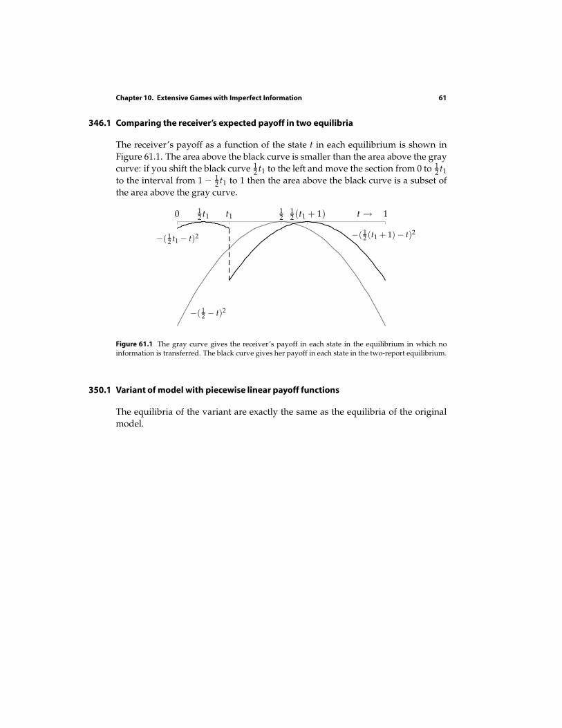
Chapter 10. Extensive Games with Imperfect Information 61
346.1 Comparing the receiver’s expected payoff in two equilibria
The receiver’s payoff as a function of the state t in each equilibrium is shown in
Figure 61.1. The area above the black curve is smaller than the area above the gray
curve: if you shift the black curve 12 t1 to the left and move the section from 0 to 1
2 t1
to the interval from 1 − 12 t1 to 1 then the area above the black curve is a subset of
the area above the gray curve.
0 12 t1 t1
12
12 (t1 + 1) t → 1
−( 12 − t)2
−( 12 t1 − t)2 −( 1
2 (t1 + 1) − t)2
Figure 61.1 The gray curve gives the receiver’s payoff in each state in the equilibrium in which noinformation is transferred. The black curve gives her payoff in each state in the two-report equilibrium.
350.1 Variant of model with piecewise linear payoff functions
The equilibria of the variant are exactly the same as the equilibria of the original
model.

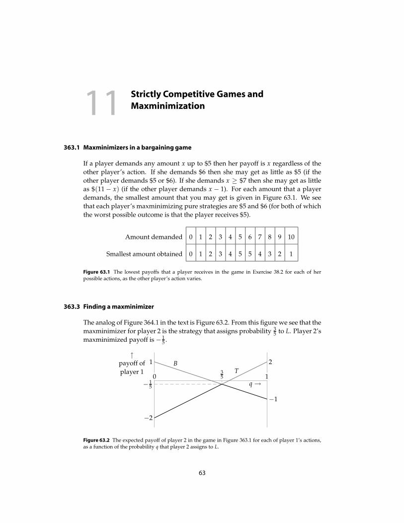
11Strictly Competitive Games and
Maxminimization
363.1 Maxminimizers in a bargaining game
If a player demands any amount x up to $5 then her payoff is x regardless of the
other player’s action. If she demands $6 then she may get as little as $5 (if the
other player demands $5 or $6). If she demands x ≥ $7 then she may get as little
as $(11 − x) (if the other player demands x − 1). For each amount that a player
demands, the smallest amount that you may get is given in Figure 63.1. We see
that each player’s maxminimizing pure strategies are $5 and $6 (for both of which
the worst possible outcome is that the player receives $5).
Amount demanded 0 1 2 3 4 5 6 7 8 9 10
Smallest amount obtained 0 1 2 3 4 5 5 4 3 2 1
Figure 63.1 The lowest payoffs that a player receives in the game in Exercise 38.2 for each of herpossible actions, as the other player’s action varies.
363.3 Finding a maxminimizer
The analog of Figure 364.1 in the text is Figure 63.2. From this figure we see that the
maxminimizer for player 2 is the strategy that assigns probability 35 to L. Player 2’s
maxminimized payoff is − 15 .
↑payoff of
player 10
− 15
1
−2
1
2
−1
q →
35
BT
Figure 63.2 The expected payoff of player 2 in the game in Figure 363.1 for each of player 1’s actions,as a function of the probability q that player 2 assigns to L.
63
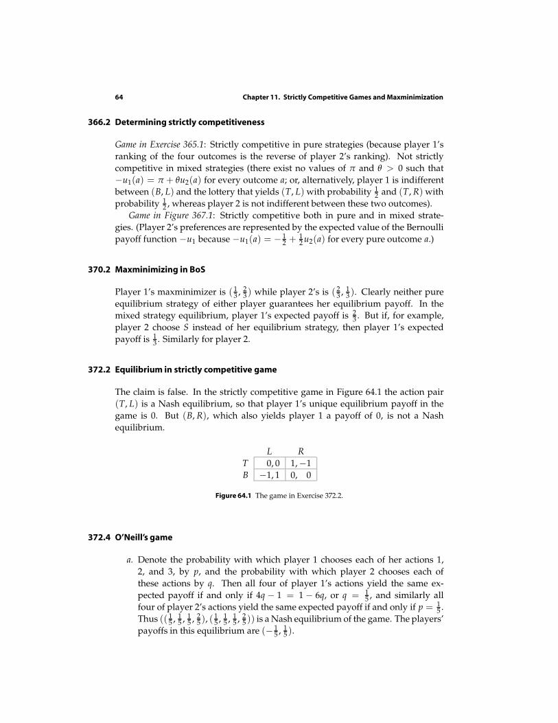
64 Chapter 11. Strictly Competitive Games and Maxminimization
366.2 Determining strictly competitiveness
Game in Exercise 365.1: Strictly competitive in pure strategies (because player 1’s
ranking of the four outcomes is the reverse of player 2’s ranking). Not strictly
competitive in mixed strategies (there exist no values of π and θ > 0 such that
−u1(a) = π + θu2(a) for every outcome a; or, alternatively, player 1 is indifferent
between (B, L) and the lottery that yields (T, L) with probability 12 and (T, R) with
probability 12 , whereas player 2 is not indifferent between these two outcomes).
Game in Figure 367.1: Strictly competitive both in pure and in mixed strate-
gies. (Player 2’s preferences are represented by the expected value of the Bernoulli
payoff function −u1 because −u1(a) = − 12 + 1
2 u2(a) for every pure outcome a.)
370.2 Maxminimizing in BoS
Player 1’s maxminimizer is ( 13 , 2
3 ) while player 2’s is ( 23 , 1
3 ). Clearly neither pure
equilibrium strategy of either player guarantees her equilibrium payoff. In the
mixed strategy equilibrium, player 1’s expected payoff is 23 . But if, for example,
player 2 choose S instead of her equilibrium strategy, then player 1’s expected
payoff is 13 . Similarly for player 2.
372.2 Equilibrium in strictly competitive game
The claim is false. In the strictly competitive game in Figure 64.1 the action pair
(T, L) is a Nash equilibrium, so that player 1’s unique equilibrium payoff in the
game is 0. But (B, R), which also yields player 1 a payoff of 0, is not a Nash
equilibrium.
L R
T 0, 0 1,−1
B −1, 1 0, 0
Figure 64.1 The game in Exercise 372.2.
372.4 O’Neill’s game
a. Denote the probability with which player 1 chooses each of her actions 1,
2, and 3, by p, and the probability with which player 2 chooses each of
these actions by q. Then all four of player 1’s actions yield the same ex-
pected payoff if and only if 4q − 1 = 1 − 6q, or q = 15 , and similarly all
four of player 2’s actions yield the same expected payoff if and only if p = 15 .
Thus (( 15 , 1
5 , 15 , 2
5 ), ( 15 , 1
5 , 15 , 2
5 )) is a Nash equilibrium of the game. The players’
payoffs in this equilibrium are (− 15 , 1
5 ).
Chapter 11. Strictly Competitive Games and Maxminimization 65
b. Let (p1, p2, p3, p4) be an equilibrium strategy of player 1. In order that it
guarantee her the payoff of − 15 , we need
−p1 + p2 + p3 − p4 ≥ − 15
p1 − p2 + p3 − p4 ≥ − 15
p1 + p2 − p3 − p4 ≥ − 15
−p1 − p2 − p3 + p4 ≥ − 15 .
Adding these four inequalities, we deduce that p4 ≤ 25 . Adding each pair of
the first three inequalities, we deduce that p1 ≤ 15 , p2 ≤ 1
5 , and p3 ≤ 15 . We
have p1 + p2 + p3 + p4 = 1, so we deduce that (p1, p2, p3, p4) = ( 15 , 1
5 , 15 , 2
5 ).
A similar analysis of the conditions for player 2’s strategy to guarantee her
the payoff of 15 leads to the conclusion that (q1, q2, q3, q4) = ( 1
5 , 15 , 1
5 , 25 ).

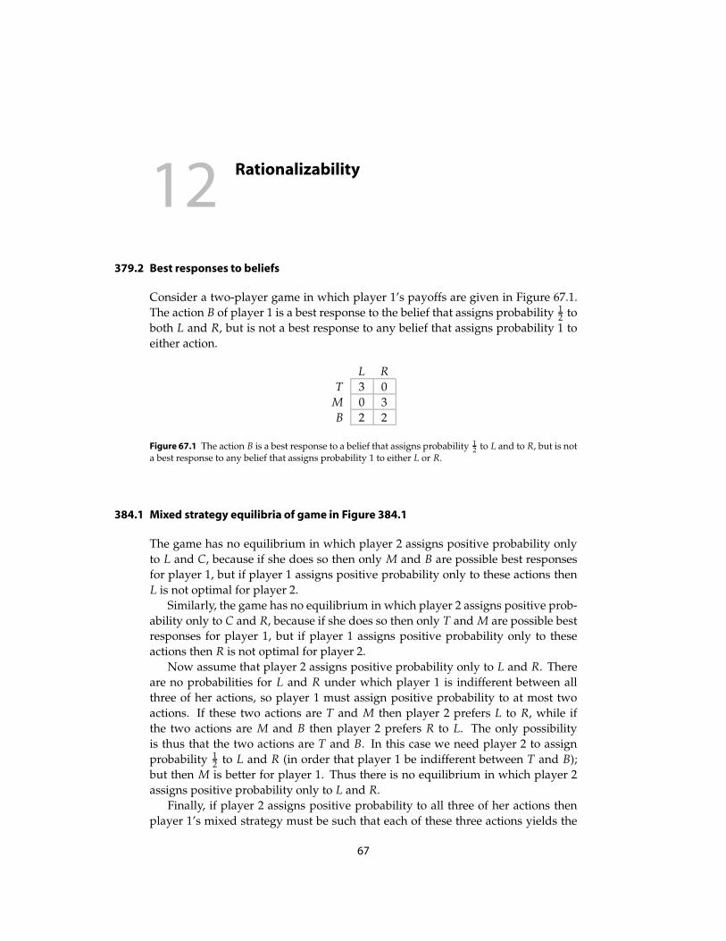
12Rationalizability
379.2 Best responses to beliefs
Consider a two-player game in which player 1’s payoffs are given in Figure 67.1.
The action B of player 1 is a best response to the belief that assigns probability 12 to
both L and R, but is not a best response to any belief that assigns probability 1 to
either action.
L R
T 3 0
M 0 3
B 2 2
Figure 67.1 The action B is a best response to a belief that assigns probability 12 to L and to R, but is not
a best response to any belief that assigns probability 1 to either L or R.
384.1 Mixed strategy equilibria of game in Figure 384.1
The game has no equilibrium in which player 2 assigns positive probability only
to L and C, because if she does so then only M and B are possible best responses
for player 1, but if player 1 assigns positive probability only to these actions then
L is not optimal for player 2.
Similarly, the game has no equilibrium in which player 2 assigns positive prob-
ability only to C and R, because if she does so then only T and M are possible best
responses for player 1, but if player 1 assigns positive probability only to these
actions then R is not optimal for player 2.
Now assume that player 2 assigns positive probability only to L and R. There
are no probabilities for L and R under which player 1 is indifferent between all
three of her actions, so player 1 must assign positive probability to at most two
actions. If these two actions are T and M then player 2 prefers L to R, while if
the two actions are M and B then player 2 prefers R to L. The only possibility
is thus that the two actions are T and B. In this case we need player 2 to assign
probability 12 to L and R (in order that player 1 be indifferent between T and B);
but then M is better for player 1. Thus there is no equilibrium in which player 2
assigns positive probability only to L and R.
Finally, if player 2 assigns positive probability to all three of her actions then
player 1’s mixed strategy must be such that each of these three actions yields the
67
68 Chapter 12. Rationalizability
same payoff. A calculation shows that there is no mixed strategy of player 1 with
this property.
We conclude that the game has no mixed strategy equilibrium in which either
player assigns positive probability to more than one action.
387.2 Finding rationalizable actions
I claim that the action R of player 2 is strictly dominated. Consider a mixed strat-
egy of player 2 that assigns probability p to L and probability 1 − p to C. Such a
mixed strategy strictly dominates R if p + 4(1− p) > 3 and 8p + 2(1− p) > 3, or if16 < p < 1
3 . Now eliminate R from the game. In the reduced game, B is dominated
by T. In the game obtained by eliminating B, L is dominated by C. Thus the only
rationalizable action of player 1 is T and the only rationalizable action of player 2
is C.
387.5 Hotelling’s model of electoral competition
The positions 0 and ` are strictly dominated by the position m:
• if her opponent chooses m, a player who chooses m ties whereas a player
who chooses 0 loses
• if her opponent chooses 0 or `, a player who chooses m wins whereas a player
who chooses 0 or ` either loses or ties
• if her opponent chooses any other position, a player who chooses m wins
whereas a player who chooses 0 or ` loses.
In the game obtained by eliminating the two positions 0 and `, the positions 1
and `− 1 are similarly strictly dominated. Continuing in the same way, we are left
with the position m.
388.2 Cournot’s duopoly game
From Figure 58.1 we see that firm 1’s payoff to any output greater than 12 (α − c)
is less than its payoff to the output 12 (α − c) for any output q2 of firm 2. Thus any
output greater than 12 (α− c) is strictly dominated by the output 1
2 (α− c) for firm 1;
the same argument applies to firm 2.
Now eliminate all outputs greater than 12 (α − c) for each firm. The maximizer
of firm 1’s payoff function for q2 = 12 (α − c) is 1
4 (α − c), so from Figure 58.1 we see
that firm 1’s payoff to any output less than 14 (α − c) is less than its payoff to the
output 14 (α − c) for any output q2 ≤ 1
2 (α − c) of firm 2. Thus any output less than14 (α − c) is strictly dominated by the output 1
4 (α − c) for firm 1; the same argument
applies to firm 2.
Chapter 12. Rationalizability 69
Now eliminate all outputs less than 14 (α − c) for each firm. Then by another
similar argument, any output greater than 38 (α − c) is strictly dominated by 3
8 (α −c). Continuing in this way, we see from Figure 59.1 that in a finite number of
rounds (given the finite number of possible outputs for each firm) we reach the
Nash equilibrium output 13 (α − c).
391.1 Example of dominancesolvable game
The Nash equilibria of the game are (T, L), any ((0, 0, 1), (0, q, 1− q)) with 0 ≤ q ≤1, and any ((0, p, 1− p), (0, 0, 1)) with 0 ≤ p ≤ 1.
The game is dominance solvable, because T and L are the only weakly domi-
nated actions, and when they are eliminated the only weakly dominated actions
are M and C, leaving (B, R), with payoffs (0, 0).
If T is eliminated, then L and C, no remaining action is weakly dominated;
(M, R) and (B, R) both remain.
391.2 Dividing money
In the first round every action ai ≤ 5 of each player i is weakly dominated by 6.
No other action is weakly dominated, because 100 is a strict best response to 0 and
every other action ai ≥ 6 is a strict best response to ai + 1. In the second round,
10 is weakly dominated by 6 for each player, and each other remaining action ai of
player i is a strict best response to a1 + 1, so no other action is weakly dominated.
Similarly, in the third round, 9 is weakly dominated by 6, and no other action is
weakly dominated. In the fourth and fifth rounds 8 and 7 are eliminated, leaving
the single action pair (6, 6), with payoffs (5, 5).
392.2 Strictly competitive extensive games with perfect information
Every finite extensive game with perfect information has a (pure strategy) sub-
game perfect equilibrium (Proposition 173.1). This equilibrium is a pure strategy
Nash equilibrium of the strategic form of the game. Because the game has only
two possible outcomes, one of the players prefers the Nash equilibrium outcome
to the other possible outcome. By Proposition 368.1, this player’s equilibrium strat-
egy guarantees her equilibrium payoff, so this strategy weakly dominates all her
nonequilibrium strategies. After all dominated strategies are eliminated, every
remaining pair of strategies generates the same outcome.

13Evolutionary Equilibrium
400.1 Evolutionary stability and weak domination
The ESS a∗ does not necessarily weakly dominate every other action in the game.
For example, in the game in Figure 395.1 of the text, X is an ESS but does not
weakly dominate Y.
No action can weakly dominate an ESS. To see why, let a∗ be an ESS and let
b be another action. Because a∗ is an ESS, (a∗, a∗) is a Nash equilibrium, so that
u(b, a∗) ≤ u(a∗, a∗). Now, if u(b, a∗) < u(a∗, a∗), certainly b does not weakly dom-
inate a∗, so suppose that u(b, a∗) = u(a∗, a∗). Then by the second condition for an
ESS we have u(b, b) < u(a∗, b). We conclude that b does not weakly dominate a∗.
405.1 Hawk–Dove–Retaliator
First suppose that v ≥ c. In this case the game has two pure symmetric Nash
equilibria, (A, A) and (R, R). However, A is not an ESS, because R is a best re-
sponse to A and u(R, R) > u(A, R). The action pair (R, R) is a strict equilibrium,
so R is an ESS. Now consider the possibility that the game has a mixed strategy
equilibrium (α, α). If α assigns positive probability to either P or R (or both) then
R yields a payoff higher than does P, so only A and R may be assigned positive
probability in a mixed strategy equilibrium. But if a strategy α assigns positive
probability to A and R and probability 0 to P, then R yields a payoff higher than
does A against an opponent who uses α. Thus the game has no symmetric mixed
strategy equilibrium in this case.
Now suppose that v < c. Then the only symmetric pure strategy equilibrium is
(R, R). This equilibrium is strict, so that R is an ESS. Now consider the possibility
that the game has a mixed strategy equilibrium (α, α). If α assigns probability 0 to
A then R yields a payoff higher than does P against an opponent who uses α; if
α assigns probability 0 to P then R yields a payoff higher than does A against an
opponent who uses α. Thus in any mixed strategy equilibrium (α, α), the strategy α
must assign positive probability to both A and P. If α assigns probability 0 to R
then we need α = (v/c, 1 − v/c) (the calculation is the same as for Hawk–Dove).
Because R yields a lower payoff against this strategy than do A and P, and the
strategy is an ESS in Hawk–Dove, it is an ESS in the present game. The remaining
possibility is that the game has a mixed strategy equilibrium (α, α) in which α
assigns positive probability to all three actions. If so, then the expected payoff to
this strategy is less than 12 v, because the pure strategy P yields an expected payoff
71
72 Chapter 13. Evolutionary Equilibrium
less than 12 v against any such strategy. But then U(R, R) = 1
2 v > U(α, R), violating
the second condition in the definition of an ESS.
In summary:
• If v ≥ c then R is the unique ESS of the game.
• If v < c then both R and the mixed strategy that assigns probability v/c to A
and 1 − v/c to P are ESSs.
405.3 Bargaining
The game is given in Figure 27.1.
The pure strategy of demanding 10 is not an ESS because 2 is a best response to
10 and u(2, 2) > u(10, 2).
Now let α be the mixed strategy that assigns probability 25 to 2 and 3
5 to 8. Each
player’s payoff at the strategy pair (α, α) is 165 . Thus the only actions a that are best
responses to α are 2 and 8, so that the only mixed strategies that are best responses
to α assign positive probability only to the actions 2 and 8. Let β be the mixed
strategy that assigns probability p to 2 and probability 1 − p to 8. We have
U(β, β) = 5p(2− p)
and
U(α, β) = 6p + 45 .
We find that U(α, β)− U(β, β) = 5(p − 25 )2, which is positive if p 6= 2
5 . Hence α is
an ESS.
Finally let α be the mixed strategy that assigns probability 45 to 4 and 1
5 to 6.
Each player’s payoff at the strategy pair (α, α) is 245 . Thus the only actions a that
are best responses to α are 4 and 6, so that the only mixed strategies that are best
responses assign positive probability only to the actions 4 and 6. Let β be the mixed
strategy that assigns probability p to 4 and probability 1 − p to 6. We have
U(β, β) = 5p(2− p)
and
U(α∗, β) = 2p + 165 .
We find that U(α, β)−U(β, β) = 5(p− 45 )2, which is positive if p 6= 4
5 . Hence α∗ is
an ESS.
408.1 Equilibria of C and of G
First suppose that (α1, α2) is a mixed strategy Nash equilibrium of C. Then for all
mixed strategies β1 of player 1 and all mixed strategies β2 of player 2 we have
U1(α1, α2) ≥ U1(β1, α2) and U2(α1, α2) ≥ U2(α1, β2).
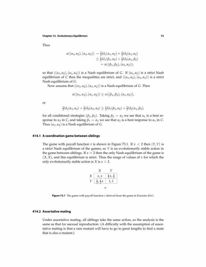
Chapter 13. Evolutionary Equilibrium 73
Thus
u((α1, α2), (α1, α2)) = 12 U1(α1, α2) + 1
2 U2(α1, α2)
≥ 12 U1(β1, α2) + 1
2 U2(α1, β2)
= u((β1, β2), (α1, α2)),
so that ((α1, α2), (α1, α2)) is a Nash equilibrium of G. If (α1, α2) is a strict Nash
equilibrium of C then the inequalities are strict, and ((α1, α2), (α1, α2)) is a strict
Nash equilibrium of G.
Now assume that ((α1, α2), (α1, α2)) is a Nash equilibrium of G. Then
u((α1, α2), (α1, α2)) ≥ u((β1, β2), (α1, α2)),
or12 U1(α1, α2) + 1
2 U2(α1, α2) ≥12 U1(β1, α2) + 1
2 U2(α1, β2),
for all conditional strategies (β1, β2). Taking β2 = α2 we see that α1 is a best re-
sponse to α2 in C, and taking β1 = α1 we see that α2 is a best response to α1 in C.
Thus (α1, α2) is a Nash equilibrium of G.
414.1 A coordination game between siblings
The game with payoff function v is shown in Figure 73.1. If x < 2 then (Y, Y) is
a strict Nash equilibrium of the games, so Y is an evolutionarily stable action in
the game between siblings. If x > 2 then the only Nash equilibrium of the game is
(X, X), and this equilibrium is strict. Thus the range of values of x for which the
only evolutionarily stable action is X is x > 2.
X Y
X x, x 12 x, 1
2
Y 12 , 1
2 x 1, 1
v
Figure 73.1 The game with payoff function v derived from the game in Exercise 414.1.
414.2 Assortative mating
Under assortative mating, all siblings take the same action, so the analysis is the
same as that for asexual reproduction. (A difficulty with the assumption of assor-
tative mating is that a rare mutant will have to go to great lengths to find a mate
that is also a mutant.)
74 Chapter 13. Evolutionary Equilibrium
416.1 Darwin’s theory of the sex ratio
A normal organism produces pn male offspring and (1 − p)n female offspring
(ignoring the small probability that the partner of a normal organism is a mutant).
Thus it has pn · ((1 − p)/p)n + (1 − p)n · n = 2(1− p)n2 grandchildren.
A mutant has 12 n male offspring and 1
2 n female offspring, and hence 12 n · ((1 −
p)/p)n + 12 n · n = 1
2 n2/p grandchildren.
Thus the difference between the number of grandchildren produced by mutant
and normal organisms is
12 n2/p − 2(1 − p)n2 = n2
(1
2p
)
(1 − 2p)2,
which is positive if p 6= 12 . (The point is that if p >
12 then the fraction of a mutant’s
offspring that are males is higher than the fraction of a normal organism’s offspring
that are males, and males each bear more offspring than females. Similarly, if p <12
then the fraction of a mutant’s offspring that are females is higher than the fraction
of a normal organism’s offspring that are females, and females each bear more
offspring than males.)
Thus any mutant with p 6= 12 invades the population; only p = 1
2 is evolution-
arily stable.
14Repeated Games: The Prisoner’s Dilemma
423.1 Equivalence of payoff functions
Suppose that a person’s preferences are represented by the discounted sum of pay-
offs with payoff function u and discount factor δ. Then if the two sequences of
outcomes (x1, x2, . . .) and (y1, y2, . . .) are indifferent, we have
∞
∑t=0
δt−1u(xt) =∞
∑t=0
δt−1u(yt).
Now let v(x) = α + βu(x) for all x, with β > 0. Then
∞
∑t=0
δt−1v(xt) =∞
∑t=0
δt−1[α + βu(xt)] =∞
∑t=0
δt−1α + β∞
∑t=0
δt−1u(xt)
and similarly
∞
∑t=0
δt−1v(yt) =∞
∑t=0
δt−1[α + βu(yt)] =∞
∑t=0
δt−1α + β∞
∑t=0
δt−1u(yt),
so that∞
∑t=0
δt−1v(xt) =∞
∑t=0
δt−1v(yt).
Thus the person’s preferences are represented also by the discounted sum of pay-
offs with payoff function v and discount factor δ.
426.1 Subgame perfect equilibrium of finitely repeated Prisoner’s Dilemma
Use backward induction. In the last period, the action C is strictly dominated for
each player, so each player chooses D, regardless of history. Now consider pe-
riod T − 1. Each player’s action in this period affects only the outcome in this
period—it has no effect on the outcome in period T, which is (D, D). Thus in
choosing her action in period T − 1, a player considers only her payoff in that pe-
riod. As in period T, her action D strictly dominates her action C, so that in any
subgame perfect equilibrium she chooses D. A similar argument applies to all pre-
vious periods, leading to the conclusion that in every subgame perfect equilibrium
each player chooses D in every period, regardless of history.
75
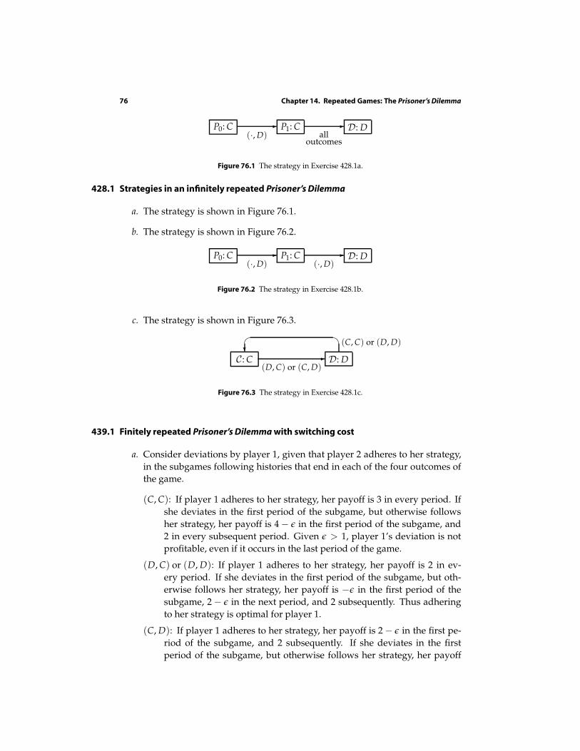
76 Chapter 14. Repeated Games: The Prisoner’s Dilemma
P0: C -(·, D)
P1: C -all
outcomes
D: D
Figure 76.1 The strategy in Exercise 428.1a.
428.1 Strategies in an infinitely repeated Prisoner’s Dilemma
a. The strategy is shown in Figure 76.1.
b. The strategy is shown in Figure 76.2.
P0: C -(·, D)
P1: C -(·, D)
D: D
Figure 76.2 The strategy in Exercise 428.1b.
c. The strategy is shown in Figure 76.3.
C : C D: D-(D, C) or (C, D)
?
(C, C) or (D, D)
Figure 76.3 The strategy in Exercise 428.1c.
439.1 Finitely repeated Prisoner’s Dilemma with switching cost
a. Consider deviations by player 1, given that player 2 adheres to her strategy,
in the subgames following histories that end in each of the four outcomes of
the game.
(C, C): If player 1 adheres to her strategy, her payoff is 3 in every period. If
she deviates in the first period of the subgame, but otherwise follows
her strategy, her payoff is 4 − ε in the first period of the subgame, and
2 in every subsequent period. Given ε > 1, player 1’s deviation is not
profitable, even if it occurs in the last period of the game.
(D, C) or (D, D): If player 1 adheres to her strategy, her payoff is 2 in ev-
ery period. If she deviates in the first period of the subgame, but oth-
erwise follows her strategy, her payoff is −ε in the first period of the
subgame, 2 − ε in the next period, and 2 subsequently. Thus adhering
to her strategy is optimal for player 1.
(C, D): If player 1 adheres to her strategy, her payoff is 2 − ε in the first pe-
riod of the subgame, and 2 subsequently. If she deviates in the first
period of the subgame, but otherwise follows her strategy, her payoff
Chapter 14. Repeated Games: The Prisoner’s Dilemma 77
is 0 in the first period of the subgame, 2 − ε in the next period, and 2
subsequently. Given ε < 2, player 1’s deviation is not optimal even if it
occurs in the last period of the game.
b. Given ε > 2, a player does not gain from deviating from (C, C) in the next-
to-last or last periods, even if she is not punished, and does not optimally
punish such a deviation by her opponent. Consider the strategy that chooses
C at the start of the game and after any history that ends with (C, C), chooses
D after any other history that has length at most T − 2, and chooses the action
it chose in period T − 1 after any history of length T − 1 (where T is the length
of the game). I claim that the strategy pair in which both players use this
strategy is a subgame perfect equilibrium. Consider deviations by player 1,
given that player 2 adheres to her strategy, in the subgames following the
various possible histories.
History ending in (C, C), length ≤ T − 3: If player 1 adheres to her strategy,
her payoff is 3 in every period of the subgame. If she deviates in the first
period of the subgame, but otherwise follows her strategy, her payoff
is 4 − ε in the first period of the subgame, and 2 in every subsequent
period (her opponent switches to D). Given ε > 1, player 1’s deviation
is not profitable.
History ending in (C, C), length ≥ T − 2: If player 1 adheres to her strategy,
her payoff is 3 in each period of the subgame. If she deviates to D in the
first period of the subgame, her payoff is 4− ε in that period, and 4 sub-
sequently (her deviation is not punished). The length of the subgame is
at most 2, so given ε > 2, her deviation is not profitable.
History ending in (D, C) or (D, D): If player 1 adheres to her strategy, her
payoff is 2 in every period. If she deviates in the first period of the
subgame, but otherwise follows her strategy, her payoff is −ε in the
first period of the subgame, 2− ε in the next period, and 2 subsequently.
Thus adhering to her strategy is optimal for player 1.
History ending in (C, D), length ≤ T − 2: If player 1 adheres to her strategy,
her payoff is 2− ε in the first period of the subgame (she switches to D),
and 2 subsequently. If she deviates in the first period of the subgame,
but otherwise follows her strategy, her payoff is 0 in the first period of
the subgame, 2 − ε in the next period, and 2 subsequently.
History ending in (C, D), length T − 1: If player 1 adheres to her strategy,
her payoff is 0 in period T (the outcome is (C, D)). If she deviates to
D, her payoff is 2 − ε in period T. Given ε > 2, adhering to her strategy
is thus optimal.
78 Chapter 14. Repeated Games: The Prisoner’s Dilemma
442.1 Deviations from grim trigger strategy
• If player 1 adheres to the strategy, she subsequently chooses D (because
player 2 chose D in the first period). Player 2 chooses C in the first period
of the subgame (player 1 chose C in the first period of the game), and then
chooses D (because player 1 chooses D in the first period of the subgame).
Thus the sequence of outcomes in the subgame is ((D, C), (D, D), (D, D), . . .),
yielding player 1 a discounted average payoff in the subgame of
(1 − δ)(3 + δ + δ2 + δ3 + · · ·) = (1 − δ)
(
3 +δ
1 − δ
)
= 3 − 2δ.
• If player 1 refrains from punishing player 2 for her lapse, and simply chooses
C in every subsequent period, then the outcome in period 2 and subsequently
is (C, C), so that the sequence of outcomes in the subgame yields player 1 a
discounted average payoff of 2.
If δ > 12 then 2 > 3 − 2δ, so that player 1 prefers to ignore player 2’s deviation
rather than to adhere to her strategy and punish player 2 by choosing D. (Note
that the theory does not consider the possibility that player 1 takes player 2’s play
of D as a signal that she is using a strategy different from the grim trigger strategy.)
443.2 Different punishment lengths in subgame perfect equilibrium
Yes, an infinitely repeated Prisoner’s Dilemma has such subgame perfect equilibria.
As for the modified grim trigger strategy, each player’s strategy has to switch to
D not only if the other player chooses D but also if the player herself chooses
D. The only subtlety is that the number of periods for which a player chooses
D after a history in which not all the outcomes were (C, C) must depend on the
identity of the player who first deviated. If, for example, player 1 punishes for
two periods while player 2 punishes for three periods, then the outcome (C, D)induces player 1 to choose D for two periods (to punish player 2 for her deviation)
while the outcome (D, C) induces her to choose D for three periods (while she is
being punished by player 2). The strategy of each player in this case is shown
in Figure 79.1. Viewed as a strategy of player 1, the top part of the figure entails
punishment of player 2 and the bottom part entails player 1’s reaction to her own
deviation. Similarly, viewed as a strategy of player 2, the bottom part of the figure
entails punishment of player 1 and the top part entails player 2’s reaction to her
own deviation.
To find the values of δ for which the strategy pair in which each player uses
the strategy in Figure 79.1 is a subgame perfect equilibrium, consider the result of
each player’s deviating at the start of a subgame.
First consider player 1. If she deviates when both players are in state P0, she
induces the outcome (D, C) followed by three periods of (D, D), and then (C, C)subsequently. This outcome path is worse for her than (C, C) in every period if
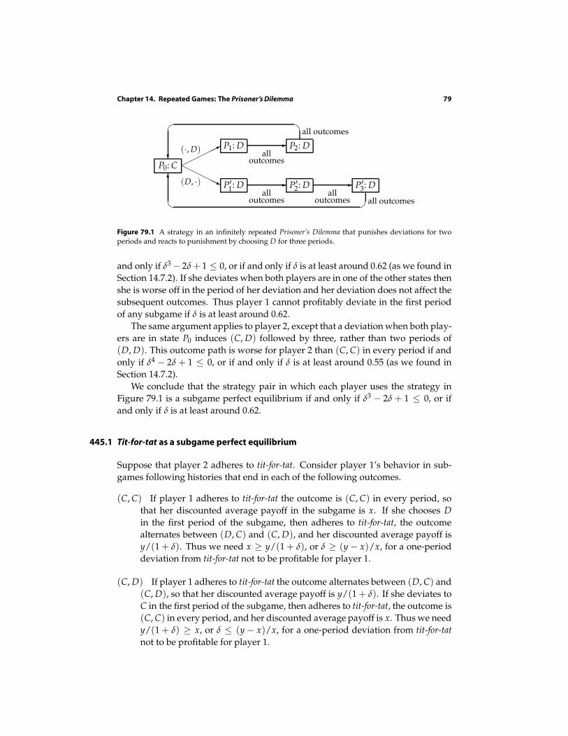
Chapter 14. Repeated Games: The Prisoner’s Dilemma 79
P0: C *(·, D) P1: D -all
outcomes
P2: D?
all outcomes
HHHHHj(D, ·) P′1: D -
alloutcomes
P′2: D -
alloutcomes
P′3: D
6
all outcomes
Figure 79.1 A strategy in an infinitely repeated Prisoner’s Dilemma that punishes deviations for twoperiods and reacts to punishment by choosing D for three periods.
and only if δ3 − 2δ + 1 ≤ 0, or if and only if δ is at least around 0.62 (as we found in
Section 14.7.2). If she deviates when both players are in one of the other states then
she is worse off in the period of her deviation and her deviation does not affect the
subsequent outcomes. Thus player 1 cannot profitably deviate in the first period
of any subgame if δ is at least around 0.62.
The same argument applies to player 2, except that a deviation when both play-
ers are in state P0 induces (C, D) followed by three, rather than two periods of
(D, D). This outcome path is worse for player 2 than (C, C) in every period if and
only if δ4 − 2δ + 1 ≤ 0, or if and only if δ is at least around 0.55 (as we found in
Section 14.7.2).
We conclude that the strategy pair in which each player uses the strategy in
Figure 79.1 is a subgame perfect equilibrium if and only if δ3 − 2δ + 1 ≤ 0, or if
and only if δ is at least around 0.62.
445.1 Titfortat as a subgame perfect equilibrium
Suppose that player 2 adheres to tit-for-tat. Consider player 1’s behavior in sub-
games following histories that end in each of the following outcomes.
(C, C) If player 1 adheres to tit-for-tat the outcome is (C, C) in every period, so
that her discounted average payoff in the subgame is x. If she chooses D
in the first period of the subgame, then adheres to tit-for-tat, the outcome
alternates between (D, C) and (C, D), and her discounted average payoff is
y/(1 + δ). Thus we need x ≥ y/(1 + δ), or δ ≥ (y − x)/x, for a one-period
deviation from tit-for-tat not to be profitable for player 1.
(C, D) If player 1 adheres to tit-for-tat the outcome alternates between (D, C) and
(C, D), so that her discounted average payoff is y/(1 + δ). If she deviates to
C in the first period of the subgame, then adheres to tit-for-tat, the outcome is
(C, C) in every period, and her discounted average payoff is x. Thus we need
y/(1 + δ) ≥ x, or δ ≤ (y − x)/x, for a one-period deviation from tit-for-tat
not to be profitable for player 1.
80 Chapter 14. Repeated Games: The Prisoner’s Dilemma
(D, C) If player 1 adheres to tit-for-tat the outcome alternates between (C, D) and
(D, C), so that her discounted average payoff is δy/(1 + δ). If she deviates to
D in the first period of the subgame, then adheres to tit-for-tat, the outcome
is (D, D) in every period, and her discounted average payoff is 1. Thus we
need δy/(1 + δ) ≥ 1, or δ ≥ 1/(y − 1), for a one-period deviation from
tit-for-tat not to be profitable for player 1.
(D, D) If player 1 adheres to tit-for-tat the outcome is (D, D) in every period, so
that her discounted average payoff is 1. If she deviates to C in the first period
of the subgame, then adheres to tit-for-tat, the outcome alternates between
(C, D) and (D, C), and her discounted average payoff is δy/(1 + δ). Thus
we need 1 ≥ δy/(1 + δ), or δ ≤ 1/(y − 1), for a one-period deviation from
tit-for-tat not to be profitable for player 1.
The same arguments apply to deviations by player 2, so we conclude that
(tit-for-tat, tit-for-tat) is a subgame perfect equilibrium if and only if δ = (y − x)/x
and δ = 1/(y − 1), or y − x = 1 and δ = 1/x.
15Repeated Games: General Results
454.3 Repeated Bertrand duopoly
a. Suppose that firm i uses the strategy si. If the other firm, j, uses sj, then its
discounted average payoff is
(1 − δ)(
12 π(pm) + 1
2 δπ(pm) + · · ·)
= 12 π(pm).
If, on the other hand, firm j deviates to a price p then the closer this price
is to pm, the higher is j’s profit, because the punishment does not depend
on p. Thus by choosing p close enough to pm the firm can obtain a profit as
close as it wishes to π(pm) in the period of its deviation. Its profit during
its punishment in the following k periods is zero. Once its punishment is
complete, it can either revert to pm or deviate once again. If it can profit
from deviating initially then it can profit by deviating once its punishment is
complete, so its maximal profit from deviating is
(1 − δ)(
π(pm) + δk+1π(pm) + δ2k+2π(pm) + · · ·)
=(1 − δ)π(pm)
1 − δk+1.
Thus for (s1, s2) to be a Nash equilibrium we need
1 − δ
1 − δk+1≤ 1
2 ,
or
δk+1 − 2δ + 1 ≤ 0.
(This condition is the same as the one we found for a pair of k-period pun-
ishment strategies to be a Nash equilibrium in the Prisoner’s Dilemma (Sec-
tion 14.7.2).)
b. Suppose that firm i uses the strategy si. If the other firm does so then its
discounted average payoff is 12 π(pm), as in part a. If the other firm deviates
to some price p with c < p < pm in the first period, and maintains this price
subsequently, then it obtains π(p) in the first period and shares π(p) in each
subsequent period, so that its discounted average payoff is
(1 − δ)(
π(p) + 12 δπ(p) + 1
2 δ2π(p) + · · ·)
= 12 (2 − δ)π(p).
If p is close to pm then π(p) is close to π(pm) (because π is continuous). In
fact, for any δ < 1 we have 2 − δ > 1, so that we can find p < pm such that
(2 − δ)π(p) > π(pm). Hence the strategy pair is not a Nash equilibrium of
the infinitely repeated game for any value of δ.
81
82 Chapter 15. Repeated Games: General Results
459.2 Detection lags
a. The best deviations involve prices slightly less than p∗. Such a deviation by
firm i yields a discounted average payoff close to
(1 − δ)(
π(p∗) + δπ(p∗) + · · ·+ δki−1π(p∗))
= (1 − δki)π(p∗),
whereas compliance with the strategy yields the discounted average payoff12 π(p∗). Thus the strategy pair is a subgame perfect equilibrium for any
value of p∗ if δk1 ≥ 12 and δk2 ≥ 1
2 , and is not a subgame perfect equilibrium
for any value of p∗ if δk1 < 12 or δk2 < 1
2 . That is, the most profitable price for
which the strategy pair is a subgame perfect equilibrium is pm if δk1 ≥ 12 and
δk2 ≥ 12 and is c if δk1 <
12 or δk2 <
12 .
b. Denote by k∗i the critical value of ki found in part a. (That is, δk∗i ≥ 12 and
δk∗i +1 < 12 .)
If ki > k∗i then no change in kj affects the outcome of the price-setting sub-
game, so j’s best action at the start of the game is θ, in which case i’s best ac-
tion is the same. Thus in one subgame perfect equilibrium both firms choose
θ at the start of the game, and c regardless of history in the rest of the game.
If ki ≤ k∗i then j’s best action is k∗j if the cost of choosing k∗j is at most 12 π(pm).
Thus if the cost of choosing k∗i is at most 12 π(pm) for each firm then the game
has another subgame perfect equilibrium, in which each firm i chooses k∗i at
the start of the game and the strategy si in the price-setting subgame.
A promise by firm i to beat another firm’s price is an inducement for con-
sumers to inform firm i of deviations by other firms, and thus reduce its
detection time. To this extent, such a promise tends to promote collusion.
16Bargaining
468.1 Twoperiod bargaining with constant cost of delay
In the second period, player 1 accepts any proposal that gives a positive amount
of the pie. Thus in any subgame perfect equilibrium player 2 proposes (0, 1) in
period 2, which player 1 accepts, obtaining the payoff −c1.
Now consider the first period. Given the second period outcome of any sub-
game perfect equilibrium, player 2 accepts any proposal that gives her more than
1− c2 and rejects any proposal that gives her less than 1− c2. Thus in any subgame
perfect equilibrium player 1 proposes (c2, 1 − c2), which player 2 accepts.
In summary, the game has a unique subgame perfect equilibrium, in which
• player 1 proposes (c2, 1− c2) in period 1, and accepts all proposals in period 2
• player 2 accepts a proposal in period 1 if and only if it gives her at least 1− c2,
and proposes (0, 1) in period 2 after any history.
The outcome of the equilibrium is that the proposal (c2, 1− c2) is made by player 1
and immediately accepted by player 2.
468.2 Threeperiod bargaining with constant cost of delay
The subgame following a rejection by player 2 in period 1 is a two-period game in
which player 2 makes the first proposal. Thus by the result of Exercise 468.1, the
subgame has a unique subgame perfect equilibrium, in which player 2 proposes
(1 − c1, c1), which player 1 immediately accepts.
Now consider the first period.
• If c1 ≥ c2, player 2 rejects any offer of less than c1 − c2 (which she obtains if
she rejects an offer), and accepts any offer of more than c1 − c2. Thus in an
equilibrium player 1 offers her c1 − c2, which she accepts.
• If c1 < c2, player 2 accepts all offers, so that player 1 proposes (1, 0), which
player 2 accepts.
In summary, the game has a unique subgame perfect equilibrium, in which
• player 1 proposes (1 − (c1 − c2), c1 − c2) if c1 ≥ c2 and (1, 0) otherwise in
period 1, accepts any proposal that gives her at least 1 − c1 in period 2, and
proposes (1, 0) in period 3
83
84 Chapter 16. Bargaining
• player 2 accepts any proposal that gives her at least c1 − c2 if c1 ≥ c2 and
accepts all proposals otherwise in period 1, proposes (1 − c1, c1) in period 2,
and accepts all proposals in period 3.
17Appendix: Mathematics
497.1 Maximizer of quadratic function
We can write the function as −x(x − α). Thus r1 = 0 and r2 = α, and hence the
maximizer is α/2.
499.3 Sums of sequences
In the first case set r = δ2 to transform the sum into 1 + r + r2 + · · ·, which is equal
to 1/(1 − r) = 1/(1 − δ2).
In the second case split the sum into (1 + δ2 + δ4 + · · ·) + (2δ + 2δ3 + 2δ5 + · · ·);
the first part is equal to 1/(1 − δ2) and the second part is equal to 2δ(1 + δ2 + δ4 +· · ·), or 2δ/(1 − δ2). Thus the complete sum is
1 + 2δ
1 − δ2.
504.2 Bayes’ law
Your posterior probability of carrying X given that you test positive is
Pr(positive test|X) Pr(X)
Pr(positive test|X) Pr(X) + Pr(positive test|¬X) Pr(¬X)
where ¬X means “not X”. This probability is equal to 0.9p/(0.9p + 0.2(1 − p)) =0.9p/(0.2 + 0.7p), which is increasing in p (i.e. a smaller value of p gives a smaller
value of the probability). If p = 0.001 then the probability is approximately 0.004.
(That is, if 1 in 1,000 people carry the gene then if you test positive on a test that
is 90% accurate for people who carry the gene and 80% accurate for people who
do not carry the gene, then you should assign probability 0.004 to your carrying
the gene.) If the test is 99% accurate in both cases then the posterior probability is
(0.99 · 0.001)/[0.99 · 0.001 + 0.01 · 0.999] ≈ 0.09.
85

References
The page numbers on which the references are cited are given in brackets after each item.
Nagel, Rosemarie (1995), “Unraveling in guessing games: an experimental study”,
American Economic Review 85, 1313–1326. [8]
Ochs, Jack (1995), “Coordination problems”, in Handbook of experimental economics
(John H. Kagel and Alvin E. Roth, eds.), 195–251. Princeton: Princeton
University Press. [6]
Shubik, Martin (1982), Game theory in the social sciences. Cambridge, MA: MIT Press.
[55]
Van Huyck, John B., Raymond C. Battalio, and Richard O. Beil (1990), “Tacit coor-
dination games, strategic uncertainty, and coordination failure”, American
Economic Review 80, 234–248. [6]
87
Related Documents