Introduction to Game Theory 4. Game Tree Search Dana Nau University of Maryland Nau: Game Theory 1

Welcome message from author
This document is posted to help you gain knowledge. Please leave a comment to let me know what you think about it! Share it to your friends and learn new things together.
Transcript
Introduction to Game Theory
4. Game Tree Search
Dana Nau
University of Maryland
Nau: Game Theory 1
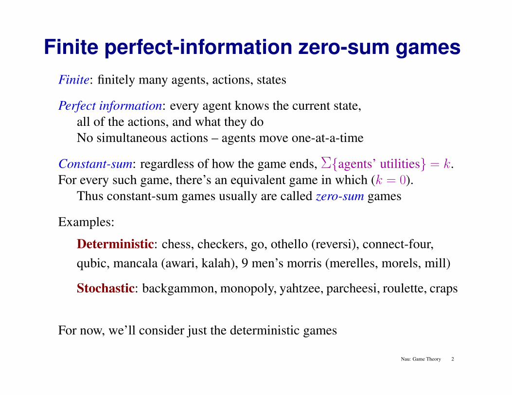
Finite perfect-information zero-sum gamesFinite: finitely many agents, actions, states
Perfect information: every agent knows the current state,all of the actions, and what they doNo simultaneous actions – agents move one-at-a-time
Constant-sum: regardless of how the game ends, Σ{agents’ utilities} = k.For every such game, there’s an equivalent game in which (k = 0).
Thus constant-sum games usually are called zero-sum games
Examples:
Deterministic: chess, checkers, go, othello (reversi), connect-four,qubic, mancala (awari, kalah), 9 men’s morris (merelles, morels, mill)
Stochastic: backgammon, monopoly, yahtzee, parcheesi, roulette, craps
For now, we’ll consider just the deterministic games
Nau: Game Theory 2
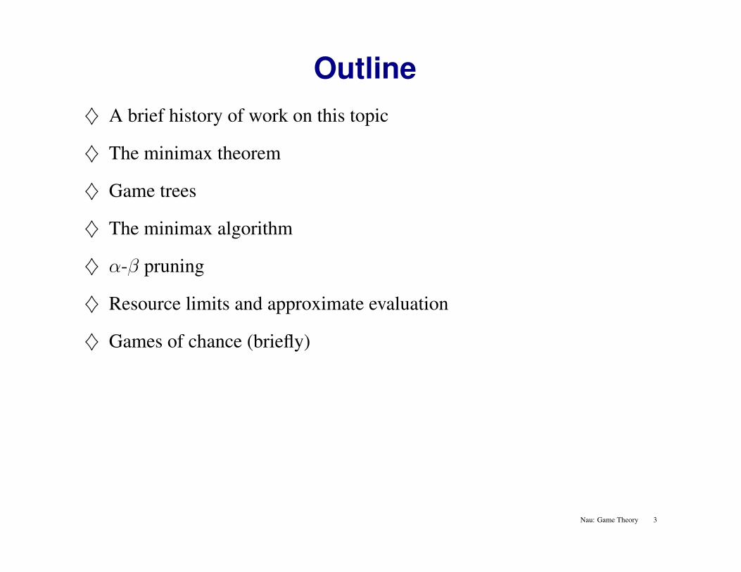
Outline♦ A brief history of work on this topic
♦ The minimax theorem
♦ Game trees
♦ The minimax algorithm
♦ α-β pruning
♦ Resource limits and approximate evaluation
♦ Games of chance (briefly)
Nau: Game Theory 3
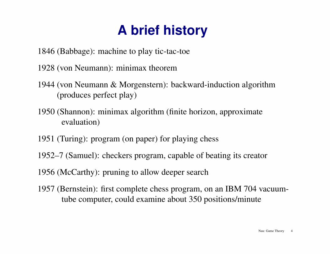
A brief history1846 (Babbage): machine to play tic-tac-toe
1928 (von Neumann): minimax theorem
1944 (von Neumann & Morgenstern): backward-induction algorithm(produces perfect play)
1950 (Shannon): minimax algorithm (finite horizon, approximateevaluation)
1951 (Turing): program (on paper) for playing chess
1952–7 (Samuel): checkers program, capable of beating its creator
1956 (McCarthy): pruning to allow deeper search
1957 (Bernstein): first complete chess program, on an IBM 704 vacuum-tube computer, could examine about 350 positions/minute
Nau: Game Theory 4
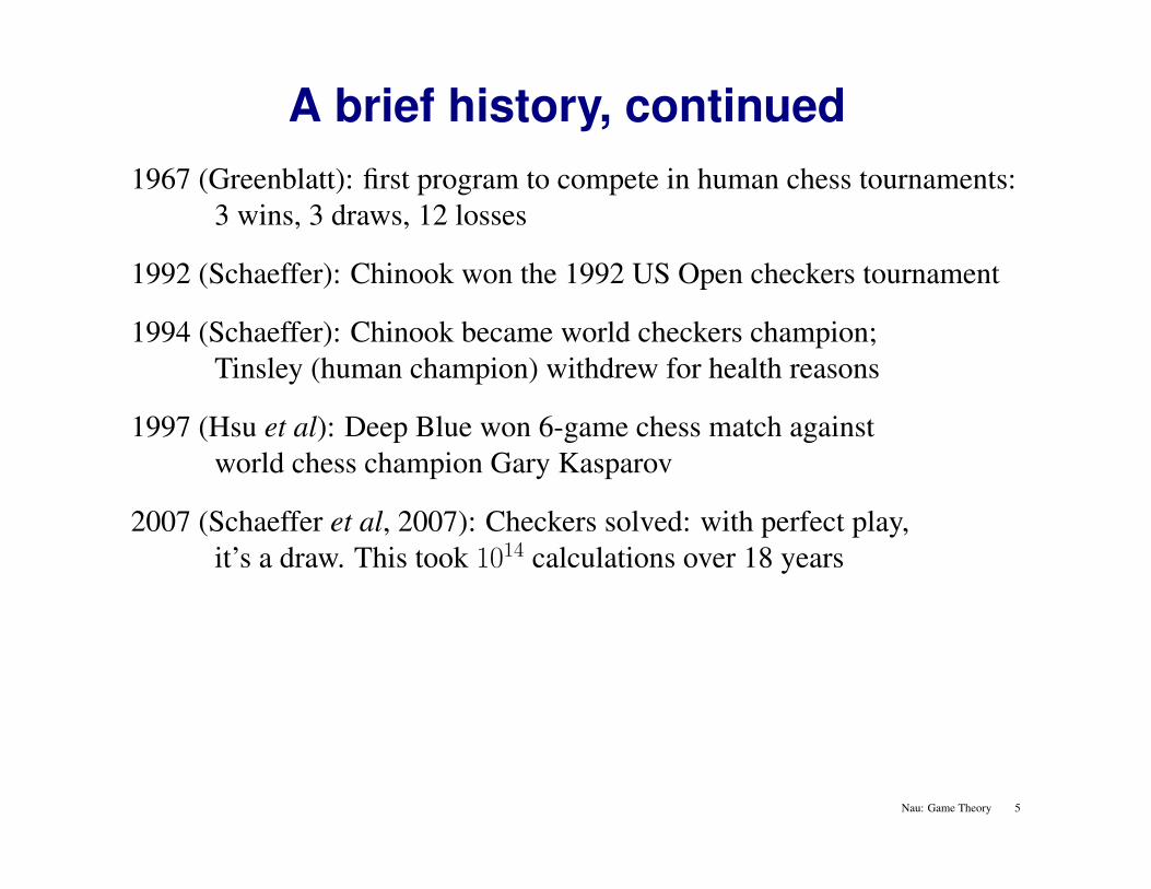
A brief history, continued1967 (Greenblatt): first program to compete in human chess tournaments:
3 wins, 3 draws, 12 losses
1992 (Schaeffer): Chinook won the 1992 US Open checkers tournament
1994 (Schaeffer): Chinook became world checkers champion;Tinsley (human champion) withdrew for health reasons
1997 (Hsu et al): Deep Blue won 6-game chess match againstworld chess champion Gary Kasparov
2007 (Schaeffer et al, 2007): Checkers solved: with perfect play,it’s a draw. This took 1014 calculations over 18 years
Nau: Game Theory 5
Quick reviewRecall that♦ A strategy tells what an agent will do in every possible situation♦ Strategies may be pure (deterministic) or mixed (probabilistic)
Suppose agents 1 and 2 use strategies s and t to play a two-person zero-sumgame G. Then
• Agent 1’s expected utility is u1(s, t)From now on, we’ll just call this u(s, t)
• Since G is zero-sum, u2(s, t) = −u(s, t)
We’ll call agent 1 Max, and agent 2 Min
Max wants to maximize u and Min wants to minimize it
Nau: Game Theory 6
The Minimax Theorem (von Neumann, 1928)♦ A restatement of the Minimax Theorem
that refers directly to the agents’ minimax strategies:
Theorem. Let G be a two-person finite zero-sum game. Then there arestrategies s∗ and t∗, and a number u∗, called G’s minimax value, such that
• If Min uses t∗, Max’s expected utility is ≤ u∗, i.e., maxs u(s, t∗) = u∗
• If Max uses s∗, Max’s expected utility is ≥ u∗, i.e., mint u(s∗, t) = u∗
Corollary 1: u(s∗, t∗) = u∗.
Corollary 2: If G is a perfect-information game,then there are pure strategies s∗ and t∗ that satisfy the theorem.
Nau: Game Theory 7
Game trees
XXXX
XX
X
XX
MAX (X)
MIN (O)
X X
O
OOX O
OO O
O OO
MAX (X)
X OX OX O XX X
XX
X X
MIN (O)
X O X X O X X O X
. . . . . . . . . . . .
. . .
. . .
. . .
TERMINALXX
−1 0 +1Utility
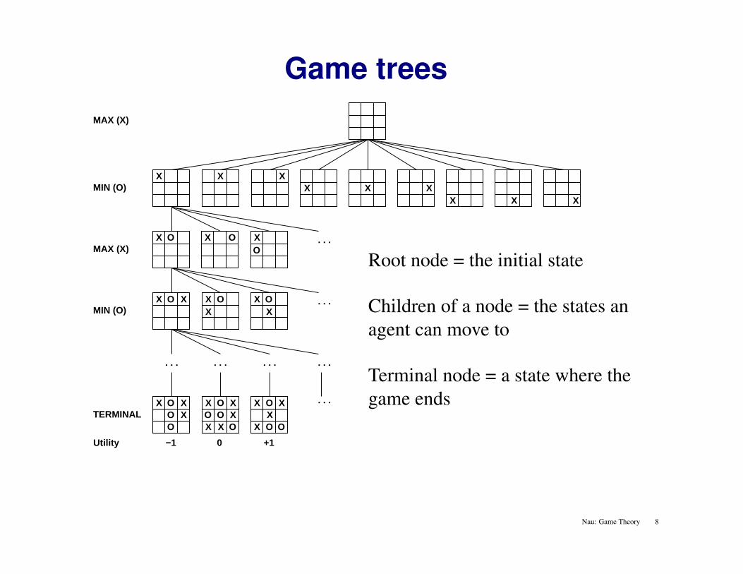
Root node = the initial state
Children of a node = the states anagent can move to
Terminal node = a state where thegame ends
Nau: Game Theory 8
Strategies on game trees
XXXX
XX
X
XX
MAX (X)
MIN (O)
X X
O
OOX O
OO O
O OO
MAX (X)
X OX OX O XX X
XX
X X
MIN (O)
X O X X O X X O X
. . . . . . . . . . . .
. . .
. . .
. . .TERMINAL
XX−1 0 +1Utility
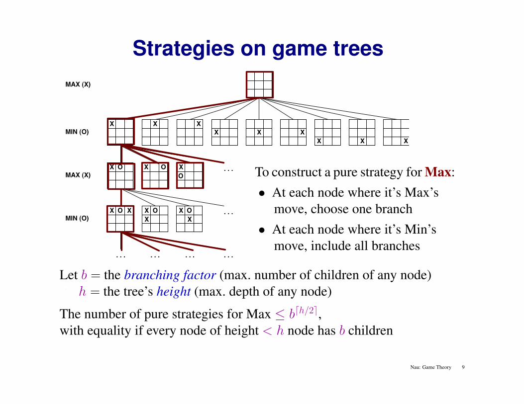
To construct a pure strategy for Max:• At each node where it’s Max’s
move, choose one branch• At each node where it’s Min’s
move, include all branches
Let b = the branching factor (max. number of children of any node)h = the tree’s height (max. depth of any node)
The number of pure strategies for Max ≤ bdh/2e,with equality if every node of height < h node has b children
Nau: Game Theory 9
Strategies on game trees
XXXX
XX
X
XX
MAX (X)
MIN (O)
X X
O
OOX O
OO O
O OO
MAX (X)
X OX OX O XX X
XX
X X
MIN (O)
X O X X O X X O X
. . . . . . . . . . . .
. . .
. . .
. . .TERMINAL
XX−1 0 +1Utility
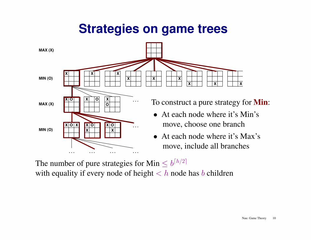
To construct a pure strategy for Min:• At each node where it’s Min’s
move, choose one branch• At each node where it’s Max’s
move, include all branches
The number of pure strategies for Min ≤ bdh/2e
with equality if every node of height < h node has b children
Nau: Game Theory 10
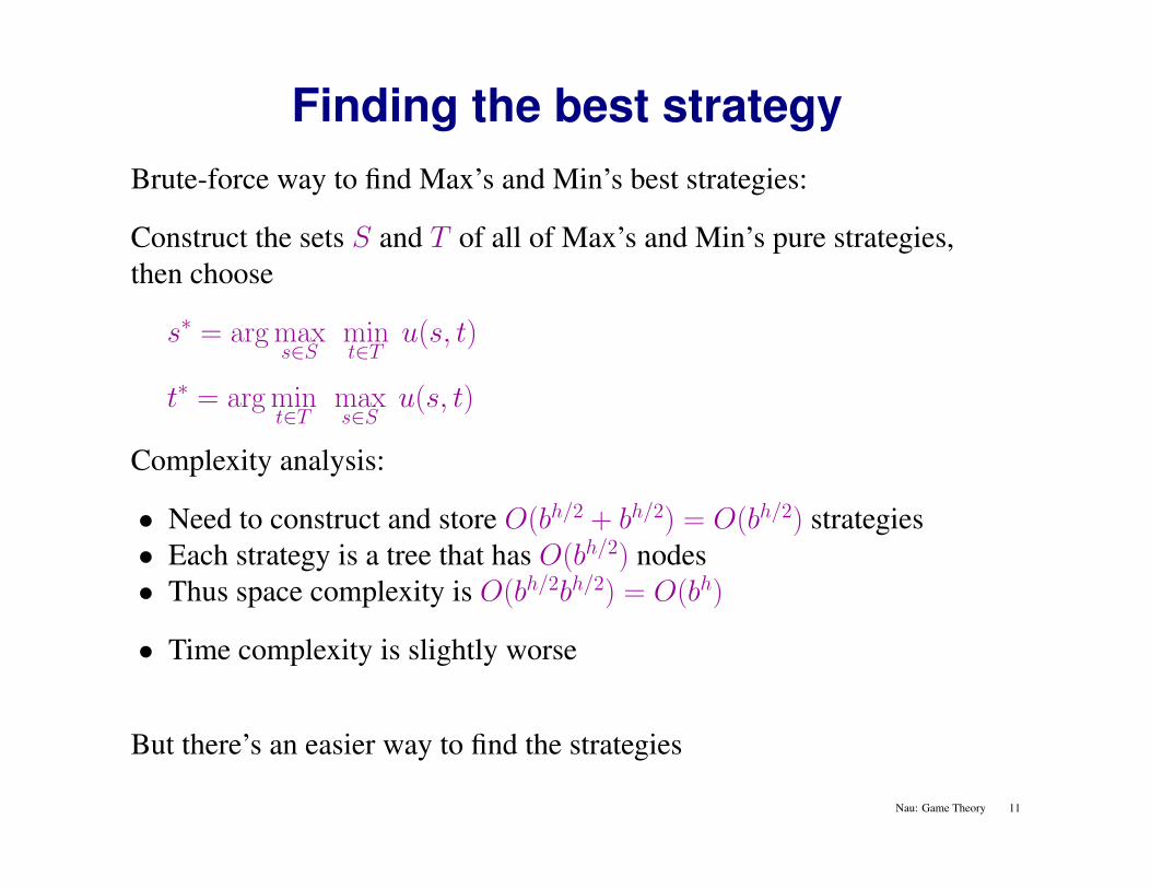
Finding the best strategyBrute-force way to find Max’s and Min’s best strategies:
Construct the sets S and T of all of Max’s and Min’s pure strategies,then choose
s∗ = arg maxs∈S
mint∈T
u(s, t)
t∗ = arg mint∈T
maxs∈S
u(s, t)
Complexity analysis:
• Need to construct and store O(bh/2 + bh/2) = O(bh/2) strategies• Each strategy is a tree that has O(bh/2) nodes• Thus space complexity is O(bh/2bh/2) = O(bh)
• Time complexity is slightly worse
But there’s an easier way to find the strategies
Nau: Game Theory 11
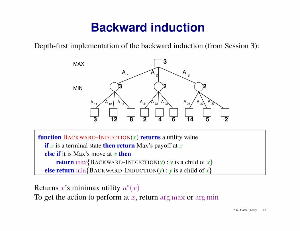
Backward inductionDepth-first implementation of the backward induction (from Session 3):
MAX
3 12 8 642 14 5 2
MIN
3A 1 A 3A 2
A 13A 12A 11 A 21 A 23A 22 A 33A 32A 31
3 2 2
function BACKWARD-INDUCTION(x) returns a utility valueif x is a terminal state then return Max’s payoff at xelse if it is Max’s move at x then
return max{BACKWARD-INDUCTION(y) : y is a child of x}else return min{BACKWARD-INDUCTION(y) : y is a child of x}
Returns x’s minimax utility u∗(x)To get the action to perform at x, return arg max or arg min
Nau: Game Theory 12
PropertiesSpace complexity: O(bh), where b and h are as defined earlier
Time complexity: O(bh)
For chess:
b ≈ 35, h ≈ 100 for “reasonable” games35100 ≈ 10135 nodes
Number of particles in the universe ≈ 1087
Number of nodes is≈ 1055 times the number of particles in the universe⇒ no way to examine every node!
Nau: Game Theory 13
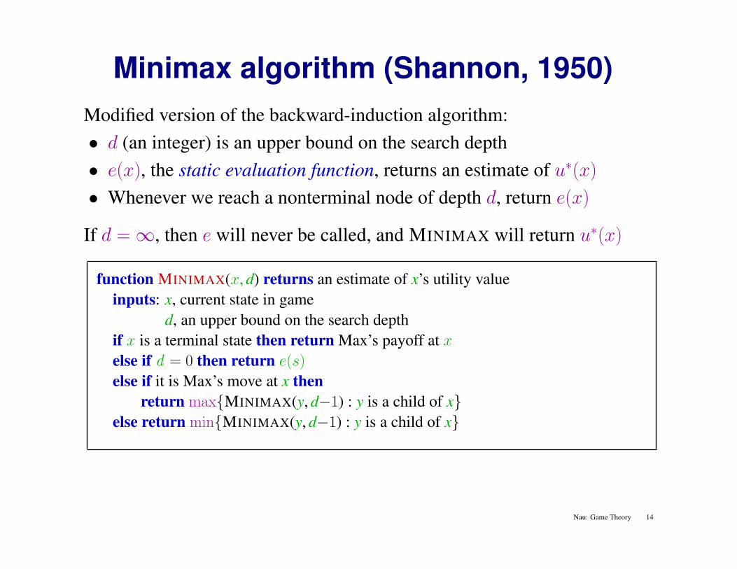
Minimax algorithm (Shannon, 1950)Modified version of the backward-induction algorithm:• d (an integer) is an upper bound on the search depth• e(x), the static evaluation function, returns an estimate of u∗(x)
• Whenever we reach a nonterminal node of depth d, return e(x)
If d =∞, then e will never be called, and MINIMAX will return u∗(x)
function MINIMAX(x, d) returns an estimate of x’s utility valueinputs: x, current state in game
d, an upper bound on the search depthif x is a terminal state then return Max’s payoff at xelse if d = 0 then return e(s)else if it is Max’s move at x then
return max{MINIMAX(y, d−1) : y is a child of x}else return min{MINIMAX(y, d−1) : y is a child of x}
Nau: Game Theory 14
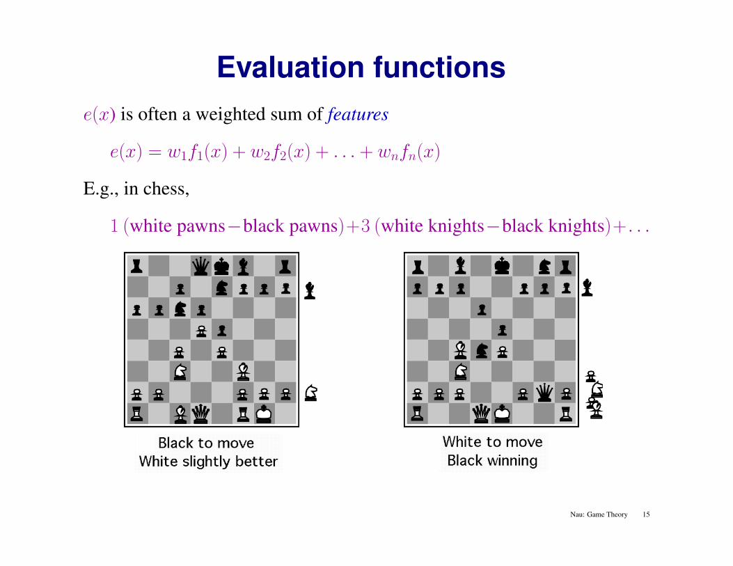
Evaluation functionse(x) is often a weighted sum of features
e(x) = w1f1(x) + w2f2(x) + . . . + wnfn(x)
E.g., in chess,
1 (white pawns−black pawns)+3 (white knights−black knights)+. . .
Nau: Game Theory 15
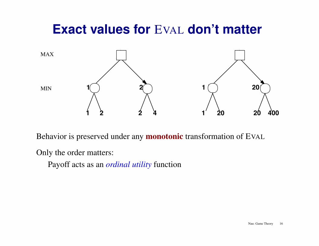
Exact values for EVAL don’t matter
MIN
MAX
21
1
42
2
20
1
1 40020
20
Behavior is preserved under any monotonic transformation of EVAL
Only the order matters:Payoff acts as an ordinal utility function
Nau: Game Theory 16
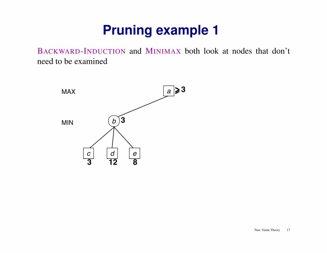
Pruning example 1BACKWARD-INDUCTION and MINIMAX both look at nodes that don’tneed to be examined
MAX
3 12 8
MIN 3
2
2
X X
3a
c d e
b
Nau: Game Theory 17
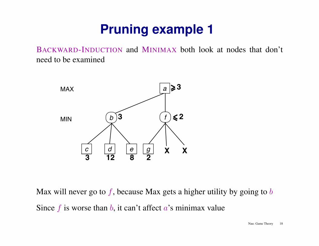
Pruning example 1BACKWARD-INDUCTION and MINIMAX both look at nodes that don’tneed to be examined
MAX
3 12 8
MIN 3
2
2
X X
3a
c d e g
fb
Max will never go to f , because Max gets a higher utility by going to b
Since f is worse than b, it can’t affect a’s minimax value
Nau: Game Theory 18
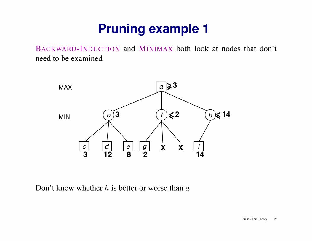
Pruning example 1BACKWARD-INDUCTION and MINIMAX both look at nodes that don’tneed to be examined
MAX
3 12 8
MIN 3
2
2
X X14
14
3a
c d e g i
fb h
Don’t know whether h is better or worse than a
Nau: Game Theory 19
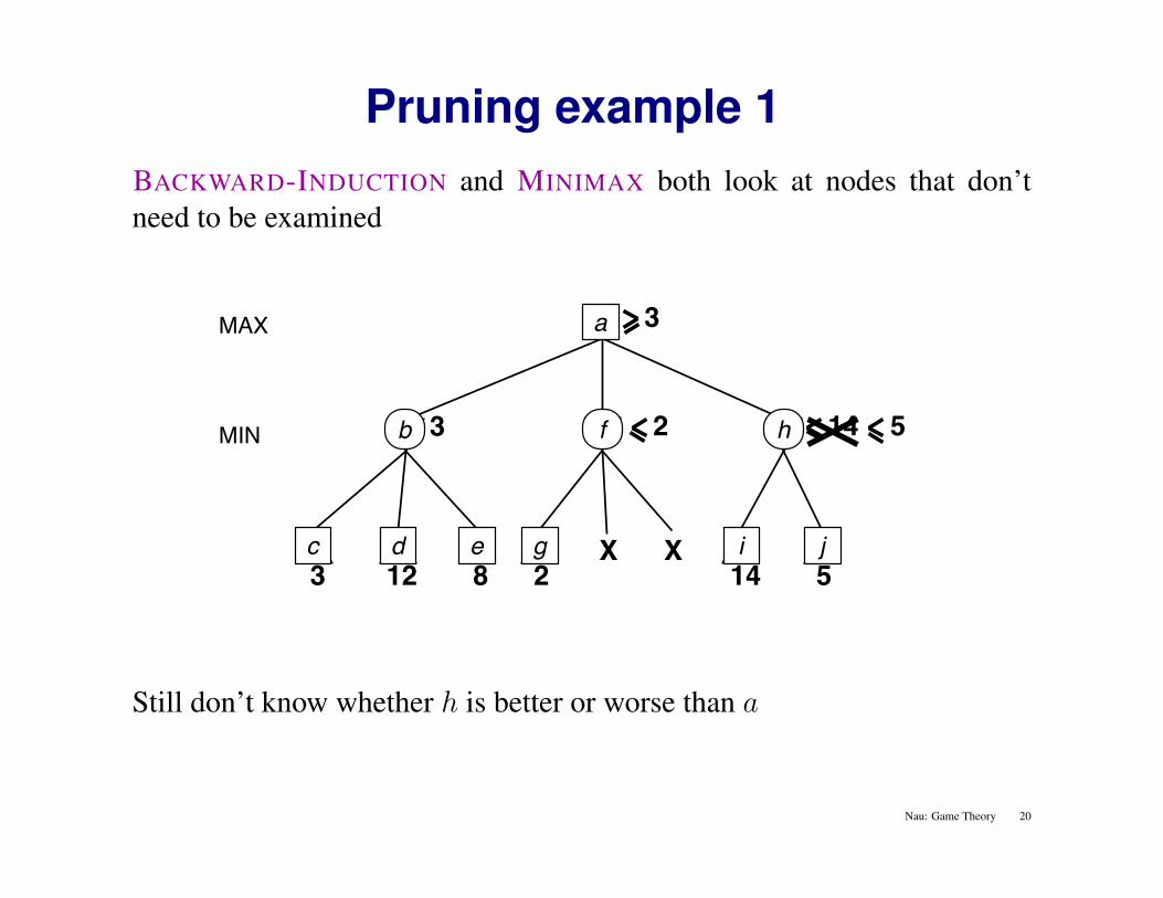
Pruning example 1BACKWARD-INDUCTION and MINIMAX both look at nodes that don’tneed to be examined
MAX
3 12 8
MIN 3
2
2
X X14
14
5
5
3a
c d e g i
fb h
j
Still don’t know whether h is better or worse than a
Nau: Game Theory 20
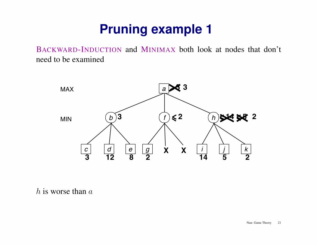
Pruning example 1BACKWARD-INDUCTION and MINIMAX both look at nodes that don’tneed to be examined
MAX
3 12 8
MIN
3
3
2
2
X X14
14
5
5
2
2
3a
c d e g i
fb h
j k
h is worse than a
Nau: Game Theory 21
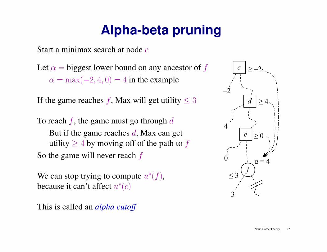
Alpha-beta pruningStart a minimax search at node c
Let α = biggest lower bound on any ancestor of fα = max(−2, 4, 0) = 4 in the example
If the game reaches f , Max will get utility ≤ 3
To reach f , the game must go through dBut if the game reaches d, Max can getutility ≥ 4 by moving off of the path to f
So the game will never reach f
We can stop trying to compute u∗(f ),because it can’t affect u∗(c)
This is called an alpha cutoff
α = 4 0
≥ 0 e
≥ –2c
f
3
–2 d
4
≥ 4
≤ 3
Nau: Game Theory 22
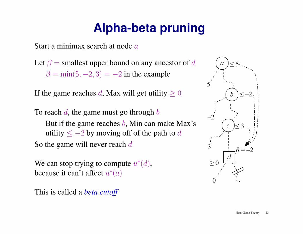
Alpha-beta pruningStart a minimax search at node a
Let β = smallest upper bound on any ancestor of dβ = min(5,−2, 3) = −2 in the example
If the game reaches d, Max will get utility ≥ 0
To reach d, the game must go through bBut if the game reaches b, Min can make Max’sutility ≤ −2 by moving off of the path to d
So the game will never reach d
We can stop trying to compute u∗(d),because it can’t affect u∗(a)
This is called a beta cutoff
β = –2 3
≤ 3 c
≤ 5a
d
0
5 b
–2
≤ –2
≥ 0
Nau: Game Theory 23
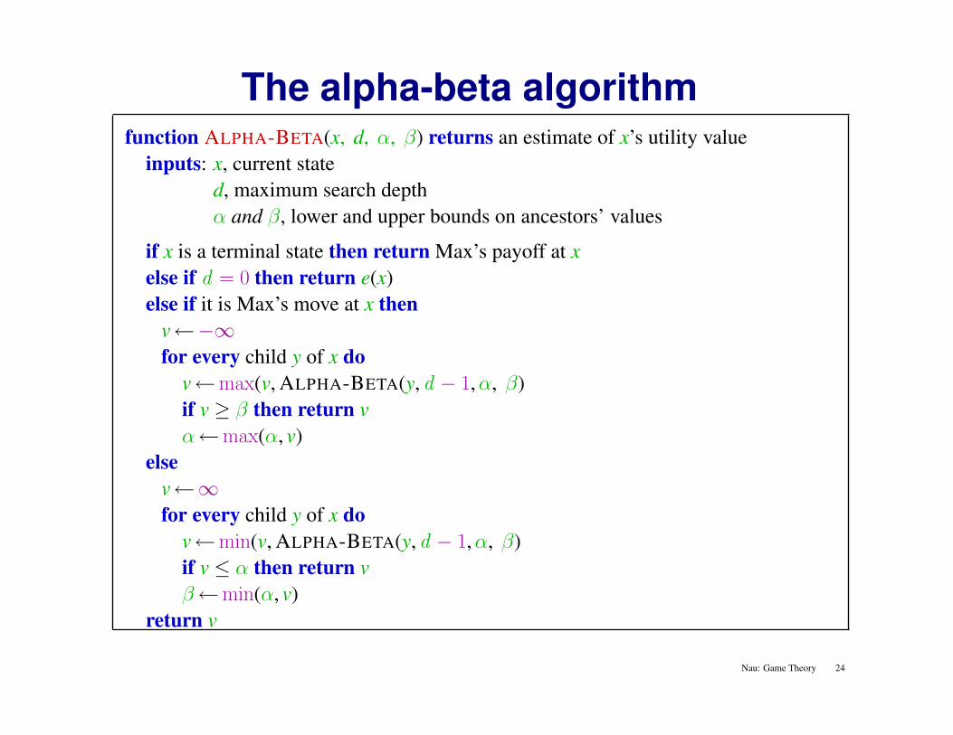
The alpha-beta algorithmfunction ALPHA-BETA(x, d, α, β) returns an estimate of x’s utility value
inputs: x, current stated, maximum search depthα and β, lower and upper bounds on ancestors’ values
if x is a terminal state then return Max’s payoff at xelse if d = 0 then return e(x)else if it is Max’s move at x then
v←−∞for every child y of x do
v←max(v, ALPHA-BETA(y,d − 1,α, β)if v ≥ β then return vα←max(α, v)
elsev←∞for every child y of x do
v←min(v, ALPHA-BETA(y,d − 1,α, β)if v ≤ α then return vβ←min(α, v)
return v
Nau: Game Theory 24
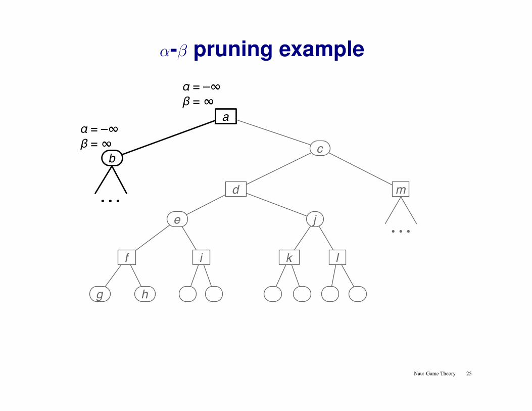
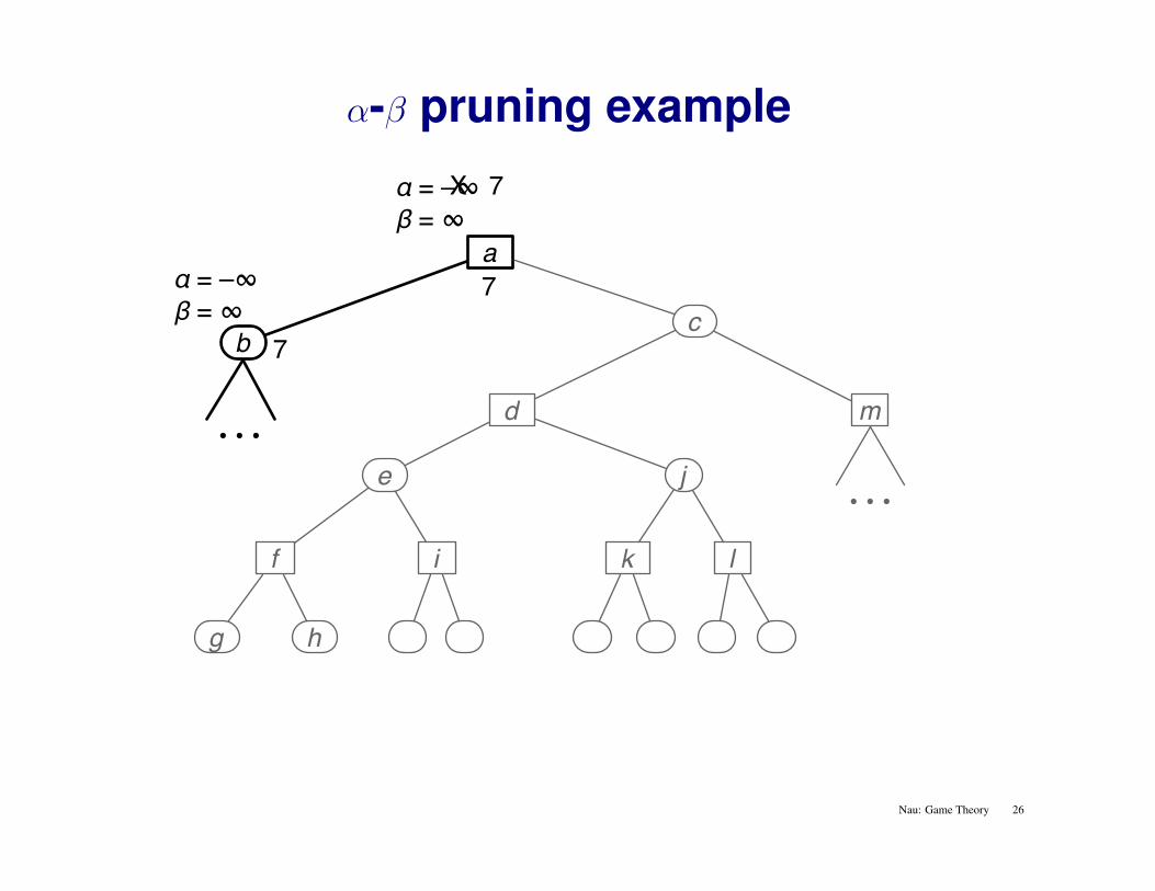
α-β pruning example
a
b c
d m
e j
f i k l
g h
• • •
• • •
α = –∞β = ∞
α = –∞β = ∞
Nau: Game Theory 25
α-β pruning example
a
b c
d m
e j
f i k l
g h
• • •
• • •
α = –∞β = ∞
α = –∞β = ∞
7
X 7
7
Nau: Game Theory 26
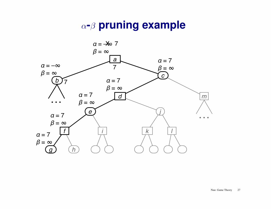
α-β pruning example
a
b c
d
e
f
g
• • •
7
α = –∞β = ∞
α = 7β = ∞
α = 7β = ∞
α = 7β = ∞
α = 7β = ∞
X 7
α = –∞β = ∞
m
j
i k l
• • •
7
h
α = 7β = ∞
Nau: Game Theory 27
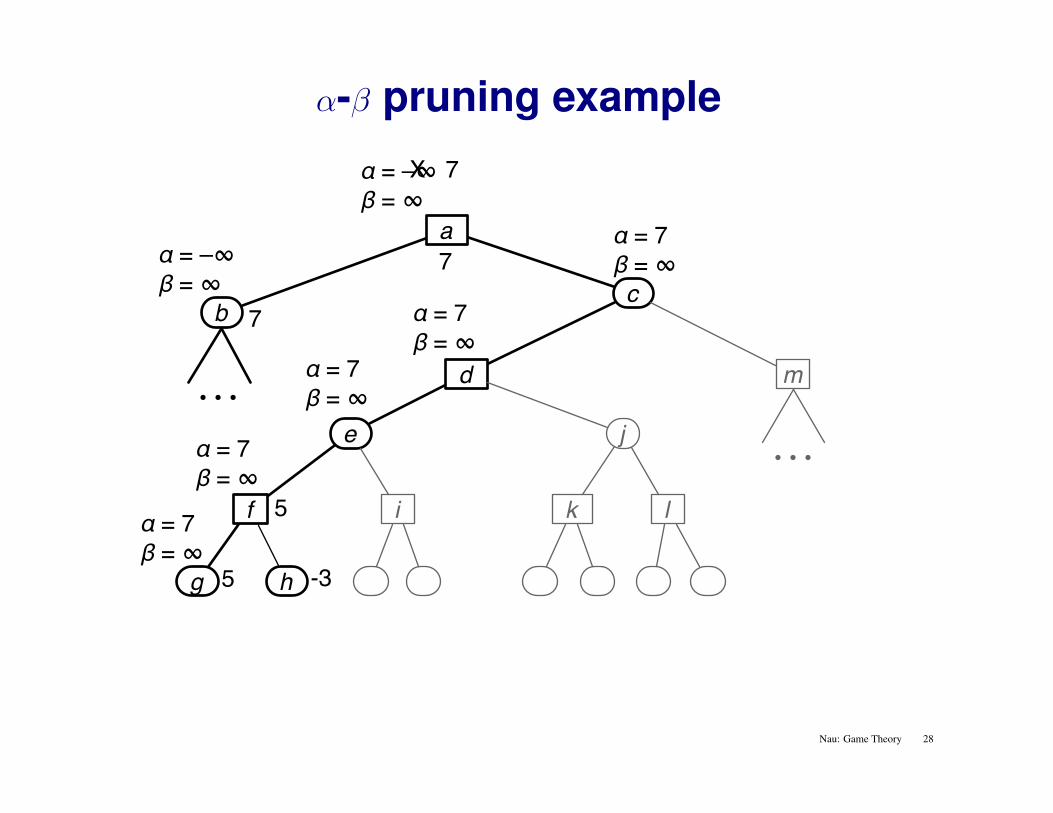
α-β pruning example
a
b c
d
5
5 -3
e
f
g h
• • •
7
α = –∞β = ∞
α = 7β = ∞
α = 7β = ∞
α = 7β = ∞
α = 7β = ∞
X 7
α = –∞β = ∞
m
j
i k l
• • •
7
α = 7β = ∞
Nau: Game Theory 28
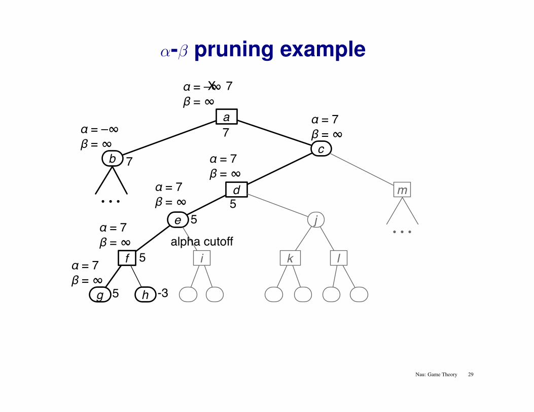
α-β pruning example
a
b c
d
5
5
5 -3
e
f
g h
• • •
7
α = –∞β = ∞
α = 7β = ∞
α = 7β = ∞
α = 7β = ∞
α = 7β = ∞
X 7
α = –∞β = ∞
m
j
i k l
• • • alpha cutoff
5
7
α = 7β = ∞
Nau: Game Theory 29
α-β pruning example
a
b c
d
5
5
5 -3
e j
f i k
g h
• • •
7
α = –∞β = ∞
α = 7β = ∞
α = 7β = ∞
α = 7β = ∞
α = 7β = ∞
α = 7β = ∞
α = 7β = ∞
X 7
α = –∞β = ∞
alpha cutoff
m
• • •
l
5
7
α = 7β = ∞
α = 7β = ∞
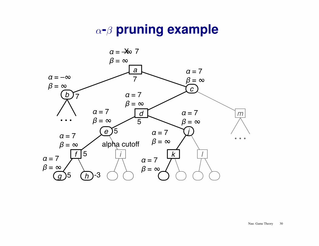
Nau: Game Theory 30
α-β pruning example
a
b c
d
5
5
5 -3
e j
f i k l
g h
• • •
7
α = –∞β = ∞
0 8
8
α = 7β = ∞
α = 7β = ∞
α = 7β = ∞
α = 7β = ∞
α = 7β = ∞
α = 7β = ∞
X 8
X 7
α = 7β = 8
α = –∞β = ∞
alpha cutoff
m
• • •
5
8
7
α = 7β = ∞
α = 7β = ∞
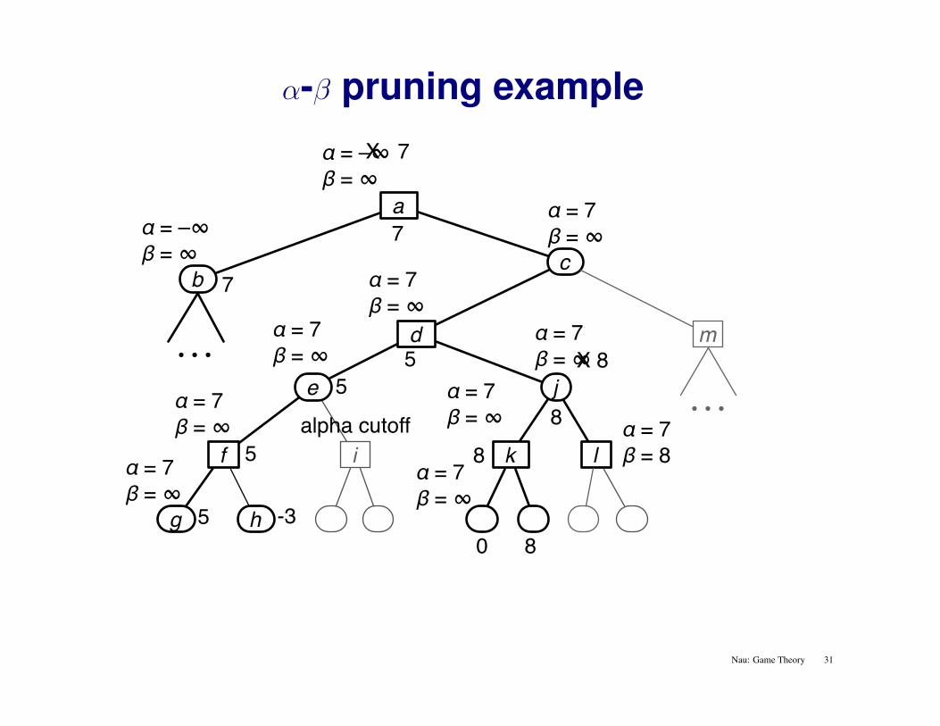
Nau: Game Theory 31
α-β pruning example
a
b c
d
5
5
5 -3
e j
f i k l
g h
• • •
7
α = –∞β = ∞
α = 7β = ∞
α = 7β = ∞
α = 7β = ∞
α = 7β = ∞
α = 7β = ∞
α = 7β = ∞
X 8
X 7
α = 7β = 8
α = –∞β = ∞
alpha cutoff
beta cutoff 9
9
m
• • •
0 8
8
5
8
7
α = 7β = ∞
α = 7β = ∞
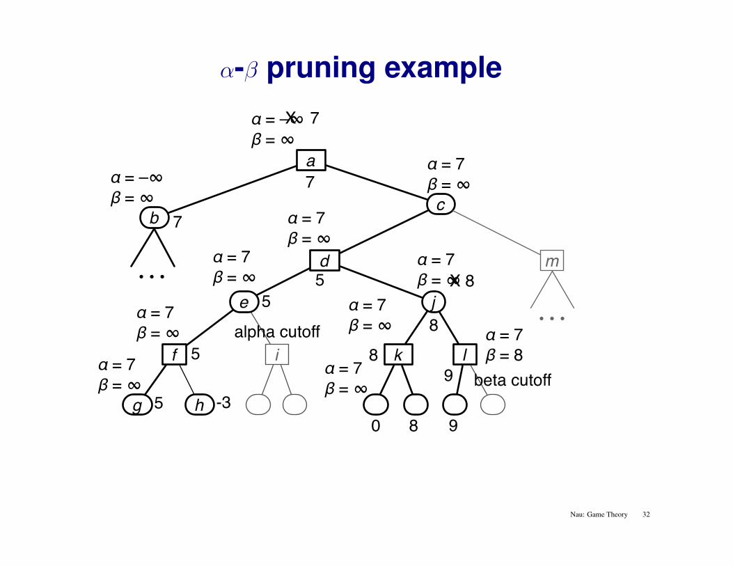
Nau: Game Theory 32
α-β pruning example
a
b c
d
5
5
5 -3
e j
f i k l
g h
• • •
7
α = –∞β = ∞
α = 7β = ∞
α = 7β = ∞
α = 7β = ∞
α = 7β = ∞
α = 7β = ∞
α = 7β = ∞
X 8
X 7
α = 7β = 8
X 8
α = –∞β = ∞
alpha cutoff
beta cutoff 9
9
0 8
8
5
8
X 8
7
m
• • •
α = 7β = ∞
α = 7β = ∞
X 8
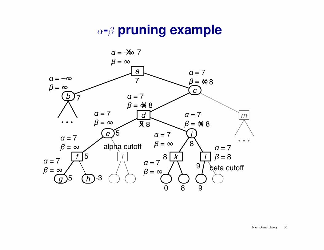
Nau: Game Theory 33
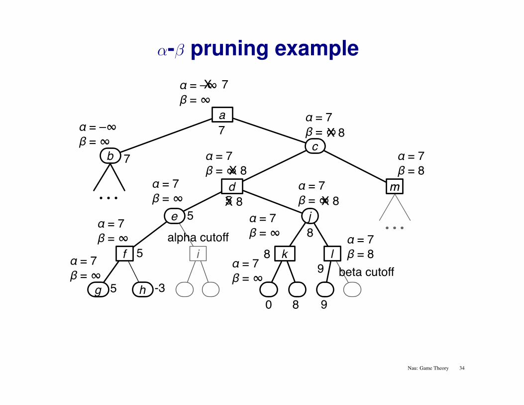
α-β pruning example
a
b c
d
5
5
5 -3
e j
f i k l
g h
• • •
7
α = –∞β = ∞
α = 7β = ∞
α = 7β = ∞
α = 7β = ∞
α = 7β = ∞
α = 7β = ∞
α = 7β = ∞
X 8
X 7
α = 7β = 8
X 8α = –∞β = ∞
alpha cutoff
m
• • • • • •
m
α = 7β = 8
beta cutoff 9
9
0 8
8
5
8
X 8
7
α = 7β = ∞
α = 7β = ∞
X 8
Nau: Game Theory 34
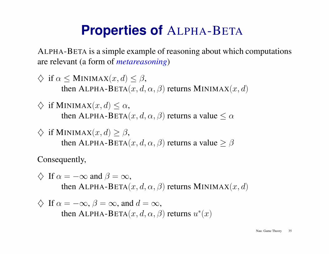
Properties of ALPHA-BETA
ALPHA-BETA is a simple example of reasoning about which computationsare relevant (a form of metareasoning)
♦ if α ≤ MINIMAX(x, d) ≤ β,then ALPHA-BETA(x, d, α, β) returns MINIMAX(x, d)
♦ if MINIMAX(x, d) ≤ α,then ALPHA-BETA(x, d, α, β) returns a value ≤ α
♦ if MINIMAX(x, d) ≥ β,then ALPHA-BETA(x, d, α, β) returns a value ≥ β
Consequently,
♦ If α = −∞ and β =∞,then ALPHA-BETA(x, d, α, β) returns MINIMAX(x, d)
♦ If α = −∞, β =∞, and d =∞,then ALPHA-BETA(x, d, α, β) returns u∗(x)
Nau: Game Theory 35
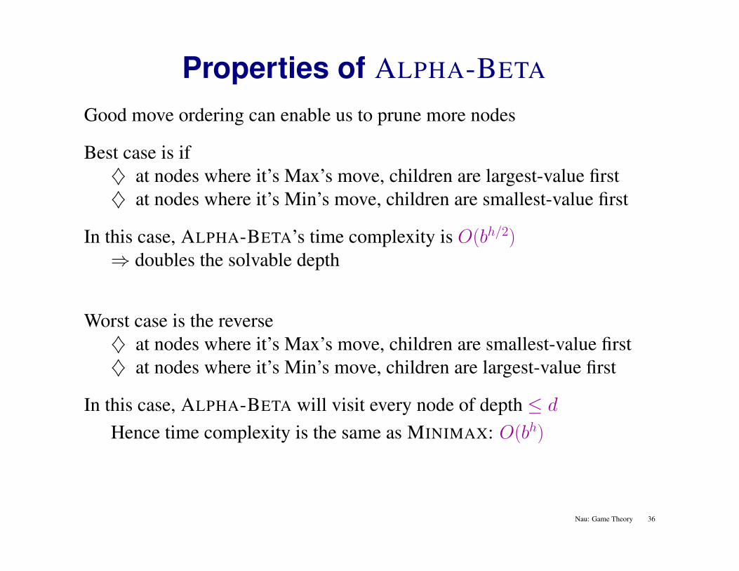
Properties of ALPHA-BETA
Good move ordering can enable us to prune more nodes
Best case is if♦ at nodes where it’s Max’s move, children are largest-value first♦ at nodes where it’s Min’s move, children are smallest-value first
In this case, ALPHA-BETA’s time complexity is O(bh/2)⇒ doubles the solvable depth
Worst case is the reverse♦ at nodes where it’s Max’s move, children are smallest-value first♦ at nodes where it’s Min’s move, children are largest-value first
In this case, ALPHA-BETA will visit every node of depth ≤ d
Hence time complexity is the same as MINIMAX: O(bh)
Nau: Game Theory 36
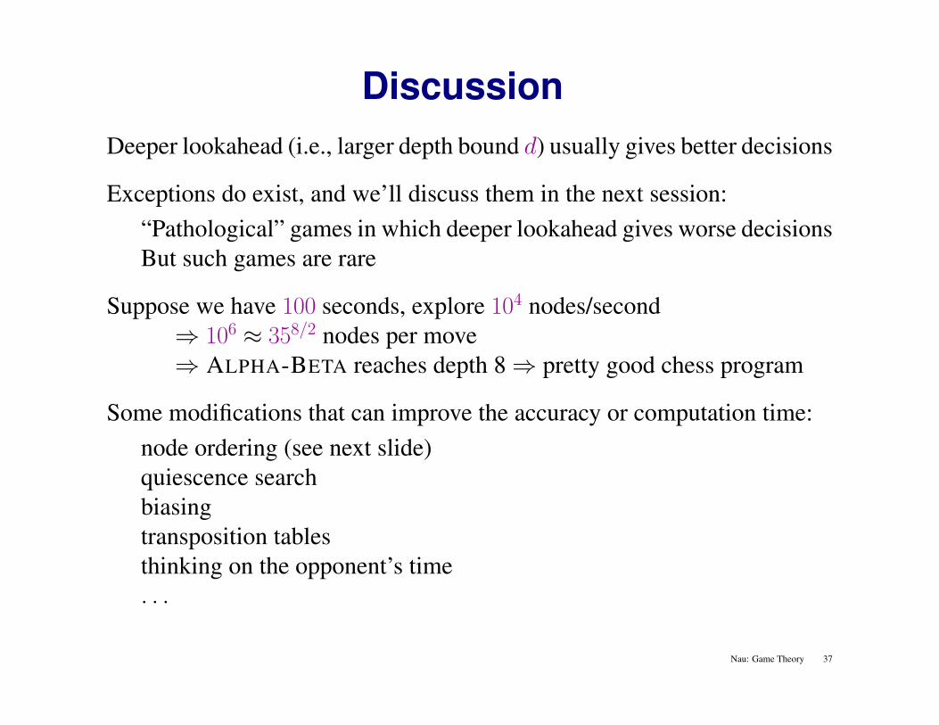
DiscussionDeeper lookahead (i.e., larger depth bound d) usually gives better decisions
Exceptions do exist, and we’ll discuss them in the next session:“Pathological” games in which deeper lookahead gives worse decisionsBut such games are rare
Suppose we have 100 seconds, explore 104 nodes/second⇒ 106 ≈ 358/2 nodes per move⇒ ALPHA-BETA reaches depth 8⇒ pretty good chess program
Some modifications that can improve the accuracy or computation time:node ordering (see next slide)quiescence searchbiasingtransposition tablesthinking on the opponent’s time. . .
Nau: Game Theory 37
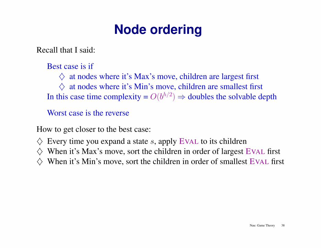
Node orderingRecall that I said:
Best case is if♦ at nodes where it’s Max’s move, children are largest first♦ at nodes where it’s Min’s move, children are smallest first
In this case time complexity = O(bh/2)⇒ doubles the solvable depth
Worst case is the reverse
How to get closer to the best case:♦ Every time you expand a state s, apply EVAL to its children♦ When it’s Max’s move, sort the children in order of largest EVAL first♦ When it’s Min’s move, sort the children in order of smallest EVAL first
Nau: Game Theory 38
Quiescence search and biasing♦ In a game like checkers or chess, where the evaluation is based greatly
on material pieces,The evaluation is likely to be inaccurate if there are pending captures
♦ Search deeper to reach a position where there aren’t pending capturesEvaluations will be more accurate here
♦ But that creates another problemYou’re searching some paths to an even depth, others to an odd depthPaths that end just after your opponent’s move will look worsethan paths that end just after your move
♦ To compensate, add or subtract a number called the “biasing factor”
Nau: Game Theory 39
Transposition tablesOften there are multiple paths to the same state (i.e., the state space is areally graph rather than a tree)
Idea:♦ when you compute s’s minimax value, store it in a hash table♦ visit s again⇒ retrieve its value rather than computing it again
The hash table is called a transposition table
Problem: far too many states to store all of them
Store some of the states, rather than all of them
Try to store the ones that you’re most likely to need
Nau: Game Theory 40
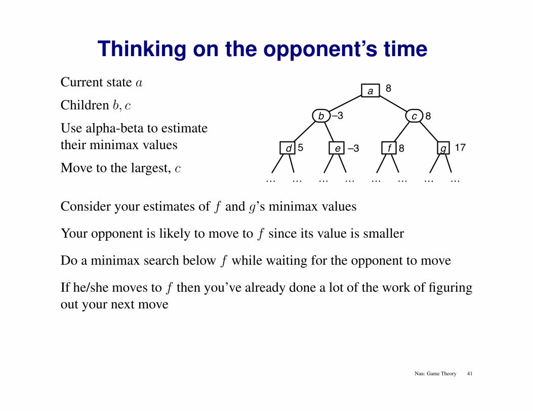
Thinking on the opponent’s timeCurrent state a
Children b, c
Use alpha-beta to estimatetheir minimax values
Move to the largest, c
a
–3 b c
8
8
e 5 d f g8 17–3
… … … … … … … …
Consider your estimates of f and g’s minimax values
Your opponent is likely to move to f since its value is smaller
Do a minimax search below f while waiting for the opponent to move
If he/she moves to f then you’ve already done a lot of the work of figuringout your next move
Nau: Game Theory 41
Game-tree search in practiceCheckers: Chinook ended 40-year-reign of human world champion Mar-ion Tinsley in 1994.
Checkers was solved in April 2007: from the standard starting position,both players can guarantee a draw with perfect play. This took 1014 calcu-lations over 18 years. Checkers has a search space of size 5× 10²⁰.
Chess: Deep Blue defeated human world champion Gary Kasparov in asix-game match in 1997. Deep Blue searches 200 million positions persecond, uses very sophisticated evaluation, and undisclosed methods forextending some lines of search up to 40 ply.
Othello: human champions refuse to compete against computers, who aretoo good.
Go: until recently, human champions didn’t compete against computersbecause the computers were too bad. But that has changed . . .
Nau: Game Theory 42
Game-tree search in the game of go
b =2
b =3
b =4
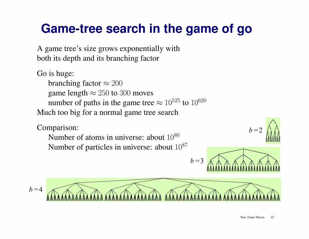
A game tree’s size grows exponentially withboth its depth and its branching factor
Go is huge:branching factor ≈ 200game length ≈ 250 to 300 movesnumber of paths in the game tree ≈ 10525 to 10620
Much too big for a normal game tree search
Comparison:Number of atoms in universe: about 1080
Number of particles in universe: about 1087
Nau: Game Theory 43
Game-tree search in the game of goDuring the past couple years, go programs have gotten much better
Main reason: Monte Carlo roll-outs
Basic idea: do a minimax search of a randomly selected subtree
At each node that the algorithm visits,
♦ It randomly selects some of the childrenThere are heuristics for deciding how many
♦ Calls itself recursively on these, ignores the others
Nau: Game Theory 44
Forward pruning in chessBack in the 1970s, some similar ideas were tried in chess
The approach was called forward pruningMain difference: select the children heuristically rather than randomlyIt didn’t work as well as brute-force alpha-beta, so people abandoned it
Why does a similar idea work so much better in go?
Nau: Game Theory 45
SummaryIf a game is two-player zero-sum,
then maximin and minimax are the same
If the game also is perfect-information,only need to look at pure strategies
If the game also is sequential, deterministic, and finite,then can do a game-tree search
minimax values, alpha-beta pruning
In sufficiently complicated games, perfection is unattainable⇒ must approximate: limited search depth, static evaluation function
In games that are even more complicated, further approximation is needed⇒Monte Carlo roll-outs
Nau: Game Theory 46
Related Documents