An approach for modeling sediment budgets in supplylimited ... · An approach for modeling sediment budgets ... Canyon, dam operations have actually increased the dura-tion of moderate

An approach for modeling sediment budgetsin supply‐limited rivers

Scott A. Wright,1 David J. Topping,2 David M. Rubin,3 and Theodore S. Melis2

Received 1 September 2009; revised 11 June 2010; accepted 18 June 2010; published 28 October 2010.

[1] Reliable predictions of sediment transport and river morphology in response tovariations in natural and human‐induced drivers are necessary for river engineeringand management. Because engineering and management applications may span a widerange of space and time scales, a broad spectrum of modeling approaches has beendeveloped, ranging from suspended‐sediment “rating curves” to complex three‐dimensionalmorphodynamic models. Suspended sediment rating curves are an attractive approachfor evaluating changes in multi‐year sediment budgets resulting from changes in flowregimes because they are simple to implement, computationally efficient, and the empiricalparameters can be estimated from quantities that are commonly measured in the field(i.e., suspended sediment concentration and water discharge). However, the standard ratingcurve approach assumes a unique suspended sediment concentration for a given waterdischarge. This assumption is not valid in rivers where sediment supply varies enough tocause changes in particle size or changes in areal coverage of sediment on the bed; both ofthese changes cause variations in suspended sediment concentration for a given waterdischarge. More complex numerical models of hydraulics and morphodynamics have beendeveloped to address such physical changes of the bed. This additional complexity comesat a cost in terms of computations as well as the type and amount of data required formodel setup, calibration, and testing. Moreover, application of the resulting sediment‐transport models may require observations of bed‐sediment boundary conditions thatrequire extensive (and expensive) observations or, alternatively, require the use of anadditional model (subject to its own errors) merely to predict the bed‐sediment boundaryconditions for use by the transport model. In this paper we present a hybrid approach thatcombines aspects of the rating curve method and the more complex morphodynamicmodels. Our primary objective was to develop an approach complex enough to capture theprocesses related to sediment supply limitation but simple enough to allow for rapidcalculations of multi‐year sediment budgets. The approach relies on empirical relationsbetween suspended sediment concentration and discharge but on a particle size specificbasis and also tracks and incorporates the particle size distribution of the bed sediment. Wehave applied this approach to the Colorado River below Glen Canyon Dam (GCD), a reachthat is particularly suited to such an approach because it is substantially sediment supplylimited such that transport rates are strongly dependent on both water discharge andsediment supply. The results confirm the ability of the approach to simulate the effects ofsupply limitation, including periods of accumulation and bed fining as well as erosionand bed coarsening, using a very simple formulation. Although more empirical in naturethan standard one‐dimensional morphodynamic models, this alternative approach isattractive because its simplicity allows for rapid evaluation of multi‐year sediment budgetsunder a range of flow regimes and sediment supply conditions, and also because it requiressubstantially less data for model setup and use.

Citation: Wright, S. A., D. J. Topping, D. M. Rubin, and T. S. Melis (2010), An approach for modeling sediment budgets insupply‐limited rivers, Water Resour. Res., 46, W10538, doi:10.1029/2009WR008600.

1. Introduction

[2] It is often important to engineers, geomorphologists,and resource managers to simulate changes in fluvial sedi-ment budgets resulting from changes in driving forces, suchas climate, dam operations, land use changes, etc. Humanshave had a dramatic impact on the world’s river systems interms of water storage and flow regulation [Nilsson et al.,

1U.S. Geological Survey, California Water Science Center,Sacramento, California, USA.

2U.S. Geological Survey, Grand Canyon Monitoring and ResearchCenter, Flagstaff, Arizona, USA.

3U.S. Geological Survey, Pacific Science Center, Santa Cruz,California, USA.

This paper is not subject to U.S. copyright.Published in 2010 by the American Geophysical Union.

WATER RESOURCES RESEARCH, VOL. 46, W10538, doi:10.1029/2009WR008600, 2010

W10538 1 of 18

http://dx.doi.org/10.1029/2009WR008600

2005] as well as sediment transport and budgets [Syvitskiet al., 2005]. Because sediment provides the physicalframework for aquatic ecosystems, management of aquaticresources requires the ability to simulate changes in sedimentbudgets resulting from natural and anthropogenic influences.[3] In response to this need, substantial research and

development has been conducted in the area of fluvialsediment‐transport modeling. The wide range of space andtime scales of interest has led to a range of modelingapproaches, from simple empirical concentration dischargerelations (i.e., sediment rating curves, see e.g., ASCE [1975])to complex multidimensional morphodynamic models. Sus-pended sediment rating curves assume a unique relationbetween suspended sediment concentration (or flux) andwater discharge and have thus often been used to evaluatechanges in flow regimes. Multidimensional morphodynamicmodels solve some form of the Navier‐Stokes equations forthe fluid and mass conservation for the sediment, sometimesfor a range of particle sizes. Because of their simplicity, ratingcurves can be applied over large space and time scales,whereas multidimensional models are typically limited in thescale of application by computation times and data require-ments. Between these two bookends lies an array of one‐dimensional, pseudo‐one‐dimensional, and two‐dimensionalmorphodynamic models, including several “general use”codes such as HEC‐RAS (Corps of Engineers), SRH‐1D and2D (Bureau of Reclamation), MIKE‐11 and 21 (DanishHydraulics Institute), and SOBEK (Delft Hydraulics), as wellas codes developed for specific research applications [e.g.,Rahuel et al., 1989, van Niekerk et al., 1992, Hoey andFerguson, 1994, Wright and Parker, 2005, among manyothers]. Even within this family of models there is a widerange of complexity, such as equilibrium versus nonequilib-rium transport, uniform sediment versus multiple particlesizes, steady versus unsteady flow, etc. The general use codestypically attempt to include all of these various options to beapplicable to a range of study areas and conditions. Recently,Ronco et al. [2009] presented criterion for simplification ofthe standard one‐dimensional models, based on theassumption of uniform flow, to facilitate long‐term simula-tions for rivers where minimal topographic information isavailable.[4] Sediment rating curves are an attractive approach for

evaluating long‐term sediment budgets resulting fromchanges in flow regimes because they are very simple, easyto implement computationally, and the empirical parameterscan be estimated from quantities that are frequently mea-sured in the field (suspended sediment concentration andwater discharge). However, an implicit assumption in thisapproach is that sediment transport is always in equilibriumwith sediment supply, i.e., that the particle size distributionof sediment on the bed of the river is not changing (or that itis uniquely correlated with discharge). Rubin and Topping[2001, 2008] presented an approach for evaluating thisassumption for sand‐bedded rivers and suspended sandtransport and showed that the bed particle size is oftenmeasurably important and sometimes as important as waterdischarge in regulating suspended sand transport. Changesin bed particle size distribution can be accounted for withmultiple size numerical formulations [e.g., Parker et al.,2000]; however, this comes at the cost of significant addi-tional complexity, not only in terms of the model formula-tion but also in terms of the boundary and initial conditions

that must be specified. For example, multiple size mor-phodynamic models require information on bed particle sizedistributions (i.e., the surface “active” layer and the under-lying substrate) and sediment flux by particle size for cali-bration and testing. The methods of Ronco et al. [2009] canpotentially overcome the limitations of the rating curveapproach by incorporating multiple size classes. However,the primary assumption in their approach, i.e., uniform flow,is not suitable to our study site because the releases fromGlen Canyon Dam (GCD) are highly unsteady, on a dailybasis, due to hydroelectric power demand. Where a modelrequires additional knowledge of sediment boundary con-ditions, either additional data must be collected, or anothermodel must be used to predict the sediment boundary con-ditions; this extra modeling step can introduce error, evenbefore the sediment‐transport model is implemented.[5] Because of the limitations of the available methods,

we have developed and tested an alternative approachthat combines aspects of several modeling methods. Theapproach uses empirically based rating curves, but in con-trast to the standard approach, they are formulated on aparticle size specific basis. This allows for calculations ofthe particle size distribution on the bed within a given reachby applying mass conservation by grain size (i.e., the Exnerequation), albeit in a substantially simplified manner. Thus,the rating curves can respond to changes in sediment supplywith a formulation that is quite simple, computationallyefficient, and easy to implement. The model is spatiallydiscretized over long reaches (∼50 km) as opposed toattempting to characterize the details of channel complexity.Herein, we present the details of this modeling approach andits application to the Colorado River below Glen CanyonDam. We do not argue that the empirical parametersdeveloped for the Colorado River have general applicability;rather, they are site specific. However, the general modelingapproach for accounting for changes in sediment supply toevaluate long‐term changes in sediment budgets shouldhave general applicability, particularly below dams wherethe flow regime and sediment supply are often dramaticallyaltered [e.g., Schmidt and Wilcock, 2008].[6] We chose to develop this alternative approach as

opposed to applying standard one‐dimensional morphody-namic modeling for several reasons. First, our approach ismuch simpler and thus more computationally efficient thantypical one‐dimensional models. Increases in computerpower have made this less of an issue, and we acknowledgethat standard 1‐D models can be applied to long reachesover multi‐year time periods, but computational efficiencyis still an advantage when considering a large number ofalternative modeling scenarios with highly variable bound-ary conditions. Second, and probably more important,standard 1‐D models require information that is not readilyavailable for our study site, namely detailed cross sectionsand information on the spatial distribution of sand thicknessand bed particle size distributions (longitudinally). Ourstudy site is a pool rapid system with very complex channelgeometry; attempting to model erosion and depositionwithin this complicated channel geometry is a difficult taskand likely not necessary for modeling multi‐year sedimentbudgets over long reaches. Finally, our modeling approachbuilds on a previously developed unsteady discharge routingmodel [Wiele and Smith, 1996] that also uses reach aver-aging to deal with this complexity. This previously devel-

WRIGHT ET AL.: MODELING APPROACH FOR LONG‐TERM SEDIMENT W10538W10538

2 of 18

oped model can provide the required flows at the compu-tational nodes and thus circumvent the need to model anewthe detailed hydraulics, including critical flow transitionsthat occur in rapids along the Colorado River in our studysite.

2. Study Site

[7] The modeling approach described in the next sectionwas developed as part of our ongoing work on the ColoradoRiver below Glen Canyon Dam (Figure 1). The constructionof Glen Canyon Dam in the early 1960s substantiallyreduced (1) the supply of sand to Grand Canyon by trappingmost of it in the upstream reservoir [Topping et al., 2000]and (2) the capacity of the river to transport sand byreducing large flood peaks [Topping et al., 2003]. In addi-tion, although operation of the dam reduced the magnitudeand frequency of floods during which most of the naturalsand transport occurred in the Colorado River in GrandCanyon, dam operations have actually increased the dura-tion of moderate discharges that can transport substantialamounts of sand [Topping et al., 2003]. The post‐dam flowregime is illustrated in Figure 2 that shows the study periodto which the model was applied (top, September 2002through March 2009), several weeks of daily fluctuatingflows including a transition between months when therelease volume typically changes (middle), and an exampleof a “controlled flood” where flows above powerplantcapacity are released with the primary goal of rebuilding

eroded sandbars (bottom) [see e.g. Schmidt, 1999]. For acomplete review of pre‐ and post‐dam flow regimes, refer tothe study by Topping et al. [2003]. Note that we use theEnglish unit for water discharge, cubic feet per second orcfs, herein because of its common use and acceptance withinthe Colorado River scientific, management, and recreationalcommunity.[8] Several attempts have been made at generalizing the

post‐dam sand budget in Grand Canyon, i.e., whether thereis long‐term erosion or accumulation in the various reachesbelow the major tributaries. The answer to this question hasimportant implications for the sustainability of sand depositsin Marble and Grand Canyons (Figure 1), typically referredto as “eddy sandbars” because they tend to form inrecirculating eddies downstream from tributary debris fans[Schmidt, 1990]. Eddy sandbars are considered a valuedresource within the Glen Canyon Dam Adaptive Manage-ment Program, a federal advisory committee established toadvise the Secretary of the Interior on operations of GlenCanyon Dam [U. S. Department of the Interior, 1996], for avariety of reasons: They are a fundamental element of thepre‐dam riverscape; they provide areas for recreational useby river runners and hikers; they provide low‐velocity,warm water habitat for potential use by juvenile native fish;they are the substrate for riparian vegetation; and they are asource of sand for upslope wind‐driven transport that mayhelp protect archeological resources [Draut and Rubin,2007]. The numerous studies of the post‐dam sand budgethave come to conflicting results about long‐term erosionversus accumulation. However, recent work indicates thateddy sandbars have been substantially eroded since con-struction of the dam and that this erosion has not beenabated by enactment of the Record‐of‐Decision (ROD)operation of Glen Canyon Dam in the mid‐1990s [U. S.Department of Interior, 1995; U. S. Department ofInterior, 1996] that constrained the allowable daily hydro-power fluctuations.[9] The approach presented herein was designed specifi-

cally to bridge the gap between approaches that have pre-viously been used to evaluate the post‐dam sand budget.Randle and Pemberton [1987] used suspended sand ratingcurves developed by Pemberton [1987] as the basis for thesand budgets used in development of the ROD, but it hassubsequently been shown by Topping et al. [1999, 2000]that sand transport rates are strongly dependent on tribu-tary sand supply as well as water discharge. This depen-dence is illustrated in Figure 3 that shows changes in therelation between suspended sand concentration and waterdischarge resulting from a flood on the Paria River (the firstmajor tributary downstream from the dam) in October 2006that delivered substantial quantities of sand directly to upperMarble Canyon (data are described in detail in a subsequentsection). It is seen that sand concentrations (for a givendischarge) are much greater during the tributary floodingand remain significantly higher than pre‐flood levels afterthe tributary flooding recedes, indicating sand accumulationand fining of the bed sediment. Over time, this fine sedimentis subsequently winnowed from the bed and concentrationsdecrease.[10] In addition to the rating curve model of Randle and

Pemberton [1987], a variety of more complex numericalmodels have been developed and applied as well, includingmultidimensional models of specific eddy sandbar sites

Figure 1. Colorado River below Glen Canyon Dam. LeesFerry is designated river‐mile 0 and is about 15 miles down-stream from Glen Canyon Dam. RM30, RM61, and RM87denote locations ofmonitoring sites and are labeled accordingto river miles downstream from Lees Ferry (i.e., RM30 isapproximately 30 river miles downstream). The Paria andLittle Colorado Rivers are the primary sand‐supplyingtributaries. RM is river‐mile.


3 of 18

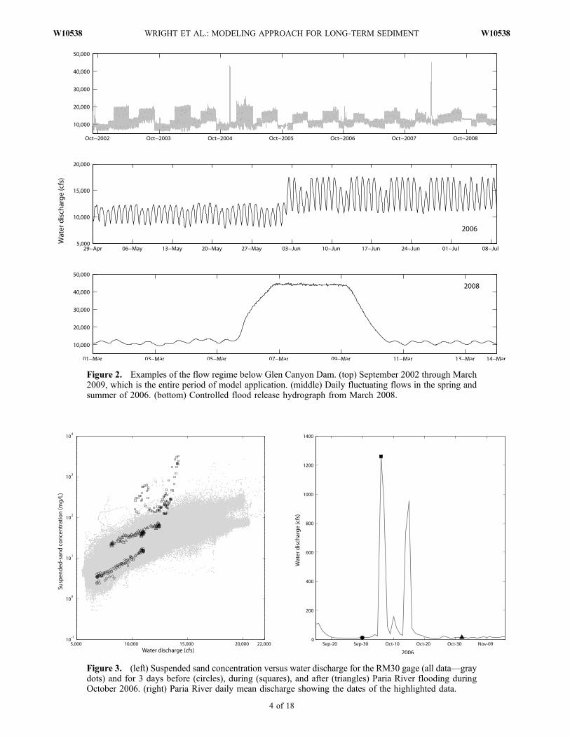
Figure 3. (left) Suspended sand concentration versus water discharge for the RM30 gage (all data—graydots) and for 3 days before (circles), during (squares), and after (triangles) Paria River flooding duringOctober 2006. (right) Paria River daily mean discharge showing the dates of the highlighted data.

Figure 2. Examples of the flow regime below Glen Canyon Dam. (top) September 2002 through March2009, which is the entire period of model application. (middle) Daily fluctuating flows in the spring andsummer of 2006. (bottom) Controlled flood release hydrograph from March 2008.


4 of 18

[Wiele et al., 1996, 1999, Wiele, 1998, Wiele and Torizzo,2005] and a pseudo‐one‐dimensional, reach averaged,multiple particle size, sand‐routing model [Wiele et al.,2007]. While the Wiele et al. [2007] model has the poten-tial for application to multi‐year time scales, its complexityin terms of initial and boundary conditions dictate that it ismore suitable to event‐scale (e.g., weeks to months) appli-cations. In contrast, the approach described herein wasdeveloped specifically to reduce the required input data andnumber of tunable parameters to facilitate multi‐year sim-ulations of sand flux and thus help address the primarysediment‐related question identified by program scientists ata knowledge assessment workshop held in July 2005 [Meliset al., 2006]: “Is there a ‘flow‐only’ (nonsediment aug-mentation) operation that will restore and maintain eddysandbar habitats over decadal time scales?”

3. Modeling Approach

[11] Because our approach was developed with a specificapplication in mind, there were several overarching goalsguiding its development, as follows:[12] 1. The model should reproduce the basic processes of

sand accumulation and fining of the bed during and imme-diately after tributary flooding, followed by erosion and bedcoarsening during tributary quiescence (see Figure 3).[13] 2. The model should be simple enough to allow for

multi‐year simulations, potentially in a Monte Carlo frame-work to account for variability in hydrology and tributarysediment supply.[14] 3. The number of adjustable empirical model para-

meters should be as few as possible and, along with theinitial/boundary conditions, be readily specifiable fromavailable data sources and ongoing monitoring programs.[15] Our approach is similar to more standard formula-

tions in that it relies on a relation between hydraulic vari-ables (e.g., depth, velocity, shear stress, discharge) andsediment‐transport rate, and sediment mass conservation forcomputing erosion, deposition, and bed particle size dis-tributions. A large number of “transport relations” have beenproposed over the past half century, for bed load, suspendedload, and combined total load [e.g., ASCE, 1975, Yang,1996], and most “general use” morphodynamic modelsallow the user a choice between various relations. Most ofthe relations are formulated in terms of power laws betweentransport rate, bed shear stress, and particle size, some withadditional complexity to account for phenomena such ashiding and exposure. Our approach differs from the generaluse models in that, instead of choosing an available trans-port relation, we have developed empirical rating curve‐typerelations specific to the Colorado River below Glen CanyonDam, as described below.[16] Rubin and Topping [2001, 2008] applied the trans-

port relation formulation of McLean [1992] to a wide rangeof hydraulic conditions and particle size distributions andfound that the results could be adequately generalized intothe following form:

C / uJ*DKb ; ð1Þ

where C is suspended sediment concentration, u* is shearvelocity, Db is the median bed particle diameter, and J and K

are empirical coefficients. For conditions with and withoutdunes and for wide and narrow bed particle size distribu-tions, Rubin and Topping [2001] found that J ranges from3.5 to 5.0, and K ranges from −1.5 to −3.0. Application ofequation (1) on a site‐specific basis requires estimation ofthe constant of proportionality and a model for shearvelocity. The longitudinal shear velocity field in a pool rapidsystem such as our study site can be quite complex, and weargue that the spatial variability is less important thanchanges with discharge for modeling broad‐scale sedimentbudgets. Thus, we have assumed that shear velocity can beapproximated as a power law function of discharge. Whilethis assumption is clearly not strictly correct, it is a rea-sonable approximation that facilitates achieving our statedgoals. We also note that for steady, uniform flow, shearvelocity goes as the square root of the depth‐slope product,and at‐a‐station hydraulic geometry [e.g., Leopold andMaddock, 1953] suggests that this quantity can often becharacterized by a power law with discharge. Applying thisassumption to equation (1) and writing in terms of indi-vidual particle sizes (necessary for bed composition calcu-lations as described below) yields:

Ci ¼ FbiAQLDK

i ; ð2Þ

where Q is water discharge, i denotes individual particlesizes, Fbi is the fraction of particle size i in the bed sediment(SFbi = 1), and A is an empirical, site‐specific constant(discussed further in the next section). Note that equation (2)is a more general form of the classical sediment rating curve,the difference being that bed particle size distributions areused to compute concentrations for individual sizes (asopposed to for all particle sizes lumped together). To applyequation (2), A, L, and K must be estimated empirically on asite‐specific basis; the advantage is that A and L can beestimated from measurements of concentration and dis-charge, two quantities that are routinely measured on manyrivers. The parameter K is more difficult to specify, as dis-cussed in the next section, but it should fall between −1.5and −3.0 as per Rubin and Topping [2001].[17] Application of equation (2) requires a method for

computing changes in the bed‐sediment particle size distri-bution (i.e., Fbi), and this is indeed the mechanism forsimulating bed fining and coarsening in response tochanging sediment supply, as outlined in modeling goal 2.For this, we apply the active layer form of the Exnerequation for bed sediment mass conservation [e.g., Parkeret al., 2000], in a slightly simplified form. For our studysite, which is a bedrock‐controlled canyon river, it is rea-sonable to approximate the mobile bed sediment, i.e., theactive layer, as a relatively thin layer of sand overlyingbedrock; this assumption is supported by data presented inthe following section. Also, underwater video and time lapseside‐scan sonar movies [Rubin and Carter, 2006] of the bedof the river within our study sites indicates the presence ofsand‐starved dunes (i.e., with gravel in the troughs) thatfurther supports the assumption of complete mixing of thesand layer (although we note that complete sand “equilib-rium” dunes and thick sand deposits in eddies without dunesalso exist, such that complete mixing is an approximation).By assuming that the substrate (i.e., bedrock, gravel, cobble)is nonerodible and that the sand layer thickness (Hs) is


5 of 18

equivalent to the active layer thickness (i.e., it is completelymixed and available to the flow), the Exner equationreduces to

1� �p

� �B@Hs

@t¼ � @Qs

@xð3Þ

1� �p

� �B@

@tHsFbið Þ ¼ � @Qsi

@x; ð4Þ

where Qs = CQ, C = SCi, Qsi = CiQ, B is channel width, andlp is bed porosity. Note that equation (3) is the result ofintegrating equation (4) over the entire bed sediment particlesize distribution since SFbi = 1 and SQsi = Qs. This for-mulation provides significant simplification over the stan-dard Exner equation because it circumvents the need to keeptrack of substrate layering and associated size distributions.[18] The nonerodible substrate (bedrock, gravel, cobble)

limits transport from a reach, in a given time step, to theamount of sediment in the reach plus what comes intothe reach during that time step (by grain size). Thus, if thepotential transport rate of a size i is greater than what isavailable for transport, the reach becomes exhausted of thatsize such that Fbi = 0 and Ci = 0. It is well known thatpatches of river contain little or no sand (e.g., rapids, gravelbars). One way to account for this is with a “bed‐sand area”correction factor in transport relations (i.e., equation (2), see,for example, Topping et al. [2007b]); however, this requiresinformation on the area of the bed that is covered in sandand how these areas are distributed with respect to bed shearstress, as well as a mechanism for simulating changes pre-sumably based on local hydraulics and sediment supply.Because our modeling approach does not incorporate thenecessary local hydraulics, we have not attempted to includethis effect. The bed‐sand area is effectively lumped into the“catch all” coefficient A in equation (2) and thus remainsconstant for our simulations. Instead, we focus on accountingfor changes in bed particle size distribution, which has beenshown to exert greater control on transport rates than bed‐sand area [Topping et al., 2007b].

[19] The set of equations (2)−(4) constitutes a model forCi, Hs, and Fbi, so long as water discharge can be estimatedor modeled independently. The boundary conditions are Qsi

at the upstream boundary and major tributaries; requiredinitial conditions are Hs and Fbi for each reach. The finalapproximation of our modeling approach is that we applythe formulation to relatively long reaches, as opposed toattempting to discretize the river into short segments. Thisassumption sacrifices the ability to accurately model short‐duration, localized, changes in concentration and bed par-ticle size distributions, such as that shown during the PariaRiver flood peak (squares) in Figure 3. That is, the spatialaveraging will tend to “smooth out” these short durationeffects while capturing the reach scale effects that havegreater influence on the long‐term flux. However, it cir-cumvents the need for detailed information on sand thick-ness and bed particle size within the reaches; instead, theseparameters are lumped into reach averages. Also, theempirical nature of equation (1) dictates that it should onlybe applied at locations where data are available to estimatethe empirical parameters (A, L, K). To this end, we appliedthe formulation to three reaches bracketed by sites wheresuspended sand concentration, grain size, and water dis-charge are monitored. The three modeling reaches areshown geographically in Figure 1 and schematically inFigure 4 and are defined as follows: (1) upper MarbleCanyon (UMC), from Lees Ferry/Paria River confluence toRM30; (2) lower Marble Canyon (LMC), from RM30 toRM61/Little Colorado River confluence; and (3) easternGrand Canyon (EGC), from RM61/Little Colorado Riverconfluence to RM87. For the model applications describedherein upwind finite differences were used to solveequations (3)−(4), with the following specifications: 15 mintime step, 20 particle sizes spaced logarithmically between0.0625 and 2 mm, B = 80 m, and lp = 0.4. While it is wellknown that channel width varies, for example, between pooland rapid, and by reach, and with discharge, these variationsin channel width are relatively small in the study area andthe use of a constant width is consistent with our reach‐averaged approach. The implication is that variability insand storage resulting from variability in channel width is

Figure 4. Schematic diagram of the three modeling reaches indicating sand inputs and export from eachreach. UMC, LMC, and EGC refer to upper Marble Canyon, lower Marble Canyon, and eastern GrandCanyon, respectively (see Figure 1).


6 of 18

not modeled. The following section describes specificationof the remaining model parameters and initial/boundaryconditions.

4. Estimation of Model Parameters

[20] Application of the modeling approach requiresspecification of the coefficients in equation (2), the initialsand thickness and bed material composition, and theincoming sediment flux (by particle size) from the Paria andLittle Colorado Rivers (the primary tributaries), as well asestimates of water discharge at RM30, RM61, and RM87(where fluxes are calculated). For the Colorado River belowGlen Canyon Dam, a program of extensive suspendedsediment transport, bed material, and bathymetric surveyinghas been ongoing in various forms since approximately1999, with previous periods of intensive monitoring as wellincluding pre‐dam years and during the high flows of themid‐1980s. One of the goals of this monitoring program isto construct reach‐based sand budgets that are used todetermine the timing of controlled flood releases from GCDfor the purposes of rebuilding sandbars [Wright et al.,2005, Topping et al., 2006a]. This monitoring programhas provided the data necessary to implement the modelingapproach, namely measurements of (1) suspended sandconcentration and water discharge at multiple sites, (2) trib-utary sand inputs, (3) sand thickness on the bed, and (4) bedparticle size.[21] The time period of available high‐resolution sand

transport data extends from September 2002 through March2009. For purposes of model calibration and validation, thisperiod was split roughly equally into two parts. The cali-bration period was from September 2002 through March2006, and the validation period was from April 2006through March 2009. Each period contains episodes ofsubstantial tributary inputs from the Paria and Little Col-orado Rivers, a range of fluctuating releases from GlenCanyon Dam, and a controlled flood release. The primarycalibration parameter is the coefficient A in equation (2); thecalibration and validation procedure is described in detailbelow following definition of the boundary and initialconditions.

4.1. Boundary Conditions

[22] The main boundary condition requirements are size‐specific sand fluxes from the major tributaries, the Paria andLittle Colorado Rivers. Mainstem sand transport at LeesFerry was assumed to be zero because the reach between thedam and Lees Ferry is substantially sand‐depleted [Gramset al., 2007] such that measured concentrations at LeesFerry are typically very low. For the Paria River, a U.S.Geological Survey (USGS) gage is located near the conflu-ence with the Colorado River (09382000 Paria River at LeesFerry, AZ) where water discharge and suspended sedimentconcentration and particle size measurements are made, pri-marily during floods, using standard USGS techniques(http://pubs.usgs.gov/twri/). The water discharge record isthen used to estimate suspended sand transport using both thesuspended sediment data and the model developed byTopping [1997]. Because sand transport in the largely alluvialParia River is essentially “flow regulated”with no systematichysteresis in suspended sand concentration during floods, areach‐averaged coupled flow and sediment‐transport

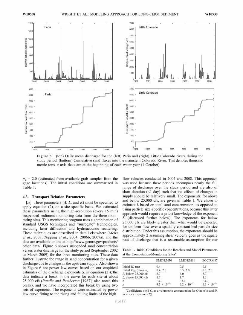
approach is used. For the Little Colorado River, data from twoUSGS gages (09402000 Little Colorado River near Cameron,AZ, and 09402300 Little Colorado River above mouth nearDesert View, AZ) were used to estimate sand transport ratesusing time‐weighted suspended sand rating curves. Dailymean water discharge and total cumulative sand flux for thesetwo tributaries for the study period are shown in Figure 5. Thetributary sand particle size distributions were estimated byaveraging the distributions from the available samples, and itwas found that log‐normal distributions (’ scale) with D50 =0.1 mm and sg = 1.8 for the Paria and 2.0 the Little Coloradofit the data very well (D50 and sg are median diameter andgeometric standard deviation, respectively). There arenumerous ungaged tributaries entering the Colorado Riveralong the study reach in addition to the Paria and LittleColorado Rivers. Recent monitoring data (not shown) indi-cate that ungaged inputs to upper Marble Canyon are about10% of Paria inputs and are significantly larger than ungagedinputs to lower Marble Canyon and eastern Grand Canyon.Thus, for modeling purposes we increased inputs to UMC by10% and neglected the ungaged inputs to the LMC and EGCreaches. We note that these estimates are different from(somewhat less than but within the error bars) those publishedby Webb et al. [2000]; we chose to use the more recent esti-mates because they are based on direct measurements ofsuspended sediment transport whereas theWebb et al. [2000]estimates were made using indirect methods.[23] Water discharge time series must also be specified at

the downstream end of each reach (i.e., at RM30, RM61,RM87) for application of equation (2). For the modelingperiod, discharge was estimated at each site from 15 minstage measurements and stage‐discharge relations based onepisodic discharge measurements. For modeling potentialfuture scenarios, the water discharges could be routeddownstream from the dam to the computational sites usingthe model of Wiele and Smith [1996].

4.2. Initial Conditions

[24] Solution of equations (3)−(4) requires specificationof the initial sand thickness and initial bed particle sizedistribution, for each of the three reaches. To estimate thesequantities, we used data from reach‐based monitoring pro-gram implemented from 2000 to 2005. This program con-sisted of remote sensing, ground surveys, and bathymetricsurveys [Kaplinski et al., 2009, Hazel et al., 2008] and bedparticle size measurements (using digital photographictechniques, Rubin [2004], Rubin et al. [2007]) for several3–5 km reaches between Lees Ferry and RM87. The reachsurveys closest in time to the beginning of the modelingperiod were conducted in May 2002. Thus, we averaged theavailable May 2002 sand thickness and particle size data(M. Breedlove, Grand Canyon Monitoring and ResearchCenter, written communication, 2007) within each modelingreach resulting in thicknesses of 0.4, 0.5, and 0.5 m andmean particle sizes of 0.4, 0.3, and 0.3 mm for UMC, LMC,and EGC, respectively. The sand thicknesses were estimatedby differencing the maximum and minimum surfaces insandy areas and thus represent the amount of erosion andaccumulation that took place during the monitoring period.The digital photographic technique provides a mean particlesize of the bed surface only; the initial size distributionswere estimated by assuming log‐normal distributions with


7 of 18

sg = 2.0 (estimated from available grab samples from thegage locations). The initial conditions are summarized inTable 1.

4.3. Transport Relation Parameters

[25] Three parameters (A, L, and K) must be specified toapply equation (2), on a site‐specific basis. We estimatedthese parameters using the high‐resolution (every 15 min)suspended sediment monitoring data from the three moni-toring sites. This monitoring program uses a combination ofstandard USGS techniques and “surrogate” technologies,including laser diffraction and hydroacoustic scattering.These techniques are described in detail elsewhere [Meliset al., 2003; Topping et al., 2004, 2006b, 2007a], and thedata are available online at http://www.gcmrc.gov/products/other_data/. Figure 6 shows suspended sand concentrationversus water discharge for the study period (September 2002to March 2009) for the three monitoring sites. These datafurther illustrate the range in sand concentration for a givendischarge due to changes in the upstream supply. Also shownin Figure 6 are power law curves based on our empiricalestimates of the discharge exponents (L in equation (2)); thedata indicate a break in the curve for each site at about25,000 cfs (Randle and Pemberton [1987], also noted thisbreak), and we have incorporated this break by using twosets of exponents. The exponents were estimated by powerlaw curve fitting to the rising and falling limbs of the high‐

flow releases conducted in 2004 and 2008. This approachwas used because these periods encompass nearly the fullrange of discharge over the study period and are also ofshort duration (<1 day) such that the effects of changes insupply should be relatively small. The exponents, for aboveand below 25,000 cfs, are given in Table 1. We chose toestimate L based on total sand concentration, as opposed tousing particle size‐specific concentrations, because this latterapproach would require a priori knowledge of the exponentK (discussed further below). The exponents for below25,000 cfs are likely greater than what would be expectedfor uniform flow over a spatially constant bed particle sizedistribution. Under this assumption, the exponents should beapproximately 2 assuming shear velocity goes as the squareroot of discharge that is a reasonable assumption for our

Table 1. Initial Conditions for the Reaches and Model Parametersat the Computation/Monitoring Sitesa

UMC/RM30 LMC/RM61 EGC/RM87

Initial Hs (m) 0.4 0.5 0.5Initial D50 (mm), sg 0.4, 2.0 0.3, 2.0 0.3, 2.0L, below 25,000 cfs 3.7 4.0 3.7L, above 25,000 cfs 1.7 1.7 1.3K −3.0 −3.0 −3.0A 4.3 × 10−26 6.2 × 10−27 6.1 × 10−26

aCoefficients yield Ci as a volumetric concentration for Q in m3/s and Di

in m (see equation (2)).

Figure 5. (top) Daily mean discharge for the (left) Paria and (right) Little Colorado rivers during thestudy period. (bottom) Cumulative sand fluxes into the mainstem Colorado River. Tmt denotes thousandmetric tons. x axis ticks are at the beginning of each water year (1 October).


8 of 18

gage locations. This is the result of the complex organizationof bed shear stress and bed particle sizes in the pool rapidsystem of the Colorado River (for example, as flow goes upit accesses finer particle sizes along the channel margins andin eddies).[26] The particle size exponent in equation (2) (K) is more

difficult to estimate empirically because it requires data onreach‐averaged particle size distributions and particle size‐specific transport rates. However, Rubin and Topping[2001] reported a range of computed exponents of −1.5 to−3.0, thus providing a range of reasonable values. Weconducted exploratory simulations and evaluated the results,particularly in terms of the degree of bed fining and coars-ening that occurred for a given K value. It was found that avalue on the high end of the reasonable range was necessaryto achieve the degree of fining and coarsening that has beenobserved (particularly during the high‐flow releases), andthus, we chose a value of K = −3.0. It is perhaps not sur-prising that an exponent that tends to accentuate particle sizedependence is necessary, given the reach‐averaged nature ofthe model and assumption of complete mixing of the bedsediment.[27] There are several options for estimating the remain-

ing coefficient in equation (2), the proportionality constantA. Because the ultimate goal of our modeling was to predictmulti‐year sand budgets for the individual reaches, we choseto calibrate A at each gage location to match the measuredtotal sand flux from the reach over the calibration timeperiod, September 2002 through March 2006. These com-putations proceeded in a downstream direction, wherebytrial and error was used for A until the total sand flux fromthe reach matched the measured sand flux to within <1%.The resulting A coefficients are given in Table 1. The formof equation (1) and its empirical nature dictate that thecoefficients are not dimensionless and are a combination ofvarious units to different powers. The values of A given inTable 1 are such that, when applied to equation (2) with Q inm3/s and Di in m, the resulting Ci is a volumetric concen-tration. Finally, the fact that A is such a small number issimply the result of the units used in its determination;concentration is linearly related to A (equation (2)) and itthus has a direct influence on modeled sand fluxes.

5. Analysis and Discussion of Results

[28] Several measures can be used to evaluate the model’sperformance, during both the calibration and validation timeperiods. Because the model was calibrated to match the totalsand flux from each reach over the calibration period(through specification of A), it is appropriate to evaluatehow well the model predictions agree with the measure-ments over shorter time scales within the calibration period.The validation time period provides an independent test ofthe model calibration. In particular, as stated in our overallmodeling goals, the model should be able to simulate sandaccumulation and bed fining in response to tributaryflooding, followed by erosion and coarsening. Both thecalibration and validation periods contain episodes of sandaccumulation and bed fining, followed by high‐flow releaseswherein substantial coarsening occurred. Substantial tribu-tary flooding and sand inputs occurred during fall 2004,winter 2005, fall 2006, and fall 2007 (Figure 3). High‐flow

Figure 6. Suspended sand concentration versus water dis-charge as measured at the three monitoring sites betweenSeptember 2002 and March 2009 and relations derived fromequation (2) with the exponents given in Table 1.


9 of 18

releases occurred in November 2004 and March 2008(Figure 2).[29] An initial test of model performance is a comparison

of the total sand flux at each monitoring site during thevalidation period, since the model was calibrated to matchthe total fluxes during the calibration period. Table 2 showspercent differences between modeled and measured fluxesover the validation period. The differences are 11%, 0.70%,and −4.6% for RM30, RM61, and RM87, respectively.Although the model overestimates the flux at RM30 by11%, it is a substantial improvement over a stable sandrating curve which underestimates this flux by 37% becauseit cannot incorporate bed fining due to large Paria Riverflooding in October 2006. A variety of reasons couldexplain the model overestimates for this reach, including thevarious model simplifications as well as uncertainty in thetributary inputs (which control the degree of bed fining).The measured and modeled cumulative sand fluxes for theentire study period for each of the three monitoring sites areshown in Figure 7 (note that the calibration procedure forcesthese to match at the end of the calibration period). Themeasurement uncertainty has been estimated to be ±5% asper Topping et al. [2000], and this envelope is included inFigure 7.

5.1. Monthly Sand Flux and Annual Sand Budgets

[30] Water discharge varies substantially on a monthlybasis below Glen Canyon Dam to meet hydroelectricitydemand; that is, release volumes are highest in the summerand winter when demand is highest and lowest in spring andfall. Thus, a potential application of the model would be tocompare monthly sand flux for a range of release volumes.To this end, measured and modeled monthly sand fluxes forthe three sites are compared in Figure 8 for both calibrationand validation periods. While the model captures the generalbehavior well, there is substantial variability and someindication of model overestimation at the lowest fluxesparticularly at RM87. The modeled and measured monthlyfluxes are compared numerically in Table 2, where R is theratio of modeled to measured monthly flux. In Table 2,values for the validation period are shown in parenthesesalongside those for the calibration period, for comparison. Avery high percentage (∼90%) of the modeled monthly fluxesare within a factor of 2 of the measurements, for bothcalibration and validation time periods. The percentage ofmodeled fluxes within a factor of 1.5 of the measured valuesranges from 56% (RM61) to 79% (RM30) for the calibrationperiod (the agreement at RM30 and RM87 is generally

Figure 7. Comparison of measured and modeled cumulative sand fluxes at the three monitoring sites forthe entire modeling period (calibration and validation). Measured fluxes are shown as an envelope with±5% uncertainty [Topping et al., 2000]. For RM30, the model results using a stable rating curve are alsoshown.


10 of 18

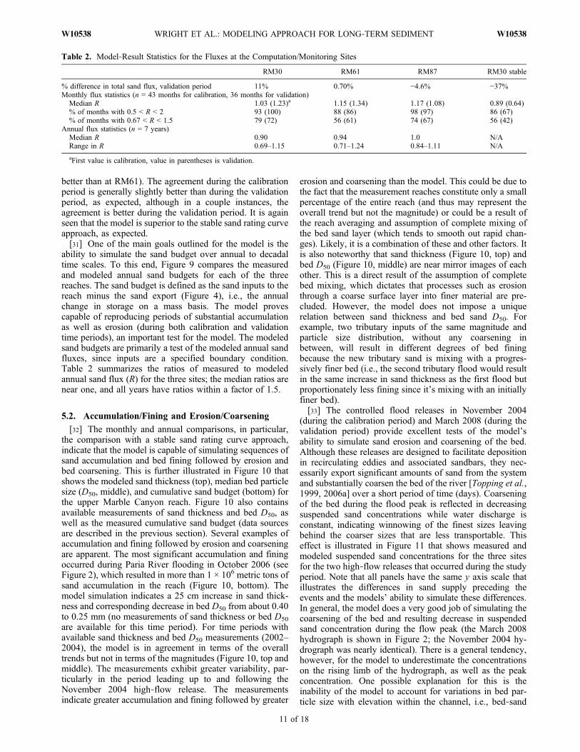
better than at RM61). The agreement during the calibrationperiod is generally slightly better than during the validationperiod, as expected, although in a couple instances, theagreement is better during the validation period. It is againseen that the model is superior to the stable sand rating curveapproach, as expected.[31] One of the main goals outlined for the model is the

ability to simulate the sand budget over annual to decadaltime scales. To this end, Figure 9 compares the measuredand modeled annual sand budgets for each of the threereaches. The sand budget is defined as the sand inputs to thereach minus the sand export (Figure 4), i.e., the annualchange in storage on a mass basis. The model provescapable of reproducing periods of substantial accumulationas well as erosion (during both calibration and validationtime periods), an important test for the model. The modeledsand budgets are primarily a test of the modeled annual sandfluxes, since inputs are a specified boundary condition.Table 2 summarizes the ratios of measured to modeledannual sand flux (R) for the three sites; the median ratios arenear one, and all years have ratios within a factor of 1.5.

5.2. Accumulation/Fining and Erosion/Coarsening

[32] The monthly and annual comparisons, in particular,the comparison with a stable sand rating curve approach,indicate that the model is capable of simulating sequences ofsand accumulation and bed fining followed by erosion andbed coarsening. This is further illustrated in Figure 10 thatshows the modeled sand thickness (top), median bed particlesize (D50, middle), and cumulative sand budget (bottom) forthe upper Marble Canyon reach. Figure 10 also containsavailable measurements of sand thickness and bed D50, aswell as the measured cumulative sand budget (data sourcesare described in the previous section). Several examples ofaccumulation and fining followed by erosion and coarseningare apparent. The most significant accumulation and finingoccurred during Paria River flooding in October 2006 (seeFigure 2), which resulted in more than 1 × 106 metric tons ofsand accumulation in the reach (Figure 10, bottom). Themodel simulation indicates a 25 cm increase in sand thick-ness and corresponding decrease in bed D50 from about 0.40to 0.25 mm (no measurements of sand thickness or bed D50

are available for this time period). For time periods withavailable sand thickness and bed D50 measurements (2002–2004), the model is in agreement in terms of the overalltrends but not in terms of the magnitudes (Figure 10, top andmiddle). The measurements exhibit greater variability, par-ticularly in the period leading up to and following theNovember 2004 high‐flow release. The measurementsindicate greater accumulation and fining followed by greater

erosion and coarsening than the model. This could be due tothe fact that the measurement reaches constitute only a smallpercentage of the entire reach (and thus may represent theoverall trend but not the magnitude) or could be a result ofthe reach averaging and assumption of complete mixing ofthe bed sand layer (which tends to smooth out rapid chan-ges). Likely, it is a combination of these and other factors. Itis also noteworthy that sand thickness (Figure 10, top) andbed D50 (Figure 10, middle) are near mirror images of eachother. This is a direct result of the assumption of completebed mixing, which dictates that processes such as erosionthrough a coarse surface layer into finer material are pre-cluded. However, the model does not impose a uniquerelation between sand thickness and bed sand D50. Forexample, two tributary inputs of the same magnitude andparticle size distribution, without any coarsening inbetween, will result in different degrees of bed finingbecause the new tributary sand is mixing with a progres-sively finer bed (i.e., the second tributary flood would resultin the same increase in sand thickness as the first flood butproportionately less fining since it’s mixing with an initiallyfiner bed).[33] The controlled flood releases in November 2004

(during the calibration period) and March 2008 (during thevalidation period) provide excellent tests of the model’sability to simulate sand erosion and coarsening of the bed.Although these releases are designed to facilitate depositionin recirculating eddies and associated sandbars, they nec-essarily export significant amounts of sand from the systemand substantially coarsen the bed of the river [Topping et al.,1999, 2006a] over a short period of time (days). Coarseningof the bed during the flood peak is reflected in decreasingsuspended sand concentrations while water discharge isconstant, indicating winnowing of the finest sizes leavingbehind the coarser sizes that are less transportable. Thiseffect is illustrated in Figure 11 that shows measured andmodeled suspended sand concentrations for the three sitesfor the two high‐flow releases that occurred during the studyperiod. Note that all panels have the same y axis scale thatillustrates the differences in sand supply preceding theevents and the models’ ability to simulate these differences.In general, the model does a very good job of simulating thecoarsening of the bed and resulting decrease in suspendedsand concentration during the flow peak (the March 2008hydrograph is shown in Figure 2; the November 2004 hy-drograph was nearly identical). There is a general tendency,however, for the model to underestimate the concentrationson the rising limb of the hydrograph, as well as the peakconcentration. One possible explanation for this is theinability of the model to account for variations in bed par-ticle size with elevation within the channel, i.e., bed‐sand

Table 2. Model‐Result Statistics for the Fluxes at the Computation/Monitoring Sites

RM30 RM61 RM87 RM30 stable

% difference in total sand flux, validation period 11% 0.70% −4.6% −37%Monthly flux statistics (n = 43 months for calibration, 36 months for validation)

Median R 1.03 (1.23)a 1.15 (1.34) 1.17 (1.08) 0.89 (0.64)% of months with 0.5 < R < 2 93 (100) 88 (86) 98 (97) 86 (67)% of months with 0.67 < R < 1.5 79 (72) 56 (61) 74 (67) 56 (42)

Annual flux statistics (n = 7 years)Median R 0.90 0.94 1.0 N/ARange in R 0.69–1.15 0.71–1.24 0.84–1.11 N/A

aFirst value is calibration, value in parentheses is validation.


11 of 18

particle size tends to be coarsest in deeper parts of thechannel and finest in higher elevation deposits such as eddysandbars [Topping et al., 2005]. This structure is to somedegree embedded in the rating curve exponents; however, itis not treated explicitly in the modeled particle size dis-tributions and would require a significantly more complexformulation. Several other explanations are possible as well,such as unsteady transport process, local hydraulics (par-ticularly in eddies), breaking of “armor layers” that releasefiner sand, among others.

6. Sensitivity Analysis

[34] Because of the simplified and empirical nature of themodeling approach, it is instructive to evaluate the sensi-tivity of the model results to the various model parametersthat must be specified, include boundary and initial condi-tions. To this end, we conducted a suite of simulations withthe following parameters varied by ±10%: (1) tributary sandloads (Paria and Little Colorado), (2) tributary sand D50,(3) initial sand thickness on the bed (Hs), (4) initial bed D50,(5) rating curve coefficient (A in equation (2)), (6) dischargeexponent (L in equation (2)), (7) bed‐sand particle sizeexponent (K in equation (2)), and (8) channel width (B). Thechoice of ±10% is arbitrary to some degree and does notnecessarily represent uncertainty in the various parameter(the uncertainty is unknown). Rather, the ±10% is simply areasonable perturbation to impose on the model to study itssensitivity. Imposing the same relative perturbation for allparameters allows for evaluation of the relative sensitivity toeach parameter and can thus provide guidance on, forexample, which parameters warrant further study andmeasurements.[35] Model sensitivity was evaluated by comparing the

sand flux at each gage for the ±10% runs with that of thecalibrated model (total flux over the simulation period(September 2002 through March 2009). While eachparameter influences the model in different and complexways, comparison of total fluxes is the simplest, most direct,and most relevant method because simulation of multi‐yearsand flux is the primary objective of the model. The resultsare displayed in Figure 12, in terms of percent differencesbetween the sensitivity runs and the calibrated model, forthe three gage locations. From Figure 12, it is immediatelyapparent that the rating‐curve exponents (L and K inequation (2)) exert, by far, the greatest control on the modelresults. The ±10% perturbation introduced in these exponentsresults in differences in total flux at the gages ranging from∼50% to 100%, depending on the site. In contrast, all otherparameters yield differences that are less than the ±10%perturbation. Tributary loads, tributary D50, initial bed D50,and the rating coefficient (A) all yield differences in the 3%−7% range, while initial sand thickness and channel widthhad almost no effect on the results (differences <0.5%).[36] It is perhaps not surprising that the exponents exert

such strong influence, given that they are substantiallygreater than one resulting in a highly nonlinear response insand concentration with changes in discharge and particlesize. This sensitivity supports our approach of directly cal-ibrating the rating coefficient A to match measured loads;without this type of calibration, large differences in loadscould easily occur. It is also instructive for sediment‐transportmodeling in general, because any model must incorporate a

Figure 8. Comparison of measured and modeled monthlysand fluxes at the three monitoring sites ((top) RM30; (mid-dle) RM61; (bottom) RM87) for the calibration and valida-tion periods; line indicates perfect agreement. Statistics aregiven in Table 2.


12 of 18

similar sediment‐transport formula whereby concentrationor flux is dependent on hydraulic variables (and particlesize) in a highly nonlinear way (for example, the Rouseequation with a near‐bed concentration predictor). Thus,some calibration of concentration or flux (directly orthrough shear‐stress partitioning) is likely always necessaryfor sediment‐transport modeling of this type.

7. Limitations of the Approach

[37] The modeling approach that we have developed andapplied is empirical in nature and substantially simplifiedwith respect to the physical processes known to governsediment transport in the study reach. The empiricism andsimplifications were necessary to meet the primary goal ofthe modeling, i.e., the ability to simulate the long‐term(decadal scale) sand budget for the reach with only oneadjustable calibration parameter. The consequences of thesimplifications have been noted throughout this article butwarrant summary here so that potential users of thisapproach have a clear understanding of the limitations, asfollows:[38] •Although the approach should have general appli-

cability to supply‐limited rivers and particularly those wherecomplete bed mixing is a reasonable approximation, the

model coefficients (Table 1) are specific to the study reachand thus do not have general applicability.[39] •The model integrates the pool‐rapid‐eddy mor-

phology over long reaches, and thus should not be expectedto capture the specific effects of this morphology on sedi-ment transport. For example, the model cannot discriminatebetween sand on the main channel bed and sand within eddysandbars.[40] •The model does not account for changes in the area

of sand covering the bed at a given time. This phenomenonis essentially lumped in the calibration of the rating curvecoefficient A. Thus, application of the model to conditionswhere large changes in bed‐sand area might be expected(e.g., long‐term substantial accumulation) must be viewedwith some caution.[41] •Although the model uses a short (15 min) time step

to capture the subdaily variability in flow, it should not beexpected to capture rapid changes in bed particle size andsuspended sand concentration, for example during tributaryflooding (e.g., Figure 3). The use of long reaches andassumption of complete mixing of the bed sediment tends to“smooth out” these rapid changes. To capture the type ofshort‐term response shown in Figure 3 (squares), an unsteady,advection‐dispersion approach for suspended sediment wouldlikely be required.

Figure 9. Comparison of measured and modeled annual sand budgets for the three reaches. The annualsand budget is defined as sand inputs minus export from the reach (based on water year), i.e., the changein storage on a mass basis.


13 of 18

[42] •The model cannot capture variability in particle sizeas a function of elevation within the channel that is knownto exist, i.e., the river bed is coarser in the deeper mainchannel than in shallower eddy environments. The modellumps all sand deposits into a single pool (for each reach)that is completely mixed.[43] •The model cannot simulate a scenario where a

coarse surface layer temporarily precludes access to a finersubstrate. This is thought to have happened following theextremely high flows of the mid‐1980s, after which trans-port rates gradually increased for a given discharge despite alikely negative sand budget. This behavior was presumablya result of morphologic adjustments of eddy sandbars fol-lowing the high flows [Topping et al., 2005]. The assump-tion of completely mixed bed sediment precludes simulationof this behavior.[44] Because of these limitations, we consider the mod-

eling approach as one that should be used in concert with anongoing monitoring program allowing for ongoing evalua-tion of the calibration parameter A. Indeed, the empiricalnature of the transport relation requires at least some mon-itoring data to specify the model parameters. The model, aswith almost all models, was designed with the intent toforecast future conditions for various hydrological and

management scenarios. However, because of the empiricalnature and inherent limitations, the approach and resultsshould be routinely evaluated and adjusted as necessary asnew data become available. Ideally, this is the approach thatshould be taken with all simulation models, but it is par-ticularly important for the approach described here.

8. Conclusions

[45] The modeling approach described herein represents acompromise between a desire for model simplicity, to limitinput data requirements as well as facilitate multi‐yearsimulations of a large number of scenarios, and the need tocapture a fundamental mechanism controlling transport ratesin the study reach, i.e., supply‐driven changes in bed particlesize and suspended sediment concentration. In the spectrumof sediment‐transport models, it lies between suspendedsediment rating curves and standard one‐dimensional, mul-tiple particle size, morphodynamic models. The approachwas formulated specifically for sand supply‐limited condi-tions, in particular the conditions along the Colorado Riverbelow Glen Canyon Dam where the relation between sus-pended sand concentration and water discharge stronglydepends on sand supply from tributaries downstream from

Figure 10. Time series of (top) measured and modeled sand thickness, (middle) bed median particlesize, and (bottom) cumulative sand budget for the upper Marble Canyon (UMC) reach. Data sourcesare described in the text.


14 of 18

the dam. A primary objective of the modeling approach wasthe ability to simulate multi‐year sediment budgets, perhapsin a Monte Carlo framework to account for variability inhydrology and tributary sediment supply. Achieving thisobjective required various simplifications and empiricism,as summarized in the previous section. The proposed for-

mulation certainly achieved this objective as the approxi-mately 7 year simulations described herein took only ∼30 son a standard desktop computer.[46] The model was applied to the reach of the Colorado

River below Glen Canyon Dam for the period September2002 through March 2009. The model was calibrated such

Figure 11. Comparison of measured (circles) and modeled (solid black lines) suspended sand concen-tration at the three monitoring sites during high‐flow releases in November 2004 (during calibrationperiod) and March 2008 (during validation period). The high‐flow hydrographs are shown light solidlines in each frame.


15 of 18

that the total sand flux from each of the three modelingreaches matched the measured total flux during the calibra-tion time period (i.e., the first 3.5 years of the simulation).Comparisons between measured and modeled monthly sandfluxes and annual sand budgets showed the model capable ofsimulating the variability in sand flux resulting from dis-charge variability as well as changes in sand supply. Model

comparisons to data were generally comparable during thecalibration and validation time periods. Comparisons ofmeasured and modeled bed sand thickness and bed D50

confirmed the models’ ability to simulate accumulation ofsand accompanied by bed fining during and immediatelyfollowing tributary flooding, followed by erosion and bedcoarsening during tributary quiescence. Comparisons of

Figure 12. Results of model sensitivity analyses for the three gage sites. The y axis portrays the percentdifference between the given scenario and the fully calibrated model, for variations in each parameter of±10%.


16 of 18

measured and modeled suspended sand concentrationsduring the high‐flow releases in November 2004 and March2008 indicate that the model can adequately simulate bedcoarsening during the peak flows but tends to underestimatesuspended sand concentration on the rising limb of the high‐flow hydrograph. The model was also shown to providesignificant improvement over a stable suspended sand ratingcurve approach for our study site, as expected. Analysis ofmodel sensitivity to input parameters illustrated strongdependencies on the rating curve exponents (discharge andparticle size), thus providing support for our procedure ofdirect calibration of the rating curve coefficient to matchmeasured loads. Finally, these comparisons provide confi-dence in application of the model to forecast future condi-tions under various dam operation scenarios, for example, toestimate how much accumulation or erosion might occur fora given dam operation and tributary supply. This informa-tion could then potentially be used to plan future high‐flowreleases designed to rebuild sandbars.[47] As formulated, the modeling approach should have

general applicability to supply‐limited rivers, particularlythose where the assumption of complete bed mixing isappropriate such as many rivers flowing through bedrockcanyons. However, the empirical model parameters (i.e.,Table 1) are not expected to have general applicability butmust rather be estimated on a site‐specific basis. Thus, thistype of approach can only be applied to river reaches wheresufficient data are available to estimate the model para-meters. Also, given the simplified and empirical nature ofthe approach, applications will be most successful if con-ducted within the context of an ongoing monitoring programso that the results can be evaluated on a regular basis, and ifnecessary, the formulation can be modified to account fornew findings related to sand transport processes withinthe river.

ReferencesAmerican Society of Civil Engineers (ASCE) (1975), Sedimentation

Engineering, edited by V. A. Vanoni, New York.Draut, A. E., and D. R. Rubin (2007), The role of Aeolian sediment in the

preservation of archaeological sites in the Colorado River Corridor,Grand Canyon, Arizona: Final report on research activities, 2003–2006,U.S. Geol. Surv. Open File Rep., 2007‐1001.

Grams, P. E., J. C. Schmidt, and D. J. Topping (2007), The rate and patternof bed incision and bank adjustment on the Colorado River in GlenCanyon downstream from Glen Canyon Dam, 1956–2000, GSA Bull.,119(5/6), 556–575.

Hazel, J. E., M. Kaplinski, R. A. Parnell, K. Kohl, and J. C. Schmidt(2008), Monitoring Fine‐Grained Sediment in the Colorado RiverEcosystem, Arizona−Control Network and Conventional Survey Tech-niques, U.S. Geol. Surv. Open File Rep., 2008‐1276, 15 pp.

Hoey, T. B., and R. Ferguson (1994), Numerical simulation of downstreamfining by selective transport in gravel bed rivers: Model developmentand illustration, Water Resour. Res., 30(7), 2251–2260, doi:10.1029/94WR00556.

Kaplinski, M., J. E. Hazel Jr., R. Parnell, M. Breedlove, K. Kohl, andM. Gonzales (2009), Monitoring fine‐sediment volume in the ColoradoRiver ecosystem, Arizona: Bathymetric survey techniques, U.S. Geol.Surv. Open File Rep., 2009–1207, 33 pp.

Leopold, L. B., and T. Maddock Jr. (1953), The hydraulic geometry ofstream channels and some physiographic implications, U.S. Geol. Surv.Prof. Pap., 252, 57 pp.

McLean, S. R. (1992), On the calculation of suspended load for noncohesivesediments, J. Geophys. Res., 97, 5759–5770, doi:10.1029/91JC02933.

Melis, T. S., D. J. Topping, and D. M. Rubin (2003), Testing laser‐basedsensors for continuous in situ monitoring of suspended sediment in theColorado River, Arizona, in Erosion and Sediment Transport Measure-

ment in Rivers: Technological and Methodological Advances, IAHSPubl., 283, edited by J. Bogen, T. Fergus, and D. E. Walling, pp. 21–27.

Melis, T. S., S. A. Wright, B. E. Ralston, H. C. Fairley, T. A. Kennedy,M. E. Andersen, L. G. Coggins Jr., and J. Korman (2006), 2005 Knowl-edge assessment of the effects of Glen Canyon Dam on the ColoradoRiver ecosystem: an experimental planning support document, 82 p.,U.S. Geol. Surv., Flagstaff, Ariz.

Nilsson, C., C. A. Reidy, M. Dynesius, and C. Revenga (2005), Fragmen-tation and flow regulation of the world’s large river systems, Science,308, 405–408.

Parker, G., C. Paola, and S. Leclair (2000), Probabilistic Exner sedimentcontinuity equation for mixtures with no active layer, J. Hydaul. Eng.,126(11), 818–826.

Pemberton, E. L. (1987), Sediment data collection and analysis for fivestations on the Colorado River from Lees Ferry to Diamond Creek,Final Tech. Rep., Glen Canyon Environmental Studies.

Rahuel, J. L., F. M. Holly, J. P. Chollet, P. J. Belleudy, and G. Yang(1989), Modeling of riverbed evolution for bedload sediment mixtures,J. Hydraul. Eng., 115(11), 1521–1542.

Randle, T. J., and E. L. Pemberton (1987), Results and analysis of STARSmodeling efforts of the Colorado River in Grand Canyon: Glen CanyonEnvironmental Studies Report, 41 p.

Ronco, P., G. Fasolato, and G. di Silvio (2009), Modelling evolution of bedprofile and grain size distribution in unsurveyed rivers, Int. J. Sediment.Res., 24(2), 127–144.

Rubin, D. M., and D. J. Topping (2001), Quantifying the relative impor-tance of flow regulation and grain‐size regulation of suspended‐sedimenttransport a and tracking changes in grain size of bed sediment b, WaterResour. Res., 37(1), 133–146, doi:10.1029/2000WR900250.

Rubin, D. M. (2004), A simple autocorrelation algorithm for determininggrain size from digital images of sediment, J. Sediment. Res., 74, 160–165.

Rubin, D. M., and C. L. Carter (2006), Bedforms, and Cross‐Bedding inAnimation, SEPM Atlas Ser., 2, DVD.

Rubin, D. M., H. Chezar, J. N. Harney, D. J. Topping, T. S. Melis, andC. R. Sherwood (2007), Underwater microscope for measuring spatialand temporal changes in bed‐sediment grain size, Sediment. Geol.,202, 402–408.

Rubin, D. M., and D. J. Topping (2008), Correction to “Quantifying therelative importance of flow regulation and grain‐size regulation of sus-pended‐sediment transport a, and tracking changes in bed‐sedimentgrain size b,” Water Resour. Res., 44(5), W09701, doi:10.1029/2008WR006819.

Schmidt, J. C. (1990), Recirculating flow and sedimentation in the ColoradoRiver in Grand Canyon, Arizona, J. Geol., 98, 709–724.

Schmidt, J. C. (1999), Summary and synthesis of geomorphic studiesconducted during the 1996 controlled flood in Grand Canyon, in TheControlled Flood in Grand Canyon, Geophys. Monogr. Ser., 110, editedby R. H. Webb et al., pp. 329–341, AGU, Washington, D.C.

Schmidt, J. C., and P. R. Wilcock (2008), Metrics for assessing the down-stream effects of dams, Water Resour. Res., 44, W04404, doi:10.1029/2006WR005092.

Syvitski, J. P. M., C. J. Vorosmarty, A. J. Kettner, and P. Green (2005),Impact of humans on the flux of terrestrial sediment to the global coastalocean, Science, 308, 376–380.

Topping, D. J. (1997), Physics of flow, sediment transport, hydraulic geo-metry, and channel geomorphic adjustment during flash floods in anephemeral river, the Paria River, Utah and Arizona, Ph.D. thesis,406 pp., University of Washington.

Topping, D. J., D. M. Rubin, J. M. Nelson III, P. J. Kinzel, and J. P. Bennett(1999), Linkage between grain‐size evolution and sediment depletionduring Colorado River floods, in The 1996 Controlled Flood in GrandCanyon, Geophys. Monogr., 110, edited by R. H. Webb et al., pp. 71–98,AGU, Washington, D. C.

Topping, D. J., D. M. Rubin, and L. E. Vierra Jr. (2000), Colorado Riversediment transport: Part 1: Natural sediment supply limitation and theinfluence of Glen Canyon Dam, Water Resour. Res., 36(2), 515–542,doi:10.1029/1999WR900285.

Topping, D. J., J. C. Schmidt, and L. E. Vierra Jr. (2003), Computation andanalysis of the instantaneous‐discharge record for the Colorado River atLees Ferry, Arizona—May 8, 1921, through September 30, 2000, U.S.Geol. Surv. Prof. Pap., 1677, 118 p.

Topping, D. J., T. S. Melis, D. M. Rubin, and S. A. Wright (2004), High‐resolution monitoring of suspended‐sediment concentration and grainsize in the Colorado River in Grand Canyon using a laser‐acoustic system,in Proceeding of the Ninth International Symposium on River Sedimenta-


17 of 18

tion, Volume IV, edited by C. Hu, Y. Tan, and C. Liu, pp. 2507–2514,Yiching, China.

Topping, D. J., D. M. Rubin, and J. C. Schmidt (2005), Regulation ofsand transport in the Colorado River by changes in the surface grainsize of eddy sandbars over multi‐year timescales, Sedimentology, 52,1133–1153.

Topping, D. J., D. M. Rubin, J. C. Schmidt, J. E. Hazel, T. S. Melis,S. A. Wright, and M. Kaplinski (2006a), Comparison of sediment‐transport and bar‐response results from the 1996 and 2004 controlledflood experiments on the Colorado River in Grand Canyon, in Proceed-ings 8th Federal Interagency Sedimentation Conference (CD‐ROM),ISBN 0‐9779007‐1‐1, Reno, Nev.

Topping, D. J., S. A. Wright, T. S. Melis, and D. M. Rubin (2006b), High‐resolution monitoring of suspended‐sediment concentration and grainsize in the Colorado River using laser‐diffraction instruments and athree‐frequency acoustic system, in Proceedings 8th Federal Inter-agency Sedimentation Conference (CDROM), ISBN 0‐9779007‐1‐1,Reno, Nev.

Topping, D. J., S. A. Wright, T. S. Melis, and D. M. Rubin (2007a), High‐resolution measurements of suspended‐sediment concentration and grainsize in the Colorado River in Grand Canyon using a multi‐frequencyacoustic system, in Proceedings of the 10th International Symposiumon River Sedimentation, vol. III, Moscow, Russia.

Topping, D. J., D. M. Rubin, and T. S. Melis (2007b), Coupled changes insand grain size and sand transport driven by changes in the upstreamsupply of sand in the Colorado River: Relative importance of changesin bed‐sand grain size and bed‐sand area, Sediment. Geol., 202(3),538–561.

U.S. Dept. of the Interior (1995), Operation of Glen Canyon Dam FinalEnvironmental Impact Statement, 337 p., Bureau of Reclamation, UpperColorado Region, Salt Lake City.

U.S. Dept. of the Interior (1996), Record of Decision, Operation of GlenCanyon Dam, 13 p., Office of the Secretary of Interior, Washington,D. C.

van Niekerk, A., K. R. Vogel, R. L. Slingerland, and J. S. Bridge (1992),Routing of heterogeneous sediments over movable bed: model develop-ment, J. Hydaul. Eng., 118(2), 246–262.

Webb, R. H., P. G. Griffiths, T. S. Melis, and D. R. Hartley (2000),Sediment delivery by ungaged tributaries of the Colorado River in GrandCanyon, Arizona, U.S. Geol. Surv. Water Resour. Invest. Rep., 00‐4055,67 pp.

Wiele, S. M., J. B. Graf, and J. D. Smith (1996), Sand deposition in theColorado River in the Grand Canyon from flooding of the Little ColoradoRiver,Water Resour. Res., 32(12), 3579–3596, doi:10.1029/96WR02842.

Wiele, S. M., and J. D. Smith (1996), A reach‐averaged model of diurnaldischarge wave propagation down the Colorado River through the GrandCanyon, Water Resour. Res., 32(5), 1375–1386, doi:10.1029/96WR00199.

Wiele, S. M. (1998), Modeling of flood‐deposited sand distributions in areach of the Colorado River below the Little Colorado River, GrandCanyon, Arizona,U.S. Geol. Surv., Water Resour. Invest. Rep., 97‐4168,15 pp.

Wiele, S. M., E. D. Andrews, and E. R. Griffin (1999), The effect of sandconcentration on depositional rate, magnitude, and location in the ColoradoRiver below the Little Colorado River, in The Controlled Flood in GrandCanyon,Geophys. Monogr., 110, edited by R. H. Webb et al., pp. 131–145.

Wiele, S. M., and M. Torizzo (2005), Modelling of sand deposition inarchaeologically significant reaches of the Colorado River in GrandCanyon, USA, in Computational Fluid Dynamics: Applications inEnvironmental Hydraulics, edited by P. D. Bates, S. N. Lane, andR. I. Ferguson, pp. 357–394.

Wiele, S. M., P. R. Wilcock, and P. E. Grams (2007), Reach‐averagedsediment routing model of a canyon river, Water Resour. Res., 43,W02425, doi:10.1029/2005WR004824.

Wright, S. A., and G. Parker (2005), Modeling downstream fining insand‐bed rivers I: Formulation, J. Hydraul. Res., 43(6), 612–619.

Wright, S. A., T. S. Melis, D. J. Topping, and D. M. Rubin (2005), Influenceof Glen Canyon dam operations on downstream sand resources of theColorado River in Grand Canyon, in The State of the Colorado RiverEcosystem in Grand Canyon, U.S. Geol. Surv. Circular, 1282, editedby S. P. Gloss, J. E. Lovich, and T. S. Melis, pp. 17–31.

Yang, C. T. (1996), Sediment Transport: Theory and Practice, McGraw‐Hill.

T. S. Melis and D. J. Topping, U.S. Geological Survey, Grand CanyonMonitoring and Research Center, Flagstaff, AZ 86001, USA.D. M. Rubin, U.S. Geological Survey, Pacific Science Center, Santa

Cruz, CA 95060, USA.S. A. Wright, U.S. Geological Survey, California Water Science Center,

Sacramento, CA 95819, USA. ([email protected])


18 of 18

An approach for modeling sediment budgets in supplylimited ... · An approach for modeling sediment budgets ... Canyon, dam operations have actually increased the dura-tion of moderate

Documents