HISTORICAL 3D MODELING OF EROSION FOR SEDIMENT …

Middle States Geographer, 2013, 46: 61-70

61

HISTORICAL 3D MODELING OF EROSION FOR SEDIMENT VOLUME ANALYSIS

USING GIS, STONY CLOVE CREEK, NY

Christopher J. Hewes

Bren School of Environmental Science & Management

University of California, Santa Barbara

Santa Barbara, CA 93106-5131

Lawrence McGlinn

Department of Geography

SUNY-New Paltz

New Paltz, NY 12561

ABSTRACT: The New York City Department of Environmental Protection identifies Stony Clove Creek as a

chronic supplier of suspended sediment to the city’s water system. Stony Clove Creek, a tributary of Esopus Creek,

feeds the Ashokan Reservoir, a major supplier of drinking water to New York City which has no filtration system to

handle sediment loads. In the Stony Clove, a bowl-shaped erosional feature (swale) began forming in the early

1970s after anthropogenic straightening of the creek just downstream. Erosion here is due to: (1) high-energy flow

at the cutbank and (2) slumping due to groundwater flow through exposed fine-sediment glacio-lacustrine clays and

clay-rich tills. Our analysis suggests that from 1970 to present, approximately 68,000 cubic meters of sediment

have entered the creek and traveled downstream. Understanding how this feature grew and estimating how much

sediment it has yielded will inform further stream channeling projects and management of similar erosion sites in

the watershed.

Keywords: GIS, 3D Modeling, erosion, water supply, turbidity

INTRODUCTION

New York City water supply background New York City (NYC) is home to over eight million people, all of whom are dependent upon accessible,

clean drinking water. This water comes entirely from watersheds located north and northwest of the city. NYC’s

water supply system does not have a filtration plant; the three watersheds from which water is collected and piped to

NYC are protected to meet federal water quality standards (NYC DEP 2014).

NYC planners first looked north to find clean, safe water supplies in the early 1800s as the city grew,

damming the Croton River 50 km north of the city to create the first Croton Reservoir and aqueduct which brought

water to the city. After the incorporation of the current five boroughs into the city, a 1905 act of the State

Legislature established the NYC Board of Water Supply which was granted powers to seize private land by eminent

domain to expand the water supply system (Pires, 2004). The Catskill and Delaware watersheds (Figure 1a) were

developed from 1905-1965 with a series of impoundments to create reservoirs and aqueducts (Mehaffey et al, 1999).

The federal Safe Drinking Water Act (SDWA) was enacted in 1974, setting national standards for public

water supply systems. The later 1989 Surface Water Treatment Rule (SWTR) under the SDWA established criteria

for filtration and disinfection treatment processes for public water supplies. For suppliers without a filtration plant,

like NYC, the Environmental Protection Agency (EPA) could issue a Filtration Avoidance Determination if the

untreated waters met standards (Pires, 2004). Adhering to the requirements for this filtration avoidance is now the

major focus for the NYC Department of Environmental Protection (DEP). Building a filtration plant for the water

supply would cost over six billion dollars and require $300 million in annual maintenance (Pires, 2004).

The Catskill and Delaware watersheds together supply 90% of public water to NYC and some surrounding

communities, about 4.5 billion liters daily (Porter, 1994). The combined watersheds cover an area of about 5,000

km2 centered 160 km northwest of NYC. This water supply continues to be among the cleanest in the nation due to

the efforts of the NYC DEP as well as a Memorandum of Agreement established in 1997 among New York state,

local governments, and environmental groups (Mehaffey et al, 1999). However, human encroachment in the

watersheds has created challenges for the NYC DEP.

Modeling of Erosion for Sediment Volume Analysis

62

The surficial geology of the watersheds is approximately 30% bedrock (or near-surface bedrock), 60% fine-

grained glacial till, and 10% alluvial deposition from the major rivers and their tributaries (Mehaffey et al, 1999). A

2006 EPA report on the watershed protection program reports that this geology puts streams and reservoirs at risk

for high levels of turbidity, fine suspended sediment that causes cloudy water. High levels of turbidity can impact

water quality and use “by affecting the water’s color and taste, interfering with chemical and ultra-violet (UV)

disinfection, and providing a medium for the growth of potentially harmful bacteria and other microorganisms”

(Lloyd & Rush, 2006, p. 12).

Ashokan Reservoir The Ashokan Reservoir is the oldest and largest reservoir in the Catskill system, constructed in 1907 with a

water surface area of 33.2 square kilometers (Mehaffy et al, 1999) and a full capacity of 484 billion liters

(NYCDEP, 2010). Figure 1a highlights its location within the NYC drinking water supply system. Figure 1b shows

the relation between the reservoir, the upper Esopus Creek which feeds the reservoir directly, and Stony Clove

Creek, a tributary to Esopus Creek. The Ashokan Reservoir contains two basins, separated by a dividing weir and

gatehouse which pulls water into the Catskill aqueduct to NYC. The upper Esopus Creek empties into the West

basin, while water in the East basin can be released into the lower Esopus Creek and eventually the Hudson River.

The Ashokan Reservoir, among others in the Catskill system, was designed to handle turbidity by

providing for settling of sediment. However, major storm events and land-cover changes in the watershed over the

past two decades have impaired the reservoir’s capacity to remove sediment (USEPA, 2006). The resulting turbidity

is a serious threat to NYC’s filtration avoidance determination, creating the need for a plan to mitigate sources of

turbidity to reduce sediments in waters that reach NYC.

Figures 1a & 1b. (a) NYC drinking water supply, Catskill/Delaware and Croton watersheds. Ashokan Reservoir area

is outlined in yellow. Map source - New York City Department of Environmental Protection, 2007. Retrieved 20

July 2013. (b) Map of Ashokan Basin, with location of Stony Clove Creek at Chichester Site 2 highlighted in green.

Basemap imagery source: Microsoft Corporation.


63

Site and Purpose

Stony Clove Creek, a tributary to Esopus Creek, has been identified by the NYC DEP as a chronic supplier

of suspended sediment to the Ashokan Reservoir (Greene County and NYC DEP, 2005). In 2012, “Stony Clove

Creek at Chichester Site 2”, which will be referred to as “Site 2”, was a 90-120 meter wide bowl-shaped erosional

feature (swale or incipient hollow) located on the cut bank of a meander on Stony Clove Creek, three kilometers

upstream from its confluence with Esopus Creek (Inside green box on Figure 1b). Figure 2 is a helicopter photo

from April 2009 showing the extent of erosion at site 2.

There are two goals in this project. First, we propose an explanation for the formation of the major,

sediment-producing swale at Chichester site 2, a common type of landform in the watershed. Human influence on

river channels is well documented (Gregory 2006), and in this case, design changes downstream from Site 2 led to

the formation of the swale. Second, we detail methods for incorporating data from a wide range of historical sources

to explain and display this complex geomorphic process and to estimate the amount of sediment transported from

this location. Understanding how and why this feature grew, how quickly it grew, and how much sediment it has

produced will help guide management of similar erosion sites and stream straightening projects.

Our techniques follow similar work by DeRose and Basher in a much less dynamic geomorphic

environment in New Zealand (2011). The use of a range of archival, historical sources was inspired and bolstered

by Trimble (2012).

Figure 2. Helicopter photo of Site 2 with yellow outline of extent of erosion in

April 2009. Examples of the “terrace” packages of slumped sediment are outlined

in red. (Looking toward the south). Photo source: Danyelle Davis, NYC DEP

PROCESS

Erosion at Site 2 Site 2’s sediment consists of red fine-grained glacio-lacustrine clays and clay-rich tills. The water table lies

at or just below the slope’s surface, creating nearly constant soil saturation. The first mechanism of erosion at Site 2

is the slumping of sediment in contact with groundwater. Streambanks with high silt-clay content, such as Stony

Clove Creek, are highly susceptible to erosion by subaerial processes (Couper, 2003, as cited by Veihe et al, 2010),

where subaerial erosion means weakening of the bank and successive falling of particles or groups of particles.

When soil moisture increases, the forces between particles decrease, causing an increase in susceptibility to shear


64

forces of river flow (Veihe et al, 2010). Increased moisture causes an increase in the weight of the potential sliding

block but also changes the pressure force, indirectly decreasing the shear strength of the material. Subaerial erosion

occurs especially through freeze-thaw cycles (Yumoto et al, 2006), such as during the spring melt in New York.

Yumoto et al (2006) found that subaerial erosion was not only a preparatory process but extended to be an effective

erosive process contributing to mass failure.

The result of this process is a swale characterized by a sharp drop of ~1.5-3 m around its upper rim. Just

below this drop there are a series of 3m to 9m-long by 1.5m to 3m-wide back-rotated blocks of sediment. Moving

down the slope, there is a discernable, concave slip surface overlain by older, heavily eroded slumps with trees

strewn about in various stages of decay. Such a profile is typical of slopes under the influence of subaerial erosion

(Sun et al, 2013). Vegetation is sparse, leftover from what grew on the slope before it slumped. Thus, the surface of

Site 2 is soft and dynamic, with most sediment exposed to the elements and little chance for vegetation to take root.

The second mechanism of erosion at Site 2 is done by the stream at the base of the ongoing slumps, often

referred to as the toe of the slope failure. This toe material is susceptible to hydraulic erosion by the flow of water at

low and moderate discharges. Even with a low-discharge the stream carries fine sediment away from Site 2 in

suspension, creating turbidity along the cut bank downstream from the meander. During storms and other high-

discharge events tremendous volumes of sediment are eroded (Simon et al, 2000). Hooke (2008) found that erosion

shows a highly responsive relationship to peak discharge. Floods are thus hypothesized to be a major control on

erosion and morphological change.

In 2012, erosion at Site 2 was thought to be occurring through (1) weakening of the bank and successive

slumping of material in contact with groundwater, especially during the spring melt period. This is followed by (2)

erosion by the creek at the base or toe of the slope, especially during periods of high discharge.

History of Site 2 Before undertaking this project, little was known about the history of how the swale formed and when.

Very little monitoring was done prior to the early 1990s when the turbidity problem was first recognized (Greene

County and NYC DEP, 2005). In 2012, the erosional feature sat on a meander bend with a straight reach

immediately downstream. A 1967 aerial photograph shows a second meander bend (nonexistent in 2012) opposite

and downstream from the first. A 1972 aerial photograph clearly shows the same straight section of creek that is

seen in 2012 (Figure 3). Thus, this downstream section of the stream appears to have been straightened between

1968 and 1972, probably to prevent the second meander bend’s encroachment on the roadway just to the north.

Figure 3. Comparison of channel from 1967 to 1972.

There are a number of geomorphologic responses to straightening of a river channel, as shown by Simon’s

Channel Evolution Model (1989 & 1994) for which the general stages of channel incision and widening apply


65

(Beechie, Pollock, & Baker, 2008). Simon (1989) summarizes that natural or human-caused changes in a fluvial

system are absorbed naturally through a series of channel adjustments. Straightening a meander bend shortens a

stream, causing an increase in the gradient at which water flows because it has a shorter distance to travel the same

decrease in elevation. To adjust for this and eventually reach an equilibrium or restabilization, the stream increases

velocity and power, incising upstream, lowering the stream bottom to decrease the gradient. Upstream erosion, such

as at Site 2, is expected after downstream straightening.

When incision reached the bank at Site 2, a feedback loop ensued in which over-steepening of the slope

caused bank failure. The creek eroded away the slumped/failed sediment which then over-steepened the bank again

as sediments slumped downslope to the stream bank. This has the overall effect of widening the channel (Simon,

1989). As discussed earlier, exposing the groundwater contact at the surface only exacerbated the weakening of the

bank and successive slumping failure. Thus, the effort to stop damage along the downstream meander appears to

have initiated the catastrophic slope failure at Site 2.

DATA AND METHODS

This paper is an effort to take advantage of two basic truths about historical geomorphic research. First,

useful historical data is often not in a uniform format, nor even in the same place. So, data in multiple formats and

in different archives must be cobbled together to document historical process (Trimble 2012). Second, historical

process is amenable to visualization, tracing a landform as it develops. GIS technology allows us to put history into

motion, animating and solidifying cartography in a way that should enhance the understanding of the reader.

GIS work for this project was conducted in ArcGIS 10.0, using ArcMap for on-screen digitizing and

ArcScene for 3D visualization and calculating volume differences. Orthophotos were obtained from a number of

sources, listed in Table 1. NAD_1983_StatePlane_NY East FIPS 3101 Feet was used as the coordinate system for

the entire project. All orthophotos were georeferenced to the 2009 orthophoto and were clipped to the same

rectangular study region, a 0.5 km2 area around the erosional feature.

Table 1. Orthophoto dates and sources.

Year Source

1959 New York City Department of Environmental Protection


1972 New York State Archives in Albany, NY


1994 New York State GIS Data Clearinghouse Orthoimagery


2004 USGS High Resolution State Orthoimagery for East New York


“Heads-up” digitizing was used to determine the banks of Stony Clove Creek for every photo as well as to

determine the horizontal extent of the slope failure. At such a small scale, determining the horizontal extent of

erosion was often difficult, so many sources were used for reference, including LiDAR data from 2001 and 2011,

publically available pictometry, and NYC DEP helicopter and ground photos from various angles (Table 2). LiDAR

data was particularly important in verifying the concave morphology of the slope which was used in modeling

sediment volume. Present-day stream bank locations and the horizontal extent of slope failure were determined

through GPS points collected in the field five times over four weeks during the summer of 2012. Each set of points

were projected into the project coordinate system and connected to form lines which were averaged together. This

creates a surface that is smoother than reality at any given time, but the surface is so dynamic that a more precise

model is not necessary to convey the erosional process at the scale of Site 2, nor to estimate sediment loss.

Table 2. Additional Sources of Data.

Data Type Source

Horizontal extent of 2012 erosion, locations of

monitoring wells and stream banks

GPS point plotting in the field, June 2012

Processed LiDAR Data, 2001 and 2011 New York City Department of Environmental Protection

1968 print orthophoto New York State Archives in Albany, NY

Daily mean discharge data for Esopus Creek USGS Instantaneous Stream Discharge Data Archive


66

Daily precipitation NOAA – Global Historical Climatology Network

2008 and 2009 Pictometry LiveLink Ulster County Pictometry Viewer

Helicopter and ground photos from 2008-2011 New York City Department of Environmental Protection

Basic 2012 elevation transects In-field surveying with GPS, Brunton and Measuring Tape

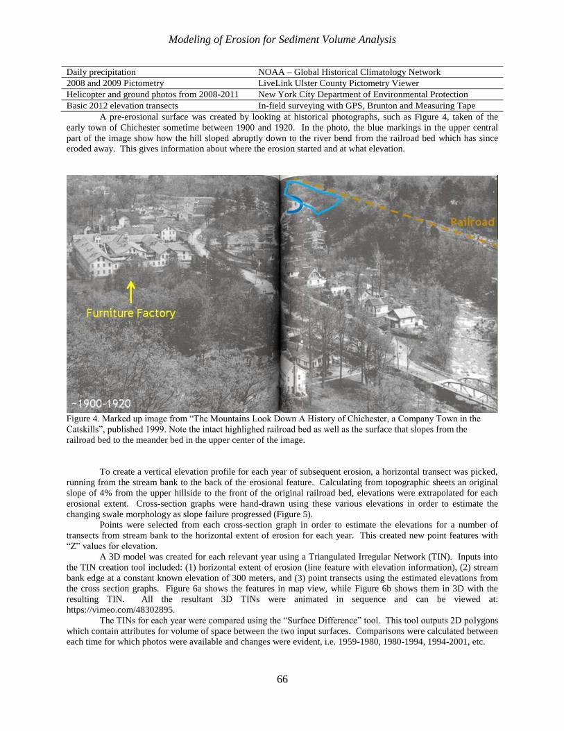
A pre-erosional surface was created by looking at historical photographs, such as Figure 4, taken of the

early town of Chichester sometime between 1900 and 1920. In the photo, the blue markings in the upper central

part of the image show how the hill sloped abruptly down to the river bend from the railroad bed which has since

eroded away. This gives information about where the erosion started and at what elevation.

Figure 4. Marked up image from “The Mountains Look Down A History of Chichester, a Company Town in the

Catskills”, published 1999. Note the intact highlighed railroad bed as well as the surface that slopes from the

railroad bed to the meander bed in the upper center of the image.

To create a vertical elevation profile for each year of subsequent erosion, a horizontal transect was picked,

running from the stream bank to the back of the erosional feature. Calculating from topographic sheets an original

slope of 4% from the upper hillside to the front of the original railroad bed, elevations were extrapolated for each

erosional extent. Cross-section graphs were hand-drawn using these various elevations in order to estimate the

changing swale morphology as slope failure progressed (Figure 5).

Points were selected from each cross-section graph in order to estimate the elevations for a number of

transects from stream bank to the horizontal extent of erosion for each year. This created new point features with

“Z” values for elevation.

A 3D model was created for each relevant year using a Triangulated Irregular Network (TIN). Inputs into

the TIN creation tool included: (1) horizontal extent of erosion (line feature with elevation information), (2) stream

bank edge at a constant known elevation of 300 meters, and (3) point transects using the estimated elevations from

the cross section graphs. Figure 6a shows the features in map view, while Figure 6b shows them in 3D with the

resulting TIN. All the resultant 3D TINs were animated in sequence and can be viewed at:

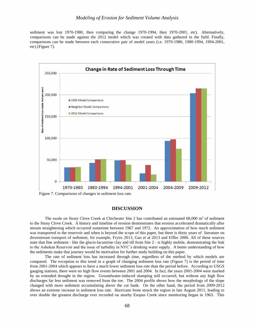
https://vimeo.com/48302895. The TINs for each year were compared using the “Surface Difference” tool. This tool outputs 2D polygons

which contain attributes for volume of space between the two input surfaces. Comparisons were calculated between

each time for which photos were available and changes were evident, i.e. 1959-1980, 1980-1994, 1994-2001, etc.


67

Figure 5. Cross sections of the erosion surface.

Figures 6a & 6b. (a) Linear and point features in 2D. (b) Linear and point features with Z-values have

been used to create a TIN in 3D. (Looking toward the southwest. Colors represent elevation.)

RESULTS

The sediment loss volumes for time intervals are presented in Figure 7. Site 2 has lost an estimated 68,000

cubic meters of sediment from 1970-2012, the equivalent volume of 27 Olympic-size swimming pools.

There are a number of ways to compare the rate of sediment loss through time, depending on which model

is used as a reference. Comparisons can be made against the pre-erosion surface (i.e. comparing how much


68

sediment was lost 1970-1980, then comparing the change 1970-1994, then 1970-2001, etc). Alternatively,

comparisons can be made against the 2012 model which was created with data gathered in the field. Finally,

comparisons can be made between each consecutive pair of model years (i.e. 1970-1980, 1980-1994, 1994-2001,

etc) (Figure 7).

Figure 7. Comparisons of changes in sediment loss rate.

DISCUSSION

The swale on Stony Clove Creek at Chichester Site 2 has contributed an estimated 68,000 m3 of sediment

to the Stony Clove Creek. A history and timeline of erosion demonstrates that erosion accelerated dramatically after

stream straightening which occurred sometime between 1967 and 1972. An approximation of how much sediment

was transported to the reservoir and when is beyond the scope of this paper, but there is thirty years of literature on

downstream transport of sediment, for example, Fryirs 2013, Gao et al 2013 and Effler 2006. All of these sources

state that fine sediment - like the glacio-lacustrine clay and till from Site 2 - is highly mobile, demonstrating the link

to the Ashokan Reservoir and the issue of turbidity in NYC’s drinking water supply. A better understanding of how

the sediments make that journey would be motivation for further study building on this paper.

The rate of sediment loss has increased through time, regardless of the method by which models are

compared. The exception to this trend in a graph of changing sediment loss rate (Figure 7) is the period of time

from 2001-2004 which appears to have a much lower sediment loss rate than the period before. According to USGS

gauging stations, there were no high flow events between 2001 and 2004. In fact, the years 2001-2004 were marked

by an extended drought in the region. Groundwater-induced slumping still occurred, but without any high flow

discharges far less sediment was removed from the toe. The 2004 profile shows how the morphology of the slope

changed with more sediment accumulating above the cut bank. On the other hand, the period from 2009-2012

shows an extreme increase in sediment loss rate. Hurricane Irene struck the region in late August 2011, leading to

over double the greatest discharge ever recorded on nearby Esopus Creek since monitoring began in 1963. This


69

extreme weather event led to increased groundwater-induced slumping and high flow discharge to carry slumped

sediment downstream.

There are a number of improvements and future extensions to this work. The models could be improved by

taking into account the lowering of the stream elevation due to headcuts that migrated upstream. A 2012 elevation

was assumed for all years as the constant elevation of the stream edge, when in reality the stream elevation lowered

through time as erosion progressed upstream.

A future extension of this project could include monitoring human changes in stream morphology

throughout the Stony Clove and even the Esopus watershed, particularly reaches that have been artificially

straightened. If detrimental landforms like Chichester Site 2 are the unintended consequences of human intervention,

then early identification should make mitigation less expensive and less problematic. Visual inspection or a routine

model written for ArcGIS could identify similar features in the Catskills or other watersheds where turbidity is an

issue. These erosional features supply a significant amount of highly mobile sediment, so mitigating their impact

could have a major cumulative effect on turbidity in a system like NYC’s water supply. Our enthusiasm for

mitigation should be tempered, however, as we develop a better understanding of how the changes we make to

remedy erosion at one location can adversely impact reaches upstream and downstream.

As validation of the importance of Site 2, in summer 2013 the NYC DEP spent hundreds of thousands of

dollars to radically remediate the site to stabilize it with riprap, and revegetate and reshape the slope to absorb the

energy of high discharges. Drainage was also installed in an effort to deal with the subaerial erosion issue (Davis

2013). This catastrophic slope failure will eventually become a case study in the success or failure of stream

engineering.

REFERENCES

Beechie, T. J., Pollock, M. M., & Baker, S. S. 2008. Channel incision, evolution and potential recovery in the Walla

Walla and Tucannon River basins, Northwestern USA. Earth Surface Processes and Landforms, 33(5), 784-800.

doi:10.1002/esp.1578

Bennett, R. 1999. The mountains look down: A history of Chichester, a company town in the Catskills.

Fleischmanns, N.Y: Purple Mountain Press.

Davis, Danyelle. 2013. Personal Communication.

DeRose, R.C. & Basher, L.R. 2011. Measurement of river bank and cliff erosion from sequential LIDAR and

historical aerial photography. Geomorphology, 126(1-2) 132-147.

Effler, S.W., Matthews, D.A., Kaser, J.W. 2006. Runoff event impacts on a water supply reservoir: suspended

sediment loading, turbid plume behavior and sediment deposition.Journal of the American Water Resources

Association. 42 (6), 1697-1710.

Fryirs,K. 2013. (Dis)Connectivity in catchment sediment cascades: a fresh look at the sediment delivery problem.

Earth Surface Processes and Landform.38: 30-46.

Gao, P., Borah, D.K., Josephson, M. 2013. Evaluation of the storm event model DWSM on a medium sized

watershed in central New York, USA. Journal of Urban and Environmental Engineering. 7(1), 1-7.

Greene County Soil and Water Conservation District & New York City Department of Environmental Protection,

2005. The Stony Clove Creek Stream Management Plan. Retrieved from

http://www.catskillstreams.org/stonyclovesmp.html (last accessed 05 January 2013).

Gregory, K.J. 2006. The human role in changing river channels. Geomorphology, 79 (3-4), 172-191.

Hooke, J. M. 2008. Temporal variations in fluvial processes on an active meandering river over a 20-year period.

Geomorphology, 100(1-2), 3-13. doi:10.1016/j.geomorph.2007.04.034


70

Lloyd, E., & Rush, P. 2006. Long-term watershed protection program. Retrieved from http://www.epa.gov/

Region2/water/nycshed/2007wp_program121406final.pdf (last accessed 05 January 2013).

Mehaffey, M.H., Wade, T.G., Nash, M.S., and Edmonds, C.M. 1999. A Landscape Analysis of New York City’s

Water Supply (1973-1998). Environmental Sciences Division, U.S. Environmental Protection Agency.

NYC DEP. 2014. Regulatory Background. Retrieved from http://www.nyc.gov/html/dep/html/watershed_

protection/regulatory_background.shtml (last accessed 15 May 2014).

NYC DEP - Bureau of Water Supply. 2010. Ashokan Reservoir Operations. Retrieved from http://www.

loweresopus.org/download/Ashokan_Reservoir_Operations.pdf (last accessed 05 January 2013).

Pires, M. 2004. Watershed protection for a world city: The case of New York. Land Use Policy, 21(2), 161.

doi: 10.1016/j.landusepol.2003.08.001

Porter, K. S. 1994. New York City: Case of a Threatened Watershed. EPA Journal, 20(1), 24.

Simon, A. 1989. A model of channel response in disturbed alluvial channels. Earth Surface Processes and

Landforms, 14(1), 11-26.

Simon, A. 1994. Gradation processes and channel evolution in modified West Tennessee streams; process, response,

and form. U. S. Geological Survey Professional Paper.

Simon, A., Curini, A., Darby, S. E., & Langendoen, E. J. 2000. Bank and near-bank processes in an incised channel.

Geomorphology, 35(3-4), 193-217.

Sun, H.Y., Zhong, J., Zhao, Y., Shen, S.J. and Shang, Y.Q. 2013. The influence of localized slumping on

groundwater seepage and slope stability. Journal of Earth Science, 24 (1), 104-110.

Thorne CR. 1982. Processes and mechanisms of river bank erosion. Gravel-Bed Rivers, ed. R.D. Hey, J.C. Bathurst,

and C.R. Thorne, pp. 227-272. Wiley: Chichester.

Trimble, S.W. 2012. Historical sources and watershed evolution. Philosophical Transactions. Series A,

Mathematical, Physical, And Engineering Sciences. 2012 May 13; Vol. 370, #1966, pp. 2075-92.

USEPA Region 2 New York City Watershed Team, 2006. Report on the City of New York’s Progress in

Implementing the Watershed Protection Program and Complying with the Filtration Avoidance Determination.

Retrieved from http://www.epa.gov/region02/water/nycshed/documents/epaeval_august2006.pdf (last accessed 05

January 2013).

Veihe, A. A., Jensen, N. H., Schiotz, I. G., & Nielsen, S. L. 2011. Magnitude and processes of bank erosion at a

small stream in Denmark. Hydrological Processes, 25(10), 1597-1613. doi:10.1002/hyp.7921

Yumoto, M., Ogata, T., Matsuoka, N., & Matsumoto, E. 2006. Riverbank freeze-thaw erosion along a small

mountain stream, Nikko volcanic area, Central Japan. Permafrost and Periglacial Processes, 17(4), 325-339.

doi:10.1002/ppp.569

HISTORICAL 3D MODELING OF EROSION FOR SEDIMENT …

Documents