agricultural policy analysis project, phase iii - USAID

IIIIIII

IIIIIII

AGRICULTURAL POLICY ANALYSIS PROJECT, PHASE III

Sponsored by the

U.S. Agency for International Development

Project Office: 4800 Montgomery Lane, Suite 600, Bethesda, MD 20814 . Telephone: (301) 913-0500Fax: (301) 652-3839' Internet: [email protected] . USAID Contract No. LAG-4201-C-OO-3052-00

Assisting USAID Bureaus, Missions and Developing Country Governmentsto Improve Food & Agricultural Policies and Make Markets Work BetterI

IIII

Prime Contractor:Subcontractors:

Affiliates:

Abt Associates Inc.Development Alternatives Inc.Food Research Institute, Stanford UniversityHarvard Institute for International Development, Harvard UniversityInternational Science and Technology InstitutePurdue UniversityTraining Resources GroupAssociates for International Resources and DevelopmentInternational Food Policy Research InstituteUniversity of Arizona

Authors:

AGRICULTURE ANDECONOMIC GROWTHIN AFRICA: PROGRESSAND ISSUES

March 1997

APAPIIIResearch ReportNo. 1016

Prepared for

Agricultural Policy Analysis Project, Phase III, (APAP III)

USAID Contract No. LAG-4201-Q-OO-3061-00

Dr. Steven Block, Abt Associates Inc.Dr. C. Peter Timmer, OIID

TABLE OF CONTENTS

ACKNOWLEDGMENTS iv

EXECUTIVE SUMMARY v

1. INTRODUCTION 1

2. AGRICULTURAL LINKAGES TO ECONOMIC GROWTH 3

2.1 Agriculture and Economic Growth: Identifying the Linkages .32.2 The Rural Economy and Growth in the Macro Economy: Specifying the

Mechanisms 52.3 Urban Bias and Economic Growth 62.4 Agricultural Productivity and Nutritional Status of Workers 1I2.5 Food Security, Food Price Stability, and Economic Growth 122.6 The Macroeconomic Impact of Stabilizing Food Prices 132.7 An Empirical Example: Stabilizing Rice Prices in Indonesia 152.8 Agricultural Linkages in Perspective 16

TABLES 17

REFERENCES 21

3. ETIDOPIA CASE STUDy 25

3.1 Introduction 253.2 Model Specification 273.3 Data Issues 393.4 Base Run of the Model 413.5 Simulation Results 433.6 Summary and Conclusions 52

APPENDIXES 56

REFERENCES 67

4. ZIMBABWE CASE STUDY 694.1 Agriculture and Zimbabwe's Economy 694.2 The Zimbabwe Simulation Model. 744.3 Estimation, Solution, and Validation of the Zimbabwe Simulation Model 804.4 Simulation Results for Zimbabwe 81

APPENDIXES 94

REERENCES 100

5. KENYA CASE STUDY ~ 1025.1 Introduction l 025.2 Model Specification 1035.3 Estimation, Solution, and Validation of the Simulation Model .1125.4 Simulation Results 1145.5 Consistency with Other Studies 123

APPENDIXES 125

REFERENCES 133

6. SUMMARY AND CONCLUSIONS : 135

ACKNOWLEDGMENTS

The authors have benefitted greatly from the insig!its, assistance, and inputs of numerouscolleagues in the course ofcompleting this study. In particular, we wish to thank GeorgeGardner and Tom Olson of USAID for their long-term support and shared interest in the role ofagriculture in economic growth. In addition, we are grateful to Carol Timmer for her editorialinput and technical assistance, W. Graeme Donovan of the World Bank for his assistance on theEthiopia case study, and James Murphy of Tufts University for his excellent research assistance.

EXECUTIVE SUMMARY

This study provides further confirmation of the central role that agriculture plays insupporting economic growth in Sub-Saharan Africa. Building on earlier work by Block andTimmer, this study addresses agriculture's contribution to economic growth from two distinct butcomplementary analytical perspectives. 1 One approach is to extend our conceptualunderstanding of the linkages through which agricultural growth stimulates non-agriculturalgrowth. The second approach is to expand the set of empirical estimates ofagriculture'saggregate contribution to economic growth in particular African countries. Our results suggeststrongly that sensible strategies for economic growth in Sub-Saharan Africa must place a highpriority on promoting a healthy and dynamic food and agricultural economy.

Agriculture contributes both directly and indirectly to economic growth. The directcontribution is simply an accounting relationship -- agricultural output is a central component ofthe economy's supply side (one-third ofGDP for a typical African economy). It is well-known,however, that agriculture accounts for a decreasing share of GDP as an economy develops. Yet,as this process occurs agriculture's indirect contributions to growth increase in importance, andfacilitate the economic transformation. For middle-income countries, a set of indirect linksbetween agriculture and the rest of the economy remains significant for overall growth.

The earlier study by Block and Timmer identified a wide range of potential indirectlinkages between the agricultural and non-agricultural economies of developing countries. Theselinkages are indirect in the sense that in general they do not operate through the factor andproduct markets which provided the mechanisms for the classic studies of agricultural growthlinkages by Lewis and Johnston and Mellor.2 These indirect linkages are not well meditated bymarkets. From among the long list ofpotential indirect linkages identified in our earlier work,the present study refines the specification of three: I) an urban bias linkage with an impact thatdepends on reversing underinvestment in the rural economy, 2) a nutritional linkage throughwhich a better-fed labor force works more productively and for more hours, and 3) a stabilitylinkage that connects unstable food prices and food insecurity with a consequent reduction in thequantity and quality of investment. Empirical support for the existence of these indirectagricultural growth linkages is drawn from a cross-section of countries.

Historical urban bias in much of Sub-Saharan Africa has led to a distorted pattern ofinvestment, with too much public and private capital invested in urban areas and too little in ruralareas. This distortion can lead to large differences in the marginal productivities of capital inurban and rural areas. Reversing this distortion would yield (at least at first) high rates of returnto investments in rural areas. This return, in part, results from the relatively greater efficiency

1 Steven Block and C. Peter Timmer, Agriculture and Economic Growth: Conceptual Issues and theKenyan Experience, C:onsulting Assistance on Economic Refonn Discussion Paper No. 26, September, 1994.

2 W. A. Lewis (1954), :'Economic Growth with Unlimited Supplies of Labor," The Manchester School,22:3-42; B. F. Johnston and John Mellor, "The Role of Agriculture in Economic Development," AmericanEconomic Review, 51(4): 566-593.

f

with which rural households allocate the resources at their disposal and the low opportunity costof much household labor. Making more resources available to these households in the form ofhigher incomes or new technologies can raise factor productivity for the entire economy becauseunderemployed factors are used to produce them. Moreover, if an historic urban bias isovercome and the rural economy is somehow transformed from one that is extremely risky, withfew productive investment opportunities, to one that is stable and dynamic, higher incomes torural households can be channeled directly into productive investments on the farm or in thelocal economy.

One symptom of urban bias is unequal per capita stocks of education in rural and urbanareas. Education levels are a common proxy for human capital, and separating urban stocks fromrural stocks is revealing in cross-country growth regressions of the potential contributions ofreduced urban bias.3 Various specifications point consistently to the same conclusion: higherper capita stocks ofrural human capital relative to urban human capital contribute positively toeconomic growth. This result holds whether growth is measured for the entire economy or onlyfor the non-rural economy.4 In other words, urban bias reduces overall economic growth.Interestingly, when a dummy variable for regions is included in the regressions, the coefficienton the variable for Sub-Saharan Africa is always negative, and is the largest and most statisticallysignificant of the regional dummy variables.

This study also presents evidence that rapid economic growth that differentially benefitsthe poor is the key to achieving food security. This conclusion is based on the important linkbetween agricultural productivity and the nutritional status of workers. Fogel's path breakingwork on Western Europe demonstrated the importance of increasing caloric intake in reducingmortality and increasing productivity of the working POOLS Fogel found that increases in foodintake among the British population since the late eighteenth century contributed substantially toincreased productivity and income per capita, explaining about 30 percent ofthe British growthin per capita income since that time.

More generally, increases in domestically produced food supplies contribute directly toincreases in average caloric intake per capita, regardless of changes in the level of imports,income per capita, income distribution, and food prices. Countries with rapidly increasing foodproduction have much better records of poverty alleviation, perhaps because of changes in thelocal economics of access to food. Improved nutrient intake among the poor is closely related to

3 Rural education levels will depend on both supply and demand factors, and urban bias will affect each inreinforcing ways. Restricting rural investment means building fewer schools, reducing the supply of educationalfacilities in rural areas; biasing the terms of trade against agriculture (another symptom of urban bias) reduces thedemand for rural education, which further reduces rural incomes relative to urban incomes.

4 It is also interesting to note that increases in urban human capital do not contribute to growth in either theentire economy or the.non-rural economy.

5 R. Fogel (1991), "The Conquest of High Mortality and Hunger in Europe and America: Timing andMechanisms." In P. Higonnet, D. Landes, and H. Rosovsky, eds., Favorites ofFortune: Technology, Growth, andEconomic Development since the Industrial Revolution. Cambridge, MA: Harvard University Press, pp. 35-71.

poverty alleviation, and the "Fogel" linkages suggest that increased food security for the poorcan contribute substantially to long-run economic growth. This study cites emerging evidence,again in a cross-country context, that nutrition plays a significant role in explaining economicgrowth.

As in the previous set of results, a dummy variable for Sub-Saharan Africa suggestsslower growth in that region, controlling for other factors influencing growth. A significantnegative dummy variable for Sub-Saharan Africa reflects a failure of the model to explainAfrican growth. This failure, however, is common to virtually every cross-country empiricalstudy of economic growth.6

A final set of indirect agricultural growth linkages arises from the macroeconomic impactof stabilizing food prices. Price stabilization affects investment and growth throughout the entireeconomy. These effects can be large when food is a large share of the economy as it clearly is innearly every country of Sub-Saharan Africa) and if world grain markets are unstable.

In short, instability in the food sector can have three important macro-level effects. It canaffect the quantity of investment through an increase in precautionary savings or a decreasecaused by greater uncertainty. It can decrease the quality of investment (as measured by the rateof return) because prices contain less information that is relevant for long-run investment.Finally, because of spillovers creating additional risk throughout the economy, instability caninduce a bias toward speculative rather than productive investment activities and thereby slowdown economic growth. Thus, of additional domestic food production helps stabilize food pricesand leads to greater food security, it will have an impact through the quantity and efficiency ofinvestment because of the "stability" linkages.7

In addition to elaborating on these newly discovered indirect contributions of agricultureto economic growth, the study presents two new case studies of agriculture's contribution togrowth in Africa. Ethiopia and Zimbabwe are the subjects of new applications of the simulationapproach applied to Kenya in our earlier study. 8

The simulation approach applied to Ethiopia and Zimbabwe provides results at a highlevel of aggregation. Using dynamic numerical simulation, these case studies estimatemacroeconomic growth multipliers for agriculture, services, and industry.9 The growth

6 For a recent example, see R. Barro, "Determinants of Economic Growth: A Cross-Country EmpiricalStudy," National Bureau of Economic Research Working Paper No. 5698. Cambridge, MA: NBER. August 1996.

7 Empirical support for the stability linkages draws largely on Asian examples. However, Pinckney (1983)shows that moderate price stabilization for maize in Southern Africa would have beneficial effects for food security.

8 The present'study includes revised (though perhaps not final) results for Kenya.

9 In the Zimbabwe case the sectoral distinctions are between agriculture, consumer goods, and capitalgoods.

multipliers describe each sector's indirect contributions to growth by estimating the increasedincome in other sectors resulting from an income shock in each particular sector. The resultspoint consistently to the importance of agriculture's indirect contributions to each country's

economic growth.

In Ethiopia, a hypothetical $1.00 increase in agricultural income ultimately adds $1.71 toGDP. Similar shocks to income in the service and industry sectors increase total GDP by $1.93and $1.38, respectively. These results paint a picture of an economy in which intersectorallinkages operate on a highly limited basis. These limits are reflected in the wide disparitybetween sectoral multipliers. Ethiopia's industrial sector is largely detached from the rest of theeconomy. A development strategy focussing on existing Ethiopian industry would clearly bemisplaced. The relatively functional linkages in Ethiopia's economy are concentrated betweenagriculture and services.

While the service sector multiplier is greater than the agricultural growth multiplier, itdoes not follow that growth strategies for Ethiopia should concentrate on the service sector. Onemust recognize two more subtle dimensions. The first is that the service sector itself createsrelatively little of the economy's underlying output. For instance, services related to foodmarketing would mean relatively little in the absence of food production. Moreover, thesimulation results suggest that the benefits of agricultural growth are much more widely sharedamong the poor.

Of the $0.93 net increment to national income generated by a $1.00 shock to servicesector income, $0.53 is concentrated in the two sectors which employ only approximately 10­15% of the country's workforce. The 85-90% of the workforce employed in agriculture sharesthe remaining $040. Of the total increase in GDP (e.g., including the initial shock) resultingfrom increased service sector income, 80% remains in the services and industrial sector. Incontrast, ofthe $0.71 net increment to GDP generated by a $1.00 shock to agricultural income,$0.57 accrues to the non-agricultural workforce. Yet, of the total increase in GDP resulting froma shock to agriculture, two-thirds remains to be shared by the poor rural majority of Ethiopia'spopulation. Thus a strategy emphasizing growth in Ethiopia's rural economy would contributesubstantially to income in non-agriculture, as well as make the greatest progress toward povertyalleviation.

The simulation results for Zimbabwe point even more clearly to the importance ofagriculture in economic growth. The growth multipliers for Zimbabwe are: agriculture, 1.93;consumer goods production, 1.92; and, capital goods production, 1.54. In contrast to the widedispersion of sectoral growth multipliers found for Ethiopia, the multipliers for Zimbabwe arerelatively close to one another. This broadly suggests a greater degree of intersectorallinkage inZimbabwe. Intuitively, the greater sophistication of both the physical and market infrastructurein Zimbabwe support the conclusion implied by the multipliers.

As in the Ethiopian case, the growth multiplier associated with capital goods production(industry in the Ethiopian case) is substantially lower than in either of the other sectors.Zimbabwean industry is not an enclave to the same extent found in Ethiopia, yet the present

results would not support a strong emphasis on industrial growth as a vehicle for povertyalleviation in Zimbabwe.

As in Ethiopia, the simulation results suggest that the benefits of agricultural incomegrowth are concentrated on the poor to a much greater extent than income growth in eitherconsumer or capital goods production. 10 For a given shock to agricultural income, two-thirds ofthe total increase in GDP are captured by the two-thirds of the total labor force employed inagriculture. In contrast, a given increase in consumer goods income concentrates 84% of thetotal increase among the 35% of the labor force employed in non-agricultural activities. Shocksto capital goods income are the most regressive in this sense: fully 93% of the total incomeincrease in that case are shared by the 35% non-agricultural share of the labor force.

Both the Zimbabwe and Ethiopia simulation results thus highlight agricultural growth asthe most efficient vehicle for poverty alleviation. In addition, the growth multipliers indicate thata concentration on agriculture in Zimbabwe would make the maximum contribution to economicgrowth. Both of these new case studies are thus consistent with the earlier, less detailed, resultsof a similar analysis of Kenya. In the Kenyan case, the agricultural growth multipliers wasnearly two and one-halftimes the magnitude of the non-agricultural growth multiplier.

10 The rural nature of Zimbabwe's poverty is clearly reflected by the fact that its agricultural sector earnsonly 12% of GDP yet employs over 65% of the labor force.

1. INTRODUCTION

This report builds on earlier work by Block and Thnmer on the role of agriculture ineconomic growth. 1 The present study follows our earlier work in addressing agriculture's role ineconomic growth from two distinct but complementary analytical perspectives. One approach isto extend our conceptual understanding of the linkages through which agricultural growthstimulates non-agricultural growth. The second approach is to expand the set of empiricalestimates of agriculture's aggregate contribution to economic growth in particular Africancountries. In both respects, the present study refines and extends our earlier work.

Our earlier study identified a wide range ofpotential indirect linkages between theagricultural and non-agricultural economies of countries at various stages of development. Theselinkages are indirect in the sense that in general they do not operate through the factor andproduct markets which provided the mechanisms for the classic studies of agricultural growthlinkages by Lewis and Johnston and Mellor.2 Instead, the indirect linkages examined below inChapter 2 are not well mediated by markets. From among the long list of potential indirectlinkages identified in our earlier work, the present study refines the specification of three: I) anurban bias linkage with an impact that depends on reversing 'underinvestment in the ruraleconomy, 2) a nutritional linkage through which a better-fed labor force works moreproductively and for more hours, and 3) a stability linkage that connects unstable food prices andfood insecurity with a consequent reduction in the quantity and quality of investment.

Chapter 2 details the mechanisms through which these indirect linkages operate andprovides preliminary empirical support for their existence in a cross-section of countries.

Chapters 3, 4, and 5 complement this conceptual approach with aggregate measurementsof agriculture's contribution to economic growth in three African countries. The approach takenin the case studies, while too highly aggregated to test the specific mechanisms identified inChapter 2, provides macroeconomic growth multipliers for agriculture and various non­agricultural sectors in Ethiopia, Zimbabwe, and Kenya.3 These case studies employ dynamicnumerical simulation of hypothetical sectoral income shocks as a means of estimating the incomegenerated in other sectors by increased income in a particular sector. The results of theseexperiments are aggregate growth multipliers which describe the total increase in GDP resultingfrom income shocks to each sector.

I Steven Block and C. Peter Timmer, Agriculture and Economic Growth: Conceptual Issues and theKenyan Experience, Consulting Assistance on Economic Refonn Discussion Paper No. 26, September, 1994.

2 W. A. Lewis (1954), "Economic Growth with Unlimited Supplies of Labor," The Manchester School, 22:3 - 42; B. F. Johnston, and J. Mellor (1961) "The Role of Agriculture in Economic Development," AmericanEconomic Review 51(4),566-593.

3 The Ethiopia and Zimbabwe case studies have been newly prepared for this report; the Kenya case studyis an updated (though perhaps not final) version of the work originally presented in Block and Timmer (1994).

I

The magnitude of the contribution varies between countries. In Kenya (a two-sectormodel) the agricultural growth multiplier is substantially greater than the non-agricultural growthmultiplier. In Ethiopia and Zimbabwe (three-sector models), the agricultural growth multiplier isclose in magnitude to the service sector or consumer goods sector multipliers, and both aresubstantially greater than the industry or capital goods multipliers. In general, the simulationresults strongly support the conclusion that a healthy and dynamic agricultural economy cancontribute in important ways to economic growth in Africa.

./

2

II,

J

2. AGRICULTURAL LINKAGES TO ECONOMIC GROWTH

A healthy and dynamic food and agricultural economy can contribute in surprisinglyimportant ways to the speed and equity with which the nonagricultural economy grows. Thelimited, but still important, circumstances in which agriculture can be a direct, significantcontributor to overall economic growth are discussed in the context of "Lewis Linkages" and"Johnston-Mellor Linkages," which operate through factor markets and product markets,respectively. In the poorest countries, in which the share of agriculture in GDP remains high,particularly in several formerly socialist countries in Central and East Asia and throughout muchof Africa, "getting agriculture moving" is crucial to achieving satisfactory macroeconomicperformance.

In these countries, stimulating the Lewis linkages and the Johnston-Mellor linkages byimproving the efficiency of markets will be a major key to maximizing the direct contribution ofagriculture to economic growth. Even in these countries, however, macroeconomic policy will bethe main determinant of whether agriculture gets moving or not. For middle-income countries, aset of indirect links between agriculture and the rest of the economy remains significant foroverall growth, and these links are not well mediated by markets. The direct contribution ofagriculture to economic growth, however, is limited by the declining share of agriculture in GDPas incomes rise.

The last part of the paper examines a more controversial dimension of the relationshipbetween agriculture and economic growth--that is, whether food security and price stability aredirectly enhanced by performance of the domestic agricultural economy, on the one hand, andstimulate growth in the rest of the economy, on the other. Theoretical models of economic growthan the empirical literature are suggestive on both counts, but the evidence remains tentative.Building further understanding of this interplay between stability and growth is an important topicfor research.

2.1 Agriculture and Economic Growth: Identifying the Linkages

Why would a policy maker in a poor country choose to invest in the agricultural sector? Itwould seem to be an unwise choice if one were influenced by the labor-surplus model ofdevelopment, with its passive role for agriculture (at best), by the persistent decline in the share ofagriculture in a growing economy, and by the long-term downward trend in prices of basic foodsduring the second half of the twentieth century. For the poorest countries, in which 40 to 50 percentof GDP, 70 to 80 percent of the work force, and 70 to 90 percent of foreign exchange earnings areaccounted for by agriculture, the answer is obvious. For these countries, the supply side of thenational income accounts means it is impossible to sustain any broad-based economic growthwithout the active participation of the rural economy.

3

The answer is less obvious for countries that have already escaped the bottom of the povertytrap, but the influence of performance in the agricultural sector on economic growth remainssignificant well into the development process. Two broad categories of linkages create thisconnection. First are the traditional market-mediated linkages that form the core of economicanalysis ofthe role ofagriculture in economic development. These are often divided into the "LewisLinkages" that operate through factor markets that transfer labor and capital from agriculture toindustry, and "Johnston-Mellor Linkages" that operate through product markets. The factor-marketlinkages between agriculture and industry have been so important to the growth process that theyled Lewis to the following observation in his famous article published in 1954, and for which he wonthe Nobel Prize in Economics.

. . . industrialization is dependent upon agricultural improvement; it is not profitableto produce a growing volume of manufactures unless agricultural productionis growing simultaneously. This is also why industrial and agrarian revolutionsalways go together, and why economies in which agriculture is stagnant do notshow industrial development (Lewis, 1954, p.29).

Historically, higher productivity in agriculture has provided labor and capital to the expandingindustrial sector, to the mutual benefit of both sectors.

In addition to these factor-market linkages, Johnston and Mellor identified a broader set oflinkages between the agricultural sector and economic growth in the nonagricultural sector.Contributions through these linkages include food for the industrial work force (thus avoiding theworsening terms of trade for industry that concerned Lewis), raw materials for agro-processingindustries, markets for industrial output, especially for the low-quality goods that cannot competein export markets but which domestic factories produce as part of a learning process, and exportearnings that pay for imported capital equipment and intermediate inputs. The Johnston-Mellorlinkages tend to be mediated by product markets that become progressively more efficient duringthe course of economic development (Johnston and Mellor, 1961; Ranis, @i[etal.], 1990; Timmer,1992; Delgado, @i[et al.], 1994).

The role of government in strengthening both the Lewis and Johnston-Mellor linkages is toinvest in the public dimensions of agricultural development at rates dictated by the profitability ofincreased commodity output and to make factor and product markets more efficient. These linkagesare the most important connections between agriculture and economic growth. They are notdiscussed further because the policy implications of the Lewis linkages and the Johnston-Mellorlinkages are well understood, even if the policies are not always implemented. A market-basedanalysis of investments in agricultural development, using standard neoclassical economicprinciples, when coupled to the physical and institutional development of markets themselves, leadsto an optimal development strategy.

4

Another category of linkages, however, is not well mediated by market forces even whenmarkets are working well. Sensitive interventions by governments into market-determined outcomesare required in these circumstances if agriculture is to play its optimal role in support of the rest ofthe economy (Timmer, 1993a; Barrett and Carter, 1994). The rest of this paper explores themechanisms that provide nonmarket links between agricultural growth and growth in productivityof the nonagricultural sector and reviews what is known about their quantitative significance.

2.2 The Rural Economy and Growth in the Macro Economy: Specifying the Mechanisms

The most satisfactory approach to measuring the nonrnarket impact of agriculture oneconomic growth is to begin by augmenting recently developed theories ofeconomic growth, whichare summarized in Barro and Sala-I-Martin(l995). Typical empirical specifications of modemgrowth models control for initial conditions, factor accumulation, and quality improvements in laborand capital and then proceed to search for control variables that affect the overall efficiency ofresource allocation. Openness of the economy, size ofgovernment, price distortions, and instabilityin the macro economy all influence this efficiency, but the potential contribution of agriculturalgrowth to economic efficiency has not been directly tested in the new models. Indeed, agricultureis not even mentioned in the volume by Barro and Sala-I-Martin.

At the most basic level, a positive relationship between the rate of economic growth andgrowth in rural economies shows clearly in the historical record. In a sample of 65 developingcountries, a highly significant positive relationship existed, from 1960 to 1985, between growth inthe agricultural sector and growth in the nonagricultural sector; about 20 percent of the growth ratein agriculture was added to the exogenous growth rate in nonagriculture (see Table 1). This directand positive association between growth in the two sectors does not, of course, show causation.Good macroeconomic policy, for example, could have caused both sectors to grow independently,or each sector could have simultaneously caused the other to grow (Timmer, 1996a). However, ratesof agricultural growth lagged five years were a separate, significant additional factor influencinggrowth in the nonagricultural economy, and such a lag suggests a more causal relationship!.

The linkages that help produce this causal relationship are indirect and hard to measurebecause the direct market-mediated linkages through Lewis and Johnston-Mellor mechanisms areautomatically included at their market values in traditional growth accounting. However, at leastthree of these nonrnarket linkages have been identified with enough analytical clarity that empiricaltests can be specified and estimated. These are an "urban bias" linkage with an impact that dependson political undervaluation of, and hence under investment in, the economic contribution of the rural

I When separate intercept terms are included for each five-year time period and forregional dummy variables for Latin America, Africa, and East Asia, the coefficient for currentgrowth in agricultural GDP remains significant, whereas the coefficient for lagged growth inagricultural GDP remains positive but becomes insignificant.

5

economy; a"nutritional" linkage that depends on a poverty trap caused by low labor productivity dueto inadequate nutrient intake; and a "stability" linkage that connects unstable food prices and foodinsecurity with a consequent reduction in the quality and quantity of investment. Each of thesemechanisms links performance in the agricultural sector to overall economic growth, afteraccounting for the market contributions of the higher agricultural output through the Lewis andJohnston-Mellor linkages.

2.3 Urban Bias and Economic Growth

Only in East and Southeast Asia has agriculture had a high priority in national plans becauseof its importance in feeding people and providing a spur to industrialization. In much of Africa andLatin America, an historically prolonged and deep urban bias is almost certain to have led to adistorted pattern of investment (Lipton, 1977; 1993). Too much public and private capital has beeninvested in urban areas and too little in rural areas. Too much capital has been held as liquid andnonproductive investments that rural households use to manage risk. Too little capital has beeninvested in raising rural productivity.

This historical record suggests that such distortions have resulted in strikingly differentmarginal productivities of capital in urban and rural areas. A new growth strategy, such as thosepursued in Indonesia after 1966,China after 1978, and Vietnam after 1989, which alters investmentpriorities in favor of rural growth, should be able to benefit from this disequilibrium in rates ofreturn, at least initially. Such a switch in investment strategy and improved rates of return on capitalwould increase factor productivity because of improved efficiency in resource allocation. Themechanisms involved include the relatively greater efficiency with which rural households allocatethe resources at their disposal and the low opportunity cost of much household labor.

Nearly all rural households face "hard" budget constraints. Many are near subsistence, somost family members work long hours even at near-zero marginal productivity in order to maximizeoutput. Such households must be highly efficient in allocating what few resources they have simplyto survive. Making more resources available to these households in the form of higher incomes ornew technologies can often result in significant gains in output. These gains raise factor productivityfor the entire economy because underemployed factors are used to produce them (Timmer, 1995).It should be possible to see this effect in the empirical record.

A further reason for the robust relationship between agricultural growth and improvementsin total factor productivity arises because of a statistical artifact. Virtually none of the savings done(at the margin) within rural households is captured in national income accounts. Because there areso few financial intermediaries in rural areas, savings by farm households are either held as liquidbut nonproductive assets, such as gold or jewelry, or they are invested in nonliquid but productiveassets, such as livestock, orchards, land improvement, farm implements, or even education(Morduch, 1991, 1995).

6

No serious problems arise from omitting, in the national income accounts, the rural savingsthat flow into gold, at least from the point ofview of growth accounting. Only "productive" capitalis relevant as a source ofgrowth, and"unproductive" capital, such as jewelry or gold, can safely beincluded as consumption. Even when viewed as a hedge against the extreme riskiness ofmany ruralactivities, these "investments" by poor households do not contribute to income as measured bynational accounts.

But what if an historic urban bias is overcome and the rural economy is somehowtransformed from one that is extremely risky, with few productive investment opportunities, to onethat is stable, dynamic, and attractive, at the level of individual households, as a place to invest?Higher incomes to rural households can then be channeled directly into productive investments onthe fann or in the local economy, even though financial intermediaries are totally absent (Birdsall,@i[et a1.], 1995; Timmer, 1995). Greater output results, most but not all of it in the agriculturalsector, and this output does show up in national income.

To statisticians attempting to account for this growth, it appears to be generated with littleor no capital, a very efficient process indeed. Capital is used, of course, and proper accountingwould identify and measure it. But such accounting would also involve a fundamental shift inattitudes about the productivity ofvery small and highly dispersed rural investments, as well as aboutthe marginal savings propensity of rural households--and thus the desirability of allowing them tohave higher incomes. Countries that overcome urban bias by stimulating higher farm incomes andencouraging rural investments reap a statistical reward in addition to the higher rural output itself:the measurement ofapparently greater total factor productivity as a contributor to their rapid growth.

The basic approach to measuring the contribution to growth of a strategy that balancesmarginal productivity in urban and rural areas is to create a variable that captures the importantdimensions of urban bias and then to use regression analysis to measure the impact of this variablein a standard Barro-style growth mode1. The variable chosen, the per capita stock of education inrural and urban areas separately, is important for two reasons. First, education levels are a commonproxy for human capital in modem growth empirics (enrollment rates are even more common), andseparating urban stocks from rural stocks should be revealing about the mechanisms by whicheducation influences the growth process.

Second, the ratio of the two stocks, that is, average education levels in rural areas comparedwith urban areas, is arguably a proxy for the broader influence ofurban bias. Rural education levelswill depend on both supply and demand factors and urban bias will affect each in reinforcing ways.Thus restricting rural investments means building fewer schools, reducing the supply ofeducationalfacilities in rural areas. Biasing the tenus of trade against agriculture through a variety ofdirect andindirect policies reduces rural incomes, thus reducing the demand for rural education, which furtherreduces rural incomes relative to urban incomes, starting a vicious circle that runs in the oppositedirection from the "virtuous circle" identified by Birdsall, @i[et aL] (1995). The net outcome, theaverage rural stock, of education as measured by years of schooling per capita, reflects the jointimpact of both sources of urban bias, especially when the comparison is in relation to urban

7

education levels. The ratio of rural education levels to urban education levels should be a veryrevealing measure of urban bias. If urban bias is an important drag on economic growth, theimpact should show up when this variable is entered into a standard growth model.

The difficulty, of course, is disaggregating the level of educational stocks into their ruraland urban components. The starting point is the data set developed by Barro and Lee (1994) tomeasure the impact of educational stocks instead of enrollment ratios, the readily available butbadly flawed proxy for human capital that had been used in growth empirics until that time.Through a combination of country statistical records, UNICEF surveys, and creative analyticsthat enforced consistency across sectors with the Barro-Leeaggregates, Chai (1995) was able todisaggregate educational stocks into their rural and urban components for a sample of 65developing countries, including 19 from Sub-Saharan Africa. The time period is from 1960 to1985, with each five-year subperiod used as an individual observation. With five subperiods and65 countries, there are 325 possible observations. Appendices 1-4 list definitions of variablesused, the means and standard deviations of these variables, the countries in the sample, and thevalue of the rural and urban educational stock for each observation.

The results of testing a number of specifications of the urban bias hypothesis are highlysatisfactory. When the dependent variable is the growth rate in real per capita GDP for the totaleconomy, rural human capital is a significant and positive contributor to growth, while the urbanhuman capital variable has a negative and significant coefficient (see Equation 1 in Table 2).2Allother variables are significant with expected signs, including the level of initial income. Thesignificantly negative coefficient on this variable indicates that per capita incomes of poorercountries grow faster than richer ones, thus leading to convergence of incomes.

Significant convergence is found for all equations reported here, which is slightlysurprising because the sample is restricted to developing countries and convergence hassometimes been difficult to confirm in these countries. Investment share has a very significantpositive coefficient, whereas both government expenditures as a share of GDP and the black\Ilarket premium on foreign currency have a significantly negative impact on economic growth.Interestingly, when a dummy variable for regions is included in the regressions, the coefficienton the variable for Sub-Saharan Africa is always negative, is the largest in absolute terms, and isthe most significant of the regional variables. Economic growth in Sub-Saharan Africa is

2The negative coefficient on urban human capital occurs whenever rural human capital isin the regression. Dropping rural human capital allows the coefficient on urban human capital tobecome positive, but it is never as significant as when rural human capital is included alone. Thelikely cause of this strange result is the importance of urban bias in reducing the rate of economicgrowth. When rural human capital is in the regression, thus controlling for the most importantform of human capital to growth of poor countries, additional urban capital reflects additionalurban bias, which has a negative effect on growth. Specifying the regression with the ratio ofthese two variables confirms this result.

8

retarded even after controlling for the high degree of urban bias found in the region.

When dummy variables for each time period and three regions are added, the separatesignificance of the two human capital variables is lost. The rural human capital variable remainspositive and marginally significant; urban human capital remains negative but becomescompletely insignificant (seeEquation 3 in Table 2). Multicollinearity between these twovariables produces these results. One obvious approach to overcoming this problem is to use theratio of the two stocks of human capital as a single variable. The results of doing so are shown inEquations 2 and 4 in Table 2.

In both specifications, the ratio of rural to urban human capital, as proxied by the percapita stock of education, performs extremely well. Even with the full set ofdummies included,this ratio has a highly significant and positive coefficient. Countries grow faster when the percapita stock of human capital in rural areas does not lag too far behind the per capita stock inurban areas (although the urban stock per capita is always higher than the rural stock percapita--see Appendix 4).3

Many of the mechanisms suggested by the urban bias literature for its impact oneconomic growth operate primarily in the rural economy itself. Thus reducing the degree ofurban bias should speed up growth in the rural economy, at some cost to growth in the urbaneconomy. Factor productivity should rise for the economy overall as the efficiency of resourceallocation is enhanced, but with more resources used in the rural areas and fewer resources in theurban areas, the non-rural economy might be expected to show slower growth fora number ofyears as urban bias is redressed.

This expectation turns out to be wrong. Including the rural and urban human capital variables ingrowth equations where the dependent variable is growth in the non-rural economy producesresults similar to those when tne dependent variable is the growth rate in GDP per capita for theentire economy (seeTable 3). The standard errors on all variables are somewhat larger, sostatistical significance is often reduced, but the pattern of results is remarkably similar.Macroeconomic distortions caused by a large share of government in the economy and blackmarket premia on foreign currency extract a higher cost on the non-rural economy alone than on

3The ratio variable has quite different statistical characteristics from the rural and urbanhuman capital variables. It increases much more slowly over time and has much smallervariance, compared with the mean, than the variables that measure stocks of human capital ineach sector. AccOl'dingly, the ratio variable is likely to proxy for general urban bias rather thanthe contribution of human capital to the growth process.

9

the overall economy, and the payoff to investment seems to be smaller. All of these variables

remain highly significant.4

The pattern of impact of the human capital variables is also the same. Rural humancapital is a significant contributor to growth in the non-rural economy; urban human capital isnot, or has a slightly negative impact (see Equation 5). When the full set of dummy variables isadded, the multicollinearity between the two variables becomes severe enough that neither issignificant(see Equation 6). But dropping urban human capital, as in Equation 7, or using theratio specification, as in Equation 8, fully restores the positive significance of rural humancapital. Again, the ratio specification is likely to be capturing rather different forces in thegrowth process than the human capital stock variables.

The significance of the rural human capital variable is puzzling in view of the potentialmechanisms already identified by which urban bias might affect the rate of economic growth.These mechanisms worked almost entirely through the rural economy itself, with little impactexpected outside of agriculture. Some other mechanisms must be at work for such a strong linkto exist between the level of rural human capital, or the ratio of rural to urban human capital, andthe rate of growth of non-rural GDP per capita.

One plausible link is identified in the political economy literature, where urban bias iscaused by extensive rent seeking on the part of powerful urban-based coalitions, such asgovernment workers, students, industrialists, or the military (Bates, 1981). Such rent seeking notonly distorts the relative balance between urban and rural areas, it also has the potential to distortinvestments in the urban economy itself, thus lowering the rate of growth there as well as in therural economy.

These potential distortions from urban-based rent seeking are in addition to the lossescaused by large government spending and macroeconomic policies that create sizable blackmarket premia for foreign currency (because these factors are also included in the regressions inTables 2 and 3). Thus, urban bias seems to be a separate factor distorting the allocation of

4The relatively larger impact of distortions on the non-rural economy alone than on theoverall economy, which includes agriculture, is somewhat puzzling. In most circumstances, therural economy produces a higher share of tradeable goods than does the non-rural economy andthus exchange rate distortions would be expected to have a larger impact there than on the moreprotected non-rural economy. One possible explanation is that the rural economy may besomewhat less vulI:l.erable to the direct effects of rent seeking on economic growth that arediscussed below. These effects seem to be very large.

10

resources, reducing their efficiency in both the rural and urban sectors. By reducing the degreeof urban bias, a government may well be able to increase the rate of growth in both sectors.That, at least, is what the empirical record from 1960 to 1985 suggests.s

2.4 Agricultural Productivity and Nutritional Status of Workers

In a long-run, dynamic context, rapid economic growth that differentially benefits thepoor is the key to achieving food security. One reason is the important link between agriculturalproductivity and the nutritional status of workers. Fogel (1991), in his work on the factorscausing the end of hunger and reductions in mortality in Western Europe, provides strongevidence for the importance of increasing caloric intake in reducing mortality and increasingproductivity of the working poor. Using a robust biomedical relationship that links height, bodymass, and mortality rates, Fogel calculates that increases in food intake among the Britishpopulation since the late eighteenth century contributed substantially to increased productivityand income per capita. "Thus, in combination, bringing the ultra poor into the labor force andraising the energy available for work by those in the labor force explains about 30 percent of theBritish growth in per capita incomes over the past two centuries (p. 63)."

Virtually all of the food that permitted this increase in nutrient intake was produced bythe agricultural revolution in eighteenth- and early nineteenth-century Great Britain. Thisagricultural revolution was not a simple response of private farmers to market signals. It washeavily stimulated by the protection offered by the Com Laws, which both raised average pricesfor cereals and stabilized them in relation to prices in world markets (Williamson, 1990; Timmer,1996a). Much investment in rural infrastructure, even by private parties, was stimulated by theseincentives.

More generally, increases in domestically produced food supplies contribute directly toincreases in average caloric intake per capita, after controlling for changes in the level of imports,income per capita, income distribution, and food prices. Countries with rapidly increasing foodproduction have much better records ofpoverty alleviation, perhaps because ofchanges in thelocal economics of access to food, changes that are not captured by aggregate statistics onincomes and prices.6 Whatever the mechanisms, intensive campaigns to raise domestic food

5These results are highly complementary to those reported by Schiff and Valdes (1992)from their extensive analysis of 18 case studies that investigated the impact of macroeconomicpolicy and commodity pricing distortions on the agricultural sector. The results presented here,however, are stronger in the sense that they draw on a much larger sample of countries and theyuse a broader measure of urban bias to capture its impact on both the rural and non-ruraleconomies.

6See Barrett and Carter (1994) for the African dimensions of this argument.

11

production, especially through rapid technical change, can be expected to have positive spillovereffects on nutrient intake among the poor. Through the "Fogel linkages" that trace the impact ofgreater nutrient intake to increased labor participation rates of the very poor and to raisedproductivity, this increased food security for the poor can contribute substantially to long-runeconomic growth.

Efforts to quantify the impact of nutritional intake on labor productivity within theframework of modem theories of economic growth have just begun. Using the extended Solowmodel developed by Mankiw, Romer, and Weil (1992) to test the importance of human capital ina neoclassical framework, Nadav (l996)included "nutritional" capital as well as more traditionalhuman capital (as proxied by school enrollment rates). With a sample of97 countries, including34 "poor" countries and 34 "intermediate" countries, Nadav found that nutrition had a large andhighly significant impact on economic growth, even when dummy variables for Latin Americanand Sub-Saharan Africa were included(see Table 4). Indeed, nutrition remained significant inexplaining economic growth at the same time that variables measuring schooling rates andgrowth in the labor force became insignificant. Nadav interpreted this evidence, and results fromsplitting the sample into three nutrition "clubs," as evidence that a low productivity trap existsthat is at least partially caused by inadequate nutritional intake.7

Much more research needs to be carried out to identify the mechanisms that cause theselow productivity traps and to determine how efforts to raise agricultural productivity might helppoor countries to break out of such traps(Dasgupta, 1993). In particular, understanding why astrong connection exists between domestic food production and domestic food consumption,especially by the poor, would help policy makers design appropriate investments and priceinterventions to stimulate this linkage (Timmer, 1996c). Much of the answer probably lies in thedifficulty and expense of marketing staple food@i[imports] in rural areas, far from ports andefficient transportation links. With most poverty in poor countries located in these rural areas, astrategy of economic growth built on manufactured exports, with foreign exchange earnings usedto pay for food imports, will have little impact on this poverty trap.

2.5 Food Security, Food Price Stability, and Economic Growth

An important reason for investing in a country's agricultural sector is the potential tostabilize the domestic food economy and thus enhance food security. This potential is greater inlarge countries that affect world prices when they import, in rice-based economies because theworld rice market is very thin and unstable, and for cropping systems in which reliance onirrigation makes domestic production less variable than prices in the world market. Food imports

7As with the results produced by Chai on the impact of urban bias, Nadav's regressionsshow a significantly retarded rate of economic growth for Sub-Saharan African countries, inrelation to other regions, when a dummy variable is included for this effect.

12

may well provide a more reliable base for food security than domestic food production in smallcountries, in wheat- and com-based food systems, and in rainfed agriculture. There are manycircumstances, however, in which imports of food may not offer greater stability.

For both microeconomic and macroeconomic reasons, no country has ever sustained theprocess of rapid economic growth without first solving the problem of food security. At themicroeconomic level, inadequate and irregular access to food limits labor productivity andreduces investment inhuman capital (Bliss and Stem, 1978; Strauss, 1986; Fogel, 1994;Williamson, 1993). At the macroeconomic level, periodic food crises undermine political andeconomic stability, reducing both the level and efficiency ofinvestment(Alesina and Perroti,1993; Barro and Sala-I-Martin, 1995; Dawe, 1996; Timmer,1989, 1996b). The politicalimportance of food security has not been entirely lost on government leaders (Kaplan, 1984;Timmer, 1993b, Islam and Thomas,1996). But its connection to economic growth raises thepotential of linking the political economy of food security to macroeconomic efficiency.

2.6 The Macroeconomic Impact of Stabilizing Food Prices

An important class of benefits from stabilizing food prices is macroeconomic in nature.Price stabilization affects investment and growth throughout the entire economy, not just in thefood sector. These effects can be large when food is a large share ofthe economy and whenworld grain markets are unstable.

Unstable food prices can increase or decrease the level of savings and investment in aneconomy. The rationale for a decrease is intuitively clear--greater uncertainty drives investors tobrighter horizons. The rationale for an increase in the rate of savings and investment draws onthe need for precautionary savings in an economy with imperfect capital markets(Deaton, 1992).Consumers need to save to protect themselves against the effects of a possible increase in foodprices, whereas farmers save to insure themselves against a sudden drop in the crop price. Theseprecautionary savings will be kept in liquid form to be called upon in the event of a suddenchange in food prices, and might not contribute much to economic growth.

Also, the quantity of investment is not the only determinant of growth. The efficiency, orquality, of that investment is equally as important. Food price instability can affect the quality ofinvestment in at least two distinct ways. When food prices increase (because of a poor harvest oran increase in world prices), consumer expenditures on food also increase, because demand isprice inelastic--that is, the percentage increase in price is greater than the percentage decline inthe quantity consumed. The increase in expenditures on food causes expenditures for othercommodities to fall, which lowers demand for all other commodities in the economy. Theopposite situation occurs in the event of a good harvest, when consumer expenditures on fooddecrease. This reduction causes demand for other commodities to increase temporarily, puttingupward pressure on prices in other sectors. Over time, if food is important in macroeconomicterms, instability in food prices causes instability in all other prices in the economy.

13

These "spillover" effects from the food economy into other sectors have two separateconsequences. First, risk is increased in all sectors, because non-food prices fluctuate more thanif food prices were stable. Second, the price changes that occur throughout the economy containrelatively little information about long-run investment opportunities--a classic example ofa"signal extraction" problem (Lucas, 1973).

The fundamental role of prices in a market economy is to serve as signals for allocatingboth consumption and investment resources. If demand curves shift because of sustained growthin incomes or a change in consumer preferences, or supply curves shift because of changes intechnology used in the production process, then relative prices should change accordingly.These price changes convey information to investors about fundamental shifts in expectedreturns on investment opportunities, shifts that should lead to a reallocation of investment. Ifprices are changing frequently in various sectors throughout the economy because of temporaryand unexpected fluctuations in the domestic grain harvest or in the world price of food, however.prices convey less information about attractive opportunities for long-run investment than if foodprices were stable. Rapid and variable rates of inflation also cause serious signal extractionproblems and hence slow down the rate of economic growth. When food is a significant share ofthe economy, highly variable food prices can cause similar problems.

The quality of investment might decline for another reason. If spillovers from the foodand agricultural sector increase risk throughout the economy, investment is biased toward morespeculative activities and away from fundamentally productive activities, such as investment inmachinery and equipment, or away from investments in the long-term development of humancapital. Both types of investment are closely associated with higher rates of economic growth(De Long and Summers, 1991).

Con~equently, instability in the food sector can have three important macro-level effects.It can affect the quantity of investment through an increase in precautionary savings or a decreasecaused by greater uncertainty. It can @i[decrease] the quality of investment (rate of return)because prices contain less information that is relevant for long-run investment. Finally, becauseof spillovers creating additional risk throughout the economy, instability can induce a @i[bias]toward speculative rather than productive investment activities and thereby slow down economicgrowth.

Greater food supplies can influence economic growth in three ways. First, if theadditional food production is stimulated by policies that redress urban bias, the greater efficiencyof resource allocation stimulates economic growth. Second, additional food supplies have adirect effect on nutrient intake and thus impact labor productivity through the "nutritional"linkages. Third, if additional domestic food production helps stabilize food prices and leads togreater food security, it will have an impact through the quantity and efficiency of investmentbecause of the "stability" linkages.

14

2.7 An Empirical Example: Stabilizing Rice Prices in Indonesia

The net effect of the stability linkages can only be determined empirically. Dawe (1996)demonstrates that when instability is transmitted to the macro economy from instability inexports, the negative impact on efficiency of investment is substantially larger than the positiveimpact on precautionary savings. Both are statistically significant. When Dawe's coefficientswere applied to the program that stabilizes rice prices in Indonesia, contributions to economicgrowth of nearly one percentage point per year were recorded in the late 1960s and early 1970s,when rice was a quarter of the Indonesian economy. In the early 1990s, despite highly unstableprices for rice in the world market, the price stabilization program contributed less than 0.2percentage points of economic growth each year, because the share of rice in the much largerIndonesian economy had declined to about 5 percent. Despite the falling share of rice in theeconomy, over the twenty-five years of the first long-term development plan (1969-94),stabilizing rice prices raised per capita GDP by about 11 percent (Timmer, 1996b).

Because Indonesia is a "large country" when it participates in the world rice market, andbecause that market historically has been extremely unstable, it is difficult to imagine howIndonesia could have been so successful in stabilizing its domestic rice price over the 1969 to1994 period with outgrowing most of the rice itself. Even for a country as large as Indonesia,however, a rigid goal of self-sufficiency probably does more to destabilize the food economythan to stabilize it. Imports and exports of rice, at the margin, have kept the cost of thestabilization program under control (Timmer, 1996b). But on average since the early 1980sIndonesia has produced nearly all of the rice it consumed. The country was able to do this whiledemand, spurred by population growth and higher income per capita, especially among the poor,was increasing at a rate of more than 3 percent per year. Food security for Indonesia meant rapidpoverty alleviation through rural-oriented economic growth and stable rice prices. The economicgrowth, its distribution toward the poor, and price stability were possible only with rapidincreases in rice production. The country made the necessary rural investments and maintained afavorable macroeconomic environment so that these gains in production and income werepossible. But the combination of growth, stability, and poverty alleviation is a story of politicaleconomy, not simply neoclassi<;al economics (Hill, 1995).

A contrasting story is told by Pinckney (1993) of efforts to stabilize food grain prices inSouthern Africa. Historically, governments in this region have held substantial buffer stocks inan effort to stabilize maize prices, but their stabilization efforts were largely unsuccessful. Aspart of structural adjustment policies designed to reduce government interventions into marketoutcomes, most stabilization agencies were disbanded in the mid-1980s. However, Pinckney'sdynamic programming optimization models suggest that free trade in maize will not provideadequate food security for these countries at the macro level. He proposed a flexible pricingscheme that would be far cheaper to implement than the historic systems but which would stillprovide adequate levels of price stability. In the face of donor opposition, however, nocomprehensive stapilization schemes have been introduced. Efforts to maintain food securitywhen world prices rose sharply in the mid-l 990s were ad hoc and not very effective.

15

2.8 Agricultural Linkages in Perspective

Much work remains to be done in identifying, specifying, and quantifying the linkagesthat connect growth in the agricultural sector to growth in the rest of the economy. The threebasic linkages discussed here--operating through urban bias, productivity effects of greaternutrient intake, and food security as reflected by stable food prices--are likely to be of varyingrelevance indifferent settings. Little is known about this variation. It is fairly clear from theempirical evidence presented that the linkages had a strong positive impact on economic growthin East and Southeast Asia, but a significantly retarding effect in Sub-Saharan Africa.

The obvious remedy for this retardation is to reverse the longstanding urban bias seenthroughout Africa, to stimulate domestic food production as a way of enhancing laborproductivity in rural areas, and to find cost-effective designs for food price stabilization as a basefor food security and political stability. To say these steps are obvious, of course, is not to saythat they are easy. Getting governments to stop doing the wrong things will probably end theretardation, but getting them to do the right things will be essential to stimulating rapid growth.

16

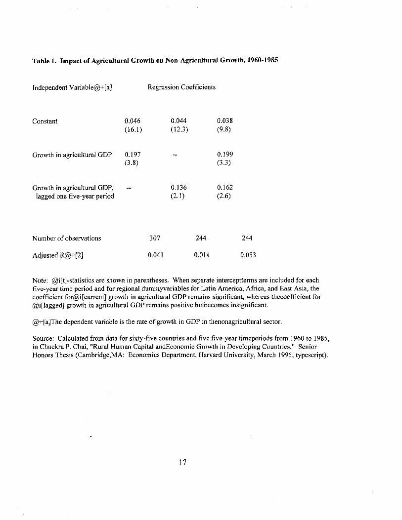
Table 1. Impact of Agricultural Growth on Non-Agricultural Growth, 1960-1985

Independent Variable@+[a] Regression Coefficients

Constant 0.046 0.044 0.038(16.1 ) (12.3) (9.8)

Growth in agricultural GDP 0.197 0.199(3.8) (3.3)

Growth in agricultural GDP, 0.136 0.162lagged one five-year period (2.1) (2.6)

Number of observations

Adjusted R@+[2]

307

0.041

244

0.014

244

0.053

Note: @i[t]~statistics are shown in parentheses. When separate interceptterms are included for eachfive-year time period and for regional dummyvariables for Latin America, Africa, and East Asia, thecoefficient for@i[current] growth in agricultural GDP remains significant, whereas thecoefficient for@i[lagged] growth in agricultural GDP remains positive butbecomes insignificant.

@+[a]The dependent variable is the rate of growth in GOP in thenonagricultural sector.

Source: Calculated from data for sixty-five countries and five five-year timeperiods from 1960 to 1985,in Chuckra P. Chai, "Rural Human Capital andEconomic Growth in Developing Countries." SeniorHonors Thesis (Cambridge,MA: Economics Department, Harvard University, March 1995; typescript).

17

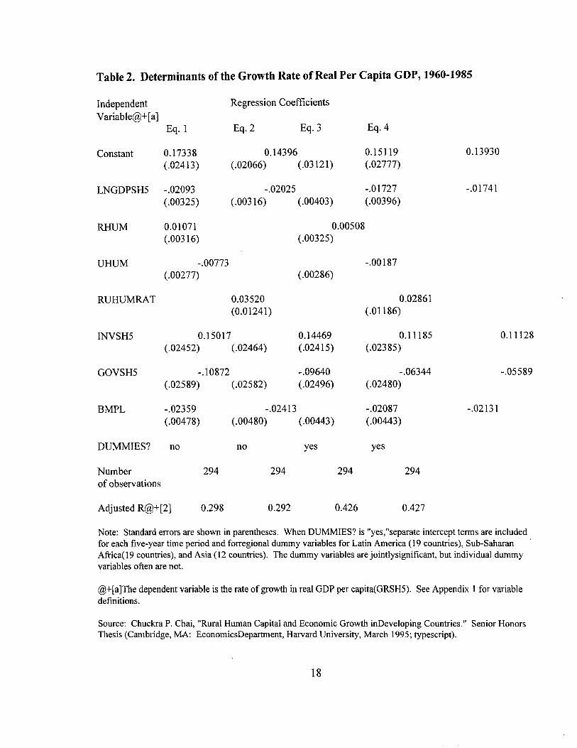
Table 2. Determinants oftbe Growth Rate of Real Per Capita GOP, 1960-1985

Independent Regression Coefficients

Variable@+[a]Eq. 1 Eq.2 Eq.3 Eq.4

Constant 0.17338 0.14396 0.15119 0.13930(.02413) (.02066) (.03121) (.02777)

LNGDPSH5 -.02093 -.02025 -.01727 -.01741(.00325) (.00316) (.00403) (.00396)

RHUM 0.01071 0.00508(.00316) (.00325)

UHUM -.00773 -.00187(.00277) (.00286)

RUHUMRAT 0.03520 0.02861(0.01241) (.01186)

INVSH5 0.15017 0.14469 0.11185 0.11128(.02452) (.02464) (.02415) (.02385)

GOVSH5 -.10872 -.09640 -.06344 -.05589(.02589) (.02582) (.02496) (.02480)

BMPL -.02359 -.02413 -.02087 -.02131(.00478) (.00480) (.00443) (.00443)

DUMMIES? no no yes yes

Number 294 294 294 294of observations

Adjusted R@+[2] 0.298 0.292 0.426 0.427

Note: Standard errors are shown in parentheses. When DUMMIES? is "yes,"separate intercept terms are includedfor each five-year time period and forregional dummy variables for Latin America (19 countries), Sub-SaharanAfrica(19 countries), and Asia (12 countries). The dummy variables are jointlysignificant, but individual dummyvariables often are not.

@+[a]The dependent variable is the rate of growth in real GDP per capita(GRSH5). See Appendix 1 for variabledefinitions.

Source: Chuckra P. Chai, "Rural Human Capital and Economic Growth inDeveloping Countries." Senior HonorsThesis (Cambridge, MA: EconomicsDepartment, Harvard University, March 1995; typescript).

18

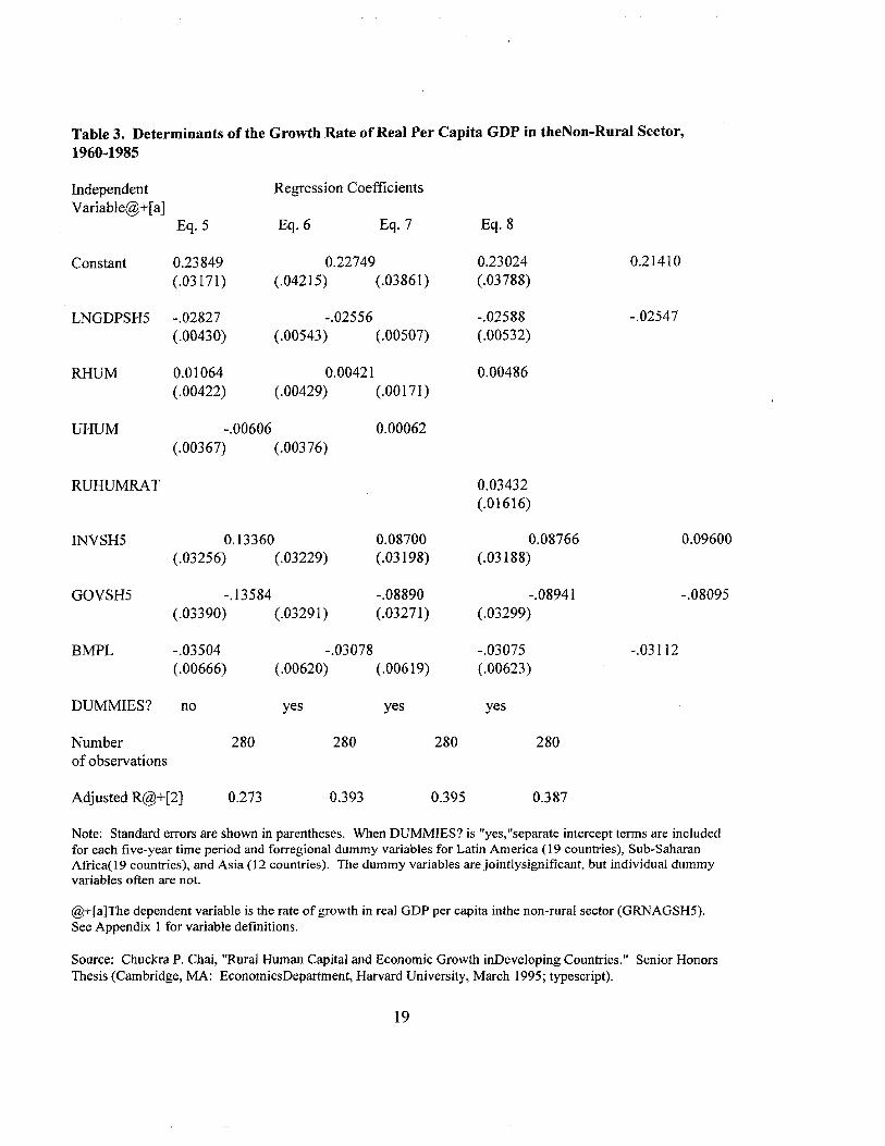
Table 3. Determinants of the Growth Rate of Real Per Capita GDP in theNon-Rural Sector,1960-1985

Independent Regression CoefficientsVariable@+[a]

Eq.5 Eg.6 Eg. 7 Eg.8

Constant 0.23849 0.22749 0.23024 0.21410(.03171) (.04215) (.03861) (.03788)

LNGDPSH5 -.02827 -.02556 -.02588 -.02547(.00430) (.00543) (.00507) (.00532)

RHUM 0.01064 0.00421 0.00486(.00422) (.00429) (.00171)

UHUM -.00606 0.00062(.00367) (.00376)

RUHUMRAT 0.03432(.01616)

INVSH5 0.13360 0.08700 0.08766 0.09600(.03256) (.03229) (.03198) (.03188)

GOVSH5 -.13584 -.08890 -.08941 -.08095(.03390) (.03291) (.03271) (.03299)

BMPL -.03504 -.03078 -.03075 -.03112(.00666) (.00620) (.00619) (.00623)

DUMMIES? no yes yes yes

Number 280 280 280 280ofobservations

Adjusted R@+[2] 0.273 0.393 0.395 0.387

Note: Standard errors are shown in parentheses. When DUMMIES? is "yes,"separate intercept terms are includedfor each five-year time period and forregional dummy variables for Latin America (19 countries), Sub-SaharanAfrica(l9 countries), and Asia (12 countries). The dummy variables are jointlysignificant, but individual dummyvariables often are not.

@+(a]The dependent variable is the rate of growth in real GDP per capita inthe non-rural sector (GRNAGSH5).See Appendix 1 for variable defmitions.

Source: Chuckra P. Chai, "Rural Human Capital and Economic Growth inDeveloping Countries." Senior HonorsThesis (Cambridge, MA: EconomicsDepartment, Harvard University, March 1995; typescript).

19

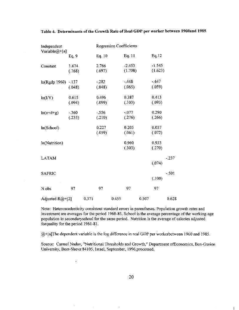
Table 4. Determinants of the Growth Rate of Real GDP per worker between 1960and 1985

Independent Regression CoefficientsVariable@+[a]

Eq.9 Eq.l0 Eq.l1 Eq.12

Constant 1.674 2.766 -2.453 -1.545(.768) (.697) (1.708) (1.623)

In(Rgdp 1960) -.137 -.282 -.448 -.447

(.048) (.048) (.065) (.059)

In(IN) 0.615 0.496 0.387 0.413(.094) (.099) (.103) (.093)

In(n+d+g) -.360 -.556 -.077 0.290(.235) (.210) (.276) (.266)

In(School) 0.227 0.205 0.037(.059) (.061) (.072)

In(Nutrition) 0.960 0.933(.303) (.270)

LATAM -.237(.074)

SAFRIC -.501(.100)

N obs 97 97 97 97

Adjusted R@+[2] 0.371 0.455 0.507 0.628

Note: Heteroscedasticity consistent standard errors in parentheses. Population growth rates andinvestment are averages for the period 1960-85. School is the average percentage of the working-agepopulation in secondaryschool for the same period. Nutrition is the average of calories adjustedforquality for the period 1961-81.

@+[a]The dependent variable is the log difference in real GDP per workerbetween 1960 and 1985.

Source: Carmel Nadav, "Nutritional Thresholds and Growth," Department ofEconomics, Ben-GurionUniversity, Beer-Sheva 84105, Israel, September, I996,processed.

20

REFERENCES

Alesina, Alberto, and Roberto Perotti. 1993. "Income Distribution, Political Instability, andInvestment." Cambridge, MA: National Bureau of Economic Research (NBER) Working Paperno. 4486, October.

Barrett, Christopher, and Michael Carter. 1994. "Does It Take More Than MarketLiberalization? The Economics of Sustainable Agrarian Growth and Transformation." WorkingPaper Series on Development at a Crossroads: Uncertain Paths to Sustain ability. no. 4.Madison, WI: Global Studies Research Program, University of Wisconsin-Madison; September.

Barro, Robert 1., and Jong-Hwa Lee. 1994. "Sources of EconomicGrowth,"@i[Carnegie-Rochester Conference Series on Public Policy]. Amsterdam:North-Holland/Elsevier, pp. 1-46.

Barro, Robert J., and Xavier Sala-I-Martin. 1995. @i[Economic Gro\\>th). New York:McGraw-Hill.

Birdsall, Nancy, David Ross, and Richard Sabot. 1995. "Inequality and Growth Reconsidered:Lessons from East Asia." @i[World Bank Economic Review], vol.9, no. 3, pp. 477-508.

Bliss, Christopher, and Nicholas Stern. 1978. "Productivity, Wages and Nutrition: Parts I andII." @i[Journal of Development Economics], vol. 5,no. 4, pp. 331-98.

Chai, Chuckra P. 1995. @i[Rural Human Capital and Economic Growth in DevelopingCountries]. Senior Honors Thesis. Cambridge, MA: Department of Economics, HarvardUniversity.

Dasgupta, Parta. 1993. @i[An Inquiry into Well-Being and Destitution). Oxford: ClarendonPress.

Dawe, David. 1996. "A New Look at the Effects of Export Instability on Investment andGrowth." @i[WorldDevelopment]. December.

Deaton, Angus S. 1992. @i[Understanding Consumption]. Oxford: Clarendon Press forOxford University Press.

Delgado, Christopher, @i[et al]. 1994. @i[Agricultural Growth Linkages in Sub-SaharanAfrica]. Washington, D.C.: United States Agency for International Development.

De Long, J. Bradford, and Lawrence H. Summers. 1991. "Equipment Investment and EconomicGrowth." @i[Quarterly Journal of Economics], vol. 106, no. 2,PP. 445-502.

21

Fogel, Robert W. 1991. "The Conquest of High Mortality and Hunger in Europe and America:Timing and Mechanisms." In Patrice Higonnet, David S. Landes, and Henry Rosovsky, eds.,@i[Favorites of Fortune: Technology, Growth, and Economic Development since the IndustrialRevolution.] Cambridge, MA: Harvard University Press, pp. 35-71.

. 1994. "Economic Growth, Population Theory, and Physiology: The Bearing of----Long-Term Processes on the Making of Economic Policy." [NobelPrize Lecture] @i[AmericanEconomic Review], vol. 84, no. 3 (June), pp.369-395.

Hill, Hal. 1995. @i[The Indonesian Economy Since 1966: Southeast Asia's Emerging Giant],Cambridge: Cambridge University Press.

Islam, Nurul and Saji Thomas. 1996. @i[Foodgrain Price Stabilization in DevelopingCountries: Issues and Experiences in Asia]. Food Policy Review no. 3. Washington, DC:International Food Policy Research Institute (IFPRI).

Johnston, Bruce F., and John W. Mellor. 1961. "The Role of Agriculture in EconomicDevelopment." @i[American Economic Review], vol. 51, no. 4, pp.566-93.

Kaplan, Steven Laurence. 1984. @i[Provisioning Paris: Merchants and Millers in the Grain andFlour Trade during the Eighteenth Century]. Ithaca, NY: Cornell University Press.

Lewis, W. Arthur. 1954. "Economic Development with Unlimited Supplies ofLabor." @i[TheManchester School], vol. 22, pp. 3-42.

Lipton, Michael. 1977. @i[Why Poor People Stay Poor: Urban Bias in World Development.]Cambridge, MA: Harvard University Press.

___. 1993. "Urban Bias: Of Consequences, Classes and Causality." In AshutoshVarshney, ed., @i[Beyond Urban Bias]. London: Frank Cass, pp.229-58.

Lucas, Robert E. 1973. "Some International Evidence on Output-Inflation Tradeoffs."@i[American Economic Review], vol. 63, pp. 326-34.

Mankiw, N. Gregory, David Romer, and David N. Weil. 1992. "A Contribution to the Empiricsof Economic Growth." @i[Quarterly Journal of Economics]. voLl07, no. 2 (May), pp. 407-437.

Morduch, Jonathan. 1991. @i[Risk and Welfare in Developing Countries]. Ph.D. Dissertation.Cambridge, MA: Department of Economics, HarvardUniversity.

___. 1995. "Income Smoothing and Consumption Smoothing." @i[Journal of EconomicPerspectives]. voL9, no. 3 (Summer), pp. 103-14.

22

Nadav, Carmel. 1996. "Nutritional Thresholds and Growth," Department of Economics,Ben-Gurion University, Beer-Sheva 84105, Israel, September, processed.

Pinckney, Thomas C. 1993. "Is Market Liberalization Compatible with Food security? Storage,Trade and Price Policies for Maize in Southern Africa." @i[Food Policy]. vol. 18, no. 4(August), pp. 325-333.

Ranis, Gustav, Frances Stewart, and Edna Angeles-Reyes. 1990. @i[Linkages in DevelopingCountries: A Philippine Study]. San Francisco, CA: ICS Press for the International Center forEconomic Growth.

Schiff, Maurice, and Alberto Valdes. 1992. @i[The Political Economy of Agricultural PricePolicy]. vol. 4. Baltimore, MD: Johns Hopkins University Press.

Strauss, John. 1986. "Does Better Nutrition Raise Farm Productivity?" @i[Journal of PoliticalEconomy], vol. 94, no. 2, pp. 297-320.

Timmer, C. Peter. 1989. "Food Price Policy: The Rationale for Government Intervention."@i[Food Policy], vol. 14, no. 1 (February), pp. 17-42.

___. 1992. "Agriculture and Economic Development Revisited." In Paul S.Teng and FritzW. T. Penning de Vries, special editors. @i[Agricultural Systems], vol. 38, no. 5 (Amsterdam:Elsevier), pp. 1-35.

___. 1993a. @i[Why Markets and Politics Undervalue the Role of Agriculture inEconomic Development.] Benjamin H. Hibbard Memorial Lecture Series. Madison, WI:Department of Agricultural Economics, University of Wisconsin-Madison.

___. 1993b. "Rural Bias in the East and Southeast Asian Rice Economy: Indonesia inComparative Perspective." In Ashutosh Varshney, ed., @i[Beyond Urban Bias]. London: FrankCass, pp. 149-76.

___. 1995. "Getting Agriculture Moving: Do Markets Provide the Right Signals?"@i[Food Policy], vol. 20, no. 5 (October), pp. 455-72.

___. 1996a. "Food Supplies and Economic Growth in Great Britain, Japan and Indonesia."Cambri~ge, MA: Harvard Institute for International Development, Harvard University;typescript.

___. 1996b. "Does BULOG Stabilize Rice Prices in Indonesia? Should It Try?"@i[Bulletin ofIndonesian Economic Studies], vol. 32, no. 2 (August),pp. 45-74.

23

· 1996c. "Agriculture and Poverty Alleviation in Indonesia." In RayA. Goldberg, ed.,---@i[Research in Domestic and International Agribusiness Management], vol. 12 (Greenwich, CT:JAI Press).

Williamson, Jeffrey G. 1990. "The Impact ofthe Com Laws Just Prior to Repeal."@i[Explorations in Economic History], vol. 27, pp. 123-56.

___. 1993. "Human Capital Deepening, Inequality, and Demographic Events along theAsia-Pacific Rim." In Naohiro Ogawa, Gavin W. Jones, and Jeffrey G.Williamson, eds.,@i[Human Resources in Development along the Asia-Pacific Rim]. Singapore: OxfordUniversity Press.

24

3. ETHIOPIA CASE STUDY

3.1 Introduction

No other country in Sub-Saharan Africa, and only two other countries in the world,derive a higher share of gross domestic product from agriculture than Ethiopia. One can alsomake similar statements about the share of Ethiopia's labor force in agriculture and the role ofagriculture in Ethiopian exports. Agriculture accounted for 57% of Ethiopian GDP in 1994,employed 86% of the labor force (1990), and comprised 69% of total exports (1993).1 Incomparison, agriculture accounted for only 28% of GDP in a typical "low-income" country,and employed 69% of the labor force. 2 Given these broad indicators, there can be little doubtabout the importance of agriculture in the Ethiopian economy.

Several further steps are required, however, to make the case that agriculture is anappropriate focus for realistic economic growth strategies in Ethiopia. After all, it is well­known that as an economy grows, agriculture accounts for a decreasing share of both GDP andemployment. Thus, the case for agriculture as a focus of economic growth strategies mustrely on identifying a set of intersectoral linkages through which agricultural growth contributesto the growth of non-agriculture in the Ethiopian economy. The fact that agriculturecomprises over half of Ethiopian GDP suggests that agriculture's direct impact on economicgrowth (or the lack of economic growth) is substantial. In the long run, however,agriculture's indirect contributions to economic growth through its catalytic effect on non­agricultural growth may be of even greater importance.

One approach to quantifying these indirect contributions to growth is to calculatemacroeconomic growth multipliers for agriculture and other sectors. The ever-growingliterature on growth linkages has focussed almost exclusively on the regional level, usinghousehold-level data to measure the forward and backward linkages arising from bothproduction and consumption in the agricultural sector. 3 These studies uniformly indicate thatthe regional growth multipliers for agriculture are substantially greater than one. Indeed,recent research conducted at IFPRI (1994) on regional agricultural growth linkages in severalSub-Saharan African countries suggests that agricultural growth multipliers are substantiallygreater than previously thought. 4

I World Bank, (1996), and Government of Ethiopia (1995).

2 World Bank (1996).

3 Examples include: S. Haggblade (1989), S. Haggblade, P. Hazell, and 1. Brown (1989), P. Hazell, andA. Roell (1983), and B. Lewis and E. Thorbecke (1992).

4 This study reports agricultural growth multipliers of2.75 in Burkina Faso, 2.48 in Zambia, 1.97 in

Senegal, and 1.96 in Niger. In general, these studies do not report non-agricultural growth multipliers.

While this literature has the advantage of substantial detail in the calculation of growthmultipliers, the methodology employed in these studies limits the interpretation of theirmultipliers to the regional level. 5 The approach taken in this paper complements the regionalgrowth linkage literature, yielding macroeconomic growth multipliers (though withsubstantially less detail than is possible in the regional models). In particular, this paperdescribes the application of a three-sector numerical simulation model of economic growth inEthiopia.

The model distinguishes among three sectoral sources of GDP in the Ethiopianeconomy: agriculture, services, and industry. Simulations of income shocks in these threesectors indicates that intersectoral linkages in the Ethiopian economy operate in somedimensions but not in others. In particular, linkages operate between the agricultural andservice sectors l and to some extent between services and industry; yet, Ethiopia's industrialsector is largely detached from the rest of the economy. This structure is reflected in thesectoral growth multipliers which result from the simulated income shocks in the three sectors.The macroeconomic growth multiplier for agriculture is 1.71, for services it is 1.93, and forindustry it is only 1.38.

These results provide one step towards developing a growth strategy for the Ethiopianeconomy. It does not follow, however, that the marginally higher growth multiplier forservices suggests that the service sector should be the focus of a growth strategy, although itclearly needs to be included. As discussed below, the critical role of agriculture in theEthiopian economy, combined with (a) a concern for poverty alleviation and (b) thedistributional implications of the results presented in this paper, suggests clearly that a viablestrategy for agricultural development is critical for economic growth in Ethiopia.

The outline of this report is as follows: section II describes the specification of thesimulation model; and the nature of the intersectorallinkages it seeks to measure; section IIIbriefly describes the data set with which the model is estimated; section IV describes themodel's base run relative to historical data; section V presents the main results of thesimulation experiments; and, section VI briefly summarizes the results and some of theirimplications for an economic growth strategy for Ethiopia.

5 In particular, the methodology (semi input-output modeling) assumes a perfectly elastic supply of non­tradables. This is plausible at a regional level, but not at the national level.

26

3.2 Model Specification

The model is designed to simulate Ethiopia I s economic growth as a function of growthin three sectors (agriculture, industry, and services) and their interaction with one another.Total GDP is the sum of value added in each of these three sectors. Increments to income inany sector add directly to GDP. In addition, the model allows for income growth in onesector to contribute both directly and indirectly to income growth in the other sectors: sectorA's contribution to increased output in sector B constitutes sector A I S indirect contribution toGDP. It is this indirect contribution that raises a sectoral growth multiplier above 1.0.

In keeping with both a goal of simplicity and the constraints imposed by the data, themodel is specified at a level of aggregation which can barely begin to capture the fullcomplexity and richness of the underlying processes. The model is thus presented primarily asa tool for measuring aggregate sectoral growth multipliers rather than as a tool for detailedpolicy analysis.

The model consists of thirteen endogenous variables and hence thirteen equations -­five identities and eight stochastic equations. Table 1 summarizes the model's structuralequations.

27

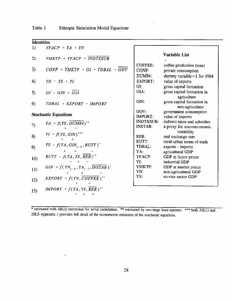
Table 1 Ethiopia Simulation Model Equations

Identities1) YFACP = YA + YN

Variable List2) YMKTP = YFACP + INDTXSUB

5) GI = GIN + GIA

4) YN = YS + YI

6) TDBAL = EXPORT - IMPORT

3) CONP = YMKTP - GI - TDBAL - GOVcoffee production (tons)private consumptiondummy variable =1 for 1984value of exportsgross capital formationgross capital formation in

agriculturegross capital formation in

non-agriculturegovernment consumptionvalue of importsindirect taxes and subsidiesa proxy for macroeconomic

instabilityreal exchange raterural-urban terms of tradeexports - importsagricultural GOPGOP at factor pricesindustrial GOPGOP at market pricesnon-agricultural GOPservice sector GOP

RER:RUTT:TOBAL:YA:YFACP:YI:YMKTP:YN:YS:

GOV:IMPORT:INOTXSUB:INSTAB:

GIN:

COFFEE:CONP:DUM84:EXPORT:GI:GlA:

+

+

+ +

+ +

+ +

+ +

R UTT = f( YA , YS, RER) "

EXPORT = f( YN, COFFEE)' *

GIN = f( YNt - 1 ' YA t - 1 , INSTAB)*

YI = f(YS, GIN)'**

YS = f(YA, GINt

_1

,RUTT)*

12)

11)

9)

10)

8)

Stochastic Equations

YA =f(YS,DUM84)**7)

13) IMPORT = f(YA, YS, RER )'*+ +

* estimated with AR(l) correction for serial correlation; ** estimated by two-stage least squares; *** both AR(l) and

2SLS Appendix 1 provides full detail of the econometric estimates of the stochastic equations.

28

The endogenous variables are on the left-hand side of the equations, and are determinedin each case by the right-hand side variables. Among the right-hand side variables, the laggedendogenous variables are indicated with time subscripts and the exogenous variables have barsover them. The sign beneath each variable indicates the direction of its estimated effect on thedependent variable. There are two aspects of these equations to be described: thespecification and estimation of the individual equations, and the manner in which thoseindividual equations interact with one another in creating the simulations.

Identities

Equations (1) through (6) are identities and definitions which ensure that thesimulations conform to basic conventions of national income accounting. Equation (1) definesthe supply (income) side of the economy: GDP as factor prices (YFACP) is the sum of outputin agriculture (YA), industry (YI), and services (YS). Equation (2) describes the nationalincome accounting identity that the difference between GDP evaluated at market prices(YMKTP) and GDP evaluated at factor prices consists of indirect taxes and subsidies(INDTXSUB, Le., trade taxes and subsidies, excise taxes, etc.).

Equation (3) ensures that the demand (expenditure) side of the economy equals thesupply (income) side. This is the familiar identity that GDP (at market prices) equals the sumof gross investment (GI), government consumption (GOV), private consumption (CONP), andthe trade balance (TDBAL -- exports minus imports). This macroeconomic balance is ensuredby specifying private consumption as a residual account -- the approach actually taken by theGovernment of Ethiopia in creating the national income accounts. Equation (4) defines non­agricultural output (YN) as the sum of output in services and industry.

Equations (5) and (6) are definitions within the expenditure side of the economy.Equation (5) defines gross domestic investment as the sum of investment in non-agriculture(GIN) and investment in agriculture (GIA). Equation (6) defines the trade balance as thedifference between exports and imports.

Stochastic Equations

The endogenous variables indicated in these identities are estimated econometrically inthe model's seven stochastic equations. Equations (7) through (9) describe output in the threeproductive sectors.

The intersectorallinkages which drive the growth multipliers result from thespecification of the output equations. Equation (6) describes agricultural output as a functionof current output in services and a dummy variable for the year 1984, when Ethiopia was hitby a particularly severe drought. This equation, at first, may seem unduly spare. In principle,one might expect that output in industry, as well as relevant prices (e.g., the rural-urban termsof trade), and some indicator of weather conditions might contribute to predicting agricultural

29

output. In practice, none of these variables is statistically significantly related to Ethiopia'sagricultural output during the period 1960-1994 over which the equation is estimated. Thelack of explanatory power of these variables provides several insights into the functioning ofthe Ethiopian economy.

A central point to emerge from efforts to specify intersectoral linkages in the Ethiopianeconomy is that the industrial sector operates essentially as an enclave with few importantlinks with the rest of the economy. Chole and Manzewal (1992) supports this view, arguingthat as a result Ethiopia's industrial sector can contribute little to the transformation of theeconomy. In this regard, it is essential to note that for purposes of estimating this model,there has been some redefinition of sector outputs in the national accounts. Specifically, thepublished national income accounts include handicrafts and small-scale industries along withmining, quarrying, construction and electricity under the single category of "industry." Uponcloser examination of handicrafts and small-scale industries, food processing activities accountfor approximately 32% of total output in that subsector. 6 This model takes the view that theseactivities are distinctly different from "heavy" industry. In fact, activities such as foodstorage, milling, and other related marketing activities are better treated as services. Theprovision of these marketing services, in practice, will playa key role in defining theintersectoral linkages in the model. Yet, it would be misleading to describe an industrialsector in general, over 85 % of which is comprised of activities not directly related toagriculture, as being closely linked to agriculture due to a relatively minor subset of activities.The approach taken here is thus to include handicrafts and small-scale industry among theservice sector accounts.

In terms of the specification of equation (7), one's prior expectation might be thatoutput in both services and industry would contribute to agricultural output. This type ofequation could capture (without distinguishing between) both forward and backward linkageswith agriculture. Forward linkages from agriculture would include purchases of non­agricultural goods and services by the agricultural sector, and agricultural product sales tonon-agriculture. Backward linkages from agriculture include purchases of manufactured inputsby the agricultural sector.

In practice, the smallholder peasant farmers who produce 95% of Ethiopia'sagricultural output consume few if any purchased inputs. Estimates of current fertilizeradoption rates vary widely, depending on source and the region covered. Nationwide,fertilizer adoption is estimated to include approximately 20% of all farmers; yet nearly 75 % oftotal fertilizer sales are concentrated in the high potential agricultural zones of Shoa, Gojam,

6 Government of Ethiopia, background document to revised national income accounts. It is also interestingto note that if one includes textile and leather production, then nearly 80% of value added in handicrafts and small­scale industry depends directly on agriculture for the majority of its inputs.

30

and Arsi. 7 Moreover, rates of fertilizer application per hectare are commonly observed to besubstantially below recommended rates, and virtually all chemical fertilizers used in Ethiopiaare imported.

More generally, McCann (1992) describes that agricultural production techniques forthe vast majority of Ethiopia's peasant farmers have changed little since pre-modern times,with oxen and crude ploughs comprising (along with a modicum of hand tools) virtually theonly purchased non-labor inputs. The lack of effective demand for industrially producedinputs results in a situation where industrial output is essentially unrelated to agriculturaloutput. Aredo (1992) also cites the "inability" of the industrial sector to develop and producenew technical inputs as one explanation for the persistence of low-input agriculture inEthiopia. Econometrically, industrial output is never statistically significant as an explanatoryvariable in the agricultural output equation.

The highly labor-intensive (and relatively unchanged) production techniques practicedby the large majority of Ethiopian peasant farmers may also explain the lack of explanatorypower of gross investment in agriculture in predicting agricultural output. Virtually alldocumented investment in agriculture during the period of estimation was public investment.The Derg regime channeled virtually all such investment into the state farms and collectivefarms. 8 Chole and Manzewal (1992) estimates that this investment thus affected no more than2% of total agricultural output and only 5% of farmers. Moreover, McCann (1990) suggeststhat the existence of surplus labor in many rural areas (even at harvest time) stronglydiscouraged capital investments by peasant farmers. Lack of access to rural credit for most

7 International Fertilizer Development Corporation (1993), and interview at Ethiopian Fertilizer Agency(April, 1995).

8 There is also a great paucity of knowledge regarding private-sector farm-level investment in agriculture(e.g., by peasant farmers). In the national accounts, the only available data on gross fixed investment of farmers andrural households are population estimates and the stock of rural dwellings. MEDAC attempts to calculate valueadded in rural dwellings based on an estimate of the average floor space of a rural dwelling (from the 1984 housingcensus) and a weighted average of per unit construction costs for different categories of dwellings. Theseconstruction costs are extrapolated from 1980/81 rural retail prices. These investments are essentially unrelated toagricultural output. Gross investment in other rural construction works (including land reclamation andimprovement, afforestation and soil conservation, and development of permanent crops) are arbitrarily set at 10% ofthe gross value of rural dwelling construction.

The more relevant component of gross fixed investment in small-scale agriculture is investment inagricultural tools and implements. Estimates for this category were introduced in 1984, based on the GeneralAgricultural Survey, which provided quantity and value of most such tools per household in 1983/84. Forsubsequent years, these base year figures were derived by assuming a constant level of implements per capita,scaling up by an assumed rate of population growth, then deflating with the GDP deflator of Small Scale Industryand Handicrafts, and depreciating the original capital stock at a rate of20% per year. This proxy is too far removedfrom reality and too small a share of gross investment in agriculture to create a statistical relationship between grossfixed investment in agticulture and aggregate agricultural output. The foregoing information is drawn fromGovernment of Ethiopia, Ministry of Planning and Economic Development (1994).

31

peasants, along with uncertain land rights, likely reinforced the disincentives to make capitalinvestments. While there has been notable agricultural investment in particular regions, suchas in Ada, such exceptions are insufficient to create a statistical relationship between measuredagricultural investment and aggregate agricultural output.

The rural-urban terms of trade also fails significantly to explain agricultural output inEthiopia. This, too, runs counter to the economist's intuition. Yet, Ethiopia perhaps morethan any other country, remains a subsistence agricultural economy. One potential explanationfor the lack of explanatory power of prices in Ethiopian agriculture is thus that approximately80-85 %of total agricultural output is consumed on-farm.9 The lack of physical and economicinfrastructure in rural areas may simply leave most farmers disconnected from markets. Brune(1992) describes that nearly 75% of Ethiopia's farms are at least a half-day's walk to thenearest all-weather road. An alternative explanation for the lack of statistical relationshipbetween the rural-urban terms of trade and agricultural output is simply that the official pricedata from the Derg period bear little relation to market reality. For much of this period, theparapublic Agricultural Marketing Corporation was charged with defending the Government'spolicy of fixing the market price of major food crops. 10 That a price indicator based on theseprices would do little to explain agricultural output is not surprising. In either case, the rural­urban terms of trade fails to explain agricultural output during the period 1960-1994 overwhich the model is estimated.

Alternative specifications of the agricultural output equation also considered the effectsof drought and rainfall. A general dummy variable for drought years is never significant inthe presence of a dummy variable for 1984, the year of a particularly severe drought. Thislack of statistical significance may reflect the localized nature of more "typical" drought,which may not be clearly reflected in the country's aggregate agricultural output. The 1984drought, in contrast, was sufficiently broad in its effects that it adds significantly to theequation's explanatory power. A similar explanation may apply to the lack of significance ofrainfall data in explaining aggregate agricultural output. Accessible time series data for annualrainfall included three regions: Addis Ababa, Combolcha, and Debre Markos. Neither theaverage annual rainfall for any of these three regions nor the average of all three regions wassignificantly related to aggregate agricultural output.

Equation (8) determines industrial output as a function of output in services and grossinvestment in non-agriculture. For essentially the same reasons mentioned above, agriculturaloutput does not play any notable role in driving output in Ethiopia's enclave industrial sector.Once one eliminates food marketing services from the industry accounts, there is virtually no

9 This estimate was suggested in an interview with counterparts at the Ministry of Economic Developmentand Cooperation, 19 August 1996.

10 AMC prices for cereals and several other food crops remained fixed (in nominal terms) for 7 yearsduring the early to mid-1980s. Brune (1992), op. cit., p. 121.

32

linkage. For instance, most construction in rural areas consists of housing (tukuls) which tendto be mud and thatch structures that require essentially no manufactured inputs. Peasantagriculture purchases essentially no outputs of domestic industry, and virtually all of thepesticides and fertilizers which are used in Ethiopian agriculture are imported. Nor doesdomestic industry rely on agriculture for a substantial share of its inputs. Terfassa (1992)documents the heavy import dependence of Ethiopian industry, particularly those branchesrequiring significant capital goods, such as metals, chemical, paper and printing, and eventobacco (though this, along with textiles, are among the few industries that do rely on domesticagriculture) .

This import dependence of Ethiopian industry does, however, point to an importantindirect link from agriculture to industry: agriculture is the primary source of the foreignexchange necessary to import industrial inputs. II

The linkages from services to industry are more direct. For instance, an increase inoutput in the services sector would lead to an increase in demand by the services sector forcertain industrial outputs, including electricity and construction. This type of backwardlinkage from services to industry likely explains most of the positive association found inequation (8). It seems less likely to be explained by industrial demand for service sectoroutputs. This perspective is in keeping with the general notion that Ethiopian industryoperates largely as an enclave, with its inputs consisting primarily of mineral resources andimported capital. There is, however, a positive association between gross investment in non­agriculture and industrial output, which is captured in equation (8). Under the Dergadministration, much of this investment originated in the public sector. It is thus reasonable toexpect a positive correlation between such investment and output in w~at were largely state­owned industrial enterprises. Given the command nature of many industrial activities duringthe period of estimation, it is also not surprising that prices (represented by the rural-urbanterms of trade) also fail to explain any significant share of the variation in industrial output.

Equation (9) describes output in the services sector (including agricultural marketingactivities). This equation complements the agricultural output equation (7) in specifying areciprocal relationship between agriculture and services. Output in either one positivelyaffects output in the other. There is a strong forward linkage between agricultural output andthe agricultural marketing services subsectors, which depend entirely on domestic agriculturefor their inputs. Within the handicraft and small-scale industry subsector, the plurality ofenterprises are involved in food marketing (largely processing).12 There is also a strongforward linkage on the consumption level, as food is the primary wage good for service sectoremployees. As Lewis (1954) first observed, good agricultural performance helps to maintain

II This linkage is among those listed in Bruce Johnston and John Mellor (1961).

12 Interview, Ethiopian Chamber of Commerce, April 4, 1995.

33

real wages in the service sector, facilitating investment in non-agriculture. (While this may betrue of industry, as well, the wage bill as a share of total costs is likely to be substantiallygreater in services than in industry owing to the relative capital intensity of the latter, thusmaking the real income effect more evident in the service sector.)

Services sector output is also specified in equation (9) as a positive function of (lagged)gross investment in non-agriculture, and a negative function of the rural-urban terms of trade.Investment in this context could take the fonn of machinery used in providing services(transportation equipment, or small-scale rice milling machines). The rural-urban tenns oftrade broadly measure the incentives shaping trade between the service and agriculturalsectors. As expected, an increase in the ratio of agricultural to non-agricultural prices leads toreduced output in the service sector. 13 Notably, industrial output does not playa role indetermining service sector output in this model. Ethiopian industry, as noted above, dependslargely on domestic mineral reserves and imported capital for its inputs. Just as there wasfound to be no substantial backward linkage from industry to agriculture, neither are theresubstantial backward linkages from industry to services. In addition, as industry (as of 1990)employed only 5% of the labor force, there is also not likely to be a substantial consumptionlinkage to the service sector. 14 Industrial output is thus never significant as an explanatoryvariable in equation (9).

The general picture to emerge from the three output equations «7) through (9» is oneof an economy in which there is substantial two-way interaction between the service andagricultural sectors, limited interaction between services and industry, and virtually nointeraction between agriculture and industry. Figure 1 summarizes this structure in a simpleflow chart tracing each sector's direct and indirect contributions to GDP.

Figure 1 parallels the model presentation in Table 1, showing GDP as the sum ofoutput in agriculture, services, and industry. The solid arrows in those cases indicate directcontributions to GDP. The dashed arrows summarize the first-stage indirect contributions asreflected in the model's intersectorallinkages. There is a two-way relationship betweenagriculture and services. This connection indicates both consumption and production linkagesacross these sectors. Increased food availability stimulates service sector output by relievingpressure on real wages, and increased agricultural income may stimulate rural demand forservices. Production linkages include the provision of agricultural marketing services, whichdepend directly on agricultural output, and which are critical in linking agricultural producers

13 As indicated by the superscripts in Table I, equation (9) is not estimated with two-stage least squares,despite the contemporaneous specification of prices and output. Two-stage least squares, with the limited availableinstruments, proved unsuccessful in yielding a plausible specification for service sector output. The potential forsimultaneity bias is mitigated, however, by the fact that government administratively set many agriculturalcommodity prices during most of the time period of estimation.

14 World Bank (1996), Appendix Table 4.

34

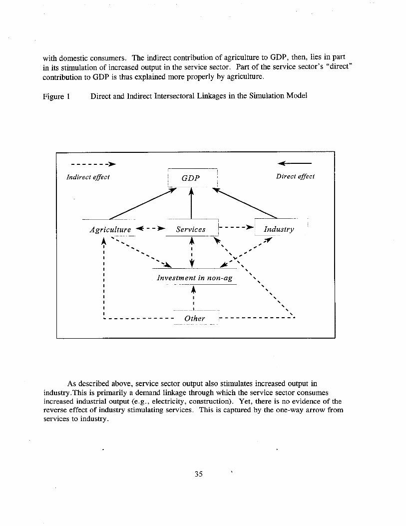
with domestic consumers. The indirect contribution of agriculture to GDP, then, lies in partin its stimulation of increased output in the service sector. Part of the service sector's "direct"contribution to GDP is thus explained more properly by agriculture.

Figure 1 Direct and Indirect Intersectoral Linkages in the Simulation Model

-------~

Indirect effect GDP Direct effect

Investment in non-ag

i.. •

i- - - - - ~i Industry~--~~----_."

~ ~, " ", "'''''" .....

~" " , , , , , , , , , , , ,

I

Other

Services

I

I~ L ,

... ... ... ...~

A"""--.. ... ... ...

i i

Agriculture i~ - - ~:~~--.-~

As described above, service sector output also stimulates increased output inindustry.This is primarily a demand linkage through which the service sector consumesincreased industrial output (e.g., electricity, construction). Yet, there is no evidence of thereverse effect of industry stimulating services. This is captured by the one-way arrow fromservices to industry.

35

Figure 1 does, however, illustrate a secondary set of linkages via investment in non­agriculture. 15 Some agricultural income growth moves across sectors and is invested in non­agriculture. Figure 1 shows that non-agricultural investment both stimulates and is stimulatedby output growth in services and industry. A secondary aspect of agriculture's indirectcontributions comes from its stimulation of investment in non-agriculture, which ultimatelycontributes to GDP via its positive effect on output in services and industry. Similarly, asdiscussed below, increased industrial output has a roundabout positive effect on agriculturaloutput which is visible in Figure 1. Increased industrial output contributes to non-agricUltural

investment, which increases output in services. This increased service sector output, in turn,stimulates agricultural output growth. Thus, the growth multiplier for industry is not zero, butit is smaller than for the other two productive sectors.

The model's remaining equations determine prices, non-agricultural investment, andthe trade balance. Equation (10) predicts the rural-urban terms of trade as a function of outputin the agriculture and service sectors and the real exchange rate. 16 The signs of agriculturaland service output are as expected. Increased agricultural output would tend to drive downagricultural prices, thus lowering the rural-urban terms of trade. Conversely, increased non­agricultural output would tend to drive down non-agricultural prices, thus increasing the rural­urban terms of trade. Again, the command nature of much of Ethiopia's industrial productionunder the Derg administration, and the controlled prices for industrial products, lead to adisassociation between industrial output and the rural-urban terms of trade. This price ratio isthus specified specifically as a function of service sector output.

The real exchange rate logically should playa role in shaping the rural-urban terms oftrade, however the direction of its effect depends on whether the share of tradables inagriculture is greater or less than the share of tradables in non-agriculture. Appendix 2demonstrates, with qualifications, that a real depreciation increases the rural-urban terms oftrade only if the share of tradables in agriculture exceeds the share of tradables in non­agriculture. While agriculture in many countries is typically thought to be more tradable thannon-agriculture, this is probably not the case in Ethiopia. Delgado (1994) argues that formany African countries, particularly landlocked countries (including Ethiopia), high transfercosts effectively make a high share of rural consumption non-tradable. 17 This approach

15 It would have been preferable to disaggregate investment in non-agriculture into investment in servicesand in industry. Unfortunately, the data did not permit such disaggregation.

],6 Th I h . h' d I . I I d us ETH h .e rea exc ange III t IS mo e IS ca cu ate as ER * (PGDP / PGDP ), were the prIces are the GDPdeflators for the US and Ethiopia. This construction for the RER has been used in numerous papers, for example,Brian Pinto (1987).

17 In particular, this study defines non-tradables as " ...goods that at prevailing relative prices are rarely, ifever, traded across the'borders...and no not have close substitutes in local consumption, in the sense that thedomestic price of the non-traded good is not well-correlated with the domestic price of the any tradable good that

36

suggests that Ethiopian agriculture is predominantly non-tradable. For instance, teff is a majorcrop in Ethiopia which is essentially not grown in other countries and certainly has no "world"price. If, as seems likely, the share of tradables in Ethiopian non-agriculture exceeds the shareof tradables in agriculture, then one would expect the real exchange rate to enter negatively inequation (10).18 Estimation of equation (10) confirms this expectation.

Gross investment in non-agriculture is described in equation (11) as a function oflagged output in agriculture and non-agriculture, as well as macroeconomic instability. Thatincreased non-agricultural income would lead to increased investment in non-agriculture isstraightforward. Yet, equation (11) also incorporates a cross-sectoral investment linkagethrough which increased agricultural income can be invested in non-agriculture. In both casesthese relationships are specified with a one-period lag. This structure takes account of thetime necessary for financial intermediation to translate increased output into investment. Thisis particularly necessary in the case of cross-sectoral investment of agricultural income intonon-agricultural investment. This lag also serves a more practical purpose in the context ofthe model, since it contributes to the dynamic properties (described below) through which asimulated shock to sectoral income dies out gradually over time.

Equation (11) also specifies non-agricultural investment as a negative function ofmacroeconomic instability. The notion that an unstable economic environment would tend toundermine investor confidence makes intuitive sense. These relationships have beeninvestigated more formally by Dawe (1996) and by Timmer (1991), who demonstrate thatinstability in exports as a share of GDP leads to lower rates of investment and growth. 19

An explicit equation for gross investment in agriculture proved unnecessary becausethere is so little investment in peasant agriculture that aggregate agricultural investment failedtoexplain the variation in agricultural output. Under the Derg administration, virtually allagricultural investment was channeled directly into highly inefficient state farms, whichproduced approximately 5% of total agricultural output. Whatever positive relationship existsbetween public investment in state farms and agricultural output is lost in the aggregate due tothe small share of state farms in total production.

could play the same role in the consumption basket." (p. 1.8)

18 If one makes the conservative assumption that the only tradable components of Ethiopian non­agricultural production are mining & quarrying, and large & medium-scale manufacturing, then at least 10% ofEthiopian non-agricultural production (as of 1993/94) would be classified as tradable. Given the perception citedabove that 85% of Ethiopian agricultural output is consumed on-farm in remote areas, and that a significant share ofmarketed agricultural output is still non-tradable (e.g., teff), it is reasonable to conclude that the share oftradables innon-agriculture could exceed the share oftradables in agriculture.

19 Following Dawe (I 996), the proxy for economic instability applied here is the three-year movingaverage of the difference between actual and expected exports (as a share ofGDP), where expected exports are thefive-year moving average of actual exports.

37

Equations (12) and (13) define exports and imports, respectively, the difference beingthe trade balance (equation (6». Exports in equation (12) are a positive function of output innon-agriculture and coffee. Coffee is Ethiopia's largest single source of foreign exchangeearnings, accounting for 50-60% of total exports by value. 20 However, controlling for coffee,agriculture more generally drops out of the equation. Ethiopia's second leading export is hidesand skins, which although ultimately agricultural in origin, is an export product of the small­scale industrial sector, and thus influences equation (12) positively through non-agriculturaloutput. Notably, the real exchange rate also fails significantly to explain the variation inEthiopia's exports. One might normally expect a real depreciation to boost exports. It may,yet this relationship was not evident in alternative specifications of equation (12).

Agricultural output does, however, enter (negatively) in explaining Ethiopian imports(equation (13». As foodstuffs comprise 16% of total Ethiopian imports,21 it is logical thatincreased agricultural production would reduce the need for food imports, and thus show anegative partial correlation with imports. The positive association between non-agriculturaloutput and imports could reflect an income effect. Most imports are consumed in urban areas,where a majority of non-agricultural labor is concentrated. Higher non-agricultural income,particularly in the service sector (which is likely to be much more labor intensive thanindustry) could thus stimulate the demand for imports in urban areas.

The sign of the real exchange rate in equation (13) remains problematic. In principle, areal depreciation (an increase in the real exchange rate) should have a positive effect onexports and a negative effect on imports. The opposite finding in equation (13), and the lackof significance in equation (12), as suggested above, might reflect some degree of simultaneitybias despite the use of two-stage least squares. 22 This may also reflect some weakness of themanner in which the real exchange rate is calculated in this exercise. Given the model'soverall specification, however, the real exchange rate (which remains exogenous) plays arelatively minor role in determining the simulated time paths for the endogenous variables.

20 Economist Intelligence Unit, Ethiopia Country Profile, 1996.

21 This figure is reported for the year 1993 in the World Bank, World Development Report, 1996. TheGovernment of Ethiopia, Statistical Abstract, 1995 reports that food and live animals accounted for 12% of thevalue of total imports in 1993. In either case, this share is one of the highest in the world.

22 The quality of available instruments is always an issue in this regard.

38

3.3. Data Issues

Virtually all of the data series used to estimate the model are drawn from Ethiopia'snational income accounts. This section provides some background on the development ofEthiopia's national accounts, without attempting a comprehensive review of coverage, surveymethods, and the many other details necessary for their publication. 23

Responsibility for collecting and publishing the national accounts has passed amongseveral government bodies. The first national accounts were published by the National Bankduring the 1950s, with responsibility passing to the Planning Board in the late 1950s and early1960s, and then to the Central Statistical Office in 1964. The CSO improved upon therudimentary approach taken by the National Bank and the Planning Board, introducing greaterobjectivity into the estimation of output and prices. The CSO published a revised series ofnational accounts in 1967. Yet, the CSO (later CSA) still lacked the data necessary to derive afully articulated system of sector accounts. Much of the national accounts data published bythe CSO'was the result of informed estimations of per capita consumption and the populationgrowth rate.

Agricultural data were a particular problem. The CSO based its calculations ofagricultural output on surveys conducted by the Ministry of Agriculture, which were widelyrecognized as flawed. Many of the estimates were based on a combination of assumedpopulation growth rates and stylized notions of per capita food expenditure. CSO continuedthis practice (albeit with a somewhat improved statistical basis) until responsibility forcomputing the national accounts passed in 1976 to the Ministry of Planning and EconomicDevelopment (MOPED, now the Ministry of Cooperation and Economic Development).

MOPED once again revised the methodology used in calculating sector accounts. Themajor revision was in agriculture. The Central Statistics Authority had taken over primaryresponsibility for estimating agricultural output, and had begun employing modem agriculturalsurvey techniques. Based on more detailed production estimates for major crops, MOPEDwas able to calculate more detailed and scientific accounts. MOPED also revised the approachto valuing agricultural commodities, substituting 1980/81 base year prices for the older methodof obtaining producers' prices of different crops for each year. The new approach, however,remained problematic. The base year prices used were the prices paid to farmers by theAgricultural Marketing Corporation. MOPED subsequently adopted a weighted price indexbased on relevant commodities from the Addis Ababa Retail Price Index. Forty percent of thechange in this index was applied to agricultural GDP at constant prices to arrive at the currentprice estimates.

23 A detailed explanation of the methodology, coverage, and definitions involved in compiling the nationalaccounts is available in Government of Ethiopia, Ministry of Planning and Economic Development (1994).

39

Continued improvements in the national data base motivated another substantialrevision of the national accounts in 1994. In practice, many of the revisions again focussed onthe agricultural sector accounts. In short, the revisions were to include a broader set ofagricultural commodities in the estimation, and to improve the methods used in valuing thatoutput. The result was a generalized increase in the measured size of the agricultural sector asa share of the total economy: in the old series of national accounts the average share ofagriculture in GDP for the period 1980-1993 is 45.5%, compared with 55.7% in the revisedseries.

The current situation is that a user of Ethiopia's national accounts is confronted with achoice between two distinct historical series of national accounts. The "old series" providesdata for the period 1960 - 1993. The newly revised series is current, but was extended backonly to 1980/81. This situation imposed a difficult choice on the present modeling exercise:the revised series are presumably of higher quality, yet provide only 15 annual observations.The old series is based on a more questionable methodology (particularly for the years 1960 ­1976), yet the older series affords 30 annual observations. The judgement made in estimatingthe present model was that the constraint in terms of degrees of freedom imposed by using therevised series was a greater problem than the marginal reduction in quality inherent in thelonger series. This model is thus based on the old series of national accounts data.

40

3.4 Base Run of the Model

The relationships described in the previous section are specified and estimated inlevels, producing a set of coefficients which then provide the basis for simulating theendogenous series in levels. Once the individual equations of the model have been specified,estimated, and the cointegration established24

, the model's performance in simulating truehistorical time paths for the endogenous variables depends on how well the individualequations work together as a system. Simulation involves simultaneously solving all thirteenequations, given starting values for the endogenous variables and actual time paths for theexogenous variables. The system is dynamic in that the values predicted for the endogenousvariables in a given year depend on previous predictions for all endogenous variables.

The result, even in such a small and simple model, is a complicated set of interactionsbetween equations. For instance, an increase in agricultural output leads to an immediateincrease in service sector output, a decrease in imports, and a decrease in the rural-urbanterms of trade. The initial increase in agricultural output also contributes to an increase innon-agricultural investment the following year. Yet, there are second and third round effectsas well. The decrease in the rural-urban terms of trade resulting from the increase inagricultural output feeds back to further stimulate service sector output. Increased servicesector output itself sets off a set of reactions in the model, including an increase in the rural­urban terms of trade, increased output in both agriculture and industry, and increases in bothimports and exports. This partial chain of events demonstrates that even in this relativelysimple model, the full result of various shocks to the system can only be seen through actualsimulation of the full system of equations. One can then validate the model based on howgood a job it does at recreating the actual time paths followed by the endogenous variables.

In general, this model does a reasonable (though not uniformly outstanding) job ofrecreating Ethiopia's recent economic history. 25 The most accurately predicted series in thebase run is also arguably the most important -- GDP at market prices. The average percentageerror in the prediction of that series is less than 5%. The model also does an excellent job ofpredicting output in the specific productive sectors: the root mean squared percentage errorsin the base run for agriculture, services, and industry are 5.4%,6.8%, and 11.5%,respectively. The model also does quite well in predicting prices -- the rural-urban terms oftrade is predicted with a root mean squared percentage error of 5.9 %. The model has greaterdifficulty, however, in predicting levels of investment. Gross investment in non-agriculture,

24 Each individual series in the model is pre-tested for order of integration and found to be I( 1). Eachequation in the model is then tested for cointegration by applying the Engle-Granger method. The results of thesetests are presented in Appendix 3.

25 Appendix 4 presents a statistical assessment of the accuracy of the model's base run.

41

for instance, has an RMSPE of 24.4 %.26 Theil inequality statistics also suggest a reasonablygood fit for the base run predictions, though a decomposition of the Theil inequality statisticssuggests a somewhat elevated degree of bias in several of the predictions for sector output.

Once one is convinced that the model is reasonably faithful in recreating actual events, it ispossible to perform counter factual experiments.

26 The RMSPE for the trade balance appears to be quite high in Appendix 4 (110.8%). This is misleadingbecause the trade balance is calculated as the difference between two other series, resulting in a small denominatorin the fraction on which the percentage error is calculated. In fact, the RMSPEs for imports and exports are 14.1 %and 13.4%, respectively.

42

3.5 Simulation Results

The primary purpose in constructing the model described above is to calculate sectoralgrowth multipliers. A sectoral growth multiplier describes the increment to total GDPgenerated by an income shock in a particular sector. As total GDP is simply the sum ofincome in the three sectors, a $1 aadition to income in sector A directly contributes $1 toGDP. The model is constructed to capture the indirect contributions of the income shock insector A by simulating the inter-sectoral linkages through which the shock contributes toincome growth in sectors Band C. For instance, if an addition of $1 income in sector A leadsto additions of $0.20 in sector Band $0.30 in sector C, the macroeconomic growth multiplierassociated with sector A is 1.50.

This section describes the results of hypothetical shocks to income in Ethiopia'sagricultural, industrial, and service sectors, through which one can derive the macroeconomicgrowth multipliers associated with each sector. The resulting growth multipliers for eachsector are as follows: agriculture = 1.71; industry = 1.38; services = 1.93.

Experiment 1: Agricultural Income Shock

The agricultural income growth multiplier, as noted above, is 1.71. This result impliesthat an incremental $1 of income in the agricultural sector generates an additional $0.71 ofincome in other sectors. The $1 represents agriculture's direct contribution to GDP, the $0.71,represents agriculture's indirect contribution.

More generally, this paper has argued that Ethiopia's industrial sector is essentially aneconomic enclave with minimal linkages to the non-industrial economy. Decomposition of theagricultural growth multiplier supports this view. Table 2 summarizes the results ofexperiment 1, distinguishing between the effects of the initial shock to agricultural income onservices, industry, and feedbacks to agriculture itself.

43

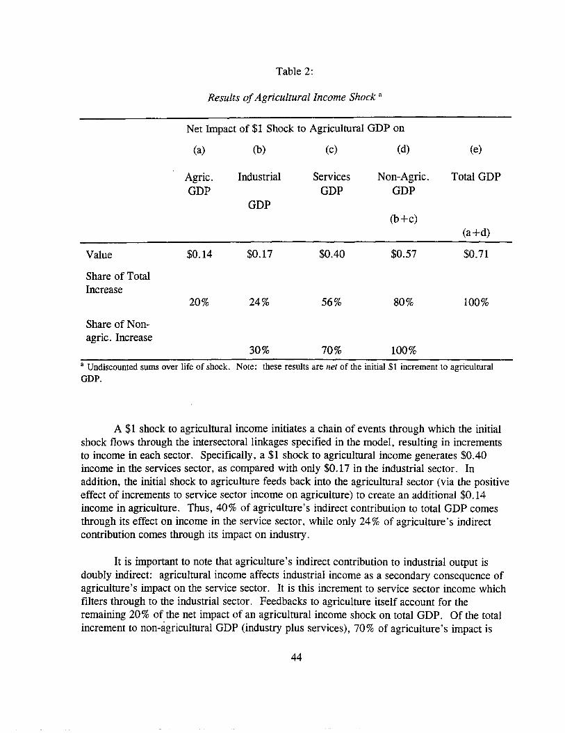
Table 2:

Results ofAgricultural Income Shock a

Net Impact of $1 Shock to Agriculrural GDP on

(a) (b) (c) (d) (e)

Agric. Industrial Services Non-Agric. Total GDPGDP GDP GDP

GDP(b+c)

(a+d)

Value

Share of TotalIncrease

Share of Non­agric. Increase

$0.14

20%

$0.17

24%

30%

$0.40

56%

70%

$0.57

80%

100%

$0.71

100%

a Undiscounted sums over life of shock. Note: these results are net of the initial $1 increment to agriculturalGDP.

A $1 shock to agricultural income initiates a chain of events through which the initialshock flows through the intersectorallinkages specified in the model, resulting in incrementsto income in each sector. Specifically, a $1 shock to agricultural income generates $0.40income in the services sector, as compared with only $0.17 in the industrial sector. Inaddition, the initial shock to agriculrure feeds back into the agriculrural sector (via the positiveeffect of increments to service sector income on agriculrure) to create an additional $0.14income in agriculture. Thus, 40% of agriculture's indirect contribution to total GDP comesthrough its effect on income in the service sector, while only 24 % of agriculrure's indirectcontribution comes through its impact on industry.

It is important to note that agriculture's indirect contribution to industrial output isdoubly indirect: agricultural income affects industrial income as a secondary consequence ofagriculture's impact on the service sector. It is this increment to service sector income whichfilters through to the industrial sector. Feedbacks to agriculture itself account for theremaining 20% of the net impact of an agricultural income shock on total GDP. Of the totalincrement to non-agricultural GDP (industry plus services), 70% of agriculture's impact is

44

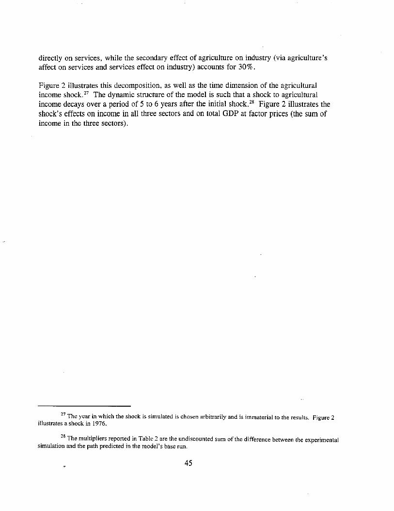
directly on services, while the secondary effect of agriculture on industry (via agriculture'saffect on services and services effect on industry) accounts for 30%.

Figure 2 illustrates this decomposition, as well as the time dimension of the agriculturalincome shock. 27 The dynamic structure of the model is such that a shock to agriculturalincome decays over a period of 5 to 6 years after the initial shock. 28 Figure 2 illustrates theshock's effects on income in all three sectors and on total GDP at factor prices (the sum ofincome in the three sectors).

27 The year in which the shock is simulated is chosen arbitrarily and is immaterial to the results. Figure 2illustrates a shock in 1976.

28 The multil1liers reported in Table 2 are the undiscounted sum of the difference between the experimentalsimulation and the path predicted in the model's base run.

45

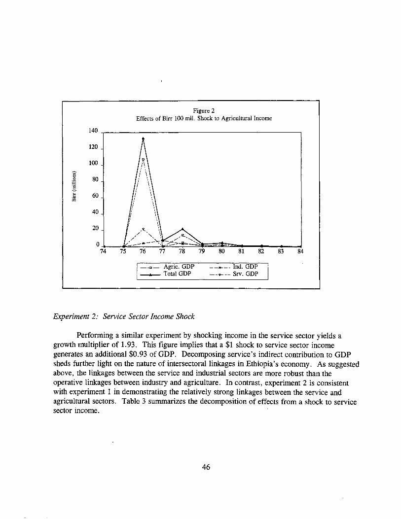
Figure 2Effects of Birr 100 mil. Shock to Agricultural Income

140

120

100-;;;-::

80:@§... 60...

:as

40

20

074 75 76 77 78 80 81 82 83 84

I--a- Agric. GDPA Total GDP

Experiment 2: Service Sector Income Shock

--.... -- Ind. GDP--'Y'--- Srv. GDP

Performing a similar experiment by shocking income in the service sector yields agrowth multiplier of 1.93. This figure implies that a $1 shock to service sector incomegenerates an additional $0.93 of GDP. Decomposing service's indirect contribution to GDPsheds further light on the nature of intersectoral linkages in Ethiopia's economy. As suggestedabove, the linkages between the service and industrial sectors are more robust than theoperative linkages between industry and agriculture. In contrast, experiment 2 is consistentwith experiment 1 in demonstrating the relatively strong linkages between the service andagricultural sectors. Table 3 summarizes the decomposition of effects from a shock to servicesector income.

46

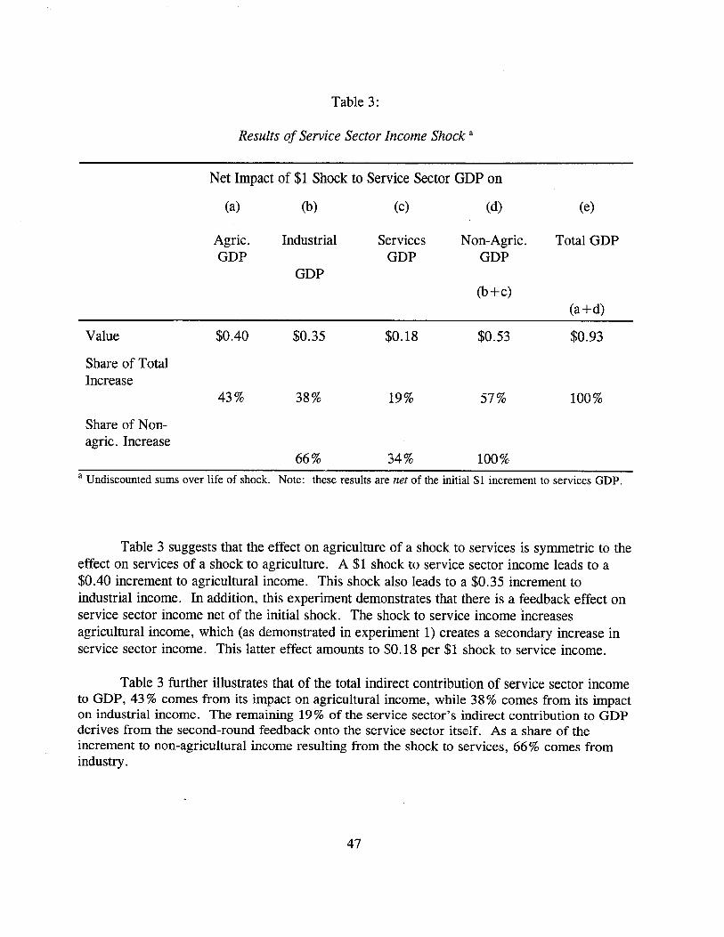
Table 3:

Results of Service Sector Income Shock a

Net Impact of $1 Shock to Service Sector GDP on

(a) (b) (c) (d) (e)

Agric. Industrial Services Non-Agric. Total GDPGDP GDP GDP

GDP(b+c)

(a+d)

Value $0.40 $0.35 $0.18 $0.53 $0.93

Share of TotalIncrease

43% 38% 19% 57% 100%

Share of Non-agric. Increase

66% 34% 100%

a Undiscounted sums over life of shock. Note: these results are net of the initial $1 increment to services GDP.

Table 3 suggests that the effect on agriculture of a shock to services is symmetric to theeffect on services of a shock to agriculture. A $1 shock to service sector income leads to a$0.40 increment to agricultural income. This shock also leads to a $0.35 increment toindustrial income. In addition, this experiment demonstrates that there is a feedback effect onservice sector income net of the initial shock. The shock to service income increasesagricultural income, which (as demonstrated in experiment 1) creates a secondary increase inservice sector income. This latter effect amounts to $0.18 per $1 shock to service income.

Table 3 further illustrates that of the total indirect contribution of service sector incometo GDP, 43% comes from its impact on agricultural income, while 38% comes from its impacton industrial income. The remaining 19% of the service sector's indirect contribution to GDPderives from the second-round feedback onto the service sector itself. As a share of theincrement to non-agricultural income resulting from the shock to services, 66% comes fromindustry.

47

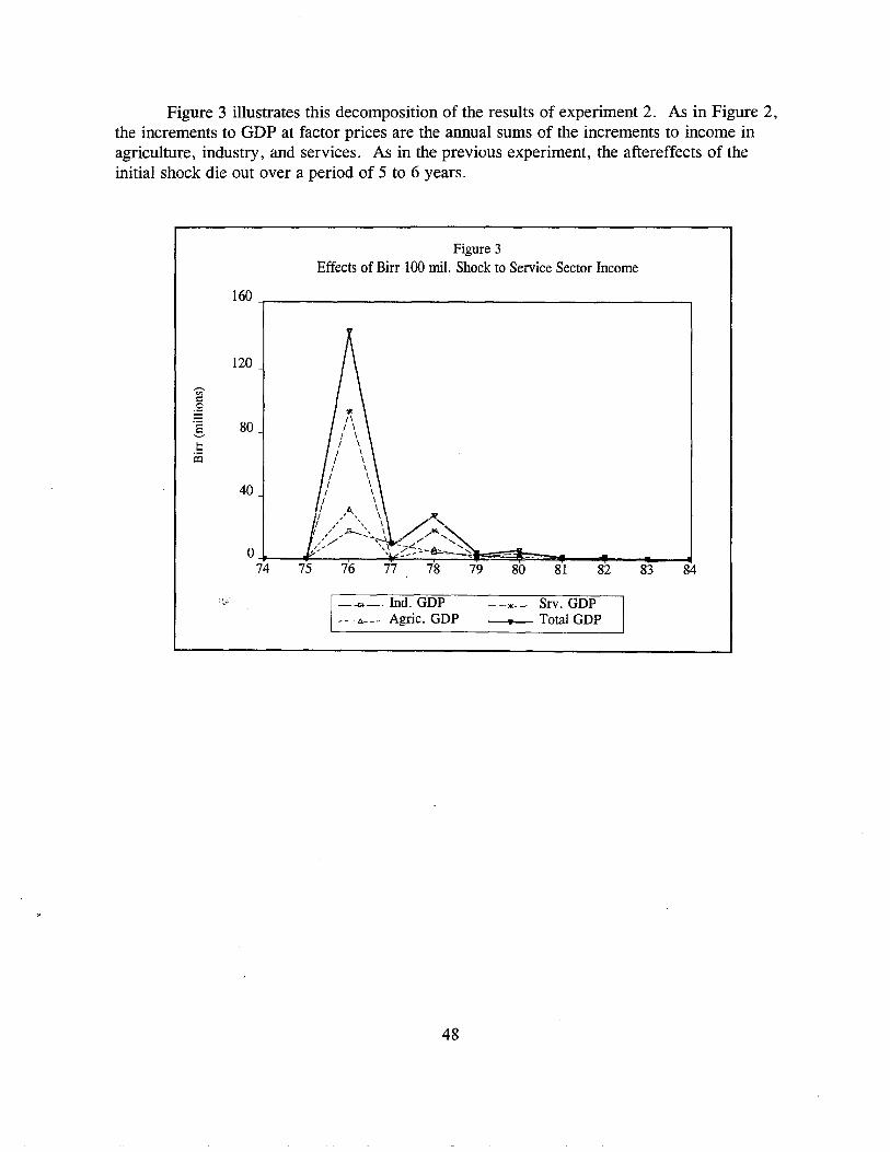
Figure 3 illustrates this decomposition of the results of experiment 2. As in Figure 2,the increments to GDP at factor prices are the annual sums of the increments to income inagriculture, industry, and services. As in the previous experiment, the aftereffects of theinitial shock die out over a period of 5 to 6 years.

Figure 3Effects of Birr 100 mil. Shock to Service Sector Income

160,-- -.,

120

---.'"=.S§ 80......

p:j

40

o7J4:-----'71!:5:.:..--7--,-6-~7~7.2:.:.:7~8::::::~7~9~~80~~8..1-....oII82---8..3----.l84

1-""'- Ind. GOP---A--- Agric. GOP

48

--.-- Srv. GOP__ Total GOP

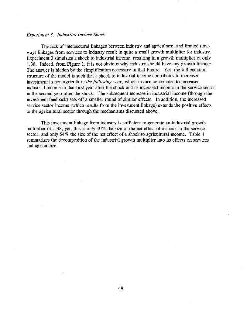
Experiment 3: Industrial Income Shock

The lack of intersectorallinkages between industry and agriculture, and limited (one­way) linkages from services to industry result in quite a small growth multiplier for industry.Experiment 3 simulates a shock to industrial income, resulting in a growth multiplier of only1.38. Indeed, from Figure 1, it is not obvious why industry should have any growth linkage.The answer is hidden by the simplification necessary in that Figure. Yet, the full equationstructure of the model is such that a shock to industrial income contributes to increasedinvestment in non-agriculture the following year, which in tum contributes to increasedindustrial income in that first year after the shock and to increased income in the service sectorin the second year after the shock. The subsequent increase in industrial income (through theinvestment feedback) sets off a smaller round of similar effects. In addition, the increasedservice sector income (which results from the investment linkage) extends the positive effectsto the agricultural sector through the mechanisms discussed above.

This investment linkage from industry is sufficient to generate an industrial growthmultiplier of 1.38; yet, this is only 40% the size of the net effect of a shock to the servicesector, and only 54% the size of the net effect of a shock to agricultural income. Table 4summarizes the decomposition of the industrial growth multiplier into its effects on servicesand agriculture.

49

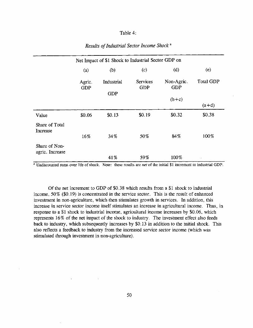
Table 4:

Results of Industrial Sector Income Shock a

Net Impact of $1 Shock to Industrial Sector GDP on

(a) (b) (c) (d) (e)

Agric. Industrial Services Non-Agric. Total GDPGDP GDP GDP

GDP(b+c)

(a+d)

Value $0.06 $0.13 $0.19 $0.32 $0.38

Share of TotalIncrease

16% 34% 50% 84% 100%

Share of Non-agric. Increase

41% 59% 100%

a Undiscounted sums over life of shock. Note: these results are net of the initial $1 increment to industrial GDP.

Of the net increment to GDP of $0.38 which results from a $1 shock to industrialincome, 50% ($0.19) is concentrated in the service sector. This is the result of enhancedinvestment in non-agriculture, which then stimulates growth in services. In addition, thisincrease in service sector income itself stimulates an increase in agricultural income. Thus, inresponse to a $1 shock to industrial income, agricultural income increases by $0.06, whichrepresents 16% of the net impact of the shock to industry. The investment effect also feedsback to industry, which subsequently increases by $0.13 in addition to the initial shock. Thisalso reflects a feedback to industry from the increased service sector income (which wasstimulated through investment in non-agriculture).

50

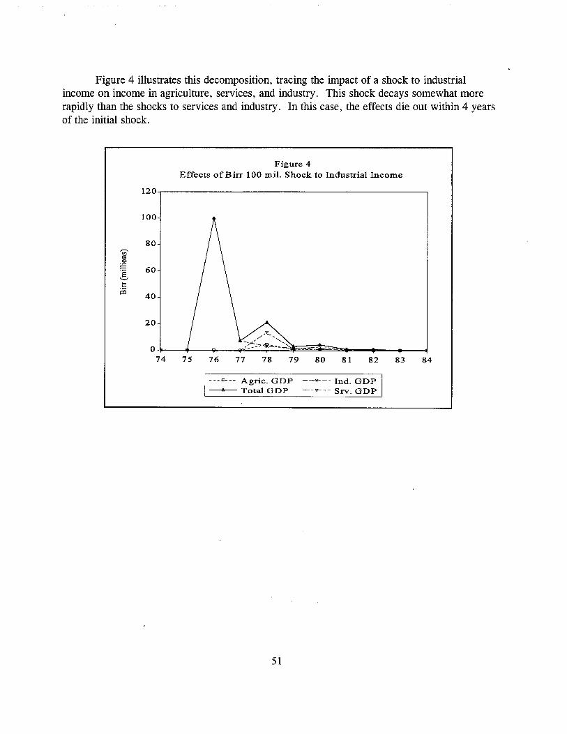
Figure 4 illustrates this decomposition, tracing the impact of a shock to industrialincome on income in agriculture, services, and industry. This shock decays somewhat morerapidly than the shocks to services and industry. In this case, the effects die out within 4 yearsof the initial shock.

Figure 4Effects of Birr 100 mil. Shock to Industrial Income

120

100

80~

'"c::

~ 60gt::

ii5 40

20

75 76 77 78 79 80 81 82 83 84

---EJ--- Agric. GOP --*""-- Ind. GOP------6-- Total GOP --9--- Srv. GOP

51

3.6 Summary and Conclusions

This report describes the construction and application of a simple numerical simulationmodel of Ethiopia's economy. The goal of this exercise is to measure the linkages between theeconomy's major productive sectors as reflected in macroeconomic growth multipliers. Table5 summarizes the multipliers to emerge from simulating shocks to income in each sector.

52

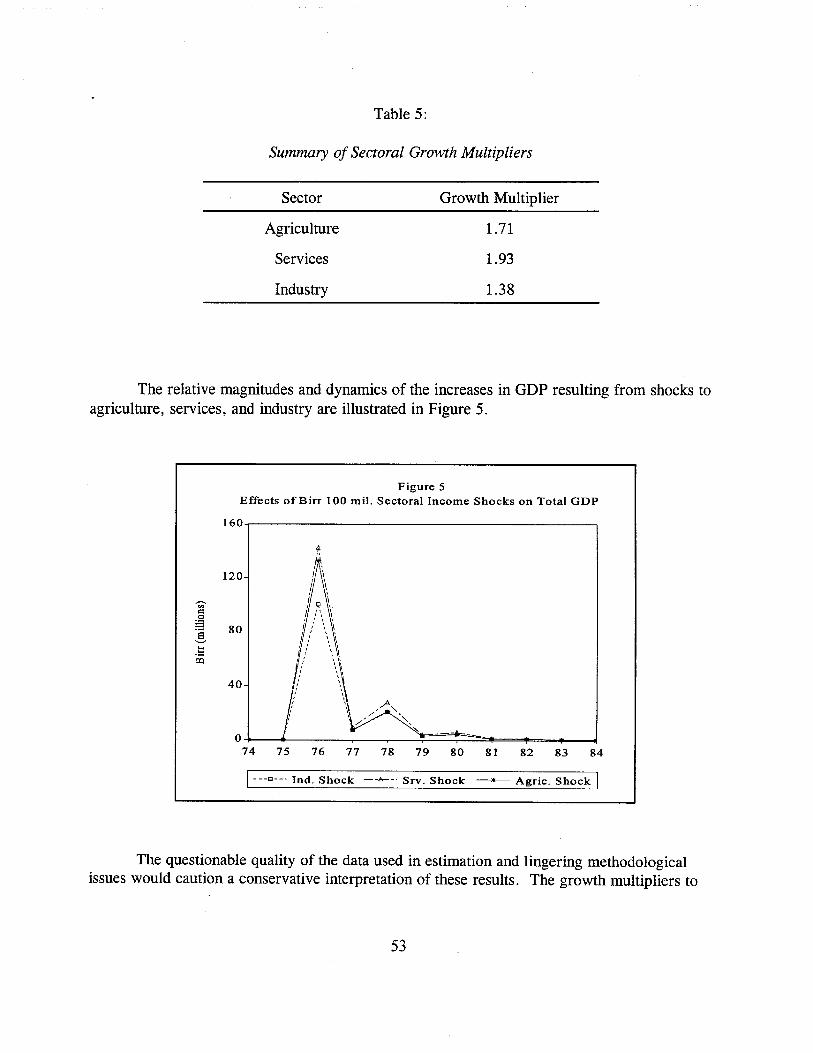
Table 5:

Summary of Sectoral Growth Multipliers

Sector

Agriculture

Services

Industry

Growth Multiplier

1.71

1.93

1.38

The relative magnitudes and dynamics of the increases in GDP resulting from shocks toagriculture, services, and industry are illustrated in Figure 5.

Figure 5Effects of Birr 100 mil. Sectoral Income Shocks on Total GDP

160

t.

120

,......'"<::

:3 80],.;a~

40

o-I----I4----,.-~----,--~~~~I===4~_ ___ol74 75 76 77 78 79 80 81 82 83 84

1---13 --. Ind. Shock --b---. Srv. Shock -- Agric. Shock I

The questionable quality of the data used in estimation and lingering methodologicalissues would caution a conservative interpretation of these results. The growth multipliers to

53

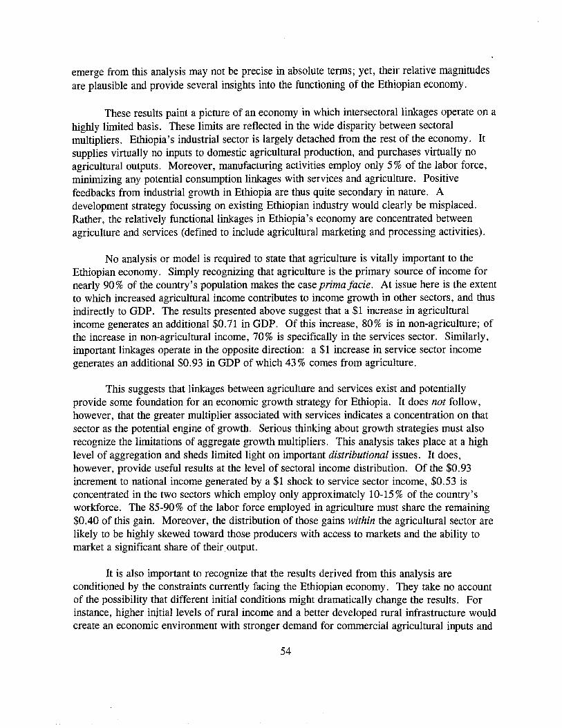
emerge from this analysis may not be precise in absolute terms; yet, their relative magnitudesare plausible and provide several insights into the functioning of the Ethiopian economy.

These results paint a picture of an economy in which intersectoral linkages operate on ahighly limited basis. These limits are reflected in the wide disparity between sectoralmultipliers. Ethiopia's industrial sector is largely detached from the rest of the economy. Itsupplies virtually no inputs to domestic agricultural prOduction, and purchases virtually noagricultural outputs. Moreover, manufacturing activities employ only 5% of the labor force,minimizing any potential consumption linkages with services and agriculture. Positivefeedbacks from industrial growth in Ethiopia are thus quite secondary in nature. Adevelopment strategy focussing on existing Ethiopian industry would clearly be misplaced.Rather, the relatively functional linkages in Ethiopia's economy are concentrated betweenagriculture and services (defined to include agricultural marketing and processing activities).

No analysis or model is required to state that agriculture is vitally important to theEthiopian economy. Simply recognizing that agriculture is the primary source of income fornearly 90% of the country's population makes the case primajacie. At issue here is the extentto which increased agricultural income contributes to income growth in other sectors, and thusindirectly to GDP. The results presented above suggest that a $1 increase in agriculturalincome generates an additional $0.71 in GDP. Of this increase, 80% is in non-agriculture; ofthe increase in non-agricultural income, 70% is specifically in the services sector. Similarly,important linkages operate in the opposite direction: a $1 increase in service sector incomegenerates an additional $0.93 in GDP of which 43% comes from agriculture.

This suggests that linkages between agriculture and services exist and potentiallyprovide some foundation for an economic growth strategy for Ethiopia. It does not follow,however, that the greater multiplier associated with services indicates a concentration on thatsector as the potential engine of growth. Serious thinking about growth strategies must alsorecognize the limitations of aggregate growth multipliers. This analysis takes place at a highlevel of aggregation and sheds limited light on important distributional issues. It does,however, provide useful results at the level of sectoral income distribution. Of the $0.93increment to national income generated by a $1 shock to service sector income, $0.53 isconcentrated in the two sectors which employ only approximately 10-15% of the country'sworkforce. The 85-90% of the labor force employed in agriculture must share the remaining$0.40 of this gain. Moreover, the distribution of those gains within the agricultural sector arelikely to be highly skewed toward those producers with access to markets and the ability tomarket a significant share of their output.

It is also important to recognize that the results derived from this analysis areconditioned by the constraints currently facing the Ethiopian economy. They take no accountof the possibility that different initial conditions might dramatically change the results. Forinstance, higher injtiallevels of rural income and a better developed rural infrastructure wouldcreate an economic environment with stronger demand for commercial agricultural inputs and

54

greater rural access to consumer goods (which are largely absent from rural areas underpresent circumstances).29 Were the same experiments to be conducted under those conditions,the agricultural growth multiplier might be substantially greater than at present. Indeed,current efforts to apply a similar model in Zimbabwe and Kenya, where rural living standardssubstantially exceed those in Ethiopia, suggest that the agricultural growth multiplier in thosecountries is 1.5 to 2.5 times (respectively) the magnitude of the non-agricultural growthmultiplier. 30 To the extent that one might consider Kenya and Zimbabwe to be successfulexamples which Ethiopia might follow, there is at least suggestive evidence that increasedrural income could eventually increase the growth multiplier of Ethiopian agriculture relativeto the growth multiplier for services.

An explicit concern for poverty alleviation would place substantial weight on thegeneration of rural income. The present analysis suggests that a strategy emphasizing growthin Ethiopia's rural economy would contribute substantially to income in non-agriculture, aswell as make the greatest progress toward poverty alleviation.

29 Antle (1983) demonstrates the importance of rural infrastructure in contributing to agriculturalproductivity.

30 Steven Block and C. Peter Timmer, forthcoming (USAID).

55

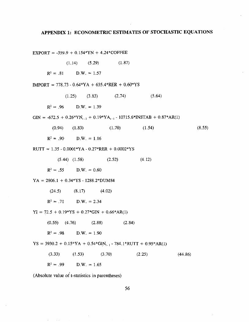
APPENDIX 1: ECONOMETRIC ESTIMATES OF STOCHASTIC EQUATIONS

EXPORT = -359.9 + O.154*YN + 4.24*COFFEE

(1.14) (5.29) (1.87)

R2 = .81 D.W. = 1.57

IMPORT = 778.73 - O.64*YA + 635.4*RER + O.60*YS

(5.64)(2.74)(1.25) (3.83)

R2 = .96 D.W. = 1.39

GIN = -672.5 + 0.26*YNt _ 1 + 0.19*YAt _) - 10715.6*INSTAB + 0.87*AR(l)

(0.94) (1.83) (1.70) (1.54) (8.55)

R2 = .90 D.W. = 1.16

RUTT = 1.35 - 0.0001 *YA - 0.27*RER + 0.0002*YS

(5.44) (1.58) (2.52) (4.12)

R2 = .55 D.W. = 0.60

YA = 2806.1 + 0.34*YS - 1288.2*DUM84

(24.5) (8.17) (4.02)

R2 = .71 D.W. = 2.34

YI = 72.5 + 0.19*YS + 0.27*GIN + 0.66*AR(l)

(0.55) (4.76) (2.88) (2.84)

R2 = .98 D.W. = 1.90

YS = 3930.2 + 0.15*YA + 0.54*GI,N t .,-784.1*RUTT + 0.95*AR(l)

(3.33) (1.53) (3.70) (2.25)

R2 = .99 D.W. = 1.65

(Absolute value of t-statistics in parentheses)

(44.86)

56

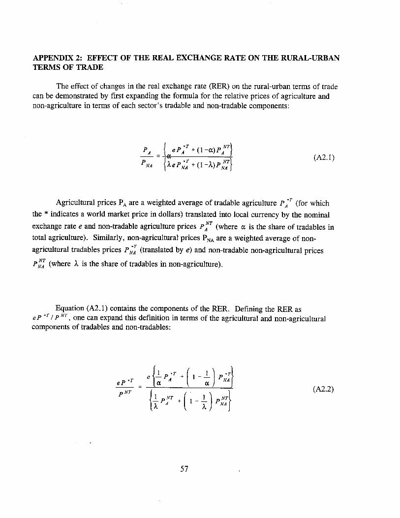
APPENDIX 2: EFFECT OF THE REAL EXCHANGE RATE ON THE RURAL-URBANTERMS OF TRADE

The effect of changes in the real exchange rate (RER) on the rural-urban terms of tradecan be demonstrated by first expanding the formula for the relative prices of agriculture andnon-agriculture in terms of each sector's tradable and non-tradable components:

(A2.1)

Agricultural prices PA are a weighted average of tradable agriculture PA*T (for which

the * indicates a world market price in dollars) translated into local currency by the nominal

exchange rate e and non-tradable agriculture prices p::T (where ex is the share of tradables in

total agriculture). Similarly, non-agricultural prices PNA are a weighted average of non­

agricultural tradables prices P;; (translated bye) and non-tradable non-agricultural prices

P;: (where).. is the share of tradables in non-agriculture).

Equation (A2.i) contains the components of the RER. Defining the RER ase P *T / P NT, one can expand this definition in terms of the agricultural and non-agriculturalcomponents of tradables and non-tradables:

eP *T

p NT

57

(A2.2)

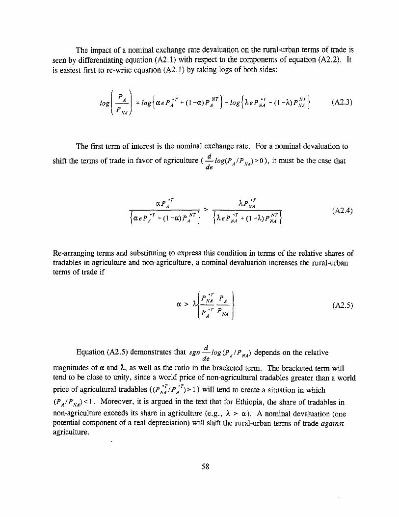
The impact of a nominal exchange rate devaluation on the rural-urban terms of trade isseen by differentiating equation (A2.I) with respect to the components of equation (A2.2). Itis easiest first to re-write equation (A2.I) by taking logs of both sides:

(PA) {*T NT} {~ *T 1 NT}log - = log aePA + (l-a)PA -log l\,ePNA + (l-I\,)P NAPNA

(A2.3)

The first term of interest is the nominal exchange rate. For a nominal devaluation to

shift the terms of trade in favor of agriculture ( .!!....log(PA IP NA) > 0), it must be the case thatde

(A2.4)

Re-arranging terms and substituting to express this condition in terms of the relative shares oftradables in agriculture and non-agriculture, a nominal devaluation increases the rural-urbanterms of trade if

a > A{p~~~)P PNAA

(A2.5)

Equation (A2.5) demonstrates that sgn.!!....log(PAIPNA ) depends on the relativede

magnitudes of a and A, as well as the ratio in the bracketed term. The bracketed term willtend to be close to unity, since a world price of non-agricultural tradables greater than a world

price of agricultural tradables ((P;: I PA'T

) > 1 ) will tend to create a situation in which

(PA I PNA) < I. Moreover, it is argued in the text that for Ethiopia, the share of tradables in

non-agriculture exceeds its share in agriculture (e.g., A > a). A nominal devaluation (onepotential component of a real depreciation) will shift the rural-urban terms of trade againstagriculture.

58

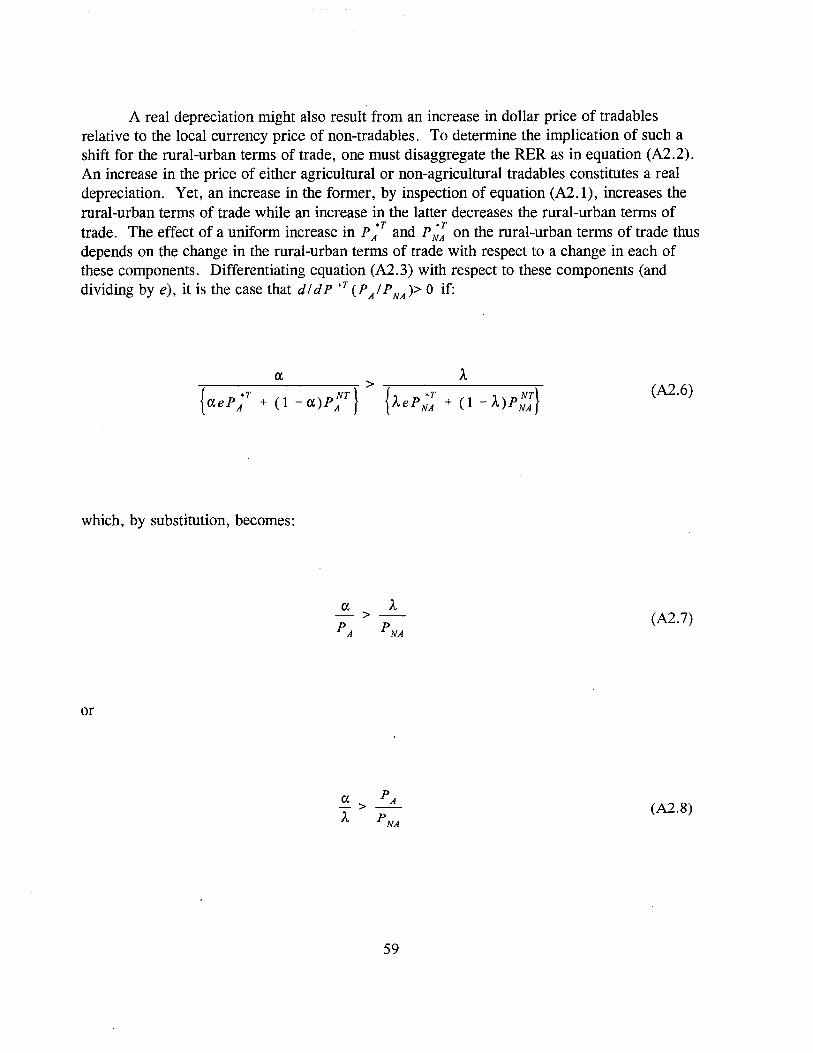
A real depreciation might also result from an increase in dollar price of tradablesrelative to the local currency price of non-tradables. To determine the implication of such ashift for the rural-urban terms of trade, one must disaggregate the RER as in equation (A2.2).An increase in the price of either agricultural or non-agricultural tradables constitutes a realdepreciation. Yet, an increase in the former, by inspection of equation (A2.1), increases therural-urban terms of trade while an increase in the latter decreases the rural-urban terms oftrade. The effect of a uniform increase in PA*T and P;: on the rural-urban terms of trade thusdepends on the change in the rural-urban terms of trade with respect to a change in each ofthese components. Differentiating equation (A2.3) with respect to these components (anddividing bye), it is the case that d / d P *T (PA/PNA» 0 if:

a > A{aepA*T + (1 - a)p;T} {Aep;: + (1 - A)P::}

which, by substitution, becomes:

or

a PA- >A. PNA

59

(A2.6)

(A2.7)

(A2.8)

Equation (A2.8) generally does not hold for Ethiopia, implying that a real depreciationin the form of a uniform increase in the prices of agricultural and non-agricultural tradablesreduces the rural-urban terms of trade. This assertion rests on the observation that the meanrural-urban terms of trade over the period in question was 0.93. The text argues that aconservative estimate of the share of tradables in non-agriculture 0.) is 0.10. Thusd / d P *T (PA / PNA) < 0 for any a < 0.093, which is plausibly the case.

Similarly, a decrease in the price of either agricultural or non-agricultural non-tradablescreates a real depreciation; yet, the former reduces the rural-urban terms of trade while thelatter increases the rural-urban terms of trade. By the same reasoning as above, in order for auniform increase in agricultural and non-agricultural non-tradable prices to increase the rural­urban terms of trade, it must be the case that:

1 - a PA--<-I -). PNA

which cannot hold in general if equation (A2.8) does not hold in general.

(A2.9)

With some qualification, then, it is reasonable to expect the result described in the textfor model equation (10) that an increase (depreciation) of the RER decreases the rural-urbanterms of trade.

60

APPENDIX 3: COINTEGRATION TESTS

Table A3.1 provides the results of Augmented Dickey-Fuller tests of the series used inestimating the model. Cointegration requires that the individual series be integrated of thesame order. In particular, Table A3.1 shows that all series are 1(1). The null hypothesis in anADF test is the existence of a unit root (indicating non-stationarity). An ADF test statistic thatexceeds the MacKinnon critical value indicates rejection of that null hypothesis suggesting thestationarity of the series. In accordance with the Engle-Granger method, after having pre­tested the order of integration of each series, cointegration of the series in the individualequations is established by the stationarity of the residuals from those equations. Table A3.2provides the results of Augmented Dickey-Fuller tests of the residuals from the model'sstochastic equations. In each case, these residuals are stationary.

61

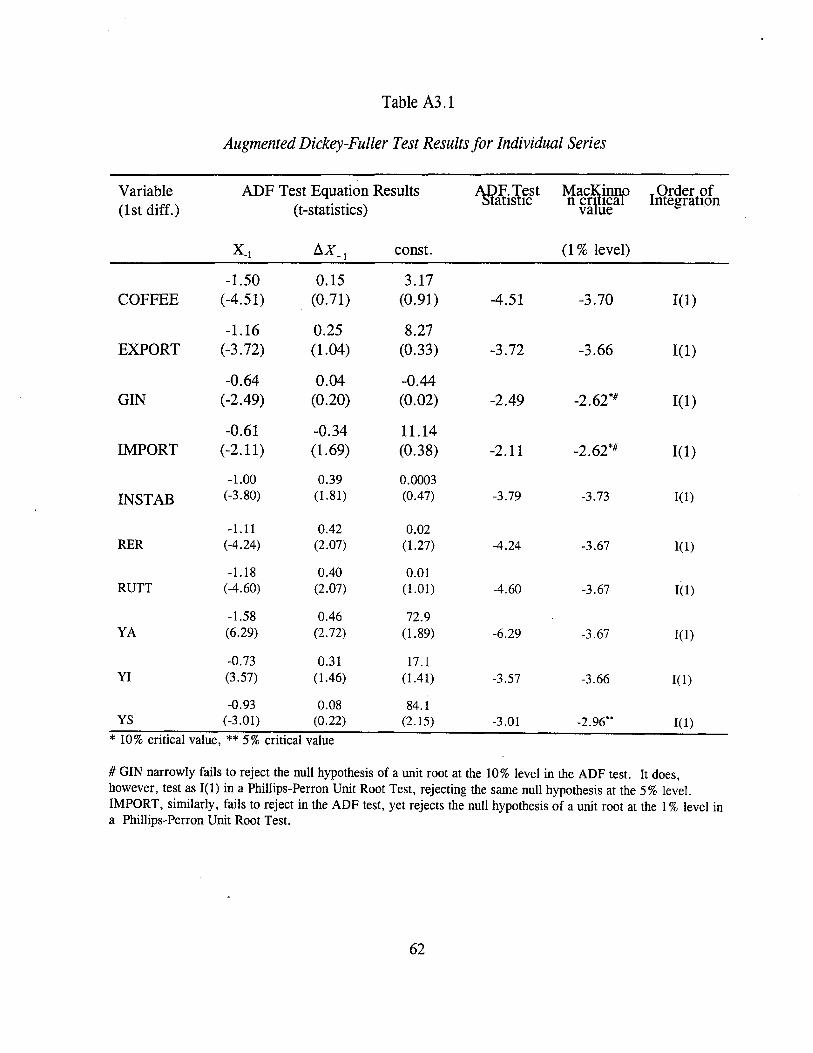
Table A3.1

Augmented Dickey-Fuller Test Results for Individual Series

Variable ADF Test Equation Results ~.~est Mac~i~ Order oftIs IC n crlica IntegratIOn

(1st diff.) (t-statistics) va ue

X_I 6X_I

canst. (1 % level)

-1.50 0.15 3.17COFFEE (-4.51) (0.71) (0.91) -4.51 -3.70 1(1)

-1.16 0.25 8.27EXPORT (-3.72) (1.04) (0.33) -3.72 -3.66 1(1)

-0.64 0.04 -0.44GIN (-2.49) (0.20) (0.02) -2.49 -2.62*# 1(1)

-0.61 -0.34 11.14IMPORT (-2.11) (1.69) (0.38) -2.11 -2.62*# 1(1)

-1.00 0.39 0.0003

INSTAB (-3.80) (1.81) (0.47) -3.79 -3.73 1(1)

-1.11 0.42 0.02RER (-4.24) (2.07) (1.27) -4.24 -3.67 I( 1)

-1.18 0.40 0.01RUTT (-4.60) (2.07) (1.01) -4.60 -3.67 1(1)

-1.58 0.46 72.9YA (6.29) (2.72) (1.89) -6.29 -3.67 1(1)

-0.73 0.31 17.1YI (3.57) (1.46) (1.41) -3.57 -3.66 I(l)

-0.93 0.08 84.1YS (-3.01) (0.22) (2.15) -3.01 -2.96·· I(l)

* 10% critical value, ** 5% critical value

# GIN narrowly fails to reject the null hypothesis of a unit root at the 10% level in the ADF test. It does,however, test as I(l) in a Phillips-Perron Unit Root Test, rejecting the same null hypothesis at the 5% level.IMPORT, similarly, fails to reject in the ADF test, yet rejects the null hypothesis of a unit root at the I % level ina Phillips-Perron Unit Root Test.

62

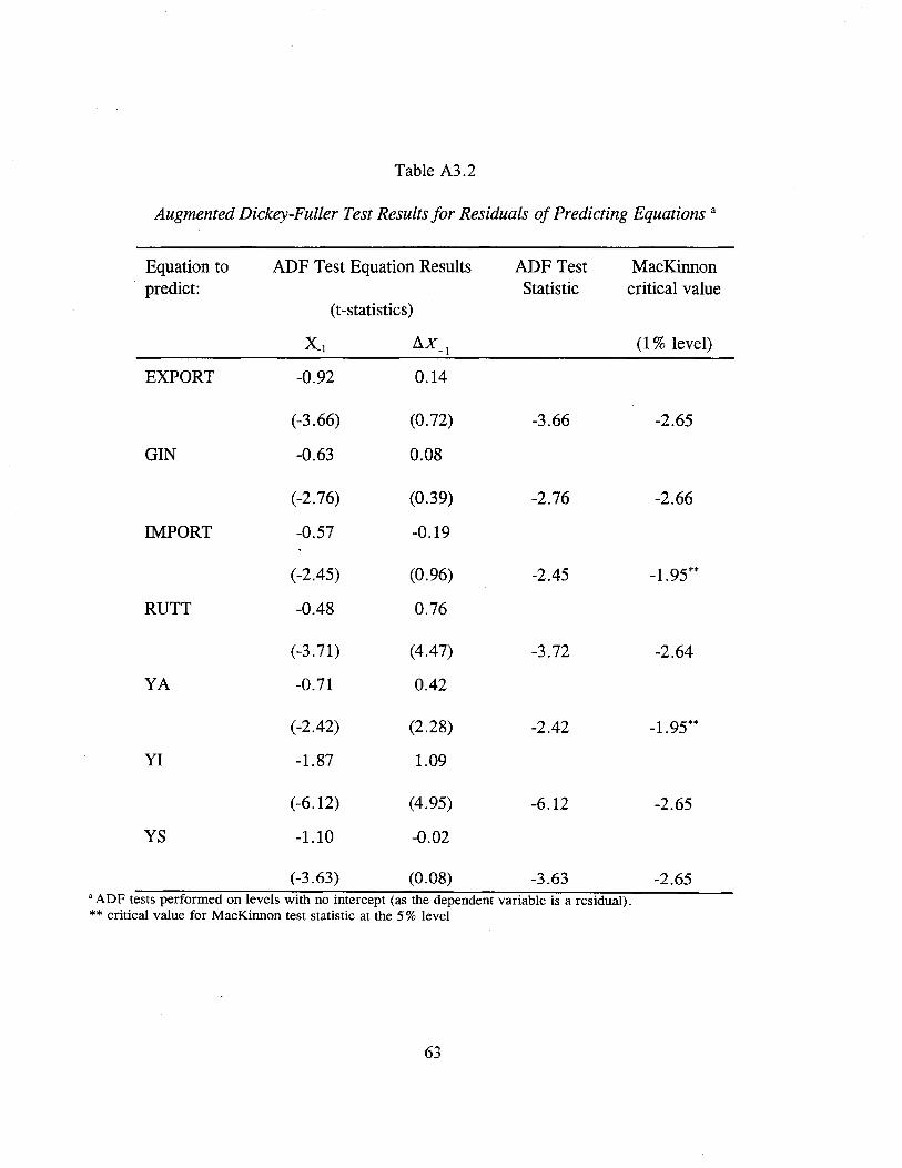
Table A3.2

Augmented Dickey-Fuller Test Results for Residuals of Predicting Equations a

Equation to ADF Test Equation Results ADF Test MacKinnonpredict: Statistic critical value

(t-statistics)

Xl llX_l

(1 % level)

EXPORT -0.92 0.14

(-3.66) (0.72) -3.66 -2.65

GIN -0.63 0.08

(-2.76) (0.39) -2.76 -2.66

IMPORT -0.57 -0.19

(-2.45) (0.96) -2.45 -1.95**

RUTT -0.48 0.76

(-3.71) (4.47) -3.72 -2.64

YA -0.71 0.42

(-2.42) (2.28) -2.42 -1.95**

YI -1.87 1.09

(-6.12) (4.95) -6.12 -2.65

YS -1.10 -0.02

(-3.63) (0.08) -3.63 -2.65a ADF tests performed on levels with no intercept (as the dependent variable is a residual).** critical value for MacKinnon test statistic at the 5 % level

63

APPENDIX 4: GOODNESS-OF-FIT STATISTICS FOR BASE RUN

Table A4.1:

Root Mean Squared Errors and Root Mean Squared Percentage Errors for Base Run

Variable RMSE RMSPE

EXPORT 130.1 13.4

GI 216.3 27.0

GIN 236.5 24.4

IMPORT 185.8 14.1

RUTT 0.1 5.9

TDBAL 233.7 110.8

YA 187.5 5.4

YFACP 438.0 5.3

YI 123.4 11.5

YMKTP 438.0 4.8

YS 246.2 6.8RMSE = root mean square error RMSPE = root mean square percentage error

T

RMSE ..!- L (Y/ - y/)2T (=1

1 .f- [ y/ - Y/ J2RMSPE = - Lt * 100T (=1 ya

t

64

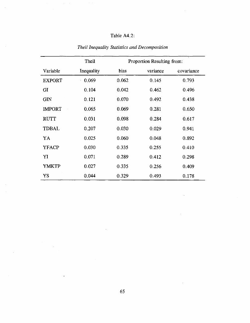
Table A4.2:

Theil Inequality Statistics and Decomposition

Theil Proportion Resulting from:

Variable Inequality bias variance covariance

EXPORT 0.069 0.062 0.145 0.793

GI 0.104 0.042 0.462 0.496

GIN 0.121 0.070 0.492 0.438

IMPORT 0.065 0.069 0.281 0.650

RUTT 0.031 0.098 0.284 0.617

TDBAL 0.207 0.030 0.029 0.941

YA 0.025 0.060 0.048 0.892

YFACP 0.030 0.335 0.255 0.410

YI 0.071 0.289 0.412 0.298

YMKTP 0.027 0.335 0.256 0.409

YS 0.044 0.329 0.493 0.178

65

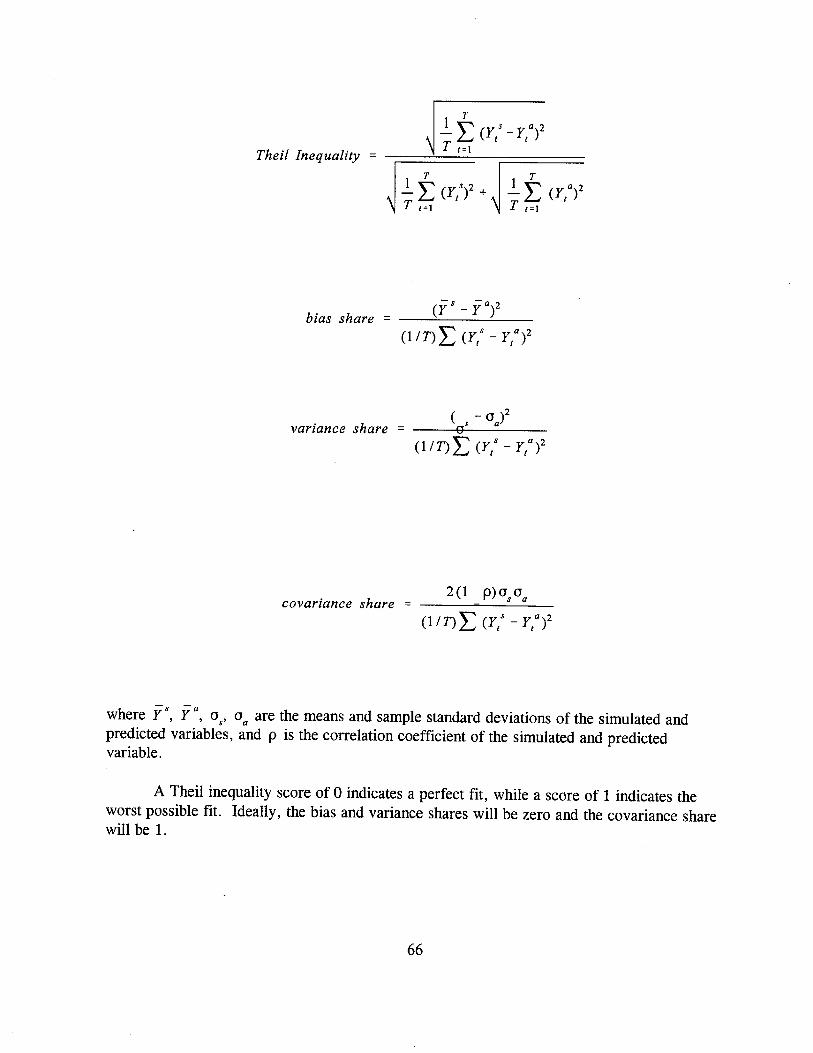
Theil Inequality =

( - a )2variance share = __~ae-s__a _

(l/T)L (Y/ - y/)2

covariance share =

where Ys, y a, a, a are the means and sample standard deviations of the simulated andS a

predicted variables, and p is the correlation coefficient of the simulated and predictedvariable.

A Theil inequality score of 0 indicates a perfect fit, while a score of 1 indicates theworst possible fit. Ideally, the bias and variance shares will be zero and the covariance sharewill be 1.

66

REFERENCES

Antle, John. 1983."Infrastructure and Aggregate Agricultural Productivity: InternationalEvidence. Economic Development and Cultural Change, Vol. 31, No.3 (April).

Aredo, Dejene. 1992. "The Relevance of the Improvement Approach to Agricultural Growthin Ethiopia," in The Ethiopian economy: structure, problems and policy issues.Proceedings of the first annual conference on the Ethiopian economy. ed. MekonenTaddesse. Addis Ababa.

Block Steven and C. Peter Timmer. 1997 forthcoming. Agriculture and Economic Growth:African Case Studies and New Linkages. USAID: Bureau for Africa.

Brune, Stefan. 1992. in Rural-Urban Inteiface in Africa: Expansion and Adaption, ed., J.Baker & P.O. Petersen. Uppsala: Nordiska Afrikainstitutet Copenhagen. 1992, p.121.

Chole, Eshetu and Makonnen Manyazewal. 1992. "The Macroeconomic Performance of theEthiopian Economy," in The Ethiopian economy : structure, problems and policyissues. Proceedings of the first annual conference on the Ethiopian economy. ed.Mekonen Taddesse. Addis Ababa.

Dawe, David. 1996. "A New Look at the Effects of Export Instability on Investment andGrowth," World Development, December.

Delgado, Christopher, et. al. 1994. Agricultural Growth Linkages in Sub-Saharan Africa,Washington, D.C. : U. S. Agency for International Development.

Economist Intelligence Unit. 1996. Ethiopia Country Profile.

Government of Ethiopia, Ministry of Planning and Economic Development. 1994. NationalAcco.unts of Ethiopia: Coverage, Sources, Methods. Addis Ababa. (September).

Government of Ethiopia. 1995. Statistical Abstract.

Haggblade, Stephen. 1989. "Agricultural Technology and Farm-Nonfarm GrowthLinkages," Agricultural Economics, 3: 345-364.

__' Peter Hazell, and James Brown. 1989. "Farm-Nonfarm Linkages in Rural Sub­Saharan Africa," World Development, Vol. 17, No.8, 1173-1201.

67

Hazell, Peter and Alissa Roell. 1983. Rural Growth Linkages: Household ExpenditurePatterns in Malaysia and Nigeria," IFPRI Research Report No. 41, Washington, D.C.:International Food Policy Research Institute.

International Fertilizer Development Corporation. 1993. Ethiopia Fertilizer and TransportSector Assessment.

Johnston, Bruce and John Mellor, "The Role of Agriculture in Economic Development,"American Economic Review, 51(4), 566-593 (1961).

Lewis, Blane and Erik Thorbecke. 1992. "District-Level Economic Linkages in Kenya:Evidence Based on a Small Regional Social Accounting Matrix," World Development,Vol. 20, No.6, 881-897.

Lewis, W. Arthur. 1954. "Economic Development with Unlimited Supplies of Labor," TheManchester School, 22:3 - 42.

McCann, James C. 1990. "Development Strategy and Growth in the Ethiopian Economy: AComparative Analysis of Pre and Post-Revolutionary Period," in Martha Ottaway, ThePolitical Economy of Ethiopia. New York: Praeger.

Pinto, Brian. 1987. "Nigeria During the Oil Boom: A Policy Comparison with Indonesia,"World Bank Economic Review, Vol. 1, No.2 (May), pp. 419-445.

Terfassa, Bulti. 1992. "Recent Trends in the Development of Manufacturing Industries inEthiopia," in The Ethiopian economy: structure, problems and policy issues.Proceedings of the first annual conference on the Ethiopian economy. ed. MekonenTaddesse. Addis Ababa.

Timmer, C. Peter. 1991. "Food Price Stabilization: Rationale, Design, andImplementation," in Reforming Economic Systems, D. Perkins and M. Roemer, eds.Cambridge, MA: Harvard Institute for International Development.

World Bank. 1996. World Development Report. New York, NY: Oxford University Press,for the World Bank.

68

4. ZIMBABWE CASE STUDY

This chapter presents a similar simulation exercise to that applied to Kenya andEthiopia. As in the other cases, the primary objective of this exercise is to calculatemacroeconomic growth multipliers for various sectors of the Zimbabwean economy. Themultipliers to emerge in this case are: agriculture, 1.93; consumer goods production, 1.92;and, capital goods production, 1.54. These results provide a step towards devising economicgrowth strategies for Zimbabwe. The following sections provide necessary backgroundinformation, describe the model's structure, and present the results of four simulationexperiments.

4.1 Agriculture and Zimbabwe's Economy

Until the 1940s, Southern Rhodesia was primarily a mining-based economy, claimingnearly half of the world's chrome production and a significant share of gold. The agriculturaland manufacturing sectors played only limited roles in the early period of economicdevelopment, as most of the first white settlers came as miners rather than as farmers. It wasonly following the First World War that commercial agriculture underwent significant growthin Southern Rhodesia with an influx of war veterans and white farmers from South Africa.The white settlers benefitted substantially from race-based land policies, thus laying thefoundation for the current bimodal structure of Zimbabwe 1s agricultural sector.

The agricultural sector lagged further behind manufacturing during the Second WorldWar, which stimulated demand for steel and domestically-manufactured consumer goods. Itwas only following the War that Zimbabwe's agricultural sector surged ahead ofmanufacturing, driven by large British concessions for the export of Virginia tobacco. Thistobacco boom resulted in substantially greater balance between agriculture and manufacturingin the structure of Zimbabwe f s economy.

During the next fifteen years, agriculture was maintained as the economy's leadingsector by continued strong UK demand for Virginia (flue cured) tobacco and by rapiddevelopments in agricultural technologies. The government developed a powerful researchand extension system and made major advancements with hybrid maize varieties (HYVs),pesticides, and nitrogenous fertilizers. Agricultural productivity and intensification grewrapidly as a result of these technologies -- fertilizer use increased five-fold from 1950 to 1965(Rukuni, 1990).

The diversification and mechanization on commercial farms far surpassed that onsmallholder farms, where growth was further stagnated by pricing policies favoring whitecommercial producers. In the face of these conditions, the number of white farmers increasedto 6200 by 1955 and the white population peaked at 219,000 in 1960 (Rukuni 1990:19).

69

During this period, manufacturing overtook mining as the second largest sector, with thenumber of manufacturing firms increasing from 700 to 1300 between 1953 and 1957.

Manufacturing surpassed agriculture for economic dominance in 1970, following fiveyears of import substitution policies and extensive foreign exchange controls. TheGovernment of Rhodesia had adopted these policies in the aftermath of its UniversalDeclaration of Independence in 1965, which resulted in the country's expulsion from theBritish Commonwealth and the imposition of broad trade sanctions. Among other things, theUK banned tobacco imports from Rhodesia, thus halting the major flow of foreign exchangeinto the country. Government intervention in agricultural markets at this time was designed topromote diversification away from tobacco. At the same time, the macroeconomy underwenta dramatic transformation, as the range of manufactured goods increased and themanufacturing sector increased its share of GDP from 19% in 1965 to 25% in 1975 (Sylvester,1991). The cotton textiles sector in Rhodesia grew rapidly during this period, stimulated bytrade ties with South Africa.

As Rhodesia emerged in 1980 as independent Zimbabwe the economy benefitted, notonly from a massive influx of foreign aid, but from two years of good rain resulting in bumperharvests. High mineral prices and sugar export concessions through the Lome Conventionfurther contributed to an economic growth rate of 11 % in 1980 and 15% in 1981.

The critical role of agriculture in supporting this growth became apparent during 1982­1984, when severe drought undercut both GDP and foreign exchange earnings from tobacco(UK trade sanctions having been removed at independence). The drought-induced decline inagricultural output undercut growth of the entire economy, which shrank by 2% in 1982 andby 3% in 1983 (Rukuni, 1990). Poor rains again contributed to poor economic performancein 1987, undermining the Government I s first Five-Year Plan. Drought struck again in 1991and 1992, reducing tobacco exports and contributing to a three-fold increase in the tradedeficit relative to 1991. This increase in the current account deficit severely hamperedZimbabwe's performance under its structural adjustment program with the World Bank. AsMasters (1994) notes, cycles of boom and bust in Zimbabwe's economy have been closely tiedto the fortunes of its agricultural sector.

Agricultural Sector Background

Currently, approximately three-fourth of Zimbabwe's population depends onagriculture for its livelihood. The sector accounts for 12% of GDP and approximately 40% oftotal foreign exchange earnings.

Zimbabwean agriculture has been highly dualistic since Southern Rhodesia firstachieved colony status in the 1920s and lands were legally partitioned into native and non-

70

native areas by the Land Apportionment Act of 1930. In the process, the white settlers wereensured access to the highest quality lands while native farmers were forced onto lowerpotential agricultural lands. This bimodal structure persists in contemporary Zimbabwe, as theMugabe Government's resettlement schemes have proceeded slowly.

White commercial farmers continue to dominate tobacco, sugar, soybeans, wheat, andhorticultural products all being foreign exchange earners, while the smallholders grow mainlystaple grains like maize, sorghum, and millet for subsistence and market and cotton as theirexport crop mainstay. These crops are less capital-intensive and less lucrative, but have theadvantage of being relatively resistant to the sometimes harsh conditions of the CommunalAreas (CAs) which are concentrated in lower potential agroecological zones.

The following section briefly describes these two types of agriculture, the large andsmall scale commercial farming (LSCF and SSCF) and the communal area (CA) farmingsystem, their development over time, and the their linkages to the macroeconomy.

Large Scale and Small Scale Commercial Farms (LSCFs and SSCFs)

Data from 1989 show that large and small scale commercial farms account for 28.7 %and 3.6% of the total land area respectively (Masters, 1994). LSCFs are clearly of greaterimportance and will be discussed in greater detail. SSCFs were created in the 1920s as NativeLand Reserves which could be purchased as far back as the 1930s and had freehold tenure.Few of the rural poor had the capital or desire to move into these areas and thus they havebeen of minor significance throughout Zimbabwe's agricultural history. The LSCFs,however, have been not only the trend setters and driving force behind Zimbabwe'sagricultural development, but also a major factor in conditioning Zimbabwe's macroeconomichealth through their dominance of export agriculture.

Statistics from 1989 show that there were approximately 1200 mainly white commercialfarmers on 4500 LSCFs averaging approximately 2500 Ha. per farm (Masters, 1994). Morethan 75 % of these farms are found in high potential zones, with the majority being in the areassurrounding Harare. Over these large expanses the actual cropped area is only about 100 to125 ha. in any given year, which is equivalent to about 4% land utilization. The remainder ofthe land is typically left fallow or used for low intensity grazing by livestock (Moyo et aI,1991).

LSCFs are quite diversified in aggregate but on individual farms production is oftenspecialized. Leading crops, as shares of total LSCF area planted, are white maize (26%),cotton (18%), Virginia tobacco (17%), soybeans (17%), and winter wheat (12%) with yellowmaize (for livestoc).<: feed), sunflower, groundnuts, and sorghum rounding out the rest of thearea. Farming is energy and input intensive with LSCFs consuming 90% of total commercial

71

energy in agriculture when diesel, agrochemical, coal/wood for curing, and electricity forirrigation are considered (Moyo et. al., 1991).

LSCF production also tends to be highly input-intensive, with the average LSCFproduction unit using 6.5 tractors (Moyo, et. al., 1991). Although minimum wage legislationand some white flight drastically reduced the number of employees on LSCFs there is stillsubstantial labor use with an average of 40 to 70 permanent employees per farm (Stonemanand Cliffe 1989, Moyo et al 1991). Thirty-six percent of LSCF land is irrigated, use of hybridmaize is universal, and yields are on average higher than FAO averages for Africa and are onpar with European and American farmers (Masters, 1994).

In terms of market share, LSCFs dominate the input, energy, and managementintensive crops and hold significant market share in all crops except traditional grains likesorghum and millet. LSCFs account for 95% - 100% of the tobacco, wheat, soybean, andyellow maize markets, and 50% of the cotton growing. In terms of livestock, LSCFs controlabout 80% of commercial beef sales through the Cold Storage Commission and quite possiblydominate other livestock sales as most Zimbabwean farmers consider cattle stores for wealthinstead of commodities (Rukuni, 1990). More specialized products like coffee, tea, sugar, andhorticultural goods (roses in particular) are completely under LSCF control as only thesefarmers have the capital to profit from such management-intensive crops. White maizeproduction has shifted notably towards smallholder agriculture, with the LSCF market sharefalling from 90% in 1974 to 26% in 1990 (Masters 1994, Stoneman and Cliffe 1989). TheLSCF dominance in the production of export crops, tobacco in particular, makes that sectorcritical to the country's macroeconomic health.

Smallholders or Communal Area Farmers (CAFs)

While the LSCF's strongly influence the health of the macroeconomy, the CAFscomprise the majority of rural Zimbabwe. Following nearly a century of discriminatory landand production policies, the economic situation of the CAFs improved significantly withZimbabwe's independence. Since 1980, the government has focussed on promoting CAFs andtheir ability to gain greater access to inputs and hybrid seeds. Unfortunately the land availableto the rural population remains inadequate despite resettlement of more than 50,000 familiessince 1980. Population density in the communal areas has contributed to over-cultivation, andsevere soil erosion is commonplace in much of the communal areas.

The CAFs occupy approximately 42 % of the land areas in Zimbabwe. Over half of thefarms are located in the lowest-potential agricultural areas. In total (as of 1989) there wereapproximately 650,000 farms and 5.2 million CAFs, producing mainly staple grains andcotton (Masters 1994). The average farm size is 25 ha., though in densely populated areas atypical farm is more on the order of 2 to 3 ha. (Masters 1994, Moyo et. al., 1991).

72

Production varies depending on climate and soil, but in general CAFs produce staple grains,groundnuts, vegetables for local market, and cotton for the export and domestic markets.More specifically, in 198952% of CA lands were planted for maize (white), 10% wereplanted for pearl millet, 10% for groundnuts, 9% for sorghum, 8% for cotton, 6% for fingermillet, and 5% for sunflower (Masters, 1994). Because approximately half of what CAFsproduce goes to subsistence their overall impact on grain and cotton markets is less than onemight expect. Nonetheless, in 1989 they produced about three quarters of all maize marketed,half of the cotton production, all of the millet, and nearly 90% of the sorghum, sunflower, andgroundnuts sold in domestic markets (Masters 1994). In total this comprises over 50% ofdeliveries to marketing boards (Stoneman and Cliffe 1989).

Production techniques in the CAs differ markedly from those of the LSCF sector.Inputs and capital are limited to some fertilizer use and oxen for plowing, when possible. Alarge minority of CAFs rely solely on hand cultivation for production (Stoneman and Cliffe1989). This limits the role of CAFs as consumers of commercial inputs -- a potentiallyimportant backward intersectorallinkage. Many of the farmers are women whose husbandsmay be working in urban areas (Stoneman and Cliffe 1989, Moyo et. aI., 1991). Yields aregenerally lower than FAD averages for Sub-Saharan Africa and are highly dependent on thequality of rainfall.

The CAFs are particularly vulnerable to drought, as little or no irrigation exists tobuffer the effects of unpredictable climate. This was clearly demonstrated in the 1992 droughtwhen maize was imported for the first time since independence (Masters 1994). Improvementshave been made since independence with expanded access to extension support and highyielding seed varieties, which over 90% of all CAFs use for maize and cotton (Stoneman andCliffe, 1989). Still, the majority of grain seed is retained by farmers and production ingeneral is most limited by high population densities, overuse of the soil, and erratic rainfall.

With farm labor mobility limited, real wages in agriculture are lower than real wagesin the formal urban sector. Agricultural laborers thus remain among the poorest people inZimbabwe. Zimbabwe's agricultural sector earns approximately 15 % of national income, butemploys approximately 75% of the labor force (Masters, 1994). Real wages have declined inall formal sectors since 1989 (MacGarry, 1993).

In a recent study, Thirtle, et. al. (1993), compare productivity growth rates betweenthe commercial areas and the communal areas before and after independence. They find thataverage annual total factor productivity growth in the commercial areas (1970-89) was 3.43%,while the average growth rate in the communal areas (1975-90) was 4.64%. Independenceand the pro-CAF policies of the Mugabe government were particularly effective in stimulatinga recovery in CAF productivity, which (unlike the commercial areas) had suffered in the finalyears before independence. In particular, CAF aggregate productivity growth decreased bynearly 2% per year during 1975-79, but rebounded following independence to an averagegrowth rate of 4.35% per year during 1980-90 (Thirtle, et. al., 1993). During this first

73

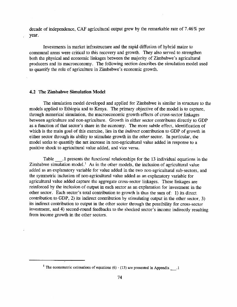
decade of independence, CAF agricultural output grew by the remarkable rate of 7.46% peryear.

Investments in market infrastructure and the rapid diffusion of hybrid maize tocommunal areas were critical to this recovery and growth. They also served to strengthenboth the physical and economic linkages between the majority of Zimbabwe's agriculturalproducers and its macroeconomy. The following section describes the simulation model usedto quantify the role of agriculture in Zimbabwe's economic growth.

4.2 The Zimbabwe Simulation Model

The simulation model developed and applied for Zimbabwe is similar in structure to themodels applied to Ethiopia and to Kenya. The primary objective of the model is to capture,through numerical simulation, the macroeconomic growth effects of cross-sector linkagesbetween agriculture and non-agriculture. Growth in either sector contributes directly to GDPas a function of that sector's share in the economy. The more subtle effect, identification ofwhich is the main goal of this exercise, lies in the indirect contribution to GDP of growth ineither sector through its ability to stimulate growth in the other sector. In particular, themodel seeks to quantify the net increase in non-agricultural value added in response to apositive shock to agricultural value added, and vice versa.

Table _.1 presents the functional relationships for the 13 individual equations in theZimbabwe simulation model. 1 As in the other models, the inclusion of agricultural valueadded as an explanatory variable for value added in the two non-agricultural sub-sectors, andthe symmetric inclusion of non-agricultural value added as an explanatory variable foragricultural value added capture the aggregate cross-sector linkages. These linkages arereinforced by the inclusion of output in each sector as an explanation for investment in theother sector. Each sector's total contribution to growth is thus the sum of: 1) its directcontribution to GDP, 2) its indirect contribution by stimulating output in the other sector, 3)its indirect contribution to output in the other sector through the possibility for cross-sectorinvestment, and 4) second-round feedbacks to the shocked sector's income indirectly resultingfrom income growth in the other sectors.

1 The econometric estimations of equations (6) - (13) are presented in Appendix _.1

74

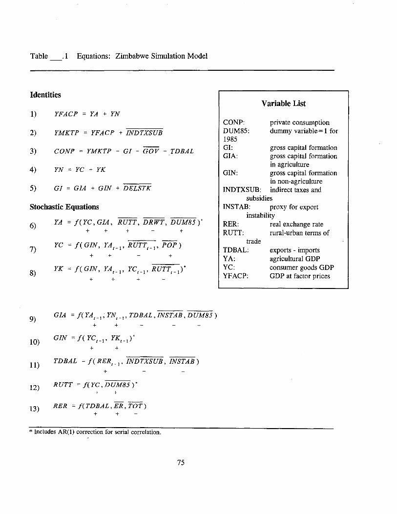
Table .1 Equations: Zimbabwe Simulation Model

IdentitiesVariable List

private consumptiondummy variable = 1 for

exports - importsagricultural GDPconsumer goods GDPGDP at factor prices

gross capital formationgross capital formationin agriculturegross capital formationin non-agriculture

INDTXSUB: indirect taxes andsubsidies

INSTAB: proxy for exportinstability

real exchange raterural-urban terms of

CONP:DUM85:1985GI:GIA:

GIN:

RER:RUTT:

tradeTDBAL:YA:YC:YFACP:

6) YA =I(YC, GIA, RUTT, DRWT, DUM85)*+ + + +

7) YC =I( GIN, YA t _ l , RUTTt _l

, POP)

+ + +

8)YK =I( GIN, YA t _ l , YCt-I' RUTTt_I )*

+ + +

3) CONP = YMKTP - GI - GOV - TDBAL

1) YFACP = YA + YN

2) YMKTP = YFACP + INDTXSUB

4) YN = YC + YK

5) GI = GIA + GIN + DELSTK

Stochastic Equations

9)GIA = I(YA t _l , YNt _l , TDBAL,INSTAB,DUM85)

+ +

10) GIN = I( YCt-I' YKt _I )*+ +

11)TDBAL = I( RERt _l' INDTXSUB, INSTAB)

+

12) RUTT =f(YC,DUM85)*+ +

13) RER = f( TDBAL, ER, TOT)+ +

* Includes AR(l) correction for serial correlation.

75

In Table .1, equations (1) - (5) are identities. Equations (1) - (3) are genericnational income accounting defInitions which ensure that the simulations conform toaccounting regularities. In short, the sources of national income (value added in agricultureand non-agriculture) must equal the uses of national income (private and public consumption,gross investment, and net trade). Equations (4) and (5) are identities specific to the structureof the model. Equation (4) indicates that non-agricultural output is the sum of two non­agricultural sub-sectors -- consumer goods and capital goods. Equation (5) specifies that grossinvestment is the sum of gross fixed investment in agriculture and non-agriculture plus thechange in stocks (for which no distinction between sectors was possible). While equations (1)through (5) ensure macroeconomic balance and provide necessary accounting definitions, themodel's primary focus is on the specifIcation of intersectorallinkages expressed in theremaining eight equations.

Intersectoral Linkages in the Zimbabwe Model

Johnston and Mellor's classic list of agriculture's linkages with the non-agriculturaleconomy portrays agriculture as a source of: 1) non-agricultural labor, 2) food for theindustrial labor force, 3) foreign exchange earnings, 4) demand for domestic industrial output,and 5) industrial inputs. The Zimbabwe model, like the Ethiopia and Kenya models, broadlycaptures the effects of these linkages on the macroeconomic level (though the model is toohighly aggregated to specify these linkages explicitly on a microeconomic level).

Equation (6) models agricultural value added as a function of consumer goods, therural-urban terms of trade, and a dummy variable for drought years. 2 One linkage captured inthis specifIcation is the "forward" linkage of the increased demand for food when non­agricultural income increases. Domestic agriculture is the primary supplier of Zimbabwe'sstaple food consumption. On average from 1961-1988, Zimbabwe more than supplied itsdomestic cereals consumption, exporting 16% of total cereals production. While smallquantities of cereals were always imported (more so in drought years), over this periodZimbabwe's quantity of cereal exports exceeded its quantity of cereals imports by a factor of3.6.

2 Equations (6), (9), and (12) also contain a correction factor in the form of a dummy variable for the year1985. That year recorded a uniquely dramatic increase in agricultural income which this simple model cannotexplain. The dummy variable for that year corrects predictions, yet provides no explanation for the anomaly.

76

Equation (6) also captures the "backward" linkage of agricultural demand for non­agricultural inputs. As noted above, the LSCF sector is highly energy and input intensive andthus provides a substantial source of demand for Zimbabwe's energy and chemicals sectors.Production in the LSCF sector is also relatively capital intensive, and relies heavily onpurchased input packages for hybrid maize. Research on agricultural supply response providesa further rationale for including consumer goods production as an explanatory variable foragriculture: the availability of consumer goods in rural areas has been shown to positivelyenhance agricultural supply response (Berthelemy and Morrisson, 1989).

Equation (6) also models agricultural output as a positive function of contemporaneousinvestment in agriculture. Prior to Zimbabwe's independence in 1980, public-sectoragricultural investments were skewed heavily towards the white-dominated LSCF and SSCFsectors. Since independence, the Government has sought to reverse this trend: between 1980and 1989 public sector investment in agriculture increased every year except three, and hasbeen consistently greater than 10% of total public investment since 1983. The emphasis inpublic sector investment in agriculture has shifted notably away from research and towardsagricultural extension in the communal areas .. In 1979 (the last year prior to independence,research accounted for 5.0% of total public expenditures on agriculture while extensionreceived only 3.1 %; in contrast, the average shares from 1985-1989 were 3.2% and 6.3%,respectively (Masters, 1994). Agricultural investment, itself, is endogenously modeled (inequation (9)) as a function of lagged agricultural output. The lag structure is intended to retainas much recursiveness as possible in the model to avoid potential simultaneity bias. Theremaining potential for such bias in equation (6) is most problematic in the case of the rural­urban terms of trade. 3

Equations (7) and (8) reflect the direct role of agriculture in stimulating non­agricultural production.4 The release of agricultural labor for non-agricultural employment asagricultural productivity increases is one of the central characteristics of structuraltransformation. This process provides part of the justification for including agricultural valueadded as an explanation for non-agricultural value added. Zimbabwe has experienced rapidurbanization in recent years. From 1983 to 1987 alone, the urban share of total populationincreased from 23.6% to 26.7 %. In part, this phenomenon reflects the importance of off-farmincome for rural households. In many cases a male head of household migrates to an urbanarea seeking formal sector employment. One study of communal areas surrounding Harare

3 Efforts to solve this problem with two-stage least squares were unsuccessful due to the poor performanceof available instrumental variables. There are thus several instances in the individual equations of the model wheresimultaneity bias is a potential issue.

4 The distinction between a "direct" and an "indirect" contribution refers to one sector's role incontributing to investntent in the other sector (indirectly contributing to output), as opposed to the directcontributions specified in equations (6) - (8).

77

found that nearly 71 % of farm operations were run by women either as widow, divorcees, orbecause their husbands had migrated to cities in search of work (Zinyama, 1992).

Equation (7) predicts value added in the production of consumer goods. Industrialproduction in Zimbabwe, particularly light industries, food processing, textiles, and footwear,remain highly dependent on domestic agriculture as a source of raw inputs. Indeed,agriculture provides 40% of all manufacturing inputs in Zimbabwe (Moyo, 1990). The majoragriculture-dependent industries in Zimbabwe include: maize milling, meat and dairyprocessing, fruit and vegetable canning, Heinz industries, and a variety of sugar products forboth molasses and as industrial inputs in the form of ethanol, animal feeds, and alcohol(Cheater and Jackson, 1994). Cotton textiles, yarn, twine, bags, and clothing are alsoimportant domestic industries that depend directly on agricultural output. Similarly, domesticcigarette production relies heavily on local tobacco production and the footwear and tanningindustries depend on local livestock production. Zimbabwe also has a well-developed pulpand paper sector which, along with furniture manufacturing, relies on domestic forestryoutput.

In addition to agriculture's role in directly supplying inputs for non-agriculturalproduction, agriculture is also a (and often, the) leading source of foreign exchange earningsnecessary to import the machinery and other foreign inputs on which Zimbabwean industrydepends. Agricultural raw material exports accounted for 52% of total exports in 1991 (agood agricultural year), and accounted for 44% of total exports even during the drought yearof 1992 (EIU, 1996). Among agricultural exports, tobacco typically accounts for 70% to 80%of total foreign exchange earnings. This linkage is particularly important for capital goodsproduction (equation (8», as most of the capital inputs in industrial production are imported(as is much of the lighter equipment used in the production of consumer goods).

In short, Zimbabwean agriculture: 1) supplies labor to non-agriculture, 2) provides asubstantial share of raw inputs, 3) pays for approximately half of imported industrial inputs,and 4) potentially provides a large market for the output of domestic non-agriculture. Theplace of lagged agricultural value added in equations (7) and (8) is thus well-established in theZimbabwean context.

Consumer goods production also plays a role in stimulating production of capitalgoods. In particular, construction, electricity, and communications are important sub-sectorsfor which the consumer goods sector provides most of the demand. In addition, bothconsumer goods aJ;ld capital goods output are a negative function of the rural-urban terms oftrade.

In addition, output in both consumer and capital goods sectors is modeled as a negativefunction of the (lagged) rural-urban terms of trade. The sign of this effect is as expected (e.g.,negative prices incentives reduce output). The lag is imposed in part to retain a recursivestructure (as two-stage least squares performed poorly); yet, to the extent that production

78

targets in state-owned industrial enterprises may have been set in response to last year's prices,the lag structure may be appropriate.

Equation (9) predicts the level of investment in agriculture. This variable emerges as apositive function of lagged output in agriculture and non-agriculture (the sum of consumer andcapital goods), and a negative function of the trade balance and economic instability. Thepositive association between output in both sectors and agricultural investment suggests thatthere are cross-sector investment flows which increase when agriculture appears moreattractive due to strong performance the previous year, and when non-agricultural incomeincreases. The negative association with the trade balance and economic instability also makeintuitive sense. A decline in the trade balance (controlling for lagged agricultural income) maydissuade potential investment in agriculture, an important component of which is exportable.Similarly, the proxy for economic instability most clearly reflects instability in exports. 5

Timmer (1991) and Dawe (1996) discuss the rationale for why instability in exports can reduceinvestment in agriculture.

The specification for investment in non-agriculture in equation (10) is more sparse.Contrary to expectation,. the data did not reflect a significant relationship between agriculturaloutput and investment in non-agriculture. Similarly, economic instability seems to have littleimpact on non-agricultural investment levels, at least as measured at this high level ofaggregation. Investment in non-agriculture is, however, a significant positive function ofincome in both consumer and capital goods production.

Equation (11) predicts the trade balance as a function of the real exchange rate, exportinstability, and net indirect taxes and subsidies. As constructed here, an increase in the realexchange rate represents a depreciation. 6 As expected, a real depreciation improvesZimbabwe's trade balance. Instability in exports, however, has the opposite effect. Thisfinding is consistent with the effect of instability on investment in agriculture: a more unstableenvironment may create disincentives to participation in that activity. Thus, a more unstableexport environment might undermine the trade balance. To the extent that indirect taxes focuson exports, an increase in indirect taxes would logically reduce the trade balance.

The specification of the rural-urban terms of trade is also quite spare (and potentiallysubject to simultaneity bias). In general, one would expect the rural-urban terms of trade to bea positive function of non-agricultural output and a negative function of agricultural output(since increased supply in a given sector, at least in the short run, should reduce its price and

5 Following Dawe (1996), the proxy for economic instability applied here is the three-year moving averageof the difference between actual and expected exports (as a share ofGDP), where expected exports are the five-yearmoving average of actual exports.

6 The proxy adopted here for the real exchange rate is the ratio of the U.S. GDP deflator to the ZimbabweGDP deflator, multiplier by the nominal exchange of Zimbabwe dollars to the U.S. dollar.

79

shift the terms of trade against that sector). While this expectation holds for consumer goodsoutput, neither agricultural output and capital goods output statistically significantly influencedthe rural-urban terms of trade. This finding may well be explained by the government'spersistent role in setting prices in Zimbabwe's economy. Masters (1994), for instance, notesthat the Government of Zimbabwe historically has intervened heavily in setting pan-territorialprices for the country's main agricultural products. Masters also notes that nominalagricultural prices almost never decline in Zimbabwe. 7 Thus, the one-sided specification ofequation (12) reflects the history of the country's agricultural pricing policy.

Finally, equation (13) predicts the country's real exchange rate. The nominal exchangerate is simply a component of the real exchange rate, and is positively associated. It is alsoknown that an expansion of imports tends to appreciate the currency. The positive associationbetween the trade balance and the real exchange rate is thus as expected. While one'sexpectation for the sign of the foreign terms of trade in determining the real exchange rate isnot clear a priori, it makes sense that a country with a negative trade balance could experiencea real depreciation when the terms of trade fall. This would be true, for instance, if thegovernment attempted to force faster nominal devaluations to compensate for declining foreignterms of trade.

4.3 Estimation, Solution, and Validation of the Zimbabwe Simulation Model

Each of the equations in Table .1 are estimated individually by ordinary leastsquares using data for the period of approximately 1968-1992.8 The relationships are specifiedand estimated in levels, producing a set of coefficients which then provide the basis forsimulating the time paths of the model's endogenous (right-hand side) series. Cointegration ofthe series in each equation is tested and established by application of the Engle-Grangermethod, the results of which are presented in Appendix . Actual parameter estimates andrelated descriptive statistics for each stochastic equation are presented in Appendix __.

Given the parameter estimates for the individual equations, solving the model requirescalculating time paths for the endogenous variables through numerical simulation. Thisprocedure involves taking initial levels of the endogenous variables and historical time pathsfor the exogenous variables, and predicting time paths for the endogenous variables based onthe interactions of the model's system of equations. The simulation is dynamic in the sense

7 Masters (1994), p. 158.

8 To maximize degrees of freedom, each equation is estimated for the longest possible period. Severalseries were not available for the earliest years, and equations including those variables are estimated for slightlyshorter periods.

80

that it uses predicted levels of endogenous variables where they appear as explanatoryvariables in other equations. 9

Validation of the model comes from the judgement that it is reasonably faithful inrecreating the actual paths of endogenous variables in a "base" run (e.g., a simulation inwhich there are no external shocks to cause deviations of the predicted from the actual paths ofthe endogenous variables). A statistical assessment of the accuracy of the base run ispresented in Appendix __. The assessment compares the predicted with the actual timepaths for all endogenous variables, providing several indicators of "goodness of fit." Ingeneral, the Zimbabwe model preforms acceptably in a base run. The percentage error in thepredicted time paths for the model's central output equations ranges from 5 % to 12%. Givenavailable data, this range of error is acceptable. The model's performance in predictinginvestment is more problematic. Percentage errors in those cases range from 18 % to 30%,with the greatest problems in predicting investment in non-agriculture. 10 The simulationresults presented below reflect the deviations from the base run in the predicted paths of keyendogenous variables resulting from various shocks to the system. The primary goal of theexperiments described below is to derive macroeconomic growth multipliers for the threeproductive sectors included in the model.

4.4 Simulation Results for Zimbabwe

This section describes the results of several simulations undertaken with the model.The most significant results arise from using the model to calculate growth multipliers foragriculture and non-agriculture. As one might expect, the simulation results for Zimbabwemore closely resemble those from Kenya than those from Ethiopia. The basic results forZimbabwe are the following macroeconomic growth multipliers: agriculture, 1.93; consumergoods, J .92; and, capital goods, 1.54. These multipliers are derived by simulating anexogenous $1.00 shock to the income of each sector. as described in the following threeexperiments.

9 The model is structured recursively to avoid problems associated with simultaneity. For instance, thereal exchange rate and the trade balance depend on one another. The recursive structure of the model is such thatthe real exchange rate depends on the trade balance in the current year (equation (12» and the trade balancedepends on the real exchange with a one-year lag (equation (9».

10 Theil inequality statistics, also reported in appendix _, also suggest that the investment predictionsexhibit an uncomfortable level of systematic bias.

81

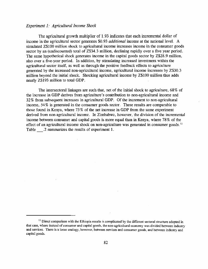
Experiment 1: Agricultural Income Shock

The agricultural growth multiplier of 1.93 indicates that each incremental dollar ofincome in the agricultural sector generates $0.93 additional income at the national level. Asimulated Z$100 million shock to agricultural income increases income in the consumer goodssector by an (undiscounted) total of Z$34.3 million, declining rapidly over a five year period.The same hypothetical shock generates income in the capital goods sector by Z$28.9 million,also over a five-year period. In addition, by stimulating increased investment within theagricultural sector itself, as well as through the positive feedback effects to agriculturegenerated by the increased non-agricultural income, agricultural income increases by Z$30.3million beyond the initial shock. Shocking agricultural income by Z$100 million thus addsnearly Z$193 million to total GDP.

The intersectorallinkages are such that, net of the initial shock to agriculture, 68 % ofthe increase in GDP derives from agriculture's contribution to non-agricultural income and32% from subsequent increases in agricultural GDP. Of the increment to non-agriculturalincome, 54% is generated in the consumer goods sector. These results are comparable tothose found in Kenya, where 73 % of the net increase in GDP from the same experimentderived from non-agricultural income. In Zimbabwe, however, the division of the incrementalincome between consumer and capital goods is more equal than in Kenya, where 78 % of theeffect of an agricultural income shock on non-agriculture was generated in consumer goods. II

Table _.2 summarizes the results of experiment 1.

II Direct comparison with the Ethiopia results is complicated by the different sectoral structure adopted inthat case, where instead of consumer and capital goods, the non-agricultural economy was divided between industryand services. There iS'a loose analogy, however, between services and consumer goods, and between industry andcapital goods.

82

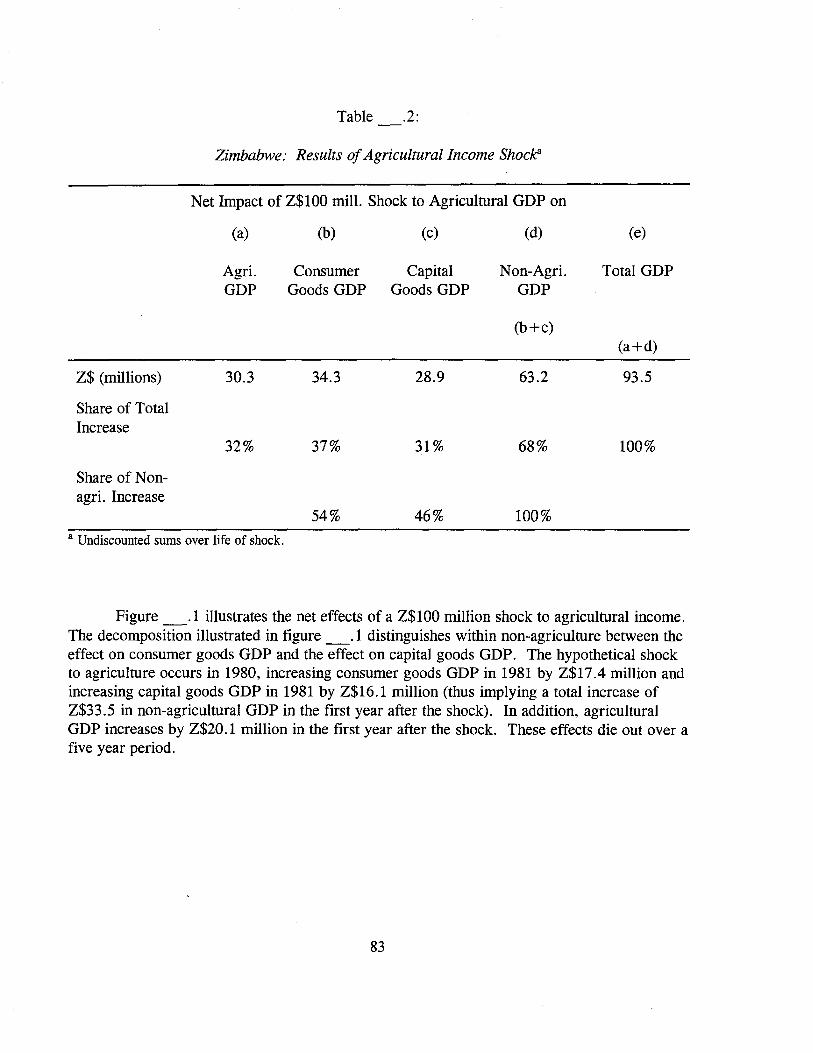
Table .2:

Zimbabwe: Results ofAgricultural Income Shoc/t'

Net Impact of Z$100 mill. Shock to Agricultural GDP on

(a) (b) (c) (d) (e)

Agri. Consumer Capital Non-Agri. Total GDPGDP Goods GDP Goods GDP GDP

(b+c)(a+d)

Z$ (millions) 30.3 34.3 28.9 63.2 93.5

Share of TotalIncrease

32% 37% 31 % 68% 100%

Share of Non-agri. Increase

54% 46% 100%

a Undiscounted sums over life of shock.

Figure _.1 illustrates the net effects of a Z$100 million shock to agricultural income.The decomposition illustrated in figure _.1 distinguishes within non-agriculture between theeffect on consumer goods GDP and the effect on capital goods GDP. The hypothetical shockto agriculture occurs in 1980, increasing consumer goods GDP in 1981 by Z$17.4 million andincreasing capital goods GDP in 1981 by Z$16.1 million (thus implying a total increase ofZ$33.5 in non-agricultural GDP in the first year after the shock). In addition, agriculturalGDP increases by Z$20.1 million in the first year after the shock. These effects die out over afive year period.

83

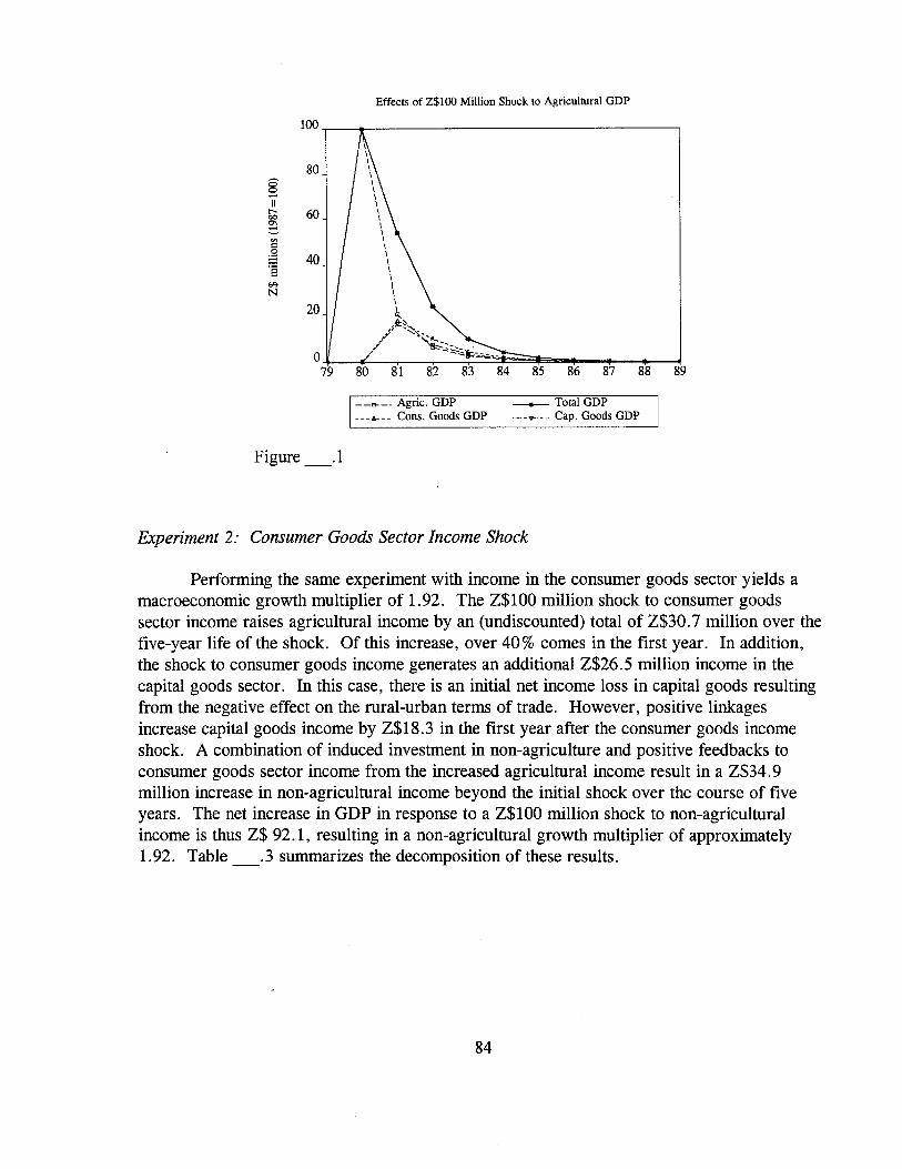
Effects of Z$l00 Million Shock to Agricultural GDP

100

80

§IIr- 6000:::~a 40.§~

N

20

80 81 82 83 84 85 86 87 88 89

--e--- Agric. GDP __ Total GDP---"'--- Cons. Goods GDP --'0--- Cap. Goods GDP

Figure_.1

Experiment 2: Consumer Goods Sector Income Shock

Performing the same experiment with income in the consumer goods sector yields amacroeconomic growth multiplier of 1.92. The Z$100 million shock to consumer goodssector income raises agricultural income by an (undiscounted) total of Z$30.7 million over thefive-year life of the shock. Of this increase, over 40% comes in the first year. In addition,the shock to consumer goods income generates an additional Z$26.5 million income in thecapital goods sector. In this case, there is an initial net income loss in capital goods resultingfrom the negative effect on the rural-urban terms of trade. However, positive linkagesincrease capital goods income by Z$18.3 in the first year after the consumer goods incomeshock. A combination of induced investment in non-agriculture and positive feedbacks toconsumer goods sector income from the increased agricultural income result in a Z$34.9million increase in non-agricultural income beyond the initial shock over the course of fiveyears. The net increase in GDP in response to a Z$100 million shock to non-agriculturalincome is thus Z$ 92.1, resulting in a non-agricultural growth multiplier of approximately1.92. Table _.3 summarizes the decomposition of these results.

84

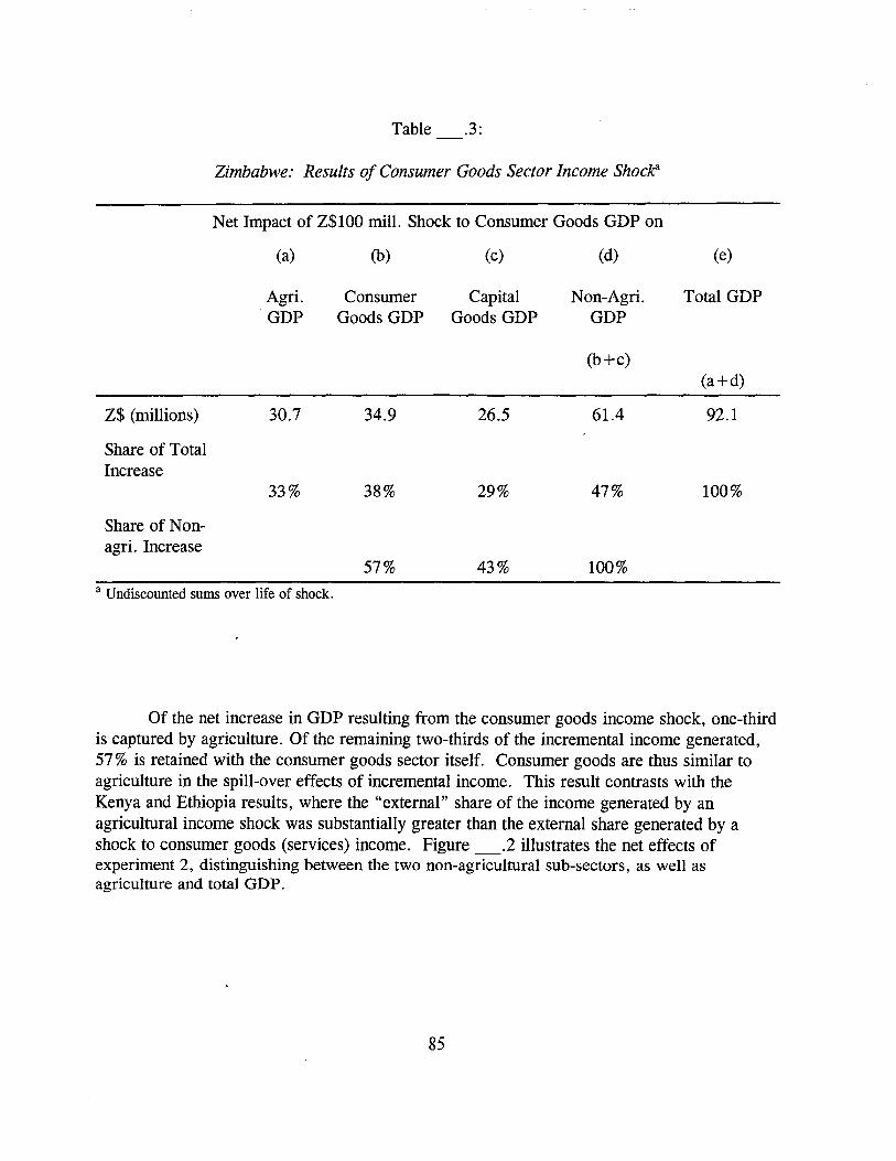
Table .3:

Zimbabwe: Results of Consumer Goods Sector Income Shock:

Net Impact of Z$100 mill. Shock to Consumer Goods GDP on

(a) (b) (c) (d) (e)

Agri. Consumer Capital Non-Agri. Total GDPGDP Goods GDP Goods GDP GDP

(b+c)(a+d)

Z$ (millions) 30.7 34.9 26.5 61.4 92.1

Share of TotalIncrease

33% 38% 29% 47% 100%

Share of Non-agri. Increase

57% 43% 100%

a Undiscounted sums over life of shock.

Of the net increase in GDP resulting from the consumer goods income shock, one-thirdis captured by agriculture. Of the remaining two-thirds of the incremental income generated,57 % is retained with the consumer goods sector itself. Consumer goods are thus similar toagriculture in the spill-over effects of incremental income. This result contrasts with theKenya and Ethiopia results, where the "external" share of the income generated by anagricultural income shock was substantially greater than the external share generated by ashock to consumer goods (services) income. Figure .2 illustrates the net effects ofexperiment 2, distinguishing between the two non-agricultural sub-sectors, as well asagriculture and total GDP.

85

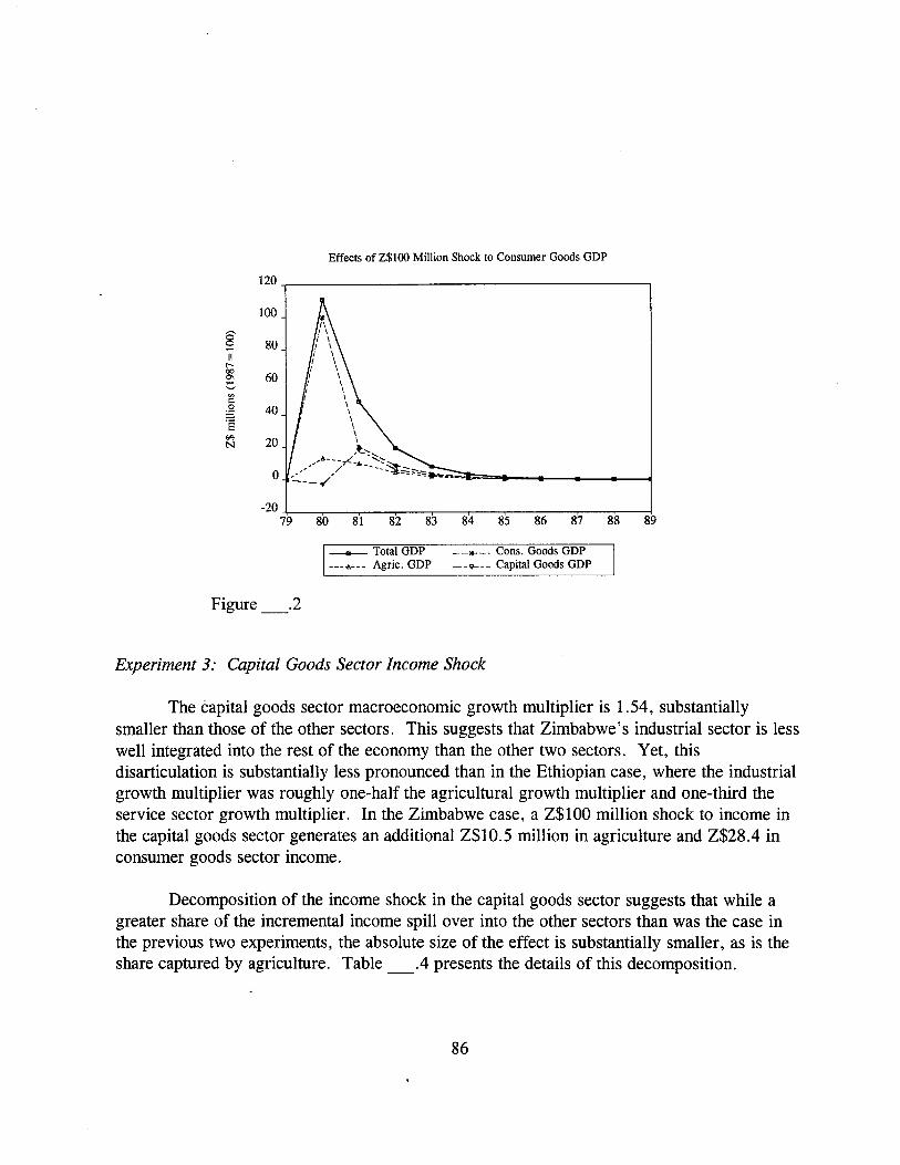
Effects of Z$I00 Million Shock to Consumer Goods GDP

120

100

@ 80II

t"-oo

60::::~

onC] 40'§<17 20N

-20 -l--~-"----''----''-----::T'---:T:--=--=--"':'':""""---::l_79 80 81 82 83 84 85 86 87 88 89

__ Total GDP __ __ Cons. Goods GDP----6--- Agric. GDP -- -- Capital Goods GDP

Figure_.2

Experiment 3: Capital Goods Sector Income Shock

The capital goods sector macroeconomic growth multiplier is 1.54, substantiallysmaller than those of the other sectors. This suggests that Zimbabwe's industrial sector is lesswell integrated into the rest of the economy than the other two sectors. Yet, thisdisarticulation is substantially less pronounced than in the Ethiopian case, where the industrialgrowth multiplier was roughly one-half the agricultural growth multiplier and one-third theservice sector growth multiplier. In the Zimbabwe case, a Z$100 million shock to income inthe capital goods sector generates an additional Z$1O.5 million in agriculture and Z$28.4 inconsumer goods sector income.

Decomposition of the income shock in the capital goods sector suggests that while agreater share of the incremental income spill over into the other sectors than was the case inthe previous two experiments, the absolute size of the effect is substantially smaller, as is theshare captured by agriculture. Table _.4 presents the details of this decomposition.

86

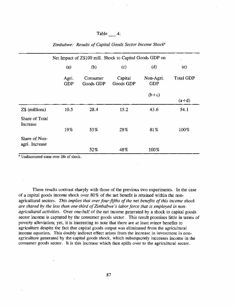
Table .4:

Zimbabwe: Results of Capital Goods Sector Income Shock:

Net Impact of Z$100 mill. Shock to Capital Goods GDP on

(a) (b) (c) (d) (e)

Agri. Consumer Capital Non-Agri. Total GDPGDP Goods GDP Goods GDP GDP

(b+c)(a+d)

Z$ (millions) 10.5 28.4 15.2 43.6 54.1

Share of TotalIncrease

19% 53% 28% 81 % 100%

Share of Non-agri. Increase

52% 48% 100%

a Undiscounted sums over life of shock.

These results contrast sharply with those of the previous two experiments. In the caseof a capital goods income shock over 80% of the net benefit is retained within the non­agricultural sectors. This implies that over four-fifths of the net benefits of this income shockare shared by the less than one-third ofZimbabwe's labor force that is employed in non­agricultural activities. Over one-half of the net income generated by a shock to capital goodssector income is captured by the consumer goods sector. This result promises little in terms ofpoverty alleviation; yet, it is interesting to note that there are at least minor benefits toagriculture despite the fact that capital goods output was eliminated from the agriculturalincome equation. This doubly indirect effect arises from the increase in investment in non­agriculture generated by the capital goods shock, which subsequently increases income in theconsumer goods sector. It is this increase which then spills over to the agricultural sector.

87

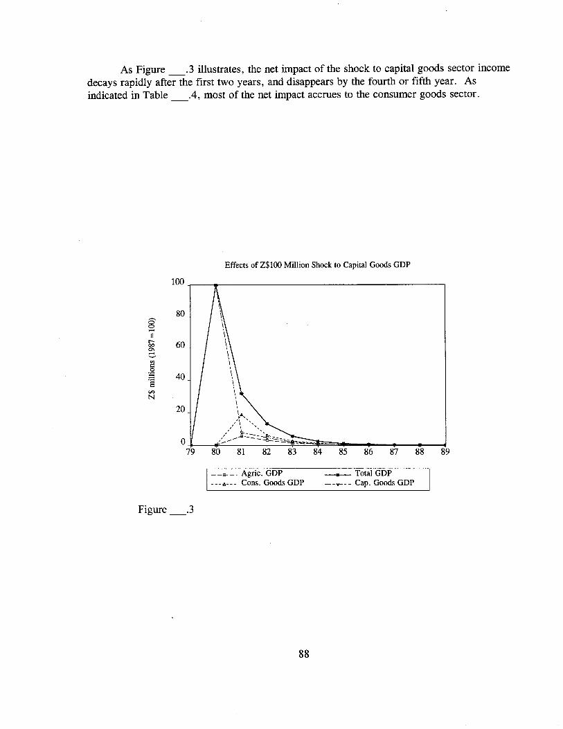
As Figure _.3 illustrates, the net impact of the shock to capital goods sector incomedecays rapidly after the first two years, and disappears by the fourth or fifth year. Asindicated in Table _.4, most of the net impact accrues to the consumer goods sector.

Effects of Z$l00 Million Shock to Capital Goods GDP

100

808'.....II

r- 60000\.....'-"

'"=a 40Os~

N

20

Figure_.3

--8--- Agric. GDP---~--- Cons. Goods GDP

88

__ TotalGDP--'i'--- Capo Goods GDP

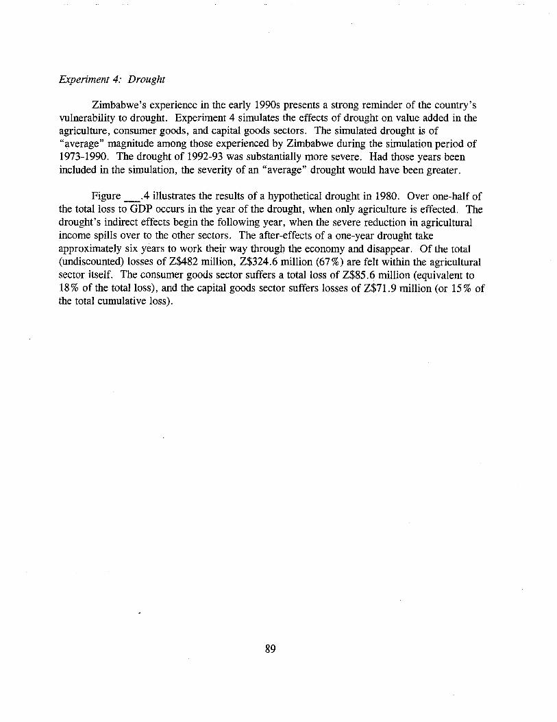
Experiment 4: Drought

Zimbabwe's experience in the early 1990s presents a strong reminder of the country'svulnerability to drought. Experiment 4 simulates the effects of drought on value added in theagriculture, consumer goods, and capital goods sectors. The simulated drought is of"average" magnitude among those experienced by Zimbabwe during the simulation period of1973-1990. The drought of 1992-93 was substantially more severe. Had those years beenincluded in the simulation, the severity of an "average" drought would have been greater.

Figure _.4 illustrates the results of a hypothetical drought in 1980. Over one-half ofthe total loss to GDP occurs in the year of the drought, when only agriculture is effected. Thedrought's indirect effects begin the following year, when the severe reduction in agriculturalincome spills over to the other sectors. The after-effects of a one-year drought takeapproximately six years to work their way through the economy and disappear. Of the total(undiscounted) losses of Z$482 million, Z$324.6 million (67 %) are felt within the agriculturalsector itself. The consumer goods sector suffers a total loss of Z$85.6 million (equivalent to18% of the total loss), and the capital goods sector suffers losses of Z$71.9 million (or 15% ofthe total cumulative loss).

89

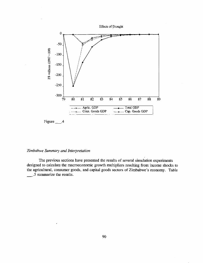
Effects of Drought

89-300 +---,---....,---,---,.----,---r---,...---,-----r---j

79 80 81 82 83 84 85 86 87 88

-50..-..8- -100IIr-oo0--'-' -150tilI::

~] -200V7N

-250

--8--- Agric. GDP---,!,.--- Cons. Goods GDP

__ TotaIGDP--,-.....-- Cap. Goods GDP

Figure_.4

Zimbabwe Summary and Interpretation

The previous sections have presented the results of several simulation experimentsdesigned to calculate the macroeconomic growth multipliers resulting from income shocks tothe agricultural, consumer goods, and capital goods sectors of Zimbabwe's economy. Table

.5 summarize the results.

90

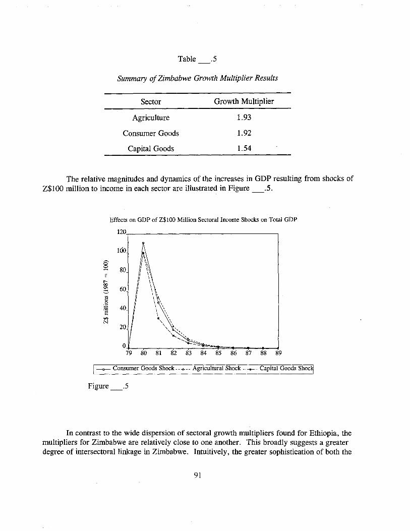
Table .5

Summary ofZimbabwe Growth Multiplier Results

Sector

Agriculture

Consumer Goods

Capital Goods

Growth Multiplier

1.93

1.92

1.54

The relative magnitudes and dynamics of the increases in GDP resulting from shocks ofZ$100 million to income in each sector are illustrated in Figure _.5.

Effects on GDP of Z$l00 Million Sectoral Income Shocks on Total GDP

120

160,....,§ 80

r--000\ 60.....'-'tilC.e·s 40"'7N

20

079 80 81 82 83 84 85 86 87 88 89

1-9- Consumer Goods Shock -- -l>- -- Agricultural Shock - - Capital Goods Shoc§

Figure_.5

In contrast to the wide dispersion of sectoral growth multipliers found for Ethiopia, themultipliers for Zimbabwe are relatively close to one another. This broadly suggests a greaterdegree of intersectoral linkage in Zimbabwe. Intuitively, the greater sophistication of both the

91

physical and market infrastructure in Zimbabwe support the conclusion implied by themultipliers. It may also be the case that Zimbabwe's isolation from international tradefollowing UDI forced the economy to function more effectively as a single unit. Enforcedimport substitution might have led to greater sectoral integration than would have occuredgiven greater opportunities for trade.

As in the Ethiopian case, the growth multiplier associated with capital goodsproduction (industry in the Ethiopian case) is substantially lower than in either of the othersectors. Industry in Zimbabwe is not an enclave to the same extent as was found in Ethiopia;yet, as discussed below, the present results would not support an emphasis on industrialgrowth as a vehicle for poverty alleviation in Zimbabwe.

The growth multipliers clearly illustrate the substantial importance of agriculture toecononomic growth in Zimbabwe. The intersectorallinkages are such that a $1.00 incomeshock in agriculture generates an additional $0.93 income, over two-thirds of which is externalto the agricultural sector itself.

It does not follow, however, that the similar magnitude of the consumer goods grwothmultiplier in Zimbabwe implies that consumer goods production has the same implications asagriculture for Zimbabwe's economic growth. An ideal situation is one in which income inthese sectors grow together. Yet, the ultimate foundation for much of the income generated inthe consumer goods sector lies in agricultural output. Consumer goods income, in part, isgenerated by such activities as marketing agricultural commodities or engaging in internationaltrade with foreign currency largely earned by agricultural exports. Moreover, to the extentthat the demand for consumer goods depends on agricultural incomes, it is difficult to envisionsustained growth in consumer goods income with a stagnant agricultural sector.

Economic development aims primarily at poverty alleviation. While Zimbabwe'sagricultural sector earns only 12% of GDP, it continues to employ over 65 % of the laborforce. This fact alone points clearly to the rural nature of Zimbabwe's poverty. The resultspresented above shed some light on the distributional implcations of sectoral growth.

A $1.00 increase in agricultural income ultimately results in a $1.30 increase inagricultural income and a $0.63 increase in non-agriculutral income. In this case, two-thirdsof the increased income ($1.30) is shared by approximately two-thirds of the labor force (e.g. ,the share employed in agriculture). In contrast, a $1.00 increase in consumer goods incomeultimately increases non-agricultural income by $1.61 and agricultural income by $0.31. Inthis case, 84% of the increased income is shared by 35 % of the labor force (the shareemployed in non-agriculture). The agricultural labor force (65 % of the labor force andgenerally poorer to begin with) would share the $0.31 -- only 16% of the total income increasefrom a shock to consumer goods.

92

In terms of the "sharing" factor, a shock to capital goods income is the mostregressive. In that case, a $1.00 shock ultimately increases non-agricultural income by $1.44and increases agricltural income by $0.11. Thus, fully 93 % of the total income increase isshared by only 35 % of the labor force, while the 65 % of the labor force employed inagriculture shares 7% of the increase.

A concern for poverty alleviation thus points clearly to agriculture as the most efficientsectoral vehicle. In addition, the growth multiplier results presented above indicate that aconcentration on agriculture would also make the maximum contribution to Zimbabwe'seconomic growth.

93

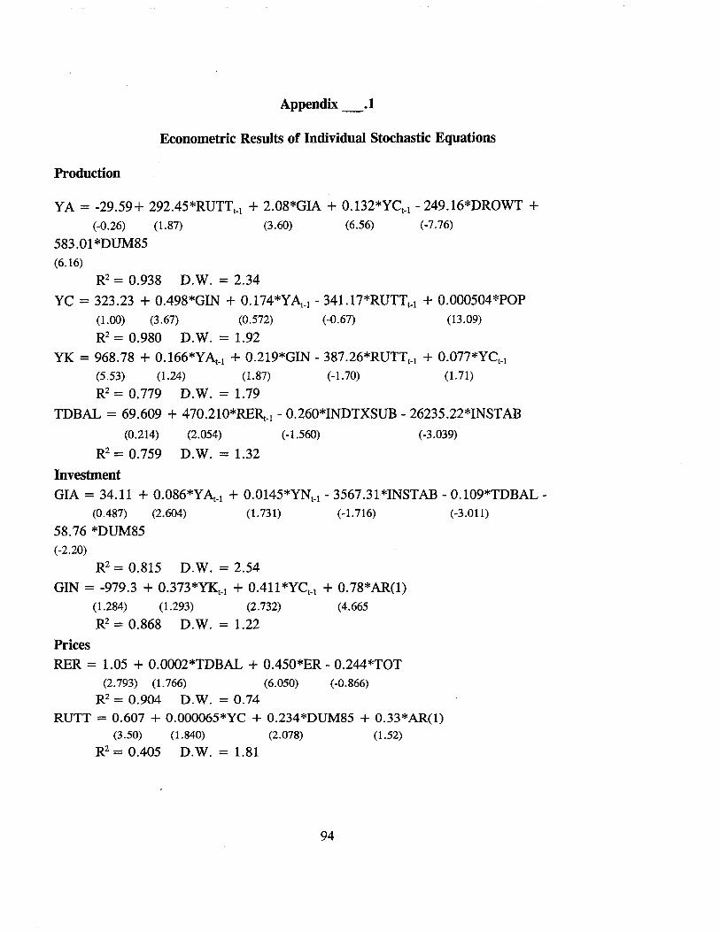
Appendix _.1

Econometric Results of Individual Stochastic Equations

Production

YA = -29.59+ 292.45*RUTTt' l + 2.08*GIA + 0.132*YCt•1 - 249. 16*DROWT +(-0.26) (1.87) (3.60) (6.56) (-7.76)

583.01*DUM85(6.16)

R2 = 0.938 D.W. = 2.34

YC = 323.23 + 0.498*GIN + 0.174*YAt_1 - 341.17*RUTTt•1 + 0.000504*POP(1.00) (3.67) (0.572) (-0.67) (13.09)

R2= 0.980 D.W. = 1.92YK = 968.78 + 0.166*YAt_1 + 0.219*GIN - 387.26*RUTTt_1 + 0.077*YCt_1

(5.53) (1.24) (1.87) (-1.70) (1.71)

R2= 0.779 D.W. = 1.79

TDBAL = 69.609 + 470.21O*RERr.l - 0.260*INDTXSUB - 26235.22*INSTAB(0.214) (2.054) (-1.560) (-3.039)

R2= 0.759 D.W. = 1.32

InvestmentGIA = 34.11 + 0.086*YAt• 1 + 0.0145*YNt_1 - 3567.31*INSTAB - 0.109*TDBAL-

(0.487) (2.604) (1.731) (-1.716) (-3.011)

58.76 *DUM85(-2.20)

R2 = 0.815 D.W. = 2.54

GIN = -979.3 + 0.373*YKt• 1 + 0.411 *YCt• 1 + 0.78*AR(1)(1.284) (1.293) (2.732) (4.665

R2 = 0.868 D.W. = 1.22

PricesRER = 1.05 + 0.0002*TDBAL + 0.450*ER - 0.244*TOT

(2.793) (1.766) (6.050) (-0.866)

R2 = 0.904 D.W. = 0.74

RUTT = 0.607 + 0.000065*YC + 0.234*DUM85 + 0.33*AR(1)(3.50) (1.840) (2.078) (1.52)

R2= 0.405 D.W. = 1.81

94

Appendix _.3

Augmented Dickey~Fuller Test Results

Table A3.1 provides the results of Augmented Dickey-Fuller tests of model's underlyingseries. In accordance with the Engle-Granger method, after having pre-tested the order ofintegration of each series, cointegration of the series in the individual equations is establishedby the stationarity of the residuals from those equations. Appropriate stationarity (ADF) testsof these residuals are reported in Table A3.2. The null hypothesis in an ADF test is theexistence of a unit root (indicating non-stationarity). An ADF test statistic that exceeds theMacKinnon critical value indicates rejection of that null hypothesis suggesting the stationarityof the series. This is the case for each equation in the model.

95

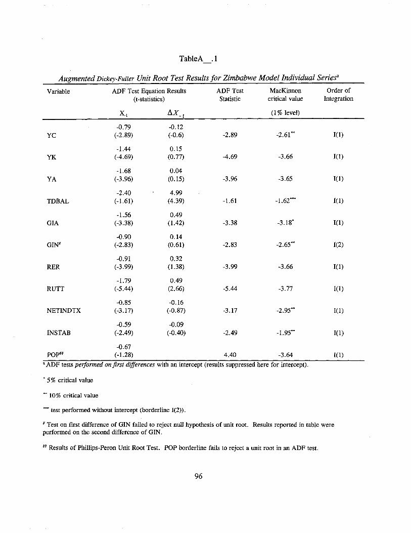
TableA .1

Augmented Dickey-Fuller Unit Root Test Results for Zimbabwe Model Individual Seriesa

Variable ADF Test Equation Results ADF Test MacKinnon Order of(t-statistics) Statistic critical value Integration

X. I D..X_1

(l % level)

-0.79 -0.12YC (-2.89) (-0.6) -2.89 -2.61** 1(1)

-1.44 0.15YK (-4.69) (0.77) -4.69 -3.66 1(1)

-1.68 0.04YA (-3.96) (0.15) -3.96 -3.65 1(1)

-2.40 4.99TDBAL (-1.61) (4.39) -1.61 -1.62*** l(l)

-1.56 0.49GIA (-3.38) (1.42) -3.38 -3.18* 1(1)

-0.90 0.14GINH (-2.83) (0.61) -2.83 -2.65** 1(2)

-0.91 0.32RER (-3.99) (1.38) -3.99 -3.66 1(1)

-1.79 0.49RUTT (-5.44) (2.66) -5.44 -3.77 1(1)

-0.85 -0.16NETINDTX (-3.17) (-0.87) -3.17 -2.95** 1(1 )

-0.59 -0.09INSTAB (-2.49) (-0.40) -2.49 -1.95** l(l)

-0.67POpiH (-1.28) 4.40 -3.64 1(1)

a ADF tests peTjormed on first differences with an intercept (results suppressed here for intercept).

*5% critical value

** 10% critical value

*** test performed without intercept (borderline 1(2».

H Test on first difference of GIN failed to reject null hypothesis of unit root. Results reported in table wereperformed on the second difference of GIN.

HH Results of Phillips-Peron Unit Root Test. POP borderline fails to reject a unit root in an ADF test.

96

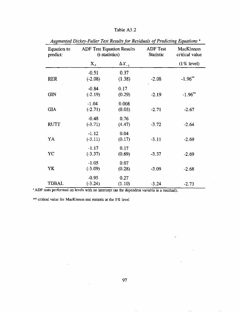
Table A3.2

Augmented Dickey-Fuller Test Results for Residuals of Predicting Equations a

Equation to ADF Test Equation Results ADF Test MacKinnonpredict: (t-statistics) Statistic critical value

X.1 !:1X_1

(l % level)

-0.51 0.37RER (-2.08) (1.38) -2.08 -1.96**

-0.84 0.17GIN (-2.19) (0.29) -2.19 -1.96**

-1.04 0.008GIA (-2.71) (0.03) -2.71 -2.67

-0.48 0.76RUTT (-3.71) (4.47) -3.72 -2.64

-1.12 0.04YA (-3.11) (0.17) -3.11 -2.69

-1.17 0.17YC (-3.37) (0.69) -3.37 -2.69

-1.05 0.07YK (-3.09) (0.28) -3.09 -2.68

-0.95 0.27TDBAL (-3.24) (1.10) -3.24 -2.73

a ADF tests performed on levels with no intercept (as the dependent variable is a residual).

** critical value for MacKinnon test statistic at the 5% level

97

Appendix .4

Descriptive Statistics and Graphs for the Simulation Base Run

Table A4.1

Root Mean Squared Errors and Root Mean Squared Percentage Errors for Base Run

Variable RMSE RMSPE

YFACP 348.8 5.2

YMKTP 348.8 4.6

CONP 236.1 5.1

YN 281.6 4.9

GI 369.9 33.1

YC 209.5 4.8

YK 114.9 8.4

YA 112.3 11.8

TDBAL 151.9 296.0

GIA 24.7 17.9

GIN 315.4 29.1

RER 0.1 6.7

RUTT 0.1 15.0

RMSE = root mean square error RMSPE = root mean square percentage error

98

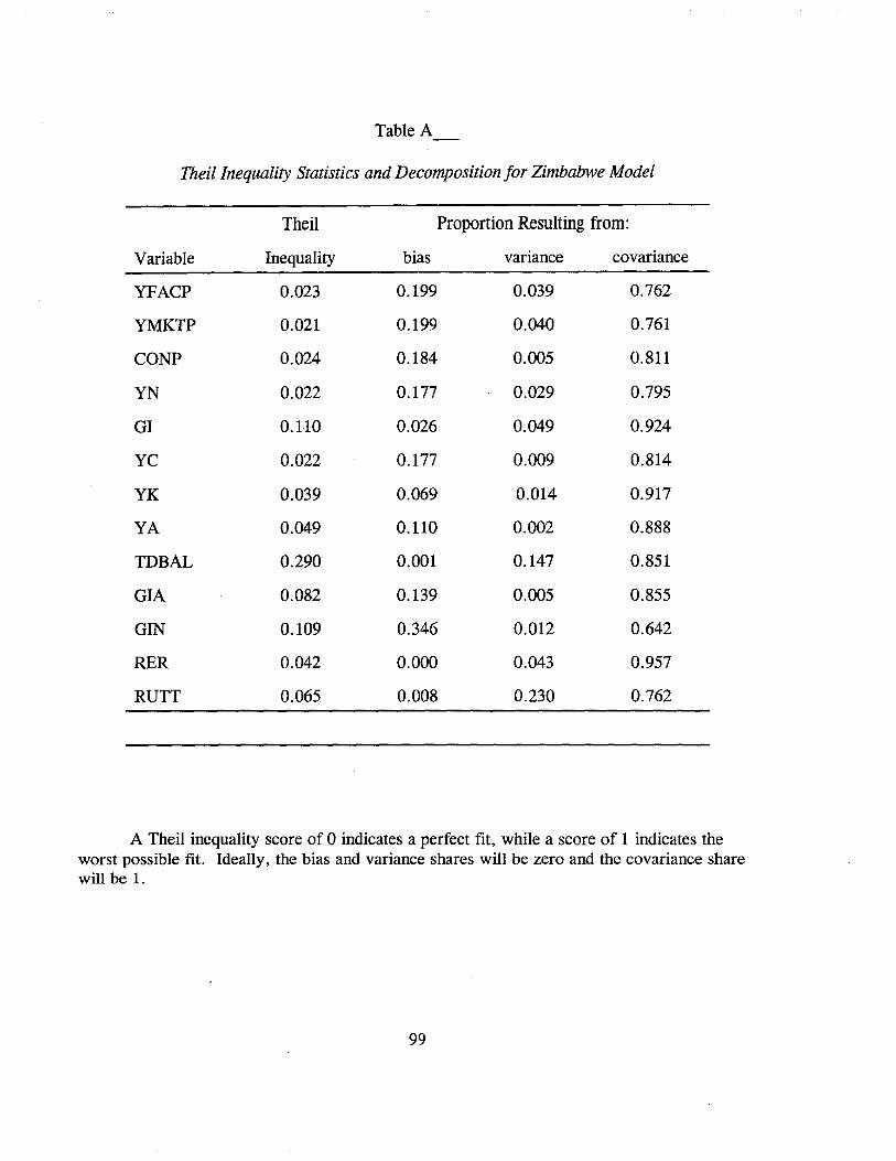
Table A

Theil Inequality Statistics and Decomposition for Zimbabwe Model

Theil Proportion Resulting from:

Variable Inequality bias variance covariance

YFACP 0.023 0.199 0.039 0.762

YMKTP 0.021 0.199 0.040 0.761

CONP 0.024 0.184 0.005 0.811

YN 0.022 0.177 0.029 0.795

GI 0.110 0.026 0.049 0.924

YC 0.022 0.177 0.009 0.814

YK 0.039 0.069 0.014 0.917

YA 0.049 0.110 0.002 0.888

TDBAL 0.290 0.001 0.147 0.851

GIA 0.082 0.139 0.005 0.855

GIN 0.109 0.346 0.012 0.642

RER 0.042 0.000 0.043 0.957

RUTT 0.065 0.008 0.230 0.762

A Theil inequality score of 0 indicates a perfect fit, while a score of 1 indicates theworst possible fit. Ideally, the bias and variance shares will be zero and the covariance sharewill be 1.

99

REFERENCES

Berthelemy, J.C., and C. Morrisson (1989) "Agricultural Development in Africa and theSupply of Manufactured Goods. OECD Development Centre Studies, Paris:Organization for Economic Cooperation and Development.

Cheater, A. & J.C. Jackson (1994) Contract Fanning in Zimbabwe: Case Studies of Sugar,Tea, and Cotton In: P. D. Little & M. J. Watts (Eds) Living Under Contract:Contract Fanning and Agrarian Transjonnation in Sub-Saharan Africa The Universityof Wisconsin Press, Madison, WI, USA.

Dawe, David (1996) "A New Look at the Effects of Export Instability on Investment andGrowth," World Development, December.

Economist (1995) Zimbabwe: Taking Risks October 21, 1995 335:(7937) p 46.

Economist Intelligence Unit (1995) Zimbabwe Country Profile: 1994-1995 London, UK.

Economist Intelligence Unit (1996) Zimbabwe Country Report: Second Quarter 1996London, UK.

Johnston, B. F., and J. Mellor (1961) "The Role of Agriculture in Economic Development,"American Economic Review 51(4), 566-593.

MacGarry, B. (1993) Growth? Without equity? : the Zimbabwe economy and the EconomicStructural Adjustment Programme. Gweru, Zimbabwe : Mambo Press in associationwith Silveira House. Silveira House social series; no. 4.

Masters, W. (1994) Government and Agriculture in Zimbabwe Praeger, Westport, CT,USA.

Moyo, et. al. (1991) Zimbabwe's Environmental Dilemma: Balancing Resource InequitiesZimbabwe Environmental Research Org. (ZERO), Harare, Zimbabwe.

Rukuni, M. (1990) The Development ojZimbabwe's Agriculture: 1890-1990 AgriculturalEconomics and Extension Working Paper 7/90, University of Zimbabwe, Harare,Zimbabwe.

Thirtle, C., et. al. (1993) "Agricultural Productivity in Zimbabwe, 1970-90," The EconomicJournal, 103 (March), 474-480.

100

Timmer, C. Peter (1991) "Food Price Stabilization: Rationale, Design, and Implementation,"in Reforming Economic Systems, D. Perkins and M. Roemer, eds. Cambridge, MA:Harvard Institute for International Development.

Stoneman, C. & L. Cliffe, (1989) Zimbabwe: Politics, Economics, and Society PrinterPublishers, London, UK.

Sylvester, C. (1991) Zimbabwe: The Terrain of Contradictory Development WestviewPress, Boulder, CO, USA.

Zinyama, L. (1992) Local Farmer Organizations and Rural Development in Zimbabwe In:D. R. F. Taylor & F. Mackenzie (Eds) Development From Within: Survival in RuralAfrica Routledge, London, UK.

101

5. KENYA CASE STUDY

5.1 Introduction

This paper examines the relative contributions of agriculture and non-agriculture toKenya's economic growth. While it is well established that agricultural income growth givesrise through intersectorallinkages to the generation of non-agricultural income, the magnitudeof these effects is rarely measured at the macroeconomic level. Regional-level studies providedetailed growth multipliers, but do not speak directly to the question of economic growth.The numerical simulation model presented in this paper furnishes intersectoral growthmultipliers for national income. The essential result is that the growth multiplier for Kenyanagriculture is two and one-half times the magnitude of the growth multiplier for non­agriculture.

The growth linkages literature has focussed almost exclusively on the regional level,using household-level data to measure the forward and backward linkages arising from bothproduction and consumption in the agricultural sector. This literature provides a fIrmempirical foundation for the Johnston-Mellor linkages between agriculture and non-agricultureJohnston and Mellor (1961). The use of household-level data permits the specificmeasurement of the various types of inter-sectoral linkages, the combined effects of which aresummarized in a growth mUltiplier. The methodology employed in those studies, however,limits the interpretation of their multipliers to the regional level. These multipliers cannot beapplied directly to the level of national income because the assumptions necessary for theircalculation in those studies do not hold at the national level. 1

The model presented below builds on the findings of those regional-level studies andcomplements their perspective: the growth linkage studies capture the richness of the localeconomies but their results do not apply directly to national income; the simulation modelpresented below measures agricultural growth multipliers at the national income level, butdoes not explicitly model the microeconomic linkages.

1The chief culprit in this regard is the semi-input-output models' assumption of a perfectly elastic supplyof non-tradables. Moreover, the studies tend to be based on regional data, which may not represent an entirecountry.

102

5.2 Model Specification2

The goal of this model is to replicate Kenya I s economic growth from 1972-92 as afunction of growth in two sectors (agriculture and non-agriculture) and the interaction betweenthem. In other words, output growth in agriculture adds directly to Kenya's overall economicgrowth in proportion to the sector's share of GDP. Yet, by taking account of the intersectorallinkages between agriculture and non-agriculture, the model attempts in addition to measureagriculture's indirect contribution to overall economic growth through agriculture'scontribution to growth in non-agriculture. Similarly, the model attempts to capture thefeedbacks from non-agriculture to agriculture, thus providing a basis for comparing therelative contributions of each sector to overall growth.

The model is intended to be as simple as possible, and is thus limited to a level ofaggregation that can barely begin to capture the full complexity and richness of the underlyingprocesses. Its primary purpose is to measure the extent of the intersectoral linkages in thegrowth process, rather than to serve as a tool for detailed policy simulation. Data are drawnfrom the national accounts and related sources from the Government of Kenya. These datahave been collected in historical time series in an extremely useful report by the KenyanMinistry of Planning and National Development.3

As noted above, the first goal of the model is to replicate the actual historical paths ofkey macroeconomic and sectoral variables. Once a model is accepted as accurately describingwhat did happen, it can be used for various counter factual experiments to assess what wouldhave happened had particular conditions been different. The simulated time paths for the"key" variables (e.g., the endogenous variables) are determined within the model. These areestimated as functions of variables that are not simulated within the model (e.g., exogenousvariables) and past values for the endogenous variables. Since the predicted value for a givenendogenous variable depends on predicted values of other endogenous variables, the modelitself consists of a system of inter-related equations each of which is used to predict the valueof one endogenous variable. The model includes thirteen endogenous variables, and thirteenequations (which are presented in Table 1).

2 The specification of this model is similar to Rangarajan (1982), though the present model differs fromRangarajan's in several key respects. The most critical difference is that agricultural value added is endogenousin the present model.

3 Short, Keyfitz, and Maundu (1994). The disaggregation of agricultural and non-agriculturalinvestment by public versus private sources is based on further research by that Ministry (Wilson, 1993).

103

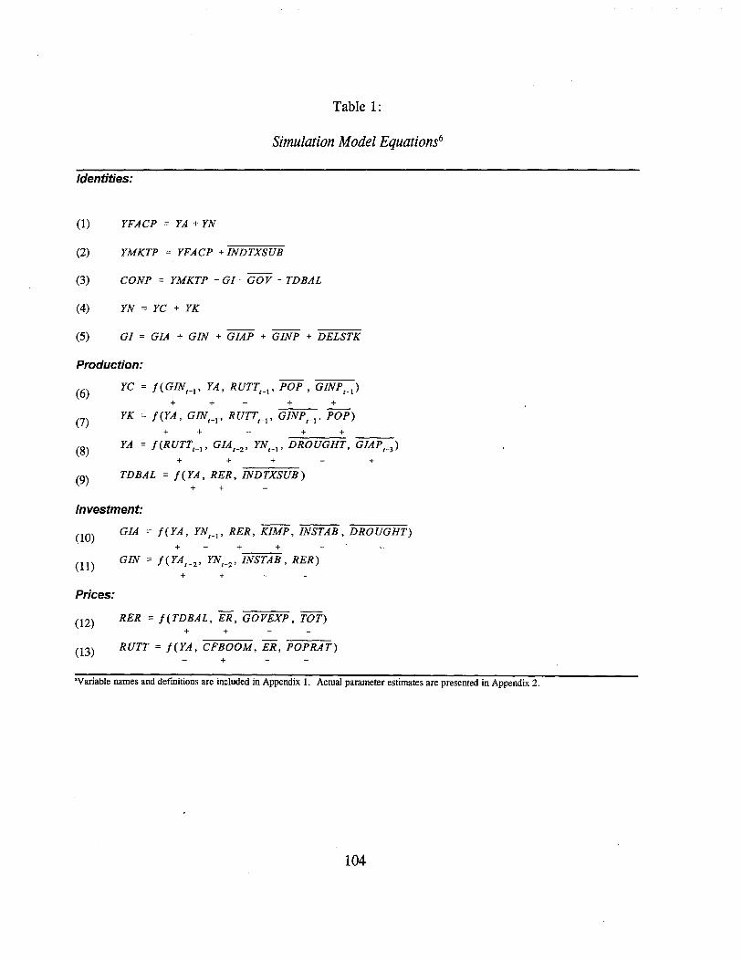
Table 1:

Simulation Model Equations6

Identities:

(1) YFACP = YA + YN

(2) YMKTP = YFACP + INDTXSUB

(3) CONP = YMKTP - GI - GOV - TDBAL

(4) YN = YC + YK

(5) GI = GIA + GIN + GIAP + GINP + DELSTK

++++(6)

Production:

YC = !(GINt-!, YA, RUTTt-!, POP, GINPH )

YK = !(YA, GINt-!' RUTTH , GINPt _1 " POP)(7)

+ + + +

(8)+ + + +

(9) TDBAL = !(YA, RER, INDTXSUB)+ +

+

+ +

+--=-:-+GIN = !(YA t - Z ' YNt-2' INSTAB, RER)

(10)

Investment:

GIA = !(YA, YNt - 1 , RER, KIMP, INSTAB, DROUGHT)

(11)

Prices:

(12) RER = !(TDBAL, ER, GOVEXP, TOT)+ +

(13) RUTT = !(YA, CFBOOM, ER, POPRAT)+

'Variable names and definitions are included in Appendix 1. Actual parameter estimates are presented in Appendix 2.

104

The endogenous variables are on the left-hand side of the equations, and are determinedin each case by the right-hand side variables. Among the right-hand side variables, the laggedendogenous variables are indicated with time subscripts and the exogenous variables have barsover them. The sign beneath each variable indicates the direction of its estimated effect on thedependent variable. There are two aspects of these equations to be described: thespecification and estimation of the individual equations, and the manner in which theindividual equations relate to one another in the simulation model.

The model consists of five identities (equations (1) - (5)) and eight stochastic equations(equations (6) - (13)). The identities impose certain relationships on the results that mustalways hold, and thus ensure that the simulations conform to balanced national accounts.Equation (1) describes the income side of the economy, stipulating that GDP (at factor prices)must always be the sum of agricultural GDP and non-agricultural GDP. In the nationalincome accounts GDP at factor prices and GDP at market prices differ by indirect taxes andsubsidies (which are excluded from GDP at factor prices). Equation (2) simply ensures thatthis relationship is always true in the model. The distinction is necessary because in thenational accounts, the expenditure side of the economy is equated with GDP at market prices.

To be internally consistent, the model must ensure that national income equals nationalexpenditures. Thus equation (2) connects the income side of the economy with the expenditureside, which is expressed in equation (3). Equation (3) is the familiar mqcroeconomic equationstating that national income equals the sum of private consumption, gross investment,government consumption, and the trade balance (e.g., Y=C+I+G+X-M). In order to ensurethat the system balances (that income equals expenditure), private consumption is calculated asa residual in equation (3). As the Government of Kenya, in balancing its national accounts,calculates private consumption as a residual, this model simply adopts the same convention.

The remaining identities are definitions. Equation (4) divides non-agricultural GDPinto two components: value added from the production of consumer goods and value addedfrom the production of capital goods.4 Equation (5) similarly defines gross fixed investment asthe sum of private and public gross capital formation (investment) in agriculture and in non­agriculture, plus the change in capital stocks. Distinguishing private from public sectorinvestment in agriculture sharpens the model's focus on private-sector decision makers withineach sector. As described below, private sector investment decisions are endogenous, whilepublic sector investment in agriculture and non-agriculture is exogenous.

The remaining equations serve the purpose of predicting values for the endogenousvariables. These equations can be grouped into blocks, each of which serves a distinctpurpose within the model. Equations (6) - (9) determine output in each sector of the

4Capital goods include mining and quarrying, building and construction, electricity and water,transportation and coIrtmunications, and forestry (as an input to construction). Consumer goods are everythingelse that is not produced on farm.

105

economy.5 Investment supply by private sector sources is determined in equations (l0) and(11). The final block (equations (12) and (13» determines prices, which consist of the realexchange rate and the rural-urban terms of trade.

The distinction noted above between agriculture I s direct and indirect contributions togrowth can be seen at this point. Figure 1 is a simplified flow chart highlighting the inter­sectoral linkages specified in the model.

5 Strictly speaking, the trade balance (TDBAL) is not a productive sector, but is included in theproduction block for convenience.

106

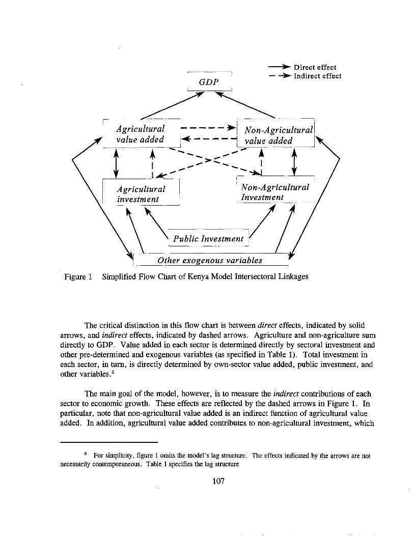
-----II~~ Direct effect- ~ Indirect effect

GDP

AgriC£ - ~riCUlturallvalue added l. - - - -""'""j value added I

t ~ ..... --- ----.. LI _->--_ II~ - - ,--~-="'-----

~-'-A-gr-i-c-u-lt-'-ur=a=l--,I .. Non-Agricultural I

investment I Investment i

\ Public Investment II

Other exogenous variables

Figure 1 Simplified Flow Chart of Kenya Model Intersectoral Linkages

The critical distinction in this flow chart is between direct effects, indicated by solidarrows, and indirect effects, indicated by dashed arrows. Agriculture and non-agriculture sumdirectly to GDP. Value added in each sector is determined directly by sectoral investment andother pre-determined and exogenous variables (as specified in Table 1). Total investment ineach sector, in turn, is directly determined by own-sector value added, public investment, andother variables.6

The main goal of the model, however, is to measure the indirect contributions of eachsector to economic growth. These effects are reflected by the dashed arrows in Figure 1. Inparticular, note that non-agricultural value added is an indirect function of agricultural valueadded. In addition, agricultural value added contributes to non-agricultural investment, which

6 For simplicity, figure 1 omits the model's lag structure. The effects indicated by the arrows are notnecessarily contemporaneous. Table 1 specifies the lag structure

107

increases non-agricultural value added, and thus adds to agriculture's indirect contribution togrowth. As indicated in Figure 1, these effects are specified symmetrically across sectors.Each sector thus has the same opportunities for indirect contributions to growth. The relativemagnitudes of these effects are determined by the data. The following description of theremaining equations in Table 1 details the rationale for the specification of inter-sectorallinkages illustrated in Figure 1.

Equations (6) - (8) determine the value added on the supply side of the economy.These equations are hybrid functions in that they are strictly neither supply nor demandequations, but contain elements of both. Equation (6) predicts income in the consumer goodssubsector as a function of lagged non-agricultural investment (both public and private inorigin), current agricultural output, lagged rural-urban terms of trade, and total population.

The presence of agricultural GDP in the output function for consumer goods reflectstwo types of intersectorallinkages. A recent study by USAID/Kenya shows that a substantialportion of consumer goods production depends directly on agriculture for its raw materials.Within Kenya's micro-enterprise sector, nearly one-half of these enterprises are based directlyon agriculture (and the figure is closer to two-thirds if one includes forestry and textiles)(Development Alternatives Inc., 1994). Abundant agricultural production would thus tend toreduce input costs in those industries and increase their output. At the same time, increasedagricultural production raises the incomes of agricultural producers, thus increasing theireffective demand for the outputs of consumer goods industries.

The highly short-run nature of these linkages (i.e., agricultural products used as non­agricultural inputs tend to be used within the same year as they were produced, and increasedfarm incomes to be spent on consumer goods may be spent soon after harvest) justify thecontemporaneous association between agricultural value added and non-agricultural valueadded.

As in each of the output equations, the explanatory variables for consumer goodsinclude lagged own-sector investment estimated separately for public and private sources.Both types of investment, along with agricultural output, positively affect consumer goodsoutput. The rural-urban terms of trade is the ratio of agricultural to non-agricultural prices.Considering food as a wage good for non-agricultural workers, the rural-urban terms of tradereflect the ratio between input costs and output prices facing non-agricultural employers. Therural-urban terms of trade thus enters negatively in equations (6) and (7). Population affectsboth production and consumption relations. Controlling for population (which, as expected,enters positively) eliminates potential bias due to population effects being wrongly attributed toagricultural output.

Equation (7) predicts the value added in capital goods industries, posited here to be afunction of lagged public and private non-agricultural investment, lagged rural-urban terms oftrade, agricultural output, and population. The inclusion of agriculture in this equation is

108

intended to reflect the increased demand for industrial products (including buildings andconstruction, electricity, and water) on the part of the agricultural sector resulting fromincreased agricultural output.

Equation (8) describes the value added in agriculture as a function of the lagged rural­urban terms of trade, lagged non-agricultural output, drought, and lagged public and privateagricultural investment. Lagged non-agricultural output enters the agriculture equation toreflect the fact that non-agriculture both supplies inputs for agricultural production andpurchases agricultural output. Both effects are enhanced by increased output in non­agriculture. The nature of agricultural planting cycles, however, in which most purchasednon-agricultural inputs must be in place at planting time, dictates that non-agricultural valueadded enter the agricultural output equation with a one-period lag. 7 The rural-urban terms oftrade are the price incentives facing agricultural producers (e.g., the prices of what they sellrelative to the prices of what they buy), and thus enter positively into equation (8). The rolesof drought and agricultural investment are straightforward.

Equation (9) predicts the trade balance, which is required to fill in the expenditure sideof the economy as described in equation (3). The trade balance is estimated as a function ofthe foreign terms of trade, as well as agricultural output, indirect taxes (the vast majority ofwhich are import and export duties), and the real exchange rate (which is also endogenouslydetermined). A real depreciation (defined here as an increase in the real exchange rate)improves the trade balance, as does increased agricultural output (agriculture accounted for54% of Kenya's total foreign exchange earnings between 1972-92). Trade tax~s are negativelyrelated to the trade balance.

Equations (10) and (11) describe gross private sector capital formation in agricultureand non-agriculture, respectively. Private sector agricultural investment is estimated inequation (10) as a function of capital imports, lagged output in non-agriculture, agriculturaloutput, the real exchange rate, a proxy for general economic instability, and drought. Laggedoutput in non-agriculture captures one direction of cross-sector investment. Interestingly, non­agricultural income enters negatively in determining agricultural investment. This may reflecta perception that investments in non-agriculture are safer, particularly when non-agriculturalincome increases. 8 Agricultural income can also be re-invested directly in agriculture, as is

7 As non-agricultural income is modeled as a contemporaneous function of agricultural income, equation(8) introduces an asymmetry into the model's lag structure which might appear to bias the subsequent multiplieranalysis in favor of agriculture. In fact, the model's intersectoral linkages and feedbacks, working in tandem withthe estimated parameters, are such that making agricultural income a contemporaneous function of non­agricultural value added does not change the non-agricultural growth multiplier, but actually increases theagricultural growth multiplier. The present lag structure is thus the more conservative approach

B Reardon, eL al. (1994) discuss conditions under which nonfarm income tends to be invested in non­agriculture.

109

reflected in the specification of equation (10). Agricultural income enters equation (10)without a lag, as a large share of agricultural investment by smallholders may be in-kind orinvestment made immediately after harvest (yet in the same year for national incomeaccounting purposes). The real exchange rate is included to reflect the increased supply ofagricultural capital sparked by improved opportunities for agricultural exports. Economicinstability (as reflected here by the deviation of actual from expected exports as a share ofGDP) is expected to have a negative influence on investment decisions. 9 Similarconsiderations enter the specification of non-agricultural investment.

Non-agricultural investment originating in the private sector is modeled in equation(11) as a function of lagged agricultural value added, lagged non-agricultural output, economicinstability, and the real exchange. Agriculture is thus modeled as a source of inter-sectoralinvestment capital. As expected, agricultural value added contributes positively to non­agricultural investment and economic instability is a disincentive to non-agriculturalinvestment. Unlike equation (10), non-agricultural investment is a lagged function of non­agricultural income. This reflects the relatively greater ,urban access to capital markets inwhich savings may be accrued over time to accomodate potentially larger or lumpierinvestments in non-agriculture.

Equations (12) and (13) predict prices. Equation (12) predicts the real exchange rate asa function of the foreign terms of trade (the price of exports relative to imports), thegovernment expenditures and the nominal exchange rate. Since GOK spending is stronglybiased in favor of non-tradables, it tends to be inflationary and thus causes the real exchangerate to appreciate. If government spending contributes to a fiscal deficit which the governmentfinances through higher inflation, the real exchange rate further appreciates. For both reasons,government expenditures enter negatively in determining the real exchange rate. The nominalexchange rate is a component of the real exchange rate. It is included here as an exogenousvariable through which the GOK might try to manage the real exchange rate (which is notdirectly under its control). The foreign terms of trade influence the real exchange rate. Whilethe expectation regarding its sign is not clear a priori, it makes sense that a country with anegative trade balance could experience a real depreciation when the terms of trade fall. Thiswould be true, for instance, if the government attempted to force faster nominal devaluationsto compensate for declining terms of trade.

Finally, equation (13) determines the rural-urban terms of trade. These relativedomestic prices are estimated as a function of the nominal exchange rate, agricultural output,and agricultural output, controlling additiona:Ily for Kenya's coffee boom (1975-77) and the

9 Dawe (1993) demonstrates the importance of this proxy in shaping both investment patterns andeconomic growth.

110

ratio of agricultural to non-agricultural population. 10 The nominal exchange rates influence therural-urban terms of trade to the extent that agriculture tends to be more tradable than non­agriculture. Thus a devaluation shifts relative prices in favor of agriculture. Increasedagricultural output, in contrast, tends to lower agricultural prices and reduce the rural-urbanterms of trade. The need to control for the ratio of agricultural to non-agricultural population,as well as its expected negative sign, follow from the standard dual sector development models(Lewis (1954), Fei-Ranis (1964), and Jorgenson (1966». This class of models suggest that themigration of labor from rural to urban areas places upwards pressure on the rural-urban termsof trade (at least in the absence of sufficiently rapid growth in agricultural productivity).Equation (13) controls for this effect.

10 The macroeconomic implications of Kenya's coffee boom are analyzed extensively in Bevan, Collier,and Gunning (1990), as well as in Bigsten and Collier (1995).

111

5.3 Estimation, Solution, and Validation of the Simulation Model

Each of the model's stochastic equations described above are estimated individually byordinary least squares using data from 1972-1992. The relationships are specified andestimated in levels, producing a set of coefficients which then provide the basis for simulatingthe endogenous series in levels. Cointegration of the series in each equation is tested andestablished by application of the Engle-Granger method. Appendix 3 presents the results ofAugmented Dickey-Fuller tests applied to the relevant residuals.

Once the individual equations of the model have been specified, estimated, and theircointegration established, the model's performance in simulating true historical time paths forthe endogenous variables depends on how well the individual equations work together as asystem. The system is dynamic in that the values predicted for the endogenous variables in agiven year depend on previous predictions for endogenous variables. The model's dynamicstructure becomes quite complicated as given changes have immediate effects which lead tosecond and third-round effects in the system.

An increase in agricultural GDP has several direct effects within the model. Inaddition to directly increasing total GDP (by definition in equation (1», and indirectlyincreasing GDP through its effect on non-agricultural output (equations (6) and (7»,agriculture increases the trade balance (equation (8», increases agricultural investment andnon-agricultural investment (equations (10) and (11», and lowers the rural-urban terms oftrade (equation (13». These effects spark a set of second-round effects. Increased outputincreases subsequent investment in both sectors, the lower rural-urban terms of trade reducesagricultural output next year (and increases non-agricultural output), and directly andindirectly increases future total GDP through the effect of increased investment on subsequentoutput in both sectors. These effects, in turn, have third round effects resulting fromincreased investment and changes in relative prices and output, and so on. Thus, even in thisrelatively simple model, the full chain of events can only be viewed by actual simulation.

Simulation involves simultaneously solving all thirteen equations, given starting valuesfor the endogenous variables and actual time paths for the exogenous variables. Thesimulation is dynamic in that endogenously predicted values are always used where laggedendogenous variables are explanatory variables in other equations. Thus the predictedoutcomes for a given year depend on the predicted outcomes for previous years. The result isa set of predicted time paths for the endogenous variables. One can then validate the modelbased on how good a job it does at recreating the actual paths followed by the endogenousvariables.

A statistical assessment of the accuracy of the base run is presented in Appendix 4. Ingeneral, the model does an excellent job of recreating Kenya's recent economic history. Ineach case except TDBAL, the root mean squared percentage error measuring the divergence ofthe predicted from the actual series was quite small (generally less than 5 %). In addition, the

112

Theil inequality statistics indicate an excellent fit between the predicted and actual series, withminimal bias. Once one is convinced that the model faithfully recreates actual events, it ispossible to perform counter factual experiments.

113

5.4 Simulation Results

This section describes the results of several simulations undertaken with the model. The mostsignificant results arise from using the model to calculate growth multipliers for agricultureand non-agriculture. Simulations for Kenya indicate that the growth multiplier fromagriculture is approximately two and one-half times the magnitude of the multiplier from non­agriculture. This result comes from having "shocked" the system with a one-time increase of100 million Kenyan pounds in 1982.

Experiment 1: Agricultural Income Shock

The agricultural growth multiplier derived from this simulation is 2.27. A 100 million Kenyanpound shock to agricultural value added increases non-agricultural value added by 92.8million Kenyan pounds cumulatively over a period of five years, and (by stimulating increasedinvestment within agriculture itself, as well as through feedbacks from increased non­agricultural income to increased agricultural income) increases agricultural value added insubsequent years by approximately 33.8 million Kenyan pounds beyond the initial shock of100 million. Shocking agricultural income by 100 million thus adds 227 million to total GDP.Net of the initial shock to agricultural value added, 73 % of the addition to GOP derives fromagriculture's contribution to non-agricultural income. This long-run multiplier is calculated asthe sum of the increases in total GOP over the entire period during which increases occurreddivided by the size of the initial shock. 11

Figure 2 illustrates this decomposition of the agricultural income shock into the netadditions to agricultural GDP, consumer goods GOP, capital goods GDP, and total GDP (theinitial shock is eliminated from figure 2, leaving the net effects). The shock to agriculturalincome illustrated in figure 2 hits in 1982, resulting in immediate increases in both consumerand capital goods GDP. The net additions to agricultural income in the first year followingthe shock result from feedback from increased non-agricultural income to increasedagricultural income. The increased agricultural income also contemporaneously increasesagricultural investment, which feeds back into increased agricultural income in the second yearfollowing the shock. The initial shock of K£ 100 million to agricultural income in 1982increases non-agricultural income (the sum of consumer goods GDP and capital goods GDP(equation (4)) by K£ 59 million in the first year, and by 6.6 million, 12.76 million, 7.54million, and 4.25 million during the next four years respectively, summing ultimately to a totaladdition of K£ 92.8 million (undiscounted) to non-agricultural income.

11 Note that in a linear model, the multiplier is insensitive to both the size and the timing of the shock.

114

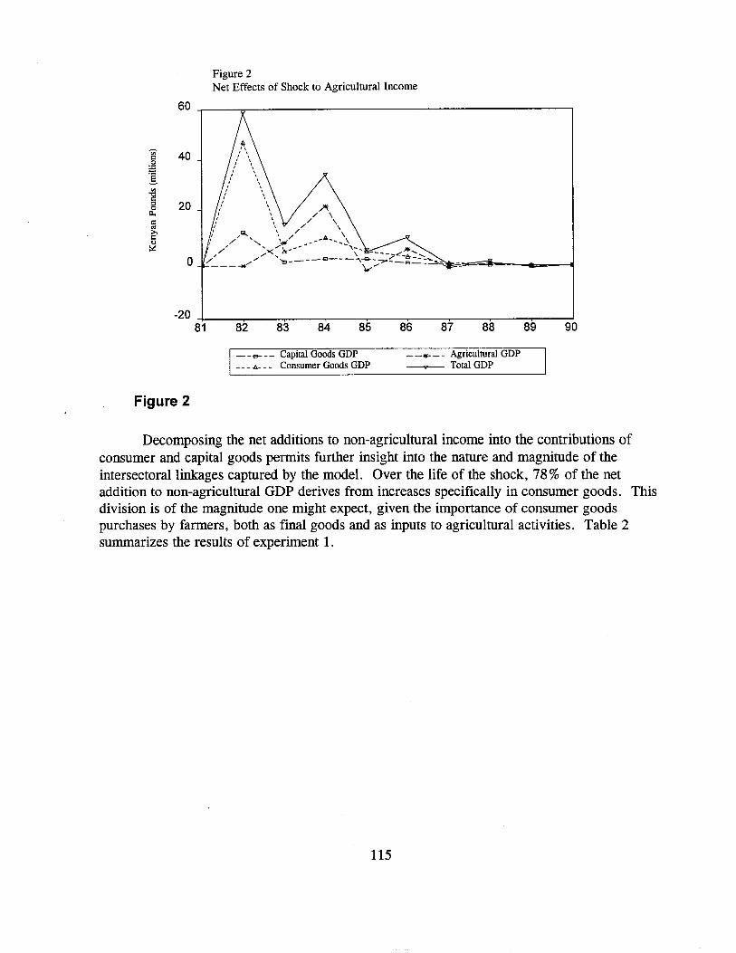
Figure 2Net Effects of Shock to Agricultural Income

60 -r-----;;----------------------,

-;;;- 40:::.sa

!'""8::l 200~

I::cd

~<)

~

0 -

-20 -+------r---,----.------,..----.----..--------.----,...------j81 82 83 84 85 86 87 88 89 90

Figure 2

- - e- - - Capital Goods GDP- - - ",,-- - _. Consumer Goods GDP

--ilf--- Agricultural GDP9 Total GDP

Decomposing the net additions to non-agricultural income into the contributions ofconsumer and capital goods permits further insight into the nature and magnitude of theintersectoral linkages captured by the model. Over the life of the shock, 78 % of the netaddition to non-agricultural GDP derives from increases specifically in consumer goods. Thisdivision is of the magnitude one might expect, given the importance of consumer goodspurchases by farmers, both as final goods and as inputs to agricultural activities. Table 2summarizes the results of experiment 1.

115

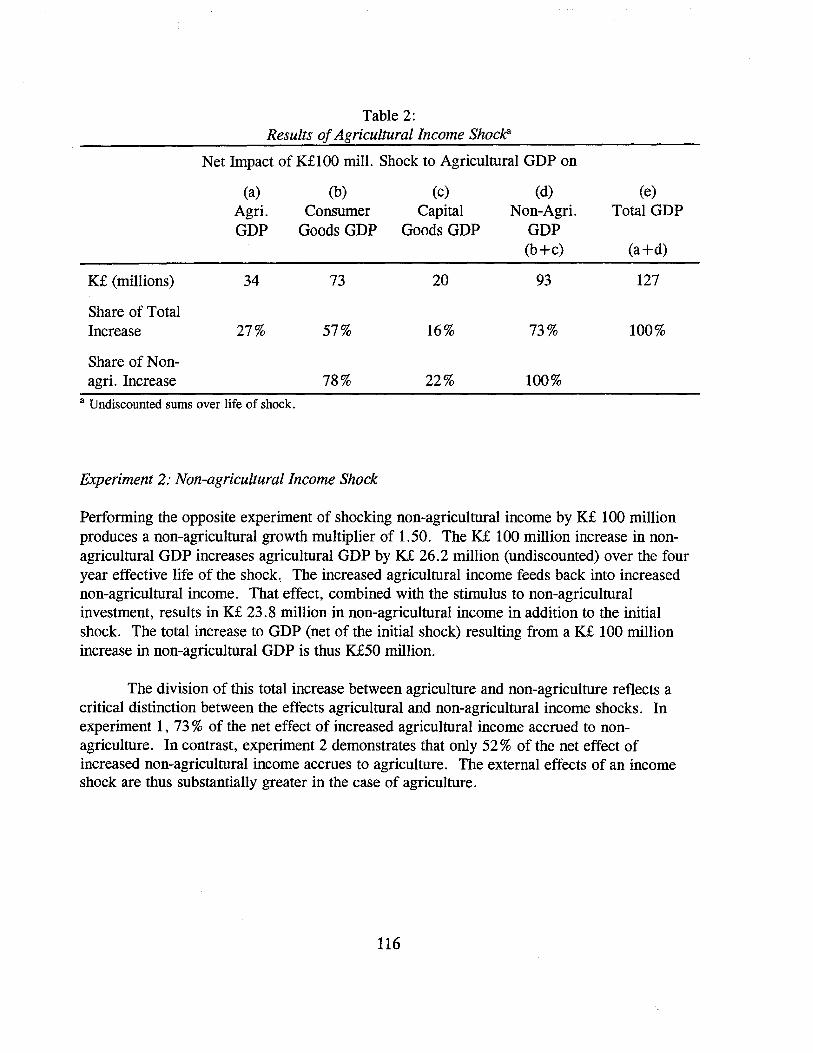
Table 2:Results ojAgricultural Income ShocfCi

Net Impact of K£100 mill. Shock to Agricultural GDP on

(a) (b) (c) (d) (e)Agri. Consumer Capital Non-Agri. Total GDPGDP Goods GDP Goods GDP GDP

(b+c) (a+d)

K£ (millions) 34 73 20 93 127

Share of TotalIncrease 27% 57% 16% 73% 100%

Share of Non-agri. Increase 78% 22% 100%

a Undiscounted sums over life of shock.

Experiment 2: Non-agricultural Income Shock

Performing the opposite experiment of shocking non-agricultural income by K£ 100 millionproduces a non-agricultural growth multiplier of 1.50. The K£ 100 million increase in non­agricultural GDP increases agricultural GDP by K£ 26.2 million (undiscounted) over the fouryear effective life of the shock. The increased agricultural income feeds back into increasednon-agricultural income. That effect, combined with the stimulus to non-agriculturalinvestment, results in K£ 23.8 million in non-agricultural income in addition to the initialshock. The total increase to GDP (net of the initial shock) resulting from a K£ 100 millionincrease in non-agricultural GDP is thus K£50 million.

The division of this total increase between agriculture and non-agriculture reflects acritical distinction between the effects agricultural and non-agricultural income shocks. Inexperiment 1, 73 % of the net effect of increased agricultural income accrued to non­agriculture. In contrast, experiment 2 demonstrates that only 52 % of the net effect ofincreased non-agricultural income accrues to agriculture. The external effects of an incomeshock are thus substantially greater in the case of agriculture.

116

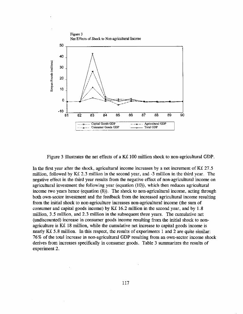
Figure 3Net Effects of Shock to Non-agricultural Income

50

40

~a 30§'"2!::l 200~

'"'"i:'10~

0

-1081 82 83 84 85 86 87 88 89 90

__ e- - - Capital Goods GDP___ ....___ Consumer Goods GDP

__.... _ _ Agricultural GDP----<i'---- TotalGDP

Figure 3 illustrates the net effects of a 1(£ 100 million shock to non-agricultural GDP.

In the first year after the shock, agricultural income increases by a net increment of K£ 27.5million, followed by K£ 2.3 million in the second year, and -3 million in the third year. Thenegative effect in the third year results from the negative effect of non-agricultural income onagricultural investment the following year (equation (10)), which then reduces agriculturalincome two years hence (equation (8)). The shock to non-agricultural income, acting throughboth own-sector investment and the feedback from the increased agricultural income resultingfrom the initial shock to non-agriculture increases non-agricultural income (the sum ofconsumer and capital goods income) by K£ 16.2 million in the second year, and by 1.8million, 3.5 million, and 2.3 million in the subsequent three years. The cumulative net(undiscounted) increase in consumer goods income resulting from the initial shock to non­agriculture is 1(£ 18 million, while the cumulative net increase to capital goods income isnearly K£ 5.8 million. In this respect, the results of experiments 1 and 2 are quite similar:76% of the total increase in non-agricultural GDP resulting from an own-sector income shockderives from increases specifically in consumer goods. Table 3 summarizes the results ofexperiment 2.

117

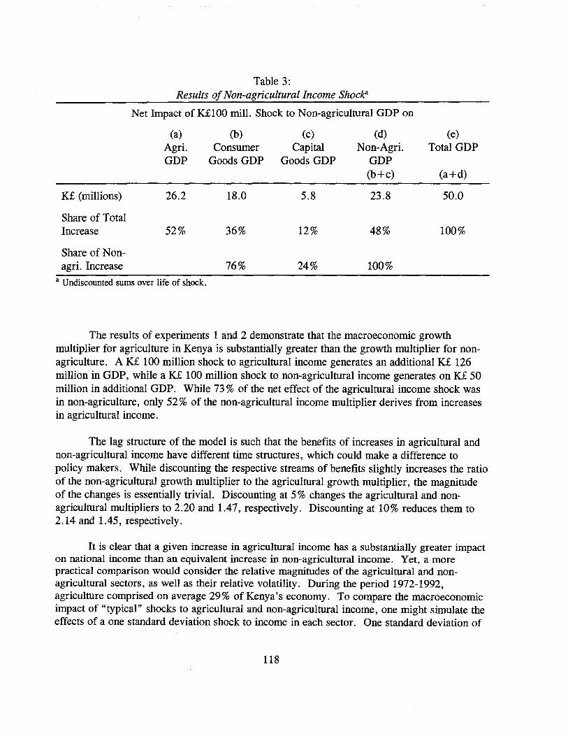
Table 3:Results ofNon-agricultural Income Shock:

Net Impact of K£100 mill. Shock to Non-agricultural GDP on

(a) (b) (c) (d) (e)Agri. Consumer Capital Non-Agri. Total GDPGDP Goods GDP Goods GDP GDP

(b+c) (a+d)

K£ (millions) 26.2 18.0 5.8 23.8 50.0

Share of TotalIncrease 52% 36% 12% 48% 100%

Share of Non-agri. Increase 76% 24% 100%

a Undiscounted sums over life of shock.

The results of experiments 1 and 2 demonstrate that the macroeconomic growthmultiplier for agriculture in Kenya is substantially greater than the growth multiplier for non­agriculture. A K£ 100 million shock to agricultural income generates an additional K£ 126million in GDP, while a K£ 100 million shock to non-agricultural income generates on K£ 50million in additional GDP. While 73 % of the net effect of the agricultural income shock wasin non-agriculture, only 52% of the non-agricultural income multiplier derives from increasesin agricultural income.

The lag structure of the model is such that the benefits of increases in agricultural andnon-agricultural income have different time structures, which could make a difference topolicy makers. While discounting the respective streams of benefits slightly increases the ratioof the non-agricultural growth multiplier to the agricultural growth multiplier, the magnitudeof the changes is essentially trivial. Discounting at 5% changes the agricultural and non­agricultural multipliers to 2.20 and 1.47, respectively. Discounting at 10% reduces them to2.14 and 1.45, respectively.

It is clear that a given increase in agricultural income has a substantially greater impacton national income than an equivalent increase in non-agricultural income. Yet, a morepractical comparison would consider the relative magnitudes of the agricultural and non­agricultural sectors, as well as their relative volatility. During the period 1972-1992,agriculture comprised on average 29% of Kenya's economy. To compare the macroeconomicimpact of "typical" shocks to agricultural and non-agricultural income, one might simulate theeffects of a one standard deviation shock to income in each sector. One standard deviation of

118

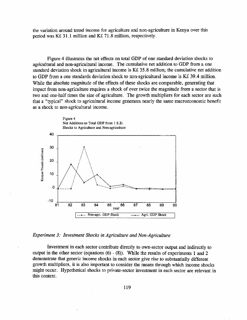
the variation around trend income for agriculture and non-agriculture in Kenya over thisperiod was K£ 31.1 million and K£ 71.8 million, respectively.

Figure 4 illustrates the net effects on total GDP of one standard deviation shocks toagricultural and non-agricultural income. The cumulative net addition to GDP from a onestandard deviation shock in agricultural income is K£ 35.8 million; the cumulative net additionto GDP from a one standards deviation shock to non-agricultural income is K£ 39.4 million.While the absolute magnitude of the effects of these shocks are comparable, generating thatimpact from non-agriculture requires a shock of over twice the magnitude from a sector that istwo and one-half times the size of agriculture. The growth multipliers for each sector are suchthat a "typical" shock to agricultural income generates nearly the same macroeconomic benefitas a shock to non-agricultural income.

Figure 4Net Additions to Total GDP from 1 S.D.Shocks to Agriculture and Non-agriculture

90898887

'""13------..Q.---

83 84 85 86year

~, ,, ,, ,, ,, ,, ,, ,, ,, ,, ,, ,, ,, ., ,, ,, ,, ..

,,

40

'<;;'30

=:Sg

20'"-g::I

~= 10co~

"t:.::

0

-1081 82

I··e.. Non-agri. GDP Shock ----.- Agri. GDP Shock

Experiment 3: Investment Shocks in Agriculture and Non-Agriculture

Investment in each sector contribute directly to own-sector output and indirectly tooutput in the other sector (equations (6) - (8». While the results of experiments 1 and 2demonstrate that generic income shocks in each sector give rise to substantially differentgrowth multipliers, it is also important to consider the means through which income shocksmight occur. Hypothetical shocks to private-sector investment in each sector are relevant inthis context.

119

The simulation model yields dramatically different macroecnomic growth multipliersfrom shocks to inv3stment in agriculture and non-agriculture: the agricultural investmentgrowth multiplier is 2.78, as compared with the non-agricultural investment growth multiplierof 0.78. Two factors explain the magnitude of the difference in macroeconomic effectsresulting from investment shocks in these two sectors. Investment in either sector increasesoutput in both sectors. Yet, as experiments 1 and 2 demonstrated, any increase in output fromagriculture gives rise to an increase in GDP of approximately two and one-half times thatresulting froman equivalent increase in non-agricultural output.

The fact that the agricultural investment growth multiplier is over three and one-halftimes the magnitude of the non-agricultural investment growth multiplier suggests that themarginal rate of return to investments in agriculture is also substantially greater than that forinvestments in non-agriculture. Such a result is consistent with the notion of "urban bias"popularized by Lipton (1977, 1993). The phenomenon of urban bias is manifested in partthrough "over-investment" in the urban sector and "under-investment" in the rural sector.The logical result of urban bias is this a disequilibrium in which marginal rates of return torural investment are greater than marginal rates of return in urban investment. Urban biascould thus explain part of the large difference between the growth multipliers from investmentin agriculture and non-agriculture.

As in experiments 1 and 2, the most realistic illustration is to juxtapose "typical"shocks to agricultual and non-agricultral investment, rather than shocks of equal magnitude.The mean levels of agricultural and non-agricultural investment (originating in the privatesector) are K£52.2 million and K£355.3 million, respectively for the period 1972 - 1992. Onestandard deviation around thrend is K£10.4 million for agricultural investment and K£45.7million for non-agricultural investment. Figure 5 illustrates the effect on total GDP ofinvestment shocks of these magnitudes in both sectors.

The total (undiscounted) increment to GDP resulting from one stand deviation shcok toagricultural investment is K£28.6 million as compared with a total increase ofK£35.7 millionfrom a one standard deviation shock to non-agricultural investment. Thus, while the totalincrease is nearly 25 % greater with the non-agricultural investment shock, it requires aninvestment increase of over 4 times the magnitude in non-agriculture to produce that result.This suggests that the macroeconomic benefits of investment in agriculture are substantiallygreater than the benefits of investment in non-agriculture in Kenya. It is important to note,

120

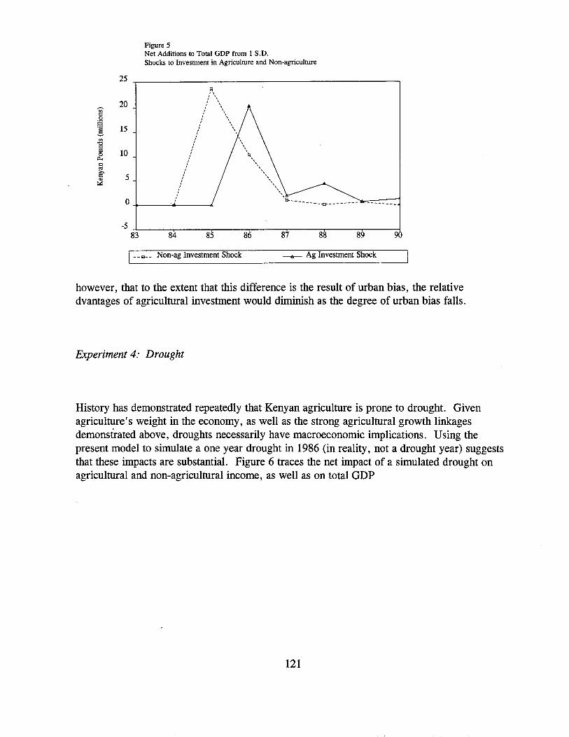
Figure 5Net Additions to Total GDP from 1 S.D.Shocks to Investment in Agriculture and Non-agriculture

908988878685

I~\, ,, ,, ', ', ', ', '-, ,

/' \\/ '

,,

,,,

,

84

25

,..... 20'"c:S§ 15

'""8~ 10c:

'"E;' 5.,~

0

-583

I--£>n Non-ag Investment Shock ----6- Ag Investment Shock

however, that to the extent that this difference is the result of urban bias, the relativedvantages of agricultural investment would diminish as the degree of urban bias falls.

Experiment 4: Drought

History has demonstrated repeatedly that Kenyan agriculture is prone to drought. Givenagriculture's weight in the economy, as well as the strong agricultural growth linkagesdemonstrated above, droughts necessarily have macroeconomic implications. Using thepresent model to simulate a one year drought in 1986 (in reality, not a drought year) suggeststhat these impacts are substantial. Figure 6 traces the net impact of a simulated drought onagricultural and non-agricultural income, as well as on total GDP

121

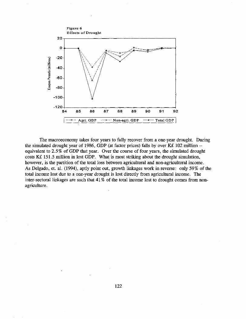
Figure 6Effects of Drought

20..,....----------------------,

-20

o -jo----<t

~

'"=:S:§, -40'""CI

§rf. -60lilS::l -80

-100

9291908988878685-120+----,----.----r----,---.,.....---r-----,.---!

84

1--<3-- Agri. GDP 6 Non-agri. GDP -- Total GDP I

The macroeconomy takes four years to fully recover from a one-year drought. Duringthe simulated drought year of 1986, GDP (at factor prices) falls by over K£ 102 million-­equivalent to 2.5% of GDP that year. Over the course of four years, the simulated droughtcosts K£ 151.5 million in lost GDP. What is most striking about the drought simulation,however, is the partition of the total loss between agricultural and non-agricultural income.As Delgado, et. al. (1994), aptly point out, growth linkages work in reverse: only 59% of thetotal income lost due to a one-year drought is lost directly from agricultural income. Theinter-sectoral linkages are such that 41 % of the total income lost to drought comes from non­agriculture.

122

5.5 Consistency with Other Studies

The simulation results presented above are consonant with previous analyses of agriculturalgrowth multipliers and, though not always directly comparable, compleinent those earlierresults. Using a model similar to that presented here, Rangarajan (1982) calculated India'sagricultural growth multiplier during the 1960's to be 1.7 as compared with a multiplier of 1.5for industry. In a more detailed simulation model of Nigeria, Byerlee (1973) also foundimportant growth linkages from agricultural to non-agricultural value added. In particular,Byerlee identified strong indirect effects of agricultural development on employment andincome distribution in non-agriculture.

An alternative methodology based on regional semi-input-output models has beenwidely applied to calculate agricultural growth multipliers. Early work in this veinconcentrated on Asia, finding agricultural growth multipliers in several regional cases on theorder of 1.6 for India and 1.8 for the Muda River region of MalaysiaY Initial applications ofthese models in Africa tended to find lower agricultural growth multipliers than those claimedfor Asia (Haggblade, Hazell, and Brown (1987), Hazell and Roell (1983)). Multipliers on theorder of 1.5 were found for regions of Sierra Leone and Nigeria, leading those authors toconclude that consumption linkages were weaker in Africa than in Asia.

Delgado, et.al. (1994), have recently demonstrated much stronger agriculturalgrowth linkages for several African countries than had previously been thought to exist. Themagnitude of the agricultural growth multipliers derived from these regional semi-input-outputmodels is quite sensitive to the categorization of goods as being either tradable or non­tradable. The earlier growth linkages literature, taking Asia as its example, counted food astradable. As such, additional spending on food does not contribute to the agricultural growthmultiplier, the consumption component of which relies on increased spending on non­tradables. In contrast, Delgado, et. al., argue that the assumption that all foodgrains aretradable is inappropriate for Sub-Saharan Africa. Their re-categorization of food as non­tradable results in substantially higher agricultural growth multipliers in their study zones thanhad previously been thought to existY They find agricultural growth multipliers of 2.75 inBurkina Paso, 2.48 in Zambia, 1.97 in Senegal, and 1.96 in Niger.

12 These results are based on a series of articles and books, including: Bell, Hazell and Slade (1982),Hazell and Haggblade (1990), Hazell (1984), Hazell, Ramasamy, and Rajagopalan (1991), and Dorosh andHaggblade (1993).

13 It is important to note that Delgado, et. al., also change their supply elasticity assumptions when foodsare reclassified from tradables to nontradables. Their semi-input-output model assumes perfectly elastic suppliesfor nontradables, but perfectly inelastic supplies for tradables. Thus, their larger multipliers arise in part becausefood is assumed to have a perfectly elastic supply when it is treated as a nontradable. Haggblade, Hammer, andHazell (1991) suggest that these fix-price models in general tend to overstate growth multipliers by approximately25 % relative to price-endogenous models.

123

Although of a comparable magnitude to the multipliers derived from the present model,one cannot strictly compare the estimated national multipliers with regional multipliers.Regional models do not consider spillover effects to other parts of the national economy.Some of these spillovers may be positive (through multiplier effects induced in adjacentregions or in major towns), but others may be negative (if regional multipliers retain or drawin valuable resources from elsewhere). Technically, then, it is difficult to know if regionalmultipliers are larger or smaller than corresponding national multipliers. Moreover, incontrast to the present model, most regional models are static and do not capture theinvestment linkages that can add importantly to the size of the multiplier. As a case in point,Lewis and Thorbecke (1992), applying a variant of this approach to the Kutu region ofKenya I s Central Province, have found agricultural growth multipliers of approximately 1.45,and non-agricultural growth multipliers of approximately 0.8.

In partial contrast to the findings of Lewis and Thorbecke, Bigsten and Collier (1995)found evidence of much weaker aggregate agricultural growth multipliers in Kenya. Basingtheir analysis on a computable general equilibrium model, Bigsten and Collier report anaggregate agricultural growth multiplier of 1.2, arising from a labor market distortion.Bigsten and Collier also find econometric evidence to support a causal link betweenagricultural income growth and expansion of the construction sector, though this sameapproach fails to support a causal link running from agriculture to manufacturing in Kenya.The econometric model presented above supports Bigsten and Collier's finding with regard toconstruction, but contradicts their lack of support for an agriculture-manufacturing linkage.

This extremely valuable literature has firmly established the superior linkages derivedfrom agriculture, and has taken advantage of its detailed data sources to measure the effects ofspecific forward and backward linkages from agriculture to non-agriculture. The regionalstudies, however, rely on a particular methodology that prevents their results from beinggeneralized directly to the level of national income. The model presented in this paper buildson those more detailed findings. While we do not explicitly model those micro-linkages, thepresent model captures their effects on the national level.

Timmer (1995) suggests that there may be more subtle inter-sectoral linkages flowingfrom agriculture that have not been measured in the previous literature. The model presentedin this paper cannot distinguish among these particular linkages. Yet, the analysis presented inBlock and Timmer (1994) provides a step in that direction, finding evidence of positive spill­over effects of agriCUltural productivity on non-agricultural productivity in Kenya.

The general message, however, is clear. Agriculture has a central role to play inAfrican economic growth. Intersectoral growth multipliers favor agriculture over industry as asource of macroeconomic income generation. African governments seeking to promoteeconomic growth cannot afford to ignore agriculture in the design of their growth strategies.

124

APPENDIX 1

Variable Names

All variables are measures in millions ofconstant Kenyan pounds (l982=lOO)

CFBOOM = dummy for coffee boom

CONP = private consumption

DELSTK = change in capital stocks

DROUGHT = dummy variable = 1 for drought years

ER = nominal exchange rate (Ksh/US$)

GI = gross capital fonnation

GIA = gross capital fonnation in agriculture originating in the private sector

GIAP = gross capital formation in agriculture originating in the public sector

GIN = gross capital formation in non-agriculture originating in the private sector

GINP = 'gross capital formation in non-agriculture originating in the public sector

GOV = government consumption

GOVEXP = government expenditures

INDTXSUB = indirect taxes and subsidies

INSTAB = a proxy for macroeconomic (export) instability

KIMP = capital goods imports

POP = total population

POPRAT = ratio of agricultural to non-agricultural population

125

US KENRER = real exchange rate = ER * (P GDP / P GDP )

RUTT = rural-urban terms of trade

TDBAL = exports - imports

TOT = foreign terms of trade = P x/P m

YA = value added in agriculture

YC = value added in consumer goods

YFACP = GDP at factor prices

YK = value added in capital goods

YMKTP = GDP at market prices

YN = value added in non-agriculture

126

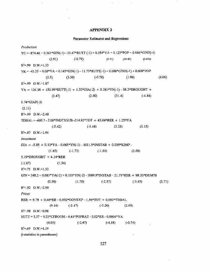
APPENDIX 2

Parameter Estimates and Regressions

Production

YC = -874.46 + 0.361 *GIN(-l) - 33.47*RUTT (-1) + 0.384*YA + 0.123*POP + 0.086*GINP(-1)

(2.91) (-0.79) (2.51) (20.43) (0.654)

R2=.99 D.W.=1.33

YK = -45.35 + 0.08*YA + 0.145*GIN(-I) - 11.73*RUTT(-I) + 0.088*GINP(-l) + 0.008*POP

(1.5) (3.30) (-0.78) 0.90) (4.06)

R2=.99 D.W.=1.87

YA = 126.38 + 150.99*RUTT(-l) + 1.32*GIA(-2) + 0.281 *YN(-l) - 58.2*DROUGHT +(3.47) (2.90) (31.4) (-4.84)

1.74*GIAP(-3)

(2.11)

R2=.99 D.W.=2.40

TDBAL = -600.7 - 2.08*INDTXSUB -214.92*TOT + 43.04*RER + 1.25*YA

(-5.42) (-1.44) (3.23) (3.15)

R~.87 D.W.=1.94

Investment

GIA = -5.85 + O.13*YA - 0.065*YN(-I) - 1011.9*INSTAB + 0.039*KIMP-

(l.45) (-1. 72) (-1.61) (2.68)

5.19*DROUGHT + 4. 14*RER

(-1.07) (1.34)

R2=.71 D.W.=1.53

GIN = 348.2 + 0.083*YA(-2) + 0.105*YN(-2) - 3009.9*INSTAB - 21.71 *RER + 98.33*DUM78

(0.56) (1.70) (-2.57) (-3.45) (5.71)

R2=.92 D.W.=2.90

Prices

RER = 9.78 + 0.46*ER - 0.OO2*GOVEXP - 1.86*TOT + 0.OO2*TDBAL

(9.14) (-2.17) (-2.26) (2.03)

R2=.98 D.W.=O.98

RUTT = 3.37 + 0.23*CFBOOM - OAl*POPRAT - 0.02*ER- O.0004*YA

(4.03) (-2.47) (-4.18) (-0.74)

R2=.69 D.W.=1.19

(t-statistics in parentheses)

127

APPENDIX 3

Augmented Dickey-Fuller Test Results

Table A3.1 provides the results of Augmented Dickey-Fuller tests of the residuals from themodel's stochastic equations. In accordance with the Engle-Granger method, after having pre­tested the order of integration of each series, cointegration of the series in the individualequations is established by the stationarity of the residuals from those equations. The nullhypothesis in an ADF test is the existence of a unit root (indicating non-stationarity). An ADFtest statistic that exceeds the MacKinnon critical value indicates rejection of that null hypothesissuggesting the stationarity of the series. This is the case for each equation in the model.

128

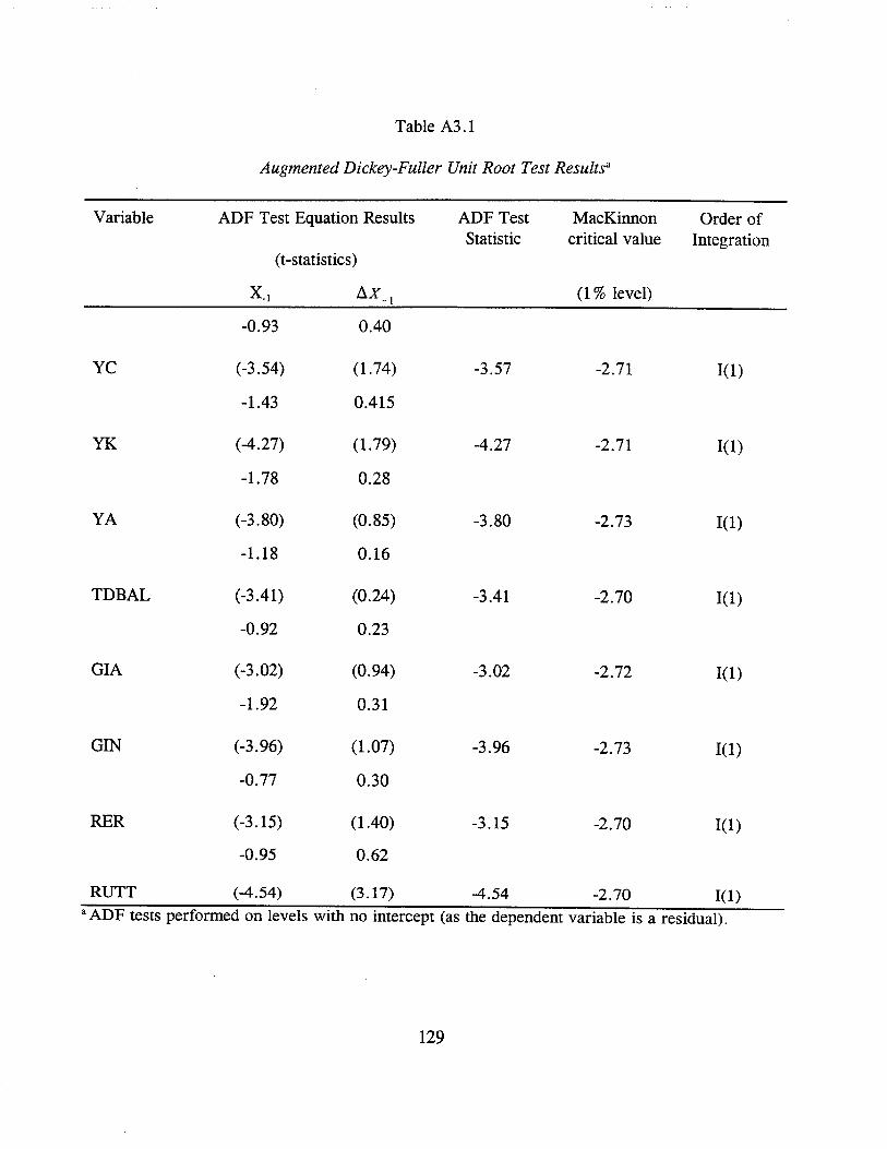
Table A3.1

Augmented Dickey-Fuller Unit Root Test Resultsa

Variable ADF Test Equation Results ADF Test MacKinnon Order ofStatistic critical value Integration

(t-statistics)

K1 !::..X_1 (1 % level)

-0.93 0.40

YC (-3.54) (1.74) -3.57 -2.71 1(1)

-1.43 0.415

YK (-4.27) (1.79) -4.27 -2.71 1(1)

-1.78 0.28

YA (-3.80) (0.85) -3.80 -2.73 1(1)

-1.18 0.16

TDBAL (-3.41) (0.24) -3.41 -2.70 1(1)

-0.92 0.23

GIA (-3.02) (0.94) -3.02 -2.72 1(1)

-1.92 0.31

GIN (-3.96) (1.07) -3.96 -2.73 1(1)

-0.77 0.30

RER (-3.15) (1.40) -3.15 -2.70 1(1)

-0.95 0.62

RUTT (-4.54) (3.17) -4.54 -2.70 1(1)a ADF tests performed on levels with no intercept (as the dependent variable is a residual).

129

APPENDIX 4

Descriptive Statistics and Graphs for the Simulation Base Run

Table A4.1

Root Mean Squared Errors and Root Mean Squared Percentage Errors for Base Run

Variable RMSE RMSPE

YFACP 33.14 1.08

YMKTP 33.14 0.93

CONP 80.65 3.78

YN 19.65 0.88

GI 15.13 1.94

YC 16.23 0.82

YK 5.23 2.09

YA 18.61 2.09

TDBAL 87.30 124.26

GIA 6.94 14.12

GIN 14.67 4.10

RER 0.38 3.95

RUTT 0.07 6.61

RMSE = root mean square error RMSPE = root mean square percentage error,

T

RMSE ~L (Y/ - y1

a)2

T 1;1

RMSPET (S aj2~L Y1 - Y1

T 1;1 y a1

130

* 100

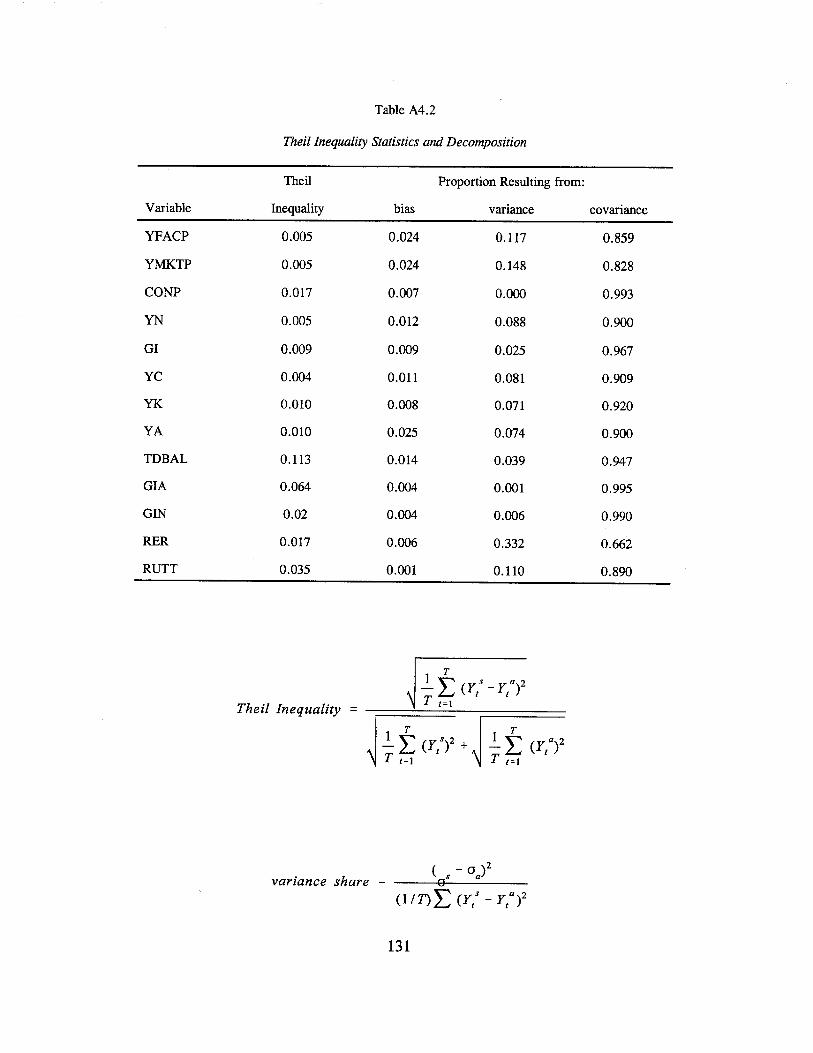
Table A4.2

Theil Inequality Statistics and Decomposition

Theil Proportion Resulting from:

Variable Inequality bias variance covariance

YFACP 0.005 0.024 0.117 0.859

YMKTP 0.005 0.024 0.148 0.828

CONP 0.017 0.007 0.000 0.993

YN 0.005 0.012 0.088 0.900

GI 0.009 0.009 0.025 0.967

YC 0.004 0.011 0.081 0.909

YK 0.010 0.008 0.071 0.920

YA 0.010 0.025 0.074 0.900

TDBAL 0.113 0.014 0.039 0.947

GIA 0.064 0.004 0.001 0.995

GIN 0.02 0.004 0.006 0.990

RER 0.017 0.006 0.332 0.662

RUTT 0.035 0.001 0.110 0.890

Theil InequalityT T

..!.- L (y/)2 + ..!.- L (y/)2\ T t;1 \ T t;1

variance share =

131

bias share =

covariance share =

where Y s, Ya, a, a are the means and sample standard deviations of the simulated and predicted variables, andS a

p is the correlation coefficient of the simulated and predicted variable.

A Theil inequality score of 0 indicates a perfect fit, while a score of 1 indicates the worst possible fit.Ideally, the bias and variance shares will be zero and the covariance share will be 1.

132

REFERENCES

Bell, c., P. Hazell, and R. Slade (1982) Project Appraisal in a Regional Perspective,Baltimore, MD: The Johns Hopkins University Press.

Bevan, D., P. Collier, and J. W. Gunning (1990) Controlled Open Economies, Oxford:Clarendon Press.

Bigsten, A., and P. Collier (1995) "Linkages from Agricultural Growth in Kenya," in J. W.Mellor (ed) Agriculture on the Road to Industrialisation, Baltimore: The Johns HopkinsUniversity Press.

Block, S. A., and C. P. Timmer (1994) Agriculture and Economic Growth: ConceptualIssues and the Kenyan Experience, Cambridge, MA: Harvard Institute forInternational Development, Development Discussion Paper, No. 498.

Byerlee, D. (1973) "Indirect Employment and Income Distribution Effects of AgriculturalDevelopment Strategies: A Simulation Approach Applied to Nigeria," African RuralEmployment Network, African Rural Employment Paper No.9, Department ofAgricultural Economics, Michigan State University, E. Lansing, ML

Dawe, D. (1993) Essays on Price Stabilization and the Macroeconomy ofLow-IncomeCountries, Ph.D. Dissertation, Harvard University, Cambridge, MA.

Delgado, C., et.al. (1994) Agricultural Growth Linkages in Sub-Saharan Africa, Washington,D.C.: U. S. Agency for International Development.

Development Alternatives Inc. (1994) A SUl1!ey of Small and Micro Enterprises in Kenya,Nairobi: USAID/Kenya.

Dorosh, P., and S. Haggblade (1992) Agricultural Growth Linkages in Madagascar, WorkingPaper, No. 22, Cornell Food and Nutrition Policy Program. Ithaca: CornellUniversity.

Haggblade, S. (1989) "Agricultural Technology and Farm-Nonfarm Growth Linkages,"Agricultural Economics, 3, 345-364.

__ , P. Hazell, J. Brown (1989) "Farm-Nonfarm Linkages in Rural Sub-Saharan Africa,"World Development, Vol. 17, No.8, 1173-1201.

, J. Hammer, and P. Hazell (1991) "Modeling Agricultural Growth Multipliers,"American Journal ofAgricultural Economics, May, Vol. 73, No.2, 361(14).

133

Hazell, P., and A. Roell (1983) Rural Growth Linkages: Household Expenditure Patterns inMalaysia and Nigeria, IFPRI Research Report No. 41, Washington, D.C.:International Food Policy Research Institute.

Johnston, B., and J. Mellor (1961) "The Role of Agriculture in Economic Development,"American Economic Review, 51(4).566-93.

Jorgenson, D. W. (1966) "Testing Alternative Theories of the Development of a DualEconomy," in I. Adelman and E. Thorbecke (eds) The Theory and Design ofDevelopment, Baltimore: Johns Hopkins University Press.

Lewis, B. D., and E. Thorbecke (1992) "District-Level Economic Linkages in Kenya:Evidence Based on a Small Regional Social Accounting Matrix," World Development,Vol. 20, No.6, 881-897.

Lewis, W. A. (1954), "Economic Development with Unlimited Supplies of Labor,"Manchester School, 22 (May) 155.

Rangarajan, C. (1982) Agricultural Growth and Industrial Peiformance in India, IFPRIResearch Report No. 33, Washington, D.C.: International Food Policy ResearchInstitute.

Ranis, G., and J. C. H. Fei (1964), Development of the Labor Surplus Economy, Homewood,IL: Irwin.

Reardon, T., E. Crawford, and V. Kelly (1994) "Links Between Nonfarm Income and FarmInvestment in African Households: Adding the Capital Market Perspective," AmericanJournal ofAgricultural Economics, 76:1172-1176.

Short, C., R. Keyfitz, and M. Maundu (1994) Historical Economic Data for Kenya: 1972­92. Technical Paper 94-01, Ministry of Planning and National Development,Government of Kenya.

Timmer, C. P. (1995) "Getting agriculture moving: do markets provide the right signals?"Food Policy, Vol. 20, No.5, 455-472.

Wilson, L. S. (1993) Public and Private Sector Capital Stock Estimates for Kenya byIndustry and Asset, 1972-1992, Technical Paper 93-05, Ministry of Planning andNational Development, Government of Kenya.

134

6. SUMMARY AND CONCLUSIONS

The three case studies presented above describe quite different economies. In particular,Ethiopia, Zimbabwe, and Kenya differ in their levels of market development, infrastructure, andincome. Yet, all three case studies point to the central role of agriculture in the growth process.The macroeconomic growth multipliers for agriculture are as great or greater than those for non­agricultural sectors in Kenya and Zimbabwe; in Ethiopia the greatest multiplier is for services,with agriculture still relatively high. These results are driven directly by the differing nature ofintersectorallinkages in each of these three economies.

A wide dispersion in the magnitude of growth multipliers within a given country signalssome measure of weakness in intersectorallinkages. In Ethiopia, for instance, the net incrementto GDP resulting from an income shock in the service sector is two and one-half times greaterthan the net increment resulting from an equivalent shock to industrial income. The netincrement to GDP resulting from a shock to agricultural income in Ethiopia is nearly twice asgreat as the net increment from a shock to industrial income. This disparity reflects thepronounced disassociation of Ethiopia's industrial sector from the rest of the economy. Inparticular, it emerged from the Ethiopia case study that there is substantial two-way interactionbetween the service and agricultural sectors, limited interaction between services and industry,and virtually no interaction between agriculture and industry. This linkage structure is reflectedin the specification of the Ethiopia simulation modeL

The sectoral definition of the Zimbabwe case study differs from that of the Ethiopia case-- industry and services in the latter are replaced by capital goods and consumer goods,respectively, in the former. The general interpretation of simulation results, however, is similarbetween the two cases. In the Zimbabwe case the sectoral growth multipliers are substantiallycloser to one another than in Ethiopia. Agriculture and consumer goods have essentially thesame multiplier, while that for capital goods is lower. Yet, the agriculture and consumer goodsmultipliers in Zimbabwe are only 1.7 times greater than the capital goods multiplier. Thiscontrast with Ethiopia indicates greater integration across sectors, which is reflected in thespecification ofthe Zimbabwe simulation modeL

As in the Ethiopia model, the specification for Zimbabwe includes two-way interactionbetween agriculture and consumer goods production, and one-way stimulation of capital goodsproduction by the consumer goods sector. The primary difference to emerge in the Zimbabwecase, however, is that there is also a one-way stimulation of capital goods production by theagricultural sector, as well. This difference in specification reflects substantial differences in thestructure and history of Zimbabwe's agricultural sector as compared with Ethiopia's. Inparticular, the historically bimodal structure ofZimbabwean agriculture has resulted in asubstantial large-scale commercial farming sub-sector (for which Ethiopia has no analogy). Thissub-sector in Zimbabwe is highly input and energy intensive, thus creating a significant demandfor electricity, machinery, and possibly construction. Zimbabwe's isolation from internationaltrade following its Unilateral Declaration ofIndependence in 1965, and forced import

135

substitution, likely contributed to the ability of the country's capital goods sector to meet theinput requirements of large-scale commercial farms.

The high growth multipliers associated with agriculture in Ethiopia and Zimbabwe areconsistent with our earlier work on Kenya (a revised version of which appears in this volume), aswell as with other recent empirical studies of agricultural growth multipliers in Africa. That theagricultural growth multipliers for Ethiopia, Zimbabwe, and Kenya to emerge from oursimulation analyses are 1.71, 1.93, and 2.27, respectively, sufficiently underscores theimportance of agriculture to economic growth in these countries. Yet, the simulation resultsprovide further reinforcement for this conclusion based on the distribution of the gains fromhypothetical income shocks to the various sectors.

Of the $0.93 net increment to national income generated by a $1.00 shock to servicesector income in Ethiopia, $0.53 is concentrated in the two sectors which employ onlyapproximately 10-15% of the country's workforce. The 85-90% of the workforce employed inagriculture shares the remaining $040. Of the total increase in GDP (e.g., including the initialshock) resulting from increased service sector income, 80% remains in the services and industrialsector. In contrast, of the $0.71 net increment to GDP generated by a $1.00 shock to agriculturalincome, $0.57 accrues to the non-agricultural workforce. Yet, of the total increase in GDPresulting from a shock to agriculture, two-thirds remains to be shared by the poor rural majorityofEthiopia's population. Thus a strategy emphasizing growth in Ethiopia's rural economywould contribute substantially to income in non-agriculture, as well as make the greatest progresstoward poverty alleviation.

In Zimbabwe, as in Ethiopia, the simulation results suggest that the benefits ofagricultural income growth are concentrated on the poor to a much greater extent than incomegrowth in either consumer or capital goods production. l For a given shock to agriculturalincome, two-thirds ofthe total increase in GDP are captured by the two-thirds of the total laborforce employed in agriculture. In contrast, a given increase in consumer goods incomeconcentrates 84% ofthe total increase among the 35% of the labor force employed in non­agricultural activities. Shocks to capital goods income are the most regressive in this sense: fully93% of the total income increase in that case are shared by the 35% non-agricultural share of thelabor force.

Both the Zimbabwe and Ethiopia simulation results thus highlight agricultural growth asthe most efficient vehicle for poverty alleviation. In addition, the growth multipliers indicate thata concentration on agriculture in Zimbabwe would make the maximum contribution to economicgrowth. Both of these new case studies are thus consistent with the earlier, less detailed, resultsof a similar analysis of Kenya.

1 The rural nature of Zimbabwe's poverty is clearly reflected by the fact that its agricultural sector earnsonly 12% of GDP yet employs over 65% of the labor force.

136

While macroeconomic growth multipliers provide a broad picture of agriculture's role ineconomic growth, they remain too highly aggregated to identifY the specific mechanisms throughwhich agriculture directly and indirectly contributes to growth. The indirect contributions, bywhich agriculture contributes to growth in non-agriculture, are of particular interest. Earlierliterature on agricultural growth linkages concentrated on product and factor markets asmechanisms. This study refines earlier work by Timmer which attempts to specify a set ofindirect linkages, not well mediated by markets.2

From among the long list of potential indirect linkages identified in earlier work, thepresent study refines the specification of three: 1) an urban bias linkage with an impact thatdepends on reversing underinvestment in the rural economy, 2) a nutritional linkage throughwhich a better-fed labor force works more productively and for more hours, and 3) a stabilitylinkage that connects unstable food prices and food insecurity with a consequent reduction in thequantity and quality of investment.

Empirical support for the existence of these indirect agricultural growth linkages is drawnfrom a cross-section ofcountries. In particular, economic growth is positively associated with:1) increases in the stock of rural human capital relative to urban human capital, 2) improvednutrition of the rural poor, and 3) increased agricultural price stability and food security. The percapita stock of human capital in rural versus urban areas is one indicator of the effects of urbanbias. Results presented above clearly indicate that reduced urban bias contributes positively toeconomic growth.

The report also cites evidence of a link between the nutritional welfare of the rural poorand economic growth. The critical mechanisms in this case is the effect of nutrition onagricultural productivity. Improved nutrition by the rural poor both increases the number ofhourwhich the poor are capable of working and increases workers' productivity during each of thosehours. A cross-country sample provides preliminary empirical support for this linkage, as well.

A final set of indirect agricultural growth linkages arises from the macroeconomic impactof stabilizing food prices. Price stabilization affects investment and growth throughout the entireeconomy. In short, instability in the food sector can have three important macro-level effects. Itcan affect the quantity of investment through an increase in precautionary savings or a decreasecaused by greater uncertainty. It can decrease the quality of investment (as measured by the rateof return) because prices contain less infonnation that is relevant for long-run investment.Finally, because of spillovers creating additional risk throughout the economy, instability can

2 C. P. Timmer, "Getting Agriculture Moving: Do Markets Provide the Right Signals?" Food Policy, Vol.20, No.5 (Oct. 1995): 455-472; C. P. Timmer, Why Markets and Politics Undervalue the Role ofAgriculture inEconomic Development, Benjamin H. Hibbard Memorial Lecture Series. Department of Agricultural Economics,University of Wisconsin-Madison, Madison, WI. 1993.; S. Block and C. P. Timmer, Agriculture and EconomicGrowth: Conceptual Issues and the Kenyan Experience, Consulting Assistance on Economic Reform DiscussionPaper No. 26, September 1994.

137

induce a bias toward speculative rather than productive investment activities and thereby slowdown economic growth. Thus, of additional domestic food production helps stabilize food pricesand leads to greater food security, it will have an impact through the quantity and efficiency ofinvestment because of the "stability" linkages. Empirical support for the stability linkages drawslargely on Asian examples. However, Pinckney (1983) shows that moderate price stabilizationfor maize in Southern Africa would have beneficial effects for food security.

Much work remains to be done in identifying, specifying, and quantifying the linkagesthat connect growth in ,the agricultural sector to growth in the rest of the economy. Clearly,agricultural growth is essential for poverty alleviating economic growth in most Africancountries. Yet, the potency of agriculture's potential catalytic influence on growth is conditionedby subtle mechanisms which can either strengthen or weaken agriculture's contribution. Thethree basic linkages identified in this study are likely to be of varying relevance in differentsettings. Little is known about this variation. It is fairly clear from the evidence presented thatthese linkages had a strong positive impact on economic growth in East and Southeast Asia, but asignificantly retarding effect in Sub-Saharan Africa.

The obvious remedy for this retardation is to reverse the longstanding urban bias seenthroughout Africa, to stimulate domestic food production as a way of enhancing laborproductivity in rural areas, and to find cost-effective designs for food price stabilization as a basefor food security and political stability. To say these steps are obvious, of course, is not to saythat they are easy. Getting governments to stop doing the wrong things will probably end theretardation, but getting then to do the right things will be essential to stimulating rapid economicgrowth.

138