Adhering to terrain characteristics for position estimation of mobile robots

Adhering to Terrain Characteristics for PositionEstimation of Mobile Robots

Michael Brunner1, Dirk Schulz1, and Armin B. Cremers2

1 Department of Unmanned Systems, Fraunhofer-Institute FKIENeuenahrer Straße 20, 53343 Wachtberg, Germany

{michael.brunner, dirk.schulz}@fkie.fraunhofer.de2 Department of Computer Science, University of Bonn

Roemerstr. 164, 53117 Bonn, [email protected]

Abstract. Outdoor environments bear the problem of different terrainsalong with changing driving properties. Therefore, compared to indoorenvironments, the kinematics of mobile robots is much more complex.In this paper we present a comprehensive approach to learn the functionof outdoor kinematics for mobile robots. Future robot positions are esti-mated by employing Gaussian process regression (GPR) in combinationwith an Unscented Kalman filter (UKF). Our approach uses optimizedterrain models according to the classification of the current terrain – ac-complished through Gaussian process classification (GPC) and a secondorder Bayesian filter (BF). Experiments showed our approach to providemore accurate estimates compared to single terrain model methods, aswell as to be competitive to other dynamic approaches.

Keywords: mobile robots, position estimation, terrain classification,Gaussian process, machine learning.

1 Introduction

The kinematics of mobile robots in outdoor scenarios is much more complex thanin indoor environments due to the varying terrain conditions. Therefore, trulyreliable velocity controls for robots which are able to drive up to 4 m/s or evenfaster (e.g. Figure 1) are hard to design. The drivability is primarily determinedby the terrain conditions. Thus, we developed a machine learning system whichpredicts the future positions of mobile robots using optimized terrain models.

In this paper we present a Gaussian processes (GPs) based method for es-timating the positions of a mobile robot. Our approach considers the differentterrain conditions to improve prediction quality. Gaussian process regression(GPR) models are utilized to estimate the translational and rotational velocitiesof the robot. These estimated velocities are transferred into the position spaceusing an unscented Kalman filter (UKF). By projecting the uncertainty values ofthe GPR estimates onto the positions, the UKF enables us to also capitalize theGPR uncertainties. To distinguish the different terrains the robot is traversing,

2 Adhering to Terrain Characteristics for Position Estimation

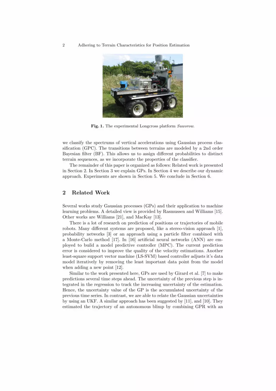
Fig. 1. The experimental Longcross platform Suworow.

we classify the spectrums of vertical accelerations using Gaussian process clas-sification (GPC). The transitions between terrains are modeled by a 2nd orderBayesian filter (BF). This allows us to assign different probabilities to distinctterrain sequences, as we incorporate the properties of the classifier.

The remainder of this paper is organized as follows: Related work is presentedin Section 2. In Section 3 we explain GPs. In Section 4 we describe our dynamicapproach. Experiments are shown in Section 5. We conclude in Section 6.

2 Related Work

Several works study Gaussian processes (GPs) and their application to machinelearning problems. A detailed view is provided by Rasmussen and Williams [15].Other works are Williams [21], and MacKay [13].

There is a lot of research on prediction of positions or trajectories of mobilerobots. Many different systems are proposed, like a stereo-vision approach [1],probability networks [3] or an approach using a particle filter combined witha Monte-Carlo method [17]. In [16] artificial neural networks (ANN) are em-ployed to build a model predictive controller (MPC). The current predictionerror is considered to improve the quality of the velocity estimations. Anotherleast-square support vector machine (LS-SVM) based controller adjusts it’s datamodel iteratively by removing the least important data point from the modelwhen adding a new point [12].

Similar to the work presented here, GPs are used by Girard et al. [7] to makepredictions several time steps ahead. The uncertainty of the previous step is in-tegrated in the regression to track the increasing uncertainty of the estimation.Hence, the uncertainty value of the GP is the accumulated uncertainty of theprevious time series. In contrast, we are able to relate the Gaussian uncertaintiesby using an UKF. A similar approach has been suggested by [11], and [10]. Theyestimated the trajectory of an autonomous blimp by combining GPR with an

Adhering to Terrain Characteristics for Position Estimation 3

UKF or ordinary differential equations (ODE), respectively. Localization of wire-less devices, like mobile telecommunication devices or mobile robots is solved bymodeling the probability distribution of the signal strength with GPs integratedin a BF [6].

Several works employ information about the current terrain conditions toimprove the navigation systems of mobile robots. One intuitive approach is todistinguish between traversable and non-traversable terrain [5], [14]. In contrastto the binary separation, Weiss et al. [20] are using a SVM to classify the ver-tical accelerations and hence the terrain type. Using spectral density analysis(SDA) and principal component analysis (PCA) Brooks et al. [2] concentrate onthe vibrations a mobile robot experiences while driving. The preprocessed datarecords are categorized through a voting scheme of binary classifiers. Anotherway to analyse the driving conditions is to measure the slippage [8], [19].

Kapoor et al. [9] are using GPs with pyramid-match kernels to classify objectsfrom visual data. Urtasun and Darrell [18] chose a GP latent variable model toachieve a better classification by reducing the input dimension.

Although many works concentrate on position estimation as well as terrainclassification, none combined GPR and GPC to solve both problems at once fora velocity controller of high speed outdoor robots.

3 Gaussian Processes

GPs are applicable to regression as well as classification tasks. In contrast toother methods GPs do not have any parameters that have to be determinedmanually. However, the kernel function affects the properties of a GP essentiallyand must be chosen by hand. The parameters of of GPs can be automaticallyoptimized using the training data. Furthermore, GPs provide uncertainty valuesadditionally to the estimates. These properties makes GPs attractive for regres-sion and classification task like position estimation and terrain classification.However, a drawback of GPs is their running time which is quadratic in thenumber of training cases due to the inversion of the kernel matrix.

3.1 Regression

Computing the predictive distribution of GPs consists of three major steps. First,we determine the Gaussian distribution of the training data and the test data.To integrate the information of the training data into the later distribution, wecompute the joint distribution. Finally, this joint distribution is transformed tothe predictive equations of GPs by conditioning it completely on the trainingdata.

Let X = [x1, . . . , xn]> be the matrix of the n training cases xi. The mea-sured process outputs are collected in y = [y1, . . . , yn]>. The noise of the randomprocess is modeled with zero mean and variance σ2

n. The kernel function is usedto computed the similarities between two cases. Our choice is the squared expo-nential kernel given by

k(xi, xj) = exp(− 12 |xi − xj |

2), (1)


where k is the kernel and xi, xj are two inputs. A further quantity we need toprovide the prior distribution of the training data is the kernel matrix of thetraining data K = K(X,X). It is given by Kij = k(xi, xj) using the kernelfunction. Now, we are able to specify the distribution of y:

y ∼ N (0,K + σ2nI). (2)

We are trying to learn the underlying function of the process. To get the distri-bution of the values of the underlying function f = [f1, . . . , fn]> we simply needto neglect the noise term from the distribution of the training data.

f ∼ N (0,K). (3)

Secondly, we determine the distribution of the test data. Let the set of n∗ testcases be assembled in a matrix as the training data, X∗ = [x∗1 , . . . , x∗n∗ ]>. f∗ =[f∗1 , . . . , f∗n∗ ]> are the function values of the test cases. The normal distributionof the test data is therefore given by

f∗ ∼ N (0,K∗∗), (4)

where K∗∗ = K(X∗, X∗) is the kernel matrix of the test cases, representing thesimilarities of this data points.

To combine training and test data distributions in a joint Gaussian distri-bution we further require the kernel matrix of both sets, denoted by K∗ =K(X,X∗). Consequently, the joint distribution of the training and test data is:[

yf∗

]∼ N

(0,

[K + σ2

nI K∗K>∗ K∗∗

]). (5)

This combination allows us to incorporate the knowledge contained in the train-ing data into the distribution of the function values of the test cases f∗, thevalues of interest.

Since the process outputs y are known, we can compute the distribution off∗ by conditioning it on y, resulting in the defining predictive distribution of GPmodels.

f∗|X, y,X∗ ∼ N (E[f∗], V[f∗]) (6)

with the mean and the variance given as

E[f∗] = K>∗ [K + σ2nI]−1y (7)

V[f∗] = K∗∗ −K>∗ [K + σ2nI]−1K∗. (8)

The final distribution is defined only in terms of the three different kernel ma-trices and the training targets y.


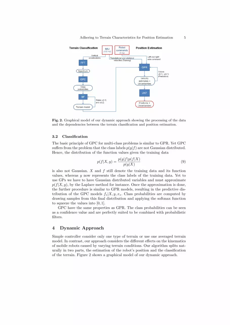
Fig. 2. Graphical model of our dynamic approach showing the processing of the dataand the dependencies between the terrain classification and position estimation.

3.2 Classification

The basic principle of GPC for multi-class problems is similar to GPR. Yet GPCsuffers from the problem that the class labels p(y|f) are not Gaussian distributed.Hence, the distribution of the function values given the training data

p(f |X, y) =p(y|f)p(f |X)

p(y|X)(9)

is also not Gaussian. X and f still denote the training data and its functionvalues, whereas y now represents the class labels of the training data. Yet touse GPs we have to have Gaussian distributed variables and must approximatep(f |X, y), by the Laplace method for instance. Once the approximation is done,the further procedure is similar to GPR models, resulting in the predictive dis-tribution of the GPC models f∗|X, y, x∗. Class probabilities are computed bydrawing samples from this final distribution and applying the softmax functionto squeeze the values into [0, 1].

GPC have the same properties as GPR. The class probabilities can be seenas a confidence value and are perfectly suited to be combined with probabilisticfilters.

4 Dynamic Approach

Simple controller consider only one type of terrain or use one averaged terrainmodel. In contrast, our approach considers the different effects on the kinematicsof mobile robots caused by varying terrain conditions. Our algorithm splits nat-urally in two parts, the estimation of the robot’s position and the classificationof the terrain. Figure 2 shows a graphical model of our dynamic approach.


4.1 Position Estimation

The position estimation consists of two methods. We use GPs to do regressionon the robot’s velocities and an UKF to transfer the results into the positionspace.

The values used were provided by an IMU installed on the robot. A seriesof preceding experiments were done to determine the composition of data typeswhich in combination with the projection into the position space allowed thebest position estimation. The data compositions compared in these experimentsvaried in two aspects, first, the type of the data, and second, the amount of pastinformation.

The data combinations considered were: (1) the change in x-direction3 andy-direction, (2) the change in x-direction, y-direction and in the orientation, (3)the x-velocity and y-velocity, (4) the x-velocity, y-velocity and the change in theorientation, (5) the translational and rotational velocity, and (6) the translationaland rotational velocity and the orientation change. The number of past valueswas altered from 1 to 4 values to determine the minimal amount of previousinformation necessary for the system to be robust, while at the same time doesnot cloud the data records and does not complicate the learning task. Leading toa total number of 24 different data compositions. While differing in the motionmodel and complexity, all approaches can be easily transformed into positions.The approaches (5) and (6) are utilizing lines and circular paths to approximatethe robot’s trajectory, whereas (1)-(4) are just using lines. Additionally, theapproaches (2), (4), and (6) are employing an independent estimation of theorientation, which may cover possible rotational slip. However, some approachessuffer from a poor transformation function, making them rather useless.

The results showed that a single past value of the translational and rotationalvelocity works best for position estimation. Thus, the data records of the GPRreads as follows:

[lt−1, lt, rt−1, rt, vt−1, ωt−1] (10)

Since our Longcross robot has a differential drive, li and ri denote the valuesof the speed commands to the robot for the left and right side of it’s drive. viand ωi represent the translational and rotational velocity, respectively. To learn acontroller we need both the commands given to the robot and the implementationof these commands. The values of interest are the current velocities, vt and ωt.

We use GPR to solve this regression task which not only provides the es-timates of translational and rotational velocities but also gives us uncertaintyvalues. We transform the estimates into positions using an UKF. Additionally,the uncertainties are projected onto these positions and are propagated over time(Figure 3). Starting with a quite certain position the sizes of the error ellipses areincreasing, due to the uncertainties of the velocity estimates and the increasinguncertainties of the previous positions they rely on.

3 All directions are relative to the robot. The x-directions points always in the frontdirection of the robot, and the y-direction orthogonal laterally.


Fig. 3. Original (red) and predicted (green) trajectory of a 30 second drive. The UKFerror ellipses are displayed in blue. Starting out with a small uncertainty the errorellipses (blue) increase over time, due to the uncertainty of previous positions and thevelocity estimates.

Given only the first translational and rotational velocity, the regression doesnot rely on any further IMU values. It takes previous estimates as inputs forthe next predictions. Assuming the first velocities to be zero (i.e. the robotis standing) makes our approach completely independent of the IMU device.However, IMU data is required for training.

For each type of terrain we trained two4 GPR models with data recordedonly on that terrain. This has several advantages: Firstly, the effects of therobot commands on a specific terrain can be learned more accurately, since theyare not contaminated by effects on other terrain types. Secondly, in combinationmore effects can be learned. And thirdly, due to the allocation of the trainingdata to several GPR models the size and complexity of each model is smallercompared to what a single model covering all terrain types would require. Theclassification described in the next paragraph enables us to select the appropriateterrain models for regression.

4.2 Terrain Classification

The terrain classification is implemented with a GPC model, and a 2nd order BFis used to model the transitions between terrains and to smooth the classificationresults.

As for the position estimation task preceding experiments were conductedto determine the best suited data records for the classification task. In contrast,here are mainly two possible data types, the vertical velocities and accelerations.

By taking a look at the raw IMU data it is evident that the different terrainsare hardly distingushable and that it may need to be preprocessed. To be sure,we classified vertical velocity and acceleration records of varying sizes. Since

4 GPs are not able to handle multi-dimensional outputs. Hence, we need one GPRmodel for each velocity, translational and rotational.


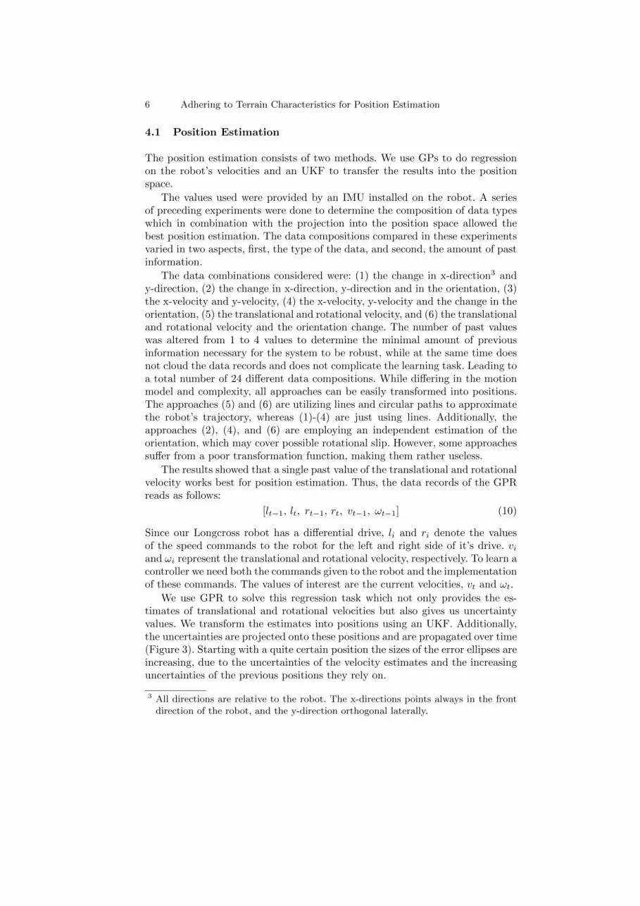
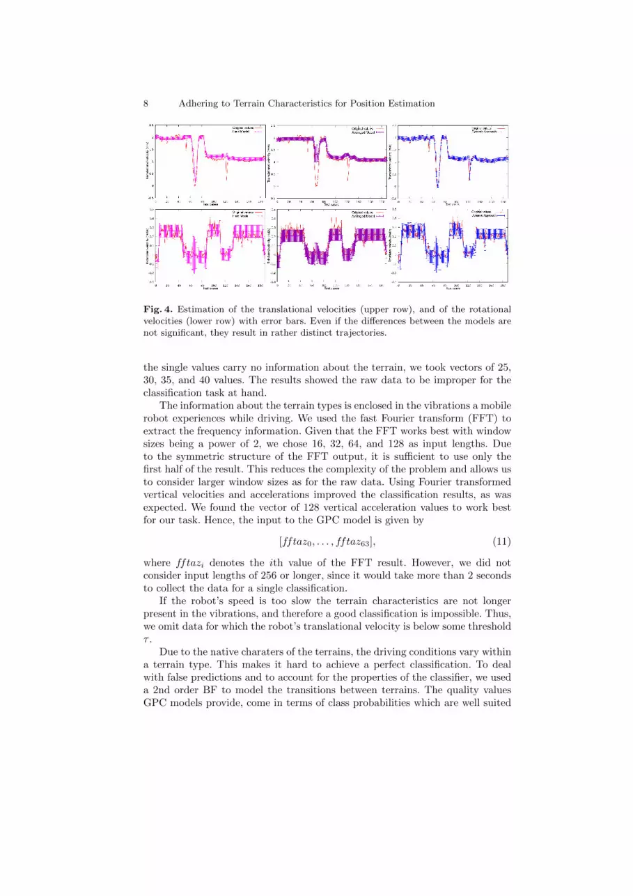
Fig. 4. Estimation of the translational velocities (upper row), and of the rotationalvelocities (lower row) with error bars. Even if the differences between the models arenot significant, they result in rather distinct trajectories.

the single values carry no information about the terrain, we took vectors of 25,30, 35, and 40 values. The results showed the raw data to be improper for theclassification task at hand.

The information about the terrain types is enclosed in the vibrations a mobilerobot experiences while driving. We used the fast Fourier transform (FFT) toextract the frequency information. Given that the FFT works best with windowsizes being a power of 2, we chose 16, 32, 64, and 128 as input lengths. Dueto the symmetric structure of the FFT output, it is sufficient to use only thefirst half of the result. This reduces the complexity of the problem and allows usto consider larger window sizes as for the raw data. Using Fourier transformedvertical velocities and accelerations improved the classification results, as wasexpected. We found the vector of 128 vertical acceleration values to work bestfor our task. Hence, the input to the GPC model is given by

[fftaz0, . . . , fftaz63], (11)

where fftazi denotes the ith value of the FFT result. However, we did notconsider input lengths of 256 or longer, since it would take more than 2 secondsto collect the data for a single classification.

If the robot’s speed is too slow the terrain characteristics are not longerpresent in the vibrations, and therefore a good classification is impossible. Thus,we omit data for which the robot’s translational velocity is below some thresholdτ .

Due to the native charaters of the terrains, the driving conditions vary withina terrain type. This makes it hard to achieve a perfect classification. To dealwith false predictions and to account for the properties of the classifier, we useda 2nd order BF to model the transitions between terrains. The quality valuesGPC models provide, come in terms of class probabilities which are well suited


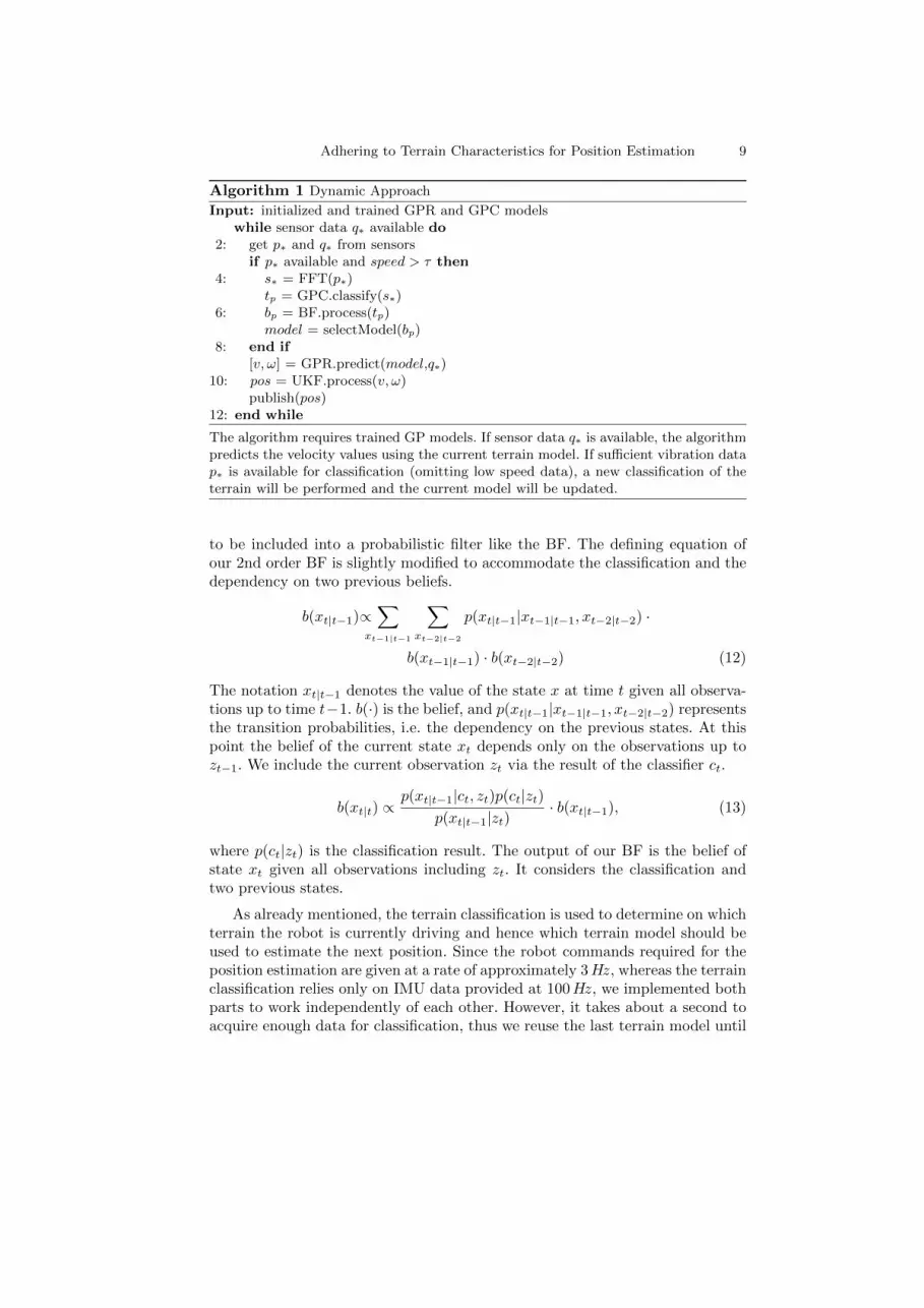
Algorithm 1 Dynamic Approach

Input: initialized and trained GPR and GPC modelswhile sensor data q∗ available do

2: get p∗ and q∗ from sensorsif p∗ available and speed > τ then

4: s∗ = FFT(p∗)tp = GPC.classify(s∗)

6: bp = BF.process(tp)model = selectModel(bp)

8: end if[v, ω] = GPR.predict(model,q∗)

10: pos = UKF.process(v, ω)publish(pos)

12: end while

The algorithm requires trained GP models. If sensor data q∗ is available, the algorithmpredicts the velocity values using the current terrain model. If sufficient vibration datap∗ is available for classification (omitting low speed data), a new classification of theterrain will be performed and the current model will be updated.

to be included into a probabilistic filter like the BF. The defining equation ofour 2nd order BF is slightly modified to accommodate the classification and thedependency on two previous beliefs.

b(xt|t−1)∝∑

xt−1|t−1

∑xt−2|t−2

p(xt|t−1|xt−1|t−1, xt−2|t−2) ·

b(xt−1|t−1) · b(xt−2|t−2) (12)

The notation xt|t−1 denotes the value of the state x at time t given all observa-tions up to time t−1. b(·) is the belief, and p(xt|t−1|xt−1|t−1, xt−2|t−2) representsthe transition probabilities, i.e. the dependency on the previous states. At thispoint the belief of the current state xt depends only on the observations up tozt−1. We include the current observation zt via the result of the classifier ct.

b(xt|t) ∝p(xt|t−1|ct, zt)p(ct|zt)

p(xt|t−1|zt)· b(xt|t−1), (13)

where p(ct|zt) is the classification result. The output of our BF is the belief ofstate xt given all observations including zt. It considers the classification andtwo previous states.

As already mentioned, the terrain classification is used to determine on whichterrain the robot is currently driving and hence which terrain model should beused to estimate the next position. Since the robot commands required for theposition estimation are given at a rate of approximately 3Hz, whereas the terrainclassification relies only on IMU data provided at 100Hz, we implemented bothparts to work independently of each other. However, it takes about a second toacquire enough data for classification, thus we reuse the last terrain model until


a new classification is available. Below we will refer to the terrain models usedby the GPR as applied models to distinguish them from the fewer classificationswhich were actually performed. Algorithm 1 summarizes our approach.

5 Experimental Results

The Longcross (Figure 1) is an experimental platform weighing about 340 kgwith a payload capacity of at least 150 kg. The compartment consists of carbon-fibre and is environmentally shielded. Our version is equipped with a SICK LMS200 2D laser scanner, a Velodyne Lidar HDL-64E S2 3D laser scanner, and anOxford Technical Solutions Ltd RT3000 combined GPS receiver and inertialunit. The software runs on a dedicated notebook with a Intel Core 2 ExtremeQuad processor and 8 GB memory.

5.1 Naive Approaches

We evaluated our approach on a test drive covering three different terrains,starting on field, continuing with grass, and ending on asphalt. The test sequenceconsists of 190 positions (about a 1 minute) almost evenly partitioned on thethree terrains. We compared our dynamic approach to a field model, an asphaltmodel, a grass model and an averaged model. The first three models were trainedonly on the specific terrain. The averaged model was trained on all three terrainsequally. All models used a total of 1500 training cases. The dynamic approachutilizes the three terrain specific models.

We used the mean squared error (MSE) and the standardized MSE to evalu-ate the quality of the regression. The SMSE is the MSE divided by the varianceof the test points, thus it does not depend on the overall scaling of the values.The MSE is not applicable to measure the quality of a trajectory because errorsat the beginning are propagated through the entire trajectory influencing all pro-ceeding positions. So we introduced the mean segment distance error (MSDE).First, we split the original trajectory and the prediction in segments of fixedsize. Each pair of segments is normalized to the same starting position and ori-entation. The distance of the resulting end positions is computed subsequently.The mean of all these distances constitutes the MSDE. We found a segment sizeof 10 to be a reasonable size.

The estimation results of the translational (upper row) and the rotationalvelocities (lower row) of the field model, the averaged model and of our dynamicapproach are shown in Figure 4. The field model is the best of the simple mod-els. The averaged model would be the model of choice if one wants to considerdifferent terrain conditions but does not want to employ a dynamic approach.

The estimation of the translational velocities by the averaged model showslittle or no reaction to any of the outliers. Averaging the effects of commands overseveral terrains involves diminishing effects of certain command-terrain combi-nations, hence causing inaccurate estimates. The field model performs best ofthe simple approaches, mainly because it recognizes the slowdown around the


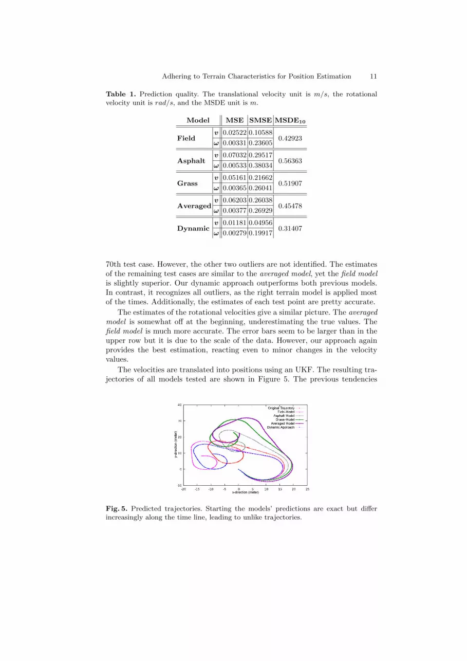
Table 1. Prediction quality. The translational velocity unit is m/s, the rotationalvelocity unit is rad/s, and the MSDE unit is m.

Model MSE SMSE MSDE10

v 0.02522 0.10588Field

ω 0.00331 0.236050.42923

v 0.07032 0.29517Asphalt

ω 0.00533 0.380340.56363

v 0.05161 0.21662Grass

ω 0.00365 0.260410.51907

v 0.06203 0.26038Averaged

ω 0.00377 0.269290.45478

v 0.01181 0.04956Dynamic

ω 0.00279 0.199170.31407

70th test case. However, the other two outliers are not identified. The estimatesof the remaining test cases are similar to the averaged model, yet the field modelis slightly superior. Our dynamic approach outperforms both previous models.In contrast, it recognizes all outliers, as the right terrain model is applied mostof the times. Additionally, the estimates of each test point are pretty accurate.

The estimates of the rotational velocities give a similar picture. The averagedmodel is somewhat off at the beginning, underestimating the true values. Thefield model is much more accurate. The error bars seem to be larger than in theupper row but it is due to the scale of the data. However, our approach againprovides the best estimation, reacting even to minor changes in the velocityvalues.

The velocities are translated into positions using an UKF. The resulting tra-jectories of all models tested are shown in Figure 5. The previous tendencies

Fig. 5. Predicted trajectories. Starting the models’ predictions are exact but differincreasingly along the time line, leading to unlike trajectories.


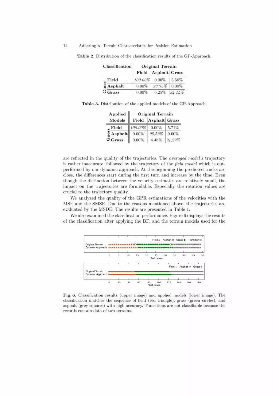
Table 2. Distribution of the classification results of the GP-Approach.

Classification Original Terrain

Field Asphalt Grass

Field 100.00% 0.00% 5.56%

Asphalt 0.00% 93.75% 0.00%

Guess

Grass 0.00% 6.25% 94.44%

Table 3. Distribution of the applied models of the GP-Approach.

Applied Original Terrain

Models Field Asphalt Grass

Field 100.00% 0.00% 5.71%

Asphalt 0.00% 95,52% 0.00%

Guess

Grass 0.00% 4.48% 94,29%

are reflected in the quality of the trajectories. The averaged model’s trajectoryis rather inaccurate, followed by the trajectory of the field model which is out-performed by our dynamic approach. At the beginning the predicted tracks areclose, the differences start during the first turn and increase by the time. Eventhough the distinction between the velocity estimates are relatively small, theimpact on the trajectories are formidable. Especially the rotation values arecrucial to the trajectory quality.

We analyzed the quality of the GPR estimations of the velocities with theMSE and the SMSE. Due to the reasons mentioned above, the trajectories areevaluated by the MSDE. The results are presented in Table 1.

We also examined the classification performance. Figure 6 displays the resultsof the classification after applying the BF, and the terrain models used for the

Fig. 6. Classification results (upper image) and applied models (lower image). Theclassification matches the sequence of field (red triangle), grass (green circles), andasphalt (grey squares) with high accuracy. Transitions are not classifiable because therecords contain data of two terrains.


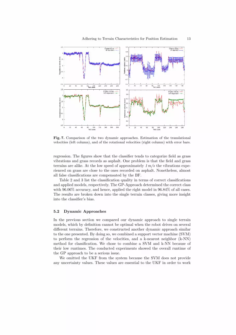
Fig. 7. Comparison of the two dynamic approaches. Estimation of the translationalvelocities (left column), and of the rotational velocities (right column) with error bars.

regression. The figures show that the classifier tends to categorize field as grassvibrations and grass records as asphalt. One problem is that the field and grassterrains are alike. At the low speed of approximately 1 m/s the vibrations expe-rienced on grass are close to the ones recorded on asphalt. Nonetheless, almostall false classifications are compensated by the BF.

Table 2 and 3 list the classification quality in terms of correct classificationsand applied models, respectively. The GP-Approach determined the correct classwith 96.06% accuracy, and hence, applied the right model in 96.84% of all cases.The results are broken down into the single terrain classes, giving more insightinto the classifier’s bias.

5.2 Dynamic Approaches

In the previous section we compared our dynamic approach to single terrainmodels, which by definition cannot be optimal when the robot drives on severaldifferent terrains. Therefore, we constructed another dynamic approach similarto the one presented. By doing so, we combined a support vector machine (SVM)to perform the regression of the velocities, and a k-nearest neighbor (k-NN)method for classification. We chose to combine a SVM and k-NN because oftheir low runtimes. The conducted experiments showed the overall runtime ofthe GP approach to be a serious issue.

We omitted the UKF from the system because the SVM does not provideany uncertainty values. These values are essential to the UKF in order to work


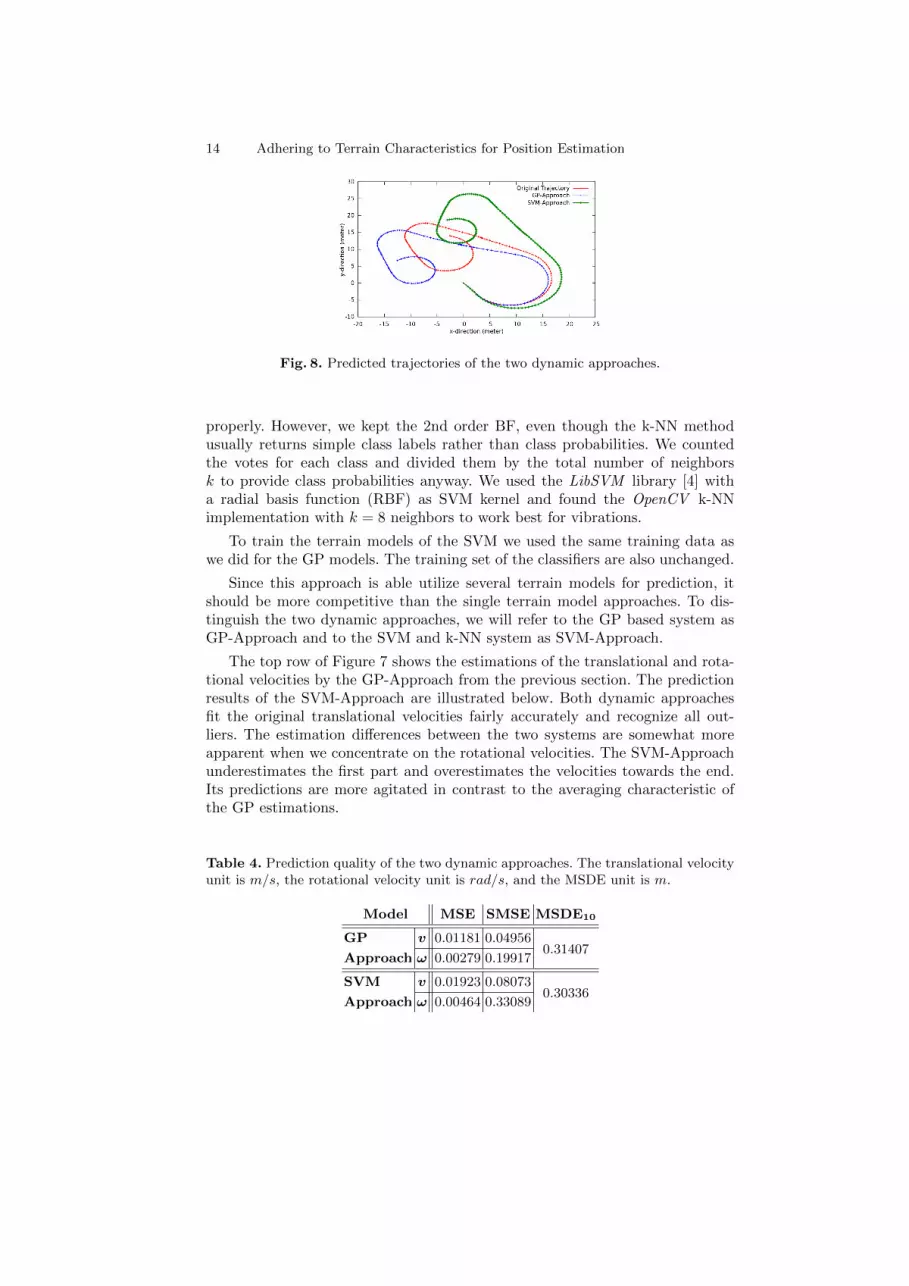
Fig. 8. Predicted trajectories of the two dynamic approaches.

properly. However, we kept the 2nd order BF, even though the k-NN methodusually returns simple class labels rather than class probabilities. We countedthe votes for each class and divided them by the total number of neighborsk to provide class probabilities anyway. We used the LibSVM library [4] witha radial basis function (RBF) as SVM kernel and found the OpenCV k-NNimplementation with k = 8 neighbors to work best for vibrations.

To train the terrain models of the SVM we used the same training data aswe did for the GP models. The training set of the classifiers are also unchanged.

Since this approach is able utilize several terrain models for prediction, itshould be more competitive than the single terrain model approaches. To dis-tinguish the two dynamic approaches, we will refer to the GP based system asGP-Approach and to the SVM and k-NN system as SVM-Approach.

The top row of Figure 7 shows the estimations of the translational and rota-tional velocities by the GP-Approach from the previous section. The predictionresults of the SVM-Approach are illustrated below. Both dynamic approachesfit the original translational velocities fairly accurately and recognize all out-liers. The estimation differences between the two systems are somewhat moreapparent when we concentrate on the rotational velocities. The SVM-Approachunderestimates the first part and overestimates the velocities towards the end.Its predictions are more agitated in contrast to the averaging characteristic ofthe GP estimations.

Table 4. Prediction quality of the two dynamic approaches. The translational velocityunit is m/s, the rotational velocity unit is rad/s, and the MSDE unit is m.

Model MSE SMSE MSDE10

GP v 0.01181 0.04956

Approach ω 0.00279 0.199170.31407

SVM v 0.01923 0.08073

Approach ω 0.00464 0.330890.30336


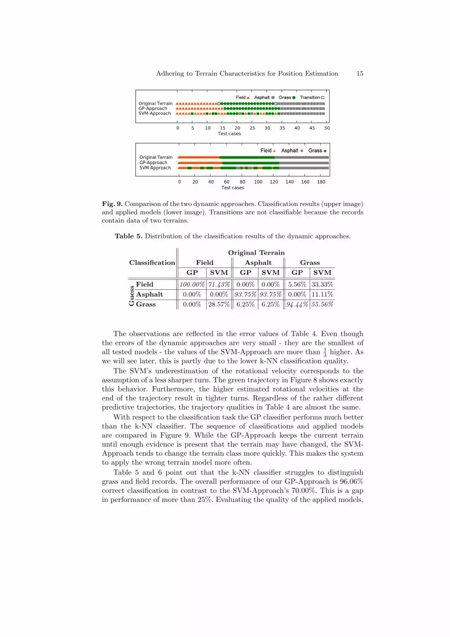
Fig. 9. Comparison of the two dynamic approaches. Classification results (upper image)and applied models (lower image). Transitions are not classifiable because the recordscontain data of two terrains.

Table 5. Distribution of the classification results of the dynamic approaches.

Original Terrain

Classification Field Asphalt Grass

GP SVM GP SVM GP SVM

Field 100.00% 71.43% 0.00% 0.00% 5.56% 33.33%

Asphalt 0.00% 0.00% 93.75% 93.75% 0.00% 11.11%

Guess

Grass 0.00% 28.57% 6.25% 6.25% 94.44% 55.56%

The observations are reflected in the error values of Table 4. Even thoughthe errors of the dynamic approaches are very small - they are the smallest ofall tested models - the values of the SVM-Approach are more than 1

3 higher. Aswe will see later, this is partly due to the lower k-NN classification quality.

The SVM’s underestimation of the rotational velocity corresponds to theassumption of a less sharper turn. The green trajectory in Figure 8 shows exactlythis behavior. Furthermore, the higher estimated rotational velocities at theend of the trajectory result in tighter turns. Regardless of the rather differentpredictive trajectories, the trajectory qualities in Table 4 are almost the same.

With respect to the classification task the GP classifier performs much betterthan the k-NN classifier. The sequence of classifications and applied modelsare compared in Figure 9. While the GP-Approach keeps the current terrainuntil enough evidence is present that the terrain may have changed, the SVM-Approach tends to change the terrain class more quickly. This makes the systemto apply the wrong terrain model more often.

Table 5 and 6 point out that the k-NN classifier struggles to distinguishgrass and field records. The overall performance of our GP-Approach is 96.06%correct classification in contrast to the SVM-Approach’s 70.00%. This is a gapin performance of more than 25%. Evaluating the quality of the applied models,


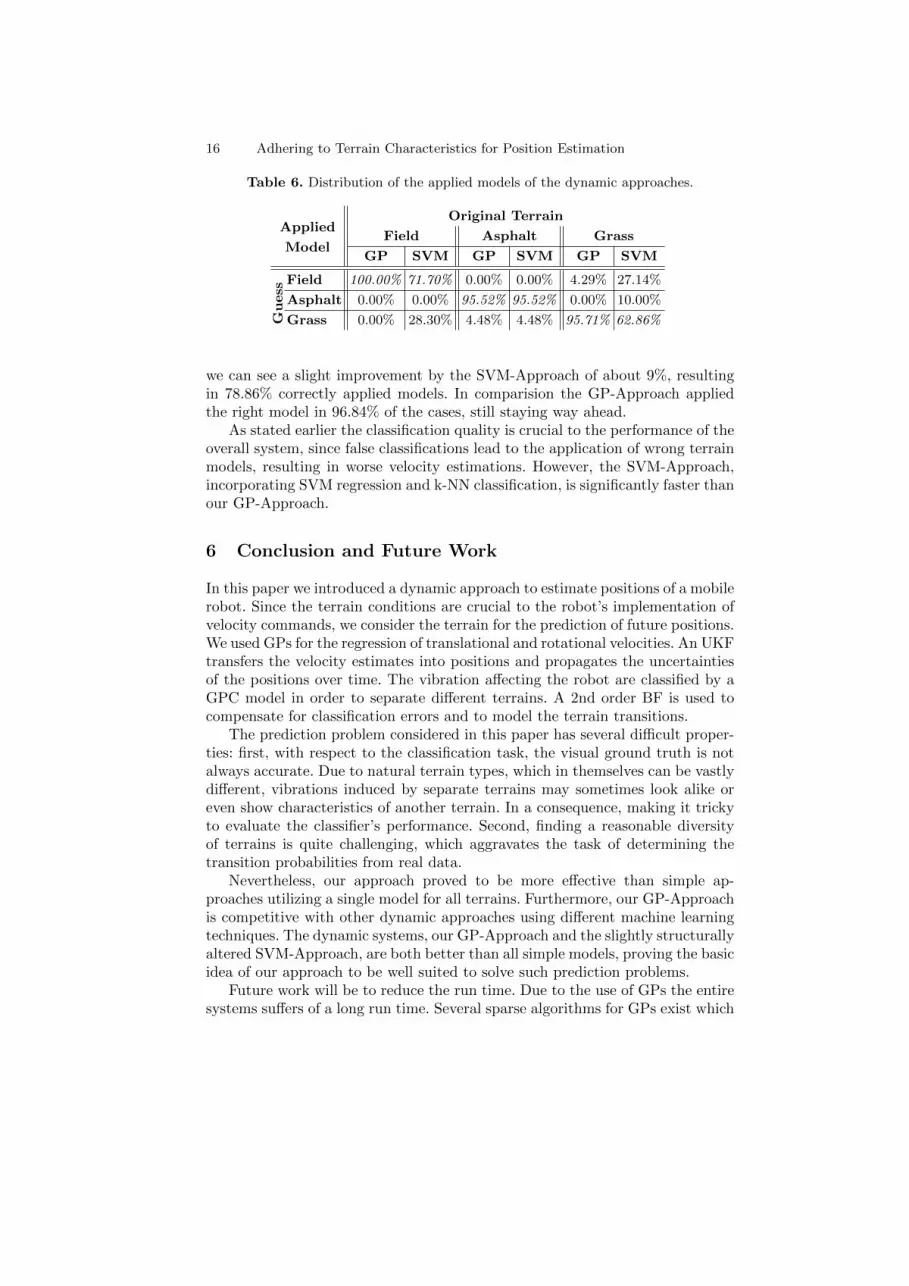
Table 6. Distribution of the applied models of the dynamic approaches.

Original TerrainApplied

Field Asphalt GrassModel

GP SVM GP SVM GP SVM

Field 100.00% 71.70% 0.00% 0.00% 4.29% 27.14%

Asphalt 0.00% 0.00% 95.52% 95.52% 0.00% 10.00%

Guess

Grass 0.00% 28.30% 4.48% 4.48% 95.71% 62.86%

we can see a slight improvement by the SVM-Approach of about 9%, resultingin 78.86% correctly applied models. In comparision the GP-Approach appliedthe right model in 96.84% of the cases, still staying way ahead.

As stated earlier the classification quality is crucial to the performance of theoverall system, since false classifications lead to the application of wrong terrainmodels, resulting in worse velocity estimations. However, the SVM-Approach,incorporating SVM regression and k-NN classification, is significantly faster thanour GP-Approach.

6 Conclusion and Future Work

In this paper we introduced a dynamic approach to estimate positions of a mobilerobot. Since the terrain conditions are crucial to the robot’s implementation ofvelocity commands, we consider the terrain for the prediction of future positions.We used GPs for the regression of translational and rotational velocities. An UKFtransfers the velocity estimates into positions and propagates the uncertaintiesof the positions over time. The vibration affecting the robot are classified by aGPC model in order to separate different terrains. A 2nd order BF is used tocompensate for classification errors and to model the terrain transitions.

The prediction problem considered in this paper has several difficult proper-ties: first, with respect to the classification task, the visual ground truth is notalways accurate. Due to natural terrain types, which in themselves can be vastlydifferent, vibrations induced by separate terrains may sometimes look alike oreven show characteristics of another terrain. In a consequence, making it trickyto evaluate the classifier’s performance. Second, finding a reasonable diversityof terrains is quite challenging, which aggravates the task of determining thetransition probabilities from real data.

Nevertheless, our approach proved to be more effective than simple ap-proaches utilizing a single model for all terrains. Furthermore, our GP-Approachis competitive with other dynamic approaches using different machine learningtechniques. The dynamic systems, our GP-Approach and the slightly structurallyaltered SVM-Approach, are both better than all simple models, proving the basicidea of our approach to be well suited to solve such prediction problems.

Future work will be to reduce the run time. Due to the use of GPs the entiresystems suffers of a long run time. Several sparse algorithms for GPs exist which


would help to improve this issue. We are working on the implementation of sucha sparse method at the moment.

Also GPRs and GPCs were compared to other well known methods for re-gression and classification, respectively. The run time of SVMs is smaller whileperforming equally. However, this would mean losing the uncertainty estimates,i.e. the quality indicators. This trade-off might be worth further investigation.Therefore and to determine the benefit of such a dynamic method in practice, weare currently integrating the SVM-based version in our local navigation software.Once the run time of the GP-based version allows the use in online applications,the integration in our local navigation framework will follow.

Moreover, expanding the current system by additional terrains as sand orgravel would be desirable. Extending the classification records by the transla-tional velocity could improve classification results, since it allows to learn theeffects of different speeds on the vibrations.

References

1. Agrawal, M. and Konolige, K. (2006). Real-time localization in outdoor environ-ments using stereo vision and inexpensive GPS. In International Conference onPattern Recognition (ICPR), volume 3, pages 1063–1068.

2. Brooks, C. A., Iagnemma, K., and Dubowsky, S. (2005). Vibration-based terrainanalysis for mobile robots. In IEEE International Conference on Robotics and Au-tomation (ICRA), pages 3415–3420.

3. Burgard, W., Fox, D., Hennig, D., and Schmidt, T. (1996). Estimating the abso-lute position of a mobile robot using position probability grids. In AAAI NationalConference on Artificial Intelligence, volume 2.

4. Chang, C.-C. and Lin, C.-J. (2001). LIBSVM: a library for support vector machines.Software available at http://www.csie.ntu.edu.tw/∼cjlin/libsvm.

5. Dahlkamp, H., Kaehler, A., Stavens, D., Thrun, S., and Bradski, G. R. (2006). Self-supervised monocular road detection in desert terrain. In Robotics: Science andSystems.

6. Ferris, B., Hahnel, D., and Fox, D. (2006). Gaussian processes for signal strength-based location estimation. In Robotics: Science and Systems.

7. Girard, A., Rasmussen, C. E., Quinonero-Candela, J., and Murray-Smith, R. (2003).Gaussian process priors with uncertain inputs - Application to multiple-step aheadtime series forecasting. In Advances in Neural Information Processing Systems(NIPS), pages 529–536.

8. Iagnemma, K. and Ward, C. C. (2009). Classification-based wheel slip detectionand detector fusion for mobile robots on outdoor terrain. Autonomous Robots,26(1):33–46.

9. Kapoor, A., Grauman, K., Urtasun, R., and Darrell, T. (2007). Active learning withgaussian processes for object categorization. In IEEE International Conference onComputer Vision (ICCV), volume 11, pages 1–8.

10. Ko, J., Klein, D. J., Fox, D., and Hahnel, D. (2007a). Gaussian processes andreinforcement learning for identification and control of an autonomous blimp. InIEEE International Conference on Robotics and Automation (ICRA), pages 742–747.


11. Ko, J., Klein, D. J., Fox, D., and Hahnel, D. (2007b). GP-UKF: Unscented Kalmanfilters with gaussian process prediction and observationmodels. In IEEE/RSJ Inter-national Conference on Intelligent Robots and Systems (IROS), pages 1901–1907.

12. Li-Juan, L., Hong-Ye, S., and Jian, C. (2007). Generalized predictive control withonline least squares support vector machines. In Acta Automatica Sinica (AAS),volume 33, pages 1182–1188.

13. MacKay, D. J. C. (1998). Introduction to gaussian processes. In Bishop, C. M.,editor, Neural Networks and Machine Learning, NATO ASI Series, pages 133–166.Springer-Verlag.

14. Rasmussen, C. E. (2002). Combining laser range, color, and texture cues for au-tonomous road following. In IEEE International Conference on Robotics and Au-tomation (ICRA).

15. Rasmussen, C. E. and Williams, C. K. I. (2005). Gaussian Processes for MachineLearning. The MIT Press.

16. Seyr, M., Jakubek, S., and Novak, G. (2005). Neural network predictive trajectorytracking of an autonomous two-wheeled mobile robot. In International Federationof Automatic Control (IFAC) World Congress.

17. Thrun, S., Fox, D., Burgard, W., and Dellaert, F. (2000). Robust monte carlolocalization for mobile robot. Artificial Intelligence, 128:99–141.

18. Urtasun, R. and Darrell, T. (2007). Discriminative gaussian process latent variablemodels for classification. In International Conference on Machine Learning (ICML).

19. Ward, C. C. and Iagnemma, K. (2007). Model-based wheel slip detection for out-door mobile robots. In IEEE International Conference on Robotics and Automation(ICRA), pages 2724–2729.

20. Weiss, C., Frohlich, H., and Zell, A. (2006). Vibration-based terrain classificationusing support vector machines. In IEEE/RSJ International Conference on Intelli-gent Robots and Systems (IROS), pages 4429–4434.

21. Williams, C. K. I. (2002). Gaussian processes. In The Handbook of Brain Theoryand Neural Networks. The MIT Press, 2 edition.

Adhering to terrain characteristics for position estimation of mobile robots

Documents