A new terrain mapping method for mobile robots obstacle ...

A new terrain mapping method for mobile robots obstacle negotiation

Cang Ye and Johann Borenstein

Advanced Technologies Lab The University of Michigan

1101 Beal Ave, Ann Arbor, MI, USA 48109-2110

ABSTRACT

This paper introduces a new terrain mapping method for mobile robots with a 2-D laser rangefinder. In the proposed method, an elevation map and a certainty map are built and used for the filtering of erroneous data. The filter, called Certainty Assisted Spatial (CAS) filter, first employs the physical constraints on motion continuity and spatial continuity to distinguish corrupted pixels (e.g., due to artifacts, random noise, or the “mixed pixels” effect) and missing data from uncorrupted pixels in an elevation map. It then removes the corrupted pixels and missing data, while missing data is filled in by a Weighted Median filter. Uncorrupted pixels are left intact so as to retain edges of objects. Our extensive indoor and outdoor mapping experiments demonstrate that the CAS filter has better performance in erroneous data reduction and map detail preservation than existing filters.

Keywords: laser rangefinder, terrain mapping, filtering, elevation map, certainty map, mixed pixels.

1. INTRODUCTION To autonomously navigate on rugged terrain (i.e., indoor environments with debris on the floor or outdoor, off-road environments), a mobile robot requires the capability to decide whether an obstacle should be traversed or circumnavigated. The ability to make this decision and to apply the appropriate action is called “obstacle negotiation” (ON). A crucial issue involved in ON is terrain mapping. Research efforts on terrain mapping have been devoted to indoor environments [1], outdoor, off-road terrain [2, 3, 4], as well as planetary terrain [5, 6, 7]. Most of the existing methods employ stereovision [2, 3, 4, 7], which is sensitive to environmental condition (e.g., ambient illumination) and has low range resolution and accuracy. As an alternative or supplement, 3-D Laser Rangefinders (LRFs) have been employed since the early nineties [5, 6, 8]. However, 3-D LRFs are very costly, bulky, and heavy. Therefore, they are not suitable for small and/or expendable robots. Furthermore, most of them are designed for stationary use due to the slow scan speed in elevation.

A more feasible solution for lower-cost robots is a 2-D LRF. Researchers at CMU [1] used a Sick 2-D LRF looking upward to perform indoor 3-D mapping. Due to the upward looking manner, the 3D map is not suitable for ON since the ground map is not available in this case. Henrick and Krotkov [9] employed an Acuity 2-D LRF to complement stereovision for obstacle and hazard detection. The scanner was pointed to the ground at 45°. Due to the small look-ahead distance, the scanner was used for safety purposes only, i.e., when an obstacle is detected, an emergency command is issued to stop the robot. More recent research at CMU [3] also used a 2-D LRF to complement stereovision in a terrain mapping application. In this work a Sick LMS 220 was mounted on CMU’s “Nomad” robot so as to “look” diagonally downward and forward. As the robot moves forward, the fanning laser beam swept the ground ahead of the robot and produced range data of the terrain. Based on this data, the Nomad produced a so called “goodness map,” which was created based on the current scan data and the previous ground level (i.e., a least square fit line in the previous scan). The “goodness map” was then combined with the map built by stereovision for path planning. In this work, the overall map was produced mainly by stereovision.

This paper presents a new terrain mapping method using a single sensor modality−a 2-D LRF, and an innovative filtering method for map building. The paper is organized as follows: In Section 2 we introduce our approach to terrain mapping and we discuss sources of map misrepresentations. We also investigate the problems in applying conventional image filters to our terrain-mapping problem and describe the principle of our filter. In Section 3 we present experimental benchmark tests performed under controlled conditions, followed by results of indoor and outdoor experiments.

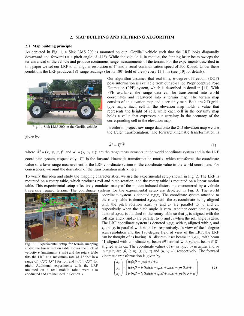
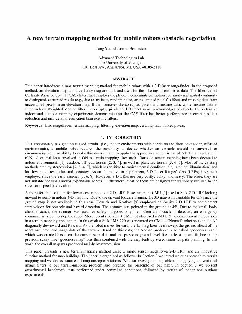
Fig. 1. Sick LMS 200 on the Gorilla vehicle

Fig. 2. Experimental setup for terrain mappingstudy: the linear motion table moves the LRF atvelocity v (maximum: 1 m/s) and the rotary tabletilts the LRF at a maximum rate of 37.5°/s in a range of [-15°, 15° ] for roll and [-40°, -25°] for pitch. Additional experiments with the LRFmounted on a real mobile robot were alsoconducted and are included in Section 3.

2. MAP BUILDING AND FILTERING ALGORITHM

2.1 Map building principle As depicted in Fig. 1, a Sick LMS 200 is mounted on our “Gorilla” vehicle such that the LRF looks diagonally downward and forward (at a pitch angle of -11°). While the vehicle is in motion, the fanning laser beam sweeps the terrain ahead of the vehicle and produce continuous range measurements of the terrain. For the experiments described in this paper we set our LRF to an angular resolution of 1° and a serial communication speed of 500 Kbaud. Under these conditions the LRF produces 181 range readings (for its 180° field of view) every 13.3 ms (see [10] for details).

Our algorithm assumes that real-time, 6-degree-of-freedom (DOF) pose information is available from our so-called Proprioceptive Pose Estimation (PPE) system, which is described in detail in [11]. With PPE available, the range data can be transformed into world coordinates and registered into a terrain map. The terrain map consists of an elevation map and a certainty map. Both are 2-D grid-type maps. Each cell in the elevation map holds a value that represents the height of cell, while each cell in the certainty map holds a value that expresses our certainty in the accuracy of the corresponding cell in the elevation map.

In order to project raw range data onto the 2-D elevation map we use the Euler transformation. The forward kinematic transformation is

given by:

lnl

n dTdvv

= (1)

where Tnnn

n zyxd ),,(=v

and Tlll

l zyxd ),,(=v

are the range measurements in the world coordinate system and in the LRF

coordinate system, respectively. nlT is the forward kinematic transformation matrix, which transforms the coordinate

value of a laser range measurement in the LRF coordinate system to the coordinate value in the world coordinate. For conciseness, we omit the derivation of the transformation matrix here.

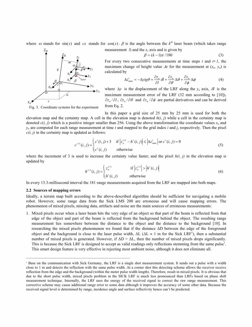
To verify this idea and study the mapping characteristics, we use the experimental setup shown in Fig. 2. The LRF is mounted on a rotary table, which produces roll and pitch rotation, and the rotary table is mounted on a linear motion table. This experimental setup effectively emulates many of the motion-induced distortions encountered by a vehicle traversing rugged terrain. The coordinate systems for the experimental setup are depicted in Fig. 3. The world

coordinate system is denoted xnynzn. The coordinate system attached to the rotary table is denoted xbybzb with the xb coordinate being aligned with the pitch rotation axis. yb and zb are parallel to yn and zn, respectively when the pitch angle is zero. Another coordinate system, denoted xlylzl, is attached to the rotary table so that yl is aligned with the roll axis and xl and zl are parallel to xb and zb when the roll angle is zero. The LRF coordinate system is denoted xsyszs with zs aligned with zl and xs and ys in parallel with xl and yl, respectively. In view of the 1-degree scan resolution and the 180-degree field of view of the LRF, the LRF can be thought of as having 181 discrete laser beams in xso3ys, with beam #1 aligned with coordinate xs, beam #91 aimed with ys, and beam #181 aligned with -xs. The coordinate values of o3 in xlylzl, o2 in xbybzb and o1 in xnynzn are (0, 0, p), (t, m, q) and (u, v, w), respectively. The forward kinematic transformation is given by

++++−+−+−+

+++=

wcpcmsqccslcslsvcpsmcqscslsslc

utpsclc

zyx

n

n

n

φθθθβφθβθφθθθβφθβθ

φβφ (2)

xn

zn

yn

zb

xb yb

v

u

w o

o1

q

m t

zl

o2

o3

zs

xs ys

yl xl

θ

φ

laser β

Fig. 3. Coordinate systems for the experiment

where sx stands for )sin(x and cx stands for )cos(x . β is the angle between the kth laser beam (which takes range

measurement l) and the xs axis and is given by 180/)1( πβ −= k (3) For every two consecutive measurements at time steps t and t+1, the maximum change of height value ∆z for the measurement at (xn, yn) is calculated by

φφ

θθ

δθ ∆∂∂

+∆∂∂

+∂∂

+∆−=∆ nnnt zzll

zytgzmax (4)

where y∆ is the displacement of the LRF along the yn axis, lδ is the maximum measurement error of the LRF (32 mm according to [10]),

lzn ∂∂ / , θ∂∂ /nz and φ∂∂ /nz are partial derivatives and can be derived from Eq. 2.

In this paper a grid size of 25 mm by 25 mm is used for both the elevation map and the certainty map. A cell in the elevation map is denoted h(i, j) while a cell in the certainty map is denoted c(i, j) which is a positive integer smaller than 256. Using the above transformation the coordinate values xn and yn are computed for each range measurement at time t and mapped to the grid index i and j, respectively. Then the pixel c(i, j) in the certainty map is updated as follows:

=∆≤−+

=+

+

otherwise ),(

0),(or ),( if 3,),( max

11

jic

jiczjihzj)(icjic

t

ttttn

tt (5)

where the increment of 3 is used to increase the certainty value faster; and the pixel h(i, j) in the elevation map is updated by

>

=++

+

otherwise ),(

),( if ),(

111

jih

jihz zjih

t

ttn

tnt (6)

In every 13.3-millisecond interval the 181 range measurements acquired from the LRF are mapped into both maps.

2.2 Sources of mapping errors Ideally, a terrain map built according to the above-described algorithm should be sufficient for navigating a mobile robot. However, some range data from the Sick LMS 200 are erroneous and will cause mapping errors. The phenomenon of mixed pixels, missing data, artifacts and noise are the main sources of erroneous measurements:

1. Mixed pixels occur when a laser beam hits the very edge of an object so that part of the beam is reflected from that edge of the object and part of the beam is reflected from the background behind the object. The resulting range measurement lies somewhere between the distance to the object and the distance to the background [10]. In researching the mixed pixels phenomenon we found that if the distance ∆D between the edge of the foreground object and the background is close to the laser pulse width, ∆L (∆L ≈ 1 m for the Sick LRF1), then a substantial number of mixed pixels is generated. However, if ∆D > ∆L, then the number of mixed pixels drops significantly. This is because the Sick LRF is designed to accept as valid readings only reflections stemming from the same pulse1. This smart design feature is very effective in rejecting most ambient noise, although it does not eliminate all.

__________________________________________________ 1 Base on the communication with Sick Germany, the LRF is a single shot measurement system. It sends out a pulse with a width close to 1 m and detects the reflection with the same pulse width. At a corner shot this detecting scheme allows the receiver receive reflection from the edge and the background (within the meter pulse width length). Therefore, result in mixed pixels. It is obvious that due to the short pulse width, mixed pixels problem in the SICK LRF is much less pronounced than LRFs based on phase shift measurement technique. Internally, the LRF uses the energy of the received signal to correct the raw range measurement. This corrective scheme may cause additional range error to some data although it improves the accuracy of some other data. Because the received signal level is determined by range, incidence angle and surface reflectivity hence can’t be predicted.

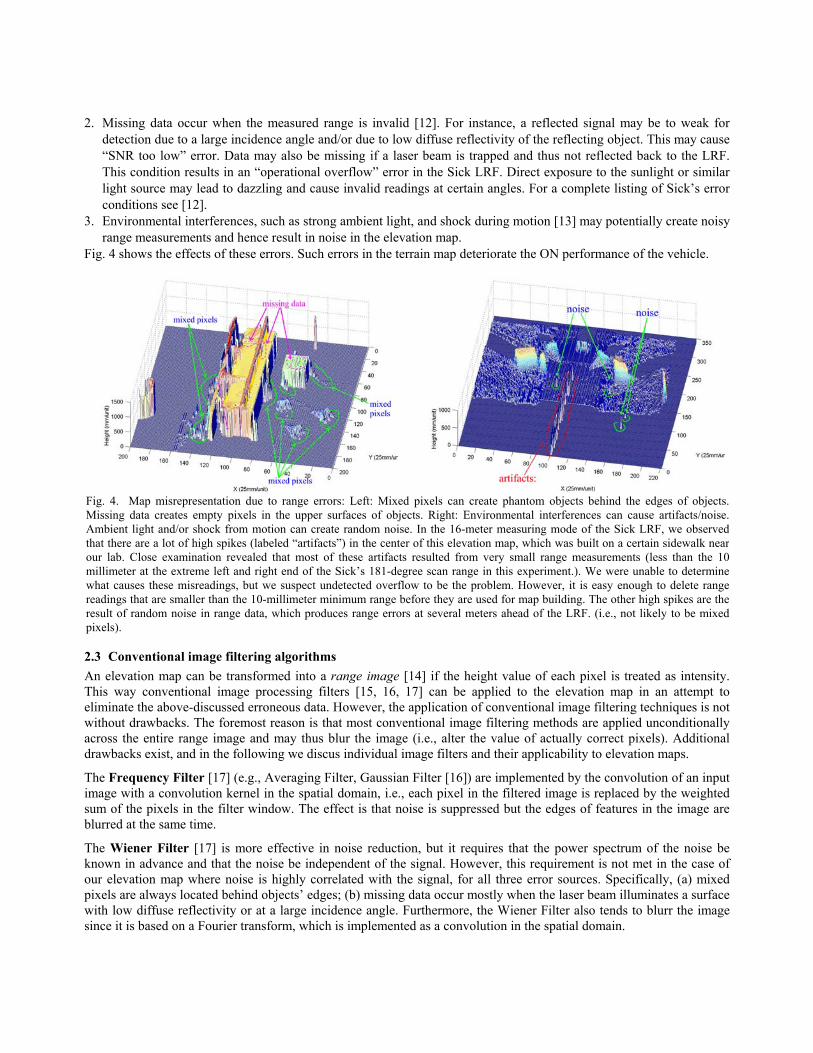
Fig. 4. Map misrepresentation due to range errors: Left: Mixed pixels can create phantom objects behind the edges of objects.Missing data creates empty pixels in the upper surfaces of objects. Right: Environmental interferences can cause artifacts/noise.Ambient light and/or shock from motion can create random noise. In the 16-meter measuring mode of the Sick LRF, we observedthat there are a lot of high spikes (labeled “artifacts”) in the center of this elevation map, which was built on a certain sidewalk nearour lab. Close examination revealed that most of these artifacts resulted from very small range measurements (less than the 10millimeter at the extreme left and right end of the Sick’s 181-degree scan range in this experiment.). We were unable to determinewhat causes these misreadings, but we suspect undetected overflow to be the problem. However, it is easy enough to delete rangereadings that are smaller than the 10-millimeter minimum range before they are used for map building. The other high spikes are theresult of random noise in range data, which produces range errors at several meters ahead of the LRF. (i.e., not likely to be mixedpixels).

2. Missing data occur when the measured range is invalid [12]. For instance, a reflected signal may be to weak for detection due to a large incidence angle and/or due to low diffuse reflectivity of the reflecting object. This may cause “SNR too low” error. Data may also be missing if a laser beam is trapped and thus not reflected back to the LRF. This condition results in an “operational overflow” error in the Sick LRF. Direct exposure to the sunlight or similar light source may lead to dazzling and cause invalid readings at certain angles. For a complete listing of Sick’s error conditions see [12].

3. Environmental interferences, such as strong ambient light, and shock during motion [13] may potentially create noisy range measurements and hence result in noise in the elevation map.

Fig. 4 shows the effects of these errors. Such errors in the terrain map deteriorate the ON performance of the vehicle.

2.3 Conventional image filtering algorithms An elevation map can be transformed into a range image [14] if the height value of each pixel is treated as intensity. This way conventional image processing filters [15, 16, 17] can be applied to the elevation map in an attempt to eliminate the above-discussed erroneous data. However, the application of conventional image filtering techniques is not without drawbacks. The foremost reason is that most conventional image filtering methods are applied unconditionally across the entire range image and may thus blur the image (i.e., alter the value of actually correct pixels). Additional drawbacks exist, and in the following we discus individual image filters and their applicability to elevation maps.

The Frequency Filter [17] (e.g., Averaging Filter, Gaussian Filter [16]) are implemented by the convolution of an input image with a convolution kernel in the spatial domain, i.e., each pixel in the filtered image is replaced by the weighted sum of the pixels in the filter window. The effect is that noise is suppressed but the edges of features in the image are blurred at the same time.

The Wiener Filter [17] is more effective in noise reduction, but it requires that the power spectrum of the noise be known in advance and that the noise be independent of the signal. However, this requirement is not met in the case of our elevation map where noise is highly correlated with the signal, for all three error sources. Specifically, (a) mixed pixels are always located behind objects’ edges; (b) missing data occur mostly when the laser beam illuminates a surface with low diffuse reflectivity or at a large incidence angle. Furthermore, the Wiener Filter also tends to blurr the image since it is based on a Fourier transform, which is implemented as a convolution in the spatial domain.

Median filters are well known for their capability of removing impulse noise and preserving image edges, and are reported to have good performance in removing mixed pixels in laser range images [15]. The standard Median Filter and its variations (Weighted Median Filter [18] and Center Weighted Median Filter [19]) often exhibit blurring when a large filter window is used, or insufficient noise reduction for a small filter window. For instance, thin edges (because thin objects are present or objects are too high such that only the front edges are sensed) in an elevation map may be completely removed by a standard Median filter. Adaptive Median Filters [20, 21] maintain a better balance between detail preservation and noise reduction, and hence achieve better performance. However, all of these median-type filters affect all the pixels in an image including uncorrupted ones. A number of median type filters [22, 23] in the literature may potentially distinguish corrupted pixels from uncorrupted ones and apply filtering only to the corrupted pixels. These filters utilize local input image characteristics (spatial information only) to identify corrupted pixels. However, a limitation of this approach is the potenential misclassification of thin edges as corrupted pixels and the subsequent removal of these pixels. For instance, a thin pole in a range image produces a line of high intensity pixels, which may be misinterpreted by the filter as impulse noise and removed. This suggests that it is insufficient to use only spatial information for the identification of corrupted pixels.

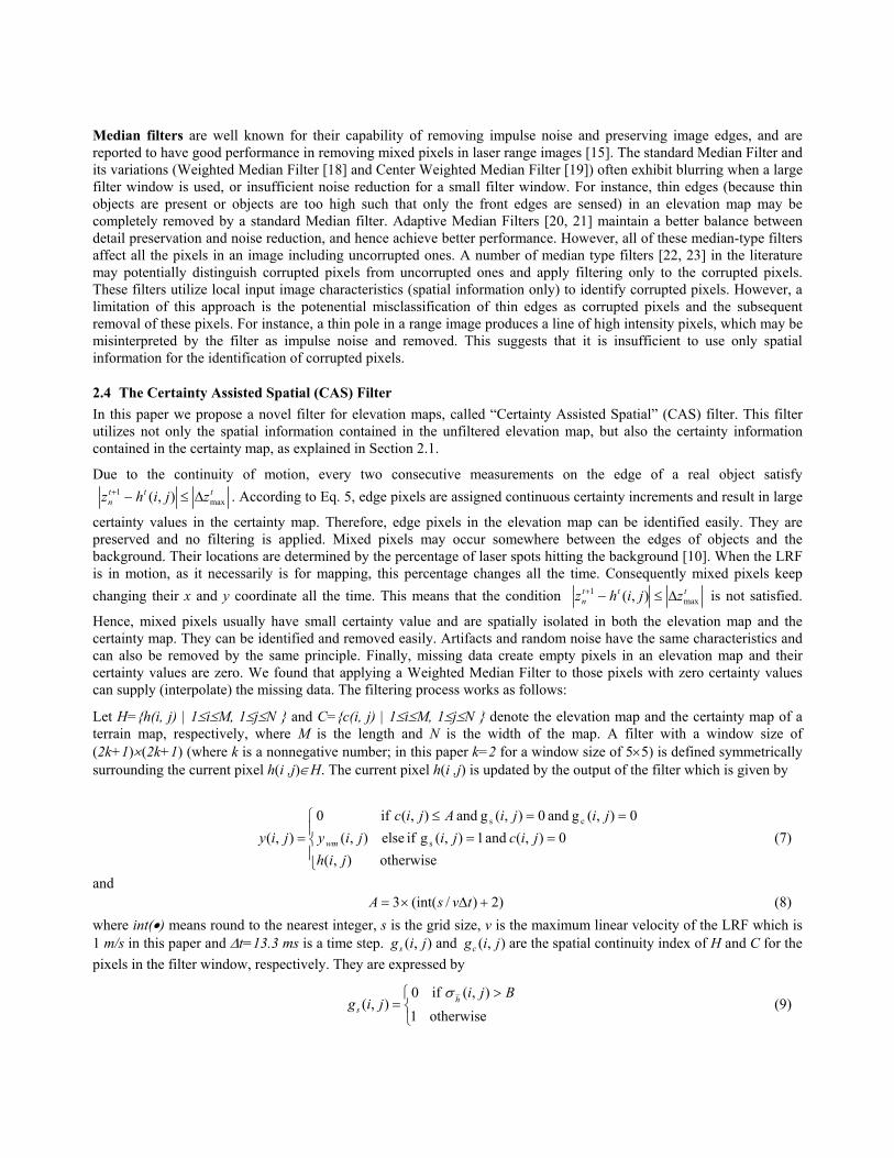
2.4 The Certainty Assisted Spatial (CAS) Filter In this paper we propose a novel filter for elevation maps, called “Certainty Assisted Spatial” (CAS) filter. This filter utilizes not only the spatial information contained in the unfiltered elevation map, but also the certainty information contained in the certainty map, as explained in Section 2.1.

Due to the continuity of motion, every two consecutive measurements on the edge of a real object satisfy ttt

n zjihz max1 ),( ∆≤−+ . According to Eq. 5, edge pixels are assigned continuous certainty increments and result in large

certainty values in the certainty map. Therefore, edge pixels in the elevation map can be identified easily. They are preserved and no filtering is applied. Mixed pixels may occur somewhere between the edges of objects and the background. Their locations are determined by the percentage of laser spots hitting the background [10]. When the LRF is in motion, as it necessarily is for mapping, this percentage changes all the time. Consequently mixed pixels keep changing their x and y coordinate all the time. This means that the condition ttt

n zjihz max1 ),( ∆≤−+ is not satisfied.

Hence, mixed pixels usually have small certainty value and are spatially isolated in both the elevation map and the certainty map. They can be identified and removed easily. Artifacts and random noise have the same characteristics and can also be removed by the same principle. Finally, missing data create empty pixels in an elevation map and their certainty values are zero. We found that applying a Weighted Median Filter to those pixels with zero certainty values can supply (interpolate) the missing data. The filtering process works as follows:

Let H={h(i, j) | 1≤i≤M, 1≤j≤N } and C={c(i, j) | 1≤i≤M, 1≤j≤N } denote the elevation map and the certainty map of a terrain map, respectively, where M is the length and N is the width of the map. A filter with a window size of (2k+1)×(2k+1) (where k is a nonnegative number; in this paper k=2 for a window size of 5×5) is defined symmetrically surrounding the current pixel h(i ,j)∈H. The current pixel h(i ,j) is updated by the output of the filter which is given by

==

==≤=

otherwise ),(0),( and 1),(g if else ),(

0),(g and 0),(g and ),( if 0),( s

cs

jihjicjijiy

jijiAjicjiy wm (7)

and )2)/(int(3 +∆×= tvsA (8) where int(•) means round to the nearest integer, s is the grid size, v is the maximum linear velocity of the LRF which is 1 m/s in this paper and ∆t=13.3 ms is a time step. ),( jigs and ),( jigc are the spatial continuity index of H and C for the pixels in the filter window, respectively. They are expressed by

>

= otherwise 1),( if 0

),(Bji

jig hs

σ (9)

2 2 2 2 2 2 2 1 2 2 2 1 1 1 2 2 2 1 2 2 2 2 2 2 2

j-2 j-1 j j+1 j+2 i-2i-1i

i+1i+2

Fig. 5. Filter skeleton for the WM filter

Fig. 6. Obstacle course for benchmark tests

and

><

= ∑++

−==

otherwise 1

if 0),(

,

,

E(i,j)σ D or c(m,n)jig c

kjki

kjni-kmc (10)

where hσ and cσ are the variance of the normalized local map

+≤≤−+≤≤−= kjnkjkimkinmh

nmhH L , )),(max(

),(

and

+≤≤−+≤≤−= kjnkjkimkinmh

nmcCL , )),(max(

),( respectively. We use 10×A for D and 0.04 for E. To keep

the computational cost low we use 7,

,

<∑++

−=−=

kjki

kjnkimLH to approximate the condition Bjih >),(σ in Eq. 9. ),( jiywm is the

output of a Weighted Median (WM) filter centered at pixels (i, j). The input pixels to the WM filter are obtained by applying a filter skeleton [18] (as depicted in Fig. 5) to the elevation map. For instance, h(i, j) has one copy while h(i-2, j-1) has two copies in the input pixels to the WM filter. The use of this skeleton is based on the following heuristic: Since we suspect h(i, j) to be a missing datum, the nearest neighboring pixels h(i±1, j±1) are also likely to be missing data, while those pixels farther from h(i, j) have a greater likelihood not to be missing data. Note, however, that this weight assignment for the WM filter potentially removes more missing data on the upper surface of an object.

When the CAS filter is applied to the raw elevation map, mixed pixels, artifacts, and random noise are identified by examining the motion continuity ( ),( jic constrained by Eq. 5) and the spatial continuity in the elevation map and the certainty map ( ),(gs ji and ),(gc ji ). Missing data is distinguished by inspecting the current pixel’s certainty value ),( jic and the spatial continuity ),(gs ji in the elevation map. Mixed pixels, artifacts, and random noise are therefore removed and the missing data are interpolated by the WM filter.

3. EXPERIMENTAL RESULTS In this paper we present extensive experimental results. These results can be grouped into two categories: Benchmark tests performed under highly controlled conditions, and mobility tests in which the LRF was mounted on a mobile platform. In all of the experiments, we used a 1.2 GHz AMD Athlon processor-based PC running RT-Linux for the real-time data collection.

3.1 Benchmark Tests Based on the experimental setup in Fig. 2, we designed the following four benchmark tests: 1) The LRF translates only (denoted ‘T’); 2) the LRF translates and rotates with roll only (denoted ‘TR’); 3) the LRF translates and rotates with pitch only (denoted TP); and 4) the LRF translates and rotates with roll and pitch (denoted TRP).

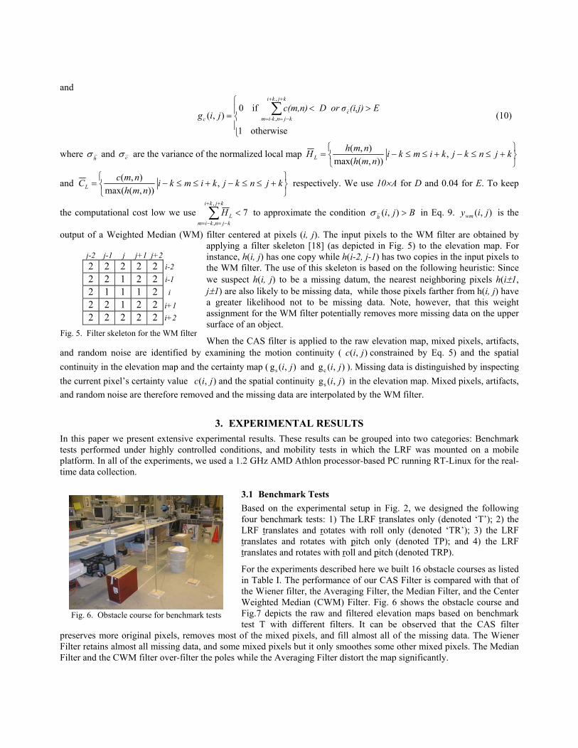
For the experiments described here we built 16 obstacle courses as listed in Table I. The performance of our CAS Filter is compared with that of the Wiener filter, the Averaging Filter, the Median Filter, and the Center Weighted Median (CWM) Filter. Fig. 6 shows the obstacle course and Fig.7 depicts the raw and filtered elevation maps based on benchmark test T with different filters. It can be observed that the CAS filter

preserves more original pixels, removes most of the mixed pixels, and fill almost all of the missing data. The Wiener Filter retains almost all missing data, and some mixed pixels but it only smoothes some other mixed pixels. The Median Filter and the CWM filter over-filter the poles while the Averaging Filter distort the map significantly.

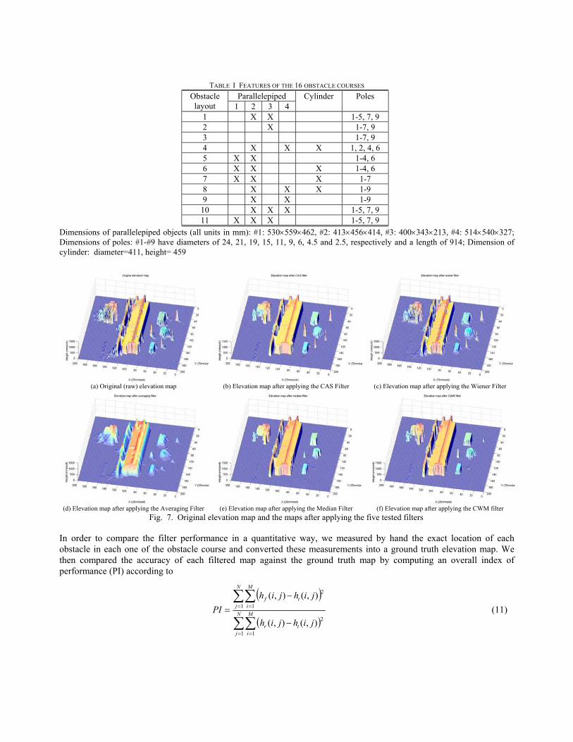
TABLE I FEATURES OF THE 16 OBSTACLE COURSES Parallelepiped Obstacle

layout 1 2 3 4 Cylinder Poles

1 X X 1-5, 7, 9 2 X 1-7, 9 3 1-7, 9 4 X X X 1, 2, 4, 6 5 X X 1-4, 6 6 X X X 1-4, 6 7 X X X 1-7 8 X X X 1-9 9 X X 1-9

10 X X X 1-5, 7, 9 11 X X X 1-5, 7, 9

Dimensions of parallelepiped objects (all units in mm): #1: 530×559×462, #2: 413×456×414, #3: 400×343×213, #4: 514×540×327; Dimensions of poles: #1-#9 have diameters of 24, 21, 19, 15, 11, 9, 6, 4.5 and 2.5, respectively and a length of 914; Dimension of cylinder: diameter=411, height= 459

In order to compare the filter performance in a quantitative way, we measured by hand the exact location of each obstacle in each one of the obstacle course and converted these measurements into a ground truth elevation map. We then compared the accuracy of each filtered map against the ground truth map by computing an overall index of performance (PI) according to

( )

( )∑∑

∑∑

= =

= =

−

−= N

j

M

itr

N

j

M

itf

jihjih

jihjihPI

1 1

2

1 1

2

),(),(

),(),( (11)

(a) Original (raw) elevation map (b) Elevation map after applying the CAS Filter (c) Elevation map after applying the Wiener Filter

(d) Elevation map after applying the Averaging Filter (e) Elevation map after applying the Median Filter (f) Elevation map after applying the CWM filter

Fig. 7. Original elevation map and the maps after applying the five tested filters

where hr(i,j), ht(i,j) and hf(i,j) are the elevation values of pixel (i, j) in the raw elevation map, the ground truth map, and the filtered map respectively. We arbitrarily selected M=80 and J=200 (which has full coverage of all obstacle courses) to evaluate the experiments here. According to Eq. 11, a smaller PI means better filter performance.

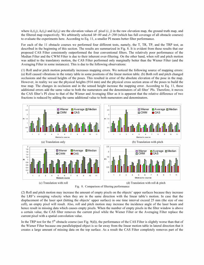
For each of the 11 obstacle courses we performed four different tests, namely, the T, TR, TP, and the TRP test, as described in the beginning of this section. The results are summarized in Fig. 8. It is evident from these results that our proposed CAS Filter consistently outperformed the four conventional filters. The relatively poor performance of the Median Filter and the CWM Filter is due to their inherent over-filtering. On the other hand, when roll and pitch motion was added to the translatory motion, the CAS Filter performed only marginally better than the Wiener Filter (and the Averaging Filter in some instances). This is due to the following observations:

(1) Roll and/or pitch motion potentially increases mapping errors. We noticed the following source of mapping errors: (a) Roll caused vibrations in the rotary table in some positions of the linear motion table. (b) Both roll and pitch changed occlusions and the sensed heights of the poses. This resulted in error of the absolute elevation of the pose in the map. However, in reality we use the physical heights (914 mm) and the physical cross section areas of the poses to build the true map. The changes in occlusion and in the sensed height increase the mapping error. According to Eq. 11, these additional errors add the same value to both the numerators and the denominators of all filter’ PIs. Therefore, it moves the CAS filter’s PI close to that of the Wiener and Averaging filter as it is apparent that the relative difference of two fractions is reduced by adding the same additional value to both numerators and denominators.

(2) Roll and pitch motion may increase the amount of empty pixels on the objects’ upper surfaces because they increase the LRF’s sweeping velocity when they are in the same direction with the linear table’s motion. In case that the displacement of the laser spot (hitting the objects’ upper surface) in one time interval exceed 25 mm (the size of one cell), an empty pixel will result. Also, roll and pitch motion may increase the incidence angle of the laser beam and hence result in missing data which causes empty pixels. When the number of empty pixels in the filter window is above a certain value, the CAS filter removes the current pixel while the Wiener Filter or the Averaging Filter replace the current pixel with a spatial convolution value.

In the TRP test for the 5th obstacle course (see Fig. 9(d)), the performance of the CAS Filter is slightly worse than that of the Wiener Filter because one parallelepiped object is so far away from the linear motion table in lateral direction that it creates a large amount of missing data on the top surface. As a result the CAS Filter completely removes part of the

0

0.5

1

1.5

2

2.5

3

1 2 3 4 5 6 7 8 9 10 11

Obst acl e cour se

P I

Wiener Average MedianCWM CAS

0

0.5

1

1.5

2

2.5

3

1 2 3 4 5 6 7 8 9 10 11

Obst acl e cour se

P I

Wiener Average MedianCWM CAS

(a) Translation only (b) Translation with pitch

00.20.40.60.8

11.21.41.61.8

2

1 2 3 4 5 6 7 8 9 10 11Obstacle course

PI

Wiener Average MedianCWM CAS

0

0.5

1

1.5

2

2.5

1 2 3 4 5 6 7 8 9 1 11Obst a c l e c our se

P I

Wiener Average MedianCWM CAS

(c) Translation with roll (d) Translation with roll & pitch

Fig. 8. Comparison of filtering performance

surface. However, we noticed that this only happens when an object is laterally far from the LRF’s path of motion. In practice, laterally distant objects have little significances in obstacle negotiation (ON) tasks.

One important feature of the CAS Filter is that it preserves the edges of objects in the elevation map, and edges are the key feature for ON. We should also mention in this discussion that, despite their relatively good PI performance, the Wiener Filter and Averaging Filter are not very suitable for ON. This is because the Wiener Filter does not remove artifacts/noise in elevation maps (see Section 3.2) while the Averaging Filter tends to lower the height of edges in the elevation maps – a highly undesirable trait in ON applications.

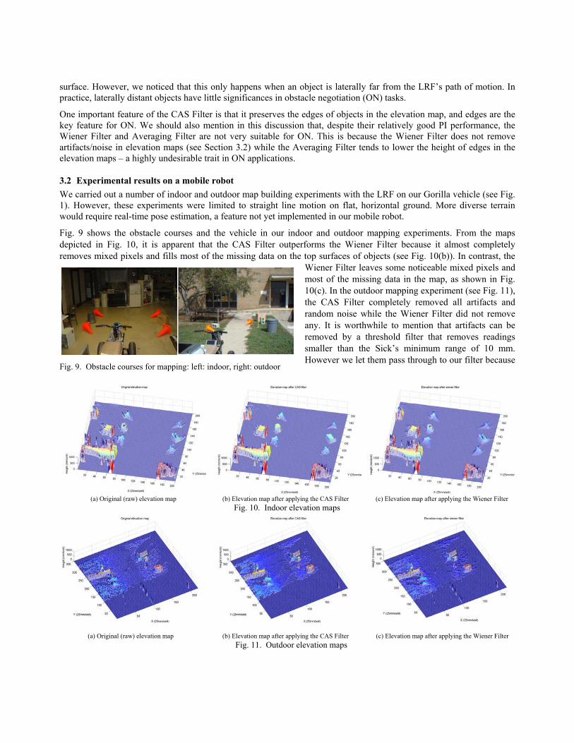
3.2 Experimental results on a mobile robot We carried out a number of indoor and outdoor map building experiments with the LRF on our Gorilla vehicle (see Fig. 1). However, these experiments were limited to straight line motion on flat, horizontal ground. More diverse terrain would require real-time pose estimation, a feature not yet implemented in our mobile robot.

Fig. 9 shows the obstacle courses and the vehicle in our indoor and outdoor mapping experiments. From the maps depicted in Fig. 10, it is apparent that the CAS Filter outperforms the Wiener Filter because it almost completely removes mixed pixels and fills most of the missing data on the top surfaces of objects (see Fig. 10(b)). In contrast, the

Wiener Filter leaves some noticeable mixed pixels and most of the missing data in the map, as shown in Fig. 10(c). In the outdoor mapping experiment (see Fig. 11), the CAS Filter completely removed all artifacts and random noise while the Wiener Filter did not remove any. It is worthwhile to mention that artifacts can be removed by a threshold filter that removes readings smaller than the Sick’s minimum range of 10 mm. However we let them pass through to our filter because

(a) Original (raw) elevation map (b) Elevation map after applying the CAS Filter (c) Elevation map after applying the Wiener Filter

Fig. 10. Indoor elevation maps

(a) Original (raw) elevation map (b) Elevation map after applying the CAS Filter (c) Elevation map after applying the Wiener Filter Fig. 11. Outdoor elevation maps

Fig. 9. Obstacle courses for mapping: left: indoor, right: outdoor

we want to test our filter’s effectiveness under unexpected outdoor factors. It is well known in image processing that random noises (e.g., Gaussian noise) are used to intentionally corrupt images, which are then used to test an image filter’s noise suppression performance. In our case, this doesn’t work because we need certainty value of each pixel, i.e., only true experiment can be used to test our filter. The artifacts and noise serve for this purpose.

4. DISCUSSION We are aware that there is an alternative to filtering mixed pixels. Adams [24] proposed an efficient mixed pixels removal method for phase shift LRFs. The algorithm is based on the detection of discontinuity of the received signal’s amplitude. However, due to the difference of measuring principles (time-of-flight in the case of the Sick LRF), this method must be modified to suit the Sick LRF. Such modification requires knowledge of the internal physics and the hardware design of the LRF, and can thus be implemented effectively only by the manufacturer, not the user. Specifically, Adam’s discontinuity detection algorithm requires several samples of the received signal (for computing the second derivative of the square of the signal amplitude with respect to the area illuminated by the laser on the edge) during the time the laser beam traverses the edge. However, at user level we can only get a single measurement on the edge. This means it is impractical to implement this algorithm. One might argue that if the Sick LRF sent out both reflectivity information and range data continuously, then similar method could be implemented outside of the Sick LRF. However, in this case the 500 Kbaud bandwidth limitation of the Sick LRF would be exceeded. This, in turn, would be force elimination of some range data – an undesirable option in mapping applications.

Finally, our method is based on the characteristics of the erroneous data and motion continuity constraint. It is device independent. Therefore, it is more general and suitable for the end users of LRFs. Differing from Adams’ algorithm, our approach removes not only mixed pixels but also unexpected outdoor artifacts and noise.

5. CONCLUSIONS In this paper we presented a novel filtering algorithm for terrain mapping with a 2-D LRF. The terrain map consists of an elevation map and a certainty map. The value of each pixel in the certainty map is determined as a function of a so-called “motion continuity constraint”. Typical erroneous data, such as mixed pixels, artifacts, and random noise don’t satisfy the motion continuity constraint and thus result in a low certainty value. Examination of the appropriate pixels in the certainty map and examination of the spatial continuity in the elevation map allows our CAS Filter to identify and remove erroneous pixels.

Missing data, such as that caused by large incidence angles and low diffuse reflection, can be identified because the affected pixels are associated with certainty values of ‘zero’ and with poor spatial continuity. Once identified, a WM filter can fill in the missing data.

Edges of objects are always associated with relatively large certainty values. As a result our CAS Filter leaves pixels representing object edges intact.

Overall, our proposed CAS Filter produces consistently better results than conventional filter algorithms because it makes use of the additional information available in the Certainty Map.

ACKNOWLEDGMENT This work was funded by the U.S. Department of Energy under Award No. DE-FG04-86NE3796 and under a grant from The University of Michigan’s Automotive Research Center (ARC), funded by TACOM.

The authors would like to thank Mr. Weber, Sick Germany for his kind help and insightful knowledge on the LRF. The authors would also like to thank James Berry for his work on the design of the rotary table.

REFERENCES 1 S. Thrun, W. Burgard and D. Fox, “A real-time algorithm for mobile robot mapping with application to multi-robot

and 3D mapping,” Proc. IEEE International Conference on Robotics and Automation, 2000, pp. 321-328.

2 S. Betgé-Brezetz, et al, “Uncertain map making in natural environments,” Proc. IEEE International Conference on Robotics and Automation, 1996, pp. 1048-1053.

3 D. S. Apostolopoulos, et al, “Technology and field demonstration of robotic search for Antarctic meteorites,” International Journal of Robotics Research, vol. 19, no. 11, pp. 1015-1032, 2000.

4 K. Fregene, R. Madhavan and L. E. Parker, “Incremental multiagent robotic mapping of outdoor terrain”, Proc. IEEE International Conference on Robotics and Automation, 2002, pp. 1339-1346.

5 I. S. Kweon and Takeo Kanade, “High-resolution terrain map from multiple sensor data,” IEEE Transactions on Pattern Analysis and Machine Intelligence, vol. 14, no. 2, pp. 278-292, 1992.

6 E. Krotkov and R. Hoffman, “Terrain mapping for a walking planetary rover,” IEEE Transactions on Robotics and Automation, vol. 10, no. 6, pp. 728-738, 1994.

7 R. Simmons, et al, “Experience with rover navigation for lunar-like terrains,” Proc. IEEE/RSJ International Conference on Intelligent Robots and System, 1995, pp. 441-446.

8 C. M. Shoemaker and J. A. Bornstein, “The demo III UGV program: a testbed for autonomous navigation research,” Proc. IEEE ISIS/CIRA/ISAS Joint Conference, 1998, pp. 644-651.

9 Henriksen L. and Krotkov E., “Natural Terrain Hazard Detection with a Laser Rangefinder.” Proc. IEEE Int. Conf. On Robotics and Automation, 1997, pp. 968-973.

10 C. Ye and J. Borenstein, “Characterization of a 2-D laser scanner for mobile robot obstacle negotiation,” Proc. IEEE International Conference on Robotics and Automation, 2002, pp. 2512-2518.

11 L. Ojeda and J. Borenstein, "FLEXnav: Fuzzy Logic Expert Rule-based Position Estimation for Mobile Robots on Rugged Terrain," Proc. IEEE International Conference on Robotics and Automation, 2002, pp. 317-322.

12 Sick Inc., LMS/LMI Telegram Listing, version 05.00, page 98. 13 A. Berman, J. Dayan and B. Friedland, “Improved EKF method of estimating locations with sudden high jumps in

the measurement noise”, Journal of Intelligent and Robotics Systems, vol. 32, no. 4, pp. 461-476, 2001. 14 P. J. Besl, Surfaces in range image understanding, Springer-Verlag, 1988. 15 M. Hebert and E. Krotkov, “3D measurements from imaging laser radars: how good are they?” Image and Vision

Computing, vol. 10, no. 3, pp. 170-178,1992. 16 C. F. Olson, “Adaptive-scale filtering and featuring detection using range data”, IEEE Transactions on Pattern

Analysis and Machine Intelligence, vol. 22, no. 9, 2000. 17 A. K. Jain, Fundamentals of Digital Image Processing, Prentice Hall, 1989. 18 D. R. K. Brownrigg, “The weighted median filter,” Communication of the ACM, vol. 27, no. 8, pp. 807-818, 1984. 19 S.-J. Ko and S.-J. Lee, “Center weighted median filters and their applications to image enhancement,” IEEE

Transactions on Circuits and Systems, vol. 38, no. 9, pp. 984-993, 1991. 20 H.-M. Lin and A. N. Willson, Jr., “Median filters with adaptive length,” IEEE Transactions on Circuits and Systems,

vol. 35, no. 6, 1988. 21 T. Chen and H. R. Wu, “Application of partition-based median type filters for suppressing noise in images,” IEEE

Transactions on Image Processing, vol. 10, no. 6, pp. 829-836, 2001. 22 H.-L. Eng and K.-K. Ma, “Noise adaptive soft-switching median filter,” IEEE Transactions on image processing,

vol. 10, no. 2, pp. 242-251, 2001. 23 T. Chen, K.-K. Ma and L.-H. Chen, “Tri-state median filter for image denoising,” IEEE Transactions on Image

Processing, vol. 8, no. 12, pp. 1834-1838, 1999. 24 M. D. Adams and P. J. Probert, “The interpretation of phase and intensity data from AMCW light detection sensors

for reliable ranging”, The International Journal of Robotics Research, vol. 15, No. 5, pp. 441-458, 1996.