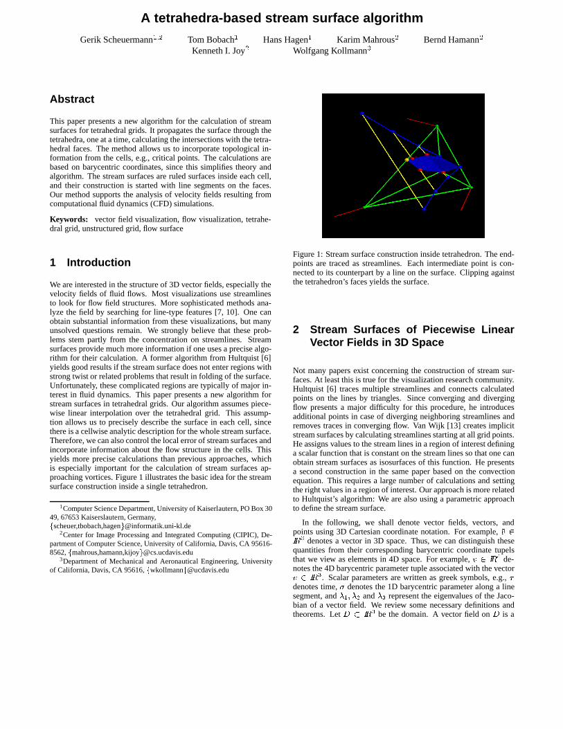
A tetrahedra-based stream surface algorithm

A tetrahedra-based stream surface algorithm

Gerik Scheuermann1;2 Tom Bobach1 Hans Hagen1 Karim Mahrous2 Bernd Hamann2

Kenneth I. Joy2 Wolfgang Kollmann3

Abstract

This paper presents a new algorithm for the calculation of streamsurfaces for tetrahedral grids. It propagates the surface through thetetrahedra, one at a time, calculating the intersections with the tetra-hedral faces. The method allows us to incorporate topological in-formation from the cells, e.g., critical points. The calculations arebased on barycentric coordinates, since this simplifies theory andalgorithm. The stream surfaces are ruled surfaces inside each cell,and their construction is started with line segments on the faces.Our method supports the analysis of velocity fields resulting fromcomputational fluid dynamics (CFD) simulations.

Keywords: vector field visualization, flow visualization, tetrahe-dral grid, unstructured grid, flow surface

1 Introduction

We are interested in the structure of 3D vector fields, especially thevelocity fields of fluid flows. Most visualizations use streamlinesto look for flow field structures. More sophisticated methods ana-lyze the field by searching for line-type features [7, 10]. One canobtain substantial information from these visualizations, but manyunsolved questions remain. We strongly believe that these prob-lems stem partly from the concentration on streamlines. Streamsurfaces provide much more information if one uses a precise algo-rithm for their calculation. A former algorithm from Hultquist [6]yields good results if the stream surface does not enter regions withstrong twist or related problems that result in folding of the surface.Unfortunately, these complicated regions are typically of major in-terest in fluid dynamics. This paper presents a new algorithm forstream surfaces in tetrahedral grids. Our algorithm assumes piece-wise linear interpolation over the tetrahedral grid. This assump-tion allows us to precisely describe the surface in each cell, sincethere is a cellwise analytic description for the whole stream surface.Therefore, we can also control the local error of stream surfaces andincorporate information about the flow structure in the cells. Thisyields more precise calculations than previous approaches, whichis especially important for the calculation of stream surfaces ap-proaching vortices. Figure 1 illustrates the basic idea for the streamsurface construction inside a single tetrahedron.

1Computer Science Department, University of Kaiserlautern, PO Box 3049, 67653 Kaiserslautern, Germany,fscheuer,tbobach,[email protected]

2Center for Image Processing and Integrated Computing (CIPIC), De-partment of Computer Science, University of California, Davis, CA 95616-8562, fmahrous,hamann,[email protected]

3Department of Mechanical and Aeronautical Engineering, Universityof California, Davis, CA 95616, [email protected]

Figure 1: Stream surface construction inside tetrahedron. The end-points are traced as streamlines. Each intermediate point is con-nected to its counterpart by a line on the surface. Clipping againstthe tetrahedron’s faces yields the surface.

2 Stream Surfaces of Piecewise LinearVector Fields in 3D Space

Not many papers exist concerning the construction of stream sur-faces. At least this is true for the visualization research community.Hultquist [6] traces multiple streamlines and connects calculatedpoints on the lines by triangles. Since converging and divergingflow presents a major difficulty for this procedure, he introducesadditional points in case of diverging neighboring streamlines andremoves traces in converging flow. Van Wijk [13] creates implicitstream surfaces by calculating streamlines starting at all grid points.He assigns values to the stream lines in a region of interest defininga scalar function that is constant on the stream lines so that one canobtain stream surfaces as isosurfaces of this function. He presentsa second construction in the same paper based on the convectionequation. This requires a large number of calculations and settingthe right values in a region of interest. Our approach is more relatedto Hultquist’s algorithm: We are also using a parametric approachto define the stream surface.

In the following, we shall denote vector fields, vectors, andpoints using 3D Cartesian coordinate notation. For example, �v 2IR3 denotes a vector in 3D space. Thus, we can distinguish thesequantities from their corresponding barycentric coordinate tupelsthat we view as elements in 4D space. For example, v 2 IR4 de-notes the 4D barycentric parameter tuple associated with the vector�v 2 IR3. Scalar parameters are written as greek symbols, e.g., �denotes time, � denotes the 1D barycentric parameter along a linesegment, and �1; �2 and �3 represent the eigenvalues of the Jaco-bian of a vector field. We review some necessary definitions andtheorems. Let D � IR3 be the domain. A vector field on D is a

map

�v : D ! IR3; (1)

�x 7! �v(�x):

Physicists and engineers are mainly interested in the stream linesand surfaces of a vector field. A stream line passing through a point�x 2 D of �v is a continuous map

�s�x : J ! IR3 ; (2)

where 0 2 J � IR is an interval and

�s�x(0) = �x and _�s�x(�) = �v��s�x(� )

�8 � 2 J: (3)

A stream surface is defined as the union of all streamlines throughthe points of a generating curve �c : I ! IR3, � 7! �c(�) whereI � IR is an interval. In parametric form we get

�f�c : I � J ! IR3; (4)

(�; �) 7! �f�c(�; �);

with the conditions

�f�c(�; 0) = �c(�) (5)@

@��f�c(�; �) = �v( �f�c(�; �)) (6)

Existence and uniqueness can be proved provided that �v isLipschitz-continuous. We consider only piecewise linear vectorfields. One reason for this restriction is the existence of exact ana-lytic solutions for the stream lines for linear elements. This fact hasbeen used before [8, 9, 11]. Since each linear tetrahedral elementof the field is defined by four values �v0; : : : ; �v3 2 IR3 at the fourvertices �p0; : : : ; �p3 2 IR3, we can use barycentric coordinates aswas done by Nielson et al. [9]. A linear vector field is defined onthe hyperplane

IB3 =

(x 2 IR4

����Xi

xi = 1

)� IR4 (7)

by the four values

v(1; 0; 0; 0) = v0 = (�00 ; : : : ; �30 ) ; (8)

v(0; 1; 0; 0) = v1 = (�01 ; : : : ; �31 ) ; (9)

v(0; 0; 1; 0) = v2 = (�02 ; : : : ; �32 ) , and (10)

v(0; 0; 0; 1) = v3 = (�03 ; : : : ; �33 ) : (11)

These values are computed by adding each velocity vector to itscorresponding vertex, computing the barycentric coordinates withrespect to all four vertices �p0; �p1; �p2; �p3 2 IR3, and finally sub-stracting the barycentric coordinates of the corresponding vertex,i.e.,

�vi + �pi =3X

j=0

��ji + Æ

ji

��pj ; (12)

where Æji is the Kronecker delta andP3

j=0

��ji + Æ

ji

�= 1. Since

the vector field is parallel to IB3 in IR4, we set

v(0; 0; 0; 0) = 0 (13)

and define the linear vector field as

v : IR4 ! IR4 (14)

x 7!�v0 v1 v2 v3

�x = V x:

This corresponds to the affine linear vector field

�v : IR3 ! IR3 (15)

�x 7! A�x+�b ;

where �v(�p0) = �v0; : : : ; and �v(�p3) = �v3. We are concerned withthe stream lines

sa : J ! IB3; (16)

� 7! sa(�; �) ;

where

sa(0) = a and (17)

_sa(�) = v�sa(�)

�: (18)

The solution to this initial value problem is given by

sa(�) = eV �

a; (19)

see [2, 5]. For a stream surface

fc : J � I ! IB3; (20)

(�; �) 7! fc(�; �);

we obtainfc(�; �) = e

V �c(�) : (21)

One can prove that V has the same eigenvalues as A, and an ad-ditional eigenvalue that is zero. When a vector field has a criticalpoint in 3D space, the position vector of this critical point in IB3 isan eigenvector associated with the additional zero eigenvalue. Thenormal form of V allows a direct computation of eV � , and 21 casesare possible. The first two cases are common. All other cases areexceptional cases characterized by A having a zero eigenvalue ortwo equal eigenvalues. We give the formulae for the two commoncases. The remaining formulae can be easily derived from the for-mulae below and Nielson’s paper [9]. The first case C1 is character-ized by three different eigenvalues �1; �2, and �3 and can be solvedby the following formulae:

(C1) V = S

0B@

0�1

�2�3

1CAS

�1;

eV � = S

0BB@

1e�1�

e�2�

e�3�

1CCAS

�1;

fc(�; �) =�e�1� � 1

�e1 + (e�2� � 1)e2 +�

e�3� � 1

�e3 + c(�) ;

e1 =V

�1

�V � �2I

�1 � �2

���3I � V

�3 � �1

�c(�) ;

e2 =V

�2

�V � �3I

�2 � �3

���1I � V

�1 � �2

�c(�) ; and

e3 =V

�3

�V � �1I

�3 � �1

���2I � V

�2 � �3

�c(�) :

S =�z e1 e2 e3

�z denotes the critical point. The dependence of the vectors e1; e2;and e3 on c(�) is limited to the magnitude, since the vectors ei areeigenvectors of the corresponding eigenvalues. Figure 2 illustrates

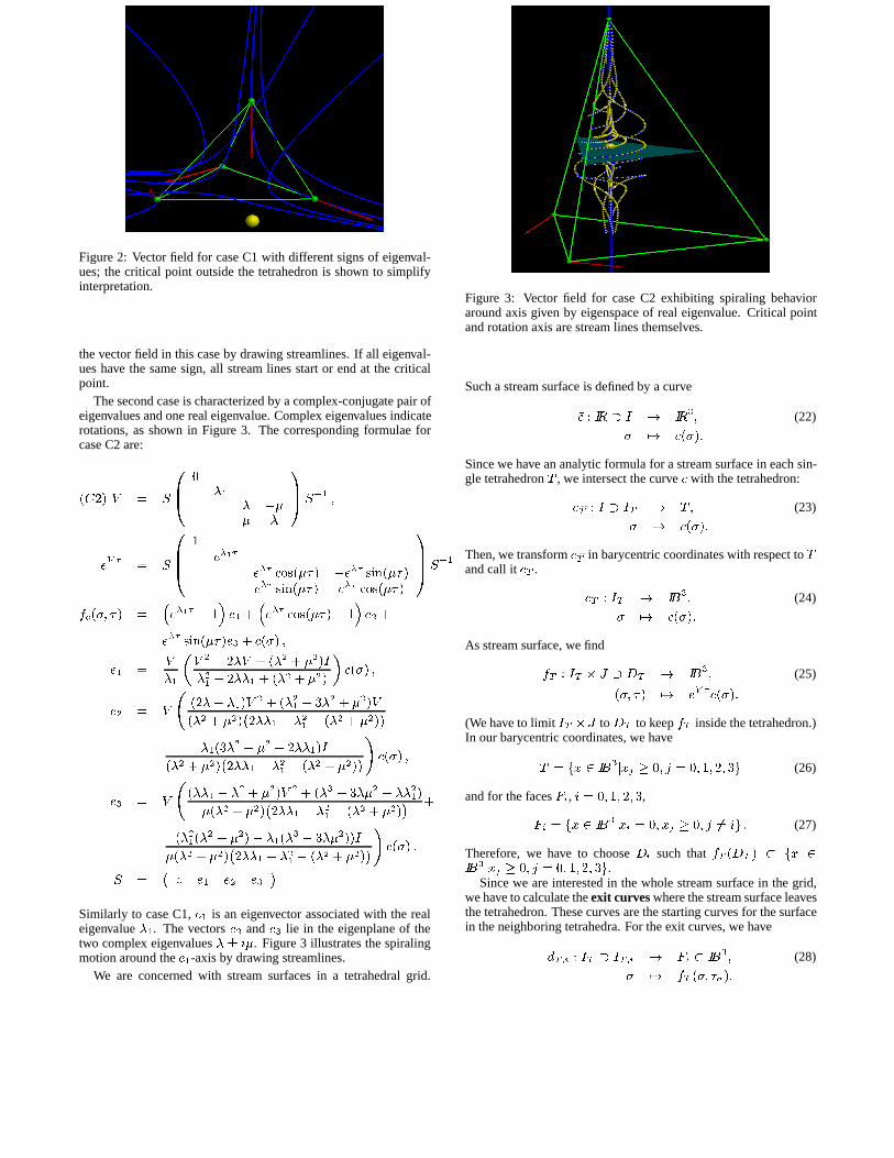
Figure 2: Vector field for case C1 with different signs of eigenval-ues; the critical point outside the tetrahedron is shown to simplifyinterpretation.

the vector field in this case by drawing streamlines. If all eigenval-ues have the same sign, all stream lines start or end at the criticalpoint.

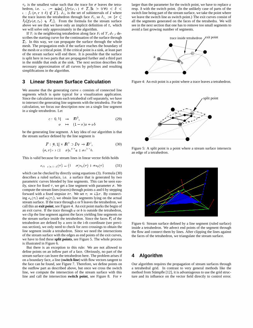
The second case is characterized by a complex-conjugate pair ofeigenvalues and one real eigenvalue. Complex eigenvalues indicaterotations, as shown in Figure 3. The corresponding formulae forcase C2 are:

(C2) V = S

0B@

0�1

� ��� �

1CAS

�1;

eV � = S

0BB@

1e�1�

e�� cos(��) �e�� sin(��)e�� sin(��) e�� cos(��)

1CCAS

�1

fc(�; �) =�e�1� � 1

�e1 +

�e�� cos(��)� 1

�e2 +

e�� sin(��)e3 + c(�) ;

e1 =V

�1

�V 2 � 2�V + (�2 + �2)I

�21 � 2��1 + (�2 + �2)

�c(�) ;

e2 = V

(2�� �1)V

2 + (�21 � 3�2 + �2)V

(�2 + �2)�2��1 � �21 � (�2 + �2)

�+�1(3�

2 � �2 � 2��1)I

(�2 + �2)�2��1 � �21 � (�2 + �2)

�!c(�) ;

e3 = V

(��1 � �2 + �2)V 2 + (�3 � 3��2 � ��21)

�(�2 + �2)�2��1 � �21 � (�2 + �2)

� +

(�21(�2 � �2)� �1(�

3 � 3��2))I

�(�2 + �2)�2��1 � �21 � (�2 + �2)

�!c(�) :

S =�z e1 e2 e3

�Similarly to case C1, e1 is an eigenvector associated with the realeigenvalue �1. The vectors e2 and e3 lie in the eigenplane of thetwo complex eigenvalues � � i�. Figure 3 illustrates the spiralingmotion around the e1-axis by drawing streamlines.

We are concerned with stream surfaces in a tetrahedral grid.

Figure 3: Vector field for case C2 exhibiting spiraling behavioraround axis given by eigenspace of real eigenvalue. Critical pointand rotation axis are stream lines themselves.

Such a stream surface is defined by a curve

�c : IR � I ! IR3; (22)

� 7! �c(�):

Since we have an analytic formula for a stream surface in each sin-gle tetrahedron �T , we intersect the curve �c with the tetrahedron:

�c �T : I � IT ! �T ; (23)

� 7! �c(�):

Then, we transform �c �T in barycentric coordinates with respect to �Tand call it cT .

cT : IT ! IB3; (24)

� 7! c(�):

As stream surface, we find

fT : IT � J � DT ! IB3; (25)

(�; �) 7! eV �

c(�):

(We have to limit IT � J to DT to keep fT inside the tetrahedron.)In our barycentric coordinates, we have

T = fx 2 IB3jxj � 0; j = 0; 1; 2; 3g (26)

and for the faces Fi, i = 0; 1; 2; 3,

Fi = fx 2 IB3jxi = 0; xj � 0; j 6= ig : (27)

Therefore, we have to choose Di such that fT (DT ) � fx 2IB3jxj � 0; j = 0; 1; 2; 3g.

Since we are interested in the whole stream surface in the grid,we have to calculate the exit curves where the stream surface leavesthe tetrahedron. These curves are the starting curves for the surfacein the neighboring tetrahedra. For the exit curves, we have

dT;i : IT � IT;i ! Fi � IB3; (28)

� 7! fT (�; ��):

�� is the smallest value such that the trace for � leaves the tetra-hedron, i.e. �� := minf� jfT (�; �) 2 T; 9� > 0 80 < Æ <� : fT (�; � + Æ) 62 Tg. ITi

is the set of subintervals of I wherethe trace leaves the tetrahedron through face Fi, so ITi

:= f� 2IT jfT (�; ��) 2 Fig. From the formula for the stream surfaceabove we see that we have only an implicit definition of �� whichwe will solve only approximately in the algorithm.

If Ti is the neighboring tetrahedron along face Fi of T , dT;i de-scribes the starting curve for the continuation of the surface throughTi. In this way, we can propagate the surface through the wholemesh. The propagation ends if the surface reaches the boundary ofthe mesh or a critical point. If the critical point is a sink, at least partof the stream surface will end there. It is possible that the surfaceis split here in two parts that are propagated further and a third partin the middle that ends at the sink. The next section describes thenecessary approximation of all curves by polylines and resultingsimplifications in the algorithm.

3 Linear Stream Surface Calculation

We assume that the generating curve �c consists of connected linesegments which is quite typical for a visualization application.Since the calculation treats each tetrahedral cell separately, we haveto intersect the generating line segments with the tetrahedra. For thecalculation, we focus our description now on a single line segmentin a single tetrahedron. Let

c : [0; 1] ! IB3; (29)

� 7! (1� �)a+ �b

be the generating line segment. A key idea of our algorithm is thatthe stream surface defined by the line segment is

F : [0; 1]� IR3 � DT ! IB

3; (30)

(�; � ) 7! (1� �)eV �a+ �e

V �b:

This is valid because for stream lines in linear vector fields holds

s(1��)a+�b(�) = (1� �)sa(�) + �sb(� ) (31)

which can be checked by directly using equations (3). Formula (30)describes a ruled surface, i.e. a surface that is generated by twoparametric curves blended by line segments. This can be seen eas-ily, since for fixed � , we get a line segment with parameter �. Wecompute the stream lines (traces) through points a and b by steppingforward with a fixed stepsize � . We set �i = i�� . By connect-ing sa(�i) and sb(�i), we obtain line segments lying on the actualstream surface. If the trace through a or b leaves the tetrahedron, wecall this an exit point, see Figure 4. An exit point marks the begin ofan exit curve. If the trace through a or b is outside the tetrahedron,we clip the line segment against the faces yielding line segments onthe stream surface inside the tetrahedron. Since the faces Fi of thetetrahedron are defined by a zero in the i-th coordinate (see previ-ous section), we only need to check for zero crossings to obtain theline segment inside a tetrahedron. Since we need the intersectionsof the stream surface with the edges as end points of the exit curves,we have to find these split points, see Figure 5. The whole processis illustrated in Figure 6.

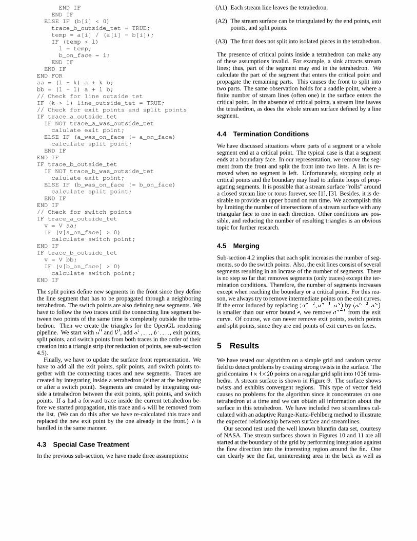
But there is an exception to this rule: We are not allowed todefine points on an inflow part of a face. Obviously, no part of thestream surface can leave the tetrahedron here. The problem arises ifon a boundary face, a line (switch line) with flow vectors tangent tothe face can be found, see Figure 7. Therefore, we define points onthe outflow part as described above, but once we cross the switchline, we compute the intersection of the stream surface with thisline and call the intersection switch point, see Figure 8. For �

larger than the parameter for the switch point, we have to replace aresp. b with the switch point. (In the unlikely case of parts of theswitch line being part of the stream surface, we take the point wherewe leave the switch line as switch point.) The exit curves consist ofall the segments generated on the faces of the tetrahedra. We willsee in the next section that one has to remove too small segments toavoid a fast growing number of segments.

exit point

a

b

trace inside tetrahedron

Figure 4: An exit point is a point where a trace leaves a tetrahedron.

split point

Figure 5: A split point is a point where a stream surface intersectsan edge of a tetrahedron.

Figure 6: Stream surface defined by a line segment (ruled surface)inside a tetrahedron. We advect end points of the segment throughthe flow and connect them by lines. After clipping the lines againstthe faces of the tetrahedron, we triangulate the stream surface.

4 Algorithm

Our algorithm requires the propagation of stream surfaces througha tetrahedral grid. In contrast to very general methods like themethod from Stampfle [12], it is advantageous to use the grid struc-ture and its influence on the vector field directly to control error.

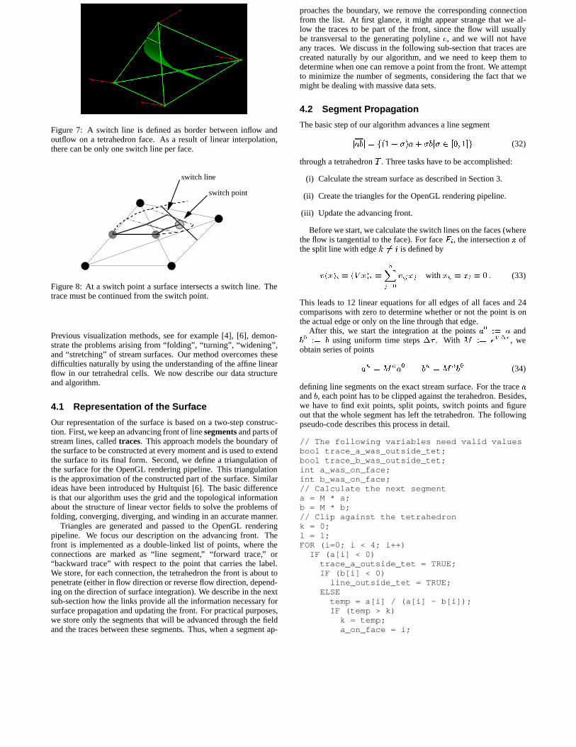
Figure 7: A switch line is defined as border between inflow andoutflow on a tetrahedron face. As a result of linear interpolation,there can be only one switch line per face.

switch line

switch point

Figure 8: At a switch point a surface intersects a switch line. Thetrace must be continued from the switch point.

Previous visualization methods, see for example [4], [6], demon-strate the problems arising from “folding”, “turning”, “widening”,and “stretching” of stream surfaces. Our method overcomes thesedifficulties naturally by using the understanding of the affine linearflow in our tetrahedral cells. We now describe our data structureand algorithm.

4.1 Representation of the Surface

Our representation of the surface is based on a two-step construc-tion. First, we keep an advancing front of line segments and parts ofstream lines, called traces. This approach models the boundary ofthe surface to be constructed at every moment and is used to extendthe surface to its final form. Second, we define a triangulation ofthe surface for the OpenGL rendering pipeline. This triangulationis the approximation of the constructed part of the surface. Similarideas have been introduced by Hultquist [6]. The basic differenceis that our algorithm uses the grid and the topological informationabout the structure of linear vector fields to solve the problems offolding, converging, diverging, and winding in an accurate manner.

Triangles are generated and passed to the OpenGL renderingpipeline. We focus our description on the advancing front. Thefront is implemented as a double-linked list of points, where theconnections are marked as “line segment,” “forward trace,” or“backward trace” with respect to the point that carries the label.We store, for each connection, the tetrahedron the front is about topenetrate (either in flow direction or reverse flow direction, depend-ing on the direction of surface integration). We describe in the nextsub-section how the links provide all the information necessary forsurface propagation and updating the front. For practical purposes,we store only the segments that will be advanced through the fieldand the traces between these segments. Thus, when a segment ap-

proaches the boundary, we remove the corresponding connectionfrom the list. At first glance, it might appear strange that we al-low the traces to be part of the front, since the flow will usuallybe transversal to the generating polyline c, and we will not haveany traces. We discuss in the following sub-section that traces arecreated naturally by our algorithm, and we need to keep them todetermine when one can remove a point from the front. We attemptto minimize the number of segments, considering the fact that wemight be dealing with massive data sets.

4.2 Segment Propagation

The basic step of our algorithm advances a line segment

jabj = f(1� �)a+ �bj� 2 [0; 1]g (32)

through a tetrahedron T . Three tasks have to be accomplished:

(i) Calculate the stream surface as described in Section 3.

(ii) Create the triangles for the OpenGL rendering pipeline.

(iii) Update the advancing front.

Before we start, we calculate the switch lines on the faces (wherethe flow is tangential to the face). For face Fi, the intersection x ofthe split line with edge k 6= i is defined by

v(x)i = (V x)i =3X

j=0

vijxj with xk = xi = 0 : (33)

This leads to 12 linear equations for all edges of all faces and 24comparisons with zero to determine whether or not the point is onthe actual edge or only on the line through that edge.

After this, we start the integration at the points a0 := a andb0 := b using uniform time steps �� . With M := eV�� , weobtain series of points

an = M

na0

bn = M

nb0 (34)

defining line segments on the exact stream surface. For the trace aand b, each point has to be clipped against the terahedron. Besides,we have to find exit points, split points, switch points and figureout that the whole segment has left the tetrahedron. The followingpseudo-code describes this process in detail.

// The following variables need valid valuesbool trace_a_was_outside_tet;bool trace_b_was_outside_tet;int a_was_on_face;int b_was_on_face;// Calculate the next segmenta = M * a;b = M * b;// Clip against the tetrahedronk = 0;l = 1;FOR (i=0; i < 4; i++)IF (a[i] < 0)

trace_a_outside_tet = TRUE;IF (b[i] < 0)

line_outside_tet = TRUE;ELSE

temp = a[i] / (a[i] - b[i]);IF (temp > k)k = temp;a_on_face = i;

END IFEND IF

ELSE IF (b[i] < 0)trace_b_outside_tet = TRUE;temp = a[i] / (a[i] - b[i]);IF (temp < l)

l = temp;b_on_face = i;

END IFEND IF

END FORaa = (1 - k) a + k b;bb = (1 - l) a + l b;// Check for line outside tetIF (k > l) line_outside_tet = TRUE;// Check for exit points and split pointsIF trace_a_outside_tet

IF NOT trace_a_was_outside_tetcalulate exit point;

ELSE IF (a_was_on_face != a_on_face)calculate split point;

END IFEND IFIF trace_b_outside_tet

IF NOT trace_b_was_outside_tetcalulate exit point;

ELSE IF (b_was_on_face != b_on_face)calculate split point;

END IFEND IF// Check for switch pointsIF trace_a_outside_tet

v = V aa;IF (v[a_on_face] > 0)calculate switch point;

END IFIF trace_b_outside_tet

v = V bb;IF (v[b_on_face] > 0)calculate switch point;

END IF

The split points define new segments in the front since they definethe line segment that has to be propagated through a neighboringtetrahedron. The switch points are also defining new segments. Wehave to follow the two traces until the connecting line segment be-tween two points of the same time is completely outside the tetra-hedron. Then we create the triangles for the OpenGL renderingpipeline. We start with a0 and b0, add a1; : : :, b1; : : :, exit points,split points, and switch points from both traces in the order of theircreation into a triangle strip (for reduction of points, see sub-section4.5).

Finally, we have to update the surface front representation. Wehave to add all the exit points, split points, and switch points to-gether with the connecting traces and new segments. Traces arecreated by integrating inside a tetrahedron (either at the beginningor after a switch point). Segments are created by integrating out-side a tetrahedron between the exit points, split points, and switchpoints. If a had a forward trace inside the current tetrahedron be-fore we started propagation, this trace and a will be removed fromthe list. (We can do this after we have re-calculated this trace andreplaced the new exit point by the one already in the front.) b ishandled in the same manner.

4.3 Special Case Treatment

In the previous sub-section, we have made three assumptions:

(A1) Each stream line leaves the tetrahedron.

(A2) The stream surface can be triangulated by the end points, exitpoints, and split points.

(A3) The front does not split into isolated pieces in the tetrahedron.

The presence of critical points inside a tetrahedron can make anyof these assumptions invalid. For example, a sink attracts streamlines; thus, part of the segment may end in the tetrahedron. Wecalculate the part of the segment that enters the critical point andpropagate the remaining parts. This causes the front to split intotwo parts. The same observation holds for a saddle point, where afinite number of stream lines (often one) in the surface enters thecritical point. In the absence of critical points, a stream line leavesthe tetrahedron, as does the whole stream surface defined by a linesegment.

4.4 Termination Conditions

We have discussed situations where parts of a segment or a wholesegment end at a critical point. The typical case is that a segmentends at a boundary face. In our representation, we remove the seg-ment from the front and split the front into two lists. A list is re-moved when no segment is left. Unfortunately, stopping only atcritical points and the boundary may lead to infinite loops of prop-agating segments. It is possible that a stream surface “rolls” arounda closed stream line or torus forever, see [1], [3]. Besides, it is de-sirable to provide an upper bound on run time. We accomplish thisby limiting the number of intersections of a stream surface with anytriangular face to one in each direction. Other conditions are pos-sible, and reducing the number of resulting triangles is an obvioustopic for further research.

4.5 Merging

Sub-section 4.2 implies that each split increases the number of seg-ments, so do the switch points. Also, the exit lines consist of severalsegments resulting in an incrase of the number of segments. Thereis no step so far that removes segments (only traces) except the ter-mination conditions. Therefore, the number of segments increasesexcept when reaching the boundary or a critical point. For this rea-son, we always try to remove intermediate points on the exit curves.If the error induced by replacing (an�2; an�1; an) by (an�2; an)is smaller than our error bound �, we remove an�1 from the exitcurve. Of course, we can never remove exit points, switch pointsand split points, since they are end points of exit curves on faces.

5 Results

We have tested our algorithm on a simple grid and random vectorfield to detect problems by creating strong twists in the surface. Thegrid contains 4�4�20 points on a regular grid split into 1026 tetra-hedra. A stream surface is shown in Figure 9. The surface showstwists and exhibits convergent regions. This type of vector fieldcauses no problems for the algorithm since it concentrates on onetetrahedron at a time and we can obtain all information about thesurface in this tetrahedron. We have included two streamlines cal-culated with an adaptive Runge-Kutta-Fehlberg method to illustratethe expected relationship between surface and streamlines.

Our second test used the well known bluntfin data set, courtesyof NASA. The stream surfaces shown in Figures 10 and 11 are allstarted at the boundary of the grid by performing integration againstthe flow direction into the interesting region around the fin. Onecan clearly see the flat, uninteresting area in the back as well as

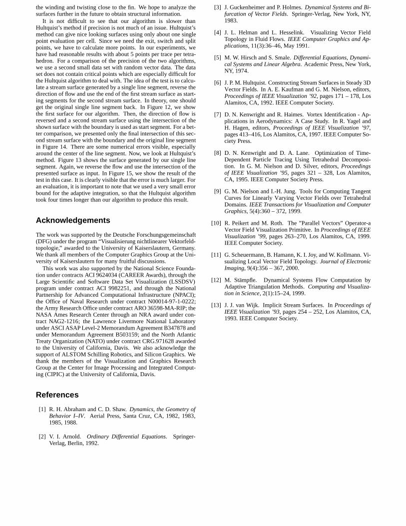
the winding and twisting close to the fin. We hope to analyze thesurfaces further in the future to obtain structural information.

It is not difficult to see that our algorithm is slower thanHultquist’s method if precision is not much of an issue. Hultquist’smethod can give nice looking surfaces using only about one singlepoint evaluation per cell. Since we need the exit, switch and splitpoints, we have to calculate more points. In our experiments, wehave had reasonable results with about 5 points per trace per tetra-hedron. For a comparison of the precision of the two algorithms,we use a second small data set with random vector data. The dataset does not contain critical points which are especially difficult forthe Hultquist algorithm to deal with. The idea of the test is to calcu-late a stream surface generated by a single line segment, reverse thedirection of flow and use the end of the first stream surface as start-ing segments for the second stream surface. In theory, one shouldget the original single line segment back. In Figure 12, we showthe first surface for our algorithm. Then, the direction of flow isreversed and a second stream surface using the intersection of theshown surface with the boundary is used as start segment. For a bet-ter comparison, we presented only the final intersection of this sec-ond stream surface with the boundary and the original line segmentin Figure 14. There are some numerical errors visible, especiallyaround the center of the line segment. Now, we look at Hultquist’smethod. Figure 13 shows the surface generated by our single linesegment. Again, we reverse the flow and use the intersection of thepresented surface as input. In Figure 15, we show the result of thetest in this case. It is clearly visible that the error is much larger. Foran evaluation, it is important to note that we used a very small errorbound for the adaptive integration, so that the Hultquist algorithmtook four times longer than our algorithm to produce this result.

Acknowledgements

The work was supported by the Deutsche Forschungsgemeinschaft(DFG) under the program “Visualisierung nichtlinearer Vektorfeld-topologie,” awarded to the University of Kaiserslautern, Germany.We thank all members of the Computer Graphics Group at the Uni-versity of Kaiserslautern for many fruitful discussions.

This work was also supported by the National Science Founda-tion under contracts ACI 9624034 (CAREER Awards), through theLarge Scientific and Software Data Set Visualization (LSSDSV)program under contract ACI 9982251, and through the NationalPartnership for Advanced Computational Infrastructure (NPACI);the Office of Naval Research under contract N00014-97-1-0222;the Army Research Office under contract ARO 36598-MA-RIP; theNASA Ames Research Center through an NRA award under con-tract NAG2-1216; the Lawrence Livermore National Laboratoryunder ASCI ASAP Level-2 Memorandum Agreement B347878 andunder Memorandum Agreement B503159; and the North AtlanticTreaty Organization (NATO) under contract CRG.971628 awardedto the University of California, Davis. We also acknowledge thesupport of ALSTOM Schilling Robotics, and Silicon Graphics. Wethank the members of the Visualization and Graphics ResearchGroup at the Center for Image Processing and Integrated Comput-ing (CIPIC) at the University of California, Davis.

References

[1] R. H. Abraham and C. D. Shaw. Dynamics, the Geometry ofBehavior I–IV. Aerial Press, Santa Cruz, CA, 1982, 1983,1985, 1988.

[2] V. I. Arnold. Ordinary Differential Equations. Springer-Verlag, Berlin, 1992.

[3] J. Guckenheimer and P. Holmes. Dynamical Systems and Bi-furcation of Vector Fields. Springer-Verlag, New York, NY,1983.

[4] J. L. Helman and L. Hesselink. Visualizing Vector FieldTopology in Fluid Flows. IEEE Computer Graphics and Ap-plications, 11(3):36–46, May 1991.

[5] M. W. Hirsch and S. Smale. Differential Equations, Dynami-cal Systems and Linear Algebra. Academic Press, New York,NY, 1974.

[6] J. P. M. Hultquist. Constructing Stream Surfaces in Steady 3DVector Fields. In A. E. Kaufman and G. M. Nielson, editors,Proceedings of IEEE Visualization ’92, pages 171 – 178, LosAlamitos, CA, 1992. IEEE Computer Society.

[7] D. N. Kenwright and R. Haimes. Vortex Identification - Ap-plications in Aerodynamics: A Case Study. In R. Yagel andH. Hagen, editors, Proceedings of IEEE Visualization ’97,pages 413–416, Los Alamitos, CA, 1997. IEEE Computer So-ciety Press.

[8] D. N. Kenwright and D. A. Lane. Optimization of Time-Dependent Particle Tracing Using Tetrahedral Decomposi-tion. In G. M. Nielson and D. Silver, editors, Proceedingsof IEEE Visualization ’95, pages 321 – 328, Los Alamitos,CA, 1995. IEEE Computer Society Press.

[9] G. M. Nielson and I.-H. Jung. Tools for Computing TangentCurves for Linearly Varying Vector Fields over TetrahedralDomains. IEEE Transactions for Visualization and ComputerGraphics, 5(4):360 – 372, 1999.

[10] R. Peikert and M. Roth. The ”Parallel Vectors” Operator-aVector Field Visualization Primitive. In Proceedings of IEEEVisualization ’99, pages 263–270, Los Alamitos, CA, 1999.IEEE Computer Society.

[11] G. Scheuermann, B. Hamann, K. I. Joy, and W. Kollmann. Vi-sualizing Local Vector Field Topology. Journal of ElectronicImaging, 9(4):356 – 367, 2000.

[12] M. Stampfle. Dynamical Systems Flow Computation byAdaptive Triangulation Methods. Computing and Visualiza-tion in Science, 2(1):15–24, 1999.

[13] J. J. van Wijk. Implicit Stream Surfaces. In Proceedings ofIEEE Visualization ’93, pages 254 – 252, Los Alamitos, CA,1993. IEEE Computer Society.

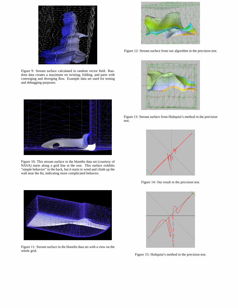
Figure 9: Stream surface calculated in random vector field. Ran-dom data creates a maximum on twisting, folding, and parts withconverging and diverging flow. Example data set used for testingand debugging purposes.

Figure 10: This stream surface in the bluntfin data set (courtesy ofNASA) starts along a grid line at the rear. This surface exhibits“simple behavior” in the back, but it starts to wind and climb up thewall near the fin, indicating more complicated behavior.

Figure 11: Stream surface in the bluntfin data set with a view on thewhole grid.

Figure 12: Stream surface from our algorithm in the precision test.

Figure 13: Stream surface from Hultquist’s method in the precisiontest.

Figure 14: Our result in the precision test.

Figure 15: Hultquist’s method in the precision test.

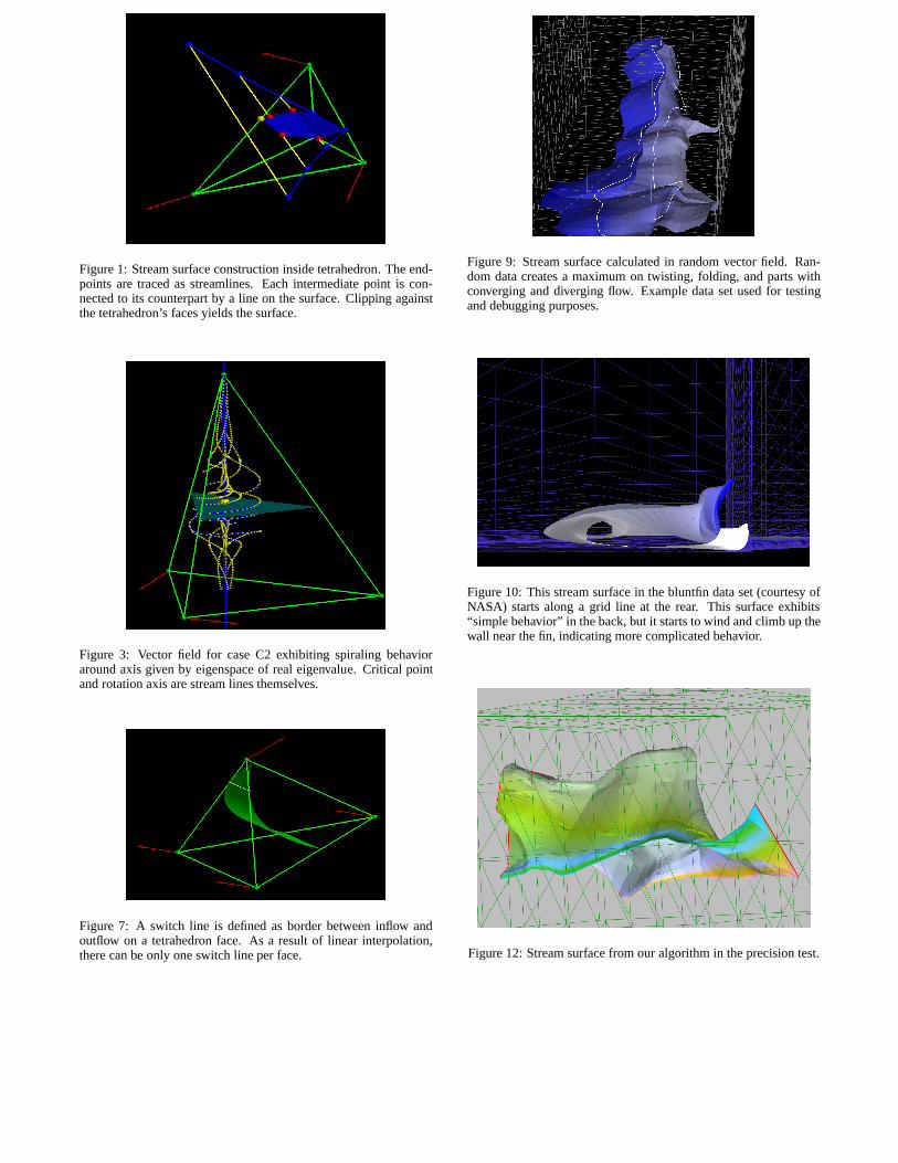
Figure 1: Stream surface construction inside tetrahedron. The end-points are traced as streamlines. Each intermediate point is con-nected to its counterpart by a line on the surface. Clipping againstthe tetrahedron’s faces yields the surface.

Figure 3: Vector field for case C2 exhibiting spiraling behavioraround axis given by eigenspace of real eigenvalue. Critical pointand rotation axis are stream lines themselves.

Figure 7: A switch line is defined as border between inflow andoutflow on a tetrahedron face. As a result of linear interpolation,there can be only one switch line per face.

Figure 9: Stream surface calculated in random vector field. Ran-dom data creates a maximum on twisting, folding, and parts withconverging and diverging flow. Example data set used for testingand debugging purposes.

Figure 10: This stream surface in the bluntfin data set (courtesy ofNASA) starts along a grid line at the rear. This surface exhibits“simple behavior” in the back, but it starts to wind and climb up thewall near the fin, indicating more complicated behavior.

Figure 12: Stream surface from our algorithm in the precision test.