A Responsive Knapsack-based Algorithm for Resource ...raj/papers/CloudWorkflow-ICPP2015.pdfA Responsive Knapsack-based Algorithm for Resource Provisioning and Scheduling of Scientific

A Responsive Knapsack-based Algorithm for Resource Provisioning and Schedulingof Scientific Workflows in Clouds

Maria A. Rodriguez and Rajkumar BuyyaCloud Computing and Distributed Systems (CLOUDS) Laboratory

Department of Computing and Information Systems, The University of Melbourne, Australiae-mail: [email protected], [email protected]

Abstract—Scientific workflows are used to process vastamounts of data and to conduct large-scale experiments andsimulations. They are time consuming and resource intensiveapplications that benefit from running in distributed platforms.In particular, scientific workflows can greatly leverage theease-of-access, affordability, and scalability offered by cloudcomputing. To achieve this, innovative and efficient ways oforchestrating the workflow tasks and managing the computeresources in a cost-conscious manner need to be developed.We propose an adaptive, resource provisioning and schedulingalgorithm for scientific workflows deployed in Infrastructureas a Service clouds. Our algorithm was designed to addresschallenges specific to clouds such as the pay-as-you-go model,the performance variation of resources and the on-demand ac-cess to unlimited, heterogeneous virtual machines. It is capableof responding to the dynamics of the cloud infrastructure andis successful in generating efficient solutions that meet a user-defined deadline and minimise the overall cost of the usedinfrastructure. Our simulation experiments demonstrate thatit performs better than other state-of-the-art algorithms.

I. INTRODUCTION

Workflows are defined as a set of computational tasksand a set of data or control dependencies between them.They are widely used by the scientific community to analyseand process large amounts of data efficiently. These large-scale scientific workflows are resource-intensive applicationsand hence are commonly deployed on distributed platforms.Scheduling algorithms play a crucial role in running work-flows efficiently as they are responsible for the orchestrationof the tasks on the distributed compute resources. Theirdecisions are guided by a collection of Quality of Service(QoS) requirements defined by the application users suchas minimising the total cost or makespan (i.e. total exe-cution time), or meeting a specified budget or deadline.This scheduling problem is non-trivial, in fact, it is a well-known NP-complete problem [1] and therefore, algorithmsmust focus on finding approximate solutions in a reasonableamount of time.

Infrastructure as a Service (IaaS) clouds offer an eas-ily accessible, flexible, and scalable infrastructure for thedeployment of large-scale scientific workflows. They allowusers to access a shared compute infrastructure on-demandwhile paying only for what they use. This is done by leasingvirtualised compute resources, or Virtual Machines (VMs),

with a predefined CPU, memory, storage and bandwidthcapacity. Different resource bundles (i.e. VM types) areavailable to users at varying prices to suit a wide range of ap-plication needs. Aside from VMs, IaaS providers also offerstorage services and network infrastructure to transport datain, out, and within their facilities. To fully take advantageof these services and opportunities, scheduling algorithmsmust consider several key characteristics of clouds.

The first one is the on-demand, elastic resource model.This feature suggests a reformulation of the scheduling prob-lem as traditionally defined for other distributed platformssuch as grids and clusters. Clouds do not offer a finiteset of compute resources, instead, they offer a virtuallyinfinite pool of VMs with various configurations ready tobe leased and used only for as long as they are needed.This model creates the need for a resource provisioningstrategy that works together with the scheduling algorithm;a heuristic that decides not only the type and number ofVMs to request from the cloud but also when is the besttime to lease and release them. Since this work is tailoredfor cloud environments, from here on, the word schedulingwill be used to refer to an algorithm capable of making both,resource provisioning and scheduling decisions.

Another feature to consider is the utility-based pricingmodel used by cloud providers. The cost of using theinfrastructure needs to be considered or otherwise, usersrisk paying prohibitive and unnecessary costs. For example,the number of VMs leased, their type, and the amount oftime they are used for, all have an impact on the totalcost of running the workflow in the cloud. Consequently,schedulers need to find a trade-off between cost and otherQoS requirements such as makespan.

A third characteristic of clouds is their dynamic stateand the uncertainties this brings with it. An example is thevariability in performance exhibited by VMs in terms ofexecution times [2]. This variability means that despite aVM type being advertised to have a specific CPU capacity, itwill most likely perform at a lower capacity that will changeovertime. It also means that two VMs of the same typemay exhibit completely different performances. Further-more, having multiple concurrent users sharing a networkmeans that performance variation is also observed in net-

working resources [2]. Yet another source of uncertainty arethe VM provisioning and deprovisioning delays [3]; there areno guarantees on their values and they can be highly variableand unpredictable. Recognising performance variability isimportant for schedulers so that they can recover fromunexpected delays and fulfil the QoS requirements.

As a result of these requirements, we propose theWorkflow Responsive resource Provisioning and Scheduling(WRPS) algorithm for scientific workflows in clouds. Oursolution finds a balance between making dynamic decisionsto respond to changes in the environment and planning aheadto produce better schedules. It aims to minimise the overallcost of the utilised infrastructure while meeting a user-defined deadline. It is capable of deciding what computeresources to use considering heterogeneous VM types, whenis the best time to lease them and when they should bereleased to avoid incurring in extra costs. Our simulationresults demonstrate it is scalable in terms of the number oftasks in the workflow, it is robust and responsive to the cloudperformance variability and it is capable of generating betterquality solutions than the state-of-the-art algorithms.

II. RELATED WORK

There have been several works since the advent ofcloud computing that aim to efficiently schedule scientificworkflows. Many of them are dynamic and are capableof adapting to changes in the environment. An exampleis the Dynamic Provisioning Dynamic Scheduling (DPDS)algorithm [4] in which the number of VMs is adjusted de-pending on how well they are being used by the application.Zhou et al. [5] also propose a dynamic approach designedto capture the dynamic nature of cloud environments fromthe performance and pricing point of view. Poola et al. [6]designed a fault tolerant dynamic algorithm based on theworkflow’s partial critical paths. The Partitioned BalancedTime Scheduling algorithm [7] estimates the optimal numberof resources needed per billing period so that a deadline ismet and the cost is minimised. Other dynamic algorithmsinclude those developed by Xu et al. [8], Huu and Mon-tagnat [9], and Oliveira et al. [10]. The main disadvantageof these approaches is their task-level optimisation strategy,which is a trade-off for their adaptability to unexpecteddelays.

On the other side of the spectrum are static algorithms. Anexample is the Static Provisioning Static Scheduling (SPSS)[4] algorithm. Designed to schedule a group of interrelatedworkflows (i.e. ensembles), it creates a provisioning andscheduling plan before running any task. Another exampleis the IaaS Cloud Partial Critical Path (IC-PCP) algorithm[11]. It is based on the workflow’s partial critical pathsand tries to minimise the execution cost while meeting adeadline constraint. Other examples include RDPS [12],DVFS-MODPSO [13] and EIPR [14]. In general, thesealgorithms are very sensitive to execution delays and runtime

estimation of tasks, which is a trade-off for their ability toperform workflow-level optimisations and compare varioussolutions before choosing the best-suited one.

Contrary to fully dynamic or static approaches, our workcombines both in order to find a better compromise betweenadaptability and the benefits of global optimisation. SCS [15]is an example of an algorithm attempting to achieve this. Ithas a global optimisation heuristic that allows it to find theoptimal mapping of task to VM type. This mapping is thenused at runtime to scale the resource pool in or out andto schedule tasks as they become ready for execution. Ourapproach is different to SCS in that the static componentdoes not analyse the entire workflow structure and insteadoptimises the schedule of a subset of the workflow tasks.Moreover, our static component generates an actual schedulefor these tasks rather than just selecting a VM type.

III. APPLICATION AND RESOURCE MODELS

We consider workflows modelled as Directed AcyclicGraphs (DAGs); that is, graphs with directed edges and nocycles or conditional dependencies. Formally, a workflow Wis composed of a set of tasks T = {t1, t2, . . . , tn} and a setof edges E. An edge e

ij

= (ti

, tj

) exists if there is a datadependency between t

i

and tj

, case in which ti

is said to bethe parent of t

j

and tj

the child of ti

. Based on this, a childtask cannot run until all of its parent tasks have completedand its input data is available in the corresponding computeresource. Also, a workflow is associated with a deadline �

W

,defined as a time limit for its execution. Additionally, weassume that the size of a task S

t

is measurable in Million ofInstructions (MIs) and that, for every task, this informationis provided as input to the scheduler.

A pay-as-you go model where VMs are leased on-demandand are charged per billing period is considered. Any partialutilisation results in the VM usage being rounded up tothe nearest billing period. We model a VM type, VMT , interms of its processing capacity PC

VMT

and cost per billingperiod C

VMT

. We define PCVMT

in terms of the numberof instructions the CPU can process per second, Million ofInstructions per Second (MIPS). It is assumed that for everyVM type, its processing capacity in MIPS can be estimatedbased on the information offered by providers.

Workflows process data in the form of files. A commonapproach used to share these files among tasks is to usea peer-to-peer (P2P) model in which files are transferreddirectly from the VM running the parent task to the VMrunning the child task. Another technique is to use a globalshared storage such as Amazon S3 as a file repository. Inthis case, tasks store their output in the global storage andretrieve their inputs from the same. We consider the lattermodel based on the advantages it offers. Firstly, the datais persisted and hence, can be used for recovery in case offailures. Secondly, it allows for asynchronous computation.In the P2P model, synchronous communication between

tasks means that VMs must be kept running until all ofthe child tasks have received the corresponding data. Witha shared storage on the contrary, the VM running the parenttask can be released as soon as the data is persisted in thestorage system. This may not only increase the resourceutilisation but also decrease the cost of VM leasing.

We assume data transfers in and out of the global storagesystem are free of charge, as is the case for products likeAmazon S3, Google Cloud Storage and Rackspace BlockStorage. As for the actual data storage, most cloud providerscharge based on the amount of data being stored. We do notinclude this cost in the total cost calculation of neither ourimplementation nor the implementation of the algorithmsused for comparison in the experiments. The reason for thisis to be able to compare our approach with others designed totransfer files in a P2P fashion. Furthermore, regardless of thealgorithm, the amount of stored data for a given workflowis most likely the same in every case or it is similar enoughthat it does not result in a difference in cost.

We acknowledge the existence of VM provisioning anddeprovisioning delays and assume that the CPU performanceof VMs is not stable [2]. Instead, it varies over time withits maximum achievable value being the CPU capacityadvertised by the provider. In addition, we assume networkcongestion causes a variation in data transfer times [16].The bandwidth assigned to a transfer depends on the currentcontention for the network link being used. In addition, weassume a global storage with an unlimited storage capacity.The rates at which it is capable of reading and writing datavary based on the number of processes currently writing orreading data from the system. Finally, the processing time ofa task t on a VM of type VMT , PTVMT

t

, is defined as thesum of its execution time and the time it takes to read theinput files from the storage and write the generated outputfiles to it. Note that whenever a parent and a child task arerunning in the same VM, there is no need to read the child’sinput file from the storage.

IV. THE WRPS ALGORITHM

This section describes the reasoning behind the WRPSheuristics as well as a detailed explanation of the algorithm.

A. Overview and MotivationWRPS has dynamic and a static features. Its dynamicity

lies in the fact that the scheduling decisions are made at run-time, every time tasks are released into an execution queue.This allows it to adapt to unexpected delays caused by poorestimates or by environmental changes such as performancevariation, network congestion, and VM provisioning delays.The static component expands the ability of the algorithmfrom making decisions based on a single task (the next onein the queue) to making decisions based on a group of tasks.The purpose is to find a balance between the local knowledgeof dynamic algorithms and the global knowledge of static

ones. This is achieved by introducing the concept of pipelineand by statically scheduling all of the tasks in the executionqueue at once. In this way, WRPS is able to make betteroptimisation decisions and find better quality schedules.

A pipeline is a common topological structure in scientificworkflows and is simply a group of tasks with a one-to-one,sequential relationship between them. Formally, a pipeline Pis defined as a set of tasks T

p

= {t1, t2, . . . , tn} where n � 2

and there is an edge ei,i+1 between task t

i

and task ti+1. In

other words t1 is the parent of t2, t2 the parent of t3, andso on. The first task in a pipeline may have more than oneparent but it must only have one child task. All other tasksmust have a single parent (the previous pipeline task) andone child (the next pipeline task). A pipeline is associatedwith a deadline �

P

which is equal to the deadline of the lasttask in the sequence. An example is shown in Figure 1a.

By identifying pipelines in a workflow, we can easilyexpand the view from a single task to a set of tasks that canbe scheduled more efficiently as a group rather than on theirown. To avoid communication and processing overheads aswell as VM provisioning and deprovisioning delays, tasksin a pipeline are clustered together and are always assignedto run on the same VM. The reasons are twofold. Firstly,the tasks are sequential and are required to run one afterthe other. There is no benefit in terms of parallelisation onassigning them to different VMs. Secondly, the output fileof a task becomes the input file of the next one, by runningon the same VM, we avoid the cost and time of transferringthese files in and out of the global storage.

The strategy used to schedule queued tasks is derived fromthe topological features of scientific workflows. Aside frompipelines, a workflow also has parallel structures composedof tasks with no dependencies between them. These taskscan run simultaneously and are generally found wheneverdata distribution or aggregation takes place. In data distribu-tion [17] a tasks’s output is distributed to multiple tasks forprocessing. In data aggregation [17] the output of multipletasks is aggregated, or processed, by a single task. Figure1a shows an example of each of these structures.

The parallel tasks in these structures can be either ho-mogeneous (same type) or heterogeneous (different types).The case in which the tasks are homogenous is common inscientific workflows; examples of well-known applicationswith this characteristic are Epigenomics, SIPHT, LIGO,Montage, and CyberShake. Based on this, we devise astrategy to efficiently schedule homogeneous parallel tasksthat are of the same size (MIs) and are at the same levelin the DAG. When using a level-based deadline distributionheuristic, these tasks will also have the same deadline. As anexample, consider the data aggregation case. All the paralleltasks have to finish running before the aggregation task canstart, therefore they can be assigned the same deadline whichwould be equal to the time the aggregation task is due tostart. Note that the case in which tasks are heterogeneous

Task Type 5

Task Type 1

Task Type 4

Task Type 2

Task Type 3

Task Type 6

Task Type 7

Task Type 4

Task Type 1

Task Type 1

Task Type 1

Task Type 1

Task Type 1

Task Type 4

Task Type 4

Data Aggregation

Parallel Tasks

Data Distribution

Parallel Tasks

Pipeline

(a)

fastq2bfq

filterContas

sol2snger

fastQSplit

mapMerge

map map

maqIndex

sol2snger

filterContas

fastq2bfq

filterContas

filterContas

sol2snger

sol2snger

fastq2bfq

fastq2bfq

map map

pileup

Bag of Pipelines

(b)

Transterm

Findterm

RNAMotif Blast

SRNA

FFN_Parse

BlastSynteny

BlastCand

BlasQRNA

BlastParalog

SRNAAnnota

te

PasterConca

te

Paster

Paster

Paster

Paster Paster

Paster

Paster

Paster

Paster

Paster

PasterPaster PasterPaster

Bag of Tasks

(c)

Figure 1. Scientific workflow examples. (a) Example of bag of tasks and three different topological structures found in workflows: data aggregation, datadistribution and pipelines. (b) Epigenomics workfow. An example of a bag of pipelines is depicted in this figure. (c) SIPHT workflow.

and at different levels in the workflow is uncommon but yetpossible. An example is the data distribution of the SRNAtask in the SIPHT workflow, shown in Figure 1c. Also, thereare other scenarios aside from distribution and aggregationwhere parallel tasks with the same properties can be found,however we focus on these as means for illustrating themotivation behind our scheduling policy.

The main static scheduling policy of WRPS consists thenon grouping queued tasks of the same type and with thesame deadline into bags. Two sample bags can be seen inFigure 1a, the first one is composed of all tasks of Type 1and the second one of all tasks of Type 4. Scheduling thesebags of tasks is much simpler than scheduling a workflow.There are no dependencies, the tasks are homogenous, andhave to finish at the same time. We model the problem ofrunning these tasks before their deadline and with minimumcost as a variation of the unbounded knapsack problem andfind an optimal solution using dynamic programming. Thesame concept is applied to pipelines, they are grouped intobags and scheduled in the same way as bags of tasks are.An example of a bag of pipelines is depicted in Figure 1b.

We have therefore designed an algorithm which is dy-namic to a certain extent in order to adapt to unexpecteddelays product of the unpredictability of cloud environmentsbut that also has a static component that enables it togenerate better quality schedules and meet deadlines at lowercosts. Moreover, it combines a heuristic-based approach withdynamic programming in order to be able to process large-scale workflows in an efficient and scalable manner. Thedetails of WRPS are presented in Section IV-C.

B. The Unbounded Knapsack Problem

The unbounded knapsack problem (UKP) is an NP-hardcombinatorial optimisation problem that derives from theproblem of selecting the most valuable items to pack in afixed-size knapsack. Given n items of different types, eachitem type 1 i n with a corresponding weight w

i

andvalue v

i

, the goal is to determine the number and type of

items to pack so that the knapsack weight limit W is notexceeded and the total value of the items is maximised.Unlimited quantities of each item type are assumed.

Let xi

� 0 be the number of items of type i to be placedin the bag. Then UKP can be defined as

maximisenX

i=1

vi

xi

subject tonX

i=1

wi

xi

W.

This problem can be solved optimally using dynamic pro-gramming by considering knapsacks of smaller capacities assubproblems and storing the best value for each capacity.Let w

i

> 0, then a vector M can be defined wherem[w

i

] is the maximum value that can be obtained with aweight less than or equal to w

i

. In this way, m[0] = 0

and m[wi

] = max

wjwi(vj + m[wi

� wj

]). The timecomplexity of this solution is O(nW ) as computing eachm[w

i

] involves examining n items and there are W values ofm[w

i

] to calculate. This running time is pseudo-polynomialas it grows exponentially with the length of W . Yet, thereare several algorithms that can efficiently solve UKP. Anexample is the EDUK [18] algorithm which combines theconcepts of dominance [19], periodicity [20], and mono-tonic recurrence [21]. Experiments performed by the authorsdemonstrate its scalability. For instance, for W > 2 ⇥ 10

8,n = 10

5, and items with weights in the [1, 105] range, theaverage running time was found to be 0.150 seconds.

C. AlgorithmWRPS first preprocesses the DAG by identifying the

pipelines and by assigning a portion of the deadline �W

to each task. To find the pipelines, tasks are first sorted intopological order, in this way we ensure data dependenciesare preserved. Afterwards, pipelines are built based on thefollowing logic. For each sorted task that has not beenprocessed, the algorithm recursively tries to build a pipelinethat starts with that task. The base cases of the recursionhappen when the processed task has no children, when ithas more than one child or, when it has a single child

with more than one parent task. The recursive stage occurswhen the processed task has strictly one child which at thesame time has strictly one parent (the processed task). Inthis case the task is added to the pipeline and the recursioncontinues with its child task. Once a pipeline was identifiedand the recursion finishes, the process is repeated for the nextunprocessed sorted task, this continues until all the taskshave been processed. A more detailed explanation of therecursive part of the algorithm is depicted in Algorithm 1.

Algorithm 1 Find a pipeline recursively1: procedure FINDPIPELINE(Task t, Pipeline p)2: if t.children.size > 1 OR t.children.size = 0 OR3: t.children[0].parents.size > 1 then4: if p.tasks.size > 0 then5: p.addTask(t)6: end if7: return8: end if9: p.addTask(t)

10: findP ipeline(t.children[0], p)11: end procedure

For the deadline distribution, the algorithm first calculatesthe earliest finish time of all tasks defined as eft

t

=

max

p2t.parents

{eftp

} + PTVMT

t

. The slowest VMT isused to calculate the task processing times. In this way, theycan only improve if different VM types are used. However, ifusing the slowest VM type means not being able to meet thedeadline, then the next fastest VM type is used to estimateruntimes and so on. Afterwards, the spare time, defined asthe difference between the deadline and the earliest finishtime of the workflow (�

W

� max

t2W

{eftt

}) is calculatedand divided between the workflow levels based on the num-ber of tasks they have. Finally, each task is assigned its dead-line �

t

= max

p2t.parents

{�p

}+ PTVMT

t

+ t.level.spare.Once a DAG is preprocessed the task scheduling begins.

During the first iteration, all the entry tasks (those with noparent tasks) become ready for execution and are placedin a scheduling queue.Tthese tasks are scheduled and afterthey finish their execution, their child tasks are released ontothe queue. This process is repeated until all of the workflowtasks have been successfully executed. To schedule the tasksin the queue, tasks are first grouped into bags of tasks andbags of pipelines. A bag of tasks bot is defined as a groupof one or more tasks T

bot

that can run in parallel. All of thetasks in a bag share the same deadline �

bot

, are of the sametype ⌧

bot

, and are not part of a pipeline. Formally, bot =

(Tbot

, �bot

, ⌧bot

). The definition of bag of pipelines bop issimilar but instead of a group of tasks, the bag containsone or more pipelines P

bop

that are parallelisable. The tuplebop = (P

bop

, �bop

), where �bop

is the deadline the pipelinesin the bag have in common, formally defines the concept.

To find the sets of bags of tasks BoT = {bot1, . . . , botn}and bags of pipelines BoP = {bop1, . . . , bopn}, each taskin the queue is processed in the following way. If the task

does not belong to a pipeline, then it is placed in the boti

thatcontains tasks of the same type and with the same deadline.If no such bot

i

exists, a new bag is created and the taskassigned to it. If, on the other hand, the task belongs to apipeline, the corresponding pipeline is placed in the bop

i

which contains pipelines with the same deadline and typesof tasks. If there is no bop

i

with these characteristics, a newbag is created with its only element being the given pipeline.

Once the sets BoP and BoT are created, we proceed toschedule them. Both types of bags are scheduled using thesame policy, with the only difference being that tasks in apipeline must be treated as a unit. We explain the heuristicusing BoT , note however that the same rules apply whenscheduling BoP . To schedule BoT , we repeat the followingprocess for each bag bot

i

2 BoT that has more than onetask (bags with a single element are treated as a special caseand scheduled accordingly). First, WRPS tries to reduce thesize of the bag and reuse already leased VMs by assigningas many tasks as possible to idle VMs. The number of tasksmapped to a free VM is determined by the number of tasksthat can finish before their deadline and before the nextbilling period of the VM. In this way, wastage of alreadypaid CPU cycles is reduced without affecting the makespanof the workflow. After this, a resource provisioning plan iscreated for the remaining tasks in the bag.

To generate an efficient resource provisioning plan, WRPSmust explore different solutions using different VM typesand compare their associated costs. We achieve this and findthe optimal combination of VMs that can finish the tasksin the bag in time with minimum cost by formulating theproblem as a variation of UKP and solve it using dynamicprogramming. A knapsack item is defined by its type,weight, and value. For our problem, we define a schedulingknapsack item SKI

j

= (VMTj

, NTj

, Cj

) where the itemtype corresponds to a VM type VMT

j

, the weight is themaximum number of tasks NT

j

that can run in a VM of typeVMT

j

before their deadline, and the value is the associatedcost C

j

of running NTj

tasks in a VM of type VMTj

.Additionally, we assume there is an unlimited quantity ofVMs of each type that can be potentially leased and definethe knapsack weight limit as the number of tasks in the bag,that is, W = |T

bot

|. The goal is to find a set of items SKIso that their combined weight (the total number of tasks) isat least as large as the knapsack weight limit (the numberof tasks in the bag) and whose combined value is minimum(the cost of running the tasks is minimum). Formally, theproblem of scheduling a bag of tasks is expressed as

minimisenX

i=1

Ci

⇥ xi

subject tonX

i=1

NTi

⇥ xi

� |Tbot

| .

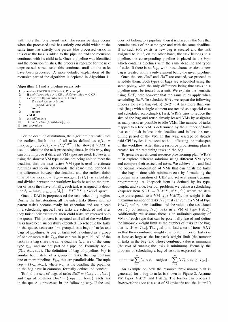
An example on how the resource provisioning plan isgenerated for a bag to tasks is shown in Figure 2. AssumeVM types, VMT1 and VMT2. The former can process 1

instructions/sec at a cost of $1/minute and the latter 10

Bag of TasksTasks: 12

Task Size: 100 insTask Deadline: 100 sec

Cloud Provider

10

ins/sec

VMT1 1 $1

VM Type

VMT2

cost/min

$101

Item #

2

Cost

VMT1 $2

Max. # of TasksVM Type

VMT2 $20

1

10

Scheduling Knapsack Items

VM1Type: VMT1

Cost: $2

VM2Type: VMT1

Cost: $2

VM3Type: VMT2Cost: $20

Knapsack (W = 12, Value = $24)

Figure 2. Example of a scheduling plan for a bag of tasks

instructions/sec at a cost of $10/minute. Consider a bagof 12 tasks, each task has a size of 100 instructions and adeadline of 100 seconds. The first knapsack item would beSKI1 = (VMT1, 1, $2). NT1 = 1 as running a task in aVM that can process 1 instructions/sec takes 100 seconds,with a deadline of 100 seconds, this means only one taskcan run on it before the deadline. C1 = $2 since the VMbilling period is 60 seconds, this means that to use it for 100seconds, two billing periods need to be paid for. Followingthe same reasoning, the second knapsack item would beSKI2 = (VMT2, 10, $20). The optimal combination ofitems to pack is then 2 items of type SKI1 and 1 itemof type SKI2. This means leasing 2 VMs of type VMT1

and running 1 task on each and leasing 1 VM of type VMT2

and running 10 tasks on it, for a total cost of $24.After solving the UKP problem, a resource provisioning

RP bot

i

= (VMTi

, numVMi

, NTi

) is obtained for each VMtype. It indicates the number of VMs of type VMT

i

to use(numVM

i

) and the maximum number of tasks to run oneach VM (NT

i

). In rare cases in which there are no VMtypes that can finish the tasks on time, a provisioning planof the form RP fastest

bot

= (VMTfastest

,W, 1) is created.This indicates that a VM of the fastest type must be leasedfor each task in the bag so that they can run in parallel andfinish as early as possible. Then, for each RP bop

i

for whichnumVM

i

> 0, WRPS tries to find a VM of type VMTi

which has already been leased and is free to use. If it exists,then NT

i

tasks from the bag are scheduled on to it. In thisway we reduce cost by using already paid for time slotsand avoid long provisioning delays of newly leased VMs.If there is no free VM of the required type, a new one isprovisioned and NT

i

tasks are scheduled on to it.We consider the case of a bags with a single task as a

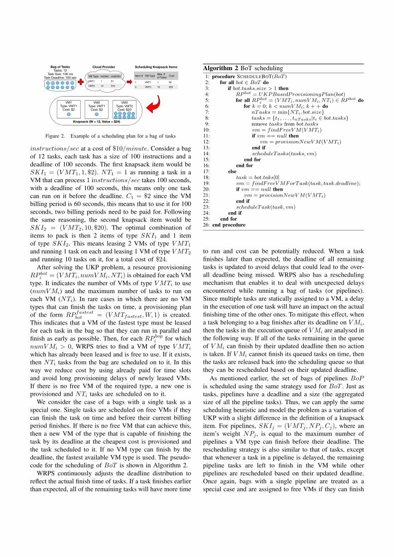
special one. Single tasks are scheduled on free VMs if theycan finish the task on time and before their current billingperiod finishes. If there is no free VM that can achieve this,then a new VM of the type that is capable of finishing thetask by its deadline at the cheapest cost is provisioned andthe task scheduled to it. If no VM type can finish by thedeadline, the fastest available VM type is used. The pseudo-code for the scheduling of BoT is shown in Algorithm 2.

WRPS continuously adjusts the deadline distribution toreflect the actual finish time of tasks. If a task finishes earlierthan expected, all of the remaining tasks will have more time

Algorithm 2 BoT scheduling1: procedure SCHEDULEBOT(BoT )2: for all bot 2 BoT do3: if bot.tasks.size > 1 then4: RP

bot = UKPBasedProvisioningP lan(bot)5: for all RP

bot

i

= (VMT

i

, numVM

i

, NT

i

) 2 RP

bot do6: for k = 0; k < numVM

i

; k ++ do7: nTasks = min{NT

i

, bot.size}8: tasks = {t1, . . . , t

nTasks

|ti

2 bot.tasks}9: remove tasks from bot.tasks

10: vm = findFreeVM(VMT

i

)11: if vm == null then12: vm = provisionNewVM(VMT

i

)13: end if14: scheduleTasks(tasks, vm)15: end for16: end for17: else18: task = bot.taks[0]19: vm = findFreeVMForTask(task, task.deadline);20: if vm == null then21: vm = provisionNewVM(VMT

i

)22: end if23: scheduleTask(task, vm)24: end if25: end for26: end procedure

to run and cost can be potentially reduced. When a taskfinishes later than expected, the deadline of all remainingtasks is updated to avoid delays that could lead to the over-all deadline being missed. WRPS also has a reschedulingmechanism that enables it to deal with unexpected delaysencountered while running a bag of tasks (or pipelines).Since multiple tasks are statically assigned to a VM, a delayin the execution of one task will have an impact on the actualfinishing time of the other ones. To mitigate this effect, whena task belonging to a bag finishes after its deadline on VM

i

,then the tasks in the execution queue of VM

i

are analysed inthe following way. If all of the tasks remaining in the queueof VM

i

can finish by their updated deadline then no actionis taken. If VM

i

cannot finish its queued tasks on time, thenthe tasks are released back into the scheduling queue so thatthey can be rescheduled based on their updated deadline.

As mentioned earlier, the set of bags of pipelines BoPis scheduled using the same strategy used for BoT . Just astasks, pipelines have a deadline and a size (the aggregatedsize of all the pipeline tasks). Thus, we can apply the samescheduling heuristic and model the problem as a variation ofUKP with a slight difference in the definition of a knapsackitem. For pipelines, SKI

j

= (VMTj

, NPj

, Cj

), where anitem’s weight NP

j

, is equal to the maximum number ofpipelines a VM type can finish before their deadline. Therescheduling strategy is also similar to that of tasks, exceptthat whenever a task in a pipeline is delayed, the remainingpipeline tasks are left to finish in the VM while otherpipelines are rescheduled based on their updated deadline.Once again, bags with a single pipeline are treated as aspecial case and are assigned to free VMs if they can finish

mImgTbl

mDiffFt

mBackground

mProjectPP

mConcatFit

mBgModel

mAdd

mShrink

mProjectPP

mBackground

mDiffFt

mPEG

mProjectPP

mProjectPP

mDiffFt

mDiffFt

mDiffFt

mDiffFt

mBackground

mBackground

(a)

Inspiral

TmpltBank

Thinca

TrigBank

TrigBank

Thinca

TmpltBank

Inspiral

TmpltBank

TmpltBank

TmpltBank

TmpltBank

TmpltBank

TmpltBank

TmpltBank

Inspiral Inspiral Inspiral Inspiral Inspiral Inspiral Inspiral

Inspiral Inspiral Inspiral Inspiral Inspiral Inspiral Inspiral Inspiral Inspiral

TrigBank

TrigBank

TrigBank

TrigBank

TrigBank

TrigBank

TrigBank

Thinca Thinca

(b)

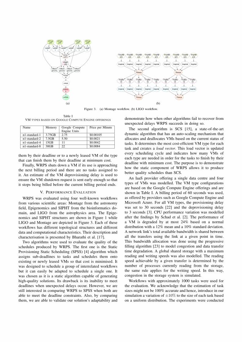
Figure 3. (a) Montage workflow. (b) LIGO workflow.

Table IVM TYPES BASED ON GOOGLE COMPUTE ENGINE OFFERINGS

Name Memory Google ComputeEngine Units

Price per Minute

n1-standard-1 3.75GB 2.75 $0.00105n1-standard-2 7.5GB 5.50 $0.0021n1-standard-4 15GB 11 $0.0042n1-standard-8 30GB 22 $0.0084

them by their deadline or to a newly leased VM of the typethat can finish them by their deadline at minimum cost.

Finally, WRPS shuts down a VM if its use is approachingthe next billing period and there are no tasks assigned toit. An estimate of the VM deprovisioning delay is used toensure the VM shutdown request is sent early enough so thatit stops being billed before the current billing period ends.

V. PERFORMANCE EVALUATION

WRPS was evaluated using four well-known workflowsfrom various scientific areas: Montage from the astronomyfield, Epigenomics and SIPHT from the bioinformatics do-main, and LIGO from the astrophysics area. The Epige-nomics and SIPHT structures are shown in Figure 1 whileLIGO and Montage are depicted in Figure 3. Each of theseworkflows has different topological structures and differentdata and computational characteristics. Their description andcharacterisation is presented by Bharathi et al. [17].

Two algorithms were used to evaluate the quality of theschedules produced by WRPS. The first one is the StaticProvisioning Static Scheduling (SPSS) [4] algorithm whichassigns sub-deadlines to tasks and schedules them ontoexisting or newly leased VMs so that cost is minimised. Itwas designed to schedule a group of interrelated workflowsbut it can easily be adapted to schedule a single one. Itwas chosen as it is a static algorithm capable of generatinghigh-quality solutions. Its drawback is its inability to meetdeadlines when unexpected delays occur. However, we arestill interested in comparing WRPS to SPSS when both areable to meet the deadline constraints. Also, by comparingthem, we are able to validate our solution’s adaptability and

demonstrate how when other algorithms fail to recover fromunexpected delays WRPS succeeds in doing so.

The second algorithm is SCS [15], a state-of-the-artdynamic algorithm that has an auto-scaling mechanism thatallocates and deallocates VMs based on the current status oftasks. It determines the most cost-efficient VM type for eachtask and creates a load vector. This load vector is updatedevery scheduling cycle and indicates how many VMs ofeach type are needed in order for the tasks to finish by theirdeadline with minimum cost. The purpose is to demonstratehow the static component of WRPS allows it to producebetter quality schedules than SCS.

An IaaS provider offering a single data centre and fourtypes of VMs was modelled. The VM type configurationsare based on the Google Compute Engine offerings and areshown in Table I. A billing period of 60 seconds was used,as offered by providers such as Google Compute Engine andMicrosoft Azure. For all VM types, the provisioning delaywas set to 30 seconds [22] and the deprovisioning delayto 3 seconds [3]. CPU performance variation was modelledafter the findings by Schad et al. [2]. The performance ofa VM is degraded by at most 24% based on a normaldistribution with a 12% mean and a 10% standard deviation.A network link’s total available bandwidth is shared betweenall the transfers using the link at a given point in time.This bandwidth allocation was done using the progressivefilling algorithm [23] to model congestion and data transfertime degradation. A global shared storage with a maximumreading and writing speeds was also modelled. The readingspeed achievable by a given transfer is determined by thenumber of processes currently reading from the storage,the same rule applies for the writing speed. In this way,congestion in the storage system is simulated.

Workflows with approximately 1000 tasks were used forthe evaluation. We acknowledge that the estimation of tasksizes might not be 100% accurate and hence, introduce in oursimulation a variation of ±10% to the size of each task basedon a uniform distribution. The experiments were conducted

(a) (b)

(c) (d)

(e) (f)

(g) (h)

Figure 4. Makespan and cost experiment results. The reference lines in the makespan line plots indicate the four deadline values. The stripped bars inthe cost bar charts indicate the deadline was not met for the corresponding deadline value. (a) LIGO makespan line plot. (b) LIGO cost bar chart. (c)Montage makespan line plot. (d) Montage cost bar chart. (e) Epigenomics makespan line plot. (f) Epigenomics cost bar chart. (g) SIPHT makespan lineplot. (h) SIPHT cost bar chart.

using four different deadlines, �W1 being the strictest one

and �W4 being the most relaxed one. For each workflow,

�W1 is equal to the time it takes to execute the tasks in

the critical path plus the time it takes to transfer all theinput files into the storage and the output files out of it. Theremaining deadlines are based on �

W1 and an interval size�int

= �W1/2: �

W2 = �W1 + �

int

, �W3 = �

W2 + �int

, and�W4 = �

W3 + �int

. The results displayed are the averageobtained after running each experiment 20 times.

A. Results and Analysis

1) Makespan and Cost Evaluation: The averagemakespan and cost obtained for each of the workflows isdepicted in Figure 4. The reference lines in the makespanline plots correspond to the four deadline values used foreach workflow. Evaluating the makespan and cost withregards to this value is essential as the main objective of

all the algorithms is to finish before the given deadline.The dashed bars in the cost bar charts indicate that thealgorithm failed to meet the corresponding deadline.

For LIGO, �W1 proves to be to tight for any of the algo-

rithms to finish on time. However, the difference between themakespan obtained by WRPS and the deadline is marginal.Additionally, WRPS generates the cheapest schedule in thiscase. The second deadline is still not relaxed enough for SCSor SPSS to achieve their goal, however, WRPS demonstratesits adaptability and ability to generate cheap schedules bybeing the only one to finish its execution before the deadlineand with the lowest cost. For the remaining deadlines, �

W3

and �W4, both SCS and WRPS are capable of meeting the

constraint, in both cases SCS has a slightly lower makespanbut WRPS has a lower cost. SPSS is only capable ofmeeting the most relaxed deadline, and in this case, WRPSoutperforms it in terms of execution cost. Overall, WRPS

meets the most deadlines and in all of the cases achievesbetter quality schedules with the cheapest costs.

In the case of Montage, SCS and WRPS meet all ofthe deadlines with WRPS consistently generating cheaperschedules. SPSS fails to meet the tightest deadline butsucceeds in meeting �

W2, �W3, and �

W4. Its success inmeeting three out of four deadlines may be explained by thefact that most of the tasks in the Montage application areconsidered small and require low CPU utilisation, leading toa potentially low CPU performance variation impact on thestatic schedule. In the case of �

W2, SPSS proves its abilityto generate cheap schedules and performs better than itscounterparts; although WRPS has a lower makespan in thiscase, its cost is slightly higher than that of SPSS. For �

W3

and �W4 however, WRPS succeeds in generating cheaper

solutions than its static counterpart.The three algorithms fail to meet �

W1 of the Epigenomicsworkflow, the closest makespan to the deadline is achievedby SCS, followed by WRPS and finally SPSS. WRPS is theonly algorithm capable of meeting �

W2 and still achieves thelowest cost. The third deadline constraint is met by SPSSand WRPS, with WRPS once again outperforming SPSSin terms of cost. Finally, as the deadlines become relaxedenough, the three algorithms succeed in meeting the deadlineand WRPS does it with the lowest cost. The high deadlinemiss percentage of SCS and SPSS in this case is due tothe high-CPU nature of the Epigenomics tasks, meaning thatCPU performance degradation will have a significant impacton the execution time of tasks causing unexpected delays.

SIPHT is an interesting application to evaluate WRPSwith due to its topological features. As mentioned earlier,it has data distribution and aggregation structures in whichthe parallel tasks differ on their type. The results demonstratethat even in cases like this, WRPS remains responsive andefficient. It succeeds in meeting all the deadlines with thelowest makespan and with the lowest cost amongst thealgorithms that meet the constraint. The large number of filesthat need to be transferred when running this workflow leadto SPSS struggling to recover from the lower data transferrates due to network congestion and hence failing to meetthe four deadlines. Even SCS fails to adapt to these delayson time and fails to meet the three tightest deadlines.

Overall, WRPS is the most successful algorithm in meet-ing deadlines. On average, it succeeds in meeting the con-straint in 87.5% of the cases while SCS succeeds in 56.25%and SPSS on 37.5%. These results are inline with what wasexpected of each algorithm. The static approach is not veryefficient in meeting the deadlines whereas the dynamism inWRPS and SCS allows them to accomplish their goal moreoften. The experiments also demonstrate the efficiency ofWRPS in terms of its ability to generate low cost solutions.It outperforms SCS an SPSS as in all of the scenariosexcept one (Montage workflow, �

W2); WRPS achieves thelowest cost when compared to those algorithms that met

(a) (b)

(c) (d)

Figure 5. Average number of files read from the storage by each algorithm.The reference lines indicate the total number of files required as input bythe given workflow. (a) LIGO. (b) Montage. (c) Epigenomics. (d) SIPHT.

the deadline. Another desirable characteristic of WRPS thatcan be observed from the results is its ability to consistentlyincrease the time it takes to run the workflow and reduce thecost as the deadline becomes more relaxed. The importanceof this relies in the fact that many users are willing to trade-off execution time for lower costs while others are willing topay higher costs for faster executions. The algorithm needsto behave within this logic in order for the deadline valuegiven by users to be meaningful.

2) Network Usage Evaluation: Network links are well-known bottlenecks in Cloud environments. For instance,Jackson et al. [16] report a data transfer time variation of upto 65% in Amazon EC2. Hence, as means of reducing thesources of unpredictability and improving the performanceof workflow applications, it is important for schedulingalgorithms to try to reduce the amount of data transferredthrough the cloud network infrastructure. In this section, weevaluate the number of files read from the global storageby each of the algorithms. Recall that a task does not needto read from the storage system whenever the input files itrequires are already available in the VM where it is running.

The bar charts in Figure 5 show the average numberof files read across the four deadlines for each workflowand algorithm. The reference line indicates the total numberof input files that are required by the workflow tasks. Byscheduling pipelines in a single VM and by running as manytasks or pipelines from the same bag in a single VM, WRPSis successful in reducing by 50% or more the number of filesread from the storage. In fact, WRPS reads the least amountof files when compared to SCS and SPSS in the cases of theLIGO and Epigenomics workflow. The files read from thestorage are reduced by 58% in the LIGO case and by 75% in

the Epigenomics case. For the Montage workflow, SCS andWRPS achieve a similar performance and reduce the numberof files by approximately 50%. Finally, even though reducedby 23%, WRPS is not as successful in reducing the numberof files as SCS and SPSS for the SIPHT workflow. The lackof pipelines and bags of tasks in the SIPHT application arethe main cause for this and as a future work we would like toexplore and develop new heuristics so that WRPS is capableof scheduling these type of workflows more efficiently.

VI. CONCLUSIONS

WRPS, a responsive resource provisioning and schedulingalgorithm for scientific workflows in clouds capable ofgenerating high quality schedules was presented. It has asobjectives minimising the overall cost of using the cloudinfrastructure while meeting a user-defined deadline. Thealgorithm is dynamic to a certain extent to respond tounexpected delays and environmental dynamics common incloud computing. It also has a static component that allowsit to find the optimal schedule for a group of workflow tasks,consequently improving the quality of the schedules it gen-erates. By reducing the workflow into bags of homogeneoustasks and pipelines that share a deadline, we are able tomodel their scheduling as a variation UKP and solve it inpseudo-polynomial time using dynamic programming.

The simulation experiments show that our solution has anoverall better performance than state-of-the-art algorithms.It is successful in meeting deadlines under unpredictable sit-uations involving performance variation, network congestionand inaccurate task size estimations. It achieves this at lowcosts, even lower than fully static approaches which have theability of using the entire workflow structure and comparingvarious solutions before the workflow execution.

REFERENCES

[1] J. D. Ullman, “Np-complete scheduling problems,” J. Com-put. System Sci., vol. 10, no. 3, pp. 384–393, 1975.

[2] J. Schad, J. Dittrich, and J.-A. Quiane-Ruiz, “Runtime mea-surements in the cloud: observing, analyzing, and reducingvariance,” Proc. VLDB Endowment, vol. 3, no. 1-2, pp. 460–471, 2010.

[3] M. Mao and M. Humphrey, “A performance study on the VMstartup time in the cloud,” in Proc. Int. Conf. Cloud Comput.(CLOUD), 2012.

[4] M. Malawski, G. Juve, E. Deelman, and J. Nabrzyski, “Cost-and deadline-constrained provisioning for scientific workflowensembles in IaaS clouds,” in Proc. Int. Conf. High Perfor-mance Comput., Netw., Storage Anal., 2012.

[5] A. C. Zhou, B. He, and C. Liu, “Monetary cost optimiza-tions for hosting workflow-as-a-service in IaaS clouds,” IEEETrans. Cloud Comput., vol. PP, no. 99, pp. 1–1, 2015.

[6] D. Poola, K. Ramamohanarao, and R. Buyya, “Fault-tolerantworkflow scheduling using spot instances on clouds,” Proce-dia Comput. Sci., vol. 29, pp. 523–533, 2014.

[7] E.-K. Byun, Y.-S. Kee, J.-S. Kim, and S. Maeng, “Costoptimized provisioning of elastic resources for applicationworkflows,” Future Generation Comput. Syst., vol. 27, no. 8,pp. 1011–1026, 2011.

[8] M. Xu, L. Cui, H. Wang, and Y. Bi, “A multiple QoS con-strained scheduling strategy of multiple workflows for cloudcomputing,” in Proc. Int. Symp. Parallel Distrib. ProcessingApplicat. (ISPA), 2009.

[9] T. T. Huu and J. Montagnat, “Virtual resources allocation forworkflow-based applications distribution on a cloud infras-tructure,” in Proc. Int. Conf. Cluster, Cloud Grid Comput.(CCGrid), 2010.

[10] D. de Oliveira, K. A. Ocana, F. Baiao, and M. Mattoso, “Aprovenance-based adaptive scheduling heuristic for parallelscientific workflows in clouds,” J. Grid Comput., vol. 10,no. 3, pp. 521–552, 2012.

[11] S. Abrishami, M. Naghibzadeh, and D. H. Epema, “Deadline-constrained workflow scheduling algorithms for infrastruc-ture as a service clouds,” Future Generation Comput. Syst.,vol. 29, no. 1, pp. 158–169, 2013.

[12] Z. Wu, Z. Ni, L. Gu, and X. Liu, “A revised discrete particleswarm optimization for cloud workflow scheduling,” in Proc.Int. Conf. Computational Intell. Security (CIS), 2010.

[13] S. Yassa, R. Chelouah, H. Kadima, and B. Granado, “Multi-objective approach for energy-aware workflow scheduling incloud computing environments,” Sci. World J., 2013.

[14] R. Calheiros and R. Buyya, “Meeting deadlines of scientificworkflows in public clouds with tasks replication,” IEEETrans. Parallel Distrib. Syst., vol. 25, no. 7, pp. 1787–1796,2014.

[15] M. Mao and M. Humphrey, “Auto-scaling to minimize costand meet application deadlines in cloud workflows,” in Proc.Int. Conf. High Performance Comput., Newt., Storage Anal.(SC), 2011.

[16] K. R. Jackson, L. Ramakrishnan, K. Muriki, S. Canon,S. Cholia, J. Shalf, H. J. Wasserman, and N. J. Wright,“Performance analysis of high performance computing ap-plications on the amazon web services cloud,” in Proc. Int.Conf. Cloud Comput. Technol. and Sci. (CloudCom), 2010.

[17] S. Bharathi, A. Chervenak, E. Deelman, G. Mehta, M.-H. Su, and K. Vahi, “Characterization of scientific work-flows,” in Proc. Workshop Workflows Support Large-Scale Sci.(WORKS), 2008.

[18] R. Andonov, V. Poirriez, and S. Rajopadhye”, “Unboundedknapsack problem: Dynamic programming revisited,” Euro-pean J. Oper. Research, vol. 123, no. 2, pp. 394 – 407, 2000.

[19] P. C. Gilmore and R. E. Gomory, “A linear programming ap-proach to the cutting stock problem-part ii,” Oper. Research,vol. 11, no. 6, pp. 863–888, 1963.

[20] P. Gilmore and R. Gomory, “The theory and computationof knapsack functions,” Oper. Research, vol. 14, no. 6, pp.1045–1074, 1966.

[21] R. Andonov and S. Rajopadhye, “A sparse knapsack algo-tech-cuit and its synthesis,” in Proc. Int. Conf. Appl. SpecificArray Processors, 1994.

[22] S. Stadill, “By the numbers: How google compute enginestacks up to amazon ec2,” https://gigaom.com/2013/03/15/by-the-numbers-how-google-compute-engine-stacks-up-to-amazon-ec2/.

[23] D. P. Bertsekas, R. G. Gallager, and P. Humblet, Datanetworks. Prentice-Hall International New Jersey, 1992.