An Exact Algorithm for the Dynamic Knapsack Problem with ...

An Exact Algorithm for the Dynamic Knapsack Problem

with Stochastic Item Sizes

Daniel Blado Alejandro TorielloH. Milton Stewart School of Industrial and Systems Engineering

Georgia Institute of Technology

Atlanta, Georgia 30332

deblado at gatech dot edu atoriello at isye dot gatech dot edu

October 31, 2018

Abstract

We consider a version of the knapsack problem in which an item size is random and revealedonly when the decision maker attempts to insert it. After every successful insertion the decisionmaker can choose the next item dynamically based on the remaining capacity and availableitems, while an unsuccessful insertion terminates the process. We propose an exact algorithmbased on a reformulation of the value function linear program, which dynamically prices variablesto refine a value function approximation and generates cutting planes to maintain a dual bound.We provide a detailed analysis of the zero-capacity case, theoretical properties of the generalalgorithm, and an extensive computational study. Our main empirical conclusion is that thealgorithm is able to significantly reduce the gap when initial bounds and/or heuristic policiesperform poorly.

1 Introduction

The deterministic knapsack problem is a fundamental discrete optimization model that has beenstudied extensively in mathematical optimization, computer science, operations research, and in-dustrial engineering. Recently, knapsack models under uncertainty have been the subject of muchwork, both to model resource allocation problems with uncertain parameters, and as subproblems inmore general discrete optimization problems under uncertainty, such as stochastic integer programs.Dynamic knapsack problems, where decisions occur in sequence and problem parameters may berevealed dynamically, have particularly been a topic of ongoing interest; such models have seenmany applications, such as in scheduling [11], equipment replacement [12], and machine learning[15, 23].

The dynamic knapsack model variant that we analyze here has stochastic item sizes that areonly revealed to the decision maker after they attempt to insert an item. After every successfulinsertion the decision maker can choose the next item dynamically based on the remaining capacityand available items, while an unsuccessful insertion terminates the process. This differs from morestatic models, in which the decision maker decides on a particular subset of items a priori, essentiallyattempting to insert the set simultaneously, and the question is whether that set fits the knapsackwith a specified probability, e.g. [14].

Having the flexibility to choose subsequent items in light of the revealed sizes of previous itemscan intuitively lead to a higher overall expected value than a more static approach. However, this

1

added freedom raises the complexity of the problem both practically and theoretically. A feasiblesolution to this problem is a policy that dictates which item the decision maker attempts to insertunder any possible state, as opposed to simply a subset of items to insert a priori. Such addeddifficulty motivates the development of reasonably tight, tractable relaxations and high-quality,efficient policies; see for instance [3, 5, 6, 11]. However, there is no known method to systematicallyimprove such relaxations to eventually arrive at an optimal solution, even under the assumptionof integer size support; our goal in this paper is thus to provide a computationally efficient, exactalgorithm with such convergence guarantees. Our contributions can be summarized as:

i) We analyze the special case where the capacity is zero: We prove that a straightforwardoptimal policy exists, and that the variables corresponding to the optimal value functionhave closed-form solutions. Such results provide both insights and a valid starting boundapplicable to the general capacity case.

ii) We develop a finitely terminating general algorithm that solves the dynamic knapsack problemunder integer sizes and capacity within an arbitrary numerical tolerance, using a dynamicvalue function approximation approach. We present both theoretical analysis and an extensivecomputational study, and show that the algorithm is able to significantly reduce the gapprecisely when the initial bounds or heuristic policies perform poorly.

The remainder of the paper is organized as follows. We conclude this section with a briefliterature review. Section 2 states the problem formulation and preliminaries, including relevantprevious results. Section 3 provides the complete analysis of the zero capacity case. Section 4then states the general algorithm and examines structural results, while Section 5 summarizesour computational study. Section 6 concludes, and an appendix contains plots and computationalexperiment data not included in the main article.

1.1 Literature Review

The knapsack problem and its generalizations have been studied for over sixty years, having wide-reaching applications in areas including budgeting, finance, and scheduling; see [18, 25]. Variousversions of the knapsack problem under uncertainty have specifically received much attention;[18, Chapter 14] surveys some of these results. Generally, optimization under uncertainty can bemodeled via a static approach that chooses a solution a priori, or a dynamic (or adaptive [9, 10, 11])approach that chooses a solution sequentially based on realized parameters. A priori knapsackmodels with uncertain item values include [7, 16, 27, 30, 31], a priori models with uncertain itemsizes include [13, 14, 19, 20], and an a priori model with both uncertain values and sizes is examinedin [26]. Dynamic models for the knapsack problem with uncertain item sizes include [4, 9, 11, 12, 15],and [17] study a dynamic model with uncertain item values. Another variant, the stochastic anddynamic knapsack, assumes items are not initially given but rather arrive dynamically accordingto a stochastic process [21, 22, 28] .

The dynamic variant of the stochastic knapsack problem examined here was first studied in[12], where the item sizes are exponentially distributed; in this particular case, the natural greedypolicy that inserts items based on their value-to-mean-size ratio is optimal, and recent work [3, 6]establishes that this policy is in fact asymptotically optimal more generally. The first study of theproblem in its full generality came in [9, 11], where the authors provide two linear programmingbounds with polynomially many variables. They show both bounds are within a constant mul-tiplicative gap using greedy heuristic policies. Later, [15, 23, 24] investigated bounds under theadditional assumption that the capacity and item sizes are integers, evaluating the performance

2

of LP relaxations of pseudo-polynomial size and developing randomized policies based on theiroptimal solutions. Their results also apply to variants beyond the problem studied here, such ascorrelated random item values, preemption, and the multi-armed bandits problem with budgetedlearning.

Using value function approximations to obtain relaxations and policies for dynamic programsdates back to [1, 8, 29, 32]. The results in [5] provide the technique’s first application to a stochasticknapsack model. Our exact algorithm uses a successive refinement of value function approximationsto converge to optimality; the only similar work we are aware of is [2], which studies the jointreplenishment problem and its generalizations.

2 Problem Formulation and Preliminaries

We have a knapsack with integer capacity b > 0 and item set N := {1, 2, . . . , n}, where everyitem i has a deterministic value ci > 0. Item sizes are independent random variables Ai ≥ 0 withinteger support; each distribution is arbitrary but known to the decision maker. An item size isonly realized after an attempted insertion. When attempting to insert i, the decision maker facestwo possible outcomes: either i fits, and we collect the value ci and update the remaining capacity;or i is too large and the process ends, i.e. we allow at most one failed insertion. A policy stipulateswhat item to insert and can depend on both the remaining items and remaining capacity. Theobjective is to maximize the expected value of successfully inserted items.

This problem can be modeled as a dynamic program (DP), where every possible state is definedby the set of remaining items M ⊆ N and remaining capacity s ∈ [0, b] := {0, 1, . . . , b}. For agiven state (M, s), the allowed possible actions consist of attempting to insert an item i ∈ M . Ifwe define v∗M (s) as the optimal expected value at state (M, s), the Bellman recursion is

v∗M (s) = maxi∈M

P(Ai ≤ s)(ci + E[v∗M\i(s−Ai)|Ai ≤ s]), (1)

with the base case v∗∅(s) = 0. Intuitively, we collect nothing if the attempted item i has size greaterthan s, but if the item does fit, we not only collect the item’s value ci, but also the optimal expectedvalue of the subsequent state, (M \ i, s − Ai). The linear programming (LP) formulation of thisproblem is

minv

vN (b) (2a)

s.t. vM∪i(s) ≥ P(Ai ≤ s)(ci + E[vM (s−Ai)|Ai ≤ s]), (2b)

i ∈ N, M ⊆ N \ i, s ∈ [0, b] (2c)

vM : [0, b]→ R+, M ⊆ N. (2d)

For every M ⊆ N , vM can be thought of as a vector in Rb+1+ , or equivalently as a real-valued

function over the integers in [0, b].

Notation To ease notation, we denote an item size’s cumulative distribution function by Fi(s) :=P(Ai ≤ s) for i ∈ N , and its complement by Fi(s) := P(Ai > s). The mean truncated size ofitem i ∈ N at capacity s ∈ [0, b] is the quantity Ei(s) := E[min{s,Ai}] [9, 11]. Intuitively, givenremaining capacity s, we do not care about the distribution of the item size past s, because in allsuch cases we end up with a failed insertion.

3

2.1 Value Function Approximations - a Survey

In general, the LP (2) cannot be solved efficiently and essentially reduces to running the Bell-man recursion (1) in Θ(b2n2n) time. However, any feasible solution to the LP provides a validupper bound on the optimal solution; earlier work in [5] examines the bound that results fromapproximating the optimal value function as the affine value function approximation (AFF)

vM (s) ≈ qs+ r0 +∑i∈M

ri, (3)

where ri intuitively represents the inherent value of having an item i available to insert, q is themarginal value of the remaining capacity s, and r0 is the intrinsic value of keeping the knapsackavailable to the decision maker.

Proposition 2.1 ([5]). The best possible bound given by affine approximation (3) is the solutionof the LP

minq,r

qb+ r0 +∑i∈N

ri

s.t. qEi(s) + r0Fi(s) + ri ≥ ciFi(s), ∀ i ∈ N, s ∈ [0, b]

r, q ≥ 0.

A Quadratic LP (Quad) introduced in [6] improves on AFF by introducing quadratic termsthat encode the notion of diminishing returns:

vM (s) ≈ qs+ r0 +∑i∈M

ri −∑

{k,`}⊆M

rk`. (4)

AFF and Quad can be formulated without the assumption of integer support, and are efficientlysolvable for many common distributions, such as those whose cumulative distribution function ispiecewise convex. Both are also asymptotically tight [6].

Finally, assuming again that item sizes have integer support, [23, 24] proposes a pseudo-polynomial (PP) bound,

maxx

∑i∈N

b∑s=0

cixi,sFi(s)

s.t.∑i∈N

b∑s=σ

xi,sFi(s− σ) ≤ 1, σ = 0, . . . , b

b∑s=0

xi,s ≤ 1, i ∈ N

x ≥ 0,

which [5] show arises from the value function approximation

vM (s) ≈∑i∈M

ri +s∑

σ=0

wσ. (5)

When available, PP is provably tighter than AFF [5] and serves as a benchmark to gauge theperformance of polynomially solvable bounds.

4

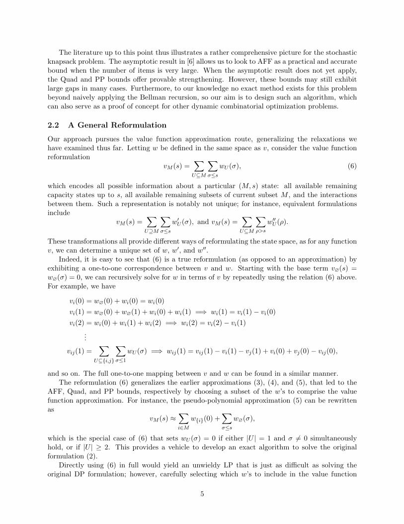
The literature up to this point thus illustrates a rather comprehensive picture for the stochasticknapsack problem. The asymptotic result in [6] allows us to look to AFF as a practical and accuratebound when the number of items is very large. When the asymptotic result does not yet apply,the Quad and PP bounds offer provable strengthening. However, these bounds may still exhibitlarge gaps in many cases. Furthermore, to our knowledge no exact method exists for this problembeyond naively applying the Bellman recursion, so our aim is to design such an algorithm, whichcan also serve as a proof of concept for other dynamic combinatorial optimization problems.

2.2 A General Reformulation

Our approach pursues the value function approximation route, generalizing the relaxations wehave examined thus far. Letting w be defined in the same space as v, consider the value functionreformulation

vM (s) =∑U⊆M

∑σ≤s

wU (σ), (6)

which encodes all possible information about a particular (M, s) state: all available remainingcapacity states up to s, all available remaining subsets of current subset M , and the interactionsbetween them. Such a representation is notably not unique; for instance, equivalent formulationsinclude

vM (s) =∑U⊇M

∑σ≤s

w′U (σ), and vM (s) =∑U⊆M

∑ρ>s

w′′U (ρ).

These transformations all provide different ways of reformulating the state space, as for any functionv, we can determine a unique set of w, w′, and w′′.

Indeed, it is easy to see that (6) is a true reformulation (as opposed to an approximation) byexhibiting a one-to-one correspondence between v and w. Starting with the base term v∅(s) =w∅(σ) = 0, we can recursively solve for w in terms of v by repeatedly using the relation (6) above.For example, we have

vi(0) = w∅(0) + wi(0) = wi(0)

vi(1) = w∅(0) + w∅(1) + wi(0) + wi(1) =⇒ wi(1) = vi(1)− vi(0)

vi(2) = wi(0) + wi(1) + wi(2) =⇒ wi(2) = vi(2)− vi(1)

...

vij(1) =∑

U⊆{i,j}

∑σ≤1

wU (σ) =⇒ wij(1) = vij(1)− vi(1)− vj(1) + vi(0) + vj(0)− vij(0),

and so on. The full one-to-one mapping between v and w can be found in a similar manner.The reformulation (6) generalizes the earlier approximations (3), (4), and (5), that led to the

AFF, Quad, and PP bounds, respectively by choosing a subset of the w’s to comprise the valuefunction approximation. For instance, the pseudo-polynomial approximation (5) can be rewrittenas

vM (s) ≈∑i∈M

w{i}(0) +∑σ≤s

w∅(σ),

which is the special case of (6) that sets wU (σ) = 0 if either |U | = 1 and σ 6= 0 simultaneouslyhold, or if |U | ≥ 2. This provides a vehicle to develop an exact algorithm to solve the originalformulation (2).

Directly using (6) in full would yield an unwieldy LP that is just as difficult as solving theoriginal DP formulation; however, carefully selecting which w’s to include in the value function

5

approximation could lead to a tight bound (or a bound within a desired numerical tolerance). Inthe spirit of cutting plane algorithms used in solving the deterministic knapsack problem, then,one could dynamically improve the value function approximation to systematically reach strongerrelaxations with certain algorithm termination. For example, defining the state space as S :={(M, s)}, let us choose as a starting point some S ⊆ S to provide the approximation

vM (s) ≈∑

(U,σ)∈S

wU (σ). (7)

Let W (S ) denote the optimal value of the associated approximation LP for (7) under set S ;clearly, W (S ) ≥W (S ). We determine whether the approximation is tight with a pricing problem

max(M,s)∈S \S

{W (S )−W (S ∪ (M, s))

},

or its weaker decision counterpart,

∃ (M, s) ∈ S \S : W (S ∪ (M, s)) < W (S )? (8)

If the current bound is not tight, we can thus identify and add a state to S and update thecurrent value function approximation, repeating until a tight bound is found. Being able to solve(8) systematically in effect guarantees finite termination of the algorithm since S is finite. We thusdevelop a general algorithm based on this framework and present its results in Section 4.

Prior to the algorithm proper, however, we first examine the special case where the capacity iszero, b = 0. The motivation for this is at least threefold. First, this case presents a simple scenarioto explore theoretically, and any insights, approaches, and results may be applicable to the moregeneral capacitated case. Second, the zero capacity case is always a valid restricted subproblemof the general capacitated case, as all wU,0 variables are still present in the general case. From apractical standpoint then, various algorithm heuristics can also be preliminarily tested on the zerocapacity subproblem. Finally, the general algorithm requires a good starting bound. In additionto the bounds covered in the previous section, the zero capacity case provides an alternate startingpoint, and we verify further below that the bound is a useful initialization for certain computationalexperiments.

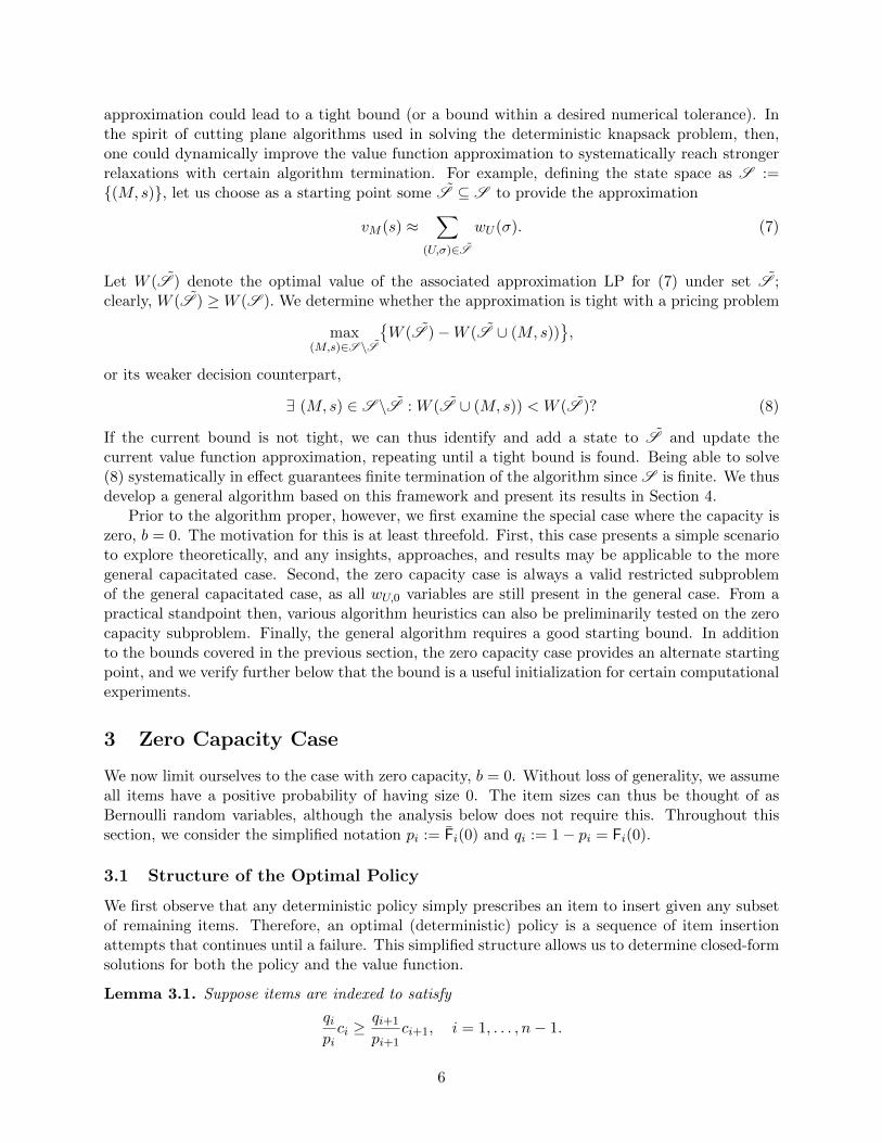
3 Zero Capacity Case

We now limit ourselves to the case with zero capacity, b = 0. Without loss of generality, we assumeall items have a positive probability of having size 0. The item sizes can thus be thought of asBernoulli random variables, although the analysis below does not require this. Throughout thissection, we consider the simplified notation pi := Fi(0) and qi := 1− pi = Fi(0).

3.1 Structure of the Optimal Policy

We first observe that any deterministic policy simply prescribes an item to insert given any subsetof remaining items. Therefore, an optimal (deterministic) policy is a sequence of item insertionattempts that continues until a failure. This simplified structure allows us to determine closed-formsolutions for both the policy and the value function.

Lemma 3.1. Suppose items are indexed to satisfy

qipici ≥

qi+1

pi+1ci+1, i = 1, . . . , n− 1.

6

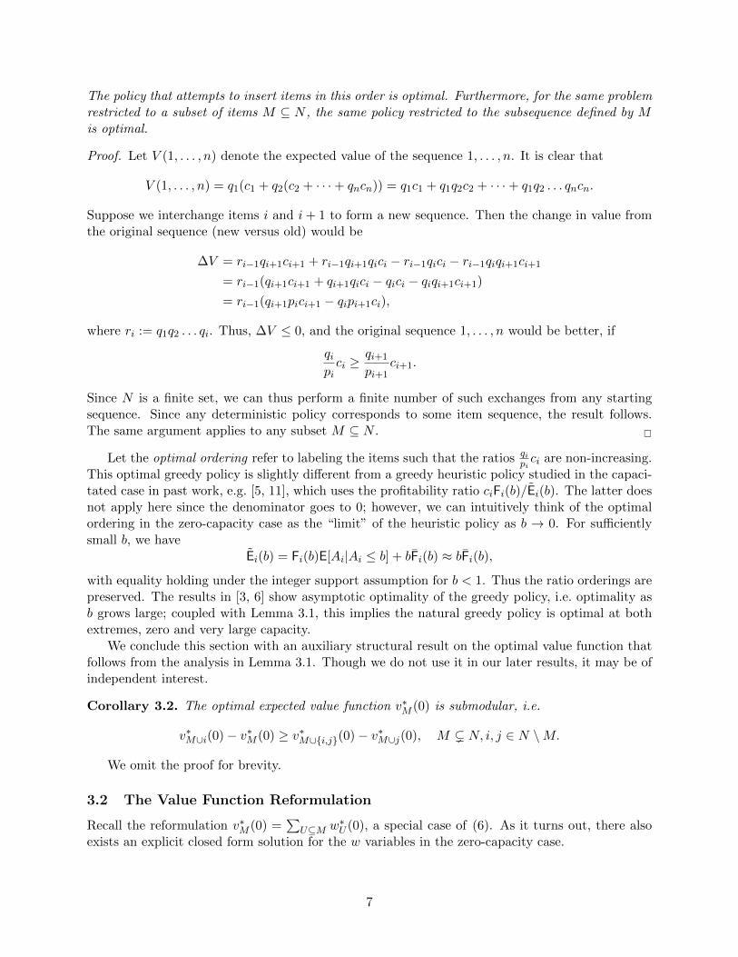
The policy that attempts to insert items in this order is optimal. Furthermore, for the same problemrestricted to a subset of items M ⊆ N , the same policy restricted to the subsequence defined by Mis optimal.

Proof. Let V (1, . . . , n) denote the expected value of the sequence 1, . . . , n. It is clear that

V (1, . . . , n) = q1(c1 + q2(c2 + · · ·+ qncn)) = q1c1 + q1q2c2 + · · ·+ q1q2 . . . qncn.

Suppose we interchange items i and i+ 1 to form a new sequence. Then the change in value fromthe original sequence (new versus old) would be

∆V = ri−1qi+1ci+1 + ri−1qi+1qici − ri−1qici − ri−1qiqi+1ci+1

= ri−1(qi+1ci+1 + qi+1qici − qici − qiqi+1ci+1)

= ri−1(qi+1pici+1 − qipi+1ci),

where ri := q1q2 . . . qi. Thus, ∆V ≤ 0, and the original sequence 1, . . . , n would be better, if

qipici ≥

qi+1

pi+1ci+1.

Since N is a finite set, we can thus perform a finite number of such exchanges from any startingsequence. Since any deterministic policy corresponds to some item sequence, the result follows.The same argument applies to any subset M ⊆ N . �

Let the optimal ordering refer to labeling the items such that the ratios qipici are non-increasing.

This optimal greedy policy is slightly different from a greedy heuristic policy studied in the capaci-tated case in past work, e.g. [5, 11], which uses the profitability ratio ciFi(b)/Ei(b). The latter doesnot apply here since the denominator goes to 0; however, we can intuitively think of the optimalordering in the zero-capacity case as the “limit” of the heuristic policy as b → 0. For sufficientlysmall b, we have

Ei(b) = Fi(b)E[Ai|Ai ≤ b] + bFi(b) ≈ bFi(b),

with equality holding under the integer support assumption for b < 1. Thus the ratio orderings arepreserved. The results in [3, 6] show asymptotic optimality of the greedy policy, i.e. optimality asb grows large; coupled with Lemma 3.1, this implies the natural greedy policy is optimal at bothextremes, zero and very large capacity.

We conclude this section with an auxiliary structural result on the optimal value function thatfollows from the analysis in Lemma 3.1. Though we do not use it in our later results, it may be ofindependent interest.

Corollary 3.2. The optimal expected value function v∗M (0) is submodular, i.e.

v∗M∪i(0)− v∗M (0) ≥ v∗M∪{i,j}(0)− v∗M∪j(0), M ( N, i, j ∈ N \M.

We omit the proof for brevity.

3.2 The Value Function Reformulation

Recall the reformulation v∗M (0) =∑

U⊆M w∗U (0), a special case of (6). As it turns out, there alsoexists an explicit closed form solution for the w variables in the zero-capacity case.

7

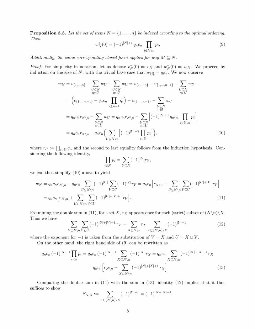
Proposition 3.3. Let the set of items N = {1, . . . , n} be indexed according to the optimal ordering.Then

w∗N (0) = (−1)|N |+1 qncn∏

i∈N\n

pi. (9)

Additionally, the same corresponding closed form applies for any M ⊆ N .

Proof. For simplicity in notation, let us denote v∗N (0) as vN and w∗N (0) as wN . We proceed byinduction on the size of N , with the trivial base case that w{i} = qici. We now observe

wN = v{1,...,n} −∑U(Nn6∈U

wU −∑U(Nn∈U

wU = v{1,...,n} − v{1,...,n−1} −∑U(Nn∈U

wU

=(v{1,...,n−1} + qncn

∏i≤n−1

qi

)− v{1,...,n−1} −

∑U(Nn∈U

wU

= qncnrN\n −∑U(Nn∈U

wU = qncnrN\n −∑U(Nn∈U

[(−1)|U |+1 qncn

∏i∈U\n

pi

]

= qncnrN\n − qncn( ∑U(N\n

[(−1)|U |+2

∏i∈U

pi

]), (10)

where rU :=∏i∈U qi, and the second to last equality follows from the induction hypothesis. Con-

sidering the following identity, ∏i∈N

pi =∑U⊆N

(−1)|U |rU ,

we can thus simplify (10) above to yield

wN = qncnrN\n − qncn∑

U(N\n

(−1)|U |∑V⊆U

(−1)|V |rV = qncn

[rN\n −

∑U(N\n

∑V⊆U

(−1)|U |+|V | rV

]= qncn

[rN\n +

∑U⊂N\n

∑V⊆U

(−1)|U |+|V |+1 rV

]. (11)

Examining the double sum in (11), for a set X, rX appears once for each (strict) subset of (N\n)\X.Thus we have ∑

U(N\n

∑V⊆U

(−1)|U |+|V |+1 rV =∑

X(N\n

rX∑

Y ((N\n)\X

(−1)|Y |+1, (12)

where the exponent for −1 is taken from the substitution of V = X and U = X ∪ Y .On the other hand, the right hand side of (9) can be rewritten as

qncn (−1)|N |+1∏i<n

pi = qncn (−1)|N |+1∑

X⊆N\n

(−1)|X| rX = qncn∑

X⊆N\n

(−1)|N |+|X|+1 rX

= qncn

[rN\n +

∑X⊂N\n

(−1)|N |+|X|+1 rX

](13)

Comparing the double sum in (11) with the sum in (13), identity (12) implies that it thussuffices to show

SN,X :=∑

Y⊂(N\n)\X

(−1)|Y |+1 = (−1)|N+|X|+1.

8

But viewing the sum SN,X combinatorially, we can rewrite

SN,X =

|N |−|X|−2∑i=0

(|N | − |X| − 1

i

)(−1)i+1 =

|N |−|X|−1∑i=0

(|N | − |X| − 1

i

)(−1)i+1 − (−1)|N |−|X|

= −k∑i=0

(k

i

)(−1)i + (−1)k = (−1)k,

where the third equality substitutes k = |N |−|X|−1, and the last equality follows from the identitythat the alternating sum of binomial coefficients is 0. Hence,

SN,X =

{−1 = (−1)|N |+|X|+1 if |N | and |X| have the same parity

1 = (−1)|N |+|X|+1 if |N | and |X| have different parity.

The entire argument above is identical for any subset M ⊆ N . �

Intuitively, this proposition says that the wM ’s exponentially decay in value as we add moreitems to M , as long as the highest indexed element is the same. In other words, the impact ormarginal value diminishes as one adds more elements to the starting set, which is consistent withthe intuition that the initial decisions are the most important. Smaller sets thus “matter” more inthe value function LP; this further motivates why we start with lower cardinality sets in all of ourcomputational experiments.

The results in this and the previous subsection solve the zero capacity case completely fromboth the bound and policy sides, and helps us quickly benchmark the general algorithm on thezero-capacity case.

4 The Algorithm

Recall the problem reformulation (6), vM (s) =∑

U⊆M∑

σ≤swU,σ. Plugging in this value functionformulation into the value function LP (2) yields constraints with left hand sides of the form

vM∪i(s)− Fi(s)E[vM (s−Ai)|Ai ≤ s] =∑

U⊆M∪i

∑σ≤s

wU,σ −∑s′≤s

P(Ai = s′)( ∑U⊆M

∑σ≤s′

wU,σ)

=∑

U⊆M∪i

∑σ≤s

wU,σ −∑U⊆M

∑σ≤s

Fi(s− σ)wU,σ

=∑U⊆M

∑σ≤s

wU∪i,σ + Fi(s− σ)wU,σ.

Thus, our master dual LP is

minw

∑U⊆N

∑σ≤b

wU,σ (14a)

s.t.∑U⊆M

∑σ≤s

wU∪i,σ + Fi(s− σ)wU,σ ≥ ciFi(s), ∀ i ∈ N,M ⊆ N\i, s ∈ [0, b] (14b)

w∅,σ = 0, ∀ σ ≤ b. (14c)

Note the empty set variables in (14) are required to be 0 via reformulation (6), as the originalformulation assumes as a base case that v∗∅(s) = 0, i.e. we cannot assign a positive value to states

9

without any items to insert. The remaining variables are unrestricted. The corresponding primalproblem is

maxx

∑i∈N

∑M⊆N\i

∑s≤b

ciFi(s)xiMs (15a)

s.t.∑i 6∈U

∑M⊆N\iM⊇U

b∑s=σ

Fi(s− σ)xiMs +∑i∈U

∑M⊆N\iM⊇U\i

b∑s=σ

xiMs = 1, ∀ ∅ 6= U ⊆ N, σ ≤ b (15b)

x ≥ 0. (15c)

Instead of solving these LP’s directly, we propose an algorithm that uses column and constraintgeneration. Before formalizing the algorithm, we first examine both the separation and pricingproblems. Given a solution w to (14), the separation problem for a fixed pair (i ∈ N, s ≤ b) is

minM⊆N\i

∑U⊆M

∑σ≤s

wU∪i,σ + Fi(s− σ)wU,σ. (16)

Since s is fixed, once an item j is included in the set M , all wU,σ variables with σ ≤ s are includedin the objective. Thus, we can rewrite problem (16) as an integer program with binary decisionvariables corresponding to whether or not an item belongs to M . Let

wU =∑σ≤s

wU∪i,σ + Fi(s− σ)wU,σ.

Then, (16) is equivalent to

miny,z

∑M⊆N\i

zU wU (17a)

s.t. zU ≤ yj , ∀ U ⊆ N\i, j ∈ U (17b)

zU ≥∑j∈U

yj − (|U | − 1), ∀ U ⊆ N, (17c)

yi, zU ∈ {0, 1}, (17d)

where the constraints and zU variables need only be defined for sets U with nonzero wU . Our nextresult shows that we cannot hope to be more efficient in separation than solving this IP formulation.

Proposition 4.1. Problem (16) is NP-hard, even in the case where only the wU variables with|U | ≤ 2 are nonzero.

The proof follows a fairly standard reduction from the max-cut problem, and we omit it forbrevity. To further clarify the proposition statement, the w values, which may be exponentiallymany in n, are part of the input, as in set packing/cover problems. In our experiments, we findthis number to typically be of reasonable size compared to the number of items.

On the other hand, the pricing problem for (14) involves both a maximization and minimizationversion, because (15) has equality constraints. Given a solution x, for each fixed σ ∈ {0, 1, . . . , b},the maximization problem is

maxU⊆N

∑i 6∈U

∑M⊆N\iM⊇U

b∑s=σ

Fi(s− σ)xiMs +∑i∈U

∑M⊆N\iM⊇U\i

b∑s=σ

xiMs, (18)

10

and the minimization problem is its analogue. Both problems can be modeled as integer programsin a similar fashion to (17), and this is how we solve them. We have not been able to establishtheir complexity, though we conjecture that they are also NP-hard.

The main idea behind the algorithm is to iteratively generate wU,σ variables and solve thecorresponding restriction of the master LP (14), to provide increasingly tighter upper boundson the optimal solution until we reach the desired numerical tolerance. On the primal side, wealso iteratively test heuristic policies (based on the candidate dual solution), which provide validlower bounds. Recall that any candidate solution w of (14) implies also an approximate valuefunction v through the linear transformation (6); this value function approximation in turn has anassociated policy given by using it inside the Bellman recursion. That is, given any value functionapproximation vM (s), at each state (M, s) we insert

arg maxi∈M

Fi(s)(ci + E[vM\i(s−Ai)|Ai ≤ s]).

Using the reformulation (6), we can rewrite the conditional expectation above as

E[vM\i(s−Ai)|Ai ≤ s] =1

Fi(s)

∑ρ≤s

P(Ai = ρ) vM\i(s−Ai)

=1

Fi(s)

∑ρ≤s

P(Ai = ρ)∑

U⊆M\i

∑σ≤s−ρ

wU,σ =1

Fi(s)

∑σ≤s

∑U⊆M\i

wU,σFi(s− σ),

which in turn simplifies the policy into

arg maxi∈M

Fi(s)ci +∑σ≤s

Fi(s− σ)∑

U⊆M\i

wU,σ. (19)

Thus, at each candidate solution, we can evaluate the associated policy via simulation and trackthe best policy value found so far. Having both an updated bound and policy value allows us tocalculate an optimality gap at each iteration of the algorithm. Algorithm 1 below formalizes ourdiscussion thus far.

We know Algorithm 1 must terminate, since there are a finite number of w variables in total.

Theorem 4.2. Algorithm 1 terminates with an optimal solution in finitely many iterations.

Our guarantee of termination in finite time is notably weaker than the Θ(b2n2n) complexityof the Bellman recursion. Nevertheless, our aim is to reach a reasonable numerical gap in a prac-tical running time, especially for instances in which DP is intractable. We demonstrate this incomputational experiments below.

Even though Theorem 4.2 guarantees dual optimality, the primal side is more complicated.We cannot necessarily guarantee that the heuristic policies are monotonically non-decreasing, oreven that the policy corresponding to the optimal solution is also optimal. We illustrate with thefollowing simple example: Consider a two-item problem in which both items have deterministic sizeb and c1 > c2. Then (14) becomes

min vN (b)

s.t. vN (b)− v1(0) ≥ c2vN (b)− v2(0) ≥ c1v1(0), v2(0) ≥ 0,

11

Algorithm 1 Exact Algorithm for the Stochastic Knapsack Problem

1: Inputs:Subsets of state space S ⊆ {(U, σ)} and constraint space C ⊆ {(i,M, s)}Primal numerical tolerance ε and dual numerical tolerance δ

2: Initialize:ALP ← Problem (14) restricted to variables in S and constraints in CSoln ← solution to ALPPol ← simulated associated policy value according to (19)

3: while SolnPol > ε do

4: Generate columns for ALP via pricing problems (18) (for each σ) and update S5: if @ generated columns then6: Declare optimal, return Soln7: else8: Soln ← solution to ALP .9: if ALP unbounded then

10: Return extreme ray, generate constraints via separation problem (16) (for each (i, s))11: else12: Return incumbent solution, generate constraints via problem (16) (for each (i, s))

13: if @ generated constraints then declare primal feasible14: TempPol ← simulated policy (19) with current w15: if TempPol > Pol then Pol ← TempPol

16: go to 317: else18: Incorporate new constraints into ALP , resolve ALP .19: Soln ← solution to ALP , go to 9

20: Return Soln, Pol

12

which has as one extreme point optimal solution v∗N (b) = c1, v∗1(0) = c1 − c2, v∗2(0) = 0. However,

policy (19) with this value function cannot distinguish between inserting item 1 or item 2 for thefirst insertion. In the event that the policy chooses to insert item 2 first, it will yield the suboptimalprofit c2 < c1. In this simple example, the problem can be avoided by checking the correspondingprimal optimal solution, which disambiguates the apparently equally good choices and identifiesitem 1 as the real optimal choice. However, it is unclear whether the primal x solutions can besimilarly leveraged in approximate cases, when the dual bound is not tight. Furthermore, our com-putational experiments provide empirical evidence that the algorithm policies are not guaranteedto systematically provide non-decreasing lower bounds in larger, more complex instances.

5 Computational Experiments

We executed several computational experiments to empirically evaluate the algorithm above. Toobtain stochastic knapsack instances, we used deterministic knapsack instances as a “base”. Fromeach deterministic instance, we generated seven stochastic ones by varying the item size distributionand keeping all other parameters the same. Given that a particular item i has size integer size aiin the deterministic instance, we generated seven discrete probability distributions:

D1 0 or 2ai each with probability 1/2.

D2 0 or 2ai each with probability 1/4, ai with probability 1/2.

D3 0 with probability 2/3 or 3ai with probability 1/3.

D4 0 with probability 3/4 or 4ai with probability 1/4.

D5 0 with probability 4/5 or 5ai with probability 1/5.

D6 ai − dai/5e or ai + dai/5e each with probability 1/2

D7 ai − dai/3e or ai + dai/3e each with probability 1/2

All the distributions are designed so an item’s expected size equals ai. Our motivation for testingthe first five distributions is at least threefold. First, these were all tested in [6], comparing theAFF, Quad and PP bounds described in Section 2; we thus wish to use the same instances underthe algorithm for the sake of consistency. Second, in preliminary experiments, we observed that theBernoulli-type instances (D1, D3, D4, D5) exhibited a significant starting gap of 20-30%, while theother instances with smaller variance (D2, D6, D7) tend to have a smaller starting gap of less than10%; these distributions allow for a sound range of initial gaps. Lastly, we included distributionsD6 and D7 to eliminate the possibility of items with size zero (which was always present in previousexperiments), and more generally to evaluate the algorithm in less extreme cases.

The deterministic base instances were generated from the advanced knapsack instance generatorfrom www.diku.dk/~pisinger/codes.html. We generated thirty total instances: ten with 10items, ten with 20 items, and ten with 30 items. Within each item number category, five instanceshad correlated sizes and profits, while the other five had uncorrelated sizes and profits. The fill ratevaries between 2 and 6, and the sizes and capacity are scaled appropriately such that the capacityis always 50. The motivation for these item numbers is to evaluate the algorithm under variouscircumstances. In preliminary experiments, the original DP formulation can solve 10-item instancesin a few minutes; the algorithm tests here help identify areas where the algorithm performs best.For 20 items, the DP formulation takes around 24 hours to complete and is effectively the practical

13

limit for this method. Lastly, examining the 30-item instances provides an environment where theDP formulation is effectively impossible. As such, the 10- and 20-item instances only run Algorithm1 from the bound side and are compared to the true optimal solution taken from the DP, while the30-item instances run Algorithm 1 from both the bound and policy sides.

We ran preliminary experiments using CPLEX 12.6.1 for all LP solves on a MacBook Pro withOS X 10.11.4 and a 2.5 GHz Intel Core i7 processor. The preliminary experiments suggest thatAlgorithm 1 may take several hours depending on the instance; for example, 20-item instancestypically completed anywhere between 14-17 master loops in 24 hours, where a master loop isdefined as a complete column and constrain generation iteration of the algorithm. We ran ourfull experiment suite in parallel on the Georgia Tech ISyE Computing Cluster using Condor, withdifferent machines of varying processing speeds and memory. All 10-item instances were run underan eight-hour time limit and 0.1% optimality gap threshold, stopping whenever either was reached.On the other hand, every 20- and 30-item instance ran Algorithm 1 for 16 master loops, regardlessof time limit, to provide for a more fair comparison and to compensate for the hardware differencesdue to parallelization. Prior to discussing the computational results, we first further elaborate onthe algorithm heuristics in the following subsection, to provide a more complete picture of thealgorithm parameters utilized.

5.1 Implementation Details

Regarding the starting bound used to initialize the algorithm, after preliminary experiments wechose the PP bound for all instances except those given by distributions D2. Recall that thisbound stems from restricting the reformulation (6) into (5), vM (s) =

∑i∈M wi,0 +

∑σ≤sw∅,σ. This

starting bound does not require initial constraint generation. Alternatively, for instances given bydistributions D2, we first solve the corresponding subproblem restricted to the zero-capacity caseexamined in Section 3. In other words, we wish to solve for all w(0), that is,

vM (0) =∑U⊆M

wU,0.

However, as solving the corresponding linear program would require exponentially many constraints,we instead apply the exact same Algorithm 1 to the case that b = 0 to generate variables andconstraints. To achieve this, we start with the initial value function approximation

vM (s) = w∅,0 +∑i∈M

wi,0

and proceed to run Algorithm 1 under the restriction that b = 0; a time limit of thirty minutes wasimposed for running the algorithm at this initialization step, as we are merely generating startingvariables and constraints for the original problem with nonzero capacity b. After initialization,if the resulting bound for the zero capacity case is infeasible under the general capacitated case,we then also perform additional constraint generation to find a feasible solution prior to contin-uing with column generation. Finally, we also considered the Quad bound given by restriction(4) as a potential starting point; however, the bound performed relatively poorly in preliminaryexperiments.

For the 30-item instances, we simulated two initial heuristic policies to generate a starting lowerbound. The first is the Greedy policy outlined in Section 3; the second is an adaptive version of thisheuristic that recomputes profitability ratios every time it must make a decision, using the currentremaining capacity. This natural adaptive greedy policy does not fix an ordering of the items,

14

but rather at every encountered state (M, s) computes the profitability ratios at current capacityciFi(s)/Ei(s) for remaining items i ∈ M and chooses a maximizing item. This is equivalent toresetting the greedy order by assuming (M, s) is the initial state. This latter policy is shown to becomputationally effective in [5].

We also considered various heuristics for column and constraint generation. For column gen-eration, these included the following ideas. We can choose to only solve the pricing problem for asubset of σ values instead of all b + 1 choices in some rotating or staggered fashion (e.g. all evenintegers in one iteration, all odd integers the next), to reduce the time that a single iteration maytake. Additionally, we attempted column deletion, where we either limit the absolute maximumnumber of variables, the maximum number of variables per σ, and/or the maximum number ofiterations that a variable can remain non-basic. In every column deletion test, we only removednon-basic variables, even if this caused us to exceed the stipulated limit. Ultimately, our prelimi-nary experiments suggested that column deletion may have the temporary benefit of faster initialloops, but exhibits slower overall progress in later loops. We observed a similar tradeoff whenrunning staggered pricing problems. In addition, column deletion did not always work as planned,since a significant fraction of the variables were usually basic. We thus did not implement columndeletion or staggered pricing in the final experiments.

We assessed similar heuristics for constraint generation. Analogously to choosing a subset of σvalues to solve the pricing problem, for each fixed i we can choose a subset of s values to solve theseparation problem, again in some rotating or staggered manner. Additionally, we can also deleteconstraints, limiting the maximum number of constraints for each item i, the maximum numberof constraints for any given (i, s) pair, or the maximum number of consecutive iterations that aconstraint remains inactive. Preliminary experiments suggested that both bounding constraintswith respect to i only and the number consecutive inactive iterations did not significantly affectperformance. On the other hand, bounding the number of constraints for each (i, s) pair seemedto improve overall performance by preventing an intermediate LP solve from taking too long; wethus implemented a bound of anywhere between 50 and 75 depending on the instance.

To help with computational tractability, we also considered a natural greedy heuristic as analternative to solving the separation and pricing problems’ IP formulations. Considering eitherproblem as an optimization over subsets M , we apply the greedy heuristic often used in submodularoptimization: Starting with M = ∅, we repeatedly add the remaining item that most improves theobjective, until no item does so, and return this final set. Unfortunately, under preliminary tests,the greedy heuristics often took longer to finish; it appears that repeatedly evaluating the objectivefunction for different sets is already too time-consuming compared to solving the corresponding IP.We thus opt to solve the IP formulations in our computational experiments below.

Lastly, we record the various numerical tolerances. We used the primal numerical toleranceε = 0.1% as the optimality gap threshold. We used dual numerical tolerance δ = 0.01% to determinewhether or not a constraint is violated when determining feasibility under constraint generation.Finally, we used a 0.1% threshold when performing the pricing problem to determine whether aprospective variable should be included.

5.2 Discussion

Tables 1, 2, and 3 provide summary results for the 10-, 20-, and 30-item experiments, respectively.For all tables, the initial and final gaps refer to the geometric mean of the gaps across all instancesof a particular distribution; thus, the closer the number is to 0%, the better the bound. Therelative remaining gap (RRG) refers to how much of the initial gap was closed over the courseof the algorithm (for example, if we start with an initial gap of 50% and end with a final gap

15

of 20%, the relative remaining gap is 40%). Recall that all 10-item instances were run under aneight-hour time limit and a 0.1% optimality gap threshold, stopping whenever either was reached.Accordingly in Table 1, then, the success rate is defined as the percentage of instances that reachedthe optimality gap within the time limit, while run time is the average run time in hours for thesuccessful instances. The incomplete remaining gap refers to the geometric mean of the remaininggap of any instance that did not reach the target optimality gap within the time limit.

We observe from Table 1 that distributions D6 and D7, the two distributions that do not havesupport for 0, have the highest success rate. Other distributions seem to have a lower success rate asthe variance of the distribution decreases; these results suggest that both including 0 in the supportand smoothing the distribution can make closing the final gap of less than 0.5% difficult. We alsoobserved that uncorrelated instances tend to take less time to complete than correlated instances,which makes sense as correlated item sizes and profits tend to make more difficult deterministicknapsack problems. Full data can be found in the Appendix.

Every 20- and 30-item instance ran Algorithm 1 for 16 “master” loops, regardless of time limit,to provide for a more fair comparison and to compensate for the hardware differences due to ourparallelized experiment runs using Condor. As such, instead of run time, we provide the “AverageInner Loops” metric, which is the average number of constraint generation loops needed for a givenmaster loop of the algorithm; this is an alternate way to compare the instance difficulty acrossdistributions. From Tables 2 and 3, the inner loop averages do not seem to have a clear correlationwith the relative remaining gap. Instead, generally speaking, we observe that higher-variancedistributions correlate with a smaller relative remaining gap. In fact, we see that D4 and D5 havetheir initial gaps being cut by more than half, while D2 and D3 see an improvement of at leasta 25% relative gap decrease. Intuitively speaking, these high variance distributions are the mostdifferent from the deterministic counterpart. Thus, our algorithm seems to work well for instancesthat most deviate from the deterministic case, where perhaps a less complex algorithm or heuristicmay suffice.

Recall that the 30-item instances do not have an optimal solution to benchmark against andmust run the corresponding policy for each tentative value function approximation after everymaster loop. Hence, the “bound gap closed” and “policy gap closed” columns in Table 3 referto the relative gap closed when we only observe the progress made via the bounds and policies,respectively (the higher the percentage, the more progress made). As with the 20-item instances,there does not seem to be a strong relationship between the inner loop averages and the distribution,although a larger number of primal loops roughly corresponds to a smaller relative remaining gap.What is most interesting about Table 3 is that the correlated instances see significantly betterimprovement than the uncorrelated instances, and that the majority of the improvement comesfrom the policy side (as much as 40 to 50%). As correlated instances deterministically have theirsize and value aligned in some way, they are more likely to have items with similar value-to-sizeratios. This makes it more difficult for our natural greedy policies to discriminate between itemsto insert for a given state, and they can thus perform rather poorly. Therefore, our algorithm hasthe ability to provide significantly better policies when the natural policies are insufficient. Onthe other hand, the uncorrelated instances generally do see a better improvement from the boundside in that the uncorrelated bound gap closed is strictly better across all distributions from theircorrelated counterparts. All in all, our algorithm is able to improve the gap in the areas that needit the most, depending on the whether the initial bound or initial policy is more lacking.

To help narrow down the types of instances that allow for better progress via Algorithm 1,Figures 1 through 3 examine various parameters for the 20-item instances against the relativeremaining gap, our main metric for progress. These plots suggest that higher fill rates, higherdistribution variance, and a higher initial gap are all positively correlated with a lower relative

16

Table 1: 10-Item Instances Summary

Dist Initial Gap Final Gap RRG Success Rate Run Time (hr) Incomplete Rem.Gap

D1 13.81% 0.49% 3.67% 40% 2.3 0.76%D2 8.07% 0.21% 2.58% 40% 2.2 0.31%D3 12.73% 0.48% 3.14% 60% 2.2 1.12%D4 14.84% 0.36% 1.82% 70% 4.7 1.06%D5 16.42% 0.30% 1.54% 80% 3.5 1.32%D6 6.12% 0.02% 0.48% 100% 2.5 -D7 5.05% 0.07% 1.69% 90% 2.5 0.60%

Table 2: 20-Item Instances Summary

Dist Initial Gap Final Gap RRG Avg. Inner Loops

D1 7.83% 6.27% 81.79% 19.79D2 5.12% 3.64% 71.99% 22.84D3 13.93% 8.45% 58.83% 26.34D4 19.51% 7.74% 30.78% 21.38D5 19.53% 9.63% 38.01% 19.12D6 3.31% 2.18% 65.44% 18.18D7 2.81% 2.15% 76.21% 24.00

Table 3: 30-Item Instances SummaryType Dist Initial Gap Final Gap RRG Bnd. GapClosed Pol. GapClosed AvgInnerLoops

Cor D1 13.45% 7.30% 58.06% 2.28% 39.89% 6.16D2 4.53% 4.42% 97.31% 2.69% 0.00% -D3 23.37% 11.14% 52.89% 3.57% 43.59% 9.29D4 34.84% 14.56% 51.25% 4.52% 45.00% 9.87D5 48.34% 17.62% 46.98% 3.27% 49.70% 15.10D6 3.52% 3.38% 95.25% 4.75% 0.00% 14.03D7 3.18% 2.91% 92.50% 2.23% 5.38% 16.22

Uncor D1 9.29% 9.00% 97.04% 2.66% 0.29% 11.22D2 3.61% 3.29% 90.79% 8.69% 0.56% -D3 13.07% 12.45% 95.40% 4.60% 0.00% 12.29D4 20.85% 18.23% 88.14% 11.86% 0.00% 7.56D5 25.02% 21.06% 84.73% 15.27% 0.00% 25.48D6 3.06% 2.47% 83.80% 8.05% 8.87% 10.57D7 2.39% 2.23% 92.55% 3.46% 4.00% 9.68

17

Figure 1: 20 Items - Distribution Variance vs. Relative Remaining Gap

Figure 2: 20 Items - Fill Rate vs. Relative Remaining Gap

18

Figure 3: 20 Items - Initial Gap vs. Relative Remaining Gap

remaining gap. Regarding fill rate, higher fill rates imply that an individual item will have agreater impact on the solution. Intuitively, then, the problem is less complex in that fewer iteminsertions on expectation are needed to fill the knapsack; this is reflected in the algorithm observinggreater progress per master loop. The same intuition applies to the distribution variance, as thehigher the variance of each item size, the greater the impact an item potentially has. Additionally,these more extreme distributions tend to have a higher observed starting gap. Since our algorithmis general-purpose, it is able to best improve the gap when there is a greater initial gap to close,i.e. when the original bounds do not perform as well. Such behavior is often observed with otherexact algorithms in practice, such as exact algorithms for (deterministic) integer programs, wheredecreasing the gap becomes increasingly difficult as we approach optimality. The same plots forthe 30-item instances reflect similar results and are thus presented in the Appendix for the sake ofbrevity.

Another metric we consider is the relative remaining gap closed per loop, which is the totalrelative gap closed divided by the number of master loops performed in the algorithm run. Thismetric provides for a fairer comparison between the instances that were unable to complete thespecified 16-loop limit due to machine-specific use limitations under the Georgia Tech ISyE Com-puting Cluster. We also compared and plotted the fill rates, distribution variance, and initial gapto this second metric, but the results are very similar and thus omitted here. For these additionalplots, please refer to the Appendix.

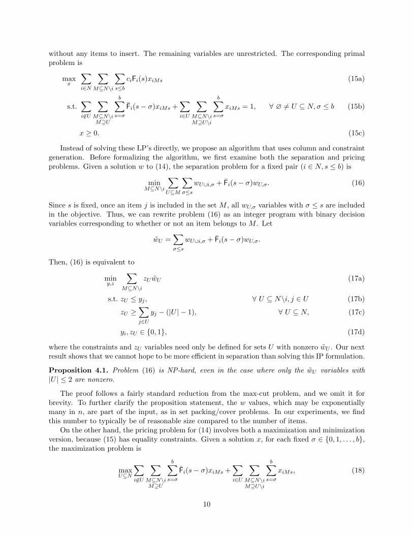
Figures 4 through 7 record the distributions of the set sizes |U | of all generated wU,σ variablesat the end of the algorithm. Recalling that the 10-item instances actually solve to (numerical)optimality, Figures 4 and 5 provide insight into which set cardinalities are more prevalent in theoptimal solution. In particular, we observe a noticeable difference in the set size distributionsbetween the Bernoulli instances (D1, D3, D4, D5) and non-Bernoulli instances (D2, D6, D7). Theplot for Bernoulli instances is more skewed to the right and has a mode of two items, which furtherexplains why the Quadratic relaxation (4) (which includes all singleton and pair item sets) wasthe best-performing approximation in earlier experiments for these instance types [6]. However,the plot for non-Bernoulli instances seems to become more normally distributed as the instance’svariance decreases: D2 is centered around set sizes of 3 and 4, D6 centered around set sizes 4 and 5,

19

Figure 4: 10 Items: wU,σ Set Size Frequencies, Bernoulli

and D7 centered around set size 5. This suggests that, at optimality, less extreme instances favorvariables that correspond to larger item set sizes, because individual items have a relatively smallerimpact, as opposed to in the more extreme Bernoulli instances.

The set sizes for 20- and 30-item instances did not exhibit a noticeable difference between theBernoulli and non-Bernoulli distributions and are thus each presented as a single summary plot.As these instances did not finish at optimality, their plots speak more to the initially generatedcolumns and can provide some insight into better starting bounds. Keeping in mind that the startingapproximation already includes all singleton set variables (which explains the disproportionatelylarge second column in the plots), both figures seem to portray a bimodal distribution. The modesare roughly one-sixth and two-thirds the number of items (4 and 13 for 20 items, 5 and 20 for 30items), although separation between modes is more pronounced for the 30-item instances. Suchbehavior suggests that including more variables of such cardinalities would make for a better startingbound. Intuitively, given the information provided by the variables at these modes, one can “fill inthe gaps” and approximate the incremental value to states corresponding to the intermediate setsizes; this can be a more efficient method than beginning with variable set sizes that are uniformlyor normally distributed, for example.

Algorithm 1 provides for a systematic way to further reduce the gap arising from otherwiseefficiently solvable bounds and policies, and it can reduce the gap significantly depending on wherethe largest areas of improvement lie. In essence, our algorithm performs well in the situations wherewe need it to the most; we observe the best progress when the initial bounds and/or heuristic policiesperform the most poorly. It remains a valid alternative to the DP formulation for larger instancesthat still see noticeable gaps from not only a time perspective, but from a space perspective as well;our algorithm typically never required more than 1.5 GB of memory throughout its run, whereasthe DP would require upwards of 15 GB memory for even the smaller 20-item instances.

20

Figure 5: 10 Items: wU,σ Set Size Frequencies, Non-Bernoulli

Figure 6: 20 Items: wU,σ Set Size Frequencies

21

Figure 7: 30 Items: wU,σ Set Size Frequencies

6 Conclusion

We have studied a dynamic version of the knapsack problem with stochastic item sizes. We de-veloped a finitely terminating exact algorithm that solves the dynamic knapsack problem withinnumerical tolerance, under the assumption of integer item sizes and capacity. The algorithm incor-porates a combination of column and constraint generation to iteratively improve a value functionapproximation based on a reformulation of the original dynamic program. We provided theoreticalresults that solve the zero-capacity case in full from both the bound and policy sides, providinginsight towards the general case, and we examined the hardness of subproblems encountered in themore general capacitated case. An extensive computational study points to the types of instancesthat see the greatest relative improvement. In particular, the algorithm significantly closes thegap from the policy side when natural heuristic greedy policies are lacking, while we also observea steady gap closure from the bound side. The bounds derived by the algorithm also performparticularly well when the initial gap is relatively large.

Our results motivate additional questions. The exact algorithm provides theoretical guaranteesfrom the bound side, while the policy side could be investigated further; moreover, more complexalgorithm heuristics may improve computational performance. Other potential future work includesnarrowing down the types of instances where the algorithm works best (such as examining differentdistributions), fine-tuning our heuristics (such as smarter or more complex column generation)for faster progress, and improving certain theoretical guarantees (such as establishing whetherthe pricing problem is NP-complete). As we do assume integer support in our analysis, it isalso of interest to explore how we can develop an algorithm for continuous distributions, akin tothe exact algorithm presented in [2] for the generalized joint replenishment problem, which hascontinuous state and action spaces. Finally, in an even more general sense, the knapsack problemis fundamental to the development of linear and integer programming. In a similar vein, it wouldbe of interest to consider whether our methods — including value function approximations anda systematic algorithm — can be applied to other combinatorial optimization problems underuncertainty, e.g., the multi-row knapsack and other more general packing problems.

22

Acknowledgements

D. Blado’s work was partially supported by an NSF Graduate Research Fellowship Program underGrant No. DGE-1650044. Both authors’ work was partially supported by the National ScienceFoundation via grant CMMI-1552479.

References

[1] D. Adelman, Price-Directed Replenishment of Subsets: Methodology and its Application toInventory Routing, Manufacturing and Service Operations Management 5 (2003), 348–371.

[2] D. Adelman and D. Klabjan, Computing Near-Optimal Policies in Generalized Joint Replen-ishment, INFORMS Journal on Computing 24 (2011), 148–164.

[3] S.R. Balseiro and D.B. Brown, Approximations to stochastic dynamic programs via informationrelaxation duality, Operations Research (2018), Forthcoming.

[4] A. Bhalgat, A. Goel, and S. Khanna, Improved Approximation Results for Stochastic KnapsackProblems, Proceedings of the Twenty-Second Annual ACM-SIAM Symposium on DiscreteAlgorithms, SIAM, 2011, pp. 1647–1665.

[5] D. Blado, W. Hu, and A. Toriello, Semi-Infinite Relaxations for the Dynamic Knapsack Prob-lem with Stochastic Item Sizes, SIAM Journal on Optimization 26 (2016), 1625–1648.

[6] D. Blado and A. Toriello, Relaxation Analysis for the Dynamic Knapsack Problem with Stochas-tic Item Sizes, SIAM Journal on Optimization (2018), Forthcoming.

[7] R.L. Carraway, R.L. Schmidt, and L.R. Weatherford, An algorithm for maximizing targetachievement in the stochastic knapsack problem with normal returns, Naval Research Logistics40 (1993), 161–173.

[8] D.P. de Farias and B. van Roy, The Linear Programming Approach to Approximate DynamicProgramming, Operations Research 51 (2003), 850–865.

[9] B.C. Dean, M.X. Goemans, and J. Vondrak, Approximating the Stochastic Knapsack Prob-lem: The Benefit of Adaptivity, Proceedings of the 45th Annual IEEE Symposium on theFoundations of Computer Science, IEEE, 2004, pp. 208–217.

[10] , Adaptivity and Approximation for Stochastic Packing Problems, Proceedings of theSixteenth Annual ACM-SIAM Symposium on Discrete Algorithms, SIAM, 2005, pp. 395–404.

[11] , Approximating the Stochastic Knapsack Problem: The Benefit of Adaptivity, Mathe-matics of Operations Research 33 (2008), 945–964.

[12] C. Derman, G.J. Lieberman, and S.M. Ross, A Renewal Decision Problem, Management Sci-ence 24 (1978), 554–561.

[13] A. Goel and P. Indyk, Stochastic load balancing and related problems, Proceedings of the 40thAnnual IEEE Symposium on the Foundations of Computer Science, IEEE, 1999, pp. 579–586.

[14] V. Goyal and R. Ravi, A PTAS for Chance-Constrained Knapsack Problem with Random ItemSizes, Operations Research Letters 38 (2010), 161–164.

23

[15] A. Gupta, R. Krishnaswamy, M. Molinaro, and R. Ravi, Approximation Algorithms for Cor-related Knapsacks and Non-Martingale Bandits, Proceedings of the 52nd IEEE Annual Sym-posium on Foundations of Computer Science, IEEE, 2011, pp. 827–836.

[16] M. Henig, Risk criteria in a stochastic knapsack problem, Operations Research 38 (1990),820–825.

[17] T. Ilhan, S.M.R. Iravani, and M.S. Daskin, The Adaptive Knapsack Problem with StochasticRewards, Operations Research 59 (2011), 242–248.

[18] H. Kellerer, U. Pferschy, and D. Pisinger, Knapsack Problems, Springer-Verlag, Berlin, 2004.

[19] J. Kleinberg, Y. Rabani, and E. Tardos, Allocating Bandwidth for Bursty Connections, Pro-ceedings of the Twenty-Ninth Annual ACM Symposium on the Theory of Computing, Asso-ciation for Computing Machinery, 1997, pp. 664–673.

[20] , Allocating Bandwidth for Bursty Connections, SIAM Journal on Computing 30 (2000),191–217.

[21] A. Kleywegt and J.D. Papastavrou, The Dynamic and Stochastic Knapsack Problem, Opera-tions Research 46 (1998), 17–35.

[22] , The Dynamic and Stochastic Knapsack Problem with Random Sized Items, OperationsResearch 49 (2001), 26–41.

[23] W. Ma, Improvements and Generalizations of Stochastic Knapsack and Multi-Armed BanditAlgorithms, Proceedings of the Twenty-Fifth Annual ACM-SIAM Symposium on DiscreteAlgorithms (SODA), SIAM, 2014, pp. 1154–1163.

[24] , Improvements and Generalizations of Stochastic Knapsack and Markovian BanditsApproximation Algorithms, Mathematics of Operations Research (2018), Forthcoming.

[25] S. Martello and P. Toth, Knapsack Problems: Algorithms and Computer Implementations,John Wiley & Sons, Ltd., Chichester, England, 1990.

[26] Y. Merzifonluoglu, J. Geunes, and H.E. Romeijn, The static stochastic knapsack problem withnormally distributed item sizes, Mathematical Programming 134 (2012), 459–489.

[27] H. Morita, H. Ishii, and T. Nishida, Stochastic linear knapsack programming problem and itsapplications to a portfolio selection problem, European Journal of Operational Research 40(1989), 329–336.

[28] J.D. Papastavrou, S. Rajagopalan, and A. Kleywegt, The Dynamic and Stochastic KnapsackProblem with Deadlines, Management Science 42 (1996), 1706–1718.

[29] P.J. Schweitzer and A. Seidmann, Generalized Polynomial Approximations in Markovian De-cision Processes, Journal of Mathematical Analysis and Applications 110 (1985), 568–582.

[30] M. Sniedovich, Preference order stochastic knapsack problems: methodological issues, Journalof the Operational Research Society 31 (1980), 1025–1032.

[31] E. Steinberg and M.S. Parks, A preference order dynamic program for a knapsack problem withstochastic rewards, Journal of the Operational Research Society 30 (1979), 141–147.

[32] M.A. Trick and S.E. Zin, Spline Approximations to Value Functions: A Linear ProgrammingApproach, Macroeconomic Dynamics 1 (1997), 255–277.

24

Appendix

Tables 4 - 6 present the raw data used to calculate the summaries in Tables 1 - 3 of the generalalgorithm’s performance in Section 5. They are separated by the number of items in each instance,recording results for 10, 20, and 30 items. For fairness in comparisons, the Avg. Inner LoopsMetric for 20 and 30 item instances is only recorded for instances that completed 16 algorithmloops. Afterward, Figures 8 - 10 display various parameters of the 30 item instances against therelative remaining gap, while Figures 11 - 16 display various parameters of the 20 and 30 iteminstances against the relative gap closed per loop (RGPL), an alternative metric for the generalalgorithm’s progress.

25

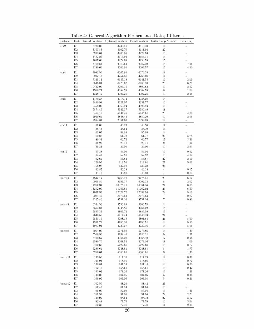
Table 4: General Algorithm Performance Data, 10 ItemsInstance Dist. Initial Solution Optimal Solution Final Solution Outer Loop Number Time (hr)

cor2 D1 3723.00 3239.51 3319.10 14 -D2 3363.83 3102.76 3111.94 22 -D3 3938.67 3403.05 3422.53 13 -D4 4487.25 3615.94 3686.11 14 -D5 4637.60 3872.09 3953.59 15 -D6 3160.84 2980.63 2982.39 15 7.66D7 3180.66 3006.91 3009.57 15 4.90

cor4 D1 7082.50 6065.80 6076.35 18 -D2 5237.13 4754.38 4763.28 14 -D3 7311.11 6637.18 6641.55 16 2.19D4 9545.81 8278.62 8283.10 23 6.79D5 10432.00 8793.15 8800.82 19 2.62D6 4300.21 4082.59 4082.59 8 1.08D7 4328.47 4097.25 4097.25 10 2.96

cor8 D1 4780.38 4013.14 4038.08 15 -D2 3490.98 3227.07 3237.77 16 -D3 5458.00 4569.94 4599.94 16 -D4 5874.46 5143.37 5180.49 18 -D5 6454.19 5444.45 5445.61 23 4.02D6 2949.64 2848.44 2850.20 10 2.06D7 2994.84 2881.66 2899.09 12 -

cor11 D1 51.00 43.23 43.30 17 -D2 36.73 33.64 33.70 14 -D3 62.05 54.88 55.88 14 -D4 70.88 61.72 61.77 20 5.78D5 80.31 66.73 66.77 17 3.36D6 31.29 29.41 29.41 9 1.97D7 31.31 29.06 29.06 10 2.94

cor12 D1 55.38 54.00 54.04 16 0.62D2 54.42 52.31 52.32 10 4.62D3 92.67 86.84 86.87 22 2.19D4 126.55 112.56 112.61 27 9.62D5 156.98 132.59 133.30 24 -D6 43.85 40.38 40.38 4 0.15D7 44.45 43.50 43.50 4 0.13

uncor4 D1 11847.17 9768.71 9775.31 20 6.87D2 10051.80 8997.37 9002.33 8 2.02D3 11287.37 10075.41 10081.86 21 6.03D4 13272.00 11757.85 11762.92 25 6.60D5 14037.35 12022.72 12032.94 24 5.19D6 9294.49 8673.63 8673.63 7 0.87D7 9265.40 8751.16 8751.16 7 0.86

uncor5 D1 6324.50 5550.89 5603.74 14 -D2 5353.84 4945.85 4964.02 18 -D3 6895.33 5803.74 5885.59 15 -D4 7646.50 6114.44 6146.73 21 -D5 6835.15 5798.18 5801.64 21 8.00D6 4991.79 4753.80 4756.51 14 5.83D7 4983.91 4730.27 4732.16 14 5.61

uncor8 D1 6064.00 5271.50 5275.86 14 1.39D2 5506.90 5138.40 5143.21 9 1.51D3 5790.67 4964.20 4965.40 17 0.96D4 5580.70 5068.55 5073.16 18 1.09D5 5702.60 5222.68 5222.68 15 0.77D6 5286.64 5048.81 5048.81 8 1.77D7 5286.61 5060.61 5060.61 8 1.33

uncor11 D1 119.50 117.10 117.19 12 0.32D2 125.91 118.56 118.66 7 0.72D3 149.81 141.35 141.44 13 0.50D4 172.16 158.61 158.61 13 0.42D5 193.02 171.26 171.26 19 1.21D6 113.00 104.25 104.25 5 0.36D7 106.96 103.00 103.01 5 0.36

uncor12 D1 102.50 88.20 88.42 21 -D2 87.43 81.24 81.64 13 -D3 91.00 82.99 83.04 15 1.21D4 101.94 91.00 91.08 29 2.74D5 110.97 98.64 98.72 27 3.12D6 82.48 77.75 77.79 10 3.64D7 82.30 77.78 77.78 11 2.95

26

Table 5: General Algorithm Performance Data, 20 ItemsInstance Dist. Initial Solution Optimal Solution Final Solution Outer Loop Number Avg. Inner Loops

cor2 D1 8215.50 7704.78 8211.96 16 5.19D2 7657.20 7329.29 7595.42 16 29.19D3 8768.33 7835.44 8722.72 13 -D4 9412.00 7980.20 9311.62 12 -D5 10061.76 8268.22 9977.12 12 -D6 7418.50 7145.35 7359.76 13 -D7 7418.50 7216.75 7380.73 13 -

cor4 D1 11434.58 10785.39 11366.11 16 21.19D2 9244.13 8790.56 9053.40 16 19.75D3 14036.33 12668.45 13526.53 16 25.625D4 16348.50 13647.61 13968.59 16 20.06D5 17548.40 15349.62 16018.84 16 14.06D6 8247.44 8040.47 8156.91 15 -D7 8267.12 8044.54 8188.33 15 -

cor8 D1 7970.17 7604.99 7950.86 16 6.25D2 6626.10 6465.55 6613.77 13 -D3 9467.67 8537.54 9282.55 16 32.88D4 11085.75 9468.87 10911.40 12 -D5 12538.87 10233.05 11744.07 16 29.56D6 6151.53 6052.42 6146.51 12 -D7 6149.83 6087.90 6144.60 13 -

cor11 D1 85.58 81.82 85.23 16 14.44D2 69.66 66.62 68.88 16 25.38D3 105.22 95.34 103.99 14 -D4 122.75 102.98 108.24 16 24.63D5 138.80 115.87 122.69 16 20.25D6 61.96 60.41 61.43 16 -D7 62.08 60.73 61.65 13 -

cor12 D1 142.17 132.53 141.31 16 23.94D2 113.41 106.60 111.08 16 23.63D3 179.50 156.37 167.61 16 22.5D4 209.00 174.25 179.37 16 20.44D5 212.00 188.03 198.43 16 12.31D6 99.67 95.79 98.45 16 22.87D7 99.67 95.99 98.96 16 22.44

uncor4 D1 17963.50 15985.06 16790.60 16 24.56D2 16218.73 15209.27 15831.79 16 17.06D3 19616.17 17090.38 18552.01 11 -D4 22192.52 18034.99 19241.36 16 18.56D5 23960.34 18967.29 20016.30 17 14.71D6 15498.38 14725.92 14901.89 16 14.44D7 15540.18 14978.42 15205.11 16 29.06

uncor5 D1 10269.29 9523.34 10245.69 16 32.25D2 9263.30 8841.85 9152.33 16 23.44D3 11529.64 10066.58 11339.29 13 -D4 12793.16 10609.44 11329.72 17 16.76D5 13933.00 11187.66 13933.00 17 20.47D6 8785.79 8508.18 8732.77 12 -D7 8785.79 8518.29 8739.33 15 -

uncor8 D1 11863.00 10938.15 11803.01 16 14.63D2 10965.69 10449.73 10841.14 16 23.31D3 12784.80 11110.73 12337.19 17 26.82D4 13741.64 10785.14 12617.26 16 31.44D5 14302.31 11663.51 12575.21 16 24.13D6 10548.00 10236.26 10512.67 14 -D7 10548.00 10277.66 10524.56 13 -

uncor11 D1 234.10 212.81 226.99 16 29.50D2 208.31 196.32 205.50 16 21.13D3 264.71 223.76 232.97 16 23.88D4 255.50 226.97 233.21 15 -D5 265.80 240.16 251.09 16 13.44D6 195.60 188.69 194.60 15 -D7 195.60 188.91 195.17 16 20.50

uncor12 D1 140.88 127.39 137.98 16 25.94D2 126.42 119.53 124.12 16 22.69D3 157.67 133.50 140.62 14 -D4 162.75 137.88 142.47 16 17.75D5 178.80 147.61 154.71 16 23.13D6 120.63 116.96 118.96 16 17.25D7 120.63 117.80 120.29 13 -

27

Table 6: General Algorithm Performance Data, 30 ItemsInstance Dist. Initial Solution Initial Policy Final Solution Final Policy Outer Loop Number Avg. Inner Loops

cor2 D1 11548.00 10608.19 11496.75 10608.19 16 5.44D2 10781.65 10460.06 10780.70 10460.06 11 -D3 12271.00 10821.49 12168.77 10821.49 15 -D4 13030.32 11194.17 12798.68 11194.17 16 9.87D5 13889.80 11387.92 13747.20 11387.92 16 9.06D6 10561.00 10320.98 10530.01 10320.98 16 17.40D7 10561.00 10317.01 10535.75 10317.01 13 22.75

cor4 D1 15557.00 13867.66 15546.03 14536.94 16 6.75D2 13301.63 12750.54 13278.03 12750.54 10 -D3 18364.25 14760.25 18251.80 16601.37 11 -D4 21442.94 15223.04 21242.73 18273.65 12 -D5 24914.60 15873.04 24549.34 21081.60 15 -D6 12304.55 11818.96 12279.25 11818.96 12 -D7 12332.46 11823.52 12330.79 11946.38 13 -

cor8 D1 11161.75 10101.19 11142.07 10649.72 16 7.07D2 9887.71 9618.24 9873.14 9618.24 11 -D3 12590.24 10681.37 12545.94 10750.26 16 11.50D4 14315.82 11291.80 14270.31 12190.66 15 -D5 16322.45 11475.97 16263.20 13196.30 14 -D6 9377.13 9186.32 9377.13 9186.32 16 12.93D7 9409.03 9163.83 9409.03 9163.83 15 -

cor11 D1 118.00 99.03 117.56 108.73 16 7.43D2 100.31 93.74 100.20 93.74 10 -D3 138.67 108.04 137.81 128.87 16 8.73D4 161.42 107.92 160.49 142.19 11 -D5 186.40 116.65 184.81 162.08 16 11.92D6 92.03 88.62 91.86 88.62 16 11.75D7 92.08 88.98 92.08 88.98 13 -

cor12 D1 192.17 164.43 191.88 176.89 16 4.13D2 162.31 153.84 162.16 153.84 10 -D3 229.56 171.46 228.11 207.56 15 -D4 271.06 189.09 268.53 239.00 14 -D5 315.87 191.34 312.04 273.81 16 24.31D6 148.72 141.28 148.72 141.28 16 -D7 148.72 144.28 148.72 144.28 16 9.69

uncor4 D1 26996.00 24412.35 26934.06 24412.35 16 11.69D2 25079.52 24063.74 24887.53 24063.74 13 -D3 28936.00 25764.59 28859.75 25764.59 11 -D4 31111.95 25727.13 30344.25 25727.13 14 -D5 33258.40 26871.57 32336.04 26871.57 16 41.75D6 24222.00 23496.94 24023.36 23496.94 15 -D7 24222.00 23591.97 24137.12 23591.97 14 -

uncor5 D1 15052.50 13961.66 15037.04 13961.66 16 8.25D2 14011.55 13569.32 14008.65 13569.32 11 -D3 16214.33 14478.62 16168.78 14478.62 16 8.56D4 17598.14 14791.72 17487.93 14791.72 16 7.56D5 19227.40 15559.64 19050.29 15559.64 16 7.69D6 13569.00 13299.03 13569.00 13299.03 16 10.08D7 13569.00 13210.18 13569.00 13210.18 16 8.47

uncor8 D1 16980.86 15874.49 16954.75 15874.49 16 7.00D2 16087.92 15618.98 16086.59 15618.98 11 -D3 17813.95 15948.73 17746.30 15948.73 16 8.19D4 18870.25 16404.04 18773.62 16404.04 12 -D5 20107.70 16816.02 19925.61 16816.02 13 -D6 15665.86 15418.97 15660.83 15418.97 16 9.56D7 15665.86 15526.89 15665.86 15526.89 16 10.79

uncor11 D1 312.82 278.75 311.66 279.25 16 8.50D2 285.95 273.25 285.79 273.60 12 -D3 341.88 299.86 338.65 299.86 14 -D4 375.50 300.32 361.71 300.32 14 -D5 407.40 311.34 375.07 311.34 15 -D6 273.91 261.64 273.91 266.20 16 12.07D7 273.91 264.26 273.91 264.26 16 9.80

uncor12 D1 205.25 188.36 204.63 188.36 16 20.67D2 189.85 184.47 188.77 184.47 12 -D3 221.58 192.00 219.65 192.00 16 20.13D4 241.25 193.68 232.82 193.68 14 -D5 263.40 206.38 255.17 206.38 16 27.00D6 183.10 176.18 182.58 176.18 13 -D7 183.10 179.43 182.99 180.11 14 -

28

Figure 8: 30 Items - Distribution Variance vs. Relative Remaining Gap

Figure 9: 30 Items - Fill Rate vs. Relative Remaining Gap

29

Figure 10: 30 Items - Initial Gap vs. Relative Remaining Gap

Figure 11: 20 Items - Distribution Variance vs. Relative Gap Closed Per Loop

30

Figure 12: 20 Items - Fill Rate vs. Relative Gap Closed Per Loop

Figure 13: 20 Items - Initial Gap vs. Relative Gap Closed Per Loop

31

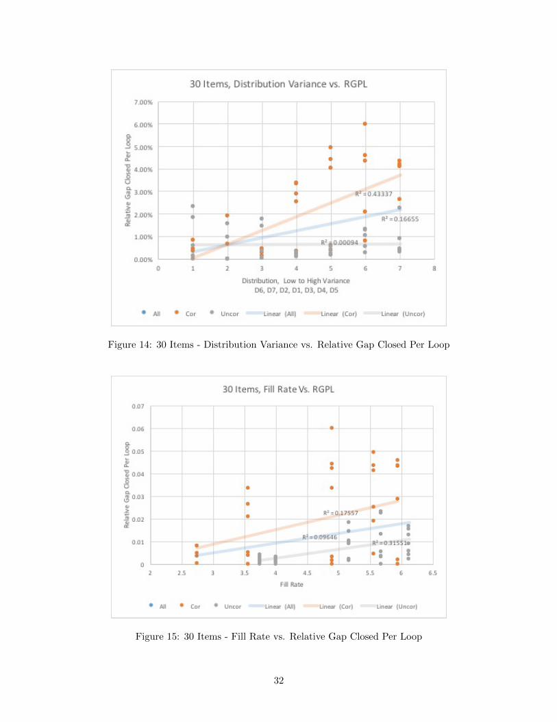
Figure 14: 30 Items - Distribution Variance vs. Relative Gap Closed Per Loop

Figure 15: 30 Items - Fill Rate vs. Relative Gap Closed Per Loop

32

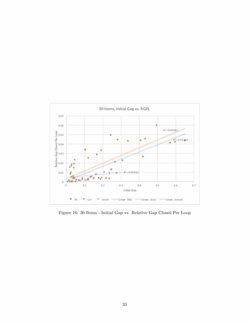
Figure 16: 30 Items - Initial Gap vs. Relative Gap Closed Per Loop

33