A cost-optimal parallel algorithm for the 0–1 knapsack ...lik/publications/Jing-Liu-PC-2015.pdfA cost-optimal parallel algorithm for the 0–1 knapsack problem and its performance

Parallel Computing 43 (2015) 27–42

Contents lists available at ScienceDirect

Parallel Computing

journal homepage: www.elsevier .com/ locate/parco

A cost-optimal parallel algorithm for the 0–1 knapsack problemand its performance on multicore CPU and GPUimplementations

http://dx.doi.org/10.1016/j.parco.2015.01.0040167-8191/� 2015 Elsevier B.V. All rights reserved.

⇑ Corresponding author at: College of Information Science and Engineering, Hunan University, Changsha, Hunan 410082, China.E-mail addresses: [email protected] (K. Li), [email protected] (J. Liu), [email protected] (L. Wan), [email protected] (S. Yin), lik@new

(K. Li).

Kenli Li a,b, Jing Liu a,b,⇑, Lanjun Wan a,b, Shu Yin a,b, Keqin Li a,b,c

a College of Information Science and Engineering, Hunan University, Changsha, Hunan 410082, Chinab National Supercomputing Center in Changsha, Changsha, Hunan 410082, Chinac Department of Computer Science, State University of New York, New Paltz, NY 12561, USA

a r t i c l e i n f o

Article history:Received 6 December 2012Received in revised form 4 January 2015Accepted 23 January 2015Available online 2 February 2015

Keywords:Cost-optimal parallel algorithmEREW PRAMGPUMulticore CPU0–1 knapsack

a b s t r a c t

The 0–1 knapsack problem has been extensively studied in the past years due to its imme-diate applications in industry and financial management, such as cargo loading, stock cut-ting, and budget control. Many algorithms have been proposed to solve this problem, mostof which are heuristic, as the problem is well-known to be NP-hard. Only a few optimalalgorithms have been designed to solve this problem but with high time complexity. Thispaper proposes the cost-optimal parallel algorithm (COPA) on an EREW PRAM model withshared memory to solve this problem. COPA is scalable and yields optimal solutions con-suming less computational time. Furthermore, this paper implements COPA on two scenar-ios – multicore CPU based architectures using Open MP and GPU based configurationsusing CUDA. A series of experiments are conducted to examine the performance of COPAunder two different test platforms. The experimental results show that COPA could reducea significant amount of execution time. Our approach achieves the speedups of up to 10.26on multicore CPU implementations and 17.53 on GPU implementations when the sequen-tial dynamic programming algorithm for KP01 is considered as a baseline. Importantly,GPU implementations outstand themselves in the experimental results.

� 2015 Elsevier B.V. All rights reserved.

1. Introduction

1.1. The problem

Given a set V of n items v1;v2; . . . ;vn to be packed into a knapsack of capacity c, where c is a positive integer, and eachitem v i has a weight wi 2 Zþ and a profit pi 2 Zþ;1 6 i 6 n, the knapsack problem is to choose a subset of items that the totalprofit of the chosen items is maximized and the total weight does not exceed the knapsack capacity c. Let X = (x1; x2; . . . ; xn)be an n-tuple of nonnegative integers. Then the above problem can be mathematically formulated as follows:

maximizeXn

i¼1

pixi; subject toXn

i¼1

wixi 6 c: ð1Þ

paltz.edu

28 K. Li et al. / Parallel Computing 43 (2015) 27–42

To avoid any trivial solution, assume that wi 6 c;8i 2 f1;2; . . . ;ng, andPn

i¼1wi > c.If xi ði ¼ 1;2; . . . ;nÞ is a nonnegative integer, that is, each item has unlimited availability, then Eq. (1) is called the

unbounded knapsack problem (KP). If xi is restricted to be the integer 0 or 1, that is, each item can appear at most oncein an optimal solution, then Eq. (1) is called the 0–1 knapsack problem (KP01), which is a special case of KP. If pi ¼ wi

and xi is restricted to be the integer 0 or 1, then Eq. (1) is called the subset sum problem (SSP), which is a special case ofKP01. For SSP, if it is only required to answer whether there is a solution and the vector X is not required, then the decisionversion of the subset sum problem (SSPd) is obtained, which is a special case of SSP. KP, KP01, SSP, and SSPd were proven tobe NP-hard. In this paper, we mainly focus on KP01.

KP01 has been applied to plentiful applications in theory as well as in practice. For practical applications, KP01 is widelyused in various cryptographic schemes [1] and industrial problems. Many industrial problems can be directly modeled asKP01, such as capital budgeting [2], stock cutting [3], cargo loading [4], and batch processor scheduling [5]. Furthermore,KP01 appears as a sub-problem in set-partitioning formulations for multi-dimensional stock cutting [6], crew scheduling,and generalized assignment problems [7].

1.2. Related work

Many algorithms have been proposed to solve KP. Because KP is NP-hard, the majority of these algorithms are heuristicswhich provide near optimal solutions. Only a few optimal algorithms have been designed to solve KP but with high timecomplexity. Classic optimal approaches to solving KP are largely based on dynamic programming (DP) [8–15] and thetwo-list algorithm [16,17], where the DP based algorithms proposed in [9,11,13,15] are designed specifically for KP01. DPbased algorithms solve KP in pseudo-polynomial time; when the capacity of the knapsack and the number of items are suf-ficiently large, two-list based algorithms outperform DP based algorithms. In this paper, we conduct our work based on thetwo-list algorithm.

By splitting the item set V of n items into two disjoint parts of equal size, Horowitz and Sahni [16] first proposed a new

technique which dramatically reduces the time complexity from Oð2nÞ obtained by brute force to Oð2n=2Þ with space Oð2n=2Þfor SSP. The new technique is known as the two-list algorithm. Also in [16], Horowitz and Sahni used the dynamic program-

ming method with splitting to solve KP01 in Oðminf2n=2;ncgÞ time and space. On the basis of the two-list algorithm, Schroep-

pel and Shamir [17] divided the set V into four parts of the same size, where each part contains 2n=4 possible combinations of

the subset sum, and proposed the two-list four-table algorithm which solves SSP in Oðn2n=2Þ time and Oð2n=4Þ space. The two-list four-table algorithm takes less space but more time to solve KP01 compared with the two-list algorithm. Although manysequential algorithms have been designed to solve SSP in the past years, Horowitz and Sahni’s algorithm still has the leastknown upper bound on the time complexity for this problem [18].

With the advent of parallelism, many parallel algorithms have been devised for solving problems in various areas toreduce the lengthy computation times required by sequential algorithms. The two-list algorithm is the best theoretical algo-rithm for solving KP in sequential models and serves as the starting point for introducing efficient parallel techniques for KP.Karnin [19] proposed a parallel algorithm for SSPd which parallelizes the generation routine of the two-list four-table algo-

rithm [17] on a PRAM (parallel randomly access machine) model. The algorithm can reduce memory space to Oð2n=6Þ by gen-

erating four tables dynamically with Oð2n=6Þ processors, but it cannot degrade the computation time which is still Oðn2n=2Þ.Amirazizi and Hellman [20] first demonstrated that parallelism could accelerate to solve larger instances of SSPd. Allowing

Oð2ð1�aÞn=2Þ processors to access concurrently a list of the same position in shared memory, they proposed a parallel algo-rithm to solve SSPd in Oðn2anÞð0 6 a 6 1=2) time. Enlightened by the parallelization of the two-list algorithm, Ferreira[21] conceived a sequential algorithm referred to as the one-list algorithm for SSPd which is easily parallelizable in contrastwith the two-list algorithm and takes less memory space. The parallelized one-list algorithm can solve SSPd in time

Oðnð2n=2ÞeÞ (0 6 e � 1) with Oðð2n=2Þ

1�eÞ processors. Chang et al. [22] claimed a parallelization of the generation stage of

the two-list algorithm on a CREW (concurrent read and exclusive write) SIMD (single instruction stream and multiple data

streams) PRAM model with shared memory. They proposed a parallel algorithm to solve SSPd in Oð2n=2Þ time with Oð2n=4Þmemory and Oð2n=8Þ processors.

Furthermore, Lou and Chang [23] proposed a novel search stage for the two-list algorithm which is combined with Chang

et al.’s generation stage, giving an optimal parallelization of the two-list algorithm. This parallel algorithm uses Oð2n=4Þmem-

ory and Oð2n=8Þ processors to solve SSPd in Oð23n=8Þ time.Unfortunately, Sanches et al. [24] proved that the time complexity ofthe generation stage of Chang et al.’s is wrong, invalidating both Chang et al.’s and Lou and Chang’s results. The correct com-

putational time is bounded by Oðn2n=2Þ rather than Oð23n=8Þ. Inspired by the work of Lou and Chang, Li et al. [25] parallelizedthe two-list algorithm on an EREW (exclusive read and exclusive write) SIMD machine with shared memory. The parallel algo-

rithm applies Oðð2n=4Þ1�eÞ processors and Oð2n=2Þmemory space to solve SSP in time Oð2n=4ð2n=4Þ

eÞÞ;0 6 e � 1, without mem-

ory conflicts. Based on a CREW PRAM model with shared memory, Sanches et al. [18] suggested a parallel algorithm to solve

SSP in time Oð2n=2=kÞ using k ¼ 2q processors, 0 6 q 6 n=2� 2 log n. This parallel algorithm is an optimal and scalable par-allelization of the two-list algorithm. Chedid [26,27] presented an optimal parallelization of the two-list algorithm for SSP

K. Li et al. / Parallel Computing 43 (2015) 27–42 29

in time Oð23n=8Þwith Oð2n=8Þ processors based on a CREW model. The optimal time-processor cost (i.e. the product of the timecomplexity and the number of processors) of the proposed algorithm is Oð2n=2Þ. Shortly, observing that the search stage ofthe two-list algorithm is closely related to the merge procedure for merging two sorted lists, Chedid [28] presented a second

optimal and scalable parallel two-list algorithm on a CREW PRAM model. The algorithm solved SSP in time Oð2n=2�aÞ usingOð2aÞ processors, for 0 6 a 6 n=2� 2 log nþ 2.

However, since the calculation of the vector X is absent, most of studies above are technically SSPd, which is the decisionversion of the subset sum problem. Furthermore, the parallel techniques which are designed to solve SSP or SSPd cannot beautomatically transplanted to solve KP01. From discussion above, we know that two-list based parallel algorithms can bringgood results for SSP. Inspired by these ideas, we design an efficient two-list based parallel algorithm for KP01.

Several programming models were designed to efficiently implement parallel algorithms, such as MPI (message passinginterface) and OpenMP. MPI is adapted to communication between distributed memory nodes. OpenMP is used for fine-grained parallelism within shared memory nodes. Lin et al. [29] used the MPI + OpenMP hybrid programming model toimplement the 0–1 knapsack algorithm by the MH method, named after Merkle and Hellman. The MH method is a publickey cryptographic algorithm based on trapdoor information, and is one of several public key cryptographic algorithms whichare first designed in the cryptography history.

Recently, GPU (graphics processing unit) computing has been recognized as a powerful way to achieve high performancefor scientific applications with long execution time due to its highly parallel, multithreaded and manycore unit. Indeed, thepeak computational capabilities of modern GPU exceed that of top-of-the-line CPU (central processing unit). NVIDIA intro-duced CUDA (compute unified device architecture) which enabled users to solve many computation intensive or complexproblems on their GPU cards. CUDA technology is based on the SIMT (single instruction and multiple threads) programmingmodel, similar to the SIMD model.

1.3. Our contributions

In this paper, we solve the KP01 problem with the following steps. First, we present a two-list algorithm based sequentialmethod for KP01. Second, combining the sequential algorithm with an optimal parallel merging algorithm, we propose thecost-optimal parallel algorithm (COPA) for KP01 on an EREW PRAM model with shared memory. COPA is composed of fivestages, i.e., a parallel generation stage, the first parallel saving max-value stage, a parallel pruning stage, the second parallel

saving max-value stage, and a parallel search stage. COPA uses Oðð2n=4Þ1�eÞ processors to solve KP01 in Oð2n=4ð2n=4Þ

eÞ time and

Oð2n=2Þ memory space, 0 6 e � 1. There is no memory conflict for COPA when all processors access the shared memorysimultaneously. Third, COPA is implemented on two scenarios– a multicore CPU architecture and a GPU configuration.The CPU architecture is implemented using the OpenMP programming model while the GPU one is via the CUDA model.

The main contributions of this paper are summarized as follows.

� We propose a sequential algorithm for KP01 which is based on the two-list algorithm. This sequential algorithm servesCOPA to be presented later.� We propose a parallel algorithm COPA for KP01 by parallelizing the sequential algorithm on an EREW PRAM model with

shared memory. The time complexity of COPA can be reduced by multiple processors, hence keep the cost in terms of theproduct of the time complexity and the number of processors invariant.� COPA avoids memory conflicts when all processors access the shared memory simultaneously.� COPA is implemented on two popular environments: multicore CPU using OpenMP and GPU with CUDA. The experimen-

tal results indicate good scalability and performance of COPA. The experimental results also show that the GPU imple-mentation outperforms the multicore CPU implementation.

The experimental results indicate that the speedup can be up to 4.35 on the multicore CPU implementation and 7.44 onthe GPU implementation of COPA compared with the implementation of our two-list based sequential algorithm. However,the experimental results show that the speedup can be as great as 10.26 on multicore CPU implementation and 17.56 on GPUimplementation of COPA when the sequential dynamic programming algorithm is regarded as a baseline.

The remainder of this paper is organized as follows. Section 2 presents some backgrounds to be used in this paper. Sec-tion 3 proposes a sequential algorithm which is based on the two-list algorithm for KP01. Section 4 proposes the parallelalgorithm COPA for KP01. Section 5 provides the methodology of the COPA performance analysis and Section 6 presentsthe experimental results and evaluations of COPA. Finally, the paper is concluded in Section 7.

2. Background

Before presenting our proposed algorithms, we first introduce two algorithms. One is the optimal parallel merging algo-rithm on an EREW model proposed by Akl et al. [30], which will be used to merge sorted lists in Section 4. The other is thefamous dynamic programming (DP) algorithm [31] for solving KP01, as one of two baselines of COPA in Section 6.

30 K. Li et al. / Parallel Computing 43 (2015) 27–42

2.1. The optimal parallel merging algorithm on an EREW model

Assume that there are two sorted vectors U ¼ ðu1;u2; . . . ;umÞ and V ¼ ðv1;v2; . . . ; vmÞ, and k processors P1; P2; . . . ; Pk,where 1 6 k 6 2m is a power of 2. According to the merging algorithm, vectors U and V can be merged without memory con-flicts into a new vector of length 2m.

The merging algorithm is described as follows with a slight modification.

Step 1: Use the k processors to partition U and V, in parallel and without memory conflicts, each into k (possibly empty)subvectors ðU1;U2; . . . ;UkÞ and ðV1;V2; . . . ;VkÞ such that

1. Uij j þ Vij j ¼ 2m=k, for 1 6 i 6 k;2. the weights of all elements in Ui and Vi are smaller than those of all elements in Uiþ1 and Viþ1, for 1 6 i 6 k� 1.

Step 2: Use processor Pi to merge Ui and Vi, for 1 6 i 6 k.

Here Step 1 can be efficiently implemented using the selection algorithm presented by Akl et al. [30]. It has been proventhat this parallel merging algorithm can be executed in the EREW PRAM model of parallel computation in time

Oð2m=kþ log k� log 2mÞ. The merging algorithm is therefore optimal for k 6 m=log2m, in view of the trivial XðmÞ lowerbound in merging two vectors of total length 2m.

2.2. The dynamic programming (DP) algorithm for KP01

The DP algorithm [31] for solving KP01 is described as follows. Given a knapsack of capacity c and n items v1;v2; . . . ;vn,where each item v i has a weight wi and a profit pi, the DP algorithm can generate an optimal solution by the following threesteps:

1. Let F½i; x� denote the maximum profit value that can be attained when the total weight is less than or equal to x usingitems up to v i. For 0 6 x 6 c; F½0; x� ¼ 0.

2. For i ¼ 1 to n, compute F½i; x� (x ¼ 0;1;2; . . . ; c) by:

F½i; x� ¼maxfF½i� 1; x�; F½i� 1; x�wi� þ pig; if x P wi;

F½i� 1; x�; if x < wi:

�ð2Þ

3. F½n; c� is the maximum profit satisfying the knapsack capacity c.

The time complexity of the DP algorithm is OðncÞ.Before presenting Section 3, some notations used in this paper are listed in Table 1.

3. A sequential algorithm for KP01

In this section, inspired by Horowitz and Sahni’s work, a sequential algorithm based on the two-list algorithm [16] is pro-posed for KP01. The algorithm can be divided into two stages which depend on the activities performed, i.e., a generation

Table 1Notations used in this paper.

Notation Definition

V the set of all the n itemsV1 a subset of VV2 a subset of V where V1 and V2 are disjoint with equal size and generate VjVij the number of items in set Viði ¼ 1;2Þn the number of items in set VN the number of subsets in set Viði ¼ 1;2Þ;N ¼ 2n=2

A the sorted list in nondecreasing order for V1

B the sorted list in nonincreasing order for V2

ai a subset of V1

bi a subset of V2

c the knapsack capacityp represents the profit dimensionw represents the weight dimensionk the number of available processorswmin represents the smallest weight among all n itemse the number of elements in each block, equal to N=k

K. Li et al. / Parallel Computing 43 (2015) 27–42 31

stage and a search stage. The generation stage is designed to generate two sorted lists. The search stage is designed to find asolution.

3.1. The generation stage

The generation stage is composed of three steps.

1. Divide V into two disjoint parts with the same size: V1 ¼ ðv1;v2; � � � ;vn=2Þ, and V2 ¼ ðvn=2þ1; vn=2þ2; � � � ;vnÞ. That is,jV1j ¼ jV2j;V1 \ V2 ¼ ;, and V1 [ V2 ¼ V , where jV1j and jV2j represent the number of elements in sets V1 and V2,respectively.

2. For any subset ai of all N ¼ 2n=2 subsets of V1, calculate its weight ai:w which is the weight sum of all items in ai and itsprofit ai:p which is the profit sum of all items in ai, sort these N possible triplets ðai; ai:w; ai:pÞ in nondecreasing order ofweight, and then store them as a list A ¼ ½ða1; a1:w; a1:pÞ; ða2; a2:w; a2:pÞ; . . . ; ðaN; aN:w; aN:pÞ�, where w represents theweight dimension and p represents the profit dimension.

3. For any subset bi of all N ¼ 2n=2 subsets of V2, calculate its weight bi:w which is the weight sum of all items in bi and itsprofit bi:p which is the profit sum of all items in bi, sort these N possible triplets ðbi; bi:w; bi:pÞ in nonincreasing order ofweight, and then store them as a list B ¼ ½ðb1; b1:w; b1:pÞ; ðb2; b2:w; b2:pÞ; . . . ; ðbN; bN:w; bN:pÞ�.

3.2. The search stage

The search stage is devised to find a solution for KP01, described as Algorithm 1. The basic idea of Algorithm 1 is first tocompute the current maximum profit value MaxBi of all subsets from bi to bN , and use notation Li to record the index of thesubset from which MaxBi is obtained, 1 6 i 6 N. Second, the solution for KP01 is searched from all the combinations of ele-ments from the two sorted lists A and B (see Fig. 1). The final Bestvalue and X show the solution, where Bestvalue representsthe maximum profit and X is a string consisting of n 0’s and 1’s, revealing which items are selected when the maximum profitBestvalue is obtained. If the ith position of X is 1, then the item v i is selected; otherwise, v i is not selected.

Algorithm 1. The search stage.

Input: two sorted list A and BOutput: the final solution Bestvalue and X1: initialize MaxBN ¼ bN :p, LN ¼ N, Bestvalue ¼ 0, and X1 ¼ ð0;0Þ2: for i ¼ N � 1 to 1 do3: if bi:p > MaxBiþ1 then4: MaxBi ¼ bi:p and Li ¼ i5: else6: MaxBi ¼ MaxBiþ1 and Li ¼ Liþ1

7: end if8:end for9: i ¼ 1 and j ¼ 110: while i � N and j � N do11: if ai:wþ bj:w > c then12: jþþ and continue13: end if14: if ai:pþMaxBj > Bestvalue then15: Bestvalue ¼ ai:pþMaxBj and X1 ¼ ðai; bLj

Þ16: end if17: iþþ18: end while19: convert two decimal components of X1 to two binary numbers, X1 ¼ ðbinary1; binary2Þ20: X = strcatðbinary1; binary2Þ /*concatenate two binaries by strcat()*/

It is clear that the time complexity of Algorithm 1 is OðNÞ.

3.3. The complete sequential algorithm

In summary, the sequential algorithm mainly consists of the following three steps.

� Step 1: divide V into two disjoint parts of the same size: V1 and V2, and then calculate the weight and profit of all subsetsof V1 and V2.

Fig. 1. The search stage.

32 K. Li et al. / Parallel Computing 43 (2015) 27–42

� Step 2: store all the subsets of V1 (V2, respectively) together with their weights and profits in nondecreasing (nonincreas-ing, respectively) order of weight as a list A (B, respectively).� Step 3: serially search the optimal solution from all the combinations of elements from the two sorted lists A and B.

Steps 1 and 2 are performed through merging, and the time complexity is OðNÞ. Let us explain how to generate the sortedlist A. First, the sorted list A and a variable IC are initialized to A0 ¼ ½ð0;0;0Þ� and IC ¼ 1, respectively. Second, let v1 ¼ IC and

the triple ðv1;v1:w;v1:pÞ is added to each element of list A0, constructing a new list A10 ¼ ½ð0þ v1;0þ v1:w; 0þ v1:pÞ� ¼

½ðIC;v1:w;v1:pÞ� ¼ ½ð1;v1:w;v1:pÞ�. Third, lists A0 and A10 are merged to generate a sorted list A1 which has 2 elements in non-

decreasing order of weight in linear time, and IC is increased by 1. Forth, let v2 ¼ IC and the triple ðv2;v2:w; v2:pÞ is added to

the list A1, resulting in a new sorted list A11. Again, the merging of lists A1 and A1

1 is performed to produce a new sorted list A2

with 4 elements, and IC is increased by 1. Repeat the process above until all the triples corresponding to all the items in V1

are performed. After processing the last triple ðvn=2;vn=2:w;vn=2:pÞ, we obtain the final sorted list An=2, that is, the sorted list A.The generation of list B is the same as that of list A except that all the elements in B are sorted in nonincreasing order of

weight. Hence, the total running time of Steps 1 and 2 isP

16i6n=2Oð2iÞ ¼ OðNÞ.Step 3 is described as Algorithm 1 and its running time is OðNÞ. Summarizing all the times spent by these three steps, the

time complexity of the sequential algorithm is OðNÞ, that is, Oð2n=2Þ.

4. The cost-optimal parallel algorithm (COPA)

In this section, we present a novel parallel algorithm COPA for solving KP01 on an EREW PRAM model with shared mem-ory. COPA aims at parallelizing the sequential algorithm described in Section 3 with low time complexity and high perfor-mance. Assume that k processors are available. We first discuss COPA for k ¼ OðN1=2Þ. In this case, COPA contains five stages:a parallel generation stage, the first parallel saving max-value stage, a parallel pruning stage, the second parallel saving max-value stage, and a parallel search stage. These five stages are depicted in detail in the following.

4.1. The parallel generation stage

In this section, we describe the generation of two sorted lists A and B. A is sorted in nondecreasing order of weight while Bis sorted in nonincreasing order of weight. Since A and B are sorted in reverse directions, their generation procedures arealmost the same, and we only introduce the procedure of generating the nondecreasing list A. In the generation procedure,the optimal parallel merging algorithm presented in Section 2 is applied to merge two lists.

Let us trace the last step of generating list A (i.e., An=2). Suppose that the sorted list An=2�1 has been generated, written asAn=2�1 ¼ ½ðan=2�1:1; an=2�1:1:w; an=2�1:1:pÞ; ðan=2�1:2; an=2�1:2:w; an=2�1:2:pÞ; . . . ; ðan=2�1:N=2; an=2�1:N=2:w; an=2�1:N=2:pÞ�. List An=2�1 has N=2elements, each of which is a triple and stored in the shared memory. We use k processors in parallel to add the triple

ðvn=2;vn=2:w;vn=2:pÞ into each element of An=2�1, attaining a new sorted list A1n=2�1 ¼ ½ðan=2�1:1 þ vn=2; an=2�1:1:wþ

vn=2:w; an=2�1:1:p þ vn=2:pÞ; ðan=2�1:2 þ vn=2; an=2�1:2:w þ vn=2:w; an=2�1:2:p þ vn=2:pÞ; . . . ; ðan=2�1:N=2 þ vn=2; an=2�1:N=2:w þ vn=2:w;an=2�1:N=2:pþ vn=2:pÞ�. The concurrent read is not permitted, so it is necessary to create a copy of (vn=2;vn=2:w; vn=2:p) for each

processor before merging, which incurs OðnN1=2Þ assistant memory cells in the shared memory. Then the optimal parallel

merging algorithm is applied to merge lists An=2�1 and A1n=2�1, which produces the sorted list An=2 (i.e., A).

No memory conflicts occur during the entire process of generating A by applying the optimal parallel merging algorithm.Considering that the time for merging is OðN=kþ log k� log N) [30], the time for generating list An=2 from list An=2�1 isOðN=2kþ N=kþ log k� log NÞ ¼ Oð3N=2kþ n2=8Þ.

As shown in Section 3.2,, to generate list An=2, we initialize A0 ¼ ½ð0;0;0Þ� and IC ¼ 1. Next, we add the triple

ðv iþ1;v iþ1:w;v iþ1:pÞ to all the elements in the sorted list Ai sequentially, generating a new sorted list A1i , where

K. Li et al. / Parallel Computing 43 (2015) 27–42 33

v iþ1 ¼ IC ¼ iþ 1 and 0 6 i 6 n=2� 1. Then, we merge lists Ai and A1i to produce the sorted list Aiþ1 which includes 2iþ1 ele-

ments. When generating list Aiþ1, at most 2i processors are required. Since there are OðN1=2Þ (i.e. Oð2n=4Þ) processors, only afraction of them are utilized when generating lists A1;A2; . . . ;An=4�1 and An=4. Whereas, all the processors must be used whengenerating lists An=4þ1;An=4þ2; . . . ;An=2�1 and An=2.

The parallel generation algorithm for generating the nondecreasing sorted list A is shown as Algorithm 2. Its basic idea isanalogous to that of the generation phase of [18], but with a slight modification.

Algorithm 2. The parallel generation algorithm.

Input: ðv i;v i:w;v i:pÞ, i ¼ 1;2; :::; n=2Output: the sorted list An=2 (i.e. A)1: initialize A0 ¼ ½ð0;0;0Þ� and IC ¼ 12: for i ¼ 0 to n=2� 1 do3: v iþ1 ¼ IC4: for all Pj, 1 � j � k, in parallel do

5: produce new list A1i by adding the triple ðv iþ1;v iþ1:w;v iþ1:pÞ to all the elements in the sorted list Ai

6: call the optimal parallel merging algorithm introduced in Section 2 to merge lists Ai and A1i in nondecreasing

order of weight, producing the sorted list Aiþ1

7: end for8: IC þþ9: end for

4.2. The first parallel saving max-value stage

In this stage, both lists A and B are evenly partitioned into k blocks. For each block, the maximum profit among all ele-ments in the block is identified.

Denote the k blocks of list A to be A1;A2; . . .Ak. Because list A contains N elements, each block contains e ¼ N=k elements.Let Ai ¼ ðai:1; ai:2; . . . ; ai:eÞ;1 6 i 6 k. Each element ai:r in Ai represents a triple (ai:r ; ai:r :w; ai:r:p), where ai:r :w and ai:r :p representthe weight and profit of the set ai:r , respectively, 1 6 i 6 k;1 6 r 6 e. All the elements in Ai are sorted in nondecreasing orderof weight. The weight of any element in Ai is not larger than that of any element in Aiþ1;1 6 i 6 n=2� 1. Then, list A can berepresented as A ¼ ðA1;A2; � � � ;Ai; . . . ;AkÞ. Likewise, list B can be represented as B ¼ ðB1;B2; . . . ;Bj; � � � ;BkÞ, where

Bj ¼ ðbj:1; bj:2; . . . ; bj:eÞ;1 6 j 6 k. The blocks of B and all the elements in each block are both sorted in nonincreasing order

of weight. After partitioning, blocks Ai and Bi are assigned to processor Pi;1 6 i 6 k. Then, the maximum profits of blocksAi and Bi are found, and denoted by MaxAi and MaxBi, respectively. MaxAi are stored in an array MaxA, and MaxBi are storedin an array MaxB. The first parallel saving max-value algorithm shown as Algorithm 3 addresses how to obtain the maximumprofit of each block.

Algorithm 3. The first parallel saving max-value algorithm.

Input: two sorted lists A and BOutput: MaxA and MaxB1: divide both A and B evenly into k blocks2: for all Pi, 1 � i � k, in parallel do

3: MaxAi ¼ ai:1:p, MaxBi ¼ bi:1:p4: for j ¼ 2 to e do5: if ai:j:p > MaxAi then6: MaxAi ¼ ai:j:p7: end if

8: if bi:j:p > MaxBi then

9: MaxBi ¼ bi:j:p10: end if11: end for12: end for

It is observed that the time complexity of Algorithm 3 is OðN1=2Þ.

34 K. Li et al. / Parallel Computing 43 (2015) 27–42

4.3. The parallel pruning stage

This stage attempts to shrink the search space of KP01 in order to reduce the search time of each processor.Before presenting the parallel pruning stage, we introduce two lemmas, which are based on the work of Lou and Chang

[23]. Since the proofs of our lemmas are similar to those of Lemmas 1 and 2 in [23], we do not repeat the proof procedures inthis paper. Each element of any block is simply a weight in [23], whereas each element of any block is a triple (the set, theweight, the profit) in this paper, 1 6 i; j 6 k.

Lemma 1. For any block pair ðAi;BjÞ;1 6 i; j 6 k;Ai ¼ ðai:1; ai:2; . . . ; ai:eÞ and Bj ¼ ðbj:1; bj:2; . . . ; bj:eÞ, if ai:1:wþ bj:e:w > c, then any

element pair (ai:r; bj:s), where ai:r 2 Ai; bj:s 2 Bj, is not a solution of KP01.

Lemma 2. For any block pair ðAi; BjÞ;1 6 i; j 6 k;Ai ¼ ðai:1; ai:2; . . . ; ai:eÞ and Bj ¼ ðbj:1; bj:2; . . . ; bj:eÞ, if ai:e:wþ bj:1:w 6 c, then any

element pair (ai:r; bj:s), where ai:r 2 Ai; bj:s 2 Bj, is a candidate solution for KP01.Based on Lemmas 1 and 2, we design the parallel pruning algorithm, which can greatly shrink the search space of each

processor. For the case of Lemma 1, because any element pair (ai:r ; bj:s) of block pair (Ai;Bj) is not a solution of KP01, we prune

(Ai;Bj). For the case of Lemma 2, because any element pair (ai:r; bj:s) of block pair (Ai;Bj) is a candidate solution for KP01, we

save the maximum profit of (Ai;Bj), namely, the sum of MaxAi and MaxBj and then prune (Ai;Bj). After pruning the blocks inthese two cases, the remaining blocks are written into different cells in the shared memory. Denote Maxvaluei as the max-imum profit value of block pair ðAi;BjmodkÞ. The parallel pruning algorithm can be described as Algorithm 4.

Algorithm 4. The parallel pruning algorithm.

Input: blocks A1, A2, ::: Ak and B1, B2, ::: Bk

Output: the remaining block pairs after pruning1: for all Pi, 1 � i � k, in parallel2: Maxvaluei ¼ 0 do3: for j ¼ i to kþ i� 1

4: Z ¼ ai:1:wþ bjmodk:e:w

5: Y ¼ ai:e:wþ bjmodk:1:w6: if Y � c then7: if MaxAi þMaxBjmodk > Maxvaluei then8: Maxvaluei ¼ MaxAi þMaxBjmodk

9: end if10: prune block pair ðAi, BjmodkÞ11: els if Z � c and Y > c then12: write block pair (Ai;Bjmodk) into different cell in the shared memory13: els if Z > c then14: prune block pair ðAi, BjmodkÞ15: end if16: end for17:end for

In Algorithm 4, each memory cell of list B is read or written by at most one processor at any time. Hence, there are nomemory conflicts in the shared memory. Thus, Algorithm 4 can be executed on the EREW PRAM model. Because each pro-cessor prunes its individual search space, it is obvious that the time complexity of Algorithm 4 is OðkÞ, i.e., Oð2n=4Þ. Before

pruning, the number of block pairs is k2. After pruning, the number of block pairs is at most 2k� 1. Based on Theorem 2in the work of Lou and Chang [23], the following theorem is to show that the number of the residual block pairs is at most2k-1.

Theorem 1. The parallel pruning algorithm picks at most 2k� 1 block pairs.

Proof. After the parallel pruning algorithm is performed, the blocks that processor Pi picks from list B are adjacent one byone according to [23]. Assume that processor Pi picks block pairs (Ai;Bj), (Ai;Bjþ1Þ; . . . ; ðAi;Bl�1), and (Ai; Bl) as shown in Fig. 2.

That is, all of the combinations of Ai and {Bj;Bjþ1; . . . ;Bl�1;Bl} must be checked later to find a solution.

K. Li et al. / Parallel Computing 43 (2015) 27–42 35

Denote BSi ¼ fBj;Bjþ1; . . . ;Bl�1;Blg. From Algorithm 4 and Fig. 2, we know that ai:e:wþ bt:1:w > c, where j 6 t 6 l. Since

ai:e:w < aiþ1:1:w and bt:1:w < bt�1:e:w, then aiþ1:1:wþ bt�1:e:w > c. Therefore, processor piþ1 prunes Bt�1, and BSi \ BSiþ1 ¼ U or{Bl}, 1 6 i < k� 1. Thus, sets BSi and BSiþ1 have at most one common block.

Let BSij j ¼ ai, where ai ð1 6 i 6 kÞ is a nonnegative integer and represents the number of blocks in BSi. The followinginequation is obtained:

a1 þ ða2 � 1Þ þ ða3 � 1Þ þ � � � þ ðak � 1Þ 6 k: ð3Þ

It follows that

a1 þ a2 þ a3 þ � � � þ ak 6 kþ ðk� 1Þ ¼ 2k� 1: ð4Þ

Therefore, Theorem 1 is true. h

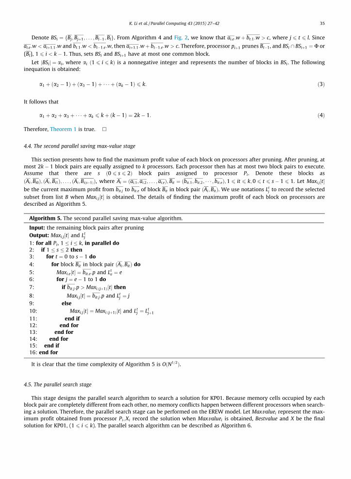
4.4. The second parallel saving max-value stage

This section presents how to find the maximum profit value of each block on processors after pruning. After pruning, atmost 2k� 1 block pairs are equally assigned to k processors. Each processor then has at most two block pairs to execute.Assume that there are s ð0 6 s 6 2Þ block pairs assigned to processor Pi. Denote these blocks as

ðAi;Bi0Þ; ðAi;Bi1Þ; . . . ; ðAi;Biðs�1ÞÞ, where Ai ¼ ðai:1; ai:2; . . . ; ai:eÞ;Bit ¼ ðbit:1; bit:2; � � � ; bit:eÞ;1 6 it 6 k;0 6 t 6 s� 1 6 1. Let Maxi:j½t�be the current maximum profit from bit:j to bit:e of block Bit in block pair ðAi;BitÞ. We use notations Lt

j to record the selectedsubset from list B when Maxi:j½t� is obtained. The details of finding the maximum profit of each block on processors aredescribed as Algorithm 5.

Algorithm 5. The second parallel saving max-value algorithm.

Input: the remaining block pairs after pruningOutput: Maxi:j½t� and Lt

j

1: for all Pi, 1 � i � k, in parallel do2: if 1 � s � 2 then3: for t ¼ 0 to s� 1 do4: for block Bit in block pair ðAi;BitÞ do

5: Maxi:e½t� ¼ bit:e:p and Lte ¼ e

6: for j ¼ e� 1 to 1 do

7: if bit:j:p > Maxi:ðjþ1Þ½t� then

8: Maxi:j½t� ¼ bit:j:p and Ltj ¼ j

9: else10: Maxi:j½t� ¼ Maxi:ðjþ1Þ½t� and Lt

j ¼ Ltjþ1

11: end if12: end for13: end for14: end for15: end if16: end for

It is clear that the time complexity of Algorithm 5 is OðN1=2Þ.

4.5. The parallel search stage

This stage designs the parallel search algorithm to search a solution for KP01. Because memory cells occupied by eachblock pair are completely different from each other, no memory conflicts happen between different processors when search-ing a solution. Therefore, the parallel search stage can be performed on the EREW model. Let Maxvaluei represent the max-imum profit obtained from processor Pi;Xi record the solution when Maxvaluei is obtained, Bestvalue and X be the finalsolution for KP01, (1 6 i 6 k). The parallel search algorithm can be described as Algorithm 6.

36 K. Li et al. / Parallel Computing 43 (2015) 27–42

Algorithm 6. The parallel search algorithm.

Input: the remaining block pairs after pruningOutput: the final solution Bestvalue and X1: for all Pi, 1 � i � k, in parallel do2: initialize t ¼ 0;Maxvaluei ¼ 0, and Xi ¼ ð0;0Þ3: while 0 � t � s� 1 do4: pick out block pair ðAi;BitÞ5: x ¼ 1 and y ¼ 16: while x � e and y � e do

7: if ai:x:wþ bit:y:w > c then8: yþþ and continue9: end if10: if ai:x:pþMaxi:y½t� > Maxvaluei then

11: Maxvaluei ¼ ai:x:pþMaxi:y½t� and Xi ¼ ðai:x; bit:LtyÞ

12: end if13: xþþ14: end while15: t þþ16: end while17: end for18: Bestvalue ¼ Maxvalue1 and X1 ¼ X1

19: for i ¼ 2 to k do20: if Bestvalue < Maxvaluei then21: Bestvalue ¼ Maxvaluei and X1 ¼ Xi

22: end if23: end for24: convert two decimal components of X1 to two binary numbers, X1 ¼ ðbinary1; binary2Þ25: X = strcatðbinary1; binary2Þ /*concatenate two binaries by strcat()*/

It is evident that the parallel search algorithm can be performed on the EREW in time OðN1=2Þ.

4.6. k < OðN1=2Þ

In this section, we extend the results stated for the case k ¼ OðN1=2Þ to the case k < OðN1=2Þ. The processes of finding solu-tions for KP01 in these two cases are almost the same. The process of finding solutions for k < OðN1=2Þ can also be divided

Fig. 2. The search space for processor Pi .

K. Li et al. / Parallel Computing 43 (2015) 27–42 37

into five stages: the parallel generation stage, the first parallel saving max-value stage, the parallel pruning stage, the secondparallel saving max-value stage, and the parallel search stage. The only difference is that the time complexities of these fivestages are changed, due to reduced available processors. Therefore, COPA can solve KP01 for both cases of k with differenttime complexities. The time complexity of COPA under these two cases is presented in detail in the following section.

5. Theoretical performance evaluation of COPA

This section presents the theoretical performance analysis of COPA and compares it with other widely discussed parallelalgorithms for solving KP01. We assume that there are k available processors and each instance of KP01 contains n items.

5.1. Performance analysis

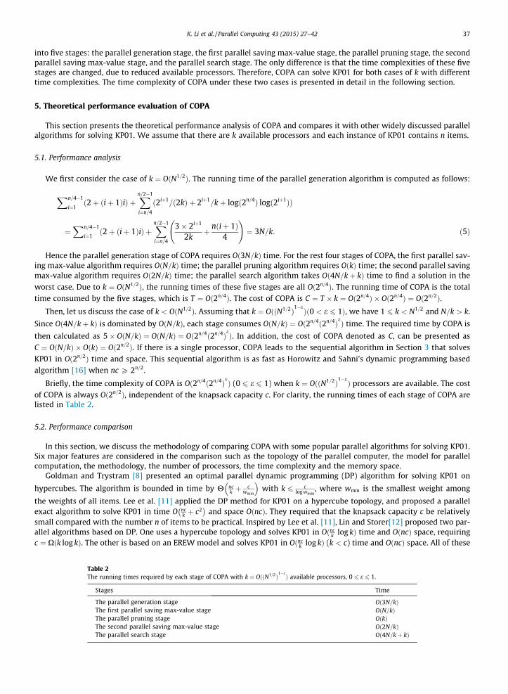
We first consider the case of k ¼ OðN1=2Þ. The running time of the parallel generation algorithm is computed as follows:

Xn=4�1

i¼1ð2þ ðiþ 1ÞiÞ þ

Xn=2�1

i¼n=4

ð2iþ1=ð2kÞ þ 2iþ1=kþ logð2n=4Þ logð2iþ1ÞÞ

¼Xn=4�1

i¼1ð2þ ðiþ 1ÞiÞ þ

Xn=2�1

i¼n=4

3� 2iþ1

2kþ nðiþ 1Þ

4

!¼ 3N=k: ð5Þ

Hence the parallel generation stage of COPA requires Oð3N=kÞ time. For the rest four stages of COPA, the first parallel sav-ing max-value algorithm requires OðN=kÞ time; the parallel pruning algorithm requires OðkÞ time; the second parallel savingmax-value algorithm requires Oð2N=kÞ time; the parallel search algorithm takes Oð4N=kþ kÞ time to find a solution in the

worst case. Due to k ¼ OðN1=2Þ, the running times of these five stages are all Oð2n=4Þ. The running time of COPA is the total

time consumed by the five stages, which is T ¼ Oð2n=4Þ. The cost of COPA is C ¼ T � k ¼ Oð2n=4Þ � Oð2n=4Þ ¼ Oð2n=2Þ.Then, let us discuss the case of k < OðN1=2Þ. Assuming that k ¼ OððN1=2Þ1�eÞð0 < e 6 1Þ, we have 1 6 k < N1=2 and N=k > k.

Since Oð4N=kþ kÞ is dominated by OðN=kÞ, each stage consumes OðN=kÞ ¼ Oð2n=4ð2n=4ÞeÞ time. The required time by COPA is

then calculated as 5� OðN=kÞ ¼ OðN=kÞ ¼ Oð2n=4ð2n=4ÞeÞ. In addition, the cost of COPA denoted as C, can be presented as

C ¼ OðN=kÞ � OðkÞ ¼ Oð2n=2Þ. If there is a single processor, COPA leads to the sequential algorithm in Section 3 that solves

KP01 in Oð2n=2Þ time and space. This sequential algorithm is as fast as Horowitz and Sahni’s dynamic programming basedalgorithm [16] when nc P 2n=2.

Briefly, the time complexity of COPA is Oð2n=4ð2n=4ÞeÞ (0 6 e 6 1) when k ¼ OððN1=2Þ1�eÞ processors are available. The cost

of COPA is always Oð2n=2Þ, independent of the knapsack capacity c. For clarity, the running times of each stage of COPA arelisted in Table 2.

5.2. Performance comparison

In this section, we discuss the methodology of comparing COPA with some popular parallel algorithms for solving KP01.Six major features are considered in the comparison such as the topology of the parallel computer, the model for parallelcomputation, the methodology, the number of processors, the time complexity and the memory space.

Goldman and Trystram [8] presented an optimal parallel dynamic programming (DP) algorithm for solving KP01 on

hypercubes. The algorithm is bounded in time by H nck þ c

wmin

� �with k 6 c

log wmin, where wmin is the smallest weight among

the weights of all items. Lee et al. [11] applied the DP method for KP01 on a hypercube topology, and proposed a parallelexact algorithm to solve KP01 in time O nc

k þ c2� �

and space OðncÞ. They required that the knapsack capacity c be relativelysmall compared with the number n of items to be practical. Inspired by Lee et al. [11], Lin and Storer[12] proposed two par-allel algorithms based on DP. One uses a hypercube topology and solves KP01 in Oðnc

k log kÞ time and OðncÞ space, requiringc ¼ Xðk log kÞ. The other is based on an EREW model and solves KP01 in Oðnc

k log kÞ (k < c) time and OðncÞ space. All of these

Table 2The running times required by each stage of COPA with k ¼ OððN1=2Þ

1�eÞ available processors, 0 6 e 6 1.

Stages Time

The parallel generation stage Oð3N=kÞThe first parallel saving max-value stage OðN=kÞThe parallel pruning stage OðkÞThe second parallel saving max-value stage Oð2N=kÞThe parallel search stage Oð4N=kþ kÞ

38 K. Li et al. / Parallel Computing 43 (2015) 27–42

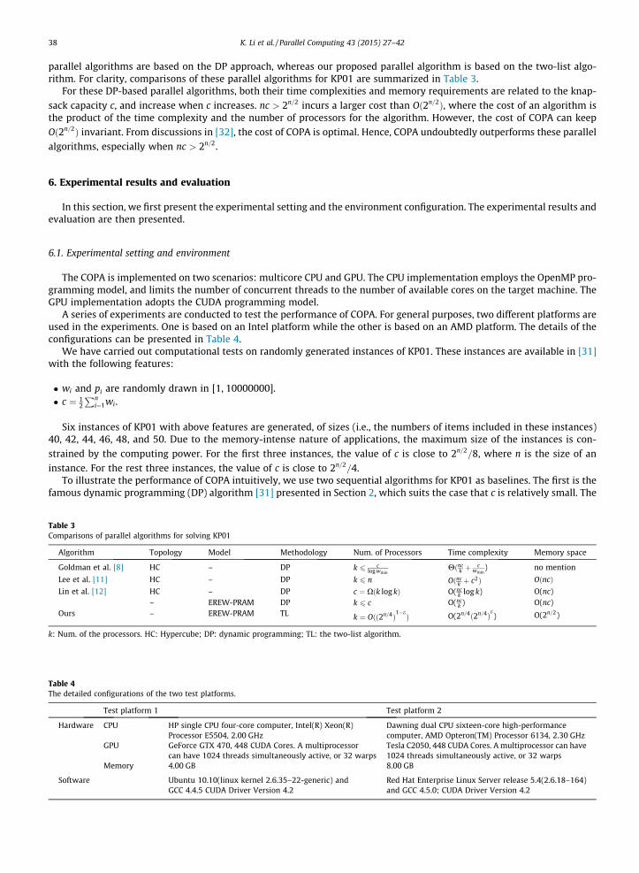
parallel algorithms are based on the DP approach, whereas our proposed parallel algorithm is based on the two-list algo-rithm. For clarity, comparisons of these parallel algorithms for KP01 are summarized in Table 3.

For these DP-based parallel algorithms, both their time complexities and memory requirements are related to the knap-

sack capacity c, and increase when c increases. nc > 2n=2 incurs a larger cost than Oð2n=2Þ, where the cost of an algorithm isthe product of the time complexity and the number of processors for the algorithm. However, the cost of COPA can keepOð2n=2Þ invariant. From discussions in [32], the cost of COPA is optimal. Hence, COPA undoubtedly outperforms these parallel

algorithms, especially when nc > 2n=2.

6. Experimental results and evaluation

In this section, we first present the experimental setting and the environment configuration. The experimental results andevaluation are then presented.

6.1. Experimental setting and environment

The COPA is implemented on two scenarios: multicore CPU and GPU. The CPU implementation employs the OpenMP pro-gramming model, and limits the number of concurrent threads to the number of available cores on the target machine. TheGPU implementation adopts the CUDA programming model.

A series of experiments are conducted to test the performance of COPA. For general purposes, two different platforms areused in the experiments. One is based on an Intel platform while the other is based on an AMD platform. The details of theconfigurations can be presented in Table 4.

We have carried out computational tests on randomly generated instances of KP01. These instances are available in [31]with the following features:

� wi and pi are randomly drawn in [1, 10000000].� c ¼ 1

2

Pni¼1wi.

Six instances of KP01 with above features are generated, of sizes (i.e., the numbers of items included in these instances)40, 42, 44, 46, 48, and 50. Due to the memory-intense nature of applications, the maximum size of the instances is con-

strained by the computing power. For the first three instances, the value of c is close to 2n=2=8, where n is the size of an

instance. For the rest three instances, the value of c is close to 2n=2=4.To illustrate the performance of COPA intuitively, we use two sequential algorithms for KP01 as baselines. The first is the

famous dynamic programming (DP) algorithm [31] presented in Section 2, which suits the case that c is relatively small. The

Table 4The detailed configurations of the two test platforms.

Test platform 1 Test platform 2

Hardware CPU HP single CPU four-core computer, Intel(R) Xeon(R)Processor E5504, 2.00 GHz

Dawning dual CPU sixteen-core high-performancecomputer, AMD Opteron(TM) Processor 6134, 2.30 GHz

GPU GeForce GTX 470, 448 CUDA Cores. A multiprocessorcan have 1024 threads simultaneously active, or 32 warps

Tesla C2050, 448 CUDA Cores. A multiprocessor can have1024 threads simultaneously active, or 32 warps

Memory 4.00 GB 8.00 GB

Software Ubuntu 10.10(linux kernel 2.6.35–22-generic) andGCC 4.4.5 CUDA Driver Version 4.2

Red Hat Enterprise Linux Server release 5.4(2.6.18–164)and GCC 4.5.0; CUDA Driver Version 4.2

Table 3Comparisons of parallel algorithms for solving KP01

Algorithm Topology Model Methodology Num. of Processors Time complexity Memory space

Goldman et al. [8] HC – DP k 6 clog wmin

Hðnck þ

cwmin

) no mention

Lee et al. [11] HC – DP k 6 n Oðnck þ c2Þ OðncÞ

Lin et al. [12] HC – DP c ¼ Xðk log kÞ O(nck log k) O(nc)

– EREW-PRAM DP k 6 c O(nck ) O(nc)

Ours – EREW-PRAM TL k ¼ Oðð2n=4Þ1�eÞ O(2n=4ð2n=4Þ

e) O(2n=2)

k: Num. of the processors. HC: Hypercube; DP: dynamic programming; TL: the two-list algorithm.

K. Li et al. / Parallel Computing 43 (2015) 27–42 39

second is our two-list based sequential algorithm (here we write it as TLS for brevity) proposed in Section 3 with the time

complexity Oð2n=2Þ, which is preferable to the DP algorithm when nc P 2n=2 for KP01.Under test platform 1 and for each instance, we first run the DP algorithm and the TLS algorithm separately on CPU with

only one thread available to obtain two sequential computational times. Second, we run COPA on CPU with only two con-current threads available, obtaining a parallel computational time. Third, we run COPA on CPU with only four concurrentthreads available, obtaining a second parallel computational time. Finally, we run COPA on GPU of GeForce GTX 470 to obtainanother parallel computational time. All these computational times are calculated in milliseconds (ms), each of which is thetotal time consumed by the five stages of COPA. After that, the speedup is computed by Eq. (6) for multicore CPU and GPUimplementations as follows:

Table 5The com

n

404244464850

Sp.: spe

Table 7The spe

n

404244464850

Sp.: Spe

Table 6The com

n

404244464850

DP: dyn

Speedup ¼ sequential computational timeparallel computational time

: ð6Þ

6.2. Experimental results and evaluation

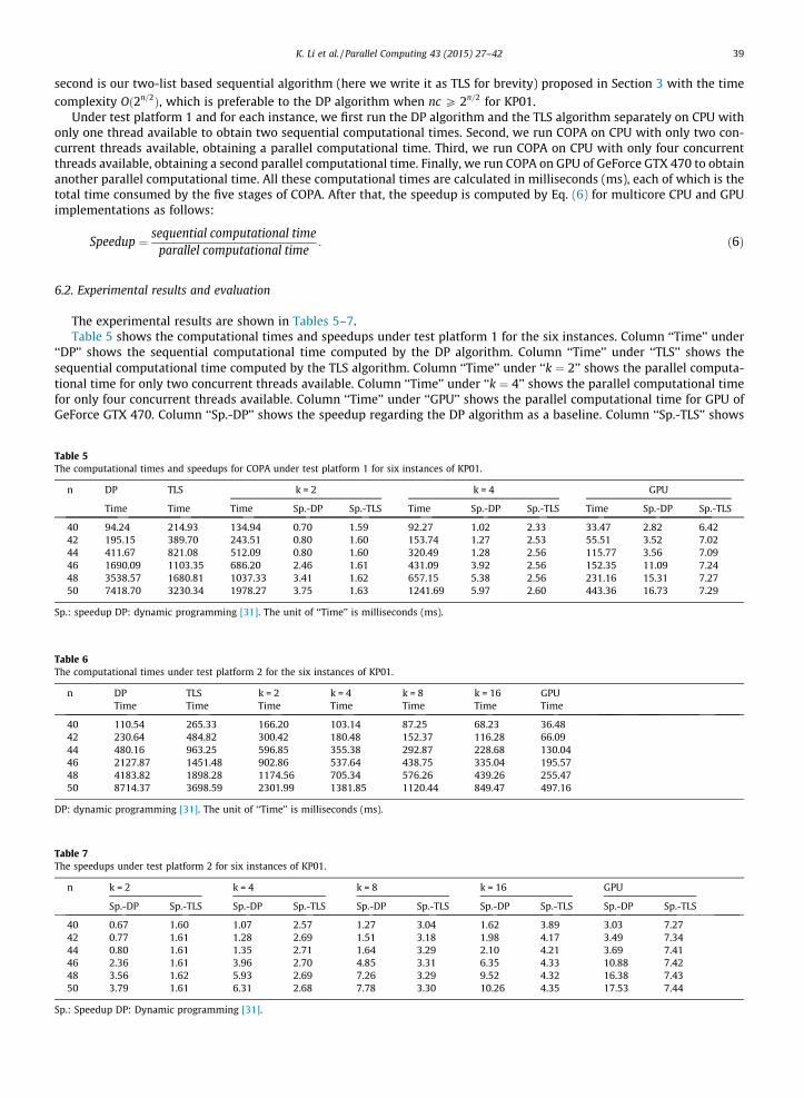
The experimental results are shown in Tables 5–7.Table 5 shows the computational times and speedups under test platform 1 for the six instances. Column ‘‘Time’’ under

‘‘DP’’ shows the sequential computational time computed by the DP algorithm. Column ‘‘Time’’ under ‘‘TLS’’ shows thesequential computational time computed by the TLS algorithm. Column ‘‘Time’’ under ‘‘k ¼ 2’’ shows the parallel computa-tional time for only two concurrent threads available. Column ‘‘Time’’ under ‘‘k ¼ 4’’ shows the parallel computational timefor only four concurrent threads available. Column ‘‘Time’’ under ‘‘GPU’’ shows the parallel computational time for GPU ofGeForce GTX 470. Column ‘‘Sp.-DP’’ shows the speedup regarding the DP algorithm as a baseline. Column ‘‘Sp.-TLS’’ shows

putational times and speedups for COPA under test platform 1 for six instances of KP01.

DP TLS k = 2 k = 4 GPU

Time Time Time Sp.-DP Sp.-TLS Time Sp.-DP Sp.-TLS Time Sp.-DP Sp.-TLS

94.24 214.93 134.94 0.70 1.59 92.27 1.02 2.33 33.47 2.82 6.42195.15 389.70 243.51 0.80 1.60 153.74 1.27 2.53 55.51 3.52 7.02411.67 821.08 512.09 0.80 1.60 320.49 1.28 2.56 115.77 3.56 7.091690.09 1103.35 686.20 2.46 1.61 431.09 3.92 2.56 152.35 11.09 7.243538.57 1680.81 1037.33 3.41 1.62 657.15 5.38 2.56 231.16 15.31 7.277418.70 3230.34 1978.27 3.75 1.63 1241.69 5.97 2.60 443.36 16.73 7.29

edup DP: dynamic programming [31]. The unit of ‘‘Time’’ is milliseconds (ms).

edups under test platform 2 for six instances of KP01.

k = 2 k = 4 k = 8 k = 16 GPU

Sp.-DP Sp.-TLS Sp.-DP Sp.-TLS Sp.-DP Sp.-TLS Sp.-DP Sp.-TLS Sp.-DP Sp.-TLS

0.67 1.60 1.07 2.57 1.27 3.04 1.62 3.89 3.03 7.270.77 1.61 1.28 2.69 1.51 3.18 1.98 4.17 3.49 7.340.80 1.61 1.35 2.71 1.64 3.29 2.10 4.21 3.69 7.412.36 1.61 3.96 2.70 4.85 3.31 6.35 4.33 10.88 7.423.56 1.62 5.93 2.69 7.26 3.29 9.52 4.32 16.38 7.433.79 1.61 6.31 2.68 7.78 3.30 10.26 4.35 17.53 7.44

edup DP: Dynamic programming [31].

putational times under test platform 2 for the six instances of KP01.

DP TLS k = 2 k = 4 k = 8 k = 16 GPUTime Time Time Time Time Time Time

110.54 265.33 166.20 103.14 87.25 68.23 36.48230.64 484.82 300.42 180.48 152.37 116.28 66.09480.16 963.25 596.85 355.38 292.87 228.68 130.042127.87 1451.48 902.86 537.64 438.75 335.04 195.574183.82 1898.28 1174.56 705.34 576.26 439.26 255.478714.37 3698.59 2301.99 1381.85 1120.44 849.47 497.16

amic programming [31]. The unit of ‘‘Time’’ is milliseconds (ms).

40 K. Li et al. / Parallel Computing 43 (2015) 27–42

the speedup considering the TLS algorithm to be a baseline. Tables 6 and 7 show the computational times and speedups,respectively, under test platform 2 for the six instances.

According to Tables 5 and 6, when the size of the instance increases, the computational time also increases. The compu-tational time obtained by the DP algorithm increases dramatically, whereas the computational times obtained by the TLSalgorithm and COPA increase at a slower rate. This difference in computational times is because the time complexityOðncÞ of the DP algorithm depends on the knapsack capacity c. When c increases, the computational time also increases.

However, the time complexity of the TLS algorithm Oð2n=2Þ and the time complexity of COPA Oð2n=4ð2n=4ÞeÞ keep unchanged

when c varies under the same hardware environment, that is, the number of the available cores is the same. When the size ofthe instance is small, the computational time obtained by the DP algorithm is shorter than that obtained by the TLS algo-rithm. The latter is almost twice as much as the former. When the size of the instance is larger, the computational timeobtained by the DP algorithm is longer than that obtained by the TLS algorithm. The former is several times as much asthe latter. For each instance, when the number of parallel cores increases, the computational time decreases.

From Tables 5 and 7, when the size of the instance increases, the speedup increases rapidly with the DP algorithm as abaseline while the speedup increases quite slowly with the TLS algorithm as a baseline. For each instance, when the numberof parallel cores increases, the speedup increases manifestly for both baselines. In Table 7, when the size of the instance is 50,the GPU implementation can achieve the maximum speedups of 17.53 and 7.44 with the DP and TLS baselines, respectively.

Through Table 5 to 7, we conclude that the number of concurrent threads available is higher and the performance of atargeted machine is better when more cores are available for a given computation. The speedup is different for the samenumber of concurrent threads under different test platforms, and the average speedup is also different for different GPU.One explanation might be that the speed of slower processors has an impact on the relative speedup.

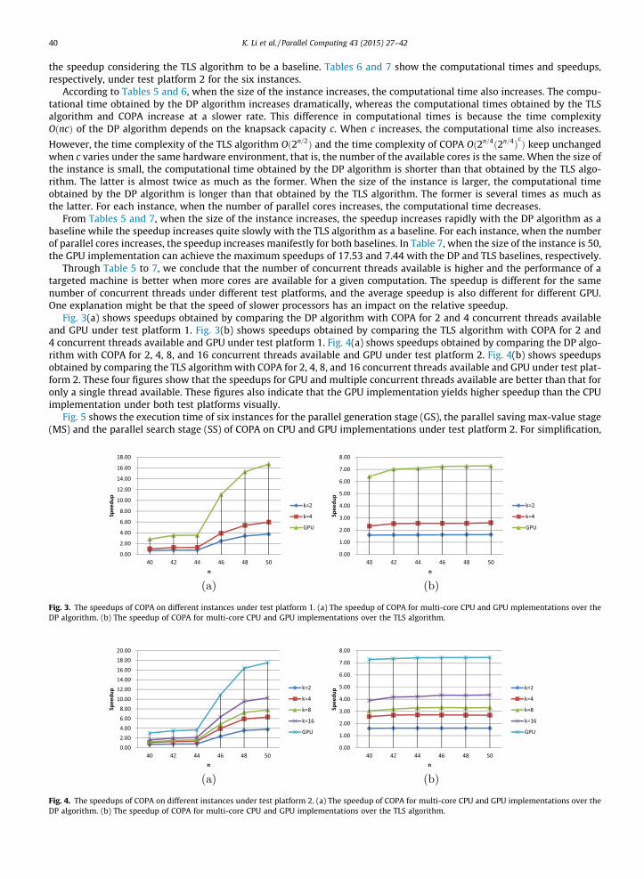
Fig. 3(a) shows speedups obtained by comparing the DP algorithm with COPA for 2 and 4 concurrent threads availableand GPU under test platform 1. Fig. 3(b) shows speedups obtained by comparing the TLS algorithm with COPA for 2 and4 concurrent threads available and GPU under test platform 1. Fig. 4(a) shows speedups obtained by comparing the DP algo-rithm with COPA for 2, 4, 8, and 16 concurrent threads available and GPU under test platform 2. Fig. 4(b) shows speedupsobtained by comparing the TLS algorithm with COPA for 2, 4, 8, and 16 concurrent threads available and GPU under test plat-form 2. These four figures show that the speedups for GPU and multiple concurrent threads available are better than that foronly a single thread available. These figures also indicate that the GPU implementation yields higher speedup than the CPUimplementation under both test platforms visually.

Fig. 5 shows the execution time of six instances for the parallel generation stage (GS), the parallel saving max-value stage(MS) and the parallel search stage (SS) of COPA on CPU and GPU implementations under test platform 2. For simplification,

Fig. 4. The speedups of COPA on different instances under test platform 2. (a) The speedup of COPA for multi-core CPU and GPU implementations over theDP algorithm. (b) The speedup of COPA for multi-core CPU and GPU implementations over the TLS algorithm.

Fig. 3. The speedups of COPA on different instances under test platform 1. (a) The speedup of COPA for multi-core CPU and GPU mplementations over theDP algorithm. (b) The speedup of COPA for multi-core CPU and GPU implementations over the TLS algorithm.

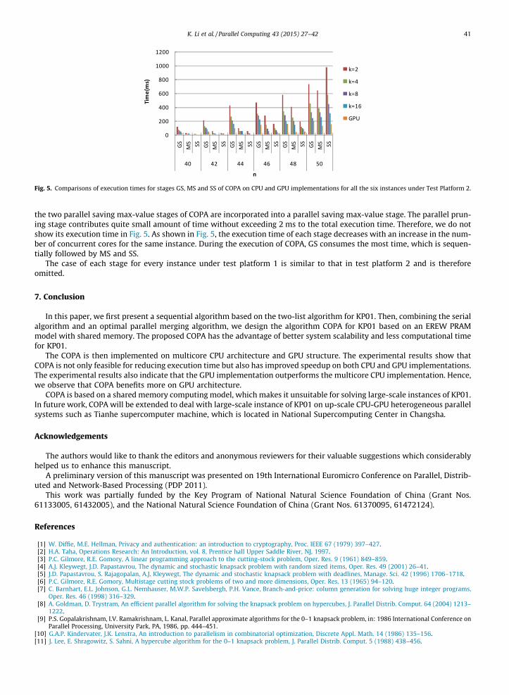
Fig. 5. Comparisons of execution times for stages GS, MS and SS of COPA on CPU and GPU implementations for all the six instances under Test Platform 2.

K. Li et al. / Parallel Computing 43 (2015) 27–42 41

the two parallel saving max-value stages of COPA are incorporated into a parallel saving max-value stage. The parallel prun-ing stage contributes quite small amount of time without exceeding 2 ms to the total execution time. Therefore, we do notshow its execution time in Fig. 5. As shown in Fig. 5, the execution time of each stage decreases with an increase in the num-ber of concurrent cores for the same instance. During the execution of COPA, GS consumes the most time, which is sequen-tially followed by MS and SS.

The case of each stage for every instance under test platform 1 is similar to that in test platform 2 and is thereforeomitted.

7. Conclusion

In this paper, we first present a sequential algorithm based on the two-list algorithm for KP01. Then, combining the serialalgorithm and an optimal parallel merging algorithm, we design the algorithm COPA for KP01 based on an EREW PRAMmodel with shared memory. The proposed COPA has the advantage of better system scalability and less computational timefor KP01.

The COPA is then implemented on multicore CPU architecture and GPU structure. The experimental results show thatCOPA is not only feasible for reducing execution time but also has improved speedup on both CPU and GPU implementations.The experimental results also indicate that the GPU implementation outperforms the multicore CPU implementation. Hence,we observe that COPA benefits more on GPU architecture.

COPA is based on a shared memory computing model, which makes it unsuitable for solving large-scale instances of KP01.In future work, COPA will be extended to deal with large-scale instance of KP01 on up-scale CPU-GPU heterogeneous parallelsystems such as Tianhe supercomputer machine, which is located in National Supercomputing Center in Changsha.

Acknowledgements

The authors would like to thank the editors and anonymous reviewers for their valuable suggestions which considerablyhelped us to enhance this manuscript.

A preliminary version of this manuscript was presented on 19th International Euromicro Conference on Parallel, Distrib-uted and Network-Based Processing (PDP 2011).

This work was partially funded by the Key Program of National Natural Science Foundation of China (Grant Nos.61133005, 61432005), and the National Natural Science Foundation of China (Grant Nos. 61370095, 61472124).

References

[1] W. Diffie, M.E. Hellman, Privacy and authentication: an introduction to cryptography, Proc. IEEE 67 (1979) 397–427.[2] H.A. Taha, Operations Research: An Introduction, vol. 8, Prentice hall Upper Saddle River, NJ, 1997.[3] P.C. Gilmore, R.E. Gomory, A linear programming approach to the cutting-stock problem, Oper. Res. 9 (1961) 849–859.[4] A.J. Kleywegt, J.D. Papastavrou, The dynamic and stochastic knapsack problem with random sized items, Oper. Res. 49 (2001) 26–41.[5] J.D. Papastavrou, S. Rajagopalan, A.J. Kleywegt, The dynamic and stochastic knapsack problem with deadlines, Manage. Sci. 42 (1996) 1706–1718.[6] P.C. Gilmore, R.E. Gomory, Multistage cutting stock problems of two and more dimensions, Oper. Res. 13 (1965) 94–120.[7] C. Barnhart, E.L. Johnson, G.L. Nemhauser, M.W.P. Savelsbergh, P.H. Vance, Branch-and-price: column generation for solving huge integer programs,

Oper. Res. 46 (1998) 316–329.[8] A. Goldman, D. Trystram, An efficient parallel algorithm for solving the knapsack problem on hypercubes, J. Parallel Distrib. Comput. 64 (2004) 1213–

1222.[9] P.S. Gopalakrishnam, I.V. Ramakrishnam, L. Kanal, Parallel approximate algorithms for the 0–1 knapsack problem, in: 1986 International Conference on

Parallel Processing, University Park, PA, 1986, pp. 444–451.[10] G.A.P. Kindervater, J.K. Lenstra, An introduction to parallelism in combinatorial optimization, Discrete Appl. Math. 14 (1986) 135–156.[11] J. Lee, E. Shragowitz, S. Sahni, A hypercube algorithm for the 0–1 knapsack problem, J. Parallel Distrib. Comput. 5 (1988) 438–456.

42 K. Li et al. / Parallel Computing 43 (2015) 27–42

[12] J. Lin, J. Storer, Processor-efficient hypercube algorithms for the knapsack problem, J. Parallel Distrib. Comput. 13 (1991) 332–337.[13] D. El Baz, M. Elkihel, Load balancing methods and parallel dynamic programming algorithm using dominance technique applied to the 0–1 knapsack

problem, J. Parallel Distrib. Comput. 65 (2005) 74–84.[14] S. Teng, Adaptive parallel algorithms for integral knapsack problems, J. Parallel Distrib. Comput. 8 (1990) 400–406.[15] W. Loots, T.H.C. Smith, A parallel algorithm for the 0–1 knapsack problem, Int. J. Parallel Program. 21 (1992) 349–362.[16] E. Horowitz, S. Sahni, Computing partitions with applications to the knapsack problem, J. ACM (JACM) 21 (1974) 277–292.[17] R. Schroeppel, A. Shamir, A T ¼ Oð2n=2Þ; S ¼ Oð2n=4Þ algorithm for certain NP-complete problems, SIAM J. Comput. 10 (1981) 456–464.[18] C.A.A. Sanches, N.Y. Soma, H.H. Yanasse, An optimal and scalable parallelization of the two-list algorithm for the subset-sum problem, Eur. J. Oper. Res.

176 (2007) 870–879.[19] E.D. Karnin, A parallel algorithm for the knapsack problem, IEEE Trans. Comput. 100 (1984) 404–408.[20] H.R. Amirazizi, M.E. Hellman, Time-memory-processor trade-offs, IEEE Trans. Inf. Theory 34 (1988) 505–512.[21] A.G. Ferreira, A parallel time/hardware tradeoff T � H ¼ Oð2n=2Þ for the knapsack problem, IEEE Trans. Comput. 40 (1991) 221–225.[22] H.K.C. Chang, J.J.R. Chen, S.J. Shyu, A parallel algorithm for the knapsack problem using a generation and searching technique, Parallel Comput. 20

(1994) 233–243.[23] D.C. Lou, C.C. Chang, A parallel two-list algorithm for the knapsack problem, Parallel Comput. 22 (1997) 1985–1996.[24] C.A.A. Sanches, N.Y. Soma, H.H. Yanasse, Comments on parallel algorithms for the knapsack problem, Parallel Comput. 28 (2002) 1501–1505.[25] K.L. Li, R.F. Li, Q.H. Li, Optimal parallel algorithms for the knapsack problem without memory conflicts, J. Comput. Sci. Technol. 19 (2004) 760–768.[26] F.B. Chedid, An optimal parallelization of the two-list algorithm of cost Oð2n=2Þ, Parallel Comput. 34 (2008) 63–65.[27] C.A.A. Sanches, N.Y. Soma, H.H. Yanasse, Observations on optimal parallelizations of two-list algorithm, Parallel Comput. 36 (2010) 65–67.[28] F.B. Chedid, A note on developing optimal and scalable parallel two-list algorithms, Algorithms Archit. Parallel Proces. (ICA3PP) (2012) 148–155.[29] Q. Lin, S. Weichang, C. Jiao, G. Duan, Application of 0–1 knapsack MPI+ OpenMP hybrid programming algorithm at MH method, in: 9th International

Conference on Fuzzy Systems and Knowledge Discovery (FSKD), 2012 (2012), pp. 2452–2456.[30] S.G. Akl, N. Santoro, Optimal parallel merging and sorting without memory conflicts, IEEE Trans. Comput. 100 (1987) 1367–1369.[31] H. Kellerer, U. Pferschy, D. Pisinger, Knapsack Problems, Springer, 2004.[32] C.A.A. Sanches, N.Y. Soma, H.H. Yanasse, Parallel time and space upper-bounds for the subset-sum problem, Theor. Comput. Sci. 407 (2008) 342–348.