A Model of Building Blocks and Total Factor Productivity–based Regulatory Approaches and Outcomes Report prepared for Australian Energy Market Commission 29 June 2010 Denis Lawrence and John Kain Economic Insights Pty Ltd 6 Kurundi Place, Hawker, ACT 2614, AUSTRALIA Ph +61 2 6278 3628 Fax +61 2 6278 5358 Email [email protected] WEB www.economicinsights.com.au ABN 52 060 723 631

Welcome message from author
This document is posted to help you gain knowledge. Please leave a comment to let me know what you think about it! Share it to your friends and learn new things together.
Transcript

A Model of Building Blocks and Total Factor Productivity–based Regulatory Approaches and Outcomes
Report prepared forAustralian Energy Market Commission
29 June 2010
Denis Lawrence and John Kain
Economic Insights Pty Ltd6 Kurundi Place, Hawker, ACT 2614, AUSTRALIAPh +61 2 6278 3628 Fax +61 2 6278 5358Email [email protected] www.economicinsights.com.auABN 52 060 723 631

Building Blocks and TFP Regulatory Model
© Economic Insights Pty Ltd 2010
This report and the associated spreadsheet models are copyright. Apart from use as permitted under the Copyright Act 1968, the report and models may be reproduced in whole or in part for study or training purposes only, subject to the inclusion of a reference to the source.
An appropriate reference to the report and models is:
Economic Insights (2010), A Model of Building Blocks and Total Factor Productivity–based Regulatory Approaches and Outcomes, Report prepared by Denis Lawrence and John Kain for the Australian Energy Market Commission, Canberra, 18 June.
Disclaimer
Economic Insights Pty Ltd (Economic Insights) has prepared this report and the associated spreadsheet models exclusively for the use of the Australian Energy Market Commission (AEMC) and for the purposes specified in the report. The report and the associated spreadsheet models are supplied in good faith and reflect the knowledge, expertise and experience of the consultants involved. They are accurate to the best of our knowledge. However, Economic Insights accepts no responsibility for any loss suffered by any person or organisation, other than the AEMC, taking action or refraining from taking action as a result of reliance on the report and the associated spreadsheet models.
i

Building Blocks and TFP Regulatory Model
CONTENTS
Executive Summary..............................................................................................................iii
1 Introduction.........................................................................................................................1
2 Modelling approach adopted...............................................................................................3
2.1 Database.......................................................................................................................3
2.2 Price cap regulation......................................................................................................3
2.3 The building blocks approach......................................................................................4
2.4 The TFP–based approach.............................................................................................6
2.5 Regulatory options modelled........................................................................................8
2.6 Regulatory scenarios modelled.....................................................................................9
2.7 Summary measures.....................................................................................................10
3 Model structure and user’s guide.....................................................................................12
3.1 Data sheets..................................................................................................................12
3.2 Building blocks sheets................................................................................................14
3.3 TFP sheets..................................................................................................................17
3.4 Comparison and summary sheets...............................................................................19
4 Results of scenarios examined..........................................................................................21
4.1 Base case....................................................................................................................21
4.2 Base case – alternative P0 and X combinations.........................................................24
4.3 Scenario 1 – unanticipated output increase................................................................26
4.4 Scenario 2 – anticipated increase in mandated standards...........................................28
4.5 Scenario 3 – anticipated increase in replacement capex.............................................30
4.6 Scenario 4 – unanticipated opex reductions...............................................................32
4.7 Scenario 5 – unanticipated capex reductions..............................................................36
5 Conclusions.......................................................................................................................38
Appendix 1: The Fisher TFP index......................................................................................39
References............................................................................................................................41
ii

Building Blocks and TFP Regulatory Model
EXECUTIVE SUMMARY
The Australian Energy Market Commission (AEMC) has commissioned Economic Insights to develop a spreadsheet model to test the economic properties of a total factor productivity (TFP) based regulatory methodology against the current arrangements for building blocks regulation.
The objectives of constructing the model are: to assist the AEMC in its current review of a TFP–based regulatory methodology; to improve stakeholders’ understanding of the effects of a TFP–based methodology; and to provide a model for stakeholders to test their own scenarios (as requested by a number of stakeholder submissions to the AEMC). At this stage the purpose is not to test the efficacy of alternative TFP output and input specifications.
Key findings
The base case spreadsheet model accompanying this report compares outcomes under building blocks and TFP–based regulation under business as usual conditions. It demonstrates that appropriately specified TFP–based regulation gives distribution businesses (DBs) achieving industry average productivity growth the opportunity to recover their revenue requirement. Those DBs achieving above industry average productivity growth have the opportunity to exceed their revenue requirement. TFP–based regulation will, however, be less attractive to DBs that do not achieve industry average productivity growth rates.
Compared to building blocks regulation, TFP–based regulation provides a more differentiated outcome by rewarding good performers and penalising poor performers. It does this by setting price cap parameters based on industry average performance rather than the DB’s own costs.
The model demonstrates that relatively small errors in forecasts in building blocks regulation can lead to significant divergences of realised revenue from revenue requirements. Because forecasting errors will inevitably occur in practice, TFP–based regulation is likely to be a somewhat less risky alternative compared to building blocks regulation under normal circumstances. Similarly, when compared over an extended period and under normal circumstances, TFP–based regulation is likely to produce a less volatile price path for customers than building blocks regulation.
The scenarios examined in the accompanying spreadsheet models demonstrate that TFP–based regulation can handle significant changes and adverse shocks relatively well provided there are regular price resets or appropriate safeguard mechanisms in place. For example, the three fixed five–year period TFP–based option performs best of the TFP–based options in the scenario involving an anticipated increase in mandated standards. And, with resets every five years and an appropriate specification, the TFP–based approach can handle even large changes such as a ‘wall of wire’ effect and produce similar profitability outcomes to the base case.
The model shows that a TFP–based option with rolling X factors and only an initial price reset can build in some ongoing adjustment to changing circumstances but fixed period TFP–based options with regular price resets generally handle large changes better.
iii

Building Blocks and TFP Regulatory Model
The spreadsheet models also compare the incentives for DBs to make cost savings additional to those anticipated at review time. For relatively static changes such as one–off and recurrent opex reductions and one–off capex reductions, building blocks and TFP–based regulatory options of similar regulatory period length provide broadly similar incentives. All TFP–based options provide substantially stronger incentives than building blocks to reduce rates of input growth. For example, the TFP–based options offer far stronger incentives for ongoing capex reductions than does the building blocks approach.
Database used
The model covers five electricity DBs including one mainly rural (DB1), one mainly urban (DB5) and three mixed rural/urban DBs (DB2, DB3 and DB4). Historic data levels and growth rates are calibrated against actual Australian DBs for DB1 and DB5 but levels have been scaled to maintain anonymity. The three mixed rural/urban DBs are formed from the rural and urban DBs with differing proportions of rural and urban coverage.
Data covers a base year, 10 ‘historical’ years and 15 future ‘out–years’. The data for each DB covers the value, quantity and price of three outputs (energy throughput, customer numbers and contracted demand or contracted reserved capacity) along with the value, quantity and price of four inputs (opex, overhead line capacity, underground cable capacity and transformer capacity). The initial capital base and annual capital expenditure for each DB are also included in the database.
In addition to data for each DB, corresponding industry variables are formed as the summation of the five DB variables and a number of economy–wide productivity and price variables are included to permit formation of the relevant X factors.
Price cap approaches modelled
The building blocks price cap included in the model is broadly consistent with the Australian Energy Regulator’s Post Tax Revenue Model (PTRM) and Roll Forward Methodology (RFM) for distribution service providers. The building blocks approach involves calculating an annual ‘revenue requirement’ for each DB based on forecasts of future opex, the return of capital, the return on capital and a benchmark tax liability. The return of capital is calculated as straight–line depreciation on the DB’s opening regulated asset base (RAB) calculated over its estimated remaining life plus straight–line depreciation of assets added during the period calculated over their estimated total lives. The return on capital is the opening RAB multiplied by the weighted average cost of capital (WACC).
Once the forecasts of annual revenue requirements and output quantities have been made, the P0 and X factors are set so that the net present value of the forecast operating revenue stream over the upcoming regulatory period is equated with the net present value of the forecast annual revenue requirement stream. Since there is an infinite number of P0 and X factor combinations which will satisfy this condition, the X factors are usually set at an exogenous value (often zero) and the P0 is set to equate the net present value streams.
The TFP–based price cap included in the model is of the CPI–X type where the X factor has the ‘differential of a differential’ form. That is, the X factor includes the difference between the industry and economy–wide productivity growth rates and the difference between the industry and economy–wide input price growth rates. The economy–wide variables are
iv

Building Blocks and TFP Regulatory Model
included because the CPI is an output price index which already incorporates the effects of general productivity and input price growth.
The TFP–based model allows for the important regulatory principle of financial capital maintenance (FCM) and uses asset capacity measures to proxy the one–hoss–shay physical depreciation profiles present in distribution capital input quantities.
The model includes price resets at the start of each TFP–based regulatory period. This allows a more like–with–like comparison between the building blocks and TFP–based outcomes. The TFP–based P0s are those required to have aligned revenue with the revenue requirement in the last year of the preceding regulatory period. The first year of the TFP–based regulatory period includes this P0 and also the X factor (to allow for productivity growth which has occurred between the last year of the preceding period and the first year of the new period). Subsequent years of the TFP–based regulatory period include just the X factor.
It should be noted that the initial price determination for a TFP methodology is quite different to the P0 decision for building blocks. The purposes are quite different and relate to different years. Under a TFP–based approach, the X factor is the industry productivity growth rate (for all DBs) and the P0 aligns opening revenues with costs for each DB. Under building blocks the P0 and X are set jointly for each DB to equate the present value of that DB’s forecast revenue and cost streams for the whole regulatory period.
Regulatory options modelled
A total of seven regulatory cases and options are examined in the spreadsheet model. For building blocks three different cases are modelled as follows:
• Building Blocks Case 1 – best review–time forecasts. This case can model perfect foresight forecasts where the realised values of all relevant variables are accurately anticipated at the start of the regulatory period or it can allow for changes in one or more relevant variables that were unanticipated at review time;
• Building Blocks Case 2 – DB–favourable forecasts (forecast opex and capex higher by 5 per cent and output quantities lower by 1 per cent than best review–time forecasts); and
• Building Blocks Case 3 – DB–unfavourable forecasts (forecast opex and capex lower by 5 per cent and output quantities higher by 1 per cent than best review–time forecasts).
The model examines four different TFP–based regulatory options as follows:
• TFP–based Option 1 – 3 fixed, 5–year periods
• TFP–based Option 2 – 2 fixed periods (7 years, then 8 years)
• TFP–based Option 3 – 1 fixed 15–year period
• TFP–based Option 4 – 10–year rolling X factor
Regulatory scenarios modelled
Five broad scenarios are modelled as well as the base case. The base case represents a ‘business as usual’ situation and compares the outcomes of the three building blocks cases and four TFP–based options. The five broad scenarios examine the impact of various external shocks – some anticipated in the building blocks analysis at review time and some
v

Building Blocks and TFP Regulatory Model
unanticipated – and how well the building blocks and TFP–based approaches handle these shocks by allowing recovery of revenue requirements.
The five broad scenarios examined are:
• Scenario 1: an unanticipated increase in output – growth rates in the customer numbers and energy throughput outputs for all five DBs increase by 2 percentage points in the last three years of the first out–period above what was forecast at review time. Customer number and energy throughput growth rates then return to their previous values. This scenario could represent a growth spurt associated with a sudden and unanticipated increase in population;
• Scenario 2: an increase in mandated standards – modelled as an anticipated increase of capex to 50 per cent above its base case levels for first three years of the second out–period only and increases in capital input quantity growth rates of 2 percentage points for the same years for all five DBs. After this capex and capital input quantity growth rates return to their base case values;
• Scenario 3: an anticipated large increase in replacement capex, or a so–called 'wall of wire' effect – modelled as capex increasing to three times its previous levels for each of the five years of the first out–period only and then returning to base case levels for all five DBs. Because the capex only replaces existing assets, there is no increase in capital input quantities above base case levels;
• Scenario 4: an unanticipated reduction in opex quantity for one DB only (taken to be DB3). Three variants of this scenario are examined:
• Scenario 4a: a one–off reduction in opex quantity of 10 per cent in year 12;
• Scenario 4b: a recurrent reduction in opex quantity of 10 per cent starting in year 11;
• Scenario 4c: a reduction in the opex quantity growth rate from 0.81 per cent per annum to 0.2 per cent per annum starting in year 11; and
• Scenario 5: an unanticipated reduction in capex for one DB only (taken to be DB3). Two variants of this scenario are examined:
• Scenario 5a: a one–off reduction in capex of 10 per cent in year 11;
• Scenario 5b: a recurrent reduction in capex of 10 per cent starting in year 11.
Results for the base case and each of the scenarios are presented in separate spreadsheet files.
Summary indicators
The model focuses on key profitability and customer summary indicators. The key profitability indicator is the ratio of the present value of the stream of excess returns to the present value of the stream of actual annual revenue requirements. Annual excess returns are defined to be the difference between operating revenue and the corresponding actual annual revenue requirement.
To assess the impact of different regulatory options on customers we present and graph the overall index of prices paid by customers. This is calculated as the sum of operating revenues across the five DBs divided by the industry output quantity index.
vi

Building Blocks and TFP Regulatory Model
We assess the strength of incentives for cost savings using retention ratios – the proportion of benefits kept by the DB.
User scenarios
The accompanying base case spreadsheet model provides a means for interested parties to undertake their own simulations of alternative scenarios by making relevant changes to the cells shaded light blue in the model. For convenience users are able to change the future growth rates of key variables where indicated. Since consistency is required among key variables (eg price times quantity must equal value), only some future period variables are able to be changed and historic data for the five DBs should not be changed.
To assist users with understanding how to implement alternative scenarios in the base case model, the cells that have been changed to implement the five scenarios examined in this report have been shaded orange in each scenario spreadsheet.
vii

Building Blocks and TFP Regulatory Model
1 INTRODUCTION
The Australian Energy Market Commission (AEMC) has initiated a review into the possible use of a total factor productivity (TFP) methodology in determining regulated prices and revenues for electricity and gas network service providers. The objective is to advise the Ministerial Council on Energy (MCE) on whether permitting the use of a TFP methodology would contribute to the national gas objective (NGO) and/or national electricity objective (NEO) and if so, to provide draft Rules amendments.
In preparing its Discussion Paper (AEMC 2009a) and the Preliminary Findings (AEMC 2009b) the AEMC considered that a number of technical issues would benefit from detailed discussion and analysis. Stakeholder responses provided to the AEMC also indicated an interest in greater technical analysis and spreadsheet modelling of TFP methodology issues.
The AEMC has commissioned Economic Insights to develop a spreadsheet model to test the economic properties of a TFP–based regulatory methodology against the current arrangements for building blocks regulation. The objectives of constructing the model are to:
• provide additional support for the Commission’s draft reasons;
• improve stakeholders’ understanding of the effects of a TFP methodology;
• provide a model for stakeholders to test their own scenarios; and
• facilitate future testing of detailed design questions in applying a TFP methodology.
The AEMC requested that the model:
• be broadly consistent with the AER’s (2008a,b) current Post Tax Revenue Model (PTRM) and roll forward methodology (RFM) available for distribution service providers;
• draw on the current TFP design example and variations set out in the AEMC (2009b) Preliminary Findings;
• use a set of common inputs (between the TFP methodology and the building block approach);
• use a weighted average price cap for the building block approach;
• test the scenarios identified in Chapter 4 of the AEMC Preliminary Findings (namely, an unanticipated increase in the growth of connections and increases in capital expenditure to maintain specified standards);
• compare the methodologies over three five–year regulatory periods;
• develop and apply an acceptable measure of return or profit to test cost recovery;
• develop and apply an acceptable measure of the strength of productivity efficiency incentives;
• measure the impact of the methodologies on users through either differences in prices and/or maximum allowed revenue;
1

Building Blocks and TFP Regulatory Model
• identify the differences between applying a fixed X or a rolling X under a TFP methodology;
• assess the impact of extending the regulatory period past five years under the TFP methodology; and
• test how the ability to use various combinations of P0 and X (consistent with the NPV=0 requirement) under the building block approach may affect the comparison between the methodologies.
The AEMC also requested Economic Insights to have regard to applying a TFP methodology that would be suitable to both the electricity and gas distribution sectors and to have regard to the spreadsheet TFP model constructed by Pacific Economic Group (PEG) for the Victorian Essential Services Commission (ESC). This model was submitted by the ESC to the AEMC in June 2009 (ESC 2009).
The ESC/PEG spreadsheet model provides a high–level stylised coverage of two regulatory options. While the model is instructive, it contains a number of significant limitations in the context of the current review including:
• a TFP regulatory option which does not include price resets nor other key aspects of the AEMC (2009a) design example;
• a ‘building block’ regulatory option which does not allow for the important role of forecasts nor the equating of the present values of future forecast revenues and costs;
• includes only two distribution businesses (DBs); and
• uses an approximate indexing method and assumes industry input prices increase each year by the same amount as the CPI, thus avoiding many of the practical problems regulators face in implementing TFP–based regulatory approaches.
The spreadsheet model Economic Insights has constructed overcomes these limitations.
It should be noted that the purpose of this modelling exercise is not to test the efficacy of alternative TFP output and input specifications which have been put forward. However, where appropriate, we note the likely implications of adopting a specification different to the one used in the model.
In the following section of this report we outline the general approach adopted in constructing the spreadsheet model and briefly describe the building blocks and TFP–based approaches to price regulation as modelled. We also describe the key summary measures used to assess the impact of the alternative regulatory options examined on cost recovery levels and the impact on customers. In section 3 we provide a commentary on the structure of the spreadsheet model and guidance to users on how to use the model to implement alternative scenarios. In section 4 we present and discuss the results from the scenarios examined as part of this exercise before drawing conclusions in section 5.
2
Building Blocks and TFP Regulatory Model
2 MODELLING APPROACH ADOPTED
In this section we provide a general description of the database used in the model and then describe the building blocks and TFP–based approaches to price regulation and the specific versions included in the model. We then review the 7 different regulatory cases and options included in the model and the 5 broad scenarios that have been modelled to date.
2.1 Database
The model covers five electricity DBs including one mainly rural (DB1), one mainly urban (DB5) and three mixed rural/urban DBs (DB2, DB3 and DB4). Historic data levels and growth rates are calibrated against actual Australian DBs for DB1 and DB5 but levels have been scaled to maintain anonymity. The three mixed rural/urban DBs are formed from the rural and urban DBs with differing proportions of rural and urban coverage.
Data covers a base year and 10 ‘historical’ years (labelled years 0 to 10) and 15 future ‘out–years’ (labelled years 15 to 25). Observed historical growth rates for each variable are used as the basis for forming the historical data. Random variations in the historical data series were then introduced. Data for the 15 out–years is formed initially using observed historical growth rates but these can be varied for each included DB to model different future scenarios. Note that only variables for the out–years can generally be altered and only a subset of variables can be altered as a number of fundamental relationships have to be maintained (eg price times quantity must equal value). Cells which can be altered in the model are shaded light blue.
The data for each DB covers the value, quantity and price of three outputs (energy throughput, customer numbers and contracted demand or contracted reserved capacity) along with the value, quantity and price of four inputs (opex, overhead line capacity, underground cable capacity and transformer capacity). The initial (year 0) capital base and annual capital expenditure for each DB are also included in the database.
In addition to data for each DB, corresponding industry variables are formed as the summation of the five DB variables and a number of economy–wide productivity and price variables are included to permit formation of the relevant X factors.
A detailed description of the variables and interrelationships between variables will be presented in section 3 on the structure and use of the model.
2.2 Price cap regulation
The building blocks and TFP–based approaches to utility regulation both involve setting price (or revenue) caps of the CPI–X form. A positive X factor means that prices (or revenue) have to fall in real terms while a negative X factor means that prices (or revenue) can increase in real terms. Ideally the X factor will be set to allow the DB the opportunity to earn its risk–adjusted rate of return. The cap provides the DB with an incentive to outperform the assumptions used in setting the X factor while also providing a means of sharing the benefits of efficiency improvements between the DB and its customers.
3

Building Blocks and TFP Regulatory Model
Caps can be set on the basis of weighted average prices, overall revenue or revenue yield (total revenue divided by the quantity of a key output). The AEMC requested that Economic Insights examine only the case of a weighted average price cap as that method is currently used in electricity and gas regulatory decisions.
In practice the price cap is typically implemented using an initial price change (known as a ‘P0’) in the first year of the regulatory period and then a common X factor across the remaining years of the regulatory period. The building blocks and TFP–based regulatory methods use quite different approaches to setting the P0 and X factors. Under building blocks the P0 and X are set jointly for each DB to equate the present value of the DB’s forecast revenue and cost streams for the whole regulatory period. Under the TFP–based approach, the X factor is generally the industry (or group) productivity growth rate (for all DBs) and the P0
aligns opening revenues with costs for each DB.
2.3 The building blocks approach
The building blocks approach to price regulation involves calculating an annual ‘revenue requirement’ for each DB based on the costs it would incur if it was acting prudently. The costs are made up of opex, capital costs and a benchmark tax liability (which usually takes account of the differences between regulatory and taxation parameters and allowances). Capital costs are, in turn, made up of the return of capital and the return on capital. The return of capital is typically calculated as straight–line depreciation on the DB’s opening regulated asset base (RAB) calculated over its estimated remaining life plus straight–line depreciation of assets added during the period calculated over their estimated total lives. The return on capital is the opening RAB multiplied by an opportunity cost rate. The opportunity cost rate is the weighted average cost of capital (WACC) which takes account of the different costs of the nominated debt and equity components of the RAB.
Financial capital maintenance (FCM) is a key principle in the building blocks approach. FCM means that a regulated business is compensated for prudent expenditure and prudent investments such that, on an ex–ante basis, its financial capital is at least maintained in present value terms.
Since the building blocks method involves setting the price cap for each DB at the start of the regulatory period, forecasts have to be made of the annual revenue requirement stream over the coming regulatory period and of the quantities of outputs that will be sold over that period. Since the opening RAB for the regulatory period will be (largely) known, the annual revenue requirements for the upcoming regulatory period can be forecast based on forecasts of opex and capex.
Once the forecasts of annual revenue requirements and output quantities have been made, the P0 and X factors are set so that the net present value of the forecast operating revenue stream over the upcoming regulatory period is equated with the net present value of the forecast annual revenue requirement stream. Since there is an infinite number of P0 and X factor combinations which will satisfy this condition, the X factors are usually set at an exogenous value (often zero) and the P0 is set to equate the net present value streams.
4
Building Blocks and TFP Regulatory Model
Regulators in different jurisdictions have applied slightly different variants of the building blocks method. The main differences are timing assumptions regarding capex (ie when assets added each year actually come into service) and whether a real WACC is used or, alternatively, a nominal WACC is used but revaluation gains are then deducted so that inflation is not allowed for twice. In the spreadsheet model we have followed the approach and assumptions contained in the AER’s PTRM as closely as possible.
A detailed description of the steps involved in calculating the building blocks revenue requirements and P0 and X factors is presented in section 3.
The model first calculates the annual revenue requirement for each year based on the actual or realised values of all relevant variables. This allows us to form a benchmark against which we can compare outcomes in the building blocks approach where forecasts are used. This same actual annual revenue requirement and its components are also used in the TFP–based approach.
Given the important role forecasts play in building blocks price regulation we then examine three different forecast cases:
• ‘best review time forecasts’ which, all else equal, come close to predicting the realised values of opex, capex and output quantities although the model allows scope for some changes to be unanticipated at review time and hence for there to be divergences between these forecasts and realised values;
• ‘DB favourable forecasts’ where the accepted review time forecasts over–predict realised costs and under–predict realised output quantities producing returns for the DBs in excess of their WACC; and
• ‘DB unfavourable forecasts’ where the accepted review time forecasts under–predict realised costs and over–predict realised output quantities producing returns for the DBs of less than their WACC.
While forecast capex and depreciation at review time may deviate from subsequently realised capex and depreciation patterns through the regulatory period, the actual capex and depreciation for that regulatory period will be recognised at the time of the next review and incorporated in the opening RAB for the next regulatory period under the AER’s RFM. That is, if DBs end up spending less capex than forecast at the start of the regulatory period then their opening RAB for the next regulatory period will be correspondingly lower and consistent with the realised rather than forecast capex and depreciation for the preceding regulatory period. Conversely, if DBs spend more capex than forecast at the start of the regulatory period then they do not get compensation for this additional expenditure within the period but, if judged prudent, it is recognised in a higher opening RAB for the next regulatory period. In line with the RFM, actual capex and depreciation for the previous period are used in the accompanying model to determine the opening RAB for each regulatory period.
A significant part of most building blocks reviews, and of the AER’s PTRM, is the calculation of the impact of differences between regulatory and taxation parameters such as depreciation rates. While regulatory parameters aim to reflect actual asset lives, tax lives may be shorter reflecting a range of government policies and assistance arrangements. As this issue does not have a major impact on the comparison of building block and TFP–based
5

Building Blocks and TFP Regulatory Model
regulatory outcomes, we simplify the building block section of our model by assuming that taxation parameters coincide with regulatory parameters.
The AER PTRM also includes allowance for customer contributions and for divergences between review–time forecasts for variables in the last year of the preceding regulatory period and their subsequent realised values. Neither of these issues is likely to be material for a comparison of building blocks and TFP–based regulatory outcomes and so they are not included in our spreadsheet model.
2.4 The TFP–based approach
Productivity–based regulation, as it has been applied to date, argues that in choosing a productivity growth rate to base X on, it is desirable that the productivity growth rate be external to the individual firm being regulated and instead reflect industry trends at a national or even international level. This way the regulated firm is given an incentive to match (or better) this productivity growth rate while having minimal opportunity to ‘game’ the regulator by acting strategically. The latter can be a problem with the building blocks method which relies more heavily on specific and projected information on the firm’s own costs and likely best practice for that specific firm.
As outlined in Lawrence (2003) and Economic Insights (2009a), traditional productivity–based regulation has typically been implemented using CPI–X price caps where, as the result of choosing the CPI to index costs, the formula for the X factor takes on the following ‘differential of a differential’ form:
(1) X ≡ [TFP1/TFP0 − TFP1E/ TFP0
E] – [W1/W0 − W1E/ W0
E] – M1/M0.
where 1 and 0 denote the most recent and preceding periods, respectively, W is a price index taken to approximate changes in the industry’s input prices, the E subscript refers to corresponding variables for the economy as a whole and M refers to monopolistic mark–ups or excess profits.
What this formula tells us is that the X factor can effectively be decomposed into three terms. The first differential term takes the difference between the industry’s TFP growth and that for the economy as a whole while the second differential term takes the difference between the firm’s input prices and those for the economy as whole. It is necessary to include the economy–wide TFP and input price variables because these are drivers of the CPI and need to be allowed for in setting an industry price cap. Thus, taking just the first two terms, if the regulated industry has the same TFP growth as the economy as a whole and the same rate of input price increase as the economy as a whole then the X factor in this case is zero. If the regulated industry has a higher TFP growth than the economy then X is positive, all else equal, and the rate of allowed price increase for the industry will be less than the CPI. Conversely, if the regulated industry has a higher rate of input price increase than the economy as a whole then X will be negative, all else equal, and the rate of allowed price increase will be higher than the CPI.
Productivity indexes are formed by aggregating output quantities into a measure of total output quantity and aggregating input quantities into a measure of total input quantity. The productivity index is then the ratio of the total output quantity to the total input quantity or, if
6
Building Blocks and TFP Regulatory Model
forming a measure of productivity growth, the change in the ratio of total output quantity to total input quantity.
To form the total output and total input measures we need a price and quantity for each output and each input, respectively. The quantities enter the calculation directly as it is changes in output and input quantities that we are aggregating. The relevant output and input prices are used to weight together changes in output quantities and input quantities into measures of total output quantity and total input quantity using revenue and cost measures, respectively. In the spreadsheet model we use the chained Fisher indexing method (see appendix A).
There has been some debate about whether just ‘billed’ outputs (ie outputs explicitly charged for) should be included in the TFP measure or whether both billed outputs and ‘unbilled’ outputs (ie outputs of value to the user – such as system reliability and redundancy – but which are not explicitly charged for) should be included. Because network industries are natural monopolies the price of billed outputs will typically not equal their marginal cost (as would be the case in a competitive industry). Furthermore, some key output dimensions that would be charged for in competitive industries may not be charged for at all in networks. Economic Insights (2009a) has recently shown that all network outputs – both billed and unbilled – should ideally be included in the productivity measure and that each output should be weighted by the difference between its price and marginal cost in deriving the X factor. However, because marginal costs are not readily observable and their estimation would currently require the use of econometric methods, it will be necessary to rely on including only billed outputs with revenue share weightings in TFP measures in the short to medium term.
Three billed outputs (energy throughput, customer numbers and contracted demand or contracted reserved capacity) are included in the spreadsheet model. The model contains a facility to alter the opening (year 0) revenue shares to examine the impact of different pricing structures. For simplicity, the prices of the three outputs are assumed to change in equal proportions in all years. Revenue shares vary after year 0 reflecting differential output quantity growth rates.
The TFP model includes four inputs – opex, overhead lines, underground cables, and transformers and other capital. The capital input quantities use asset capacity measures to proxy one–hoss–shay physical depreciation profiles (where an asset’s carrying capacity tends to stay relatively constant over its lifetime rather than decaying by equal amounts or equal proportions each year). This is required for the TFP model to accurately reflect distribution industry production characteristics. The overall capital user cost is measured exogenously based on ex ante FCM in an analogous manner to the building blocks approach. The alternative approach of using an endogenous user cost of capital would not satisfy the important property of ex ante FCM (except by accident). The overall user cost is allocated to the three capital components using DB–specific asset shares. For simplicity these asset user cost shares are assumed to remain constant. The industry input price index is derived by dividing total costs by the total input quantity index.
To be consistent with the AEMC’s design example, we include price resets at the start of each TFP–based regulatory period. This also allows a more like–with–like comparison between the building blocks and TFP–based outcomes. As a result, TFP–based P0s are those required to
7
Building Blocks and TFP Regulatory Model
have aligned revenue with the revenue requirement in the last year of the preceding regulatory period. The first year of the TFP–based regulatory period will, therefore, include this P0 and also the X factor (to allow for productivity growth which has occurred between the last year of the preceding period and the first year of the new period). Subsequent years of the TFP–based regulatory period will just include the X factor.
By using the P0 process to align opening revenue with opening costs (and, hence, there are no excess profits at the start of the regulatory period), the excess profit terms, M, can be ignored in the X factor formula (1).
To recap, the initial price determination for a TFP methodology is quite different to the P0
decision for building blocks. The purposes are quite different and relate to different years. Under a TFP–based approach, the X factor is the industry productivity growth rate (for all DBs) and the P0 aligns opening revenues with costs for each DB. Under building blocks the P0 and X are set jointly for each DB to equate the present value of the forecast revenue and cost streams for the whole regulatory period for each DB.
TFP annual growth rates observed for the historical period in the model’s database range from 1.2 per cent (DB1) to 1.7 per cent (DB5) with an industry average TFP growth rate of 1.4 per cent.
2.5 Regulatory options modelled
A total of seven regulatory cases and options are examined in the spreadsheet model. For building blocks three different cases are modelled as follows:
• Building Blocks Case 1 – best review–time forecasts. This case can model perfect foresight forecasts where the realised values of all relevant variables are accurately anticipated at the start of the regulatory period or it can allow for changes in one or more relevant variables that were unanticipated at review time;
• Building Blocks Case 2 – DB–favourable forecasts (forecast opex and capex higher by 5 per cent and output quantities lower by 1 per cent than best review–time forecasts); and
• Building Blocks Case 3 – DB–unfavourable forecasts (forecast opex and capex lower by 5 per cent and output quantities higher by 1 per cent than best review–time forecasts).
As noted in section 2.3, the building blocks approach does not involve either clawing back of excess revenue or retrospective compensation for inadequate revenue resulting from past mis–forecasts. However, actual capex from the last regulatory period is used to roll forward the opening RAB for the next regulatory period.
The model examines four different TFP–based regulatory options as follows:
• TFP–based Option 1 – 3 fixed, 5–year periods
• TFP–based Option 2 – 2 fixed periods (7 years, then 8 years)
• TFP–based Option 3 – 1 fixed 15–year period
• TFP–based Option 4 – 10–year rolling X factor
8

Building Blocks and TFP Regulatory Model
There is a price reset at the start of each TFP–based regulatory period. Thus, option 1 has three resets (in years 11, 16 and 21), option 2 has two resets (in years 11 and 18) and options 3 and 4 only have one reset (in year 11).
2.6 Regulatory scenarios modelled
Five broad scenarios are modelled (each in a separate spreadsheet file) as well as the base case. The base case represents a ‘business as usual’ situation and compares the outcomes of the three building blocks cases and four TFP–based options outlined in the preceding section. The five broad scenarios examine the impact of various external shocks – some anticipated in the building blocks analysis at review time and some unanticipated – and how well the building blocks and TFP–based approaches handle these shocks.
The five broad scenarios examined are:
• Scenario 1: an unanticipated increase in output – growth rates in the customer numbers and energy throughput outputs for all five DBs increase by 2 percentage points in the last three years of the first out–period above what was forecast at review time. Customer number and energy throughput growth rates then return to their previous values. This scenario could represent a growth spurt associated with a sudden and unanticipated increase in population;
• Scenario 2: an increase in mandated standards – there is an anticipated increase of capex to 50 per cent above its base case levels for first three years of the second out–period only and increases in capital input quantity growth rates of 2 percentage points for the same years for all five DBs. After this capex and capital input quantity growth rates return to their base case values;
• Scenario 3: an anticipated large increase in replacement capex, or a so–called 'wall of wire' effect – capex increases to three times its previous levels for each of the five years of the first out–period only and then returns to base case levels for all five DBs. Because the capex only replaces existing assets, there is no increase in capital input quantities above base case levels;
• Scenario 4: an unanticipated reduction in opex quantity for one DB only (taken to be DB3). Three variants of this scenario are examined:
• Scenario 4a: a one–off reduction in opex quantity of 10 per cent in year 12;
• Scenario 4b: a recurrent reduction in opex quantity of 10 per cent starting in year 11;
• Scenario 4c: a reduction in the opex quantity growth rate from 0.81 per cent per annum to 0.2 per cent per annum starting in year 11; and
• Scenario 5: an unanticipated reduction in capex for one DB only (taken to be DB3). Two variants of this scenario are examined:
• Scenario 5a: a one–off reduction in capex of 10 per cent in year 11;
• Scenario 5b: a recurrent reduction in capex of 10 per cent starting in year 11.
9

Building Blocks and TFP Regulatory Model
Results for each of the scenarios are presented in a separate spreadsheet file and will be discussed in section 4. To assist users with understanding of the model, the input cells which have been changed to implement each scenario are shaded orange rather than light blue.
2.7 Summary measures
Three key summary measures are presented to assist with assessing the performance of building blocks and TFP–based regulation. Two of these relate to DB profitability and one to the prices faced by customers.
The first profitability measure presented is the average of the deviation of the annual realised rate of return from the WACC over the 15 out–years. The realised rate of return is calculated as the ratio of operating revenue less opex less regulatory depreciation less benchmark tax liability to the nominal RAB. However, while informative, this measure does not take account of timing differences between periods of realised rates of return above and below the WACC.
The second profitability measure presented does take account of timing differences and is our primary profitability measure. It is the ratio of the present value of the stream of excess returns to the present value of the stream of actual annual revenue requirements. Annual excess returns are defined to be the difference between operating revenue and the corresponding actual annual revenue requirement. But because operating revenue normally diverges from the actual annual revenue requirement in any one year, it is necessary to look at this measure over the course of the regulatory period (or periods) rather than on a year–by–year basis. And to provide a relevant basis for aggregation and comparisons, it is necessary to take present values. This measure is presented for the first future regulatory period and for the total of the three future regulatory periods. The graph near the end of the model presents the measure for the three future regulatory periods.
To assess the impact of different regulatory options on customers we present and graph the overall index of prices paid by customers. This is calculated as the sum of operating revenues across the five DBs divided by the industry output quantity index. The overall price index is presented for the future period and is based to a value of one in year 10.
In scenarios 4 and 5 we look at the effects of unanticipated opex and capex savings, respectively, for one DB. By examining the retention ratios – the proportion of benefits kept by the DB – across the different regulatory options we are able to assess the incentive effects of the regulatory options. The higher the retention ratio, the stronger the incentive for the DB to seek out and implement cost savings.
The retention ratio’s numerator is the present value of benefits going to the DB which is the difference between the savings scenario’s profits and the corresponding base case profits. The relevant profits are the difference between operating revenue and the corresponding actual annual revenue requirement. The retention ratio’s denominator is the present value of the total benefits available which is the difference between the base case and the relevant actual annual revenue requirement. The retention ratio formula is1:
(3) PV[(ORSSua – RRSS) – (ORBC – RRBC)] / PV[RRBC – RRSS]
1 It should be noted this retention ratio formula differs from the stylised version used in AEMC (2009b).
10

Building Blocks and TFP Regulatory Model
where OR is operating revenue, RR is actual annual revenue requirement, BC is base case, SS is savings scenario, ua in unanticipated and PV is the present value operator with a discount rate of the WACC and calculated over the 15 out–years. Note that benefits are calculated over the 15 out–years of the model rather than over the total life of recurrent and ongoing savings which could be considerably more than 15 years. So that the major part of the effect is captured in present value terms, modelled savings occur at the start of the future period.
11
Building Blocks and TFP Regulatory Model
3 MODEL STRUCTURE AND USER’S GUIDE
The spreadsheet model has been constructed using Microsoft Excel 2003 and is made up of 31 separate sheets. These sheets can be grouped as follows:
• a Notes sheet which provides a brief description of the model;
• a General data sheet which contains a number of general variables including economy–wide productivity and input prices;
• 6 Data sheets which contain the databases for the five DBs and the industry;
• a WACC calculation sheet which contains the key cost of capital parameters;
• 5 Building blocks calculations sheets, one for each DB, which calculate P0s, X factors and revenue for each of the DBs under the three building blocks forecast cases;
• a TFP calculations sheet which calculates the TFP and related indexes;
• 5 TFP–based regulation sheets, one for each DB, which calculate P0s, X factors and revenue for each of the DBs under the four TFP–based options;
• 3 TFP chart sheets graphing key TFP components;
• 5 Comparisons sheets, one for each DB, which construct key summary measures for each regulatory option;
• a Summary sheet which presents the key summary indicators for all DBs; and
• 2 Summary chart sheets which graph the key profitability and customer indicators.
Users can test the impact of a range of future scenarios by changing data in the cells shaded light blue in the General data, Data, WACC calculation and Building blocks calculation sheets. For convenience users are able to change the future growth rates of key variables where indicated. Since consistency is required among key variables (eg price times quantity must equal value), only some future period variables are able to be changed and historic data for the five DBs are locked in.
It should be noted that after any data has been changed users will need to run the macro by clicking on the box near cell H172 in any of the DB Building blocks sheets. Clicking the macro box on any of the building blocks sheets will undertake all relevant building block calculations for all five DBs. Note that the macro returns the user to the DB1 Building blocks sheet. Users will need to have their security settings set to enable macros to be run.
In the following sections we describe each of the types of sheets in more detail and the data users are able to change to test different scenarios.
3.1 Data sheets
The General data sheet contains data on key revenue and cost shares for the five DBs, key economy–wide and industry price indexes and economy–wide productivity growth. The first data block gives the year 0 revenue shares for the five DBs and is user changeable. Changing the initial revenue shares would reflect the impact of different DB pricing structures. For
12

Building Blocks and TFP Regulatory Model
simplicity, after year 0 prices for each DB are assumed to move in equal proportions but revenue shares vary reflecting varying output quantity growth rates.
The second data block shows the shares of the three capital assets in total capital costs. These shares are fixed for each DB and are not user changeable. Since asset lives for the three asset types – overhead lines, underground cables and transformers – will be broadly similar, shares in annual user costs will broadly reflect shares in asset value (assuming broadly similar age profiles across the three asset types). Consequently the rural DB1 has a highest share of overhead lines while the urban DB5 has the highest share of underground cables.
The third data block contains the CPI, the economy–wide multi–factor productivity index, the economy–wide input price index and the distribution industry opex price index. Future values of the latter three indexes can be changed by changing their annual growth rates in the blue shaded cells. The common future CPI growth rate is user changeable in the WACC calculation sheet rather than this sheet.
The five DB Data sheets contain the values, quantities and prices for the three outputs (energy throughput, customer numbers and reserved capacity or contract demand) and four inputs (opex, overhead lines, underground cables, and transformers and other capital). Starting with revenue, historic total revenue is set equal to the actual annual revenue requirement for that year (calculated in the relevant Building block sheet). Year 0 revenue for the three outputs is year 0 total revenue multiplied by the initial revenue shares specified in the General data sheet. Subsequent historic years’ revenue for the three outputs is calculated by forming a notional total revenue series formed by multiplying the year 0 price of each output by its current year quantity. Total revenue (taken to be equal to the actual annual revenue requirement) is then disaggregated using the shares of each output in the notional total revenue series. This allows for output prices moving in equal proportions and the differences in relative output quantity growth rates to be reflected in the revenue shares.
For the out–years, the price of each of the three outputs is assumed to move forward by CPI–X where an indicative X value of one per cent in used. Multiplying these prices by the respective current year’s output quantities allows each outputs revenue to be formed and total revenue is the sum of the three component revenues. These out–year revenues are used only in forming the TFP index which will be invariant to the indicative X factor used (given the assumption of equal proportional price changes for the three outputs). For the building blocks and TFP–based regulation analyses the relevant operating revenues are formed using the P0
and X values from the analyses.
Capital input user costs are formed by multiplying the asset cost shares in the General data sheet by the return on and return of capital from the relevant Building blocks sheet. This return on and return of capital is used in the TFP analysis because it is consistent with the important regulatory property of financial capital maintenance and the sunk cost nature of network assets (see section 2.4). Annual capex is also listed on the DB Data sheets and is used in forming the return on and return of capital in the Building blocks sheets.
Throughput, contract demand and customer output quantities are measured in GWh, MW and numbers, respectively. The quantity of opex inputs is measured in constant year 0 dollars and the quantity of capital inputs are measured in physical capacity units – MVAkms for overhead lines and underground cables and MVA for transformer and other assets. Physical quantities
13
Building Blocks and TFP Regulatory Model
provide a means of proxying one–hoss–shay depreciation of capital quantities. That is, an asset’s useful carrying capacity tends to stay relatively constant over its lifetime rather than decaying by equal amounts or equal proportions each year. The alternative approach of using either straight–line or declining balance constant price asset values would likely understate capital input quantities over time and, hence, overstate the rate of TFP growth.
Input and output prices are formed by dividing the relevant value by its corresponding quantity, with the exception of opex where the external price index from the General data sheet is used. In the case of opex the value is formed by multiplying the price by quantity series (measured in constant year 0 dollars).
Future period output and input quantities and capex move forward by multiplying the preceding year’s amount by one plus a specified growth rate. The default growth rates specified in the model generally reflect a continuation of historic growth rates. Users can alter the future growth rates of the output and input quantities and of capex in the blue shaded cells at the bottom of the DB Data sheets to reflect different scenarios.
The last of the Data sheets presents data for the distribution industry as a whole. Values and quantities for each output and input are formed by summing the corresponding items across the five DB Data sheets. Industry output and input prices are formed by dividing the relevant value by its corresponding quantity, again with the exception of the opex price which is taken directly from the General data sheet. User changes cannot be made to the industry Data sheet as it is simply the summation of the five DB Data sheets. Rather, industry changes derive from changes entered on the relevant DB Data sheets.
3.2 Building blocks sheets
The first of the building blocks group of sheets presents key cost of capital parameters. The WACC calculations sheet reproduces the corresponding sheet from the AER’s PTRM. The key parameters used in the subsequent analysis are the nominal vanilla WACC and the real vanilla WACC. The WACC is built up from information on the shares of debt and equity, the inflation rate, the cost of debt, corporate tax rates, effective tax rates on debt and equity, risk free rates of return, market risk premiums and equity betas.
The only user changeable parameter on the WACC calculations sheet is the future (common) inflation rate. Values for other input parameters (appearing in red type in the model) are taken from the AER PTRM but could in principle also be changed. Derived values appear in black type.
The DB Building blocks sheets each contain five sections. The first section lists key parameters that will be used in the calculations such as the inflation rate, inflation index, the WACC values and key WACC components. The second section calculates the actual annual revenue requirement. This allows us to calculate an estimate of each DB’s actual total costs based on the PTRM methodology. This section uses actual realised data for the out–years taken from the DB Data sheets. The next three sections calculate annual revenue requirements for the out–years based on three different forecast scenarios and go on to calculate P0 and X factors for each scenario. The first scenario involves ‘best review–time’ forecasts. If the regulator is able to correctly anticipate all future changes then the data used will be actual
14

Building Blocks and TFP Regulatory Model
data, the same as used in calculating the actual annual revenue requirement. However, if the regulator does not anticipate all output and input changes for the forthcoming regulatory period than there will be deviations between the best review–time forecasts and realised data.
The second and third forecast scenarios involve more systematic deviations of forecasts from actual realised data. The second forecast scenario presents systematic differences that would be favourable to the DB. These involve forecasts which underestimate output quantities and overestimate input quantities at review time. DBs earn positive excess profits under this scenario where realised revenues are higher and costs lower than those accepted at review time. The third forecast scenario presents systematic differences that would be unfavourable to the DB. These involve forecasts which overestimate output quantities and underestimate input quantities at review time. DBs earn negative excess profits under this scenario.
We will now examine the annual revenue requirement calculations. These calculations are the same for the actual and three forecast scenarios presented in the Building blocks sheets although the data used for capex and opex varies across the four cases. As noted in section 2.3, the building blocks annual revenue requirement is based on the costs a DB would incur if it was acting prudently. The costs are made up of capital costs, opex and a benchmark tax liability. Capital costs are, in turn, made up of the return of capital and the return on capital. The return of capital is calculated using straight–line depreciation on the DB’s initial RAB calculated over its estimated remaining life plus straight–line depreciation of assets added during the period calculated over their estimated total lives. The return on capital is the opening RAB multiplied by the WACC.
The first part of the annual revenue requirement covered in the Building blocks sheets is real capex and the initial capital base or initial RAB. Assets added each year in the PTRM are not recognised until the start of the following year but DBs are allowed a half–year return on the associated capex so that last year’s real capex is brought in at the start of the current year but is increased by half a year’s real return (using the real vanilla WACC) on that capex.
The second part of the annual revenue requirement covered in the Building blocks sheets is real straight–line depreciation. New assets are assumed to have a life of 50 years and the opening capital stock is assumed to have a remaining life of 25 years. Total real depreciation is formed by summing the real straight–line depreciation on the initial capital base and the real straight–line depreciations on previous years’ capex.
The next part forms the RAB series. The real end–of–period RAB is formed as the real start–of–period (or opening) RAB less total real straight–line depreciation plus total real capex. The nominal RAB is formed by multiplying the real RAB by the inflation index. Because a nominal vanilla WACC is applied to a nominal RAB, a valuation gain has to be calculated and deducted from the annual revenue requirement to avoid double counting the effects of inflation. This valuation gain is the inflation increase on each year’s opening RAB and is the nominal opening RAB multiplied by the inflation rate. The way this is implemented in the PTRM is to deduct the inflation increase from straight–line depreciation to form a variable called ‘regulatory depreciation’ which is then used in the revenue requirement.
We make a simplification for convenience by only working with the total initial RAB and total capex. The AER PTRM allows for up to 30 RAB and capex components with differing capex scenarios and equipment lives. Since the lifetimes of the three broad asset categories
15
Building Blocks and TFP Regulatory Model
used in the TFP–based approach (namely overhead lines, underground cables and transformers) are likely to be similar, this simplification should not affect overall comparability of the building blocks and TFP–based outcomes as modelled.
As noted in section 2.3, while forecast capex at review time may deviate from subsequently realised capex patterns through the regulatory period, the actual capex for that regulatory period is recognised at the time of the next review and incorporated in the opening RAB for the next regulatory period. Consequently, while the formulae for the opening RAB for the three forecast cases generally refer to the preceding year’s closing RAB, capex and depreciation forecast for that year, the opening RAB for the first year of the second and third regulatory periods instead refers to the closing RAB in the preceding year from the actual annual revenue requirement block. That is, actual capex and depreciation in the first (second) regulatory period is used to form the opening RAB for the first year of the second (third) regulatory period. In other words, changes in the period which were unanticipated at review time are recognised and incorporated at the start of the next period.
The next part of the revenue requirements sections draws together the building blocks components and forms the revenue requirement as the sum of the components. The components are return on capital (nominal opening RAB times nominal vanilla WACC), return of capital (regulatory depreciation), opex and the benchmark tax liability. The benchmark tax liability is formed as tax payable less the value of imputation credits.
The next three parts of the revenue requirements blocks do the tax calculations. The first part assembles information of the debt and equity shares of the RAB and their returns. The return on equity is the post–tax nominal rate of return on equity (before imputation credits) times the equity share of the RAB. The return on debt is the nominal pre–tax cost of debt times the debt share of the RAB.
The next part calculates tax expenses as the sum of opex, depreciation and interest on debt. In the AER PTRM the difference between tax and regulatory depreciation is allowed for. In the interests of simplification and because this is not material to a comparison of building blocks and TFP–based regulatory approaches, we assume regulatory and tax values coincide.
Tax payable is calculated as pre–tax income (the annual revenue requirement less tax expenses) times the statutory corporate tax rate. Imputation credits are assumed to be 50 per cent of tax payable leaving a benchmark tax liability of also 50 per cent of tax payable.
For the three forecast cases the next part of the calculations covers forecast revenue for the three output components. This is formed as the forecast output quantity times a price which is rolled forward by (1+CPI)(1–X). We then distinguish between total forecast revenue (calculated from reset prices and forecast quantities) and realised operating revenue (calculated from reset prices and actual or realised quantities).
The final part of the three forecast cases calculates the P0 and X values. First the net present value of the stream of forecast revenue requirements is calculated. Next the net present value of the stream of total forecast revenue is calculated. Then the P0 and X values are changed so that the NPV of the total forecast revenue is equated to the NPV of the forecast revenue requirements. Because there is an infinite number of P0 and X values that will satisfy this condition, the X’s are set exogenously to a specified value (or values) and the P0 is changed to
16

Building Blocks and TFP Regulatory Model
equate the NPV values. In common with the AER PTRM, this process is implemented using the ‘goal seek’ function in Excel. This is initiated via an Excel macro which is executed by clicking on the box near cell H172 in any of the Building blocks sheets. When the macro is executed it solves the P0 values for all five DBs, for all three forecast cases and all three future regulatory periods. It then returns the user to the Building blocks sheet for DB1 (regardless of which sheet it was initiated in).
Users are able to make changes in three separate places on the Building blocks sheets. The first is change the relationship between best review–time forecasts and actual data. The default forecast values for capex, opex quantities and the three output quantities are formed using the same annual growth rates as in the respective DB Data sheets. This corresponds to a situation of perfect foresight on the regulator’s part or the ability to anticipate all changes. Unanticipated changes (at review time) can be introduced by putting in growth rates for one or more of these variables which differ from the realised actual growth rates.
The other two places where users can make changes in the Building blocks sheets are in the relationships between the DB–favourable and DB–unfavourable capex, opex and output quantities and the corresponding variables in the best review–time forecasts case. The default values of these are 5 per cent differences in capex and opex and 1 per cent differences in output quantities. Note that in all cases, actual capex for the preceding period (as opposed to the inaccurately forecast values at the earlier review time) are used to form the opening RAB for the first year of the next regulatory period. Similarly, inaccurate forecasts of opex for the last year of the preceding period are overridden by actual opex levels in the last year of the preceding period when opex growth rates are applied to form the opex level for the first year of the next regulatory period.
Note that after any data change or changes are made by the user (to the Building blocks sheets or elsewhere), the goal seek macro has to be run manually to form the relevant building blocks P0 value.
3.3 TFP sheets
The first of the TFP sheets provides details of the TFP index calculations. Total output and total input quantity indexes are constructed using the chained Fisher index method and the TFP index is then the ratio of the total output index to the total input index. Indexes and year–to–year changes are presented in the top half of this sheet.
The bottom half of the sheet contains the detailed index calculations. As shown in appendix 1, the chained Fisher index is the geometric mean of the chained Laspeyres and chained Paasche indexes. For any pair of observations, the Laspeyres index uses the first observation’s weights while the Paasche index uses the second observation’s weights. By taking a geometric mean of the two, the Fisher index avoids the so–called ‘index number problem’ where weights do not accurately reflect the characteristics of the observations being compared. Applying the index formulae in appendix 1 produces the year–to–year change between the two observations and these are listed first in the blocks in the lower half of the sheet. These are converted to indexes by setting the value for the first observation equal to
17

Building Blocks and TFP Regulatory Model
one and then progressively multiplying through by the year–to–year changes. The indexes are presented below the year–to–year changes in each of the blocks in the lower half of the sheet.
As discussed in section 2.4, the TFP model includes three outputs (energy throughput, customer numbers and contracted demand or contracted reserved capacity) and, for convenience, revenue share weights are used. The model includes four inputs – opex, overhead lines, underground cables, and transformers and other capital. The capital input quantities use asset capacity measures to proxy one–hoss–shay physical depreciation profiles and the overall capital user cost is measured exogenously based on ex ante FCM in an analogous manner to the building blocks approach.
The next five sheets calculate the TFP–based P0 and X factors for the five DBs and the four TFP options examined. There is a price reset at the start of each TFP–based regulatory period using the method described in section 2.4. The P0 is the change that would be required to align operating revenue with the revenue requirement in the last year of the preceding regulatory period. The X factor is then set using equation (2) which is a more detailed variant of the ‘differential of a differential’ equation (1):
(2) X ≡ [TFP1/TFP0 − TFP1E/ TFP0
E] – [(sXWX1/WX
0 + sKRK1/RK
0) − W1E/ W0
E]
where 1 and 0 denote the most recent and preceding periods, respectively, W is a price index taken to approximate changes in the industry’s input prices, the E subscript refers to corresponding variables for the economy as a whole, X refers to opex, K to capital, s to the cost share of the input and R to the exogenous, FCM–consistent capital user cost based on the return of and return on capital (similar to that used in building blocks). The X factor is included in the first year of each regulatory period – in addition to the P0 – to take account of efficiency improvements between this year and the preceding year from which the P0 is derived.
At the top of the TFP–based sheets the first block of data presents the industry and economy–wide variables that will be used in setting the price cap. The CPI and economy–wide MFP and input price indexes are taken from the General data sheet while the industry TFP index is taken from the TFP calculations sheet. The industry input price index is the sum of the DB revenue requirements (ie total cost) divided by the industry input quantity index. The next block presents year–to–year changes for the same variables.
The DB–specific output quantities and revenue requirement are then presented. These are sourced from the relevant DB Data sheet and Building blocks sheet, respectively.
The next four blocks calculate the P0 and X values for the four TFP options. Ten year growth rates are used to form the X factor components listed in equation (2) above. For the first three TFP options these are the growth rates for the ten years up to and including the last year of the preceding regulatory period. For the fourth TFP option a rolling approach is used so the ten year growth rate is updated each year to be the ten years up to the year before the current one.
There has been some debate about the appropriate way of calculating the relevant growth rates. One option is to use an endpoint–to–endpoint method that takes the natural logarithm of the ratio of the last to the first observation and then divides this by the number of annual changes in the series. This method is computationally convenient but is prone to distortion if there are outliers at either endpoint of the series. The alternative method is to form a
18
Building Blocks and TFP Regulatory Model
regression–based trend rate of growth for the series where the natural logarithm of the relevant variable is regressed against a constant and a time trend. The coefficient on the time trend is the growth rate in this case. This method is less prone to outlier distortions but is computationally more complex and requires the use of an econometric method in addition to the index number method. For convenience the model uses the endpoint–to–endpoint method for calculating growth rates.
Because revenue for the historic period has been set equal to the relevant revenue requirement for all DBs, the TFP–based year 11 P0s equal zero in all cases.
Under each set of P0 and X values we present the resulting output prices and the sum of these multiplied by the relevant output quantities produce annual operating revenue for each of the four TFP options.
Following the TFP–based sheets the model contains three sheets which, respectively, graph the total outputs, total inputs and TFP indexes for the five DBs and the industry. These graphs provide a ready mans of seeing the impact of scenario data changes on TFP and its key components.
There is no provision for user changes in the TFP sheets as relevant data changes flow from changes input to the General data and DB Data sheets.
3.4 Comparison and summary sheets
The five Comparisons sheets compare outcomes for each DB under the three building blocks cases and the four TFP–based options considered. The first block in the Comparisons sheets presents the revenue requirement and its key components (other than the return on capital) drawn from the relevant Building blocks sheet.
The next block presents operating revenue for the best review–time forecasts building blocks case and then calculates the realised return on capital as the difference between operating revenue and opex, regulatory depreciation and the benchmark tax liability. The realised rate of return is then calculated as the ratio of the realised return on capital to the nominal opening RAB. The next rows present the difference between the realised rate of return and the nominal vanilla WACC and excess revenue (the difference between operating revenue and the annual revenue requirement). As noted in section 2.7, timing differences have to be taken into account when considering excess returns and so our key profitability summary measure is the ratio of the net present value of the stream of excess revenue to the net present value of the stream of annual revenue requirements. This summary measure is presented for two time periods – the first regulatory out–period (years 11 to 15) and for the three regulatory out–periods (years 11 to 25).
The following six blocks on the Comparisons sheets repeat these calculations for the other two building blocks forecast cases and the four TFP–based regulatory options.
The Summary sheet presents the three key summary indicators. Two of these relate to profitability and one to the impact on customers. The first profitability summary indicator presented is the average deviation of the realised rate of return from the WACC over the 15 out–years for each of the five DBs. As noted in section 2.7, this measure does not take
19
Building Blocks and TFP Regulatory Model
account of timing differences and so the second profitability summary indicator is the ratio of the net present value of the stream of excess revenue to the net present value of the stream of annual revenue requirements for each of the five DBs over the 15 out–years. We also present the industry and DB–specific TFP growth rates over the historic period in these blocks for reference.
The summary indicator of the impact on customers is the index of the overall price paid by customers. This is formed as the sum of the five DB operating revenues divided by the industry output quantity index. This overall price paid index is based at one in year 10 and presented for the out–years.
Following the Summary sheet, the two key indicators – the net present value of the stream of excess revenue to the net present value of the stream of annual revenue requirements and the index of he overall price paid by customers – are graphed in the last two sheets in the spreadsheet model.
Again, there is no provision for user changes in the Comparisons and Summary sheets as relevant data changes would be input to the General data, DB Data and Building blocks sheets.
20

Building Blocks and TFP Regulatory Model
4 RESULTS OF SCENARIOS EXAMINED
4.1 Base case
The base case model represents a ‘business as usual’ scenario with the key output and input variables continuing to grow at their observed historic rates. In the base case the building blocks X values are set to zero so that all adjustment occurs through the P0 values. Results are presented in the model for the three building blocks regulation cases and the four TFP–based regulation options using the two profitability summary indicators and the overall price to customers indicator.
The average deviations of the realised rates of return from the WACC are relatively small for nearly all TFP–based regulation outcomes. The largest deviations are between 0.6 and 0.7 per cent for the DB–favourable building blocks forecasts case. However, as noted, this indicator does not take account of timing differences and so we focus on the present value of excess revenues relative to the resent value of the annual revenue requirements indicator. It should be noted that this indicator produces values that are considerably larger in absolute value (but generally of the same sign) compared to the average deviation of the realised rate of return from the WACC indicator.
Figure 1: Base case profitability indicators, years 11–25
-4%
-3%
-2%
-1%
0%
1%
2%
3%
4%
BB - BestReview-Time
Forecasts
BB - DB-FavourableForecasts
BB - DB-Unfavourable
Forecasts
TFP 3 Fixed5-YearPeriods
TFP 2 FixedPeriods
TFP - 1 FixedPeriod
TFP - 10-Year Rolling
X Factor
DB1DB2DB3DB4DB5
Present Value of Excess Returns Relative to Present Value of Revenue Requirement
Source: Economic Insights building blocks and TFP regulatory model
The base case present value profitability indicators are presented in figure 1. As the base case best review–time forecasts fully anticipate future changes, the corresponding building blocks profitability outcomes all produce zero net present values. However, if the review–time
21
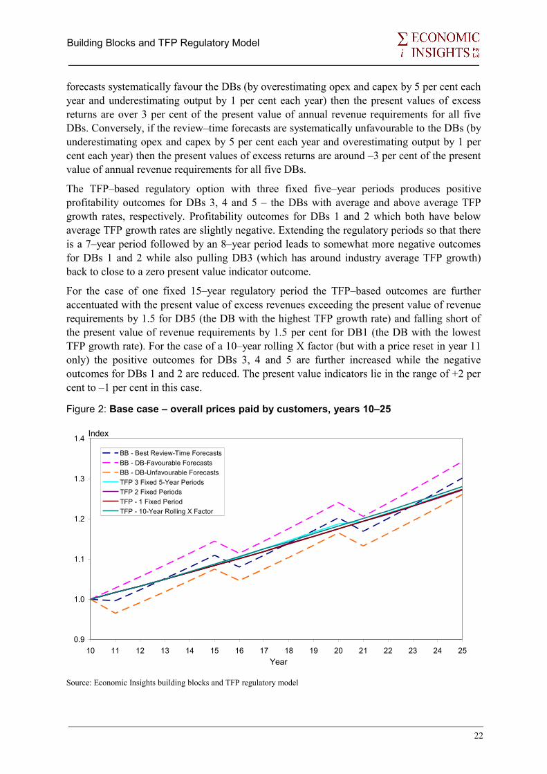
Building Blocks and TFP Regulatory Model
forecasts systematically favour the DBs (by overestimating opex and capex by 5 per cent each year and underestimating output by 1 per cent each year) then the present values of excess returns are over 3 per cent of the present value of annual revenue requirements for all five DBs. Conversely, if the review–time forecasts are systematically unfavourable to the DBs (by underestimating opex and capex by 5 per cent each year and overestimating output by 1 per cent each year) then the present values of excess returns are around –3 per cent of the present value of annual revenue requirements for all five DBs.
The TFP–based regulatory option with three fixed five–year periods produces positive profitability outcomes for DBs 3, 4 and 5 – the DBs with average and above average TFP growth rates, respectively. Profitability outcomes for DBs 1 and 2 which both have below average TFP growth rates are slightly negative. Extending the regulatory periods so that there is a 7–year period followed by an 8–year period leads to somewhat more negative outcomes for DBs 1 and 2 while also pulling DB3 (which has around industry average TFP growth) back to close to a zero present value indicator outcome.
For the case of one fixed 15–year regulatory period the TFP–based outcomes are further accentuated with the present value of excess revenues exceeding the present value of revenue requirements by 1.5 for DB5 (the DB with the highest TFP growth rate) and falling short of the present value of revenue requirements by 1.5 per cent for DB1 (the DB with the lowest TFP growth rate). For the case of a 10–year rolling X factor (but with a price reset in year 11 only) the positive outcomes for DBs 3, 4 and 5 are further increased while the negative outcomes for DBs 1 and 2 are reduced. The present value indicators lie in the range of +2 per cent to –1 per cent in this case.
Figure 2: Base case – overall prices paid by customers, years 10–25
0.9
1.0
1.1
1.2
1.3
1.4
10 11 12 13 14 15 16 17 18 19 20 21 22 23 24 25
BB - Best Review-Time ForecastsBB - DB-Favourable ForecastsBB - DB-Unfavourable ForecastsTFP 3 Fixed 5-Year PeriodsTFP 2 Fixed PeriodsTFP - 1 Fixed PeriodTFP - 10-Year Rolling X Factor
Index
Year
Source: Economic Insights building blocks and TFP regulatory model
22

Building Blocks and TFP Regulatory Model
The overall prices paid by customers are presented in figure 2. The four TFP–based regulatory options all produce relatively smooth customer price indexes with only very minor ‘kinks’ at review time reflecting the presence of a P0 in those years in addition to the X factor. By contrast, the three building blocks cases produce more volatile customer price indexes, each with a distinct ‘zig–zag’ pattern. This reflects the relatively greater emphasis on P0
adjustments in the building blocks case, particularly where the X factor is set to zero (as it is in the base case).
It is also instructive to compare the price paths under the building blocks and TFP–based approaches with the unit annual revenue requirement for the industry. We do this in figure 3 where we compare the building blocks best review–time forecasts price path, the TFP–based three fixed five–year period price path and the unit annual revenue requirement path. The latter is the annual revenue requirement for the industry as a whole divided by the output quantity index for the industry as a whole. All three series are converted to index form and equal one in year 10.
Figure 3: Base case price paths and unit annual revenue requirements, years 10–25
0.9
1.0
1.1
1.2
1.3
1.4
10 11 12 13 14 15 16 17 18 19 20 21 22 23 24 25
Price BB - Best Review-Time ForecastsPrice TFP 3 Fixed 5-Year PeriodsPer unit Annual Revenue Requirement
Index
Source: Economic Insights building blocks and TFP regulatory model
Although the best review–time forecasts building blocks price path moves above and below the unit annual revenue requirement, in present value terms the two will be equal at the start of each review period by construction (in the absence of forecast errors which are inevitable in reality). The three fixed five–year period TFP–based price path follows the unit annual revenue requirement very closely. It spends some time above the unit annual revenue requirement, reflecting the positive profitability outcomes presented in figure 1 for three of the five DBs. This means that industry working capital requirements would be no higher under the TFP–based approach compared to the building blocks approach. Indeed, where the
23
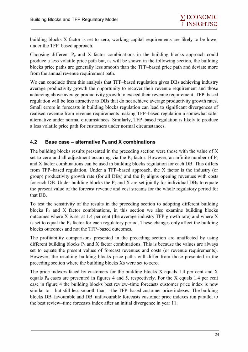
Building Blocks and TFP Regulatory Model
building blocks X factor is set to zero, working capital requirements are likely to be lower under the TFP–based approach.
Choosing different P0 and X factor combinations in the building blocks approach could produce a less volatile price path but, as will be shown in the following section, the building blocks price paths are generally less smooth than the TFP–based price path and deviate more from the annual revenue requirement path.
We can conclude from this analysis that TFP–based regulation gives DBs achieving industry average productivity growth the opportunity to recover their revenue requirement and those achieving above average productivity growth to exceed their revenue requirement. TFP–based regulation will be less attractive to DBs that do not achieve average productivity growth rates. Small errors in forecasts in building blocks regulation can lead to significant divergences of realised revenue from revenue requirements making TFP–based regulation a somewhat safer alternative under normal circumstances. Similarly, TFP–based regulation is likely to produce a less volatile price path for customers under normal circumstances.
4.2 Base case – alternative P0 and X combinations
The building blocks results presented in the preceding section were those with the value of X set to zero and all adjustment occurring via the P0 factor. However, an infinite number of P0
and X factor combinations can be used in building blocks regulation for each DB. This differs from TFP–based regulation. Under a TFP–based approach, the X factor is the industry (or group) productivity growth rate (for all DBs) and the P0 aligns opening revenues with costs for each DB. Under building blocks the P0 and X are set jointly for individual DBs to equate the present value of the forecast revenue and cost streams for the whole regulatory period for that DB.
To test the sensitivity of the results in the preceding section to adopting different building blocks P0 and X factor combinations, in this section we also examine building blocks outcomes where X is set at 1.4 per cent (the average industry TFP growth rate) and where X is set to equal the P0 factor for each regulatory period. These changes only affect the building blocks outcomes and not the TFP–based outcomes.
The profitability comparisons presented in the preceding section are unaffected by using different building blocks P0 and X factor combinations. This is because the values are always set to equate the present values of forecast revenues and costs (or revenue requirements). However, the resulting building blocks price paths will differ from those presented in the preceding section where the building blocks Xs were set to zero.
The price indexes faced by customers for the building blocks X equals 1.4 per cent and X equals P0 cases are presented in figures 4 and 5, respectively. For the X equals 1.4 per cent case in figure 4 the building blocks best review–time forecasts customer price index is now similar to – but still less smooth than – the TFP–based customer price indexes. The building blocks DB–favourable and DB–unfavourable forecasts customer price indexes run parallel to the best review–time forecasts index after an initial divergence in year 11.
24

Building Blocks and TFP Regulatory Model
Figure 4: Base case X=1.4 – overall prices paid by customers, years 10–25
0.9
1.0
1.1
1.2
1.3
1.4
10 11 12 13 14 15 16 17 18 19 20 21 22 23 24 25
BB - Best Review-Time ForecastsBB - DB-Favourable ForecastsBB - DB-Unfavourable ForecastsTFP 3 Fixed 5-Year PeriodsTFP 2 Fixed PeriodsTFP - 1 Fixed PeriodTFP - 10-Year Rolling X Factor
Index
Year
Source: Economic Insights building blocks and TFP regulatory model
Figure 5: Base case X=P0 – overall prices paid by customers, years 10–25
0.9
1.0
1.1
1.2
1.3
1.4
10 11 12 13 14 15 16 17 18 19 20 21 22 23 24 25
BB - Best Review-Time ForecastsBB - DB-Favourable ForecastsBB - DB-Unfavourable ForecastsTFP 3 Fixed 5-Year PeriodsTFP 2 Fixed PeriodsTFP - 1 Fixed PeriodTFP - 10-Year Rolling X Factor
Index
Year
Source: Economic Insights building blocks and TFP regulatory model
25

Building Blocks and TFP Regulatory Model
For the X equals P0 case in figure 5 the building blocks best review–time forecasts customer price index is again similar to – but still less smooth than – the TFP–based customer price indexes. But the building blocks DB–favourable and DB–unfavourable forecasts customer price indexes now diverge from the best review–time forecasts index rather than paralleling it. This produces a less smooth price path for customers.
The building blocks best review–time forecasts case which fully anticipates future output and input changes is unlikely to occur in practice because forecasting errors will inevitably occur. As a result, when taken compared over an extended period, building blocks outcomes are likely to produce less smooth customer price paths than TFP–based regulatory options.
4.3 Scenario 1 – unanticipated output increase
Under scenario 1 customer numbers and energy throughput outputs growth rates for all five DBs increase by 2 percentage points in the last three years of the first out–period above what was forecast at review time. Customer number and energy throughput growth rates then return to their previous levels. This scenario could represent a growth spurt associated with a sudden and unanticipated increase in population.
Figure 6: Unanticipated output increase profitability indicators, years 11–25
-3%
-2%
-1%
0%
1%
2%
3%
4%
5%
6%
BB - BestReview-Time
Forecasts
BB - DB-FavourableForecasts
BB - DB-Unfavourable
Forecasts
TFP 3 Fixed5-YearPeriods
TFP 2 FixedPeriods
TFP - 1 FixedPeriod
TFP - 10-Year Rolling
X Factor
DB1DB2DB3DB4DB5
Present Value of Excess Returns Relative to Present Value of Revenue Requirement
Source: Economic Insights building blocks and TFP regulatory model
Because the building blocks best review–time forecasts do not anticipate the increased growth in output in the second half of the first out–period, the present value profitability indicator for this case is now positive rather than zero for all five DBs as shown in figure 6. Similarly, the building blocks DB–favourable and DB–unfavourable forecasts cases are correspondingly more positive and less negative, respectively, compared to the base case. This is because the
26

Building Blocks and TFP Regulatory Model
DBs are able to keep the extra revenue from increased output in the first period but this higher level of output is recognised at review time for the second out–period and factored into the buildings blocks analyses for the second (and also the third) out–periods.
Compared to the base case, the TFP–based regulatory option involving three fixed five–year periods provides slightly less profitable outcomes than the base case. This is accentuated by the model’s use of the endpoint–to–endpoint method to calculate the industry TFP growth rate. While the DBs make higher profits in the first out–period, the higher output levels in year 15 (the last year of the first out–period) lead to a higher TFP growth rate for the 10–year period up to that year. This is then extrapolated to apply to the second regulatory out–period even though TFP growth actually returns to its previous rate (ie before the output growth spurt) in the second out–period. This leads to lower profitability in the second out–period and a subsequent compensating P0 adjustment at the start of the third out–period.
By contrast, in the two period TFP–based regulatory option, DBs get the benefit of the original lower TFP growth rate and consequently higher profits for longer before there is a price reset. This leads to correspondingly better profitability indicator outcomes compared to the corresponding base case option. This effect is most pronounced in the one fixed 15–year TFP–based option where there is no subsequent price reset and no recognition of the higher TFP growth. Profitability outcomes for all five DBs are strongly positive in this case. The rolling X factor case also has positive outcomes for all five DBs but somewhat less so than under the fixed 15–year case. This is because although there is also only an initial price reset, the higher TFP growth resulting from the output growth spurt is progressively incorporated in the X factor over time.
Figure 7: Unanticipated output increase – prices paid by customers, years 10–25
0.9
1.0
1.1
1.2
1.3
1.4
10 11 12 13 14 15 16 17 18 19 20 21 22 23 24 25
BB - Best Review-Time ForecastsBB - DB-Favourable ForecastsBB - DB-Unfavourable ForecastsTFP 3 Fixed 5-Year PeriodsTFP 2 Fixed PeriodsTFP - 1 Fixed PeriodTFP - 10-Year Rolling X Factor
Index
Year
Source: Economic Insights building blocks and TFP regulatory model
27

Building Blocks and TFP Regulatory Model
Turning to the customer price index outcomes presented in figure 7, the building block price paths are more volatile compared to the base case with larger P0 effects in year 16. However, the three period and two period TFP–based option price paths are also now less smooth than in the base case. As discussed above, with the three period option prices over adjust downwards in the second period and have to be adjusted back upwards in the third period leading to a less smooth and more stepped price path. Similarly, the two period TFP–based option now has a step down in year 18 (the first year of its second out–period). The one fixed period price path is unchanged compared to the base case but is now too high and the rolling X factor price path adjusts downwards but at too slow a rate.
Overall, the building blocks and TFP–based approaches both cope relatively well with this scenario with the three fixed five–year period TFP–based option performing the best overall.
4.4 Scenario 2 – anticipated increase in mandated standards
Under scenario 2 there is an anticipated increase in mandated standards which leads to capex increasing to 50 per cent above its base case levels for the first three years of the second five–year out–period (ie years 16, 17 and 18) only and increases in capital input quantity growth rates of 2 percentage points for the same years for all five DBs. After this, capex and capital input quantity growth rates return to their base case values.
Figure 8: Anticipated increase in standards profitability indicators, years 11–25
-4%
-3%
-2%
-1%
0%
1%
2%
3%
4%
BB - BestReview-Time
Forecasts
BB - DB-FavourableForecasts
BB - DB-Unfavourable
Forecasts
TFP 3 Fixed5-YearPeriods
TFP 2 FixedPeriods
TFP - 1 FixedPeriod
TFP - 10-Year Rolling
X Factor
DB1DB2DB3DB4DB5
Present Value of Excess Returns Relative to Present Value of Revenue Requirement
Source: Economic Insights building blocks and TFP regulatory model
Because the increase in mandated standards in the first half of the second five–year out–period is fully anticipated at the time of the second regulatory review, the building blocks profitability outcomes presented in figure 8 are the same as those in the base case model.
28
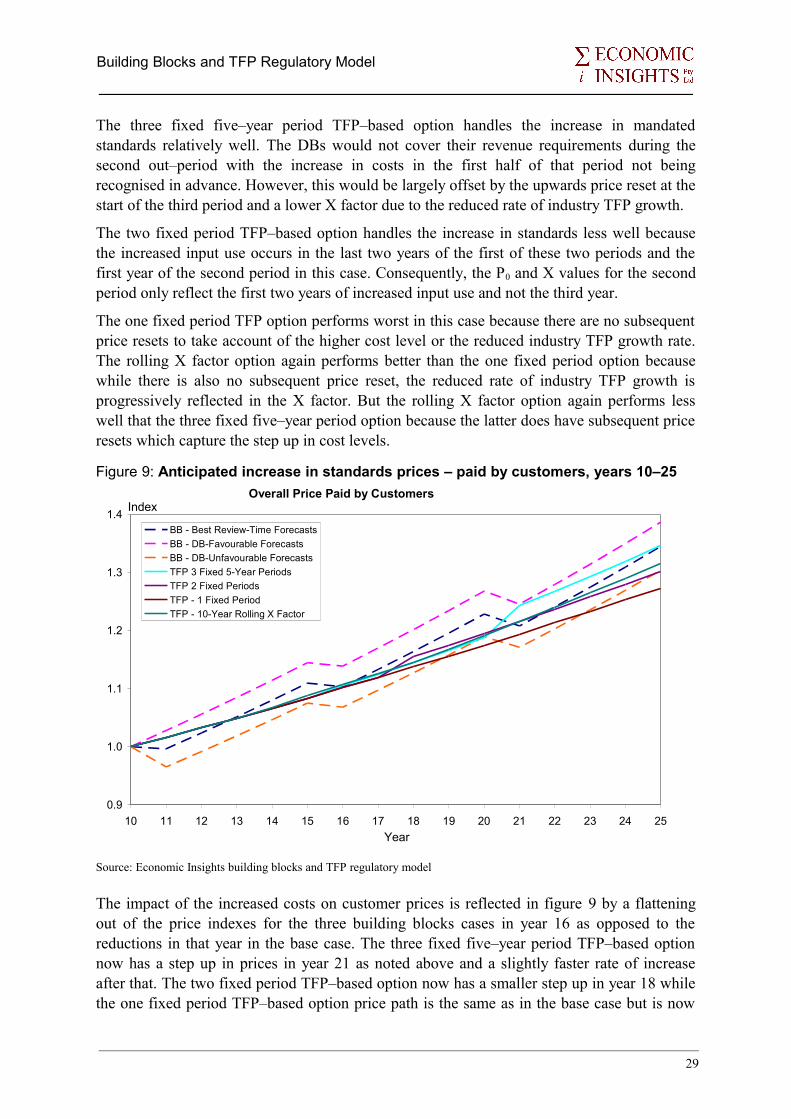
Building Blocks and TFP Regulatory Model
The three fixed five–year period TFP–based option handles the increase in mandated standards relatively well. The DBs would not cover their revenue requirements during the second out–period with the increase in costs in the first half of that period not being recognised in advance. However, this would be largely offset by the upwards price reset at the start of the third period and a lower X factor due to the reduced rate of industry TFP growth.
The two fixed period TFP–based option handles the increase in standards less well because the increased input use occurs in the last two years of the first of these two periods and the first year of the second period in this case. Consequently, the P0 and X values for the second period only reflect the first two years of increased input use and not the third year.
The one fixed period TFP option performs worst in this case because there are no subsequent price resets to take account of the higher cost level or the reduced industry TFP growth rate. The rolling X factor option again performs better than the one fixed period option because while there is also no subsequent price reset, the reduced rate of industry TFP growth is progressively reflected in the X factor. But the rolling X factor option again performs less well that the three fixed five–year period option because the latter does have subsequent price resets which capture the step up in cost levels.
Figure 9: Anticipated increase in standards prices – paid by customers, years 10–25
0.9
1.0
1.1
1.2
1.3
1.4
10 11 12 13 14 15 16 17 18 19 20 21 22 23 24 25
BB - Best Review-Time ForecastsBB - DB-Favourable ForecastsBB - DB-Unfavourable ForecastsTFP 3 Fixed 5-Year PeriodsTFP 2 Fixed PeriodsTFP - 1 Fixed PeriodTFP - 10-Year Rolling X Factor
Index
Year
Overall Price Paid by Customers
Source: Economic Insights building blocks and TFP regulatory model
The impact of the increased costs on customer prices is reflected in figure 9 by a flattening out of the price indexes for the three building blocks cases in year 16 as opposed to the reductions in that year in the base case. The three fixed five–year period TFP–based option now has a step up in prices in year 21 as noted above and a slightly faster rate of increase after that. The two fixed period TFP–based option now has a smaller step up in year 18 while the one fixed period TFP–based option price path is the same as in the base case but is now
29

Building Blocks and TFP Regulatory Model
too low after year 15. The rolling X factor price path now starts to diverge from the one fixed period path from year 17 onwards but at too slow a rate for DBs 1, 2 and 3 to obtain equivalent outcomes to those under the base case. The three fixed five–year period option again performs best of the TFP–based options in this scenario.
4.5 Scenario 3 – anticipated increase in replacement capex
Under scenario 3 there is an anticipated large increase in replacement capex, or a so–called 'wall of wire' effect. This is modelled by capex increasing to three times its previous levels for each of the five years of the first out–period only and then returning to base case levels for all five DBs. Because the capex only replaces existing assets, there is no increase in capital input quantities above base case levels.
Figure 10: Anticipated increase replacement capex profitability indicators, years 11–25
-20%
-15%
-10%
-5%
0%
5%
BB - BestReview-Time
Forecasts
BB - DB-FavourableForecasts
BB - DB-Unfavourable
Forecasts
TFP 3 Fixed5-YearPeriods
TFP 2 FixedPeriods
TFP - 1 FixedPeriod
TFP - 10-Year Rolling
X FactorDB1DB2DB3DB4DB5
Present Value of Excess Returns Relative to Present Value of Revenue Requirement
Source: Economic Insights building blocks and TFP regulatory model
Because the increased replacement capex requirements during the first out–period are anticipated in the building blocks analyses, the profitability outcomes presented in figure 10 are again the same as those in the base case.
For the three fixed five–year period TFP–based option profitability outcomes are very similar to those in the base case. Although the DBs do not get any compensation for their increased capital costs during the first out–period, the price reset at the start of the second out–period recognises the step up in costs and subsequent X factors also allow annual real price increases. This is mainly because of the price differential term in the X factor. Although capital input quantities have not changed relative to the base case, the capital user cost increases substantially with the increase in the RAB associated with the large increase in
30
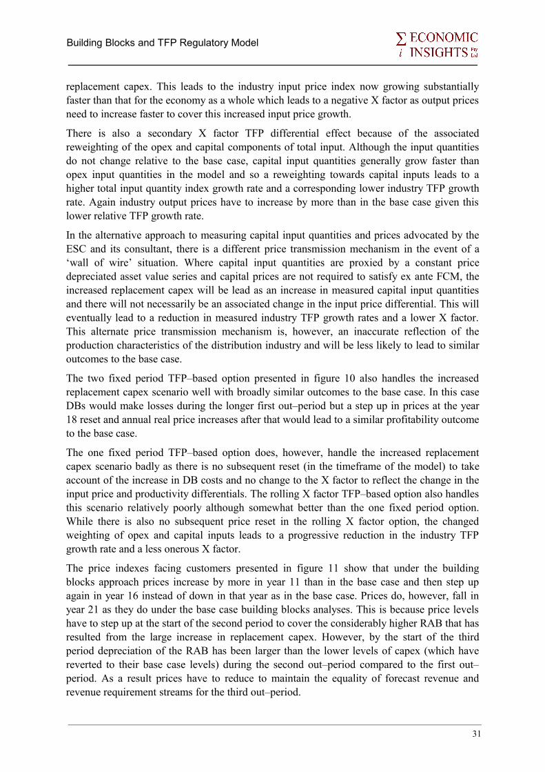
Building Blocks and TFP Regulatory Model
replacement capex. This leads to the industry input price index now growing substantially faster than that for the economy as a whole which leads to a negative X factor as output prices need to increase faster to cover this increased input price growth.
There is also a secondary X factor TFP differential effect because of the associated reweighting of the opex and capital components of total input. Although the input quantities do not change relative to the base case, capital input quantities generally grow faster than opex input quantities in the model and so a reweighting towards capital inputs leads to a higher total input quantity index growth rate and a corresponding lower industry TFP growth rate. Again industry output prices have to increase by more than in the base case given this lower relative TFP growth rate.
In the alternative approach to measuring capital input quantities and prices advocated by the ESC and its consultant, there is a different price transmission mechanism in the event of a ‘wall of wire’ situation. Where capital input quantities are proxied by a constant price depreciated asset value series and capital prices are not required to satisfy ex ante FCM, the increased replacement capex will be lead as an increase in measured capital input quantities and there will not necessarily be an associated change in the input price differential. This will eventually lead to a reduction in measured industry TFP growth rates and a lower X factor. This alternate price transmission mechanism is, however, an inaccurate reflection of the production characteristics of the distribution industry and will be less likely to lead to similar outcomes to the base case.
The two fixed period TFP–based option presented in figure 10 also handles the increased replacement capex scenario well with broadly similar outcomes to the base case. In this case DBs would make losses during the longer first out–period but a step up in prices at the year 18 reset and annual real price increases after that would lead to a similar profitability outcome to the base case.
The one fixed period TFP–based option does, however, handle the increased replacement capex scenario badly as there is no subsequent reset (in the timeframe of the model) to take account of the increase in DB costs and no change to the X factor to reflect the change in the input price and productivity differentials. The rolling X factor TFP–based option also handles this scenario relatively poorly although somewhat better than the one fixed period option. While there is also no subsequent price reset in the rolling X factor option, the changed weighting of opex and capital inputs leads to a progressive reduction in the industry TFP growth rate and a less onerous X factor.
The price indexes facing customers presented in figure 11 show that under the building blocks approach prices increase by more in year 11 than in the base case and then step up again in year 16 instead of down in that year as in the base case. Prices do, however, fall in year 21 as they do under the base case building blocks analyses. This is because price levels have to step up at the start of the second period to cover the considerably higher RAB that has resulted from the large increase in replacement capex. However, by the start of the third period depreciation of the RAB has been larger than the lower levels of capex (which have reverted to their base case levels) during the second out–period compared to the first out–period. As a result prices have to reduce to maintain the equality of forecast revenue and revenue requirement streams for the third out–period.
31
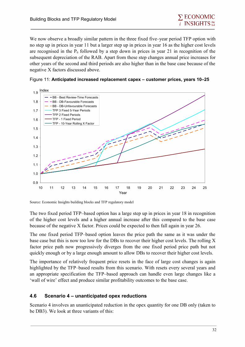
Building Blocks and TFP Regulatory Model
We now observe a broadly similar pattern in the three fixed five–year period TFP option with no step up in prices in year 11 but a larger step up in prices in year 16 as the higher cost levels are recognised in the P0 followed by a step down in prices in year 21 in recognition of the subsequent depreciation of the RAB. Apart from these step changes annual price increases for other years of the second and third periods are also higher than in the base case because of the negative X factors discussed above.
Figure 11: Anticipated increased replacement capex – customer prices, years 10–25
0.9
1.0
1.1
1.2
1.3
1.4
1.5
1.6
1.7
1.8
1.9
10 11 12 13 14 15 16 17 18 19 20 21 22 23 24 25
BB - Best Review-Time ForecastsBB - DB-Favourable ForecastsBB - DB-Unfavourable ForecastsTFP 3 Fixed 5-Year PeriodsTFP 2 Fixed PeriodsTFP - 1 Fixed PeriodTFP - 10-Year Rolling X Factor
Index
Year
Source: Economic Insights building blocks and TFP regulatory model
The two fixed period TFP–based option has a large step up in prices in year 18 in recognition of the higher cost levels and a higher annual increase after this compared to the base case because of the negative X factor. Prices could be expected to then fall again in year 26.
The one fixed period TFP–based option leaves the price path the same as it was under the base case but this is now too low for the DBs to recover their higher cost levels. The rolling X factor price path now progressively diverges from the one fixed period price path but not quickly enough or by a large enough amount to allow DBs to recover their higher cost levels.
The importance of relatively frequent price resets in the face of large cost changes is again highlighted by the TFP–based results from this scenario. With resets every several years and an appropriate specification the TFP–based approach can handle even large changes like a ‘wall of wire’ effect and produce similar profitability outcomes to the base case.
4.6 Scenario 4 – unanticipated opex reductions
Scenario 4 involves an unanticipated reduction in the opex quantity for one DB only (taken to be DB3). We look at three variants of this:
32

Building Blocks and TFP Regulatory Model
• Scenario 4a: a one–off reduction in opex quantity of 10 per cent in year 12;
• Scenario 4b: a recurrent reduction in opex quantity of 10 per cent starting in year 11; and
• Scenario 4c: a reduction in the opex quantity growth rate from 0.81 per cent per annum to 0.2 per cent per annum starting in year 11.
Our primary interest in examining this scenario and the following one involving unanticipated capex reductions is to assess the incentive effects of the alternative regulatory approaches. By examining the retention ratios – the proportion of benefits kept by the DB – across the different regulatory options we are able to assess the relative incentive effects. The higher the retention ratio, the stronger the incentive for the DB to seek out and implement cost savings.
Details of the calculation of the retention ratio were given in section 2.7. The relevant calculations for scenarios 4 and 5 are contained in the separate spreadsheet file ‘Economic Insights AEMC TFP v BB Model Incentive Analysis.xls’. The calculations are not included in the general model file because they only are only relevant to scenarios involving unanticipated input reductions. Retention ratios for the building blocks best review–time forecast case and the four TFP–based options are presented in table 1 for each of the three opex reduction scenarios.
Table 1: Retention ratios for unanticipated opex reductions for DB3, years 11–25
Retention Ratios
One–off opex reduction in year 12 only
Recurrent opex reduction starting
in year 11
Reduced opex growth rate starting
in year 11BB Case 1 – Unanticipated 100% 41% 17%TFP Option 1 – 3 fixed periods 100% 39% 36%TFP Option 2 – 2 fixed periods 100% 51% 52%TFP Option 3 – 1 fixed period 100% 100% 100%TFP Option 4 – Rolling X 84% 88% 91%Source: Economic Insights building blocks and TFP regulatory model
Turning first to scenario 4a involving a one–off reduction in the opex quantity of 10 per cent in year 12 for DB3 only, we see from table 1 that in the building blocks and the three fixed period TFP–based options all of the savings are retained by the DB. In the building blocks case opex savings over and above those forecast at review time are not clawed back at the next review and, because the reduction is one–off, opex levels at the end of the first out–period are the same as in the base case. This means the outcomes in the second and third out–periods are then the same as in the base case. Hence, all of the benefits from the one–off saving are retained by the DB.
A similar outcome applies in the three fixed period TFP–based options. Because the one–off reduction occurs in the second year of the first out–period the TFP growth rates used to calculate the X factors for the second and third out–periods remain the same as in the base case. Because of the use of the endpoint–to–endpoint growth rate method in the model, if the one–off reduction had occurred in either the first or the last year of the regulatory period then future measured TFP growth rates would be affected and there would be a variation from the base case.
33

Building Blocks and TFP Regulatory Model
In the case of the rolling X factor TFP–based option, the endpoint–to–endpoint growth rate method does cause a minor distortion between years 13 and 21. This is because the impact of the opex quantity reduction in year 12 for DB3 is picked up in the industry TFP growth rate in year 13. Even though DB3’s opex quantity returns to its base case level in year 13, the endpoint–to–endpoint growth rate method for year 14 applies the change between years 13 and 4 to the lower index for year 12. The index hence continues at a lower level than in the base case until year 22 when year 12 again becomes an endpoint and this effect is corrected. As a result, DB3 obtains the full extent of its one–off savings in year 12 but then loses part of these over years 13 to 21 as the result of a slightly higher X factor than in the base case. As a result DB3 only retains 84 per cent of its one–off savings in present value terms in the rolling X factor option.
In scenario 4b involving an unanticipated recurrent opex quantity reduction for DB3 starting in year 11, under building blocks DB3 retains 41 per cent of the saving (over the 15 year period). This is because it retains all of the savings in the first out–period but the lower level of opex usage relative to the base case is recognised by the regulator at the time of the review for the second out–period and is built into the building blocks analyses for the second and third out–periods.
Many building blocks schemes include efficiency carry–over mechanisms to allow DBs to keep the benefits of unanticipated opex reductions for a period equal to the length of the regulatory period, regardless of the year during the regulatory period that the saving is achieved. Without such a mechanism DBs would have an incentive to delay implementing additional cost savings to the start of the next regulatory period rather than implement them towards the end of a regulatory period. The model does not explicitly include an efficiency carry–over mechanism but by implementing the opex reduction in year 11 we capture the full extent of potential benefits going to the DB.
A broadly similar result is obtained using the three fixed five–year period TFP–based option. Again the DB keeps the full benefits from its savings during the first out–period but the lower level of opex requirement is recognised in the price rest at the start of the second out–period. In addition the savings for DB3 feed through to a slightly higher industry TFP growth rate used in the second out–period’s X factor.
Around half of the benefits are retained by DB3 in the two fixed period TFP–based option. This is because the DB can keep all of the benefits from a longer first out–period before the price reset recognises the lower level of opex requirement. In this option the reset occurs in year 18 rather than year 16 as in the three fixed five–year period option.
In the one fixed 15–year period TFP–based option all of the benefits are retained by the DB because there is no subsequent price reset or recalculation of the industry TFP growth rate (within the model’s timeframe) to recognise the ongoing cost savings. In the rolling X factor case the DB retains 88 per cent of the benefits because, while there is no subsequent price reset, some of the benefits are passed back to consumers as the savings feed through to a slightly higher industry TFP growth rate and hence a higher X factor than in the base case.
In scenario 4c involving a reduced growth rate of the quantity of opex inputs for DB3 starting year 11 there is a significant difference in the retention ratios of the building blocks and the TFP–based approaches. Under the building blocks approach DB3 only retains 17 per cent of
34
Building Blocks and TFP Regulatory Model
the benefits of the reduced opex quantity growth rate. This is because it retains the full benefit for the first out–period but in the review for the second out–period the regulator recognises both the changed opex level and the changed opex growth rate and these are built into the building blocks analyses for the second and third out–periods. DB3 therefore retains none of the benefits from these later periods. This scenario is similar to that presented in AEMC (2009b, pp.13–15).
By contrast, under the TFP–based approaches DB3 keeps all of the benefits from the first out–period, prices are then reset at the start of the next period to recognise the lower opex level but the changes in prices in the second and subsequent periods are determined by the industry TFP growth rate rather than DB3’s TFP growth rate. Consequently, DB3 retains the benefits from its reduced opex quantity growth rate during each out–period. For the three fixed five–year period TFP–based option DB3 retains 36 per cent of the benefit while it retains over half the benefit for the two fixed period option. It again retains all of the benefit for the one fixed period option and over 90 per cent of the benefit under the rolling X factor option. Again, while there is no subsequent price reset under the rolling X factor option, the small increase in the industry TFP growth rate resulting from DB3’s reduced opex growth rate is progressively built into the rolling X factor.
Figure 12: Unanticipated reduced opex growth profitability indicators, years 11–25
-2.0%
-1.5%
-1.0%
-0.5%
0.0%
0.5%
1.0%
1.5%
2.0%
2.5%
BB - Best Review-Time Forecasts
TFP 3 Fixed 5-Year Periods
TFP 2 FixedPeriods
TFP - 1 FixedPeriod
TFP - 10-YearRolling X Factor
DB1DB2DB3DB4DB5
Present Value of Excess Returns Relative to Present Value of Revenue Requirement
Source: Economic Insights building blocks and TFP regulatory model
The profitability summary indicators from scenario 4c are presented in figure 12. Again these highlight the effect of the higher retention ratios of the TFP–based options compared to the building blocks case where there is a reduced rate of input growth. In all cases the effects on overall customer prices are relatively small compared to the base case.
35

Building Blocks and TFP Regulatory Model
4.7 Scenario 5 – unanticipated capex reductions
Scenario 5 involves an unanticipated reduction in capex for one DB only (again taken to be DB3). Two variants of this scenario are examined:
• Scenario 5a: a one–off reduction in capex of 10 per cent in year 11;
• Scenario 5b: a recurrent reduction in capex of 10 per cent starting in year 11.
There are no changes in capital input quantities in these scenarios. This could, for example, represent the development of new means of extending asset lives thus reducing the need for replacement capex (either for one year or on an ongoing basis, respectively).
We again concentrate on retention ratios to assess the incentive effects of the building blocks and TFP–based regulatory approaches.
Table 2: Retention ratios for unanticipated capex reductions for DB3, years 11–25
Retention RatiosOne–off capex reduction
in year 12 onlyRecurrent capex reduction
starting in year 11BB Case 1 – Unanticipated 37% 12%TFP Option 1 – 3 fixed periods 31% 37%TFP Option 2 – 2 fixed periods 43% 50%TFP Option 3 – 1 fixed period 100% 100%TFP Option 4 – Rolling X 88% 91%Source: Economic Insights building blocks and TFP regulatory model
In contrast to the case of a one–off opex reduction where the change in costs is confined to one year only, a one–off reduction in capex produces a lower RAB in subsequent years and thus lower return on and return of capital components of the annual revenue requirements in subsequent years. With a one–off reduction in capex in year 11, 37 per cent of the benefit is retained by DB3 under the building blocks approach. DB3 retains all of the benefits during the first out–period but at the review for the second out–period the regulator recognises the lower actual capex during the first period in the RAB roll–forward and so DB3 retains none of the benefits in the second and third out–periods.
In the three fixed 5–year period TFP–based option DB3 retains 31 per cent of the benefits. Again it retains all of the benefits during the first out–period. But in this case prices are reset at the start of the second out–period to equate revenues and actual revenue requirements (as at the last year of the first out–period) rather than to equate the forecast net present values of revenue and revenue requirements over the whole second out–period as in building blocks. There will be only a very minor impact on the X factor for the second and later out–periods associated with a consequential change in the industry input price growth rate.
Retention ratios are higher for the longer fixed TFP–based periods with DB3 retaining 43 per cent and 100 per cent under the two period and one period option, respectively. Under the rolling X factor approach a small proportion of benefits are passed onto customers as the changing weights away from capital and towards opex progressively lead to a higher measured TFP growth rate and hence a higher X factor compared to the base case.
36

Building Blocks and TFP Regulatory Model
A major difference in retention ratios emerges in the recurrent reduction in capex scenario. This scenario is effectively similar to scenario 4c where there was a reduction in the opex quantity growth rate. In this case the recurrent percentage drop in capex leads to a reduced rate of growth of the RAB over time – and, hence, of the return of and return on capital annual revenue requirement components. In the building blocks case DB3 retains all of the benefit of this reduced cost over the first out–period but in the review for the second period the regulator recognises this change in both the cost level and the growth rate of costs and builds this into the building blocks analyses. DB3 hence retains none of the (increasing) benefits in the second and subsequent out–periods. DB3 retains only 12 per cent of the total benefits.
Under the three fixed five–year period TFP–based option DB3 retains 37 per cent of the benefit. It again retains all of the benefit for the first out–period and, while prices are reset at the start of the second and subsequent periods, DB3 also retains the in–period increase in benefits for these later periods. Again, the longer the fixed period, the higher retention ratio with DB3 retaining 50 per cent and 100 per cent of the benefits for the two fixed period and one fixed period options, respectively. Again under the rolling X factor option the changing composition of costs and associated weight changes leads to a progressive but small increase in the measured rate of industry TFP growth. This leads to an associated small increase in the X factor leading to customers getting 12 per cent of the benefit under this option.
Overall, the TFP–based options offer far stronger incentives for ongoing capex reductions than does the building blocks approach.
37
Building Blocks and TFP Regulatory Model
5 CONCLUSIONS
The base case spreadsheet model accompanying this report compares outcomes under building blocks and TFP–based regulation under business as usual conditions. It demonstrates that appropriately specified TFP–based regulation gives DBs achieving industry average productivity growth the opportunity to recover their revenue requirement. Those DBs achieving above industry average productivity growth have the opportunity to exceed their revenue requirement. TFP–based regulation will, however, be less attractive to DBs that do not achieve industry average productivity growth rates.
The model demonstrates that relatively small errors in forecasts in building blocks regulation can lead to significant divergences of realised revenue from revenue requirements. Because forecasting errors will inevitably occur in practice, TFP–based regulation is likely to be a somewhat less risky alternative compared to building blocks regulation under normal circumstances. Similarly, when compared over an extended period and under normal circumstances, TFP–based regulation is likely to produce a less volatile price path for customers than building blocks regulation.
The scenarios examined in the accompanying spreadsheet models demonstrate that TFP–based regulation can handle significant changes and adverse shocks relatively well provided there are regular price resets. For example, the three fixed five–year period TFP–based option performs best of the TFP–based options in the scenario involving an anticipated increase in mandated standards. And, with resets every five years and an appropriate specification, the TFP–based approach can handle even large changes like a ‘wall of wire’ effect and produce similar profitability outcomes to the base case.
The model shows that a TFP–based option with rolling X factors and only an initial price reset can build in some ongoing adjustment to changing circumstances but fixed period TFP–based options with regular price resets generally handle large changes better.
The spreadsheet models also compare the incentives for DBs to make cost savings additional to those anticipated at review time. For relatively static changes such as one–off and recurrent opex reductions and one–off capex reductions, building blocks and TFP–based regulatory options of similar regulatory period length provide broadly similar incentives. TFP–based options with longer regulatory periods provide stronger incentives than standard building blocks approaches. All TFP–based options provide substantially stronger incentives than building blocks to reduce rates of input growth. For example, the TFP–based options offer far stronger incentives for ongoing capex reductions than does the building blocks approach.
The accompanying base case spreadsheet model provides a means for interested parties to undertake their own simulations of alternative scenarios by making relevant changes to the cells shaded light blue in the model. To assist users with understanding how to implement alternative scenarios in the base case model, the cells that have been changed to implement the five scenarios examined in this report have been shaded orange in each scenario spreadsheet.
38

Building Blocks and TFP Regulatory Model
APPENDIX 1: THE FISHER TFP INDEX
TFP growth is defined as the proportional change in total output divided by the proportional change in total inputs used between two periods. Mathematically, this is given by:
(A1) )/(/)/( BtBt IIQQTFP =
where Q is total output quantity, I is total input quantity, t refers to year t and B to the base period.
To operationalise equation (A1) we need a way to combine changes in diverse output and input quantities into measures of change in total output quantity and total input quantity. To aggregate these changes in diverse components into a total change, index number methodology essentially takes a weighted average of the changes in the components. Different index number methods form this weighted average change in different ways. Alternative index number methods can be evaluated by examining their economic properties or by assessing their performance relative to a number of axiomatic tests. The index number which performs best against these tests and which is being increasingly favoured by statistical agencies is the Fisher ideal index (Diewert 1993).
Mathematically, the Fisher ideal output quantity index is given by:
(A2) ∑ ∑ ∑ ∑= = = == mi
mj
mi
mj
Bj
tj
ti
ti
Bj
Bj
ti
Bi
tF YPYPYPYPQ 1 1 1 1
5.0)]/)(/[(
where: tFQ is the Fisher ideal output quantity index for observation t;
BiP is the price of the ith output for the base observation;
tiY is the quantity of the ith output for observation t;
tiP is the price of the ith output for observation t; and
BjY is the quantity of the jth output for the base observation.
In this case we have three outputs (so m = 3) and 26 years (so t = 1, …, 26).
Similarly, the Fisher ideal input quantity index is given by:
(A3) ∑ ∑ ∑ ∑= = = == ni
nj
ni
nj
Bj
tj
ti
ti
Bj
Bj
ti
Bi
tF XWXWXWXWI 1 1 1 1
5.0)]/)(/[(
where: tFI is the Fisher ideal input quantity index for observation t;
BiW is the price of the ith input for the base observation;
tiX is the quantity of the ith input for observation t;
tiW is the price of the ith input for observation t; and
BjX is the quantity of the jth input for the base observation.
39

Building Blocks and TFP Regulatory Model
In this case we have four inputs (so n = 4) and 26 years (so t = 1, …, 26).
The Fisher ideal TFP index is then given by:
(A4) tF
tF
tF IQTFP /= .
The Fisher index can be used in either the unchained form denoted above or in the chained form used in this study where weights are more closely matched to pair–wise comparisons of observations. Denoting the Fisher output index between observations i and j by ji
FQ , , the chained Fisher index between observations 1 and t is given by:
(A5) ttFFF
tF QQQQ ,13,22,1,1 ....1 −××××= .
40

Building Blocks and TFP Regulatory Model
REFERENCES
Australian Energy Market Commission (AEMC) (2009a), Review into the use of Total Factor Productivity for the determination of prices and revenues, Design Discussion Paper, Sydney, 28 August.
Australian Energy Market Commission (AEMC) (2009b), Review into the use of Total Factor Productivity for the determination of prices and revenues, Preliminary Findings, Sydney, 17 December.
Australian Energy Regulator (AER) (2008a), Electricity distribution network service providers, Post–tax revenue model, Final Decision, Melbourne, 26 June (spreadsheet revised 19 June 2009).
Australian Energy Regulator (AER) (2008b), Electricity distribution network service providers, Roll forward model, Final Decision, Melbourne, June.
Diewert, W.E. (1993), The Measurement of Productivity: A Survey, Swan Consultants (Canberra) conference on Measuring the Economic Performance of Government Enterprises, Sydney.
Economic Insights (2009a), The theory of network regulation in the presence of sunk costs, Technical Report by Erwin Diewert, Denis Lawrence and John Fallon to the Commerce Commission, Canberra, 8 June.
Economic Insights (2009b), Assessment of Data Currently Available to Support TFP–based Network Regulation, Report by Denis Lawrence and John Kain to the Australian Energy Market Commission, Canberra, 9 June.
Economic Insights (2009c), Energy Network Total Factor Productivity Sensitivity Analysis, Report by Denis Lawrence to the Australian Energy Market Commission, Canberra, 9 June.
Economic Insights (2009d), Total Factor Productivity Index Specification Issues, Report by Denis Lawrence, Erwin Diewert and John Fallon to the Australian Energy Market Commission, Canberra, 7 December.
Essential Services Commission (ESC) (2009), Supplemental submission to the AEMC Review into the use of Total Factor Productivity for the determination of prices and revenues, Melbourne, May.
Lawrence, Denis (2003), Regulation of Electricity Lines Businesses, Analysis of Lines Business Performance – 1996–2003, Report by Meyrick and Associates for the New Zealand Commerce Commission, 19 December, Canberra.
41
Related Documents