A fast nonstationary iterative method with convex penalty ...jinq/Jin_Lu_2013.pdf · E-mail: [email protected] and [email protected] Abstract. In this paper we consider the

A fast nonstationary iterative method with convexpenalty for inverse problems in Hilbert spaces

Qinian Jin1 and Xiliang Lu2

1Mathematical Sciences Institute, Australian National University, Canberra,ACT 0200, Australia2School of Mathematics and Statistics, Wuhan University, Wuhan 430072, China

E-mail: [email protected] and [email protected]

Abstract. In this paper we consider the computation of approximate solutionsfor inverse problems in Hilbert spaces. In order to capture the special featureof solutions, non-smooth convex functions are introduced as penalty terms. Byexploiting the Hilbert space structure of the underlying problems, we propose afast iterative regularization method which reduces to the classical nonstationaryiterated Tikhonov regularization when the penalty term is chosen to be the squareof norm. Each iteration of the method consists of two steps: the first step involvesonly the operator from the problem while the second step involves only the penaltyterm. This splitting character has the advantage of making the computationefficient. In case the data is corrupted by noise, a stopping rule is proposed toterminate the method and the corresponding regularization property is established.Finally, we test the performance of the method by reporting various numericalsimulations, including the image deblurring, the determination of source term inPoisson equation, and the de-autoconvolution problem.

1. Introduction

We consider the ill-posed inverse problems of the form

Ax = y, (1.1)

where A : X → Y is a bounded linear operator between two Hilbert spaces X and Ywhose inner products and the induced norms are denoted as 〈·, ·〉 and ‖ · ‖ respectivelywhich should be clear from the context. Here the ill-posedness of (1.1) refers to thefact that the solution of (1.1) does not depend continuously on the data which is acharacteristic property of inverse problems. In practical applications, one never hasexact data, instead only noisy data are available due to errors in the measurements.Even if the deviation is very small, algorithms developed for well-posed problemsmay fail, since noise could be amplified by an arbitrarily large factor. Therefore,regularization methods should be used in order to obtain a stable numerical solution.One can refer to [7] for many useful regularization methods for solving (1.1); thesemethods, however, have the tendency to over-smooth solutions and hence are not quitesuccessful to capture special features.

In case a priori information on the feature of the solution of (1.1) is available, wemay introduce a proper, lower semi-continuous, convex function Θ : X → (−∞,∞] suchthat the sought solution of (1.1) is in D(Θ) = x ∈ X : Θ(x) <∞. By taking x0 ∈ X

2

and ξ0 ∈ ∂Θ(x0), the solution of (1.1) with the desired feature can be determined bysolving the constrained minimization problem

minDξ0Θ(x, x0) subject to Ax = y, (1.2)

where Dξ0Θ(x, x0) denotes the Bregman distance induced by Θ at x0 in the directionξ0, i.e.

Dξ0Θ(x, x0) = Θ(x)−Θ(x0)− 〈ξ0, x− x0〉.When only a noisy data yδ is available, an approximate solution can be constructed bythe Tikhonov-type method

xδα := arg minx∈X

‖Ax− yδ‖2 + αDξ0Θ(x, x0)

. (1.3)

When the regularization parameter α is given, many efficient solvers were developedto compute xδα when Θ is the L1 or the total variation function. Unfortunately almostall these methods do not address the choice of α which, however, is important forpractical applications. In order to use these solvers, one has to perform the trial-and-error procedure to find a reasonable α which is time consuming. On the other hand,some iterative methods, equipping with proper termination criteria, were developedto find approximate solutions of (1.2), see [16] and references therein. These iterativemethods have the advantage of avoiding the difficulty for choosing the regularizationparameter. However in each iteration step one has to solve a minimization problemsimilar to (1.3), and overall it may take long time.

In this paper we will propose a fast iterative regularization methods for solving(1.2) by splitting A and Θ into different steps. Our idea is to exploit the Hilbert spacestructure of the underlying problem to build each iterate by first applying one stepof a well-established classical regularization method and then penalizing the resultantby the convex function Θ. To motivate the method, we consider the exact data case.We take an invertible bounded linear operator M : Y → Y which can be viewed as apreconditioner and rewrite (1.2) into the equivalent form

minDξ0Θ(x, x0) subject to MAx = My.

The corresponding Lagrangian is

L(x, p) := Dξ0Θ(x, x0) + 〈p,My −MAx〉,where p ∈ Y represents the dual variable. Then a desired solution of (1.2) can be foundby determining a saddle point of L if exists. Let (xc, pc) be a current guess of a saddlepoint of L, we may update it to get a new guess (x+, p+) as follows: We first updatepc by solving the proximal maximization problem

p+ := arg maxp∈X

L(xc, p)−

1

2t‖p− pc‖2

with a suitable step length t > 0. We then update xc by solving the minimizationproblem

x+ := arg minx∈XL(x, p+).

By straightforward calculation and simplification it follows

p+ = pc − tM(Axc − y),

x+ = arg minx∈XΘ(x)− 〈ξ0 +A∗M∗p+, x〉

3

which is the one step result of the Uzawa algorithm [1] or the dual subgradient method[22], where A∗ : Y → X and M∗ : Y → Y denote the adjoint operators of A and Mrespectively. By setting ξc = ξ0 +A∗M∗pc and ξ+ = ξ0 +A∗M∗p+, the above equationcan be transformed into the form

ξ+ = ξc − tA∗M∗M(Axc − y),x+ = arg minx∈X Θ(x)− 〈ξ+, x〉 .

(1.4)

Now we may apply the updating scheme (1.4) to Ax = y iteratively but withdynamic preconditioning operator Mn : Y → Y and variable step size tn > 0. Thisgives rise to the following iterative methods

ξn+1 = ξn − tnA∗M∗nMn(Axn − y),xn+1 = arg minx∈X Θ(x)− 〈ξn+1, x〉 .

(1.5)

The performance of the method (1.5) depends on the choices of Mn. If we takeMn = I for all n, (1.5) becomes the method that has been studied in [4, 15] whichis the generalization of the classical Landweber iteration and is known to be a slowlyconvergent method.

In this paper we will consider (1.6) with Mn = (αnI + AA∗)−1/2 for all n, whereαn is a decreasing sequence of positive numbers. This yields the nonstationaryiterative method

ξn+1 = ξn − tnA∗(αnI +AA∗)−1(Axn − y),xn+1 = arg minx∈X Θ(x)− 〈ξn+1, x〉 .

(1.6)

Observing that when Θ(x) = ‖x‖2/2 and tn = 1 for all n, (1.6) reduces to thenonstationary iterated Tikhonov regularization

xn+1 = xn −A∗(αnI +AA∗)−1(Axn − y) (1.7)

whose convergence has been studied in [10] and it has been shown to be a fast convergentmethod when αn is a geometric decreasing sequence. This strongly suggests that ourmethod (1.6) may also exhibit fast convergence property if αn and tn are chosenproperly. We will confirm this in the present paper. It is worthy to point out that eachiteration in (1.6) consists of two steps: the first step involves only the operator A andthe second step involves only the convex function Θ. This splitting character can makethe computation much easier.

This paper is organized as follows. In section 2, we start with some preliminaryfacts from convex analysis, and then give the convergence analysis of the method (1.6)when the data is given exactly. In case the data is corrupted by noise, we proposea stopping rule to terminate the iteration and establish the regularization property.We also give a possible extension of our method to solve nonlinear inverse problemsin Hilbert spaces. In section 3 we test the performance of our method by reportingvarious numerical simulations, including the image deblurring, the determination ofsource term in Poisson equation and the de-autoconvolution problem.

2. Convergence analysis of the method

In this section we first give the convergence analysis of (1.6) with suitable chosen tnwhen Θ : X → (−∞,∞] is a proper, lower semi-continuous function that is stronglyconvex in the sense that there is a constant c0 > 0 such that

Θ(sx+ (1− s)x) + c0s(1− s)‖x− x‖2 ≤ sΘ(x) + (1− s)Θ(x) (2.1)

4

for all 0 ≤ s ≤ 1 and x, x ∈ X . We then consider the method when the data containsnoise and propose a stopping rule to render it into a regularization method. Ouranalysis is based on some important results from convex analysis which will be recalledin the following subsection.

2.1. Tools from convex analysis

Given a convex function Θ : X → (−∞,∞], we will use D(Θ) := x ∈ X ,Θ(x) < ∞to denote its effective domain. It is called proper if D(Θ) 6= ∅. Given x ∈ X , the set

∂Θ(x) := ξ ∈ X : Θ(x)−Θ(x)− 〈ξ, x− x〉 ≥ 0 for all x ∈ Xis called the subdifferential of Θ at x and each element ξ ∈ ∂Θ(x) is called a subgradient.

Our convergence analysis of (1.6) will not be carried out directly under the normof X . Instead we will use the Bregman distance ([5]) induced by Θ. Given ξ ∈ ∂Θ(x),the quantity

DξΘ(x, x) := Θ(x)−Θ(x)− 〈ξ, x− x〉, x ∈ Xis called the Bregman distance induced by Θ at x in the direction ξ. It is clear thatDξΘ(x, x) ≥ 0. However, Bregman distance is not a metric distance since it does notsatisfy the symmetry and the triangle inequality in general. Nevertheless, when Θ isstrongly convex in the sense of (2.1), there holds ([23])

DξΘ(x, x) ≥ c0‖x− x‖2, ∀x ∈ X and ξ ∈ ∂Θ(x)

which means that the Bregman distance can be used to detect information under thenorm of X .

Although Θ could be non-smooth, its Fenchel conjugate can have enough regularityprovided Θ has enough convexity. The Fenchel conjugate of Θ is defined by

Θ∗(ξ) := supx∈X〈ξ, x〉 −Θ(x) , ∀ξ ∈ X .

For a proper, lower semi-continuous, convex function Θ, there always holds

ξ ∈ ∂Θ(x)⇐⇒ x ∈ ∂Θ∗(ξ)⇐⇒ Θ(x) + Θ∗(ξ) = 〈ξ, x〉.Consequently, the Bregman distance can be equivalently written as

DξΘ(x, x) = Θ(x) + Θ∗(ξ)− 〈ξ, x〉. (2.2)

If in addition Θ is strongly convex in the sense of (2.1), then D(Θ∗) = X , Θ∗ is Frechetdifferentiable, and its gradient ∇Θ∗ satisfies

‖∇Θ∗(ξ)−∇Θ∗(η)‖ ≤ ‖ξ − η‖2c0

, (2.3)

i.e. ∇Θ∗ is Lipschitz continuous. These facts are crucial in the forthcoming convergenceanalysis and their proofs can be found in many standard textbooks, cf. [23].

2.2. The method with exact data

We consider the convergence of the method (1.6) under the condition that Θ is proper,lower semi-continuous, and strongly convex in the sense of (2.1). We will always assumethat (1.1) has a solution in D(Θ). By taking ξ0 ∈ X and define

x0 = arg minx∈XΘ(x)− 〈ξ0, x〉

5

as an initial guess, we define x† to be the solution of (1.1) in D(Θ) satisfying

Dξ0Θ(x†, x0) = min Dξ0Θ(x, x0) : Ax = y . (2.4)

It is easy to show that such x† is uniquely defined. Our aim is to show that the sequencexn produced by (1.6) eventually converges to x† if tn is chosen properly.

To this end, we first consider the monotonicity of the Bregman distanceDξnΘ(x, xn) with respect to n for any solution x of (1.1) in D(Θ). By the subdifferentialcalculus and the definition of xn, it is easy to see that ξn ∈ ∂Θ(xn) and hencexn = ∇Θ∗(ξn). Therefore, in view of (2.2) and (2.3) we have

Dξn+1Θ(x, xn+1)−DξnΘ(x, xn) = Θ∗(ξn+1)−Θ∗(ξn)− 〈ξn+1 − ξn, x〉

= Θ∗(ξn+1)−Θ∗(ξn)− 〈ξn+1 − ξn,∇Θ∗(ξn)〉 − 〈ξn+1 − ξn, x− xn〉

=

∫ 1

0

〈ξn+1 − ξn,∇Θ∗(ξn + s(ξn+1 − ξn))−∇Θ∗(ξn)〉ds

−〈ξn+1 − ξn, x− xn〉

≤∫ 1

0

1

2c0s‖ξn+1 − ξn‖2ds− 〈ξn+1 − ξn, x− xn〉

=1

4c0‖ξn+1 − ξn‖2 − 〈ξn+1 − ξn, x− xn〉.

Using the definition of ξn+1 in (1.6) and Ax = y we obtain

Dξn+1Θ(x, xn+1)−DξnΘ(x, xn) ≤ 1

4c0t2n‖A∗(αnI +AA∗)−1(Axn − y)‖2

− tn〈(αnI +AA∗)−1(Axn − y), Axn − y〉.If Axn − y 6= 0, we may choose tn such that

tn =µ0〈(αnI +AA∗)−1(Axn − y), Axn − y〉‖A∗(αnI +AA∗)−1(Axn − y)‖2

(2.5)

with 0 < µ0 < 4c0, then it yields

Dξn+1Θ(x, xn+1)−DξnΘ(x, xn)

≤ −(

1− µ0

4c0

)tn‖(αnI +AA∗)−1/2(Axn − y)‖2 ≤ 0. (2.6)

When Axn − y = 0, the inequality (2.6) obviously holds for any tn ≥ 0. We observethat the tn chosen by (2.5) could be very large when ‖Axn − y‖ is small. Using sucha choice of tn it could make the method numerically unstable, in particular when thedata contains noise. To avoid this, we take a preassigned number µ1 > 0 and then set

tn = min

µ0〈(αnI +AA∗)−1(Axn − y), Axn − y〉‖A∗(αnI +AA∗)−1(Axn − y)‖2

, µ1

. (2.7)

The above argument then shows the following monotonicity result.

Lemma 2.1 If tn is chosen by (2.7) with 0 < µ0 < 4c0 and µ1 > 0, then

Dξn+1Θ(x, xn+1) ≤ DξnΘ(x, xn)

and

c1tn‖(αnI +AA∗)−1/2(Axn − y)‖2 ≤ DξnΘ(x, xn)−Dξn+1Θ(x, xn+1) (2.8)

for any solution x of (1.1) in D(Θ), where c1 := 1− µ0/(4c0).

6

We will use Lemma 2.1 to derive the convergence of the method (1.6). For thestep size tn defined by (2.7), it is easy to see that

minµ0, µ1 ≤ tn ≤ µ1,

where we used the inequality ‖A∗(αnI + AA∗)−1/2‖ ≤ 1 to derive the left inequality.This together with (2.8) implies

limn→∞

‖(αnI +AA∗)−1/2(Axn − y)‖ = 0. (2.9)

Since ‖(αnI +AA∗)1/2‖ ≤√α0 + ‖A‖2, we can further derive that

limn→∞

‖Axn − y‖ = 0. (2.10)

The following main result shows that the method (1.6) is indeed convergent if tnis chosen by (2.7).

Theorem 2.2 Let Θ : X → (−∞,∞] be a a proper, lower semi-continuous functionthat is strongly convex in the sense of (2.1). If αn is a decreasing sequence of positivenumbers and if tn is chosen by (2.7) with 0 < µ0 < 4c0 and µ1 > 0, then for the method(1.6) there hold

limn→∞

‖xn − x†‖ = 0 and limn→∞

DξnΘ(x†, xn) = 0.

The proof is based on the following useful result.

Proposition 2.3 Consider the equation (1.1). Let Θ : X → (−∞,∞] be a proper,lower semi-continuous and strong convex function. Let xn ⊂ X and ξn ⊂ X besuch that

(i) ξn ∈ ∂Θ(xn) for all n;

(ii) for any solution x of (1.1) in D(Θ) the sequence DξnΘ(x, xn) is monotonicallydecreasing;

(iii) limn→∞ ‖Axn − y‖ = 0.

(iv) there is a subsequence nk with nk →∞ such that for any solution x of (1.1) inD(Θ) there holds

liml→∞

supk≥l|〈ξnk − ξnl , xnk − x〉| = 0. (2.11)

Then there exists a solution x∗ of (1.1) in D(Θ) such that

limn→∞

DξnΘ(x∗, xn) = 0.

If, in addition, ξn+1 − ξn ∈ R(A∗) for all n, then x∗ = x†.

Proof. This is a slight modification of [15, Proposition 3.6], we include here theproof for completeness.

We first show the convergence of xnk. For any l < k we have from the definitionof Bregman distance that

DξnlΘ(xnk , xnl) = Dξnl

Θ(x, xnl)−DξnkΘ(x, xnk) + 〈ξnk − ξnl , xnk − x〉. (2.12)

By the monotonicity of DξnΘ(x, xn) and (2.11) we obtain that DξnlΘ(xnk , xnl)→ 0

as k, l → ∞. In view of the strong convexity of Θ, it follows that xnk is a Cauchysequence in X . Thus xnk → x∗ for some x∗ ∈ X . Since limn→∞ ‖Axn − y‖ = 0, wehave Ax∗ = y.

7

In order to show x∗ ∈ D(Θ), we use ξnk ∈ ∂Θ(xnk) to obtain

Θ(xnk) ≤ Θ(x) + 〈ξnk , xnk − x〉. (2.13)

In view of (2.11) and xnk → x∗ as k →∞, there is a constant C0 such that

|〈ξnk − ξn0, xnk − x〉| ≤ C0 and |〈ξn0

, xnk − x〉| ≤ C0, ∀k.Therefore |〈ξnk , xnk − x〉| ≤ 2C0 for all k. By using the lower semi-continuity of Θ weobtain

Θ(x∗) ≤ lim infk→∞

Θ(xnk) ≤ Θ(x) + 2C0 <∞.

This implies that x∗ ∈ D(Θ).Next we derive the convergence in Bregman distance. Since DξnΘ(x∗, xn) is

monotonically decreasing, the limit ε0 := limn→∞DξnΘ(x∗, xn) ≥ 0 exists. By takingk →∞ in (2.12) with x = x∗ and using the lower semi-continuous of Θ, we obtain

DξnlΘ(x∗, xnl) ≤ Dξnl

Θ(x∗, xnl)− ε0 + supk≥l|〈ξnk − ξnl , xnk − x∗〉|

which is true for all l. Letting l → ∞ and using (2.11) gives ε0 ≤ ε0 − ε0 = 0. Thusε0 = 0, i.e. limn→∞DξnΘ(x∗, xn) = 0.

Finally we show that x∗ = x†. We use (2.13) with x replaced by x† to obtain

Dξ0Θ(xnk , x0) ≤ Dξ0Θ(x†, x0) + 〈ξnk − ξ0, xnk − x†〉. (2.14)

Because of (2.11), for any ε > 0 we can find k0 such that∣∣〈ξnk − ξnk0 , xnk − x†〉∣∣ < ε/2, ∀k ≥ k0.

We next consider 〈ξnk0 − ξ0, xnk − x†〉. Since ξn+1 − ξn ∈ R(A∗), we can find v ∈ Y

such that ξnk0 − ξ0 = A∗v. Consequently

|〈ξnk0 − ξ0, xnk − x†〉| = |〈v,Axnk − y〉| ≤ ‖v‖‖Axnk − y‖.

Since ‖Axn − y‖ → 0 as n→∞, we can find k1 ≥ k0 such that

|〈ξnk0 − ξ0, xnk − x†〉| < ε/2, ∀k ≥ k1.

Therefore |〈ξnk − ξ0, xnk − x†〉| < ε for all k ≥ k1. Since ε > 0 is arbitrary, we obtainlimk→∞〈ξnk − ξ0, xnk − x†〉 = 0. By taking k →∞ in (2.14) and using the lower semi-continuity of Θ we obtain Dξ0Θ(x∗, x0) ≤ Dξ0Θ(x†, x0). According to the definitionof x† we must have Dξ0Θ(x∗, x0) = Dξ0Θ(x†, x0). By uniqueness it follows x∗ = x†.

Proof of Theorem 2.2. We will use Proposition 2.3 to complete the proof. By thedefinition of ξn we always have ξn+1 − ξn ∈ R(A∗). It remains to verify the fourconditions in Proposition 2.3. By the definition of xn we have ξn ∈ ∂Θ(xn) whichimplies (i) in Proposition 2.3. Moreover, Lemma 2.1 and (2.10) confirm (ii) and (iii)in Proposition 2.3 respectively.

It remains only to verify (iv) in Proposition 2.3. To this end, we consider

Rn := ‖(αnI +AA∗)−1/2(Axn − y)‖.In view of (2.9), we have limn→∞Rn = 0. Moreover, by the definition of the method(1.6), if Rn = 0 for some n, then Rm = 0 for all m ≥ n. Consequently, we may choosea strictly increasing subsequence nk of integers such that n0 = 0 and nk, for eachk ≥ 1, is the first integer satisfying

nk ≥ nk−1 + 1 and Rnk ≤ Rnk−1.

8

For this chosen nk it is easy to see that

Rn ≥ Rnk , ∀0 ≤ n ≤ nk. (2.15)

Inddeed, for 0 ≤ n < nk, we can find 0 ≤ l < k such that nl ≤ n < nl+1 and thus, bythe definition of nl+1, we have Rn ≥ Rnl ≥ Rnk . With the above chosen nk, we willshow that (2.11) holds for any solution x of (1.1) in D(Θ). By the definition of ξn wehave for l < k that

〈ξnl − ξnk , x− xnk〉 =

nk−1∑n=nl

〈ξn+1 − ξn, xnk − x〉

= −nk−1∑n=nl

tn〈(αnI +AA∗)−1(Axn − y), Axnk − y〉.

Therefore

|〈ξnl − ξnk , x− xnk〉|

≤nk−1∑n=nl

tn‖(αnI +AA∗)−1/2(Axn − y)‖‖(αnI +AA∗)−1/2(Axnk − y)‖.

By using the monotonicity of αn and (2.15), we have for 0 ≤ n ≤ nk that

‖(αnI +AA∗)−1/2(Axnk − y)‖ ≤ ‖(αnkI +AA∗)−1/2(Axnk − y)‖ = Rnk ≤ Rn.Consequently, it follows from (2.8) that

|〈ξnl − ξnk , x− xnk〉| ≤nk−1∑n=nl

tnR2n ≤

1

c1

(Dξnl

Θ(x, xnl)−DξnkΘ(x, xnk)

)which, together with the monotonicity of DξnΘ(x, xn), implies (2.11). The proof istherefore complete.

2.3. The method with noisy data

We next consider the situation that the data contains noise. Thus, instead of y, weonly have noisy data yδ satisfying

‖yδ − y‖ ≤ δwith a small known noise level δ > 0. The corresponding method takes the form

ξδn+1 = ξδn − tδnA∗(αnI +AA∗)−1(Axδn − yδ),xδn+1 = arg minx∈X

Θ(x)− 〈ξδn+1, x〉

(2.16)

with suitably chosen step length tδn > 0, where ξδ0 := ξ0 and xδ0 := x0. In order toterminate the method, we need some stopping criterion. It seems that a natural one isthe discrepancy principle

‖Axδnδ − yδ‖ ≤ τδ < ‖Axδn − yδ‖, 0 ≤ n < nδ (2.17)

for some number τ > 1. Unfortunately, we can not prove the regularizationproperty for the method terminated by the discrepancy principle; furthermore,numerical simulations indicate that the discrepancy principle might not always producesatisfactory reconstruction result. Therefore, the discrepancy principle might not bea natural rule to terminate (2.16). Recall that when we motivate our method, weconsider the preconditioned equation

(αnI +AA∗)−1/2Ax = (αnI +AA∗)−1/2y

9

instead of Ax = y. This indicates that it might be natural to stop the iteration as longas

‖(αnI +AA∗)−1/2(Axδn − yδ)‖ ≤ τ‖(αnI +AA∗)−1/2(y − yδ)‖ (2.18)

is satisfied for the first time. The stopping rule (2.18) can be viewed as the discrepancyprinciple applied to the preconditioned equation. Since the right hand side of(2.18) involves y which is not available, it can not be used in practical applications.Considering ‖(αnI+AA∗)−1/2‖ ≤ 1/

√αn, we may replace the right hand side of (2.18)

by τδ/√αn which leads to the following stopping rule.

Rule 2.1 Let τ > 1 be a given number. We define nδ to be the first integer such that

αnδ〈(αnδI +AA∗)−1(Axδnδ − yδ), Axδnδ − y

δ〉 ≤ τ2δ2.

In the context of Tikhonov regularization for linear ill-posed inverse problems, asimilar rule was proposed in [19, 9] to choose the regularization parameter. The rule wasthen generalized and analyzed in [21, 14] for nonlinear Tikhonov regularization and wasfurther extended in [12] as a stopping rule for the iteratively regularized Gauss-Newtonmethod for solving nonlinear inverse problems in Hilbert spaces.

Combining Rule 2.1 with (2.16) and using suitable choice of the step length tδn ityields the following algorithm.

Algorithm 2.1 (Nonstationary iterative method with convex penalty)

(i) Take τ > 1, µ0 > 0, µ1 > 0 and a decreasing sequence αn of positive numbers;

(ii) Take ξ0 ∈ X and define x0 := arg minx∈X Θ(x)− 〈ξ0, x〉 as an initial guess;

(iii) For each n = 0, 1, · · · define ξδn+1 and xδn+1 by (2.16), where

tδn = min

µ0〈(αnI +AA∗)−1(Axδn − yδ), Axδn − yδ〉‖A∗(αnI +AA∗)−1(Axδn − yδ)‖2

, µ1

(2.19)

(iv) Let nδ be the integer determined by Rule 2.1 and use xδnδ as an approximatesolution.

The following lemma shows that Algorithm 2.1 is well defined and certainmonotonicity result holds along the iteration if µ0 > 0 is suitably small.

Lemma 2.4 Let Θ : X → (−∞,∞] be a a proper, lower semi-continuous function thatis strongly convex in the sense of (2.1). If αn is a decreasing sequence of positivenumbers and tδn is chosen by (2.19) with 0 < µ0 < 4c0(1− 1/τ) and µ1 > 0, then Rule2.1 defines a finite integer nδ. Moreover, if nδ ≥ 1, then for the sequences ξδn andxδn defined by (2.16) there holds

Dξδn+1Θ(x, xδn+1) ≤ Dξδn

Θ(x, xδn), 0 ≤ n < nδ (2.20)

for any solution x of (1.1) in D(Θ).

Proof. Let 0 ≤ n < nδ. By using the similar argument in the proof of Lemma2.1 we can obtain

Dξδn+1Θ(x, xδn+1)−Dξδn

Θ(x, xδn) ≤ 1

4c0‖ξδn+1 − ξδn‖2 − 〈ξδn+1 − ξδn, x− xδn〉

=1

4c0(tδn)2‖A∗(αnI +AA∗)−1(Axδn − yδ)‖2

− tδn〈(αnI +AA∗)−1(Axδn − yδ), Axδn − y〉.

10

In view of ‖yδ − y‖ ≤ δ and the choice of tδn, it follows that

Dξδn+1Θ(x, xδn+1)−Dξδn

Θ(x, xδn) ≤ −(

1− µ0

4c0

)tδn‖(αnI +AA∗)−1/2(Axδn − yδ)‖2

+ tδn‖(αnI +AA∗)−1/2(Axδn − yδ)‖δ√αn

.

By the definition of nδ and n < nδ we have

δ√αn≤ 1

τ‖(αnI +AA∗)−1/2(Axδn − yδ)‖. (2.21)

Therefore, we have with c2 := 1− 1/τ − µ0/(4c0) > 0 that

Dξδn+1Θ(x, xδn+1)−Dξδn

Θ(x, xδn) ≤ −c2tδn‖(αnI +AA∗)−1/2(Axδn − yδ)‖2 ≤ 0.

This shows the monotonicity result (2.20) and

c2tδn‖(αnI +AA∗)−1/2(Axδn − yδ)‖2 ≤ Dξδn

Θ(x, xδn)−Dξδn+1Θ(x, xδn+1)

for all 0 ≤ n < nδ. We may sum the above inequality over n from n = 0 to n = m forany m < nδ to get

c2

m∑n=0

tδn‖(αnI +AA∗)−1/2(Axδn − yδ)‖2 ≤ Dξ0Θ(x, x0).

By the choice of tδn it is easy to check that tδn ≥ minµ0, µ1. Therefore, in view of(2.21), we have

c2 minµ0, µ1τ2δ2m∑n=0

1

αn≤ Dξ0Θ(x, x0) (2.22)

for all m < nδ. Since αn ≤ α0 for all n, it follows from (2.22) that nδ <∞. The proofis therefore complete.

Remark 2.1 By taking m = nδ − 1 in (2.22), the integer nδ defined by Rule 2.1 canbe estimated by

c3δ2nδ−1∑n=0

1

αn≤ Dξ0Θ(x, x0), (2.23)

where c3 := c2 minµ0, µ1τ2. In case αn is chosen such that αn+1/αn ≤ q for all nfor some constant 0 < q < 1, then

nδ−1∑n=0

1

αn≥ 1

α0

nδ−1∑n=0

q−n =1− qnδ

α0(1− q)qnδ−1≥ 1

α0qnδ−1.

It then follows from (2.23) that c3α−10 δ2q−nδ+1 ≤ Dξ0Θ(x, x0) which implies that

nδ = O(1 + | log δ|). Therefore, with such a chosen αn, Algorithm 2.1 exhibits thefast convergence property.

In order to use the results given in Lemma 2.4 and Theorem 2.2 to prove theconvergence of the method (2.16), we need the following stability result.

Lemma 2.5 Let ξn and xn be defined by (1.6) with tn chosen by (2.7), and letξδn and xδn be defined by (2.16) with tδn chosen by (2.19). Then for each fixedinteger n there hold

limδ→0‖xδn − xn‖ = 0 and lim

δ→0‖ξδn − ξn‖ = 0.

11

Proof. We prove the result by induction on n. It is trivial when n = 0 becauseξδ0 = ξ0 and xδ0 = x0. Assume next that the result is true for some n ≥ 0. We willshow that ξδn+1 → ξn+1 and xδn+1 → xn+1 as δ → 0. We consider two cases:

Case 1: Axn 6= y. In this case we must have A∗(αnI+AA∗)−1(Axn−y) 6= 0 sinceotherwise

0 = 〈A∗(αnI +AA∗)−1(Axn − y), xn − x†〉 = ‖(αnI +AA∗)−1/2(Axn − y)‖2 > 0.

Therefore, by the induction hypothesis it is straightforward to see that tδn → tn asδ → 0. According to the definition of ξδn+1 and the induction hypothesis, we thenobtain limδ→0 ‖ξδn+1 − ξn+1‖ = 0. Recall that

xn+1 = ∇Θ∗(ξn+1) and xδn+1 = ∇Θ∗(ξδn+1).

We then obtain limδ→0 ‖xδn+1 − xn+1‖ = 0 by the continuity of ∇Θ∗.Case 2: Axn = y. In this case we have ξn+1 = ξn. Therefore

ξδn+1 − ξn+1 = ξδn − ξn − tδnA∗(αnI +AA∗)−1(Axδn − yδ).Consequently, by the induction hypothesis, we have

lim supδ→0

‖ξδn+1 − ξn+1‖ ≤ lim supδ→0

(‖ξδn − ξn‖+

µ1√αn‖Axδn − yδ‖

)=

µ1√αn‖Axn − y‖ = 0.

By using again the continuity of ∇Θ∗, we obtain limδ→0 ‖xδn+1 − xn+1‖ = 0.

We are now in a position to give the main result concerning the regularizationproperty of the method (2.16) with noisy data when it is terminated by Rule 2.1.

Theorem 2.6 Let Θ : X → (−∞,∞] be proper, lower semi-continuous and strongconvex in the sense of (2.1). Let αn be a decreasing sequence of positive numbersand let tδn be chosen by (2.19) with 0 < µ0 < 4c0(1− 1/τ) and µ1 > 0. Let nδ be thefinite integer defined by Rule 2.1. Then for the method (2.16) there hold

limδ→0‖xδnδ − x

†‖ = 0 and limδ→0

DξδnδΘ(x†, xδnδ) = 0.

Proof. Due to the strong convexity of Θ, it suffices to show thatlimδ→0Dξδnδ

Θ(x†, xδnδ) = 0. By the subsequence-subsequence argument, we may

complete the proof by considering two cases.Assume first that yδk is a sequence satisfying ‖yδk − y‖ ≤ δk with δk → 0 such

that nk := nδk → n as k → ∞ for some finite integer n. We may assume nk = n forall k. From the definition of n := nk we have

√αn‖(αnI +AA∗)−1/2(Axδkn )− yδk)‖ ≤ τδk. (2.24)

By taking k → ∞ and using Lemma 2.5, we can obtain Axn = y. In view of thedefinition of ξn and xn, this implies that ξn = ξn and xn = xn for all n ≥ n. SinceTheorem 2.2 implies that xn → x† as n → ∞, we must have xn = x†. Moreover, byLemma 2.5, ξδknk → ξn as k →∞. Therefore, by the continuity of Θ∗ we can obtain

limk→∞

Dξδknk

Θ(x†, xδknk) = limk→∞

(Θ(x†) + Θ∗(ξδknk)− 〈ξδknk , x

†〉)

= Θ(xn) + Θ∗(ξn)− 〈ξn, xn〉 = 0.

12

Assume next that yδk is a sequence satisfying ‖yδk − y‖ ≤ δk with δk → 0 suchthat nk := nδk → ∞ as k → ∞. Let n be any fixed integer. Then nk > n for large k.It then follows from (2.20) in Lemma 2.4 that

Dξδknk

Θ(x†, xδknk) ≤ Dξδkn

Θ(x†, xδkn ) = Θ(x†) + Θ∗(ξδkn )− 〈ξδkn , x†〉.

By using Lemma 2.5 and the continuity of Θ∗ we obtain

lim supk→∞

Dξδknk

Θ(x†, xδknk) ≤ Θ(x†) + Θ∗(ξn)− 〈ξn, x†〉 = DξnΘ(x†, xn).

Since n can be arbitrary and since Theorem 2.2 implies that DξnΘ(x†, xn) → 0 asn→∞, we therefore have limk→∞D

ξδknk

Θ(x†, xδknk) = 0.

Remark 2.2 In certain applications, the solution of (1.1) may have some physicalconstraints. Thus, instead of (1.1), we need to consider the constrained problem

Ax = y subject to x ∈ C,where C is a closed convex subset in X . Correspondingly, (2.16) can be modified intothe form

ξδn+1 = ξδn − tδnA∗(αnI +AA∗)−1(Axδn − yδ),xδn+1 = arg minx∈C

Θ(x)− 〈ξδn+1, x〉

(2.25)

which can be analyzed by the above framework by introducing ΘC := Θ + ıC , where ıCdenotes the indicator function of C, i.e.

ıC(x) =

0, x ∈ C,+∞, x 6∈ C

When tδn is chosen by (2.19) and (2.25) is terminated by Rule 2.1, we still have‖xδnδ −x

†‖ → 0 and DξδnδΘC(x

†, xδnδ)→ 0 as δ → 0. However, DξδnδΘ(x†, xδnδ) may not

converge to 0 because ξδnδ is not necessarily in ∂Θ(xδnδ).

Remark 2.3 In order to implement Algorithm 2.1, a key ingredient is to solve theminimization problem

x = arg minz∈XΘ(z)− 〈ξ, z〉 (2.26)

for any given ξ ∈ X . For some choices of Θ, this minimization problem can be efficientlysolved numerically. When X = L2(Ω), where Ω is a bounded Lipschitz domain inEuclidean space, there are at least two important choices of Θ that are crucial forsparsity recovery and discontinuity detection. The first one is

Θ(x) :=1

2β

∫Ω

|x(ω)|2dω +

∫Ω

|x(ω|dω (2.27)

with β > 0, the minimizer of (2.26) can be given explicitly by

x(ω) = βsign(ξ(ω)) max|ξ(ω)| − 1, 0, ω ∈ Ω.

The second one is

Θ(x) :=1

2β

∫Ω

|x(ω)|2dω + TV(x) (2.28)

with β > 0, where TV(x) denotes the total variation of x, i.e.

TV(x) := sup

∫Ω

x divfdω : f ∈ C10 (Ω;RN ) and ‖f‖L∞(Ω) ≤ 1

.

13

Then the minimization problem (2.26) can be equivalently formulated as

x = arg minz∈L2(Ω)

1

2β‖z − βξ‖2L2(Ω) + TV(z)

which is the total variation denoising problem ([20]). Although there is no explicitformula for the minimizer of (2.26), there are many efficient numerical solvers developedin recent years, see [2, 3, 6, 17]. For the numerical simulations involving total variationpresented in Section 3, we always use the denoising algorithm FISTA from [2, 3]. Indeed,when solving (2.26) with Θ given by (2.28), FISTA is used to solve its dual problemwhose solution determines the solution of the primal problem (2.26) directly; one mayrefer to the algorithm on page 2462 in [3] and its monotone version.

Remark 2.4 Another key ingredient in implementing Algorithm 2.1 is to determinev := (αI + AA∗)−1r for α > 0, where r := Axδn − yδ. This amounts to solving thelinear equation

(αI +AA∗)v = r

for which many efficient solvers from numerical linear algebra can be applied. WhenA has special structure, this equation can even be solved very fast. For instance, if Ais a convolution operator in Rd, say

Ax(σ) =

∫Rdk(σ − η)x(η)dη

with the kernel k decaying sufficiently fast at infinity, then v can be determined as

v = F−1

(F(r)

α+ |F(k)|2

),

where F and F−1 denote the Fourier transform and the inverse Fourier transformrespectively. Therefore v can be calculated efficiently by the fast Fourier transform.

2.4. Possible extension for nonlinear inverse problems

Our method can be extended for solving nonlinear inverse problems in Hilbert spacesthat can be formulated as the equation

F (x) = y, (2.29)

where F : D(F ) ⊂ X → Y is a nonlinear continuous operator between two Hilbertspaces X and Y with closed convex domain D(F ). We assume that for each x ∈ D(F )there is a bounded linear operator L(x) : X → Y such that

limh0

F (x+ h(z − x))− F (x)

h= L(x)(z − x), ∀z ∈ D(F ).

In case F is Frechet differentiable at x, L(x) is exactly the Frechet derivative of F atthat point.

In order to find the solution of (2.29) with special feature, as before we introduce apenalty function Θ : X → (−∞,∞] which is proper, convex and lower semi-continuous.Let yδ be the only available noisy data satisfying

‖yδ − y‖ ≤ δwith a small known noise level δ > 0. Then an obvious extension of Algorithm 2.1 forsolving (2.29) takes the following form.

14

Algorithm 2.2 (Nonstationary iterative method for nonlinear problem)

(i) Take τ > 1, µ0 > 0, µ1 > 0 and a decreasing sequence αn of positive numbers;

(ii) Take ξ0 ∈ X and define x0 := arg minx∈D(F )Θ(x)− 〈ξ0, x〉 as an initial guess;

(iii) For each n = 0, 1, · · · define

ξn+1 = ξn − tnL(xn)∗(αnI + L(xn)L(xn)∗)−1(F (xn)− yδ),xn+1 = arg min

x∈D(F )Θ(x)− 〈ξn+1, x〉,

where

tn = min

µ0〈(αnI + L(xn)L(xn)∗)−1(F (xn)− yδ), F (xn)− yδ〉‖L(xn)∗(αnI + L(xn)L(xn)∗)−1(F (xn)− yδ)‖2

, µ1

;

(iv) Let nδ be the first integer such that

αnδ〈(αnδI + L(xnδ)L(xnδ)∗)−1(F (xnδ)− yδ), F (xnδ)− yδ〉 ≤ τ2δ2

and use xnδ to approximate the solution of (2.29).

We remark that when Θ(x) = 12‖x‖

2, Algorithm 2.2 reduces to a method which issimilar to the regularized Levenberg-Marquardt method in [13] for which convergence isproved under certain conditions on F . For general convex penalty function Θ, however,we do not have convergence theory on Algorithm 2.2 yet. Nevertheless, we will givenumerical simulations to indicate that it indeed performs very well.

3. Numerical simulations

In this section we will provide various numerical simulations on our method. The choiceof the sequence αn plays a crucial role for the performance: if αn decays faster,only fewer iterations are required but the reconstruction result is less accurate; on theother hand, if αn decays slower, more iterations are required but the reconstructionresult is more accurate. In order to solve this dilemma, we choose fast decaying αnat the beginning, and then choose slow decaying αn when the method tends to stop.More precisely, we choose αn according to the following rule.

Rule 3.1 Let 0 < γ0 ≤ γ1 ≤ 1 and ρ > 1 be preassigned numbers. We take somenumber α0 > 0 and for n ≥ 0 define

ρn :=

√αn‖(αnI +AA∗)−1/2(Axδn − yδ)‖

τδ.

If ρn > ρ we set αn+1 = γ0αn; otherwise we set αn+1 = γ1αn.

All the computation results in this section are based on αn chosen by this rulewith γ0 ≈ 0.5, γ1 ≈ 1 and ρ ≈ 2.5. Our tests were done by using MATLAB R2012a onan Lenovo laptop with Intel(R) Core(TM) i5 CPU 2.30 GHz and 6 GB memory.

3.1. Integral equation of first kind in dimension one

We first consider the integral equation of the form

Ax(s) :=

∫ 1

0

k(s, t)x(t)dt = y(s) on [0, 1], (3.1)

where

k(s, t) =

40s(1− t), s ≤ t40t(1− s), s ≥ t.

15

It is easy to see, that A is a compact linear operator from L2[0, 1] to L2[0, 1]. Our goalis to find the solution of (3.1) using noisy data yδ satisfying ‖y − yδ‖L2[0,1] = δ forsome specified noise level δ. In our numerical simulations, we divide [0, 1] into N = 400subintervals of equal length and approximate any integrals by the trapezoidal rule.

0 0.5 1−2

0

2

4

6

exact solution

0 0.5 1−2

0

2

4

6

δ=0.01, nδ=6

0 0.5 1−2

0

2

4

6

δ=0.001, nδ=9

0 0.5 1−2

0

2

4

6

δ=0.0001, nδ=22

0 0.5 1

−5

0

5

exact solution

0 0.5 1

−5

0

5

δ=0.001, nδ=17

0 0.5 1

−5

0

5

δ=0.0001, nδ=20

0 0.5 1

−5

0

5

δ=1e−05, nδ=26

Figure 1. Reconstruction results for (3.1) by our method using noisy data withvarious noise levels

In Figure 1 we report the numerical performance of Algorithm 2.1. The sequenceαn is selected by Rule 3.1 with α0 = 0.01, γ0 = 0.6, γ1 = 0.99 and ρ = 2.5. Thefirst row gives the reconstruction results using noisy data with various noise levelswhen the sought solution is sparse; we use the penalty function Θ given in (2.27) withβ = 10. The second row reports the reconstruction results for various noise levelswhen the sought solution is piecewise constant; we use the penalty function Θ givenin (2.28) with β = 100. When the 1d TV-denoising algorithm FISTA in [2, 3] is usedto solve the minimization problems associated with this Θ, it is terminated as long asthe number of iterations exceeds 2500 or the error between two successive iterates issmaller than 10−6. During these computations, we use ξ0(t) ≡ 0 and the parametersτ = 1.01, µ0 = 1/β and µ1 = 1 in Algorithm 2.1. The computational times for the firstrow are 0.0677, 0.0826 and 0.1017 seconds respectively, and the computation times forthe second row are 0.2963, 0.4458 and 1.0672 seconds respectively. This shows thatAlgorithm 2.1 indeed is a fast method with the capability of capturing special featuresof solutions.

3.2. Determine source term in Poisson equation

Let Ω = [0, 1] × [0, 1]. We consider the problem of determining the source termf ∈ L2(Ω) in the Poisson equation

−4u = f in Ω, u = 0 on ∂Ω

from an L2(Ω) measurement uδ of u with ‖uδ − u‖L2(Ω) ≤ δ. This problem takesthe form (1.1) if we define A := (−4)−1, where −4 : H2 ∩ H1

0 (Ω) → L2(Ω) is an

16

isomorphism. The information on A can be obtained by solving the equation.In order to solve the Poisson equation numerically, we take (N + 1)× (N + 1) grid

points

(xi, yj) := (i/N, j/N), i, j = 0, 1, · · · , Non Ω, and write ui,j for u(xi, yj) and fi,j for f(xi, yj). By the finite differencerepresentation of −4u, the Poisson equation has the discrete form

4ui,j − ui+1,j − ui−1,j − ui,j+1 − ui,j−1 = h2fi,j , i, j = 1, · · · , N − 1, (3.2)

where h = 1/N . Since u = 0 on ∂Ω, the discrete sine transform can be used to solve(3.2). Consequently ui,j can be determined by the inverse discrete sine transform ([18])

ui,j = (S−1u)i,j := 4h2N−1∑p=1

N−1∑q=1

up,q sin(iphπ) sin(jqhπ)

for i, j = 1, · · · , N − 1, where

up,q = (Λf)p,q :=h2fp,q

4− 2 cos(phπ)− 2 cos(qhπ)

and fp,q is determined by the discrete sine transform

fp,q = (Sf)p,q :=

N−1∑i=1

N−1∑j=1

fi,j sin(iphπ) sin(jqhπ).

Let A = S−1ΛS. Then f can be determined by solving the equation Af = u. Whenapplying Algorithm 2.1, we need to determine v = (αI + AA∗)−1r for various α > 0and vectors r. This can be computed as

v = S(αI + Λ2)−1S−1r,

where, for any vector w, Sw and S−1w can be implemented by the fast sine and inversesine transforms respectively, while

[(αI + Λ2)−1w]i,j = wi,j/(α+ h4/(4− 2 cos(ihπ)− 2 cos(jhπ))2)

Therefore v can be computed efficiently.

0

0.5

1

0

0.5

1

0

2

4

6

8

10

12

0

0.5

1

0

0.5

1

0

2

4

6

8

10

12

0

2

4

6

8

10

12

0

2

4

6

8

10

12

Figure 2. Reconstruction of the source term in Poisson equation using noisy datawith δ = 10−3

17

We apply Algorithm 2.1 to reconstruct the source term which is assumed to bepiecewise constant. In our computation we use a noisy data with noise level δ = 10−3.The left plot in Figure 2 is the exact solution. The right plot in Figure 2 is thereconstruction result by Algorithm 2.1 using initial guess ξ0 ≡ 0 and the penaltyfunction

Θ(f) =1

2β‖f‖F + TVI(f),

where ‖f‖F is the Frobenius norm of f and TVI(f) denotes the discrete isotropic TVdefined by ([3])

TVI(f) :=

N−1∑i=1

N−1∑j=1

√(fi,,j − fi+1,j)2 + (fi,j − fi,j+1)2

+

N−1∑i=1

|fi,N − fi+1,N |+N−1∑j=1

|fN,j − fN,j+1|.

In each step of Algorithm 2.1, the minimization problem associate with Θ is solvedby performing 400 iterations of the 2d TV-denoising algorithm FISTA in [3]. In ourcomputation, we use N = 120, and for those parameters in Algorithm 2.1, we takeτ = 1.01, β = 20, µ0 = 0.4/β and µ1 = 2. When using Rule 3.1 to choose αn we takeα0 = 0.001, γ0 = 0.5, γ1 = 0.95 and ρ = 2. The reconstruction result indicates that ourmethod succeeds in capturing the feature of the solution. Moreover, the computationterminates after nδ = 17 iterations and takes 11.7092 seconds.

3.3. Image deblurring

Blurring in images can arise from many sources, such as limitations of the opticalsystem, camera and object motion, astigmatism, and environmental effects ([11]).Image deblurring is the process of making a blurry image clearer to better representthe true scene.

We consider grayscale digital images which can be represented as rectangularmatrices of size m × n. Let X and B denote the true image and the blurred imagerespectively. The blurring process can be described by an operator L : Rm×n → Rm×nsuch that B = L(X). We consider the case that the model is shift-invariant and L islinear. By stacking the columns of X and B we can get two long column vectors x andb of length N := mn. Then there is a large matrix A ∈ RN×N such that b = Ax.Considering the appearance of unavoidable random noise, one in fact has

bδ = Ax + e,

where e denotes the noise. The blurring matrix A is determined by the point spreadfunction (PSF) P—the function that describes the blurring and the resulting image ofthe single bright pixel (i.e. point source).

Throughout this subsection, periodic boundary conditions are assumed on allimages. Then A is a matrix which is block circulant with circulant blocks; each blockis built from P. It turns out that A has the spectral decomposition

A = F∗ΛF

where F is the two-dimensional unitary discrete Fourier transform matrix and Λ is thediagonal matrix whose diagonal entries are eigenvalues of A. The diagonal matrix Λ iseasily determined by the smaller matrix P, and the action of F and F∗ can be realized

18

(a) (b)

(c) (d)

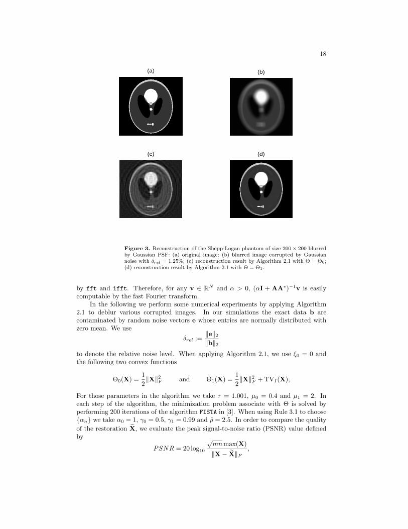
Figure 3. Reconstruction of the Shepp-Logan phantom of size 200 × 200 blurredby Gaussian PSF: (a) original image; (b) blurred image corrupted by Gaussiannoise with δrel = 1.25%; (c) reconstruction result by Algorithm 2.1 with Θ = Θ0;(d) reconstruction result by Algorithm 2.1 with Θ = Θ1.

by fft and ifft. Therefore, for any v ∈ RN and α > 0, (αI + AA∗)−1v is easilycomputable by the fast Fourier transform.

In the following we perform some numerical experiments by applying Algorithm2.1 to deblur various corrupted images. In our simulations the exact data b arecontaminated by random noise vectors e whose entries are normally distributed withzero mean. We use

δrel :=‖e‖2‖b‖2

to denote the relative noise level. When applying Algorithm 2.1, we use ξ0 = 0 andthe following two convex functions

Θ0(X) =1

2‖X‖2F and Θ1(X) =

1

2‖X‖2F + TVI(X),

For those parameters in the algorithm we take τ = 1.001, µ0 = 0.4 and µ1 = 2. Ineach step of the algorithm, the minimization problem associate with Θ is solved byperforming 200 iterations of the algorithm FISTA in [3]. When using Rule 3.1 to chooseαn we take α0 = 1, γ0 = 0.5, γ1 = 0.99 and ρ = 2.5. In order to compare the quality

of the restoration X, we evaluate the peak signal-to-noise ratio (PSNR) value definedby

PSNR = 20 log10

√mnmax(X)

‖X− X‖F,

19

(a) (b)

(c) (d)

Figure 4. Restoration of the 256 × 256 Cameraman image blurred by motion:(a) original images; (b) images blurred by motion and noise; (c) restoration byAlgorithm 2.1 with Θ = Θ0; (d) restoration by Algorithm 2.1 with Θ = Θ1.

where max(X) denotes the maximum possible pixel value of the true image X.In Figure 3 we plot the restoration results of the Shepp-Logan phantom of size

200 × 200 which is blurred by a 15 × 15 Gaussian PSF with standard derivation 30and is contaminated by Gaussian white noise with relative noise level δrel = 1.25%.The original and blurred images are plotted in (a) and (b) of Figure 3 respectively. InFigure 3 (c) we plot the restoration result by Algorithm 2.1 with Θ = Θ0. With suchchosen Θ, the method in Algorithm 2.1 reduces to the classical nonstationary iteratedTikhonov regularization (1.7) which has the tendency to over-smooth solutions. Theplot clearly indicates this drawback because of the appearance of the ringing artifacts.The corresponding PSNR value is 21.3485. In Figure 3 (d) we plot the restorationresult by Algorithm 2.1 with Θ = Θ1. Due to the appearance of the total variationterm in Θ1, the artifacts are significantly removed. In fact the corresponding PSNRvalue is 24.8653; the computation terminates after nδ = 45 iterations and takes 55.8815seconds.

In Figure 4 we plot the restoration results of the 256 × 256 Cameraman imagecorrupted by a 21× 25 linear motion kernel generated by fspecial(’motion’,30,40)

and a Gaussian white noise with relative noise level δrel = 0.2%. The original andblurred images are plotted in (a) and (b) of Figure 4 respectively. In (c) and (d) ofFigure 4 we plot the restoration results by Algorithm 2.1 with Θ = Θ0 and Θ = Θ1

respectively. The plot in (c) contains artifacts that degrade the visuality, the plot in(d) removes the artifacts significantly. In fact the PSNR values corresponding to (c)and (d) are 26.9158 and 29.8779 respectively. The computation for (d) terminates after

20

nδ = 35 iterations and takes 76.8809 seconds.

3.4. De-autoconvolution

We finally present some numerical simulations for nonlinear inverse problems by solvingthe autoconvolution equation∫ t

0

x(t− s)x(s)ds = y(t) (3.3)

defined on the interval [0, 1]. The properties of the autoconvolution operator

[F (x)](t) :=∫ t

0x(t− s)x(s)ds have been discussed in [8]. In particular, as an operator

from L2[0, 1] to L2[0, 1], F is Frechet differentiable; its Frechet derivative and theadjoint are given respectively by

[F ′(x)v] (t) = 2

∫ t

0

x(t− s)v(s)ds, v ∈ L2[0, 1],

[F ′(x)∗w] (s) = 2

∫ 1

s

w(t)x(t− s)dt, w ∈ L2[0, 1].

0 0.5 1

2

3

4

5

exact solution

0 0.5 1

2

3

4

5

δ=0.01, nδ =12 and time =0.60733s

0 0.5 1

2

3

4

5

δ=0.001, nδ =16 and time =0.82163s

0 0.5 1

2

3

4

5

δ=0.0001, nδ =17 and time =0.87646s

Figure 5. Reconstruction results for the de-autoconvolution problem byAlgorithm 2.2 using noisy data with various noise levels.

We assume that (3.3) has a piecewise constant solution and use a noisy data yδ

satisfying ‖yδ − y‖L2[0,1] = δ to reconstruct the solution. In Figure 5 we report thereconstruction results by Algorithm 2.2 using L(xn) = F ′(xn) and the Θ given in(2.28) with β = 20. All integrals involved are approximated by the trapezoidal rule bydividing [0, 1] into N = 400 subintervals of equal length. For those parameters involvedin the algorithm, we take τ = 1.01, µ0 = 0.4/β and µ1 = 1. We also take the constant

21

function ξ0(t) ≡ 1/β as an initial guess. The sequence αn is selected by Rule 3.1with A replaced by L(xn) in which α0 = 1, γ0 = 0.5, γ1 = 0.99 and ρ = 3. Whenthe 1d-denoising algorithm FISTA in [2, 3] is used to solve the minimization problemsassociated with Θ, it is terminated as long as the number of iterations exceeds 1200 orthe error between two successive iterates is smaller than 10−5. We indicate in Figure5 the number of iterations and the computational time for various noise levels δ; theresults show that Algorithm 2.2 is indeed a fast method for this problem.

4. Conclusion

We proposed a nonstationary iterated method with convex penalty term for solvinginverse problems in Hilbert spaces. The main feature of our method is its splittingcharacter, i.e. each iteration consists of two steps: the first step involves only theoperator from the underlying problem so that the Hilbert space structure can beexploited, while the second step involves merely the penalty term so that only arelatively simple strong convex optimization problem needs to be solved. This featuremakes the computation much efficient. When the underlying problem is linear, weproved the convergence of our method in the case of exact data; in case only noisy dataare available, we introduced a stopping rule to terminate the iteration and proved theregularization property of the method. We reported various numerical results whichindicate the good performance of our method.

Acknowledgement

Q. Jin is partially supported by the DECRA grant DE120101707 of Australian ResearchCouncil and X. Lu is partially supported by National Science Foundation of China (No.11101316 and No. 91230108).

References

[1] K. J. Arrow, L. Hurwicz, H. Uzawa, Studies in linear and nonlinear programming, StanfordMathematical Studies in the Social Sciences, vol. II. Stanford University Press, Stanford,1958

[2] A. Beck and M. Teboulle, A fast iterative shrinkage-thresholding algorithm for linear inverseproblems, SIAM J. Imaging Sci., 2 (2009), 183–202.

[3] A. Beck and M. Teboulle, Fast gradient-based algorithms for constrained total variation imagedenoising and deblurring problems, IEEE Trans. Image Process, 18 (2009), no. 11, 2419–2434.

[4] R. Bot and T. Hein, Iterative regularization with a general penalty term—theory and applicationto L1 and TV regularization, Inverse Problems, 28 (2012), 104010(19pp).

[5] L. M. Bregman, The relaxation method for finding common points of convex sets and itsapplication to the solution of problems in convex programming, USSR Comput. Math. Math.Phys. 7 (1967), 200–217.

[6] A. Chambolle and T. Pock, A first-order primal-dual algorithm for convex problems withapplications to imaging, J. Math. Imaging Vis. 40 (2011), 120–145.

[7] H. W. Engl, M. Hanke and A. Neubauer, Regularization of Inverse Problems, Kluwer, Dordrecht,1996.

[8] R. Gorenflo and B. Hofmann, On autoconvolution and regularization, Inverse Problems, 10(1994), 353–373.

[9] H. Gfrerer, An a posteriori parameter choice for ordinary and iterated Tikhonov regularizationof ill-posed problems leading to optimal convergence rates, Math. Comp., 49(180): 507–522,S5–S12, 1987.

[10] M. Hanke and C. W. Groetsch, Nonstationary iterated Tikhonov regularization, J. Optim.Theory Appl. 97(1998), 37–53.

22

[11] P. C. Hansen, J. G. Nagy, and D. P. O’Leary, Deblurring Images - Matrices, Spectra, andFiltering, SIAM, Philadelphia, 2006.

[12] Q. Jin, On the iteratively regularized Gauss-Newton method for solving nonlinear ill-posedproblems, Math. Comp., 69(2000), 1603–1623.

[13] Q. Jin, On a regularized Levenberg-Marquardt method for solving nonlinear inverse problems,Numer. Math., 115 (2010), 229–259.

[14] Q. Jin and Z. Y. Hou, On an a posteriori parameter choice strategy for Tikhonov regularizationof nonlinear ill-posed problems, Numer. Math., 83(1999), 139–159.

[15] Q. Jin and W. Wang, Landweber iteration of Kaczmarz type with general non-smooth convexpenalty functionals, Inverse Problems, 29 (2013), 085011(22pp).

[16] Q. Jin and M. Zhong, Nonstationary iterated Tikhonov regularization in Banach spaces withgeneral convex penalty terms, Numer. Math. to appear, 2013.

[17] C. A. Micchelli, L. X. Shen and Y. S. Xu, Proximity algorithms for image models: denoising,Inverse Problems, 27(2011), 045009.

[18] W. H. Press, S. A. Teukolsky, W. T. Vetterling and B. P. Flannery, Numerical Recipes: TheArt of Scientific Computing, (3rd ed.) New York: Cambridge University Press, 2007.

[19] T. Raus, The principle of the residual in the solution of ill-posed problems, Tartu Riikl. Ul.Toimetised, (672): 16–26, 1984.

[20] L. Rudin, S. Osher, and C. Fatemi, Nonlinear total variation based noise removal algorithm,Phys. D, 60 (1992), pp. 259–268.

[21] O. Scherzer, H. W. Engl and K. Kunisch, Optimal a posteriori parameter choice for Tikhonovregularization for solving nonlinear ill-posed problems, SIAM J. Numer. Anal. 30 (1993),1796–1838.

[22] N. Z. Shor, Minimization Methods for Non-Differentiable Functions, Springer, 1985.[23] C. Zalinscu, Convex Analysis in General Vector Spaces, World Scientific Publishing Co., Inc.,

River Edge, New Jersey, 2002.