A Bayesian Approach to Pathway Analysis by Integrating Gene–Gene Functional Directions and Microarray Data

Stat Biosci (2012) 4:105–131DOI 10.1007/s12561-011-9046-1

A Bayesian Approach to Pathway Analysisby Integrating Gene–Gene Functional Directionsand Microarray Data

Yifang Zhao · Ming-Hui Chen · Baikang Pei ·David Rowe · Dong-Guk Shin · Wangang Xie ·Fang Yu · Lynn Kuo

Received: 1 June 2011 / Accepted: 2 December 2011 / Published online: 29 December 2011© International Chinese Statistical Association 2011

Abstract Many statistical methods have been developed to screen for differentiallyexpressed genes associated with specific phenotypes in the microarray data. How-ever, it remains a major challenge to synthesize the observed expression patternswith abundant biological knowledge for more complete understanding of the biolog-ical functions among genes. Various methods including clustering analysis on genes,

Y. Zhao · M.-H. Chen · L. Kuo (�)Department of Statistics, University of Connecticut, Storrs, CT 06269, USAe-mail: [email protected]

Y. Zhaoe-mail: [email protected]

M.-H. Chene-mail: [email protected]

B. PeiMYSM School of Medicine, Yale University, New Haven, USAe-mail: [email protected]

D. RoweSchool of Dental Medicine, University of Connecticut Health Center, Farmington, CT 06030, USAe-mail: [email protected]

D.-G. ShinComputer Science & Engineering, University of Connecticut, Storrs, CT 06269, USAe-mail: [email protected]

W. XieAbbott Lab, Chicago, USAe-mail: [email protected]

F. YuDepartment of Biostatistics, University of Nebraska Medical Center, Omaha, USAe-mail: [email protected]

106 Stat Biosci (2012) 4:105–131

neural network, Bayesian network and pathway analysis have been developed to-ward this goal. In most of these procedures, the activation and inhibition relationshipsamong genes have hardly been utilized in the modeling steps. We propose two novelBayesian models to integrate the microarray data with the putative pathway struc-tures obtained from the KEGG database and the directional gene–gene interactionsin the medical literature. We define the symmetric Kullback–Leibler divergence of apathway, and use it to identify the pathway(s) most supported by the microarray data.Monte Carlo Markov Chain sampling algorithm is given for posterior computation inthe hierarchical model. The proposed method is shown to select the most supportedpathway in an illustrative example. Finally, we apply the methodology to a real mi-croarray data set to understand the gene expression profile of osteoblast lineage atdefined stages of differentiation. We observe that our method correctly identifies thepathways that are reported to play essential roles in modulating bone mass.

Keywords Bayesian belief network · Bayesian model selection · KEGG pathways ·Microarray data · Prior construction · Symmetric Kullback–Leibler divergence

1 Introduction

Genome informatics was born to cope with the vast amount of data generated bythe genomic studies, in particular, to support experimental projects. The challengesfor post-genome informatics are on synthesis of biological knowledge from genomicinformation toward understanding of general principles of life. So post-genome infor-matics has to be coupled with systematic experiments in functional genomics. How-ever, the coupling is in a different direction where informatics plays a dominant rolein designing experiments and prediction.

High-throughput gene analysis technology such as cDNA microarray and oligonu-cleotide arrays has enabled parallel analysis of thousands of genes simultaneously.Numerous statistical methods have been developed to screen for differentially ex-pressed genes, either up- or down-regulated, in these experiments. While theseprojects rapidly determine gene catalogs for an increasing number of organisms,functional annotation of individual genes is still largely incomplete. It would be es-sential to have knowledge on coregulated genes and their interactions. Consequently,various methods have been developed toward these goals. The methods include clus-tering analysis on genes, neural network, Bayesian network (BN), and pathway anal-ysis. In this paper, we will focus on pathway and Bayesian network approaches.

There are multiple sources of knowledge on pathway and gene interaction. Ky-oto Encyclopedia of Genes and Genomes (KEGG) database [17] was initiated byJapanese human genome program in 1995 to link genomic information with higherorder functional information by computerizing current knowledge on cellular pro-cesses and by standardizing gene annotations. These databases are often called meta-data, which means data about data. KEGG consists of three databases: PATHWAY forrepresenting higher order functions in terms of the network of interacting molecules,GENES for the collection of gene catalogs for all completely sequenced genomesand some partial genomes, and LIGAND for the collection of chemical compounds

Stat Biosci (2012) 4:105–131 107

in the cell, enzyme molecules and enzymatic reactions. A pathway is a collection ofgraphical diagrams of interacting molecules obtained from many years of intensivebiomedical research representing the present knowledge on various cellular or phys-iologic functions. It is supposed to be a computer representation of the biologicalsystem, so it can be used as part of the systems biology approach.

In addition to KEGG, such databases also include gene ontology (GO) database(Gene Ontology Consortium, 2001), and BioCarta (www.biocarta.com). We are fo-cusing on the KEGG pathway database because it contains the directional relationship(activation or inhibition) between genes that is extremely useful in the system biologyapproach. Moreover, it provides a rich set of possible structures on the gene to generelationships. The KEGG pathway can be expanded to a general pathway database toinclude recently developed and published pathways.

Another valuable source of biological knowledge is the gene-to-gene activation orinhibition knowledge aggregated from past experiments or literature search. We de-posit these directional relationships among genes in a database called PrimeDB. Sofrom this database, we can search for evidence of gene-to-gene activation or inhibi-tion measured by the number of journals reporting these interactions.

Our goal is to investigate gene to gene interactions by integrating the followingthree components: the structure information of putative pathways available from path-way networks, the gene relations uncovered by literature mining as in PrimeDB andthe microarray gene expression data. The first two components can be obtained beforethe microarray experiments, so we consider them as prior information. We will de-scribe how we could revise our prior opinion on pathway after seeing the microarrayresults using Bayesian methods. Moreover, we develop methods for ranking pathwaysin terms of their degree of agreement with the microarray data. Figure 1 provides aschematic summary of the database integration.

Current statistics methods on pathway activities are mostly in the area of geneset enrichment analysis (GSEA) where a set of regulated genes in a pathway arecompared to the regulated gene set in the microarray studies to determine whetherthe set is particular enriched by the pathway. Curtis et al. [3] have provided a tableof software, annotation, and statistical methods used in each software. In general,Gene ontology (GO), GenMapp, KEGG, and Biocarta have been used for the annota-

Fig. 1 Flowgram of data setsintegration

108 Stat Biosci (2012) 4:105–131

tions. Efron and Tibshirani [4] and Newton et al. [23] have provided more improvedmethods for gene enrichment analysis. However, all these methods are restricted tocounting methods where the number of regulated genes is counted in each pathway.They have not incorporated the putative information on activation and inhibition re-lationships given in the KEGG database and PrimeDB.

There are also several Bayesian papers studying pathways or networks. Friedmanet al. [7] propose an adaptive iterative search algorithm for an optimal Bayesian net-work (BN) while search is restricted to the most promising candidate parents of eachgene based on some local statistics (such as correlation). Their learning algorithmuses no prior biological knowledge nor constraints. Hartemink et al. [10] extend theBN by adding edge annotation, which allows representation of additional informationabout the dependence relationships among genes. Sachs et al. [24] outline modelingthe cell signaling pathways using BN. Sebastiani et al. [25] show the application ofBN to the analysis of various types of genomic data including genomic markers andgene expression data. They also introduce the Generalized Gamma Networks to de-pict the possibly nonlinear parent–child dependencies. Werhli and Husmeier [29] useBayesian networks to reconstruct gene regulatory network by integrating microarraydata and multiple sources of prior knowledge such as KEGG pathways and promotermotifs. The prior probability of a network is modeled by a Gibb distribution, in whicheach source is encoded by a separate energy function. Shen and West [26] developprobability pathway annotation (PROPA) to match outcomes in gene expression tomultiple biological pathway gene sets from curated databases. Monni and Li [22]show how to utilize the prior genetic pathway and network information in the anal-ysis of genomic data in order to obtain a more interpretable list of genes that areassociated with the genotypes. Ellis and Wong [5] have examined computational al-gorithms for determining BN structures from experimental data. However, as far aswe know, the activation and inhibition relationships among genes have hardly beenutilized in the modeling steps of these procedures, except Ellis and Wong.

In this paper, we consider the pathways given in KEGG as possible models. Eachpathway is a weighted graph that includes the activation and inhibition binary rela-tionships. Given our microarray data, we are interested in knowing which pathway,or a set of pathways are most agreeable to our microarray experiment results. In theframe work of model selection, we are essentially asking which pathway is mostsupported by the microarray data. Instead of the best one, we can also select a fewpathways that are most supported by the data.

Our approach considers the results of microarray analysis as data. So we start withthe selected regulated (significant) gene list from microarray analysis. The outcomefor each selected genes is modeled as a discrete random variable taking values of 1and 0, representing up-regulated and down-regulated, respectively. Then we considera set of putative pathways (say 80 for example) from KEGG that needs to be studied.We first modify them slightly so each pathway can be considered as a BN with adirected acyclic graph. Then for each pathway structure in the set, we write downthe local prior distribution for each node in the pathway. The hyperparameters inthe prior information representing not only the propensities for a gene to have anactivation or an inhibition effect on other genes, but also indicating the strength ofthis prior belief. They may have a big influence on the decision making of ranking

Stat Biosci (2012) 4:105–131 109

pathways. So the formulations of them are guided by the PrimeDB which are beingconstructed by the informatics group of the authors here. We propose two possiblesolutions to the choice of hyperparameters: (A) Use the prior information obtainedfrom PrimeDB to formulate good estimates of these hyperparameters. Then we justplug in these estimates for the hyperparameters. (B) Treat these hyperparameters asrandom variables to build another layer of hierarchial model sensibly guided by thePrimeDB and to achieve more robust results. We will develop both methods andexamine their effects. We update these local distributions from KEGG and PrimeDBinformation conditioning on the data using the Bayes theorem. Then we rank thepathways by using the symmetric Kullback–Leibler divergence [19]. The most likelypathway has the smallest symmetric Kullback–Leibler divergence between the priorand the posterior distributions. We also extend our methodology to include all thegenes in the microarray as data as given in Sect. 5.

This rest of this paper is organized as follows: Sect. 2 describes the simpleBayesian model which uses PrimeDB to specify prior directly, and defines the sym-metric Kullback–Leibler divergence to measure pathway activities; Sect. 3 extendsthis divergence measure to the multilevel model, in which the second level prior gov-erns our prior belief on the activation or inhibition effect aggregated by PrimeDB, AMarkov chain Monte Carlo (MCMC) algorithm is proposed for posterior estimatescomputation; Sect. 4 demonstrates our method with a simple example, and Sect. 5evaluates model performance through an osteoblast microarray study. We concludethe paper with a brief discussion in Sect. 6.

2 Simple Bayesian Model Using PrimeDB Directly

The easiest way to represent a network is to use a graph, which is a collection of ver-tices (nodes) and edges that connect vertices. The vertices can be genes, transcriptionfactors, proteins, ligands, etc. All vertices need not be connected in a graph. A di-rected graph has one-way edges (arcs) that can represent an irreversible molecularreaction. In a weighted graph, weights (costs) are assigned to the edges, for exampleto distinguish between activation and inhibition in a signal transduction pathway.

We will first treat a pathway as a BN. A BN comprises two components: a directedacyclic graph (DAG) and a probability distribution. It is a graph with no path thatstarts and ends at the same node. The nodes in DAG depict stochastic variables. Sothe node can represent the outcome of a gene after a microarray experiment. Thearcs in the DAG display directed dependencies among variables that are quantifiedby conditional probability distributions. Lack of arcs between two nodes indicatesconditional independence. Heckerman [11] provides an excellent tutorial on the BN.We are highlighting the key points here.

Let Y = (Y1, . . . , YQ) denote the outcomes of Q nodes in a BN. A BN consistsof:

1. a network structure S that encodes a set of conditional independence assertionsabout the variables in Y;

2. a set of local probability distributions associated with each node.

110 Stat Biosci (2012) 4:105–131

In our application of BN on pathways, S comprises not only the set of conditionalindependence assertions among genes, but also the activation and inhibition effectamong them. Note that in model derivation, we focus on the pathways in which eachgene has a single parent, either activator or inhibitor. We also restrict our attention toa binary BN, where for each variable yi takes on only two values, with yi = 1,0 forrepresenting gene i being up- or down-regulated, respectively. In Sect. 5, we demon-strate that our model is readily extended to pathways which consist of equivalentlyexpressed genes and/or genes with multiple parents.

2.1 Notations and Transition Probabilities

We classify a gene in a pathway into three categories: (1) with no parents, (2) with anactivator parent, and (3) with an inhibitor parent. In particular, we have the followingnotations for the three categories:

Pa = {i : i ∈ (1,2, . . . ,Q), such that gi has no parents.}: the index set of geneswithout parents.

A = {i : i ∈ (1,2, . . . ,Q)\Pa, and gi is activated by its parent.}: the index set ofgenes with Activator parents in a pathway of Q genes.

I = {i : i ∈ (1,2, . . . ,Q)\Pa, and gi is inhibited by its parent.}: the index set ofgenes with Inhibitor parents in a pathway of Q genes.

We use θi to denote the probability of gene i being up-regulated, for i ∈ Pa. Givenwe assume a gene can be either up- or down-regulated, so a Bernoulli distributionwith probability θi suffices to model this outcome. We use θ s = {θi : i ∈ Pa} to de-scribe the set of initial states of a pathway, that is, for the gene(s) without parents.

For genes with parents, we need to define their transition probabilities. Let Yi

denote the outcome for gi with its parent to be gj . Use symbols ∪ for beingup-regulated, and ∩ being down-regulated. Then we define the transition proba-bilities for the connected genes as in Tables 1 and 2. That is: If gj activates gi ,then we assume Pr(Yi = ∪|Yj = ∪) = Pr(Yi = ∩|Yj = ∩) = θi|j . Consequently,Pr(Yi = ∩|Yj = ∪) = Pr(Yi = ∪|Yj = ∩) = 1−θi|j . If gj inhibits gi , then we assumePr(Yi = ∩|Yj = ∪) = Pr(Yi = ∪|Yj = ∩) = φi|j . Consequently, Pr(Yi = ∪|Yj =∪) = Pr(Yi = ∩|Yj = ∩) = 1 − φi|j . Observe that θi|j represents an activation ef-fect and φi|j an inhibition effect from gene j to i. So the transition probabilitiesdefine the local distribution of each node (gene) in the pathway, which is a collectionof Bernoulli distributions. Observe if we let φi|j = 1 − θi|j , then we can collapseTables 1 and 2 into one table.

Let θ s = (θ s , θ∗s ,φs) be the parameter vector of pathway S, where θ s = {θi : i ∈

Pa} is the vector of up-regulated genes with no parents, and θ∗s = {θi|j : i ∈ A} and

Table 1 Transitionprobabilities for gj to activategi

gi

∪ ∩∪ θi|j 1 − θi|j

gj

∩ 1 − θi|j θi|j

Stat Biosci (2012) 4:105–131 111

Table 2 Transitionprobabilities for gj to inhibit gi

gi

∪ ∩∪ 1 − φi|j φi|j

gj

∩ φi|j 1 − φi|j

φs = {φi|j : i ∈ I} are the vectors of transition probabilities for genes being activatedand inhibited, respectively. Let D denote the data, which are assumed to be a randomsample from the joint distribution of Y. So D consists of (1) n, the total number ofmicroarray experiments being analyzed, (2) ni , the count for being up-regulated in n

experiments for each i ∈ Pa, and (3) ni|j denotes the number of concordant pairs ((∩∩) or (∪, ∪)) for gene j and gene i ordered pair in n experiments where gene j isa parent, and gene i ∈ A. If gene i ∈ I , then ni|j denotes the number of discordantpairs ((∩ ∪) or (∪, ∩)) for the gene j and gene i pair. By the local Markov propertyof the BN which says that each node is independent of its non-descendants given theparent nodes, the likelihood function, L(θ s |D), of a given pathway S is the productof the local distributions over all the genes in it. It is given as

L(θ s |D) =∏

i∈Pa

θni

i (1 − θi )n−ni

∏

i∈Aθ

ni|ji|j (1 − θi|j )n−ni|j

∏

i∈Iφ

ni|ji|j (1 − φi|j )n−ni|j .

2.2 Prior Elicitation and the Posterior Distributions

Suppose in the PrimeDB, there are ai|j journal articles citing that gj activates gi

and bi|j journal articles citing gj inhibits gi . To incorporate these prior information,we would first assume Simple Bayesian model using PrimeDB directly. We assumeθi|j ∼ βe(ai|j , bi|j ) for the activation effect, and φi|j ∼ βe(bi|j , ai|j ) for the inhibi-tion effect. If PrimeDB does not provide information on the initial state, we can usea vague prior for it, for example, θi ∼ βe(1,1). Assuming that the parameters aremutually independent over i, the joint prior distribution can be written as:

π(θ s |S) = π(θ s , θ∗s ,φs |S) = π(θ s |S)π(θ∗

s |S)π(φs |S)

=∏

i∈Pa

π(θi |S)∏

i∈Aπ(θi|j |S)

∏

i∈Iπ(φi|j |S). (2.1)

Assuming there are no missing data, i.e., for each node in the BN we observe somedata, the posterior distribution π(θ s |D,S) is then given as:

π(θ s |D,S) = π(θ s , θ∗s ,φs |D,S)

=∏

i∈Pa

π(θi |D,S)∏

i∈Aπ(θi|j |D,S)

∏

i∈Iπ(φi|j |D,S). (2.2)

So it is obtained by updating the local posterior distributions of θi|j or φi|j . Supposethat KEGG suggests that gj activates gi , we need to update θi|j given the data. So wecount the number (denoted by ni|j ) of ordered pairs with outcomes to be ∪ to ∪ or∩ to ∩ from gj to gi . It is actually the number of concordant pairs for the outcomesof (gj , gi). The number of discordant pairs with ∪ to ∩ or ∩ to ∪ is n − ni|j . So the

112 Stat Biosci (2012) 4:105–131

distribution of θi|j given data is updated to βe(ai|j + ni|j , bi|j + n − ni|j ). Similarly,if KEGG suggests that gj inhibits gi ,the posterior distribution of φi|j given data isβe(bi|j + ni|j , ai|j + n − ni|j ).

2.3 Selection Criterion of Supported Pathways: Symmetric Kullback–LeiblerDivergence

We propose to use the symmetric Kullback–Leibler divergence [19] to select the bestpathway. The smaller symmetric Kullback–Leibler divergence between the prior andposterior distributions of a given pathway, the more supported by the data this path-way is.

The Kullback–Leibler (KL) divergence is conventionally used to measure the dif-ference between two densities. The KL divergence of the probability distributionf1(y) from f2(y) is defined as

KL(f1, f2) =∫

ln

(f1(y)

f2(y)

)f1(y) dy.

We highlight the key properties of KL divergence as follows. First, the KL divergenceis not a distance because it is asymmetric, i.e., KL(f1, f2) �= KL(f2, f1), and it doesnot satisfy the triangle inequality. Second, using Jensen’s inequality, it can be shownthat the KL divergence is nonnegative if f2 is a proper density, and equals zero if andonly if f1 = f2. Third, the KL divergence measures how much information f2 carriesabout f1, if f1 is considered the “true” distribution of the data.

For more intuitive interpretation, we adopt the definition of the symmetric KLdivergence introduced by Kullback and Leibler (1951)

SKL(f1, f2) = KL(f1, f2) + KL(f2, f1).

Let us first define the symmetric KL divergence of gene i in the simple model as:

SKL(π(γi |S),π(γi |D,S)

)

:=∫

ln

[π(γi |S)

π(γi |D,S)

]π(γi |S)dγi +

∫ln

[π(γi |D,S)

π(γi |S)

]π(γi |D,S)dγi

=∫ [

lnp(yi |pai , γi, S)]π(γi |D,S)dγi −

∫ [lnp(yi |pai , γi, S)

]π(γi |S)dγi,

(2.3)

where

γi =

⎧⎪⎨

⎪⎩

θi if i ∈ Pa,

θi|j if i ∈ A,

φi|j if i ∈ I,

and p(yi |pai , γi, S) is the local probability distribution for gene i, and pai denotesthe configuration of its parent. Note that in our single-parent pathways, it can be anempty set or a singleton set having parent gene j . Equation (2.3) is an immediateconsequence of the fact that π(γi |S) is a proper prior and its normalized constantis 1.

Stat Biosci (2012) 4:105–131 113

Because different pathways have different gene sizes, we use the geometric meanof the symmetric KL divergence for individual genes to correct for different dimen-sions. We thus define the symmetric KL divergence of a pathway S with Q genesas

SKL(S) =∫

ln

[π(θ s |S)

π(θ s |D,S)

]1/Q

π(θ s |S)dθ s

+∫

ln

[π(θ s |D,S)

π(θ s |S)

]1/Q

π(θ s |D,S)dθ s . (2.4)

Let π∗(θ s |S) be the kernel density of the prior, and let C0(S) and CD(S) be thenormalizing constants of prior and posterior distributions, respectively. We can write

π(θ s |S) = π∗(θ s |S)

C0(S),

and

π(θ s |D,S) = L(θ s |D)π∗(θ s |S)

CD(S).

Then (2.4) becomes

SKL(S)

= 1

Q

(∫ln

[L(θ s |D)

]π(θ s |D,S)dθ s −

∫ln

[L(θ s |D)

]π(θ s |S)dθ s

),(2.5)

after canceling out ln(CD(S)/C0(S)) and ln(C0(S)/CD(S)) in the evaluation. Thismakes the definition of the symmetric KL divergence more attractive, because thecomputation of CD(S)/C0(S) can be very expensive.

By local Markov property of BN, the likelihood function, L(θ s |D), is the prod-uct of the local probability distributions. Moreover, as shown in (2.1) and (2.2), theprior distribution of pathway S can also be decomposed into the product of localprior distributions of its component genes, so can be the joint posterior distribution.Consequently, we have

SKL(S) = 1

Q

Q∑

i=1

(∫ [lnp(yi |pai , γi, S)

]π(γi |D,S)dγiπ(θ s(−γi )

|D,S)dθ s(−γi )

−∫ [

lnp(yi |pai , γi, S)]π(γi |S)dγiπ(θ s(−γi )

|S)dθ s(−γi )

)

= 1

Q

Q∑

i=1

(∫lnp(yi |pai , γi, S)

(π(γi |D,S) − π(γi |S)

)dγi

)

= 1

Q

Q∑

i=1

SKL(π(γi |S),π(γi |D,S)

).

Here θ s(−γi )denotes the transition probability vector of pathway S without gene i’s

transition probability γi . Note∫π(θ s(−γi )

|S)dθ s(−γi )= 1, and

∫π(θ s(−γi )

|D,S)dθ s(−γi )= 1.

114 Stat Biosci (2012) 4:105–131

Hence, the symmetric KL divergence of a pathway is the average of the symmet-ric KL divergences of its component genes. This has sensible interpretation. Whena pathway is supported by the microarray data, we expect that, on average, the dis-crepancy between the local conditional distributions of its genes and their prior dis-tributions will be small. And so will be the discrepancy between the local conditionaldistributions and the posterior distributions, because the prior is part of the posterior.

Since the log likelihood breaks into the sum of three parts: the one of log localdistributions of initial states, of activated genes and of inhibited genes, we have

SKL(S) = 1

Q(I1 + I2 + I3),

where

I1 =∑

i∈Pa

∫ 1

0

[ln θ

ni

i (1 − θi )n−ni

] 1

B(1 + ni ,1 + n − ni )θ

ni

i (1 − θi )n−ni dθi

−∫ 1

0ln θ

ni

i (1 − θi )n−ni dθi ,

I2 =∑

i∈A

∫ 1

0

[ln θ

ni|ji|j (1 − θi|j )n−ni|j ]θ

ai|j +ni|j −1i|j (1 − θi|j )bi|j +n−ni|j −1

B(ai|j + ni|j , bi|j + n − ni|j )dθi|j

−∫ 1

0

[ln θ

ni|ji|j (1 − θi|j )n−ni|j ]θ

ai|j −1i|j (1 − θi|j )bi|j −1

B(ai|j , bi|j )dθi|j ,

I3 =∑

i∈I

∫ 1

0

[lnφ

ni|ji|j (1 − φi|j )n−ni|j ]φ

bi|j +ni|j −1i|j (1 − φi|j )ai|j +n−ni|j −1

B(bi|j + ni|j , ai|j + n − ni|j )dφi|j

−∫ 1

0

[lnφ

ni|ji|j (1 − φi|j )n−ni|j ]φ

bi|j −1i|j (1 − φi|j )ai|j −1

B(bi|j , ai|j )dφi|j ,

and B(z,w) = �(z)�(w)�(z+w)

. To evaluate the I1, I2 and I3, we will make use of the fol-lowing result.

Proposition 1 If Z ∼ βe(α,β), and a, b > 0, then∫ 1

0

[ln zn1(1 − z)n2

] 1

B(α,β)zα−1(1 − z)β−1 dz

= n1ψ(α) + n2ψ(β) − (n1 + n2)ψ(α + β),

where ψ(α) is the standard digamma function defined as

ψ(α) = d

dαln�(α) = �′(α)

�(α).

It is straightforward to verify the proposition by interchanging the order of in-tegration (with respect to z) and differentiation (with respect to α, β , or α + β).Consequently, we have

Stat Biosci (2012) 4:105–131 115

I1 =∑

i∈Pa

(niψ(ni) + (n − ni )ψ(n − ni ) − nψ(n + 2) + n + 2

), (2.6)

I2 =∑

i∈Ani|j

[ψ(ai|j + ni|j ) − ψ(ai|j )

] + (n − ni|j )[ψ(bi|j + n − ni|j ) − ψ(bi|j )

]

− n[ψ(ai|j + bi|j + n) − ψ(ai|j + bi|j )

]. (2.7)

I3 is similar to I2 except ai|j is replaced by bi|j , and vice versa.Hence, in the simple model, the computation of SKL(S) boils down to evaluating

the sum of a series of the difference of digamma functions, weighted by the gene sizeof the pathway.

Our average Q value attempts to adjust for the size of the pathways. In spite ofthe fact that larger pathways would be less sensitive to a few extreme SKL scores onthe gene level, it is not necessary that the Q score always gives advantage to largerpathways.

3 Extension of the Symmetric KL Divergence to the Multilevel Model

3.1 Multilevel Model Guided by PrimeDB

An extra level of hierarchical Bayesian model can be constructed to allow informationsharing among the same types of gene, one for activation, the other for inhibition.We define the first level prior distribution: for all i and j , θi|j |θ ∼ βe(ai|j θ, bi|j θ),they are independent over all i and j given θ . Similarly, φi|j |φ ∼ βe(bi|jφ, ai|jφ)

and are independent given φ. The second level prior θ ∼ E (μ) is independent ofφ ∼ E (ν) with known μ and ν, where E (μ) denotes an exponential distribution withmean μ. By the way, it is possible to allow unknown μ and ν, so we can build athird level to allow sharing between the types of gene. For the time being, we areonly considering two levels with μ and ν known. Note the first level specificationyields E(θi|j |θ) = ai|j /(ai|j +bi|j ). This is the same mean as in the Simple Bayesianmodel. However Var(θi|j |θ) = ai|j bi|j /[(ai|j + bi|j )2(ai|j θ + bi|j θ + 1)]. So thishierarchical model adds one more parameter θ that controls our prior belief of thePrimeDB. The bigger the θ , the stronger the belief on the PrimeDB. Note that whenμ = ν = 1, the distributions of transition probabilities conditional on θ and φ are thesame as in the simple model. All genes with an activation effect suggested by KEGGshare a common factor θ that can be learned from the data and PrimeDB. Similarconsiderations apply to the inhibition parameters.

3.2 Symmetric KL Divergence for Multilevel Model

We first extend the definitions of SKL(π(γi |S),π(γi |D,S)) and SKL(S) in the mul-tilevel model. Including the hyperparameters that govern our belief on the activa-tion or inhibition effect from PrimeDB, the parameter vector of pathway S becomesθ s = (θ s , θ

∗s ,φs , θ,φ). Let

116 Stat Biosci (2012) 4:105–131

γi =

⎧⎪⎨

⎪⎩

θi if i ∈ Pa,

(θi|j , θ) if i ∈ A,

(φi|j , φ) if i ∈ I.

Then the definition of SKL for gene i given in (2.3) sustains. Explicitly, for activatedgenes π(γi |D,S) = π(θi|j |θ,D,S)π(θ |D,S), and for inhibited genes π(γi |D,S) =π(φi|j |φ,D,S)π(φ|D,S).

To generalize the definition of SKL(S) to the multilevel model, it is easy to seethat we need to modify (2.5) to

SKL(S) = 1

Q

(∫ [lnL(θ s |D)

]π(θ s , θ

∗s ,φs , θ,φ|D,S)dθ s

−∫ [

lnL(θ s |D)]π(θ s , θ

∗s ,φs , θ,φ|S)dθ s

). (3.1)

Following the same logic in deriving SKL(S) in the simple model, we can verify thatin the multilevel model,

SKL(S) = 1

Q

Q∑

i=1

SKL(π(γi |S),π(γi |D,S)

).

Now, the joint prior distribution can be collapsed as

π(θ s , θ∗s ,φs , θ,φ|S)

= π(θ s , θ∗s ,φs |θ,φ,S)π(θ,φ|S)

= π(θ s |S)π(θ∗s |θ, S)π(θ |S)π(φs |φ,S)π(φ|S) (3.2)

={∏

i∈Pa

π(θi |S)∏

i∈Aπ(θi|j |θ, S)

∏

i∈Iπ(φi|j |φ,S)

}π(θ |S)π(φ|S), (3.3)

where (3.2) follows the facts that θ s does not depend on θ or φ, θ∗s |θ is independent

of φ, φs |φ is independent of θ , θ and φ are independent. Both the assumptions ofθi|j |θ being independent over i and j for i ∈ A, and φi|j |φ being independent over i

and j for i ∈ I , yield (3.3).Similarly, the joint posterior distribution can be collapsed as

π(θ s , θ∗s ,φs , θ,φ|D,S)

=(∏

i∈Pa

π(θi |D,S)∏

i∈Aπ(θi|j |θ,D,S)

∏

i∈Iπ(φi|j |φ,D,S)

)π(θ,φ|D,S).

Substituting the specific forms of log likelihood function, the collapsed prior andposterior distributions into (3.1), we can rewrite SKL(S) as a sum of symmetric KLdivergence for the genes without parents, activated, and inhibited:

SKL(S) = 1

Q(I ′

1 + I ′2 + I ′

3), (3.4)

where

Stat Biosci (2012) 4:105–131 117

I ′1 =

∑

i∈Pa

(niψ(ni) + (n − ni )ψ(n − ni ) − nψ(n + 2) + n + 2

),

I ′2 =

∑

i∈A

∫g∗

iA(θ)π(θ,φ|D,S)dθ dφ −∫

giA(θ)π(θ |S)dθ, (3.5)

I ′3 =

∑

i∈I

∫g∗

iI (φ)π(θ,φ|D,S)dθ dφ −∫

giI (φ)π(φ|S)dφ, (3.6)

with

g∗iA(θ) =

∫ [ln θ

ni|ji|j (1 − θi|j )n−ni|j ]θ

ai|j θ+ni|j −1i|j (1 − θi|j )bi|j θ+n−ni|j −1

B(ai|j θ + ni|j , bi|j θ + n − ni|j )dθi|j

= ni|jψ(ai|j θ + ni|j ) + (n − ni|j )ψ(bi|j θ + n − ni|j )− nψ(ai|j θ + bi|j θ + n), (3.7)

giA(θ) =∫ [

ln θni|ji|j (1 − θi|j )n−ni|j ]θ

ai|j θ−1i|j (1 − θi|j )bi|j θ−1

B(ai|j θ, bi|jφ)dθi|j

= ni|jψ(ai|j θ) + (n − ni|j )ψ(bi|j θ) − nψ(ai|j θ + bi|j θ), (3.8)

g∗iI (φ) =

∫ [lnφ

ni|ji|j (1 − φi|j )n−ni|j ]φ

bi|j φ+ni|j −1i|j (1 − φi|j )ai|j φ+n−ni|j −1

B(bi|j φ + ni|j , ai|jφ + n − ni|j )dφi|j

= ni|jψ(bi|jφ + ni|j ) + (n − ni|j )ψ(ai|jφ + n − ni|j )− nψ(bi|jφ + ai|jφ + n), (3.9)

and

giI (φ) =∫ [

lnφni|ji|j (1 − φi|j )n−ni|j ]φ

bi|j φ−1i|j (1 − φi|j )ai|j φ−1

B(bi|j φ, ai|jφ)dφi|j

= ni|jψ(bi|jφ) + (n − ni|j )ψ(ai|jφ) − nψ(ai|jφ + bi|jφ). (3.10)

Equations (3.7)–(3.10) are direct results of Proposition 1. It is easy to observe that I ′1

equals to I1 that is given in the simple model, because θi does not depend on θ or φ.Next, we derive the optimal form for numerically evaluating

∑

i∈A

∫g∗

iA(θ)π(θ,φ|D,S)dθ dφ and∑

i∈I

∫g∗

iI (φ)π(θ,φ|D,S)dθ dφ.

Notice that

π(θ,φ|D,S) =∫

π(θ∗s ,φs , θ,φ|D,S)dθ∗

s dφs

=∫

L(θ∗s ,φs |D)π(θ∗

s ,φs , θ,φ|S)

c∗ dθ∗s dφs , (3.11)

where c∗ is the normalizing constant for π(θ∗s ,φs , θ,φ|D,S), the prior π(θ∗

s ,φs ,

θ,φ|S) is a proper density, and,

L(θ∗s ,φs |D) =

∏

i∈Aθ

ni|ji|j (1 − θi|j )n−ni|j

∏

i∈Iφ

ni|ji|j (1 − φi|j )n−ni|j .

118 Stat Biosci (2012) 4:105–131

Now we can write

c∗ =∫

L(θ∗s ,φs |D)π(θ∗

s ,φs , θ,φ|S)dθ∗s dφs dθ dφ,

and plug it into (3.11), it follows that

π(θ,φ|D,S) =∫

L(θ∗s ,φs |D)π(θ∗

s ,φs , θ,φ|S)dθ∗s dφs∫

L(θ∗s ,φs |D)π(θ∗

s ,φs , θ,φ|S)dθ∗s dφs dθ dφ

= h(θ,φ)μe−μθνe−νφ

∫h(θ,φ)μe−μθνe−νφ dθ dφ

, (3.12)

where

h(θ,φ)

=∫

L(θ∗s ,φs |D)π(θ∗

s ,φs |θ,φ,S)dθ∗s dφs

=∏

i∈A

∫θ

ni|ji|j (1 − θi|j )n−ni|j 1

B(ai|j θ, bi|j θ)θ

ai|j θ−1i|j (1 − θi|j )bi|j θ−1 dθi|j

×∏

i∈I

∫φ

ni|ji|j (1 − φi|j )n−ni|j 1

B(bi|j φ, ai|jφ)φ

bi|j φ−1i|j (1 − φi|j )ai|j φ−1 dφi|j

=∏

i∈A

B(ai|j θ + ni|j , bi|j θ + n − ni|j )B(ai|j θ, bi|j θ)

∏

i∈I

B(bi|j φ + ni|j , ai|jφ + n − ni|j )B(bi|j φ, ai|jφ)

.

(3.13)

So the first term of I ′2 in (3.5) can be expressed as

∑

i∈A

∫g∗

iA(θ)π(θ,φ|D,S)dθ dφ =∑

i∈A

∫g∗

iA(θ)h(θ,φ)μe−μθνe−νφ dθ dφ∫h(θ,φ)μe−μθνe−νφ dθ dφ

=∑

i∈A

∫g∗

iA(θ)h1(θ)μe−μθdθ∫h1(θ)μe−μθdθ

.

Likewise, the first term of I ′3 in (3.6) can be written as

∑

i∈I

∫g∗

iI (φ)π(θ,φ|D,S)dθ dφ =∑

i∈I

∫g∗

iI (φ)h2(φ)νe−νφ dφ∫h2(φ)νe−νφ dφ

.

Therefore, when we use Monte Carlo methods to numerically evaluate the inte-grals in I ′

2 and I ′3, we sample from the prior distribution only, rather than sample

from both prior and posterior distribution of θ and φ. This greatly improves the effi-ciency of computing KL divergence.

We now summarize the algorithm for calculating the symmetric KL divergence inthe multilevel model:

1. Draw θ(t) from E (μ), and draw independently φ(t) from E (ν), for t = 1, . . . ,N .2. I ′

2 is approximated by

Stat Biosci (2012) 4:105–131 119

I ′2 =

∑

i∈A

{∑Nt=1 g∗

iA(θ(t))h1(θ(t))

∑Nt=1 h1(θ(t))

− 1

N

N∑

t=1

giA(θ(t)

)}

,

and I ′3 is approximated by

I ′3 =

∑

i∈I

{∑Nt=1 g∗

iI (φ(t))h2(φ(t))

∑Nt=1 h2(φ(t))

− 1

N

N∑

t=1

giI(φ(t)

)}

,

where g∗iA(θ), g∗

iI (φ), giA(θ), and giI (φ) are given in (3.7), (3.8), (3.9),and (3.10), and

h1(θ) =∏

i∈A

B(ai|j θ + ni|j , bi|j θ + n − ni|j )B(ai|j θ, bi|j θ)

,

h2(φ) =∏

i∈I

B(bi|j φ + ni|j , ai|jφ + n − ni|j )B(bi|j φ, ai|jφ)

.

3. I ′1 can be directly calculated as

I ′1 =

∑

i∈Pa

(niψ(ni) + (n − ni )ψ(n − ni ) − nψ(n + 2) + n + 2

).

4. SKL(S) = 1Q

(I ′1 + I ′

2 + I ′3).

Remark It is natural to generate two Monte Carlo (MC) samples from π(θ |S) to

approximate ri1 =∫

g∗iA(θ)h1(θ)μe−μθ dθ∫

h1(θ)μe−μθ dθfor i ∈ A, so that one sample is used for com-

puting∫

g∗iA(θ)h1(θ)μe−μθ dθ , while the other for

∫h1(θ)μe−μθ dθ . However, we

generate only one MC sample from π(θ |S) to compute ri1. Chen et al. [2] pointedout that the use of two MC samples in obtaining the MC estimate of ri1 may notnecessarily be more efficient than the use of just one MC sample. They showed thatthe latter actually reduces the asymptotic variance of the estimate.

3.3 MCMC Algorithm for Sampling from the Posterior Distributions

To update the unknown parameters, we first know that the probabilities of initialstates, (θi : i ∈ Pa), do not depend on the hyperparameters θ and φ, so their poste-rior distributions are βe(1 + ni ,1 + n − ni ). Then we will employ Metropolis [21]within Gibbs sampling algorithm to update the transition probabilities and hyperpa-rameters (θ∗

s ,φs , θ,φ). Chen et al. [1] provide more details on the algorithm. Usingthe collapsing technique in drawing the Gibbs sampler proposed by Liu [20],

[θ∗s ,φs , θ,φ|D,S] = [θ∗

s ,φs |θ,φ,D,S][θ,φ|D,S]= [θ∗

s |θ,D,S][φs |φ,D,S][θ |D,S][φ|D,S].The last step results from conditional independence. Therefore, given the hyperpa-rameters θ and φ and data, we update the transition probabilities (θ∗

s ,φs) amonggenes by sampling from the beta distributions. From (3.12) and (3.13), we knowthat π(θ |D,S) is proportional to h1(θ)μe−μθ , and π(φ|D,S) is proportional to

120 Stat Biosci (2012) 4:105–131

h2(φ)νe−νφ , and they are independent. We use the Metropolis–Hastings algorithmto sample from π(θ |D,S) and π(φ|D,S). The MCMC algorithm to sample the pos-terior distribution can be implemented as follows:

Step 1. Generate θ and φ independently given the data using the Metropolis algo-rithm having the following target densities:

π(θ |D,S) ∝ μe−μθ∏

i∈A

B(ai|j θ + ni|j , bi|j θ + n − ni|j )B(ai|j θ, bi|j θ)

and

π(φ|D,S) ∝ νe−νφ∏

i∈I

B(bi|j φ + ni|j , ai|jφ + n − ni|j )B(bi|jφ, ai|jφ)

.

Since θ > 0, the local Metropolis algorithm in this step is done by sampling ξ =log(θ) instead of θ using the following steps:

1.1 Obtain the conditional density function π(ξ |D,S) by the transformation fromπ(θ |D,S).

1.2 Obtain the proposal distribution N (ξ , σ 2ξ ), where ξ maximizes the logarithm of

π(ξ |D,S) for ξ , and 1/σ 2ξ is minus the second derivative of the logarithm of

π(ξ |D,S) with respect to ξ valuated at ξ .1.3 Let θ0 be the current value of θ . Then ξ has a current value ξ0 = log(θ0).1.4 Generate a proposal value ξ from the proposal distribution N (ξ , σ 2

ξ ).

1.5 Update ξ from ξ0 to ξ1 with probability min(π(ξ1|D,S)ϕ(

ξ0−ξ

σξ)

π(ξ0|D,S)ϕ(ξ1−ξ

σξ),1), where ϕ is the

probability density function of a standard normal variate.1.6 Calculate θ1 = exp(ξ1).

Similarly, we can sample φ independently through the above steps 1.1–1.6 by defin-ing ζ = log(φ) and using π(φ|D,S).Step 2. Given the current values of θ , φ and data, update the transition probabilities:

θi|j |θ,D,S ∼ βe(ai|j θ + ni|j , bi|j θ + n − ni|j ) if i ∈ A

and

φi|j |φ,D,S ∼ βe(bi|jφ + ni|j , ai|jφ + n − ni|j ) if i ∈ I.

In step 1.2, we use the optimization program optim in the R stats package. Theoptimization method is an implementation of the conjugate gradients method basedon that by Fletcher and Reeves [6]. It will also return a numerically differentiatedHessian matrix (second derivative for a univariate case) as requested. For convergencediagnostics, we use the R coda package. The Geweke [8] method is applied here. Itis based on a test for equality of the means of the first and last part of the samplesfrom the Markov chain. If the samples are drawn from the stationary distribution ofthe chain, the two means are expected to be equal and Geweke’s statistics has anasymptotically standard normal distribution.

Stat Biosci (2012) 4:105–131 121

4 Examples

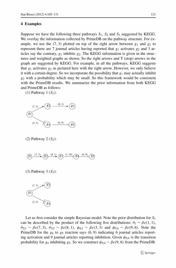
Suppose we have the following three pathways S1, S2 and S3 suggested by KEGG.We overlay the information collected by PrimeDB on the pathway structure. For ex-ample, we use the (7,3) plotted on top of the right arrow between g1 and g2 torepresent there are 7 journal articles having reported that g1 activates g2 and 3 ar-ticles say the contrary, g1 inhibits g2. The KEGG information is given in the struc-tures and weighted graphs as shown. So the right arrows and T (stop) arrows in thegraph are suggested by KEGG. For example, in all the pathways, KEGG suggeststhat g1 activates g2 as pictured here with the right arrow. However, we only believeit with a certain degree. So we incorporate the possibility that g1 may actually inhibitg2 with a probability which may be small. So this framework would be consistentwith the PrimeDB results. We summarize the prior information from both KEGGand PrimeDB as follows:

(1) Pathway 1 (S1):

�g1����

���

�g2

�g4��

� �g3

�g5(6,9)

(8,1)(7,3)

(3,3)

(2) Pathway 2 (S2):

�g1 � �g2 � �g3 �g4 �g5(7,3) (8,1) (1,10) (6,9)

(3) Pathway 3 (S3):

�g1����

���

�g2

�g4��

(7,3)

(3,3)

Let us first consider the simple Bayesian model. Note the prior distribution for S1

can be described by the product of the following five distributions: θ1 ∼ βe(1,1),θ2|1 ∼ βe(7,3), θ3|2 ∼ βe(8,1), φ4|1 ∼ βe(3,3) and φ5|4 ∼ βe(9,6). Note thePrimeDB for the g4 to g5 reaction says (6,9) indicating 6 journal articles report-ing activation and 9 journal articles reporting inhibition. Given φ5|4 is the transitionprobability for g4 inhibiting g5. So we construct φ5|4 ∼ βe(9,6) from the PrimeDB.

122 Stat Biosci (2012) 4:105–131

Table 3 Summary of the directional counts and SKL per gene

Genes ai bi ni n − ni SKLi

g1 1 1 2 1 2ψ(2) + ψ(1) − 3ψ(5) + 5 = 0.75

Genes ai|j bi|j ni|j n − ni|j SKLi|j

g2|1 7 3 1 2 ψ(8) − ψ(7) + 2[ψ(5) − ψ(3)] − 3[ψ(13) − ψ(10)] = 0.4868

g3|2 8 1 2 1 2[ψ(10) − ψ(8)] + ψ(2) − ψ(1) − 3[ψ(12) − ψ(9)] = 0.5662

g4|1 3 3 2 1 ψ(4) − ψ(3) + 2[ψ(5) − ψ(3)] − 3[ψ(9) − ψ(6)] = 0.1964

g5|4 6 9 2 1 ψ(7) − ψ(6) + 2[ψ(11) − ψ(9)] − 3[ψ(18) − ψ(15)] = 0.0249

g4|3 1 10 3 0 3[ψ(13) − ψ(10)] − 3[ψ(14) − ψ(11)] = 0.0692

Table 4 Pathway selectionbased on the simple model Pathway SKL(S)

S115 (SKL1 + SKL2|1 + SKL3|2 + SKL4|1 + SKL5|4) = 0.4049

S215 (SKL1 + SKL2|1 + SKL3|2 + SKL4|3 + SKL5|4) = 0.3794

S313 (SKL1 + SKL2|1 + SKL3|2) = 0.4777

The prior distribution for S2 is the product of θ1 ∼ βe(1,1), θ2|1 ∼ βe(7,3), θ3|2 ∼βe(8,1), φ4|3 ∼ βe(10,1), and φ5|4 ∼ βe(9,6). Note that the parameters in the betadistribution in the latter two components are in reverser order due to the inhibitioneffect proposed by KEGG. Suppose we have three microarray experiments yieldingthe following results (∪,∩,∪,∩,∪), (∩,∩,∩,∪,∪), (∪,∩,∩,∪,∩) for g1, . . . , g5.Then the likelihood for the data under S1 is θ2

1 (1 − θ1)θ2|1(1 − θ2|1)2θ23|2(1 −

θ3|2)φ24|1(1 −φ4|1)φ2

5|4(1 −φ5|4). So the posterior distribution is the joint distributionof the independent components with θ1 ∼ βe(3,2), θ2|1 ∼ βe(8,5), θ3|2 ∼ βe(10,2),φ4|1 ∼ βe(5,4) and φ5|4 ∼ βe(11,7). And, the likelihood under S2 is similar to S1

except φ24|1(1−φ4|1) is replaced by φ3

4|3, so the posterior distribution for S2 is similarto that of S1 except the posterior component for φ4|1 is replaced by φ4|3 ∼ βe(13,1).

On the pathway selection, we need to evaluate the symmetric KL divergence foreach path. We tabulate the activation and inhibition counts (ai|j , bi|j ) from PrimeDB,and the concordant and discordant counts (ni|j , n−ni|j ), from the microarray exper-iments in Table 3. Use the notation SKLi|j for the symmetric KL divergence for genei with parent j . SKLi|j can be easily calculated using (2.6) and (2.7).

We summarize the symmetric KL divergence for the three pathways in Table 4,and conclude that S2 is best supported by the microarray experiments.

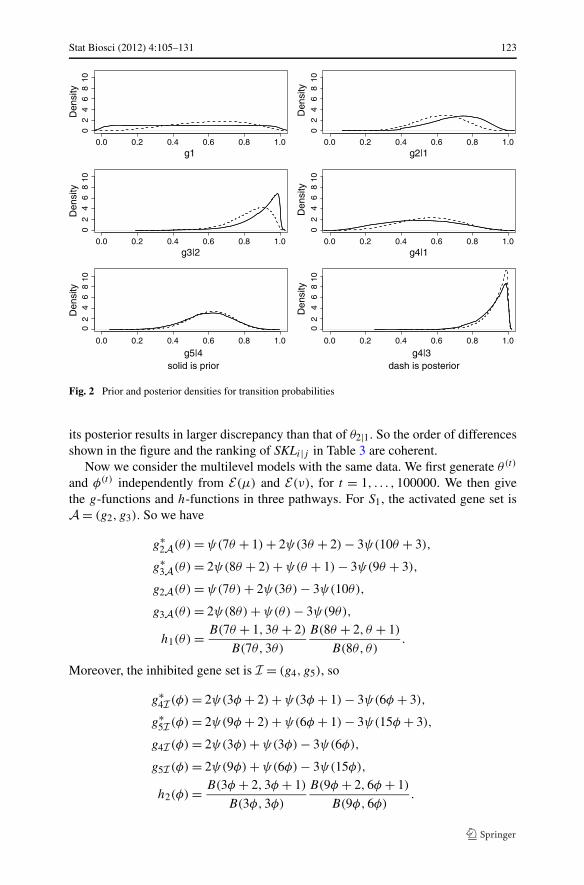
Figure 2 displays the discrepancy between the prior and posterior densities foreach transition probability in these three pathways. Among the comparison of thesix graphs, the prior and posterior of φ5|4 overlap to the largest extent. For φ4|3, thediscrepancy mainly lies in the tiny area underneath the peak, while the moderatedifference for φ4|1 ranges from 0.1 to 0.8. The big piece of prior for θ3|2 protruding

Stat Biosci (2012) 4:105–131 123

Fig. 2 Prior and posterior densities for transition probabilities

its posterior results in larger discrepancy than that of θ2|1. So the order of differencesshown in the figure and the ranking of SKLi|j in Table 3 are coherent.

Now we consider the multilevel models with the same data. We first generate θ(t)

and φ(t) independently from E (μ) and E (ν), for t = 1, . . . ,100000. We then givethe g-functions and h-functions in three pathways. For S1, the activated gene set isA = (g2, g3). So we have

g∗2A(θ) = ψ(7θ + 1) + 2ψ(3θ + 2) − 3ψ(10θ + 3),

g∗3A(θ) = 2ψ(8θ + 2) + ψ(θ + 1) − 3ψ(9θ + 3),

g2A(θ) = ψ(7θ) + 2ψ(3θ) − 3ψ(10θ),

g3A(θ) = 2ψ(8θ) + ψ(θ) − 3ψ(9θ),

h1(θ) = B(7θ + 1,3θ + 2)

B(7θ,3θ)

B(8θ + 2, θ + 1)

B(8θ, θ).

Moreover, the inhibited gene set is I = (g4, g5), so

g∗4I (φ) = 2ψ(3φ + 2) + ψ(3φ + 1) − 3ψ(6φ + 3),

g∗5I (φ) = 2ψ(9φ + 2) + ψ(6φ + 1) − 3ψ(15φ + 3),

g4I (φ) = 2ψ(3φ) + ψ(3φ) − 3ψ(6φ),

g5I (φ) = 2ψ(9φ) + ψ(6φ) − 3ψ(15φ),

h2(φ) = B(3φ + 2,3φ + 1)

B(3φ,3φ)

B(9φ + 2,6φ + 1)

B(9φ,6φ).

124 Stat Biosci (2012) 4:105–131

Table 5 SKL(S) based on the multilevel model

Pathways μ = 1 μ = 0.5 μ = 0.5 μ = 1 μ = 0.25 μ = 1 μ = 0.25

ν = 1 ν = 0.5 ν = 1 ν = 0.5 ν = 0.25 ν = 0.25 ν = 1

S1 0.7194 0.5090 0.5608 0.6680 0.3694 0.6330 0.4540

S2 0.6285 0.4535 0.4700 0.6131 0.3376 0.6009 0.3636

S3 0.7216 0.5539 0.6225 0.6524 0.4388 0.6070 0.5521

Table 6 Posterior estimatesbased on the simple model S1 S2

Param. Mean Std. Error Param. Mean Std. Error

θ2|1 0.6154 0.1300 θ2|1 0.6154 0.1300

θ3|2 0.8333 0.1034 θ3|2 0.8333 0.1034

φ4|1 0.5556 0.1571 φ4|3 0.9286 0.0665

φ5|4 0.6111 0.1118 φ5|4 0.6111 0.1118

Observing that S2 differs from S1 only in the arc g4, which is inhibited by g3 ratherby g1. So in S2, we replace g∗

4I , g4I , and h2(φ) with

g∗4I (φ) = 3ψ(10φ + 3) − 3ψ(11φ),

g4I (φ) = 3ψ(10φ) − 3ψ(11φ),

h2(φ) = B(10φ + 3, φ)

B(10φ,φ)

B(9φ + 2,6φ + 1)

B(9φ,6φ).

S3 is a subgraph of S1 with g1 activating g2 and inhibiting g4. We use the corre-sponding g-functions, and change h1(θ) = B(7θ+1,3θ+2)

B(7θ,3θ)and h2(φ) = B(3φ+2,3φ+1)

B(3φ,3φ).

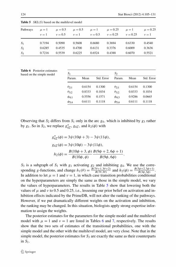
In addition to let μ = 1 and ν = 1, in which case transition probabilities conditionalon the hyperparameters are simply the same as those in the simple model, we varythe values of hyperparameters. The results in Table 5 show that lowering both thevalues of μ and ν to 0.5 and 0.25, i.e., lessening our prior belief on activation and in-hibition effects indicated by the PrimeDB, will not alter the ranking of the pathways.However, if we put dramatically different weights on the activation and inhibition,the ranking may be changed. In this situation, biologists apply strong expertise infor-mation to assign the weights.

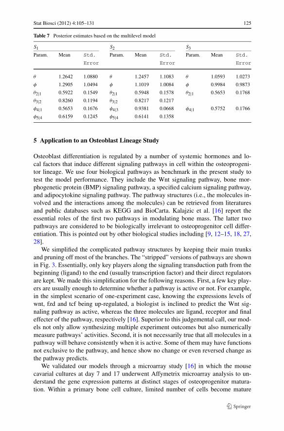
The posterior estimates for the parameters for the simple model and the multilevelmodel with μ = 1 and ν = 1 are listed in Tables 6 and 7, respectively. The resultsshow that the two sets of estimates of the transitional probabilities, one with thesimple model and the other with the multilevel model, are very close. Note that in thesimple model, the posterior estimates for S3 are exactly the same as their counterpartsin S1.

Stat Biosci (2012) 4:105–131 125

Table 7 Posterior estimates based on the multilevel model

S1 S2 S3

Param. Mean Std. Param. Mean Std. Param. Mean Std.

Error Error Error

θ 1.2642 1.0880 θ 1.2457 1.1083 θ 1.0593 1.0273

φ 1.2905 1.0494 φ 1.1019 1.0084 φ 0.9984 0.9873

θ2|1 0.5922 0.1549 θ2|1 0.5948 0.1578 θ2|1 0.5653 0.1768

θ3|2 0.8260 0.1194 θ3|2 0.8217 0.1217

φ4|1 0.5653 0.1676 φ4|3 0.9381 0.0668 φ4|1 0.5752 0.1766

φ5|4 0.6159 0.1245 φ5|4 0.6141 0.1358

5 Application to an Osteoblast Lineage Study

Osteoblast differentiation is regulated by a number of systemic hormones and lo-cal factors that induce different signaling pathways in cell within the osteoprogeni-tor lineage. We use four biological pathways as benchmark in the present study totest the model performance. They include the Wnt signaling pathway, bone mor-phogenetic protein (BMP) signaling pathway, a specified calcium signaling pathway,and adipocytokine signaling pathway. The pathway structures (i.e., the molecules in-volved and the interactions among the molecules) can be retrieved from literaturesand public databases such as KEGG and BioCarta. Kalajzic et al. [16] report theessential roles of the first two pathways in modulating bone mass. The latter twopathways are considered to be biologically irrelevant to osteoprogenitor cell differ-entiation. This is pointed out by other biological studies including [9, 12–15, 18, 27,28].

We simplified the complicated pathway structures by keeping their main trunksand pruning off most of the branches. The “stripped” versions of pathways are shownin Fig. 3. Essentially, only key players along the signaling transduction path from thebeginning (ligand) to the end (usually transcription factor) and their direct regulatorsare kept. We made this simplification for the following reasons. First, a few key play-ers are usually enough to determine whether a pathway is active or not. For example,in the simplest scenario of one-experiment case, knowing the expressions levels ofwnt, fzd and tcf being up-regulated, a biologist is inclined to predict the Wnt sig-naling pathway as active, whereas the three molecules are ligand, receptor and finaleffecter of the pathway, respectively [16]. Superior to this judgemental call, our mod-els not only allow synthesizing multiple experiment outcomes but also numericallymeasure pathways’ activities. Second, it is not necessarily true that all molecules in apathway will behave consistently when it is active. Some of them may have functionsnot exclusive to the pathway, and hence show no change or even reversed change asthe pathway predicts.

We validated our models through a microarray study [16] in which the mousecavarial cultures at day 7 and 17 underwent Affymetrix microarray analysis to un-derstand the gene expression patterns at distinct stages of osteoprogenitor matura-tion. Within a primary bone cell culture, limited number of cells become mature

126 Stat Biosci (2012) 4:105–131

Fig. 3 Four simplified signaling pathways

osteoblasts and represent only a small proportion of the total cell populations. There-fore, it is never certain whether the observed gene expression changes based on aheterogenous cell mixture are associated with fully differentiated osteoblast only orwith other cell populations. To overcome this problem, Kalajzic et al. utilized Col1a1promoter-green fluorescent protein transgenic mouse lines to generate more homo-geneous cell populations at the preosteoblastic stage and mature osteoblast stage.They demonstrated the importance for doing this cell separation for valid microarrayinterpretation. For illustration purpose, we focused on the gene intensities in sortedmature osteoblast only. They were taken from the cells with 2.3GFPpos and cellswith 2.3GFPneg in the 17-day-old cultures. In this three-replicate data set, we firstcategorized the genes in the pathways of interest as up-regulated (∪), down-regulated(∩), or equivalently expressed (EE) if their fold changes are greater than 2, less than1/2, or in between, respectively. If a gene has a single activator parent, we counted thenumber of coherence (denoted as nceq in Table 8) for the ordered pair (parent, child)with the outcomes to be (∪,∪), (∩,∩) or (EE, EE). If a gene has a single inhibitorparent, nceq is for the (parent, child) outcomes being (∪,∩), (∩,∪) or (EE, EE). Ifa gene has odd number of multiple parents, in each replication, we checked coher-ence for each individual parent related to the child as in a single-parent case, thenused majority rule to decide overall being coherent or not. Here, nceq is the count foroverall coherence for all replications. Likewise, if a gene has even number of multi-ple parents and inhibitor parents are present, we used the inhibitor outcomes only toconclude being overall coherent or not per replication. If a gene has even number ofsingle-type parents (i.e., all activators or all inhibitors), we either used majority ruleto decide overall coherence per replication in no ties case, or favored being coherentin tie case.

Stat Biosci (2012) 4:105–131 127

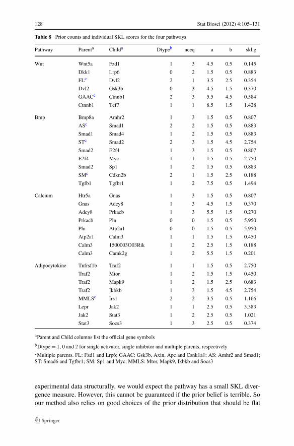
Given the PrimeDB is still under construction, we use the KEGG database asa proxy for the PrimeDB in this example. We queried the biological pathway in-formation stored in KEGG database to get the prior knowledge of the pathways.Each pairwise interaction in the pathways was checked against all the pathways inKEGG database. For a gene with single activator, we counted the number of path-ways a, where parent–child activation interaction exists. Parameter a is then definedas a + 0.5, the number 0.5 is added to all prior counts to avoid improper prior causedby zero counts. We also defined parameter b from the number of pathways whereboth parent and child exist but have no activation association between. Likewise, theactivation interaction was replaced with inhibition in defining a and b for genes withsingle inhibitor parent. For a multiple-parent case, we defined parameter a similarlyfrom the number of pathways where at least one of the parents has interaction point-ing to the child, and parameter b from the number of pathways where at least oneparent exists together with the child but have no interaction between any parent–child pair. The interaction feature between parents and child, i.e., activation or in-hibition, was determined by majority rule. All the KEGG pathway information wasdownloaded and stored in a relational database, such that the prior parameters can beretrieved automatically.

Table 8 lists the parent–child directional interaction (denoted as Dtype), the priorparameters, number of coherence, and individual SKL score per child (skl.g) basedon the simple model for the four signaling pathways. Dtype takes value of 1, 0 and2 to stand for activation, inhibition and multiple-parent case, respectively. Table 9gives the SKL scores for the four pathways based on the simple model and multilevelmodel. The two signaling pathways that play essential role in the osteoblast lineageprogression, Wnt and BMP, have smaller SKL scores than the other two pathways.In multilevel models 1–3, we set the values of the hyperparameters that govern ourbelief on the prior counts acquired from KEGG, at all equal to 1, 2 or 0.5. The rankingof the pathways is not sensitive to the choice values of hyperparameters.

It is worthwhile noting that the above extension to multiple parents does notseem to follow along the line of a Bayesian network. It is possible to have theusual Bayesian network extension to construct conditional distribution given mul-tiple parental nodes. However, lack of prior information from the literature search inpractice has made us resolve to a more realistic approach, as presented here.

6 Discussion

We have proposed a novel methodology to integrate the high-throughput data, path-way structure and medical literature regarding the gene-gene directional interactions(PrimeDB). We construct BN from a pathway database, and use PrimeDB to guidethe choices of prior parameters or hyperparameters in the BN. Then we show how toupdate these information using high-throughput genomics experiments. Our methodnumerically measures the strength of agreement between each pathway and the ex-periment using the symmetric Kullback Leibler measure incorporating the activa-tion/inhibition association permeated in the biomedical literature. So we can rank theimportance of these pathways in terms of their relatedness to the biological experi-ments to gain further knowledge in system biology. When a pathway agrees with the

128 Stat Biosci (2012) 4:105–131

Table 8 Prior counts and individual SKL scores for the four pathways

Pathway Parenta Childa Dtypeb nceq a b skl.g

Wnt Wnt5a Fzd1 1 3 4.5 0.5 0.145

Dkk1 Lrp6 0 2 1.5 0.5 0.883

FLc Dvl2 2 1 3.5 2.5 0.354

Dvl2 Gsk3b 0 3 4.5 1.5 0.370

GAACc Ctnnb1 2 3 5.5 4.5 0.584

Ctnnb1 Tcf7 1 1 8.5 1.5 1.428

Bmp Bmp8a Amhr2 1 3 1.5 0.5 0.807

ASc Smad1 2 2 1.5 0.5 0.883

Smad1 Smad4 1 2 1.5 0.5 0.883

STc Smad2 2 3 1.5 4.5 2.754

Smad2 E2f4 1 3 1.5 0.5 0.807

E2f4 Myc 1 1 1.5 0.5 2.750

Smad2 Sp1 1 2 1.5 0.5 0.883

SMc Cdkn2b 2 1 1.5 2.5 0.188

Tgfb1 Tgfbr1 1 2 7.5 0.5 1.494

Calcium Htr5a Gnas 1 3 1.5 0.5 0.807

Gnas Adcy8 1 3 4.5 1.5 0.370

Adcy8 Prkacb 1 3 5.5 1.5 0.270

Prkacb Pln 0 0 1.5 0.5 5.950

Pln Atp2a1 0 0 1.5 0.5 5.950

Atp2a1 Calm3 1 1 1.5 1.5 0.450

Calm3 1500003O03Rik 1 2 2.5 1.5 0.188

Calm3 Camk2g 1 2 5.5 1.5 0.201

Adipocytokine Tnfrsf1b Traf2 1 1 1.5 0.5 2.750

Traf2 Mtor 1 2 1.5 1.5 0.450

Traf2 Mapk9 1 2 1.5 2.5 0.683

Traf2 Ikbkb 1 3 1.5 4.5 2.754

MMLSc Irs1 2 2 3.5 0.5 1.166

Lepr Jak2 1 1 2.5 0.5 3.383

Jak2 Stat3 1 2 2.5 0.5 1.021

Stat3 Socs3 1 3 2.5 0.5 0.374

aParent and Child columns list the official gene symbols

bDtype = 1, 0 and 2 for single activator, single inhibitor and multiple parents, respectivelycMultiple parents. FL: Fzd1 and Lrp6; GAAC: Gsk3b, Axin, Apc and Csnk1a1; AS: Amhr2 and Smad1;ST: Smad6 and Tgfbr1; SM: Sp1 and Myc; MMLS: Mtor, Mapk9, Ikbkb and Socs3

experimental data structurally, we would expect the pathway has a small SKL diver-gence measure. However, this cannot be guaranteed if the prior belief is terrible. Soour method also relies on good choices of the prior distribution that should be flat

Stat Biosci (2012) 4:105–131 129

Table 9 SKL(S) of the four pathways

Pathways Simple Multilevel Multilevel Multilevel

Model Model1 Model2 Model3

Wnt 1.0922 1.0673 1.1565 0.9828

Bmp 1.3916 1.2471 1.4976 1.0197

Calcium 1.8263 1.7778 2.0835 1.4889

Adipocytokine 1.7081 1.4572 1.7602 1.1823

and has huge support. In the illustration using real data, we have chosen the KEGGpathway database as the primary source of pathway structure and its gene-gene inter-action as representative of medical journal counts (PrimeDB). The result might relyon the extant knowledge from a single data repository. However, our methodologyis general enough that can be applied to any good databases that include gene-genedirection relationships as a substitute of the PrimeDB.

When a pathway is identified, it suggests the pathway is most agreeable with thedata presented. On the other hand, the pathway with the highest K–L divergencesuggests the pathway structure is not well supported by the data. This may be causedby (1) unexpected data, (2) dubious pathway structure, or both. So it has potential toprovide more insights into the pathways.

We have used small sample size in our simulated and real examples, primarilysmall sample size is common in microarray experiments. Nevertheless, our methodcan handle any sample size as well. Microarray techniques are known to be noisyfor biologists, so their results are often questioned by the biologists. Small sampleexacerbates this situation. So incorporating a Bayesian frame work and borrowinginformation from the literature will add credibility to the microarray studies. More-over, the multilevel model provides a more robust framework for sharing informationamong similar genes in evaluating the pathways.

Our method can handle large networks quite efficiently. It first computes the SKLscore for each gene independently, then takes their averages as the pathway SKLscore. In the simple model, the gene-specific SKL score reduces to a linear function ofdigamma functions. It hence can readily handle large pathways at fast speed. For themultilevel model, we use a collapsing technique and as a result sample from the priordistribution only instead of from both prior and posterior distributions of θ and φ, thetwo parameters that govern prior belief of the literature count. This greatly improvesthe efficiency in the numerical evaluation of the integrals in I ′

2 and I ′3, the sums of the

SKL scores for activated genes and inhibited genes. R programs have been developedbased on this method. In the osteoblast lineage study, the four pathways have 11, 12,9 and 10 genes, respectively. It takes less than 13 seconds in total to compute theirSKL scores of the multilevel model using R 2.13.0 on a laptop computer with 2ndgeneration Intel Core i5-2410M processor 2.30 GHz. So it should not be a burden tocompute SKL for large pathways which consist of about a hundred nodes at most asshown in KEGG.

Starting with the gene expression data from microarray, we first applied some sta-tistical tests to classify the genes as up-regulated, down-regulated, or equivalently ex-pressed. Fold change was used in our real data analysis. Then we construct Bayesian

130 Stat Biosci (2012) 4:105–131

network for each pathway. So our study applies to the continuous gene expressions.However, we simplify the agreement assessment by discretizing the data. It wouldbe interesting to extend our method to directly using the continuous gene expression.Nevertheless, we do not think the extension will be straightforward especially on arealistic prior construction.

We think the strength of this paper is on its ability to handle directed graphs withdirected prior information on gene functions. On the other hand, our method canbe modified to handle undirected graphs. In that, we will not differentiate activationor inhibition direction, change all of them into connection, then our method withreduced parameters can handle the undirected graph. For mixed graphs with directedand undirected edges, we need to add the connected part for the direction-unknownedges, then we can handle them similarly.

In this paper, we also assume that microarray outcomes are available for all thegenes considered in the pathway (BN). However, it is often in practice so, that thepathway includes genes that microarray may not explore. So this falls into the miss-ing data problem in BN. Conditional inference with incomplete data and model se-lection can still be carried out using Expectation and Maximization (EM) algorithmor MCMC. Further investigation on this issue should be worthwhile.

Acknowledgements The work of Yifang Zhao, Baikang Pei, David Rowe, Dong-Guk Shin, WangangXie, Fang Yu, and Lynn Kuo was partially supported by Grants NIH/NIGMS P20GM65764, NIH/NIDCRU24DE016495, and State of Connecticut Stem Cell Initiative 06SCC04. Ming-Hui Chen’s work was par-tially supported by NIH grants GM70335 and CA74015.

References

1. Chen M-H, Shao Q-M, Ibrahim JG (2000) Monte Carlo methods in Bayesian computation. Springer,New York

2. Chen M-H, Huang L, Ibrahim JG, Kim S (2008) Bayesian variable selection and computation forgeneralized linear models with conjugate priors. Bayesian Anal 3:585–614

3. Curtis RK, Oresic M, Vidal-Puig A (2005) Pathways to the analysis of microarray data. TrendsBiotechnol 23(8):429–435

4. Efron B, Tibshirani R (2007) On testing the significance of sets of genes. Ann Appl Stat 1:107–1295. Ellis B, Wong WH (2008) Learning causal Bayesian network structures from experimental data. J Am

Stat Assoc 103:778–7896. Fletcher R, Reeves CM (1964) Function minimization by conjugate gradients. Comput J 7:148–1547. Friedman N, Linial M, Nachman I, Pe’er D (2000) Using Bayesian networks to analyze expression

data. J Comput Biol 7(3–4):601–6208. Geweke J (1992) Evaluating the accuracy of sampling-based approaches to calculating posterior mo-

ments. In: Bernado JM, Berger JO, Dawid AP, Smith AFM (eds) Bayesian statistics 4. Clarendon,Oxford

9. Hartmann C (2006) A Wnt canon orchestrating osteoblastogenesis. Trends Cell Biol 16(3):151–15810. Hartemink A, Gifford DK, Jaakkola TS, Young RA (2002) Bayesian methods for elucidating genetic

regulatory networks. IEEE Intell Syst Biol 17(2):37–4311. Heckerman D (1995) A tutorial on learning Bayesian networks. Technical Report MSR-TR-95-06,

Microsoft Research12. Hoffmann A, Gross G (2001) BMP signaling pathways in cartilage and bone formation. Crit Rev

Eucar Gene Expr 11(1–3):23–4613. Ishii M, Kurachi Y (2006) Muscarinic acetylcholine receptors. Curr Pharm Des 12(28):3573–358114. Jensen ED, Gopalakrishnan R, Westendorf JJ (2010) Regulation of gene expression in osteoblasts.

BioFactors 36(1):25–32

Stat Biosci (2012) 4:105–131 131

15. Jimia E, Hirataa S, Shina M, Yamazakia M, Fukushimaa H (2010) Molecular mechanisms of BMP-induced bone formation: Cross-talk between BMP and NF-?B signaling pathways in osteoblastogen-esis. Jpn Dent Sci Rev 46(1):33–42

16. Kalajzic I, Staale A, Yang W-P, Wu Y, Johnson SE, Feyen JHM, Krueger W, Maye P, Yu F, ZhaoY, Kuo L, Gupta RR, Achenie LEK, Wang H-W, Shin D-G, Rowe DW (2005) Expression profile ofosteoblast lineage at defined stages of differentiation. J Biol Chem 280:24618–24626

17. Kanehisa M, Goto S (2000) KEGG: Kyoto encyclopedia of genes and genomes. Nucleic Acids Res28(1):27–30

18. Kay GG, Abou-Donia MB, Messer WS, Murphy DG, Tsao JW, Ouslander JG (2005) Antimuscarinicdrugs for overactive bladder and their potential effects on cognitive function in older patients. J AmGeriatr Soc 53(12):2195–2201

19. Kullback S, Leibler RA (1951) On information and sufficiency. Ann Math Stat 22(1):79–8620. Liu JS (1994) The collapsed Gibbs sampler with applications to a gene regulation problem. J Am Stat

Assoc 89:958–96621. Metropolis N, Rosenbluth AW, Rosenbluth MN, Teller AH, Teller E (1953) Equation of state calcu-

lations by fast computing machines. J Chem Phys 21:1087–109222. Monni S, Li H (2010) Bayesian methods for network-structures genomic data. In: Chen MH, Dey

DK, Muller P, Sun D, Ye K (eds) Frontiers of statistical decision making and Bayesian analysis: Inhonor of James O. Berger. Springer, New York, pp 303–315

23. Newton M, Quintana F, Den Boon J, Sengupta S, Ahlquist P (2007) Random-set methods identifydistinct aspects of the enrichment signal in gene-set analysis. Ann Appl Stat 1:85–106

24. Sachs K, Gifford D, Jaakkola T, Sorger P, Lauffenburger DA (2002) Bayesian network approach tocell signaling pathway modeling. Sci Signal Transduct Knowl Environ 148:pe38

25. Sebastiani P, Abad M, Ramoni M (2004) Bayesian networks for genomic analysis. In: Dougherty ER,Shmulevich I, Chen J, Wang ZJ (eds) Genomic signal processing and statistics. Hindawi PublishingCorporation, New York, pp 281–320

26. Shen H, West M (2010) Bayesian modeling for biological annotation of gene expression pathwaysignatures. In: Chen MH, Dey DK, Muller P, Sun D, Ye K (eds) Frontiers of statistical decisionmaking and Bayesian analysis: In honor of James O. Berger. Springer, New York, pp 285–302

27. Tilg H, Moschen AR (2006) Adipocytokines: mediators linking adipose tissue, inflammation andimmunity. Nat Rev Immunol 6:772–783

28. van Amerongen R, Nusse R (2009) Towards an integrated view of Wnt signaling in development.Development 136(19):3205–3214

29. Werhli A, Husmeier D (2007) Reconstructing gene regulatory networks with Bayesian network bycombining expression data with multiple sources of prior knowledge. Stat Appl Genet Mol Biol6(1):1–45