Bayesian Inference of Genetic Regulatory Networks from Time Series Microarray Data Using Dynamic Bayesian Networks Yufei Huang , Jianyin Wang, Jianqiu Zhang, Maribel Sanchez, and Yufeng Wang Abstract — Reverse engineering of genetic regulatory net- works from time series microarray data are investigated. We propose a dynamic Bayesian networks (DBNs) modeling and a full Bayesian learning scheme. The proposed DBN directly models the continuous expression levels and also is associ- ated with parameters that indicate the degree as well as the type of regulations. To learn the network from data, we proposed a reversible jump Markov chain Monte Carlo (RJMCMC) algorithm. The RJMCMC algorithm can pro- vide not only more accurate inference results than the de- terministic alternative algorithms but also an estimate of the a posteriori probabilities (APPs) of the network topol- ogy. The estimated APPs provide useful information on the confidence of the inferred results and can also be used for efficient Bayesian data integration. The proposed approach is tested on yeast cell cycle microarray data and the results are compared with the KEGG pathway map. I. INTRODUCTION In the cell of a living organism, there are thousands of genes interacting with each other at any given time to ac- complish complicated biological tasks. Genetic regulatory networks (GRNs) are collections of gene-gene regulatory relations in a genome and are models that display causal re- lationships between gene activities. The system level view of gene functions provided by GRNs is of tremendous im- portance in understanding the underlying biological pro- cess of living organisms, providing new ideas for treating complicated diseases, and designing new drugs. Inevitably, uncovering GRNs has become a trend in recent biomedical researches [1], [2]. In this paper, we study signal processing solutions to the inference of GRNs based on microarray data. Microarray, a technology allowing measurements of mRNA expression levels of thousands of genes, provides first-hand informa- tion on genome wide molecular interactions and thus, it is logical to deduce that these data can be used to infer GRNs. Inference of GRNs based on microarray data is referred to as ‘reverse engineering’ [3], as the microarray expression Corresponding Author: Yufei Huang Y. Huang and J. Wang are with the Department of Electrical and Computer Engineering, University of Texas at San Antonio (UTSA), San Antonio, TX 78249-0669. E-mail: [email protected]. Phone: (210)4586270. Fax: (210)4585947. J. Zhang is with the Department of ECE, University of New Hamp- shire, Durham, NH 03824. E-mail: [email protected] M. Sanchez and Y. Wang are with the Department of Biology, UTSA. Email: [email protected] This work was supported by in part by an NSF Grant CCF-0546345 to Y. Huang and NIH 1R21AI067543-01A1, San Antonio Area Foun- dation Biomedical Research funds, UTSA Faculty Research Award to Y. Wang. Y. Wang is also supported by NIH RCMI grant 2G12 RR013646-06A1. levels are the outcome of gene regulation. Mathematically, reverse engineering is a traditional inverse problem. The solution to the problem is, however, not trivial, as it is com- plicated by the enormously large scale of the unknowns in a rather small sample size. In addition, the inherent ex- perimental defects, noisy readings, and many other factors play a role. These complexities call for heavy involvement of statistical signal processing, which, we foresee, will play an increasingly important role in this research. The microarray data can be classified as from static or from time series experiments. In static experiments, snap- shots of the expression of genes under different conditions are measured. In time series experiments, temporal molec- ular processes are measured. In particular, these time series data reflect the dynamics of gene activities in cell cycles. They are very important for understanding cellular aging (senescence) and programmed cell death (apoptosis), pro- cesses involved in the development of cancers, and other diseases associated with the aging process [4]. While build- ing GRNs based on static microarray data is still of great interest and solutions based on probabilistic Boolean net- works [5], [6], Bayesian networks [7], [8], [9], and many others [10] have been proposed, the study of using time se- ries data has drawn increasing attention [11], [12]. Unlike the case of static experiments, extra attention is needed in modeling the time series experiments to account for tem- poral correlation. Such time series models can in turn com- plicate the inference, thus making the task of reverse engi- neering even more challenging than it already is. In this paper, we apply dynamic Bayesian networks (DBNs) to model the time series microarray experiment and develop a full Bayesian solution for learning the net- works. The use of DBNs is not foreign to the reverse en- gineering of GRNs. The framework of such usage was first proposed in [13]. Details of modeling and learning with DBNs were investigated first in [14] and then in [15] and the proposed frameworks were tested on yeast cell cycle data. However, the proposed DBNs only took discretized expression levels and quantization on the expression level has to be performed, which resulted in loss of informa- tion. Also, only the connectivity of genes were modeled and no estimate was provided on the degree as well as the types of regulation. In [16] and [17], state-space model based DBNs were proposed, where hidden variables were allowed to account for factors that were not captured by the microarray experiments. Despite the elegance of such modeling and the proposed expectation-maximization and 46 JOURNAL OF MULTIMEDIA, VOL. 2, NO. 3, JUNE 2007 © 2007 ACADEMY PUBLISHER

Welcome message from author
This document is posted to help you gain knowledge. Please leave a comment to let me know what you think about it! Share it to your friends and learn new things together.
Transcript
Bayesian Inference of Genetic Regulatory Networksfrom Time Series Microarray Data Using Dynamic
Bayesian NetworksYufei Huang , Jianyin Wang, Jianqiu Zhang, Maribel Sanchez, and Yufeng Wang
Abstract— Reverse engineering of genetic regulatory net-works from time series microarray data are investigated. Wepropose a dynamic Bayesian networks (DBNs) modeling anda full Bayesian learning scheme. The proposed DBN directlymodels the continuous expression levels and also is associ-ated with parameters that indicate the degree as well asthe type of regulations. To learn the network from data,we proposed a reversible jump Markov chain Monte Carlo(RJMCMC) algorithm. The RJMCMC algorithm can pro-vide not only more accurate inference results than the de-terministic alternative algorithms but also an estimate ofthe a posteriori probabilities (APPs) of the network topol-ogy. The estimated APPs provide useful information on theconfidence of the inferred results and can also be used forefficient Bayesian data integration. The proposed approachis tested on yeast cell cycle microarray data and the resultsare compared with the KEGG pathway map.
I. INTRODUCTION
In the cell of a living organism, there are thousands ofgenes interacting with each other at any given time to ac-complish complicated biological tasks. Genetic regulatorynetworks (GRNs) are collections of gene-gene regulatoryrelations in a genome and are models that display causal re-lationships between gene activities. The system level viewof gene functions provided by GRNs is of tremendous im-portance in understanding the underlying biological pro-cess of living organisms, providing new ideas for treatingcomplicated diseases, and designing new drugs. Inevitably,uncovering GRNs has become a trend in recent biomedicalresearches [1], [2].
In this paper, we study signal processing solutions to theinference of GRNs based on microarray data. Microarray,a technology allowing measurements of mRNA expressionlevels of thousands of genes, provides first-hand informa-tion on genome wide molecular interactions and thus, it islogical to deduce that these data can be used to infer GRNs.Inference of GRNs based on microarray data is referred toas ‘reverse engineering’ [3], as the microarray expression
Corresponding Author: Yufei Huang
Y. Huang and J. Wang are with the Department of Electrical and
Computer Engineering, University of Texas at San Antonio (UTSA),
San Antonio, TX 78249-0669. E-mail: [email protected]. Phone:
(210)4586270. Fax: (210)4585947.
J. Zhang is with the Department of ECE, University of New Hamp-
shire, Durham, NH 03824. E-mail: [email protected]. Sanchez and Y. Wang are with the Department of Biology,
UTSA. Email: [email protected] work was supported by in part by an NSF Grant CCF-0546345
to Y. Huang and NIH 1R21AI067543-01A1, San Antonio Area Foun-
dation Biomedical Research funds, UTSA Faculty Research Award
to Y. Wang. Y. Wang is also supported by NIH RCMI grant 2G12
RR013646-06A1.
levels are the outcome of gene regulation. Mathematically,reverse engineering is a traditional inverse problem. Thesolution to the problem is, however, not trivial, as it is com-plicated by the enormously large scale of the unknowns ina rather small sample size. In addition, the inherent ex-perimental defects, noisy readings, and many other factorsplay a role. These complexities call for heavy involvementof statistical signal processing, which, we foresee, will playan increasingly important role in this research.
The microarray data can be classified as from static orfrom time series experiments. In static experiments, snap-shots of the expression of genes under different conditionsare measured. In time series experiments, temporal molec-ular processes are measured. In particular, these time seriesdata reflect the dynamics of gene activities in cell cycles.They are very important for understanding cellular aging(senescence) and programmed cell death (apoptosis), pro-cesses involved in the development of cancers, and otherdiseases associated with the aging process [4]. While build-ing GRNs based on static microarray data is still of greatinterest and solutions based on probabilistic Boolean net-works [5], [6], Bayesian networks [7], [8], [9], and manyothers [10] have been proposed, the study of using time se-ries data has drawn increasing attention [11], [12]. Unlikethe case of static experiments, extra attention is needed inmodeling the time series experiments to account for tem-poral correlation. Such time series models can in turn com-plicate the inference, thus making the task of reverse engi-neering even more challenging than it already is.
In this paper, we apply dynamic Bayesian networks(DBNs) to model the time series microarray experimentand develop a full Bayesian solution for learning the net-works. The use of DBNs is not foreign to the reverse en-gineering of GRNs. The framework of such usage was firstproposed in [13]. Details of modeling and learning withDBNs were investigated first in [14] and then in [15] andthe proposed frameworks were tested on yeast cell cycledata. However, the proposed DBNs only took discretizedexpression levels and quantization on the expression levelhas to be performed, which resulted in loss of informa-tion. Also, only the connectivity of genes were modeledand no estimate was provided on the degree as well as thetypes of regulation. In [16] and [17], state-space modelbased DBNs were proposed, where hidden variables wereallowed to account for factors that were not captured bythe microarray experiments. Despite the elegance of suchmodeling and the proposed expectation-maximization and
46 JOURNAL OF MULTIMEDIA, VOL. 2, NO. 3, JUNE 2007
© 2007 ACADEMY PUBLISHER
variational Bayes solutions, the learning requires unreal-istically large amount of data, thus greatly limiting theirapplication.
The DBN used in this paper is close to that in [18], whichmodels the continuous expression level and the degree ofregulation. However, unlike in [18], we target cases whereonly microarray data are available for network inference.Consequently, instead of assuming a nonlinear model basedon B-spline as in [18], a more conservative linear regula-tory model is adopted here since, with very limited data,more complex models will greatly reduce the credibilityof the inferred results. On the other hand, we are par-ticularly interested in full Bayesian solutions for learningthe networks, which can provide estimates on the a pos-teriori probabilities (APPs) of the inferred network topol-ogy. This type of solution is termed ‘probabilistic’ or ‘soft’in signal processing and digital communications. This re-quirement separates the proposed solutions from most ofthe existing approaches such as step-wise search and sim-ulated annealing based algorithms, all of which produceonly point estimates of the networks and are consideredas “hard” solutions. The advantage of soft solutions hasbeen demonstrated in digital communications [19]. In thecontext of GRNs, the APPs from the soft solutions providevaluable measurements of confidence on inference, which isdifficult with hard solutions. Moreover, they are necessaryfor Bayesian data integration. Here, we propose a soft so-lution based on reversible jump Markov chain Monte Carlo(RJMCMC) sampling. To combat the distortion due tosmall sample size, we impose an upper limit on the num-ber of parents and carefully design the topology priors.
The rest of the paper is organized as follows: In sectionII, the issues on modeling the time series data with DBNsare discussed. The detailed model for gene regulation isalso provided. In section III, tasks related to learning thenetworks are discussed and the Bayesian solution is derived.In section IV, the test results of the proposed approachon the simulated networks and yeast cell cycle data areprovided. The paper concludes in V with remarks on futurework.
II. Modeling with Dynamic Bayesian Networks
Like all graphical models, a DBN is a marriage of graph-ical and probabilistic theories. In particular, DBNs area class of directed acyclic graphs (DAGs) that modelprobabilistic distributions of stochastic dynamic processes.DBNs enable easy factorization on joint distributions ofdynamic processes into products of simpler conditional dis-tributions according to the inherent Markov properties andthus greatly facilitate the task of inference. DBNs areshown to be a generalization of a wide range of popularmodels, which include hidden Markov models (HMMs) andKalman filtering models or state-space models. They havebeen successfully applied in computer vision, speech pro-cessing, target tracking, and wireless communications. Re-fer to [20] for a comprehensive discussion on DBNs.
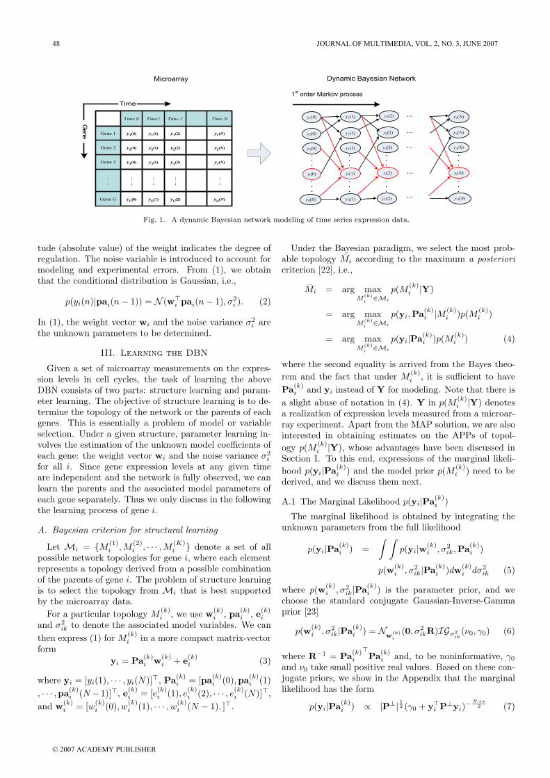
A DBN consists of nodes and directed edges. Each noderepresents a variable in the problem while a directed edge
indicates the direct association between the two connectednodes. In a DBN, the direction of an edge can carry thetemporal information. To model the gene regulation fromcell cycle using DBNs, we assume a microarray that mea-sures the expression levels of G genes at N +1 evenly sam-pled consecutive time instances. We then define a ran-dom variable matrix Y ∈ RG×(N+1) with the (i, n)th el-ement yi(n − 1), denoting the expression level of gene imeasured at time n − 1 (See Figure 1). We further as-sume that the gene regulation follows a first-order time-homogeneous Markov process. As a result, we need only toconsider regulatory relationships between two consecutivetime instances; this relationship remains unchanged overthe course of the microarray experiment. This assump-tion may be insufficient but will facilitate the modelingand inference. Also, we call the regulating genes the “par-ent genes” or “parents” for short.
Based on these definitions and assumptions, the struc-ture of the proposed DBNs for modeling the cell cycle reg-ulation is illustrated in Figure 1. In this DBN, each nodedenotes a random variable in Y and all the nodes are ar-ranged the same way as the corresponding variables in thematrix Y. An edge between two nodes denotes the regu-latory relationship between the two associated genes andthe arrow indicates the direction of regulation. For exam-ple, we see from Figure 1 that genes 1, 3, and G regulategene i. Even though, like all Bayesian networks, DBNs donot allow circles in the graph, they, however, are capableof modeling circular regulatory relationship, an importantproperty that is not possessed by regular Bayesian net-works. As an example, a circular regulation can be seenin Figure 1 between gene 1 and 2 even though no circularloops are used in the graph.
To complete modeling with DBNs, we need to define theconditional distributions of each child node over the graph.Then the desired joint distribution can be represented asa product of these conditional distributions. To define theconditional distributions, we let pai(n) denote a columnvector of the expression levels of all the parent genes thatregulate gene i measured at time n. As an example inFigure 1, pai(n)� = [y1(n), y3(n), yG(n)]. Then, the con-ditional distributions of each child nodes over the DBNscan be expressed as p(yi(n)|pai(n − 1)) ∀i. To determinethe expression of the distributions, we assume linear reg-ulatory relationship, i.e., the expression level of gene i isthe result of a linear combination of the expression levelsof the regulating genes at a previous sample time. Mathe-matically, we have the following expression
yi(n) = w�i pai(n − 1) + ei(n), n = 1, 2, · · · , N (1)
where wi ∈ R is the weight vector independent of time nand ei(n) is assumed to be white Gaussian noise with vari-ance σ2. The assumption on white Gaussian noise may notbe realistic for the system error of microarray experiments[21]. However, it simplifies the learning of networks. Theweight vector is indicative of the degree and the types ofthe regulation [16]. A gene is up-regulated if the weightis positive and is down-regulated otherwise. The magni-
JOURNAL OF MULTIMEDIA, VOL. 2, NO. 3, JUNE 2007 47
© 2007 ACADEMY PUBLISHER
Microarray
y2(0)
y1(0)
yG(0)
y2(1)
y1(1)
y3(1)
yG(1)
yi(0) yi(1)
y2(2)
y1(2)
y3(2)
yG(2)
yi(2)
y2(N)
y1(N)
y3(N)
yG(N)
yi(N)
1
st
order Markov process
...
...
...
...
...
Dynamic Bayesian Network
y3(0)
yG(N)yG(2)yG(1)yG(0)Gene G
:
:
:
:
:
:
:
:
:
:
y3(N)y3(2)y3(1)y3(0)Gene 3
y2(N)y2(2)y2(1)y2(0)Gene 2
y1(N)y1(2)y1(1)y1(0)Gene 1
Time NTime 2Time1Time 0
yG(N)yG(2)yG(1)yG(0)Gene G
:
:
:
:
:
:
:
:
:
:
y3(N)y3(2)y3(1)y3(0)Gene 3
y2(N)y2(2)y2(1)y2(0)Gene 2
y1(N)y1(2)y1(1)y1(0)Gene 1
Time NTime 2Time1Time 0
Time
Gene
Fig. 1. A dynamic Bayesian network modeling of time series expression data.
tude (absolute value) of the weight indicates the degree ofregulation. The noise variable is introduced to account formodeling and experimental errors. From (1), we obtainthat the conditional distribution is Gaussian, i.e.,
p(yi(n)|pai(n − 1)) = N (w�i pai(n − 1), σ2
i ). (2)
In (1), the weight vector wi and the noise variance σ2
i arethe unknown parameters to be determined.
III. Learning the DBN
Given a set of microarray measurements on the expres-sion levels in cell cycles, the task of learning the aboveDBN consists of two parts: structure learning and param-eter learning. The objective of structure learning is to de-termine the topology of the network or the parents of eachgenes. This is essentially a problem of model or variableselection. Under a given structure, parameter learning in-volves the estimation of the unknown model coefficients ofeach gene: the weight vector wi and the noise variance σ2
i
for all i. Since gene expression levels at any given timeare independent and the network is fully observed, we canlearn the parents and the associated model parameters ofeach gene separately. Thus we only discuss in the followingthe learning process of gene i.
A. Bayesian criterion for structural learning
Let Mi = {M (1)
i , M(2)
i , · · · , M (K)
i } denote a set of allpossible network topologies for gene i, where each elementrepresents a topology derived from a possible combinationof the parents of gene i. The problem of structure learningis to select the topology from Mi that is best supportedby the microarray data.
For a particular topology M(k)
i , we use w(k)
i , pa(k)
i , e(k)
i
and σ2
ik to denote the associated model variables. We canthen express (1) for M
(k)
i in a more compact matrix-vectorform
yi = Pa(k)
i w(k)
i + e(k)
i (3)
where yi = [yi(1), · · · , yi(N)]�, Pa(k)
i = [pa(k)
i (0),pa(k)
i (1), · · · ,pa(k)
i (N −1)]�, e(k)
i = [e(k)
i (1), e(k)
i (2), · · · , e(k)
i (N)]�,and w(k)
i = [w(k)
i (0), w(k)
i (1), · · · , w(k)
i (N − 1), ]�.
Under the Bayesian paradigm, we select the most prob-able topology Mi according to the maximum a posterioricriterion [22], i.e.,
Mi = arg maxM
(k)i
∈Mi
p(M (k)
i |Y)
= arg maxM
(k)i
∈Mi
p(yi,Pa(k)
i |M (k)
i )p(M (k)
i )
= arg maxM
(k)i
∈Mi
p(yi|Pa(k)
i )p(M (k)
i ) (4)
where the second equality is arrived from the Bayes theo-rem and the fact that under M
(k)
i , it is sufficient to havePa(k)
i and yi instead of Y for modeling. Note that there isa slight abuse of notation in (4). Y in p(M (k)
i |Y) denotesa realization of expression levels measured from a microar-ray experiment. Apart from the MAP solution, we are alsointerested in obtaining estimates on the APPs of topol-ogy p(M (k)
i |Y), whose advantages have been discussed inSection I. To this end, expressions of the marginal likeli-hood p(yi|Pa(k)
i ) and the model prior p(M (k)
i ) need to bederived, and we discuss them next.
A.1 The Marginal Likelihood p(yi|Pa(k)
i )
The marginal likelihood is obtained by integrating theunknown parameters from the full likelihood
p(yi|Pa(k)
i ) =∫ ∫
p(yi|w(k)
i , σ2
ik,Pa(k)
i )
p(w(k)
i , σ2
ik|Pa(k)
i )dw(k)
i dσ2
ik (5)
where p(w(k)
i , σ2
ik|Pa(k)
i ) is the parameter prior, and wechoose the standard conjugate Gaussian-Inverse-Gammaprior [23]
p(w(k)
i , σ2
ik|Pa(k)
i ) = Nw
(k)i
(0, σ2
ikR)IGσ2ik
(ν0, γ0) (6)
where R−1 = Pa(k)
i
�Pa(k)
i and, to be noninformative, γ0
and ν0 take small positive real values. Based on these con-jugate priors, we show in the Appendix that the marginallikelihood has the form
p(yi|Pa(k)
i ) ∝ |P⊥| 12 (γ0 + y�i P⊥yi)−
N+ν2 (7)
48 JOURNAL OF MULTIMEDIA, VOL. 2, NO. 3, JUNE 2007
© 2007 ACADEMY PUBLISHER
where P⊥ = IN −Pa(k)
i (Pa(k)
i
�Pa(k)
i +R−1)−1Pa(k)
i
�and
IN is an N × N identity matrix.
B. The topology prior p(M (k)
i )
There have been discussions in the literature on choosingthe topology prior, most of which, however, are designed forlarge data samples. For cases of small data sample size asin most GRNs problems, the choice of the topology prior isa subtle issue and can sometimes affect the inference resultto a large degree. One interesting choice of the prior isthe one proposed in [24] that uses the description lengthprinciple and can be written as
p(M (k)
i ) =(
G
Pk
)−1
/G. (8)
where Pk denotes the total number of the parents underM
(k)
i . Apparently, this prior favors topologies with smallnumber or large number of parents. Especially, the ratiobetween the largest (Pk = G) and the smallest (Pk = G/2)prior probabilities are
rm =(
G
G/2
)=
G!G2!
(9)
which can be very large for large G. For cases of small sam-ple size, this prior can be too ‘informative’ so that it over-whelms the information carried by the likelihood, resultinga topology with either very large or very small number ofthe parents. Notice that this description length prior alsoimplies a uniform distribution of the number of parents Q,i.e.,
p(Q = Pk) =(
G
Pk
)(G
Pk
)−1
/G = 1/G. (10)
Instead, we assume that each gene has the same a prioriprobability, say q, to be a parent gene. This assumptionimplies a geometric distribution on the prior, which is ex-pressed as
p(M (k)) = qPk(1 − q)G−Pk . (11)
As a result, the number of the parents Q follows a Binomialdistribution
p(Q = Pk) =(
G
Pk
)qPk(1 − q)G−Pk . (12)
Since the mean number of parents Q = Gq, the probabilityq can be calculated from the mean as
q = Q/G. (13)
Therefore, the choice of q reflects our prior knowledgeabout the average number of the parents. As a specialcase, when q = 0.5, the prior becomes the popular uniformprior. Notice that this uniform prior implies a prior as-sumption of an average number of parents being G/2, anunrealistic scenario for large G. Thereby, the choice of theuniform prior is inappropriate as well.
Having derived the marginal likelihood and specified theprior on topology, we look at how the optimization in (4)
can be performed and at the same time, how calculationon APPs can be obtained. The difficulties of the task aretwo fold. First, the sample size N is normally much smallerthan the total number of testing genes G. A direct resultof it is that the problem becomes ill-conditioned. Thus,additional constraints must be imposed. Secondly, the op-timization and calculation of APPs themselves are NP hardand exact solutions are infeasible for large G. For instance,when G = 58, the size K of M is about 2.88e17, and anexhaustive search over the space of this size is already pro-hibitive, not to mention that G can be in thousands inpractice. As a result, we need to resort to numerical meth-ods.
C. The proposed solutions
To the end of first difficulty, we impose an upper limitQmax on the number of the parents and restrict Qmax < N .The restriction can be realistic in many genetic systems dueto the restricted size of the regulatory region in genes. Thisconstraint essentially forces us to search only among thetopologies whose regulatory models are over-determined.It, in turn, also serves to reduce the size of the search spaceand helps alleviate the second difficulty. Nevertheless, thesize of the search space can still be enormous even with anupper limit Qmax. We therefore propose to use reversiblejump Markov chain Monte Carlo (RJMCMC) to approx-imate the MAP solution and the APPs. RJMCMC, pro-posed by Green in [25], is an MCMC algorithm for samplingfrom a joint topology-parameter space. In our case, sincethe parameters have been analytically marginalized out,the objective of the RJMCMC is to generate random sam-ples from the APPs p(M (k)|Y). Then, the MAP solutioncan be approximated with the most-frequently-occurringsample. What is more, these samples can be also used toproduce an approximation to the desired APPs, which isdifficult with the deterministic schemes.
The algorithm of the proposed RJMCMC is summarizedin the following box.
Algorithm: RJMCMC
Provide an initial topology and assign it to M(0). Iterate Ttimes and at the tth iteration perform the following steps .
1. Candidate selection: Suppose M(t − 1) = M(k)
i .
If Pk = 1, randomly select a gene from the non-parent genes; If Pk = Qmax, randomly select agene from the parent genes; Otherwise, randomlyselect a gene from all G genes
2. If the gene is a parent in M(t − 1)- Death move: Remove the node associatedwith the selected gene from M (k) to obtain
topology M(j)i . Set M(t) = M
(j)i with probability
λ = min{BF (j, k), α(j, k)}/α(j, k)Otherwise M(t) = M
(k)
i .else
- Birth move: Add the node associated with
JOURNAL OF MULTIMEDIA, VOL. 2, NO. 3, JUNE 2007 49
© 2007 ACADEMY PUBLISHER
the select gene to M (k) to obtain topology M(l)i .
Set M(t) = M(l)i with probability
λ = min{BF (l, k), α(l, k)}/α(l, k).Otherwise M(t) = M
(k)
i .
In this algorithm, BF (Mi, Mk) is the Bayes factor be-tween Mi and Mk and is defined as
BF (j, k) =p(y|Pa(j)
i )
p(y|Pa(k)
i )(14)
In addition, α(j, k) is calculated as the product of the topol-ogy prior ratio rt and the probability ratio of moves rm,i.e.,
α(j, k) = rt(j, k)rm(j, k) (15)
where
rt(j, k) =p(Mj)p(Mk)
=
{1−q
q for death moveq
1−q for birth move(16)
and
rm(j, k) =
⎧⎨
⎩
Qmax
G if Pk = QmaxG−1
G if Pk = 11 otherwise
(17)
α can be considered as a threshold on Bayes factor BF .However, unlike that used in various deterministic Bayesiansearch algorithms, α produce random moves. When BF >α, the proposed move is accepted with the probability of1 and otherwise it is accepted with the probability BF/α.This stochastic move can avoid being trapped on local highdensity regions, and thus, possibly produce a global so-lution. Also, notice that unlike in most of deterministicsearch schemes where the threshold is defined by experienceor heretics, α is calculated from the topology priors and theprobability of move, both of which have clear meanings.
This proposed RJMCMC algorithm is very similar toa random-sweep Gibbs sampler [26], [27] in the topologyspace. The similarity lies in the fact that, in each iterationof the algorithm, a candidate gene is randomly picked forsample update while samples of the other genes are keptunchanged. In fact, when Pk, the number of parents, isbetween 1 and Qmax, this RJMCMC algorithm is exactlya random-sweep Gibbs sampler. However, due to the im-posed upper limit Qmax and the assumption that theremust be at least one parent, the use of the Gibbs samplerbecomes nontrivial. The difficulty arises when Pk = 1 orQmax. For example, when Pk = Qmax, the candidate genecan only be chosen from the existing Qmax parents andotherwise there is a possibility for Pk > Qmax. In thiscase, the dimension of variable space changes from 58 toQmax and a standard random-sweep Gibbs sampler cannothandle the problem. Of course, the fundamental theoriesof MCMC for designing proper transition distributions ofthe underlying Markov chains and proposing an extension
to the standard random-sweep Gibbs sampler can be reliedupon. (This can be done by carefully defining the transitiondistributions of the underlying Markov chain.) Such effortwould eventually lead to an equivalent form of the proposedRJMCMC. RJMCMC, on the other hand, is specifically de-signed for problems with dimensional changes. There is astandard procedure to follow when deriving the algorithmfor a particular case. Therefore, the process is much moreroutine, and mistakes associated with designing the tran-sition distributions in an extension to the random-sweepGibbs sampler can be avoided. Additionally, the proposedRJMCMC algorithm is readily extended to handle non-linear and/or nonGaussian regulatory models. Thus, thisRJMCMC framework is more general.
When the algorithm finishes, there will be T samples ofM
(k)
i and, as a common practice, we discard the first coupleof samples (which is called burn-in) to account for conver-gence of Markov chain. Afterwards, if supposing that thereare T ′ samples left, then the APPs can be approximatedby
p(M (k)
i ) =1T ′
T ′∑
t=1
δ(M (k)
i − M(t)) (18)
where δ(·) is the Kronecker Delta function and M(t) de-notes the tth sample in the final collection.
D. Parameter learning
Once we determine the topology of the network, themodel parameters wi and σ2
i can be estimated accordingto the minimum mean squared error (MMSE) criterion.Given the linear Gaussian model (1), these estimates canbe obtained analytically and shown as
wi,MMSE = µ(k)
i (19)
and
σ2
i,MMSE =y�
i P⊥yi+γ02
N+ν02
− 1. (20)
where we assume the selected topology is M(k)
i and µ(k)
i
is defined by equation (24) in Appendix I. The covariancematrix and variance of these estimates are calculated by
Cw = B−1 (21)
and
vσ2 =(y�
i P⊥yi+γ02
)2
(N+ν02
− 1)2(N+ν02
− 2)(22)
where B is defined through equation (25). These variancesare indications on how well the MMSE estimates are.
IV. Test Results
A. Description of data set and algorithm settings
We tested the proposed DBN and the RJMCMC learn-ing algorithm on the cDNA microarray data of 58 genes inthe yeast cell cycles, reported in [28] and [29]. The dataset from [28] contains 18 samples evenly measured over a
50 JOURNAL OF MULTIMEDIA, VOL. 2, NO. 3, JUNE 2007
© 2007 ACADEMY PUBLISHER
period of 119 minutes where a synchronization treatmentbased on α mating factor was used. On the other hand, thedata set from [28] contains 17 samples evenly measured over160 minutes, and a temperature-sensitive cdc15 mutant wasused for synchronization. For each gene, the data is rep-resented as the log
2{(expression at time t)/(expression in
mixture of control cells)}. Missing values exist in both datasets, which indicate that there was not a sufficiently strongsignal in the spot. In this case, simple spline interpolationwas used to fill in the missing data.
As to the RJMCMC algorithm, in all of the experimentswe used γ0 = 0.36 and ν0 = 1.2; we found that, as long asthey are kept small, the results are insensitive to their spe-cific values. Also, when implementing the RJMCMC algo-rithm, we set T = 10, 000 and ran the algorithm 10 timesindependently. In each independent run, we discard thefirst 1000 samples. This resulted in a total of 90,000 sam-ples. By having independent runs, we reduce the chanceof the Markov chains being trapped in local high densityregions, thus lowering the bias of the samples.
B. Test on a simulated network
0 0.1 0.2 0.3 0.4 0.5 0.6 0.7 0.8
10
-3
10
-2
10
-1
Noise variance (
2
)
Pro
ba
bility o
f e
rro
r
MCMC
K2
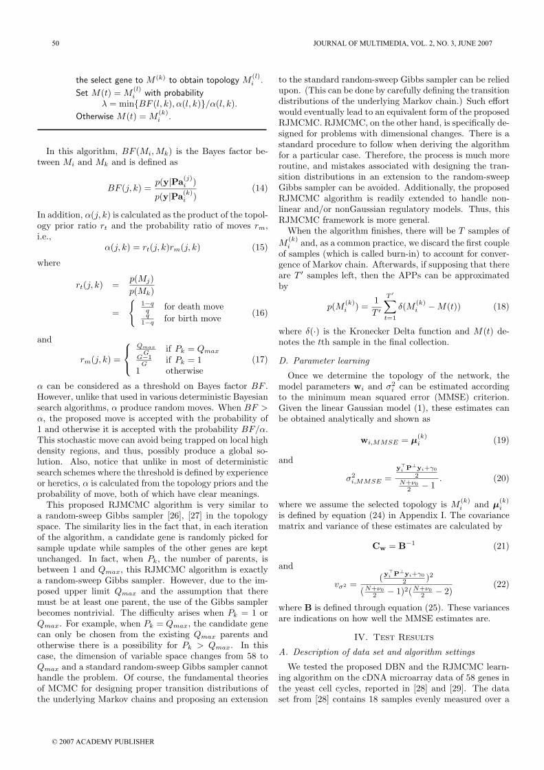
Fig. 2. Plot of the probability of error vs. the noise variance for the
RJMCMC and the K2 algorithms.
We first tested the RJMCMC algorithm on a simu-lated network and compared the performance with the wellknown K2 algorithm [30]. Since the algorithm was appliedto each gene separately, we thus only tested the perfor-mance of the algorithm on a randomly selected gene. Torealistically simulate the network of the selected gene, wefirst ran the RJMCMC algorithm on the real data set fromthe α factor synchronization to estimate the parents, theassociated weights, and the noise variance. Then the re-sults on the parents and the weights were used as the truemodel parameters when simulating the expression level ofthe selected gene for time samples 2 to 18, whereas the ex-pression level of the parent genes were still taken from thereal data set. The resulted data set was then almost thesame as the real data set, except the data of the selectedgene were replaced by the simulated data. In Figure 2,we plotted the probability of errors (POE) vs. the noise
variance σ2 of the RJMCMC and K2 algorithms. For bothalgorithms, the POE at a given σ2 was calculated basedon 100 Monte Carlo trials. For the RJMCMC, we choseQmax = 5 and q = 2/58. For the K2 algorithm, since noordering was available, we performed an exhaustive searchto determine the first possible parent of the selected gene.Also, the geometric prior on topology was included in theK2 algorithm. Figure 2 clearly demonstrates better per-formance of the RJMCMC algorithm, especially for smallσ2. Notice that the POE of the RJMCMC decreases drasti-cally with σ2, whereas the POE of the K2 algorithm almostremains flat for different σ2. This suggests that the K2was trapped in some local solutions. The figure also sug-gests that when σ2 increases to a point that noise becomesmuch stronger than the information from data, neither al-gorithm could perform well. However, this case is of littleinterest and more data should be included instead. Theestimated variance from the real data set is 0.52. Giventhe correctness of the model, we would then expect betterperformance of the RJMCMC than the K2 when both wereapplied to the real data set. In summary, through this teston the simulated network, we are assured that the RJM-CMC indeed works and has the potential to provide muchbetter results.
C. Tests on the real data sets
Up regulate
Down regulate
Weight from 0—0.4
Weight from 0.4—0.8
Weight from 0.8—1.5
Unconfirmed by
KEGG pathway
Bub1
Dbf4
Bub2
Rad24 Swi6 Mad1
Tem1
Cdc28
Mec3
Ddc1 Scc3
Cln3
Tup1
Cks1
Bub3
Pho85
Clb6
Dbf20
Swi5 Cdc14
Cdc6 Cdc15
Pex2
Pho5
Mad3
Pds1
Cdh1
Mbp1
Rad17
Swe1
Esp1
Fus3
Esc5
Hsl1
Cyc8
Pcl1
Hsl7
Swi4
Cdc7
Mih1
Pho4 Cdc5
Cdc45
Sic1
Rad53 Grf10
Clb1
Dbf2 Cdc20
Far1
Rad9
Cln1
Lte1
Smc3 Cak1
Pho80 Met30 Esr1
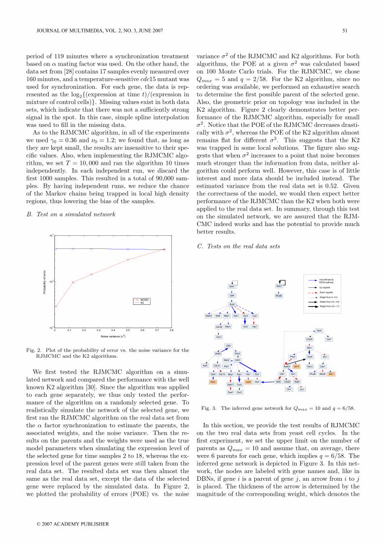
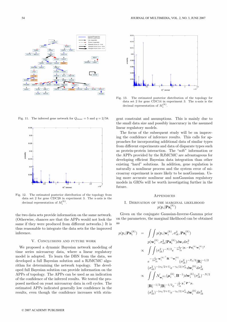
Fig. 3. The inferred gene network for Qmax = 10 and q = 6/58.
In this section, we provide the test results of RJMCMCon the two real data sets from yeast cell cycles. In thefirst experiment, we set the upper limit on the number ofparents as Qmax = 10 and assume that, on average, therewere 6 parents for each gene, which implies q = 6/58. Theinferred gene network is depicted in Figure 3. In this net-work, the nodes are labeled with gene names and, like inDBNs, if gene i is a parent of gene j, an arrow from i to jis placed. The thickness of the arrow is determined by themagnitude of the corresponding weight, which denotes the
JOURNAL OF MULTIMEDIA, VOL. 2, NO. 3, JUNE 2007 51
© 2007 ACADEMY PUBLISHER
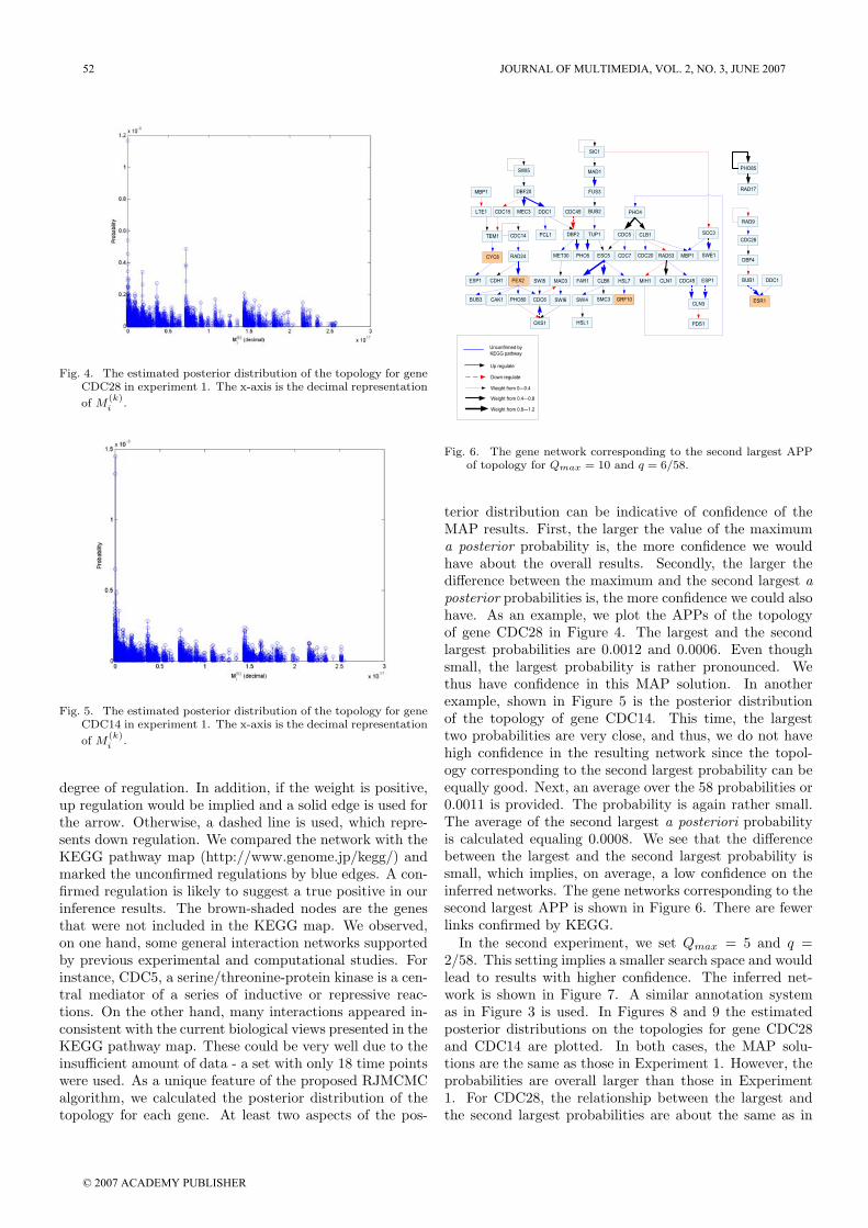
Fig. 4. The estimated posterior distribution of the topology for gene
CDC28 in experiment 1. The x-axis is the decimal representation
of M(k)i .
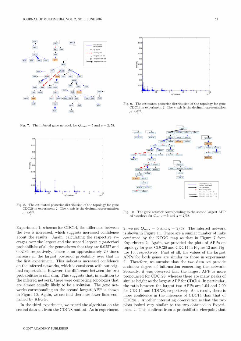
Fig. 5. The estimated posterior distribution of the topology for gene
CDC14 in experiment 1. The x-axis is the decimal representation
of M(k)i .
degree of regulation. In addition, if the weight is positive,up regulation would be implied and a solid edge is used forthe arrow. Otherwise, a dashed line is used, which repre-sents down regulation. We compared the network with theKEGG pathway map (http://www.genome.jp/kegg/) andmarked the unconfirmed regulations by blue edges. A con-firmed regulation is likely to suggest a true positive in ourinference results. The brown-shaded nodes are the genesthat were not included in the KEGG map. We observed,on one hand, some general interaction networks supportedby previous experimental and computational studies. Forinstance, CDC5, a serine/threonine-protein kinase is a cen-tral mediator of a series of inductive or repressive reac-tions. On the other hand, many interactions appeared in-consistent with the current biological views presented in theKEGG pathway map. These could be very well due to theinsufficient amount of data - a set with only 18 time pointswere used. As a unique feature of the proposed RJMCMCalgorithm, we calculated the posterior distribution of thetopology for each gene. At least two aspects of the pos-
BUB2
FUS3
PEX2
RAD24
MAD3
CDC6
MET30
CDH1
CDC14
CDC20
CLB1
PDS1
CLN3
DBF20
SWI5
CDC5
PHO4
CLB6
ESC5
ESP1
RAD53
SWE1
SCC3
SMC3
DBF4
CDC28
BUB3
RAD17
PHO85
BUB1
DDC1MEC3
CDC7
HSL1
SWI4
TEM1
LTE1 CDC15
CAK1
MIH1
CDC45
SIC1
SWI6
MAD1
PHO80
CKS1
GRF10
HSL7
PHO5
DBF2 TUP1
PCL1
FAR1
CLN1
RAD9
CYC8
MBP1
SWI5
ESR1
MBP1
ESP1
CDC45
Up regulate
Down regulate
Weight from 0—0.4
Weight from 0.4—0.8
Weight from 0.8—1.2
Unconfirmed by
KEGG pathway
DDC1
Fig. 6. The gene network corresponding to the second largest APP
of topology for Qmax = 10 and q = 6/58.
terior distribution can be indicative of confidence of theMAP results. First, the larger the value of the maximuma posterior probability is, the more confidence we wouldhave about the overall results. Secondly, the larger thedifference between the maximum and the second largest aposterior probabilities is, the more confidence we could alsohave. As an example, we plot the APPs of the topologyof gene CDC28 in Figure 4. The largest and the secondlargest probabilities are 0.0012 and 0.0006. Even thoughsmall, the largest probability is rather pronounced. Wethus have confidence in this MAP solution. In anotherexample, shown in Figure 5 is the posterior distributionof the topology of gene CDC14. This time, the largesttwo probabilities are very close, and thus, we do not havehigh confidence in the resulting network since the topol-ogy corresponding to the second largest probability can beequally good. Next, an average over the 58 probabilities or0.0011 is provided. The probability is again rather small.The average of the second largest a posteriori probabilityis calculated equaling 0.0008. We see that the differencebetween the largest and the second largest probability issmall, which implies, on average, a low confidence on theinferred networks. The gene networks corresponding to thesecond largest APP is shown in Figure 6. There are fewerlinks confirmed by KEGG.
In the second experiment, we set Qmax = 5 and q =2/58. This setting implies a smaller search space and wouldlead to results with higher confidence. The inferred net-work is shown in Figure 7. A similar annotation systemas in Figure 3 is used. In Figures 8 and 9 the estimatedposterior distributions on the topologies for gene CDC28and CDC14 are plotted. In both cases, the MAP solu-tions are the same as those in Experiment 1. However, theprobabilities are overall larger than those in Experiment1. For CDC28, the relationship between the largest andthe second largest probabilities are about the same as in
52 JOURNAL OF MULTIMEDIA, VOL. 2, NO. 3, JUNE 2007
© 2007 ACADEMY PUBLISHER
Pho80
Pex2
Mih1
Swi6
Cdc14
Esc5
Cdc20
Cdc5
Dbf2
Far1
Clb6
Cln3
Rad53
Clb1
Cdc45
Smc3
Swi4
Swe1
Mec3
Rad24
Mad1 Tup1 Scc3
Tem1
Dbf20
Esp1
Cak1
Cdc15
Cdc6
Swi5
Ddc1
Rad17
Pho85
Cdc7
Hsl1
Sic1
Cks1
Grf10
Hsl7
Pho4
Pho5
Fus3
Cdc28
Rad9
Cyc8
Met30
Esr1
Lte1
Up regulate
Down regulate
Weight from 0—0.4
Weight from 0.4—0.8
Weight from 0.8—1.5
Bub3
Bub2
Cdh1
Mbp1 Mad3
Dbf4
Bub1
Pcl1
Cln1
Pds1
Unconfirmed by
KEGG pathway
Fig. 7. The inferred gene network for Qmax = 5 and q = 2/58.
Fig. 8. The estimated posterior distribution of the topology for gene
CDC28 in experiment 2. The x-axis is the decimal representation
of M(k)i .
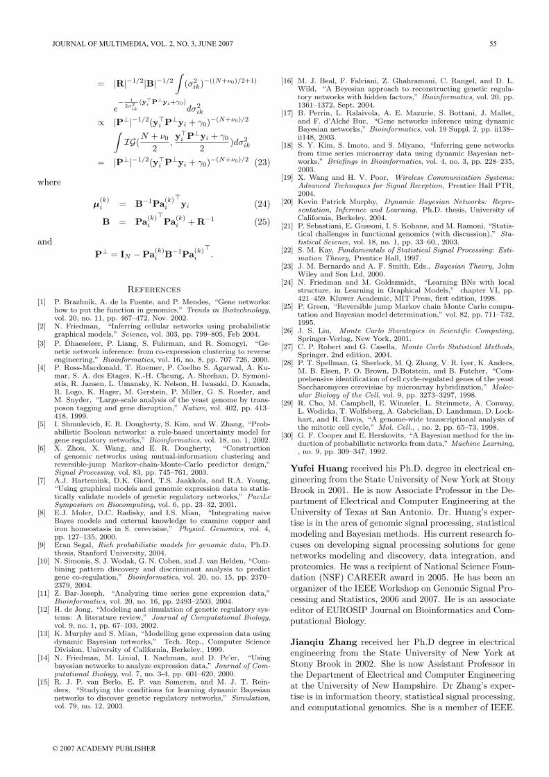
Experiment 1, whereas for CDC14, the difference betweenthe two is increased, which suggests increased confidenceabout the results. Again, calculating the respective av-erages over the largest and the second largest a posterioriprobabilities of all the genes shows that they are 0.0257 and0.0203, respectively. There is an approximately 20 timesincrease in the largest posterior probability over that inthe first experiment. This indicates increased confidenceon the inferred networks, which is consistent with our orig-inal expectation. However, the difference between the twoprobabilities is still slim. This suggests that, in addition tothe inferred network, there were competing topologies thatare almost equally likely to be a solution. The gene net-works corresponding to the second largest APP is shownin Figure 10. Again, we see that there are fewer links con-firmed by KEGG.
In the third experiment, we tested the algorithm on thesecond data set from the CDC28 mutant. As in experiment
Fig. 9. The estimated posterior distribution of the topology for gene
CDC14 in experiment 2. The x-axis is the decimal representation
of M(k)i .
BUB2
FUS3
PEX2
PHO85
MAD3
DDC1 CDH1
DBF20
CDC14
CDC20
CLB1
PDS1
CLN3
CDC5
CLB6
CKS1
CDC45
HSL7
SMC3
SWI4
SWE1
RAD53
DBF4
BUB3
RAD17
BUB1
MEC3
RAD24
CDC7
MIH1
HSL1
TEM1
CAK1
SWI6
SIC1
SCC3
MAD1
PHO80
GRF10
TUP1
PHO5
DBF2
ESC5
PHO4
PCL1
FAR1
CLN1
CDC28
CYC8
MBP1
CDC15
MET30
CDC6
ESR1
LTE1
ESP1
RAD9
SWI5
Up regulate
Down regulate
Weight from 0—0.4
Weight from 0.4—0.8
Weight from 0.8—1.2
Unconfirmed by
KEGG pathway
Fig. 10. The gene network corresponding to the second largest APP
of topology for Qmax = 5 and q = 2/58.
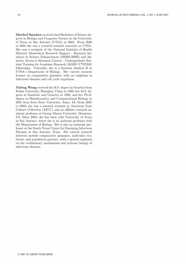
2, we set Qmax = 5 and q = 2/58. The inferred networkis shown in Figure 11. There are a similar number of linksconfirmed by the KEGG map as that in Figure 7 fromExperiment 2. Again, we provided the plots of APPs ontopology for gene CDC28 and CDC14 in Figure 12 and Fig-ure 13, respectively. First of all, the values of the largestAPPs for both genes are similar to those in experiment2. Therefore, we surmise that the two data set providea similar degree of information concerning the network.Secondly, it was observed that the largest APP is morepronounced for CDC 28, whereas there are many peaks ofsimilar height as the largest APP for CDC14. In particular,the ratio between the largest two APPs are 1.04 and 2.09for CDC14 and CDC28, respectively. As a result, there ismore confidence in the inference of CDC14 than that ofCDC28 . Another interesting observation is that the twoplots looked very similar to the two obtained in Experi-ment 2. This confirms from a probabilistic viewpoint that
JOURNAL OF MULTIMEDIA, VOL. 2, NO. 3, JUNE 2007 53
© 2007 ACADEMY PUBLISHER
BUB2
CYC8
PEX2
DDC1
MAD3
CDH1
CDC14
CDC20
CLB1
ESP1
PDS1
PCL1
DBF20
SWI6
CDC5
SMC3
MBP1
CC45
CLB6
SWE1 DBF4
HSL7
BUB3 RAD17
BUB1
MEC3
TEM1
CDC7
SWI5
CAK1
MIH1
HSL1
CLN3
CLN1
SIC1
FAR1
PHO4
RAD24
MAD1
PHO80
CKS1
GRF10
PHO5
ESC5
DBF2
CDC28
RAD53
LTE1
FUS3
CC15
MET30
CDC6
ESR1
PHO85
RAD9
TUP1
SWI4
SCC3
Up regulate
Down regulate
Weight from 0—0.4
Weight from 0.4—0.8
Weight from 0.8—1.2
Unconfirmed by
KEGG pathway
Fig. 11. The inferred gene network for Qmax = 5 and q = 2/58.
Fig. 12. The estimated posterior distribution of the topology from
data set 2 for gene CDC28 in experiment 3. The x-axis is the
decimal representation of M(k)i .
the two data sets provide information on the same network.(Otherwise, chances are that the APPs would not look thesame if they were produced from different networks.) It isthus reasonable to integrate the data sets for the improvedinference.
V. Conclusions and future work
We proposed a dynamic Bayesian network modeling oftime series microarray data, where a linear regulatorymodel is adopted. To learn the DBN from the data, wedeveloped a full Bayesian solution and a RJMCMC algo-rithm for determining the network topology. The devel-oped full Bayesian solution can provide information on theAPPs of topology. The APPs can be used as an indicationof the confidence of the inferred results. We tested the pro-posed method on yeast microarray data in cell cycles. Theestimated APPs indicated generally low confidence in theresults, even though the confidence increases with strin-
Fig. 13. The estimated posterior distribution of the topology for
data set 2 for gene CDC14 in experiment 3. The x-axis is the
decimal representation of M(k)i .
gent constraint and assumptions. This is mainly due tothe small data size and possibly inaccuracy in the assumedlinear regulatory models.
The focus of the subsequent study will be on improv-ing the confidence of inference results. This calls for ap-proaches for incorporating additional data of similar typesfrom different experiments and data of disparate types suchas protein-protein interaction. The “soft” information orthe APPs provided by the RJMCMC are advantageous fordeveloping efficient Bayesian data integration than otherexisting “hard” solutions. In addition, gene regulation isnaturally a nonlinear process and the system error of mi-croarray experiment is more likely to be nonGaussian. Us-ing more accurate nonlinear and nonGaussian regulatorymodels in GRNs will be worth investigating further in thefuture.
Appendices
I. Derivation of the marginal likelihoodp(yi|Pa(k)
i )
Given on the conjugate Gaussian-Inverse-Gamma prioron the parameters, the marginal likelihood can be obtainedas
p(yi|Pa(k)
i ) =∫ ∫
p(yi|w(k)
i , σ2
ik,Pa(k)
i )
p(w(k)
i , σ2
ik|Pa(k)
i )dwidσ2
i
∝∫ ∫
(σ2
ik)−N/2e− 1
2σ2ik
|yi−Pa(k)i
w(k)i
|2
e− 1
2σ2ik
w(k)i
�R−1w
(k)i (σ2
ik)−Pk/2|R|−1/2
(σ2
ik)−(ν0/2+1)e−γ0/2/σ2ikdw(k)
i dσ2
ik
∝∫ ∫
Nw
(k)i
(µ(k)
i ,B−1)dw(k)
i (σ2
ik)−N/2
|R|−1/2|B|−1/2e− 1
σ2ik
y�i P⊥yi
(σ2
ik)−(ν0/2+1)e−γ0/2/σ2ikdw(k)
i dσ2
ik
54 JOURNAL OF MULTIMEDIA, VOL. 2, NO. 3, JUNE 2007
© 2007 ACADEMY PUBLISHER
= |R|−1/2|B|−1/2
∫(σ2
ik)−((N+ν0)/2+1)
e− 1
2σ2ik
(y�i P⊥yi+γ0)
dσ2
ik
∝ |P⊥|−1/2(y�i P⊥yi + γ0)−(N+ν0)/2
∫IG(
N + ν0
2,y�
i P⊥yi + γ0
2)dσ2
ik
= |P⊥|−1/2(y�i P⊥yi + γ0)−(N+ν0)/2 (23)
where
µ(k)
i = B−1Pa(k)
i
�yi (24)
B = Pa(k)
i
�Pa(k)
i + R−1 (25)
andP⊥ = IN − Pa(k)
i B−1Pa(k)
i
�.
References
[1] P. Brazhnik, A. de la Fuente, and P. Mendes, “Gene networks:
how to put the function in genomics,” Trends in Biotechnology,vol. 20, no. 11, pp. 467–472, Nov. 2002.
[2] N. Friedman, “Inferring cellular networks using probabilistic
graphical models,” Science, vol. 303, pp. 799–805, Feb 2004.
[3] P. Dhaeseleer, P. Liang, S. Fuhrman, and R. Somogyi, “Ge-
netic network inference: from co-expression clustering to reverse
engineering,” Bioinformatics, vol. 16, no. 8, pp. 707–726, 2000.
[4] P. Ross-Macdonald, T. Roemer, P. Coelho S. Agarwal, A. Ku-
mar, S. A. des Etages, K.-H. Cheung, A. Sheehan, D. Symoni-
atis, R. Jansen, L. Umansky, K. Nelson, H. Iwasaki, D. Kanada,
R. Logo, K. Hager, M. Gerstein, P. Miller, G. S. Roeder, and
M. Snyder, “Large-scale analysis of the yeast genome by trans-
poson tagging and gene disruption,” Nature, vol. 402, pp. 413–
418, 1999.
[5] I. Shmulevich, E. R. Dougherty, S. Kim, and W. Zhang, “Prob-
abilistic Boolean networks: a rule-based uncertainty model for
gene regulatory networks,” Bioinformatics, vol. 18, no. 1, 2002.
[6] X. Zhou, X. Wang, and E. R. Dougherty, “Construction
of genomic networks using mutual-information clustering and
reversible-jump Markov-chain-Monte-Carlo predictor design,”
Signal Processing, vol. 83, pp. 745–761, 2003.
[7] A.J. Hartemink, D.K. Giord, T.S. Jaakkola, and R.A. Young,
“Using graphical models and genomic expression data to statis-
tically validate models of genetic regulatory networks,” PaciLcSymposium on Biocomputing, vol. 6, pp. 23–32, 2001.
[8] E.J. Moler, D.C. Radisky, and I.S. Mian, “Integrating naive
Bayes models and external knowledge to examine copper and
iron homeostasis in S. cerevisiae,” Physiol. Genomics, vol. 4,
pp. 127–135, 2000.
[9] Eran Segal, Rich probabilistic models for genomic data, Ph.D.
thesis, Stanford University, 2004.
[10] N. Simonis, S. J. Wodak, G. N. Cohen, and J. van Helden, “Com-
bining pattern discovery and discriminant analysis to predict
gene co-regulation,” Bioinformatics, vol. 20, no. 15, pp. 2370–
2379, 2004.
[11] Z. Bar-Joseph, “Analyzing time series gene expression data,”
Bioinformatics, vol. 20, no. 16, pp. 2493–2503, 2004.
[12] H. de Jong, “Modeling and simulation of genetic regulatory sys-
tems: A literature review,” Journal of Computational Biology,vol. 9, no. 1, pp. 67–103, 2002.
[13] K. Murphy and S. Mian, “Modelling gene expression data using
dynamic Bayesian networks,” Tech. Rep., Computer Science
Division, University of California, Berkeley., 1999.
[14] N. Friedman, M. Linial, I. Nachman, and D. Pe’er, “Using
bayesian networks to analyze expression data,” Journal of Com-putational Biology, vol. 7, no. 3-4, pp. 601–620, 2000.
[15] R. J. P. van Berlo, E. P. van Someren, and M. J. T. Rein-
ders, “Studying the conditions for learning dynamic Bayesian
networks to discover genetic regulatory networks,” Simulation,
vol. 79, no. 12, 2003.
[16] M. J. Beal, F. Falciani, Z. Ghahramani, C. Rangel, and D. L.
Wild, “A Beyesian approach to reconstructing genetic regula-
tory networks with hidden factors,” Bioinformatics, vol. 20, pp.
1361–1372, Sept. 2004.
[17] B. Perrin, L. Ralaivola, A. E. Mazurie, S. Bottani, J. Mallet,
and F. d’Alche Buc, “Gene networks inference using dynamic
Bayesian networks,” Bioinformatics, vol. 19 Suppl. 2, pp. ii138–
ii148, 2003.
[18] S. Y. Kim, S. Imoto, and S. Miyano, “Inferring gene networks
from time series microarray data using dynamic Bayesian net-
works,” Briefings in Bioinformatics, vol. 4, no. 3, pp. 228–235,
2003.
[19] X. Wang and H. V. Poor, Wireless Communication Systems:Advanced Techniques for Signal Reception, Prentice Hall PTR,
2004.
[20] Kevin Patrick Murphy, Dynamic Bayesian Networks: Repre-sentation, Inference and Learning, Ph.D. thesis, University of
California, Berkeley, 2004.
[21] P. Sebastiani, E. Gussoni, I. S. Kohane, and M. Ramoni, “Statis-
tical challenges in functional genomics (with discussion),” Sta-tistical Science, vol. 18, no. 1, pp. 33–60., 2003.
[22] S. M. Kay, Fundamentals of Statistical Signal Processing: Esti-mation Theory, Prentice Hall, 1997.
[23] J. M. Bernardo and A. F. Smith, Eds., Bayesian Theory, John
Wiley and Son Ltd, 2000.
[24] N. Friedman and M. Goldszmidt, “Learning BNs with local
structure, in Learning in Graphical Models,” chapter VI, pp.
421–459. Kluwer Academic, MIT Press, first edition, 1998.
[25] P. Green, “Reversible jump Markov chain Monte Carlo compu-
tation and Bayesian model determination,” vol. 82, pp. 711–732,
1995.
[26] J. S. Liu, Monte Carlo Starategies in Scientific Computing,Springer-Verlag, New York, 2001.
[27] C. P. Robert and G. Casella, Monte Carlo Statistical Methods,Springer, 2nd edition, 2004.
[28] P. T. Spellman, G. Sherlock, M. Q. Zhang, V. R. Iyer, K. Anders,
M. B. Eisen, P. O. Brown, D.Botstein, and B. Futcher, “Com-
prehensive identification of cell cycle-regulated genes of the yeast
Saccharomyces cerevisiae by microarray hybridization,” Molec-ular Biology of the Cell, vol. 9, pp. 3273–3297, 1998.
[29] R. Cho, M. Campbell, E. Winzeler, L. Steinmetz, A. Conway,
L. Wodicka, T. Wolfsberg, A. Gabrielian, D. Landsman, D. Lock-
hart, and R. Davis, “A genome-wide transcriptional analysis of
the mitotic cell cycle,” Mol. Cell., , no. 2, pp. 65–73, 1998.
[30] G. F. Cooper and E. Herskovits, “A Bayesian method for the in-
duction of probabilistic networks from data,” Machine Learning,, no. 9, pp. 309–347, 1992.
Yufei Huang received his Ph.D. degree in electrical en-gineering from the State University of New York at StonyBrook in 2001. He is now Associate Professor in the De-partment of Electrical and Computer Engineering at theUniversity of Texas at San Antonio. Dr. Huang’s exper-tise is in the area of genomic signal processing, statisticalmodeling and Bayesian methods. His current research fo-cuses on developing signal processing solutions for genenetworks modeling and discovery, data integration, andproteomics. He was a recipient of National Science Foun-dation (NSF) CAREER award in 2005. He has been anorganizer of the IEEE Workshop on Genomic Signal Pro-cessing and Statistics, 2006 and 2007. He is an associateeditor of EUROSIP Journal on Bioinformatics and Com-putational Biology.
Jianqiu Zhang received her Ph.D degree in electricalengineering from the State University of New York atStony Brook in 2002. She is now Assistant Professor inthe Department of Electrical and Computer Engineeringat the University of New Hampshire. Dr Zhang’s exper-tise is in information theory, statistical signal processing,and computational genomics. She is a member of IEEE.
JOURNAL OF MULTIMEDIA, VOL. 2, NO. 3, JUNE 2007 55
© 2007 ACADEMY PUBLISHER
Maribel Sanchez received dual Bachelors of Science de-grees in Biology and Computer Science at the Universityof Texas at San Antonio (UTSA) in 2004. From 2000to 2004 she was a research scientist associate at UTSA.She was a recipient of the National Institute of HealthMinority Biomedical Research Support - Research Ini-tiative in Science Enhancement (MBRS-RISE) and Mi-nority Access to Research Careers - Undergraduate Stu-dent Training for Academic Research (MARC-U*STAR)fellowships. Currently, she is a Systems Analyst II atUTSA’s Department of Biology. Her current researchfocuses on comparative genomics with an emphasis ininfectious diseases and cell cycle regulation.
Yufeng Wang received her B.S. degree in Genetics fromFudan University, Shanghai, China in 1993, her M.S. de-grees in Statistics and Genetics in 1998, and her Ph.D.degree in Bioinformatics and Computational Biology in2001 from Iowa State University, Ames, IA. From 2001to 2003, she was a research scientist at American TypeCulture Collection (ATCC) and an affiliate research as-sistant professor at George Mason University, Manassas,VA. Since 2003, she has been with University of Texasat San Antonio, where she is an assistant professor withthe Department of Biology. She is also an assistant pro-fessor at the South Texas Center for Emerging InfectiousDiseases at San Antonio, Texas. Her current researchinterests include comparative genomics, molecular evo-lution, and population genetics, with a special emphasison the evolutionary mechanisms and systems biology ofinfectious diseases.
56 JOURNAL OF MULTIMEDIA, VOL. 2, NO. 3, JUNE 2007
© 2007 ACADEMY PUBLISHER
Related Documents


![Learning Bayesian Networks in R · 2013-07-10 · Bayesian Networks Essentials Bayesian Networks Bayesian networks [21, 27] are de ned by: anetwork structure, adirected acyclic graph](https://static.cupdf.com/doc/110x72/5f3267ce969e2b02050fd06c/learning-bayesian-networks-in-r-2013-07-10-bayesian-networks-essentials-bayesian.jpg)


