METHODS IN MOLECULAR BIOLOGY ™ 377 Edited by Microarray Data Analysis Michael J. Korenberg Methods and Applications

Welcome message from author
This document is posted to help you gain knowledge. Please leave a comment to let me know what you think about it! Share it to your friends and learn new things together.
Transcript

METHODS IN MOLECULAR BIOLOGY™ • 377SERIES EDITOR: John M. Walker
Methods in Molecular Biology™ • 377MICROARRAY DATA ANALYSIS: Methods and Applications ISBN: 1-58829-540-0 ISBN 13: 978-1-58829-540-8E-ISBN: 1-59745-390-0 E-ISBN 13: 978-1-59745-390-5ISSN: 1543–1894humanapress.com
METHODS IN MOLECULAR BIOLOGY™ 377
MiMB377
Korenberg
CONTENTS
FEATURES
Microarray D
ata Analysis
Microarray Data AnalysisMethods and Applications
Edited by Michael J. Korenberg
Queen’s University, Kingston, Ontario, Canada
In this new volume, renowned authors contribute fascinating, cutting-edge insights into microarray data analysis. This innovative book includes in-depth presentations of ge-nomic signal processing, artificial neural network use for microarray data analysis, signal processing and design of microarray time series experiments, application of regression methods, gene expression profiles and prognostic markers for primary breast cancer, and factors affecting the cross-correlation of gene expression profiles. Also detailed are use of tiling arrays for large genome analysis, comparative genomic hybridization data on cDNA microarrays, integrated high-resolution genome-wide analysis of gene dosage and gene expression in human brain tumors, gene and MeSH ontology, and survival prediction in follicular lymphoma using tissue microarrays.
The protocols follow the successful Methods in Molecular Biology™ series format, offering step-by-step instructions, an introduction outlining the principles behind the technique, lists of the necessary equipment and reagents, and tips on troubleshooting and avoiding pitfalls.
Information on an array of topics including genomic signal processing, matrix algebra and genetic networks, predictive models of gene regulation, comparing microarray studies, identifying progression-associated genes in astrocytoma, analysis of comparative genomic hybridization data on cDNA microarrays, statistical framework for gene expression analysis, and interpretation of microarray results with gene ontology and MeSH ontology.
Use classic, novel, and state-of-the-art methods in a readily reproducible format
Master tricks of the trade, troubleshoot, and avoid known pitfalls
Microarray Data Analysis: An Overview of Design, Methodology and Analysis. Genomic Signal Process-ing: From Matrix Algebra to Genetic Networks. Online Analysis of Microarray Data Using Artificial Neural Networks. Signal Processing and the Design of Micro-array Time-Series Experiments. Predictive Models of Gene Regulation: Application of Regression Methods to Microarray Data. Statistical Framework for Gene Expression Data Analysis. Gene Expression Profiles and Prognostic Markers for Primary Breast Cancer. Comparing Microarray Studies. A Pitfall in Series of Microarrays: The Position of Probes Affects the Cross Correlation of Gene Expression Profiles. In-Depth Query of Large Genomes
Using Tiling Arrays. Analysis of Comparative Genomic Hybridization Data on cDNA Microarrays. Integrated High-Resolution Genome-Wide Analysis of Gene Dosage and Gene Expression in Human Brain Tumors. Progres-sion-Associated Genes in Astrocytoma Identified by Novel Microarray Gene Expression Data Reanalysis. Interpreting Microarray Results With Gene Ontology and MeSH. Incorporation of Gene Ontology Annota-tions to Enhance Microarray Data Analysis. Predicting Survival in Follicular Lymphoma Using Tissue Microarrays.
Edited by
Microarray Data Analysis
Michael J. Korenberg
Methods and Applications

Microarray Data Analysis

M E T H O D S I N M O L E C U L A R B I O L O G Y™
John M. Walker, SERIES EDITOR
402. PCR Primer Design, edited by Anton Yuryev, 2007
401. Neuroinformatics, edited by Chiquito J.Crasto, 2007
400. Methods in Lipid Membranes, edited byAlex Dopico, 2007
399. Neuroprotection Methods and Protocols,edited by Tiziana Borsello, 2007
398. Lipid Rafts, edited by Thomas J. McIntosh, 2007397. Hedgehog Signaling Protocols, edited by Jamila
I. Horabin, 2007396. Comparative Genomics, Volume 2, edited by
Nicholas H. Bergman, 2007395. Comparative Genomics, Volume 1, edited by
Nicholas H. Bergman, 2007394. Salmonella: Methods and Protocols, edited by
Heide Schatten and Abe Eisenstark, 2007393. Plant Secondary Metabolites, edited by
Harinder P. S. Makkar, P. Siddhuraju, and KlausBecker, 2007
392. Molecular Motors: Methods and Protocols,edited by Ann O. Sperry, 2007
391. MRSA Protocols, edited by Yinduo Ji, 2007390. Protein Targeting Protocols, Second Edition,
edited by Mark van der Giezen, 2007389. Pichia Protocols, Second Edition, edited by
James M. Cregg, 2007388. Baculovirus and Insect Cell Expression
Protocols, Second Edition, edited by David W.Murhammer, 2007
387. Serial Analysis of Gene Expression (SAGE):Digital Gene Expression Profiling, edited by KareLehmann Nielsen, 2007
386. Peptide Characterization and ApplicationProtocols, edited by Gregg B. Fields, 2007
385. Microchip-Based Assay Systems: Methods andApplications, edited by Pierre N. Floriano, 2007
384. Capillary Electrophoresis: Methods and Protocols,edited by Philippe Schmitt-Kopplin, 2007
383. Cancer Genomics and Proteomics: Methods andProtocols, edited by Paul B. Fisher, 2007
382. Microarrays, Second Edition: Volume 2, Applicationsand Data Analysis, edited by Jang B. Rampal, 2007
381. Microarrays, Second Edition: Volume 1, SynthesisMethods, edited by Jang B. Rampal, 2007
380. Immunological Tolerance: Methods and Protocols,edited by Paul J. Fairchild, 2007
379. Glycovirology Protocols, edited by Richard J.Sugrue, 2007
378. Monoclonal Antibodies: Methods and Protocols,edited by Maher Albitar, 2007
377. Microarray Data Analysis: Methods andApplications, edited by Michael J. Korenberg, 2007
376. Linkage Disequilibrium and AssociationMapping: Analysis and Application, edited byAndrew R. Collins, 2007
375. In Vitro Transcription and Translation Protocols:Second Edition, edited by Guido Grandi, 2007
374. Quantum Dots: Applications in Biology,edited by Marcel Bruchez and Charles Z. Hotz, 2007
373. Pyrosequencing® Protocols, edited by SharonMarsh, 2007
372. Mitochondria: Practical Protocols, edited byDario Leister and Johannes Herrmann, 2007
371. Biological Aging: Methods and Protocols, edited byTrygve O. Tollefsbol, 2007
370. Adhesion Protein Protocols, Second Edition, editedby Amanda S. Coutts, 2007
369. Electron Microscopy: Methods and Protocols,Second Edition, edited by John Kuo, 2007
368. Cryopreservation and Freeze-Drying Protocols,Second Edition, edited by John G. Day and GlynStacey, 2007
367. Mass Spectrometry Data Analysis in Proteomics,edited by Rune Matthiesen, 2007
366. Cardiac Gene Expression: Methods and Protocols,edited by Jun Zhang and Gregg Rokosh, 2007
365. Protein Phosphatase Protocols: edited by GregMoorhead, 2007
364. Macromolecular Crystallography Protocols:Volume 2, Structure Determination, edited by SylvieDoublié, 2007
363. Macromolecular Crystallography Protocols:Volume 1, Preparation and Crystallizationof Macromolecules, edited by Sylvie Doublié, 2007
362. Circadian Rhythms: Methods and Protocols,edited by Ezio Rosato, 2007
361. Target Discovery and Validation Reviewsand Protocols: Emerging Molecular Targetsand Treatment Options, Volume 2, edited byMouldy Sioud, 2007
360. Target Discovery and Validation Reviewsand Protocols: Emerging Strategies for Targetsand Biomarker Discovery, Volume 1, edited byMouldy Sioud, 2007
359. Quantitative Proteomics by Mass Spectrometry,edited by Salvatore Sechi, 2007
358. Metabolomics: Methods and Protocols, edited byWolfram Weckwerth, 2007
357. Cardiovascular Proteomics: Methods and Protocols,edited by Fernando Vivanco, 2006
356. High-Content Screening: A Powerful Approachto Systems Cell Biology and Drug Discovery,edited by D. Lansing Taylor, Jeffrey Haskins,and Ken Guiliano, and 2007
355. Plant Proteomics: Methods and Protocols, editedby Hervé Thiellement, Michel Zivy, CatherineDamerval, and Valerie Mechin, 2007
354. Plant–Pathogen Interactions: Methods andProtocols, edited by Pamela C. Ronald, 2006
353. Protocols for Nucleic Acid Analysisby Nonradioactive Probes, Second Edition,edited by Elena Hilario and John Mackay, 2006
352. Protein Engineering Protocols, edited by KristianMüller and Katja Arndt, 2006

M E T H O D S I N M O L E C U L A R B I O L O G Y™
MicroarrayData Analysis
Methods and Applications
Edited by
Michael J. KorenbergDepartment of Electrical and Computer Engineering
Queen’s University, Kingston, Ontario, Canada

© 2007 Humana Press Inc.999 Riverview Drive, Suite 208Totowa, New Jersey 07512
www.humanapress.com
All rights reserved. No part of this book may be reproduced, stored in a retrieval system, or transmitted inany form or by any means, electronic, mechanical, photocopying, microfilming, recording, or otherwisewithout written permission from the Publisher. Methods in Molecular BiologyTM is a trademark of TheHumana Press Inc.
All papers, comments, opinions, conclusions, or recommendations are those of the author(s), and do notnecessarily reflect the views of the publisher.
This publication is printed on acid-free paper. ∞ANSI Z39.48-1984 (American Standards Institute) Permanence of Paper for Printed Library Materials.
Cover design by Nancy K. Fallatt
Cover illustration: Support Vector Machine analysis constructs planes in multidimensional space such thatsets of genes separate into distinct classes based on an iterative training algorithm (Fig. 6, Chapter 2; seecomplete caption on p. 32 and discussion on pp. 31–32).
For additional copies, pricing for bulk purchases, and/or information about other Humana titles, contactHumana at the above address or at any of the following numbers: Tel.: 973-256-1699; Fax: 973-256-8341;E-mail: [email protected]; or visit our Website: www.humanapress.com
Photocopy Authorization Policy:Authorization to photocopy items for internal or personal use, or the internal or personal use of specificclients, is granted by Humana Press Inc., provided that the base fee of US $30.00 per copy is paid directlyto the Copyright Clearance Center at 222 Rosewood Drive, Danvers, MA 01923. For those organizationsthat have been granted a photocopy license from the CCC, a separate system of payment has been arrangedand is acceptable to Humana Press Inc. The fee code for users of the Transactional Reporting Service is:[978-1-58829-540-8 • 1-58829-540-0/07 $30.00].
Printed in the United States of America. 10 9 8 7 6 5 4 3 2 1
ISSN 1064-3745
E-ISBN 1-59745-390-0
Library of Congress Catloging-in-Publication Data
Microarray data analysis : methods and applications / edited by Michael J.Korenberg. p. ; cm. -- (Methods in molecular biology ; 377) Includes bibliographical references and index. ISBN-13: 978-1-58829-540-8 (alk. paper) ISBN-10: 1-58829-540-0 (alk. paper) 1. DNA microarrays. 2. Gene expression. I. Korenberg, Michael J. II.Series: Methods in molecular biology (Clifton, N.J.) ; v. 377. [DNLM: 1. Microarray Analysis--methods. 2. Gene Expression Profil-ing. W1 ME9616J v. 377 2007 / QU 450 M6256 2007] QP624.5.D726M512 2007 572.8'636--dc22
2006037730

To my Mother and Father,
and to June


vii
Preface
When the series editor, Prof. John Walker, asked me to edit a book onmicroarray data analysis, I began by writing to a number of researchers whosework I admired. Many of them agreed to contribute chapters. One of them, Dr.Orly Alter, suggested several others to me, and I am very grateful to her. Thecontributed chapters speak for themselves. They indeed cover a wide range oftopics in both methods and applications; I found them fascinating, and thankthe authors for all their work. I am very fortunate to have dealt with such anelite group.
Michael J. Korenberg

ix
Contents
Preface ........................................................................................................... viiContributors .....................................................................................................xi
1 Microarray Data Analysis: An Overview of Design,Methodology, and Analysis
Ashani T. Weeraratna and Dennis D. Taub .......................................... 12 Genomic Signal Processing: From Matrix Algebra
to Genetic NetworksOrly Alter ............................................................................................ 17
3 Online Analysis of Microarray Data UsingArtificial Neural Networks
Braden Greer and Javed Khan ............................................................ 614 Signal Processing and the Design of Microarray
Time-Series ExperimentsRobert R. Klevecz, Caroline M. Li, and James L. Bolen...................... 75
5 Predictive Models of Gene Regulation: Applicationof Regression Methods to Microarray Data
Debopriya Das and Michael Q. Zhang ............................................... 956 Statistical Framework for Gene Expression Data Analysis
Olga Modlich and Marc Munnes ...................................................... 1117 Gene Expression Profiles and Prognostic Markers
for Primary Breast CancerYixin Wang, Jan Klijn, Yi Zhang, David Atkins,
and John Foekens .......................................................................... 1318 Comparing Microarray Studies
Mayte Suárez-Fariñas and Marcelo O. Magnasco ............................ 1399 A Pitfall in Series of Microarrays: The Position of Probes
Affects the Cross-Correlation of Gene Expression ProfilesGábor Balázsi and Zoltán N. Oltvai ................................................. 153
10 In-Depth Query of Large Genomes Using Tiling ArraysManoj Pratim Samanta, Waraporn Tongprasit,
and Viktor Stolc ............................................................................ 16311 Analysis of Comparative Genomic Hybridization
Data on cDNA MicroarraysSven Bilke and Javed Khan................................................................ 175

x Contents
12 Integrated High-Resolution Genome-Wide Analysis of GeneDosage and Gene Expression in Human Brain Tumors
Dejan Juric, Claudia Bredel, Branimir I. Sikic, and Markus Bredel ....................................................................... 187
13 Progression-Associated Genes in Astrocytoma Identifiedby Novel Microarray Gene Expression Data Reanalysis
Tobey J. MacDonald, Ian F. Pollack, Hideho Okada,Soumyaroop Bhattacharya, and James Lyons-Weiler .................. 203
14 Interpreting Microarray Results With Gene Ontologyand MeSH
John D. Osborne, Lihua (Julie) Zhu, Simon M. Lin,and Warren A. Kibbe .................................................................... 223
15 Incorporation of Gene Ontology Annotations to EnhanceMicroarray Data Analysis
Michael F. Ochs, Aidan J. Peterson,Andrew Kossenkov, and Ghislain Bidaut ..................................... 243
16 Predicting Survival in Follicular LymphomaUsing Tissue Microarrays
Michael J. Korenberg, Pedro Farinha,and Randy D. Gascoyne ............................................................... 255
Index ............................................................................................................ 269

xi
Contributors
ORLY ALTER • Department of Biomedical Engineering, Institute for Cellular andMolecular Biology and Institute for Computational Engineering and Sciences,University of Texas at Austin, Austin, TX
DAVID ATKINS • Veridex LLC, a Johnson and Johnson Company,San Diego, CA
GÁBOR BALÁZSI • Department of Molecular Therapeutics, University of Texas M. D.Anderson Cancer Center, Houston, TX
SOUMYAROOP BHATTACHARYA • Center for Biomedical Informatics,Pittsburgh PA
GHISLAIN BIDAUT • Center for Bioinformatics, Department of Genetics, Universityof Pennsylvania School of Medicine, Philadelphia, PA
SVEN BILKE • Oncogenomics Section, Pediatric Oncology Branch, AdvancedTechnology Center, National Cancer Institute, Gaithersburg, MD
JAMES L. BOLEN • Dynamics Group, Department of Biology, Beckman ResearchInstitute of the City of Hope Medical Center, Duarte CA
CLAUDIA BREDEL • Division of Oncology, Center for Clinical Sciences Research,Stanford University School of Medicine, Stanford, CA
MARKUS BREDEL • Department of Neurosurgery and Division of Oncology, Centerfor Clinical Sciences Research, Stanford University Schoolof Medicine, Stanford, CA
DEBOPRIYA DAS • Lawrence Berkeley National Laboratory, Berkeley, CAPEDRO FARINHA • Department of Pathology, British Columbia Cancer Agency,
Vancouver, British Columbia, CanadaJOHN FOEKENS • Department of Medical Oncology, Erasmus Medical Center, Daniel
den Hoed Cancer Center, Rotterdam, The NetherlandsRANDY D. GASCOYNE • Department of Pathology, British Columbia Cancer Agency,
Vancouver, British Columbia, CanadaBRADEN GREER • Oncogenomics Section, Pediatric Oncology Branch, Advanced
Technology Center, National Cancer Institute, Gaithersburg, MDDEJAN JURIC • Division of Oncology, Center for Clinical Sciences Research,
Stanford University School of Medicine, Stanford, CAJAVED KHAN • Oncogenomics Section, Pediatric Oncology Branch, Advanced
Technology Center, National Cancer Institute, Gaithersburg, MDWARREN A. KIBBE • Robert H. Lurie Comprehensive Cancer Center, Northwestern
University, Chicago, ILROBERT R. KLEVECZ • Dynamics Group, Department of Biology, Beckman Research
Institute of the City of Hope Medical Center, Duarte, CAJAN KLIJN • Department of Medical Oncology, Erasmus Medical Center, Daniel den
Hoed Cancer Center, Rotterdam, The Netherlands

xii Contributors
MICHAEL J. KORENBERG • Department of Electrical and ComputerEngineering, Queen’s University, Kingston, Ontario, Canada
ANDREW KOSSENKOV • Fox Chase Cancer Center, Philadelphia, PACAROLINE M. LI • Dynamics Group, Department of Biology, Beckman Research
Institute of the City of Hope Medical Center, Duarte, CASIMON M. LIN • Robert H. Lurie Comprehensive Cancer Center, Northwestern
University, Chicago, ILJAMES LYONS-WEILER • Center for Biomedical Informatics, Benedum Center
for Oncology Informatics/Center for Pathology Informatics, and Universityof Pittsburgh Medical Center/Cancer Institute, Pittsburgh, PA
TOBEY J. MACDONALD • Center for Cancer and Immunology Research, Children’sResearch Institute, Department of Hematology-Oncology, Children's NationalMedical Center, Washington, DC
MARCELO O. MAGNASCO • Center for Studies in Physics and Biology,The Rockefeller University, New York, NY
OLGA MODLICH • Institute of Chemical Oncology, University of Düsseldorf,Düsseldorf, Germany
MARC MUNNES • Bayer Healthcare AG, Diagnostic Research Germany, Leverkusen,Germany
MICHAEL F. OCHS • Fox Chase Cancer Center, Philadelphia, PAHIDEHO OKADA • Departments of Neurosurgery and Pathology, Cancer Institute
Brain Tumor Center , University of Pittsburgh Medical Center and Children'sHospital of Pittsburgh, Pittsburgh, PA
ZOLTÁN N. OLTVAI • Department of Pathology, University of Pittsburgh,Pittsburgh, PA
JOHN D. OSBORNE • Robert H. Lurie Comprehensive Cancer Center, NorthwesternUniversity, Chicago, IL
AIDAN J. PETERSON • Fox Chase Cancer Center, Philadelphia, PAIAN F. POLLACK • Departments of Neurosurgery and Pathology, Cancer Institute
Brain Tumor Center, University of Pittsburgh Medical Center and Children'sHospital of Pittsburgh, Pittsburgh, PA
MANOJ PRATIM SAMANTA • Systemix Institute, Cupertino, CABRANIMIR I. SIKIC • Division of Oncology, Center for Clinical Sciences Research,
Stanford University School of Medicine, Stanford, CAVIKTOR STOLC • Systemix Institute, Cupertino, CAMAYTE SUÁREZ-FARIÑAS • Center for Studies in Physics and Biology,
The Rockefeller University, New York, NYDENNIS D. TAUB • Laboratory of Immunology, National Institutes of Health, National
Institute on Aging, Gerontology Research Center, Baltimore, MDWARAPORN TONGPRASIT • Systemix Institute, Cupertino, CAYIXIN WANG • Veridex LLC, a Johnson and Johnson Company, San Diego, CAASHANI T. WEERARATNA • Laboratory of Immunology, National Institutes of Health,
National Institute on Aging, Gerontology Research Center, Baltimore, MD

Contributors xiii
MICHAEL Q. ZHANG • Cold Spring Harbor Laboratory, Cold Spring Harbor, NYYI ZHANG • Veridex LLC, a Johnson and Johnson Company, San Diego, CALIHUA (JULIE) ZHU • Robert H. Lurie Comprehensive Cancer Center, Northwestern
University, Chicago, IL

1
Microarray Data AnalysisAn Overview of Design, Methodology, and Analysis
Ashani T. Weeraratna and Dennis D. Taub
SummaryMicroarray analysis results in the gathering of massive amounts of information concerning
gene expression profiles of different cells and experimental conditions. Analyzing these data canoften be a quagmire, with endless discussion as to what the appropriate statistical analyses forany given experiment might be. As a result many different methods of data analysis have evolved,the basics of which are outlined in this chapter.
Key Words: Microarray data analysis; MIAME; clustering.
1. IntroductionMicroarray technology is widely used to examine the gene expression
profiles of a multitude of cells and tissues. This technology is based on thehybridization of RNA from tissues or cells to either cDNA or oligonucleotidesimmobilized on a glass chip or, in increasingly rare cases, on a nylon mem-brane. One of the first experiments in which cDNA clones were arrayed ontoa filter, and then hybridized with cell lysates, analyzed the gene expressionprofiles of colon cancer, and examined the expression of 4000 genes therein(1). Since then, the identification of genes by the Human Genome Project (2)has allowed for the expansion of the number of cDNA clones or oligonu-cleotides spotted on a single slide. Today, the average commercial microarraycontains roughly 20,000 clones or oligonucleotides, many of which are unique.Some companies, such as Agilent Technologies, also make a slide that encom-passes genes from the whole genome with over 44,000 genes spotted on theirarrays. Obviously, the analysis of so many data can prove quite overwhelmingand labor intensive. The purpose of this chapter is to outline the available tech-niques for microarray data analysis.
1
From: Methods in Molecular Biology, vol. 377, Microarray Data Analysis: Methods and ApplicationsEdited by: M. J. Korenberg © Humana Press Inc., Totowa, NJ
01_Weeraratna.qxd 6/3/07 10:16 AM Page 1
2. Experimental DesignSuccessful data analysis begins with a good experimental design, and often, one
of the most crucial and most overlooked parts of performing an informative arrayexperiment is designating an appropriate reference, or standard. For example,when analyzing a given disease, it is useful to assign a “control” or “frame-of-reference” sample that can be used as a comparison for all states of that disease.This could be a sample such as a normal, nonmalignant tissue of origin when ana-lyzing cancer, or resting T-cells as compared with those activated through the T-cell or cytokine receptors. It is, however, often difficult to determine what “normal” tissue or cell is best to use, and what exactly defines normal. Many usersprefer to utilize universal RNA, so that comparisons can be made between severaldifferent gene expression profiles that may not have a common normal counter-part. To assess what constitutes a good reference for an experiment, the researchersmust first have a clear idea of what precise questions they want to answer. Often,researchers fall into the trap of comparing experimental and control conditionsdirectly to each other, when a slightly more complex experiment using a commonreference for both experimental and control conditions may provide a more sophis-ticated analysis of the data. For example, when treating cancer cell lines with adrug, it is tempting to simply compare treated to untreated cell lines. However,more information could potentially be gathered by comparing both treated anduntreated cell lines to a normal, untreated control cell line (e.g., melanocytes vsmelanomas treated with different agents or vehicle controls). Ultimately, the morecomplex statistical analyses that can be performed on these types of data mayreveal more subtle, but equally important, gene expression patterns.
3. Minimal Information About a Microarray ExperimentIn an effort to standardize the thousands of array experiments, the
Microarray Gene Expression Database (MIAME) society established guide-lines that require researchers to conform to MIAME guidelines (3). MIAMEdescribes the minimal information about a microarray experiment that is requiredto interpret the results of the experiment, and compare it with other experimentsfrom other groups. The checklist for complying with the MIAME guidelinesis quite extensive and can be found at http://www.mged.org/Workgroups/MIAME/miame_checklist.html
In brief, these guidelines include:
1. Array design: information regarding the platform of the array, description of theclones and oligomers, and catalog numbers for commercial arrays. This also shouldinclude the location of each feature as well as the explanations of feature annotation.
2. Experimental design: a description and the goals of the experiment, rationale forcells/tissues and treatment used, quality control steps, and links to any publicdatabases necessary.
2 Weeraratna and Taub
01_Weeraratna.qxd 6/3/07 10:16 AM Page 2

3. Sample selection: criteria for the selection of samples, description of the proce-dures used for RNA extraction, and sample labeling.
4. Hybridization: conditions of hybridization, including blocking and washing of slides.5. Data analysis: description of the raw data, as well as of the original images,
hardware, and software used, and also the criteria used for processing and nor-malization of data.
In addition to the obvious benefits of standardizing microarray data, many ofthe top journals in the field currently require researchers to comply with theseguidelines, so it is worth examining your selected array format for MIAMEcompliance prior to starting a microarray experiment.
4. Image Acquisition and AnalysisOnce the RNA has been isolated and hybridized to the chip, the first stage of
data analysis begins. This requires successful acquisition of the fluorescent orradioactive signal bound to the chip or membrane. With radioactive membranes,it is standard procedure to expose the membrane several times and then take aneducated average of the best exposures (4). With fluorescent dyes, it is essentialto utilize a high-resolution scanner and that the first scan be performed as quicklyand accurately as possible, as the dyes are quickly bleached and multiple scansare not possible. Some salient points of image acquisition are outlined next.
4.1. Quality of Scanner
It is important to use a scanner that can detect at a resolution of 10 micronsor greater. In addition, the scanner must be able to excite and detect Cy3 (532 nm)and Cy5 fluorescence (633 nm). An adjustable photomultiplier tube to ensureequal scanning, while reducing as much bleaching as possible, is also ideal.Typically, the settings for the photomultiplier tube are around 30%.
4.2. Orientation of Image
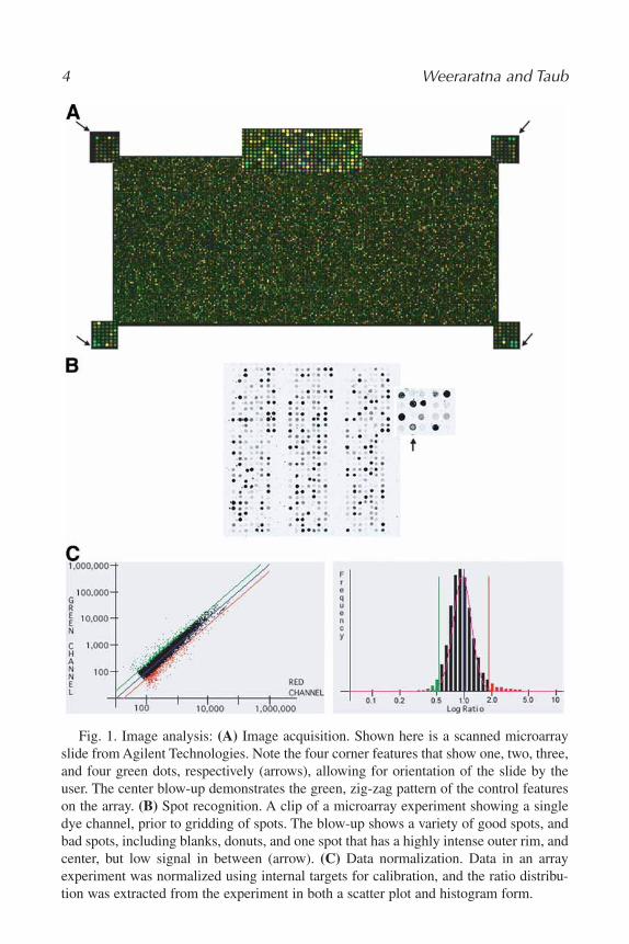
The orientation of the image becomes particularly important when combin-ing arrays from one company with a scanner from a different company asimages may be inverted depending on the scanner being used. Thus, it is cru-cial that the array include “landing lights”—control cDNAs or oligonucleotidesspotted on the arrays that yield a distinct pattern when the array is in the cor-rect orientation (Fig. 1A).
4.3. Spot Recognition
Often referred to as “gridding,” this is the process used to identify each spoton the array prior to extracting information from it. When purchasing arrays andscanners from commercial sources, programs for spot recognition and informa-tion extraction are often included. Agilent and Affymetrix both have their own
Microarray Data Analysis 3
01_Weeraratna.qxd 6/3/07 10:16 AM Page 3
4 Weeraratna and Taub
Fig. 1. Image analysis: (A) Image acquisition. Shown here is a scanned microarrayslide from Agilent Technologies. Note the four corner features that show one, two, three,and four green dots, respectively (arrows), allowing for orientation of the slide by theuser. The center blow-up demonstrates the green, zig-zag pattern of the control featureson the array. (B) Spot recognition. A clip of a microarray experiment showing a singledye channel, prior to gridding of spots. The blow-up shows a variety of good spots, andbad spots, including blanks, donuts, and one spot that has a highly intense outer rim, andcenter, but low signal in between (arrow). (C) Data normalization. Data in an arrayexperiment was normalized using internal targets for calibration, and the ratio distribu-tion was extracted from the experiment in both a scatter plot and histogram form.
01_Weeraratna.qxd 6/3/07 10:16 AM Page 4

feature extractor software, which uses control spots on the array for automatedspot recognition and feature extraction. Many other programs require that theuser intervene and flag “bad” spots, and realign grids to fit the spots.
4.4. Segmentation
Once grids have been placed, information as to the pixel intensity within thespots must be extracted. This process is known as segmentation. Various meth-ods exist to perform this including fixed circle segmentation, adaptive circle seg-mentation, fixed shape segmentation, adaptive shape segmentation, and seededregion growing method (also known as the histogram-based method).
1. Fixed circle segmentation: assumes that spots are circular, with a fixed radius—allinformation is extracted from within this fixed radius.
2. Adaptive circle segmentation: allows for radius to be adapted to the spot.3. Adaptive shape segmentation-seeded region growing method: the foreground and
background intensities are adapted from two initial growing seeds.4. Histogram-based segmentation: uses a target mask that is larger than the spot, and
calculates intensity from both foreground and background using given thresholdvalues from the masked areas.
Lately, an approach that utilizes model-based recognition of spots, based onBayesian information criterion has greatly improved this process, making thecommonly seen “donuts,” scratches, and blank spots (Fig. 1B) not addressed bythe above methods much easier to recognize and remove from the analysis (5).This method combines a histogram-based spot recognition, using a flexibleadaptive shape segmentation approach with finding the large spatially con-nected components (>100 pixels) within each cluster of pixels, and may soonbe available commercially. Finally, experimentation using DAPI to stain thespots on the array has been quite successful in removing limitations of thesetypes of algorithmic approaches (6). It has been suggested that this approachmay lead to fully automated image analysis but has not as yet entered into thegeneral mainstream of array data analysis. Ultimately, the goal of all thesemethods is to subtract background intensity from foreground intensity and givespot intensity for each dye channel, while reducing misinformation from con-taminants, such as dust and scratches.
4.5. Analysis of the Quality of the Hybridization
All of these imaging parameters can then be used to analyze the quality ofthe microarray experiment. Intensities in each channel should ultimately clus-ter around a central norm in a Gaussian distribution (Fig. 1C). Backgroundintensity abnormalities can be calculated statistically by computing the averagebackground intensity and using the standard deviation among this intensity tocalculate a confidence interval, the upper limit of which is used to assume back-ground correction.
Microarray Data Analysis 5
01_Weeraratna.qxd 6/3/07 10:16 AM Page 5

4.6. Data Normalization
In order to normalize the information received from a microarray experi-ment, several methods have been designed and are outlined next.
4.6.1. Housekeeping Genes
The use of housekeeping genes to normalize array data assumes that there isa set of standard genes whose expression does not change with experimentalcondition, or sample type, thus providing a basis for comparison between sam-ples. However, as commonly used housekeeping genes such as GAPDH andactin can indeed change from one condition to another, it is sometimes danger-ous to base calculations on this assumption.
4.6.2. Control Targets
Many arrays, especially commercial arrays, have targets for control featuresprinted onto the chip. These targets are often DNA sequences that are designedto hybridize to positive control sequences on the chip. With Agilent chips, forexample, the control nucleotides (Cy3-TAR25_C and Cy5-TAR25_C) arealready labeled with Cy-3 or Cy-5 and are added to the solution just prior tohybridization. These targets hybridize to control features, Pro25+, on the array,which are arranged in a specific pattern. These control features can also serveas “landing lights” to help the user orient the slide image.
4.6.3. Global Normalization Techniques
Global normalization assumes that the majority of genes on the array are non-differentially expressed between the Cy-3 and Cy-5 channels, and that the num-ber of genes expressed preferentially in one channel is equal to that of the genesexpressed preferentially in the other. Thus, several algorithms can be used.Integral balance analysis assumes constant mRNA for all samples, whereas lin-ear regression methods assume constant expression among most genes, regard-less of experimental conditions (7,8). Regression methods can account forintensity and spatial dependence on dye bias variables (9,10). In both types ofnormalization, a best-fit equation is used and the normalization signal becomeseither the logarithmic or linear mean of expression intensity, or expression inten-sity ratios. The pitfall of this type of analysis is that when the reference RNA issignificantly different from the experimental RNA, or when intensities vary sig-nificantly, the assumptions may be invalid. Newly available methods attempt toaddress these discrepancies. In a recent paper by Zhao et al. (11), a mixturemodel-based normalization method was used to analyze dual channel (fluores-cent) experiments. As with all other parts of microarray data analysis, the nor-malization method selected should be tailored to the experiment and biologicalsamples in question.
6 Weeraratna and Taub
01_Weeraratna.qxd 6/3/07 10:16 AM Page 6

4.7. Data Transformation
After background correction has been performed, the data must be trans-formed for statistical analysis. The analyses applied to the data (e.g., parametricvs nonparametric) determine the type of transformation that must be performed.Parametric tests are the most commonly utilized, as these tests are much moresensitive and require the data to be normally distributed. This is often achievedby using log transformation of the spot intensities to achieve a Gaussian distri-bution of the data. However, log transformation is not recommended for alltypes of downstream analysis, as some analyses rely on a distance measure (seeSubheadings 5.2.1. and 5.2.2.).
5. Differential Gene ExpressionDifferential gene expression is often measured by the ratio of intensity (as a
measure of expression level) between two samples. Many early microarrayexperiments assigned a fold-change cutoff, and considered genes above thisfold-change significant. However, this treatment of the data does not take intoaccount interexperimental variability and requires that a few replicates of thearrays be performed. Recently, several model-based techniques have beendeveloped, the newest of which assumes multiplicative noise, and eliminatesstatistically significant outliers from the data (12). In addition, several statisti-cal analyses can be utilized including maximum-likelihood analysis, F-statistic,ANOVA (analysis of variance), and t-tests. The results of these tests can oftenbe improved by log transformation of data as mentioned previously, and by ran-dom permutations of the data. Nonparametric tests used to analyze microarraydata include Mann–Whitney tests and Kruskal–Williams rank analysis.
5.1. Reducing Error Rate: False-Positives and False-Negatives
Ultimately, all of the statistical tests calculate significance values for geneexpression, most commonly as a “p-value.” P-values are then compared to α-levels, which determine the false-positive and false-negative rates by setting apredetermined acceptance level for the p-value. False-negative rates depend notonly on α-levels, as do false-positive rates, but also on the number of replicates,the population effect size, and random errors of measurement. These methodscalculate the overall chance that at least one gene is a false-positive or -negative,i.e., the family-wise error rate (13). Another method for discovering false posi-tive/negative data is the Bonferoni approach, a stringent analysis that uses mul-tiple tests. This linear step-up approach multiplies the uncorrected p-value bythe number of genes tested treating each gene as an individual test, which cansignificantly increase specificity by reducing the number of false-positivesidentified, but unfortunately leads to a decrease in sensitivity by increasingthe number of false-negatives. A modification of the Bonferoni approach,
Microarray Data Analysis 7
01_Weeraratna.qxd 6/3/07 10:16 AM Page 7
the false-discovery rate, uses random permutation while assuming each gene isan independent test, and bootstrapping approaches can improve significantly onthe Bonferoni approach, as they are less stringent (14). Resampling-based falsediscovery rate-controlling procedures can also be used (15), and software toperform this analysis is available at www.math.tau.ac.il/~ybenja.
5.2. Pattern Discovery
Often called exploratory or unsupervised data analysis, this approach canencompass a number of different techniques listed next that allow for a globalview of the data. These methods often rely on clustering techniques that allowfor quick viewing of distinct gene expression patterns within a dataset. Clusteranalysis is available free of charge as part of the gene expression omnibus, a sitethat attempts to catalog gene expression data (16), providing a valuable datamining resource (http://www.ncbi.nlm.nih.gov/geo/). Dimension reduction tech-niques such as principal component analysis (PCA) and multidimensional scal-ing analysis can often be used in conjunction with other supervised techniquessuch as artificial neural networks to provide even more robust data analysis.
5.2.1. PCA
PCA can analyze multivariate data by expressing the maximum variance asa minimum number of principal components. Redundant components are elim-inated, thus reducing the dimensions of the input vectors. For information onthe mathematical origins of this equation, see http://www.cis.hut.fi/~jhollmen/dippa/node30.html.
5.2.2. Multidimensional Scaling
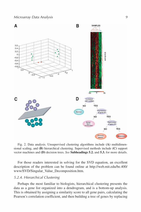
This analysis is often based on a pair-wise correlation coefficient and assessesthe similarities and dissimilarities between samples and assigns the difference asa “distance” between samples, such that the more similar two samples are, thecloser they are together, and vice versa (Fig. 2A). The multi- as opposed to two-dimensional analysis comes into play when not only the degree of difference(distance) but also the spatial relationship of three or more samples to each other(direction) is taken into account. For further mathematical description of thisprocess, see http://www.statsoft.com/textbook/stmulsca.html.
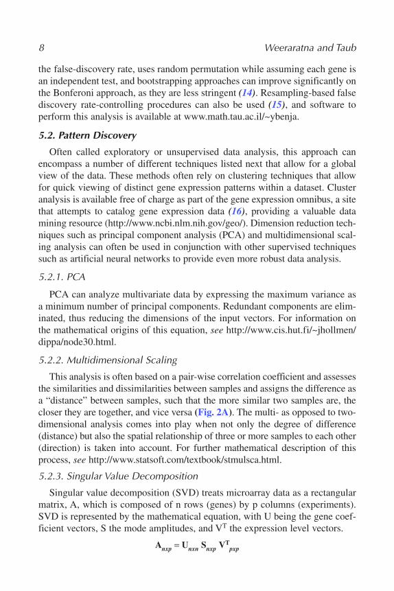
5.2.3. Singular Value Decomposition
Singular value decomposition (SVD) treats microarray data as a rectangularmatrix, A, which is composed of n rows (genes) by p columns (experiments).SVD is represented by the mathematical equation, with U being the gene coef-ficient vectors, S the mode amplitudes, and VT the expression level vectors.
Anxp = Unxn Snxp VTpxp
8 Weeraratna and Taub
01_Weeraratna.qxd 6/3/07 10:16 AM Page 8
For those readers interested in solving for the SVD equation, an excellentdescription of the problem can be found online at http://web.mit.edu/be.400/www/SVD/Singular_Value_Decomposition.htm.
5.2.4. Hierarchical Clustering
Perhaps the most familiar to biologists, hierarchical clustering presents thedata as a gene list organized into a dendrogram, and is a bottom-up analysis.This is obtained by assigning a similarity score to all gene pairs, calculating thePearson’s correlation coefficient, and then building a tree of genes by replacing
Microarray Data Analysis 9
Fig. 2. Data analysis. Unsupervised clustering algorithms include (A) multidimen-sional scaling, and (B) hierarchical clustering. Supervised methods include (C) supportvector machines and (D) decision trees. See Subheadings 5.2. and 5.3. for more details.
01_Weeraratna.qxd 6/3/07 10:16 AM Page 9

the two most similar genes with a node that contains the average, then repeat-ing the process for the next closest pair of data points, and then the next. Thisprocess is repeated several times (iterative process) to generate the dendrogramor Treeview, as well as heat maps that represent a two-color checkerboard viewof the data (Fig. 2B) (17).
5.2.5. K-Means Clustering
K-means clustering is a top-down technique that groups a collection of nodesinto a fixed number of clusters (k) that are subjected to an iterative process.Each class must have a center point that is the average position of all the dis-tances in that class (representative element), and each sample must fall into theclass to which its center is closest. Fuzzy k-means is performed by “soft”assignment of genes to these clusters (17).
5.2.6. Self-Organizing Maps
These maps are basically two-dimensional grids containing nodes of genesin “K”-dimensional space. These can be represented by sample and weight vec-tors, which are composed of the data and their natural location. Weight vectorsare initialized, and then sample vectors are randomly selected to determinewhich weight best represents that sample, and these are used to map the nodesinto K-dimensional space into which the gene expression data falls. Like thepreviously mentioned methods, this is also iterative and is often repeated morethan 1000 times, and these methods can often be used in combination to gener-ate the best overview of the data (18).
5.3. Class Prediction
Class prediction is based on supervised data analysis methods that imposeknown groups on datasets. First, a training set is identified—this is a group ofgenes with a known pattern of expression that is used to “train” a dataset, bycomparing the data to the training set and thus classifying it (19). This particu-lar method is very useful in the subclassification of similar samples (20), can-cer diagnosis (21), or to predict cell or patient response to drug therapy (22,23).In some cases, this type of analysis has also been used to predict patient out-come (24), allowing for a very clinically relevant use of microarray data.Importantly, gene selection by these methods relies on the assignment of dis-criminatory weights to these genes, i.e., how often a single gene correlates to agiven class or phenotype, often calculated using random permutation tests.Random permutation tests are also used to calculate p (probability the weightcan be obtained by chance) and α (probability of high weight resulting fromrandom classification) values for these weights. Many different statistical meth-ods can be used to find discriminant genes.
10 Weeraratna and Taub
01_Weeraratna.qxd 6/3/07 10:16 AM Page 10

5.3.1. Fisher Linear Discriminant Analysis
This theory assumes that a random vector x has a multivariate normal dis-tribution between each defined class or group, and the covariance withineach group is identical for all the groups. This makes the optimal decisionfunction for the comparison of data a linear transformation of x (25).Variations on this theme include quadratic discriminant analysis, flexiblediscriminant analysis, penalized discriminant analysis, and mixture discrim-inant analysis.
5.3.2. Nearest-Neighbor Classification
These methods are based on a measure of distance (e.g., Euclidean distance)between two gene expression profiles. Observations are given a value (x) andthe number of observations (k) closest to x is used to choose the class. Thevalue of k can be determined by using cross-validation techniques (26).
5.3.3. Support Vector Machines
This type of analysis is based on constructing planes in a multidimensionalspace that separate the different classes of genes, and set decision boundariesusing an iterative training algorithm (27). Data is mapped into the higherdimensional space from its original input space, and a nonlinear decisionboundary is assigned (Fig. 2C). This plane is known as the maximal marginhyperplane, and can be located by the use of a kernel function (a nonparametricweighting function). For further mathematical description, see http://www.statsoft.com/textbook/stsvm.html.
5.3.4. Artificial Neural Networks
Neural networks, or perceptrons, another machine-learning technique, are sonamed because they model the human brain—they learn by experience.Multilayer perceptrons can be used to classify samples based on their geneexpression (28,29). Gene expression data for a sample are input into the model,and a response is generated in the next layer, ultimately triggering a response inthe output layer. This output perceptron should represent the class to which thesample belongs.
5.3.5. Decision Trees
These are built by using criteria to divide samples into nodes. Samples aredivided recursively until they either fall into partitions, or until a terminationcondition is met (30). Ultimately the intermediate nodes represent splittingpoints or partitioning criteria, and the leaf nodes represent those decisions(Fig. 2D).
Microarray Data Analysis 11
01_Weeraratna.qxd 6/3/07 10:16 AM Page 11

6. Pathway Analysis ToolsOnce all the genes in an experiment have been analyzed, the next step is to
biologically interpret the data. The use of gene ontology programs, such asthose listed next, take the gene lists identified by the experiment and comparethe patterns therein to the available literature, and thus extract informationabout potentially important pathways affected by the experiment. All of theseprograms are available online, but only a few are freely available.
6.1. GoMiner
GoMiner maps lists of genes to functional categories using a tree view. This pro-gram also links to PubMed, and LocusLink. In addition it provides biological molec-ular interaction map and signaling pathway packages for more detailed analysis (31).
6.2. Database for Annotation, Visualization, and Integrated Discovery (DAVID)
DAVID is available at http://www.david.niaid.nih.gov; this program has fourcomponents (32).
1. Annotation tool: annotates the gene lists by adding gene descriptions from publicdatabases.
2. GoCharts: functionally categorizes genes based on user-selected classificationsand term specificity level.
3. KeggCharts: assigns genes to the Kyoto Encyclopedia of Genes and Genomes(KEGG) metabolic processes and enables users to view genes in the context ofbiochemical pathway maps.
4. DomainCharts: groups genes according to conserved protein domains.
6.3. PATIKA: Pathway Analysis Tool for Integration and KnowledgeAcquisition
Patika is a multi-user tool that is composed of a server-side, scalable, object-oriented database and client-side. As with the other programs, there is pathwaylayout, functional computation support, advanced querying, and a user-friendlygraphical interface (33).
6.4. Ingenuity Pathway Analysis
Of all the above programs, Ingenuity pathway analysis is perhaps the mostefficient at analyzing multiple datasets across different experimentation plat-forms. Like GOMiner, Ingenuity can identify key functional pathways (34). Itis currently the largest curated database that comprises individually modeledrelationships between proteins, genes, complexes, cells, tissues, drugs, and dis-eases, and provides a large variety in the presentation of the data.
12 Weeraratna and Taub
01_Weeraratna.qxd 6/3/07 10:16 AM Page 12

7. Data ValidationAs complex and robust as the available analyses for microarray data cur-
rently are, there is always room for error, and many inherent problems in theexperimental technique. Thus, it is critical that researchers validate their databefore drawing any firm biological conclusions from the data. One of the mostcommon techniques for validating array data is the use of real-time PCR (35).Real-time PCR effectively quantitates differences in transcript levels betweendifferent samples (36), but it must be remembered that the ratios acquired froma microarray experiment are quite likely to be much lower than fold changesseen in real-time PCR, as this method is much more sensitive.
Ultimately, protein expression is of course the final confirmation, as mostgene expression-profiling experiments, whether of a classifier or exploratorynature seek protein markers, and this is most often confirmed using immuno-histochemistry. As such, tissue microarrays have become an important compan-ion to DNA microarrays. These are slides that contain small punches ofparaffin-embedded tissue, often up to 500 sections on one slide (37). Tissuearrays often encompass all the stages of a disease being studied or can be madefrom animal tissues, as confirmation for in vivo mouse experiments, for exam-ple. The current large whole-genome arrays pose a problem when it comes tothis aspect, as the actual rate of antibody production for all these novel proteins,many of which are hypothetical, lags far behind the rate of gene discovery. Onecan only hope that soon this will catch up with the available genomic data, leav-ing us with valuable tools to identify markers and pathways, and that truly takeus from bench to bedside.
8. Future of Microarray Analysis and TechnologyOver the last decade, microarray analysis has been utilized almost exclu-
sively as a research tool that requires significant effort and computer time bytrained individuals to prepare high-quality RNA, label and hybridize the arrays,and analyze the data. As evidenced by the recent surge of microarray use in themedical literature over the past 5 yr, this technique has become increasinglypopular in comparing “normal” to “diseased” tissues or “treated” to “untreated”cells or clinical samples derived from various conditions. Despite this recentuse in clinical studies, several significant hurdles need to be overcome to opti-mize it for routine clinical lab use. Considerable improvements are required tooptimize microarray fabrication, hybridization methodology, and analysis thatwill permit a great deal of these processes to become fully automated and thusincrease the reproducibility within and across experiments. New technologies,such as the use of carbon nanotubules to produce microarray-like devices, mayincrease the use, automation, accuracy, and throughput in the study of gene
Microarray Data Analysis 13
01_Weeraratna.qxd 6/3/07 10:16 AM Page 13
expression within research, clinical, and diagnostic samples. Moreover, contin-ual advances in the field of proteomics, in combination with microarray tech-nology, should greatly enhance our ability to identify proteins and antigens fortherapeutic use. Several commercial software vendors have already initiatedmodifications in their data-mining software to link the nucleotide and proteindatabases and analysis tools to permit the examination of an individual genetranscription and translation. With the advent of new technologies and morerapid methods of analysis, the microarray technique will most likely become amore commonplace and invaluable tool not only for basic research studies butalso for clinical analysis and diagnosis.
AcknowledgmentsWe thank Dr. Kevin Becker for helpful comments on the manuscript.
References1. Augenlicht, L. H., Wahrman, M. Z., Halsey, H., Anderson, L., Taylor, J., and
Lipkin, M. (1987) Expression of cloned sequences in biopsies of human colonictissue and in colonic carcinoma cells induced to differentiate in vitro. Cancer Res.47, 6017–6021.
2. Lander, E. S., Linton, L. M., Birren, B., et al. (2001) Initial sequencing and analy-sis of the human genome. Nature 409, 860–921.
3. Brazma, A., Hingamp, P., Quackenbush, J., et al. (2001) Minimum informationabout a microarray experiment (MIAME)-toward standards for microarray data.Nat. Genet. 29, 365–371.
4. Dodson, J. M., Charles, P. T., Stenger, D. A., and Pancrazio, J. J. (2002)Quantitative assessment of filter-based cDNA microarrays: gene expression pro-files of human T-lymphoma cell lines. Bioinformatics 18, 953–960.
5. Li, Q., Fraley, C., Bumgarner, R.E., Yeung, K.Y., and Raftery, A.E. (2005) In:“Technical Report no. 473” (http://www.stat.washington.edu/www/research/reports/2005/tr473.pdf, Ed.), University of Washington, Seattle.
6. Jain, A. N., Tokuyasu, T. A., Snijders, A. M., Segraves, R., Albertson, D. G., andPinkel, D. (2002) Fully automatic quantification of microarray image data.Genome Res. 12, 325–332.
7. Quackenbush, J. (2002) Microarray data normalization and transformation. NatGenet 32 (Suppl), 496–501.
8. Zien, A., Aigner, T., Zimmer, R., and Lengauer, T. (2001) Centralization: a newmethod for the normalization of gene expression data. Bioinformatics 17 (Suppl 1),S323–S331.
9. Yang, Y. H., Dudoit, S., Luu, P., et al. (2002) Normalization for cDNA microarraydata: a robust composite method addressing single and multiple slide systematicvariation. Nucleic Acids Res. 30, e15.
10. Kepler, T. B., Crosby, L., and Morgan, K. T. (2002) Normalization and analysis ofDNA microarray data by self-consistency and local regression. Genome Biol. 3,RESEARCH0037.
14 Weeraratna and Taub
01_Weeraratna.qxd 6/3/07 10:16 AM Page 14

11. Zhao, Y., Li, M. C., and Simon, R. (2005) An adaptive method for cDNA microar-ray normalization. BMC Bioinformatics 6, 28.
12. Sasik, R., Calvo, E., and Corbeil, J. (2002) Statistical analysis of high-densityoligonucleotide arrays: a multiplicative noise model. Bioinformatics 18, 1633–1640.
13. Li, H., Wood, C. L., Getchell, T. V., Getchell, M. L., and Stromberg, A. J. (2004)Analysis of oligonucleotide array experiments with repeated measures using mixedmodels. BMC Bioinformatics 5, 209.
14. Meuwissen, T. H., and Goddard, M. E. (2004) Bootstrapping of gene-expressiondata improves and controls the false discovery rate of differentially expressedgenes. Genet. Sel. Evol. 36, 191–205.
15. Reiner, A., Yekutieli, D., and Benjamini, Y. (2003) Identifying differentiallyexpressed genes using false discovery rate controlling procedures. Bioinformatics19, 368–375.
16. Barrett, T., Suzek, T. O., Troup, D. B., et al. (2005) NCBI GEO: mining millionsof expression profiles—database and tools. Nucleic Acids Res. 33 Database Issue,D562–D566.
17. Sherlock, G. (2000) Analysis of large-scale gene expression data. Curr. Opin.Immunol. 12, 201–205.
18. Wang, J., Delabie, J., Aasheim, H., Smeland, E., and Myklebost, O. (2002)Clustering of the SOM easily reveals distinct gene expression patterns: results of areanalysis of lymphoma study. BMC Bioinformatics 3, 36.
19. Dharmadi, Y., and Gonzalez, R. (2004) DNA microarrays: experimental issues,data analysis, and application to bacterial systems. Biotechnol. Prog. 20, 1309–1324.
20. Bittner, M., Meltzer, P., Chen, Y., et al. (2000) Molecular classification of cuta-neous malignant melanoma by gene expression profiling. Nature 406, 536–540.
21. Ramaswamy, S., Tamayo, P., Rifkin, R., et al. (2001) Multiclass cancer diagnosisusing tumor gene expression signatures. Proc. Natl. Acad. Sci. USA 98,15,149–15,154.
22. Cunliffe, H. E., Ringner, M., Bilke, S., et al. (2003) The gene expression responseof breast cancer to growth regulators: patterns and correlation with tumor expres-sion profiles. Cancer Res. 63, 7158–7166.
23. Burczynski, M. E., Oestreicher, J. L., Cahilly, M. J., et al. (2005) Clinical pharma-cogenomics and transcriptional profiling in early phase oncology clinical trials.Curr. Mol. Med. 5, 83–102.
24. Nutt, C. L., Mani, D. R., Betensky, R. A., et al. (2003) Gene expression-based clas-sification of malignant gliomas correlates better with survival than histologicalclassification. Cancer Res. 63, 1602–1607.
25. Mendez, M. A., Hodar, C., Vulpe, C., Gonzalez, M., and Cambiazo, V. (2002)Discriminant analysis to evaluate clustering of gene expression data. FEBS Lett.522, 24–28.
26. Olshen, A. B., and Jain, A. N. (2002) Deriving quantitative conclusions frommicroarray expression data. Bioinformatics 18, 961–970.
27. Brown, M. P., Grundy, W. N., Lin, D., et al. (2000) Knowledge-based analysis ofmicroarray gene expression data by using support vector machines. Proc. Natl.Acad. Sci. USA 97, 262–267.
Microarray Data Analysis 15
01_Weeraratna.qxd 6/3/07 10:16 AM Page 15

28. Khan, J., Wei, J. S., Ringner, M., et al. (2001) Classification and diagnostic predic-tion of cancers using gene expression profiling and artificial neural networks. NatMed 7, 673–679.
29. Ringner, M., Peterson, C., and Khan, J. (2002) Analyzing array data using super-vised methods. Pharmacogenomics 3, 403–415.
30. Zhang, H., Yu, C. Y., Singer, B., and Xiong, M. (2001) Recursive partitioning fortumor classification with gene expression microarray data. Proc. Natl. Acad. Sci.USA 98, 6730–6735.
31. Zeeberg, B. R., Feng, W., Wang, G., et al. (2003) GoMiner: a resource for biolog-ical interpretation of genomic and proteomic data. Genome Biol. 4, R28.
32. Dennis, G., Jr., Sherman, B. T., Hosack, D. A., et al. (2003) DAVID: Database forAnnotation, Visualization, and Integrated Discovery. Genome Biol. 4, P3.
33. Demir, E., Babur, O., Dogrusoz, U., et al. (2002) PATIKA: an integrated visualenvironment for collaborative construction and analysis of cellular pathways.Bioinformatics 18, 996–1003.
34. Raponi, M., Belly, R. T., Karp, J. E., Lancet, J. E., Atkins, D., and Wang, Y. (2004)Microarray analysis reveals genetic pathways modulated by tipifarnib in acutemyeloid leukemia. BMC Cancer 4, 56.
35. Jenson, S. D., Robetorye, R. S., Bohling, S. D., et al. (2003) Validation of cDNAmicroarray gene expression data obtained from linearly amplified RNA. Mol.Pathol. 56, 307–312.
36. Winer, J., Jung, C. K., Shackel, I., and Williams, P. M. (1999) Development andvalidation of real-time quantitative reverse transcriptase-polymerase chain reactionfor monitoring gene expression in cardiac myocytes in vitro. Anal. Biochem. 270,41–49.
37. Kononen, J., Bubendorf, L., Kallioniemi, A., et al. (1998) Tissue microarrays forhigh-throughput molecular profiling of tumor specimens. Nat. Med. 4, 844–847.
16 Weeraratna and Taub
01_Weeraratna.qxd 6/3/07 10:16 AM Page 16
2
Genomic Signal Processing: From Matrix Algebra to Genetic Networks
Orly Alter
SummaryDNA microarrays make it possible, for the first time, to record the complete genomic sig-
nals that guide the progression of cellular processes. Future discovery in biology and medi-cine will come from the mathematical modeling of these data, which hold the key tofundamental understanding of life on the molecular level, as well as answers to questionsregarding diagnosis, treatment, and drug development. This chapter reviews the first data-driven models that were created from these genome-scale data, through adaptations and gen-eralizations of mathematical frameworks from matrix algebra that have proven successful indescribing the physical world, in such diverse areas as mechanics and perception: the singu-lar value decomposition model, the generalized singular value decomposition model compar-ative model, and the pseudoinverse projection integrative model. These models providemathematical descriptions of the genetic networks that generate and sense the measured data,where the mathematical variables and operations represent biological reality. The variables,patterns uncovered in the data, correlate with activities of cellular elements such as regulatorsor transcription factors that drive the measured signals and cellular states where these ele-ments are active. The operations, such as data reconstruction, rotation, and classification insubspaces of selected patterns, simulate experimental observation of only the cellular pro-grams that these patterns represent. These models are illustrated in the analyses of RNAexpression data from yeast and human during their cell cycle programs and DNA-binding datafrom yeast cell cycle transcription factors and replication initiation proteins. Two alternativepictures of RNA expression oscillations during the cell cycle that emerge from these analy-ses, which parallel well-known designs of physical oscillators, convey the capacity of themodels to elucidate the design principles of cellular systems, as well as guide the design ofsynthetic ones. In these analyses, the power of the models to predict previously unknown bio-logical principles is demonstrated with a prediction of a novel mechanism of regulation thatcorrelates DNA replication initiation with cell cycle-regulated RNA transcription in yeast.These models may become the foundation of a future in which biological systems are mod-eled as physical systems are today.
17
From: Methods in Molecular Biology, vol. 377, Microarray Data Analysis: Methods and ApplicationsEdited by: M. J. Korenberg © Humana Press Inc., Totowa, NJ
02_Alter 6/3/07 10:35 AM Page 17
Key Words: Singular value decomposition (SVD); generalized SVD (GSVD); pseudoinverseprojection; blind source separation (BSS) algorithms; genome-scale RNA expression and proteins’ DNA-binding data; cell cycle; yeast Saccharomyces cerevisiae; human HeLa cell line;analog harmonic and digital ring oscillators.
1. Introduction1.1. DNA Microarray Technology and Genome-Scale MolecularBiological Data
The Human Genome Project, and the resulting sequencing of completegenomes, fueled the emergence of the DNA microarray hybridization technologyin the past decade. This novel experimental high-throughput technology makes itpossible to assay the hybridization of fluorescently tagged DNA or RNA mol-ecules, which were extracted from a single sample, with several thousand syn-thetic oligonucleotides (1) or DNA targets (2) simultaneously. Different typesof molecular biological signals, such as DNA copy number, RNA expressionlevels, and DNA-bound proteins’ occupancy levels, that correspond to activi-ties of cellular systems, such as DNA replication, RNA transcription, and bind-ing of transcription factors to DNA, can now be measured on genomic scales(e.g., refs. 3 and 4). For the first time in human history it is possible to moni-tor the flow of molecular biological information, as DNA is transcribed toRNA, RNA is translated to proteins, and proteins bind to DNA, and thus toobserve experimentally the global signals that are generated and sensed by cel-lular systems. Already laboratories all over the world are producing vast quan-tities of genome-scale data in studies of cellular processes and tissue samples(e.g., refs. 5–9).
Analysis of these new data promises to enhance the fundamental understand-ing of life on the molecular level and might prove useful in medical diagnosis,treatment, and drug design. Comparative analysis of these data among two ormore organisms promises to give new insights into the universality as well as the specialization of evolutionary, biochemical, and genetic pathways.Integrative analysis of different types of these global signals from the sameorganism promises to reveal cellular mechanisms of regulation, i.e., globalcausal coordination of cellular activities.
1.2. From Technology and Large-Scale Data to Discovery and Controlof Basic Phenomena Using Mathematical Models: Analogy FromAstronomy
Biology and medicine today, with these recent advances in DNA microarraytechnology, may very well be at a point similar to where physics was after theadvent of the telescope in the 17th century. In those days, astronomers were
18 Alter
02_Alter 6/3/07 10:35 AM Page 18

Genomic Signal Processing 19
compiling tables detailing observed positions of planets at different times fornavigation. Popularized by Galileo Galilei, telescopes were being used in thesesky surveys, enabling more accurate and more frequent observations of a grow-ing number of celestial bodies. One astronomer, Tycho Brahe, compiled someof the more extensive and accurate tables of such astronomical observations.Another astronomer, Johannes Kepler, used mathematical equations from ana-lytical geometry to describe trends in Brahe’s data, and to determine three lawsof planetary motion, all relating observed time intervals with observed dis-tances. These laws enabled the most accurate predictions of future positions ofplanets to date. Kepler’s achievement posed the question: why are the planetarymotions such that they follow these laws? A few decades later, Isaac Newtonconsidered this question in light of the experiments of Galileo, the data ofBrahe, and the models of Kepler. Using mathematical equations from calculus,he introduced the physical observables mass, momentum, and force, anddefined them in terms of the observables time and distance. With these postu-lates, the three laws of Kepler could be derived within a single mathematicalframework, known as the universal law of gravitation, and Newton concludedthat the physical phenomenon of gravitation is the reason for the trendsobserved in the motion of the planets (10). Today, Newton’s discovery andmathematical formulation of the basic phenomenon that is gravitation enablescontrol of the dynamics of moving bodies, e.g., in exploration of outer space.
The rapidly growing number of genome-scale molecular biological datasetshold the key to the discovery of previously unknown molecular biological prin-ciples, just as the vast number of astronomical tables compiled by Galileo andBrahe enabled accurate prediction of planetary motions and later also the dis-covery of universal gravitation. Just as Kepler and Newton made their discov-eries by using mathematical frameworks to describe trends in these large-scaleastronomical data, also future predictive power, discovery, and control in biol-ogy and medicine will come from the mathematical modeling of genome-scalemolecular biological data.
1.3. From Complex Signals to Simple Principles Using MathematicalModels: Analogy From Neuroscience
Genome-scale molecular biological signals appear to be complex, yet theyare readily generated and sensed by the cellular systems. For example, the divi-sion cycle of human cells spans an order of one day only of cellular activity. Theperiod of the cell division cycle in yeast is of the order of an hour.
DNA microarray data or genomic-scale molecular biological signals, ingeneral, may very well be similar to the input and output signals of the
02_Alter 6/3/07 10:35 AM Page 19

20 Alter
central nervous system, such as images of the natural world that are viewed bythe retina and the electric spike trains that are produced by the neurons in thevisual cortex. In a series of classic experiments, the neuroscientists Hubel andWiesel (11) recorded the activities of individual neurons in the visual cortex inresponse to different patterns of light falling on the retina. They showed that thevisual cortex represents a spatial map of the visual field. They also discoveredthat there exists a class of neurons, which they called “simple cells,” each ofwhich responds selectively to a stimulus of an edge of a given scale at a givenorientation in the neuron’s region of the visual field. These discoveries posed thequestion: what might be the brain’s advantage in processing natural images witha series of spatially localized scale-selective edge detectors? Barlow (12) sug-gested that the underlying principle of such image processing is that of sparsecoding, which allows only a few neurons out of a large population to be simul-taneously active when representing any image from the natural world. Naturally,such images are made out of objects and surfaces, i.e., edges. Two decades later,Olshausen and Field (13; see also Bell and Sejnowski, ref. 14) developed a novelalgorithm, which separates or decomposes natural images into their optimalcomponents, where they defined optimality mathematically as the preservationof a characteristic ensemble of images as well as the sparse representation of thisensemble. They showed that the optimal sparse linear components of a naturalimage are spatially localized and scaled edges, thus validating Barlow’s postulate.
The sensing of the complex genomic-scale molecular biological signals bythe cellular systems might be governed by simple principles, just as the process-ing of the complex natural images by the visual cortex appear to be governed bythe simple principle of sparse coding. Just as the natural images could be repre-sented mathematically as superpositions, i.e., weighted sums of images, whichcorrelate with the measured sensory activities of neurons, also the complexgenomic-scale molecular biological signals might be represented mathemati-cally as superpositions of signals, which might correspond to the measuredactivities of cellular elements.
1.4. Matrix Algebra Models for DNA Microarray Data
This chapter reviews the first data-driven predictive models for DNAmicroarray data or genomic-scale molecular biological signals in general.These models use adaptations and generalizations of matrix algebra frameworks(15) in order to provide mathematical descriptions of the genetic networks thatgenerate and sense the measured data. The singular value decomposition (SVD)model formulates a dataset as the result of a simple linear network (Fig. 1A):the measured gene patterns are expressed mathematically as superpositions ofthe effects of a few independent sources, biological or experimental, and the
02_Alter 6/3/07 10:35 AM Page 20
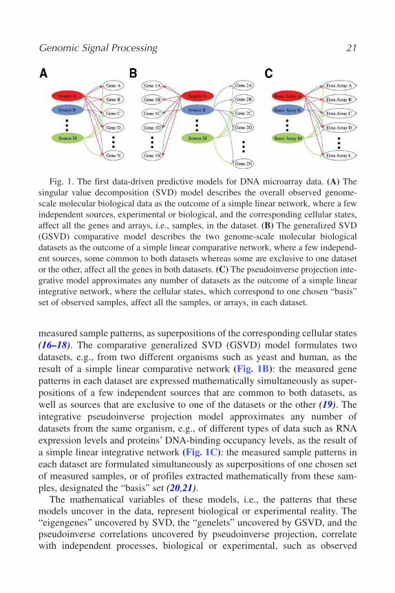
measured sample patterns, as superpositions of the corresponding cellular states(16–18). The comparative generalized SVD (GSVD) model formulates twodatasets, e.g., from two different organisms such as yeast and human, as theresult of a simple linear comparative network (Fig. 1B): the measured genepatterns in each dataset are expressed mathematically simultaneously as super-positions of a few independent sources that are common to both datasets, aswell as sources that are exclusive to one of the datasets or the other (19). Theintegrative pseudoinverse projection model approximates any number ofdatasets from the same organism, e.g., of different types of data such as RNAexpression levels and proteins’ DNA-binding occupancy levels, as the result ofa simple linear integrative network (Fig. 1C): the measured sample patterns ineach dataset are formulated simultaneously as superpositions of one chosen setof measured samples, or of profiles extracted mathematically from these sam-ples, designated the “basis” set (20,21).
The mathematical variables of these models, i.e., the patterns that these models uncover in the data, represent biological or experimental reality. The“eigengenes” uncovered by SVD, the “genelets” uncovered by GSVD, and thepseudoinverse correlations uncovered by pseudoinverse projection, correlatewith independent processes, biological or experimental, such as observed
Genomic Signal Processing 21
Fig. 1. The first data-driven predictive models for DNA microarray data. (A) Thesingular value decomposition (SVD) model describes the overall observed genome-scale molecular biological data as the outcome of a simple linear network, where a fewindependent sources, experimental or biological, and the corresponding cellular states,affect all the genes and arrays, i.e., samples, in the dataset. (B) The generalized SVD(GSVD) comparative model describes the two genome-scale molecular biologicaldatasets as the outcome of a simple linear comparative network, where a few independ-ent sources, some common to both datasets whereas some are exclusive to one datasetor the other, affect all the genes in both datasets. (C) The pseudoinverse projection inte-grative model approximates any number of datasets as the outcome of a simple linearintegrative network, where the cellular states, which correspond to one chosen “basis”set of observed samples, affect all the samples, or arrays, in each dataset.
02_Alter 6/3/07 10:35 AM Page 21

22 Alter
genome-wide effects of known regulators or transcription factors, the cellularelements that generate the genome-wide RNA expression signals most com-monly measured by DNA microarrays. The corresponding “eigenarrays”uncovered by SVD and “arraylets” uncovered by GSVD, correlate with the cor-responding cellular states, such as measured samples in which these regulatorsor transcription factors are overactive or underactive.
The mathematical operations of these models, e.g., data reconstruction, rota-tion, and classification in subspaces spanned by these patterns also representbiological or experimental reality. Data reconstruction in subspaces of selectedeigengenes, genelets, or pseudoinverse correlations, and corresponding eigenar-rays or arraylets, simulates experimental observation of only the processes andcellular states that these patterns represent, respectively. Data rotation in thesesubspaces simulates the experimental decoupling of the biological programsthat these subspaces span. Data classification in these subspaces maps themeasured gene and sample patterns onto the processes and cellular states thatthese subspaces represent, respectively.
Because these models provide mathematical descriptions of the geneticnetworks that generate and sense the measured data, where the mathematicalvariables and operations represent biological or experimental reality, thesemodels have the capacity to elucidate the design principles of cellular systemsas well as guide the design of synthetic ones (e.g., ref. 22). These models alsohave the power to make experimental predictions that might lead to experi-ments in which the models can be refuted or validated, and to discover previ-ously unknown molecular biological principles (21,23). Ultimately, thesemodels might enable the control of biological cellular processes in real timeand in vivo (24).
Although no mathematical theorem promises that SVD, GSVD, andpseudoinverse projection could be used to model DNA microarray data orgenome-scale molecular biological signals in general, these results are notcounterintuitive. Similar and related mathematical frameworks have alreadyproven successful in describing the physical world, in such diverse areas asmechanics and perception (25).
First, SVD, GSVD, and pseudoinverse projection, interpreted as they arehere as simple approximations of the networks or systems that generate andsense the processed signals, belong to a class of algorithms called blind sourceseparation (BSS) algorithms. BSS algorithms, such as the linear sparse codingalgorithm by Olshausen and Field (13), the independent component analysisby Bell and Sejnowski (14) and the neural network algorithms by Hopfield(26), separate or decompose measured signals into their mathematically definedoptimal components. These algorithms have already proven successful in mod-eling natural signals and computationally mimicking the activity of the brain asit expertly perceives these signals, for example, in face recognition (27,28).
02_Alter 6/3/07 10:35 AM Page 22

Second, SVD, GSVD, and pseudoinverse projection can be also thought of asgeneralizations of the eigenvalue decomposition (EVD) and generalized EVD(GEVD) of Hermitian matrices, and inverse projection onto an orthogonal matrix,respectively. In mechanics, EVD of the Hermitian matrix, which tabulates theenergy of a system of coupled oscillators, uncovers the eigenmodes and eigenfre-quencies of this system, i.e., the normal coordinates, which oscillate indep-endently of one another, and their frequencies of oscillations. One of these eigen-modes represents the center of mass of the system. GEVD of the Hermitian matri-ces, which tabulate the kinetic and potential energies of the oscillators, comparesthe distribution of kinetic energy among the eigenmodes with that of the poten-tial energy. The inverse projection onto the orthogonal matrix, which tabulates theeigenmodes of this system, is equivalent to transformation of coordinates to the frame of reference, which is oscillating with the system (e.g., ref. 29). SVD, GSVD, and pseudoinverse projection are, therefore, generalizations of the frameworks that underlie the mathematical theoretical description of the phys-ical world.
In this chapter, the mathematical frameworks of SVD, GSVD, and pseudoin-verse projection are reviewed with an emphasis on the mathematical definitionof the optimality of the components, or patterns, that each algorithm uncoversin the data. These models are illustrated in the analyses of RNA expression datafrom yeast and human during their cell cycle programs and DNA-binding datafrom yeast cell cycle transcription factors and replication initiation proteins.The correspondence between the mathematical frameworks and the genetic net-works that generate and sense the measured data is outlined in each case, focus-ing on the correlations between the mathematical patterns and the observedcellular programs, as well as between the mathematical operations in subspacesspanned by selected patterns and the experimental observation of the cellularprograms. Two alternative pictures of RNA expression oscillations during thecell cycle that emerge from these analyses are considered, and parallels betweenthese pictures and well-known designs of physical oscillators, namely the analogharmonic oscillator and the digital ring oscillator, are drawn to convey thecapacity of the models to elucidate the design principles of cellular systems, aswell as guide the design of synthetic ones. Finally, the power of these modelsto predict previously unknown biological principles is demonstrated with a prediction of a novel mechanism of regulation that correlates DNA replicationinitiation with cell cycle-regulated RNA transcription in yeast.
2. SVD for Modeling DNA Microarray DataThis section reviews the SVD model for DNA microarray data (16–18, 22–24).
SVD is a BSS algorithm that decomposes the measured signal, i.e., the measuredgene and array patterns of, e.g. RNA expression, into mathematically decorrelated
Genomic Signal Processing 23
02_Alter 6/3/07 10:35 AM Page 23
and decoupled patterns, the “eigengenes” and “eigenarrays.” The correspon-dence between these mathematical patterns uncovered in the measured signaland the independent biological and experimental processes and cellular statesthat compose the signal is illustrated with an analysis of genome-scale RNAexpression data from the yeast Saccharomyces cerevisiae during its cell cycleprogram (6). The picture of RNA expression oscillations during the yeast cellcycle that emerges from this analysis suggests an underlying genetic network orcircuit that parallels the analog harmonic oscillator.
2.1. Mathematical Framework of SVD
Let the matrix e of size N-genes × M-arrays tabulate the genome-scale signal,e.g., RNA expression levels, measured in a set of M samples using M DNA
microarrays. The vector in the mth column of the matrix , , lists theexpression signal measured in the mth sample by the mth array across all N genes
simultaneously. The vector in the nth row of the matrix , lists the
signal measured for the nth gene across the different arrays, which correspond tothe different samples.*
SVD is a linear transformation of this DNA microarray dataset from the N-genes × M-arrays space to the reduced L-eigenarrays × L-eigengenes space(Fig. 2), where L = min{M,N},
. (1)
In this space, the dataset or matrix is represented by the diagonal nonneg-ative matrix ε of size L-eigenarrays × L-eigengenes. The diagonality of ε meansthat each eigengene is decoupled of all other eigengenes, and each eigenarrayis decoupled of all other eigenarrays, such that each eigengene is expressedonly in the corresponding eigenarray.
The “fractions of eigenexpression” {pl} are calculated from the “eigenex-pression levels” {εl}, which are listed in the diagonal of ε,
(2)
These fractions of eigenexpression indicate for each eigengene and eigenarraytheir significance in the dataset relative to all other eigengenes and eigenarraysin terms of the overall expression information that they capture in the data. Notethat each fraction of eigenexpression can be thought of as the probability forany given gene among all genes in the dataset to express the corresponding
pll
kk
L=
=∑
ε
ε
2
2
1
.
e
ˆ ˆˆ ˆe u vT= ε
ˆ, ˆe g n en ≡
a e mm ≡ ˆe
24 Alter
*In this chapter, m denotes a matrix, |v⟩ denotes a column vector, and ⟨u| denotes a row vector,such that, m |v⟩, ⟨u|m , and ⟨u|v⟩ all denote inner products and |v⟩⟨u| denotes an outer product.
02_Alter 6/3/07 10:35 AM Page 24

Genomic Signal Processing 25
eigengene, and at the same time, the probability for any given array among allarrays to express the corresponding eigenarray.
The “normalized Shannon entropy” of the dataset,
(3)
measures the complexity of the data from the distribution of the overall expres-sion information between the different eigengenes and corresponding eigenar-rays, where d = 0 corresponds to an ordered and redundant dataset in which allexpression is captured by one eigengene and the corresponding eigenarray, andd = 1 corresponds to a disordered and random dataset where all eigengenes andeigenarrays are equally expressed.
The transformation matrices û and vT define the N-genes × L-eigenarrays andthe L-eigengenes × M-arrays basis sets, respectively. The vector in the lth column of the matrix û, |αl⟩ ≡ û|l⟩, lists the genome-scale expression signal ofthe lth eigenarray. The vector in the lth row of the matrix vT, ⟨γl| ≡ ⟨l|vT, lists thesignal of the lth eigengene across the different arrays. The eigengenes and eige-narrays are orthonormal superpositions of the genes and arrays, such that thetransformation matrices û and vT are both orthogonal,
(4)
where Î is the identity matrix. The signal of each eigengene and eigenarray is,therefore, not only decoupled but also decorrelated from that of all other
ˆ ˆ ˆ ˆ ˆ,u u v v IT T= =
01
11
≤ = − ≤=
∑dL
p pkk
L
klog( ) ,
Fig. 2. Raster display of the SVD of the yeast cell cycle RNA expression dataset,with overexpression (red), no change in expression (black), and underexpression(green) around the steady state of expression of the 4579 yeast genes. SVD is a lineartransformation of the data from the 4579-genes × 22-arrays space to the reduced diag-onalized 22-eigenarrays × 22-eigengenes space, which is spanned by the 4579-genes ×22-eigenarrays and 22-eigengenes × 22-arrays bases.
02_Alter 6/3/07 10:35 AM Page 25
26 Alter26 Alter
eigengenes and eigenarrays, respectively. The eigengenes and eigenarrays areunique up to phase factors of ±1 for a real data matrix e, such that each eigengeneand eigenarray captures both parallel and antiparallel gene and array expressionpatterns, except in degenerate subspaces, defined by subsets of equal eigenexpres-sion levels. SVD is, therefore, data driven, except in degenerate subspaces.
2.2. SVD Analysis of Cell Cycle RNA Expression Data From Yeast
In this example, SVD is applied to a dataset that tabulates RNA expressionlevels of 4579 genes in 22 yeast samples, 18 samples of a time course monitor-ing the cell cycle in an α factor-synchronized culture, and two samples each ofyeast strains where the genes CLN3 and CLB2, which encode G1 and G2/Mcyclins, respectively, are overexpressed or overactivated (6).
2.2.1. Significant Eigengenes and Corresponding Eigenarrays CorrelateWith Genome-Scale Effects of Independent Sources of Expression and Their Corresponding Cellular States
Consider the 22 eigengenes of the α factor, CLB2, and CLN3 dataset (Fig. 3A).The first eigengene, which captures about 80% of the overall expression signal(Fig. 3B), and describes sample-invariant expression, is inferred to representsteady-state expression (Fig. 3C). The second and third eigengenes, which cap-ture about 9.5% and 2% of the overall expression signal, respectively, describeinitial transient increase and decrease in expression, respectively, superimposedon time-invariant expression during the cell cycle. These eigengenes areinferred to represent the responses to synchronization by the pheromone α fac-tor. The fourth through ninth and 11th eigengenes, which capture together about5% of the overall expression information, show expression oscillations of twoperiods during the α factor-synchronized cell cycle, and are inferred to repre-sent cell cycle expression oscillations (Fig. 3D–F).
The corresponding eigenarrays are associated with the corresponding cellu-lar states. An eigenarray is parallel and antiparallel associated with the mostlikely parallel and antiparallel cellular states, or none thereof, according to theannotations of the two groups of n genes each, with largest and smallest levelsof signal, e.g., expression, in this eigenarray among all N genes, respectively. A coherent biological theme might be reflected in the annotations of either oneof these two groups of genes. The p-value of a given association by annotationis calculated using combinatorics and assuming hypergeometric probability dis-tribution of the K annotations among the N genes, and of the subset of k � Kannotations among the subset of n � N genes,
P k n N KN
n
K
l
N K
n ll
( ; , , ) =⎛⎝⎜
⎞⎠⎟
⎛⎝⎜
⎞⎠⎟
−−
⎛⎝⎜
⎞⎠⎟
−
=
1
kk
n
∑ ,
02_Alter 6/3/07 10:35 AM Page 26
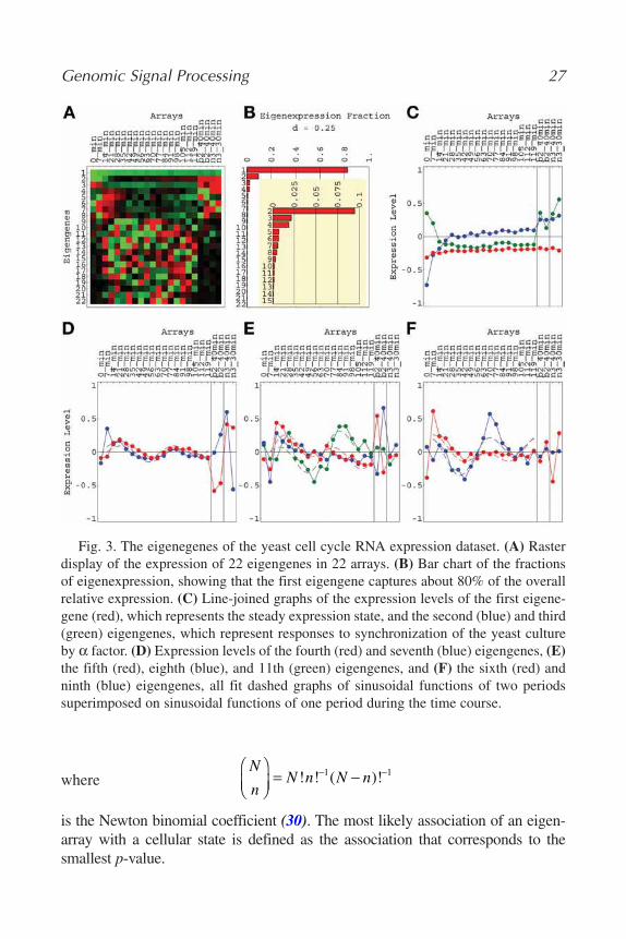
Genomic Signal Processing 27
where
is the Newton binomial coefficient (30). The most likely association of an eigen-array with a cellular state is defined as the association that corresponds to thesmallest p-value.
N
nN n N n
⎛⎝⎜
⎞⎠⎟
= −− −! ! ( )!1 1
Fig. 3. The eigenegenes of the yeast cell cycle RNA expression dataset. (A) Rasterdisplay of the expression of 22 eigengenes in 22 arrays. (B) Bar chart of the fractionsof eigenexpression, showing that the first eigengene captures about 80% of the overallrelative expression. (C) Line-joined graphs of the expression levels of the first eigene-gene (red), which represents the steady expression state, and the second (blue) and third(green) eigengenes, which represent responses to synchronization of the yeast cultureby α factor. (D) Expression levels of the fourth (red) and seventh (blue) eigengenes, (E)the fifth (red), eighth (blue), and 11th (green) eigengenes, and (F) the sixth (red) andninth (blue) eigengenes, all fit dashed graphs of sinusoidal functions of two periodssuperimposed on sinusoidal functions of one period during the time course.
02_Alter 6/3/07 10:35 AM Page 27
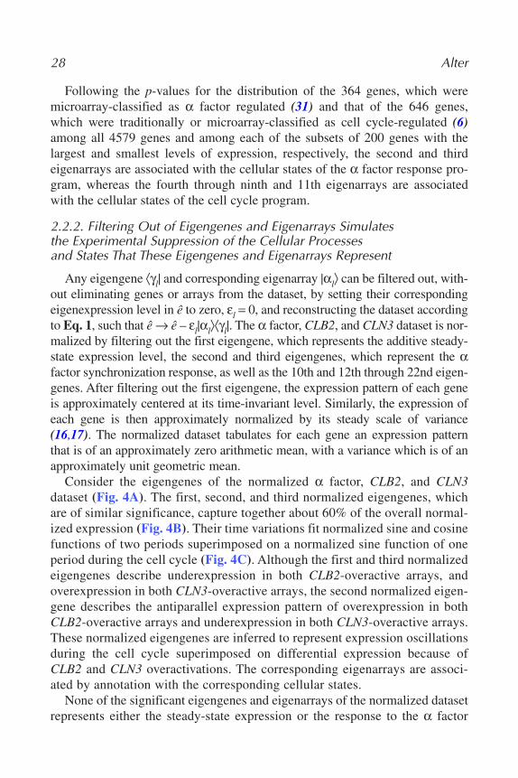
28 Alter
Following the p-values for the distribution of the 364 genes, which weremicroarray-classified as α factor regulated (31) and that of the 646 genes,which were traditionally or microarray-classified as cell cycle-regulated (6)among all 4579 genes and among each of the subsets of 200 genes with thelargest and smallest levels of expression, respectively, the second and thirdeigenarrays are associated with the cellular states of the α factor response pro-gram, whereas the fourth through ninth and 11th eigenarrays are associatedwith the cellular states of the cell cycle program.
2.2.2. Filtering Out of Eigengenes and Eigenarrays Simulates the Experimental Suppression of the Cellular Processes and States That These Eigengenes and Eigenarrays Represent
Any eigengene ⟨γl| and corresponding eigenarray |αl⟩ can be filtered out, with-out eliminating genes or arrays from the dataset, by setting their correspondingeigenexpression level in ê to zero, εl = 0, and reconstructing the dataset accordingto Eq. 1, such that ê → ê – εl|αl⟩⟨γl|. The α factor, CLB2, and CLN3 dataset is nor-malized by filtering out the first eigengene, which represents the additive steady-state expression level, the second and third eigengenes, which represent the αfactor synchronization response, as well as the 10th and 12th through 22nd eigen-genes. After filtering out the first eigengene, the expression pattern of each geneis approximately centered at its time-invariant level. Similarly, the expression ofeach gene is then approximately normalized by its steady scale of variance(16,17). The normalized dataset tabulates for each gene an expression pattern that is of an approximately zero arithmetic mean, with a variance which is of anapproximately unit geometric mean.
Consider the eigengenes of the normalized α factor, CLB2, and CLN3dataset (Fig. 4A). The first, second, and third normalized eigengenes, whichare of similar significance, capture together about 60% of the overall normal-ized expression (Fig. 4B). Their time variations fit normalized sine and cosinefunctions of two periods superimposed on a normalized sine function of oneperiod during the cell cycle (Fig. 4C). Although the first and third normalizedeigengenes describe underexpression in both CLB2-overactive arrays, andoverexpression in both CLN3-overactive arrays, the second normalized eigen-gene describes the antiparallel expression pattern of overexpression in bothCLB2-overactive arrays and underexpression in both CLN3-overactive arrays.These normalized eigengenes are inferred to represent expression oscillationsduring the cell cycle superimposed on differential expression because ofCLB2 and CLN3 overactivations. The corresponding eigenarrays are associ-ated by annotation with the corresponding cellular states.
None of the significant eigengenes and eigenarrays of the normalized datasetrepresents either the steady-state expression or the response to the α factor
02_Alter 6/3/07 10:35 AM Page 28

Genomic Signal Processing 29
synchronization. The normalized dataset simulates an experimental measure-ment of only the cell cycle program and the differential expression in responseto overactivation of CLB2 and CLN3.
2.2.3. Rotation in an Almost Degenerate Subspace SimulatesExperimental Decoupling of the Biological Programs the Subspace Spans
The almost degenerate subspaces spanned by the first, second, and thirdeigengenes and corresponding eigenarrays are approximated with degeneratesubspaces, by setting each of the corresponding eigenexpression levels equal,
and reconstructing the dataset according to Eq. 1.
With this approximation, the three eigengenes and corresponding eigenarrayscan be rotated, such that the same expression subspaces that are spanned bythese eigenegenes, and eigenarrays will be spanned by three orthogonal super-positions of these eigengenes and eigenarrays, i.e., by three rotated eigengenesand eigenarrays. Requiring two of these three rotated eigengenes to describeequal expression in the CLB2-overactive samples as in the CLN3-overactivesamples, so that only the one remaining rotated eigengene captures the differ-ential expression between these two sets of arrays, gives unique angles of rota-tions in the three-dimensional subspaces of eigengenes and eigenarrays, andtherefore also unique rotated eigengenes and eigenarrays.
ε ε ε ε ε ε1 2 3 12
22
32 3, , ( ) ,→ + +
Fig. 4. The eigengenes of the normalized yeast cell cycle RNA expression dataset.(A) Raster display. (B) Bar chart of the fractions of eigenexpression, showing that thefirst, second, and third normalized eigengenes capture approximately 20% of the over-all normalized expression information each, and span an approximately degenerate sub-space. (C) Line-joined graphs of the expression levels of the first (red), second (blue),and third (green) normalized eigengenes, fit dashed graphs of two-period sinusoidalfunctions superimposed on one-period sinusoidal functions during the time course.
02_Alter 6/3/07 10:35 AM Page 29
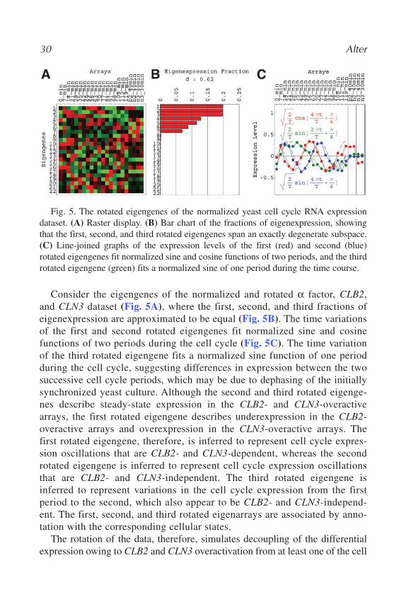
30 Alter
Consider the eigengenes of the normalized and rotated α factor, CLB2,and CLN3 dataset (Fig. 5A), where the first, second, and third fractions ofeigenexpression are approximated to be equal (Fig. 5B). The time variationsof the first and second rotated eigengenes fit normalized sine and cosinefunctions of two periods during the cell cycle (Fig. 5C). The time variationof the third rotated eigengene fits a normalized sine function of one periodduring the cell cycle, suggesting differences in expression between the twosuccessive cell cycle periods, which may be due to dephasing of the initiallysynchronized yeast culture. Although the second and third rotated eigenge-nes describe steady-state expression in the CLB2- and CLN3-overactivearrays, the first rotated eigengene describes underexpression in the CLB2-overactive arrays and overexpression in the CLN3-overactive arrays. Thefirst rotated eigengene, therefore, is inferred to represent cell cycle expres-sion oscillations that are CLB2- and CLN3-dependent, whereas the secondrotated eigengene is inferred to represent cell cycle expression oscillationsthat are CLB2- and CLN3-independent. The third rotated eigengene isinferred to represent variations in the cell cycle expression from the firstperiod to the second, which also appear to be CLB2- and CLN3-independ-ent. The first, second, and third rotated eigenarrays are associated by anno-tation with the corresponding cellular states.
The rotation of the data, therefore, simulates decoupling of the differentialexpression owing to CLB2 and CLN3 overactivation from at least one of the cell
Fig. 5. The rotated eigengenes of the normalized yeast cell cycle RNA expressiondataset. (A) Raster display. (B) Bar chart of the fractions of eigenexpression, showingthat the first, second, and third rotated eigengenes span an exactly degenerate subspace.(C) Line-joined graphs of the expression levels of the first (red) and second (blue)rotated eigengenes fit normalized sine and cosine functions of two periods, and the thirdrotated eigengene (green) fits a normalized sine of one period during the time course.
02_Alter 6/3/07 10:35 AM Page 30
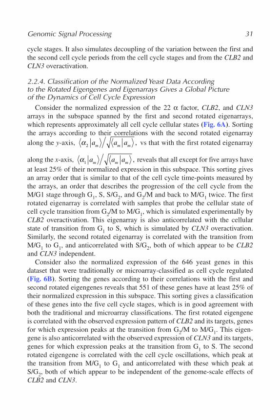
Genomic Signal Processing 31
cycle stages. It also simulates decoupling of the variation between the first andthe second cell cycle periods from the cell cycle stages and from the CLB2 andCLN3 overactivation.
2.2.4. Classification of the Normalized Yeast Data According to the Rotated Eigengenes and Eigenarrays Gives a Global Picture of the Dynamics of Cell Cycle Expression
Consider the normalized expression of the 22 α factor, CLB2, and CLN3arrays in the subspace spanned by the first and second rotated eigenarrays,which represents approximately all cell cycle cellular states (Fig. 6A). Sortingthe arrays according to their correlations with the second rotated eigenarrayalong the y-axis, vs that with the first rotated eigenarray
along the x-axis, reveals that all except for five arrays haveat least 25% of their normalized expression in this subspace. This sorting givesan array order that is similar to that of the cell cycle time-points measured bythe arrays, an order that describes the progression of the cell cycle from theM/G1 stage through G1, S, S/G2, and G2/M and back to M/G1 twice. The firstrotated eigenarray is correlated with samples that probe the cellular state ofcell cycle transition from G2/M to M/G1, which is simulated experimentally byCLB2 overactivation. This eigenarray is also anticorrelated with the cellularstate of transition from G1 to S, which is simulated by CLN3 overactivation.Similarly, the second rotated eigenarray is correlated with the transition fromM/G1 to G1, and anticorrelated with S/G2, both of which appear to be CLB2and CLN3 independent.
Consider also the normalized expression of the 646 yeast genes in thisdataset that were traditionally or microarray-classified as cell cycle regulated(Fig. 6B). Sorting the genes according to their correlations with the first andsecond rotated eigengenes reveals that 551 of these genes have at least 25% oftheir normalized expression in this subspace. This sorting gives a classificationof these genes into the five cell cycle stages, which is in good agreement withboth the traditional and microarray classifications. The first rotated eigengeneis correlated with the observed expression pattern of CLB2 and its targets, genesfor which expression peaks at the transition from G2/M to M/G1. This eigen-gene is also anticorrelated with the observed expression of CLN3 and its targets,genes for which expression peaks at the transition from G1 to S. The secondrotated eigengene is correlated with the cell cycle oscillations, which peak atthe transition from M/G1 to G1 and anticorrelated with these which peak atS/G2, both of which appear to be independent of the genome-scale effects ofCLB2 and CLN3.
α1 a a am m m ,
α2 a a am m m ,
02_Alter 6/3/07 10:35 AM Page 31

32 Alter
Classification of the yeast arrays and genes in the subspaces spanned bythese two rotated eigenarrays and corresponding eigengenes gives a picture thatresembles the traditional understanding of yeast cell cycle regulation (32):G1 cyclins, such as CLN3, and G2/M cyclins, such as CLB2, drive the cell cyclepast either one of two antipodal checkpoints, from G1 to S and from G2/M toM/G1, respectively (Fig. 6C).
2.3. SVD Model for Genome-Wide RNA Expression During the Cell Cycle Parallels the Analog Harmonic Oscillator
With all 4579 genes sorted, the normalized cell cycle expression approxi-mately fits a traveling wave, varying sinusoidally across both genes and arrays(Fig. 7A). The normalized expression in the CLB2- and CLN3-overactive arraysapproximately fits standing waves, constant across the arrays and varying sinu-soidally across the genes only, which appear anticorrelated and correlated withthe first eigenarray, respectively. The gene variations of the first and secondrotated eigenarrays fit normalized cosine and sine functions of one periodacross all genes, respectively (Fig. 7B,C). In this picture, all 4579 genes, aboutthree-quarters of the yeast genome, appear to exhibit periodic expression dur-ing the cell cycle. This picture is in agreement with the recent observation byKlevecz et al. (33; see also Li and Klevecz, ref. 34) that DNA replication isgated by genome-wide RNA expression oscillations, which suggests that thewhole yeast genome might exhibit expression oscillations during the cell cycle.
Fig. 6. The normalized yeast RNA expression in the SVD cell cycle subspace. (A)Correlations of the normalized expression of each of the 22 arrays with the first and sec-ond rotated eigenarrays along the x- and y-axes, color-coded according to the classifi-cation of the arrays into the five cell cycle stages: M/G1 (yellow), G1 (green), S (blue),S/G2 (red), and G2/M (orange). The dashed unit and half-unit circles out-line 100% and25% of overall normalized array expression in this subspace. (B) Correlations of thenormalized expression of each of the 646 cell cycle-regulated genes with the first andsecond rotated eigengenes along the x- and y-axes, color-coded according to either thetraditional or microarray classifications. (C) The SVD picture of the yeast cell cycle.
02_Alter 6/3/07 10:35 AM Page 32

Genomic Signal Processing 33
It is still an open question whether all yeast genes or only a subset of the yeastgenes, and if so, which subset, show periodic expression during the cell cycle.
This SVD model describes, to first order, the RNA expression of most of theyeast genome during the cell cycle program as being driven by the activities oftwo periodically oscillating cellular elements or modules, which are orthogonal,i.e., π/2 out of phase relative to one another. The underlying genetic network orcircuit suggested by this model might be parallel in its design to the analog har-monic oscillator. This well-known oscillator design principle is at the founda-tions of numerous physical oscillators, including (1) the mechanical pendulum,the position and momentum of which oscillate periodically in time with a phasedifference of π/2; (2) the electronic LC circuit, where the charge on the capaci-tor and the current flowing through the inductor oscillate periodically in timewith a phase difference of π/2; and (3) the chemical Lotka-Volterra irreversibleautocatalytic reaction model, where, far from thermodynamic equilibirum, the
Fig. 7. The sorted and normalized yeast cell cycle RNA expression dataset and itssorted and rotated eigenarrays. (A) Raster display of the normalized expression of the4579 genes across the 22 arrays. The genes are sorted by relative correlation of theirnormalized expression patterns with the first and second rotated eigengenes. This rasterdisplay shows a traveling wave of expression during the cell cycle and standing wavesof expression in the CLB2- and CLN3-overactive arrays. (B) Raster display of therotated eigenarrays, where the expression patterns of the first and second eigenarrays,which correspond to the first and second eigengenes, respectively, display the sorting.(C) Line-joined graphs of the first (red) and second (green) rotated eigenarrays, fit nor-malized cosine and sine functions of one period across all genes.
02_Alter 6/3/07 10:35 AM Page 33
34 Alter
concentrations of two intermediate reactants exhibit periodic oscillations intime that are π/2 out of phase relative to one another (35–37).
3. GSVD for Comparative Modeling of DNA Microarray DatasetsThis section reviews the GSVD comparative model for DNA microarray
datasets (19). GSVD is a comparative BSS algorithm that simultaneouslydecomposes two measured signals, i.e., the measured gene and array patternsof, e.g., RNA expression in two organisms, into mathematically decoupled“genelets” and two sets of “arraylets.” The correspondence between these mathe-matical patterns uncovered in the measured signals and the similar and dissimilaramong the biological programs that compose each of the two signals is illus-trated with a comparative analysis of genome-scale RNA expression data fromyeast (6) and human (7) during their cell cycle programs. One common pictureof RNA expression oscillations during both the yeast and human cell cyclesemerges from this analysis, which suggests an underlying eukaryotic geneticnetwork or circuit that parallels the digital ring oscillator.
Comparisons of DNA sequence of entire genomes already give new insightsinto evolutionary, biochemical, and genetic pathways. Recent studies showedthat the addition of RNA expression data to DNA sequence comparisonsimproves functional gene annotation and might expand the understanding ofhow gene expression and diversity evolved. For example, Stuart et al. (38) andindependently also Bergmann, Ihmels, and Barkai (39) identified pairs of genes forwhich RNA coexpression is conserved, in addition to their DNA sequences, acrossseveral organisms. The evolutionary conservation of the coexpression of thesegene pairs confers a selective advantage to the functional relations of these genes.The GSVD comparative model is not limited to genes of conserved DNAsequences, and as such it elucidates universality as well as specialization of molec-ular biological mechanisms that are truly on genomic scales. For example, theGSVD comparative model might be used to identify genes of common functionacross different organisms independently of the DNA sequence similarity amongthese genes, and therefore also to study nonorthologous gene displacement (40).
3.1. Mathematical Framework of GSVD
Let the matrix ê1 of size N1-genes × M1-arrays tabulate the genome-scale sig-nal, e.g., RNA expression levels, measured in a set of M1 samples using M1 DNAmicroarrays. As before, the mth column vector in the matrix ê1, |a1,m⟩, lists theexpression signal measured in the mth sample by the mth array across all N1 genessimultaneously. The nth row vector in the matrix ê1, ⟨g1,n|, lists the signal meas-ured for the nth gene across the different arrays, which correspond to the differentsamples. Let the matrix ê2 of size N2-genes × M2-arrays tabulate the genome-scale signal, e.g., RNA expression levels, measured in a set of M2 samples underM2 experimental conditions that correspond one-to-one to the M1 conditions
02_Alter 6/3/07 10:35 AM Page 34
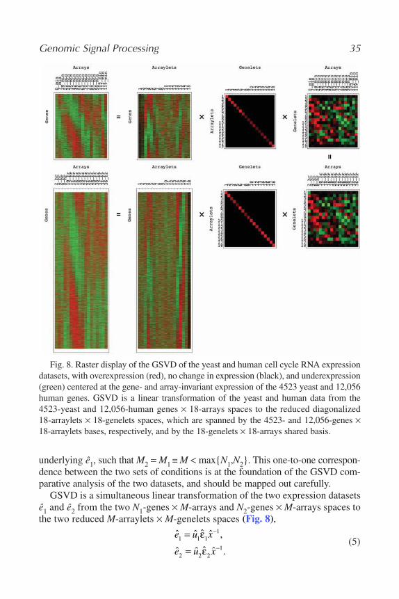
Genomic Signal Processing 35
underlying ê1, such that M2 = M1 ≡ M < max{N1,N2}. This one-to-one correspon-dence between the two sets of conditions is at the foundation of the GSVD com-parative analysis of the two datasets, and should be mapped out carefully.
GSVD is a simultaneous linear transformation of the two expression datasetsê1 and ê2 from the two N1-genes × M-arrays and N2-genes × M-arrays spaces tothe two reduced M-arraylets × M-genelets spaces (Fig. 8),
(5)ˆ ˆ ˆ ˆ ,
ˆ ˆ ˆ ˆ .
e u x
e u x1 1 1
1
2 2 21
=
=
−
−
ε
ε
Fig. 8. Raster display of the GSVD of the yeast and human cell cycle RNA expressiondatasets, with overexpression (red), no change in expression (black), and underexpression(green) centered at the gene- and array-invariant expression of the 4523 yeast and 12,056human genes. GSVD is a linear transformation of the yeast and human data from the4523-yeast and 12,056-human genes × 18-arrays spaces to the reduced diagonalized18-arraylets × 18-genelets spaces, which are spanned by the 4523- and 12,056-genes ×18-arraylets bases, respectively, and by the 18-genelets × 18-arrays shared basis.
02_Alter 6/3/07 10:35 AM Page 35
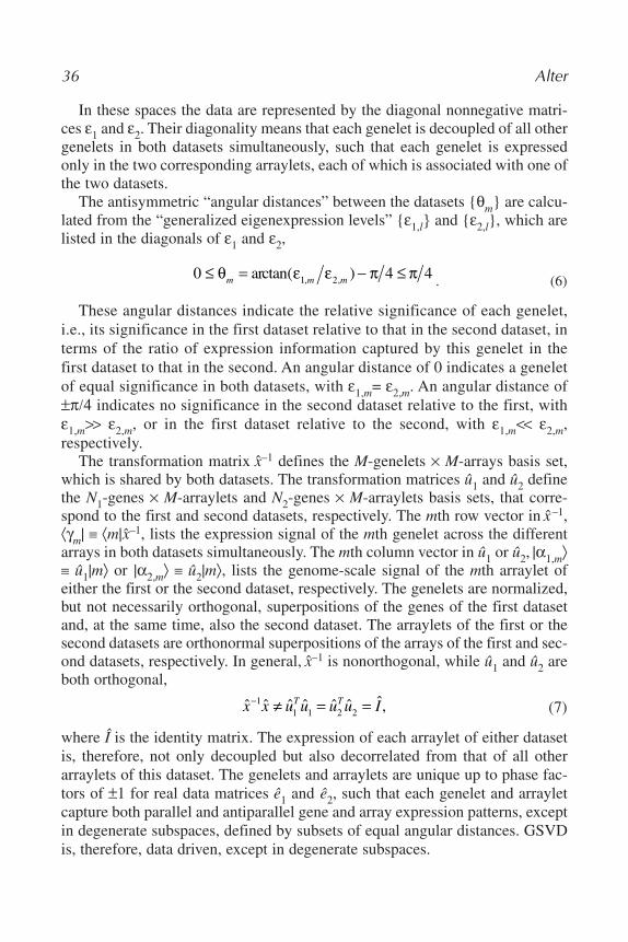
36 Alter
In these spaces the data are represented by the diagonal nonnegative matri-ces ε1 and ε2. Their diagonality means that each genelet is decoupled of all othergenelets in both datasets simultaneously, such that each genelet is expressedonly in the two corresponding arraylets, each of which is associated with one ofthe two datasets.
The antisymmetric “angular distances” between the datasets {θm} are calcu-lated from the “generalized eigenexpression levels” {ε1,l} and {ε2,l}, which arelisted in the diagonals of ε1 and ε2,
. (6)
These angular distances indicate the relative significance of each genelet,i.e., its significance in the first dataset relative to that in the second dataset, interms of the ratio of expression information captured by this genelet in thefirst dataset to that in the second. An angular distance of 0 indicates a geneletof equal significance in both datasets, with ε1,m= ε2,m. An angular distance of±π/4 indicates no significance in the second dataset relative to the first, withε1,m>> ε2,m, or in the first dataset relative to the second, with ε1,m<< ε2,m,respectively.
The transformation matrix x–1 defines the M-genelets × M-arrays basis set,which is shared by both datasets. The transformation matrices û1 and û2 definethe N1-genes × M-arraylets and N2-genes × M-arraylets basis sets, that corre-spond to the first and second datasets, respectively. The mth row vector in x–1,⟨γm| ≡ ⟨m|x–1, lists the expression signal of the mth genelet across the differentarrays in both datasets simultaneously. The mth column vector in û1 or û2, |α1,m⟩≡ û1|m⟩ or |α2,m⟩ ≡ û2|m⟩, lists the genome-scale signal of the mth arraylet ofeither the first or the second dataset, respectively. The genelets are normalized,but not necessarily orthogonal, superpositions of the genes of the first datasetand, at the same time, also the second dataset. The arraylets of the first or thesecond datasets are orthonormal superpositions of the arrays of the first and sec-ond datasets, respectively. In general, x–1 is nonorthogonal, while û1 and û2 areboth orthogonal,
(7)
where Î is the identity matrix. The expression of each arraylet of either datasetis, therefore, not only decoupled but also decorrelated from that of all otherarraylets of this dataset. The genelets and arraylets are unique up to phase fac-tors of ±1 for real data matrices ê1 and ê2, such that each genelet and arrayletcapture both parallel and antiparallel gene and array expression patterns, exceptin degenerate subspaces, defined by subsets of equal angular distances. GSVDis, therefore, data driven, except in degenerate subspaces.
ˆ ˆ ˆ ˆ ˆ ˆ ˆ,x x u u u u IT T− = =11 1 2 2≠
0 4 41 2≤ = − ≤θ ε ε π πm m marctan( ), ,
02_Alter 6/3/07 10:35 AM Page 36
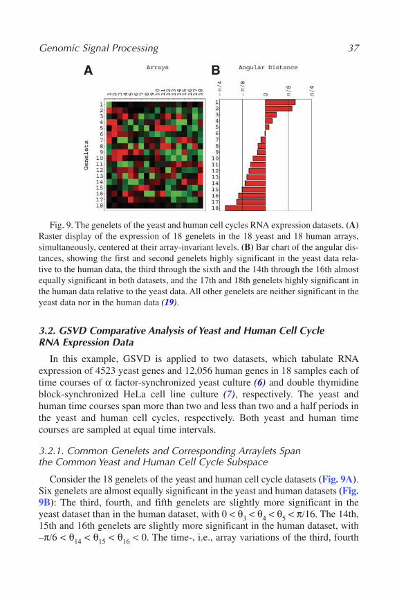
Genomic Signal Processing 37
3.2. GSVD Comparative Analysis of Yeast and Human Cell Cycle RNA Expression Data
In this example, GSVD is applied to two datasets, which tabulate RNAexpression of 4523 yeast genes and 12,056 human genes in 18 samples each oftime courses of α factor-synchronized yeast culture (6) and double thymidineblock-synchronized HeLa cell line culture (7), respectively. The yeast andhuman time courses span more than two and less than two and a half periods inthe yeast and human cell cycles, respectively. Both yeast and human timecourses are sampled at equal time intervals.
3.2.1. Common Genelets and Corresponding Arraylets Span the Common Yeast and Human Cell Cycle Subspace
Consider the 18 genelets of the yeast and human cell cycle datasets (Fig. 9A).Six genelets are almost equally significant in the yeast and human datasets (Fig.9B): The third, fourth, and fifth genelets are slightly more significant in theyeast dataset than in the human dataset, with 0 < θ3 < θ4 < θ5 < π/16. The 14th,15th and 16th genelets are slightly more significant in the human dataset, with–π/6 < θ14 < θ15 < θ16 < 0. The time-, i.e., array variations of the third, fourth
Fig. 9. The genelets of the yeast and human cell cycles RNA expression datasets. (A)Raster display of the expression of 18 genelets in the 18 yeast and 18 human arrays,simultaneously, centered at their array-invariant levels. (B) Bar chart of the angular dis-tances, showing the first and second genelets highly significant in the yeast data rela-tive to the human data, the third through the sixth and the 14th through the 16th almostequally significant in both datasets, and the 17th and 18th genelets highly significant inthe human data relative to the yeast data. All other genelets are neither significant in theyeast data nor in the human data (19).
02_Alter 6/3/07 10:35 AM Page 37

38 Alter
and fifth genelets fit normalized cosine functions of two periods and initialphases of π/3, 0 and −π/3, respectively, superimposed on time-invariant expres-sion (Fig. 10A). The 14th, 15th and 16th genelets fit normalized cosines of twoand a half periods and initial phases of −π/3, π/3, and 0, respectively (Fig. 10B).The time variations of the six common genelets suggest that they span the cellcycle subspace, which is common to both the yeast and human genomes, and ismanifested in both datasets.
The corresponding six yeast and six human arraylets are associated by anno-tation with the corresponding yeast and human cell cycle cellular states, follow-ing the p-values for the distribution of the 604 yeast genes and 750 humangenes, that were microarray-classified, and the 77 yeast genes and 73 humangenes that were traditionally classified as cell cycle regulated, among all 4523yeast and 12,056 human genes and among each of the subsets of 100 genes withlargest and smallest levels of expression in each of the arraylets. The associa-tions of the yeast and human arraylets are in agreement with the expression pat-terns of the genelets, taking into account the initial synchronization of the yeastculture in the cell cycle stage M/G1 and that of the human culture in S. Forexample, the expression pattern of the fourth genelet is of 0 initial phase, sug-gesting that this genelet is correlated with the yeast cell cycle expression oscil-lations that peak at the stage M/G1 and the human cell cycle expression
Fig. 10. Line-joined graphs of the expression levels of the significant genelets. (A)The third (red), fourth (blue), and fifth (green) genelets, which are associated with thecommon yeast and human cell cycle gene expression oscillations, fit dashed graphs ofnormalized cosines of two periods and initial phases of π/3 (red), 0 (blue) and –π/3(green), respectively. (B) The 14th (red), 15th (blue) and 16th (green) genelets, whichare also associated with cell cycle gene expression oscillations, fit dashed graphs ofnormalized cosines of two and a half periods and initial phases of –π/3 (red), π/3 (blue)and 0 (green), respectively. (C) The first (red) and second (blue) genelets are associatedwith the exclusive yeast response to the pheromone α factor, the 17th (orange) and 18th(green) are associated with the exclusive human stress response, and the sixth (violet)is associated with both the yeast and human transitions from synchronization responsesinto the cell cycle.
02_Alter 6/3/07 10:35 AM Page 38
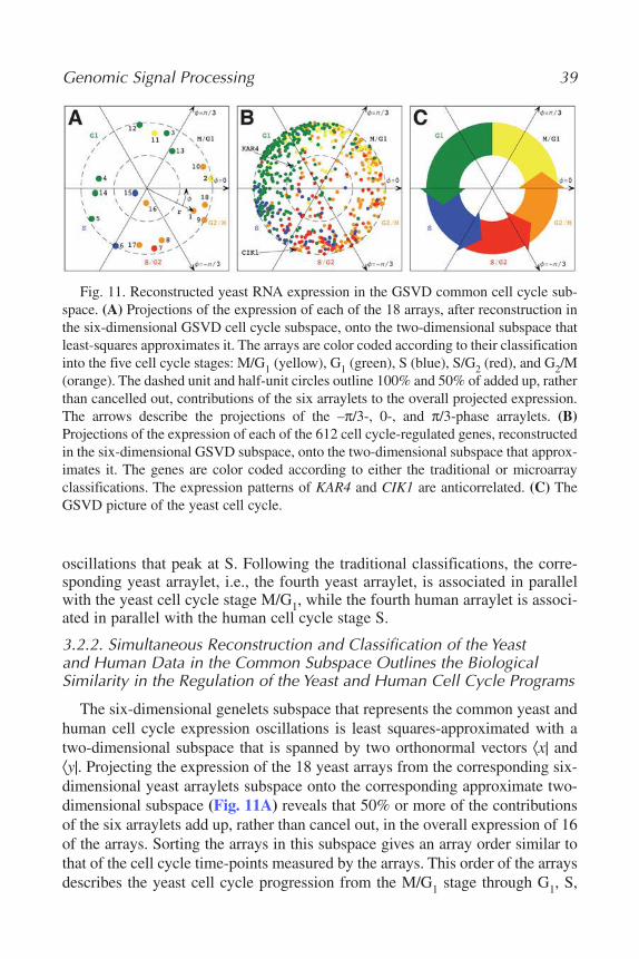
Genomic Signal Processing 39
oscillations that peak at S. Following the traditional classifications, the corre-sponding yeast arraylet, i.e., the fourth yeast arraylet, is associated in parallelwith the yeast cell cycle stage M/G1, while the fourth human arraylet is associ-ated in parallel with the human cell cycle stage S.
3.2.2. Simultaneous Reconstruction and Classification of the Yeast and Human Data in the Common Subspace Outlines the BiologicalSimilarity in the Regulation of the Yeast and Human Cell Cycle Programs
The six-dimensional genelets subspace that represents the common yeast andhuman cell cycle expression oscillations is least squares-approximated with atwo-dimensional subspace that is spanned by two orthonormal vectors ⟨x| and⟨y|. Projecting the expression of the 18 yeast arrays from the corresponding six-dimensional yeast arraylets subspace onto the corresponding approximate two-dimensional subspace (Fig. 11A) reveals that 50% or more of the contributionsof the six arraylets add up, rather than cancel out, in the overall expression of 16of the arrays. Sorting the arrays in this subspace gives an array order similar tothat of the cell cycle time-points measured by the arrays. This order of the arraysdescribes the yeast cell cycle progression from the M/G1 stage through G1, S,
Fig. 11. Reconstructed yeast RNA expression in the GSVD common cell cycle sub-space. (A) Projections of the expression of each of the 18 arrays, after reconstruction inthe six-dimensional GSVD cell cycle subspace, onto the two-dimensional subspace thatleast-squares approximates it. The arrays are color coded according to their classificationinto the five cell cycle stages: M/G1 (yellow), G1 (green), S (blue), S/G2 (red), and G2/M(orange). The dashed unit and half-unit circles outline 100% and 50% of added up, ratherthan cancelled out, contributions of the six arraylets to the overall projected expression.The arrows describe the projections of the –π/3-, 0-, and π/3-phase arraylets. (B)Projections of the expression of each of the 612 cell cycle-regulated genes, reconstructedin the six-dimensional GSVD subspace, onto the two-dimensional subspace that approx-imates it. The genes are color coded according to either the traditional or microarrayclassifications. The expression patterns of KAR4 and CIK1 are anticorrelated. (C) TheGSVD picture of the yeast cell cycle.
02_Alter 6/3/07 10:35 AM Page 39
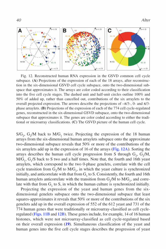
40 Alter
S/G2, G2/M back to M/G1 twice. Projecting the expression of the 18 humanarrays from the six-dimensional human arraylets subspace onto the approximatetwo-dimensional subspace reveals that 50% or more of the contributions of thesix arraylets add up in the expression of 16 of the arrays (Fig. 12A). Sorting thearrays describes the human cell cycle progression from S through G2, G2/M,M/G1, G1/S back to S two and a half times. Note that, the fourth and 16th yeastarraylets, which correspond to the two 0-phase genelets, correlate with the cellcycle transition from G2/M to M/G1, in which the yeast culture is synchronizedinitially, and anticorrelate with that from G1 to S. Consistently, the fourth and 16thhuman arraylets anticorrelate with the transition from G2/M to M/G1, and corre-late with that from G1 to S, in which the human culture is synchronized initially.
Projecting the expression of the yeast and human genes from the six-dimensional genelets subspace onto the two-dimensional subspace that leastsquares-approximates it reveals that 50% or more of the contributions of the sixgenelets add up in the overall expression of 552 of the 612 yeast and 731 of the774 human genes that were traditionally or microarray-classified as cell cycle-regulated (Figs. 11B and 12B). These genes include, for example, 14 of 16 humanhistones, which were not microarray-classified as cell cycle-regulated basedon their overall expression (19). Simultaneous classification of the yeast andhuman genes into the five cell cycle stages describes the progression of yeast
Fig. 12. Reconstructed human RNA expression in the GSVD common cell cyclesubspace. (A) Projections of the expression of each of the 18 arrays, after reconstruc-tion in the six-dimensional GSVD cell cycle subspace, onto the two-dimensional sub-space that approximates it. The arrays are color coded according to their classificationinto the five cell cycle stages. The dashed unit and half-unit circles outline 100% and50% of added up, rather than cancelled out, contributions of the six arraylets to theoverall projected expression. The arrows describe the projections of –π/3-, 0- and π/3-phase arraylets. (B) Projections of the expression of each of the 774 cell cycle-regulatedgenes, reconstructed in the six-dimensional GSVD subspace, onto the two-dimensionalsubspace that approximates it. The genes are color coded according to either the tradi-tional or microarray classifications. (C) The GSVD picture of the human cell cycle.
02_Alter 6/3/07 10:35 AM Page 40

Genomic Signal Processing 41
and human cell cycles along the yeast and human genes, respectively, and is ingood agreement with both yeast and human microarray and traditional classifi-cations. Note that, the two 0-phase genelets, the fourth and 16th genelets, cor-relate with cell cycle expression oscillations, which peak at the initial stagesof synchronization of both yeast and human genes.
Simultaneous reconstruction and classification of the yeast and human arraysand genes in the subspaces spanned by the six yeast and six human arraylets,and six shared genelets, respectively, gives a picture that resembles the tradi-tional understanding of the biological similarity in the regulation of the yeastand human, and perhaps all eukaryotic, cell cycles (32) of two antipodal check-points, at the transition from G1 to S and at that from G2/M to M/G1, that areregulated independently of other cell cycle events (Figs. 11C and 12C).
3.2.3. Exclusive Genelets and Corresponding Arraylets Span the Exclusive Yeast and Human Synchronization Responses Subspaces
The first and second genelets, which capture most of the expression informa-tion in the yeast dataset, yet very little of the expression information in thehuman dataset, with θ1,θ2 > π/7 (Fig. 9B), describe initial transient increase anddecrease in expression, respectively (Fig. 10C). A theme of yeast response topheromone synchronization emerges from the annotations of the genes withthe largest and smallest levels of expression in the first and second yeastarraylets. The sixth genelet, equally significant in both datasets, with θ ~ 0,describes an initial transient increase in expression superimposed on cosinu-sidial variation. A theme of transition from the response to the pheromone αfactor into cell cycle progression emerges from the annotations of the yeastgenes with the largest and smallest expression levels in the sixth yeast arraylet.These three genelets and corresponding three yeast arraylets are associatedwith the pheromone response program, which is exclusive to the yeastgenome. Classification of the yeast genes and arrays into stages in thepheromone response in the subspaces spanned by these genelets and arraylets,respectively (Fig. 13), is in good agreement with the traditional understandingof this program (41).
The 17th and 18th genelets are insignificant in the yeast dataset relative tothat of the human, with q17,q18 < –p/4. A theme of human synchronizationstress response emerges from the annotations of the genes with the largestand smallest expression levels in the 17th and 18th genelets. Also, from theannotations of the human genes with the largest and smallest expression levelsin the sixth human arraylet emerges a theme of transition from stressresponse into cell cycle progression. These three genelets and correspondingthree human arraylets are associated with this human exclusive stressresponse. Classification of the human genes and arrays into stress response
02_Alter 6/3/07 10:35 AM Page 41

Fig. 13. Reconstructed yeast RNA expression in the GSVD yeast exclusive syn-chronization response subspace. (A) Projections of the expression of each of the 18arrays, reconstructed in the three-dimensional GSVD synchronization response sub-space, onto the two-dimensional subspace that least-squares approximates it. Thearrays are color coded according to their classification into six stages in this responseto synchronization program, which outlines the response to the pheromone α factorand the transition into cell cycle progression: early E1 (red) and E2 (orange), middleM1 (yellow) and M2 (green), and late L1 (blue) and L2 (violet). The dashed unit andhalf-unit circles outline 100% and 50% of added up, rather than cancelled out, contri-butions of the three arraylets to the overall projected expression. The arrows describethe projections of the three arraylets. (B) Projections of the expressions of 172 genes,reconstructed in the three-dimensional GSVD subspace, onto the two-dimensionalsubspace that approximates it. The genes are color coded according to the traditionalunderstanding of the α factor synchronization response program. Genes that peak inE1 are known to be involved in α factor response, mating, adaptation-to-mating sig-nal, and cell cycle arrest; E2 – filamentous and pseudohyphal growths and cell polar-ity; M1 – ATP synthesis; M2 – chromatin modeling; L1 – chromatin binding andarchitecture; and L2 – phosphate and iron transport. The expression patterns of KAR4and CIK1 are correlated.
42 Alter
stages in the subspaces spanned by these genelets and arraylets, respectively(19), is in agreement with the current, somewhat limited, understanding ofthis program (7).
3.2.4. Data Reconstruction and Classification in the Common andExclusive Subspaces Simulate Observation of Differential Expression in the Cell Cycle and Synchronization Response Programs
According to their expression in the yeast exclusive pheromone response sub-space, the RNA expression patterns of the yeast genes KAR4 and CIK1 are cor-related: The expression of both genes peaks early in the time course together
02_Alter 6/3/07 10:35 AM Page 42
with the expression of other genes known to be involved in the response to theα factor (Fig. 13B). In the common cell cycle subspace KAR4 and CIK1 are anti-correlated: KAR4 peaks at the G1 cell cycle stage, whereas CIK1 peaks almosthalf a cell cycle period later (and also earlier) at S/G2 (Fig. 13B). This differencein the relation of the expression patterns of CIK1 and KAR4 in the response topheromone program as compared with that of the cell cycle is in agreement withthe experimental observation of Kurihara et al. (42) that induction of CIK1depends on that of KAR4 during mating, which is mediated by the α factorpheromone, and is independent of KAR4 during the mitotic cell cycle.
In the human exclusive stress response subspace, most human histones reachtheir expression minima early. In the common cell cycle subspace, most his-tones peak early, together with other genes known to peak in the cell cycle stageS. This differential expression of most histones may explain why these histonesdo not appear to be cell cycle regulated based on their overall expression (7):The superposition of the expression of the histones during the cell cycle andthat in response to the synchronization leads to an overall steady-state expres-sion early in the time course (19).
GSVD uncovers the program-dependent variation in the expression patternsof the human histones, as well as the program-dependent variation in the rela-tions between the expression patterns of the yeast genes KAR4 and CIK1.
3.3.1. GSVD Comparative Model for Genome-Scale RNA ExpressionDuring the Yeast and Human Cell Cycles Parallels the Digital Ring Oscillator
With all 4523 yeast and 12,056 human genes sorted according to their phasesin the GSVD common cell cycle subspace, the reconstructed yeast and humanexpressions approximately fit traveling waves of one period cosinusoidal vari-ation across the genes, and of two or two and a half periods across the arrays,respectively (Fig. 14A). The gene variations of the six yeast and six humanarraylets approximately fit one period cosines of π/3, 0, and –π/3 initial phases,such that the initial phase of each arraylet is similar to that of its correspondinggenelet (Fig. 14B,C). In this picture, all 4523 yeast genes, about three-quartersof the yeast genome, as well as all 12,056 human genes, about two-thirds of thehuman genome according to current estimates (35), appear to exhibit periodicexpression during the cell cycle.
This GSVD model describes, to first order, the RNA expression of most ofthe yeast and human genomes during their common cell cycle programs asbeing driven by the activities of three periodically oscillating cellular elementsor modules, which are π/3 out of phase relative to one another. The underlyingeukaryotic genetic network or circuit suggested by this model might be parallelin its design to the digital three-inverter ring oscillator. Elowitz and Leibler (44)
Genomic Signal Processing 43
02_Alter 6/3/07 10:35 AM Page 43

44 Alter
Fig. 14. Yeast and human cell cycles’ RNA expression, reconstructed in the six-dimensional GSVD common subspace, with genes sorted according to their phases inthe two-dimensional subspace that approximates it. (A) Yeast expression of the sorted4523 genes in the 18 arrays, centered at their gene- and array-invariant levels, show-ing a traveling wave of expression. (B) Yeast expression of thesorted 4523 genes
02_Alter 6/3/07 10:35 AM Page 44

Genomic Signal Processing 45
recently demonstrated a synthetic genetic circuit analogous to this digital ringoscillator (see also Fung et al., ref. 45).
4. Pseudoinverse Projection for Integrative Modeling of DNA Microarray Datasets
Integrative analysis of different types of global signals, such as these meas-ured by DNA microarrays from the same organism, promises to reveal globalcausal co-ordination of cellular activities. For example, Bussemaker, Li, andSiggia (46) predicted new regulatory motifs by linear regression of profiles ofgenome-scale RNA expression in yeast vs profiles of the abundance levels, orcounts of DNA oligomer motifs in the promoter regions of the same yeastgenes. Lu, Nakorchevskiy, and Marcotte (47) associated the knockout pheno-type of individual yeast genes with cell cycle arrest by deconvolution of theRNA expression profiles measured in the corresponding yeast mutants into theRNA expression profiles measured during the cell cycle for all yeast genes thatwere microarray-classified as cell cycle regulated.
This section reviews the pseudoinverse projection integrative model for DNAmicroarray datasets and other large-scale molecular biological signals (20,21).Pseudoinverse projection is an integrative BSS algorithm that decomposes themeasured gene patterns of any given “data” signal of, e.g., proteins’ DNA-bindinginto mathematically least squares-optimal pseudoinverse correlations with themeasured gene patterns of a chosen “basis” signal of, e.g., RNA expression, ina different set of samples from the same organism. The measured array patternsof the data signal are least squares-approximated with a decomposition into themeasured array patterns of the basis. The correspondence between these mathe-matical patterns that are uncovered in the measured signals and the independent
Fig. 14. (Continued) in the 18 arraylets, centered at their array-invariant levels.The expression patterns of the third through fifth and 14th through 16th arraylets dis-play the sorting. (C) The third (red), fourth (blue), and fifth (green) yeast arraylets fitone period cosines of π/3 (red), 0 (blue) and –π/3 (green) initial phases. (D) The 14th(red), 15th (blue), and 16th (green) yeast arraylets fit one period cosines of –π/3-(red), π/3- (blue), and 0- (green) phases. (E) Human expression of the sorted 12,056genes in the 18 arrays, centered at their gene- and array-invariant levels, showing atraveling wave of expression. (F) Human expression of the sorted 12,056 genes in the18 arraylets, centered at their array-invariant levels. The expression patterns of thethird through fifth and 14th through 16th arraylets display the sorting. (G) The third(red), fourth (blue), and fifth (green) human arraylets fit one period cosines of π/3-(red), 0- (blue), and –π/3- (green) phases. (H) The 14th (red), 15th (blue) and 16th(green) human arraylets fit one period cosines of –π/3- (red), π/3- (blue) and 0-(green) phases.
02_Alter 6/3/07 10:35 AM Page 45

46 Alter
activities of cellular elements that compose the signals is illustrated with anintegration of yeast genome-scale DNA-binding occupancy of cell cycle tran-scription factors (8) and DNA replication initiation proteins (9) with RNAexpression during the cell cycle, using as basis sets the eigenarrays andarraylets determined by SVD and GSVD, respectively. One consistent pictureemerges that predicts novel correlation between DNA replication initiation andRNA transcription during the yeast cell cycle. This novel correlation, whichmight be due to a previously unknown mechanism of regulation, demonstratesthe power of the SVD, GSVD, and pseudoinverse projection models to predictpreviously unknown biological principles.
4.1. Mathematical Framework of Pseudoinverse Projection
Let the basis matrix b of size N-genomic sites or open reading frames(ORFs) × M-basis profiles tabulate M genome-scale molecular biological pro-files of, e.g., RNA expression, measured from a set of M samples or extractedmathematically from a set of M or more measured samples. As before, the mthcolumn vector in the matrix b, |bm⟩ ≡ b|m⟩, lists the signal measured in the mthsample by the mth array across all N ORFs simultaneously. The nth row vec-tor in the matrix b, ⟨n|b, lists the signal measured in the nth ORF across thedifferent arrays, which correspond to the different samples. Let the datamatrix d of size N-ORFs × L-data samples tabulate L genome-scale molecu-lar biological profiles of, e.g., proteins’ DNA binding, measured for the sameORFs in L samples from the same organism. The lth column vector in thematrix d, |dl⟩ ≡ d|l⟩, lists the signal measured in the lth sample across all NORFs simultaneously.
Moore–Penrose pseudoinverse projection of the data matrix d onto the basismatrix b is a linear transformation of the data d from the N-ORFs × L-datasamples space to the M-basis profiles × L-data samples space (Fig. 15),
(8)
where the matrix b†, that is, the pseudoinverse of b, satisfies
(9)
such that the transformation matrices bb† and b†b are orthogonal projectionmatrices for a real basis matrix b.
ˆ ˆ ˆ ˆ,ˆ ˆ ˆ ˆ ,
( ˆ ˆ ) ˆ ˆ ,
( ˆ
†
† † †
† †
bb b b
b bb b
bb bbT
=
=
=
bb b b bT† †ˆ) ˆ ˆ,=
ˆ ˆ ˆ,ˆ ˆ ˆ,†
d bc
b d c
→
≡
02_Alter 6/3/07 10:35 AM Page 46

Genomic Signal Processing 47
In this space the data matrix d is represented by the pseudoinverse correla-tions matrix c. The vector in the mth row of the matrix c, ⟨cm| ≡ ⟨m|c, lists thepseudoinverse correlations of the L data profiles with the mth basis profile. Thepseudoinverse correlations matrix c is unique, i.e., data driven.
4.2. Pseudoinverse Projection Integrative Analysis of Yeast Cell CycleRNA Expression and Proteins’ DNA-Binding Data
In this example, a data matrix that tabulates DNA-binding occupancy levelsof nine yeast cell cycle transcription factors (8) and four yeast replication initi-ation proteins (9) across 2928 yeast ORFs is pseudoinverse projected onto (1)
Fig. 15. Raster display of the pseudoinverse projection of the yeast cell cycletranscription factors and replication initiation proteins’ DNA-binding data onto theSVD and GSVD cell cycle RNA expression bases, with overexpression (red), nochange in expression (black) and underexpression (green) centered at ORF- andsample-invariant expression, and with the ORFs sorted according to their SVD andGSVD phases, respectively. Pseudoinverse projection is a linear transformation ofthe proteins’ binding data from the 2227 ORFs × 13-data samples space to the nineeigenarrays of the SVD basis × 13-data samples space (upper), and also of the pro-teins’ binding data from the 2139 ORFs × 13-data samples space to the six arrayletsof the GSVD basis × 13-data samples space (lower).
02_Alter 6/3/07 10:35 AM Page 47
48 Alter
the SVD cell cycle RNA expression basis matrix, which tabulates the expres-sion of the nine most significant eigenarrays of the α factor, CLB2, and CLN3dataset, including the two eigenarrays that span the SVD cell cycle subspace,across 4579 ORFs, 2227 of which are present in the data matrix; and (2) theGSVD cell cycle RNA expression basis matrix, which tabulates the expressionof the six arraylets that span the GSVD cell cycle subspace across 4523 ORFs,2139 of which are present in the data matrix.
4.2.1. Pseudoinverse Correlations Uncovered in the Data Correspond to Reported Functions of Transcription Factors
The nine transcription factors are ordered, following Simon et al. (8),from these that have been reported to function in the cell cycle stage G1,through these that have been reported to function in S, S/G2, G2/M, andM/G1: Mbp1, Swi4, Swi6, Fkh1, Fkh2, Ndd1, Mcm1, Ace2, and Swi5. Withthis order, the SVD- and GSVD-pseudoinverse correlations approximatelyfit cosine functions of one period and of varying initial phases across thenine transcription factors’ samples and are approximately invariant acrossthe four samples of the replication initiation proteins, Mcm3, Mcm4, Mcm7,and Orc1 (Fig. 16). Transcription factors that have been reported to functionin antipodal cell cycle stages, such as Mbp1, Swi4, and Swi6 that are knownto function in G1 and Mcm1 that is known to function in G2/M, consistentlyexhibit anticorrelated levels of DNA-binding in all patterns of pseudoinversecorrelations. Each pattern of pseudoinverse correlations ⟨cm| represents theactivity of the transcripition factors during the cell cycle stage that the cor-responding basis profile ⟨bm| correlates with. For example, the first SVDbasis profile, i.e., the first eigenarray, correlates with RNA expression oscil-lations at the transition from the cell cycle stage G2/M to M/G1 and anticor-relates with oscillations at the transition from G1 to S (Fig. 6C).Correspondingly, the first pattern of SVD-pseudoinverse correlationsdescribes enhanced activity of the transcription factor Mcm1 and reducedactivity of Mbp1, Swi4, and Swi6 (Fig. 16B).
4.2.2. Pseudoinverse Reconstruction of the Data in the Basis SimulatesExperimental Observation of Only the Cellular States Manifest in the Data that Correspond to Those in the Basis
The proteins’ DNA-binding data is SVD- and independently also GSVD-reconstructed using pseudoinverse projections in the intersections of the SVD andGSVD bases matrices with the data matrix (Fig. 17). With the 2227 and 2139ORFs sorted according to their SVD and GSVD cell cycle phases, respectively,
02_Alter 6/3/07 10:35 AM Page 48

Genomic Signal Processing 49
the variations of the SVD- and GSVD-reconstructed binding profiles across theORFs approximately fit cosine functions of one period and of varying initialphases.
The SVD- and GSVD-reconstructed transcription factors’ data approxi-mately fit traveling waves, cosinusoidally varying across the ORFs as well asthe nine samples. Simon et al. (8) observed a similar traveling wave in the bind-ing data from the nine transcription factors, ordered as in Subheading 4.2.1.above, across only 213 ORFs. These traveling waves are in agreement with cur-rent understanding of the progression of cell cycle transcription along the genesand in time as it is regulated by DNA binding of the transcription factors at thepromoter regions of the transcribed genes. Pseudoinverse reconstruction of thedata in both the SVD and GSVD bases, therefore, simulates experimentalobservation of only the proteins’ DNA-binding cellular states that correspond tothose of RNA expression during the cell cycle.
Fig. 16. Pseudoinverse correlations of the proteins’ DNA-binding data with the SVDand GSVD cell cycle RNA expression. (A) Raster display of the correlations with thenine eigenarrays that span the SVD basis. (B) Line-joined graphs of the correlationswith the first (red) and second (blue) most significant eigenarrays that span the SVDsubspace. (C) Raster display of the correlations with the six arraylets that span theGSVD basis and the GSVD subspace. (D) Line-joined graphs of the correlations withthird (red), fourth (blue), and fifth (green) arraylets, and (E) the 14th (red), 15th (blue),and 16th (green) arraylets.
02_Alter 6/3/07 10:35 AM Page 49
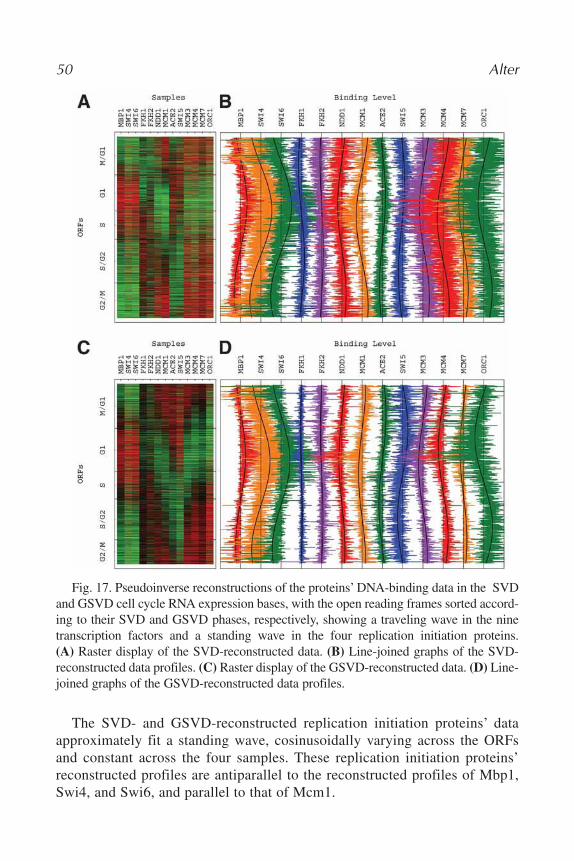
50 Alter
The SVD- and GSVD-reconstructed replication initiation proteins’ dataapproximately fit a standing wave, cosinusoidally varying across the ORFsand constant across the four samples. These replication initiation proteins’reconstructed profiles are antiparallel to the reconstructed profiles of Mbp1,Swi4, and Swi6, and parallel to that of Mcm1.
Fig. 17. Pseudoinverse reconstructions of the proteins’ DNA-binding data in the SVDand GSVD cell cycle RNA expression bases, with the open reading frames sorted accord-ing to their SVD and GSVD phases, respectively, showing a traveling wave in the ninetranscription factors and a standing wave in the four replication initiation proteins. (A) Raster display of the SVD-reconstructed data. (B) Line-joined graphs of the SVD-reconstructed data profiles. (C) Raster display of the GSVD-reconstructed data. (D) Line-joined graphs of the GSVD-reconstructed data profiles.
02_Alter 6/3/07 10:35 AM Page 50

Genomic Signal Processing 51
4.2.3. Classification of the Basis-Reconstructed Data Samples Maps the Cellular States of the Data Onto Those of the Basis and Gives a Global Picture of Possible Causal Coordination of These States
Projected from the SVD basis, that is spanned by nine eigenarrays, onto theSVD cell cycle subspace, that is spanned by the two most significant of theseeigenarrays, all SVD-reconstructed samples have at least 25% of their bindingprofiles in this subspace, except for Fkh2 (Fig. 18A). Projected from the six-dimensional GSVD cell cycle subspace, that is spanned by six arraylets, ontothe two-dimensional subspace that approximates it, 50% or more of the contri-butions of the six arraylets to each GSVD-reconstructed sample add up, ratherthan cancel out (Fig. 18B).
Sorting the samples according to their SVD or GSVD phases gives an arrayorder that is similar to that of Simon et al. (8), and describes the yeast cell cycleprogression from the cellular state of Mbp1’s binding through that of Swi5’s.The SVD and GSVD mappings of the transcription factors’ binding profiles
Fig. 18. Reconstructed yeast proteins’ DNA-binding data in the RNA expressionbases. (A) Correlations of the reconstructed binding of each of the 13 proteins with thefirst and second rotated eigenarrays along the x- and y-axes. The transcription factorsare color coded according to their classification into the five cell cycle stages: M/G1(yellow), G1 (green), S (blue), S/G2 (red), and G2/M (orange). The replication initiationproteins are colored violet. The dashed unit and half-unit circles outline 100% and 25%of overall normalized array expression in this subspace. (B) Projections of the bindingof each of the nine transcription factors and four replication initiation proteins, afterreconstruction in the six-dimensional GSVD cell cycle subspace, onto the two-dimen-sional subspace that least-squares approximates it. The dashed unit and half-unit cir-cles outline 100% and 50% of added up, rather than cancelled out, contributions of thesix arraylets to the overall projected reconstructed binding. The arrows describe the pro-jections of the –π/3-, 0-, and π/3-phase arraylets.
02_Alter 6/3/07 10:35 AM Page 51
52 Alter
onto the expression subspaces are also in agreement with the current under-standing of the cell cycle program. Mapping the binding of Mbp1, Swi4, andSwi6 onto the cell cycle expression stage G1 corresponds to the biological coor-dination between the binding of these factors to the promoter regions of ORFsand the subsequent peak in transcription of these ORFs during G1. The mappingof Mbp1, Swi4, and Swi6 onto G1, which is antipodal to G2/M, also corre-sponds to their binding to promoter regions of ORFs that exhibit transcriptionminima or shutdown during G2/M, and to their minimal or lack of binding atpromoter regions of ORFs which transcription peaks in G2/M. Similarly, themapping of Mcm1 onto G2/M corresponds to its binding to the promoterregions of ORFs that are subsequently transcribed during the transition fromG2/M to M/G1. The binding profiles of the replication initiation proteins areSVD- and GSVD-mapped onto the cell cycle stage that is antipodal to G1.These SVD and GSVD mappings are consistent with the reconstructed profilesof Mcm3, Mcm4, Mcm7, and Orc1 being antiparallel to those of Mbp1, Swi4,and Swi6 and parallel to that of Mcm1.
The parallel and antiparallel associations by annotation of the proteins’DNA-binding profiles with the cellular states of RNA expression during the cellcycle are also consistent with the SVD and GSVD mappings. These associa-tions follow the p-values for the distribution of the 400 and 377 ORFs that weremicroarray-classified and the 58 and 60 ORFs that were traditionally classifiedas cell cycle regulated among all 2227 and 2139 ORFs that are mapped onto theSVD and GSVD subspaces, respectively, and among each of the subsets of 200ORFs with largest and smallest levels of binding occupancy in each of the pro-files. Again, the binding profiles of all four DNA replication initiation proteins,Mcm3, Mcm4, Mcm7, and Orc1 are anticorrelated with RNA expression in thecell cycle stage G1, together with the profile of the transcription factor Mcm1,whereas the profiles of the transcription factors Mbp1, Swi4, and Swi6 that areknown to drive the cell cycle stage G1, are correlated with RNA expression inthis stage (20,21).
Thus, DNA-binding of Mcm3, Mcm4, Mcm7, and Orc1 adjacent to ORFs ispseudoinverse-correlated with minima or even shutdown of the transcription ofthese ORFs during the cell cycle stage G1. This novel correlation suggests a pre-viously unknown genome-scale coordination between DNA replication initia-tion and RNA transcription during the cell cycle in yeast.
The correlation between Mcm3, Mcm4, Mcm7, and Orc1 and the transcrip-tion factor Mcm1 suggests a genome-scale, or maybe even a genome-widecoordination in the activities of the DNA replication initiation proteins and Mcm1.One possible explanation of this correlation may be provided by the recent sugges-tion by Chang et al. (48; see also Donato, Chang and Tye, ref. 49) that Mcm1binds origins of replication, and thus functions as a replication initiation protein
02_Alter 6/3/07 10:35 AM Page 52
in addition to its function as a transcription factor. However, this correlationdoes not necessarily mean that Mcm1 colocalizes with origins. It is the ten-dency of ORFs adjacent to Mcm1’s binding sites to exhibit transcription min-ima during the cell cycle stage G1, which correlates with a similar tendency ofthose ORFs that are adjacent to binding sites of the replication initiation proteins.
4.3. Pseudoinverse Projection Integrative Model for Genome-Scale RNATranscription and DNA-Binding of Cell Cycle Transcription Factors and Replication Initiation Proteins in Yeast
One consistent picture emerges upon integrating the genome-scale proteins’DNA-binding data with the SVD and GSVD cell cycle RNA expression bases,which is in agreement with the current understanding of the yeast cell cycle pro-gram (50–53), and is supported by recent experimental results (49). This picturecorrelates for the first time the binding of replication initiation proteins with min-ima or shutdown of the transcription of adjacent ORFs during the cell cycle stageG1, under the assumption that the measured cell cycle RNA expression levels areapproximately proportional to cell cycle RNA transcription activity. It was shownby Diffley et al. (50) that replication initiation requires binding of Mcm3, Mcm4,Mcm7, and Orc1 at origins of replication across the yeast genome during G1 (seealso ref. 51). And, it was shown by Micklem et al. (52) that these replication ini-tiation proteins are involved with transcriptional silencing at the yeast mating loci(see also ref. 53). Either one of at least two mechanisms of regulation may beunderlying this novel genome-scale correlation between DNA replication initia-tion and RNA transcription during the yeast cell cycle: the transcription of genesmay reduce the binding efficiency of adjacent origins. Or, the binding of replica-tion initiation proteins to origins of replication may repress, or even shut down,the transcription of adjacent genes.
This is the first time that a data-driven mathematical model, where the math-ematical variables and operations represent biological or experimental reality,has been used to predict a biological principle that is truly on a genome scale.The ORFs in either one of the basis or data matrices were selected based on dataquality alone, and were not limited to ORFs that are traditionally or microarray-classified as cell cycle regulated, suggesting that the RNA transcription signa-tures of yeast cell cycle cellular states may span the whole yeast genome.
5. Are Genetic Networks Linear and Orthogonal?The SVD model, the GSVD comparative model, and the pseudoinverse pro-
jection integrative model are all mathematically linear and orthogonal. Thesemodels formulate genome-scale molecular biological signals as linear superpo-sitions of mathematical patterns, which correlate with activities of cellular ele-ments, such as regulators or transcription factors, that drive the measured signal
Genomic Signal Processing 53
02_Alter 6/3/07 10:35 AM Page 53

54 Alter
and cellular states where these elements are active. These models associate theindependent cellular states with orthogonal, i.e., decorrelated, mathematicalprofiles suggesting that the overlap or crosstalk between the genome-scaleeffects of the corresponding cellular elements or modules is negligible.
Recently, Ihmels, Levy, and Barkai (54) found evidence for linearity as wellas orthogonality in the metabolic network in yeast. Integrating genome-scaleRNA expression data with the structural description of this network, theyshowed that at the network’s branchpoints, only distinct branches are coex-pressed, and concluded that transcriptional regulation biases the metabolic flowtoward linearity. They also showed that individual isozymes, i.e., chemicallydistinct but functionally similar enzymes, tend to be corregulated separatelywith distinct processes. They concluded that transcriptional regulation usesisozymes as means for reducing crosstalk between pathways that use a commonchemical reaction.
Orthogonality of the cellular states that compose a genetic network suggestsan efficient network design. With no redundant functionality in the activities ofthe independent cellular elements, the number of such elements needed to carryout a given set of biological processes is minimized. An efficient network, how-ever, is fragile. The robustness of biological systems to diverse perturbations,e.g., phenotypic stability despite environmental changes and genetic variation,suggests functional redundancy in the activities of the cellular elements, andtherefore also correlations among the corresponding cellular states. Carslon andDoyle (55) introduced the framework of “highly optimized tolerance” to studyfundamental aspects of complexity in, among others, biological systems thatappear to be naturally selected for efficiency as well as robustness. Theyshowed that trade-offs between efficiency and robustness might explain thebehavior of such complex systems, including occurrences of catastrophic fail-ure events.
Linearity of a genetic network may seem counterintuitive in light of the non-linearity of the chemical processes, which underlie the network. Arkin and Ross(56) showed that enzymatic reaction mechanisms can be thought to compute themathematically nonlinear functions of logic gates on the molecular level. Theyalso showed that the qualitative logic gate behavior of such a reaction mecha-nism may not change when situated within a model of the cellular program thatuses the reaction. This program functions as a biological switch from one path-way to another in response to chemical signals, and thus computes a nonlinearlogic gate function on the cellular scale. Another cellular program that can bethought to compute nonlinear functions is the well-known genetic switch in thebacteriophage λ, the program of decision between lysis and lysogeny (57).McAdams and Shapiro (58) modeled this program with a circuit of integrated
02_Alter 6/3/07 10:35 AM Page 54

logic components. However, even if the kinetics of biochemical reactions arenonlinear, the mass balance constraints that govern these reactions are linear.Schilling and Palsson (59) showed that the underlying pathway structure of abiochemical network, and therefore also its functional capabilities, can beextracted from the linear set of mass balance constraints corresponding to theset of reactions that compose this network.
That genetic networks might be modeled with linear and orthogonal mathe-matical frameworks does not necessarily imply that these networks are linearand orthogonal(e.g., refs. 60–62). Dynamical systems, linear and nonlinear, areregularly studied with linear orthogonal transforms (63). For example, SVDmight be used to reconstruct the phase-space description of a dynamical systemfrom a series of observations of the time evolution of the coordinates of the sys-tem. In such a reconstruction, the experimental data are mapped onto a sub-space spanned by selected patterns that are uncovered in the data by SVD. Thephase-space description of linear systems, for which the time evolution, or“motion,” of the coordinates is periodic, such as the analog harmonic oscillator,is the “limit cycle.” The phase-space description of nonlinear systems, for whichthe coordinates’ motion is chaotic, such as the chemical Lotka-Volterra irre-versible autocatalytic reaction (35–37), is the “strange attractor.” Broomheadand King (64) were the first to use SVD to reconstruct the strange attractor.
Although it is still an open question whether genetic networks are linear andorthogonal, linear and orthogonal mathematical frameworks have already provensuccessful in describing the physical world, in such diverse areas as mechanicsand perception. It may not be surprising, therefore, that linear and orthogonalmathematical models for genome-scale molecular biological signals (1) providemathematical descriptions of the genetic networks that generate and sense themeasured data, where the mathematical variables and operations represent bio-logical or experimental reality; (2) elucidate the design principles of cellular sys-tems as well as guide the design of synthetic ones; and (3) predict previouslyunknown biological principles.
These models may become the foundation of a future in which biological sys-tems are modeled as physical systems are today.
AcknowledgmentsThe author thanks D. Botstein and P. O. Brown for introducing her to
genomics, G. H. Golub for introducing her to matrix and tensor computation andM. van de Rijn for introducing her to translational cancer research. The authoralso thanks T. M. Baer, G. M. Church, J. F. X. Diffley, J. Doyle, S. R. Eddy, P.Green, R. R. Klevecz, E. Rivas, and J. J. Wyrick for thoughtful and thoroughreviews of parts of the work presented in this chapter. This work was supported
Genomic Signal Processing 55
02_Alter 6/3/07 10:35 AM Page 55

56 Alter
by a National Human Genome Research Institute Individual Mentored ResearchScientist Development Award in Genomic Research and Analysis (K01HG00038-05) and by a Sloan Foundation and Department of Energy PostdoctoralFellowship in Computational Molecular Biology (DE-FG03-99ER62836).
References1. Fodor, S. P., Rava, R. P., Huang, X. C., Pease, A. C., Holmes, C. P., and Adams, C. L.
(1993) Multiplexed biochemical assays with biological chips. Nature 364, 555–556.2. Schena, M., Shalon, D., Davis, R. W., and Brown, P. O. (1995) Quantitative mon-
itoring of gene expression patterns with a complementary DNA microarray.Science 270, 467–470.
3. Brown, P. O., and Botstein, D. (1999) Exploring the new world of the genome withDNA microarrays. Nat. Genet. 21, 31–37.
4. Pollack, J. R., and Iyer, V. R. (2002) Characterizing the physical genome. Nat.Genet. 32, 515–521.
5. Sherlock, G., Hernandez-Boussard, T., Kasarskis, A., et al. (2001) The Stanfordmicroarray database. Nucleic Acids Res. 29, 152–155.
6. Spellman, P. T., Sherlock, G., Zhang, M. Q., et al. (1998) Comprehensive identifi-cation of cell cycle-regulated genes of the yeast Saccharomyces cerevisiae bymicroarray hybridization. Mol. Biol. Cell 9, 3273–3297.
7. Whitfield, M. L., Sherlock, G., Saldanha, A., et al. (2002) Identification of genesperiodically expressed in the human cell cycle and their expression in tumors. Mol.Biol. Cell 13, 1977–2000.
8. Simon, I., Barnett, J., Hannett, N., et al. (2001) Serial regulation of transcriptionalregulators in the yeast cell cycle. Cell 106, 697–708.
9. Wyrick, J. J., Aparicio, J. G., Chen, T., et al. (2001) Genome-wide distribution ofORC and MCM proteins in S. cerevisiae: high-resolution mapping of replicationorigins. Science 294, 2301–2304.
10. Newton, I. (1999) The Principia: Mathematical Principles of Natural Philosophy.(Cohen, I. B., and Whitman, A., trans.) University of California Press, Berkeley, CA.
11. Hubel, D. H., and Wiesel, T. N. (1968) Receptive fields and functional architectureof monkey striate cortex. J. Physiol. 195, 215–243.
12. Barlow, H. B. (1972) Single units and sensation: a neuron doctrine for perceptualpsychology? Perception 1, 371–394.
13. Olshausen, B. A., and Field, D. J. (1996) Emergence of simple-cell receptive fieldproperties by learning a sparse code for natural images. Nature 381, 607–609.
14. Bell, A. J., and Sejnowski, T. J. (1997) The “independent components” of naturalscenes are edge filters. Vision Res. 37, 3327–3338.
15. Golub, G. H., and Van Loan, C. F. (1996) Matrix Computation, 3rd ed., JohnsHopkins University, Press, Baltimore, MD.
16. Alter, O., Brown, P. O., and Botstein, D. (2000) Singular value decomposition forgenome-wide expression data processing and modeling. Proc. Natl. Acad. Sci. USA97, 10,101–10,106.
02_Alter 6/3/07 10:35 AM Page 56

17. Alter, O., Brown, P. O., and Botstein, D. (2001) Processing and modelinggenome-wide expression data using singular value decomposition. In:Microarrays: Optical Technologies and Informatics, vol. 4266 (Bittner, M. L.,Chen, Y., Dorsel, A. N., and Dougherty, E. R., eds.), Int. Soc. Optical Eng.,Bellingham, WA, pp. 171–186.
18. Nielsen, T. O., West, R. B., Linn, S. C., et al. (2002) Molecular characterisation ofsoft tissue tumours: a gene expression study. Lancet 359, 1301–1307.
19. Alter, O., Brown, P. O., and Botstein, D. (2003) Generalized singular value decom-position for comparative analysis of genome-scale expression data sets of two dif-ferent organisms. Proc. Natl. Acad. Sci. USA 100, 3351–3356.
20. Alter, O., Golub, G. H., Brown, P. O., and Botstein, D. (2004) Novel genome-scalecorrelation between DNA replication and RNA transcription during the cell cyclein yeast is predicted by data-driven models. In: Proc. Miami Nat. Biotechnol.Winter Symp. on the Cell Cycle, Chromosomes and Cancer, vol. 15 (Deutscher, M.P., Black, S., Boehmer, P. E., et al., eds.), Univ. Miami Sch. Med., Miami, FL,www.med.miami.edu/mnbws/Alter-.pdf.
21. Alter, O. and Golub, G. H. (2004) Integrative analysis of genome-scale data byusing pseudoinverse projection predicts novel correlation between DNA replica-tion and RNA transcription. Proc. Natl. Acad. Sci. USA 101, 16,577–16,582.
22. Alter, O., and Golub, G. H. (2005) Reconstructing the pathways of a cellular sys-tem from genome-scale signals using matrix and tensor computations. Proc. Natl.Acad. Sci. USA 102, 17,559–17,564.
23. Alter, O., and Golub, G. H. (2006) Singular value decomposition of genome-scalemRNA lengths distribution reveals asymmetry in RNA gel electrophoresis bandbroadening. Proc. Natl. Acad. Sci. USA 103, 11,828–11,833.
24. Alter, O. (2006) Discovery of principles of nature from mathematical modeling ofDNA microarray data. Proc. Natl. Acad. Sci. USA 103, 16,063–16,064.
25. Wigner, E. P. (1960) The unreasonable effectiveness of mathematics in the naturalsciences. Commun. Pure Appl. Math. 13, 1–14.
26. Hopfield, J. J. (1999) Odor space and olfactory processing: collective algorithmsand neural implementation. Proc. Natl. Acad. Sci. USA 96, 12,506–12,511.
27. Sirovich, L., and Kirby, M. (1987) Low-dimensional procedure for the characteri-zation of human faces. J. Opt. Soc. Am. A 4, 519–524.
28. Turk, M., and Pentland, A. (1991) Eigenfaces for recognition. J. Cogn. Neurosci.3, 71–86.
29. Landau, L. D., and Lifshitz, E. M. (1976) Mechanics, 3rd ed. (Sykes, J. B., andBell, J. S., trans.), Butterworth-Heinemann, Oxford, UK.
30. Tavazoie, S., Hughes, J. D., Campbell, M. J., Cho, R. J., and Church, G. M. (1999)Systematic determination of genetic network architecture. Nat. Genet. 22, 281–285.
31. Roberts, C. J., Nelson, B., Marton, M. J., et al. (2000) Signaling and circuitry ofmultiple MAPK pathways revealed by a matrix of global gene expression profiles.Science 287, 873–880.
32. Alberts, B., Bray, D., Lewis, J., Raff, M., Roberts, K., and Watson, J. D. (1994)Molecular Biology of the Cell, 3rd ed., Garland Pub., New York, NY.
Genomic Signal Processing 57
02_Alter 6/3/07 10:35 AM Page 57

58 Alter
33. Klevecz, R. R., Bolen, J., Forrest, G., and Murray, D. B. (2004) A genomewideoscillation in transcription gates DNA replication and cell cycle. Proc. Natl. Acad.Sci. USA 101, 1200–1205.
34. Li, C. M., and Klevecz, R. R. (2006) A rapid genome-scale response of the tran-scriptional oscillator to perturbation reveals a period-doubling path to phenotypicchange. Proc. Natl. Acad. Sci. USA 103, 16,254–16,259.
35. Nicolis, G. and Prigogine, I. (1971) Fluctuations in nonequilibrium systems. Proc.Natl. Acad. Sci. USA 68, 2102–2107.
36. Rössler O. E. (1976) An equation for continuous chaos. Phys. Lett. A 35, 397–398.37. Roux, J. -C., Simoyi, R. H., and Swinney, H. L. (1983) Observation of a strange
attractor. Physica D 8, 257–266.38. Stuart, J. M., Segal, E., Koller, D., and Kim, S. K. (2003) A gene-coexpression net-
work for global discovery of conserved genetic modules. Science 302, 249–255.39. Bergmann, S., Ihmels, J., and Barkai, N. (2004) Similarities and differences in
genome-wide expression data of six organisms. PLoS Biol 2, E9.40. Mushegian, A. R., and Koonin, E. V. (1996) A minimal gene set for cellular life
derived by comparison of complete bacterial genomes. Proc. Natl. Acad. Sci. USA93, 10,268–10,273.
41. Dwight, S. S., Harris, M. A., Dolinski, K., et al. (2002) Saccharomyces GenomeDatabase (SGD) provides secondary gene annotation using the Gene Ontology(GO). Nucleic Acids Res. 30, 69–72.
42. Kurihara, L. J., Stewart, B. G., Gammie, A. E., and Rose, M. D. (1996) Kar4p,a karyogamy-specific component of the yeast pheromone response pathway. Mol.Cell. Biol. 16, 3990–4002.
43. Ewing, B. and Green, P. (2000) Analysis of expressed sequence tags indicates35,000 human genes. Nat. Genet. 25, 232–234.
44. Elowitz, M. B., and Leibler, S. (2000) A synthetic oscillatory network of transcrip-tional regulators. Nature 403, 335–338.
45. Fung, E., Wong, W. W., Suen, J. K., Butler, T., Lee, S. G., and Liao, J. C. (2005) Asynthetic gene-metabolic oscillator. Nature 435, 118–122.
46. Bussemaker, H. J., Li, H., and Siggia, E. D. (2001) Regulatory element detectionusing correlation with expression. Nat. Genet. 27, 167–171.
47. Lu, P., Nakorchevskiy, A., and Marcotte, E. M. (2003) Expression deconvolution:a reinterpretation of DNA microarray data reveals dynamic changes in cell popu-lations. Proc. Natl. Acad. Sci. USA 100, 10,370–10,375.
48. Chang, V. K., Fitch, M. J., Donato, J. J., Christensen, T. W., Merchant, A. M., andTye, B. K. (2003) Mcm1 binds replication origins. J. Biol. Chem. 278,6093–6100.
49. Donato, J. J., Chung, S. C., and Tye, B. K. (2006) Genome-wide hierarchy of repli-cation origin usage in Saccharomyces cerevisiae. PloS Genet. 2, E9.
50. Diffley, J. F. X., Cocker, J. H., Dowell, S. J., and Rowley, A. (1994) Two steps inthe assembly of complexes at yeast replication origins in vivo. Cell 78, 303–316.
51. Kelly, T. J. and Brown, G. W. (2000) Regulation of chromosome replication. Annu.Rev. Biochem. 69, 829–880.
02_Alter 6/3/07 10:35 AM Page 58

Genomic Signal Processing 59
52. Micklem, G., Rowley, A., Harwood, J., Nasmyth, K., and Diffley, J. F. X. (1993)Yeast origin recognition complex is involved in DNA replication and transcrip-tional silencing. Nature 366, 87–89.
53. Fox, C. A. and Rine, J. (1996) Influences of the cell cycle on silencing. Curr. Opin.Cell Biol. 8, 354–357.
54. Ihmels, J., Levy, R., and Barkai, N. (2004) Principles of transcriptional control inthe metabolic network of Saccharomyces cerevisiae. Nat. Biotechnol. 60, 86–92.
55. Carlson, J. M. and Doyle, J. (1999) Highly optimized tolerance: a mechanism forpower laws in designed systems. Phys. Rev. E 60, 1412–1427.
56. Arkin, A. P. and Ross, J. (1994) Computational functions in biochemical reactionnetworks. Biophys. J. 67, 560–578.
57. Ptashne, M. (1992) Genetic Switch: Phage Lambda and Higher Organisms, 2nded., Blackwell Publishers, Oxford, UK.
58. McAdams, H. H. and Shapiro, L. (1995) Circuit simulation of genetic networks.Science 269, 650–656.
59. Schilling, C. H. and Palsson, B. O. (1998) The underlying pathway structure of bio-chemical reaction networks. Proc. Natl. Acad. Sci. USA 95, 4193–4198.
60. Yeung, M. K., Tegner, J., and Collins, J. J. (2002) Reverse engineering gene net-works using singular value decomposition and robust regression. Proc. Natl. Acad.Sci. USA 99, 6163–6168.
61. Price, N. D., Reed, J. L., Papin, J. A., Famili, I., and Palsson, B. O. (2003) Analysisof metabolic capabilities using singular value decomposition of extreme pathwaymatrices. Biophys. J. 84, 794–804.
62. Vlad, M. O., Arkin, A. P., and Ross, J. (2004) Response experiments for nonlinear sys-tems with application to reaction kinetics and genetics. Proc. Natl. Acad. Sci. USA101, 7223–7228.
63. Doyle, J. and Stein, G. (1981) Multivariable feedback design: Concepts for a clas-sical/modern synthesis. IEEE Trans. Automat. Contr. 26, 4–16.
64. Broomhead, D. S. and King, G. P. (1986) Extracting qualitative dynamics fromexperimental-data. Physica D 20, 217–236.
02_Alter 6/3/07 10:35 AM Page 59

02_Alter 6/3/07 10:35 AM Page 60

3
Online Analysis of Microarray Data Using ArtificialNeural Networks
Braden Greer and Javed Khan
SummaryHerein we have set forth a detailed method to analyze microarray data using artificial neural
networks (ANN) for the purpose of classification, diagnosis, or prognosis. All aspects of thisanalysis can be carried out online via a website. The reader is guided through each step of theanalysis including data partitioning, preprocessing, ANN architecture, and learning parameterselection, gene selection, and interpretation of the results. This is one possible method of manybut we have found it suitable to microarray data and attempted to discuss universal guidelines forthis type of analysis along the way.
Key Words: Microarray; gene expression; artificial neural networks; neural networks;machine learning; artificial intelligence; cancer; ANN; disease classification; disease diagnosis;disease prognosis.
1. IntroductionArtificial neural networks (ANNs) are computer learning algorithms that are
patterned after the ability of the human neuron to learn by example. When ahuman neuron is presented with a similar signal repeatedly it can rewire itssynapses to more efficiently recognize and transmit a signal. Similarly, when anartificial neuron is presented with a repeated signal (the training data), it canadjust its weighting factors through a process of error minimization accordingto the pertinent features of the input data and efficiently recognizes subsequentexamples (the testing data). For a more detailed background of the theory ofANNs and their use, the reader is directed to several reviews and books (1–6).ANNs are being increasingly developed and applied to classify, diagnose, andpredict prognosis of diseases according to their gene expression signatures asmeasured by microarrays (7–24). The wealth and complexity of microarraydata lends itself well to the application of ANNs, and the ultimate promise of
61
From: Methods in Molecular Biology, vol. 377, Microarray Data Analysis: Methods and ApplicationsEdited by: M. J. Korenberg © Humana Press Inc., Totowa, NJ
03_Khan.qxd 6/3/07 12:13 PM Page 61

the combination of these two technologies is accurate, inexpensive, and rapiddiagnosis and prognosis in the clinic. To date, cancer research has nearlymonopolized this powerful combination (7–24) with the exception of a studypredicting the risk of coronary artery disease (22). Although their diversegenetic mutations and misregulations make cancers excellent candidates formicroarray and ANN, cancer is certainly not the only context that stands tobenefit—the treatment and understanding of nearly every genetic disease couldbe advanced. In this chapter, the reader is guided through each step of the analy-sis process, from data partitioning, preprocessing, ANN architecture and learn-ing parameter selection, gene selection, and interpretation of the results. It isour hope that the clear step-by-step instructions in this chapter and the user-friendly website we have developed will further the use of this powerful com-bination and benefit the greater research and medical communities.
2. Materials1. Microarray data in tab-delimited .TXT format from samples with some known dif-
ferential phenotype.2. A computer with internet access.
3. Methods3.1. Partition Data Into Training and Testing Sets
Care needs to be taken in this first very crucial step. An ample number ofsamples should be selected for training the networks lest they be naıve, and anample number of samples should be selected for testing to give credence to thetraining. A rule of thumb we have used is to have at the very least 10 examplesfrom each class for training (the heterogeneity of your data may require addi-tional samples, but it is not recommended to use fewer) (see Note 1). In addi-tion, the samples should be randomly distributed between training and testingsuch that no known distinctions delineate the two groups. One must avoid thetemptation of putting the trouble samples into the training set and thereby arti-ficially enhance the testing results. Finally, replicate samples are acceptable inthe training set but should be not be split between training and testing sets.
3.2. Preparing the Input Files
There are two input files necessary to perform the ANN analysis via our website:a class file (see Table 1) and a data file (see Table 2). The data file should be in tab-delimited text format with the genes in rows and the samples in columns. The firstcolumn must be gene identifiers that must contain at least one non-numerical char-acter in each gene name (i.e., ‘12345’ is not acceptable, but ‘Gene12345’ is accept-able). The data file should have exactly one header row with the names of thesamples in the exact row order of the samples in the class file (see Table 1).
62 Greer and Khan
03_Khan.qxd 6/3/07 12:13 PM Page 62

The class file should also be in tab-delimited text format and its purpose is toconvey the a priori class information, as well as to designate samples for train-ing or testing (see Table 1). The first column is a list of sample names thatshould each contain at least one character, similar to the gene identifier in thedata file. It is imperative that the rows of samples in the class file be in the exactcolumn order of the samples in the data file. The second column is the classname used for display purposes in the results, which should also include at leastone character. For test samples, it is sufficient to put “Test” as the class name.The third column tells the program which color you want each class to be asso-ciated with. The colors and their numbers are listed on the website (Fig. 1).There should a one-to-one correspondence between the “Class” and “Color”columns. The fourth and last column tells the program which samples are to beused for training and which are to be used for testing. Assign a ‘1’ to all thetraining samples and a ‘0’ to all the testing samples.
3.3. Preprocess the Data
There are two major steps for data preprocessing available at our website: nor-malization and dimension reduction via principal components analysis (PCA).
3.3.1. Normalize the Data
Normalization is an important step in any data analysis. If the data is not nor-malized appropriately the rest of the analysis suffers. If you are analyzing ratiodata, it is recommended that you always log the data prior to any analysis.
Analysis of Microarray Data Using ANN 63
Table 1Sample Class File
Sample Classname Color Train1;Test0
Sample1 Class1 4 1Sample2 Class1 4 1Sample3 Class1 4 1Sample4 Class2 2 1Sample5 Class2 2 1Sample6 Class2 2 1Sample7 TEST 5 0… … … …SampleM TEST 5 0
This file must be in tab-delimited text (.TXT) format. The header should be included but theexact column titles do not matter, only the order of the columns. The samples in rows should bein the exact column-order of the samples in the data file (see Table 2). Class name must not beexclusively numeric but must contain some text. In a leave-one-out analysis and a gene minimiza-tion analysis, the samples designated as “test” (0 in the Train/Test Column) will be discarded.
03_Khan.qxd 6/3/07 12:13 PM Page 63
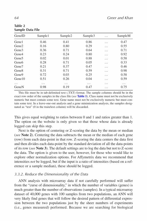
This gives equal weighting to ratios between 0 and 1 and ratios greater than 1.The option on the website is only given so that those whose data is alreadylogged can skip this step.
Next is the option of centering or Z-scoring the data by the mean or median(see Note 2). Centering the data subtracts the mean or the median of each gene(row) from each data-point in that row. Z-scoring the data centers the data firstand then divides each data-point by the standard deviation of all the data-pointsof its row (see Note 3). The default settings are to log the data but not to Z-scorethe data. The option is given to the user, however, for those who would like toexplore other normalization options. For Affymetrix data we recommend thatintensities not be logged, but if the input is a ratio of intensities (based on a ref-erence or a sample median), these should be logged.
3.3.2. Reduce the Dimensionality of the Data
ANN analysis with microarray data if not carefully performed will sufferfrom the “curse of dimensionality,” in which the number of variables (genes) ismuch greater than the number of observations (samples). In a typical microarraydataset of 40,000 genes with 100 samples from two populations, an ANN willvery likely find genes that will follow the desired pattern of differential expres-sion between the two populations just by the sheer numbers of experiments (i.e., genes measured) performed. Because we are searching for biological
64 Greer and Khan
Table 2Sample Data File
GeneID Sample1 Sample2 Sample3 … SampleM
Gene1 0.46 0.41 0.86 … 0.47Gene2 0.16 0.80 0.29 … 0.55Gene3 0.36 0.71 0.64 … 0.71Gene4 0.23 0.24 0.80 … 0.92Gene5 0.02 0.01 0.88 … 0.58Gene6 0.28 0.71 0.05 … 0.33Gene7 0.21 0.37 0.47 … 0.46Gene8 0.31 0.71 0.59 … 0.98Gene9 0.72 0.03 0.25 … 0.58Gene10 0.51 0.26 0.04 … 0.59… … … … … …GeneN 0.98 0.19 0.47 … 0.75
This file must be in tab-delimited text (.TXT) format. The sample columns should be in theexact row order of the samples in the class file (see Table 1). Class name must not be exclusivelynumeric but must contain some text. Gene name must not be exclusively numeric but must con-tain some text. In a leave-one-out analysis and a gene minimization analysis, the samples desig-nated as “test” (0 in the train/test column) will be discarded.
03_Khan.qxd 6/3/07 12:13 PM Page 64
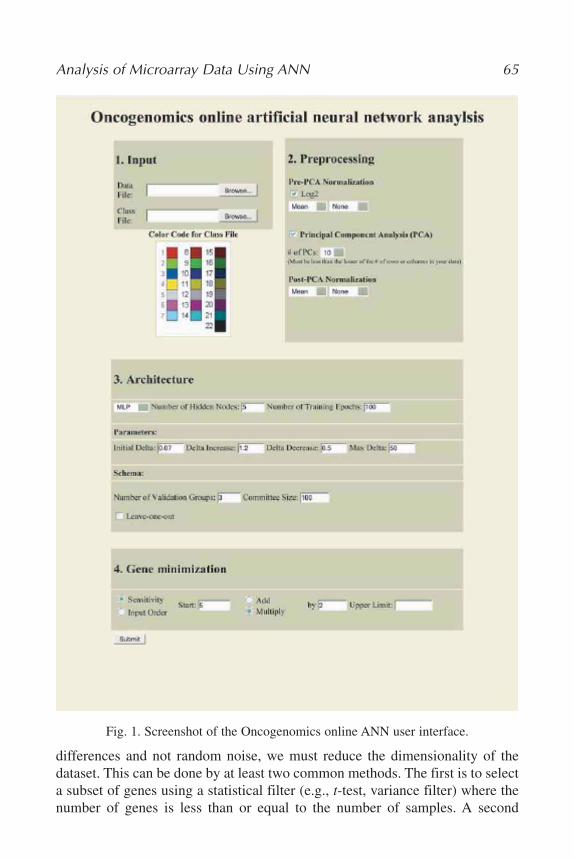
differences and not random noise, we must reduce the dimensionality of thedataset. This can be done by at least two common methods. The first is to selecta subset of genes using a statistical filter (e.g., t-test, variance filter) where thenumber of genes is less than or equal to the number of samples. A second
Analysis of Microarray Data Using ANN 65
Fig. 1. Screenshot of the Oncogenomics online ANN user interface.
03_Khan.qxd 6/3/07 12:13 PM Page 65
method, PCA (see Note 4), is available in the preprocessing stage. In brief,PCA transforms the data by first identifying the direction of greatest variancein the high-dimensional dataset and then creating new axes such that the firstdimension is along the direction of greatest variance and subsequent axes cap-ture less and less of the original variance. The result is that one can use the first2 to 10 dimensions (components) of the transformed data for example, and notlose much information. This generates an input dataset that does not suffer fromthe “curse of dimensionality” because the number of variables (i.e., componentsin rows) is now much smaller than the number of observations (i.e., samples incolumns). Next, the number of components used for input to the network mustbe selected. This decision depends on the complexity of the data. Somewherein the range of 5 to 10 components should suffice for most microarray datasetson the order of 50k genes. Beyond 10 components the data will likely capturevery little of the original variance in the data. As the number of genes in anexperiment increases dramatically, the number of principal components neces-sary to capture the variance of the data may also increase. The default is to per-form PCA and use the top 10 components as input.
3.3.3. Normalize the Reduced Data
The final step in preprocessing is to normalize the dimensional-reduceddataset. Some believe it is good practice to Z-score the reduced dataset prior totraining to give equal variance to each of the components to aid training.Similar normalization options are available as described in Subheading 3.3.1.The default is to Z-score the principal components.
3.4. Architecture
In this section we will discuss the methods and parameters for learning.The first decision is the choice between a linear network and a multilayer per-ceptron (MLP) network. The linear network has only two layers: an input andan output layer; whereas the MLP network inserts one hidden layer betweenthe input and output layers (in principle many hidden layers can be used, butwe have implemented only one hidden layer, which should be sufficient formost microarray studies). The hidden layer in the MLP allows the network tolearn more complex nonlinear signals from the data (see Note 5). If MLP isselected the number of hidden nodes needs to be chosen. There are a widevariety of rules of thumb for selecting the appropriate number of hiddennodes and some are listed next. We are not in favor of any of these becausethey do not take into account several factors including number of trainingcases, noise, and so on. We have included them, however, to give the user astarting point to work from.
66 Greer and Khan
03_Khan.qxd 6/3/07 12:13 PM Page 66

1. Size of this (hidden) layer to be somewhere between the input layer size and theoutput layer size (25).
2. Number of inputs + outputs * (2/3).3. Never require more than twice the number of hidden units as you have inputs in
an MLP with one hidden layer (26,27).4. As many hidden nodes as dimensions (principal components) needed to capture
70–90% of the variance of the input dataset (28).
Trial-and-error starting from one or more of these rules of thumb is our sug-gested method. Remember, though, that the greater number of hidden nodes,the more complicated signal the networks can learn. We have found only mini-mal benefit, to more than three to five hidden nodes for our datasets. Do yourown experimenting however, and determine how many nodes will suit your par-ticular situation. Finally, the number of training epochs or cycles needs to beset. The default value of 100 epochs should be sufficient for most applications.Often the error has reached its lower limit well before 100 epochs, but it is bet-ter to perform too many epochs rather than too few. The risk of overtrainingthrough too many epochs is minimal if one has taken care to reduce the dimen-sionality of the data appropriately and incorporate an appropriate cross-validationscheme (see Subheading 3.4.2.).
3.4.1. Learning Parameters
We chose to use the resilient back-propagation algorithm to train the neuralnetworks for our website for its speed and ease of use. This algorithm has thedesirable property that it is relatively insensitive to changes in the learningparameters (29). This is an excellent property for someone who wants to useANNs but is not get bogged down endlessly tuning a host of learning parame-ters. Nonetheless, the pertinent learning parameters for this algorithm areadjustable from the user interface. Resilient back-propagation employs a tuningparameter, referred to as “delta,” which controls the degree to which the weightsof the network will be penalized for error. “Initial delta” is the penalty for thefirst error, after which the penalty will increase and decrease according to “deltaincrease” and “delta decrease,” respectively. “Max delta” sets the upper limitfor the delta penalty factor. For most applications it will be sufficient to leavethese parameters at their defaults. The defaults are as follows: initial delta, 0.07;max delta, 50; delta increase, 1.2; delta decrease, 0.5.
3.4.2. Cross-Validation
Cross-validation is an important procedure to ensure properly trained net-works. In this context, validation is a technique whereby a subset of trainingsamples are set aside during the learning process and used to validate thetrained networks. The classification error of the validation samples is monitored
Analysis of Microarray Data Using ANN 67
03_Khan.qxd 6/3/07 12:13 PM Page 67

as the learning process cycles through the specified number of epochs. The clas-sification error of the validation samples should decrease rapidly and remainlow. If the validation error increases with increasing epochs, then the networkis learning features of the training set that are not generalizable, but are samplespecific, and training is stopped. The validation samples act as a kind of warn-ing for the network to stop learning to prevent what is known as “over-training.”Our software allows you to partition the training data into a specified numberof randomly selected validation groups. This works as follows: if the userchooses m validation groups, and there are N training samples, then N(m–1)/msamples will be used to train and N/m samples will be used to validate the net-work. The program will iterate through each of the m groups such that each onewill be employed as a validation group exactly one time, for a total of m train-ing iterations. A general rule of thumb for choosing the number of validationgroups is to ensure at least 1⁄2 of your training samples from the category withthe fewest samples will always be in the N(m–1)/m group. For example, if youhave 30 (N) samples from 2 populations and the least-represented populationhas 10 samples, then 6 (m) validation groups would be a good choice becausethe validation groups would have 5 samples and there would never be a situa-tion where there were very few training samples from either population (seeNote 6). Another consideration is to ensure that all populations will be repre-sented in the validation group. If you split your 30 samples into 15 validationgroups, it’s very likely that many of your randomly selected groups of two willonly have one population represented. If the number of training samples, N, isnot divisible by the number of selected groups, m, the program will compensateand form validation groups with slightly different sample sizes.
3.4.3. Committee Voting
When randomly selecting groups for cross-validation (Subheading 3.4.2.) itis possible that one could introduce a bias by grouping all of a certain sampletype, or problem samples together in a validation group. To avoid this possibleerror, it is important to repeat the process of randomly selecting groups, train-ing, and validating many times over and report results based on averages ofthese analyses. In addition, repeating the training process many times allows usto calculate an empirical confidence interval from the training data by which wecan accept or reject the output votes for the testing set. The default value of 100should be sufficient for most applications, but it is a good idea to verify this bymonitoring the results with several increments of votes (see Note 7).
3.4.4. Leave-One-Out Analysis
The leave-one-out option (see Note 8) is useful to see what would happenif each of your samples was presented to the fully-trained network as a blind
68 Greer and Khan
03_Khan.qxd 6/3/07 12:13 PM Page 68
test sample. This is a separate consideration from cross-validation discussedin Subheading 3.4.2. In this case, 1 sample from the N total samples is setaside and is not used in the learning process at all. After each network istrained, the 1 sample is presented as a test and the resulting vote is stored.After all of the networks have completed training (the number of which isdecided by the number of committees) and the test sample is tested each time,the average vote for the test sample is calculated. Next, the test sample isreplaced into the dataset and a new test sample is selected and the process isrepeated until each of the N samples has been presented to the network as ablind test sample exactly one time. The results are as if all of your sampleswere in the testing set. It is a very conservative way to analyze your data. Asyou could imagine it can take a long time to run—sometimes several days ofcomputing are required (see Note 9).
3.5. Gene Minimization
In a typical microarray experiment the expression of tens of thousands of genes is measured, and in a typical study the number of genes that are sig-nificantly differentially expressed is on the order of tens or hundreds, occasion-ally thousands. It is therefore advantageous to remove the uninteresting genesand thereby reduce the noise in the dataset, as well as discover meaningful biol-ogy through the identification of genes implicated in a disease or process. Toachieve these ends we have implemented a gene minimization algorithm thatwill rank the genes based on their importance to the classification and thenretrain the networks using increasing numbers of the top-ranking genes whilemonitoring the classification error (see Note 10). One can then select the sub-set of top-ranking genes that produces the minimum error to train and then testblinded samples. The option is given to you also to perform the minimizationusing the “Input Order” if your data file is already sorted according to yourfavorite gene ranking statistic (e.g., t-test, rank-sum test) (see Note 11). Theorder should be from most to least important (e.g., the first gene should havethe highest t-value or lowest p-value).
The “Start” parameter allows you to choose the number of top-ranking genesto train with in the first run. You can then choose to increase the number of top-ranking genes to use in successive training by adding or multiplying the currentnumber by a user-defined factor. For example, if you start with 5 and multiplyby 2, you will train with the top 5, 10, 20, 40, 80, and so on genes. You can alsolimit the number of additional trainings by defining the upper limit. For exam-ple, if you started with 100 genes and added 100 genes and defined the upperlimit as 500, you would train with the top 100, 200, 300, 400, and 500 genes.The default is to start with the top 5 genes and multiply by 2 while the numberof selected genes is less than or equal to the total number of genes.
Analysis of Microarray Data Using ANN 69
03_Khan.qxd 6/3/07 12:13 PM Page 69

3.6. Results
When the program has completed analyzing your data, you will be notifiedvia email with a link you can download your results from. The files will be asfollows:
1. A .TXT file with “Votes” in the file name and columns with the sample names,train/test value, class number, ANN prediction, confidence intervals (when the num-ber of classes > 2), average committee vote (i.e., validation votes for training sam-ples and test votes for testing samples), and standard error of the committee votes.
2. A .JPG file with “Votes” in the file name visually representing the voting data inthe .TXT file described in item 1 only if there are two classes, if there are more itis difficult to visualize this.
3. A .TXT file with “GeneRank” in the file name with the columns GeneID, rank,total sensitivity, sensitivity, and sign. (Sensitivity and sign will be repeated foreach class in analyses with three or more classes. In the case of two classes, thereis only one output and therefore, one sensitivity measure.)
4. A .JPG file with the “Legend” in the name which contains the class names and col-ors for each of the output figures described in items 2 and 5.
5. A .JPG file of the first three principal components of the data (if PCA was per-formed).
6. A .JPG file with “GeneMinimization” in the name, which is a barplot of the aver-age number of misclassifications of training samples (y-axis) including standarderror with training based on increasing numbers of the top-ranking genes (x-axis).
4. Notes1. The number of training samples necessary to perform a valid analysis is also pro-
portional to the complexity of the question being asked. In the case of diagnosisbetween different tumor types, for example, 10 samples might be sufficient. Onthe other hand, a prognosis study might require many more samples because thedifference between the classes is likely to be much more subtle and the expressionprofile within a class more heterogeneous.
2. The choice between mean or median for centering purposes will not usually alterthe results too drastically. In fact with increasing number of samples from a nor-mal distribution, the median should approximate the mean. The median is helpfulto reduce the influence of an extreme outlier that could affect the mean of a datasetwith a small number of samples. With increasing sample size, however, the influ-ence of an outlier on the mean is diminished.
3. All of the normalization options on our website perform normalization in the genedirection (in our case, row-wise). If you have systematic sample-specific biasowing to different microarray print lots or who performed the experiment, youshould remove these via normalization in the sample direction (in our case, col-umn-wise). See ref. 30 for a review of normalization techniques.
4. For a more in-depth description of the theory of principal components analysis,see ref. 31.
70 Greer and Khan
03_Khan.qxd 6/3/07 12:13 PM Page 70
5. The choice between linear and MLP is dependent on the complexity of the inputsignal. From our experience, an MLP will yield somewhat better results. Withmany datasets, though, a linear network will yield sufficient results. The reader isencouraged to explore both options with their dataset.
6. This rule of thumb is very conservative. In reality, when choosing m samples atrandom from a dataset with N samples across several populations, the expectednumber of randomly selected samples, p, from the least represented populationwith r samples is, of course, proportional: p = mr/N. So, one would expect theleast-represented population to have the least samples in the validation group.Where sample size is relatively equal across populations, the rule of thumb fromSubheading 3.4.2. should be followed. If sample size is very unequal across pop-ulations, then one may use the above expectation value as a guide to selecting thevalidation group size. Remember that the fewer the validation groups, the fasterthe run time.
7. In particular, watch that the confidence interval and gene ranking stabilize. The vot-ing results should stabilize with relatively few votes, but the confidence interval andgene ranking require more votes to stabilize.
8. There is sometimes some misunderstanding regarding the leave-one-out analysis. Itis important not to confuse this with the cross-validation step. The leave-one-outanalysis is outside of the cross-validation step, in that the cross-validation has noknowledge of the left-out sample. Indeed, it would not be prudent to perform aleave-one-out cross-validation as the one validation sample would not be represen-tative of the entire training population and the result would be a training process tai-lored to the one validation sample. In the leave-one-out analysis in Subheading3.4.4., the left-out sample has no affect on the training of the networks whatsoever.It is as if you performed as many analyses as you had samples each time designat-ing one sample for testing (marked with a ‘0’ in the train/test column in the classfile) and concatenated the testing results into one spreadsheet or one visualization.Therefore, the training of the networks is not tailored to the one left-out sample inthis analysis.
9. One important caveat is that you should not perform any supervised gene selec-tion prior to the leave-one-out analysis. If you do, the blind test sample is nolonger blind because it has influenced the selection of the genes. This is why thetest is usually a more conservative estimate of the ability of your data to predictblind test samples. If you do an analysis with separate training and testing datasets,you will be able to minimize the genes (and thereby reduce noise), and an increasein the prediction accuracy should be realized. Leave-one-out analysis resultsshould be interpreted with this in mind.
10. The sensitivity of a gene is calculated by taking the derivative of the outputdivided by the derivative of the input. For complete details see the SupplementaryMethods in ref. 18.
11. It was noted before in Note 9, but it is worth repeating that any supervised geneselection should not have included the test samples. If you select your genes tak-ing the test samples into consideration, they are no longer blind test samples.
Analysis of Microarray Data Using ANN 71
03_Khan.qxd 6/3/07 12:13 PM Page 71
References1. Peterson, C. and Ringner, M. (2003) Analyzing tumor gene expression profiles.
Artif. Intell. Med. 28, 59–74.2. Ringner, M. and Peterson, C. (2003) Microarray-based cancer diagnosis with arti-
ficial neural networks. Biotechniques Suppl, 30–35.3. Ringner, M., Peterson, C., and Khan, J. (2002) Analyzing array data using super-
vised methods. Pharmacogenomics 3, 403–415.4. Greer, B. T. and Khan, J. (2004) Diagnostic classification of cancer using DNA
microarrays and artificial intelligence. Ann. NY Acad. Sci. 1020, 49–66.5. Dayhoff, J. E. and Deleo, J. M. (2001) Artificial neural networks: opening the black
box. Cancer 91, 1615–1635.6. Haykin, S. (1999) Neural Networks: A Comprehensive Foundation Prentice-Hall,
Upper Saddle River, NJ.7. Ando, T., Suguro, M., Hanai, T., Kobayashi, T., Honda, H., and Seto, M. (2002)
Fuzzy neural network applied to gene expression profiling for predicting the prog-nosis of diffuse large B-cell lymphoma. Jpn. J. Cancer Res. 93, 1207–1212.
8. Berrar, D. P., Downes, C. S., and Dubitzky, W. (2003) Multiclass cancer classifi-cation using gene expression profiling and probabilistic neural networks. Pac.Symp. Biocomput. 5–16.
9. Bicciato, S., Pandin, M., Didone, G., and Di Bello, C. (2003) Pattern identificationand classification in gene expression data using an autoassociative neural networkmodel. Biotechnol. Bioeng. 81, 594–606.
10. Bloom, G., Yang, I. V., Boulware, D., et al. (2004) Multi-platform, multi-site,microarray-based human tumor classification. Am. J. Pathol. 164, 9–16.
11. Ellis, M., Davis, N., Coop, A., et al. (2002) Development and validation of amethod for using breast core needle biopsies for gene expression microarray analy-ses. Clin. Cancer Res. 8, 1155–1166.
12. Futschik, M. E., Reeve, A., and Kasabov, N. (2003) Evolving connectionist sys-tems for knowledge discovery from gene expression data of cancer tissue. Artif.Intell. Med. 28, 165–189.
13. Gruvberger, S., Ringner, M., Chen, Y., et al. (2001) Estrogen receptor status inbreast cancer is associated with remarkably distinct gene expression patterns.Cancer Res. 61, 5979–5984.
14. Gruvberger, S. K., Ringner, M., Eden, P., et al. (2003) Expression profiling to pre-dict outcome in breast cancer: the influence of sample selection. Breast CancerRes. 5, 23–26.
15. Gruvberger-Saal, S. K., Eden, P., Ringner, M., et al. (2004) Predicting continuousvalues of prognostic markers in breast cancer from microarray gene expressionprofiles. Mol. Cancer Ther. 3, 161–168.
16. Kan, T., Shimada, Y., Sato, F., et al. (2004) Prediction of lymph node metastasiswith use of artificial neural networks based on gene expression profiles inesophageal squamous cell carcinoma. Ann. Surg. Oncol. 11, 1070–1078.
72 Greer and Khan
03_Khan.qxd 6/3/07 12:13 PM Page 72
17. Linder, R., Dew, D., Sudhoff, H., et al. (2004) The ‘subsequent artificial neural net-work’ (SANN) approach might bring more classificatory power to ANN-basedDNA microarray analyses. Bioinformatics 20, 3544–3552.
18. Khan, J., Wei, J. S., Ringner, M., et al. (2001) Classification and diagnostic predic-tion of cancers using gene expression profiling and artificial neural networks. Nat.Med. 7, 673–679.
19. Liu, B., Cui, Q., Jiang, T., and Ma, S. (2004) A combinational feature selection andensemble neural network method for classification of gene expression data. BMCBioinformatics 5, 136.
20. O’Neill, M. C. and Song, L. (2003) Neural network analysis of lymphoma micro-array data: prognosis and diagnosis near-perfect. BMC Bioinformatics 4, 13.
21. Selaru, F. M., Xu, Y., Yin, J., et al. (2002) Artificial neural networks distinguishamong subtypes of neoplastic colorectal lesions. Gastroenterology 122, 606–613.
22. Tham, C. K., Heng, C. K., and Chin, W. C. (2003) Predicting risk of coronaryartery disease from DNA microarray-based genotyping using neural networks andother statistical analysis tool. J. Bioinform. Comput. Biol. 1, 521–539.
23. Wei, J. S., Greer, B. T., Westermann, F., et al. (2004) Prediction of clinical outcomeusing gene expression profiling and artificial neural networks for patients with neuro-blastoma. Cancer Res. 64, 6883–6891.
24. Xu, Y., Selaru, F. M., Yin, J., et al. (2002) Artificial neural networks and gene fil-tering distinguish between global gene expression profiles of Barrett’s esophagusand esophageal cancer. Cancer Res. 62, 3493–3497.
25. Blum, A. (1992) Neural Networks in C++. Wiley, New York, NY.26. Swingler, K. (1996) Applying Neural Networks: A Practical Guide Academic Press,
London, UK.27. Berry, M. A. L., G (1997) Data Mining Techniques John Wiley and Sons, New
York, NY.28. Boger, Z. and Guterman, H. (1997) Knowledge extraction from artificial neural
network models. IEEE Systems, Man, and Cybernetics Conference, Orlando, FL.29. Demuth, H. B., Mark (2001) Neural Network Toolbox 4th. The Mathworks,
Natick, MA.30. Yang, Y. H., Dudoit, S., Luu, P., et al. (2002) Normalization for cDNA microarray
data: a robust composite method addressing single and multiple slide systematicvariation. Nucleic Acids Res. 30, e15.
31. Joliffe, I. T. (2002) Principal Component Analysis, 2nd ed., Springer-Verlag, NewYork, NY.
Analysis of Microarray Data Using ANN 73
03_Khan.qxd 6/3/07 12:13 PM Page 73

03_Khan.qxd 6/3/07 12:13 PM Page 74

4
Signal Processing and the Design of Microarray Time-Series Experiments
Robert R. Klevecz, Caroline M. Li, and James L. Bolen
SummaryRecent findings of a genome-wide oscillation involving the transcriptome of the budding yeast
Saccharomyces cerevisiae suggest that the most promising path to an understanding of the cell as adynamic system will proceed from carefully designed time-series sampling followed by the devel-opment of signal-processing methods suited to molecular biological datasets. When everythingoscillates, conventional biostatistical approaches fall short in identifying functional relationshipsamong genes and their transcripts. Worse, based as they are on steady-state assumptions, suchapproaches may be misleading. In this chapter, we describe the continuous gated synchrony systemand the experiments leading to the concept of genome-wide oscillations, and suggest methods ofanalysis better suited to dissection of oscillating systems. Using a yeast continuous-culture system,the most precise and stable biological system extant, we explore analytical tools such as waveletmultiresolution decomposition, Fourier analysis, and singular value decomposition to uncover thedynamic architecture of phenotype.
Key Words: Genome-wide; transcription; oscillation; attractor; microarray; singular valuedecomposition; SVD; replicates.
1. IntroductionThe idea that the cell is an oscillator, an attractor, and that time is a variable
of the system, though well supported by both theory and experimental findings,is still something of a novelty in genomics (1–4). Prior to the development ofgenome-wide assays, experimental support for viewing the cell as an attractorwas limited to measurement of single constituents or to analysis of the responseof cells to intentional perturbations to the cell cycle (5).
Now, for the first time, we have the capacity to make precise measurementsof all of the transcripts of a cell, most of the metabolites and, soon, one mightproject, all of the proteins in a quantitative manner. Recently, we took advan-tage of microarray technology to measure all of the transcripts of yeast cells
75
From: Methods in Molecular Biology, vol. 377, Microarray Data Analysis: Methods and ApplicationsEdited by: M. J. Korenberg © Humana Press Inc., Totowa, NJ
04_Klevecz.qxd 6/3/07 3:18 PM Page 75
growing synchronously with respect to their respiratory/reductive cycle (6).This cycle, which switches its redox state from respiration to reduction withgreat precision, gives us the first glimpse into the evolutionary early molecularorganization of cells as they dealt with the transition from a reductive to an oxi-dizing environment. The metabolic state of these cultures appears to be anexcellent benchmark and manifestation of the temporal organization of tran-scription. As a practical matter, the precision and stability of the cycle allowsthe ready development of techniques for time-series analysis of microarray datathat can be used in mammalian systems.
Feasibility forces the consideration of when genome-wide oscillations can beexploited to give a clearer insight into cellular regulatory mechanisms andwhen, because of limited control over the biological system, they can, at best,only be accounted for and not exploited. In either case, it is no longer sufficientto assume because no particular effort has been put into synchronizing a cellu-lar system, that it is necessarily random or exponential. If cell-to-cell signalingin a single-celled organism such as yeast gives rise to spontaneous oscillationsand gated synchrony in the culture as a whole, then mammalian cell culturesand tissues, where cell-to-cell connectivity and signaling are well recognized,partial synchronization is a near certainty, and the deviation from randomnessthat this represents, becomes a problem for microarray analysis.
Most important for the microarray field at the present moment is the realizationthat it may be much more informative to take a careful sampling of a systemthrough time than to take multiple samples without regard to time. We will showevidence in this work that once the uncertainty from time variation in gene expres-sion is removed, the Affymetrix system is capable of remarkable precision withsignal to noise of 60 decibels in respiratory-phase transcripts. In these studies, onlya few of the samples were done in duplicate or triplicate in the conventional statis-tical sense. Rather, close time sampling through multiple cycles were taken givingthe option of phase aligning and averaging the data into a single cycle, and by thisact, generating a combined biological and oscillator-phase replicate, or displayingthe dataset as an oscillation and analyzing it using signal-processing methods.
All of the data presented and analyzed here is derived from expression-arrayanalysis using the Affymetrix yeast S98 chip and the new Yeast2 chip. In order tooptimize new analysis methods, we felt it would be best to use the most accuratebiological and measurement systems. Spotted-array analyses were not includedbecause of their greater inherent noise and platform-to-platform variability.
2. Materials1. Fermenters (B. Braun Biotech, Aylesbury, Buckinghamshire, UK; model: Biolab
CP; working volume of 650 mL).2. KH2PO4 monobasic, CaCl2·2H2O, (NH4)2SO4, MgSO4·7H2O, CuSO4·5H2O, and
MnCl2 ·4H2O (J. T. Baker, Philipsburg, NJ); H2SO4, acid-washed glass beads,
76 Klevecz et al.
04_Klevecz.qxd 6/3/07 3:18 PM Page 76

2- mercaptoethanol, antifoam A and D(+)-glucose monohydrate (Sigma, St. Louis,MO); FeSO4·7H2O (Mallinckrodt, Paris, KY); ZnSO4·7H2O (EM Science,Darmstadt, Germany); yeast extract (Difco, Sparks, MD); RNA later, GeneChipExpression Kit, and poly(A) standards (Ambion, Ambion, TX); RLT buffer, RNAeasy mini kit, and DNase (Qiagen, Valencia, CA).
3. The Mini Bead beater (BioSpec Products, Inc., Bartlesille, OK.).4. RNA was examined for quality using capillary electrophoresis with the Agilent
2100 Biosizer (Agilent Technologies, Palo Alto, CA).5. RNA Lab-On-A-Chip (Caliper Technologies Corp., Mountain View, CA).6. Yeast arrays, GeneChip hybridization oven 640, Fluidics Station 450, and
GeneArray scanner (Affymetrix, Santa Clara, CA).7. Mathcad is from Mathsoft Inc. (Cambridge, MA); Mathematica is from Wolfram
Research (Champaign, IL); SigmaPlot is from Systat Software Inc. (PointRichmond, CA); and MatLab is from The Mathworks Inc. (Natick, MA).
3. Methods3.1. Culture Conditions and Monitoring of the Oscillation
1. The basic medium: (NH4)2SO4 (5 g/L), KH2PO4 (2 g/L), MgSO4 (0.5 g/L), CaCl2(0.1 g/L), FeSO4 (0.02 g/L), ZnSO4 (0.01 g/L), CuSO4 (0.005 g/L), MnCl2(0.001 g/L), 70% H2SO4 (1 mL/L), and yeast extract (1 g/L).
2. Glucose medium is supplemented with 22 g/L glucose monohydrate and 0.2 mL/Lantifoam A.
3. The fermenters are operated at an agitation rate of 750 rpm, an aeration rate of 150 mL/min, a temperature of 30°C, and a pH of 3.4 or 4.0. Cultures are not nutrientlimited and glucose levels oscillate between 50 and 200 µM in each cycle.
4. The oscillations reported are not unique to this strain, IFO 0233, and are achievedunder culture conditions suited to an acidophile, such as Saccharomyces cere-visiae. The system for establishing and continuously monitoring synchrony hasbeen carefully engineered to make it possible to perform molecular, biological,and cell biological sampling as frequently as required without perturbation. Thestrains have been analyzed by flow cytometry together with a number of com-monly used haploid and diploid strains to show that it is a diploid. The diploidstrains IFO 0224, NCYC 87, NCYC 240, and PC 3087 have also been tested andshow oscillatory dynamics under different conditions (unpublished). Along withIFO 0233, these are all wild-type brewing, distilling, bread and/or spoilage strainsof S. cerevisiae.
5. Continuous synchrony cultures of yeast are typically maintained and monitoredfor many weeks after their initial establishment (Fig. 1). Measurement of the dis-solved oxygen (DO) concentration, O2, CO2, and H2S levels are made every 10 sand determination of the period of the oscillation and its variability is made eachday. Periods typically are in the range of 40–45 ± 0.5 min (7–10). As part of thestandard procedure in the lab, the oscillation in dissolved O2 is monitored before,during, and following sampling for RNA isolation. In this way, it is possible toreduce concerns regarding the degree of synchrony, the absence of perturbation,and the stability of the oscillation.
Signal Processing and Microarray Design 77
04_Klevecz.qxd 6/3/07 3:18 PM Page 77
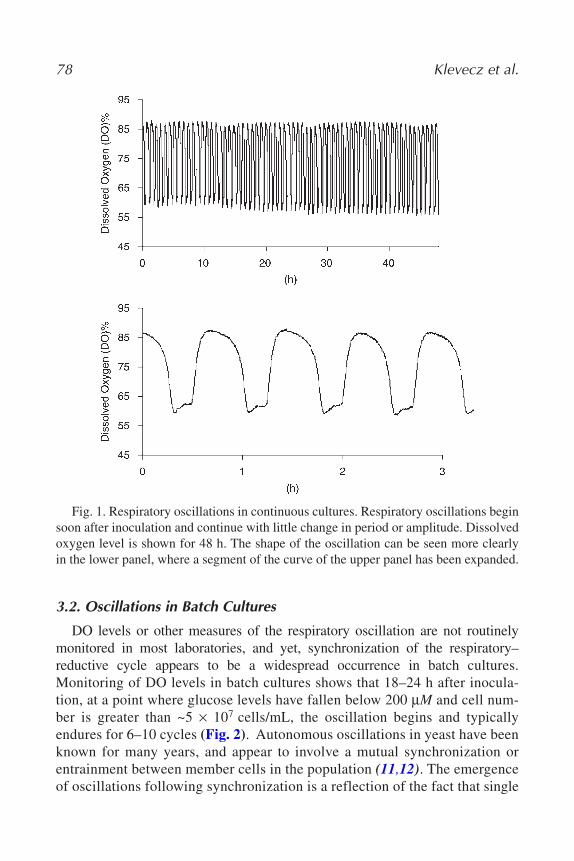
78 Klevecz et al.
Fig. 1. Respiratory oscillations in continuous cultures. Respiratory oscillations beginsoon after inoculation and continue with little change in period or amplitude. Dissolvedoxygen level is shown for 48 h. The shape of the oscillation can be seen more clearlyin the lower panel, where a segment of the curve of the upper panel has been expanded.
3.2. Oscillations in Batch Cultures
DO levels or other measures of the respiratory oscillation are not routinelymonitored in most laboratories, and yet, synchronization of the respiratory–reductive cycle appears to be a widespread occurrence in batch cultures.Monitoring of DO levels in batch cultures shows that 18–24 h after inocula-tion, at a point where glucose levels have fallen below 200 µM and cell num-ber is greater than ~5 × 10⁷ cells/mL, the oscillation begins and typicallyendures for 6–10 cycles (Fig. 2). Autonomous oscillations in yeast have beenknown for many years, and appear to involve a mutual synchronization orentrainment between member cells in the population (11,12). The emergenceof oscillations following synchronization is a reflection of the fact that single
04_Klevecz.qxd 6/3/07 3:18 PM Page 78
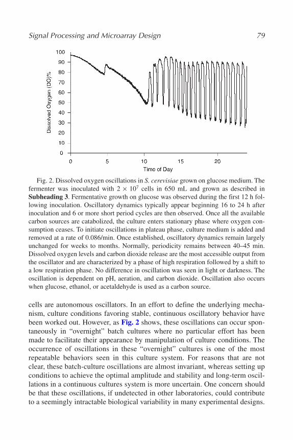
cells are autonomous oscillators. In an effort to define the underlying mecha-nism, culture conditions favoring stable, continuous oscillatory behavior havebeen worked out. However, as Fig. 2 shows, these oscillations can occur spon-taneously in “overnight” batch cultures where no particular effort has beenmade to facilitate their appearance by manipulation of culture conditions. Theoccurrence of oscillations in these “overnight” cultures is one of the mostrepeatable behaviors seen in this culture system. For reasons that are notclear, these batch-culture oscillations are almost invariant, whereas setting upconditions to achieve the optimal amplitude and stability and long-term oscil-lations in a continuous cultures system is more uncertain. One concern shouldbe that these oscillations, if undetected in other laboratories, could contributeto a seemingly intractable biological variability in many experimental designs.
Signal Processing and Microarray Design 79
Fig. 2. Dissolved oxygen oscillations in S. cerevisiae grown on glucose medium. Thefermenter was inoculated with 2 × 10⁷ cells in 650 mL and grown as described inSubheading 3. Fermentative growth on glucose was observed during the first 12 h fol-lowing inoculation. Oscillatory dynamics typically appear beginning 16 to 24 h afterinoculation and 6 or more short period cycles are then observed. Once all the availablecarbon sources are catabolized, the culture enters stationary phase where oxygen con-sumption ceases. To initiate oscillations in plateau phase, culture medium is added andremoved at a rate of 0.086/min. Once established, oscillatory dynamics remain largelyunchanged for weeks to months. Normally, periodicity remains between 40–45 min.Dissolved oxygen levels and carbon dioxide release are the most accessible output fromthe oscillator and are characterized by a phase of high respiration followed by a shift toa low respiration phase. No difference in oscillation was seen in light or darkness. Theoscillation is dependent on pH, aeration, and carbon dioxide. Oscillation also occurswhen glucose, ethanol, or acetaldehyde is used as a carbon source.
04_Klevecz.qxd 6/3/07 3:18 PM Page 79

3.3. Total RNA Preparation
1. Cells from the fermenter (0.5 mL) were collected every 4 min (see Note 1 for sam-pling interval). The cells are pelleted, the supernatant decanted, and the pellet isplaced in a dry ice acetone bath or in liquid nitrogen. Samples are stored at –80°C.The time from removal of the sample to freezing is less than 1 min. Cell numbersare kept between 0.5–1 × 10⁹/mL.
2. For RNA isolation, the pellet is resuspended in 0.5 mL of RNA later containing 10 µL 2-mercaptoethanol/mL RNA later. Cells are lysed by beating in a Mini Beadbeater for 3 min with 0.5 mL acid-washed glass beads. After the cell lysate isremoved, the beads are washed three times with 0.5 mL Qiagen RLT buffer con-taining 10 µL 2-mercaptoethanol/mL RLT buffer by bead beater (1 min each wash).The cell lysate and washes are pooled. An equal volume of 70% ethanol is added,and RNA is purified with RNA easy columns according to the manufacturer. DNAis digested on the columns according to the instructions. RNA is eluted two timesin RNase-free water with a volume of 50 µL each time so that the total volume is0.1 mL. The final RNA samples are analyzed by capillary electrophoresis. Typicaltotal RNA yields are 20–40 µg with absorbance 260/280 ratios of 1.8–2.2.
3. In a synchronous cell system, where there is reason to think that the level ofmRNA is not constant through the cycle, a method for adjusting for differences inrecovery, for amplification, and for hybridization is essential (see Note 2). In orderto normalize RNA yields between different samples, a fixed amount of polyadeny-lated B. subtilis lys, phe, thr, and dap poly(A) standards are added to cells beforelysis. Fourteen microliters of 1:500 premixed poly(A) standards are added to every0.5 mL pellet of cells resuspended in 0.5 mL of RNA later before cell lysis andRNA purification in order to achieve a reasonable signal on the microarray.
4. The new yeast S2 chip contains the complete probe set for both S. cerevisiae andS. pombe, and this combination offers a second and potentially more robustmethod of normalization. A constant number of S. pombe cells (about 5% of theS. cerevisiae cells) is added to each experimental sample, and the two RNAs wereisolated together. Control experiments have shown that less than 20 of the 5000pombe transcripts bind at greater than background levels to the S. cerevisiaeprobes. By setting the total hybridization or a selected subset of the hybridizedtranscripts to a constant value, variations in mRNA yields between samples can benormalized. More details are described in Subheading 3.7.
3.4. Target Preparation/Processing for Affymetrix GeneChip Analysis
1. Purified total RNA samples are processed as recommended in the AffymetrixGeneChip Expression Analysis Technical Manual. RNA samples are adjusted to afinal concentration of 1 µg/µL. Typically, 25–250 ng are loaded onto an RNA Lab-On-A-Chip and analyzed in an Agilent Bioanalyzer 2100.
2. Double-stranded cDNA is synthesized from 5 µg of total RNA using GeneChipExpression 3′-Amplification Reagents One-Cycle cDNA Synthesis Kit and oligo-dT primers containing a T7 RNA polymerase promoter.
80 Klevecz et al.
04_Klevecz.qxd 6/3/07 3:18 PM Page 80
3. Double-stranded cDNA is used as a template to generate biotinylated cRNA usingthe GeneChip Expression 3′-Amplification Reagents for IVT Labeling (see Notes 3and 4). The biotin-labeled cRNA is fragmented to 35–200 bases following theAffymetrix protocol.
4. Five micrograms of fragmented cRNA is hybridized to Yeast 2.0 Affymetrix arraysat 45°C for 16 h in a hybridization oven.
5. The GeneChip arrays were washed and then stained with streptavidin-phycoerythrinon an Affymetrix Fluidics Station 450, followed by scanning on an AffymetrixGeneArray scanner.
3.5. Data Analysis
In the Notes section, we describe the standard path for analysis of microarrayexperiments. Raw results are collected first into Excel where the P,M,A, (pres-ent, marginal, or absent) discrimination is made. Adjustments are then made forhybridization and RNA-recovery differences and the intensity values werescaled accordingly. These adjustments could also be done using the AffymetrixGCOS software. In some instances, the Excel files are converted back to .txt or.csv to permit further processing. These files are then put into Mathcad,Mathematica, SigmaPlot, or MatLab. Intensity values for each of the verifiedopen reading frames (ORFs) in the S98 chip and the yeast S2 chip are linked tothe SGD (Saccharomyces Genome Database) site and both their genetic andphysical map locations can be associated with the intensity values for each gene.The results for all ORFs scored as present using the default Affymetrix settingsare identified according to the original sample number and the phase in the DOoscillation to which they are mapped for presentation. Further analysis was per-formed for all ORFs present in all samples in each of the three cycles. In a recentexperiment, of the ORFs scored as present by these criteria, all 5443 had aver-age p-values less than 0.035 and 5254 had p-values less than 0.01.
3.6. Normalization With Constitutive or Maintenance Genes
One important issue that must be considered relates to the general applica-bility of the proposed time-series analyses. The findings reported here indicatethat the choice of controls must involve more than the assumption that if a cul-ture has not been intentionally synchronized or perturbed, it is necessarily ran-dom or stable. In several microarray-assay systems, housekeeping genes havebeen used as internal standards or as a means of estimating noise in the assay.
The use of actin and other constitutive, maintenance, or housekeeping genesas normalizing standards is a time-honored practice in PCR and other amplifi-cation assays. Both the singular value decomposition (SVD) and waveletdecomposition studies rely in different ways on the global behavior of tran-scription to make their case. It is now clear from our earlier study that the
Signal Processing and Microarray Design 81
04_Klevecz.qxd 6/3/07 3:18 PM Page 81

constitutive gene transcripts are not constant through the transcriptional cycle.Earlier, Warrington et al. (18) addressed this question in an analysis of humanadult and fetal tissues. Of the 535 genes identified as highly expressed in all tis-sues examined, all but 47 varied by greater than 1.9-fold. They caution that fur-ther analysis might find regular variations in these transcripts as well. A genemay be constitutive even though its transcript is not maintained at a constantlevel through a cycle. Constitutive expression is not constant expression.
3.7. Normalizing for RNA Recovery, Copying, Amplification, and Hybridization
At each stage in the process of measuring transcript levels in the Affymetrixsystem, the protocol calls for bringing the amount of material to the same concen-tration. Upon completion of the procedures, each chip is scaled to a target value.This raises a point of interest. How can one expect to quantify, or even qualita-tively detect differences between samples using this approach? It assumes that thetotal message synthesis and the levels of specific messages will be very similarbetween samples. As we have seen, this appears not to be the case in the gatedsynchrony system. Because there is evidence in our system, as well as mam-malian systems, that constitutive transcripts are not constant through the cycle,their use as a standard for normalization is not correct. However, because theamplitude of their oscillation is low with an average 1.25- fold peak-to-troughratio, they can be used semiquantitatively to verify that there is a change in thosetranscripts showing high-amplitude oscillations. This is not an entirely satisfac-tory solution to the problem. We have sought other methods to normalize the data.
There is the potential for a phase obliteration artifact in the standard methodsof expression-array analysis using Affymetrix chips or one-color-spotted arrays.Consider an extreme instance where 90% of the transcripts are made at one briefphase of the cycle with the remaining transcripts made uniformly through theremainder of the cycle. Adding equal amounts of message to the copying andamplification mix will reduce the contribution of the high transcript phase sig-nificantly. If we further normalize by requiring equal total hybridization in allsamples, then we have pretty much insured that all phases of the cycle will haveequal numbers of transcripts maximally expressed. The only sure way to avoidthis is to spike into the samples at the time of RNA isolation a set of standardsnot expressed by the cells of interest and normalize each microarray to constantexpression in these standards.
Our approach using the S2 chip and early experiments with the S98 chip isto use the B. subtilis poly(A) standards spiked into the cell pellet at the begin-ning of the RNA isolation as a measure of both recovery and variations inamplification. This approach, although imperfect, gives at least some assurancethat variations in total transcript levels for all transcripts in any one chip is not
82 Klevecz et al.
04_Klevecz.qxd 6/3/07 3:18 PM Page 82
because of differences in recovery. It also overcomes the inherent bias in adjust-ing the input RNA to a constant level throughout the procedure.
What then should be the sequence of adjustments for a time-series experi-ment where samples have been prepared as described previously? The proce-dure we adopted works back from the chip results to the isolation. First, startingwith the raw un-normalized data, adjust for differences in hybridization effi-ciency using the biotinylated E. coli transcript standards. Then adjust for ampli-fication and recovery differences using the B. subtilis poly(A) standards andfinally, if applicable, adjust for differences in mRNA recovery using the S. pombe spiked standard. In Fig. 3, two time-series expression profiles for arespiratory and a reductive phase transcript are shown to compare the raw dataand the result using the poly(A) standards together with the hybridization stan-dards. In this system, the adjustments for RNA recovery change the absolutelevel of expression but not the pattern of the oscillation.
Another solution to this problem using the yeast S2 chip, which containsboth the S. pombe and S. cerevisiae probe sets, appears to be the use of an S. pombe cell spike. The correct amount of S. pombe to be used will depend onthe isolation procedure. In contrast to the poly(A) spike, the cellular RNAs gothrough the same isolation procedures. Whether the recovery of RNA frompombe is different from S. cerevisiae is not a concern because the S. pombespike is identical in all samples. Although this approach has the advantage thatthe B. subtilis standards can be used exactly as recommended by Affymetrix,allowing for independent evaluation of hybridization, copying, and recovery, ithas not yet been fully evaluated by this laboratory.
In the original studies, transcripts were included in the analysis if at leastthree of the samples in each cycle were scored as present using the standardAffymetrix defaults. We find, using the new S2 chip, that the results can beimproved by including only those transcripts present throughout the experimen-tal series. The initial inclusion was done to avoid the possibility of eliminatingsamples whose oscillations were extreme. However, it appears that the algo-rithm used by Affymetrix does not eliminate any of the transcripts of interesteven when levels fall to near zero. Among the 191 questionable genes, only asmall fraction (16) show average expression levels greater than 100 and noneshow strong signal at the 40-min cycle time and all of these have p-values lessthan 0.05. Although we might choose to include this group into our analysis forsome purposes, they can probably be eliminated from consideration in a studyin which the global properties of the system are being examined. All of thegenes with the most dramatic cyclic behavior were present in all 32 samples.
One question we wished to resolve was the lower limits of signal in a time-series analysis. The Affymetrix S2 chip has both the S. cerevisiae and S. pombeprobe sets together and interspersed. This seemed to offer an opportunity to find
Signal Processing and Microarray Design 83
04_Klevecz.qxd 6/3/07 3:18 PM Page 83

84 Klevecz et al.
Fig. 3. Controlling for RNA recovery, copying, amplification, and hybridization.Levels of expression in two probe sets, YGL184C and YOR186W, are shown (repre-sented by the line). Addition of the B. subtilis poly(A) RNA was made prior to disrup-tion of the cells in the Mini-Bead-Beater. For each chip, the values of the two poly(A)standards, AFFX-r2-Bs-thr-3_s_at and AFFX-r2-Bs-phe-3_at, were determined andaveraged with the entire series and then scaled by the average. The resulting ratio was
04_Klevecz.qxd 6/3/07 3:18 PM Page 84

a true machine plus amplification plus a hybridization boundary below which weshould find the system, as opposed to biological, noise. Of the 5000 S. pombeprobe sets on the chip, all but 20 are entirely absent in all 32 samples for allgenes. We used the values for the entire S. pombe scored as absent as a lowerboundary for noise in our pair-wise comparisons. This lower boundary can beput under 16 intensity units in an experiment where the average intensity for allprobe sets is greater than 2000 and the maximum intensity is greater than 16,000.
3.8. Being Misled by Scatterplots and the Pair-Wise Comparison Paradigm
It has become commonplace to argue that many replicates are required tomake a “change call” in expression. The numbers suggested are extraordinary,varying upward to 25. The time-averaged value of any oscillating constituent isa constant and one might expect that sampling done in ignorance of thedynamic state will tend to eliminate all of the most stable oscillatory compo-nents of the system leaving as “changed” the most unstable high-amplitudeoscillations. We will argue that since the system is oscillatory, or in most cases,unknown, it makes more sense to take single samples through multiple cyclesand use signal processing to characterize patterns of expression. The mostimportant point to be taken from this work is the demonstration that biologicalvariability is not intractable and that the notion that 25 biological replicates arenecessary overlooks the obvious problem that the samples used to derive sucha number are either not time resolved or resolved poorly.
As an example of how multiple samples done without knowledge of theunderlying cellular dynamics might be misleading, we have taken two samples40 min apart but taken from the same phase of the transcriptional cycle, and twosamples taken 20 min apart from differing phases and compared them using thestandard pair-wise comparison. Each gene scored as present in both samples isplotted vs itself. In Fig. 4, the raw data are shown. In doing the comparison inthis way we are placing an additional burden on the biological system, the moreso because it is difficult to impossible to sample at precisely the identical phasein two successive cycles. Nevertheless, the agreement is quite good as the leftpanel of Fig. 4 shows. In contrast, the right panel shows the paired samplestaken 20 min apart, but out of phase.
Consider the case in most yeast laboratories where no measurements of the res-piratory state of the cell is taken. Even in the case where replicates are taken from
Signal Processing and Microarray Design 85
Fig. 3. (Continued) used to scale each transcript for all chips (represented by theline with squares). The disadvantage to this approach is that the poly(A) standards wereintended to be used only to verify the quality of the copying and amplification, and notas a standard for recovery.
04_Klevecz.qxd 6/3/07 3:18 PM Page 85

the same culture, small differences in sampling time may be sufficient to yieldquite different patterns of expression. In the respiratory phase of the cycle,half-lives of 2–4 min are common such that the time required to sample, cen-trifuge, and flash-freeze a sample before returning for a replicate would be suf-ficient to alter the pattern. This is perhaps an extreme example but consider amore realistic case where a treated and control series of samples are beingtaken from two overnight batch cultures, one treated and one control. Similaroptical densities or cell counts are not adequate to insure an identical phase ofthe oscillation. What are, in fact, regular temporal patterns of expression wouldbe incorrectly identified by conventional statistical treatments as outliers, partof the intractable noise—and the limit for making a change call would neces-sarily need to be increased; a lot more replicates would be recommended to noparticular benefit.
3.9. Genome-Wide Oscillations in Transcription: Expression Microarray Analysis
Thus far the concern has been with the details of getting a reliable and quan-titative measure from a time-series experiment. Far more crucial is the conse-quence of doing microarray experiments in the absence of any knowledge of thedynamics of the biological system being used.
Microarray analysis from a yeast continuous synchrony culture systemshows a genome-wide oscillation in transcription. Maximums in transcript levels occur at three nearly equally spaced intervals in this approx 40-min cycleof respiration and reduction. Fig. 2 in the published work (6) shows the time of
86 Klevecz et al.
Fig. 4. Pair-wise comparison of samples resolved and purposely not resolved withrespect to time of sampling. Each of the 5243 transcripts scored as present in all 32 ofthe Affymetrix chips through three cycles of the oscillation was included in this com-parison. In the left panel, two samples taken approximately one cycle apart are com-pared. In the right, the two samples were taken at roughly one-half cycle apart.
04_Klevecz.qxd 6/3/07 3:18 PM Page 86

maximum transcript level for all expressed genes as a color-contour plot. Thetime of maximum was determined by averaging the expression level in the threereplicates from the same phase in three cycles of the oscillation. Note that theserepresent combined technical and biological replicates. Once the time of maxi-mum was assigned it was fixed for all subsequent analyses. The results for allthree cycles can be seen as a color “temperature map” in the supplemental datafrom the published work (6).
The preferred representation for whole-genome data displays is the color“temperature” map in which high levels of expression are represented in redsand orange and low levels in blue (6). Such maps can also be converted to a sim-pler contour map. Here we have taken the three cycles of expression data, aver-aged it, and ordered the genes according to when in the cycle they aremaximally expressed (Fig. 5). Because every gene will have a maximum some-where in the cycle, more quantitative measures may be needed if the claim ofgenome-wide periodicity is to be supported.
3.10. Fast Fourier Transform Filtering of Expression Microarray Data
The classical tool for investigating periodicity in sampled sequences is thediscrete Fourier transform, realized almost exclusively as the fast Fourier trans-form (FFT) in the modern analytical toolbox. This tool is especially effectivewhen the periodic nature of a sequence closely resembles a sine or cosine wave-form. In this case the transformed sequence is singular or nearly so, indicatingthat perhaps the entire signal is represented, or matched, by a single functionwith a constant frequency. The FFT can be thought of as a high fidelity-matchedfilter producing an optimum representation.
Fourier analysis has the virtue of being the most mainstream of signal-processing methods, but has not been widely applied in molecular biologicalstudies because the datasets usually available are short and sparsely sampled.This was the reason that our original reanalysis of the Stanford cell cycledata (13,14) employed wavelet multi resolution decomposition (WMD). Indesigning our own microarray experiments we sought to avoid some of theseshortcomings by first optimizing sampling structures with signal processingor other nonlinear methods in mind. For techniques such as FFT, the datashould encompass at least three cycles to permit detection of the period ofinterest. Equal sampling intervals throughout are essential and for some signal-processing treatments, such as FFT or wavelet decomposition, thetotal sample set should be dyadic (a power of two). Although this dyadicseries limit can be overcome with selected wavelet families or the use ofcomplex Fourier techniques, with some increase in computation time onlythe simple FFT is discussed here. A somewhat shorter series may be ade-quate for WMD and it appears that of the methods discussed here, SVD isthe most forgiving in this regard (15–17). Sampling frequencies of 8–10
Signal Processing and Microarray Design 87
04_Klevecz.qxd 6/3/07 3:18 PM Page 87

88 Klevecz et al.
Fig. 5. Average expression levels from three cycles of the respiratory oscillation. Ablack-and-white contour (intensity) map of the expression levels of the 5329 expressedgenes are shown for all 32 samples through 3 cycles of the dissolved oxygen oscillation.Genes were scored as present based on the Affymetrix default settings as discussed inSubheading 3.5. Values shown here were scaled by dividing the average expression levelfor each gene into each of the time-series samples for that gene. Transcripts were orderedaccording to their phase of maximum expression in the average of the three replicates.
samples/cycle would provide an adequate dataset for wavelet signal process-ing and would allow oscillations to be mapped into concentration space bymeans of lag plotting or other attractor reconstruction methods.
3.11. Analysis by FFT of the Genome-Wide Approx 40-Min Oscillationsin Transcription
In Fig. 6, the FFTs, applied to each time-series expression pattern, were used asa filter, the power in the transform at frequencies near 40 min were sorted fromgreatest to least, and the original untransformed datasets ordered according to their
04_Klevecz.qxd 6/3/07 3:18 PM Page 88

power at 40 min. Of the 5437 genes scored as present in a recent experiment, 4332showed maximum power at 40 min. As an example of what might be seen usingsuch a filter, compare Fig. 5, where all transcripts are organized according to theirtime of maximum, with Fig. 6 in which the 50 most periodic (showing the strongestsignal at 40 min) are plotted. In the transcriptome as a whole, respiratory-phasetranscripts, those showing maximum expression in the respiratory phase, representonly about 16% of all transcripts, while in the Fourier filtered data, the relationshipis reversed, with 85% being classed among the 50 most periodic.
3.12. Wavelet Match Filtering and Wavelet Decomposition
If the periodic sequence does not resemble a sine or cosine, or if the signalis nonstationary, then the effectiveness of the FFT for producing a matched
Signal Processing and Microarray Design 89
Fig. 6. Raw expression patterns sorted by fast Fourier transform (FFT) power at 40 min. All transcripts scored as present were analyzed individually using the defaultFFT function in Mathcad. The transformations were sorted according to their power andthose with periods of approx 40 min were identified in the original untransformed data.The contour plot shown is for the 50 most periodic by this criterion taken from the rawAffymetrix dataset.
04_Klevecz.qxd 6/3/07 3:18 PM Page 89
filter representation may be very much reduced. In such cases, a different signal-processing approach should be sought despite the familiarity with FFTanalysis. In earlier studies using data taken from spotted-array studies wherethe quality of the signal was poor, wavelet decomposition was used touncover the 40- and 80-min oscillations (16,17). This topic is beyond thescope of this analysis.
3.13. SVD
Some suggestion of a genome-wide cell cycle or half cell cycle quantized(18) oscillation in transcription appeared in a series of reanalyses of theStanford cell cycle data where methods more suited to short, sparse, and noisydata were employed (3–17). Alter et al. (16,17), Rifkin and Kim (15) in theirSVD-based analyses, Klevecz and Douse (13), and Klevecz (14) using waveletdecomposition, all showed evidence for genome-wide oscillation in transcrip-tion. The amplitude of the oscillation was low, with about a twofold differencefor the average of all non-cell cycle genes. There was not a consensus in thesereports with respect to the period of the oscillation. SVD has proven to be anexcellent method for developing a global representation of the expression pro-files and seems as well to identify both biological perturbations and measure-ment variability. Perturbations because of serum or media additions weredetected in the Alter et al. analysis (17), and two major oscillatory componentscontributing to the global pattern of expression were seen, as well in the analy-sis of synchronized mammalian cell cultures. In our own study, SVD uncoveredthe discontinuity between the two experiments used based on small differencesin phase and amplitude of the oscillation as shown in Fig. 7.
3.14. Analysis by SVD of the Genome-Wide Approx 40-Min Oscillationsin Transcription
Application of SVD to the unscaled data in our recent results shown in Fig. 5led to the following interpretation: in the first four eigengene results (Fig. 7, leftpanel), eigengene 1 was directly related to the total intensity found in eachexpression profile whereas eigengene 2 found a discontinuity between the twoindependent experiments used in the original study (6) and suggested that thedata was acquired from two independent experiments with slightly differentperiod lengths and amplitudes. A plot of eigengene 3 vs eigengene 4 (Fig. 7,right panel) shows that the decomposition collected most of the oscillatorybehavior into these two eigengenes. Assigning the same initial phase to the firsttime point in this graph then allows determination of phase assignments for theremaining time-points. This phase assignment was in good agreement with thatused (6) based on their timing in the dissolved oxygen traces (Fig. 4).
90 Klevecz et al.
04_Klevecz.qxd 6/3/07 3:18 PM Page 90
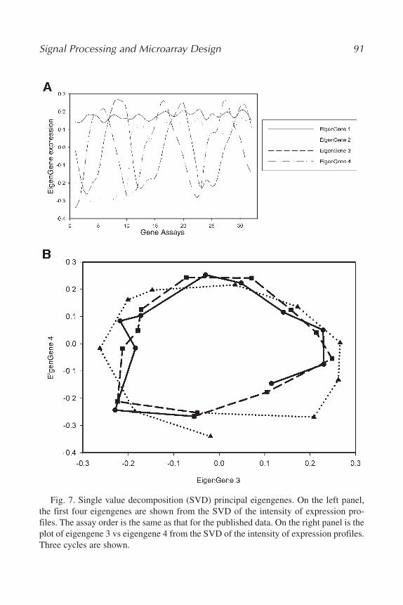
Signal Processing and Microarray Design 91
Fig. 7. Single value decomposition (SVD) principal eigengenes. On the left panel,the first four eigengenes are shown from the SVD of the intensity of expression pro-files. The assay order is the same as that for the published data. On the right panel is theplot of eigengene 3 vs eigengene 4 from the SVD of the intensity of expression profiles.Three cycles are shown.
04_Klevecz.qxd 6/3/07 3:18 PM Page 91
From a purely practical perspective, a significant effort should be put intoresolving the question of genome-wide oscillations using the microarraytechnologies if for no other reason than to improve the signal-to-noise ratio.The application of analytical methods that are suited to nonlinearities intime-series data should also find a wider use. It seems clear that the mostsuccessful and widely applied method so far is SVD. In theory, waveletanalysis has some advantages over FFTs for the data length and densitieslikely to be encountered in expression-array studies. It will be muchimproved if optimized wavelet families are found that can represent the tran-script or other biological signal of interest efficiently and accurately. Havingsaid that, we were surprised to find that FFT filtering, that is, using theFourier transform to sort those transcripts showing a particular frequencywas very successful; though it must be added that this was a relatively longand densely sampled dataset.
3.15. Sampling in Clinical Studies
Exempted from the criticisms and conclusions developed here are clinicalstudies where the biology is unavoidably bad but where the solution—to dotime-series analysis—is not feasible in most instances under prevailing proto-cols. It will be of interest to see whether using the limited information availableregarding the time of day when a sample was taken can improve the diagnosticutility of expression microarrays and begin the process of uncovering thedynamics of expression in tumor cells.
The presence of genome-wide oscillations in yeast raises the possibility ofsimilar dynamics in mammalian cells and tissues. Circadian and higher fre-quency oscillations have been known for more than 50 yr and are well charac-terized in extensive literature. In both dividing and nondividing mammaliantissues, oscillations with periods from a few hours to a day in length have beenobserved in essentially every constituent examined. For some genes importantin chemotherapy, day-to-night variation can be as much as 10-fold. If samplesare taken from differing tumor tissues without regard to time, with the idea thatvariation between samples may be exploitable for diagnostic clustering ortreatment, the possibility that the variation may have more to do with circadianor regular higher frequency oscillations than with any exploitable intrinsic dif-ference must be considered.
4. Notes1. Optimize experimental design and sampling for time-series analysis. Take a mini-
mum of 8 samples/cycle. Sampling interval should be such that 8 samples multipliedby the sample interval is exactly equal to the cycle time. For example, if the cycletime equals 43 min, then the sampling interval should be 5.38 min.
92 Klevecz et al.
04_Klevecz.qxd 6/3/07 3:18 PM Page 92

2. Total RNA content, and in particular mRNA content, may not be constant throughthe cycle. To control for biological vs recovery differences, all samples are spikedwith a constant amount of a poly-A standard before beginning isolation. OtherRNA standards can be used including S. pombe mRNA.
3. It should be possible to use the single-step amplification using the IVT kit.4. If all samples cannot be done on the same day in the same batch, randomize the
sample series. If time-series replicates are available run replicates separately ineach batch.
5. Use raw data with all Affymetrix normalization and scaling factors set to 1.6. Currently, no commercial software products have adequate time-series analysis
algorithms. Paste Affymetrix txt files into Excel. Excel has the virtue that all datamanipulation is open—there are no black boxes as there are in commercial packages.
7. Copy out cerevisiae and standards to separate worksheets.8. To avoid missing interesting low expressers, retain all transcripts in which at least
one sample in each cycle is called “P” (present).9. For a cleaner less noisy result, remove all transcripts from the entire time series if
any member of the time series contains an “A” (absent) calls.10. Adjust all samples in the time series for differences in hybridization using the
biotinylated standards and a polynomial fit. Calculate the mean of the hybridiza-tion standards. Fit a polynomial to these mean values. Correct each of the stan-dards in the time-series data to the fitted result. Correct the signals for expressedtranscripts by this same technique.
11. Test all samples for large differences in mRNA recovery using the B. subtilispoly(A) standards. Use the same routine as described in Note 10. If no large dis-crepancies are seen, use the result from Note 10.
12. A number of suitable Math packages are available including Bioconductor, anR-based collection, as well as the more standard Mathcad, Matlab, S-Plus, andJMP. Both Matlab and Mathcad have a very complete set of signal-processingroutines including FFT, SVD, and WMD.
References1. Kauffman, S. and Wille, J. J. (1975) The mitotic oscillator in Physarum poly-
cephalum. J. Theor. Biol. 55, 47–93.2. Klevecz, R. R. and Shymko, R. M. (1985) Quasi-exponential generation time dis-
tributions from a limit cycle oscillator. Cell Tissue Kinet. 18, 263–271.3. Mackey, M. C. and Glass, L. (1977) Oscillation and chaos in physiological control
systems. Science 197, 287–289.4. Klevecz, R. R. (1998) Phenotypic heterogeneity and genotypic instability in cou-
pled cellular arrays. Physica D 124, 1–10.5. Klevecz, R. R., Kros, J., and Gross, S. D. (1978) Phase response versus positive
and negative division delay in animal cells. Exp. Cell Res. 116, 285–290.6. Klevecz, R. R., Bolen, J., Forrest, G., and Murray, D. B. (2004) A genomewide
oscillation in transcription gates DNA replication and cell cycle. Proc. Natl. Acad.Sci. USA 101, 1200–1205.
Signal Processing and Microarray Design 93
04_Klevecz.qxd 6/3/07 3:18 PM Page 93
7. Klevecz, R. R. and Murray, D. B. (2001) Genome wide oscillations in expression.Mol. Biol. Reports 28, 73–82.
8. Murray, D. B., Klevecz, R. R., and Lloyd, D. (2003) Generation and maintenanceof synchrony in Saccharomyces cerevisiae continuous culture. Exp. Cell. Res. 287,10–15.
9. Satroutdinov, A. D., Kuriyama, H., and Kobayashi, H. (1992) Oscillatory metabo-lism of Saccharomyces cerevisiae in continuous culture. FEMS Microbiol Lett. 77,261–267.
10. Murray, D. B., Engelen, F., Lloyd, D., and Kuriyama, H. (1999) Involvement ofglutathione in the regulation of respiratory oscillation during a continuous cultureof Saccharomyces cerevisiae. Microbiol. 145, 2739–3747.
11. Mochan, E. and Pye, E. K. (1973) Respiratory oscillations in adapting yeast cul-tures. Nat. New Biol. 242, 177–179.
12. Poole, R. K., and Lloyd, D. Oscillations of enzyme activities during the cell-cycleof a glucose-repressed fission-yeast, Schizosaccharomyces pombe 972h-. Biochem. J.136, 195–207.
13. Klevecz, R. R. and Dowse, H. B. (2000) Tuning in the transcriptome: basins ofattraction in the yeast cell cycle. Cell Proliferation 33, 209–218.
14. Klevecz, R. R. (2000) Dynamic architecture of the yeast cell cycle uncovered bywavelet decomposition of expression microarray data. Funct. Integr. Genom. 1,186–192.
15. Rifkin, S. A. and Kim, J. (2002) Geometry of gene expression dynamics.Bioinformatics 18, 1176–1183.
16. Alter, O., Brown, P. O., and Botstein, D. (2000) Singular value decomposition forgenome-wide expression data processing and modeling.) Proc. Natl. Acad. Sci.USA 100, 3351–3356.
17. Alter, O., Brown, P. O., and Botstein, D. (2003) Generalized singular value decom-position for comparative analysis of genome-scale expression datasets of two dif-ferent organisms. Proc. Natl. Acad. Sci. USA 97, 10,101–10,106.
18. Warrington, J. A., Nair, A., Mahadevappa, M., and Tsyganskaya, M. (2000)Comparison of human adult and fetal expression and identification of 535 house-keeping/maintenance genes. Physiol. Genomics 2, 143–147.
94 Klevecz et al.
04_Klevecz.qxd 6/3/07 3:18 PM Page 94

5
Predictive Models of Gene RegulationApplication of Regression Methods to Microarray Data
Debopriya Das and Michael Q. Zhang
SummaryEukaryotic transcription is a complex process. A myriad of biochemical signals cause activa-
tors and repressors to bind specific cis-elements on the promoter DNA, which help to recruit thebasal transcription machinery that ultimately initiates transcription. In this chapter, we discusshow regression techniques can be effectively used to infer the functional cis-regulatory elementsand their cooperativity from microarray data. Examples from yeast cell cycle are drawn todemonstrate the power of these techniques. Periodic regulation of the cell cycle, connection withunderlying energetics, and the inference of combinatorial logic are also discussed. An implemen-tation based on regression splines is discussed in detail.
Key Words: Transcription regulation; regression; splines; cooperativity; correlation; yeast;cell cycle; cis-regulatory element; MARS.
1. IntroductionIn the past decade, there have been tremendous advances in high-throughput
molecular technologies for measuring mRNA levels genome wide. Such tech-nologies not only provide information on which genes are over- or under-expressed, but along with genomic sequence data, also allow one to obtain adeeper insight into the cis-regulatory mechanisms that drive gene transcription.One problem that has been intensively studied in this context is to identify thecis-elements that control and regulate the transcription process. The traditionalapproach to solve this problem has been to cluster genes by their expressionprofiles across multiple conditions and to find over-represented motifs in pro-moters of genes in each cluster (1). Clustering-based approaches gaveresearchers a starting tool kit to obtain a snapshot of key regulatory elements.However, it became increasingly clear that such approaches have severallimitations. First, many genes often do not cluster tightly enough to allow for
95
From: Methods in Molecular Biology, vol. 377, Microarray Data Analysis: Methods and ApplicationsEdited by: M. J. Korenberg © Humana Press Inc., Totowa, NJ
05_Das.qxd 6/3/07 3:19 PM Page 95
identification of their regulatory elements with reasonable accuracy. Second,gene regulation is combinatorial with a significant amount of cooperativity,especially in mammals. Classifying genes into disjoint clusters can often leadto incomplete identification of functional motif combinations. Additionally,some genes in an expression cluster may exist because of secondary effects andmay be regulated by elements different from those for the primary responsegenes. Most importantly, clustering methods require expression data from mul-tiple conditions, which is not always available.
Over the past few years, a new paradigm has emerged involving methodolo-gies that can efficiently extract information on functional cis-regulatory elementsand their functional combinations from microarray data on just a few condition.We will review these interesting developments in this chapter. This is by nomeans an exhaustive survey. But, we hope to convey the essential points. We willprimarily use yeast cell cycle expression data to compare the techniques.
2. Regression Approach to Cis-Regulatory Element Analysis2.1. Basic Idea
In order to obtain functional regulatory motifs on promoter DNA frommicroarray expression data using regression, one correlates the motif occur-rences with the logarithm of expression ratios (2). The basic idea behind thiscan be explained as follows. For a given cell type, only a limited set of tran-scription factors (TFs) are active under any given condition. The extent towhich genes are up/downregulated in these cells depends directly on thestrength with which these TFs and their combinations bind to their promoterDNA, if they bind at all. For a low eukaryote like yeast, the motifs are largelynondegenerate and the strength of binding to a particular motif is directlyrelated to its count in the promoter of each gene. Thus, the mRNA levels mustdirectly correlate with the modulation of motif occurrences across the genes. Aregulatory motif that is active would strongly correlate with the expression lev-els and vice versa. Regression analyses exploit these correlations to infer thefunctional cis-elements and their cooperativity.
Consider, for example, that we are interested in the effect of the MCB (MLuIcell-cycle box) element, ACGCGT, on yeast cell cycle at a particular time-point. To do this, one records the counts ng of the MCB motif in the promoterof each gene g and also the logarithm of their expression ratios, log(Eg/EgC),where Eg is the mRNA level of gene g at the given time-point and EgC is thatfor the control set C. The control can be, for example, a homogeneous mix ofmRNAs across all the cell cycle phases. One then examines correlation betweenthe log(Eg/EgC) values and the counts ng by fitting a straight line:
ygp = a + bng (1)
96 Das and Zhang
05_Das.qxd 6/3/07 3:19 PM Page 96
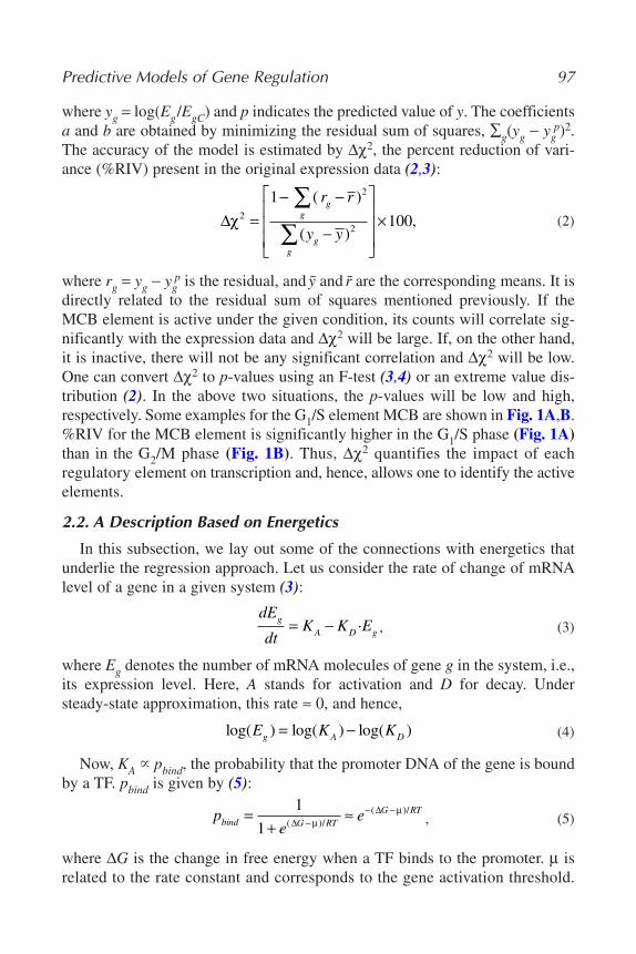
where yg = log(Eg/EgC) and p indicates the predicted value of y. The coefficientsa and b are obtained by minimizing the residual sum of squares, ∑g(yg − yg
p)2.The accuracy of the model is estimated by ∆χ2, the percent reduction of vari-ance (%RIV) present in the original expression data (2,3):
(2)
where rg = yg − ygp is the residual, and y and r are the corresponding means. It is
directly related to the residual sum of squares mentioned previously. If theMCB element is active under the given condition, its counts will correlate sig-nificantly with the expression data and ∆χ2 will be large. If, on the other hand,it is inactive, there will not be any significant correlation and ∆χ2 will be low.One can convert ∆χ2 to p-values using an F-test (3,4) or an extreme value dis-tribution (2). In the above two situations, the p-values will be low and high,respectively. Some examples for the G1/S element MCB are shown in Fig. 1A,B.%RIV for the MCB element is significantly higher in the G1/S phase (Fig. 1A)than in the G2/M phase (Fig. 1B). Thus, ∆χ2 quantifies the impact of eachregulatory element on transcription and, hence, allows one to identify the activeelements.
2.2. A Description Based on Energetics
In this subsection, we lay out some of the connections with energetics thatunderlie the regression approach. Let us consider the rate of change of mRNAlevel of a gene in a given system (3):
, (3)
where Eg denotes the number of mRNA molecules of gene g in the system, i.e.,its expression level. Here, A stands for activation and D for decay. Understeady-state approximation, this rate ≈ 0, and hence,
(4)
Now, KA � pbind, the probability that the promoter DNA of the gene is boundby a TF. pbind is given by (5):
, (5)
where ∆G is the change in free energy when a TF binds to the promoter. µ isrelated to the rate constant and corresponds to the gene activation threshold.
pe
ebind G RTG RT=
+≈−
− −1
1 ( )/( )/
∆∆
µµ
log( ) log( ) log( )E K Kg A D= −
dE
dtK K Eg
A D g= − ·
∆χ ×2
2
2
1
100=− −
−
⎡
⎣
⎢⎢⎢
⎤
⎦
⎥⎥⎥
∑∑
( )
( ),
r r
y y
gg
gg
Predictive Models of Gene Regulation 97
05_Das.qxd 6/3/07 3:19 PM Page 97
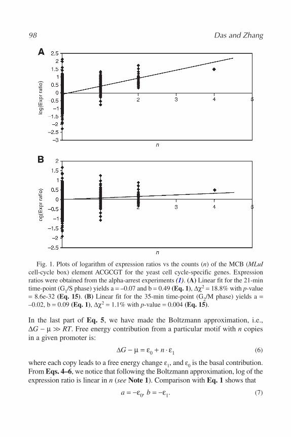
In the last part of Eq. 5, we have made the Boltzmann approximation, i.e.,∆G − µ >> RT. Free energy contribution from a particular motif with n copiesin a given promoter is:
∆G − µ = ε0 + n · ε1 (6)
where each copy leads to a free energy change ε1, and ε0 is the basal contribution.From Eqs. 4–6, we notice that following the Boltzmann approximation, log of theexpression ratio is linear in n (see Note 1). Comparison with Eq. 1 shows that
a = −ε0, b = −ε1. (7)
98 Das and Zhang
Fig. 1. Plots of logarithm of expression ratios vs the counts (n) of the MCB (MLuIcell-cycle box) element ACGCGT for the yeast cell cycle-specific genes. Expressionratios were obtained from the alpha-arrest experiments (1). (A) Linear fit for the 21-mintime-point (G1/S phase) yields a = –0.07 and b = 0.49 (Eq. 1), ∆χ2 = 18.8% with p-value= 8.6e-32 (Eq. 15). (B) Linear fit for the 35-min time-point (G2/M phase) yields a =–0.02, b = 0.09 (Eq. 1), ∆χ2 = 1.1% with p-value = 0.004 (Eq. 15).
05_Das.qxd 6/3/07 3:19 PM Page 98

That is, the fit coefficients of regression models of expression ratios are ameasure of binding free energy (see Note 2). This can be very nicely seen fromthe predicted time courses of MCB and SCB (Swi4/6 cell-cycle box) elementsduring the yeast cell cycle (2). MCB and SCB elements are active during theG1/S phase of the cell cycle. From Fig. 1A of ref. 2, we notice that the fit coef-ficients are strongly positive near the G1/S phase (time-points 21 and 77) andstrongly negative near the G2/M phase (time-point 56). Thus, according to theprevious discussions, the binding energies are strongly negative at the G1/Sphase, i.e., it is favorable to bind the MCB and SCB elements in this phase. Onthe other hand, in the G2/M phase, the binding energies are positive, and MCBand SCB elements are very unfavorable to be bound, i.e., they are inactive.
2.3. Combinatorial Regulation via Multivariate Linear Models
REDUCE (Regulatory Element Detection Using Correlation with Expression),proposed by Bussemaker et al. (2), goes a step ahead and considers the effects ofcombinatorial regulation via multiple transcription factors. Here multiple motifscontribute additively to the log of expression ratio:
(8)
where the index µ indicates motif id and ngµ is the count of motif µ for gene g.
The coefficient bµ is the (free energy) contribution from the motif µ. The sig-nificant motifs are determined by a step-wise linear regression and the coeffi-cients a and {bµ} are obtained finally by a multivariate linear fit. Using theyeast cell cycle data as an example, Bussemaker et al. showed that REDUCEcan verify many regulatory motifs important in the cell cycle obtained by theclustering approach (1,6). MCB, SCB, SFF, Swi5, and stress response elementSTRE and Met31/32 are some such examples. Using Mcm1 as an example, theyfurther showed that if a position weight matrix (PWM) score is used instead ofword counts, the accuracy, as determined by %RIV, can go up by as much as80% (see Note 3). A more comprehensive analysis using weight matrices waslater done by Conlon et al. (4). They designed the algorithm, MotifRegressor,which combines the ab-initio motif finder MDscan (7) with multivariate linearregression. Thus, MDscan was used to generate a large number of PWMs. Aprioritized list of motifs was initially selected from this set by applying regres-sion on individual motifs. The significant motifs were finally determined bystep-wise linear regression on the prioritized set, leading to the model:
(9)y a b Sgp
g= + ∑ µµ
µ
y a b ngp
g= + ∑ µµ
µ
Predictive Models of Gene Regulation 99
05_Das.qxd 6/3/07 3:20 PM Page 99
where Sgµ is the PWM score (4) for the motif µ in the promoter of gene g.
MotifRegressor, like REDUCE, could identify several key regulatory motifs inthe yeast cell cycle and other experiments.
3. CooperativityThe prior models do not account for cooperativity. Cooperativity among TFs
is a salient aspect of eukaryotic transcription (8,9). This is even more so inmammals, where transcription is considered to be almost promiscuous (9).Hence, such synergistic effects must be incorporated in the computational mod-els to get an accurate view of the underlying regulation process. Cooperativityamong multiple motifs is reflected in more than additive contributions fromsuch motifs, in contrast to what is captured by the linear models in the previoussection.
3.1. Expression Coherence Score Approach
Models of cooperativity which did not rely on clustering were first proposedby Pilpel et al. (10) and later advanced by Banerjee et al. (11,12). The methodis based on the use of expression coherence scores. Here, one first finds motifsin the promoters of the genes and considers all possible pairs of motifs. For agiven pair of motifs A and B, three sets of genes are considered: those that haveboth A and B, those that have A but not B, and those that have B but not A. Foreach set, an expression coherence (EC) score is calculated, which measureshow tightly correlated the expression levels of an average pair of genes in theset (relative to a random pair) are based on a distance measure (Euclidean dis-tance [10] or correlation coefficient [11]). For a synergistic motif pair, the geneset with both motifs A and B has a much higher EC score than those with eitherof them alone. Banerjee et al. (11) later quantified this difference in terms of ap-value based on a hypergeometric distribution. This method reproduced sev-eral well-known synergistic pairs in yeast (10,11): Mcm1-SFF (cell cycle),Mcm1-Ste12 (sporulation), Bas1-Gcn4 (heat shock), Mbp1-Swi6 (cell cycle),Swi4-Swi6 (cell cycle), Ndd1-Stb1 (cell cycle). The last three pairs are citedfrom ref. 11, where ChIP-chip data was used to identify the targets of a givenTF, and then microarray data was used to obtain the cooperative TF pairs.
3.2. Toward a Synthesis: Regression Models of Cooperativity
The disadvantage of the EC score framework is that it is hard to quantify therelative impact of individual motifs and pairs of motifs on gene expression. Also,it needs expression data across multiple time-points to calculate the correlationmeasures. These limitations can be easily overcome if cooperativity is builtdirectly into a regression model. This was implemented by Keles et al. (13) in
100 Das and Zhang
05_Das.qxd 6/3/07 3:20 PM Page 100
the program SCVmotif, where cooperativity was introduced as product terms inthe model. Thus, for example, for motifs 1 and 2, Eq. 6 needs to be modified as:
(10)
Thus, two motifs make more than (or less than) additive contributions tothe log expression ratio leading to synergistic effects. Here, relative distance,orientation, or other parameters related to the physical locations of the twomotifs are not considered. Thus, the assumption here is that for a given numberof motifs of type 1 and 2, each pair of these two motifs makes a similar freeenergy contribution on average upon TF binding, independent of their relativephysical locations on the promoter DNA.
SCVmotif (13) considers interactions between all pairs of motifs. Thus, themodel has the structure:
, (11)
where the Greek indices indicate motif ids. The authors used a variant of wordcounts that incorporated the probability distribution of the words in the pro-moter regions (13). Interaction terms involving the same motif were ignored.Significant motifs and motif pairs were determined by a combination of for-ward and backward selection, and cross-validation. Yeast cell cycle was used toshow that several motifs can be correctly predicted in the G1/S phase by includ-ing interactions. MCB and SCB are two such examples. Interaction betweenthem was also found to be significant.
4. Spline Models of Cooperative Gene RegulationThe previous methods provided a foundation for the regression approach to
identification of functional motifs from gene-expression data. However, closeranalysis revealed several limitations. For example, when applied to the yeastcell cycle data, we found that linear models learnt by REDUCE (2) lead to a%RIV of only 10% on average (noise level accounts for ~50% [2]). The modelsthat include cooperativity, as discussed previously, are also limiting. With thefeature selection approach proposed by Keles et al. (13,14), we found that eitherthe known pairs of motifs are not quite often correctly predicted or the accuracyof the regression model does not improve significantly (<5%) when interactingpairs are introduced in the model, which is inconsistent with the biologicalnotion of synergistic gene regulation. Furthermore, gene transcription is stronglynonlinear (8). None of these models captures the nonlinearities.
Many of these limitations can be avoided by using spline models (3). Wefirst note that the TF-binding probabilities have a sigmoidal dependence
y a b n c n ngp
g g g= + +∑ ∑µµ
µµ
µ
µν
ν
ν,
∆G n n n n n n− = + + + + +µ ε ε ε ε ε0 1 1 2 2 11 1 1 22 2 2· · ·( · ) ( · ) εε12 1 2·( · )n n
Predictive Models of Gene Regulation 101
05_Das.qxd 6/3/07 3:20 PM Page 101
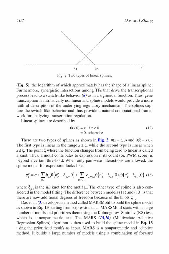
(Eq. 5), the logarithm of which approximately has the shape of a linear spline.Furthermore, synergistic interactions among TFs that drive the transcriptionalprocess lead to a switch-like behavior (8) as in a sigmoidal function. Thus, genetranscription is intrinsically nonlinear and spline models would provide a morefaithful description of the underlying regulatory mechanism. The splines cap-ture the switch-like behavior and thus provide a natural computational frame-work for analyzing transcription regulation.
Linear splines are described by
θ(x,0) = x, if x ≥ 0 (12)= 0, otherwise
There are two types of splines as shown in Fig. 2: θ(x − ξ,0) and θ(ξ − x,0).The first type is linear in the range x ≥ ξ, while the second type is linear when x ≤ ξ. The point ξ where the function changes from being zero to linear is calleda knot. Thus, a motif contributes to expression if its count (or, PWM score) isbeyond a certain threshold. When only pair-wise interactions are allowed, thespline model for expression looks like:
(13)
where ξµ,i is the ith knot for the motif µ. The other type of spline is also con-sidered in the model fitting. The difference between models (11) and (13) is thatthere are now additional degrees of freedom because of the knots ξµ,i.
Das et al. (3) developed a method called MARSMotif to build the spline modelas shown in Eq. 13 starting from expression data. MARSMotif starts with a largenumber of motifs and prioritizes them using the Kolmogorov–Smirnov (KS) test,which is a nonparametric test. The MARS (15,16) (Multivariate AdaptiveRegression Splines) algorithm is then used to build the spline model in Eq. 13using the prioritized motifs as input. MARS is a nonparametric and adaptivemethod. It builds a large number of models using a combination of forward
y a b n c ngp
ii
g i i j g= + −( ) + −∑ µµ
µµ µ
µµθ ξ θ ξ,
,, , , ,, 0 ν ,, ,
, , ,
, · ,i g ji j
n0 0( ) −( )∑ θ ξµ
νν
ν
102 Das and Zhang
Fig. 2. Two types of linear splines.
05_Das.qxd 6/3/07 3:20 PM Page 102

selection and backward elimination. The terms and knots are enumerated by min-imizing the residual sum of squares. The final model is selected by minimizing thegeneral cross-validation score (GCV), which controls overfitting:
(14)
where M is the effective number of parameters in the model and N is the totalnumber of genes. M is estimated by cross validation. GCV-based model selec-tion ensures the number of terms in the model is small (3). Interactions involv-ing the same motif are written as a sum of splines in MARS. Thus, µ ≠ v in thethird term in Eq. 13. MARSMotif works with both motif counts and weightmatrix scores. In fact, it can work with a hybrid set of such inputs (3).
4.1. Periodic Regulation of Cell Cycle
We first discuss the differences between a linear model and a MARSMotifmodel for a single motif and a pair of motifs. When the expression level of a givenTF is low, the cis-regulatory motif to which it binds is inactive, and the correspon-ding regression model for this motif must yield ∆χ2 ≈ 0. On the other hand, whenthe expression level of the TF is high, its binding cis-motif is active (under typi-cal conditions), and its regression model must lead to ∆χ2 >> 0. Because theexpression levels of some of the key regulators vary periodically with the cellcycle (1,2), the %RIV for their corresponding binding elements should also varyperiodically. This is shown in Fig. 3A,B for SCB and MCB elements, respec-tively, where word counts have been used as inputs. There are actually two cellcycles in these experiments. But, because ∆χ2 ≥ 0, there are four peaks in thesefigures instead of two. For a single motif with word count, we notice that the lin-ear and MARSMotif models are almost identical. This is not surprising becausea linear model with word counts already has a built-in cutoff as word counts are dis-crete, and thus in a sense, mimics linear splines. This is not the case for position-weight matrices, as shown in Fig. 3C, where we show the time course of theMcm1 motif. Mcm1 is a very degenerate motif with two conserved dinucleotides,separated by six nucleotides (2). In this case, the periodicity is still retained in thelinear model, but peaks are much sharper in the MARSMotif model. We have alsoshown here the model that uses only a single linear spline. Both in terms of peri-odicity and sharpness of peaks, this seems to be the optimal choice (see Note 4).Thus, for a single motif, the analog of a linear model with motif count as input isa linear spline model with PWM score as input. For a pair of motifs, the interac-tions are important. In this case (Fig. 3D), the periodicity is lost in a linear model,and in the MARSMotif model, it clearly stands out.
GCV
E E y
M N
g gC gp
g
N
=−⎡⎣ ⎤⎦
−=
∑ log( / )
[ / ]
2
1
21
Predictive Models of Gene Regulation 103
05_Das.qxd 6/3/07 3:20 PM Page 103
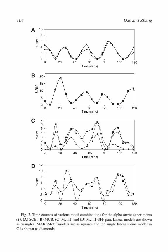
104 Das and Zhang
Fig. 3. Time courses of various motif combinations for the alpha-arrest experiments(1): (A) SCB, (B) MCB, (C) Mcm1, and (D) Mcm1-SFF pair. Linear models are shownas triangles, MARSMotif models are as squares and the single linear spline model inC is shown as diamonds.
05_Das.qxd 6/3/07 3:20 PM Page 104

4.2. Summary of MARSMotif Results
Das et al. (3) applied MARSMotif to the yeast cell cycle data (1,17) using sixinput sets of motifs generated by different ab-initio motif-finding algorithms:(1) counts of motifs found by AlignACE (10), a Gibbs-sampling approach, (2)weight matrix scores of motifs from AlignACE (10), (3) counts of motifs dis-covered by cross-species conservation (18), (4) counts of a curated set of motifs(3), (5) counts of 5–7mer DNA words, which were clustered by their similarityto each other to obtain a nonredundant set, and (6) same as set (5), except thatclustering was done using motifs obtained by cross-species conservation (18) astemplates. MARSMotif yielded a higher %RIV than REDUCE, regardless ofwhich type of motif input was used: 13.9–32.9% on an average, which is about1.5–3.5 times that of REDUCE. The %RIV is highest for word counts, as in set(5), and worst for set (3). Because REDUCE was done with word counts, trueimprovement lies toward the upper end of this range. When interactions wereincluded in the model, %RIV increased in 69–88% of the cases, and the frac-tional increase in %RIV in these cases was 47–96%, depending on which motifset was used. This shows that MARSMotif can suitably model synergistic effectsthat are widespread in eukaryotic transcription regulation. It is sensitive towhich type of motif set is used as input. When both %RIV and modeling of syn-ergistic effects are considered, combination of word counts and cross-speciesconservation (input set [5] above) is the optimal choice for yeast.
MARSMotif not only led to a higher quantitative accuracy, but also detectedseveral motifs and motif pairs previously known as important regulators of cellcycle. For example, the classical cell cycle-regulatory motifs were found at thecorrect stages of cell cycle: MCB and SCB in G1/S phase, Mcm1 and SFF atthe G2/M phase, and Ace2, Swi5, and Ste12 at the M/G1 phase. Several nonclas-sical motifs, e.g., Rme1, Adr1, and Rap1, were also identified as significant.Among motif pairs, the well-known Mcm1-SFF pair was identified as func-tional in the G2/M phase. Other examples of known cell cycle-regulatory pairsdetected by MARSMotif included Mcm1-Ste12 and Ace2-Swi5. The rest of thepairs identified as significant by MARSMotif were either known pairs that par-ticipate in processes secondary to the cell cycle (e.g., Alpha2-Mcm1), com-pletely novel (e.g., GCR1-SWI4), or were supported by other computationalmethods (e.g., Ace2-SFF). An important point is that, in contrast to a method likethe EC score approach, MARSMotif can identify the specific phase/time-pointwhere a given motif combination is active. More details are available in ref. 3.
5. SummaryIn this chapter we have reviewed how regression methods can be used to extract
information on transcription regulation from microarray data in eukaryotic
Predictive Models of Gene Regulation 105
05_Das.qxd 6/3/07 3:20 PM Page 105
systems. Here all genes are fit. So regulatory information of all genes can beobtained, at least in principle. The relative impact of each motif and motif pairon gene expression can be directly quantified as well. Percent reduction in vari-ance of expression log ratios, on the other hand, provides a quantitative estimateof how complete the discovery is. No background sequence sets or any priorsystem-specific knowledge of transcription are necessary either. In this sense,the methods are quite unbiased. They can work with limited expression data:microarray data from a single time-point and a control set are sufficient to dothe analysis. Additionally, regression splines model the underlying bioenerget-ics and can produce a quantitatively highly accurate model of transcription reg-ulation. Individual motifs and cooperative motif combinations, which are activeunder a specific condition, can also be very accurately predicted. Apart frommodeling energetics, linear splines help to filter noise present in the input motifsets by allowing nonzero contributions only beyond a certain threshold.
Predicting gene expression levels from DNA sequence information andinvoking combinatorial logic in this prediction are important topics of currentresearch in modeling gene regulation (19). It is very easy to see from the previ-ous discussions that regression methods allow one to predict expression levelsof a gene from sequence data. Combinatorial logic of the type AND, OR, andNOT are also captured in the splines framework. Presence of AND logic isobvious from the product terms in Eq. 13. OR logic can be seen from theinvolvement of terms of type θ(S1 − ξ1,0) + θ(S2 − ξ2,0) where Si is the PWMscore of the motif i. There is a finite contribution to expression if S1 > ξ1 orS2 − ξ2 or both. An example of NOT logic would be a term like θ(S1 − ξ1,0),where the knot ξ1 is very small. That is, this term is finite only when the motifis absent.
Use of cross-species conservation in promoter regions has been shown toimprove the performance of regression methods (14). However, conservation isalso known to increase the false-negative rate of identifying motifs specific to agiven organism (20). Constraints on regulatory elements, e.g., relative orienta-tion, distance from transcription start site, and so on need to be incorporated toobtain a more accurate view of transcription regulation. In this context, appli-cation of Bayesian networks is noteworthy (19). Several classification methodshave also been applied to the problem of regulatory element identification thatwe have not reviewed here (21,22).
Regression methods have been applied to expression data from highereukaryotes as well, e.g., in Drosophila (23), and have now been successfullyextended to mammals (24). Additionally, linear splines allow one to predictdirect targets of active motif combinations from a small amount of microarraydata with high accuracy (24). In conclusion, current developments lead us tobelieve that regression methods will allow researchers to comprehensively
106 Das and Zhang
05_Das.qxd 6/3/07 3:20 PM Page 106
dissect the transcription-regulation process across a wide range of eukaryoticsystems even when only a limited amount of microarray data is available.
6. MARSMotif: An ImplementationHere we discuss how to implement the MARSMotif algorithm (3). We first
discuss the algorithm for individual motifs, and then for combinations of motifsallowing for interactions.
6.1. MARSMotif for Individual Motifs
Given a set of candidate motifs, we first examined association of each motifwith expression using the KS test. It is a nonparametric test that assigns a p-value based on the maximum distance between the two respective cumulativedistribution functions. For any given motif, we compared the distribution ofexpression values for the genes that have the motif with the distribution forgenes that do not have that motif. The KS test was implemented using the sub-routine given in ref. 25. This subroutine works only when ne = n1n2/(n1 + n2) ≥ 4,where n1 and n2 are the number of genes in the two samples. For all other cases,we used the KS test available in S-PLUS.
The top 100 motifs by KS p-value were used in MARS regression. MARSwas run iteratively with 40 motifs at a time; at most, top 30 motifs were retainedfrom the previous run where motif ranking is based on the variable importancereported by MARS. This was augmented with additional motifs to make thenumber up to a maximum of 40. The final run produced the list of significantmotifs.
We used the MARS program available from Salford Systems (26)(http://www.salford-systems.com/). We ran MARS with basis functions (linearsplines and their products) at six times the number of motifs (minimum num-ber of basis functions = 25) and speed=1, allowing for no interactions betweendistinct motifs (int=1). Speed=1 ensures that the accuracy of the program ishighest, although at the expense of speed. We used 10-fold cross validation toobtain the effective number of parameters appearing in the GCV score (Eq. 14)(see Note 5).
6.2. MARSMotif for Pairs of Motifs
For a given set of input motifs, the pairs of motifs were first constructedfrom the top 100 motifs selected using the KS test for individual motifs(see Subheading 6.1.). For any given pair of motifs, we compared the expres-sion values of genes that have that pair of the motifs with the expression valuesof genes that have one or the other motif (but not both) using the KS test. Thiscomparison allowed us to capture the potentially synergistic pairs. KS test wasimplemented as in Subheading 6.1.
Predictive Models of Gene Regulation 107
05_Das.qxd 6/3/07 3:20 PM Page 107

The top 200 motif pairs from the KS test were then used in MARS regression.In each MARS iteration, every time a motif was included all of its interactingpartners detected via KS test were included as well. We stopped adding motifsto the input set for a given iteration as soon as the number of motifs exceeded 40.MARS was run allowing for pair-wise (int = 2) and third-order (int = 3) inter-actions separately. Apart from the interactions, the settings for MARS runswere the same as those for the individual motifs (see Subheading 6.1.).
For each interaction setting, the motifs that were found significant by MARSwere then combined with the set of motifs found significant in the MARS run withindividual motifs (see Subheading 6.1.). MARS was then rerun allowing for thesame order of interactions (int=2 or 3) in this set. The motifs and motif pairs iden-tified to be important by MARS in this final run were considered as significant.
6.3. Final Model Selection
For each interaction setting, p-values of motifs and motif pairs discovered byMARS were computed based on an F-test (16) (see Note 6):
(15)
where RSS1 is the residual sum of squares of the final MARS model with p1 + 1terms, and RSS0 is the residual sum of squares of the MARS model without aparticular motif (or, motif pair) which has p0 + 1 terms in it. N is the numberof genes used in the model. The F statistic has an F distribution with p1 − p0numerator degrees of freedom and N − p1 − 1 denominator degrees of freedom.The corresponding p-value was calculated in S-PLUS. The p-values were thencorrected for multiple testing (3). Following corrections, if p > 0.01 for a motif(or a motif pair), all the basis functions involving that motif (or motif pair) weredeleted from the MARS model. This is the final pruned model for a giveninteraction setting. We then obtain the ∆χ2 corresponding to this pruned model.The interaction setting for which the pruned model had ∆χ2 as maximum wasidentified as the optimal model by MARSMotif.
7. Notes1. The advantage of using ratios of expression levels is that only a few motifs that are
different between the test and control samples contribute significantly to the model.2. Here n.ε1 represents the total binding free energy owing to the motif under the
given condition. Thus, ε1 is implicitly dependent on the average concentration ofthe TF binding to this motif.
3. When interactions are included through a more complete modeling via linearsplines, this is generally not true. Word counts perform better than the weight matri-ces in yeast.
FRSS RSS p p
RSS N p=
− −− −
( ) ( )
( )0 1 1 0
1 1 1
108 Das and Zhang
05_Das.qxd 6/3/07 3:20 PM Page 108

4. We think this is because of the noise arising from use of multiple splines in MARSfor the case of one motif.
5. Use of a large number of basis functions can unusually slow down the program.6. Although a third-order combination can be directly inferred from the int=3 model,
we decomposed such combinations into pairs because more often experimentalevidence for pairs of motifs are reported in the literature.
AcknowledgmentsWe thank Gengxin Chen for a careful reading of the manuscript. This work
was supported by NIH grants HG01696 (M. Q. Z) and GM60513 (M. Q. Z) andCSHL Association Fellowship (D. D.).
References1. Spellman, P. T., Sherlock, G., Zhang, M. Q., et al. (1998) Comprehensive identifi-
cation of cell cycle-regulated genes of the yeast Saccharomyces cerevisiae bymicroarray hybridization. Mol. Biol. Cell. 9, 3273–3297.
2. Bussemaker, H. J., Li, H., and Siggia, E. D. (2001) Regulatory element detectionusing correlation with expression. Nat. Genet. 27, 167–171.
3. Das, D., Banerjee, N., and Zhang, M. Q. (2004) Interacting models of cooperativegene regulation. Proc. Natl. Acad. Sci. USA 101, 16,234–16,239.
4. Conlon, E. M., Liu, X. S., Lieb, J. D., and Liu, J. S. (2003) Integrating regulatorymotif discovery and genome-wide expression analysis. Proc. Natl. Acad. Sci. USA100, 3339–3344.
5. Djordjevic, M., Sengupta, A. M., and Shraiman, B. I. (2003) A biophysicalapproach to transcription factor binding site discovery. Genome Res. 13, 2381–2390.
6. Tavazoie, S., Hughes, J. D., Campbell, M. J., Cho, R. J., and Church, G. M. (1999)Systematic determination of genetic network architecture. Nat. Genet. 22,281–285.
7. Liu, X. S., Brutlag, D. L., and Liu, J. S. (2002) An algorithm for finding protein-DNA binding sites with applications to chromatin-immunoprecipitation microarrayexperiments. Nat. Biotechnol. 20, 835–839.
8. Carey, M. (1998) The enhanceosome and transcriptional synergy. Cell 92, 5–8.9. Ptashne, M. and Gann, A. (1997) Transcriptional activation by recruitment. Nature
386, 569–577.10. Pilpel, Y., Sudarsanam, P., and Church, G. M. (2001) Identifying regulatory net-
works by combinatorial analysis of promoter elements. Nat. Genet. 29, 153–159.11. Banerjee, N. and Zhang, M. Q. (2003) Identifying cooperativity among trans-
cription factors controlling the cell cycle in yeast. Nucleic Acids Res. 31,7024–7031.
12. Kato, M., Hata, N., Banerjee, N., Futcher, B., and Zhang, M. Q. (2004) Identifyingcombinatorial regulation of transcription factors and binding motifs. Genome Biol.5, R56.
13. Keles, S., van der Laan, M., and Eisen, M. B. (2002) Identification of regulatoryelements using a feature selection method. Bioinformatics 18, 1167–1175.
Predictive Models of Gene Regulation 109
05_Das.qxd 6/3/07 3:20 PM Page 109
14. Chiang, D. Y., Moses, A. M., Kellis, M., Lander, E. S., and Eisen, M. B. (2003)Phylogenetically and spatially conserved word pairs associated with gene-expressionchanges in yeasts. Genome Biol. 4, R43.
15. Friedman, J. H. (1991) Multivariate Adaptive Regression Splines. Annals ofStatistics 19, 1–67.
16. Hastie, T., Tibshirani, R., and Friedman, J. H. (2001) The Elements of StatisticalLearning, Springer Verlag, New York, NY.
17. Cho, R. J., Campbell, M. J., Winzeler, E. A., et al. (1998) A genome-wide trans-criptional analysis of the mitotic cell cycle. Mol. Cell. 2, 65–73.
18. Kellis, M., Patterson, N., Endrizzi, M., Birren, B., and Lander, E. S. (2003)Sequencing and comparison of yeast species to identify genes and regulatoryelements. Nature 423, 241–254.
19. Beer, M. A. and Tavazoie, S. (2004) Predicting gene expression from sequence.Cell 117, 185–198.
20. Pennacchio, L. A. and Rubin, E. M. (2001) Genomic strategies to identify mam-malian regulatory sequences. Nat. Rev. Genet. 2, 100–109.
21. Keles, S., van der Laan, M. J., and Vulpe, C. (2004) Regulatory motif finding bylogic regression. Bioinformatics 20, 2799–2811.
22. Phuong, T. M., Lee, D., and Lee, K. H. (2004) Regression trees for regulatory ele-ment identification. Bioinformatics 20, 750–757.
23. Orian, A., van Steensel, B., Delrow, J., et al. (2003) Genomic binding by theDrosophila Myc, Max, Mad/Mnt transcription factor network. Genes Dev. 17,1101–1114.
24. Das, D., Nahle, Z., and Zhang, M. Q. (2006) Adaptively inferring human transcrip-tional subnetworks. Mol. Syst. Biol. 2, 2006. 0029.
25. Press, W. H., Flannery, B. P., Teukolsky, S. A., and Vetterling, W. T. (1992)Numerical Recipes in C: The Art of Scientific Computing,Cambridge UniversityPress, Cambridge, UK.
26. Steinberg, D. and Colla, P. (1999) MARS: An Introduction. Salford Systems, SanDiego, CA.
110 Das and Zhang
05_Das.qxd 6/3/07 3:20 PM Page 110
6
Statistical Framework for Gene Expression Data Analysis
Olga Modlich and Marc Munnes
SummaryDNA (mRNA) microarray, a highly promising technique with a variety of applications, can
yield a wealth of data about each sample, well beyond the reach of every individual’s compre-hension. A need exists for statistical approaches that reliably eliminate insufficient and uninfor-mative genes (probe sets) from further analysis while keeping all essentially important genes.This procedure does call for in-depth knowledge of the biological system to analyze.
We conduct a comparative study of several statistical approaches on our own breast cancerAffymetrix microarray datasets. The strategy is designed primarily as a filter to select subsets ofgenes relevant for classification. We outline a general framework based on different statisticalalgorithms for determining a high-performing multigene predictor of response to the preopera-tive treatment of patients. We hope that our approach will provide straightforward and usefulpractical guidance for identification of genes, which can discriminate between biologically rele-vant classes in microarray datasets.
Key Words: Microarray; prognostic classification; algorithm; preoperative chemotherapy;breast cancer.
1. IntroductionThe broad application of microarrays during the last years gave an enormous
impulse for biomedical research and promoted numerous studies in all fields ofthe biological and medical disciplines. There are numerous questions beingaddressed with microarray experiments in this field. One of the most popular ofthem belongs to diagnostic and prognostic prediction, treatment selection, andindividualized medicine. Microarrays have been utilized extensively for the char-acterization of cancerous tissues in cancer diagnosis (1,2). The underlyingassumption is that gene expression profiles might serve as molecular fingerprintsallowing a far more accurate classification of the tumor type and fate comparedwith present day “traditional” marker detection. Although preliminary data pub-lished in this area are promising, there is a need for proper validation of themicroarray data in the realm of their feasibility. This validation does refer on the
111
From: Methods in Molecular Biology, vol. 377, Microarray Data Analysis: Methods and ApplicationsEdited by: M. J. Korenberg © Humana Press Inc., Totowa, NJ
06_Modlich.qxd 6/3/07 11:00 AM Page 111
one hand to the technology of high multiplex measurement themselves, but evenmore to the compiled gene lists, which describe certain properties of a trainingcohort and have to show their power also in independent validation groups.
Because micoarray technology has reached almost industrial standard,today’s more problematic aspect of DNA microarray technology is the nonstan-dardized area of data analysis. This inconsistency does on the one hand reflectthe different array platforms used in the scientific community. On the otherhand, it reflects the need for an individual adoption of the statistical techniquesapplied to a certain biological question. Standardization does take place in thegeneration of raw data values and in the experiment description (e.g., minimuminformation about a microarray experiment [MIAME] standard). Neverthelessthere are many obvious and hidden pitfalls in the microarray data analysis thatmay lead to erroneous decisions. The success of analysis relies on the rightchoice of appropriate statistical method and a clear understanding of the sub-tleties of analysis (3).
The first statistical efforts in the microarray field dealt with such problems ascross-hybridization on the array, normalization between different array experi-ments and their reproducibility, and automated image analysis for arrayhybridization experiments. Because the technology became more mature, thepreference of problems has changed.
As already mentioned, one of the present problems concerns compatibility ofdifferent microarray platforms and data exchange. Microarray technology isevolving rapidly. Laboratories studying global gene expression in samples ofsimilar origin often use different microarray platforms. These platforms differ indeposition technology, design, probe sets, as well as handling protocols. Therehave been few studies examining the data correlation among different platforms.The results demonstrated both concordance and discordance of different plat-forms depending on the applied procedures for raw data readout and normaliza-tion. Obviously, these technological differences may influence the results ofgene expression profiling (4). Nonetheless, the remarkable degree of overlap forresults of differential gene expression has been demonstrated in one of the lateststudies on “cross platform comparison” for genes commonly represented onAffymetrix, Aglient, and Amersham CodeLink platforms. This study was basedon the oligonucleotide reporters used for the different platforms (5).
At the beginning of the last decade, the number of genes whose expressioncould be examined on the array was limited to several hundreds. Since then, thesituation has changed. Although the technology itself allows collection of ahuge amount of gene expression data quickly, accurate analysis and the correctinterpretation of the data are still a really big problem for many investigators.
The microarray technology relies on mathematical statistics because of thediverse nature of experiments, and the huge number of genes under study (6).Additionally, there are different sorts of questions, which are addressed with
112 Modlich and Munnes
06_Modlich.qxd 6/3/07 11:00 AM Page 112
microarray experiments. A question of interest requires the appropriate statisti-cal method, which will be applied for analysis. Categories of questions include:(1) search for genes differentially expressed in different classes (time-points,treatment groups, and so on); (2) identification of genes whose expression iscorrelated with each other; (3) identification of gene sets involved in the samebiological processes (pathway or network oriented); and (4) classification ofsamples based on their gene expression profiles (patients groups, tissues, andso on). Nonparametric methods, such as nonparametric t-test, Wilcoxon (orMann–Whitney) rank sum test, and a heuristic method based on high Pearsoncorrelation are suitable for identification of differentially expressed genes butalso for coregulation or coexpression of gene sets (7). Such statistical tech-niques as regression methods and discriminant analyses have been applied todetermine predictive gene sets (8). Nearly all categories of questions can beapproached with clustering techniques, which, if they are applied in an unsuper-vised fashion, can give an overview of the manifold features of a biological sys-tem (9). But any of these techniques will lead to a proper result only if the inputdatasets are carefully chosen to answer that very question, and the overallexpression has been “debulked” for genes, which would hinder the identifica-tion of a significant classifier. This “debulking” process may not be restricted togenes but can also include samples. It is mandatory to exclude a whole datasetfrom further analysis if the overall expression or even the signal intensities ofcertain areas on the microarray surface are affected by artifacts. The impact ofsuch disturbances on the overall data structure may differ between the individ-ual microarray platforms. In order to get the optimum at the end one shouldraise the bar right from the beginning.
There are also some biological aspects, which make the microarray applica-tion to the field of cancer characterization more difficult. Most cancers are het-erogeneous diseases. The development of every tumor is a unique event becauseevery gene dysregulation may be highly specific to each individual patient.There can occur DNA amplification and chromosomal rearrangement, loss ofwhole chromosomes, and aneuploidity. All these factors will have an impact onthe overall expression level of a certain tumor sample and on the selection of genes that can be identified as up- or downregulated. Therefore, statistical methods using average gene expression may hide important expression sub-types. Additionally, it is important to remember that tumor samples are typi-cally a mixture of different cell types. Almost in all studies, the tumor sampleis treated as homogeneous. However, different compounds of tumor includingtumor cells, surrounding stroma, and blood vessels will react in different waywhen the tumor is under treatment. How important are such interactions withinthe tumor for the patient’s outcome or response to therapy? We believe that it isone of the very important questions to ask. While cell culture systems do offer
Statistical Methods for Microarray Data Analysis 113
06_Modlich.qxd 6/3/07 11:00 AM Page 113

the chance to monitor drug activity within a certain cell type, it is practicallyimpossible to control and study the different tumor compounds under treatmentin vivo. Therefore, almost all research groups working in this area try to useexpression levels of genes in pretreatment tumor samples, as individual portraits,which can hide the patient’s destiny.
Precise clinicopathological information and an appropriate data analysis arethe anchor stones to successfully build up a tumor classification based on tran-scription profiling. Because the number of tissue samples examined is usuallymuch smaller than the number of genes on a given array, efficient data decon-volution and dimensional reduction is important. Reliable statistical proce-dures should be able to eliminate most of the unaffected genes from furtherconsideration while keeping essentially all genes whose expressional changesare potentially important for the aim of a study.
The purpose of this report is to describe an analytic statistical framework fora gene expression-based tumor classification scheme that can allow data analy-sis in a formal and systematic manner. Here we provide a brief outline of a mul-tistep data analysis, which resulted in a predictor set of 59 genes for predictingresponse to neoadjuvant epirubicin/cyclophosphamide (EC) chemotherapy ofbreast cancer patients, and a comparison of this predictor with gene sets obtainedby appropriate application of other statistical methods.
2. Materials2.1. Breast Cancer Data
The example database comes from our recent study on prediction of clinicaloutcome after neoadjuvant chemotherapy in patients with primary breast cancerdisease, in which Affymetrix platform (namely GeneChip HG-U133A consist-ing of 22,283 probe sets) has been used (10). For marker discovery we used a 56patient training cohort and 5 normal breast tissue samples. An additional 27 sam-ples were used later on as an independent test cohort for validation purposes.
2.2. Software
Expressionist Analyst software (GeneData, Basel, Switzerland) was appliedfor statistical data analyses. Additionally, partial least squares discriminantanalysis (PLS-DA) using SIMCA-P 10.0 software (Umetrics, Umea, Sweden)has been used.
3. MethodsThe methods described next outline (1) data filtering; (2) short description of
statistical methods applied for the development of predictive gene sets; (3) thediscovery and validation of the 59-gene predictor set; (4) the validation of thegene predictor on the independent cohort; (5) partial least squared regression
114 Modlich and Munnes
06_Modlich.qxd 6/3/07 11:00 AM Page 114

analysis of expression data from the training cohort and results from the valida-tion on the test cohort; and (6) the description of the alternative statistical analysisfor the development of a multigene predictor gene ranking using ANOVA.
3.1. Data Filtering
The analytical approach used in this study to minimize the gene probe set isdepicted graphically in Fig. 1. In brief, raw data from all microarray hybridiza-tion experiments were acquired using MicroSuite 5.0 software (Affymetrix)and normalized to a common arbitrary global expression value (target signalvalue [TGT]; TGT=100). All data were imported into GeneData’s Expressionistsoftware package for further detailed statistical analyses.
3.1.1. Selection of Gene Probe Sets Based on Their Signal Quality
In order to get only high-quality signatures we excluded gene probe setsfrom the subsequent analysis owing to various reasons.
1. 59 probe sets corresponding to hybridization controls (housekeeping genes, and soon) as identified by Affymetrix were removed from the analysis. We kept the infor-mation for the 3′ located probe set for the GAPDH and β-actin genes as indicatedby the manufacturer.
2. 100 genes, whose expression levels are routinely used in order to normalizebetween HG-U133A and HG-U133B GeneChip versions, were also removed fromthe analysis because their expression levels did not vary over a broad spectrum ofhuman tissues.
3. Genes with potentially high levels of noise (81 probe sets), which is frequentlyobserved for genes with low absolute expression values (below 30 relative lightunits [RLU] through all experiments), were removed from the dataset.
4. The remaining genes were preprocessed to eliminate those genes (3196), which werelabeled as “absent” or above a trustful p-value of 0.04 by MicroSuite 5.0. To apply ahigher stringency to the data we eliminated genes whose significance level (p < 0.04)was only reached in 10% of all breast cancer samples ever analyzed by our institu-tions. This further filtering step resulted in the exclusion of 3841 probe sets.
Data for the remaining 15,006 probe sets were used for all subsequent analysissteps as described in Subheading 3.1.2.
3.1.2. Prefiltering of Data Regarding ER Alpha Status and Genes Involvedin the Regulation of the Immune System
1. The content of immune cells varies in breast cancer tissue samples to a greatextent. In addition, it is difficult to clearly decipher the amount and the impact ofthese cells on the overall gene expression. The “immune” genes (1025 probe sets)were selected by their biological properties and based on prior published knowl-edge and excluded from further analysis.
Statistical Methods for Microarray Data Analysis 115
06_Modlich.qxd 6/3/07 11:00 AM Page 115

116 Modlich and Munnes
Fig.1. Statistical analysis method used in this study. A whole set of probe sets wasfiltered on signal intensity, regulation fold change, and statistical significance.
06_Modlich.qxd 6/3/07 11:00 AM Page 116
2. Genes whose expression is related to ER alpha were also excluded from the finalgene lists. It is known that a large number of genes expressed in breast tumors areassociated with ER alpha status (11), and the expression signatures of ER-relatedgenes may camouflage additional signatures we desired to identify. Based on ourprevious analysis on two patient cohorts with positive and negative ER status(100 patients each) we identified 828 Affymetrix probe sets by ANOVA and t-test(p < 0.005) with a median fold change of 1.2 or more between the two groups. Byrejection of the ER alpha-related probe sets, the dataset subsequently used instatistical procedures contained 13,145 probe sets.
3.2. Statistical Analysis
To identify genes differentially expressed in response to chemotherapy weexplored several methods including the nonparametric Wilcoxon rank sum test,two-sample independent Student’s t-test, and two-sample Welch’s t-statistics(12). A nonparametric Wilcoxon (or Mann–Whitney–U) test is an alternative tothe t-tests with less power. The Wilcoxon test works better under the assump-tion that distribution of data under comparison are nonsymmetrical. This testoperates on rank-transformed data rather that the raw values (13).
In a next step, the p-value for each gene for the null hypothesis that expres-sion values for all experiments are drawn from the same probability distributionand calculated in all tests. For groups with less than 9 samples, the random per-mutation test has been applied to calculate the p-value. Therefore, if the p-valueis close to zero, than the null hypothesis is probably wrong, and the medians ofexpression values are significantly different in the two classes. By combiningthe individual results of these tests with criteria of p < 0.05 and median foldchange between groups > 2 in a SUM-Rank test we could determine an orderof the top performing probe sets in each of the statistical tests applied.
The application of one-way analysis of variance (ANOVA) and Kruskal–Wallistests appeared to be useful in this study setting because we were dealing withtwo well-defined sample groups, pCR (complete remission) and NC (nochange) as the most extreme response patterns to chemotherapy, and with athird group of partial responders (PR), which was expected to show features ofthe other two. The Kruskal–Wallis test is a nonparametrical version of theANOVA (14). It uses the ranks of the data, and is an extension of the Wilcoxontest to more than two groups. If all classes under comparison have at least fivesamples, the distribution of discriminatory weights can be approximated by aχ2 distribution. Then, if the p-value is close to zero it suggests that the nullhypothesis is wrong, and the median of expression levels for at least one groupof samples is significantly different from the others.
Principal components analysis (PCA) was most prominently used for datadisplay and structural analysis but in certain steps of the identification process
Statistical Methods for Microarray Data Analysis 117
06_Modlich.qxd 6/3/07 11:00 AM Page 117
also for dimensional (probe set) reduction (15). Principal components are theorthogonal linear combinations of the genes showing the greatest variabilityamong the cases. Using principal components as predictive features provides areduction in the dimension of the expression data. However, the PCA has twolimitations. First of all, the principal components are not necessarily good pre-dictors. Second, utilization of such principal components as a predictor requiresmeasuring expression of all genes in the particular dataset to classify. Thismakes the PCA unsuitable for routine clinical applications. For the subsequentclassification process and the mandatory cross-validation procedures we selectedthe rather robust k-nearest neighbors (k-NN) algorithm (16). All these differenttools were used as implemented in the Gene Data Expressionist Analyst soft-ware package and were only modified by selection of starting parameters andappropriate distance weight matrices.
PLS-DA is a partial least squares regression of one set of binary variables onthe other set of predictor variables. This technique is specially suited to dealwith a much larger number of predictors than observations and with the multi-collineality, which are two of the main problems encountered when analyzingmicroarray data. PLS is known as a “supervised” method because it uses theindependent (expression levels) as well as the dependent variables (classes).The multivariate statistical methods, soft independent modeling of class anal-ogy, and partial least squares modeling with latent variables (PLS) allow allvariables to be analyzed simultaneously.
When PLS is applied to microarray data, it is a better method than PCA (17).PCA finds the directions in multivariate space and is capable of identifyingcommon variability rather than distinguishing “among-classes” variability. PLS-DA finds a model that discriminates among classes of objects on the basis oftheir N variables (18). Additionally, PLS-DA provides a quantitative estimationof the discriminatory power of each descriptor by means of VIP (variableimportance for the projection) parameters. VIP values represent an appropriatequantitative statistical parameter ranking descriptors (gene expression values)according to their ability to discriminate different sample classes (tumor types).
The ability to successfully distinguish between tumor classes using geneexpression data is an important aspect of cancer classification. Feature selection,as an important step in the process of PLS-DA, is used to identify genes that aredifferentially expressed among the classes. So far several variations in the algo-rithms based on linear discriminant analysis (LDA) have been published and usedon data from microarray studies for class prediction. One of those is the LDA,which is a classical statistical approach for classifying samples of unknownclasses, based on training samples with known classes (19). Fisher’s LDA is anoldest form of linear discriminant, but it performs well only if the number ofselected genes is small compared with the number of samples. Sparse discriminant
118 Modlich and Munnes
06_Modlich.qxd 6/3/07 11:00 AM Page 118
analysis is a special case of Fisher’s discriminant analysis, which makes it possi-ble to analyze many genes when the number of samples is small (20).
Support vector machines (SVMs) are well suited for two-class or multiclasspattern recognition (21). A SVMs algorithm implements the following idea: itmaps the input vectors, i.e., samples into a high-dimensional feature space(variables or genes) and constructs an optimal separating hyperplane, whichmaximizes the distance (margin) between the hyperplane and nearest data-points of each class in the space. It is important to mention that SVMs canhandle large feature spaces while effectively avoiding overfitting and can auto-matically identify a small subset of informative data-points. The classificationof biological samples and thereby the identification of a neoplastic lesion aswell as the response of such lesion to therapeutic agents based on gene expres-sion data is often a multiclass classification task.
k-NN as a nonparametric pattern recognition approach is one of the suitablealgorithms to opt for when predicting class membership. The method of k-NNproposed by T. M. Cover and P. E. Hart (22) is quite easy and efficient. Partlybecause of its perfect mathematical theory, the NN method has developed intoseveral variations. As we know, if we have infinitely many sample points thenthe density estimates converge to the actual density function. The classifierbecomes the Bayesian classifier if samples on a large scale are provided. But inpractice, given a small number of samples, the Bayesian classifier usually failsin the estimation of the Bayes error especially in a high-dimensional space,which is called the disaster of dimension. Therefore, the method of k-NN has agreat disadvantage that the number of training samples must be large enough.
In k-NN classification, the training data set is used to classify each member of a“target” dataset. The structure of the data is that there is a classification (categori-cal) variable of interest (e.g., “responder” (CR) or NC), and a number of additionalpredictor variables (gene expression values). Generally speaking, the algorithmworks as follows:
1. For each sample in the dataset to be classified, locate the k-NN of the training dataset. A Euclidean distance measure can be used to calculate how close each mem-ber of the training set is to the target sample being examined.
2. Examine the k–NN; which classification do most of them belong to? Assign thiscategory to the sample being examined.
3. Repeat this procedure for the remaining samples in the target set.
Of course the computing time goes up as k goes up, but the advantage is thathigher values of k provide smoothing that reduces vulnerability to noise in thetraining data. In practical applications, typically, k is in units or tens rather thanin hundreds or thousands. The distance to the “NN” in higher dimensional spacemay also be determined. The k-NN method gathers the nearest k neighbors and
Statistical Methods for Microarray Data Analysis 119
06_Modlich.qxd 6/3/07 11:00 AM Page 119

lets them vote; the class with highest number of neighbors wins. Theoretically,the more neighbors we consider, the smaller the error rate. Ben-Dor et al. (23)and Dudoit et al. (24) compared several simple and complex methods on severalpublic datasets, both have found that k-NN classification generally performed aswell as or better than other methods (21,22).
3.3. Discovery and Validation of 59 Genes Predictor Set
3.3.1. Discovery of Multigene Predictor Set
1. The training cohort of 56 cases with known response was used to develop and trainour predictors (Fig. 1). 8 of the training cases experienced a pathologically con-firmed pCR, 40 cases experienced PR, and 8 experienced stable or progressive dis-ease (NC). In order to identify the most significant genes determining eachgroup’s properties we considered the following comparisons for the trainingset: (I) n=40 PR vs n=8 NC; (II) n=8 pCR vs n=40 PR, and (III) n=8 pCR vs n=8NC. These comparisons were made by nonparametric t-test, Welch, Wilcoxon, andKolmogorov–Smirnov tests. We reported as significant only those genes thatreached significance at the level p < 0.05 in all tests. Altogether, 2301 probe setswere qualified.
2. Because such statistical filtering does not take signal strength or factor of generegulation in the individual groups into account, we applied the following restric-tions: at least twofold change of median expression level and average expressionmore than 30 RLU for all three groups were under comparison. Only 1512 probesets were qualified for further analyses following this independent filtering step.
3. In parallel, statistical significance in the comparison of all three response classes(n=8 pCR vs n=40 PR vs n=8 NC) was measured with the Kruskal–Wallis andone-way ANOVA tests. For this study we assumed that those tumors with a mediocreresponse to chemotherapy but at least a reduction of the tumor mass of 25% (PR)may represent an individual gene signature. For the three-group tests we applied acutoff of p < 0.05. Only 414 probe sets passing this filter were identified. Basedon Venn diagram analysis of the three gene sets derived from previous individualanalyses we qualified 397 probe sets to go on with. These genes do combine therequested features of appropriate signal intensity, regulation fold change, andstatistical significance.
4. PCA using all predefined tissue classes, normal tissue (collection of > 100 differ-ent tissue/cell types; NT), normal breast tissue (NB), pCR, cCR (good clinicalresponse), PR, and NC, was applied to the 397 probe sets, to filter based on themajor components (eigengenes). In our particular case the separation of pCR andcCR tumors on the one hand and of NC samples on the other was defined by onlytwo most distinguishing components. We applied a cutoff on the correlationmatrix of the PCA and filtered for genes at < –0.4 and > 0.4. This removed 72 andleft 325 probe sets.
5. Because a further gene reduction of the predictor set was mandatory for ease ofusability later on, we performed filtering for genes based on biological knowledge.
120 Modlich and Munnes
06_Modlich.qxd 6/3/07 11:00 AM Page 120

We filtered out probe sets highly expressed in blood vessels, adipocytes, and mus-cle tissue vs expression profiles obtained from individual tumor cells dissected bylaser capture microdissection from breast cancer tissue samples. Besides this attemptto filter out nontumor-specific gene expression, we identified two genes (FHL1and CLDN5) as highly discriminative between most “normal” tissue samples andall breast cancer samples analyzed. We combined the two genes with the 57 genesidentified before as top ranked in a SUM-Rank test for all samples and with respectto the 13,145 genes.
3.3.2. Cross Validation
The model discovery process is depicted graphically in Fig. 2. Cross-validationwas performed for the training set and for classes NB, pCR, PR, and NC usingthe k- NN with k=3 and 59 probe sets (57 filtered probe sets and 2 genes, whichcan distinguish between normal and cancerous breast tissue). Thus, each samplewas represented by a pattern of expression that consisted of 59 genes. Each sam-ple was then classified according to the class memberships of its k-NN, as deter-mined by the Euclidean distance in higher dimensional space. Training error was determined using “leave-25%-out” cross-validation method. Cross-validationremoves randomly each time 25% of observations in turn, constructs the classi-fier, and then computes whether this classifier correctly classifies the removed testfraction. Finally, a k-NN model was built using all 56 training cases (with no sam-ples left out), which was then used to predict classification of the test cases. Thespecificity of the best performing classifier on the training set was 99% for nor-mal breast tissue, approx 90% for pCR, 80% for PR, and 25% for NC.
3.3.3. Optimization of the Gene Classifier Using Decision Tree
This classifier could be subdivided into three groups of genes. These containgenes/probe sets, which are able to distinguish:
1. Normal breast vs breast cancer tissues (two genes).2. pCR or cCR (collectively, CR) cases vs the nonfavorable outcomes PR or NC
(31 probe sets or “good response signature”).3. NC vs PR (26 probe sets or “poor response signature”).
We expected that both signatures, good and poor, would effectively recog-nize expression patterns corresponding to those that it was trained on. It is nec-essary to admit that the fuzziness of the ultrasound imaging applied fortumor-size determination prior to chemotherapy, compared with the ratheraccurate measurement by a pathologist on the resected tumor margins, hasintroduced an undesirable error in true response status and, subsequently, in thefurther statistical analysis. Therefore, the developed model may have lower sen-sitivity (i.e., predict many NC cases as PR and vice versa), which is reflected inlow prediction accuracy for NC cases (see above).
Statistical Methods for Microarray Data Analysis 121
06_Modlich.qxd 6/3/07 11:00 AM Page 121

122 Modlich and Munnes
Fig. 2. A supervised learning approach to develop multigene predictors of clinicaloutcome. pCR, complete tumor remission; cCR, good clinical response; PR, partialresponse; NC, no change or progressive disease.
06_Modlich.qxd 6/3/07 11:00 AM Page 122

3.4. Validation on Independent Cohort
The classifier was tested on an independent test cohort (n = 27; 3 pCR and 1cCR, 4 NC, 19 PR) as follows (Fig. 2). Classification was performed by k-NNalgorithm (k=3) in three steps of a decision tree algorithm using the 59 genesmentioned in Subheading 3.3.1.
1. All 27 tumor samples were correctly qualified as cancerous tissues using the two-gene signature (FHL1 and CLDN5).
2. Using the genes from the “good response signature” a group of 7 tumor sampleswas classified as CR, and the remaining 20 tumors as other (i.e., NC and PRtogether).
3. The latter 20 tumors were classified as either NC or PR by use of the “poorresponse signature.”
All CR and NC cases were correctly predicted. Results of classification forthe test cohort are shown in Table 1.
3.5. PLS-DA Using Training Set and Results Validation on the Test Set
1. Following the experimental setup as described herein, the training and test cohortsconsisting of 56 and 27 samples, respectively, have been used. PLS-DA wascarried out first with those 13,145 probe sets that passed the quality control filter-ing process (see Subheading 3.1.). Although this leads to an over-parameterizedmodel with poor prediction properties, it provides a first assessment about themost important discriminant variables. We let the algorithm work on two inde-pendent starting models each consisting of two classes: model 1: class 1 – pCR,class 2 – NC (PR cases were excluded); and model 2: class 1 – pCR, class 2 – NCand PR together. Another model, with three classes (pCR, NC, and PR), demon-strated rather poor prediction power because it strongly depends on the definitionof PR, which may often be rather controversial.
2. Three and four components were defined by PLS-DA in models 1 and 2, respec-tively. Then those variables satisfying criteria of having expression levels morethan 60 RLU (as a mean value in at least one of each sample group, pCR and NC),ratio (pCR/NC) > 1.9 or < 0.55, and VIP of > 1.9 were retained. We performed asecond iteration of the PLS-DA of model 1 with the selected 96 probe sets andmodel 2 with 90 probe sets. Figure 3A,B shows a scatter plot of samples in thetraining set grouped according to the two components for either PLS in the model1 (96 probe sets; Fig. 3A) or in the model 2 (90 probe sets; Fig. 3B). The pCR andNC samples are clearly discriminated, although results of permutation tests forboth models (data not shown) demonstrated that both reduced models were stillover-parameterized.
3. Thus, we retained the 20 probe sets deduced from model 1 (pCR vs NC) and 20probe sets from model 2 (pCR vs NC and PR) with highest VIP values. A reassess-ment of the performance of both second iteration models is shown in Fig. 4A,B.
Statistical Methods for Microarray Data Analysis 123
06_Modlich.qxd 6/3/07 11:00 AM Page 123

Table 1Comparison of Predicted and Pathological Response in Test Cohort
PredictedPredicted responseresponse PLS-DA Predicted
k-NN. model 1: response PredictedDecision pCR vs PLS-DA response
treeAlgorithm NC; without model 2:pCR k-NN (63Tumor Response, (59 genes) PR vs NC&PR probe sets)
Case reduction (%) pathologic (Subheading 3.4.) (Subheading 3.5.) (Subheading 3.5.) (Subheading 3.6.)
N1 0 NC NC NC PR PRN2 0 NC NC NC NC PRN3 0 NC NC NC PR NCN4 10 NC NC NC PR PRN5 100 pCR CR CR CR PRN6 100 pCR CR CR CR PRN7 100 pCR CR CR CR PRN8 100 cCR CR CR CR CRN9 40 PR PR CR CR PRN10 47 PR PR NC NC NC
124
06_Modlich.qxd 6/3/07 11:00 AM Page 124
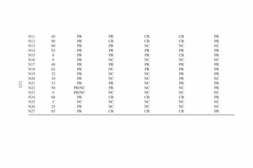
N11 40 PR PR CR CR PRN12 90 PR CR CR CR PRN13 80 PR PR NC NC NCN14 92 PR PR PR PR PRN15 0 PR PR PR CR PRN16 0 PR NC NC NC NCN17 40 PR PR PR PR PRN18 62 PR NC PR PR PRN19 22 PR NC NC PR PRN20 10 PR NC NC PR NCN21 33 PR PR NC PR PRN22 50 PR/NC PR NC NC PRN23 0 PR/NC NC NC NC NCN24 68 PR CR CR CR PRN25 5 NC NC NC NC NCN26 25 PR NC NC NC NCN27 85 PR CR CR CR PR
125
06_Modlich.qxd 6/3/07 11:00 AM Page 125

126 Modlich and Munnes
Fig. 3. PLS discrimination according to tumor response class using the variablesselected by PLS (VIP > 1.9) and ratio (pCR/NC) > 1.9 or < 0.55. (A) Model 1 (PR caseswere deleted; class 1 – pCR, black boxes; class 2 – NC, open triangles); 96 probe sets(cDNAs) retained. (B) Model 2(class 1 – pCR, black boxes; class 2 – NC, open trian-gles and PR, stars); 90 probe sets retained.
In both cases, models performed much better than expected by chance. Both groupsof selected probe sets were compared and nine probe sets were found to be repre-sented in both lists. The combined list of unique probe sets we used for model vali-dation contained 31 probe sets.
4. For an independent validation, a group of 27 tumor samples was used in order totest the discriminative power of the final gene list. The results are presented in
06_Modlich.qxd 6/3/07 11:00 AM Page 126

Table 1. It is obvious that true pCR cases are correctly predicted in both models,while NC cases are better predicted in model 1. Nevertheless, it was interesting tosee that also by PLS-DA as before by statistical tests partial responding tumors
Statistical Methods for Microarray Data Analysis 127
Fig. 4. Validation of PLS discrimination analysis by permutation. (A) Model 1 (class1 – pCR; class 2 – NC; PR cases were deleted) using 20 selected from 96 probe sets.(B) Model 2 (class 1 – pCR; class2 – NC and PR together) using 20 selected from 90probe sets. The horizontal axis shows the correlation between the permuted andactual data, the vertical axis is the value of R2 (the variance explained in fitting) andQ2 (the variance explained in predicting). The two values on the right hand corner r=1correspond to the values of R2 and Q2 for the actual data. Each symbol represents apermutation result, R2 is shown by black dots and Q2, by squares.
06_Modlich.qxd 6/3/07 11:00 AM Page 127
with either good (>60% tumor shrinkage) or very poor response to therapy werepredicted to show potentially complete response (e.g., N12, N24, N27) or nochange of tumor (e.g., N22, N25, N26), respectively. This observation indicatesthat for further studies the monitoring of tumor shrinkage during preoperative sys-temic chemotherapy is pivotal to correctly judge the final pathological responseclassification.
A comparison of results obtained by applying the two statistical approachesin microarray data analysis, one that resulted in a 59-gene EC predictor set, andthe other resulting in 96- and 90-gene sets identified by PLS-DA, showed that19 genes were identified by both statistical approaches. However, the PLS-DAitself had overall worse predictive ability in comparison to the first multistepanalysis combined with a k-NN classification at the end.
3.6. Gene Ranking—ANOVA
Additionally, for the purpose of comparison, we applied Fisher’s and SparseLDA, SVMs, and k-NN classification in a gene ranking procedure to find genesthat are significant for response to EC chemotherapy in our training set.
Unfiltered data consisting of all 22,283 probe sets were used. The minimalmisclassification rate for each of three algorithms, Sparse LDA, SVMs, and k-NN together corresponded to the gene set containing 63 probe sets. The pre-dictive accuracy demonstrated by such a gene set in a cross validation (k-NN)was high: 100% for CR, 61% for PR, and 88% for NC. Unfortunately, anindependent validation on the test cohort was less successful than by use of the59-gene classifier. Validation results are shown in Table 1. Only one case ineach group, CR and NC, was correctly predicted.
This problem is also known as “overfitting” the training set. We had so manyparameters that they could fit all of the random variations well. Therefore, alltests have found predictors, which fit the model in the training set very well, butprovided inaccurate predictions for the independent test cohort.
4. ConclusionsThis statistical approach offers a possibility for successful expression data
filtering and analyses concerning the development of a multigene predictor set.We have applied several simple but very effective steps for the data reductionand prefiltering. Statistical methods described here provide improved approachesto microarray data analysis. After applying a proposed model, a predictiveprobe set was selected, which could be successfully validated on the independ-ent cohort of samples. The data reduction and an appropriate statistical analy-sis algorithm are crucially important for the identification of new molecularmarkers for response prediction.
128 Modlich and Munnes
06_Modlich.qxd 6/3/07 11:00 AM Page 128
References1. Olson, J. A., Jr. (2004) Application of microarray profiling to clinical trials in
cancer. Surgery 136, 519–523.2. Jain, K. K. (2004) Applications of biochips: from diagnostics to personalized med-
icine. Curr. Opin. Drug Discov. Devel. 7, 285–289.3. Simon, R. (2003) Diagnostic and prognostic prediction using gene expression pro-
files in high-dimensional microarray data. Br. J. Cancer 89, 1599–1604.4. Hardiman, G. (2004) Microarray platforms—comparisons and contrasts.
Pharmacogenomics 5, 487–502.5. Shippy, R., Sendera, T. J., Lockner, R., et al. (2004) Performance evaluation of
commercial short-oligonucleotide microarrays and the impact of noise in makingcross-platform correlations. BMC Genomics 5, 61.
6. Quackenbush, J. (2001) Computational analysis of microarray data. Nat. Rev.Genet. 2, 418–427.
7. Troyanskaya, O. G., Garber, M. E., Brown, P. O., Botstein, D., and Altman, R. B.(2002) Nonparametric methods for identifying differentially expressed genes inmicroarray data. Bioinformatics 18, 1454–1461.
8. Liu, Y. and Ringner, M. (2003) Multiclass discovery in array data. BMCBioinformatics 5, 70.
9. Shannon, W., Culverhouse, R., and Duncan, J. (2003) Analyzing microarray datausing cluster analysis. Pharmacogenomics 4, 41–52.
10. Modlich, O., Prisack, H-B., Munnes, M., Audretsch, W., and Bojar, H. (2005)Predictors of primary breast cancers responsiveness to preoperative Epirubicin/Cyclophosphamide chemotherapy: translation of microarray data into clinicallyuseful predictive signatures. J. Transl. Med. 3, 32.
11. Gruvberger-Saal, S. K., Eden, P., Ringner, M., et al. (2004) Predicting continuousvalues of prognostic markers in breast cancer from microarray gene expressionprofiles. Mol. Cancer Ther. 3, 161–168.
12. Walpole, R. E. and Myers, R. H. (eds.) (1985) Probability and Statistics forEngineers and Scientists, 3rd ed., Macmillan, New York, NY.
13. Wilcoxon, F. (1945) Individual comparisons by ranking methods. Biometrics1, 80–83.
14. Kruskal, W. H. and Wallis, W. A. (1952) Use of ranks in one-criterion varianceanalysis. J. Amer. Statist. Assoc. 47, 583–621.
15. Manly, B. F. J. (ed.) (2004) Multivariate Statistical Methods: A Primer, 3rd ed.,Chapman Hall, London, UK.
16. Duda, R. O. and Hart, P. E. (1973) Pattern Classification and Scene Analysis,Wiley, New York, NY.
17. Datta, S. (2001) Exploring relationships in gene expressions: a partial least squaresapproach. Gene Expr 9, 249–255.
18. Wold, S., Sjöström, M., and Erikson, L. (1998) PLS in chemistry. In: TheEncyclopedia of Computational Chemistry (Schleyer, P.v.R., Schreiner, P. R.,Allinger, N. L., et al, eds.), John Wiley & Sons, Chichester, UK, pp. 2006–2020.
Statistical Methods for Microarray Data Analysis 129
06_Modlich.qxd 6/3/07 11:00 AM Page 129
19. Johnson, R. A. and Wichern, D. W. (eds.) (1982) Applied Multivariate StatisticalAnalysis. Prentice-Hall, Englewood Cliffs, NJ.
20. Cox, J. (2002) Comparative study of classification algorithms and gene selectionmethods for the discrimination of cancer tissue samples using microarray expres-sion data. 3rd Intl. Conf. on Systems Biology, Stockholm, Sweden.
21. Vapnik, V. (ed.) (1998) Statistical Learning Theory. Wiley, New York, NY.22. Cover, T. M. and Hart, P. E. (1967) Nearest neighbour pattern classification. IEEE
Transactions on Information Theory 13, 21–27.23. Ben-Dor, A., Bruhn, L., Friedman, N., Nachman, I., Schummer, M., and Yakhini,
Z. (2000) Tissue classification with gene expression profiles. J. Comput. Biol.7, 559–583.
24. Dudoit, S., Fridlyand, J., and Speed, T. P. (2002) Comparison of discriminationmethods for the classification of tumors using gene expression data. J. Am. Stat.Assoc. 97, 77–87.
130 Modlich and Munnes
06_Modlich.qxd 6/3/07 11:00 AM Page 130
7
Gene Expression Profiles and Prognostic Markers for Primary Breast Cancer
Yixin Wang, Jan Klijn, Yi Zhang, David Atkins, and John Foekens
SummaryGenome-wide measures of gene expression have been used to classify breast tumors into clin-
ically relevant subtypes, as well as provide a better means of risk assessment on an individualbasis for lymph node-negative (LNN) breast cancer patients. We have applied AffymetrixGeneChips of 22,000 transcripts to analyze total RNA of frozen tumor samples from 286 LNNbreast cancer patients in order to identify a gene signature for identification of patients at highrisk for distant recurrence.
Key Words: Microarray; gene expression; node-negative breast cancer; prognosis.
1. IntroductionGenome-wide measures of gene expression provide a powerful approach to
identify gene expression patterns that are correlated to tumor behaviors. Severalreports in colon, breast, lung, and lymphoma cancers suggest that the newapproach could be complementary to clinical or pathological examination (1,2).Based on gene expression patterns, breast tumors could be classified as thosewith different clinically relevant subtypes (3–6), different prognosis, andresponse to chemotherapy (7–17). Determining prognosis of the breast tumorfor an individual patient requires careful assessment of multiple clinical andpathological parameters; however, traditional prognostic factors are not alwayssufficient to predict patient outcomes accurately. It is important to identify thosepatients at high risk for relapse and who definitely need adjuvant systemic ther-apy after primary surgery, instead of giving adjuvant therapy to all lymph node-negative (LNN) patients, resulting in over-treatment. There have been manyattempts to find novel gene or protein markers for breast cancer progression.Few have been implemented in routine practice. A possible reason for theseindividual marker candidates is that breast cancer progression is a complex
131
From: Methods in Molecular Biology, vol. 377, Microarray Data Analysis: Methods and ApplicationsEdited by: M. J. Korenberg © Humana Press Inc., Totowa, NJ
07_Wang.qxd 6/3/07 11:01 AM Page 131

function of multiple molecular events that may arise within the malignant tumorcells or may be induced by stromal events. Genome-wide measurements allowus to perform a more comprehensive assessment of these molecular events inLNN primary breast cancer (18).
2. Materials2.1. Patient Samples
1. Frozen tumor specimens from LNN patients treated during 1980–1995, butuntreated with systemic adjuvant therapy, were selected from our tumor bank atthe Erasmus Medical Center (Rotterdam, Netherlands).
2. The tumor samples were originally collected from 25 regional hospitals. Theguidelines for primary treatment were the same for all hospitals.
3. 436 invasive tumor samples were screened for inclusion to the study. Patients witha poor, intermediate, and good clinical outcome were included. Samples wererejected based on insufficient tumor content (53), poor RNA quality (77), and poorchip quality (20) leaving 286 samples eligible for further analysis.
4. The study was conducted according to the approved protocol by the institution’sMedical Ethical Committee (MEC no. 02·953).
5. Median age of the patients at the time of surgery was 52 yr (range, 26–83 years).6. Prior to inclusion, all the 286 tumor samples were confirmed to have sufficient
(>70%) and uniform involvement of tumor in H&E-stained, 5-µm sections cutfrom the frozen tumors.
7. Estrogen receptor (ER) (and progesterone receptor [PgR]) levels were measuredby ligand-binding assay or enzyme immunoassay (19) or by immunohistochem-istry (in nine tumors). The cutoffs used to classify tumors as ER or PgR positivewere >10 fmol/mg protein or >10% positive tumor, respectively.
8. Patient followup involved examination every 3 mo during the first 2 yr, every 6 mofor year 2 to 5, and annually from year 5 of the followup period.
9. Date of distant metastasis was defined as the date of confirmation of metastasisafter complaints and/or clinical symptoms, or at regular followup.
10. Of the 286 patients included, 93 (33%) showed evidence of distant metastasis within5 yr and were counted as failures in the analysis of distant metastasis-free survival.
2.2. Reagents
1. Total RNA Isolation. Life Technologies Trizol Reagent Total RNA Isolating(Invitrogen).
2. cDNA synthesis.a. 50 µM GeneChip T7-Oligo(dT) Promoter Primer kit, 5′–GGCCAGT
GAATTGTAATACGACTCACTATAGGGAGGCGG-(dT)24–3′, HPLC-purified(Affymetrix, P/N 900375).
b. SuperScript™ II (Invitrogen Life Technologies, P/N 18064-014) or SuperScriptChoice System for cDNA synthesis (Invitrogen Life Technologies).
c. Escherichia coli DNA ligase (Invitrogen Life Technologies, P/N 18052-019).
132 Wang et al.
07_Wang.qxd 6/3/07 11:01 AM Page 132

d. E. coli DNA polymerase I (Invitrogen Life Technologies).e. E. coli RNaseH (Invitrogen Life Technologies).f. T4 DNA polymerase (Invitrogen Life Technologies, P/N 18005-025).g. 5X Second-strand buffer (Invitrogen Life Technologies, P/N 10812-014).h. 10 mM dNTP (Invitrogen Life Technologies).i. 0.5 M EDTA.
3. Sample Clean-Up (Sample Cleanup Module; Affymetrix).4. Synthesis of biotin-labeled cRNA (Enzo BioArray HighYield RNA Transcript Label-
ing kit (10); Enzo Life Sciences).5. cRNA fragmentation (all from Sigma-Aldrich): Trizma base, magnesium acetate
(P/N M2545), potassium acetate, and glacial acetic acid.6. Target hybridization.
a. Water (molecular biology grade, BioWhittaker Molecular Applications/Cambrex).
b. 50 mg/mL Bovine serum albumin solution (Invitrogen Life Technologies).c. Herring sperm DNA (Promega Corporation).d. GeneChip eukaryotic hybridization control kit (Affymetrix) contains control
cRNA and control Oligo B2.e. 3 nM Control Oligo B2 (Affymetrix).f. 5 M NaCl (RNase-free, DNase-free) (Ambion).g. MES hydrate (SigmaUltra; Sigma-Aldrich).h. MES sodium salt (Sigma-Aldrich).i. 0.5 M Solution EDTA disodium salt (100 mL) (Sigma-Aldrich).j. DMSO (Sigma-Aldrich).k. 10%Surfact-Amps 20 (Tween-20) (Pierce Chemical).
7. Washing, staining, and scanning.a. Water (molecular biology grade; BioWhittaker Molecular Applications/Cambrex).b. Distilled water (Invitrogen Life Technologies).c. 50 mg/mL Bovine serum albumin solution (Invitrogen Life Technologies).d. R-phycoerythrin streptavidin (Molecular Probes).e. 5 M NaCl (RNase-free, DNase-free; Ambion).f. PBS, pH 7.2 (Invitrogen Life Technologies).g. 20X SSPE: 3 M NaCl, 0.2 M NaH2PO4, 0.02 M EDTA (BioWhittaker
Molecular Applications/Cambrex).h. Goat IgG (reagent grade; Sigma-Aldrich).i. Anti-streptavidin antibody (goat) (biotinylated; Vector Laboratories).j. 10%Surfact-Amps 20 (Tween-20) (Pierce Chemical).
3. Methods3.1. RNA Extraction
1. Homogenize tissue samples in 1 mL of Trizol reagent per 50–100 mg of tissue usingthe disperser/homogenizer (Ultra-turrax T8 dispersers/homogenizers; IKA Works).Wash the stainless-steel probe with the following solutions in sequence: absolute
Gene Expression Profiles and Prognostic Markers 133
07_Wang.qxd 6/3/07 11:01 AM Page 133

ethanol, RNase-free water, RNase away, and RNase-free water twice. Then dry theprobe with Kim wipes. Repeat this between processing two samples.
2. Incubate the homogenized samples for 5 min at room temp to permit the com-plete dissociation of nucleoprotein complexes. Add 200 µL of chloroform per 1 mL of TRIzol reagent. Cap sample tubes securely and shake vigorously by handfor 15 s. Incubate them at room temp for 2–3 min. Centrifuge the samples at nomore than 12,000g for 15 min at 4°C. Following centrifugation, the mixture sep-arates into a lower red, phenol–chloroform phase, an interphase, and a colorlessupper aqueous phase. RNA remains exclusively in the aqueous phase. The vol-ume of the aqueous phase is about 60% of the volume of TRIzol reagent used forhomogenization.
3. Transfer the aqueous upper phase to a fresh tube. Precipitate the RNA from theaqueous phase by mixing with isopropyl alcohol. Use 500 µL of isopropanol per1 mL of TRIzol reagent used for the initial homogenization. Incubate samples at–20°C for 30 min and centrifuge at no more than 12,000g for 10 min at 4°C. TheRNA precipitate, often invisible before centrifugation, forms a gel-like pellet onthe side and bottom of the tube.
4. Remove the supernatant from step 3. Wash the RNA pellet once with 75% ethanol(in DEPC water), adding at least 1 mL of 75% ethanol per 1 mL of TRIzol reagentused for the initial homogenization. Mix the sample by vortexing and centrifugeat no more than 7500g for 5 min at 4°C. The RNA precipitate can be stored in 75%ethanol at 4°C for at least 1 wk, or at least 1 yr at –20°C.
5. Briefly dry the RNA pellet (air-dry for 5–10 min). Be careful not to let the pelletdry completely as this will decrease solubility. Add Rnase-free water (how muchdepends on the size of the pellet and how concentrated or dilute you want yoursample), vortex, and heat the sample at 55–60°C for 10 min.
6. If using microcuvet (pathlength of 0.5 cm), make a 1:5 dilution in a volume of 10 µL (8 µL of water + 2 µL RNA) in a fresh tube. Take absorbance readings usingthe Hewlett Packard spectrophotometer at 260 and 280 wavelengths. Calculate the260/280 ratio. A ratio of <1.6 indicates the sample is only partially dissolved.A260 × 40 × 2 (cuvet pathlength is adjusted to 1 cm) × 5 (dilution factor)/1000 = µg/µL.
7. Assess the integrity of total RNA samples on an Agilent 2100 Bioanalyzer. For ahigh-quality total RNA sample, two well-defined peaks corresponding to the 18Sand 28S ribosomal RNAs should be observed, similar to a denaturing agarose gel,with ratios approaching 2:1 for the 28S to 28S bands. The sum of percent areasunder the 18S and 28S ribosomal RNAs should be more than 15.
3.2. Gene Expression Analysis
1. Biotinylated targets were prepared using published methods (Affymetrix) (20) andhybridized to Affymetrix oligonucleotide microarray U133a GeneChip. Arrayswere scanned using the standard Affymetrix protocol.
2. Expression values for each gene were calculated using Affymetrix GeneChipanalysis software MAS 5·0.
134 Wang et al.
07_Wang.qxd 6/3/07 11:01 AM Page 134
3. In order to normalize the chip signals, all probe sets were scaled to a target inten-sity of 600 and scale mask files were not selected. Chips were rejected if averageintensity was less than 40 or if the background signal exceeded 100.
3.3. Statistical Analysis
1. Gene expression data was filtered to include genes called “present” in two or moresamples. 17,819 genes passed this filter and were used for hierarchical clustering.
2. Each gene was divided by its median expression level in the patients. This stan-dardization step minimized the effect of the magnitude of expression of genes, andgrouped together genes with similar patterns of expression in the clustering analy-sis. Average linkage hierarchical clustering was performed on both the genes andthe samples using GeneSpring 6·0.
3. To identify gene markers that best discriminate between patients who developed adistant metastasis and those who remained metastasis free within 5 yr, we usedsupervised class prediction approaches.
4. The patients were first placed into one of the two subgroups stratified by ER sta-tus. Each patient subgroup was then analyzed separately in order to select mark-ers. The patients in the ER-positive subgroup were divided into a training set of 80patients and a testing set of 129 patients. The patients in the ER-negative subgroupwere divided into a training set of 35 patients and a testing set of 42 patients. Theselection of the patients into the training and the testing set was entirely random.
5. As a quality control step, Kaplan–Meier survival curves (21) of the training andthe testing set were evaluated to ensure that there was no significant difference andno bias was introduced by the random selection of the training and the testing set.The training set was used for gene selection and the testing set was used for inde-pendent validation.
6. The sample size of the training set was determined by a resampling method toensure its statistical confidence level. Briefly, the number of patients in the train-ing set started at 15 patients and was increased by 5 at a time. For a given samplesize, 10 training sets with randomly selected patients were made. A gene signaturewas constructed from each of training sets and then tested in a designated testingset of patients using receiver operating characteristic (ROC) curve analysis usingdistant metastasis within 5 yr as the defining point. The mean and the coefficientof variation of the area under the curve (AUC) for a given sample size were deter-mined. A minimum number of patients required for the training set were chosenat the point that the average AUC plateaued and the coefficient of variation of the10 AUCs was below 5%.
7. Univariate Cox proportional hazards regression was used to identify geneswhose expression levels (on log2 scale) were correlated with the length of distantmetastasis-free survival.
8. To reduce the effect of multiple testing and to test the robustness of the selectedgenes, the Cox model was performed with bootstrapping of the patients in the train-ing set (22). Briefly, 400 bootstrap samples of the training set were constructed,each containing 80 patients randomly chosen with replacement. The Cox model
Gene Expression Profiles and Prognostic Markers 135
07_Wang.qxd 6/3/07 11:01 AM Page 135

was run on each of the bootstrap samples. A bootstrap score was created for eachgene by removing the top and bottom 5% p-values and then averaging the inversesof the remaining bootstrap p-values. This score was used to rank the genes.
9. To construct a multiple gene signature, combinations of gene markers were testedby adding one gene at a time according to the rank order. ROC analysis using dis-tant metastasis within 5 yr as the defining point was performed to calculate AUCfor each signature with increasing number of genes until a maximum AUC valuewas reached.
10. The Relapse Score (RS) was used to determine each patient’s risk of distant metas-tasis. The score was defined as the linear combination of weighted expression sig-nals with the standardized Cox regression coefficient as the weight:
Here A and B are constants, and I = 1 if ER level > 10 and otherwise I = 0. The wiand wj are the standardized Cox regression coefficients for ER+ and ER– markersrespectively, and xi and xj are the expression values of ER+ and ER– markers,respectively, in log2 scale.
11. The threshold was determined from the ROC curve of the training set to ensure100% sensitivity and the highest specificity. The values of the constants A of 313.5and B of 280 were chosen to center the threshold of RS to zero for both ER posi-tive and ER negative patients.
12. Patients with positive RS scores were classified into the poor prognosis group andpatients with negative RS scores were classified into the good prognosis group.The gene signature and the cutoff were validated in the testing set.
13. Kaplan–Meier survival plots and log-rank tests were used to assess the differencesin time-to-distant metastasis of the predicted high- and low-risk groups.
14. Sensitivity was defined as the percent of the distant metastasis patients within 5 yrthat were predicted correctly by the gene signature, and specificity was defined asthe percent of the patients free of distant recurrence for at least 5 yr that were pre-dicted as being free of recurrence by the gene signature.
15. Odds ratio was calculated as the ratio of the odds of distant metastasis between thepredicted relapse patients and relapse-free patients.
16. All statistical analyses were performed using S-Plus 6·1 software (Insightful,Seattle, WA).
3.4. Pathway Analysis
1. The list of Affymetrix probe set IDs was used as the input to search for the bio-logical networks built by the software. A functional class was assigned to each ofthe genes in the prognostic signature. Pathways analysis was performed using theIngenuity 1.0 software (Ingenuity Systems, Redwood City, CA).
2. Biological networks identified by the program were then confirmed by using gen-eral functional classes in gene ontology classification. Pathways that have two ormore genes in the prognostic signature were selected and evaluated.
RS A B (1 ) 11
60
1
16
= ⋅ + ⋅ + ⋅ − + −( ) ⋅= =∑ ∑I I w x I I w xii
ij
j jj
136 Wang et al.
07_Wang.qxd 6/3/07 11:01 AM Page 136

References1. Ntzani, E. and Ionnidis, J. P. A. (2003) Predictive ability of DNA microarrays for
cancer outcomes and correlates: an empirical assessment. Lancet 362, 1439–1444.2. Wang, Y., Jatkoe, T., Zhang, Y., et al. (2004) Gene expression profiles and molecu-
lar markers to predict recurrence of Dukes’ B colon cancer. J. Clin. Oncol. 22,1564–1571.
3. Perou, C. M., Sørlie, T., Eisen, M. B., et al. (2000) Molecular portraits of humanbreast tumors. Nature 406, 747–752.
4. Sørlie, T., Perou, C. M., Tibshirani, R., et al. (2001) Gene expression patterns ofbreast carcinomas distinguish tumor subclasses with clinical implications. Proc.Natl. Acad. Sci. USA 98, 10,869–10,874.
5. Sørlie, T., Tibshirani, R., Parker, J., et al. (2003) Repeated observation of breasttumor subtypes in independent gene expression data sets. Proc. Natl. Acad. Sci.USA 100, 8418–8423.
6. Korkola, J. E., DeVries, S., Fridlyand, J., et al.: Differentiation of lobular versus duc-tal breast carcinomas by expression microarray analysis. Cancer Res. 63, 7167–7175.
7. Van’t Veer, L., Dai, H., Van de Vijver, M. J., et al. (2002) Gene expression profil-ing predicts clinical outcome of breast cancer. Nature 415, 530–536.
8. Van de Vijver, M. J., Yudong, H. E., Van’t Veer, L., et al. (2002) A gene expressionsignature as a predictor of survival in breast cancer. N. Engl. J. Med. 347,1999–2009.
9. Ahr, A., Kam, T., Solbach, C., et al. (2002) Identification of high-risk breast-can-cer patients by gene-expression profiling. Lancet 359, 131–132.
10. Huang, E., Cheng, S. H., Dressman, H., et al. (2003) Gene expression predictors ofbreast cancer outcomes. Lancet 361, 1590–1596.
11. Sotiriou, C., Neo, S. -Y., McShane, L. M., et al. (2003) Breast cancer classificationand prognosis based on gene expression profiles from a population-based study.Proc. Natl. Acad. Sci. USA 100, 10,393–10,398.
12. Woelfle, U., Cloos, J., Sauter, G., et al. (2003) Molecular signature associated withbone marrow micrometastasis in human breast cancer. Cancer Res. 63, 5679–5684.
13. Ma, X. -J., Salunga, R., Tuggle, J. T., et al. (2003) Gene expression profiles ofhuman breast cancer progression. Proc. Natl. Acad. Sci. USA 100, 5974–5979.
14. Ramaswamy, S., Ross, K. N., Lander, E. S., et al. (2003) A molecular signature ofmetastasis in primary solid tumors. Nat. Genet. 33, 1–6.
15. Chang, J. C., Wooten, E. C., Tsimelzon, A., et al. (2003) Gene expression profilingfor the prediction of therapeutic response to docetaxel in patients with breast can-cer. Lancet 362, 362–369.
16. Sotiriou, C., Powles, T. J., Dowsett, M., et al. (2003) Gene expression profilesderived from fine needle aspiration correlate with response to systemic chemother-apy in breast cancer. Breast Cancer Res. 4, R3.
Gene Expression Profiles and Prognostic Markers 137
07_Wang.qxd 6/3/07 11:01 AM Page 137

17. Hedenfalk, I., Duggan, D., Chen, Y., et al. (2001) Gene-expression profiles inhereditary breast cancer. N. Engl. J. Med. 344, 539–548.
18. Wang, Y., Klijn, J., Zhang, Y., et al. (2005) Gene-expression profiles to predict dis-tant metastasis of lymph-node-negative primary breast cancer. Lancet 365, 671–679.
19. Foekens, J. A., Portengen, H., van Putten, W. L. J., et al. (1989) Prognostic valueof estrogen and progesterone receptors measured by enzyme immunoassays inhuman breast tumor cytosols. Cancer Res. 49, 5823–5828.
20. Lipshutz, R. J., Fodor, S. P., Gingeras, T. R., et al. (1999) High density syntheticoligonucleotide arrays. Nat. Genet. 21, 20–24.
21. Kaplan, E. L. and Meier, P. (1958) Non-parametric estimation of incomplete obser-vations. J. Am. Stat. Assoc. 53, 457–481.
22. Efron, B. (1981) Censored data and the bootstrap. J. Am. Stat. Assoc. 76, 312–319.
138 Wang et al.
07_Wang.qxd 6/3/07 11:01 AM Page 138
8
Comparing Microarray Studies
Mayte Suárez-Fariñas and Marcelo O. Magnasco
SummaryWe present a practical guide to some of the issues involved in comparing or integrating
different microarray studies. We discuss the influence that various factors have on the agreementbetween studies, such as different technologies and platforms, statistical analysis criteria, proto-cols, and lab variability. We discuss methods to carry out or refine such comparisons, and detailseveral common pitfalls to avoid. Finally, we illustrate these ideas with an example case.
Key Words: Microarray; meta-analysis; crossplatform comparisons.
1. IntroductionIn the past few years a profusion of research has dealt with comparisons of
different microarray studies, both to cross-validate or integrate different studiesas well as to assess the differences between platforms (1–9). The latter regalenewcomers to the field with a bewildering array of orthogonal conclusions—some conclude that different platforms generate largely incompatible data,whereas others conclude that laboratory variability is in general greater thanthat from the platform, and so on. Upon closer inspection it is seen that thesestudies assess equality or difference in dramatically different ways, that somecomparisons are dramatically less fairer than others, and some may be down-right incorrect. In light of the profusion of different “comparison technologies,”the aim of this chapter is to introduce the reader to the problems and issues thatarise in comparing high-throughput experiments in general and microarraystudies in particular.
The traditional notion of equality or equivalence (of a measurement) is predi-cated on overlap: the measurements of two objects occupy the same footprint.This is so because all measurements are inaccurate, so we must measure severaltimes to estimate a probability distribution, and then compare the distributions.We say that two things weigh the same if, when we weigh each many times,
139
From: Methods in Molecular Biology, vol. 377, Microarray Data Analysis: Methods and ApplicationsEdited by: M. J. Korenberg © Humana Press Inc., Totowa, NJ
08_Magnasco.qxd 6/3/07 11:03 AM Page 139
140 Suárez-Fariñas and Magnasco
there is substantial overlap between the measurements of both, as assessed, forexample, by checking that the difference between the means is smaller than thestandard errors (a t-test).
But in high-dimensional spaces (when we are measuring many things at thesame time) overlap vanishes exponentially fast. Imagine we repeat 101 timesan experiment with a microarray probing 10,000 transcripts in a given tissue.Just like 2 points determine a line and 3 points determine a plane, these 101microarray measurements determine a 100-dimensional hyperplane in the10000-dimensional space of gene expression values. The overlap between geo-metrical objects is dictated by their dimensionalities; if the sum of the dimen-sions of the objects is smaller than the dimension of the ambient space, theobjects are unlikely to intersect at all. If we now repeat the experiment, treat-ing the tissue with some factor, the 100-dimensional planes corresponding toour two experiments have a zero chance of intersecting—even if the treatmentdid not do anything. Thus, comparing microarray experiments (or any otherhigh-dimensional measurement) cannot be done as with low-dimensionalexperiments by comparing the measurements as probability distributions inthe space of the measurement.
Some further modeling is required to compare experiments, and may beimplicit in the form the comparison takes. For instance, assuming that individualgene expression values are statistically independent the probability distributionfactors into a product; 10,000 independent tests can be applied to assess differ-ences. This comparison (and the p-values obtained thereof) is only valid under the(likely incorrect) assumption of statistical independence. In a radically differentvein one may coarse grain over sets of genes, e.g., participating in given pathwaysor having common gene ontology classifications. All such comparisons have animplicit model and may give incorrect results if the model is too far off the markin the particular case at hand.
To keep the discussion as practical and how-to as possible, we shall explain,not only how to do something, but a number of things to avoid, which we col-lect in Subheading 2. (an “anti-methods” if you will), and also notes are pro-vided. We present as example one case study.
2. Pitfalls2.1. Correlation of Absolute Expression Values Against Relative Values
Not infrequently cross-platform comparisons are carried out through the correlation of signal intensities for individual transcripts (4,6,7). We follow herean argument given in ref. 10 demonstrating that such comparisons are mislead-ing because they are adversely affected by “probe effects:” probe-specific andplatform-specific multiplicative factors that have a large variability (11–13).
08_Magnasco.qxd 6/3/07 11:03 AM Page 140

The advantage of relative expression over absolute expression can be easilyunderstood if the following model is considered.
Yijk = θi + φij + εijk
where Yijk is the k-th measurement of expression (in log scale) on a gene i byplatform j, θi is the real expression of a gene, φij is the platform-specificprobe/spot effect and ε is a random error in the measurement, and all effects inthe model are independent random variables with variances σ 2
θ, σ 2φ and σ 2
ε,respectively. In Affymetrix arrays the probe-effect variability σ 2
φ is larger thanthe variance of the expression level, σ 2
θ (14). The within-platform correlation isgiven by
(1)
and is usually near one because σ 2ε is much smaller than σ 2
θ + σ 2φ. The across-
platform correlation can be written as:
(2)
and it is smaller than the within-platform correlation because the probe effect isnot common to both platforms, so the term σ 2
φ does not appear in the numerator.The probe effect can be calibrated (11) so absolute mRNA concentrations canbe estimated, but to do so nominal concentrations of spiked-in mRNAs must beprovided. A simpler solution to avoid the probe-effect problem is to consideronly relative expression values. Usually in microarrays we are comparing con-trol vs condition. If we consider YA
ijk, YBijk, the absolute expression values for
samples A and B, the relative expression value can be modeled as:
Mijk = YAijk – YB
ijk = di + ϕij + ηijk (3)
where di is the true amount of differential expression (in log-fold change). Theterms φij should be the same for sample A and B so the probe effect cancels out.As in practice this is not removed completely, the term ϕij in Eq. 3 is includedto represent a platform-dependent bias. The within- and across-platform corre-lation of the M-values are respectively:
but now the term σ 2ϕ is much smaller than σ 2
φ. The confirmation of this theoret-ical effect can be checked in the results of ref. 15 and our examples.
corr M M corrij ij
d( , )1 2 and=+
+ +
σ σσ σ σ
2 2
2 2 2
ϕ
θ ϕ η
(( , )M Mi k i kd
1 2 =+ +
σσ σ σ
2
2 2 2θ ϕ η
corr Y Yi k i k( , )1 2 =+ +
σσ σ σ
θ
θ φ ε
2
2 2 2
corr Y Yij ij( , )1 2 =+
+ +
σ σσ σ σ
θ φ
θ φ ε
2 2
2 2 2
Comparing Microarray Studies 141
08_Magnasco.qxd 6/3/07 11:03 AM Page 141
2.2. Preprocessing Steps
In all microarray technologies, a good amount of preprocessing follows imageanalysis. Various groups have shown the impact of normalization and backgroundcorrection procedures on downstream analysis in Affymetrix (16) and cDNA(17). As an example, we compute expression values for Affymetrix’ Spike-inexperiments (HGU133a chips) using four of the most popular algorithms. Figure 1shows the magnitude of the differences between each pair of algorithms’ out-comes. Note that for a substantial number of genes the difference can be biggerthan twofold changes. It is then not surprising that those discrepancies can affectagreement across platforms, as shown in ref. 5, where correlation of M-valuesbetween Affymetrix and cDNA Agilent platform varies from 0.6 to 0.7 whenRMA (16), MAS5, and dChip (14) algorithms are used to compute expressionvalues. Most of the authors (2,3,7–9,18) use the default algorithm provided by thearray manufacturer’s software to preprocess the data. Although analytical soft-ware provided by manufacturers require very little input from the user, there arealternatives developed by the academic community shown to have better perform-ance. Reference 15 clearly shows how the agreement within and between plat-forms can be increased by proper use of available alternative algorithms.
2.3. Annotations
Agreement between platforms can be affected by the identification of com-mon genes as refs. 3 and 9 suggested in their studies. The selection of the iden-tifiers is a difficult issue because none of them maps genes one-to-one. Forexample, the number of common genes for the three experiments in our casestudy is almost 8000 using Unigene identifiers, but around 15,000 using LocusLink identifiers. Sequence-matched probes can increase cross-platform correla-tion between M-values as reported in ref. 5 (see Note 2). However, matchingthe sequences could be a hard procedure especially if more than two studies anda large number of genes are involved. One solution is to take the intersection ofvarious identifiers, i.e., genes matched by two or more identifiers, which canimprov the cross-platform agreement (15).
2.4. Statistical Protocol
Although researchers are quite aware that experimental results are sensitiveto the protocol used, it is not unusual that studies using different statisticalapproaches are compared on the same basis. This is particularly delicate if weare trying to assess platform reproducibility. For example, refs. 2, 4, and 18based their comparisons on the agreement of lists generated from different statistical criteria. There is only one solution to this problem: the data must bereanalyzed using the same statistical approach.
142 Suárez-Fariñas and Magnasco
08_Magnasco.qxd 6/3/07 11:03 AM Page 142
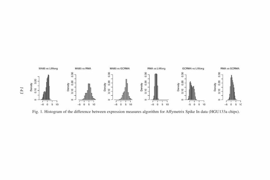
143
Fig. 1. Histogram of the difference between expression measures algorithm for Affymetrix Spike In data (HGU133a chips).
08_Magnasco.qxd 6/3/07 11:03 AM Page 143
Yet, is the intersection of individual lists a good strategy to measure concor-dance? Even with the same statistical protocol some studies concluded that asmall amount of genes lay in the intersection (7,8). The caveat here is that theintersection between lists should be considered as a compound statistical test,whereby the null hypothesis (for the intersection) is rejected only when all threenull hypothesis (for the individual lists) are rejected. The false-positive rate ofthe intersection is thus the product of the individual false-positive rates; how-ever the true positive (TP) rate is also the product of the three individual TPrates, and as these are also smaller than one, their product could be quite small.As a result, the p-values which generate adequate lists with good false-positivecontrol will be inadequate for intersecting (too few TPs at the intersection). Inorder to use list intersection as a criterion for comparing studies, care shouldbe taken that the p-values for the individual lists should be chosen so as to givegood numbers at the intersection, not on individual lists.
2.5. Lab Effect
Gene expression is the nervous system of cells, easily imprinted by anything inthe environment; gene expression is affected by the way the laboratory sets up theexperiment—sample collection methods in the case of tumors, culture system vari-ables for cultured tissues, and animal feeding and maintenance protocols. Forexample, a study (3) found poor correlations between M-values using samples ofcancer cell lines, but it was carried out independently in two different laboratories,and variations that may have arisen from independent cell culturing, RNA isola-tion, and purification were not controlled. The influence of the lab effect on cross-platform agreement was pointed out in ref. 8, where the sample variability wasrevealed to be the main source of data variation, and was confirmed in ref. 15.
3. MethodsWe now present some ideas as to how comparisons can be carried out soundly;
we anticipate that better methods will be devised in the future as our understand-ing evolves, and the practitioner in the field should try to keep aware of the latesttechniques. We shall first outline the basic overall flow and then the pieces.
3.1. Overall Flow
1. Get the raw data for all studies.2. Use uniform data preprocessing steps.3. Identification of the common genes for all studies.
a. Obtain up-to-date annotations for all the studies.b. Try to match the sequence or use more than one identifier to match them.
4. Further reduce the scope of the comparisons by eliminating genes that mighthave been erratically affected; e.g., by the integrated correlations approach (seeSubheading 3.3.).
144 Suárez-Fariñas and Magnasco
08_Magnasco.qxd 6/3/07 11:03 AM Page 144

5. Use the same statistical methodology to define differential expression for the indi-vidual studies and the most powerful available tests (see Note 4).
6. Create a list of common differentially expressed genes; by list intersection or by sum-mary statistics (see Subheading 2.5.). The p-value of the intersection has to be set,which is the product of individual p-values, if intersection is considered (see Note 5).
3.2. Raw Data
The researcher attempting comparative studies should procure the rawestlevel of data possible from all sources. There is no current standard as to how toanalyze data in the field, and studies are published with vastly different analysismethods. It is thus imperative to redo the analysis from scratch. For AffymetrixGeneChip data, the raw “.CEL” files should be procured; these contain data fromindividual probes and permit execution of quality control algorithms diagnosing,e.g., the quality of the hybridization or presence of blemishes (19), as well asusage of other summarization methods besides the “closed-box” AffymetrixMAS5 algorithms. In the case of cDNA-like techniques, the database containingforeground and background intensities can be used, assessing the quality trough,e.g., arrayMagic (20). Nevertheless, for a better standardization in the case ofstudies where the image analysis software used different feature extraction cri-teria, processing the original image will be a plus.
3.3. Integrated Correlations Approach
To reduce the “lab effect,” it would be advisable to identify and eliminatefrom the analysis genes that which appear to be affected erratically across labs;for example, many in vivo studies are afflicted by immunity genes flaring upbecause of some flu or other condition affecting a litter of animals. Integrativecorrelation analysis was introduced to validate agreement across studies and toselect genes that exhibit a consistent behavior across them (21) by examiningall pair-wise correlations of gene expression.
Define xg to be the expression profile for a gene g, and ρsp = corr(xg1
, xg2),
the correlation for the pair of genes p=(g1,g2) in the study s. Based on ρsp we
can assess both overall reproducibility between studies and gene-specificreproducibility. The integrated correlation I(s,s′) = corr(ρs
p, ρs′p ), quantifies the
reproducibility between studies. If this expression is calculated considering onlythe pairs containing a gene g, then we have a measure of the gene-specific repro-ducibility between two studies, that is Rs,s′ (g) = corr(ρs
p, ρs′p ), where p=(g,j).
When more than two studies are involved, the average over all s and s′ is used asa reproducibility score for a gene g,
.RR g
ng sn
s s
s s
=⎛⎝⎜
⎞⎠⎟
= ∑∑ 1
2
′>
′, ( )
Comparing Microarray Studies 145
08_Magnasco.qxd 6/3/07 11:03 AM Page 145

3.4. Coinertia
Another technique to measure agreement between studies is the coinertiaanalysis (COIA). Initially developed in the ecological area, it was applied toperform cross-platform comparisons in ref. 22. It does not require cross refer-encing the annotation of the transcript or statistically based filtering of dataprior to cross-platform analysis, but it is only possible if both experiments haveexactly the same amount of arrays with the same sample. Furthermore, it doesnot offer a way to identify common differentially expressed genes.
The idea of COIA is to produce for each study a new representation of thearrays in a gene hyperspace where the two new representations maximize thesquare covariance (of the arrays) between the two studies. This produces a setof axes, one from each dataset, where the first pair of axes is chosen so as to bemaximally covariant and represent the most important joint trend in the twodatasets. The second pair of axes is chosen so as to be maximally covariant butorthogonal to the first pair, and so on for the rest of the axes. Once the new rep-resentations are obtained, the similarity is measured either as the correlationbetween the data-points projected on the first corresponding axes for each studyor by the RV-coefficient, a multivariate extension of the Pearson correlation.
3.5. List Intersection or Summary Statistics
We discussed briefly the problems with list intersection previously men-tioned (see Subheading 1.4.). Here we reiterate that intersecting lists is anextremely valuable technique that can potentially refine results by consideringwhat has been seen to happen repeatably in many experiments; the fundamen-tal trick is to recreate the lists from scratch because the cutoff criteria that givegood control over the false-positive and -negative rates in an intersection are farfrom those that give good control to each individual list (23).
Another approach (24) is the use of summary statistics based on individ-ual p-values. The p-values for each gene in each study is obtained (normalsingle study). The meta-analysis consists in defining the summary statistic
. The distribution of S is obtained by simulation and a “sum-mary P” for gene g is defined as P(S>Sg). This technique is potentially sensi-tive to outliers because a single large value in one of the studies can place a geneon the list, and would be best to use with a robust approach.
3.6. Discussion: A Case Study
We illustrate the practical use of these procedures through a study (23) carriedout to compare three different studies of human embryonic stem cells (HESC).Each (25–27) study concluded with a list of genes that are upregulated in stemcells, but the three lists of significantly upregulated genes, as published, are quite
S pi= − ∑2 log( )
146 Suárez-Fariñas and Magnasco
08_Magnasco.qxd 6/3/07 11:03 AM Page 146

different. Their intersection is shown in Fig. 2A: seven genes appear in all threestudies out of the 2226 total genes in the union. This is particularly troublesomebecause all three studies appear to be technically reliable and each study has goodreproducibility between replicates. After we carried out the procedure describednext we obtained a much more significant level of agreement illustrated in Fig. 2B.
The Bhattacharya study (25) has 6 cDNA chips (8 × 4,23 × 23 design)where different HESC lineages were hybridized to the red channel (Cy5), andcontrol samples hybridized to the green channel (Cy3) were isolated from acollection of adult human tissues. The Sperger study (26) used a 12 × 4, 30 × 30design of cDNA chips, also hybridizing individual lineages; the control sampleswere also a common reference pool of mRNA. The Sato study (27) had sixAffymetrix HGU133A chips, three replicates of H1 cells, and three replicatesof “nonlineage-directed differentiation.”
We then proceeded as follow:
1. We carried out the analysis using the open-source R language version 2.0 (28) andpackages provided in Bioconductor project (29).
2. For cDNA arrays: we used the same image analysis criteria to exclude low-qual-ity spots for cDNA arrays. Transcripts with excessive numbers of low-qualityspots across the set of arrays were excluded from the analysis. The marray pack-age from the Bioconductor suite was used for preprocessing. Normalization wasexecuted in two steps, first within-print-tip-group location-dependent intensitynormalization followed by a within-print-tip group scale normalization usingmedian absolute deviation. Single-channel normalization of two-color cDNA wasdone as proposed by ref. 30, using quantile normalization.
3. For Affymetrix chips, the GCRMA algorithm was used to summarize data as pro-posed in ref. 31. This algorithm improves the widely used RMA (16) by including
Comparing Microarray Studies 147
Fig. 2. Intersection between the published lists of upregulated genes for each study.(A) As published. (B) After reanalysis.
08_Magnasco.qxd 6/3/07 11:03 AM Page 147

an extra step to adjust for nonspecific binding, and computing the sequence-specific affinities between probes as described (13).
4. We verified that within-platform reproducibility is fairly good in all the studies,even noting that Battacharya’s and Sperger’s designs contain different lineages ofHESC rather than true replicates of a single lineage.
5. Annotations were obtained with the raw data from each study. For both Bhattacharyaand Sperger studies, annotations were obtained from SOURCE from the Stanfordmicroarray data homepage (http://source.standford.edu). For Affymetrix data, annota-tions packages from Bioconductor were used. The IMAGE clone IDs and theAffymetrix probes were matched using Unigene Cluster Annotation. Genes with noUnigene identifier were eliminated and duplicated probes/spots were averaged together.
6. After this process there are 7373 genes common to all three studies. We filtered forevidence of variation across samples, reducing our set of interesting genes to 2463.
7. Within this universe of 2463 genes we executed an integrated correlation approach.The integrated correlation coefficients between studies were extremely small (0.13in the best case) and inspection of correlation between M-values indicates poorgeneral agreement between studies. For each pair of studies, the two-dimensionaldensity of the pair-wise correlations (data not shown) suggests that we can findmany “negatively coherent” pairs of genes, positive correlated in one study andnegatively correlated in the other, and in any such pair, one must be inconsistent.Figure 3 paints a much more hopeful picture. The histograms of the coherencescores between study pairs (shown as marginal distributions around the two-dimensional densities in Fig. 3) reveal the existence of a group of genes with highcoherence scores in all study pairs. The bivariate density of the coherence scorebetween pairs of studies shows that despite variations, there is a group of genes wherescores between Bhattacharya–Sperger are similar to the score of Bhattacharya–Sato,those that have higher values in both are part of the coherent set. The histogram ofthe average pair-wise reproducibility (Fig. 4) shows a bimodal distribution, withan apparently clear-cut distinction between two groups of genes, one of them havingpositive reproducibility scores (“coherent”) and the other one close to zero (“erratics”)or negative (“incoherents”). So the general poor agreement observed between thestudies is a result of averaging over a set of genes with both positive and negativecoherences. We decided to keep for further analysis the 739 genes in the top30% of the gene-coherence distribution. Eliminating erratic genes enormouslyimproves the general agreement between the studies, with integrated correlationvalue of 0.78 in the worst case.
8. Within the set of coherent genes, we study those that are up- or downregulated in stemcells vs their differentiated controls in each one of the studies. Exactly the samestatistical tests and criteria were applied to all three studies, with a strict cutoff valueselection based both on a p-value and a positive log of the odds (that a gene is differ-entially expressed) (32). We used the moderated t-statistics as proposed in ref. 33 andthe false discovery rate procedure was used to adjust the p-values for multiple hypothesis(34). P-value cutoff was set at 0.01, which implies than the probability of error is10−4 in the pair-wise comparison and 10-6 when the three studies are considered.
148 Suárez-Fariñas and Magnasco
08_Magnasco.qxd 6/3/07 11:03 AM Page 148

149
Fig. 3. Bivariate densities of the coherence score.
08_Magnasco.qxd 6/3/07 11:03 AM Page 149

The intersection between the lists is now quite a bit larger and statistically signif-icant (see Fig. 2B), 111 genes were found to be upregulated genes common to allthree studies (95 downregulated) against 3 expected by chance. Notice that the 111upregulated genes in this list are not necessarily the “most” upregulated for anyindividual study; yet they are significantly upregulated for each study.
4. Notes1. Different ways to measure the agreement. Some comparisons are solely based on
correlation of signal or correlation of M-values, others are based on intersectionof the list or alternatives analysis such as COIA. As an example, refs. 3 and 22used the same panel of 60 cell lines from the National Cancer Institute to compareAffymetrix and cDNA arrays, arriving at different conclusions.
2. Although in a recent study (4) it was concluded that verification of sequence iden-tity appears to play only a small role in the improvement of the result, the studywas limited to the analysis of baseline quantitation of biological replicates anddoes not compare the arrays ability to detect changes.
3. The agreement between platform can be affected by slow signal (1,3), cross-hybridization (18), and GC-content (3).
4. t-test: with small number of replicates, the variance is easily underestimated andhence significance can be overestimated. Recently proposed solutions to this prob-lem include the moderated t-test (33).
5. p-values: do not forget that expression of genes is a coordinated business, and henceadjustments for multiple hypothesis should be made, e.g., as described in ref. 34.
References1. Barczak, A., Rodriguez, M. W., Hanspers, K., et al. (2003) Spotted long oligonu-
cleotide arrays for human gene expression analysis. Genome Res. 13,1775–1785.
150 Suárez-Fariñas and Magnasco
Fig. 4. Gene-coherence score (average over all three comparisons).
08_Magnasco.qxd 6/3/07 11:03 AM Page 150

2. Kothapalli, R., Yoder, S. J., Mane, S., and Loughran, T. P., Jr. (2002) Microarrayresults: how accurate are they? BMC Bioinformatics 3, 22.
3. Kuo, W. P., Jenssen T. K., Butte A. J., et al. (2002) Analysis of matched mRNA meas-urements from two different microarray technologies. Bioinformatics 18, 405–412.
4. Mah, N., Thelin, A., Lu, T., et al. (2004) A comparison of oligonucleotide andcDNA-based microarray systems. Phys. Genom. 16, 361–370.
5. Mecham, B. H., Klus, G. T., Strovel, J., et al. (2004) Sequence-matched probesproduce increased cross-platform consistency and more reproducible biologicalresults in microarray-based gene expression measurements. Nucl. Acids Res. 32, e74.
6. Rogojina, A., Orr, W. E., Song, B. K., and Geisert, E. E., Jr. (2003) Comparing theuse of Affymetrix to spotted oligonucleotide microarrays using two retinal pigmentepithelium cell lines. Mol. Vision 9, 482–496.
7. Tan, P., Downey, T. J., Spitznagel, E. L., Jr., et al. (2003) Evaluation of gene expres-sion measurements from commercial microarray platforms. Nucl. Acids Res. 31,5676–5684.
8. Yauk, C., Beendt, M. L, Williams, A., Douglas, G. R., et al. (2004) Comprehensivecomparison of six microarray technologies. Nucl. Acids Res. 32, e124.
9. Yuen, T., Wurmbach, E., Pfeffer, R. L., Ebersole, B. J., and Sealfon, S. C. (2002)Accuracy and calibration of commercial oligonucleotide and custom cDNAmicroarrays. Nucl. Acids Res. 30, e48.
10. Irizarry, R. A., Warren, D., Spencer, F., et al. (2005) Multiple-laboratory compari-son of microarray platforms (vol 2, pg 345, 2005). Nat. Methods 2, 477–477.
11. Hekstra, D., Taussig, A. R., Magnasco, M., and Naef, F. (2003) Absolute mRNAconcentrations from sequence-specific calibration of oligonucleotide arrays. Nucl.Acids Res. 31, 1962–1968.
12. Naef, F., Lim, D. A., Patil, N., and Magnasco, M. (2002) DNA hybridization tomismatched templates: A chip study. Phys. Rev. E. 65 (040902).
13. Naef, F. and Magnasco, M. (2003) Solving the riddle of the bright mismatches:Labeling and effective binding in oligonucleotide arrays. Phys. Rev. E. 68 (011906).
14. Li, C. and Wong, W. (2001) Model-based analysis of oligonucleotide arrays:Expression index computation and outlier detection. Proc. Natl. Acad. Sci. USA 98,31–36.
15. Irizarry, R. A., et al. (2004) Multiple Lab Comparisons of Microarray Platforms,in Dept. of Biostatistics Working Papers, Johns Hopkins University.
16. Irizarry, R. A., Bolstad, B. M., Collin, F., Cope, L. M., Hobbs, B., and Speed, T. P.(2003) Summaries of Affymetrix GeneChip probe level data. Nucl. Acids Res. 31, e15.
17. Yang, Y. H., Dudoit. S., Luu. P., et al. (2002) Normalization for cDNA microarraydata: a robust composite method addressing single and multiple slide systematicvariation. Nucl. Acids Res. 30, e15.
18. Li, J., Pankratz, M., and Johnson, J. (2002) Differential gene expression patternsrevealed by oligonucleotide versus long cDNA arrays. Toxicol. Sci. 69, 383–390.
19. Suárez-Fariñas, M., Haider, A., and Wittkowski, K. M. (2005) “Harshlighting”small blemishes on microarrays. BMC Bioinformatics 6, 65.
Comparing Microarray Studies 151
08_Magnasco.qxd 6/3/07 11:03 AM Page 151

20. Buness, A., Huber, W., Steiner, K., Sultmann, H., and Poustka, A. (2005) arrayMagic:two-colour cDNA microarray quality control and preprocessing. Bioinformatics 21,554–556.
21. Parmigiani, G., Garrett-Mayer, E. S., Anbazhagan, R., and Gabrielson, E. (2004) Across-study comparison of gene expression studies for the molecular classificationof lung cancer. Clin. Cancer Res. 10, 2922–2927.
22. Culhane, A., Perriere, G., and Higgins, D. (2003) Cross-platform comparisonand visualisation of gene expression data using co-inertia analysis. BMCBioinformatics 4, 1600–1608.
23. Suárez-Fariñas, M., Noggle, S., Heke, M., Hemmati-Brivanlou. A, and Magnasco,M. O., et al. (2005) How to compare microarray studies: The case of human embry-onic stem cells. BMC Genomics 4.
24. Rhodes, D., Barrette, T. R., Rubin, M. A., Ghosh, D., and Chinnaiyan, A. M. (2002)Meta-analysis of microarrays: Interstudy validation of gene expression profilesreveals pathway dysregulation in prostate cancer. Cancer Res. 62, 4427–4433.
25. Bhattacharya, B., Miura, T., Brandenberger, R., et al. (2004) Gene expression inhuman embryonic stem cell lines: unique molecular signature. Blood 103, 2956–2964.
26. Sperger, J. M., Chen, X., Draper, J. S., et al. (2003) Gene expression patterns inhuman embryonic stem cells and human pluripotent germ cell tumors. Proc. Natl.Acad. Sci. USA 100, 13,350–13,355.
27. Sato, N., Sanjuan, I. M., Heke, M., et al. (2003) Molecular signature of humanembryonic stem cells and its comparison with the mouse. Dev. Biol. 260, 404–413.
28. Available from: http://www.r-project.org. Last accessed: 10/19/2006.29. Available from: http://www.bioconductor.org. Last accessed: 10/19/2006.30. Yang, Y. H. and Thorne, N. (2003) Normalization for two-color cDNA microarray
data. In: Science and Statistics: A Festschrift for Terry Speed, (Goldstein, D. R., ed.)IMS Lecture Notes Monograph Series, vol 40, pp. 403–418.
31. Wu, Z., Irizarry, R. A., Gentleman, R., Martinez-Murillo, F., and Spencer, F. (2004)A model based background adjustement for oligonucleotide expression arrays. J. Amer. Stat. Assoc. 99, 909–917.
32. Lonnstedt, I. and Speed, T. (2002) Replicated microarray data. Statistica Sinica 12,31–46.
33. Smyth, G. K. (2004) Linear models and empirical Bayes methods for assessing differential expression in microarray experiments. Stat. Appl. Genet. Mol. Biol.3, Article 3.
34. Dudoit, S., Shaffer, J., and Boldrick, J. (2003) Multiple hypothesis testing inmicroarray experiments. Stat. Sci. 18, 71–103.
152 Suárez-Fariñas and Magnasco
08_Magnasco.qxd 6/3/07 11:03 AM Page 152
9
A Pitfall in Series of MicroarraysThe Position of Probes Affects the Cross-Correlation of Gene Expression Profiles
Gábor Balázsi and Zoltán N. Oltvai
SummaryUsing Escherichia coli cDNA microarray slides and Affymetrix GeneChips, we study how the
relative position of probes on microarrays affects the cross-correlation of gene expression pro-files. We find that in cDNA arrays, every spot located within the same block is affected by a sim-ilar, experiment-specific bias. As a result, the cross-correlation between some gene expressionprofiles is significantly altered, depending on the similarity between these “block-dependent”biases through the series of cDNA microarray experiments. In addition, the position of probeswithin the blocks can also contribute to the measured gene expression. We outline the necessarysteps to computationally identify and correct these biases.
Key Words: Microarray; bias; gene expression; cross-correlation; position; block; probe; spot;correction.
1. IntroductionMicroarray technology is used to simultaneously monitor the mRNA expres-
sion levels of all genes within a given organism (1,2) and has become an indis-pensable tool in cell biology (3). Following the experiments and data collection,possible avenues of microarray data analysis range in complexity from the iden-tification of significantly affected genes (4) to the application of sophisticatedcomputational methods to cluster, classify, and interpret the observed geneexpression patterns (5–7). Unfortunately, in addition to biological variations ingene expression (8), microarray data are also affected by a large number oftechnological factors (9–13). To gain a better understanding of the assayed bio-logical phenomena, it is crucial to identify the source of technological biases
153
From: Methods in Molecular Biology, vol. 377, Microarray Data Analysis: Methods and ApplicationsEdited by: M. J. Korenberg © Humana Press Inc., Totowa, NJ
09_Balazsi.qxd 6/3/07 8:45 PM Page 153

and to develop computational or experimental methods for their reduction orelimination (10–15).
By using Escherichia coli gene expression data collected from in-house-printed cDNA arrays (16), we show that the relative position of probes onmicroarrays affects their coexpression, and can have important consequenceson gene coexpression measurement and clustering of expression profiles. Weoutline the steps necessary to identify and reduce such errors in existingmicroarray data. No significant bias was found using Affymetrix GeneChip(17) data.
2. SoftwareFor data processing, identification, and correction of position-dependent
bias, we used Microsoft Excel and Matlab® by The Mathworks, Inc.
3. Methods3.1. Microarray Platforms
We used two types of microarray platforms to identify the effect of relativeposition on gene coexpression (see Note 1): in-house-printed cDNA arrays (16)and commercial Affymetrix GeneChips (17).
All the steps needed to construct the in-house-printed cDNA array have beendescribed in detail before (16). Therefore, we omit discussing the constructionprocedure, and focus on the identification and correction of biases instead.
The custom-built cDNA array slides contained three copies of the E. coligenome in a total of 24 blocks of spots (8 blocks per genome, see Fig. 1). Eachblock contained 26 columns and 23 rows, or a total of NB = 576 spots in a rec-tangular array (the last row of spots was incomplete, containing only fourspots). The total number of spots per genome was 4608 and there were 13,824spots per slide. The spreadsheets for data analysis were generated with theGenePix Pro 4.0 software (Axon Instruments), and contained 14,352 entries(including the 22 empty spots from the last row of each block).
The second type of microarray was the commercially available Affymetrix E.coli GeneChip (17). The chips contained duplicate probe sets (“perfect match”and “mismatch”) for 7312 locations on the E. coli chromosome (includingintergenic regions).
3.2. Data Processing–cDNA Microarrays
We generated expression data tables in Microsoft Excel, containing the fol-lowing information for each of the 14,352 entries: block (B), column (X), androw (Y) number, red foreground (RF) and background (RB), green foreground(GF) and background (GB) intensity. The position of each probe within a block,P is defined by the pair of integers (X,Y).
154 Balázsi and Oltvai
09_Balazsi.qxd 6/3/07 8:45 PM Page 154

We subtracted the background intensities from the foreground intensities,and then used the corrected red (RC) and green (GC) intensities to calculate thelog10 ratios, or lg ratios (E) of gene expression:
(1)
In some cases, when the intensity of the background was higher than or equalto the intensity of the foreground, the resulting lg ratios became complex orinfinity. These values were eliminated using the find, imag, and isfinite func-tions in Matlab® (see Note 2).
3.3. Block-Dependent Biases–cDNA Microarrays
Using the find, nanmean, and nanstd functions in Matlab, we calculatedaverages and standard deviations within each block for each of the foregroundand background intensities, as well as the corrected values and the lg ratios. Inthe absence of block-dependent biases, one would expect the average correctedlog ratios
(2)
to be around 0 and show no systematic differences. However, as Fig. 2 indi-cates, systematic differences between blocks are present even after the back-ground subtraction and calculation of lg ratios. These systematic differences(biases) originate in the biases of the original red and green foreground andbackground intensities, and background subtraction or other global normaliza-tion methods are not sufficient to eliminate them (see Note 1).
EN
EB
ii
NB
==∑1
1
ER
G
R R
G GC
C
F B
F B
=⎛
⎝⎜⎞
⎠⎟=
−−
⎛⎝⎜
⎞⎠⎟
lg lg
A Pitfall in Series of Microarrays 155
Fig. 1. Geometry of the custom-built cDNA microarray.
09_Balazsi.qxd 6/3/07 8:45 PM Page 155

3.4. Position-Dependent Biases of Higher OrderTo identify position-dependent biases of higher order, biases of order 0 have
to be corrected (see Subheading 3.6. and Note 3). If the 0th order-corrected lgratio values E0, plotted in the sequential order of rows and columns contain sys-tematic trends, the microarray data are affected by higher order bias.
Experimental noise can in general be reduced by increasing the number ofexperiments and averaging the results of repeated experiments. Contrary toexpectation, the effect of position-dependent biases on the cross-correlationbetween gene expression profiles increases instead of decreasing with thelength of the experiment series (12). This is an important problem becausecross-correlation is the most frequently used distance metric in hierarchicalclustering (5).
To illustrate the adverse effect of multiple experiments, we plot in Fig. 3 theaverage cross-correlation <ρ(P1,P2)> between probes as a function of their rel-ative distance within blocks d(P1,P2), defined as
(3)
The cross-correlation between probes, ρ(P1,P2) is defined as
, (4)
where the averages are taken over the experiment series and the standard devi-ation over N experiments is
.(5)σ =
−−( )∑1
1
2
NE E
ρ( , )P PE E E E
1 21 2 1 2
1 2
=−
σ σ
d P P X X Y Y( , )1 2 1 2
2
1 2
2= −( ) + −( )
156 Balázsi and Oltvai
Fig. 2. The average red foreground (RF, plot A), green foreground (GF, plot B), red
background (RB, plot C), green background (GB, plot D), red corrected (RC, plot E), green
corrected (GC, plot F), uncorrected lg ratio (EU, plot G) and corrected lg ratio (E, plot H)
within each of the 24 blocks on the cDNA microarray slide.
09_Balazsi.qxd 6/3/07 8:45 PM Page 156

Selecting all probes located at the same relative distance d(P1,P2) (withinblocks), their average cross-correlations as a function of distance indicate thestrong contribution of biases to the cross-correlation (Fig. 3).
Ideally, all correlations should be around 0 (as in Fig. 3G), except when thegenes probed by the spots are identical, when ρ(P,P) should be 1. This wouldhappen, for example, within block 1, when d = 0 (see the first data-point inFig. 3E), or within two blocks, B1 and B2, for which B2 = B1 + 8k (such as blocks1 and 9, 2 and 18, etc.), while cross-correlation for any pair of spots for which d ≠ 0 or for which B2 ≠ B1 + 8k should be around 0. For example, cross-correlations between blocks 1 and 2 should be nonsignificant because theyprobe different genes printed by different tips. However, as Fig. 3 indicates,spots in blocks 1 and 2 are affected by very similar biases (Fig. 3A,B, ρ = 0.92),and the result is a strong cross-correlation (Fig. 3F). On the other hand, onewould expect a strong correlation between spots in blocks 1 and 9, especially ford = 0, as they probe the same set of genes and have been printed by the same tip(Fig. 1). Nevertheless, the biases affecting blocks 1 and 9 (Fig. 3A,D) are moredifferent (ρ = 0.33) than the ones affecting blocks 1 and 2 (Fig. 3A,B, ρ = 0.92),and the result is a reduced cross-correlation (Fig. 3H). Notice that the cross-cor-relation between spots probing identical genes (located at d = 0 within blocks 1 and 9—first data-point on Fig. 3H) is slightly higher than for the rest of the spotpairs, but is far less than 1, the value expected in the absence of bias and noise.
3.5. Position-Dependent Biases (Affymetrix GeneChips)
The position (X,Y) of probe sets containing the perfect match and mismatchsequences was defined as the pair of averages (<X>,<Y>) over all probes within
A Pitfall in Series of Microarrays 157
Fig. 3. Average expression values (biases) within blocks 1, 2, 4, and 9 in the series of 8microarray experiments (A, B, C, D), and the average cross-correlation ρ(P1,P2) betweenvarious pairs of blocks as a function of the relative distance d(P1,P2) of spots within the
blocks (E, F, G, H). The cross-correlation values ρ shown on the bottom of graphs E, F,G, H were calculated between the bias on graph A, and graphs A, B, C, D, respectively.
09_Balazsi.qxd 6/3/07 8:45 PM Page 157

the probe set. We used MAS5 (Microarray Suite Software) normalized datafrom 24 Affymetrix GeneChip experiments to study position-dependent bias.
A method similar to the one described in Subheading 3.4. was applied todetermine the effect of relative probe set position on the corresponding cross-correlation. The formulas used to calculate d and ρ were identical to Eqs. 3, 4, and5, except X was replaced by <X> and Y was replaced by <Y>. Cross-correlationsρ(P1,P2) of probe set pairs (P1,P2) were averaged over increasing distances dranging from k < d < k + 10, k = 0,1,2,3,….
As Fig. 4 indicates, probe sets located at certain distances tend to have a slight(nonsignificant) increase in cross-correlation. As a result, the cross-correlationseems to fluctuate as a function of the distance d between probe set pairs.
3.6. Correction of the Biases
Ideally, the value of the block-dependent biases should be 0. It is straight for-ward to achieve this by calculating the bias <E> for each block and subtractingit from all the individual expression values within the block:
(6)
Even after the correction of position-dependent biases of order 0, biases ofhigher order often persist within blocks, visible as column- or row-dependenttrends (see Fig. 5). To better visualize them, lg ratios can be averaged overcolumns and/or rows and plotted as a function of row number Y and columnnumber X, respectively. Higher order biases can be eliminated by linear inter-polation within individual columns and/or rows (using the fit function inMatlab), and subtraction of the linear trend (see Note 3).
E E E EN
Ei i iB
jj
NB
,01
1= − = −
=∑
158 Balázsi and Oltvai
Fig. 4. Position-dependent bias in Affymetrix GeneChips.
09_Balazsi.qxd 6/3/07 8:45 PM Page 158

Although position-dependent biases can be reduced computationally, it mightbe safer to prevent them by appropriate experimentation (see Notes 4 and 5).
4. Notes1. Microarray data are frequently preprocessed and subject to other normalization
techniques (14,15). Nevertheless, it is important to check for the presence of position-dependent biases, which often remain present after global normalization methodsaffecting all the spots.
2. Before identifying position-dependent biases, data from all “flagged” spots shouldbe replaced with “NaN” (not a number). This assures that appropriately measuredintensities are used to identify and correct biases.
3. Position-dependent biases of higher order are column- or row-dependent trendsthat can occasionally be nonlinear. In this case, linear interpolation is not appro-priate to remove them. A quadratic or higher order polynomial or other functionscan then be used instead of the linear fit to remove the remaining biases.
4. The origin of position-dependent biases in cDNA arrays is unclear. Incorrect esti-mation of background intensities within spots might play an important role (10).Because different blocks are affected differently, it is likely that the volume andthe concentration of the material deposited are print-tip and print-time dependent.One possible method to diminish position-dependent biases experimentally is torandomize the position of probes on the microarrays, so that nearby spots becomedistant from slide to slide.
5. The intensity of the green (Cy3) channel is affected by a spot-localized con-taminating fluorescence, which can be reduced by allowing the slides to drybefore printing (10). Also, using a hyperspectral scanner to obtain the Cy3 andCy5 intensities (13) will likely improve data quality and might result in thecomplete elimination of position-dependent biases. However, at the present itis not known if spot-localized contaminating fluorescence is the main sourceof position-dependent bias.
A Pitfall in Series of Microarrays 159
Fig. 5. Column-dependent bias within block 5 of the first cDNA microarray remain-ing after first-degree correction. The decreasing trends within rows (left) correspond toa “darkening” tendency of the lg ratios toward the right-hand side of block 5 (right).
09_Balazsi.qxd 6/3/07 8:45 PM Page 159

AcknowledgmentsThe authors thank John W. Campbell and Krin A. Kay for designing the
cDNA microarrays, performing the experiments, and providing the data, as wellas the Applied BioDynamics Laboratory (Boston University) for providing theAffymetrix data. This work was supported by the U.S. Department of Energy,the National Institutes of Health and the National Science Foundation.
References1. Schena, M., Shalon, D., Davis, R. W., and Brown, P. O. (1995) Quantitative mon-
itoring of gene expression patterns with a complementary DNA microarray.Science 270, 467–470.
2. Wodicka, L., Dong, H., Mittmann, M., Ho, M. H., and Lockhart, D. J. (1997)Genome-wide expression monitoring in Saccharomyces cerevisiae. Nat. Biotechnol.15, 1359–1367.
3. Brown, P. O. and Botstein, D. (1999) Exploring the new world of the genome withDNA microarrays. Nat. Genet. 21, 33–37.
4. Wei, Y., Lee, J. M., Richmond, C., Blattner, F. R., Rafalski, J. A., and LaRossa, R. A.(2001) High-density microarray-mediated gene expression profiling of Escherichiacoli. J. Bacteriol. 183, 545–556.
5. Eisen, M. B., Spellman, P. T., Brown, P. O., and Botstein, D. (1998) Cluster analy-sis and display of genome-wide expression patterns. Proc. Natl. Acad. Sci. USA 95,14,863–14,868.
6. Salmon, K., Hung, S. P., Mekjian, K., Baldi, P., Hatfield, G. W., and Gunsalus,R. P. (2003) Global gene expression profiling in Escherichia coli K12. The effectsof oxygen availability and FNR. J. Biol. Chem. 278, 29,837–29,855.
7. Alter, O., Brown, P. O., and Botstein, D. (2003) Generalized singular value decom-position for comparative analysis of genome-scale expression data sets of two dif-ferent organisms. Proc. Natl. Acad. Sci. USA 100, 3351–3356.
8. Kaern, M., Elston, T. C., Blake, W. J., and Collins, J. J. (2005) Stochasticity in geneexpression: from theories to phenotypes. Nat. Rev. Genet. 6, 451–464.
9. Kerr, M. K. and Churchill, G. A. (2002) Experimental design for gene expressionmicroarrays. Biostatistics 2, 183–201.
10. Martinez, M. J., Aragon, A. D., Rodriguez, A. L., et al. (2003) Identification andremoval of contaminating fluorescence from commercial and in-house printedDNA microarrays. Nucleic Acids Res. 31, e18.
11. Yang,Y. H., Dudoit, S., Luu, P., Lin, D. M., Peng, V., Ngai, J., and Speed, T. P. (2002)Normalization for cDNA microarray data: a robust composite method addressing sin-gle and multiple slide systematic variation. Nucleic Acids Res. 30, e15.
12. Balázsi, G., Kay, K. A., Barabási, A. L., and Oltvai, Z. N. (2003) Spurious spatialperiodicity of co-expression in microarray data due to printing design. NucleicAcids Res. 31, 4425–4433.
13 Timlin, J. A., Haaland, D. M., Sinclair, M. B., Aragon, A. D., Martinez, M. J., andWerner-Washburne, M. (2005) Hyperspectral microarray scanning: impact on theaccuracy and reliability of gene expression data. BMC Genomics 6, 72.
160 Balázsi and Oltvai
09_Balazsi.qxd 6/3/07 8:45 PM Page 160

14. Cui, X., Kerr, M. K., and Churchill, G. A., Transformations for cDNA microarraydata. (2003) Stat. Appl. Gen. Mol. Biol. 2, Article 4.
15. Quackenbush J. (2002) Microarray data normalization and transformation. Nat.Genet. 32, 496–501.
16. Tong, X., Campbell. J. W., Balázsi, G., et al. (2004) Genome-scale identification ofconditionally essential genes in E. coli by DNA microarrays. Biochem. Biophys.Res. Commun. 322, 347–354.
17. Selinger, D. W., Cheung, K. J., Mei, R., et al. (2000) RNA expression analysisusing a 30 base pair resolution Escherichia coli genome array. Nat. Biotechnol. 18,1262–1268.
A Pitfall in Series of Microarrays 161
09_Balazsi.qxd 6/3/07 8:45 PM Page 161

09_Balazsi.qxd 6/3/07 8:45 PM Page 162

10
In-Depth Query of Large Genomes Using Tiling Arrays
Manoj Pratim Samanta, Waraporn Tongprasit, and Viktor Stolc
SummaryIdentification of the transcribed regions in the newly sequenced genomes is one of the major
challenges of postgenomic biology. Among different alternatives for empirical transcriptomemapping, whole-genome tiling array experiment emerged as the most comprehensive and unbi-ased approach. This relatively new method uses high-density oligonucleotide arrays with probeschosen uniformly from both strands of the entire genomes including all genic and intergenicregions. By hybridizing the arrays with tissue specific or pooled RNA samples, a genome-widepicture of transcription can be derived. This chapter discusses computational tools and techniquesnecessary to successfully conduct genome tiling array experiments.
Key Words: Tiling array; oligonucleotide array; maskless array synthesizer; transcriptome;human genome; mammalian genome.
1. IntroductionMicroarray is a powerful technology that combines the complementary
base pairing properties of the DNA molecules with microfabrication tech-niques of the electronics industry to quantitatively measure cellular transcriptlevels at a global scale (1). Innovative applications of this experimental toolhave revolutionized biology over the last decade. Such novel uses includemonitoring of differential gene expressions under multiple conditions (2–4),locating transcription factor binding sites on the chromosomes (5), identifica-tion of chromosomal replication sites (6), and monitoring of small RNA andmiRNA expressions (7). In all of the examples, the real power of the arraytechnology is in its ability to conduct high-throughput measurements, and inproviding quantitative rather than qualitative estimates of the transcript lev-els. The success of the DNA arrays has inspired development of other arraytechniques for measuring protein and glucose levels that respectively utilizeantigen–antibody- and glucose–lectin-binding properties (8,9).
163
From: Methods in Molecular Biology, vol. 377, Microarray Data Analysis: Methods and ApplicationsEdited by: M. J. Korenberg © Humana Press Inc., Totowa, NJ
10_Samanta.qxd 6/3/07 11:11 AM Page 163

Innovative applications of the array technologies mentioned in the previousparagraph were mostly on model organisms, such as yeast S. cerevisiae, wormC. elegans, and fruit fly D. melanogaster, with well-annotated genome struc-tures. In recent years, chromosomes of several other eukaryotic organisms havebeen partially or fully sequenced. With rapidly rising sequencing capabilitiesaround the globe, it is anticipated that many more genomes will be decoded inthe near future. A key challenge therefore is to quickly develop comprehensiveannotations for the new genomes, so that further downstream experiments canbe conducted (10). Unfortunately, this process has become a large bottleneck inthe postgenomic era. Conventional approaches for annotating new genomeshave several shortcomings. Computational gene prediction algorithms (11)often produce many erroneous genes, and the results must be empirically veri-fied before further use. On the other hand, traditional experimental approachesfor genome annotation, such as sequencing of expressed sequence tags and full-length cDNAs, are not comprehensive enough, but biased toward detecting thehighly expressed genes.
Genome tiling array is a relatively new application of the microarray technol-ogy to comprehensively identify the transcribed regions of large complexgenomes (12–21). This powerful, but relatively inexpensive, technology can sub-stantially reduce the gap between sequencing and annotation. In this method,millions of oligonucleotide probes are chosen uniformly from the entire genome,synthesized on proper substrates, and hybridized with biotinylated RNA samplesextracted from the tissues under study. Strong signals on consecutive probesmatching a segment of the genome suggest transcription of the correspondinggenomic region. Therefore, by properly mapping all observed probe signals backto the genome, genome-wide transcriptional activities can be identified in a com-prehensive manner.
Recent emergence of genome tiling arrays is not accidental, but closelylinked to the continual improvements of semiconductor fabrication technolo-gies guided by Moore’s law. Several alternatives currently exist for developinghigh-density arrays necessary for genome tiling studies. In one approach, com-mercialized by Affymetrix™, chromium-based masks are used to pattern chem-icals on the arrays (12,13). The second approach, marketed by Nimblegen™,utilizes a maskless array synthesizer, where an optical virtual mask is used toguide patterning of the nucleotides on the arrays (14–17,22,23). In a third alter-native, Agilent™ builds their arrays applying a modified ink-jet technology.We should note here that for initial annotations of the large genomes, mask-less technologies offer more flexibilities than the mask-based technologies.Huge fixed costs of designing the masks in the mask-based technologies pro-hibit reselecting locations or lengths of the probes for further refinements ofthe annotations.
164 Samanta, Tongprasit, and Stolc
10_Samanta.qxd 6/3/07 11:11 AM Page 164
Irrespective of the underlying array technology, the computational chal-lenges faced by a researcher in designing of whole-genome tiling array exper-iments and data analysis remain similar (21). This chapter describes thegeneral methods for successfully completing the task. In this context, oneshould keep in mind that significant differences exist between the goals of tra-ditional array-based projects for differential gene expression monitoring, andthe tiling arrays applied for genome-wide identification of the transcripts.Therefore, the design and the data analysis techniques differ substantiallybetween the two projects. Also, tiling array technology is an emerging andactive area of research, and some of the theoretical issues for analysis are notfully settled yet.
2. Materials1. Latest release of the genome sequence.2. Latest annotation of the genome, if any. Annotations for all protein-coding genes,
small RNAs, and other genomic features should be considered.
3. MethodsA typical situation often faced by the scientists leading the genome sequenc-
ing projects is as follows: (1) draft genome sequence of the organism of inter-est is assembled, (2) a number of genes are computationally predicted from thedraft sequence, but many of those genes do not have homologs in any otherorganism, (3) several large segments of the genome do not contain any pre-dicted gene. The key questions that need to be answered at this point are: howdo we know for sure, whether the predicted genes are real? Is the list of genesexhaustive or are there other transcribed regions on the genome?
Genome tiling array experiments can answer the previous questions in acomprehensive but cost-effective manner. In this approach, oligonucleotideprobes are chosen uniformly from the entire genome (Fig. 1) and hybridizedwith either pooled RNA from many tissues or RNA extracted from selectedindividual tissues. Figure 2 shows the steps necessary to successfully conducttiling array experiment on a large genome. Computational skills and resourcesare necessary at two stages: (1) in design of the experiment and more specifi-cally in selecting the probes that are being placed on the arrays, (2) in analysisof the array data after completion of the hybridization. The following three subsections discuss the steps in further details.
3.1. Design of Experiment
1. Conducting tiling array experiment on a large genome is expensive (although rela-tively cheaper than other alternatives to achieve the same goal of transcription map-ping), and many of the important decisions need to be made at an early stage. Oncethe probes are selected and hybridized on the arrays, correction of any earlier error
Large Genomes Using Tiling Arrays 165
10_Samanta.qxd 6/3/07 11:11 AM Page 165

becomes very costly. Therefore, several parameters need to be thoughtfully chosenat the design phase to obtain most information about the genome.
2. The first parameter in designing an array experiment is the choice of the optimalprobe size. Very short probes (<20 nucleotides) are not specific enough and arelikely to cross-hybridize with different RNAs in the sample. Very long probes, onthe other hand, may miss smaller genes and exons. Also, the cost of synthesizinglonger probes can be considerably higher, especially if mask-based technologiesare used. Currently published studies in the literature have used probe sizes of 25or 36 nucleotides. 36-mer probes are favored by the maskless designs because theyprovide additional sensitivities than the 25-mer probes without significant costincrease (24).
166 Samanta, Tongprasit, and Stolc
Fig. 1. Probe selection in a tiling array experiment. Oligonucleotide probes chosenuniformly from the entire genome are synthesized on a substrate and hybridized withmRNA extracted from any cell line. This provides a comprehensive and unbiased mapof the entire transcriptome.
Fig. 2. Flowchart showing all components of a tiling array experiment. Steps neces-sary in successful completion of a genome-wide tiling array experiment.
10_Samanta.qxd 6/3/07 11:11 AM Page 166
3. Density of the selected probes on the given genome is the next important designparameter. Probes can be chosen overlapping each other, end-to-end, or with gapsof few bases between the consecutive ones. The previous choice depends on theavailable resources, genome size, and the expected lengths of the exons andintrons. On a tighter budget, the best option is to choose probes tiling only the pre-dicted gene regions. For a complete transcriptional profiling of an entire genome,choosing probes end-to-end or with small interprobe gap (~1/3 of the probe size)has been sufficient. A pilot study on Arabidopsis thaliana found that choosingoverlapping probes did not add many additional values (13).
4. The third design criterion is the type of RNA sample to be used and the number ofreplicates necessary to successfully conduct the array experiment. The goal of agenome tiling project is to identify all transcribed regions within the entire genome.To complete this task in a comprehensive manner for an unexplored genome, theoptimal strategy is to first use pooled RNA samples from several tissues and meas-ure only one replicate. A followup experiment to probe tissue-specific activities canbe conducted by synthesizing the detected expressed segments within one array,and hybridizing multiple replicates of the array with RNA from different tissues.Single replicate for the genome tiling study (first experiment above) has proved tobe sufficient (16,24).
3.2. Probe Selection and Placement
1. The latest assembled version of the genome is obtained and the repeat regions aremasked using repeat-masker software. This step is very important for large mam-malian genomes, where up to 40% of the sequence may contain repeat regions.
2. Assuming that the probe size (N) and the density has been decided, the simplestway to select the probes would be to start from one end of the genome and con-tinue choosing N-mers uniformly from both strands until the other end is reached.This approach is generally followed, although with certain modifications to ensurethat the potential cross-hybridizing probes are excluded.
3. To properly account for the cross-hybridization effect, the following method isused. The entire genome is split into all overlapping 17-mers, and the genome-wide frequencies of the 17-mers are counted. Subsequently, for each 36-merwithin the genome, an “average frequency parameter” is computed by averagingthe frequencies of all 17-mers within it. 36-mers with large “average frequencyparameters” (>5) are more likely to hybridize with multiple regions of the genomeand therefore they are excluded. This description assumes a 36-mer probe size, butthe same approach can easily be extended to other sizes.
4. Additional filtering criteria include (1) discarding self-looping probes, (2) remov-ing probes with unusually large AT or GC content, (3) filtering out low complexitysequences, and (4) removing probes that require too many synthesis cycles.
5. Probes are chosen uniformly from the rest of the 36-mers. However, instead ofselecting probes with uniform spacing, a possible improvement would be toslightly vary the distances between them and ensure that the melting temperaturesof all probes in an array lie within a range.
Large Genomes Using Tiling Arrays 167
10_Samanta.qxd 6/3/07 11:11 AM Page 167
6. In addition to the previous oligonucleotides chosen from the entire genome, eacharray contains two sets of probes to facilitate the data analysis. The first categoryconsists of probes that do not match any other region of the genome. Those probesare used as negative controls in the analysis. The second category contains a set ofrandomly chosen genomic probes, and they are placed in each array. They are usedto ensure proper normalization of data between the arrays.
7. Locations of all probes are randomized before being placed on the arrays, so thatthe probes from neighboring genomic locations do not lie next to each other in thearrays. This helps one avoid any possible spatial bias during the hybridization orthe scanning stages.
8. As a ballpark estimate, a large genome of size approx ~120 Mb (Arabidopsisthaliana) requires 13 arrays, each with approx 400,000 features. This estimate isbased on the choices of a probe length of 36 bases and 10 base interprobe distances.
3.3. Analysis of Data
1. All probes are mapped onto the latest version of the genome sequence. This stepis often necessary for large genomes because between the time when the probesare selected and when the array hybridization is completed, an additional draft ofthe assembled genome may be released.
2. Data from different arrays are normalized to reduce any array-to-array experimen-tal variation. The simplest way to normalize is to divide the intensity of each probefrom an array by the median signal of the entire array.
3. The normalization scheme only equates the medians (location parameters) of distributions from all arrays, but does not match their standard deviations (scaleparameters). A more sophisticated approach to fully match the distributions of allarrays is to convert the array data to percentile or quantile scores (see Note 1). Thequantiles can further be mapped to the average of all array distributions (25).Normalization of data is verified by comparing the signals on common probes thatwere placed in all arrays for that purpose.
4. At this point, transcription of any gene of interest can be detected by visualinspection of the normalized data mapped back on to the genome and presentedin a graphical format (Fig. 3). From Fig. 3, one can clearly identify the intronand exon boundaries of the gene. Similar plots for other genomic regions ofArabidopsis thaliana and several other organisms are available from http://www.systemix.org/At/.
5. It is not possible to visually inspect every gene and find whether it is expressed.Therefore, computer algorithms are developed to perform this task. Most algo-rithms first derive the threshold level between the expressed and the nonexpressedprobes. The threshold is determined based on the specially placed probes notmatching any other genomic region, or in their absence, based on the probes fromthe promoter regions of the previously verified genes (13,16,20). Choice of thethreshold ensures that 95% of either the nonmatching or the promoter probes havesignals below it, implying that the expected false-positive rate is only 5%.
168 Samanta, Tongprasit, and Stolc
10_Samanta.qxd 6/3/07 11:11 AM Page 168

6. Whether an annotated gene is expressed or not is determined from the signalson all probes located fully within its exon regions. If a statistically significantnumber of the exons have signals above the threshold level, the gene is consid-ered to be expressed (see Notes 2 and 3). The simplest approach is to determinethe median signal of all exonic probes and check whether it is above the prede-termined cutoff (13,16,20).
7. A modified method was developed by Bertone et al. that did not rely on either thepromoter region or the normalization between the arrays. They checked whether astatistically significant number of probes located within a gene had signals abovethe median of the array (also see Notes 4 and 5). By definition, only half in a setof randomly chosen probes were expected to have activities above the median.Therefore, nonrandom activities of probes within a gene could be determinedbased on a binomial distribution (15), because the probability of k or more probesout of N to have above-median signals by chance is:
(1)p Ni
N
i k
N= ( )=∑( . )0 5
Large Genomes Using Tiling Arrays 169
Fig. 3. Tiling array data for a known gene. The activities near the gene At1g01100of Arabidopsis thaliana are shown. Introns and exons of the gene on the Crick strandare displayed below the figure. A colored version of the same plot and similar plots forother genomic regions is available from http://www.systemix.org/At.
10_Samanta.qxd 6/3/07 11:11 AM Page 169

8. A second component of the analysis is to identify novel transcribed regionswithin the genome (also see Notes 6 and 7). Both methods previously discussedfor verifying known genes can be extended to perform this task. In the simplerapproach, all possible open-reading frames on the genome with lengths >50amino acids are determined and the median signals for probes within them arecomputed. If the median is higher than the threshold, the open-reading frame islikely to represent potential exon. The method of Bertone et al. is extended bytaking signals on 10 consecutive probes (or any appropriate number dependingon the average exon size of the organism), which are tested using Eq. 1 for theirtranscription by chance. For a large genome, Bonferroni correction to Eq. 1needs to be made to avoid too many false positives (13).
9. Further confirmation of the identified novel transcribed regions can be made usinghomologies with other organisms, identification of a polyadenylation signal,matching with the expressed sequence tag databases, and so on. Owing to the
170 Samanta, Tongprasit, and Stolc
Fig. 4. Probe signals for a known miRNA. The activities around ath-MIR166g areshown. Signal near the peak is observed by both 25-mer and 36-mer based studies, andis therefore likely to be real transcript. The smaller peak observed by 36-mer based studyis unconfirmed by the 25-mer probes measuring four different cell-lines. However, thisdifference may not be noise, and can also be explained by higher sensitivity of the 36-mer probes.
10_Samanta.qxd 6/3/07 11:11 AM Page 170

incompleteness of above alternatives, most studies experimentally confirm thenew transcripts using RT-PCR technique.
4. Notes1. Normalization procedures in Subheading 3.3. assume that the data from all arrays
have similar distributions. This may not be true for large genomes. In typical tilingarray designs, probes for different chromosomal segments are placed on differentarrays. If one chromosome is gene rich and another one is gene poor, then it maynot be correct to assume the arrays to have identical distributions. The simplestsolution of randomizing all probes from the entire genome among all arrays posessome practical difficulties. Typical mammalian genomes require measurements ona hundred or more arrays. If probes are randomized over all arrays, it is not possi-ble to monitor the hybridization quality until experiments on all arrays are com-pleted. A good workable compromise between the two ends is to mix a gene-richchromosome with a gene-poor chromosome, and then randomize the probes forthe combined set among a group of arrays.
2. Tiling arrays can also be used to monitor alternate splicing of genes under differ-ent conditions. In this case, additional probes bridging the splice junctions need tobe chosen. Reference 14 demonstrated one example in D. melanogaster.
3. Owing to preferential priming of the mRNAs from their 3′ ends in some experi-mental methods, signals for the probes near the 3′ end of a gene could be strongerthan the 5′ end. Therefore, the algorithm to decide whether an annotated gene isexpressed needs to be modified accordingly.
4. Probe-to-probe variation within a gene is a matter of great concern in analyzingtiling array data (15). Mismatch probes are used in some designs (26,27) to accountfor this effect. Such mismatch probes function only partially, and do not eliminatethe noise (15). It is important to keep in mind that including a mismatch probe forevery probe on the array would reduce the extent of the genome covered by half.The cost vs benefit tradeoff in including the mismatch probes also depends on theprobe size and other technological factors.
5. Probe-to-probe variations can also be reduced by applying appropriate smoothingtechniques. An example is provided in ref. 26, where probe signals within each100 nucleotide sliding window are replaced by their Hodges–Lehman estimators.
6. One of the surprising observations of tiling array-based studies is the presence ofantisense activities for many known genes (13,16). The biological reason of sucheffect is not clear.
7. In addition to protein-coding genes, tiling arrays also show activities for othernoncoding RNAs (16). In Fig. 4, signals around a known miRNA of Arabidopsisis shown.
AcknowledgmentsThis work was partly supported by grants to V. Stolc from the NASA Center
for Nanotechnology, the NASA Fundamental Biology Program, and the CICTprograms (contract NAS2-99092).
Large Genomes Using Tiling Arrays 171
10_Samanta.qxd 6/3/07 11:11 AM Page 171

References1. Schena, M., Shalon, D., Davis, R. W., and Brown, P. O. (1995) Quantitative monitor-
ing of gene expression patterns with a complementary DNA microarray. Science 270,467–470.
2. Chu, S., DeRisi, J., Eisen, M., et al. (1998) The transcriptional program of sporu-lation in budding yeast. Science 282, 1421.
3. Spellman, P. T., Sherlock, G., Zhang, M. Q., et al. (1998) Comprehensive identifica-tion of cell-cyle regulated genes of the yeast Saccharomyces cerevisiae by microarrayhybridization. Mol. Biol. Cell 9, 3273–3297.
4. White, K. P., Rifkin, S. A., Hurban, P., and Hogness, D. S. (1999) Microarrayanalysis of Drosophila development during metamorphosis. Science 286,2179–2184.
5. Lee, T. I., Rinaldi, N. J., Robert, F., et al. (2002) Transcriptional regulatory net-works in Saccharomyces cerevisiae. Science 298, 799–804.
6. Raghuraman, M. K., Winzeler, E. A., Collingwood, D., et al. (2001) Replicationdynamics of the yeast genome. Science 294, 115–121.
7. Lu, J., Getz, G., Miska, E. A., et al. (2005) MicroRNA expression profiles classifyhuman cancers. Nature 435, 834–838.
8. Zhu, H., Bilgin, M., Bangham, R., et al. (2001) Global analysis of protein activi-ties using proteome chips. Science 293, 2101–2105.
9. Pilobello, K. T., Krishnamoorthy, L., Slawek, D., and Mahal, L. K. (2005)Development of a lectin microarray for the rapid analysis of protein glycopatterns.Chembiochem 6, 985–989.
10. Roberts, R. J. (2004) Identifying protein function—a call for community action.PLoS Biol 2, E42.
11. Zhang, M. Q. (2002) Computational prediction of eukaryotic protein-coding genes.Nat. Rev. Genet. 3, 698–709.
12. Shoemaker, D. D., Schadt, E. E., Armour C. D., et al. (2001) Experimental anno-tation of the human genome using microarray technology. Nature 409, 922–927.
13. Yamada, K., Lim, J., Dale, J. M., et al. (2003) Empirical analysis of transcriptionalactivity in the Arabidopsis genome. Science 302, 842–846.
14. Stolc, V., Gauhar, Z., Mason, C., et al. (2004) A gene expression map for theeuchromatic genome of Drosophila melanogaster. Science 306, 655–660.
15. Bertone, P., Stolc, V., Royce, T. E., et al. (2004) Global Identification of HumanTranscribed Sequences with Genome Tiling Arrays. Science 306, 2242–2246.
16. Stolc, V., Samanta, M. P., Tongprasit, W. et al. (2005) Identification of novel tran-scribed Sequences in Arabidopsis thaliana using high-resolution genome tilingarrays. Proc. Nat. Acad. Sci. USA 102, 4453–4458.
17. Stolc, V., Samanta, M. P., Tongprasit, W., and Marshall, W. (2005) Genome-widetranscriptional analysis of flagellar regeneration in Chlamydomonas reinhardtiiidentifies orthologs of ciliary disease genes. Proc. Natl. Acad. Sci. USA 102,3703–3707.
18. The ENCODE Project Consortium (2004) The ENCODE (ENCyclopedia of DNAElements) Project. Science 306, 636–640.
172 Samanta, Tongprasit, and Stolc
10_Samanta.qxd 6/3/07 11:11 AM Page 172

19. Johnson, J. M., Edwards, S., Shoemaker, D., and Schadt, E. E. (2005) Dark matterin the genome: evidence of widespread transcription detected by microarray tilingexperiments. Trends Genet. 21, 93–102.
20. Mockler, T. C., Chan, S., Sundaresan, A., Chen, H., Jacobsen, S. E., and Ecker, J. R.(2005) Applications of DNA tiling arrays for whole-genome analysis. Genomics85, 655.
21. Royce, T. E., Rozowsky, J. S., Bertone, P., et al. (2005) Issues in the analysis ofoligonucleotide tiling microarrays for transcript mapping. Trends Genet. 21,466–475.
22. Singh-Gasson, S., Green, R. D., Yue, Y., et al. (1999) Maskless fabrication of light-directed oligonucleotide microarrays using a digital micromirror array. Nat.Biotechnol. 17, 974.
23. Nuwaysir, E. F., Huang, W., Albert, T. J., et al. (2002) Gene expression analysisusing oligonucleotide arrays produced by maskless photolithography. Genome Res.12, 1749.
24. Samanta, M. P., Tongprasit, W., and Stolc V. (unpublished).25. Bolstad, B. M., Irizarry R. A., Astrand, M., and Speed, T. P. (2003) A comparison
of normalization methods for high density oligonucleotide array data based on biasand variance. Bioinformatics 19, 185–193.
26. Kampa, D., Cheng, J., Kapranov, P., et al. (2004) Novel RNAs identified from anin-depth analysis of the transcriptome of human chromosomes 21 and 22. GenomeRes. 13, 331–342.
27. Cheng, J., Kapranov, P., Drenkow, J., et al. (2005) Transcriptional maps of 10human chromosomes at 5-nucleotide resolution. Science 308, 1149–1154.
Large Genomes Using Tiling Arrays 173
10_Samanta.qxd 6/3/07 11:11 AM Page 173

10_Samanta.qxd 6/3/07 11:11 AM Page 174
11
Analysis of Comparative Genomic Hybridization Dataon cDNA Microarrays
Sven Bilke and Javed Khan
SummaryWe present a detailed method to analyze DNA copy number data generated on cDNA microar-
rays. A web interface is made available for those steps in the workflow that are not typically usedin gene expression analysis so that these steps can be carried out online. The end result of theanalysis is a list of p-values for the presence of genomic gains or losses for each sample individ-ually or an average p-value, which we show is useful to identify recurrent genomic imbalances.
Key Words: Microarray; comparative genomic hybridization; cancer; disease diagnosis;disease prognosis.
1. IntroductioncDNA microarrays are becoming increasingly popular for applications in
comparative genomic hybridization aiming to detect genomic imbalances.Gains or losses of specific DNA regions are frequently observed in tumors (1).Cancers of different diagnostic types often have characteristic genomic alter-ation profiles, and some profiles are predictive of aggressive behavior (2).Therefore, considerable efforts have been taken to map these genomic alter-ations for specific cancers in order to identify the genes responsible for theaggressive phenotype. “Traditional” methods to observe DNA copy numberchanges include metaphase comparative genomic hybridization and fluorescentin situ hybridization. Although these are very powerful tools, both have intrin-sic limitations. For example, metaphase comparative genomic hybridization hasa relatively low spatial resolution (on the order of 10–20 MBp), as well as a lowsensitivity. Fluorescent in situ hybridization, on the other hand, provides a goodspatial resolution, however, the coverage of the genome is limited to a smallnumber of locations.
175
From: Methods in Molecular Biology, vol. 377, Microarray Data Analysis: Methods and ApplicationsEdited by: M. J. Korenberg © Humana Press Inc., Totowa, NJ
11_Bilke.qxd 6/3/07 11:29 AM Page 175

Array-based comparative genomic hybridization (aCGH) combines both ahigh spatial resolution as well as broad coverage of the genome (3–5). Within awide range, these parameters are limited only by the number of spots on the array.In this way, aCGH partially overcomes the limitations of older methods (3,4,6–8).Different sources of DNA are currently being used for immobilization on theglass carrier, each of which has its own strength. Bacterial artificial chromosomes(BACs), genomic DNA amplified in bacteria, provides probably the highest levelof sensitivity as a result of the fact that BAC–DNA sequences are much longerthan the sequences used in competing approaches (3). Unfortunately, it is stillvery laborious to generate BACs and BAC libraries are not widely available. Amajor advantage of oligonucleotide arrays is the almost complete control over thespotted sequences and the availability from several commercial sources. The pop-ularity of cDNA arrays for gene expression analysis makes these arrays availablein many laboratories. The probably biggest advantage for cDNA aCGH is the factthat the very same type of chips can not only be used to analyze DNA copy num-ber changes but also for expression analysis. This makes cDNA arrays a superiortool for the investigation of causal links between DNA copy number changes andchanges of transcript levels via gene dosage effects (6,7). However, the signalsobservable with cDNA arrays tend to be relatively weak for small DNA copynumber changes (7,8) because cDNA sequences with typically around 1000 bpare shorter than the average BAC clone (but longer than oligosequences).Furthermore, cDNA sequences were cloned from mature mRNA and may there-fore often differ from the corresponding genomic DNA because of removal ofintrons and as a result of splicing.
One important problem in the analysis of aCGH data generated on cDNAarrays, and to a decreasing extend also for oligonucleotide and BAC arrays, isa reduction of noise in order to be able to detect the lowest levels of gains orlosses. This chapter deals mostly with aspects of noise reduction. In the nextsection we briefly describe the theoretical background of the material coveredin this chapter. For the practitioner it is not absolutely necessary to go throughthis in every detail, the “hands on” description is sufficient to execute thedescribed analysis. Nevertheless it is helpful to understand some of the basicsin order to be able to make educated decisions about parameters.
1.1. Theoretical Background
The principle of detecting genomic alterations in CGH data is simple: if thefluorescent ratio of a DNA probe exceeds a specific threshold Θ in comparisonto normal DNA, the probe is said to be gained (or lost, if the ratio falls below athreshold). To do so with statistical confidence it is necessary that the signalinduced by the change of the DNA copy number is sufficiently stronger than theinherent noise. With cDNA and oligoarrays (and to an extent also for BAC
176 Bilke and Khan
11_Bilke.qxd 6/3/07 11:29 AM Page 176

arrays), the signal-to-noise ratio for single probes is in most cases not largeenough to detect the lowest level copy number changes with sufficient statisti-cal confidence. It is not uncommon to find that the noise level (root mean squareamplitude of the noise) is of the same magnitude or even larger than the signalintensity. Noise reduction, therefore, is a crucial step for a detection of low levelDNA copy number changes.
Sources of measurement uncertainties can broadly be categorized into systematicand stochastic errors. Stochastic noise is a purely random fluctuation of observedvalues around the true value. Because this type of noise is undirected (the averagesignal contributed in many repeated experiments is zero) the noise level can bereduced arbitrarily by repeating experiments. Systematic errors differ from that inthat they induce a bias, a constant difference between the observed signal com-pared with the true value. Consequently, this type of error cannot be reduced by arepetition of experiments. It turns out that both error sources significantly reducethe sensitivity of a CGH chips.
1.1.1. Stochastic Noise
Repeating experiments sufficiently often will eventually reduce stochasticnoise below the level that is required to detect genomic alterations with suffi-cient confidence. In practice, a repetition of hybridizations is rarely used for thispurpose because the number of necessary repeats makes this approach tooexpensive; for example, with the cDNA arrays used by the authors one wouldneed up to 30 repeats to detect single copy losses. Instead “in-slide” noisereduction strategies are commonly used, often combined with a breakpointdetection (9,10). In the biology-related literature, variants of the “running aver-age” smoothing filter are the most frequently used filters to reduce stochasticnoise in aCGH data. This algorithm calculates the average observation for a cer-tain number W of consecutive probes in genomic order. The idea is that adja-cent probes, within a region of a constant DNA copy number, provide repeatedestimates of the same DNA copy number. The result of the averaging isassigned to the respective center position for a “sliding window” moving acrossthe entire genome. In this way each location (with the exception of a fewboundary locations) gets assigned a noise-reduced estimate of the local DNAcopy number ratio. A factor f parameterizes the level of noise reduction, e.g.,f = 1/2 indicates a reduction of noise by 50%. When using a running averagesmoothing kernel this factor f is determined by the window’s size. Under reasonable assumptions (11) for “well-behaved” noise (that is, following anapproximately normal distribution) one finds that
(1)f WW
W f f( ) ( )= = −1 2or
cDNA Microarrays 177
11_Bilke.qxd 6/3/07 11:29 AM Page 177

the noise factor f shrinks with the inverse square-root of the window size W.Inversely, the required window size grows quadratically with f. For example, toreduce the root mean square stochastic noise level by a factor f = 1/2, the windowsize needed is W ≥ 4. To reduce the noise level further by another factor 2, that isf = 1/4, the window size is already W ≥ 16. This quadratic growth rapidly reducesthe effective spatial resolution; after noise reduction the individual probes are nolonger independent from neighboring probes. This does no harm as long as theentire window of probes is within a region of a constant DNA copy number.However, imbalance regions considerably smaller than W cannot be detectedbecause the signal gets dampened by the probes outside of the imbalance region,eventually making signals undetectable. Also, the exact location of a genomicbreakpoint, the boundary of the imbalance region, is blurred. Theoretically, onefinds that after applying a running average of size W, the distance to the nexteffectively uncorrelated (as defined by the integrated autocorrelation time [12])probe is W/2. This implies that from the N probes on an array one has
(2)
effectively uncorrelated measurements for W > 2. The relevance of this numberis that it allows estimating the effective spatial resolution of a aCGH measure-ment after reduction of stochastic noise. For example, if one assumes that theprobes are homogeneously distributed over the genome, one finds in the humangenome with approx 3 × 10⁹ nucleotides a resolution
(3)
nucleotides per effectively independent probe. The observation that the resolu-tion decreases with the window size may lead one to choose a small W. In fact,this resolution-driven choice is frequently used in the literature, typically withW = 5…10. Although this strategy is perfectly valid, it is important to keep inmind that choosing W sets a limit on the sensitivity via the right expression inEq. 1. Consequently low level genomic alterations may not be detectable whenthe resulting noise reduction factor f is not small enough. Therefore, if the pri-mary concern is the ability to detect low level alterations, a sensitivity-drivenchoice for W is advisable; first estimate the necessary level of noise reductionf and only then choose the window size W( f ) using Eq. 1.
But, what is an appropriate level of noise reduction? This depends on howstatistically certain one wants to be about the results. Two parameters arenecessary to discuss this: the false-positive rate α (see Note 1) and the false-negative rate β (see Note 2). In essence, the reduced noise level σ′ = fσ mustbe small enough such that threshold Θ used to define gain or loss is several
Res = 3 102
9*W
N
NN
Weff = 2,
178 Bilke and Khan
11_Bilke.qxd 6/3/07 11:29 AM Page 178

standard variations away from both the null level (to avoid false positives) andthe average signal level (to avoid false negatives). In mathematical terms, thiscan be expressed as
(4)
as a function of the raw noise level σ, the signal Γ for a one copy change, thelowest level S of DNA copy number change to be observed. Variable a meas-ures the threshold Θ in units of the reduced level of noise σ′, while b uses thesame units to parameterize the distance between the expected signal for the flu-orescent ratio <ΓS> and the threshold Θ. This leads to an expression
(5)
for this threshold.
1.1.2. Systematic Noise
Systematic errors cannot be reduced by a repetition of experiments. Differentfrom the case for stochastic noise, repetitions may even rather increase the rel-ative importance of a bias, as their level remains constant while the amplitudeof the random noise gets smaller. This is particularly problematic when one isdealing with the weak signals typical for cDNA-aCGH data analysis. It is notuncommon that the amplitude of the bias reaches the level of the true biologi-cal signal. In ref. 11 it was shown that a part of the bias varies slowly across thegenome leading to a significantly increased false-discovery rate, i.e., regionswere labeled as “genomic imbalance” even though they are truly unaltered.
In principle, it would be quite inexpensive to remove a bias by a simple sub-traction if one knew the exact magnitude of a bias. However, the systematicerror is hardly ever known a priori. Algorithmic approaches to bias reductiontypically make quite strong assumptions about the nature of the bias, estimaterelevant parameters from the data, and subsequently subtract the estimate fromthe signal. One example is the LOWESS (13,14) algorithm that reduces inten-sity-dependent effects in log-ratio data. Background signals are typically esti-mated and removed by the image analysis software packages. Print-tipnormalization (15) reduces a bias introduced in the printing process of themicroarrays. Although these and other methods were originally developed inthe context of expression analysis they are in most cases also beneficial foraCGH data analysis. However, despite their effectiveness in removing thosefalse signals that follow the basic assumptions of the algorithms it is not uncom-mon that a significant residue remains reducing the sensitivity of the system.
Θ Γ=+
Sa
a b
Wa b
S
a
b= +⎡
⎣⎢⎤⎦⎥
=
=
−
−
( ) ( )
(
σ αΓ
2 1
1
2
2with
erfc
erfc ββ).
cDNA Microarrays 179
11_Bilke.qxd 6/3/07 11:29 AM Page 179

Our approach to bias removal, which we found to be very effective in con-text with CGH analysis (11), uses data from so-called “self–self” hybridizationsto estimate a bias. In this type of additional experiments the same DNA is splitinto two groups, labeled with Cy3 or Cy5, respectively, merged again andhybridized on an array. The interesting point of such experiments is that, inprinciple, the result of measurements is known and trivial, namely a constantfluorescent ratio of one for the entire chip. Reproducible patterns resulting fromsystematic errors are thus easy to identify and remove.
2. Methods2.1. Plan Ahead
Understand what the biological question under investigation requires interms of resolution and sensitivity. This step should always be done before anyhybridization experiments take place. As discussed in Subheading 1.1.1., it isnot possible, for a given technological platform, to choose sensitivity and reso-lution independently. Noise reduction increases the sensitivity for the detectionof lower level genomic alterations, however, at the expense of spatial resolution.
It should be decided if the biological problem requires a detection of lowlevel genomic alterations. If the primary focus is on the localization of break-points, no or only weak filtering (with W ≤ 5) should be used. The use of thefull resolution provided by the array using all probes is typically only possiblefor amplicons, more than 10 extra copies of DNA in amplified regions. As a ruleof thumb, amplifications can be detected with an n-fold analysis without extranoise reduction if the signal exceeds an adjustable threshold Θ the correspon-ding genomic locus is said to be amplified. For this type of analysis it is suffi-cient to execute the steps described in Subheading 2.2. and 2.5.). To reduceproblems related to outliers it is common practice to require that at least twoadjacent probes indicate an amplification.
If the biological question requires the detection of low level genomic alter-ations more planning is necessary. In Subheading 1.1.1. it was discussed thatan increase of sensitivity via noise reduction typically leads to a loss of spatialresolution; low level genomic alterations can only be detected if the affectedregion is covered by several probes. At the same time, the precise location ofthe breakpoint is blurred by this process. Consequently, it is generally not pos-sible for a given dataset to choose both sensitivity and resolution. We found itvery helpful to acquire a few extra hybridization experiments for an optimiza-tion of noise reduction. Self–self hybridizations (see Note 3) allow us to esti-mate the level σ of stochastic noise by calculating the variance of the ratio data.These experiments (at least two) can furthermore be used to reduce systematicerrors (see Note 4).
180 Bilke and Khan
11_Bilke.qxd 6/3/07 11:29 AM Page 180

2.2. Image Analysis, Quality Control
Image analysis, the translation of the scanned fluorescent images to the setof numbers used in the subsequent numerical analysis, is the first step in everyanalysis pipeline. The procedure for CGH arrays does not differ significantlyfrom the steps familiar from gene expression analysis. If your scanning appli-cation makes it possible to label bad spots based on the fluorescent intensity,keep in mind that a loss of both copies of DNA may (and should) reduce theintensity in the signal channel to numbers close to zero. The option to flag low-intensity spots as low quality may be counterproductive because this couldremove regions with DNA loss from the subsequent analysis. It is safe, though,to remove spots with too low intensity in the reference channel, which typicallyreflects normal DNA copy numbers.
Most image analysis software will label bad spots automatically based onimage pathologies. Nevertheless, it is a good practice to eyeball the scannerimages individually for obvious pathologies. Although it is practically impossibleto identify every, however small, pathology, this step assures that major artifactsdo not negatively impact the statistical power of the entire dataset. The overallnumber of spots marked as “bad” on the different slides may be a good indicatorto identify problematic arrays that should either be repeated or removed.
In order to use the software on our website, the result of the image analysisneeds to be stored as a flat text file in tab-delimited format. It is expected thatthe first row contains alpha-numerical column descriptors, typically experimentidentifiers. The subsequent rows represent the data for one clone each and theexpected format is
id <tab> R/G1 <tab> [R1 <tab> G1 <tab> Q1 <tab>] R/G2....
The row’s first column contains the clone (or UniGene) identifier, the secondcolumn the ratio of fluorescent intensities for microarray one and (whenneeded) in columns three to five the red, green intensities and quality, wherezero indicates a bad spot and one perfect quality. This data is optional and canbe used for an intensity-dependent normalization.
2.3. Normalization
Several physical constants, such as the fluorescent efficiency of the dyes,affect how the numerical scanner value corresponds to the quantity of interest,the (relative) concentration of DNA molecules. Many of the relevant constantsare unknown and may vary from experiment to experiment. Consequently, onecannot expect that the ratio of the raw fluorescent signals resulting from red andgreen DNA molecules in the same concentration is equal to the expected valueone. Adjustment for these unknown parameters, commonly called normaliza-tion, is an essential step for CGH array analysis. In general it is safe to use the
cDNA Microarrays 181
11_Bilke.qxd 6/3/07 11:29 AM Page 181

normalization schemes the reader is accustomed to (see Note 5). The algo-rithms in later step, the probabilistic detection of gains and losses (Subheading2.7.) partially deals with the potential problems described in Note 6.
Our website currently supports LOWESS as well as global normalization. Atab-delimited file in the format described in Subheading 2.2. can be uploadedto that website. The user can choose the normalization method and (when avail-able) whether to use the simplified format with only ratio data or the formatcontaining intensity as well as quality information. The normalized file can bedownloaded and is formatted in the correct format for the subsequent stepdescribed in Subheading 2.5.
2.4. Check for Systematic Errors
If at least two self–self hybridizations are available it is now easy to test theimportance of systematic errors on the specific array platform used by calculatingPearson correlation coefficients between these experiments. Remember that theexpected correlation coefficient for perfect self–self hybridizations is r = 0because the experiments should lack any correlated patterns. In our experienceit is not uncommon to observe r ≥ 0.5 indicating that more than 50% of the datavariability are of systematic origin.
2.5. Gene Sorting
To facilitate the interpretation of the data it is helpful (and in fact necessaryfor the noise reduction) to sort the ratio data in genomic order. Our website pro-vides sorting service where tab-delimited files can be uploaded, the expectedformat is
id <tab> D1 <tab> ... Dn [<tab> Q1 <tab> ....Qn]
with an id-column, n data columns, and (optional: mirroring the order of thedata columns) quality indicators ranging from zero (unusable) to one (perfect)for each data column.
Our website currently supports unigene and image clone identifiers for theid-field, which need to be selected accordingly. If the data contains quality infor-mation (see Note 7) the checkbox contains quality data needs to be selected. Ifthe option use quality information is checked, poorly measured clones are eitherremoved or substituted with reasonable values; if excessively many hybridiza-tions (defined by the option maximal number of bad spots) are flagged as badthe entire clone is removed, whereas with fewer bad spots the values for badspots are substituted with the average of the remaining spots not marked as bad.If the option merge clones is checked, the program averages the values for repli-cates of the same clone on the microarray or values for distinct clones mappingto the same genomic location into one measurement. This option must bechecked if the user wishes to use our algorithm for the detection.
182 Bilke and Khan
11_Bilke.qxd 6/3/07 11:29 AM Page 182

In our studies we frequently remove the data for the X and Y chromosomesbecause these gender-dependent chromosomes tend to confuse subsequentanalysis steps by an apparent change of the DNA copy number. After removingthese chromosomes it is generally a good idea to repeat the normalization step(Subheading 2.3.).
2.6. Parameter Estimation
The noise-reduction algorithm featured on our website requires the user toadjust how aggressively noise should be removed. As this step works at theexpense of spatial resolution one wants to have an estimate about what level isabsolutely necessary. First one has to decide what levels of statistical significanceare required, namely the false-discovery rate α and the false-negative rate β. In ouranalysis we typically set α = β = 0.05. Note that these numbers are not adjustedfor multiple comparison, nevertheless these values turned out to be sufficient forthe detection of the biologically relevant recurrent regions (Subheading 2.8.).
Besides these user-adjustable thresholds it is necessary to estimate the levelof stochastic noise. If you did perform self–self hybridizations, use yourfavorite statistics program to estimate the variance σ for all samples and calcu-late the average overall self–self hybridizations. Without self–self hybridiza-tions one can instead use hybridizations where by visual inspection one doesnot observe a strong signal for a (pessimistic) estimate of σ.
Another important factor is the sensitivity of the microarray platform: howmuch does the observed fluorescent ratio change with a change of the DNA copynumber? One way to estimate this parameter is to analyze well-characterizedcell lines: extract the data for all probes within regions of known DNA copynumber, calculate the median fluorescent ratio within these regions, and thenestimate by linear regression the response coefficient Γ. Alternatively, one canuse normal, diploid DNA with distinct number of copies of the X chromosome(the details of the biochemistry is outside the scope of this chapter and we referto refs. 4 and 16 for details) for the estimation of Γ (see Note 8). One advantageof this choice is that the autosome data of these hybridizations can substitute theself–self hybridizations discussed previously because in the autosome both sig-nal and background represent the same constant diploid chromosome content.
On the webpage the option Parameter Estimation implements Eq. 4 and cal-culates the required minimal window size. Typical values obtained for the plat-form used by the authors are W = 20 for the detection of single copy gains andW = 35 for one copy losses.
2.7. Detection of Genomic Imbalances
The implementation of the topological statistics algorithm (11) on our web-site expects tab-delimited text files in the format
cDNA Microarrays 183
11_Bilke.qxd 6/3/07 11:29 AM Page 183
id <tab> D1 <tab> ... Dngenerated by the gene sorter. If data from self–self hybridizations are available forbias reduction, the option Reduce Bias should be selected and the file containingthe data for two or more self–self hybridizations can be uploaded (see Note 9).As a result the program returns –log2 of the p-values multiplied by minus one forlosses (negative numbers), whereas gains generate positive numbers.
2.8. Recurrent Alterations
One major biological interest in analyzing genomic alterations in cancer isthe identification of recurrent alterations, particularly the identification ofsmallest regions of overlap (SRO) which may hint toward the presence of onco-genes in gained regions or tumor-suppressor genes if DNA is lost. It is quite dif-ficult to define an SRO in a mathematically rigorous way if one or moresamples do not have an alteration in that region; strictly speaking there is noSRO in this case, whereas heuristics, which exclude the samples without alter-ations are very prone to false discoveries when the number of samplesincreases. Instead we suggest using the frequency of gains or losses for a cleandefinition of SRO. For the case when all samples are affected, a region with afrequency of one is equivalent to an SRO. For the case when only part of thesamples have a genomic instability, a region of local maximum frequency is anacceptable definition for an SRO.
Our website offers a program that estimates the frequency of alterations directlyfrom the log2 p-values generated by topological statistics (Subheading 2.7.) with-out the need for a threshold (11,17). On the website select gain or loss to calculatethe frequency of gains or losses, respectively. As a result a file with two columnsid, and frequency v is returned. Note that an approximation based on the averagep-value is used to estimate v leading to a continuous distribution of numbers ratherthan a discrete set one would expect from a small set of samples.
3. Notes1. The false-positive rate is the probability that a statistical test rejects the null hypoth-
esis even though the null hypothesis is true. In this context, the false-positive rateestimates the fraction of tested probes where by chance the statistical test identifiesa genomic instability, whereas the true answer is no genomic instability.
2. The false-negative rate is the probability that a statistical test accepts the null hypoth-esis even though the null hypothesis is false. In this context, the false-negative rateestimates the fraction of probes with a genomic instability that remain undetected.
3. In a self–self hybridization a DNA sample is split into two groups, labeled withCy3 and Cy5, respectively, and is then cohybridized on a microarray. At first sightthis may seem wasteful because the measurement is apparently uninformative asit is known a priori that the measurement should return a ratio of one everywhere.
184 Bilke and Khan
11_Bilke.qxd 6/3/07 11:29 AM Page 184
It may therefore seem that one cannot learn from this type of experiment. In fact,the opposite is true; this setup is one of the few microarray experiments where onehas complete knowledge about what the measurement results should be.Deviations from this expected behavior provide important information, for exam-ple, a reproducible pattern points to systematic noise whereas other deviationsmake it possible to estimate the level of stochastic noise.
4. The self–self hybridizations are used to estimate a potential bias induced by themicroarray. It is well known that subtle changes in hybridization conditions may alterthe bias pattern. It is therefore advisable to do the self–self hybridizations in parallelwith the biological samples in order to capture as similar bias patterns as possible.
5. The probable most frequently used normalization scheme is a global normalization.In this strategy the array-wide median ratio is adjusted to one (or zero if applied tolog-transformed data) by dividing each fluorescent ratio by the observed medianratio, or for log-transformed data by subtracting the observed median log ratio. Inthe print-tip normalization (15) this step is done independently for the sets of clonesprinted with the same needle in order to reduce a potential print-tip bias. LOWESSnormalization (14) normalizes and reduces intensity-dependent nonlinearities fromthe data.
6. An implicit assumption of the typical normalization methods (see Note 5) is thatonly a small fraction of the probes on the array show a signal ratio different fromone (or, somewhat weaker, that gains and losses are symmetric and cancel out onthe global scale). For cancer DNA this assumption is very often violated. Genomicalterations of large parts of the genome are not uncommon (see Note 10).Multimixture models like in ref. 9 could be useful to determine the median selec-tively for the unchanged regions in the presence of larger genomic alterations.However, in our experience, cDNA data is too noisy to be used effectively withthis algorithm. Similarly, the copy numbers for the X and Y chromosome are gen-der dependent and the pseudosignal induced by these chromosomes may distortnormalization. If the biological problem allows it may be helpful to repeat normal-ization after sorting the data in genomic order (Subheading 2.5.) and repeat theanalysis for the X, Y chromosomes and the autosome separately.
7. The normalization software provided on our website automatically outputs fileswith quality information. For these files it is always necessary to select containsquality even if the user did not provide quality information in the normalizationstep. In this case the quality was set to one (perfect) for all data-points.
8. Cell samples from tumors do, in most cases, contain an admixture from normalcells. The normal, diploid genomes of these cells further reduce the expected sig-nal. One way to take this into account is to correct the coefficient Γ accordingly,i.e., if only 50% of the sample are tumor cells, one can use Γ′ = 0.5Γ .
9. It is essential that both the data file and the self–self hybridization data contain thesame number of clones in the same order. Note that the program does not verify ifthis assumption is met.
10. The normalization schemes remove ploidy information. A change of the globalDNA copy number is offset by the adjustment of the median ratio.
cDNA Microarrays 185
11_Bilke.qxd 6/3/07 11:29 AM Page 185

References1. Mittelman, A. (1962) Tumor etiology and chromosome pattern. Science 176,
1340–1341.2. Forozan, F., Karhu, R., Kononen, J., et al. (1997) Genome screening by compara-
tive genomic hybridization. Trends Genet. 13, 405–409.3. Pinkel, D., Segraves, R., Sudar, D., et al. (1998) High resolution analysis of DNA
copy number variation using comparative genomic hybridization to microarrays.Nat Genet. 20, 207–211.
4. Pollack, J. R., Perou, C. M., Alizadeh, A. A., et al. (1999) Genome-wide analysisof DNA copy-number changes using cDNA microarrays. Nat. Gen. 23, 41–46.
5. Pinkel, D. and Albertson, D. G. (2005) Array comparative genomic hybridizationand its applications in cancer. Nat Genet. 37 Suppl, S11–S17.
6. Pollack, J. R., Sorlie, T., Perou, C. M., et al. (2002) Microarray analysis reveals amajor direct role of DNA copy number alteration in the transcriptional program ofhuman breast tumors. Proc Natl Acad Sci USA 99, 12,963–12,968.
7. Hyman, E., Kauraniemi, P., Hautaniemi, S., et al. (2002) Impact of DNA amplifi-cation on gene expression patterns in breast cancer. Cancer Res. 62, 6240–6245.
8. Beheshti, B., Braude, I., Marrano, P., et al. (2003) Chromosomal localization ofDNA amplifications in neuroblastoma tumors using cDNA microarray compara-tive genomic hybridization. Neoplasia 5, 53–62.
9. Hupe, P., Stransky, N., Thiery, J., et al. (2004) Analysis of array CGH data: fromsignal ratio to gain and loss of DNA regions, Bioinformatics 20, 3413–3422.
10. Jong, K., Marchiori, E., Meijer, G., et al. (2004) Breakpoint identification and smooth-ing of array comparative genomic hybridization data, Bioinformatics 20, 3636–3637.
11. Bilke, S., Chen Q. R., Whiteford, C. C., et al. (2005) Detection of low levelgenomic alterations by comparative genomic hybridization based on cDNA micro-arrays. Bioinformatics 21, 1138–1145.
12. Sokal, A. (1996) Monte Carlo methods in statistical mechanics: foundations andnew algorithms. In: Dewitt-Morette, C., Castier, P., Folacci, A. (eds.) Lectures atthe Cargèse Summer School on “Functional Integration: Basics and Applications.”Proc. ASI, Cargèse, France, p. 431.
13. Cleveland, W. S. (1979) Robust locally weighted regression and smoothing scatter-plots. J. Amer. Stat. Assoc. 74, 829–836.
14. Dudoit, S., Yang, Y. H., Callow, M. J., et al. (2002) Statistical methods for identi-fying differentially expressed genes in replicated cDNA microarray experiments.Statist. Sinica. 12, 111–139.
15. Yang, Y. H., Dudoit, S., Luu, P., et al. (2002) Normalization for cDNA microarraydata: a robust composite method addressing single and multiple slide systematicvariation. Nucl. Acids Res. 30, e15.
16. Chen, Q. R., Bilke, S., Wei, J. S., et al. (2004) cDNA Array-CGH profiling identi-fies genomic alterations specific to stage and MYCN-amplification in neuroblas-toma. BMC Genomics 5, 70.
17. Bilke, S., Chen, Q. R., Westerman, F., et al. (2005) Inferring a tumor progressionmodel for neuroblastoma from genomic data. J. Clin. Oncol. 23, 7322–7331.
186 Bilke and Khan
11_Bilke.qxd 6/3/07 11:29 AM Page 186
12
Integrated High-Resolution Genome-Wide Analysis of Gene Dosage and Gene Expression in Human Brain Tumors
Dejan Juric, Claudia Bredel, Branimir I. Sikic, and Markus Bredel
SummaryA hallmark genomic feature of human brain tumors is the presence of multiple complex struc-
tural and numerical chromosomal aberrations that result in altered gene dosages. These geneticalterations lead to widespread, genome-wide gene expression changes. Both gene expression aswell as gene copy number profiles can be assessed on a large scale using microarray methodol-ogy. The integration of genetic data with gene expression data provides a particularly effectiveapproach for cancer gene discovery. Utilizing an array of bioinformatics tools, we describe ananalysis algorithm that allows for the integration of gene copy number and gene expression pro-files as a first-pass means of identifying potential cancer gene targets in human (brain) tumors.This strategy combines circular binary segmentation for the identification of gene copy numberalterations, and gene copy number and gene expression data integration with a modification ofsignal-to-noise ratio computation and random permutation testing. We have evaluated thisapproach and confirmed its efficacy in the human glioma genome.
Key Words: Array-comparative genomic hybridization; array-CGH; brain tumor; circularbinary segmentation; cDNA microarray; gene copy number alteration; gene expression profiling;glioma; permutation testing; signal-to-noise ratio.
1. IntroductionGene copy number alterations and changes in gene expression patterns are
hallmarks of human cancer. Chromosomal instability in particular has been rec-ognized as a major mechanism that confers a selective advantage to tumor cells(1), leading to accelerated inactivation of tumor-suppressor genes, activation ofoncogenes, and an increase in proliferation rate because of diminished cellcycle checkpoint controls. Recurrent, nonrandom patterns of genetic alterationshave been detected by the systematic cytogenetic exploration in a majority oftumor types (2). Brain tumors demonstrate complex chromosomal aberrations
187
From: Methods in Molecular Biology, vol. 377, Microarray Data Analysis: Methods and ApplicationsEdited by: M. J. Korenberg © Humana Press Inc., Totowa, NJ
12_Bredel.qxd 6/3/07 11:36 AM Page 187

that result in altered gene copy numbers. These aberrations include largeregional changes—involving chromosomal fragments, chromosomal arms, orwhole chromosomes—that are typically of low amplitude (i.e., gains and losses)and circumscribed alterations of only few neighboring genes (i.e., amplificationor deletion), which, on the plus side, can be of high amplitude. Although forsome of these altered regions, certain genes have been implicated in gliomagen-esis, for others the presumed relevant target genes remain to be identified.
Microarray technology enables the comprehensive high-resolution, genome-wide analysis of gene copy number aberrations in a wide variety of experimen-tal and clinical settings. This technology has revolutionized the systematicexploration of global gene expression and has proved its usefulness in molecu-lar tumor classification, treatment response and survival prediction, and theidentification of potential drug targets. However, the molecular processesunderlying tumor pathogenesis are highly complex. Comprehensive under-standing of the mechanisms and pathways leading to the initiation and the pro-gression of tumors requires the analysis of multiple molecular levels and theintegration of data on genetic, epigenetic, transcriptomic, and proteomic deter-minants of tumor phenotype.
Recent optimization of microarray protocols and the design of advancedbioinformatics tools now allow for the concurrent large-scale profiling of geneexpression and gene copy numbers (the latter is commonly referred to asmicroarray-based comparative genomic hybridization or array-comparativegenomic hybridization [CGH]) in a wide variety of biological specimens. Thisintegrated approach provides several advantages compared with the single levelanalyses. It particularly enables the prioritization of seemingly random genecopy number aberrations in tumors by immediately assessing their effect on themRNA level. This feature may provide a first-pass means of distinguishing bio-logically irrelevant bystander genes from potential cancer gene targets. On theother hand, the determination of gene copy number levels adds an additionalmore consistent dimension to the highly dynamic and fluctuant gene expressionprofiles of tumors and, thus, facilitates the detection of key transcriptionalchanges. Finally, such integrated analysis may enhance our understanding ofthe global influence of genome instability and widespread gene copy numberchanges on the regulation of gene expression in human tumors.
We here describe the major tools necessary for the integration of microarraygene expression and gene copy number data, and demonstrate their applicationin brain tumor research using an academic cDNA microarray platform. Wefocus on data analysis methodologies, in particular on the circular binary seg-mentation (CBS) algorithm for the identification of gene copy number alter-ations and on signal-to-noise ratio computations coupled with statisticalsignificance determination by random permutation testing.
188 Juric et al.
12_Bredel.qxd 6/3/07 11:36 AM Page 188

2. Materials2.1. RNA and DNA Isolation From Brain Tumor Specimens
1. RNeasy lipid tissue midi kit (Qiagen, Valencia, CA).2. DNeasy tissue kit (Qiagen).
2.2. Microarray-Based Comparative Genomic Hybridization
1. DpnII restriction enzyme QIAquick PCR purification kit (Qiagen).2. Male and female human genomic DNA (Promega, Madison, WI).3. Bioprime labeling kit (Invitrogen, Carlsbad, CA).4. 10X dNTP mix: 1.2 mM each of dATP, dGTP, and dTTP, and 0.6 mM of dCTP in
TE buffer (pH 8.0).5. Cy3-dCTP and Cy5-dCTP fluorescent dyes (Amersham Biosciences, Piscataway, NJ).6. Microcon YM-30 filters (Millipore, Billerica, MA).7. TE buffer (pH 8.0): 10 mM Tris-HCl, pH 8.0, and 1 mM EDTA.8. TE buffer (pH 7.4): 10 mM Tris-HCl, pH 7.4, and 1 mM EDTA.9. Yeast tRNA (Invitrogen).
10. Human Cot-1 DNA (Invitrogen).11. poly(dA-dT) (Sigma-Aldrich, St. Louis, MO).12. UltraPure 20X SSC buffer (Invitrogen).13. 10% SDS.14. cDNA microarrays and appropriate hybridization and scanning equipment.
2.3. Microarray-Based Gene Expression Profiling
1. 3DNA array 900 Cy3 and Cy5 indirect labeling kits (Genisphere, Hatfield, PA).2. DyeSaver2 anti-fade coating solution (Genisphere).3. Universal human reference RNA (Stratagene, La Jolla, CA).4. cDNA microarrays and appropriate hybridization and scanning equipment.
2.4. Software
Table 1 lists major software packages used in our analysis as well as importantalternative tools.
3. MethodsAs in any microarray application, the integrated analysis of gene copy num-
ber and gene expression data relies on a number of carefully executed and con-trolled experimental steps, as well as on a data analysis pipeline consisting ofraw data acquisition, data normalization and filtering, followed by the identifi-cation of gene copy number alterations and significant gene expression changes.
3.1. RNA and DNA Isolation From Brain Tumor Specimens
There is a wide variety of methodologies available for the isolation andpurification of total RNA and DNA from tumor samples. We are generallyusing column-based techniques as supplied by Qiagen for both RNA and DNA
Gene Dosage and Expression Integration Profiles 189
12_Bredel.qxd 6/3/07 11:36 AM Page 189

extraction (see Note 1). We are utilizing 43,000-feature cDNA microarraysmanufactured by the Stanford Functional Genomics Facility for both geneexpression and gene copy number profiling. Although parallel global assess-ment of gene expression and gene copy numbers can be performed on multipleplatforms, the use of a common (cDNA) platform for both molecular levelsreduces the need for downstream data adjustments (see Note 2).
3.2. Microarray-Based Comparative Genomic Hybridization
1. For microarray-based CGH, we are performing labeling of digested DNA andmicroarray hybridizations essentially as described by Pollack et al. (3), with slightmodifications. For labeling reactions, 6 µg each of normal human reference genomicDNA and tumor DNA are digested separately with DpnII at 37°C for 1.5 h (total volume of 40 µL, 1.5 µL DpnII, and 6 µL DpnII buffer).
2. After DpnII inactivation by heating at 65°C for 20 min, samples are snap-cooledon ice for 2 min. Digests are purified using the QIAquick PCR purification kit.Samples are resuspended in 50 µL of EB buffer (see Note 3).
3. For microarray hybridization, 2 µg each of digested reference and tumor DNA ina volume of 22.5 µL are separately labeled using the Bioprime labeling kit, with
190 Juric et al.
Table 1Major Software Packages Used by the Authors and Important Alternative Tools
Software Platform Source Reference
GeneralcomputationRa R www.r-project.org (7)MATLAB MATLAB www.mathworks.com Commercial
NormalizationMIDAS* Java www.tigr.org/software/tm4/
midas.html (4)SNOMAD WWW pevsnerlab.kennedykrieger.org/
snomad.htm (14)SMA R www.r-project.org (15)
VisualizationCaryoscopea Java caryoscope.stanford.edu (12)
Gene copy number aberrationidentificationDNAcopya R www.bioconductor.com (6)CGH-Plotter MATLAB sigwww.cs.tut.fi/TICSP/CGH-Plotter (11)CGH-Miner MS Excel www-stat.stanford.edu/
~wp57/CGH-Miner (17)Multiple hypothesis
testing correctionQVALUEa R www.bioconductor.org (19)aSoftware commonly used by authors.
12_Bredel.qxd 6/3/07 11:36 AM Page 190

the kit’s dNTP mix substituted with a custom 10X dNTP mix adjusted for dCTP.To each sample, 20 µL of 2.5X random primers are added, the mixture is boiledfor 5 min at 100°C and snap-cooled on ice for 5 min. After adding 5 µL of 10XdNTP labeling mix, 3 µL of Cy3-dCTP and Cy5-dCTP fluorescent dye to thepaired hybridization samples, and 1 µL of concentrated Klenow enzyme, samplesare incubated for 2 h at 37°C.
4. Reactions are stopped by adding 5 µL of stop buffer, placed on ice for 5 min, andcentrifuged at 18,000g for 2 min.
5. Labeled products are then purified using Microcon YM-30 filters. CorrespondingCy3- and Cy5-labeled probes are combined to the centrifugal filter unit, 400 µLof 1X TE buffer (pH 7.4) are added, and the mixture is inverted several times andcentrifuged at 13,800g for 7 min.
6. After two additional washes with 450 µL of 1X TE (pH 7.4), a mixture of 380 µLof 1X TE (pH 7.4), 20 µL of 5 µg/µL yeast tRNA, 50 µL of 1 µg/µL human Cot-1DNA, and 2 µL of 10 µg/µL poly(dA-dT) is added to block nonspecific binding,hybridization to repetitive elements, and undesired hybridization to extendedpoly(A) tails, respectively. The mixture is concentrated to <32 µL by centrifugationat 12,000g for 12 to 14 min. Probes are recovered by inverting filters into a newMicrocon tube and centrifugation at 14,000g for 2 min.
7. After adjusting the volume to 32 µL with 1X TE (pH 7.4), 6.8 µL of 20X SSC, and1.2 µL of 10% SDS are added and the mixture is denatured at 100°C for 2 min.Following a 30-min Cot-1 DNA preannealing step at 37°C, probes are hybridizedto cDNA microarrays containing more than 43,000 cDNA sequences (manufac-tured by the Stanford Functional Genomics Facility) under a 22 × 60-mm glasscover slip and incubated in a hybridization chamber at 65°C for 15–18 h.
8. After overnight hybridization, cover slips are removed by briefly dipping microar-rays into a 65°C 2X SSC and 0.03% SDS washing solution. To remove unboundlabeled DNA, microarrays are sequentially washed in 2X SSC, 0.03% SDS at65°C for 5 min, rinsed in 2X SSC at 65°C, followed by shaking washes 5 min eachat room temperature in 1X SSC (one wash) and 0.2X SSC (two washes).Microarrays are finally centrifuged dry at 500g for 5 min.
3.3. Microarray-Based Gene Expression Profiling
1. For microarray-based gene expression profiling, we are using total RNA and anindirect labeling approach, utilizing the 3DNA Array 900 labeling system byGenisphere. We are here strictly following the procedural protocol provided by themanufacturer without any modifications. For cDNA synthesis, 3 µg of sample andreference total RNA are separately reverse transcribed using the Cy5- and Cy3-specific primers, respectively (see Notes 4 and 5).
2. Arrays are hybridized overnight at 65°C (see Note 6). In our experience, when smallamounts of input material are used, the indirect labeling strategy generates robust andreliable gene expression data as compared with traditional direct labeling methods.
3.4. Normalization and Filtering
There are multiple sources of random variation and systematic biases atevery step of the microarray experiment. In order to ensure the validity and
Gene Dosage and Expression Integration Profiles 191
12_Bredel.qxd 6/3/07 11:36 AM Page 191
reliability of the measured gene expression and gene copy number ratios, itis necessary to perform several data normalization and transformation proce-dures. The basic normalization strategy involves background correction andthe application of global mean normalization to the raw array-element inten-sities, followed by logarithmic (log2) transformation. Because additionalbiases are distributed nonuniformly across the microarray surface and acrossthe range of signal intensities, it is important to employ a normalizationstrategy that takes these factors into account. This is particularly critical inthe integrated analysis of gene expression and gene copy number databecause local-, spatial-, or intensity-based trends will be erroneously inter-preted as regional genomic events.
We are using a local normalization approach that is implemented in theInstitute for Genomic Research Microarray Data Analysis System (TIGRMIDAS) function of the freely available Java application-based TM4 microar-ray software suite (4), which enables the necessary data preprocessing requiredfor subsequent higher level analyses (see Note 7). After image scanning anddata acquisition, using GenePix Pro 5.1 software (Axon Instruments, UnionCity, CA), raw data “.gpr” files are converted to MIDAS input files using thebuilt-in ExpressConverter. Data are background corrected, filtered using a flagand background filter (1.5-minimal signal-over-background ratio for expressionarrays in either channel; 2.5 minimal signal-over-background ratio in the refer-ence channel and regression correlation >0.6 in both channels for array-CGH),and normalized by the LOWESS normalization function in microarray block-by-block mode. Finally, block standard deviation regulation is applied and thenormalized log2-transformed data are exported for downstream analyses. Datanormalization and transformation are performed separately for the gene expres-sion and gene copy number datasets. Because we use universal human referenceRNA and not RNA derived from the tissue of tumor origin for the referencechannel, gene expression values are mean centered. The GoldenPath HumanGenome Assembly (http://genome.ucsc.edu) is used to map fluorescent ratiosof the arrayed human cDNAs to chromosomal positions.
3.5. Identification of Gene Copy Number Alterations
The method most commonly used for the identification of gene copy num-ber aberrations in array-CGH data applies thresholds to moving averagesmoothed data (5). These thresholds are usually based on reference self-to-selfhybridizations and can be further supported by the hybridization of genomicDNA from cell lines with varying numbers of X chromosomes. However, thisapproach does not take into account the spatial relationship between the genesalong the genome, and therefore alternative methods have been developed thatare primarily based on gene position information.
192 Juric et al.
12_Bredel.qxd 6/3/07 11:36 AM Page 192
CBS is a novel method for the analysis of array-CGH data developed byOlshen et al. (6) and is implemented in the freely available DNAcopy packagefor R (7). This method is a modification of binary segmentation that translatesnoisy intensity measurements into regions of equal copy number and that hasbeen successfully applied to the high-resolution characterization of tumorgenomes (8).
The use of the DNAcopy package is straightforward and requires minimalknowledge of the R environment. A normalized and quality-filtered gene copynumber data matrix, together with genome position index and chromosomeassignment vectors, need to be provided in tab-delimited format. The built-infunction CNA creates the “copy number array” object used in all subsequentcomputations. Single point outlier detection and data smoothing are performedby smooth.CNA. The CBS algorithm is executed by segment, which segmentsgene copy number data into constant level regions that can be visualized byplot.DNAcopy or can be exported for further analyses. Detailed explana-tions of a number of tuning parameters, which allow modification of the algo-rithm’s sensitivity and computation speed, can be found in the softwaredocumentation (see Note 8). In Note 9, we provide some important suggestionsfor alternative gene copy number aberration identification tools.
Figure 1 exemplary shows the application of the CBS algorithm to the raw array-CGH data derived from a crude brain tumor tissue sample. Low-amplitude genecopy number alterations over large chromosomal regions are apparent and includeknown cytogenetic changes such as gain of chromosome 7 and losses of chromo-somes 10, 17p, and 22. In addition, small high-amplitude changes mirroring geneamplifications (such as epidermal growth factor receptor [EGFR] and cyclin-dependent kinase 4 [CDK4] amplicons) are readily identified by the algorithm.
3.6. Identification of Associations Between Gene Copy Number Leveland Gene Expression
Significant associations between gene copy number alterations and geneexpression can be detected using signal-to-noise ratio computation and permu-tation testing. This approach was initially used for the selection of gene markers and class prediction based on gene expression (9) and has been suc-cessfully applied to the integration of gene expression and gene copy numberprofiles (8,10).
After initial transformation of the noisy signal intensity measurements foreach gene into regions of equal copy number, and assignment of log2 ratiosaccording to the corresponding chromosomal segment, translated gene copynumber values are deemed changed as compared with normal human referenceDNA, if they fall beyond the ±3 standard deviations range of distribution of allsegmented values of control self-to-self hybridizations. In view of the known
Gene Dosage and Expression Integration Profiles 193
12_Bredel.qxd 6/3/07 11:36 AM Page 193

ubiquitous presence and the considerable extent of gene copy number alter-ations in human tumors, we feel that this is a robust and conservative approachand particularly reasonable for the hypothesis-generating nature of microarrayexperiments. In our experience, the thresholds that are calculated by this strat-egy are well in the range of those that are generated by other automated aber-rations calling algorithms (11).
The global influence of copy number alteration for each gene on its transcriptcan then be determined by simple and intuitive computation of a signal-to-noiseratio (s2n), as initially described by Hyman et al. (10). The s2n is defined by thedifference of the means (m) of expression levels in the groups of altered (m1)and unaltered (m0) samples, divided by the sum of standard deviations (s) ofexpression levels in both groups (s1 and s0, respectively).
s nm m
s s2 1 0
1 0
=−+
194 Juric et al.
Fig. 1. (Continued)
12_Bredel.qxd 6/3/07 11:37 AM Page 194

Here, the CGH data are first transformed into a binary system and repre-sented by a labeling matrix, in which gene copy number alteration is assigneda value of one and no gene copy number alteration is assigned a value of zero.The significance of all computed ratios can then be assessed by randomly per-muting the vector labels multiple times and by applying a probability (p)-valuethreshold of 0.05 (see Note 10). These procedures should be performed sepa-rately for the genes with gene copy number gain in at least two samples and forthose with gene copy number loss in at least two samples. All required compu-tations can be performed in any higher level statistical program. Simple func-tions s2n and permute displayed next are written in R and execute thesignal-to-noise computation and estimation of p-values by permutation testing:
Gene Dosage and Expression Integration Profiles 195
Fig. 1. Circular binary segmentation (CBS) of gene copy number data in a humanglioblastoma multiforme. (A) Displays the raw, normalized log2 signal intensity ratiosplotted for 38,435 clones in genome order. (B) Shows the result of translating the noisyintensity measurements into regions of equal copy number, using the CBS algorithm.Various characteristic low- and high-amplitude gene copy number alterations have beenreadily depicted by the algorithm.
12_Bredel.qxd 6/3/07 11:37 AM Page 195
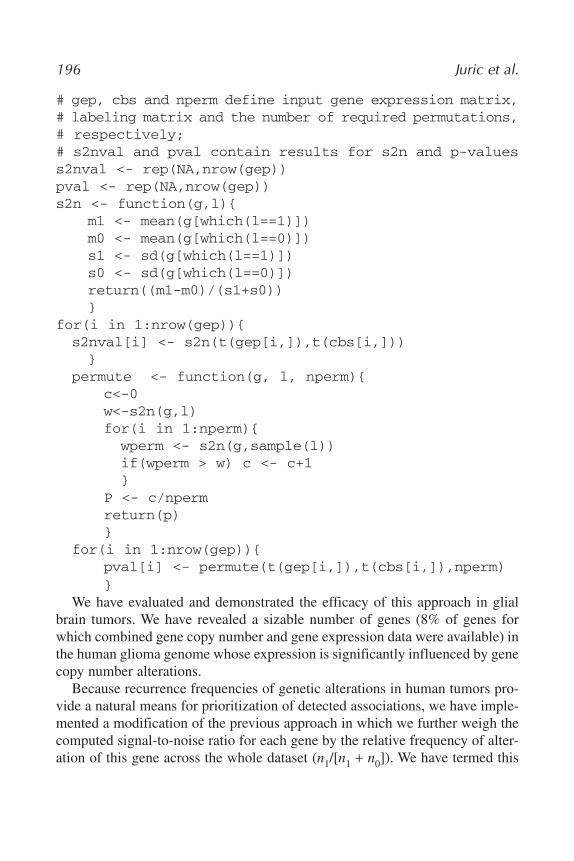
# gep, cbs and nperm define input gene expression matrix,# labeling matrix and the number of required permutations,# respectively;# s2nval and pval contain results for s2n and p-valuess2nval <- rep(NA,nrow(gep))pval <- rep(NA,nrow(gep))s2n <- function(g,l){
m1 <- mean(g[which(l==1)])m0 <- mean(g[which(l==0)])s1 <- sd(g[which(l==1)])s0 <- sd(g[which(l==0)])return((m1-m0)/(s1+s0))}
for(i in 1:nrow(gep)){s2nval[i] <- s2n(t(gep[i,]),t(cbs[i,]))}
permute <- function(g, l, nperm){c<-0w<-s2n(g,l)for(i in 1:nperm){wperm <- s2n(g,sample(l))if(wperm > w) c <- c+1}
P <- c/npermreturn(p)}
for(i in 1:nrow(gep)){pval[i] <- permute(t(gep[i,]),t(cbs[i,]),nperm)}
We have evaluated and demonstrated the efficacy of this approach in glialbrain tumors. We have revealed a sizable number of genes (8% of genes forwhich combined gene copy number and gene expression data were available) inthe human glioma genome whose expression is significantly influenced by genecopy number alterations.
Because recurrence frequencies of genetic alterations in human tumors pro-vide a natural means for prioritization of detected associations, we have imple-mented a modification of the previous approach in which we further weigh thecomputed signal-to-noise ratio for each gene by the relative frequency of alter-ation of this gene across the whole dataset (n1/[n1 + n0]). We have termed this
196 Juric et al.
12_Bredel.qxd 6/3/07 11:37 AM Page 196
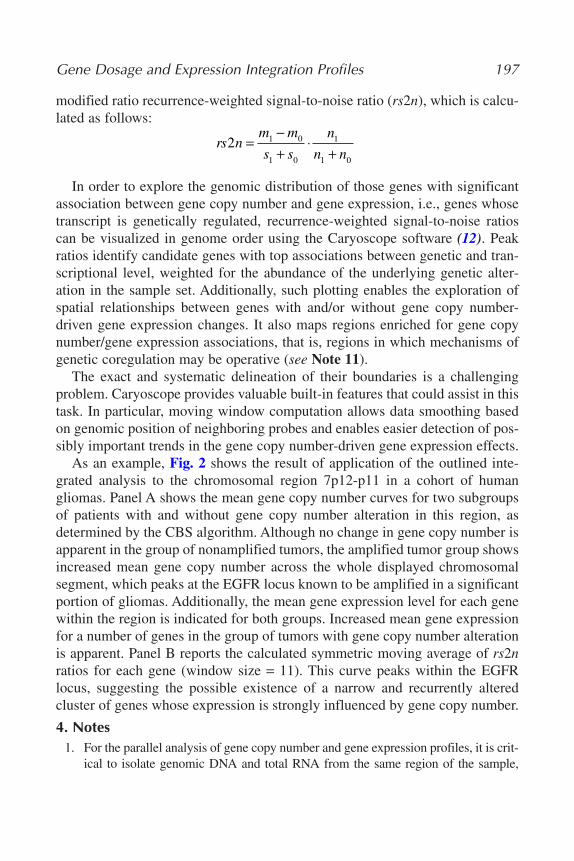
modified ratio recurrence-weighted signal-to-noise ratio (rs2n), which is calcu-lated as follows:
In order to explore the genomic distribution of those genes with significantassociation between gene copy number and gene expression, i.e., genes whosetranscript is genetically regulated, recurrence-weighted signal-to-noise ratioscan be visualized in genome order using the Caryoscope software (12). Peakratios identify candidate genes with top associations between genetic and tran-scriptional level, weighted for the abundance of the underlying genetic alter-ation in the sample set. Additionally, such plotting enables the exploration ofspatial relationships between genes with and/or without gene copy number-driven gene expression changes. It also maps regions enriched for gene copynumber/gene expression associations, that is, regions in which mechanisms ofgenetic coregulation may be operative (see Note 11).
The exact and systematic delineation of their boundaries is a challengingproblem. Caryoscope provides valuable built-in features that could assist in thistask. In particular, moving window computation allows data smoothing basedon genomic position of neighboring probes and enables easier detection of pos-sibly important trends in the gene copy number-driven gene expression effects.
As an example, Fig. 2 shows the result of application of the outlined inte-grated analysis to the chromosomal region 7p12-p11 in a cohort of humangliomas. Panel A shows the mean gene copy number curves for two subgroupsof patients with and without gene copy number alteration in this region, asdetermined by the CBS algorithm. Although no change in gene copy number isapparent in the group of nonamplified tumors, the amplified tumor group showsincreased mean gene copy number across the whole displayed chromosomalsegment, which peaks at the EGFR locus known to be amplified in a significantportion of gliomas. Additionally, the mean gene expression level for each genewithin the region is indicated for both groups. Increased mean gene expressionfor a number of genes in the group of tumors with gene copy number alterationis apparent. Panel B reports the calculated symmetric moving average of rs2nratios for each gene (window size = 11). This curve peaks within the EGFRlocus, suggesting the possible existence of a narrow and recurrently alteredcluster of genes whose expression is strongly influenced by gene copy number.
4. Notes1. For the parallel analysis of gene copy number and gene expression profiles, it is crit-
ical to isolate genomic DNA and total RNA from the same region of the sample,
rs nm m
s s
n
n n2 1 0
1 0
1
1 0
=−+
⋅+
Gene Dosage and Expression Integration Profiles 197
12_Bredel.qxd 6/3/07 11:37 AM Page 197

198 Juric et al.
12_Bredel.qxd 6/3/07 11:37 AM Page 198

especially if crude tumor samples are analyzed. Genetic heterogeneity present intumors can hamper the analysis if large tumor tissue samples are dissected in several pieces and the isolation of nucleic acids is not performed on directlyneighboring parts. Ideally, protocols that allow concomitant isolation of both DNAand RNA (Qiagen) should be used. However, for RNA isolation from lipid-rich tis-sues, such as the brain, these kits do not produce optimal results. In brain tumors,the Qiagen RNeasy lipid tissue kit provides an excellent method for RNA recovery.We have noticed that the subsequent extraction of genomic DNA from the organicphase does not meet a quality necessary for array-CGH analysis.
2. Although custom or commercially available cDNA microarrays are a convenientchoice for both applications, two different microarray platforms, each optimizedfor the best results, could also be used. This approach requires array-CGH datainterpolation, so that expression measurements can be mapped to their correspon-ding gene copy number levels. At the same time, it avoids data interpretation dif-ficulties related to possible tight correlations between expression and copy numbermeasurements because of individual probe performance. Although gene expres-sion profiling can be performed on a number of oligonucleotide microarray plat-forms, the best CGH results have been obtained with cDNA and bacterial artificialchromosome arrays. Use of oligonucleotide arrays for CGH analysis typicallyrequires PCR-based genomic DNA complexity reduction that introduces addi-tional biases. Recently, protocols and bioinformatics analysis tools were devel-oped, which allow high-resolution, genome-wide gene copy number profilingusing long oligonucleotide arrays and full-complexity DNA (13).
3. We are routinely quantifying digestion products by spectrophotometry at 260 and280 λ prior to DNA labeling; because of the considerable non-DNA contamina-tion of even purified genomic DNA from lipid-rich brain tumors, the amount ofdigest does not properly reflect the amount of input genomic DNA.
4. We have successfully used the scaled-up protocol for the cDNA preparation from ourreference RNA described in the Genisphere 3DNA Array 900 manual. This large-scale preparation of reference cDNA is not only highly convenient but also assures
Gene Dosage and Expression Integration Profiles 199
Fig. 2. (Opposite page) Integration of gene copy number and gene expression datain chromosomal region 7p12-p11 in a cohort of glial brain tumors. (A) Shows the meangene copy number curves for two subgroups of patients with and without gene copynumber alteration at this locus, based on calculating the regional gene copy numberprofile for each tumor using the circular binary segmentation algorithm. The group oftumors with amplification shows increased mean gene copy number across the wholedisplayed chromosomal segment, which peaks at the epidermal growth factor receptor(EGFR) locus. Mean gene expression levels for all genes within the segment are plot-ted separately for both subgroups. There is increased mean gene expression for a num-ber of genes in the subgroup of tumors with gene copy number alteration. (B) Reportsthe corresponding smoothed (see Subheading 3.6.) rs2n ratio curve, which peaks at theEGFR locus, indicating that the expression of a cluster of genes around EGFR is pri-marily genetically regulated and recurrently altered in the tumors.
12_Bredel.qxd 6/3/07 11:37 AM Page 199

that a cDNA product as constant as possible over a larger study cohort (which maybe hybridized in a number of experiment sets) is used for the reference channel.
5. Because of increased fading of Genisphere Cy5 3DNA Array 900 reagent, we areapplying the Genisphere DyeSaver2 anti-fade coating to each microarray immedi-ately after the last wash. We are here sequentially drying the slide by centrifugationat 1000g for 30 s, dipping the microarray into DyeSaver2 for 3 s, and centrifugingthe slide for 50 s. This procedure does not add any background to the microarraysbut ensures that there is enough time (several hours) to scan the microarrays.
6. Using the Genisphere labeling protocol, bovine serum albumin prehybridizationfor background reduction is not necessary on our microarrays. We are only per-forming a postprocessing procedure (immediately before hybridization) in whichthe microarrays are sequentially ultraviolet cross-linked with 60 mJ, agitated inisopropanol for 15 min, placed into boiling nuclease-free water (95°C) for 2 min,and dried by centrifugation at 400g for 1 min.
7. In addition to the MIDAS software, other normalization tools are readily available.Particularly easy to use is the standardization and normalization of microarray data(SNOMAD) tool (14), an internet-accessible interactive application that is excel-lent for the normalization and preprocessing of smaller sample sets. An alternativefor the R environment is the SMA package developed by Yang and Dudoit (15).
8. In order to increase the number of change points obtained by CBS, we routinely setthe alpha parameter of the segment function to 0.05. For the purpose of parallelanalysis of gene copy number and gene expression, we do not use the available “undo”option that eliminates change points, which are not at least three standard deviationsapart. An independent measurement by the gold standard that is usually needed toremove “unnecessary” change points is rarely available for all the genes in the dataset.
9. The CBS algorithm is also implemented in the more user-friendly CGHPRO dataanalysis tool offering interactive graphical interface (16). Several alternative genecopy number aberration identification tools are available. CGH-Plotter is a freelyavailable MATLAB-toolbox for array CGH data analysis (11). It enables a quickanalysis of large datasets and includes a highly customizable graphical output.Similar to the CBS algorithm, actual gain/loss calling depends on user definedthresholds. CGH-Miner (17) uses a new “Cluster along chromosomes” algorithmfor the identification of chromosomal regions with different gene copy number lev-els. It provides an automated gain/loss calling function with false discovery rateestimation based on normal–normal array hybridizations. It also generates “consen-sus curves” that reflect the recurrence of gene copy number alterations in a studyset. This program is written in R and available as Excel add-in. A comprehensivecomparative analysis of various tools and algorithms for CGH data analysis is alsoavailable and provides valuable insights into their performance characteristics (18).
10. These p-values are determined in the context of multiple hypothesis testing.Appropriate procedures have to be used in order to control the number of falselypositive results. The use of the permutation-based q-value, which measures statis-tical significance in terms of false discovery rate, offers a sensible balance betweenthe number of true and false positives and provides an automatically calibrated and
200 Juric et al.
12_Bredel.qxd 6/3/07 11:37 AM Page 200
easily interpreted approach for the estimation of statistical significance in genome-wide studies (19).
11. Proper interpretation of the observed regions requires careful handling of proberedundancy because a major source of focal effects detected in rs2n plots could bebecause of the presence of multiple probes per gene. Combination of multiple log2ratios or, alternatively, rs2n values into one estimate per gene avoids this difficulty.
References1. Albertson, D. G., Collins, C., McCormick, F., and Gray, J. W. (2003) Chromosome
aberrations in solid tumors. Nat. Genet. 34, 369–376.2. Mertens, F., Johansson, B., Hoglund, M., and Mitelman, F. (1997) Chromosomal
imbalance maps of malignant solid tumors: a cytogenetic survey of 3185 neo-plasms. Cancer Res. 57, 2765–2780.
3. Pollack, J. R., Perou, C. M., Alizadeh, A. A., et al. (1999) Genome-wide analysisof DNA copy-number changes using cDNA microarrays. In: Nat. Genet., Vol. 23,pp. 41–46.
4. Saeed, A. I., Sharov, V., White, J., et al. (2003) TM4: a free, open-source systemfor microarray data management and analysis. Biotechniques 34, 374–378.
5. Pollack, J. R., Sorlie, T., Perou, C. M., et al. (2002) Microarray analysis reveals amajor direct role of DNA copy number alteration in the transcriptional program ofhuman breast tumors. Proc. Natl. Acad. Sci. USA 99, 12,963–12,968.
6. Olshen, A. B., Venkatraman, E. S., Lucito, R., and Wigler, M. (2004) Circular binarysegmentation for the analysis of array-based DNA copy number data. Biostatistics5, 557–572.
7. Ihaka, R. and Gentleman, R. (1996) R: a language for data analysis and graphics.J. Comput. Graph. Stat. 5, 299–314.
8. Aguirre, A. J., Brennan, C., Bailey, G., et al. (2004) High-resolution characteriza-tion of the pancreatic adenocarcinoma genome. Proc. Natl. Acad. Sci. USA 101,9067–9072.
9. Golub, T. R., Slonim, D. K., Tamayo, P., et al. (1999) Molecular classification ofcancer: class discovery and class prediction by gene expression monitoring. Science286, 531–537.
10. Hyman, E., Kauraniemi, P., Hautaniemi, S., et al. (2002) Impact of DNA amplifi-cation on gene expression patterns in breast cancer. Cancer Res. 62, 6240–6245.
11. Autio, R., Hautaniemi, S., Kauraniemi, P., et al. (2003) CGH-Plotter: MATLABtoolbox for CGH-data analysis. Bioinformatics 19, 1714–1715.
12. Awad, I. A., Rees, C. A., Hernandez-Boussard, T., Ball, C. A., and Sherlock, G.(2004) Caryoscope: an Open Source Java application for viewing microarray datain a genomic context. BMC Bioinformatics 5, 151.
13. Brennan, C., Zhang, Y., Leo, C., et al. (2004) High-resolution global profiling ofgenomic alterations with long oligonucleotide microarray. Cancer Res. 64, 4744–4748.
14. Colantuoni, C., Henry, G., Zeger, S., and Pevsner, J. (2002) SNOMAD(Standardization and NOrmalization of MicroArray Data): web-accessible geneexpression data analysis. Bioinformatics 18, 1540–1541.
Gene Dosage and Expression Integration Profiles 201
12_Bredel.qxd 6/3/07 11:37 AM Page 201

15. Yang, Y. H., Dudoit, S., Luu, P., et al. (2002) Normalization for cDNA microarraydata: a robust composite method addressing single and multiple slide systematicvariation. Nucleic Acids Res. 30, e15.
16. Chen, W., Erdogan, F., Ropers, H. H., Lenzner, S., and Ullmann, R. (2005) CGH-PRO—a comprehensive data analysis tool for array CGH. BMC Bioinformatics 6, 85.
17. Wang, P., Kim, Y., Pollack, J., Narasimhan, B., and Tibshirani, R. (2005) A methodfor calling gains and losses in array CGH data. Biostatistics 6, 45–58.
18. Lai, W. R., Johnson, M. D., Kucherlapati, R., and Park, P. J. (2005) Comparativeanalysis of algorithms for identifying amplifications and deletions in array CGHdata. Bioinformatics 21, 3763–3770.
19. Storey, J. D. and Tibshirani, R. (2003) Statistical significance for genomewidestudies. Proc. Natl. Acad. Sci. USA 100, 9440–9445.
202 Juric et al.
12_Bredel.qxd 6/3/07 11:37 AM Page 202

13
Progression-Associated Genes in Astrocytoma Identifiedby Novel Microarray Gene Expression Data Reanalysis
Tobey J. MacDonald, Ian F. Pollack, Hideho Okada, Soumyaroop Bhattacharya, and James Lyons-Weiler
SummaryAstrocytoma is graded as pilocytic (WHO grade I), diffuse (WHO grade II), anaplastic (WHO
grade III), and glioblastoma multiforme (WHO grade IV). The progression from low- to high-grade astrocytoma is associated with distinct molecular changes that vary with patient age, yetthe prognosis of high-grade tumors in children and adults is equally dismal. Whether specificgene expression changes are consistently associated with all high-grade astrocytomas, independ-ent of patient age, is not known. To address this question, we reanalyzed the microarray datasetscomprising astrocytomas from children and adults, respectively. We identified nine genes consis-tently dysregulated in high-grade tumors, using four novel tests for identifying differentiallyexpressed genes. Four genes encoding ribosomal proteins (RPS2, RPS8, RPS18, RPL37A) wereupregulated, and five genes (APOD, SORL1, SPOCK2, PRSS11, ID3) were downregulated inhigh-grade by all tests. Expression results were validated using a third astrocytoma dataset.APOD, the most differentially expressed gene, has been shown to inhibit tumor cell and vascularsmooth muscle cell proliferation. This suggests that dysregulation of APOD may be critical formalignant astrocytoma formation, and thus a possible novel universal target for therapeutic inter-vention. Further investigation is needed to evaluate the role of APOD, as well as the other genesidentified, in malignant astrocytoma development.
Key Words: Astrocytoma; tumor progression; gene expression; microarray.
1. IntroductionAstrocytoma is the most common brain tumor in children and adults. Although
adult and childhood astrocytomas can be distinguished by distinct clinical andgenetic characteristics, the malignant forms are histologically identical and sharea dismal prognosis, regardless of patient age (1–4). The World Health Organization(WHO) grades astrocytomas based on histopathological characteristics as pilocytic(WHO grade I), diffuse (WHO grade II), which often progresses to high-grade
203
From: Methods in Molecular Biology, vol. 377, Microarray Data Analysis: Methods and ApplicationsEdited by: M. J. Korenberg © Humana Press Inc., Totowa, NJ
13_MacDonald.qxd 6/3/07 11:48 AM Page 203

astrocytoma, anaplastic (WHO grade III), and glioblastoma multiforme (WHOgrade IV) (1). Pilocytic astrocytomas, the most common brain tumor in chil-dren, rarely exhibit malignant progression, and are considered to be a biologi-cally distinct entity from nonpilocytic astrocytomas (1). Because these are wellcircumscribed and rarely infiltrative, a complete surgical resection and cure isexpected in the majority of patients. In contrast, nonpilocytic astrocytomas,which account for the vast majority of astrocytomas in adults and a sizeablesubgroup of astrocytomas in children, are diffusely infiltrative and are often notamenable to complete resection (5). Upon recurrence, grade II diffuse astrocy-tomas have a tendency for malignant progression to anaplastic astrocytoma and,ultimately, glioblastoma multiforme. There is increasing evidence that the pro-gression from grade II to higher grade astrocytoma is the result of a sequenceof genetic alterations that are acquired during the process of transformation(5–7). Glioblastomas evolving from a previous lower grade astrocytoma aredefined as secondary (ScGBM), while those arising without any evidence of aprevious low-grade precursor are termed primary (PrGBM) (1). AlthoughPrGBM and ScGBM are histologically indistinguishable, the two types exhibitdistinct molecular alterations (8–11). PrGBM usually occur in older patientsand are characterized by amplification and overexpression of EGFR, PTENmutations, and loss of INK4a (8–11). ScGBM tend to occur in younger adultsand are associated with TP53 mutations and overexpression of PDGFA and itsreceptor (8–12). High-grade astrocytomas of childhood clinicopathologicallyresemble PrGBM of adulthood, yet these tumors rarely demonstrate EGFRamplification (13). Childhood HGA also rarely exhibit TP53 mutations.However, overexpression of EGFR and the TP53 gene and protein is common(14–16).
Determining whether there are common underlying molecular changes asso-ciated with malignant astrocytoma, independent of patient age, and demonstrat-ing a critical role for these changes in the formation of malignant astrocytomamay ultimately lead to the development of novel and universal cancer therapiestargeting these alterations. Microarray gene expression analysis has been aninvaluable tool with which to unveil unforeseen patterns in the molecular alter-ations of cancers with indistinguishable phenotypes and histological characteri-stics (17–21). Cancer progression from benign-to-malignant grade, in whichtumor cells acquire the ability to migrate away from the primary tumor, invadethrough the surrounding microenvironment, initiate angiogenesis, and establisha distant colony is a highly complex process that is dependent on critical geneticchanges. In principle, the identification of significantly differentially expressedgenes between benign and malignant astrocytomas from patients of all agesshould provide insight into the underlying genetic regulation of this process inthis disease.
204 MacDonald et al.
13_MacDonald.qxd 6/3/07 11:48 AM Page 204

In this study, we sought to identify and validate gene expression patterns thatuniversally differentiate higher from lower grades of astrocytomas. To this end,we reanalyzed two previously published microarray datasets of expression inten-sities of astrocytomas, comprised of childhood and adult astrocytomas, respec-tively (14,22). We applied a series of four novel supervised statistical analyses toidentify differentially expressed genes, followed by unsupervised clustering ofthe samples using leave-one-out validation and cross-dataset predictions to assessclassification error. Each gene set was used to cluster the tumor samples in boththe datasets. We performed iterative cross-validation on the union of the genesfound to be significant in both datasets by all tests. A list of marker genes was cre-ated that was comprised of genes found to be significant under all tests in bothdatasets. We then validated our derived gene list using a third published dataset(23) and found the same genes differentially expressed using the same tests.
2. Materials2.1. The K dataset
This study analyzed the expression of 12,625 probe sets (Affymetrix U95Av2oligonucleotide array) in 13 childhood astrocytoma samples of two classes (14).Out of 13, 6 samples were low-grade astrocytomas (LGAs) whereas 7 were ofhigh grades (HGAs). The aim of their study was to determine an overlap ofastrocytoma progression markers with a preselected gene list of angiogenesismarkers. They used expression profiling of 133 angiogenesis-related genes andfound a list of 44 differentially expressed genes (17 overexpressed and 27 under-expressed), which were also present in their list of angiogenesis markers. Theyused hierarchical clustering and principal components analysis and succeededin classifying HGAs from LGAs using all genes as well as 133 angiogenesis-related genes. These data were downloaded from http://microarray.cnmcresearch.org/resources.htm.
2.2. The V Dataset
This study compared the expression profiles of 7,129 probe sets (AffymetrixHUGFL oligonucleotide array) in 16 astrocytoma samples (HGAs and LGAs)(22). Of 16 samples, 8 were of primary and 8 were of recurrent high-gradeastrocytomas. They identified 66 genes that exhibited twofold or greater differ-ence in expression between primary and higher grade tumors. They furthervalidated 12 of those genes by further analysis. These data were downloadedfrom http://dot.ped.med.umich.edu:2000/pub/astrocytoma/index.html
Both datasets are also “on-tap” for ease of reanalysis in our online open sourcegene expression analysis web application (http://bioinformatics.upmc.edu/GE2/GEDA.html).
Astrocytoma Progression Genes by Microarray Reanalysis 205
13_MacDonald.qxd 6/3/07 11:48 AM Page 205
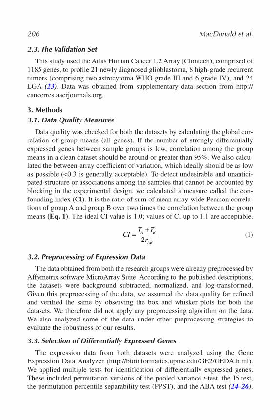
2.3. The Validation Set
This study used the Atlas Human Cancer 1.2 Array (Clontech), comprised of1185 genes, to profile 21 newly diagnosed glioblastoma, 8 high-grade recurrenttumors (comprising two astrocytoma WHO grade III and 6 grade IV), and 24LGA (23). Data was obtained from supplementary data section from http://cancerres.aacrjournals.org.
3. Methods3.1. Data Quality Measures
Data quality was checked for both the datasets by calculating the global cor-relation of group means (all genes). If the number of strongly differentiallyexpressed genes between sample groups is low, correlation among the groupmeans in a clean dataset should be around or greater than 95%. We also calcu-lated the between-array coefficient of variation, which ideally should be as lowas possible (<0.3 is generally acceptable). To detect undesirable and unantici-pated structure or associations among the samples that cannot be accounted byblocking in the experimental design, we calculated a measure called the con-founding index (CI). It is the ratio of sum of mean array-wide Pearson correla-tions of group A and group B over two times the correlation between the groupmeans (Eq. 1). The ideal CI value is 1.0; values of CI up to 1.1 are acceptable.
(1)
3.2. Preprocessing of Expression Data
The data obtained from both the research groups were already preprocessed byAffymetrix software MicroArray Suite. According to the published descriptions,the datasets were background subtracted, normalized, and log-transformed.Given this preprocessing of the data, we assumed the data quality far refinedand verified the same by observing the box and whisker plots for both thedatasets. We therefore did not apply any preprocessing algorithm on the data.We also analyzed some of the data under other preprocessing strategies to evaluate the robustness of our results.
3.3. Selection of Differentially Expressed Genes
The expression data from both datasets were analyzed using the GeneExpression Data Analyzer (http://bioinformatics.upmc.edu/GE2/GEDA.html).We applied multiple tests for identification of differentially expressed genes.These included permutation versions of the pooled variance t-test, the J5 test,the permutation percentile separability test (PPST), and the ABA test (24–26).
CIr r
rA B
AB
=+
2
206 MacDonald et al.
13_MacDonald.qxd 6/3/07 11:48 AM Page 206

Because we know that all genes do not exhibit the same distribution, even withinsample groups, it does not make sense to apply a single threshold of significancefor all genes. Instead, we randomized the sample labels 1000 times to determinea null distribution of the test statistic(s) for each gene. All permutation testswere performed at α = 0.05.
3.4. Pooled Variance t-Test
The difference in gene expression for each gene is determined by comparingthe average expression value within each group using a studentized test statis-tic, t, which employs the pooled variance error term (Eq. 2). This form of thetest statistic is more appropriate as it takes into account the difference in num-ber of samples in the two groups.
(2)
3.5. J5 Test
The J5 test gives a statistic based on the magnitude of the difference betweenthe means (Eq. 3). It essentially compares the difference of means in any geneto the average difference in means over the whole array. This test appears to bemost useful when the number of samples is low.
(3)
3.6. Significance Analysis of Microarrays
Significance analysis of microarrays (SAM) determines genes to be statisti-cally significant based on changes in their expression determined by gene-specificmodified t-tests (27,28). An individual score is assigned to each gene based onthe change in their expression relative to the sum of standard deviation and a fudge factor for repeated measurements for that gene. The score is in fact a t-statistic with an added fudge factor in the denominator. The purpose of thefudge factor is to prevent a large test statistic for genes with low variance.Genes carrying a score over a set threshold are identified as significant. The setof genes called significant is large or small depending on the threshold. SAMuses permutations to construct a null distribution for the t-values and estimat-ing the proportion of significant genes identified by chance, which is termed as
Ja b
na b
ii i
k kk
n=
−
−=
∑1
1
tn s n s
n n n
=−
− + −+ −
⎡
⎣⎢
⎤
⎦⎥
µ µ1 2
1 12
2 22
1 2 1
1 1
21( ) ( )
++⎛⎝⎜
⎞⎠⎟
1
2n
Astrocytoma Progression Genes by Microarray Reanalysis 207
13_MacDonald.qxd 6/3/07 11:48 AM Page 207

the false discovery rate (FDR). FDR is estimated by counting and averagingthe number of false-positives over the permutations of the measurements.SAM is incorporated in caGEDA; a detailed description of SAM can be foundat http://bioinformatics.upmc.edu/Help/SAM/SAMINFO.htm.
3.7. PPST Test
PPST is a test for detecting genes that exhibit a significant number of sam-ples of one group that exhibit expression intensities that are beyond a certainpercentile of the observed intensities of the samples in the other group (24–26).Differentially expressed genes are generally reported as being either overex-pressed or underexpressed in case or control samples. The PPST is capable ofidentifying genes that are differentially expressed in only a subset of samples inone group, which may have been missed by tests that compare population-leveldifferences (means). In general, the search for differentially expressed genesshould include the search for genes that are differentially expressed in a subsetof patients to foster the transition toward individualized medicine.
For each gene, the number of samples in group A (e.g., HGA) was countedthat had intensities above the 95th percentile of the intensities of group B (i.e.,LGAs). This number is s1. To this number is added the number of samples ingroup B that exhibit expression intensities below the 5th percentile of group A(s2). These scores are calculated for all 1000 permutations and a null distribu-tion for each gene is generated. Genes with s1 + s2 values beyond the sum s1 + s2associated with a 5% type I error risk (gleaned from the null distribution result-ing from permutation) are classified as overexpressed in HGAs. Similar scoresare calculated for the opposite pattern (underexpression in HGA; s3 + s4) andcompared with the s3 + s4 null distribution.
3.8. ABA Test
The ABA test identifies genes with two significant subsets with oppositeexpression differentials (24–26). Genes that exhibit an unusual expression(ABA or BAB) patterns are likely to be missed by the tests that seek population-level biomarkers. Genes that have significant s1 + s2 or s3 + s4 scores are eitherover- or underexpressed in HGAs. Some genes can have both significant s1 + s2and s3 + s4 scores, and are said to exhibit ABA (A > B > A) pattern. The PPSTtest is slightly reformulated to determine ABA patterns so the number of occur-rences of ABA-type patterns becomes the statistic of interest. Under the ABAtest, a gene is significant if and only if it is differentially expressed in bothdirections (i.e., simultaneously overexpressed and underexpressed in a signifi-cant number of samples).
208 MacDonald et al.
13_MacDonald.qxd 6/3/07 11:48 AM Page 208
3.9. Distance and Clustering
Once a set of genes has been identified as significant the samples are clus-tered in a “semi-supervised” mode because the user first identifies significantgenes (feature selection) in a supervised manner, and the samples are classifiedusing the retained genes as features (29). The clustering algorithm does not usethe sample label to enforce the clustering. We performed a variety of clusteringalgorithms to assess the importance of the known and unknown assumptionsimplied by each clustering method. Classification trees for each dataset weregenerated using distances measured by a variety of distance metrics to assessthe robustness of the various gene lists to known and unknown assumptionsimplied by each distance metric.
3.10. Computational Validation
The true validation we have performed is a result of the discovery of genesdifferentially expressed in two separate populations using data originating intwo separate laboratories. Within-dataset computational validation of the resultsusing leave-one-out validation was also performed. In leave-one-out validation,samples are removed, one at a time, and the feature set is determined using atest applied to the remaining n – 1 samples. These features are then applied tomake a prediction on the placement of the sample left out. The procedure isrepeated for all samples, and a score (usually the proportion of correct predic-tions) is tallied. Leave-one-out validation uses n – 1 samples as a training set,predicts on the sample left out, and the score of 1 – P (correct inference) leadsto a classification error rate (30).
3.11. Validation
The previously mentioned tests were applied identically to the Godarddataset (23) for comparison in order to validate the derived marker gene listfrom the Khatua (14) and van den Boom (22) studies.
4. Results4.1. Visualization of Data Quality
The quality of datasets was judged by observing the box and whisker plotsfor both datasets (Fig. 1). The datasets exhibit similar distributions and thereforeno significant variability among the samples was detected. The data qualityparameters are within acceptable limits (Table 1). Overall, the two datasetsexhibit high among sample all-gene distributions, and appeared to require nofurther normalization.
Astrocytoma Progression Genes by Microarray Reanalysis 209
13_MacDonald.qxd 6/3/07 11:48 AM Page 209

210 MacDonald et al.
Fig. 1. Box and Whisker plots for the three datasets. Plots for van den Boom et al.(22) (A and C) and Khatua et al. (14) (B and D) present the quality of the data. The x-axis represents the samples and y-axis represents the expression intensities. Samples ofgroup one are high grade (blue) and those of group two are low-grade (red) astrocy-tomas. In an ideal experiment, the median (or mean), first standard deviation, upper andlower second medians, and the 95th percentile should be approximately the same acrossall arrays. HGA, high-grade astrocytoma; LGA, low-grade astrocytoma.
4.2. Differentially Expressed Genes
The K and V datasets were reanalyzed using pooled variance t-test and J5 test(both in conjunction with jackknife), and the PPST and ABA tests. The numbersof genes found to be significant at the 5% type 1 error rate are summarized in
13_MacDonald.qxd 6/3/07 11:48 AM Page 210
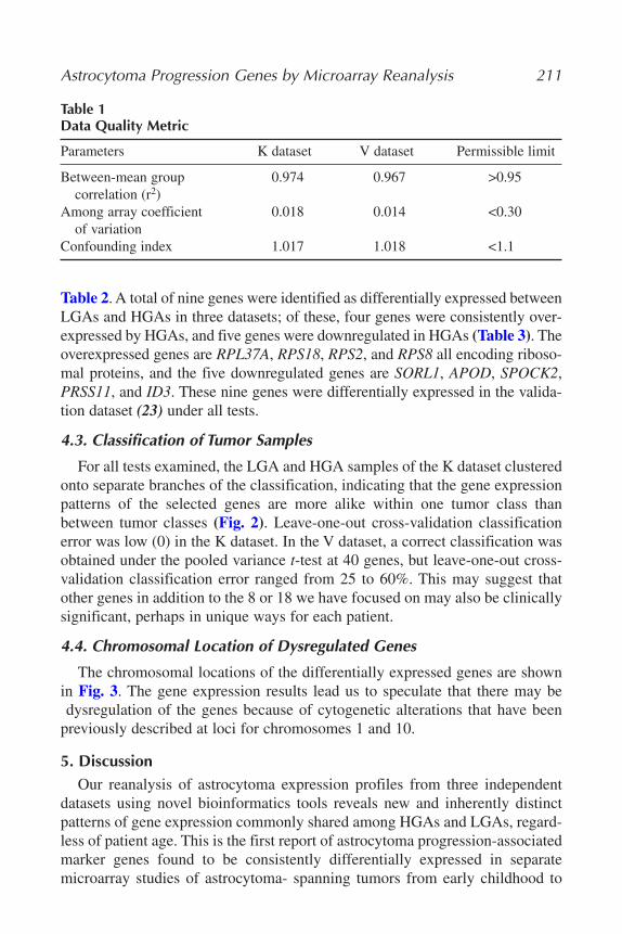
Astrocytoma Progression Genes by Microarray Reanalysis 211
Table 1Data Quality Metric
Parameters K dataset V dataset Permissible limit
Between-mean group 0.974 0.967 >0.95correlation (r2)
Among array coefficient 0.018 0.014 <0.30of variation
Confounding index 1.017 1.018 <1.1
Table 2. A total of nine genes were identified as differentially expressed betweenLGAs and HGAs in three datasets; of these, four genes were consistently over-expressed by HGAs, and five genes were downregulated in HGAs (Table 3). Theoverexpressed genes are RPL37A, RPS18, RPS2, and RPS8 all encoding riboso-mal proteins, and the five downregulated genes are SORL1, APOD, SPOCK2,PRSS11, and ID3. These nine genes were differentially expressed in the valida-tion dataset (23) under all tests.
4.3. Classification of Tumor Samples
For all tests examined, the LGA and HGA samples of the K dataset clusteredonto separate branches of the classification, indicating that the gene expressionpatterns of the selected genes are more alike within one tumor class thanbetween tumor classes (Fig. 2). Leave-one-out cross-validation classificationerror was low (0) in the K dataset. In the V dataset, a correct classification wasobtained under the pooled variance t-test at 40 genes, but leave-one-out cross-validation classification error ranged from 25 to 60%. This may suggest thatother genes in addition to the 8 or 18 we have focused on may also be clinicallysignificant, perhaps in unique ways for each patient.
4.4. Chromosomal Location of Dysregulated Genes
The chromosomal locations of the differentially expressed genes are shownin Fig. 3. The gene expression results lead us to speculate that there may bedysregulation of the genes because of cytogenetic alterations that have been
previously described at loci for chromosomes 1 and 10.
5. DiscussionOur reanalysis of astrocytoma expression profiles from three independent
datasets using novel bioinformatics tools reveals new and inherently distinctpatterns of gene expression commonly shared among HGAs and LGAs, regard-less of patient age. This is the first report of astrocytoma progression-associatedmarker genes found to be consistently differentially expressed in separatemicroarray studies of astrocytoma- spanning tumors from early childhood to
13_MacDonald.qxd 6/3/07 11:48 AM Page 211

212 MacDonald et al.
Table 2Genes Found to be Significant in Three Datasets Using the Five Tests
Test Threshold K dataset V dataset
Pooled t-test α = 0.01 217 39SAM ∆ = 0.6 874 53J5 test T = 4.0 331 847PPST α = 0.05 1281 2304ABA α = 0.05 51 69
Note: In pooled t-test with Jackknife, there were six overlapping genes (three overexpressedand three underexpressed in HGAs), whereas J5 with jackknife results showed five overlappinggenes (two overexpressed and three underexpressed in HGAs). In the PPST test we observed fiveoverlapping genes (four overexpressed and one underexpressed in HGAs) and ABA test gave outfive overlaps in the lists of differentially expressed genes in K and V datasets.
Table 3Genes Identified as Differentially Expressed in Three Datasets by the Four Tests
GenBank Chromosomal ProteinSymbol Gene name accession location function
Overexpressed in high-grade astrocytomas
RPS8 Ribosomal X67247 1p34.1 Unknownprotein S8
RPS2 Ribosomal AB007147 16p13.3 Unknownprotein S2
RPS18 Ribosomal X69150 6p21.3 Unknownprotein S18
RPL37A Ribosomal L11567 5p Unknownprotein L37A
Underexpressed in high-grade astrocytomas
APOD Apolipoprotein D J02611 3q26.2 Lipid metabolism & transport
PRSS11 Protease, AF157623 10q25.3 Cell growth serine, 11 regulation
ID3 Inhibitor of DNA X73428 1p36.13 Transcription binding 3 corepressor
SORL1 Sortilin-related Y08110 11q23.2 Lipid metabolismreceptor 1 & transport
KIAA0275 SPOCK2 D87465 10q21 Cell differentiation
13_MacDonald.qxd 6/3/07 11:48 AM Page 212
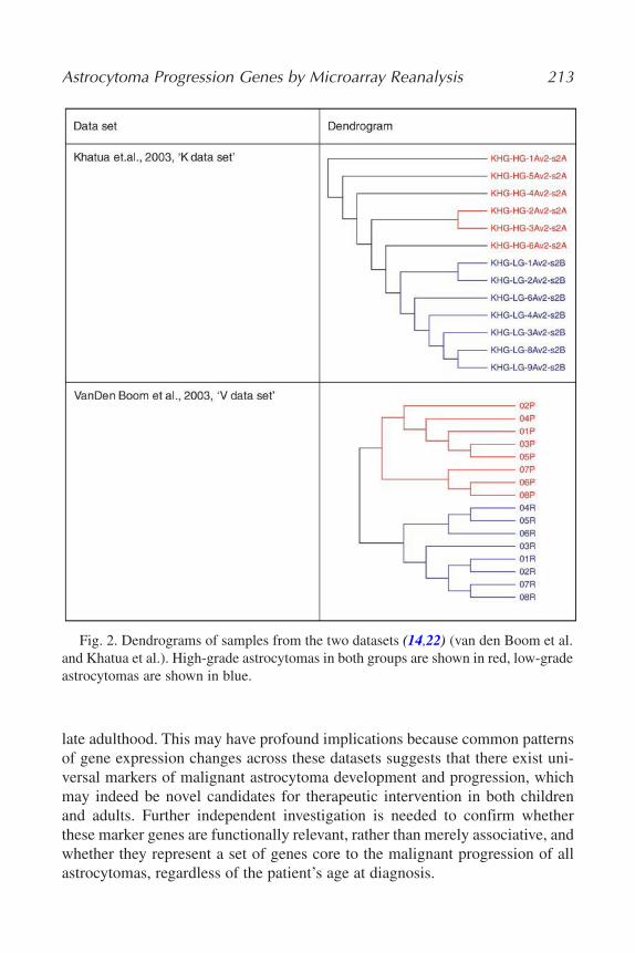
Astrocytoma Progression Genes by Microarray Reanalysis 213
Fig. 2. Dendrograms of samples from the two datasets (14,22) (van den Boom et al.and Khatua et al.). High-grade astrocytomas in both groups are shown in red, low-gradeastrocytomas are shown in blue.
late adulthood. This may have profound implications because common patternsof gene expression changes across these datasets suggests that there exist uni-versal markers of malignant astrocytoma development and progression, whichmay indeed be novel candidates for therapeutic intervention in both childrenand adults. Further independent investigation is needed to confirm whetherthese marker genes are functionally relevant, rather than merely associative, andwhether they represent a set of genes core to the malignant progression of allastrocytomas, regardless of the patient’s age at diagnosis.
13_MacDonald.qxd 6/3/07 11:48 AM Page 213
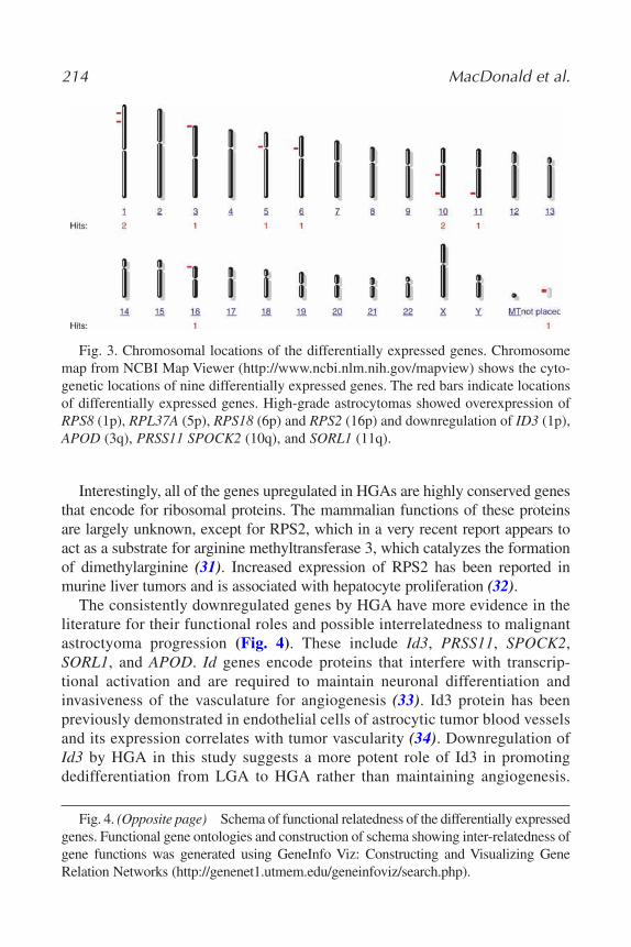
Interestingly, all of the genes upregulated in HGAs are highly conserved genesthat encode for ribosomal proteins. The mammalian functions of these proteinsare largely unknown, except for RPS2, which in a very recent report appears toact as a substrate for arginine methyltransferase 3, which catalyzes the formationof dimethylarginine (31). Increased expression of RPS2 has been reported inmurine liver tumors and is associated with hepatocyte proliferation (32).
The consistently downregulated genes by HGA have more evidence in theliterature for their functional roles and possible interrelatedness to malignantastroctyoma progression (Fig. 4). These include Id3, PRSS11, SPOCK2,SORL1, and APOD. Id genes encode proteins that interfere with transcrip-tional activation and are required to maintain neuronal differentiation andinvasiveness of the vasculature for angiogenesis (33). Id3 protein has beenpreviously demonstrated in endothelial cells of astrocytic tumor blood vesselsand its expression correlates with tumor vascularity (34). Downregulation ofId3 by HGA in this study suggests a more potent role of Id3 in promotingdedifferentiation from LGA to HGA rather than maintaining angiogenesis.
214 MacDonald et al.
Fig. 3. Chromosomal locations of the differentially expressed genes. Chromosomemap from NCBI Map Viewer (http://www.ncbi.nlm.nih.gov/mapview) shows the cyto-genetic locations of nine differentially expressed genes. The red bars indicate locationsof differentially expressed genes. High-grade astrocytomas showed overexpression ofRPS8 (1p), RPL37A (5p), RPS18 (6p) and RPS2 (16p) and downregulation of ID3 (1p),APOD (3q), PRSS11 SPOCK2 (10q), and SORL1 (11q).
Fig. 4. (Opposite page) Schema of functional relatedness of the differentially expressedgenes. Functional gene ontologies and construction of schema showing inter-relatedness ofgene functions was generated using GeneInfo Viz: Constructing and Visualizing GeneRelation Networks (http://genenet1.utmem.edu/geneinfoviz/search.php).
13_MacDonald.qxd 6/3/07 11:48 AM Page 214
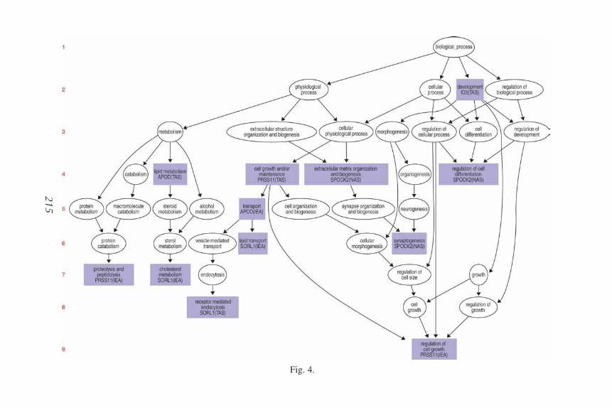
215
Fig. 4.
13_MacDonald.qxd 6/3/07 11:48 AM Page 215

The former concept is supported by studies showing that forced expression ofId3 in erythroid progenitor cells promotes erythroid differentiation and down-regulation of Id3 by retinoic acid-induced differentiation of neuroblastomacells (35,36). Similarly, treatments with phorbol ester, another inducer of neu-roblastoma cell differentiation, also resulted in coordinated downregulation ofId3 gene expression, underscoring the significant role of Id genes in differen-tiation (36). Finally, downregulation of Id3 has also been observed in primaryovarian tumors and was detected in only about 30% cases (37).
PRSS11 encodes the serine protease HtrA1, a candidate tumor suppressorimplicated in protease-induced cell death (38). Downregulation of PRSS11has been observed in ovarian cancer as well as during melanoma progression(39,40). Furthermore, microarray analysis of metastatic melanoma cells identi-fied downregulation of PRSS11 compared with nonmetastatic melanoma cellsand overexpression of PRSS11 resulted in the inhibition of melanoma growth(41). Differential expression of PRSS11 has also been observed between highlymigratory U373MG glioma cells compared with slower moving primaryglioblastoma cells (42). Taken together, these findings implicate PRSS11 as apotential tumor suppressor gene in astrocytoma as well.
KIAA0275 (SPOCK2, testican 2) encodes a calcium-binding proteoglycanprimarily expressed in the brain, but to date there is very little informationregarding its function. SPOCK2 has been recently shown to remove inhibitionof MT1- or MT3-MMP-mediated pro-MMP-2 activation by other testican familymembers (43). This would appear to be counterproductive to promoting protease-mediated invasion. However, as in our study, expression levels of all testicanfamily members in astrocytomas were found to decrease as tumor grade increases(43). These findings would appear to indicate an alternative, and as yet unknown,functional role for SPOCK2.
SORL1 (SorLA/LR11) encodes a recently identified member of the LDLreceptor superfamily, which is broadly expressed in the nervous system andfunctions as a neuronal apolipoprotein E receptor. Unlike the other downregu-lated genes, a connection between SORL1 and tumor progression has yet to bedemonstrated. Of note is that significant and consistent loss of the LR11 proteinin histologically normal-appearing neurons has been observed in Alzheimerpatients (44). LR11 has also been shown to interact with the plasminogen-activating system and PDGF-BB signaling, which has potential implications forastrocytoma progression (45).
APOD encodes a human plasma protein, apolipoprotein D, which belongsto the lipocalin superfamily. Our results showing downregulation of APODacross all age groups with malignant astrocytoma is further supported by otherreports that have showed APOD as a marker for low-grade, noninfiltratingastrocytomas (46,47). Moreover, in human breast cancer cells, increased
216 MacDonald et al.
13_MacDonald.qxd 6/3/07 11:48 AM Page 216

expression of APOD was accompanied by an inhibition of cell proliferationand a progression through a more differentiated phenotype (48). Likewise,apo-D secretion was inversely correlated to cell proliferation and cell densityin human prostate cancer cells (49).
The most frequent cytogenetic changes observed in astrocytomas have beenlosses of loci on 9p, 10, and 22 along with gains on 7, 19, and 20. The chromo-somal locations of the differentially expressed genes identified by our approachreside on chromosomes 1, 3, 6, 7, 10, 11, and 16; however, only downregula-tion of PRSS11, located on chromosome 10, would possibly follow previouslydescribed changes. Thus, dysregulation of these genes would appear to be secondary to factors other than cytogenetic alterations.
6. ConclusionThe genes we have found to be differentially expressed are robust to the test
used in two different datasets generated by two separate laboratories. The genescan distinguish between low-grade and high-grade astrocytomas, independentof age of the patient at diagnosis. These results imply that these genes mayindeed be universal targets and hence most appropriate for therapeutic interven-tion in all malignant astrocytomas. However, the functional roles of these genesin astrocytomas need confirmation, and further studies are needed to characterizetheir roles in the regulatory pathways. Larger studies are also warranted toensure that the associated genes maintain their patterns of expression observedin this study.
AcknowledgmentsWe are grateful to the participants in the Khatua study and Dr. Hanash and
other researchers involved in the van den Boom study for making their respec-tive datasets available to the public. This research was funded by a grant fromthe Claude Worthington Benedum Foundation to Dr. Michael Becich and Dr.Ronald Herberman. These funds helped establish the Benedum OncologyInformatics Center and the Oncology Informatics program at UPCI. The spe-cific funds used for this project were from Dr. Lyons-Weiler’s faculty recruit-ment package.
All the tests for differentially expressed genes and cluster analysis can beapplied to any dataset on the Cancer Gene Expression Data Analysis (caGEDA)web application at http://bioinformatics.upmc.edu/GE2/GEDA.html. It is partof the University of Pittsburgh Bioinformatics Web Application Collection(http://bioinformatics.upmc.edu), which runs on a JAVA web server and isavailable for public usage. Researchers can upload their data and run a widerange of analyses options available in caGEDA, or download and installcaGEDA locally.
Astrocytoma Progression Genes by Microarray Reanalysis 217
13_MacDonald.qxd 6/3/07 11:48 AM Page 217

References1. Kleihues, P. and Cavenee, W. K. (ed.) (2000) Pathology & Genetics. Tumours of the
Nervous System. IARC Lyon, France.2. Batchelor, T. T., Betensky, R. A., Esposito, J. M., et al. (2004) Age-dependent
prognostic effects of genetic alterations in glioblastoma. Clin. Cancer Res. 10,228–233.
3. Simmons, M. L., Lamborn, K. R., Takahashi, M., et al. (2001) Analysis of complexrelationships between age, p53, epidermal growth factor receptor, and survival inglioblastoma patients. Cancer Res. 61, 1122–1128.
4. Sung, T., Miller, D. C., Hayes, R. L., Alonso, M., Yee, H., and Newcomb, E. W.(2000) Preferential inactivation of the p53 tumor suppressor pathway and lack ofEGFR amplification distinguish de novo high grade pediatric astrocytomas from denovo adult astrocytomas. Brain Pathol. 10, 249–259.
5. Wessels, P. H., Weber, W. E., Raven, G., Ramaekers, F. C., Hopman, A. H., andTwijnstra, A. (2003) Supratentorial grade II astrocytoma: biological features andclinical course. Lancet Neurol. 2, 395–403.
6. Shapiro, J. R. (2002) Genetic alterations associated with adult diffuse astrocytictumors. Am. J. Med. Genet. 115, 94–201.
7. Fan, X., Munoz, J., Sanko, S. G., and Castresana, J. S. (2002) PTEN, DMBT1, andp16 alterations in diffusely infiltrating astrocytomas. Int. J. Oncol. 21, 667–674.
8. Biernat, W., Tohma, Y., Yonekawa, Y., Kleihues, P., and Ohgaki, H. (1997)Alterations of cell cycle regulatory genes in primary (de novo) and secondaryglioblastomas. Acta. Neuropathol. (Berl). 94, 303–309.
9. Watanabe, K., Tachibana, O., Sato, K., Yonekawa, Y., Kleihues, P., and Ohgaki, H.(1996) Overexpression of the EGF receptor and p53 mutations are mutually exclusive in the evolution of primary and secondary glioblastomas. Brain Pathol.6, 217–224.
10. Kleihues, P. and Ohgaki, H. (1999) Primary and secondary glioblastomas: fromconcept to clinical diagnosis. Neuro-oncol. 1, 44–51.
11. Hegi, M. E., zur Hausen, A., Rüedi, D., Malin, G., and Kleihues, P. (1997)Hemizygous or homozygous deletion of the chromosomal region containing thep16INK4a gene is associated with amplification of the EGF receptor gene inglioblastomas. Int. J. Cancer 73, 57–63.
12. Hermanson, M., Funa, K., Koopmann, J., et al. (1996) Association of loss of het-erozygosity on chromosome 17p with high platelet-derived growth factor alphareceptor expression in human malignant gliomas. Cancer Res. 56, 164–171.
13. Kraus, J. A., Felsberg, J., Tonn, J. C., Reifenberger, G., and Pietsch, T. (2002)Molecular genetic analysis of the TP53, PTEN, CDKN2A, EGFR, CDK4 andMDM2 tumour-associated genes in supratentorial primitive neuroectodermaltumours and glioblastomas of childhood. Neuropathol. Appl. Neurobiol. 28,325–333.
14. Khatua, S., Peterson, K. M., Brown, K. M., et al. (2003) Overexpression of theEGFR/FKBIP/HIF-2a patahway identified in chilhood astrocytomas by angiogen-esis gene profiling. Cancer Res. 63, 1865–1870.
218 MacDonald et al.
13_MacDonald.qxd 6/3/07 11:48 AM Page 218

15. Bredel, M., Pollack, I. F., Hamilton, R. L., and James, C. D. (1999) Epidermal growthfactor receptor expression and gene amplification in high-grade non-brainstemgliomas of childhood. Clin. Cancer Res. 5, 1786–1792.
16. Pollack, I. F., Finkelstein, S. D., Woods, J., et al. (2002) Expression of p53 andprognosis in children with malignant gliomas. N. Engl. J. Med. 346, 420–427.
17. Golub, T. R., Slonim, D. K., Tamayo, P., et al. (1999) Molecular classification ofcancer: class discovery and class prediction by gene expression monitoring.Science 286, 531–537.
18. Perou, C. M., Sorlie, T., Eisen, M. B., et al. (2000) Molecular portraits of humanbreast tumours. Nature 406, 747–752.
19. Bittner, M., Meltzer, P., Chen, Y., et al. (2000) Molecular classification of cuta-neous malignant melanoma by gene expression profiling. Nature 406, 536–540.
20. Alon, U., Barkai, N., Notterman, D. A., et al. (1999) Broad patterns of gene expres-sion revealed by clustering analysis of tumor and normal colon tissues probed byoligonucleotide arrays. Proc. Natl. Acad. Sci. USA 96, 6745–6750.
21. Alizadeh, A., Eisen, M., Davis, R. E., et al. (2000) Distinct types of diffuse largeB-cell lymphoma identified by gene expression profiling. Nature 403, 503–511.
22. van den Boom, J., Wolter, M., Kuik, R., et al. (2003) Characterization of geneexpression profiles associated with astrocytoma progression using ologinucleotide-based microarray analysis and real-time reverse transcription-polymerase chainreaction. Am. J. Path. 163, 1033–1043.
23. Godard, S., Gatz, G., Delorenzi, M., et al. (2003) Classification of human astro-cytic astrocytomas on the basis of gene expression: A correlated group of geneswith angiogenic activity emerges as a strong predictor of subtypes. Cancer Res. 63,6613–6625.
24. Lyons-Weiler, J., Patel, S., Becich, M. J., and Godfrey, T. E. (2004) Tests for find-ing complex patterns of differential expression in cancers: towards individualizedmedicine. BMC Bioinformatics 12, 110.
25. Bhattacharya, S., Long, D., and Lyons-Weiler, J. (2003) Overcoming confoundedcontrols in the analysis of gene expression data from microarray experiments.Appl. Bioinformatics 2, 197–208.
26. Lyons-Weiler, J., Patel, S., and Bhattacharya, S. A. (2003) Classification-basedmachine learning approach for the analysis of genome-wide expression data.Genome Res. 13, 503–512.
27. Pan, W. (2002) A comparative review of statistical methods for discovering differ-entially expressed genes in replicated microarray experiments. Bioinformatics18, 546–554.
28. Tusher, V. G., Tibshirani, R., and Chu, G. (2001) Significance analysis of microarraysapplied to the ionizing radiation response. Proc. Natl. Acad. Sci. USA 98, 5116–5121.
29. Shannon, W., Culverhouse, R., and Duncan, J. (2003) Analyzing microarray datausing cluster analysis. Pharmacogenomics 4, 41–52.
30. Hastie, T., Tibshirani, R., Eisen, M. B., et al. (2000) ‘Gene shaving’ as a methodfor identifying distinct sets of genes with similar expression patterns. Genome Biol.1, RESEARCH0003.
Astrocytoma Progression Genes by Microarray Reanalysis 219
13_MacDonald.qxd 6/3/07 11:48 AM Page 219

31. Swiercz, R., Person, M. D., and Bedford, M. T. (2005) Ribosomal protein S2 is asubstrate for mammalian PRMT3 (protein arginine methyltransferase 3). Biochem. J.386, 85–91.
32. Kowalczyk, P., Woszczynski, M., and Ostrowski, J. (2002) Increased expression ofribosomal protein S2 in liver tumors, posthepactomized livers, and proliferatinghepatocytes in vitro. Acta. Biochim. Pol. 49, 615–624.
33. Lyden, D., Young, A. Z., Zagzag, D., et al. (1999) Id1 and Id3 are required for neu-rogenesis, angiogenesis and vascularization of tumour xenografts. Nature 401,670–677.
34. Vandeputte, D. A., Troost, D., Leenstra, S., et al. (2002) Expression and distribu-tion of id helix-loop-helix proteins in human astrocytic tumors. Glia 38, 329–338.
35. Deed, R. W., Jasiok, M., and Norton, J. D. (1998) Lymphoid-specific expression of theId3 gene in hematopoietic cells. Selective antagonism of E2A basic helix-loop-helixprotein associated with Id3-induced differentiation of erythroleukemia cells. J. Biol. Chem. 273, 8278–8286.
36. Lopez-Carballo, G., Moreno, L., Masia, S., Perez, P., and Barettino, D. (2002)Activation of the phosphatidylinositol 3-kinase/Akt signaling pathway by retinoicacid is required for neural differentiation of SH-SY5Y human neuroblastoma cells.J. Biol. Chem. 277, 25,297–25,304.
37. Arnold, J. M., Mok, S. C., Purdie, D., and Chenevix-Trench, G. (2001) Decreasedexpression of the Id3 gene at 1p36.1 in ovarian adenocarcinomas. Br. J. Cancer 84,352–359.
38. Gray, C. W., Ward, R. V., Karran, E., et al. (2000) Characterization of humanHtrA2, a novel serine protease involved in the mammalian cellular stress response.Eur. J. Biochem. 267, 5699–5710.
39. Shridhar, V., Sen, A., Chien, J., et al. (2002) Identification of underexpressed genesin early- and late-stage primary ovarian tumors by suppression subtractionhybridization. Cancer Res. 62, 262–270.
40. Baldi, A., De Luca, A., Morini, M., et al. (2002) The HtrA1 serine protease isdown-regulated during human melanoma progression and represses growth ofmetastatic melanoma cells. Oncogene 21, 6684–6688.
41. Baldi, A., Battista, T., De Luca, A., et al. (2003) Identification of genes down-regulated during melanoma progression: a cDNA array study. Exp. Dermatol. 12,213–218.
42. Tatenhorst, L., Senner, V., Puttmann, S., and Paulus, W. (2004) Regulators of G-protein signaling 3 and 4 (RGS3, RGS4) are associated with glioma cell motility.J. Neuropathol. Exp. Neurol. 63, 210–222.
43. Nakada, M., Miyamori, H., Yamashita, J., and Sato, H. (2003) Testican 2 abrogatesinhibition of membrane-type matrix metalloproteinases by other testican familyproteins. Cancer Res. 63, 3364–3369.
44. Scherzer, C. R., Offe, K., Gearing, M., et al. (2004) Loss of apolipoprotein E recep-tor LR11 in Alzheimer disease. Arch. Neurol. 61, 1200–1205.
45. Gliemann, J., Hermey, G., Nykjaer, A., Petersen, C. M., Jacobsen, C., andAndreasen, P. A. (2004) The mosaic receptor sorLA/LR11 binds components of the
220 MacDonald et al.
13_MacDonald.qxd 6/3/07 11:48 AM Page 220
plasminogen-activating system and platelet-derived growth factor-BB similarly toLRP1 (low-density lipoprotein receptor-related protein), but mediates slow inter-nalization of bound ligand. Biochem. J. 381, 203–212.
46. Gutmann, D. H., James, C. D., Poyhonen, M., et al. (2003) Molecular analysis of astrocytomas presenting after age 10 in individuals with NF1. Neurology 61,1397–1400.
47. Hunter, S., Young, A., Olson, J., et al. (2002) Differential expression between pilo-cytic and anaplastic astrocytomas: identification of apolipoprotein D as a markerfor low-grade, non-infiltrating primary CNS neoplasms. J. Neuropathol. Exp.Neurol. 61, 275–281.
48. Lopez-Boado, Y. S., Tolivia, J., and Lopez-Otin, C. (1994) Apolipoprotein D geneinduction by retinoic acid is concomitant with growth arrest and cell differentiationin human breast cancer cells. J. Biol. Chem. 269, 26,871–26,878.
49. Sugimoto, K., Simard, J., Haagensen, D. E., and Labrie, F. (1994) Inverse relation-ships between cell proliferation and basal or androgen-stimulated apolipoprotein D secretion in LNCaP human prostate cancer cells. J. Steroid Biochem. Mol. Biol.51, 167–174.
Astrocytoma Progression Genes by Microarray Reanalysis 221
13_MacDonald.qxd 6/3/07 11:48 AM Page 221

13_MacDonald.qxd 6/3/07 11:48 AM Page 222
14
Interpreting Microarray Results With Gene Ontologyand MeSH
John D. Osborne, Lihua (Julie) Zhu, Simon M. Lin, and Warren A. Kibbe
SummaryMethods are described to take a list of genes generated from a microarray experiment and
interpret these results using various tools and ontologies. A workflow is described that detailshow to convert gene identifiers with SOURCE and MatchMiner and then use these convertedgene lists to search the gene ontology (GO) and the medical subject headings (MeSH) ontology.Examples of searching GO with DAVID, EASE, and GOMiner are provided along with an inter-pretation of results. The mining of MeSH using high-density array pattern interpreter with a setof gene identifiers is also described.
Key Words: Microarray; GO; MeSH; protocol; DAVID; HAPI; SOURCE; MatchMiner;Interpret.
1. IntroductionAfter identifying a list of differentially expressed genes, researchers often
ask, “what is known about the biological function of these genes? What bio-chemical properties are known for the encoded proteins? What functional cate-gories/pathways/networks do these genes belong to? What diseases are thesegenes associated with?” Answers to these questions can be directly addressedor inferred by looking at names of the gene, inspecting their database entries,or reading related literature. These time-consuming and error-prone steps canbe facilitated by a formal computational approach using ontologies. An ontol-ogy is a controlled vocabulary. It has a formal structure that relates the conceptsrepresented by each term in the ontology with other terms in the same ontology(1). Each concept, such as “induction of apoptosis,” is coded with an identifier.Further, each relationship, such as “apoptosis” (a kind of “cell death”), is alsocoded so that database and computational inference can be done with them.
Gene ontology (GO; [2]) is one of the vocabularies of open biomedicalontologies and it is designed to describe knowledge of the biological process, the
223
From: Methods in Molecular Biology, vol. 377, Microarray Data Analysis: Methods and ApplicationsEdited by: M. J. Korenberg © Humana Press Inc., Totowa, NJ
14_Lin.qxd 6/3/07 8:48 PM Page 223

molecular function of gene products, and the localization/compartmentaliza-tion/aggregation of gene products, much as medical subject headings (MeSH)ontology is designed to describe medical findings and implications. GO can beused to annotate the biological knowledge of a gene or gene product, just asMeSH can be used to annotate medical literature (see Note 1).
Formally, GO is comprised of three separate “knowledge trees” describingbiological process, biochemical function, and cellular location/compartmental-ization. Each tree is a directed acyclic graph, with the property that the pathfrom any node (term) to the root term (e.g., biological process) must be true.These properties are key to many of the computationally important uses of GOin knowledge discovery.
MeSH is a controlled vocabulary developed by National Library of Medicinefor indexing, cataloging, and retrieving medical literatures. MeSH containsabout 22,568 descriptors and their relationships among each other. MeSHdescriptors are organized in 15 categories and each category is further dividedinto subcategories. Within each subcategory, descriptors are organized as a treestructure with the most general descriptors on the top and the most specificdescriptors as leaves. Each MeSH descriptor appears in one or more branches inthe trees. The disease category in MeSH complements GO biological processesand molecular function for describing a gene. Database for annotation, visuali-zation, and integrated discovery (DAVID), Gene Ontology Miner (GOMiner),and Expression Analysis Systematic Explorer (EASE) allows one to groupgenes according to GO biological process and molecular functions, whereashigh-density array pattern interpreter (HAPI) (3) allows one to relate genesaccording to disease-related MeSH descriptors.
The general workflow in this chapter is described as follows (see Note 2).Retrieving the GO annotation for each gene identified in a microarray experi-ment is facilitated through database lookups using appropriate gene identifiers,such as Genbank, LocusLink, or Unigene. Converting the identifiers to a stan-dard, interoperable identifier is a prerequisite to use many ontology analysisprograms and is sometimes the first step of the ontology analysis illustrated inFig. 1. The starting list of genes (identified by any identifier) should be con-verted by a program such as SOURCE (4) or MatchMiner (5) to a set of iden-tifiers used by GOMiner or DAVID if necessary. The resulting list of identifierscan then processed by DAVID or GOMiner to retrieve annotation lookups foreach gene, and the results are clustered according to GO. Clusters with lowerp-values may indicate biologically important areas of functionality or biologi-cal process for the gene list. The same gene list can also be analyzed throughHAPI to search for conceptual clusters according to MeSH.
2. MaterialsSoftware tools and databases are listed in Table 1 (see Note 3).
224 Osborne et al.
14_Lin.qxd 6/3/07 8:48 PM Page 224
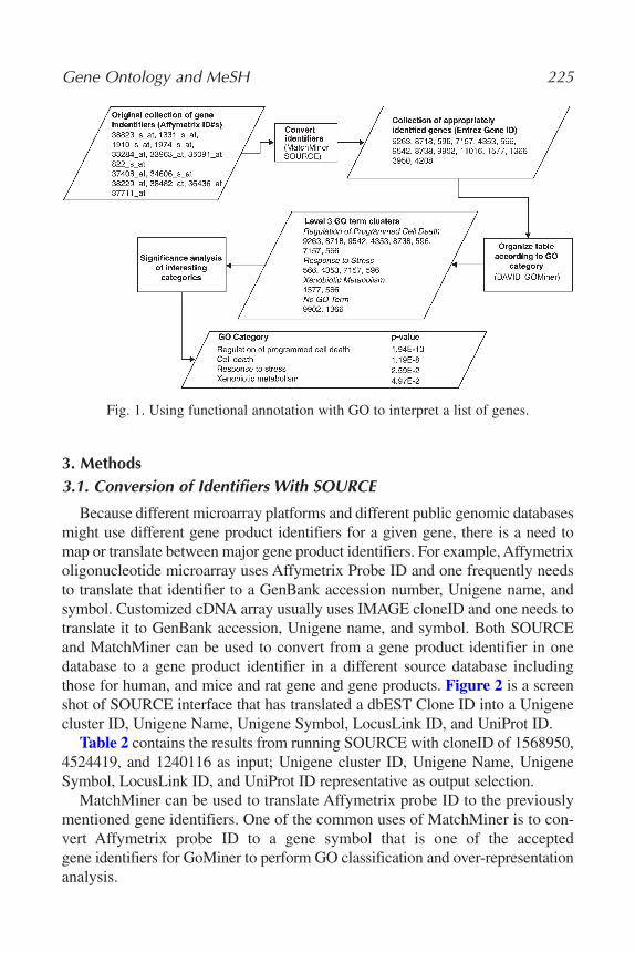
3. Methods3.1. Conversion of Identifiers With SOURCE
Because different microarray platforms and different public genomic databasesmight use different gene product identifiers for a given gene, there is a need tomap or translate between major gene product identifiers. For example, Affymetrixoligonucleotide microarray uses Affymetrix Probe ID and one frequently needsto translate that identifier to a GenBank accession number, Unigene name, andsymbol. Customized cDNA array usually uses IMAGE cloneID and one needs totranslate it to GenBank accession, Unigene name, and symbol. Both SOURCEand MatchMiner can be used to convert from a gene product identifier in onedatabase to a gene product identifier in a different source database includingthose for human, and mice and rat gene and gene products. Figure 2 is a screenshot of SOURCE interface that has translated a dbEST Clone ID into a Unigenecluster ID, Unigene Name, Unigene Symbol, LocusLink ID, and UniProt ID.
Table 2 contains the results from running SOURCE with cloneID of 1568950,4524419, and 1240116 as input; Unigene cluster ID, Unigene Name, UnigeneSymbol, LocusLink ID, and UniProt ID representative as output selection.
MatchMiner can be used to translate Affymetrix probe ID to the previouslymentioned gene identifiers. One of the common uses of MatchMiner is to con-vert Affymetrix probe ID to a gene symbol that is one of the accepted gene identifiers for GoMiner to perform GO classification and over-representationanalysis.
Gene Ontology and MeSH 225
Fig. 1. Using functional annotation with GO to interpret a list of genes.
14_Lin.qxd 6/3/07 8:48 PM Page 225
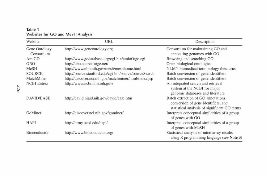
226
Table 1Websites for GO and MeSH Analysis
Website URL Description
Gene Ontology http://www.geneontology.org Consortium for maintaining GO andConsortium annotating genomes with GO
AmiGO http://www.godatabase.org/cgi-bin/amioO/go.cgi Browsing and searching GOOBO http://obo.sourceforge.net/ Open biological ontologiesMeSH http://www.nlm.nih.gov/mesh/meshhome.html NLM’s biomedical terminology thesaurusSOURCE http://source.stanford.edu/cgi-bin/source/sourceSearch Batch conversion of gene identifiersMatchMiner http://discover.nci.nih.gov/matchminer/html/index.jsp Batch conversion of gene identifiersNCBI Entrez http://www.ncbi.nlm.nih.gov/ An integrated search and retrieval
system at the NCBI for major genomic databases and literature
DAVID/EASE http://david.niaid.nih.gov/david/ease.htm Batch extraction of GO annotations,conversion of gene identifiers, and statistical analysis of significant GO terms
GoMiner http://discover.nci.nih.gov/gominer/ Interprets conceptual similarities of a group of genes with GO
HAPI http://array.ucsd.edu/hapi/ Interprets conceptual similarities of a group of genes with MeSH
Bioconductor http://www.bioconductor.org/ Statistical analysis of microarray results using R programming language (see Note 3)
14_Lin.qxd 6/3/07 8:48 PM Page 226
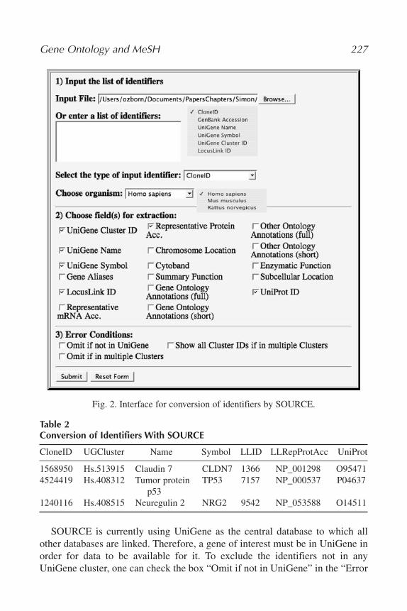
Gene Ontology and MeSH 227
Fig. 2. Interface for conversion of identifiers by SOURCE.
Table 2Conversion of Identifiers With SOURCE
CloneID UGCluster Name Symbol LLID LLRepProtAcc UniProt
1568950 Hs.513915 Claudin 7 CLDN7 1366 NP_001298 O954714524419 Hs.408312 Tumor protein TP53 7157 NP_000537 P04637
p531240116 Hs.408515 Neuregulin 2 NRG2 9542 NP_053588 O14511
SOURCE is currently using UniGene as the central database to which allother databases are linked. Therefore, a gene of interest must be in UniGene inorder for data to be available for it. To exclude the identifiers not in anyUniGene cluster, one can check the box “Omit if not in UniGene” in the “Error
14_Lin.qxd 6/3/07 8:48 PM Page 227

Conditions” section of the form. Similarly, to exclude the identifiers in multipleUniGene clusters, one can check the box “Omit if in multiple Clusters.” Toinclude the identifiers in multiple UniGene clusters, one can check the box“Show all Cluster IDs if in multiple Clusters.”
3.2. Browsing GO
An ontology is usually a hierarchical structure similar to the “table of con-tents” in a book. As mentioned earlier, GO is organized into a structure knownas a directed acyclic graph (DAG). Each ontology term is encoded with aunique identifier to precisely specify the concept and prevent it from being con-fused with similar terms. For instance, the GO term “apoptosis” is assigned theidentifier GO:0006915, which is a special case of its parent term of “pro-grammed cell death.” The AMIGO browser is an easy way to browse the GOontology, and a screenshot is shown in Fig. 4 of Subheading 3.4.
3.3. Retrieving GO Annotations of a Gene
GO is an international standard for annotating the biological function of genesand gene products, including cellular components (where—location of the event),molecular functions (what—physical activity), and biological processes (why—biological goals). Instead of using free text to describe the function(s) of a geneproduct, GO can be used to annotate very precisely the published literaturedescribing the function of the gene product (6). For example, the function ofthe bax gene can be either described verbally (Fig. 3A) or using GO (Fig. 3B).The use of ontology renders further analysis easier because well-defined con-cepts can be parsed and linked to associated terms easily. As we discuss later,the use of a standard vocabulary, and even better, the use of GO enables compar-ative studies between experiments and enables multiple labs working on similarprocesses in different systems to compare results. For example, apoptosis can befound as a significant process of a certain type of cancer in both clinical samplesand mouse models studied by different labs.
GO annotations can be retrieved as needed from a variety of different pro-grams including the NCBI Entrez database (that is useful when browsing for asingle gene), third party software like DAVID/EASE (useful for retrievingannotations from a list), or directly from the GO consortium. The GO databaseis easy to set up and use locally.
3.4. Retrieving Genes Associated With a GO Annotation
The AmiGO website can be used to retrieve a list of genes associated witha GO annotation. These associations are made through “evidence codes” thatcouple the annotation, the gene, and the experimental evidence behind theassignment of each annotation to a gene or gene product (Table 3).
228 Osborne et al.
14_Lin.qxd 6/3/07 8:48 PM Page 228

Gene Ontology and MeSH 229
For instance, to perform a basic search in AmiGO enter a single GO termusing the name “apoptosis” or identifier “0006915” (Fig. 4A). If a term nameis used to search, the precise term name (apoptosis) must be selected from theretrieved list of other terms containing the search term. In an advanced searcha list of terms may be used to search AmiGO. The results may also be filtered,in the example shown in Fig. 4B, and only human genes are queried by settingthe gene product filter to H. sapiens.
3.5. Annotating a Gene List Using DAVID
To facilitate the biological interpretation of gene lists derived from theanalysis of microarray and proteomic experiments, gene lists can be groupedinto different GO categories. DAVID can be used to classify the gene listsaccording to a GO term or branch in the GO hierarchy. Using DAVID requiresa list of genes to annotate in tab-delimited format. Only the identifiers need bepresent but additional columns can be present in the file.
The process is intuitive and is as follows (Fig. 5):
1. Select the identifier to query with from the drop-down box. This can be a Genbankaccession #, Affymetrix ID, or any of the other identifiers listed.
Fig. 3. (A) GO text annotation of the bax gene. (B) GO annotation of the bax gene.
14_Lin.qxd 6/3/07 8:48 PM Page 229

230 Osborne et al.
2. Enter the list of genes either by browsing and selecting a file prepared earlier orby copying the list into the text box. Click on submit.
3. After submission, the next step requires the selection of annotation types toannotate your gene list with. Using DAVID 2.0 the default annotation results will
Fig. 4. Browsing GO annotations with AMIGO. “Apoptosis” is defined and assignedwith an identifier (A). The tree structure (B) of GO can also be represented graphicallyas a directed acrylic graph (DAG) (C, facing page).
14_Lin.qxd 6/3/07 8:48 PM Page 230
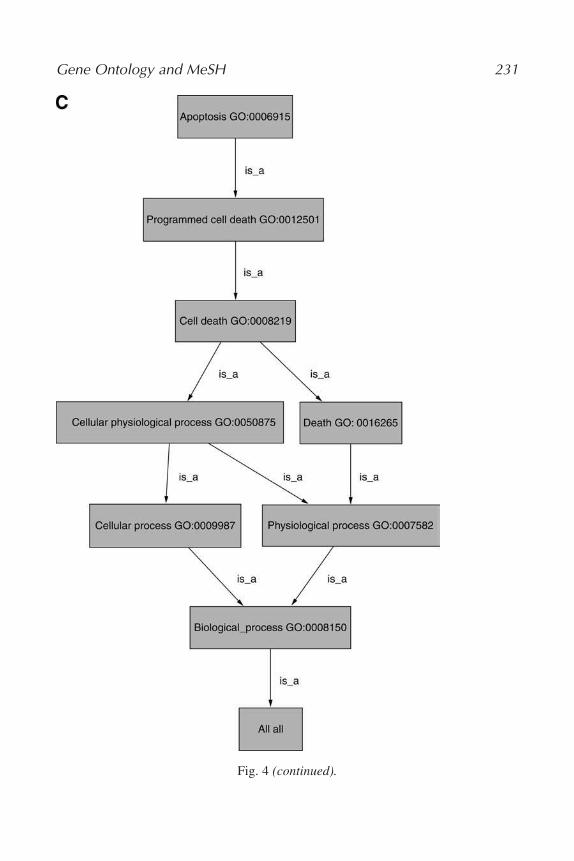
Gene Ontology and MeSH 231
Fig. 4 (continued).
14_Lin.qxd 6/3/07 8:48 PM Page 231

include the Entrez gene ID#, Uniprot ID#, GO biological process and molecularfunction, KEG and Biocarta pathway information, and Swiss Prot PIR keywords(SP_PIR_KEYWORDS). In our example we also selected GOTERM, BiologicalProcess with a “Level” value of 3 (see Note 4). Click on “Get Annotation.”
4. The genes are now annotated. To display the annotations of a particular type in achart format, click on the “Chart” button in the Data Source Summary. The entiregene list, complete with all annotations, can be viewed by checking all the anno-tations on the Data Source Summary section and then selecting “Create Table.”
5. To export the annotated gene list, select the format to export in (html, txt, or xls)and click on all pages. Exporting in either html or txt format will make it easy touse the list again.
Figure 6 is a screen shot after running DAVID on the sample input list,selecting for “Biological Process” classifications at level 3. There are 32 (19.5%)
232 Osborne et al.
Table 3Human Genes Associated With GO Annotation of Apoptosis
Gene Symbol Datasource Evidence Full Name
A4_HUMAN ATGCC/GOst UniProt TAS Amyloid beta A4 protein precursor
AA2AR_HUMAN ATGCC/GOst UniProt TAS Adenosine A2a receptor
ABS_HUMAN ATGCC/GOst UniProt TAS DEAD-box proteinabstrakt homolog
ADA1A_HUMAN ATGCC/GOst UniProt TAS Alpha-1A adrenergicreceptor
AG22_HUMAN ATGCC/GOst UniProt TAS Type-2 angiotensin || receptor
AHR_HUMAN ATGCC/GOst UniProt TAS Aryl hydrocarbon receptor precursor
APAF_HUMAN ATGCC/GOst UniProt TAS Apoptotic proteaseactivating factor 1
APGB_HUMAN ATGCC/GOst UniProt TAS Autophagy protein 12-like
ARHG6_HUMAN ATGCC/GOst UniProt TAS Rho guanine nucleotideexchange factor 6
B2L10_HUMAN ATGCC/GOst UniProt TAS Apoptosis regulatorBcl-B
BCLX_HUMAN ATGCC/GOst UniProt TAS Apoptosis regulatorBcl-X
GO contains a number of “Evidence Codes” to validate an annotation. The TAS evidence codeindicates a Traceable Author Statement, generally from a review paper or a book.
14_Lin.qxd 6/3/07 8:48 PM Page 232
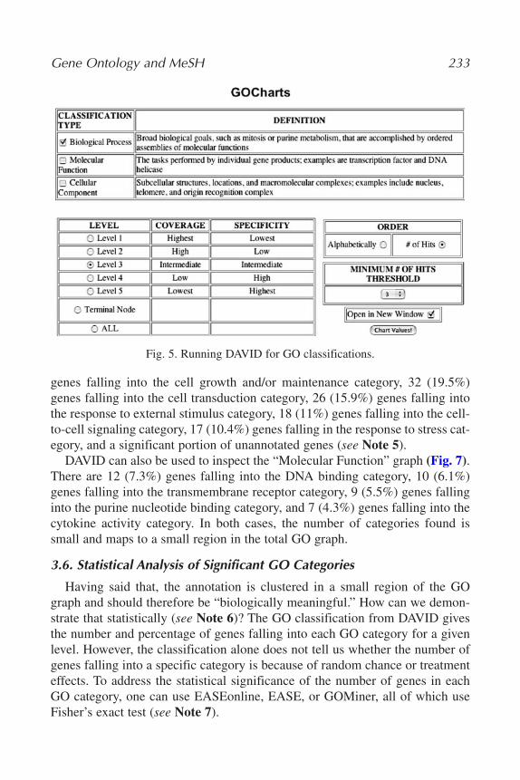
genes falling into the cell growth and/or maintenance category, 32 (19.5%)genes falling into the cell transduction category, 26 (15.9%) genes falling intothe response to external stimulus category, 18 (11%) genes falling into the cell-to-cell signaling category, 17 (10.4%) genes falling in the response to stress cat-egory, and a significant portion of unannotated genes (see Note 5).
DAVID can also be used to inspect the “Molecular Function” graph (Fig. 7).There are 12 (7.3%) genes falling into the DNA binding category, 10 (6.1%)genes falling into the transmembrane receptor category, 9 (5.5%) genes fallinginto the purine nucleotide binding category, and 7 (4.3%) genes falling into thecytokine activity category. In both cases, the number of categories found issmall and maps to a small region in the total GO graph.
3.6. Statistical Analysis of Significant GO Categories
Having said that, the annotation is clustered in a small region of the GOgraph and should therefore be “biologically meaningful.” How can we demon-strate that statistically (see Note 6)? The GO classification from DAVID givesthe number and percentage of genes falling into each GO category for a givenlevel. However, the classification alone does not tell us whether the number ofgenes falling into a specific category is because of random chance or treatmenteffects. To address the statistical significance of the number of genes in eachGO category, one can use EASEonline, EASE, or GOMiner, all of which useFisher’s exact test (see Note 7).
Gene Ontology and MeSH 233
Fig. 5. Running DAVID for GO classifications.
14_Lin.qxd 6/3/07 8:48 PM Page 233
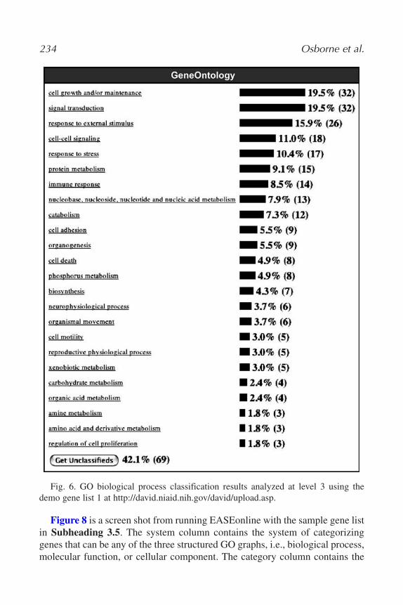
Figure 8 is a screen shot from running EASEonline with the sample gene listin Subheading 3.5. The system column contains the system of categorizinggenes that can be any of the three structured GO graphs, i.e., biological process,molecular function, or cellular component. The category column contains the
234 Osborne et al.
Fig. 6. GO biological process classification results analyzed at level 3 using thedemo gene list 1 at http://david.niaid.nih.gov/david/upload.asp.
14_Lin.qxd 6/3/07 8:48 PM Page 234
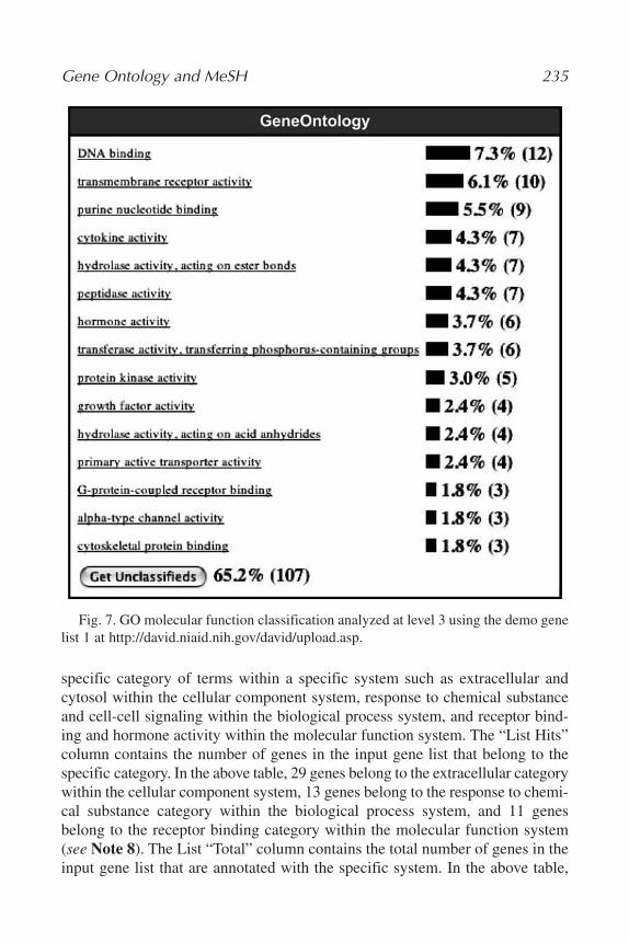
specific category of terms within a specific system such as extracellular andcytosol within the cellular component system, response to chemical substanceand cell-cell signaling within the biological process system, and receptor bind-ing and hormone activity within the molecular function system. The “List Hits”column contains the number of genes in the input gene list that belong to thespecific category. In the above table, 29 genes belong to the extracellular categorywithin the cellular component system, 13 genes belong to the response to chemi-cal substance category within the biological process system, and 11 genesbelong to the receptor binding category within the molecular function system(see Note 8). The List “Total” column contains the total number of genes in theinput gene list that are annotated with the specific system. In the above table,
Gene Ontology and MeSH 235
Fig. 7. GO molecular function classification analyzed at level 3 using the demo genelist 1 at http://david.niaid.nih.gov/david/upload.asp.
14_Lin.qxd 6/3/07 8:48 PM Page 235
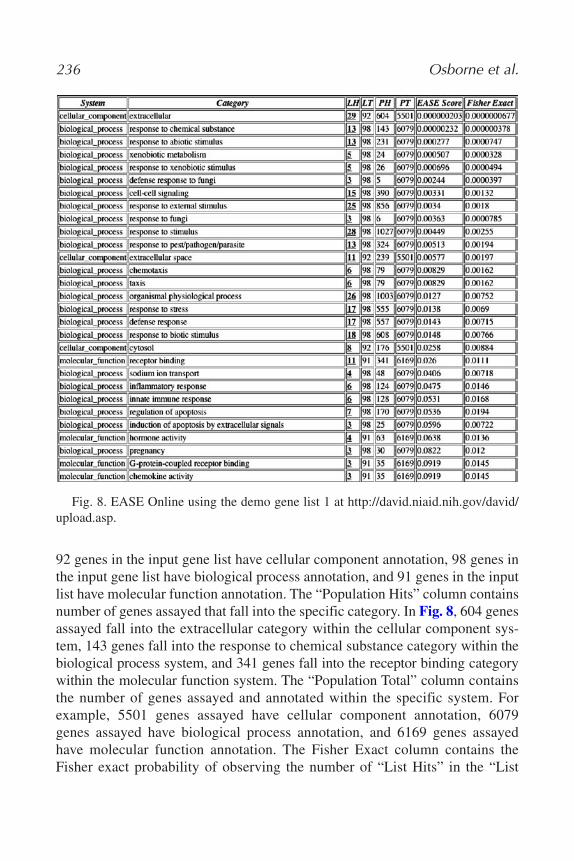
92 genes in the input gene list have cellular component annotation, 98 genes inthe input gene list have biological process annotation, and 91 genes in the inputlist have molecular function annotation. The “Population Hits” column containsnumber of genes assayed that fall into the specific category. In Fig. 8, 604 genesassayed fall into the extracellular category within the cellular component sys-tem, 143 genes fall into the response to chemical substance category within thebiological process system, and 341 genes fall into the receptor binding categorywithin the molecular function system. The “Population Total” column containsthe number of genes assayed and annotated within the specific system. Forexample, 5501 genes assayed have cellular component annotation, 6079genes assayed have biological process annotation, and 6169 genes assayedhave molecular function annotation. The Fisher Exact column contains theFisher exact probability of observing the number of “List Hits” in the “List
236 Osborne et al.
Fig. 8. EASE Online using the demo gene list 1 at http://david.niaid.nih.gov/david/upload.asp.
14_Lin.qxd 6/3/07 8:48 PM Page 236

Gene Ontology and MeSH 237
Total” given the frequency of “Population Hits” in the “Population Total.” TheEASE score column contains the adjusted Fisher exact probability using theJackknife Fisher exact test that strongly penalizes the significance of categoriessupported by few genes and negligibly penalizes categories supported by manygenes. It therefore yields more robust results and the EASE score is the defaultmetric used by EASE to rank categories of genes by over-representation.
Based on the EASE score and using 0.05 as a cut-off value in Fig. 8, we willconclude that the input gene list is over-represented by genes whose productsare likely to be found extracellularly, in the extracellular space or in the cytosol.The input gene list is also over-represented in more than 20 biological functioncategories ranging from chemical substance response to inflammatoryresponse. Note that all of the categories in the above table including regulationof apoptosis and induction of apoptosis by extracellular signals would havebeen considered as over-represented in the input list if Fisher Exact probabilityhad been used instead of EASE score (see Note 9).
3.7. Search and Browsing MeSH
Similar to GO, MeSH is an ontology to describe concepts and relationshipsin medical research and practice (2). MeSH has been used to index medicalliterature. Annotating genes with a controlled vocabulary of MeSH terms providesthe disease context for understanding the gene list of interest.
As an example, MeSH defines the term “apoptosis” (Fig. 9), provides syn-onyms and spelling variations, and relates this term to other terms (Fig. 10).The development of MeSH is independent from GO. We can see some overlapsbetween the MeSH ontology and the GO ontology in some areas. A unifyingopen biological ontology is under active development to describe all biomedi-cal phenomena (7).
3.8. Interpreting a Gene List Using MeSH Terms
Clusters of genes that have been identified through DAVID or other softwarecan be analyzed through HAPI to search for similarities in MeSH category anddescriptors among the genes in the cluster. HAPI takes a tab-delimited text filewith the first column identified by GenBank accession numbers, Affymetrixprobeset identifiers, or UniGene identifiers, and outputs the number of matchesin each MeSH category and the number of matches for individual MeSHdescriptors in each MeSH category. Figure 10 shows the most significant MeSHdescriptor matches in the disease category of MeSH from running HAPI usingthe sample gene list. There are 35 genes associated with neoplasms and 5 ofthose genes are related to leukemia. One can view the detailed gene information
14_Lin.qxd 6/3/07 8:48 PM Page 237

238 Osborne et al.
Fig. 9. (A) MsSH definition of “apoptosis.” (B) – MeSH browsing details of the term“apoptosis.”
14_Lin.qxd 6/3/07 8:48 PM Page 238
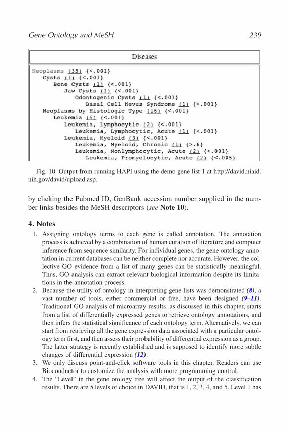
by clicking the Pubmed ID, GenBank accession number supplied in the num-ber links besides the MeSH descriptors (see Note 10).
4. Notes1. Assigning ontology terms to each gene is called annotation. The annotation
process is achieved by a combination of human curation of literature and computerinference from sequence similarity. For individual genes, the gene ontology anno-tation in current databases can be neither complete nor accurate. However, the col-lective GO evidence from a list of many genes can be statistically meaningful.Thus, GO analysis can extract relevant biological information despite its limita-tions in the annotation process.
2. Because the utility of ontology in interpreting gene lists was demonstrated (8), avast number of tools, either commercial or free, have been designed (9–11).Traditional GO analysis of microarray results, as discussed in this chapter, startsfrom a list of differentially expressed genes to retrieve ontology annotations, andthen infers the statistical significance of each ontology term. Alternatively, we canstart from retrieving all the gene expression data associated with a particular ontol-ogy term first, and then assess their probability of differential expression as a group.The latter strategy is recently established and is supposed to identify more subtlechanges of differential expression (12).
3. We only discuss point-and-click software tools in this chapter. Readers can useBioconductor to customize the analysis with more programming control.
4. The “Level” in the gene otology tree will affect the output of the classificationresults. There are 5 levels of choice in DAVID, that is 1, 2, 3, 4, and 5. Level 1 has
Gene Ontology and MeSH 239
Fig. 10. Output from running HAPI using the demo gene list 1 at http://david.niaid.nih.gov/david/upload.asp.
14_Lin.qxd 6/3/07 8:48 PM Page 239
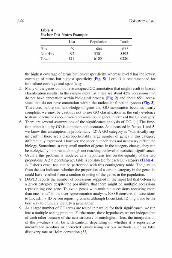
the highest coverage of terms but lowest specificity, whereas level 5 has the lowestcoverage of terms but highest specificity (Fig. 5). Level 3 is recommended forimmediate coverage and specificity.
5. Many of the genes do not have assigned GO annotation that might result in biasedclassification results. In the sample input list, there are about 42% accessions thatdo not have annotation within biological process (Fig. 2) and about 65% acces-sions that do not have annotation within the molecular function system (Fig. 3).Therefore, before our knowledge of gene and GO association becomes nearlycomplete, we must be cautious not to use GO classification as the only evidenceto draw conclusions about over-representation of genes in terms of the GO category.
6. There are several assumptions of the significance analysis of GO. (1) The func-tion annotation by GO is complete and accurate. As discussed in Notes 1 and 5,we know this assumption is problematic. (2) A GO category is “statistically sig-nificant” if there are a disproportionably large number of genes in this categorydifferentially expressed. However, the sheer number does not necessary reflect thebiology. Sometimes, a very small number of genes in the category change, they canbe biologically important, although not reaching the level of statistical significance.
7. Usually this problem is modeled as a hypothesis test on the equality of the twoproportions. A 2 × 2 contingency table is constructed for each GO category (Table 4).A Fisher’s exact test can be performed with this contingency table. The p-valuefrom the test indicates whether the proportion of a certain category in the gene listcould have resulted from a random drawing of the genes in the population.
8. DAVID reports the number of accessions supplied in the input list that belong toa given category despite the possibility that there might be multiple accessionsrepresenting one gene. To avoid genes with multiple accessions receiving morethan one “vote” in the over-representation analysis, EASE converts all accessionsto LocusLink ID before reporting counts although LocusLink ID might not be thebest way to uniquely identify a gene either.
9. As a large number of GO terms are tested in parallel for their significance, we runinto a multiple testing problem. Furthermore, these hypotheses are not independentof each other because of the nest structure of ontologies. Thus, the interpretationof the p-values shall be with caution, depending on whether it is reported asuncorrected p-values or corrected values using various methods, such as falsediscovery rate or Holm correction (11).
240 Osborne et al.
Table 4Fischer Test Notes Example
List Population Totals
Hits 29 604 633NonHits 92 5501 5593Totals 121 6105 6226
14_Lin.qxd 6/3/07 8:48 PM Page 240
10. HAPI annotates genes with a rudimentary process of extracting information fromMedline records. This process is error prone. Thus, any statistically significantcategories should be manually checked by clicking the links from HAPI results.
References1. Bard, J. B. and Rhee, S. Y. (2004) Ontologies in biology: design, applications and
future challenges. Nat. Rev. Genet. 5, 213–222.2. Gene Ontology Consortium (2006). The Gene Ontology project in 2006. Nucleic
Acids Res. 34 (database issue), D322–D326.3. Lowe, H. J. and Barnett, G. O. (1994) Understanding and using the medical subject
headings (MeSH) vocabulary to perform literature searches. JAMA 271, 1103–1108.4. Diehn, M., Sherlock, G., Binkley, G., et al. (2003) SOURCE: a unified genomic
resource of functional annotations, ontologies, and gene expression data. NucleicAcids Res. 31, 219–223.
5. Bussey, K. J., Kane, D., Sunshine, M., et al. (2003) MatchMiner: a tool for batchnavigation among gene and gene product identifiers. Genome Biol. 4, R27.
6. Ashburner, M., Ball, C. A., Blake, J. A., et al. (2000) Gene ontology: tool for theunification of biology. The Gene Ontology Consortium. Nat. Genet. 25, 25–29.
7. Blake, J. (2004) Bio-ontologies-fast and furious. Nat. Biotechnol. 22, 773–774.8. Masys, D. R., Welsh, J. B., Fink, J. L., et al. (2001) Use of keyword hierarchies to
interpret gene expression patterns. Bioinformatics 17, 319–326.9. Khatri, P., Draghici, S., Ostermeier, C., and Krawetz, S. (2002) Profiling gene
expression using onto-express. Genomics 79, 266–270.10. Al-Shahrour, F., Diaz-Uriarte, R., and Dopazo, J. (2004) FatiGO: a web tool for
finding significant associations of Gene Ontology terms with groups of genes.Bioinformatics 20, 578–580.
11. Beissbarth, T. and Speed, T. P. (2004) GOstat: find statistically overrepresentedGene Ontologies within a group of genes. Bioinformatics 20, 1464–1465.
12. Ben-Shaul, Y., Bergman, H., and Soreq, H. (2005) Identifying subtle interrelatedchanges in functional gene categories using continuous measures of gene expres-sion. Bioinformatics 21, 1129–1137.
Gene Ontology and MeSH 241
14_Lin.qxd 6/3/07 8:48 PM Page 241

14_Lin.qxd 6/3/07 8:48 PM Page 242
15
Incorporation of Gene Ontology Annotations to Enhance Microarray Data Analysis
Michael F. Ochs, Aidan J. Peterson, Andrew Kossenkov, and Ghislain Bidaut
SummaryTypical microarray or GeneChip™ experiments now provide genome-wide measurements on
gene expression across many conditions. Analysis often focuses on only a few of the genes, look-ing for those that are “differentially expressed” between conditions or groups of conditions.However, the large number of measurements both present statistical problems to such single geneapproaches and offers a tremendous amount of information for methods focused on biologicalprocesses rather than individual genes. Here we provide a method to utilize biological annotationsin the form of gene ontologies to interpret the results of individual or multiple pattern recognitionanalyses of a microarray experiment.
Key Words: Microarray; gene ontology; biological process; pattern recognition; clustering.
1. IntroductionMicroarrays and GeneChips™ have become standard tools in molecular biol-
ogy, providing researchers with the ability to probe the levels of thousands of genetranscripts routinely. GeneChips are high-density oligonucleotide arrays providingmultiple probes per gene, with these individual probe measurements being com-bined to estimate the expression level of a gene (1). Microarrays typically arecoated microscope slides with spots placed on the surface either through roboticspotting of liquid containing cDNA or oligonucleotide (2) or through in situgrowth of individual oligonucleotides using modified inkjet technology (3). Theseplatforms followed the initial use of arrays using older technologies (4,5).
Microarrays provide insight into cellular processes on an unprecedented scale.The ability to query the transcript level for essentially every known gene, as wellas most predicted genes in a single hybridization, allows researchers to ask ques-tions on a global scale. However, perhaps because microarrays originally grew
From: Methods in Molecular Biology, vol. 377, Microarray Data Analysis: Methods and ApplicationsEdited by: M. J. Korenberg © Humana Press Inc., Totowa, NJ
243
15_Ochs.qxd 6/3/07 11:53 AM Page 243
out of the concept of Northern blots (6), the analytical approach often searchesfor individual genes that show differences in transcript levels between conditions.This approach requires very careful statistical analysis because the number ofmeasurements being made is far larger than in a Northern blot (7–10).
Another approach to analysis more fitting to the global scale of the measure-ment being made is to focus on biological processes that involve regulation ofsets of genes. In general, the biological transcriptional response of an organismis not the differential expression of a single gene, but instead the initiation of a complex response involving changes in the transcription of many genes inaddition to other processes (such as regulation of transport). By focusing onprocesses rather than individual genes, a number of problems related to thelarge number of simultaneous measurements can be avoided. This approachdoes require additional information to allow the genes to be queried as a group.
The most natural way to identify genes that are likely to be coregulated isthrough transcription factors. However, our information on the links betweentranscription factors and regulated genes is still small, as reflected in the limitedinformation available in transcription factor databases (11,12). Although thisinformation is growing, especially through the use of ChIP-on-chip approaches(13), transcription factors alone may not link to biological processes, unless theycan be directly linked to known signaling pathways or have other detailed infor-mation. More information is available, however, from the growing gene ontol-ogy databases (14). Gene ontology comprises a set of three parallel annotations,biological process, molecular function, and cellular location (15). The biologicalprocess annotation is of particular interest because upregulation of a set ofgenes with the same process annotation provides evidence that a specific cel-lular process has been activated. This approach can even link an expression signature on a microarray-to-signaling pathway activity (16).
2. Materials1. The TIGR Multiexperiment Viewer (MeV or TMEV) from The Institute for
Genomics Research (Rockville, MD) is described in ref. 17 and is downloadablefrom http://www.tigr.org/software/tm4/mev.html.
2. The dataset used in this chapter is described in ref. 18 and a preprocessed versionis available from http://bioinformatics.fccc.edu/papers/methods/.
3. A new version of the automated sequence annotation pipeline (ASAP II) is avail-able at http://bioinformatics.fccc.edu/software/OpenSource/ASAP/ASAP.shtml.The original version is described in ref. 19.
4. The ClutrFree visualization and gene ontology analysis tool is available fromhttp://bioinformatics.fccc.edu/software/OpenSource/ClutrFree/clutrfree.shtml andis described in ref. 20.
5. The Go Tree Machine web analysis system can be found at http://genereg.ornl.gov/gotm/ and is described in ref. 21.
244 Ochs et al.
15_Ochs.qxd 6/3/07 11:53 AM Page 244

6. The SOURCE tool for conversion between various gene identifiers can be foundat http://source.stanford.edu.
7. The Bayesian Decomposition tool and a description of the advanced analysisusing it and ASAP are given at http://bioinformatics.fccc.edu/methods/BD, as thedetailed description was too long for this chapter.
Nomenclature for this chapter includes italic for on-screen text, SMALL CAPS
for buttons, and courierfont for files and folders.
3. MethodsThe methods outlined next describe the analysis of microarray data using
gene ontology. It is assumed that the reader can perform standard proceduresincluding preprocessing to correct for background hybridization and to nor-malize the data, as well as create a tab-delimited file summarizing an experi-ment. The tools listed in Subheading 2. will all work with a tab-delimited file with the first row being a header and the first column being Gene IDs. Thisdata file should have a file extension .txt. The header row labels the conditions, one column for each condition. If available, an auxiliary file with the extension .unc containing uncertainties will be used by BayesianDecomposition. In addition, Bayesian Decomposition has the ability to run ina supervised learning mode, with assignment of conditions to groups (22),which is accomplished by providing details on the number of conditions pergroup in a file with the extension .cls. This chapter will focus on applicationof K-means clustering using the TMEV tool and of Bayesian Decompositionto the Project Normal data, collection of annotations using SOURCE or ASAP,and interpretation of the results using ClutrFree and GOTreeMachine.
3.1. Simple Clustering and GoTree Machine
3.1.1. Applying K-Means Clustering With TMEV
The downloaded dataset comprises six files with extensions .txt,.unc, and.cls. The following steps focus on using the ProjNormSmall files, as thesehave only 827 genes and are more useful for rapid analysis. TheProjNormLarge files may be used in the same way and contain 3024 geneschosen for having gene ontology annotations. Only the ProjNormSmall.txtfile is needed for this step, as K-means clustering does not use uncertainty or clas-sification information, which is contained in the .unc and .cls files, respec-tively. Start the TMEV by double-clicking on the TMEV.bat file on Windows or onthe MEV_3_0_Mac_OSX file on Macintosh (OS X required). Use the followingsteps to load the data and generate K-means clusters on the log-transformed data.
1. Choose “New Multiple Array Viewer” from the “File” menu.2. Choose “Load Data” from the “File” menu on the new window.
Gene Ontology Annotations 245
15_Ochs.qxd 6/3/07 11:53 AM Page 245
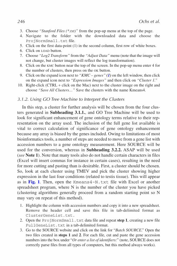
3. Choose “Stanford Files (*.txt)” from the pop-up menu at the top of the page.4. Navigate to the folder with the downloaded data and choose the
ProjNormSmall.txt file.5. Click on the first data-point (1) in the second column, first row of white boxes.6. Click on LOAD button.7. Choose “Log2 Transform” from the “Adjust Data” menu (note that the image will
not change, but cluster images will reflect the log transformation).8. Click on the KMC button near the top of the screen. In the pop-up menu enter 4 for
the number of clusters, then press on the OK button.9. Click on the expand icon next to “KMC – genes” (1) on the left window, then click
on the expand icon next to “Expression Images” and then click on “Cluster 1.”10. Right-click (CTRL + click on the Mac) next to the cluster image on the right and
choose “Save All Clusters…” Save the clusters with the name Kmeans4.
3.1.2. Using GO Tree Machine to Interpret the Clusters
In this step, a cluster for further analysis will be chosen from the four clus-ters generated in Subheading 3.1.1., and GO Tree Machine will be used tolook for significant enhancement of gene ontology terms relative to their rep-resentation on the array used. The inclusion of the full gene list available isvital to correct calculation of significance of gene ontology enhancementbecause any array is biased by the genes included. Owing to limitations of mostbioinformatics tools, a number of steps are needed to move from a gene list withaccession numbers to a gene ontology measurement. Here SOURCE will beused for the conversion, whereas in Subheading 3.2.2. ASAP will be used (see Note 1). Note that many tools also do not handle certain characters in files(Excel will insert commas for instance in certain cases), resulting in the needfor more cutting and pasting than is desirable. First, a cluster should be chosen.So, look at each cluster using TMEV and pick the cluster showing higherexpression in the last four conditions (related to testis tissue). This will appearas in Fig. 1. Then, open the Kmeans4-N.txt file with Excel or anotherspreadsheet program, where N is the number of the cluster you have picked(clustering algorithms generally proceed from a random starting point so Nmay vary on repeat of this method).
1. Highlight the column with accession numbers and copy it into a new spreadsheet.Remove the header cell and save this file in tab-delimited format asClusterGeneList.txt.
2. Open the ProjNormSmall.txt data file and repeat step 1, creating a new fileFullGeneList.txt in a tab-delimited format.
3. Go to the SOURCE website and click on the link for “Batch SOURCE.” Open thetwo files created in steps 1 and 2. For each file, cut and paste the gene accessionnumbers into the box under “Or enter a list of identifiers:” (note, SOURCE does notcorrectly parse files from all types of computers, but this method always works).
246 Ochs et al.
15_Ochs.qxd 6/3/07 11:53 AM Page 246

4. Choose “GenBank Accession” as the type of input identifier and “Mus musculus” asthe organism. Then in section 2 check the box next to “UniGene Cluster ID” and thenclick the SUBMIT button. Do steps 3 and 4 separately for each file, saving the down-loaded files as ClusterUGList.txt and FullUGList.txt, respectively.
5. Open the files created in step 4 and remove the accession number column andheader row, leaving only the UniGene Cluster IDs (i.e., Mm.NNNNN labels).
6. Go to the GO Tree Machine website and log in (you will need to register the first time,however this is free). After the Welcome page, you will see a Make New Tree page.
7. Enter a name for the analysis in section 1, choose the “UNIGENE ID” option insection 2, and the “interesting gene list vs. reference gene list” option in section 3.
8. In section 4, click on the BROWSE (or CHOOSE FILE) button and choose theClusterUGList.txt file. In section 5b, click on the BROWSE button andchoose the FullUGList.txt file.
9. Click on the MAKE TREE button. A new screen will open showing the progress inuploading files and building the gene ontology tree. When completed, click on theCHECK GO TREE button.
10. The tree can be navigated by clicking on the + icons opening up the tree structures.To see the enhanced GO categories directly, click on the number link at the top(NN): “Gene Numbers in NN GO Categories were relatively enhanced.”
Gene Ontology Annotations 247
Fig. 1. The screen image of the desired cluster for analysis in the TMEV tool. The clus-ter here shows higher expression (red on screen, gray here) in the last four conditions.
15_Ochs.qxd 6/3/07 11:53 AM Page 247

11. In this example, the testis tissue-related cluster was chosen, and the biologicalprocesses related to testis show as significantly enhanced.
12. A bar chart and a directed acyclic graph (DAG) can also be created (see Fig. 2),by clicking on the BAR CHART or DAG VIEW buttons, respectively, at the top of thepage. The level of the gene ontology for the bar chart is given by the pop-up menuunder the button. The tree can also be exported as a text file by clicking on theEXPORTGOTREE button.
3.2. Multiple Clustering and ClutrFree
3.2.1. Applying K-Means Clustering With TMEV
Start TMEV as in Subheading 3.1.1. Use the following steps to load the dataand generate multiple K-means clustering results on the log transform data.
1. Choose “New Multiple Array Viewer” from the “File” menu.2. Choose “Load Data” from the “File” menu on the new window.
248 Ochs et al.
Fig. 2. The directed acyclic graph output option from GO Tree Machine. The geneontology categories with significant enhancement will be highlighted in red on the web-page (here in gray). On the webpage, all three gene ontology categories are shown,however here we have focused only on biological process ontology.
15_Ochs.qxd 6/3/07 11:53 AM Page 248
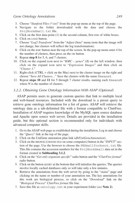
3. Choose “Stanford Files (*.txt)” from the pop-up menu at the top of the page.4. Navigate to the folder downloaded with the data and choose the
ProjNormSmall.txt file.5. Click on the first data-point (1) in the second column, first row of white boxes.6. Click on LOAD button.7. Choose “Log2 Transform” from the “Adjust Data” menu (note that the image will
not change, but clusters will reflect the log transformation).8. Click on the KMC button near the top of the screen. In the pop-up menu enter 4 for
the number of clusters, then press on the OK button.9. Repeat step 8 for 5, 6, and 7 clusters.
10. Click on the expand icon next to “KMC – genes” (1) on the left window, thenclick on the expand icon next to “Expression Images” and then click on“Cluster 1.”
11. Right-click (CTRL + click on the Mac) next to the cluster image on the right andchoose “Save All Clusters…” Save the clusters with the name Kmeans4.
12. Repeat steps 10 and 11 for 5 through 7 cluster results, naming each KmeansNwhere N is the number of clusters.
3.2.2. Obtaining Gene Ontology Information With ASAP (Optional)
ASAP permits users to generate custom queries that link to multiple localand web-based resources. Included with the download is a preset query toretrieve gene ontology information for a list of genes. ASAP will retrieve theontology data as a tab-delimited file with a format compatible to ClutrFree.Installation of ASAP requires knowledge of the MySQL open source databaseand Apache open source web server. Details are provided in the installationguide, but this optional section is recommended only for individuals withadvanced computer skills.
1. Go to the ASAP web page as established during the installation. Log in and choosethe “Query” link at the top of the page.
2. Click on the UniGene annotation plan link (db/UniGeneAnnotation).3. Click on the BROWSE (CHOOSE FILE on some computers) button in the “INPUT” sec-
tion of the page. Use the browser to choose the PNSmallforAnnot.txt file.This file contains the accession numbers for the ProjNormSmall data set in the format created in Subheading 3.1.2.
4. Click on the “Get only organism specific” radio button and the “ClutrFree format”radio button.
5. Click on the button QUERY at the bottom that will initialize the queries. The queriesinvolve locally cached databases only so will take only a few minutes.
6. Retrieve the annotations from the web server by going to the “status” page andclicking on the name or number of your annotation run. The key annotations forthis work are biological process, so click on the “Download” link on the“Biological Process” ClutrFree format file line.
7. Save this file as ontology.txt in your experiment folder (see Note 2).
Gene Ontology Annotations 249
15_Ochs.qxd 6/3/07 11:53 AM Page 249

3.2.3. Interpreting the Multiple Results With ClutrFree
ClutrFree is a visualization tool for linking the results of multiple analyses,either performed with the same algorithm as here or performed with differentalgorithms. It also presents visualization of gene ontology or other annotationsif associated files are present. These files have been created using the ASAPsystem, as described in Subheading 3.3.2., and included with the downloadeddatasets for users who skip Subheading 3.2.2. Start the ClutrFree tool by double-clicking on the ClutrFree.jar file (see Note 3).
1. Place the results of the K-means clustering into a file structure such that there is asingle parent folder named experiment (the name is unimportant). In this folder, cre-ate a series of folders analysis1, analysis2, analysis3, and analy-sis4 (any series of names can be used). Into these folders place the output filesfrom the TMEV with one set of clusters in each folder (e.g., Kmeans4-1.txt …Kmeans4-4.txt into the folder analysis1). Also place the ontology.txtfile generated in Subheading 3.2.2. in the experiment folder.
2. If Subheading 3.2.2. was skipped, place the ProjNormSmall.ann in the experi-ment folder and rename it to ontology.txt. Place the ProjNormSmall.gnmfile in the experiment folder and rename it to annot.txt. Place theProjNormSmall.exp file in the experiment folder and rename it to exp-names.txt. These files provide ClutrFree with gene ontology data, gene ID’s,and condition names, respectively. Descriptions of their formats can be found in theClutrFree user guide.
3. Choose the “Import data…” option from the “File” menu in ClutrFree and navigateto the folder containing the experiment folder you created in step 1. Highlight theexperiment folder icon and click on the CHOOSE button. ClutrFree will loadthe data and bring up a window for viewing the cluster shapes and a tree relating theclusters to each other for each analysis (see Fig. 3). The >> button allows the userto view the individual cluster shapes (or patterns). Click on this arrow until the pat-tern looks like Fig. 3 (the number at the top may differ as clustering causes thelabeling of groups to be random from run to run). The key is that the bars are downin the first 12 conditions (kidney and liver) and up in the last 4 (testis). Note thenumber before the : at the top of the screen (call it N). This is the cluster thatshows genes with high expression in testis.
4. There are many options for exploring the data using ClutrFree. Here we will focuson two features that utilize gene ontology and the ability of ClutrFree to determineif genes are consistently assigned in clusters. Press on the GENE TABLE button toopen two new windows (see Fig. 4).
5. The gene table contains a listing of all the genes in the experiment file, a meas-ure of the strength of assignment of each gene to a pattern (here since clusteringis used this is binary), and a measure of the persistence of the gene in the cluster (i.e., a measure of how many levels of the tree linked to the node containthe gene). Full options are described in the User’s Guide downloaded withClutrFree.
250 Ochs et al.
15_Ochs.qxd 6/3/07 11:53 AM Page 250
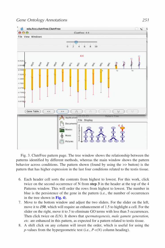
6. Each header cell sorts the contents from highest to lowest. For this work, clicktwice on the second occurrence of N from step 3 in the header at the top of the 4Patterns window. This will order the rows from highest to lowest. The number inblue is the persistence of the gene in the pattern (i.e., the number of occurrencesin the tree shown in Fig. 4).
7. Move to the bottom window and adjust the two sliders. For the slider on the left,move it to 150, which will require an enhancement of 1.5 to highlight a cell. For theslider on the right, move it to 5 to eliminate GO terms with less than 5 occurrences.Then click twice on E(N). It shows that spermatogenesis, male gamete generation,etc. are enhanced in this pattern, as expected for a pattern related to testis tissue.
8. A shift click on any column will invert the order, which is useful for using the p-values from the hypergeometric test (i.e., P-v(N) column heading).
Gene Ontology Annotations 251
Fig. 3. ClutrFree pattern page. The tree window shows the relationship between thepatterns identified by different methods, whereas the main window shows the patternbehavior across conditions. The pattern shown (found by using the >> button) is the pattern that has higher expression in the last four conditions related to the testis tissue.
15_Ochs.qxd 6/3/07 11:53 AM Page 251
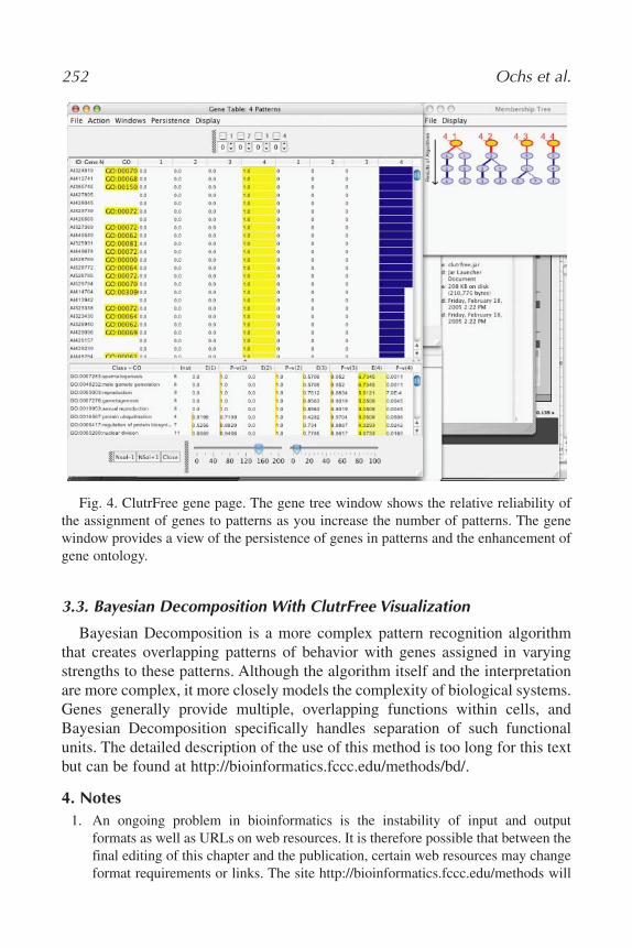
3.3. Bayesian Decomposition With ClutrFree Visualization
Bayesian Decomposition is a more complex pattern recognition algorithmthat creates overlapping patterns of behavior with genes assigned in varyingstrengths to these patterns. Although the algorithm itself and the interpretationare more complex, it more closely models the complexity of biological systems.Genes generally provide multiple, overlapping functions within cells, andBayesian Decomposition specifically handles separation of such functionalunits. The detailed description of the use of this method is too long for this textbut can be found at http://bioinformatics.fccc.edu/methods/bd/.
4. Notes1. An ongoing problem in bioinformatics is the instability of input and output
formats as well as URLs on web resources. It is therefore possible that between thefinal editing of this chapter and the publication, certain web resources may changeformat requirements or links. The site http://bioinformatics.fccc.edu/methods will
252 Ochs et al.
Fig. 4. ClutrFree gene page. The gene tree window shows the relative reliability ofthe assignment of genes to patterns as you increase the number of patterns. The genewindow provides a view of the persistence of genes in patterns and the enhancement ofgene ontology.
15_Ochs.qxd 6/3/07 11:53 AM Page 252
maintain a web request form to answer problems that users have applying the tech-niques described here. We will also maintain a list that updates any neededchanges discovered in response to submitted requests.
2. The annotation methods used by SOURCE and ASAP differ slightly, so there willbe minor differences in annotations on some accession numbers. This is typical forannotations as different databases have different ways of linking accession num-bers to UniGene clusters.
3. The annotation information available on genes changes rapidly. For instance, theoriginal publication on the type of analysis presented here was done by hand cal-culation after retrieval of data using the original annotation pipeline (22). In theintervening 3 yr, numerous tools have appeared to aid such calculations and thenumber of mouse genes with gene ontology annotation has roughly quadrupled. Inaddition, assignment of accession numbers (and therefore nucleotide sequences)to UniGene clusters changes routinely. As such, application of Subheading 3.2.with newly downloaded annotations may not yield exactly the same results asshown previously, although the broad results will remain consistent, demonstrat-ing the value of using a global method in a domain where individual measure-ments are subject to error. In addition, some genes on the microarray may nolonger be linked to gene ontology information, however this will not cause prob-lems for the tools described previously.
References1. Lockhart, D. J., Dong, H., Byrne, M. C., et al. (1996) Expression monitoring by
hybridization to high-density oligonucleotide arrays. Nat. Biotechnol. 14, 1675–1680.2. Schena, M., Shalon, D., Davis, R. W., and Brown, P. O. (1995) Quantitative mon-
itoring of gene expression patterns with a complementary DNA microarray.Science 270, 467–470.
3. Hughes, T. R., Mao, M., Jones, A. R., et al. (2001) Expression profiling usingmicroarrays fabricated by an ink-jet oligonucleotide synthesizer. Nat. Biotechnol.19, 342–347.
4. Augenlicht, L. H., Wahrman, M. Z., Halsey, H., Anderson, L., Taylor, J., and Lipkin,M. (1987) Expression of cloned sequences in biopsies of human colonic tissue and incolonic carcinoma cells induced to differentiate in vitro. Cancer Res. 47, 6017–6021.
5. Augenlicht, L. H. and Kobrin, D. (1982) Cloning and screening of sequencesexpressed in a mouse colon tumor. Cancer Res. 42, 1088–1093.
6. Rohde, W. and Sanger, H. L. (1981) Detection of complementary RNA intermedi-ates of viroid replication by Northern blot hybridization. Biosci. Rep. 1, 327–336.
7. Claverie, J. M. (1999) Computational methods for the identification of differentialand coordinated gene expression. Hum. Mol. Genet. 8, 1821–1832.
8. Ideker, T., Thorsson, V., Siegel, A. F., and Hood, L. E. (2000) Testing for differentially-expressed genes by maximum-likelihood analysis of microarray data. J. Comput. Biol.7, 805–817.
9. Newton, M. A., Kendziorski, C. M., Richmond, C. S., Blattner, F. R., and Tsui, K.W. (2001) On differential variability of expression ratios: improving statistical
Gene Ontology Annotations 253
15_Ochs.qxd 6/3/07 11:53 AM Page 253
inference about gene expression changes from microarray data. J. Comput. Biol.8, 37–52.
10. Tusher, V. G., Tibshirani, R., and Chu, G. (2001) Significance analysis of microar-rays applied to the ionizing radiation response. Proc. Natl. Acad. Sci. USA 98,5116–5121.
11. Matys, V., Fricke, E., Geffers, R., et al. (2003) TRANSFAC: transcriptional regu-lation, from patterns to profiles. Nucleic Acids Res. 31, 374–378.
12. Ghosh, D. (1992) TFD: the transcription factors database. Nucleic Acids Res.20 Suppl, 2091–2093.
13. Ren, B., Robert, F., Wyrick, J. J., et al. (2000) Genome-wide location and functionof DNA binding proteins. Science 290, 2306–2309.
14. Consortium, T. G. O. (2001) Creating the gene ontology resource: design andimplementation. Genome Res. 11, 1425–1433.
15. Ashburner, M., Ball, C. A., Blake, J. A., et al. (2000) Gene ontology: tool for theunification of biology. The Gene Ontology Consortium. Nat. Genet. 25, 25–29.
16. Bidaut, G., Moloshok, T. D., Grant, J. D., Manion, F. J., and Ochs, M. F. (2002)Bayesian Decomposition analysis of gene expression in yeast deletion mutants. In:Methods of Microarray Data Analysis II (Johnson, K. and Lin, S., eds.), KluwerAcademic, Boston, pp. 105–122.
17. Saeed, A. I., Sharov, V., White, J., et al. (2003) TM4: a free, open-source systemfor microarray data management and analysis. Biotechniques 34, 374–378.
18. Pritchard, C. C., Hsu, L., Delrow, J., and Nelson, P. S. (2001) Project normal:defining normal variance in mouse gene expression. Proc. Natl. Acad. Sci. USA98, 13,266–13,271.
19. Kossenkov, A., Manion, F. J., Korotkov, E., Moloshok, T. D., and Ochs, M. F.(2003) ASAP: automated sequence annotation pipeline for web-based updating ofsequence information with a local dynamic database. Bioinformatics 19, 675–676.
20. Bidaut, G. and Ochs, M. F. (2004) ClutrFree: cluster tree visualization and inter-pretation. Bioinformatics 20, 2869–2871.
21. Zhang, B., Schmoyer, D., Kirov, S., and Snoddy, J. (2004) GOTree Machine(GOTM): a web-based platform for interpreting sets of interesting genes usingGene Ontology hierarchies. BMC Bioinformatics 5, 16.
22. Moloshok, T. D., Datta, D., Kossenkov, A. V., and Ochs, M. F. (2003) BayesianDecomposition classification of the Project Normal data set. In: Methods ofMicroarray Data Analysis III (Johnson, K. F. and Lin, S. M., eds.), KluwerAcademic, Boston, pp. 211–232.
254 Ochs et al.
15_Ochs.qxd 6/3/07 11:53 AM Page 254

16
Predicting Survival in Follicular Lymphoma Using Tissue Microarrays
Michael J. Korenberg, Pedro Farinha, and Randy D. Gascoyne
SummaryA tissue microarray (TMA) containing diagnostic biopsies was used to develop predictors of
outcome in a group of 105 patients having advanced-stage follicular lymphoma (FL). Thepatients were staged and uniformly treated, and the usable cases had been randomly divided intoa subgroup of 50 patients with outcomes identified, and a reserved subgroup of 43 patients whoseoutcomes were masked for blind testing of the predictors. Using training-input data from somepatients with known outcomes, parallel cascade identification developed two predictors of over-all survival based on a number of biomarkers. Both predictors had statistically significant per-formance over the remaining patients with known outcomes. The first predictor had beenidentified with model architectural settings and encoding scheme chosen, for the particular train-ing input used, to enhance classification accuracy over remaining patients in the known subgroup.The second predictor was obtained without changing the settings and encoding scheme, but froman entirely different training input corresponding to novel cases from the TMA. Not surprisingly,the first predictor showed much higher accuracy over the known subgroup, but when tested overthe reserved subgroup of 43 patients, averaged about 58% correct and did not reach statistical sig-nificance. The other predictor performed very similarly over the known and the reserved sub-groups, with prediction on the reserved subgroup highly significant at p = 0.0056 inKaplan–Meier survival analysis. We conclude that a predictor based on a number of biomarkersobtainable at diagnosis has the potential to improve prediction of overall survival in FL.
Key Words: Overall survival; clinical outcome; treatment response; biomarkers; tissuemicroarrays; follicular lymphoma.
1. IntroductionFollicular lymphoma (FL) frequently exhibits a long clinical course, with
median survival time of 8–10 yr (1,2). A follicular lymphoma internationalprognostic index, based on five clinical variables, has been used to predict clin-ical outcome (3,4). Recent success in building a gene expression-based predic-tor of outcome has demonstrated that molecular characteristics present in tumorsamples at time of diagnosis of FL are important for determining survival (1).
255
From: Methods in Molecular Biology, vol. 377, Microarray Data Analysis: Methods and ApplicationsEdited by: M. J. Korenberg © Humana Press Inc., Totowa, NJ
16_Korenberg.qxd 6/3/07 8:34 PM Page 255
The latter study found both a favorable pattern or signature of gene expressionassociated with good prognosis, and an unfavorable signature predictingdecreased survival. Both signatures were mostly derived from the nonmalignantcells of a tumor microenvironment. The favorable signature was enriched withgenes characteristic of T-cells and the unfavorable one with genes expressed onmacrophages and dendritic cells.
Farinha et al. (4) recognized that the genes involved in this unfavorable sig-nature suggested the importance of macrophages in influencing FL survival.They built a tissue microarray (TMA) with diagnostic biopsies from 105patients with advanced-stage FL uniformly treated at the British ColumbiaCancer Agency with a BP-VACOP protocol consisting of chemotherapy(bleomycin, cisplatin, etoposide, doxorubicin, cyclophosphamide, vincristine,and prednisone) followed by radiotherapy of the involved sites. The proteinexpression of different markers in both malignant and nonmalignant cells wasstudied using immunohistochemistry and scored in terms of cell content as wellas morphological patterns. Fourteen biomarkers were defined. Of these bio-markers, they found that a lymphoma-associated macrophage (LAM) score pre-dicted overall survival independently of the clinical prognostic index (4). Inparticular, a LAM score of more than 15 cells per high-power field predicted apoor outcome (12 patients). Their results revealed the importance ofmacrophages in the biology of FL. None of the markers other than the LAMscore appeared to be predictive of outcome (4).
In this chapter, essentially the same TMA is used to build a predictor of over-all survival, this time based on a number of biomarkers to see whether it leadsto increased accuracy. The present work has two main objectives. The first is todevelop a predictor whose accuracy is verified over a reserved subgroup ofpatients where the outcomes have been masked. The second objective is toinvestigate whether the predictor can discriminate over the low-macrophagesubgroup of patients (81 usable cases), all of whom would be predicted to sur-vive based on the LAM score.
2. Materials and Patient Samples2.1. Tissue Microarray
1. The data are the same as in ref. 4. In particular, the TMA was constructed usingduplicate 1-mm cores from biopsy material in paraffin blocks (BeecherInstruments, Silver Spring, MD).
2. Hematoxylin and eosin staining was used on the TMA; further details of histologyand immunohistochemistry are presented in ref. 4. Although 14 biomarkers wereanalyzed there (4), some were scored by multiple measures, such as for both archi-tectural pattern and number of positively stained cells. CD20 was performed toensure tumor cell content in all cores.
256 Korenberg, Farinha, and Gascoyne
16_Korenberg.qxd 6/3/07 8:34 PM Page 256
3. Counting each of the measures separately, we used 20 biomarkers (Table 1), anumber of which were scored qualitatively, such as CD10(F), CD10(IF), CD21,BCL2, and BCL-XL.
2.2. Patient Samples
1. All patients had advanced-stage indolent follicular lymphoma, and had been uni-formly treated at the British Columbia Cancer Agency between July of 1987 andMay 1993 (4).
2. Informed consent was obtained. The University of British Columbia–BritishColumbia Cancer Agency provided approval to review, analyze, and publish the data.
3. In total, 93 FL cases were available where all 20 biomarkers had been assessed,and survival status was known. Of these, 50 (29 alive/21 dead) were randomlyselected and the clinical outcome indicated for each. The remaining 43 had out-come masked and were for validation.
3. MethodsThe following approach to building parallel cascade identification (PCI) pre-
dictors of treatment response and clinical outcome has previously been usedwith gene expression data (5,6), and was also briefly reviewed in ref. 7.
3.1. Numerically Encoding Biomarkers
1. Because some of the biomarkers were qualitatively assessed, they had to beassigned numerical values for analysis (Table 1, right column). As examples, forBCL-XL, BCL2, CD10(F), CD10(IF), and TIA1(10%), “negative” was scored as 1and “positive” as –1. For CD68(cells), the number N of cells per high-power fieldwas converted to –N/5. This helped to keep the magnitude similar to that for otherbiomarkers, so that the resulting predictor did not overemphasize one measure.
2. The scoring system tended to give lower values to features believed to be unfavor-able to outcome, such as a higher MIB1 proliferation rate. However, there aresome inconsistencies in this pattern, such as oppositely scoring CD3(int) andCD7(int), although higher values of both these biomarkers are believed to befavorable. However, a training input that is consistently lower for failed outcomesdoes not typically have the variability useful for system identification (see Note 1),and changes in scoring had been introduced into Table 1 to increase the effectivenessof the resulting first predictor over the subgroup of patients with known outcomes.
3.2. Forming a Training Input and Output
1. Building an outcome predictor began with forming a training input from a selectednumber of cases from the TMA associated with failed and successful outcomes. Forthe first predictor, the training input used biomarkers from the first three cases ofthe TMA for patients with failed (F) outcome, denoted F1–F3, and the first threecases for survivors (S), denoted S1–S3 (see Note 2). In particular, the average valueof each biomarker for the three failed outcomes was compared with that for the
Predicting Survival in Follicular Lymphoma 257
16_Korenberg.qxd 6/3/07 8:34 PM Page 257
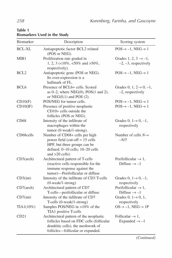
258 Korenberg, Farinha, and Gascoyne
Table 1Biomarkers Used in the Study
Biomarker Description Scoring system
BCL-XL Antiapoptotic factor BCL2 related POS→ –1, NEG→ 1(POS or NEG).
MIB1 Proliferation rate graded in Grades 1, 2, 3 → –1,1, 2, 3 (<10%, <50% and >50%, –2, –3, respectivelyrespectively).
BCL2 Antiapoptotic gene (POS or NEG). POS→ –1, NEG→ 1Its over-expression is a hallmark of FL.
BCL6 Presence of BCL6+ cells. Scored Grades 0, 1, 2→ 0, –1,as 0–2, where NEG(0), POS(1 and 2), –2, respectivelyor NEG(0,1) and POS (2).
CD10(F) POS/NEG for tumor cells. POS→ –1, NEG→ 1CD10(IF) Presence of positive neoplastic POS→ –1, NEG→ 1
CD10+ cells outside the follicles (POS or NEG).
CD68 Intensity of the infiltrate of Grades 0, 1→ 0, –1,macrophages within the respectivelytumor (0-weak/1-strong).
CD68cells Number of CD68+ cells per high Number of cells N→power field (cut-off = 15 cells –N/5HPF, but three groups can be defined: 0–10 cells; 10–20 cells and >20 cells)
CD3(arch) Architectural pattern of T-cells Perifollicular → 1,(reactive cells responsible for the Diffuse → –1immune response against the tumor)—Perifollicular or diffuse
CD3(int) Intensity of the infiltrate of CD3 T-cells Grades 0, 1→ 0, –1,(0-weak/1-strong) respectively
CD7(arch) Architectural pattern of CD7 Perifollicular → 1,T-cells—perifollicular or diffuse Diffuse → –1
CD7(int) Intensity of the infiltrate of CD7 Grades 0, 1→ 0, 1,T-cells (0-weak/1-strong) respectively
TIA1(10%) Samples POS/NEG in >10% of the OS→ –1, NEG→ 1PTIA1 positive T-cells
CD21 Architectural pattern of the neoplastic Follicular → 1,follicles based on FDC cells (follicular Expanded → –1dendritic cells), the meshwork of follicles—follicular or expanded.
(Continued)
16_Korenberg.qxd 6/3/07 8:34 PM Page 258
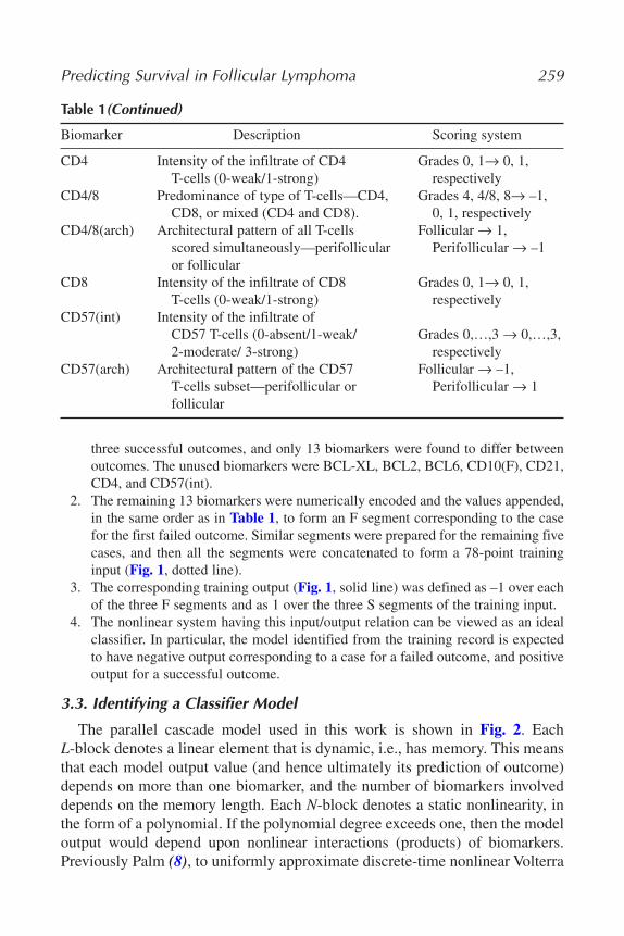
Predicting Survival in Follicular Lymphoma 259
Table 1(Continued)
Biomarker Description Scoring system
CD4 Intensity of the infiltrate of CD4 Grades 0, 1→ 0, 1,T-cells (0-weak/1-strong) respectively
CD4/8 Predominance of type of T-cells—CD4, Grades 4, 4/8, 8→ –1,CD8, or mixed (CD4 and CD8). 0, 1, respectively
CD4/8(arch) Architectural pattern of all T-cells Follicular → 1,scored simultaneously—perifollicular Perifollicular → –1or follicular
CD8 Intensity of the infiltrate of CD8 Grades 0, 1→ 0, 1,T-cells (0-weak/1-strong) respectively
CD57(int) Intensity of the infiltrate of CD57 T-cells (0-absent/1-weak/ Grades 0,…,3 → 0,…,3,2-moderate/ 3-strong) respectively
CD57(arch) Architectural pattern of the CD57 Follicular → –1,T-cells subset—perifollicular or Perifollicular → 1follicular
three successful outcomes, and only 13 biomarkers were found to differ betweenoutcomes. The unused biomarkers were BCL-XL, BCL2, BCL6, CD10(F), CD21,CD4, and CD57(int).
2. The remaining 13 biomarkers were numerically encoded and the values appended,in the same order as in Table 1, to form an F segment corresponding to the casefor the first failed outcome. Similar segments were prepared for the remaining fivecases, and then all the segments were concatenated to form a 78-point traininginput (Fig. 1, dotted line).
3. The corresponding training output (Fig. 1, solid line) was defined as –1 over eachof the three F segments and as 1 over the three S segments of the training input.
4. The nonlinear system having this input/output relation can be viewed as an idealclassifier. In particular, the model identified from the training record is expectedto have negative output corresponding to a case for a failed outcome, and positiveoutput for a successful outcome.
3.3. Identifying a Classifier Model
The parallel cascade model used in this work is shown in Fig. 2. EachL-block denotes a linear element that is dynamic, i.e., has memory. This meansthat each model output value (and hence ultimately its prediction of outcome)depends on more than one biomarker, and the number of biomarkers involveddepends on the memory length. Each N-block denotes a static nonlinearity, inthe form of a polynomial. If the polynomial degree exceeds one, then the modeloutput would depend upon nonlinear interactions (products) of biomarkers.Previously Palm (8), to uniformly approximate discrete-time nonlinear Volterra
16_Korenberg.qxd 6/3/07 8:34 PM Page 259

260 Korenberg, Farinha, and Gascoyne
Fig. 1. Training input x(i) (dotted line) formed by splicing together the numerically-encoded biomarkers (Table 1, right column) from the first three “failed outcome” (F)cases and the first three “survivor outcome” (S) cases. The biomarkers used were the 13whose average values differed between the three F and the three S cases. Training out-put y(i) (solid line) defined as –1 over the “failed outcome” portions of the traininginput and 1 over the “survivor outcome” portions. The training input and output wereused to identify a parallel cascade model of the form in Fig. 2.
systems, suggested a parallel LNL cascade model in which the static nonlinear-ities were exponential and logarithmic functions rather than the polynomialsused here (9).
Parallel cascade identification is then used to identify the model directly fromthe training input and output. Briefly, a first cascade of a dynamic linear elementfollowed by a static nonlinearity is found to approximate the defined input/outputrelation. The residual, i.e., the difference between the cascade output and the train-ing output, is treated as the output of a new nonlinear system, and a second cas-cade is found to approximate the latter system. The new residual is then computed,
16_Korenberg.qxd 6/3/07 8:34 PM Page 260
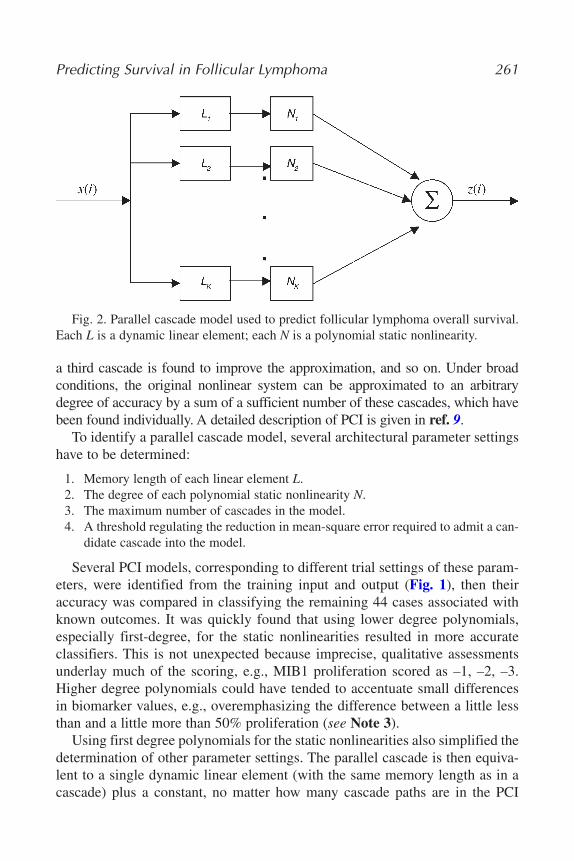
Predicting Survival in Follicular Lymphoma 261
Fig. 2. Parallel cascade model used to predict follicular lymphoma overall survival.Each L is a dynamic linear element; each N is a polynomial static nonlinearity.
a third cascade is found to improve the approximation, and so on. Under broadconditions, the original nonlinear system can be approximated to an arbitrarydegree of accuracy by a sum of a sufficient number of these cascades, which havebeen found individually. A detailed description of PCI is given in ref. 9.
To identify a parallel cascade model, several architectural parameter settingshave to be determined:
1. Memory length of each linear element L.2. The degree of each polynomial static nonlinearity N.3. The maximum number of cascades in the model.4. A threshold regulating the reduction in mean-square error required to admit a can-
didate cascade into the model.
Several PCI models, corresponding to different trial settings of these param-eters, were identified from the training input and output (Fig. 1), then theiraccuracy was compared in classifying the remaining 44 cases associated withknown outcomes. It was quickly found that using lower degree polynomials,especially first-degree, for the static nonlinearities resulted in more accurateclassifiers. This is not unexpected because imprecise, qualitative assessmentsunderlay much of the scoring, e.g., MIB1 proliferation scored as –1, –2, –3.Higher degree polynomials could have tended to accentuate small differencesin biomarker values, e.g., overemphasizing the difference between a little lessthan and a little more than 50% proliferation (see Note 3).
Using first degree polynomials for the static nonlinearities also simplified thedetermination of other parameter settings. The parallel cascade is then equiva-lent to a single dynamic linear element (with the same memory length as in acascade) plus a constant, no matter how many cascade paths are in the PCI
16_Korenberg.qxd 6/3/07 8:34 PM Page 261

model (see Note 4). Thus, provided that the memory length was not excessive(see Note 5), there was no danger of introducing more variables into the modelthan output points used for training and it was not necessary to restrict the num-ber of cascades in the model. Hence, when the static nonlinearities were first-degree polynomials, memory length of the dynamic linear elements was theonly architectural parameter setting that had to be determined (see Note 6).
The latter was chosen by trial and error, exploring a range of memorylengths, as well as small variations in the encoding scheme, and checking theresulting classifier accuracy over the remaining 44 cases of the TMA not usedto form the training input, for which the outcomes were known. A memorylength of nine samples appeared to produce an effective classifier, when thescoring system of Table 1 was employed (see Subheading 3.5.).
However, because the memory length, polynomial degree, and encodingscheme had been chosen for the particular training exemplars to enhance classi-fication accuracy over the remaining cases with known outcomes, this does notmean that the resulting predictor will perform well on novel cases from the TMA.To gauge whether these parameter settings and encoding scheme could be effec-tive for classifiers trained on different exemplars, the next three cases correspon-ding to failed outcomes (denoted F4–F6), and the next three for successfuloutcomes (denoted S4–S6), were instead used to construct a new training input.This time, 18 biomarkers (all except BCL2, CD4/8[arch]) were found to differ onaverage between the 3 F and 3 S training cases, so that a 108-point training inputresulted. This produced a second predictor that was then tested on the remaining44 cases from the TMA with known outcomes. A third predictor was trainedusing the next three cases from each class (denoted F7–F9, S7–S9), tested onremaining known outcome cases, and so on. Each time the same PCI architectureparameter settings and encoding scheme from Table 1 were used, and Fisher’sexact test was employed to measure the effectiveness of the resulting classifier.Although 29 cases were associated with successful outcomes, there were only 21cases for failed outcomes, so that 7 outcome predictors in total were produced.
Only a predictor statistically significant over known outcome cases, not usedfor the training input, was allowed to predict over the reserved subgroup withmasked outcomes. A one-tailed test was used to determine which predictorsreached significance over the known subgroup of cases. This is because, owingto the way each model had been trained (–1 denoted failure and 1 denoted suc-cessful outcome), it was expected to have negative output for failed outcomesand positive output for successful outcomes. Indeed, any predictor whose pre-dicted outcome negatively correlated with actual outcome, no matter howstrong the correlation, was regarded as performing insignificantly and rejected.Kaplan–Meier survival analysis (10) was used to evaluate the predicted out-come over the reserved subgroup.
262 Korenberg, Farinha, and Gascoyne
16_Korenberg.qxd 6/3/07 8:34 PM Page 262

3.4. Using a Classifier Model to Predict Outcome
1. The novel case to be classified was first converted to an input signal by using theright column of Table 1 to numerically encode those biomarkers that were usedby the predictor. The resulting values were then appended in the order the bio-markers appear in Table 1. For the first predictor, this produced a 13-point inputsignal, and for the second predictor, an 18-point signal.
2. The input signal was fed through the classifier model and, once the memory lengthwas reached, the resulting output signal was averaged. For example, each of the 7 predictors had memory length of 9, so for the first predictor, output points 9 to13 were averaged. For the second predictor, output points 9 to 18 were averaged.
3. If the average output value was negative, then a failed outcome was predicted, andotherwise a successful outcome was predicted.
3.5. Results
3.5.1. Subgroup for Which Outcomes Were Labeled
For the results in Table 2, note that the 44 test cases (18F, 26S) are notexactly the same for the 7 predictors because each predictor was evaluated onall but the 6 cases used to construct its training input. Only the first two predic-tors were significant on Fisher’s exact test, so only these were chosen to predictoutcome over the subgroup with masked outcomes. The sixth predictor corre-lated quite strongly with outcome, but negatively, and hence was treated as notsignificant and rejected on the one-tail test.
On this subgroup, the first predictor performs best; however, for its particulartraining input, the PCI architectural parameter values and the encoding schemehad been tailored to enhance accuracy. No further searching for good parametervalues was conducted to build the remaining predictors from their respectivetraining inputs: they were simply identified from their training data after adopt-ing the same architectural settings and encoding scheme as used for the first pre-dictor. So one might expect that the second predictor is less likely to have itsaccuracy inflated over this subgroup than the first predictor. The second predic-tor made 14 errors, and was much more accurate recognizing S than F profiles.
One point of interest is how the second predictor performs over the low-intensity CD68 lymphomas, forming a low-macrophage subgroup. These arethe cases whose LAM score is less than 15 cells per high-power field. For thetraining input of this predictor, all 3 S cases were low-macrophage (LAMscores: 10, 8, 9), as were 2 of the 3 F ones (LAM scores: 12, 20, 7). Over the24 low-macrophage S cases not used in the training input for this predictor,22 were correctly classified. Over the 14 low-macrophage F cases not used inthe training input, 5 were correctly classified. Thus over these low-macrophagecases, Matthews’ correlation (11) coefficient r equalled .34, p < 0.05, one-tail,on Fisher’s exact test.
Predicting Survival in Follicular Lymphoma 263
16_Korenberg.qxd 6/3/07 8:34 PM Page 263

264 Korenberg, Farinha, and Gascoyne
Table 2Predictor Performance Over Subgroup With Known Outcomes
Number of No. of 18 F No. of 26 S CorrelationTraining biomarkers cases cases with p-value
Predictor cases used correct correct outcome (one-tailed)
1 F1–F3, 13 13 18 0.41 0.00775S1–S3
2 F4–F6, 18 8 22 0.32 0.038S4–S6
3 F7–F9, 11 4 16 –0.17 nsS7–S9
4 F10–F12, 15 8 19 0.18 0.189S10–S12
5 F13–F15, 12 14 3 –0.14 nsS13–S15
6 F16–F18, 16 2 13 –0.4 nsS16–S18
7 F19–F21, 14 8 11 –0.13 nsS19–S21
ns, not significant.
3.5.2. Subgroup for Which Outcomes Were Masked
Of the 43 cases in this subgroup, the first predictor classified 17 as S and26 as F. The researcher who did this analysis was not told which predictionswere correct, but that there were a total of 18 errors, with 12 actual S and 6actual F misclassified. The approx 58% success rate here is considerablylower than the accuracy of about 70% observed over the subgroup withknown outcomes. The disparity seems a result of having tailored the modelarchitectural settings and encoding scheme for the particular training input, toenhance accuracy over the known subgroup.
This supposition is supported by the fact that the second predictor, whichdid not have any readjustments for its training input, had very similar accuracyover the masked subgroup of cases as it did over the known subgroup. Again,it made 14 errors in total, and was much more accurate recognizing S than Fprofiles: 3 actual S and 11 actual F were misclassified. Figure 3 shows theoverall survival comparing the predicted successful group of 31 patients withthe predicted failure group of 12 patients. On Kaplan–Meier survival analysis,the difference between the groups is highly significant at p = 0.0056.
The next question was whether the second predictor could distinguish fail-ures from successful outcomes over the low-macrophage patients, as it had
16_Korenberg.qxd 6/3/07 8:34 PM Page 264
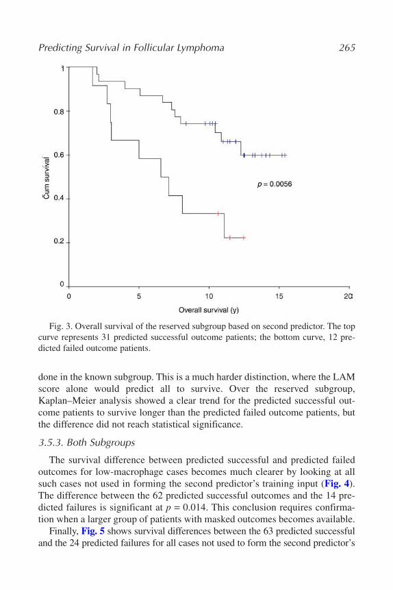
Predicting Survival in Follicular Lymphoma 265
Fig. 3. Overall survival of the reserved subgroup based on second predictor. The topcurve represents 31 predicted successful outcome patients; the bottom curve, 12 pre-dicted failed outcome patients.
done in the known subgroup. This is a much harder distinction, where the LAMscore alone would predict all to survive. Over the reserved subgroup,Kaplan–Meier analysis showed a clear trend for the predicted successful out-come patients to survive longer than the predicted failed outcome patients, butthe difference did not reach statistical significance.
3.5.3. Both Subgroups
The survival difference between predicted successful and predicted failedoutcomes for low-macrophage cases becomes much clearer by looking at allsuch cases not used in forming the second predictor’s training input (Fig. 4).The difference between the 62 predicted successful outcomes and the 14 pre-dicted failures is significant at p = 0.014. This conclusion requires confirma-tion when a larger group of patients with masked outcomes becomes available.
Finally, Fig. 5 shows survival differences between the 63 predicted successfuland the 24 predicted failures for all cases not used to form the second predictor’s
16_Korenberg.qxd 6/3/07 8:34 PM Page 265
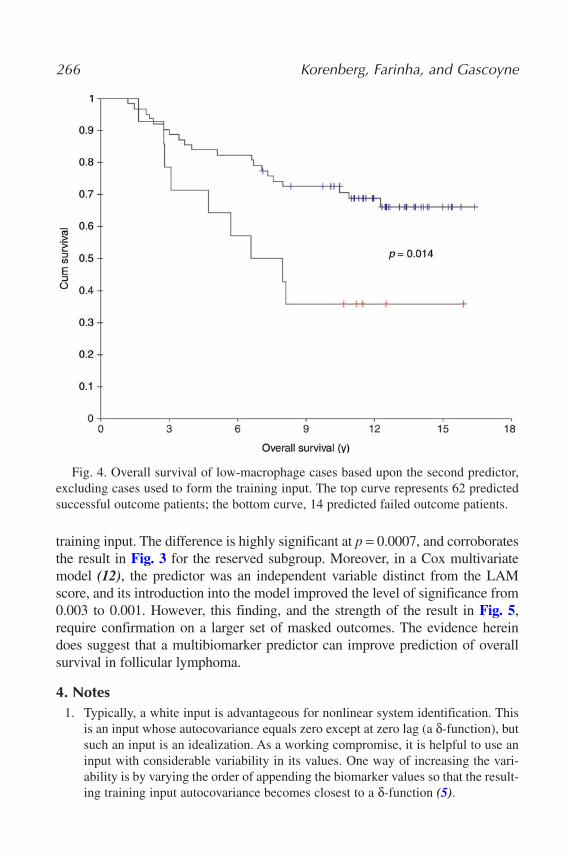
266 Korenberg, Farinha, and Gascoyne
Fig. 4. Overall survival of low-macrophage cases based upon the second predictor,excluding cases used to form the training input. The top curve represents 62 predictedsuccessful outcome patients; the bottom curve, 14 predicted failed outcome patients.
training input. The difference is highly significant at p = 0.0007, and corroboratesthe result in Fig. 3 for the reserved subgroup. Moreover, in a Cox multivariatemodel (12), the predictor was an independent variable distinct from the LAMscore, and its introduction into the model improved the level of significance from0.003 to 0.001. However, this finding, and the strength of the result in Fig. 5,require confirmation on a larger set of masked outcomes. The evidence hereindoes suggest that a multibiomarker predictor can improve prediction of overallsurvival in follicular lymphoma.
4. Notes1. Typically, a white input is advantageous for nonlinear system identification. This
is an input whose autocovariance equals zero except at zero lag (a δ-function), butsuch an input is an idealization. As a working compromise, it is helpful to use aninput with considerable variability in its values. One way of increasing the vari-ability is by varying the order of appending the biomarker values so that the result-ing training input autocovariance becomes closest to a δ-function (5).
16_Korenberg.qxd 6/3/07 8:34 PM Page 266
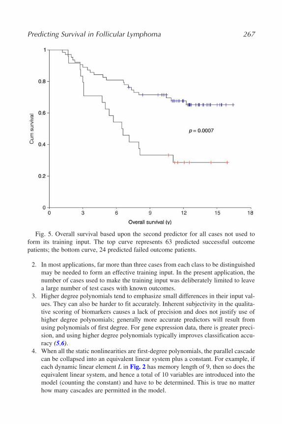
2. In most applications, far more than three cases from each class to be distinguishedmay be needed to form an effective training input. In the present application, thenumber of cases used to make the training input was deliberately limited to leavea large number of test cases with known outcomes.
3. Higher degree polynomials tend to emphasize small differences in their input val-ues. They can also be harder to fit accurately. Inherent subjectivity in the qualita-tive scoring of biomarkers causes a lack of precision and does not justify use ofhigher degree polynomials; generally more accurate predictors will result fromusing polynomials of first degree. For gene expression data, there is greater preci-sion, and using higher degree polynomials typically improves classification accu-racy (5,6).
4. When all the static nonlinearities are first-degree polynomials, the parallel cascadecan be collapsed into an equivalent linear system plus a constant. For example, ifeach dynamic linear element L in Fig. 2 has memory length of 9, then so does theequivalent linear system, and hence a total of 10 variables are introduced into themodel (counting the constant) and have to be determined. This is true no matterhow many cascades are permitted in the model.
Predicting Survival in Follicular Lymphoma 267
Fig. 5. Overall survival based upon the second predictor for all cases not used toform its training input. The top curve represents 63 predicted successful outcomepatients; the bottom curve, 24 predicted failed outcome patients.
16_Korenberg.qxd 6/3/07 8:34 PM Page 267
5. Suppose a predictor that uses first-degree polynomials has memory length 9 andits training input is based on 13 biomarkers. This allows those output points cor-responding to points 9–13 of each of the 6 training input segments, hence 30points in total, to be used to determine the 10 variables. If instead the traininginput is based on 18 biomarkers, then training output points corresponding topoints 9–18 of each training input segment can be used in the identification; hence60 output points in total are available to determine the 10 variables.
6. When there is no downside to allowing more cascade paths, a threshold of zero,admitting every candidate cascade, can be used. Here 100 cascades were addedbecause the mean-square of the residual did not decline significantly thereafter.
References1. Glas, A. M., Kersten, M. J., Delahaye, L. J. M. J., et al. (2005) Gene expression
profiling in follicular lymphoma to assess clinical aggressiveness and to guide thechoice of treatment. Blood 105, 301–307.
2. Horning, S. J. and Rosenberg, S. A. (1984) The natural history of initially untreatedlow-grade non-Hodgkin’s lymphomas. N. Engl. J. Med. 311, 1471–1475.
3. Solal-Celigny, P., Roy, P., Colombat, P., et al. (2004) Follicular lymphoma interna-tional prognostic index. Blood 104, 1258–1265.
4. Farinha, P., Masoudi, H., Skinnider, B. F., et al. (2005) Analysis of multiple bio-markers shows that lymphoma-associated macrophage (LAM) content is an inde-pendent predictor of survival in follicular lymphoma (FL). Blood 106, 2169–2174.
5. Korenberg, M. J. (2002) Prediction of treatment response using gene expressionprofiles. J. Proteome Res. 1, 55–61.
6. Korenberg, M. J. (2003) Gene expression monitoring accurately predicts medul-loblastoma positive and negative clinical outcomes. FEBS Lett. 533, 110–114.
7. Kirkpatrick, P. (2002) Look into the future. Nature Rev. Drug Discovery 1, 334.8. Palm, G. (1979) On representation and approximation of nonlinear systems. Part II:
Discrete time. Biol. Cybern. 34, 49–52.9. Korenberg, M. J. (1991) Parallel cascade identification and kernel estimation for
nonlinear systems. Ann. Biomed. Eng. 19, 429–455.10. Kaplan, E. L. and Meier, P. (1958) Nonparametric estimation for incomplete obser-
vations. Am. J. Stat. Assoc. 53, 457–481.11. Matthews, B. W. (1975) Comparison of the predicted and observed secondary
structure of T4 phage lysozyme. Biochim. Biophys. Acta 405, 442–451.12. Cox, D. R. (1972) Regression models and life tables. J. R. Stat. Soc. B34, 187–220.
268 Korenberg, Farinha, and Gascoyne
16_Korenberg.qxd 6/3/07 8:34 PM Page 268

269
Index
Activation, 97AlignACE. See Software and web toolsAlgorithms. See Software and web toolsAlternate splicing, 171AmiGO. See Software and web toolsAnti-fade coating, 200Arabidopsis thaliana, 167–169Area under the curve (AUC). See
Receiver operating characteristicArray. See MicroarrayArray-CGH. See Comparative genomic
hybridizationArtificial neural networks, 11, 61
architecture, 66–67committee voting, 68cross-validation, 67–68learning parameters, 67
Astrocytoma, 203–205differentially expressed genes, 212,
215gene functions, 214–217
Background intensity, 154–157Bias, 153–159, 179, 185
block-dependent, 155correction of, 158–159of higher order, 156–159of order 0, 156, 158position-dependent, 156–159
Binomial distribution, 169Biomarkers, 256–259, 262
lymphoma-associated macrophage(LAM) score, 256, 263
scoring system, 257–259, 261Blind source separation (BSS), 19–24, 34,
45–46in neuroscience, 19, 20, 22
Boltzmann approximation, 98Bonferoni approach, 7
Brain tumors, 187Breast cancer, 114–115, 121–122, 131–132
ER, 115, 117, 132, 135, 136lymph node-negative (LNN), 131, 132PgR, 132
CGH. See Comparative genomichybridization
Chromosomal instability, 187Circular binary segmentation (CBS), 193,
200Cis-regulatory elements, 95–96
combinations, 96Cis-regulatory mechanisms, 95Clustering, 95, 245
K-means, 245–246, 248–249Coherence score, 148–150Coinertia, 146Combinatorial regulation, 99Comparative genomic hybridization
(CGH), 175array based, 176, 190
Cooperativity, 100Correlations analysis
cross-correlation, 156–158integrated, 145
Coxmultivariate model, 266proportional hazards regression, 135
Cross hybridization, 167Cross-validation score, general (GCV),
103, 107Cutoff, 169Data normalization. See NormalizationData preprocessing. See MicroarraysData validation, 13DAVID. See Software and web toolsDecay, 97Decision trees, 11

270 Index
Designing a microarray experiment, 2MIAME guidelines, 2, 112
Differential gene expression, 7–11class prediction, 11error rates, 7pattern discovery, 8–10
Dimension reduction. See MicroarraysDiscriminant analysis
linear (LDA), 118partial least squares (PLS-DA), 114,
118variable importance for the
projection (VIP), 118DNA isolation, 189–190EASEonline. See Software and web toolsEnergetics, 97, 106Evolutionary benefit, 76Expression Coherence (EC) Score
Approach, 100Expression values
correlation of, 140–142, 144–146, 148,150
relative vs. absolute, 140–141probe effects, 140–141
Fast Fourier Transform (FFT), 87–90, 92–93
Faulty paradigms, 85FFT. See Fast Fourier TransformFisher linear discriminant analysis, 11Fisher’s exact test, 262–263Follicular lymphoma, 255–256Foreground intensity, 154–157Fruit fly, 164F-test, 108Gene annotation
UniGene, 247, 249, 253Gene copy number alteration, 187
amplification and deletion, 188identification of, 192, 200influence on gene expression, 193
Gene expression, 111, 131, 256Gene expression analysis, 134–136. See
also Microarrayscross-validation, 121
decision tree, 121predictor set, 120pre-filtering of data, 115test cohort, 123training cohort, 120
Gene expression and gene copy numbers,parallel profiling of, 188
Gene expression data, 205–206K dataset, 205, 211validation dataset, 206V dataset, 205, 211
Gene expression profiling, microarray-based, 191
direct labeling, 191indirect labeling, 191
Gene minimization, 69Gene ontology/pathway analysis. See
OntologyGene selection analyses, 206–209
ABA test, 208, 212distance and clustering, 209–210, 213J5 test, 207, 212pooled variance t-test, 207, 212PPST test, 208, 212significance analysis of microarrays
(SAM), 207–208, 212computational validation, 209confounding index (CI), 206data quality metric, 211
Gene signature, 131, 135Generalized singular value decomposition
(GSVD), 34–45Genomic alterations, 175Genomic signals and systems, 17–23HAPI. See Software and web toolsHierarchical clustering, 9–10Hodges-Lehman estimator, 171Human cell cycle, 37–45
GSVD comparative model of, 43–45Human synchronization response, 42,
43Hypergeometric distribution, 27, 28,
100Image acquisition and analysis, 3–5
Index 271
Inkjet, 164Intersection of lists, 144, 146–147K-means clustering, 10Kaplan-Meier survival analysis, 262, 264
survival curves, 135–136, 265–267Leave-one-out analysis, 68–69lg-ratio. See Log-ratioLog of the odds (lodds), 148Log ratio, 155, 193, 201Log2 ratio. See Log ratioLog10 ratio. See Log ratioMARS. See Software and web toolsMARSMotif. See Software and web toolsMaskless array synthesizer, 164MatchMiner. See Software and web
toolsMatrix algebra, 20-23
in physics, 23MCB element. See Regulatory motifMcm1. See Regulatory motifMdscan. See Software and web toolsMedical Subject Headings (MeSH), 224,
226, 237–239Microarrays, 131
Affymetrix, 111GenChip, 134–135, 154, 157–159
application, 113tumor classification, 114
cDNA,154–157, 159, 190data analysis, 112, 114, 153
data filtering, 115overfitting, 128
dimension reduction, 64–65platform, 112, 154
common platform, 190preprocessing, 63, 142, 144, 147technology, 111–112, 153tissue. See Tissue microarrays
miRNA, 170–171Mismatch probe, 171Motif. See Regulatory motifMotifRegressor. See Software and web
toolsMultidimensional scaling, 8
Multiple hypothesis testing, 200Multivariate adaptive regression splines
(MARS). See Software and webtools
Nearest neighbor classification, 11k-nearest neighbors (k-NN), 118, 119,
123, 128Noise reduction, 176Normalization, 5, 63–64, 80–82, 93, 168,
171, 191–192, 200global, 192local, 192RNA recovery, 82un-normalized data, 83
Odds ratio, 136Ontology
definition, 223Gene Ontology (GO), 12, 136, 223–
224, 244, 246–248biological process, 244, 249–250cellular localization, 244molecular function, 244
Optimal probe size, 166Oscillation, 75–93
genome-wide, 75–76, 86–90, 92Oscillator
analog harmonic, 33, 34digital ring, 43-45
Pair-wise comparison, 85–86Parallel cascade identification (PCI), 257,
260–262model, 259
memory length, 259, 261, 262,267–268
polynomial degree, 259, 261, 262,267
training input and output, 257, 259Partitioning data into training and testing
sets, 62Percent reduction of variance. See
VariancePermutation testing, 195–196Polyadenylation, 170Position weight matrix (PWM), 99
272 Index
Predictors, 210–217, 256, 262–263Box and Whisker plot, 210chromosomal location, 211, 214, 217functional relationships, 215, 217histological clustering, 212–213performance, 263–266
Preparing input files, 62Principal component analysis (PCA), 8,
66, 117–118Probe selection, 167Prognostic markers, 131, 135–136Promoter, 168Pseudoinverse projection, 45–53Random, 76Real-time PCR, 13Receiver operating characteristic (ROC),
135–136Recurrent alterations, 184Redox, 76REDUCE. See Software and web toolsRegression, 96, 100, 106Regulatory motif, 96
cis-regulatory, 103MCB element, 96–97, 99, 103–105Mcm1, 99, 103–105SCB element, 99, 103–105SFF, 105
Relapse Score, 136Repeat masker, 167Reproducibility
across platforms, 141–142gene specific, 145lab effects, 144–145score, 145within platform, 141,148
Respiratory/reductive cycle, 76,78, 83,85–86, 88–89
Ribonucleic acid. See RNARNA, 133–134
isolation, 77, 80–83, 93, 189–190recovery, 81–85, 93
Running average, 177SCB element. See Regulatory motifSCVmotif. See Software and web tools
Self-organizing maps, 10Self-self hybridizations, 180, 182, 184Sensitivity, 136SFF. See Regulatory motifSigmoidal dependence, 101–102Signal processing, 76–77, 80–83, 85–87Signal-to-noise ratio (s2n), 194
recurrence weighted, 197Singular value decomposition (SVD), 8–
9, 23–34, 75, 81, 87, 90–93Smallest regions of overlap, 184Software and web tools, 190, 226
AlignACE, 105AmiGO, 226, 228–229ASAP, 244, 249, 253Bayesian Decomposition, 244–245,
252CaGEDA, 217–218ClutrFree, 244, 248–252DAVID, 12, 224, 226, 230, 233, 239–
240EASEonline, 226, 233–234Expressionist Analyst, GeneData,
114GCRMA, 147GeneSpring 6·0, 135GoMiner, 12Go Tree Machine, 244, 246–248HAPI, 224, 226, 237, 241Ingenuity, 12, 136MARS, 102–103, 107–109MARSMotif, 102–105, 107–108MAS5, 134, 158MatchMiner, 225–226MDscan, 99MicroSuite 5.0, 115MotifRegressor, 99–100Oncogenomics online ANN, 62–65,
67, 70PATIKA, 12REDUCE, 99–101, 105SCVmotif, 101SIMCA-P 10.0, 114S-Plus 6·1, 136
Index 273
SOURCE, 225–227, 245–246, 253TIGR Multiexperiment Viewer (MeV
or TMEV), 244–248, 250SOURCE. See Software and web toolsSpecificity, 136Spline, 101
knot, 102–103linear, 102
Statistical tests, 112ANOVA, 115, 117chi-square distribution, 117Fisher’s LDA, 128Kolmogorov-Smirnov (KS) test, 102,
107, 120Kruskal-Wallis, 117Sparse LDA, 128Student’s t-test, non-parametric, 117
moderated t-statistic, 148pooled variance, 207, 212
Venn diagram, 120Welch, 117, 120Wilcoxon, 117, 120
Stem cells, human embryonic, 146Stochastic noise, 177, 183Support vector machines (SVMs), 11,
119, 128
Survival, 255–256, 264–266low-macrophage subgroup, 256, 263–
265SVD. See Singular value decompositionSVD model of yeast cell cycle. See Yeast
cell cycleSystematic errors, 179Systemix, 168Tiling array, 163–165, 169, 171Tissue microarrays, 13, 256–257Transcription factor (TF), 96Variance, percent reduction of (%RIV),
97, 105Wavelets, 89Worm, 164Yeast, 164Yeast cell cycle, 27–34, 37–54, 96
models of,GSVD comparative, 43–45pseudoinverse projection
integrative, 53SVD, 32-34
regulators, 26–32replication initiation proteins, 47–53transcription factors, 47–53
Yeast synchronization response, 42, 43

Related Documents