A C plications, &ics, and puting* ' wm

Welcome message from author
This document is posted to help you gain knowledge. Please leave a comment to let me know what you think about it! Share it to your friends and learn new things together.
Transcript
A
C
plications,&ics, and
puting* '
wm

Applications, Basics, and Computing ofExploratory Data Analysis
By Paul F. Velleman, Cornell University andDavid C. Hoaglin, Abt Associates, Inc.
and Harvard University
Previously published by Duxbury Press, BostonCopyright 2004 by Paul F. Velleman and David Hoaglin
Republished byThe Internet-First University Press
This manuscript is among the initial offerings beingpublished as part of a new approach to scholarly publishing.The manuscript is freely available from the Internet-FirstUniversity Press repository within DSpace at CornellUniversity at
http://dspace.library.cornell.edu/handle/1813/62
The online version of this work is available on an openaccess basis, without fees or restrictions on personal use. Aprofessionally printed and bound version may be purchasedthrough Cornell Business Services by contacting:
All mass reproduction, even for educational or not-for-profituse, requires permission and license. For more information,please contact [email protected]. We will provide adownloadable version of this document from the Internet-First University Press.
Ithaca, N.Y.January, 2004
Applications, Basics, and Computingof
Exploratory Data Analysis


To
John W. Tukey

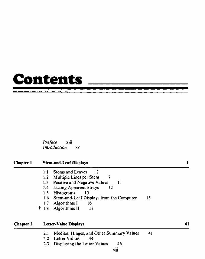
Contents
Preface xiiiIntroduction xv
Chapter 1 Stem-and-Leaf Displays
1.1 Stems and Leaves 21.2 Multiple Lines per Stem 71.3 Positive and Negative Values 111.4 Listing Apparent Strays 121.5 Histograms 131.6 Stem-and-Leaf Displays from the Computer 151.7 Algorithms I 16
f 1.8 Algorithms II 17
Chapter 2 Letter-Value Displays 41
2.1 Median, Hinges, and Other Summary Values 412.2 Letter Values 442.3 Displaying the Letter Values 46
V l l
ABCs of EDA
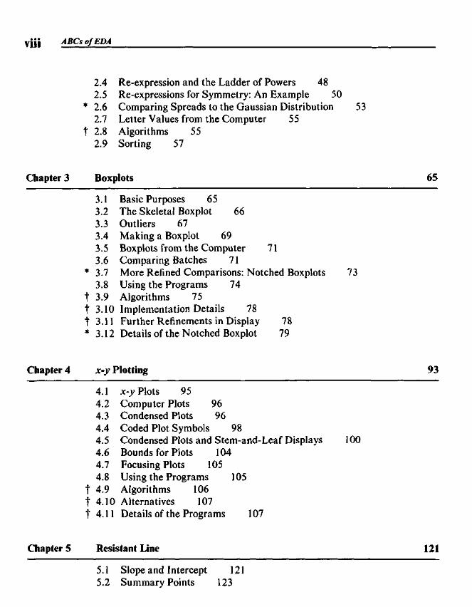
2.4 Re-expression and the Ladder of Powers 482.5 Re-expressions for Symmetry: An Example 502.6 Comparing Spreads to the Gaussian Distribution 532.7 Letter Values from the Computer 552.8 Algorithms 552.9 Sorting 57
Chapter 3 Boxplots 65
3.1 Basic Purposes 653.2 The Skeletal Boxplot 663.3 Outliers 673.4 Making a Boxplot 693.5 Boxplots from the Computer 713.6 Comparing Batches 71
* 3.7 More Refined Comparisons: Notched Boxplots 733.8 Using the Programs 74
t 3.9 Algorithms 75t 3.10 Implementation Details 78t 3.11 Further Refinements in Display 78* 3.12 Details of the Notched Boxplot 79
Chapter 4 x-y Plotting 93
4.1 x-y Plots 954.2 Computer Plots 964.3 Condensed Plots 964.4 Coded Plot Symbols 984.5 Condensed Plots and Stem-and-Leaf Displays 1004.6 Bounds for Plots 1044.7 Focusing Plots 1054.8 Using the Programs 105
t 4.9 Algorithms 106t 4.10 Alternatives 107t 4.11 Details of the Programs 107
Chapter 5 Resistant Line 121
5.1 Slope and Intercept 1215.2 Summary Points 123
Contents
5.3 Finding the Slope and the Intercept 1255.4 Residuals 1265.5 Polishing the Fit 1275.6 Example: Breast Cancer Mortality versus Temperature 1275.7 Outliers 1345.8 Straightening Plots by Re-expression 1355.9 Interpreting Fits to Re-expressed x-y Data 142
* 5.10 Resistant Lines and Least-Squares Regression 1445.11 Resistant Lines from the Computer 144
t 5.12 Algorithms 145
Chapter 6 Smoothing Data 159
6.1 Data Sequences and Smooth Summaries 1596.2 Elementary Smoothers 1636.3 Compound Smoothers 1706.4 Smoothing the Endpoints 1736.5 Splitting and 3RSSH 1776.6 Looking at the Rough 1786.7 Smoothing and the Computer 181
t 6.8 Algorithms 182
Chapter 7 Coded Tables 201
7.1 Displaying Tables 2037.2 Coded Tables from the Computer 2037.3 Coded Tables and Boxplots 207
t 7.4 Algorithms 2097.5 Details and Alternatives 212
Chapter 8 Median Polish 219
8.1 Two-Way Tables 2198.2 A Model for Two-Way Tables 2208.3 Residuals 2238.4 Fitting an Additive Model by Median Polish 2258.5 Re-expressing for Additivity 2338.6 Median Polish from the Computer 240
* 8.7 Median Polish and ANOVA 241
ABCs of EDA
* 8.8 Data Structure 241t 8.9 Algorithms 242
Chapter 9 Rootograms 255
9.1 Histograms and the Area Principle 2579.2 Comparisons and Residuals 2629.3 Rootograms 2639.4 Fitting a Gaussian Comparison Curve 2679.5 Suspended Rootograms 2749.6 Rootograms from the Computer 2779.7 More on Double Roots 281
Appendix A Computer Graphics 293
A.I Terminology 293A.2 Exploratory Displays 295A.3 Resistant Scaling 295A.4 Printer Plots 296A.5 Display Details 297
Appendix B Utility Programs 301
B.I BASIC 301B.2 FORTRAN 308
Appendix C Programming Conventions 319
C.I BASIC 319C.2 FORTRAN 325
Appendix D Minitab Implementation 335
D.I Stem-and-Leaf Displays 337D.2 Letter-Value Displays 337D.3 Boxplots 338D.4 Condensed Plotting 339
Contents
D.5 Resistant Lines 340D.6 Resistant Smoothing 341D.7 Coded Tables 342D.8 Median Polish 343D.9 Suspended Rootograms 344
Index 347
The BASIC programs in this book are available in machine-readableform from CONDUIT, P.O. Box 388, Iowa City, Iowa 52244 (319)353-5789.
The FORTRAN programs in this book are available in machine-readable form from CONDUIT and from International Mathematical &Statistical Libraries, Inc., 6th Floor, NBC Building, 7500 Bellaire Boulevard,Houston, Texas 77036 (713)772-1927.
A version of the BASIC programs tailored for the Apple microcomputer is available from CONDUIT.

Preface
Exploratory data analysis techniques have added a new dimension to the waythat people approach data. Over the past ten years, we have continually beenimpressed by how easily they have enabled us, our colleagues, and our studentsto uncover features concealed among masses of numbers. Unfortunately, thediversity of these techniques has at times discouraged students and dataanalysts who may want to learn a few methods without studying the fullcollection of exploratory tools. In addition, the lack of precisely specifiedalgorithms has meant that computer programs for these techniques have notbeen widely available. This software gap has delayed the spread of exploratorymethods.
We have selected nine exploratory techniques that we have found mostoften useful. Each of these forms the basis for a chapter, in which we
• Lay the foundations for understanding the technique,• Describe useful variations,• Illustrate applications to real data, and• Provide computer programs in FORTRAN and BASIC.
The choice of languages makes it very likely that at least one of the programsfor each technique can be readily installed on whatever computer system isavailable, from personal microcomputers to the largest mainframe.
• • •Xl l l
x | v ABCs of EDA
Most of this book requires no college level mathematics and no morethan an introduction to statistical concepts. It can serve as a supplementarytext to introduce the ideas and techniques of exploratory data analysis into abeginning course in statistics. (In draft form we have used portions of the bookin just this way.) Some chapters include advanced sections which assume someknowledge of statistics and are intended to relate the exploratory techniques totraditional statistical practice. These sections will be of greater interest toresearchers who wish to use the methods and programs in their own dataanalysis. A reader who is primarily interested in computational aspects ofexploratory data analysis will find both the essential details and manyrefinements in our programs. At the other extreme, a student who has nobackground in programming and no access to a computer should have nodifficulty in learning the techniques and applying them by pencil and paper.Between these two extremes, the reader who has access to the Minitabstatistical system can take immediate advantage of our programs because theyhave been incorporated into Minitab (Releases 81.1 and later).
Acknowledgments
We are deeply grateful to the colleagues and friends who encouraged andaided us while we were developing this book. John Tukey originally suggestedthat we provide computer software for exploratory data analysis; later heparticipated in formulating the new resistant-line algorithm in Chapter 5, andhe gave us critical comments on the manuscript. Frederick Mosteller gave ussteadfast encouragement and invaluable advice, helped us to aim our writingat a high standard, and made many of the arrangements that facilitated ourcollaboration. Cleo Youtz painstakingly worked through the manuscript andhelped us to eliminate a number of errors, large and small. John Emerson,Kathy Godfrey, Colin Goodall, Arthur Klein, J. David Velleman, StanleyWasserman, and Agelia Ypelaar read various drafts and contributed helpfulsuggestions. Stephen Peters, Barbara Ryan, Thomas Ryan, and Michael Stotogave us critical comments on the programs. Jeffrey Birch, Lambert Koop-mans, Douglas Lea, Thomas Louis, and Thomas Ryan reviewed the manu-script and suggested improvements. Teresa Redmond typed the manuscript,and Evelyn Maybee and Marjorie Olson typed some earlier draft material.
We also appreciate the support provided by the National ScienceFoundation through grant SOC75-15702 to Harvard University.
Initial versions of some BASIC programs were developed on a Model4051 on loan from Tektronix, Inc.
Introduction
One recent thrust in statistics, primarily through the efforts of John Tukey,has produced a wealth of novel and ingenious methods of data analysis. In his1977 book, Exploratory Data Analysis, and elsewhere, Tukey has expoundeda practical philosophy of data analysis which minimizes prior assumptions andthus allows the data to guide the choice of appropriate models. Four majoringredients of exploratory data analysis stand out:
• Displays visually reveal the behavior of the data and the structure of theanalyses;
• Residuals focus attention on what remains of the data after some analysis;• Re-expressions, by means of simple mathematical functions such as the
logarithm and the square root, help to simplify behavior and clarifyanalyses; and
• Resistance ensures that a few extraordinary data values do not undulyinfluence the results of an analysis.
This book presents selected basic techniques of exploratory data analysis,illustrates their application to real data, and provides a unified set of computerprograms for them.
The student learning exploratory data analysis (EDA) soon becomesfamiliar with many pencil-and-paper techniques for data display and analysis.But computers have become valuable aids to data analysis, and even in EDAwe may want to turn to them when:
XV
ABCs of EDA
• We have already acquired a feel for the working of a method and want toconcentrate on the results rather than the arithmetic;
• We face a large amount of data;• We want to eliminate tedious arithmetic and the errors that inevitably
creep in;• We want to combine exploratory methods with other data analytic
techniques already programmed.
This book shows how we can use the computer for exploratory data analysis.Exploratory methods, however, call for frequent application of the analyst'sjudgment, and this judgment cannot readily be cast in simple rules andplugged into computer programs. In developing the algorithms in this book, wehave often had to give precise rules for judgments such as determining whichscale makes a display "look nice," rinding points "representative" of a part ofthe data, or terminating an iterative procedure. In choosing these, we havetried to preserve the underlying resistant features of EDA. For example, theprecept that an extraordinary data value should not unduly influence ananalysis has led to displays whose message cannot be ruined by such points.
At times the beauty of EDA can be marred by the limitations of thecomputer. Choices other than our rules and heuristics are possible and may bepreferable in some situations. We have tried to offer opportunities to overrulethe programs' default decisions. We have also presented the pencil-and-paperversions of the techniques to encourage readers to work by hand when possibleand to be aware of the constraints of the computer environment otherwise.
After studying the examples and gaining experience with the EDAtechniques, readers who already know some statistics may want to learn moreabout how an EDA technique compares with a similar traditional method. Insome chapters, a starred section (indicated by a * at the section heading)provides brief background information. Generally, a full comparative discus-sion would involve statistical theory.1
The variety of approaches, as well as the alternative analyses that wepresent for some sets of data, serves to emphasize that practical applications ofdata analysis generally do not lead to a single "correct" answer. The analyst'sjudgment and the circumstances surrounding the data also play importantroles.
Each chapter also contains a short discussion of programming details(indicated by a t at the section heading), including the algorithm used by theprogram, alternative methods, and potential implementation difficulties. Thissection of the chapter, intended primarily for readers interested in statistical
'Such discussions are the subject of The Statistician's Guide to Exploratory Data Analysis, now beingprepared under the editorship of David Hoaglin, Frederick Mosteller, and John Tukey.
Introduction
computing and for instructors, provides necessary background and aids ininstalling the programs.
Readers of the programs and background discussions should have someknowledge of computing, an acquaintance with EDA and, for some sections, aknowledge of statistics. Readers intending to install the programs are advisedto follow a different path, or thread, through the book, and read chapters notin the order natural for learning exploratory data analysis but in the ordereasiest for understanding the programs.
This book, then, has two main audiences, and each will thread its waythrough the chapters in a quite different order; so we think of this book as athreaded text. Students of exploratory data analysis, researchers intending touse EDA methods, and especially readers who already have the programsavailable to them on a computer can use the thread that follows the chapters inorder, skip the (t) sections of program listings and technical discussions, andselect the statistically advanced (*) sections that suit them. For programmers,the thread is best described by the following order of chapters:
C Programming ConventionsB Utility Programs2 Letter-Value Displays7 Coded TablesA Computer Graphics3 Boxplots1 Stem-and-Leaf Displays4 x-y Plotting (condensed plots)5 Resistant Line6 Smoothing Data8 Median Polish9 RootogramsD Minitab Implementation
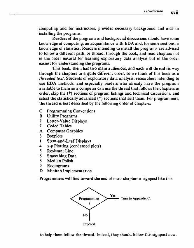
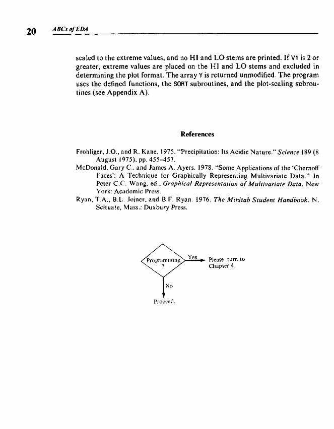
Programmers will find toward the end of most chapters a signpost like this
YesTurn to Appendix C.
to help them follow the thread. Indeed, they should follow this signpost now.
x v j j | ABCs of EDA
Note to the Student
If you have not used a computer before, we must warn you that despite ourefforts to write simple programs, the programs we give may not run withoutchange on your computing system. Unfortunately, all computing systems aredifferent, and few sophisticated programs can be run on many differentsystems and remain readable. Therefore, you may need help from an expert onyour particular computing system, and he or she will find assistance in theappendices of this book. If the programs already work on your computingsystem, you will still need to learn the local conventions for using them. Thisbook tells you how to control an analysis procedure, but local conventions willdetermine how you actually talk to the machine to tell it what to do.
In your first experience with a computer, you must remember that thecomputer is not doing anything you do not already know how to do by hand (orwill know by the time you get to that chapter)—the computer just works morequickly and more accurately. All the same, the machine is stupid, andoccasionally you will want to modify its programmed decisions so as to make adisplay look different or make an analysis work in a different way. Manychapters show you how the modification can be done. We hope that, byrelieving you of tedious hand computation and hand graphing, we will free youto interpret the results of the analyses and understand how the methods work.
Note to the Instructor
Many of the chapters in this book can fit in nicely as supplements to anintroductory statistics course. In our teaching we have found stem-and-leafdisplays and letter-value displays very useful at the start of an introductorycourse. Boxplots are a useful accompaniment to the comparison of groups.
The resistant line serves as an excellent introduction to simple regres-sion. It provides an elementary yet well-defined method of fitting a line to x-ydata, and it offers the pedagogical advantage of a slope formula in thestandard form of "change in y divided by change in x." The contrast betweenresistant lines and least-squares lines helps students to understand the useful-ness and limitations of each.
We commonly use boxplots again to introduce one-way analysis ofvariance. Coded tables and median polish serve as an excellent introduction tothe additive structure of two-way analysis of variance. Here, as with regres-sion, we find that teaching the exploratory method first makes the least-squares methods easier to understand.
Introduction v i v
We have also used EDA to introduce ideas less common in introduc-tory courses. First, we think it is valuable to present more than one method forimportant statistical models. This counteracts the impression that there is oneand only one correct way to analyze data, and it promotes understanding ofthe strengths and weaknesses of different methods. We have consistentlyfound it valuable to teach data re-expression even in the most elementarycourses, and we encourage instructors to use those parts of Chapters 2, 5, and8. We have also found that the identification and discussion of outliers(Section 3.3) is a useful part of an introductory course.
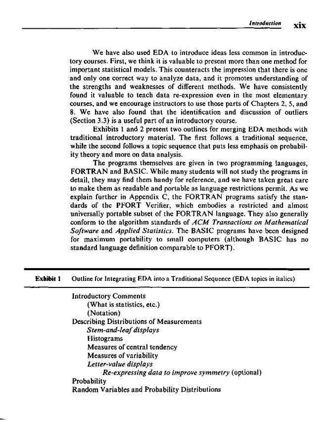
Exhibits 1 and 2 present two outlines for merging EDA methods withtraditional introductory material. The first follows a traditional sequence,while the second follows a topic sequence that puts less emphasis on probabil-ity theory and more on data analysis.
The programs themselves are given in two programming languages,FORTRAN and BASIC. While many students will not study the programs indetail, they may find them handy for reference, and we have taken great careto make them as readable and portable as language restrictions permit. As weexplain further in Appendix C, the FORTRAN programs satisfy the stan-dards of the PFORT Verifier, which embodies a restricted and almostuniversally portable subset of the FORTRAN language. They also generallyconform to the algorithm standards of ACM Transactions on MathematicalSoftware and Applied Statistics. The BASIC programs have been designedfor maximum portability to small computers (although BASIC has nostandard language definition comparable to PFORT).
Exhibit 1 Outline for Integrating EDA into a Traditional Sequence (EDA topics in italics)
Introductory Comments(What is statistics, etc.)(Notation)
Describing Distributions of MeasurementsStem-and-leaf displaysHistogramsMeasures of central tendencyMeasures of variabilityLetter-value displays
Re-expressing data to improve symmetry (optional)ProbabilityRandom Variables and Probability Distributions
x x ABCs of EDA
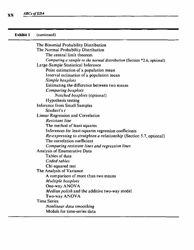
Exhibit 1 (continued)
The Binomial Probability DistributionThe Normal Probability Distribution
The central limit theoremComparing a sample to the normal distribution (Section *2.6, optional)
Large-Sample Statistical InferencePoint estimation of a population meanInterval estimation of a population meanSimple boxplotsEstimating the difference between two meansComparing boxplots
Notched boxplots (optional)Hypothesis testing
Inference from Small SamplesStudent's /
Linear Regression and CorrelationResistant lineThe method of least squaresInferences for least-squares regression coefficientsRe-expressing to straighten a relationship (Section 5.7, optional)The correlation coefficientComparing resistant lines and regression lines
Analysis of Enumerative DataTables of dataCoded tablesChi-squared test
The Analysis of VarianceA comparison of more than two meansMultiple boxplotsOne-way ANOVAMedian polish and the additive two-way modelTwo-way ANOVA
Time SeriesNonlinear data smoothingModels for time-series data
Introduction \ \ \
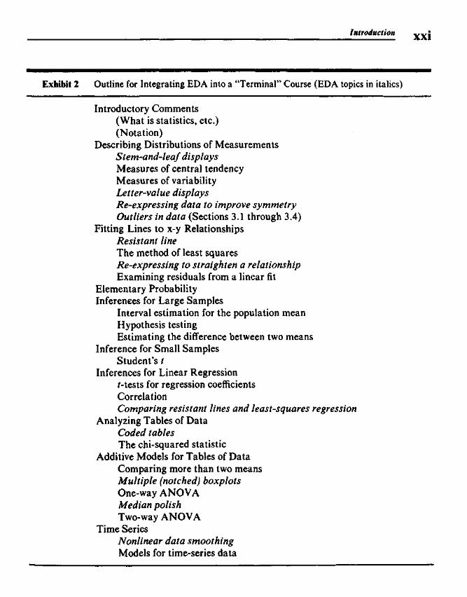
Exhibit 2 Outline for Integrating EDA into a "Terminal" Course (EDA topics in italics)
Introductory Comments(What is statistics, etc.)(Notation)
Describing Distributions of MeasurementsStem-and-leaf displaysMeasures of central tendencyMeasures of variabilityLetter-value displaysRe-expressing data to improve symmetryOutliers in data (Sections 3.1 through 3.4)
Fitting Lines to x-y RelationshipsResistant lineThe method of least squaresRe-expressing to straighten a relationshipExamining residuals from a linear fit
Elementary ProbabilityInferences for Large Samples
Interval estimation for the population meanHypothesis testingEstimating the difference between two means
Inference for Small SamplesStudent's /
Inferences for Linear Regression/-tests for regression coefficientsCorrelationComparing resistant lines and least-squares regression
Analyzing Tables of DataCoded tablesThe chi-squared statistic
Additive Models for Tables of DataComparing more than two meansMultiple (notched) boxplotsOne-way ANOVAMedian polishTwo-way ANOVA
Time SeriesNonlinear data smoothingModels for time-series data


Chapter 1Stem-and-Leaf Displays
batch
display
stem-and-leaf
Data can come in many forms. The simplest form is a collection, or batch, ofdata values. While we probably know something about the data, we areusually wise to assume little at first and just examine the data. Exploratorydata analysis provides tools and guidelines for getting acquainted with thedata.
The first step in any examination of data is drawing an appropriatepicture or display. Displays can show overall patterns or trends. They also canreveal surprising, unexpected, or amusing features of the data that mightotherwise go unnoticed.
The stem-and-leaf display has all of these virtues and can beconstructed and read easily. With it we can readily see:
• How wide a range of values the data cover;• Where the values are concentrated;• How nearly symmetric the batch is;• Whether there are gaps where no values were observed;• Whether any values stray markedly from the rest.
These are features that might go unnoticed if we looked no deeper than thedata values.
ABCs of EDA
In a stem-and-leaf display, the data values are sorted into numericalorder and brought together graphically. When we work by hand, we cancombine these operations into a single process. When the data have beenentered into a computer, a stem-and-leaf display brings the individual valuesback into view in a way that helps us to see important patterns.
1.1 Stems and Leaves
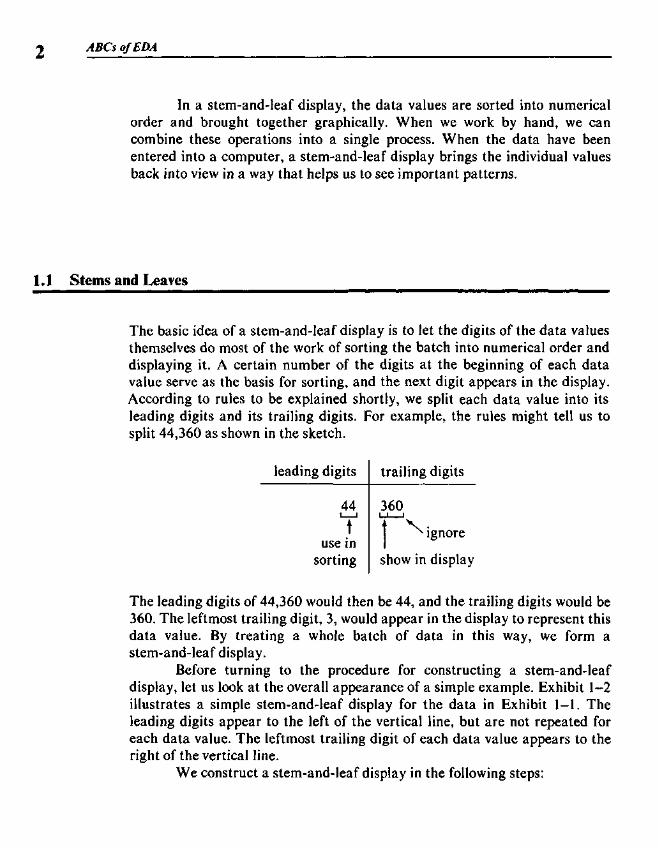
The basic idea of a stem-and-leaf display is to let the digits of the data valuesthemselves do most of the work of sorting the batch into numerical order anddisplaying it. A certain number of the digits at the beginning of each datavalue serve as the basis for sorting, and the next digit appears in the display.According to rules to be explained shortly, we split each data value into itsleading digits and its trailing digits. For example, the rules might tell us tosplit 44,360 as shown in the sketch.
leading digits
44
sorting
trailing digits
360
' I x ignoreuse in
show in display
The leading digits of 44,360 would then be 44, and the trailing digits would be360. The leftmost trailing digit, 3, would appear in the display to represent thisdata value. By treating a whole batch of data in this way, we form astem-and-leaf display.
Before turning to the procedure for constructing a stem-and-leafdisplay, let us look at the overall appearance of a simple example. Exhibit 1-2illustrates a simple stem-and-leaf display for the data in Exhibit 1-1. Theleading digits appear to the left of the vertical line, but are not repeated foreach data value. The leftmost trailing digit of each data value appears to theright of the vertical line.
We construct a stem-and-leaf display in the following steps:
Stem-and-Leaf Displays
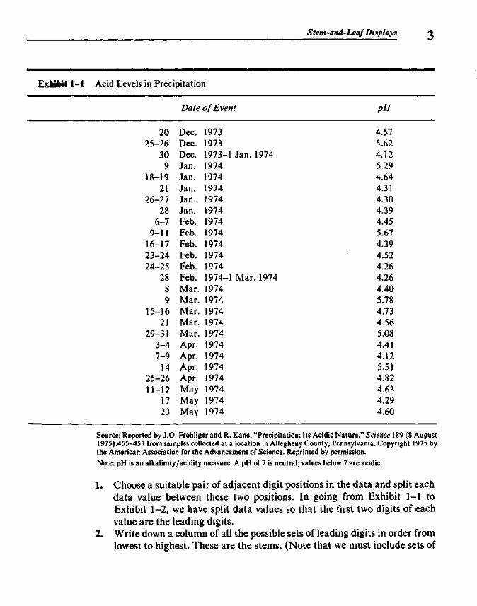
Exhibit 1-1 Acid Levels in Precipitation
Date of Event pH
2025-26
309
18-1921
26-2728
6-79-11
16-1723-2424-25
2889
15-1621
29-313-47-9
1425-2611-12
1723
Dec.Dec.Dec.Jan.Jan.Jan.Jan.Jan.Feb.Feb.Feb.Feb.Feb.Feb.Mar.Mar.Mar.Mar.Mar.Apr.Apr.Apr.Apr.MayMayMay
197319731973-1 Jan. 197419741974197419741974197419741974197419741974-1 Mar. 1974197419741974197419741974197419741974197419741974
4.575.624.125.294.644.314.304.394.455.674.394.524.264.264.405.784.734.565.084.414.125.514.824.634.294.60
Source: Reported by J.O. Frohliger and R. Kane, "Precipitation: Its Acidic Nature," Science 189 (8 August1975):455-457 from samples collected at a location in Allegheny County, Pennsylvania. Copyright 1975 bythe American Association for the Advancement of Science. Reprinted by permission.
Note: pH is an alkalinity/acidity measure. A pH of 7 is neutral; values below 7 are acidic.
1. Choose a suitable pair of adjacent digit positions in the data and split eachdata value between these two positions. In going from Exhibit 1-1 toExhibit 1-2, we have split data values so that the first two digits of eachvalue are the leading digits.
2. Write down a column of all the possible sets of leading digits in order fromlowest to highest. These are the stems. (Note that we must include sets of
ABCs of EDA
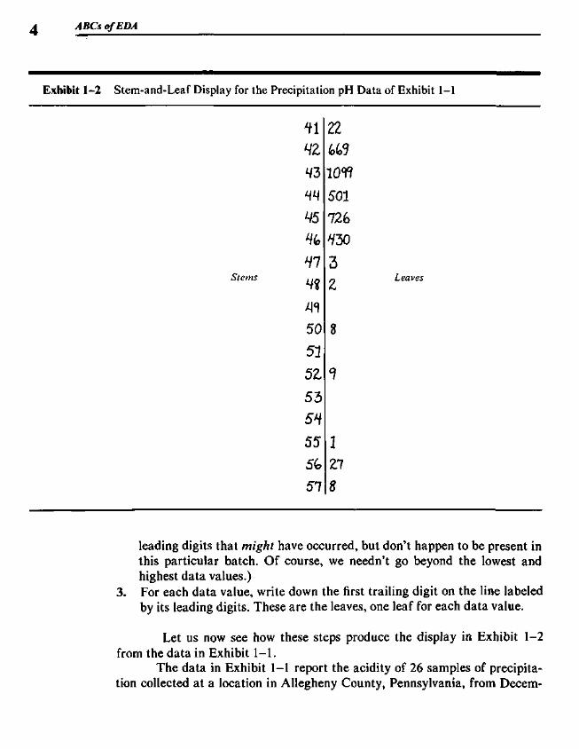
Exhibit 1-2 Stem-and-Leaf Display for the Precipitation pH Data of Exhibit 1-1
Stems
HZ
HI
50
51
53
5H
55
51
22
501
726
430
27
Leaves
leading digits that might have occurred, but don't happen to be present inthis particular batch. Of course, we needn't go beyond the lowest andhighest data values.)
3. For each data value, write down the first trailing digit on the line labeledby its leading digits. These are the leaves, one leaf for each data value.
Let us now see how these steps produce the display in Exhibit 1-2from the data in Exhibit 1-1.
The data in Exhibit 1-1 report the acidity of 26 samples of precipita-tion collected at a location in Allegheny County, Pennsylvania, from Decem-
Stem-and-Leaf Displays
ber 1973 to June 1974. The data are pH values—pH 7 is neutral; lower valuesare more acidic. They could bear on the theory that air pollution causesrainfall to be more acidic than it would naturally be.
Exhibit 1-2 shows the stem-and-leaf display of these values. To makethe display, we must split each number into a stem portion and a leaf portion.For the stem-and-leaf display in Exhibit 1-2, the pH values were split betweenthe tenths digit and the hundredths digit. For example, the entry in Exhibit1-1 for 20 Dec. 1973, which is 4.57, became 45|7, so that the stem is 45 and the
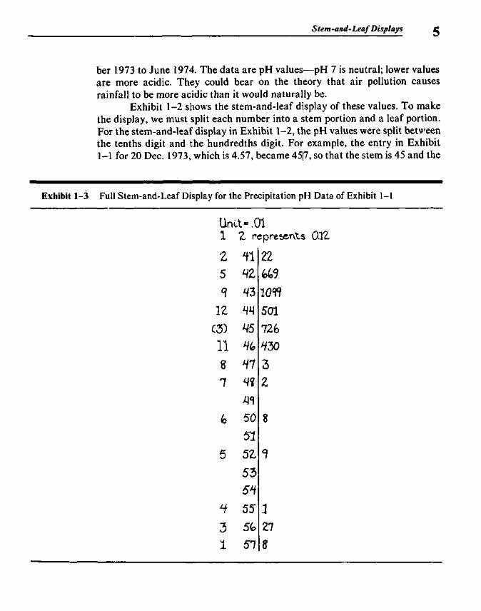
Exhibit 1-3 Full Stem-and-Leaf Display for the Precipitation pH Data of Exhibit 1-1
Unit-.011 2 represents 0.12
2 415 42
12 44
C3) 45
11 %
22(>W1099
501
726H30
8 47
(o
5
31
5051525354
55
57
8
<?
111
S
ABCs of EDA
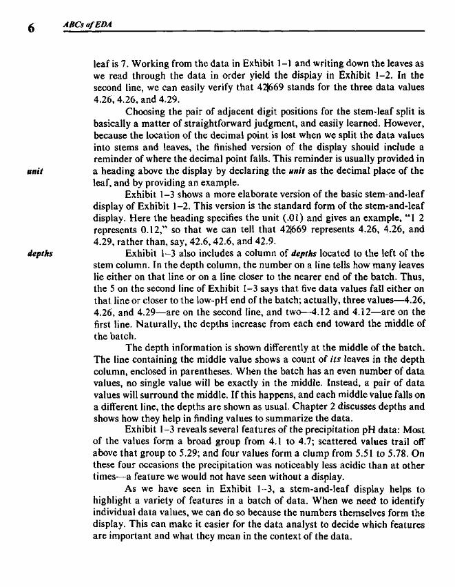
leaf is 7. Working from the data in Exhibit 1-1 and writing down the leaves aswe read through the data in order yield the display in Exhibit 1-2. In thesecond line, we can easily verify that 42|669 stands for the three data values4.26, 4.26, and 4.29.
Choosing the pair of adjacent digit positions for the stem-leaf split isbasically a matter of straightforward judgment, and easily learned. However,because the location of the decimal point is lost when we split the data valuesinto stems and leaves, the finished version of the display should include areminder of where the decimal point falls. This reminder is usually provided in
unit a heading above the display by declaring the unit as the decimal place of theleaf, and by providing an example.
Exhibit 1-3 shows a more elaborate version of the basic stem-and-leafdisplay of Exhibit 1-2. This version is the standard form of the stem-and-leafdisplay. Here the heading specifies the unit (.01) and gives an example, " 1 2represents 0.12," so that we can tell that 42|669 represents 4.26, 4.26, and4.29, rather than, say, 42.6, 42.6, and 42.9.
depths Exhibit 1-3 also includes a column of depths located to the left of thestem column. In the depth column, the number on a line tells how many leaveslie either on that line or on a line closer to the nearer end of the batch. Thus,the 5 on the second line of Exhibit 1-3 says that five data values fall either onthat line or closer to the low-pH end of the batch; actually, three values—4.26,4.26, and 4.29—are on the second line, and two—4.12 and 4.12—are on thefirst line. Naturally, the depths increase from each end toward the middle ofthe batch.
The depth information is shown differently at the middle of the batch.The line containing the middle value shows a count of its leaves in the depthcolumn, enclosed in parentheses. When the batch has an even number of datavalues, no single value will be exactly in the middle. Instead, a pair of datavalues will surround the middle. If this happens, and each middle value falls ona different line, the depths are shown as usual. Chapter 2 discusses depths andshows how they help in finding values to summarize the data.
Exhibit 1-3 reveals several features of the precipitation pH data: Mostof the values form a broad group from 4.1 to 4.7; scattered values trail offabove that group to 5.29; and four values form a clump from 5.51 to 5.78. Onthese four occasions the precipitation was noticeably less acidic than at othertimes—a feature we would not have seen without a display.
As we have seen in Exhibit 1-3, a stem-and-leaf display helps tohighlight a variety of features in a batch of data. When we need to identifyindividual data values, we can do so because the numbers themselves form thedisplay. This can make it easier for the data analyst to decide which featuresare important and what they mean in the context of the data.
Stem-and-Leaf Displays
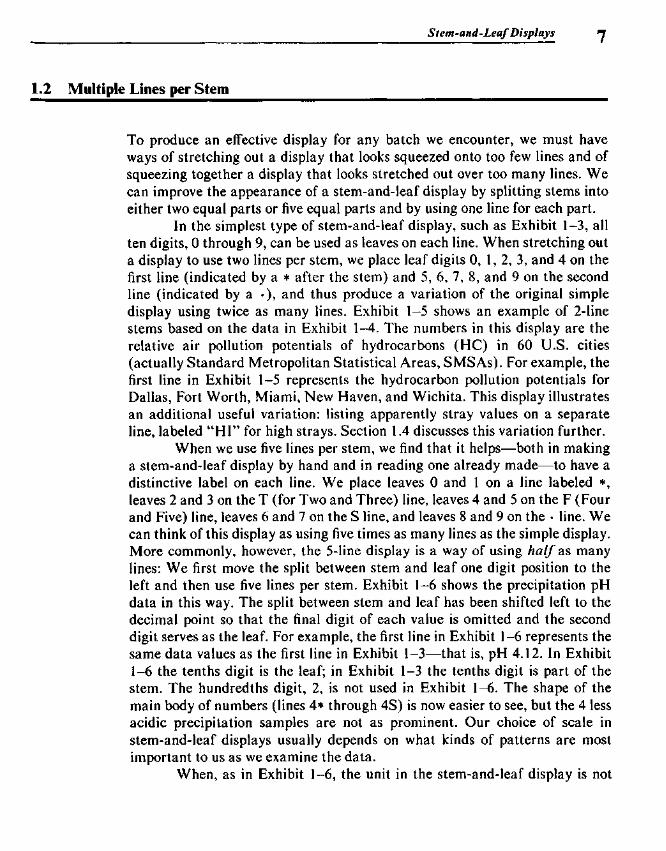
1.2 Multiple Lines per Stem
To produce an effective display for any batch we encounter, we must haveways of stretching out a display that looks squeezed onto too few lines and ofsqueezing together a display that looks stretched out over too many lines. Wecan improve the appearance of a stem-and-leaf display by splitting stems intoeither two equal parts or five equal parts and by using one line for each part.
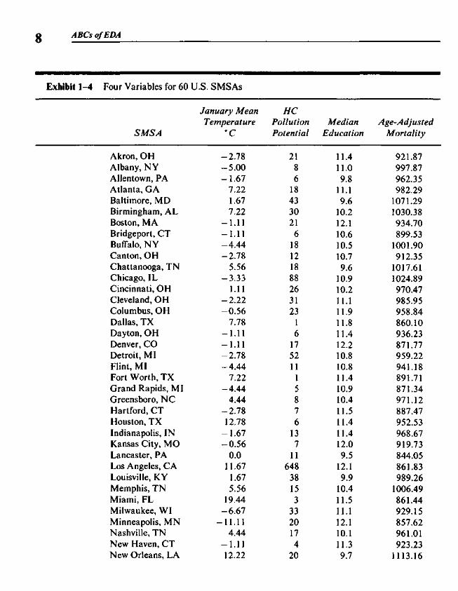
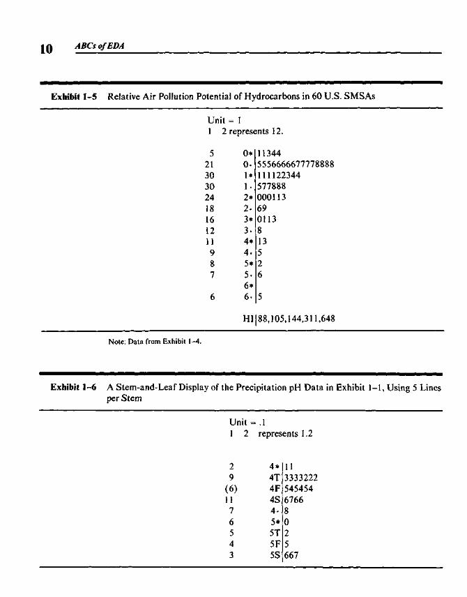
In the simplest type of stem-and-leaf display, such as Exhibit 1-3, allten digits, 0 through 9, can be used as leaves on each line. When stretching outa display to use two lines per stem, we place leaf digits 0, 1,2, 3, and 4 on thefirst line (indicated by a * after the stem) and 5, 6, 7, 8, and 9 on the secondline (indicated by a -), and thus produce a variation of the original simpledisplay using twice as many lines. Exhibit 1-5 shows an example of 2-linestems based on the data in Exhibit 1-4. The numbers in this display are therelative air pollution potentials of hydrocarbons (HC) in 60 U.S. cities(actually Standard Metropolitan Statistical Areas, SMSAs). For example, thefirst line in Exhibit 1-5 represents the hydrocarbon pollution potentials forDallas, Fort Worth, Miami, New Haven, and Wichita. This display illustratesan additional useful variation: listing apparently stray values on a separateline, labeled "HI" for high strays. Section 1.4 discusses this variation further.
When we use five lines per stem, we find that it helps—both in makinga stem-and-leaf display by hand and in reading one already made—to have adistinctive label on each line. We place leaves 0 and 1 on a line labeled *,leaves 2 and 3 on the T (for Two and Three) line, leaves 4 and 5 on the F (Fourand Five) line, leaves 6 and 7 on the S line, and leaves 8 and 9 on the • line. Wecan think of this display as using five times as many lines as the simple display.More commonly, however, the 5-line display is a way of using half as manylines: We first move the split between stem and leaf one digit position to theleft and then use five lines per stem. Exhibit 1-6 shows the precipitation pHdata in this way. The split between stem and leaf has been shifted left to thedecimal point so that the final digit of each value is omitted and the seconddigit serves as the leaf. For example, the first line in Exhibit 1-6 represents thesame data values as the first line in Exhibit 1-3—that is, pH 4.12. In Exhibit1-6 the tenths digit is the leaf; in Exhibit 1-3 the tenths digit is part of thestem. The hundredths digit, 2, is not used in Exhibit 1-6. The shape of themain body of numbers (lines 4* through 4S) is now easier to see, but the 4 lessacidic precipitation samples are not as prominent. Our choice of scale instem-and-leaf displays usually depends on what kinds of patterns are mostimportant to us as we examine the data.
When, as in Exhibit 1-6, the unit in the stem-and-leaf display is not
8 ABCs of EDA
Exhibit 1-4 Four Variables for 60 U.S. SMSAs
SMSA
Akron, OHAlbany, NYAllentown, PAAtlanta, GABaltimore, MDBirmingham, ALBoston, MABridgeport, CTBuffalo, NYCanton, OHChattanooga, TNChicago, ILCincinnati, OHCleveland, OHColumbus, OHDallas, TXDayton, OHDenver, CODetroit, MIFlint, MIFort Worth, TXGrand Rapids, MIGreensboro, NCHartford, CTHouston, TXIndianapolis, INKansas City, MOLancaster, PALos Angeles, CALouisville, KYMemphis, TNMiami, FLMilwaukee, WIMinneapolis, MNNashville, TNNew Haven, CTNew Orleans, LA
January MeanTemperature
°C
-2.78-5 .00-1.67
7.221.677.22
-1.11-1.11-4.44-2.78
5.56-3.33
1.11-2.22-0.56
7.78-1.11-1.11-2.78-4.44
7.22-4.44
4.44-2.7812.78
-1.67-0.56
0.011.67
1.675.56
19.44-6.67
-11.114.44
-1.1112.22
HCPollutionPotential
2186
18433021
618121888263123
16
175211
15876
137
11648
38153
3320174
20
MedianEducation
11.411.09.8
11.19.6
10.212.110.610.510.79.6
10.910.211.111.911.811.412.210.810.811.410.910.411.511.411.412.09.5
12.19.9
10.411.511.112.110.111.39.7
Age-AdjustedMortality
921.87997.87962.35982.29
1071.291030.38934.70899.53
1001.90912.35
1017.611024.89970.47985.95958.84860.10936.23871.77959.22941.18891.71871.34971.12887.47952.53968.67919.73844.05861.83989.26
1006.49861.44929.15857.62961.01923.23
1113.16
Stem-and-Leaf Displays
Exhibit 1-4 (continued)
SMS A
New York, NYPhiladelphia, PAPittsburgh, PAPortland, ORProvidence, RIReading, PARichmond, VARochester, NYSt. Louis, MOSan Diego, CASan Francisco, CASan Jose, CASeattle, WASpringfield, MASyracuse, NYToledo, OHUtica, NYWashington, DCWichita, KSWilmington, DEWorcester, MAYork, PAYoungstown, OH
January MeanTemperature
°C
0.560.0
-1.673.33
-1.670.563.89
-3.890.0
12.788.899.444.44
-2.22-4.44-3.33-5.00
2.780.00.56
-4.440.56
-2.22
HCPollutionPotential
41294556
611127
3114431110520
58
115
654
1478
14
MedianEducation
10.710.510.612.010.19.6
11.011.19.7
12.112.212.212.211.111.410.710.312.312.111.311.19.0
10.7
Age-AdjustedMortality
994.651015.02991.29893.99938.50946.19
1025.50874.28953.56839.71911.70790.73899.26904.16950.67972.46912.20967.80823.76
1003.50895.70911.82954.44
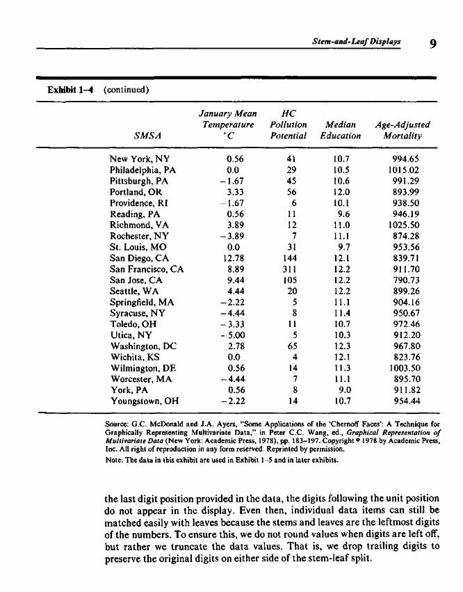
Source: G.C. McDonald and J.A. Ayers, "Some Applications of the 'Chernoff Faces': A Technique forGraphically Representing Multivariate Data," in Peter C.C. Wang, ed., Graphical Representation ofMultivariate Data (New York: Academic Press, 1978), pp. 183-197. Copyright ° 1978 by Academic Press,Inc. All right of reproduction in any form reserved. Reprinted by permission.
Note: The data in this exhibit are used in Exhibit 1-5 and in later exhibits.
the last digit position provided in the data, the digits following the unit positiondo not appear in the display. Even then, individual data items can still bematched easily with leaves because the stems and leaves are the leftmost digitsof the numbers. To ensure this, we do not round values when digits are left off,but rather we truncate the data values. That is, we drop trailing digits topreserve the original digits on either side of the stem-leaf split.
10 ABCs of EDA
Exhibit 1-5 Relative Air Pollution Potential of Hydrocarbons in 60 U.S. SMSAs
Unit1 2
52130302418161211987
6
= 1represents 12.
0*0-1*1.2*2-3*3-4*4-5*5-6*6-
HI
113445556666677778888111122344577888000113690113813526
5
88,105,144,311,648
Note: Data from Exhibit 1-4.
Exhibit 1-6 A Stem-and-Leaf Display of the Precipitation pH Data in Exhibit 1-1, Using 5 Linesper Stem
Unit =1 2
29(6)1176543
.1represents 1.2
4*4T4F4S4-5*5T5F5S
11333322254545467668025667
Stem-and-Leaf Displays 11
1.3 Positive and Negative Values
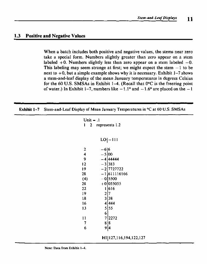
When a batch includes both positive and negative values, the stems near zerotake a special form. Numbers slightly greater than zero appear on a stemlabeled +0. Numbers slightly less than zero appear on a stem labeled —0.This labeling may seem strange at first; we might expect the stem — 1 to benext to +0, but a simple example shows why it is necessary. Exhibit 1-7 showsa stem-and-leaf display of the mean January temperatures in degrees Celsiusfor the 60 U.S. SMSAs in Exhibit 1-4. (Recall that 0°C is the freezing pointof water.) In Exhibit 1-7, numbers like —1.1° and — 1.6° are placed on the — 1
Exhibit 1-7 Stem-and-Leaf Display of Mean January Temperatures in °C at 60 U.S. SMSAs
Unit =1 2
249121928(4)282219181613
1176
.1represents 1.2
LO
— 6-5— 4-3-2-1-0+ 0123456789
-111
600444443837727722611116166550005505561673844455
227284
HII 127,116,194,122,127
Note: Data from Exhibit 1-4.
12 ABCs of EDA
stem. The —0 stem is needed for numbers like —0.5°. The special value 0.0could be placed on either of the two 0 stems. To preserve the outline of thedisplay, we split the 0.0 values equally between the +0 stem and the - 0stem.
In Exhibit 1-7, the major feature is the 41 cities that have meanJanuary temperatures between — 6.6°C and +2.7°C. One clump of cities—generally those in the Southwest—stands out from 7.2°C to 9.4°C. Fivecities—Houston, Los Angeles, Miami, New Orleans, and San Diego—appearon the HI stem; and Miami, at 19.4°C, is the highest. Minneapolis, at-11.1 °C, appears on the LO stem.
1.4 Listing Apparent Strays
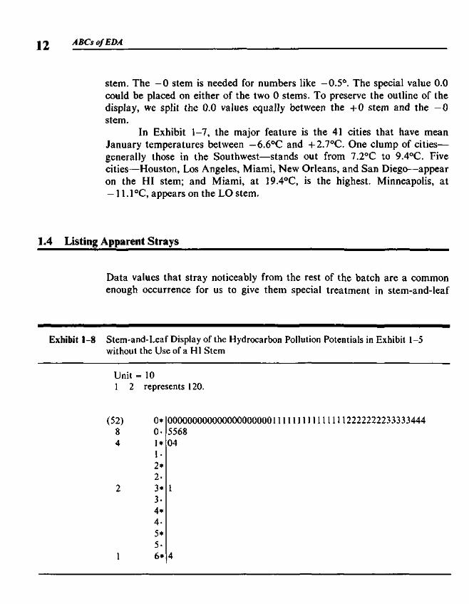
Data values that stray noticeably from the rest of the batch are a commonenough occurrence for us to give them special treatment in stem-and-leaf
Exhibit 1-8 Stem-and-Leaf Display of the Hydrocarbon Pollution Potentials in Exhibit 1-5without the Use of a HI Stem
Unit =1 2
(52)84
2
1
10represents 120.
0*0-1*1-2*2-3*3-4*4-5*5-6*
0000000000000000000001111111111111112222222233333444556804
1
4
Stem-and-Leaf Displays 13
displays. We want to avoid a display in which most data values are squeezedonto a few lines of the display, the strays occupy a line or two at one or bothextremes, and many lines lie blank in between. For example, Exhibit 1-8shows what the display in Exhibit 1-5 would have looked like if we had notisolated the stray high values.
Once we have decided which data values to treat as strays, we caneasily list them separately at the low or high end of the display where theybelong. We introduce these lists with the labels LO and HI in the stemcolumn, and we leave at least one blank line between each list and the body ofthe display in order to emphasize the separation.
When we produce the display by hand, we can usually use ourjudgment in differentiating strays from the rest of the data. A computerprogram, however, must rely on a rule of thumb to make this decision in hopesof producing reasonable displays for most batches. This rule is discussed indetail in Chapter 3.
1.5 Histograms
histogram Data batches are often displayed in a histogram to exhibit their shape. Ahistogram is made up of side-by-side bars. Each data value is represented byan equal amount of area in its bar. We can see at a glance whether the batch is
symmetric generally symmetric—that is, approximately the same shape on either side of askewed line down the center of the histogram—or whether it is skewed—that is,
stretched out to one side or the other of the center. We can also see whether aunimodal histogram rises to a single main hump—a unimodal pattern—or exhibits twobimodal or more humps—a bimodal or multimodal pattern, respectively. The parts onmultimodal either end of a histogram are usually called the tails. We can characterize atails histogram as showing short, medium, or long tails according to how stretched
out they are. Finally, we can spot straggling data values that seem to bedetached from the main body of the data.
Unimodal symmetric batches are usually the easiest to deal with.Multiple humps may indicate identifiable subgroups—for example, male andfemale—that might be more usefully examined separately. (One way to dealwith skewness, or asymmetry, is described in Chapter 2; extraordinary datavalues are discussed more precisely in Chapter 3.)
The stem-and-leaf display resembles a histogram in that both of themdisplay the distribution of the data values in the batch by representing each
•tA ABCsofEDA
value with an equal amount of area. In a stem-and-leaf display, each digitoccupies the same amount of space. In a histogram, each data value isrepresented by an equal amount of area in a bar delineated by lines.Occasionally a histogram is made up of printed symbols by using a singlecharacter—typically * or X—to represent each value. (This is done by manycomputer programs.) For large batches, a single * can represent several datavalues in a histogram in order to preserve a manageable size. Thus a histogramcan serve as an "overflow" alternative to a stem-and-leaf display when thebatch is large (several hundred values or so). With several hundred leaves wewould be less able to concentrate on detail anyway.
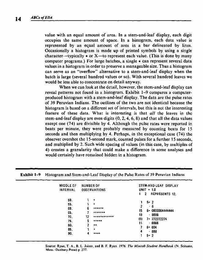
When we can look at the detail, however, the stem-and-leaf display canreveal patterns not found in a histogram. Exhibit 1-9 compares a computer-produced histogram with a stem-and-leaf display. The data are the pulse ratesof 39 Peruvian Indians. The outlines of the two are not identical because thehistogram is based on a different set of intervals, but this is not the interestingfeature of these data. What is interesting is that all the leaves in thestem-and-leaf display are even digits (0, 2, 4, 6, 8) and that all the data valuesexcept one (74) are divisible by 4. Although the pulse rates were reported inbeats per minute, they were probably measured by counting beats for 15seconds and then multiplying by 4. Perhaps, in the exceptional case (74) theobserver overshot the 15-second mark, counted pulses for a further 15 seconds,and multiplied by 2. Such wide spacing of values (in this case, by multiples of4) creates a granularity that could make a difference in some analyses andwould certainly have remained hidden in a histogram.
Exhibit 1-9 Histogram and
MIDDLE
Stem-and-Leaf Display of the
OF NUMBER OF
INTERVAL OBSERVATIONS
5055
60cc
70
75
80
85
90
1 *
1 •g ******
5 * * * * *
2 * •
1 *4 • * * •
Pulse Rates of 39 Peruvian Indians
STEM-AND-LEAF DISPLAY
UNIT = 1.0
1 2 REPRESENTS 12.
1 5* 2
2 • 615 6* 0000004444444
19 • 8888(9) 7* 222222224
11 • 6666
7 8* 004
4 • 888
1 9« 2
Source: Ryan, T. A., B. L. Joiner, and B. F. Ryan. 1976. The Minitab Student Handbook (N. Scituate,Mass.: Duxbury Press) p. 277.
Stem-and-Leaf Displays -i c
A subtler granularity can be seen in the mean January temperatures inExhibit 1-7. Inspection of this exhibit reveals that no more than two differentleaf values occur on any stem and that the actual values are symmetric aroundthe zero stem. For example, stems 3 and —3 have only leaves of 3 or 8; stems 1and — 1 have only leaves of 1 or 6. This granularity occurs because thetemperatures originally were recorded to the nearest degree in Fahrenheit andthen were converted to Celsius. Patterns of this kind are the ones most likely tobe overlooked when data are analyzed on a computer. They highlight animportant function of the stem-and-leaf display—keeping the individual datavalues in view.
1.6 Stem-and-Leaf Displays from the Computer
It is easy to construct a stem-and-leaf display by hand. With a little practiceone quickly learns to choose the number of lines per stem that neither stretchesout the display too far nor cramps it into too few lines.
It is not nearly as easy to write a general computer program to producestem-and-leaf displays. Computers cannot follow instructions such as "choosea display format so that the display will be neither too stretched out nor toocramped." Instead, we must devise specific rules that the computer will applyin making the necessary decisions. However, once the program is written, it iseasy to use because all the essential decisions can be left to the computer. Weneed only tell the computer what data we wish it to display. How to dothis—and, indeed, how you tell your computer to do anything—will dependon the way your computer is set up. If you don't already know how to run theprograms in this book on your computer, ask for assistance from someoneexpert in using it.
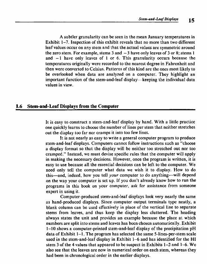
Computer-produced stem-and-leaf displays look very nearly the sameas hand-produced displays. Since computer output terminals type neatly, ablank column can be used effectively in place of the vertical line to separatestems from leaves, and thus keep the display less cluttered. The headingalways states the unit and provides an example because the place at whichnumbers are split into stems and leaves has been chosen automatically. Exhibit1-10 shows a computer-printed stem-and-leaf display of the precipitation pHdata of Exhibit 1-1. The program has selected the same 5-lines-per-stem scaleused in the stem-and-leaf display in Exhibit 1-6 and has identified for the HIstem 3 of the 4 values that appeared to be suspect in Exhibits 1-2 and 1-6. Wealso see that the leaves are now in numerical order on each stem, whereas theyhad been in chronological order in the earlier displays.
ABCsofEDA
Exhibit 1-10 Computer-Printed Stem-and-Leaf Display of thePrecipitation pH Data of Exhibit 1-1
STEM-ANCUNIT
1 2
29
(6)117654
= 0.
J-LEAF DISPLAY
1000
REPRESENTS 1.2
4*TFS
4-5*TF
HI
112223333
4445556667
802
en
56,56,57
program Many of the programs in this book include options that will allow you tooptions tailor a display or computation to the specific needs of your analysis. One such
option is to forbid the use of the HI and LO stems and display all of the datavalues from lowest to highest in the main body of the stem-and-leaf display.While this is desirable in some situations, the result may look like Exhibit 1-8.How you specify this option or any option for any of the programs will, ofcourse, depend on the way your computer is set up.
1.7 Algorithms I
Although the stem-and-leaf display is one of the simplest exploratory dataanalysis methods, the stem-and-leaf programs in this chapter are very sophisti-cated and are among the longest programs in the book. Many decisions mustbe made when a stem-and-leaf display is created. When we work by hand, wemake these decisions so easily that they almost go unnoticed. A program,however, must be prepared for every situation it might face in producing astem-and-leaf display, and it must specify explicitly how each decision shouldbe made in every situation.
Several of the decision rules used in the programs at the end of thischapter are subtle and were developed only after considerable trial and error.Some depend upon aspects of data analysis discussed in later chapters. If you
Stem-and-Leaf Displays -i n
are planning to study the programs and the algorithm and have not yetfollowed the "fhread" through Appendices A, B, and C and Chapters 2, 7, and3, please stop and read them first. If you are reading the book in chapter order,please skip the rest of this chapter. When you return to this section afterreading the other chapters, you will be able to see how the stem-and-leafalgorithm combines ideas introduced in other chapters and adds new ideasspecial to this technique.
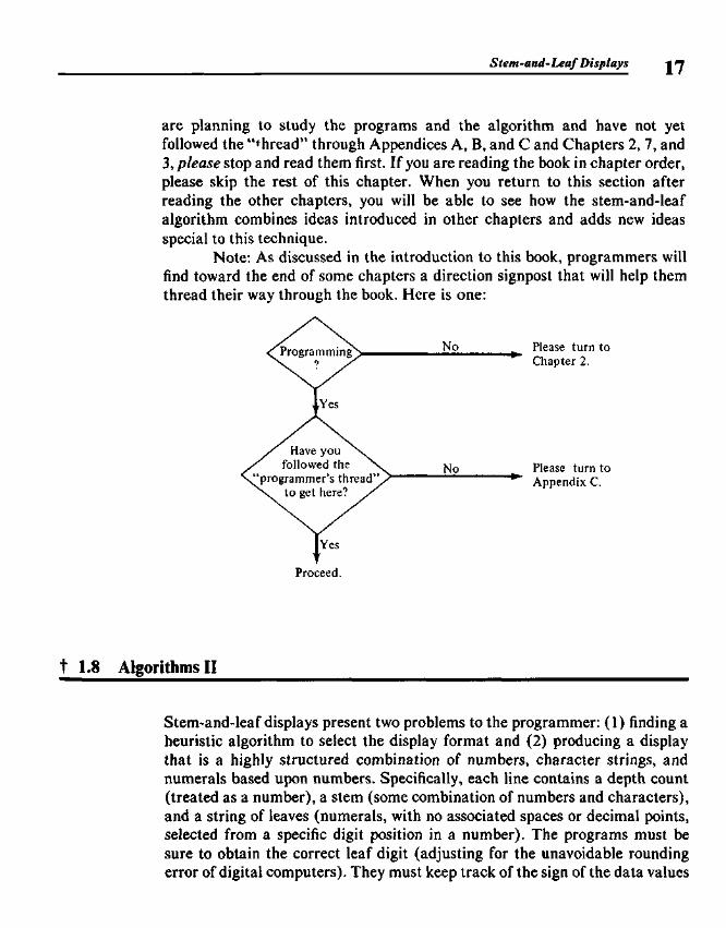
Note: As discussed in the introduction to this book, programmers willfind toward the end of some chapters a direction signpost that will help themthread their way through the book. Here is one:
No Please turn toChapter 2.
Have youfollowed the
programmer's threadto get here?
No Please turn toAppendix C.
t 1.8 Algorithms II
Stem-and-leaf displays present two problems to the programmer: (1) finding aheuristic algorithm to select the display format and (2) producing a displaythat is a highly structured combination of numbers, character strings, andnumerals based upon numbers. Specifically, each line contains a depth count(treated as a number), a stem (some combination of numbers and characters),and a string of leaves (numerals, with no associated spaces or decimal points,selected from a specific digit position in a number). The programs must besure to obtain the correct leaf digit (adjusting for the unavoidable roundingerror of digital computers). They must keep track of the sign of the data values
ABCsofEDA
and of the allocation of data values to lines of the display. Each line is ahalf-open interval including the inside limit, which is closer to zero andcorresponds to a data value whose leaf is zero on that line. The interval extendsto, but does not include, the inner limit of the next line away from zero. Thezero stems are special because both the +0 and —0 stems label intervals thatinclude the value 0.0. The programs must thus pay special attention to zeros inthe data.
If the data batch is not already in order, it is first sorted (see Section2.9 for a discussion of sorting methods). Next, the program must decidewhether any extreme data values should appear on the special LO and HIstems. If so, only the remaining numbers will be used in choosing the displayformat. The details of this decision are discussed in Section 3.3.
The program then determines the unit and the display format byestimating how many lines ought to be used in all to display the numbers.Experience has shown that, if we have n numbers, 10 x log,0« is a good firstguess at the number of lines needed for a good display. (Here the number ofdata values, n, excludes the stray values assigned to the LO and HI stems.)The program first computes the range of values that would be covered by eachline if the maximum number of lines were used. This line width is the result ofdividing the range of the (non-straying) data values by the approximatenumber of lines desired (10 x Iog10«). Because each line must accommodateeither two, five, or ten possible leaf digit values, the line width is rounded up tothe next larger number representable as 2, 5, or 10 times an integer power of10. Rounding up guarantees that no more than 10 x Iog10/i lines will be used.The power of 10 yields the unit, and the multiplier (2, 5, or 10) is the numberof leaf digits on each line. (Note that 10/(number of leaf digits) yields thenumber of lines per stem.) The program then prints the display heading, whichincludes the unit decided upon and an example. The example uses a stem of 1and a leaf of 2 to illustrate where the decimal point should be placed.
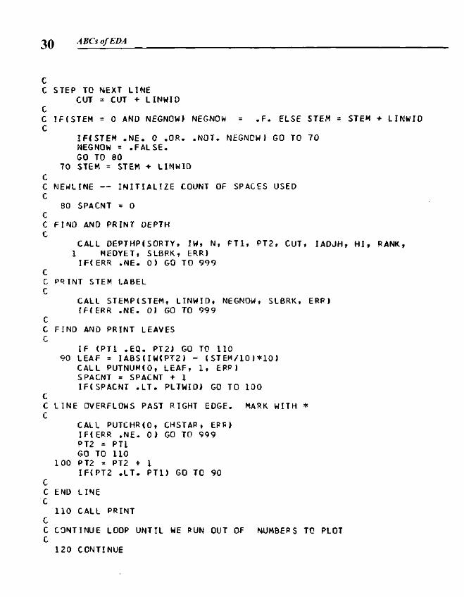
Now the program can step through the ordered data and print out oneline of the display at a time. The program must print each stem according tothe format selected and must use the correct numeral for each leaf. If theleaves to be printed on a line would extend beyond the right margin, theprogram uses the available spaces and then inserts an asterisk in the rightmostspace to show that the overflow occurred. (The depth still provides a completecount and thus indicates the number of values omitted.) These steps requirecareful programming so that they work for all possible cases.
For each line of the display, the program first looks down the ordereddata batch to identify the data values to be displayed on that line. It countsthese values and computes the depth, which it places on the output line. It thenconstructs the stem and places it on the output line. Finally, it scans through
Stem-and-Leaf Displays
the data values and computes and prints leaves. This requires only one passthrough the data because one line begins, after allowing for lines that have noleaves, where the previous line ends.
FORTRAN
The F O R T R A N programs that produce a stem-and-leaf display consist of fivesubroutines, STMNLF, SLTITL, OUTLYP, DEPTHP, and STEMP. To produce a stem-and-leaf display for data in the vector Y, use the F O R T R A N statement
CALL STMNLF(Y, N, SORTY, IW, XTREMS, ERR)
where the parameters have the following meanings:
Y() is the N-long vector of data values;
N is the number of data values;SORTY() is an N-long workspace for real numbers;IW() is an N-long workspace for integers;XTREMS is a logical flag, set .TRUE, if the plot should include
all data values or set .FALSE, to permit HI and LOstems;
ERR is the error flag, whose values are0 normal
11 N < 112 internal error—see program13 page has fewer than 5 spaces for leaves.
The subroutine STMNLF first determines the display format. It callsSLTITL to print the headings. If necessary, it then calls OUTLYP to print the LOstem. Then it steps through the sorted data, calling DEPTHP to compute andprint depths and STEMP to compute and print stems. STMNLF places the leaveson each line itself. If necessary, it calls OUTLYP to print the HI stem.Throughout, STMNLF uses the utility output routines (see Appendix C).
BASIC
The BASIC subroutine for stem-and-leaf display is entered with the N datavalues to be displayed in the array Y. If the version number, V1, is 1, the plot is
20 ABCs of EDA
scaled to the extreme values, and no HI and LO stems are printed. If V1 is 2 orgreater, extreme values are placed on the HI and LO stems and excluded indetermining the plot format. The array Y is returned unmodified. The programuses the defined functions, the SORT subroutines, and the plot-scaling subrou-tines (see Appendix A).
References
Frohliger, J.O., and R. Kane. 1975. "Precipitation: Its Acidic Nature." Science 189 (8August 1975), pp. 455-457.
McDonald, Gary C, and James A. Ayers. 1978. "Some Applications of the 'ChernoffFaces1: A Technique for Graphically Representing Multivariate Data." InPeter C.C. Wang, ed., Graphical Representation of Multivariate Data. NewYork: Academic Press.
Ryan, T.A., B.L. Joiner, and B.F. Ryan. 1976. The Minitab Student Handbook. N.Scituate, Mass.: Duxbury Press.
"Programming^) Y e s » Please turn toChapter 4.
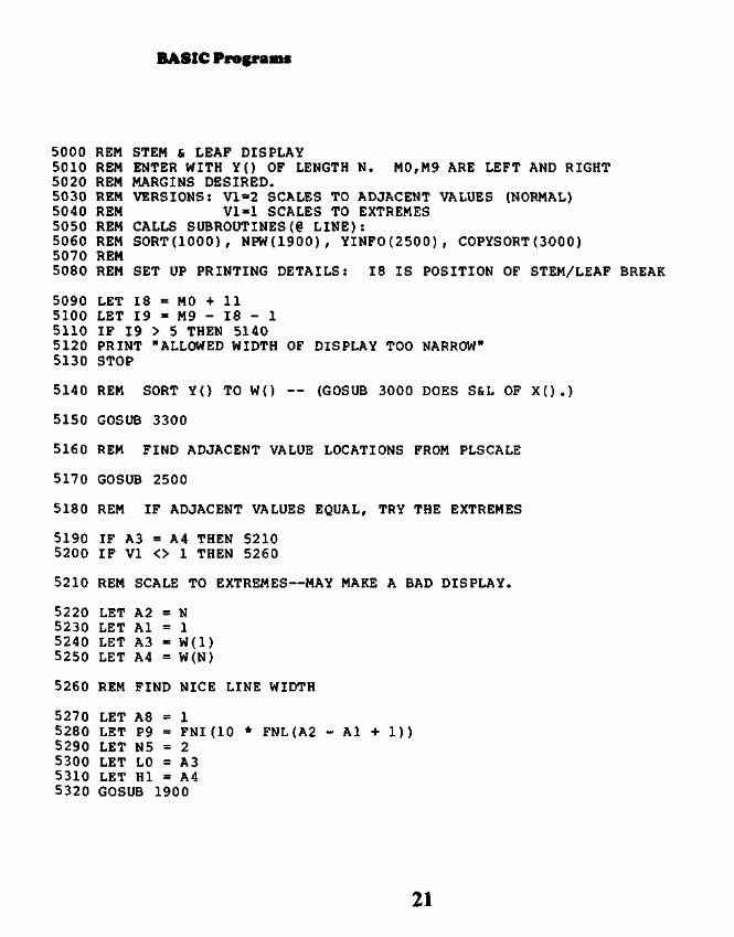
BASIC Programs
5000 REM STEM & LEAF DISPLAY5010 REM ENTER WITH Y() OF LENGTH N. M0,M9 ARE LEFT AND RIGHT5020 REM MARGINS DESIRED.5030 REM VERSIONS: Vl=2 SCALES TO ADJACENT VALUES (NORMAL)5040 REM Vl=l SCALES TO EXTREMES5050 REM CALLS SUBROUTINES(@ LINE):5060 REM SORT(1000)f NPW(1900), YINFO(2500), COPYSORT(3000)5070 REM5080 REM SET UP PRINTING DETAILS: 18 IS POSITION OF STEM/LEAF BREAK
5090 LET 18 = M0 + 115100 LET 19 = M9 - 18 - 15110 IF 19 > 5 THEN 51405120 PRINT "ALLOWED WIDTH OF DISPLAY TOO NARROW"5130 STOP
5140 REM SORT Y() TO W() — (GOSUB 3000 DOES S&L OF X().)
5150 GOSUB 3300
5160 REM FIND ADJACENT VALUE LOCATIONS FROM PLSCALE
5170 GOSUB 2500
5180 REM IF ADJACENT VALUES EQUAL, TRY THE EXTREMES
5190 IF A3 = A4 THEN 52105200 IF VI <> 1 THEN 5260
5210 REM SCALE TO EXTREMES—MAY MAKE A BAD DISPLAY.
5220 LET A2 = N5230 LET Al = 15240 LET A3 = W(l)5250 LET A4 = W(N)
5260 REM FIND NICE LINE WIDTH
5270 LET A8 = 15280 LET P9 = FNI (10 * FNL(A2 - Al + 1))5290 LET N5 = 25300 LET L0 = A35310 LET HI = A45320 GOSUB 1900
21
22 ABCs of EDA
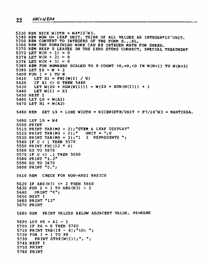
5330 REM NICE WIDTH = N4*10~N3.5340 REM NOW U= LEAF UNIT. THINK OF ALL VALUES AS INTEGER*10~UNIT.5350 REM CONVERT TO INTEGERS OF THE FORM S...SL.5360 REM THE REMAINING WORK CAN BE INTEGER MATH FOR SPEED.5370 REM KEEP 0 LEAVES ON THE ZERO STEMS CORRECT, SPECIAL TREATMENT5372 LET W(N + 1) = 05374 LET W(N + 2) = 05376 LET W(N + 3) = 05380 REM FOR NUMBERS SCALED TO 0 COUNT >0f=0,<0 IN W(N+1) TO W(N+3)5390 LET Z0 = N + 25400 FOR I = 1 TO N5410 LET XI = FNI(W(I) / U)5420 IF XI <> 0 THEN 54405430 LET W(Z0 + SGN(W(I))) = W(Z0 + SGN(W(I))) + 15440 LET W(I) = XI5450 NEXT I5460 LET LO = W(A1)5470 LET HI = W(A2)
5480 REM SET L9 = LINE WIDTH = NICEWIDTH/UNIT = P7/10~N3 = MANTISSA.
5490 LET L9 = N45500 PRINT5510 PRINT TAB(M0 + 2);"STEM & LEAF DISPLAY"5520 PRINT TAB(MO + 2);" UNIT = ";U5530 PRINT TAB(MO + 2);"1 2 REPRESENTS " ;5540 IF U < 1 THEN 55705550 PRINT FNI(12 * U)5560 GO TO 56705570 IF U <> .1 THEN 56005580 PRINT "1.2"5590 GO TO 56705600 PRINT "0.";
5610 REM CHECK FOR NON-ANSI BASICS
5620 IF ABS(N3) <= 2 THEN 56605630 FOR I = 1 TO ABS(N3) - 25640 PRINT "0";5650 NEXT I5660 PRINT "12"5670 PRINT
5680 REM PRINT VALUES BELOW ADJACENT VALUE. P6=RANK
5690 LET P6 = Al - 15700 IF P6 = 0 THEN 57605710 PRINT TAB(I8 - 4);"LO: ";5720 FOR I = 1 TO P65730 PRINT STR$(W(I));",5740 NEXT I5750 PRINT5760 PRINT
BASIC 23
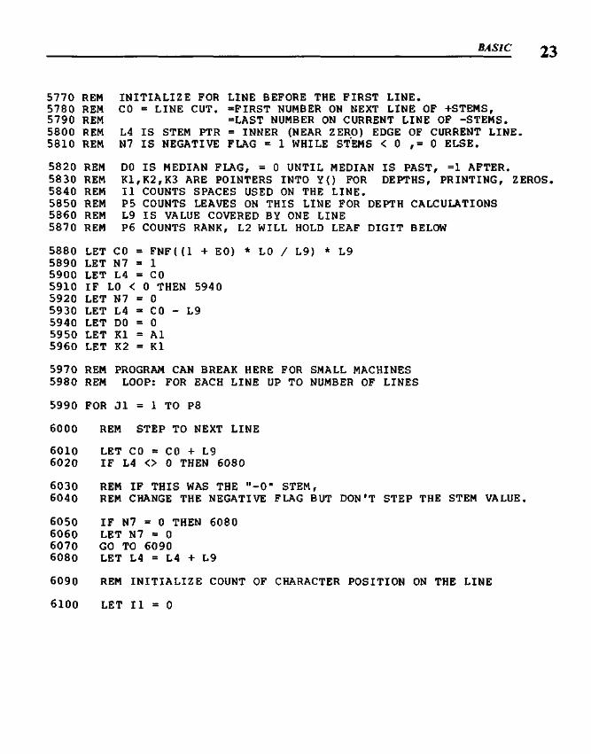
5770 REM INITIALIZE FOR LINE BEFORE THE FIRST LINE.5780 REM CO = LINE CUT. =FIRST NUMBER ON NEXT LINE OF +STEMS,5790 REM =LAST NUMBER ON CURRENT LINE OF -STEMS.5800 REM L4 IS STEM PTR = INNER (NEAR ZERO) EDGE OF CURRENT LINE.5810 REM N7 IS NEGATIVE FLAG = 1 WHILE STEMS < 0 ,= 0 ELSE.
5820 REM DO IS MEDIAN FLAG, = 0 UNTIL MEDIAN IS PAST, =1 AFTER.5830 REM KlrK2,K3 ARE POINTERS INTO Y() FOR DEPTHS, PRINTING, ZEROS,5840 REM II COUNTS SPACES USED ON THE LINE.5850 REM P5 COUNTS LEAVES ON THIS LINE FOR DEPTH CALCULATIONS5860 REM L9 IS VALUE COVERED BY ONE LINE5870 REM P6 COUNTS RANK, L2 WILL HOLD LEAF DIGIT BELOW
5880 LET CO = FNF((1 + EO) * LO / L9) * L95890 LET N7 = 15900 LET L4 = CO5910 IF LO < 0 THEN 59405920 LET N7 = 05930 LET L4 = CO - L95940 LET DO = 05950 LET Kl = Al5960 LET K2 = Kl
5970 REM PROGRAM CAN BREAK HERE FOR SMALL MACHINES5980 REM LOOP: FOR EACH LINE UP TO NUMBER OF LINES
5990 FOR Jl = 1 TO P8
6000 REM STEP TO NEXT LINE
6010 LET CO = CO + L96020 IF L4 <> 0 THEN 6080
6030 REM IF THIS WAS THE "-0" STEM,6040 REM CHANGE THE NEGATIVE FLAG BUT DON'T STEP THE STEM VALUE.
6050 IF N7 = 0 THEN 60806060 LET N7 = 06070 GO TO 6090
6080 LET L4 = L4 + L9
6090 REM INITIALIZE COUNT OF CHARACTER POSITION ON THE LINE
6100 LET II = 0
ABCs of EDA
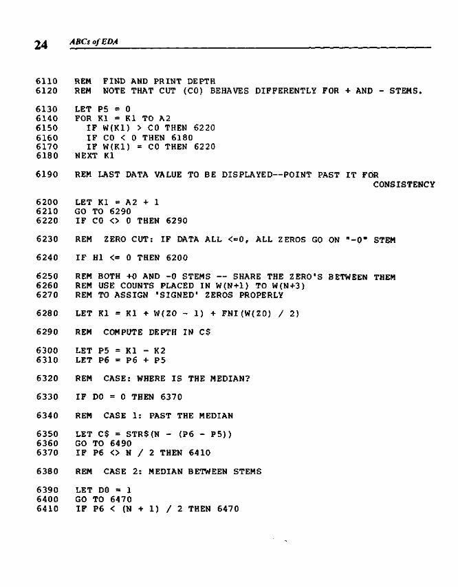
6110 REM FIND AND PRINT DEPTH6120 REM NOTE THAT CUT (CO) BEHAVES DIFFERENTLY FOR + AND - STEMS.
6130 LET P5 = 06140 FOR Kl = Kl TO A26150 IF W(K1) > CO THEN 62206160 IF CO < 0 THEN 61806170 IF W(K1) = CO THEN 62206180 NEXT Kl
6 1 9 0 REM LAST DATA VALUE TO BE DISPLAYED—POINT PAST IT FORCONSISTENCY
6200 LET Kl = A2 + 16210 GO TO 62906220 IF CO <> 0 THEN 6290
6230 REM ZERO CUT: IF DATA ALL <=0, ALL ZEROS GO ON "-0" STEM
6240 IF HI <= 0 THEN 6200
6250 REM BOTH +0 AND -0 STEMS — SHARE THE ZERO'S BETWEEN THEM6260 REM USE COUNTS PLACED IN W(N+1) TO W(N+3)6270 REM TO ASSIGN 'SIGNED' ZEROS PROPERLY
6280 LET Kl = Kl + W(Z0 - 1) + FNI(W(Z0) / 2)
6290 REM COMPUTE DEPTH IN C$
6300 LET P5 = Kl - K2
6310 LET P6 - P6 + P5
6320 REM CASE: WHERE IS THE MEDIAN?
6330 IF DO = 0 THEN 6370
6340 REM CASE 1: PAST THE MEDIAN
6350 LET C$ = STR$ (N - (P6 - P5))6360 GO TO 6490
6370 IF P6 <> N / 2 THEN 6410
6380 REM CASE 2: MEDIAN BETWEEN STEMS
6390 LET DO = 16400 GO TO 64706410 IF P6 < (N + 1) / 2 THEN 6470
BASIC 25
6420 REM CASE 3: MEDIAN ON THIS LINE
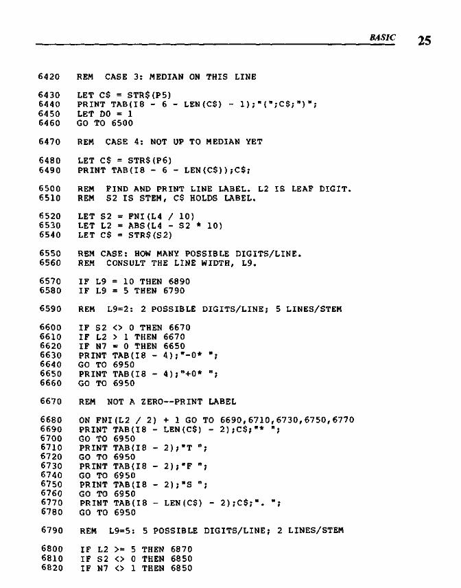
6430 LET C$ = STR$(P5)6440 PRINT TAB(18 - 6 - LEN(C$) - 1);" ( ";C$;")";6450 LET DO = 16460 GO TO 6500
6470 REM CASE 4: NOT UP TO MEDIAN YET
6480 LET C$ = STR$(P6)6490 PRINT TAB(I8 - 6 - LEN(C$));C$;
6500 REM FIND AND PRINT LINE LABEL. L2 IS LEAP DIGIT.6510 REM S2 IS STEM, C$ HOLDS LABEL.
6520 LET S2 = FNI(L4 / 10)6530 LET L2 = ABS(L4 - S2 * 10)6540 LET C$ = STR$(S2)
6550 REM CASE: HOW MANY POSSIBLE DIGITS/LINE.6560 REM CONSULT THE LINE WIDTH, L9.
6570 IF L9 = 10 THEN 6890
6580 IF L9 = 5 THEN 6790
6590 REM L9=2: 2 POSSIBLE DIGITS/LINE; 5 LINES/STEM
6600 IF S2 <> 0 THEN 66706610 IF L2 > 1 THEN 66706620 IF N7 = 0 THEN 66506630 PRINT TAB(18 - 4);"-0* ";6640 GO TO 69506650 PRINT TAB(18 - 4);"+0* ";6660 GO TO 69506670 REM NOT A ZERO—PRINT LABEL
6680 ON FNI(L2 / 2) + 1 GO TO 6690,6710,6730,6750,67706690 PRINT TAB(I8 - LEN(C$) - 2);C$;"* ";6700 GO TO 69506710 PRINT TAB(18 - 2);"T w;6720 GO TO 69506730 PRINT TAB(18 - 2);"F ";6740 GO TO 69506750 PRINT TAB(18 - 2);"S " ;6760 GO TO 69506770 PRINT TAB(18 - LEN(C$) - 2);C$;". M;6780 GO TO 6950
6790 REM L9=5: 5 POSSIBLE DIGITS/LINE; 2 LINES/STEM
6800 IF L2 >= 5 THEN 68706810 IF S2 <> 0 THEN 68506820 IF N7 <> 1 THEN 6850
ABCs of EDA
6830 REM "-0*" LINE — PRINT THE "-n
6840 PRINT TAB(18 - 3);"-",•6850 PRINT TAB(I8 - LEN(C$) - 1);C$;"* ";6860 GO TO 69506870 PRINT TAB(18 - 1);". ";6880 GO TO 6950
6890 REM L9=10: 10 POSSIBLE DIGITS/LINE; 1 LINE/STEM
6900 IF S2 <> 0 THEN 69406910 IF N7 <> 1 THEN 69406920 PRINT TAB(18 - 3);"-0 ";6930 GO TO 69506940 PRINT TAB(I8 - LEN(C$) - l)?C$;n ";
6950 REM FROM K2 TO Kl, FIND LEAVES AND PRINT THEM. D = LEAF,
6960 IF K2 = Kl THEN 70706970 LET D = ABS(W(K2) - FNI(W(K2) / 10) * 10)6980 PRINT STR$(D);6990 LET II = II + 17000 IF II < 19 - 1 THEN 70407010 PRINT "*";7020 LET K2 = Kl7030 GO TO 70507040 LET K2 = K2 + 17050 IF K2 > N THEN 71707060 IF K2 < Kl THEN 6970
7070 REM END LINE
7080 PRINT
7090 NEXT Jl
7100 REM PRINT HIGH VALUES BEYOND ADJACENT VALUE
7110 IF Kl > N THEN 71707120 PRINT7130 PRINT TAB(I8 - 4);"HI:7140 FOR I = Kl TO N7150 PRINT STR$(W(I));",7160 NEXT I7170 PRINT7180 RETURN
FORTRAN Programs
SUBROUTINE STMNLF(Y, N« SORTY, IW, XTREMS, ERR)C
INTEGER N, IW(N) , ERRREAL Y(N), SORTY(N)LOGICAL XTPEMS
CC PRODUCE A STEM-AND-LEAF DISPLAY CF THE DATA IN Y ( )CC IW( ) IS AN INTEGER WORK ARRAY. SORTYO IS A PEAL WORK ARPAYC XTREMS IS A LOGICAL FLAG, .TRUE. IF SCALING TO EXTREMES.C (OTHERWISEt SCALES TO FENCES).CC COMMON BLOCKS AND VARIABLES FOR OUTPUTC
COMMON/CHRBUF/P, PMAX, PMIN, OUTPTR, MAXPTR, OUNITINTEGER P ( 1 3 0 ) , PMAX, PMIN, OUTPTP, MAXPTR, OUNITCOMMON/NUMBRS/EPSI, MAX INTREAL EPSI , MAXINT
CC FUNCTIONSC
INTEGER INTFN, FLOORCC CALLS SUBROUTINES DEPTHP, NPOSW, OUTLYP, PRINT, PUTCHR, PUTNUM,C SLTITLt STEMP, YINFOCC LOCAL VARIABLESC
REAL MED, HL , HH, ADJL, ADJH, STEP, UNIT, FRACT, NICN0SC4), NPWINTEGER I, SLBRK, PLTWID, RANK, IADJL, IADJH, NLINSINTEGER NLMAX, LINWIDINTEGER LOW, HI, CUT, STEM, PT1, PT2, J, SPACNT, LEAF, NN, CHSTARLOGICAL NEGNOW, MEOYET
CC DATA DEFINITIONS: A USEFUL CHARACTER AND THE SCALING OPTIONSC
DATA CHSTAR/41/D A T A N I C N O S ( l ) , N I C N O S ( 2 ) , N I C N O S O ) , N I C N O S t 4 ) / l . O , 2 . 0 , 5 . 0 , 1 0 . 0 /DATA NN/4/
CC
IF(N . G E . 2 ) GO TO 5ERR = 11GO TO 999
CC SETUP — FIND WIDTH OF PLOTTING REGION, STEM-LEAF BREAK POSITION, ETCC
5 SLBRK = PMIN + 11PLTWID = PMAX - SLBPK - 2IF(PLTWID . G T . 5 ) GO TO 10ERR = 13GO TO 999
27
2© ABCs of EDA
CC FIND THE BEST SCALE FCR THE PLOTCC SORT Y IN SORTY AND GET SUMMARY INFORMATIONC
10 DO 20 I = 1 , NSORTY(I) = Y d )
20 CONTINUECALL YINFO(SOPTY,N,MED,HL,HH,ADJL,ADJH,IADJL,IADJH,STEP,EPR)IF(ERR . N E . 0 ) GO TO 999
CC FIND NICE LINE WIDTH FOR PLOTCC IF ADJACENT VALUES EQUAL OR USEP DEMANDS I T , FAKE THE ADJACENTC VALUES TO BE THE EXTREMESC
IFUADJH .GT. ADJL) .AND. .NOT. XTPEMS) GO TO 25IADJL = 1IADJH = NADJL = Y( IADJL)ADJH - Y(IADJH)
25 NLMAX = INTFNU0.0*AL0G10(FLCAT< IADJH - IADJL + 1 ) ) , EPR)IF(ADJH . G T . ADJL) GO TO 27
CC EVEN I F ALL VALUES AFE EQUAL WE CAN PRODUCE A DISPLAYC
ADJH = ADJL + 1.0NLMAX = 1
27 CALL NPOSWiADJH, ADJL, NICNOS, NN, NLMAX, .TRUE. , NLINS, FRACT,1 UNIT, NPW, ERR)
IF(EPR .NE . 0 ) GO TO 999CC RESCALE EVERYTHING ACCORDING TO UNIT. HEREAFTER EVERYTHING ISC INTEGER, AND DATA ARE OF THE FORM SS...SLC.)C NOTE THAT INTFN PERFORMS EPSILON ADJUSTMENTS FOR CORRECT ROUNDING,C AND CHECKS THAT THE REAL NUMBER IS NOT TOO LARGE FCR AN INTEGERC VARIABLE.C
DO 30 I = 1, NIW( I ) - INTFN(SORTY(I)/UNIT, ERR)
30 CONTINUEIFCERR .NE. 0) GO TO 999
CIF (FRACT .EQ. 10.0) GO TO 40
CC IF ALL LEAVES ARE ZERO, WE SHOULD BE IN ONE-LINE-PER-STEM FORMATC
DO 35 I = IADJL, IADJHIF (MOD(IWd), 10) .NE. 0) GO TO 40
35 CONTINUE
FORTRAN
FRACT = 1 0 , 0NPW = FRACT * UNITNLINS = INTFN(ADJH/NPW, ERR) - INTFN(ADJL/NPW, ERR) + 1IF(ADJH * ADJL . L T . 0 . 0 .OR. ADJH .EQ. 0 . 0 ) NLINS = NLINS+1
40 LOW = IW(IADJL)HI = IW(IAOJH)
CC LINEWIDTH NOW IS NICEWIDTH/UNIT = FRACTC
LINWID = INTFN(FRACT, ERR)C
CALL SLT ITL(UNIT , ERR)IFIERR . N E . 0 ) GO TO 999
CC PRINT VALUES BELOW LOW ADJACENT VALUE ON "LO" STEMC
RANK = IADJL - 1IFdADJL .EQ. 1) GO TO 50CALL OUTLYPdW, N, 1, RANK, .FALSE., SLBRK, ERR)IF(ERR .NE. 0) GO TO 999
CC INITIALIZE FOR MAIN PART OF DISPLAY.C INITIAL SETTINGS ARE TO LINE BEFORE FIRST ONE PRINTEDC
50 CUT = FLOOR!(1.0 + EPSI)*FLOAT(LOW)/FLOAT(LINWID)) * LINWIDNEGNOW = .TRUE.STEM = CUTIFCLOW .LT. 0) GO TO 60
CC FIRST STEM POSITIVEC
NEGNOW - .FALSE.STEM = CUT - LINWID
60 MEDYET = .FALSE.CC TWO POINTERS ARE USED. PT1 COUNTS FIDST FOR DEPTHS, PT2 FOLLOWSC FOR LEAF PRINTING. BOTH ARE INITIALIZED ONE POINT EARLY.C
PT1 = IADJLPT2 = PT1
CC MAIN LOOP. FOR EACH LINEC
DO 120 J = 1, NLINSC VARIABLE USES:C CUT = FIRST NUMBER ON NEXT LINE OF POSITIVE STEMSt BUTC = LAST NUMBER ON CURRENT LINE OF NEGATIVE STEMSC STEM = INNER (NEAR ZEFO) EDGE OF CURRENT LINEC SPACNT COUNTS SPACES USED ON THIS LINE
29
in ABCsofEDA
CC STEP TO NEXT LINE
CUT = CUT + LINWIOCC IF(STEM = 0 AND NEGNOW) NEGNOW = .F. ELSE STEM = STEM + LINWIDC
IFCSTEM .NE. 0 .OR- .NOT. NEGNOW ) GO TO 70NEGNOW - .FALSE.GO TO 80
70 STEM = STEM + LINWIDCC NEWLINE — INITIALIZE COUNT OF SPACES USEDC
80 SPACNT = 0CC FIND AND PRINT DEPTHC
CALL DEPTHP(SORTY, IW, N, PT1, PT2, CUT, IADJH, HI, RANK,1 MEDYET, SLBP.K, ERR)IF(ERR .NE. 0) GO TO 999
CC PRINT STEM LABELC
CALL STEMPtSTEM, LINWID, NEGNOW, SLBRK, ERR)IF(ERR .NE. 0) GO TO 999
CC FIND AND PRINT LEAVESC
IF (PT1 . E Q . PT2J GO TO 11090 LEAF = IABSUWCPT2) - { STEM/10) *10 )
CALL PUTNUMtO, LEAF, 1 , ERP)SPACNT = SPACNT + 1IF(SPACNT . L T . PLTWID) GO TO 100
CC L INE OVERFLOWS PAST RIGHT EDGE. MARK WITH *C
CALL PUTCHRCO, CHSTAP, EPR)IF(ERR . N E . 0 ) GO TO 999PT2 = PT1GO TO 110
100 PT2 = PT2 + 1IF (PT2 . L T . PT1J GO TO 90
CC END LINEC
110 CALL PRINTCC CONTINUE LOOP UNTIL WE RUN OUT OF NUMBERS TO PLOTC
120 CONTINUE
FORTRAN 31
cC PRINT VALUES ABOVE HI ADJACENT VALUE ON "HI" STEMC
IF(PT1 .GT. N) GO TO 990CALL OUTLYPUW, N, PT1 , N, .TRUE. , SLBRK, ERR)
990 WRITECOUNIT, 5990)5990 FORMAT(IX)
999 RETURNEND
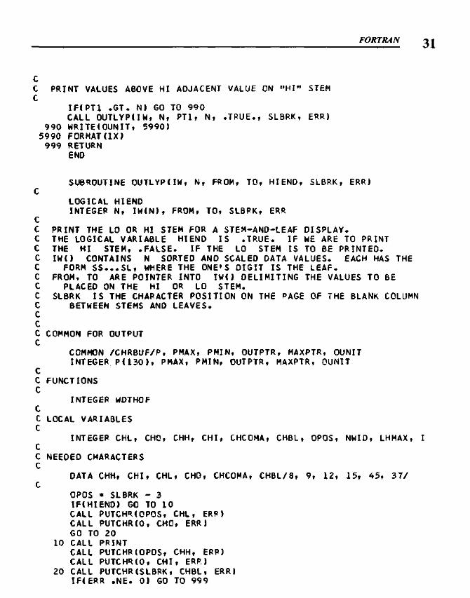
SUBROUTINE OUTLYPUW, N, FROM, TO, HIEND, SLBRK, ERR)C
LOGICAL HIENDINTEGER N, I W ( N ) , FROM, TO, SLBPK, ERR
CC PRINT THE LO OR HI STEM FOR A STEM-AND-LEAF DISPLAY.C THE LOGICAL VARIABLE HIEND I S .TRUE. IF WE ARE TO PRINTC THE HI STEM, .FALSE. IF THE LO STEM IS TO BE PRINTED.C IWO CONTAINS N SORTED AND SCALED DATA VALUES. EACH HAS THEC FORM S S . . . S L , WHERE THE ONE'S DIGIT IS THE LEAF.C FROM, TO ARE POINTER INTO IWO DELIMITING THE VALUES TO BEC PLACED ON THE HI OR LO STEM.C SLBRK IS THE CHARACTER POSITION ON THE PAGE OF THE BLANK COLUMNC BETWEEN STEMS AND LEAVES.CCC COMMON FOR OUTPUTC
COMMON /CHRBUF/P, PMAX, PMIN, OUTPTR, MAXPTR, OUNITINTEGER P ( 1 3 0 ) , PMAX, PMIN, OUTPTR, MAXPTR, OUNIT
CC FUNCTIONSC
INTEGER WDTHOFCC LOCAL VARIABLESC
INTEGER CHL, CHO, CHH, CHI, CHCOMA, CHBL, OPOS, NWID, LHMAX, ICC NEEDED CHARACTERSC
DATA CHH, CHI, CHL, CHO, CHCOMA, CHBL/8, 9, 12, 15, 45, 37/C
OPOS - SLBRK - 3IF(HIEND) GO TO 10CALL PUTCHR(OPOS, CHL, ERR)CALL PUTCHRCO, CHO, ERR)GO TO 20
10 CALL PRINTCALL PUTCHP(OP0S, CHH, ERP)CALL PUTCHRiO, C H I , ERR)
20 CALL PUTCHR(SLBRK, CHBL, ERR)IFiERR . N E . 0 ) GO TO 999
ABCs of EDA
NWID = MAXO( WDTHOF(IW(FROM)), WDTHOF(IW(TO)) )LHMAX = PMAX - NWID - 200 40 I = FROM, TO
CALL PUTNUM(O, IW(I), NWID, ERR)CALL PUTCHRCO, CHCOMA, ERR)CALL PUTCHR(O, CHBL, ERR)IF(OUTPTR .LT. LHMAX) GO TO 30CALL PRINTCALL PUTCHR(SLBRK, CHBL, EPR)
30 IF(ERR .NE. 0) GO TO 99940 CONTINUE
CC BUT DONT PRINT THE FINAL COMMAC
OPOS = MAXPTR - 1CALL PUTCHRCCPOS, CHBL, ERR)CALL PRINTIFC.NOT. HIEND) CALL PRINT
999 RETURNEND
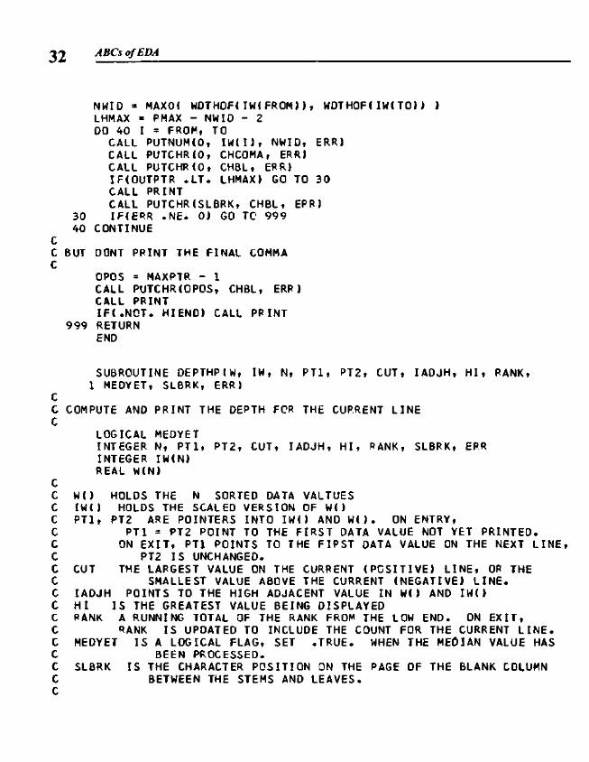
SUBROUTINE DEPTHPIW, IW, N, PT1, PT2, CUT, IADJH, HI, RANK,1 MEDYET, SLBRK, ERR)
CC COMPUTE AND PRINT THE DEPTH FCR THE CURRENT LINEC
LOGICAL MEDYETINTEGER N, PT1, PT2, CUT, IADJH, HI, RANK, SLBRK, ERRINTEGER IW(N)REAL W(N)
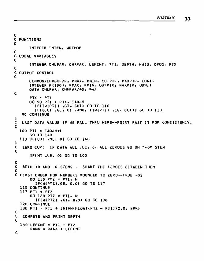
CC W O HOLDS THE N SORTED DATA VALTUESC IWO HOLDS THE SCALED VERSION OF W OC PT1, PT2 ARE POINTERS INTO IWO AND W O . ON ENTRY,C PT1 = PT2 POINT TO THE FIRST DATA VALUE NOT YET PRINTED.C ON EXIT, PT1 POINTS TO THE FIRST DATA VALUE ON THE NEXT LINE,C PT2 IS UNCHANGED.C CUT THE LARGEST VALUE ON THE CURRENT (POSITIVE) LINE, OP THEC SMALLEST VALUE ABOVE THE CURRENT (NEGATIVE) LINE.C IADJH POINTS TO THE HIGH ADJACENT VALUE IN W O AND IWOC HI IS THE GREATEST VALUE BEING DISPLAYEDC RANK A RUNNING TOTAL OF THE RANK FROM THE LOW END. ON EXIT,C RANK IS UPDATED TO INCLUDE THE COUNT FOR THE CURRENT LINE.C MEDYET IS A LOGICAL FLAG, SET .TRUE. WHEN THE MEDIAN VALUE HASC BEEN PROCESSED.C SLBRK IS THE CHARACTER POSITION ON THE PAGE OF THE BLANK COLUMNC BETWEEN THE STEMS AND LEAVES.C
FORTRAN
CC FUNCTIONSC
INTEGER INTFNt WDTHOFCC LOCAL VARIABLESC
INTEGER CHLPAR, CHRPAR, LEFCNT, PTZ, DEPTH, NWID, OPOSt PTXCC OUTPUT CONTROLC
COMMON/CHRBUF/Pf PMAX, PMIN, OUTPTR, MAXPTR, OUNITINTEGER P(130), PMAX, PMIN, OUTPTR, MAXPTR, OUNITDATA CHLPAR, CHRPAR/43, 44/
CPTX = PT1DO 90 PT1 = PTX, IADJH
IFdW(PTl) .GT. CUT) GO TO 110IFUCUT .GE. 0) .AND. (IW(PTl) .EQ. CUT)) GO TO 110
90 CONTINUECC LAST DATA VALUE IF WE FALL THRU HERE—POINT PAST IT FOR CONSISTENCY,C
100 PT1 = IADJH+1GO TO 140
110 IFCCUT .NE. 0) GO TO 140CC ZERO CUT: IF DATA ALL .LE. 0, ALL ZEROES GO ON "-0" STEMC
IF1HI .LE. 0) GO TO 100
CC BOTH +0 AND -0 STEMS — SHARE THE ZEROES BETWEEN THEMCC FIRST CHECK FOR NUMBERS ROUNDED TO ZERO—TRUE -OS
DO 115 PTZ = PT1, NIF(W(PTZ).GE. 0.0) GO TO 117
115 CONTINUE117 PT1 = PTZ
DO 120 PTZ = PT1, NIF(W(PTZ) .GT. 0.0) GO TO 130
120 CONTINUE130 PT1 = PT1 + INTFN(FLOAT(PTZ - P T D / 2 . 0 , ERR)
CC COMPUTE AND PRINT DEPTHC
140 LEFCNT = PT1 - PT2RANK = RANK + LEFCNT
C
ABCsofEDA
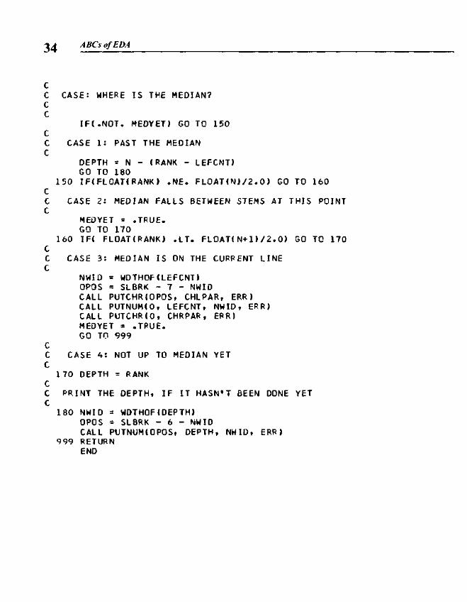
CC CASE: WHERE IS THE MEDIAN?CC
IFC.NOT. MEDYET) GO TO 150CC CASE 1: PAST THE MEDIANC
DEPTH = N - (RANK - LEFCNT)GO TO 180
150 IF(FLOATCFANK) . N E . F L O A T ( N ) / 2 . 0 ) GO TO 160CC CASE 2 : MEDIAN FALLS BETWEEN STEMS AT THIS POINTC
MEDYET = .TRUE.GO TO 170
160 IF( FLOAT(RANK) . L T . FLOAT<N+1) /2 .0 ) GO TO 170CC CASE 3 : MEDIAN IS ON THE CURRENT LINEC
NWID = WDTHOF(LEFCNT)OPOS = SLBRK - 7 - NWIDCALL PUTCHR(OPOS, CHLPAR, ERR)CALL PUTNUM(O, LEFCNT, NWID, ERR)CALL PUTCHR(O, CHRPAR, ERR)MEDYET = .TRUE.GO TO 999
CC CASE V. NOT UP TO MEDIAN YETC
170 DEPTH = RANKCC PRINT THE DEPTH, IF IT HASN'T BEEN DONE YETC
180 NWID = WDTHOF(DEPTH)OPOS = SLBRK - 6 - NWIDCALL PUTNUM(OPOS, DEPTH, NWID, ERR)
999 RETURNEND
FORTRAN
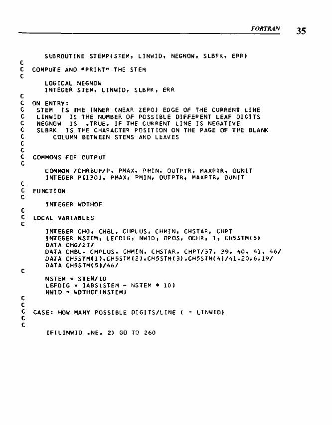
SUBROUTINE STEMP(STEM, L INWID, NEGNOW, SLBPK, ERPJCC COMPUTE AND "PRINT" THE STEMC
LOGICAL NEGNOWINTEGER STEM, LINWID, SLBRK, ERR
CC ON ENTRY:C STEM IS THE INNER (NEAR ZERO) EDGE OF THE CURRENT LINEC LINWID IS THE NUMBER OF POSSIBLE DIFFERENT LEAF DIGITSC NEGNOW IS .TRUE. IF THE CURRENT LINE IS NEGATIVEC SLBRK IS THE CHARACTER POSITION ON THE PAGE OF THE BLANKC COLUMN BETWEEN STEMS AND LEAVESC
cC COMMONS FOP OUTPUTC
COMMON /CHRBUF/P, PMAX, PMIN, OUTPTR, MAXPTR, OUNITINTEGER P U 3 0 ) , PMAX, PMIN, OUTPTR, MAXPTR, OUNIT
CC FUNCTIONC
INTEGER WDTHOFCC LOCAL VARIABLESC
INTEGER CHO, CHBL, CHPLUS, CHMIN, CHSTAP, CHPTINTEGER NSTEM, LEFDIG, NWID, OPOS, OCHR, I, CH5STM(5)DATA CHO/27/DATA CHBL, CHPLUS, CHMIN, CHSTAR, CHPT/37, 39, 40, 41, 46/DATA CH5STM(1),CH5STM(2),CH5STM(3),CH5STM(4)/41,20,6,19/DATA CH5STM(5)/46/
CNSTEM = STEM/10LEFDIG = IABS(STEM - NSTEM * 10)NWID = WDTHOF(NSTEM)
CCC CASE: HOW MANY POSSIBLE DIGITS/LINE ( = LINWID)Cc
IFCLINWID .NE. 2) GO TO 260
35
ABCs of EDA
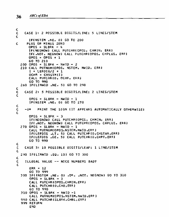
CC CASE l : 2 POSSIBLE DIGITS/LINE; 5 LINES/STEMC
IFCNSTEM .NE. 0) GO TO 200C PLUS OR MINUS ZERO
OPOS = SLBRK - 4IF(NEGNOW) CALL PUTCHR(OPOS, CHMIN, ERR)IF( .NOT. NEGNOW) CALL PUTCHR(OPOS, CHPLUS, ERP)OPOS = OPOS + 1GO TO 2 1 0
2 00 OPOS - SLBPK - NWID - 2210 CALL PUTNUMCOPOS, NSTEM, NWID, ERR)
I = LEFDIG/2 + 1OCHR = CH5STMU)CALL PUTCHRCOt OCHP, ERR)GO TO 990
260 IF(LINWID . N E . 5) GO TO 290CC CASE 2 : 5 POSSIBLE D IG ITS /L INE ; 2 LINES/STEMC
OPOS = SLBRK - NWID - 1IF(NSTEM .NE. 0) GO TO 270
CC - 0 * PRINT THE SIGN ( I T APPEARS AUTOMATICALLY OTHERWISE)C
OPOS = SLBPK - 3IF(NEGNOW) CALL PUTCHRCOPCS, CHMIN, ERR)IF( .NOT. NEGNOW) CALL PUTCHRfOPOS, CHPLUS, EPR)
270 OPOS = SLBRK - NWID - 1CALL PUTNUM(OPOS,NSTEM,NWID,ERD)IFCLEFDIG . L T . 5) CALL PUTCHP(0,CHSTAR,ERR)IFCLEFDIG .GE . 5) CALL PUTCHR(0,CHPT,ERR)GO TO 990
CC CASE 3: 10 POSSIBLE DIGITS/LEAF; 1 LINE/STEMC
290 IF(LINWID .EQ. 10) GO TO 300CC ILLEGAL VALUE — NICE NUMBERS BAD?C
ERR = 12GO TO 999
300 IF((NSTEM .NE. 0) .OR. .NOT. NEGNOW) GO TO 310OPOS = SLBRK - 3CALL PUTCHR(OPOS,CHMIN,ERR)CALL PUTCHR(O,CHO,ERR)GO TO 990
310 OPOS = SLBPK - NWID - 1CALL PUTNUMCOPOS,NSTEM,NWID,EPP)
990 CALL PUTCHR(SLBRK,CHBL,ERR)999 RETURN
END
FORTRAN 37
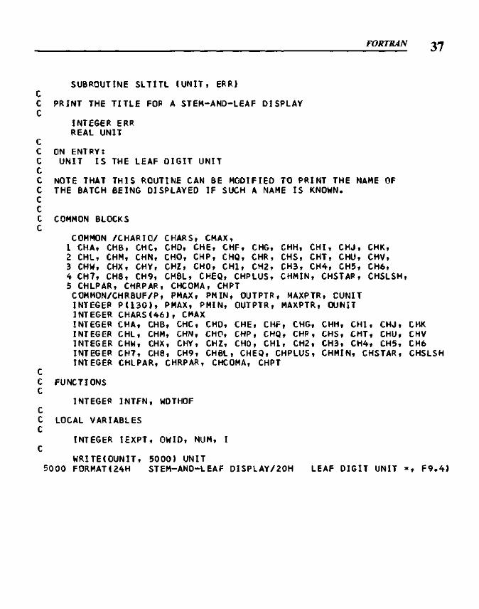
SUBROUTINE SLTITL ( U N I T , ERR)
PRINT THE TITLE FOP A STEM-AND-LEAF DISPLAY
INTEGER ERRREAL UNIT
ON ENTRY:UNIT IS THE LEAF DIGIT UNIT
NOTE THAT THIS ROUTINE CAN BE MODIFIED TO PRINT THE NAME OFTHE BATCH BEING DISPLAYED IF SUCH A NAME IS KNOWN.
COMMON BLOCKS
COMMON /CHARIC/ CHARS, CMAX,1 CHA, CHB, CHC, CHD, CHE, CHF, CHG, CHH, C H I , CHJ, CHK,2 CHL, CHM, CHN, CHO, CHP, CHQ, CHR, CHS, CHT, CHU, CHV,3 CHW, CHX, CHY, CHZ, CHO, C H I , CH2, CH3, CH4, CH5, CH6,4 CH7, CH8, CH9, CHBL, CHEQ, CHPLUS, CHMIN, CHSTAP, CHSLSH,5 CHLPAR, CHRPAR, CHCOMA, CHPTCOMMON/CHRBUF/P, PMAX, PMIN, OUTPTR, MAXPTR, CUNITINTEGER P(130), PMAX, PMIN, OUTPTR, MAXPTR, OUNITINTEGER CHARS(46), CMAXINTEGER CHA, CHB, CHC, CHD, CHE, CHF, CHG, CHH, CHI, CHJ, CHKINTEGER CHL, CHM, CHN, CHO, CHP, CHQ, CHP, CHS, CHT, CHU, CHVINTEGER CHW, CHX, CHY, CHZ, CHO, CHI, CH2, CH3, CH4, CH5, CH6INTEGER CH7, CH8, CH9, CHBL, CHEQ, CHPLUS, CHMIN, CHSTAR, CHSLSHINTEGER CHLPAR, CHRPAR, CHCOMA, CHPT
FUNCTIONS
INTEGER INTFN, WDTHOF
LOCAL VARIABLES
INTEGER IEXPT, OWID, NUM, I
WRITE(OUNIT, 5000) UNIT5000 F0RMAT(24H STEM-AND-LEAF DISPLAY/20H LEAF DIGIT UNIT =, F9.4)
38
ccc
ccc
ABCs of EDA
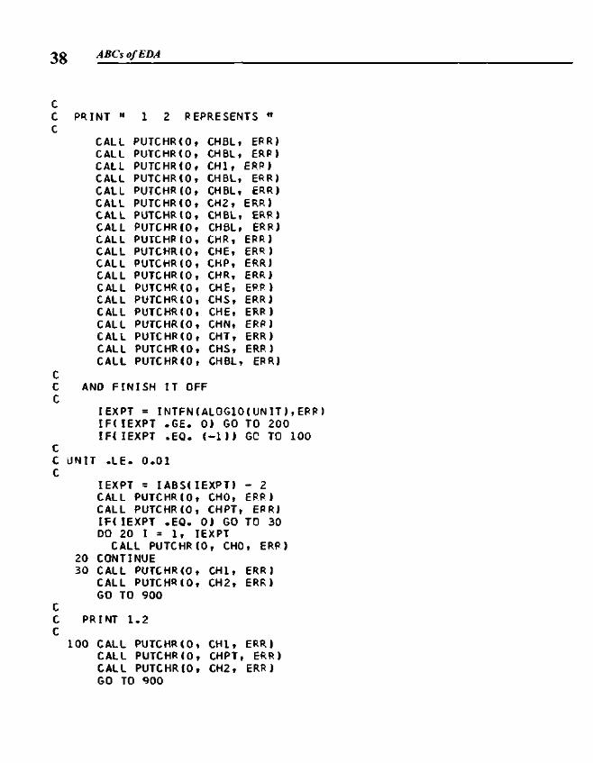
PRINT "
CALLCALLCALLCALLCALLCALLCALLCALLCALLCALLCALLCALLCALLCALLCALLCALLCALLCALLCALL
1 2 REPRESENTS "
PUTCHRCO,PUTCHR(OtPUTCHRCO,PUTCHRCO,PUTCHRCO,PUTCHRCO,PUTCHR(0,PUTCHRCO,PUTCHP(O,PUTCHRiO,PUTCHR(O,PUTCHR(O,PUTCHRCO,PUTCHRCO,PUTCHRCO,PUTCHRCO,PUTCHRCO,PUTCHRCO,PUTCHRCO,
AND FINISH IT OFF
CHBL,CHBL,C H I ,CHBL,CHBL,CH2,CHBL,CHBL,CHR,CHE,CHP,CHR,CHE,CHS,CHE,CHN,CHT,CHS,CHBL,
ERR)ERP)
ERP)ERR)ERR)
ERR)ERR)ERR)
ERR)ERR)ERR)ERR)ERP )ERR)ERR)ERP)ERR)ERR)
ERR)
IEXPT = INTFNCALOG1OCUNIT),ERP)IFCIEXPT .GE. 0 ) GO TO 200IFC IEXPT .EQ. ( - 1 ) ) GC TO 100
UNIT . L E . 0 . 0 1
IEXPT = IABSCIEXPT) - 2CALL PUTCHRCO, CHO, ERR)CALL PUTCHRCO, CHPT, ERR)IFC IEXPT .EQ. 0 ) GO TO 30DO 20 I = 1 , IEXPT
CALL PUTCHRCO, CHO, ERP)20 CONTINUE30 CALL PUTCHRCO, CHI , ERR)
CALL PUTCHRCO, CH2, ERR)GO TO 900
PRINT 1.2
100 CALL PUTCHRCO,CALL PUTCHRCO,CALL PUTCHRCO,GO TO 900
C H I , ERR)CHPT, ERR)CH2, ERR)
FORTRAN 39
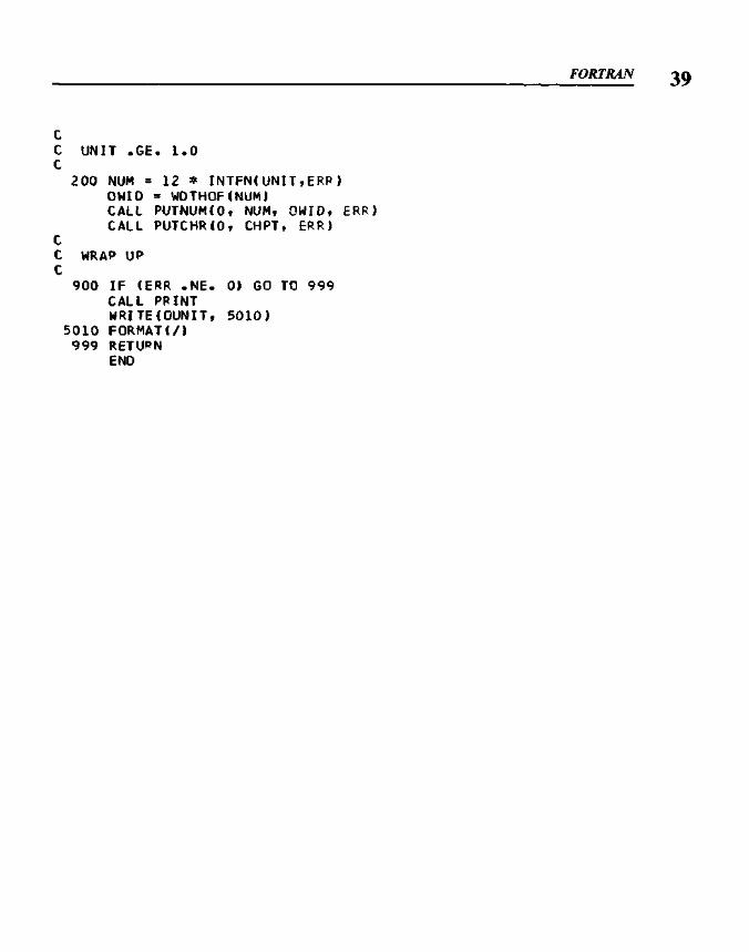
cC UNIT .GE . 1 .0C
200 NUM = 12 * INTFNiUNIT,ERR)OWID = WDTHOF(NUM)CALL PUTNUM(Ot NUM, OWID, ERR)CALL PUTCHRtO, CHPT, ERR)
CC WRAP UPC
900 IF (ERR .NE. 0) GO TO 999CALL PRINTWRITECOUNIT, 5010)
5010 FORMAT!/)999 RETURN
END

Chapter 1Letter-Value Displays
It is often convenient to summarize a data batch after we have taken an initiallook at it and have seen each individual data item. For example, we can use acentral value to summarize the size or general level of the numbers in thebatch. We also want to describe how spread out or variable the numbers in thebatch are, and we might look for ways to describe more precisely the shapesand patterns we can see in the outline of a stem-and-leaf display. As always,when we explore data, we must be alert for extraordinary values that mightrequire special attention. Letter values provide information for several of thesesummaries, and the letter-value display presents the letter values in a conve-nient form.
2.1 Median, Hinges, and Other Summary Values
Before we determine the letter values, we must first order the data batch fromlowest value to highest. When we analyze data by hand, a stem-and-leafdisplay provides a quick, crude ordering of the batch. Computers can order the
41
ABCs of EDA
data with special sorting programs (see Section 2.9). When a data batch isordered, a set of suitably selected data values and simple averages of thesevalues can convey many important features of the batch concisely. The lettervalues are just such a set of values.
One of the most important characteristics of a data value in an orderedbatch is how far it is from the low or high end of the batch. We therefore
depth define the depth of each data value. This is just the value's position in anenumeration of values that starts at the nearer end of the batch. (Recall fromChapter 1 that depths appear in a column at the left of a finished stem-and-leaf display.) Each extreme value is the first value in the enumeration andtherefore has a depth of 1; the second largest and second smallest values eachhave a depth of 2; and so on. In general, in a batch of size n, two data valueshave depth i: the ith and the (« + 1 — /)th. Conversely, the depth of the ithdata value in an ordered batch is the smaller of / and n + \ — i because depthis measured from the nearer end. We find letter values at certain selecteddepths.
If n is odd, there is a "deepest' data value—one as far from either endof the ordered batch as possible, and thus not part of a pair of equal-depth
median numbers. This data value is the median, and it marks the middle of thebatch—in the sense that exactly half the remaining n - 1 numbers in thebatch are less than or equal to it, and exactly half are greater than or equal toit.
It is easy to calculate the depth of the median. It is simply (n + l ) /2 .Because the depth of the ith data value in an ordered batch of n values is thesmaller of / and n + 1 — /, the maximum depth occurs where i = n + 1 — /, or,equivalently, 2/ = n + 1. Thus
depth of median = (n + l ) /2 ,
which we abbreviate d(M) = (n + l ) /2 . For example, if we have 3 data valuesin order, the median is the second value because one value is less than themedian and one is greater. If we have a batch of 5 values, the median has 2values below it and 2 values above it, so that it is the third largest value or thethird smallest value, depending on whether we count from the top or from thebottom.
But, what if a batch has an even count? We then have two "middle"values. If these two values are different—as they usually are—no one datavalue divides the batch in half. Then, d{M) = (n + l ) /2 will have a fractionalpart equal to % and this depth points between the two middle data values.Because half the data values lie below the median and half lie above it, weadopt the usual convention of averaging the middle two data values, each ofwhich has depth (n + l ) /2 - % We label the median with the letter M.
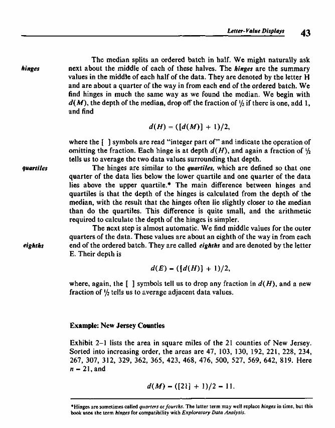
Letter- Value Displays 43
hinges
quartiles
eighths
The median splits an ordered batch in half. We might naturally asknext about the middle of each of these halves. The hinges are the summaryvalues in the middle of each half of the data. They are denoted by the letter Hand are about a quarter of the way in from each end of the ordered batch. Wefind hinges in much the same way as we found the median. We begin withd(M), the depth of the median, drop off the fraction of x/i if there is one, add 1,and find
where the [ ] symbols are read "integer part of" and indicate the operation ofomitting the fraction. Each hinge is at depth d(H), and again a fraction of x/itells us to average the two data values surrounding that depth.
The hinges are similar to the quartiles, which are defined so that onequarter of the data lies below the lower quartile and one quarter of the datalies above the upper quartile.* The main difference between hinges andquartiles is that the depth of the hinges is calculated from the depth of themedian, with the result that the hinges often lie slightly closer to the medianthan do the quartiles. This difference is quite small, and the arithmeticrequired to calculate the depth of the hinges is simpler.
The next step is almost automatic. We find middle values for the outerquarters of the data. These values are about an eighth of the way in from eachend of the ordered batch. They are called eighths and are denoted by the letterE. Their depth is
where, again, the [ ] symbols tell us to drop any fraction in d(H), and a newfraction of x/i tells us to average adjacent data values.
Example: New Jersey Counties
Exhibit 2-1 lists the area in square miles of the 21 counties of New Jersey.Sorted into increasing order, the areas are 47, 103, 130, 192, 221, 228, 234,267, 307, 312, 329, 362, 365, 423, 468, 476, 500, 527, 569, 642, 819. Heren = 21, and
d{M) = ([21] = 11.
* Hinges are sometimes called quarters or fourths. The latter term may well replace hinges in time, but thisbook uses the term hinges for compatibility with Exploratory Data Analysis.
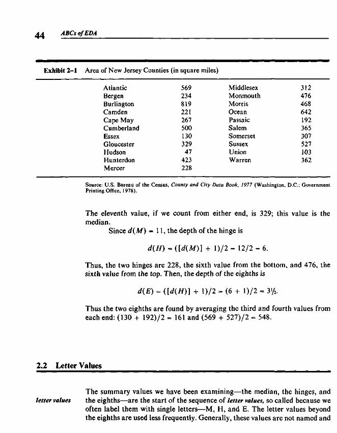
A A ABCs of EDA
Exhibit 2-1 Area of New Jersey Counties (in square miles)
AtlanticBergenBurlingtonCamdenCape MayCumberlandEssexGloucesterHudsonHunterdonMercer
56923481922126750013032947
423228
MiddlesexMonmouthMorrisOceanPassaicSalemSomersetSussexUnionWarren
312476468642192365307527103362
Source: U.S. Bureau of the Census, County and City Data Book, 1977 (Washington, D.C.: GovernmentPrinting Office, 1978).
The eleventh value, if we count from either end, is 329; this value is themedian.
Since d(M) = 11, the depth of the hinge is
d(H) = ([d(M)] + l)/2 = 12/2 - 6.
Thus, the two hinges are 228, the sixth value from the bottom, and 476, thesixth value from the top. Then, the depth of the eighths is
d(E) - = (6 = 3>/2.
Thus the two eighths are found by averaging the third and fourth values fromeach end: (130 + 192)/2 = 161 and (569 + 527)/2 = 548.
2.2 Letter Values
The summary values we have been examining—the median, the hinges, andletter values the eighths—are the start of the sequence of letter values, so called because we
often label them with single letters—M, H, and E. The letter values beyondthe eighths are used less frequently. Generally, these values are not named and
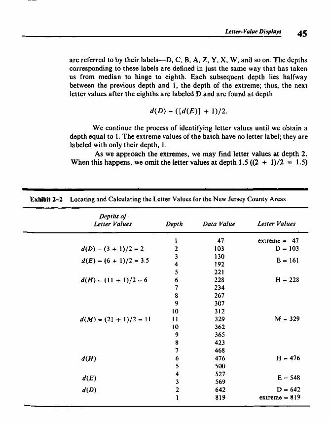
Letter- Value Displays 45
are referred to by their labels—D, C, B, A, Z, Y, X, W, and so on. The depthscorresponding to these labels are defined in just the same way that has takenus from median to hinge to eighth. Each subsequent depth lies halfwaybetween the previous depth and 1, the depth of the extreme; thus, the nextletter values after the eighths are labeled D and are found at depth
We continue the process of identifying letter values until we obtain adepth equal to 1. The extreme values of the batch have no letter label; they arelabeled with only their depth, 1.
As we approach the extremes, we may find letter values at depth 2.When this happens, we omit the letter values at depth 1.5 ((2 + l)/2 = 1.5)
Exhibit 2-2 Locating and Calculating the Letter Values for the New Jersey County Areas
Depths ofLetter Values Depth Data Value Letter Values
d(E) = (6 + l)/2 = 3.5
(11
d(M)~ (21 + l ) / 2 = 11
d(H)
d(E)
d(D)
123456789101110987654321
47103130192221228234267307312329362365423468476500527569642819
extreme =D =E =
H =
M =
H =
E =
D =extreme =
47103
161
228
329
476
548
642819
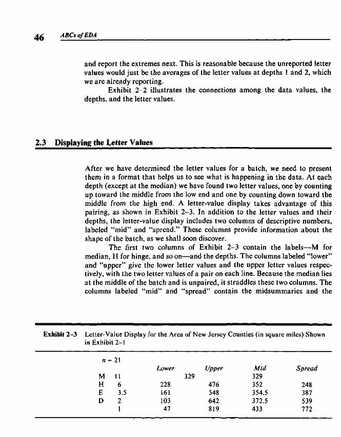
ABCs of EDA
and report the extremes next. This is reasonable because the unreported lettervalues would just be the averages of the letter values at depths 1 and 2, whichwe are already reporting.
Exhibit 2-2 illustrates the connections among the data values, thedepths, and the letter values.
2.3 Displaying the Letter Values
After we have determined the letter values for a batch, we need to presentthem in a format that helps us to see what is happening in the data. At eachdepth (except at the median) we have found two letter values, one by countingup toward the middle from the low end and one by counting down toward themiddle from the high end. A letter-value display takes advantage of thispairing, as shown in Exhibit 2-3. In addition to the letter values and theirdepths, the letter-value display includes two columns of descriptive numbers,labeled "mid" and "spread." These columns provide information about theshape of the batch, as we shall soon discover.
The first two columns of Exhibit 2-3 contain the labels—M formedian, H for hinge, and so on—and the depths. The columns labeled "lower"and "upper" give the lower letter values and the upper letter values respec-tively, with the two letter values of a pair on each line. Because the median liesat the middle of the batch and is unpaired, it straddles these two columns. Thecolumns labeled "mid" and "spread" contain the midsummaries and the
Exhibit 2-3 Letter-Value Display for the Area of New Jersey Counties (in square miles) Shownin Exhibit 2-1
/i = 21
MHED
1163.521
Lower
22816110347
329Upper
476548642819
Mid329352354.5372.5433
Spree
248387539772
Letter- Value Displays 47
spreads, each of which is calculated from the corresponding letter values asdescribed in the following discussion.
In Exhibit 2-3, we readily see that the median county size is 329square miles, that the counties range from 47 square miles to 819 square miles,and that the middle half of the 21 counties runs from 228 to 476 square miles.
Since letter values come in pairs symmetrically placed at the samedepth, we might ask whether their values are also symmetric. We can find outby calculating the average value for each pair of letter values. This value
midsummary midway between the two letter values is a midsummary. Specifically, themidhinge average of the two hinges is called the midhinge (midH). We can also find themideighth mideighth (midE), the midD, and other midsummaries, including the ntidex-midextreme treme, also called midrange. The median is, by being in the middle of the batch,midrange already a midsummary. Note that, in finding midsummaries, we do not
average depths, but rather we average the two letter values found at aparticular depth.
We can learn a lot about how nearly symmetric a batch of values is bycomparing the other midsummaries to the median or by looking for a trend inthe midsummaries. If all the midsummaries are approximately equal, then thevalues of the hinges, eighths, and so on are nearly symmetric about themedian. If the midsummaries become progressively larger, the batch is skewedtoward the high side. If they decrease steadily, the batch is skewed toward thelow side.
Returning to the example of the county areas, we see in Exhibit 2-3that the midsummaries increase gradually, indicating a slight skewnesstoward the high side; the midextreme, 433, stands out because of the size ofBurlington County.
As we noted in Chapter 1, symmetric batches of data values are ofteneasier to summarize and analyze than batches that are asymmetric. When abatch of values is not symmetric but has a main hump and a generally smoothstem-and-leaf display, symmetry can often be attained by re-expressing thenumbers. Re-expression is discussed in Section 2.4, and its use to promotesymmetry is illustrated in Section 2.5.
We can learn in detail how variable the data are by examining thespread column of spreads in a letter-value display. Each spread is the difference
between the two letter values in a pair, calculated by subtracting the lowerletter value from the upper letter value. It is named after the letter-value pair.
H-spread For example, the H-spread (H-spr for short) is the difference between thehinges and thus tells the range covered by the middle half of the data. Otherspreads have similar interpretations; for example, the E-spread gives the rangeof the middle three-quarters of the data. The difference between the extremes
r<tnge is simply called the range. All these spreads respond to variability in data. The

AQ ABCs of EDA
more variable the data, the larger the spreads will be. Taken together, thespreads in a letter-value display provide information about how the tails of thedata behave. Section 2.6 discusses this further.
2.4 Re-expression and the Ladder of Powers
data One way to change the shape of a batch is to re-express each data value in there-expression batch. For example, we might raise each value to some power, p. When we
work by hand, we can use a calculator or a book of tables to re-express values,but for a large batch even using a calculator can be tedious. Re-expressions aremore practical when we work on a computer because the machine can do allthe work quickly. When we use powers, each value of p will have a slightlydifferent effect on the batch, but if we place these powers in order, their effectson the batch will also be ordered. This order leads to the ladder of powerslisted in Exhibit 2-4.
The arrow in Exhibit 2-4 marks the power p = 1. This is "home base"because the original data values can be thought of as being re-expressed to thepower 1. Raising each value in the batch to a power less than 1 will pull in astretched-out upper tail while stretching out a bunched-in lower tail. Raisingeach data value to a power higher than 1 will have the reverse effect:Asymmetry to the low side will be alleviated. Thus a trend in the midsumma-ries indicates the direction we should move on the ladder of powers. The ladderis useful because the further we move from p = 1 in either direction, thegreater the effect on the shape of the batch. We can thus hunt for an optimalre-expression by trying a power and examining the midsummaries in theletter-value display of the re-expressed batch. A trend in the new midsumma-ries will point the direction in which we should now move from where we areon the ladder for a better result. See Section 2.5 for an example.
Usually y° is defined to be 1. However, it would be useless to re-expressall the values in a batch to 1. It turns out that, when we order the powersaccording to the strength of their effect on the data, the logarithm, or log, fallsnaturally at the zero power. The mathematical reasons for this are beyond thescope of this book, but the truth of the statement will become evident as we usethe ladder of powers to find re-expressions for data.
We can save much time when working by hand by noting that we neednot re-express the entire batch to construct a new letter-value display. Instead
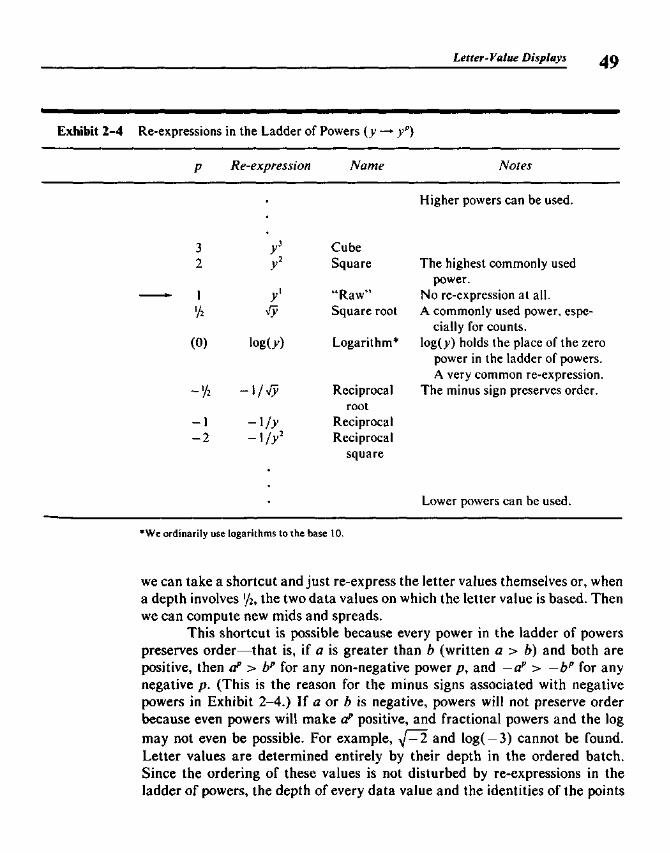
Letter- Value Displays 49
Exhibit 2-4 Re-expressions in the Ladder of Powers {y — yp)
p Re-expression Name Notes
Higher powers can be used.
32
1
72
(0)
- l- 2
-\/y
CubeSquare
"Raw"Square root
Logarithm*
Reciprocalroot
ReciprocalReciprocal
square
The highest commonly usedpower.
No re-expression at all.A commonly used power, espe-
cially for counts.\og(y) holds the place of the zero
power in the ladder of powers.A very common re-expression.
The minus sign preserves order.
Lower powers can be used.
•We ordinarily use logarithms to the base 10.
we can take a shortcut and just re-express the letter values themselves or, whena depth involves % the two data values on which the letter value is based. Thenwe can compute new mids and spreads.
This shortcut is possible because every power in the ladder of powerspreserves order—that is, if a is greater than b (written a > b) and both arepositive, then <f > bp for any non-negative power p, and —ap> —bp for anynegative p. (This is the reason for the minus signs associated with negativepowers in Exhibit 2-4.) If a or b is negative, powers will not preserve orderbecause even powers will make a? positive, and fractional powers and the logmay not even be possible. For example, yj—2 and log( —3) cannot be found.Letter values are determined entirely by their depth in the ordered batch.Since the ordering of these values is not disturbed by re-expressions in theladder of powers, the depth of every data value and the identities of the points
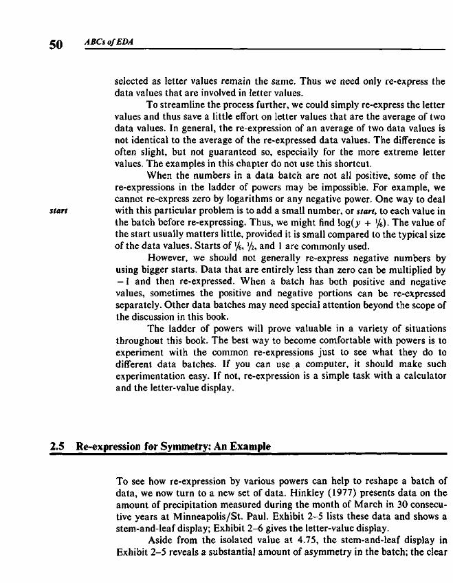
ABCs of EDA
selected as letter values remain the same. Thus we need only re-express thedata values that are involved in letter values.
To streamline the process further, we could simply re-express the lettervalues and thus save a little effort on letter values that are the average of twodata values. In general, the re-expression of an average of two data values isnot identical to the average of the re-expressed data values. The difference isoften slight, but not guaranteed so, especially for the more extreme lettervalues. The examples in this chapter do not use this shortcut.
When the numbers in a data batch are not all positive, some of there-expressions in the ladder of powers may be impossible. For example, wecannot re-express zero by logarithms or any negative power. One way to deal
start with this particular problem is to add a small number, or start, to each value inthe batch before re-expressing. Thus, we might find log(j> + %). The value ofthe start usually matters little, provided it is small compared to the typical sizeof the data values. Starts of % % and 1 are commonly used.
However, we should not generally re-express negative numbers byusing bigger starts. Data that are entirely less than zero can be multiplied by- 1 and then re-expressed. When a batch has both positive and negativevalues, sometimes the positive and negative portions can be re-expressedseparately. Other data batches may need special attention beyond the scope ofthe discussion in this book.
The ladder of powers will prove valuable in a variety of situationsthroughout this book. The best way to become comfortable with powers is toexperiment with the common re-expressions just to see what they do todifferent data batches. If you can use a computer, it should make suchexperimentation easy. If not, re-expression is a simple task with a calculatorand the letter-value display.
2.5 Re-expression for Symmetry: An Example
To see how re-expression by various powers can help to reshape a batch ofdata, we now turn to a new set of data. Hinkley (1977) presents data on theamount of precipitation measured during the month of March in 30 consecu-tive years at Minneapolis/St. Paul. Exhibit 2-5 lists these data and shows astem-and-leaf display; Exhibit 2-6 gives the letter-value display.
Aside from the isolated value at 4.75, the stem-and-leaf display inExhibit 2-5 reveals a substantial amount of asymmetry in the batch; the clear
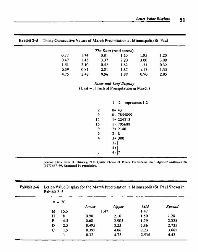
Letter- Value Displays 51
Exhibit 2-5 Thirty Consecutive Values of March Precipitation at Minneapolis/St. Paul
The Data (read across)0.770.471.510.594.75
1.741.432.100.812.48
0.813.370.522.810.96
1.202.201.621.871.89
1.953.001.311.180.90
1.203.090.321.352.05
Stem-and-Leaf Display(Unit = .1 Inch of Precipitation in March)
1 2 represents 1.2
291515954
1
0*0-1*1-2*2-3*3-4*4-
43785589922431379568821408300
7
Source: Data from D. Hinkley, "On Quick Choice of Power Transformation," Applied Statistics 26(1977):67-69. Reprinted by permission.
Exhibit 2-6 Letter-Value Display for the March Precipitation in Minneapolis/St. Paul Shown inExhibit 2-5
30
MHEDC
15.584.52.51.51
Lower
0.900.680.4950.3950.32
Upper1.47
2.102.9053.234.064.75
Mid1.471.501.791.862.232.535
Spreai
1.202.2252.7353.6654.43
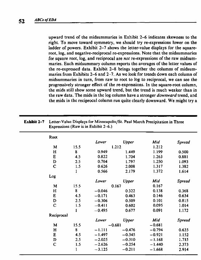
52 ABCs of EDA
upward trend of the midsummaries in Exhibit 2-6 indicates skewness to theright. To move toward symmetry, we should try re-expressions lower on theladder of powers. Exhibit 2-7 shows the letter-value displays for the square-root, log, and negative-reciprocal re-expressions. Note that the midsummariesfor square root, log, and reciprocal are not re-expressions of the raw midsum-maries. Each midsummary column reports the averages of the letter values ofthe re-expressed data. Exhibit 2-8 brings together the columns of midsum-maries from Exhibits 2-6 and 2-7. As we look for trends down each column ofmidsummaries in turn, from raw to root to log to reciprocal, we can see theprogressively stronger effect of the re-expressions. In the square-root column,the mids still show some upward trend, but the trend is much weaker than inthe raw data. The mids in the log column have a stronger downward trend, andthe mids in the reciprocal column run quite clearly downward. We might try a
Exhibit 2-7 Letter-Value DisplaysExpressions
Root
MHEDC
Log
MHEDC
Reciprocal
MHEDC
(Raw is in
15.584.52.51.51
15.584.52.51.51
15.584.52.51.51
for Minneapolis/StExhibit 2-6.)
Lower1.212
0.9490.8220.7040.6260.566
Lower0.167
-0.046-0.171-0.306-0.411-0.495
Lower-0.681
-1.111-1.497-2.025-2.626-3.125
. Paul March
Upper
1.4491.7041.7972.0082.179
Upper
0.3220.4630.5090.6020.677
Upper
-0.476-0.345-0.310-0.254-0.211
Precipitation
Mid1.2121.1991.2631.2501.3171.372
Mid0.1670.1380.1460.1010.0950.091
Mid-0.681-0.794-0.921-1.168-1.440-1.668
in Three
Spread
0.5000.8811.0931.3821.614
Spread
0.3680.6340.8151.0141.172
Spread
0.6351.1521.7152.3732.914
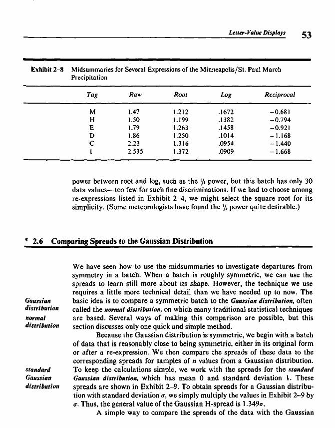
Letter-Value Displays 53
Exhibit 2-8 Midsummaries for Several Expressions of the Minneapolis/St. Paul MarchPrecipitation
Tag Raw Root Log Reciprocal
MHEDC1
1.471.501.791.862.232.535
1.2121.1991.2631.2501.3161.372
.1672
.1382
.1458
.1014
.0954
.0909
-0.681-0.794-0.921-1.168-1.440-1.668
power between root and log, such as the !/t power, but this batch has only 30data values—too few for such fine discriminations. If we had to choose amongre-expressions listed in Exhibit 2-4, we might select the square root for itssimplicity. (Some meteorologists have found the xfo power quite desirable.)
2.6 Comparing Spreads to the Gaussian Distribution
Gaussiandistribution
normaldistribution
standardGaussiandistribution
We have seen how to use the midsummaries to investigate departures fromsymmetry in a batch. When a batch is roughly symmetric, we can use thespreads to learn still more about its shape. However, the technique we userequires a little more technical detail than we have needed up to now. Thebasic idea is to compare a symmetric batch to the Gaussian distribution, oftencalled the normal distribution, on which many traditional statistical techniquesare based. Several ways of making this comparison are possible, but thissection discusses only one quick and simple method.
Because the Gaussian distribution is symmetric, we begin with a batchof data that is reasonably close to being symmetric, either in its original formor after a re-expression. We then compare the spreads of these data to thecorresponding spreads for samples of n values from a Gaussian distribution.To keep the calculations simple, we work with the spreads for the standardGaussian distribution, which has mean 0 and standard deviation 1. Thesespreads are shown in Exhibit 2-9. To obtain spreads for a Gaussian distribu-tion with standard deviation <r, we simply multiply the values in Exhibit 2-9 bya. Thus, the general value of the Gaussian H-spread is 1.349o\
A simple way to compare the spreads of the data with the Gaussian
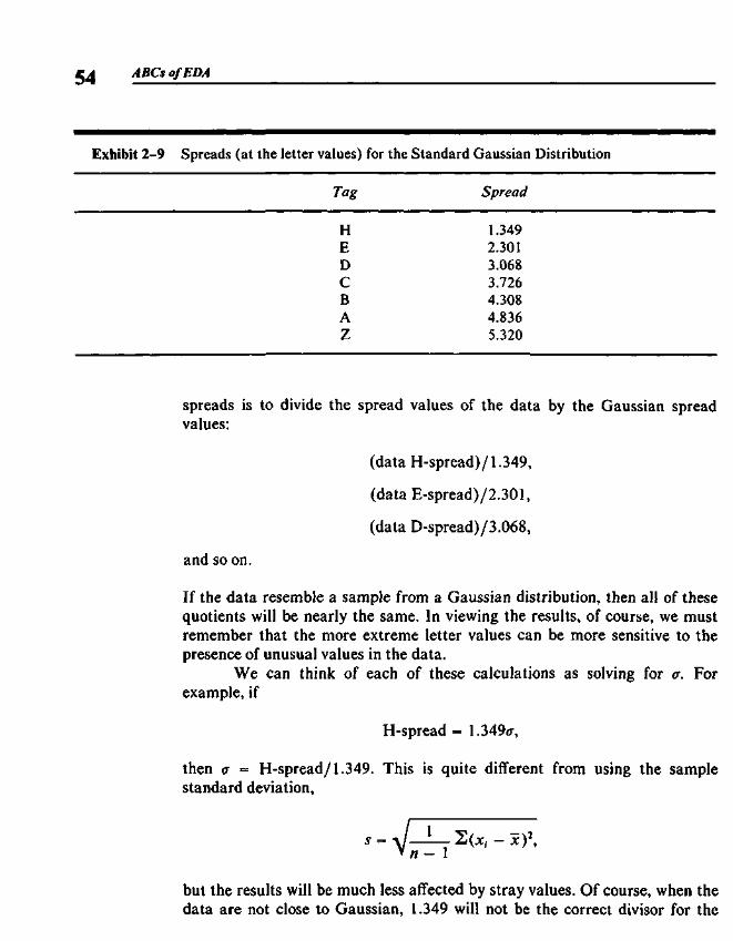
5 4 ABCs of EDA
Exhibit 2-9 Spreads (at the letter values)
Tag
for the Standard Gaussian
Spread
Distribution
H 1.349E 2.301D 3.068C 3.726B 4.308A 4.836Z 5.320
spreads is to divide the spread values of the data by the Gaussian spreadvalues:
(data H-spread)/1.349,
(dataE-spread)/2.301,
(data D-spread)/3.068,
and so on.
If the data resemble a sample from a Gaussian distribution, then all of thesequotients will be nearly the same. In viewing the results, of course, we mustremember that the more extreme letter values can be more sensitive to thepresence of unusual values in the data.
We can think of each of these calculations as solving for a. Forexample, if
H-spread = 1.349<r,
then a = H-spread/1.349. This is quite different from using the samplestandard deviation,
n -
but the results will be much less affected by stray values. Of course, when thedata are not close to Gaussian, 1.349 will not be the correct divisor for the
Letter- Value Displays s s
H-spread. Fortunately, the estimate of a will not be terribly sensitive to thepopulation shape, at least for the H-spread. As we go to the E-spread orD-spread, sensitivity increases.
A clear trend in the quotients derived from the spreads provides anindication of how the data depart from the Gaussian shape. If the quotientsgrow, the tails of the batch are heavier than the tails of the Gaussian shape. Ifthe quotients shrink, the tails of the data are lighter.
In Chapter 9 we will see another use of the Gaussian distribution as astandard of comparison.
2.7 Letter Values from the Computer
A letter-value display is simply a table of numbers arranged in columns. Thefirst column contains labels. Columns 2 through 6 contain depths, lower lettervalues, upper letter values, mids, and spreads, in that order. Computers havelittle trouble printing such tables. A computer-generated letter-value displayusually looks exactly like a neatly typed letter-value display without the ruledlines sometimes used to set off the letter values themselves.
The program must be told which data batch to display. How to tell thisto the program depends upon the particular implementation of the program.All decisions are made automatically, so no further information is needed.
t 2.8 Algorithms
The FORTRAN and BASIC programs for letter values work in slightlydifferent ways, illustrating two alternative organizations of the tasks involved.The FORTRAN program finds all the letter values first and places them andtheir depths in arrays for subsequent printing. This has the advantage ofmaking the letter values available for other computations. The BASIC versionprints the letter values as it finds them and uses no additional storage. TheBASIC program also attempts to position the columns of the display in orderto make the best use of the available page area.
It is difficult for portable programs to control the number of decimalplaces printed and to align the decimal points of the numbers in each column.
ABCs of EDA
Implementers of the FORTRAN version may want to use run-time formats toavoid the possibility of a number's overflowing the formatted size allowedhere. Implementers of the BASIC version who have a PRINT USING statementavailable in their BASIC may wish to use it to format the columns.
FORTRAN
The F O R T R A N programs for finding letter values and displaying themconsist of two subroutines: LVALS and LVPRNT. LVALS accepts the data in a vectorand returns a vector of depths and an array of pairs of letter values. It is usedthrough the statement
CALL LVALS(Y, N, D, YLV, NLV, SORTY, ERR)
where the arguments are as follows:
Y() is the N-long vector of data values;N is the number of data values;D( 15) is the vector of depths;YLV( 15,2) is the array of letter values [YLV( 1,1) and YLV( 1,2) both
contain the median, and the remaining pairs ofletter values are in order from the hinges out to theextremes, with the lower letter value first];
NLV returns the number of pairs of letter values;SORTY() is the N-long workspace for sorting Y();ERR is the error flag, whose values are
0 normal21 N < 2 or N > 24576—too few or too many
data values22 NLV < 3 or NLV > 1523 page width < 64 print positions—too narrow
for letter-value display.
The subroutine LVPRNT uses the information on depths and letter values to printthe letter-value display in essentially the format shown in Exhibits 2 -3 and2-6 . The calling statement is
CALL LVPRNTfNLV, D, YLV, ERR)
where the arguments are as described above.
Letter- Value Displays 57
BASIC
The BASIC program requires only the defined functions and the SORT from Y()to W() subroutines. It leaves X() and Y() unchanged.
2.9 Sorting
sortingThe process of putting a set of numbers or other elements, such as names, intoorder is known as sorting. Because an ordered batch makes it easy to pick outthe letter values, as well as to detect potentially stray values at either end,sorting is an important operation in exploratory data analysis. This sectiondiscusses the reasons for including certain sorting programs in this book; it alsoprovides selected references so that interested readers can pursue the subjectof sorting further.
Computer scientists have devoted considerable imagination and energyto designing and analyzing algorithms for sorting. Their analyses tell us,among other things, how much time a given sorting algorithm requires toprocess a batch of n numbers when n is large. For some algorithms this time isproportional to n2. This is easy to understand if we imagine making n — 1comparisons to pick out the smallest number, n — 2 comparisons to find thenext smallest, and so on. The total number of comparisons is (n — 1) +(n — 2) + . . . + 1 = n{n — l)/2, which resembles n2/2 when n is large.
However, it is possible to sort much more efficiently than in timeproportional to n2. Fast sorting algorithms require time proportional ton log(rt), and the difference between n log(«) and n2 becomes greater as nincreases. If we want only a few values at selected positions in the orderedbatch, we can even obtain these values without sorting the batch completely.Such a "partial sorting" algorithm could, for example, deliver the median intime proportional to n.
The sorting algorithms used in the programs in this book are not themost elegant algorithms available, but they are among the simplest toprogram. Their simplicity makes them easier to read and understand, and theytake up much less space than do the faster methods—both are an advantage onsmall computers. Also, users of these programs will often be concerned onlywith situations in which n is small—for example, n less than 50—and thegreater effort that the fast algorithms put into bookkeeping may not beworthwhile. Sorting programs for a variety of applications are available in
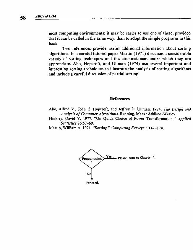
eo ABCs of EDA
most computing environments; it may be easier to use one of these, providedthat it can be called in the same way, than to adopt the simple programs in thisbook.
Two references provide useful additional information about sortingalgorithms. In a careful tutorial paper Martin (1971) discusses a considerablevariety of sorting techniques and the circumstances under which they areappropriate. Aho, Hopcroft, and Ullman (1974) use several important andinteresting sorting techniques to illustrate the analysis of sorting algorithmsand include a careful discussion of partial sorting.
References
Aho, Alfred V., John E. Hopcroft, and Jeffrey D. Ullman. 1974. The Design andAnalysis of Computer Algorithms. Reading, Mass.: Addison-Wesley.
Hinkley, David V. 1977. "On Quick Choice of Power Transformation." AppliedStatistics 26:67-69.
Martin, William A. 1971. "Sorting." Computing Surveys 3:147-174.
Programming^ Y e s » Please turn to Chapter 7.
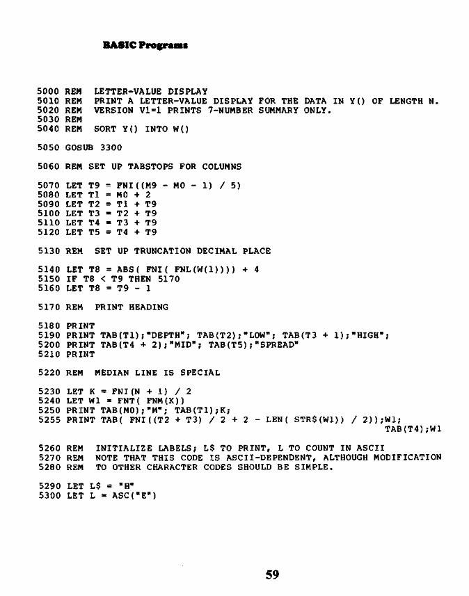
BASIC Programt
5 0 0 0 REM LETTER-VALUE DISPLAY5 0 1 0 REM PRINT A LETTER-VALUE DISPLAY FOR THE DATA IN Y() OF LENGTH N.5 0 2 0 REM VERSION V l = l PRINTS 7-NUMBER SUMMARY ONLY.5 0 3 0 REM5040 REM SORT Y() INTO W()
5050 GOSUB 3300
5060 REM SET UP TABSTOPS FOR COLUMNS
5070 LET T9 = FNI((M9 - M0 - 1) / 5)5080 LET Tl = MO + 25090 LET T2 = Tl + T95100 LET T3 = T2 + T95110 LET T4 = T3 + T95120 LET T5 = T4 + T9
5130 REM SET UP TRUNCATION DECIMAL PLACE
5140 LET T8 = ABS( FNI( FNL(W(1)))) + 45150 IF T8 < T9 THEN 51705160 LET T8 = T9 - 1
5170 REM PRINT HEADING
5180 PRINT5190 PRINT TAB(Tl);"DEPTH"; TAB(T2);"LOW"; TAB(T3 + 1);"HIGH";5200 PRINT TAB(T4 + 2);"MID"; TAB(T5);"SPREAD"5210 PRINT
5220 REM MEDIAN LINE IS SPECIAL
5230 LET K = FNI(N + 1) / 25240 LET Wl = FNT( FNM(K))5250 PRINT TAB(M0);"M"; TAB(T1);K;5255 PRINT TAB( FNI((T2 + T3) / 2 + 2 - LEN( STR$(W1)) / 2));W1;
TAB(T4);W1
5260 REM INITIALIZE LABELS; L$ TO PRINT, L TO COUNT IN ASCII5270 REM NOTE THAT THIS CODE IS ASCII-DEPENDENT, ALTHOUGH MODIFICATION5280 REM TO OTHER CHARACTER CODES SHOULD BE SIMPLE.
5290 LET L$ = "H"5300 LET L = ASC("E")
59
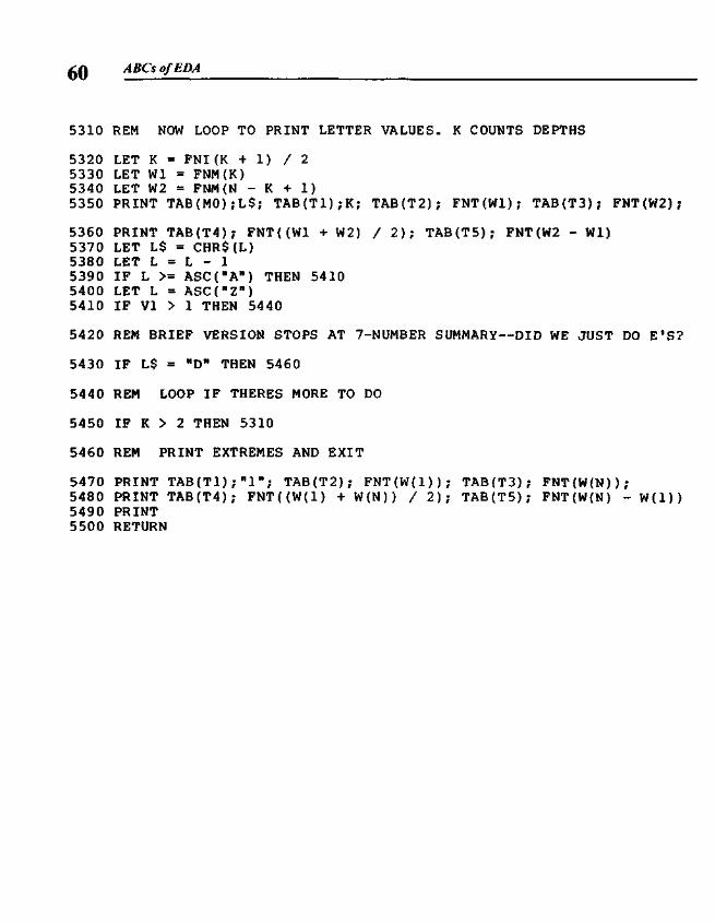
ABCs of EDA
5310 REM NOW LOOP TO PRINT LETTER VALUES. K COUNTS DEPTHS
5320 LET K = FNI (K + 1) / 25330 LET Wl = FNM(K)5340 LET W2 = FNM(N - K + 1)5350 PRINT TAB(M0);L$; TAB(T1);K; TAB(T2); FNT(Wl); TAB(T3); FNT(W2);
5360 PRINT TAB(T4); FNT((W1 + W2) / 2); TAB(T5); FNT(W2 - Wl)5370 LET L$ = CHR$(L)5380 LET L = L - 15390 IF L >= ASC("A") THEN 54105400 LET L = ASC("Z")5410 IF VI > 1 THEN 5440
5420 REM BRIEF VERSION STOPS AT 7-NUMBER SUMMARY—DID WE JUST DO E'S?
5430 IF L$ = "D" THEN 5460
5440 REM LOOP IF THERES MORE TO DO
5450 IF K > 2 THEN 5310
5460 REM PRINT EXTREMES AND EXIT
5470 PRINT TAB(Tl);"1"; TAB(T2); FNT(W(1)); TAB(T3); FNT(W(N));5480 PRINT TAB(T4); FNT((W(1) + W(N)) / 2); TAB(T5); FNT(W(N) - W(l))5490 PRINT5500 RETURN
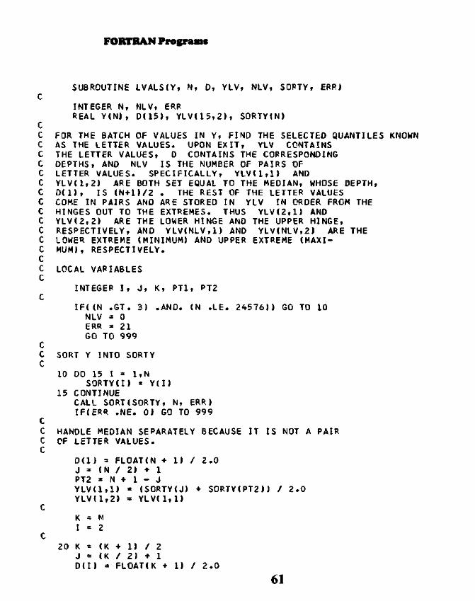
FORTRAN Programs
SUBROUTINE LVALS(Y, N, D, YLV, NLV, SOPTY, ERR)C
INTEGER N, NLV, ERRREAL Y(NJ, D(15), YLV(15,2), SORTY(N)
CC FOR THE BATCH OF VALUES IN Y, FIND THE SELECTED QUANTILES KNOWNC AS THE LETTER VALUES. UPON EXIT, YLV CONTAINSC THE LETTER VALUES, D CONTAINS THE CORRESPONDINGC DEPTHS, AND NLV IS THE NUMBER OF PAIRS OFC LETTER VALUES. SPECIFICALLY, YLV(1,1) ANDC YLV(1,2) ARE BOTH SET EQUAL TO THE MEDIAN, WHOSE DEPTH,C D(l), IS (N + D / 2 . THE REST OF THE LETTER VALUESC COME IN PAIRS AND ARE STORED IN YLV IN ORDER FROM THEC HINGES OUT TO THE EXTREMES. THUS YLV(2,1) ANDC YLV(2,2) ARE THE LOWER HINGE AND THE UPPER HINGE,C RESPECTIVELY, AND YLV(NLV,1) AND YLV(NLV,2) ARE THEC LOWER EXTREME (MINIMUM) AND UPPER EXTREME (MAXI-C MUM), RESPECTIVELY.CC LOCAL VARIABLESC
INTEGER. It J, K, PT1, PT2C
IF((N .GT. 3) .AND. (N .LE. 24576)) GO TO 10NLV = 0ERR = 21GO TO 999
CC SORT Y INTO SORTYC
10 DO 15 I - 1,NSORTY(I) = Y(I)
15 CONTINUECALL SORT(SORTY, N, ERR)IF(ERR .NE. 0) GO TO 999
CC HANDLE MEDIAN SEPARATELY BECAUSE IT IS NOT A PAIRC OF LETTER VALUES.C
D ( l ) = FLOAT(N • 1) / 2 .0J 3 (N / 2) + 1PT2 - N + 1 - JYLV(1,1) = (SCRTY(J) + S0RTY(PT2)) / 2 .0YLV(1,2) = YLV(1,1)
CK ~ NI = 2
C20 K * (K + 1) / 2
J = (K / 2) + 1D ( I ) = FLOAT(K + 1) / 2.0
61
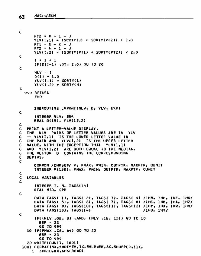
62 ABCs of EDA
PT2 = K + 1 - JY L V ( I t l ) = (SCRTY(J) + S0PTY(PT2)) / 2 . 0PT1 = N - K + JPT2 = N + 1 - JY L V ( I , 2 ) = (SORTY(PTl) + S0RTY(PT2M / 2 . 0
1 = 1 + 1I F ( D U - l ) . G T . 2 . 0 ) GO TO 20
NLV = ID ( I ) = 1 .0Y L V ( I t l ) = SORTY(l)Y L V ( I , 2 ) = SORTY(N)
999 RETURNEND
SUBROUTINE LVPRNT(NLV, D, YLV, ERP)
INTEGER NLV, ERRREAL 0 ( 1 5 ) , Y L V ( 1 5 , 2 )
PRINT A LETTER-VALUE DISPLAY.THE NLV PAIRS OF LETTER VALUES ARE I N YLV~ Y L V ( I , 1 J IS THE LOWER LETTER VALUE INTHE PAIR AND Y L V ( I , 2 ) IS THE UPPER LETTERVALUE, WITH THE EXCEPTION THAT YLV ( 1 , 1 )AND Y L V ( 1 , 2 ) ARE BOTH EQUAL TO THE MEDIAN.THE VECTOR D CONTAINS THE CCRRESPONDINGDEPTHS.
COMMON /CHRBUF/ P, PMAX, PMIN, OUTPTR, MAXPTR, OUNITINTEGER P ( 1 3 0 ) , PMAX, PMIN, OUTPTR, MAXPTR, OUNIT
LOCAL VARIABLES
INTEGER I , N, TAGS(14)REAL MID, SPP
DATA TAGS(DATA TAGS(
1 ) ,5) ,
DATA TAGS( 9 ) ,DATA TAGS(13),
TAGS( 2 ) ,TAGS( 6 ) ,TAGS(IO),TAGS(14)
TAGS( 3 ) ,TAGS( 7 ) ,TAGS(ll),
TAGS( 4)TAGS( 8)TAGS(12)
/1HM,/1HC,/1HY,/1HU,
1HH,1HB,1HX,1HT/
1HE, 1HD/1HA, 1HZ/1HW, 1HV/
10
201001
I F ( ( N L VERP =GO TO
IF(PMAXERR =GO TO
.GE,22999• G£23999
3) .AND. (NLV . L E . 1 5 ) ) GO TO 10
64) GO TO 20
WRITE(OUNIT, 1001)FORMAT(5X,5HDEPTH,7X,5HLOWER,8X,5HUPPER,1IX,
. 3HMID,8X,6HS«READ)
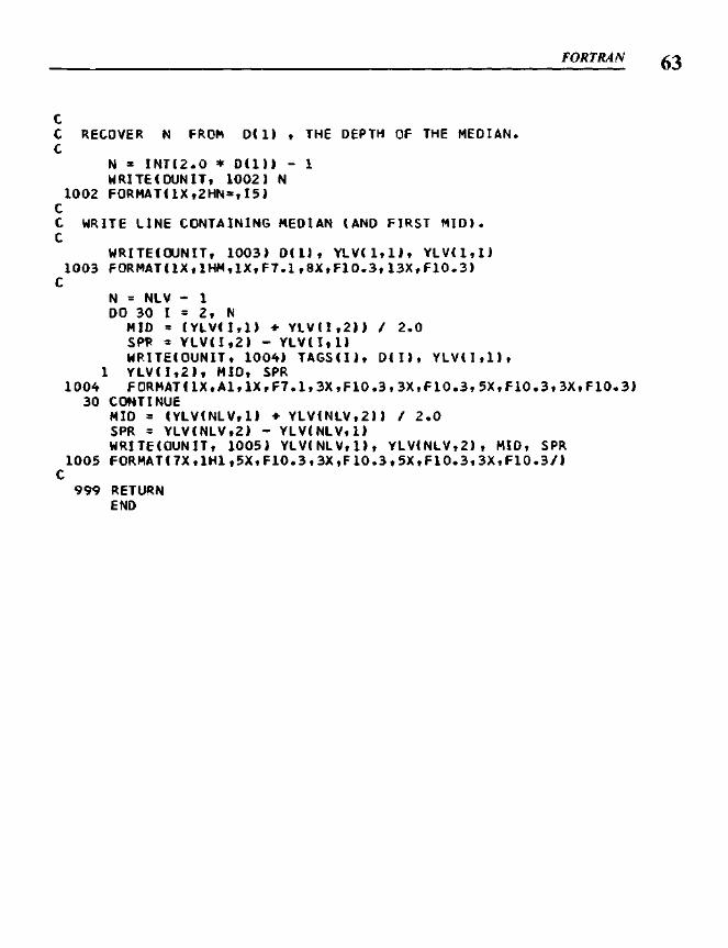
FORTRAN
CC RECOVER N FROM D ( l ) , THE DEPTH OF THE M E D I A N .C
N = INTC2.0 * D(D) - 1WRITE(OUNIT, 1002) N
1002 FORMAT(1X,2HN=,I5)CC WRITE LINE CONTAINING MEDIAN (AND FIRST MID).C
WRITE(OUNIT, 1003) 0(1), YLV<1,1), YLV(1,1)1003 FORMAT(1X,1HM,1X,F7.1,8X,F1O.3,13X,F1O.3)
CN = NLV - 1DO 30 I = 2, N
MID - (YLV<I,1) + YLV(I,2)) / 2.0SPP = YLV(I,2) - YLV(I,1)WRITE(OUNIT, 1004) TAGS(I), D(I)t YLV(I.l),
1 YLV(I,2), MID, SPR1004 F0RMAT(lX,Al,lX,F7.1,3X,F10.3,3X,F10.3,5X,F10.3,3X,F10.3)
30 CONTINUEMID = (YLV(NLV,1) + YLV(NLV,2)) / 2.0SPR = YLV(NLV,2) - YLV(NLV,1)WRITE(OUNIT, 1005) YLV(NLV,1), YLV(NLV,2), MID, SPR
1005 FORMAT(7X,1H1,5X,F10.3,3X,F10.3,5X,F10.3,3X,F10.3/)C
999 RETURNEND
63

3Boxplots
In Chapter 1 we saw that stem-and-leaf displays provide a flexible andeffective way to view a batch of data as a whole. In Chapter 2 we considered anumerical summary of a batch using a few values at selected depths.Frequently, we can make good use of something between these two extremes inthe form of a picture or graphical summary. We want to represent the datavalues graphically, but we do not want to see all the detail. This is just the taskfor which boxplots were invented.
3.1 Basic Purposes
Most batches of data pile up in the middle and spread out toward the ends. Tosummarize the behavior of a batch, we need a clear picture of where themiddle lies, roughly how spread out the middle is, and just how the tails relateto it. Since the middle is generally better defined than the tails of the data, weneed to see less detail at the middle—we want to focus more of our attentionon possible strays at the ends because these often give clues to unexpected
65
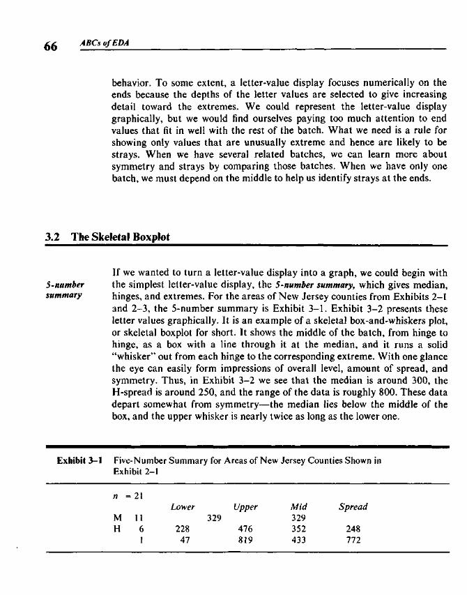
66 ABCs of EDA
behavior. To some extent, a letter-value display focuses numerically on theends because the depths of the letter values are selected to give increasingdetail toward the extremes. We could represent the letter-value displaygraphically, but we would find ourselves paying too much attention to endvalues that fit in well with the rest of the batch. What we need is a rule forshowing only values that are unusually extreme and hence are likely to bestrays. When we have several related batches, we can learn more aboutsymmetry and strays by comparing those batches. When we have only onebatch, we must depend on the middle to help us identify strays at the ends.
3.2 The Skeletal Boxplot
If we wanted to turn a letter-value display into a graph, we could begin with5-number the simplest letter-value display, the 5-number summary, which gives median,summary hinges, and extremes. For the areas of New Jersey counties from Exhibits 2-1
and 2-3, the 5-number summary is Exhibit 3-1. Exhibit 3-2 presents theseletter values graphically. It is an example of a skeletal box-and-whiskers plot,or skeletal boxplot for short. It shows the middle of the batch, from hinge tohinge, as a box with a line through it at the median, and it runs a solid"whisker" out from each hinge to the corresponding extreme. With one glancethe eye can easily form impressions of overall level, amount of spread, andsymmetry. Thus, in Exhibit 3-2 we see that the median is around 300, theH-spread is around 250, and the range of the data is roughly 800. These datadepart somewhat from symmetry—the median lies below the middle of thebox, and the upper whisker is nearly twice as long as the lower one.
Exhibit 3-1 Five-Number Summary for Areas of New Jersey Counties Shown inExhibit 2-1
n = 21
MH
1161
Lower
22847
329Upper
476819
Mid329352433
Spread
248772
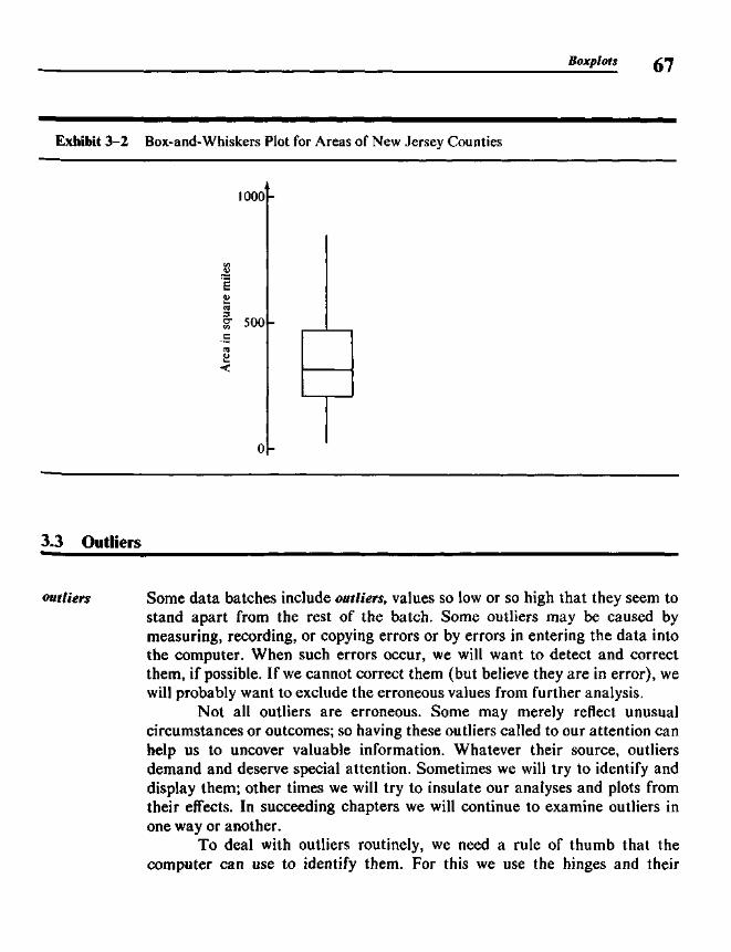
Boxplots 67
Exhibit 3-2 Box-and-Whiskers Plot for Areas of New Jersey Counties
1000-
500
3.3 Outliers
outliers Some data batches include outliers, values so low or so high that they seem tostand apart from the rest of the batch. Some outliers may be caused bymeasuring, recording, or copying errors or by errors in entering the data intothe computer. When such errors occur, we will want to detect and correctthem, if possible. If we cannot correct them (but believe they are in error), wewill probably want to exclude the erroneous values from further analysis.
Not all outliers are erroneous. Some may merely reflect unusualcircumstances or outcomes; so having these outliers called to our attention canhelp us to uncover valuable information. Whatever their source, outliersdemand and deserve special attention. Sometimes we will try to identify anddisplay them; other times we will try to insulate our analyses and plots fromtheir effects. In succeeding chapters we will continue to examine outliers inone way or another.
To deal with outliers routinely, we need a rule of thumb that thecomputer can use to identify them. For this we use the hinges and their
68 ABCs of EDA
inner fences
outer fences
outsidefar outside
adjacentvalue
difference, the H-spread. We define the inner fences as
lower hinge - (1.5 x H-spread)
upper hinge + (1.5 x H-spread)
and the outer fences as
lower hinge - (3 x H-spread)
upper hinge + (3 x H-spread).
Any data value beyond either inner fence we term outside, and any data valuebeyond either outer fence we call/ar outside. The outermost data value on eachend that is still not beyond the corresponding inner fence is known as anadjacent value.
For the New Jersey counties example, we have seen (in Exhibit 3-1)that the hinges are at 228 and 476 square miles, so the H-spread is476 — 228 = 248. Thus, the inner fences are at
228 - 1.5 x 248 = 228 - 372 = -144
476 + 1.5 x 248 = 476 + 372 = 848
and the outer fences are at
228 - 3 x 248 = 228 - 744 = -516
476 + 3 x 248 = 476 + 744 = 1220.
Because neither of the extreme values is "outside," the adjacent values are theextremes, 47 and 819.
By contrast, the precipitation pH data, which appear in Exhibit 1-1,have three outside values. From the letter-value display in Exhibit 3-3, we seethat the hinges are 4.31 and 4.82. Thus, the inner fences are 3.545 and 5.585,and the outer fences are 2.78 and 6.35. The three data values 5.62, 5.67, and5.78 are outside, and thus, by this rule of thumb, outlying. The adjacent valuesare 4.12 and 5.51.
We can also use this rule for identifying outliers in the stem-and-leafdisplay. If outside values appear on the special LO and HI stems, the LO and
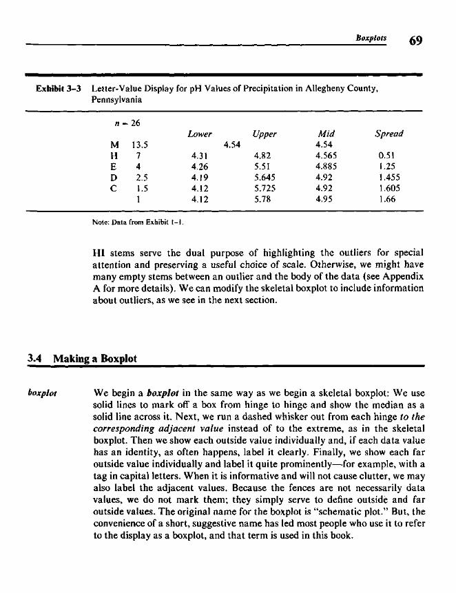
Boxplots
Exhibit 3-3 Letter-Value Display for pH Values of Precipitation in Allegheny County,Pennsylvania
Lower Upper Mid SpreadMHEDC
13.5742.51.51
4.314.264.194.124.12
4.544.825.515.6455.7255.78
4.544.5654.8854.924.924.95
0.511.251.4551.6051.66
Note: Data from Exhibit 1-1.
HI stems serve the dual purpose of highlighting the outliers for specialattention and preserving a useful choice of scale. Otherwise, we might havemany empty stems between an outlier and the body of the data (see AppendixA for more details). We can modify the skeletal boxplot to include informationabout outliers, as we see in the next section.
3.4 Making a Boxplot
boxplot We begin a boxplot in the same way as we begin a skeletal boxplot: We usesolid lines to mark off a box from hinge to hinge and show the median as asolid line across it. Next, we run a dashed whisker out from each hinge to thecorresponding adjacent value instead of to the extreme, as in the skeletalboxplot. Then we show each outside value individually and, if each data valuehas an identity, as often happens, label it clearly. Finally, we show each faroutside value individually and label it quite prominently—for example, with atag in capital letters. When it is informative and will not cause clutter, we mayalso label the adjacent values. Because the fences are not necessarily datavalues, we do not mark them; they simply serve to define outside and faroutside values. The original name for the boxplot is "schematic plot." But, theconvenience of a short, suggestive name has led most people who use it to referto the display as a boxplot, and that term is used in this book.
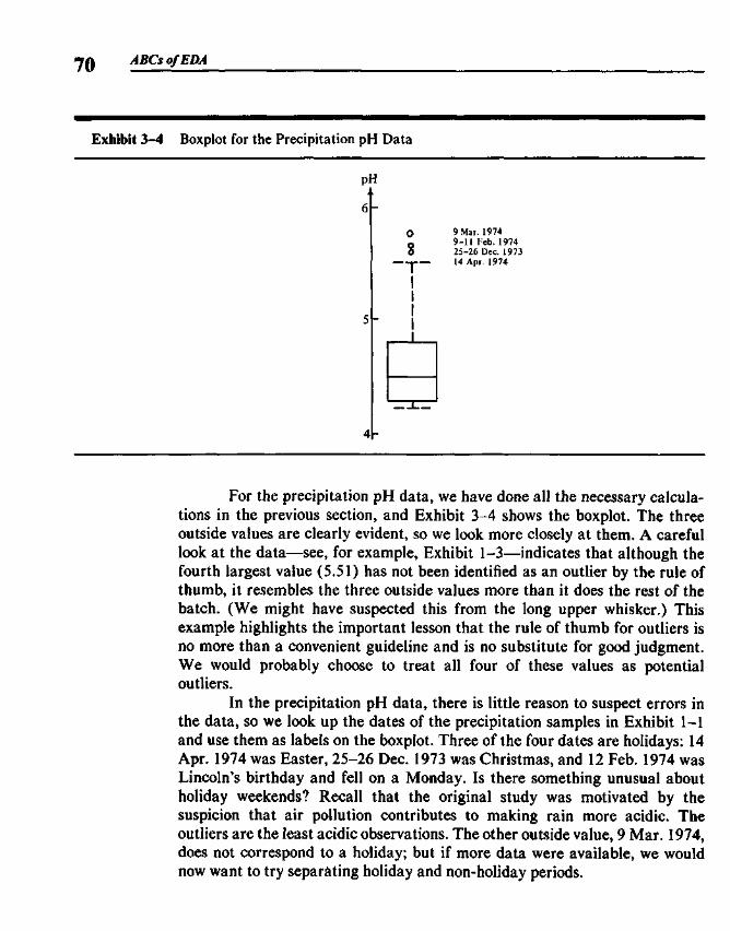
ABCs of EDA
Exhibit 3-4 Boxplot for the Precipitation pH Data
pHi
6 -
4 -
o
8
I
9 Mar. 19749-11 Feb. 197425-26 Dec. 197314 Apr. 1974
For the precipitation pH data, we have done all the necessary calcula-tions in the previous section, and Exhibit 3-4 shows the boxplot. The threeoutside values are clearly evident, so we look more closely at them. A carefullook at the data—see, for example, Exhibit 1-3—indicates that although thefourth largest value (5.51) has not been identified as an outlier by the rule ofthumb, it resembles the three outside values more than it does the rest of thebatch. (We might have suspected this from the long upper whisker.) Thisexample highlights the important lesson that the rule of thumb for outliers isno more than a convenient guideline and is no substitute for good judgment.We would probably choose to treat all four of these values as potentialoutliers.
In the precipitation pH data, there is little reason to suspect errors inthe data, so we look up the dates of the precipitation samples in Exhibit 1-1and use them as labels on the boxplot. Three of the four dates are holidays: 14Apr. 1974 was Easter, 25-26 Dec. 1973 was Christmas, and 12 Feb. 1974 wasLincoln's birthday and fell on a Monday. Is there something unusual aboutholiday weekends? Recall that the original study was motivated by thesuspicion that air pollution contributes to making rain more acidic. Theoutliers are the least acidic observations. The other outside value, 9 Mar. 1974,does not correspond to a holiday; but if more data were available, we wouldnow want to try separating holiday and non-holiday periods.
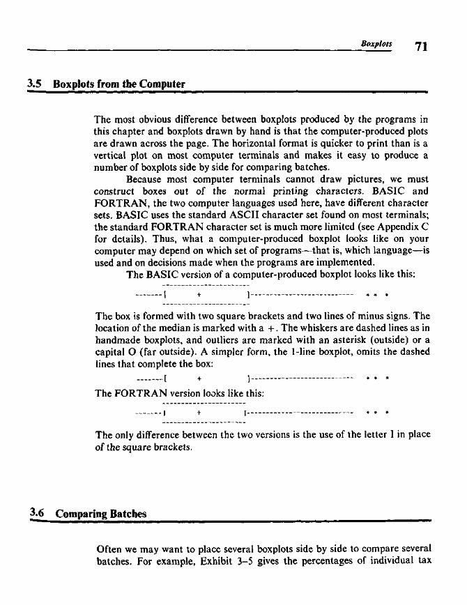
Boxplots n i
3.5 Boxplots from the Computer
The most obvious difference between boxplots produced by the programs inthis chapter and boxplots drawn by hand is that the computer-produced plotsare drawn across the page. The horizontal format is quicker to print than is avertical plot on most computer terminals and makes it easy to produce anumber of boxplots side by side for comparing batches.
Because most computer terminals cannot draw pictures, we mustconstruct boxes out of the normal printing characters. BASIC andFORTRAN, the two computer languages used here, have different charactersets. BASIC uses the standard ASCII character set found on most terminals;the standard FORTRAN character set is much more limited (see Appendix Cfor details). Thus, what a computer-produced boxplot looks like on yourcomputer may depend on which set of programs—that is, which language—isused and on decisions made when the programs are implemented.
The BASIC version of a computer-produced boxplot looks like this:
The box is formed with two square brackets and two lines of minus signs. Thelocation of the median is marked with a +. The whiskers are dashed lines as inhandmade boxplots, and outliers are marked with an asterisk (outside) or acapital O (far outside). A simpler form, the 1-line boxplot, omits the dashedlines that complete the box:
The FORTRAN version looks like this:
The only difference between the two versions is the use of the letter I in placeof the square brackets.
3.6 Comparing Batches
Often we may want to place several boxplots side by side to compare severalbatches. For example, Exhibit 3-5 gives the percentages of individual tax
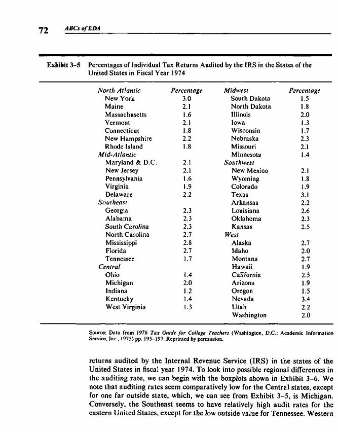
72 ABCs of EDA
Exhibit 3-5 Percentages of Individual Tax Returns Audited by the IRS in the States of theUnited States in Fiscal Year 1974
North AtlanticNew YorkMaineMassachusettsVermontConnecticutNew HampshireRhode Island
Mid-AtlanticMaryland & D.C.New JerseyPennsylvaniaVirginiaDelaware
SoutheastGeorgiaAlabamaSouth CarolinaNorth CarolinaMississippiFloridaTennessee
CentralOhioMichiganIndianaKentuckyWest Virginia
Percentage3.02.11.62.11.82.21.8
2.12.11.61.92.2
2.32.32.32.72.82.71.7
1.42.01.21.41.3
MidwestSouth DakotaNorth DakotaIllinoisIowaWisconsinNebraskaMissouriMinnesota
SouthwestNew MexicoWyomingColoradoTexasArkansasLouisianaOklahomaKansas
WestAlaskaIdahoMontanaHawaiiCaliforniaArizonaOregonNevadaUtahWashington
Percentage1.51.82.01.31.72.32.11.4
2.11.81.93.12.22.62.32.5
2.72.02.71.92.51.91.53.42.22.0
Source: Data from 1976 Tax Guide for College Teachers (Washington, D.C: Academic InformationService, Inc., 1975) pp. 195-197. Reprinted by permission.
returns audited by the Internal Revenue Service (IRS) in the states of theUnited States in fiscal year 1974. To look into possible regional differences inthe auditing rate, we can begin with the boxplots shown in Exhibit 3-6. Wenote that auditing rates seem comparatively low for the Central states, exceptfor one far outside state, which, we can see from Exhibit 3-5, is Michigan.Conversely, the Southeast seems to have relatively high audit rates for theeastern United States, except for the low outside value for Tennessee. Western
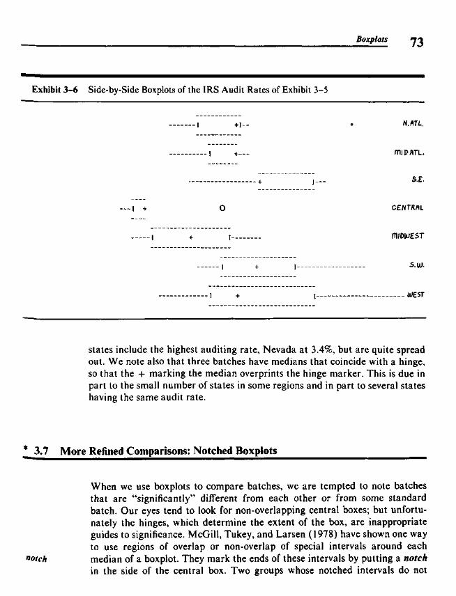
Boxplots '7'i
Exhibit 3-6 Side-by-Side Boxplots of the IRS Audit Rates of Exhibit 3-5
+ 1—
I +— miPATL.
I — S.E.
— I + O CENTRAL
miDUJEST
S.UL
IAJEST
states include the highest auditing rate, Nevada at 3.4%, but are quite spreadout. We note also that three batches have medians that coincide with a hinge,so that the + marking the median overprints the hinge marker. This is due inpart to the small number of states in some regions and in part to several stateshaving the same audit rate.
3.7 More Refined Comparisons: Notched Boxplots
When we use boxplots to compare batches, we are tempted to note batchesthat are "significantly" different from each other or from some standardbatch. Our eyes tend to look for non-overlapping central boxes; but unfortu-nately the hinges, which determine the extent of the box, are inappropriateguides to significance. McGill, Tukey, and Larsen (1978) have shown one wayto use regions of overlap or non-overlap of special intervals around each
notch median of a boxplot. They mark the ends of these intervals by putting a notchin the side of the central box. Two groups whose notched intervals do not
n A ABCs of EDA
overlap can be said to be significantly different at roughly the 5% level. (Thisis an individual 5% level—that is, no allowance is made for the number ofcomparisons considered.)
The notches in these plots are placed symmetrically around themedian, falling at
median ± 1.58 x (H-spr)/V7i.
The multiplying factor, 1.58, combines contributions from three differentsources: the relationship between the H-spread and the (population) standarddeviation, the variability of the sample median, and the factor used in settingconfidence limits. The details underlying the choice of 1.58 are given inSection 3.12 at the end of this chapter.
Computer-produced boxplots indicate notches on the main line of thedisplay. A notched boxplot in BASIC looks like this:
[ > + < ] * « * o 0
In the FORTRAN programs, the notches are marked with parentheses:
Exhibit 3-7 shows the audit data of Exhibit 3-5 with notches added.We note that in some regions, and especially when the median is near a hinge,one of the notches actually falls outside the box. Now we can see, for example,ihat, although we might have been tempted to declare the median audit ratesfor the Mid-Atlantic and Southeast regions significantly different, we cannotbe confident of this difference at the 5% level.
3.8 Using the Programs
The boxplot programs are quite automatic. They produce a display forwhatever data batch is specified. (Again, how you specify a data batch to yourcomputer depends upon how the programs have been implemented.) Theoptions offered by the boxplot programs are the choice of a 1-line or 3-linedisplay and the inclusion or exclusion of notches. The 3-line version looks morelike the hand-drawn boxplot and may be preferred for single batches.However, because multiple 3-line boxplots can become cluttered and may takeup too many lines on a CRT screen,* we often use the 1-line display tocompare more than 3 or 4 groups. One-line notched boxplots can be particu-larly useful for comparing batches.
*A Cathode Ray Tube (CRT) is like a television screen and is used in many computer terminals to displayoutput. Often it can display only 20 lines or so at a time.
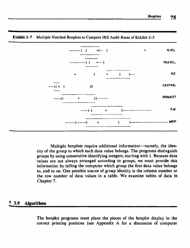
Boxplots
Exhibit 3-7 Multiple Notched Boxplots to Compare IRS Audit Rates of Exhibit 3-5
1 ( + I _ _ ) * H.PilL.
1 ( + — ) miPATL.
—1( + ) O CENTRAL
-—(-I + 5.W.
) T WEST
Multiple boxplots require additional information—namely, the iden-tity of the group to which each data value belongs. The programs distinguishgroups by using consecutive identifying integers, starting with 1. Because datavalues are not always arranged according to groups, we must provide thisinformation by telling the computer which group the first data value belongsto, and so on. One possible source of group identity is the column number orthe row number of data values in a table. We examine tables of data inChapter 7.
t 3.9 Algorithms
The boxplot programs must place the pieces of the boxplot display in thecorrect printing positions (see Appendix A for a discussion of computer
ABCs of EDA
graphics). In addition, the programs must take care that if two charactersmaking up the display fall at the same printing position, the one actuallyprinted will convey as much information about the plot as possible. Theprograms accomplish this by first constructing each line of the boxplot displayin an array and then printing the contents of the array.
Characters are positioned on the output line according to the plot scale.nice position The logical width of one character position, called the nice position width,width NPW, is found by using the utility plot-scaling routines (see Appendix A). The
number of the printing position that corresponds to the data value, y, can thenbe found as
[(y - min{y))/NPW] + 1
where min(>>) is the minimum data value and [ ] indicates the integer part.The programs ensure correct priority of plot symbols by placing them
in the output array in a specified order, allowing later entries to replace earlierones if they fall at the same character position. The correct placementorder—and, hence, the order from least important to most important—is:whisker hyphens (-); outside values (*); far outside values (0); hinges ([ ] orI); notches, if any (> < or ( )); and median ( + ). It is usually easy to read evenseverely distorted boxplots generated in this order. Thus,
is a boxplot in which the H-spread is small and the median is offset to the highend and thus occupies the same position as the upper hinge. In a very extremecase,
* + • 00
is a display in which most of the data clusters very near the median and thereare a few very extreme outliers. Exhibit 3-7 includes several boxes in whichoverprinting is evident. In each of these, the careful choice of symbol hierarchyhas preserved the full information in the plot. Multiple boxplots require asingle scale that is usually chosen to cover the range of the entire combineddata set.
FORTRAN
The FORTRAN programs for creating and displaying boxplots consist ofthree subroutines, BOXES, BOXP, and BOXTOP, and the function PLTPOS. Thedisplay of one or several boxplots is initiated by the statement
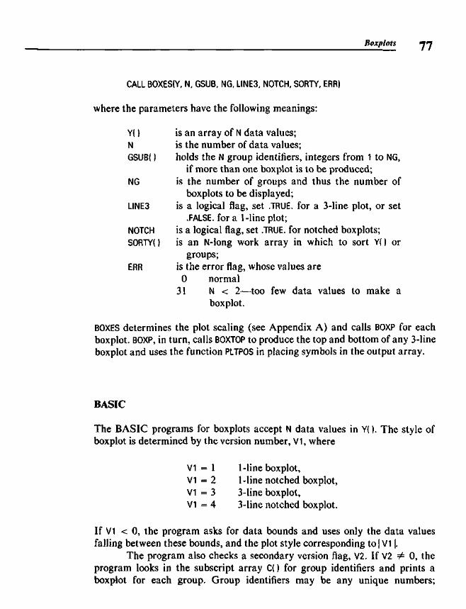
BoxplotS HH
CALL BOXES(Y, N, GSUB, NG, LINE3, NOTCH, SORTY, ERR)
where the parameters have the following meanings:
Y() is an array of N data values;
N is the number of data values;GSUB() holds the N group identifiers, integers from 1 to NG,
if more than one boxplot is to be produced;NG is the number of groups and thus the number of
boxplots to be displayed;LINE3 is a logical flag, set .TRUE, for a 3-line plot, or set
.FALSE, for a 1-line plot;NOTCH is a logical flag, set .TRUE, for notched boxplots;SORTY() is an N-long work ar ray in which to sort Y() or
groups;ERR is the error flag, whose values are
0 normal31 N < 2—too few data values to make a
boxplot.
BOXES determines the plot scaling (see Appendix A) and calls BOXP for eachboxplot. BOXP, in turn, calls BOXTOP to produce the top and bottom of any 3-lineboxplot and uses the function PLTPOS in placing symbols in the output array.
BASIC
The BASIC programs for boxplots accept N data values in Y(). The style ofboxplot is determined by the version number, V1, where
V1 = 1 1-line boxplot,V1 = 2 1-line notched boxplot,V1 = 3 3-line boxplot,V1 = 4 3-line notched boxplot.
If V1 < 0, the program asks for data bounds and uses only the data valuesfalling between these bounds, and the plot style corresponding to | V11.
The program also checks a secondary version flag, V2. If V2 # 0, theprogram looks in the subscript array C() for group identifiers and prints aboxplot for each group. Group identifiers may be any unique numbers;
no ABCs of EDA
sequential integers are simplest. Multiple boxplots use a single global scaleand are printed in group-number order. Each group is labeled with its groupnumber, if that label is less than 5 characters long. Boxplots are scaled to fitbetween the margins, MO and M9.
The BASIC program does not change X() or R().
t 3.10 Implementation Details
The boxplot programs depend on the available character set more heavily thando any of the other computer programs in this book. FORTRAN program-mers are likely to have available a larger set of characters than are in theFORTRAN standard. They may wish to substitute non-FORTRAN charac-ters when these are available.
The variable that identifies the groups for a multiple boxplot should beimplemented as a data vector if at all possible. Note that we have also useddata vectors to hold row and column subscripts for tables in Section 7.3.
t 3.11 Further Refinements in Display
Many readers may have available a device that enables their computer to drawdisplays made up of lines. Boxplots are very well suited to many of thesecomputer graphics devices because boxplots consist almost entirely of verticaland horizontal lines. The same principles used to determine the scale of theplots in the programs provided in this chapter can be used for such displays.
In the paper mentioned in Section 3.7, McGill, Tukey, and Larsensuggest making the width of a boxplot (the fatness of the box) proportional toyfn, the square root of the batch count. While we could approximate avariable-width boxplot with a "variable-line" boxplot, printer plotting does notprovide sufficient precision to justify the trouble. Readers with access to moresophisticated graphics devices that are capable of drawing lines may wish toexperiment with this idea.
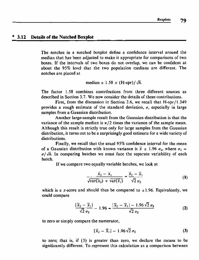
Boxplots
3.12 Details of the Notched Boxplot
The notches in a notched boxplot define a confidence interval around themedian that has been adjusted to make it appropriate for comparisons of twoboxes. If the intervals of two boxes do not overlap, we can be confident atabout the 95% level that the two population medians are different. Thenotches are placed at
median ± 1.58 x (H-spr)/V«.
The factor 1.58 combines contributions from three different sources asdescribed in Section 3.7. We now consider the details of these contributions.
First, from the discussion in Section 2.6, we recall that H-spr/1.349provides a rough estimate of the standard deviation, or, especially in largesamples from a Gaussian distribution.
Another large-sample result from the Gaussian distribution is that thevariance of the sample median is 7r/2 times the variance of the sample mean.Although this result is strictly true only for large samples from the Gaussiandistribution, it turns out to be a surprisingly good estimate for a wide variety ofdistributions.
Finally, we recall that the usual 95% confidence interval for the meanof a Gaussian distribution with known variance is 3c ± 1.96 o ,̂ where oj =a/yfn. In comparing batches we must face the separate variability of eachbatch.
If we compare two equally variable batches, we look at
X-y X\ Xj — X\
—— = - * p — - (1)Vvar(x2) + var(x,) V2 a^
which is a z-score and should thus be compared to ±1.96. Equivalently, wecould compare
1*2 ~ *>l . o . l*2 - x, | - 1.96V2o-j- 1 . 9 6 = -?= (2)
V2
m - 1 . 9 6 = -?=
V2 o-j V2 o-j
to zero or simply compare the numerator,
\x2 - 3c,| - 1.96V2O-J (3)to zero; that is, if (3) is greater than zero, we declare the means to besignificantly different. To represent this calculation as a comparison between
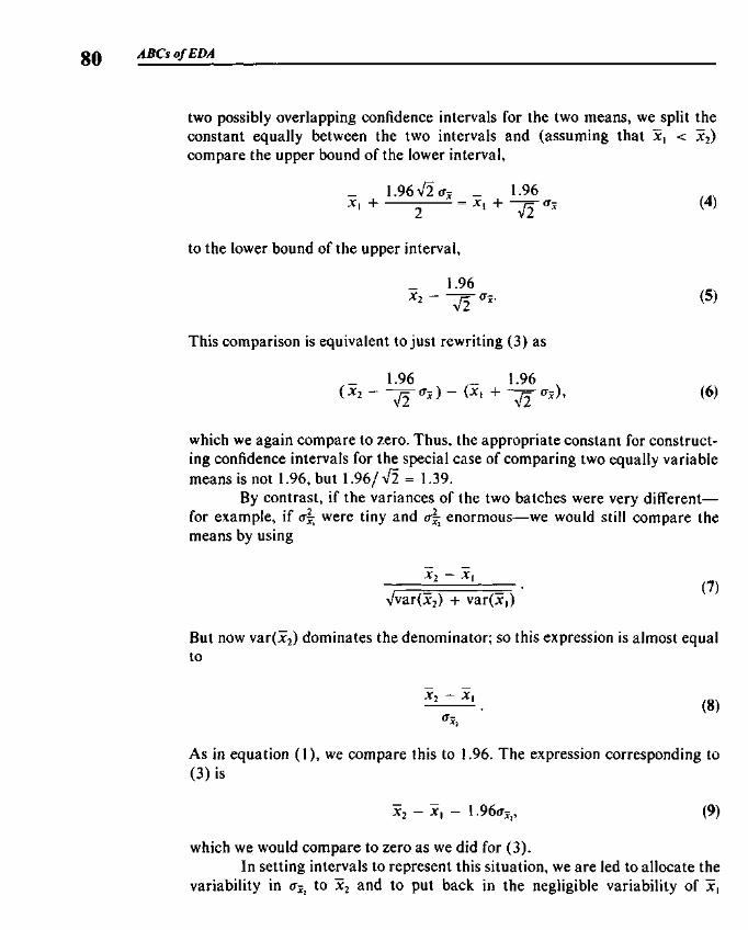
on ABCs of EDA
two possibly overlapping confidence intervals for the two means, we split theconstant equally between the two intervals and (assuming that 3c, < 3c2)compare the upper bound of the lower interval,
5 _ 1.96= *i + ~j[ °x (4)
to the lower bound of the upper interval,
1.96Xl~~42a*- (5)
This comparison is equivalent to just rewriting (3) as
1.96 _ 1.96
which we again compare to zero. Thus, the appropriate constant for construct-ing confidence intervals for the special case of comparing two equally variablemeans is not 1.96, but 1.96/ V2 = 1.39.
By contrast, if the variances of the two batches were very different—for example, if erf; were tiny and a\ enormous—we would still compare themeans by using
x? — -^i
(7)Vvar(x2)
But now var(3c2) dominates the denominator; so this expression is almost equalto
(8)
As in equation (1), we compare this to 1.96. The expression corresponding to(3) is
x 2 - x t - 1.960-5,, (9)
which we would compare to zero as we did for (3).In setting intervals to represent this situation, we are led to allocate the
variability in oj2 to x2 and to put back in the negligible variability of 3c,
Boxplots 81
measured by o-̂ . We thus use
and
x2 ± 1.96crSi
x, ± 1.96a,.
The two extreme situations just described lead to using 1.39 and 1.96as approximate multiplying constants for these intervals. A reasonablecompromise for the general case is the average of the two constants:
(1.96 + 1.39)/2 = 1.7.
Assembling the three factors—the estimate of a from the H-spread,the standard deviation of the median relative to the mean, and the compromisemultiplier for constructing comparison intervals—now gives us
(H-spr/1.349) x V(TT/2) X (1.7/Vn) = 1.58 x H-spr/Vn.
For further discussion of multiplicity and the statistical problem of multiplecomparisons, the interested reader may consult the book by Miller (1966).
References
McGill, Robert, John W. Tukey, and Wayne A. Larsen. 1978. "Variations of BoxPlots," The American Statistician 32:12-16.
Miller, Rupert G. 1966. Simultaneous Statistical Inference. New York: McGraw-Hill.
1976 Tax Guide for College Teachers. 1975. Washington, D.C.: Academic Informa-tion Service, Inc.
Please turn toChapter 1.
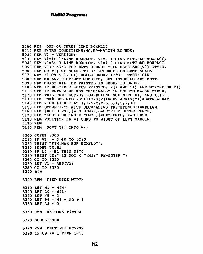
BASIC Programs
ONE OR THREE LINE BOXPLOTENTRY CONDITIONS:M0,M9=MARGIN BOUNDS;VI = VERSION:Vl=l: 1-LINE BOXPLOT, Vl=2 1-LINE NOTCHED BOXPLOT,Vl=3: 3-LINE BOXPLOT, Vl=4 3-LINE NOTCHED BOXPLOTV K O ASKS FOR DATA BOUNDS THEN USES ABS(Vl) STYLE.C9 = # OF BOXES TO BE PRODUCED ON SAME SCALEIF C9 > 1, C() HOLDS GROUP ID'S. THESE CANBE ANY DISTINCT NUMBERS, BUT INTEGERS ARE BEST.BOXES WILL BE PRINTED IN GROUP ID ORDER.IF MULTIPLE BOXES PRINTED, Y() AND C() ARE SORTED ON C()IF DATA WERE NOT ORIGINALLY IN COLUMN-MAJOR ORDER,THIS CAN DESTROY CORRESPONDENCE WITH R() AND X().P9=# DESIRED POSITIONS;P()=CHR ARRAY;Y()=DATA ARRAYNICE #S SET AT 1,1.5,2,2.5,3,4,5,7,10OVERPRINTS WITH DECREASING PRECEDENCE:+=MEDIAN,]=HI HINGE,[=LO HINGE,O=OUTSIDE OUTER FENCE,*=OUTSIDE INNER FENCE,|=EXTREMES,-=WHISKERPOSITION FN =# CHRS TO RIGHT OF LEFT MARGIN
SORT Y() INTO W()
5200 GOSUB 33005210 IF VI >= 0 GO TO 52905220 PRINT "MIN,MAX FOR BOXPLOT";5230 INPUT LO,H1
< HI THEN 5270IS NOT < W;H1;" RE-ENTER
500050105020503050405050506050705080509051005110512051305140515051605170518051855190
REMREMREMREMREMREMREMREMREMREMREMREMREMREMREMREMREMREMREMREMREM
5240 IF L05250 PRINT L0;5260 GO TO 52205270 LET VI = ABS(Vl)5280 GO TO 53305290 REM
5300 REM FIND NICE WIDTH
5310 LET HI = W(N)5320 LET L0 = W(l)5330 LET N5 = 35340 LET P9 = M9 - M0 + 1
5350 LET A8 = 0
5360 REM RETURNS P7=NPW
5370 GOSUB 1900
5380 REM MULTIPLE BOXES?5390 IF C9 <= 1 THEN 5750
82
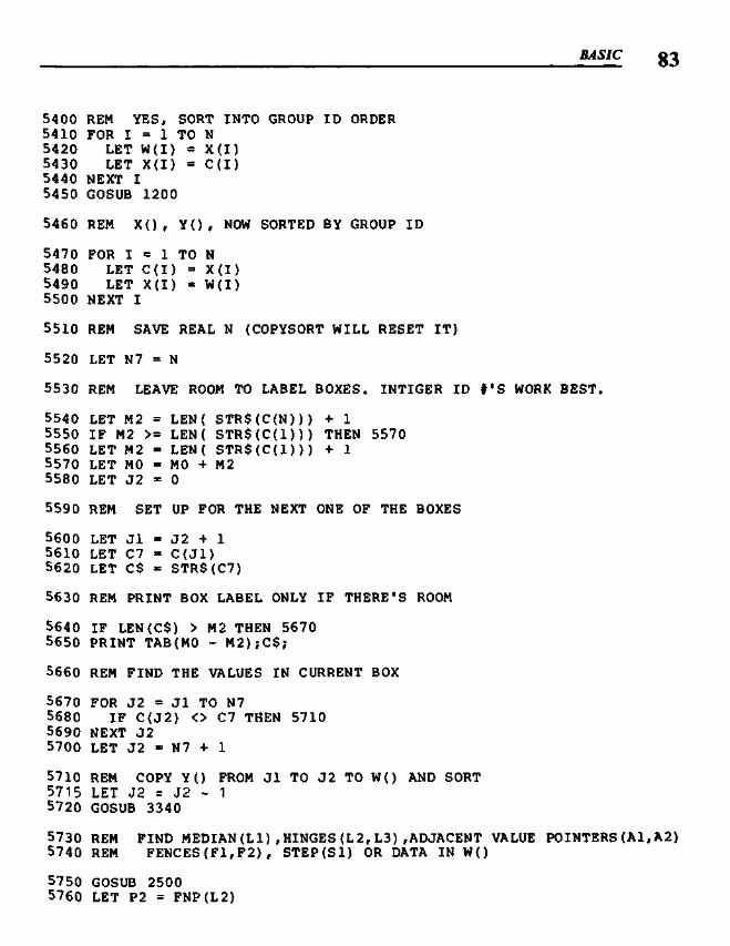
BASIC 83
5400 REM YES, SORT INTO GROUP ID ORDER5410 FOR I * 1 TO N5420 LET W(I) = X(I)5430 LET X(I) = C(I)5440 NEXT I5450 GOSUB 1200
5460 REM X(), Y(), NOW SORTED BY GROUP ID
5470 FOR I = 1 TO N5480 LET C(I) = X(I)5490 LET X(I) = W(I)5500 NEXT I
5510 REM SAVE REAL N (COPYSORT WILL RESET IT)
5520 LET N7 = N
5530 REM LEAVE ROOM TO LABEL BOXES. INTIGER ID #'S WORK BEST.
5540 LET M2 = LEN( STR$(C(N))) + 15550 IF M2 >= LEN( STR$(C(1))) THEN 55705560 LET M2 = LEN( STR$(C(1))) + 15570 LET MO = MO + M25580 LET J2 = 0
5590 REM SET UP FOR THE NEXT ONE OF THE BOXES
5600 LET Jl = J2 + 15610 LET C7 = C(J1)5620 LET C$ = STR$(C7)
5630 REM PRINT BOX LABEL ONLY IF THERE'S ROOM
5640 IF LEN(C$) > M2 THEN 56705650 PRINT TAB(M0 - M2);C$;
5660 REM FIND THE VALUES IN CURRENT BOX
5670 FOR J2 = Jl TO N75680 IF C(J2) <> C7 THEN 57105690 NEXT J25700 LET J2 = N7 + 1
5710 REM COPY Y() FROM Jl TO J2 TO W() AND SORT5715 LET J2 = J2 - 15720 GOSUB 3340
5730 REM FIND MEDIAN(Ll),HINGES(L2,L3),ADJACENT VALUE POINTERS(AlfA2)5740 REM FENCES(F1,F2), STEP(Sl) OR DATA IN W()
5750 GOSUB 25005760 LET P2 = FNP(L2)
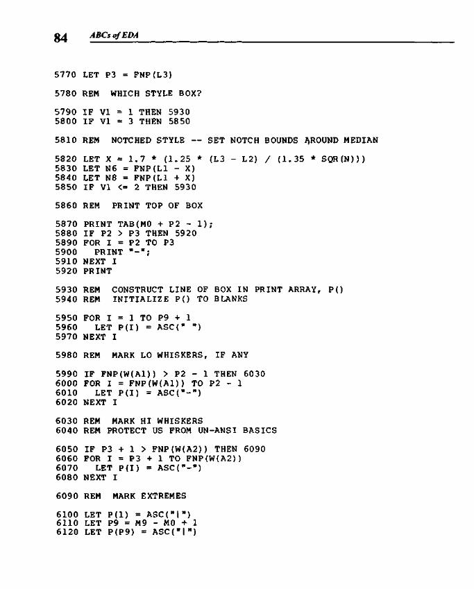
04 ABCs of EDA
5770 LET P3 = FNP(L3)
5780 REM WHICH STYLE BOX?
5790 IF VI = 1 THEN 59305800 IF VI = 3 THEN 5850
5810 REM NOTCHED STYLE — SET NOTCH BOUNDS AROUND MEDIAN
5820 LET X = 1.7 * (1.25 * (L3 - L2) / (1.35 * SQR(N)))5830 LET N6 = FNP(L1 - X)5840 LET N8 = FNP(L1 + X)5850 IF VI <= 2 THEN 5930
5860 REM PRINT TOP OF BOX
5870 PRINT TAB(M0 + P2 - 1);5880 IF P2 > P3 THEN 59205890 FOR I = P2 TO P35900 PRINT "-";5910 NEXT I5920 PRINT
5930 REM CONSTRUCT LINE OF BOX IN PRINT ARRAY, P()5940 REM INITIALIZE P() TO BLANKS
5950 FOR I = 1 TO P9 + 15960 LET P(I) = ASC(" ")5970 NEXT I
5980 REM MARK LO WHISKERS, IF ANY
5990 IF FNP(W(A1)) > P2 - 1 THEN 60306000 FOR I = FNP(W(A1)) TO P2 - 16010 LET P(I) = ASCC-")6020 NEXT I
6030 REM MARK HI WHISKERS6040 REM PROTECT US FROM UN-ANSI BASICS
6050 IF P3 + 1 > FNP(W(A2)) THEN 60906060 FOR I = P3 + 1 TO FNP(W(A2))6070 LET P(I) = ASC("-n)6080 NEXT I
6090 REM MARK EXTREMES
6100 LET P(l) = ASC("|")6110 LET P9 = M9 - MO + 16120 LET P(P9) = ASC("|")
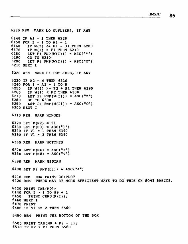
BASIC 85
6130 REM MARK LO OUTLIERS, IF ANY
6140 IF Al = 1 THEN 62206150 FOR I = 1 TO Al - 16160 IF W(I) <= Fl - SI THEN 62006170 IF W(I) > Fl THEN 62106180 LET P( FNP(W(I))) = ASC("*n)6190 GO TO 62106200 LET P( FNP(W(I))) = ASC("O")6210 NEXT I
6220 REM MARK HI OUTLIERS, IF ANY
6230 IF A2 = N THEN 63106240 FOR I = A2 + 1 TO N6250 IF W(I) >= F2 + SI THEN 62906260 IF W(I) < F2 THEN 63006270 LET P( FNP(W(I))) = ASC("*H)6280 GO TO 63006290 LET P( FNP(W(I))) = ASC("O")6300 NEXT I
6310 REM MARK HINGES
6320 LET P(P2) = 916330 LET P(P3) = ASC(n]")6340 IF VI = 1 THEN 63906350 IF VI = 3 THEN 6390
6360 REM MARK NOTCHES
6370 LET P(N6) = ASC(">")6380 LET P(N8) = ASC("<")
6390 REM MARK MEDIAN
6400 LET P( FNP(Ll)) = ASC("+")
6410 REM NOW PRINT BOXPLOT6420 REM THERE MAY BE MORE EFFICIENT WAYS TO DO THIS ON SOME BASICS.
6430 PRINT TAB(MO);6440 FOR I = 1 TO P9 + 16450 PRINT CHR$(P(I));6460 NEXT I6470 PRINT6480 IF VI <= 2 THEN 6560
6490 REM PRINT THE BOTTOM OF THE BOX
6500 PRINT TAB(MO + P2 - 1);6510 IF P2 > P3 THEN 6560
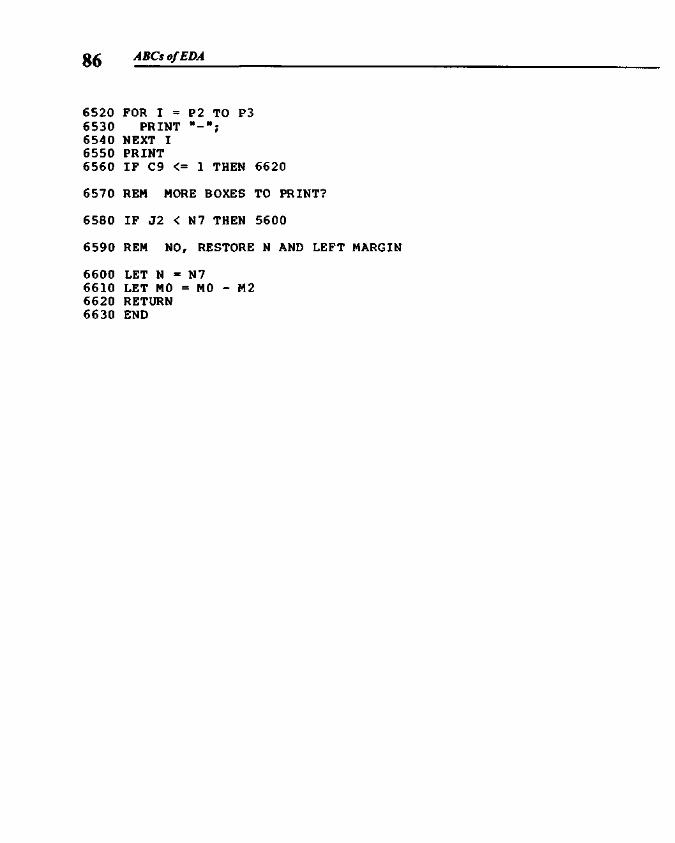
ABCs of EDA
6520 FOR I = P2 TO P36530 PRINT "-";6540 NEXT I6550 PRINT6560 IF C9 <= 1 THEN 6620
6570 REM MORE BOXES TO PRINT?
6580 IF J2 < N7 THEN 5600
6590 REM NOr RESTORE N AND LEFT MARGIN
6600 LET N = N76610 LET M0 = M0 - M26620 RETURN6630 END
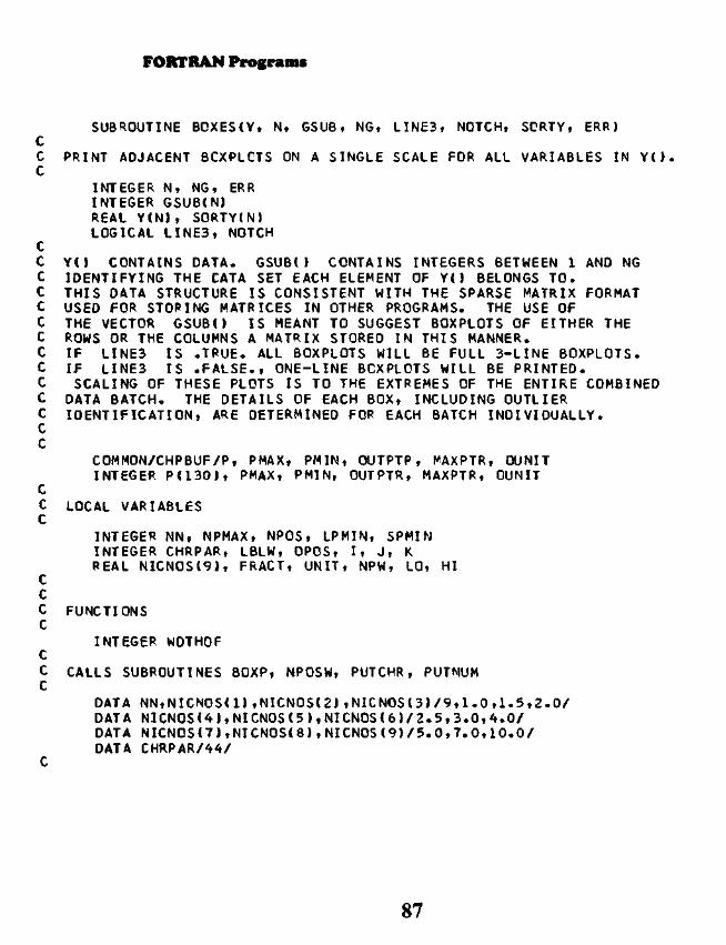
FORTRAN Programs
SUBROUTINE BOXESCY, N, GSUB, NG, LINE3, NOTCH, SORTY, ERR)CC PRINT ADJACENT BCXPLCTS ON A SINGLE SCALE FOR ALL VARIABLES IN Y()C
INTEGER N, NG, ERRINTEGER GSUB(N)REAL Y(N), SORTY(N)LOGICAL LINE3t NOTCH
CC Y() CONTAINS DATA. GSUB() CONTAINS INTEGERS BETWEEN 1 AND NGC IDENTIFYING THE CATA SET EACH ELEMENT OF Y() BELONGS TO.C THIS DATA STRUCTURE IS CONSISTENT WITH THE SPARSE MATRIX FORMATC USED FOR STORING MATRICES IN OTHER PROGRAMS. THE USE OFC THE VECTOR GSUBO IS MEANT TO SUGGEST BOXPLOTS OF EITHER THEC ROWS OR THE COLUMNS A MATRIX STORED IN THIS MANNER.C IF LINE3 IS .TRUE. ALL BOXPLOTS WILL BE FULL 3-LINE BOXPLOTS.C IF LINE3 IS .FALSE., ONE-LINE BCXPLOTS WILL BE PRINTED.C SCALING OF THESE PLOTS IS TO THE EXTREMES OF THE ENTIRE COMBINEDC DATA BATCH. THE DETAILS OF EACH BOX, INCLUDING OUTLIERC IDENTIFICATION, ARE DETERMINED FOR EACH BATCH INDIVIDUALLY.CC
COMMON/CHPBUF/P, PMAX, PMIN, OUTPTP , MAXPTR, OUNITINTEGER P(130), PMAX, PMIN, OUTPTR, MAXPTR, OUNIT
CC LOCAL VARIABLESC
INTEGER NN, NPMAX, NPOS, LPMIN, SPMININTEGER CHRPAR, LBLW, OPOS, I, J, KREAL NICN0S(9), FRACT, UNIT, NPW, LO, HI
C
cC FUNCTIONSC
INTEGER WDTHOFCC CALLS SUBROUTINES BOXP, NPOSW, PUTCHR, PUTMUMC
DATA NN,NICNOS(1),NICNOS(2),NICNOS(3)/9,1.0 ,1.5,2.0/DATA NICNOS(4),NICN0S(5),NICNOS(6)/2.5,3.0,4.0/DATA NICNOS<7),NICNOS(8),NICNOS(9)/5.0,7.0,10.0/DATA CHRPAR/44/
87
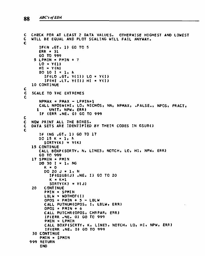
oo ABC's of EDA
C CHECK FOR AT LEAST 2 DATA VALUES. OTHERWISE HIGHEST AND LOWESTC WILL BE EQUAL AND PLOT SCALING WILL FAIL ANYWAY.C
IF(N .GT. 1) GO TO 5ERR = 31GO TO 999
5 LPMIN = PMIN • 7LO = Y(l)HI = Y(NJDO 10 I M , h
IFCLO .GT. Y( I) ) LO = Y d )IF(HI .LT. Y d ) ) HI = Y d )
10 CONTINUECC SCALE TO THE EXTREMESC
NPMAX = PMAX - LPMIN+1CALL NPOSW(HI, LO, NICNOS, NN, NPMAX, .FALSE., NPOS, FRACT,1 UNIT, NPW, ERR)IF (ERR .NE. 0) GO TO 999
CC NOW PRINT ALL THE BOXES.C DATA SETS ARE IDENTIFIED BY THEIR CODES IN GSUBOC
IF (NG .GT. 1) GO TO 17DO 15 K « It N
SORTY(K) ^ Y(K)15 CONTINUE
CALL BOXPCSORTY, N, LINE3, NOTCH, LO, HI, NPW, ERR)GO TO 999
17 SPMIN - PMINDO 30 1 » It NG
K * 0DO 20 J * It N
I F ( G S U B U ) . N E . I ) GO TO 20K * K + lSORTY(K) * Y ( J )
20 CONTINUEPMIN = SPMINLBLW - WDTHCF(I)OPOS - PMIN + 5 - LBLWCALL PUTNUM(OPOS, I , LBLW, ERR)OPOS » PMIN + 6CALL PUTCHRCOPOS, CHRPAR, ERR)IF(ERR . N E . 0) GO TO 999PMIN - LPMINCALL BOXPCSCRTY, K, LINE3, NOTCH, LO, HI, NPW, ERR)IF(ERR .NE. 0) GO TO 999
30 CONTINUEPMIN - SPMIN
999 RETURNEND
FORTRAN
SUBROUTINE BOXP(SORTY, Nt L I N E 3 , NOTCH, LO, H I , NPW, ERR)CCC PRINT A BCXPLOT CF THE DATA IN SORTYOCC
INTEGER N, EP RREAL SORTY(N), LO, H I , NPWLOGICAL L I N E 3 , NOTCH
CC PLOT SCALING HAS BEEN DONE BY THE CALLING PROGRAM WITH NEEDEDC INFORMATION PASSED I N AS LO (THE LOW EXTREME), HI (THE HIGHC EXTREME) AND NPW (THE NICE POSITION WIDTH FOR PLOTTING).C TYPICALLY THIS WILL BE ONE OF SEVERAL BOXPLOTS SCALED AND PRINTEDC TOGETHER.C IF LINE3 IS .TRUE. A 3 -L INE BOXPLOT (FULL BOXES) IS PRINTED.C IF NOT, THE SIMPLE ONE-LINE BOXPLOT IS PRINTED. BOTH CONVEY THEC SAME INFORMATION, BUT THE 3-L INE VERSION MAY LOOK NICER.C I F NOTCH IS .TRUE. A CONFIDENCE INTERVAL AROUND THE MEDIAN ISC INDICATED WITH PARENTHESES.C
COMMON/CHRBUF/P, PMAX, PMIN, OUTPTR, MAXPTR, OUNITINTEGER P ( 1 3 O ) , PMAX, PMIN, OUTPTR, MAXPTR, OUNIT
CC FUNCTIONSC
INTEGER PLTPOSCC CALL SUBROUTINES BOXTOP, PRINT, PUTCHR, YINFOCC LOCAL VARIABLESC
INTEGER I t IADJL, IADJH, IFROM, ITO, LPMAX, LPMININTEGER OPOS, C H I , CHO, CHSTAR, CHMIN, CHPLUSt CHRPAR, CHLPARREAL MED, HL, HH, ADJL» ADJH, STEPREAL FLOATN, NSTEP, LNOTCH, HNOTCH, OFENCL, OFENCH
CDATA C H I , CHO, CHPLUSt CHMIN, CHSTAR/9, 15 , 3 9 , 4 0 , 4 1 /DATA CHLPAR, CHFPAR/43, 4 4 /
CLPMAX = PMAXLPMIN = PMINCALL YINFO(SORTY, N, MED, HL, HH, ADJLt ADJH, IADJL, IADJH,
1 STEP, ERR)I F (ERR . N E . 0) GO TO 999FLOATN = FLOAT(N)NSTEP = 1 .7 * ( 1 . 2 5 * ( H H - H L ) / ( 1 . 3 5 * SQRT(FLOATN)))LNOTCH = MED - NSTEPHNOTCH = MED + NSTEP
C PRINT TOP OF BOX, IF 3 -L INE VERSIONI F ( L I N E 3 ) CALL BOXTOP(LO, H I , HL , HH, NPW, ERR)IF(ERR . N E . 0 ) GO TO 999
<)() ABCs of EDA
HIHITO
, NPWt, NPW,31
EPP)ERR)
cC FILL CENTER LINE OF DISPLAY — NOTE CAREFUL HIERARCHYC OF OVERPRINTING. LAST PLACED CHARACTER IS ONLY ONE TO APPEARCC MARK WHISKERSC
IFROM = P L T P O S ( A D J L T LO, H I , NPW, ERR)ITO = PLTPOS(HLT LO, H I , NPW, ERR) - 1I F ( I F R O M . G T . I T O ) GO TO 2 1DO 20 I = IFROM, ITO
CALL PUTCHP. ( I t CHMIN, ERP)20 CONTINUE21 CONTINUE
IFROM = PLTPOS(HH, LO,ITO = PLTPOS(ADJH, LO,IF (IFROM . G T . ITO) GODO 30 I = IFPCM, ITC
CALL PUTCHRU, CHMIN, EPP )30 CONTINUE31 CONTINUE
CC MARK LOW OUTLIERS, IF ANYC
IF(IADJL .EQ. 1) GO TO 41OFENCL = HL - 2.0*STEPITO = IADJL - 1DO 40 I = 1, ITO
OPOS = PLTPOS(SORTY(I), LO, HI, NPW, ERR)IF(SORTYU) .LT. OFENCL) CALL PUTCHR(OPOS, CHO, ERP)IF(SORTYd) .GE. OFENCL) CALL PUTCHR(OPOS, CHSTAR, EPP)
40 CONTINUE41 CONTINUE
CC MARK HIGH OUTLIERS, IF ANYC
IF(IADJH .EQ. N) GO TO 51OFENCH = HH + 2.0*STEPIFROM = IADJH + 1DO 50 I = IFROM, N
OPOS = PLTPOS(SOPTY(I), LO, HI, NPW, ERR)IF(SORTYU) .GT. OFENCH) CALL PUTCHR(OPOS, CHO, ERR)IF(SORTYU) .LE. OFENCH) CALL PUTCHR(OPOS, CHSTAR, ERR)
50 CONTINUE51 CONTINUE
FORTRAN
CC MARK HINGES, NOTCHES, AND MEDIANC
OPOS = PLTPOS(HLt LO, H I , NPW, ERR)CALL PUTCHR1OPOS, C H I , ERP)OPOS = PLTPOSiHH, LO, H I , NPW, ERR)CALL PUTCHR1OPOS, C H I , ERP)OPOS = PLTPOS(LNOTCH, LO, H I , NPW, ERR)IF(NCTCH) CALL PUTCHR(OPOS, CHLPAR, ERR)OPOS = PLTPOS(HNOTCH, LO, HI, NPW, ERR)IF(NOTCH) CALL PUTCHR(OPOS, CHRPAR, ERR)OPOS = PLTPOS(MED, LO, H I , NPW, ERR)CALL PUTCHR (OPOS, CHPLUS, ERR)
CC AND PRINT THE BOXPLOTC
IFCEPR . N E . 0 ) GO TO 999CALL PRINT
CC PRINT THE BOTTOM OF THE BOXC
IFCLINE3) CALL BOXTOPiLO, HI, HL , HH, NPW, ERR)999 RETURN
END
SUBROUTINE B0XT0PU0, HI, HL, HH, NPW, ERR)C
REAL LO, HI, HL, HH, NPWINTEGER ERR
CC PRINT THE TOP OR BOTTOM OF A BOXPLOT DISPLAYCC HI AND LO ARE EDGES OF THE PLOTTING REGION USED BY THE PLTPOSC FUNCTION.C HL AND HH ARE THE LOW AND HIGH HINGESC NPW IS THE NICE POSITION WIDTH SET BY THE PLOT SCALING ROUTINESCC LOCAL VARIABLESC
INTEGER I , IFROM, ITO, CHMINCC FUNCTIONC
INTEGER PLTPOSCC DATAC
DATA CHMIN/40/
91
92 ABCs of EDA
1011
999
IFROM = PLTPOStHLt LOt H I , NPW, ERR)ITO = PLTPOS(HH, LO, H I , NPW, ERR)IF (IFROM . G T , ITO) GO TO 11DO 10 I « IFPOM, ITO
CALL PUTCHRU, CHMIN, EPP )CONTINUECONTINUEI F (ERR .EQ. 0) CALL PRINTRETURNEND
INTEGER FUNCTION PLTPOS(X, LO, H I , NPW, ERR)
FIND THE POSITION CORRESPONDING TO X ON PLOT BOUNDEDBETWEEN LO AND HI AND SCALED ACCORDING TO NPW.
REAL X, LO, H I , NPWINTEGER ERR
FUNCTIONS
INTEGER INTFN
COMMON
COMMON /CHRBUF/P, PMAX, PMIN, OUTPTR, MAXPTR, OUNITINTEGER P(130), PMAX, PMIN, OUTPTR, MAXPTR, OUNIT
PLTPOS = INTFN((X-LO)/NPW, ERR) + PMINIF (PLTPOS .LT. PMIN) PLTPOS = PMINIF (PLTPOS .GT. PMAX) PLTPOS = PMAXRETURNEND
Chapter 4x-y Plotting
ordered pair
arraysubscript
Data that come as paired observations are usually displayed by drawing an x-yplot. This is a very common procedure and a powerful exploratory data-analysis tool. Plots of y versus x show at a glance how x and y are related toeach other. For example, if larger >>-values are often paired with largerx-values and smaller ^-values with smaller jc-values, that association will beevident in the plot. If the x-y points fall on or near a straight line, that will beclear from the plot—and we may be able to say more about the relationshipbetween x and y, as we will see in Chapter 5. If the pattern of the plot shows asmooth change in >>-values as we move from each x-value to the next largerone, we may want to look for a smooth pattern with techniques discussed inChapter 6. And, as always, we will check the plot for any extraordinary pointsthat do not seem to fit whatever pattern is present, for these points maydeserve special attention.
x-y data are often presented as ordered pairs, (x, y)—one ordered pairfor each observation. Alternatively, such data can come as a pair of columns ofnumbers—one column for the x-values and one for the corresponding ^-values.Such columns, whose values are in an established order (in this case, pairedwith each other), are examples of arrays. To refer to the ith value in an array,we attach the subscript i to the name of the array; for example, xt. The ith x-yobservation is (xh y().
93
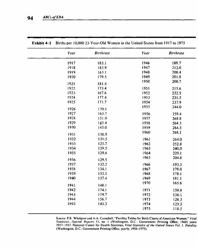
Q4 ABCs of EDA
Exhibit 4-1 Births per 10
Year
,000 23-Year-Old Women
Birthrate
intheUnited States
Year
from 1917 to 1975
Birthrate
1917191819191920
19211922192319241925
19261927192819291930
19311932193319341935
19361937193819391940
19411942194319441945
183.1183.9163.1179.5
181.4173.4167.6177.4171.7
170.1163.7151.9145.4145.0
138.9131.5125.7129.5129.6
129.5132.2134.1132.1137.4
148.1174.1174.7156.7143.3
19461947194819491950
19511952195319541955
19561957195819591960
19611962196319641965
19661967196819691970
19711972197319741975
189.7212.0200.4201.8200.7
215.6222.5231.5237.9244.0
259.4268.8264.3264.5268.1
264.0252.8240.0229.1204.8
193.3179.0178.1181.1165.6
159.8136.1126.3123.3118.5
Source: P.K. Whelpton and A.A. Campbell, "Fertility Tables for Birth Charts of American Women," VitalStatistics—Special Reports 51, no. 1 (Washington, D.C.: Government Printing Office, 1960) years1917-1957. National Center for Health Statistics, Vital Statistics of the United States Vol. I, Natality(Washington, D.C.: Government Printing Office, yearly, 1958-1975).
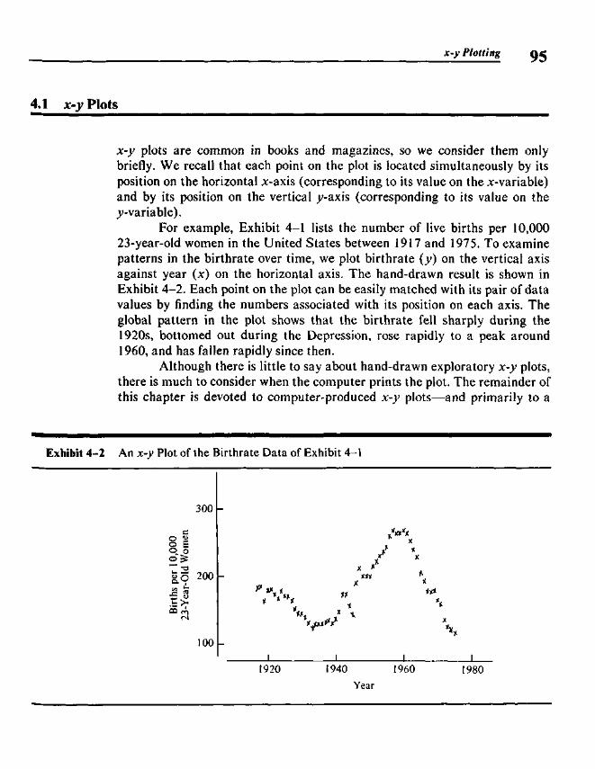
x-y Plotting 95
4.1 x-y Plots
x-y plots are common in books and magazines, so we consider them onlybriefly. We recall that each point on the plot is located simultaneously by itsposition on the horizontal x-axis (corresponding to its value on the x-variable)and by its position on the vertical y-axis (corresponding to its value on the^-variable).
For example, Exhibit 4-1 lists the number of live births per 10,00023-year-old women in the United States between 1917 and 1975. To examinepatterns in the birthrate over time, we plot birthrate (y) on the vertical axisagainst year (x) on the horizontal axis. The hand-drawn result is shown inExhibit 4-2. Each point on the plot can be easily matched with its pair of datavalues by finding the numbers associated with its position on each axis. Theglobal pattern in the plot shows that the birthrate fell sharply during the1920s, bottomed out during the Depression, rose rapidly to a peak around1960, and has fallen rapidly since then.
Although there is little to say about hand-drawn exploratory x-y plots,there is much to consider when the computer prints the plot. The remainder ofthis chapter is devoted to computer-produced x-y plots—and primarily to a
Exhibit 4-2 An x-y Plot of the Birthrate Data of Exhibit 4-1
c
o EO o
irth
sY
ear-
03 co
300
200
100
-
<
-1
*****h x
* x/ *
x *w <
1 1 1
1920 1940 1960Year
1980
ABCs of EDA
particular type of plot designed for exploratory data analysis and for interac-tive computing on a standard typewriter-style computer terminal. If you donot intend to use a computer in your exploratory analyses, you can skip the restof this chapter without any loss of continuity. If your computer system isalready equipped with some other version of x-y plotting (as it will almostcertainly be if you are using a statistical package), you may prefer tosubstitute that version for the method presented here. Nevertheless, youshould read the rest of this chapter because it includes fundamental ideasabout computer-printed plots and provides a useful background for anyoneusing the computer to print x-y plots.
4.2 Computer Plots
Most computer programs for x-y plots concentrate on making them nice insome chosen way. The programs presented here concentrate on making theplot concise, so that it can be generated quickly on a computer terminal, andon making the scaling and labeling of the plot natural and close to what wemight choose if we were drawing it by hand.
In drawing a plot by hand, we can place points exactly where theybelong, guided by the ruled grid lines of the graph paper. A point can fall on agrid line or anywhere between the sets of lines. However, computer terminalsare usually limited to choosing a character position across the line to representthe jc-coordinate, choosing a print line on the page to represent the y-coordinate, and printing a character at that location. We may think of such acomputer plot as being drawn on graph paper on which each box of the gridmust either be entirely colored in or left blank. To make matters worse, theboxes are not even square, since printing characters are usually about twice astall as they are wide. Nevertheless, such plots can be made easy to read andare valuable ways to display data. Exhibit 4-3 shows a fairly typical computer-terminal plot of the birthrate in Exhibit 4-1 with the character 0 as theplotting symbol.
4.3 Condensed Plots
Since computer plots must use either all of a "character box" or none of it, weare tempted to make the plots large so that each character box will have a
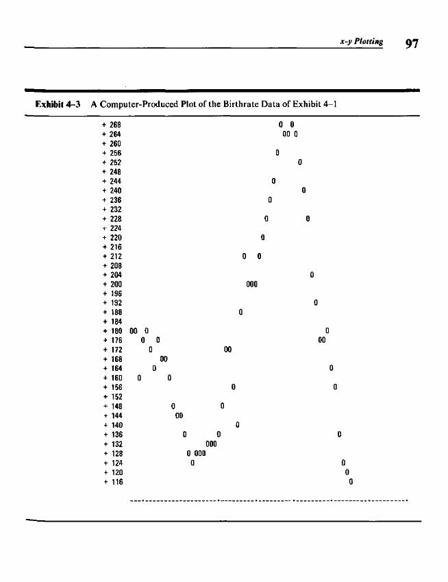
x-y Plotting QH
Exhibit 4-3 A Computer-Produced Plot of the Birthrate Data of Exhibit 4-1
+ 268 0 0+ 264 00 0+ 260+ 256 0+ 252 0+ 248+ 244 0+ 240 0+ 236 0+ 232+228 0 0+ 224+ 220 0+ 216+212 0 0+ 208+ 204 0+ 200 000+ 196+ 192 0+ 188 0+ 184+ 180 00 0 0+ 176 0 0 00+ 172 0 00+ 168 00+ 164 0 0+ 160 0 0+156 0 0+ 152+148 0 0+ 144 00+ 140 0+136 0 0 0+ 132 000+ 128 0 000+ 124 0 0+ 120 0+ 116 0
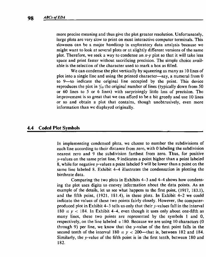
ABCs of EDA
more precise meaning and thus give the plot greater resolution. Unfortunately,large plots are very slow to print on most interactive computer terminals. Thisslowness can be a major handicap in exploratory data analysis because wemight want to look at several plots or at slightly different versions of the sameplot. Therefore, we seek a way to condense an x-y plot so that it will take lessspace and print faster without sacrificing precision. The simple choice avail-able is the selection of the character used to mark a box as filled.
We can condense the plot vertically by squeezing as many as 10 lines ofplot into a single line and using the printed character—say, a numeral from 0to 9—to indicate the original line occupied by the point. This devicereproduces the plot in % the original number of lines (typically down from 50or 60 lines to 5 or 6 lines) with surprisingly little loss of precision. Theimprovement is so great that we can afford to be a bit greedy and use 10 linesor so and obtain a plot that contains, though unobtrusively, even moreinformation than we displayed originally.
4.4 Coded Plot Symbols
In implementing condensed plots, we choose to number the subdivisions ofeach line according to their distance from zero, with 0 labeling the subdivisionnearest zero and 9 the subdivision farthest from zero. Thus, for positive^-values on the same print line, 9 indicates a point higher than a point labeled8, while for negatives-values a point labeled 9 will be lower than a point on thesame line labeled 8. Exhibit 4-4 illustrates the condensation in plotting thebirthrate data.
Comparing the two plots in Exhibits 4-3 and 4-4 shows how condens-ing the plot uses digits to convey information about the data points. As anexample of the details, let us see what happens to the first point, (1917, 183.1),and the fifth point, (1921, 181.4), in these plots. In Exhibit 4-2 we couldindicate the values of these two points fairly closely. However, the computer-produced plot in Exhibit 4-3 tells us only that their ^-values fall in the interval180 < y < 184. In Exhibit 4-4, even though it uses only about one-fifth asmany lines, these two points are represented by the symbols 1 and 0,respectively, on the line labeled + 180. Because we are using 10 characters (0through 9) per line, we know that the >>-value of the first point falls in thesecond tenth of the interval 180 < y < 200—that is, between 182 and 184.Similarly, the .y-value of the fifth point is in the first tenth, between 180 and182.
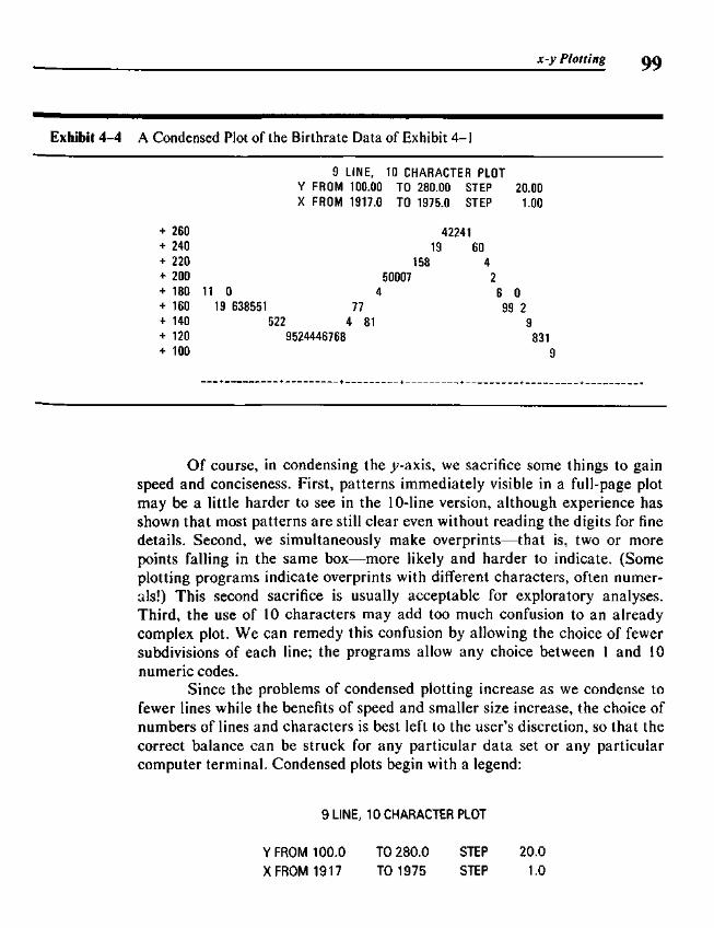
x-y Plotting QQ
Exhibit 4-4 A Condensed Plot of the Birthrate Data of Exhibit 4-1
9 LINE, 10 CHARACTER PLOT
Y FROM 100.00 TO 280.00 STEP 20.00
X FROM 1917.0 TO 1975.0 STEP 1.00
+ 260 42241
+ 240 19 60
+ 220 158 4
+ 200 50007 2
+ 180 11 0 4 6 0
+ 160 19 638551 77 99 2
+ 140 522 4 81 9
+ 120 9524446768 831
+ 100 9
Of course, in condensing the >>-axis, we sacrifice some things to gainspeed and conciseness. First, patterns immediately visible in a full-page plotmay be a little harder to see in the 10-line version, although experience hasshown that most patterns are still clear even without reading the digits for finedetails. Second, we simultaneously make overprints—that is, two or morepoints falling in the same box—more likely and harder to indicate. (Someplotting programs indicate overprints with different characters, often numer-als!) This second sacrifice is usually acceptable for exploratory analyses.Third, the use of 10 characters may add too much confusion to an alreadycomplex plot. We can remedy this confusion by allowing the choice of fewersubdivisions of each line; the programs allow any choice between 1 and 10numeric codes.
Since the problems of condensed plotting increase as we condense tofewer lines while the benefits of speed and smaller size increase, the choice ofnumbers of lines and characters is best left to the user's discretion, so that thecorrect balance can be struck for any particular data set or any particularcomputer terminal. Condensed plots begin with a legend:
9 LINE, 10 CHARACTER PLOT
Y FROM 100.0 TO 280.0 STEP 20.0
X FROM 1917 TO 1975 STEP 1.0
ABCsofEDA
Exhibit 4-5 A 6-Line, 4-Character Plot of the Birthrate Data of Exhibit 4-1
24021018015012090
Y FROM
X FROM
00 0
13 3232210
90.00
1917.00
01
3303321011111123 3
TO 270.00
TO 1975.0
STEP
STEP
023333310
0123
222231
30.00
1.000
033 21
2003
The legend tells how many lines the plot actually requires and how finely thelines are subdivided—that is, the number of characters. It then reports theextent of the data values accommodated by the entire plot and the range ofdata values accommodated by each line (y STEP) and by each horizontalcharacter position (x STEP). Together, these make it easy to determine themagnitude of the data values (the >>-axis labels do not include decimal points)and to translate any particular plotted point into its numeric value. Becausethe >>-axis labels report the value of the inner (near zero) edge of each line, thej>-bounds reported in the legend will typically extend beyond the outer axislabels. Note that a 40-line, 1-character plot is essentially the standard x-y plotmade on a computer terminal. Indeed, that is how Exhibit 4-3 was generated.Exhibit 4-5 shows a 6-line, 4-character plot of the birthrate data. This form ofthe display was originally proposed by Andrews and Tukey (1973).
4.5 Condensed Plots and Stem-and-Leaf Displays
Astute readers may have noticed a resemblance between condensed plots andstem-and-leaf displays. The >;-axis labels are similar to stems, and thecharacters chosen to provide additional information about the ^-values aremuch like leaves. All we have done is stretch the leaves across the pageaccording to the value of some other variable represented on the x-axis.
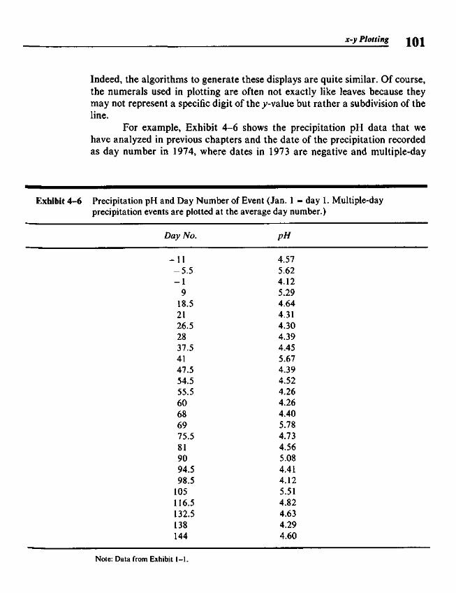
x-y Plotting
Indeed, the algorithms to generate these displays are quite similar. Of course,the numerals used in plotting are often not exactly like leaves because theymay not represent a specific digit of the j>-value but rather a subdivision of theline.
For example, Exhibit 4-6 shows the precipitation pH data that wehave analyzed in previous chapters and the date of the precipitation recordedas day number in 1974, where dates in 1973 are negative and multiple-day
Exhibit 4-6 Precipitation pH and Day Number of Event (Jan. 1 = day 1. Multiple-dayprecipitation events are plotted at the average day number.)
Day No. pH
- 1 1 4.57-5 .5 5.62- 1 4.12
9 5.2918.5 4.6421 4.3126.5 4.3028 4.3937.5 4.4541 5.6747.5 4.3954.5 4.5255.5 4.2660 4.2668 4.4069 5.7875.5 4.7381 4.5690 5.0894.5 4.4198.5 4.12
105 5.51116.5 4.82132.5 4.63138 4.29144 4.60
Note: Data from Exhibit 1-1.
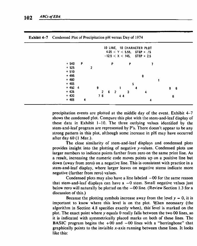
1 0 2 ABCsofEDA
Exhibit 4-7 Condensed Plot of Precipitation pH versus Day of 1974
10 LINE, 10 CHARACTER PLOT4.05 < Y < 5.55, STEP = .15
-12.5 < X < 145, STEP = 2.5
+ 540 P P P 7+ 525 2+ 510+ 495 8+ 480+ 465 5+ 450 4 9 1 4+ 435 2 6 2 3 4+420 7 6 4 4+ 405 4 4
precipitation events are plotted at the middle day of the event. Exhibit 4-7shows the condensed plot. Compare this plot with the stem-and-leaf display ofthese data in Exhibit 1-10. The three outlying values identified by thestem-and-leaf program are represented by P's. There doesn't appear to be anystrong pattern in this plot, although some increase in pH may have occurredafter day 60(1 Mar.).
The close similarity of stem-and-leaf displays and condensed plotsprovides insight into the plotting of negative ^-values. Condensed plots uselarger numbers to indicate points farther from zero on the same print line. Asa result, increasing the numeric code moves points up on a positive line butdown (away from zero) on a negative line. This is consistent with practice in astem-and-leaf display, where larger leaves on negative stems indicate morenegative (farther from zero) values.
Condensed plots may also have a line labeled —00 for the same reasonthat stem-and-leaf displays can have a —0 stem. Small negative values justbelow zero will naturally be plotted on the —00 line. (Review Section 1.3 for adiscussion of this.)
Because the plotting symbols increase away from the level y = 0, it isimportant to know where this level is on the plot. \\£hen necessary (thealgorithm in Section 4.8 specifies exactly when), this level is marked on theplot. The exact point where y equals 0 really falls between the two 00 lines, soit is indicated with symmetrically placed marks on both of these lines. TheBASIC program begins the +00 and - 0 0 lines with a "herringbone" thatgraphically points to the invisible jc-axis running between these lines. It lookslike this:
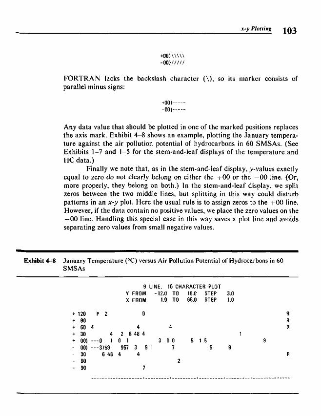
x-y Plotting
+00)\\\\\-00)/////
FORTRAN lacks the backslash character (\), so its marker consists ofparallel minus signs:
+00)-00)
Any data value that should be plotted in one of the marked positions replacesthe axis mark. Exhibit 4-8 shows an example, plotting the January tempera-ture against the air pollution potential of hydrocarbons in 60 SMSAs. (SeeExhibits 1-7 and 1-5 for the stem-and-leaf displays of the temperature andHC data.)
Finally we note that, as in the stem-and-leaf display, >>-values exactlyequal to zero do not clearly belong on either the +00 or the —00 line. (Or,more properly, they belong on both.) In the stem-and-leaf display, we splitzeros between the two middle lines, but splitting in this way could disturbpatterns in an x-y plot. Here the usual rule is to assign zeros to the +00 line.However, if the data contain no positive values, we place the zero values on the— 00 line. Handling this special case in this way saves a plot line and avoidsseparating zero values from small negative values.
Exhibit 4-8 January Temperature (°C) versus Air Pollution Potential of Hydrocarbons in 60SMSAs
9 LINE, 10 CHARACTER PLOT
Y FROM -12.0 TO 15.0 STEP 3.0
X FROM 1.0 TO 66.0 STEP 1.0
R
R
R
+120 P 2+ 90+ 60 4+ 30 4+ 00) — 0 1- 00) —3759- 3 0 6 46- 60- 90
42 8 480 1957 34 4
0
44
3 0 09 1 7
27
5 1 55
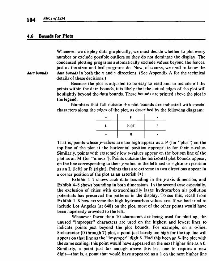
ABCsofEDA
4.6 Bounds for Plots
Whenever we display data graphically, we must decide whether to plot everynumber or exclude possible outliers so they do not dominate the display. Thecondensed plotting programs automatically exclude values beyond the fences,just as the stem-and-leaf programs do. Now, of course, we need to know the
data bounds data bounds in both the x and y directions. (See Appendix A for the technicaldetails of these decisions.)
Because the plot is adjusted to be easy to read and to include all thepoints within the data bounds, it is likely that the actual edges of the plot willbe slightly beyond the data bounds. These bounds are printed above the plot inthe legend.
Numbers that fall outside the plot bounds are indicated with specialcharacters along the edges of the plot, as described by the following diagram:
»
L
*
P
PLOT
M
*
R
»
That is, points whose ^-values are too high appear as a P (for "plus") on thetop line of the plot at the horizontal position appropriate for their x-value.Similarly, points with extremely low ^-values appear on the bottom line of theplot as an M (for "minus"). Points outside the horizontal plot bounds appear,on the line corresponding to their ^-value, in the leftmost or rightmost positionas an L (left) or R (right). Points that are extreme in two directions appear ina corner position of the plot as an asterisk (*).
Exhibit 4-7 shows such data bounding in the .y-axis dimension, andExhibit 4-8 shows bounding in both dimensions. In the second case especially,the exclusion of cities with extraordinarily large hydrocarbon air pollutionpotentials has preserved the patterns in the display. To see this, recall fromExhibit 1-8 how extreme the high hydrocarbon values are. If we had tried toinclude Los Angeles (at 648) on the plot, most of the other points would havebeen hopelessly crowded to the left.
Whenever fewer than 10 characters are being used for plotting, theunused "improper" characters are used on the highest and lowest lines toindicate points just beyond the plot bounds. For example, on a 6-line,8-character (0 through 7) plot, a point just barely too high for the top line willappear on that line as the "improper" digit 8. Had this been an 8-line plot withthe same scaling, this point would have appeared on the next higher line as a 0.Similarly, a point just far enough above this last one to require a newdigit—that is, a point that would have appeared as a 1 on the next higher line
x-y Plotting
had there been one—will appear as a 9. Points too far away from the plotcenter to be represented with improper digits are plotted with M and P. Thiscoding provides precise information about the location of points printed forsuch "near outliers" will indicate how many lines they are beyond the edge ofthe plot. Thus, a 2 says that the point is on the second line beyond the lines nowprinted.
4.7 Focusing Plots
Although the condensed plotting programs provide default choices of databounds, at times it is useful to override these choices. The plotting programscan be focused on any region of the x-y plane by specifying minimum andmaximum values for each axis. If the data extremes are specified, the plot willinclude all of the data points. If a small region is selected, this region will beblown up to fill the entire plotting area, and points beyond the specifiedborders of that region will be treated as outliers. This feature makes it possibleto focus on a portion of a complex display so as to better understand its finestructure.
It is also possible to divide part of the x-y plane into equal-sizedrectangular regions and to generate condensed plots for each region (or just forregions known to contain data points). These plots can then be pasted togetherto obtain a highly precise montage display. If the regions are the same size, theplots will have the same scale. With practice, the top and bottom plot lines,which will fill with "outliers," can be made superfluous by overlapping theregions slightly. For example, five 10-line, 10-character plots can be used tocover a smoothly increasing relationship by choosing regions placed diagonallyacross the x-y plane. The resulting montage will have the same verticalresolution as a 500-line printer plot—close to the resolution possible on manygraphics devices—yet the display will have taken only 50 lines and about 2minutes (at 30 characters per second) to print.
4.8 Using the Programs
The condensed plot programs accept pairs of data values specified as corre-sponding elements of two arrays. For example, the first element of one array
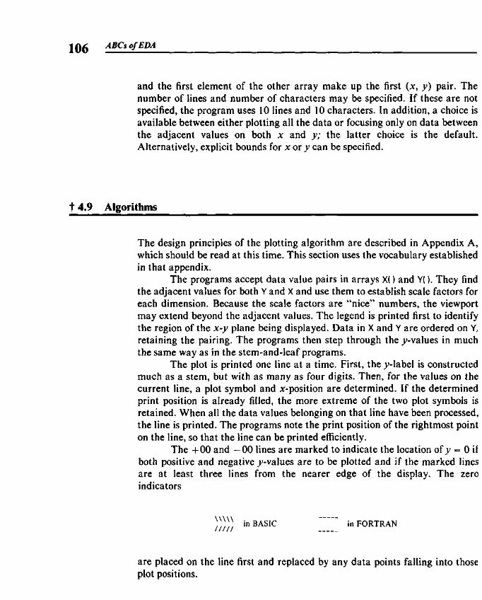
ABCsofEDA
and the first element of the other array make up the first (x, y) pair. Thenumber of lines and number of characters may be specified. If these are notspecified, the program uses 10 lines and 10 characters. In addition, a choice isavailable between either plotting all the data or focusing only on data betweenthe adjacent values on both x and y; the latter choice is the default.Alternatively, explicit bounds for x or y can be specified.
14.9 Algorithms
The design principles of the plotting algorithm are described in Appendix A,which should be read at this time. This section uses the vocabulary establishedin that appendix.
The programs accept data value pairs in arrays X() and Y(). They findthe adjacent values for both Y and X and use them to establish scale factors foreach dimension. Because the scale factors are "nice" numbers, the viewportmay extend beyond the adjacent values. The legend is printed first to identifythe region of the x-y plane being displayed. Data in X and Y are ordered on Y,retaining the pairing. The programs then step through the >>-values in muchthe same way as in the stem-and-leaf programs.
The plot is printed one line at a time. First, the y-label is constructedmuch as a stem, but with as many as four digits. Then, for the values on thecurrent line, a plot symbol and x-position are determined. If the determinedprint position is already filled, the more extreme of the two plot symbols isretained. When all the data values belonging on that line have been processed,the line is printed. The programs note the print position of the rightmost pointon the line, so that the line can be printed efficiently.
The +00 and -00 lines are marked to indicate the location of y = 0 ifboth positive and negative ^-values are to be plotted and if the marked linesare at least three lines from the nearer edge of the display. The zeroindicators
in BASIC in FORTRAN
are placed on the line first and replaced by any data points falling into thoseplot positions.
x-y Plotting
14.10 Alternatives
It is possible to produce plots that offer a compromise between precision andgraphic impact by choosing plotting symbols that themselves contribute to thegraphics. What is needed is a set of symbols that prints progressively higher onthe line. One possible set is |_ - }. This scheme can easily go awry when theprograms can be used from many different output terminals. (The example setgiven would become I"—f} on some devices—far from the intended impres-sion.)
More palatable alternatives are available to users with high-qualitygraphic devices. The resolution of many of these devices is 500 to 1000 verticalplot positions, which is far better than we can achieve with a condensed plot ofreasonable size. Readers wishing to use such devices may want to use theplot-scaling programs provided in this book (see Appendices A and B). Theseprograms can be modified easily to suit any plotting device, and theyincorporate several features valuable in exploratory analyses. Appendix Adiscusses these features and their function in exploratory analysis.
t 4.11 Details of the Programs
FORTRAN
The FORTRAN subroutine PLOT is invoked with the statement
CALL PLOT(Y, X, N, WY, WX, LINSET, CHRSET, XMIN, XMAX, YMIN, YMAX, ERR)
where
X() and Y() hold the N ordered pairs (X(i), Y(i));
N is the number of da ta values;WX() and WY() a re N-long work ar rays to hold the (x, y)
values sorted on y\LINSET specifies the max imum number of lines to be
used in the body of the plot. (The scalingroutines may decide to use fewer lines.);
JQO ABCsofEDA
CHRSET
XMIN and XMAX
YMIN and YMAX
ERR
specifies the number of subdivisions (charac-ters) of each line. It can be no greater than10. If either LINSET or CHRSET is zero, theplot format defaults to 10 lines, 10 charac-ters;
specify the range of x-values to be covered bythe plot;
specify the range of ^-values to be covered bythe plot;For either pair of bounds, if the minimumand maximum bounds are equal, theprogram defaults to using adjacent valueson that dimension;
is the error flag, whose values are0
4142
4445
normalN < 5—tooviolates 5 <
1 <all x-valuesall ^-values
few points to plotlines < 40 orcharacters < 10equal; no plot possibleequal; no plot produced.
BASIC
The BASIC subroutine is entered with N data pairs (X(i), Y(i)) in arrays X() andY(). The plot format is specified by the version number, V1:
V1 = 1 6-line, 4-character (Andrews-Tukey) plot;V1 = 2 10-line, 10 character plot;V1 = 3 30-line, 1-character plot (ordinary computer plot);V1 < 0 asks for input to override all scaling options.
All of the pre-set plots are scaled automatically to the adjacent values in bothdimensions. The program builds each line of the plot in the P() vector so thatoverprints can be dealt with gracefully. Because the program stores the ASCIIvalues of characters and numerals, the check performed to select the moreextreme of two values falling at the same plot position depends on the ASCIIcollating sequence. Programmers on non-ASCII systems should check theindicated portions of the code to be sure the collating sequence that theirsystems use is compatible.
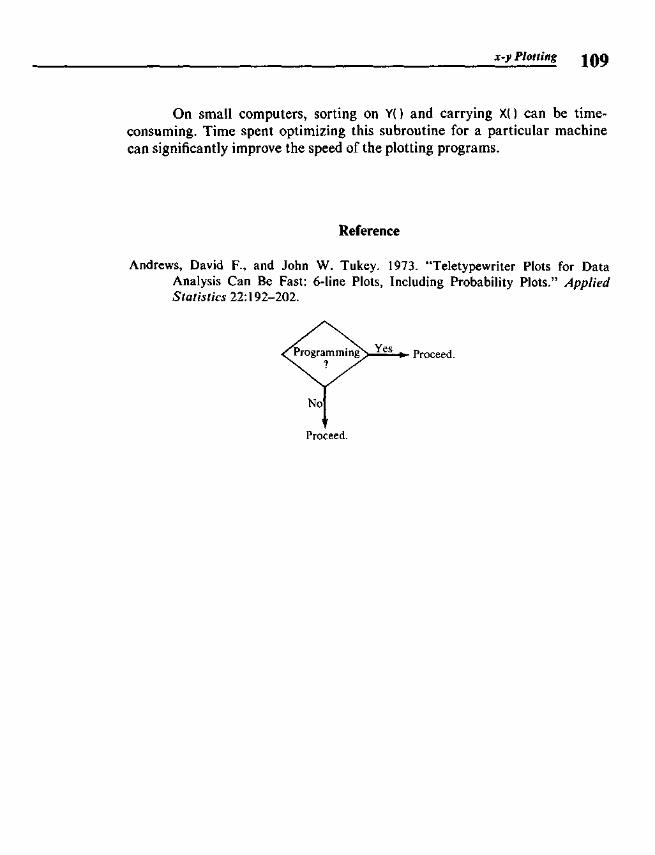
x-y Plotting
On small computers, sorting on Y() and carrying X() can be time-consuming. Time spent optimizing this subroutine for a particular machinecan significantly improve the speed of the plotting programs.
Reference
Andrews, David F., and John W. Tukey. 1973. "Teletypewriter Plots for DataAnalysis Can Be Fast: 6-line Plots, Including Probability Plots." AppliedStatistics 22:192-202.
Programming^ Y e s » Proceed.
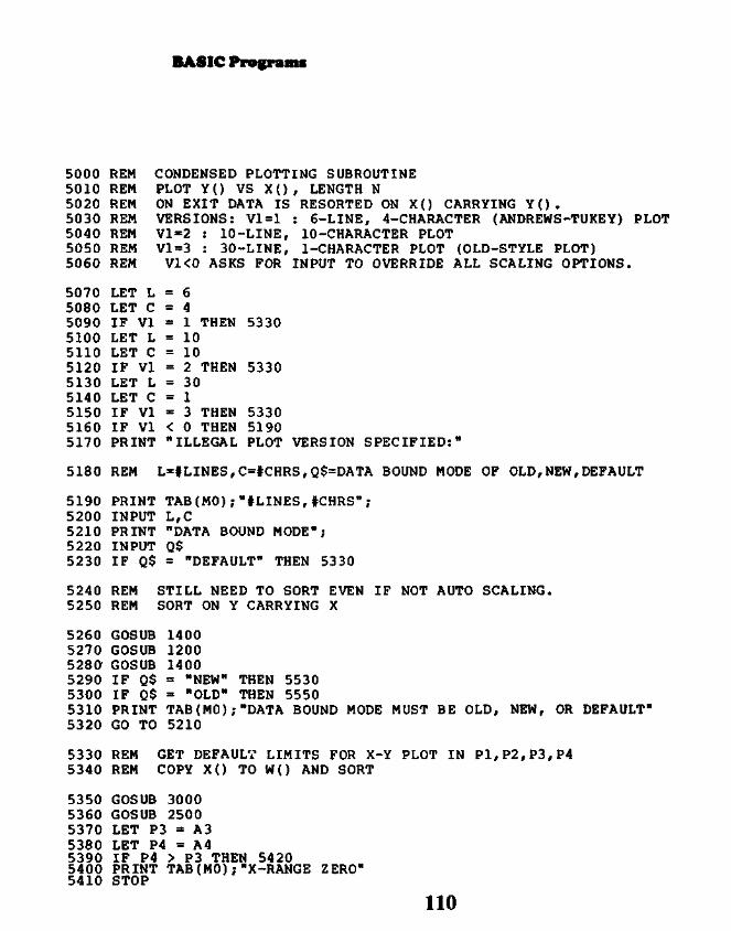
BASIC Programs
5000 REM CONDENSED PLOTTING SUBROUTINE5010 REM PLOT Y() VS X(), LENGTH N5020 REM ON EXIT DATA IS RESORTED ON X() CARRYING Y().5030 REM VERSIONS: Vl=l : 6-LINE, 4-CHARACTER (ANDREWS-TUKEY) PLOT5040 REM Vl=2 : 10-LINE, 10-CHARACTER PLOT5050 REM Vl=3 : 30-LINE, 1-CHARACTER PLOT (OLD-STYLE PLOT)5060 REM V K O ASKS FOR INPUT TO OVERRIDE ALL SCALING OPTIONS.
5070 LET L = 65080 LET C = 45090 IF VI = 1 THEN 53305100 LET L = 105110 LET C = 105120 IF VI = 2 THEN 53305130 LET L = 305140 LET C = 15150 IF VI = 3 THEN 53305160 IF VI < 0 THEN 51905170 PRINT "ILLEGAL PLOT VERSION SPECIFIED:"
5180 REM L=#LINES,C=#CHRS,Q$=DATA BOUND MODE OF OLD,NEW,DEFAULT
5190 PRINT TAB(MO);"#LINES,#CHRS";5200 INPUT L,C5210 PRINT "DATA BOUND MODE";5220 INPUT Q$5230 IF Q$ = "DEFAULT" THEN 5330
5240 REM STILL NEED TO SORT EVEN IF NOT AUTO SCALING.5250 REM SORT ON Y CARRYING X
5260 GOSUB 14005270 GOSUB 12005280 GOSUB 14005290 IF Q$ = "NEW" THEN 55305300 IF Q$ = "OLD" THEN 55505310 PRINT TAB(M0);"DATA BOUND MODE MUST BE OLD, NEW, OR DEFAULT"5320 GO TO 5210
5330 REM GET DEFAULT LIMITS FOR X-Y PLOT IN P1,P2,P3,P45340 REM COPY X() TO W() AND SORT
5350 GOSUB 30005360 GOSUB 25005370 LET P3 = A35380 LET P4 = A45390 IF P4 > P3 THEN 54205400 PRINT TAB(M0);"X-RANGE ZERO115410 STOP
110
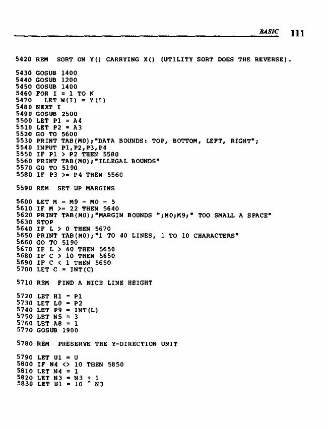
BASIC
5420 REM SORT ON Y() CARRYING X() (UTILITY SORT DOES THE REVERSE)
5430 GOSUB 14005440 GOSUB 12005450 GOSUB 14005460 FOR I = 1 TO N5470 LET W(I) = Y(I)5480 NEXT I5490 GOSUB 25005500 LET PI = A45510 LET P2 = A35520 GO TO 56005530 PRINT TAB(MO);"DATA BOUNDS: TOP, BOTTOM, LEFT, RIGHT";5540 INPUT P1,P2,P3,P45550 IF PI > P2 THEN 55805560 PRINT TAB(MO);"ILLEGAL BOUNDS"5570 GO TO 51905580 IF P3 >= P4 THEN 5560
5590 REM SET UP MARGINS
5600 LET M = M9 - MO - 55610 IF M >= 22 THEN 56405620 PRINT TAB(MO);"MARGIN BOUNDS ";M0;M9;" TOO SMALL A SPACE"5630 STOP5640 IF L > 0 THEN 56705650 PRINT TAB(M0);"l TO 40 LINES, 1 TO 10 CHARACTERS"5660 GO TO 51905670 IF L > 40 THEN 56505680 IF C > 10 THEN 56505690 IF C < 1 THEN 56505700 LET C = INT(C)
5710 REM FIND A NICE LINE HEIGHT
5720 LET HI = PI5730 LET LO = P25740 LET P9 = INT(L)5750 LET N5 = 35760 LET A8 = 15770 GOSUB 1900
5780 REM PRESERVE THE Y-DIRECTION UNIT
5790 LET Ul = U5800 IF N4 <> 10 THEN 58505810 LET N4 = 15820 LET N3 = N3 + 15830 LET Ul = 10 " N3
111
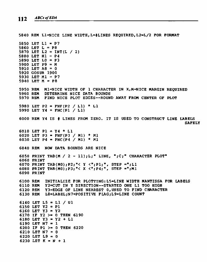
ABCsofEDA
5840 REM L1=NICE LINE WIDTH,L=#LINES REQUIRED,L2=L/2 FOR FORMAT
5850 LET LI = P75860 LET L = P85870 LET L2 = INT(L / 2)5880 LET HI = P45890 LET LO = P35900 LET P9 = M5910 LET A8 = 05920 GOSUB 19005930 LET Ml = P75940 LET M = P8
5950 REM M1=NICE WIDTH OF 1 CHARACTER IN X,M=NICE MARGIN REQUIRED5960 REM DETERMINE NICE DATA BOUNDS5970 REM FIND NICE PLOT EDGES—ROUND AWAY FROM CENTER OF PLOT
5980 LET P2 = FNF(P2 / LI) * LI5990 LET Y4 = FNC(P1 / LI)
6000 REM Y4 IS # LINES FROM ZERO. IT IS USED TO CONSTRUCT LINE LABELSSAFELY
6010 LET PI = Y4 * LI6020 LET P3 = FNF(P3 / Ml) * Ml6030 LET P4 = FNC(P4 / Ml) * Ml
6040 REM NOW DATA BOUNDS ARE NICE
6050 PRINT TAB(M / 2 - 11);L;W LINE, ";C;" CHARACTER PLOT"6060 PRINT6070 PRINT TAB(M0);P2;"< Y <";P1;", STEP =";L16080 PRINT TAB(MO);P3;"< X <";P4;", STEP = ";M16090 PRINT
6100 REM INITIALIZE FOR PLOTTING:L5=LINE WIDTH MANTISSA FOR LABELS6110 REM Y2=CUT IN Y DIRECTION—STARTED ONE LI TOO HIGH6120 REM Y3=EDGE OF LINE NEAREST 0,USED TO FIND CHARACTER6130 REM L8=LABEL;N7=POSITIVE FLAG;L9=LINE COUNT
6140 LET L5 = LI / Ul6150 LET Y2 = PI6160 LET Y3 = Y26170 IF Y2 >= 0 THEN 61906180 LET Y3 = Y2 + LI6190 LET N7 = 16200 IF PI >= 0 THEN 62206210 LET N7 = 06220 LET L9 = 06230 LET K = N + 1
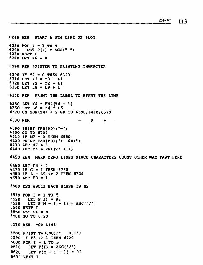
BASIC 113
6240 REM START A NEW LINE OF PLOT
6250 FOR I = 1 TO M6260 LET P(I) = ASC(" ")6270 NEXT I6280 LET P6 = 0
6290 REM POINTER TO PRINTING CHARACTER
6300 IF Y2 = 0 THEN 63206310 LET Y3 = Y3 - LI6320 LET Y2 = Y2 - LI6330 LET L9 = L9 + 1
6340 REM PRINT THE LABEL TO START THE LINE
6350 LET Y4 = FNI(Y4 - 1)6360 LET L8 = Y4 * L56370 ON SGN(Y4) + 2 GO TO 6390,6410,6670
6380 REM o +
6390 PRINT TAB(MO);"-";6400 GO TO 67006410 IF N7 = 0 THEN 65806420 PRINT TAB(M0);"+ 00:";6430 LET N7 = 06440 LET Y4 = FNI(Y4 + 1)
6450 REM MARK ZERO LINES SINCE CHARACTERS COUNT OTHER WAY PAST HERE
6460 LET F3 = 06470 IF C = 1 THEN 67206480 IF L - L9 <= 2 THEN 67206490 LET F3 = 1
6500 REM ASCII BACK SLASH IS 92
6510 FOR I = 1 TO 56520 LET P(I) = 926530 LET P(M - I + 1) = ASC("/")6540 NEXT I6550 LET P6 = M6560 GO TO 6720
6570 REM -00 LINE
6580 PRINT TAB(MO);"- 00:";6590 IF F3 <> 1 THEN 67206600 FOR I = 1 TO 56610 LET P(I) = ASC("/M)6620 LET P(M - I + 1) = 926630 NEXT I
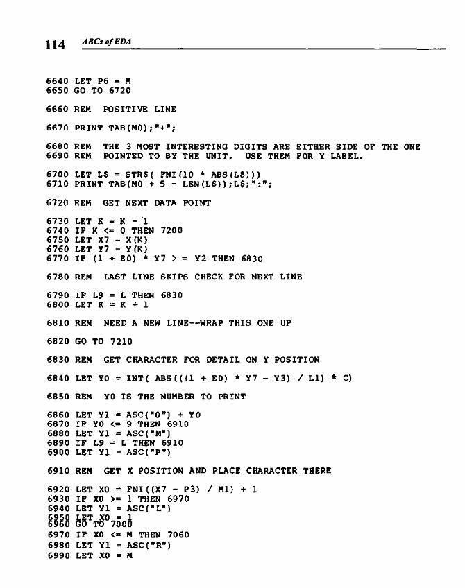
\\A ABCsofEDA
6640 LET P6 = M6650 GO TO 6720
6660 REM POSITIVE LINE
6670 PRINT TAB(MO);"+";
6680 REM THE 3 MOST INTERESTING DIGITS ARE EITHER SIDE OF THE ONE6690 REM POINTED TO BY THE UNIT. USE THEM FOR Y LABEL.
6700 LET L$ = STR$( FNI(10 * ABS(L8)))6710 PRINT TAB(MO + 5 - LEN (L$));L$;":";
6720 REM GET NEXT DATA POINT
6730 LET K = K - 16740 IF K <= 0 THEN 72006750 LET X7 = X(K)6760 LET Y7 = Y(K)6770 IF (1 + EO) * Y7 > = Y2 THEN 6830
6780 REM LAST LINE SKIPS CHECK FOR NEXT LINE
6790 IF L9 = L THEN 68306800 LET K = K + 1
6810 REM NEED A NEW LINE—WRAP THIS ONE UP
6820 GO TO 7210
6830 REM GET CHARACTER FOR DETAIL ON Y POSITION
6840 LET YO = INT( ABS(((1 + EO) * Y7 - Y3) / LI) * C)
6850 REM YO IS THE NUMBER TO PRINT
6860 LET Yl = ASC("0") + YO6870 IF YO <= 9 THEN 69106880 LET Yl = ASC("M")6890 IF L9 = L THEN 69106900 LET Yl = ASC("P")
6910 REM GET X POSITION AND PLACE CHARACTER THERE
6920 LET XO = FNI ((X7 - P3) / Ml) + 16930 IF XO >= 1 THEN 69706940 LET Yl = ASC("L")
jg LET_X0_=.lGO TO 70006970 IF XO <= M THEN 70606980 LET Yl = ASCCR")6990 LET XO = M
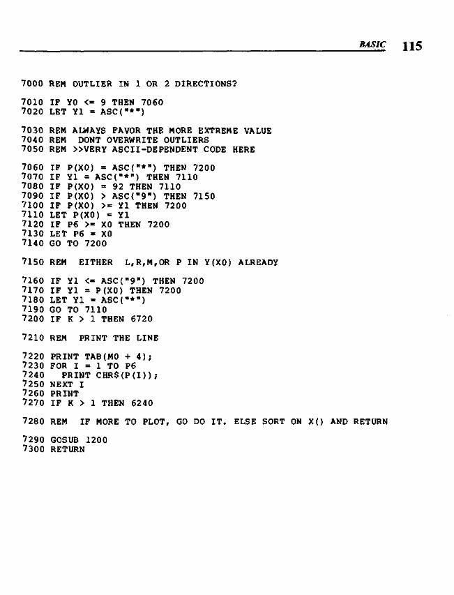
BASIC
7000 REM OUTLIER IN 1 OR 2 DIRECTIONS?
7010 IF Y0 <= 9 THEN 70607020 LET Yl = ASC("*")
7030 REM ALWAYS FAVOR THE MORE EXTREME VALUE7040 REM DONT OVERWRITE OUTLIERS7050 REM »VERY ASCI I-DE PENDENT CODE HERE
7060 IF P(X0) = ASC(H*") THEN 72007070 IF Yl = ASC("*") THEN 71107080 IF P(X0) = 92 THEN 71107090 IF P(X0) > ASC("9") THEN 71507100 IF P(X0) >= Yl THEN 72007110 LET P(X0) = Yl7120 IF P6 >= XO THEN 72007130 LET P6 = XO7140 GO TO 7200
7150 REM EITHER L,R,M,OR P IN Y(X0) ALREADY
7160 IF Yl <= ASC("9") THEN 72007170 IF Yl = P(X0) THEN 72007180 LET Yl = ASC("*")7190 GO TO 71107200 IF K > 1 THEN 6720
7210 REM PRINT THE LINE
7220 PRINT TAB(MO + 4);7230 FOR I = 1 TO P67240 PRINT CHR$(P(I));7250 NEXT I7260 PRINT7270 IF K > 1 THEN 6240
7280 REM IF MORE TO PLOT, GO DO IT. ELSE SORT ON X() AND RETURN
7290 GOSUB 12007300 RETURN
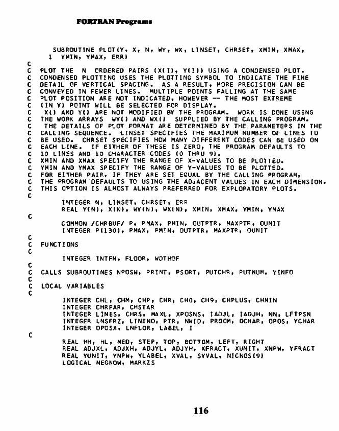
FORTRAN Programs
SUBROUTINE PLOKY, X, Nt WY, WX , LINSET, CHRSET, XMIN, XMAX,1 YMINt YMAX, ERR)
CC PLOT THE N CRDERED PAIRS (X(I), Yd)) USING A CONDENSED PLOT.C CONDENSED PLOTTING USES THE PLOTTING SYMBOL TO INDICATE THE FINEC DETAIL OF VERTICAL SPACING. AS A RESULT, MORE PRECISION CAN BEC CONVEYED IN FEWER LINES. MULTIPLE POINTS FALLING AT THE SAMEC PLOT POSITION ARE NOT INDICATED, HOWEVER ~ THE MOST EXTREMEC (IN Y) POINT WILL BE SELECTED FOP DISPLAY.C X() AND Y() APE NOT MODIFIED BY THE PROGRAM. WORK IS DONE USINGC THE WORK ARRAYS WY() AND WX() SUPPLIED BY THE CALLING PROGRAM.C THE DETAILS OF PLOT FORMAT ARE DETERMINED BY THE PARAMETERS IN THEC CALLING SEQUENCE. LINSET SPECIFIES THE MAXIMUM NUMBER OF LINES TOC BE USED. CHRSET SPECIFIES HOW MANY DIFFERENT CODES CAN BE USED ONC EACH LINE. IF EITHER OF THESE IS ZERO, THE PROGRAM DEFAULTS TOC 10 LINES AND 10 CHARACTER CODES (0 THRU 9).C XMIN AND XMAX SPECIFY THE RANGE OF X-VALUES TO BE PLOTTED.C YMIN AND YMAX SPECIFY THE RANGE OF Y-VALUES TO BE PLOTTED.C FOR EITHER PAIR, IF THEY ARE SET EQUAL BY THE CALLING PROGRAM,C THE PROGRAM DEFAULTS TO USING THE ADJACENT VALUES IN EACH DIMENSION.C THIS OPTION IS ALMOST ALWAYS PREFERRED FOR EXPLORATORY PLOTS.C
INTEGER N, LINSET, CHRSET, ERRREAL Y(N), X(N), WY(N), WX(N), XMIN, XMAX, YMIN, YMAX
CCOMMON /CHPBUF/ P, PMAX, PMIN, OUTPTR, MAXPTR, OUNITINTEGER PU30), PMAX, PMIN, OUTPTR, MAXPTP, OUNIT
CC FUNCTIONSC
INTEGER INTFN, FLOOR, WDTHOFCC CALLS SUBROUTINES NPOSW, PRINT, PSORT, PUTCHR, PUTNUM, YINFOCC LOCAL VARIABLESC
INTEGER CHL, CHM, CHP, CHR, CHO, CH9, CHPLUS, CHMININTEGER CHRPAR, CHSTARINTEGER LINES, CHRS, MAXL, XPOSNS, IADJL, IADJH, NN, LFTPSNINTEGER LNSFRZ, LINENO, PTR, NWID, PROOM, OCHAR, OPOS, YCHARINTEGER OPOSX, LNFLOR, LABEL, I
CREAL HH, HL, MED, STEP, TOP, BOTTOM, LEFT, RIGHTREAL ADJXL, ADJXH, ADJYL, ADJYH, XFRACT, XUNIT, XNPW, YFRACTREAL YUNIT, YNPW, YLABEL, XVAL, SYVAL, NICN0SC9)LOGICAL NEGNOW, MARKZS
116
FORTRAN 111
DATA CHLt CHM, CHP, CHR, CHOt CH9/12, 13, 16, 18, 27, 36 /DATA CHPLUS,CHMIN,CHSTAR,CHRPAR/39,40,41,44/DATA NN, NICNOS(l), NICNOS(2), NICNOS(3) / 9 , 1 .0 , 1 .5, 2 . 0 /DATA NICNOSU), NICN0S(5), NICN0S(6) / 2 . 5 , 3 . 0 , 4 . 0 /DATA NICN0SC7), NICN0S(8), NICN0SC9) / 5 . 0 , 7 . 0 , 10 .0 /DATA MARKZS / .FALSE. /
IF { N .GE. 5) GO TO 10ERR = 4.1GO TO 999
10 LFTPSN ' PMIN • 6LINES = 10CHRS » 10IFCLINSET .EQ. 0 .OR. CHRSET .EQ. 0) GO TO 30LINES - LIN.SETCHRS - CHRSETERR = 42IF(LINES .LT. 5 .OR. LINES .GT. 40) GO TO 999IFCCHRS .LT. 1 .OR. CHRS .GT. 10) GO TO 999ERP = 0
SET UP SCALES AND PLCT BOUNDARY INFORMATION
30 LFTPSN = PMIN + 6PROOM = PMAX - LFTPSN • 1DO 40 I = 1, N
WX(I) = X(I)40 CONTINUE
IFtXMIN -GE. XMAX) GO TO 45CALL YINFO(WX, N, MED, HL, HH, ADJXL, ADJXH, IADJL, IADJH,
1 STEP, ERR)IF(EPR .NE. 0) GO TO 999IFCADJXL . L T . ADJXH) GO TO 50
IF X-AOJACENT VALUES EQUAL, TPY USING THE EXTREMES
45 ADJXL = WX(1)ADJXH = WX(N)ERR = 44IFCADJXL .GE. ADJXH) GO TO 999ERR = 0
50 CALL NPOSW(ADJXH, ADJXL, NICNOS, NN, PROOM, .FALSE., XPOSNS,1 XFRACT, XUNIT, XNPW, ERP)
ABCsofEDA
ADJYL, ADJYH, IADJL, IADJH,
SCALE Y —SORT (X , Y) PAIRED ON Y
DO 60 I * I t NWXU) - X ( I )WY(I) = Y d )
60 CONTINUECALL PSORTifcY, WX, N, ERR)IF(YMIN .GE- YMAX) GO TO 65CALL YINFO(WY, N, MED, HL, HH,
1 STEP, ERR)IF1ERR .NE. 0) GO TO 999GO TO 68
65 ADJYL = WY(1)ADJYH ' WY(N)ERR - 45IFCADJYL .GE. ADJYH) GO TO 999ERR = 0
68 MAXL = LINESCALL NPOSW(ADJYH, ADJYL, NICNOS,
1 YFRACT, YUNIT, YNPW, ERR)IF(ERR .NE . 0) GO TO 999I F (YFRACT .NE. 1 0 . 0 ) GO TO 70YFRACT = 1.0YUNIT = YUNIT*10.0
FIND NICE PLOT EDGES — ROUND AWAY FROM CENTER OF PLOT
70 LNSFRZ * -FLOORC-ADJYH/YNPW)TOP = FLOAT(LNSFRZ) * YNPWBOTTOM * FLOAT(FLOOR(ADJYL/YNPW)) * YNPWLEFT * FLOAT(FLOOR(ADJXL/XNPW)) * XNPWRIGHT = FLOAT(-FLOOR(-ADJXH/XNPW)) * XNPW
PRINT SCRAWL
NN, MAXL, .TRUE. , LINES,
WRITE(OUNIT, 9070) LINES, CHRS9070 F0RMATQ5X, 13, 7H L INE , , 13 ,
WRITECOUNIT, 9080)BOTTOM, TOP,9080 F0RMAT(15X, 8H Y FROM , F12.6,
1 15X, 8H X FROM , F12.6, 4H TO
15H CHARACTER PLOT)YNPW, LEFT, RIGHT, XNPW4H TO , F 1 2 . 6 , 7H STEP , F 1 2 . 6 /
F 1 2 . 6 , 7H STEP , F 1 2 . 6 / / )IN IT IAL IZE FOR PLOTTING—ONE LINE TOO HIGH
LNSFRZ COUNTS # LINES AWAY FROM ZERO—+00 AND - 0 0 ARE 0 LINES AWAY
YLABEL ~ FLOAT(LNSFRZ) * YFRACTLNFLOR = LNSFRZNEGNOW ' .FALSE.IF(TOP .GT. 0 . 0 ) GO TO 80LNSFRZ = LNSFRZ + 1NEGNOW - .TRUE.
80 LINENO = 0PTP = N+l
FORTRAN 119
cC START A NEW LINE OF THE PLOTC
ccc
ccc
90
JUST
95
97
LNFLOR =LINENO -
LNFLGR -LINENO •
OPOS - PMINIF(LNSFRZ . G T . 0 .
WENT NEGATIVE
NEGNOW -GO TO 97LNSFRZ *YLABEL =CONTINUE
THE LIME
.TRUE.
LNSFRZ -YLABEL -
LABEL
11
OR. NEGNOW)
1YFPACT
GO TO 95
IFC.NOT. NEGNOWI CALL PUTCHR(OPOS, CHPLUS, ERR)IF(NEGNOW) CALL PUTCHRCOPOS, CHMIN, ERR)IFCYLABEL . N E . 0 . 0 ) GO TO 120OPOS = PMIN + 3CALL PUTCHR(OP0St CHO , ERR)CALL PUTCHRCO, CHO, ERR)IFUCHRS . G T . 1) .AND. ( (L INES-L INENO) .GE. 3 ) ) MARKZS = .TRUE,OPOS = PMIN + 5CALL PUTCHP(OPOS, CHRPAR, ERR)I F ( . N O T . MARKZS) GO TO 111DO 100 I = 1 , 5
I F ( . N O T . NEGNOW) CALL PUTCHR<0, CHMIN, ERR)IF(NEGNOW) CALL PUTCHRCO, CHMIN, ERR)
100 CONTINUEOPOSX = PMAX - 5DO 110 OPOS = OPOSX, PMAX
I F U N O T . NEGNOW) CALL PUTCHRCO, CHMIN, ERR)IF(NEGNCW) CALL PUTCHR(O, CHMIN, ERR)
110 CONTINUE111 CONTINUE
GO TO 125CC PRINT NON-ZERO LABELC
120 LABEL = INTFNdO.O * ABS(YLABEL), ERR)I F ( EPR . N E . 0 ) GO TO 999NWID = WDTHOF(LABEL)OPOS = PMIN + 5 - NWIDCALL PUTNUM(OPOS, LABEL, NWID, ERR)IF (ERR . N E . 0) GO TO 999
CC GET NEXT DATA POINTC
125 PTR * PTR - 1IFCPTR .LE. 0) GO TO 135XVAL ' WX(PTR)SYVAL - WY(PTR)/YNPW
1 2 0 ABCs °fEDA
IF ( INTFN(SVVAL, ERR) .GT. LNFLOR) GO TO 140IF ( INTFN(SYVAL, ERR).EQ.LNFLOR .AND. SYVAL .GE . 0 . 0 ) GO TO 140
CC TIME TO START NEXT LINEC IF THIS IS THE LAST LINE, PRINT IT ANYWAY AND USE "M" FOR LOW NO.C
130 IF(LINENO .EQ. LINES) GO TO 140CC BACK UP THE POINTERC
PTP = PTR + 1CC WRAP UP LINEC
135 IF<ERR .NE. 0) GO TO 999CALL PRINT
CC AND START A NEW LINEC
GO TO 90CC GET Y-CHARACTERC
140 YCHAR = IFIX(ABS(SYVAL - FLOAT(LNSFRZ) ) * FLOAT(CHRS))OCHAR = CHO + YCHARIFCOCHAR -GE. CHO .AND. OCHAR .LE. CH9) GO TO 145OCHAR = CHPIF(LINENO .EQ. LINES) OCHAP = CHM
CC GET X-POSITIONC
145 OPOS - PMIN • 5 + INTFNUXVAL - LEFTJ/XNPW, ERR) + 1IF (XVAL .GE. LEFT) GO TO 150OPOS = PMIN • 6IFCOCHAR .LT. CHO .OR. OCHAR .GT. CH9) GO TO 147OCHAR - CHLGO TO 160
147 OCHAR - CHSTARGO TO 160
150 IFCXVAL .LE. RIGHT) GO TO 160OPOS = PMAXIFCOCHAR .LT. CHO .OR. OCHAP .GT, CH9) GO TO 157OCHAP = CHRGO TO 160
157 OCHAR - CHSTAR160 CONTINUE
CALL PUTCHRCOPOS, OCHAR, ERR)IF(ERR .NE. 0) GO TO 999IFCPTR .GT. 1) GO TO 125CALL PRINT
999 RETURNEND
Chapter 5EResistant Line
In Chapter 4 we focused our attention on flexible techniques for plotting aresponse response, y, against a factor, x. When the pattern of a plot suggests that thefactor value of y depends on the value of x, we often try to summarize this
dependence in terms of the simplest possible description—namely, a straightline. We can represent any straight line with the equation
y = a + bx
just by choosing values for a and b. Once we have a and b, every pair ofnumbers (x, y) that satisfies the relationship y = a + bx will lie on a straightline when plotted. In order to summarize any particular x-y data, we neednumerical values for a and b that will make a line pass close to the data. Thischapter shows one way to find these values.
5.1 Slope and Intercept
The numbers represented by a and b in the equation of a line have specificslope meanings. The slope of the line, b, tells us how tilted the line is; more precisely,
121
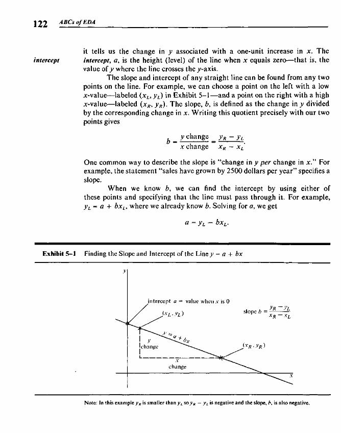
ABCsofEDA
intercept
it tells us the change in y associated with a one-unit increase in x. Theintercept, a, is the height (level) of the line when x equals zero—that is, thevalue of y where the line crosses the >>-axis.
The slope and intercept of any straight line can be found from any twopoints on the line. For example, we can choose a point on the left with a lowx-value—labeled (xL, yL) in Exhibit 5-1—and a point on the right with a highx-value—labeled (xR, yR). The slope, b, is defined as the change in y dividedby the corresponding change in x. Writing this quotient precisely with our twopoints gives
, v change yR - yL
xchange xR — x
One common way to describe the slope is "change in y per change in x." Forexample, the statement "sales have grown by 2500 dollars per year" specifies aslope.
When we know b, we can find the intercept by using either ofthese points and specifying that the line must pass through it. For example,yL = a + bxL, where we already know b. Solving for a, we get
a = yL- bxL.
Exhibit 5-1 Finding the Slope and Intercept of the Line y = a + bx
intercept a = value when .v is 0
Note: In this example yR is smaller than yL so yR — yL is negative and the slope, b, is also negative.
Resistant Line 123
We can equally well get
a = yR- bxR.
Exhibit 5-1 shows the geometry behind these calculations.
5.2 Summary Points
When we deal with a line itself, it doesn't matter which two points we use tocalculate a and b because every point we consider is exactly on the line.However, we can't expect real data to line up perfectly. While many pointsmay be near a line, few will lie exactly on it. Many different lines could passclose enough to the data to be reasonable summaries. Consequently, we can'tjust pick any two points from the data and expect to find a good line. Insteadwe want to find points that summarize the data well so that the line theydetermine will be close to the data.
To get an estimate of the slope, we need to pick a typical x-value neareach end of the range of x-values but not so near as to risk being anextraordinary x-value. We do this by dividing the data into three portions orregions—points with low x-values (on the left), points with middle x-values,and points with high x-values (on the right)—with roughly a third of thepoints in each portion. Exhibit 5-2 illustrates this partitioning. If we can't putexactly the same number of points into each portion because n/3 leaves aremainder, we still allocate the points symmetrically. A single "extra" pointgoes into the middle portion; when two "extra" points remain, one goes intoeach outer portion. Whenever several data points have the same x-value, theymust go into the same portion. Such ties may make it more difficult to comeclose to equal allocation. When we work by hand, we can usually use ourjudgment to resolve the problem of equal allocation. Precise rules to handle allsituations may be found in the programs at the end of this chapter.
Within each portion (or third) of the data, we forget about the pairingbetween the x-value and the y-value in x-y data and summarize the x-valuesand the >>-values separately. In each portion, we first treat the x-values as abatch (and ignore y) and find their median. We then treat the corresponding^-values as a batch and find their median. Thus, we obtain an (x, y) pair ofmedians in each of the three portions. The points that these median pairsspecify need not be original data points, but they may be. Nothing forces themedian x-value and the median ^-value to come from the same data point,even though the assignment of ^-values to portions is determined entirely by
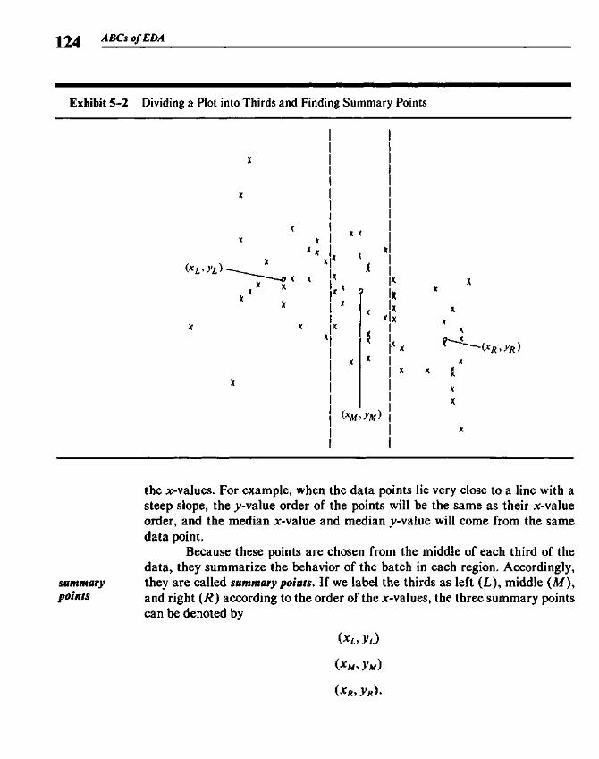
J 2 4 ABCsofEDA
Exhibit 5-2 Dividing a Plot into Thirds and Finding Summary Points
x x
summarypoints
the Jt-values. For example, when the data points lie very close to a line with asteep slope, the >>-value order of the points will be the same as their jc-valueorder, and the median x-value and median y-value will come from the samedata point.
Because these points are chosen from the middle of each third of thedata, they summarize the behavior of the batch in each region. Accordingly,they are called summary points. If we label the thirds as left (L), middle (M),and right (R) according to the order of the ^-values, the three summary pointscan be denoted by
(xL,yL)
,yM)
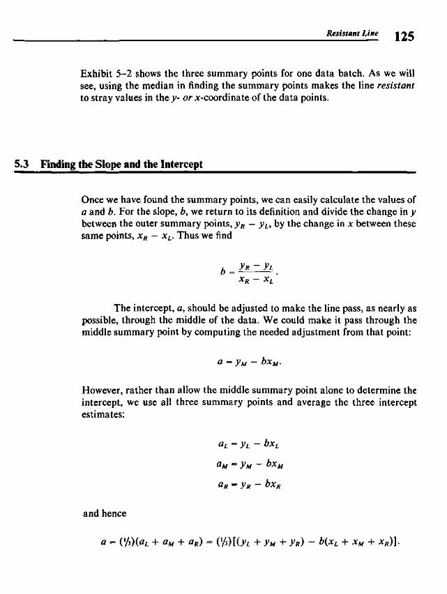
Resistant Line 125
Exhibit 5-2 shows the three summary points for one data batch. As we willsee, using the median in finding the summary points makes the line resistantto stray values in the y- or x-coordinate of the data points.
5.3 Finding the Slope and the Intercept
Once we have found the summary points, we can easily calculate the values ofa and b. For the slope, b, we return to its definition and divide the change in ybetween the outer summary points, yR — yLi by the change in x between thesesame points, xR — xL. Thus we find
XR ~ XL
The intercept, a, should be adjusted to make the line pass, as nearly aspossible, through the middle of the data. We could make it pass through themiddle summary point by computing the needed adjustment from that point:
- bxM.
However, rather than allow the middle summary point alone to determine theintercept, we use all three summary points and average the three interceptestimates:
aR = yR- bxR
and hence
a = (l/i)(aL + aM + aR) = Olz)[{yL 4- yM + yR) - KxL + xM + xR)].
126 ABCsofEDA
5.4 Residuals
A fundamental step in most data analysis and in all exploratory analysis is theresiduals computation and examination of residuals. While we usually begin to examine
data with some elementary displays such as those presented in Chapters 1model through 4, most analyses propose a simple structure or model to begin
describing the patterns in the data. Such models differ widely in structure andpurpose, but all attempt to fit the data closely. We therefore refer to any such
fit description of the data as a fit. The residuals are, then, the differences at eachpoint between the observed data value and the fitted value:
residual = data — fit.
The resistant line provides one way to find a simple fit, and its residuals, r, arefound for each data value, (xh >>,-), as
n = y,- - {a + bx().
resistant line
A pessimist might view residuals as the failure of a fit to describe thedata accurately. He might even speak of them as "errors," although a perfectfit, which leaves all residuals equal to zero, would arouse suspicion. Anoptimist sees in residuals details of the data's behavior previously hiddenbeneath the dominant patterns of the fit. Both points of view are correct. Thebest fits leave small residuals, and systematically large residuals may indicatea poorly chosen model. Nevertheless, even a good fit may do nothing morethan describe the obvious—for example, prices increased during the 1970s; thepopulation of the United States grew during the same period—and leavebehind the interesting patterns—for example, the Vietnam war affected theU.S. economy; the birthrate dropped sharply.
Any method of fitting models must determine how much each pointcan be allowed to influence the fit. Many statistical procedures try to keep thefit close to every data point. If the data include an outlier, these proceduresmay permit it to have an undue influence on the fit. As always in exploratorydata analysis, we try to prevent outliers from distorting the analysis. Usingmedians in fitting lines to data provides resistance to outliers, and thus theline-fitting technique of this chapter is called the resistant line.
Resistant Line 111
5.5 Polishing the Fit
Resistance to outliers has one price. The values found at first for the intercept,a, and the slope, b, are often not the most appropriate ones. A good way tocheck the values we have found is to calculate the residuals, treat the points
(x, residual) = (xh yt - (a + bXj) ),
as x-y data, and find summary points as before. If the slope, b', between theouter summary points is zero (or very close to zero), we are done. If not, wecan adjust the original slope by adding the residual slope b' to it. We will, ofcourse, want to compute the new residuals to see whether their slope is nowclose enough to zero.
Sometimes we will have overcorrected, and the new residuals will tiltthe other way. When we have two slopes, one too small (residuals have apositive slope) and one too large (residuals have a negative slope), we knowthat the correct slope lies between them. We can often improve the slopeestimate very efficiently by using the correction formula
Here bx and b2 are the two slope estimates, and b\ and b'2 are the slopes of theresiduals when bx and b2 were tried. The example in the next section illustratesthis process and shows how still more corrections can be made if needed.
5.6 Example: Breast Cancer Mortality versus Temperature
In a 1965 report, Lea discussed the relationship between mean annualtemperature and the mortality rate for a type of breast cancer in women. Thedata, pertaining to certain regions of Great Britain, Norway, and Sweden, arelisted in Exhibit 5-3 and are plotted in Exhibit 5-4.
In this example, n = 16 and n/3 = 51/}. To keep the thirds symmetric,we want to allocate the spare data value to the middle third in order to have 5points in the left third, 6 in the middle third, and 5 in the right third; because
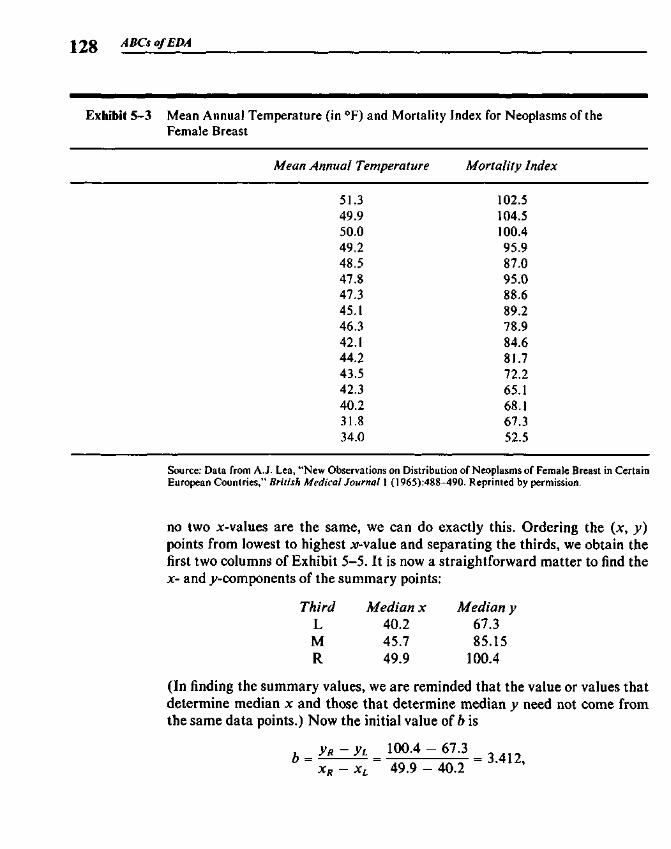
128 ABCsofEDA
Exhibit 5-3 Mean Annual Temperature (in °F) and Mortality Index for Neoplasms of theFemale Breast
Mean Annual Temperature Mortality Index
51.3 102.549.9 104.550.0 100.449.2 95.948.5 87.047.8 95.047.3 88.645.1 89.246.3 78.942.1 84.644.2 81.743.5 72.242.3 65.140.2 68.131.8 67.334.0 52.5
Source: Data from A.J. Lea, "New Observations on Distribution of Neoplasms of Female Breast in CertainEuropean Countries," British Medical Journal 1 (1965):488-490. Reprinted by permission.
no two x-values are the same, we can do exactly this. Ordering the (x, y)points from lowest to highest rvalue and separating the thirds, we obtain thefirst two columns of Exhibit 5-5. It is now a straightforward matter to find thex- and ^-components of the summary points:
ThirdLMR
Median x40.245.749.9
Median y67.385.15
100.4
(In finding the summary values, we are reminded that the value or values thatdetermine median x and those that determine median y need not come fromthe same data points.) Now the initial value of b is
, _yR~yL_ 100.4 -67 .3 _xR - xL 49.9 - 40.2 " '
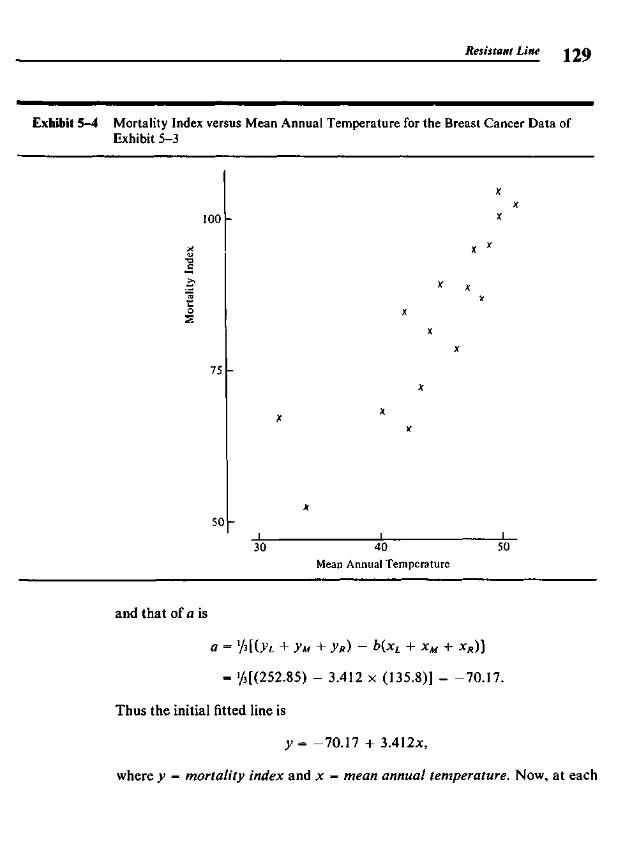
Resistant Line 129
Exhibit 5-4 Mortality Index versus Mean Annual Temperature for the Breast Cancer Data ofExhibit 5-3
100
75
50
30 40Mean Annual Temperature
50
and that of a is
a = %(yL + y*t + yR) - b{xL + xM + xR)]
= y3[(252.85) - 3.412 x (135.8)] = -70.17.
Thus the initial fitted line is
y= -70.17 + 3.412*,
where y = mortality index and x = mean annual temperature. Now, at each
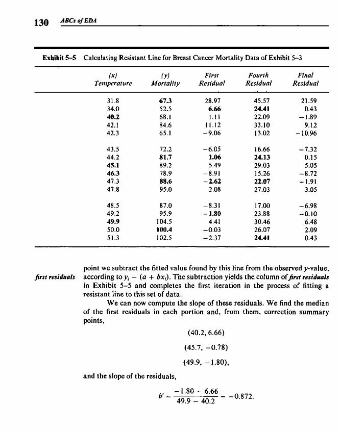
1 ^fl ABCs of EDA
Exhibit 5-5 Calculating Resistant
(x)Temperature
Line for Breast
(y)Mortality
Cancer Mortality
FirstResidual
Data of Exhibit
FourthResidual
5-3
FinalResidual
31.834.040.242.142.3
43.544.245.146.347.347.8
48.549.249.950.051.3
67.352.568.184.665.1
72.281.789.278.988.695.0
87.095.9
104.5100.4102.5
28.976.661.11
11.12-9.06
-6.051.065.49
-8.91-2.62
2.08
-8.31-1.80
4.41-0.03-2.37
45.5724.4122.0933.1013.02
16.6624.1329.0315.2622.0727.03
17.0023.8830.4626.0724.41
21.590.43
-1.899.12
-10.96
-7.320.155.05
-8.72-1.91
3.05
-6.98-0.10
6.482.090.43
point we subtract the fitted value found by this line from the observed y-value,first residuals according toj>, — (a + bxi). The subtraction yields the column of first residuals
in Exhibit 5-5 and completes the first iteration in the process of fitting aresistant line to this set of data.
We can now compute the slope of these residuals. We find the medianof the first residuals in each portion and, from them, correction summarypoints,
(40.2, 6.66)
(45.7, -0.78)
(49.9,-1.80),
and the slope of the residuals,
-1-80-6.66b. 49.9 - 40.2
Resistant Line 131
The second slope estimate is then
b2 = 3.412 - 0.872 = 2.540.
The residuals from the line with this slope and the original intercept are the"second residuals." Their slope, b'2, is found in the same way. Here it is 0.624.We could adjust the intercept as well, but it is easier to wait until we have asatisfactory slope estimate.
We now have two slope estimates, 3.412, and 2.540, which leaveresidual slopes with opposite signs: —0.872 and 0.624. These are all we need toapply the second correction formula. We compute a new slope estimate as
b3 = 2.540 - 0.624[(2.540 - 3.412)/(0.624 - (-0.872))] = 2.904.
We then compute the residuals from the line with slope b3 and find their slope.In this example, b'3 = -0.024—much closer to zero than the previous residualslopes.
Although a residual slope of —0.024 is small enough for most purposes,we will try one more correction step. Because the final slope must lie between aslope estimate that is too low (with positively sloped residuals) and one that istoo high,(with negatively sloped residuals), we use the current best guesses forthese two estimates. Our latest estimate has negatively sloped residuals(b'3 = —0.024), so we use it and its residual slope in place of our former highslope estimate, 3.412. This yields
b4 = 2.904 - (-0.024)[(2.904 - 2.540)/(-0.024 - 0.624)] = 2.890.
The residuals from the line with slope b4 and the original intercept are in thecolumn of "fourth residuals" in Exhibit 5-5. They have slope 0.0, so no furtheradjustment is possible. Exhibit 5-6 summarizes these steps.
We can now compute the intercept using the summary points of thefourth residuals. We find
a4 = i/3(24.41 + 23.10 + 24.41) = 23.98.
Thus the final fit is
y = (-70.17 + 2.890*) + 23.98 or >> = -46.19 + 2.890*.
We interpret this line as saying that mortality from this type of breast cancerincreases with increasing mean annual temperature at the rate of about 2.9
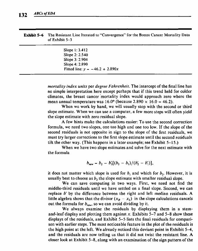
ABCs of EDA
Exhibit 5-6 The Resistant Line Iterated to "Convergence" for the Breast Cancer Mortality Dataof Exhibit 5-3
Slope 1:3.412Slope 2: 2.540Slope 3: 2.904Slope 4: 2.890Fitted line:^ = -46.2 + 2.890*
mortality index units per degree Fahrenheit. The intercept of the final line hasno simple interpretation here except perhaps that if this trend held for colderclimates, the breast cancer mortality index would approach zero where themean annual temperature was 16.0° (because 2.890 x 16.0 = 46.2).
When we work by hand, we will usually stop with the second or thirdslope estimate. When we can use a computer, a few more steps will often yieldthe slope estimate with zero residual slope.
A few hints make the calculations easier: To use the second correctionformula, we need two slopes, one too high and one too low. If the slope of thesecond residuals is not opposite in sign to the slope of the first residuals, wemust try larger corrections to the first slope estimate until the second residualstilt the other way. (This happens in a later example; see Exhibit 5-15.)
When we have two slope estimates and solve for the next estimate withthe formula
bnew = b2-b'2[{b2-bx)/{b'2-b\)],
it does not matter which slope is used for bx and which for b2. However, it isusually best to choose as b2 the slope estimate with smaller residual slope.
We can save computing in two ways. First, we need not find themiddle-third residuals until we have settled on a final slope. Second, we canreplace b' by the difference between the right and left median residuals. Alittle algebra shows that the divisor (xR — xL) in the slope calculations cancelsout the formula for bnew, so we can avoid dividing by it.
We always examine the residuals by displaying them in a stem-and-leaf display and plotting them against x. Exhibits 5-7 and 5-8 show thesedisplays of the residuals, and Exhibit 5-5 lists the final residuals for compari-son with earlier steps. The most noticeable feature in the plot of the residuals isthe high point at the left. We already noticed this deviant point in Exhibit 5-4,and the residuals are now telling us that it did not twist the resistant line. Acloser look at Exhibit 5-8, along with an examination of the sign pattern of the
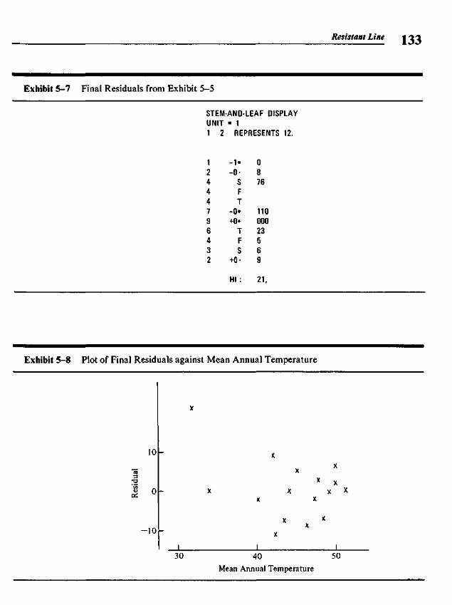
Resistant Line 133
Exhibit 5-7 Final Residuals from Exhibit 5-5
STEM-AND-LEAF DISPLAYUNIT = 11 2 REPRESENTS 12.
12444796432
- 1 *-0-
SFT
-0*+0*
TFS
+0-
0876
11000023569
H I : 21,
Exhibit 5-8 Plot of Final Residuals against Mean Annual Temperature
10
- 1 0
X X
30 40 50Mean Annual Temperature
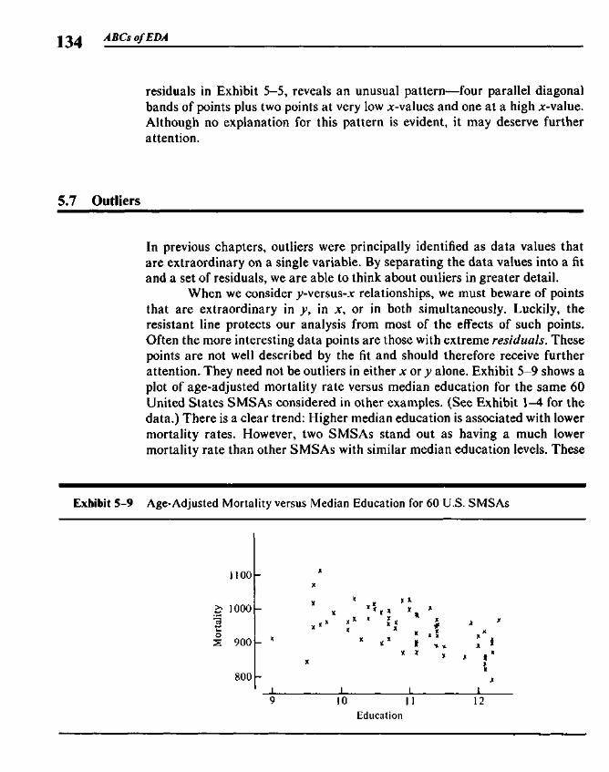
ABCsofEDA
residuals in Exhibit 5-5, reveals an unusual pattern—four parallel diagonalbands of points plus two points at very low x-values and one at a high x-value.Although no explanation for this pattern is evident, it may deserve furtherattention.
5.7 Outliers
In previous chapters, outliers were principally identified as data values thatare extraordinary on a single variable. By separating the data values into a fitand a set of residuals, we are able to think about outliers in greater detail.
When we consider y-versus-x relationships, we must beware of pointsthat are extraordinary in y, in x, or in both simultaneously. Luckily, theresistant line protects our analysis from most of the effects of such points.Often the more interesting data points are those with extreme residuals. Thesepoints are not well described by the fit and should therefore receive furtherattention. They need not be outliers in either x or y alone. Exhibit 5-9 shows aplot of age-adjusted mortality rate versus median education for the same 60United States SMSAs considered in other examples. (See Exhibit 1-4 for thedata.) There is a clear trend: Higher median education is associated with lowermortality rates. However, two SMSAs stand out as having a much lowermortality rate than other SMSAs with similar median education levels. These
Exhibit 5-9 Age-Adjusted Mortality versus Median Education for 60 U.S. SMSAs
1100
£• 1000
S 900
800
v *x x x
* x t
10 11Education
12
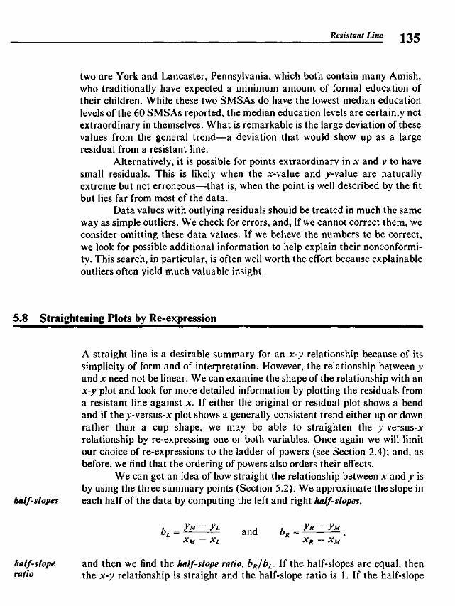
Resistant Line 135
two are York and Lancaster, Pennsylvania, which both contain many Amish,who traditionally have expected a minimum amount of formal education oftheir children. While these two SMSAs do have the lowest median educationlevels of the 60 SMSAs reported, the median education levels are certainly notextraordinary in themselves. What is remarkable is the large deviation of thesevalues from the general trend—a deviation that would show up as a largeresidual from a resistant line.
Alternatively, it is possible for points extraordinary in x and y to havesmall residuals. This is likely when the x-value and >>-value are naturallyextreme but not erroneous—that is, when the point is well described by the fitbut lies far from most of the data.
Data values with outlying residuals should be treated in much the sameway as simple outliers. We check for errors, and, if we cannot correct them, weconsider omitting these data values. If we believe the numbers to be correct,we look for possible additional information to help explain their nonconformi-ty. This search, in particular, is often well worth the effort because explainableoutliers often yield much valuable insight.
5.8 Straightening Plots by Re-expression
A straight line is a desirable summary for an x-y relationship because of itssimplicity of form and of interpretation. However, the relationship between yand x need not be linear. We can examine the shape of the relationship with anx-y plot and look for more detailed information by plotting the residuals froma resistant line against x. If either the original or residual plot shows a bendand if the >>-versus-x plot shows a generally consistent trend either up or downrather than a cup shape, we may be able to straighten the >--versus-xrelationship by re-expressing one or both variables. Once again we will limitour choice of re-expressions to the ladder of powers (see Section 2.4); and, asbefore, we find that the ordering of powers also orders their effects.
We can get an idea of how straight the relationship between x and y isby using the three summary points (Section 5.2). We approximate the slope in
half-slopes each half of the data by computing the left and right half-slopes,
bL = y^Ul and bR-y*-y\L R
XM ~ XL XR ~ XM
half-slope and then we find the half-slope ratio, bR/bL. If the half-slopes are equal, thenratl° the x-y relationship is straight and the half-slope ratio is 1. If the half-slope
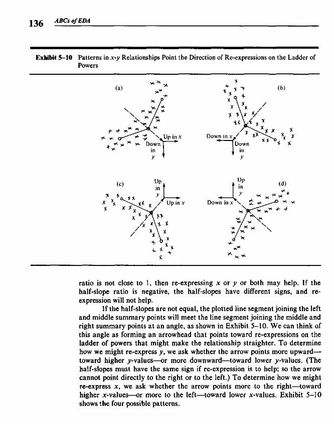
i tys ABCs of EDA
Exhibit 5-10 Patterns in x-y Relationships Point the Direction of Re-expressions on the Ladder ofPowers
(a)
Down in x \
ratio is not close to 1, then re-expressing x or y or both may help. If thehalf-slope ratio is negative, the half-slopes have different signs, and re-expression will not help.
If the half-slopes are not equal, the plotted line segment joining the leftand middle summary points will meet the line segment joining the middle andright summary points at an angle, as shown in Exhibit 5-10. We can think ofthis angle as forming an arrowhead that points toward re-expressions on theladder of powers that might make the relationship straighten To determinehow we might re-express y, we ask whether the arrow points more upward—toward higher ^-values—or more downward—toward lower ^-values. (Thehalf-slopes must have the same sign if re-expression is to help; so the arrowcannot point directly to the right or to the left.) To determine how we mightre-express x, we ask whether the arrow points more to the right—towardhigher x-values—or more to the left—toward lower ^-values. Exhibit 5-10shows the four possible patterns.
Resistant Line 137
Thus, the rule for selecting a re-expression to straighten a plot is thatwe consider moving the expression of y or x in the direction the arrow points.That is, if the arrow points down, toward lower y, we might try re-expressionsof y lower on the ladder of powers. Recall that raw data is the 1 power; so,moving down the ladder, we would try y/y (l/2 power), log(>>) (0 power), - 1 / Vy( — x/i power), and so on. If the arrow points to the right, toward higher x, wemight try re-expressions of x higher on the ladder of powers, such as x2 or x3.
As we saw when we re-expressed data to improve symmetry, the ladderof powers orders re-expressions according to the strength of their effect. Thus,if the half-slope ratio is well above 1 and the bend in the plot suggests movingdown the ladder of powers in y, Vy will probably be straighter against x. If -Jystill shows a bend pointing toward lower ^-values, then log(y) is likely to bebetter. Of course, if we move far enough down the ladder of powers, thehalf-slope ratio will eventually fall below 1, and the bend in the plot will pointthe other way. Thus we can systematically seek a re-expression by examiningthe half-slope ratio and letting it guide changes to stronger or less strongre-expressions.
A little thought will reveal how re-expressing can straighten an x-yrelationship and why this mnemonic rule works. If the half-slopes point downand to the right, as in part (a) of Exhibit 5-10, the higher y-values need to bepulled together more to straighten the relationship. This is what re-expressionslower than 1 on the ladder of powers do. For example, 0, 25, 100, and 225 aremade equally spaced by a square-root re-expression, and 1,10, 100, and 1000are made equally spaced by a log re-expression. If larger ^-values grow morerapidly than smaller ^-values, re-expressing y by square roots or logs (or somelower power) is likely to slow their growth and make the relationshipstraighter.
An alternative interpretation of the "down and to the right" pattern isto stretch out the higher x-values so that they grow as rapidly as theircorresponding ^-values. Re-expressions above 1 on the ladder of powers dothis. For example, 0, 5, 10, and 15 are stretched to 0, 25, 100, and 225 bysquaring and to 0, 125, 1000, and 3375 by cubing.
Thus, re-expressions alter the shape of data by stretching or shrinkingthe larger values differently from the smaller ones. Consequently, databatches in which the larger values are many times larger than the smaller oneswill be more affected by re-expressing than will batches in which the largestand smallest values are of about the same magnitude. Re-expressing data thatrange from 10.3 to 13.8 is pointless, but data stretching from 3 to 3000 willrespond to even a small move along the ladder of powers.
The pair of half-slope lines meeting at the middle summary point will,of course, suggest re-expressions for both x and y. We may choose tore-express either y or x or both. Often the nature of the data will lead us to
1 3 8 ABCsofEDA
prefer re-expressing one or the other. Sometimes a particular re-expression forx or y will be suggested by the units in which the data are measured or by someother aspect of the data, but if re-expressing one of x and y does not straightenthe relationship sufficiently, we might try re-expressing the other. If either xor y covers a much greater range of magnitude than the other, it will be moreaffected by re-expression, so we might try to re-express it first and use theother to "fine tune" the result. Finally, we often prefer to re-express y, simplybecause we think of x as the circumstance or the base from which to predict ordescribe^, and thus we prefer to have x in its original units.
When we work on a computer, we usually will not mind re-expressingall of the x- or ^-values, computing a new half-slope ratio, and drawing a newplot. When we work by hand (or when getting the results from the computertakes too long or costs too much), we can learn almost as much from the threesummary points alone. The summary points of re-expressed data can be foundby re-expressing the appropriate coordinates of the original summary pointsbecause the summary points are defined in terms of the ordered datavalues—first by using the ordered x-values to divide the data into thirds andthen by using the ordered x-values and ordering the ^-values to find medianswithin each third. We already have seen (in Section 2.4) that re-expressions onthe ladder of powers preserve order. Thus, the coordinates of the summarypoints of the re-expressed data are simply the re-expressed coordinates of theoriginal summary points.
The half-slope ratio is computed from the summary points. Thus weneed not re-express all of the data; we can re-express the summary points aloneand compute a new half-slope ratio. We can then explore a variety ofre-expressions quickly and easily without having to re-express every data valuefor each try. However, (as Section 2.4 warned) when two data values havebeen averaged to compute a median for a summary point coordinate, we mayprefer to re-express each of them and then average so we can be moreaccurate.
Example: Automobile Gasoline Mileage
Exhibit 5-11 reports mileage (in miles per gallon) and engine size (specifical-ly, displacement in cubic inches) for thirty-two 1976-model automobiles. Thedata are plotted in Exhibit 5-12. The plot clearly bends in a direction thatindicates a move down in the power of x or down for y. The half-slopes are—0.083 and -0.022, and their ratio is 0.268. We could try to re-express x or y,and the nature of the data suggests one re-expression. Gasoline mileage wasactually estimated by driving a measured course and observing the amount ofgasoline consumed—that is, by finding gallons used per mile. If we take the
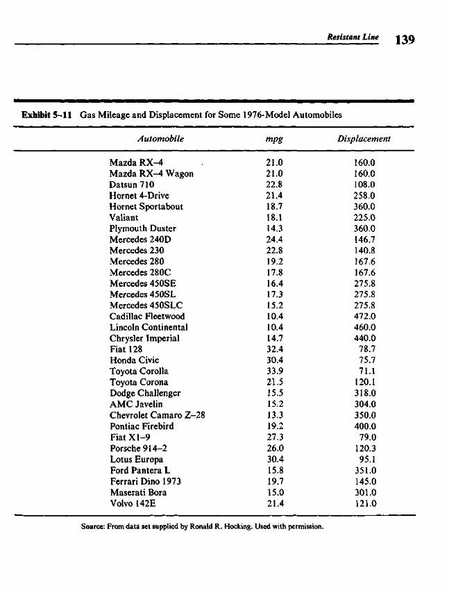
Resistant Line 139
Exhibit 5-11 Gas Mileage and Displacement for Some 1976-Model Automobiles
Automobile mpg Displacement
Mazda RX-4Mazda RX-4 WagonDatsun710Hornet 4-DriveHornet SportaboutValiantPlymouth DusterMercedes 240DMercedes 230Mercedes 280Mercedes 280CMercedes 450SEMercedes 450SLMercedes 450SLCCadillac FleetwoodLincoln ContinentalChrysler ImperialFiat 128Honda CivicToyota CorollaToyota CoronaDodge ChallengerAMC JavelinChevrolet Camaro Z-28Pontiac FirebirdFiat XI-9Porsche 914-2Lotus EuropaFord Pantera LFerrari Dino 1973Maserati BoraVolvo 142E
21.021.022.821.418.718.114.324.422.819.217.816.417.315.210.410.414.732.430.433.921.515.515.213.319.227.326.030.415.819.715.021.4
160.0160.0108.0258.0360.0225.0360.0146.7140.8167.6167.6275.8275.8275.8472.0460.0440.0
78.775.771.1
120.1318.0304.0350.0400.0
79.0120.395.1
351.0145.0301.0121.0
Source: From data set supplied by Ronald R. Hocking. Used with permission.
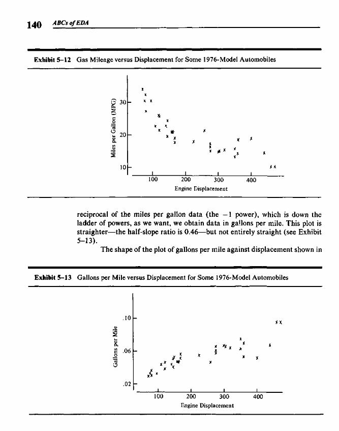
ABCsofEDA
Exhibit 5-12 Gas Mileage versus Displacement for Some 1976-Model Automobiles
O 30OH
O20
10
K
X X
X KX
X X
100 200 300
Engine Displacement400
reciprocal of the miles per gallon data (the - 1 power), which is down theladder of powers, as we want, we obtain data in gallons per mile. This plot isstraighter—the half-slope ratio is 0.46—but not entirely straight (see Exhibit5-13).
The shape of the plot of gallons per mile against displacement shown in
Exhibit 5-13 Gallons per Mile versus Displacement for Some 1976-Model Automobiles
.10
£ .06o
.02
*
. , ,
100 200 300
Engine Displacement400
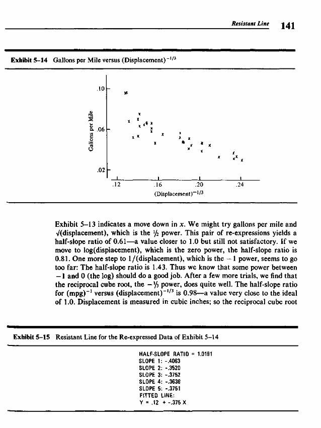
Resistant Line 141
Exhibit 5-14 Gallons per Mile versus (Displacement) -1/3
.10 -
8. .06
.02
.12
x x
.16 .20
(Displacement)"1/3
.24
Exhibit 5-13 indicates a move down in x. We might try gallons per mile andV(displacement), which is the x/i power. This pair of re-expressions yields ahalf-slope ratio of 0.61—a value closer to 1.0 but still not satisfactory. If wemove to log(displacement), which is the zero power, the half-slope ratio is0.81. One more step to 1/(displacement), which is the — 1 power, seems to gotoo far: The half-slope ratio is 1.43. Thus we know that some power between— 1 and 0 (the log) should do a good job. After a few more trials, we find thatthe reciprocal cube root, the — lfr power, does quite well. The half-slope ratiofor (mpg)"1 versus (displacement)~1/3 is 0.98—a value very close to the idealof 1.0. Displacement is measured in cubic inches; so the reciprocal cube root
Exhibit 5-15 Resistant Line for the Re-expressed Data of Exhibit 5-14
HALF-SLOPE RATIO = 1.0191SLOPE 1: -.4063SLOPE 2: -.3520SLOPE 3: -.3752SLOPE 4: -.3636SLOPE 5: -.3751FITTED LINE:Y = .12 + -.375 X
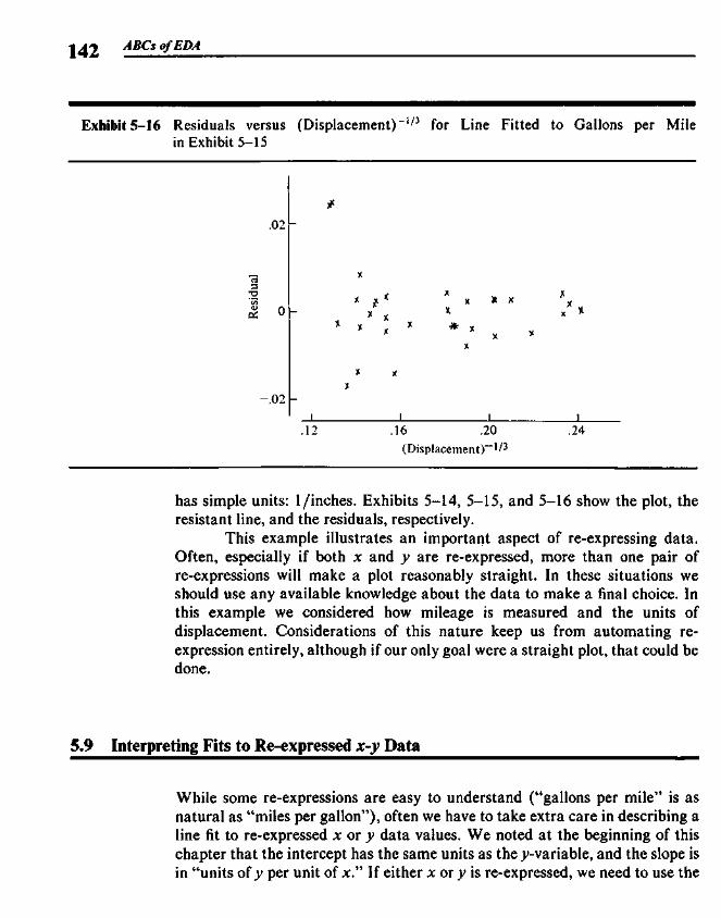
142 ABCs of EDA
Exhibit 5-16 Residuals versus (Displacement) 1/3 for Line Fitted to Gallons per Milein Exhibit 5-15
.02
-.02
.12
x * x
.16 .20(Displacement)""1/3
.24
has simple units: 1/inches. Exhibits 5-14, 5-15, and 5-16 show the plot, theresistant line, and the residuals, respectively.
This example illustrates an important aspect of re-expressing data.Often, especially if both x and y are re-expressed, more than one pair ofre-expressions will make a plot reasonably straight. In these situations weshould use any available knowledge about the data to make a final choice. Inthis example we considered how mileage is measured and the units ofdisplacement. Considerations of this nature keep us from automating re-expression entirely, although if our only goal were a straight plot, that could bedone.
5.9 Interpreting Fits to Re-expressed x~y Data
While some re-expressions are easy to understand ("gallons per mile" is asnatural as "miles per gallon"), often we have to take extra care in describing aline fit to re-expressed x or y data values. We noted at the beginning of thischapter that the intercept has the same units as the ^-variable, and the slope isin "units of y per unit of x." If either x or y is re-expressed, we need to use the
Resistant Line 143
re-expressed units in interpreting the slope and intercept. Thus in the gasmileage example (Exhibit 5-15), the intercept could be interpreted as .12gallons per mile, and the slope as —0.375 gallons per mile per reciprocal inchof engine size. Because we have re-expressed both x and y, the units of theslope are further away from the units of the original data. We can, however,check that the sign of the slope is reasonable—a smaller engine would have alarger reciprocal size and hence would use fewer gallons of gasoline permile—and it is still easy to use a new engine size in predicting gasolineconsumption.
When we have re-expressed y, an alternative interpretation can befound by inverting the re-expression to obtain a fit for y in its original units.Instead of the fitted linear equation -Jy = a + bx, we could consider theequivalent form
2x2y = (a + bx)2 = a2 + labx + b2x
Instead of the fitted linear equation log(>>) = a + bx, we could consider theform y = \0ia+bx\ Generally, whatever we gain by simplifying the expression ofy, we lose by making the fitted equation more complex. We have, in theresistant line, a convenient technique for fitting a line to an x-y relationship.Re-expressions extend the power of this technique to cover a far wider range ofx-y relationships without the need for new fitting methods.
The residuals from a line fit to re-expressed ^-values must be computedin the re-expressed units. Thus the residuals in the gas mileage example arefound from
1 - [0.12 - 0.375(disp)~1/3]observed mpg
and are in the re-expressed units, gallons per mile.Sometimes, the first hint of a need to re-express y will be that the
residuals would look better after re-expression. For example, often larger^-values are measured less precisely than smaller values. The residuals willthen show a wedge pattern when plotted against x—that is, they will be morespread out at the x-values corresponding to large ^-values, less spread outwhere the ^-values (and the measurement fluctuations) were smaller. Re-expressing y by moving down the ladder of powers will often make themeasurement fluctuations more comparable and make the residuals moreevenly spread out. When a single re-expression of y both straightens the x-yrelationship and evens up the residual pattern, we might have additional faiththat it is a worthwhile re-expression, and we would rather use it to straightenthe relationship than re-express the jc-variable.
\AA ABCsofEDA
* 5.10 Resistant Lines and Least-Squares Regression
The resistant line is one of many ways to fit a linear model to >>-versus-x data.The most common method is least-squares regression. Of course, these twomethods will generally not yield the same slope and intercept estimates, butoften the two sets of estimates will agree quite closely.
When our data contain outliers, or even when the distribution of theresiduals—from either fitted line—has long tails, the resistant line is likely todiffer more markedly from the regression line. The primary reason for thisdifference is that least-squares regression is not resistant to the effects ofoutliers.
When the distribution of the residuals is close to Gaussian and the datasatisfy some other restrictions, least-squares regression permits us to makestatistical inferences about the line. The resistant line is not yet accompaniedby an inference procedure. However, if the data do not meet the conditions forregression, it is dangerous to draw inferences from a least-squares line. In suchinstances, the resistant-line technique is likely to provide a better descriptionof the data.
Most statistical computer packages include programs for least-squaresregression. When we are analyzing data with such a package, it is usuallyworthwhile to fit both a resistant line and a least-squares regression andcompare the two lines. If they are similar, the regression line might bepreferred for the inference calculations it allows. If the lines differ, theresiduals from the resistant line may reveal the reason.
When we work by hand, we will usually prefer the resistant linebecause of its simpler calculations. When we use a computer, it is often helpfulto fit a resistant line first. This allows us to (1) check that the >>-versus-xrelationship is linear, (2) find a re-expression to straighten the relationship ifnecessary, and (3) check the residuals for outliers. Once we are reassured thatthe data are well-behaved in these ways, we can fit a least-squares regressionline.
5.11 Resistant Lines from the Computer
As we have seen, the computer can save us much calculating work in finding aresistant line and can print the slope of the fitted line at each step of theiteration. We must tell the programs which variables to treat as x and y. In
Resistant Line 145
addition, we should specify where the residuals are to be put. These specifica-tions may not be necessary in some implementations. They are automatic inthe BASIC programs.
The programs offer two modes of operation: verbose and silent. Inverbose mode—the recommended mode for exploring data—each iteration ofline polishing is reported. In silent mode, only the final fit is reported. As anadditional option, the programs can be told to limit the number of polishiterations. The default limit is 10 iterations—usually more than enough. Somepeculiar x-y data (especially when ties among x-values drastically reduce thesize of the middle third) may require more iterations.
In addition to the resistant line and residuals, the programs also reportthe half-slope ratio for assessing the straightness of the x-y relationship.However, the program will attempt to fit a line even if the half-slope ratioindicates nonlinearity. It is up to the data analyst to recognize and treat thisdifficulty.
t 5.12 Algorithms
The programs begin by dividing the batch into thirds and finding summarypoints. The algorithm to do this ensures that points with the same x-values willbe assigned to the same region and that no region will have too few points. (Ifone of the outer regions has fewer than 3 points, the line will not be resistant.)If only two distinct regions can be defined, the programs proceed with them. Ifeven this is impossible, the programs report the error.
Resistant-line polishing iterates until the slope estimate is correct to atleast four digits. (The algorithm does this by keeping an upper and a lowerbound on the correct slope.) The user must supply a maximum for the numberof steps, in case the process fails to converge. If this happens, the programsreturn the last bounds on the slope. Otherwise, they return the final slopeestimate and an intercept estimate chosen to make the median of the residualszero.
FORTRAN
The FORTRAN program for resistant line is a single subroutine, RLINE. Whenin verbose mode (TRACE set .TRUE.), it writes a report of each iteration.However, in both verbose and silent modes, the program returns the final fit
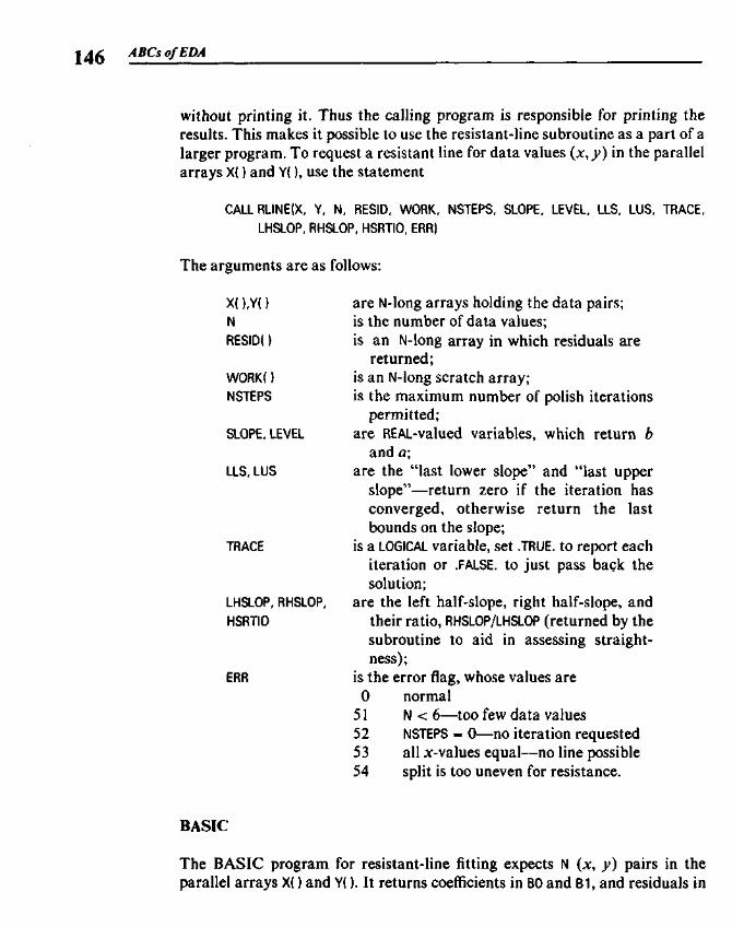
ABCsofEDA
without printing it. Thus the calling program is responsible for printing theresults. This makes it possible to use the resistant-line subroutine as a part of alarger program. To request a resistant line for data values (x, y) in the parallelarrays X() and Y(), use the statement
CALLRLINE(X, Y, N, RESID, WORK, NSTEPS, SLOPE, LEVEL, LLS, LUS, TRACE,
LHSLOP, RHSLOP, HSRTIO, ERR)
The arguments are as follows:
X( ),Y() are N-long arrays holding the data pairs;N is the number of data values;RESID() is an N-long array in which residuals are
returned;WORM ) is an N-long scratch array;NSTEPS is the maximum number of polish iterations
permitted;SLOPE, LEVEL a re REAL-valued variables , which re tu rn b
and a\LLS, LUS a re the " las t lower s lope" and " las t upper
s lope"—re tu rn zero if the i terat ion hasconverged, otherwise return the lastbounds on the slope;
TRACE is a LOGICAL var iab le , set .TRUE, to repor t eachi tera t ion or .FALSE, to ju s t pass back t hesolution;
LHSLOP, RHSLOP, a r e the left half-slope, r ight half-slope, andHSRTIO their rat io, RHSLOP/LHSLOP ( re turned by the
subroutine to aid in assessing straight-ness);
ERR is the error flag, whose values are0 normal
51 N < 6—too few data values52 NSTEPS = 0—no iteration requested53 all ^-values equal—no line possible54 split is too uneven for resistance.
BASIC
The BASIC program for resistant-line fitting expects N (x, y) pairs in theparallel arrays X() and Y(). It returns coefficients in BO and B1, and residuals in
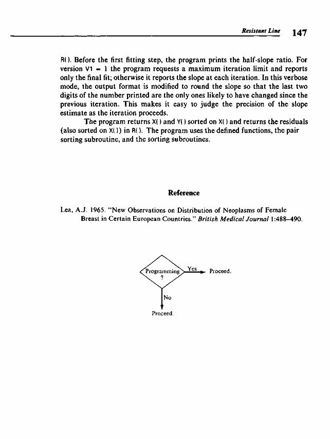
Resistant Line 147
R(). Before the first fitting step, the program prints the half-slope ratio. Forversion V1 = 1 the program requests a maximum iteration limit and reportsonly the final fit; otherwise it reports the slope at each iteration. In this verbosemode, the output format is modified to round the slope so that the last twodigits of the number printed are the only ones likely to have changed since theprevious iteration. This makes it easy to judge the precision of the slopeestimate as the iteration proceeds.
The program returns X() and Y() sorted on X() and returns the residuals(also sorted on X()) in R(). The program uses the defined functions, the pairsorting subroutine, and the sorting subroutines.
Reference
Lea, A.J. 1965. "New Observations on Distribution of Neoplasms of FemaleBreast in Certain European Countries." British Medical Journal 1:488-490.
Proceed.
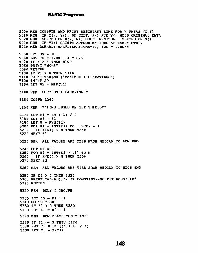
BASIC Programs
5000 REM COMPUTE AND PRINT RESISTANT LINE FOR N PAIRS (X,Y)5010 REM IN X()# Y(). ON EXIT, X() AND Y() HOLD ORIGINAL DATA5020 REM SORTED ON X(); R() HOLDS RESIDUALS SORTED ON X().5030 REM IF V1>1 PRINTS APPROXIMATIONS AT EVERY STEP.5040 REM DEFAULT MAX#ITERATIONS=10, TOL = 1.0E-4
5050 LET J9 = 105060 LET TO = 1.0E - 4 * 0.55070 IF N > 5 THEN 51005080 PRINT "N<=5"5090 RETURN5100 IF VI > 0 THEN 51405110 PRINT TAB(M0);"MAXIMUM # ITERATIONS";5120 INPUT J95130 LET VI = ABS(Vl)
5140 REM SORT ON X CARRYING Y
5150 GOSUB 1200
5160 REM **FIND EDGES OF THE THIRDS**
5170 LET El = (N + 1) / 25180 LET E3 = El5190 LET M = FNN(El)5200 FOR El = INT(El) TO 1 STEP - 15210 IF X(E1) < M THEN 52505220 NEXT El
5230 REM ALL VALUES ARE TIED FROM MEDIAN TO LOW END
5240 LET El = 05250 FOR E3 = INT(E3 + .5) TO N5260 IF X(E3) > M THEN 53505270 NEXT E3
5280 REM ALL VALUES ARE TIED FROM MEDIAN TO HIGH END
5290 IF El > 0 THEN 53205300 PRINT TAB(M0);"X IS CONSTANT—NO FIT POSSIBLE"5310 RETURN
5320 REM ONLY 2 GROUPS
5330 LET E3 = El + 15340 GO TO 53805350 IF El > 0 THEN 53805360 LET El = E3 - 1
5370 REM NOW PLACE THE THIRDS
5380 IF El <= 3 THEN 54705390 LET Tl = INT((N +1) / 3)5400 LET XI = X(T1)
148
BASIC 149
5410 REM IF Tl > El THEN LOOP IS SKIPPED AND El = E9
5420 LET E9 = El5430 FOR El = Tl TO E95440 IF X(E1 + 1) <> XI THEN 54705450 NEXT El5460 LET El = E9
5470 REM PLACE HIGH THIRD
5480 IF E3 >= N - 2 THEN 55705490 LET T3 = N - Tl + 15500 LET X3 = X(T3)5510 LET E9 = E3
5520 REM IF T3 < E3 THEN LOOP IS SKIPPED AND E3 = E9
5530 FOR E3 = T3 TO E9 STEP - 15540 IF X(E3 - 1) <> X3 THEN 55705550 NEXT E35560 LET E3 = E9
5570 REM **NOW El AND E3 ARE INNER EDGES OF OUTER THIRDS**5580 REM **SET UP FOR FITTING**
5590 LET Nl = E l5600 LET N3 = N - E3 + 15610 LET N2 = N - N l - N35620 LET N9 = N5630 IF N2 < 2 THEN 57205640 IF Nl > 2 THEN 57005650 IF N3 > 2 THEN 56805660 PRINT TAB(M0);"NOT ENOUGH DIFFERENT X-VALUES"5670 RETURN5680 LET El = E3 - 15690 GO TO 57205700 IF N3 > 2 THEN 57805710 LET E3 = El + 1
5720 REM ONLY 2 GROUPS
57305740575057605770
5780
579058005810
LETLETLETLETLET
REM
LETLETLET
NlN2N3X2Y2
= El= 0= N -= 0= 0
CONTINUE
MlM2M3
= (Nl= (N2= (N3
E3 +
j
+ 1)+ 1)+ 1)
1
/ 2/ 2/ 2
| C Q ABCs of EDA
5820 REM GET X-MEDIANS (STILL SORTED ON X)
5830 LET XI = FNN(Ml)5840 LET X4 = X(E1)5850 IF N2 = 0 THEN 58705860 LET X2 = FNN(E1 + M2)5870 LET X3 = FNN(E3 + M3 - 1)5880 LET X5 = X(E3)5890 LET D8 = X3 - XI
5900 REM GET Y-MEDIANS
5910 LET N = Nl5920 GOSUB 33005930 LET Yl = FNM(Ml)5940 LET Y4 = W(l)5950 LET Y5 = W(N1)5960 IF N2 = 0 THEN 60105970 LET Jl = El + 15980 LET J2 = El + N25990 GOSUB 33406000 LET Y2 = FNM(M2)6010 LET Jl = E36020 LET J2 = N96030 GOSUB 33406040 LET Y3 = FNM(M3)6050 LET Y6 = W(l)6060 LET Y7 = W(N)
6070 REM ON FIRST ITERATION, REPORT ON BEND
6080 IF VI < 2 THEN 61406090 IF N2 = 0 THEN 61406100 LET B6 = (Y3 - Y2) / (X3 - X2)6110 LET B5 = (Y2 - Yl) / (X2 - XI)6120 IF ABS(B5) <= EO THEN 61406130 PRINT TAB(MO);"HALF-SLOPE RATIO = ";B6 / B5
6140 REM FIRST 2 STEPS OF POLISH TO START
6150 LET B2 = (Y3 - Yl) / D86160 GOSUB 70406170 LET Bl = B26180 LET Dl = D26190 LET RO = 46200 IF VI < 2 GO TO 62206210 PRINT TAB(MO);"SLOPE 1: "; FNR(Bl)6220 LET B3 = B26230 LET D6 = D2 / D86240 IF ABS(D6) < EO THEN 68506250 LET B2 = B3 + D66260 GOSUB 70406270 IF SGN(D2) <> SGN(Dl) THEN 63206280 LET D6 = D6 + D66290 LET Bl = B2
BASIC
6300 LET Dl = D26310 GO TO 62506320 IF VI < 2 THEN 63406330 PRINT TAB(MO);"SLOPE 2: "; FNR(B2)
6340 REM ITERATION BASED UPON ZEROIN (SEE FORSYTH, MALCOM, & MOLER)
6350 LET J8 = 26360 LET B3 = Bl6370 LET D3 = Dl6380 LET B4 = B2 - Bl6390 LET B5 = B46400 IF ABS(D3) >= ABS(D2) GO TO 64706410 LET Bl = B26420 LET B2 = B36430 LET B3 = Bl6440 LET Dl = D26450 LET D2 = D36460 LET D3 = Dl6470 IF J8 > J9 GO TO 6820
6480 REM T1,T2,T3 USED FOR TOLERANCES FROM HERE ON
6490 LET Tl = 2 * EO * ABS(B2) + TO6500 LET B6 = 0.5 * (B3 - B2)6510 IF ABS(B6) <= Tl GO TO 68506520 IF D2 = 0 GO TO 6850
6530 REM TRY AGAIN
6540 LET D4 = D2 / Dl6550 LET T2 = 2 * B6 * D46560 LET T3 = 1 - D46570 IF T2 < 0 GO TO 65906580 LET T3 = - T36590 LET T2 = ABS(T2)6600 IF 2 * T2 >= 3 * B6 * T3 - ABS(T1 * T3) GO TO 66606610 IF T2 >= ABS(0.5 * B5 * T3) GO TO 66606620 LET B5 = B46630 LET B4 = T2 / T36640 GO TO 6680
6650 REM BISECT FOR NEXT TRY
6660 LET B4 = B66670 LET B5 = B4
6680 REM SECANT RULE
6690 LET Bl = B26700 LET Dl = D26710 LET B2 = B2 + B46720 IF ABS(B4) > Tl GO TO 67406730 LET B2 = Bl + Tl * SGN(B6)6740 LET J8 = J8 + 1
151
152 ABC s of EDA
6750 REM REPORT STEP
6760 IF VI < 2 GO TO 67906770 LET R0 = - FNF( FNL(B6)) + 16780 PRINT TAB(MO);"SLOPE ";J8;": "; FNR(B2)6790 GOSUB 70706800 IF SGN(D2) = SGN(D3) GO TO 63606810 GO TO 64006820 PRINT "FAILED TO CONVERGE AFTER ";J9;" ITERATIONS."6830 PRINT TAB(M0);B2;" <= B <= ";B3
6840 REM COMPUTE INTERCEPT AND RESIDUALS ANYWAY6850 REM EXIT — PRINT FINAL EQUATION
6860 LET N = N96870 FOR I = 1 TO N6880 LET W(I) = Y(I) - B2 * X(I)6890 LET R(I) = W(I)6900 NEXT I6910 GOSUB 10006920 LET BO = FNM((N + 1) / 2)6930 PRINT6940 PRINT TAB(MO);"FITTED LINE:"6950 PRINT "Y =";6960 PRINT FNR(BO);6970 IF ABS(D2) > EO THEN 69906980 LET RO = 76990 PRINT " + "; FNR(B2);" X"7000 FOR I = 1 TO N7010 LET R(I) = R(I) - BO7020 NEXT I7030 RETURN
7040 REM SUBROUTINE TO FIND MEDIAN RESIDUALS AND THEIR DIFFERENCE.7050 REM ENTERED WITH TRIAL SLOPE IN B27060 REM PUTS DIFFERENCE BETWEEN LEFT AND RIGHT MEDIAN RESIDS IN D2
7070 LET N = Nl7080 FOR I = 1 TO Nl7090 LET W(I) = Y(I) - X(I) * B27100 NEXT I7110 GOSUB 10007120 LET Zl = FNM(Ml)7130 LET N = 07140 FOR I = E3 TO N97150 LET N = N + 17160 LET W(N) = Y(I) - X(I) * B27170 NEXT I7180 GOSUB 10007190 LET D2 = FNM(M3) - Zl7200 RETURN
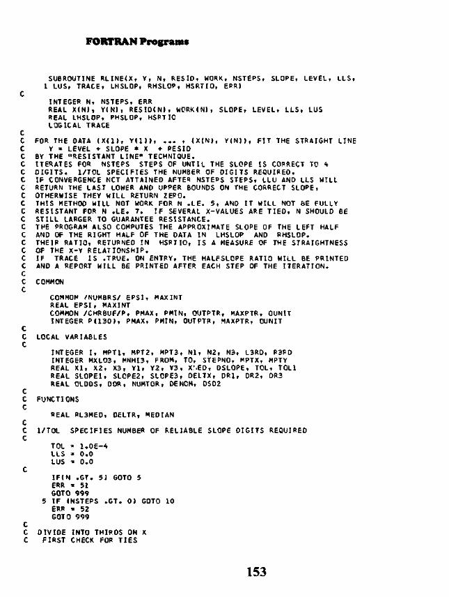
FORTRAN Programs
SUBROUTINE RLINE(X, Y, N, RESID, WORK, NSTEPSt SLOPE, LEVEL, LLS,1 LUS, TRACE, LHSLOP, RHSLOP, HSRTIO, ERR)
CINTEGER N, NSTEPS, ERRREAL X(N), Y(N), RESID(N), WCRK(N), SLOPE, LEVEL, LLS, LUSREAL LHSLOP, PHSLOP, HSPTIOLOGICAL TRACE
CC FOR THE DATA (X(l), Y U M , ... , (X(N), Y(N)), FIT THE STRAIGHT LINEC Y = LEVEL + SLOPE * X + PESIDC BY THE "RESISTANT LINE" TECHNIQUE.C ITERATES FOR NSTEPS STEPS OF UNTIL THE SLOPE IS CORRECT TO 4C DIGITS. 1/TOL SPECIFIES THE NUMBER OF DIGITS REQUIRED.C IF CONVERGENCE NCT ATTAINED AFTER NSTEPS STEPS, LLU AND LLS WILLC RETURN THE LAST LOWER AND UPPER BOUNDS ON THE CORRECT SLOPE,C OTHERWISE THEY WILL RETURN ZERO.C THIS METHOD WILL NOT WORK FOR N .LE. 5, AND IT WILL NOT BE FULLYC RESISTANT FOR N .LE. 7. IF SEVERAL X-VALUES ARE TIED, N SHOULD BEC STILL LARGER TO GUARANTEE RESISTANCE.C THE PROGRAM ALSO COMPUTES THE APPROXIMATE SLOPE OF THE LEFT HALFC AND OF THE RIGHT HALF OF THE DATA IN LHSLOP AND RHSLOP.C THEIR RATIO, RETURNED IN HSRTIO, IS A MEASURE OF THE STRAIGHTNESSC OF THE X-Y RELATIONSHIP.C IF TRACE IS .TRUE. ON ENTRY, THE HALFSLOPE RATIO WILL BE PRINTEDC AND A REPORT WILL BE PRINTED AFTER EACH STEP OF THE ITERATION.CC COMMONC
COMMON /NUMBRS/ EPSI, MAX INTREAL EPSI, MAXINTCOMMON /CHRBUF/P, PMAX, PMIN, OUTPTR, MAXPTR, OUNITINTEGER P(130), PMAX, PMIN, OUTPTR, MAXPTR, OUNIT
CC LOCAL VARIABLESC
INTEGER I, MPT1, MPT2, MPT3, Nl, N2, N3, L3RD, P3RDINTEGER MXL03, MNHI3, FROM, TO, STEPNO, MPTX, MPTYREAL XI, X2, X3, Yl, Y2, Y3, X.'.ED, DSLOPE, TOL, TOL1REAL SLOPE1, SLOPE2, SLOPE3, DELTX, DR1, DR2, DR3REAL OLDOS, DDR, NUMTOR, DENCM, DSD2
CC FUNCTIONSC
REAL RL3MED, DELTR, MEDIANCC 1/TOL SPECIFIES NUMBER OF RELIABLE SLOPE DIGITS REQUIREDC
TOL - 1.0E-4LLS = 0.0LUS - 0.0
CIF(N .GT. 5) GOTO 5ERR = 51GOTO 999
5 IF (NSTEPS .GT. 0) GOTO 10ERP = 52GOTO 999
CC DIVIDE INTO THIRDS ON XC FIRST CHECK FOR TIES
153
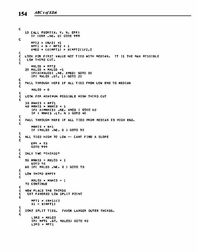
ABC s of EDA
C10 CALL PSORT(X, Y, N, ERR)
IF (ERR .NE. 0) GOTO 999C
MPT2 = (N/2) +1MPT1 » N - MPT2 + 1XMED = (X(MPT1) + X(MPT2))/2.0
CC LOOK FOR FIRST VALUE NOT TIED WITH MEDIAN. IT IS THE MAX POSSIBLEC LOW THIRD CUT.C
MXL03 » MPT220 MXL03 » MXL03 -1
IF(X(MXL03) .NE. XMED) GOTO 30IF( MXL03 .GT- 1) GOTO 20
CC FALL THROUGH HEPE IF ALL TIED FROM LOW END TO MEDIANC
MXL03 = 0CC LOOK FOR MINIMUM POSSIBLE HIGH THIRD CUTC
30 MNHI3 = MPT140 MNHI3 = MNHI3 + 1
IF( X(MNHI3) .NE. XMED ) GOTO 60IF ( MNHI3 .LT. N ) GOTO 40
CC FALL THROUGH HEPE IF ALL TIED FROM MEDIAN TO HIGH END.C
MNHI3 = N+lIF <MXL03 .NE. 0 ) GOTO 50
CC ALL TIED HIGH TO LOW — CANT FIND A SLOPEC
ERR * 53GOTO 999
CC ONLY TWO "THIRDS"C
50 MNHI3 = MXL03 + 1GOTO 70
60 IF( MXL03 .NE. 0 ) GOTO 70CC LOW THIRD EMPTYC
MXLO3 = MNHI3 - 170 CONTINUE
CC NOW PLACE THE THIRDSC GET FAVORED LOW SPLIT POINTC
MPT1 * (N + D / 3XI = X(MPT1)
CC DONT SPLIT TIES. FAVOR LARGER OUTER THIRDS.C
L3RD » MXL03IF( MPT1 .GT. MXL03) GOTO 90L3RD » MPT1
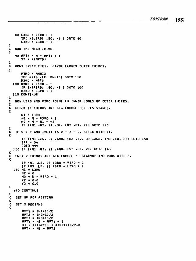
FORTRAN 155
80 L3RD = L3R0 • 1IF ( X(L3RD) .EQ. XI ) GOTO 80L3R0 » L3RD - 1
CC NOW THE HIGH THIRDC
90 MPT3 =* N - MPT1 + 1X3 * X(MPT3)
CC OONT SPLIT TIES. FAVOR LARGER OUTER THIRDS.C
P3RD = MNHI3IF( MPT3 .LE. MNHI3) GOTO 110R3RD = MPT3
100 R3RD » R3RD - 1IF (X(R3RD) .EQ. X3 ) GOTO 100R3RD « R3PD • 1
110 CONTINUECC NOW L3RD AND R3P0 POINT TO INNER EDGES OF OUTER THIRDS.CC CHECK IF THIRDS ARE BIG ENOUGH FOP PESISTANCE.C
Nl * L3P.DN3 * N - R3RD + 1N2 » N - Nl - N3IF {(Nl .GT. 2) .OR. (N3 .GT. 2)) GOTO 120
CC IF N « 7 AND SPLIT IS 2 - 3 - 2, STICK WITH IT.C
IF ((Nl .EQ. 2) .AND. (N2 .EQ. 3) .AND. (N3 .EQ. 2)) GOTO 140ERR * 54GOTO 999
120 IF ((Nl .GT. 2) .AND. (N3 .GT. 2)) GOTO 140CC ONLY 2 THIRDS ARE BIG ENOUGH — REGROUP AND WORK WITH 2.C
IF (Nl .LE. 2) L3RD = R3RD - 1IF (N3 .LE. 2) R3RD * L3R0 + 1
130 Nl = L3RDN2 * 0N3 = N - R3RD + 1X2 = 0.0Y2 = 0.0
C140 CONTINUE
ccccc
SET
GET
UP FORFITTING
X MEDIANS
MPT1 »MPT2 =MPT 3 »MPTY =
(Nl+D/2(N2+D/2(N3+1I/2Nl - MPT1 + 1
XI » (X(MPT1) + X(MPTY) ) /2 .0MPTX = Nl • MFT2
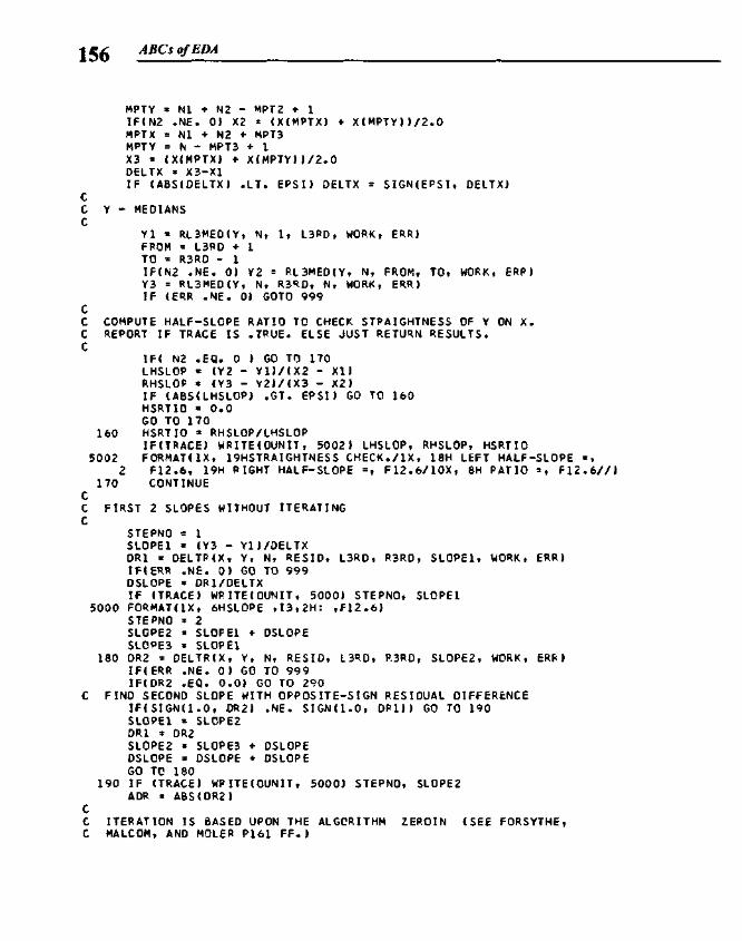
1 5 6 ABC s of EDA
MPTY = Nl + N2 - MPT2 + 1IF(N2 .NE. 0) X2 = (X(MPTX) + X lMPTY) ) /2 .0MPTX = Nl + N2 + MPT3MPTY = K - MPT3 + 1X3 = (X(MPTX) • X(MPTY)) /2 .0OELTX = X3-X1IF (ABS(OELTX) . I T . EPS IJ DELTX = SIGN(EPSI, DELTX)
CC Y - MEDIANSC
Yl = RL3MED(Y, N, 1 , L3RD, WORK, ERR)FROM = L3RD + 1TO = R3R0 - 1IF(N2 .NE. 0) Y2 = RL3MED(Y, N, FROM, TO, WORK, ERR)Y3 = RL3ME0(Y, N, R3RD, N, WORK, ERR)IF (ERR .NE. 0) GOTO 999
CC COMPUTE HALF-SLOPE RATIO TO CHECK STPAIGHTNESS OF Y ON X.C REPORT IF TRACE IS .TRUE. ELSE JUST RETURN RESULTS.C
IF( N2 .EQ. 0 ) GO TO 170LHSLOP = (Y2 - Y 1 ) / ( X 2 - X I )RHSLOP * (Y3 - Y 2 ) / ( X 3 - X2)IF (ABS(LHSLOP) .GT. EPSI) GO TO 160HSRTIO = 0 .0GO TO 170
160 HSRTIO » RHSLOP/LHSLOPIF(TRACE) WRITE(OUNIT, 5002) LHSLOP, RHSLOP, HSRTIO
5002 FORMATdX, 19HSTRAIGHTNESS CHECK./1X, 18H LEFT HALF-SLOPE =,2 F12 .6 , 19H RIGHT HALF-SLOPE =, F12 .6 /10X , 8H PATIO =, F 1 2 . 6 / / )
170 CONTINUECC FIRST 2 SLOPES WITHOUT ITERATINGC
STEPNO = 1SL0PE1 * (Y3 - YD/OELTX0R1 = DELTP<X, Y, N, RESID, L3RD, R3RD, SL0PE1, WORK, ERR)IFCERR .NE. 0 ) GO TO S99DSLOPE = DR1/DELTXIF (TRACE) WPITE(OUNIT, 5000) STEPNO, SL0PE1
5000 FORMATdX, 6HSL0PE , I 3 , 2 H : ,F12 .6 )STEPNO = 2SL0PE2 = SL0PE1 + DSLOPESL0PE3 = SL0PE1
180 DR2 = DELTR(X, Y, N, RESID, L3RD, R3RD, SL0PE2, WORK, ERR)IF(ERR .NE. 0 ) GO TO 999IF(DR2 .EQ. 0 .0 ) GO TO 290
C FIND SECOND SLOPE WITH OPPOSITE-SIGN RESIDUAL DIFFERENCEIFCSIGNd.O, 0R2) .NE. S I G N d . O , DPI)) GO TO 190SL0PE1 = SL0PE2DR1 * DR2SL0PE2 = SL0PE3 + DSLOPEDSLOPE = DSLOPE + DSLOPEGO TO 180
190 IF (TRACE) WPITE(OUNIT, 5000) STEPNO, SL0PE2ADR * ABS(DR2)
CC ITERATION IS BASED UPON THE ALGORITHM ZEROIN (SEE FORSYTHE,C MALCOM, AND MOLER P161 FF.)
FORTRAN 157
220 SL0PE3 = SL0PE1DR3 = DR1DSLOPE = SL0PE2 - SL0PE1OLDDS = DSLOPE
230 IF( ABS(DR3> .GE. ABS(0R2) ) GO TO 240SL0PE1 = SL0PE2SL0PE2 = SL0PE3SL0PE3 = SL0PE1DR1 » DR2DR2 - DR30R3 = DR1
TEST CONVERGENCE
240 IF( STEPNO .GE. NSTEPS ) GO TO 285T0L1 » 2 .0 * EPSI * ABS1SL0PE2J + 0.5 * TOLDSD2 = .5 * (SL0PE3 - SL0PE2)!F(ABS(0SD2) .LE. TOLD GO TO 290IF(DR2 .EQ. 0 .0 ) GO TO 290
TRY AGAIN
OOR - DR2/DR1NUMTOR a 2 .0 • DSD2 * DDPDENOM = 1.0 - DDRIr< NUMTOR .GT. 0 .0 ) DENOM » -DENOMNUMTOR » ABS(NUMTOR)I F ( ( 2 . 0 * NUMTOR) .GE. ( 3 . 0 • DSD2 * DENOM - ABS(TOL1 * DENOM)))
1 GO TO 270IF( NUMTOR .GE. ABS(0.5 * OLDDS * DENOM) ) GO TO 270OLDDS = DSLOPEDSLOPE » NUMTCR/DENOMGO TO 280
BISECT
270 OSLOPE = DSD2OLDDS - DSLOPE
280 SL0PE1 * SL0PE2DR1 * DR2IF( ABS(DSLOPE) .GT. T0L1 ) SL0PE2 = SL0PE2 + DSLOPEIFt ABS(DSLOPE) .LE. T0L1 ) SL0PE2 = SL0PE2 + SIGNlT0L1,DSD2)STEPNC = STEPNO + 1IF(TRACE) WRITE(OUNIT, 5000) STEPNO, SL0PE2DR2 = DELTRCX, Y t Nt RESID, L3RD. R3RDf SL0PE2, WORK,ERR)IF( ER» .NE. 0) GO TO 999IF( (DR2 * (DR3/ABS(DR3))) .GT. 0.0 ) GO TO 220GO TO 230
RAN OUT OF STEPS
285 LLS - AMINKSLOPE1, SL0PE3)LUS - AMAXKSLOPE1, SL0PE3)GO TO 999
EXIT
ABC s of EDA
C290 SLOPE = SL0PE2
DO 300 I = 1 , NWORKU) = Y ( I ) - SLOPE * X ( I )
300 CONTINUECALL SORT( WORK, N, ERR)IF(ERR . N E . 0 ) GO TO 9 9 9LEVEL = MEDIAN(WORK, N)00 310 I * 1 , N
R E S I D ( I ) - Y d ) - SLOPE*X( I ) - LEVEL310 CONTINUE999 RETURN
ENDREAL FUNCTION RL3MED(Yt N, FROM, TOt WORK, ERP)
CC RETURNS THE MEDIAN OF THE NUMBERS FROM Y(FROM) TO Y ( T O ) , INCLUSIVE.C
INTEGER N t FRCM, TO, ERRREAL Y ( N ) , WORK(N)
CC LOCAL VARIABLESC
INTEGER I , JCC FUNCTIONC
REAL MEDIANC
J = 000 10 1 - FRCM, TO
J = J + lWORK(J) = Y ( I )
10 CONTINUECALL SORT(WORK, J , ERR)I F (ERR . N E . 0 ) GOTO 999RL3MED = MEDIANCWORK, J )
999 RETURNENDREAL FUNCTION DELTR(X, Y , N, RESID, L3RD, R3PD, SLOPE, WORK, ERR)
CC RETURNS THE DIFFERENCE BETWEEN THE MEDIAN RESIDUALS IN THE LEFT ANDC RIGHT 3RDS OF THE DATA FOR A LINE WITH SPECIFIED SLOPE.C
INTEGER N, L3RD, R3RD, ERRREAL X ( N ) , Y ( K ) , R E S I D ( N ) , WORK(N), SLOPE
CINTEGER I
CC FUNCTIONC
REAL RL3ME0C
DO 10 I * I t NRESIDCI) * Y ( I ) - SLOPE * X ( I )
10 CONTINUEDELTR = RL3MED(RESID, N, R3RD, N, WORK, ERR)
2 - RL3MED(RESI0, N , 1 , L3RD, WORK, ERR)RETURNEND
Chapter 6Smoothing Data
The two previous chapters have presented techniques for plotting ^-versus-xdata and for summarizing such data with a resistant line. Often it is useful tosearch for patterns much more general than a straight line. When the x-valuesare equally spaced or almost equally spaced, we might ask only that y changesmoothly from point to point along the x-axis. This chapter presentstechniques for discovering and summarizing smooth data patterns.
6.1 Data Sequences and Smooth Summaries
When the x-values are equally spaced, their structure is so simple and regularthat y often receives most of the attention. Lists of such data may even omitthe x-values in favor of reporting the interval at which the data were recorded.
data sequence We refer to such ^-values as a data sequence. Examples are the monthly rate ofunemployment, the daily high and low temperatures at a weather station, andthe number of votes cast in each U.S. presidential election.
When the sequence comes about by recording a value for each159
160 ABCsofEDA
time series successive time interval, as in these examples, the y-values are known as a timeseries. (Sometimes this term is reserved for such data sequences in which manyconsecutive values are available.) However, the order of data values in asequence need not be defined by time. We might consider the sequence ofbirthrates as mother's age increases, heart-attack frequencies ordered bypatient's weight, or the differences between low and high tide heights at pointsalong a shoreline ordered by latitude. Data sequences are thus a specializedform of (x, y) data in which the values of x are important primarily for theorder they specify—in time, in space, or whatever. Nevertheless, the terminol-ogy of time series is well suited to atemporal sequences as well. We might, forexample, refer to a data value "earlier than" or "previous to" another valueeven if the ordering were not temporal. We therefore denote the order-definingvalue by t rather than x and often write it as a subscript to the variable y. Anydata sequence can thus be represented as a sequence of values, yt, orderedby t.
While the techniques in this chapter are usually applied to data whoser-values are evenly spaced, the essential feature of data sequences is that theirf-values are in order. Sometimes we can take a fairly lax attitude toward thedetails of the spacing, provided that the spacing is not too irregular. Thus, aslong as / defines an order, we may be able to use these techniques.
The Smooth and the Rough
In Chapter 5 we found it useful to treat a resistant line as a simple descriptionof a >»-versus-x relationship and to separate the data values into
data = fit + residual.
Such a separation can be useful even when the fit is not described by aformula. All we require is that the fit be a simple, well-structured descriptionof the data and, ideally, that it capture much of the underlying pattern of thedata.
Usually our attempts at a simple fit are smooth curves. When workingby hand, we might plot the sequence of ^-values against their correspondingx-values and sketch in a freehand curve. With such a curve we would try tocapture the large-scale behavior of the data sequence—that is, where thesequence rises, where it falls, and whether it shows regularities or cycles (forexample, greater sales in December of every year). Small-scale fluctuations,such as isolated data values out of line or small, rapidly changing oscillations,would then appear in the residuals.
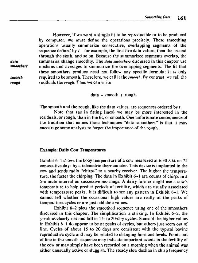
Smoothing Data 1 f> 1
datasmoothers
smoothrough
However, if we want a simple fit to be reproducible or to be producedby computer, we must define the operations precisely. These smoothingoperations usually summarize consecutive, overlapping segments of thesequence defined by t—for example, the first five data values, then the secondthrough the sixth, and so on. Because the summarized segments overlap, thesummaries change smoothly. The data smoothers discussed in this chapter usemedians and averages to summarize the overlapping segments. The fit thatthese smoothers produce need not follow any specific formula; it is onlyrequired to be smooth. Therefore, we call it the smooth. By contrast, we call theresiduals the rough. Thus we can write
data = smooth + rough.
The smooth and the rough, like the data values, are sequences ordered by t.Note that (as in fitting lines) we may be more interested in the
residuals, or rough, than in the fit, or smooth. One unfortunate consequence ofthe tradition that names these techniques "data smoothers" is that it mayencourage some analysts to forget the importance of the rough.
Example: Daily Cow Temperatures
Exhibit 6-1 shows the body temperature of a cow measured at 6:30 A.M. on 75consecutive days by a telemetric thermometer. This device is implanted in thecow and sends radio "chirps" to a nearby receiver. The higher the tempera-ture, the faster the chirping. The data in Exhibit 6-1 are counts of chirps in a5-minute interval on successive mornings. A dairy farmer might use a cow'stemperature to help predict periods of fertility, which are usually associatedwith temperature peaks. It is difficult to see any pattern in Exhibit 6-1. Wecannot tell whether the occasional high values are really at the peaks oftemperature cycles or are just odd data values.
Exhibit 6-2 plots the smoothed sequence using one of the smoothersdiscussed in this chapter. The simplification is striking. In Exhibit 6-2, the^-values clearly rise and fall in 15- to 20-day cycles. Some of the higher valuesin Exhibit 6-1 do appear to be at peaks of cycles, but others just seem out ofline. Cycles of about 15 to 20 days are consistent with the typical bovinereproductive cycle and may be related to changing hormone levels. Points outof line in the smooth sequence may indicate important events in the fertility ofthe cow or may simply have been recorded on a morning when the animal waseither unusually active or sluggish. The steady slow decline in chirp frequency
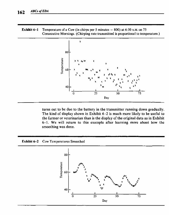
162 ABCsofEDA
Exhibit 6-1 Temperature of a Cow (in chirps per 5 minutes — 800) at 6:30 A.M. on 75Consecutive Mornings. (Chirping rate transmitted is proportional to temperature.)
80
E 60
40
X X x x X* )
X
— X XXX „ X
X Xx - X
xx
XX XX
X X
X
I
x * xXX » » X
25 50Day
75
turns out to be due to the battery in the transmitter running down gradually.The kind of display shown in Exhibit 6-2 is much more likely to be useful tothe farmer or veterinarian than is the display of the original data as in Exhibit6-1. We will return to this example after learning more about how thesmoothing was done.
Exhibit 6-2 Cow Temperatures Smoothed
80
60
40
- xxxx
f
25 50Day
75
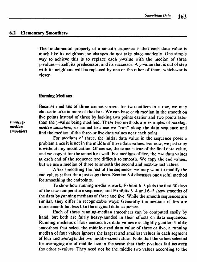
Smoothing Data \(%\
6.2 Elementary Smoothers
The fundamental property of a smooth sequence is that each data value ismuch like its neighbors; so changes do not take place suddenly. One simpleway to achieve this is to replace each >>-value with the median of three^-values—itself, its predecessor, and its successor. A y-value that is out of stepwith its neighbors will be replaced by one or the other of them, whichever iscloser.
running-mediansmoothers
Running Medians
Because medians of three cannot correct for two outliers in a row, we maychoose to take in more of the data. We can base each median in the smooth onfive points instead of three by looking two points earlier and two points laterthan the >>-value being modified. These two methods are examples of running-median smoothers, so named because we "run" along the data sequence andfind the median of the three or five data values near each point.
For medians of three, the initial data value in the sequence poses aproblem since it is not in the middle of three data values. For now, we just copyit without any modification. Of course, the same is true of the final data value,and we copy it for the smooth as well. For medians of five, the two data valuesat each end of the sequence are difficult to smooth. We copy the end values,but we use a median of three to smooth the second and next-to-last values.
After smoothing the rest of the sequence, we may want to modify theend values rather than just copy them. Section 6.4 discusses one useful methodfor smoothing the endpoints.
To show how running medians work, Exhibit 6-3 plots the first 30 daysof the cow-temperature sequence, and Exhibits 6-4 and 6-5 show smooths ofthe data by running medians of three and five. While the smooth sequences aresimilar, they differ in recognizable ways: Generally the medians of five aremore smooth but less like the original data sequence.
Each of these running-median smoothers can be computed easily byhand, but both are fairly heavy-handed in their effects on data sequences.Running medians of four consecutive data values are slightly gentler. Unlikesmoothers that select the middle-sized data value of three or five, a runningmedian of four values ignores the largest and smallest values in each segmentof four and averages the two middle-sized values. Note that the values selectedfor averaging are of middle size in the sense that their ^-values fall betweenthe other >>-values. They need not be the middle two values according to the
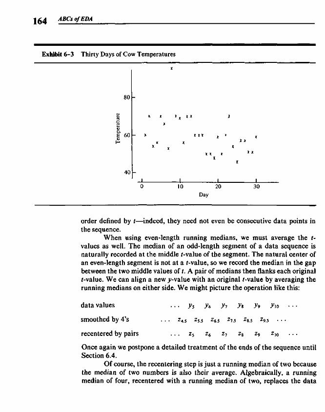
ABCsofEDA
Exhibit 6-3 Thirty Days of Cow Temperatures
80
E 6 0
40
x x x „ x x
t txx x
XX Xt
I X
10 20Day
30
order defined by /—indeed, they need not even be consecutive data points inthe sequence.
When using even-length running medians, we must average the t-values as well. The median of an odd-length segment of a data sequence isnaturally recorded at the middle /-value of the segment. The natural center ofan even-length segment is not at a /-value, so we record the median in the gapbetween the two middle values of /. A pair of medians then flanks each original/-value. We can align a new >>-value with an original /-value by averaging therunning medians on either side. We might picture the operation like this:
data values
smoothed by 4's
recentered by pairs
J>7
Z7.5
Z6 Z9lo
Once again we postpone a detailed treatment of the ends of the sequence untilSection 6.4.
Of course, the recentering step is just a running median of two becausethe median of two numbers is also their average. Algebraically, a runningmedian of four, recentered with a running median of two, replaces the data
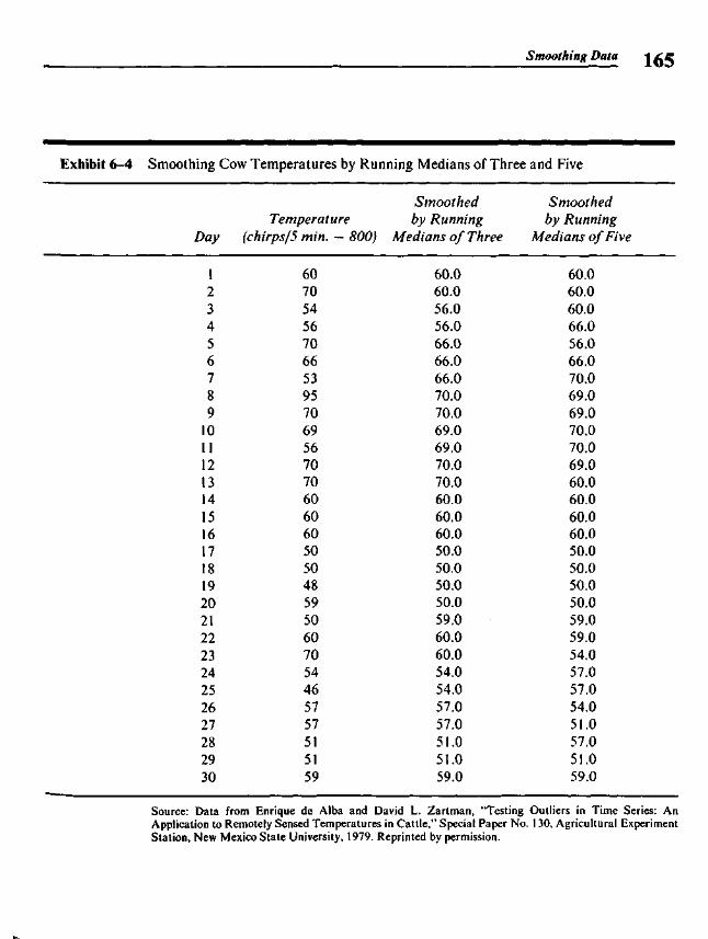
Smoothing Data
Exhibit 6-4 Smoothing Cow Temperatures by Running Medians of Three and Five
Smoothed SmoothedTemperature by Running by Running
Day (chirps/'5 min. — 800) Medians of Three Medians of Five
123456789101112131415161718192021222324252627282930
607054567066539570695670706060605050485950607054465757515159
60.060.056.056.066.066.066.070.070.069.069.070.070.060.060.060.050.050.050.050.059.060.060.054.054.057.057.051.051.059.0
60.060.060.066.056.066.070.069.069.070.070.069.060.060.060.060.050.050.050.050.059.059.054.057.057.054.051.057.051.059.0
Source: Data from Enrique de Alba and David L. Zartman, "Testing Outliers in Time Series: AnApplication to Remotely Sensed Temperatures in Cattle," Special Paper No. 130, Agricultural ExperimentStation, New Mexico State University, 1979. Reprinted by permission.
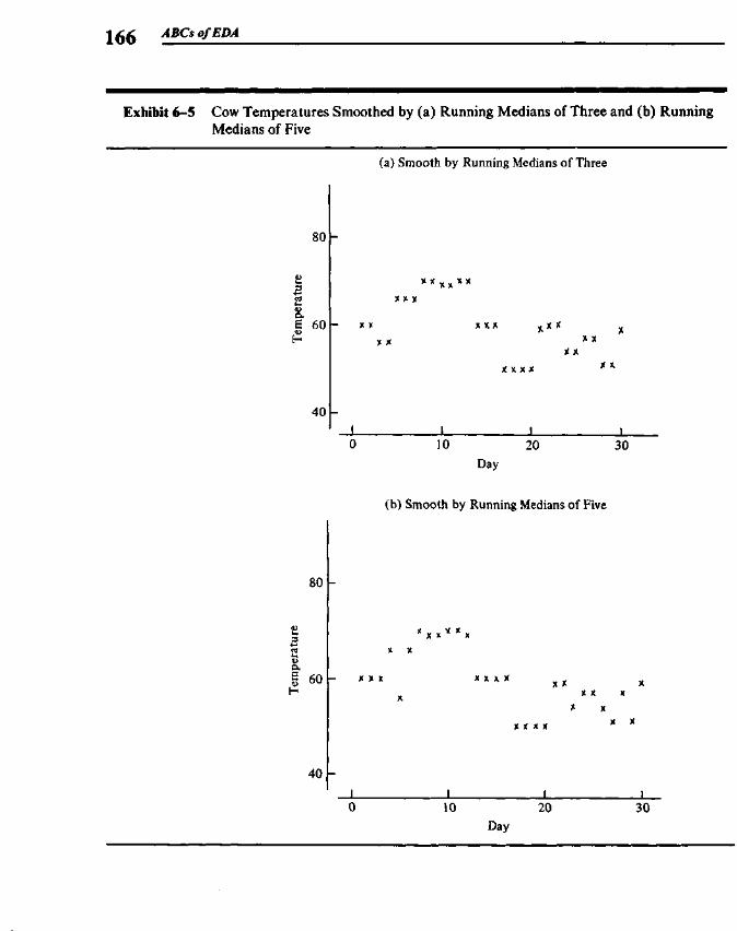
ABCsofEDA
Exhibit 6-5 Cow Temperatures Smoothed by (a) Running Medians of Three and (b) RunningMedians of Five
(a) Smooth by Running Medians of Three
80
E 60
40
X X X
X X
XXX X
10 20
Day30
(b) Smooth by Running Medians of Five
80
I 60
40
X X X XXX X
XX X
* X
x x x xX X
10 20 30
Day
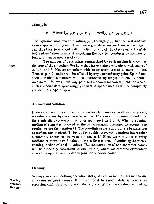
Smoothing Data -t £H
value yt by
span
t_u yt, yt+u yt+2}).
This equation uses five data values, y,_2 through yt+2, but the first and lastvalues appear in only one of the two segments whose medians are averaged,and thus they have about half the effect of any of the other points. Exhibits6-6 and 6-7 show results of smoothing the cow temperatures by medians offour and then by medians of two.
The number of data values summarized by each median is known asthe span of the smoother. We have thus far examined smoothers with spans of2, 3, 4, and 5. Median smoothers with larger spans can resist more outliers.Thus, a span-2 median will be affected by any extraordinary point. Span-3 andspan-4 median smoothers will be unaffected by single outliers. A span-3median will follow an outlying pair, but a span-4 median will cut the size ofsuch a 2-point data spike roughly in half. A span-5 median will be completelyresistant to a 2-point spike.
A Shorthand Notation
In order to provide a compact notation for elementary smoothing operations,we refer to them by one-character names. The name for a running median isthe single digit corresponding to its span, such as 3 or 5. When a runningmedian of span 4 is followed by the pair-averaging operation to recenter theresults, we use the notation 42. The two-digit name is appropriate because twooperations are involved. (In fact, a few sophisticated combinations insert otherelementary operations between a 4 and a 2.) Since we rarely use runningmedians of more than 7 points, there is little chance of confusing 42 with arunning median of 42 data values. The concatenation of one-character nameswill be especially convenient in Section 6.3, where we combine elementarysmoothing operations in order to gain better performance.
runningweightedaverage
Hanning
We may want a smoothing operation still gentler than 42. For this we can usea running weighted average. It is traditional to smooth data sequences byreplacing each data value with the average of the data values around it.
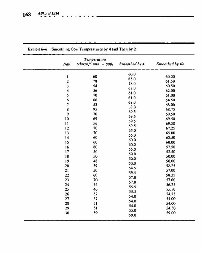
ABCsofEDA
Exhibit 6-6 Smoothing Cow Temperatures by 4 and Then by 2
TemperatureDay (chirps/5 min. — 800) Smoothed by 4 Smoothed by 42
60.0061.5060.5062.0061.0064.5068.0068.7569.5069.5069.5067.2565.0062.5060.0057.5052.5050.0050.0052.2557.0058.2557.0056.2555.5054.7554.0054.0054.5059.00
123456789101112131415161718192021222324252627282930
607054567066539570695670706060
605050485950607054465757515159
60.065.058.063.061.061.068.068.069.569.569.569.565.065.060.060.055.050.050.0
50.054.559.557.057.055.555.554.0
54.054.0
55.059.0
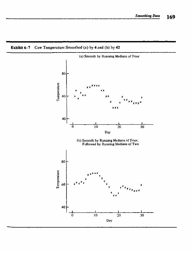
Smoothing Data
Exhibit 6-7 Cow Temperature Smoothed (a) by 4 and (b) by 42
(a) Smooth by Running Medians of Four
80
OH
E 60
40
xx
XXX
10 20 30
Day
(b) Smooth by Running Medians of Four,Followed by Running Medians of Two
80
3
sCD
I 60
40
- x x *
X X
10 20
Day
30
ABCsofEDA
Sometimes the data values are multiplied in each averaging operation byweights. Thus, for example, we might replace yt by
An unlimited number of running weighted averages are possible (allwe require is that the weights—here •/>, x/i, '/t—sum to 1), but we limitourselves to this particular formula for most data exploration. This smoother is
hanning called hanning, after Julius von Hann, who advocated its use, and it is denotedby H. Any running weighted average will be badly affected by even a singleoutlier, so we will generally use such smoothers only after outliers have beensmoothed away by a running-median smoother.
6.3 Compound Smoothers
While simple running medians will smooth a data sequence and can withstandoccasional extraordinary data values, the smooth sequences they produce maydescribe the data only crudely. We can improve on the description—obtainingdata smoothers whose smooth sequences come closer to the data without losingtheir smoothness—through the judicious combination of smoothing proce-dures.
Resmoothing
Applying one smoother to the results of a previous smoother is known asresmoothing resmoothing. As with the name 42, we denote such a series of elementary
operations by concatenating their one-character names. If we are workingentirely by hand, we may choose to use only running medians of 3 andresmooth repeatedly until further resmoothing yields no further changes. Wedenote this repeated combination by 3R.
Reroughing
Running-median smoothers generally smooth a data sequence too much; theyremove interesting patterns. A complementary operation can be used to
Smoothing Data 1 7 1
reroughing
tmcing
recover smooth patterns from the residuals—that is, from the part called"rough" in the formula
data = smooth + rough.
We smooth the rough sequence and add the result to the smooth sequence. Ourhope is that patterns that have been smoothed away by the first pass ofsmoothing can be recovered from the rough and used to make the smooth alittle more like the original data sequence. By analogy with resmoothing, thisoperation is called reroughing.
Exhibits 6-8 and 6-9 show the span-5 median seen in Exhibit 6-4 asreroughed by a span-5 median. We often use the same smoother in bothsmoothing and reroughing, and we call this using a smoother twice. Thus thisexample illustrates smoothing by 5,twice.
Reroughing is an example of an operation found in several exploratorytechniques that polish a fit. In the resistant line (Chapter 5), the "reroughing"step involves fitting a line to the residuals and adding this line to the fit. Wewill see a similar operation in Chapter 8 as the basis for median polish.
4253H
Compound smoothers often combine several elementary smoothers by bothresmoothing and reroughing. The early steps in a compound smoother concen-trate on protection from outliers in the data sequence. Later steps of resmooth-ing can then employ a running weighted average. Curiously, running mediansof 3 or 5 can alter some rapidly oscillating sequences strangely. For example,the infinite sequence . . . , + 1 , - 1 , + 1 , - 1 , + 1 , — 1 , . . . is not modified at allby a span-5 running median, although the sequence oscillates rapidly. Strang-er still, a span-3 running median will invert the sequence, as if each value hadbeen multiplied by — 1. Thus, even-span running medians are sometimespreferred—especially when a computer is available to do all the averagingthey require.
Similar considerations arise in reroughing because the rough, bydesign, will contain spikes reflecting the outliers present in the original dataand will generally oscillate rapidly. Therefore, the smoothers applied to therough must also be resistant to these features.
One combination of smoothers that seems to perform quite well is4253H. It starts with a running median of four, 4 recentered by 2. It thenresmooths by 5, by 3, and finally—now that outliers have been smoothed
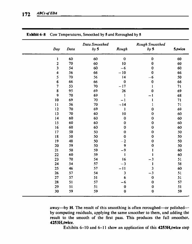
ABCsofEDA
Exhibit 6-8 Cow Temperatures, Smoothed by 5 and Reroughed by 5
Data Smoothed Rough SmoothedDay Data by 5 Rough by 5 5,twice
123456789101112131415161718192021222324252627282930
607054567066539570695670706060605050485950607054465757515159
606060665666706969707069606060605050505059595457575451575159
010-6-10140
-17261
-1-14
11000000
-29
-9116-3-11
36
-600
0000
-6010
_ |1100000000011
_313
-30000
606060665066716968717169606060605050505060605158605151575159
away—by H. The result of this smoothing is often reroughed—or polished—by computing residuals, applying the same smoother to them, and adding theresult to the smooth of the first pass. This produces the full smoother,4253H,twice.
Exhibits 6-10 and 6-11 show an application of this 4253H,twice step
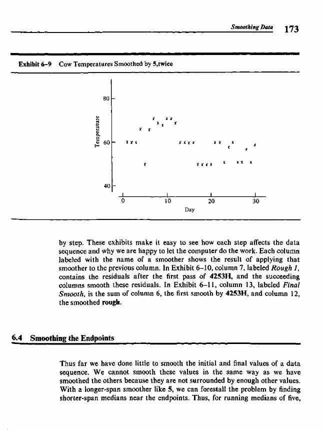
Smoothing Data
Exhibit 6-9 Cow Temperatures Smoothed by 5,twice
80 -
| 60
40 -
t xxX , t
X X X X XX X
10 20Day
30
by step. These exhibits make it easy to see how each step affects the datasequence and why we are happy to let the computer do the work. Each columnlabeled with the name of a smoother shows the result of applying thatsmoother to the previous column. In Exhibit 6-10, column 7, labeled Rough 1,contains the residuals after the first pass of 4253H, and the succeedingcolumns smooth these residuals. In Exhibit 6-11, column 13, labeled FinalSmooth, is the sum of column 6, the first smooth by 4253H, and column 12,the smoothed rough.
6.4 Smoothing the Endpoints
Thus far we have done little to smooth the initial and final values of a datasequence. We cannot smooth these values in the same way as we havesmoothed the others because they are not surrounded by enough other values.With a longer-span smoother like 5, we can forestall the problem by findingshorter-span medians near the endpoints. Thus, for running medians of five,
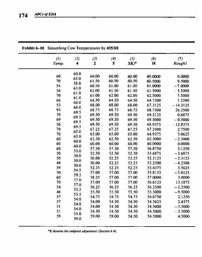
ABCsofEDA
Exhibit 6-10 Smoothing Cow Temperatures by 4253H
(I) (2) (3) (4) (5) (6) (7)Temp. 4 2 5 3(E)» H Rough!
,„ 60.0
70 6 5 °54 5 8 °« 63.0
'" 61.0
3 6 8 °95 6 8 ' °70 6 9 ' 5
69 6 9 5
Z 695
0 6 9 5
70 6 5 °60 6 5 0
60 6 0 °60 6 0 °
0 5 5 °50 5 0 °48 5 0 °59 5 0 °50 5 4 ' 5
59 5
70 - 0
It «54 6 55 5575 5 4 '°51 M 0
5 54.0
9 5 5 °59.0
*E denotes the endpoint adjustment (Section 6.4).
60.0061.5060.5062.0061.0064.5068.0068.7569.5069.5069.5067.2565.0062.5060.0057.5052.5050.0050.0052.2557.0058.2557.0056.2555.5054.7554.0054.0054.5059.00
60.0060.5061.0061.5062.0064.5068.0068.7569.5069.5069.5067.2565.0062.5060.0057.5052.5052.2552.2552.2557.0057.0057.0056.2555.5054.7554.5054.5054.5059.00
60.0060.5061.0061.5062.0064.5068.0068.7569.5069.5069.5067.2565.0062.5060.0057.5052.5052.2552.2552.2557.0057.0057.0056.2555.5054.7554.5054.5054.5054.50
60.000060.500061.000061.500062.500064.750067.312568.750069.312569.500068.937567.250064.937562.500060.000056.875053.687552.312552.250053.437555.812557.000056.812556.250055.500054.875054.562554.500054.500054.5000
0.00009.5000
-7.0000-5.50007.50001.2500
-14.312526.25000.6875
-0.5000-12.9375
2.75005.0625
-2.50000.00003.1250
-3.6875-2.3125-4.25005.5625
-5.81253.000013.1875-2.2500-9.50002.12502.4375
-3.5000-3.50004.5000
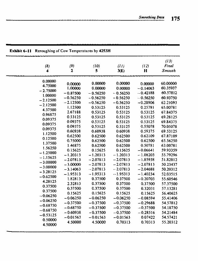
Smoothing Data -i ns
Exhibit 6-11 Reroughing of Cow Temperatures by 4253H
(8)4
(9)2
0.000001.000000.875000.562502.125001.125002.671880.531250.093750.093750.609380.62500O.75OOO1.468750.156251.203132.078133.000003.140631.953131.828132.328130.375000.156250.062500.375000.687500.609380.015634.50000
(10)5
0.000000.00000
-0.56250-0.56250-0.562500.531250.531250.531250.531250.531250.609380.625000.625000.625000.15625
-1.20313-2.07813-2.07813-2.07813-1.953130.375000.375000.375000.15625
-0.06250-0.37500-0.37500-0.37500-0.015634.50000
(11)3(E)
0.000000.00000
-0.56250-0.56250-0.562500.531250.531250.531250.531250.531250.609380.625000.625000.625000.15625
-1.20313-2.07813-2.07813-2.07813-1.953130.375000.375000.375000.15625
-0.06250-0.37500-0.37500-0.37500-0.015630.70313
(12)H
0.00000-0.14063-0.42188-0.56250-0.289060.257810.531250.531250.531250.550780.593750.621090.625000.50781
-0.06641-1.08203-1.85938-2.07813-2.04688-1.40234-0.207030.375000.320310.15625
-0.08594-0.29688-0.37500-0.285160.074220.70313
(IS)Final
Smooth
60.0000060.3593760.5781260.9375062.2109365.0078167.8437569.2812569.8437570.0507869.5312567.8710965.5625063.0078159.9335955.7929651.8281250.2343750.2031252.0351555.6054657.3750057.1328156.4062555.4140654.5781254.1875054.2148454.5742155.20312
0.000004.750002.750001.000002.125002.125004.375000.968750.093750.093750.093751.125000.125001.375001.56250
-1.25000-1.15625-3.00000-3.00000-3.28125-0.625004.281250.375000.37500
-0.06250-0.06250-0.68750-0.68750-0.531250.500004.50000
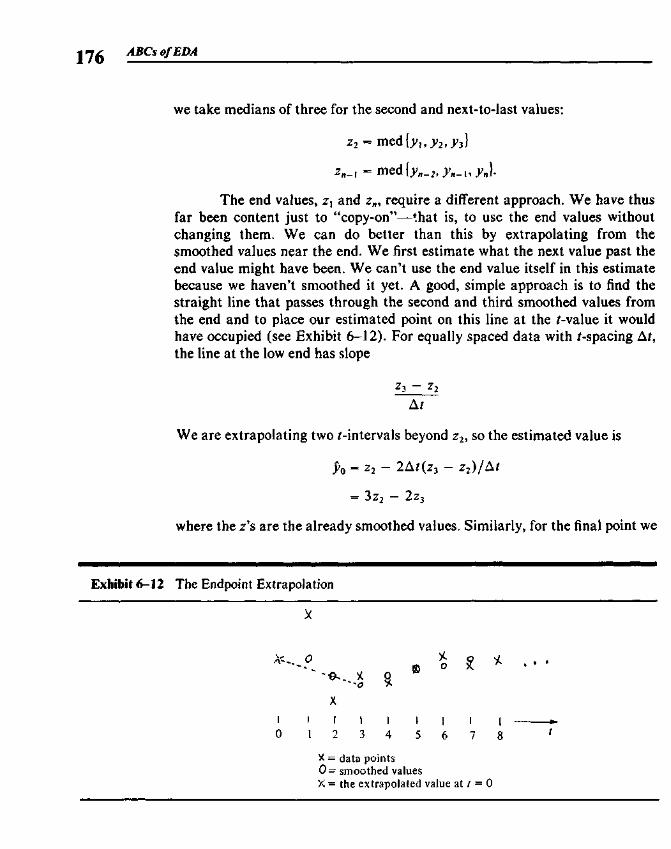
ABCs of EDA
we take medians of three for the second and next-to-last values:
z2 =
zn_, = med{yn_2,yn_l,yn}.
The end values, zx and zn, require a different approach. We have thusfar been content just to "copy-on"—that is, to use the end values withoutchanging them. We can do better than this by extrapolating from thesmoothed values near the end. We first estimate what the next value past theend value might have been. We can't use the end value itself in this estimatebecause we haven't smoothed it yet. A good, simple approach is to find thestraight line that passes through the second and third smoothed values fromthe end and to place our estimated point on this line at the /-value it wouldhave occupied (see Exhibit 6-12). For equally spaced data with /-spacing At,the line at the low end has slope
At
We are extrapolating two /-intervals beyond z2, so the estimated value is
yo = z2- 2A/(z3 - z2)/At
= 3z2 — 2z3
where the z's are the already smoothed values. Similarly, for the final point we
Exhibit 6-12 The Endpoint Extrapolation
i i i i t i l1 2 3 4 5 6 7
X = data points0 = smoothed valuesX = the extrapolated value at t = 0
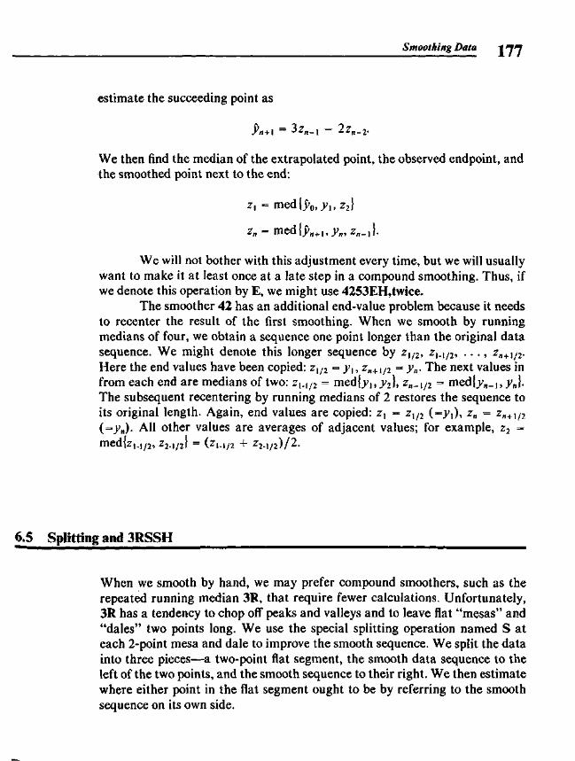
Smoothing Data t nn
estimate the succeeding point as
yn+\ = 3zn_ l - 2zn_2.
We then find the median of the extrapolated point, the observed endpoint, andthe smoothed point next to the end:
z, = med{yo,yuz2)
zn = me&{yn+x,yn,zn_x\.
We will not bother with this adjustment every time, but we will usuallywant to make it at least once at a late step in a compound smoothing. Thus, ifwe denote this operation by E, we might use 4253EH,twice.
The smoother 42 has an additional end-value problem because it needsto recenter the result of the first smoothing. When we smooth by runningmedians of four, we obtain a sequence one point longer than the original datasequence. We might denote this longer sequence by z1/2, zM / 2 , . . . , zn+1/2.Here the end values have been copied: z1/2 = y\, zn+1/2 = yn. The next values infrom each end are medians of two: z,.1/2 = med{^,,72}, zn_x/2 = n\Qd{yn_u yn}.The subsequent recentering by running medians of 2 restores the sequence toits original length. Again, end values are copied: zx = z1/2 (=yx), zn = zn+1/2
(=yn). All other values are averages of adjacent values; for example, z2 =med{zM/2, z2.,/2) = (zM / 2 + z2.i/2)/2.
6.5 Splitting and 3RSSH
When we smooth by hand, we may prefer compound smoothers, such as therepeated running median 3R, that require fewer calculations. Unfortunately,3R has a tendency to chop off peaks and valleys and to leave flat "mesas" and"dales" two points long. We use the special splitting operation named S ateach 2-point mesa and dale to improve the smooth sequence. We split the datainto three pieces—a two-point flat segment, the smooth data sequence to theleft of the two points, and the smooth sequence to their right. We then estimatewhere either point in the flat segment ought to be by referring to the smoothsequence on its own side.
170 ABCs of EDA
The estimation method is much the same as the endpoint rule discussedin Section 6.4. If, in the smooth by 3R, the sequence
is to the right of the two-point flat segment
we predict what yf_x would have been if it were on the straight line formed byyf+x and yf+2. As we found in extrapolating for the endpoints, we can predict
We now use this extrapolated value in a span-3 median centered at y/.
zf= med{3.y/+1 - 2yf+1,yf,yf+x).
Note that all of the values in this operation have already been smoothed by 3R.This is the only difference between this operation and the endpoint smoothingoperation, which uses both the unsmoothed end value and nearby smoothedvalues.
We perform the corresponding operation on the other half of thetwo-point flat segment; that is, we predict yf from the line through >y_3 and yf_2
and use the predicted value in a span-3 median to calculate zf_x. After splittingeach two-point mesa and dale, we resmooth the entire sequence by 3R.Although splitting is tedious by hand, we are likely to need it at only a fewplaces in a data sequence.
One good combination of these operations for smoothing by handrepeats S (each time automatically followed by 3R). It is 3RSSH,twice.Although it is primarily a hand smoothing technique, the computer programsin this chapter provide 3RSSH,twice as an option. Exhibit 6-13 shows thesteps of 3RSSH applied to the cow temperatures of Exhibits 6-3 through6-11.
6.6 Looking at the Rough
We are often as interested in the residual, or rough, sequence as we are in thesmooth. The rough can reveal outliers, as well as portions of the sequence that
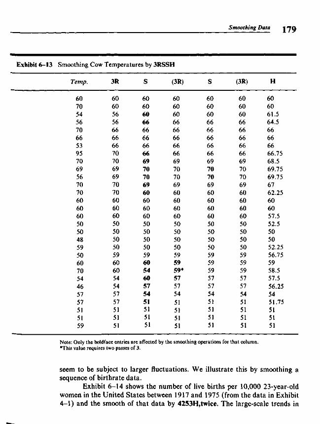
Exhibit 6-13 Smoothing Cow Temperatures
Temp. 3R
by
S
3RSSH
(3R) S
Smoothing Data
(3R) H
179
607054567066539570695670706060605050485950607054465757515159
606056566666667070696970706060605050505059606054545757515151
606060666666666669707069606060605050505059605460575451515151
6060606666666666697070696060606050505050595959*57575451515151
606060666666666669707069606060605050505059595957575451515151
606060666666666669707069606060605050505059595957575451515151
606061.564.566666666.7568.569.7569.756762.25606057.552.5505052.2556.755958.557.556.255451.75515151
Note: Only the boldface entries are affected by the smoothing operations for that column.*This value requires two passes of 3.
seem to be subject to larger fluctuations. We illustrate this by smoothing asequence of birthrate data.
Exhibit 6-14 shows the number of live births per 10,000 23-year-oldwomen in the United States between 1917 and 1975 (from the data in Exhibit4-1) and the smooth of that data by 4253H,twice. The large-scale trends in
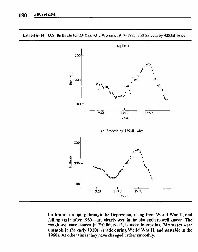
ABCsofEDA
Exhibit 6-14 U.S. Birthrate for 23-Year-Old Women, 1917-1975, and Smooth by 4253H,twice
(a) Data
300
200CQ
100
xx
%K
1920 1940
Year
1960
300
r 200s
100
(b) Smooth by 4253H,twice
*****
1920 1940 1960Year
birthrate—dropping through the Depression, rising from World War II, andfalling again after 1960—are clearly seen in the plot and are well known. Therough sequence, shown in Exhibit 6-15, is more interesting. Birthrates wereunstable in the early 1920s, erratic during World War II, and unstable in the1960s. At other times they have changed rather smoothly.
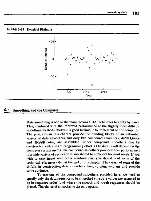
Smoothing Data I f t i
Exhibit 6-15 Rough of Birthrate
+ 20 -
CQ
fo
- 2 0
1920 1940Year
1960
6.7 Smoothing and the Computer
Data smoothing is one of the more tedious EDA techniques to apply by hand.This, combined with the improved performance of the slightly more difficultsmoothing methods, makes it a good technique to implement on the computer.The programs in this chapter provide the building blocks of an unlimitedvariety of data smoothers, but only two compound smoothers, 4253H,twiceand 3RSSH,twice, are assembled. Other compound smoothers can beconstructed with a slight programming effort. (The details will depend on thecomputer system used.) The compound smoothers provided here perform wellin a wide variety of applications and should be sufficient for most needs. If youwish to experiment with other combinations, you should read some of thetechnical references cited at the end of this chapter. They warn of some of thepitfalls in constructing data smoothers from running medians and providesome guidance.
To use one of the compound smoothers provided here, we need tospecify only the data sequence to be smoothed (the data values are assumed tobe in sequence order) and where the smooth and rough sequences should beplaced. The choice of smoother is the only option.
1 8 2 ABCsofEDA
t 6.8 Algorithms
Data smoothers are often constructed from several similar smoothing opera-tions. The programs for data smoothing take advantage of the great similarityamong elementary smoothing operations. These programs, more than anyothers in this book, are built of many smaller units. This structure makes iteasy to build compound smoothers with them.
Several individual algorithms are needed. The most general and mostcomplex is the running-median algorithm. This algorithm uses two temporarywork arrays. One of these arrays keeps a "snapshot" of the region of the datasequence surrounding the point to be smoothed. The size of this region isspecified by the span of the smoother. The data values are preserved in thiswork area because each data value participates in the calculation of thesmooth values of its successors. Once a data value has been smoothed, itsunsmoothed value must be remembered for the subsequent smoothing calcula-tions. The second work array holds the same local data values, but they aresorted in order so that the median can be found.
These work arrays are (conceptually) slid along the data sequence sothat they can hold the succession of local regions of the data used in themedian operations. The smooth value at the current data point is found as themedian of the sorted work array. To compute the smooth value at the nextdata point, the "earliest" data value is found at the beginning of the snapshotwork array. (The corresponding value in the data array has already beenreplaced by its smooth value.) A matching value is then found by searching thesorted work array. (If more than one of the local values is identical to theearliest value, it doesn't matter which is found.) Both the earliest value and itsmatch in the sorted array are removed, and the next data value to beconsidered as the local region slides along by one lvalue is then placed in eachwork array. The sorted work array is re-sorted to find the new median, whichis the next smooth value.
The running-median program does not smooth at all near theendpoints. Values not accompanied by at least (span — l ) /2 data values oneach side are left unmodified and must be dealt with separately.
Running medians of three are not computed with the same algorithm.Instead, a special program computes them. The program simply compares thethree numbers to determine the median. In addition, it reports whether thesmooth value is the middle value according to the sequence ordering on /. Thisinformation makes it easy to check the stopping condition of 3R.
The algorithms for hanning, smoothing endpoints, and splitting havebeen specified in Sections 6.2, 6.4, and 6.5, respectively. They are imple-mented as described in those sections.
Smoothing Data
Subroutines for each smoothing unit are provided. Each one smoothsvalues near the end explicitly and calls the appropriate general smoothingsubroutine.
FORTRAN
The FORTRAN program for data smoothing consists of 13 subroutines: RSM,S4253H, S3RSSH, S2, S3, S4, S5,HANN, S3R, ENDPTS, SPLIT, MEDOF3, and RUNMED. Tosmooth a data sequence in Y(), use the FORTRAN statement
CALL RSM(Y, N, SMOOTH, ROUGH, VERSN, ERR)
where
Y(} is the N-long data vector holding the sequence tobe smoothed;
N is the length of the sequence;SMOOTH() is an N-long array in which the smooth is
returned;ROUGH() is an N-long array in which the rough is returned;VERSN is a flag = 1 to smooth by 3RSSH,twice,
= 2 to smooth by 4253H,twice;ERR is the error flag, whose values are
0 normal61 N < 7—sequence too short to smooth62 insufficient work array room—span of
running median is greater than allocatedspace
63 internal error—possibly an error in thesort program—especially if another sortprogram has been substituted for the oneprovided. If so, this could result fromincorrect use of that program.
BASIC
The BASIC program for data smoothing consists of 13 subroutines divided inthe same way as the FORTRAN subroutines just named. The data sequence
ABCsofEDA
of N values to be smoothed is in Y(). The smooth sequence is returned in Y() andthe rough sequence in R(). Arrays C() and W() are used as work arrays. Thearray X() is not changed because it is likely to be a useful x-axis for plotting thesmooth and the rough. The version number V1 selects the smoother: V1 = 1 for3RSSH,twice, V1 = 2 for 4253H,twice. Programmers should pay specialattention to the use of variables SO through S9 to save temporary copies of endvalues.
The smoothing routines require the defined functions and the sortingsubroutines. They can nest subroutine calls five deep and use defined functionsfrom the deeper levels. This may strain the capacity of some very smallcomputers.
References
de Alba, Enrique, and David L. Zartman. 1979. "Testing Outliers in Time Series: AnApplication to Remotely Sensed Temperatures in Cattle," Special Paper No.130. Agricultural Experiment Station, New Mexico State University, LasCruces.
Mallows, C.L. 1980. "Some Theory of Nonlinear Smoothers," Annals of Statistics8:695-715.
Velleman, Paul F. 1980. "Definition and Comparison of Robust Nonlinear DataSmoothing Algorithms, Journal of the American Statistical Association75:609-615.
Please turn toChapter 8.
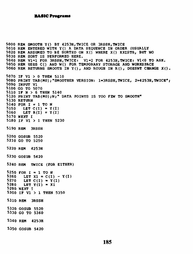
BASIC Programs
5000 REM SMOOTH Y{) BY 4253HrTWICE OR 3RSSH,TWICE5010 REM ENTERED WITH Y() A DATA SEQUENCE IN ORDER (USUALLY5020 REM ASSUMED TO BE SORTED ON X() WHERE X() EXISTS, BUT NO5030 REM SORT IS PERFORMED HERE.5040 REM Vl=l FOR 3RSSH,TWICE: Vl=2 FOR 4253H,TWICE: V K 0 TO ASK.5050 REM USES C() AND W() FOR TEMPORARY STORAGE AND WORKSPACE5060 REM RETURNS SMOOTH IN Y(), AND ROUGH IN R(), DOESNT CHANGE X().
5070 IF VI > 0 THEN 51105080 PRINT TAB(MO);"SMOOTHER VERSION: 1=3RSSH,TWICE, 2=4253H,TWICE";5090 INPUT VI5100 GO TO 50705110 IF N > 6 THEN 51405120 PRINT TAB(M0);N;" DATA POINTS IS TOO FEW TO SMOOTH"5130 RETURN5140 FOR I = 1 TO N5150 LET C(I) = Y(I)5160 LET R(I) = Y(I)5170 NEXT I5180 IF VI > 1 THEN 5230
5190 REM 3RSSH
5200 GOSUB 55205210 GO TO 5250
5220 REM 4253H
5230 GOSUB 5420
5240 REM TWICE (FOR EITHER)
5250 FOR I = 1 TO N5260 LET XI = C(I) - Y(I)5270 LET C(I) = Y(I)5280 LET Y(I) = XI5290 NEXT I5300 IF VI > 1 THEN 5350
5310 REM 3RSSH
5320 GOSUB 55205330 GO TO 5360
5340 REM 4253H
5350 GOSUB 5420
185
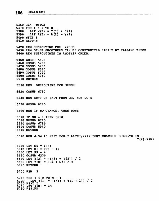
ABCsofEDA
5360 REM TWICE5 3 7 0 FOR I = 1 TO N5 3 8 0 LET Y ( I ) = Y ( I ) + C ( I )5 3 9 0 LET R ( I ) = R ( I ) - Y ( I )5 4 0 0 NEXT I5 4 1 0 RETURN
5 4 2 0 REM SUBROUTINE FOR 4253H5 4 3 0 REM OTHER SMOOTHERS CAN BE CONSTRUCTED EASILY BY CALLING THESE5 4 4 0 REM SUBROUTINES IN ANOTHER ORDER.
5 4 5 0 GOSUB 56205 4 6 0 GOSUB 57005 4 7 0 GOSUB 57605 4 8 0 GOSUB 6 5 7 05 4 9 0 GOSUB 60205 5 0 0 GOSUB 59405 5 1 0 RETURN
5 5 2 0 REM SUBROUTINE FOR 3RSSH
5 5 3 0 GOSUB 6710
5 5 4 0 REM S8=0 ON EXIT FROM 3R, NOW DO S
5 5 5 0 GOSUB 6 7 8 0
5 5 6 0 REM IF NO CHANGE, THEN DONE
5 5 7 0 IF S8 = 0 THEN 56105 5 8 0 GOSUB 67105 5 9 0 GOSUB 6 7 8 05 6 0 0 GOSUB 59405 6 1 0 RETURN
5 6 2 0 REM 4 : S 4 IS KEPT FOR 2 LATER, Y ( l ) ISNT CHANGED—RESULTS INY ( 2 ) - Y ( N )
5 6 3 0 LET S4 = Y(N)5 6 4 0 LET S I = Y(N - 1)5 6 5 0 LET S9 = 45 6 6 0 GOSUB 6 2 3 05 6 7 0 LET Y ( 2 ) = ( Y ( l ) + Y ( 2 ) ) / 25 6 8 0 LET Y(N) = ( S I + S 4 ) / 25 6 9 0 RETURN
5 7 0 0 REM 2
5 7 1 0 FOR I = 2 TO N - 15 7 2 0 LET Y ( I ) = ( Y ( I ) + Y ( I + 1 ) ) / 25 7 3 0 NEXT I5 7 4 0 LET Y(N) = S45 7 5 0 RETURN
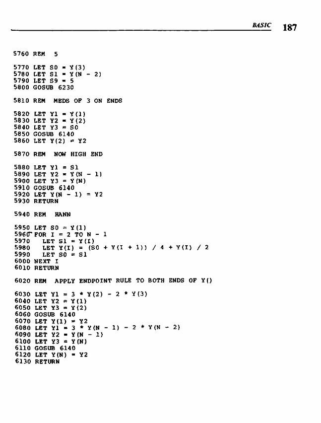
BASIC 187
5760 REM 5
5770 LET SO = Y(3)5780 LET SI = Y(N - 2)5790 LET S9 = 55800 GOSUB 6230
5810 REM MEDS OF 3 ON ENDS
5820 LET Yl = Y(l)5830 LET Y2 = Y(2)5840 LET Y3 = SO5850 GOSUB 61405860 LET Y(2) = Y2
5870 REM NOW HIGH END
5880 LET Yl = SI5890 LET Y2 = Y(N - 1)5900 LET Y3 = Y(N)5910 GOSUB 61405920 LET Y(N - 1) = Y25930 RETURN
5940 REM HANN
5950 LET SO = Y(l)596(TFOR I = 2 TO N - 15970 LET SI = Y(I)5980 LET Y(I) = (SO + Y(I +1)) / 4 + Y(I) / 25990 LET SO = SI6000 NEXT I6010 RETURN
6020 REM APPLY ENDPOINT RULE TO BOTH ENDS OF Y()
6030 LET Yl = 3 * Y(2) - 2 * Y(3)6040 LET Y2 = Y(l)6050 LET Y3 = Y(2)6060 GOSUB 61406070 LET Y(l) = Y26080 LET Yl = 3 * Y ( N - l ) - 2 * Y ( N - 2 )6090 LET Y2 = Y(N - 1)6100 LET Y3 = Y(N)6110 GOSUB 61406120 LET Y(N) = Y26130 RETURN
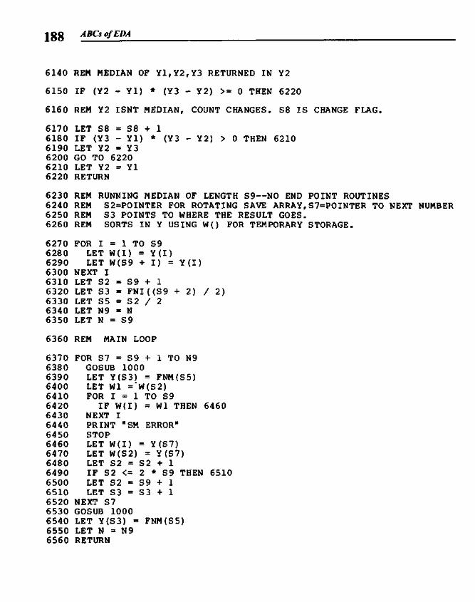
188 ABCs of EDA
6140 REM MEDIAN OF Y1,Y2,Y3 RETURNED IN Y2
6150 IF (Y2 - Yl) * (Y3 - Y2) >= 0 THEN 6220
6160 REM Y2 ISNT MEDIAN, COUNT CHANGES. S8 IS CHANGE FLAG.
6170 LET S8 = S8 + 16180 IF (Y3 - Yl) * (Y3 - Y2) > 0 THEN 62106190 LET Y2 = Y36200 GO TO 62206210 LET Y2 = Yl6220 RETURN
6230 REM RUNNING MEDIAN OF LENGTH S9—NO END POINT ROUTINES6240 REM S2=POINTER FOR ROTATING SAVE ARRAY,S7=POINTER TO NEXT NUMBER6250 REM S3 POINTS TO WHERE THE RESULT GOES.6260 REM SORTS IN Y USING W() FOR TEMPORARY STORAGE.
6270 FOR I = 1 TO S96280 LET W(I) = Y(I)6290 LET W(S9 + I) = Y(I)6300 NEXT I6310 LET S2 = S9 + 16320 LET S3 = FNI((S9 +2) / 2)6330 LET S5 = S2 / 26340 LET N9 = N6350 LET N = S9
6360 REM MAIN LOOP
6370 FOR S7 = S9 + 1 TO N96380 GOSUB 10006390 LET Y(S3) = FNM(S5)6400 LET Wl ="W(S2)6410 FOR I = 1 TO S96420 IF W(I) = Wl THEN 64606430 NEXT I6440 PRINT "SM ERROR"6450 STOP6460 LET W(I) = Y(S7)6470 LET W(S2) = Y(S7)6480 LET S2 = S2 + 16490 IF S2 <= 2 * S9 THEN 65106500 LET S2 = S9 + 16510 LET S3 = S3 + 16520 NEXT S76530 GOSUB 10006540 LET Y(S3) = FNM(S5)6550 LET N = N96560 RETURN
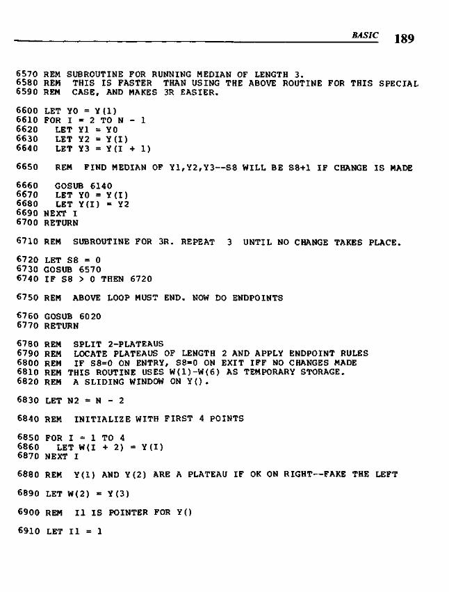
BASIC 189
6570 REM SUBROUTINE FOR RUNNING MEDIAN OF LENGTH 3.6580 REM THIS IS FASTER THAN USING THE ABOVE ROUTINE FOR THIS SPECIAL6590 REM CASE, AND MAKES 3R EASIER.
6600 LET YO = Y(l)6610 FOR I = 2 TO N - 16620 LET Yl = YO6630 LET Y2 = Y(I)6640 LET Y3 = Y(I + 1 )
6650 REM FIND MEDIAN OF Y1,Y2,Y3—S8 WILL BE S8+1 IF CHANGE IS MADE
6660 GOSUB 61406670 LET YO = Y(I)6680 LET Y(I) = Y26690 NEXT I6700 RETURN
6710 REM SUBROUTINE FOR 3R. REPEAT 3 UNTIL NO CHANGE TAKES PLACE.
6720 LET S8 = 06730 GOSUB 65706740 IF S8 > 0 THEN 6720
6750 REM ABOVE LOOP MUST END. NOW DO ENDPOINTS
6760 GOSUB 60206770 RETURN
6780 REM SPLIT 2-PLATEAUS6790 REM LOCATE PLATEAUS OF LENGTH 2 AND APPLY ENDPOINT RULES6800 REM IF S8=0 ON ENTRY, S8=0 ON EXIT IFF NO CHANGES MADE6810 REM THIS ROUTINE USES W(l)-W(6) AS TEMPORARY STORAGE.6820 REM A SLIDING WINDOW ON Y().
6830 LET N2 = N - 2
6840 REM INITIALIZE WITH FIRST 4 POINTS
6850 FOR I - 1 TO 46860 LET W(I + 2) = Y(I)6870 NEXT I
6880 REM Y(l) AND Y(2) ARE A PLATEAU IF OK ON RIGHT—FAKE THE LEFT
6890 LET W(2) = Y(3)
6900 REM II IS POINTER FOR Y()
6910 LET II = 1
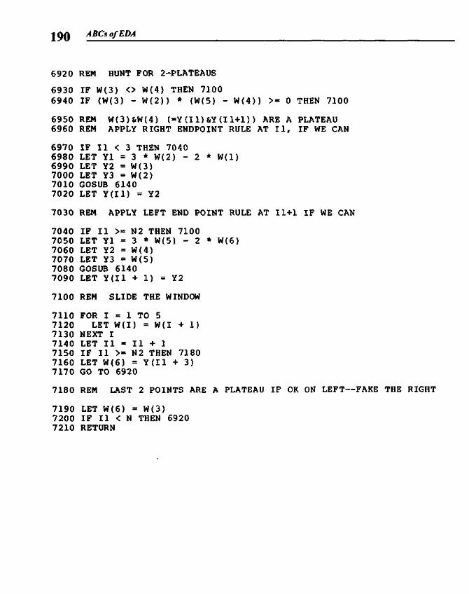
ABCs of EDA
6920 REM HUNT FOR 2-PLATEAUS
6930 IF W(3) <> W(4) THEN 71006940 IF (W(3) - W(2)) * (W(5) - W(4)) >= 0 THEN 7100
6950 REM W(3)&W(4) (=Y(I1)&Y(I1+1)) ARE A PLATEAU6960 REM APPLY RIGHT ENDPOINT RULE AT II, IF WE CAN
6970 IF II < 3 THEN 70406980 LET Yl = 3 * W(2) - 2 * W(l)6990 LET Y2 = W(3)7000 LET Y3 = W(2)7010 GOSUB 61407020 LET Y(I1) = Y2
7030 REM APPLY LEFT END POINT RULE AT I1+1 IF WE CAN
7040 IF II >= N2 THEN 71007050 LET Yl = 3 * W(5) - 2 * W(6)7060 LET Y2 = W(4)7070 LET Y3 = W(5)7080 GOSUB 61407090 LET Y(I1 + 1) = Y2
7100 REM SLIDE THE WINDOW
7110 FOR I = 1 TO 57120 LET W(I) = W(I + 1)7130 NEXT I7140 LET II = II + 17150 IF II >= N2 THEN 71807160 LET W(6) = Y(I1 + 3)7170 GO TO 6920
7180 REM LAST 2 POINTS ARE A PLATEAU IF OK ON LEFT—FAKE THE RIGHT
7190 LET W(6) = W(3)7200 IF II < N THEN 69207210 RETURN
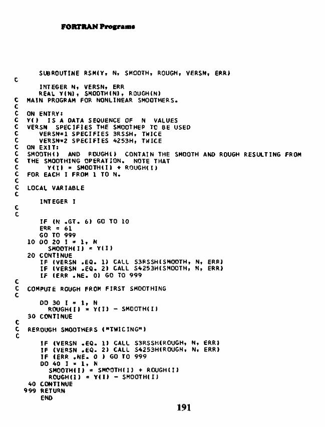
FORTRAN Programs
SUBROUTINE RSM(Y, Nt SMOOTH, ROUGH, VERSN, ERR)
INTEGER N, VERSN, ERRREAL Y(N), SMOOTH(N), ROUGH(N)
MAIN PROGRAM FOR NONLINEAR SMOOTHERS.
ON ENTRY:Y() IS A DATA SEQUENCE OF N VALUESVERSN SPECIFIES THE SMOOTHER TC BE USED
VERSN-1 SPECIFIES 3RSSH, TWICEVERSN*2 SPECIFIES 4253H, TWICE
ON EXIT:SMOOTH() AND ROUGH!) CONTAIN THE SMOOTH AND ROUGH RESULTING FROMTHE SMOOTHING OPERATION. NOTE THAT
Y(II = SMOOTH(I) + ROUGH(I)FOR EACH I FROM 1 TO N.
LOCAL VARIABLE
INTEGER I
IF (N .GT. 6) GO TO 10ERR = 61GO TO 999
10 DO 20 I = It NSMOOTHi I) = Y d )
20 CONTINUEIF (VERSN .EQ. 1) CALL S3RSSHCSM00TH, N, ERR)IF (VERSN .EQ. 2) CALL S4253HCSM00TH, N, ERR)IF (ERR .NE. 0) GO TO 999
COMPUTE ROUGH FROM FIRST SMOOTHING
DO 30 I « It NROUGHd) = Y(I) - SMOOTH(I)
30 CONTINUE
REROUGH SMOOTHERS ("TWICING")
IF (VERSN .EQ. 1) CALL S3RSSH(R0UGH, N, ERR)IF (VERSN .EQ. 2) CALL S4253H(R0UGH, N, ERR)IF (ERR .NE. 0 ) GO TO 999DO 40 I = It N
SMOOTH(I) - SMOOTH(I) + ROUGHd)ROUGHd) = Y d ) - SMOOTH(I)
40 CONTINUE999 RETURN
END
191
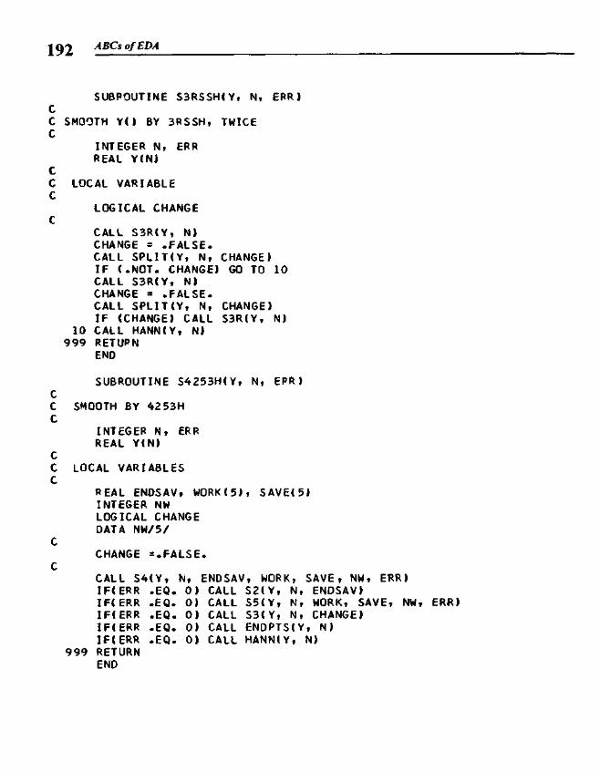
1 9 2 ABCsofEDA
SUBPOUTINE S3RSSHCY, N, ERR)CC SMOOTH Y ( ) BY 3RSSH, TWICEC
INTEGER N, ERRREAL Y(N)
CC LOCAL VARIABLEC
LOGICAL CHANGEC
CALL S3RCY, N)CHANGE = .FALSE.CALL SPL IT (Y , N, CHANGE)I F ( .NOT. CHANGE) GO TO 10CALL S3R(Y, N)CHANGE = .FALSE.CALL SPL IT (Y , N, CHANGE)IF (CHANGE) CALL S3R(Y, N)
10 CALL HANN(Y, N)999 RETURN
END
SUBROUTINE S4253H(Y, N, ERR)CC SMOOTH BY 4253HC
INTEGER Nt ERRREAL Y(N)
CC LOCAL VARIABLESC
REAL ENDSAVt W0RK(5), SAVE(5)INTEGER NWLOGICAL CHANGEDATA NW/5/
CCHANGE =.FALSE.
CCALL S4(Y, N, ENDSAV, WORK, SAVE, NW, ERR)IF(ERR .EQ. 0) CALL S2(Y, N, ENDSAV)IF(ERR .EQ. 0) CALL S5(Y, N, WORK, SAVE, NW, ERR)IF(ERR .EQ. 0) CALL S3(Y, N, CHANGE)IF(ERR .EQ. 0) CALL ENDPTS(Y, N)IF(ERR .EQ. 0) CALL HANN(Y, N)
999 RETURNEND
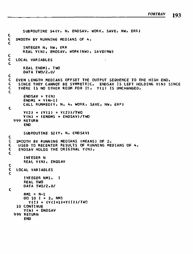
FORTRAN 193
SUBROUTINE S4(Yt NT ENDSAV, WORK, SAVE, NW, ERR)CC SMOOTH BY RUNNING MEDIANS OF 4.C
INTEGER N, NW, ERRREAL Y(N), ENDSAV, WOPK(NW), SAVE(NW)
CC LOCAL VARIABLESC
REAL ENDM1, TWODATA TWO/2.0/
CC EVEN LENGTH MEDIANS OFFSET THE OUTPUT SEQUENCE TO THE HIGH END,C SINCE THEY CANNOT BE SYMMETRIC. ENDSAV IS LEFT HOLDING Y(N) SINCEC THERE IS NO OTHER ROOM FOR IT. Y(l) IS UNCHANGED.C
ENDSAV = Y(N)ENDM1 = Y(N-1>CALL RUNMED(Y, N, 4, WORK, SAVE, NW, ERP)
CY(2) - (Y(l) + Y(2))/TWOY(N) = (ENDM1 + ENDSAV)/TWO
999 RETURNEND
SUBROUTINE S2 (Y , N, ENDSAV)CC SMOOTH BY PUNNING MEDIANS (MEANS) OF 2 .C USED TO RECENTER RESULTS OF RUNNING MEDIANS OF 4 .C ENDSAV HOLDS THE ORIGINAL Y ( N ) .C
INTEGER NREAL Y ( N ) , ENDSAV
CC LOCAL VARIABLESC
INTEGER NM1, IREAL TWODATA TWO/2 .0 /
CNM1 = N-lDO 10 I » 2 i NM1
Y ( I ) = ( Y ( I + 1 ) + Y ( I ) ) / T W O10 CONTINUE
Y(N) - ENDSAV999 RETURN
END
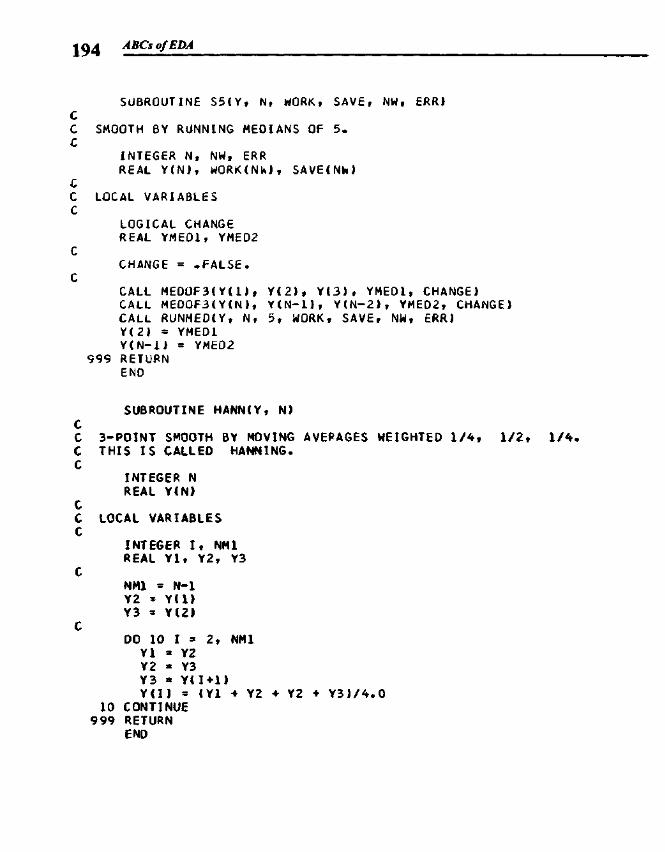
ABCsofEDA
SUBROUTINE S5(Y, N, WORK, SAVE, NW, ERR)CC SMOOTH BY RUNNING MEOIANS OF 5,C
INTEGER N, NW, ERRREAL Y(N), WORK(Nh), SAVE(NW)
CC LOCAL VARIABLESC
LOGICAL CHANGEREAL YMED1, YMED2
CCHANGE = .FALSE.
CCALL MEDOF3(Y(1), Y(2), Y(3), YMEO1, CHANGE)CALL ME00F3(Y(N), Y(N-l), Y(N-2), YME02, CHANGE)CALL RUNMED(Y, N, 5, WORK, SAVE, NU, ERR)Y(2) = YMEO1Y(N-l) = YMED2
999 RETURNEND
SUBROUTINE HANN(Y, N)CC 3-POINT SMOOTH BY MOVING AVERAGES WEIGHTED 1 / 4 , 1 / 2 , 1 /4 ,C THIS IS CALLED HANNING.C
INTEGER NREAL Y<N)
CC LOCAL VARIABLESC
INTEGER I , NM1REAL Y l t Y2, Y3
CNM1 = N-lY2 = Y ( l )Y3 = Y(2)
CDO 10 I = 2 , NM1
Yl = Y2Y2 = Y3Y3 = Y U + 1 )Y d ) = ( Y l 4 Y2 + Y2 + Y 3 ) / 4 . 0
10 CONTINUE999 RETURN
END
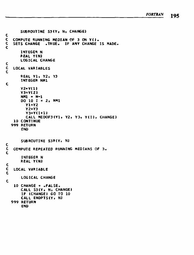
FORTRAN
SUBROUTINE S 3 ( Y , N, CHANGE)CC COMPUTE RUNNING MEDIAN OF 3 ON Y ( ) .C SETS CHANGE .TRUE. IF ANY CHANGE IS MADE.C
INTEGER NREAL Y(N)LOGICAL CHANGE
CC LOCAL VARIABLESC
REAL Y l , Y 2 , Y3INTEGER NM1
CY2=Y(1)Y3=Y<2)NM1 = N- lDO 10 I - 2 , NM1
Y1=Y2Y2=Y3Y 3 = Y ( I + 1 )CALL MED0F3(Ylt Y2t Y 3 , Y ( I ) t CHANGE)
10 CONTINUE999 RETURN
END
SUBROUTINE S3R(Y, N)CC COMPUTE REPEATED RUNNING MEDIANS OF 3 .C
INTEGER NREAL Y(N)
CC LOCAL VARIABLEC
LOGICAL CHANGEC
10 CHANGE = .FALSE.CALL S3(Y , N, CHANGEIIF (CHANGE) GO TO 10CALL ENDPTS(Y, N)
999 RETURNEND
195
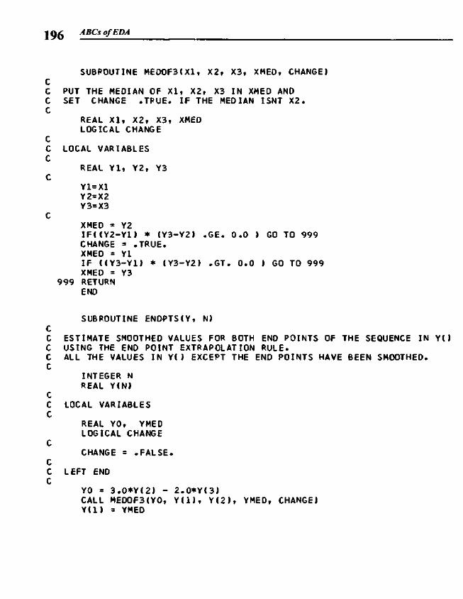
ABCsofEDA
SUBROUTINE MED0F3U1, X2, X3, XMED, CHANGE)CC PUT THE MEDIAN OF X I , X2, X3 IN XMED ANDC SET CHANGE .TRUE, IF THE MEDIAN ISNT X2 .C
REAL X I , X2 , X3, XMEDLOGICAL CHANGE
CC LOCAL VARIABLESC
REAL Y l , Y2 , Y3C
Y1=X1Y2=X2Y3=X3
CXMED = Y2I F U Y 2 - Y 1 ) * (Y3-Y2) .GE. 0 , 0 ) GO TO 999CHANGE = .TRUE.XMED = YlIF (CY3-Y1) * (Y3-Y2) .GT . 0 .0 ) GO TO 999XMED = Y3
999 RETURNEND
SUBROUTINE ENDPTSCY, N)CC ESTIMATE SMOOTHED VALUES FOR BOTH END POINTS OF THE SEQUENCE IN Y()C USING THE END POINT EXTRAPOLATION RULE.C ALL THE VALUES IN Y() EXCEPT THE END POINTS HAVE BEEN SMOOTHED.C
INTEGER NREAL Y(N)
CC LOCAL VARIABLESC
REAL YO, YMEDLOGICAL CHANGE
CCHANGE ' .FALSE.
CC LEFT ENDC
YO = 3 . 0 * Y ( 2 ) - 2 . 0 * Y ( 3 )CALL MED0F3(Y0, Y d ) , Y ( 2 ) , YMED, CHANGE)Y d ) = YMED
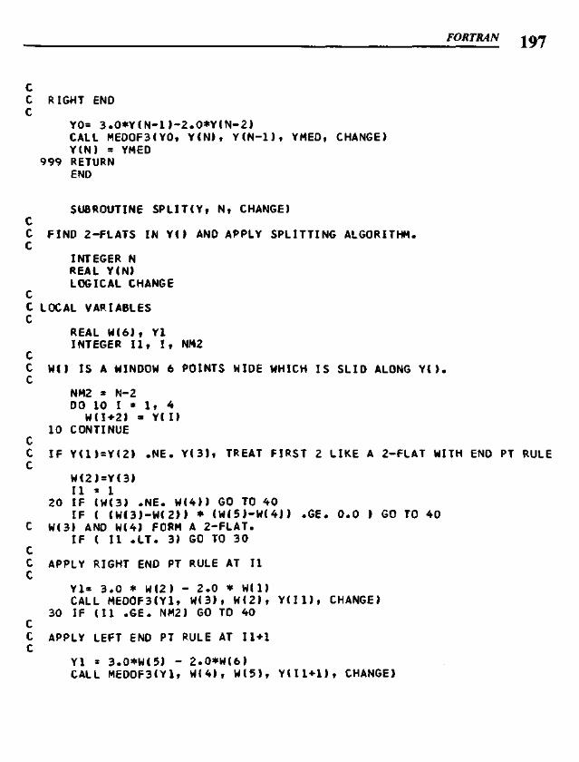
FORTRAN 197
cC RIGHT ENDC
Y0= 3 . 0 * Y ( N - l ) - 2 . 0 * Y ( N - 2 )CALL MEDOF3(YOt Y (N) , Y ( N - l ) , YMED, CHANGE)Y(N) = YMED
999 RETURNEND
SUBROUTINE SPLIT(Y, N, CHANGE)CC FIND 2-FLATS IN YO AND APPLY SPLITTING ALGORITHM.C
INTEGER NREAL Y(N)LOGICAL CHANGE
CC LOCAL VARIABLESC
REAL W ( 6 ) t Y lINTEGER lit It NM2
CC W O IS A WINDOW 6 POINTS WIDE WHICH IS SLID ALONG Y O .C
NM2 = N-200 10 I * If 4
WU+2) « Y( I)10 CONTINUE
CC IF Y(1)=Y(2) .NE. Y(3)f TREAT FIRST 2 LIKE A 2-FLAT WITH END PT RULEC
W(2)=Y<3)II * 1
20 IF (W(3) .NE. W(4)) GO TO 40IF ( (W(3)-W(2)) * (W<5)-W(4i) *GE. 0.0 ) GO TO 40
C W(3) AND W(4) FORM A 2-FLAT.IF ( II .LT. 3) GO TO 30
CC APPLY RIGHT END PT RULE AT IIC
Yl= 3.0 * W(2) - 2.0 * W O )CALL MEDOF3(Y1» W(3)f W(2), Y d l ) , CHANGE)
30 IF (II .GE. NM2) GO TO 40CC APPLY LEFT END PT RULE AT 11 + 1C
Yl = 3.0*W(5) - 2.0*W<6)C A L L M E D 0 F 3 C Y 1 , W ( 4 ) , W ( 5 ) , Y U 1 + 1 ) , C H A N G E )
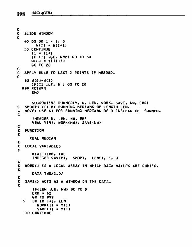
J Q O ABCs of EDA
CC SLIDE WINDOWC
40 DO 50 I * It 5Will ' WU+1)
50 CONTINUEII = 11+1IF (II .GE. NM2) GO TO 60W(6) * Y(11+3)GO TO 20
CC APPLY RULE TO LAST 2 POINTS IF NEEDED.C
60 W(6)=W(3)IF ( I I . L T . N ) GO TO 20
999 RETURNEND
SUBROUTINE RUNMED(Yt N, LEN, WORK, SAVE, NW, ERR)C SMOOTH Y ( ) BY RUNNING MEDIANS OF LENGTH LEN.C NOTE: USE S3 FOR RUNNING MEDIANS OF 3 INSTEAD OF RUNMED.C
INTEGER Nt LEN, NW, ERRREAL Y(N)» WORK(NW), SAVE(NW)
CC FUNCTIONC
REAL MEDIANCC LOCAL VARIABLESC
REAL TEMP, TWOINTEGER SAVEPT, SMOPT, LENP1, I , J
CC WORKC) IS A LOCAL ARRAY IN WHICH DATA VALUES ARE SORTED.C
DATA T W O / 2 . 0 /CC SAVEO ACTS AS A WINDOW ON THE DATA.C
IFCLEN . L E . NW) GO TO 5ERR * 62GO TO 999
5 DO 10 1 * 1 , LENWORK(I) = Y ( I JSAVE( I ) = Y d )
10 CONTINUE
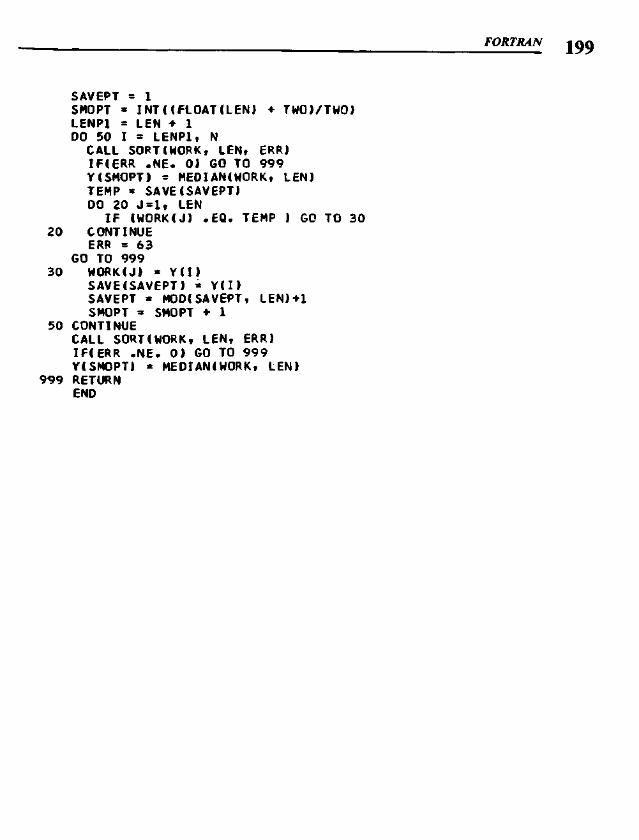
FORTRAN 199
SAVEPT = 1SMOPT = INT((FLOAT(LEN) + TWOJ/TWO)LENPI = LEN * 1DO 50 I = LENPI , N
CALL SORTCWORK, LEN, ERR)IF(ERR . N E . 0 ) GO TO 999Y(SMOPT) = MEDIANiWORK, LEN)TEMP * SAVE(SAVEPT)DO 20 J = l , LEN
I F (WORK(J) .EQ. TEMP ) GO TO 3020 CONTINUE
ERR = 63GO TO 999
30 WORK(J) = Y ( I )SAVE(SAVEPT) - Y ( I )SAVEPT = MOD(SAVEPT, LENJ+1SMOPT = SMOPT + 1
50 CONTINUECALL SORTCWORK, LEN, ERR)IFIERR . N E . 0 ) GO TO 999Y(SMOPT) = MEDIANIWORK, LEN)
999 RETURNEND

Chapter 7Coded Tables
We have examined data with several types of structure. In this chapter wetwo-way consider another data structure, the table. Tables of numbers are a commontable w a y to organize data when each data value is related simultaneously to two
factors. For example, Exhibit 7-1 shows the death rates (in deaths per 1000for men) reported in a British study of the health effects of smoking. Each rowof the table in Exhibit 7-1 reports a different cause of death, and each columnholds data for different amounts of smoking. Any number in the table caneasily be identified with its row and column labels. Thus, for example,non-smokers died of chronic bronchitis at the rate of about .12 per 1000.
The kinds of patterns we might look for in tables are much the same asthose we have sought in other kinds of data, except that in tables we have threethings to keep track of: the row identity, the column identity, and the datavalue in the cell. For example, if, as in Exhibit 7-1, the columns have a naturalorder, we might look for trends as we move from left to right in the table.These might be an overall trend—for example, men who smoke more die at agreater rate than non-smokers—or trends in single rows—for example, thistrend is especially strong for lung cancer. Of course, if the rows had a naturalorder (say, from top to bottom in the table), we might also look for trendsagainst this order.
201
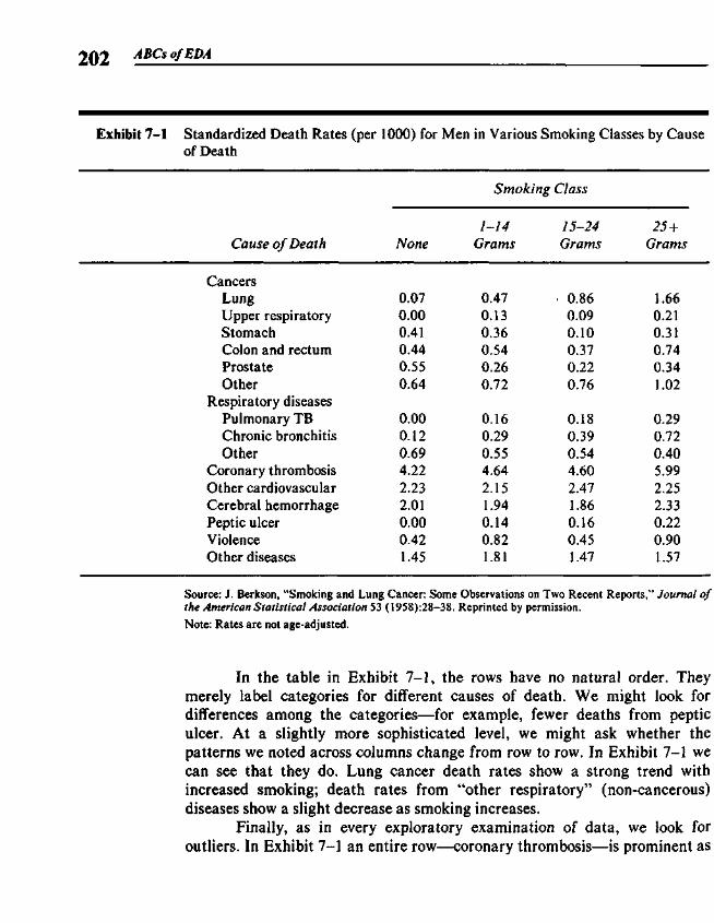
2 Q 2 ABCs of EDA
Exhibit 7-1 Standardized Death Rates (per 1000) for Men in Various Smoking Classes by Causeof Death
Cause of Death
CancersLungUpper respiratoryStomachColon and rectumProstateOther
Respiratory diseasesPulmonary TBChronic bronchitisOther
Coronary thrombosisOther cardiovascularCerebral hemorrhagePeptic ulcerViolenceOther diseases
None
0.070.000.410.440.550.64
0.000.120.694.222.232.010.000.421.45
Smoking Class
1-14Grams
0.470.130.360.540.260.72
0.160.290.554.642.151.940.140.821.81
15-24Grams
0.860.090.100.370.220.76
0.180.390.544.602.471.860.160.451.47
25+Grams
1.660.210.310.740.341.02
0.290.720.405.992.252.330.220.901.57
Source: J. Berkson, "Smoking and Lung Cancer: Some Observations on Two Recent Reports," Journal ofthe American Statistical Association 53 (1958):28—38. Reprinted by permission.
Note: Rates are not age-adjusted.
In the table in Exhibit 7-1, the rows have no natural order. Theymerely label categories for different causes of death. We might look fordifferences among the categories—for example, fewer deaths from pepticulcer. At a slightly more sophisticated level, we might ask whether thepatterns we noted across columns change from row to row. In Exhibit 7-1 wecan see that they do. Lung cancer death rates show a strong trend withincreased smoking; death rates from "other respiratory" (non-cancerous)diseases show a slight decrease as smoking increases.
Finally, as in every exploratory examination of data, we look foroutliers. In Exhibit 7-1 an entire row—coronary thrombosis—is prominent as
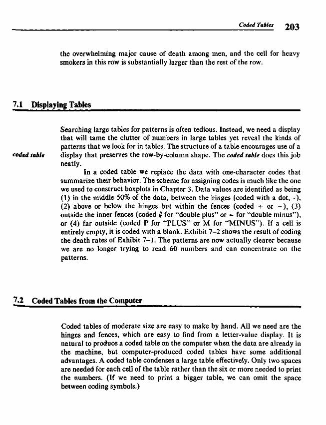
Coded Tables 203
the overwhelming major cause of death among men, and the cell for heavysmokers in this row is substantially larger than the rest of the row.
7.1 Displaying Tables
Searching large tables for patterns is often tedious. Instead, we need a displaythat will tame the clutter of numbers in large tables yet reveal the kinds ofpatterns that we look for in tables. The structure of a table encourages use of a
coded table display that preserves the row-by-column shape. The coded table does this jobneatly.
In a coded table we replace the data with one-character codes thatsummarize their behavior. The scheme for assigning codes is much like the onewe used to construct boxplots in Chapter 3. Data values are identified as being(1) in the middle 50% of the data, between the hinges (coded with a dot, -),(2) above or below the hinges but within the fences (coded + or - ) , (3)outside the inner fences (coded # for "double plus" or = for "double minus"),or (4) far outside (coded P for "PLUS" or M for "MINUS"). If a cell isentirely empty, it is coded with a blank. Exhibit 7-2 shows the result of codingthe death rates of Exhibit 7-1. The patterns are now actually clearer becausewe are no longer trying to read 60 numbers and can concentrate on thepatterns.
7.2 Coded Tables from the Computer
Coded tables of moderate size are easy to make by hand. All we need are thehinges and fences, which are easy to find from a letter-value display. It isnatural to produce a coded table on the computer when the data are already inthe machine, but computer-produced coded tables have some additionaladvantages. A coded table condenses a large table effectively. Only two spacesare needed for each cell of the table rather than the six or more needed to printthe numbers. (If we need to print a bigger table, we can omit the spacebetween coding symbols.)
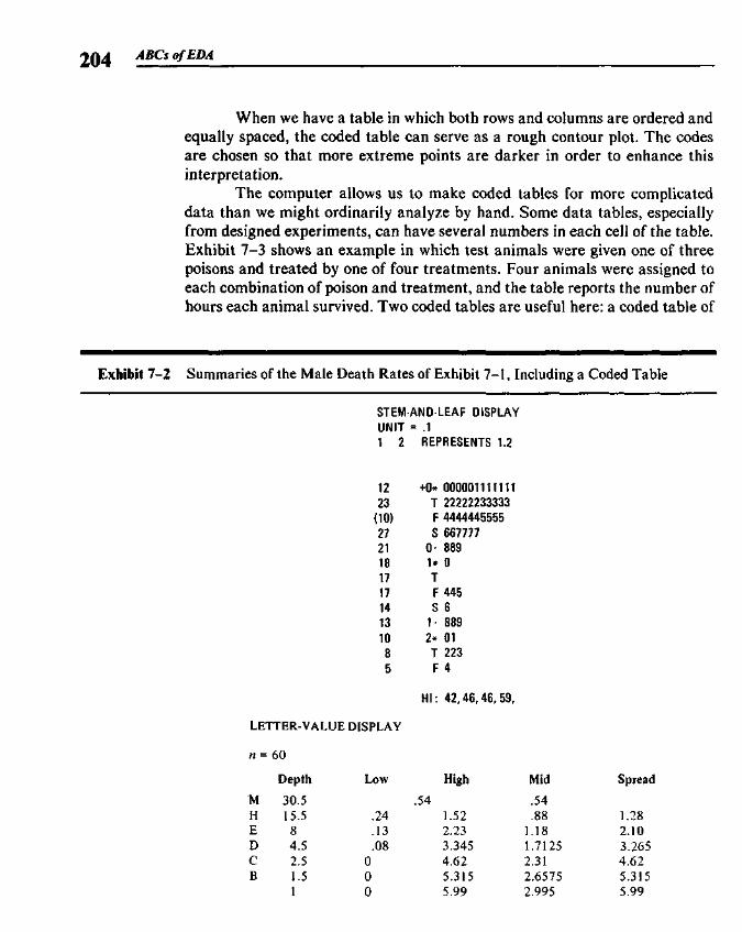
204
When we have a table in which both rows and columns are ordered andequally spaced, the coded table can serve as a rough contour plot. The codesare chosen so that more extreme points are darker in order to enhance thisinterpretation.
The computer allows us to make coded tables for more complicateddata than we might ordinarily analyze by hand. Some data tables, especiallyfrom designed experiments, can have several numbers in each cell of the table.Exhibit 7-3 shows an example in which test animals were given one of threepoisons and treated by one of four treatments. Four animals were assigned toeach combination of poison and treatment, and the table reports the number ofhours each animal survived. Two coded tables are useful here: a coded table of
Exhibit 7-2 Summaries of the Male Death Rates of Exhibit 7-1, Including a Coded Table
STEM-AND-LEAF DISPLAYUNIT =1 2
1223
(10)272118171714131085
= .1REPRESENTS 1.2
+0* 000001111111T 22222233333F 4444445555S 667777
0- 8891» 0TF 445S 6
1- 8892* 01T 223F 4
HI: 42,46,46,59,
LETTER-VALUE DISPLAY
n = 60
MHEDCB
Depth
30.515.584.52.51.51
Low
.24
.13
.08000
High
.541.522.233.3454.625.3155.99
Mid
.54
.881.181.71252.312.65752.995
Sprea<
1.282.103.2654.625.3155.99
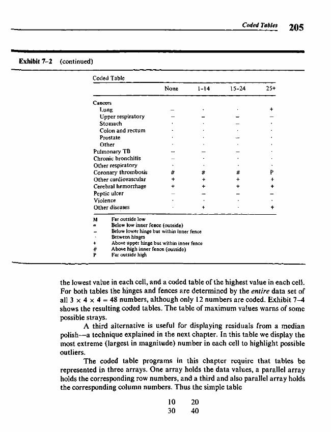
Coded Tables 205
Exhibit 7-2 (continued)
Coded Table
None 1-14 15-24 25+
CancersLungUpper respiratoryStomachColon and rectumProstateOther
Pulmonary TBChronic bronchitisOther respiratoryCoronary thrombosisOther cardiovascularCerebral hemorrhagePeptic ulcerViolenceOther diseases
M Far outside low= Below low inner fence (outside)- Below lower hinge but within inner fence
Between hinges+ Above upper hinge but within inner fence# Above high inner fence (outside)P Far outside high
the lowest value in each cell, and a coded table of the highest value in each cell.For both tables the hinges and fences are determined by the entire data set ofall 3 x 4 x 4 = 48 numbers, although only 12 numbers are coded. Exhibit 7-4shows the resulting coded tables. The table of maximum values warns of somepossible strays.
A third alternative is useful for displaying residuals from a medianpolish—a technique explained in the next chapter. In this table we display themost extreme (largest in magnitude) number in each cell to highlight possibleoutliers.
The coded table programs in this chapter require that tables berepresented in three arrays. One array holds the data values, a parallel arrayholds the corresponding row numbers, and a third and also parallel array holdsthe corresponding column numbers. Thus the simple table
10 2030 40
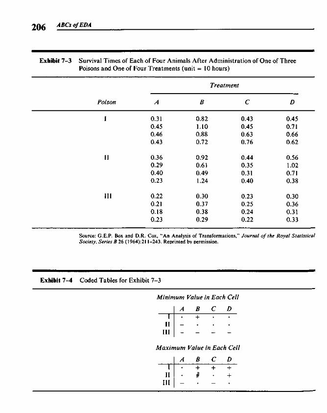
ABCs of EDA
Exhibit 7-3 Survival Times of Each of Four Animals After Administration of One of ThreePoisons and One of Four Treatments (unit = 10 hours)
Poison A
0.310.450.460.43
0.360.290.400.23
0.220.210.180.23
B
0.821.100.880.72
0.920.610.491.24
0.300.370.380.29
Treatment
C
0.430.450.630.76
0.440.350.310.40
0.230.250.240.22
D
0.450.710.660.62
0.561.020.710.38
0.300.360.310.33
II
III
Source: G.E.P. Box and D.R. Cox, "An Analysis of Transformations," Journal of the Royal StatisticalSociety, Series B 26 (1964):211-243. Reprinted by permission.
Exhibit 7-4 Coded Tables for Exhibit 7-3
Minimum Value in Each Cell
A B C DI
IIIII
Maximum Value in Each Cell
III
III
A•
-
B+
•
C+
-
D++•
Coded Tables 207
would be described to the programs as
Data10203040
Row1122
Column1212
While this structure uses slightly more space than other ways of storing atable, it offers great flexibility. For example, it easily accommodates an emptycell: The combination of its row and column numbers simply never appears.Similarly, multiple data values in a cell are specified by repeating the cell'srow and column numbers for each data value. When the table has more thanone data value in some cells, the programs must be told whether to code themaximum, minimum, or most extreme value in the cell.
7.3 Coded Tables and Boxplots
Boxplots and coded tables display data in similar ways. Both describe overallpatterns in the data and highlight individual extraordinary data values, andboth use letter values as a basis for these descriptions. Therefore, it is notsurprising that these two displays complement each other well.
Coded tables preserve the row and column location of each data value.This helps to reveal two-dimensional patterns but can be distracting when wewant to make comparisons among rows or columns alone. When that is OUFgoal, boxplots may do better.
Exhibit 7-5 shows a table of the U.S. birthrate (live births per 1000women aged 15-44 years) recorded monthly from 1937 through 1947, andExhibit 7-6 shows a coded table for the same data. As we saw when wesmoothed annual birthrates in the last chapter (see Exhibits 6-14 and 6-15),this period witnessed rapid changes in the U.S. birthrate due, in part, to WorldWar II. The monthly data allow us to examine these changes more closely.
The coded table in Exhibit 7-6 shows some of the patterns we wouldexpect: lower birthrates in 1937-1940 beginning to increase in the early 1940s,decline in the late years of World War II, and the sharp increase of thepostwar baby boom. We can now see that the increases in both 1942 and 1946accelerated in July and August of those years.
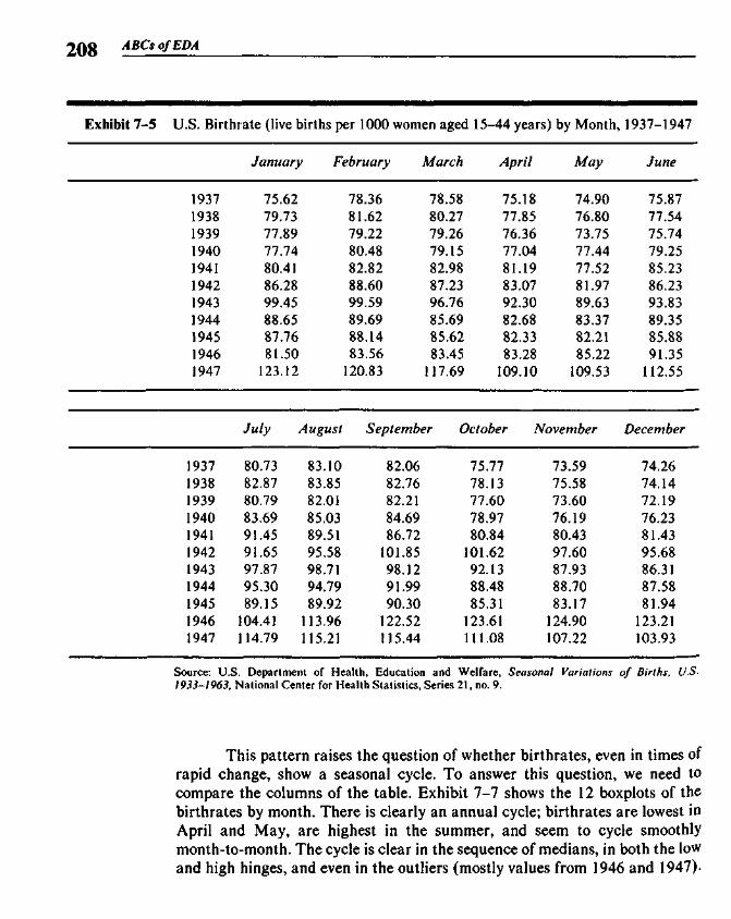
2QC ABCs of EDA
Exhibit 7-5 U.S. Birthrate (live births per 1000 women aged 15-44 years) by Month, 1937-1947
January February March April May June
19371938193919401941194219431944
75.6279.7377.8977.7480.4186.2899.4588.65
78.3681.6279.2280.4882.8288.6099.5989.69
78.5880.2779.2679.1582.9887.2396.7685.69
75.1877.8576.3677.0481.1983.0792.3082.68
74.9076.8073.7577.4477.5281.9789.6383.37
75.8777.5475.7479.2585.2386.2393.8389.35
1945 87.76 88.14 85.62 82.33 82.21 85.881946 81.50 83.56 83.45 83.28 85.22 91.351947 123.12 120.83 117.69 109.10 109.53 112.55
July August September October November December
19371938193919401941194219431944194519461947
80.7382.8780.7983.6991.4591.6597.8795.3089.15104.41114.79
83.1083.8582.0185.0389.5195.5898.7194.7989.92113.96115.21
82.0682.7682.2184.6986.72101.8598.1291.9990.30122.52115.44
75.7778.1377.6078.9780.84101.6292.1388.4885.31123.61111.08
73.5975.5873.6076.1980.4397.6087.9388.7083.17124.90107.22
74.2674.1472.1976.2381.4395.6886.3187.5881.94123.21103.93
Source: U.S. Department of Health, Education and Welfare, Seasonal Variations of Births, U.S.1933-1963, National Center for Health Statistics, Series 21, no. 9.
This pattern raises the question of whether birthrates, even in times ofrapid change, show a seasonal cycle. To answer this question, we need tocompare the columns of the table. Exhibit 7-7 shows the 12 boxplots of thebirthrates by month. There is clearly an annual cycle; birthrates are lowest inApril and May, are highest in the summer, and seem to cycle smoothlymonth-to-month. The cycle is clear in the sequence of medians, in both the lowand high hinges, and even in the outliers (mostly values from 1946 and 1947).
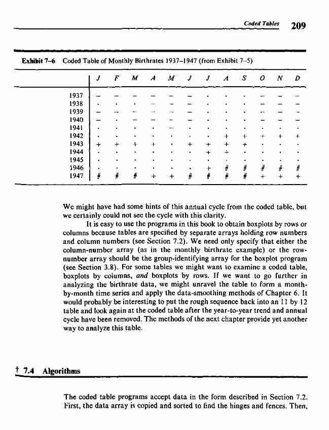
Coded Tables 209
Exhibit 7-6 Coded Table of Monthly Birthrates 1937-1947 (from Exhibit 7-5)
J F M A M J O N D
19371938193919401941194219431944194519461947 # # + # #
# # #
We might have had some hints of this annual cycle from the coded table, butwe certainly could not see the cycle with this clarity.
It is easy to use the programs in this book to obtain boxplots by rows orcolumns because tables are specified by separate arrays holding row numbersand column numbers (see Section 7.2). We need only specify that either thecolumn-number array (as in the monthly birthrate example) or the row-number array should be the group-identifying array for the boxplot program(see Section 3.8). For some tables we might want to examine a coded table,boxplots by columns, and boxplots by rows. If we want to go further inanalyzing the birthrate data, we might unravel the table to form a month-by-month time series and apply the data-smoothing methods of Chapter 6. Itwould probably be interesting to put the rough sequence back into an 11 by 12table and look again at the coded table after the year-to-year trend and annualcycle have been removed. The methods of the next chapter provide yet anotherway to analyze this table.
t 7 . 4 Algorithms
The coded table programs accept data in the form described in Section 7.2.First, the data array is copied and sorted to find the hinges and fences. Then,
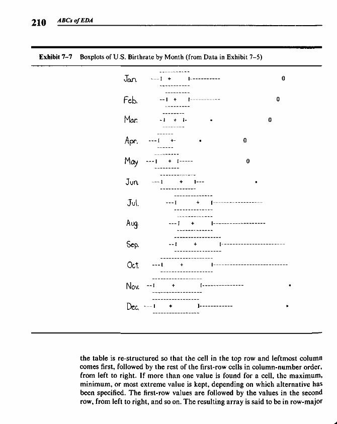
2 J 0 ABCsofEDA
Exhibit 7-7 Boxplots of U.S. Birthrate by Month (from Data in Exhibit 7-5)
Jan. - 1 + '
Feb. - 1 + '
Mar -i + i-
Apr. — i +-
—i +
Jun ---i + i—
Jul. —i + i—-
Aug. — i + i—-
Sep. --i + i-
Oct — i + i—-
Nov. - 1 + i
Dec. — i + i
the table is re-structured so that the cell in the top row and leftmost columncomes first, followed by the rest of the first-row cells in column-number order,from left to right. If more than one value is found for a cell, the maximum,minimum, or most extreme value is kept, depending on which alternative hasbeen specified. The first-row values are followed by the values in the secondrow, from left to right, and so on. The resulting array is said to be in row-major
Coded Tables 211
format. The programs use an internally determined code to mark any emptycells. This code is not a missing-value code and is not used outside theseprograms. The empty code is generated internally to ensure that it is unique.
The re-ordered table is now in the right order for generating thecoded table. Values are considered in turn. They are compared to the hingesand fences, and their codes are printed a line at a time. Empty cells appear asblank cells in the coded table.
FORTRAN
The FORTRAN program for coded tables is invoked with the statement
CALL CTBL (Y, RSUB, CSUB, N, NN, NR, NC, SORTY, CHOOSE, ERR)
where
RSUB( ), CSUB(
N
NN
NR
NC
SORTY()
CHOOSE
ERR
is the N-long vector of data values;are N-long integer arrays of row and column
subscripts;is the number of data values and, hence, the
length of RSUB and CSUB as well;is the length of SORTY()—not less than the
larger of N and NR*NC;
is the number of rows in the table—theintegers in RSUB() thus count from 1 toNR;
is the number of columns in the table—theintegers in CSUB() thus count from 1 toNC;
is an NN-long work array for sorting thevalues in Y();
is an integer flag to indicate selection whenthere are multiple values in a cell:1 choose most extreme value in cell,2 choose maximum value, or3 choose minimum value;
is the error flag, whose values are0 normal
2 2 2 ABCsofEDA
71 the table has a zero dimension (NR =0 or NC = 0)
72 too many columns—will not fit onpage at current margins
73 insufficient room in SORTY().
The FORTRAN program constructs each row of the coded table,using PUTCHR to put symbols in the output line. Each line is printed as it iscompleted.
BASIC
The BASIC subroutine for coded tables is entered with the N data values inY(), row subscripts in R(), and column subscripts in C(). The data are firstsorted into the work array, W(), and hinges and fences are determined. Thehinges are placed in L2 and L3, the inner fences in F1 and F2, and the step(= 1.5 x H-spr) in S1. The table is then copied in row-major form into W( )•The coded table is printed cell-by-cell as it is generated.
7.5 Details and Alternatives
One obvious enhancement of a coded table is the use of color. Values above themedian might be given green codes, while values below the median might havered codes. Users with more sophisticated graphics devices might preferanother choice of codes. However, it is doubtful that increasing the number ofcode alternatives would improve the coded table very much. Seven alternativesseems to be a comfortable number for the human mind to work with. See, forexample, Miller (1956).
When the rows and columns have not only an order but also a naturalor estimated spacing, it can be useful to lay out the rows and columns of thecoded table according to that spacing. This is difficult to do well on a printer,but is easily accomplished with more sophisticated graphics equipment. Onesource of such a spacing is the row and column effects found by a medianpolish of the table (see Chapter 8).
Coded Tables 213
Yes Please turnto Appendix A.
References
Berkson, J. 1958. "Smoking and Lung Cancer: Some Observations on Two RecentReports." Journal of the American Statistical Association 53:28-38.
Box, G.E.P., and D.R. Cox. 1964. "An Analysis of Transformations." Journal of theRoyal Statistical Society, Series B 26:211-243.
Miller, G.A. 1956. "The Magical Number Seven, Plus or Minus Two: Some Limits onOur Capacity for Processing Information." Psychological Review 63:81-97.
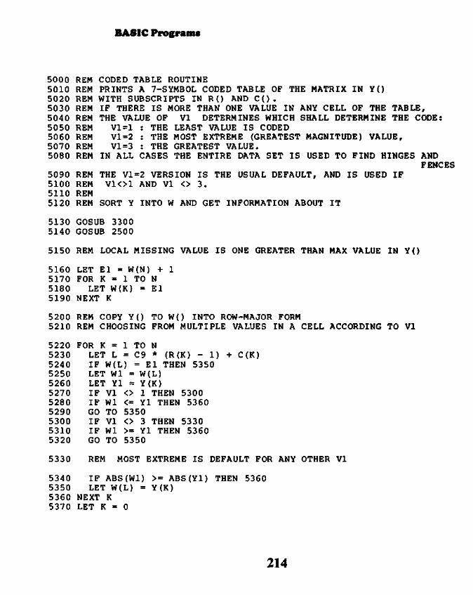
BASIC Programs
500050105020503050405050506050705080
5090510051105120
REMREMREMREMREMREMREMREMREM
REMREMREMREM
CODED TABLE ROUTINEPRINTS A 7-SYMBOL CODED TABLE OF THE MATRIX IN Y()WITH SUBSCRIPTS IN R() AND C().IF THERE IS MORE THAN ONE VALUE IN ANY CELL OF THE TABLE,THE VALUE OF VI DETERMINES WHICH SHALL DETERMINE THE CODE:
Vl=l : THE LEAST VALUE IS CODEDVI=2 : THE MOST EXTREME (GREATEST MAGNITUDE) VALUE,Vl=3 : THE GREATEST VALUE.
IN ALL CASES THE ENTIRE DATA SET IS USED TO FIND HINGES ANDFENCES
THE Vl=2 VERSION IS THE USUAL DEFAULT, AND IS USED IFV1O1 AND VI <> 3.
SORT Y INTO W AND GET INFORMATION ABOUT IT
5130 GOSUB 33005140 GOSUB 2500
5150 REM LOCAL MISSING VALUE IS ONE GREATER THAN MAX VALUE IN Y()
5160 LET El = W(N) + 15170 FOR K = 1 TO N5180 LET W(K) = El5190 NEXT K
5200 REM COPY Y() TO W() INTO ROW-MAJOR FORM5210 REM CHOOSING FROM MULTIPLE VALUES IN A CELL ACCORDING TO VI
5220 FOR K = 1 TO N5230 LET L = C9 * (R(K) - 1) + C(K)5240 IF W(L) = El THEN 53505250 LET Wl = W(L)5260 LET Yl = Y(K)5270 IF VI <> 1 THEN 53005280 IF Wl <= Yl THEN 53605290 GO TO 53505300 IF VI <> 3 THEN 53305310 IF Wl >= Yl THEN 53605320 GO TO 5350
5330 REM MOST EXTREME IS DEFAULT FOR ANY OTHER VI
5340 IF ABS(Wl) >= ABS(Yl)5350 LET W(L) = Y(K)5360 NEXT K5370 LET K = 0
THEN 5360
214
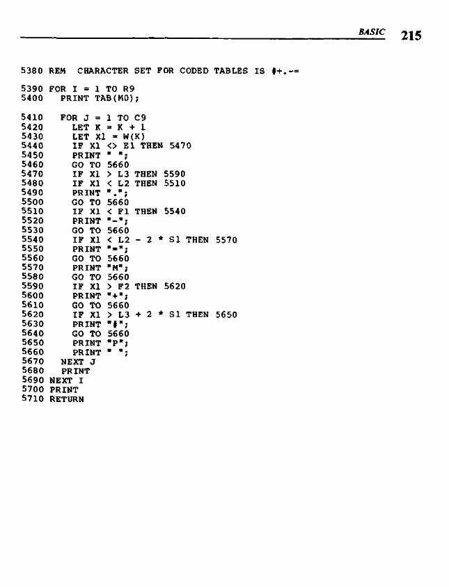
BASIC 215
5380 REM CHARACTER SET FOR CODED TABLES IS #+.-=
5390 FOR I = 1 TO R95400 PRINT TAB(MO);
5410542054305440545054605470548054905500551055205530554055505560557055805590560056105620563056405650566056705680569057005710
FOR J =LET KLET XIIF XIPRINTGO TOIF XIIF XIPRINTGO TOIF XIPRINTGO TOIF XIPRINTGO TOPRINTGO TOIF XIPRINTGO TOIF XIPRINTGO TOPRINTPRINT
NEXT JPRINT
NEXT IPRINTRETURN
1 TO C9= K + 1= W(K)
<> El THENN H .
/5660> L3< L2it m .
• i
5660< FlH n .
#5660< L2n_ n .~~ i
5660"M";5660> F2W i n .
• i
5660> L3"#";5660"P";n n .
THENTHEN
THEN
- 2 *
THEN
+ 2 *
5470
55905510
5540
SI THEN
5620
SI THEN 5650
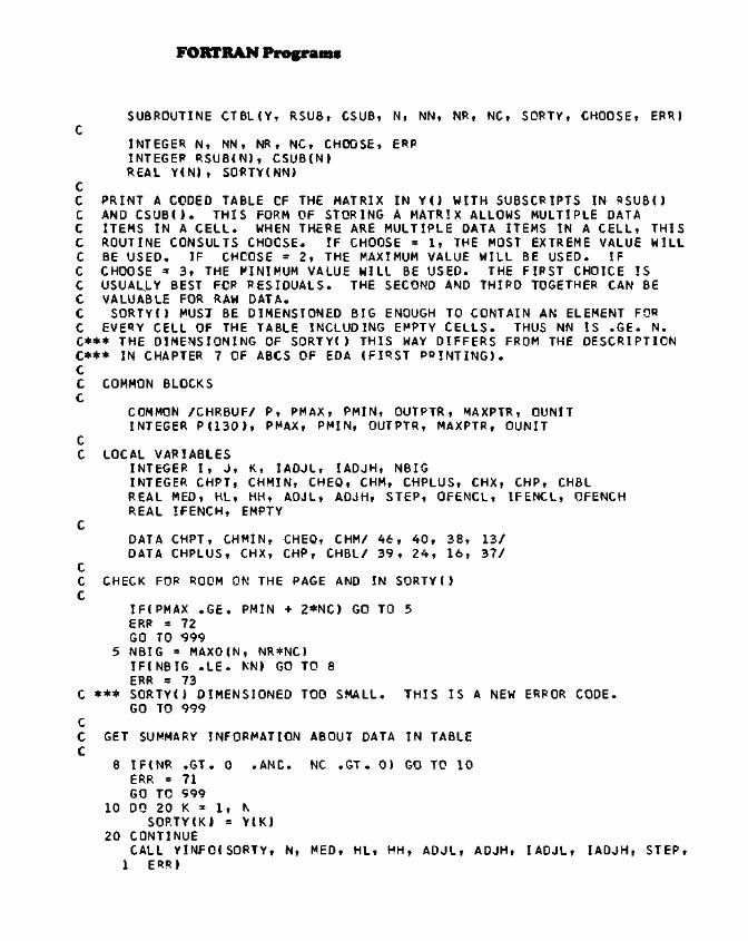
FORTRAN Programs
SUBROUTINE CTBLCY, RSUB, CSUB» N, NN, NR, NC, SOPTY, CHOOSE, ERR)C
INTEGER N, NN , NR, NC, CHOOSE* ERRINTEGER RSUB(N), CSUB(N)REAL Y(N), SORTY(NN)
CC PRINT A CODED TABLE CF THE MATRIX IN Y() WITH SUBSCRIPTS IN RSUBOC AND CSUBU. THIS FORM OF STORING A MATRIX ALLOWS MULTIPLE DATAC ITEMS IN A CELL. WHEN THERE ARE MULTIPLE DATA ITEMS IN A CELLt THISC ROUTINE CONSULTS CHOCSE. IF CHOOSE = 1, THE MOST EXTREME VALUE WILLC BE USED. IF CHCOSE = 2, THE MAXIMUM VALUE WILL BE USED. IFC CHOOSE = 3, THE MINIMUM VALUE WILL BE USED. THE FIRST CHOICE ISC USUALJ-Y BEST FCP RESIDUALS. THE SECOND AND THIRD TOGETHER CAN BEC VALUABLE FOR RAW DATA.C SORTYO MUST BE DIMENSIONED BIG ENOUGH TO CONTAIN AN ELEMENT FORC EVERY CELL OF THE TABLE INCLUDING EMPTY CELLS. THUS NN IS .GE. N.C*** THE DIMENSIONING OF SORTY() THIS WAY DIFFERS FROM THE DESCRIPTIONC*** IN CHAPTER 7 OF ABCS OF EDA (FIRST POINTING).CC COMMON BLOCKSC
COMMON /CHRBUF/ P, PMAX, PMIN, OUTPTR, MAXPTR, OUNITINTEGER P(130)t PMAX, PMIN, OUTPTR, MAXPTR, OUNIT
CC LOCAL VARIABLES
INTEGER I, J, K, IADJL, IADJH, NBIGINTEGER CHPT, CHMIN, CHEQ, CHM, CHPLUS, CHX, CHP, CHBLREAL MED, HL, HH, ADJL, ADJH, STEP, OFENCL, IFENCL, OFENCHREAL IFENCH, EMPTY
CDATA CHPT, CHMIN, CHEQ, CHM/ 46, 40, 38, 13/DATA CHPLUS, CHX, CHP, CHBL/ 39, 24, 16, 37/
CC CHECK FOR ROOM ON THE PAGE AND IN SORTY()C
IFiPMAX .GE. PMIN + 2*NC) GO TO 5ERR - 72GO TO <399
5 NBIG = MAXCXN, NR*NC)I F ( N B I G . L E . NN) GO TO 8ERR = 73
C * * * SORTYO DIMENSIONED TOO SMALL. TH IS I S A NEW ERROR CODE.GO TO 999
CC GET SUMMARY INFORMATION ABOUT DATA I N TABLEC
8 I F ( N R . G T . 0 . A N C . NC . G T . 0 ) GO TO 10ERR = 71GO TO S99
10 DO 20 K = 1 , NSORTY(K) = Y ( K )
20 CONTINUECALL YINFOCSORTY, N, MED, H L , H H , A D J L , ADJH, I A D J L , I A D J H , STEP,
1 ERR)
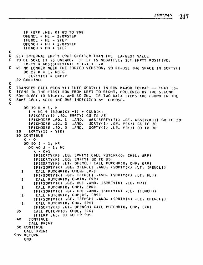
FORTRAN 211
IF (ERR .NE. 0) GC TO 999OFENCL * HL - 2.0*STEPIFENCL = HL - STEPOFENCH = HH + 2.0*STEPIFENCH = HH + STEP
SET INTERNAL EMPTY CCDE GREATER THAN THE LARGEST VALUETO BE SURE IT IS UNIQUE. IF IT IS NEGATIVE, SET EMPTY POSITIVE.
.1+1.0VERSION,
EMPTY = ABSCSCRTY(N)) * 1WE NO LCNGER NEED THE SORTED
DO 2 2 K = 1, NBIGSCRTY(K) = EMPTY
22 CONTINUE
SO RE-USE THE SPACE IN SORTYO
TRANSFER CATA FRCM Y( ) INTOITEMS IN THE FIRST ROW FROMROW (LEFT TO RIGHT), AND SO
SORTYO IN ROW MAJOR FORMAT — THAT I S ,LEFT TO RIGHT, FOLLOWED BY THE SECONDON. IF TWO DATA ITEMS APE FOUND IN THE
SAME CELL, KEEP THE ONE INDICATED BY CHOOSE.
DO 30 K = 1 , hI = NC * (PSUB(K) - 1 ) +IF(SORTYd) .EQ. EMPTY)
CSUB(K)GO TO 25
ABS(SORTY(I))SCRTY(I) .GE.SOPTY(I) . L E .
2530
35
40
50
999
IF(CHOOSE .EQ. 1 .AND.IF(CHOOSE .EQ. 2 .AND.IF(CHOOSE .EQ. 3 .AND.SOPTYU ) = Y(K)
CONTINUEK = 0DO 50 I = 1 , NR
DO 40 J = 1 , NCK = K + lIF(SOPTY(K) .EQ.IF(SOPTY(K) .EQ.IF(SOPTY(K) . L T .IF((SORTY(K) .GE. OFENCL) .AND.
L CALL PUTCHP(O, CHEQ, ERR)IF((SORTY(K) .GE. IFENCL) .AND.
L CALL PUTCHP(O, CKMIN, ERR)IF((SOPTY(K) .GE. HL) .AND. (SORTY(K)
I CALL PUTCHP(O, CHPT» ERR)IF((SORTY(K) .GT. HH) .AND. (SORTY(K)
L CALL PUTCHR(O, CHPLUS, ERR)IF((SOPTY(K) .GT. IFENCH) .AND. (SORTY(K) .
L CALL PUTCHP(O, CHX, EPP)IF(SOPTY(K) .GT. OFENCH) CALL PUTCHP(O, CHPCALL PUTCHR(O, CHBL, ERR)IF(ERR .NE. 0) GO TC 999
CONTINUECALL PRINT
CONTINUECALL PRINTRETURNEND
.GE. ABS(Y(K))Y(K)) GC TO 30Y(K)) GO TO 30
GO TO 30
EMPTY) CALL PUTCHR(0, CHBL, ERR)EMPTY) GO TO 35OFENCL) CALL PUTCHR(0, CHM, ERR)
(SOPTY(K) .LT. IFENCL))
(SORTY(K) .LT. HL))
.LE. HH))
.LE. IFENCH))
LE. OFENCH))
ERR)

Chapter 8Median Polish
The coding technique of Chapter 7 displays two-way tables of data and revealspatterns in these tables. Such graphical displays are important, but often theyinvite us to analyze the data—to summarize the overall pattern simply andexamine the residuals it leaves behind. To summarize a pattern in a table, wemust find a way to characterize the patterns that we are likely to encounter intwo-way tables. Median polish is a simple method for discovering a commontype of pattern.
Two-Way Tables
Patterns in two-way tables are often described in terms of differences amongentire rows or columns of data values. Thus, a row with larger-than-averagedata values might be noted. We often label each data value in a cell of atwo-way table with the number of the row and the number of the column inwhich the value appears, and we think of the row and column identities as
factors factors that help us to account for observed patterns. For example, the data
219
2 2 0 ABCs °fEDA
value in the second row and third column of a table is denoted by y2j. Moregenerally, the data value in the ith row and7th column is denoted by yhj.
While the rows and columns are the factors helping to describe thedata values in the table, the data values themselves are thought of as the
response response. This dichotomy is much the same as we saw for fitting lines inChapter 5—where x was the factor and y was the response—and forsmoothing in Chapter 6—where t was the factor and y was the response. Ineach model we attempt to describe the response, y, using the factors, and weknow that the description cannot be expected to fit the observed data exactly.
The death rate table we examined in Chapter 7 provides a convenientexample. The data shown in Exhibit 7-1 are repeated in Exhibit 8-1. Here theresponse is the death rate, and the two factors are the cause of death and theaverage amount of tobacco smoked. As the data are laid out, the rowscorrespond to the causes, and the columns correspond to the extent of smoking.We naturally expect some causes to be responsible for many more deaths thanothers. The row medians in Exhibit 8-1 and the coded table in Exhibit 7-2both reveal higher death rates from coronary thrombosis, other cardiovasculardiseases, and cerebral hemorrhage, and lower rates from upper respiratorycancer, pulmonary TB, and peptic ulcer. In light of today's knowledge, wewould expect smoking to affect the death rate for several causes. If this patternis present, it is not obvious, but we may be able to judge more clearly afteradjusting for the differences among the typical death rates for the variouscauses.
8.2 A Model for Two-Way Tables
When we chose a model to describe x-y data in Chapter 5, we used a straightline because of its simplicity. Two-way tables require a different kind of modelbecause they involve three components—the row factor, the column factor,and the response—but we still aim for simplicity.
The straight line is a convenient model for y versus x because it fitseach y-va.\ue with the sum of two simple components: a constant interceptvalue to anchor the line where x = 0 and a slope multiplied by x to account forchanges in y associated with changes in x away from x = 0. Because these twocomponents are added in the fit, we can polish the resistant line by addingadjustments to the slope and intercept.
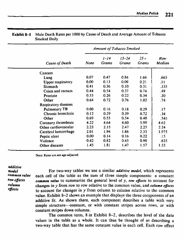
Median Polish 111
Exhibit 8-1 Male Death Rates per 1000 by Cause of Death and Average Amount of TobaccoSmoked Daily
Amount of Tobacco Smoked
Cause of Death None1-14
Grams15-24Grams
25 +Grams
RowMedian
CancersLungUpper respiratoryStomachColon and rectumProstateOther
Respiratory diseasesPulmonary TBChronic bronchitisOther
Coronary thrombosisOther cardiovascularCerebral hemorrhagePeptic ulcerViolenceOther diseases
0.070.000.410.440.550.64
0.000.120.694.222.232.010.000.421.45
0.470.130.360.540.260.72
0.160.290.554.642.151.940.140.821.81
0.860.090.100.370.220.76
0.180.390.544.602.471.860.160.451.47
1.660.210.310.740.341.02
0.290.720.405.992.252.330.220.901.57
421
1
.665
.11
.335
.49
.30
.74
.17
.34
.545
.62
.24
.975
.15
.635
.52
Note: Rates are not age-adjusted.
additivemodelcommon valuerow effectscolumneffects
For two-way tables we use a similar additive model, which representseach cell of the table as the sum of three simple components: a constantcommon value to summarize the general level of y, row effects to account forchanges in y from row to row relative to the common value, and column effectsto account for changes in y from column to column relative to the commonvalue. Exhibit 8-2 shows an example that displays the three components of anadditive fit. As shown there, each component describes a table with verysimple structure—constant, or with constant stripes across rows, or withconstant stripes down columns.
The common term, 8 in Exhibit 8-2, describes the level of the datavalues in the table as a whole. It can thus be thought of as describing atwo-way table that has the same constant value in each cell. Each row effect
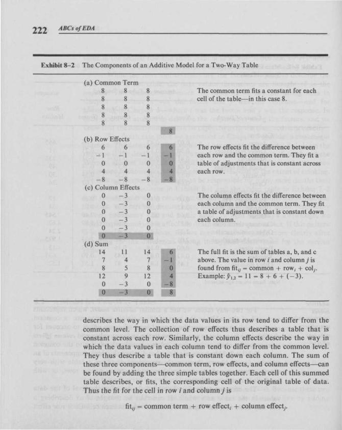
2 2 2 ABCs °fEDA
Exhibit 8-2 The Components of an Additive Model for a Two-Way Table
(a) Common Term88888
88888
(b) Row Effects6
- 104
- 8
6- 1
04
- 8(c) Column Effects
000000
(d) Sum1478
1200
- 3- 3- 3- 3- 3- 3
11459
- 3- 3
88888
6- 1
04
- 8
000000
1478
1200
8
6- 1
04
- 8
6- 1
04
- 88
The common term fits a constant for eachcell of the table—in this case 8.
The row effects fit the difference betweeneach row and the common term. They fit atable of adjustments that is constant acrosseach row.
The column effects fit the difference betweeneach column and the common term. They fita table of adjustments that is constant downeach column.
The full fit is the sum of tables a, b, and cabove. The value in row / and column j isfound from fit,7 = common + row, + col,.Example: yU2 = 11 = 8 + 6 + ( - 3 ) .
describes the way in which the data values in its row tend to differ from thecommon level. The collection of row effects thus describes a table that isconstant across each row. Similarly, the column effects describe the way inwhich the data values in each column tend to differ from the common level.They thus describe a table that is constant down each column. The sum ofthese three components—common term, row effects, and column effects—canbe found by adding the three simple tables together. Each cell of this summedtable describes, or fits, the corresponding cell of the original table of data.Thus the fit for the cell in row / and column j is
fit,7 = common term + row effect, + column effect,.
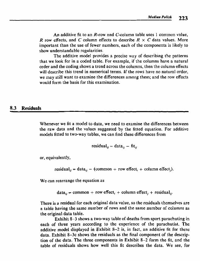
Median Polish 223
An additive fit to an /?-row and C-column table uses 1 common value,R row effects, and C column effects to describe R x C data values. Moreimportant than the use of fewer numbers, each of the components is likely toshow understandable regularities.
The additive model provides a precise way of describing the patternsthat we look for in a coded table. For example, if the columns have a naturalorder and the coding shows a trend across the columns, then the column effectswill describe this trend in numerical terms. If the rows have no natural order,we may still want to examine the differences among them; and the row effectswould form the basis for this examination.
8.3 Residuals
Whenever we fit a model to data, we need to examine the differences betweenthe raw data and the values suggested by the fitted equation. For additivemodels fitted to two-way tables, we can find these differences from
residual^ = data,7 - fit,-,
or, equivalently,
residual,, = data,-, — (common + row effect, + column effect,).
We can rearrange the equation as
data,-, = common + row effect, + column effect, + residual,-,-.
There is a residual for each original data value, so the residuals themselves area table having the same number of rows and the same number of columns asthe original data table.
Exhibit 8-3 shows a two-way table of deaths from sport parachuting ineach of three years according to the experience of the parachutist. Theadditive model displayed in Exhibit 8-2 is, in fact, an additive fit for thesedata. Exhibit 8-3c shows the residuals as the final component of the descrip-tion of the data. The three components in Exhibit 8-2 form the fit, and thetable of residuals shows how well this fit describes the data. We see, for
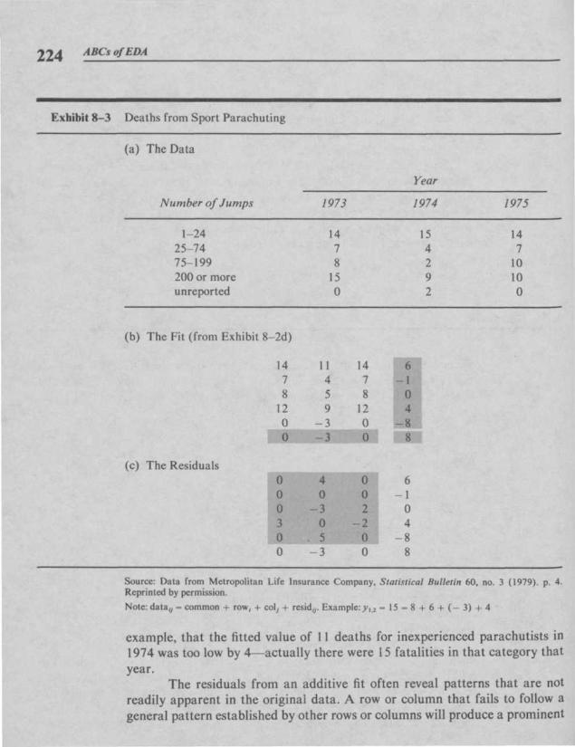
2 2 4 ABCs °fEDA
Exhibit 8-3 Deaths from Sport Parachuting
(a) The Data
Number of Jumps
1-2425-7475-199200 or moreunreported
1973
1478
150
Year
1974
154292
1975
147
10100
(b) The Fit (from Exhibit 8-2d)
(c) The Residuals
1478
1200
000300
11459
-3
~ 3
40
- 30
. 5- 3
1478
1200
002
- 200
6- 1
o4
- 88
6_ i
04
- 88
Source: Data from Metropolitan Life Insurance Company, Statistical Bulletin 60, no. 3 (1979) . p. 4.Reprinted by permission.
Note: data / y - common + row, + coly + resid,,. Example: yl2 - 1 5 - 8 + 6 + ( - 3 ) + 4
example, that the fitted value of 11 deaths for inexperienced parachutists in1974 was too low by 4—actually there were 15 fatalities in that category thatyear.
The residuals from an additive fit often reveal patterns that are notreadily apparent in the original data. A row or column that fails to follow ageneral pattern established by other rows or columns will produce a prominent
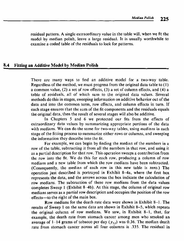
Median Polish 225
residual pattern. A single extraordinary value in the table will, when we fit themodel by median polish, leave a large residual. It is usually worthwhile toexamine a coded table of the residuals to look for patterns.
8.4 Fitting an Additive Model by Median Polish
There are many ways to find an additive model for a two-way table.Regardless of the method, we must progress from the original data table to (1)a common value, (2) a set of row effects, (3) a set of column effects, and (4) atable of residuals, all of which sum to the original data values. Severalmethods do this in stages, sweeping information on additive behavior out of thedata and into the common term, row effects, and column effects in turn. Ifeach stage ensures that the sum of the fit components and the residuals equalsthe original data, then the result of several stages will also be additive.
In Chapters 5 and 6 we protected our fits from the effects ofextraordinary data values by summarizing appropriate portions of the datawith medians. We can do the same for two-way tables, using medians in eachstage of the fitting process to summarize either rows or columns, and sweepingthe information they describe into the fit.
For example, we can begin by finding the median of the numbers in arow of the table, subtracting it from all the numbers in that row, and using itas a partial description for that row. This operation sweeps a contribution fromthe row into the fit. We do this for each row, producing a column of rowmedians and a new table from which the row medians have been subtracted.(Consequently, the median of each row in this new table is zero.) Theoperation just described is portrayed in Exhibit 8-4a, where the first boxrepresents the data, and the arrows across the box indicate the calculation ofrow medians. The subtraction of these row medians from the data valuescompletes Sweep 1 (Exhibit 8-4b). At this stage, the column of original rowmedians serves as a partial row description and occupies the position of the roweffects—to the right of the main box.
Row medians for the death rate data were shown in Exhibit 8-1. Theresults of Sweep 1 on the same data are shown in Exhibit 8-5, which repeatsthe original column of row medians. We saw, in Exhibit 8-1, that, forexample, the death rate from stomach cancer among men who smoked anaverage of 1-14 grams of tobacco per day (y^2)
w a s 0-36. The median deathrate from stomach cancer across all four columns is .335. The residual in
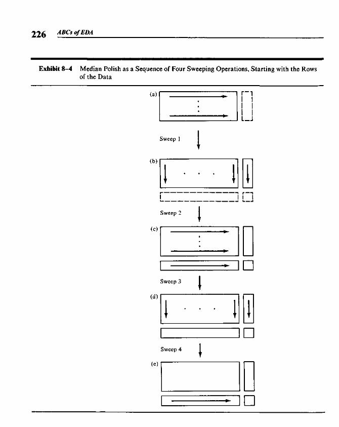
2 2 6 ABCs °fEDA
Exhibit 8-4 Median Polish as a Sequence of Four Sweeping Operations, Starting with the Rowsof the Data
(a) ni iL_J
Sweep 1
(b)
(c)
(d)
(e)
ISweep 2
Sweep 3
1 •
Sweep 4
•
•
1•
1
I
•
•
•
• 1
1
1
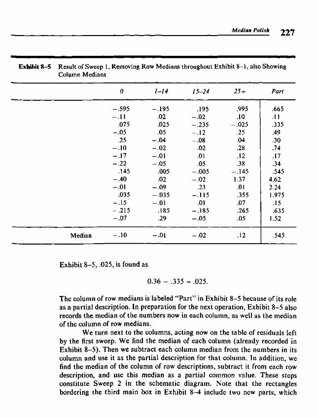
Median Polish 227
Exhibit 8-5 Result of Sweep 1, Removing Row Medians throughout Exhibit 8-1, also ShowingColumn Medians
0 1-14 15-24 25+ Part
- .595- .11
.075- .05
.25- .10- .17- .22
.145- .40- .01
.035- .15- .215- .07
Median —.10
- .195.02.025.05
- .04- .02- .01- .05
.005
.02- .09- .035- .01
.185
.29
- .01
.195- .02- .235- .12- .08
.02
.01
.05-.005- .02
.23-.115
.01- .185- .05
- .02
.995
.10-.025
.25
.04
.28
.12
.38-.1451.37.01.355.07.265.05
.12
.665
.11
.335
.49
.30
.74
.17
.34
.5454.622.241.975.15.635
1.52
.545
Exhibit 8-5, .025, is found as
0.36 - .335 = .025.
The column of row medians is labeled "Part" in Exhibit 8-5 because of its roleas a partial description. In preparation for the next operation, Exhibit 8-5 alsorecords the median of the numbers now in each column, as well as the medianof the column of row medians.
We turn next to the columns, acting now on the table of residuals leftby the first sweep. We find the median of each column (already recorded inExhibit 8-5). Then we subtract each column median from the numbers in itscolumn and use it as the partial description for that column. In addition, wefind the median of the column of row descriptions, subtract it from each rowdescription, and use this median as a partial common value. These stepsconstitute Sweep 2 in the schematic diagram. Note that the rectanglesbordering the third main box in Exhibit 8-4 include two new parts, which
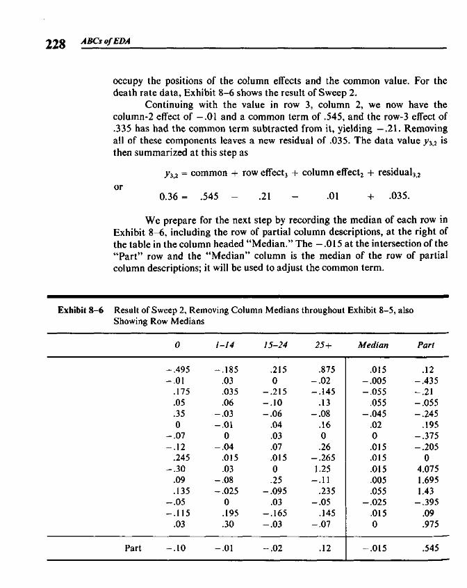
2 2 8 ABCs °fEDA
occupy the positions of the column effects and the common value. For thedeath rate data, Exhibit 8-6 shows the result of Sweep 2.
Continuing with the value in row 3, column 2, we now have thecolumn-2 effect of —.01 and a common term of .545, and the row-3 effect of.335 has had the common term subtracted from it, yielding —.21. Removingall of these components leaves a new residual of .035. The data value j>32
IS
then summarized at this step as
or
y32 = common + row effect3 + column effect2 + residual3 2
0.36 = .545 - .21 - .01 + .035.
We prepare for the next step by recording the median of each row inExhibit 8-6, including the row of partial column descriptions, at the right ofthe table in the column headed "Median." The - .015 at the intersection of the"Part" row and the "Median" column is the median of the row of partialcolumn descriptions; it will be used to adjust the common term.
Exhibit 8-6 Result of Sweep 2, Removing Column Medians throughout Exhibit 8-5, alsoShowing Row Medians
0 1-14 15-24 25+ Median Part
- .495- .01
.175
.05
.350
- .07- .12
.245- . 3 0
.09
.135- .05- .115
.03
Part - . 10
- .185.03.035.06
- . 03- .01
0- .04
.015
.03- .08- .025
0.195.30
- .01
.2150
- .215- .10- .06
.04
.03
.07
.0150.25
- .095.03
- .165- . 03
- .02
.875- .02- .145
.13- .08
.160.26
- .2651.25
- .11.235
- .05.145
- .07
.12
.015- .005-.055
.055- .045
.020.015.015.015.005.055
- .025.0150
- .015
.12- .435- .21- .055- .245
.195-.375- .205
04.0751.6951.43
- .395.09.975
.545
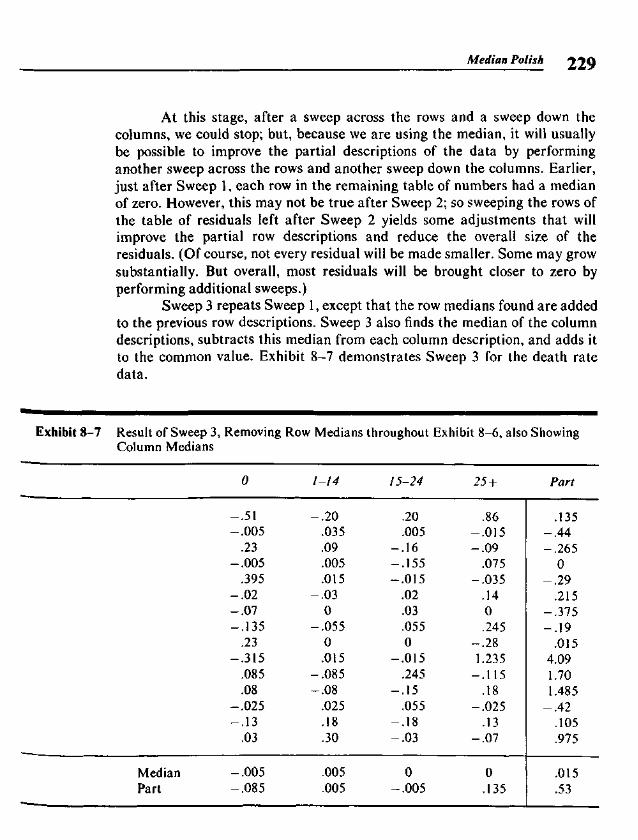
Median Polish 229
At this stage, after a sweep across the rows and a sweep down thecolumns, we could stop; but, because we are using the median, it will usuallybe possible to improve the partial descriptions of the data by performinganother sweep across the rows and another sweep down the columns. Earlier,just after Sweep 1, each row in the remaining table of numbers had a medianof zero. However, this may not be true after Sweep 2; so sweeping the rows ofthe table of residuals left after Sweep 2 yields some adjustments that willimprove the partial row descriptions and reduce the overall size of theresiduals. (Of course, not every residual will be made smaller. Some may growsubstantially. But overall, most residuals will be brought closer to zero byperforming additional sweeps.)
Sweep 3 repeats Sweep 1, except that the row medians found are addedto the previous row descriptions. Sweep 3 also finds the median of the columndescriptions, subtracts this median from each column description, and adds itto the common value. Exhibit 8-7 demonstrates Sweep 3 for the death ratedata.
Exhibit 8-7 Result of Sweep 3, Removing Row Medians throughout Exhibit 8-6, also ShowingColumn Medians
0 1-14 15-24 25 + Part
MedianPart
- .51- .005
.23-.005
.395- .02- .07- .135
.23-.315
.085
.08-.025- .13
.03
- .005-.085
- .20.035.09.005.015
- .030
-.0550.015
-.085- .08
.025
.18
.30
.005
.005
.20
.005- .16- .155-.015
.02
.03
.0550
-.015.245
- .15.055
- .18- .03
0- .005
.86-.015- .09
.075-.035
.140.245
- .281.235
-.115.18
-.025.13
- .07
0.135
.135- .44- .265
0- .29
.215- .375- .19
.0154.091.701.485
- .42.105.975
.015
.53
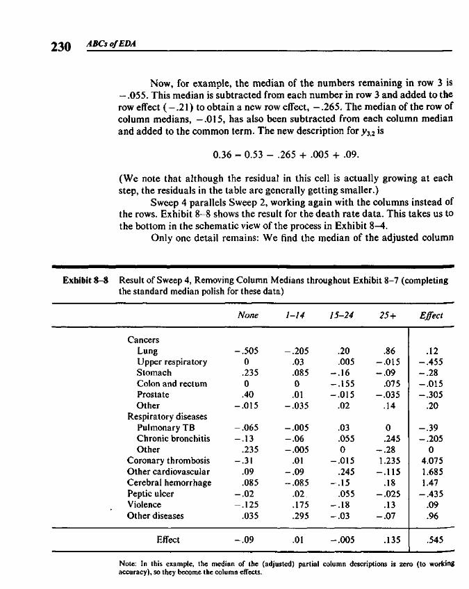
2 3 0 ABCs of EDA
Now, for example, the median of the numbers remaining in row 3 is— .055. This median is subtracted from each number in row 3 and added to therow effect ( — .21) to obtain a new row effect, - .265. The median of the row ofcolumn medians, —.015, has also been subtracted from each column medianand added to the common term. The new description for >>32 is
0.36 = 0.53 - .265 + .005 + .09.
(We note that although the residual in this cell is actually growing at eachstep, the residuals in the table are generally getting smaller.)
Sweep 4 parallels Sweep 2, working again with the columns instead ofthe rows. Exhibit 8-8 shows the result for the death rate data. This takes us tothe bottom in the schematic view of the process in Exhibit 8-4.
Only one detail remains: We find the median of the adjusted column
Exhibit 8-8 Result of Sweep 4, Removing Column Medians throughout Exhibit 8-7 (completingthe standard median polish for these data)
CancersLungUpper respiratoryStomachColon and rectumProstateOther
Respiratory diseasesPulmonary TBChronic bronchitisOther
Coronary thrombosisOther cardiovascularCerebral hemorrhagePeptic ulcerViolenceOther diseases
Effect
None
-.5050.2350.40
-.015
-.065-.13
.235-.31
.09
.085-.02-.125
.035
-.09
1-14
-.205.03.0850.01
-.035
-.005-.06-.005
.01-.09-.085
.02
.175
.295
.01
15-24
.20
.005-.16-.155-.015
.02
.03
.0550
-.015.245
-.15.055
-.18-.03
-.005
25+
.86-.015-.09
.075-.035
.14
0.245
-.281.235
-.115.18
-.025.13
-.07
.135
Effect
.12-.455-.28-.015-.305
.20
-.39-.205
04.0751.6851.47
-.435.09.96
.545
Note: In this example, the median of the (adjusted) partial column descriptions is zero (to workingaccuracy), so they become the column effects.
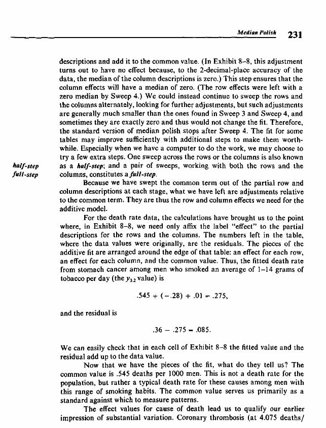
Median Polish 231
descriptions and add it to the common value. (In Exhibit 8-8, this adjustmentturns out to have no effect because, to the 2-decimal-place accuracy of thedata, the median of the column descriptions is zero.) This step ensures that thecolumn effects will have a median of zero. (The row effects were left with azero median by Sweep 4.) We could instead continue to sweep the rows andthe columns alternately, looking for further adjustments, but such adjustmentsare generally much smaller than the ones found in Sweep 3 and Sweep 4, andsometimes they are exactly zero and thus would not change the fit. Therefore,the standard version of median polish stops after Sweep 4. The fit for sometables may improve sufficiently with additional steps to make them worth-while. Especially when we have a computer to do the work, we may choose totry a few extra steps. One sweep across the rows or the columns is also known
half-step as a half-step; and a pair of sweeps, working with both the rows and thefull-step columns, constitutes a full-step.
Because we have swept the common term out of the partial row andcolumn descriptions at each stage, what we have left are adjustments relativeto the common term. They are thus the row and column effects we need for theadditive model.
For the death rate data, the calculations have brought us to the pointwhere, in Exhibit 8-8, we need only affix the label "effect" to the partialdescriptions for the rows and the columns. The numbers left in the table,where the data values were originally, are the residuals. The pieces of theadditive fit are arranged around the edge of that table: an effect for each row,an effect for each column, and the common value. Thus, the fitted death ratefrom stomach cancer among men who smoked an average of 1-14 grams oftobacco per day (the yX2 value) is
.545 + (- .28) + .01 = .275,
and the residual is
.36 - .275 = .085.
We can easily check that in each cell of Exhibit 8-8 the fitted value and theresidual add up to the data value.
Now that we have the pieces of the fit, what do they tell us? Thecommon value is .545 deaths per 1000 men. This is not a death rate for thepopulation, but rather a typical death rate for these causes among men withthis range of smoking habits. The common value serves us primarily as astandard against which to measure patterns.
The effect values for cause of death lead us to qualify our earlierimpression of substantial variation. Coronary thrombosis (at 4.075 deaths/
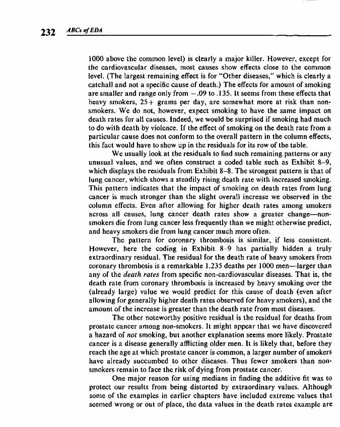
2 3 2 ABCs °fEDA
1000 above the common level) is clearly a major killer. However, except forthe cardiovascular diseases, most causes show effects close to the commonlevel. (The largest remaining effect is for "Other diseases," which is clearly acatchall and not a specific cause of death.) The effects for amount of smokingare smaller and range only from - .09 to .135. It seems from these effects thatheavy smokers, 25+ grams per day, are somewhat more at risk than non-smokers. We do not, however, expect smoking to have the same impact ondeath rates for all causes. Indeed, we would be surprised if smoking had muchto do with death by violence. If the effect of smoking on the death rate from aparticular cause does not conform to the overall pattern in the column effects,this fact would have to show up in the residuals for its row of the table.
We usually look at the residuals to find such remaining patterns or anyunusual values, and we often construct a coded table such as Exhibit 8-9,which displays the residuals from Exhibit 8-8. The strongest pattern is that oflung cancer, which shows a steadily rising death rate with increased smoking.This pattern indicates that the impact of smoking on death rates from lungcancer is much stronger than the slight overall increase we observed in thecolumn effects. Even after allowing for higher death rates among smokersacross all causes, lung cancer death rates show a greater change—non-smokers die from lung cancer less frequently than we might otherwise predict,and heavy smokers die from lung cancer much more often.
The pattern for coronary thrombosis is similar, if less consistent.However, here the coding in Exhibit 8-9 has partially hidden a trulyextraordinary residual. The residual for the death rate of heavy smokers fromcoronary thrombosis is a remarkable 1.235 deaths per 1000 men—larger thanany of the death rates from specific non-cardiovascular diseases. That is, thedeath rate from coronary thrombosis is increased by heavy smoking over the(already large) value we would predict for this cause of death (even afterallowing for generally higher death rates observed for heavy smokers), and theamount of the increase is greater than the death rate from most diseases.
The other noteworthy positive residual is the residual for deaths fromprostate cancer among non-smokers. It might appear that we have discovereda hazard of not smoking, but another explanation seems more likely. Prostatecancer is a disease generally afflicting older men. It is likely that, before theyreach the age at which prostate cancer is common, a larger number of smokershave already succumbed to other diseases. Thus fewer smokers than non-smokers remain to face the risk of dying from prostate cancer.
One major reason for using medians in finding the additive fit was toprotect our results from being distorted by extraordinary values. Althoughsome of the examples in earlier chapters have included extreme values thatseemed wrong or out of place, the data values in the death rates example are
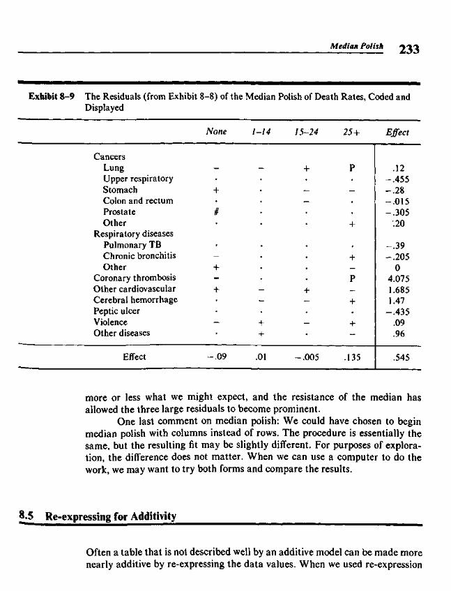
Median Polish 233
Exhibit 8-9 The Residuals (from Exhibit 8-8) of the Median Polish of Death Rates, Coded andDisplayed
None 1-14 15-24 25+ Effect
CancersLungUpper respiratoryStomachColon and rectumProstateOther
Respiratory diseasesPulmonary TBChronic bronchitisOther
Coronary thrombosisOther cardiovascularCerebral hemorrhagePeptic ulcerViolenceOther diseases
Effect
=•+
#•
•-+=+••-•
- .09
—••
••
——
++
.01
+•——
•
+_
—•
- .005
P•—
+
+—P
+
+-
.135
.12-.455- .28- .015-.305
.20
- .39- .205
04.0751.6851.47
- .435.09.96
.545
more or less what we might expect, and the resistance of the median hasallowed the three large residuals to become prominent.
One last comment on median polish: We could have chosen to beginmedian polish with columns instead of rows. The procedure is essentially thesame, but the resulting fit may be slightly different. For purposes of explora-tion, the difference does not matter. When we can use a computer to do thework, we may want to try both forms and compare the results.
8.5 Re-expressing for Additivity
Often a table that is not described well by an additive model can be made morenearly additive by re-expressing the data values. When we used re-expression
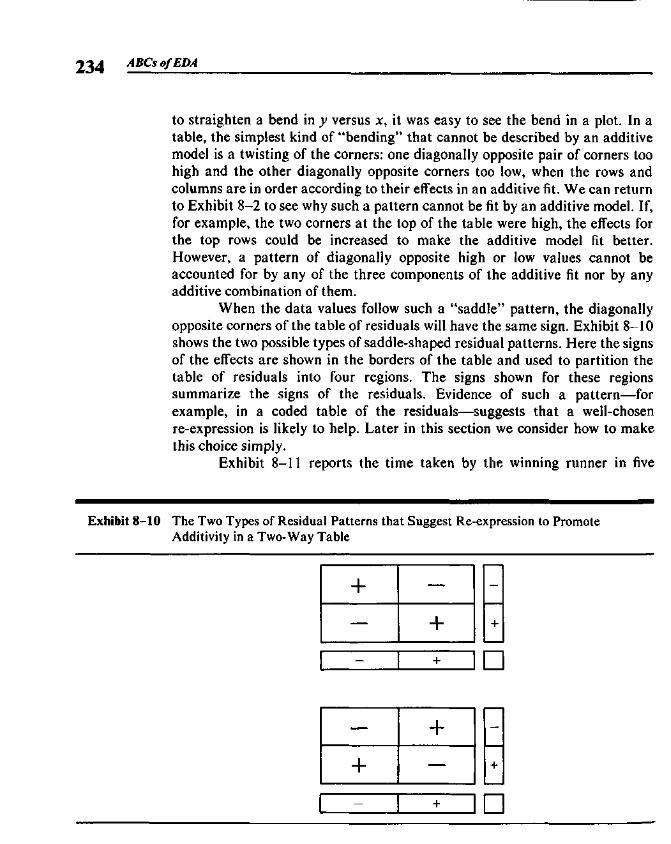
234
to straighten a bend in y versus x, it was easy to see the bend in a plot. In atable, the simplest kind of "bending" that cannot be described by an additivemodel is a twisting of the corners: one diagonally opposite pair of corners toohigh and the other diagonally opposite corners too low, when the rows andcolumns are in order according to their effects in an additive fit. We can returnto Exhibit 8-2 to see why such a pattern cannot be fit by an additive model. If,for example, the two corners at the top of the table were high, the effects forthe top rows could be increased to make the additive model fit better.However, a pattern of diagonally opposite high or low values cannot beaccounted for by any of the three components of the additive fit nor by anyadditive combination of them.
When the data values follow such a "saddle" pattern, the diagonallyopposite corners of the table of residuals will have the same sign. Exhibit 8-10shows the two possible types of saddle-shaped residual patterns. Here the signsof the effects are shown in the borders of the table and used to partition thetable of residuals into four regions. The signs shown for these regionssummarize the signs of the residuals. Evidence of such a pattern—forexample, in a coded table of the residuals—suggests that a well-chosenre-expression is likely to help. Later in this section we consider how to makethis choice simply.
Exhibit 8-11 reports the time taken by the winning runner in five
Exhibit 8-10 The Two Types of Residual Patterns that Suggest Re-expression to PromoteAdditivity in a Two-Way Table
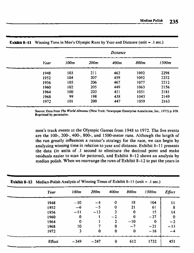
Median Polish 235
Exhibit 8-11 Winning Time in Men's Olympic Runs by Year and Distance (unit = .1 sec.)
Year
1948195219561960196419681972
100m
10310410510210099101
200m
211207206205203198200
Distance
400m
462459467449451438447
800m
1092109210771063105110431059
1500m
2298225222122156218121492163
Source: Data from The World Almanac (New York: Newspaper Enterprise Association, Inc., 1973) p. 858.Reprinted by permission.
men's track events at the Olympic Games from 1948 to 1972. The five eventsare the 100-, 200-, 400-, 800-, and 1500-meter runs. Although the length ofthe run greatly influences a runner's strategy for the race, we can begin byanalyzing winning time in relation to year and distance. Exhibit 8-11 presentsthe data (in units of .1 second to eliminate the decimal point and makeresiduals easier to scan for patterns), and Exhibit 8-12 shows an analysis bymedian polish. When we rearrange the rows of Exhibit 8-12 to put the years in
Exhibit 8-12 Median-Polish Analysis of Winning Times of Exhibit 8-11 (unit = .1 sec.)
Year
1948195219561960196419681972
Effect
100m
-10-6-1100103
-349
200m
-4-5-12
1170
-247
400m
002
-2200
0
800m
182100
-10-70
612
1500m
1046115
-270
-21-16
1732
Effect
118140
-2-13-4
451
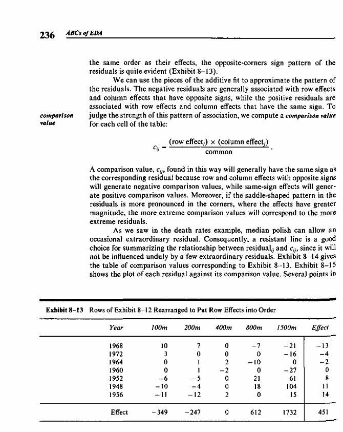
2 3 5 ABCs °fEDA
comparisonvalue
the same order as their effects, the opposite-corners sign pattern of theresiduals is quite evident (Exhibit 8-13).
We can use the pieces of the additive fit to approximate the pattern ofthe residuals. The negative residuals are generally associated with row effectsand column effects that have opposite signs, while the positive residuals areassociated with row effects and column effects that have the same sign. Tojudge the strength of this pattern of association, we compute a comparison valuefor each cell of the table:
(row effect,) x (column effect,)iJ common
A comparison value, ctj, found in this way will generally have the same sign asthe corresponding residual because row and column effects with opposite signswill generate negative comparison values, while same-sign effects will gener-ate positive comparison values. Moreover, if the saddle-shaped pattern in theresiduals is more pronounced in the corners, where the effects have greatermagnitude, the more extreme comparison values will correspond to the moreextreme residuals.
As we saw in the death rates example, median polish can allow anoccasional extraordinary residual. Consequently, a resistant line is a goodchoice for summarizing the relationship between residual,-,- and c,-,-, since it willnot be influenced unduly by a few extraordinary residuals. Exhibit 8-14 givesthe table of comparison values corresponding to Exhibit 8-13. Exhibit 8-15shows the plot of each residual against its comparison value. Several points in
Exhibit 8-13 Rows of Exhibit 8-12 Rearranged to Put Row Effects into Order
Year
1968197219641960195219481956
Effect
100m
10300
-6-10-11
-349
200m
1011
-5-4-12
-247
400m
002
-2002
0
800m
_7
0-10
021180
612
1500m
-21-16
0-276110415
1732
Effect
-13-4-2081114
451
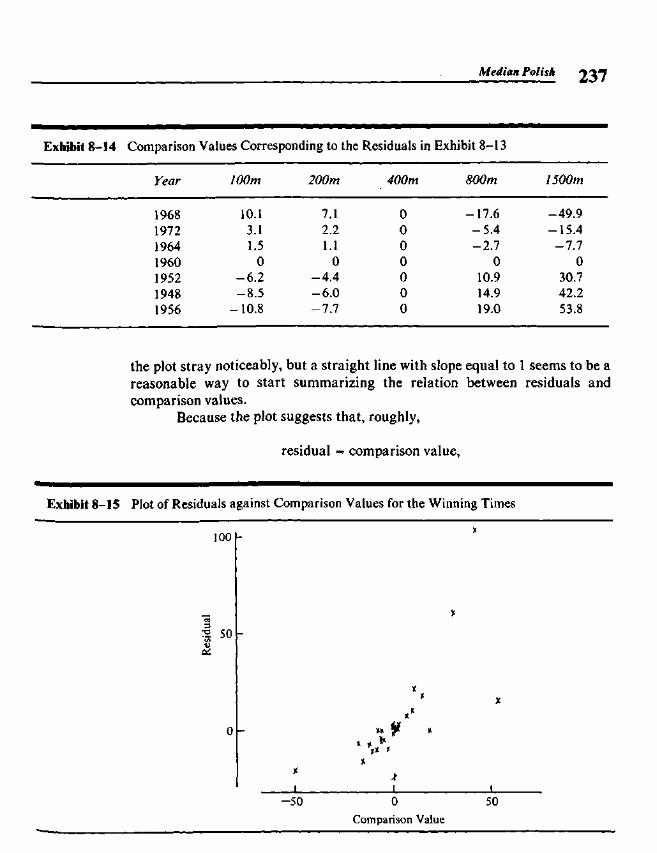
Median Polish 237
Exhibit 8-14 Comparison Values Corresponding to the Residuals in Exhibit 8-13
Year 100m 200m 400m 800m 1500m
1968197219641960195219481956
10.13.11.50
-6.2-8.5-10.8
7.12.21.10
-4.4-6.0-7.7
0000000
-17.6-5.4-2.7
010.914.919.0
-49.9-15.4-7.7
030.742.253.8
the plot stray noticeably, but a straight line with slope equal to 1 seems to be areasonable way to start summarizing the relation between residuals andcomparison values.
Because the plot suggests that, roughly,
residual = comparison value,
Exhibit 8-15 Plot of Residuals against Comparison Values for the Winning Times
100 h
I 50s
»yV *
- 5 0 0
Comparison Value
50
2 3 8 ABCs °fEDA
one very simple action is possible. We could add the comparison values to ouradditive model (and subtract them from the residuals) to get a betterdescription of the data:
data,y = common + row effect, + column effect,
(row effect,) x (column effect,) . , ,4- — + residual,-,.
common
However, we usually use the line relating residuals to comparison values as aguide for selecting a re-expression instead.
The extended model (in the previous equation) including the compari-son values could be rewritten as
/ row effectA / column effectA . , ,data,, = common x 1 + x 1 + - + residual,..1 \ common / • V common /
As we noted in Section 8.1, we prefer models in which the pieces add ratherthan multiply; so we are led to try re-expressing by logarithms because
\og(a x b x c) = log(a) + log(6) + log(c).
Exhibit 8-16 shows the logs of the Olympic runs data, and Exhibit 8-17 showsthe additive model and the residuals obtained by median polish. The analysis isclearly improved; almost all the residuals are quite small. Thus we can focusmost of our attention on the fit. Because adding a constant to the logarithm ofa number is equivalent to multiplying the number by a constant, the additiveanalysis for the log re-expression is not difficult to interpret. For example, thecolumn effects indicate that the winning time for the 1500m run is typicallyabout five times that for the 400m run. (Algebraically, log( 1500m effect) =log(400m effect) + .690 = log(400m effect) + log(4.9); so the 1500m effect isroughly equal to the 400m effect times 4.9.) Beyond the fact that the columneffects increase steadily with the length of the race, the differences betweenadjacent effects are almost constant. It would seem that a doubling of racelength leads to slightly more than a doubling of time. (Because log(2) = .301,a constant effect difference of 301 for the first four races would have indicateda doubling of time.) To look further, we might plot the column effect againstthe log of the race length.
We might also plot the row effects against the year of the Olympiad.
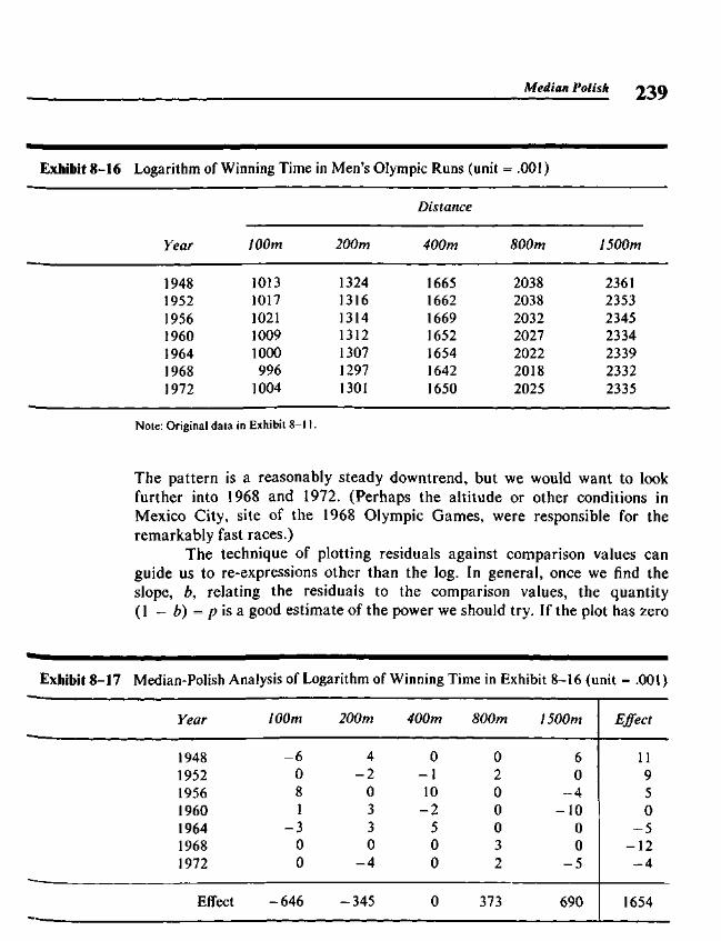
Median Polish 239
Exhibit 8-16 Logarithm of Winning Time in Men's Olympic Runs (unit = .001)
Distance
Year 100m 200m 400m 800m 1500m
1948195219561960196419681972
101310171021100910009961004
1324131613141312130712971301
1665166216691652165416421650
2038203820322027202220182025
2361235323452334233923322335
Note: Original data in Exhibit 8-11.
The pattern is a reasonably steady downtrend, but we would want to lookfurther into 1968 and 1972. (Perhaps the altitude or other conditions inMexico City, site of the 1968 Olympic Games, were responsible for theremarkably fast races.)
The technique of plotting residuals against comparison values canguide us to re-expressions other than the log. In general, once we find theslope, b, relating the residuals to the comparison values, the quantity(1 - b) = p is a good estimate of the power we should try. If the plot has zero
Exhibit 8-17 Median-Polish Analysis of Logarithm of Winning Time in Exhibit 8-16 (unit = .001)
Year
1948195219561960196419681972
Effect
100m
-6081
-300
-646
200m
4-20330
-4
-345
400m
0-110__2500
0
800m
0200032
373
1500m
60
-4-10
00
_5
690
Effect
11950
-5-12-4
1654
2 4 0 ABCs °fEDA
slope (b = 0), then p = 1, and no re-expression is needed. In our example, bwas nearly 1; sop = 0, and we chose the log. (Recall from Section 2.4 that thelog plays the role of the zero power in the ladder of powers.) In finding theslope, it is important to use judgment, as well as a technique such as theresistant line (Chapter 5), which will not be affected by the large residualsthat median polish can leave when a data value is unusual. The combinedprocess—median polish, the plot of residuals against comparison values, andthen the resistant line—makes the search for a re-expression quite resistant tooutliers.
8.6 Median Polish from the Computer
Iterative techniques such as median polish are often easier to program for acomputer than to do by hand. The programs at the end of this chapter requirethat the data table be specified in three parallel arrays: one array for data, onefor row numbers, and one for column numbers. (For a detailed description ofthis format, see Section 7.3.) These programs compute the row effects, columneffects, common term, and residuals, but they do not print out any of theseresults. The best methods for displaying the results as tables depend upon thecomputer system being used; any simple programs provided here would havehad difficulty with large tables. Nevertheless, the array of residuals returnedby the programs is in an appropriate form for the coded-table programsdiscussed in Chapter 7.
When we use the computer, we can consider analyzing more complextables. For example, the programs allow for empty cells in a table. The effectfor any row or column containing an empty cell is based on the remainingnon-empty cells. A fitted value can be found for an empty cell, but no residualcan be computed.
Although median polish is an iterative procedure, no convergencecheck to stop the iteration automatically is included. Instead, users of theprograms must specify the number of sweeps or half-steps. For data explora-tion, four half-steps seems adequate in most situations.
In addition, users must choose whether to remove medians from rowsor columns first. For some data, the final fit and residuals will differ whenthese two starts are compared. Although it is quite rare for the gross structureof the fitted models to differ in important ways, the availability of machine-
Median Polish 241
computed median polish makes it practical to find both versions and comparethem.
* 8.7 Median Polish and ANOVA
Readers who are acquainted with the two-way analysis of variance (ANOVA)will have noticed that median polish and two-way ANOVA both start with thesame data. The two-way ANOVA uses the same additive model as medianpolish, but it fits this model by finding row and column means. The differencebetween median polish and ANOVA is related to the difference between theresistant line and least-squares regression (Section 5.10). The exploratorytechniques are resistant to outliers and require iterative calculations. However,they do not as yet provide any hypothesis-testing mechanisms.
Statistically sophisticated readers may wish to compare the techniqueof Section 8.5 with Tukey's "one degree of freedom for non-additivity"(Tukey, 1949) for selecting a re-expression to improve the additivity of a table.The method given here is the natural exploratory analogue of that commonlyused technique.
* 8.8 Data Structure
We pause to note the advantages of three-array form as a data structure formedian polish. Empty cells, cells with several data values, and unbalancedtables with different numbers of data values in each cell need no specialprogramming. One restriction is that the programs assume that row numbersand column numbers are consecutive and start from 1. If a row or a column iscompletely missing, the BASIC programs give an error message, and theFORTRAN programs return a zero effect.
In addition, it is possible, through suitable bookkeeping in a driverprogram, to make some analyses of three-way designs—that is, tables involv-ing a response and three factors. The data structure permits a driver programto maintain three arrays of subscripts—say, row, column, and layer—and pass
2 4 2 ABCs °fEDA
any pair of these arrays to the median-polish program along with the data.This will produce an analysis of the subtable formed by collapsing the tablealong the un-passed dimension. In this way the "main effects" can becomputed easily. (A more sophisticated driver program could use the median-polish routine to fit more complicated models to three- and more-than-three-way tables.)
t 8.9 Algorithms
The programs work by stepping through rows or columns and copying them toa scratch array so that the median can by found. The subscripts of cells fromwhich data values have been taken are preserved so that the newly found rowor column median can be subtracted from these cells efficiently. On exit, theresidual vector is in exactly the same order as the original data vector and usesthe same row and column subscripts. (In the BASIC programs the residualsreplace the data vector.)
Comparison values are placed in a vector exactly parallel to, and usingthe same row and column subscripts as, the data and residuals. This arrange-ment allows the vector of comparison values and the vector of residuals to bepassed as a set of (x, y) pairs to the x-y plot program or to the resistant-lineprogram without having to tell those programs about the subscript arrays.
FORTRAN
The FORTRAN programs for median polish are invoked with theFORTRAN statement
CALL MEDPOL(Y, RSUB, CSUB, N, NR, NC, G, RE, CE, RESID, HSTEPS, START,SORTY, SUBSAV, NS, ERR)
where
Y() the data array containing N items;RSUB(), CSUB() integer arrays containing the N row and
column subscripts, respectively, of eachelement of Y();
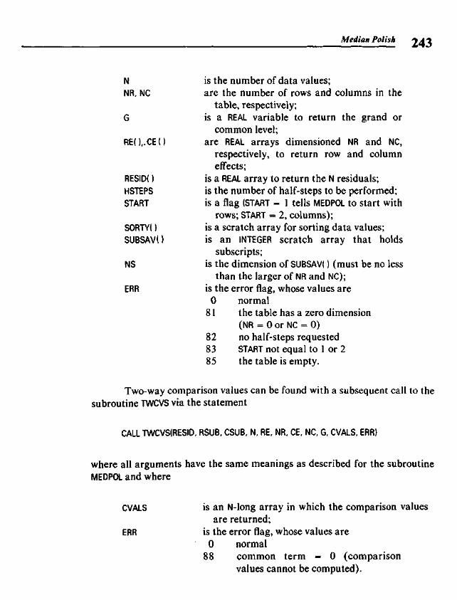
Median Polish 243
NNR, NC
G
RE(),XE(
RESID()HSTEPSSTART
SORTY()SUBSAV(
NS
ERR
is the number of data values;are the number of rows and columns in the
table, respectively;is a REAL variable to return the grand or
common level;are REAL arrays dimensioned NR and NC,
respectively, to return row and columneffects;
is a REAL array to return the N residuals;is the number of half-steps to be performed;is a flag (START = 1 tells MEDPOL to start with
rows; START = 2, columns);is a scratch array for sorting data values;is an INTEGER scratch array that holds
subscripts;is the dimension of SUBSAV() (must be no less
than the larger of NR and NC);is the error flag, whose values are
0 normal81 the table has a zero dimension
(NR = 0 or NC = 0)82 no half-steps requested83 START not equal to 1 or 285 the table is empty.
Two-way comparison values can be found with a subsequent call to thesubroutine TWCVS via the statement
CALL TWCVS(RESID, RSUB, CSUB, N, RE, NR, CE, NC, G, CVALS, ERR)
where all arguments have the same meanings as described for the subroutineMEDPOL and where
CVALS
ERR
is an N-long array in which the comparison valuesare returned;
is the error flag, whose values are0 normal
88 common term = 0 (comparisonvalues cannot be computed).
2 4 4 ABCs °fEDA
BASIC
The BASIC program for median polish is entered with the data in Y() and rowand column subscripts in R() and C(), respectively. On entry, N is the length ofY(), R9 is the number of rows, C9 is the number of columns, and J9 is thenumber of half-steps to be computed. The version number, V1, has thefollowing effects: V1 = 1 means skip initialization and continue polishing analready polished table, V1 = 2 means initialize and do 4 half-steps startingwith rows, V1 >: 3 means initialize and do J9 half-steps starting according tothe order switch. The order switch, 0$, must be set to "ROW" to start theiteration with rows and to "COL" to start the iteration with columns.
On return, Y(1) through Y(N) hold residuals, Y(R8 + 1) through Y(R8 + R9)hold row effects, Y(C8 + 1) through Y(C8 + C9) hold column effects and Y(G8)holds the common or grand effect. The program sets C8 = N, R8 = N + C9, andG8 = N + R9 + C9 + 1. In addition, the subscripts in R() and C() are extended toindicate that the column effects are in the R9 + 1 row, and the row effects arein the C9 + 1 column. A program (not provided here) to print a table from Y(),R(), and C() would then place the effects correctly. Placing the effects in a newrow and a new column of the data vector is also appropriate for generalizingthe program to handle three- or four-way tables.
Reference
Tukey, J.W. 1949. "One Degree of Freedom for Non-additivity." Biometrics 5:232-242.
Proceed.
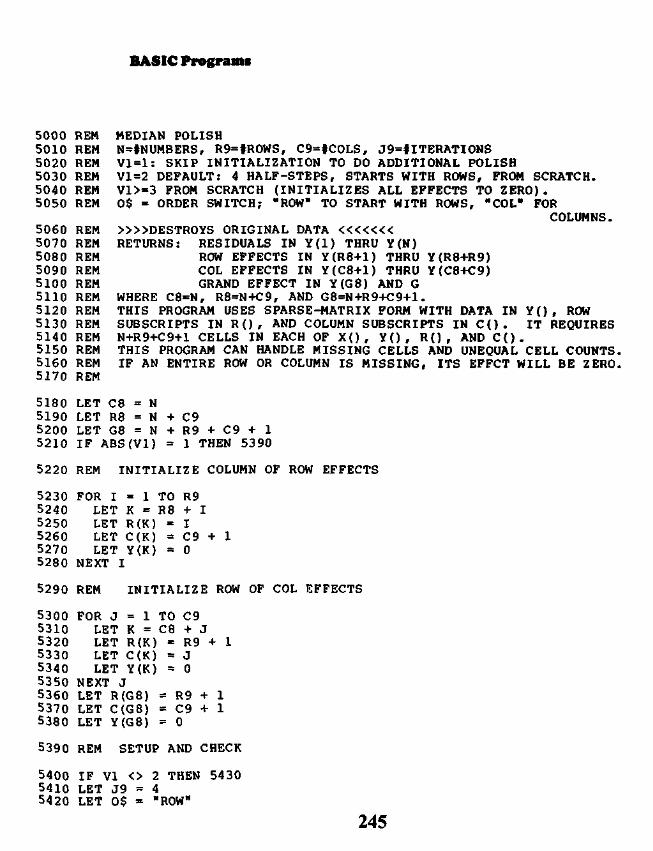
BASIC Programs
5000 REM MEDIAN POLISH5010 REM N=#NUMBERSf R9=#ROWS, C9=#COLS, J9=#ITERATIONS5020 REM Vl=l: SKIP INITIALIZATION TO DO ADDITIONAL POLISH5030 REM Vl=2 DEFAULT: 4 HALF-STEPS, STARTS WITH ROWS, FROM SCRATCH.5040 REM Vl>=3 FROM SCRATCH (INITIALIZES ALL EFFECTS TO ZERO).5050 REM O$ = ORDER SWITCH; "ROW" TO START WITH ROWS, "COL" FOR
COLUMNS.5060 REM >>>>DESTROYS ORIGINAL DATA <<<<<<<5070 REM RETURNS: RESIDUALS IN Y(l) THRU Y(N)5080 REM ROW EFFECTS IN Y(R8+1) THRU Y(R8+R9)5090 REM COL EFFECTS IN Y(C8+1) THRU Y(C8+C9)5100 REM GRAND EFFECT IN Y(G8) AND G5110 REM WHERE C8=N, R8=N+C9, AND G8=N+R9+C9+1.5120 REM THIS PROGRAM USES SPARSE-MATRIX FORM WITH DATA IN Y(), ROW5130 REM SUBSCRIPTS IN R(), AND COLUMN SUBSCRIPTS IN C(). IT REQUIRES5140 REM N+R9+C9+1 CELLS IN EACH OF X(), Y(), R(), AND C().5150 REM THIS PROGRAM CAN HANDLE MISSING CELLS AND UNEQUAL CELL COUNTS.5160 REM IF AN ENTIRE ROW OR COLUMN IS MISSING, ITS EFFCT WILL BE ZERO.5170 REM
5180 LET C8 = N5190 LET R8 = N + C95200 LET G8 = N + R9 + C9 + 15210 IF ABS(Vl) = 1 THEN 5390
5220 REM INITIALIZE COLUMN OF ROW EFFECTS
5230 FOR I = 1 TO R95240 LET K = R8 + I5250 LET R(K) = I5260 LET C(K) = C9 + 15270 LET Y(K) = 05280 NEXT I
5290 REM INITIALIZE ROW OF COL EFFECTS
5300 FOR J = 1 TO C95310 LET K = C8 + J5320 LET R(K) = R9 + 15330 LET C(K) = J5340 LET Y(K) = 05350 NEXT J5360 LET R(G8) = R9 + 15370 LET C(G8) = C9 + 15380 LET Y(G8) = 0
5390 REM SETUP AND CHECK
5400 IF VI <> 2 THEN 54305410 LET J9 = 45420 LET 0$ = "ROW"
245
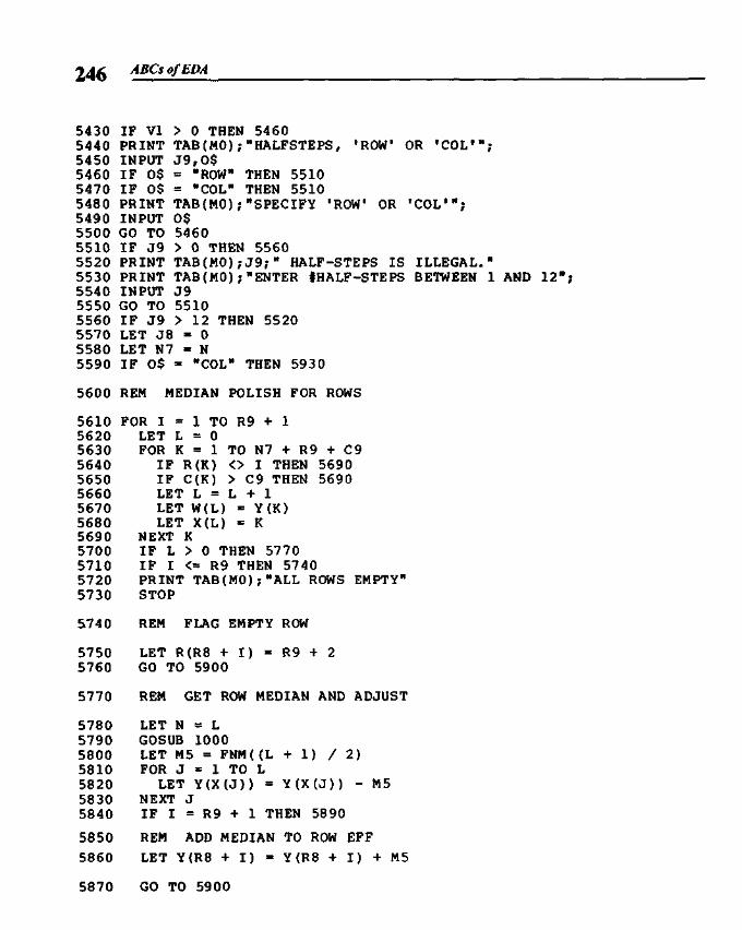
246 ABCs of EDA
5430 IF VI > 0 THEN 54605440 PRINT TAB(MO);"HALFSTEPS, "ROW1 OR 'COL1";5450 INPUT J9,O$5460 IF 0$ = "ROW" THEN 55105470 IF 0$ = "COL" THEN 55105480 PRINT TAB(MO);"SPECIFY 'ROW1 OR 'COL'";5490 INPUT 0$5500 GO TO 54605510 IF J9 > 0 THEN 55605520 PRINT TAB(M0);J9;" HALF-STEPS IS ILLEGAL."5530 PRINT TAB(MO);"ENTER #HALF-STEPS BETWEEN 1 AND 12";5540 INPUT J95550 GO TO 55105560 IF J9 > 12 THEN 55205570 LET J8 = 05580 LET N7 = N5590 IF 0$ = "COL" THEN 5930
5600 REM MEDIAN POLISH FOR ROWS
5610 FOR I = 1 TO R9 + 15620 LET L = 05630 FOR K = 1 TO N7 + R9 + C95640 IF R(K) <> I THEN 56905650 IF C(K) > C9 THEN 56905660 LET L = L + 15670 LET W(L) = Y(K)5680 LET X(L) = K5690 NEXT K5700 IF L > 0 THEN 57705710 IF I <= R9 THEN 57405720 PRINT TAB(M0);"ALL ROWS EMPTY"5730 STOP
5740 REM FLAG EMPTY ROW
5750 LET R(R8 + I) = R9 + 25760 GO TO 5900
5770 REM GET ROW MEDIAN AND ADJUST
5780 LET N = L5790 GOSUB 10005800 LET M5 = FNM((L + 1 ) / 2)5810 FOR J = 1 TO L5820 LET Y(X(J)) = Y(X(J)) - M55830 NEXT J5840 IF I = R9 + 1 THEN 5890
5850 REM ADD MEDIAN TO ROW EFF
5860 LET Y(R8 + 1 ) = Y(R8 + I) + M5
5870 GO TO 5900
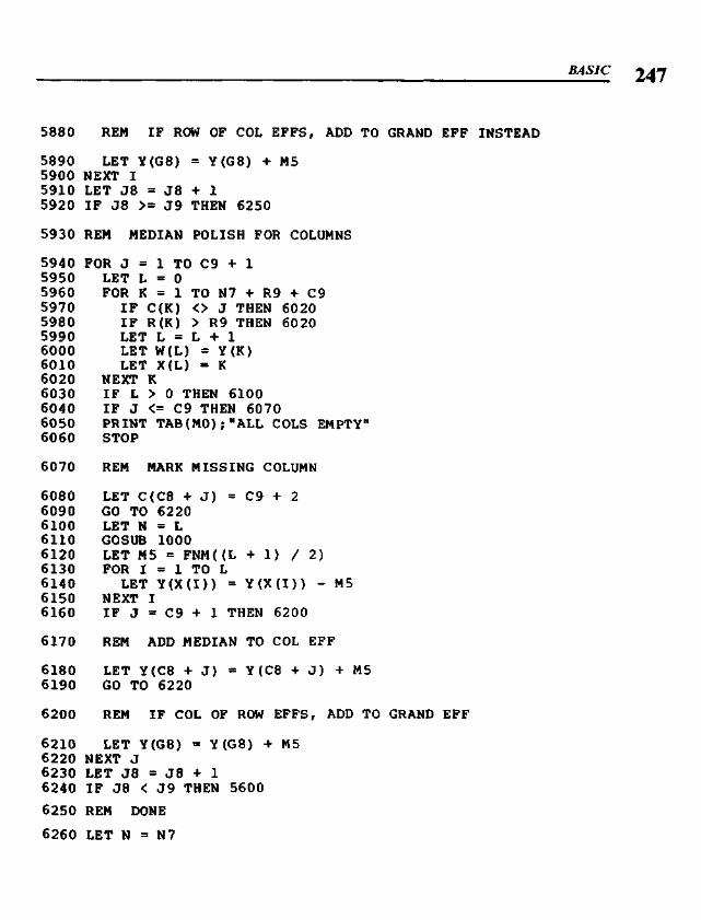
BASIC 247
5880 REM IF ROW OF COL EFFSr ADD TO GRAND EFF INSTEAD
5890 LET Y(G8) = Y(G8) + M55900 NEXT I5910 LET J8 = J8 + 15920 IF J8 >= J9 THEN 6250
5930 REM MEDIAN POLISH FOR COLUMNS
5940 FOR J = 1 TO C9 + 15950 LET L = 05960 FOR K = 1 TO N7 + R9 + C95970 IF C(K) <> J THEN 60205980 IF R(K) > R9 THEN 60205990 LET L = L + 16000 LET W(L) = Y(K)6010 LET X(L) = K6020 NEXT K6030 IF L > 0 THEN 61006040 IF J <= C9 THEN 60706050 PRINT TAB(MO);"ALL COLS EMPTY"6060 STOP
6070 REM MARK MISSING COLUMN
6080 LET C(C8 + J) = C9 + 26090 GO TO 62206100 LET N = L6110 GOSUB 10006120 LET M5 = FNM((L +1) / 2)6130 FOR I = 1 TO L6140 LET Y(X(I)) = Y(X(I)) - M56150 NEXT I6160 IF J = C9 + 1 THEN 6200
6170 REM ADD MEDIAN TO COL EFF
6180 LET Y(C8 + J) = Y(C8 + J) + M56190 GO TO 6220
6200 REM IF COL OF ROW EFFS, ADD TO GRAND EFF
6210 LET Y(G8) = Y(G8) + M56220 NEXT J6230 LET J8 = J8 + 16240 IF J8 < J9 THEN 5600
6250 REM DONE
6260 LET N = N7
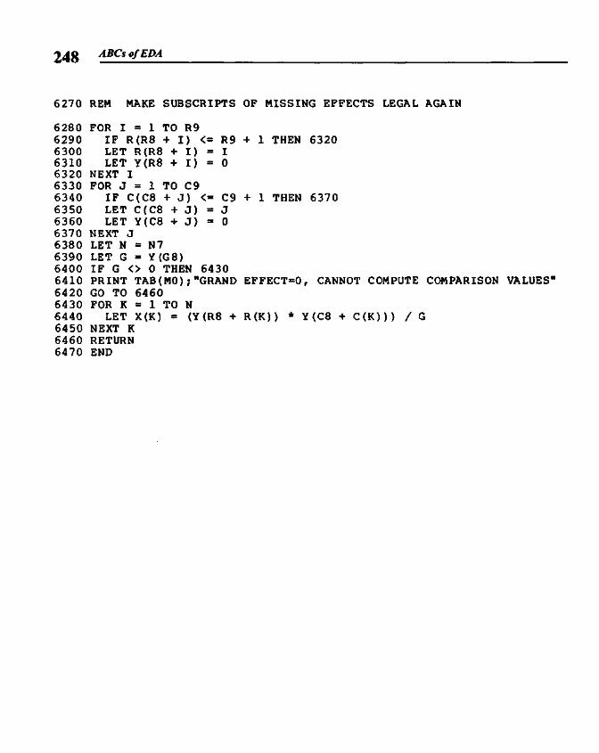
2 4 8 ABCs °fEDA
6270 REM MAKE SUBSCRIPTS OF MISSING EFFECTS LEGAL AGAIN
6280 FOR I = 1 TO R96290 IF R(R8 +1) <= R9 + 1 THEN 63206300 LET R(R8 + I) = I6310 LET Y(R8 + I) = 06320 NEXT I6330 FOR J = 1 TO C96340 IF C(C8 + J) <= C9 + 1 THEN 63706350 LET C(C8 + J) = J6360 LET Y(C8 + J) = 06370 NEXT J6380 LET N = N76390 LET G = Y(G8)6400 IF G <> 0 THEN 64306410 PRINT TAB(M0);"GRAND EFFECT=0, CANNOT COMPUTE COMPARISON VALUES"6420 GO TO 64606430 FOR K = 1 TO N6440 LET X(K) = (Y(R8 + R(K)) * Y(C8 + C(K))) / G6450 NEXT K6460 RETURN6470 END
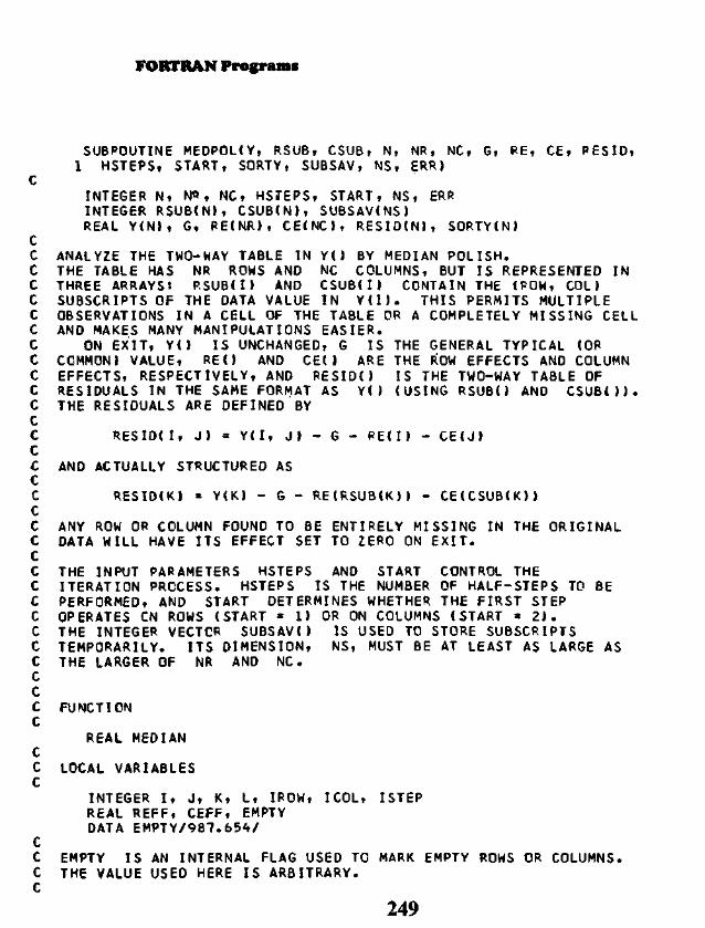
FORTRAN Programs
SUBROUTINE MEDPOL(Y, RSUB, CSUB, N , NR, NC, G t P E , CEt P E S I D ,1 HSTEPSt START, SORTY, SUBSAV, N S , ERR)
CINTEGER Nt NP , N C , HSTEPS, START, N S , ERRINTEGER R S U B ( N ) , C S U B ( N ) , SUBSAV(NS)REAL Y ( N ) t G , P E ( N R ) , C E ( N C ) , R E S I O ( N ) , SORTY(N)
CC ANALYZE THE TWO-WAY TABLE IN Y() BY MEDIAN POLISH.C THE TABLE HAS NR ROWS AND NC COLUMNS, BUT IS REPRESENTED INC THREE ARRAYS: PSUB(I) AND CSUB(I) CONTAIN THE (ROW, COL)C SUBSCRIPTS OF THE DATA VALUE IN Y d ) . THIS PERMITS MULTIPLEC OBSERVATIONS IN A CELL OF THE TABLE OR A COMPLETELY MISSING CELLC AND MAKES MANY MANIPULATIONS EASIER.C ON EXIT, Y() IS UNCHANGED, G IS THE GENERAL TYPICAL (OPC CCMMON) VALUE, REO AND CE( ) ARE THE ROW EFFECTS AND COLUMNC EFFECTS, RESPECTIVELY, AND RESIDO IS THE TWO-WAY TABLE OFC RESIDUALS IN THE SAME FORMAT AS Y( ) (USING RSUBO AND CSUBCM.C THE RESIDUALS ARE DEFINED BYCC RESIDCI, J) = Yd, J) - G - PE(I) - CE(J)CC AND ACTUALLY STRUCTURED ASCC RESID(K) - Y(K) - G - REIRSUBCKM - CE(CSUBCK))CC ANY ROW OR COLUMN FOUND TO BE ENTIRELY MISSING IN THE ORIGINALC DATA WILL HAVE ITS EFFECT SET TO ZERO ON EXIT.CC THE INPUT PARAMETERS HSTEPS AND START CONTROL THEC ITERATION PROCESS. HSTEPS IS THE NUMBER OF HALF-STEPS TO BEC PERFORMED, AND START DETERMINES WHETHER THE FIRST STEPC OPERATES CN ROWS (START = 1) OR ON COLUMNS (START = 2).C THE INTEGER VECTOR SUBSAVO IS USED TO STORE SUBSCRIPTSC TEMPORARILY. ITS DIMENSION, NS, MUST BE AT LEAST AS LARGE ASC THE LARGER OF NR AND NC.CCC FUNCTIONC
REAL MEDIANCC LOCAL VARIABLESC
INTEGER If J, K, L, IPOW, ICOL, ISTEPREAL REFF, CEFF, EMPTYDATA EMPTY/987.654/
CC EMPTY IS AN INTERNAL FLAG USED TO MARK EMPTY ROWS OR COLUMNS.C THE VALUE USED HERE IS ARBITRARY.C
249
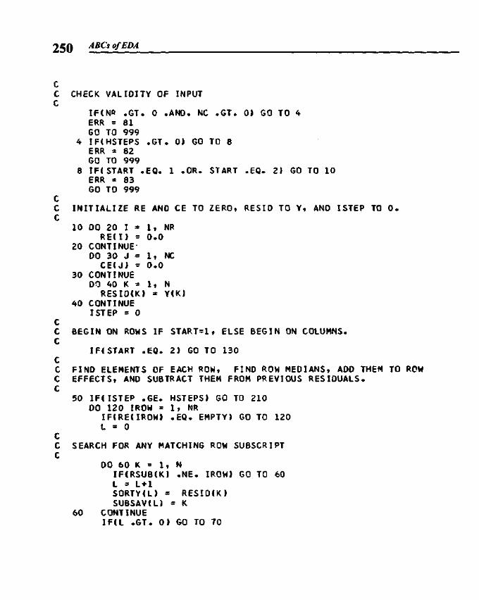
250
cC CHECK VALIDITY OF INPUTC
IFCNR .GT. 0 .AND. NC . G T . 0) GO TO 4ERR = 81GO TO 999
4 IFtHSTEPS . G T . 0) GO TO 8ERR = 82GO TO 999
8 IF(START .EQ. 1 .OR. START .EQ. 2) GO TO 10ERR * 83GO TO 999
CC I N I T I A L I Z E RE AND CE TO ZERO, RESID TO Y, AND ISTEP TO 0 .C
10 00 20 I > I t NRRE(I) - 0 . 0
20 CONTINUEDO 30 J * 1 , NC
CE(J ) = 0 . 030 CONTINUE
DO 40 K = I t NRESID(K) = Y(K)
40 CONTINUEISTEP = 0
CC BEGIN ON ROWS IF START=1, ELSE BEGIN ON COLUMNS.C
IF(START .EQ. 2 ) GO TO 130CC FIND ELEMENTS OF EACH ROW, FIND ROW MEDIANS, ADD THEM TO ROWC EFFECTS, AND SUBTRACT THEM FROM PREVIOUS RESIDUALS.C
50 IF(ISTEP .GE. HSTEPS) GO TO 210DO 120 IROW = I* NR
IF(RECIROW) .EQ. EMPTY) GO TO 120L - 0
CC SEARCH FOR ANY MATCHING ROW SUBSCRIPTC
DO 60 K * 1» NIFCRSUBCK) .NE. IROW) GO TO 60L = L + lSORTY(L) = RESID(K)SUBSAV(L) = K
60 CONTINUEIF(L .GT. 0) GO TO 70
FORTRAN 251
cC NO DATA IN THIS ROW, MARK THE ROW EMPTY TO AVOID FUTURE SEARCHESC
RE(IROW) = EMPTYGO TO 120
70 I F ( L . G T . 1 ) GO TO 80REFF = SOPTY<1)GO TO 100
80 I F ( L .EQ. 2 ) GO TO 90CALL SORT(SCRTY, L, ERR)IFCERR . N E . 0) GO TO 999
90 REFF = MEDIAN(SORTY, L)CC ADJUST FOR ROW EFFECT NOW IN REFFC
100 RE(IROW) = REUROW) + PEFFDO 110 I * 1 * L
J - SUBSAV(I)RESID(J) * RESID(J) - REFF
110 CONTINUE120 CONTINUE
ISTEP - ISTEP • 1CC FIND ELEMENTS OF EACH COLUMN, FIND COLUMN MEDIANS, ADD THEM TOC COLUMN EFFECTS, AND SUBTRACT THEM FROM PREVIOUS RESIDUALS.C
130 IF(ISTEP .GE. HSTEPS) GO TO 210DO 200 ICOL = 1, NC
IF(CECICOL) .EQ. EMPTY) GO TO 200L = 0
CC SEARCH FOR ANY MATCHING COLUMN SUBSCRIPTC
DO 140 K ' If NIF(CSUB(K) .NE. ICOL) GO TO 140L = L + lSORTY(L) = RESID(K)SUBSAV(L) - K
140 CONTINUEIF(L .GT. 0) GO TO 150
CC NO DATA IN THIS COLUMN, MARK IT EMPTY TO AVOID FUTURE SEARCHESC
CE(ICOL) = EMPTYGO TO 200
150 I F ( L .GT . 1 ) GO TO 160CEFF = SORTY(l)GO TO 180
160 I F ( L .EQ. 2 ) GO TO 170CALL SORT(SORTY, L, ERR)IFCERR . N E . 0 ) GO TO 999
170 CEFF = MEDIANCSORTY, L)
2 5 2 ABCs °fEDA
cC ADJUST FOR COLUMN EFFECT NOW IN CEFF.C
180 CE(ICOL) = CE(ICOL) + CEFFDO 190 I = 1, L
J = SUBSAV(I)RESID(J) = RESID(J) - CEFF
190 CONTINUE200 CONTINUE
ISTEP = ISTEP+1GO TO 50
CC NOW CENTER ROW EFFECTS AND COLUMN EFFECTS TO HAVE MEDIAN ZERO,C AND COMBINE THE CONTRIBUTIONS TO THE COMMON VALUE.C
210 L - 0DO 220 I = 1, NR
IF(REd) .EQ. EMPTY) GO TO 220L = L+lSOPTY(L) = RE(I)
220 CONTINUEIF(L .NE. 0) GO TO 230ERR = 85GO TO 999
2 30 CALL SORT(SORTY, L, ERR)IFCERR .NE. 0) GO TO 999G = MEDIANCSORTY, L)DO 240 I = It NR
IF(RECI) .NE. EMPTY) RE(I) = RE(I) - GCC RETURN ZERO FOR EFFECT OF EMPTY ROWC
IF(REU) .EQ. EMPTY) RE(I) = 0.0240 CONTINUE
L - 0DO 250 J = 1, NC
IF(CE(J) .EQ. EMPTY) GO TO 250L = L+lSORTY(L) * CE(J)
250 CONTINUEIF(L .NE. 0) GO TO 260ERR - 85GO TO 999
260 CALL SORTCSORTY, L, ERR)IF(ERR .NE. 0) GO TO 999CEFF = MEDIAN(SORTY, L)G = G+CEFFDO 270 J - 1, NC
IFCCECJ) .NE. EMPTY) CE(J) = CE(J) - CEFF
FORTRAN 253
cC RETURN ZERO FOR EFFECT OF EMPTY COLSC
I F ( C E U ) .EQ. EMPTY) CE(J) = 0 . 0270 CONTINUE
C999 RETURN
END
SUBROUTINE TWCVS(RSUB, CSUB, N, RE, NR, CE, NC, G, CVALS,1 ERR)
CINTEGER NR, NC, N, ERRINTEGER RSUB(N), CSUB(N)REAL RE(NR) , CE(NC) , G, CVALS(N)
CC CALCULATES THE COMPARISON VALUES FOR A TWO-WAYC TABLE. THE F I T ON WHICH THESE ARE BASED CONSISTS OF THEC ROW EFFECTS, R E ( 1 ) , . . . , R E ( N R ) , THE COLUMN EFFECTS,C C E ( 1 ) , . . . , C E ( N C ) , AND THE COMMON VALUE, G . BYC DEFIN IT ION, THE COMPARISON VALUE FOR CELL ( I , J ) ISCC R E ( I ) * CE(J ) / GCC CVALS() IS INDEXED BY THE ROW AND COLUMN SUBSCRIPTSC FOUND IN THE CORRESPONDING LOCATIONS IN RSUBO AND CSUBO.C THIS SUBROUTINE IDENTIFIES THE ROW AND COLUMN EFFECTS ASSOCIATEDC WITH EACH RESIDUAL AND PUTSC THE CORRESPONDING COMPARISON VALUES IN CVALSO.C
cC LOCAL VARIABLESC
INTEGER I, J, KC
IF(NR .GT. 0 .AND. NC .GT. 0) GO TO 10ERR = 81GO TO 999
10 IF(G .NE. 0.0) GO TO 30ERR = 88GO TO 999
C30 DO 50 K = 1,N
I = RSUB(K)J = CSUB(K)CVALS(K) = RE(I) * CE(J) / G
50 CONTINUE999 RETURN
END

Chapter 9Rootograms
Batches of data are sometimes recorded by splitting the range of possiblebins values into intervals, or bins, and simply counting the data values that fall into
each bin. In a large batch, lack of room to construct a stem-and-leaf displaywould lead us to use bins. If we had 500 data values, we would usually recordhow many values fall on each line of the display instead of showing a leaf foreach data value.
Some variables almost always take this form. For example, ages ofadults seldom appear in more detail than the year (for most purposes five-yearor ten-year intervals are standard), so it is common to report age data ascounts of people at each age or in each age category. When the individual datavalue is a count—especially a small count—there are often many repeatedvalues, and it is easiest to record the number of times each possible valueoccurs. For example, from data on the number of traffic tickets that individualdrivers received in one year, we would record how many drivers received zerotickets, how many received one ticket, and so on.
This chapter shows how to display such batches effectively, how tocompare them to standard shapes, and what residuals to calculate in thesecomparisons. The exploratory techniques are known as the rootogram—forbasic display—and the suspended rootogram—for comparisons and residu-als.
255
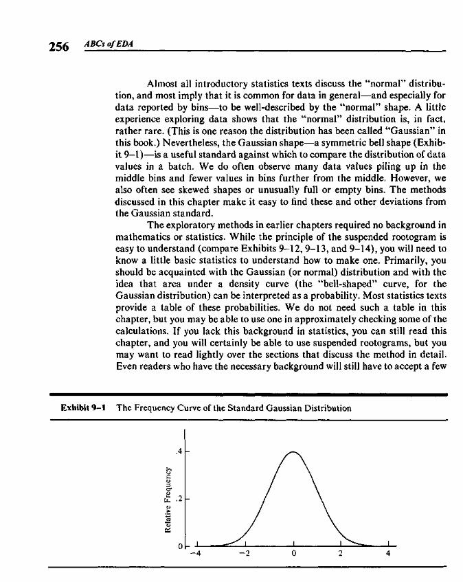
2 5 5 ABCs °fEDA
Almost all introductory statistics texts discuss the "normal" distribu-tion, and most imply that it is common for data in general—and especially fordata reported by bins—to be well-described by the "normal" shape. A littleexperience exploring data shows that the "normal" distribution is, in fact,rather rare. (This is one reason the distribution has been called "Gaussian" inthis book.) Nevertheless, the Gaussian shape—a symmetric bell shape (Exhib-it 9-1)—is a useful standard against which to compare the distribution of datavalues in a batch. We do often observe many data values piling up in themiddle bins and fewer values in bins further from the middle. However, wealso often see skewed shapes or unusually full or empty bins. The methodsdiscussed in this chapter make it easy to find these and other deviations fromthe Gaussian standard.
The exploratory methods in earlier chapters required no background inmathematics or statistics. While the principle of the suspended rootogram iseasy to understand (compare Exhibits 9-12, 9-13, and 9-14), you will need toknow a little basic statistics to understand how to make one. Primarily, youshould be acquainted with the Gaussian (or normal) distribution and with theidea that area under a density curve (the "bell-shaped" curve, for theGaussian distribution) can be interpreted as a probability. Most statistics textsprovide a table of these probabilities. We do not need such a table in thischapter, but you may be able to use one in approximately checking some of thecalculations. If you lack this background in statistics, you can still read thischapter, and you will certainly be able to use suspended rootograms, but youmay want to read lightly over the sections that discuss the method in detail.Even readers who have the necessary background will still have to accept a few
Exhibit 9-1 The Frequency Curve of the Standard Gaussian Distribution
.4
0\-- 4 - 2
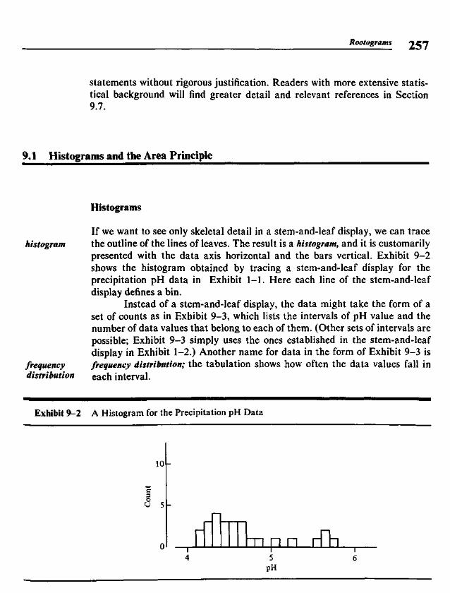
Rootograms
statements without rigorous justification. Readers with more extensive statis-tical background will find greater detail and relevant references in Section9.7.
9.1 Histograms and the Area Principle
histogram
frequencydistribution
Histograms
If we want to see only skeletal detail in a stem-and-leaf display, we can tracethe outline of the lines of leaves. The result is a histogram, and it is customarilypresented with the data axis horizontal and the bars vertical. Exhibit 9-2shows the histogram obtained by tracing a stem-and-leaf display for theprecipitation pH data in Exhibit 1-1. Here each line of the stem-and-leafdisplay defines a bin.
Instead of a stem-and-leaf display, the data might take the form of aset of counts as in Exhibit 9-3, which lists the intervals of pH value and thenumber of data values that belong to each of them. (Other sets of intervals arepossible; Exhibit 9-3 simply uses the ones established in the stem-and-leafdisplay in Exhibit 1-2.) Another name for data in the form of Exhibit 9-3 isfrequency distribution; the tabulation shows how often the data values fall ineach interval.
Exhibit 9-2 A Histogram for the Precipitation pH Data
10
If n jfb.5
pH
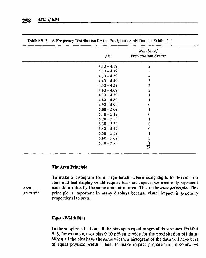
2 5 8 ABCs °fEDA
Exhibit 9-3 A Frequency Distribution for the Precipitation pH Data of Exhibit 1-1
pHNumber of
Precipitation Events
4.10-4.194.20-4.294.30-4.394.40 - 4.494.50-4.594.60-4.694.70-4.794.80-4.894.90-4.995.00-5.095.10-5.195.20-5.295.30-5.395.40-5.495.50-5.595.60-5.695.70-5.79
23433311010100121
26
areaprinciple
The Area Principle
To make a histogram for a large batch, where using digits for leaves in astem-and-leaf display would require too much space, we need only representeach data value by the same amount of area. This is the area principle. Thisprinciple is important in many displays because visual impact is generallyproportional to area.
Equal-Width Bins
In the simplest situation, all the bins span equal ranges of data values. Exhibit9-3, for example, uses bins 0.10 pH-units wide for the precipitation pH data.When all the bins have the same width, a histogram of the data will have barsof equal physical width. Then, to make impact proportional to count, we
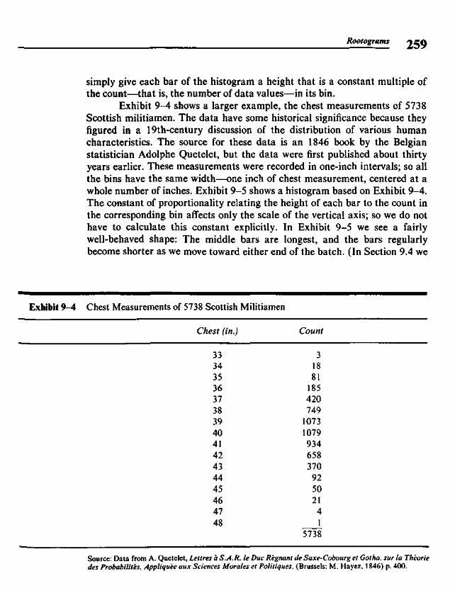
Rootograms
simply give each bar of the histogram a height that is a constant multiple ofthe count—that is, the number of data values—in its bin.
Exhibit 9-4 shows a larger example, the chest measurements of 5738Scottish militiamen. The data have some historical significance because theyfigured in a 19th-century discussion of the distribution of various humancharacteristics. The source for these data is an 1846 book by the Belgianstatistician Adolphe Quetelet, but the data were first published about thirtyyears earlier. These measurements were recorded in one-inch intervals; so allthe bins have the same width—one inch of chest measurement, centered at awhole number of inches. Exhibit 9-5 shows a histogram based on Exhibit 9-4.The constant of proportionality relating the height of each bar to the count inthe corresponding bin affects only the scale of the vertical axis; so we do nothave to calculate this constant explicitly. In Exhibit 9-5 we see a fairlywell-behaved shape: The middle bars are longest, and the bars regularlybecome shorter as we move toward either end of the batch. (In Section 9.4 we
Exhibit 9-4 Chest Measurements of 5738 Scottish Militiamen
Chest (in.) Count
33 3
34 1835 8136 18537 42038 74939 107340 107941 93442 65843 37044 9245 5046 2147 448 1_
5738
Source: Data from A. Quetelet, Lettres a S.A.R. le Due Regnant de Saxe-Cobourg et Gotha, sur la Theoriedes Probabilites, Appliquee aux Sciences Morales et Politiques. (Brussels: M. Hayez, 1846) p. 400.
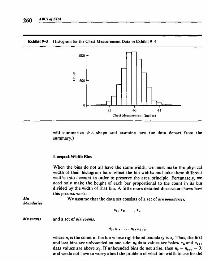
ABCs of EDA
Exhibit 9-5 Histogram for the Chest Measurement Data in Exhibit 9-4
1000 -
ou 500
0 - I40 45
Chest Measurement (inches)
will summarize this shape and examine how the data depart from thesummary.)
binboundaries
Unequal-Width Bins
When the bins do not all have the same width, we must make the physicalwidth of their histogram bars reflect the bin widths and take these differentwidths into account in order to preserve the area principle. Fortunately, weneed only make the height of each bar proportional to the count in its bindivided by the width of that bin. A little more detailed discussion shows howthis process works.
We assume that the data set consists of a set of bin boundaries,
bin counts and a set of bin counts,
nk->
where n{ is the count in the bin whose right-hand boundary is xt. Thus, the firstand last bins are unbounded on one side: nQ data values are below x0 and nk+\data values are above xk. If unbounded bins do not arise, then n0 = nk+l = 0,and we do not have to worry about the problem of what bin width to use for the
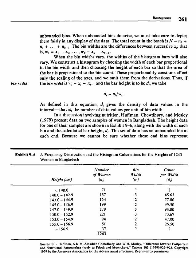
Rootograms
bin width
unbounded bins. When unbounded bins do arise, we must take care to depictthem fairly in any display of the data. The total count in the batch is N = n0 +«, + . . . + nk+l. The bin widths are the differences between successive x,; thatis, w, = x, - x0,. . ., wk = xk - xk_x.
When the bin widths vary, the widths of the histogram bars will alsovary. We construct a histogram by choosing the width of each bar proportionalto the bin width and then choosing the height of each bar so that the area ofthe bar is proportional to the bin count. These proportionality constants affectonly the scaling of the axes, and we omit them from the derivations. Thus, ifthe bin width is u>, = xt — x^x and the bar height is to be dh we take
t = n,/wt.
theAs defined in this equation, dt gives the density of data values ininterval—that is, the number of data values per unit of bin width.
In a discussion involving nutrition, Huffman, Chowdhury, and Mosley(1979) present data on two samples of women in Bangladesh. The height datafor one of their samples are shown in Exhibit 9-6, along with the width of eachbin and the calculated bar height, dt. This set of data has an unbounded bin ateach end. Because we cannot be sure whether these end bins represent
Exhibit 9-6 A Frequency Distribution and the Histogram Calculations for the Heights of 1243Women in Bangladesh
Height (cm)
Numberof Women
BinWidth
Countper Width
< 140.0140.0-142.9143.0- 144.9145.0-146.9147.0-149.9150.0-152.9153.0-154.9155.0-156.9
> 156.9
71137154199279221945137
9
3223322?
9
45.6777.0099.5093.0073.6747.0025.507
1243
Source: S.L. Huffman, A.K.M. Alauddin Chowdhury, and W.H. Mosley, "Difference between Postpartumand Nutritional Amenorrhea (reply to Frisch and McArthur)," Science 203 (1979):922-923. Copyright1979 by the American Association for the Advancement of Science. Reprinted by permission.
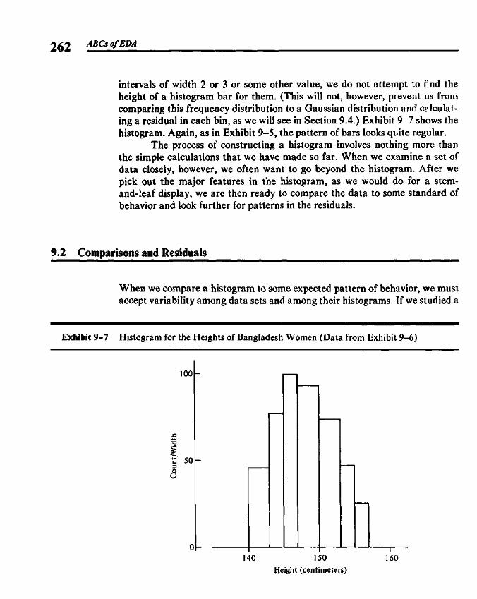
262 ABCs °fEDA
intervals of width 2 or 3 or some other value, we do not attempt to find theheight of a histogram bar for them. (This will not, however, prevent us fromcomparing this frequency distribution to a Gaussian distribution and calculat-ing a residual in each bin, as we will see in Section 9.4.) Exhibit 9-7 shows thehistogram. Again, as in Exhibit 9-5, the pattern of bars looks quite regular.
The process of constructing a histogram involves nothing more thanthe simple calculations that we have made so far. When we examine a set ofdata closely, however, we often want to go beyond the histogram. After wepick out the major features in the histogram, as we would do for a stem-and-leaf display, we are then ready to compare the data to some standard ofbehavior and look further for patterns in the residuals.
9.2 Comparisons and Residuals
When we compare a histogram to some expected pattern of behavior, we mustaccept variability among data sets and among their histograms. If we studied a
Exhibit 9-7 Histogram for the Heights of Bangladesh Women (Data from Exhibit 9-6)
100-
50
140 150
Height (centimeters)
I160
Rootograms *Yf%\
large number of histograms from closely related sets of data—for example,many samples of women's heights in Bangladesh—we would generally findthat bar height varies more in bins with long bars than in bins with short bars.Put in terms of the counts in the frequency distribution, the variability of thecounts increases as their typical size increases. This is hardly surprising. Acount that is typically 2 might often come out 1 or 0 or 3 or 4 in an observedfrequency distribution, but it would rarely come out 10. However, if the countis typically 100, observed values of 90 or 110 would be quite common. Thus,when we make direct comparisons and use residuals to look closer at patternsof deviation, we must take into account the fact that variability is not constantfrom one bin to another.
A re-expression can approximately remove the tendency for the vari-ability of a count to increase with its typical size. The most helpful re-expression is a familiar one: the square root. In addition to its helpful qualityof stabilizing variability, the square-root re-expression for counts has sometheoretical justifications. We consider some of these justifications in the nextsection (and in Section 9.7).
9.3 Rootograms
When we apply the square-root re-expression to a histogram, we obtain arootogram rootogram. The bin widths (u>,) have not changed; so we keep the same bar
widths as in the histogram, but we now use ^ as the height of the bar for bini. The chest measurement data of Exhibit 9-4 provide a straightforwardexample. Exhibit 9-8 gives the square-root calculations, and Exhibit 9-9shows the rootogram. In the rootogram we see a regular pattern, just as wefound in the histogram (Exhibit 9-5). When we compare Exhibits 9-5 and 9-9more closely, we find that the rootogram looks much more regular—almostinviting us to drape a curve over it—primarily because the square-rootre-expression has more impact on the longer bars in the middle than on theshorter bars toward the ends. Just as we saw in earlier chapters, a suitablere-expression can make data more regular and easier to look at.
Note that in using a rootogram we have abandoned the area princi-ple—area is no longer proportional to count. As we move from display toanalysis, and so from examining the raw data to fitting a shape and examiningthe residuals, it will be more important to stabilize the variability of fluctua-tions than to picture the raw counts directly in terms of area.
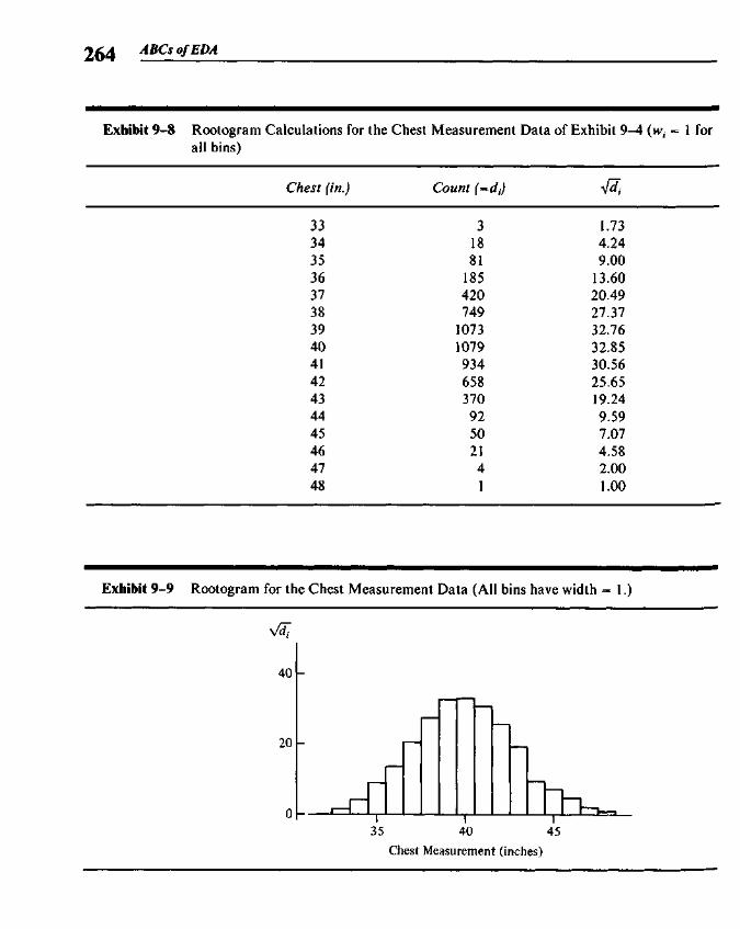
ABCs °fEDA
Exhibit 9-8 Rootogram Calculations for the Chest Measurement Data of Exhibit 9-4 (w, = 1 forall bins)
Chest (in.) Count (=dj
33343536373839404142434445464748
318811854207491073107993465837092502141
1.734.249.0013.6020.4927.3732.7632.8530.5625.6519.249.597.074.582.001.00
Exhibit 9-9 Rootogram for the Chest Measurement Data (All bins have width = 1.)
40
20
40 45
Chest Measurement (inches)
Rootograms
Double-Root Residuals
When we compare a set of observed counts to the corresponding fitted counts,we want to calculate and examine residuals. We could simply subtract fittedfrom observed, but this would do nothing to make fluctuations roughly thesame size across all bins. Therefore, we will work with both observed countsand fitted counts in a square-root scale. We can form residuals in this scale insuch a way that they behave approximately like observations from a standardGaussian distribution and hence are easy to interpret.
We could take
^observed - ^/fitted
as the residual, but a slightly different re-expression avoids some difficultieswith small counts. First we replace the observed count by
+ 4 (observed) if observed ¥=• 0
1 if observed = 0
and we replace the fitted count by
yj\ +4 (fitted).
double-root Then we define the double-root residual (DRR) as the difference between theseresidual tWo:
DRR = y/2 + 4 (observed) - ^ 1 + 4 (fitted) if observed ^ 0
1 - ^ / 1 + 4 (fitted) if observed = 0.
These square-root re-expressions have the name "double root" because theyare close to two times the usual square root. We will soon see that, as a result,the double-root residuals have an especially convenient scale.
The constants that have been added, 2 for observed and 1 for fitted,help to relieve the compression imposed on small counts by the restriction thatcounts always be greater than or equal to zero. Because fitted counts arealmost always greater than zero—although they can sometimes be smallfractions—we need not add as large a constant to fitted counts: 1 will doinstead of 2. (Section 9.7 provides some further background on double roots.)
Throughout this section we treat the fitted values as given; nothing has
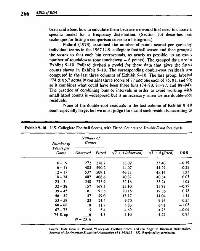
ABCs of EDA
been said about how to calculate them because we would first need to choose aspecific model for a frequency distribution. (Section 9.4 describes onetechnique for fitting a comparison curve to a histogram.)
Pollard (1973) examined the number of points scored per game byindividual teams in the 1967 U.S. collegiate football season and then groupedthe scores so that each bin corresponds, as nearly as possible, to an exactnumber of touchdowns (one touchdown = 6 points). The grouped data are inExhibit 9-10. Pollard devised a model for these data that gives the fittedcounts shown in Exhibit 9-10. The corresponding double-root residuals arecomputed in the last three columns of Exhibit 9-10. The last group, labeled"74 & up," actually contains three scores of 77 and one each of 75, 81, and 90;so it combines what could have been three bins (74-80, 81-87, and 88-94).The practice of combining bins or intervals in order to avoid working withsmall fitted counts is widespread but is unnecessary when we use double-rootresiduals.
None of the double-root residuals in the last column of Exhibit 9-10seem especially large, but we must judge the size of such residuals according to
Exhibit 9-10 U.S. Collegiate Football Scores, with
Number ofPoints per
Game
0- 56-11
12- 1718-2425-3132-3839-4546-5253-5960-6667-7374 &up
Number ofGames
Observed
2724855374072581571015723
856
7V=2316
Fitted
278.7490.2509.1406.6275.9167.393.549.024.411.75.44.3
Fitted Counts and
y]2 + 4 (observed)
33.0244.0746.3740.3732.1625.1020.1515.179.705.834.695.10
Double-Root Residuals
V/ + 4 (fitted)
33.4044.2945.1440.3433.2425.8919.3614.049.936.914.754.27
DRR
-0.39-0.22
1.230.03
-1.08-0.79
0.781.13
-0.23-1.08-0.06
0.83
Source: Data from R. Pollard, "Collegiate Football Scores and the Negative Binomial Distribution,Journal of the American Statistical Association 68 (1973):351-352. Reprinted by permission.
Rootograms
some standard. Usually (as in Chapters 5 and 8) we examine residuals as abatch to get an indication of their typical size and to identify any largeresiduals. Double-root residuals, however, come with a built-in standard ofsize. When the model fits the data well, an individual double-root residualbehaves approximately like an observation from the Gaussian (or normal)distribution with mean 0 and variance 1. Thus, nearly 95 percent of the time aDRR should be between — 1.96 and +1.96. These limits can be found from thetable of the "normal" distribution given in most statistics texts. It isconvenient to define a large DRR as one below - 2 or above +2. When thefitted count is less than 1.0, the DRR may be less like a Gaussian observation;so it may be wise to look more closely at any DRR below -1 .5 or above +1.5.
By these standards, Pollard's model fits quite well (perhaps too well):The largest DRR is 1.23. It would be interesting to fit the same model to datafrom other collegiate football seasons.
In this section we have seen that rootograms stabilize the variabilityfrom bar to bar while preserving the form of a histogram and that double-rootresiduals provide an effective numerical way to compare data with fit. We nowturn to one technique for fitting smooth curves to counts in bins.
9.4 Fitting a Gaussian Comparison Curve
When a histogram summarizes a large batch in terms of a set of bins, it iscommon practice to superimpose a smooth frequency curve on the histogram.The most common curve for this purpose is the one belonging to the Gaussiandistribution. Its standard form (mean = 0, variance = 1) is given for all valuesof z, positive and negative alike, by the mathematical function
where TT and e are common mathematical constants: TT ̂ 3.14159,e « 2.71828. A graph of this function against z follows the bell shape shown inExhibit 9-1.
To match this standard curve to a batch of data, we can slide it until itscenter matches the middle of the batch and stretch it (or compress it)uniformly until its hinges match the hinges of the batch. Because the area
ABCs of EDA
beneath/(z) is 1, we must also multiply by TV so that the curve represents thesame total count as the batch. The result is the curve
(x-m\
\ s >
whose mean, m, and standard deviation, s, can be calculated from the hingesof the data. Specifically, if HL and Hv are the lower and upper hinges, respec-tively, we take
m = y2(HL + Hv)
and
s = (Hu-HL)/1.349,
because any Gaussian distribution has its hinges at m — 0.67455 and m +0.67455 and thus has an H-spr of 2 x 0.67455 = 1.3495. We could use the datain other ways to calculate m and 5. For example, we might (as is often done)use the sample mean for m and the sample standard deviation for 5. Thehinges, however, are resistant to the ill effects of outliers and are oftenavailable in exploratory summaries such as the letter-value display. When wecannot obtain the hinges from the complete data, we may still be able toestimate them by interpolation.
Interpolated Hinges
When we must work from the bin boundaries,
and the bin counts,
as in Section 9.1, we generally do not know the hinges of the data exactly.Nevertheless, we can easily find the bins that contain the two hinges and thenestimate a value for each hinge by interpolation. From the total count, TV, we
Rootograms
know (Section 2.1) that the depth of the hinges is given by d(H) =[(N + l)/2 = l]/2. The bins at which the sums of the bin counts (the «.),summing in from each end, first exceed or equal d{H) are the bins thatcontain the hinges.
Let us suppose that the lower hinge lies in the bin whose boundaries arexL_i and xL and whose observed count is nL. Then we interpolate by treatingthe nL data values in the bin as if they were spread evenly across the width ofthe bin. More specifically, we act as if the bin is divided into nL equalsubintervals of width wL/nL, each with a data value at its center. (Recall thatwL = xL - xL_,.) Thus, the leftmost spread-out value falls at
0.5wL
the next value comes at
l.5wL
and so on. Thus if the depth of the hinge is d{H), we place the interpolatedlower hinge at
, ( ) - f a + . . . +ifc.,)-0.5XL-\ + " H>L.
nL
For the chest measurement data in Exhibit 9-4, we have TV = 5738, so
[(S739)/2 + 1]
Summing the bin counts from the low end of the frequency distribution, wefind that
«o + . . . + «5 = 0 + 3 + . . . + 420 = 707
and
1456.
27Q ABCs of EDA
Thus, because H>, = 1 for all the bins, we estimate the lower hinge as
Similarly, if the upper hinge lies in the bin whose boundaries are xv_x
and xv—that is, nu+x + . . . + nk+x < d(H) < nv + . . . + nk+x—we place theinterpolated upper hinge at
d{H) - (nu+x nk+x) - 0.5nu
w
Warning: If either hinge lies in a half-open bin—that is, to the left of x0
or to the right of xk—we will be unable to interpolate and hence unable to fitthe comparison curve from the interpolated hinges. (The computer programsin this chapter check for this unlikely possibility and indicate an errorcondition if it occurs.) Such a situation may require a re-expression of thedata.
cumulativedistributionfunction
Fitted Counts
Finally, from the fitted comparison curve, we must obtain a fitted count foreach bin. The fitted count is just the area beneath the fitted curve, (N/s) xf((x — m)/s), between the bin boundaries. We could approximate this areafairly closely by multiplying the bin width by the height of the curve at thecenter of the bin, but we would have difficulty with the half-open bins (whichcan have appreciable fitted counts even when their observed counts are zero).Thus we employ, instead, the cumulative distribution function, F, for thestandard Gaussian distribution.
The cumulative distribution function tells how much probability lies tothe left of any given value on the scale of the data. When we fit a Gaussianshape, F(z) is the amount of probability to the left of z in the standardGaussian distribution. For the fitted Gaussian comparison curve,
N x F
is the total fitted count to the left of JC,. We can thus begin with the left
Rootograms
half-open bin and calculate its fitted count, h0, from
and continue by calculating
and so on. In general,
except for the right half-open bin:
If we wish, we can sketch in the comparison curve as a background for arootogram, but we calculate double-root residuals from the nt and the ht.
The standard Gaussian cumulative function, F, has no simple formulalike that given earlier for the density function, / . Good approximations for Fare available, however, for computers or calculators. The programs at the endof this chapter use a reasonably accurate simple approximation developed byDerenzo (1977) for use on hand-held calculators: If \z\ < 5.5, f(z) isapproximated by setting v = | z |, calculating
((83v + 3Sl)v + S62)v703 + 165v
and returning
F{z) = xJip if z < 0
F(z) = 1 - >/2p i f z > 0 .
When \z\> 5.5, the FORTRAN program uses another approximation fromDerenzo, while the BASIC program sets p to zero in the preceding equation
2 7 2 ABCs of EDA
for F(z). Because \z\ > 5.5 corresponds to a probability smaller than1/10,000,000, this difference between the programs is of no practical conse-quence.
Example: Chest Measurements
To illustrate the steps in fitting a Gaussian comparison curve, we return to thechest measurement data in Exhibit 9-4. The data are repeated, and the keyresults of the fitting calculations are shown in Exhibit 9-11. Here, with TV =5738, we find the depth of the hinge: d(H) = [(5738 + l ) /2 + l ] /2 = 1435.Adding up the nt from the low end, we find that
n0 + . . . + ns = 707 < 1435 < 1456 = n0 + .. . + n6,
so that the lower hinge, HL, lies between x5 = 37.5 and x6 = 38.5. Interpolationthen gives
, d{H) - fa+ . . . +nL_j) - 0.5HL = xL_x + wL
nL
_ 3 ? s + .435 -101 - 0 , ,
= 38.471.
Similarly, summing the n{ from the high end yields
nl0 + . . . + nxl = 1196 < 1435 < 2130 = n9 + . . . + «i7,
so that the upper hinge, HUy lies between xs = 40.5 and xg = 41.5. Again,interpolation gives
d(H)-(nu+{ + ... + nk+l) - 0 . 5"u = xu ~ wu
n„ c 1435 - 1196 - 0 . 5
= 4 1 - 5 " 934
= 41.245.
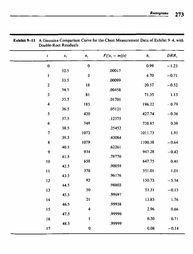
Exhibit 9-11 A Gaussian ComparisonDouble-Root Residuals
/
Curve
»,
for the
1
Chest
m, -
Measurement
- m)ls)
Data
Rootograms 273
of Exhibit 9-4, with
DRRt
0
1
2
3
4
5
6
7
8
9
10
11
12
13
14
15
16
17
32.5
33.5
34.5
35.5
36.5
37.5
38.5
39.5
40.5
41.5
42.5
43.5
44.5
45.5
46.5
47.5
48.5
0
3
18
81
185
420
749
1073
1079
934
658
370
92
50
21
4
1
0
.00017
.00099
.00458
.01701
.05121
.12575
.25452
.43084
.62261
.78770
.90059
.96176
.98803
.99697
.99938
.99990
.99999
0.99
4.70
20.57
71.35
196.22
427.74
738.85
1011.73
1100.38
947.28
647.75
351.01
150.73
51.31
13.85
2.96
0.50
0.08
-1.23
-0.71
-0.52
1.13
-0.79
-0.36
0.38
1.91
-0.64
-0.42
0.41
1.01
-5.34
-0.15
1.76
0.66
0.71
-0.14
2 7 4 ABCs °fEDA
From the hinges it is then simple to find
m = \j1{HL + Hu) = 39.858 and s = {Hv - HL)/1.349 = 2.056.
We now use the approximation for F{z) to calculate the fourth column ofExhibit 9-11, the values of F((x, - m)/s). The differences between adjacententries, multiplied by TV = 5738, are the «,-. The column of double-rootresiduals, calculated as in Section 9.3, completes the numerical work on thisexample.
The double-root residuals now tell us how closely the comparison curvefollows the data. Immediately, our attention focuses on bin 12, where DRR =-5.34. Surely something is amiss in Quetelet's data. The original source of thedata, published in 1817, gives the joint frequency distribution of height andchest measurement in each of eleven militia regiments. It has a total count of5732, and its bin counts differ by as much as 76—in bin 12, it turns out—fromthe bin counts reported by Quetelet. It seems that Quetelet made some seriouscopying errors in forming his frequency distribution, but he did not notice thediscrepancy that is so evident in Exhibit 9-11.
Except for bin 12, DRR values in Exhibit 9-11 indicate that the fit isreasonable. If we look back at the rootogram in Exhibit 9-9, we may agreethat the bar for bin 12 looks a bit low. When we fit the Gaussian comparisoncurve, however, the double-root residual makes it impossible for this isolatedproblem to escape notice. We have gained considerably by looking at the fit inthis way.
Note also that, because we used the hinges to fit the comparison curve,the one extraordinary bin—which involved a change of only about 1% of thecases—did not have an undue influence on the fit. Correcting the error wouldchange the comparison curve only slightly and thus would not alter the fit atthe other bins.
9.5 Suspended Rootograms
In the preceding sections, we concentrated on fitting a comparison curve to ourdata and on finding the proper residuals. Our approach was different from theapproaches we used for other data structures such as >>-versus-jc and two-waytables, because we fitted the comparison curve to the raw data but calculatedresiduals in the square-root scale. However, Tukey (1971) describes a way of
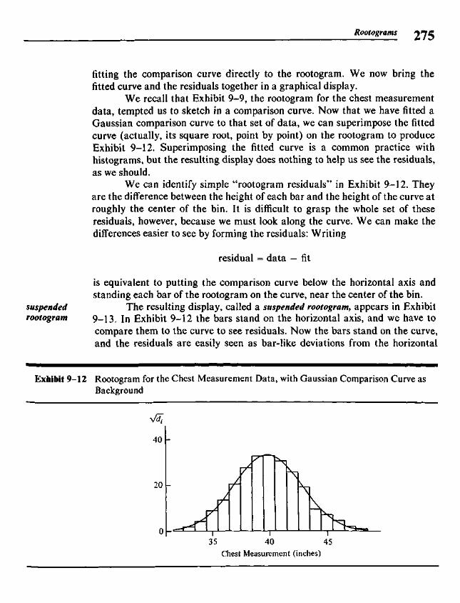
Rootograms
fitting the comparison curve directly to the rootogram. We now bring thefitted curve and the residuals together in a graphical display.
We recall that Exhibit 9-9, the rootogram for the chest measurementdata, tempted us to sketch in a comparison curve. Now that we have fitted aGaussian comparison curve to that set of data, we can superimpose the fittedcurve (actually, its square root, point by point) on the rootogram to produceExhibit 9-12. Superimposing the fitted curve is a common practice withhistograms, but the resulting display does nothing to help us see the residuals,as we should.
We can identify simple "rootogram residuals" in Exhibit 9-12. Theyare the difference between the height of each bar and the height of the curve atroughly the center of the bin. It is difficult to grasp the whole set of theseresiduals, however, because we must look along the curve. We can make thedifferences easier to see by forming the residuals: Writing
residual = data — fit
is equivalent to putting the comparison curve below the horizontal axis andstanding each bar of the rootogram on the curve, near the center of the bin.
suspended The resulting display, called a suspended rootogram, appears in Exhibitrootogram 9-13. In Exhibit 9-12 the bars stand on the horizontal axis, and we have to
compare them to the curve to see residuals. Now the bars stand on the curve,and the residuals are easily seen as bar-like deviations from the horizontal
Exhibit 9-12 Rootogram for the Chest Measurement Data, with Gaussian Comparison Curve asBackground
40 h
20
35 40 45Chest Measurement (inches)
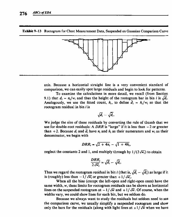
2 7 5 ABCs °fEDA
Exhibit 9-13 Rootogram for Chest Measurement Data, Suspended on Gaussian Comparison Curve
\
axis. Because a horizontal straight line is a very convenient standard ofcomparison, we can easily spot large residuals and begin to look for patterns.
To examine the calculations in more detail, we recall (from Section9.1) that dj = fit/wi and thus the height of the rootogram bar in bin i is y^dt.Analogously, we use the fitted count, hf, to define dt = «,/w( so that therootogram residual in bin / is
We judge the size of these residuals by converting the rule of thumb that weuse for double-root residuals: A DRR is "large" if it is less than —2 or greaterthan +2. Because d{ and dt have «, and fit as their numerators and w, as theirdenominator, we begin with
DRRt = yj2 + 4/2, - Vl + 4/i,-,
neglect the constants 2 and 1, and multiply through by 1/(2 y/Wj) to obtain
DRR, r-r
Thus we regard the rootogram residual in bin i (that is, y[dt — yjdt) as large if itis (roughly) less than - 1 / Vvvj or greater than +1 / Vvv̂ .
When all the bins (except the left-open and right-open ones) have thesame width, w, these limits for rootogram residuals can be shown as horizontallines on the suspended rootogram at — 1 / VvP and +1 / VH\ Of course, when thewidths vary, we could show lines for each bin, but we seldom do.
Because we always want to study the residuals but seldom need to seethe comparison curve, we usually simplify a suspended rootogram and showonly the bars for the residuals (along with light lines at ± 1 / Vvv when we have
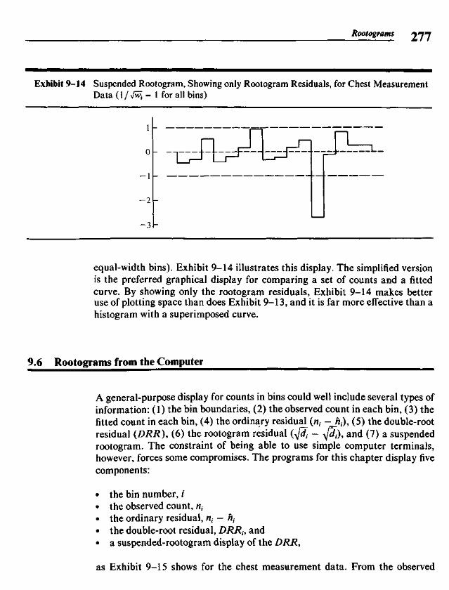
Rootograms 2 7 7
Exhibit 9-14 Suspended Rootogram, Showing only Rootogram Residuals, for Chest MeasurementData (1 / ^ = 1 for all bins)
1
0
i
— 2
- 3
equal-width bins). Exhibit 9-14 illustrates this display. The simplified versionis the preferred graphical display for comparing a set of counts and a fittedcurve. By showing only the rootogram residuals, Exhibit 9-14 makes betteruse of plotting space than does Exhibit 9-13, and it is far more effective than ahistogram with a superimposed curve.
9.6 Rootograms from the Computer
A general-purpose display for counts in bins could well include several types ofinformation: (1) the bin boundaries, (2) the observed count in each bin, (3) thefitted count in each bin, (4) the ordinary residual («, - «,.), (5) the double-rootresidual (DRR), (6) the rootogram residual ( ^ - ^ ) , and (7) a suspendedrootogram. The constraint of being able to use simple computer terminals,however, forces some compromises. The programs for this chapter display fivecomponents:
• the bin number, i• the observed count, nt
• the ordinary residual, nt - h(
• the double-root residual, DRRh and• a suspended-rootogram display of the DRR,
as Exhibit 9-15 shows for the chest measurement data. From the observed
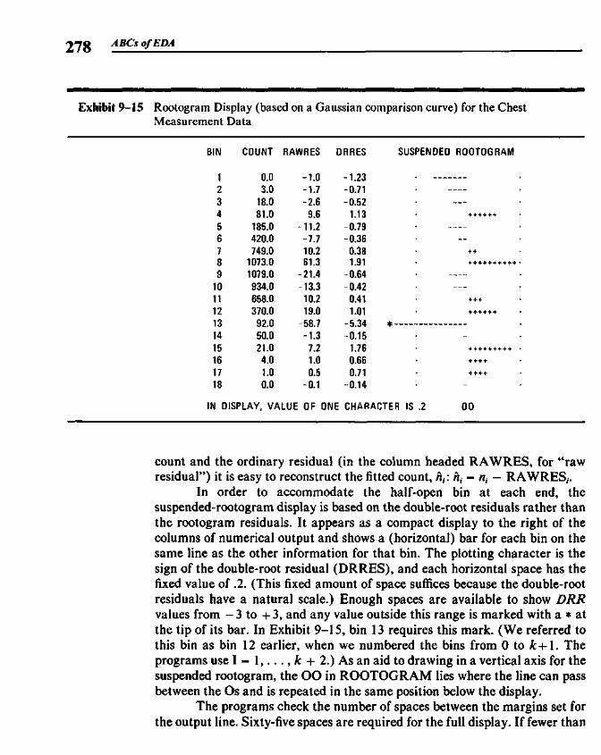
278 ABCs of EDA
Exhibit 9-15 Rootogram Display (based on a Gaussian comparison curve) for the ChestMeasurement Data
BIN COUNT RAWRES DRRES SUSPENDED ROOTOGRAM
1 0.0 -1.0 -1.23 •2 3.0 -1.7 -0.71 •3 18.0 -2.6 -0.524 81.0 9.6 1.13 • ++++++5 185.0 -11.2 -0.79 •6 420.0 -7.7 -0.367 749.0 10.2 0.388 1073.0 61.3 1.91 • ++++++++++.9 1079.0 -21.4 -0.64 •10 934.0 -13.3 -0.4211 658.0 10.2 0.41 • +++12 370.0 19.0 1.01 • ++++++
13 92.0 -58.7 -5.34 *14 50.0 -1.3 -0.1515 21.0 7.2 1.76 • + + + + + + + + + •16 4.0 1.0 0.6617 1.0 0.5 0.7118 0.0 -0.1 -0.14
IN DISPLAY, VALUE OF ONE CHARACTER IS .2 OO
count and the ordinary residual (in the column headed RAWRES, for "rawresidual") it is easy to reconstruct the fitted count, «,: ht = nt — RAWRES,.
In order to accommodate the half-open bin at each end, thesuspended-rootogram display is based on the double-root residuals rather thanthe rootogram residuals. It appears as a compact display to the right of thecolumns of numerical output and shows a (horizontal) bar for each bin on thesame line as the other information for that bin. The plotting character is thesign of the double-root residual (DRRES), and each horizontal space has thefixed value of .2. (This fixed amount of space suffices because the double-rootresiduals have a natural scale.) Enough spaces are available to show DRRvalues from —3 to +3 , and any value outside this range is marked with a * atthe tip of its bar. In Exhibit 9-15, bin 13 requires this mark. (We referred tothis bin as bin 12 earlier, when we numbered the bins from 0 to k+l. Theprograms use I = 1 , . . . , k + 2.) As an aid to drawing in a vertical axis for thesuspended rootogram, the OO in ROOTOGRAM lies where the line can passbetween the Os and is repeated in the same position below the display.
The programs check the number of spaces between the margins set forthe output line. Sixty-five spaces are required for the full display. If fewer than
Rootogrants
65 but at least 30 spaces are available, only the numerical columns areprinted.
FORTRAN
Two FORTRAN subroutines, RGCOMP and RGPRNT, handle the computationsand output for a rootogram display. RGCOMP, in turn, uses the function GAU,which gives the value of the standard Gaussian cumulative distributionfunction. Separating the computation from the display makes it easy to use thefitted counts or the double-root residuals in other calculations or displays.
For input, the vector X() holds the bin boundaries, and the vector Y()holds the bin counts. (Y() is REAL rather than INTEGER because some frequencydistributions include non-integer counts. The most common reason is that oneor more data values fell on a bin boundary and were counted as one half ineach of the bins that share the boundary.) As in Section 9.1, Y(l) is the count forthe bin whose right-hand boundary is X(l). Now I runs from 1 to L (so that L =k + 2 in the notation of Section 9.1), and again X(L) is not used. Y(1) and Y(L)hold counts for the unbounded extreme bins and must be zero whenever thedata have no unbounded bins.
To fit a Gaussian comparison curve and calculate the double-rootresiduals, use the following FORTRAN statement
CALL RGCOMP(X, Y, L, MU, SIGMA, YHAT, DRR, MHAT, SHAT, ERR)
where
X() is the vector of bin boundaries—X(L) is unused;Y() is the vector of observed counts;L is the number of bins;MU allows the user to specify the mean of the fitted
Gaussian distribution;SIGMA allows the user to specify the standard deviation of the
fitted Gaussian distribution (if SIGMA = 0.0, theprogram ignores the values of MU and SIGMA);
YHAT() is returned as the vector of fitted counts;DRR() is returned as the vector of double-root residuals;MHAT is returned as the mean of the fitted comparison
curve;SHAT is returned as the standard deviation of the fitted
comparison curve;
ABCs of EDA
ERR is the error flag, whose values are0 normal
91 too few bins (L < 3)92 a hinge falls in a half-open bin (so that interpo-
lation is not possible).
Then, to produce the rootogram display using the observed counts, the fittedcounts, and double-root residuals just calculated, use the F O R T R A N state-ment
CALL RGPRNT (Y, L, YHAT, DRR, ERR)
where the parameters are as defined for RGCOMP and
ERR is the error flag, whose values are0 normal
93 margins too narrow for numerical part ofdisplay ( < 30 spaces available)
94 margins wide enough for numerical columns butnot for graphical display, so graphical displaynot printed (30 < spaces < 65).
Both of these subroutines assume that the data take the form of afrequency distribution. When it is necessary to construct the frequencydistribution from a batch of data, the number of bins and the scaling used bythe stem-and-leaf display programs generally provide a good starting point.
BASIC
The BASIC program for suspended rootograms is entered with bin boundariesin the array X() and bin counts in the array Y(). As in Section 9.1, Y(l) is thecount for the bin whose right-hand boundary is X(l). I runs from 1 to N (so thatN = k + 2 in the notation of Section 9.1), and X(N) is not used. Y(1) and Y(N) holdthe counts for the unbounded extreme bins and must be zero if the data haveno unbounded bins. The defined function FNG(Z) is an approximate Gaussiancumulative distribution function; it returns the probability below Z in astandard Gaussian distribution (when | Z | < 5.5—see Section 9.4).
The program leaves X() and Y() unchanged and returns fitted counts inC() and double-root residuals in R().
Rootograms
* 9.7 More on Double Roots
This section briefly brings together several useful facts about double-rootresiduals. The theoretical background for double-root residuals comesprimarily from work on transformations to stabilize the variance of Poissondata. Bartlett (1936) discussed the use of V3c and ^x + */? for counted datagenerated by a Poisson distribution, and others subsequently investigatedmodifications of these re-expressions. Generally, if the random variable Xfollows a Poisson distribution with mean m, the re-expressed variable approxi-mately follows a Gaussian distribution whose mean is a function of m andwhose variance is approximately '/t. The main points are that (1) the varianceafter the re-expression depends only slightly on m and (2) the approximationbecomes better as m grows larger.
In order to do better for small values of m, Freeman and Tukey (1950)suggested the re-expression
As Freeman and Tukey (1949) point out (see also Bishop, Fienberg, andHolland, 1975), the average value of yfx + yjX + 1 is well approximated forPoisson X by
and its variance is close to 1. It is customary to substitute the estimated orfitted count, m, for the (unknown) average value, m. The resulting residuals,
^ + 1,
are known as Freeman-Tukey deviates.For the observed counts, x = 1, 2, . . . , it is easy to check that Vx +
yjx + 1 and yj4x + 2 are only very slightly different. Thus double-rootresiduals and Freeman-Tukey deviates are essentially equivalent. (Recall that1 replaces y]4x + 2 in the definition of the double-root residual when x = 0.This is the main difference between using Vx + yjx + 1 and using yj4x + 2 =2yjx + x/i without special treatment of zero.) The approximate behavior of theFreeman-Tukey deviate is the basis for treating individual DRR values as ifthey were observations from a standard Gaussian distribution.
For descriptive and diagnostic purposes, we can treat the double-rootresiduals from a fitted frequency distribution as if they were a Gaussian
2 8 2 ABCs °fEDA
sample. Naturally, the DRR values are not all independent; the sum of fittedcell counts must equal the sum of observed cell counts, and it is usuallynecessary to estimate some parameters from the data—for example, m and sfor the Gaussian comparison curve—but this lack of independence is seldom aserious problem.
Clearly, double-root residuals tell something about goodness of fitbetween model and data. The almost universally used measure of goodness offit is the (Pearson) chi-squared statistic,
= ym,
How might the double-root residuals be related to X21 Because of theapproximately Gaussian behavior of the DRRh
T.DRR2
follows roughly a chi-squared distribution. The usual number of degrees offreedom—that is, the number of d.f. appropriate for X2—takes into accountthe dependence among the DRR(. For example, from Exhibit 9-11, we get"EDRR2 = 42.48; and, because there are 18 bins and 2 estimated parameters(besides the total), we should refer this sum to the xfs distribution. When wedo this, we are led to reject the hypothesis that the differences between theobserved and fitted bin counts are due to chance; in fact, p < .0005. The valueof A'2 for this same fit is 37.13, which is almost significant at the .001 level.Both measures indicate strongly that the fit is not satisfactory. (Almost all thedifference between X1 and XDRR2 comes from the bin centered at 44 inches;DRR2 is 28.52, while the contribution to X2 is 22.88.) The practice ofbeginning by looking at the individual DRRt will call early attention to any binwhere the fit is poor. Forming 2DRR2 as a second step will then provide anoverall measure (in case the fit is generally poor but not unusually bad in anyone cell).
In using X2, it is customary to combine bins at either end of thefrequency distribution until every bin has a fitted count no smaller than 1.While some further research is required, this restriction does not seem to benecessary for double-root residuals. (Tukey suggests that we can make arather satisfactory allowance for small fitted counts by subtracting 2(1 — ht)
2,where only bins with n, < 1 contribute to the sum, from the conventionalnumber of degrees of freedom.)
Rootograms
References
Bartlett, M.S. 1936. "The Square Root Transformation in Analysis of Variance."Supplement to the Journal of the Royal Statistical Society 3:68-78.
Bishop, Y.M.M., S.E. Fienberg, and P.W. Holland. 1975. Discrete MultivariateAnalysis: Theory and Practice. Cambridge, Mass.: MIT Press.
Derenzo, Stephen E. 1977. "Approximations for Hand Calculators Using SmallInteger Coefficients." Mathematics of Computation 31:214-225.
Freeman, Murray F., and John W. Tukey. 1949. "Transformations Related to theAngular and the Square Root." Memorandum Report 24. Statistical ResearchGroup, Princeton University, Princeton, N.J.
Freeman, Murray F., and John W. Tukey. 1950. "Transformations Related to theAngular and the Square Root." Annals of Mathematical Statistics 21:607-611.
Huffman, Sandra L., A.K.M. Alauddin Chowdhury, and W. Henry Mosley. 1979."Difference Between Postpartum and Nutritional Amenorrhea" (reply toFrisch and McArthur). Science 203 (2 March 1979), pp. 922-923.
Pollard, R. 1973. "Collegiate Football Scores and the Negative Binomial Distribu-tion." Journal of the American Statistical Association 68:351-352.
Quetelet, A. 1846. Lett res a S.A.R. le Due Regnant de Saxe-Cobourg et Got ha, sur laTheorie des Probabilites, Appliqu'ee aux Sciences Morales et Politiques.Brussels: M. Hayez.
Tukey, John W. 1971. Exploratory Data Analysis, limited preliminary edition, vol.III. Reading, Mass.: Addison-Wesley.
Tukey, John W. 1972. "Some Graphic and Semigraphic Displays." In T.A. Bancroft,ed., Statistical Papers in Honor of George W. Snedecor. Ames: Iowa StateUniversity Press, pp. 293-316.
BASIC Programs
5000 REM SUSPENDED ROOTOGRAM5010 REM ON ENTRY X() HOLDS BIN BOUNDARIES (N-l OF THEM).5020 REM Y() HOLDS BIN COUNTS (N OF THEM), N=# OF BINS.5030 REM Y(l) AND Y(N) ARE ASSUMED TO HOLD COUNTS BELOW X(l)5040 REM AND ABOVE X(N)f RESPECTIVELY. THEY MUST BE5050 REM SET TO ZERO IF THEY ARE NOT NEEDED.5060 REM FNG(X) IS ASSUMED TO BE DEFINED AS THE CUMULATIVE5070 REM PROBABILITY FUNCTION TO BE FIT (THE GAUSSIAN BY DEFAULT)5080 REM IF V K O REQUESTS VALUES FOR MEAN AND STANDARD DEVIATION5090 REM AND SKIPS FITTING PROCEDURE.5100 REM ON EXIT, X() AND Y() ARE UNCHANGED. THE FITTED COUNTS5110 REM ARE IN C() f AND THE DOUBLE-ROOT RESIDUALS ARE IN R().5120 REM
5130 IF N >= 3 THEN 51605140 LET E9 = 915150 RETURN
5160 REM FIND TOTAL COUNT
5170 LET A = 05180 FOR I = 1 TO N5190 LET A = A + Y(I)5200 NEXT I5210 IF VI > 0 THEN 5290
5220 REM GET USER-SUPPLIED PARAMTERS
5230 PRINT TAB(M0);"MEAN, STANDARD DEVIATION";5240 INPUT LI,SI5250 IF SI > 0 THEN 55905260 PRINT TAB(M0);"S.D. MUST BE > 0, RE-ENTER ";5270 GO TO 5230
5280 REM FIND HINGES
5290 LET Al = ( INT((A + 1) / 2) + 1) / 25300 IF Al > Y(l) THEN 53305310 PRINT TAB(M0);"HINGE IN LEFT-OPEN BIN IN ROOTOGRAM"5320 STOP5330 LET A2 = Y(l)5340 FOR I = 2 TO N - 15350 LET A2 = A2 + Y(I)5360 IF A2 >= Al THEN 54005370 NEXT I5380 PRINT TAB(MO);"HINGE IN RIGHT-OPEN BIN IN ROOTOGRAM"5390 STOP
284
BASIC 285
5400 REM FIND LOW HINGE BY INTERPOLATION AND PUT IN L2
5410 LET A2 = A2 - Y(I)
5420 LET L2 = X(I - 1) + (X(I) - X(I - 1)) * (Al - A2 - .5) / Y(I)
5430 REM NOW FIND THE HIGH HINGE
5440 IF Al <= Y(N) THEN 53805450 LET A4 = Y(N)5460 FOR I = N - 1 TO 2 STEP - 15470 LET A4 = A4 + Y(I)5480 IF A4 >= Al THEN 55105490 NEXT I5500 GO TO 53105510 LET A4 = A4 - Y(I)5520 LET L3 = X(I) - (X(I) - X(I - 1)) * (Al - A4 - .5) / Y(I)
5530 REM L2 AND L3 ARE NOW THE HINGES. USE THE MIDHINGE AS A CENTER5540 REM AND HINGESPREAD/1.349 AS A SCALE IN GAUSSIAN.
5550 LET LI = (L2 + L3) / 25560 LET SI = (L3 - L2) / 1.349
5570 REM C7 ACCUMULATES CUMULATIVE PROBABILITY5580 REM IS TOTAL COUNT. C() GETS FITTED COUNT,5590 REM R() GETS DOUBLE-ROOT RESIDUALS.
5600 LET C7 = 05610 FOR I = 1 TO N - 15620 LET C8 = FNG((X(I) - LI) / SI)5630 LET C(I) = A * (C8 - C7)5640 LET R(I) = SQR(2 + 4 * Y(I)) - SQR(1 + 4 * C(I))5650 IF Y(I) > 0 THEN 56705660 LET R(I) = 1 - SQR(1 + 4 * C(I))5670 LET C7 = C85680 NEXT I
5690 REM NOW HANDLE RIGHT-OPEN BIN
5700 LET C(N) = A * (1 - C7)5710 LET R(N) = SQR(2 + 4 * Y(N)) - SQR(1 + 4 * C(N))5720 IF Y(N) > 0 THEN 57405730 LET R(N) = 1 - SQR(1 + 4 * C(N))
5740 REM5750 REM PRINT ROOTOGRAM RESULTS5760 REM
5770 LET Ml = M9 - MO + 15780 IF Ml > 30 THEN 58105790 PRINT TAB(MO);"PAGE TOO NARROW TO DISPLAY ROOTOGRAM RESULTS"5800 RETURN
ABCs °fEDA
5810 REM SET UP TABS
5820 LET Tl = MO + 45830 LET T2 = Tl + 85840 LET T3 = T2 + 85850 LET T4 = T3 + 8
5860 REM R3 IS PRINTING FLAG: 0= PRINT TABLE,5870 REM 1 = PRINT TABLE AND ROOTOGRAM, 2 = ROOTOGRAM ONLY
5880 LET R3 = 15890 IF Ml >= 60 THEN 59105900 LET R3 = 05910 PRINT5920 PRINT TAB(MO);"BIN#n; TAB(T1 + 1);"COUNT"; TAB(T2);"RAW RES";5930 PRINT TAB(T3);"D-R RES";5940 IF R3 = 0 THEN 5970
5950 REM HEADING FOR ROOTOGRAM DISPLAY
5960 PRINT TAB(T4 + 4);"SUSPENDED ROOTOGRAM";5970 PRINT5980 PRINT5990 FOR I = 1 TO N6000 LET Rl = Y(I) - C(I)6010 LET RO = 16020 PRINT TAB(M0);I;6030 IF R3 = 2 THEN 60806040 PRINT TAB(Tl); FNR(Y(I)); TAB(T2); FNR(Rl);6050 LET RO = 26060 PRINT TAB(T3); FNR(R(I));6070 IF R3 = 0 THEN 6420
6080 REM PUT ONE LINE OF ROOTOGRAM IN P()
6090 LET 01 = ASC(" ")6100 FOR J = 1 TO 326110 LET P(J) = 016120 NEXT J6130 LET P(6) = ASC(".")6140 LET P(27) = ASC(".")6150 LET Jl = 06160 IF R(I) = 0 THEN 63606170 LET XI = FNC(5 * ABS(R(I)))6180 IF XI <= 15 THEN 62006190 LET XI = 156200 IF R(I) > 0 THEN 6290
BASIC 287
6210 REM CONSTRUCT ROOTOGRAM LINE FOR RESIDUAL < 0
6220 LET Jl = 16
6230 FOR J = Jl TO Jl - XI STEP - 16240 LET P(J) = ASC("-")6250 NEXT J6260 IF XI < 15 THEN 63606270 LET P(l) = ASC("*")6280 GO TO 6360
6290 REM CONSTRUCT ROOTOGRAM LINE FOR RESIDUAL>0
6300 LET Jl = 17 + XI6310 FOR J = 17 TO Jl6320 LET P(J) = ASC("+")6330 NEXT J6340 IF XI < 15 THEN 63606350 LET P(32) = ASC("*")6360 IF Jl >= 27 THEN 63806370 LET Jl = 276380 PRINT TAB(T4);6390 FOR J = 1 TO Jl6400 PRINT CHR$(P(J));6410 NEXT J6420 PRINT6430 NEXT I
6440 REM GO BACK TO PRINT ROOTOGRAM?
6450 IF R3 >= 1 THEN 65106460 LET R3 = 26470 LET T4 = MO + 46480 IF Ml > T4 + 30 THEN 59506490 PRINT TAB(MO);"PAGE TOO NARROW FOR ROOTOGRAM"6500 GO TO 6550
6510 PRINT
6520 REM WRAPUP
6530 PRINT TAB(T4 + 15);"/"; CHR$(92)6540 PRINT TAB(M0);"IN DISPAY, VALUE OF ONE SPACE IS .2'6550 RETURN
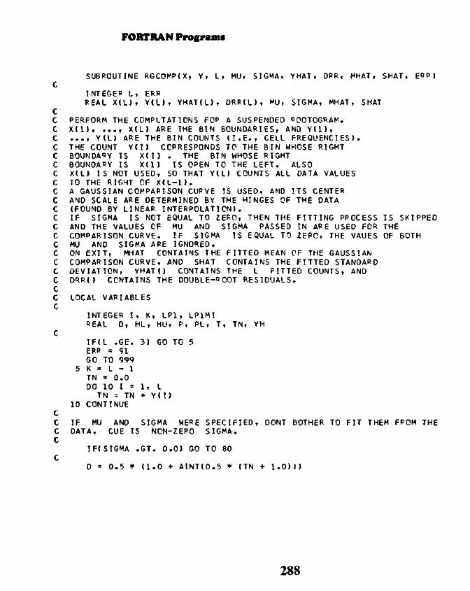
FORTRAN Programs
SUBROUTINE RGCOMP(X, Y, L, MU» SIGMA, YHATt DPR, MHATt SHAT, EPP)C
INTEGER L, ERRREAL X(L), Y(L), YHAT(L), DRR(L), MU, SIGMA, MHAT, SHAT
CC PERFORM THE COMPLTATIONS FOP A SUSPENDED ROOTOGRAM.C X(l), ..., X(L) ARE THE BIN BOUNDARIES, AND Y(l),C ..., Y(L) ARE THE BIN COUNTS (I.E., CELL FREQUENCIES).C THE COUNT Y d ) CORRESPONDS TO THE BIN WHOSE RIGHTC BOUNDARY IS X(I) . THE BIN WHOSE RIGHTC BOUNDARY IS X(l) IS OPEN TO THE LEFT. ALSOC X(L) IS NOT USED, SO THAT Y(L) COUNTS ALL DATA VALUESC TO THE RIGHT OF X(L-l).C A GAUSSIAN COMPARISON CURVE IS USED, AND ITS CENTERC AND SCALE ARE DETERMINED BY THE HINGES OF THE DATAC (FOUND BY LINEAR INTERPOLATICN).C IF SIGMA IS NOT EQUAL TO ZERO, THEN THE FITTING PROCESS IS SKIPPEDC AND THE VALUES CF MU AND SIGMA PASSED IN ARE USED FOR THEC COMPARISON CURVE. IF SIGMA IS EQUAL TO ZERO, THE VAUES OF BOTHC MU AND SIGMA APE IGNORED.C ON EXIT, MHAT CONTAINS THE FITTED MEAN OF THE GAUSSIANC COMPARISON CURVE, AND SHAT CONTAINS THE FITTED STANDARDC DEVIATION, YHATO CONTAINS THE L FITTED COUNTS, ANDC DRRO CONTAINS THE DOUBLE-ROOT RESIDUALS.CC LOCAL VARIABLESC
INTEGER I, K, LP1, LP1MIREAL D, HL, HU, P, PL, T, TN, YH
CIF(L .GE. 3) GO TO 5ERR = 91GO TO 999
5 K = L - 1TN = 0.0DO 10 I = 1, LTN = TN + Y d )
10 CONTINUECC IF MU AND SIGMA WERE SPECIFIED, DONT BOTHER TO FIT THEM FPOM THEC DATA. CUE IS NON-ZERO SIGMA.C
IF(SIGMA .GT. 0.0) GO TO 80C
D = 0.5 * (1.0 + AINT(0.5 * (TN + 1.0)))
288
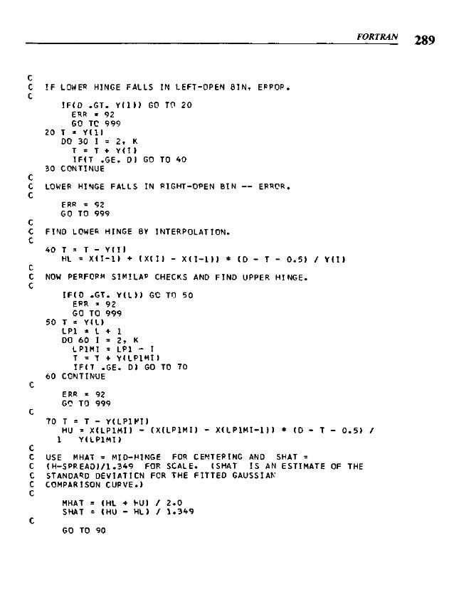
FORTRAN 289
cC IF LOWER HINGE FALLS IN LEFT-OPEN B IN , EPPOP.C
IF(D .GT. Y ( U ) GO TO 20ERR = 92GO TC 999
20 T = Y ( l )DO 30 I = 2 , K
T = T + Y d )IF(T .GE. D) GO TO 40
30 CONTINUECC LOWER HINGE FALLS IN RIGHT-OPEN BIN — ERROR.C
ERR = 92GO TO 999
CC FIND LOWER HINGE BY INTERPOLATION.C
40 T = T - Y d )HL = XU-1) + (X(I) - X(I-l)) * (D - T - 0.5) / Y(I)
CC NOW PERFORM SIMILAR CHECKS AND FIND UPPER HINGE.C
IF(D .GT. Y(D) GC TO 50ERR = 92GO TO 999
50 T = Y(L)LP1 = L + 1DO 60 I = 2, KLP1MI = LP1 - IT = T + Y(LPIMI)IF(T .GE. D) GO TO 70
60 CONTINUEC
ERR = 92GO TO 999
C70 T = T - Y(LPIMI)
HU - X(LPIMI) - (X(LPIMI) - X(LPIMI-D) * (D - T - 0.5) /1 Y(LPIMI)
CC USE MHAT = MID-HINGE FOR CENTERING AND SHAT =C (H-SPREAD)/1.349 FOR SCALE. (SHAT IS AN ESTIMATE OF THEC STANDARD DEVIATICN FOR THE FITTED GAUSSIANC COMPARISON CURVE.)C
MHAT = (HL + HU) / 2.0SHAT = (HU - HL) / 1.349
CGO TO 90
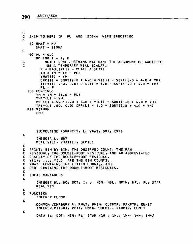
2 9 0 ABCs °fEDA
SKIP TO HERE IF MU AND SIGMA WERE SPECIFIED
80 MHAT = MUSHAT = SIGMA
90 PL = 0.0DO 100 I = 1 , K
NOTE: SOME FORTRANS MAY WANT THE ARGUMENT OF GAU() TOBE A TEMPORARY REAL SCALAR.
P = GAUUX( I ) - MHAT) / SHAT)YH = TN * (F - PL)YHAT(I) = YH
SQRTC2.0 • 4 . 0 * Y d ) ) - SQRTd.O • 4 . 0 * YH)DRR(I)I F ( Y U )PL = P
100 CONTINUEYH = TN *YHAT(L) =
EQ. 0 . 0 ) DRR(I) = 1.0 - SQRTd.O • 4 . 0 * YH)
999
- PL)( 1 . 0YH
DRR(L) - S Q R T ( 2 . 0 + 4 . 0 * Y ( D ) - S Q R T d . O «• 4 . 0I F ( Y ( L ) . E Q . 0 . 0 ) DRR(L) = 1 .0 - S Q R T d . O «• 4 . 0 *RETURNEND
YH)YH)
SUBROUTINE RGPPNT(Y, L, YHAT, DPR, ER")
INTEGER L, ERRREAL Y ( L ) , YHAT<L), DRR(L)
PRINT, BIN BY BIN, THE OBSERVED COUNT, THE RAWRESIDUAL, THE DOUBLE-ROOT RESIDUAL, AND AN ABBREVIATEDOISPLAY OF THE DCUBLE-ROOT RESIDUAL.Y d ) , . . . , Y(L) ARE THE BIN COUNTS.YHAT CONTAINS THE FITTED COUNTS, ANDORR CONTAINS THE DOUBLE-ROOT RESIDUALS.
LOCAL VARIABLES
INTEGER BL, BO, DOT, I , J , MIN, NBL, NMIN, NPL, PL, STARREAL RES
FUNCTIONINTEGER FLOOR
COMMON /CHRBUF/ P, PMAX, PMIN, OUTPTP, MAXPTR, OUNITINTEGER P ( 1 3 0 ) , PMAX, PMIN, OUTPTR, MAXPTR, OUNIT
DATA BL, DOT, MIN, PL, STAR /1H , 1 H . , 1 H - , 1H+, 1H* /
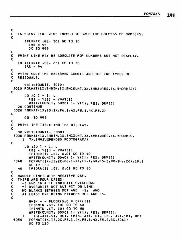
FORTRAN 291
cC IS PRINT LINE WIDE ENOUGH TO HOLD THE COLUMNS OF NUMBERS.C
IFCPMAX .GE. 30) GO TO 10ERP = 93GO TO 999
CC PRINT LINE MAY BE ADEQUATE FOP NUMBERS BUT NOT DISPLAY.C
10 IFCPMAX .GE. 65) GO TO 30ERR = 94
CC PRINT ONLY THE OBSERVED COUNTS AND THE TWO TYPES OFC RESIDUALS.C
WRITECOUNIT, 5010)5010 FORMATI1X,3HBIN,3X,5HC0UNT,3X,6HRAWRES,3X,5HDRRES/)
CDO 20 I = li L
RES * Y(I) - YHAT(I)WRITECOUNIT, 5020) I, Y d ) , PES, DR&CI)
20 CONTINUE5020 FORMATC1X,I3,2X,F6.1,4X,F5.1,4X,F5.2)
CGO TO 999
CC PRINT THE TABLE AND THE DISPLAY.C
30 WRITECOUNIT, 5030)5030 F0RMAT(lX,3HBIN,3X,5HC0UNT,3X,6HPAWRES,4X,5HDRPES,
1 7X,19HSUSPENDED ROOTOGRAM/)C
DO 1 2 0 I = 1 , LRES = YCI) - YHATCI)IFCDRRCI) .NE. 0.0) GO TO 40WRITECOUNIT, 5040) I, YCI), PES, DRP(I)
5040 FORMAT(1X,I3,2X,F6.1,4X,F5.1,4X,F5.2,8X,1H.,2 0X,1H.)GO TC 120
40 IFCDRRCI) .GT. 0.0) GO TO 80CC HANDLE LINES WITH NEGATIVE DRP.C THERE ARE FOUR CASES:C -S END IN * TO INDICATE OVERFLOW,C -S OVERWRITE DOT BUT FIT ON LINE,C NO BLANKS BETWEEN DOT AND -S, ANDC AT LEAST ONE BLANK BETWEEN DOT AND -S.C
NMIN = - FLC0RC5.0 * DR^CIMIFCNMIN .GT. 10) GO TO 60IFCNMIN .LT. 10) GO TO 50WRITECOUNIT, 5050) I, YCI), RES, DRR(I),
1 (BLfJ=l,5), DOT, CMIN, J=l,10), CBL, J=l,10), DOT5050 FORMATC1X,I3,2X,F6.1,4X,F5.1,4X,F5.2,3X,32A1)
GO TO 120
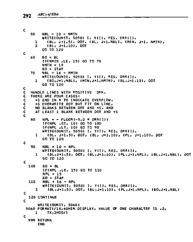
2 O 2 ABCs of EDA
50 NBL - 10 - NMINWRITE(OUNIT, 5050) I, Y d ) , PES, DRR(I),
1 (BLt J-1.5), DOT, (BL, J=1,NBL), (MIN, J*l, NMIN),2 (BL, J=l,10), DOT
GO TO 120C
60 BO = BLIF(NMIN .LE. 15) GO TO 70NMIN = 15BO - STAR
70 NBL * 16 - NMINWRITECOUNIT, 5050) I, Y d ) , RES, DRR(I),
1 (BO,J*1,NBL), (MIN,J=l,NMIN), (BL,J*1,1O), DOTGO TO 120
CC HANDLE LINES WITH POSITIVE DPR.C THERE ARE FOUR CASES:C *S END IN * TO INDICATE OVERFLOW,C +S OVERWRITE DOT BUT FIT ON LINE,C NO BLANKS BETWEEN DOT AND +S, ANDC AT LEAST 1 BLANK BETWEEN DOT AND +SC
80 NPL - - FL00R(-5.0 * DRR(D)IF(NPL .GT. 10) GO TO 100IF(NPL .LT. 10) GO TO 90WRITE(OUNIT, 5050) I, YCI), RES, DPR(I),
1 (BL, J-1,5), DOT, (BL, J=l,10), (PL, J=l,10), DOTGO TO 120
C90 NBL ' 1 0 - NPL
WPITE(OUNIT, 5050) I, Y d ) , RES, DRR(I),1 (BLtJ»lt5)t DOT, (BLfJ*lflO)f (PL,J*l,NPL), (BL,J-1,NBL), DOT
GO TO 120C
100 BO * BLIF(NPL . L E . 15) GO TO 110NPL - 15BO * STAR
110 NBL * 16 - NPLWRITE(OUNIT, 5050) I , Y d ) , PES, D R R ( I ) ,
1 < B L , J * 1 , 5 ) , DOT, ( B L , J = 1 , 1 O ) , ( P L , J - l , N P L ) , ( B O , J * 1 , N B L )C
120 CONTINUEC
WRITE(OUNIT, 5060)5060 FORMAT(/1X,4OHIN DISPLAY, VALUE OF ONE CHARACTEP IS . 2 ,
1 7X,2HOO/)C
999 RETURNEND
Appendix AComputer Graphics
Many exploratory techniques are graphical or have a graphical component.Computer programs to produce displays must be able to accommodate widelydisparate batches of data and adjust the display parameters to show eachbatch clearly. Decisions about display formats reflect the purposes of theprograms. Displays for exploratory data analysis often do best when format-ting decisions are different from the decisions common to traditional practicein computer graphics. This appendix discusses the philosophy, the defaultdisplay-formatting algorithms, and the technical details of the displayprograms in this book.
A.I Terminology
The vocabulary of computer graphics has developed from work in severaldisciplines and is not standardized. This section defines one common terminol-ogy for use in this appendix.
293
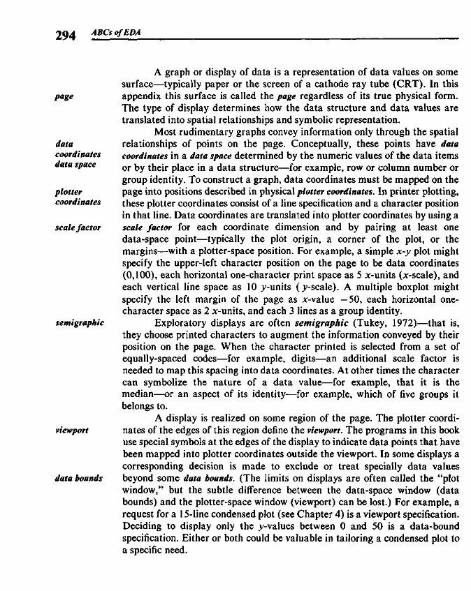
2 9 4 ABCs °fEDA
page
datacoordinatesdata space
plottercoordinates
scale factor
semigraphic
viewport
data bounds
A graph or display of data is a representation of data values on somesurface—typically paper or the screen of a cathode ray tube (CRT). In thisappendix this surface is called the page regardless of its true physical form.The type of display determines how the data structure and data values aretranslated into spatial relationships and symbolic representation.
Most rudimentary graphs convey information only through the spatialrelationships of points on the page. Conceptually, these points have datacoordinates in a data space determined by the numeric values of the data itemsor by their place in a data structure—for example, row or column number orgroup identity. To construct a graph, data coordinates must be mapped on thepage into positions described in physical plotter coordinates. In printer plotting,these plotter coordinates consist of a line specification and a character positionin that line. Data coordinates are translated into plotter coordinates by using ascale factor for each coordinate dimension and by pairing at least onedata-space point—typically the plot origin, a corner of the plot, or themargins—with a plotter-space position. For example, a simple x-y plot mightspecify the upper-left character position on the page to be data coordinates(0,100), each horizontal one-character print space as 5 x-units (x-scale), andeach vertical line space as 10 j>-units (^-scale). A multiple boxplot mightspecify the left margin of the page as x-value - 5 0 , each horizontal one-character space as 2 x-units, and each 3 lines as a group identity.
Exploratory displays are often semigraphic (Tukey, 1972)—that is,they choose printed characters to augment the information conveyed by theirposition on the page. When the character printed is selected from a set ofequally-spaced codes—for example, digits—an additional scale factor isneeded to map this spacing into data coordinates. At other times the charactercan symbolize the nature of a data value—for example, that it is themedian—or an aspect of its identity—for example, which of five groups itbelongs to.
A display is realized on some region of the page. The plotter coordi-nates of the edges of this region define the viewport. The programs in this bookuse special symbols at the edges of the display to indicate data points that havebeen mapped into plotter coordinates outside the viewport. In some displays acorresponding decision is made to exclude or treat specially data valuesbeyond some data bounds. (The limits on displays are often called the "plotwindow," but the subtle difference between the data-space window (databounds) and the plotter-space window (viewport) can be lost.) For example, arequest for a 15-line condensed plot (see Chapter 4) is a viewport specification.Deciding to display only the ^-values between 0 and 50 is a data-boundspecification. Either or both could be valuable in tailoring a condensed plot toa specific need.
Computer Graphics
A.2 Exploratory Displays
Displays for exploratory data analysis should be modified for computergeneration in ways that reflect their use. The programs in this book followseveral rules to achieve effective exploratory displays:
1. Displays should be structured so that features of the data can be seeneasily.
2. Display scales and formats should be resistant to the effects of extraordi-nary points but should clearly indicate such points when they are present.
3. Displays must be concise so that several can be produced on an interactivecomputer terminal without lengthy delays. (30 seconds per plot at 30characters per second is a reasonable maximum.)
Other common requirements of computer displays are less importantin exploratory work and have been sacrificed when necessary. For example,the three rules just given contradict the common rule that every data pointmust be displayed. Exploratory displays often exclude extraordinary pointsfrom the main part of the display so that patterns in the main body of the datastand out. (The programs in this book always allow the data analyst tooverride this decision.) Features such as extensive axis labels and sophisticatedoptions for display titles are desirable in ordinary computer graphics but areunnecessary here and have not been included in these programs. (Neverthe-less, these features can be valuable if they are designed to be concise.Implementors of these programs—and especially implementors adding themto an existing high-level program— should consider adding these features.)
A.3 Resistant Scaling
A single plot-scaling algorithm serves all of the programs for displays in thisbook. It uses the H-spread (see Chapter 2) as an estimate of the variability of abatch. We first define a
step = 1.5 x H-spread.
The (inner) fences are then placed at one step beyond each hinge. (Chapter 3
ABCs of EDA
adjacentvalue
nice numbers
nice positionwidth
discusses fences from a data analysis perspective.) The outermost data valueon each end that is not beyond the inner fence is called an adjacent value. Thehigh and low adjacent values provide a good frame for the body of a databatch. Data values beyond the fences are treated as outliers. Data valuesbetween the fences are displayed in ways that make their important featuresclearly visible.
For easy comprehension, displays should be made in simple units.Thus, for printer plots, the data-space size of one line or one character spaceshould be easy to understand and easy to count. We call numbers suitable forthis purpose nice numbers. Nice numbers have the form m x 10e, where e is aninteger and m is selected from a restricted set of numbers. These programsselect between two sets of numbers form: {l, 2, 5, 10} and {l, 1.5, 2, 2.5, 3, 4, 5,7, 10}. The 1 is redundant, but including both 1 and 10 simplifies theprograms. These sets of numbers are chosen to be approximately equallyspaced in their logarithms while still being integers or half-integers. Thisspacing limits the error introduced in approximating a number by a nicenumber: In the first set, the approximation error is no more than about 40% ofthe number; in the second set, it is no more than about 20% of the number.(This error bound can be cut to 18% by including 1.25.)
Display scaling is accomplished by finding a nice position width for eachdimension of the display. This is the largest data-space width of a plot position(character space or line), chosen from a set of nice number choices, such thatthe available number of plot positions (viewport) will accommodate all thenumbers between the data bounds. Some displays can have lines labeled —0,which appear to the display scaling algorithm as extra plot positions. Theprograms allow for these extra lines when they are needed. Because the widthof a plot position is approximated with a greater or equal nice value, the rangeactually covered by a display will generally be slightly larger than thatindicated by the data bounds.
A.4 Printer Plots
All the displays in this book have been designed or modified to be produced ona typewriter-style device and are intended to be used interactively. Both ofthese constraints influence the design of display formatting decisions.
Each display is produced line by line, starting from the top of the page.This may be different from the way the display would be drawn by hand or on
Computer Graphics
a more sophisticated graphics device. All displays start at or near the leftmargin, so little time is wasted on an interactive terminal spacing out to thedisplay. Axis labels are placed on the left to keep empty lines short.
Printer plots are inherently granular. Rounding each data-space coor-dinate to one of, say, 50 character positions distorts a display, although thisrarely diminishes the display's usefulness in an exploratory analysis. Printedcharacters are usually taller than they are wide. As a result, the horizontal andvertical scales of a plot may not be comparable; and, for example, the apparentslope of a line may not be closely related to the actual slope value. The displaysin this book openly treat each axis differently.
These inconveniences are balanced by a wide choice of plottingcharacters. Almost every display in this book takes advantage of this choiceeither to report numbers with greater precision (stem-and-leaf display,condensed plot) or to code important characteristics (boxplot, coded table).The programming languages used here have dictated some choices of codes(see Appendix C). Other choices would be reasonable in other languages.
The experienced programmer reading these programs will probablyfind FORTRAN especially stifling in this respect. The FORTRAN languagehas a very restricted character set and limited abilities in character manipula-tion. Occasionally, our attempts to write clear, portable, easily understoodprograms for graphics may have been stymied by the FORTRAN language,and for this we ask the programming reader's indulgence.
A.5 Display Details
Each of the exploratory displays considered in the text implements differentaspects of the methods described in this appendix. This section discusses eachdisplay specifically. The discussion assumes knowledge of the displays them-selves.
Stem-and-leaf displays (Chapter 1) bound the data strictly at theadjacent values. Data values beyond these bounds appear on special HI andLO lines (even if they might have fit as the most extreme numbers on the finalstems) and do not affect the scale. The display scale is the smallest nicenumber (with m chosen from the set f 1, 2, 5, 10}) such that no more than 10 xIog10« lines are needed to display all data values between the fences. When
2 9 8 ARCs of EDA
both positive and negative numbers are in the batch, room is allocated for the— 0 stem. The selection of m determines the form of the display. Regardless ofthe display scale, the character codes always have the same scale, 1 x 10', andthus hold the next digit of each number after the last digit forming the stem.The horizontal viewport is the line length specified by the line margins. Linesoverflowing the right margin end with a * to indicate the omission of pointsfalling beyond the viewport.
Boxplots (Chapter 3) do not bound the data at all because one of theprimary purposes of a boxplot is to display outliers. One horizontal characterposition is scaled to the smallest nice number (using m e {l, 1.5, 2, 2.5, 3, 4, 5,7, 10}) that accommodates the range of the data on the available line width.Special codes are assigned to outliers, to the median, and to the hinges, asdetailed in Chapter 3. When multiple boxplots are generated, one or threelines are allocated to each group depending upon the form of the boxplot.
Condensed plots (Chapter 4) bound data in both dimensions implicitlythrough the plot scaling. Scales in x and y are nice numbers with m e {l, 1.5, 2,2.5, 3, 4, 5, 7, 10}. The >>-scale allows for a - 0 line if positive and negative^-values are present. The scales are the smallest nice numbers that accommo-date the data between the adjacent values in each dimension within thespecified number of lines (>>-scale) or allowed line width (jc-scale). As a result,fewer lines than the specified maximum may be needed, and data valuesbeyond the fences may fit within the viewport. Data values mapped outside theviewport are indicated with special characters at the edges of the plot, asdescribed in Section 4.6. Character codes are scaled according to C, thenumber of characters specified for the display. The vertical line size indata-space units is divided into C equal intervals. Plot symbols starting with 0and counting through successive integers are assigned outward from the edgeof the interval nearer to zero. Options allow the user to specify data bounds tosupplant the adjacent values in scale calculation, viewport (as number oflines—the x-dimension viewport is defined by the line width), and numberof codes (as number of characters). These options allow the display to focus onany segment of the data, enlarge it to any size, and magnify the verticalprecision up to 10 times by coding. The default settings of these options aredesigned to produce the display most likely to be useful in an exploratoryanalysis.
Coded tables (Chapter 7) require no scaling. The data structuredetermines the format on the page. One line is allocated per row of the table.Two character positions are allocated per column of the table. Codes arescaled to identify data-value characteristics with respect to the data batchbased upon the hinges and fences as detailed in Section 7.1.
Computer Graphics 2 9 9
Suspended rootograms (Chapter 9) need no special display scaling; thenumbers displayed are automatically well-scaled. One line is allocated to eachbin and contains both numeric and graphical output. The rootogram displayplots the double-root residuals, which, as computed, are expected to behave asif drawn from a standard Gaussian distribution. The display allocates onecharacter position to a unit of .2 in data (double-root-residual) space.
Programming^ Y e s •» Please turn to Chapter 3.

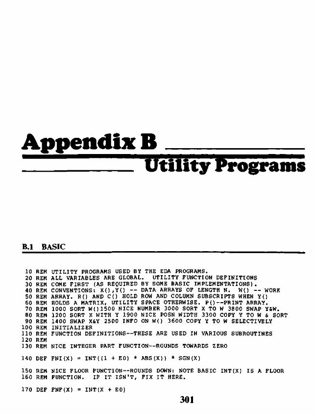
Appendix BUtility Programs
B.I BASIC
10 REM UTILITY PROGRAMS USED BY THE EDA PROGRAMS.20 REM ALL VARIABLES ARE GLOBAL. UTILITY FUNCTION DEFINITIONS30 REM COME FIRST (AS REQUIRED BY SOME BASIC IMPLEMENTATIONS).40 REM CONVENTIONS: X(),Y() — DATA ARRAYS OF LENGTH N. W() — WORK50 REM ARRAY. R() AND C() HOLD ROW AND COLUMN SUBSCRIPTS WHEN Y()60 REM HOLDS A MATRIX, UTILITY SPACE OTHERWISE. P()—PRINT ARRAY.70 REM 1000 SORT W()1500 NICE NUMBER 3000 SORT X TO W 3800 SWAP Y&W.80 REM 1200 SORT X WITH Y 1900 NICE POSN WIDTH 3300 COPY Y TO W & SORT90 REM 1400 SWAP X&Y 2500 INFO ON W() 3600 COPY Y TO W SELECTIVELY100 REM INITIALIZER110 REM FUNCTION DEFINITIONS—THESE ARE USED IN VARIOUS SUBROUTINES120 REM130 REM NICE INTEGER PART FUNCTION—ROUNDS TOWARDS ZERO
140 DEF FNI(X) = INT((1 + E0) * ABS(X)) * SGN(X)
150 REM NICE FLOOR FUNCTION—ROUNDS DOWN: NOTE BASIC INT(X) IS A FLOOR160 REM FUNCTION. IF IT ISN'T, FIX IT HERE.
170 DEF FNF(X) = INT(X + E0)
301
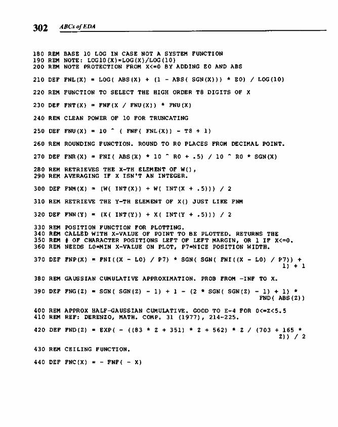
3 0 2 ABCs °fEDA
180 REM BASE 10 LOG IN CASE NOT A SYSTEM FUNCTION190 REM NOTE: LOG10(X)=LOG(X)/LOG(10)200 REM NOTE PROTECTION FROM X<=0 BY ADDING EO AND ABS
210 DEF FNL(X) = LOG( ABS(X) + (1 - ABS( SGN(X))) * EO) / LOG(IO)
220 REM FUNCTION TO SELECT THE HIGH ORDER T8 DIGITS OF X
230 DEF FNT(X) = FNF(X / FNU(X)) * FNU(X)
240 REM CLEAN POWER OF 10 FOR TRUNCATING
250 DEF FNU(X) = 10 ~ ( FNF( FNL(X)) - T8 + 1)
2 6 0 REM ROUNDING FUNCTION. ROUND TO RO PLACES FROM DECIMAL POINT.
2 7 0 DEF FNR(X) = F N I ( ABS(X) * 1 0 ~ RO + . 5 ) / 1 0 * RO * SGN(X)
2 8 0 REM RETRIEVES THE X-TH ELEMENT OF W ( ) ,2 9 0 REM AVERAGING IF X I S N ' T AN INTEGER.
3 0 0 DEF FNM(X) = (W( I N T ( X ) ) + W( INT(X + . 5 ) ) ) / 2
3 1 0 REM RETRIEVE THE Y-TH ELEMENT OF X ( ) JUST LIKE FNM
3 2 0 DEF FNN(Y) = (X( I N T ( Y ) ) + X( INT(Y + . 5 ) ) ) / 2
3 3 0 REM POSITION FUNCTION FOR PLOTTING.3 4 0 REM CALLED WITH X-VALUE OF POINT TO BE PLOTTED. RETURNS THE3 5 0 REM # OF CHARACTER POSITIONS LEFT OF LEFT MARGIN, OR 1 I F X < = 0 .3 6 0 REM NEEDS L0=MIN X-VALUE ON PLOT, P7=NICE POSITION WIDTH.
3 7 0 DEF FNP(X) = F N I ( ( X - LO) / P 7 ) * SGN( SGN( F N I ( ( X - LO) / P 7 ) ) +1 ) + 1
3 8 0 REM GAUSSIAN CUMULATIVE APPROXIMATION. PROB FROM - I N F TO X.
3 9 0 DEF FNG(Z) = SGN( SGN(Z) - 1 ) + 1 - (2 * SGN( SGN(Z) - 1 ) + 1 ) *FND( A B S ( Z ) )
400 REM APPROX HALF-GAUSSIAN CUMULATIVE. GOOD TO E-4 FOR 0<=Z<5.5410 REM REF: DERENZO, MATH. COMP. 31 (1977), 214-225.
420 DEF FND(Z) = EXP( - ((83 * Z + 351) * Z + 562) * Z / (703 + 165 *
Z)) / 2
430 REM CEILING FUNCTION.
440 DEF FNC(X) = - FNF( - X)
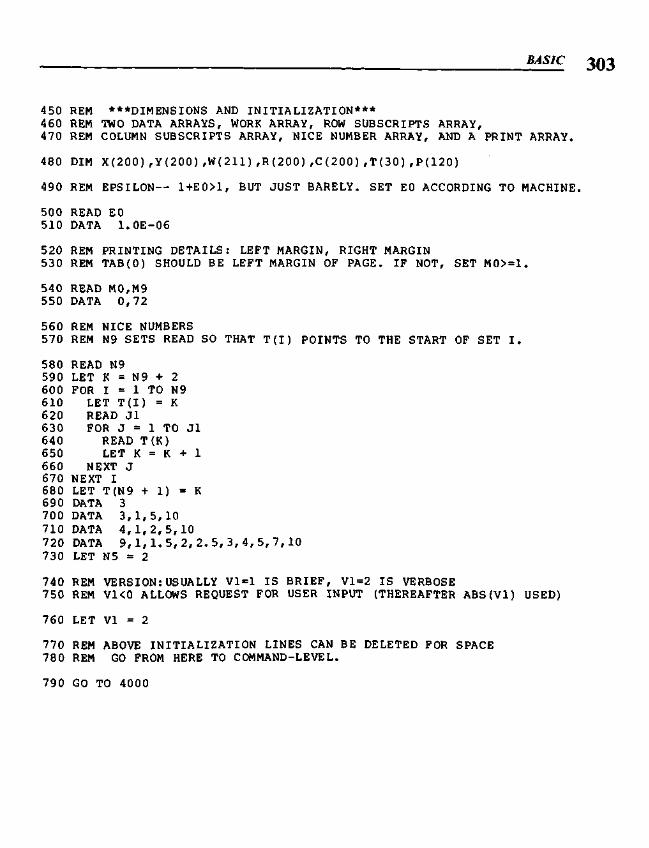
BASIC 303
450 REM ***DIMENSIONS AND INITIALIZATION***460 REM TWO DATA ARRAYS, WORK ARRAY, ROW SUBSCRIPTS ARRAY,470 REM COLUMN SUBSCRIPTS ARRAY, NICE NUMBER ARRAY, AND A PRINT ARRAY.
480 DIM X(200),Y(200),W(211),R(200),C(200),T(30)fP(120)
490 REM EPSILON— 1+EO>1, BUT JUST BARELY. SET EO ACCORDING TO MACHINE.
500 READ EO510 DATA 1.0E-06
520 REM PRINTING DETAILS: LEFT MARGIN, RIGHT MARGIN530 REM TAB(0) SHOULD BE LEFT MARGIN OF PAGE. IF NOT, SET MO>=1.
540 READ M0,M9550 DATA 0,72
560 REM NICE NUMBERS570 REM N9 SETS READ SO THAT T(I) POINTS TO THE START OF SET I.
580 READ N9590 LET K = N9 + 2600 FOR I = 1 TO N9610 LET T(I) = K620 READ Jl630 FOR J = 1 TO Jl640 READ T(K)650 LET K = K + 1660 NEXT J670 NEXT I680 LET T(N9 + 1) = K690 DATA 3700 DATA 3,1,5,10710 DATA 4,1,2,5,10720 DATA 9,1,1.5,2,2.5,3,4,5,7,10730 LET N5 = 2
740 REM VERSION:USUALLY Vl=l IS BRIEF, Vl=2 IS VERBOSE750 REM VKO ALLOWS REQUEST FOR USER INPUT (THEREAFTER ABS(Vl) USED)
760 LET VI = 2
770 REM ABOVE INITIALIZATION LINES CAN BE DELETED FOR SPACE780 REM GO FROM HERE TO COMMAND-LEVEL.
790 GO TO 4000
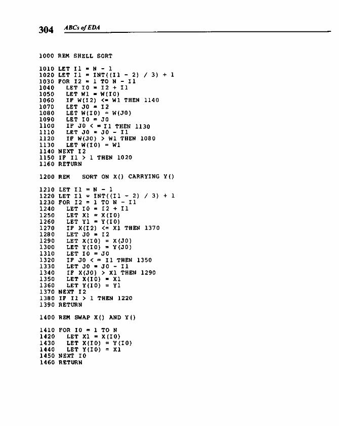
3 0 4 ABCs °fEDA
1000 REM SHELL SORT
1010 LET II = N - 11020 LET II = INT((I1 - 2) / 3) + 11030 FOR 12 = 1 TO N - II1040 LET 10 = 12 + II1050 LET Wl = W(I0)1060 IF W(I2) <= Wl THEN 11401070 LET JO = 121080 LET W(I0) = W(J0)1090 LET 10 = JO1100 IF JO < = II THEN 11301110 LET JO = JO - II1120 I F W(J0) > Wl THEN 10801130 LET W(I0 ) = Wl1140 NEXT 121150 IF II > 1 THEN 10201160 RETURN
1200 REM SORT ON X() CARRYING Y()
1210 LET II = N - 11220 LET II = INT((I1 - 2) / 3) + 11230 FOR 12 = 1 TO N - II1240 LET 10 = 12 + II1250 LET XI = X(I0)1260 LET Yl = Y(I0)1270 IF X(I2) <= XI THEN 13701280 LET JO = 121290 LET X(I0) = X(J0)1300 LET Y(I0) = Y (JO)1310 LET 10 = JO1320 IF JO < = II THEN 13501330 LET JO = JO - II1340 IF X(J0) > XI THEN 12901350 LET X(I0) = XI1360 LET Y(I0) = Yl1370 NEXT 121380 IF II > 1 THEN 12201390 RETURN
1400 REM SWAP X() AND Y()
1410 FOR 10 = 1 TO N1420 LET XI = X(I0)1430 LET X(I0) = Y(I0)1440 LET Y(I0) = XI1450 NEXT 101460 RETURN
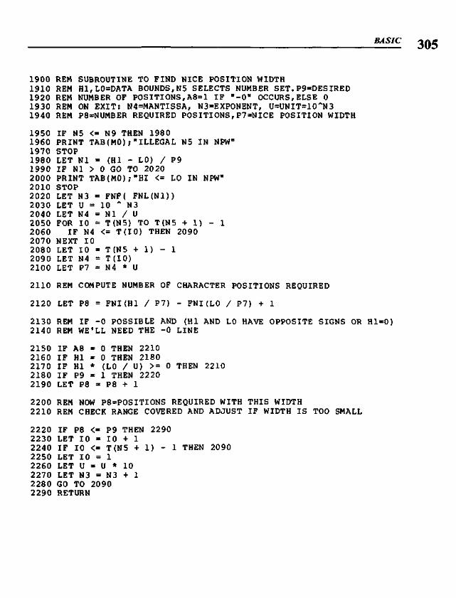
BASIC
1900 REM SUBROUTINE TO FIND NICE POSITION WIDTH1910 REM H1,LO=DATA BOUNDS,N5 SELECTS NUMBER SET.P9=DESIRED1920 REM NUMBER OF POSITIONS, A8=l IF "-011 OCCURS, ELSE 01930 REM ON EXIT: N4=MANTISSA, N3=EXPONENT, U=UNIT=10*N31940 REM P8=NUMBER REQUIRED POSITIONS,P7=NICE POSITION WIDTH
1950 IF N5 <= N9 THEN 19801960 PRINT TAB(M0);"ILLEGAL N5 IN NPW"1970 STOP1980 LET Nl = (HI - LO) / P91990 IF Nl > 0 GO TO 20202000 PRINT TAB(M0);"HI <= LO IN NPW"2010 STOP2020 LET N3 = FNF( FNL(Nl))2030 LET U = 10 " N32040 LET N4 = Nl / U2050 FOR 10 = T(N5) TO T (N 5 + 1) - 12060 IF N4 <= T(I0) THEN 20902070 NEXT 102080 LET 10 = T(N5 + 1) - 12090 LET N4 = T(I0)
2100 LET P7 = N4 * U
2110 REM COMPUTE NUMBER OF CHARACTER POSITIONS REQUIRED
2120 LET P8 = FNI(H1 / P7) - FNI (LO / P7) + 12130 REM IF -0 POSSIBLE AND (HI AND LO HAVE OPPOSITE SIGNS OR Hl=0)2140 REM WE'LL NEED THE -0 LINE
2150 IF A8 = 0 THEN 22102160 IF HI = 0 THEN 21802170 IF HI * (LO / U) >= 0 THEN 22102180 IF P9 = 1 THEN 22202190 LET P8 = P8 + 1
2200 REM NOW P8=POSITIONS REQUIRED WITH THIS WIDTH2210 REM CHECK RANGE COVERED AND ADJUST IF WIDTH IS TOO SMALL
2220 IF P8 <= P9 THEN 22902230 LET 10 = 10 + 12240 IF 10 <= T(N5 + 1) - 1 THEN 20902250 LET 10 = 12260 LET U = U * 102270 LET N3 = N3 + 12280 GO TO 20902290 RETURN
305
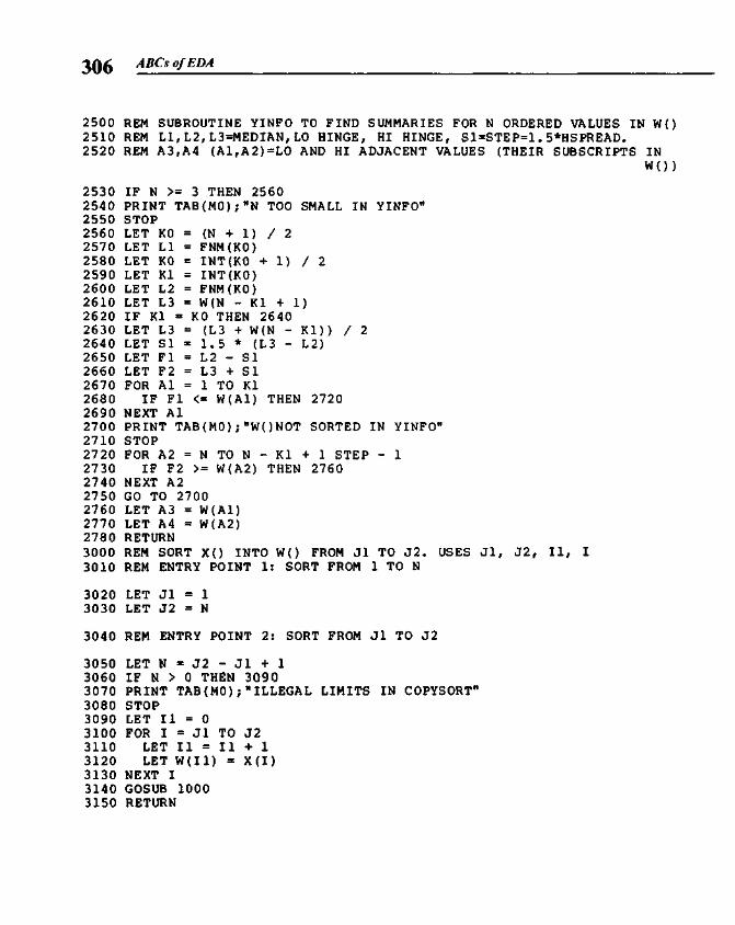
ABCs °fEDA
2 5 0 0 REM SUBROUTINE YINFO TO FIND SUMMARIES FOR N ORDERED VALUES IN W()2 5 1 0 REM L 1 , L 2 , L 3 = M E D I A N , L O HINGE, HI HINGE, S 1 = S T E P = 1 . 5 * H S P R E A D .2 5 2 0 REM A 3 , A 4 ( A 1 , A 2 ) = L O AND HI ADJACENT VALUES (THEIR SUBSCRIPTS IN
W ( ) )
2530 IF N >= 3 THEN 25602540 PRINT TAB(M0);"N TOO SMALL IN YINFO"2550 STOP2560 LET K0 = (N + 1) / 22570 LET LI = FNM(KO)2580 LET KO = INT(K0 + 1) / 22590 LET Kl = INT(KO)2600 LET L2 = FNM(KO)2610 LET L3 = W(N - Kl + 1)2620 IF Kl = KO THEN 26402630 LET L3 = (L3 + W(N - Kl)) / 22640 LET SI = 1.5 * (L3 - L2)2650 LET Fl = L2 - SI2660 LET F2 = L3 + SI2670 FOR Al = 1 TO Kl2680 IF Fl <= W(A1) THEN 27202690 NEXT Al2700 PRINT TAB(MO);"W()NOT SORTED IN YINFO"2710 STOP2720 FOR A2 = N TO N - Kl + 1 STEP - 12730 IF F2 >= W(A2) THEN 27602740 NEXT A22750 GO TO 27002760 LET A3 = W(A1)2770 LET A4 = W(A2)2780 RETURN3000 REM SORT X() INTO W() FROM Jl TO J2. USES Jl, 32, II, I3010 REM ENTRY POINT 1: SORT FROM 1 TO N
3020 LET Jl = 13030 LET J2 = N
3040 REM ENTRY POINT 2: SORT FROM Jl TO J2
3050 LET N = J2 - Jl + 13060 IF N > 0 THEN 30903070 PRINT TAB(MO);"ILLEGAL LIMITS IN COPYSORT"3080 STOP3090 LET II = 03100 FOR I = Jl TO J23110 LET II = II + 13120 LET W(I1) = X(I)3130 NEXT I3140 GOSUB 10003150 RETURN
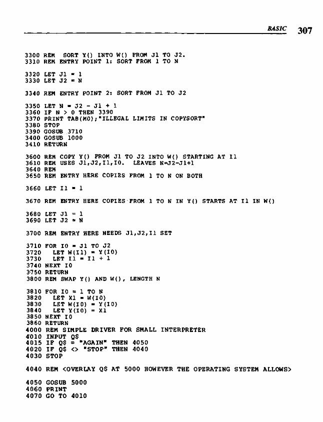
BASIC
3300 REM SORT Y() INTO W() FROM Jl TO J2.3310 REM ENTRY POINT 1: SORT FROM 1 TO N
3320 LET Jl = 13330 LET J2 = N
3340 REM ENTRY POINT 2: SORT FROM Jl TO J2
3350 LET N = J2 - Jl + 13360 IF N > 0 THEN 33903370 PRINT TAB(MO);"ILLEGAL LIMITS IN COPYSORT"3380 STOP3390 GOSUB 37103400 GOSUB 10003410 RETURN
3600 REM COPY Y() FROM Jl TO J2 INTO W() STARTING AT II3610 REM USES Jl,J2,Il,I0. LEAVES N=J2-J1+13640 REM3650 REM ENTRY HERE COPIES FROM 1 TO N ON BOTH
3660 LET II = 1
3670 REM ENTRY HERE COPIES FROM 1 TO N IN Y() STARTS AT II IN W()
3680 LET Jl = 13690 LET J2 = N
3700 REM ENTRY HERE NEEDS J1,J2,I1 SET
3710 FOR 10 = Jl TO J23720 LET W(I1) = Y(I0)3730 LET II = II + 13740 NEXT 103750 RETURN3800 REM SWAP Y() AND W(), LENGTH N
3810 FOR 10 = 1 TO N3820 LET XI = W(I0)3830 LET W(I0) « Y(I0)3840 LET Y(I0) = XI3850 NEXT 103860 RETURN4000 REM SIMPLE DRIVER FOR SMALL INTERPRETER4010 INPUT Q$4015 IF Q$ = "AGAIN" THEN 40504020 IF Q$ <> "STOP" THEN 40404030 STOP
4040 REM <OVERLAY Q$ AT 5000 HOWEVER THE OPERATING SYSTEM ALLOWS>
4050 GOSUB 50004060 PRINT4070 GO TO 4010
307
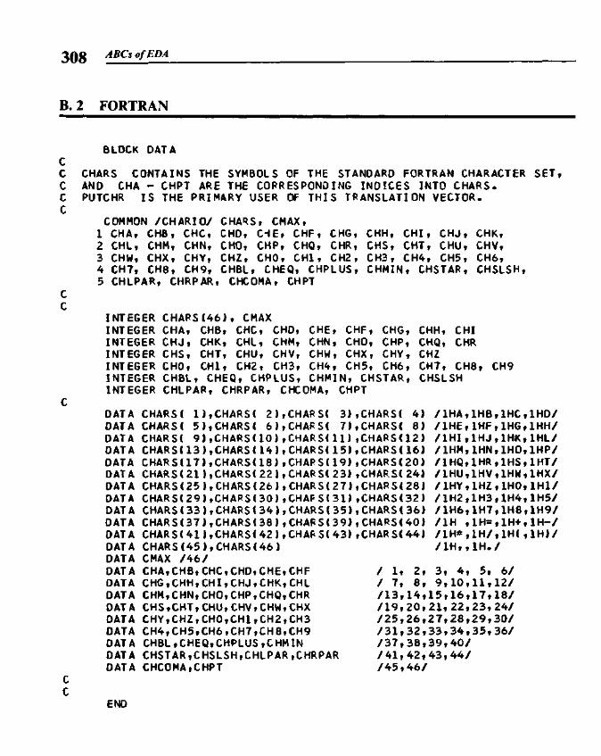
3 0 8 ABCs °fEDA
B. 2 FORTRAN
BLOCK DATA
CHARS CONTAINS THE SYMBOLS OF THE STANDARD FORTRAN CHARACTER SET,AND CHA - CHPT ARE THE CORRESPONDING INDICES INTO CHARS.PUTCHR IS THE PRIMARY USER OF THIS TRANSLATION VECTOR.
COMMON /CHARIO/ CHARS, CMAX,1 CHA, CHB, CHC, CHD, CHE, CHF, CHG, CHH, C H I , CHJ, CHK,2 CHL, CHM, CHN, CHO, CHP, CHQ, CHR, CHS, CHT, CHU, CHV,3 CHW, CHX, CHY, CHZ, CHO, C H I , CH2, CH3, CH4, CH5, CH6,4 CH7, CH8, CH9, CHBL, CHEQ, CHPLUS, CHMIN, CHSTAP, CHSLSH,5 CHLPAR, CHRPAR, CHCOMA, CHPT
INTEGER CHAPS(46) , CMAXINTEGER CHA, CHB, CHC, CHD, CHE, CHF, CHG, CHH, CHIINTEGER CHJ, CHK, CHL, CHM, CHN, CHO, CHP, CHQ, CHRINTEGER CHS, CHT, CHU, CHV, CHW, CHX, CHY, CHZINTEGER CHO, CHI , CH2, CH3, CH4, CH5, CH6, CH7, CH8, CH9INTEGER CHBL, CHEQ, CHPLUS, CHMIN, CHSTAR, CHSLSHINTEGER CHLPAR, CHRPAR, CHCOMA, CHPT
DATADATADATADATADATADATADATADATADATADATADATADATADATADATADATADATADATADATADATADATADATADATA
END
CHARSC 1),CHARSC 2),CHARS( 3)CHARS( 5),CHARSC 6),CHARS( 7)CHARSC 9),CHARS(10),CHARS(11)CHARS(13),CHARSC14),CHARSC15)CHARSC17),CHARSC18),CHAPSC19)CHARS(21),CHARSC22),CHARSC23)CHARSC25),CHARS(26),CHARS (27)CHARS(29),CHAPS(30),CHAFS(31)CHARS(33),CHARS(34),CHARS(35)CHARS(37),CHARS(38),CHAPS(39)CHARS(41),CHARS(42),CHAFS(43)CHARS(45),CHARS(46)CMAX /46/CHA,CHB,CHC,CHD,CHE,CHFCHG,CHH,CHI,CHJ,CHK,CHLCHM,CHN,CHO,CHP,CHQ,CHRCHS,CHT,CHU,CHV,CHW,CHXCHY,CHZ,CH0,CHl,CH2,CH3CH4,CH5,CH6,CH7,CH8,CH9CHBL,CHEQ,CHPLUS,CHMINCHSTAR,CHSLSH,CHLPAR,CHRPARCHCOMA,CHPT
,CHARS( 4),CHARS( 8),CHARS(12),CHARS(16),CHARS(20),CHARS(24),CHARS(28),CHARSC32),CHARSC36),CHARSC40),CHARSC44)
/1HA,/1HE,/1HI,/1HM,/1HQ,/1HU,/1HY,/1H2,/1H6,/1H ,/1H*,/1H,,
1HB,1HC,1HF,1HG,1HJ,1HK,1HN,1HO,1HR,1HS,1HV,1HH,1HZ,1HO,1H3,1H4,1H7,1H8,1H=,1H+,1H/.1HC,1H./
1HD/1HH/1HL/1HP/1HT/1HX/1H1/1H5/1H9/1H-/1H)/
/ 1,/ 7,/13,/19,/25,/31,/37,M l ,/45,
2, 3,8, 9,14,15,20,21,26,27,32,33,38,39,42,43,46/
4, 5, 6/10,11,12/16,17,18/22,23,24/28,29,30/34,35,36/40/44/
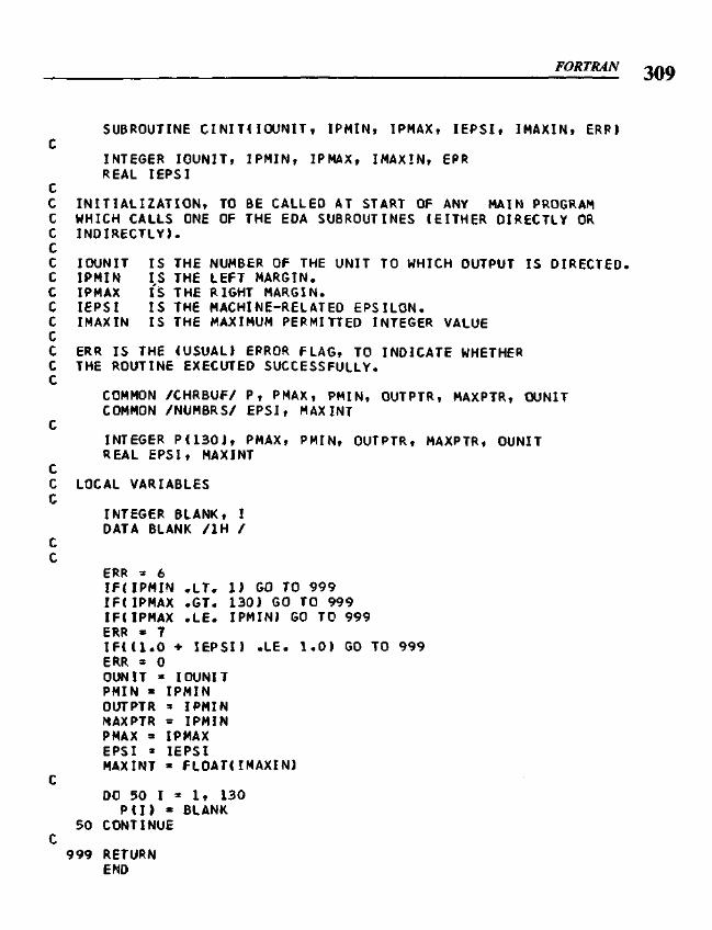
FORTRAN 309
SUBROUTINE CINITdOUNIT, IPMIN, IPMAX, IEPSI, IMAXIN, ERR)
INTEGER IOUNIT, IPMIN, IPMAX, IMAXIN, EPRREAL IEPSI
INITIALIZATION, TO BE CALLED AT START OF ANY MAIN PROGRAMWHICH CALLS ONE OF THE EDA SUBROUTINES (EITHER DIRECTLY ORINDIRECTLY).
IOUNIT IS THE NUMBER OF THE UNIT TO WHICH OUTPUT IS DIRECTED.IPMIN IS THE LEFT MARGIN.IPMAX IS THE RIGHT MARGIN.IEPSI IS THE MACHINE-RELATED EPSILON.IMAXIN IS THE MAXIMUM PERMITTED INTEGER VALUE
ERR IS THE (USUAL) ERROR FLAG, TO INDICATE WHETHERTHE ROUTINE EXECUTED SUCCESSFULLY.
COMMON /CHRBUF/ P, PMAX, PMIN, OUTPTR, MAXPTR, OUNITCOMMON /NUMBRS/ EPSI, MAX INT
INTEGER P(130), PMAX, PMIN, OUTPTR, MAXPTR, OUNITREAL EPSI, MAXINT
LOCAL VARIABLES
INTEGER BLANK, IDATA BLANK /1H /
1) GO TO 999130) GO TO 999IPMIN) GO TO 999
IEPSI) .LE. 1.0) GO TO 999
50
ERR = 6IFUPMIN .LT .IF( IPMAX .GT.IF(IPMAX .LE.ERR = 7IFU1.0 +ERR = 0OUNIT = IOUNITPMIN = IPMINOUTPTR ' IPMINMAXPTR = IPMINPMAX =* IPMAXEPSI = IEPSIMAXINT = FLOAT(IMAXIN)
DO 50 I = It 130P(I) = BLANK
CONTINUE
999 RETURNEND
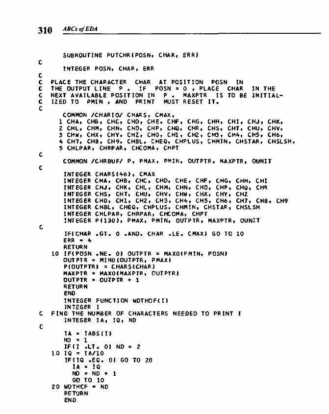
ABCsofEDA
SUBROUTINE PUTCHRtPOSNt CHAR, ERR)C
INTEGER POSN, CHAR, ERRCC PLACE THE CHARACTER CHAR AT POSITION POSN INC THE OUTPUT LINE P . IF POSN * 0 , PLACE CHAR IN THEC NEXT AVAILABLE POSITION IN P . MAXPTR IS TO BE INITIAL-C IZED TO PMIN , AND PRINT MUST RESET IT.C
COMMON /CHARIO/ CHARS, CMAX,1 CHA, CHB, CHC, CHO, CHE, CHF, CHG, CHH, CHI, CHJ, CHK,2 CHL, CHM, CHN, CHO, CHP, CHQ, CHR, CHS, CHT, CHU, CHV,3 CHW, CHX, CHY, CHZ, CHO, CHI, CH2, CH3, CH4, CH5, CH6,4 CH7, CH8, CH9, CHBL, CHEQ, CHPLUS, CHMIN, CHSTAR, CHSLSH,5 CHLPAR, CHRPAR, CHCOMA, CHPT
CCOMMON /CHRBUF/ P, PMAX, PMIN, OUTPTR, MAXPTR, OUNIT
CINTEGER CHARSC46), CMAXINTEGER CHA, CHB, CHC, CHD, CHE, CHF, CHG, CHH, CHIINTEGER CHJ, CHK, CHL, CHM, CHN, CHO, CHP, CHQ, CHRINTEGER CHS, CHT, CHU, CHV, CHW, CHX, CHY, CHZINTEGER CHO, CHI, CH2, CH3, CH4, CH5, CH6, CH7, CH8, CH9INTEGER CHBL, CHEQ, CHPLUS, CHMIN, CHSTAR, CHSLSHINTEGER CHLPAR, CHRPAR, CHCOMA, CHPTINTEGER P(130), PMAX, PMIN, OUTPTR, MAXPTR, OUNIT
CIFCCHAR .GT. 0 .AND. CHAR .LE. CMAX) GO TO 10ERR = 4RETURN
10 IFCPOSN . N E . 0) OUTPTR = MAXO(PMIN, POSN)OUTPTR = MINO(OUTPTR, PMAX)P(OUTPTR) = CHARS(CHAR)MAXPTR = MAXOCMAXPTR, OUTPTR)OUTPTR = OUTPTR + 1RETURNENDINTEGER FUNCTION WDTHOF(I)INTEGER I
C FIND THE NUMBER OF CHARACTERS NEEDED TO PRINT IINTEGER I A , I Q , ND
CIA = I A B S ( I )ND = 1I F ( I . L T . 0) ND = 2
10 IQ = I A / 1 0I F ( I Q .EQ. 0) GO TO 20
IA = IQND ' ND + 1GO TO 10
20 WDTHCF = NDRETURNEND
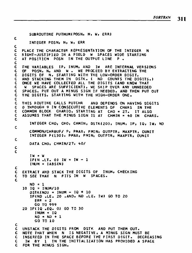
FORTRAN 311
SUBROUTINE PUTNUMCPOSN, N, W, ERR)C
INTEGER POSN, N, Wt ERR
cC PLACE THE CHARACTER REPRESENTATION OF THE INTEGER NC RIGHT-JUSTIFIED IN A FIELD W SPACES WIDE STARTINGC AT POSITICN POSN IN THE OUTPUT LINE P .CC THE VARIABLES I P , INUM, AND IW ARE INTERNAL VERSIONSC OF POSN, N, AND W . WE PROCEED BY EXTRACTING THEC DIGITS OF N, STARTING WITH THE LOW-ORDER D I G I T ,C AND STACKING THEM IN DSTK. ( ND COUNTS THE D I G I T S . )C ONCE WE HAVE COLLECTED ALL THE DIGITS (AND KNOW THATC W SPACES ARE SUFFICIENT) , WE SKIP OVER ANY UNNEEDEDC SPACES, PUT OUT A MINUS SIGN I F NEEDED, AND THEN PUT OUTC THE D IG ITS , STARTING WITH THE HIGH-ORDER ONE.CC THIS ROUTINE CALLS PUTCHR AND DEPENDS ON HAVING DIGITSC 0 THROUGH 9 IN CONSECUTIVE ELEMENTS OF CHARS IN THEC COMMON BLOCK CHARIO, STARTING AT CHO = 27. IT ALSOC ASSUMES THAT THE MINUS SIGN IS AT CHMIN = 40 IN CHARS.C
INTEGER CHD, CHO, CHMIN, DSTK(20), INUM, IP, IQ, IW, NDC
COMMON/CHRBUF/ P, PMAX, PMIN, OUTPTR, MAXPTR, OUNITINTEGER P(130), PMAX, PMIN, OUTPTR, MAXPTR, OUNIT
CDATA CHO, CHMIN/27, 40/
CC
IW = WIF(N .LT. 0) IW = IW - 1INUM = IABS(N)
CC EXTRACT AND STACK THE DIGITS OF INUM, CHECKINGC TO SEE THAT N FITS IN W SPACES.C
ND = 110 IQ = INUM/10
DSTK(ND) = INUM - IQ * 10I F ( N D . L E . 20 . A N D . ND . L E . IW) GO TO 2 0
ERR = 2GO TO 9 9 9
20 I F ( I Q . E Q . 0 ) GO TO 3 0INUM - IQND = ND + 1GO TO 10
CC UNSTACK THE DIGITS FROM DSTK AND PUT THEM OUT.C NOTE THAT WHEN N IS NEGATIVE, A MINUS SIGN MUST BEC INSERTED IN THE SPACE BEFORE THE FIRST D I G I T . DECREASINGC IW BY 1 IN THE IN IT IAL IZAT ION HAS PROVIDED A SPACEC FOR THE MINUS SIGN.
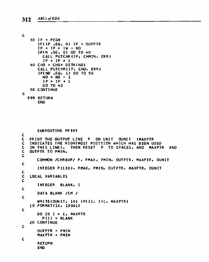
3 2 2 ABCsofEDA
30 IP = PCSNIF( IP .EQ. 0) IP = OUTPTRIP = IP • IW - NDI F ( N .GE. 0) GO TO 40
CALL PUTCHRUP, CHMIN, ERR)IP = IP + 1
40 CHD = CHO+ DSTK(ND)CALL PUTCHRUP, CHD, ERR)IFCND .EQ. 1) GO TO 50
NO = ND - 1I P = IP + 1GO TO 40
50 CONTINUEC
999 RETURNEND
SUBROUTINE PRINTCC PRINT THE OUTPUT LINE P ON UNIT OUNIT (MAXPTRC INDICATES THE RIGHTMOST POSITION WHICH HAS BEEN USEDC IN THIS L I N E ) . THEN RESET P TO SPACES, AND MAXPTR ANDC OUTPTR TO PMIN.C
COMMON /CHRBUF/ P, PMAX, PMIN, OUTPTR, MAXPTR, OUNITC
INTEGER P ( 1 3 0 ) , PMAX, PMIN, OUTPTR, MAXPTR, OUNITCC LOCAL VARIABLESC
INTEGER BLANK, IC
DATA BLANK /1H /C
WRITE(OUNIT, 10) ( P ( I ) , 1 = 1 , MAXPTR)10 FORMATdX, 130A1)
CDO 20 I = 1 , MAXPTR
P(I) = BLANK20 CONTINUE
COUTPTR = PMINMAXPTR = PMIN
CRETURNEND
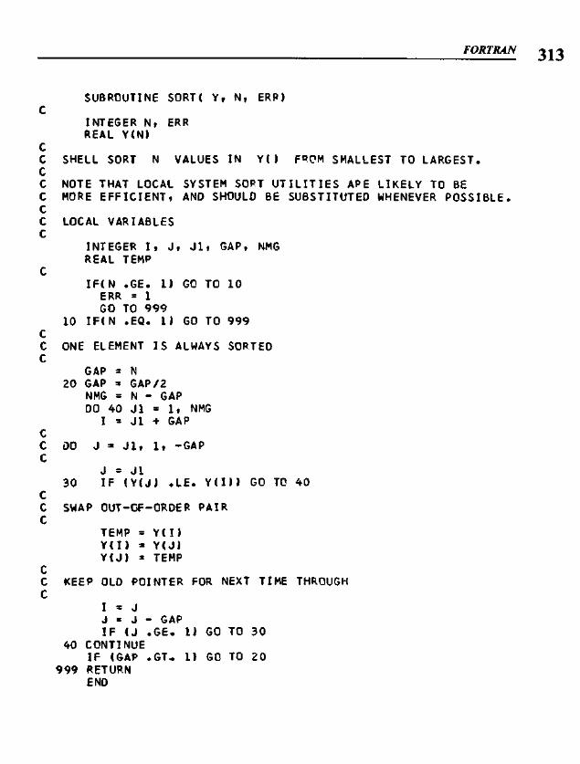
FORTRAN
SUBROUTINE SORT( Y, N, ERP)C
INTEGER N, ERRREAL Y(N)
CC SHELL SORT N VALUES IN Y d FROM SMALLEST TO LARGEST.CC NOTE THAT LOCAL SYSTEM SORT UTILITIES APE LIKELY TO BEC MORE EFFICIENT, AND SHOULD BE SUBSTITUTED WHENEVER POSSIBLE.CC LOCAL VARIABLESC
INTEGER It J, Jl» GAP, NMGREAL TEMP
CIF(N .GE. 1) GO TO 10ERR = 1GO TO 999
10 IF(N .EQ. 1) GO TO 999CC ONE ELEMENT IS ALWAYS SORTEDC
GAP - N20 GAP = GAP/2
NMG - N - GAPDO 40 Jl = 1, NMG
I * Jl • GAPCC DO J = Jl, 1, -GAPC
J = Jl30 IF (Y(J) .LE. Y(I)) GO TO 40
CC SWAP OUT-CF-ORDEP PAIRC
TEMP a Y d )Y ( I ) * Y ( J )Y ( J ) = TEMP
CC KEEP OLD POINTER FOR NEXT TIME THROUGHC
I « JJ = J - GAPIF (J .GE. 1) GO TO 30
40 CONTINUEIF (GAP .GT- 1) GO TO 20
999 RETURNEND
313
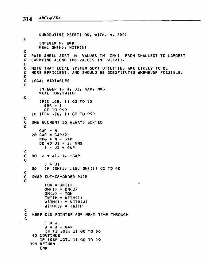
ABCsofEDA
SUBROUTINE PSORT( ONt WITH, N, ERR)C
INTEGER N, ERRREAL ON(N), WITH(N)
CC PAIR SHELL SORT N VALUES IN ON() FROM SMALLEST TO LARGESTC CARRYING ALONG THE VALUES IN WITHC).CC NOTE THAT LOCAL SYSTEM SORT UTILITIES ARE LIKELY TO BEC MORE EFFICIENT, AND SHOULD BE SUBSTITUTED WHENEVER POSSIBLE,CC LOCAL VARIABLESC
INTEGER I* J, Jit GAP, NMGREAL TON,TWITH
CIF(N .GE. 1) GO TO 10ERR = 1GO TO 999
10 IF( N .EQ. 1) GO TO 999CC ONE ELEMENT IS ALWAYS SORTEDC
GAP = N20 GAP = GAP/2
NMG - N - GAPDO 40 Jl = 1, NMG
I * Jl • GAPCC DO J = Jl, 1, -GAPC
J = Jl30 IF (CN(J) .LE. ON(I)) GO TO 40
CC SWAP CUT-CF-ORDER PAIRC
TON = ON(I)ON(I) - ON(J)ON(J) = TONTWITH = WITH(I)WITH(I) = WITH(J)WITH(J) = TWITH
CC KEEP OLD POINTER FOR NEXT TIME THROUGHC
I * JJ =* J - GAPIF (J .GE. 1) GO TO 30
40 CONTINUEIF (GAP .GT. 1) GO TG 20
999 RETURNEND
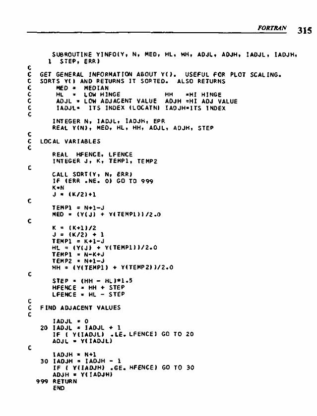
FORTRAN 315
SUBROUTINE YINFOCY, N, MEDt HL, HH, ADJLt ADJH, IADJlt IADJH,1 STEP, ERR)
CC GET GENERAL INFORMATION ABOUT Y<). USEFUL FOR PLOT SCALING.C SORTS Y() AND RETURNS IT SOPTED. ALSO RETURNSC MED * MEDIANC HL * LOW HINGE HH =HI HINGEC ADJL = LOW ADJACENT VALUE ADJH =HI ADJ VALUEC IADJL* ITS INDEX (LOCATN) IADJH=ITS INDEXC
INTEGER N, IADJL, IADJH, EPRREAL Y ( N ) , MED, HL, HH, ADJL, ADJH, STEP
CC LOCAL VARIABLESC
REAL HFENCE, LFENCEINTEGER J , K, TEMPI, TEMP2
CCALL SORTCY, N, ERR)IF (ERR .NE. 0) GO TO 999K=NJ ' (K /2J+1
CTEMPI = N + l - JMED = (Y (J ) + Y(TEMP1)) /2.O
CK = ( K + D / 2J = (K /2 ) + 1TEMPI = K + l - JHL = (Y (J ) + Y(TEMP1)) /2 ,OTEMPI » N-K+JTEMP2 ' N + l - JHH - (Y(TEMPl) + Y(TEMP2) ) /2 .0
CSTEP = (HH - HL) *1 .5HFENCE * HH + STEPLFENCE = HL - STEP
CC FIND ADJACENT VALUESC
IADJL = 020 IADJL * IADJL + 1
IF ( Y(IADJL) .LE. LFENCE) GO TO 20ADJL * Y(IADJL)
CIADJH = N+l
30 IADJH = IADJH - 1IF ( Y(IADJH) .GE. HFENCE) GO TO 30ADJH * Y(IADJH)
999 RETURNEND
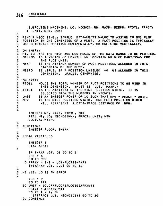
316 ABCs of EDA
SUBROUTINE NPOSW(HI, LOt NICNOS, NN, MAXP, MZERC, PTOTL, FPACTt1 UNIT, NPW, ERR)
FIND A NICE (I.E.* SIMPLE) DATA-UNITS VALUE TO ASSIGN TO ONE PLOTPOSITION IN ONE DIMENSION OF A PLOT. A PLOT POSITION IS TYPICALLYONE CHARACTER POSITION HORIZONTALLY, OR ONE LINE VERTICALLY.
ON ENTRY:HI, LO ARE THE HIGH AND LOW EDGES OF THE DATA RANGE TO BE PLOTTED,NICNOS IS A VECTOR OF LENGTH NN CONTAINING NICE MANTISSAS FOR
THE PLOT UNIT.MAXP IS THE MAXIMUM NUMBER OF PLOT POSITIONS ALLOWED IN THIS
DIMENSION OF THE PLOT.MZERO IS .TRUE. IF A POSITION LABELED -0 US ALLOWED IN THIS
DIMENSION, .FALSE. OTHERWISE.
CN EXIT:PTOTL HOLDS THE TOTAL NUMBER OF PLOT POSITIONS TC BE USED IN
THIS DIMENSION. (MUST BE .LE. MAXP.)FRACT IS THE MANTISSA OF THE NICE POSITION WIDTH. IT IS
SELECTED FROM THE NUMBERS IN NICNOS.UNIT IS AN INTEGER POWER OF 10 SUCH THAT NPW = FFACT * UNIT.NPW IS THE NICE POSITION WIDTH. ONE PLOT POSITION WIDTH
WILL REPRESENT A DATA-SPACE DISTANCE OF NPW.
INTEGER NN, MAXP, PTOTL, ERRREAL HI, LO, NICNOS(NN), FRACT, UNIT, NPWLOGICAL MZERO
FUNCTIONSINTEGER FLOOR, INTFN
LOCAL VARIABLES
INTEGER IREAL APRXW
IF (MAXP .GT. 0) GO TO 5ERR = 8GO TO 999
5 APRXW = ( H I - LO)/FLOAT(MAXP)IF(APRXW . G T . 0 . 0 ) GO TO 10
HI . L E . LO IS AN ERROR
ERR = 9GO TO 999
10 UNIT = 10.0**FLOOR(ALOG10(APRXW) )FRACT = APRXW/UNITDO 20 I = 1 , NNIF(FRACT .LE. NICNOS(D) GO TO 30
20 CONTINUE
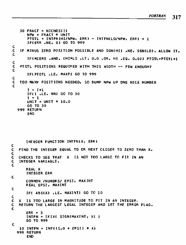
FORTRAN 317
30 FRACT = NICNOS(I )NPW = FRACT * UNITPTOTL = INTFNCHI/NPW, ERR) - INTFNCLO/NPW, ERR) + 1IFCERR . N E . 0 ) GO TO 999
CC IF MINUS ZERO POSITION POSSIBLE AND SGN(HI) . N E . SGN(LO), ALLOW I T .C
IF(MZERO .AND. (H I *LO . L T . 0 . 0 .OR. HI . E Q . 0 . 0 ) ) PTOTL=PTOTL+1CC PTOTL POSITIONS REQUIRED WITH THIS WIDTH — FEW ENOUGH?C
IF(PTOTL . L E . MAXP) GO TO 999CC TOO MANY POSITIONS NEEDED, SO BUMP NPW UP ONE NICE NUMBERC
I = 1+1I F ( I .LE. NN) GO TO 30I = 1UNIT = UNIT * 10.0GO TO 30
999 RETURNEND
INTEGER FUNCTION INTFN(X, ERR)CC FIND THE INTEGER EQUAL TO OR NEXT CLOSER TO ZERO THAN X.CC CHECKS TO SEE THAT X IS NOT TOO LARGE TO FIT IN ANC INTEGER VARIABLE.C
REAL XINTEGER ERR
CCOMMON /NUMBRS/ EPSI, MAX INTREAL EPSI, MAXINT
CIF( ABS(X) .LE. MAXINT) GO TC 10
CC X IS TOO LARGE IN MAGNITUDE TO FIT IN AN INTEGER,C RETURN THE LARGEST LEGAL INTEGER AND SET THE ERROR FLAG.C
ERR = 3INTFN = IFIX( SIGN(MAXINT, X) )GO TO 999
C10 INTFN = INTU1.0 + EPSI) * X)
999 RETURNEND
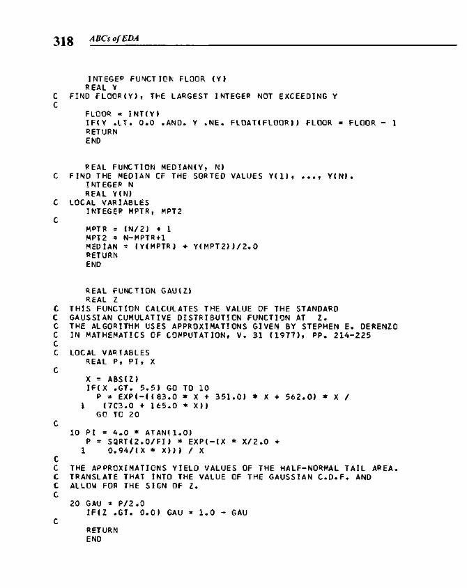
ABCsofEDA
I N T E G E P F U N C T I O N FLOOR ( Y )REAL Y
C FIND FLOOR(Y), THE LARGEST INTEGEP NOT EXCEEDING YC
FLOOR = INT(Y)IF(Y .LT. 0.0 .AND. Y .NE. FLOAT!FLOOR)) FLOOR = FLOOR - 1RETURNEND
PEAL FUNCTION MEDIAN(Y, N)C FIND THE MEDIAN CF THE SORTED VALUES Y d ) , . . . , Y ( N ) .
INTEGER NREAL Y(N)
C LOCAL VARIABLESINTEGEP MPTR, MPT2
CMPTR = (N/2) + 1MPT2 = N-MPTR+1MEDIAN * (Y(MPTR) + Y ( M P T 2 ) ) / 2 . 0RETURNEND
REAL FUNCTION GAU(Z)REAL Z
C THIS FUNCTION CALCULATES THE VALUE OF THE STANDARDC GAUSSIAN CUMULATIVE DISTRIBUTION FUNCTION AT Z .C THE ALGORITHM USES APPROXIMATIONS GIVEN BY STEPHEN E. DERENZOC IN MATHEMATICS OF COMPUTATION, V . 31 ( 1 9 7 7 ) , PP. 2 1 4 - 2 2 5CC LOCAL VARIABLES
REAL P, P I , XC
X = ABS(Z)I F ( X . G T . 5 . 5 ) GO TO 1 0
P = E X P < - < ( 8 3 . 0 * X + 3 5 1 . 0 ) * X + 5 6 2 . 0 ) * X /1 ( 7C3 .0 + 1 6 5 . 0 * X ) )
GO TO 20C
10 P I = 4 . 0 * A T A N ( l . O )P = SQRTC2 .0 /F I ) * E X P ( - ( X * X / 2 . 0 +
1 0 . 9 4 / < X * X ) ) ) / XCC THE APPROXIMATIONS YIELD VALUES OF THE HALF-NORMAL TAIL AREA.C TRANSLATE THAT INTO THE VALUE OF THE GAUSSIAN C . D . F . ANDC ALLOW FOP THE SIGN OF Z.C
20 GAU = P / 2 . 0I F ( Z .GT . 0 . 0 ) GAU = 1 .0 - GAU
CRETURNEND
Appendix CProgramming
Conventions
The programs in this book form two sets of routines, one in BASIC and one inFORTRAN. This appendix discusses the structure and language conventionsadopted for these programs. The first part of the appendix covers the BASICprograms. The second part deals with the FORTRAN programs.
C.I BASIC
Environment
The BASIC programs in this book are written to run conveniently oncomputers using an interactive BASIC interpreter. In particular, most mini-and microcomputers should accept these programs with only minor modifica-tions. Users of systems where BASIC is compiled rather than interpreted mayhave to write a driver program to facilitate interprogram communication. This
319
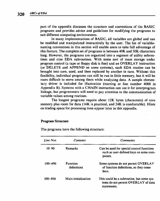
3 2 0 ABCs °fEDA
part of the appendix discusses the structure and conventions of the BASICprograms and provides advice and guidelines for modifying the programs tosuit different computing environments.
In many implementations of BASIC, all variables are global and canbe modified and manipulated interactively by the user. The list of variable-naming conventions in this section will enable users to take full advantage ofthis feature. The complete set of programs is between 40K and 50K characterslong. However, the programs are organized into a segment of utility subrou-tines and nine EDA subroutines. With some sort of mass storage underprogram control (a tape or floppy disk is fine) and an OVERLAY instruction(or DELETE and APPEND on some systems), each EDA routine can bebrought into core, used, and then replaced by another in turn. Without thisflexibility, individual programs can still be run in little memory, but it will bemore difficult to move among them while analyzing data. A sample elemen-tary driver is included for illustration (starting at line number 4000 inAppendix B). Systems with a CHAIN instruction can use it for interprogramlinkage, but programmers will need to pay attention to the communication ofvariable values among routines.
The longest programs require about 12K bytes (characters) of corememory plus room for data (16K is practical, and 24K is comfortable). Hintson trading space for processing time appear later in this appendix.
Program Structure
The programs have the following structure:
Line Nos.
10-90
100-490
500-800
Contents
Remarks
Functiondefinitions
Main initialization
Comments
Can be used for special control functionssuch as user-defined keys on some com-puters.
Some systems do not permit OVERLAYof function definitions, so they comehere.
This could be a subroutine, but some svs-terns do not permit OVERLAY of datastatements.
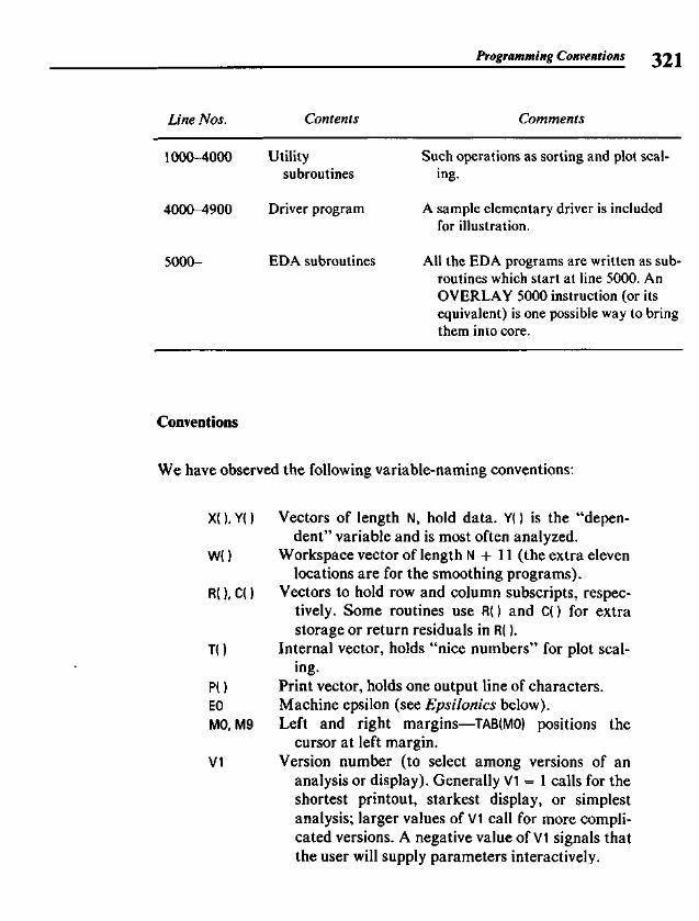
Programming Conventions 3 2 1
Line Nos. Contents Comments
1000-4000 Utilitysubroutines
4000-4900 Driver program
5000- EDA subroutines
Such operations as sorting and plot scal-ing.
A sample elementary driver is includedfor illustration.
All the EDA programs are written as sub-routines which start at line 5000. AnOVERLAY 5000 instruction (or itsequivalent) is one possible way to bringthem into core.
Conventions
W e have observed the following variable-naming conventions:
X(). Y() Vectors of length N, hold data. Y() is the "depen-dent" variable and is most often analyzed.
W() Workspace vector of length N + 11 (the extra elevenlocations are for the smoothing programs).
R(), C() Vectors to hold row and column subscripts, respec-tively. Some routines use R() and C() for extrastorage or return residuals in R().
T() Internal vector, holds "nice numbers" for plot scal-ing.
P() Print vector, holds one output line of characters.E0 Machine epsilon (see Epsilonics below).M0, M9 Left and right margins—TAB(MO) positions the
cursor at left margin.V1 Version number (to select among versions of an
analysis or display). Generally V1 = 1 calls for theshortest printout, starkest display, or simplestanalysis; larger values of V1 call for more compli-cated versions. A negative value of V1 signals thatthe user will supply parameters interactively.
3 2 2 ABCs °fEDA
Whenever possible, work is done in W(), and X() and Y() are preserved or onlyreordered. The design philosophy of the BASIC programs has favoredminimizing the space required for the storage of data. At times this requiresthat X() and Y() be destroyed or used to return a result. On systems with noconstraints on storage, extra arrays to preserve X() and Y() would be valuableand could easily be introduced.
Space versus Speed
The most expensive operation commonly performed by these programs issorting. Users of microcomputers may find the sorting process noticeably slow.A machine-language sorting program will significantly extend the size of databatches that can be conveniently analyzed. Programmers who wish to optimizethis code for a specific machine should first provide a fast sorting program. Noother optimization will have nearly as great an effect.
To save space, programs may delete lines 480-790 after they have beenexecuted. Or, if permitted, initialization can be made a subroutine at line 5000to be called first. Also, most of the EDA subroutines (and all the longsubroutines) can be split into two or more segments to be executed insequence. Thus, for example, plot options could be checked in one programsegment; then a second segment could determine plot scaling; and finally, athird segment could produce the plot.
Epsilonics
The decimal numbers with which humans customarily work cannot generallybe represented exactly in the binary (or, sometimes, hexadecimal) forms usedby most computers. For example, when written as a binary fraction, thenumber 1/10 is a repeating fraction (.000110011 . . . in binary digits).Because computers store real numbers in fixed-length words, their internalrepresentation will usually be only a very close approximation to the truenumber. For example, LOG(1000) may be slightly different from 3.0. Therepresentation errors that occur in converting decimal numbers to binary andthe rounding errors that arise in subsequent arithmetic have a negligible effecton most EDA calculations, but there are important exceptions. One of these isthe floor operation (the INT function in BASIC; see Rounding Functions,
Programming Conventions
below), used especially in scaling plots and placing characters precisely fordisplays. For example, INT(2.9999) yields 2.0. Thus, because LOG(IOOO)may not be represented as exactly 3, INT(LOG(1000)) might come out 2rather than 3. If we do not allow for these errors, small as they may be, manyprograms will run into serious (and obscure) trouble. To correct this problem,we introduce a machine-dependent constant, epsilon (E0 in the BASICprograms), which is the smallest number such that (in the computer'sarithmetic) 1.0 + e > 1.0. We use a slightly larger number for E0. (1.0 E-6works well on most machines which use 4 bytes to hold a number.) If E0 is toosmall, many anomalous things can happen, including incorrect stem-and-leafdisplays and x-y plots.
Some BASIC implementations provide a user-adjusted "fuzz" factorthat will accomplish a similar function in computations. This feature may beable to replace the epsilon in the defined functions FNF and FNI.
BASIC Portability
The BASIC programs in this book are written in a dialect of BASIC as closeto the ANSI minimal BASIC standard as possible. Since few BASICimplementations are in fact ANSI-standard, we note here some specificfeatures that may require the attention of a programmer when installing theseprograms. (Our reference for some of these notes is "BASIC REVISITED,An Update to Interdialect Translatability of the BASIC ProgrammingLanguage" by Gerald L. Isaacs, CONDUIT, University of Iowa, 1976.)
Variable Names. BASIC variable names are single letters or a single letterfollowed by a single digit. Some implementations of BASIC permit longervariable names, but a program using longer names would not be portable. Wehave deliberately made some variable names mnemonic. Thus L0 (L-zero) andH1 (H-one) often hold the low and high data values of a batch. String variablesobey the same rules and end in $. We have restricted array names to singleletters. This is less general than the ANSI standard but required by someBASIC implementations.
String Functions. Three string-related functions not in the ANSI standardare used throughout the programs for displays. These are
LEN(A$) The number of characters in the string A$.STR$(N) The numerals representing the number INI. This
3 2 4 ABCs °fEDA
function is needed to produce a numeral with noblank spaces before or after it. One possiblesubstitute is a subroutine that constructs thenumeral string by selecting characters from astring array or from the string "0123456789" byusing a substring operation.
ASCC'C") The ASCII code value of the character "C". Thisfunction is used for ease of exposition and caneasily be replaced by the literal numeric value.Non-ASCII systems should use the appropriatecharacter codes.
Some of these functions have different names on some systems.
String Variables. The programs occasionally use string variables and stringconstants. String constants are enclosed in double quotes (")• Numeric codescan be substituted for many, but not all, string uses.
Loops. FOR loops are supposed to check the index variable at the top of theloop. Thus FOR I = 10 TO 9 STEP 1 should skip the loop entirely (rather thanexecuting it once). Some versions of BASIC test the index variable at the endof the loop instead. We have, therefore, provided special checks whennecessary before loops. Similarly, index variables are not defined reliably atthe end of loops. We have inserted an assignment statement after some loopsto ensure that the index variable is set correctly.
Margins. The left margin, MO, is usually set to zero. In some versions ofBASIC, TAB(O) is not the same as the first print position, so MO may need to beset to 1.
Defined Functions. The programs include several user-defined functions,but one-line defined functions are sufficient, provided that a defined functioncan use a previously defined function in its definition. The ANSI standardrequires a single argument for defined functions and global access to allvariables. If multiple-line or multiple-argument defined functions are avail-able, programmers may wish to modify some of the functions for greaterefficiency and clarity.
Rounding Functions. The programs require a function that returns thelargest integer not exceeding its argument. This is commonly known as the"floor function," but it is called INT in BASIC. Rounding functions can be asource of great confusion (and subtle bugs). We might round a number in fourways, as shown in the table.
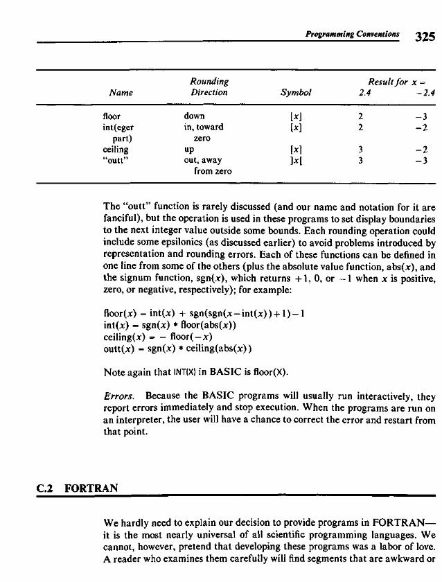
Programming Conventions 3 2 5
Rounding Result for x =Name Direction Symbol 2.4 — 2.4
floorint(eger
part)ceiling"outt"
downin, toward
zeroupout, away
from zero
wM
M}x[
22
33
- 3_ 2
- 2- 3
The "outt" function is rarely discussed (and our name and notation for it arefanciful), but the operation is used in these programs to set display boundariesto the next integer value outside some bounds. Each rounding operation couldinclude some epsilonics (as discussed earlier) to avoid problems introduced byrepresentation and rounding errors. Each of these functions can be defined inone line from some of the others (plus the absolute value function, abs(;t), andthe signum function, sgn(jc), which returns +1, 0, or - 1 when x is positive,zero, or negative, respectively); for example:
floor(x) = int(x) + sgn(sgn(x-int(x)) +1 ) -1int(x) = sgn(x) * floor(abs(jc))ceiling(jc) = - floor(-x)outt(x) = sgn(x) * ceiling(abs(x))
Note again that INT(X) in BASIC is floor(X).
Errors. Because the BASIC programs will usually run interactively, theyreport errors immediately and stop execution. When the programs are run onan interpreter, the user will have a chance to correct the error and restart fromthat point.
C.2 FORTRAN
We hardly need to explain our decision to provide programs in FORTRAN—it is the most nearly universal of all scientific programming languages. Wecannot, however, pretend that developing these programs was a labor of love.A reader who examines them carefully will find segments that are awkward or
3 2 6 ABCs °fEDA
tedious because FORTRAN is ill-suited to the programming needs of moderndata analysis. For example, the output capabilities of FORTRAN are far toorigid for the graphic and semi-graphic displays that are common in explor-atory data analysis. On the whole, however, the advantages of making theseprograms as widely available as possible outweighed the difficulties ofFORTRAN.
If programs are to be widely used, they must be portable. That is, itmust be possible to move them from one computing environment to anotherwith an absolute minimum number of changes. Fortunately for us, others havelaid substantial groundwork in developing portable (or, strictly speaking,semi-portable) FORTRAN programs. As a result, a number of practices thatfacilitate portability are well-established, and computer software to supportthe most valuable of them is available. In this part of the appendix we brieflydescribe the practices we have followed and the role they have played in thedevelopment of our programs.
Consistency of style is also important for any set of programs that areintended to be used (and read) together. Thus we also describe the particularconventions we have chosen to follow. These range from simple choices thataffect only the appearance of the printed programs to overall decisions thataffect the structure and interrelations among all the programs in this book.
Related to interconnections is the question of just how one mightcustomarily use these programs. We briefly discuss and illustrate twoapproaches to this.
And finally there are the utility routines, which perform a variety ofessential services for the data analysis routines presented in Chapters 1through 9. Listings for the utility routines appear in Appendix B.
Portability
A fully portable program or subroutine can be moved gracefully from onecomputing machine to another. And even though the computers are ofdifferent manufacture and have different systems software, the programcompiles without errors, executes without errors, and produces identically thesame results on both. This is the ideal situation. Unfortunately, it can rarely beattained in practice; but with reasonable effort a good approximation to it ispossible. The two primary obstacles to overcome are differences amongdialects of the FORTRAN language and differences in characteristics of thearithmetic hardware. (One must also contend with variations in systemconventions, but these are generally less serious.)
Programming Conventions
The solution to the problem of dialects is conceptually quite simple:One uses only a subset of FORTRAN that is handled in the same way byessentially all known systems. In practice it is all too easy to slip backunknowingly into using some facility or construction which is acceptable inone's own environment but unacceptable in certain others. To avoid this, wehave restricted our FORTRAN to a particular subset known as PFORT. Thisis an attractive solution because this subset of FORTRAN is supported by apiece of software, the PFORT Verifier (Ryder 1974), that takes aFORTRAN program as input and reports on all its departures from thissubset of the language. Especially valuable is the Verifier's ability to process amain program and all associated subroutines and to identify potential difficul-ties of communication among them, including misuse of COMMON.
When a particular construction is acceptable in many (but not all)dialects of FORTRAN, it is tempting to use it—especially when it wouldmake the programs easier to understand—and then to announce, "Theprograms conform to PFORT, except for.. . ." For example, subscript expres-sions of the form N + 1 - I are common (as in LVALS, MEDPOL, and RGCOMP),but the strict FORTRAN definition of subscript expressions is too restrictiveto permit this form. We have decided to avoid such complications and adhereto PFORT. Thus we can state that all the FORTRAN programs in this bookhave been processed by the PFORT Verifier without any warning messages.
The problem of arithmetic hardware characteristics is somewhat moredifficult than the problem of language dialects. Fortunately, EDA techniquesgenerally involve much less numerical computation than one finds in mostmathematical software. In fact, our programs need only two machine-relatedconstants: an epsilon, whose role was described earlier, and the REAL value ofthe largest valid integer. We have isolated these as the variables EPSI andMAXINT in the COMMON block NUMBRS so that they can be set once atinitialization. The initialization subroutine, CINIT, takes care of this.
CINIT, which should be called before any of the other FORTRANroutines in this book, also sets several other variables that may vary frominstallation to installation or from run to run:
OUNIT the FORTRAN unit number for output (often unit 6),PMIN the left margin in the output line,PMAX the right margin in the output line.
In CINIT, the corresponding subroutine arguments all begin with the letter I toindicate that they are initialization values. CINIT performs several basic checkson these and then completes the initialization process. In the course of a
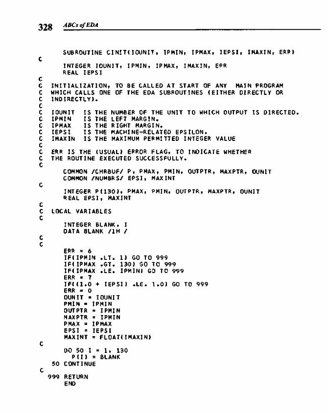
3 2 8 ABCs °fEDA
SUBROUTINE CINITdOUNIT, IPMIN, IPMAX, IEPSI, IMAXIN, ERR)C
INTEGER IOUNIT, IPMIN, IPMAX, IMAXIN, EPRREAL IEPSI
CC INITIALIZATION, TO BE CALLED AT START OF ANY MAIN PROGRAMC WHICH CALLS ONE OF THE EDA SUBROUTINES (EITHER DIRECTLY ORC INDIRECTLY).CC IOUNIT IS THE NUMBER OF THE UNIT TO WHICH OUTPUT IS DIRECTED,C IPMIN IS THE LEFT MARGIN.C IPMAX IS THE RIGHT MARGIN.C IEPSI IS THE MACHINE-RELATED EPSILON.C IMAXIN IS THE MAXIMUM PERMITTED INTEGER VALUECC ERR IS THE (USUAL) ERROR FLAG, TO INDICATE WHETHERC THE ROUTINE EXECUTED SUCCESSFULLY.C
COMMON /CHRBUF/ P, PMAX, PMIN, OUTPTR, MAXPTR, OUNITCOMMON /NUMBRS/ EPSI, MAX INT
CINTEGER P(130), PMAX, PMIN, OUTPTR, MAXPTR, OUNITREAL EPSI, MAXINT
CC LOCAL VARIABLESC
INTEGER BLANK, IDATA BLANK /1H /
CC
ERR = 6IFdPMIN .LT. 1) GO TO 999IF( IPMAX .GT. 130) GO TO 999IF(IPMAX .LE. IPMIN) GO TO 999ERR * 7I F d l . O + I E P S I ) . L E . 1 . 0 ) GO TO 999ERR = 0OUNIT * IOUNITPMIN = IPMINOUTPTR - IPMINMAXPTR = IPMINPMAX - IPMAXEPSI * IEPSIMAXINT - FLOAT(IMAXIN)
CDO 50 I = 1 , 130
P(I) = BLANK50 CONTINUE
C999 RETURN
END
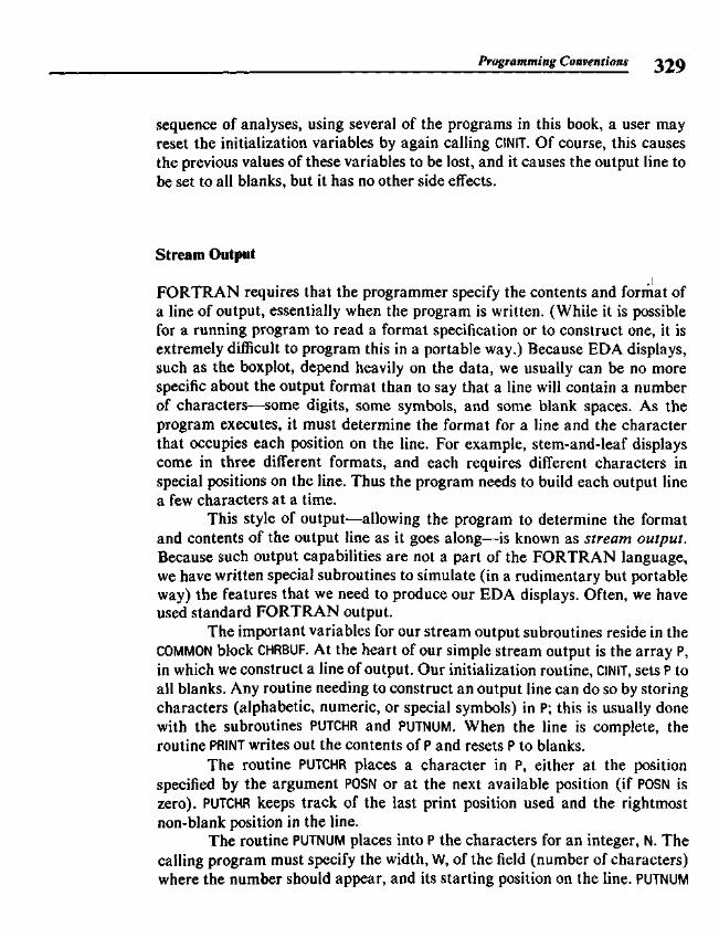
Programming Conventions 'X'JQ
sequence of analyses, using several of the programs in this book, a user mayreset the initialization variables by again calling CINIT. Of course, this causesthe previous values of these variables to be lost, and it causes the output line tobe set to all blanks, but it has no other side effects.
Stream Output
FORTRAN requires that the programmer specify the contents and format ofa line of output, essentially when the program is written. (While it is possiblefor a running program to read a format specification or to construct one, it isextremely difficult to program this in a portable way.) Because EDA displays,such as the boxplot, depend heavily on the data, we usually can be no morespecific about the output format than to say that a line will contain a numberof characters—some digits, some symbols, and some blank spaces. As theprogram executes, it must determine the format for a line and the characterthat occupies each position on the line. For example, stem-and-leaf displayscome in three different formats, and each requires different characters inspecial positions on the line. Thus the program needs to build each output linea few characters at a time.
This style of output—allowing the program to determine the formatand contents of the output line as it goes along—is known as stream output.Because such output capabilities are not a part of the FORTRAN language,we have written special subroutines to simulate (in a rudimentary but portableway) the features that we need to produce our EDA displays. Often, we haveused standard FORTRAN output.
The important variables for our stream output subroutines reside in theCOMMON block CHRBUF. At the heart of our simple stream output is the array P,in which we construct a line of output. Our initialization routine, CINIT, sets P toall blanks. Any routine needing to construct an output line can do so by storingcharacters (alphabetic, numeric, or special symbols) in P; this is usually donewith the subroutines PUTCHR and PUTNUM. When the line is complete, theroutine PRINT writes out the contents of P and resets P to blanks.
The routine PUTCHR places a character in P, either at the positionspecified by the argument POSN or at the next available position (if POSN iszero). PUTCHR keeps track of the last print position used and the rightmostnon-blank position in the line.
The routine PUTNUM places into P the characters for an integer, N. Thecalling program must specify the width, W, of the field (number of characters)where the number should appear, and its starting position on the line. PUTNUM
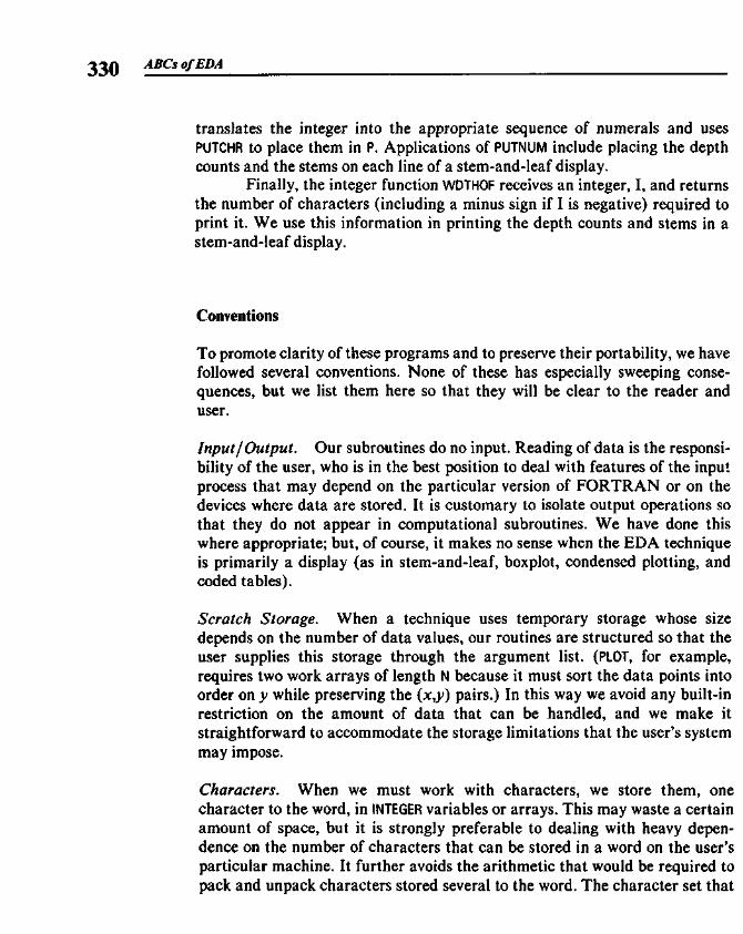
3 3 0 ABCs of EDA
translates the integer into the appropriate sequence of numerals and usesPUTCHR to place them in P. Applications of PUTNUM include placing the depthcounts and the stems on each line of a stem-and-leaf display.
Finally, the integer function WDTHOF receives an integer, I, and returnsthe number of characters (including a minus sign if I is negative) required toprint it. We use this information in printing the depth counts and stems in astem-and-leaf display.
Conventions
To promote clarity of these programs and to preserve their portability, we havefollowed several conventions. None of these has especially sweeping conse-quences, but we list them here so that they will be clear to the reader anduser.
Input/Output. Our subroutines do no input. Reading of data is the responsi-bility of the user, who is in the best position to deal with features of the inputprocess that may depend on the particular version of FORTRAN or on thedevices where data are stored. It is customary to isolate output operations sothat they do not appear in computational subroutines. We have done thiswhere appropriate; but, of course, it makes no sense when the EDA techniqueis primarily a display (as in stem-and-leaf, boxplot, condensed plotting, andcoded tables).
Scratch Storage. When a technique uses temporary storage whose sizedepends on the number of data values, our routines are structured so that theuser supplies this storage through the argument list. (PLOT, for example,requires two work arrays of length N because it must sort the data points intoorder on y while preserving the (x,y) pairs.) In this way we avoid any built-inrestriction on the amount of data that can be handled, and we make itstraightforward to accommodate the storage limitations that the user's systemmay impose.
Characters. When we must work with characters, we store them, onecharacter to the word, in INTEGER variables or arrays. This may waste a certainamount of space, but it is strongly preferable to dealing with heavy depen-dence on the number of characters that can be stored in a word on the user'sparticular machine. It further avoids the arithmetic that would be required topack and unpack characters stored several to the word. The character set that
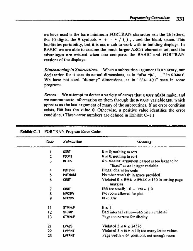
Programming Conventions 3 3 1
we have used is the bare minimum FORTRAN character set: the 26 letters,the 10 digits, the 9 symbols = 4 - - * / ( ) , . and the blank space. Thisfacilitates portability, but it is not much to work with in building displays. InBASIC we are able to assume the much larger ASCII character set, and theadvantages are evident when one compares the BASIC and FORTRANversions of the displays.
Dimensioning in Subroutines. When a subroutine argument is an array, ourdeclaration for it uses its actual dimensions, as in "REAL Y(N), . . . " in STMNLF.We have not used "dummy" dimensions, as in "REAL A(D" seen in someprograms.
Errors. We attempt to detect a variety of errors that a user might make, andwe communicate information on them through the INTEGER variable ERR, whichappears as the last argument of many of the subroutines. If no error conditionexists, ERR has the value 0. Otherwise, a positive value identifies the errorcondition. (These error numbers are defined in Exhibit C-l.)
Exhibit C-l FORTRAN Program Error Codes
Code Subroutine Meaning
N < 0; nothing to sortN < 0; nothing to sortX > MAXINT; argument passed is too large to be
"fixed" as an integer variableIllegal character codeNumber won't fit in space providedViolated 0 < IPMIN < IPMAX < 130 in setting page
marginsEPSI too small; 1.0 + EPSI = 1.0No room allowed for plotHI < LOW
N <: 1Bad internal value—bad nice numbers?Page too narrow for display
Violated 2 < N < 24576Violated 3 < NLV < 15; too many letter valuesPage width < 64 positions, not enough room
123
456
789
111213
212223
SORTPSORTINTFN
PUTCHRPUTNUMCINIT
CINITNPOSWNPOSW
STMNLFSTEMPSTMNLF
LVALSLVPRNTLVPRNT
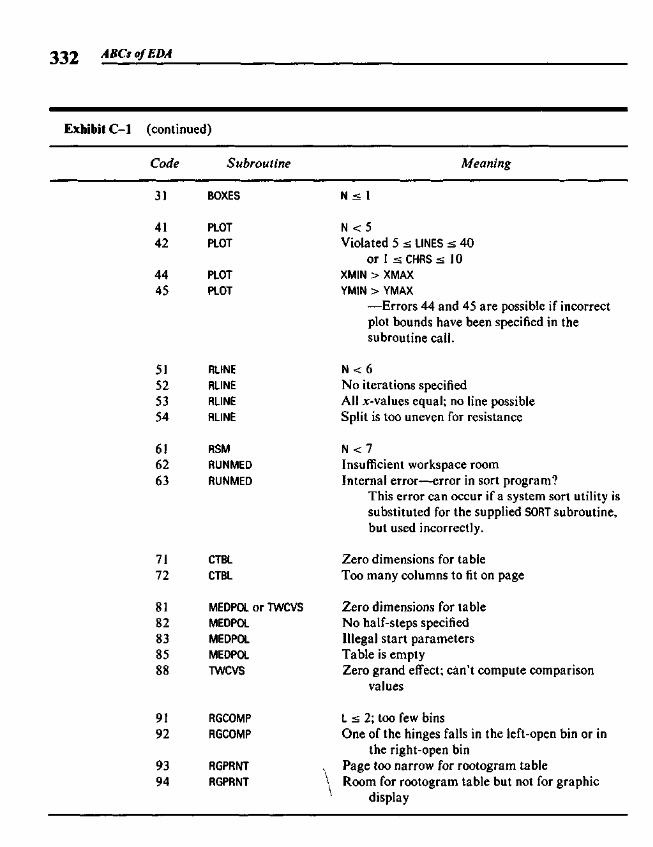
3 3 2 ABCs °fEDA
Exhibit C-l (continued)
Code Subroutine Meaning
31 BOXES N < 1
4142
4445
PLOTPLOT
PLOTPLOT
51525354
616263
RUNERUNERLINERUNE
RSMRUNMEDRUNMED
7172
8182838588
9192
9394
CTBLCTBL
MEDPOL or TWCVSMEDPOLMEDPOLMEDPOLTWCVS
RGCOMPRGCOMP
RGPRNTRGPRNT
N < 5Violated 5 < LINES < 40
or 1 <CHRS< 10XMIN > XMAXYMIN > YMAX
—Errors 44 and 45 are possible if incorrectplot bounds have been specified in thesubroutine call.
N < 6No iterations specifiedAll x-values equal; no line possibleSplit is too uneven for resistance
N < 7Insufficient workspace roomInternal error—error in sort program?
This error can occur if a system sort utility issubstituted for the supplied SORT subroutine,but used incorrectly.
Zero dimensions for tableToo many columns to fit on page
Zero dimensions for tableNo half-steps specifiedIllegal start parametersTable is emptyZero grand effect; can't compute comparison
values
L < 2; too few binsOne of the hinges falls in the left-open bin or in
the right-open binPage too narrow for rootogram tableRoom for rootogram table but not for graphic
display
Programming Conventions
Exits. Each of our subroutines has a single exit, the RETURN statementimmediately preceding the END statement. In most subroutines this RETURNbears the statement number 999.
Output FORMAT statements. We place each FORMAT statement immedi-ately after the first WRITE statement that uses it. For our programs, which donot use the same FORMAT statement in many different and widely separatedWRITE statements and often rely on the stream output routines describedearlier, this leads to much better readability than if we grouped all FORMATstatements at the end of the subroutine.
Declared Identifiers. We do not rely on "implicit typing" to determine(according to its first letter) whether an identifier is INTEGER or REAL. Instead,we explicitly declare all the identifiers used in each subprogram, except for thestandard FORTRAN functions. We strongly endorse this practice, which afew FORTRAN compilers support by issuing a warning message for anyundeclared identifier, because it aids greatly in eliminating misspelled names.(The PFORT Verifier, for example, lists all the identifiers in each programunit, so that such errors stand out.)
Indentation. We find that it is generally easier to follow the logic of aprogram when statements within a DO loop or following an IF statement areindented slightly, and we have used this device throughout our programs.
Reference
Isaacs, Gerald L. 1976. "BASIC REVISITED, An Update to Interdialect Translat-ability of the BASIC Programming Language." CONDUIT, The University ofIowa, Iowa City.
Ryder, B.G. 1974. "The PFORT Verifier." Software—Practice and Experience4:359-377.
Glance at Appendix Band turn to Chapter 2.

Appendix DMinitab Implementation
The FORTRAN programs presented in this book have been incorporated intothe Minitab statistics package. This appendix gives the syntax of the Minitabcommands for exploratory data analysis techniques. It assumes a familiaritywith the Minitab package. Readers unfamiliar with Minitab should read theMinitab Student Handbook, (Ryan, Joiner, and Ryan, 1976) or the MinitabReference Manual (Ryan, Joiner, and Ryan, 1981).
The commands given here may change slightly as the Minitab systemchanges. For details of the current status of the system, use the Minitab HELPcommand or refer to the latest edition of the Minitab Reference Manual.
Minitab is an excellent environment for exploratory data analysiscomputing, especially when used interactively. Minitab works with data keptin a computer worksheet, where the data values are stored in columnsdesignated C1, C 2 , . . . , or in matrices designated M1, M2, . . . . Single numberscan be stored in constants designated K1, K2, . . . . Although variables in theworksheet may have names (which are surrounded by quotes, like 'INCOME' or'RACE'), the command syntax usually shows the generic names C for column, Kfor constant, and M for matrix. Thus, the command specified as
335
3 3 5 ABCs °fEDA
STEMC
indicates a command in which C is to be replaced by any column identifier (forexample, C3, C17, 'MONEY').
When portions of a Minitab command line are optional, we enclosethese portions in square brackets. Some commands allow subcommands thatmodify the main command. When a subcommand follows the main commandline, Minitab requires that the main command line end with a semicolon. Eachsubsequent subcommand line ends with a semicolon, up to the final subcom-mand, which ends with a period.
Minitab command lines may contain free text, which further describesthe operation performed but has no effect on Minitab. The command descrip-tions in this appendix take advantage of this feature to include brief explana-tions of the commands and subcommands. Only the portions of the commanddescriptions in boldface are actually required.
References
Ryan, Thomas A., Brian L. Joiner, and Barbara F. Ryan. 1976. Minitab StudentHandbook. Boston: Duxbury Press.
Ryan, Thomas A., Brian L. Joiner, and Barbara F. Ryan. 1981. Minitab ReferenceManual. University Park, Pennsylvania: Minitab Project, The PennsylvaniaState University.
Mini tab Implementation
D.I Stem-and-Leaf Displays
STEM-AND-LEAF DISPLAY OF C C
Gives a separate stem-and-leaf display for each column named.
Optional Subcommands
TRIM OUTLIERS (default)Scale to the adjacent values.
NOTRIM
Scale to the extremes of the data—no HI or LO stems.
ExamplesSTEM 'RAINPH'
STEM'HC 'JANTMP'
STEM 'HC;
NOTRIM.
D.2 Letter-Value Displays
LVALS OF C [PUT LETTER VALUES IN CIMIDS IN C [SPREADS IN C]]]
This command prints a letter-value display. Optionally, the lettervalues, mids, and spreads can be stored in specified columns. Thecolumn of letter values will be roughly twice as long as the columns ofmids and spreads, and will start with the low extreme and proceed inorder to the high extreme.
ExamplesLVALS OF 'NJCOUNT
LVALS OF 'MSPRAIN' PUB IN C1, 'MIDS', 'SPREADS'
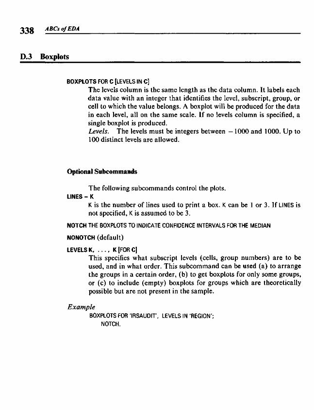
ABCs of EDA
D.3 Boxplots
BOXPLOTS FOR C [LEVELS IN C]
The levels column is the same length as the data column. It labels eachdata value with an integer that identifies the level, subscript, group, orcell to which the value belongs. A boxplot will be produced for the datain each level, all on the same scale. If no levels column is specified, asingle boxplot is produced.Levels. The levels must be integers between -1000 and 1000. Up to100 distinct levels are allowed.
Optional Subcommands
The following subcommands control the plots.LINES = K
K is the number of lines used to print a box. K can be 1 or 3. If LINES isnot specified, K is assumed to be 3.
NOTCH THE BOXPLOTS TO INDICATE CONFIDENCE INTERVALS FOR THE MEDIAN
NONOTCH ( d e f a u l t )
LEVELS K K [FOR C]
This specifies what subscript levels (cells, group numbers) are to beused, and in what order. This subcommand can be used (a) to arrangethe groups in a certain order, (b) to get boxplots for only some groups,or (c) to include (empty) boxplots for groups which are theoreticallypossible but are not present in the sample.
ExampleBOXPLOTS FOR 'IRSAUDIT', LEVELS IN 'REGION';
NOTCH.
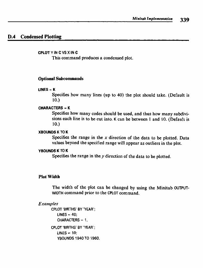
Minitab Implementation 3 3 Q
D.4 Condensed Plotting
CPLOT Y IN C VS X IN C
This command produces a condensed plot.
Optional Subcommands
LINES = K
Specifies how many lines (up to 40) the plot should take. (Default is10.)
CHARACTERS = K
Specifies how many codes should be used, and thus how many subdivi-sions each line is to be cut into. K can be between 1 and 10. (Default is10.)
XBOUNDS K TO K
Specifies the range in the x direction of the data to be plotted. Datavalues beyond the specified range will appear as outliers in the plot.
YBOUNDS K TO K
Specifies the range in the y direction of the data to be plotted.
Plot Width
The width of the plot can be changed by using the Minitab OUTPUT-WIDTH command prior to the CPLOT command.
ExamplesCPLOT'BIRTHS'BY'YEAR';
LINES = 40;
CHARACTERS = 1.
CPLOT'BIRTHS'BY'YEAR';
LINES = 10;
YBOUNDS 1940 TO 1960.
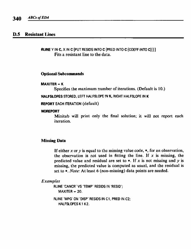
340
D.5 Resistant Lines
RLINE Y IN C, X IN C [PUT RESIDS INTO C [PRED INTO C [COEFF INTO C]Fits a resistant l ine to the data.
Optional Subcommands
MAXITER = K
Specifies the maximum number of iterations. (Default is 10.)
HALFSLOPES STORED, LEFT HALFSLOPE IN K, RIGHT HALFSLOPE IN K
REPORT EACH ITERATION ( d e f a u l t )
NOREPORTMinitab will print only the final solution; it will not report eachiteration.
Missing Data
If either x or y is equal to the missing value code, *, for an observation,the observation is not used in fitting the line. If x is missing, thepredicted value and residual are set to *. If x is not missing and y ismissing, the predicted value is computed as usual, and the residual isset to *. Note: At least 6 (non-missing) data points are needed.
ExamplesRLINE 'CANCR' VS TEMP' RESIDS IN 'RESID';
MAXITER = 20.
RLINE 'MPG' ON 'DISP' RESIDS IN C1, PRED IN C2;HALFSLOPES K1 K2.
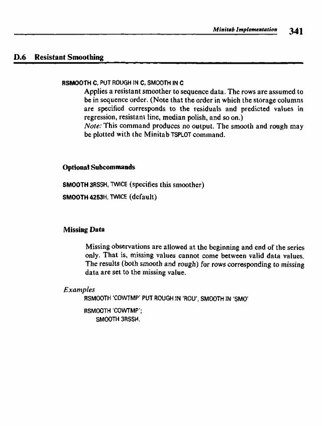
Minitab Implementation 3 4 1
D.6 Resistant Smoothing
RSMOOTH C, PUT ROUGH IN C, SMOOTH IN C
Applies a resistant smoother to sequence data. The rows are assumed tobe in sequence order. (Note that the order in which the storage columnsare specified corresponds to the residuals and predicted values inregression, resistant line, median polish, and so on.)Note: This command produces no output. The smooth and rough maybe plotted with the Minitab TSPLOT command.
Optional Subcommands
SMOOTH 3RSSH, TWICE (specifies this smoother)
SMOOTH 4253H, TWICE (default)
Missing Data
Missing observations are allowed at the beginning and end of the seriesonly. That is, missing values cannot come between valid data values.The results (both smooth and rough) for rows corresponding to missingdata are set to the missing value.
ExamplesRSMOOTH 'COWTMP' PUT ROUGH IN 'ROU', SMOOTH IN 'SMO'
RSMOOTH 'COWTMP';
SMOOTH 3RSSH.
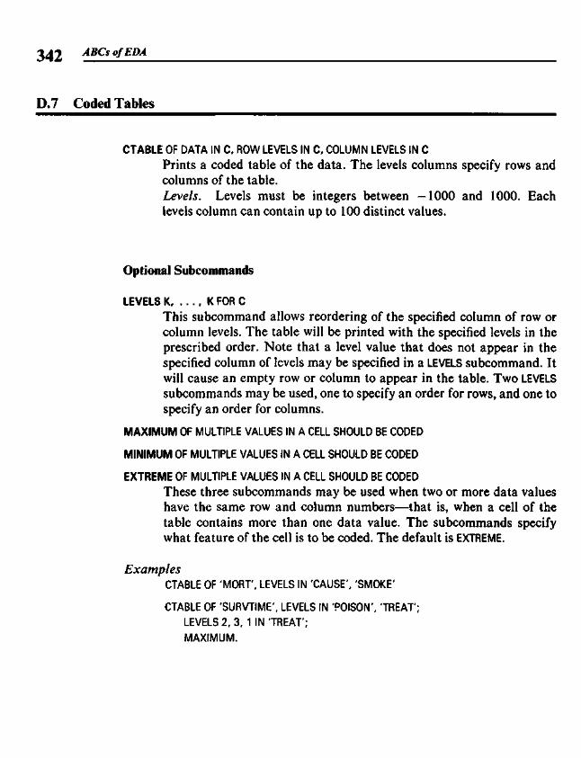
ABCs °fEDA
D.7 Coded Tables
CTABLE OF DATA IN C, ROW LEVELS IN C. COLUMN LEVELS IN CPrints a coded table of the data. The levels columns specify rows andcolumns of the table.Levels. Levels must be integers between —1000 and 1000. Eachlevels column can contain up to 100 distinct values.
Optional Subcommands
LEVELS K K FOR CThis subcommand allows reordering of the specified column of row orcolumn levels. The table will be printed with the specified levels in theprescribed order. Note that a level value that does not appear in thespecified column of levels may be specified in a LEVELS subcommand. Itwill cause an empty row or column to appear in the table. Two LEVELSsubcommands may be used, one to specify an order for rows, and one tospecify an order for columns.
MAXIMUM OF MULTIPLE VALUES IN A CELL SHOULD BE CODED
MINIMUM OF MULTIPLE VALUES IN A CELL SHOULD BE CODED
EXTREME OF MULTIPLE VALUES IN A CELL SHOULD BE CODED
These three subcommands may be used when two or more data valueshave the same row and column numbers—that is, when a cell of thetable contains more than one data value. The subcommands specifywhat feature of the cell is to be coded. The default is EXTREME.
ExamplesCTABLE OF 'MORT', LEVELS IN 'CAUSE', 'SMOKE'
CTABLE OF 'SURVTIME', LEVELS IN 'POISON', 'TREAT';LEVELS 2, 3, 1 IN 'TREAT;MAXIMUM.
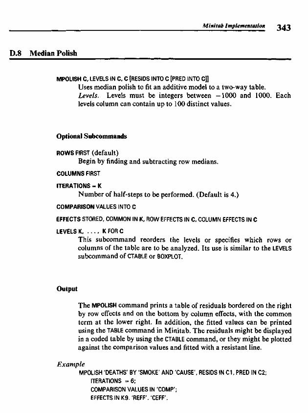
Minitab Implementation 'XA'X
D.8 Median Polish
MPOLISH C, LEVELS IN C, C [RESIDS INTO C [PRED INTO C]]Uses median polish to fit an additive model to a two-way table.Levels. Levels must be integers between -1000 and 1000. Eachlevels column can contain up to 100 distinct values.
Optional Subcommands
ROWS FIRST (default)
Begin by finding and subtracting row medians.
COLUMNS FIRST
ITERATIONS = K
Number of half-steps to be performed. (Default is 4.)COMPARISON VALUES INTO C
EFFECTS STORED, COMMON IN K, ROW EFFECTS IN C, COLUMN EFFECTS IN C
LEVELS K K FOR CThis subcommand reorders the levels or specifies which rows orcolumns of the table are to be analyzed. Its use is similar to the LEVELSsubcommand of CTABLE or BOXPLOT.
Output
The MPOLISH command prints a table of residuals bordered on the rightby row effects and on the bottom by column effects, with the commonterm at the lower right. In addition, the fitted values can be printedusing the TABLE command in Minitab. The residuals might be displayedin a coded table by using the CTABLE command, or they might be plottedagainst the comparison values and fitted with a resistant line.
ExampleMPOLISH 'DEATHS' BY 'SMOKE' AND 'CAUSE', RESIDS IN C1, PRED IN C2;
ITERATIONS = 6;COMPARISON VALUES IN 'COMP';EFFECTS IN K9.'REFF'.'CEFF'.
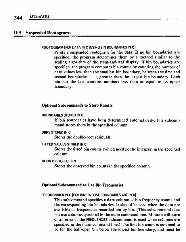
ABCs of EDA
D.9 Suspended Rootograms
ROOTOGRAM [FOR DATA IN C [USING BIN BOUNDARIES IN C]]
Prints a suspended rootogram for the data. If no bin boundaries arespecified, the program determines them by a method similar to thescaling algorithm of the stem-and-leaf display. If bin boundaries arespecified, the program computes bin counts by counting the number ofdata values less than the smallest bin boundary, between the first andsecond boundaries, . . . , greater than the largest bin boundary. Eachbin but the last contains numbers less than or equal to its upperboundary.
Optional Subcommands to Store Results
BOUNDARIES STORED IN C
If bin boundaries have been determined automatically, this subcom-mand stores them in the specified column.
DRRS STORED IN C
Stores the double-root residuals.
FITTED VALUES STORED IN C
Stores the fitted bin counts (which need not be integers) in the specifiedcolumn.
COUNTS STORED IN C
Stores the observed bin counts in the specified column.
Optional Subcommand to Use Bin Frequencies
FREQUENCIES IN C [FOR BINS WHOSE BOUNDARIES ARE IN C]
This subcommand specifies a data column of bin frequency counts andthe corresponding bin boundaries. It should be used when the data areavailable as frequencies recorded bin by bin. (This subcommand doesnot use columns specified in the main command line. Minitab will warnof an error if the FREQUENCIES subcommand is used when columns arespecified in the main command line.) The first bin count is assumed tobe for the half-open bin below the lowest bin boundary, and must be
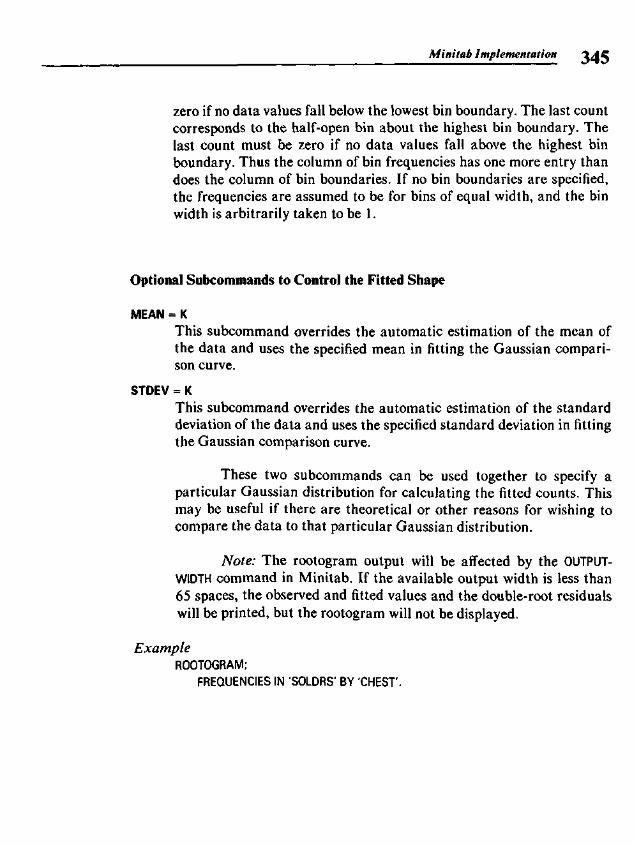
Minitab Implementation
zero if no data values fall below the lowest bin boundary. The last countcorresponds to the half-open bin about the highest bin boundary. Thelast count must be zero if no data values fall above the highest binboundary. Thus the column of bin frequencies has one more entry thandoes the column of bin boundaries. If no bin boundaries are specified,the frequencies are assumed to be for bins of equal width, and the binwidth is arbitrarily taken to be 1.
Optional Subcommands to Control the Fitted Shape
MEAN = KThis subcommand overrides the automatic estimation of the mean ofthe data and uses the specified mean in fitting the Gaussian compari-son curve.
STDEV = K
This subcommand overrides the automatic estimation of the standarddeviation of the data and uses the specified standard deviation in fittingthe Gaussian comparison curve.
These two subcommands can be used together to specify aparticular Gaussian distribution for calculating the fitted counts. Thismay be useful if there are theoretical or other reasons for wishing tocompare the data to that particular Gaussian distribution.
Note: The rootogram output will be affected by the OUTPUT-WIDTH command in Minitab. If the available output width is less than65 spaces, the observed and fitted values and the double-root residualswill be printed, but the rootogram will not be displayed.
ExampleROOTOGRAM;
FREQUENCIES IN 'SOLDRS' BY 'CHEST.

Index
Special symbols come first, in an order similar to the order established by theASCII character set. These are followed by the numeric symbols associated withresistant smoothing.
Page numbers in boldface indicate the definition of a term or concept or thefull tabulation of a data set.
# to code high outside values, 203
as notches, 76to mark middle stem, 6
as boxplot outside value, 76as point beyond x-y plot, 104in stems, 7to indicate line overflow, 18,
278, 298
as median in boxplot, 76to code values, 203
as boxplot whisker, 76to code values, 203to mark y = 0 in plot, 103
in stems, 7to code middle values, 203
/ \ to mark>> = 0 in plot, 103= to code low outside values, 203> < as notches in boxplot, 76[]:
as boxplot hinges, 76greatest integer, 43, 325outt function, 325
2,1673,1673R, 170, 177-178, 1823RSSH,twice, 178, 181,1844,16742,1674253H, 171-1734253H,twice, 172, 179-181. 1845,167
347
348 Index
A (letter value), 44-45Acid rain. See data, precipita-
tion pHadditive model, 221, 225, 233,
238,241additivity, re-expressing for,
233-240adjacent value, 68-69, 106,
296-298analysis of variance, 241area principle, 14, 258-263array, 93, 205, 240-241ASCII, 71, 102-103, 109,331
B (letter value), 44-45Bangladesh. See data, women's
heightsBASIC:
ANSI standard, 323ASC, 324boxplots, 71, 74, 77-78, 82-86coded table, 212, 214-215condensed plot, 102-103,
109-115defined functions, 301-302, 324environment, 319-320epsilonics, 322-323error handling, 325initialization, 303, 320, 322LEN, 323letter-value display, 57, 59-60loops, 324margins, 324median polish, 243-248nice position width, 305optimizing, 322portability, 323program structure, 320-321resistant line, 146-152rounding functions, 324smoothers, 183-190sort programs, 304stem-and-leaf display, 19-26STR$, 324string functions, 323-324string variables, 324suspended rootogram, 280,
284-287
variable-naming conventions,321-323
version flag (Vt), 77, 109, 146,184,243-244,321
YINFO, 306batch, 1
bimodal, 13,multimodal, 13skewed, 13symmetric, 13unimodal, 13
bell-shaped curve. See Gaussiandistribution
bimodal, 13bin, 255
boundaries, 260, 268, 277counts, 260, 268, 277unbounded, 260-261, 270width, 261, 263
bins:combining, 266equal-width, 258-260, 276unequal-width, 260-262, 276
boxplot, 69algorithm, 75-76and coded table, 203, 207-210from computer, 71in comparing batches, 71-75in Minitab, 338notched, 73-75, 77, 79-811-line, 71,74, 77scaling, 298skeletal, 663-line, 71,74, 77variable-width, 78
C (letter value), 44-45cathode ray tube (CRT), 75, 294ceiling function, 325center (of batch). See medianchi-squared, 281-282circumstance, 138coded table, 203
algorithm, 209-211and additive model, 223and boxplots, 207-210from computer, 203-207
Index 349
in Minitab, 342of residuals, 232, 240
codes, equally-spaced, 294. Seealso plot symbols
color (in coded table), 212column:
in Minitab, 335in 2-way table, 201-203of numbers, 93
column effect, 221, 225, 236common value, 221, 225, 231, 236comparison curve, Gaussian,
267-271,281comparison value, 236-238, 242compound smoothers, 170-173,
182computer graphics, 293condensed plot, 96-100
algorithm, 106and stem-and-leaf display,
100-103in Minitab, 339legend, 100
contour plot, 204coordinates:
data, 294, 297plotter, 294
copy-on, 176correction formula (slope), 127count, 255, 257
fitted, 265, 270-274, 277observed, 265, 277small, 265-266, 282
CRT. See cathode ray tubecumulative distribution function,
270approximation for Gaussian, 271
D (letter value), 44-45, 43, 43
l)/2,42data:
birthrate by month, 208-210birthrate by year, 94-95, 97, 99,
100,178-181,207breast cancer mortality, 127,
128-134
chest measurements, 259-260,264, 269-270, 272-278
cow temperatures, 161-162,164-166, 168-169, 172-175
football scores, 266-267gasoline mileage, 138,139-143male death rates, 201-202, 204-
205, 220-221, 227-233Minneapolis precipitation, 51-53New Jersey counties, 43-44, 46,
66-67Olympic runs, 235-239poisons by treatments, 206precipitation pH, 3-4
as batch, 4-6, 257-258by day, 101-102outliers, 69-70
pulse rates, 14sport parachuting deaths, 223,
224tax returns, 72-73, 75U.S. SMSAs:
age-adjusted mortality, 8-9,134-135
hydrocarbon pollution poten-tials, 8-9, 10, 12, 103
January temperatures, 8-9,11-12, 103
median education, 8-9,134-135
women's heights, 261-262data bounds, 77,104, 294, 298data coordinates, 294, 297data sequence, 159data smoother, 161ffdata space, 294degrees of freedom, 282density (in bin), 261, 263density curve, 256dependence, 121depth, 6, 17-18,42-45diagnostic plot, 236-240digits, leading, 2digits, trailing, 2, 8display, 1,293,326
details, 297-299exploratory, 295
350 Index
display {continued)montage, 105semigraphic, 294
distribution:Gaussian, 53, 79, 144, 256, 267normal, 256Poisson, 280tails of, 13, 48
double-root residual, 265-267, 271,274, 277-278
double roots, 280-282DRR, 265DRRES, 278
E (for eighth), 43E (endpoint smoothing), 177effects, 221,225, 231,236eighths, 43empty cell, 207, 211,240-241endpoints, smoothing, 173-177epsilonics, 322-323E-spread, 47extremes, 42, 66
F (four, five in stems), 7factor, 121, 138,201,219
column, 220row, 220
far outside, 68-69P and M to code, 203
fences, 104,203,209inner, 68-69outer, 68-69
first residuals, 130fit, 126, 142-143, 160, 222, 231,
267,2745-number summary, 66floor function, 325FORTRAN, 325-326
BLOCK DATA, 308BOXES, 76-77, 87-88, 332BOXP, 76-77, 89-91boxplot, 76-77BOXTOP, 76-77, 91-92character set, 71, 74, 78, 103,
106,297CHRBUF, 329CINIT, 309, 327-329, 331
coded table, 211-212COMMON, 327condensed plot, 107-108CTBL, 211,216-217, 332DELTR, 158DEPTHP, 19,32-34dialects, 326ENDPTS, 183, 196-197error codes, 331-332FLOOR, 318GAU, 318HANN, 183, 194initialization, 327-329INTFN, 317, 331letter-value display, 56LVALS, 56, 61-62, 331LVPRNT, 56, 62-63, 331MEDIAN, 318
median polish, 242-243MEDOF3, 183, 196MEDPOL, 242, 249-253, 332NPOSW, 316-317, 331NUMBRS, 327OUNIT, 327OUTLYP, 19,31-32output, 326, 327, 329-330PLOT, 107, 116-120,332PLTPOS, 76-77, 92PMAX, 327PMIN, 327portability, 326-329PRINT, 312, 329programming conventions,
330-333PSORT, 314, 331PUTCHR, 212, 310, 329-331PUTNUM,311-312, 329-331resistant line, 145-146RGCOMP, 279, 288-290, 332RGPRNT, 279, 290-292, 332RL3MED, 158RUNE, 145-146, 153-158,332rootogram, 279-280RSM, 183, 191,332RUNMED, 183, 198-199,33252, 183, 19353, 183, 195S3R, 183, 195
Index 351
S3RSSH, 183, 19254, 183, 193S4253H, 183, 19255, 183, 194SLTITL, 19,37-39smoothers, 183SORT, 313, 331SPLIT, 183, 197-198stem-and-leaf display, 19STEMP, 19,35-36,331STMNLF, 19,27-31,331stream output, 329-330, 333subscripts, 327TWCVS, 243, 253, 332utility routines, 309-318, 326WDTHOF, 310, 330YINFO, 315
fourths (=hinges), 43Freeman-Tukey deviate, 281frequency distribution, 257-258full-step, 231
Gaussian distribution, 53, 79, 144,256, 267
c.d.f. approximation, 271-272frequency curve, 256, 267hinges, 268standard, 53,267, 281
Gaussian shape, 256, 270goodness of fit, 281-282granularity, 14-15, 96, 297graph paper, 96groups, comparing, 75, 77
H (for hinge), 43H (for hanning), 170half-open bin. See bin, unboundedhalf-slope, 135half-slope ratio, 135half-step, median polish, 231, 240hanning, 170HI, 14, 18,69,297hinges, 43, 46
and outliers, 68in boxplot, 66, 69, 71, 76, 298in coding table, 203, 209-211,
298
in fitting comparison curve,267-270
in scaling, 295interpolated, 268-270
histogram, 13,257-263H-spr ( = H-spread), 47, 68, 74.
79, 295
I (as boxplot hinges), 76"improper" characters
(in condensed plot), 104inner fences, 68-69, 203, 295, 298integer part ([ ]), 43intercept, 122, 125, 127, 142, 145intervals (bins), 255, 257int function, 325iterative refinement. See polish-
ing and reroughing
L (for left):in condensed plot, 104in resistant line, 124
ladder of powers, 48-49, 135-136,239-240
leaf, 4, 17, 100least squares, 143-144, 241legend (in condensed plot),
99-100, 106letter-value display, 41, 46-48,
337letter values, 41, 42, 44-46
algorithm, 55-56depths of, 42-45
LEVELS, 338, 342, 343. See alsogroups
line:- 0 , 296, 298- 0 0 and +00, 102, 106resistant, 123-127, 143-144, 240straight, 121, 127, 135,220
LO, 13, 18,69,297location, measures of. See mean
and medianlogarithm, 48-49, 238
M:for median, 42for middle, 124
352 Index
M: (continued)for MINUS:
in coded tables, 203in condensed plots, 104
margins, 278, 321,324, 327mean, 241,267-268median, 42
as letter value, 46-47in boxplot, 66, 69in notched boxplot, 74, 79in resistant line, 123-124, 126in smoothing, 161, 163in stem-and-leaf display, 6in two-way table, 225running, 163-167, 171, 182
median polish, 225-233, 240-241,343
algorithms, 242from computer, 240
mid, 46, 49middle (of batch), 1, 42, 47, 65,
267midE ( = mideighth), 47midextreme, 47midH ( = midhinge), 47midrange, 47midsummary, 47, 48Minitab, xiv, 335, 345mode, 1,13model, 126
additive, 221, 225, 233, 238,241
montage display, 105multimodal, 13multiplicity, 74, 81
nice numbers, 296-298nice position width, 76, 296non-additivity, 234-240, 241normal distribution, 256. See also
Gaussian distributionnotch (in boxplot), 73-74, 79-81,
338NPW (=nice position width),
76, 296numbers, nice, 296
O as boxplot far outside value, 76ODOFFNA, 241
ordered pair, 93outer fences, 68-69, 203-205outliers, 67. See also stray values
in boxplot, 71in sequences, 171, 178in two-way table, 202, 232-233,
236in y-versus-x data, 134-135,
144resistance to, 126-127, 268,
295-296outside, 68-69, 203outt function, 325
P (for PLUS)in coded tables, 203in condensed plots, 104
page, 294patterns (in data), xv. See also
re-expressionin batches, 1, 13,41,47,65in frequency distributions, 256in parallel batches, 72-75, 207-210in residuals, 126, 178-181,
224-225,234in sequences, 159-160in tables, 201,219-223in ̂ -versus-x data, 93, 121
PFORT, 327, 333plot:
computer terminology, 294condensed, 98, 294, 297contour, 204focusing, 105printer, 296-297schematic, 696-line, 100, 109x-y, 93
plot bounds, 104,294plot scaling, 17-19, 106, 294-296plot symbols. See #, (), *, +,
- , •, =, x , [], L, M,P, R, semigraphic displays
priority of, 76, 106plotter coordinates, 294plotting characters, 98-102, 297-
298plot window, 294
Index 353
PLUS-one fit, 238Poisson distribution, 280polishing, 127, 131, 145, 172,
225-233portability of programs, 323,
326-327powers, ladder of, 48-49, 135-136,
239-240printer plots, 96-100, 296-297probability, 256programmer's thread, xvii, 17programming conventions,
321-323, 330-333program options, 16
boxplot, 74-75, 77-78, 338coded table, 203-207, 211-212,
342condensed plot, 105-106,
107-109,339letter values, 55-57, 337median polish, 240, 241-244, 343resistant line, 144-147, 340rootogram, 277-280, 344-346smoothing, 181, 183-184,341stem-and-leaf, 19-20,337
quarters (=hinges),43quartiles, 43Quetelet, Adolphe, 259, 274
R (for right):in condensed plot, 104in resistant line, 124
range, 47RAWRES, 278recentering even smooths,
164-167, 177re-expression, 47-50, 270
for additivity, 233-240, 241for straightness, 135-143for symmetry, 50-53of counts, 263, 280-282
regression, 143-144, 241representation error, 322reroughing, 170-171residuals, 126
and re-expression, 143, 234, 263double-root, 265-267, 271, 274,
277-278
first, 130for rootogram, 255, 263,
265-267, 274-277in sequences, 160-161in two-way table, 223-225,
231-232,234in y-versus-x data, 126-127,
134-135, 144residual slope, 127, 131resistance, xv, 126-127, 240,
274, 295-296resistant line, 123-127, 340
algorithm, 145and regression, 143-144, 241for diagnostic plot, 236, 240from computer, 144-145
resistant smoothing in Minitab,341. See also smoothing
resmoothing, 170response, 121, 220rootogram, 255, 263
suspended, 255-256, 275-277rootogram display, 277-279, 299rootogram residuals, 275-277rough, 161, 171, 178rounding, 7-8, 17rounding error, 322row, 201-203, 219-220row effect, 221, 225, 236row-major format, 210-211running-median smoother,
163-167, 171, 182running weighted average,
167-170
S (for six and seven in stems), 7S (for splitting in smoothing),
177-178scale factor, 294, 297-298schematic plot, 69. See also
boxplotsemigraphic display, 14, 96-100,
294, 297, 326sequence, data, 159signpost. See programmer's threadskewness, 47, 50-53slope, 121-122, 125, 127, 142
of diagnostic plot, 239-240smooth, 161, 178
354 Index
smooth curves, 160smoother, compound, 170-173, 182smoothing:
algorithms, 182by computer, 181
sorting, 41-42, 57-58, 109, 322span (of smoother), 167, 182sparse-matrix representation,
207, 241splitting, 177-178spread, 41, 47-49, 53-55, 66square root, 49, 263, 265, 274standard deviation, 53-54, 74,
79-81,268standard Gaussian distribution,
53,267,281start (for re-expression), 50stem, 3-4, 7, 17, 100
- 0 , 11-13, 18,298stem-and-leaf display, 1-20, 100-
103, 132,255,257,280,297-298, 337
-Ostem, 11, 18, 102,298+ 0stem, 11, 18, 102algorithm, 17-19and histograms, 13-15construction, 2-35-line, 7from computer, 15heading, 6, 18line overflow (*), 18number of lines, 18squeezing together, 7stretching out, 62-line, 7
step, 295straight line, 121, 127, 135,220straightness, re-expressing for,
135-143stray values, 1,7, 12-13,65-66,
205. See also outliersstream output, 329-330, 333summary points, 123-125suspended rootogram, 256,
275-277, 299, 344-345from computer, 277-278
sweeping, 225, 226
symmetry, 1,13, 47, 66re-expressing for, 50-53
T (for two and three in stems), 7table:
three-way, 241two-way, 201-203
coded, 203-209, 223replicated, 205
unbalanced, 241thirds, 123-124, 145three-array form (oCmatrix). See
sparse-matrix representationthree-way table, 241tilt. See slopetime series, 160transformation. See re-expressiontruncation, 7-8twicing, 171two-way table, 201-203, 219-223typical value. See median
unimodal, 13unit (in display), 6, 18
simple, 296
variability, 41, 47-49, 53-55,178-181,207
of counts, 263, 280-282of median, 79-81
viewport, 106,294,298
W (letter value), 44-45whisker, 69
X (letter value), 44-45jc-axis, 95xSTEP, 100,294,298x-y plot. See condensed plot
Y (letter value), 44-45y-a.x'\s, 95ySTEP, 100,294,298y versus x, 220
Z (letter value), 44-45z-score, 79


ABC
cs, andputing
lysis
The Authors:
PaulF. Ve lie man is associate professor of Economic and SocialStatistics at Cornell University. He earned the A.B. degree inmathematics and social science from Dartmouth College and the M.S.and Ph.D. degrees in statistics from Princeton University. At Cornell,Dr. Velleman has developed curriculum materials to incorporateexploratory data analysis and computing in introductory statisticscourses. His research interests include data analysis methods,statistical computing, nonlinear data smoothing, and robust statistics.He is an associate editor of the Journal of the American StatisticalAssociation.
David C. Hoaglin is a senior scientist at Abt Associates Inc. andresearch associate in statistics at Harvard University. Previously hewas a member of the faculty in the Department of Statistics atHarvard. Dr. Hoaglin received the B.S. in mathematics from DukeUniversity and the Ph.D. in statistics from Princeton University. Inaddition to extensive experience in teaching and applying exploratorydata analysis, he is actively engaged in research on data analysis andstatistical computing and has worked on applications of statistics tohousing, education, health care, criminal justice, and welfare. He is aFellow of the American Statistical Association and of the AmericanAssociation for the Advancement of Science, a member of the editorialboard of SI AM Journal of Scientific and Statistical Computing, anda former associate editor of the Journal of the American StatisticalAssociation.
36G0480 ISBN O-
(previously ISBN 0-87872-273-4)
Related Documents