6D SLAM – Mapping Outdoor Environments · 6D SLAM – Mapping Outdoor Environments Andreas Nu¨chter, ... The RESOLV project aimed at ... wi,j is assigned 1 if the i-th point ofM

6D SLAM Mapping Outdoor EnvironmentsAndreas Nuchter, Kai Lingemann, Joachim Hertzberg

University of OsnabruckInstitute for Computer Science

Knowledge-Based Systems Research Group

Albrechtstrae 28D-49069 Osnabruck, Germany

nuechter@informatik.uni-osnabrueck.de

Hartmut Surmann

Fraunhofer Institute forAutonomous Intelligent Systems (AIS)

Schloss BirlinghovenD-53754 Sankt Augustin, Germanyhartmut.surmann@ais.fraunhofer.de

Abstract 6D SLAM (Simultaneous Localization and Map-ping) of mobile robots considers six dimensions for the robotpose, namely, the x, y and z coordinates and the roll, yawand pitch angles. Robot motion and localization on naturalsurfaces, e.g., when driving with a mobile robot outdoor, mustregard these degrees of freedom. This paper presents a roboticmapping method based on locally consistent 3D laser rangescans. Scan matching, combined with a heuristic for closedloop detection and a global relaxation method, results in ahighly precise mapping system for outdoor environments. Themobile robot Kurt3D was used to acquire data of the SchlossBirlinghoven campus. The resulting 3D map is compared withground truth, given by an aerial photograph.

I. INTRODUCTION

For protecting humans, it is nowadays important to buildrobots that are able to operate in earthquake, fire, explosiveand chemical disaster areas. The community of UrbanSearch and Rescue Robotics (USAR) grows very fast. Manyrobots are manufactured, both from research institutes andfrom industry. However, until now, there have been no sys-tems that can reliably map their environment. The mobilerobot Kurt3D is capable of mapping its environment in 3Dand self localize in six degrees of freedom, i.e., consideringits x, y and z positions and the roll, yaw and pitch angles(6D SLAM). The robot maps large surrounding areas thatcan be indoor environments [17], urban environments [18],tunnel and mines [14] and natural landscapes, e.g., forestareas. These mapping abilities makes the system suitablefor Urban Search and Rescue tasks.

Automatic environment sensing and modeling is a fun-damental scientific issue in robotics, since the presence ofmaps is essential for many robot tasks. Manual mappingof environments is a hard and tedious job: Thrun et al.report a time of about one week hard work for creatinga map of the museum in Bonn for the robot RHINO[19]. Especially mobile systems with 3D laser scannersthat automatically perform multiple steps such as scanning,gaging and autonomous driving have the potential to greatlyimprove mapping. Many application areas benefit from 3Dmaps, e.g., industrial automation, architecture, agriculture,the construction or maintenance of tunnels and mines andrescue robotic systems.

The robotic mapping problem is that of acquiring a spa-tial model of a robots environment. If the robot poses were

known precisely, the local sensor inputs of the robot, i.e.,local maps, could be registered into a common coordinatesystem to create a map. Unfortunately, any mobile robotsself localization suffers from imprecision and therefore thestructure of the local maps, e.g., of single scans, needs tobe used to create a precise global map. Finally, robot posesin natural outdoor environments involve yaw, pitch, rollangles and elevation, turning pose estimation as well as scanregistration into a problem in six mathematical dimensions.

This paper proposes algorithms that allow to digitizelarge environments and solve the 6D SLAM problem. Inprevious works we have already presented partially our6D SLAM algorithm [14], [17], [18]. In [14] we use aglobal relaxation scan matching algorithm to create a modelof an abandoned mine and in [18] we presented our first3D model containing a closed loop. This papers maincontribution is an overview of our 6D SLAM mappingsystem.

A. State of the Art

1) SLAM.: Depending on the map type, mapping algo-rithms differ. State of the art for metric maps are probabilis-tic methods, where the robot has probabilistic motion anduncertain perception models. By integrating of these twodistributions with a Bayes filter, e.g., Kalman or particlefilter, it is possible to localize the robot. Mapping is oftenregarded as an extension to this estimation problem. Besidethe robot pose, positions of landmarks are estimated. Closedloops, i.e., a second encounter of a previously visited areaof the environment, play a special role here. Once detected,they enable the algorithms to bound the error by deformingthe already mapped area such that a topologically consistentmodel is created. However, there is no guarantee for acorrect model. Several strategies exist for solving SLAM.Thrun reviews in [20] existing techniques, i.e., maximumlikelihood estimation [7], expectation maximization [6],[21], extended Kalman filter [4] or (sparse extended) infor-mation filter [23]. In addition to these methods, FastSLAM[22] that approximates the posterior probabilities, i.e., robotposes, by particles, and the method of Lu Milios on thebasis of IDC scan matching [13] exist.

In principle, these probabilistic methods are extendableto 6D. However no reliable feature extraction nor a strategy

for reducing the computational costs of multi hypothesistracking, e.g., FastSLAM, that grows exponentially with thedegrees of freedom, has been published to our knowledge.

2) 3D Mapping.: Instead of using 3D scanners, whichyield consistent 3D scans in the first place, some groupshave attempted to build 3D volumetric representations ofenvironments with 2D laser range finders. Thrun et al. [22]and Fruh et al. [8] use two 2D laser scanners finders for ac-quiring 3D data. One laser scanner is mounted horizontally,the other vertically. The latter one grabs a vertical scan linewhich is transformed into 3D points based on the currentrobot pose. The horizontal scanner is used to compute therobot pose. The precision of 3D data points depends on thatpose and on the precision of the scanner.

A few other groups use highly accurate, expensive 3Dlaser scanners [1], [9], [16]. The RESOLV project aimed atmodeling interiors for virtual reality and tele-presence [16].They used a RIEGL laser range finder on robots and theICP algorithm for scan matching [3]. The AVENUE projectdevelops a robot for modeling urban environments [1],using a CYRAX scanner and a feature-based scan matchingapproach for registering the 3D scans. Nevertheless, in theirrecent work they do not use data of the laser scanner in therobot control architecture for localization [9]. The groupof M. Hebert has reconstructed environments using theZoller+Frohlich laser scanner and aims to build 3D modelswithout initial position estimates, i.e., without odometryinformation [10].

Recently, different groups employ rotating SICK scan-ners for acquiring 3D data [24]. Wulf et al. let the scannerrotate around the vertical axis. They acquire 3D data whilemoving, thus the quality of the resulting map cruciallydepends on the pose estimate that is given by inertialsensors, i.e., gyros. In addition, their SLAM algorithms donot consider all six degrees of freedom.

B. The Exploration Robot Kurt3D

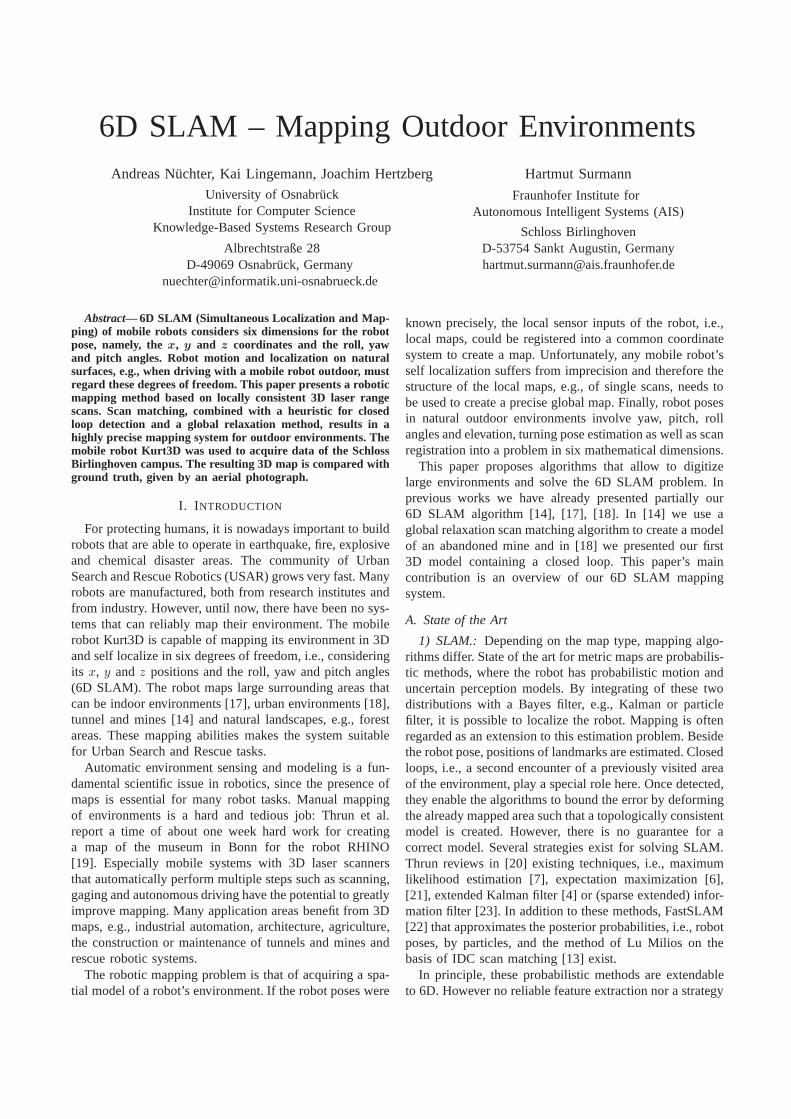
In our experiments we use the exploration robot Kurt3D,that is also used in RoboCup Rescue competitions. Fig. 1shows the robot that is equipped with a tiltable SICK laserrange finder in a natural outdoor environment.

II. RANGE IMAGE REGISTRATION AND ROBOTRELOCALIZATION

Multiple 3D scans are necessary to digitalize environ-ments without occlusions. To create a correct and consistentmodel, the scans have to be merged into one coordinatesystem. This process is called registration. If the robot

Fig. 1. Kurt3D in a natural environment, i.e., lawn, forest track, pavement.

carrying the 3D scanner were precisely localized, the reg-istration could be done directly based on the robot pose.However, due to unprecise robot sensors, self localizationis erroneous, so the geometric structure of overlapping 3Dscans has to be considered for registration. As a by-product,successful registration of 3D scans relocalizes the robot in6D, by providing the transformation to be applied to therobot pose estimation at the recent scan point.

The following method registers point sets into a commoncoordinate system. It is called Iterative Closest Points (ICP)algorithm [3]. Given two independently acquired sets of 3Dpoints, M (model set) and D (data set) which correspond toa single shape, we aim to find the transformation consistingof a rotation R and a translation t which minimizes thefollowing cost function:

E(R, t) =

|M|X

i=1

|D|X

j=1

wi,j ||mi (Rdj + t)||2. (1)

wi,j is assigned 1 if the i-th point of M describes the samepoint in space as the j-th point of D. Otherwise wi,j is 0.Two things have to be calculated: First, the correspondingpoints, and second, the transformation (R, t) that minimizesE(R, t) on the base of the corresponding points.

The ICP algorithm calculates iteratively the point cor-respondences. In each iteration step, the algorithm selectsthe closest points as correspondences and calculates thetransformation (R, t) for minimizing equation (1). Theassumption is that in the last iteration step the point cor-respondences are correct. Besl et al. prove that the methodterminates in a minimum [3]. However, this theorem doesnot hold in our case, since we use a maximum tolerabledistance dmax for associating the scan data. Such a thresh-old is required though, given that 3D scans overlap onlypartially.

In every iteration, the optimal transformation (R, t) hasto be computed. Eq. (1) can be reduced to

E(R, t) 1

N

NX

i=1

||mi (Rdi + t)||2, (2)

with N =|M|

i=1

|D|j=1 wi,j , since the correspondence

matrix can be represented by a vector containing the pointpairs.

Four direct methods are known to minimize Eq. (2) [12].In earlier work [14], [17], [18] we used a quaternion basedmethod [3], but the following one, based on singular valuedecomposition (SVD), is robust and easy to implement,thus we give a brief overview of the SVD-based algorithm.It was first published by Arun, Huang and Blostein [2].The difficulty of this minimization problem is to enforcethe orthonormality of the matrix R. The first step of thecomputation is to decouple the calculation of the rotationR from the translation t using the centroids of the pointsbelonging to the matching, i.e.,

cm =1

N

NX

i=1

mi, cd =1

N

NX

i=1

dj (3)

and

M = {mi = mi cm}1,...,N , D

= {di = di cd}1,...,N . (4)

After substituting (3) and (4) into the error function,E(R, t) Eq. (2) becomes:

E(R, t)

NX

i=1

m

i Rd

i

2 with t = cm Rcd. (5)

The registration calculates the optimal rotation by R =VU

T . Hereby, the matrices V and U are derived by thesingular value decomposition H = UVT of a correlationmatrix H. This 3 3 matrix H is given by

H =NX

i=1

dim

Ti =

0

@

Sxx Sxy SxzSyx Syy SyzSzx Szy Szz

1

A , (6)

with Sxx =N

i=1 mixd

ix, Sxy =

Ni=1 m

ixd

iy, . . . [2].

We use algorithms to accelerate ICP, namely point reduc-tion and approximate kd-trees as proposed and evaluated in[14], [17], [18].

III. ICP-BASED 6D SLAM

A. Calculating Initial Estimations for ICP Scan Matching

To match two 3D scans with the ICP algorithm it isnecessary to have a sufficient starting guess for the secondscan pose. In earlier work we used odometry [17] or theplanar HAYAI scan matching algorithm [11]. However,the latter cannot be used in arbitrary environments, e.g.,the one presented in Fig. 1 (bad asphalt, lawn, woodland,etc.). Since the motion models change with differentgrounds, odometry alone cannot be used either. Here therobot pose is the 6-vector P = (x, y, z, x, y, z) or,equivalently the tuple containing the rotation matrix andtranslation vector, written as 44 OpenGL-style matrixP [5].1 The following heuristic computes a sufficientlygood initial estimation. It is based on two ideas. First, thetransformation found in the previous registration is appliedto the pose estimation this implements the assumptionthat the error model of the pose estimation is locallystable. Second, a pose update is calculated by matchingoctree representations of the scan point sets rather than thepoint sets themselves this is done to speed up calculation:

1) Extrapolate the odometry readings to all six degreesof freedom using previous registration matrices. Thechange of the robot pose P given the odometryinformation (xn, zn, y,n), (xn+1, zn+1, y,n+1)and the registration matrix R(x,n, y,n, z,n) iscalculated by solving:

1Note the bold-italic (vectors) and bold (matrices) notation. The con-version between vector representations, i.e., Euler angles, and matrixrepresentations is done by algorithms from [5].

0

BBBBB@

xn+1yn+1zn+1

x,n+1y,n+1z,n+1

1

CCCCCA

=

0

BBBBB@

xnynzn

x,ny,nz,n

1

CCCCCA

+

0

BBBBB@

R(x,n, y,n, z,n) 0

1 0 00 0 1 0

0 0 1

1

CCCCCA

0

BBBBB@

xn+1yn+1zn+1

x,n+1y,n+1z,n+1

1

CCCCCA

.

| {z }

P

Therefore, calculating P requires a matrix inver-sion. Finally, the 6D pose Pn+1 is calculated by

Pn+1 = P Pn

using the poses matrix representations.

2) Set P best to the 6-vector (t, R(x,n, y,n, z,n)) =(0, R(0)).

3) Generate an octree OM for the n-th 3D scan (modelset M ).

4) Generate an octree OD for the (n + 1)-th 3D scan(data set D).

5) For search depth t [tStart, . . . , tEnd] in the octrees es-timate a transformation P best = (t, R) as follows:

a) Calculate a maximal displacement and rotationP max depending on the search depth t andcurrently best transformation P best.

b) For all discrete 6-tuples P i [P max, P max] in the domainP = (x, y, z, x, y, z) displace ODby Pi P Pn. Evaluate the matchingof the two octrees by counting the numberof overlapping cubes and save the besttransformation as P best.

6) Update the scan pose using matrix multiplication,i.e.,

Pn+1 = Pbest P Pn.

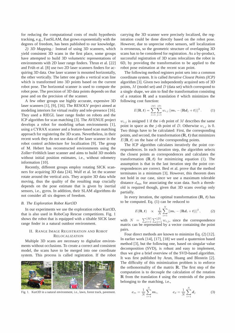
Note: Step 5b requires 6 nested loops, but the com-putational requirements are bounded by the coarse-to-finestrategy inherited from the octree processing. The size ofthe octree cubes decreases exponentially with increasing t.We start the algorithm with a cube size of 75 cm3 andstop when the cube size falls below 10 cm3. Fig. 2 showstwo 3D scans and the corresponding octrees. Furthermore,note that the heuristic works best outdoors. Due to the

Fig. 2. Left: Two 3D point clouds. Middle: Octree corresponding to theblack point cloud. Right: Octree based on the blue points.

C

D

AB

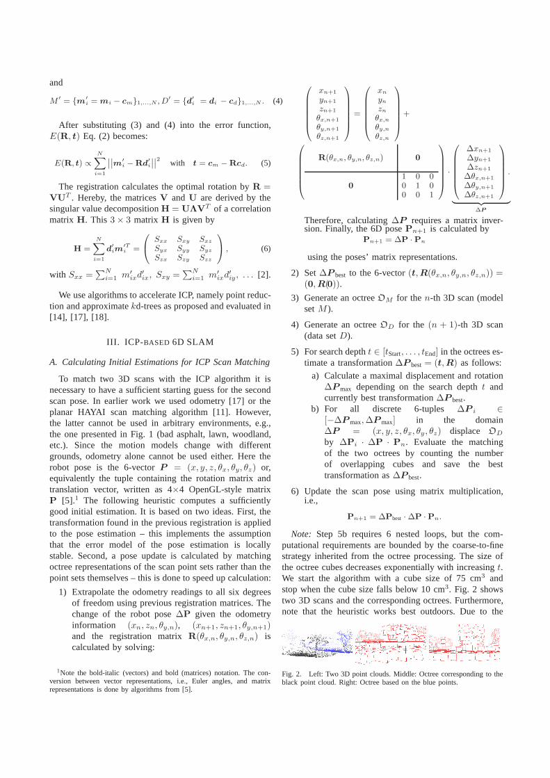
Fig. 3. Top left: Model with loop closing, but without global relaxation. Top right: Model based on incremental matching before closing the loop,containing 77 scans each with approx. 100000 3D points. The grid at the bottom denotes an area of 2020m2 for scale comparison. The 3D scanposes are marked by blue points. Bottom: Aerial view of the scene. The points A D are used as reference points in the comparison in Table I.

diversity of the environment the match of octree cubes willshow a significant maximum, while indoor environmentswith their many geometry symmetries and similarities, e.g.,in a corridor, are in danger of producing many plausiblematches.

After an initial starting guess is found, the range imageregistration from section 2 proceeds and the 3D scans areprecisely matched.

B. Computing Globally Consistent Scenes

After registration, the scene has to be correct and globallyconsistent. A straightforward method for aligning several3D scans is pairwise matching, i.e., the new scan is

registered against a previous one. Alternatively, an incre-mental matching method is introduced, i.e., the new scan isregistered against a so-called metascan, which is the unionof the previously acquired and registered scans. Each scanmatching has a limited precision. Both methods accumulatethe registration errors such that the registration of a largenumber of 3D scans leads to inconsistent scenes and toproblems with the robot localization. Closed loop detectionand error diffusing avoid these problems and computeconsistent scenes.

1) Closing the Loop.: After matching multiple 3D scans,errors have accumulated and loops would normally not beclosed. Our algorithm automatically detects a to-be-closed

loop by registering the last acquired 3D scan with earlieracquired scans. Hereby we first create a hypothesis basedon the maximum laser range and on the robot pose, sothat the algorithm does not need to process all previousscans. Then we use the octree based method presented insection III-A to revise the hypothesis. Finally, if registrationis possible, the computed error, i.e., the transformation (R,t) is distributed over all 3D scans. The respective part isweighted by the distance covered between the scans:

ci =length of path from start of the loop to scan pose i

overall length of path.

1) The translational part is calculated as ti = cit.2) Of the three possibilities of representing rotations,

namely, orthonormal matrices, quaternions and Eulerangles, quaternions are best suited for our interpola-tion task. The problem with matrices is to enforce or-thonormality and Euler angles show Gimbal locks [5].A quaternion as used in computer graphics is the 4vector q [5]. It describes a rotation by an axis a R3

and an angle that are computed by The angle isdistributed over all scans using the factor ci.

2) Diffusing the Error.: Pulli presents a registrationmethod that minimizes the global error and avoids inconsis-tent scenes [15]. Based on the idea of Pulli we designed therelaxation method simultaneous matching, that is describedin detail in [17], [18].

IV. EXPERIMENT AND RESULTS

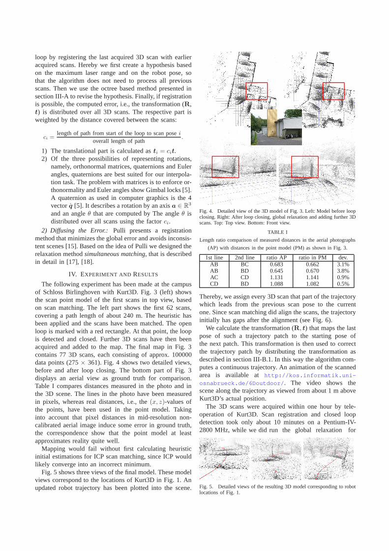
The following experiment has been made at the campusof Schloss Birlinghoven with Kurt3D. Fig. 3 (left) showsthe scan point model of the first scans in top view, basedon scan matching. The left part shows the first 62 scans,covering a path length of about 240 m. The heuristic hasbeen applied and the scans have been matched. The openloop is marked with a red rectangle. At that point, the loopis detected and closed. Further 3D scans have then beenacquired and added to the map. The final map in Fig. 3contains 77 3D scans, each consisting of approx. 100000data points (275 361). Fig. 4 shows two detailed views,before and after loop closing. The bottom part of Fig. 3displays an aerial view as ground truth for comparison.Table I compares distances measured in the photo and inthe 3D scene. The lines in the photo have been measuredin pixels, whereas real distances, i.e., the (x, z)-values ofthe points, have been used in the point model. Takinginto account that pixel distances in mid-resolution non-calibrated aerial image induce some error in ground truth,the correspondence show that the point model at leastapproximates reality quite well.

Mapping would fail without first calculating heuristicinitial estimations for ICP scan matching, since ICP wouldlikely converge into an incorrect minimum.

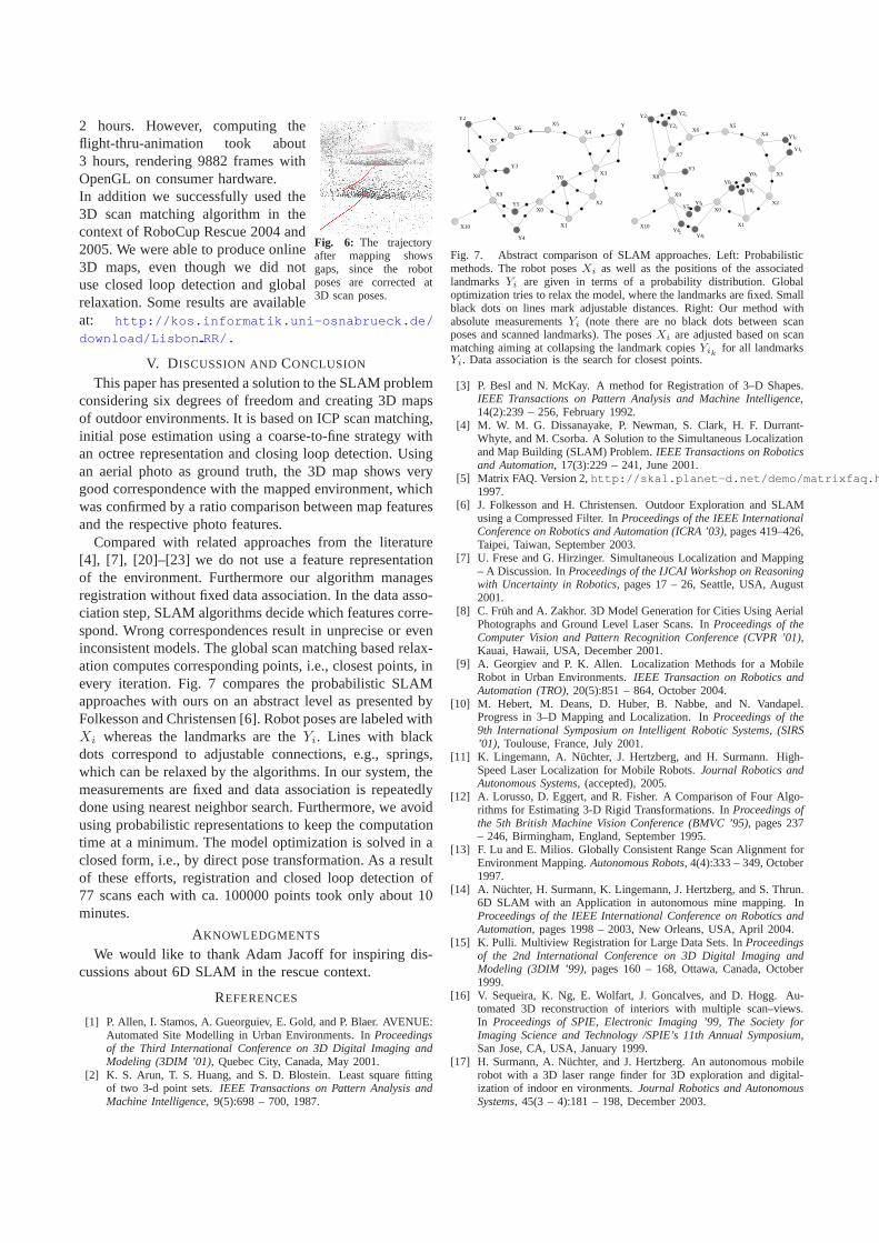
Fig. 5 shows three views of the final model. These modelviews correspond to the locations of Kurt3D in Fig. 1. Anupdated robot trajectory has been plotted into the scene.

Fig. 4. Detailed view of the 3D model of Fig. 3. Left: Model before loopclosing. Right: After loop closing, global relaxation and adding further 3Dscans. Top: Top view. Bottom: Front view.

TABLE I

Length ratio comparison of measured distances in the aerial photographs

(AP) with distances in the point model (PM) as shown in Fig. 3.

1st line 2nd line ratio AP ratio in PM dev.AB BC 0.683 0.662 3.1%AB BD 0.645 0.670 3.8%AC CD 1.131 1.141 0.9%CD BD 1.088 1.082 0.5%

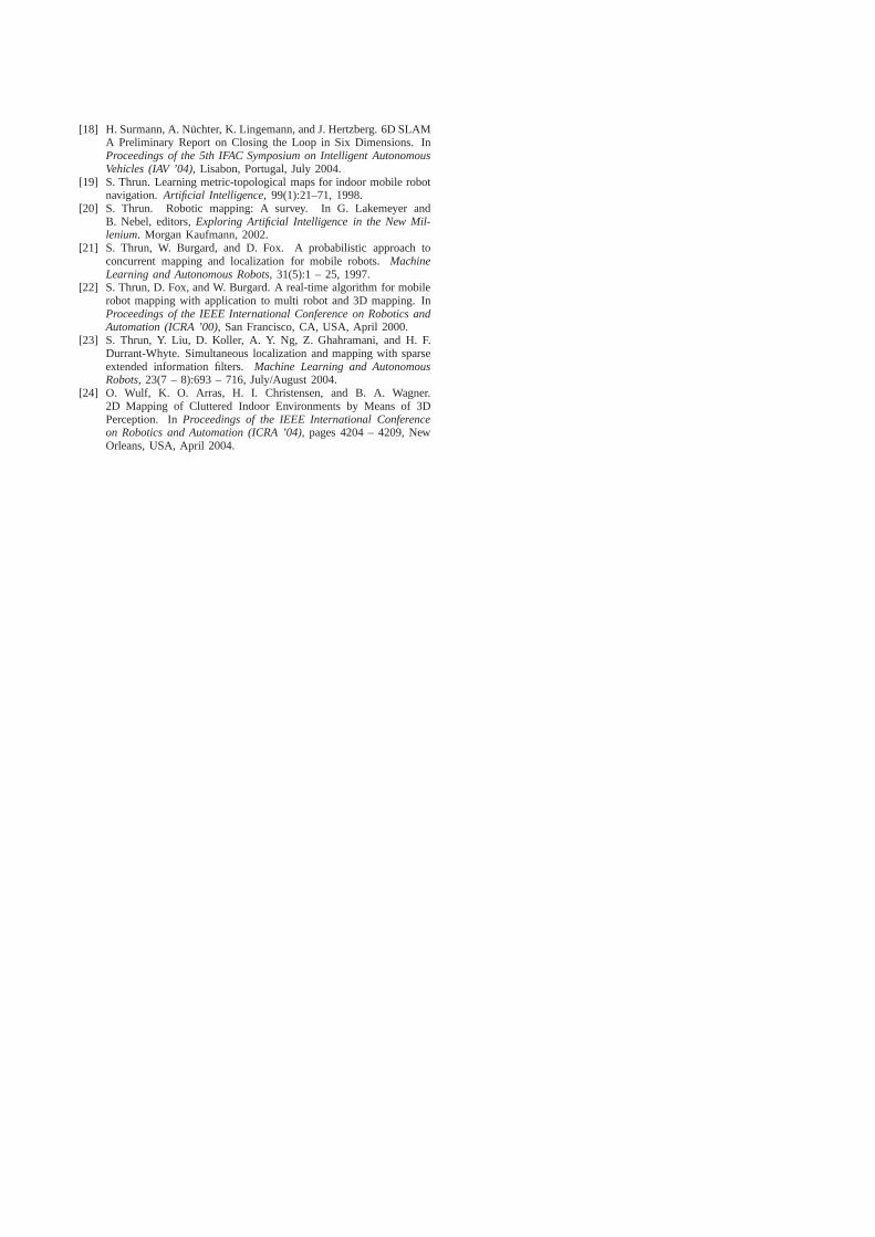
Thereby, we assign every 3D scan that part of the trajectorywhich leads from the previous scan pose to the currentone. Since scan matching did align the scans, the trajectoryinitially has gaps after the alignment (see Fig. 6).

We calculate the transformation (R, t) that maps the lastpose of such a trajectory patch to the starting pose ofthe next patch. This transformation is then used to correctthe trajectory patch by distributing the transformation asdescribed in section III-B.1. In this way the algorithm com-putes a continuous trajectory. An animation of the scannedarea is available at http://kos.informatik.uni-osnabrueck.de/6Doutdoor/. The video shows thescene along the trajectory as viewed from about 1 m aboveKurt3Ds actual position.

The 3D scans were acquired within one hour by tele-operation of Kurt3D. Scan registration and closed loopdetection took only about 10 minutes on a Pentium-IV-2800 MHz, while we did run the global relaxation for

Fig. 5. Detailed views of the resulting 3D model corresponding to robotlocations of Fig. 1.

2 hours. However, computing theflight-thru-animation took about3 hours, rendering 9882 frames withOpenGL on consumer hardware.In addition we successfully used the3D scan matching algorithm in thecontext of RoboCup Rescue 2004 and2005. We were able to produce online3D maps, even though we did notuse closed loop detection and globalrelaxation. Some results are available

Fig. 6: The trajectoryafter mapping showsgaps, since the robotposes are corrected at3D scan poses.

at: http://kos.informatik.uni-osnabrueck.de/download/Lisbon RR/.

V. DISCUSSION AND CONCLUSIONThis paper has presented a solution to the SLAM problem

considering six degrees of freedom and creating 3D mapsof outdoor environments. It is based on ICP scan matching,initial pose estimation using a coarse-to-fine strategy withan octree representation and closing loop detection. Usingan aerial photo as ground truth, the 3D map shows verygood correspondence with the mapped environment, whichwas confirmed by a ratio comparison between map featuresand the respective photo features.

Compared with related approaches from the literature[4], [7], [20][23] we do not use a feature representationof the environment. Furthermore our algorithm managesregistration without fixed data association. In the data asso-ciation step, SLAM algorithms decide which features corre-spond. Wrong correspondences result in unprecise or eveninconsistent models. The global scan matching based relax-ation computes corresponding points, i.e., closest points, inevery iteration. Fig. 7 compares the probabilistic SLAMapproaches with ours on an abstract level as presented byFolkesson and Christensen [6]. Robot poses are labeled withXi whereas the landmarks are the Yi. Lines with blackdots correspond to adjustable connections, e.g., springs,which can be relaxed by the algorithms. In our system, themeasurements are fixed and data association is repeatedlydone using nearest neighbor search. Furthermore, we avoidusing probabilistic representations to keep the computationtime at a minimum. The model optimization is solved in aclosed form, i.e., by direct pose transformation. As a resultof these efforts, registration and closed loop detection of77 scans each with ca. 100000 points took only about 10minutes.

AKNOWLEDGMENTSWe would like to thank Adam Jacoff for inspiring dis-

cussions about 6D SLAM in the rescue context.

REFERENCES

[1] P. Allen, I. Stamos, A. Gueorguiev, E. Gold, and P. Blaer. AVENUE:Automated Site Modelling in Urban Environments. In Proceedingsof the Third International Conference on 3D Digital Imaging andModeling (3DIM 01), Quebec City, Canada, May 2001.

[2] K. S. Arun, T. S. Huang, and S. D. Blostein. Least square fittingof two 3-d point sets. IEEE Transactions on Pattern Analysis andMachine Intelligence, 9(5):698 700, 1987.

X1

Y0

X0X2

X3

X4

X5X6

X7

X8

X9

X10

Y1Y2

Y3

Y5

Y4

X1

X0X2

X3

X4

X5X6

X8

X9

X10

X7

Y4

Y0

Y0

Y0

Y1

Y1

Y2

Y2

Y3

Y4

Y5Y5

1

1

1

1

2

2

2

2

2

3

3Y2

1

Fig. 7. Abstract comparison of SLAM approaches. Left: Probabilisticmethods. The robot poses Xi as well as the positions of the associatedlandmarks Yi are given in terms of a probability distribution. Globaloptimization tries to relax the model, where the landmarks are fixed. Smallblack dots on lines mark adjustable distances. Right: Our method withabsolute measurements Yi (note there are no black dots between scanposes and scanned landmarks). The poses Xi are adjusted based on scanmatching aiming at collapsing the landmark copies Yik for all landmarksYi. Data association is the search for closest points.

[3] P. Besl and N. McKay. A method for Registration of 3D Shapes.IEEE Transactions on Pattern Analysis and Machine Intelligence,14(2):239 256, February 1992.

[4] M. W. M. G. Dissanayake, P. Newman, S. Clark, H. F. Durrant-Whyte, and M. Csorba. A Solution to the Simultaneous Localizationand Map Building (SLAM) Problem. IEEE Transactions on Roboticsand Automation, 17(3):229 241, June 2001.

[5] Matrix FAQ. Version 2, http://skal.planet-d.net/demo/matrixfaq.htm1997.

[6] J. Folkesson and H. Christensen. Outdoor Exploration and SLAMusing a Compressed Filter. In Proceedings of the IEEE InternationalConference on Robotics and Automation (ICRA 03), pages 419426,Taipei, Taiwan, September 2003.

[7] U. Frese and G. Hirzinger. Simultaneous Localization and Mapping A Discussion. In Proceedings of the IJCAI Workshop on Reasoningwith Uncertainty in Robotics, pages 17 26, Seattle, USA, August2001.

[8] C. Fruh and A. Zakhor. 3D Model Generation for Cities Using AerialPhotographs and Ground Level Laser Scans. In Proceedings of theComputer Vision and Pattern Recognition Conference (CVPR 01),Kauai, Hawaii, USA, December 2001.

[9] A. Georgiev and P. K. Allen. Localization Methods for a MobileRobot in Urban Environments. IEEE Transaction on Robotics andAutomation (TRO), 20(5):851 864, October 2004.

[10] M. Hebert, M. Deans, D. Huber, B. Nabbe, and N. Vandapel.Progress in 3D Mapping and Localization. In Proceedings of the9th International Symposium on Intelligent Robotic Systems, (SIRS01), Toulouse, France, July 2001.

[11] K. Lingemann, A. Nuchter, J. Hertzberg, and H. Surmann. High-Speed Laser Localization for Mobile Robots. Journal Robotics andAutonomous Systems, (accepted), 2005.

[12] A. Lorusso, D. Eggert, and R. Fisher. A Comparison of Four Algo-rithms for Estimating 3-D Rigid Transformations. In Proceedings ofthe 5th British Machine Vision Conference (BMVC 95), pages 237 246, Birmingham, England, September 1995.

[13] F. Lu and E. Milios. Globally Consistent Range Scan Alignment forEnvironment Mapping. Autonomous Robots, 4(4):333 349, October1997.

[14] A. Nuchter, H. Surmann, K. Lingemann, J. Hertzberg, and S. Thrun.6D SLAM with an Application in autonomous mine mapping. InProceedings of the IEEE International Conference on Robotics andAutomation, pages 1998 2003, New Orleans, USA, April 2004.

[15] K. Pulli. Multiview Registration for Large Data Sets. In Proceedingsof the 2nd International Conference on 3D Digital Imaging andModeling (3DIM 99), pages 160 168, Ottawa, Canada, October1999.

[16] V. Sequeira, K. Ng, E. Wolfart, J. Goncalves, and D. Hogg. Au-tomated 3D reconstruction of interiors with multiple scanviews.In Proceedings of SPIE, Electronic Imaging 99, The Society forImaging Science and Technology /SPIEs 11th Annual Symposium,San Jose, CA, USA, January 1999.

[17] H. Surmann, A. Nuchter, and J. Hertzberg. An autonomous mobilerobot with a 3D laser range finder for 3D exploration and digital-ization of indoor en vironments. Journal Robotics and AutonomousSystems, 45(3 4):181 198, December 2003.

[18] H. Surmann, A. Nuchter, K. Lingemann, and J. Hertzberg. 6D SLAMA Preliminary Report on Closing the Loop in Six Dimensions. InProceedings of the 5th IFAC Symposium on Intelligent AutonomousVehicles (IAV 04), Lisabon, Portugal, July 2004.

[19] S. Thrun. Learning metric-topological maps for indoor mobile robotnavigation. Artificial Intelligence, 99(1):2171, 1998.

[20] S. Thrun. Robotic mapping: A survey. In G. Lakemeyer andB. Nebel, editors, Exploring Artificial Intelligence in the New Mil-lenium. Morgan Kaufmann, 2002.

[21] S. Thrun, W. Burgard, and D. Fox. A probabilistic approach toconcurrent mapping and localization for mobile robots. MachineLearning and Autonomous Robots, 31(5):1 25, 1997.

[22] S. Thrun, D. Fox, and W. Burgard. A real-time algorithm for mobilerobot mapping with application to multi robot and 3D mapping. InProceedings of the IEEE International Conference on Robotics andAutomation (ICRA 00), San Francisco, CA, USA, April 2000.

[23] S. Thrun, Y. Liu, D. Koller, A. Y. Ng, Z. Ghahramani, and H. F.Durrant-Whyte. Simultaneous localization and mapping with sparseextended information filters. Machine Learning and AutonomousRobots, 23(7 8):693 716, July/August 2004.

[24] O. Wulf, K. O. Arras, H. I. Christensen, and B. A. Wagner.2D Mapping of Cluttered Indoor Environments by Means of 3DPerception. In Proceedings of the IEEE International Conferenceon Robotics and Automation (ICRA 04), pages 4204 4209, NewOrleans, USA, April 2004.