20101 LUES Report Draft 9.4

1

Land Use and Stream Health in the Rivanna Basin, 2007-2009

By John Murphy

Science Advisor, StreamWatch

September 30, 2011

StreamWatch

P.O. Box 681

Charlottesville, VA 22901

www.streamwatch.org

________________________________________________________________________

ACKNOWLEDGMENTS

This report reflects the work of scores of individuals and thousands of person-hours. We

extend our deep gratitude to the following individuals and organizations, without whose

generosity and dedication this study would not have been possible.

StreamWatch Partners

Albemarle County / City of Charlottesville / Fluvanna County / The Nature Conservancy

Rivanna Conservation Society / Rivanna River Basin Commission / Rivanna Water and

Sewer Authority / Thomas Jefferson Planning District Commission / Thomas Jefferson

Soil and Water Conservation District

Science Collaborators

For guidance with study design, assistance with modeling, and review of analytical

methods, we extend our special thanks to Karen McGlathery and Todd Scanlon of

University of Virginia’s Department of Environmental Sciences. For contributing research

on stream sedimentation, we extend our special thanks to Christine May of James Madison

University’s Department of Biology.

Technical Support

For development and management of GIS-based information about the Rivanna basin, we

extend our special thanks to Chris Bruce of The Nature Conservancy, to Rick Odom, to

Chesapeake Bay Funders Network, and to WorldView Solutions, Inc.

StreamWatch Technical Advisory Committee

For general guidance and support, and for review of text and analysis, we thank

StreamWatch’s Technical Advisory Committee:

Samuel Austin, U.S. Geological Survey / Greg Harper, Albemarle County /

David Hirschman, Center for Watershed Protection / John Kauffman, Virginia Department

of Game and Inland Fisheries / Karen McGlathery, University of Virginia / Rick Odom,

Ecologist, GIS specialist / Brian Richter, The Nature Conservancy

2

Todd Scanlon, University of Virginia / William Van Wart, Virginia Department of

Environmental Quality

Volunteers and Interns

Our profound and heartfelt gratitude goes out to the many volunteers and interns who

assisted with data collection and data management. We could not have completed this

study without your hard work. Thank you!

Volunteers

Jennifer Alexander / Michael Baker / Dav Banks / Cameron Beers / Calvin Biesecker

Steve Botts / Kelly Bowman / Rachel Bush / Nora Byrd / David Carr / Tina Colom

Gus Colom / Cristina Cornell / Erin Cornell / Nancy Cornell / Aaron Cross / Vince Dish

Laura Dollard / Sharon Ellison / Terri Ellison / Brendan Ferreri-Hamberry / Jane Fisher

Nancy Ford / Ned Foss / Doug Fraser / Nancy Friend / Diane Frisbee / James Gano

Kathy Gerber / Nancy Gercke / Repp Glaettli / Helen Gordon / Sean Grzegorczyk

Shane Grzegorczyk / Deb Hackett / Elise Hackett / Ralph Hall / Shirley Halladay

Allen Hard / Bob Henricks / Tana Herndon / Joel Howard / John Ince / Stefan Jirka

Karen Joyner / Jim Kabat / Terri Keffert / Aidan Keith-Hynes / Bronwyn Keith-Hynes

Patrick Keith-Hynes / Frances Lee-Vandell / Vera Leone / Keggie Mallett

Ann McLeod-Lambert / Vicki Metcalf / Susan Meyer / Jill Meyer / Leslie Middleton

Janet Miller / Becky Minor / Maggie Murphy / Sarah Murphy / Rose Sgarlat Myers

Jim Nix / Marianne O’Brien / Cindy O’Connell / Killian O’Connell / James Peacock

Frank Persico / Art Petty / Kristin Pickering / Elena Prien / Patrick Punch

Anne Rasmussen / Nicola (Nicky) Roberts / Pat Schnatterly / Steve Schnatterly

Marjorie Siegel / Susan Sleight / Hugo Spaulding / Will Spaulding / Edward Strickler Jr.

Ida Swenson / Roger Temples / Pat Temples / Michelle Thompson / Rob Tilghman

Dorothy Tompkins / Rachel Vigour / John Walsh / Tom Walsh / Phyllis White

Frank Wilczek / Pat Wilczek / Steve Sylvan Willig / James Winsett / Laurel Woodworth

Interns

Aaron Bloch / Will Devault-Weaver / Kelsey Ducklow / Alissa Gador / Erin Gallagher

Benjamin Hines / Aryn Hoge / Margaret Jarosz / Sarah Kang / Katie Layman

Andrew Moore / Robert Noffsinger / Scott Osborne / Catherine Pham / Eleanor Preston

Peter Swigert / Brian Walton / Megan Wood

Funders

Albemarle County

Chesapeake Bay Restoration Fund

City of Charlottesville

Fluvanna County

J & E Berkley Foundation

Rivanna Water and Sewer Authority

The Nature Conservancy

Virginia Environmental Endowment

3

Contents

1) Summaries......................................................................................................................................4

1.1) Abstract. ................................................................................................................................4 1.2) Bulleted list of key findings....................................................................................................4

2) Background.....................................................................................................................................5 2.1) Overview: land use and stream health..................................................................................5 2.2) The Rivanna basin. ...............................................................................................................6 2.3) StreamWatch. .......................................................................................................................6 2.4) Scope of this study................................................................................................................6 2.5) Terminology...........................................................................................................................7 2.6) Watershed classifications......................................................................................................8 2.7) Measuring biological condition; StreamWatch assessment tiers; Virginia regulatory standard......................................................................................................................................13 2.8) Why bugs? ..........................................................................................................................14

3) Findings ........................................................................................................................................15 3.1) Relationships between stream biological condition and watershed land use/land cover. ..15

3.1.1) Across the full range data, spanning reference to urban systems, biological condition correlates more strongly with impervious cover than with other land use/land cover variables...............................................................................................................................15

3.1.1.1) Land use/land cover and biology were more strongly related in smaller streams than in larger streams......................................................................................19

3.1.2) In non-urban systems, forest cover and impervious cover together predict stream biological condition better than impervious cover alone. .....................................................20 3.1.3) Degradation begins very early in the watershed disturbance continuum. Our healthiest benthic communities were found exclusively in basins with forest cover ≥ 99%.24 3.1.4) Failure to meet the Virginia aquatic life regulatory standard becomes common at the exurban stage of the land use continuum. Most of the Rivanna basin is exurban. .............26 3.1.5) Based on impervious cover and forest cover, we estimate that most small streams in the Rivanna basin do not meet the Virginia biological standard..........................................29 3.1.6) Potential effects of future land use change. ..............................................................31

3.2) We found no relationship between stream biological condition and cattle operations quantified at the watershed scale...............................................................................................35 3.3) Relationships between stream biology and reach-scale environmental variables. ............37

3.3.1) Bank stability, sediment deposition, and related channel variables correlated with biological condition, particularly in exurban and rural streams............................................37 3.3.2) Streambed permeability and substrate sediment concentration. ..............................43

3.3.2.1) Streambed permeability was generally low. ....................................................43 3.3.2.2) Streambed permeability and substrate sediment concentration did not strongly correlate with biological condition. ................................................................................44 3.3.2.3) Streambed permeability and substrate sediment concentration correlated moderately with watershed land use/land cover, as did other substrate-related variables. .......................................................................................................................47

3.3.3) Forested riparian buffers may help improve biological health, but only within constraints set by watershed-wide land use/land cover. .....................................................51

3.4) Bacterial counts were little related land use/land cover, and were completely unrelated to biological condition as measured by benthic macroinvertebrate samples. ................................53

4) Bird’s eye tour: typical and atypical examples of relationships between biological health and environmental factors........................................................................................................................55 5) Recommendations for further study. ............................................................................................62 6) Appendix A – Methods..................................................................................................................63

6.1) Site selection .......................................................................................................................63 6.2) Assessing biological condition. ...........................................................................................63

6.2.1) Relationship between average biological index score and the Virginia biological standard. ..............................................................................................................................64

6.3) Classification of land use/land cover...................................................................................65 6.4) Estimating human population density .................................................................................66

4

6.5) Estimating cattle populations ..............................................................................................66 6.6) Reach-scale habitat data ....................................................................................................66 6.7) Substrate permeability ........................................................................................................69 6.8) Bacteria ...............................................................................................................................69

7) Appendix B - Comprehensive correlation matrix ..........................................................................70 8) Appendix C - Overview of bedrock and soils in the Rivanna River drainage ...............................72 9) Appendix D - References .............................................................................................................73

1) Summaries

1.1) Abstract.

We examined relationships between land use, stream habitat, and stream benthic

macroinvertebrate condition (stream biological condition) in central Virginia’s Rivanna

River basin. Benthic macroinvertebrate condition was assessed at 51 sites per a slightly

modified version of the Virginia Stream Condition Index protocol. Basin land use/land

cover was classified at high resolution based on planimetrics and aerial imagery. Cattle

population densities and grazed pasture were determined from aerial imagery. Across a

set of 42 systems ranging from urban to nearly undisturbed conditions, watershed percent

impervious cover predicted over 80% of variation in biological condition. When more

highly urbanized systems were excluded from analysis, both forest cover and impervious

cover emerged as distinctive, equally strong predictors of health, and together accounted

for over 60% of biological condition variation. Noticeable biological degradation was

associated with a very early stage of watershed disturbance; the healthiest benthic

communities were found exclusively in basins with forest cover ≥ 99%. About 60% of the

Rivanna basin is exurban (population density ranging from 40 to 160 per square mile;

acres per dwelling ranging from 9 to 37 acres; impervious cover ranging from 1.2% to

3.1%). About half of studied exurban systems failed the Virginia aquatic life regulatory

standard. Generally, the regulatory threshold was breached before systems reached 3%

impervious cover. Cattle operations, quantified at the landscape scale, showed no

correlation with biological condition. Streambed permeability was generally low,

suggesting excess sedimentation. Several reach-scale habitat variables correlated weakly

to moderately with biological condition, but were generally far less predictive of biological

condition than was watershed land use/land cover. In rural, exurban, and suburban

systems, riparian buffer condition explained some biological variation not captured by

land use/land cover, suggesting that forested stream buffers can positively influence

stream biology, but only within limits set by watershed land use/land cover. In rural and

exurban systems, bank erosion and sediment deposition explained some biological

variation not captured by land use/land cover.

1.2) Bulleted list of key findings.

• Most streams we studied failed Virginia’s biological standard. This standard tells

us whether streams support a variety of life forms. Streams with more life have

better water quality, and can provide better services to humans. Such services

include water supply, recreation, and aesthetic enjoyment.

• Stream health is closely related to land use. Rural landscapes with lots of forest

have healthy streams. Urban areas have unhealthy streams. In between, health

5

declines predictably as land use intensifies. The relationship is so strong that we

can estimate stream health based on the amount of forest and development in the

surrounding area.

• Unlike development and deforestation, cattle operations, quantified at the

watershed scale, did not have a big impact on stream health. However, we did not

study the effects of cattle located close to streams.

• Based on land use, we estimate that 70% of Rivanna streams fail the Virginia

standard. Fortunately, only 5% to 10% of streams are severely degraded. Most

streams sit near the pass/fail cusp and might meet the standard with better care.

• Most of the Rivanna basin is semi-rural (exurban). In this exurban landscape, forest

cover averages about 70%, and there are about 17 acres for every house. This

amount of disturbance may seem mild, yet more than half of exurban streams failed

the biological standard.

• Rural and exurban streams decline rapidly with increased development or

deforestation. In urban areas, stream health is already poor. Therefore, urban

streams do not respond dramatically to additional development.

• Within 20 years, increased development in non-urban areas could reduce the

number of healthy streams by about a third.

• Unstable banks and excess sediment appears to affect stream health in many

Rivanna streams.

• Forested buffers alongside streams can protect and improve stream health.

2) Background

2.1) Overview: land use and stream health.

A substantial body of scientific literature documents relationships between land use

and stream health (Allan 1997, Schueler 2009, Coles 2004, King 2010, Morse 2003, Ourso

2003). Conceptual models such as Center for Watershed Protection’s Reformulated

Impervious Cover Model provide useful frameworks for understanding the land use/stream

health relationship in general terms (Schueler 2009). But this relationship varies across

stream condition parameters (e.g. water quality, channel condition, biological integrity),

and probably also varies across regions. Further, watershed management and conservation

at the ground level often demands local data rather than generalist models.

Previous StreamWatch studies have illustrated strong relationships between land

use/land cover and biological condition in the Rivanna basin (Murphy 2006, Murphy

2008). Those studies not only showed strong correlations between land use/land cover and

biology, they also suggested that significant biological degradation commenced at fairly

low levels of landscape disturbance. The current study draws from more extensive field

data than previous studies, and utilizes land use/land cover data that is of far higher quality

6

than that of earlier studies. The study examines empirical relationships between land

use/land cover (LU/LC), channel and riparian conditions, and stream biological conditions

as expressed by benthic macroinvertebrate multimetric index scores. With these newer,

better, and more comprehensive data, we have been able to confirm that biological

degradation in streams does indeed begin at the earliest stages of the landscape degradation

continuum, and that Rivanna streams commonly fail Virginia’s regulatory biological

standard at levels of land disturbance commensurate with the basin’s characteristically

exurban landscape.

2.2) The Rivanna basin.

The Rivanna River drains 765-square miles of central Virginia’s Jefferson country.

The basin is about 70% forested and 3.2% impervious. Population centers such as the City

of Charlottesville notwithstanding, the majority of the basin is exurban, with a mixture of

residential and agricultural land uses. Agriculture—mostly cattle grazing—is only lightly

to moderately intensive. Forestry is practiced mostly in the form of loblolly pine

plantations and periodic harvesting of hardwoods.

For a detailed description of the basin’s bedrock geology and soils, see Appendix

C.

2.3) StreamWatch.

StreamWatch is a community-based monitoring program focused on the Rivanna

Basin. We leverage volunteer labor to enhance data collection capacity for community

partners ranging from the water and sewer authority to local governments to non-

governmental organizations. This organizational model has helped to produce a robust,

dense, benthic macroinvertebrate dataset that helps inform Rivanna basin watershed

management and conservation. StreamWatch is professionally staffed and is committed to

highest data quality standards. Our benthic macroinvertebrate protocol is subject to a

Quality Assurance Project Plan approved by the Virginia Department of Environmental

Quality (DEQ), and the DEQ uses StreamWatch data to list and de-list streams in its

305(b) reports.

2.4) Scope of this study.

The StreamWatch Land Use Study (LUS) was conceived to explore relationships

between stream biological condition, reach-scale habitat conditions, and watershed-scale

land use/land cover ( LU/LC). The study was designed primarily to examine relationships

between watershed scale LU/LC and stream biological condition, but we also explored

possible links between landscape conditions (e.g. impervious cover) and reach-scale stream

habitat conditions (e.g. sedimentation). The study was designed to provide information

useful for land use planning, watershed management, and conservation. As such, the study

focuses on human-mediated factors, and seeks to filter out the effects of natural variables

as much as possible.

The study was not designed to trace causal links between environmental and

biological conditions. Rather, we looked for empirical relationships, mostly in the form of

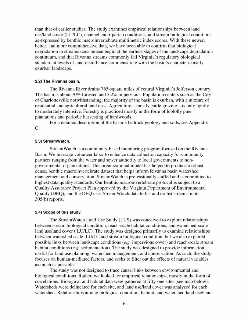
correlations. Biological and habitat data were gathered at fifty-one sites (see map below).

Watersheds were delineated for each site, and land use/land cover was analyzed for each

watershed. Relationships among biological condition, habitat, and watershed land use/land

7

cover were analyzed using a variety of statistical techniques. For more information on

methods, see Appendix A.

Above: Icons show location and biological condition of study sites, with green indicating healthiest conditions, and black indicating poorest conditions.

2.5) Terminology.

• IC: impervious cover – expressed as the percentage of a given area (e.g. a

watershed) that is covered by paved or unpaved roads, parking lots, sidewalks,

rooftops, and railroads.

• LU/LC: land use/land cover – the terms land use and land cover have overlapping

definitions. For instance, a pine plantation can be classified both as a land use

(monoculture forestry) and a land cover (pine forest). For the purposes of our

report, we chose to combine the terms.

• Scales:

8

• Reach scale – the stream reach and riparian zone at and upstream of the

sampling site. Depending on stream size, this area can extend up to 1,000

meters upstream of the site. Riparian zone width for our study is

approximately 18 meters.

• Watershed scale or landscape scale – the scale of the entire watershed

draining to the sampling site. Areal extent varies from less than 1 square mile

to more than 700 square miles.

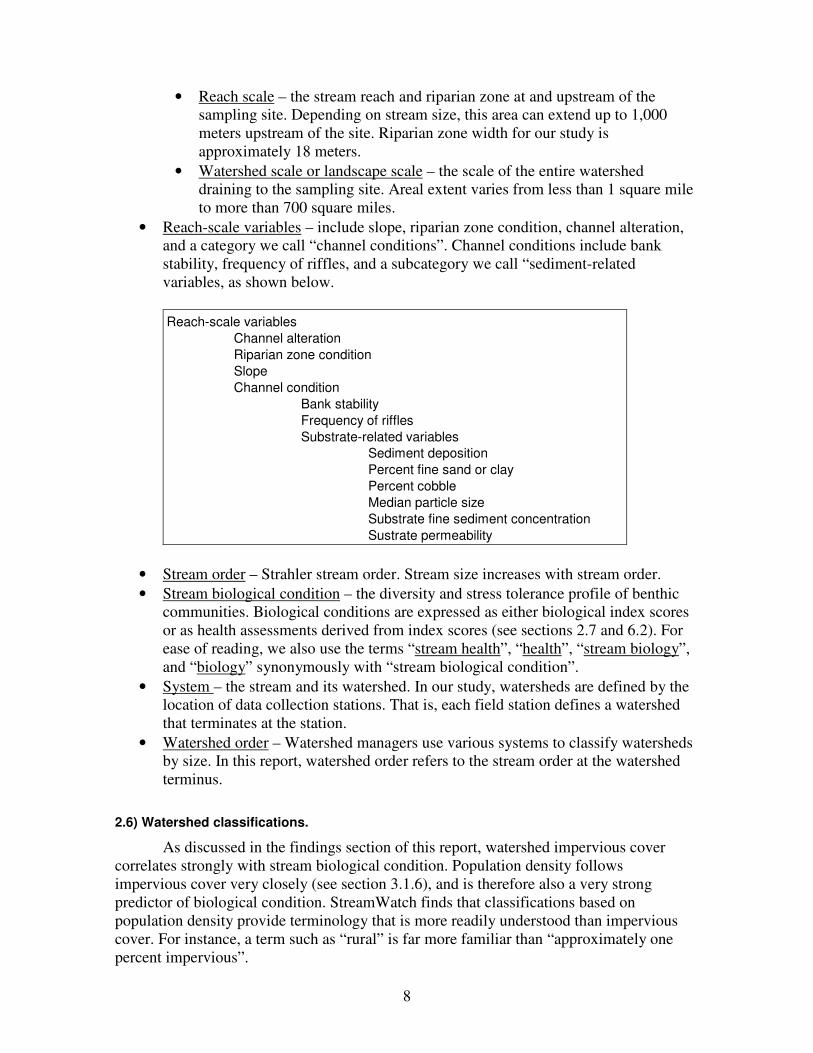
• Reach-scale variables – include slope, riparian zone condition, channel alteration,

and a category we call “channel conditions”. Channel conditions include bank

stability, frequency of riffles, and a subcategory we call “sediment-related

variables, as shown below.

Riparian zone condition

Substrate-related variables

Sediment deposition

Percent fine sand or clay

Percent cobble

Median particle size

Substrate fine sediment concentration

Sustrate permeability

Bank stability

Frequency of riffles

Reach-scale variables

Channel alteration

Slope

Channel condition

• Stream order – Strahler stream order. Stream size increases with stream order.

• Stream biological condition – the diversity and stress tolerance profile of benthic

communities. Biological conditions are expressed as either biological index scores

or as health assessments derived from index scores (see sections 2.7 and 6.2). For

ease of reading, we also use the terms “stream health”, “health”, “stream biology”,

and “biology” synonymously with “stream biological condition”.

• System – the stream and its watershed. In our study, watersheds are defined by the

location of data collection stations. That is, each field station defines a watershed

that terminates at the station.

• Watershed order – Watershed managers use various systems to classify watersheds

by size. In this report, watershed order refers to the stream order at the watershed

terminus.

2.6) Watershed classifications.

As discussed in the findings section of this report, watershed impervious cover

correlates strongly with stream biological condition. Population density follows

impervious cover very closely (see section 3.1.6), and is therefore also a very strong

predictor of biological condition. StreamWatch finds that classifications based on

population density provide terminology that is more readily understood than impervious

cover. For instance, a term such as “rural” is far more familiar than “approximately one

percent impervious”.

9

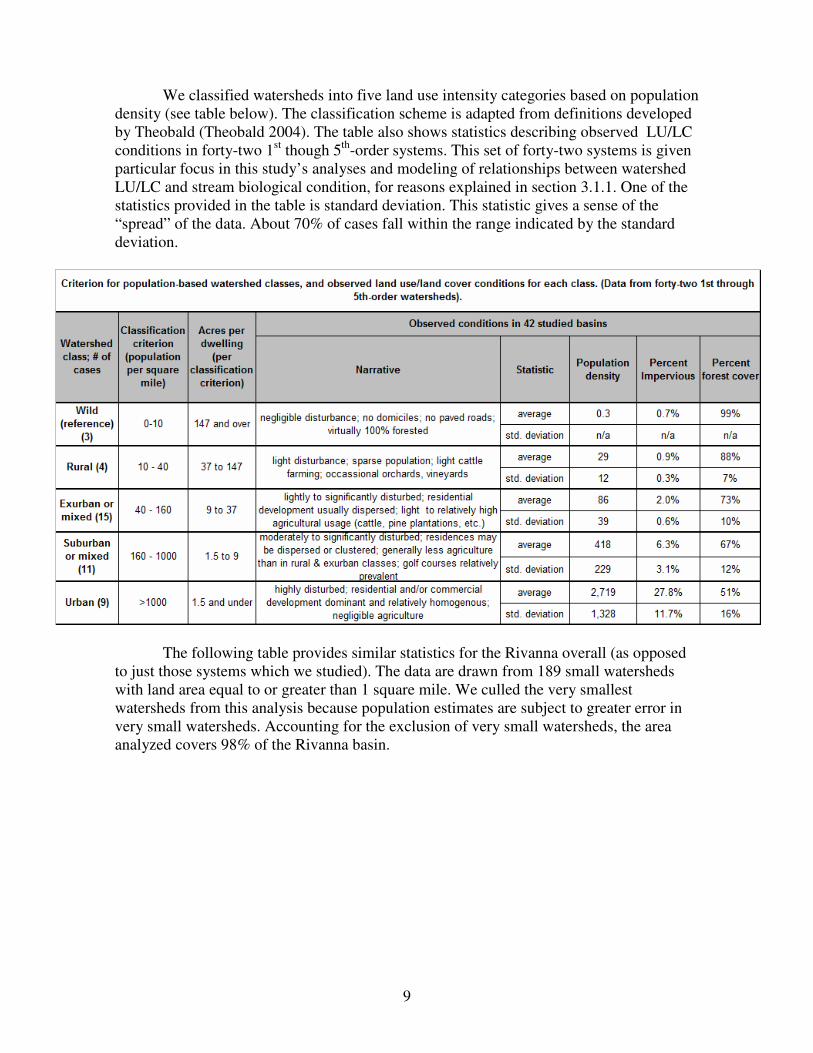
We classified watersheds into five land use intensity categories based on population

density (see table below). The classification scheme is adapted from definitions developed

by Theobald (Theobald 2004). The table also shows statistics describing observed LU/LC

conditions in forty-two 1st though 5

th-order systems. This set of forty-two systems is given

particular focus in this study’s analyses and modeling of relationships between watershed

LU/LC and stream biological condition, for reasons explained in section 3.1.1. One of the

statistics provided in the table is standard deviation. This statistic gives a sense of the

“spread” of the data. About 70% of cases fall within the range indicated by the standard

deviation.

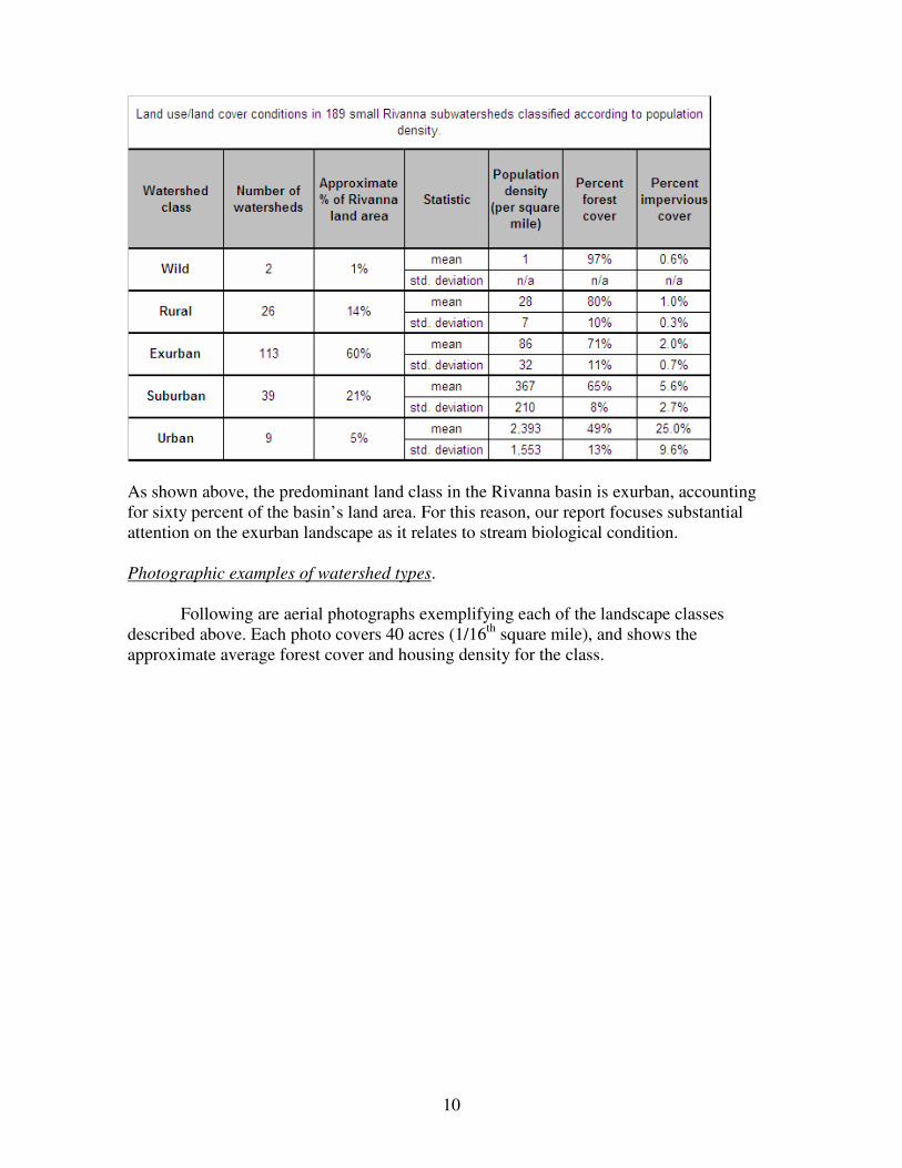
The following table provides similar statistics for the Rivanna overall (as opposed

to just those systems which we studied). The data are drawn from 189 small watersheds

with land area equal to or greater than 1 square mile. We culled the very smallest

watersheds from this analysis because population estimates are subject to greater error in

very small watersheds. Accounting for the exclusion of very small watersheds, the area

analyzed covers 98% of the Rivanna basin.

10

As shown above, the predominant land class in the Rivanna basin is exurban, accounting

for sixty percent of the basin’s land area. For this reason, our report focuses substantial

attention on the exurban landscape as it relates to stream biological condition.

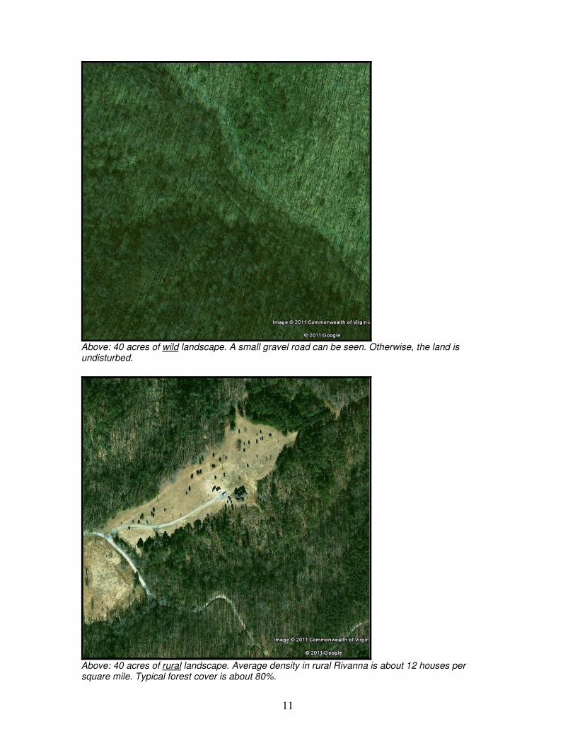
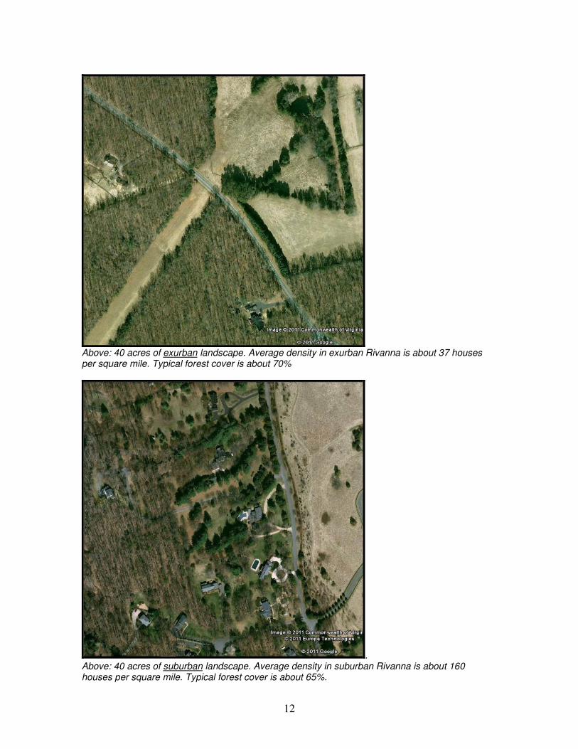
Photographic examples of watershed types.

Following are aerial photographs exemplifying each of the landscape classes

described above. Each photo covers 40 acres (1/16th

square mile), and shows the

approximate average forest cover and housing density for the class.

11

Above: 40 acres of wild landscape. A small gravel road can be seen. Otherwise, the land is undisturbed.

Above: 40 acres of rural landscape. Average density in rural Rivanna is about 12 houses per square mile. Typical forest cover is about 80%.

12

Above: 40 acres of exurban landscape. Average density in exurban Rivanna is about 37 houses per square mile. Typical forest cover is about 70%

. Above: 40 acres of suburban landscape. Average density in suburban Rivanna is about 160 houses per square mile. Typical forest cover is about 65%.

13

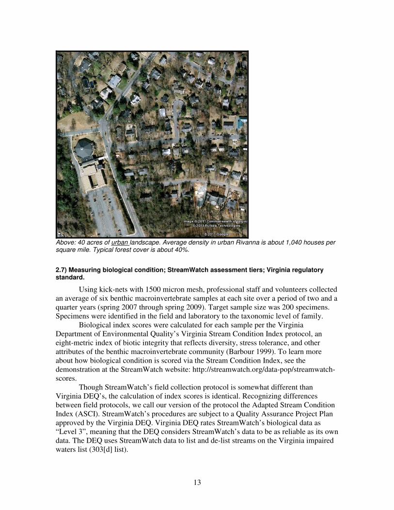
Above: 40 acres of urban landscape. Average density in urban Rivanna is about 1,040 houses per square mile. Typical forest cover is about 40%.

2.7) Measuring biological condition; StreamWatch assessment tiers; Virginia regulatory standard.

Using kick-nets with 1500 micron mesh, professional staff and volunteers collected

an average of six benthic macroinvertebrate samples at each site over a period of two and a

quarter years (spring 2007 through spring 2009). Target sample size was 200 specimens.

Specimens were identified in the field and laboratory to the taxonomic level of family.

Biological index scores were calculated for each sample per the Virginia

Department of Environmental Quality’s Virginia Stream Condition Index protocol, an

eight-metric index of biotic integrity that reflects diversity, stress tolerance, and other

attributes of the benthic macroinvertebrate community (Barbour 1999). To learn more

about how biological condition is scored via the Stream Condition Index, see the

demonstration at the StreamWatch website: http://streamwatch.org/data-pop/streamwatch-

scores.

Though StreamWatch’s field collection protocol is somewhat different than

Virginia DEQ’s, the calculation of index scores is identical. Recognizing differences

between field protocols, we call our version of the protocol the Adapted Stream Condition

Index (ASCI). StreamWatch’s procedures are subject to a Quality Assurance Project Plan

approved by the Virginia DEQ. Virginia DEQ rates StreamWatch’s biological data as

“Level 3”, meaning that the DEQ considers StreamWatch’s data to be as reliable as its own

data. The DEQ uses StreamWatch data to list and de-list streams on the Virginia impaired

waters list (303[d] list).

14

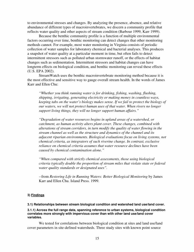
This study’s analyses and findings discuss biological condition in terms of both

scores and assessments. Section 6.2 describes our methods for producing biological

condition scores and assessments. The following table provides a reference for comparing

scores, stream biological condition assessment tiers, and narrative descriptions of

communities in different tiers.

Biological

condition

assessment tier

Approximate

range of

biological index

scores

Relationship to

Virginia

regulatory

standard

Narrative description

Very good 70 and over

Natural or nearly natural biological condition. The benthic macroinvertebrat community is

diverse. Many types of organisms are present. The majority of the population is intolerant

of human-caused stresses.

Good 60 - 70

Somewhat degraded. The community is diverse. Many types of organisms are present,

but the number of types of sensitive organisms is somewhat reduced relative to the "very

good" community. The majority of the population is intolerant of human-caused stresses.

Fair 40 - 60

Moderately degraded. The community is fairly diverse. Many types of organisms are

present, but the number of types of sensitive organisms is reduced relative to the "very

good" community. The majority of the population is tolerant of human-caused stresses.

Poor 25 - 40

Substantially degraded. The community is clearly less diverse than "very good"

communities. Fewer types of organisms are present, and the number of types of

sensitive organisms is deeply reduced. The great majority of the population is tolerant of

human-caused stresses.

Very poor 0 - 25Severely degraded. The community contains very few types of organisms, virtually all of

which are tolerant of human-caused stresses.

meets Virgina

standard

fails Virginia

standard

Biological condition assessment tiers, associated index scores, and generalized descriptions of benthic macroinvertebrate communities

associated with health tiers.

Per our data collection and computation, StreamWatch believes that those streams

we assess as very good or good meet the Virginia aquatic life regulatory standard, and that

streams assessed as fair, poor, or very poor fail the standard. Established by the Virginia

DEQ, and pursuant to the federal Clean Water Act, the Virginia aquatic life standard is

designed to identify whether or not water bodies support “the propagation and growth of a

balanced, indigenous population of aquatic life” (State Water Control Board, 2011).

As discussed in section 6.2, the Virginia DEQ considers StreamWatch’s data to be

as reliable as its own data, and uses StreamWatch data to place streams on or remove

streams from the Virginia impaired waters list (303[d] list).

As described in section 6.2, the process of assigning sites to an assessment tier

involves several factors including but not limited to average biological index score.

Because average score is not the sole factor by which assessments are derived, actual

average scores for sites assigned to a given tier can deviate slightly from the ranges listed

in the table above.

2.8) Why bugs?

StreamWatch determines the biological condition of streams by sampling and

analyzing stream benthic macroinvertebrate communities. The organisms comprising these

communities, including insects, crustaceans, snails, and worms, are variously responsive

15

to environmental stresses and changes. By analyzing the presence, absence, and relative

abundance of different types of macroinvertebrates, we discern a community profile that

reflects water quality and other aspects of stream condition (Barbour 1999, Karr 1999).

Because the benthic community profile is a function of multiple environmental

factors occurring over time, benthic monitoring can detect changes that other monitoring

methods cannot. For example, most water monitoring in Virginia consists of periodic

collection of water samples for laboratory chemical and bacterial analyses. This produces

a snapshot of water quality at a particular moment in time, but often fails to detect

intermittent stressors such as polluted urban stormwater runoff, or the effects of habitat

changes such as sedimentation. Intermittent stressors and habitat changes can have

longterm effects on biological condition, and benthic monitoring can reveal these effects

(U.S. EPA 2002).

StreamWatch uses the benthic macroinvertebrate monitoring method because it is

the most effective and sensitive way to gauge overall stream health. In the words of James

Karr and Ellen Chu:

“Whether you think running water is for drinking, fishing, washing, flushing,

shipping, irrigating, generating electricity or making money in countless ways,

keeping tabs on the water’s biology makes sense. If we fail to protect the biology of

our waters, we will not protect human uses of that water. When rivers no longer

support living things, they will no longer support human affairs.”

“Degradation of water resources begins in upland areas of a watershed, or

catchment, as human activity alters plant cover. These changes, combined with

alterations of stream corridors, in turn modify the quality of water flowing in the

stream channel as well as the structure and dynamics of the channel and its

adjacent riparian environments. Biological evaluations focus on living systems, not

chemical criteria, as integrators of such riverine change. In contrast, exclusive

reliance on chemical criteria assumes that water resource declines have been

caused by chemical contamination alone.”

“When compared with strictly chemical assessments, those using biological

criteria typically double the proportion of stream miles that violate state or federal

water quality standards or designated uses”.

--from Restoring Life in Running Waters: Better Biological Monitoring by James

Karr and Ellen Chu. Island Press. 1999.

3) Findings

3.1) Relationships between stream biological condition and watershed land use/land cover.

3.1.1) Across the full range data, spanning reference to urban systems, biological condition correlates more strongly with impervious cover than with other land use/land cover variables.

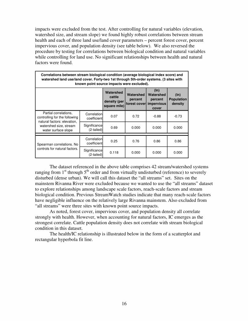
We tested for correlations between biological condition at sites and land use/land

cover parameters in site-defined watersheds. Three study sites with known point source

16

impacts were excluded from the test. After controlling for natural variables (elevation,

watershed size, and stream slope) we found highly robust correlations between stream

health and each of three land use/land cover parameters – percent forest cover, percent

impervious cover, and population density (see table below). We also reversed the

procedure by testing for correlations between biological condition and natural variables

while controlling for land use. No significant relationships between health and natural

factors were found.

Watershed

cattle

density (per

square mile)

Watershed

percent

forest cover

(ln)

Watershed

percent

impervious

cover

(ln)

Population

density

Correlation

coefficient0.07 0.72 -0.88 -0.73

Significance

(2-tailed)0.69 0.000 0.000 0.000

Correlation

coefficient0.25 0.76 0.86 0.86

Significance

(2-tailed)0.118 0.000 0.000 0.000

Correlations between stream biological condition (average biological index score) and

watershed land use/land cover. Forty-two 1st through 5th-order systems. (3 sites with

known point source impacts were excluded).

Partial correlations,

controlling for the following

natural factors: elevation,

watershed size, stream

water surface slope

Spearman correlations. No

controls for natural factors.

The dataset referenced in the above table comprises 42 stream/watershed systems

ranging from 1st through 5

th order and from virtually undisturbed (reference) to severely

disturbed (dense urban). We will call this dataset the “all streams” set. Sites on the

mainstem Rivanna River were excluded because we wanted to use the “all streams” dataset

to explore relationships among landscape scale factors, reach-scale factors and stream

biological condition. Previous StreamWatch studies indicate that many reach-scale factors

have negligible influence on the relatively large Rivanna mainstem. Also excluded from

“all streams” were three sites with known point source impacts.

As noted, forest cover, impervious cover, and population density all correlate

strongly with health. However, when accounting for natural factors, IC emerges as the

strongest correlate. Cattle population density does not correlate with stream biological

condition in this dataset.

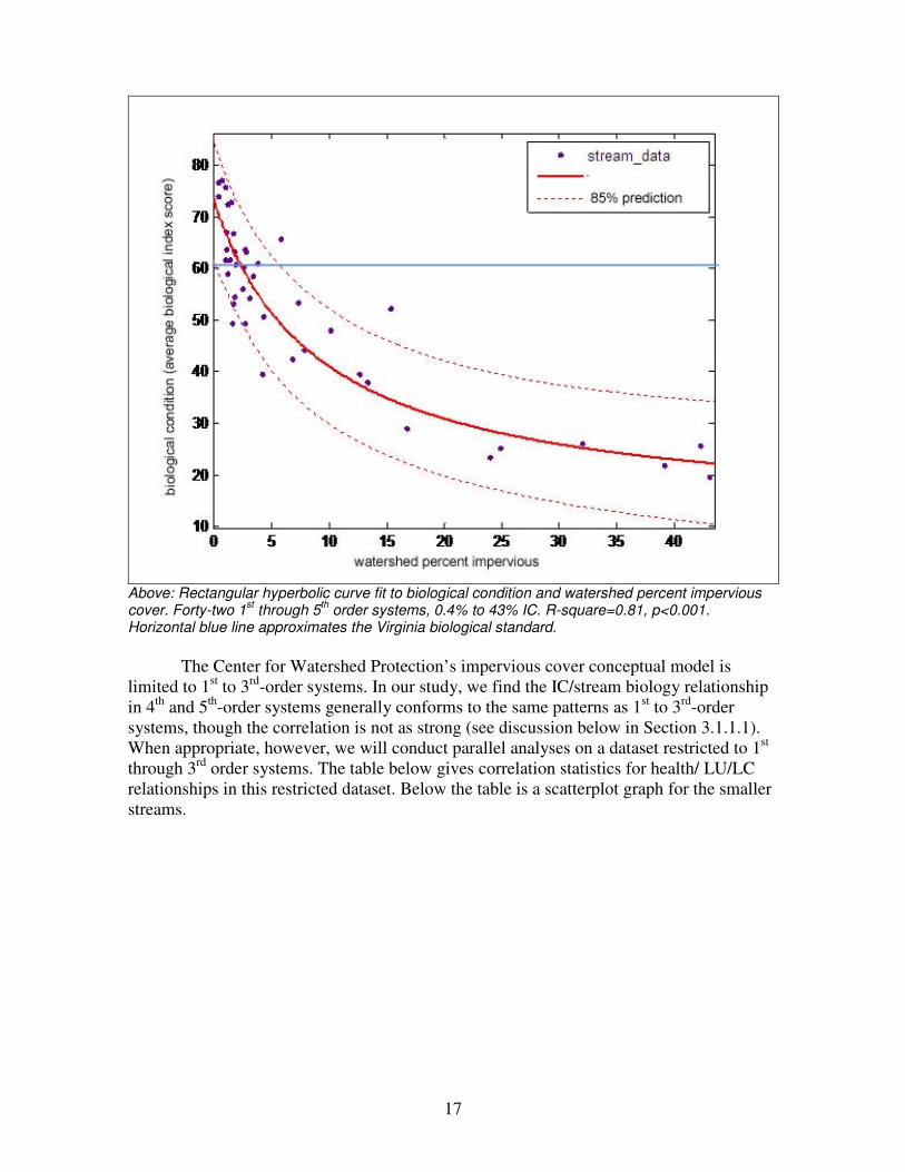
The health/IC relationship is illustrated below in the form of a scatterplot and

rectangular hyperbola fit line.

17

Above: Rectangular hyperbolic curve fit to biological condition and watershed percent impervious cover. Forty-two 1

st through 5

th order systems, 0.4% to 43% IC. R-square=0.81, p<0.001.

Horizontal blue line approximates the Virginia biological standard.

The Center for Watershed Protection’s impervious cover conceptual model is

limited to 1st to 3

rd-order systems. In our study, we find the IC/stream biology relationship

in 4th

and 5th

-order systems generally conforms to the same patterns as 1st to 3

rd-order

systems, though the correlation is not as strong (see discussion below in Section 3.1.1.1).

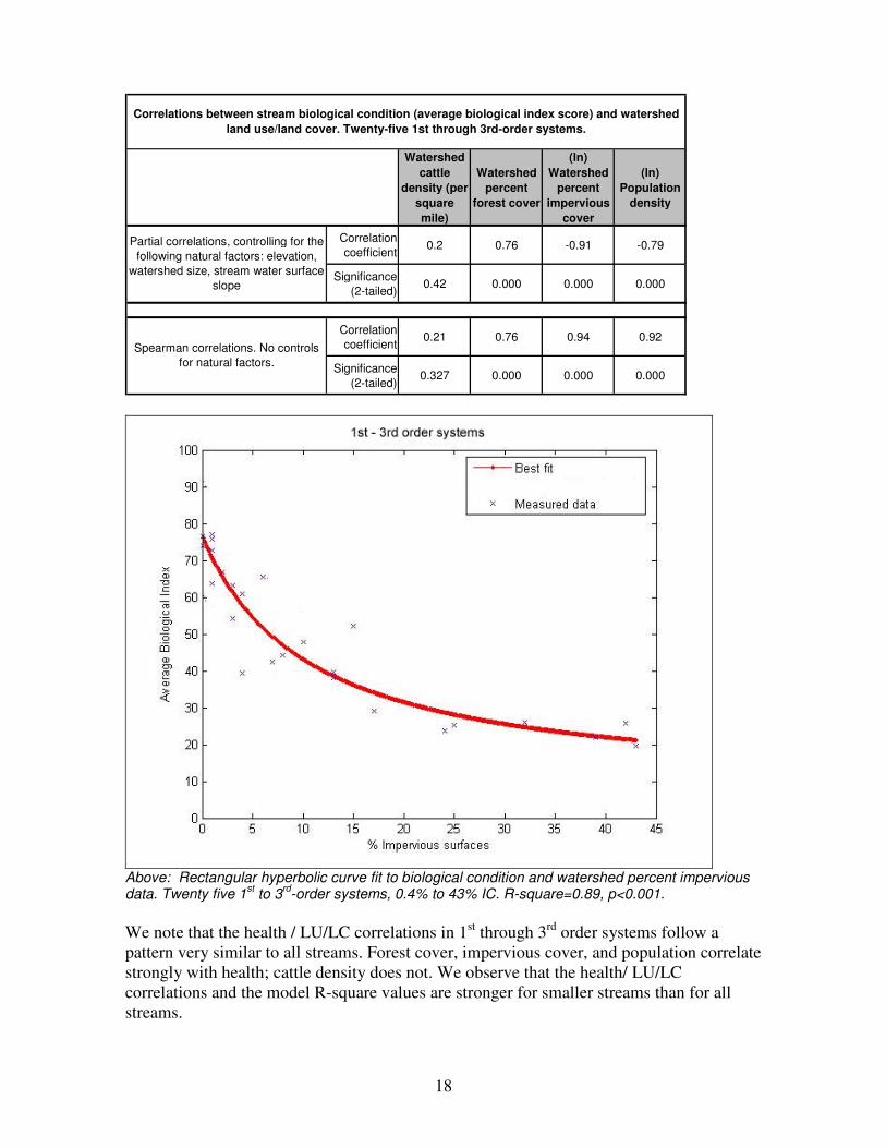
When appropriate, however, we will conduct parallel analyses on a dataset restricted to 1st

through 3rd

order systems. The table below gives correlation statistics for health/ LU/LC

relationships in this restricted dataset. Below the table is a scatterplot graph for the smaller

streams.

18

Watershed

cattle

density (per

square

mile)

Watershed

percent

forest cover

(ln)

Watershed

percent

impervious

cover

(ln)

Population

density

Correlation

coefficient0.2 0.76 -0.91 -0.79

Significance

(2-tailed)0.42 0.000 0.000 0.000

Correlation

coefficient0.21 0.76 0.94 0.92

Significance

(2-tailed)0.327 0.000 0.000 0.000

Correlations between stream biological condition (average biological index score) and watershed

land use/land cover. Twenty-five 1st through 3rd-order systems.

Partial correlations, controlling for the

following natural factors: elevation,

watershed size, stream water surface

slope

Spearman correlations. No controls

for natural factors.

Above: Rectangular hyperbolic curve fit to biological condition and watershed percent impervious data. Twenty five 1

st to 3

rd-order systems, 0.4% to 43% IC. R-square=0.89, p<0.001.

We note that the health / LU/LC correlations in 1st through 3

rd order systems follow a

pattern very similar to all streams. Forest cover, impervious cover, and population correlate

strongly with health; cattle density does not. We observe that the health/ LU/LC

correlations and the model R-square values are stronger for smaller streams than for all

streams.

19

We also observe in both sets considerable scatter in the range of data representing

systems with about 1.5% to 10% IC. As noted, our study’s 4th

and 5th

-order systems fall

entirely within this range, therefore the “all streams” dataset exhibits higher variance.

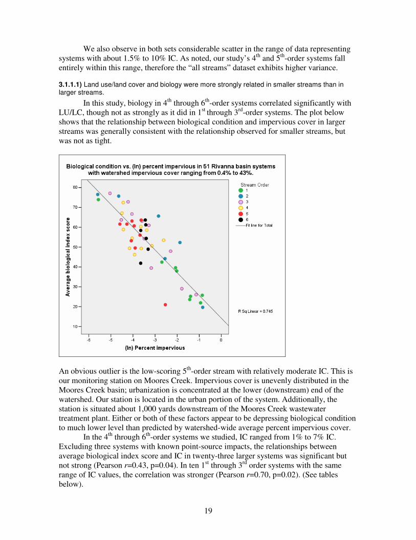
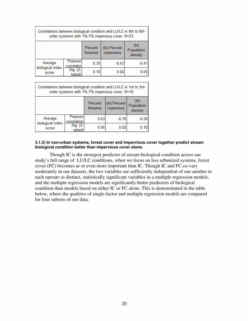
3.1.1.1) Land use/land cover and biology were more strongly related in smaller streams than in larger streams.

In this study, biology in 4th

through 6th

-order systems correlated significantly with

LU/LC, though not as strongly as it did in 1st

through 3rd

-order systems. The plot below

shows that the relationship between biological condition and impervious cover in larger

streams was generally consistent with the relationship observed for smaller streams, but

was not as tight.

An obvious outlier is the low-scoring 5th

-order stream with relatively moderate IC. This is

our monitoring station on Moores Creek. Impervious cover is unevenly distributed in the

Moores Creek basin; urbanization is concentrated at the lower (downstream) end of the

watershed. Our station is located in the urban portion of the system. Additionally, the

station is situated about 1,000 yards downstream of the Moores Creek wastewater

treatment plant. Either or both of these factors appear to be depressing biological condition

to much lower level than predicted by watershed-wide average percent impervious cover.

In the 4th

through 6th

-order systems we studied, IC ranged from 1% to 7% IC.

Excluding three systems with known point-source impacts, the relationships between

average biological index score and IC in twenty-three larger systems was significant but

not strong (Pearson r=0.43, p=0.04). In ten 1st through 3

rd order systems with the same

range of IC values, the correlation was stronger (Pearson r=0.70, p=0.02). (See tables

below).

20

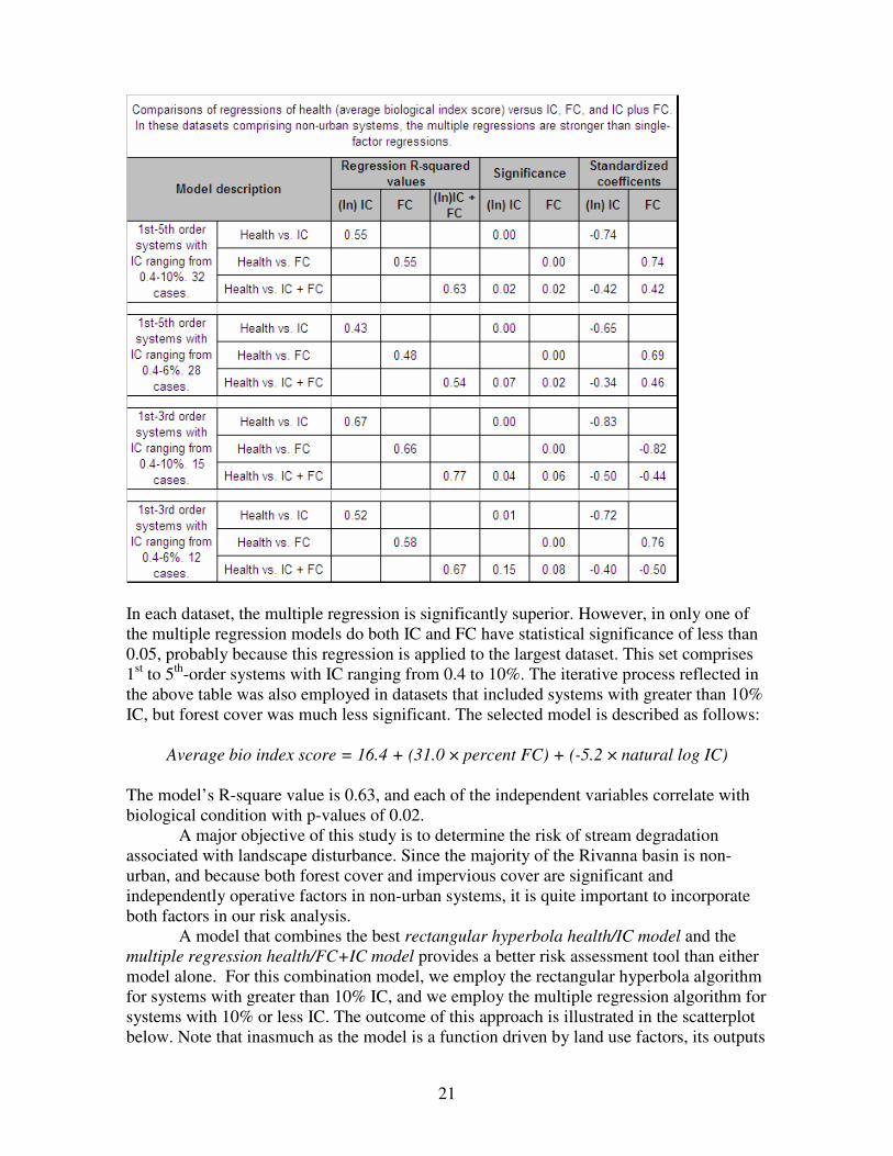
3.1.2) In non-urban systems, forest cover and impervious cover together predict stream biological condition better than impervious cover alone.

Though IC is the strongest predictor of stream biological condition across our

study’s full range of LU/LC conditions, when we focus on less urbanized systems, forest

cover (FC) becomes as or even more important than IC. Though IC and FC co-vary

moderately in our datasets, the two variables are sufficiently independent of one another to

each operate as distinct, statistically significant variables in a multiple regression models,

and the multiple regression models are significantly better predictors of biological

condition than models based on either IC or FC alone. This is demonstrated in the table

below, where the qualities of single-factor and multiple regression models are compared

for four subsets of our data.

21

In each dataset, the multiple regression is significantly superior. However, in only one of

the multiple regression models do both IC and FC have statistical significance of less than

0.05, probably because this regression is applied to the largest dataset. This set comprises

1st to 5

th-order systems with IC ranging from 0.4 to 10%. The iterative process reflected in

the above table was also employed in datasets that included systems with greater than 10%

IC, but forest cover was much less significant. The selected model is described as follows:

Average bio index score = 16.4 + (31.0 × percent FC) + (-5.2 × natural log IC)

The model’s R-square value is 0.63, and each of the independent variables correlate with

biological condition with p-values of 0.02.

A major objective of this study is to determine the risk of stream degradation

associated with landscape disturbance. Since the majority of the Rivanna basin is non-

urban, and because both forest cover and impervious cover are significant and

independently operative factors in non-urban systems, it is quite important to incorporate

both factors in our risk analysis.

A model that combines the best rectangular hyperbola health/IC model and the

multiple regression health/FC+IC model provides a better risk assessment tool than either

model alone. For this combination model, we employ the rectangular hyperbola algorithm

for systems with greater than 10% IC, and we employ the multiple regression algorithm for

systems with 10% or less IC. The outcome of this approach is illustrated in the scatterplot

below. Note that inasmuch as the model is a function driven by land use factors, its outputs

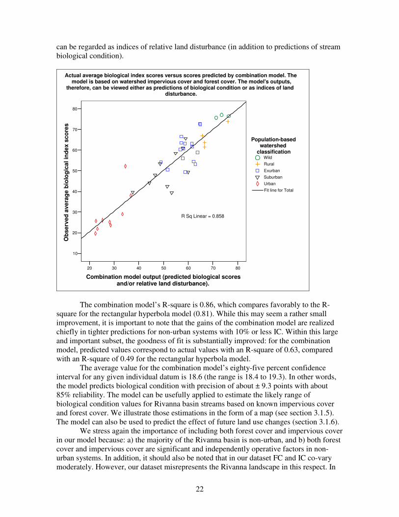
22

can be regarded as indices of relative land disturbance (in addition to predictions of stream

biological condition).

80706050403020

Combination model output (predicted biological scoresand/or relative land disturbance).

80

70

60

50

40

30

20

10

Ob

se

rve

d a

ve

rag

e b

iolo

gic

al

ind

ex

sc

ore

s

Fit line for Total

Urban

Suburban

Exurban

Rural

Wild

Population-basedwatershed

classification

Actual average biological index scores versus scores predicted by combination model. Themodel is based on watershed impervious cover and forest cover. The model's outputs,

therefore, can be viewed either as predictions of biological condition or as indices of landdisturbance.

R Sq Linear = 0.858

The combination model’s R-square is 0.86, which compares favorably to the R-

square for the rectangular hyperbola model (0.81). While this may seem a rather small

improvement, it is important to note that the gains of the combination model are realized

chiefly in tighter predictions for non-urban systems with 10% or less IC. Within this large

and important subset, the goodness of fit is substantially improved: for the combination

model, predicted values correspond to actual values with an R-square of 0.63, compared

with an R-square of 0.49 for the rectangular hyperbola model.

The average value for the combination model’s eighty-five percent confidence

interval for any given individual datum is 18.6 (the range is 18.4 to 19.3). In other words,

the model predicts biological condition with precision of about ± 9.3 points with about

85% reliability. The model can be usefully applied to estimate the likely range of

biological condition values for Rivanna basin streams based on known impervious cover

and forest cover. We illustrate those estimations in the form of a map (see section 3.1.5).

The model can also be used to predict the effect of future land use changes (section 3.1.6).

We stress again the importance of including both forest cover and impervious cover

in our model because: a) the majority of the Rivanna basin is non-urban, and b) both forest

cover and impervious cover are significant and independently operative factors in non-

urban systems. In addition, it should also be noted that in our dataset FC and IC co-vary

moderately. However, our dataset misrepresents the Rivanna landscape in this respect. In

23

208 Rivanna small watersheds with under 10% IC, IC and FC co-vary only minimally. If

IC and FC predict biological condition independently in our sample dataset, there is good

reason to believe they operate even more independently in the “total population” of non-

urban Rivanna subwatersheds.

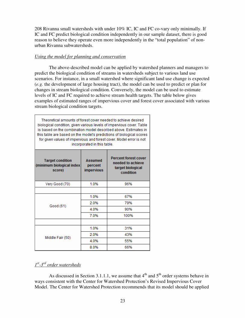
Using the model for planning and conservation

The above-described model can be applied by watershed planners and managers to

predict the biological condition of streams in watersheds subject to various land use

scenarios. For instance, in a small watershed where significant land use change is expected

(e.g. the development of large housing tract), the model can be used to predict or plan for

changes in stream biological condition. Conversely, the model can be used to estimate

levels of IC and FC required to achieve stream health targets. The table below gives

examples of estimated ranges of impervious cover and forest cover associated with various

stream biological condition targets.

1st-3

rd order watersheds

As discussed in Section 3.1.1.1, we assume that 4th

and 5th

order systems behave in

ways consistent with the Center for Watershed Protection’s Revised Impervious Cover

Model. The Center for Watershed Protection recommends that its model should be applied

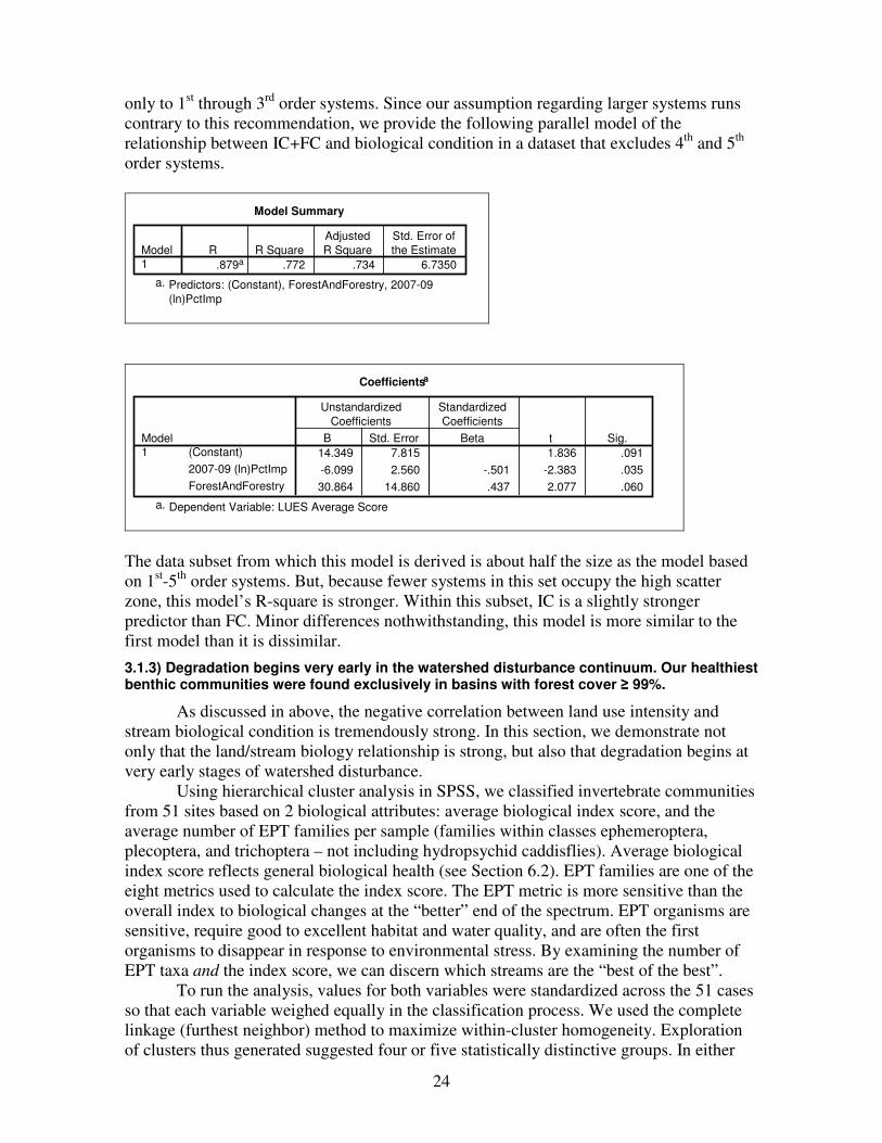
24

only to 1st through 3

rd order systems. Since our assumption regarding larger systems runs

contrary to this recommendation, we provide the following parallel model of the

relationship between IC+FC and biological condition in a dataset that excludes 4th

and 5th

order systems.

Model Summary

.879a .772 .734 6.7350

Model

1

R R Square

Adjusted

R Square

Std. Error of

the Estimate

Predictors: (Constant), ForestAndForestry, 2007-09

(ln)PctImp

a.

Coefficientsa

14.349 7.815 1.836 .091

-6.099 2.560 -.501 -2.383 .035

30.864 14.860 .437 2.077 .060

(Constant)

2007-09 (ln)PctImp

ForestAndForestry

Model1

B Std. Error

Unstandardized

Coefficients

Beta

Standardized

Coefficients

t Sig.

Dependent Variable: LUES Average Scorea.

The data subset from which this model is derived is about half the size as the model based

on 1st-5

th order systems. But, because fewer systems in this set occupy the high scatter

zone, this model’s R-square is stronger. Within this subset, IC is a slightly stronger

predictor than FC. Minor differences nothwithstanding, this model is more similar to the

first model than it is dissimilar.

3.1.3) Degradation begins very early in the watershed disturbance continuum. Our healthiest benthic communities were found exclusively in basins with forest cover ≥ 99%.

As discussed in above, the negative correlation between land use intensity and

stream biological condition is tremendously strong. In this section, we demonstrate not

only that the land/stream biology relationship is strong, but also that degradation begins at

very early stages of watershed disturbance.

Using hierarchical cluster analysis in SPSS, we classified invertebrate communities

from 51 sites based on 2 biological attributes: average biological index score, and the

average number of EPT families per sample (families within classes ephemeroptera,

plecoptera, and trichoptera – not including hydropsychid caddisflies). Average biological

index score reflects general biological health (see Section 6.2). EPT families are one of the

eight metrics used to calculate the index score. The EPT metric is more sensitive than the

overall index to biological changes at the “better” end of the spectrum. EPT organisms are

sensitive, require good to excellent habitat and water quality, and are often the first

organisms to disappear in response to environmental stress. By examining the number of

EPT taxa and the index score, we can discern which streams are the “best of the best”.

To run the analysis, values for both variables were standardized across the 51 cases

so that each variable weighed equally in the classification process. We used the complete

linkage (furthest neighbor) method to maximize within-cluster homogeneity. Exploration

of clusters thus generated suggested four or five statistically distinctive groups. In either

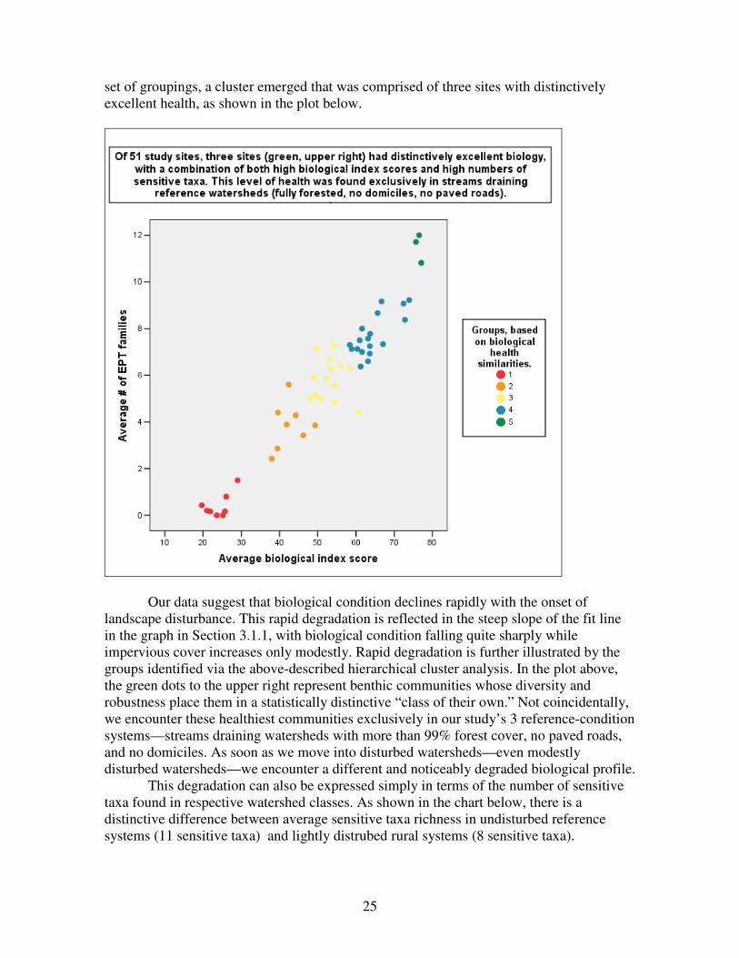
25

set of groupings, a cluster emerged that was comprised of three sites with distinctively

excellent health, as shown in the plot below.

Our data suggest that biological condition declines rapidly with the onset of

landscape disturbance. This rapid degradation is reflected in the steep slope of the fit line

in the graph in Section 3.1.1, with biological condition falling quite sharply while

impervious cover increases only modestly. Rapid degradation is further illustrated by the

groups identified via the above-described hierarchical cluster analysis. In the plot above,

the green dots to the upper right represent benthic communities whose diversity and

robustness place them in a statistically distinctive “class of their own.” Not coincidentally,

we encounter these healthiest communities exclusively in our study’s 3 reference-condition

systems—streams draining watersheds with more than 99% forest cover, no paved roads,

and no domiciles. As soon as we move into disturbed watersheds—even modestly

disturbed watersheds—we encounter a different and noticeably degraded biological profile.

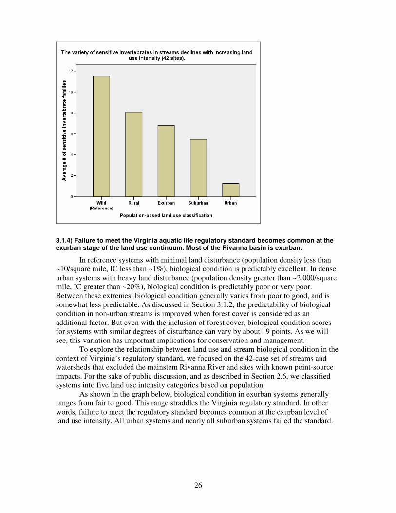
This degradation can also be expressed simply in terms of the number of sensitive

taxa found in respective watershed classes. As shown in the chart below, there is a

distinctive difference between average sensitive taxa richness in undisturbed reference

systems (11 sensitive taxa) and lightly distrubed rural systems (8 sensitive taxa).

26

3.1.4) Failure to meet the Virginia aquatic life regulatory standard becomes common at the exurban stage of the land use continuum. Most of the Rivanna basin is exurban.

In reference systems with minimal land disturbance (population density less than

~10/square mile, IC less than ~1%), biological condition is predictably excellent. In dense

urban systems with heavy land disturbance (population density greater than ~2,000/square

mile, IC greater than ~20%), biological condition is predictably poor or very poor.

Between these extremes, biological condition generally varies from poor to good, and is

somewhat less predictable. As discussed in Section 3.1.2, the predictability of biological

condition in non-urban streams is improved when forest cover is considered as an

additional factor. But even with the inclusion of forest cover, biological condition scores

for systems with similar degrees of disturbance can vary by about 19 points. As we will

see, this variation has important implications for conservation and management.

To explore the relationship between land use and stream biological condition in the

context of Virginia’s regulatory standard, we focused on the 42-case set of streams and

watersheds that excluded the mainstem Rivanna River and sites with known point-source

impacts. For the sake of public discussion, and as described in Section 2.6, we classified

systems into five land use intensity categories based on population.

As shown in the graph below, biological condition in exurban systems generally

ranges from fair to good. This range straddles the Virginia regulatory standard. In other

words, failure to meet the regulatory standard becomes common at the exurban level of

land use intensity. All urban systems and nearly all suburban systems failed the standard.

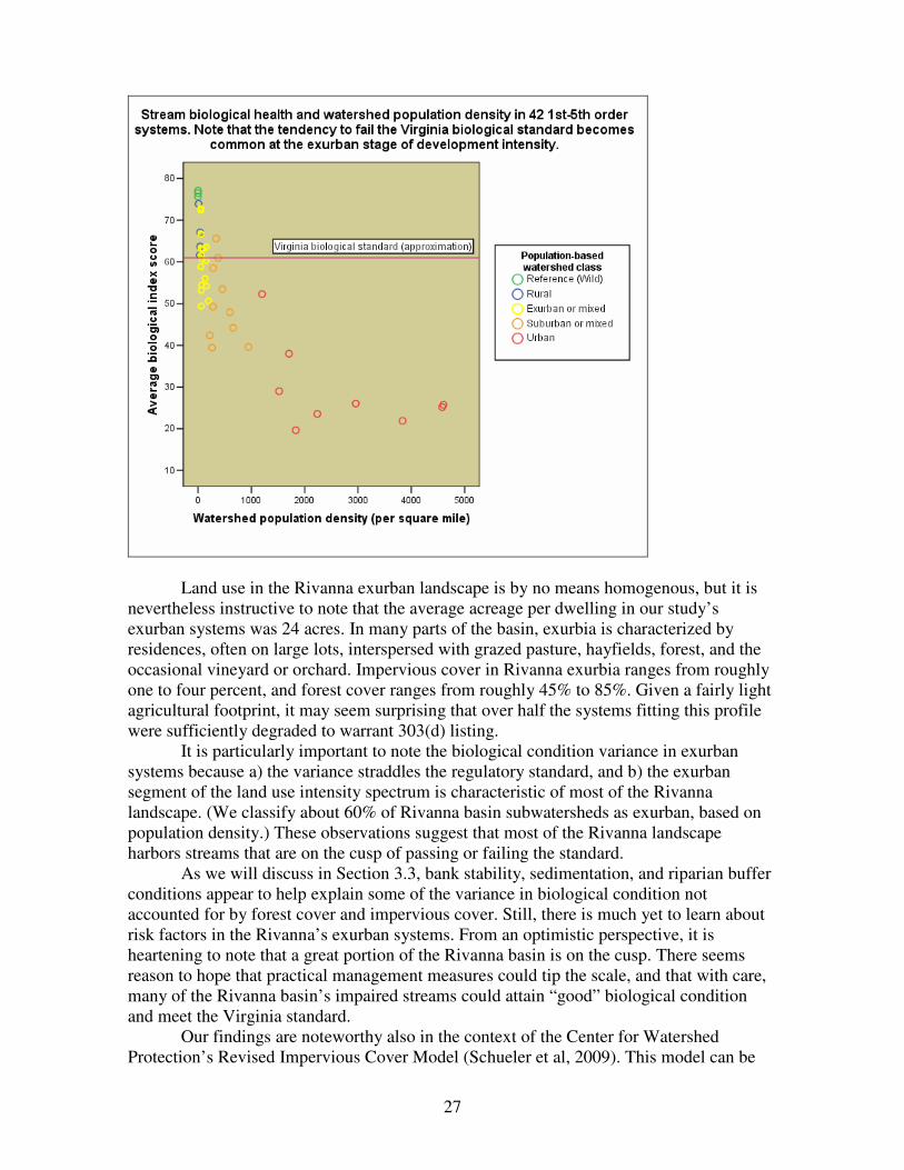
27

Land use in the Rivanna exurban landscape is by no means homogenous, but it is

nevertheless instructive to note that the average acreage per dwelling in our study’s

exurban systems was 24 acres. In many parts of the basin, exurbia is characterized by

residences, often on large lots, interspersed with grazed pasture, hayfields, forest, and the

occasional vineyard or orchard. Impervious cover in Rivanna exurbia ranges from roughly

one to four percent, and forest cover ranges from roughly 45% to 85%. Given a fairly light

agricultural footprint, it may seem surprising that over half the systems fitting this profile

were sufficiently degraded to warrant 303(d) listing.

It is particularly important to note the biological condition variance in exurban

systems because a) the variance straddles the regulatory standard, and b) the exurban

segment of the land use intensity spectrum is characteristic of most of the Rivanna

landscape. (We classify about 60% of Rivanna basin subwatersheds as exurban, based on

population density.) These observations suggest that most of the Rivanna landscape

harbors streams that are on the cusp of passing or failing the standard.

As we will discuss in Section 3.3, bank stability, sedimentation, and riparian buffer

conditions appear to help explain some of the variance in biological condition not

accounted for by forest cover and impervious cover. Still, there is much yet to learn about

risk factors in the Rivanna’s exurban systems. From an optimistic perspective, it is

heartening to note that a great portion of the Rivanna basin is on the cusp. There seems

reason to hope that practical management measures could tip the scale, and that with care,

many of the Rivanna basin’s impaired streams could attain “good” biological condition

and meet the Virginia standard.

Our findings are noteworthy also in the context of the Center for Watershed

Protection’s Revised Impervious Cover Model (Schueler et al, 2009). This model can be

28

(mis)interpreted to infer that systems with less than 20-25% IC generally support

regulatory standards. Carefully examined, the model does make room for regulatory failure

at lower levels of IC. The model’s authors note that metrics based on benthic communities

are particularly responsive to increasing IC. Data from the Rivanna basin support this

view. Along with other workers, we find that biological condition begins to degrade at the

earliest stages of watershed disturbance (Coles 2004, King 2010, Morse 2003, Ourso

2003). In general, the regulatory threshold is breached at less than 3% IC in the Rivanna

systems we studied (see graph in Section 3.1.1). We do not interpret this finding to mean

that IC is the sole landscape-scale cause of biological degradation in the Rivanna’s

moderately disturbed exurban landscape. Nevertheless, given the justifiable currency of the

Revised Impervious Cover Model, we think it important to say that our findings argue for a

conservative, cautionary interpretation of the model when it comes to benthic thresholds.

In our study, failure of the aquatic life standard generally occurred at about one level of

magnitude lower than 20-25% IC, and all systems with 20% or more IC were substantially

or severely degraded.

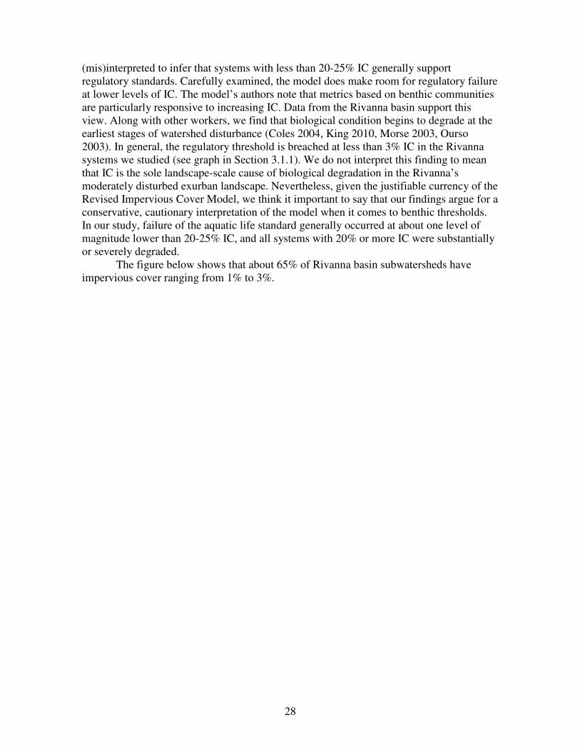
The figure below shows that about 65% of Rivanna basin subwatersheds have

impervious cover ranging from 1% to 3%.

29

Above: A majority of the basin’s watersheds have between 1% and 3% impervious cover. The histogram is based on 189 small watersheds with land area exceeding 1 square mile. The dataset covers 98% of the basin’s land area.

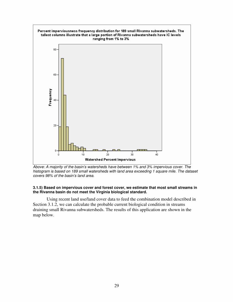
3.1.5) Based on impervious cover and forest cover, we estimate that most small streams in the Rivanna basin do not meet the Virginia biological standard.

Using recent land use/land cover data to feed the combination model described in

Section 3.1.2, we can calculate the probable current biological condition in streams

draining small Rivanna subwatersheds. The results of this application are shown in the

map below.

30

Above: Modeled current health of streams in small Rivanna watersheds.

As illustrated in the map, we estimate that only about 30% of systems meet the Virginia

regulatory standard (teal or green shading), and that about 70% of systems fail the standard

(brown shading or worse). Fortunately, most of the failing systems are moderately rather

than severely degraded. Only about 6% of systems are likely to be in “poor” health (see

table in Section 3.1.6 below).

31

3.1.6) Potential effects of future land use change.

The model used to generate the map in Section 3.1.5 above can be applied to future

scenarios in order to predict the possible effects of land use change. We created a scenario

whereby impervious cover in the Rivanna basin’s non-urban subwatersheds was increased

by an average of thirty-three percent—from the current average of 2.6% impervious per

subwatershed to a future average of 3.4%. Forest cover was decreased slightly. This

change corresponds to a 50% increase in the population of the non-urban areas, which

would occur in about 20 years assuming population growth rates reported in the 2010

Census. We assumed little change in urban watersheds with current population of 1,000 or

more people per square mile. We also assume no growth in watersheds situated primarily

in Shenandoah National Park. The scenario is a speculation conducted for the purpose of

generating conversation about the effects of land use change. The scenario uses very

simple assumptions, and we recognize that future change may unfold quite differently than

in our scenario. For instance, it is unlikely that the spatial distribution of future population-

driven IC change will occur as formulaically as it does in our scenario. The speculative

map is shown below.

32

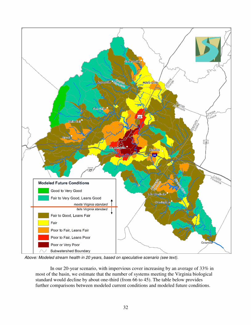
Above: Modeled stream health in 20 years, based on speculative scenario (see text).

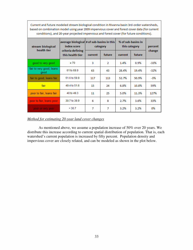
In our 20-year scenario, with impervious cover increasing by an average of 33% in

most of the basin, we estimate that the number of systems meeting the Virginia biological

standard would decline by about one-third (from 66 to 45). The table below provides

further comparisons between modeled current conditions and modeled future conditions.

33

Method for estimating 20-year land cover changes

As mentioned above, we assume a population increase of 50% over 20 years. We

distribute this increase according to current spatial distribution of population. That is, each

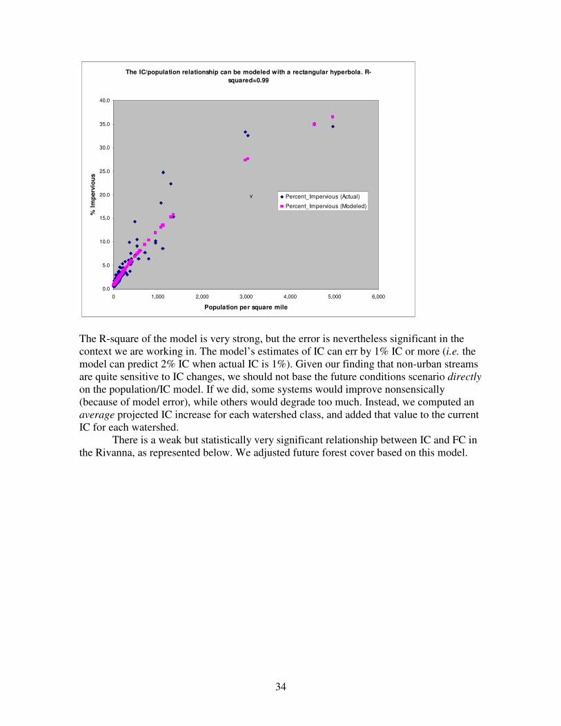
watershed’s current population is increased by fifty percent. Population density and

impervious cover are closely related, and can be modeled as shown in the plot below.

34

The IC/population relationship can be modeled with a rectangular hyperbola. R-

squared=0.99

0.0

5.0

10.0

15.0

20.0

25.0

30.0

35.0

40.0

0 1,000 2,000 3,000 4,000 5,000 6,000

Population per square mile

% I

mp

erv

iou

s

Percent_Impervious (Actual)

Percent_Impervious (Modeled)

v

The R-square of the model is very strong, but the error is nevertheless significant in the

context we are working in. The model’s estimates of IC can err by 1% IC or more (i.e. the

model can predict 2% IC when actual IC is 1%). Given our finding that non-urban streams

are quite sensitive to IC changes, we should not base the future conditions scenario directly

on the population/IC model. If we did, some systems would improve nonsensically

(because of model error), while others would degrade too much. Instead, we computed an

average projected IC increase for each watershed class, and added that value to the current

IC for each watershed.

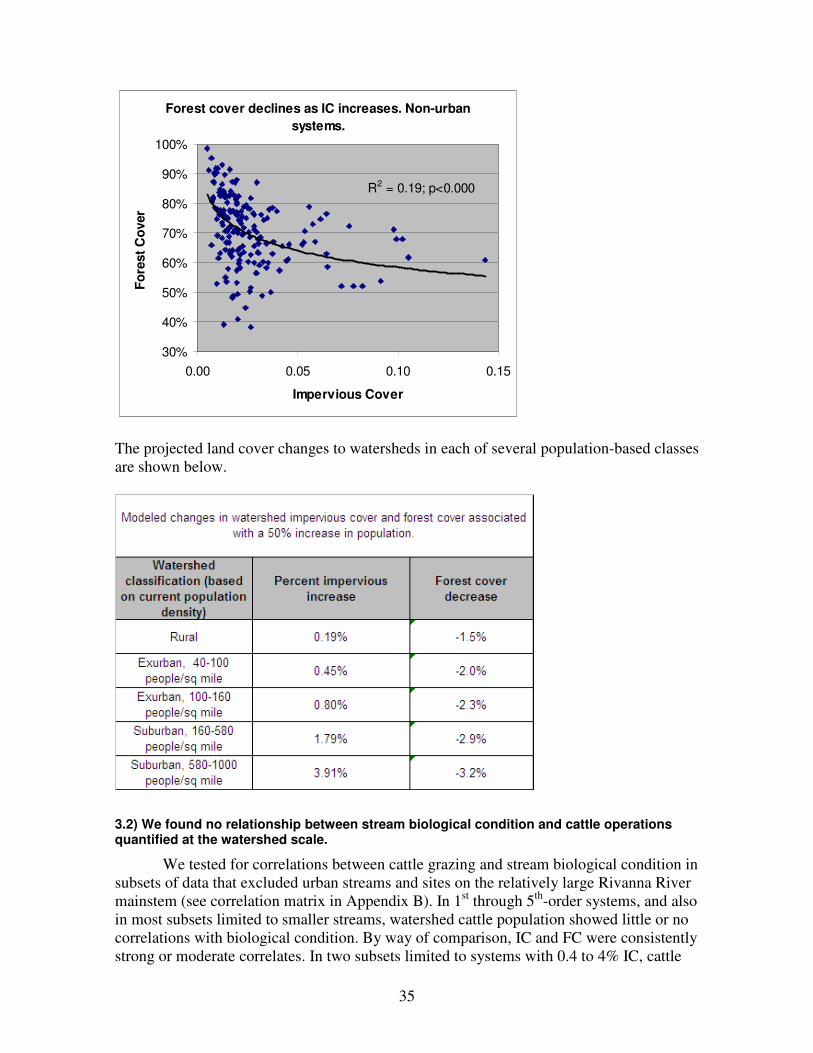
There is a weak but statistically very significant relationship between IC and FC in

the Rivanna, as represented below. We adjusted future forest cover based on this model.

35

Forest cover declines as IC increases. Non-urban

systems.

R2 = 0.19; p<0.000

30%

40%

50%

60%

70%

80%

90%

100%

0.00 0.05 0.10 0.15

Impervious Cover

Fo

rest

Co

ver

The projected land cover changes to watersheds in each of several population-based classes

are shown below.

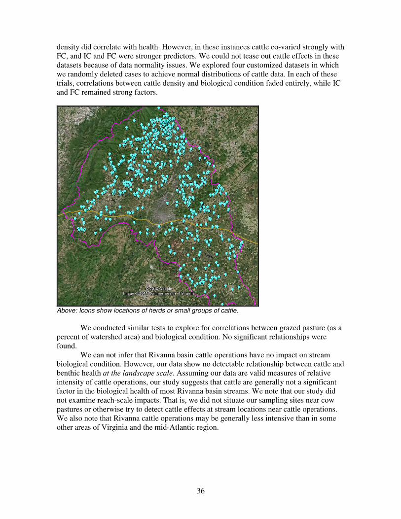
3.2) We found no relationship between stream biological condition and cattle operations quantified at the watershed scale.

We tested for correlations between cattle grazing and stream biological condition in

subsets of data that excluded urban streams and sites on the relatively large Rivanna River

mainstem (see correlation matrix in Appendix B). In 1st through 5

th-order systems, and also

in most subsets limited to smaller streams, watershed cattle population showed little or no

correlations with biological condition. By way of comparison, IC and FC were consistently

strong or moderate correlates. In two subsets limited to systems with 0.4 to 4% IC, cattle

36

density did correlate with health. However, in these instances cattle co-varied strongly with

FC, and IC and FC were stronger predictors. We could not tease out cattle effects in these

datasets because of data normality issues. We explored four customized datasets in which

we randomly deleted cases to achieve normal distributions of cattle data. In each of these

trials, correlations between cattle density and biological condition faded entirely, while IC

and FC remained strong factors.

Above: Icons show locations of herds or small groups of cattle.

We conducted similar tests to explore for correlations between grazed pasture (as a

percent of watershed area) and biological condition. No significant relationships were

found.

We can not infer that Rivanna basin cattle operations have no impact on stream

biological condition. However, our data show no detectable relationship between cattle and

benthic health at the landscape scale. Assuming our data are valid measures of relative

intensity of cattle operations, our study suggests that cattle are generally not a significant

factor in the biological health of most Rivanna basin streams. We note that our study did

not examine reach-scale impacts. That is, we did not situate our sampling sites near cow

pastures or otherwise try to detect cattle effects at stream locations near cattle operations.

We also note that Rivanna cattle operations may be generally less intensive than in some

other areas of Virginia and the mid-Atlantic region.

37

3.3) Relationships between stream biology and reach-scale environmental variables.

3.3.1) Bank stability, sediment deposition, and related channel variables correlated with biological condition, particularly in exurban and rural streams.

An overview of the relationships among biological condition, watershed-scale land

use, and reach-scale conditions is given in the matrix of Spearman correlations in

Appendix B. Note that Spearman correlation coefficients and p-values will differ from

Pearson correlations, and that both Spearman and Pearson correlations are applied in our

analyses, depending on setting and purpose. (Pearson correlations are best with normal

data distributions and linear relationships. The normal distribution generally follows the

classic bell curve. Spearman correlations, on the other hand, can reveal or suggest linear or

non-linear relationships among variables that are not necessarily normally distributed.) In

the correlation matrix, correlations possessing significance of p=0.05 or better are

highlighted in grey, and correlations possessing very strong significance (p=0.001 or

better) are highlighted in purple. Significance, in statistics speak, is a measure of likelihood

that the correlation is a product of random chance. The lower the number, the more likely

the relationship is not a product of chance.

The matrix is arranged such that correlations can be examined in each of various

subsets of our data. The reason we examine subsets along with the total dataset is because

the relative importance of ecological factors can vary according to system attributes. For

instance, we parse datasets according to land use intensity because our data strongly

suggest that streams in heavily urbanized watersheds show little response to incremental

increases in watershed impervious surface, while rural streams respond dramatically to the

same amount of impervious surface increase. Urban streams may also respond (or not

respond) to reach-scale factors differently than do non-urban streams.

We parse data according to stream order because other studies suggest that 1st

through 3rd

-order systems are responsive to impervious cover, while larger systems are not

(Schueler 2009. As discussed in Section 3.1.1.1 above, the data in our study suggest that

larger streams do respond to IC and other indicators of landscape disturbance, though less

robustly than smaller streams.

A scan of the correlation matrix shows that biological condition (labeled “average

bio score”) correlates more consistently and strongly with watershed LU/LC than with any

other environmental variable. (In the matrix, the LU/LC factor is labeled “landscape

factors (combo model output)”. This variable consists of the output of the model described

in Section 3.1.2, and can be understood as an index of watershed land use intensity derived

from percent forest cover and percent impervious cover.)

The variable with the next greatest amount of consistency of correlation with

biological condition is riparian zone condition. We will discuss the riparian zone in Section

3.3.3.

A number of channel variables including bank stability, frequency of riffles, and

substrate-related variables correlated with biological condition, particularly in non-urban

streams, and most particularly in rural and exurban streams. Slope correlates with

biological condition in non-urban streams.

Though correlations between biology and channel conditions are generally fairly

weak, they are statistically robust. Clearly, in the systems we studied, biological condition

is significantly associated with various conditions in the channel. Even though LU/LC

predicts biology more powerfully than reach-scale conditions, common sense tells us that

landscape-scale conditions are not directly felt by stream organisms. Rather, landscape

alterations precipitate a cascade of changes that ultimately alter the flow regime, water

38

quality, and physical habitat experienced by stream organisms at the scale of the habitat

they occupy through their lifecycles. Of course, this framework of cause and effect is not

all-encompassing or absolute. Sometimes, for instance, habitat disturbance within a reach

is related to spatially proximate conditions or events (e.g. road crossings, cattle wallows,

riparian forest clearance, etc.).

The observation that watershed LU/LC is a stronger predictor of biology than

channel conditions makes intuitive sense inasmuch as the effects of landscape alteration

are distributed over multiple processes and features in the stream, and no single habitat

factor within the reach will have as much influence on biology as the sum of all factors.

Seen from another angle, many habitat conditions in the reach are integrated at the scale of

the watershed. Our study, however, does not shed clear light on the relationships between

LU/LC and channel conditions. Nor does our study capture all of the factors that influence

biology. What our study does show clearly is that land use/land cover at the scale of the

watershed usually predicts biological condition far more powerfully than any single local-

scale factor we studied, and more powerfully than any combination of local-scale factors.

In addition to tremendously strong statistical evidence, the dominant role of watershed-

scale LU/LC in predicting biological condition is evident by example: Even though our

data suggest generally that reach-scale attributes such as bank stability and substrate can

affect biology, we find examples in our reference systems of biologically healthy streams

with fairly unstable banks and/or excessive sedimentation. In these systems, complete

forestation and the lack of impervious surfaces throughout the watershed appear to trump

habitat deficiencies in the reach.

As noted above, in the datasets comprising 1st through 5

th-order streams, we

observe correlations between biology and a number of channel variables. We also observe

that these correlations strengthen as the dataset becomes less urbanized. The relationships

are strongest in the dataset limited to twenty-five systems with 0.4% to 4% IC. These

comprise our wild (reference), rural, and exurban systems, as well as three systems

classified as suburban. In the remainder of the discussion we focus on this set, not only

because it best reveals relationships between channel conditions and biology, but also

because it, like the Rivanna basin, is dominated by exurban systems.

The matrix below focuses on the strongest correlations among biology, LU/LC

(combo model output), residuals of the LU/LC→biology model, and channel conditions in

the subject dataset.

39

Pearson correlations among biological condition, channel conditions, watershed land use intensity, and residuals of land use/biological condition

model. 1st through 5th-order systems with IC ranging from 0.4% to 4%.

1 .594** .716** .723** .594** .649** .509* -.510*

.002 .000 .000 .002 .001 .011 .011

25 25 25 25 24 24 24 24

.594** 1 -.136 .370 .509* .431* .365 -.250

.002 .517 .068 .011 .035 .079 .238

25 25 25 25 24 24 24 24

.716** -.136 1 .569** .260 .398 .288 -.395

.000 .517 .003 .219 .054 .172 .056

25 25 25 25 24 24 24 24

.723** .370 .569** 1 .620** .556** .603** -.570**

.000 .068 .003 .001 .005 .002 .004

25 25 25 25 24 24 24 24

.594** .509* .260 .620** 1 .799** .729** -.756**

.002 .011 .219 .001 .000 .000 .000

24 24 24 24 24 24 24 24

.649** .431* .398 .556** .799** 1 .517** -.594**

.001 .035 .054 .005 .000 .010 .002

24 24 24 24 24 24 24 24

.509* .365 .288 .603** .729** .517** 1 -.810**

.011 .079 .172 .002 .000 .010 .000

24 24 24 24 24 24 24 24

-.510* -.250 -.395 -.570** -.756** -.594** -.810** 1

.011 .238 .056 .004 .000 .002 .000

24 24 24 24 24 24 24 24

Pearson Correlation

Sig. (2-tailed)

N

Pearson Correlation

Sig. (2-tailed)

N

Pearson Correlation

Sig. (2-tailed)

N

Pearson Correlation

Sig. (2-tailed)

N

Pearson Correlation

Sig. (2-tailed)

N

Pearson Correlation

Sig. (2-tailed)

N

Pearson Correlation

Sig. (2-tailed)

N

Pearson Correlation

Sig. (2-tailed)

N

LUES Average Score

Combo model

residuals

Combo model output

LN__Slope

Frequency of Riffles

Bank Stability

Sediment Deposition

% Fine Sand/Clay

LUES

Average

Score

Combo

model

residuals

Combo

model

output

LN__

Slope

Frequency

of Riffles

Bank

Stability

Sediment

Deposition

% Fine

Sand/

Clay

Correlation is significant at the 0.01 level (2-tailed).**.

Correlation is significant at the 0.05 level (2-tailed).*.

Above: Pearson correlations among biological condition, channel conditions, watershed land use intensity, and residuals of land use/biological condition model. Wild, rural, and exurban 1st through 5th-order systems with IC ranging from 0.4% to 4%.

As shown above, riffle frequency, bank stability, sediment deposition, percent

fines, and slope all correlate significantly with biological condition. They also correlate

with one another. Sediment deposition and percent fines are so highly correlated that they

may be regarded as a single factor. The same can be said for bank stability and frequency

of riffles. Overall, the data reflect what we know from common sense: flatter streams tend

to harbor finer substrate, and are more prone to sediment deposition than steeper streams.

The data also suggest a relationship that is less obvious to the casual observer: flatter

streams appear to have a higher risk of bank erosion.

Most of the channel factors do not appear to correlate significantly with LU/LC

(bank stability may be an exception). Slope, however, is moderately correlated with

LU/LC, probably reflecting a tendency toward greater land use intensity in less

mountainous landscapes. Two or three channel factors—frequency of riffles, bank

stability, and (marginally) sediment deposition—correlate with residuals of the

combination model, suggesting a potential effect on biological condition that is not

captured by the LU/LC→biology model (but only within systems with this range of land

use intensity). Frequency of riffle data are abnormally distributed, and, to be statistically

strict, the Pearson correlations between riffle frequency and other variables should be

interpreted cautiously.

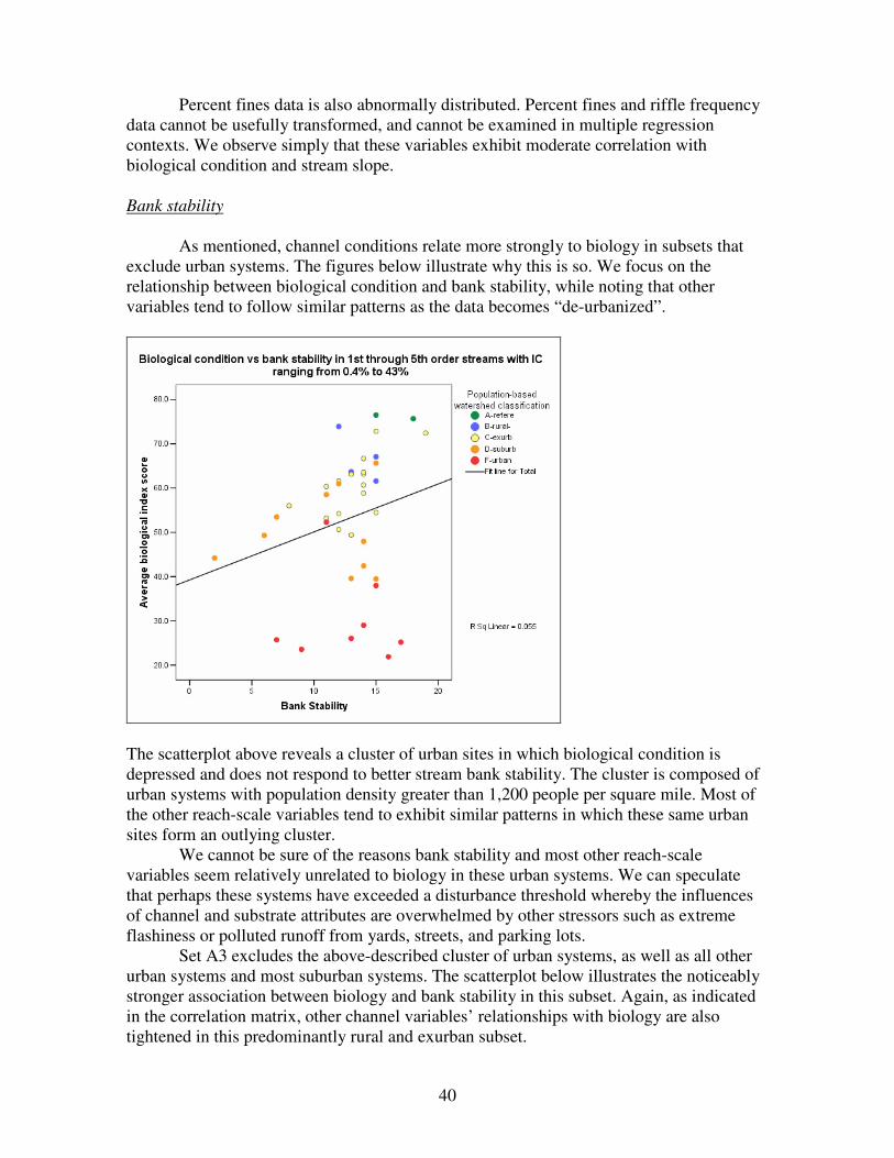
40

Percent fines data is also abnormally distributed. Percent fines and riffle frequency

data cannot be usefully transformed, and cannot be examined in multiple regression

contexts. We observe simply that these variables exhibit moderate correlation with

biological condition and stream slope.

Bank stability

As mentioned, channel conditions relate more strongly to biology in subsets that

exclude urban systems. The figures below illustrate why this is so. We focus on the

relationship between biological condition and bank stability, while noting that other

variables tend to follow similar patterns as the data becomes “de-urbanized”.

The scatterplot above reveals a cluster of urban sites in which biological condition is

depressed and does not respond to better stream bank stability. The cluster is composed of

urban systems with population density greater than 1,200 people per square mile. Most of

the other reach-scale variables tend to exhibit similar patterns in which these same urban

sites form an outlying cluster.

We cannot be sure of the reasons bank stability and most other reach-scale

variables seem relatively unrelated to biology in these urban systems. We can speculate

that perhaps these systems have exceeded a disturbance threshold whereby the influences

of channel and substrate attributes are overwhelmed by other stressors such as extreme

flashiness or polluted runoff from yards, streets, and parking lots.

Set A3 excludes the above-described cluster of urban systems, as well as all other

urban systems and most suburban systems. The scatterplot below illustrates the noticeably

stronger association between biology and bank stability in this subset. Again, as indicated

in the correlation matrix, other channel variables’ relationships with biology are also

tightened in this predominantly rural and exurban subset.

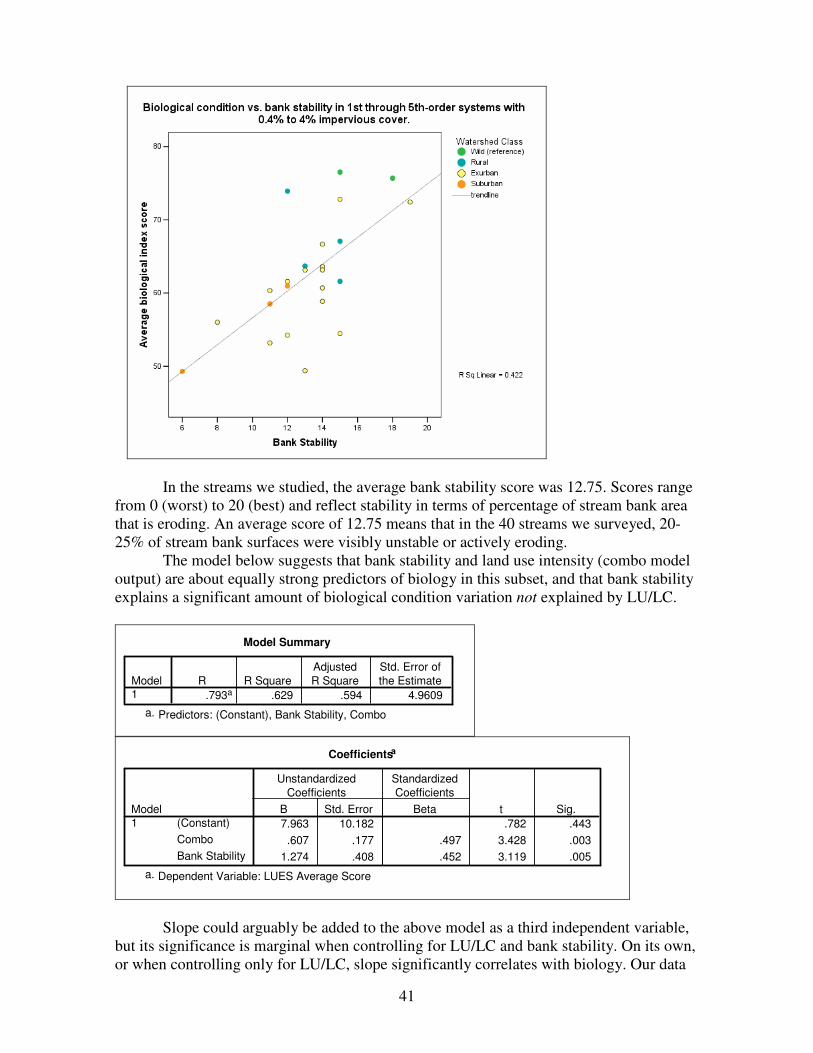
41

In the streams we studied, the average bank stability score was 12.75. Scores range

from 0 (worst) to 20 (best) and reflect stability in terms of percentage of stream bank area

that is eroding. An average score of 12.75 means that in the 40 streams we surveyed, 20-

25% of stream bank surfaces were visibly unstable or actively eroding.

The model below suggests that bank stability and land use intensity (combo model

output) are about equally strong predictors of biology in this subset, and that bank stability

explains a significant amount of biological condition variation not explained by LU/LC.

Model Summary

.793a .629 .594 4.9609

Model1

R R Square

Adjusted

R Square

Std. Error of

the Estimate

Predictors: (Constant), Bank Stability, Comboa.

Coefficientsa

7.963 10.182 .782 .443

.607 .177 .497 3.428 .003

1.274 .408 .452 3.119 .005

(Constant)

Combo

Bank Stability

Model

1

B Std. Error

Unstandardized

Coefficients

Beta

Standardized

Coefficients

t Sig.

Dependent Variable: LUES Average Scorea.

Slope could arguably be added to the above model as a third independent variable,

but its significance is marginal when controlling for LU/LC and bank stability. On its own,

or when controlling only for LU/LC, slope significantly correlates with biology. Our data

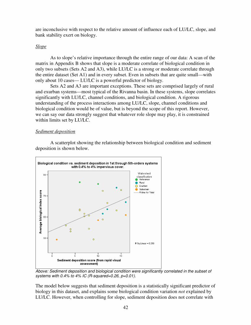
42

are inconclusive with respect to the relative amount of influence each of LU/LC, slope, and

bank stability exert on biology.

Slope

As to slope’s relative importance through the entire range of our data: A scan of the

matrix in Appendix B shows that slope is a moderate correlate of biological condition in

only two subsets (Sets A2 and A3), while LU/LC is a strong or moderate correlate through

the entire dataset (Set A1) and in every subset. Even in subsets that are quite small—with

only about 10 cases— LU/LC is a powerful predictor of biology.

Sets A2 and A3 are important exceptions. These sets are comprised largely of rural

and exurban systems—most typical of the Rivanna basin. In these systems, slope correlates

significantly with LU/LC, channel conditions, and biological condition. A rigorous

understanding of the process interactions among LU/LC, slope, channel conditions and

biological condition would be of value, but is beyond the scope of this report. However,

we can say our data strongly suggest that whatever role slope may play, it is constrained

within limits set by LU/LC.

Sediment deposition

A scatterplot showing the relationship between biological condition and sediment

deposition is shown below.

Above: Sediment deposition and biological condition were significantly correlated in the subset of systems with 0.4% to 4% IC (R-squared=0.26, p=0.01).

The model below suggests that sediment deposition is a statistically significant predictor of

biology in this dataset, and explains some biological condition variation not explained by

LU/LC. However, when controlling for slope, sediment deposition does not correlate with

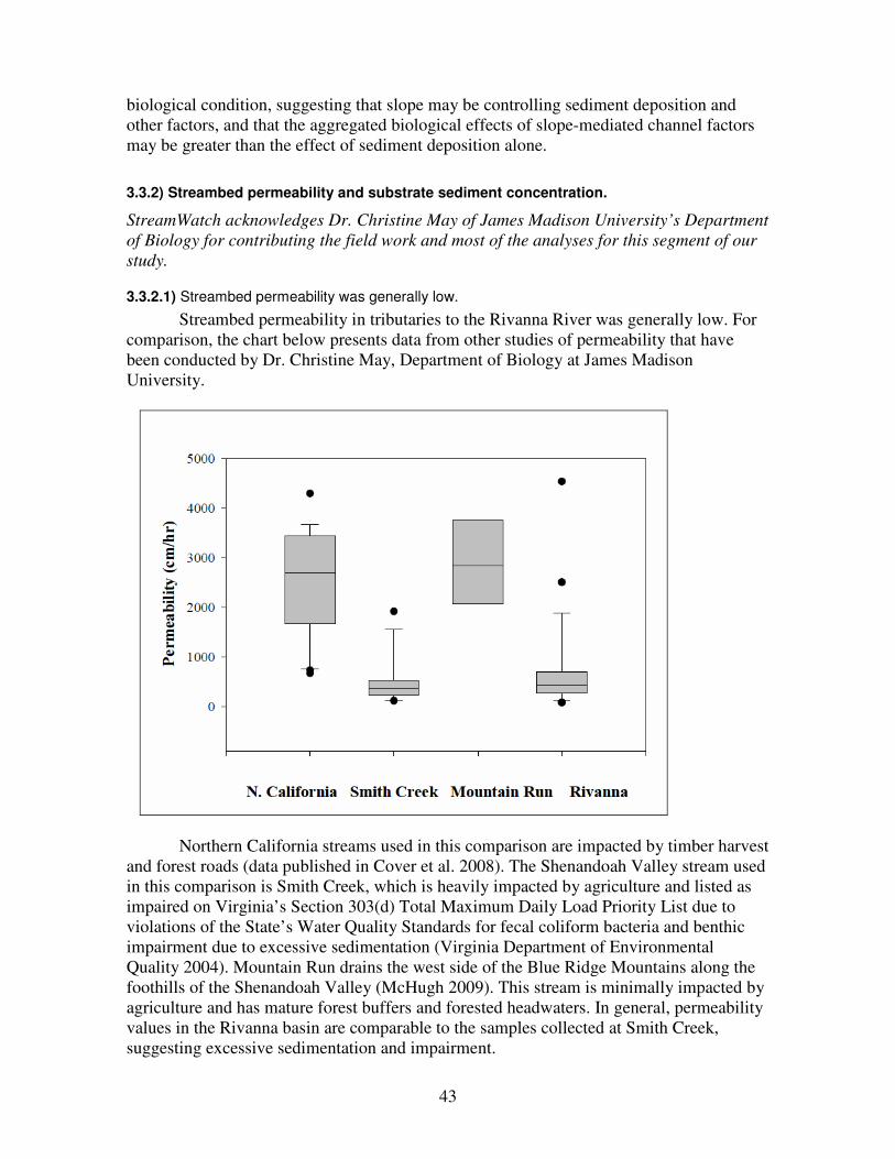
43

biological condition, suggesting that slope may be controlling sediment deposition and

other factors, and that the aggregated biological effects of slope-mediated channel factors

may be greater than the effect of sediment deposition alone.

3.3.2) Streambed permeability and substrate sediment concentration.

StreamWatch acknowledges Dr. Christine May of James Madison University’s Department

of Biology for contributing the field work and most of the analyses for this segment of our

study.

3.3.2.1) Streambed permeability was generally low.

Streambed permeability in tributaries to the Rivanna River was generally low. For

comparison, the chart below presents data from other studies of permeability that have

been conducted by Dr. Christine May, Department of Biology at James Madison

University.

Northern California streams used in this comparison are impacted by timber harvest

and forest roads (data published in Cover et al. 2008). The Shenandoah Valley stream used

in this comparison is Smith Creek, which is heavily impacted by agriculture and listed as

impaired on Virginia’s Section 303(d) Total Maximum Daily Load Priority List due to

violations of the State’s Water Quality Standards for fecal coliform bacteria and benthic

impairment due to excessive sedimentation (Virginia Department of Environmental

Quality 2004). Mountain Run drains the west side of the Blue Ridge Mountains along the

foothills of the Shenandoah Valley (McHugh 2009). This stream is minimally impacted by

agriculture and has mature forest buffers and forested headwaters. In general, permeability

values in the Rivanna basin are comparable to the samples collected at Smith Creek,

suggesting excessive sedimentation and impairment.

44

3.3.2.2) Streambed permeability and substrate sediment concentration did not strongly correlate with biological condition.

Permeability values observed in this study of the Rivanna basin were highly

variable within and among streams. Within each stream, one riffle was sampled, and

within this riffle permeability was measured at three separate placements of the sampling

instrument (see Section 6.7 for methods). For data gathered at each instrument location, the

variability was very low (average coefficient of variation 9%), indicating high precision of

the sampling method. However, variability among instrument locations within the same

riffle was often high, indicating that streambed conditions were very patchy (average

coefficient of variation 68%). Because of the high within-stream variation, comparisons

among streams will have low statistical power. This will make it difficult to detect

relationships between permeability and other ecological variables, and it will make it

difficult to detect changes through time. It is possible that modifications to the protocol

could overcome this difficulty in future studies.

Usually, when data variance is high, data distribution is skewed and the number of

samples is low (as with our permeability data), median values are considered to be a better

statistical representation than average values. However, due to the variance described

above, statistical relationships between permeability and other ecological variables are

somewhat tenuous, so in the spirit of thorough exploration we will consider both the

median and the average of the three permeability values gathered at each site. We will

consider two datasets. Set 1 consists of all 25 sites at which permeability data were

gathered. This set includes 3 heavily urbanized systems and 1 suburban system. Set 2, a

subset of Set 1, comprises 21 primarily rural and exurban systems. For this second subset,

systems with more than 10% watershed IC were excluded. The 10% cutoff was used so

that this analysis would parallel the analyses applied to other stream habitat variables. The

result of applying this cutoff was that the systems populating Set 2 have watershed IC

ranging from 0.4% to 3.8%. (By chance, no permeability data were collected in systems

with IC ranging from 4% to 10%).

The table below, built from Set 1, shows Pearson correlations among biological

condition, substrate-related variables (median and average permeability; average sediment

concentration; percent fines and percent cobble from Wolman pebble counts; sediment

deposition score from rapid visual assessment) and watershed land use/land cover variables

(percent impervious; output of combination model driven by percent impervious and

percent forest cover (see Section 3.1.2 for explanation of combination model)).

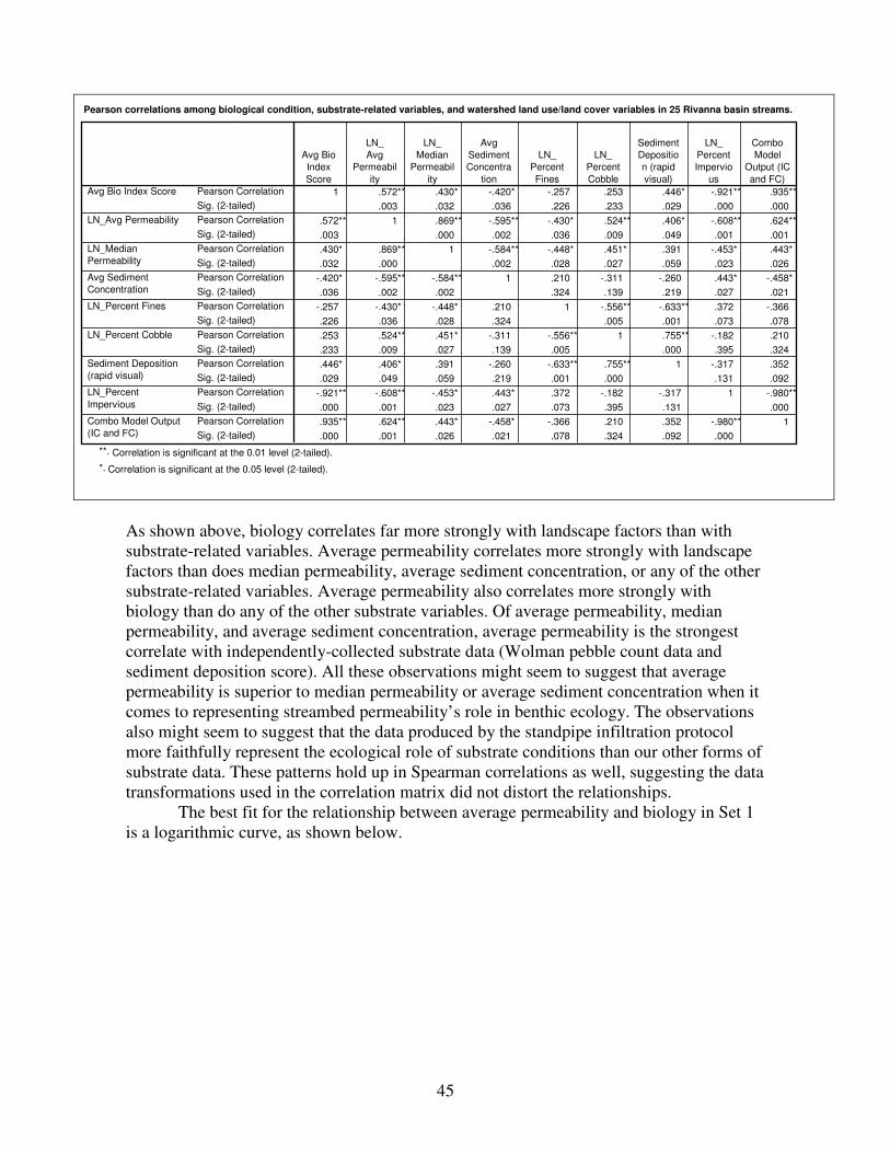
45

Pearson correlations among biological condition, substrate-related variables, and watershed land use/land cover variables in 25 Rivanna basin streams.

1 .572** .430* -.420* -.257 .253 .446* -.921** .935**

.003 .032 .036 .226 .233 .029 .000 .000

.572** 1 .869** -.595** -.430* .524** .406* -.608** .624**

.003 .000 .002 .036 .009 .049 .001 .001

.430* .869** 1 -.584** -.448* .451* .391 -.453* .443*

.032 .000 .002 .028 .027 .059 .023 .026

-.420* -.595** -.584** 1 .210 -.311 -.260 .443* -.458*

.036 .002 .002 .324 .139 .219 .027 .021

-.257 -.430* -.448* .210 1 -.556** -.633** .372 -.366

.226 .036 .028 .324 .005 .001 .073 .078

.253 .524** .451* -.311 -.556** 1 .755** -.182 .210

.233 .009 .027 .139 .005 .000 .395 .324

.446* .406* .391 -.260 -.633** .755** 1 -.317 .352

.029 .049 .059 .219 .001 .000 .131 .092

-.921** -.608** -.453* .443* .372 -.182 -.317 1 -.980**

.000 .001 .023 .027 .073 .395 .131 .000

.935** .624** .443* -.458* -.366 .210 .352 -.980** 1

.000 .001 .026 .021 .078 .324 .092 .000

Pearson Correlation

Sig. (2-tailed)

Pearson Correlation

Sig. (2-tailed)

Pearson Correlation

Sig. (2-tailed)

Pearson Correlation

Sig. (2-tailed)

Pearson Correlation

Sig. (2-tailed)

Pearson Correlation

Sig. (2-tailed)

Pearson Correlation

Sig. (2-tailed)

Pearson Correlation

Sig. (2-tailed)

Pearson Correlation

Sig. (2-tailed)

Avg Bio Index Score

LN_Avg Permeability

LN_Median

Permeability

Avg Sediment

Concentration

LN_Percent Fines

LN_Percent Cobble

Sediment Deposition

(rapid visual)

LN_Percent

Impervious

Combo Model Output

(IC and FC)

Avg Bio

Index

Score

LN_

Avg

Permeabil

ity

LN_

Median

Permeabil

ity

Avg

Sediment

Concentra

tion

LN_

Percent

Fines

LN_

Percent

Cobble

Sediment

Depositio

n (rapid

visual)

LN_

Percent

Impervio

us

Combo

Model

Output (IC

and FC)

Correlation is significant at the 0.01 level (2-tailed).**.

Correlation is significant at the 0.05 level (2-tailed).*.

As shown above, biology correlates far more strongly with landscape factors than with

substrate-related variables. Average permeability correlates more strongly with landscape

factors than does median permeability, average sediment concentration, or any of the other

substrate-related variables. Average permeability also correlates more strongly with

biology than do any of the other substrate variables. Of average permeability, median

permeability, and average sediment concentration, average permeability is the strongest

correlate with independently-collected substrate data (Wolman pebble count data and

sediment deposition score). All these observations might seem to suggest that average

permeability is superior to median permeability or average sediment concentration when it

comes to representing streambed permeability’s role in benthic ecology. The observations

also might seem to suggest that the data produced by the standpipe infiltration protocol

more faithfully represent the ecological role of substrate conditions than our other forms of

substrate data. These patterns hold up in Spearman correlations as well, suggesting the data

transformations used in the correlation matrix did not distort the relationships.

The best fit for the relationship between average permeability and biology in Set 1

is a logarithmic curve, as shown below.

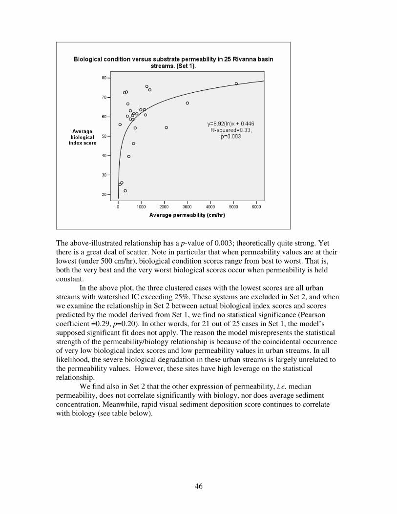
46

The above-illustrated relationship has a p-value of 0.003; theoretically quite strong. Yet

there is a great deal of scatter. Note in particular that when permeability values are at their

lowest (under 500 cm/hr), biological condition scores range from best to worst. That is,

both the very best and the very worst biological scores occur when permeability is held

constant.

In the above plot, the three clustered cases with the lowest scores are all urban

streams with watershed IC exceeding 25%. These systems are excluded in Set 2, and when

we examine the relationship in Set 2 between actual biological index scores and scores

predicted by the model derived from Set 1, we find no statistical significance (Pearson

coefficient =0.29, p=0.20). In other words, for 21 out of 25 cases in Set 1, the model’s

supposed significant fit does not apply. The reason the model misrepresents the statistical

strength of the permeability/biology relationship is because of the coincidental occurrence

of very low biological index scores and low permeability values in urban streams. In all

likelihood, the severe biological degradation in these urban streams is largely unrelated to

the permeability values. However, these sites have high leverage on the statistical

relationship.

We find also in Set 2 that the other expression of permeability, i.e. median

permeability, does not correlate significantly with biology, nor does average sediment

concentration. Meanwhile, rapid visual sediment deposition score continues to correlate

with biology (see table below).

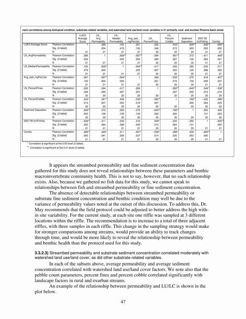
47

Pearson correlations among biological condition, substrate-related variables, and watershed land use/land cover variables in 21 primarily rural and exurban Rivanna basin streams.

1 .289 .163 -.367 -.222 .543* .629** -.636** .695**

.204 .479 .102 .346 .013 .003 .002 .000

21 21 21 21 20 20 20 21 21

.289 1 .829** -.597** -.394 .581** .372 -.411 .449*

.204 .000 .004 .085 .007 .106 .064 .041

21 21 21 21 20 20 20 21 21

.163 .829** 1 -.584** -.417 .439 .355 -.243 .211

.479 .000 .005 .067 .053 .125 .288 .359

21 21 21 21 20 20 20 21 21

-.367 -.597** -.584** 1 .269 -.532* -.375 .418 -.457*

.102 .004 .005 .251 .016 .104 .059 .037

21 21 21 21 20 20 20 21 21

-.222 -.394 -.417 .269 1 -.582** -.645** .549* -.538*

.346 .085 .067 .251 .007 .002 .012 .014

20 20 20 20 20 20 20 20 20

.543* .581** .439 -.532* -.582** 1 .782** -.422 .498*

.013 .007 .053 .016 .007 .000 .064 .025

20 20 20 20 20 20 20 20 20

.629** .372 .355 -.375 -.645** .782** 1 -.350 .439

.003 .106 .125 .104 .002 .000 .131 .053

20 20 20 20 20 20 20 20 20

-.636** -.411 -.243 .418 .549* -.422 -.350 1 -.900**

.002 .064 .288 .059 .012 .064 .131 .000

21 21 21 21 20 20 20 21 21

.695** .449* .211 -.457* -.538* .498* .439 -.900** 1

.000 .041 .359 .037 .014 .025 .053 .000

21 21 21 21 20 20 20 21 21

Pearson Correlation

Sig. (2-tailed)

N

Pearson Correlation

Sig. (2-tailed)

N

Pearson Correlation

Sig. (2-tailed)

N

Pearson Correlation

Sig. (2-tailed)

N

Pearson Correlation

Sig. (2-tailed)

N

Pearson Correlation

Sig. (2-tailed)

N

Pearson Correlation

Sig. (2-tailed)

N

Pearson Correlation

Sig. (2-tailed)

N

Pearson Correlation

Sig. (2-tailed)

N

LUES Average Score

LN_AvgPermeability

LN_MedianPermeability

Avg_sed_mgPerLiter

LN_PercentFines

LN_PercentCobble

Sediment Deposition

2007-09 (ln)PctImp

Combo

LUES

Average

Score

LN_

Avg

Permeability

LN_

Median

Permeability

Avg_sed_

mgPerLiter

LN_

PercentFines

LN_

Percent

Cobble

Sediment

Deposition

2007-09

(ln)PctImp Combo

Correlation is significant at the 0.05 level (2-tailed).*.

Correlation is significant at the 0.01 level (2-tailed).**.

It appears the streambed permeability and fine sediment concentration data

gathered for this study does not reveal relationships between these parameters and benthic

macroinvertebrate community health. This is not to say, however, that no such relationship

exists. Also, because we gathered no fish data for this study, we cannot speak to

relationships between fish and streambed permeability or fine sediment concentration.

The absence of detectable relationships between streambed permeability or

substrate fine sediment concentration and benthic condition may well be due to the

variance of permeability values noted at the outset of this discussion. To address this, Dr.

May recommends that the field protocol could be adjusted to better address the high with-

in site variability. For the current study, at each site one riffle was sampled at 3 different

locations within the riffle. The recommendation is to increase to a total of three adjacent

riffles, with three samples in each riffle. This change in the sampling strategy would make

for stronger comparisons among streams, would provide an ability to track changes

through time, and would be more likely to reveal the relationship between permeability

and benthic health than the protocol used for this study.

3.3.2.3) Streambed permeability and substrate sediment concentration correlated moderately with watershed land use/land cover, as did other substrate-related variables.

In each of the subsets above, average permeability and average sediment

concentration correlated with watershed land use/land cover factors. We note also that the

pebble count parameters, percent fines and percent cobble correlated significantly with

landscape factors in rural and exurban streams.

An example of the relationship between permeability and LU/LC is shown in the

plot below.

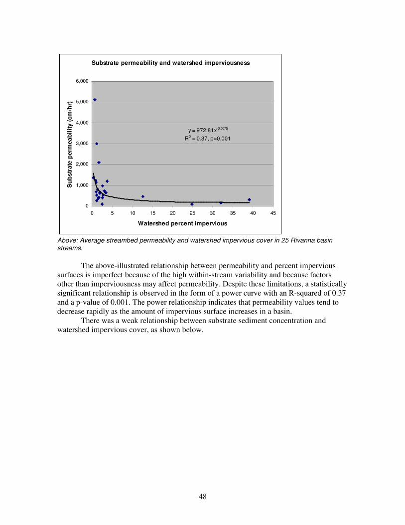
48

Substrate permeability and watershed imperviousness

y = 972.81x-0.5075

R2 = 0.37, p=0.001

0

1,000

2,000

3,000

4,000

5,000

6,000

0 5 10 15 20 25 30 35 40 45

Watershed percent impervious

Su

bstr

ate

perm

eab

ilit

y (

cm

/hr)

Above: Average streambed permeability and watershed impervious cover in 25 Rivanna basin streams.

The above-illustrated relationship between permeability and percent impervious

surfaces is imperfect because of the high within-stream variability and because factors

other than imperviousness may affect permeability. Despite these limitations, a statistically

significant relationship is observed in the form of a power curve with an R-squared of 0.37

and a p-value of 0.001. The power relationship indicates that permeability values tend to

decrease rapidly as the amount of impervious surface increases in a basin.

There was a weak relationship between substrate sediment concentration and

watershed impervious cover, as shown below.

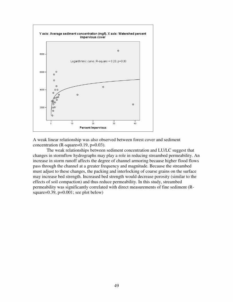
49

A weak linear relationship was also observed between forest cover and sediment

concentration (R-square=0.19, p=0.03).

The weak relationships between sediment concentration and LU/LC suggest that

changes in stormflow hydrographs may play a role in reducing streambed permeability. An

increase in storm runoff affects the degree of channel armoring because higher flood flows

pass through the channel at a greater frequency and magnitude. Because the streambed

must adjust to these changes, the packing and interlocking of coarse grains on the surface

may increase bed strength. Increased bed strength would decrease porosity (similar to the

effects of soil compaction) and thus reduce permeability. In this study, streambed

permeability was significantly correlated with direct measurements of fine sediment (R-

square=0.39, p=0.001; see plot below)

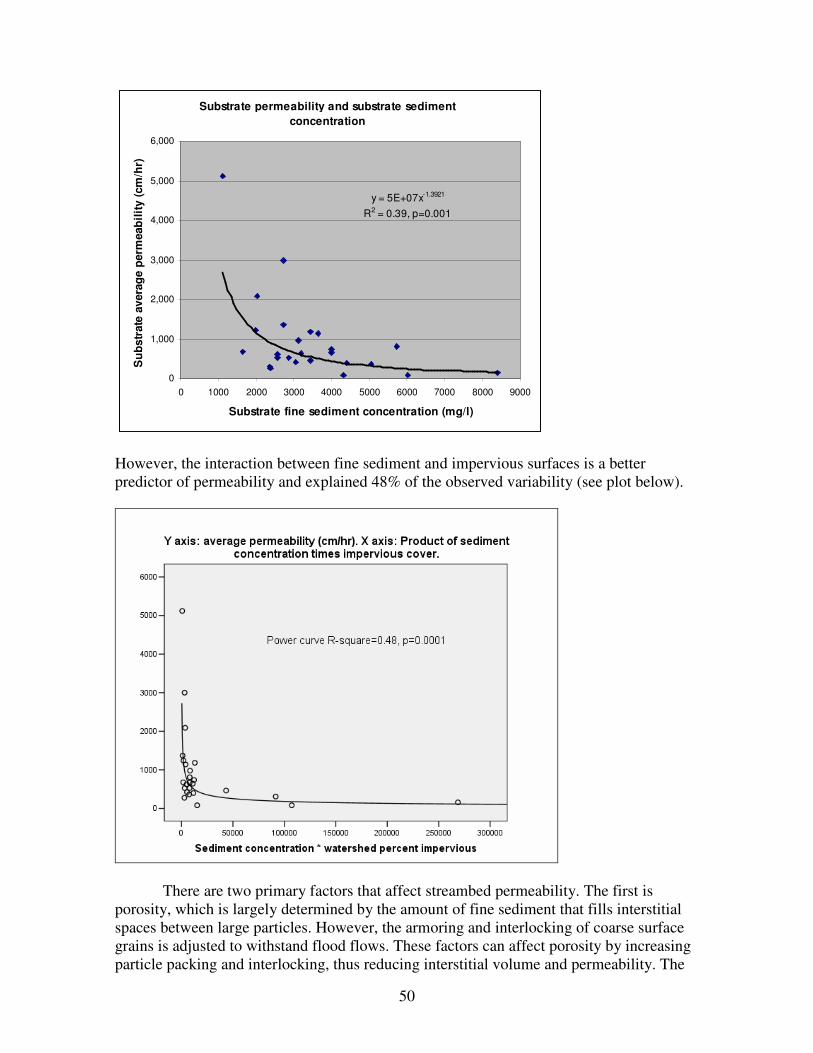
50

Substrate permeability and substrate sediment

concentration

y = 5E+07x-1.3921

R2 = 0.39, p=0.001

0

1,000

2,000

3,000

4,000

5,000

6,000

0 1000 2000 3000 4000 5000 6000 7000 8000 9000

Substrate fine sediment concentration (mg/l)

Su

bstr

ate

avera

ge p

erm

eab

ilit

y (

cm

/hr)

However, the interaction between fine sediment and impervious surfaces is a better

predictor of permeability and explained 48% of the observed variability (see plot below).

There are two primary factors that affect streambed permeability. The first is

porosity, which is largely determined by the amount of fine sediment that fills interstitial

spaces between large particles. However, the armoring and interlocking of coarse surface

grains is adjusted to withstand flood flows. These factors can affect porosity by increasing

particle packing and interlocking, thus reducing interstitial volume and permeability. The

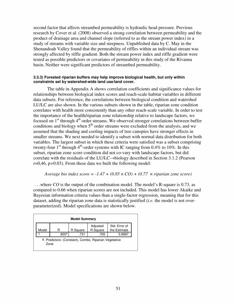
51

second factor that affects streambed permeability is hydraulic head pressure. Previous

research by Cover et al. (2008) observed a strong correlation between permeability and the

product of drainage area and channel slope (referred to as the stream power index) in a

study of streams with variable size and steepness. Unpublished data by C. May in the

Shenandoah Valley found that the permeability of riffles within an individual stream was

strongly affected by riffle gradient. Both the stream power index and riffle gradient were

tested as possible predictors or covariates of permeability in this study of the Rivanna

basin. Neither were significant predictors of streambed permeability.

3.3.3) Forested riparian buffers may help improve biological health, but only within constraints set by watershed-wide land use/land cover.

The table in Appendix A shows correlation coefficients and significance values for

relationships between biological index scores and reach-scale habitat variables in different

data subsets. For reference, the correlations between biological condition and watershed

LU/LC are also shown. In the various subsets shown in the table, riparian zone condition

correlates with health more consistently than any other reach-scale variable. In order to test

the importance of the health/riparian zone relationship relative to landscape factors, we

focused on 1st through 4

th order streams. We observed stronger correlations between buffer

conditions and biology when 5th

order streams were excluded from the analysis, and we

assumed that the shading and cooling impacts of tree canopies have stronger effects in

smaller streams. We next needed to identify a subset with normal data distribution for both

variables. The largest subset in which these criteria were satisfied was a subset comprising

twenty-four 1st through 4

th-order systems with IC ranging from 0.4% to 10%. In this

subset, riparian zone score condition did not co-vary with landscape factors, but did

correlate with the residuals of the LU/LC→biology described in Section 3.1.2 (Pearson

r=0,46, p=0.03). From these data we built the following model:

Average bio index score = -1.47 + (0.85 × CO) + (0.77 × riparian zone score)

. . .where CO is the output of the combination model. The model’s R-square is 0.73, as

compared to 0.66 when riparian scores are not included. This model has lower Akaike and

Bayesian information criteria values than a single-factor regression, meaning that for this

dataset, adding the riparian zone data is statistically justified (i.e. the model is not over-

parameterized). Model specifications are shown below.

Model Summary

.855a .731 .705 5.8997

Model1

R R Square

Adjusted

R Square

Std. Error of

the Estimate

Predictors: (Constant), Combo, Riparian Vegetative

Zone

a.

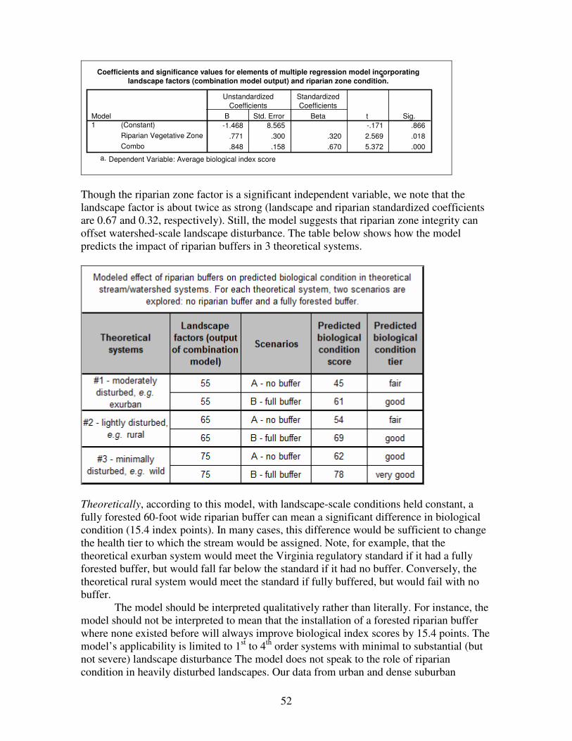
52

Coefficients and significance values for elements of multiple regression model incorporating

landscape factors (combination model output) and riparian zone condition.a

-1.468 8.565 -.171 .866

.771 .300 .320 2.569 .018

.848 .158 .670 5.372 .000

(Constant)

Riparian Vegetative Zone

Combo

Model

1

B Std. Error

Unstandardized

Coefficients

Beta

Standardized

Coefficients

t Sig.

Dependent Variable: Average biological index scorea.

Though the riparian zone factor is a significant independent variable, we note that the

landscape factor is about twice as strong (landscape and riparian standardized coefficients

are 0.67 and 0.32, respectively). Still, the model suggests that riparian zone integrity can

offset watershed-scale landscape disturbance. The table below shows how the model

predicts the impact of riparian buffers in 3 theoretical systems.

Theoretically, according to this model, with landscape-scale conditions held constant, a

fully forested 60-foot wide riparian buffer can mean a significant difference in biological

condition (15.4 index points). In many cases, this difference would be sufficient to change

the health tier to which the stream would be assigned. Note, for example, that the

theoretical exurban system would meet the Virginia regulatory standard if it had a fully

forested buffer, but would fall far below the standard if it had no buffer. Conversely, the

theoretical rural system would meet the standard if fully buffered, but would fail with no

buffer.

The model should be interpreted qualitatively rather than literally. For instance, the

model should not be interpreted to mean that the installation of a forested riparian buffer

where none existed before will always improve biological index scores by 15.4 points. The

model’s applicability is limited to 1st to 4

th order systems with minimal to substantial (but

not severe) landscape disturbance The model does not speak to the role of riparian

condition in heavily disturbed landscapes. Our data from urban and dense suburban

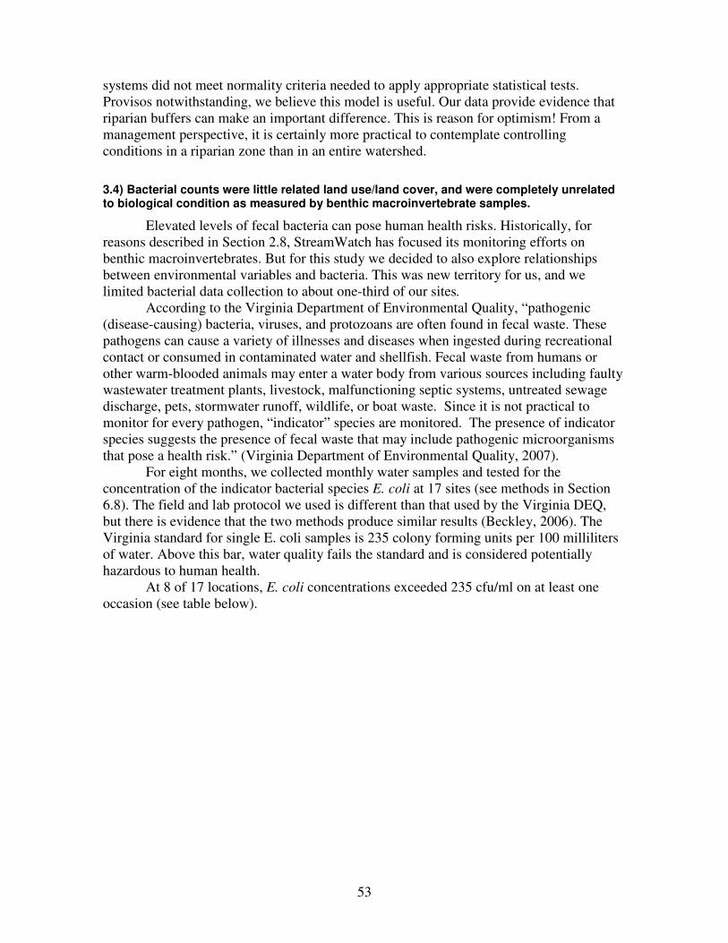
53

systems did not meet normality criteria needed to apply appropriate statistical tests.

Provisos notwithstanding, we believe this model is useful. Our data provide evidence that

riparian buffers can make an important difference. This is reason for optimism! From a

management perspective, it is certainly more practical to contemplate controlling

conditions in a riparian zone than in an entire watershed.

3.4) Bacterial counts were little related land use/land cover, and were completely unrelated to biological condition as measured by benthic macroinvertebrate samples.

Elevated levels of fecal bacteria can pose human health risks. Historically, for

reasons described in Section 2.8, StreamWatch has focused its monitoring efforts on

benthic macroinvertebrates. But for this study we decided to also explore relationships

between environmental variables and bacteria. This was new territory for us, and we

limited bacterial data collection to about one-third of our sites.

According to the Virginia Department of Environmental Quality, “pathogenic

(disease-causing) bacteria, viruses, and protozoans are often found in fecal waste. These

pathogens can cause a variety of illnesses and diseases when ingested during recreational

contact or consumed in contaminated water and shellfish. Fecal waste from humans or

other warm-blooded animals may enter a water body from various sources including faulty

wastewater treatment plants, livestock, malfunctioning septic systems, untreated sewage

discharge, pets, stormwater runoff, wildlife, or boat waste. Since it is not practical to

monitor for every pathogen, “indicator” species are monitored. The presence of indicator

species suggests the presence of fecal waste that may include pathogenic microorganisms

that pose a health risk.” (Virginia Department of Environmental Quality, 2007).

For eight months, we collected monthly water samples and tested for the

concentration of the indicator bacterial species E. coli at 17 sites (see methods in Section

6.8). The field and lab protocol we used is different than that used by the Virginia DEQ,

but there is evidence that the two methods produce similar results (Beckley, 2006). The

Virginia standard for single E. coli samples is 235 colony forming units per 100 milliliters

of water. Above this bar, water quality fails the standard and is considered potentially

hazardous to human health.

At 8 of 17 locations, E. coli concentrations exceeded 235 cfu/ml on at least one

occasion (see table below).

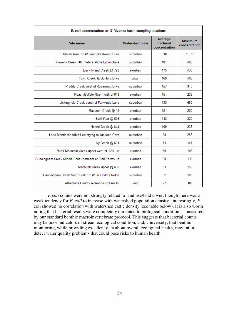
54

E.coli counts were not strongly related to land use/land cover, though there was a

weak tendency for E. coli to increase with watershed population density. Interestingly, E.

coli showed no correlation with watershed cattle density (see table below). It is also worth

noting that bacterial results were completely unrelated to biological condition as measured

by our standard benthic macroinvertebrate protocol. This suggests that bacterial counts

may be poor indicators of stream ecological condition, and, conversely, that benthic

monitoring, while providing excellent data about overall ecological health, may fail to

detect water quality problems that could pose risks to human health.

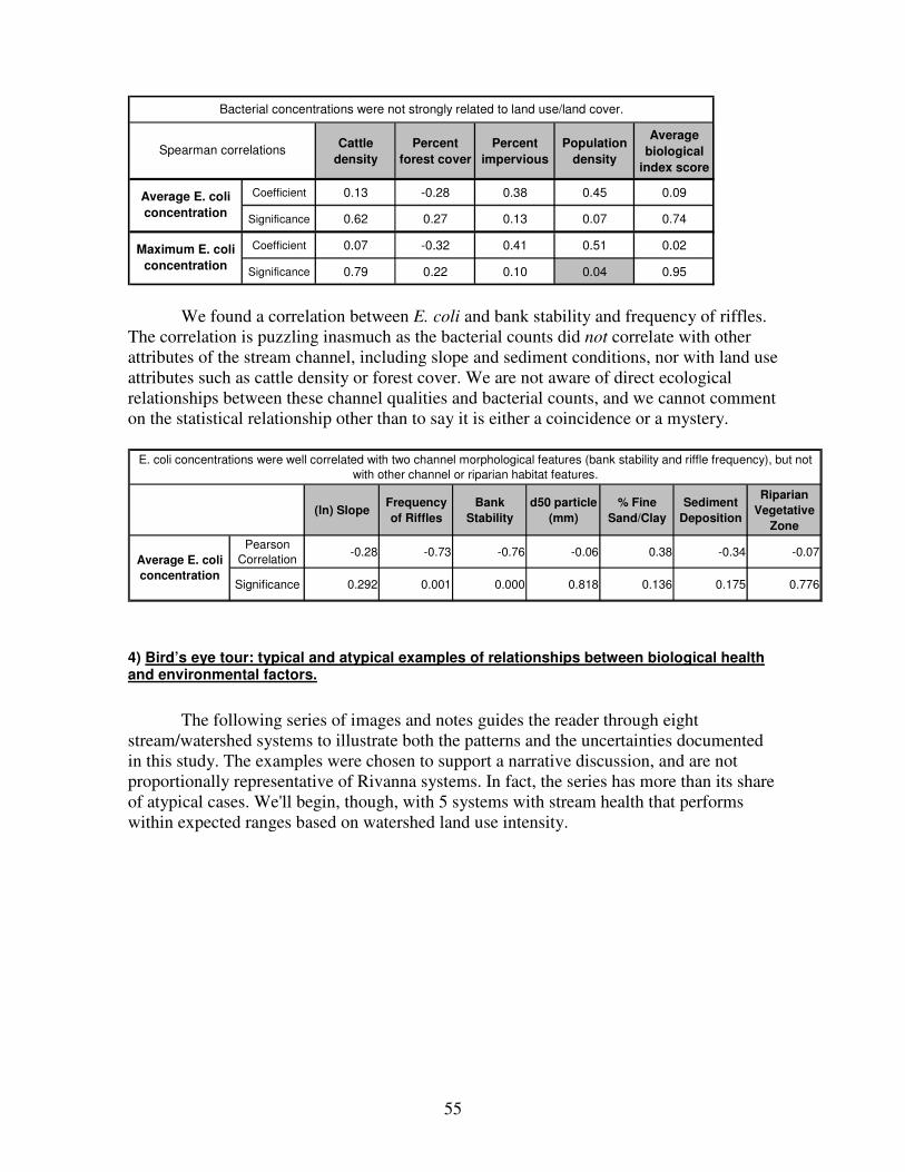
55

Cattle

density

Percent

forest cover

Percent

impervious

Population

density

Average

biological

index score

Coefficient 0.13 -0.28 0.38 0.45 0.09

Significance 0.62 0.27 0.13 0.07 0.74

Coefficient 0.07 -0.32 0.41 0.51 0.02

Significance 0.79 0.22 0.10 0.04 0.95

Maximum E. coli

concentration

Spearman correlations

Bacterial concentrations were not strongly related to land use/land cover.

Average E. coli

concentration

We found a correlation between E. coli and bank stability and frequency of riffles.

The correlation is puzzling inasmuch as the bacterial counts did not correlate with other

attributes of the stream channel, including slope and sediment conditions, nor with land use

attributes such as cattle density or forest cover. We are not aware of direct ecological

relationships between these channel qualities and bacterial counts, and we cannot comment

on the statistical relationship other than to say it is either a coincidence or a mystery.

(ln) SlopeFrequency

of Riffles

Bank

Stability

d50 particle

(mm)

% Fine

Sand/Clay

Sediment

Deposition

Riparian

Vegetative

Zone

Pearson

Correlation-0.28 -0.73 -0.76 -0.06 0.38 -0.34 -0.07

Significance 0.292 0.001 0.000 0.818 0.136 0.175 0.776

Average E. coli

concentration

E. coli concentrations were well correlated with two channel morphological features (bank stability and riffle frequency), but not

with other channel or riparian habitat features.

4) Bird’s eye tour: typical and atypical examples of relationships between biological health and environmental factors.

The following series of images and notes guides the reader through eight

stream/watershed systems to illustrate both the patterns and the uncertainties documented

in this study. The examples were chosen to support a narrative discussion, and are not

proportionally representative of Rivanna systems. In fact, the series has more than its share

of atypical cases. We'll begin, though, with 5 systems with stream health that performs

within expected ranges based on watershed land use intensity.

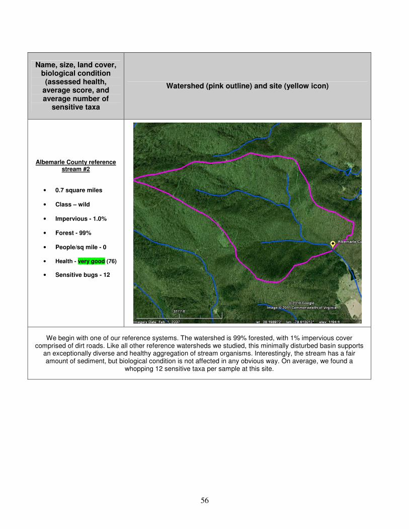
56

Name, size, land cover, biological condition (assessed health,

average score, and average number of

sensitive taxa

Watershed (pink outline) and site (yellow icon)

Albemarle County reference stream #2

• 0.7 square miles

• Class – wild

• Impervious - 1.0%

• Forest - 99%

• People/sq mile - 0

• Health - very good (76)

• Sensitive bugs - 12

We begin with one of our reference systems. The watershed is 99% forested, with 1% impervious cover comprised of dirt roads. Like all other reference watersheds we studied, this minimally disturbed basin supports

an exceptionally diverse and healthy aggregation of stream organisms. Interestingly, the stream has a fair amount of sediment, but biological condition is not affected in any obvious way. On average, we found a

whopping 12 sensitive taxa per sample at this site.

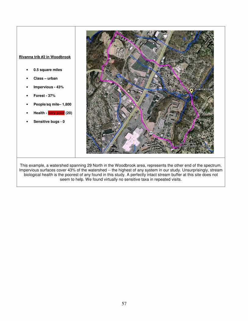
57

Rivanna trib #2 in Woodbrook

• 0.5 square miles

• Class – urban

• Impervious - 43%

• Forest - 37%

• People/sq mile– 1,800

• Health - very poor (20)

• Sensitive bugs - 0

This example, a watershed spanning 29 North in the Woodbrook area, represents the other end of the spectrum. Impervious surfaces cover 43% of the watershed -- the highest of any system in our study. Unsurprisingly, stream

biological health is the poorest of any found in this study. A perfectly intact stream buffer at this site does not seem to help. We found virtually no sensitive taxa in repeated visits.

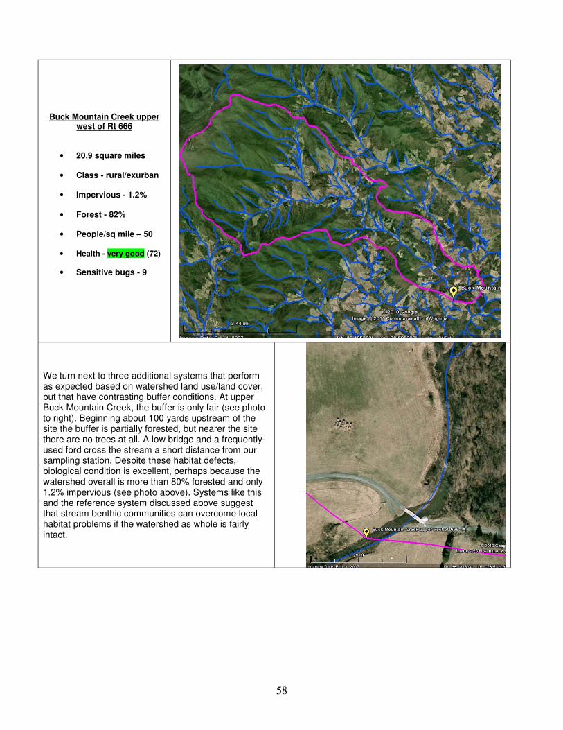
58

Buck Mountain Creek upper west of Rt 666

• 20.9 square miles

• Class - rural/exurban

• Impervious - 1.2%

• Forest - 82%

• People/sq mile – 50

• Health - very good (72)

• Sensitive bugs - 9

We turn next to three additional systems that perform as expected based on watershed land use/land cover, but that have contrasting buffer conditions. At upper Buck Mountain Creek, the buffer is only fair (see photo to right). Beginning about 100 yards upstream of the site the buffer is partially forested, but nearer the site there are no trees at all. A low bridge and a frequently-used ford cross the stream a short distance from our sampling station. Despite these habitat defects, biological condition is excellent, perhaps because the watershed overall is more than 80% forested and only 1.2% impervious (see photo above). Systems like this and the reference system discussed above suggest that stream benthic communities can overcome local habitat problems if the watershed as whole is fairly intact.

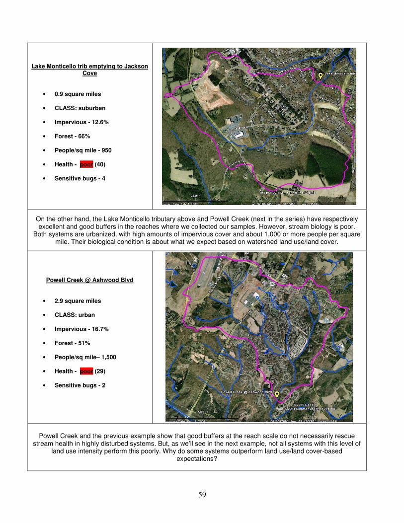
59

Lake Monticello trib emptying to Jackson Cove

• 0.9 square miles

• CLASS: suburban

• Impervious - 12.6%

• Forest - 66%

• People/sq mile - 950

• Health - poor (40)

• Sensitive bugs - 4

On the other hand, the Lake Monticello tributary above and Powell Creek (next in the series) have respectively excellent and good buffers in the reaches where we collected our samples. However, stream biology is poor.

Both systems are urbanized, with high amounts of impervious cover and about 1,000 or more people per square mile. Their biological condition is about what we expect based on watershed land use/land cover.

Powell Creek @ Ashwood Blvd

• 2.9 square miles

• CLASS: urban

• Impervious - 16.7%

• Forest - 51%

• People/sq mile– 1,500

• Health - poor (29)

• Sensitive bugs - 2

Powell Creek and the previous example show that good buffers at the reach scale do not necessarily rescue stream health in highly disturbed systems. But, as we’ll see in the next example, not all systems with this level of

land use intensity perform this poorly. Why do some systems outperform land use/land cover-based expectations?

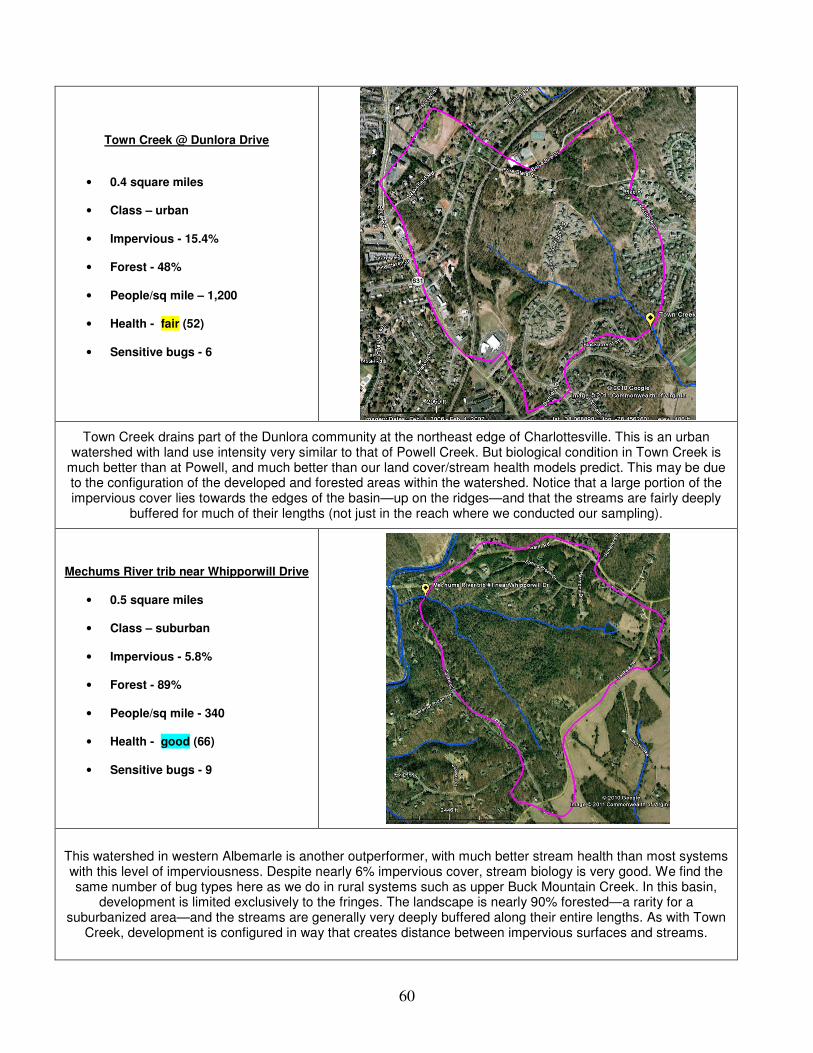
60

Town Creek @ Dunlora Drive

• 0.4 square miles

• Class – urban

• Impervious - 15.4%

• Forest - 48%

• People/sq mile – 1,200

• Health - fair (52)

• Sensitive bugs - 6

Town Creek drains part of the Dunlora community at the northeast edge of Charlottesville. This is an urban watershed with land use intensity very similar to that of Powell Creek. But biological condition in Town Creek is

much better than at Powell, and much better than our land cover/stream health models predict. This may be due to the configuration of the developed and forested areas within the watershed. Notice that a large portion of the impervious cover lies towards the edges of the basin—up on the ridges—and that the streams are fairly deeply

buffered for much of their lengths (not just in the reach where we conducted our sampling).

Mechums River trib near Whipporwill Drive

• 0.5 square miles

• Class – suburban

• Impervious - 5.8%

• Forest - 89%

• People/sq mile - 340

• Health - good (66)

• Sensitive bugs - 9

This watershed in western Albemarle is another outperformer, with much better stream health than most systems with this level of imperviousness. Despite nearly 6% impervious cover, stream biology is very good. We find the same number of bug types here as we do in rural systems such as upper Buck Mountain Creek. In this basin,

development is limited exclusively to the fringes. The landscape is nearly 90% forested—a rarity for a suburbanized area—and the streams are generally very deeply buffered along their entire lengths. As with Town

Creek, development is configured in way that creates distance between impervious surfaces and streams.

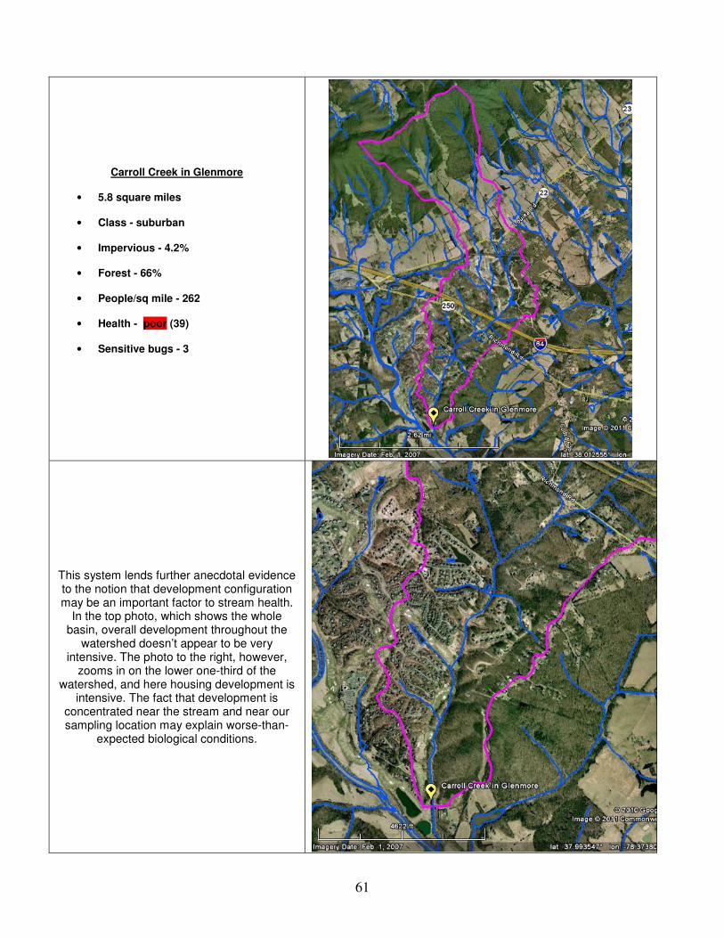
61

Carroll Creek in Glenmore

• 5.8 square miles

• Class - suburban

• Impervious - 4.2%

• Forest - 66%

• People/sq mile - 262

• Health - poor (39)

• Sensitive bugs - 3

This system lends further anecdotal evidence to the notion that development configuration may be an important factor to stream health.

In the top photo, which shows the whole basin, overall development throughout the

watershed doesn’t appear to be very intensive. The photo to the right, however,

zooms in on the lower one-third of the watershed, and here housing development is

intensive. The fact that development is concentrated near the stream and near our sampling location may explain worse-than-

expected biological conditions.

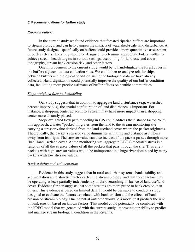
62

5) Recommendations for further study.

Riparian buffers

In the current study we found evidence that forested riparian buffers are important

to stream biology, and can help dampen the impacts of watershed-scale land disturbance. A

future study designed specifically on buffers could provide a more quantitative assessment

of buffer effects. The study should be designed to determine appropriate buffer widths to

achieve stream health targets in various settings, accounting for land use/land cover,

topography, stream bank erosion risk, and other factors.

One improvement to the current study would be to hand-digitize the forest cover in

the buffers adjacent to data collection sites. We could then re-analyze relationships

between buffers and biological condition, using the biological data we have already

collected. Hand-digitization could potentially improve the quality of our buffer condition

data, facilitating more precise estimates of buffer effects on benthic communities.

Slope-weighted flow path modeling

Our study suggests that in addition to aggregate land disturbance (e.g. watershed

percent impervious), the spatial configuration of land disturbance is important. For

instance, a shopping center adjacent to a stream may have more impact than a shopping

center more distantly placed.

Slope-weighted flow path modeling in GIS could address the distance factor. With

this approach, a water “packet” migrates from the land to the stream monitoring site

carrying a stressor value derived from the land use/land cover where the packet originates.

Theoretically, the packet’s stressor value diminishes with time and distance as it flows

away from its origin. The stressor value can also increase if the packet passes through more

"bad" land use/land cover. At the monitoring site, aggregate LU/LC-mediated stress is a

function of all the stressor values of all the packets that pass through the site. Thus a few

packets with high stressor values would be unimportant in a huge river dominated by many

packets with low stressor values.

Bank stability and sedimentation

Evidence in this study suggest that in rural and urban systems, bank stability and

sedimentation are distinctive factors affecting stream biology, and that these factors may

be operating at least partially independently of the overarching influence of land use/land

cover. Evidence further suggests that some streams are more prone to bank erosion than

others. This evidence is based on limited data. It would be desirable to conduct a study

designed to evaluate the factors associated with bank erosion and the effects of bank

erosion on stream biology. One potential outcome would be a model that predicts the risk

of bank erosion based on known factors. This model could potentially be combined with

the IC/FC model that we generated with the current study, improving our ability to predict

and manage stream biological condition in the Rivanna.

63

6) Appendix A – Methods

6.1) Site selection

We gathered stream biological and habitat data at 51 sites in drainages with widely

varying land use intensity. Sites were selected to ensure a stratified dataset, with

representation of urban, suburban, exurban, rural, and wild (reference) systems. Nearly all

stations were situated on warmwater Piedmont streams. The full range of Rivanna basin

stream orders were represented, with the result that sites and watersheds of smaller streams

were sometimes nested within the larger watersheds of distant downstream sites. In our

judgment, nesting did not diminish the distinctiveness of the studied systems, and we

treated data from all sites as independent samples. Site locations are shown in Section 2.4.

6.2) Assessing biological condition.

StreamWatch’s methods for collecting stream invertebrates and producing

biological index scores are described in Section 2.7.

Biological condition was measured an average of six times at each site.

Assessments of biological condition were based on an analysis of the multiple biological

index scores generated during the study period, per StreamWatch’s established assessment

protocol. Assessments are driven by average score, variance, and trend. The procedure is

outlined in the table below.

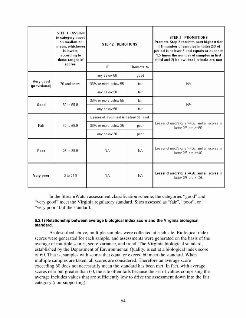
64

In the StreamWatch assessment classification scheme, the categories “good” and

“very good” meet the Virginia regulatory standard. Sites assessed as “fair”, “poor”, or

“very poor” fail the standard.

6.2.1) Relationship between average biological index score and the Virginia biological standard.

As described above, multiple samples were collected at each site. Biological index

scores were generated for each sample, and assessments were generated on the basis of the

average of multiple scores, score variance, and trend. The Virginia biological standard,

established by the Department of Environmental Quality, is set at a biological index score

of 60. That is, samples with scores that equal or exceed 60 meet the standard. When

multiple samples are taken, all scores are considered. Therefore an average score

exceeding 60 does not necessarily mean the standard has been met. In fact, with average

scores near but greater than 60, the site often fails because the set of values comprising the

average includes values that are sufficiently low to drive the assessment down into the fair

category (non-supporting).

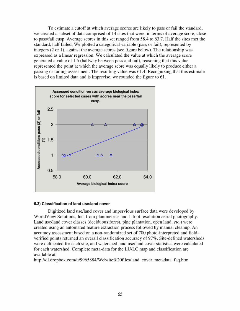
65

To estimate a cutoff at which average scores are likely to pass or fail the standard,

we created a subset of data comprised of 14 sites that were, in terms of average score, close

to pass/fail cusp. Average scores in this set ranged from 58.4 to 63.7. Half the sites met the

standard; half failed. We plotted a categorical variable (pass or fail), represented by

integers (2 or 1), against the average scores (see figure below). The relationship was

expressed as a linear regression. We calculated the value at which the average score

generated a value of 1.5 (halfway between pass and fail), reasoning that this value

represented the point at which the average score was equally likely to produce either a

passing or failing assessment. The resulting value was 61.4. Recognizing that this estimate

is based on limited data and is imprecise, we rounded the figure to 61.

Assessed condition versus average biological index

score for selected cases with scores near the pass/fail

cusp.

0.5

1

1.5

2

2.5

58.0 60.0 62.0 64.0

Average biological index score

As

se

ss

ed

co

nd

itio

n:

pa

ss

(2

) o

r fa

il

(1)

6.3) Classification of land use/land cover

Digitized land use/land cover and impervious surface data were developed by

WorldView Solutions, Inc. from planimetrics and 1-foot resolution aerial photography.

Land use/land cover classes (deciduous forest, pine plantation, open land, etc.) were

created using an automated feature extraction process followed by manual cleanup. An

accuracy assessment based on a non-randomized set of 700 photo-interpreted and field-

verified points returned an overall classification accuracy of 97%. Site-defined watersheds

were delineated for each site, and watershed land use/land cover statistics were calculated

for each watershed. Complete meta-data for the LU/LC map and classification are

available at

http://dl.dropbox.com/u/9965884/Website%20files/land_cover_metadata_faq.htm

66

6.4) Estimating human population density

Population density for each subwatershed was estimated based on 2008 data

supplied by the Weldon Cooper Center for Public Service. Localities’ populations were

adjusted slightly to account for the effects of non-residential (workforce) populations.

Using a geographic information system, localities’ populations were distributed onto the

landscape via geographical points representing buildings and addresses. Areal densities for

each subwatershed were then calculated.

6.5) Estimating cattle populations

Under guidance from a trained interpreter of aerial imagery of agricultural

landscapes, a project team composed of StreamWatch staff and volunteers estimated cattle

population densities of Rivanna subwatersheds by locating and counting cattle that were

visible in 2009 Virginia leaf-off base map imagery. Year 2010 USDA estimates of county

cattle populations, apportioned to the Rivanna basin according to contributing land area,

give an estimate of about 23,750 head for the Rivanna basin. Our imagery-based count

identified approximately 13,500 head on the Rivanna landscape in early spring 2009, or

approximately 57% of the 2010 USDA-derived estimate. Both the USDA-based estimates

and the imagery-based counts are subject to error. We believe we located a majority of the

Rivanna’s cattle, and we reason that the spatially distributed cattle counts we generated

provide a useful representation of relative cattle densities across Rivanna subwatersheds.

We note that cattle operations are generally non-intensive in the Rivanna basin, with an

average of 31 head per square mile according to the USDA-based estimate of the overall

Rivanna cattle population. By contrast, agriculturally intensive counties in the nearby

Shenandoah Valley (Rockingham and Augusta counties) have densities of 130 head per

square mile.

6.6) Reach-scale habitat data

We gathered reach-scale data per three methods: Wolman pebble count, stream

slope survey, and EPA rapid visual assessment. All reach-scale data were developed in

reaches terminating at our biosampling stations and extending upstream for a distance of

twenty to forty times base-flow channel width.

Pebble counts were conducted in 10 transects per reach, with transects selected to

reflect the proportion of pool and riffle habitat extant in the reach. Ten particles were

collected and measured at each transect, for a total of 100 particles (Rosgen 1996). The

surveys produced data for median particle size (d50), percent fine sand/clay (≤0.24 mm),

and percent cobble (64-256 mm).

The rapid visual protocol involves walking the stream reach and scoring each of ten

habitat parameters using a standard field sheet (Barbour 1999). Scores range from zero to

twenty. The field sheet provides guidance by qualitatively and quantitatively describing

condition gradients of habitat features and appropriate scores for given conditions (see

field sheet below). The rapid visual protocol is subject to observer bias. To reduce bias and

increase data quality, StreamWatch has added additional standards to the protocol.

Specifically, StreamWatch breaks the reach into ten or more sub-reaches, scores each sub-

reach, and averages the sub-reach scores.

Of EPA rapid visual data, parameters regarded as reliable and useful for this study

were: sediment deposition, bank stability, frequency of riffles, and riparian buffer.

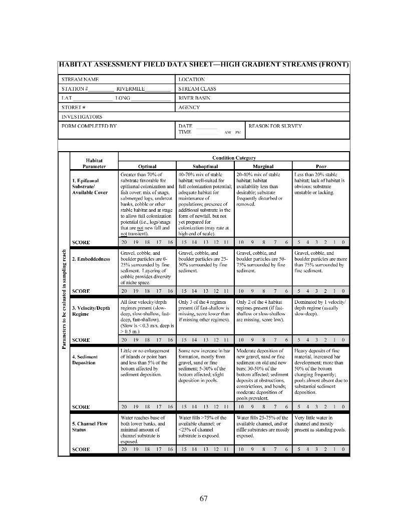
67

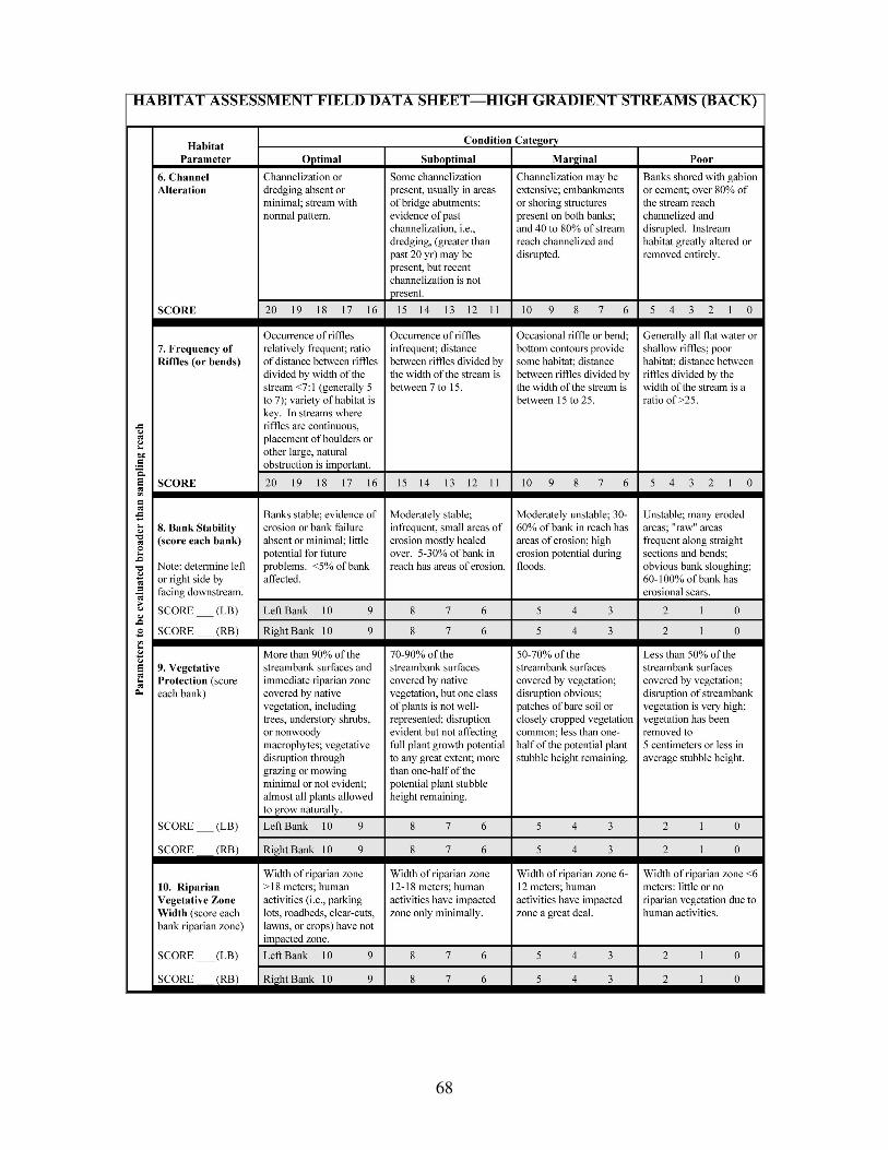
68

69

6.7) Substrate permeability

To explore the condition of substrate in Rivanna streams, 25 sites were selected.

The array of sites represented a broad range of stream and watershed conditions, ranging

from undeveloped mountain streams to urban waterways. Within each stream one riffle

was sampled (the same riffle at which benthic macroinvertebrate samples were collected).

In each riffle three permeability measurements were made, with multiple replicate

measurements made during each sample. After permeability measurements were

completed, fine sediment was directly sampled using a bulk sampling core and vacuum

pump extraction. Riffle gradient was also measured with an auto-level and survey rod for

the full length of the riffle.

Within each riffle, in-situ measurements of substrate permeability were made with

a perforated standpipe driven into the streambed. Three sample sites per riffle were

measured, with five to six replicate samples drawn per site. The stand pipe was driven into

the streambed to reach a sampling depth from 10 to 17cm below the bed surface. Water

was pumped out of the standpipe in the upper 2.5 cm of the water column, and the rate at

which interstitial water refilled the void was used to calculate subsurface flow rates

through the gravel. From in-situ measurements in the standpipe, the water volume

extracted per unit time is calculated as the ‘inflow rate’. Permeability is then interpolated

from empirical rating curves of permeability versus inflow rate (Terhune 1958; Barnard

and McBain 1994). Permeability values are then corrected for temperature, using a

viscosity correction factor. It is important to note that extremely low permeability values

cannot be calculated because the existing rating curve does not extend to inflow rates < 2.0

ml/sec, resulting in a non-temperature adjusted permeability of 80 cm/hr.

Fine sediment stored in the streambed was directly sampled with a 30.5 cm

diameter core sampler place directly over the site where permeability was measured. The

core sampler was embedded into the streambed to a depth of 10-15 cm. Substrate within

the core was overturned while a vacuum pump extracted the water, suspended sediment

and organic matter contained within the core. Vacuum-extracted samples were filtered

through a 1 mm diameter sieve and collected in a large storage container that was agitated

while a 250 ml sub-sample was collected for laboratory analysis. The organic fraction of

the sub-sample was combusted by igniting the sample on a glass fiber filter at 550°C for

24h, desiccated, and weighed. The ash-free dry mass of inorganic sediment <1 mm was

weighed on a high precision balance. The <1 mm size fraction represents sediment

consisting of coarse sand and finer particles, including silt and clay. The concentration of

fine sediment was calculated by the mass of inorganic sediment divided by the sample

volume.

6.8) Bacteria

Bacterial samples were collected by interns at 17 sites once per month for eight

months from April through November 2008. For seven of the eight months, two samples

were collected during each field visit. Samples were transported to a lab where Coliscan

Easygel media were inoculated. Inoculated media were incubated for 24 hours, after which

E. coli colonies were counted. Data were recorded in excel and were expressed in units of

cfu/100ml. (Cfu stands for colony forming units.) Results from replicate samples were

averaged.

70

Most samples were collected under base flow conditions, but the final samples

were collected following a storm that delivered approximately 1 inch of rain over the two

days preceding the collection.

7) Appendix B - Comprehensive correlation matrix

The subsets for this matrix were selected with the following rationale: The most

complete dataset comprises all 1st to 5

th-order streams (except for 3 with known point-

source impacts). The next smallest set excludes urban and dense suburban systems (10% or

greater IC). The 10% threshold was somewhat arbitrary by intention. We wanted to

exclude the most disturbed systems in order to better detect patterns in systems that are

more typical of the basin. At the same time, we did not want to bias our analysis with a

hunt for a threshold that spuriously distinguishes portions of our dataset, and we did not

want to infer that we had identified any such threshold. Instead, we picked a round number

(10% IC) that we knew would separate heavily developed watersheds from moderately and

lightly developed watersheds. The next smallest subset consists of systems with 4% or less

IC. This range of IC is very similar that of the rural and exurban landscape that

characterizes most of the Rivanna basin. The disadvantage of this subset, however, is that

it contains fewer data points.

The same culling was applied to a more limited set consisting of 1st to 3rd order

streams. The Center for Watershed Protection advises that its Revised Impervious Cover

Model applies only to ≤3rd

-order streams; and we wanted to reference our analyses against

that model.

The last subset in the matrix consists of substantially and severely disturbed

systems (≥10% IC). These all happen to be fairly small systems; none is larger than 3rd

order

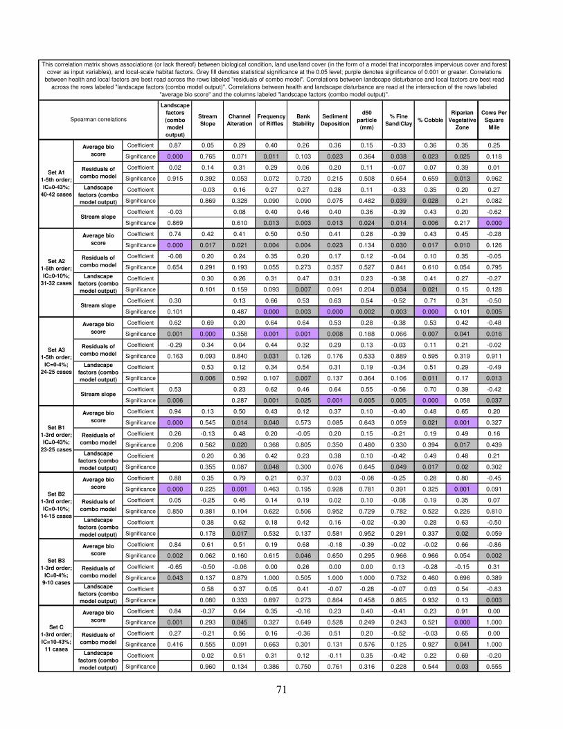
71

Landscape

factors

(combo

model

output)

Stream

Slope

Channel

Alteration

Frequency

of Riffles

Bank

Stability

Sediment

Deposition

d50

particle

(mm)

% Fine

Sand/Clay% Cobble

Riparian

Vegetative

Zone

Cows Per

Square

Mile

Coefficient 0.87 0.05 0.29 0.40 0.26 0.36 0.15 -0.33 0.36 0.35 0.25

Significance 0.000 0.765 0.071 0.011 0.103 0.023 0.364 0.038 0.023 0.025 0.118

Coefficient 0.02 0.14 0.31 0.29 0.06 0.20 0.11 -0.07 0.07 0.39 0.01

Significance 0.915 0.392 0.053 0.072 0.720 0.215 0.508 0.654 0.659 0.013 0.962

Coefficient -0.03 0.16 0.27 0.27 0.28 0.11 -0.33 0.35 0.20 0.27

Significance 0.869 0.328 0.090 0.090 0.075 0.482 0.039 0.028 0.21 0.082

Coefficient -0.03 0.08 0.40 0.46 0.40 0.36 -0.39 0.43 0.20 -0.62

Significance 0.869 0.610 0.013 0.003 0.013 0.024 0.014 0.006 0.217 0.000

Coefficient 0.74 0.42 0.41 0.50 0.50 0.41 0.28 -0.39 0.43 0.45 -0.28

Significance 0.000 0.017 0.021 0.004 0.004 0.023 0.134 0.030 0.017 0.010 0.126

Coefficient -0.08 0.20 0.24 0.35 0.20 0.17 0.12 -0.04 0.10 0.35 -0.05

Significance 0.654 0.291 0.193 0.055 0.273 0.357 0.527 0.841 0.610 0.054 0.795

Coefficient 0.30 0.26 0.31 0.47 0.31 0.23 -0.38 0.41 0.27 -0.27

Significance 0.101 0.159 0.093 0.007 0.091 0.204 0.034 0.021 0.15 0.128

Coefficient 0.30 0.13 0.66 0.53 0.63 0.54 -0.52 0.71 0.31 -0.50

Significance 0.101 0.487 0.000 0.003 0.000 0.002 0.003 0.000 0.101 0.005

Coefficient 0.62 0.69 0.20 0.64 0.64 0.53 0.28 -0.38 0.53 0.42 -0.48

Significance 0.001 0.000 0.358 0.001 0.001 0.008 0.188 0.066 0.007 0.041 0.016

Coefficient -0.29 0.34 0.04 0.44 0.32 0.29 0.13 -0.03 0.11 0.21 -0.02

Significance 0.163 0.093 0.840 0.031 0.126 0.176 0.533 0.889 0.595 0.319 0.911

Coefficient 0.53 0.12 0.34 0.54 0.31 0.19 -0.34 0.51 0.29 -0.49

Significance 0.006 0.592 0.107 0.007 0.137 0.364 0.106 0.011 0.17 0.013

Coefficient 0.53 0.23 0.62 0.46 0.64 0.55 -0.56 0.70 0.39 -0.42

Significance 0.006 0.287 0.001 0.025 0.001 0.005 0.005 0.000 0.058 0.037

Coefficient 0.94 0.13 0.50 0.43 0.12 0.37 0.10 -0.40 0.48 0.65 0.20

Significance 0.000 0.545 0.014 0.040 0.573 0.085 0.643 0.059 0.021 0.001 0.327

Coefficient 0.26 -0.13 0.48 0.20 -0.05 0.20 0.15 -0.21 0.19 0.49 0.16

Significance 0.206 0.562 0.020 0.368 0.805 0.350 0.480 0.330 0.394 0.017 0.439

Coefficient 0.20 0.36 0.42 0.23 0.38 0.10 -0.42 0.49 0.48 0.21

Significance 0.355 0.087 0.048 0.300 0.076 0.645 0.049 0.017 0.02 0.302

Coefficient 0.88 0.35 0.79 0.21 0.37 0.03 -0.08 -0.25 0.28 0.80 -0.45

Significance 0.000 0.225 0.001 0.463 0.195 0.928 0.781 0.391 0.325 0.001 0.091

Coefficient 0.05 -0.25 0.45 0.14 0.19 0.02 0.10 -0.08 0.19 0.35 0.07

Significance 0.850 0.381 0.104 0.622 0.506 0.952 0.729 0.782 0.522 0.226 0.810

Coefficient 0.38 0.62 0.18 0.42 0.16 -0.02 -0.30 0.28 0.63 -0.50

Significance 0.178 0.017 0.532 0.137 0.581 0.952 0.291 0.337 0.02 0.059

Coefficient 0.84 0.61 0.51 0.19 0.68 -0.18 -0.39 -0.02 -0.02 0.66 -0.86

Significance 0.002 0.062 0.160 0.615 0.046 0.650 0.295 0.966 0.966 0.054 0.002

Coefficient -0.65 -0.50 -0.06 0.00 0.26 0.00 0.00 0.13 -0.28 -0.15 0.31

Significance 0.043 0.137 0.879 1.000 0.505 1.000 1.000 0.732 0.460 0.696 0.389

Coefficient 0.58 0.37 0.05 0.41 -0.07 -0.28 -0.07 0.03 0.54 -0.83

Significance 0.080 0.333 0.897 0.273 0.864 0.458 0.865 0.932 0.13 0.003

Coefficient 0.84 -0.37 0.64 0.35 -0.16 0.23 0.40 -0.41 0.23 0.91 0.00

Significance 0.001 0.293 0.045 0.327 0.649 0.528 0.249 0.243 0.521 0.000 1.000

Coefficient 0.27 -0.21 0.56 0.16 -0.36 0.51 0.20 -0.52 -0.03 0.65 0.00

Significance 0.416 0.555 0.091 0.663 0.301 0.131 0.576 0.125 0.927 0.041 1.000

Coefficient 0.02 0.51 0.31 0.12 -0.11 0.35 -0.42 0.22 0.69 -0.20

Significance 0.960 0.134 0.386 0.750 0.761 0.316 0.228 0.544 0.03 0.555

Average bio

score

This correlation matrix shows associations (or lack thereof) between biological condition, land use/land cover (in the form of a model that incorporates impervious cover and forest

cover as input variables), and local-scale habitat factors. Grey fill denotes statistical significance at the 0.05 level; purple denotes significance of 0.001 or greater. Correlations

between health and local factors are best read across the rows labeled "residuals of combo model". Correlations between landscape disturbance and local factors are best read

across the rows labeled "landscape factors (combo model output)". Correlations between health and landscape disturbance are read at the intersection of the rows labeled

"average bio score" and the columns labeled "landscape factors (combo model output)".

Set A2

1-5th order;

IC=0-10%;

31-32 cases

Set A3

1-5th order;

IC=0-4%;

24-25 cases

Residuals of

combo model

Set B1

1-3rd order;

IC=0-43%;

23-25 cases

Set B2

1-3rd order;

IC=0-10%;

14-15 cases

Stream slope

Stream slope

Average bio

score

Residuals of

combo model

Residuals of

combo model

Landscape

factors (combo

model output)

Average bio

score

Average bio

score

Residuals of

combo model

Landscape

factors (combo

model output)

Average bio

score

Residuals of

combo model

Landscape

factors (combo

model output)

Stream slope

Set C

1-3rd order;

IC=10-43%;

11 cases

Set B3

1-3rd order;

IC=0-4%;

9-10 cases

Average bio

score

Residuals of

combo model

Landscape

factors (combo

model output)

Landscape

factors (combo

model output)

Landscape

factors (combo

model output)

Average bio

score

Residuals of

combo model

Spearman correlations

Set A1

1-5th order;

IC=0-43%;

40-42 cases

Landscape

factors (combo

model output)

72

8) Appendix C - Overview of bedrock and soils in the Rivanna River drainage

Contributed by Aaron Cross, Geologist, Division of Geology and Mineral Resources,

Virginia Department of Mines, Minerals, and Energy

The major headwater tributaries of the Rivanna River drainage — Swift Run, Buck

Mountain Creek, Doyles River, Moormans River, and Stockton Creek — begin on the

Eastern flank of the Blue Ridge Mountains and drain generally eastward. The higher

slopes of the Blue Ridge are underlain by the late-Proterozoic/Cambrian-age metabasalt of

the Catoctin Formation, while the lower slopes are underlain by the Proterozoic Swift Run

Formation, a heterogeneous assemblage of phyllite and metasandstone with lesser

metaconglomerate, schist, quartzite, and slate. These rocks produce the Myersville-

Catoctin-Lew assemblage of stony, well-drained soils. Surface runoff is rapid and the

hazard of erosion is severe. Most of this land is in forest.

At the foothills of the Blue Ridge Mountains, the Rivanna drainage begins to cross

rocks of the Blue Ridge Basement Complex, which underlies the core of the Blue Ridge

Anticlinorium, a major structural fold. The western upland portion of the Basement

Complex is a disorganized assemblage of Middle Proterozoic pyroxene granulite gneisses

and biotite granulite gneisses that have been intruded by plutons of Grenville age,

particularly charnockite, a pyroxene-bearing granite/granodiorite containing blue quartz, as

well as the Crozet Granite, a leucocratic, coarse-grained, porphyritic alkali feldspar granite.

In the past, these units were grouped under the term Pedlar Formation. These granitic

rocks in the western upland areas of the Basement Complex produce the Parkers-Chester-

Porters assemblage of deep, stony, excessively drained soils, now mostly in second-growth

forest. Surface runoff is rapid and the hazard of erosion is severe.

The western portion of the Basement Complex is separated from the eastern portion

by a bifurcated belt of mylonite and cataclastic rocks. This belt represents a fault zone

with multiple movement history — late pre-Cambrian extension, Paleozoic contraction,

and reactivation during Mesozoic extension. Lithology is highly variable depending on the

parent rock. In the central part of the Basement Complex, Braddock-Thurmont-Unison

soils are formed on colluvial material washed from the Blue Ridge. These soils are deep

and well drained, with loamy subsoil. Many of the soils within the Basement Complex are

agriculturally important; unfortunately, they are subject to considerable sheet erosion when

cultivated and in many places the red clay subsoil has been exposed.

The eastern portion of the Basement Complex is dominated by Proterozoic

porphyroblastic biotite-plagioclase augen gneiss, sometimes referred to as the Lovingston

Gneiss. Infolded into this augen gneiss is a long, thin graben containing the Mechums

River Formation, a metagraywacke and meta-argillite with quartzose schist and

conglomerate. Locally, the Lovingston Gneiss is intruded with a two-mica, two-feldspar

granite, or with the alkali feldspar granite of the Proterozoic Robertson River Igneous

Suite. Granitic rocks in the eastern part of the Basement Complex produce the Hayesville-

Ashe-Chester assemblage of deep, well-drained soils. This soil is locally run down owing

to poor farming methods.

Downstream from the Rivanna River Reservoir, the drainage passes through a

succession of metasedimentary rocks of the Lynchburg Group, including the Lynchburg

Fanglomerate, a matrix-supported, pebbly to cobbly lithic conglomerate; the Lynchburg

Metagraywacke, containing beds of conglomerate, graphitic phyllite, metasiltstone, slate,

and quartzite; and the Charlottesville Formation, a coarse-grained, pebbly metasandstone

73

and quartzite interbedded with micaceous siltstone, graphitic phyllite, and slate.

Amphibolite dikes cut the Lynchburg Group and occur as sills in the Charlottesville

Formation; they are probably part of the Catoctin basalt feeder system. This collection of

metasedimentary bedrock produces the Elioak-Hazel-Glenelg soil assemblage.

The Rivanna River exits the Blue Ridge Anticlinorium through a gap between

Southwest Mountain and Carters Mountain, both of which are formed from Catoctin

metabasalt and together represent the eastern limb of the Anticlinorium. The base of these

slopes host Davidson soil, which is particularly well suited for cultivated crops.

To the east of the line of Southwest and Carters mountains is a broad belt of the

Cambrian-age Candler Formation, composed of schistose and phyllitic metasiltstone,

ferruginous metatuff, dolomitic marble, and phyllite. Adjacent to the Candler Formation is

a belt of the Proterozoic- to Ordovician-age Mine Run Complex, composed of

metagraywacke, quartzose schist, and mélange. Together, these metasedimentary rocks

produce Nason-Tatum soils that are strongly acidic. Most of this area is in woodland, as

these soils have low fertility and are not well suited for sustained agriculture.

Where the Rivanna drainage narrows toward its point of entry into the James River,

it passes quickly through the Cambrian-age Chopawamsic Formation of interlayered felsic

and mafic metavolcanics and the infolded Arvonia Formation of slate and porphyroblastic

schist. These rocks produce shallow, poorly drained Manteo-Wehadkee soils. Near the

point of entry, the Rivanna cuts into the Carysbrook Pluton of Proterozoic granite and the

Columbia Pluton of Ordovician granite. These rocks produce Louisburg soils that are

shallow, on slopes, and mostly in woodland.

For soil conservation purposes, soil management practices are far more important

than natural factors such as soil type and slope. Regardless of setting or soil type, land

disturbance practices such as forest clearance and construction, even when well managed,

can increase the potential for erosion by factors many times greater than risks associated

with natural circumstances (Pitt 2007).

References:

Virginia State Geological Map, 1993: Virginia Department of Mineral Resources

Soil Survey of Albemarle County, 1940: U.S. Department of Agriculture

Soil Survey of Albemarle County, Virginia, 1981: U.S. Department of Agriculture

Soil Survey of Fluvanna County, 1958: U.S. Department of Agriculture

9) Appendix D - References

Beckley, J. 2006. Coliscan Easygel: How Volunteer Monitoring Can Help the TMDL

Process. PowerPoint presentation. http://www.deq.virginia.gov/tmdl/pdf/coliscan.pdf

Allan, JD, Erickson, DL and Fay, J. 1997. The Influence of Catchment Land Use on

Stream Integrity across Multiple Spatial Scales. Freshwater Biology 37: 149–161.

Barbour, MT, Gerritsen J, Snyder, BD, Stribling JB. 1999. Rapid Bioassessment

Protocols for Use in Streams and Wadeable Rivers: Periphyton, Benthic

Macroinvertebrates and Fish, Second Edition. EPA 841-B-99-002. U.S. Environmental

Protection Agency; Office of Water. Washington D.C.

74

Barnard, K, and McBain, S. 1994. Standpipe to determine permeability, dissolved oxygen,

and vertical particle size distribution in salmonid spawning gravels. USDA Forest Service,

Fish Habitat Relationships Technical Bulletin 15.

Burton, J, Gerritsen, J. TetraTech. 2003. A Stream Condition Index for Virginia Non-

Coastal Streams. http://www.deq.virginia.gov/watermonitoring/pdf/vastrmcon.pdf

Coles, JG, Cuffney, TF, McMahon, G, Beaulieu, K. 2004. The effects of urbanization on

the biological, physical, and chemical characteristics of coastal New England streams: U.S.

Geological Survey Professional Paper 1695, 47 p.

Cover, M, May, CL, Dietrich, WE, and Resh, VH. 2008. Quantitative linkages among

sediment supply, streambed fine sediment, and benthic macroinvertebrates in northern

California streams. The North American Benthological Society 27: 135-149.

Karr, JR, Chu, EW. 1999. Restoring Life in Running Waters – Better Biological

Monitoring. Island Press. Washington, D.C.

King, RS, Baker, ME. 2010. Considerations for analyzing ecological community

thresholds in response to anthropogenic environmental gradients. Journal of the North

American Benthological Society. 29(3):998–1008

Morse, CC, Huryn, AD, Cronan, CS. 2003. Impervious surface area as a predictor of the

effects of urbanization on stream insect communities in Maine, USA. Environmental

Monitoring and Assessment 89: 95-127.

McHugh, MH. 2009. Using gravel permeability to evaluate restoration efforts in Smith

Creek, Virginia. Master’s thesis, James Madison University. 50 p.

Murphy, JA. 2008. Biological Conditions at Thirty-Three Rivanna Basin Long-term

Monitoring Sites. StreamWatch, Charlottesville VA. www.streamwatch.org/reports

Murphy, JA. 2006. Living in Our Watershed – Correlates of Biological Condition in

Streams and Rivers of the Rivanna Basin. StreamWatch, Charlottesville VA.

www.streamwatch.org/reports

Ourso, RT and Frenzel, SA. 2003. Identification of linear and threshold responses in

streams along a gradient of urbanization in Anchorage, Alaska. Hydrobiologia. 501: 117-

131.

Pitt, R, Clark, S, Lake, D. 2007. Construction site erosion and sediment controls. DEStech

Publications, Inc. Lancaster, Pennsylvania.

Rosgen, DL. 1996. Applied River Morphology. Wildland Hydrology, Pagosa Springs, CO.

Schueler, TR, Fraley-McNeal, L, Cappiella, K. 2009. Is Impervious Cover Still Important?

Review of Recent Research. Journal of Hydrologic Engineering. 14:4: 309-315, 7 p.

75

State Water Control Board. 2006. 9 VAC 25-260. Virginia Water Quality Standards.

Statutory Authority: § 62.1-44.15 3a of the Code of Virginia, with amendments effective

January 6, 2011.

Terhune, LDB. 1958. The Mark VI groundwater standpipe for measuring seepage through

salmon spawning gravel. Canada Fisheries Research Board Journal 15: 1027-1063.

Theobald, DM. 2004. Placing Exurban Land-use Change in a Human Modification

Framework. Frontiers in Ecology and the Environment. 2(3): 139–144

United States Environmental Protection Agency, Office of Water. 2002. Biological

Assessments and Criteria: Crucial Components of Water Quality Programs. Document

reference: EPA 822-F-02-006.

http://www.epa.gov/waterscience/biocriteria/technical/brochure.pdf

Virginia Department of Environmental Quality. 2007. Virginia Citizen Water Quality

Monitoring Program Methods Manual.

http://www.deq.virginia.gov/cmonitor/guidance.html