WOODS HOLE LABORATORY REFERENCE DOCUMENT NO. 84-18 Programs for Fish Stock Assessment Znd edition prepared by Resource Assessment Division Analytical Programs Working Group edited by F.P. Almeida (B'1PPROVED FOR y.. (APPROVING OfFICIAL) (DATE) 17 &; J9!'1 National Marine Fisheries Service Northeast Fisheries Center Woods Hole Laboratory Woods Massachusetts 02543

Welcome message from author
This document is posted to help you gain knowledge. Please leave a comment to let me know what you think about it! Share it to your friends and learn new things together.
Transcript
WOODS HOLE LABORATORY REFERENCE DOCUMENT NO. 84-18
Comp~ter Programs for Fish Stock Assessment Znd edition
prepared by Resource Assessment Division
Analytical Programs Working Group
edited by F.P. Almeida
(B'1PPROVED FOR DISTaIBUTIO~ y..
(APPROVING OfFICIAL)
(DATE) 17 &; J9!'1
National Marine Fisheries Service Northeast Fisheries Center
Woods Hole Laboratory Woods Hole~ Massachusetts 02543

INTRODUCTION
The following manual is an updated edition of the
Computer Programs for Fish Stock Assessment manual prepared
by the Resource Assessment Division ADP Needs Committee in
January 1976. The programs in this manual have been written
by Northeast Fisheries Center (NEFC) personnel utilizing
FORTRAN77 to run on the NEFC/WHOI VAX 11/785 computer, or by
programmers in other institutions and converted, as
necessary, to run on the VAX system. Each of the programs
has been tested and is assumed to be error free, however,
any problems encountered while using the programs should be
reported to the Analytical Programs Working Group. No
responsibility can be accepted for problems or consequences
resulting from the use of these programs. The Manual is not
intended to represent a completed software library;
suggestions for additional analytical programs are welcome.
The. programs in this library are arranged into six
sections based upon the type of analysis performed.
Documentation includes a description, instructions for
running, any specific restrictions~ references, and an
example run of each program. Any program may be run
interactively, although runs u.tilizing the larger programs
should be submitted to run in batch mode. Recommended
methods for running are discussed in each program's
documentation
i
All of' the programs reside in a ·master subdirectory of
Account 712. Subdirectortes containing sample data files
and command files (where applicable) are also available.
The directory arrangement is as follows:
Executable files Source code listings Sample data files Command files
FSHA:[712.MASTER.XEQ] FSHA:[712.~ASTER.SOURCE] FSHA:[7i2.MASTER.DATA] FSHA' [712.MASTER.COM]
The following persons, listed alphabetically, wrote, converted and/or documented the programs in this manual: Frank Almeida, Stephen Clark, Michael Fogarty, Karen Foster, Wendy Gabriel, Anne Lange, Ralph Mayo, Steven Murawski, Gordon Waring, NEFC, Resource Assessment Division; Jeremy Collie, WHO!; and Brian O'Gorman, Massachusetts Division of Marine Fisheries.
ii
Accessing the NEFC/WHOI VAX 11/785 Computer
To access the VAX computer system, the following instructions must be used.
MODEM communication
1) Dial the telephone number for the system:
Baud Rate
300 (AJ & TI only) or 1200
NEFC Data phone
540-6000
iii
2) When the high-pitched tone is heard, either place the handset in the acoustic coupler (AJ or TI terminals) or flip the CONNECT switch on the high speed modems, and press the RETURN key twice on the terminal keyboard.
3) After the computer responds with:
enter class
type GRAY and you will then be prompted for your Username and Password.
4) Once you have gained access to the system, follow the INSTRUCTIONS FOR RUNNING section in the program you intend to run.
COAXIAL CABLE communication
If the terminal you are using communicates with the VAX via the coaxial cable network, to access the system simply turn the terminal on and press the RETURN key twice on the keyboard and proceed from step 4 above.
CONTENTS
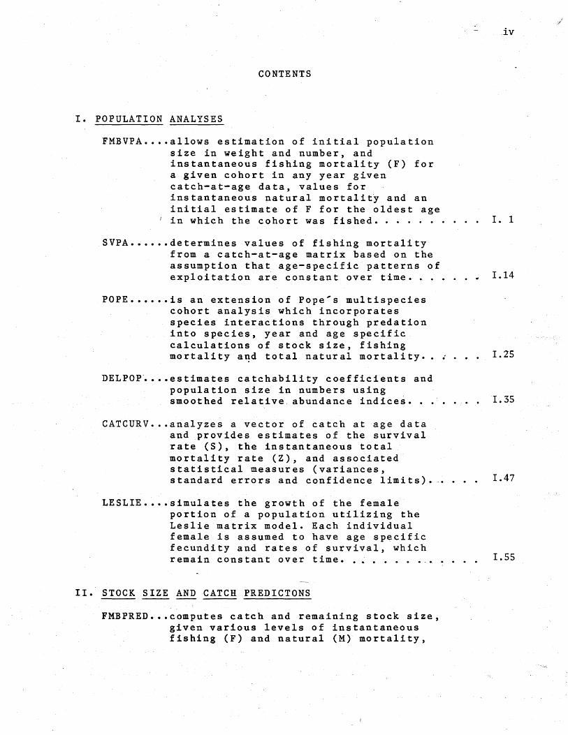
I. POPULATION ANALYSES
FMBVPA •••• allows estimation of initial population size in weight and number, and instantaneous fishing mortality (F) for a given cohort in any year given catch-at-age data, values for instantaneous natural mortalitj and an initial estimate of F for the oldest age
I in which the cohort was fished •.....
SVPA •••••• determines values of fishing mortality from a catch-at-age matrix based on the assumption that age-specific patterns of exploitation are constant over time •..
POPE •••••• is an extension of Pope's multispecies cohort analysis which incorporates species interactions through predation into species, year and age specific calculations of stock size, fishing mortality a~d total natural mortality.
DELPOp· •••• estimates catchability coefficients and population size in numbers using smoothed relative. abundance indices •..
CATCURV ••• analyzes a vector of catch at age data and provides estimates of the survival rate (S), the instantaneous total mortality rate (Z), and associated statistical measures (variances, standard errors and confidence limits).
LESLIE •••• simulates the growth of the femaleportion of a population utilizing the Leslie matrix model. Each individual female is assumed to have age specific fecundity and rates of survival, which remain constant over time •• ~ ..... .
II. STOCK SIZE AND CATCH PREDICTONS
FMBPRED ••• computes catch and remaining stock size, given various levels of instantaneous fishing (F) and natural (M) mortality,
iv
I. 1
. . . - 1.14
1.25
1.35
1.47
1.55
initial stock size, and recruitment, according to the Murphy catch equation.
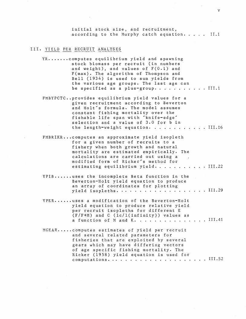
III. YIELD PER RECRUIT ANALYSES
yR ..••... computes equilibrium yield and spawning stock biomass per recruit (in numbers and weight), and values of F(O.l) and F(max). The algorithm of Thompson and Bell (1934) is used to sum yields from the various age groups. The last age can
v
II.1
be specified as a plus-group. . . . .. . .. 111.1
FMBYPCTC .• provides equilibrium yield values for a given recruitment according to Beverton and Holt's formula. The model assumes constant fishing mortality over the fishable life span with 'knife-edge' selection and a value of 3.0 for b in the leng th-we igh t equa tion. . .......... 111.16
FMBRIKR .•• computes an approximate yield isopleth for a given number of recruits to a fishery when both growth and natural mortality are estimated empirically. The calculations are carried out using a modified form of Ricker's method for estimating equilibrium yield. . . . .. ..' III.22
yPIB •••••• uses the incomplete Beta function in the Beverton-Holt yield equation to produce an array of coordinates for plotting yield isopleths. . . . ............. 111.29
YPER .•.•.• uses a modification of the Beverton-Holt yield equation to produce relative yield per recruit isopleths for different E (F/F+M) and C (lc/l(infinity)) values as a function of M and K.
MGEAR .•..• computes estimates of yield per recruit and several related parameters for fisheries that are exploited by several gears which may have differing vectors of age specific fishing mortality. The Ricker (1958) yield equation is used for
... III.41
computations ...................... 111.52
IV. CATCH EFFORT ANALYSES
PCNT •••••• computes the percentage composition of a single species in the total commercial landings of a series of fishing trips on a trip by trip landed weight basis. Summary data are displayed arrayed in
vi
5 - per c en tin t e r val s by m 0 nth. . . • . • . • . IV. 1
FPOW •••••• estimates relative fishing power and relative population density utilizing analysis of va.riance. . • . . • . . . ...•. IV.6
ESP3 •••••• provides an estimation procedure for determining relative fishing power coefficients using a two-way classification model with no interaction. Fishing effort is adjusted to an arbitrarily selected standard ( e • g. g ear - ton nag e c las s c om bin a t ion) ,.. . . . . . IV. 15
V. SURPLUS PRODUCTION MODELS
GENPROD ••• fits the generalized stock production model to catch and effort data and estimates equilibrium yield as a fun c t ion 0 f e f for t .•....•.. .• . . . . 'V · 1
PRODFIT ••• fits the generalized stock production model to fishery catch and effort data by least squares using an equilibrium approxim'ation approach •....•.....•..•. V.11
VI. GROWTH ANALYSE~
BGCII ••••• fits the von Bertalanffy growth curve by least squares with weights proportional to sample size at each age group. A constant time interval between ages is required, but the number of lengths in the age groups may be unequal. . .... VI.l
BGCIII •••• fits the von Bertalanffy growth in length curve to unequally spaced age groups with unequal sample sizes for separate ages. · · · · • • · · · . • .
BGCIV ••••• fits the von Bertalanffy growth in length equation when lengths of an
VI.s
individual fish at points in time are known, but the absolute age of the fish may not. It lends itself well to fitting
vii
the equation to mark and recapture data ..... VI.lO
NORMSEP ... separates length frequency sampling distributions into component normal distributions. It is used to estimate relative abundance of age groups in length samples when age data are not available.. . . . . . . . . . . . .. . ...... VI.lS
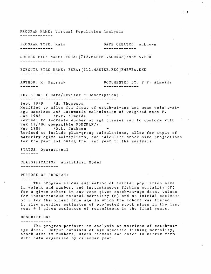
PROGRAM NAME: Virtual Population Analysis
PROGRAM TYPE: Main DATE CREATED: unknown
SOURCE FILE NAME: FSHA: [712.MASTER.SOURCE]FMBVPA.FOR
EXECUTE FILE NAME: FSHA: [712.MASTER.XEQ]FMBVPA.EXE
AUTHOR: M. Parrack DOCUMENTED BY: F.P. Almeida
REVISIONS ( Date/Reviser - Description)
Sept 1979 /M. Thompson Modified to allow for input of catch-at-age and mean weight-atage matrices and automatic calculation of weighted mean F. Jan 1982 /F.P. Almeida Revised to increase number of age classes and to conform with VAX 11/780 compatible FORTRAN77. Nov 1984 /O.L. Jackson Revised to include plus-group calculations, allow for input of maturity ogive multipliers, and calculate stock size projections for the year following the last year in the analysis.
STATUS: Operational
CLASSIFICATION: Analytical Model
PURPOSE OF PROGRAM:
The program allows estimation of initial population size in weight and number, and instantaneous fishing mortality (F) for a given cohort in any year given catch-at-age data, values for instantaneous natural mortality (M) and an initial estimate of F for the oldest true age in which the cohort was fished. It also provides estimates of projected stock sizes in the last year + 1 given estimates of recruitment in the final years.
DESCRIPTION:
The program performs an analysis on matrices of catch-atage data. Output consists of age specific fishing mortality, stock size in numbers, stock biomass and catch in matrix form with data organized by calendar year.
1.1
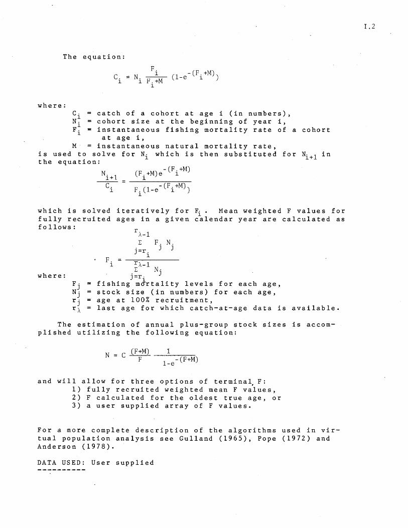
The equation:
where:
C. = N. F i ( 1-e - (F i +M) ) 1 1 F.+M
1
Ci = catch of a cohort at age i (in numbers), Ni = cohort size at the beginning of year i, F· = instantaneous fishing mortality rate of a cohort
1 at age i,
M' = instantaneous natural mortality rate, i sus edt 0 sol v e for N i w h i chi s the n sub s tit ute d for Ni + 1 i n the equation:
N. 1 1+
C. 1
(F.+M)e-(Fi+M) 1 = ---------~--~-
F. (1- e - (F i +M) ) 1
which is solved iteratively for ~. Mean weighted F values for fully recruited ages in a given calendar year are calculated as follows:
where:
F. 1
rA
_1
L: F. N. j =r. J J
1
r A-1 L: Nj , j=r.
= fishing mJrtality levels for each age, = stock size (in numbers) for each age,
age at 100% recruitment, last age for which catch-at-age data is available.
The estimation of annual plus-group stock sizes is accomplished utilizing the following equation:
N C (F+M) F
1 1_e-(F+M)
and will allow for three options of terminal F: 1) fully recruited weighted mean F values, 2) F calculated for the oldest true age, or 3) a user supplied array of F values.
For a more complete description of the algorithms used in virtual population analysis see Gulland (1965), Pope (1972) and Anderson (1978).
DATA USED: User supplied
1.2
1.3
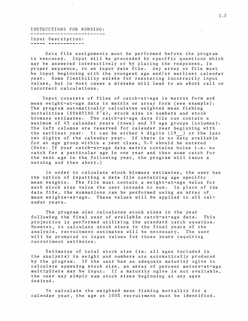
INSTRUCTIONS FOR RUNNING:
Input Description:
Data file assignments must be performed before the program is executed. Input will be preceeded by specific questions which may be answered interactively or by placing the responses, in proper sequence, in an input data file. Any array or file must be input beginning with the youngest age and/or earliest calendar year. Some flexibility exists for reentering incorrectly input values, but in most cases a mistake will lead to an abort call or incorrect calculations.
Input consists of files of catch-at-age in matrix form and mean weight-at-age data in matrix or array form (see example). The program automatically calculates weighted mean fishing mortalities (STARTING F's), stock size in numbers and stock biomass estimates. The catch-at-age data file can contain a maximum of 45 calendar years (rows) and 35 age groups (columns). The left columns are reserved for calendar year beginning with the earliest year. It can be either 4 digits (19 ) or the last two digits of the calendar year. If there is no data available for an age group within a year class, 0.0 should be entered (Note: If your catch-at-age data matrix contains holes i.e. no catch for a particular age in one year and then some catch for the next age in th~ following year, the program'will issue a warning and then abort.)
In order to calculate stock biomass estimates, the user has the option of inputting a data file containing age specific mean weights. The file must contain a weight-at-age value for each stock size value the user intends to sum. In place of the data file, the summations can be performed using an array of mean weights-at-age. These values will be applied to all calendar years.
The program also calculates stock sizes in the year following the final year of available catch-at-age data. This projection is performed utilizing the standard catch equation. However, to calculate stock sizes in the final years of the analysis, recruitment estimates will be necessary. The user will be prompted to input values for those years requiring recruitment estimates.
Estimates of total stock size (ie. all ages included in the analysis) in weight and numbers are automatically produced by the progr'am. If the user has an adequate maturity ogive to calculate spawning stock size, an array of percent mature-at-age multipliers may be input. If a maturity ogive is not available, the user may simply sum stock sizes beginning at any ages desired.
To calculate the weighted mean fishing mortality for a calendar year, the age at 100% recruitment must be identified.
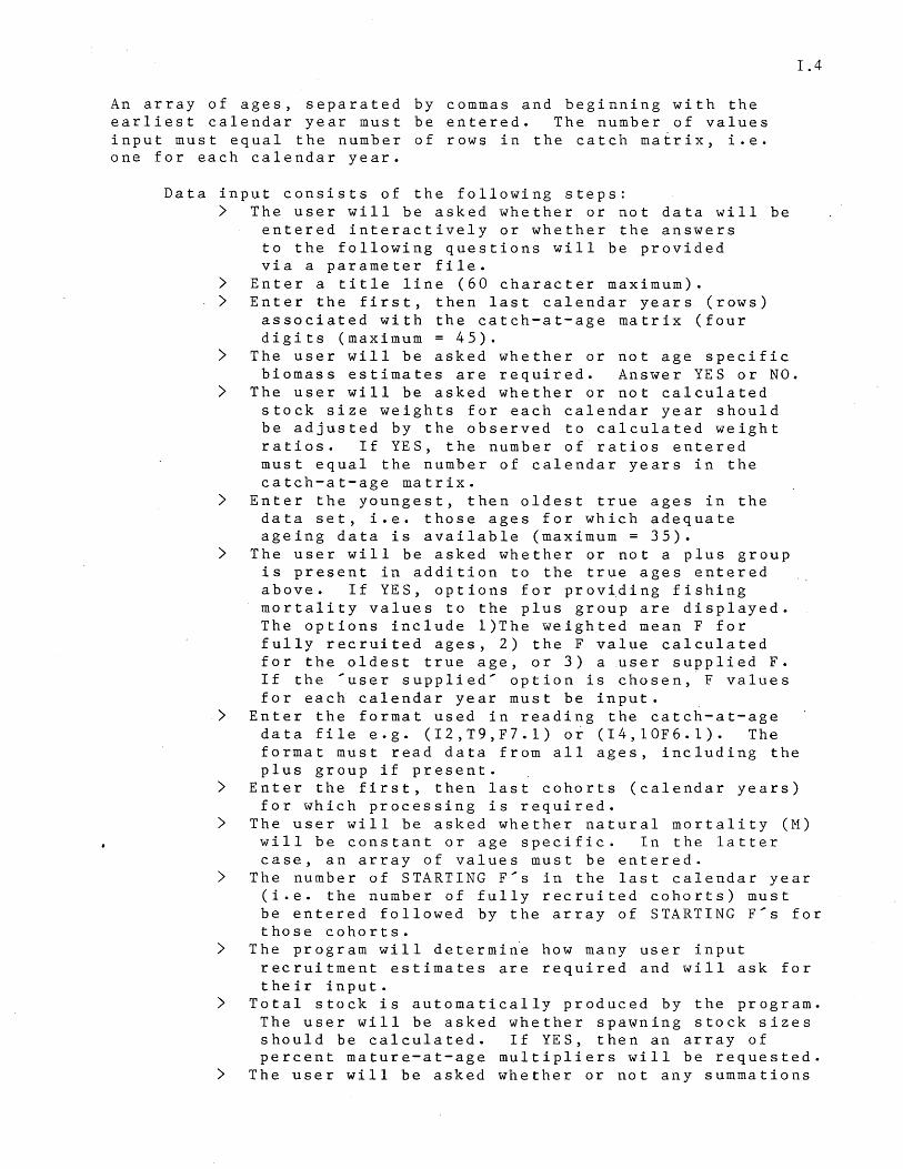
An array of ages, separated by commas and beginning with the earliest calendar year must be entered. The number of values input must equal the number of rows in the catch matrix, i.e. one for each calendar year.
Data input consists of the following steps: > The user will be asked whether or not data will be
entered interactively or whether the answers to the following questions will be provided via a parameter file.
> Enter a title line (60 character maximum). > Enter the first, then last calendar years (rows)
associated with the catch-at-age matrix (four digits (maximum = 45).
> The user will be asked whether or not age specific biomass estimates are required. Answer YES or NO.
> The user will be asked whether or not calculated stock size weights for each calendar year should be adjusted by the observed to calculated weight ratios. If YES, the number of ratios entered must equal the number of calendar years in the catch-at-age matrix.
> Enter the youngest, then oldest true ages in the data set, i.e. those ages for which adequate ageing data is available (maximum = 35).
> The user will be asked whether or not a plus group is present in addition to the true ages entered above. If YES, options for providing fishing mortality values to the plus group are displayed. The options include l)The weighted mean F for fully recruited ages, 2) the F value calculated for the oldest true age, or 3) a user supplied F. If the 'user supplied' option is chosen, F values for each calendar year must be input.
1.4
> Enter the format used in reading the catch-at-age data file e.g. (I2,T9,F7.1) or (I4,10F6.1). The format must read data from all ages, including the plus group if present.
> Enter the first, then last cohorts (calendar years) for which processing is required.
> The user will be asked whether natural mortality (M) will be constant or age specific. In the latter case, an array of values must be entered.
> The number of STARTING F's in the last calendar year (i.e. the number of fully recruited cohorts) must be entered followed by the array of STARTING F's for those cohorts.
> The program will determiie how many user input recruitment estimates are required and will ask for their input.
> Total stock is automatically produced by the program. The user will be asked whether spawning stock sizes should be calculated. If YES, then an array of percent mature-at-age multipliers will be requested.
> The user will be asked whether or not any summations
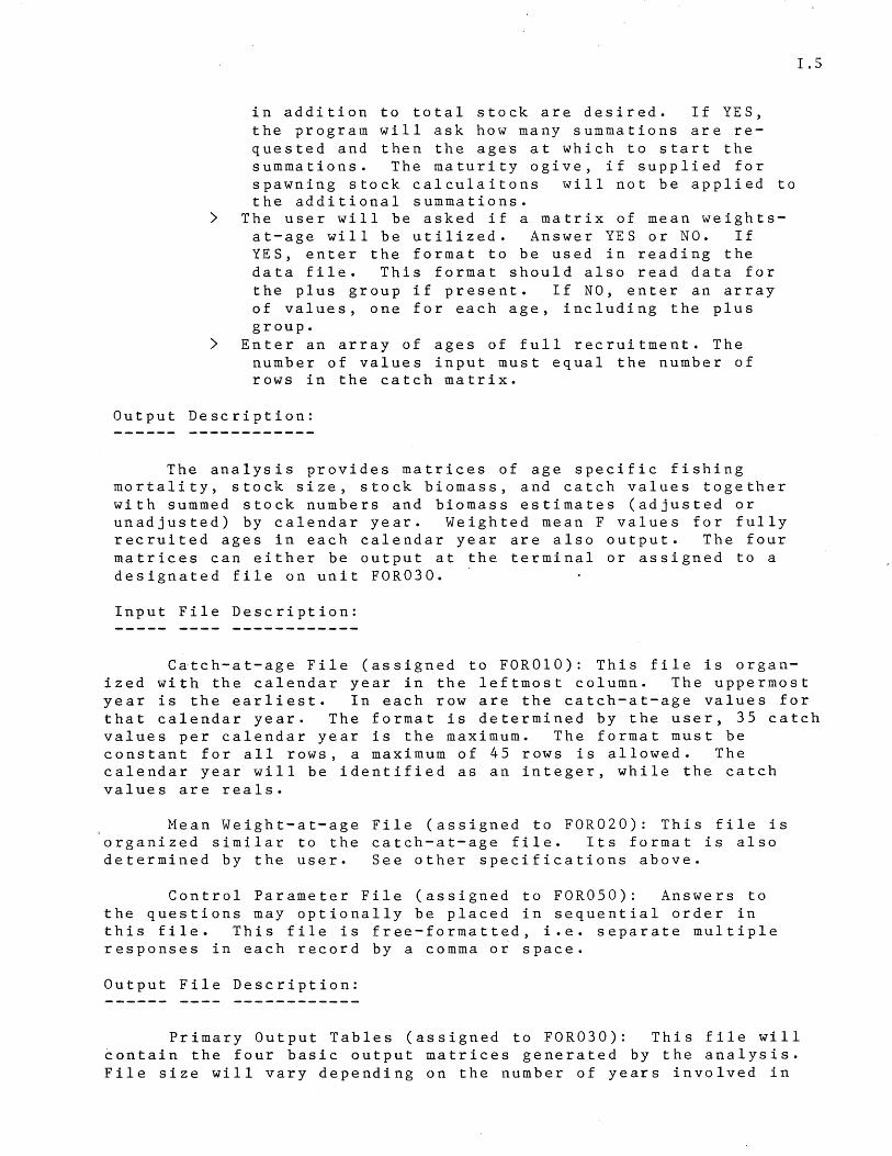
in addition to total stock are desired. If YES, the program will ask how many summations are requested and then the ages at which to start the summations. The maturity ogive, if supplied for spawning stock calculaitons will not be applied to the additional summations.
> The user will be asked if a matrix of mean weightsat-age will be utilized. Answer YES or NO. If YES, enter the format to be used in reading the data file. This format should also read data for the plus group if present. If NO, enter an array of values, one for each age, including the plus group.
> Enter an array of ages of full recruitment. The number of values input must equal the number of rows in the catch matrix.
Output Description:
The analysis provides matrices of age specific fishing mortality, stock size, stock biomass, and catch values together with summed stock numbers and biomass estimates (adjusted or unadjusted) by calendar year. Weighted mean F values for fully recruited ages in each calendar year are also output. The four matrices can either be output at the terminal or assigned to a designated file on unit FOR030.
Input File Description:
1.5
Catch-at-age File (assigned to FOROIO): This file is organized with the calendar year in the leftmost column. The uppermost year is the earliest. In each row are the catch-at-age values for that calendar year. The format is determined by the user, 35 catch values per calendar year is the maximum. The format must be constant for all rows, a maximum of 45 rows is allowed. The calendar year will be identified as an integer, while the catch values are reals.
Mean Weight-at-age File (assigned to FOR020): This file is organized similar to the catch-at-age file. Its format is also determined by the user. See other specifications above.
Control Parameter File (assigned to FOR050): Answers to the questions may optionally be placed in sequential order in this file. This file is free-formatted, i.e. separate multiple responses in each record by a comma or space.
Output File Description:
Primary Output Tables (assigned to FOR030): This file will contain the four basic output matrices generated by the analysis. File size will vary depending on the number of years involved in
1.6
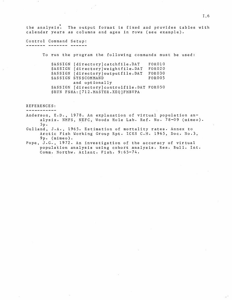
the analysis~ The output format is fixed and provides tables with calendar years as columns and ages in rows (see example).
Control Command Setup:
To run the program the following commands must be used:
$ASSIGN [directory]catchfile.DAT $ASSIGN [directory]weightfile.DAT $ASSIGN [directory]outputfile.DAT $ASSIGN SYS$COMMAND
and optionally $ASSIGN [directory]controlfile.DAT $RUN FSHA: [712.MASTER.XEQ]FMBVPA
REFERENCES:
FOR010 FOR020 FOR030 FOR005
FOR050
Anderson, E.D., 1978. An explanation of virtual population analysis. NMFS, NEFC, Woods Hole Lab. Ref. No. 78-09 (mimeo). 5p. .
Gulland, J.A., 1965. Estimation of mortality rates. Annex to Arctic Fish Working Group Rpt. ICES C.M. 1965, Doc. No.3, 9p. (mimeo).
Pope, J.G., 1972. An investigation of the accuracy of virtual popula~ion analysis using cohort analysis. Res. Bull. Int. Comm. Northw. Atlant. Fish. 9:65-74.
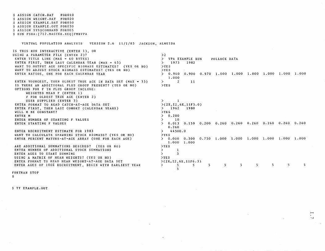
$ ASSIGN .CATCH.DAT FOR010 $ ASSIGN WEIGHT.DAT FOR020 $ ASSIGN EXAMPLE.DAT FORO SO $ ASSIGN EXAMPLE.OUT FOR030 $ ASSIGN SYS$COMMAND FOROOS $ RUN FSHA:[712.MASTER.XEQ]FMBVPA
VIRTUAL POPULATION ANALYSIS VERSION 2.6 11/I/8S JACKSON, ALMEIDA
IS THIS RUN INTERACTIVE (ENTER 1), OR USING A PARAMETER FILE (ENTER 2)?
ENTER TITLE LINE (MAX = 60 BYTES) ENTER FIRST, THEN LAST CALENDAR YEAR (MAX = 4S) WANT TO OUTPUT AGE SPECIFIC BIOMASS ESTIMATES? (YES OR NO) WANT TO ADJUST STOCK BIOMASS ESTIMATES? (YES OR NO) ENTER RATIOS, ONE FOR EACH CALENDAR YEAR
ENTER YOUNGEST, THEN OLDEST TRUE AGE IN DATA SET (MAX = 3S) IS THERE AN ADDITIONAL PLUS GROUP PRESENT? (YES OR NO) OPTIONS FOR F IN PLUS GROUP INCLUDE:
WEIGHTED MEAN F (ENTER 1) F FOR OLDEST TRUE AGE (ENTER 2) USER SUPPLIED (ENTER 3)
ENTER FORMAT TO READ CATCH-AT-AGE DATA SET ENTER FIRST, THEN LAST COHORT (CALENDAR YEARS) WILL M BE CONSTANT? ENTER M ENTER NUMBER OF STARTING F VALUES ENTER STARTING F VALUES
ENTER RECRUITMENT ESTIMATE FOR 1983 WANT TO CALCULATE SPAWNING STOCK BIOMASS? (YES OR NO) ENTER PERCENT MATURE-AT-AGE ARRAY (ONE FOR EACH AGE)
ARE ADDITIONAL SUMMATIONS DESIRED? (YES OR NO) ENTER NUMBER OF ADDITIONAL STOCK SUMMATIONS ENTER AGES TO START SUMMING USING A MATRIX OF MEAN WEIGHTS? (YES OR NO) ENTER FORMAT TO READ MEAN WEIGHT-AT-AGE DATA SET ENTER AGES OF 100% RECRUITMENT, BEGIN WITH EARLIEST YEAR
FORTRAN STOP $
$ TY EXAMPLE.OUT
)2 ) VPA EXAMPLE RUN POLLOCK DATA ) 1973 1982 )YE S )YES ) 0.940 0.900 0.970 1.000 1.000 1.000 1.000 1.000 1.000
1.000 ) 2 11 )YES
) 1 )(2X,I2.6X,11FS.0) ) 1962 1980 )YES ) 0.200 ) 10 ) 0.013 0.lS9 0.200 0.260 0.260 0.260 0.260 0.260 0.260
0.260 ) 44500.0 )YES ) 0.000 0.300 0.7S0 1.000 1.000 1.000 1.000 1.000 1.000
1. 000 1. 000 )YES ) 1 ) 3 )YES )(2X~I2,6X,11F6.3)
) S S 5
S S 5 5 5 5 5
H
'-J
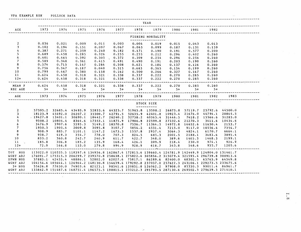
VPA EXAMPLE RUN POLLOCK DATA
YEAR ----------------------------------------------------------------------------------------------------------
AGE 1973 1974 1975 1976 1977 1978 1979 1980 1981 1982 -------------------------------------------------------------------------------------~----------------------------------
FISHING MORTALITY -----------------
2 0.036 0.021 0.009 0.011 0.003 0.004 0.019 0.015 0.043 0.013 3 0.102 0.194 O. 151 0.097 0.067 0.065 0.099 0.187 0.131 0.159 4 0.387 0.271 0.359 0.240 0.182 0.171 0.190 0.191 0.577 0.200 5 0.689 0.458 0.285 0.326 0.255 0.255 0.212 0.296 0.402 0.260 6 0.401 0.465 0.392 0.305 0.372 0.309 0.254 0.296 0.256 0.260 7 0.589 0.348 0.361 0.415 0.491 0.490 O. 191 0.203 0.190 0.260 8 0.574 0.715 0.147 0.284 0.508 0.621 0.184 0.137 0.126 0.260 9 0.756 0.347 0.187 0.040 0.315 0.663 0.365 0.154 0.199 0.260
10 0.799 0.467 0.380 0.158 0.162 0.500 0.266 0.327 0.167 0.260 11 0.624 0.458 0.318 0.321 0.338 0.337 0.222 0.270 0.285 0.260 12+ 0.624 0.458 0.318 0.321 0.338 0.337 0.222 0.270 0.285 0.260
------------------------------------------------------------------------------------------------------------------------MEAN F 0.624 0.458 0.318 0.321 0.338- 0.337 0.222 0.270 0.285 0.260
REC AGE 5+ 5+ 5+ 5+ 5+ 5+ 5+ 5+ 5+ 5+ ------------------------------------------------------------------------------------------------------------------------
AGE 1973 1974 1975 1976 1977 1978 1979 1980 1981 1982 1983 ------------------------------------------------------------------------------------------------------------------------
STOCK SIZE ----------
2 57595.2 32685.4 43493.9 52833.6 64325.7 51963.8 13598.2 26873.8 57119.7 25792.6 44500.0 3 18123.9 45492.0 26207.2 35300.7 42791.5 52635.9 42401.8 10923.4 21676.0 44794.1 20844.5 4 19427.8 13401.1 30690.1 18442.7 26240.2 32758.2 40365.4 31446.5 7418.2 15566.6 31283.0 5 9508.2 10804.4 8364.6 17553.1 11875.9 17906.8 22599.8 27332.6 21270.3 3411. 6 10434.6 6 3476.9 3907.6 5595.3 5149.2 10370.8 7536.7 11364.5 14972.8 16652.6 11650.4 2153.7 7 1950.5 1905.4 2009.8 3095.8 3107.7 5854.2 4531.4 7215.0 9117.0 10556.4 7354.7 8 908.9 885.7 1101.1 1147.2 1673.3 1557.8 2937.4 3064.3 4824.1 6170.7 6664.1 9 938.7 419.3 354.7 778.0 707.3 824.5 685.3 2001.5 2188.1 3483.6 3895.4
10 833.2 360.8 242.7 240.9 611.7 422.7 348.0 389.6 1405.3 1468.3 2199.1 11 185.8 306.8 185.2 135.9 168.4 426.1 2'()9.9 218.4 230.0 974.1 926.9 12+ 72.9 166.8 153.0 279.8 994.9 928.9 618.7 343.8 548.6 935.7 1205.6
----------------------------------------------------------------------~~------------------------------------------------TOT NOS 113022.0 110335 .. 5 118397.6 134956.8 162867.4 172815.6 139660.4 124781.9 142449.9 124804.0 131461.7 WGHT ADJ 176091.7 175315.3 206299.7 239370.8 258638.1 275822.6 305856.2 315079.4 321595.4 296739.8 300913.6 SPWN NOS 37883.1 42455.4 48886.1 52802.0 62027.6 75817.1 86289.6 82400.0 68302.5 63763.9 64549.8 WGHT ADJ 104154.6 103644.1 126964.2 148130.8 154639.4 179292.8 237037.0 257622.3 243106.1 229273.5 233675.6
3+ NOS 55426.8 77650.0 74903.6 82123.1 98541.6 120851.8 126062.2 97908.0 85330.3 99011.4 86961.7 WGHT ADJ 133862.9 151487.6 168751.4 196575.5 198815.1 233212.3 295793.5 287130.6 269502.3 279639.3 271410.1 ------------------------------------------------------------------------------------------------------------------------
H
00
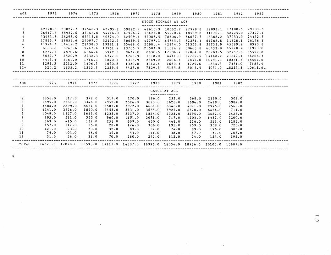
------------------------------------------------------------------------------------------------------------------------AGE 1973 1974 1975 1976 1977 1978 1979 1980 1981 1982 1983
------------------------------------------------------------------------------------------------------------------------STOCK BIOMASS AT AGE --------------------
2 42228.8 23827.7 37548.3 42795.2 59822.9 42610.3 10062.7 27948.8 52093.1 17100.5 29503.5 3 26917.6 58957.6 37368.8 54716.0 47926.4 58425.8 55970.4 18569.8 31170.1 58725.0 27327.1 4 43463.8 26293.0 62515.8 40574.0 42509.1 52085.5 78308.9 66037.7 18308.2 37033.0 74422.3 5 27885.7 29852.6 24097.7 52132.7 30639.9 42797.1 65765.5 82271.1 61768.8 11828.1 36176.8 6 11994.7 14419.2 21438.3 19361.1 35468.0 26981.4 42844.0 51356.8 59732.9 45389.9 8390.8 7 8103.8 8745.6 9747.6 13961.9 13766.9 25583.0 21524.2 30663.8 40433.8 45920.2 31993;0 8 4237.5 4870.6 6664.4 5942.3 9672.0 8630.5 17506.7 17864.8 26783.5 32957.6 35592.8 9 5029.7 2520.9 2432.3 4777.0 4766.9 5318.0 4441.0 12769.5 14148.2 21647.1 24206.3
10 4417.4 2361.0 1716.3 1840.2 4318.9 2849.0 2606.7 2852.0 10291.3 10351.5 15504.0 11 1292.5 2212.0 1406.5 1040.8 1320.0 3212.6 1660.3 1729.6 1834.4 7551.0 7185.4 12+ 520.2 1255.2 1363.7 2229.6 8427.0 7329.3 5165.8 3015.5 5031.0 -82 J 5 Ai--- 1 0 6 1 1 . 6 .-
AGE 1973 1974 1975 1976 1977 1918 1979 1980 1981 1982
CATCH AT AGE ------------
2 1856.0 617.0 372.0 514.0 170.0 196.0 233.0 368.0 2180.0 302.0 3 1595.0 7281.0 3346.0 2952.0 2526.0 3023.0 3628.0 1694.0 2419.0 5984.0 4 5684.0 2899.0 8434.0 3583.0 3972.0 4686.0 6348.0 4971.0 2975.0 2566.0 5 4341.0 3626.0 1890.0 4453.0 2431.0 3665.0 3922.0 6370.0 6424.0 711. 0 6 1049.0 1327.0 1655.0 1233.0 2937.0 1824.0 2323.0 3495.0 3422.0 2428.0 7 795.0 511. 0 555.0 960.0 1101.0 2071.0 717.0 1203.0 ,1437.0 2200.0 8 363.0 415.0 137.0 258.0 609.0 660.0 448.0 356.0 517.0 1286.0 9 457.0 112.0 55.0 28.0 174.0 366.0 191. 0 259.0 359.0 726.0
10 421. 0 123.0 70.0 32.0 83.0 152.0 74.0 99.0 196.0 306.0 11 79.0 103.0 46.0 34.0 44.0 111. 0 38.0 47.0 52.0 203.0 12 31.0 56.0 38.0 70.0 260.0 242.0 112.0 74.0 124.0 195.0
------------------------------------------------------------------------------------------------------------------------TOTAL 16671.0 17070.0 16598.0 14117.0 14307.0 16996.0 18034.0 18936.0 20105.0 16907.0
$
H
CD
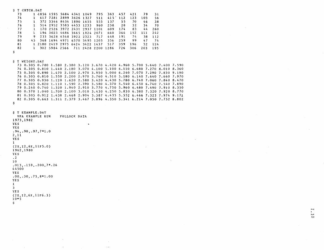
$ T CA:TCH.DAT 73 1 ~856 1595 5684 4341 1049 795 363 457 421 79 31 74 1 617 7281 2899 3626 1327 511 415 - 112 123 103 56 75 1 372 3346 8434 1890 1655 555 137 55 70 46 38 76 1 514 2952 3583 4453 1233 960 258 28 32 34 70 77 1 170 2526 3972 2431 2937 1101 609 174 83 44 260 78 1 196 3023 4686 3665 1824 2071 660 366 152 111 242 79 9 233 3628 6348 3922 2323 717 448 191 74 38 112 80 45 368 1694 4971 6370 3495 1203 356 259 99 47 74 81 1 2180 2419 2975 6424 3422 1437 517 359 196 52 124 82 1 302 5984 2566 711 2428 2200 1286 726 306 203 195
$
$ T WEIGHT.DAT 73 0.305 0.780 1.580 2.380 3.120 3.670 4.420 4.960 5.700 5.640 7.400 7.590 74 0.305 0.810 1.440 2.180 3.070 4.100 5.100 6.110 6.680 7.270 8.010 8.360 75 0.305 0.890 1.470 2.100 2.970 3.950 5.000 6.240 7.070 7.290 7.830 9.190 76 0.305 0.810 1.550 2.200 2.970 3.760 4.510 5.180 6.140 7.640 7.660 7.970 77 0.305 0.930 1.120 1.620 2.580 3.420 4.430 5.780 6.740 7.060 7.840 8.470 78 0.305 0.820 1.110 1.590 2.390 3.580 4.370 5.540 6.450 6.740 7.540 7.890 79 0.240 0.740 1.320 1.940 2.910 3.770 4.750 5.960 6.480 7.490 7.910 8.350 80 0.370 1.040 1.700 2.100 3.010 3.430 4.250 5.830 6.380 7.320 7.920 8.770 81 0.305 0.912 1.438 2.468 2.904 3.587 4.435 5.552 6.466 7.323 7.974 9.171 82 0.305 0.663 1.311 2.379 3.467 3.896 4.350 5.341 6.214 7.050 7.752 8.802
$
$ T EXAMPLE.DAT VPA EXAMPLE RUN
1973,1982 YES YES .94, .90, .97,7*1.0 2,11 YES 1 (2X,I2,6X,llF5.0) 1962,1980 YE S .2 10 .013, .159, .200,7*.26 44500 YES .00, .30, .75,8*1.00 YES 1 3 YE S (2X, I2,6X, 11F6. 3) 10*5 $
POLLOCK DATA
H
..--. o
Pages 1.11 - 1.13 intentionally left blank
1.14
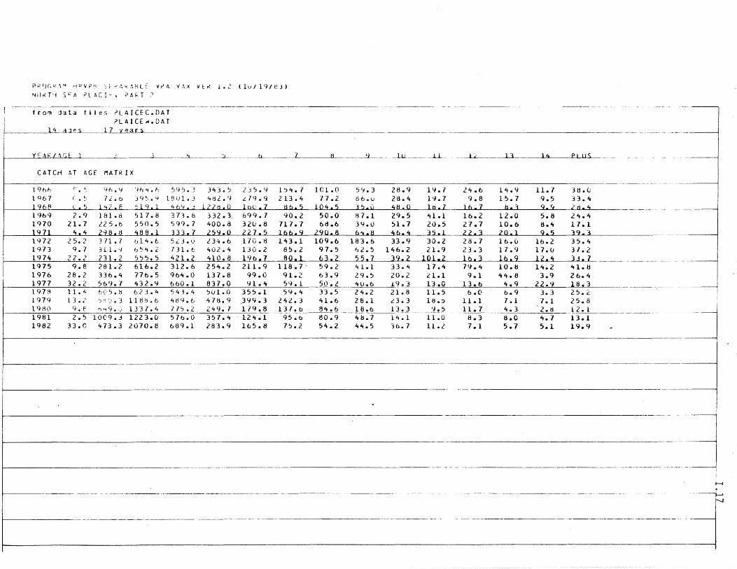
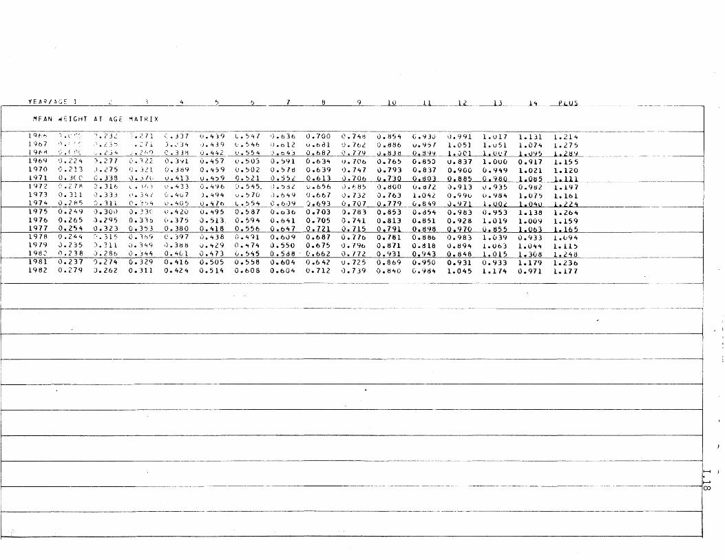
PROGRAM NAME: Separable VPA
PROGRAM TYPE: Main DATE CREATED: Jan 1 1982
SOURCE FILE NAME: FSHA: [7l2.MASTER.SOURCE]SVPA.FOR
EXECUTE FILE NAME: FSHA: [7l2.MASTER.XEQ]SVPA.EXE
AUTHOR: J.G. Shepherd DOCUMENTED BY: W.L. Gabriel
REVISIONS ( Date/Reviser - Description)
February 1983 /J.K. Hunton Before receipt at NMFS October 1983 /O.L. Jackson Expanded dimension, altered I/O, converted for VAX 11 November 1983 . /F.P. Almeida Added I/O options
STATUS: Operational
CLASSIFICATION: Analytical model
PURPOSE OF PROGRAM:
The method determines values of F from a catch-at-age matrix based on the assumption that age-specific patterns of exploitation are constant over time.
DESCRIPTION:
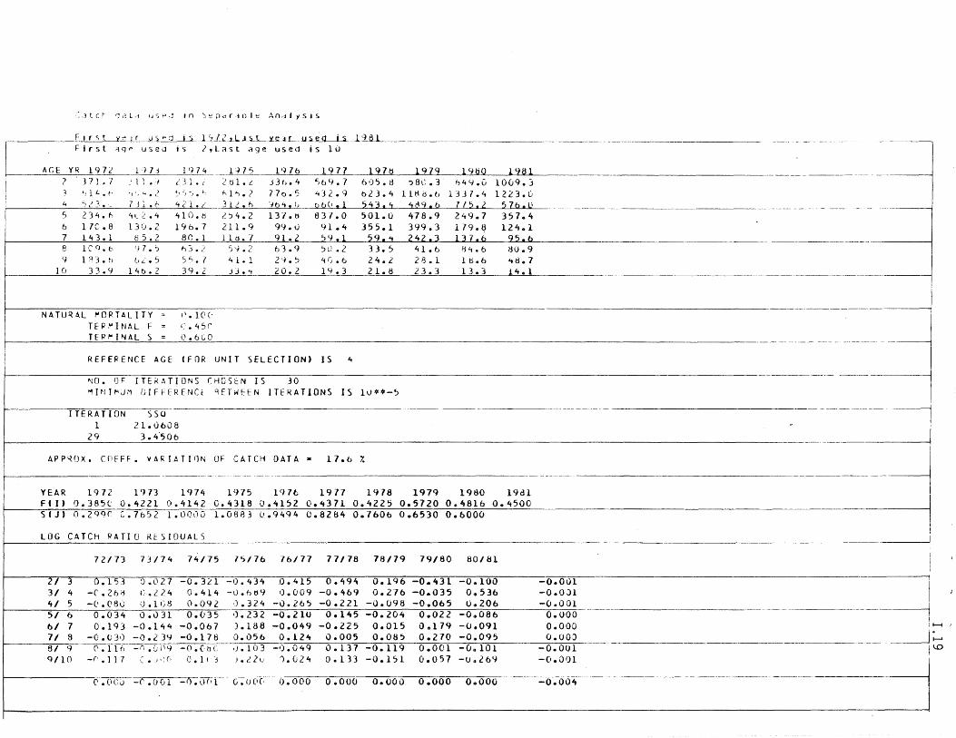
The original guide, Separable VPA: User's Guide (Shepherd and Stevens, 1983) provides a complete description. However, in our version, spawning biomass calculations are not available and I/O instructions are not applicable. The analysis can'be applied to 36 years of data containing 36 ages. In extreme situations where the data do not meet the assumptions of separability, the extended analysis may include a zero in the denominator, leading to a fatal execution error.
DATA USED: User supplied
INSTRUCTIONS FOR RUNNING:
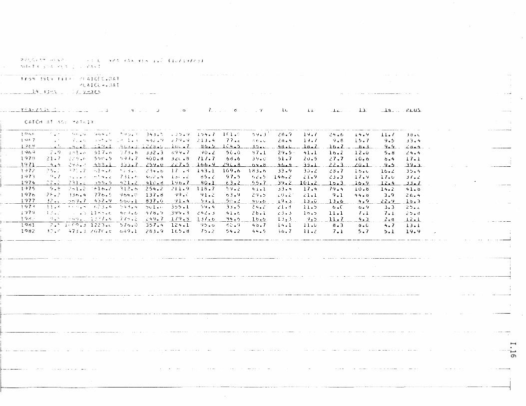
Data sets required: a. Catch at age matrix, one line per year, formatted
I.I5
b. Weight at age matrix, one line per year, formatted The remainder of the program is interactive. To run the pro-gram, type:
$RUN FSHA: [7l2.MASTER.XEQ]SVPA
You will be prompted for answers. If the output conatins more than 18 age classes, increase the horizontal print density before printing at the terminal.
REFERENCES:
Shepherd, J. G. 1982. Two overall measures of averall fishing mortality. International Council for the Exploration of the Sea. CM 1982/G:28, Demersal Fish Committee. Mimeo.
Shepherd, J. G. and S. M. Stevens. 1983. Separable VPA: User's Guide. Internal Report No.8., Ministry of Agriculture, Fisheries and Food, Directorate of Fisheries Research, Lowestoft, U. K.
~) .: r • ,- " .' " 1"_ T j ... \1 ':
t r ') 11 j', tJ til'
.. ~_J~_'L_ t~·~_~_
~...L~-=-'-:'
• r' '. 'I ,\ ~ "l" 1. r~' .~. '"
,J: '\ I C£ ~:. il t. T .) L 6. 1 C i ". :) fl, T
-1 __ i~LS
..l '1 ~
C (I T C rl :. T ~ :- ' .... > T ", 1;( I
r
1
~--
~ I
1 () ~, f-
1. ~ 7? .J '-J.
1 Cj 7 '3 ('j • 1 1 '} 7 4 -, ~ ,
'- {If L..
lq75 9.f.i 197b ? 1:- • ? 1,·/77 3?, -------l tj 7 ~ 1 1 • ,. i (nr~ 1,' •. 1 (~,~ .' ,~ . 191)1 7 • <-
19HZ -~ -,' . ('
I ~ __ ~ ____________ _
f---
-- -- ----- - - --- _. ---- -~- _.-
( 1,' / -I I {' } )
Q
')"1.4
C. 4 c.. J 131.b
::;S.D 7 ').2.
.cl
Y,:l
'11 .t l'34.6
~------.---.-
I-J;", • '-I
54
'i lL J...1 1.L-_ Li ".Lit,_ _ ~.Lus..
9.1 44.tJ 13.b .--~~-
~l.'l 11. S b.( b.<-t 2 b. 1 L 3. j It1.:J 11.1 7.1
U! 3 :J-.!~ ____ U..J. __ ,_~_ 1 't • 1 11.0 8.3 /j.e OJ 6. 7 Ii. 2 7.1 5.7
-----_._-------------- -------- --- --.--.-
--------- - ---~. --- ------ -~- ------ ---- -------_._---- -----------_.-._-
----..;
I-t
f-' (J)
p;..> r) (,~. \ '1 H l> V P ~, ') r r' .\ " ~ K L 0 V? A 'oj ~ J( II t K 1. 2 (1 v I 1 91 c~ ,; ) ~ I I K T '1 S (: /I P L '\ C I :. ? A ~ T !
f rO'1ljata t j I es r>LAICEC.OAT ?LAICE,.,.DAT
7
CATCrl AT AGE MA TR I X
1966 (i. ~ 4h.9 'lh4.h SY ~. 3 1 0 67 ( . :: 72.b j9~;.Y 1801.3
1969 2.9 181.6 517.8 373.8 1910 21.1 n 5.6 550.5 599.7
911 ~.4 228.tl ~88.1 333.1 1972 25.2 "371 .7 b14.6 5i3.(· 197) 9.7 311. ~ b54.2 731.6 1974 22.2 231.2 555.5 4Z1!Z 1975 9.8 281.2 616.2 312.6 1976 28.2 336.4 776.5 964.0 1971 32.2 569.7 432.9 660.1 1978 11. L. be, 5. tj 623.4 543.4 1979 13 .~' ') ') ~; • 3 1180.6 40Y.6 1980 q.f h"t9. ,~ 1337.4 775.2 1981 2.5 10('9.3 1223.0 576.0 1982 33.0 473.3 2010.8 689.1
343.; Zj,.Y 1':> 4. 7 4d2.9 t.79.Q 213.4
!;ib.5 332.3 699.7 90.2 400.8 32u.8 117.7 25~.Q 221.5 Ibb.9 L 3'1.6 17C,. '8 143.1 402.4 130.2 85.2 410.8 1Y6.1 8 254.2 211.9 118.7' 131.8 99.0 91.2 837.0 91.4 59.1 ~01. 0 355.1 59.4 471j.9 399.3 242.3 249.7 179.8 131.0 357.4 124.1 95.6 283.9 165.6 7':J.2
101.0 77.2 lQ~.5 50.0 6d.6
29CJ.8 109.6 97.5
59.2 63.9 50.2 33.5 41.6 84.6 80.9 54.2
:-=l _llL_~ __ ~_...u._ . __ ~_~_~ )4 PillS
-_.- --- --- _._-59.3 28.9 IlJ.7 24.6 14.'1 11.7 )tl.(;
e 6. v 28.4 leJ.7 9.8 15.7 9.5 33.4 -3 ~ .ol-! ~f.I. {l lti.Z ]6.1 fl.) 9.!".t id.~ --- ---.- - - .-
87.1 29.5 "tl.l 16.2 12.0 5.8 24.4 3'1.0 51.1 20.5 21.7 10.6 8.4 17.1 b~.8 ~b.~ 35.1 22.3 20 .ol 9.5 39.3 --------
183.6 33.9 30.2 28.7 16.0 16.2 35.4 62.5 146.2 21.9 23.3 17.9 17.u 31.2
41.1 33.4 11.4 19.4 10.8 14.2 41.B 29.5 20.2 21.1 9.1 44.8 3.9 26.4 40.6 19.3 13.0 13.6 4.9 2,.9 ~ 24.2 21.8 11.5 6.0 6.9 3.3 2~.2
26.1 ~3.3 18.:> 11.1 7.1 l.l 25.8 i
18.6 13.3 9.5 -- 11.7 4.3 l.tI 12.1 -_._ ..... _ .... _ .•.. =J 48.7 14.1 11.0 8.3 6.0 4.7 13.1 44.5 36.7 11. L 7.1 5.7 5.1 19.9
-_.-
----------- -
-----
-'-L ~
----
YF.Aq/~G~ J 7 8
MEAN "jEIGHT AT AG E .... ATK!X
lQt,:> 1 • l !' ~ '~ • ? 3 L: ~;. ? 71 ;'.337 (I. it j 9 L. 547 'J • 63 /) 0.700 1.967 '1 .' (r " • t' j.., • "27 i :) ..... 1 j 1t ,j. 439 l'. ') 46 i) • b 1 Z ~j .001 19t-M ,~, • ( r'( ~ • <:' j 4 .' • Z f-.. C) C.33~ _0.442 (). 554 ..I.tl4~ 0.687 1969 ~) • 2' 24 ).277 l'. i 22 (l.3'11 0.457 0.~03 0.591 0.6)4 1970 C.213 .1.275 fJ. 3 Z 1 O.3b9 0.459 0.502 O.S71:l 0.639 1971 o. j( C' 0.338 ,J. 37(, \J.413 U.4~9 0.':121 O.55i 0.613 1972 C~.27R ;) • 316 \.." • ,fj·' l' • 4:3 3 0.4'16 ~J. 545, ',J • '):j 2. v.656 1973 O. 31 1 ,.J. 33:3 \,1. 34 I ('.4v7 ).494 v.'>70 .J.6it'J 0.667 1974 v.2M5 J.311 (I. j:, 4 l.'. 4G ') 0.470 L.S54 (:.6·)9 '}.693 1975 0.249 0.30\) (). 33C 0.420 lJ. ~9 5 0.587 0.036 0.103 1976 0.265 .).295 0.336 (, • 375 0.513 0.594 0.641 0.705 1977 0.2'>4 0.323 0.353 0.380 0.418 0.556 0.641 0.721 197A 0.244 ~, • 31 :- ().169 e. 397 0.438 0.491 0.609 0.b87
~ 1979 J.235 ). 311 d.349 .) • 3 (j tl 1,).429 0 ... 74 0.550 0.675 1982 0.238 J.286 O. j44 0.401 0.473 0.545 0.5d8' 0.b62 1981 0.237 I).27lt 0.329 0.416 0.505 0.558 0.604 0.642
I 1962 0.279 J.262 0.311 0.424 0.514 0.608 0.604 0.712
r
I
9 10 11 12
I) • 74t:! v.854 G. '-i 30 1).991 U.762. 0.836 u.9S7 1.051 (). 779 J.83e 0.3'1'1 1.QCl U.706 0.765 0.85~ U.837 I). 747 0.793 0.837 0.900 0.706 o 73 dO Q.88~ ,). to 85 \).800 u. d 72 0.913 tJ. 732 0.763 1.Olt2 0.99u
Q.779 ~. 849 Q~971
0.653 O.d54 0.963 0.613 0.851 0.928 o 19 - 0.~98 Q~91Q
0.776 0.761 0.886 0.963 IJ.796 0.871 O.tHB 0.894 0.772 0.431 0.943 0.848 u.725 0.869 0.950 0.931 0.739 0.840 0.984 1.045
--- ----------- - ~-----
----.----~
-- --------- ---
--_ .. _-----
13 1 ..
1.u17 1.131 1.u51 1.074 1!lH",'7 1~~'J2 1.0UO 0.917 O.9lt9 1.021 Q.9~Q 1.Q~~ 0.935 0.91:lZ 0.984 1.075 l.UQ' l~Q~lJ 0.953 1.138 1.019 1.009 Q!~5~ 1.~bJ 1.039 0.933 1.063 1.U44 1.015 1.308 0.933 1.179 1.174 0.971
PLUS
1.214 1.275 1. • .2tj<.J 1.155 1.120 1.111 1.197 1. It>! 1 • .22~ 1.264 1.159 1.lb5 1.L'94 1.115 1.240 1.236 1.177
-- _. -~.--- -- ----
-.. -------~------- -~ ---_.+
--
-----------~
~----------.-----~--------
-------
~ I
I -----------1
_ .. -----
___ w ______
1--1
I--' 0:>
: 1 t C r '1,1 L ., IJ '; t"' ,! In) ~ P d r ,-I 0 I tAn d I y SIS
First Y~Jr U,)Pj j':) l~lZ,L~st ve~r used is 1981 First Clq'" usea is 2,Lrtst age used is 10
AGE YI< 1972 1·,73 371 • l ' 1 1 .1
': 1 L. • ',',. " • /
"':'21. 73~.f:.
5 234. !t,-2.4 6 17C.8 13:j.Z 7 143.1 05.2 8 1CQ.b '17.':1 9 13J.b /.,L.5
l() 33.9 146.2
NATU~AL ~ORTALITY
TEPI"INAL F TEP"'I"4AL S
1974 c _~ 1 • c' ~).:.., ~I • '-:
421../ 410.b 196.7
80.1 h'j.2
S.:,. 7 39.2
('. 1 (t c: C.45(' 0.6(,0
1)75 ;: tll. i hh. ? 3 U. h
2)4.2 211.9 11(j.7 5~.2
41. 1 33."1
1976 1977 197tl 197~ 19bO 1981 33h.4 ~69.7 605.e ~8~.3 ~4Y.0 lOG9.} 770.5 432.9 623.4 1186.b 13J7.4 1223.G '/64 , () 0 b (J • 1 54 3 • 1 1 t\ 9 • 6 7 ~ 5 7 b • li
137.b 837.0 501.0 478.9 249.7 357.4 99.0 91.4 355.1 399.3 179.8 124.1 91.~ ,9.1 5q.~ 242.3 131.6 95.6 63.9 ~0.2 33.5 41.6 H4.b 80.9 2'-/. ~ 20.2
4G.6 14.3
24.2 21.8
28.1. 23.3
1 ti. 6 13.3
'ttl. 7 14.1
REFERENCE AGE (FOR UNIT SELECTION) IS 4
------ . -.-~-----
--------------_._--_ .. ',--,-------_. -'
_ ... ------------_._- -- -------" -
~O. OF ITEi<ATIONS CH05E:N IS 30 ---------.---- ---.-- I 11 Pl1 I'"J,'1 [] IFF ER f Net '1 ET ~ EE N I TE ~A T IONS I S IIJ .... -~ .. __ . ____ - - -------=J-
ITERATION SSG 1 21.0608
29 3.4'506 --------
APP~OX. cnFFF. VARIATlilN OF CATCH DATA" 17.6 7. I
YEAR 1972 1973 1974 1975 1976 1977 1978 1979 1980 19d1 ~ fIll O.3aSe 0.42210.4142 0.4318 0.4152 0.4371 0.4225 0.5720 0.481b 0.4500 I SfJ) O.29Qr C.7652 1.0000 1.0883 U.9494 0.8284 0.7606 0.6530 0.6000
I
LOG CATCH PATIO KESIOUALS _____ . i
72173 7)174 74175 15l7b_lbI77 77178 78/79 79/80 80/81~____ ___ ----~--==J 21 3 0.153 0.021 -0.3il -0.434 0.415 0.494 0.196 -0.431 -0.100 -0.001 31 4 -('.26/j C.224 0.414 -ll.otj9 0.009 -0.469 0.276 -0.035 0 .. 536 -O.OJl 41 5 -Co. (180 i).1GJj 0.092 0.324 -O.2b~ -0.221 -0.098 -0.065 0 .. 206 -0.001 51 6 0.034 0.031 0.{)35 0.232 -0.210 0.145 -0.204 0.022 -0 .. 086 0.000 61 7 0.193 -O.14~ -0.067 ).188 -0.049 -0.225 0.015 0.179 -(J .. 091 0.000 ; I-i I
71 8 -0.030 -0.239 -0.178 0.056 0.124 0.005 0.085 0.270 -0 .. 095 0.00;) ,___ ___ II-' 81 9 (' • 1 1 h - II • C; (' 9 - 0 • C b C .) • 103 -').04 <} 0.137 -0.119 0.001 -0 0 101 -O.OUI I~ 9/10 -(' • 1 ] 7 l~.-'\~(~ (]. 1 ( 'j ).22\..·· 1.G24 0.133 -0.151 0.057 -u .. 269 -0.01)1
('.(leG -C' • () 0 1 -0. 0(;1-' G-:u-(i,(;-- (). 000 0.000 0.000 0.000 00000 -O.O~
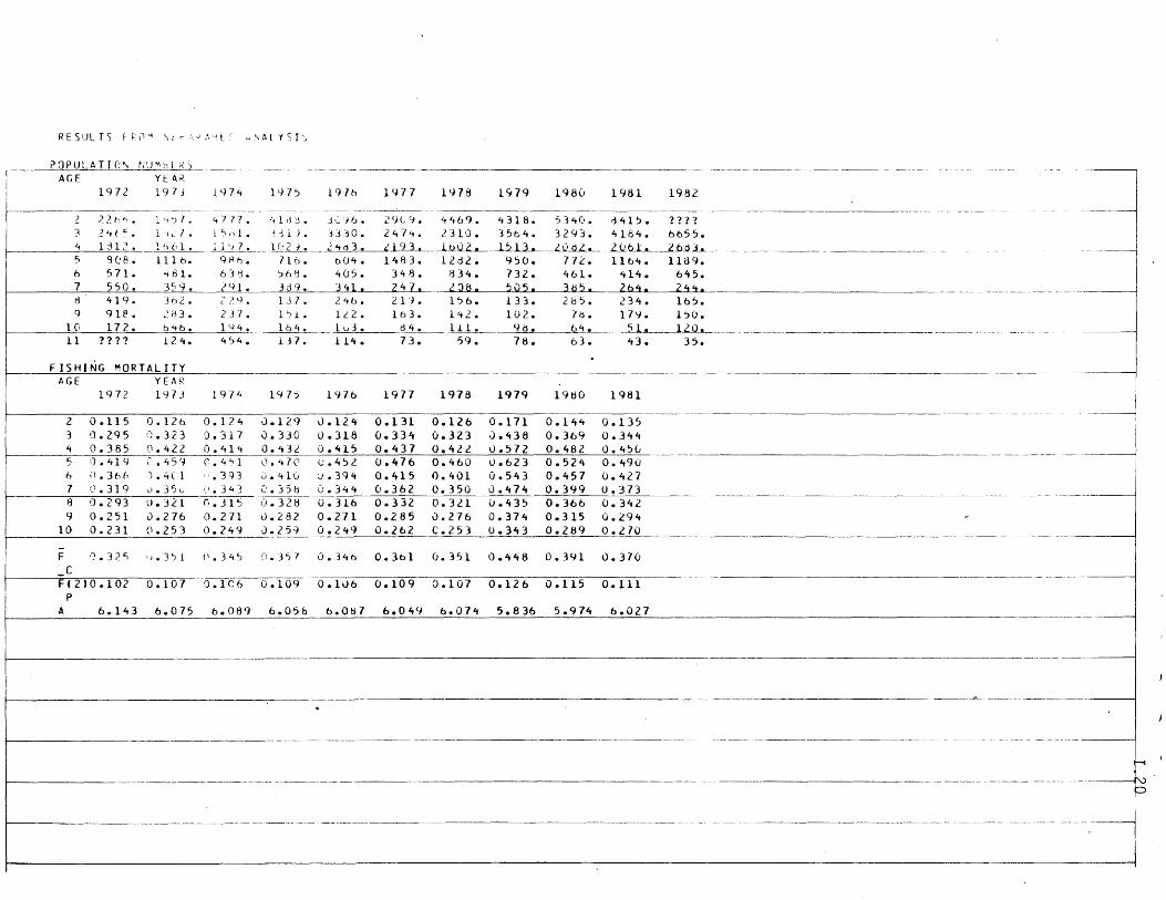
RESULT) ~ ~_ i1 '-1 " t r' _\ .... ,', d L ' ~~AlI'SI"
?OPULATrr~'" ~'U"':~l '~) ------- ~--------~--------------~--.-----~
I AGE YE Ai( 1972 t 9 7J 1<.J74 1 '17') 191b 1<.J77 1<.J76 1979 1980 1981 1982
-- -.------- -- -------------- ". --,-_ .. _----. - -- ----- "--- --- --- -----1 ?2h~. 1 '1 ') 1 • 47 7? 4lrH. jl~-i 6. 2ge 9. 4469. 4 318. 5340. d41~. 111 ? 3 ,: it t t:: • 1 -l L 7 • 1') cd. Hl). jjjO. 247'-t • 2310. 3St,4. 3243. 4184. 6055. 4 1 :3L? 1. '_l 01. : 1 '1 L~ __ ll: 2 -} • __ .2... '-t 0 3 • ,193. _..lQ~- 1~13. __ LllJiL___ NtLL.._-.Z1Ldh __ 5 .9C:8. 1116. 9Rt. 716. bU4. 1483. 1282. 950. 772. 1164. 1189. 6 571. <t 61. b 38. ':lh9. 405. 348. 834. 732. 461. 414. 645. 7 550. 359. 791. 3d9. 341. Z 47 I ZQe. ~Q51 3ti5. 2bj. 244. -- --.--.--~-.-.---- --- ---.--
13 419. 3h2. i?Y. 13 7. 246. 21'1. 156. 133. 2b5. 234. 165. q 9le. .:'H3. 231. 1 ':>1- liZ. 163. 142. lU2. 7b. 17l.). 150.
10 172. b4b. 1 '-14. ---~-- Iv3. 04. 111. 98. Q4" -~~ 11 ?111 12'-1. 4 ,}4 • 137. 114. 73. 59. 78. 63. 43. 35.
-~ FISHING MORTALITY .. -_._-_ ..• ----_.---
AGE YEAR
i 1972 197J 1971. 1 q 7:> 1976 1977 1978 1979 19tiO 1981
2 0.115 0.120 0.124 0.129 0.124 0.131 0.126 0.171 0.14~ O.13~
.....•• ~~ ..••... - .- ........ -] 3 0.295 ().323 0.317 0.330 0.318 0.33lt 0.323 J.438 0.369 0.344 4 0.385 0.422 0.41<' 0.'t3i 0.415 0.437 0.ltZ2 0.572 0.482 0.450 5 :) • 41 9 i'.459 C' • 4" 1 ,).470 u.452 0.476 0.460 0.623 0.524 0.490 6 i\. 36 h ) • .; ( 1 ".3Q3 ~i. 410 ~.394 0.415 0.401 0.543 0.457 0.427 7 c\ • 31 9 u.3S'-... ':\. :3 "'-3 O.j5b (;.344 0.362 0.350 0.474 0.399 0.373
- -'-~-----------.-~----"-------.---~------ -------- - - - _. ------_._---
8 ').293 U.321 (,.315 1=1.328-- 0.316 0.332 0.321 0.435 0.366 0.342 9 0.251 l).276 0.271 t). 282 0.271 0.285 0.276 0.374 0.315 0.294
10 0.231 (\.253 0.249 0.259 0.249 0.262 e.2S3 U.343 0.289 0.270 ---~--- ---"-
-F I; • 32 'i '1.3') 1 (\ • 34 ':l ~-) • :3 57 0.34b 0.301 0.351 0.448 0.391 0.370
C F(2)0.102 0.107 . 0 • 1 f)-r;- 0 • 1 09 0.lv6 0.109 0.107 0.126 0.115 0.111
p
A 6.143 6.075 0.089 6.056 6.0tj7 6.049 6.074 5.836 5.974 6.027
_---'iL _______________ _
-- ---. --.- -------------- -- ---- -- -- ------ -----1
---------------_._---.- ------- - - .. ------ - --- -----
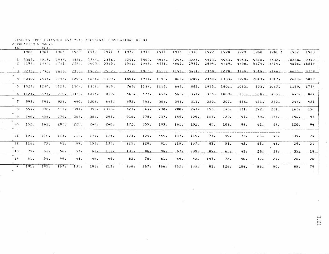
~ E S U L.. T S F ~ 0'" r l T r • i C t~) !, ' .. i\l Y ) I) (11: k ,'I I ,... ALP CPU L A T I U W) u') E: [) ) ~CJPlJLh.TI~N t~U,'1!1tr<)
AGf YEA,,-1966 19b7 1 Yf, 8 1909 11.)70 1471 1972. 1973 1 '-I7~ 1975 I--J76 1977 1978 1979 1980 1<.J81 1'182 1983 I
1 3305. :51:)1'1 •. --'-~3') •.. ~l.....L_l.Lb4--,-- 2830. 2291. 5400. 't~16. 3295. 322a. 2 .3 19 ? .J .; 1:. :' I j 1 • Z 2 '/ J • 3 u \) 1 • 33 tl S • 2 ., 62 • 2 I..i It 9. 4 b 7., • 4 () 65 • 2972 •
4973. 4983. 5953. 931U. 453/. 2H<.J4. 4469. ~lt98. ~374. b414.
2dHbH. 11'1'1 ,.
~09d. L608'l !
3 YZ'3B. .!.l··n. l'6!h. Ll:.i2.L_ .~ ... ~ ~ __ ~ ........ _ I '2"> ti • ..llY3..a........hLL..... .. 2..l.b...9. ............ i 078. 3'- h9 • 3'114. .~ .. ~ ~~ 4059 I
I ~ Z049. 7443. 2154. 1893. 1621. 1199. 1801. 1931. 115b. Hb3. 3209. 2350. 1733. 12'10. 2013. 1917. 2083.
5 112? lzqn. ~C26. l')d..,. 1358. 81.)9. 769. 1134. 10')5. 649. 503. 11.)90. 150C. 1053. 703. lU8 7. 1189. 177't i I
6 1121. ~ll, ?In, ]3 K 3 •. 10ft? 849. 56H ... _~ b4? ?b6. 347. 325. } 0(,9. 6tH. '>O(J. ~ _____ ~~\
7 593. 791. 523. 490. 2208. 642. 552. 352. 305. 397. 311. 220. 207. 516. ~21. 282. 244. 421
8 554. ]qn. ~13. 391. 35d. 131H. 423. 364. 238. 200. 247. 195. 143. 131. 292. 251. 165. 15v
9 240. 405. 279. 3b5. J06. 258. 916. 278. 237. 15S. 125. 163. 129. 97.. 79.
10 152. 161. 28'5. 2 Z ,). 248. 240. 172. 655. 193. 161. 102. 85. 109. 94. 62.
11 101. 11 ( • 1 1 d • Ll('. l71. 115. 173. 124. 454. 137. l14. 73. ')<.J. 7tl. 63.
12 116. 73. AI. S9. 153. 135. 125. 128. 91. 315. 107. 83. 53. 42. 53.
13 75. 81. 56. 5l. 65. 112. 101. 86. 94. 67. 209. 89. 63. 43. 28.
14 61. :> "I. ">1.1. 43. 4v. 49. BL. 76. 61. 69. SCI. 147. 7b. 50. 32.
+ 191 • 195. 167. 135. 101. 213. 11:iO. 167. 166. 2(;2. 133 • 81. 126. lOoteD 56.
164. - .. -~--.~ 54. 120. 94 I
I
43. 3~. 74
.---------.-----~
48. 29. 21 I 37. ~ 19 I
t
LI. lb. 26 i i
50. 85. ~
t--f
N f-l
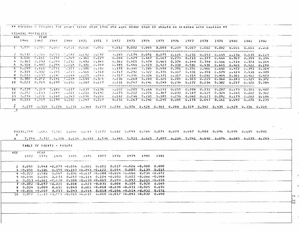
--------.---~- ----~-- - --~------ ~-------- .. - ---------•• ~lrnina - ~~su'ts 1~r years 'at~r than 19til and dyes older than 10 should be treated witn caution ••
FISHING "'flcTe.LITY AGE YfAR .----- .. -.. --
1966 1~67 19~8 196~ 1970 1971
') • 0 'J r-. l • lJ () I: (1 • \) (, Ij (t • C) 1 U • (' u b (~ • 002
2 () • :) "32 \. 'J L t
3 0.116 0.1h1 4 0.363 0.293 5 0.318 0.497 6 0.249' G.411 7 0.319 0.332 A 0.212 u.233
10
12 13 14
-
(). Z 5 2 ().234 0.223
;,'.2 (; 9 c.l')3 C.2Zb 0.2('5
II • (. ') I-; ( •• ~ d I v • l tl L ,) • l 9 7 'j. 2 3-1-:'-:-2~-cl. 361- 0 • 229 -(·.25Y ,C' • 296 (' .• ;> 71 ,..\. 141 v. 24C 0.141 0.195
'). 18 l ::.245 i) • 16 R 0. 19 ~
C.232 0.264
27 • 1:'
:..;. 44
C.2d8 0.152
) • 490J ('. 370 v.J8b v.416 v.L25 :) • 144 0.24,7
(\.345 ('.359 .J. 33(.; .: • 31 tl ,.'.2 b J o. )'(' ') (j. 2. 2. 7
() • 2. .2 7- J-:~'O. L 3 6 -~ '- .211 l.l11 0.190 0.249 0.186 O.LOb 0.152 (.247 0.227
1972 1973 1974 1975 1976 1977 1978 1979 19tiO 19~1 19BL
0.012 0.002 0.005 0.003 0.v09 0.007 0.002 0.OU2 O.uOl 0.001 v.vul
.).165 -0.264 0.36.3 0.385 ,}'378 .J • 317 ll. 317 ,) • l 36 'J.231
'.).2..02 0.275 0.1d2 0.231
l'.174 0.429 0.505 0.464 0.340 0.292 0.33u \).268 0.267
0.051 O.~67
0.479 0.523 ).38~
IJ.322 lJ.J26 J.283 0.240
0.075 0.167 0.463 0.527 0.498 0.376 0.371 0.325 0.245
v.205 0.c66 0.143 0.212 v.20b 0.307 0.246 0.210 0.185 0.267 0.240 0.245
O.lLo 0.273 0.378 0.338 0.356 0.307 \1.317 0.285 0.234
0.215 0.093 0.254 0.085
0.231 0.213 ().3~9
0.58(; ,).35(; 0.331 v.31~
0.303 0.272
0.153 u.377 0.398 0.430 u.460 0.358 0.282 0.219 0.236
0.208 0.231 0.187 0.125 0.060 0.123 0.178 0.047
O.14t5 O.4't4t 0.506 0.645 (j.640 O. ';)79 0.404 0.360 0.302
0.287 0.324 0.192 0.161
0.130_ 0.135 U.lLY 0.507 0.359 0.394t 0.516 0.378 0.314 0.465 0.422 0.2ati 0.~72 0.393 0.J14 0.414 0.438 0.389 0.361 0.412 0.423 0.283 0.325 0.372 u.257 0.320 0.38~
O.i13 0 • .311 0.26'5 0.202 0.179 0.260 0.(;97 0.270
u.~02
0.302 O.lB6 0.235
F 0.277 0.319 0.226 L.231 U.Jb4 0.273 0.283 0.376 0.428 0.363 0.288 0.319 0.342 0.439 b.429 0.336 0.314 c
F(})O.259,.Chj C'.IJf):' v.Ubt. ·j.l}tH (.(72 (;.Jd2 u.W}) O.OcH) 0.0740.079 V.087 (;.08B 0.090 0.095 0.Uti5 O.Otil P ~
. _. 7.7r 7 6.63 R 5 b. 5 96 945 5.921 6.625 7.097 6.204 5. 94l __ h .. JH.Q ~~b. 085 6.199 6 .. 2.44
TABLE Of F(EXT) - F(SfP) ------_. __ ._- ----
---~--- ---- -_ .. -AGE YEAR
1972 1973 1974 1975 1976 1977 197d 1979 1980 1981 _.---------_._.- ------- - ---- --_._- ------- -- -- --- --
2 0.050 0.0~8 -0.073 -0.054 0.002 0.101 0.027 -0.026 -0.008 0.000 3 -0.031 0.106 0.150 -0.163 -0.045 -0.122 o.ost, 0.007 0.139 0.015 4 -0.022 o. (1 8) 0.(165 0.031 -0.037 -0.088 -0.024 -0.066 0.034 -0.072 5 -0.03~ 0. ('0 ~ O. C 73 0.057 -0.114 0.104 -0.030 0.022 -0.06U -0.068 6 0.013 -0.061 -0.U08 0.088 -0.039 -0.065 0.O5~ 0.097 0.015 -O.03t,
"~-----'--'---'-
7 -O.Oe2 -0.057 -0.021 0.018 v.023 -0.031 0.008 0.105 0.020 0.065 8 0.024 0.009 O.Oll 0.043 O.uOl -0.018 -0.039 -0.031 -0.005 0.070 9 -0.016 -0.007 0.013 0.043 0.014 0.016 -0.056 -0.~14 -0.032 0.031
10 O.O(C' ( • ,I 1 3 - <) • (, (' >1 - 0 • 0 1 S -tJ. G 15 0.010 -0.017 -0.041 -0.032 0.050
.. -----_____ 0 .. -------... ---.-.-l
.-- ---------I
- -,--.---~-- ---- ------
~
N N
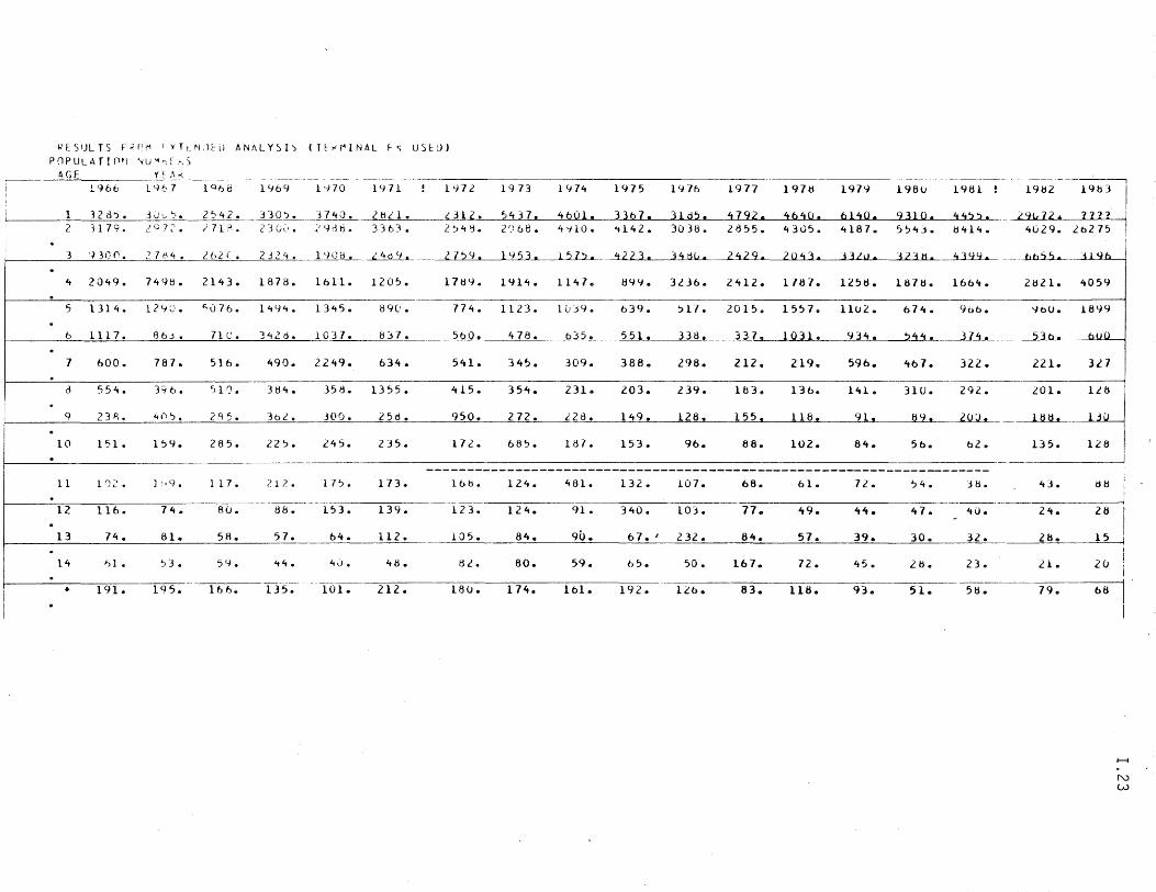
k'ESULTS F~(.IM fyT(N.)tlJ ANALYSIS (TEt<~INAL f.') USEtJ) P (l P U L A T I fl ~ I '..j U '1 t; [ ~_ S
AGE '(",\.<. - ---~-- - --_.- --- --------
1.966 lc}b7 1 Qf:Ji:l 1469 l'no 1471 1')72 1973 14H 1915 1 CJ 76 1917 1911:) 197'1 198u 19tH !
1 32 ib. j \.) \.. ,:: .• 2:'42. _ ::I )O~_j 7'1i) 0_ 2 tiL 1 • ~Jl,! 5431. 4bQl. JJt'!l. j 1 d!i. ~192. ~b~u. bHO. 2310. ~~2) • 2 31 79. ! G 7 ~-. • ;71~. Z'3 (;(, • i"-} ~ 6 • 336] • 2? 413. 2f) be. 4'i 10. -.142. 3038. 2855. 4305. 4181. 5'243. 11414.
3 930(\. ? 7 1'>4 • 262 ( • 2324. __ L~~-,-~_ 2.7'24. 1453. 1.57,. .~22 3. 34%. 2~ 2043. 3-32\1. -iF-Hi. 43<)Y.
4 2049. 749t3. 2143. 1878. 1611. 120'2. 1713'/. 1914. 1147. 899. 3236. 2412. 1187. 125d. 1alB. 1664.
5 1314. 124U. ~076. 14lJ4. 13'15. 890. 774. 1123. lCd9. 639. :>17. 2015. 1557. 11ui. 614. 906.
6 1117. 8 6J • 71 c. 342 d. ~Q_) 7. iD 7. 560. 478. b35. 551. 338. 337. _._- lQ31. 934 • :>44. 37't •
7 600. 787. 516. 490. 2249. 634. 541. 345. 309. 388. 298. 212. 219. 596. 467. 322.
d 554. 396. ')10. 384. 3513. 13'25. 415. 354. 231. 203. 239. un. 136. 141. 310. 292.
9 23~. 40? • 2 A 5. 3b£. 300. 25d. 950. 272. £28. 149. l.Z8! 125 1 118! 9l. !:I'I. ~-
10 151. 1'29. 285. 225. 245. 235. 172. 685. 187. 153. 96. 88. 102. 6it. 56. 62.
----------------------------------------------------------------------11 102. ] '.19. 1 17. ?l? 17:>. 173. 16b. 124. 481. 132. 107. 68. bl. ll. ~4. 3tl.
----------12 116. 74. 8u. 88. 153. 139. 123. 124. 91. 340. 103. 77. 49. 44. 47. 4().
13 74. 81. 58. 57. 64. 112. lO5. 84. 90. 67. I 232. 84. 57. 39. 30. 32.
14 I) 1 • ':13 • 59. .. 4. 40. 48. 82. 80. 59. 65 • 50. 167. 72. 45. 28. 23.
+ 191. ~.- 166. 135. 101. 212. 18u. 174. 161. 192. li6. 83. 118. 93. 51. 58.
I
19H2 19b)
I ~91.t 12 II 2~ 4029.
ob5,). -i I Qh
2821. it059
'/ou. 18'19
--~ bUO
221. 32.7
201. 1£8
l~d. 1.H.1
135. 128
43. d8
21t. 28
28. 15
21 .. ZU i
--~-~
I
I--t
N W
------~-----
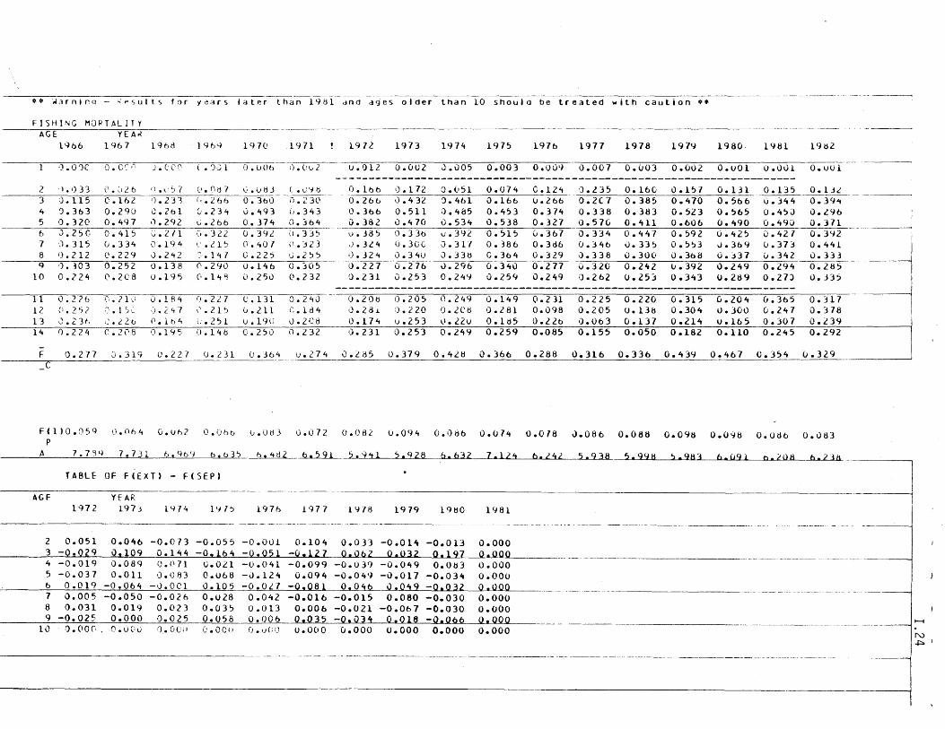
~* ·.,jarnlr.q - ';'psults for '1~ars I a t er thdn 19til dna ages older than 10 shoula be treated with caution q. FISHING MOPTAllTY
AGE YEAK
1'166 1967 1968 19by 1970 1971 1972. 1973 1974 1975 1976 1977 1978 1979 1980· 1981 19t1l
')'0,)( O.C':t, J. (I C(-: ( • ')) 1 O.UOb ~).t·1.,.2 u.012 O.OUl 0.005 0.003 0.009 0.007 0.u03 0.002 O.uOl o • O~H O.vUl ----------------------------------------------------------------------
2 .j. I) 33 (' • ~) 2 b c) • V ~ 7 (I. n d 7 I). () 113 C.u'jlj 0.166 1).172 0.(151 0.O7~ C.12~ ').2.35 0.160 0.157 0.131 0.135 0.13i 3 :). 115 0.162 c}. 231 (,.266 0.360 -- --I') • 2. 30- 0.26b· 0.432 ).461 0.166 v.l66
. -
0.2e7 0.385 0.470 0.566 0.344 0.39 .. 4 'J.363 0.290 0.261 (',.234 0.493 IJ. 343 0.366 0.511 0.485 0.4')3 0.37lt 0.338 0.383 0.523 0.565 0.45;) O.2lJ6 5 0.320 0.497 .).2Q2 ~.2.66 0.374 0.364 0.382 0.470 0.534 0.538 0.327 O.57G 0.411 0.606 0.490 0.490 0.371 6 0.25C 0.415 ~. 211 '~'.322 0.392 ().335 v.J85 0.336 0.392 0.515 0.367 0.334 0.447 0.592 u~425 v. 42 7 O.3'Jl 7 0.315 u.334 0.194 \~ .• Z 15 (1.407 i\ .323 ,).324 0.3G0 0.317 0.386 0.3db u.346 0.335 0.553 iJ.369 u.373 0.441 8 I) • 2. 12 0.229 \).2~2 '). 147 C.22~ v.Z" ,).32 it 0.34U J.33tl C.3bit 0.329 ·).338 0.300 0.360 0.:;'37 0.342 0.333 Q 'J. i03 0.252 0.138 0.2l/0 (J.146 O.jO~ 0.227 0.276 0.296 0.340 0.277 0.320 0.242 lJ. 392 0.249 0.294 0.285
10 0.224 C.Ze8 u.195 (I. lit '3 1.).250 0.232 'j.l31 0.253 0.2itlJ 0.259 0.249 0.262 0.253 0.343 0.289 0.27) 0.335 ----------------------------------------------------------------------
11 0.226 1-:'.21 \.: 0.1£14 n.22l C.131 O.2~J O.20b 0.Z05 0.249 O.lit9 0.231 0.225 0.220 0.315 (J.204 0.365 0.317 12 c: .252 .,: • 1 'J,~ ,j. 2't 7 \' • 21? v.211 C.ld4 I).ZB.l 0.220 o.zce 0.281 0.098 0.205 0.138 0.304 0.300 0.247 0.378 13 \.~.23t, ,_'.22 b 0.1h4 (;.2')1 () .19U 0.2e8 0.174 u.253 0.220 0.ld5 0.220 0.063 0.137 0.214 u .16 5 0.307 0.239 14 0.224 c. 2i"'\ 8 0.19 '5 O.14b C.25\) 0.232 0.231 0.253 0.249 0.259 0.085 0.155 0.050 0.182 0.110 0.245 0.292
-F 0.277 ,).319 0.227 0.231 CJ.364 0.274 I)./.. 85 0.379 0.42e 0.366 0.288 0.316 0.336 0.439 0.467 0.354 0.329 --------
C
FCl)O.OSQ O.Oh4 0.u62 O.Obo G.ue) 0.072 0.082 v.094 0.086 0.074 0.018 0.086 0.088 0.098 0.098 0.086 0.083 P
A 7.794 7.731 6.Qb~ 6.b3~ _ b.~d2 6.591~ 5.941 S.Q28 6.632 7.124 6.242 5.938 5.9l/8 ~.983 6.091 b.JOU b.21k
AGF
TABLE OF F(EXr) - F(SEP)
1'172 YEAR
1973 1974 l'-i 1 'J 1976 1977 1978 1979 19tjO 1l/81
2 0.051 0.046 -0.073 -0.055 -0.001 0.104 0.033 -0.014 -0.013 0.000 3 - 0 • 0 2 9 0, 10 9 0 • 1 4 4 - 0 • 16 4 - 0 • 05 1 -0. 1 2 7 O __ Q b Z_~O~L 0 • 1 97 0 • 000 4 -0.019 0.089 0.071 0.021 -U.O~1 -0.099 -0.039 -0.049 0.O~3 0.000 5 -0.037 0.011 0.U83 0.068 -0.124 0.094 -0.049 -0.017 -0.034 0.000 6 0.019 -0.064 -v.OCI 0.105 -D.Ol7 -0.061 0.046 0.049 -0.032 0.000 _H _________ _
7 0.005 -0.050 -0.026 O.Ul8 0.042 -0.016 -0.015 0.080 -0.030 0.000 6 0.031 0.019 0.023 0.03~ 0.013 O.OOb -0.021 -0.067 -0.030 0.000 9 -0.025 0.000 0.025 0.058 0.006 0.035 -O.03~ __ Q.016 -0.066 0.000
10 o.(\or,. 0.0('0 f).oe;1 O.OCI) (;.u(;U 0.000 0.000 0.000 0.000 0.000
-_ .. _- - - -- .- ------------------------ -_._-----._------
_ ____________ ,_H
. - --~-------'I
~I I
I--t
N +:=0 '
PROGRAM NAME: Multispecies Cohort Analysis
PROGRAM TYPE: Main DATE CREATED: Oct 1979
SOURCE FILE NAME: FSHA: [7l2.MASTER.SOURCE]POPE.FOR
EXECUTE FILE NAME: NONE - see INSTRUCTIONS FOR RUNNING
AUTHOR: J.G. Pope DOCUMENTED BY: K.L. Foster
REVISIONS ( Date/Reviser - Description)
Jun 13 1983 /K.L. Foster Revised to allow for species and age specific basal natural mortality rates and converted to FORTRAN77 to run on Vax 11/780
STATUS: Operational
CLASSIFICATION: Analytical Model
PURPOSE OF PROGRAM:
I.25
This program is an extension of Pope's (1979) multispecies cohort analysis which incorporates species interactions through predation into species, year and age specific calculations of stock size, fishing mortality and total natural mortality.
DESCRIPTION:
Species interaction through predation is incorporated into calculations of stock size (Ni), natural mortality (AM, basal natural mortality plus predation mortality), and fishing mortality (F) for all years, species and ages considered in the model. This program is different from Pope's (1979) original program because it uses a species and age specific basal natural mortality rate instead of a constant rate for all species and ages. This model assumes the fraction of food contributed by fish species remains constant over the years independent of whether prey biomass increases or decreases. There has been criticism of this because it does not allow for contributions of 'other food' not included in the model.
Tables are generated for stock size, natural mortality and fishing mortality by species. Each table contains that species' ages and the years used in the analysis. Foster (1982) describes the analytical procedures used in this analysis.
I.26
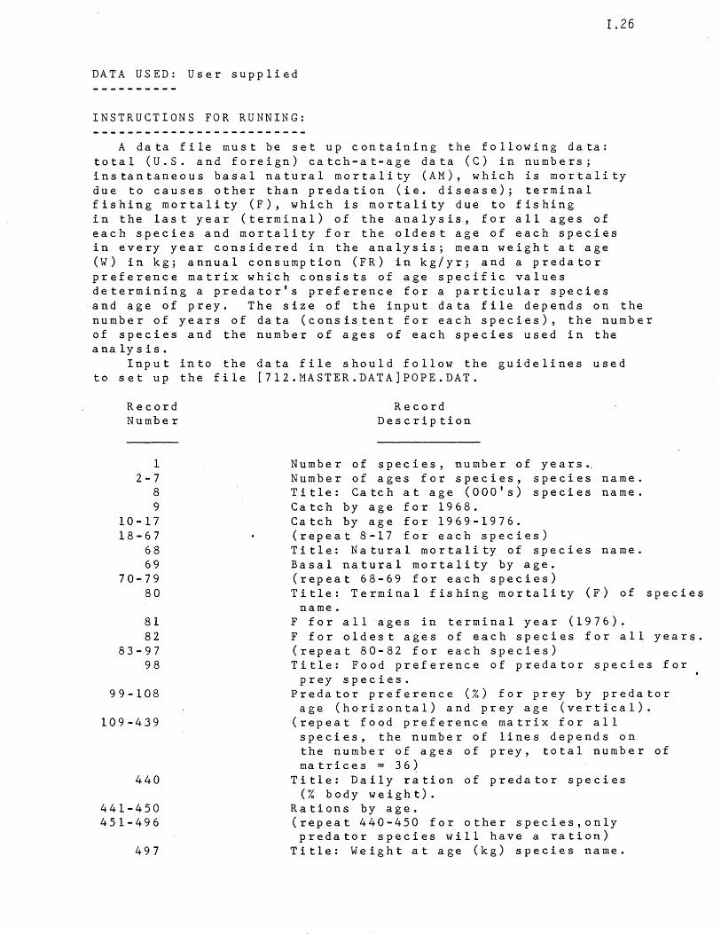
DATA USED: User supplied
INSTRUCTIONS FOR RUNNING:
A data file must be set up containing the following data: total (U.S. and foreign) catch-at-age data (C) in numbers; instantaneous basal natural mortality (AM), which is mortality due to causes other than predation (ie. disease); terminal fishing mortality (F), which is mortality due to fishing in the last year (terminal) of the analysis, for all ages of each species and mortality for the oldest age of each species in every year considered in the analysis; mean weight at age (W) in kg; annual consumption (FR) in kg/yr; and a predator preference matrix which consists of age specific values determining a predator's preference for a particular species
'and age of prey. The size of the input data file depends on the number of years of data (consistent for each species), the number of species and the number of ages of each species used in the analysis.
Input into the data file should follow the guidelines used to set up the file [7l2.MASTER.DATA]POPE.DAT.
Record Number
1 2-7
8 9
10-17 18-67
68 69
70-79 80
81 82
83-97 98
99-108
109-439
440
441-450 451-496
497
Record Description
Number of species, number of years .. Number of ages for species, species name. Title: Catch at age (OOO's) species name. Catch by age for 1968. Catch by age for 1969-1976. (repeat 8-17 for each species) Title: Natural mortality of species name. Basal natural mortality by age. (repeat 68-69 for each species) Title: Terminal fishing mortality (F) of species
name. F for all ages in terminal year (1976). F for oldest ages of each species for all years. (repeat 80-82 for each species) Title: Food preference of predator species for
prey species. Predator preference (Z) for prey by predator
age (horizontal) and prey age (vertical). (repeat food preference matrix for all species, the number of lines depends on the number of ages of prey, total number of matrices = 36)
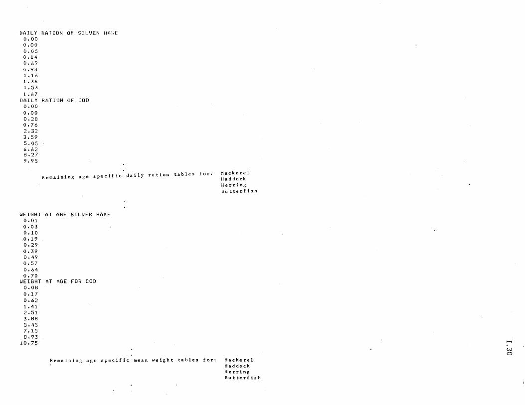
Title: Daily ration of predator species (Z body weight).
Rations by age. (repeat 440-450 for other species,only predator species will have a ration)
Title: Weight at age (kg) species name.
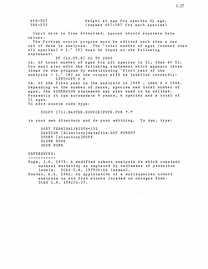
498-507 508-553
Weight at age for species by age. (repeat 497-507 for each species)
Input data is free formatted, spaces should separate data values.
1.27
The Fortran source program must be editted each time a new set of data is analyzed. The 'total number of ages (summed over all spe,cies) + 1.' (4f) must be input at the following statement:
IF (IJ.GT.4f) GO TO 2003 ie. if total number of ages for all species is 51, then 4f= 52. You must also edit the following statement which appears three times in the program by substituting 'first year of the analysis - 1.' (4f) so the output will be labelled correctly:
ITTT=ITT + 4f ie. if the first year in the analysis is 1969 then 4f = 1968. Depending on the number of years, species and total number of ages, the DIMENSION statement may also need to be editted. Presently it can accomadate 9 years, 6 species and a total of 51 ages. To edit source code type:
$COPY [7l2.MASTER.SOURCE]POPE.FOR *.*
to your own directory and do your editting.
$SET TERMINAL/WIDTH=132 $ASSIGN [directory]datafile.DAT FOR005 '$ FO R T [d ire c tory] PO P E $LINK POPE $RUN POPE
REFERENCES:
To run, type:
Pope, J.G. 1979. A modified cohort analysis in which constant n~tural mortality is replaced by estimates of predation levels. ICES C.M. 1979/H:16 (mimeo).
Foster, K.L. 1982. An application of a multispecies cohort analysis to six fish stocks located on Georges Bank. ICES C.M. 1982/G:37.
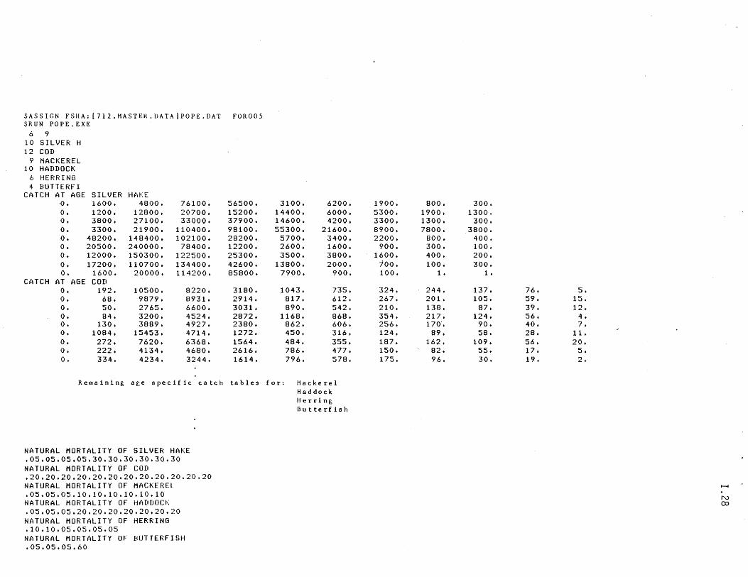
$ASSIGN FSHA: [712.MASTEH.DATA]POPE.DAT $RUN POPE.EXE
6 9 10 SILVER H 12 COD
9 MACKEREL 10 HADDOCK
6 HERRING 4 BUTTERFI
CATCH AT AGE SILVER HAKE ~. 1600. 4800. 76100. o. 1200. 12800. 20700. o. 3800. 27100. 33000. O. 3300. 21900. 110400. o. 48200. 148400. 102100. O. 20500. 240000. 78400. O. 12000. 150300. 122500. O. 17200. 110700. 134400. o. 1600. 20000. 114200.
CATCH AT AGE COD O. 192. 10500. 8220. o. 68. 9879. 8931. O. 50. 2765. 6600. O. 84. 3200. 4524. o. 130. 3889. 4927. o. 1084. 15453. 4714. O. 272. 7620. 6368. O. 222. 4134. 4680. O. 334. 4234. 3244.
Remaining age specific catch
NATURAL MORTALITY OF SILVER HAKE .05.05.05.05.30.30.30.30.30.30 NATURAL MORTALITY OF COD .20.20.20.20.20.20.20.20.20.20.20.20 NATURAL MORTALITY OF MACKEREL .05.05.05.10.10.10.10.10.10 NATURAL MORTALITY OF HADDOCK .05.05.05.20.20.20.20.20.20.20 NATURAL MORTALITY OF HERRING .10.10.05.05.05.05 NATURAL MORTALITY OF BUTTERFISH .05.05.05.60
FOROOS
56500. 15200. 37900. 98100. 28200. 12200. 25300. 42600. 85800.
3180. 2914. 3031. 2872. 2380. 1272. 1564. 2616. 1614.
ta b 1 e s
3100. 6200. 1900. 14400. 6000. 5300. 14600. 4200. 3300. 55300. 21600. 8900.
5700. 3400. 2200. 2600. 1600. 900. 3500. 3800. 1600.
13800. 2000. 700. 7900. 900. 100.
1043. 735. 324. 817. 612. 267. 890. 542. 210.
1168. 868. 354. 862. 606. 256. 450. 316. 124. 484. 355. 187. 786. 477. 150. 796. 578. 175.
for: Mackerel Haddock Herring Butterfish
800. 300. 1900. 1300. 1300. 300. 7800. 3800.
BOO. 400. 300. 100. 400. 200. 100. 300.
1. 1.
244. 137. 201. 105. 138. 87. 217. 124. 170'. 90.
89. 58. 162. 109.
82. 55. 96. 30.
76. 59. 39. 56. 40. 28. 56. 17. 19.
5. 15. 12.
4. 7.
11. 20.
c-..I.
2.
I--f
N CO
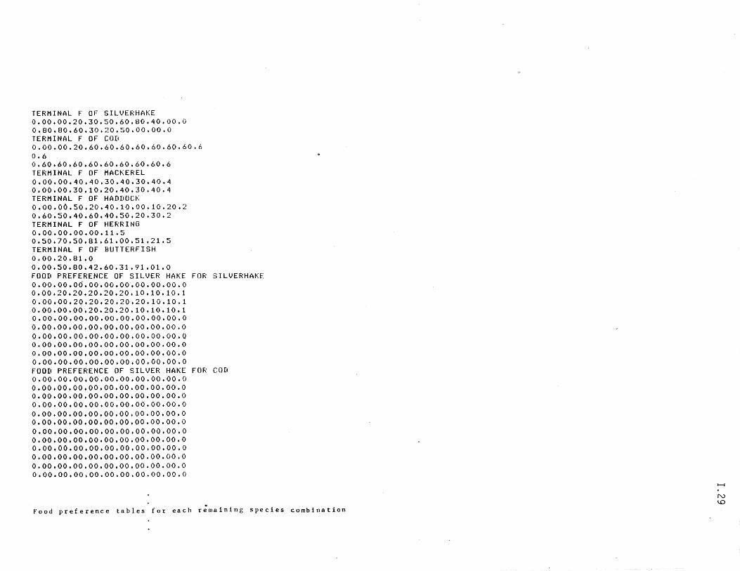
TERMINAL F OF SILVERHAKE 0.00.00.20.30.50.60.80.40.00.0 0.80.80.60.30.20.50.00.00.0 TERMINAL F OF COD 0.00.00.20.60.60.60.60.60.60.60.6 0.6 0.60.60.60.60.60.60.60.60.6 TERMINAL F OF MACKEREL 0.00.00.40.40.30.40.30.40.4 0.00.00.30.10.20.40.30.40.4 TERMINAL F OF HADDOCK 0.00.00.50.20.40.10.00.10.20.2 0.60.50.40.60.40.50.20.30.2 TERMINAL F OF HERRING 0.00.00.00.00.11.5 0.50.70.50.81.61.00.51.21.5 TERMINAL F OF BUTTERFISH 0.00.20.81.0 0.00.50.80.42.60.31.91.01.0 FOOD PREFERENCE OF SILVER HAKE FOR SILVERHAKE 0.00.00.06.00.00.00.00.00.00.0 0.00.20.20.20.20.20.10.10.10.1 0.00.00.20.20.20.20.20.10.10.1 0.00.00.00~20.20.20.10.10.10.1 0.00.00.00.00.00.00.00.00.00.0 0.00.00.00.00.00.00.00.00.00.0 Q.OO.OO.OO.OO.OO.OO.OO.OO.OO.Q 0.00.00.00.00.00.00.00.00.00.0 0.00.00.00.00.00.00.00.00.00.0 0.00.00.00.00.00.00.00.00.00.0 FOOD PREFERENCE OF SILVER HAKE FOR COD 0.00.00.00.00.00.00.00.00.00.0 0.00.00.00.00.00.00.00.00.00.0 0.00.00.00.00.00.00.00.00.00.0 0.00.00.00.00.00.00.00.00.00.0 0.00.00.00.00.00.00.00.00.00.0 0.00.00.00.00.00.00.00.00.00.0 0.00.00.00.00.00.00.00.00.00.0 0.00.00.00.00.00.00.00.00.00.0 0.00.00.00.00.00.00.00.00.00.0 0.00.00.00.00.00.00.00.00.00.0 0.00.00.00.00.00.00.00.00.00.0 0.00.00.00.00.00.00.00.00.00.0
Food preference tables for each r;maining species combination
1-1
N \.0
D A I L Y RAT ION 0 F 5 I LV E R H A I( E 0.00 0.00 0.05 0.14 0.69 0.93 1.16 1.36 1.53 1 .67
DAILY RATION OF COD 0.00 0.00 0.28 0.76 2.32 3.59 5.05 6.62 8.27 9.95
Remaining age specific daily ration tables for:
WEIGHT AT AGE SILVER HAKE 0.01 0.03 0.10 0.19 0.29 0.~9 0.49 0.57 0.64 0.70
WEIGHT AT AGE FOR COD 0.08 0.17 0.62 1. 41 2.51 3.88 5.45 7.15 8.93
10.75
Mackerel Haddock Herring Butterfish
Remaining age specific mean weight tables for: Mackerel Haddock Herring Butterfish
1-1
w a
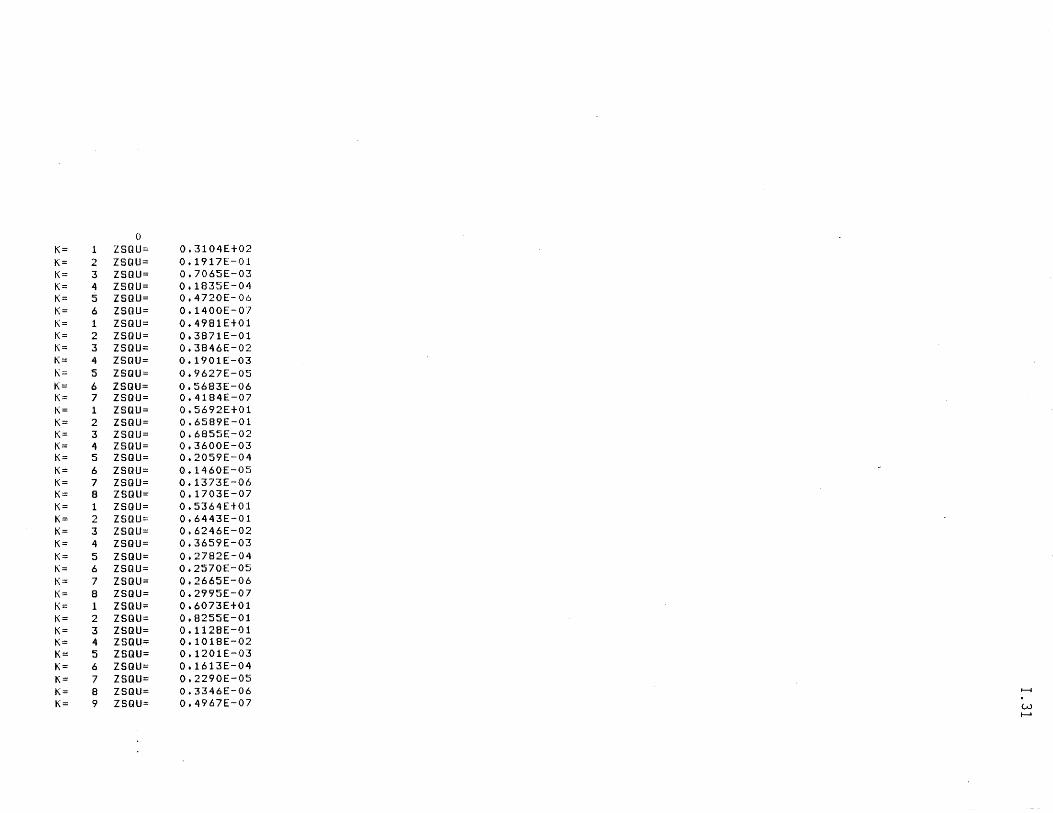
0 K= 1 ZSQU= 0.3104£+02 K= 2 ZSQU= 0.1917£-01 K= 3 ZSQU= 0.7065£-03 K= 4 ZSQU= 0.1835£-04 K= :5 ZSQU= 0.4720£-06 /'i"-.- 6 ZSQU= 0.1400£-0] K= 1 ZSQU= 0.4981£+01 K= 2 ZSQU= 0.3871£-01 K= 3 ZSQU= 0.3846E-02 K= 4 ZSQU= 0.1901£-03 K= 5 ZSQU= 0.9627£-05 K= 6 ZSQU= 0.5683£-06 K= 7 ZSQU= 0.4184£-07 K= 1 ZSQU= 0.5692E+01 K= 2 ZSQU= 0.6589£-01 K= 3 ZSQU= 0.6855£-02 K= 4 ZSQU= 0.3600E-03 K= 5 ZSQU= 0.2059£-04 K= 6 ZSQU= 0.1460£-05 K= 7 ZSQU= 0.1373£-06 K= 8 ZSQU= 0.1703£-07 K= 1 ZSQU= 0.5364£+01 K= 2 ZSQU= 0.6443£-01 K= 3 ZSQU= 0.6246£-02 K= 4 ZSQU= 0.3659£-03 K= 5 ZSQU= 0.2782£-04 K= 6 ZSQU= 0.2570£-05 K= 7 ZSQU= 0.2665£-06 K= 8 ZSQU= 0.2995£-07 K= 1 ZSQU= 0.6073£+01 K= 2 ZSQU= 0.8255£-01 K= 3 ZSQU= 0.1128£-01 K= 4 ZSQU= 0.1018£-02 K= 5 ZSQU= 0.1201£-03 K= 6 ZSQU= 0.1613£-04 K= 7 ZSQU= 0.2290£-05 K= 8 ZSQU= 0.3346£-06 1-1
K= 9 ZSQU= 0.4967£-07 w .........
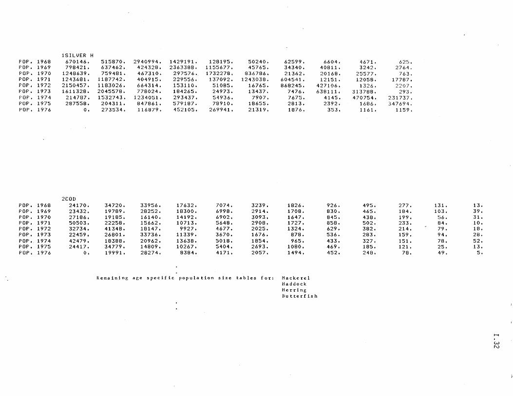
1SILVER H POP. 1968 670146. POP. 1969 798421. POP. 1970 1248639. POP. 1971 1243681. POP. 1972 2150457. POP. 1973 1611328. POP. 1974 214787. POP. 1975 287558. POP. 1976 O.
2COIl POP. 1968 24170. POP. 1969 23432. POP. 1970 27186. POP. 1971 50503. POP. 1972 32734. POP. 1973 22459. POP. 1974 42479. POP. 1975 24417. POP. 1976 O.
515870. 2940994. 1429191. 128195. 50240. 62599. 6604. 637462. 424328. 2363388. 1155677. 45765. 34340. 40811. 759481. 467310. 297576. 1732278. 836786. 21362. 20168.
1187742. 404915. 229556. 137092. 1243038. 604541. 12151. 1183026. 664314. 153110. 51085. 16765. 868245. 427106. 2045578. 778024. 184265. 24973. 13437. 7476. 638111. 1532743. 1234051. 293437. 54936. 7907. 7675. 204311. 847861. 579187. 78910. 18655. 2813. 273534. 116879. 452105. 269941. 21319. 1876.
34720. 33956. 17632. 7074. 3239. 1826. 19789. 28252. 18300. 6998. 2914. 1708. 19185. 16140. 14192. 6902. 3093. 1647. 22258. 15662. 10713. 5648. 2908. 1727. 41348. 18147. 9927. 4677. 2025. 1324. 26801. 33736. 11339. 3670. 1676. 878. 18388. 20962. 13638. 5018. 1854. 965. 34779. 14809. 10267. 5404. 2693. 1080. 19991. 28274. 8384. 4171. 2057. 1494.
Remaining age specific population size tables for: Mackerel Haddock Herring Butterfish
4145. 2392.
353.
926. 830. 845. 858. 629. 536. 433. 469. 452.
4671. 62~j • 3242. 2764.
25577. 763. 12058. 17787.
1326. 2207. 313788. 293. 470754. 231737.
1686. 347694. 1161. 1159.
495. 277. 465. 184. 438. 199. 502. 233. 382. 214. 283. 159. 327. 151. 185. 121. 248. 78.
131. 103. 56. 84. 79. 94. 78. 25. 49.
13. 39. 31. 10. 18. 28. 52. 13.
a::-..J.
I--i
W N
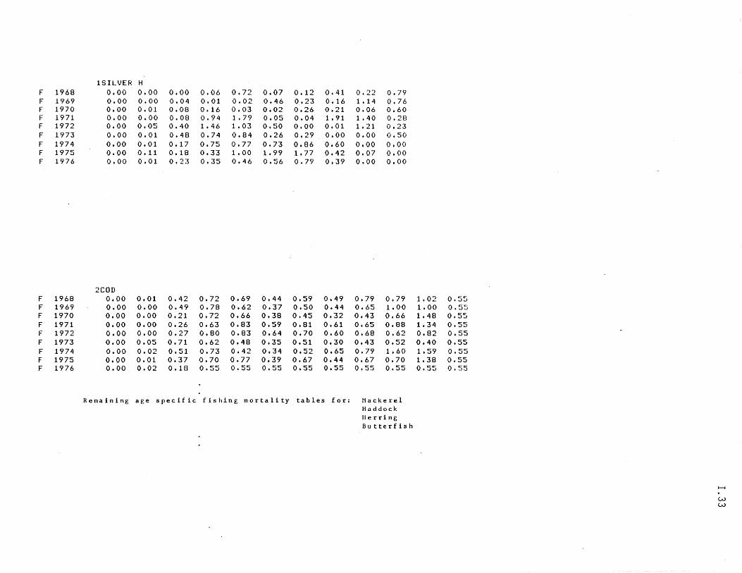
1SILVEF: H F 1968 0.00 0.00 0.00 0.06 0.72 0.07 F 1969 0.00 0.00 0.04 0.01 0.02 0.46 F 1970 0.00 0.01 0.08 0.16 0.03 0.02 F 1971 0.00 0.00 0.08 0.94 1. 79 0.05 F 1972 0.00 0.05 0.40 1.46 1.03 0.50 F 1973 0.00 0.01 0.48 0.74 0.84 0.26 F 1974 0.00 0.01 0.17 0.75 0.77 0.73 F 1975 0.00 0.11 0.18 0.33 1.00 1.99 F 1976 0.00 0.01 0.23 0.35 0.46 0.56
2COD F 1968 0.00 0.01 0.42 0.72 0.69 0.44 F 1969 0.00 0.00 0.49 0.78 0.62 0.37 F 1970 0.00 0.00 0.21 0.72 0.66 0.38 F 1971 0.00 0.00 0.26 0.63 0.83 0.59 F 1972· 0.00 0.00 0.27 0.80 0.83 0.64 F 1973 0.00 0.05 0.71 0.62 0.48 0.35 F 1974 0.00 0.02 0.51 0.73 0.42 0.34 F 1975 0.00 0.01 0.37 0.70 0.77 0.39 F 1976 0.00 0.02 0.18 0.55 0.55 0.55
Remaining age specific fishing mortality
0.12 0.41 0.23 0.16 0.26 0.21 0.04 1. 91 0.00 0.01 0.29 0.00 0.86 0.60 1.77 0.42 0.79 0.39
0.59 0.49 0.50 0.44 0.45 0.32 0.81 0.61 0.70 0.60 0.51 0.30 0.52 0.65 0.67 0.44 0.55 0.55
tables for:
0.22 0.79 1. 14 0.76 0.06 0.60 1.40 0.28 1. 21 0.23 0.00 0.50 0.00 0.00 0.07 0.00 0.00 0.00
0.79 0.79 0.65 1.00 0.43 0.66 0.65 0.88 0.68 0.62 0.43 0.52 0.79 1.60 0.67 0.70 0.55 0.55
Mackerel Haddock Herring Bu tterfish
1. 02 1.00 1. 48 1. 34 0.82 0.40 1.59 1. 38 0.55
0.55 0.55 0.55 0.55 0.55 0.55 0.55 0.55 0.55
I-i
w w
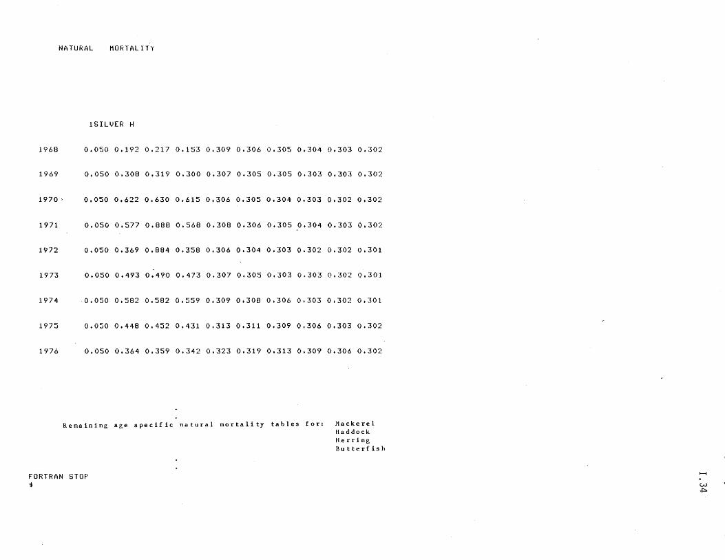
NATURAL MORTALITY
1968
1969
1970 >
1971
1972
1973
1974
1975
1976
lSILVEF: H
0.050 0.192 0.217 0.153 0.309 0.306 0.305 0.304 0.303 0.302
0.050 0.308 0.319 0.300 0.307 0.305 0.305 0.303 0.303 0.302
0.050 0.622 0.630 0.615 0.306 0.305 0.304 0.303 0.302 0.302
0.050 0.577 0.888 0.568 0.308 0.306 0.305 0.304 0.303 0.302
0.050 0.369 0.884 0.358 0.306 0.304 0.303 0.302 0.302 0.301
0.050 0.493 0.490 0.473 0.307 0.305 0.303 0.303 0.302 0.301
0.050 0.582 0.582 0.559 0.309 0.308 0.306 0.303 0.302 0.301
0.050 0.448 0.452 0.431 0.313 0.311 0.309 0.306 0.303 0.302
0.050 0.364 0.359 0.342 0.323 0.319 0.313 0.309 0.306 0.302
Remaining age specific natural mortality tables for: Mackerel Haddock Herring Butterfish
FORTRAN STOP $
I--i
w .p:.
I.35
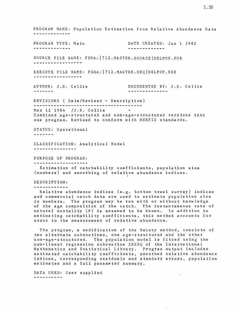
PROGRAM NAME: Population Estimation from Relative Abundance Data
PROGRAM TYPE: Main DATE CREATED: Jan 1 1982
SOURCE FILE NAME: FSHA: [712.MASTER.SOURCE]DELPOP.FOR
EXECUTE FILE NAME: FSHA: [712.MASTER.XEQ]DELPOP.EXE
AUTHOR: J.S. Collie DOCUMENTED BY: J.S. Collie
REVISIONS ( Dite/Reviser - Description)
Mar 12 1984 /J.S. Collie Combined age-structured and non-age-structured versions into one program. Revised to conform with NERFIS standards.
STATUS: Operational
CLASSIFICATION: Analytical Model
PURPOSE OF PROGRAM:
Estimation of catchability coefficients, population size (numbers) and smoothing of relative abundance indices.
DESCRIPTION:
Relative abundance indices (e.g. bottom trawl survey) indices and commercial catch data are used to estimate population size in numbers. The program may be run with or without knowledge of the age composition of the catch. The instantaneous rate of natural mortality (M) is assumed to be known. In addition to estimating catchability coefficients, this method accounts for error in the measurement 6f relative abundance.
The program, a modification of the DeLury method, consists of two alternate subroutines, one age-structured and the other non-age-structured. The.population model is fitted using the non-linear regression subroutine ZXSSQ of the International Mathematics and Statistical Library. Program output includes estimated catchability coefficients, smoothed relative abundance indices, corresponding residuals and standard errors, population estimates and a full parameter summary.
DAIA USED: User supplied
I.36
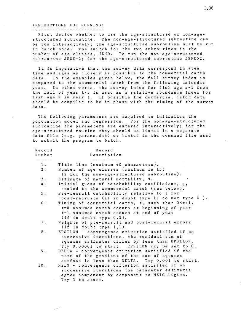
INSTRUCTIONS FOR RUNNING:
First decide whether to use the age-structured or non-agestructured subroutine. The non-age-structured subroutine can be run interactively; the age-structured subroutine must be run in batch mode. The switch for the two subroutines is the number of age classes, JEND. To run the non-age-structured subroutine JEND=2; for the age-structured subroutine JEND>2.
It is imperative that the survey data correspond in area, time and ages as closely as possible to the commercial catch data. In the examples given below, the fall survey index is compared to the commercial catch from the following calendar year. In other words, the survey index for fish age a-l from the fall of year t-l is used as a relative abundance index for fish age a in year t. If possible the commercial catch data should be compiled to be in phase w'ith the timing of the survey da ta.
The following parameters are required to initialize the population model and regression. For the non-age-structured subroutine the parameters are entered interactively; for the age-structured routine they should be listed in a separate data file (e.g. params.dat) or listed in the command file used to submit the program to batch.
Record Record Number Description
1. Title line (maximum 40 characters). 2.> Number of age classes (maximum is 15)
(2 for the non-age-structured subroutine). 3. Estimate of natural mortality, M. 4. Initial guess of catchability coefficient, q,
scaled to the commercial catch (see below). 5. Pre-recruit catchability relative to 1 for
post-recruits (if in doubt type 1; do not type 0 ). 6. Timing of commercial catch, t, such that O<t<l.
t=O assumes catch occurs at beginning of year t=l assumes catch occurs at end of year (if in doubt type 0.5).
7. Weights of pre-recruit and post-recurit errors (if in doubt type 1,1).
8. EPSILON - convergence criterion satisfied if on successive iterations, the residual'sum of squares estimates differ by less than EPSILON. Try 0.00001 to start. EPSILON may be set to O.
9. DELTA -convergence criterion satisfied if the norm of the gradient of the sum of squares surface is less than DELTA. Try 0.001 to start.
10. NSIG - convergence criterion satisfied if on successive iterations the parameter estimates agree component by component to NSIG digits. Try 3 to start.
Convergence is considered achieved if anyone of the three conditions is satisfied. The convergence criteria should be varied until an acceptable fit is obtained. All data input, except the title, is free format.
The survey indices and commercial catch must be scaled so that they are roughly the same magnitude. The catchability coefficient, q, will then be scaled by the same factor. The maximum number of years is 30. Output requires a wide carriage terminal.
I. 37
For the non-age-structured subroutine one data file, 'INFILE', is required with each record consisting of the following: Year, pre-recruit index, post-recruit index, commercial catch.
To run DELPOP with non-age-structured data, type:
$ASSIGN [directory]data.dat INFILE $ASSIGN [directory]output.ext OUTFILE $RUN [7l2.MASTER.XEQ]DELPOP
The age-structured subroutine requires two data files, 'POPFILE' and 'CATFILE'. 'POPFILE' contains the survey catch-at-age data; 'CATFILE' the correspondi~g commercial catch-at-age. Each record should consist of: Year, catch at age 1, catch at age 2, catch at age 3,
To run DELPOP with age-structured data submi~ the following command file:
$ASSIGN [directory]params.dat $ASSIGN [directory]survey.dat $ASSIGN [directory]catch.dat $ASSIGN [directory]output.ext $RUN [712.MASTER.XEQ]DELPOP
REFERENCE S:
FOROOS POPFILE CATFILE OUTFILE
Collie, J.S. and M.P. Sissenwine 1983. Estimating population size from relative abundance data measured with error. Can. J. Fish. Aquat. Sci. 40:1871-1879.
International Mathematical and Statistical Library, 1982. 9 the d i t ion, H 0 u s tO,n T e x as. Vol u m e 4, sub r 0 uti n e Z X S SQ.
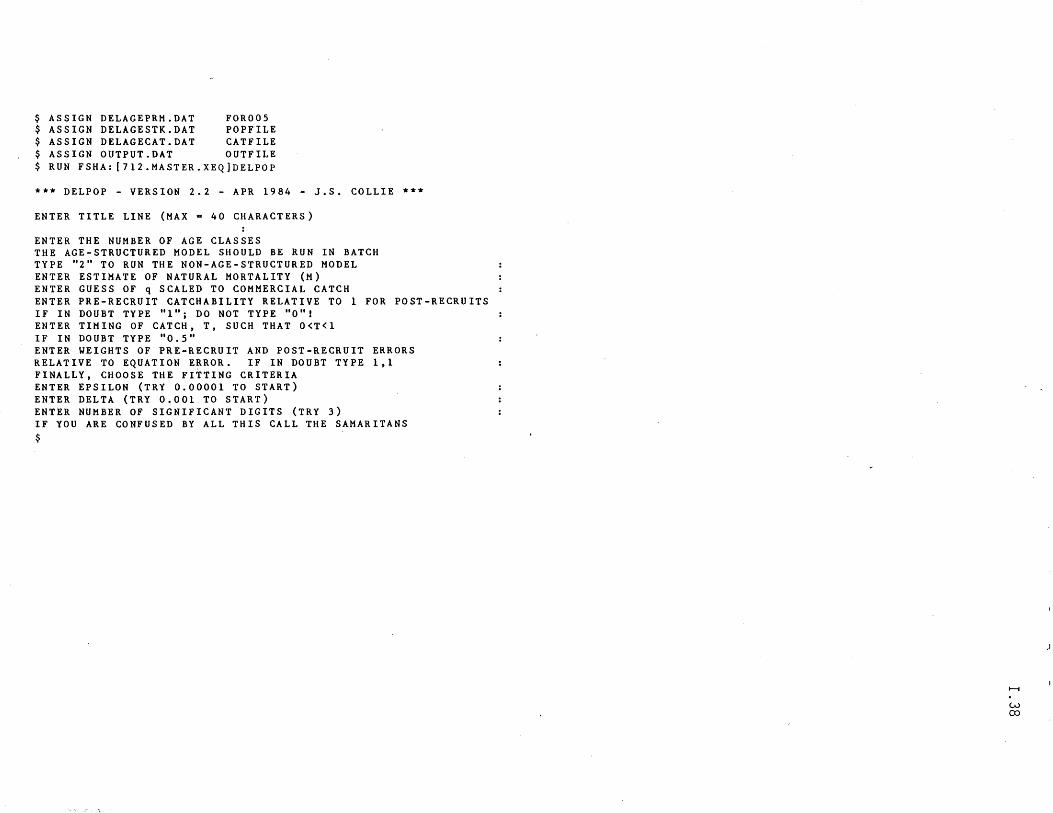
$ ASSIGN DELAGEPRM.DAT FOR005 $ ASSIGN DELAGESTK.DAT POPFILE $ ASSIGN DELAGECAT.DAT CATFILE $ ASSIGN OUTPUT.DAT OUTFILE $ RUN FSHA: [712.MASTER.XEQ]DELPOP
*** DELPOP - VERSION 2.2 - APR 1984 - J.S. COLLIE ***
ENTER TITLE LINE (MAX = 40 CHARACTERS)
ENTER THE NUMBER OF AGE CLASSES THE AGE-STRUCTURED MODEL SHOULD BE RUN IN BATCH TYPE "2" TO RUN THE NON-AGE-STRUCTURED MODEL ENTER ESTIMATE OF NATURAL MORTALITY (M) ENTER GUESS OF q SCALED TO COMMERCIAL CATCH ENTER PRE-RECRUIT CATCHABILITY RELATIVE TO 1 FOR POST-RECRUITS IF IN DOUBT TYPE "1"; DO NOT TYPE "O"! ENTER TIMING OF CATCH, T, SUCH THAT O<T<l IF IN DOUBT TYPE "0.5" ENTER WEIGHTS OF PRE-RECRUIT AND POST-RECRUIT ERRORS RELATIVE TO EQUATION ERROR. IF IN DOUBT TYPE 1,1 FINALLY, CHOOSE THE FITTING CRITERIA ENTER EPSILON (TRY 0.00001 TO START) ENTER DELTA (TRY 0.001 TO START) ENTER NUMBER OF SIGNIFICANT DIGITS (TRY 3) IF YOU ARE CONFUSED BY ALL THIS CALL THE SAMARITANS $
.......
w CO
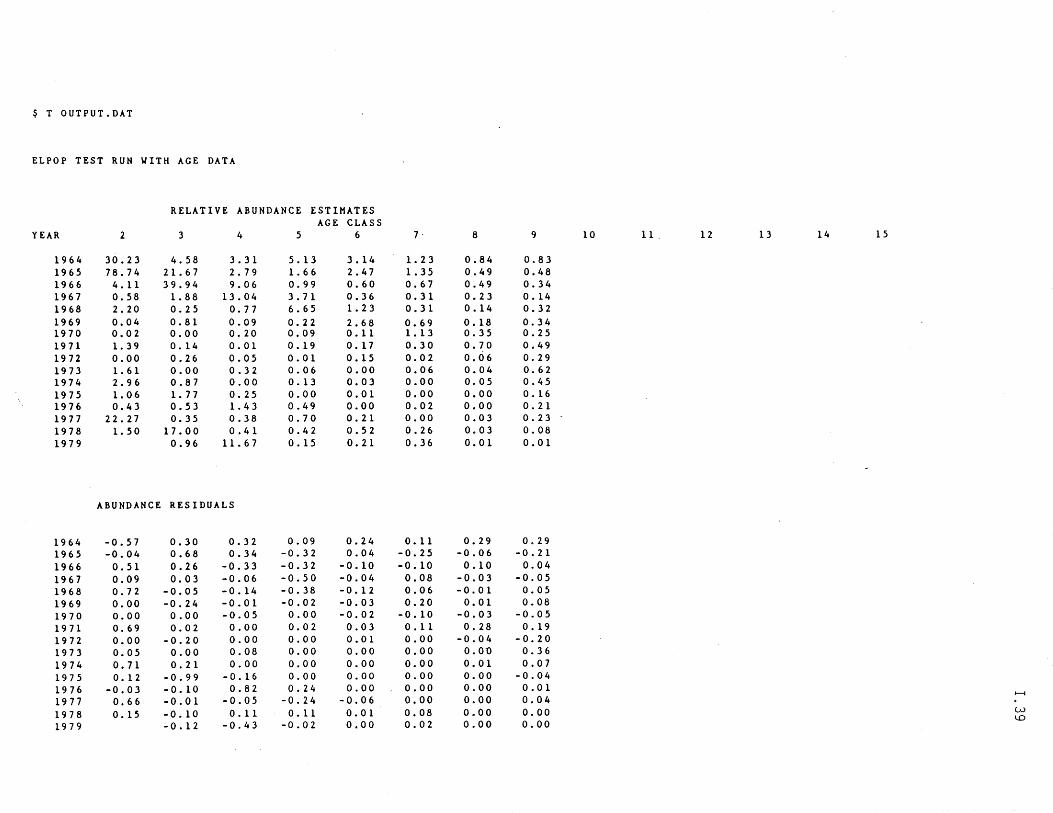
$ T OUTPUT.DAT
ELPOP TEST RUN WITH AGE DATA
RELATIVE ABUNDANCE ESTIMATES AGE CLASS
YEAR 2 3 4 5 6 7· 8 9 10 11. 12 13 14 15
1964 30.23 4.58 3.31 5. 13 3.14 1. 23 0.84 0.83 1965 78.74 21. 67 2. 79 1. 66 2. 47 1. 35 0.49 0.48 1966 4.11 39.94 9.06 0.99 0.60 0.67 0.49 0.34 1967 0.58 1. 88 13.04 3.71 0.36 0.31 0.23 0.14 1968 2.20 0.25 0.77 6.65 1. 23 0.31 0.14 0.32 1969 0.04 0.81 0.09 0.22 2.68 0.69 0.18 0.34 1970 0.02 0.00 0.20 0.09 0.11 1. 13 0.35 0.25 1971 1. 39 0.14 0.01 0.19 0.17 0.30 0.70 0.49 1972 0.00 0.26 0.05 0.01 0.15 0.02 0.06 0.29 1973 1. 61 0.00 0.32 0.06 0.00 0.06 0.04 0.62 1974 2. 9 6 0.87 0.00 0.13 0.03 0.00 0.05 0.45 1975 1. 06 1. 77 0.25 0.00 0.01 0.00 0.00 0.16 1976 0.43 0.53 1. 43 0.49 0.00 0.02 0.00 0.21 1977 22.27 0.35 0.38 0.70 0.21 0.00 0.03 0.23 1978 1. 50 17.00 0.41 0.42 0.52 0.26 0.03 0.08 1979 0.96 11. 67 0.15 0.21 0.36 0.01 0.01
ABUNDANCE RESIDUALS
1964 -0.57 0.30 0.32 0.09 0.24 0.11 0.29 0.29 1965 -0.04 0.68 0.34 -0.32 0.04 -0.25 -0.06 -0.21 1966 0.51 0.26 -0.33 -0.32 -0.10 -0.10 0.10 0.04 1967 0.09 0.03 -0.06 -0.50 -0.04 0.08 -0.03 -0.05 1968 0.72 -0.05 -0.14 -0.38 -0.12 0.06 - 0.01 0.05 1969 0.00 -0.24 -0.01 -0.02 -0.03 0.20 0.01 0.08 1970 0.00 0.00 -0.05 0.00 -0.02 -0.10 -0.03 -0.05 1971 0.69 0.02 0.00 0.02 0.03 0.11 0.28 0.19 1972 0.00 -0.20 0.00 0.00 0.01 0.00 -0.04 -0.20 1973 0.05 0.00 0.08 0.00 0.00 0.00 0.00 0.36 1974 0.71 0.21 0.00 0.00 0.00 0.00 0.01 0.07 1975 0.12 -0.99 - O. 16 0.00 0.00 0.00 0.00 -0.04 1976 -0.03 - 0.10 0.82 0.24 0.00 0.00 0.00 0.01 .......... 1977 0.66 -0.01 -0.05 -0.24 -0.06 0.00 0.00 0.04 1978 0.15 -0.10 O. 11 0.11 0.01 0.08 0.00 0.00 w
1979 -0.12 -0.43 -0.02 0.00 0.02 0.00 0.00 l...O
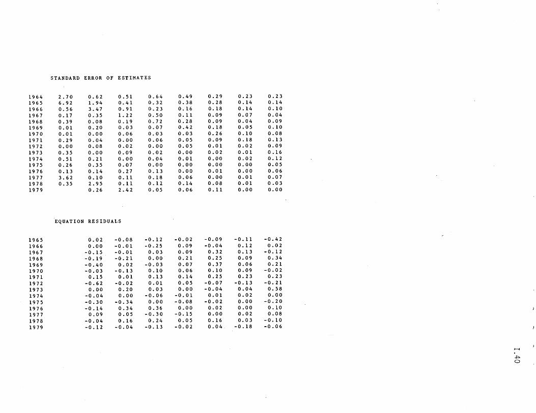
STANDARD ERROR OF ESTIMATES
1964 2.70 0.62 0.51 0.64 0.49 0.29 0.23 0.23 1965 6.92 1. 94 0.41 0.32 0.38 0.28 0.14 0.14 1966 0.56 3.47 0.91 0.23 0.16 0.18 0.14 0.10 1967 0.17 0.35 1. 22 0.50 0.11 0.09 0.07 0.04 1968 0.39 0.08 0.19 0.72 0.28 0.09 0.04 0.09 1969 0.01 0.20 0.03 0.07 0.42 0.18 0.05 0.10 1970 0.01 0.00 0.06 0.03 0.03 0.26 0.10 0.08 1971 0.29 0.04 0.00 0.06 0.05 0.09 0.18 0.13 1972 0.00 0.08 0.02 0.00 0.05 0.01 0.02 0.09 1973 0.35 0.00 0.09 0.02 0.00 0.02 0.01 0.16 1974 0.51 0.21 0.00 0.04 0.01 0.00 0.02 0.12 1975 0.26 0.35 0.07 0.00 0.00 0.00 0.00 0.05 1976 0.13 0.14 0.27 0.13 0.00 0.01 0.00 0.06 1977 3.62 0.10 0.11 0.18 0.06 0.00 0.01 0.07 1978 0.35 2.95 0.11 0.12 0.14 0.08 0.01 0.03 1979 0.26 2. 42 0.05 0.06 0.11 0.00 0.00
EQUATION RESIDUALS
1965 0.02 -0.08 -0.12 -0.02 -0.09 -0.11 -0.42 1966 0.00 -0.01 -0.25 0.09 -0.04 0.12 0.02 1967 -0.15 -0.01 0.03 0.09 0.32 0.13 -0.12 1968 -0.19 -0.21 0.00 0.21 0.25 0.09 0.34 1969 -0.40 0.02 -0.03 0.07 0.37 0.06 0.21 1970 -0.03 -0.13 0.10 0.06 0.10 0.09 -0.02 1971 0.15 0.01 0.13 0.14 0.25 0.23 0.23 1972 -0.62 -0.02 0.01 0.05 -0.07 -0.13 -0.21 1973 0.00 0.20 0.03 0.00 -0.04 0.04 0.58 1974 -0.04 0.00 -0.06 -0.01 0.01 0.02 0.00 1975 -0.30 -0.34 0.00 -0.08 -0.02 0.00 -0.20 1976 -0.14 0.34 0.36 0.00 0.02 0.00 0.10 1977 0.09 0.05 -0.30 -0.15 0.00 0.02 0.08 1978 -0.04 0.16 0.24 0.05 0.16 0.03 -0.10 1979 -0.12 -0.04 -0.13 -0.02 0.04 -0.18 -0.06
I--t
-J::::. 0
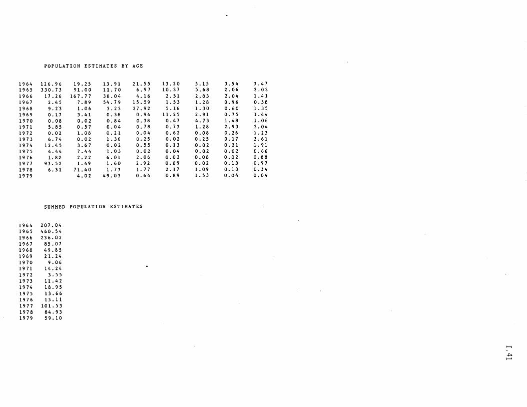
POPULATION ESTIMATES BY AGE
1964 126.96 19.25 13.91 21. 55 1965 330.73 91. 00 11. 70 6.97 1966 17. 26 167.77 38.04 4. 16 1967 2. 45 7. 89 54.79 15.59 1968 9.2"3 1. 06 3.23 27.92 1969 0.17 3.41 0.38 0.94 1970 0.08 0.02 0.84 0.38 1971 5.85 0.57 0.04 0.78 1972 0.02 1. 08 0.21 0.04 1973 6.74 0.02 1. 36 0.25 1974 12. 45 3.67 0.02 0.55 1975 4.44 7.44 1. 03 0.02 1976 1. 82 2. 22 6. 01 2. 06 1977 93.52 1. 49 1. 60 2. 92 1978 6.31 71. 40 1. 73 1. 77 1979 4.02 49.03 0.64
SUMMED POPULATION ESTIMATES
1964 207.04 1965 460.54 1966 236.02 1967 85.07 1968 49.85 1969 21.24 1970 9.06 1971 14.24 1972 3.55 1973 11.42 1974 18.95 1975 13.66 1976 13.11 1977 101.53 1978 84.93 1979 59.10
13.20 5. 15 10.37 5.68
2. 51 2. 83 1. 53 1. 28 5.16 1. 30
11. 25 2. 91 0.47 4.73 0.73 1. 28 0.62 0.08 0.02 0.25 0.13 0.02 0.04 0.02 0.02 0.08 0.89 0.02 2. 17 1. 09 0.89 1. 53
3.54 2. 06 2. 04 0.96 0.60 0.75 1. 48 2. 93 0.26 O. 17 0.21 0.02 0.02 0.13 0.13 0.04
3.47 2. 03 1. 41 0.58 1. 35 1. 44 1. 06 2. 04 1. 23 2. 61 1. 91 0.66 0.88 0.97 0.34 0.04
I-t
...j::::. 1--1
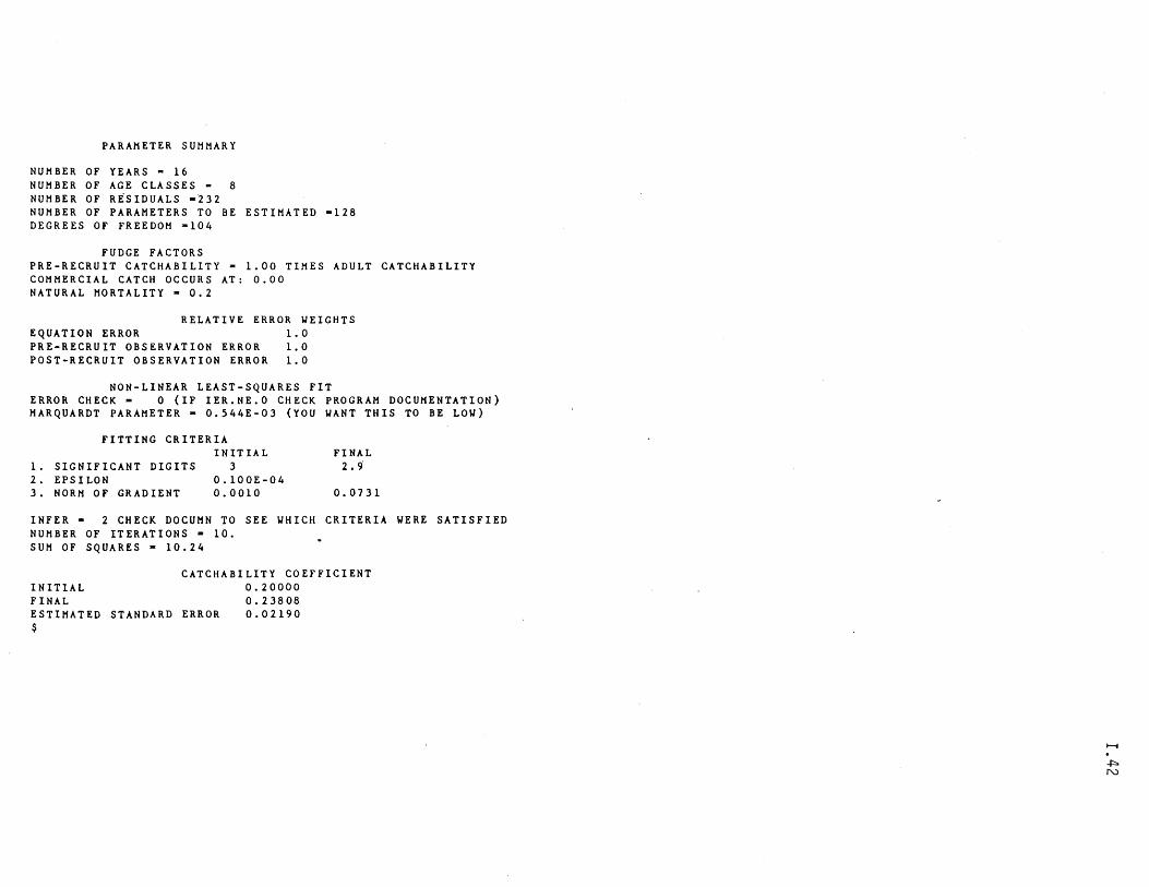
PARAMETER SUMMARY
NUMBER OF YEARS - 16 NUMBER OF AGE CLASSES - 8 NUMBER OF RESIDUALS -232 NUMBER OF PARAMETERS TO BE ESTIMATED -128 DEGREES OF FREEDOM -104
FUDGE FACTORS PRE-RECRUIT CATCHABILITY - 1.00 TIMES ADULT CATCHABILITY COMMERCIAL CATCH OCCURS AT: 0.00 NATURAL MORTALITY - 0.2
RELATIVE ERROR WEIGHTS EQUATION ERROR 1.0 PRE-RECRUIT OBSERVATION ERROR 1.0 POST-RECRUIT OBSERVATION ERROR 1.0
NON-LINEAR LEAST-SQUARES FIT ERROR CHECK - 0 (IF IER.NE.O CHECK PROGRAM DOCUMENTATION) MARQUARDT PARAMETER - 0.544E-03 (YOU WANT THIS TO BE LOW)
FITTING CRITERIA INITIAL
1. SIGNIFICANT DIGITS 3 2. EPSILON 0.100E-04 3. NORM OF GRADIENT 0.0010
FINAL 2.9
0.0731
INFER - 2 CHECK DOCUMN TO SEE WHICH CRITERIA WERE SATISFIED NUMBER OF ITERATIONS - 10. SUM OF SQUARES - 10.24
INITIAL CATCHABILITY COEFFICIENT
0.20000 FINAL ESTIMATED STANDARD ERROR $
0.23808 0.02190
........
+::> N
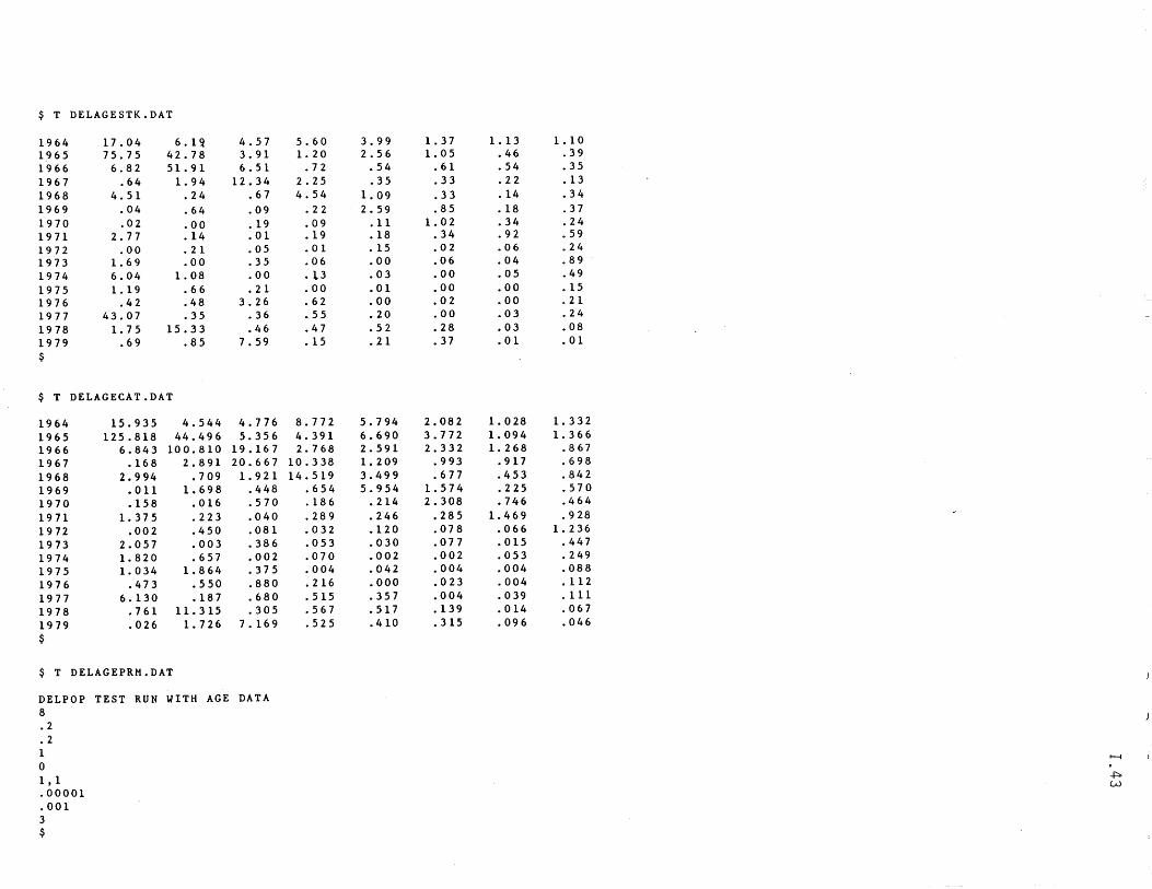
$ T DELAGESTK.DAT
1964 17. 04 6.1'l 4.57 5.60 3.99 1. 37 1. 13 1. 10 1965 75.75 42.78 3.91 1. 20 2.56 1. 05 .46 .39 1966 6.82 51. 91 6.51 .72 .54 .61 .54 .35 1967 .64 1. 94 12.34 2. 25 .35 .33 .22 . 13 1968 4.51 .24 .67 4.54 1. 09 .33 .14 .34 1969 .04 .64 .09 .22 2. 59 .85 .18 .37 1970 .02 .00 .19 .09 .11 1. 02 .34 .24 1971 2. 77 .14 .01 .19 .18 .34 .92 .59 1972 .00 .21 .05 .01 .15 .02 .06 .24 1973 1. 69 .00 .35 .06 .00 .06 .04 .89 1974 6.04 1. 08 .00 .1.3 .03 .00 .05 .49 1975 1. 19 .66 .21 .00 .01 .00 .00 .15 1976 .42 .48 3.26 .62 .00 .02 .00 .21 1977 43.07 .35 .36 .55 .20 .00 .03 .24 1978 1. 75 15.33 .46 .47 .52 .28 .03 .08 1979 .69 .85 7.59 . 15 .21 .37 .01 .01 $
$ T DELAGECAT.DAT
1964 15.935 4.544 4.776 8.772 5.794 2.082 1.028 1. 332 1965 125.818 44.496 5.356 4.391 6.690 3.772 1. 094 1. 366 1966 6.843 100.810 19.167 2.768 2. 591 2.332 1. 268 .867 1967 .168 2.891 20.667 10.338 1.209 .993 .917 .698 1968 2. 994 .709 1.921 14.519 3.499 .677 .453 .842 1969 .011 1.698 .448 .654 5.954 1.574 .225 .570 1970 .158 .016 .570 .186 .214 2.308 .746 .464 1971 1. 375 .223 .040 .289 .246 .285 1. 469 .928 1972 .002 .450 .081 .032 .120 .078 .066 1.236 1973 2. 057 .003 .386 .053 .030 .077 .015 .447 1974 1. 820 .657 .002 .070 .002 .002 .053 .249 1975 1.034 1. 8 64 .375 .004 .042 .004 .004 .088 1976 .473 .550 .880 .216 .000 .023 .004 .112
1977 6.130 .187 .680 .515 .357 .004 .039 . 111 1978 .761 11.315 .305 .567 .517 .139 .014 .067 1979 .026 1.726 7. 169 .525 .410 .315 .096 .046
$
$ T DELAGEPRM.DAT
DELPOP TEST RUN WITH AGE DATA 8 .2 .2 1 t-I
0 1, 1 +::>0
w .00001 .001 3 $
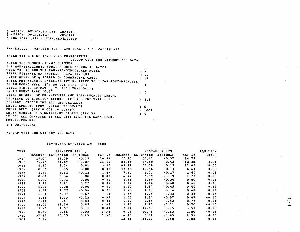
$ ASSIGN DELNOAGES.DAT INFILE $ ASSIGN OUTPUT.DAT OUTFILE $ RUN FSHA: [712.MASTER.XEQ).DELPOP
••• DELPOP - VERSION 2.2 - APR 1984 - J.S. COLLIE •••
ENTER TITLE LINE (MAX - 40 CHARACTERS) : DELPOP TEST RUN WITHOUT AGE DATA
ENTER THE NUMBER OF AGE CLASSES THE AGE-STRUCTURED MODEL SHOULD BE RUN IN BATCH TYPE "2" TO RUN THE NON-AGE-STRUCTURED MODEL 2 ENTER ESTIMATE OF NATURAL MOR~ALITY (M) .2 ENTER GUESS OF q SCALED TO COMMERCIAL CATCH ~2 ENTER PRE-RECRUIT CATCHABILITY RELATIVE TO 1 FOR POST-RECRUITS IF IN DOUBT TYPE "I"; DO NOT TYPE "O"! 1 ENTER TIMING OF CATCH, T, SUCH THAT O<T<l IF IN DOUBT TYPE "0.5" 0 ENTER WEIGHTS OF PRE-RECRUIT AND POST-RECRUIT ERRORS RELATIVE TO EQUATION ERROR. IF IN DOUBT TYPE 1,1 1,1 FINALLY, CHOOSE THE FITTING CRITERIA ENTER EPSILON (TRY 0.00001 TO START) 0 ENTER DELTA (TRY 0.001 TO START) .001 ENTER NUMBER OF SIGNIFICANT DIGITS (TRY 3) 4 IF YOU ARE CONFUSED BY ALL THIS CALL THE SAMARITANS SUCCESSFUL RUN
$ T OUTPUT.DAT
DELPOP TEST RUN WITHOUT AGE DATA
ESTIMATED RELATIVE ABUNDANCE
YEAR PRE-RECRUITS POST-RECRUITS OBSERVED ESTIMATED RESIDUAL EST SE OBSERVED ESTIMATED RESIDUAL
1964 17. 04 21. 39 -0.23 10.59 23.95 34.61 -0.37 1965 75.75 81. 49 -0.07 26.15 52.35 34.50 0.42 1966 6.82 6.74 0.01 3.56 61. 21 52.59 0.15 1967 0.65 0.65 0.00 0.35 17.56 19.96 -0.13 1968 4.51 5.12 -0.13 2.47 7.35 8.72 -0.17 1969 0.04 0.04 0.00 0.02 4.94 5.99 -0.19 1970 0.02 0.02 0.00 0.01 1. 99 2. 69 -0.30 1971 2. 77 2. 21 0.22 0.89 2. 37 1. 46 0.48 1972 0.00 0.00 0.00 0.00 1. 19 1. 87 -0.45 1973 1. 69 1. 77 -0.04 0.75 1. 40 1. 21 0.14 1974 6.04 3.09 0.67 1. 15 1. 78 1. 29 0.32 1975 1. 19 1. 35 -0.13 0.67 1. 03 2. 12 -0.97 1976 0.42 0.41 0.03 0.21 4.59 2. 69 0.53 1977 43.01 18.30 0.85 4.47 1. 73 1. 93 -0.11 1978 1. 75 1. 57 o. 11 0.83 17.17 14.83 0.15 1979 0.69 0.66 0.05 0.35 9.19 10.49 -0.13 1980 37.29 2J.85 0.45 9.52 4.38 6.88 -0.45 1981 2. 22 13.21 21. 71 -0.50
EQUATION EST SE ERROR
14.77 12. 28 0.01 11. 66 0.00
4.41 0.00 2.65 0.01 1. 22 0.03 0.80 0.08 0.60 0.23 0.60 -0.12 0.48 0.14 0.56 0.03 0.87 -0.26 t-t
0.77 0.11 ..J:::>o 0.70 -0.10 ..J:::>o
3.51 -0.06 2. 80 -0.08 2.35 -0.08 7.83 -0.02
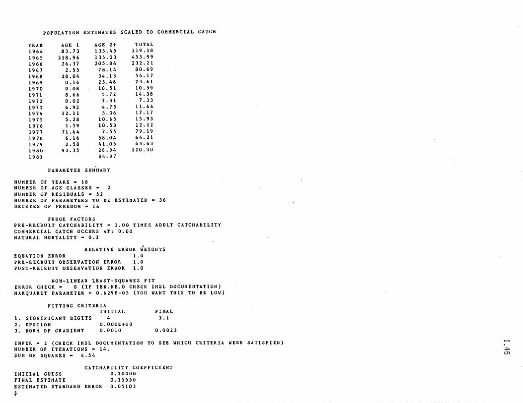
POPULATION ESTIMATES SCALED TO COMMERCIAL CATCH
YEAR AGE 1 AGE 2+ TOTAL 1964 83.73 135.45 219.18 1965 318.96 135.03 453.99 1966 26.37 205.84 232.21 1967 2.55 78.14 80.69 1968 20.04 34.13 54.17 1969 0.16 23.46 23.61 1970 0.08 10.51 10.59 1971 8.66 5.72 14.38 1972 0.02 7.31 7. 33 1973 6.92 4.75 11. 66 1974 12. 11 5.06 17. 17 1975 5.28 10.65 15.93 1976 1. 59 10.53 12. 12 1977 71. 64 7. 55 79. 19 1978 6.16 58.04 64.21 1979 2. 58 41. 05 43.63 1980 93.35 26.94 120.30 1981 84.97
PARAMETER SUMMARY
NUMBER OF YEARS - 18 NUHBER OF AGE CLASSES - 2 NUHBER OF RESIDUALS - 52 NUHBER OF PARAMETERS TO BE ESTIMATED - 36 DEGREES OF FREEDOH - 16
FUDGE FACTORS PRE-RECRUIT CATCHABILITY - 1.00 TIMES ADULT CATCHABILITY COMHERCIAL CATCH OCCURS AT: 0.00 NATURAL HORTALITY - 0.2
RELATIVE ERROR UEIGHTS EQUATION ERROR 1.0 PRE-RECRUIT OBSERVATION ERROR 1.0 POST-RECRUIT OBSERVATION ERROR 1.0
NON-LINEAR LEAST-SQUARES FIT ERROR CHECK - 0 (IF IER.NE.O CHECK IMSL DOCUMENTATION) MARQUARDT PARAMETER - 0.629E-05 (YOU UANT THIS TO BE LOU)
FITTING CRITERIA INITIAL
1. SIGNIFICANT DIGITS 2. EPSILON J. NORM OF GRADIENT
4 O.OOOE+OO 0.0010
FINAL 3.1
0.0023
INFER - 2 (CHECK IHSL DOCUMENTATION TO SEE UHICH CRITERIA UERE SATISFIED) NUMBER OF ITERATIONS - 14. SUM OF SQUARES - 4.54
INITIAL GUESS FINAL ESTIMATE
CATCHABILITY COEFFICIENT 0.20000
ESTIHATED STANDARD ERROR $
0.25550 0.05103
1-1
~ Ul
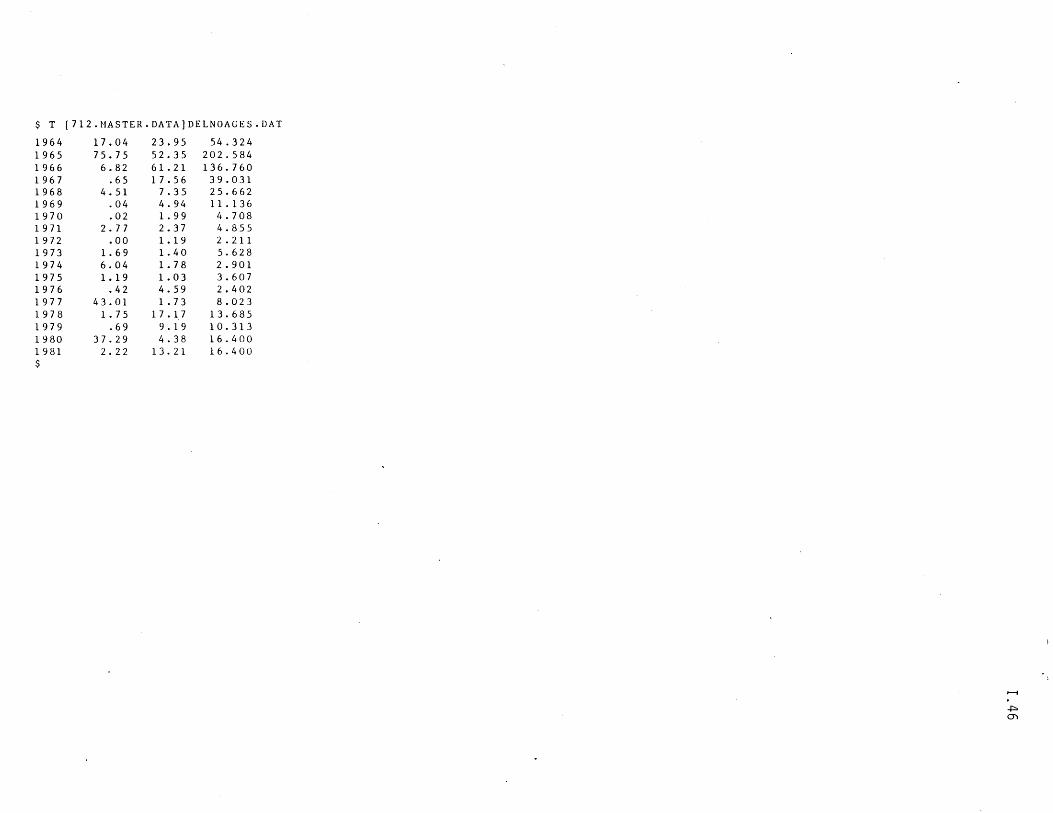
$ T
1964 1965 1966 1967 1968 1969 1970 1971 1972 1973 1974 1975 1976 1977 1978 1979 1980 1981 $
[712.MASTER.DATA]DELNOAGES.DAT
17.04 23.95 54.324 75.75 52.35 202.584 6.82 61.21 136.760
.65 1 7 .56 39.031 4.51 7.35 25.662
.04 4.94 11.136
.02 1. 99 4.708 2.77 2.37 4.855
.00 1. 19 2 .211 1. 69 1. 40 5.628 6.04 1. 78 2.901 1. 19 1. 03 3.607
.42 4.59 2.402 43.01 1. 73 8.023
1. 75 17.17 13.685 .69 9. 19 10.313
37.29 4.38 16.400 2.22 13. 21 16.400
;......j
...f::::. en
PROGRAM NAME: Analysis of a Catch Curve
PROGRAM TYPE: Main DATE CREATED: Jan 1 1964
SOURCE FILE NAME: FSHA: [7l2.MASTER.SOURCE]CATCURV.FOR
EXECUTE FILE NAME: FSHA: [7l2.MASTER.XEQ]CATCURV.EXE
AUTHOR: L.E. Gales DOCUMENTED BY: S.H. Clark
REVISIONS ( Date/Reviser - Description)
Jan 16 1984 /F.P. Almeida, S.H. Clark Converted to FORTRAN77 to run on VAXll/780
STATUS: Operational
CLASSIFICATION: Analytical Model
PURPOSE OF PROGRAM:
1.47
The program analyzes a vector of ca"tch at age data and provides estimates of the survival rate (S), the instantaneous total mortality rate (Z), and associated statistical measures (variances, standard errors and confidence limits). Options are available to evaluate assumptions concerning age at full r e c r u i t men t , to com bin e d a t a for w h i c hag e s are un c"e r t a in, and to subdivide the catch curve and analyze resulting segments separately.
DESCRIPTION:
The program employs a series of algorithms to analyze catch curve data as presented by Chapman and Robson (1960) and Robson and Chapman (1961). The user should consult these papers before running CATCURV. A description of each option and the algorithms used is given in the following sections.
Option 1: Assumes constant recruitment and survival, that all ages in the catch vector are fully available to the fishing/sampling gear, and all ages are known. Let N(O), N(l), N(2) .... be the numbers of fish caught at (coded) ages 0, 1, 2 ... 1; let n = total number summed over all ages, and let T = N(l) + 2N(2) + 3N(3) + ... + IN(I). Then S = T/(T + n - 1) and the variance, standard error, and confidence interval about this estimate are calculated. An estimate is also provided for the instantaneous total mortality rate (Z) together with
1.48
variance, standard error, and confidence interval, as for S:
S ( survival rate) T/(T + n - 1)
variance of S S[S - (T - l)/(n + T - 2)]
standard error of S SQRT(Variance of S)
confidence interval about S S + 2(Standard error of S) to S - 2(Standird error of S)
Option 2: Tests the hypothesis that the relative frequency in the first age group does not deviate significantly from that observed for older ages, i.e. that the first age group is fully available. Heinke's estimate of S (n - N(O»/n is calculated and used with the estimate of S derived in Option 1. If Chi exceeds the tabular value (use 3.84) with 1 degree of freedom, then a significant deficit in N(O) is implied, which could result from incomplete vulnerability or other factors (Robson and Chapman 1961). Data are recoded (N(l) to N(O), N(2) to N ( 1 ), etc.) and cal cuI a t ion s rep eat e dun til the s ta tis tic i s less than the value of Chi entered, after which computations and output are then the same as under Option 1.
Option 3: May be used when ages for older groups are uncertain. If ages above N(K) are uncertain, data for the N(K + 1) group and all older groups are eombined, viz. m = N(K + 1) + ... N(I) where N(I) is the last observation in the data set. Calculations are then performed as under Option 1 using the vector N(l), N(2), N(3) m. The user enters the K value corresponding to the last known age (K = 1, N).
Option 4: Computes the same output as Option 1 for each segment of the catch vector defined by the user, e.g. K values 1 to 3, 2 to 4, etc. The program allows use of overlapping segments, i.e. one age group may appear in more than one segment. The user specifies the K values corresponding to the derived segment endpoints.
DATA USED: User supplied
INSTRUCTIONS FOR RUNNING:
Input values are free - formatted; data values should be entered separated by commas. Program output requires a wide carriage terminal. To run the program, type:
$RUN FSHA:[712.MASTER.XEQ]CATCURV
The user is then prompted for an identifier title (40 byte maximum), catch values, and option number and age at full recruitment (may be different from the first value entered). Following each run, the user may rerun the program with a different option and/or new catch values. A different age at
full recruitment can also be requested by changing the appropiate value on the "option" record.
1.49
The user may also choose to create a data file and use the following:
$ASSIGN datafile.DAT FOR005 $RUN FSHA: [712.MASTER.XEQ]CATCURV
Restrictions: Number of age groups less than or equal to 1000 and number of segments less than or equal to 10.
REFERENCES:
Chapman, D.G. and D.S. Robson 1960. The analysis of a catch curve. Biometrics 16:354-368.
Robson, D.S. and D.G. Chapman 1961. Catch curves and mortality rates. Trans. Am. Fish. Soc. 90: 181:--189.
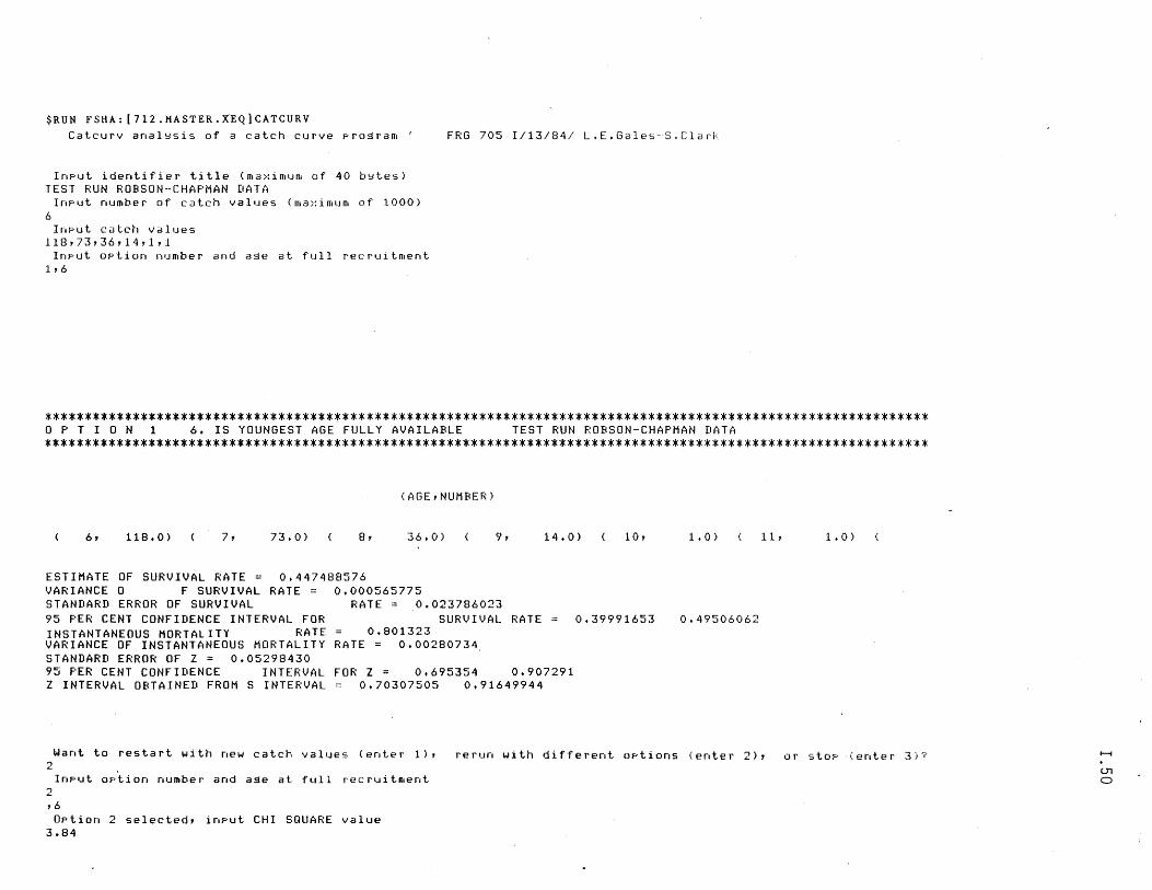
$RUN FSHA: [712.MASTER.XEQ)CATCURV Catcurv anal~sis of a catch curve pro~raffi I
Input identifier title (ffiaxiffiuffi of 40 b~tes) TEST RUN ROBSON-CHAPMAN DATA
Input nUffiber of catch valu~s (ffiaxiffiuffi of 1000) 6
Input catch values 118,73,36,14,1,1
Input option nUffiber and a~e at full recruitment 1,6
FRG 705 1/13/84/ L.E.Gales-S.Clark
************************************************************************************************************** OPT ION 1 6. IS YOUNGEST AGE FULLY AVAILABLE TEST RUN ROBSON-CHAPMAN DATA **************************************************************************************************************
(AGE,NUMBER)
6, 118.0) 7, 73.0) 8, 36.0) 9, 14.0) 10, 1.0) 11, 1. 0)
ESTIMATE OF SURVIVAL RATE = 0.447488576 VARIANCE 0 F SURVIVAL RATE = 0.000565775 STANDARD ERROR OF SURVIVAL RATE = ,0.023786023 95 PER CENT CONFIDENCE INTERVAL FOR SURVIVAL RATE 0.39991653 0.49506062 INSTANTANEOUS MORTALITY RATE 0.801323 VARIANCE OF INSTANTANEOUS MORTALITY RATE = 0.00280734, STANDARD ERROR OF Z = 0.05298430 95 PER CENT CONFIDENCE INTERVAL FOR Z = 0.695354 0.907291 Z INTERVAL OBTAINED FROM S INTERVAL 0.70307505 0.91649944
Want to restart with new catch values (enter 1), rerun with different options (enter 2), or stop (enter 3)7 2
Input option number and a~e at full recruitment 2 ,6 Option 2 selected, input CHI SQUARE value
3.84
t--t
U1 o
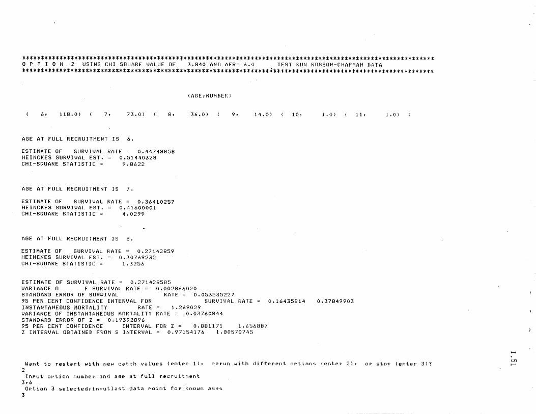
************************************************************************************************************** OPT ION 2 USING CHI SQUARE VALUE OF 3.840 AND AFR= 6.0 TEST RUN ROBSON-CHAPMAN DATA
******************************************************************i*******************************************
(AGE, NUMBEF:)
6, 118.0) 7, 73.0) 8, 36.0) 9, 14.0) 10,
AGE AT FULL RECRUITMENT IS 6.
ESTIMATE OF SURVIVAL RATE = 0.44748858 HEINCKES SURVIVAL EST. 0.51440328 CHI-SQUARE STATISTIC = 9.8622
AGE AT FULL RECRUITMENT IS 7.
ESTIMATE OF SURVIVAL RATE = 0.36410257 HEINCKES SURVIVAL EST. 0.41600001 CHI-SQUARE STATISTIC = 4.0299
AGE AT FULL RECRUITMENT IS 8.
ESTIMATE OF SURVIVAL RATE = 0.27142859 HEINCKES SURVIVAL EST. 0.30769232 CHI-SQUARE STATISTIC = 1.3256
ESTIMATE OF SURVIVAL RATE = 0.271428585 VARIANCE 0 F SURVIVAL RATE = 0.002866020 STANDARD ERROR OF SURVIVAL RATE = 0.053535227 95 PER CENT CONFIDENCE INTERVAL FOR SURVIVAL RATE Q.16435814 INSTANTANEOUS MORTALITY RATE 1.269029 VARIANCE OF INSTANTANEOUS MORTALITY RATE = 0.03760844 STANDARD ERROR OF Z = 0.19392896 95 PER CENT CONFIDENCE INTERVAL FOR Z = 0.881171 1.656887 Z INTERVAL OBTAINED FROM S INTERVAL 0.97154176 1.80570745
1. 0) 11, 1. 0)
0.37849903
Want to restart with new catch values (enter 1), rerun with different options (enter 2), or stop (enter 3)1 2 Input option number and a~e at full recruitment
3,6 Option 3 selected,inputlast data point for known ades
3
1-1
U1 .......
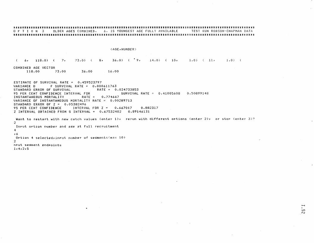
************************************************************************************************************** OPT ION 3 OLDER AGES COMBINED. 6. IS YOUNGEST AGE FULLY AVAILABLE TEST RUN ROBSON-CHAPMAN DATA
**************************************************************************************************************
(AGE, tWMBEF:)
6, 118.0) 7, 73.0) 8, 36.0) 9, 14.0) 10,
COMBINED AGE VECTOR 118.00 73.00 36.00 16.00
ESTIMATE OF SURVIVAL RATE = 0.459523797 VARIANCE 0 F SURVIVAL RATE = 0.000611763 STANDARD ERROR OF SURVIVAL RATE = 0.024733853 95 PER CENT CONFIDENCE INTERVAL FOR SURVIVAL RATE 0.41005608 INSTANTANEOUS MORTALITY RATE 0.774667 VARIANCE OF INSTANTANEOUS MORTALITY RATE = 0.00289713 STANDARD ERROR OF Z = 0.05382496 95 PER CENT CONFIDENCE INTERVAL FOR Z = 0.667017 0.882317 Z INTERVAL OBTAINED FROM S INTERVAL 0.67532402 0.89146131
1. 0) 11. , 1.0)
0.50899148
Want to restart with new catch values (enter 1), rerun with different options (enter 2), or stop (enter 3)? 2
Input option number and aSe at full recruitment 4 ,6 Option 4 selected,input number of seSments(max 10)
2 nput seSment endpoints 1,4,2,5
1-1
Ul N
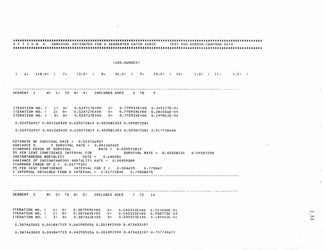
************************************************************************************************************** OPT ION 4 SURVIVAL ESTIMATES FOR A SEGMENTED CATCH CURVE TEST RUN ROBSON-CHAPMAN DATA
**************************************************************************************************************
(AGE,NUMBER)
6, 118.0) 7, 73.0) 8, 36.0) 9, 14.0) 10,
SEGMENT 1 N( 1) TO N( 4) INCLUDES AGES 6 TO 9
ITERATION NO. l) S= 0.524717E+00 X= 0.775934E+00 0.369177E-01 ITERATION NO. 2) S= 0.524727E+00 X= 0.775934E+00 0.281036E-04 I TERAT.I ON NO. 3) S= 0.524727E+00 X= 0.775934E+00 o • 1 4 9 ()'12 E - 0 6
0.524726927 0.001265425 0.035572819 0.453581303 0.595872581
0.524726927 0.001265425 0.035572819 0.453581303 0.595872581 0.517728448
ESTIMATE OF SURVIVAL RATE = 0.524726927 VARIANCE 0 F SURVIVAL RATE = 0.001265425 STANDARD ERROR OF SURVIVAL RATE = 0.035572819 95 PER CENT CONFIDENCE INTERVAL FOR SURVIVAL RATE 0.45358130 INSTANTANEOUS MORTALITY RATE 0.640281 VARIANCE OF INSTANTANEOUS MORTALITY RATE = 0.00459589 STANDARD ERROR OF"Z = 0.06779301 95 PER CENT CONFIDENCE INTERVAL FOR Z = 0.504695 0.775867 Z INTERVAL OBTAINED FROM S INTERVAL 0.51772845 0.79058075
SEGMENT 2 N( 2) TO N( 5) INCLUDES AGES 7 TO 10
ITERATION NO. l) S= 0.387559E+00 X= 0.540323E+00 0.253430E-Ol ITERATION NO. 2) S= 0.387463E+00 X= 0.540323EtOO 0.9-38773E---04 ITERATION NO. ( 3) S= 0.387463EtOO X= 0.540323E+00 0.149012E-06
0.387463003 0.001847715 0.042985056 0.301492900 0.473433107
0.387463003 0.001847715 0.042985056 0.301492900 0.473433107 0.747744679
1 .0) 11 ~ 1.'0 )
0.59587258
I--t
Ul w
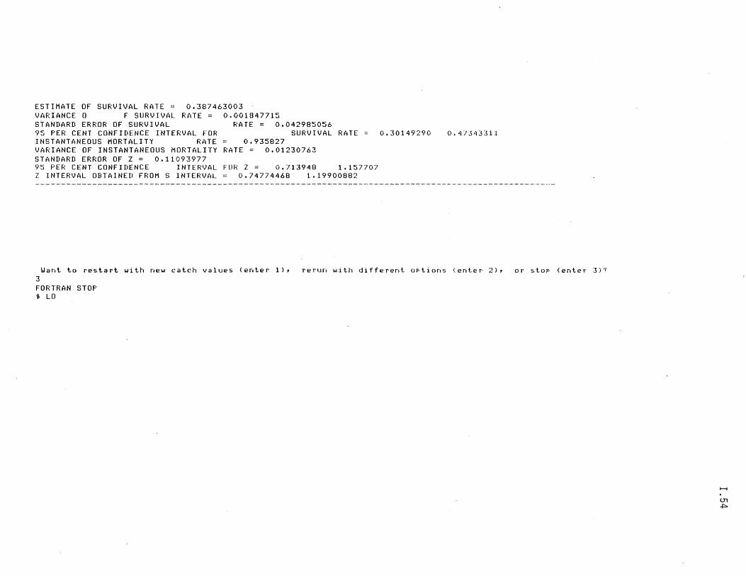
ESTIMATE OF SURVIVAL RATE = VARIANCE 0 F SURVIVAL StANDARD ERROR OF SURVIVAL
0.387463003 RATE = 0.001847715
95 PER CENT CONFIDENCE INTERVAL FOR INSTANTANEOUS MORTALITY RATE VARIANCE OF INSTANTANEOUS MORTALITY STANDARD ERROR OF Z = 0.11093977
RATE = 0.042985056 SURVIVAL RATE
0.935827 RATE = 0.01230763
95 PER CENT CONFIDENCE INTERVAL FOR Z = 0.713948 1.157707 Z INTERVAL OBTAINED FROM S INTERVAL 0.74774468 1.19900882
0.30149290 0.47343311
Want to restart with new catch values (enter 1), rerun with different options (enter 2), or stop (enter 3)? 3 FORTRAN STOP $ LO
~
U1 .,J:::.
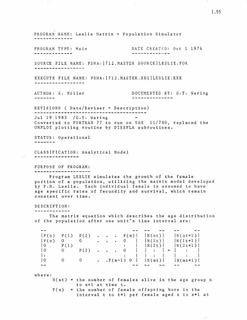
PROGRAM NAME: Leslie Matrix - Population Simulator
PROGRAM TYPE: Main DATE CREATED: Oct 1 1974
SOURCE FILE NAME: FSHA: [712.MASTER SOURCE]LESLIE.FOR
EXECUTE FILE NAME: FSHA: [712.MASTER.XEQ]LESLIE.EXE
AUTHOR: S. Miller DOCUMENTED BY: G.T. Waring
REVISIONS ( Date/Reviser - Description)
Jul 19 1983 /G.T. Waring Converted to FORTRAN 77 to run on VAX 11/780, replaced the UMPLOT plotting routine by DISSPLA subroutines.
STATUS: Operational
CLASSIFICATION: Analytical Model
PURPOSE OF PROGRAM:
I.55
Program LESLIE simulates the growth of the female portion of a population, utilizing the matrix model developed by P.H. Leslie. Each individual female is assumed to have age specific rates of fecundity and survival, which remain constant over time.
DESCRIPTION:
The matrix equation which describes the age distribution of the population after one unit's time interval are:
IF(o) F(l) Ip(o) 0 10 P(l) 10 0 1 : 10 0
where: N(xt)
F(x)
F(2) F (m) 1 IN(ot) 1 IN(ot+1)1 0 0 1 IN(lt) 1 IN(lt+1)1
1 IN(2t) 1 IN(2t+1)1 P(2) 0 I 1 1 1 1
I I 1 1 : 1 0 .P(m-1) 0 1 IN(mt) 1 IN(mt+1)1
the number of females alive in the age group x to x+1 at time t. the number of female offspring born in the interval t to t+1 per female aged x to x+l at
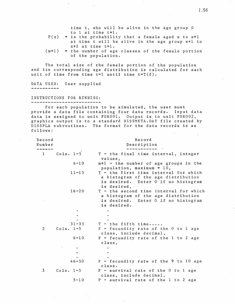
P(x)
(m+1)
time t, who will be alive in the age group P to 1 at time t+1.
'I.56
is the probability that a female aged x to x+1 at time t will be alive in the age group x+1 to x+2 at time t+1. the number of age classes of the female portion of the population.
The total size of the female portion of the population and its corresponding age distribution is calculated for each unit of time from time t=l until time t=T(f).
DATA USED: User supplied
INSTRUCTIONS FOR RUNNING:
For each population to be simulated, the user must provide a data file containing four data records. Input data data is assigned to unit FOR001. Output is to unit FOR002, graphics output is to a standard DISSMETA.DAT file created by DISSPLA subroutines. The format for the data records is as follows:
Record Number
1
2
3
Cols. 1-5
6-10
11-15
16-20
31-35 Cols. 1-5
6-10
46-50
Cols. 1-5
5-10
Record Description
T - the final time interval, integer values,
m+1 - the number of age groups in the population, maximum = 10,
T - the first time interval for which a histogram of the age distribution is desired. Enter 0 if no histogram is desired,
T - the second time interval for which a histogram of the age distribution is desired. Enter 0 if no histogram is desired.
T - the fifth time .•... F - fecundity rate of the 0 to 1 age class, include decimal,
F - fecundity rate of the 1 to 2 age class,
F - fecundity rate of the 9 to 10 age class.
P - survival rate of the 0 to 1 age class, include decimal,
P - survival rate of the 1 to 2 age
1.57
class,
46-50 P - survival rate of the 9 to 10 age class.
4 Co1s. 1-5 N - number of females aged 0 to 1 at time t=l, integer values,
6-10 N - number of females aged 1 to 2 at time t=l,
46-50 N - number of females aged 9 to 10 at time t=l.
Input, interactively, the scaling factor for the Y-axis of the total population size plot. To determine a reasonable factor, examine the total sizes of each time interval from the tabular output.
Records 2, 3 and 4 should contain m+1 data values each. All data must be right justifi,ed in the fields of columns indicated.
To run the program enter the following commands:
$ASSIGN [directory]datafile.DAT FOROOl $ASSIGN SYS$OUTPUT FOR002 $RUN DSKA:[712.MASTER.XEQ]LESLIE
The output from the program consists of tables of agespecific population sizes for each time interval. Graphic output is of two forms:
(1) A histogram of the percent of the total population size in each age class and a listing of the number of females in each age class is printed at time t=l, T(l), T(2), T(3), T(4), T(5), and T(f). This allows the user to select up to five time intervals for which a histogram is desired. The program automatically produces a histogram at time t=l and t=T(f).
(2) A graph plotting the total population size versus time is printed for time t=l until time t=T(f).
REFERENCE S:
Leslie, P.R. 1945. On the use of matrices in certain population mathematics. Biometrika 23:183-212
Pielou, E.C. 1969. An introduction to mathematical ecology. Wiley, New York
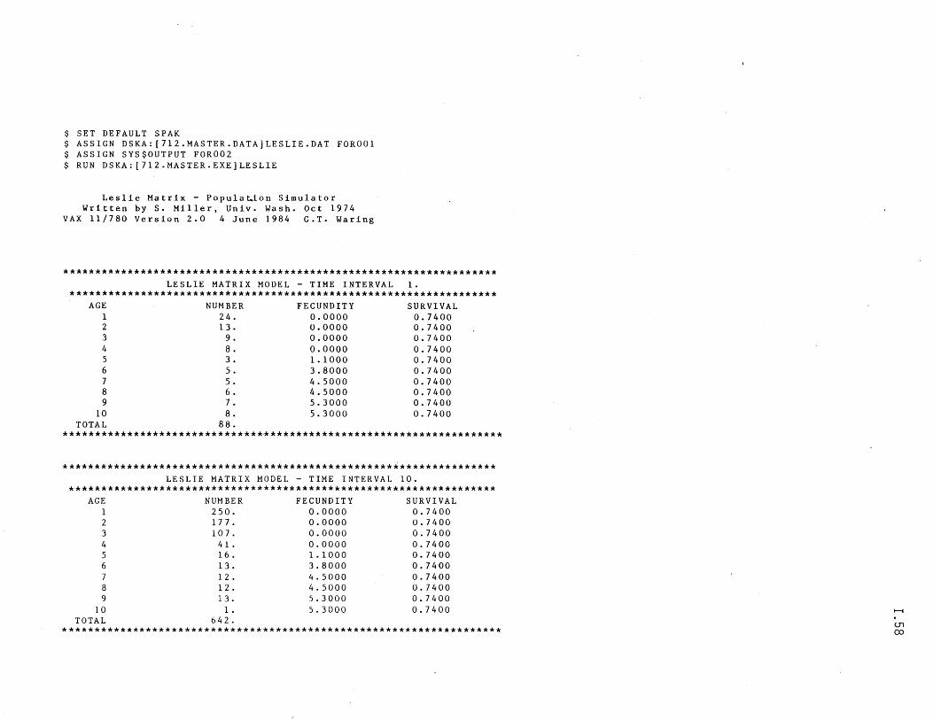
$ SET DEFAULT SPAK $ ASSIGN DSKA:[712.MASTER.DATA]LESLIE.DAT FOR001 $ ASSIGN SYS$OUTPUT FOR002 $ RUN DSKA:[712.MASTER.EXE]LESLIE
Leslie Matrix - Popula~ion Simulator Written by S. Miller, Univ. Wash. Oct 1974
VAX 11/780 Version 2.0 4 June 1984 G.T. Waring
******************************************************************* LESLIE MATRIX MODEL - TIME INTERVAL 1.
****************************************************************** AGE NUMBER FECUNDITY SURVIVAL
1 24. 0.0000 0.7400 2 13. 0.0000 0.7400 3 9. 0.0000 0.7400 4 8. 0.0000 0.7400 5 3. 1.1000 0.7400 6 5. 3.8000 0.7400 7 5. 4.5000 0.7400 8 6. 4.5000 0.7400 9 7. 5.3000 0.7400
10 8. 5.3000 0.7400 TOTAL 88.
*******************************~************************************
******************************************************************* LESLIE MATRIX MODEL - TIME INTERVAL 10.
****************************************************************** AGE NUMBER FECUNDITY SURVIVAL
1 250. 0.0000 0.7400 2 177. 0.0000 0.7400 3 107. 0.0000 0.7400 4 41- 0.0000 0.7400 5 16. 1.1000 0.7400 6 13. 3.8000 0.7400 7 12. 4.5000 0.7400 8 12. 4.5000 0.7400 9 13. 5.3000 0.7400
10 1. 5.3000 0.7400 TOTAL 642.
********************************************************************
........
<J1 OJ
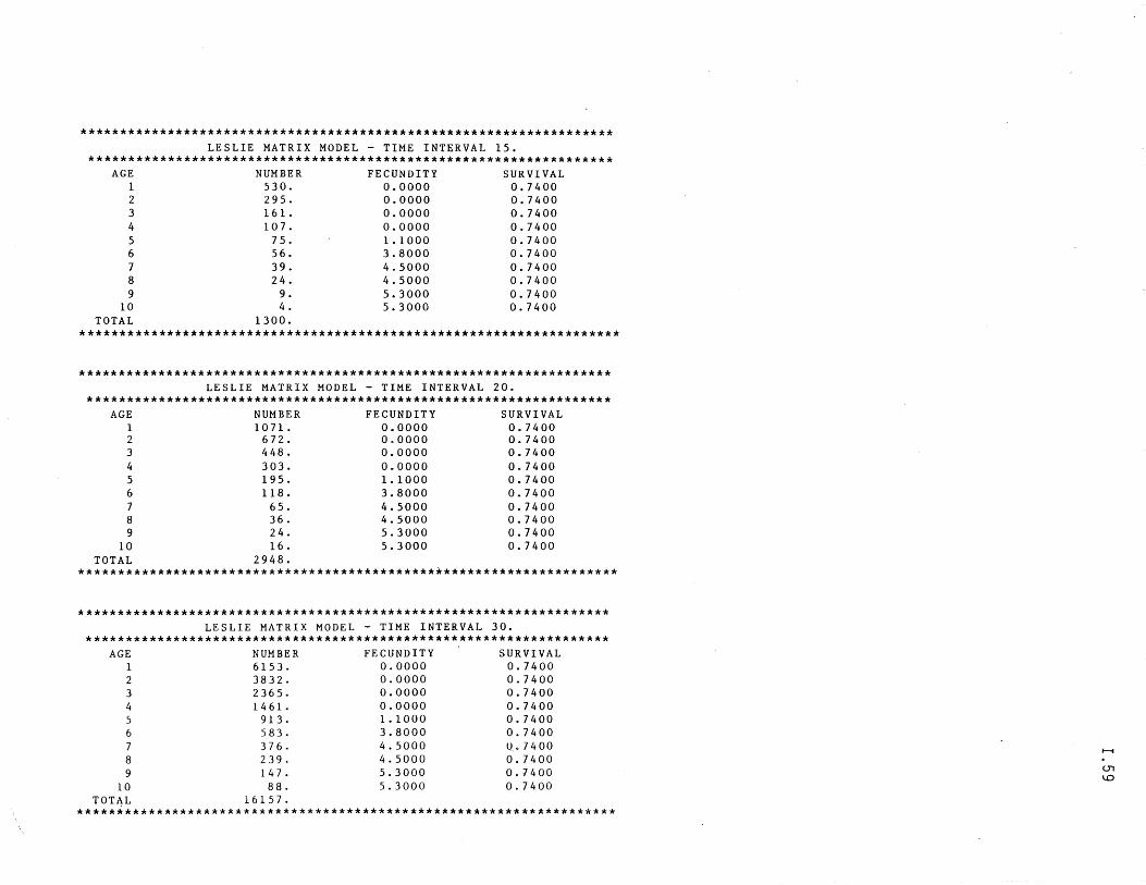
******************************************************************* LESLIE MATRIX MODEL - TIME INTERVAL 15.
****************************************************************** AGE NUMBER FECUNDITY SURVIVAL
1 530. 0.0000 0.7400 2 295. 0.0000 0.7400 3 161- 0.0000 0.7400 4 107. 0.0000 0.7400 5 75. 1.1000 0.7400 6 56. 3.8000 0.7400 7 39. 4.5000 0.7400 8 24. 4.5000 0.7400 9 9. 5.3000 0.7400
10 4. 5.3000 0.7400 TOTAL 1300.
********************************************************************
******************************************************************* LESLIE MATRIX MODEL - TIME INTERVAL 20.
****************************************************************** AGE NUMBER FECUNDITY SURVIVAL
1 1071. 0.0000 0.7400 2 672. 0.0000 0.7400 3 448. 0.0000 0.7400 4 303. 0.0000 0.7400 5 195. 1.1000 0.7400 6 118. 3.8000 0.7400 7 65. 4.5000 0.7400 8 36. 4.5000 0.7400 9 24. 5.3000 0.7400
10 16. 5.3000 0.7400 TOTAL 2948.
********************************************************************
******************************************************************* LESLIE MATRIX MODEL - TIME INTERVAL 30.
****************************************************************** AGE NUMBER FECUNDITY SURVIVAL
1 6153. 0.0000 0.7400 2 3832. 0.0000 0.7400 3 2365. 0.0000 0.7400 4 1461. 0.0000 0.7400 5 913. 1.1000 0.7400 6 583. 3.8000 0.7400 7 376. 4.5000 U.7400 8 239. 4.5000 0.7400 9 147. 5.3000 0.7400
10 88. 5.3000 0.7400 TOTAL 16157.
********************************************************************
t--f
U1 1.0
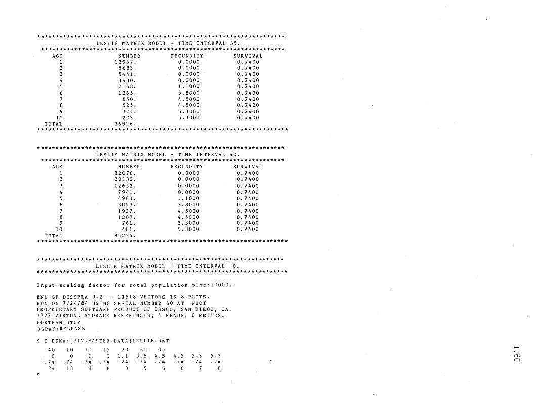
******************************************************************* LESLIE MATRIX MODEL - TIME INTERVAL 35.
****************************************************************** AGE NUMBER FECUNDITY SURVIVAL
1 13937. 0.0000 0.7400 2 8683. 0.0000 0.7400 3 5441. 0.0000 0.7400 4 3430. 0.0000 0.7400 5 2168. 1.1000 0.7400 6 1365. 3.8000 0.7400 7 850. 4.5000 0.7400 8 525. 4.5000 0.7400 9 324. 5.3000 0.7400
10 203. 5.3000 0.7400 TOTAL 36926.
********************************************************************
******************************************************************* LESLIE MATRIX MODEL - TIME INTERVAL 40.
****************************************************************** AGE NUMBER FECUNDITY SURVIVAL
1 32076. 0.0000 0.7400 2 20132. 0.0000 0.7400 3 12653. 0.0000 0.7400 4 7941. 0.0000 0.7400 5 4963. 1.1000 0.7400 6 3093. 3.8000 0.7400 7 1927. 4.5000 0.7400 8 1207. 4.5000 0.7400 9 761. 5.3000 0.7400
10 481. 5.3000 0.7400 TOTAL 85234.
*****************************************~************ **************
******************************************************************* LESLIE MATRIX MODEL - TIME INTERVAL O.
********************************************************************
Input scaling factor for total population plot:10000.
END OF DISSPLA 9.2 -- 11518 VECTORS IN 8 PLOTS. RUN ON 7/24/84 USING SERIAL NUMBER 60 AT WHO I PROPRIETARY SOFTWARE PRODUCT OF ISSCO, SAN DIEGO, CA. 3727 ~IRTUAL STORAGE REFERENCES; 4 READS; 0 WRITES. FORTRAN STOP $SPAK/RELEASE
$ T DSKA: [712.MASTER.DATAjLESLIE.DAT
40 10 10 15 20 30 3S 0 0 0 0 1.1 3.8 4.5 4.5 5.3 5.3
.74 .74 .74 .74 .74 .74 .74 .74 .74 .74 24 13 9 8 3 5 6 7 8
$
..........
(J)
a
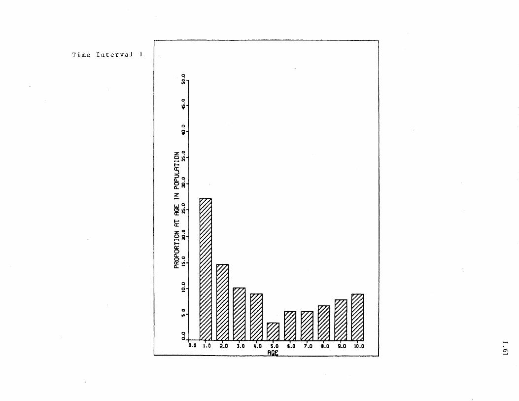
1.6
1
I"'r'-~--~"O
2 a
-a .. a ~ _
__
_ ~ _
__
__
_ ~ _
__
_ -r __
__
__
~ _
__
_ ~ _
__
__
_ '-
__
__
~~ _
__
__
_ --_
_ ~ _
__
__
_ ~o
O"O
S
O"g.
O'O
t O
"St O
"OC
O"SZ
O"O
Z O
"SI 0
'01
o 5
NO 1.Ll:J1OdOd N I
300 lij NO [lOO~d
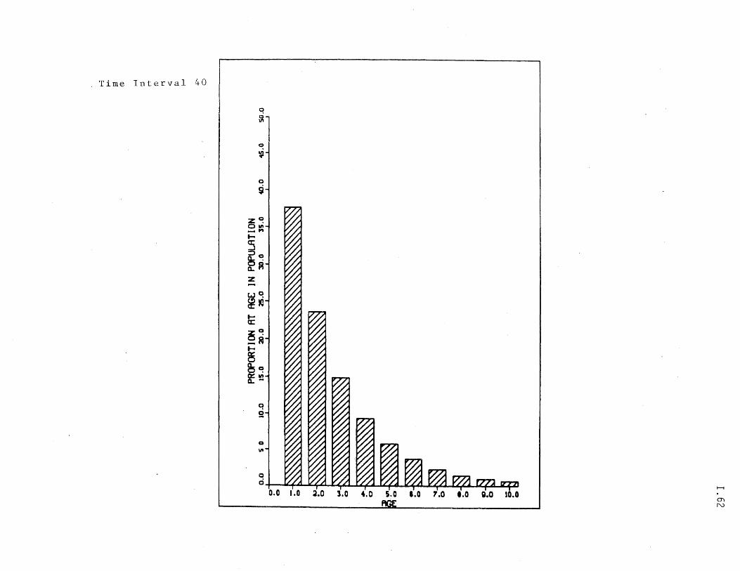
1.62
Q
r------r------~----~------_r------~------~----~------~----~~----~o
0" O
S 0
"5£
O
"at O
"SZ
O
"at 0
'51
0"01
os
NO I.UnndO
d N [
300 lH NO I lW
dOH
d
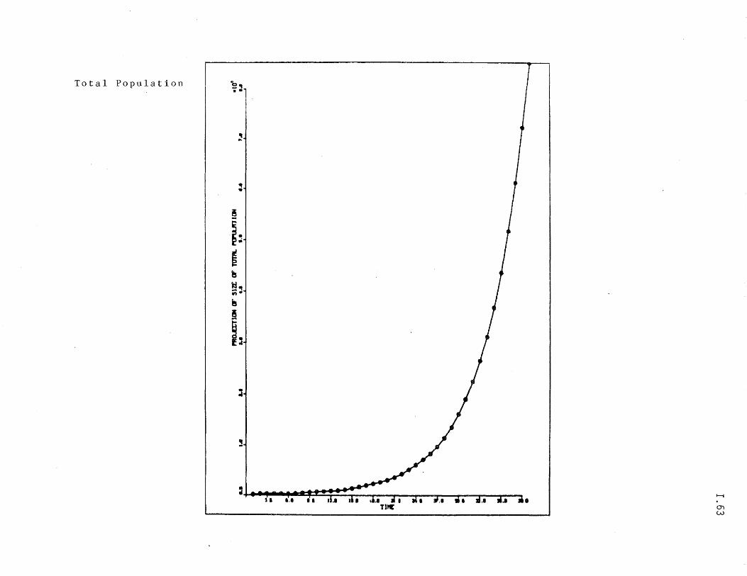
...., cO .j..J
o H
rt
... •.•
rt
" fill ~ "1U
01 .6J
321ft .6J tC)lllrO
H.I
rl
1.63
... • ..
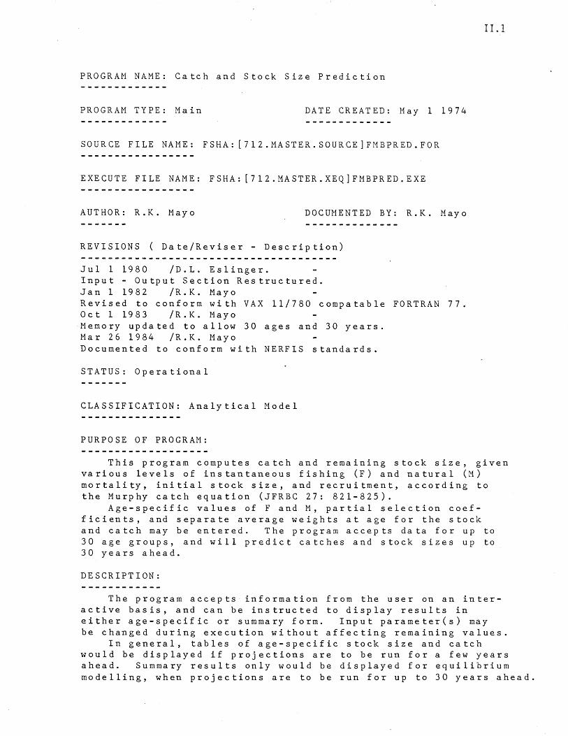
PROGRAM NAME: Catch and Stock Size Prediction
PROGRAM TYPE: Main DATE CREATED: May 1 1974
SOURCE FILE NAME: FSHA: [712.MASTER.SOURCE]FMBPRED.FOR
EXECUTE FILE NAME: FSHA: [7l2.MASTER.XEQ]FMBPRED.EXE
AUTHOR: R.K. Mayo DOCUMENTED BY: R.K. Mayo
REVISIONS ( Date/Reviser - Description)
Jul 1 1980 /D.L. Eslinger. Input - Output Section Restructured. Jan 1 1982 /R.K. Mayo Revised to conform with VAX 11/780 compatab1e FORTRAN 77. Oct 1 1983 /R.K. Mayo Memory updated to allow 30 ages and 30 years. Mar 26 1984 /R.K. Mayo Documented to conform with NERFIS standards.
STATUS: Operational
CLASSIFICATION: Analytical Model
PURPOSE OF PROGRAM:
II.l
This program computes catch and remaining stock size, given various levels of instantaneous fishing (F) and natural (M) mortality, initial stock size, and recruitment, according to the Murphy catch equation (JFRBC 27: 821-825).
Age-specific values of F and M, partial selection coefficients, and separate average weights at age for the stock and catch may be entered. The program accepts data for up to 30 age groups, and will predict catches and stock sizes up to 30 years ahead.
DESCRIPTION:
The program accepts information from the user on an interactive basis, and can be instructed to display results in either age-specific or summary form. Input parameter(s) may be changed during execution without affecting remaining values.
In general, tables of age-specific stock size and catch would be displayed if projections are to be run for a few years ahead. Summary results only would be displayed for equilibrium modelling, when projections are to be run for up to 30 years ahead.
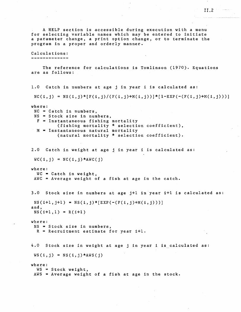
II.2
A HELP section is accessible during execution with a menu for selecting variable names which may be entered to initiate a parameter change, a print option change, or to terminate the program in a proper and orderly manner.
Calculations:
The reference for calculations is Tomlinson (1970). Equations are as follows:
1.0 Catch in numbers at age j in year i is calculated as:
NC(i,j) = NS(i,j)*[F(i,j)/(F(i,j)+M(i,j»]*[l-EXP(-(F(i,j)+M(i,j»)]
where: NC = Catch in numbers, NS = Stock size in numbers,
F = Instantaneous fishing mortality (fishing mortality * selection coefficient),
M = Instantaneous natural mortality (natural mortality * selection coefficient).
2.0 Catch in weight at age j in year i is calculated as:
WC(i,j) = NC(i,j)*AWC(j)
where: we = Catch in weight,
AWe = Average weight of a fish at age in the catch.
3.0 Stock size in numbers at age j+1 in year i+1 is calculated as:
NS(i+1,j+1) = NS(i,j)*[EXP(-(F(i,j)+M(i,j»)] and, NS(i+1,1) = R(i+l)
where: NS = Stock size in numbers,
R = Recruitment estimate for year i+1.
4.0 Stock size in weight at age j in year i is calculated as:
WS(i,j) = NS(i,j)*AWS(j)
where: WS = Stock weight,
AWS = Average weight of a fish at age in the stock.
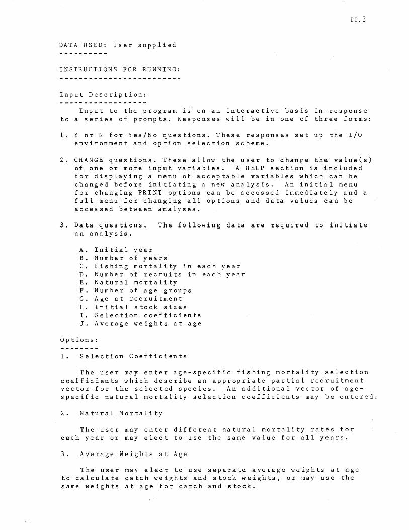
II.3
DATA USED: User supplied
INSTRUCTIONS FOR RUNNING:
Input Description:
Input to the program is on an interactive basis in response to a series of prompts. Responses will be in one of three forms:
1. Y or N for Yes/No questions. These responses set up the I/O environment and option selection scheme.
2. CHANGE questions. These allow the user to change the value(s) of one or more input variables. A HELP section is included for displaying a menu of acceptable variables which can be changed before initiating a new analysis. An initial menu for changing PRINT options can be accessed immediately and a full menu for changing all options and data values can be accessed between analyses.
3. Data questi?ns. an analysis.
A. Initial year
The following data are required to initiate
B. Number of years C. Fishing mortality in each year D. Number of recruits in each year E. Natural mortality F. Number of age groups G. Age at recruitment H. Initial stock sizes I. Selection coefficients J. Average weights at age
Options:
1. Selection Coefficients
The user may enter age-specific fishing mortality selection coefficients which describe an appropriate partial recruitment vector for the selected species. An additional vector of agespecific natural mortality selection coefficients may be entered.
2. Natural Mortality
The user may enter different natural mortality rates for each year or may elect to use the same value for a.ll years.
3. Average Weights at Age
The user may elect to use separate average weights at age to calculate catch weights and stock weights, or may use the same weights at age for catch and stock.
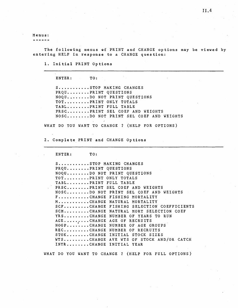
I I. 4
Menus:
The following menus Qf PRINT and CHANGE options may be viewed by entering HELP in respons~ to a CHANGE question:
1. Initial PRINT Options
ENTER: TO:
S .•..••.•... STOP MAKING CHANGES PRQU ..•..•.. PRINT QUESTIONS NOQU •••..... DO NOT PRINT QUESTIONS TOT •••.••••• PRINT ONLY TOTALS TABL ..•••.•• PRINT FULL TABLE PRSC .•...... PRINT SEL COEF AND WEIGHTS NOSC .•.....• DO NOT PRINT SEL COEF AND WEIGHTS
WHAT DO YOU WANT TO CHANGE? (HELP FOR OPTIONS)
2. Complete. PRINT and CHANGE Options
ENTER: TO:
S .•••.••..•• STOP MAKING CHANGES PRQU .••..••• PRINT QUESTIONS NOQU •••.•.•. DO NOT PRINT QUESTIONS TOT ......... PRINT ONLY TOTALS TABL ..•....• PRINT FULL TABLE PRSC .••••••. PRINT SEL COEF AND WEIGHTS NOSC ......•. DO NOT PRINT SEL COEF AND WEIGHTS F .......••.. CHANGE FISHING MORTALITY M .•..••..• ;.CHANGE NATURAL MORTALITY SCF •.•••..•• CHANGE FISHING SELECTION COEFFICIENTS SCM ......... CHANGE NATURAL MORT SELECTION COEF YRS ..•.•..•. CHANGE NUMBER OF YEARS TO RUN AGE ...•. : ... CHANGE AGE OF RECRUITS NOGP .•.•.... CHANGE NUMBER OF AGE GROUPS REC ..•....•• CHANGE NUMBER OF RECRUITS STOK .••...•. CHANGE INITIAL STOCK SIZES WTS .•.....•• CHANGE AVE WTS OF STOCK AND/OR CATCH INYR ••...•.• CHANGE INITIAL YEAR
WHAT DO YOU WANT TO CHANGE? (HELP FOR FULL OPTIONS)
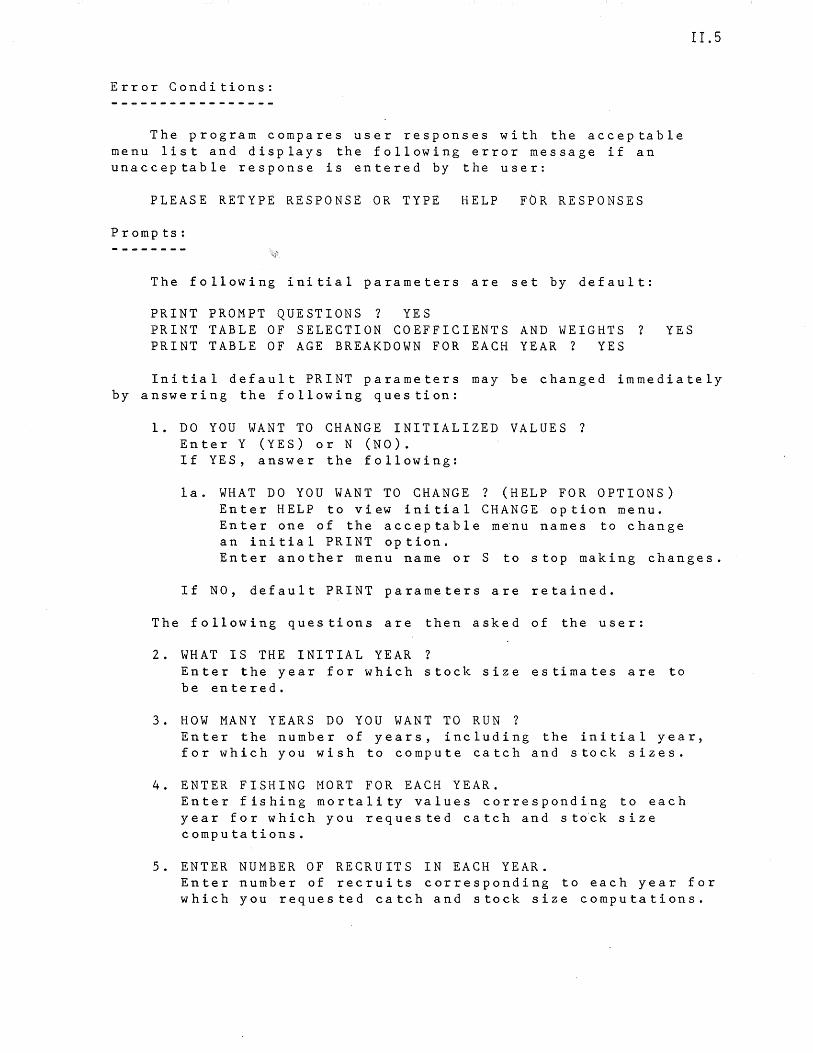
Error Conditions:
The program compares user responses with the acceptable menu list and displays the following error message if an unacceptable response is entered by the user:
PLEASE RETYPE RESPONSE OR TYPE HELP FOR RESPONSES
Prompts:
The following initial parameters are set by default:
PRINT PROMPT QUESTIONS? YES
II.5
PRINT TABLE OF SELECTION COEFFICIENTS AND WEIGHTS? YES PRINT TABLE OF AGE BREAKDOWN FOR EACH YEAR? YES
Initial default PRINT parameters may be changed immediately by answering the following question:
1. DO YOU WANT TO CHANGE INITIALIZED VALUES? Enter Y (YES) or N (NO). If YES, answer the following:
lao WHAT DO YOU WANT TO CHANGE? (HELP FOR OPTIONS) Enter HELP to view initial CHANGE option menu. Enter one of the acceptable manu names to change an initial PRINT option. Enter another menu name or S to stop making changes.
If NO, default PRINT parameters are retained.
The following questions are then asked of the user:
2. WHAT IS THE INITIAL YEAR? Enter the year for which stock size estimates are to be entered.
3. HOW MANY YEARS DO YOU WANT TO RUN? Enter the number of years, including the initial year, for which you wish to compute catch and stock sizes.
4. ENTER FISHING MORT FOR EACH YEAR. Enter fishing mortality values corresponding to each year for which you requested catch and stock size computations.
5. ENTER NUMBER OF RECRUITS IN EACH YEAR. Enter number of recruits corresponding to each year for which you requested catch and stock size computations.
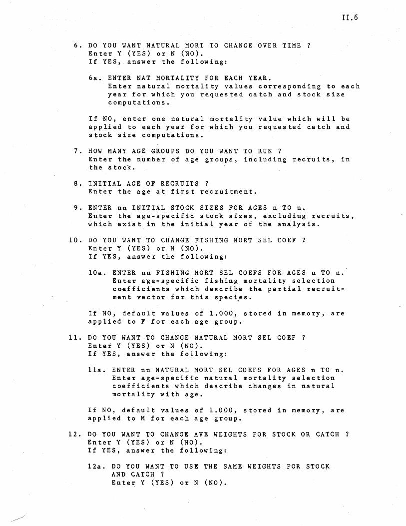
6. DO YOU WANT NATURAL MORT TO CHANGE OVER TIME 1 Enter Y (YES) or N (NO). If YES, answer the following:
6a. ENTER NAT MORTALITY FOR EACH YEAR.
II.6
Enter natural mortality values corresponding to each year for which you requested catch and stock size computations.
If NO, enter one natural mortality value which will be applied to each year for which you requested catch and stock size computations.
7. HOW MANY AGE GROUPS DO YOU WANT TO RUN 1 Enter the number of age groups, including recruits, in the stock.
8. INITIAL AGE OF RECRUITS 1 Enter the age at first recruitment.
9. ENTER nn INITIAL STOCK SIZES FOR AGES n TO n. Enter the age-specific stock sizes, excluding recruits, which exist.in the initial year of the analysis.
10. DO YOU WANT TO CHANGE FISHING MORT SEL COEF 1 Enter Y (YES) or N (NO). If YES, answer the following:
lOa. ENTER nn FISHING MORT SEL COEFS FOR AGES n TO n. Enter age-specific fishing mortality selection coefficients which describe the partial recruitment vector for this spec~~s.
If NO, default values of 1.000, stored in memory, are applied to F for each age group.
11. DO YOU' WANT to CHANGE NATURAL MORT SEL COEF 1 Enter Y (YES) or N (NO). If YES, answer the following:
lla. ENTER nn NATURAL MORT SEL COEFS FOR AGES n TO n. Enter age-specific natural mortality selection coefficients which describe changes in natural mortality with age.
If NO, de f au 1 t val u e s 0 fl. 000, s tor e din me m 0 ry, are applied to M for each age group.
12. DO YOU WANT TO CHANGE AVE WEIGHTS FOR STOCK OR CATCH 1 Enter Y (YES) or N (NO). If YES, answer the following:
l2a. DO YOU WANT TO USE THE SAME WEIGHTS FOR STOC~
AND CATCH 1 Enter Y (YES) or N (NO).
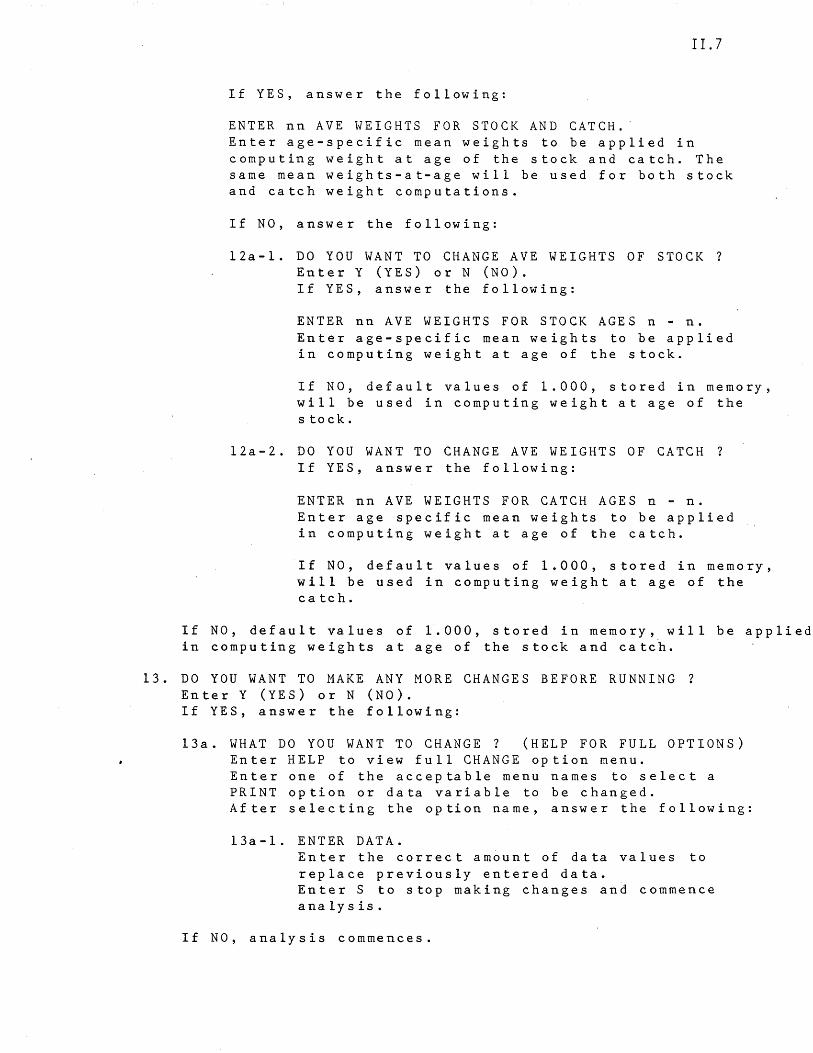
II.?
If YES, answer the following:
ENTER nn AVE WEIGHTS FOR STOCK AND CATCH.· Enter age-specific mean weights to be applied in computing weight at age of the stock and catch. The same mean weights-at-age will be used for both stock and catch weight computations.
If NO, answer the following:
12a-1. DO YOU WANT TO CHANGE AVE WEIGHTS OF STOCK? Enter Y (YES) or N (NO). If YES, answer the following:
ENTER nn AVE WEIGHTS FOR STOCK AGES n - n. Enter age-specific mean weights to be applied in computing weight at age of the stock.
If NO, default values of 1.000, stored in memory, will be used in computing weight at age of the stock.
12a-2. DO YOU WANT TO CHANGE AVE WEIGHTS OF CATCH? If YES, answer the following:
ENTER nn AVE WEIGHTS FOR CATCH AGES n - n. Enter age specific mean weights to be applied in computing weight at age of the catch.
If NO, default values of 1.000, stored in memory, will be used in computing weight at age of the catch.
If NO, default values of 1.000, stored in memory, will be applied in computing weights at age of the stock and catch.
13. DO YOU WANT TO MAKE ANY MORE CHANGES BEFORE RUNNING? Enter Y (YES) or N (NO). If YES, answer the following:
13a. WHAT DO YOU WANT TO CHANGE? (HELP FOR FULL OPTIONS) Enter HELP to view full CHANGE option menu. Enter one of the acceptable menu names to select a PRINT option or data variable to be changed. After selecting the option name, answer the following:
13a-1. ENTER DATA. Enter the correct amount of data values to replace previously entered data. Enter S to stop making changes and commence analysis.
If NO, analysis commences.
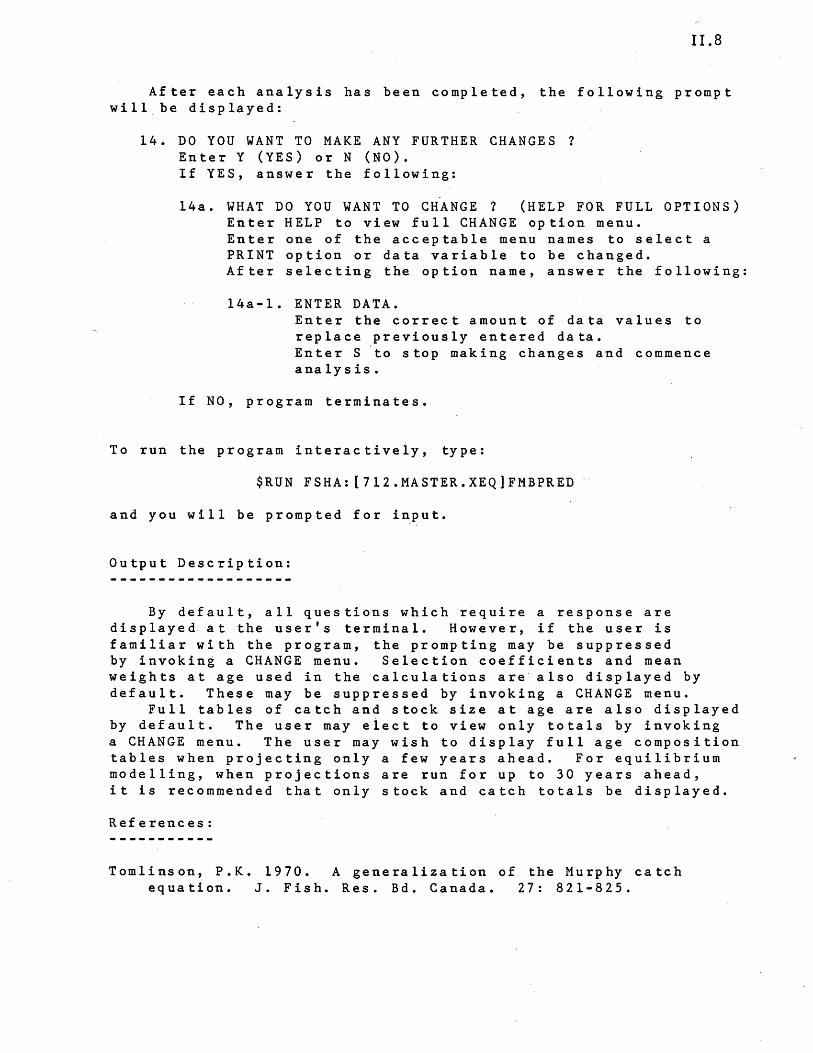
II.8
After each analysis has been completed, the following prompt will be displayed:
14. DO YOU WANT TO MAKE ANY FURTHER CHANGES? Enter Y (YES) or N (NO). If YES, answer the following:
l4a. WHAT DO YOU WANT TO CHANGE? (HELP FOR FULL OPTIONS) Enter HELP to view full CHANGE option menu. Enter one of the acceptable menu names to select a PRINT option or data variable to be changed. After selecting the option name, answer the following:
l4a-l. ENTER DATA. Enter the correct amount of data values to replace previously entered data. Enter S 'to stop making changes and commence analysis.
If NO, program terminates.
To run the program interactiveiy, type:
$RUN FSHA: [7l2.MASTER.XEQ]FMBPRED
and you will be prompted for input.
Output Description:
By default, all questions which require a response are displayed at the userls terminal. However, if the user is familiar with the program, the prompting may be suppressed by invoking a CHANGE menu. Selection coefficients and mean weights at age used in the calculations are' also displayed by default. These may be suppressed by invoking a CHANGE menu.
Full tables of catch and stock size at age are also displayed by default. The user may eiect to view only totals by invoking a CHANGE menu. The user may wish to display full age composition tables when projecting only a few years ahead. For equilibrium modelling, when projections are run for up to 30 years ahead, it is recommended that only stock and catch totals be displayed.
References:
Tomlinson, P.K. 1970. A generalization of the Murphy catch equation. J. Fish. Res. Bd. Canada. 27: 821-825.
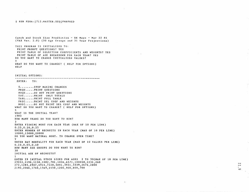
$ RUN FSHA:[712.MASTER.XEQ]FMBPRED
Catch and Stock Size Prediction - RK Mayo - Mar 22 84 (VAX Ver. 2.0) (30 Age Groups and 31 Year Projections)
THIS PROGRAM IS INITIALIZED TO: PRINT PROMPT QUESTIONS? YES PRINT TABLE OF SELECTION COEFFICIENTS AND WEIGHTS? YES PRINT TABLE OF AGE BREAKDOWN FOR EACH YEAR? YES
DO YOU WANT TO CHANGE INITIALIZED VALUES? Y WHAT DO YOU WANT TO CHANGE? ( HELP FOR OPTIONS) HELP
INITIAL OPTIONS;
ENTER: TO:
S ..•••••• STOP MAKING CHANGES PRQU .•... PRINT QUESTIONS NOQU ..... DO NOT PRINT QUESTIONS TOT ....•. PRINT ONLY TOTALS TABL ..•.. PRINT FULL TABLE PRSC ..... PRINT SEL COEF AND WEIGHTS NOSC .••.. DO NOT PRINT SEL COEF AND WEIGHTS
WHAT DO YOU WANT TO CHANGE? ( HELP FOR OPTIONS) S WHAT IS THE INITIAL YEAR? 1983 HOW MANY YEARS DO YOU WANT TO RUN? 3 ENTER FISHING MORT FOR EACH YEAR (MAX OF 10 PER LINE) 0.25,0.20,0.25 ENTER NUMBER OF RECRUITS IN EACH YEAR (MAX OF 10 PER LINE) 10000,15000,20000 DO YOU WANT NATURAL MORT. TO CHANGE OVER TIME? Y ENTER NAT MORTALITY FOR EACH YEAR (MAX OF 10 VALUES PER LINE) 0.10,0.05,0.10 HOW MANY AGE GROUPS DO YOU WANT TO RUN? 30 INITIAL AGE OF RECRUITS? 1 ENTER 29 INITIAL STOCK SIZES FOR AGES 2 TO 30(MAX OF 10 PER LINE') 23222,1196,1138,1082,781,1036,6571,100048,1231,260 272,1285,2907,4914,7228,5091,3931,3339,2676,2800 2190,2066,1740,1569,1450,1200,900,800,700
I--f I--f
~
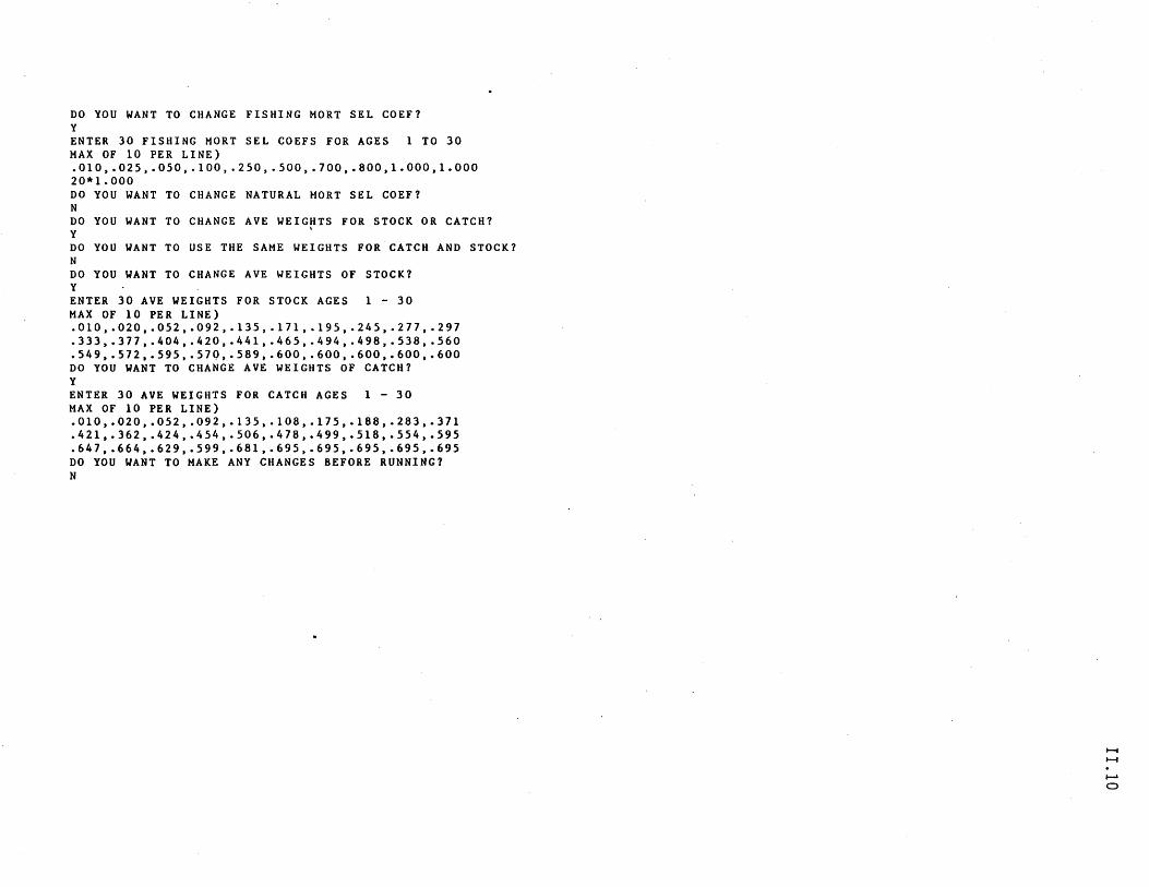
DO YOU WANT TO CHANGE FISHING MORT SEL COEF? Y ENTER 30 FISHING MORT SEL COEFS FOR AGES 1 TO 30 MAX OF 10 PER LINE) .010,.025,.050,.100,.250,.500,.700,.800,1.000,1.000 20*1.000 DO YOU WANT TO CHANGE NATURAL MORT SEL COEF? N DO YOU WANT TO CHANGE AVE WEIG~TS FOR STOCK OR CATCH? Y DO YOU WANT TO USE THE SAME WEIGHTS FOR CATCH AND STOCK? N DO YOU WANT TO CHANGE AVE WEIGHTS OF STOCK? Y ENTER 30 AVE WEIGHTS FOR STOCK AGES 1 - 30 MAX OF 10 PER LINE) .010,.020,.052,.092,.135,.171,.195,.245,.277,.297 .333,.377,.404,.420,.441,.465,.494,.498,.538,.560 .549,.572,.595,.579,·589,.600,.600,.600,.600,.600 DO YOU WANT TO CHANGE AVE WEIGHTS OF CATCH? Y ENTER 30 AVE WEIGHTS FOR CATCH AGES 1 - 30 MAX OF 10 PER LINE) .010,.020,.052,.092,.135,.108,.175,.188,.283,.371 .421,.362,.424,.454,.506,.478,.499,.518,.554,.595 .647,.664,.629,.599,.681,.695,.695,.695,.695,.695 DO YOU WANT TO MAKE ANY CHANGES BEFORE RUNNING? N
I-t ....... ~
a
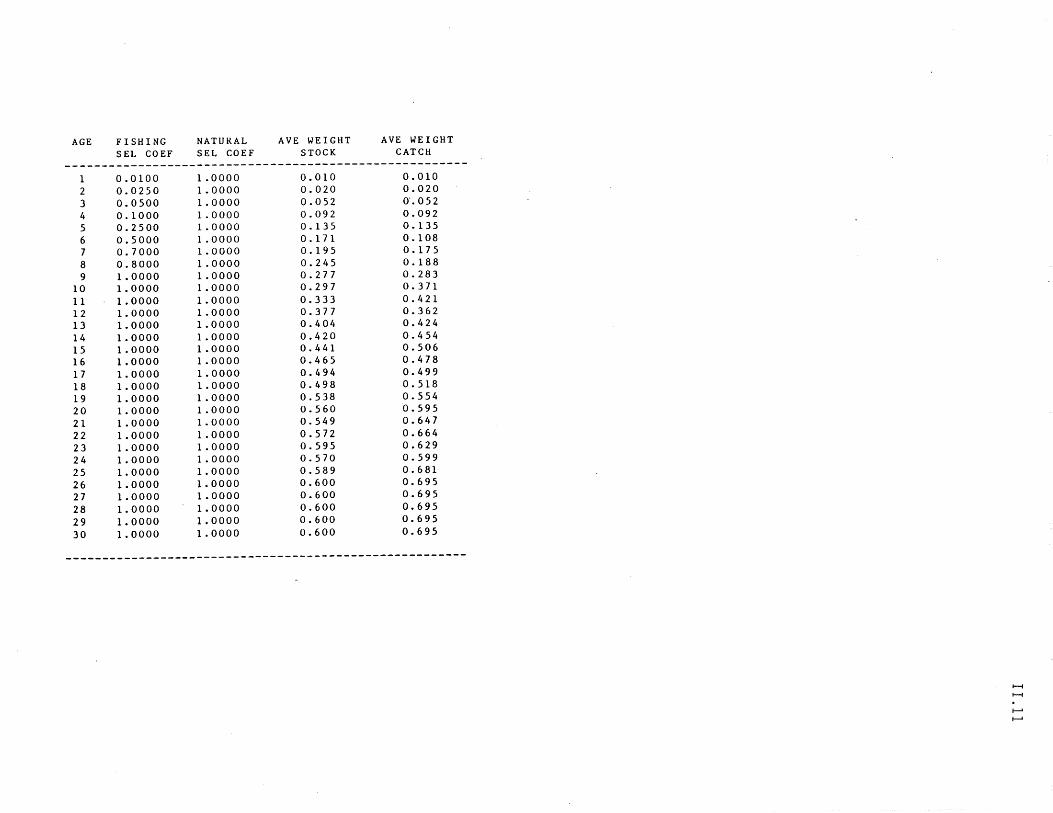
AGE FISHING NATURAL AVE WEIGHT AVE WEIGHT SEL COEF SEL COEF STOCK CATCH
-------------------------------------------------------1 0.0100 1.0000 0.010 0.010 2 0.0250 1.0000 0.020 0.020
3 0.0500 1.0000 0.052 a'. 052 4 0.1000 1.0000 0.092 0.092 5 0.2500 1.0000 0.135 0.135 6 0.5000 1.0000 0.171 0.108 7 0.7000 1.0000 0.195 0.175 8 0.8000 1.0000 0.245 0.188 9 1.0000 1.000Q 0.277 0.283
10 1.0000 1.0000 0.297 0.371
11 1.0000 1.0000 0.333 0.421 12 1.0000 1.0000 0.377 0.362 13 1. 0000 1. 0000 0.404 0.424 14 1.0000 1.0000 0.420 0.454 15 1. 0000 1.0000 0.441 0.506 16 1. 0000 1.0000 0.465 0.478 17 1.0000 1. 0000 0.494 0.499 18 1.0000 1.0000 0.498 0.518 19 1.0000 1.0000 0.538 0.554 20 1.0000 1.0000 0.560 0.595
21 1. 0000 1.0000 0.549 0.647
22 1.0000 1. 0000 0.572 0.664 23 1.0000 1. 0000 0.595 0.629 24 1.0000 1.0000 0.570 0.599
25 1.0000 1.0000 0.589 0.681
26 1. 0000 1. 0000 0.600 0.695
27 1. 0000 1.0000 0.600 0.695
28 1.0000 1. 0000 0.600 0.695
29 1.0000 1.0000 0.600 0.695
30 1. 0000 1.0000 0.600 0.695
-------------------------------------------------------
I--t I--t
I-' I-'
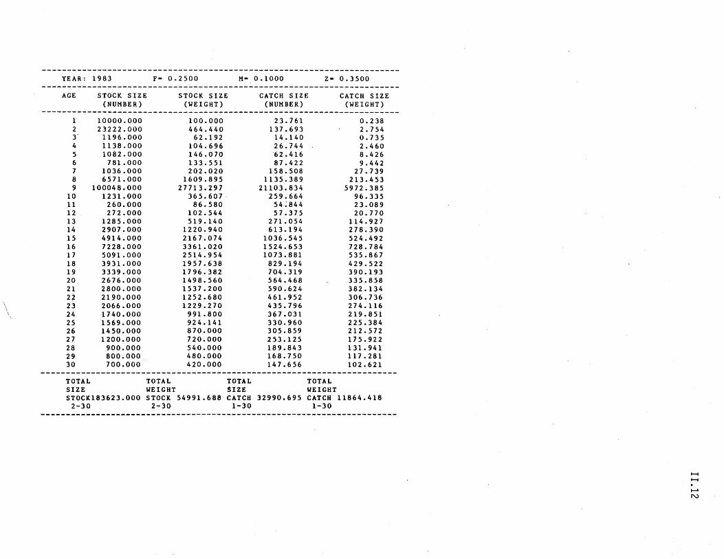
YEAR: 1983 F'"' 0.2500 M- 0.1000 Z- 0.3500
AGE STOCK SIZE (NUMBER)
1 10000.000 2 23222.000 3' 1196.000 4 1138.000 5 1082.000 6 781.000 7 1036.000 8 6571.000 9 100048.000
10 1231.000 11 260.000 12 272.000 13 1285.000 14 2907.000 15 4914.000 16 7228.000 17 5091.000 18 3931.000 19 3339.000 20 2676.000 21 2800.000 22 2190.000 23 2066.000 24 1740.000 25 1569.000 26 1450.000 27 1200.000 28 900.000 29 800.000 30 700.000
STOCK SIZE (WEIGHT)
100.000 464.440
62.192 104.696 146.070 133.551 202.020
1609.895 27713.297
365.607 86.580
102.544 519.140
1220.940 2167.074 3361.020 251,4.954 1957.638 1796.382 1498.560 1537.200 1252.680 1229.270
991.800 924.141 870.000 720.000 540.000 480.000 420.000
CATCH SIZE (NUMBER)
23.761 137.693
14.140 26.744 62.416 87.422
158.508 1135.389
21103.834 259.664
54;844 57.375
271.054 613.194
1036.545 1524.653 1073.881
829.194 704.319 564.468 590.624 461.952 435.796 367.031 330.960 305.859 253.125 189.843 168.750 147.656
TOTAL TOTAL TOTAL TOTAL SIZE WEIGHT SIZE WEIGHT
CATCH SIZE (WEIGHT)
0.238 2.754 0.735 2.460 8.426 9.442
27.739 213.453
5972.385 96.335 23.089 20.770
114.927 278.390 524.492 728.784 535.867 429.522 390.193 335.858 382.134 306.736 274.116 219.851 225.384 212.572 175.922 131.941 117.281 102.621
STOCK183623.000 STOCK 54991.688 CATCH 32990.695 CATCH 11864.418 2-30 2-30 1-30 1-30
.......
....... ~
N
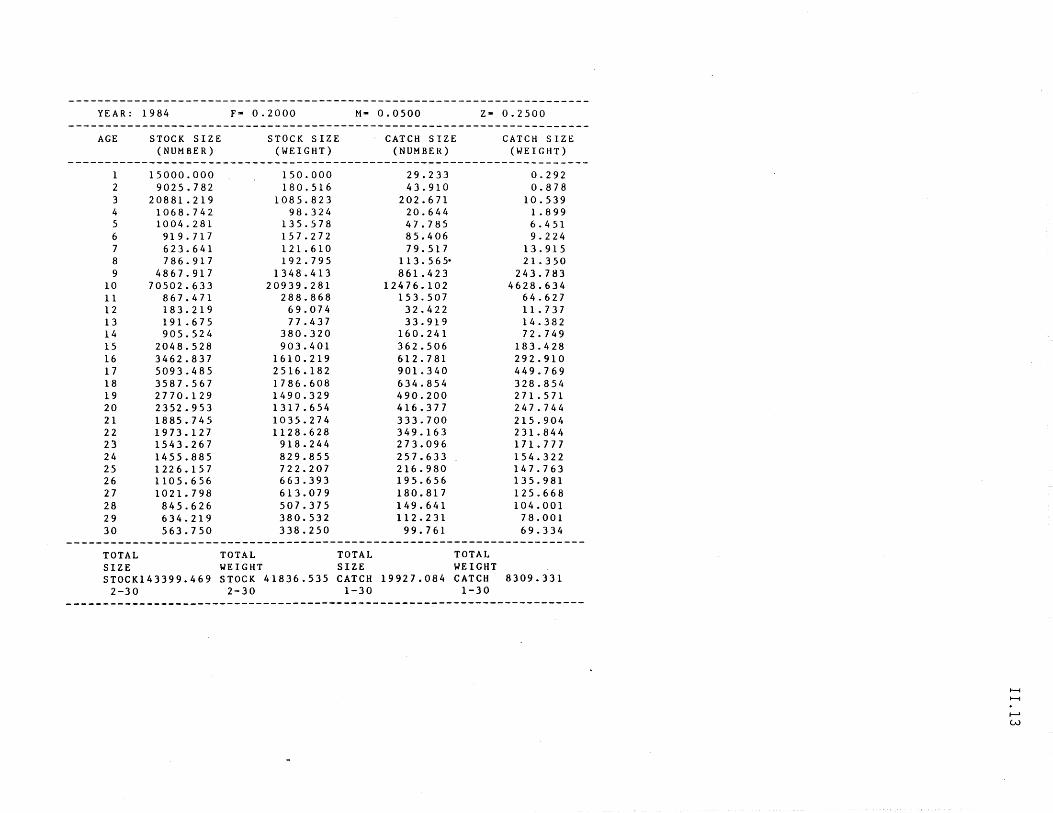
YEAR: 1984 F=- 0.2000 M- 0.0500 Z- 0.2500
AGE
1 2 3 4 5 6 7 8 9
10 11 12 13 14 15 16 17 18 19 20 21 22 23 24 25 26 27 28 29 30
STOCK SIZE (NUMBER)
15000.000 9025.782
20881.219 1068.742 1004.281 919.717 623.641 786.917
4867.917 70502.633
867.471 183.219 191.675 905.524
2048.528 3462.837 5093.485 3587.567 2770.129 2352.953 1885.745 1973.127 1543.267 1455.885 1226.157 1105.656 1021.798 845.626 634.219 563.750
STOCK SIZE (WEIGHT)
150.000 180.516
1085.823 98.324
135.578 157.272 121.610 192.795
1348.413 20939.281
288.868 69.074 77.437
380.320 903.401
1610.219 2516.182 1786.608 1490.329 1317.654 1035.274 1128.628
918.244 829.855 722.207 663.393 613.079 507.375 380.532 338.250
CATCH SIZE (NUMBER)
29.233 43.910
202.671 20.644 47.785 85.406 79.517
113.565· 861.423
12476.102 153.507 32.422 33.919
160.241 362.506 612.781 901.340 634.854 490.200 416.377 333.700 349.163 273.096 257.633 216.980 195.656 180.817 149.641 112.231
99.761
TOTAL TOTAL TOTAL TOTAL SIZE WEIGHT SIZE WEIGHT
CATCH SIZE (WEIGHT)
0.292 0.878
10.539 1. 899 6.451 9.224
13.915 21. 350
243.783 4628.634
64.627 11. 737 14.382 72.749
183.428 292.910 449.769 328.854 271.571 247.744 215.904 231.844 171. 777 154.322 147.763 135.981 125.668 104.001
78.001 69.334
STOCK143399.469 STOCK 41836.535 CATCH 19927.084 CATCH 8309.331 2-30 2-30 1-30 1-30
I-f I-f
I-' W
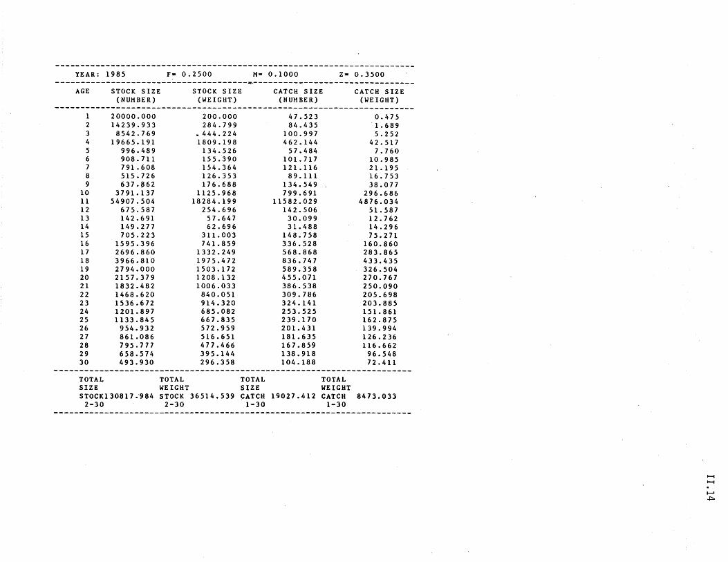
YEAR: 1985 F- 0.2500 M- 0.1000 Z- 0.3500
AGE
1 2 3 4 5 6 7 8 9
10 11 12 13 14 15 16 17 18 19 20 21 22 23 24 25 26 27 28 29 30
STOCK SIZE (NUMBER)
20000.000 14239.933 8542.769
19665.191 996.489 908.711 791.608 515.726 637.862
3791.137 54907.504
675.587 142.691 149.277 705.223
1595.396 2696.860 3966.810 2794.000 2157.379 1832.482 1468.620 1536.672 1201.897 1133.845
954.932 861.086 795.777 658.574 493.930
STOCK SIZE (WEIGHT)
200.000 284.799
.444.224 1809.198
134.526 155.390 154.364 126.353 176.688
1125.968 18284.199
254.696 57.647 62.696
311.003 741.859
1332.249 1975.472 1503.172 1208.132 1006.033 840.051 914.320 685.082 667.835 572.959 516.651 477.466 395.144 296.358
CATCH SIZE (NUMBER)
47.523 84.435
100.997 462.144
57.484 101.717 121.116
89.111 134.549 799.691
11582.029 142.506 30.099 31.488
148.758 336.528 568.868 836.747 589.358 455.071 386.538 309.786 324.141 253.525 239.170 201.431 181.635 167.859 138.918 104.188
TOTAL TOTAL TOTAL TOTAL SIZE WEIGHT SIZE WEIGHT
CATCH SIZE (WEIGHT)
0.475 1. 689 5.252
42.517 7.7QO
10.985 21.195 16.753 38.077
296.686 4876.034
51.587 12.762 14.296 75.271
160.860 283.865 433.435 326.504 270.767 250.090 205.698 203.885 151.861 162.875 139.994 126.236 116.662
96.548 72.411
STOCK130817."984 STOCK 36514.539 CATCH 19027.412 CATCH 8473.033 2-30 2-30 1-30 1-30
......
...... f--I +==-
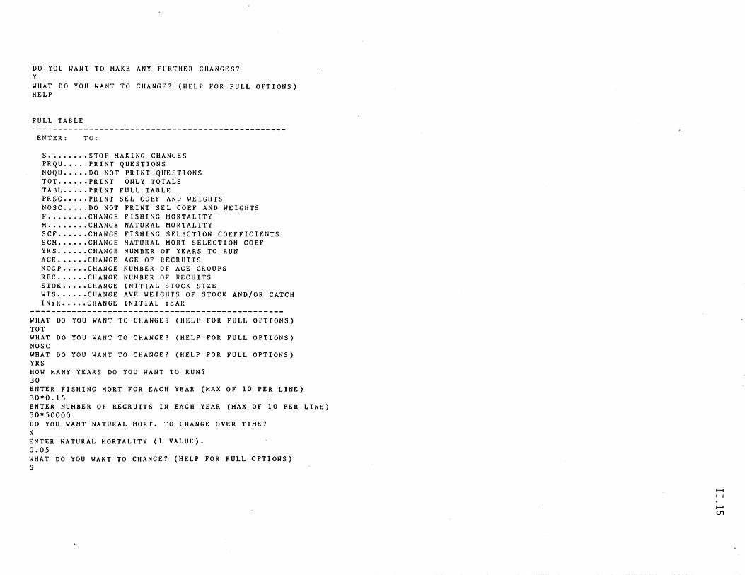
DO YOU WANT TO MAKE ANY FURTHER CHANGES? Y WHAT DO YOU WANT TO CHANGE? (HELP FOR FULL OPTIONS) HELP
FULL TABLE
ENTER: TO:
S ........ STOP MAKING CHANGES PRQU ..... PRINT QUESTIONS NOQU ..... DO NOT PRINT QUESTIONS TOT ..•..• PRINT ONLY TOTALS TABL ..... PRINT FULL TABLE PRSC ..•.. PRINT SEL COEF AND WEIGHTS NOSC ...•. DO NOT PRINT SEL COEF AND WEIGHTS F .......• CHANGE FISHING MORTALITY M ..•.•... CHANGE NATURAL MORTALITY SCF ...... CHANGE FISHING SELECTION COEFFICIENTS SCM ....•• CHANGE NATURAL MORT SELECTION COEF YRS .•.•.• CHANGE NUMBER OF YEARS TO RUN AGE .•.•.• CHANGE AGE OF RECRUITS NOGP .•..• CHANGE NUMBER OF AGE GROUPS REC ...... CHANGE NUMBER OF RECUITS STOK ..... CHANGE INITIAL STOCK SIZE WTS •..•.• CHANGE AVE WEIGHTS OF STOCK AND/OR CATCH INYR ..... CHANGE INITIAL YEAR
WHAT DO YOU WANT TO CHANGE? (HELP FOR FULL OPTIONS) TOT WHAT DO YOU WANT TO CHANGE? (HELP FOR FULL OPTIONS) NOSC WHAT DO YOU WANT TO CHANGE? (HELP FOR FULL OPTIONS) YRS HOW MANY YEARS DO YOU WANT TO RUN? 30 ENTER FISHING MORT FOR EACH YEAR (MAX OF 10 PER LINE) 30*0.15 ENTER NUMBER OF RECRUITS IN EACH YEAR (MAX OF 10 PER LINE) 30*50000 DO YOU WANT NATURAL MORT. TO CHANGE OVER TIME? N ENTER NATURAL MORTALITY (1 VALUE). 0.05 WHAT DO YOU WANT TO CHANGE? (HELP FOR FULL OPTIONS) S
I--j
I--j
f--I <.J1
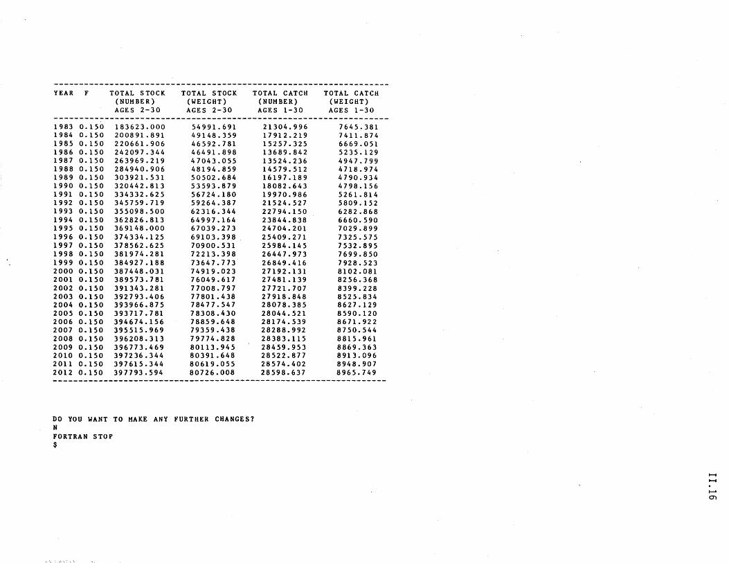
------------------------------------------------------------------YEAR F TOTAL STOCK TOTAL STOCK TOTAL CATCH TOTAL CATCH
(NUMBER) (WEIGHT) (NUMBER) (WEIGHT) AGES 2-30 AGES 2-30 AGES 1-30 AGES 1-30
------------------------------------------------------------------1983 0.150 183623.000 54991.691 21304.996 7645.381 1984 0.150 200891.891 49148.359 17912.219 7411.874 1985 0.150 220661.906 46592.781 15257.325 6669.051 1986 0.150 242097.344 46491.898 13689.842 5235.129 1987 0.150 263969.219 47043.055 13524.236 4947.799 1988 0.150 284940.906 48194.859 14579.512 4718.974 1989 0.150 303921.531 50502.684 16197.189 4790.934 1990 0.150 320442.813 53593.879 18082.643 4798.156 1991 0.150 334332.625 56724.180 19970.986 5261.814 1992 0.150 345759.719 59264.387 21524.527 5809.152 1993 0.150 355098.500 62316.344 22794.150 6282.868 1994 0.150 362826.813 64997.164 23844.838 6660.590 1995 0.150 369148.000 67039.273 24704.201 7029.899 1996 0.150 374334.125 69103.398 25409.271 7325.575 1997 0.150 378562.625 70900.531 25984.145 7532.895 1998 0.150 381974.281 72213.398 26447.973 7699.850 1999 0.150 384927.188 73647.773 26849.416 7928.523 2000 0.150 387448.031 74919.023 27192.131 8102.081 2001 0.150 389573.781 76049.617 27481.139 8256.368 2002 0.150 391343.281 77008.797 27721.707 8399.228 2003 0.150 392793.406 77801.438 27918.848 8525.834 2004 0.150 393966~875 78477.547 28078.385 8627.129 2005 0.150 393717.781 78308.430 28044.521 8590.120 2006 0.150 394674.156 78859.648 28174.539 8671.922 2007 0.150 395515.969 79359.438 28288.992 8750.544 2008 0.150 396208.313 79774.828 28383.115 8815.961 2009 0.150 396773.469 80113.945 28459.953 8869.363 2010 0.150 397236.344 80391.648 28522.877 8913.096 2011 0.150 397615.344 80619.055 28574.402 8948.907 2012 0.150 397793.594 80726.008 28598.637 8965.749 ------------------------------------------------------------------
DO YOU WANT TO HAKE ANY FURTHER CHANGES? N FORTRAN STOP $
,.,', ,,\
1-1 1-1
f-& 0')
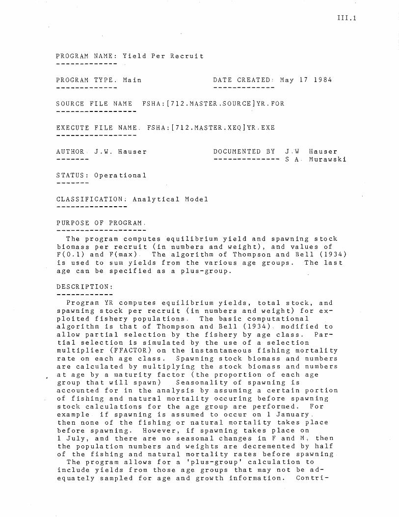
111.1
PROGRAM NAME: Yield Per Recruit
PROGRAM TYPE. Main DATE CREATED: May 17 1984
SOURCE FILE NAME FSHA: [712.MASTER.SOURCE]YR.FOR
EXECUTE FILE NAME. FSHA:[712.MASTER.XEQ]YR.EXE
AUTHOR J.W. Hauser
STATUS: Operational
CLASSIFICATION: Analytical Model
PURPOSE OF PROGRAM,
DOCUMENTED BY J.W Hauser -------------- S A· Murawski
The program computes equilibrium yield and spawning stock biomass per recruit (in numbers and weight), and values of F(O.l) and F(max). The algorithm of Thompson and Bell (1934) is used to sum yields from the various age groups. The last age can be specified as a plus-group.
DESCRIPTION:
Program YR computes equilibrium yields, total stock, and spawning stock per recruit (in numbers and weight) for exploited fishery populations. The basic computational algorithm is that of Thompson and Bell (1934). modified to allow partial selection by the fishery by age class. Partial selection is simulated by the use of a selection multiplier (FFACTOR) on the instantaneous fishing mortality rate on each age class. Spawning stock biomass and numbers are calculated by multiplying the stock biomass and numbers at age by a maturity factor (the proportion of each age group that will spawn) Seasonality of spawning is accounted for in the analysis by assuming a certain portion of fishing and natural mortality occuring before spawning stock calculations for the age group are performed. For example if spawning is assumed to occur on 1 January. then none of the fishing or natural mortality takes place before spawning. However, if spawning takes place on 1 July, and there are no seasonal changes in F and M, then the population numbers and weights are decremented by half of the fishing and natural mortality rates before spawning
The program allows for a 'plus-group' calculation to include yields from those age groups that may not be adequately sampled for age and growth information. Contri-
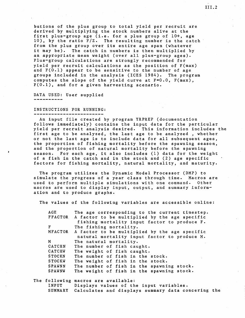
111.2
butions of the plus group to total yield per recruit are derived by multiplying the stock numbers alive at the first plus-group age (i.e. fox a plus group of 10+, age 10), by the ratio F/z. The resulting number is the catch from the plus group over its entire age span (whatever it may be). The catch in numbers is then multiplied by an appropriate mean weight (over all plus-group ages). Plus-group calculations are strongly recommended for yield per recruit calculations as the position of F(max) and F(O.I) appear to be sens~tive to the number of age groups included in the analysis (ICES 1984). The program computes the slope of the yield curve at F=O.O, F(max), F(O.I), and for a given harvesting scenario.
DATA USED: User supplied
INSTRUCTIONS FOR RUNNING:
An input file created by program YRPREP (documentation follows immediately) contains the input data for the particular yield per recruit analysis desired. This information includes the first age to be analyzed, the last age to be analyzed , whether or not the last age is to include data for all subsequent ages, the proportion of fishing mortality before the spawning season, and the proportion of natural mortality before the spawning season. For each age, it also includes (1) data for the weight of a fish in the catch and in the stock and (2) age specific factors for fishing mortality, natural mortality, and maturity.
The program utilizes the Dynamic Model Processor (DMP) to simulate the progress of a year class through time. Macros are used to perform multiple simulations with one command. Other macros are used to display input, output, and summary information and to produce graphs.
The values of the following variables are accessible online:
AGE The age corresponding to the current timestep. FFACTOR A factor to be multiplied by the age specific
fishing mortality input factor to produce F. F The fishing mortality. MFACTOR A factor to be multiplied by the age specific
natural mortality input factor to produce M. M The natural mortality. CATCHN The number of fish caught. CATCHW The weight of fish caught. STOCKN The number of fish in the stock. STOCKW The weight of fish in the stock. SPAWNN The number of fish in the spawning stock. SPAWNW The weight of fish in the spawning stock.
The following macros are available: INPUT Displays values of the input variables. SUMMARY Calculates and displays summary data concering the
"::
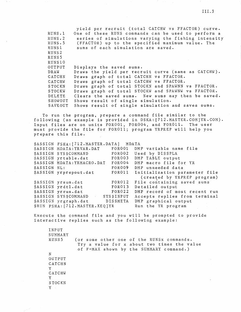
RUNS.I RUNS.2 RUNS.S RUNSI RUNS2 RUNSS RUNSIO OUTPUT DRAW CATCHN CATCHW STOCKN STOCKW DELETE SHOWOUT SAVE OUT
111.3
yield per recruit (total CATCHW vs FFACTOR) curve. One of these RUNS commands can be used to perform a series of simulations varying the fishing intensity (FFACTOR) up to the specified maximum value. The sums of each simulation are saved.
Displays the saved sums. Draws the yield per recruit curve (same as CATCHW). Draws graph of total CATCHN vs FFACTOR. Draws graph of total CATCHW vs FFACTOR. Draws graph of total STOCKN and SPAWNN vs FFACTOR. Draws graph of total STOCKW and SPAWNW vs FFACTOR. Clears the saved sums. New sums may then be saved. Shows result of single simulation. Shows result of single simulation and saves sums.
To run the program, prepare a command file similar to the following (an example is provided in DSKA: [7I2.MASTER.COM]YR.COM). Input files are on units FOROOI, FOR004, and FOROII. The user must provide the file for FOROI1; program YRPREP will help you prepare this file.
$ASSIGN $ASSIGN $ASSIGN $ASSIGN $ASSIGN $ASSIGN $ASSIGN
FSHA: [7I2.MASTER.DATA] MDATA MDATA:YRVAR.DAT FOROOl DMP variable name file SYS$COMMAND FOR002 Used by DISSPLA yrtable.dat FOR003 DMP TABLE output MDATA:YRMACRO.DAT FOR004 DMP macro file for YR NL: FOR009 DMP unneeded data yrprepout.dat FOROll Initialization parameter file
$ASSIGN yrsum.dat FOROI2 $ASSIGN yrdtl.dat FOROI3 $ASSIGN yrrun.dat FOR022 $ASSIGN SYS$COMMAND SYS$INPUT $ASSIGN yrgraph.dat DISSMETA $RUN FSHA: [7I2.MASTER.XEQ]YR
(created by YRPREP program) File co~taining saved sums Detailed output DMP record of most recent run Accepts replies from terminal DMP graphical output Run the YR program
Execute the command file and you will be prompted to provide interactive replies such as the following example:
INPUT SUMMARY RUNSS
N OUTPUT CATCHN Y CATCHW Y STOCKN Y
(or some other one of the RUNSx commands. Try a value for x about two times the value of F-MAX shown by the SUMMARY command.)
STOCKW Y EXIT
Deferred graphical output is accessed using DISSPLOT.
REFERENCES:
International Council for the Exploration of the Sea. 1984.
111.4
Report of the Working Group on Methods of Fish Stock Assessment. ICES Cooperative Research Report 129. 134p.
Thompson, W.F., and F.H. Bell. 1934. Biological statistics of the Pacific halibut fishery. 2. Effect of changes in intensity upon total yield and yield per unit of gear. Rep. Int. Fish. (Pacific Hilibut) Comm. 8:49p.
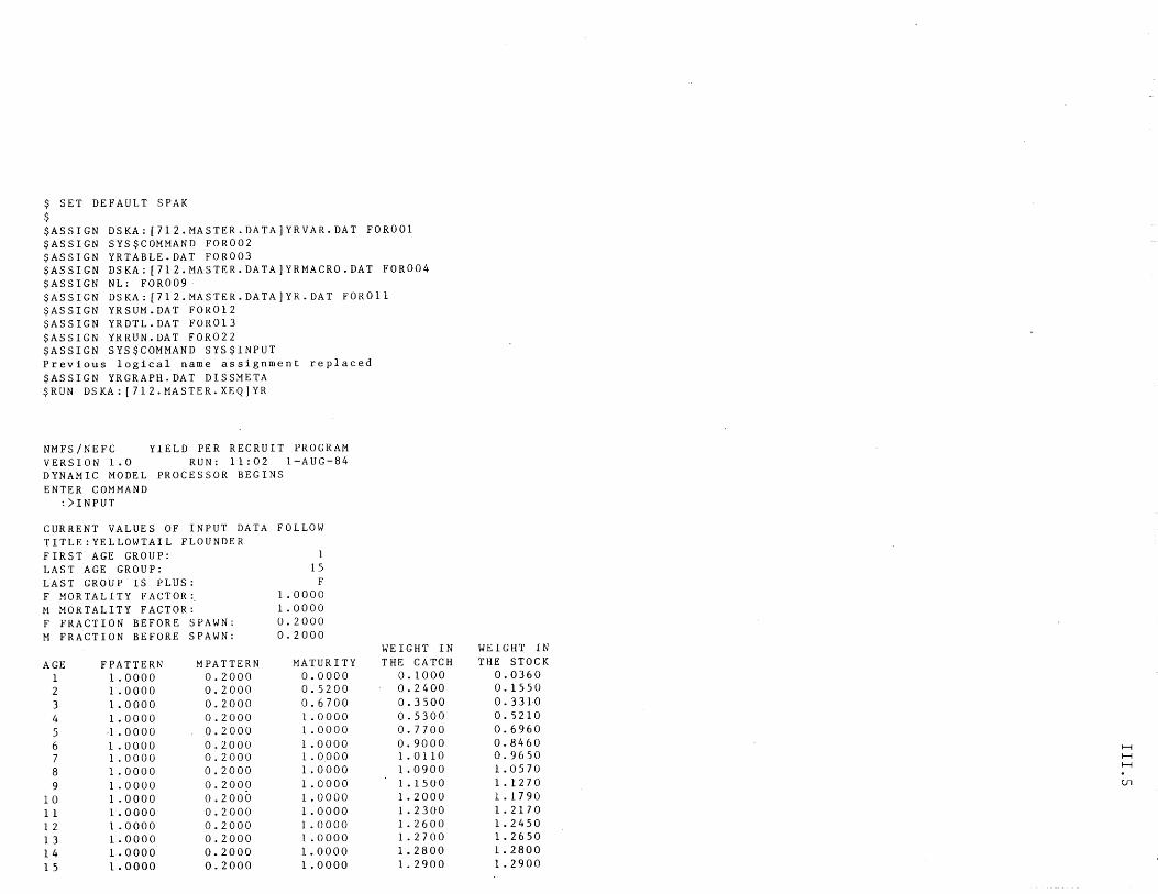
$ SET DEFAULT SPAK $ $ASSIGN DSKA: [712.MASTER.DATA]YRVAR.DAT FOR001 $ASSIGN SYS$COMMAND FOR002 $ASSIGN YRTABLE.DAT FOR003 $ASSIGN DSKA: [712.MASTER.DATA]YRMACRO.DAT FOR004 $ASSIGN NL: FOR009· $ASSIGN DSKA:[712.MASTER.DATA]YR.DAT FOR011 $ASSIGN YRSUM.DAT FOR012 $ASSIGN YRDTL.DAT FOR013 $ASSIGN YRRUN.DAT FOR022 $ASSIGN SYS$COMMAND SYS$INPUT Previous logical name assignment replaced $ASSIGN YRGRAPH.DAT DISSMETA $RUN DSKA: [712.MASTER.XEQ]YR
NMFS/NEFC YIELD PER RECRUIT PROGRAM VERSION 1.0 RUN: 11:02 1-AUG-84 DYNAMIC MODEL PROCESSOR BEGINS ENTER COMMAND
:)INPUT
CURRENT VALUES OF INPUT DATA FOLLOW TITLE:YELLOWTAIL FLOUNDER FIRST AGE GROUP: LAST AGE GROUP: LAST GROUP IS PLUS: F MORTALITY FACTOR: M MORTALITY FACTOR: F FRACTION BEFORE SPAWN: M FRACTION BEFORE SPAWN:
AGE 1 2 3 4 5 6 7 8 9
10 11 12 13 14 15
FPATTERN 1.0000 1.0000 1.0000 1.0000 -1.0000 1.0000 1.0000 1.0000 1.0000 1.0000 1.0000 1.0000 1.0000 1.0000 1.0000
MPATTERN 0.2000 0.2000 0.2000 0.2000 0.2000 0.2000 0.2000 0.2000 0.2000 0.2000 0.2000 0.2000 0.2000 0.2000 0.2000
1 15
F 1.0000 1.0000 0.2000 0.2000
MATURITY 0.0000 0.5200 0.6700 1.0000 1.0000 1.0000 1.0000 1.0000 1.0000 1.0000 1.0000 1.0000 1.0000 1.0000 1.0000
WEIGHT IN THE CATCH
0.1000 0.2400 0.3500 0.5300 0.7700 0.9000 1.0110 1.0900 1.1500 1.2000 1.2300 1.2600 1. 2700 1.2800 1.2900
WEIGHT IN THE STOCK
0.0360 0.1550 0.331-0 0.5210 0.6960 0.8460 0.9650 1.0570 1.1270 1.1790 1.2170 1.2450 1.2650 1.2800 1.2900
H H H
Ul
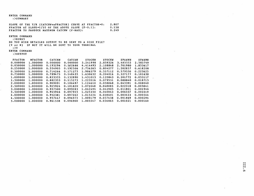
ENTER COMMAND :)SUMMARY
SLOPE OF THE Y/R (CATCHWvsFFACTOR) CURVE AT FFACTOR=O: 2.807 0.158 0.249
FFACTOR AT SLOPE-1/10 OF THE ABOVE SLOPE (F-0.1): FFACTOR TO PRODUCE MAXIMUM CATCHW (F-MAX):
ENTER COMMAND :)RUNS5
DO YOU WISH DETAILED OUTPUT TO BE SENT TO A DISK FILE? (Y or N) IF NOT IT WILL BE SENT TO YOUR TERMINAL
:)Y ENTER COMMAND
:)OUTPUT
FFACTOR MFACTOR CATCHN CATCHW STOCKN STOCKW SPAWNN 0.000000 1.000000 0.000000 0.000000 5.241998 2.859326 3.48555~ 0.050000 1.000000 0.195296 0.1.02686 4.414493 2.108848 2.701980 0.250000 1.000000 0.554905 0.192506 2.756365 0.804277 1.202857 0.500000 1.000000 0.714266 0.171275 1.986379 0.357112 0.579550 0.750000 1.000000 0.789473 0.148435 1.630632 0.204016 0.327177 1.000000 1.000000 0.833333 0.132890 1.431013 0.135843 0.201772 1.500000 1.000000 0.882353 0.115273 1.223516 0.079531 0.088840 2.000000 1.000000 0.909091 0.106497 1.124610 0.058068. 0.043391 2.500000 1.000000 0.925926 0.101820 1.072048 0.048085 0.022318 3.000000 1.000000 0.937500 0.099283 1.042494 0.042905 0.011801 3.500000 1.000000 0.945946 0.097935 1.025350 0.040043 0.006337 4.000000 1.000000 0.952381 0.097262 1.015224 0.038401 0.003433 4.500000 1.000000 0.957447 0.096973 1.009179 0.037438 0.001869 5.000000 1.000000 0.961538 0.096900 1. 005547 0.036865 0.001021
SPAWNW 2.583749 1.853617 0.618208 0.223625 0.101638 0.053117 0.018715 0.008040 0.003841 0.001946 0.001019 0.000544 0.000294 0.000160
H H H
0\
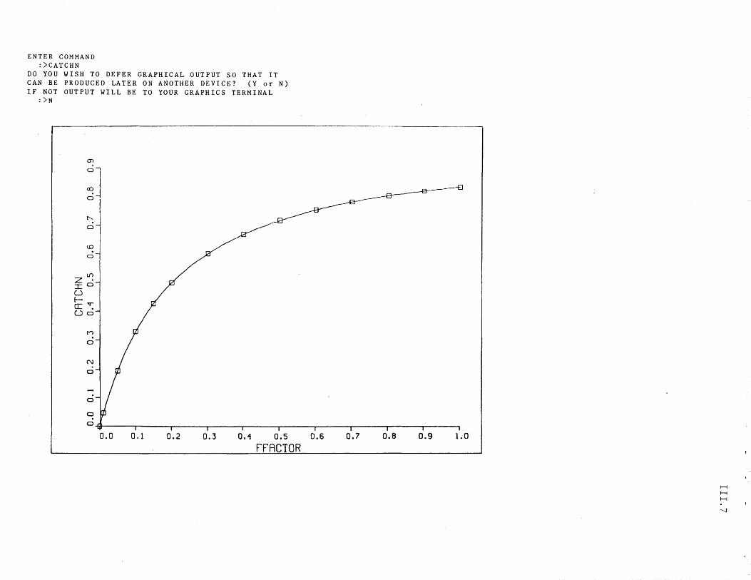
ENTER COMMAND :>CATCHN
DO YOU WISH TO DEFER GRAPHICAL OUTPUT SO THAT IT CAN BE PRODUCED LATER ON ANOTHER DEVICE? (Y or N) IF NOT OUTPUT WILL BE TO YOUR GRAPHICS TERMINAL
:>N
01
:l .~
0
~ 0
(0
0
lJ"')
Z· I O
U r-cr:~ Uo
n 0
N
a
0
a 0
"f'
0.0 0.1 0.2 0.3 o.~ 0.5 0.6
rrAeTOR 0.7 0.8 0.9 1.0
H H H
'-l
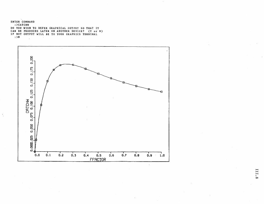
ENTER COMMAND :)CATCHW
DO YOU WISH TO DEFER GRAPHICAL OUTPUT SO THAT IT CAN BE PRODUCED LATER ON ANOTHER DEVICE? (Y or N) IF NOT OUTPUT WILL BE TO YOUR GRAPHICS TERMINAL
:)N
0 0 N
0
If)
" 0
0 If)
0
If) N .
° ~8 0-........ a: O
Olf) t--. 0
0
0 Lf) 0
0
Lf)
~
§ 0 . 0
'" I 0.0 0.1 0.2 0.3 o.~ 0.5 0.6
PrAeTOR 0.7 0.8 0.9 1.0
H H H
00
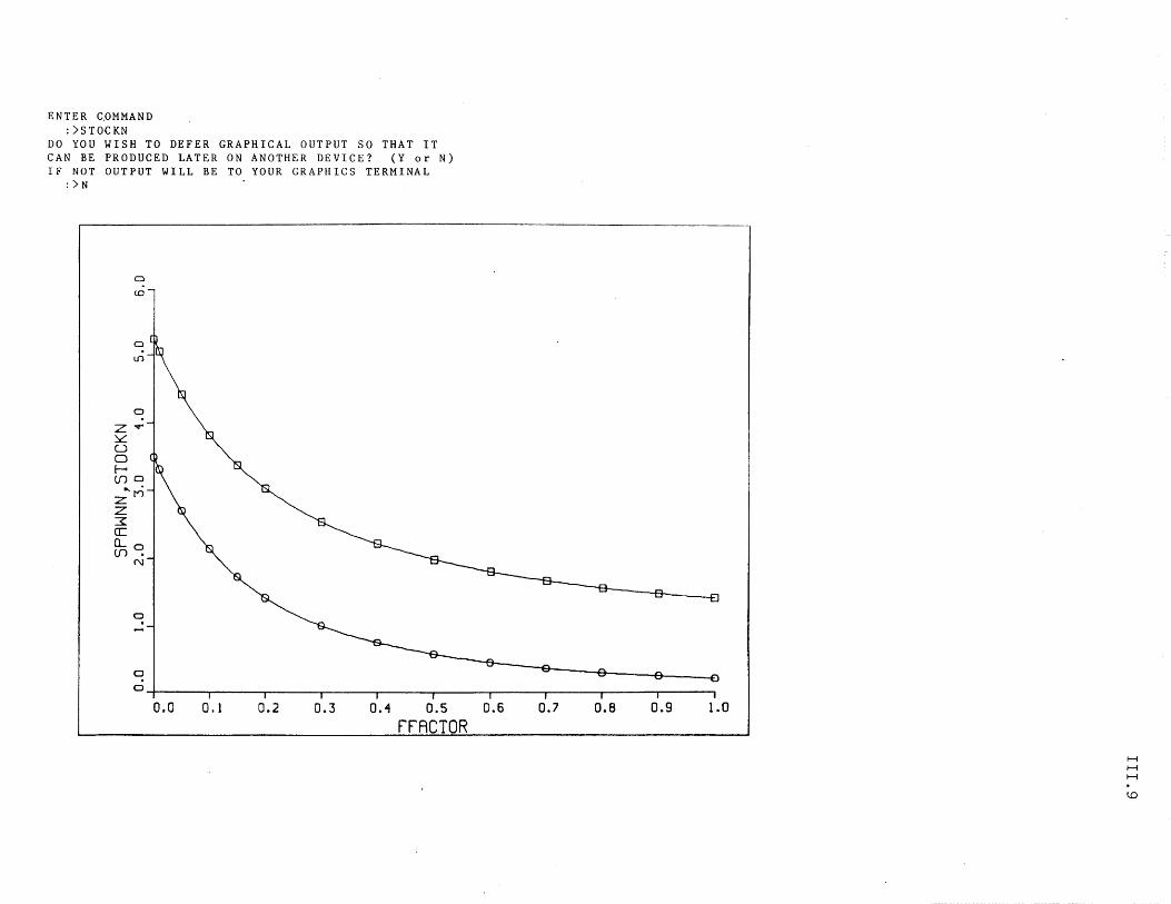
ENTER C,OMMAND :)STOCKN
DO YOU WISH TO DEFER GRAPHICAL OUTPUT SO THAT IT CAN BE PRODUCED LATER ON ANOTHER DEVICE? (Y or N) IF NOT OUTPUT WILL BE TO YOUR GRAPHICS TERMINAL
: )N
a
COl
a If)
a Z";' ~ U o f(f)a
z"'n z ~ cr: (La (f).
N
a
a a-r-------r-------r-------r-------r------~------_,------_,------_,------_,r_----_,
0.0 0.1 0.2 0.3 0.1 0.5 0.6 0.7 0.8 0.9 1.0
PPAeTOR H H H
tD
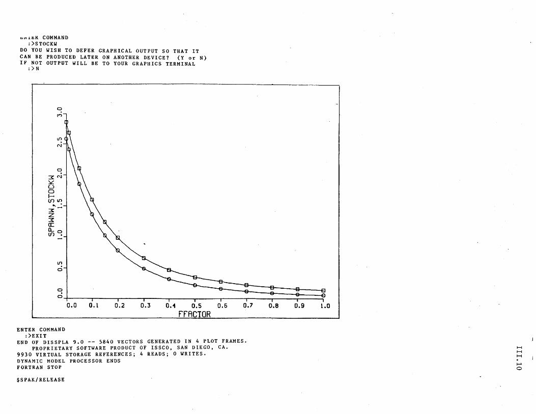
c.n.&.1!.l{ COMMAND :)STOCKW
DO YOU WISH TO DEFER GRAPHICAL OUTPUT SO THAT IT CAN BE PRODUCED LATER ON ANOTHER DEVICE? (Y or N) IF NOT OUTPUT WILL BE TO YOUR GRAPHICS TERMINAL
:) N
a
I'll
If')
N
a
3: N ~ (..)
o f-t (I) If') ... . ::::3:-Z 3: CC (La (I).
If')
a
o . a ,
ENTER COMMAND :)EXIT
0.0 0.1 0.2 0.3 0.1 0.5 0.6 PPAeTOR
0.7
END OF DISSPLA 9.0 -- 5840 VECTORS GENERATED IN 4 PLOT FRAMES. PROPRIETARY SOFTWARE PRODUCT OF ISSCO, SAN DIEGO, CA.
9930 VIRTUAL STORAGE REFERENCES; 4 READS; 0 WRITES. DYNAMIC MODEL PROCESSOR ENDS FORTRAN STOP
$SPAK/RELEASE
I
0.8 0.9 1.0
H H H
I-l o
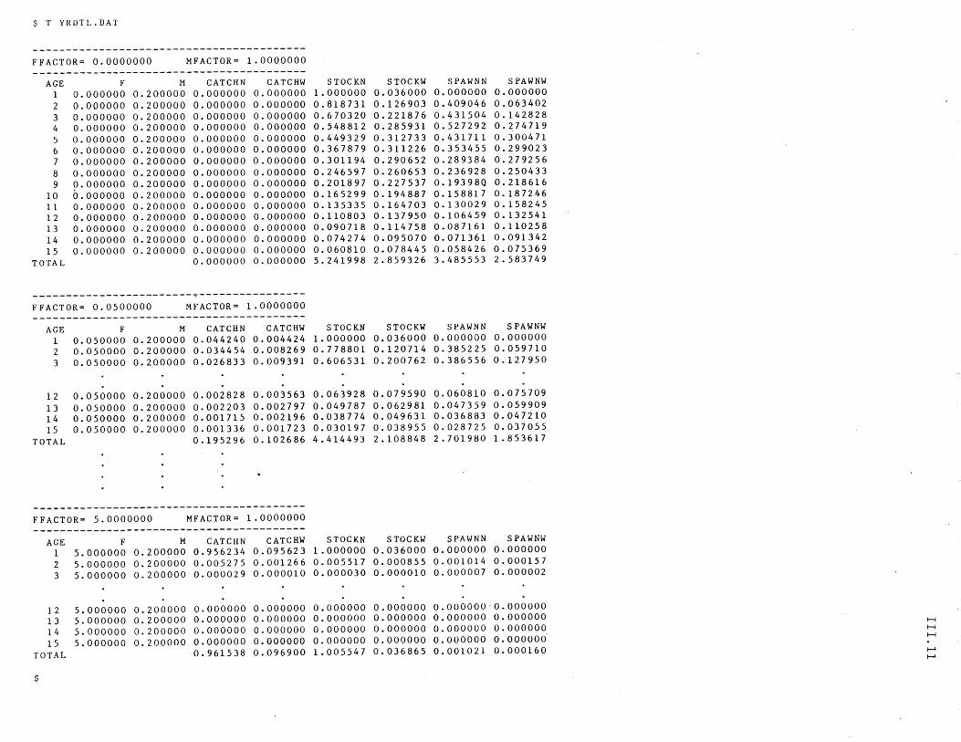
$ T YRDTL.DAT
-----------------------------------------FFACTOR= 0.0000000 MFACTOR= 1.0000000 -----------------------------------------
AGE F M CATCHN CATCHW STOCKN STOCKW SPAWNN SPAWNW
1 0.000000 0.200000 0.000000 0.000000 1.000000 0.036000 0.000000 0.000000 2 0.000000 0.200000 0.000000 0.000000 0.818731 0.126903 0.409046 0.063402 3 0.000000 0.200000 0.000000 0.000000 0.670320 0.221876 0.431504 0.142828 4 0.000000 0.200000 0.000000 0.000000 0.548812 0.285931 0.527292 0.274719 5 0.000000 0.200000 0.000000 0.000000 0.449329 0.312733 0.431711 0.300471 6 0.000000 0.200000 0.000000 0.000000 0.367879 0.311226 0.353455 0.299023 7 0.000000 0.200000 0.000000 0.000000 0.301194 0.290652 0.289384 0.279256 8 0.000000 0.200000 0.000000 0.000000 0.246597 0.260653 0.236928 0.250433 9 0.000000 0.200000 0.000000 0.000000 0.201897 0.227537 0.19398Q 0.218616
10 0.000000 0.200000 0.000000 0.000000 0.165299 0.194887 0.158817 0.187246 11 0.000000 0.200000 0.000000 0.000000 0.135335 0.164703 0.130029 0.158245 12 0.000000 0.200000 0.000000 0.000000 0.110803 0.137950 0.106459 0.132541 13 0.000000 0.200000 0.000000 0.000000 0.090718 0.114758 0.087161 0.110258 14 0.000000 0.200000 0.000000 0.000000 0.074274 0.095070 0.071361 0.091342 15 0.000000 0.200000 0.000000 0.000000 0.060810 0.078445 0.058426 0.075369
TOTAL 0.000000 0.000000 5.241998 2.859326 3.485553 2.583749
------------------------~----------------
FFACTOR= 0.0500000 MFACTOR= 1.0000000 -----------------------------------------
AGE F M CATCHN CATCHW STOCKN STOCKW SPAWNN SPAWNW
1 0.050000 0.200000 0.044240 0.004424 1.000000 0.036000 0.000000 0.000000 2 0.050000 0.200000 0.034454 0.008269 0.778801 0.120714 0.385225 0.059710 3 0.050000 0.200000 0.026833 0.009391 0.606531 0.200762 0.386556 0.127950
12 0.050000 0.200000 0.002828 0.003563 0.063928 0.079590 0.060810 0.075709
13 0.050000 0.200000 0.002203 0.002797 0.049787 0.062981 0.047359 0.059909 14 0.050000 0.200000 0.001715 0.002196 0.038774 0.049631 0.036883 0.047210 15 0.050000 0.200000 0.001336 0.001723 0.030197 0.038955 0.028725 0.037055
TOTAL 0.195296 0.102686 4.414493 2.108848 2.701980 1.853617
-~---------------------------------------
FFACTOR= 5.0000000 MFACTOR= 1.0000000 -----------------------------------------
AGE F M CATCHN CATCHW STOCKN STOCKW SPAWNN SPAWNW
1 5.000000 0.200000 0.956234 0.095623 1.000000 0.036000 0.000000 0.000000 2 5.000000 0.200000 0.005275 0.001266 0.005517 0.000855 0.001014 0.000157 3 5.000000 0.200000 0.000029 0.000010 0.000030 0.000010 0.000007 0.000002
12 5.000000 0.200000 0.000000 0.000000 0.000000 0.000000 0.000000-0.000000 13 5.000000 0.200000 0.000000 0.000000 0.000000 0.000000 0.000000 0.000000 14 5.000000 0.200000 0.000000 0.000000 0.000000 0.000000 0.000000 0.000000
H H
15 5.000000 0.200000 0.000000 0.000000 0.000000 0.000000 0.000000 0.000000 H
TOTAL 0.961538 0.096900 1.005547 0.036865 0.001021 0.000160 ~
~
$
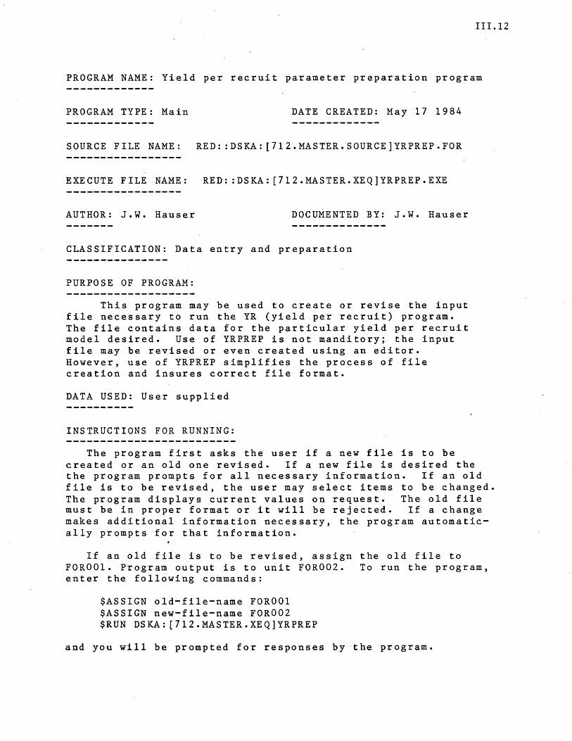
111.12
PROGRAM NAME: Yield per recruit parameter preparation program
PROGRAM TYPE: Main DATE CREATED: May 17 1984
SOURCE FILE NAME: RED::DSKA:[712.MASTER.SOURCE]YRPREP.FOR
EXECUTE FILE NAME: RED: :DSKA:[712.MASTER.XEQ]YRPREP.EXE
AUTHOR: J.W. Hauser DOCUMENTED BY: J.W. Hauser
CLASSIFICATION: Data entry and preparation
PURPOSE OF PROGRAM:
This program may be used to create or revise the input file necessary to run the YR (yield per recruit) program. The file contains data for the particular yield per recruit model desired. Use of YRPREP is not manditory; the input file may be revised or even created using an editor. However, use of YRPREP simplifies the process of file creation and insures correct file format.
DATA USED: User supplied
INSTRUCTIONS FOR RUNNING:
The program first asks the user if a new file is to be created or an old one revised. If a new file is desired the the program prompts for all necessary information. If an old file is to be revised, the user may select items to be changed. The program displays current values on request. The old file must be in proper format or it will be rejected. If a change makes additional information necessary, the program automatically prompts for that information.
If an old file is to be revised, assign the old file to FOROOI. Program output is to unit FOR002. To run the program, enter the following commands:
$ASSIGN old-file-name FOROOI $ASSIGN new-file-name FOR002 $RUN DSKA:[712.MASTER.XEQ]YRPREP
and you will be prompted for responses by the program.
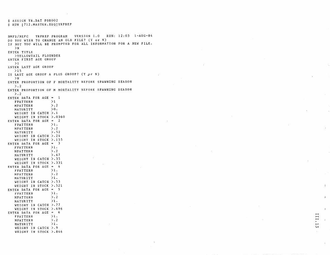
$ ASSIGN YR.DAT FOR002 $ RUN [712.MASTER.XEQ]YRPREP
NMFS/NEFC YRPREP PROGRAM VERSION 1.0 RUN: 12:03 l-AUG-84 DO YOU WISH TO CHANGE AN OLD FILE? (Y or N) IF NOT YOU WILL BE PROMPTED FOR ALL INFORMATION FOR A NEW FILE.
)N
ENTER TITLE )YELLOWTAIL FLOUNDER
ENTER FIRST AGE GROUP )1
ENTER LAST AGE GROUP )15
IS LAST AGE GROUP A PLUS GROU'P? (Y ..or N) )N
ENTER PROPORTION OF F MORTALITY BEFORE SPAWNING SEASON ).2
ENTER PROPORTION OF M MORTALITY BEFORE SPAWNING SEASON ).2
ENTER DATA FOR AGE 1 FPATTERN )1 MPATTERN ).2 MATURITY )0. WEIGHT IN CATCH ).1 WEIGHT IN STOCK ).0360
ENTER DATA FOR AGE 2 FPATTERN )1-
MPATTERN ).2 MATURITY ).52 WEIGHT IN CATCH ).24 WEIGHT IN STOCK ).155
ENTER DATA FOR AGE 3 FPATTERN )1-
MPATTERN ).2 MATURITY ).67 WEIGHT IN CATCH ).35 WEIGHT IN STOCK ).331
ENTER DATA FOR AGE 4 FPATTERN )1-
MPATTERN ).2 MATURITY )1-
WEIGHT IN CATCH ).53 WEIGHT IN STOCK ).521
ENTER DATA FOR AGE 5 FPATTERN )1-
MPATTERN ).2 MATURITY )1-
WEIGHT IN CATCH ).77 WEIGHT IN STOCK ).696
ENTER DATA FOR AGE 6 FPATTERN )1-
MPATTERN ).2 MATURITY )1-
WEIGHT IN CATCH ).9 WEIGHT IN STOCK ).846
H H H
f--'. (N
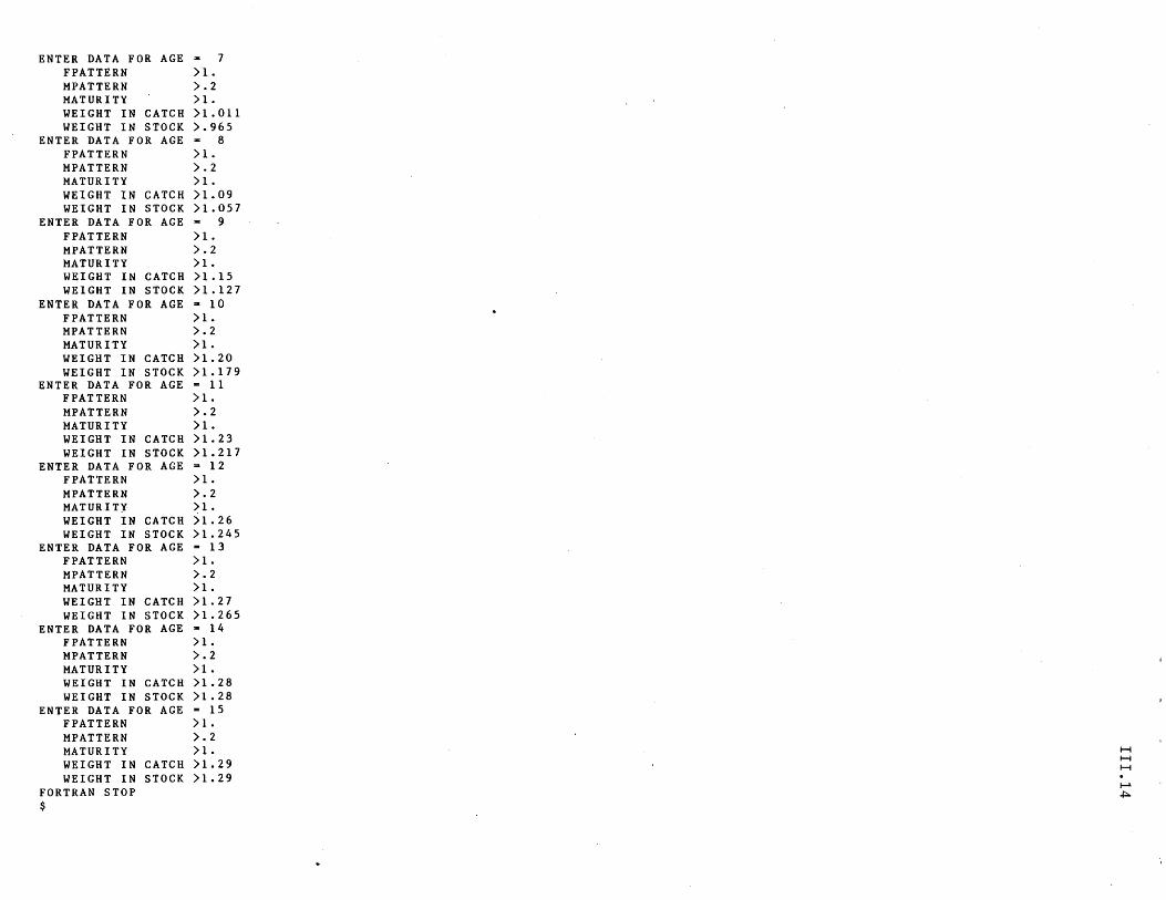
ENTER DATA FOR AGE a 7 FPATTERN >1. MPATTERN >.2 MATURITY >1. WEIGHT IN CATCH >1.011 WEIGHT IN STOCK >.965
ENTER DATA FOR AGE z 8 FPATTERN >1. MPATTERN >.2 MATURITY >1. WEIGHT IN CATCH >1.09 WEIGHT IN STOCK >1.057
ENTER DATA FOR AGE = 9 FPATTERN >1. MPATTERN >.2 MATURITY >1. WEIGHT IN CATCH >1.15 WEIGHT IN STOCK >1.127
ENTER DATA FOR AGE ~ 10 FPATTERN >1. MPATTERN >.2 MATURITY >1. WEIGHT IN CATCH >1.20 WEIGHT IN STOCK >1.179
ENTER DATA FOR AGE = 11 FPATTERN >1. MPATTERN >.2 MATURITY >1. WEIGHT IN CATCH >1.23 WEIGHT IN STOCK >1.217
ENTER DATA FOR AGE = 12 FPATTERN >1. MPATTERN >.2 MATURITX >1. WEIGHT IN CATCH )1.26 WEIGHT IN STOCK >1.245
ENTER DATA FOR AGE = 13 FPATTERN >1. MPATTERN >.2 MATURITY >1. WEIGHT IN CATCH >1.27 WEIGHT IN STOCK >1.265
ENTER DATA FOR AGE a 14 FPATTERN >1. MPATTERN >.2 MATURITY >1. WEIGHT IN CATCH >1.28 WEIGHT IN STOCK >1.28
ENTER DATA FOR AGE = 15 FPATTERN >1. MPATTERN >.2 MATURITY >1. WEIGHT IN CATCH >1.29 WEIGHT IN STOCK >1.29
FORTRAN STOP $
1-1 1-1 1-1
I-l ..t;:..
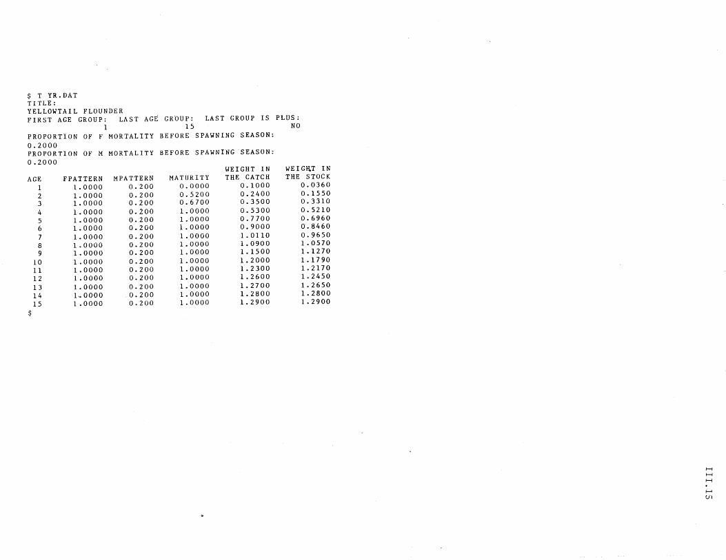
$ T YR.DAT TITLE: YELLOWTAIL FLOUNDER FIRST AGE GROUP: LAST AGE GROUP: LAST GROUP IS
1 15 PROPORTION OF F MORTALITY BEFORE SPAWNING SEASON: 0.2000 PROPORTION OF M MORTALITY BEFORE SPAWNING SEASON: 0.2000
WEIGHT IN AGE FPATTERN MPATTERN MATURITY THE CATCH
1 1.0000 0.200 0.0000 0.1000
2 1.0000 0.200 0.5200 0.2400 3 1.0000 0.200 0.6700 0.3500
4 1.0000 0.200 1.0000 0.5300 5 1.0000 0.200 1.0000 0.7700 6 1.0000 0.200 1.0000 0.9000
7 1.0000 0.200 1.0000 1.0110 8 1.0000 0.200 1.0000 1.0900 9 1.0000 0.200 1.0000 1.1500
10 1.0000 0.200 1.0000 1.2000 11 1.0000 0.200 1.0000 1.2300 12 1.0000 0.200 1.0000 1.2600
13 1.0000 0.200 1.0000 1.2700 14 1..0000 0.200 1. 0000 1.2800 15 1.0000 0.200 1.0000 1.2900
$
PLUS: NO
WEIGll.T IN THE STOCK
0.0360 0.1550 0.3310 0.5210 0.6960 0.8460 0.9650 1.0570 1.1270 1. 1790 1.2170 1.2450 1.2650 1.2800 1.2900
H H H
f-l U1
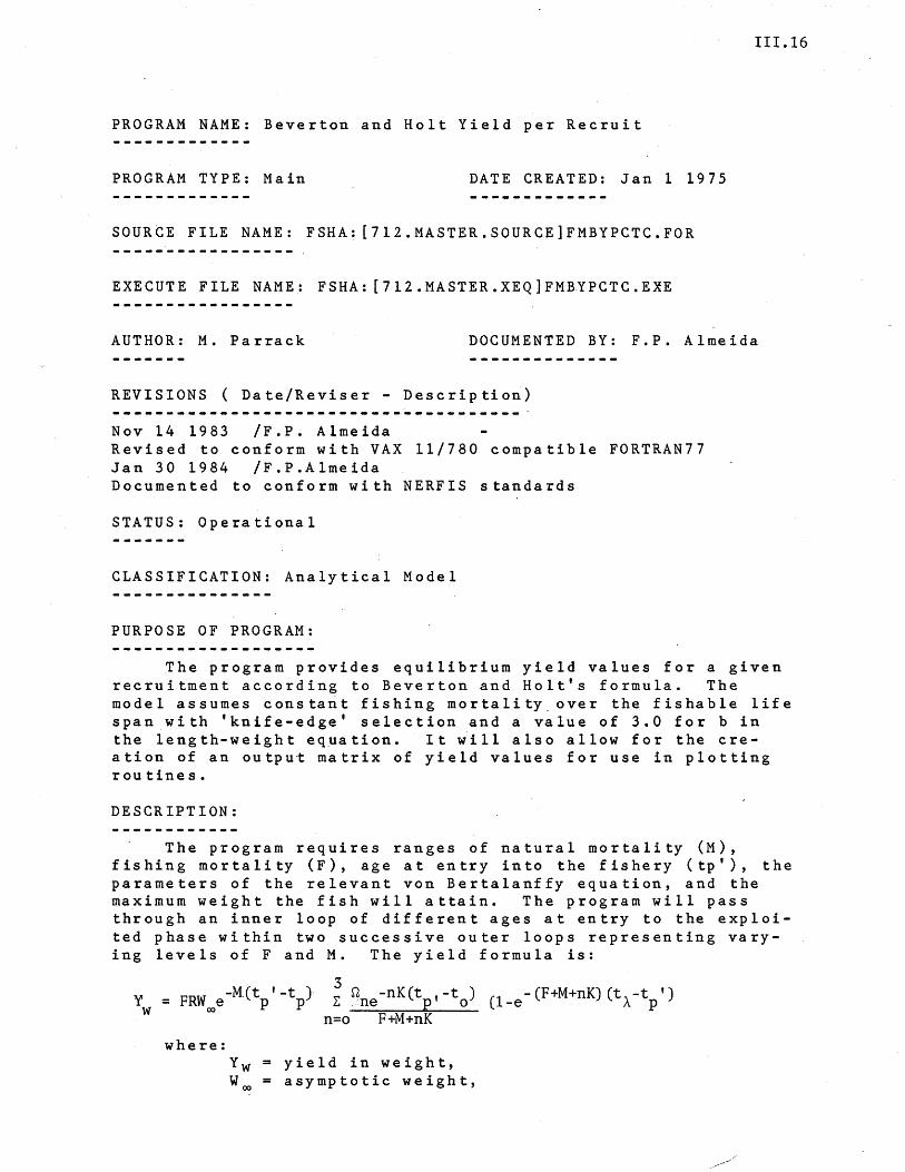
111.16
PROGRAM NAME: Beverton and Holt Yield per Recruit
PROGRAM TYPE: Main DATE CREATED: Jan 1 1975
SOURCE FILE NAME: FSHA: [7l2.MASTER.SOURCE]FMBYPCTC.FOR
EXECUTE FILE NAME: FSHA: [7l2.MASTER.XEQ]FMaYPCTC.EXE
AUTHOR: M. Parrack DOCUMENTED BY: F.P. Almeida
REVISIONS ( Date/Reviser - Description)
Nov 14 1983 /F.P. Almeida Revised to conform with VAX 11/780 compatible FORTRAN77 Jan 30 1984 /F.P.Almeida Documented to conform with NERFIS standards
STATUS: Operational
CLASSIFICATION: Analytical Model
PURPOSE OF PROGRAM:
The program provides equilibrium yield values for a given recruitment according to Beverton and Holt's formula. The model assumes constant fishing mortality, over the fishable life span with 'knife-edge' selection and a value of 3.0 for b in the length-weight eq~ation. It will also allow for the creation of an output matrix of yield values for use in plotting routines.
DESCRIPTION:
The program requires ranges of natural mortality (M), fishing mortality (F), age at entry into the fishery (tp'), the parameters of the relevant von Bertalanffy equation, and the maximum weight the fish will attain. The program will pass through an inner loop of different ages at entry to the exploited phase within two successive outer loops representing varying levels of F and M. The yield formula is:
whe re: Yw = yield in weight, Woo = asymptotic weight,
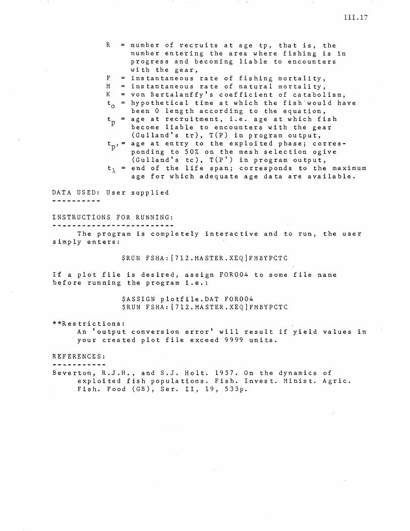
111.17
R number of recruits at age tp, that is, the number entering the area where fishing is in progress and becoming liable to encounters with the gear,
F instantaneous rate of fishing mortality, M instantaneous rate of natural mortality, K von Bertalanffy's coefficient of catabolism, to hypothetical time at which the fish"would have
been 0 length according to the equation, tp = age at recruitment, i.e. age at which fish
become liable to encounters with the gear (Gul1and's tr), T(P) in program output,
t p '= age at entry to the exploited phase; corresponding to 50% on the mesh selection ogive (Gu1Iand's tc), T(P') in program output,
tA end of the life span; corresponds to the maximum age for which adequate age data are available.
DATA USED: User supplied
INSTRUCTIONS FOR RUNNING:
The program is completely interactive and to run, the user simply enters:
$RUN FSHA: [712.MASTER.XEQ]FMBYPCTC
If a plot file is desired, assign FOR004 to some file name before running the program i.e.:
$ASSIGN p1otfi1e.DAT FOR004 $RUN FSHA: [7l2.MASTER.XEQ]FMBYPCTC
**Res trictions: An 'output conversion error' will result if yield values in your created plot file exceed 9999 units.
REFERENCES:
Beverton, R.J.H., and S.J. Holt. 1957. On the dynamics of exploited fish populations. Fish. Invest. l1inist. Agric. Fish. Food (GB), Sere II, 19, 533p.
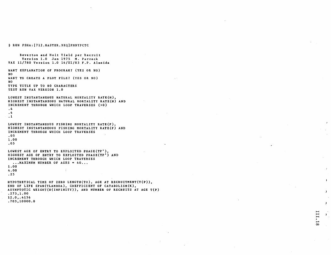
$ RUN FSHA:[112.MASTER.XEQ]FMBYPCTC
Beverton and Holt Yield per Recruit Version 1.0 Jan 1915. M. Parrack
VAX 11/780 Version 1.0 14/XI/83 F.P. Almeida
WANT EXPLANATION OF PROGRAM? (YES OR NO) NO WANT TO CREATE A PLOT FILE? (YES OR NO) NO TYPE TITLE UP TO 80 CHARACTERS TEST RUN VAX VERSION 1.0
LOWEST INSTANTANEOUS NATURAL MORTALITY RATE(M), HIGHEST INSTANTANEOUS NATURAL MORTALITY RATE(M) AND INCREMENT THROUGH WHICH LOOP TRAVERSES (>0) .4 .4 .1
LOWEST INSTANTANEOUS FISHING MORTALITY RATE(F), HIGHEST INSTANTANEOUS FISHING MORTALITY RATE(F) AND INCREMENT THROUGH WHICH LOOP TRAVERSES .05 1.00 .05
LOWEST AGE OF ENTRY TO EXPLOITED PHASE(TP'), HIGHEST AGE OF ENTRY TO EXPLOITED PHASE(TP') AND INCREMENT THROUGH WHICH LOOP TRAVERSES
••• MAXIMUM NUMBER OF AGES ~ 40 ... 1.00 4.00 .25
HYPOTHETICAL TIME OF ZERO LENGTH(TO), AGE AT RECRUITMENT(T(P», END OF LIFE SPAN(TLAMBDA), COEFFICIENT OF CATABOLISM(K), ASYMPTOTIC WEIGHT(W(INFINITY», AND NUMBER OF RECRUITS AT AGE T(P) .213,1.00 12.0,.4156 .103,10000.0
H H H
I-l 00
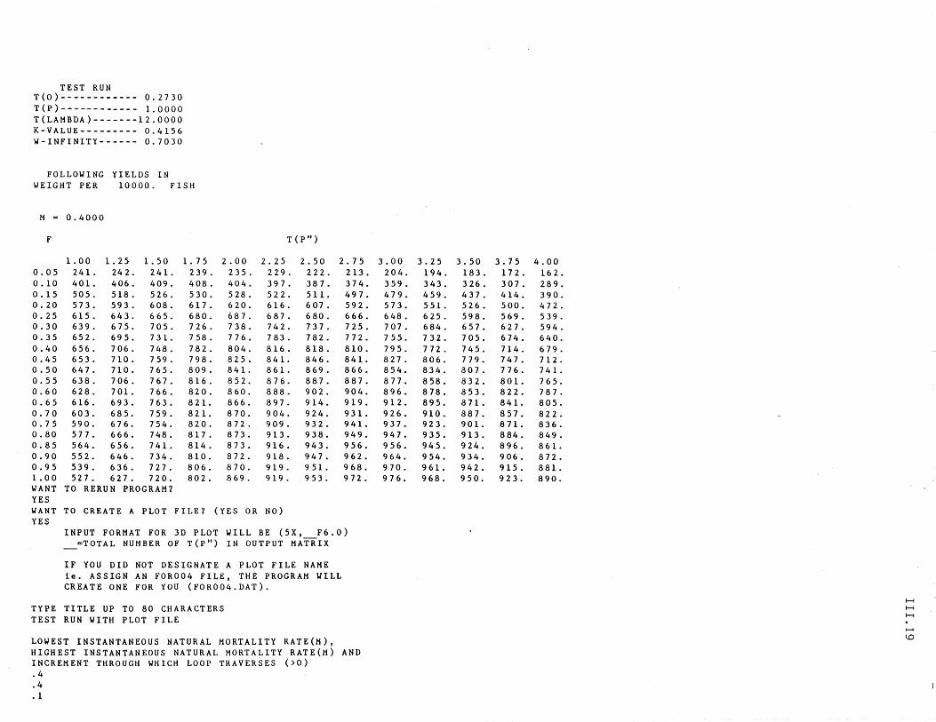
TEST RUN T{O)------------ 0.2730 T{P)------------ 1.0000 T{LAMBDA)-------12.0000 K-VALUE--------- 0.4156 W-INFINITY------ 0.7030
FOLLOWING YIELDS IN WEIGHT PER 10000. FISH
M = 0.4000
F T{p II)
1.00 1. 25 1. 50 1. 75 2.00 2.25 2.50 2.75 0.05 241. 242. 241. 239. 235. 229. 222. 213. 0.10 401. 406. 409. 408. 404. 397. 387. 374. 0.15 505. 518. 526. 530. 528. 522. 511. 497. 0.20 573. 593. 608. 617. 620. 616. 607. 592. 0.25 615. 643. 665. 680. 687. 687. 680. 666. 0.30 639. 675. 705. 726. 738. 742. 737. 725. 0.35 652. 695. 731. 758. 776. 783. 782. 772. 0.40 656. 706. 748. 782. 804. 816. 818. 810. 0.45 653. 710. 759. 798. 825. 841- 846. 841. 0.50 647. 710. 765. 809. 841. 861. 869. 866. 0.55 638. 706. 767. 816. 852. 876. 887. 887. 0.60 628. 701. 766. 820. 860. 888. 902. 904. 0.65 616. 693. 763. 821. 866. 897. 914. 919. 0.70 603. 685. 759. 821. 870. 904. 924. 931. 0.75 590. 676. 754. 820. 872. 909. 932. 941. 0.80 577. 666. 748. 817. 873. 913. 938. 949. 0.85 564. 656. 741. 814. B73. 916. 943. 956. 0.90 552. 646. 734. 810. B 7 2. 91B. 947. 962. 0.95 539. 636. 727. B06. 870. 919. 951. 968. 1.00 527. 627. 720. B02. 869. 919. 953. 972. WANT TO RERUN PROGRAM? YES WANT TO CREATE A PLOT FILE? (YES OR NO) YES
INPUT FORMAT FOR 3D PLOT WILL BE (5X, F6.0) =TOTAL NUMBER OF T(p II
) IN OUTPUT MATRIX -IF YOU DID NOT DESIGNATE A PLOT FILE NAME ie. ASSIGN AN FOR004 FILE, THE PROGRAM WILL CREATE ONE FOR YOU (FOROO4.DAT).
TYPE TITLE UP TO BO CHARACTERS TEST RUN WITH PLOT FILE
LOWEST INSTANTANEOUS NATURAL MORTALITY RATE(M), HIGHEST INSTANTANEOUS NATURAL MORTALITY RATE(M) AND INCREMENT THROUGH WHICH LOOP TRAVERSES (>0) .4 .4 .1
3.00 3.25 3.50 204. 194. 183. 359. 343. 326. 479. 459. 437. 573. 551. 526. 648. 625. 598. 707. 684. 657. 755. 732. 705. 795. 772. 745. 827. 806. 779. 854. 834. 807. 877. 858. 832. 896. 878. 853. 912. 895. 871. 926. 910. 887. 937. 923. 901. 947. 935. 913. 956. 945. 924. 964. 954. 934. 970. 961. 942. 976. 968. 950.
3.75 172. 307. 414. 500. 569. 627. 674. 714. 747. 776. 801. 822. 841. 857. 871. 884. 896. 906. 915. 923.
4.00 162. 289. 390. 472. 539. 594. 640. 679. 712-741. 765. 787. 805. 822. 836. 849. 861. B72. 881. 890.
H H H
~
I..D
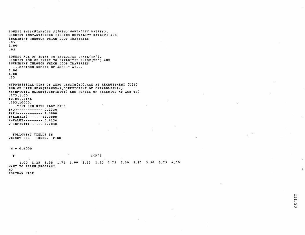
LOWEST INSTANTANEOUS FISHING MORTALITY RATE(F), HIGHEST INSTANTANEOUS FISHING MORTALITY RATE(F) AND INCREMENT THROUGH WHICH LOOP TRAVERSES .05 1.00 .05
LOWEST AGE OF ENTRY TO EXPLOITED PHASE(TP'), HIGHEST AGE OF ENTRY TO EXPLOITED PHASE(TP') AND INCREMENT THROUGH WHICH LOOP TRAVERSES
... MAXIMUM NUMBER OF AGES = 40 ... 1.00 4.00 .25
HYPOTHETICAL ·TIME OF ZERO LENGTH(TO),AGE AT RECRUITMENT (T(P) END OF LIFE SPAN(TLAMBDA),COEFFICIENT OF CATABOLISM(K), ASYMPTOTIC WEIGHT(WINFINITY) AND NUMBER OF RECRUITS AT AGE TP) .273,1.00 12.00,.4156 .703,10000.
TEST RUN WITH PLOT FILE T(O)------------ 0.2730 T(P)------------ 1.0000 T(LAMBDA)-------12.0000 K-VALUE--------- 0.4156 W-INFINITY------ 0.7030
FOLLOWING YIELDS IN WEIGHT PER 10000. FISH
M .. 0.4000
F T(p II)
1.00 1.25 1.50 1.75 2.00 2.25 2.50 2.75 3.00 3.25 3.50 3.75 4.00 WANT TO RERUN PROGRAM? NO • FORTRAN STOP
H H H
N o
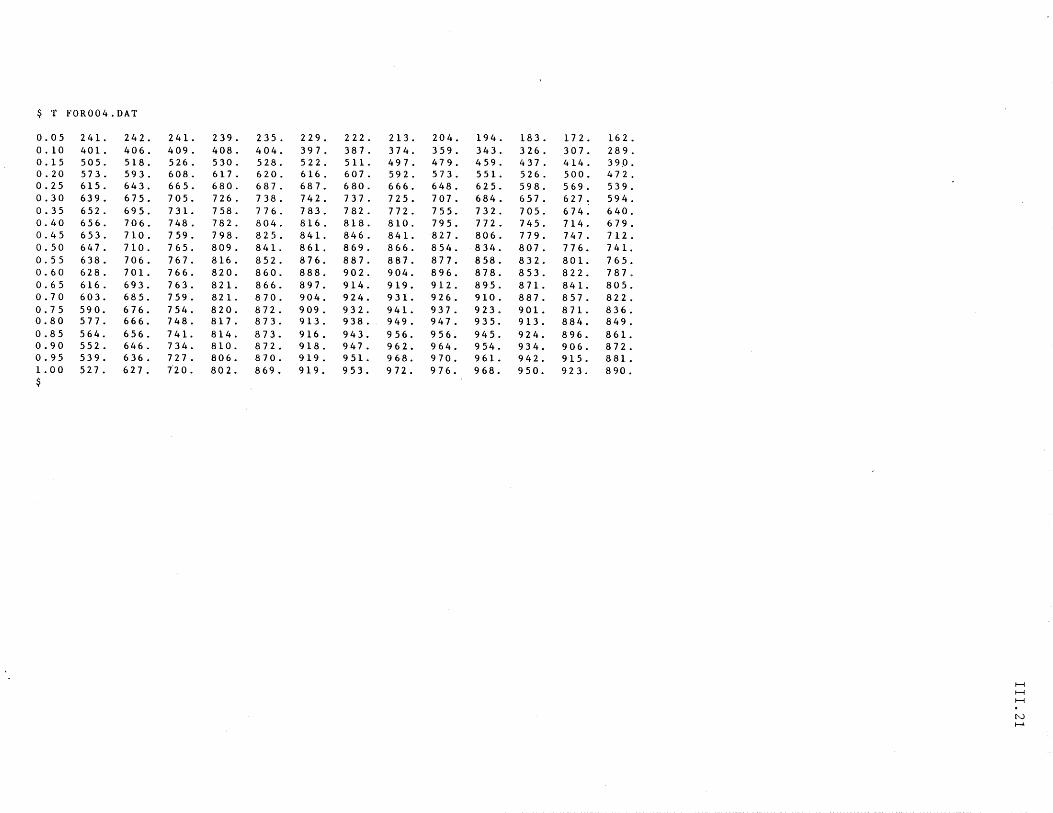
$ T FOR004.DAT
0.05 24l. 242. 24l. 239. 235. 229. 222. 0.10 40l. 406. 409. 408. 404. 397. 387. 0.15 505. 518. 526. 530. 528. 522. 511. 0.20 573. 593. 608. 617. 620. 616. 607. 0.25 615. 643. 665. 680. 687. 687. 680. 0.30 639. 675. 705. 726. 738. 742. 737 . 0.35 652. 695. 73l. 758. 776. 783. 782. 0.40 656. 706. 748. 782. 804. 816. 818. 0.45 653. 710. 759. 798. 825. 84l. 846. 0.50 647. 710. 765. 809. 84l. 861. 869. 0.55 638. 706. 767. 816. 852. 876. 887. 0.60 628. 70 l. 766. 820. 860. 888. 902. 0.65 616. 693. 763. 82l. 866. 897. 914. 0.70 603. 685. 759. 821. 870. 904. 924. 0.75 590. 676. 754. 820. 872. 909. 932. 0.80 577. 666. 748. 817. 873. 913. 938. 0.85 564. 656. 74l. 814. 873. 916. 943. 0.90 552. 646. 734. 810. 872. 918. 947. 0.95 539. 636. 727. 806. 870. 919. 95l. 1. 00 527. 627. 1'20. 802. 869. 919. 953. $
213. 204. 194. 374. 359. 343. 497. 479. 459. 592. 573. 551. 666. 648. 625. 725. 707. 684. 772. 755. 732. 810. 795. 772. 841. 827. 806. 866. 854. 834. 887. 877. 858. 904. 896. 878. 919. 912. 895. 931. 926. 910. 94l. 937. 923. 949. 947. 935. 956. 956. 945. 962. 964. 954. 968. 970. 96l. 972. 976. 968.
183. 172. 326. 307. 437. 414. 526. 500. 598. 569. 657. 627. 705. 674. 745. 714. 779. 747. 807. 776. 832. 80 l. 853. 822. 87l. 84l. 887. 857. 90l. 87l. 913. 884. 924. 896. 934. 906. 942. 915. 950. 923.
162. 289. 39,0. 472. 539. 594. 640. 679. 712. 74l. 765. 787. 805. 822. 836. 849. 861. 872. 88l. 890.
H H H
N f-1
111.22
PROGRAM NAME: Piece-wise Integration 'of Yield Curves
PROGRAM TYPE: Main DATE CREATED: Apr 1 1964
SOURCE FILE NAME: FSHA: [7l2.MASTER.SOURCE]FMBRIKR.FOR
EXECUTE FILE NAME: FSHA: [7l2.MASTER.XEQ]FMBRIKR.EXE
AUTHOR: L.E. Gales DOCUMENTED BY: G.T. Waring
REVISIONS ( Date/Reviser - Description)
Feb 01 1982 /G.T. Waring Revised to conform with VAX 11/780 FORTRAN 77
STATUS: Operational
CLASSIFICATION: Analytical Model
PURPOSE OF PROGRAM:
This program will compute an approximate yield isopleth for a given number of recruits to a fishery when both growth and natural mortality are estimated empirically. The calculations are carried out using a modified form of Ricker's method for estimating equilibrium yield (see Ricker, 1958, pp. 238-239).
The program is extremely general in that growth, natural mortality and fishing mortality rates need not be measured using the same time intervals. Fishing mortality rates can be age specific (up to 400 different rates can be applied during the life of the fish) but the over-all level of fishing mortality can be varied by means of multipliers which apply to all of the individual age specific rates. The range and the intervals between ages at first capture can also be varied by the user.
DESCRIPTION:
The program has two approximation options: 1) an exponential mode which assumes that the biomass of the stock changes in a strickly exponential manner during any intetval when growth, natural mortality and fishing rates are all constant (see equation 10.4 Ricker,1958); or, 2) an arithmetic mode which uses the arithmetic mean of the stock biomass at the start and at the end of any interval during which all three rates are constant as an estimate of the average biomass
II1.23
present during the interval (see equation 10.3 Ricker,1958). Input to the program can be given in the form of instan
taneous rates for growth, natural mortality and fishing mortality or the program can compute the instantaneous growth and natural mortality rates frow weight-at-time input and from numbers-at-time input. If the lstter form of input is employed the instantaneous average growth rate during the i period is ~alculated from the formula:
g. = ln (Wt
/Wt
) / (t. I-t .) 1 . l' 1+ 1
1+ 1
where ti time at which the weight of an individual fish is exactly Wt . weight units,
Wt . weight of lan individual fish at time tie 1
Instantaneous natural mortality rates are calculated similarly from the formula:
M. = ..,.In (Nt! / Ntl .) / (tl - t!.) 1 . i+l 1 i+l 1
whe re t! = 'i
M. 1
DATA USED:
time at which the number of fish in the stock is exactly N pieces if natural mortality is the only source of mortality present, instantaneous natural mortality rate during the ith time interval, number of fish in the stock at time tl
1when natural
mortality is the only source of mortal~ty.
User supplied
INSTRUCTIONS FOR RUNNING:
The program is completely interactive, input is free formatted with question prompts. The user must answer the following questions to set the control parameters:
Record Number
1
2
3
4
5
Record Description
Weight at growth scale divisions (enter 1) or instantaneous growth rates (enter 2)7
Numbers for natural mortality computations (enter 1) or instantaneous natural mortality rates (enter 2)7
Yield in arithmetic mode (enter 1) or in exponential mode (enter 2)7
Output biomass only (enter 1) or biomass and yield matrix (enter 2) or yield matrix only (enter 3)7
Enter title (80 character maximum)
Af ter answering control parameters,
the five questions for setting the the user will have to provide values on
growth, natural mortality and fishing mortality ln response to a series of questions (see example).
To run the program, simply type:
$RUN FSHA:[712.MASTER.XEQ]FMBRIKR
111.24
and you will be prompted for values, or create a data file and run using:
$ASSIGN datafi1e.DAT FOR005 $RUN FSHA: [712.MASTER.XEQ]FMBRIKR
REFERENCES:
Paulik, G.J. and Bayliff, W.F. 1967. A generalized computer program for the Ricker model of equilibrium yield per recr'uitment. J. Fish. Res. Bd. Canada, 24(2) 249-259.
Ricker, W.E. 1958. Handbook of computations for biological statistics of fish populations. Bull. Fish. Res. Board Can. 119:300p ..
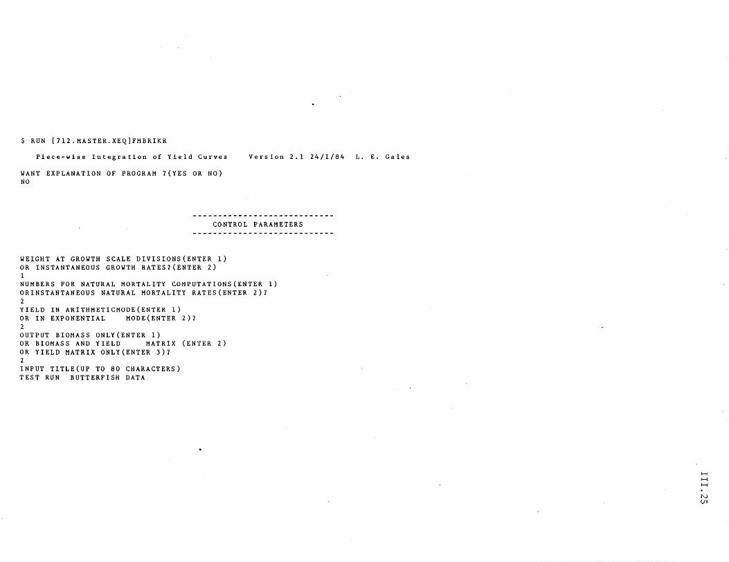
$ RUN [712.MASTER.XEQ]FMBRIKR
Piece-wise Integration of Yield Curves
WANT EXPLANATION OF PROGRAM 1(YES OR NO) NO
Version 2.124/1/84 L. E. Gales
CONTROL PARAMETERS
WEIGHT AT GROWTH SCALE DIVISIONS(ENTER 1) OR INSTANTANEOUS GROWTH RATES1(ENTER 2) 1 NUMBERS FOR NATURAL MORTALITY COMPUTATIONS(ENTER 1) ORINSTANTANEOUS NATURAL MORTALITY RATES(ENTER 2)1 2 YIELD IN ARITHMETICMODE(ENTER 1) OR IN EXPONENTIAL MODE(ENTER 2)1 2 OUTPUT BIOMASS ONLY(ENTER 1) OR BIOMASS AND YIELD MATRIX (ENTER 2) OR YIELD MATRIX ONLY(ENTER 3)1 2 INPUT TITLE(UP TO 80 CHARACTERS) TEST RUN BUTTERFISH DATA
H H H
N Ul
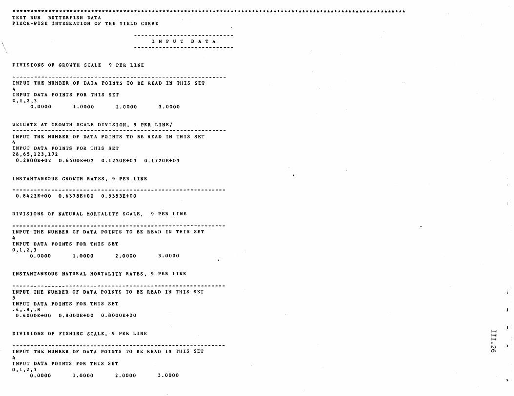
************************************************************************************************************** TEST RUN BUTTERFISH DATA PIECE-WISE INTEGRATION OF THE YIELD CURVE
I N PUT D A T A
DIVISIONS OF GROWTH SCALE 9 PER LINE
INPUT THE NUMBER OF DATA POINTS TO BE READ IN THIS SET 4 INPUT DATA POINTS FOR THIS SET 0,1,2,3
0.0000 1. 0000 2.0000 3.0000
WEIGHTS AT GROWTH SCALE DIVISION, 9 PER LINE/
INPUT THE NUMBER OF DATA POINTS TO BE READ IN THIS SET 4 INPUT DATA POINTS FOR THIS SET 28,65,123,172
0.2800E+02 0.6500E+02 0.1230E+03 0.1720E+03
INSTANTANEOUS GROWTH RATES, 9 PER LINE
0.8422E+00 0.6378E+00 0.3353E+00
DIVISIONS OF NATURAL MORTALITY SCALE, 9 PER LINE
INPUT THE NUMBER OF DATA POINTS TO BE READ IN THIS SET 4 INPUT DATA POINTS FOR THIS SET 0,1,2,3
. 0.0000 1. 0000 2.0000 3.0000
INSTANTANEOUS NATURAL MORTALITY RATES, 9 PER LINE
INPUT THE NUMBER OF DATA POINTS TO BE READ IN THIS SET 3 INPUT DATA POINTS FOR THIS SET .4,.8,.8 0.4000E+00 0.8000E+00 0.8000E+00
DIVISIONS OF FISHING SCALE, 9 PER LINE
INPUT THE NUMBER OF DATA POINTS TO BE READ IN THIS SET 4 INPUT DATA POINTS FOR THIS SET 0,1,2,3
0.0000 1. 0000 2.0000 3.0000
H H H
N 0\
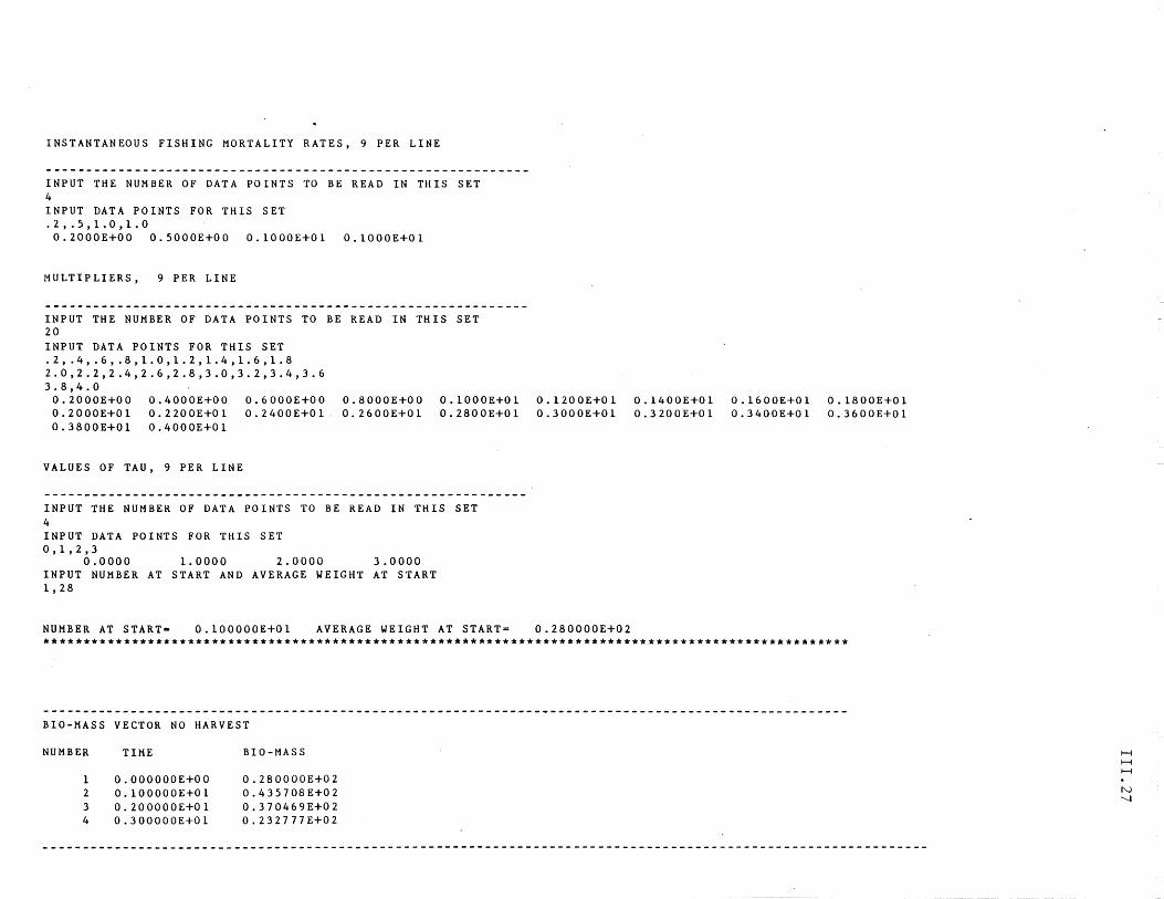
INSTANTANEOUS FISHING MORTALITY RATES, 9 PER LINE
INPUT THE NUMBER OF DATA POINTS TO BE READ IN THIS SET 4 INPUT DATA POINTS FOR THIS SET .2, .5,1.0,1.0 0.2000E+00 0.5000E+00 0.1000E+Ol 0.1000E+Ol
MULTIPLIERS, 9 PER LINE
INPUT THE NUMBER OF DATA POINTS TO BE READ IN THIS SET 20 INPUT DATA POINTS FOR THIS SET .2, .4, .6, .8,1.0,1.2,1.4,1.6,1.8 2.0,2.2,2.4,2.6,2.8,3.0,3.2,3.4,3.6 3.8,4.0
0.2000E+00 0.4000E+00 0.6000E+00 0.8000E+00 0.1000E+Ol 0.1200E+01 0.2000E+01 0.2200E+01 0.2400E+01. 0.2600E+01 0.2800E+01 0.3000E+01 0.3800E+Ol 0.4000E+01
VALUES OF TAU, 9 PER LINE
INPUT THE NUMBER OF DATA POINTS TO BE READ IN THIS SET 4 INPUT DATA POINTS FOR THIS SET 0,1,2,3
0.0000 1.0000 2.0000 3.0000 INPUT NUMBER AT START AND AVERAGE WEIGHT AT START 1,28
NUMBER AT START= 0.100000E+Ol AVERAGE WEIGHT AT START= 0.280000E+02
0.1400E+01 0.1600E+01 0.1800E+01 0.3200E+01 0.3400E+01 0.3600E+01
****************************************************************************************************
BIO-MASS VECTOR NO HARVEST
NUMBER TIME BIO-MASS
1 O.OOOOOOE+OO 0.280000E+02 2 0.100000E+01 0.435708E+02 3 0.200000E+Ol 0.370469E+02 4 0.300000E+Ol 0.232777E+02
H H H
N '-l
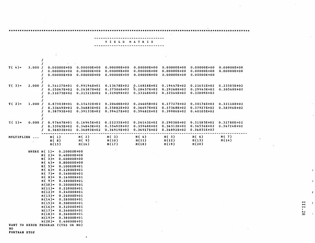
****************************************************************************w*********************************
I I
T ( 4)= 3.000 I O.OOOOOE+OO O.OOOOOE+OO I O.OOOOOE+OO O.OOOOOE+OO I O.OOOOOE+OO O.OOOOOE+OO I I
T ( 3)= 2.000 I 0.54127E+Ol 0.99196E+Ol I 0.25067E+02 0.26387E+02 I 0.31075E+02 0.31521E+02 I I
T ( 2)= 1.000 I 0.87303E+Ol o • 15432 E+O 2 I 0.33649E+02 0.34883E+02 I 0.38793E+02 0.39133E+02 I I
T ( 1) ... 0.000 I 0.97667E+Ol 0.16945E+02 I 0.33965E+02 0.34843E+02 I 0.36832E+02 0.36893E+02'
MULTIPLIER M ( 1) M ( 8) M(15)
M( 2) M( 9) M (16)
WHERE M( 1)M ( 2)M ( 3)M ( 4)M ( 5)M ( 6)M ( 7)M ( 8)M ( 9)M (10)M(11)M(12)M(13)M(14)M(15)M(16)" M(17)M(18)M (19)M(20)-
WANT TO RERUN PROGRAM NO FORTRAN STOP
0.20000E+00 0.40000E+00 0.60000E+00 0.80000E+00 0.10000E+01 0.12000E+01 0.14000E+01 0.16000E+01 0.18000E+Ol 0.20000E+Ol 0.22000E+Ol 0.24000E+01 0.26000E+01 0.28000E+Ol 0.30000E+Ol 0.32000E+Ol 0.34000E+Ol 0.36000E+01 0.38000E+Ol 0.40000E+01
1(YES OR NO)
Y I E L D MAT R I X
O.OOOOOE+OO O.OOOOOE+OO O.OOOOOE+OO
0.13678E+02 0.27506E+02 0.31909E+02
0.20600E+02 0.35882E+02 0.39427E+02
0.22235E+02 0.35492E+02 0.36919E+02
M ( 3) M (10) M (17 )
O.OOOOOE+OO O.OOOOOE+OO O.OOOOOE+OO
0.16818E+02 O.28457E+02 0.32248E+02
0.24605E+02 0.36697E+02 0.39682E+02
0.26143E+02 0.35968E+02 0.36917E+02
M ( 4) M(11) M(18)
O.OOOOOE+OO O.OOOOOE+OO O.OOOOOE+OO
0.19447E+02 0.29268E+02 0.32546E+02
0.27727E+02 0.37368E+02 0.39906E+02
0.29038E+02 0.36312E+02 0.36893E+02
M( 5) M(12) M(19)
O.OOOOOE+OO O.OOOOOE+OO O.OOOOOE+OO
0.21651E+02 0.29963E+02 0.32809E+02
0.30176E+02 0.37927E+02 0.40105E+02
0.31185E+02 0.36556E+02 0.36851E+02
M( 6) M(13) M(20)
O.OOOOOE+OO O.OOOOOE+OO
0.23505E+02 0.30560E+02
0.32110E+02 0.38396E+02
0.32780E+02 0.36724E+02
M( 7) M(14)
H H H
N 00
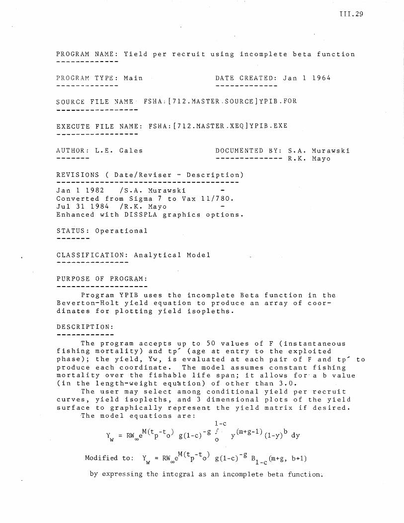
111.29
PROGRAM NAME: Yield per recruit using incomplete beta function
PROGRAM TYPE: Main DATE CREATED: Jan 1 1964
SOURCE FILE NAME: FSHA.[712.MASTER.SOURCE]YPIB.FOR
EXECUTE FILE NAME: FSHA: [712.MASTER.XEQ]YPIB.EXE
AUTHOR; L.E. Gales DOCUMENTED BY:
REVISIONS ( Date/Reviser - Description)
Jan 1 1982 /S.A. Murawski Converted from Sigma 7 to Vax 11/780. Jul 31 1984 /R.K. Mayo Enhanced with DISSPLA graphics options.
STATUS: Operational
CLASSIFICATION: Analytical Model
PURPOSE OF PROGRAM:
S.A. Murawski R.K. Mayo
Program YPIB uses the incomplete Beta function in the Beverton-Holt yield equation to produce an array of coordinates for plotting yield isopleths.
DESCRIPTION:
The program accepts up to 50 values of F (instantaneous fishing mortality) and tp' (age at entry to the exploited phase); the yield, Yw, is evaluated at each pair of F and tp' to produce each coordinate. The model assumes constant fishing mortality over the fishable life span; it allows for' a b value (in the length-weight equ~tion) of other than 3.0.
The user may select among conditional yield per recruit curves, yield isopleths, and 3 dimensional plots of the yield surface to graphically represent the yield matrix if desired.
~he model equations are: l-c
Met -t ) -g J Y = RW e p 0 g(l-c) w 00 0 y(m+g-l) (l_y)b dy
Modified to: M(t -t ) -g Yw
= RWooe p 0 g(l-c) Bl _c (m+g, b+l)
by expressing the integral as an incomplete beta function~
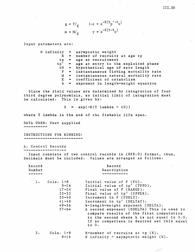
g = F/K
m = M/K
-K(t '-t ) l-c = e p 0
y = e-K(t-to)
111.30
Input parameters are:
W infinity R
tp tp
,
to F M K b
= = = = = = = = =
asymptotic weight number of recruits at age tp age at recruitment age at entry to the exploited phase hypothetical age of zero length instantaneous fishing mortality rate instantaneous natural mortality rate coefficient of catabolism exponent in length-weight equation
Since the- yield values are determined by integration of four third degree polynomials, an initial limit of integration must be calculated. This is given by:
S = exp(-K(T lambda - to))
where T lambda is the end of the fishable life span.
DATA USED: User supplied
INSTRUCTIONS FOR RUNNING:
A. Control Records
Input consists of two control records in (8F8.0) format, thus, decimals must be included. Values are arranged as follows:
Record Number
1 .
2.
Cols. 1-8 9-16
17-24 25-32 33-40 41-48 49-56 57-64
Cols. 1-8 9-16
Record Description
Initial value of F (Fa). Initial value of tp' (TPPO). Final value of F (RANGE). Final value of tp' (UPPER). Increment in F (FDELT). Increment in tp' (DELTAT). b-Iength-weight exponent (DELTA). A second exponent (DDELTA) This is used to
compare results of the first computation to the second where b is not equal to 3.0. If no comparison is desired set this equal to O.
R-number of recruits at tp (R). W infinity - asymptotic weight (W).
111.31
17-24 25-32 33-40 41-48 49-56 57-64
M - instantaneous natural mortality (AM). K - coefficeint of catabolism (AK). tp - age at recruitment (TP). to - age at 0 length (TO). t lambda - maximum age (T LAMBA). S - initial limit of integration (XINTO).
Input must be from a file on input device FOR001. Tabular output of the computed yield matrix is produced on an output file ASSIGNed to device FOR007.
B. Interactive Graphics Option
Graphic representation of the two-dimensional yield per recruit (YPR) matrix may be obtained interactively during program execution. Before attempting any plots, the user must examine the tabular output matrix to determine the minimum and maximum bounds of the computed yield values.
The graphics mode is entered by responding to the following question:
1.0. Do You Want to Plot Results? Enter Y or N.
Enter Y to proceed with the graphics option. Enter N to terminate program execution.
The following questions allow the user to select Bmong various plot types, axis annotation and plot parameter features.
2.0. Enter Descriptive Label (max = 64 Characters).
Enter a name or other descriptive label to appear at the top of the plots.
3.0. Enter: COND for conditional Curves ISOP for Isopleths 3DEE for 3 Dimensional Plots
3.1. COND produces 1 or more conditional YPR curves taken through the yield matrix at user-specified Level(s) of Tp'. The axis coordinate system for this plot type is:
X axis - Instantaneous Fishing Mortality (F) Y axis - Yield per Recruit
Axis annotation must be set up by responding to the following prompts:
3.1.1. Enter X axis Increment of F. The user must specify the increment along the X axis.
3.1.2. Ente~ Minimum YPR, Maximum YPR, and Increment of YPR. The user must specify the lower and upper bounds of
the computed yield values, and the increment along the Y axis.
Plot parameters must be set up by responding to the following prompts:
3.1.3. How Many Curves Do You Want to Plot? The number of curves must not exceed the number of age at entry values indicated on the first control record.
3.1.4. Enter nn Ages Between nn and nne The ages must be within the range indicated on the first control record.
111.32
3.2. ISOP produces a contoured Yield isopleth of the lattice points at the intersections of F and Tp', as indicated on the first control record. The axis coordinate system for this plot type is:,
X axis - Instantaneous Fishing Mortality (F) - Y axis - Age at Entry (Tp')
Axis annotation must be set up by responding to the following prompts:
3.2.1. Enter X axis Increment of F. The user must specify the increment along the X axis.
3.2.2. Enter Y axis Increment of Tp'. The user must specify the increment along the Y axis.
Plot parameters must be set up by responding to the following prompt:
3.2.3. Enter Contour Resolution (YPR Units). The user must specify the distance between contour lines in units of computed Yield per Recruit.
3.3. 3DEE produces a 3 dimensional representation of the yield per recruit surface. The user may select any viewing angle in the X-Y (Horizontal) and Z (Vertical) planes. The axis coordinate system for this plot type is:
X axis - Instantaneous Fishing Mortality (F) Y axis - Age at Entry (Tp') Z axis - Yield per Recruit (YPR)
Axis annotation must be set up by responding to the following prompts:
3.3.1. Enter X axis Increment of F. The user must specify the increment along the X axis.
3.3.2. Enter Y axis Increment of Tp'.
111.33
The user must specify the increment along the Y axis.
3.3.3. Enter Minimum YPR, Maximum YPR, and Increment of YPR. The user must specify the lower and upper bounds of the computed yieLd values, and the increment along the Z axis.
Plot parameters must be set up by responding to the following prompt:
3.3.4. Enter X-Y View Angle, Z View Angle, View Distance.
The X-Y view angle ailows the entire axis system to be rotated about a 360 degree arc in the horizontal (X-Y) plane as illustrated below:
-180
Y Axis
+90 I I I I
<---------------------------) 0 I I I I
-90
X Axis
The Z view angle represents the vertical angle in degrees above (1 to 90) or below (-1 to -90) the horizontal (X-Y) plane from which the plot is viewed.
The view distance is the distance from the center of the ~-D work space in absolute -D units from which the plot is viewed. (Try 5 for starters)
Optional replotting capability is allowed within each plot type, allowing the user to adjust the existing plot parameters of the current plot. After each plot is completed, the program pauses to allow the user to examine the results and/or obtain a hard copy. At this point, the user MUST enter a Carriage Return to proceed. The user may then elect to replot the data in the current form, select another plot type, or terminate the program by responding to the following prompt:
4.0. Enter: C for Current plot type. N for New plot type.
Enter C to adjust the existio& plot parameters and replot the data. When Current (C) is elected, the user will be asked to supply the plot parameters appropriate
111.34
for the current plot type as specified in parts 3.1, 3.2 or 3.3 above.
Enter N to select another plot type. When New (N) is elected, the prompt sequence will be restarted at 3.0 above. At this point, the user may continue with the graphics option or elect to terminate program execution by responding to the following question:
5.0. Do You Want Any More Plots? Enter Y or N.
Enter Y to continue with graphics option. Enter N to terminate program execution.
Proper termination of the program is indicated by the following message:
.. TABULAR RESULTS SENT TO FOR007 DEVICE
To run the proiram, enter the following commands:
$ASSIGN [directory]datafile.DAT $ASSIGN tabular output $RUN DSKA: [712.MASTER.XEQ]YPIB
REFERENCE S:
FOROOI FOR007
Paulik, G.J., and L.E. Gales. 1964. Allometric growth and the Beverton-Holt yield equation. Trans. Amer. Fish. Soc. 93 (4):369-381.
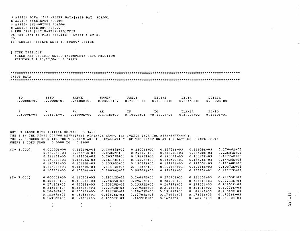
$ ASSIGN DSKA:[712.MASTER.DATA]YPIB.DAT FOR001 $ ASSIGN SYS$INPUT FOR005 $ ASSIGN SYS$OUTPUT FOR006 $ ASSIGN YPIB.OUT FOR007 $ RUN DSKA:[712.MASTER.XEQ]YPIB Do You Want to Plot Results? Enter Y or N. NO :: TABULAR RESULTS SENT TO FOR007 DEVICE
$ TYPE YPIB.OUT YIELD PER RECRUIT USING INCOMPLETE BETA FUNCTION VERSION 2.1 23/11/84 L.E.GALES
************************************************************************************************************** INPUT DATA **************************************************************************************************************
FO O.OOOOE+OO
R 0.1000E+04
TPPO 0.2000E+01
W 0.2157E+Ol
RANGE 0.9600E+00
AM O.1000E+00
OUTPUT BLOCK WITH INITIAL DELTA= 3.3450
UPPER 0.2000E+02
AK 0.1712E+00
FDELT DELTAT 0.2000E-01 0.1000E+01
TP TO 0.1000E+01 -0.4400E-Ol
DELTA 0.3345E+01
TLAMBA 0.2400E+02
DDELTA O.OOOOE+OO
XINTO 0.1630E-Ol
THE T IN THE FIRST COLUMN REPRESENTS DISTANCE ALONG THE T-AXIS (FOR THE BETA-INTEGRAL). THE 49 NUMBERS OPPOSITE THE T-COLUMN ARE THE EVALUATIONS OF THE FUNCTION AT THE LATTICE POINTS (F,T) WHERE F GOES FROM 0.0000 TO 0.9600
(T" 2.000) O.OOOOOE+OO 0.11510E+03 0.18685E+03 0.23001E+03 0.25436E+03 0.26639E+03 0.26928E+03 0.26493E+03 0.25862E+03 0.25119E+03 0.24320E+03 0.23500E+03 0.21886E+03 0.21115E+03 0.20377E+03 0.19673E+03 0.19004E+03 0.18372E+03 0.17209E+03 0.16676E+03 0.16173E+03 0.15698E+03 0.15250E+03 0.14826E+03 O.14047E+03 0.13689E+03 0.13350E+03 0.13029E+03 0.12724E+03 0.12435E+03 0.11899E+03 0.11650E+03 0.114l4E+03 0.11188E+03 0.10973E+03 0.10768E+03 0.10385E+03 0.10206E+03 O. L0034E+03 0.98704E+02 0.97131E+02 0.95623E+02
(Ta 3.000) O.OOOOOE+OO 0.11625E+03 0.19212E+03 0.24067E+03 0.27075E+03 0.28835E+03
0.27040E+03 o • 2 2 6 84 E +0 3 0.17774E+03 0.14426E+03 0.12160E+03 o • 1 0 5 7 2 E +0 3 0.94177E+02
0.29755E+03 0.30113E+03 0.30096E+03 0.29835E+03 0.29417E+03 0.28902E+03 0.28331E+03 '0. 2773 3E +03 0.27125E+03 0.26521E+03 0.25928E+03 0.25352E+03 0.24797E+03 0.24263E+03 0.23751E+03 0.23262E+03 0.22796E+03 0.22352E+03 0.21928E+03 0.21525E+03 0.21141E+03 0.20775E+03 0.20426E+03 0.20094E+03 0.19778E+03 0.19475E+03 0.19187E+03 O. 1 8 91 2 E +0 3 O. 1864 9E +0 3 0.18397E+03 0.18156E+03 0.17926E+03 0.17705E+03 0.17494E+03 o • 1 7 2 9 1 E +0 3 0.17096E+03 0.16910E+03 0.16730E+03 0.16557E+03 0.16391E+03 0.16232E+03 O. 1607 8E +0 3 0.15930E+03
H H H
tN U1
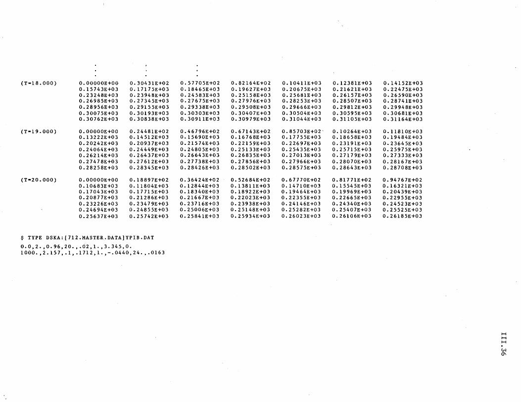
(T a 18.000) O.OOOOOE+OO 0.30431E+02 0.57705E+02 0.82164E+02 0.15743E+03 0.17175E+03 0.18465E+03 0.19627E+03 0.23248E+03 0.23948E+03 0.24583E+03 0.25158E+03 0.26985E+03 0.27345E+03 0.27675E+03 0.27976E+03 0.28956E+03 0.29155E+03 0.29338E+03 0.29508E+03 0.30075E+03 0.30193E+03 0.30303E+03 0.30407E+03 0.30762E+03 0.30838E+03 0.30911E+03 0.30979E+03
(T-19.000) O.OOOOOE+OO o . 2 44 8 1 E +0 2 0.46796E+02 0.67143E+02 0.13222E+03 0.14512E+03 0.15690E+03 0.16768E+03 0.20242E+03 0.20937E+03 0.21574E+03 0.22159E+03 0.24064E+03 0.24449E+03 0.24805E+03 0.25133E+03 0.26214E+03 0.26437E+03 0.26643E+03 0.26835E+03 0.27478E+03 0.27612E+03 0.27738E+03 0.27856E+03 0.28258E+03 0.28345E+03 0.28426E+03 0.28502E+03
(T-20.000) O.OOOOOE+OO 0.18897E+02 0.36424E+02 0.52684E+02 o . 1 0 6 83 E +0 3 0.11804E+03 0.12844E+03 o • 1 38 11 E +03 0.17043E+03 0.17715E+03 0.18340E+03 0.18922E+03 0.20877E+03 0.21286E+03 0.21667E+03 0.22023E+03 0.23226E+03 0.23479E+03 0.23716E+03 0.23938E+03 0.24694E+03 0.24855E+03 0.25006E+03 0.25148E+03 0.25637E+03 0.25742E+03 0.25841E+03 0.25934E+03
$ TYPE DSKA:[712.MASTER.DATA]YPIB.DAT
0.0,2.,0.96,20.,.02,1.,3.345,0. 1000. ,2.157, .1, .1712,1. ,-.0440,24 .•• 0163
0.10411E+03 O. 1 2 3 8 1 E +0 3 0.20675E+03 0.21621E+03 0.25681E+03 0.26157E+03 0.28253E+03 0.28507E+03 0.29666E+03 0.29812E+03 0.30504E+03 0.30595E+03 0.31044E+03 0.31105E+03
0.85703E+02' O. 1 02 6 4 E +0 3 0.17755E+03 0.18658E+03 0.22697E+03 0.23191E+03 0.25435E+03 0.25715E+03 0.27013E+03 0.27179E+03 0.27966E+03 0.28070E+03 0.28575E+03 0.28643E+03
0.67770E+02 o • 8 1 7 71 E +0 2 O. 1471 OE +0 3 0.15545E+03 0.19464E+03 0.19969E+03 0.22355E+03 0.22665E+03 0.24146E+03 0.24340E+03 0.25282E+03 0.25407E+03 0.26023E+03 0.26106E+03
0.14152E+03 0.22475E+03 0.26590E+03 0.28741E+03 0.29948E+03 0.30681E+03 0.31164E+03
0.11810E+03 0.19484E+03 0.23645E+03 0.25975E+03 0.27333E+03 0.28167E+03 0.28708E+03
0.94767E+02 0.16321E+03 0.20439E+03 0.22955E+03 0.24523E+03 0.25525E+03 0.26185E+03
H H H
(,N
0\
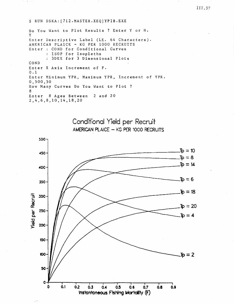
$ RUN DSKA: [712.MASTER.XEQ]YPIB.EXE
Do You Want to Plot Results ? Enter Y or N. Y Enter Descriptive Label (LE. 64 Characters)o AMERICAN PLAICE - KG PER 1000 RECRUITS Enter
COND
COND for Conditional Curves ISOP for Isopleths 3DEE for 3 Dimensional Plots
Enter X Axis Increment of F~
0,1 Enter Minimum YPR j Maximum YPR, Increment of YPR. 0,500,50 How Many Curves Do You Want to Plot ? 8 Enter 8 Ages Between 2 and 20 2,4,6,8,10,14,18,20
Conditional Yield per Recruit AMERICAN PLAICE - KG PER 1000 RECRUITS
__ -=-------Tp = 10 ,...,-:::.:::::..---------__ Tp == 8
Jp = 14-.-------350
-~Tp==6
Tp = 18 ------___ --Tp :: 20
Tp =4
Tp=2"
o~------~--~----__ --__ ----~----~--__ ----__ --__ o 0.1 0.2 0.3 0.. o.s 0.6 0.7 0.& 0.1
tns1on1aneous Flshlng MortdIty (F)
111.37
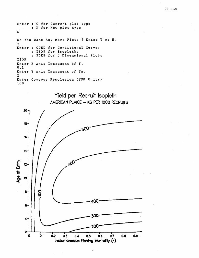
Enter
N
C for Current plot type N for ~ew plot type
Do You Want Any More Plots ? Enter Y or N. Y Enter
ISOP Enter 0.1 Enter 2 Enter 100
20
18
16
14
COND for Conditional Curves ISOP for Isopleths 3DEE for 3 Dimensional Plots
X Axis
Y Axis
Contour
Increment of F.
Increment of Tp.
Resolution (YPR Units).
Yield per Recruit Isopleth A~ERICAN PlAICE - KG PER 1000 RECRU{TS
'-__ ------~o--------------300-
2~~~~--~----P-~~----__ --~----~--~~--~--o 0.1 0..2 0.3 0.. 0.5 0.8 0.7 0.1 0.'
Insian1aneous FlshIng t.4ortctty (F)
111.38
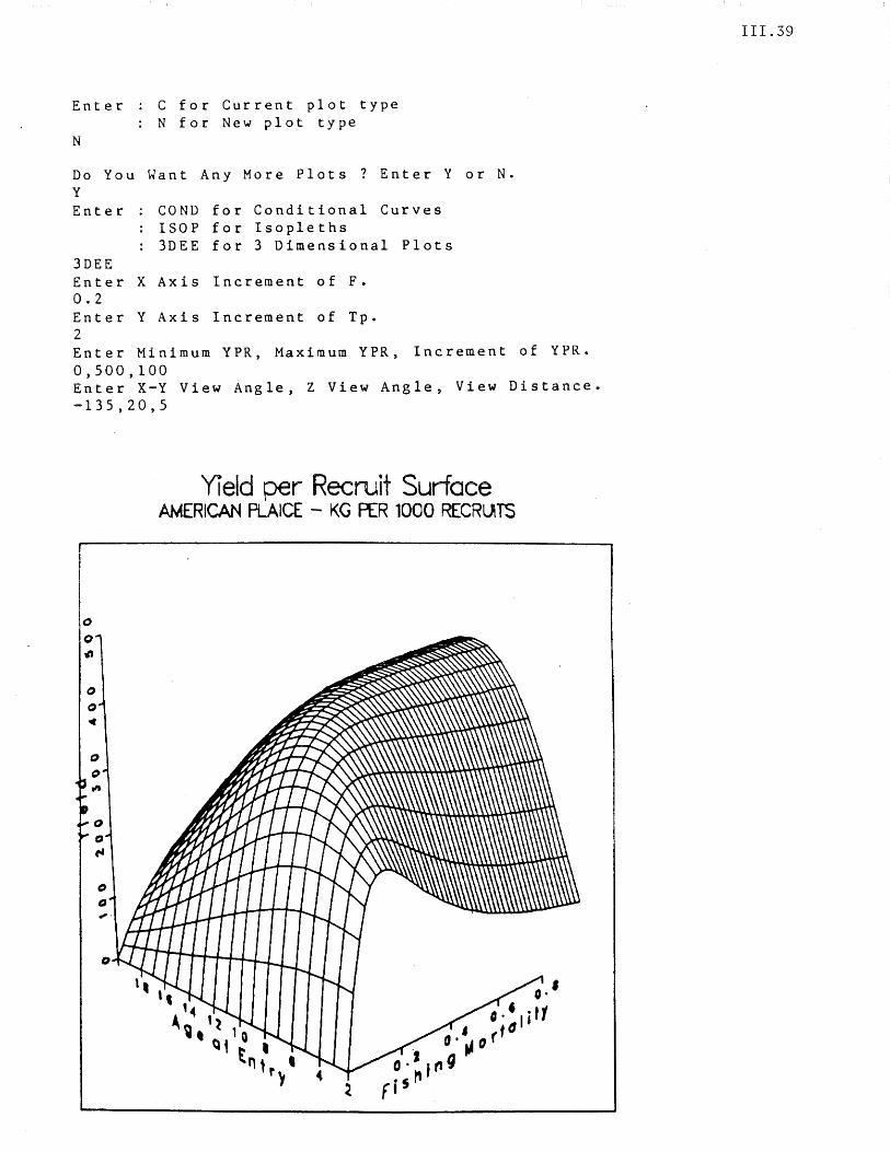
Enter
N
C for Current plot type N for New plot type
Do You Want Any More Plots? Enter Y or N. y
Enter COND for Conditional Curves ISOP for Isopleths 3DEE for 3 Dimensional Plots
3DEE Enter X Axis Increment of F 0
0.2 Enter Y Axis Increment of Tp. 2 Enter Minimum YPR, Maximum YPR, Increment of YPR. 0,500,100 Enter X-Y View Angle, Z View Angle, View Distance. -135,20,5
Yield per Recruit Surface AMERICAN PLAICE - KG FtR 1000 RECRUTS
111.39
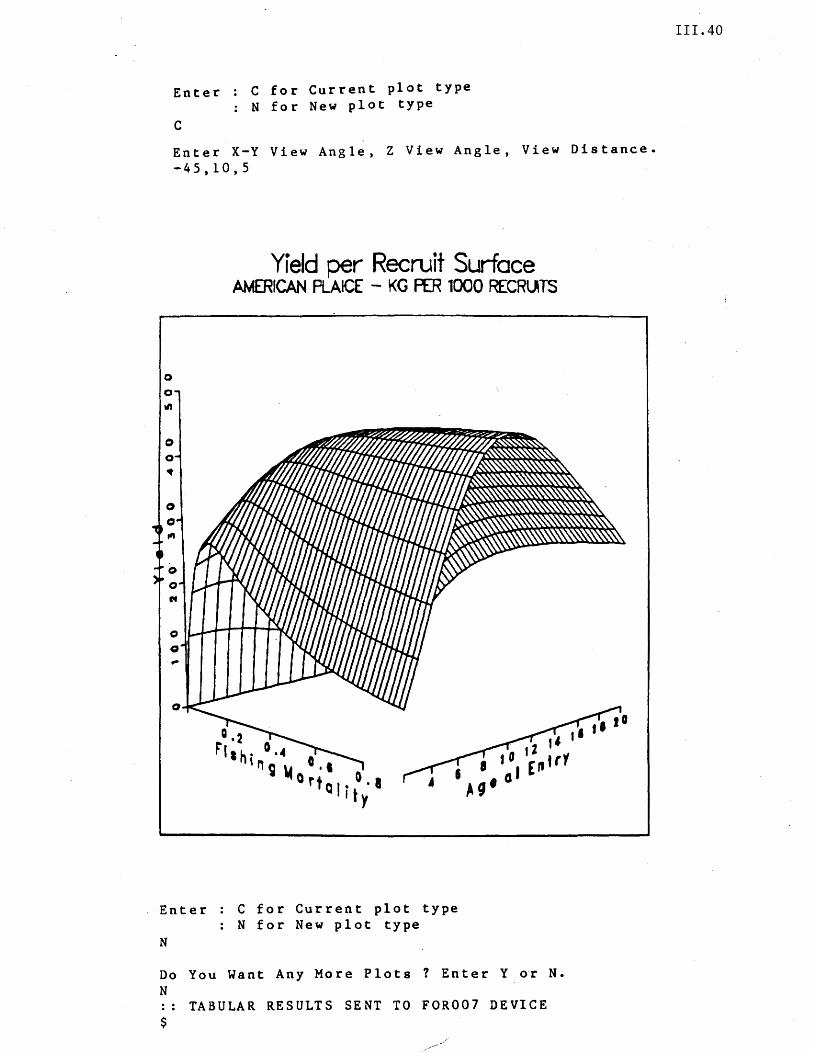
Enter
C
C for Current plot type N for New plot type
Enter X-Y View Angle, Z View Angle, View Distance. -45,10,5
o o 1ft
Enter
N
Yield per Recruit Surface AMERICAN PLAICE - KG ~ 1000 RECRUTS
, l' t 2 1
• to E"trY • • a I
C for Current plot type N for New plot type
~9
Do You Want Any More Plots ? Enter Y ~r N. N .. TABULAR RESULTS SENT TO FOR007 DEVICE $
t' 10
III.40
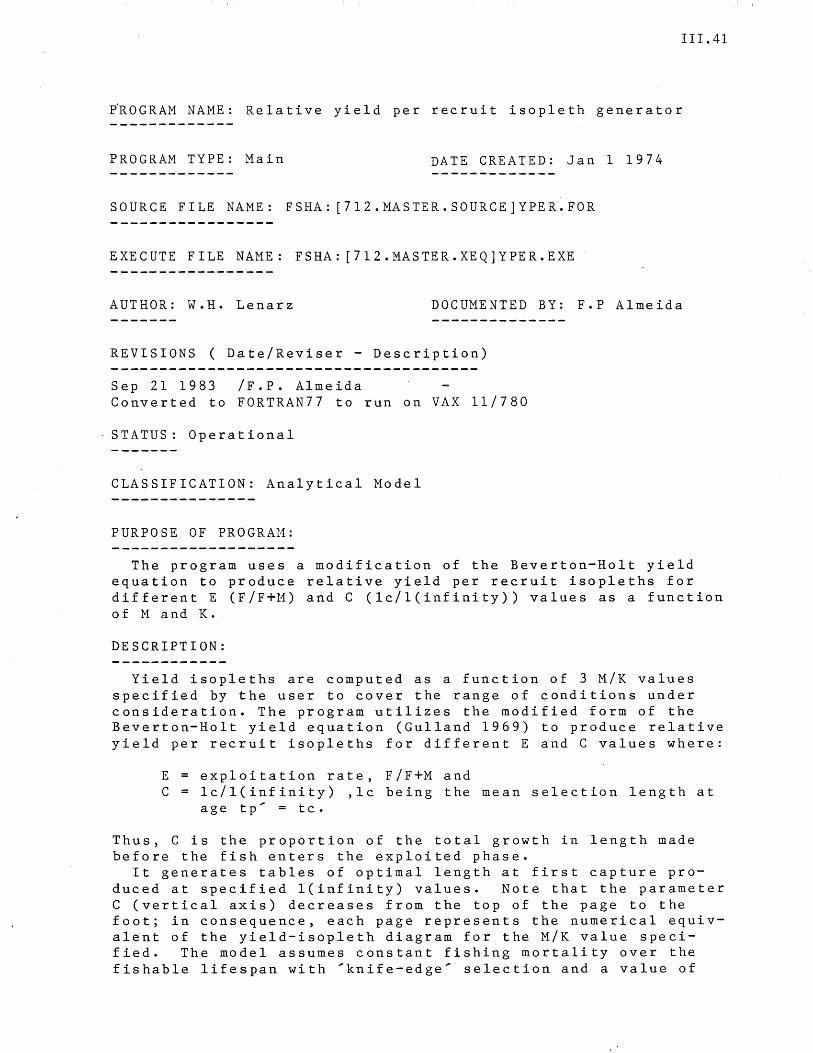
111.41
~ROGRAM NAME: Relative yield per recruit isopleth generator
PROGRAM TYPE: Main DATE CREATED: Jan 1 1974
SOURCE FILE NAME: FSHA: [712.MASTER.SOURCE]YPER.FOR
EXECUTE FILE NAME: FSHA: [712.MASTER.XEQ]YPER.EXE
AUTHOR: WeHe Lenarz DOCUMENTED BY: F.P Almeida
REVISIONS ( Date/Reviser - Description)
Sep 21 1983 /F.P. Almeida Converted to FORTRAN77 to run on VAX 11/780
STATUS: Operational
CLASSIFICATION: Analytical Model
PURPOSE OF PROGRAM:
The program uses a modification of the Beverton-Holt yield equation to produce relative yield per recruit isopleths for different E (F/F+M) and C (lc/1(infinity)) values as a function of M and K.
DESCRIPTION:
Yield isopleths are computed as a function of 3 M/K values specified by the user to cover the range of conditions under consideration. The program utilizes the modified form of the Beverton-Holt yield equation (Gulland 1969) to produce relative yield per recruit isopleths for different E and C values where:
E exploitation rate, F/F+M and C lc/l(infinity) ,lc being the mean selection length at
age tp' = tc.
Thus, C is the proportion of the total growth in length made before the fish enters the exploited phase.
It generates tables of optimal length at first capture produced at specified l(infinity) values. Note that the parameter C (vertical axis) decreases from the top of the page to the foot; in consequence, each page represents the numerical equivalent of the yield-isopleth diagram for the M/K value specified. The model assumes constant fishing mortality over the fishable lifespan with 'knife-edge' selection and a value of
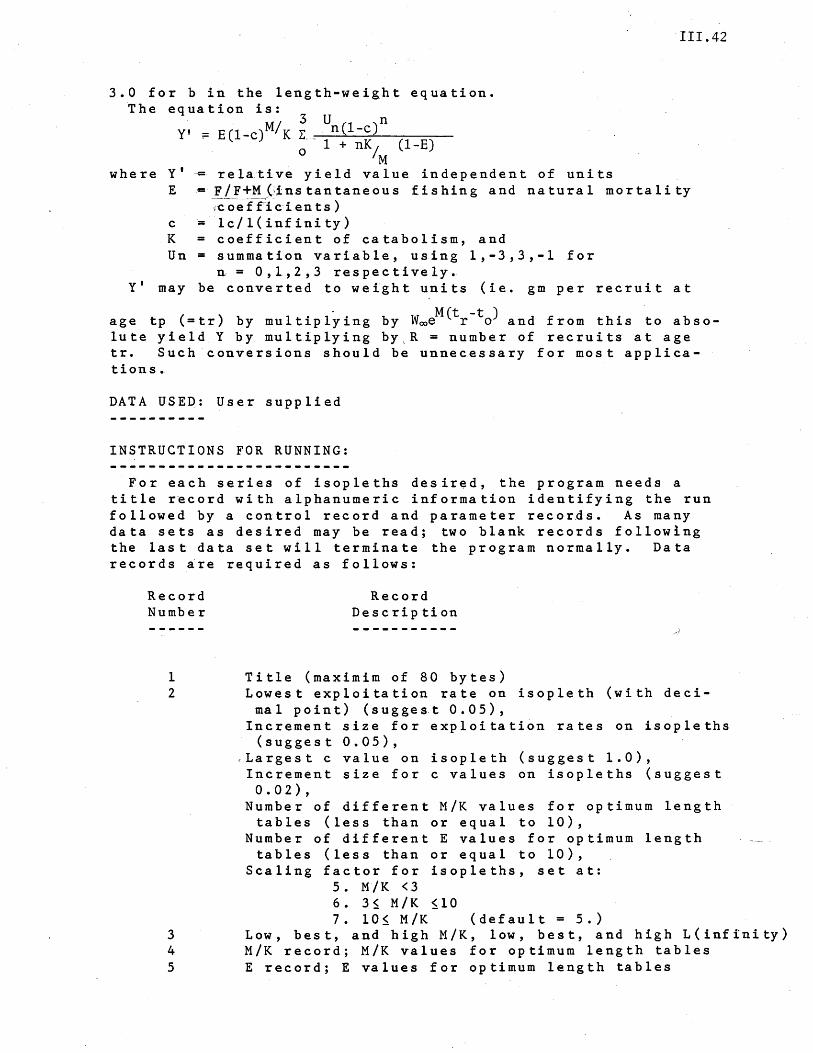
III.42
3.0 for b in the length-weight equation. The eq ua tion is:
. 3 U n Y' := E (l-c) M/ K 2:. _~ .. _n_(;,.....l_---,c )"--~ __
o 1 + nK/ (l-E) M
where y' ~ relative yield value independent of units E ~ F/F+M0instantaneous fishing and natural mortality
;:c-oe-rti-ci en ts) c = lc/l(infinity) K = coefficient of catabolism, and Un = summation variable, using 1,-3,3,-1 for
n = 0,1,2,3 respectively. Y' may be converted to weight units (ie. gm per recruit at
age t p ( = t r) by m u 1 tip 1 yin g by W ooeM (t r - to) and fro m t his to a b s 0 -
lute yield Y by multiplying bY,R = number of recruits at age tr. Such conversions should be unnecessary for most applications.
DATA USED: User supplied
INSTRUCTIONS FOR RUNNING:
For each series of isopleths desired, the program needs a title record with alphanumeric information identifying the run followed by a control record and parameter records. As many data sets as desired may be read; two blank records following the last data set will terminate the program normally. Data records are required as follows:
Record Number
1 2
3 4 5
Record Des c rip t ion
Title (maximim of 80 bytes)
",i
Lowest exploitation rate on isopleth (with decimal point) (sugges.t 0.05),
Increment size for exploitation rates on isopleths (suggest 0.05),
<Largest c value on isopleth (suggest 1.0), Increment size for c values on isopleths (suggest 0.02),
Number of different M/K values for optimum length tables (less than or equal to 10),
Number of different E values for optimum length tables (less than or equal to 10),
Scaling factor for isopleths, set at: 5. MIK <3 6. 3~ M/K ~10 7. 10~ M/K (default = 5.)
Low, best, and high M/K, low, best, and high L(infinity) M/K record; M/K values for optimum length tables E record; E values for optimum length tables
III.43
Input is free formatted, data values should be separated by commas. Program output requires a wide carriage terminal. To run the program, simply type:
$RUN FSHA: [7l2.MASTER.XEQ]YPER and you will be prompted for values, or create a data file with the abo veda t a and use:
REFERENCES:
$ASSIGN datafile.DAT FOROOS $RUN FSHA:[7l2.MASTER.XEQ]YPER
Lenarz, W.H., W.W. Fox, Jr., G.T. Sakagawa, and B.J. Rothschild 1974. An estimation of the yield per recruit basis for a minimum size regulation for Atlantic yellowfin tuna, Thunnis albacares. Fish. Bull. 72(1):37-61.
Gulland, J.A. 1969. Manual of methods for fish stock assessment. F.A.O. Manual in Fishery Science #4.
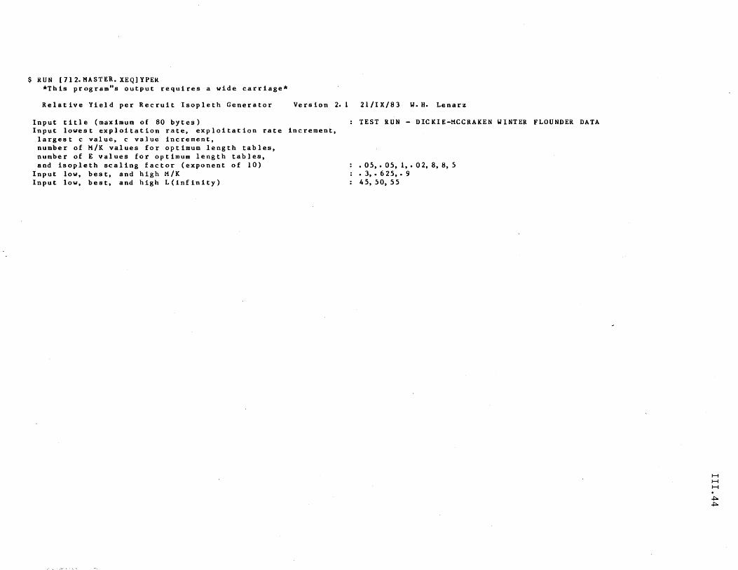
$ RUN (712.MASTER.XEQ)YPER *This program"s output requires a wide carriage*
Relative Yield per Recruit Isopleth Generator Vers ion 2. 1
Input title (maximum of 80 bytes) Input lowest exploitation rate, exploitation rate increment, largest c value, c value increment, number of M/K values for optimum length tables, number of E values for optimum length tables, and isopleth scaling factor (exponent of 10)
Input low, bes t, and high M /K Input low, best, and high L(1nfinity)
- , '\ ,-~' " \~ " '
21/IX/83 W. H. Lenarz
TEST RUN - DICKIE-MCCRAKEN WINTER FLOUNDER DATA
• OS,. OS, 1,.02,8,8,5 .3,.625,.9 45, 50, 55
H H H
~ ~
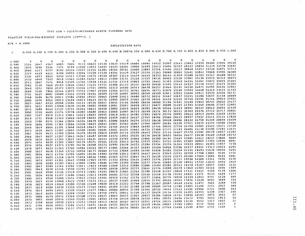
TEST KUN - DICKIE-MCCRAKEN WINTER FLOUNDEK DATA
R ELAT I VE YI ELD-PEK-R ECR UIT ISOPLETH (10**-5. )
M/K - 0.3000 EXPLOITATION RATE
C 0.050 0.100 0.150 0.200 0.250 0.300 0.350 0.400 0.450 0.500-0.550 0.600 0.650 0.700 0.750 0.800 0.850 0.900 0.950 1.000
1. 000 0 0 0 0 0 0 0 0 0 0 0 0 0 0 0 0 0 0 0 0
O. 980 1524 3047 4567 6085 7600 91 12 10621 12126 13625 15119 16606 18084 19552 21007 22445 23862 25250 26600 27894 29106
O. 960 1850 3696 5536 7371 9199 11020 12832 14635 16425 18201 19960 21699 23412 25094 26737 28327 29850 31279 32578 33685
O. 940 2060 4113 6157 8192 10216 12227 14224 16204 18164 20101 22009 23883 25716 27496 29211 30840 32357 33720 34871 35713
O. 920 2215 4419 6611 8789 10952 13096 15220 17320 19391 21429 23427 25376 27265 29080 30801 32401 33842 35068 35995 36500
O. 900 2336 4657 6962 9250 1151 7 13760 15976 18160 20307 22410 24459 26445 28352 30163 31850 33380 34703 35747 36409 36537
O. 880 2433 4849 7245 9618 11965 14283 16567 1881 1 21009 23151 25228 27225 29124 30903 32530 33961 35138 35973 36343 36075
O. 860 2514 5007 7476 9918 12329 14704 17038 19324 21554 23718 25803 27793 29665 31393 32940 34254 35264 35872 35935 35264
O. 840 2582 5139 7668 10165 12626 15045 17416 19731 21980 24152 26231 28199 30030 31693 33145 34327 35158 35527 35275 34204
O. 820 2640 5251 7830 10372 12872 15324 17721 20054 22312 24480 26543 28478 30257 31844 33191 34230 34873 34995 34426 32963
O. 800 2689 5346 7966 10544 13075 15553 17967 20309 22566 24723 26761 28654 30373 31876 33109 33999 34448 34319 33435 31592
O. 780 2731 5427 8081 10689 13244 15739 18164 20509 22759 24897 26902 28748 30399 31811 32925 33660 33911 33532 32336 30131
O. 760 2768 5496 8179 1081 1 13384 15891 18321 20662 22899 25012 26980 28772 30351 31667 32657 33235 33286 32657 31158 28609
O. 740 2800 5556 8262 10913 13499 16013 18443 20776 22995 25079 27005 28739 30241 31459 32322 32740 32591 31716 29922 27051
O. 720 2827· 5607 8333 10998 13594 16111 18536 20857 23054 25106 26985 28658 30080 31196 31931 32189 31842 30725 28646 25477
O. 700 2851 5651 8392 11068 13670 16186 18605 20909 23081 25097 26928 28537 29877 30889 31495 31593 31049 29696 27345 23902
O. 680 2872 5688 8442 11127 13731 16244 18652 20938 23082 25059 26839 28382 29639 30546 31023 30961 30225 28642 26033 22339
O. 660 2890 5720 8485 11174 13778 16285 18680 20945 23060 24997 26723 28199 29371 30173 30521 30302 29376 27572 24717 20801
O. 640 2905 5747 8519 11212 13814 16313 18693 20935 23018 24912 26585 27992 29079 29776 29995 29622 28512 26494 23409 19294
O. 620 2918 5771 8548 11242 13840 16328 18692 20910 22959 24810 26427 27765 28766 29360 29452 28927 27637 25414 22114 17828
O. 600 2930 5790 8571 11264 13856 16334 18679 20871 22886 24693 26254 27522 28438 28928 28896 28222 26758 24339 20839 16409
O. 580 2940 5806 8590 11281 13866 16330 18655 20821 22801 24562 26067 27266 28097 28484 28330 27511 25879 23274 19590 15040
O. 560 2948 5819 8604 11291 13868 16318 18623 20761 22705 24421 25869 26999 27746 28033 27758 26798 25005 22223 18371 13728
O. 540 2955 5830 8615 11297 13865 16300 18584 20694 22601 24271 25663 26724 27388 27575 27183 26086 24138 21190 17185 12474
O. 520 2961 5839 8622 11299 13856 16276 18538 20619 22489 24114 25450 26442 27024 27114 26607 25378 23281 20178 16037 11282
O. 500 2966 5845 8627 11297 13843 16247 18487 20538 22372 23951 25231 26156 26658 26652 26034 24677 22438 19189 14928 10153
O. 480 2970 5850 8629 11293 13827 16213 18431 20453 22250 23783 25008 25866 26289 26191 25465 23985 21611 18227 13860 9089
O. 460 2974 5854 8629 11285 13807 16176 18371 20364 22124 23612 24782 25575 25921 25732 24901 23303 20802 17292 12836 8091
O. 440 2976 5856 8627 11275 13785 16136 18308 20272 21995 23439 24555 25284 25554 25276 24344 22633 20011 16387.11857 7158
O. 420 2978 5857 8623 11263 13 760 16094 18242 20177 21864 23264 24327 24993 25189 24826 23796 21977 19241 15513 10923 6292
O. 400 2980 5857 8618 11249 13733 16050 18175 20080 21732 23088 24099 24704 24828 24382 23258 21335 18493 14670 10036 5491
O. 380 2981 5856 8612 11234 13705 16004 18106 19982 21598 22912 23872 24417 24471 23945 22731 20709 17768 13861 9196 4754
O. 360 2982 5855 8605 11218 13676 15956 18036 19884 21465 22737 23647 24133 24120 23516 22215 20100 17066 13084 8403 4081
O. 340 2982 5852 8597 11201 13645 15908 17965 19785 21332 22562 23424 23853 23774 23095 21711 19508 16388 12341 7656 3470
O. 320 2982 5850 8589 11183 13614 15860 17894 19686 21199 22390 23204 23577-23434 22683 21220 18934 15735 11633 6956 2919
O. 300 2982 5847 8580 11164 13582 1581 1 17823 19588 21068 22219 22986 23306 23102 22281 20742 18378 15107 10957 6302 2426
O. 280 2982 5843 8570 11146 13550 15761 17752 19490 20938 22050 22773 23041 22776 21889 20278 17840 14503 10316 5694 1989
O. 260 2981 5840 8560 11126 13518 15712 17681 19393 20810 21885 22563 22780 22458 2150i 19828 17321 13925 9708 5129 1606
O. 240 2981 5836 8550 11107 13486 15663 17612 19298 20683 21722 22358 22526 22148 21136 19392 16821 13371 9133 4608 1273
O. 220 2980 5832 8540 11088 13454 15615 17543 19204 20559 21562 22156 22277 21846 20776 18970 16339 12842 8591 4128 988
O. 200 2979 5827 8530 11068 13422 15567 1747519111 20437 21405 21960 22034 21552 20426 18562 15876 12338 8081 3689 748
O. 180 2978 5823 8519 11049 13390 15520 17408 19020 20318 21252 21768 21798 21267 20087 18168 15431 11857 ]b01 3289 550
O. 160 2977 5819 8509 11030 13359 15473 17342 18931 20200 21102 21580 21568 20989 19759 17788 15005 11400 7151 2927 389
O. 140 2976 5815 8499 11011 13329 15427 17277 18844 20086 20956 21398 21344 20720 19441 17422 14596 10966 6731 2600 262
O. 120 2975 5810 8489 10992 13299 15382 17214 18758 19974 20814 21220 21127 20459 19134 17070 14205 10553 6339 2307 166
O. 100 2974 5806 8479 10974 13269 153~8 17152 18675 19865 20675 21047 20915 20206 18838 16731 13830 10163 5973 2045 97
O. 080 2973 5802 8469 10956 13240 15295 17091 18593 19758 20539 20878 20710 19961 18551 16404 13472 9793 5633 1812 SO H
0.060 2972 5798 8460 10938 13212 15253 17032 18513 19655 20407 20715 20511 19724 18274 16090 13130 9442 5317 1607 21 H
2971 5794 8450 10921 13184 15212 16975 18436 19553 20279 20555 20318 19494 18007 15789 12802 91 11 5024 1427 6 H
O. 040 O. 020 2970 5790 8441 10904 13157 15172 16918 18360 19455 20154 20401 20130 19271 17749 15498 12490 8797 4752 1269 ~
Ul
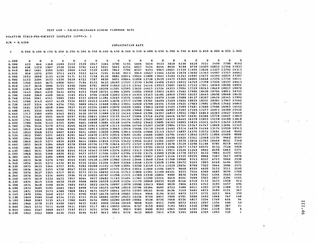
TEST RUN - DICKlE-MCCRAKEN WINTEK FLOUNDER DATA
R ELAT I VE Yl ELO-PER -R EC aUlT ISOPLET H (10**-5. )
M/K - 0.6250 EXPLOITATIuN RATE
C O. 050 O. 100 O. 1 50 O. 200 O. 250 O. 300 O. 350 0 •. 400 O. 450 O. 500 O. 550 O. 600 O. 650 O. 700 O. 750 O. 800 O. 850 O. 900 O. 950 1. 000
1. 000 0 0 0 0 0 0 0 0 0 0 0 0 0 0 0 0 0 0 0 0 O. 980 423 846 1268 1689 2110 2529 2947 3364 3780 4194 4606 5016 5423 5828 6230 6628 7021 7409 7190 8162 O. 960 638 1273 1907 2538 3166 3791 4413 5031 5645 6254 6857 7454 8044 8626 9198 9758 10305 10835 11346 11833 O. 940 802 1601 2395 3185 3969 4748 5520 6285 7042 7190 8527 9253 9965 10661 11339 11995 12626 13227 13792 14313 O. 920 938 1870 2795 3713 4623 5523 6414 7294 8160 9013 9849 10667 11464 12236 12979 13690 14362 14987 15557 16062 O. 900 1053 2098 3133 4158 5171 6172 7158 8129 9081 10014 10924 11808 12662 13482 14263 14997 15677 16293 16835 17287 0.880 1153 2294 3423 4539 5639 6722 7187 8830 9851 10844 '11808 12738 13629 14475 15269 16004 16668 17250 17736 18111 O. 860 1240 2465 3675 4868 6041 7194 8322 9425 10497 11537 12539 13498 14408 15263 16053 16769 17398 17926 18337 18613 O. 840 1317 2616 3896 5155 6390 7600 8781 9929 11042 12115 13141 14116 15032 15881 16652 17333 17911 18369 18690 18854 O. 820 1385 2748 4089 5405 6693 7950 9173 10358 11501 12595 13635 14615 15524 16355 17094 17729 18243 18619 18837 18879 O. 800 1445 2865 4259 5624 6956 8253 9509 10721 11884 12991 14036 15010 15903 16705 17402 17980 18420 18704 18811 18725 O. 780 1499 2969 4409 5816 7185 8513 9796 11028 12203 13315 14355 15315 16184 16949 17595 18107 18465 18650 18640 18420 O. 760 1546 3061 4541 5983 7383 8737 10039 11284 12465 13574 14604 15543 16379 17100 17688 18127 18397 18476 18345 17992 O. 740 1589 3142 4657 6129 7554 8927 10243 11495 12676 13777 14789 15701 16499 17169 17694 18055 18231 18201 '17947 17460 O. 720 1627 3214 4759 6256 7701 9089 10414 11668 12843 13931 14920 15799 16554 17168 17624 17903 17981 17840 17462 16845 O. 700 1661 3278 4848 6366 7827 9225 10554 11805 12970 14039 15001 15843 16550 17105 17489 17681 17660 17406 16905 16162 O. 680 1691 3334 4926 6461 7934 9338 10666 11911 13062 14109 15040 15841 16496 16987 17295 17399 17277 16911 16289 15426 0.660 1717 3383 4993 6542 8023 9430 10755 11989 13122 14144 15040 15796 16397 16822 17053 17067 16843 16365 15627 14649 O. 640 1741 3426 5051 6610 8097 9503 10821 12042 13155 14147 15006 15716 16259 16616 16767 16691 16366 15778 14927 13843 0.620 1761 3464 5101 6668 8156 9560 10868 12073 13162 14124 14942 15603 16087 16375 16445 16278 15853 15158 14199 13018 0.600 1780 3496 5143 6715 8204 9601 10898 12084 13148 14076 14852 15462 15885 16103 16093 15835 15311 14513 13453 12183 0.580 1796 3524 5179 6753 8240 9629 10912 12078 13114 14006 14740 15297 15658 15804 15714 15367 14747 13849 12694 11345 O. 560 1810 3548 5208 6784 8266 9645 10913 12056 13063 13918 14606 15110 15410 15485 15314 14879 14166 13174 11930 10513 O. 540 1822 3568 5232 6807 8283 9651 10901 12020 12996 13814 14456 14906 15143 15147 14897 14376 13572 12491 11166 9692 O. 520 1832 3585 5251 6823 8291 9647 10878 11972 12916 13695 14291 14686 14860 14794 14467 13862 12972 11806 10409 8888 O. 500 1841 3599 5266 6834 8293 9634 10845 11913 12825 13564 14113 14453 14566 14430 14026 13341 12368 11124 9662 8105 0.480 1849 3610 5277 6839 8289 9614 10804 11846 12724 13422 13924 14211 14261 14057 13579 12816 11765 10449 8931 7349 0.460 1855 3619 5284 6840 8278 9588 10756 11770 12614 13272 13727 13959 13949 13678 13129 12290 11166 9784 8218 6622
0.440 1861 3626 5288 6837 8263 9556 10702 11687 12497 13115 13523 13702 13632 13296 12677 11767 10574 913~ 7528 5929 0.420 1865 3631 5289 6830 8244 9519 10642 11599 12374 12952 13313 13439 13311 12911 12226 11249 9992 8498 6863 5271 0.400 1868 3634 5288 6820 8221 9477 10577 11506 12247 12784 13100 13174 12989 12528 11778 10737 9422- 7882 6225 4651
O. 380 1871 3635 5284 6808 8194 9433 10509 11409 12116 12613 12883 12907 12667 12146 11335 10235 8866 7287 5617 4070
O. 360 1873 3636 5279 6793 8165 9385 10438 11309 11982 12440 12666 12640 12346 11768 10900 9743 8327 6715 5040 3530
0.340 1874 3635 5272 6776 8134 9335 10364 11206 11846 12266 12448 12374 12028 11396 10472 9265 7805 6168 4496 3031
0.320 1875 3633 5264 6757 8101 9283 10288 11102 11709 12091 12230 12110 11713 11029 10054 8799 7j02 5646 3986 2575
0.300 1876 3631 5255 6738 8067 9229 10211 10997 11571 11916 12014 11848 11404 10671 9648 8350 6820 5152 3511 2160
o. 280 1876 3627 5245 6717 8031 9175 10134 10892 11434 11743 11800 11591 11100 10321 9253 7916 6360 4685 3070 1788
O. 260 1876 3624 5234 6695 7994 9119 10055 10787 11298 11571 11589 11338 10804 9980 8870 7499 5921 4246 2665 1456
O. 240 1875 3619 5222 6672 7957 9064 9977 10682 11162 11401 11382 11090 10514 9649 8501 7099 5505 3837 2294 1164
O. 220 1874 3615 5210 6650 7920 9008 9899 10578 11029 11234 11179 10848 10233 9329 8146 6718 5112 3455 1958 912
O. 200 1874 3610 5198 6626 7883 8953 9822 10476 10897 11070 10980 10613 9960 9020 7806 6355 4742 3103 1657 696
O. 180 1872 3605 5185 6603 7845 8898 9746 10375 10768 10910 10786 10384 9695 8722 7480 6011 4395 2778 1388 515
O. 160 1871 3599 5173 6580 7808 8843 9671 10275 10641 10753 10597 10161 9440 8436 7169 5685 4072 2482 1151 367 O. 140 1870 3594 5160 6557 7771 8790 9597 10178 10518 10601 10414 9946 9194 8162 6873 5377 3771 2212 944 250 O. 120 1869 3589 5148 6534 7735 8737 9524 10083 10397 10453 10236 9739 8957 7899 6591 5088 3492 1968 767 160 O. 100 1868 3583 5135 6512 7700 8685 9454 9990 10280 10309 10064 9538 8730 7648 6324 4817 3234 1749 616 94 0.080 1866 3578 5123 6490 7665 8635 93.85 9900 10166 10169 9898 9345 8511 7409 6072 4563 2997 1554 490 49 H
H 0.060 1865 3572 5111 6468 7631 8585 9317 9812 10055 10034 9737 9159 8302 7182 5833 4326 2780 1380 387 21 H
0.040 1864 3567 5099 6447 7597 8537 9251 9726 9947 9903 9582 8980 8102 6965 5608 4105 2581 1228 304 6 • 0.020 1862 3562 5088 6426 7565 8490 9187 9643 9843 9776 9432 8809 7911 6759 5395 3899 2399 1093 239 1 ~
0\
,~ • \ ';7
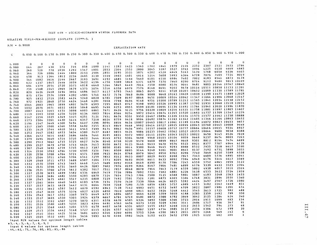
TEST KUN - UICKIE-HCCRAKEN WINTER FLOUNUEH. DATA
RELATIVE YIELD-PER-RECRUIT ISOPLETH (10**-5. )
:1 /K - O. 9000 EXPLOITATION RATE
C 0.050 0.100 0.150 0.200 0.250 0.300 0.350 0.400 0.450 0.500 0.550 0.600 0.650 0.700 0.750 0.800 0.850 0.900 0.950 1.000
1.000 0 0 0 0 0 0 0 0 0 0 0 0 0 0 0 0 0 0 0 0
O. 980 144 287 430 573 716 858 1000 1 141 1282 1423 1563 1702 1841 1979 2116 2252 2387 2521 2653 2784
o. 960 260 520 778 1036 1292 1547 1801 2053 2304 2553 2800 3045 3287 3527, 3763 3996 4225 4450 4669 4883
o. 940 364 726 1086 1444 1800 2153 2504 2851 3195 3535 3871 4202 4528 4849 5163 5470 5768 . 6058 6336 6603
o. 920 458 913 1364 181 2 2256 2695 3130 3559 3983 4401 4811 5214 5608 5993 6366 6728 7076 7409 77 24 8019
o. 900 544 1082 1616 2144 2667 3183 3691 4192 4685 5168 5640 6101 6550 6984 7402 7802 8183 8541 8873 9178
O. 880 622 1237 1845 2446 3039 3622 4196 4758 5309 5848 6371 6879 7370 7840 8290 8714 9112 9480 9813 10109
o. 860 694 1379 2054 2720 3375 4018 4648 5264 5865 6449 7014 7558 8080 8576 9044 9481 9883 10246 10567 10840
O. 840 759 1508 2245 2969 3679 4375 5054 5716 6358 6979 7576 8148 8691 9202 9678 10116 10511 10858 11153 11391
O. 820 820 1626 2418 3194 3954 4696 541 7 6117 6793 7443 8065 8655 9211 9728 10203 10632 11009 11330 11589 11781
o. 800 875 1734 2576 3399 4202 4983 5741 6472 71 76 7848 8486 9088 9648 10163 10628 11039 11390 11675 11889 12028
o. 780 925 1832 2719 3583 4424 5240 6028 6785 7509 8197 8846 9451 10009 10514 10962 11347 11664 11906 12068 12147
o. 760 972 1921 2848 3750 4624 5468 6281 7058 7798 8496 9148 9751 10300 10789 11212 11565 11841 12034 12138 12152
o. 740 1014 2003 2965 3899 480r 5670 6503 7295 8045 8747 9398 9993 10526 10993 11387 11702 11931 12068 12110 12055
o. 720 1052 2076 3071 4032 4959 5848 6695 7498 8253 8955 9599 10181 10694 11134 11492 11764 11941 12020 11996 11870
o. 700 1087 2143 3165 4151 5098 6003 6861 7671 8426 9123 9756 10320 10809 11216 11535 11758 11881 11897 11805 11607
O. 680 1119 2203 3250 4256 5220 6136 7003 7814 8566 9254 9872 10414 10874 11245 11520 11693 11757 11709 11547 11276
O. 660 1147 2256 3325 4349 5325 6251 71 21 7931 8676 9351 9950 10467 10894 11226 11454 11573 11577 11462 11230 10888
O. 640 1173 2304 3391 4430 5416 6347 7218 8024 8759 9418 9994 10482 10874 11163 11342 11405 11346 11164 1086310452
O. 620 1196 2347 3449 4500 5494 6427 7296 8094 8816 9456 10007 10463 10817 11061 11189 11194 11072 10823 10453 9977
o. 600 1217 2385 3500 4560 5558 6492 7355 8143 8849 9468 9992 i0414 10727 10925 10999 10945 10760 10445 10008 9469
O. 580 1235 2418 3544 4610 5611 6543 7399 8174 8862 9456 ·9951 10337 10608 10757 10777 10664 10416 10035 9534 8937
O. 560 1252 2447 3582 4653 5654 6580 7427 8187 8855 9424 9886 10235 10462 10562 10527 10355 10044 9600 9038 8388
o. 540 1266 2472 3614 4687 5686 6606 7441 8185 8831 9372 9802 10111 10294 10343 10253 10022 9650 9145 8526 7828
O. 520 1279 2494 3640 4714 5710 6622 7444 8169 8792 9304 9698 9968 10105 10104 9959 9669 9237 8674 8003 7263
O. 500 1290 2512 3662 4735 5725 6627 7434 8140 8738 9220 9579 9808 9899 9847 9648 9301 8812 8194 7474 6699
O. 480 1299 2527 3679 4750 5733 6624 7415 8100 8672 9123 9446 9633 9678 9576 9323 8921 8377 7707 6944 6139
O. 46'0 1307 2540 3692 4759 5735 6613 7387 8050 8595 9014 9300 9446 9445 9293 8988 8532 7935 7218 6417 5590
O. 440 1314 2550 3702 4764 5730 6595 7351 7991 8509 8895 9144 9248 9201 9001 8645 8137 7492 673 t 5898 5055
O. 420 1320 2558 3708 4764 5721 6571 7308 7925 8414 8768 8979 9042 8950 8702 8296 7740 7049 6250 5389 4538
O. 400 1325 2564 371 1 4760 5706 6541 7259 7852 8312 8633 8807 8829 8693 8398 7945 7343 6609 5776 4895 4041
O. 380 1329 2568 3711 4753 5688 6507 7204 7773 8205 8493 8630 8611 8433 8092 7594 6949 6176 5314 4417 3569
o. 360 1332 2570 3709 4743 5665 6468 7145 7689 8092 8348 8449 8390 8170 7786 7245 6559 5752 4865 3959 3122
o. 340 1334 2571 3706 4731 5640 6426 7083 7602 7976 8199 8264 8167 7906 7481 6899 6176 5339 4432 3523 2704
0.320 1336 2571 3700 4716 5612 6382 7017 7511 7857 8048 8078 7944 7643 71 79 6559 5802 4938 4017 3111 2316
o. 300 1337 2570 3693 4699 5582 6334 6949 7419 7736 7896 7892 7721 7382 6881 6226 5438 4553 3622 2724 1959
o. 280 1337 2568 3684 4681 5550 6285 6879 7324 7614 7743 7706 7500 7125 6588 5901 5087 4183 3248 2363 1633
O. 260 1338 2565 3675 4661 5517 6235 6808 7229 7492 7591 7521 7281 6873 6303 5586 4748 3831 2896 2031 1340
O. 240 1337' 2561 3664 4640 5483 6183 6736 7134 7370 7439 7339 7066 6626 6025 5282 4424 3497 2567 1726 1080
o. 220 1337 2557 3653 4619 5447 6131 6664 7038 7248 7290 71 59 6856 6385 5757 4989 4115 3182 2262 1449 851
o. 200 1336 2552 3642 4597 5412 6079 6592 6943 7128 7142 6983 6651 6152 5497 4709 3822 2887 1981 1201 654
O. 180 1335 2547 3630 4575 5376 6027 6520 6850 7010 6998 6811 6452 5926 5248 4442 3545 2613 1725 982 488
O. 160 1334 2542 361 7 4552 5340 5975 6449 6757 6894 6857 6644 6258 5709 5010 4188 3285 2359 1492 789 350
o. 140 1333 2537 3605 4530 5305 5924 6379 6667 6781 6719 6481 6072 5500 4782 3949 3042 2125 1284 624 240
o. 120 1332 2532 3592 4507 5270 5873 6311 6578 6670 6585 6324 5892 5300 4566 3723 2816 1911 1099 483 154
o. 100 1331 2526 3580 4485 5235 5823 6244 6491 6563 6456 6173 5720 5109 4361 3511 2606 1717 936 367 91
o. 080 1329 2521 3568 4463 5201 5775 6178 6407 6458 6331 6027 5555 4927 4168 3312 2413 1542 794 273 48 H
O. 060 1328 2515 3556 4442 5168 5727 6115 6326 6357 6210 5887 5397 4754 3985 3127 2236 1386 672 199 20 H
O. 040 1327 2510 3544 4421 5136 5681 6053 6246 6260 6094 5753 5246 4590 3813 2955 2073 1246 569 142 6 H
O. 020 1325 2505 3532 4401 5104 5636 5993 6170 6166 5982 5624 5102 4435 3652 2795 1925 1122 482 101 .j:::.
'-l Input M/K values for optimum length tables
il 3, • 4, • 5, • 6, • 7, . 8, • 9, 1 Input E values for optimum length tables
.44,.62,. 71,. 76,.80,.83,.85,.86
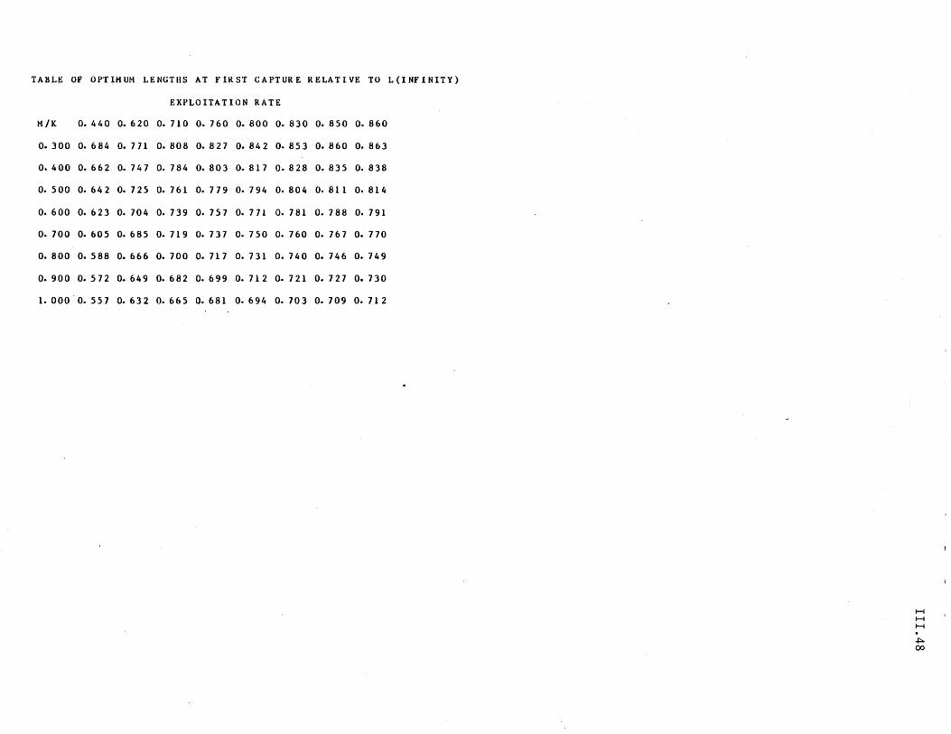
TABLE OF OPTIMUM LENGTHS AT FIRST CAPTURE RELATIVE TO L{INFINITY)
EXPLOITATION RATE
M/K o. 4 40 O. 620 O. 7 1 0 O. 7 60 O. 800 O. 830 O. 850 O. 860
o. 300 O. 6 84 O. 7 71 O. 808 O. 8 27 O. 84 2 O. 85 3 O. 860 O. 863
0.400 0.662 0.747 0.784 0.803 0.817 0.828 0.835 0.838
o. 500 O. 64 2 O. 7 25 o. 76 1 O. 7 7 9 O. 7 94 o. 804 O. 8 1 1 O. 81 4
O. 600 O. 6 23 O. 704 O. 739 o. 75 7 O. 7 71 O. 7 81 O. 7 88 O. 7 9 1
O. 700 O. 605 O. 685 O. 71 9 o. 7 3 7 o. 7 50 O. 760 O. 76 7 O. 7 70
O. 800 O. 588 O. 666 0.700 O. 717 0.731 O. 740 O. 746 o. 749
O. 900 o. 5 72 O. 649 O. 682 O. 699 O. 71 2 O. 721 O. 727 O. 730
1.000 '0.557 0.632 0.665 0.681 0.694 0.703 0.709 0.712
H H H
.j:;::. 00
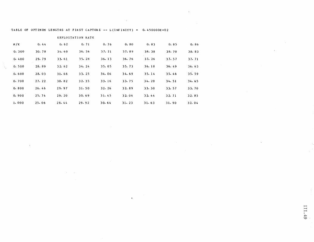
TABLE OF OPTIMUM LENGTHS AT FIRST CAPTURE -- L(INFINITY)
EXPLOITATION RATE
M/K O. 44 O. 62 0.71 O. 76 O. 80
O. 300 30. 78 34. 69 36. 36 37. 21 37. 89
O. 400 29. 79 33. 61 35. 28 36. 13 36. 76
O. 500 28. 89 32. 62 34. 24 35. 05 35. 73
O. 600 28. 03 31. 68 33. 25 34. 06 34. 69
O. 700 27. 22 30. 82 32. 35 33. 16 33. 75
O. 800 26. 46 29.97 31. 50 32. 26 32. 89
O. 900 25. 74 29. 20 30. 69 31. 45 32. 04
1. 000 25. 06 28. 44 29. 92 30. 64 31. 23
... 0.450000E+02
O. 83 O. 85
38. 38 38. 70
37. 26 37. 57
36. 18 36. 49
35. 14 35. 46
34. 20 34. 51
33. 30 33. 57
32. 44 32. 71
31. 63 31. 90
O. 86
38. 83
37. 71
36. 63
35. 59
34. 65
33. 70
32. 85
32. 04
H H H
~ 1..0
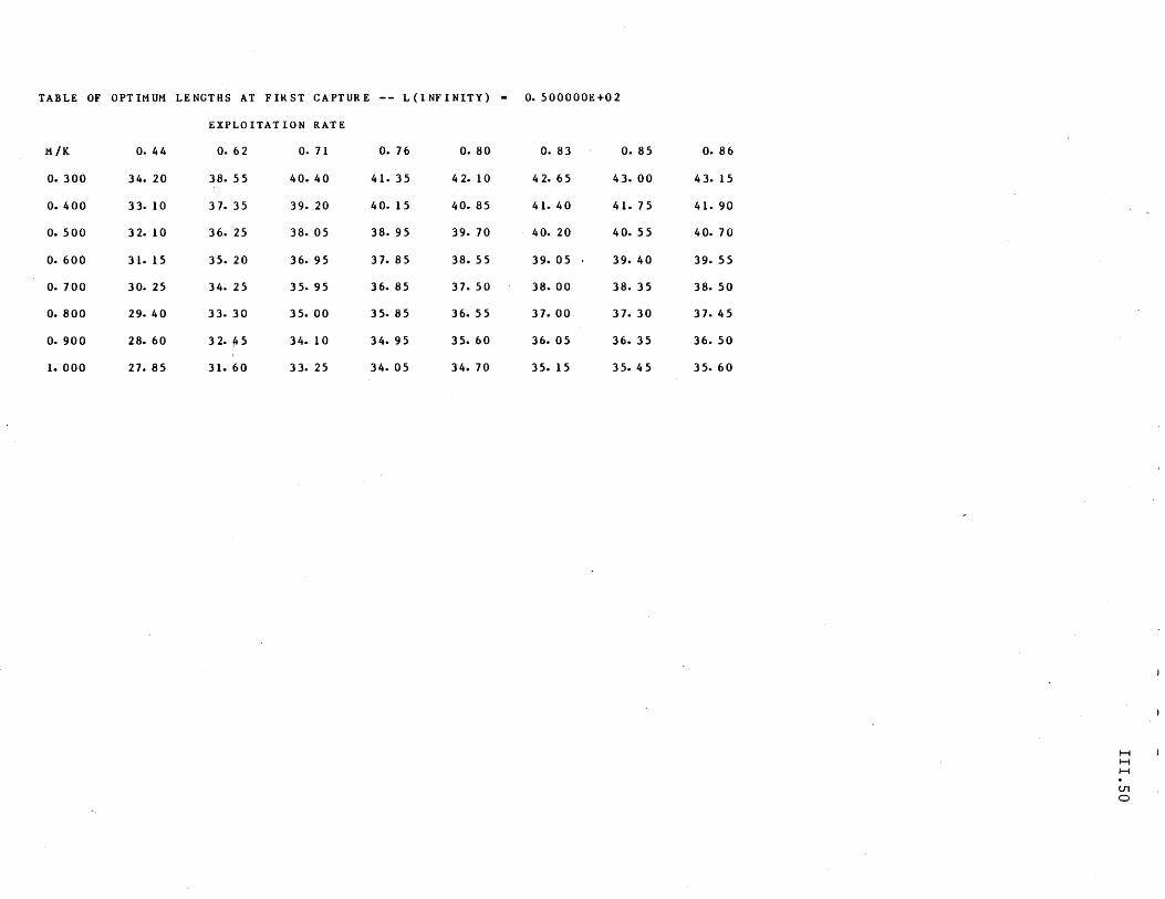
TABLE OF OPTIMUM LENGTHS AT FIRST CAPTURE -- L (INFINITY) -
EXPLOITATION RATE
M/K O. 44 O. 62 O. 71 O. 76 0.80
O. 300 34. 20 38. 55 40. 40 41. 35 42. 10
O. 400 33. 10 37. 35 39. 20 40. 15 40. 85
O. 500 32. 10 36. 25 38. 05 38. 95 39. 70
O. 600 31. 15 35. 20 36. 95 37. 85 38. 55
o. 700 30. 25 34. 25 35. 95 36. 85 37. 50
O. 800 29. 40 33. 30 35. 00 35. 85 36. 55
O. 900 28. 60 3 2. ~5 34. 10 34. 95 35. 60
1. 000 27. 85 31. 60 33. 25 34. 05 34. 70
O.500000E+02
O. 83 O. 85
42. 65 43. 00
41. 40 41. 75
40. 20 40. 55
39. 05 . 39. 40
38. 00 38. 35
37. 00 37. 30
36. 05 36. 35
35. 15 35. 45
O. 86
43. 15
41. 90
40. 70
39. 55
38. 50
37. 45
36. 50
35. 60
H H H
U1 o
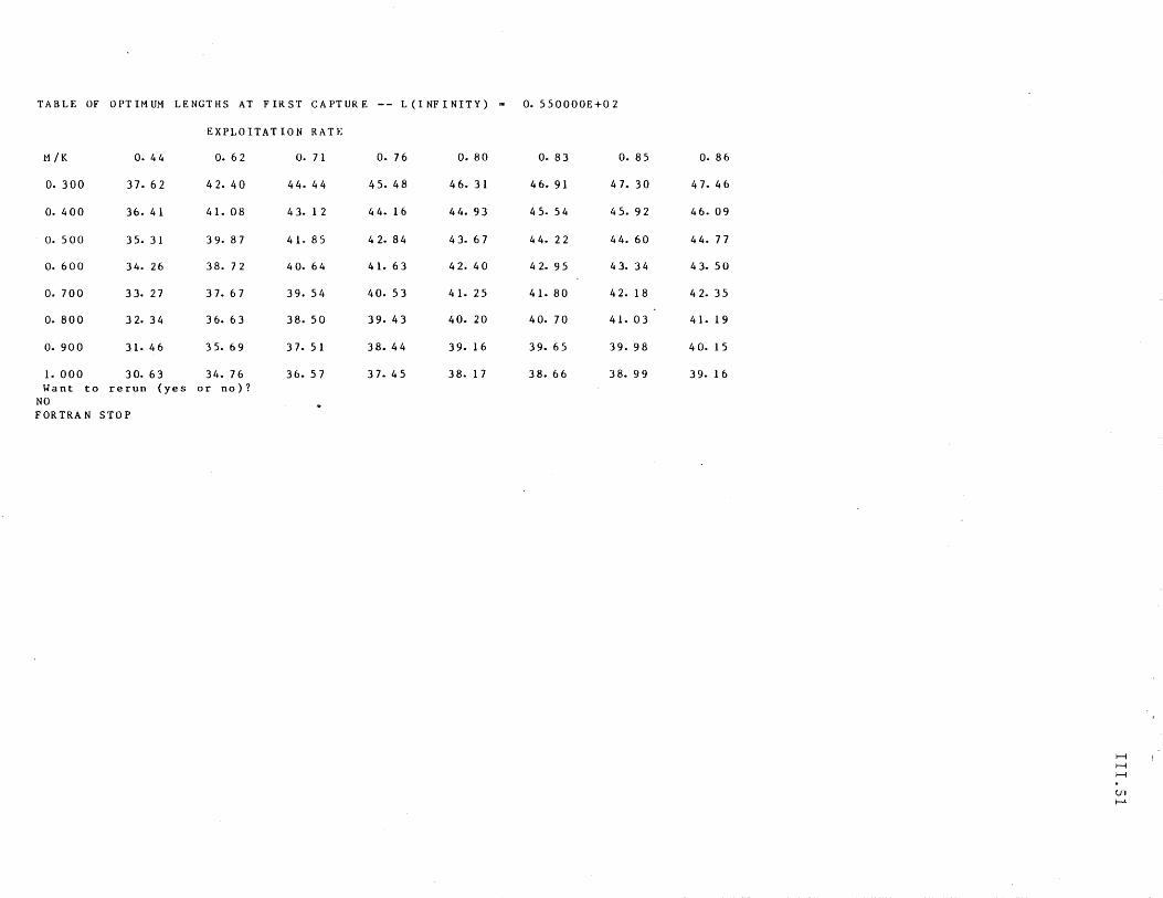
TABLE OF OPTIMUM LENGTHS AT FIRST CAPTURE -- L(INFINITY)
EXPLOITATION RATE
M/K O. 44 o. 62 o. 71 O. 76 o. 80
O. 300 37. 62 42. 40 44. 44 45. 48 46. 31
o. 400 36. 41 41. 08 43. 1 2 44. 16 44. 93
o. 500 35. 31 39. 87 41. 8 S 42. 84 43. 67
o. 600 34. 26 38. 72 4 O. 64 41. 63 42. 40
O. 700 33. 27 37. 67 39. S4 40. 53 41. 25
o. 800 32. 34 36. 63 38. 50 39. 43 40. 20
o. 900 31. 46 3 S. 69 37. 51 38. 44 39. 16
1. 000 30. 63 34. 76 36. 57 37. 45 38. 17 Want to rerun (yes or no)?
NO FORTRAN STOP
- O. 550000E+0 2
O. 83 O. 85
46. 91 47. 30
45. 54 45. 92
44. 22 44. 60
42. 95 43. 34
41. 80 42. 18
40. 70 41. 03
39. 65 39. 98
38. 66 38. 99
O. 86
47. 46
46. 09
44. 77
43. 50
42. 35
41. 19
4 o. 15
39. 16
H H H
Ul I-'
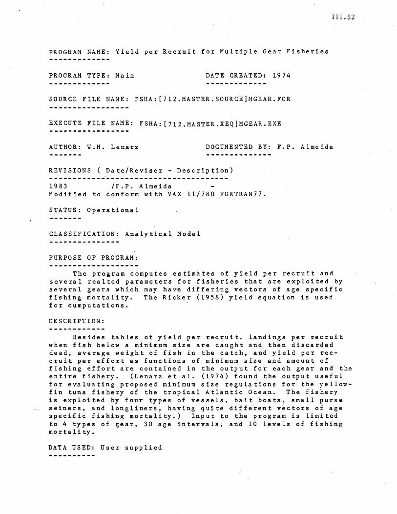
111.52
PROGRAM NAME: Yield per Recruit for Multiple Gear Fisheries
PROGRAM TYPE: Main DATE CREATED: 1.974
SOURCE FILE NAME: FSHA: [712.MASTER.SOURCE]MGEAR.FOR
EXECUTE FILE NAME: FSHA: [7l2.MASTER.XEQ]MGEAR.EXE
AUTHOR: W.H. Lenarz DOCUMENTED BY: F.P. Almeida
REVISIONS ( Date/Reviser - Description)
1983 /F.P. Almeida Modified to conform with VAX 11/780 FORTRAN77.
STATUS: Operational
CLASSIFICATION: Analytical Model
PURPOSE OF PROGRAM:
The program computes estim~tes of yield per recruit and several realted parameters for fisheries that are exploited by several gears which may have differing vectors of age specific fishing mortality. The Ricker (1958) yield equation is used for cumputations.
DESCRIPTION:
Besides tables of yield per recruit, landings per recruit when fish below a minimum size are caught and then discarded dead, average weight of fish in the catch, and yield per reccruit per effort as functions of minimum size and amount of fishing effort are contained in the output for each gear and the entire fishery. (Lenarz et al. (1974) found the output useful for evaluating proposed minimum size regulations for the yellowfin tuna fishery of the tropical Atlantic Ocean. The fishery is exploited by four types of vessels, bait boats, small purse seiners, and longliners, having quite different v~ctors of age specific fishing mortality.) Input to the program is limited to 4 types of gear, 30 age intervals, and 10 levels of fishing mo rta 1 i ty.
DATA USED: User supplied
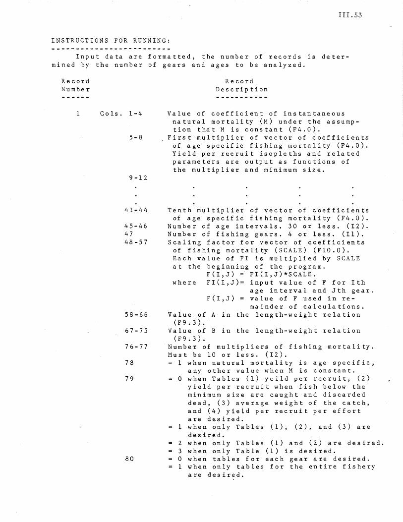
III.53
INSTRUCTIONS FOR RUNNING:
Input data are formatted, the number of records is determined by the number of gears and ages to be analyzed.
Record Number
1 Cols. 1-4
Record Description
Value of coefficient of instantaneous natural mortality (M) under the assumption that M is constant (F4.0).
5-8 First multiplier of vector of coefficients
9-12
41-44
45-46 47 48-57
58-66
67-75
76-77
78
79
80
of age specific fishing mortality (F4.0). Yield per recruit isopleths and related parameters are output as functions of the multiplier and minimum size.
Tenth multiplier of vector of coefficients of age specific fishing mortality (F4.0).
Number of age intervals. 30 or less. (12). Number of fishing gears. 4 or less. (11). Scaling factor for vector of coefficients
of fishing mortality (SCALE) (F10.0). Each value of FI is multiplied by SCALE at the beginning of the program.
F(I,J) ~ FI(I,J)*SCALE. where FI(I,J)= input value of F for Ith
age interval and Jth gear. F(I,J) = value of F used in re
mainder of calculations. Value of A in the length-weight relation
(F9.3). Value of B in the length-weight relation
(F9.3). Number of multipliers of fishing mortality. Must be 10 or less. (12).
1 when natural mortality is age specific, any other value when M is constant.
o when Tables (1) yeild per recruit, (2) yield per recruit when fish below the minimum size are caught and discarded dead, (3) average weight of the catch, and (4) yield per rec~uit per effort are desired.
1 when only Tables (1), (2), and (3) are desired.
2 when only Tables (1) and (2) are desired. 3 when only Table (1) is desired. o when tables for each gear are desired. 1 when only tables for the entire fishery
are desired.
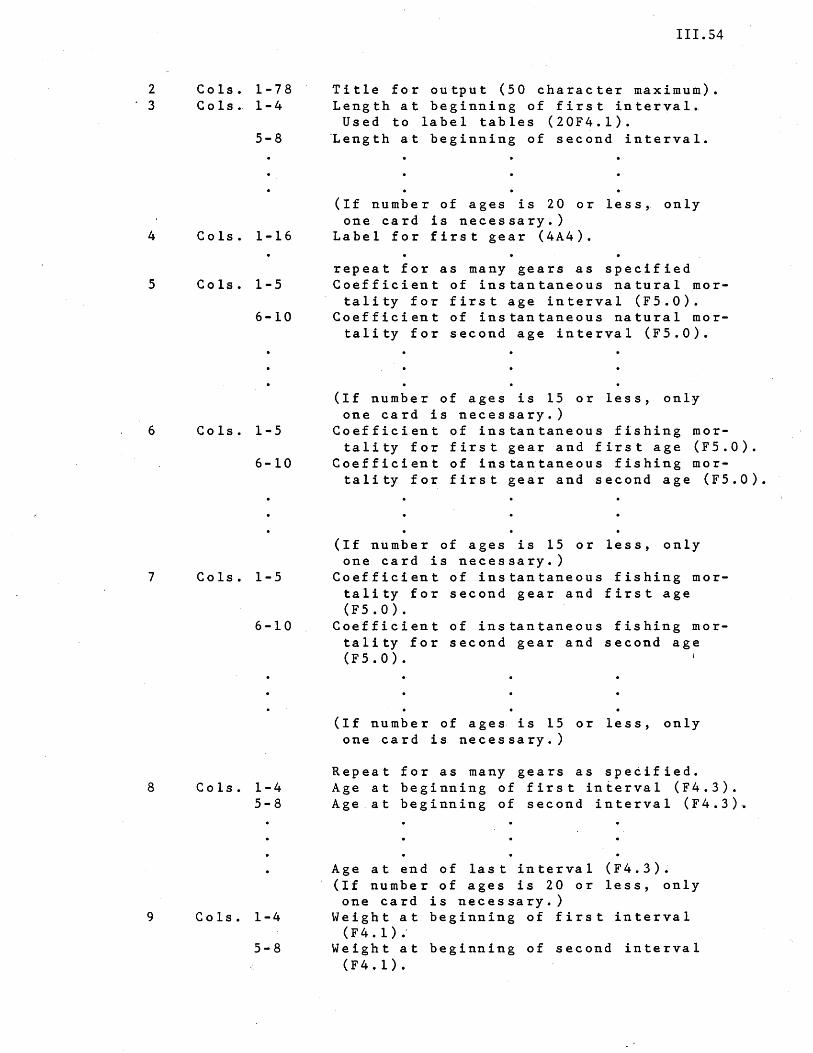
2 3
4
5
6
7
8
9
Cols. 1-78 Cols. 1-4
5-8
Cols. 1-16
Cols. 1-5
6-10
Cols.1-5
6-10
Cols. 1-5
6-10
Cols. 1-4 5-8
Cols. 1-4
111.54
Title for output (50 character maximum). Length at beginning of first interval.
Used to label tables (20F4.l). ~ength at beginning of second interval.
(If number of ages is 20 or less, only one card is necessary.)
Label for first gear (4A4).
repeat for as many gears as specified Coefficient of instantaneous natural mortality for first age interval (F5.0).
Coefficient of instantaneous natural mortality for second age interval (F5.0).
(If number of ages is 15 or less, only one card is necessary.)
Coefficient of instantaneous fishing mortality for first gear and first age (F5.0).
Coefficient of instantaneous fishing mortality for first gear and second age (F5.0).
(If number of ages is 15 or less, only one card is necessary.)
Coefficient of instantaneous fishing mortality for second gear and first age (F5.0).
Coefficient of instantaneous fishing mortality for second gear and second age (F5.0). I
(If number of ages is 15 or less, only one card is necessary.)
Repeat for as many gears as specified. Age at beginning of first interval (F4.3). Age at beginning of second interval (F4.3)~
Age at end of last interval (F4.3). (If number of ages is 20 or less, only one card is necessary.)
Weight at beginning of first interval (F 4 • 1 ) .'
5-8 Weight at beginning of second interval (F4.l).
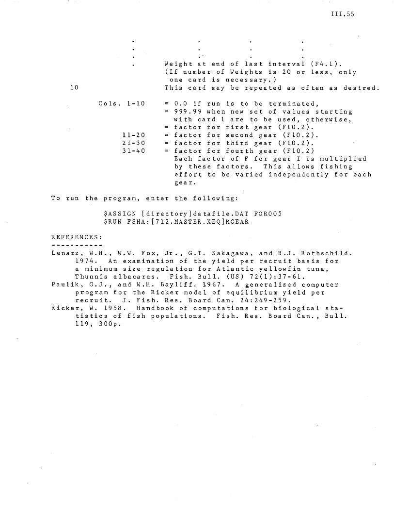
10
111.55
Weight at end of last interval (F4.1). (If number of Weights is 20 or less, only
one card is necessary.) This card may be repeated as often as desired.
Cols. 1-10 0.0 if run is to be terminated,
11-20 21- 3 0 31-40
= 999.99 when new set of values starting with card 1 are to be used, otherwise, factor for first gear (F10.2). factor for second gear (F10.2). factor for third gear (F10.2).
= factor for fourth gear (F10.2) Each factor of F for gear I is multiplied by these factors. This allows fishing effort to be varied independently for each gea r.
To run the program, enter the following:
REFERENCES:
$ASSIGN [directory]datafile.DAT FOR005 $RUN FSHA: [712.MASTER.XEQ]MGEAR
Lenarz, W.H., W.W. Fox, Jr., G.T. Sakagawa, and B.J. Rothschild. 1974. An examination of the yield per recruit basis for a minimum size regulation for Atlantic yellowfin tuna, Thunnis albacares. Fish. Bull. (US) 72(1):37-61.
Paulik, G.J., and W.H. Bayliff. L967. A generalized computer program for the Ricker model of equilibrium yield per recruit. J. Fish. Res. Board Can. 24:249-259.
Ricker, W. 1958. Handbook of computations for biological statistics of fish populations. Fish. Res. Board Can., Bull. 119, 300p.
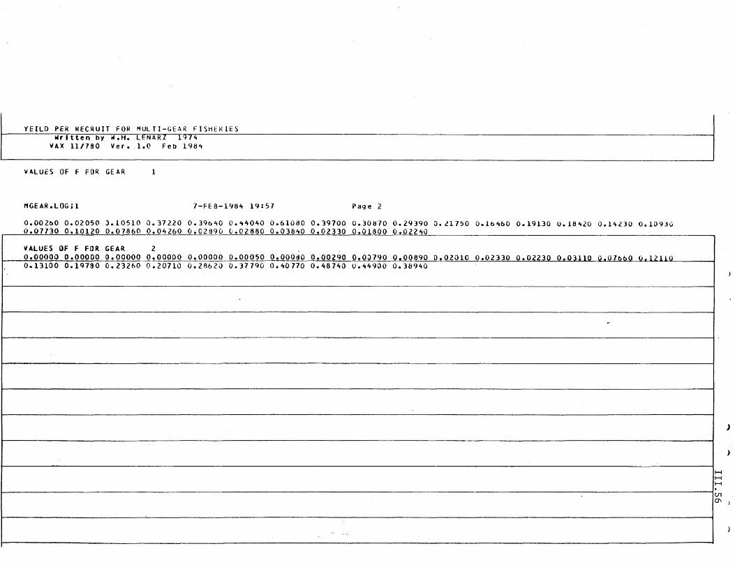
¥EllO PER RECRUIT FOR MULTI-GEAR FISHERIES W r Itt e n- by W.-H • lENA R. Z -19 71t
VAX 11/760 Ver. 1.0 Feb 198~
VALUES OF F FOR GEAR 1
I1GEAR.lOG; 1 7-FEB-1984 19:57 Page 2
0.002bO 0.02050 J.I0510 0.37220 0.39640 0.44040 0.61080 0.39700 0.30870 0.29390 O.l1750 0.lb460 0.19130 0.18420 0.14230 0.10930 0.07730 0.10120 0.07860 0.04260 0.02890 ('.02880 0.03840 0.02330 0.01600 0.02240
VALUES OF f FOR GEAR 2 0.00000 0.00000 0.00000 0.00000 0.00000 0.00050 0.00080 0.00290 0.00790 0.00890 0.02010 0.02330 0.02230 0.03110 0.07660 0.12110 0.13100 0.19760 0.23260 0.20710 0.28620 0.37790 0.40770 0.48740 0.44900 0.38940
~
I: H H H II (Jl 0\
J
)
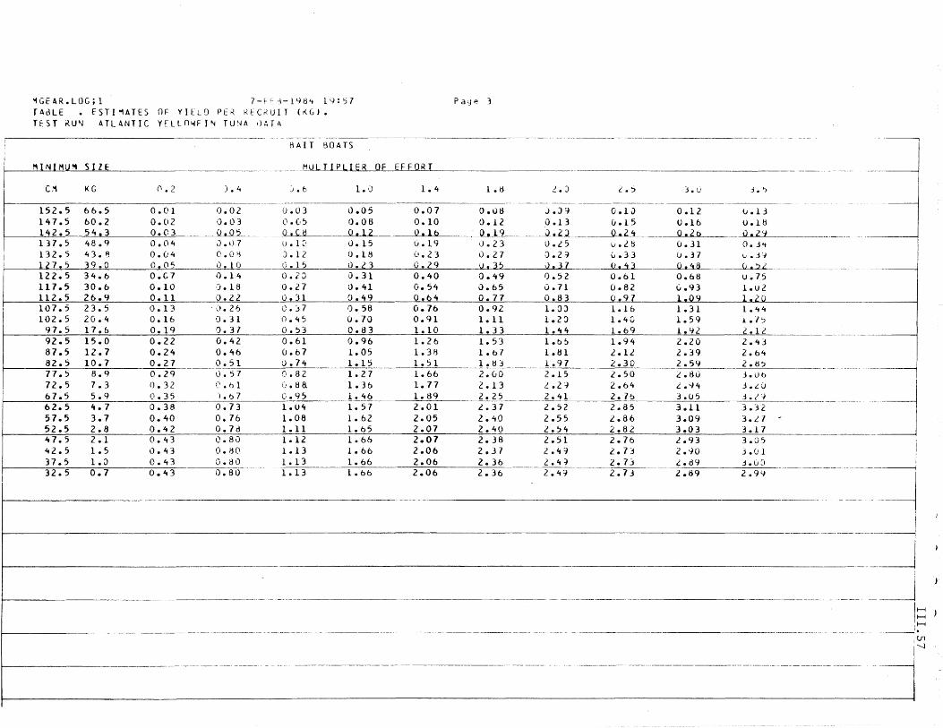
~GEAR.LOG;l 7-F ~-14H4 lq:~7 Pa;,le 3 TAaLE • fSTI~ATES OF YIELD PE~ RfCKUIT (KG). TtST KU~ ATLANTIC YELLn~Fr~ TUNA I)ATA
---, HAlT BOATS
MINIMUM SIZE ___ tUL!., TIP LI E R 0 F E F FOR T -- --_.- -" - -
Cr .. KG :) • b 1.0 1.4 1 • tl 2.) 2. j J.u 3.')
-----0.02 0.03 0.05 0.07 0.08 J.J~ 0.10 0.12 v.13 0.03 0.05 0.08 0.10 0.12 0.13 0.15 U.16 U.IH 0.05 o.ce 0.12 0.16 0.19 J.2) 0.24 0.20 V.2~
o • l) 7 u • 1 C' O. 1 5 u • 1 9 J • 2 3 0 • L 5 lJ • 2. bu. 3 1 O. j'1
O.O~ J.12 O.lH 0.23 0.27 ).21 G.33 U.37 ~.j~
.05 0.10 0.15 J.l3 0.29 0.35 J.37 0.43 Q.48 0.)2 ~--.- ---.----+--~-
0.14 0.20 0.31 0.40 0.49 0.52 0.61 0.68 u.75 0.18 0.27 0.41 0.54 0.65 0.71 0.82 0.93 1.u2 0.22 0.31 0.49 0.64 0.77 0.83 0.97 1.09 1.20
107.5 23.5 0.13 -0.26 O.~7 0.58 0.76 0.92 1.0J 1.16 1.31 1.44
... .. .. - .- ......... ....... .6 .. ....... .- . ........ -- ............. .- _ .. -'" .... -.., ....... A." _ , .... , ~ &.. • .£.L. .----_._----- -
92.5 15.0 0.22 0.42 0.61 0.96 1. 26 1.53 1.6~ 1.94 2.20 2.43 87.5 12.7 0.24 0.46 0.61 1.05 1.38 1.61 1.Hl 2..12. 2.39 2.64 82.5 10.1 0.21 0.51 '.).14 1.15 1.51 1.tn 1.97 2.30 2.59 2.1:i? 17.5 8.9 0.29 1).57 0.82 1.27 1.66 2.00 2.15 2.50 2.8u 3.00 -.--- --- -j -
---_.-
------------ --------- ~' ----
-~---
12.5 7.3 0.32 (\ • b 1 (I. H a 1.36 1.77 2.13 !..2'..J 2.64 i.'-J4 3.iU 67.5 5.9 0.35 ).67 C.95 1.46 1.89 2.25 2.41 2.76 3.05 .-~---62.5 't.7 0.38 0.13 1.04 1.57 2.01 2..37 2.52 2.85 3.11 3.32 57.5 3.7 0.40 0.76 1.08 1. 62 2.05 2.40 2.55 2.86 3.09 3.1. 7 ~
52.5 2.8 0.42 0.7d 1.11 1.b5 2.07 2.40 2.,4 2.82 3.03 3.17 47.5 2.1 0.43 0.80 1.12 1.66 2.01 2.38 2.51 2.76 2..93 3.05 42.5 1.5 l). 43 0.130 1.13 1.66 2.06 2.37 Z.4':J 2..73 2.'-10 Lv 1 37.5 1.0 0.43 O.HO 1.13 1.66 2.06 2.36 Z.4~ 2.73 L.89 j. U~) - - ~ - - - ----- - ------- -----32.5 0.7 0.43 0.80 1
----- j: -------
---_ ..
----~) --~~
IUl '-I '
--- ~---------. -----_ .. - -- .. _--
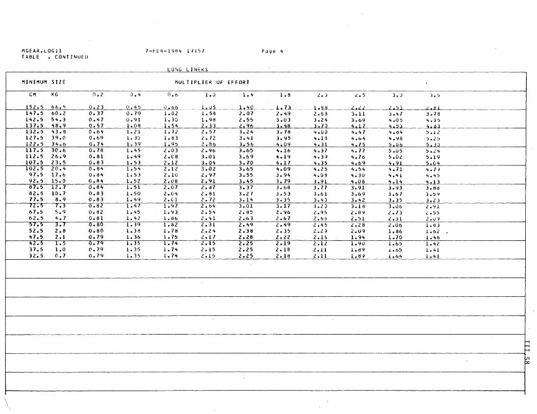
MGEAR.LOGil 7-FEB-19f3't l'J:57 Page 4 TABLE • CONTINUED
LO~G LINEKS
MINIMUM SIZE MULTIPLIER UF EFFORT \
eM KG 0.2 0.4 (I.b 1.;) . 1." 1.8 L.} i..5 3.J j.?
152.5 66.1) 0.23 O.4~ 0.66 1. 05 ~ ____ 40 1.73 I.btl 2.22 2.~3 Llli 147.5 60.2 0.37 0.70 1.02 1.513 2.07 2.49 2.b3 3.11 'j.47 3.78 142.5 54.3 0.47 0.91 1.30 1.98 2.55 3.03 3.24 3.69 4.05 't.3'> 137.5 48.9 0.57 1.0R 1.54 2.33 2.96 3.48 3.7~ 4.17 4.5j 't.d) 132.5 43.8 0.64 1.21 1.72 2.57 3.24 3.78 4.UO 't.47 't.d4 ~.l2 127.5 39.0 0.69 1. 3:) 1. 1:13 2.. 72 3.41 3.'15 4.1:1 't.04 4.'18 ').2. ? 122.5 34.6 0.7'1 1.39 1.95 2.86 3.56 4.09 4.31 't.15 '>.06 ~.3() 117.5 30.6 0.78 1.45 2.03 2.96 3.65 4.16 4.37 4.77 5.05 ').~ 't 112.5 26.9 0.81 1.49 2.(;8 3.01 3.69 4.19 't.3:j 4.76 5.02 5.19 107.5 23.5 0.83 1.53 2.12 3.04 3.70 4.17 4.35 4.69 4.91 S.Cl4 102.5 20.4 0.84 1.54 2.12 3.02 3.65 4.09 4.25 4.54 4.71 4.7'; 97.5 17.6 0.84 1.53 2.1U 2.97 3.55 3.94 4.03 4.30 4.41 4.45 92.5 15.0 0.84 1.52 2.08 2.91 3.45 3.79 3.91 4.08 4.14 4.13 87.5 12.7 0.84 1.51 2.07 2.d7 3.37 3.68 3.77 3.91 3.'13 3. tHi 82.5 10.7 0.83 1.50 2.04 2.81 3.27 3. 53 3.61 3.69 3.67 3.')'1 77.5 8.9 0.83 1.49 2.Cl 2.72 3.1'1 3.35 3.4) 3.42 3.35 3.23 72.5 7.3 0.82 1. 47 1.47 2.64 3.01 3.17 3.20 3.1d 3.06 2.'11 67.5 5.9 0.82 1. 45 1.9~ 2.5't 2.85 2.l.Jb 2.9~ 2.(j'J 2.13 2.55 62.5 4.7 0.81 1. 42 1.ti6 2.~1 2.63 2.67 2.bj 2.~1 2.31 2.09 57.5 3.7 0.80 1.39 1.82 2.31 2.49 ~.49 2.45 2.28 L.06 1.63 52.5 2.8 0.80 1.38 1.78 2.24 2.38 2.3~ 2.2=1 2.U9 1.d6 1.62 ~
47.5 2.1 0.79 1.36 1.75 2.17 2.28 2.22 2.1~ 1.94 1.70 1.46 42.5 1.5 0.7Q 1.35 1.74 2.15 2.25 2.19 2.12 1.90 1.65 1.42 37.5 1.0 ().7Q 1.35 1.74 2.15 2.25 2.18 2.11 1.d9 1.65 1.41 32.5 0.7 0.79 1.35 1.71t 2.15 2.25 2.1d 2.11 1.tH 1.64 1.41
~
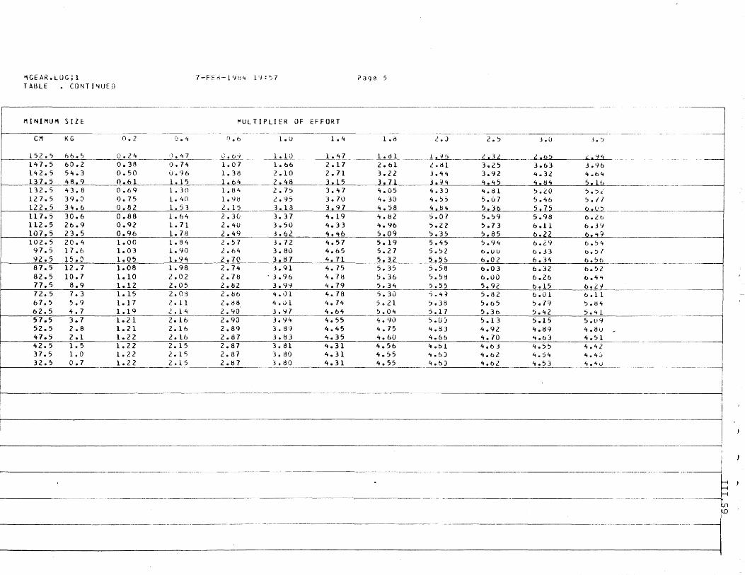
'1GEAR.LUG;! 7 - F t r\ - 1 4 tJ 't 1 '-J : 'J 7 TABLE • CONTI~UED
--- ~---- -----_._---
MINIMUM SIZE ~ULTIPLIER OF EFFORT - - ----,--
eM KG 0.2 [j.4 neb 1.u 1.4
152.5 66.5 0.24 :) • it 7 __ C • b":; _____ 1.10 1.47 147.5 60.2 0.38 c). 74 1.07 1.66 2.17 142.5 54.3 0.50 0.96 1.38 Z.lO 2.71 137.5 48.9 0.61 1. 15 1. 64 2.48 3.15 132.5 43.8 0.69 1. 30 1.84 2.7S 3.47 127.5 39.:) 0.75 1. 40 1. '/b 2.95 3.70 122. , 34.6 0.82 1.53 2.1S 3.13 3.97 117.5 30.6 0.88 1.64 2.30 3.37 4.19 112.5 26.9 0.92 1.71 2.40 3.50 4.33 107.5 23.5 0.96 1.78 .2.49 3.62 4.46 102.5 20.4 1.00 1.84 2.57 3.72 4.57 97., 17.6 1.03 1.90 2.64 3.80 4.65 92.5 15.0 1.05 1.94 2.70 3. til 4.71 87.5 12.7 1.08 1.98 2.74 3.91 4. 75 82.5 10.7 1.10 2.02 2.71:3 . 3.96 4.7tl 11.5 8.9 1.12 2.05 2.82 3.9C} 4.79 72.5 7.3 1.15 2.0~ 2.bb ~ • I) 1 4.78 61.5 5.9 1.17 2. 11 Z.bS 'i.Jl 4. 74 62.5 4.7 1.1q 2.14 2.90 J. '-17 4.04 57.5 3.7 1.21 2.16 2.90 3.94 4.55 52.5 2.8 1.21 2.16 2.89 3.tl'-J 4.45 'tl.5 2.1 1.22 2.16 2.87 3. 83 4.35 42.5 1.5 1.22 2.15 2.87 3.dl 4.31 37.5 1.0 1.22 2.15 2.87 3.80 4.31
'--32.5 0.7 1.22 2.15 2.87 3. 1:30 4.31
?age :)
------------l.d 2.J 2.S
__~. ________ 1.~ ____ ~.3,
2.01 L.dl 3.25 3.22 3.44 3.92 3!71 2. 9 4 4!45 4.05 4.3) 4.dl 4. 30 4.S' 5.07 4.58 - 4.blt 5.3b 4.82 5.07 5.59 4.96 5.22 5.73 5.09 5.35 5.85 5.19 5.45 5.94 5.27 5.52 o. U lJ 5.32 5.S!> 6.02 5.35 5.58 0.0 3 5.36 5.5~ 6.00 5.34 5.55 5.92 5.30 oj.4~ 5.82 5.21 ':>.3B 5.65 5.04 5.17 5.36 4.90 5.0) 5.13 4.75 4.B3 4.92 4.60 4.ob 4.70 4.50 4.bl 4.63 4.55 ~.b) 4.02 4.55 4.b) 1t.62
----
J.O J.?
--- ~~Q2 ,.'1~
3.63 3.96 4.3.2 4.64 j.1:j4 !:!.lb 5.iO 5.~i'
5.46 ':J.1l 5 1 1!:! Q .!.I 2 5.98 6.Lb b.ll b.34 6.22. ~'t:j
6.29 b.54 b.33 b.~7
6.34 6.56 6.32 6.52 6.20 6.44 b.1S 6.i.-I 6.01 b.ll 5.79 ~.b4
5.42 ~. '11 5.15 ') .Lt9 4.89 4.8u 4.03 4.51 4.55 4.42 4.54 4.itJ 4.53 4.40
~--~---
------ -.-------- "-~-
------- ------
---- -- I
.__ I -- I I
i I --------1 -- =----=4
... --3 ----------- k.J,
~
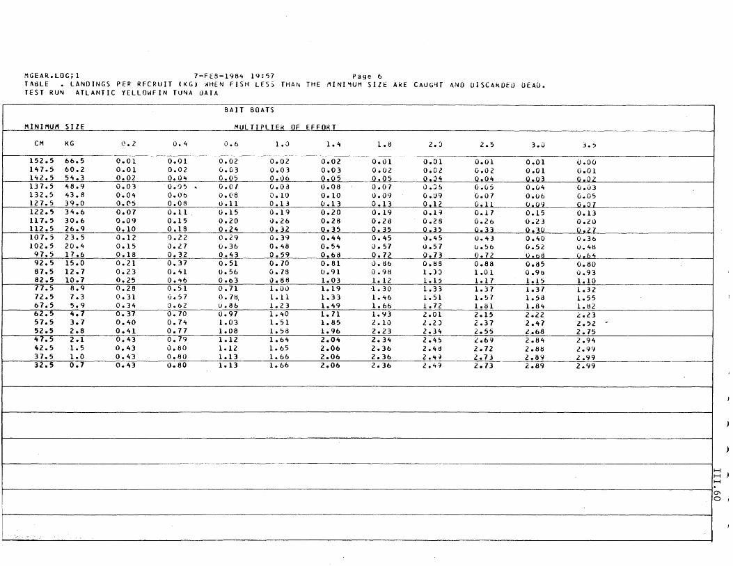
I
MGEAR.lOG;l 7-FE8-198~ 19:57 Page 6 TA~LE • LANDINGS PER RECRUIT (KG) ~HEN FISH LESS THAN THE MINI~UM SIZE ARE CAUG~T AND OISCAkDED DEAO. TEST RUN ATLANTIC YELLOWFIN TUNA DATA
BAIT BOATS
MINIMUM SIZE MULTIPLIEK OF EFFORT
CM KG 0.2 0.4 0.6 1.0 1.4 1.8 2.~ 2.5 3.11
152.5 66.5 0.01 0.01 0.02 0.02 0.02 0.01 0.01 0.01 0.01 Ilt7.5 60.2 0.01 0.02 0.03 0.03 0.03 0.02 O.Ol 0.02 0.01 Ilt2.5 54.3 0.02 0.04 0.05 0.06 J}.j15 0.05 0.:)4 0.04 ~.1 137.5 48.9 0.03 . 0.')5 - 0.01 o.oa 0.08 0.07 O.J~ 0.05 0.04 132.5 43.8 0.04 O.Ob o. ('8 0.10 0.10 0.09 0.:}9 0.07 0.06 127.5 39.0 0.05 0.08 0.11 0.13 0.13 0.13 0.12 0.11 0.09 122.5 34.6 0.07 0.11. 0.15 0.19 0.20 0.19 0.1~ 0.17 0.15 117.5 30.6 0.09 0.15 0.20 0.26 0.28 0.28 0.28 0.26 0.23 112.5 26.9 0.10 0.18 0.24 0.32 0.35 0.35 0.35 0.33 0.30 107.5 23.5 0.12 0.22 0.29 0.39 0.44 0.45 1l.45 0.43 0.40 102.5 20.4 0.15 0.27 0.36 0.48 0.54 0.57 0.57 lJ.~6 0.52 97.5 17.6 0.18 0.32 0.43 0.59 0.68 0.72 0.73 0.72 O.b8 92.5 15.0 0.21 0.37 0.51 0.70 0.81 0.86 0.86 0.88 0.85 87.5 12.7 0.23 0.41 0.56 0.78 0.91 0.98 1.) 1.01 O.9b 82.5 10.7 0.25 0.~6 0.b3 0.88 1.03 1.12 1.1, 1.17 1.15 77.5 8.q 0.28 0.51 (\.71 1.0J 1.19 '1.30 1.33 1.37 1.37 72.5 7.3 0.31 1).57 O.7t3, 1.11 1.33 1.46 1.51 1.57 1.sa 67.5 5.9 0.34 u.b2 0.86 1.23 1.49 1.66 1.72 1.01 1.84 62.5 1t.7 0.37 0.70 0.97 1.40 1.71 1.~3 2.01 2.15 2.22 57.5 3.7 0.40 0.74 1.03 1.51 1.85 2.10 2.2) 2.37 2.47 52.5 2.8 0.41 0.77 1.08 1.58 1.96 2.23 2.34 .2.55 2 .• 68 47.5 2.1 0.43 0.79 1.12 1.61t 2.04 2.34 2.4~ .2.69 2.84 42.5 1.5 0.43 0.80 1.12 1.65 2.06 2.36 2.4d 2.72 2.8ti 37.5 1.0 0.43 0.60 1.13 1.66 2.06 2.36 2.4-1 2.73 2.89 32.5 0.7 0.43 0.80 1.13 1.66 2.06 2.36 2.4~ 2.73 2.89
r.-~, • .. .. ',
3.j
O.OU 0.01
Ji . ..Jl2 0.03 0.05 0.07 0.13 0.20 0.27 0.30 0.48 09.64 0.80 (;.93 1.10 1.32 1.55 1.ij2 ~.l3
2.52 .2.75 2.94 2..99 2.~9
2.99
~
H H H
)
(j\ 0,
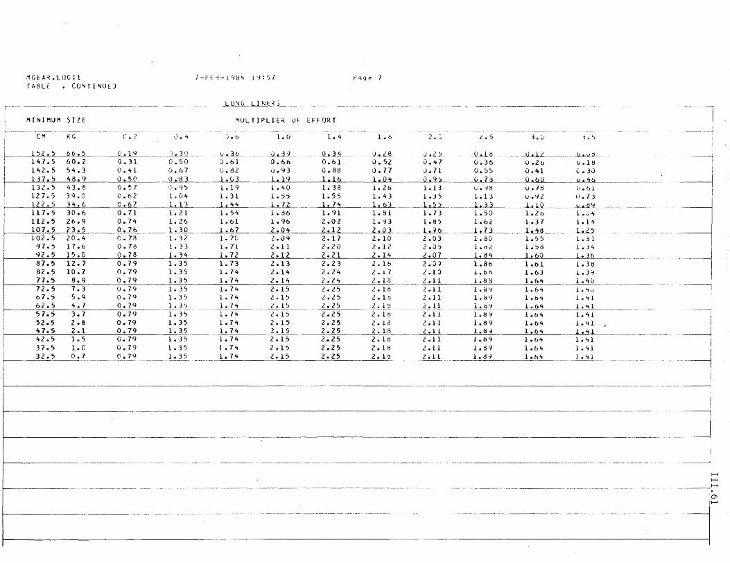
MGEA~.LiJG;l
TABLE • CO~TI~UEJ
MINIMUM SIZE
eM KG
152.5 6b.5 147.5 60.2 142.5 54.3 137.5 48.9 132.5 43.8 127.5 39.0 122.5 34.6 117.5 30.6 112.5 26.9 107.5 23.5 102.5 20.4 97.5 17.6 92.5 15.0 87.5 12.7 82.5 10.7 77.5 8.9 72.5 7.3 67.5 5.9 62.5 4. 7 57.5 3.7 52.5 2.8 47.5 2.1
37.5 1
C.2
0.19 0.31 0.41 0.50 0.57 0.62 G.b7 0.71 0.74 0.76 (; • 7 B 0.78 0.78 0.79 0.79 0.79 0.79 O.7Q 0.79 0.79 0.79 0.79
1-Ff:~-lCJt)'t 19:)7
--.LilliL LI N E: ~ :i
MULTIPLIE~ uF EFFORT - -----~---------- - - --------------
tJ.4 'j. b 1.0 1.4
-~-- ._Jd~ .... _____ ~_ Jl....3.!L. 0.50 J.bl 0.66 0.61 0.67 u.ti2 J.93 0.88 0.83 1. ~~ l!lt) lilt! f,-). 9 ~ 1.19 1. 40 1.38 1. 04 1. 31 1. jj 1.55 1. 11 1.44 1.72 1.74 1. 21 1.54 1. db 1.91 1.26 1. bl 1.96 2.02 1.30 1.67 2.04 2.12 1.32 1.70 2.09 2.17 1. 33 1. 71 2.11 2.20 1. Vt 1.72 2.12 2.21 1. 35 1. 73 2.13 2.23 1. 35 1.74 2.14 2.24 1.35 1.74 2. 14 2.24 1. 35 1. 74 2. 15 2.25 1.35 1.74 2.15 2.25 1. 3') 1.74 2.15 2.25 - ---
1.35 1.74 2.15 2.25 1. 35 1.74 2. 15 2.25 1. 35 1.74 2.15 2.25
32.5 0.7 0.79 1.35 1.74 2.15 2.25 --------------
PClge 7
1.b
. J. .. _LJi 0.52 0.77 ~ 1.2b 1. 43 1.63 1.81 1.93 2.03 2.10 2. 12 2. 14 2.16 2.17 2.18 2.18 2.1t1 2. 1 t1 2. 1!j 2.1d 2.18
2.1d
2. ::, L.S
J..J..2 __ _It ... 1JL. 0.47 (;.36 J.71 0.55 ~-- !.i.ZIj 1.13 t;.9d 1.35 1.13 L22.. ___ -L..D 1. 73 1. 50 1.tl5 1.62 ~- 1.73 2.03 1. 80 2.0~ l.ot: 2.07 1. 84 2. en leSt> 2.1) l.bb 0.l.L ___ L 11!i 2.11 l.dc; 2.11 1.b,!
.-~---~--~ 2.11 1.tjt) 2.11 1.89 2.11 1.8.J 2.11 1.b9 2.11 1.till 2.11 1.d~ ---.-
3.~ j. ~
~---.-.--,~ .. U.Zb li.ld 0.41 (-.30 0.60 v.4b v.l'd LI.bl v.YZ (1.73 ltlQ ~ 1.26 1.",4 1.37 1.14 1!~1:1 ~ 1.~5 1.31 1.?ti 1 • .14
1.bO 1.36 1.b1 1.31j 1.63 1.3j l.h4 1.40 1. 64 1.'tiJ l.blt 1.41 l.b4 1. 't 1 1.bit 1.41 1.b4 1.41 1.b4 1.41 1.b~ 1.41 1.64 1.41 1.b4 1.41
·----1
-, i I I !
.. _----- ~ -----_._-_ ... - ,.--
...... -l -----l
._.---1
i I ----, I
! , _._---_._- .. _----_._---- '_._'---'- ----!
--~.--------~----------- ---- -_._, --. _. ---- -- --
I
._ I ~
----.--J ------I
'H
H ... _____ H
._--
Q\ I ......
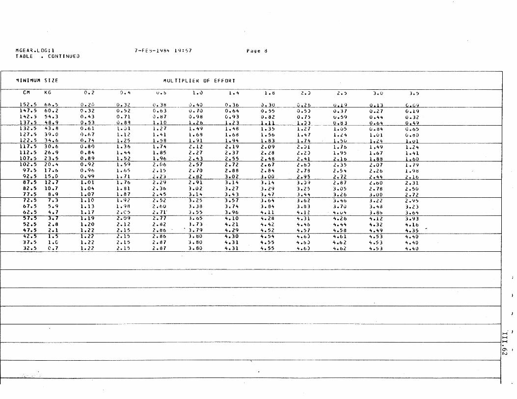
MGEA~.LOG;1 7-FE~-lY84 19:57 TABLE • CONTINUED
:o1INIMUM SIZE MULTIPLIEK OF EFFORT
eM KG 0.2 'J.1t U.b 1.0 1.4
152.5 6b.~ O.2i) 0.32 ().3~ 0.40 0.36 141.5 60.2 0.32 0.52 0.b3 0.70 0.64 142.5 54.3 0.43 0.11 .) .In 0.98 0.93 131.5 48.9 0.53 ().8~ 1.10 1.2 b 1.23 132.5 43.8 0.61 1.01 1.27 1.49 1.48 127.5 39.0 0.67 1.12 1.41 1.68 1.b8 122.5 34.6 0.74 1.25 1.~8 1.91 1.94 117.5 30.6 0.81) 1.36 1.74 2.12 2.19 112.5 26.9 0.84 1.44 1.85 2.27 2.37 107.5 23.5 0.89 1.52 1.96 2.43 2.55 102.5 20.4 0.92 1.59 2.06 2.57 2.72 97.5 17.6 0.96 1.65 2.15 2.70 2.88 92.5 15.0 0.99 1.71 2.2j 2.d2 3.02 87.5 12.7 1.01 1.76 2.2.9 2.91 3.14 82.5 10.7 1.04 1.81 2.36 3.02 3.21 77.5 8.9 1.01 1.81 2.45 3.14 3.43 72.5 7.3 1.10 1.92 2.52 3.25 3.57 67.5 5.9 1.13 1.98 2.60 3.38 3.74 62.5 4.7 1.17 2. C S 2.71' 3.55 3.96 57.5 3.7 1.19 2.09 2.77 3.65 4.10 52.5 2.8 1.20 2.12 2.82 3.73 4.21 1t7.5 2.1 1.22 2.15 2.ti6 . 3.79 4.29 42.5 1.5 1.2? 2.15 2.86 3.tiO 4.30 37.5 1.0 1.22 2.15 2.87 3.80 4.31 32 • .5 e.7 1.22 2.15 2.87 3.80 4.31
,:,,0' .
P ag e d
l.ti 2. ) l.~
0.30 0 1 26 (j~l9
0.55 0.5:> u.37 0.82 0.7) u.59 1.11 1.:>3 0.ti3 1.35 1.27 1.uS 1.56 1.'17 1.llt 1.83 1.74 1.50 2.09 2.:>1 1.7b 2.28 2.2:> 1.95 2.48 2.41. 2.10 2.67 l.b:> 2.35 2.84 2.76 2.5 .. 3.00 2.95 2.72 3.14 3.:n 2.87 3.29 3.25 3.05 3.47 3.44 3.2b 3.64 3.b2 3.46 3.84 3.83 3.71J 4.11 4.1~ it.u" 4.28 it.31 4.26 4.42 4.4b 4.44 4.52 4.57 4.58 4.54 4.b) 4.61 4.55 4.b:> 4.b 2 4.55 4.6) 4.62
3.0
QdJ 0.27 0.4" 0.6'1 (J.84 1.C)! 1.24 1.49 1.67 1.68 2.07 2.26 2.44 2.bO 2.78 3.00 3.22 3.48 3.80 4.12 4.32 4.49 4.53 4.53 4.53
3.~
1.!.G~ 0.19 0.32 0§49 0.b5 (J./jO
1.ul 1.2'1 1.41 1.bO 1.79 1.9~
2.1b 2.31 2.50 2.72 2.YS 3.23 3.b4 3.93 4.1b 4.35 4.40 4.40 1t.40
~
H H H
0\ ) N
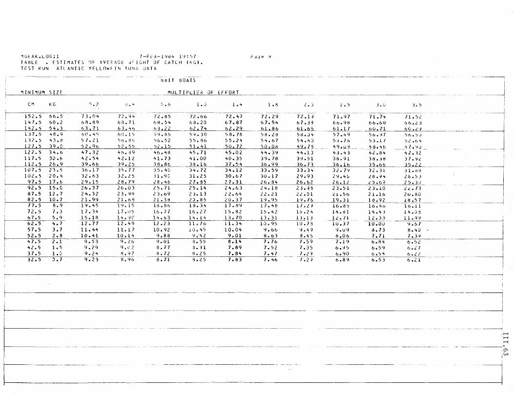
'IGEAR.LOG;l 7-Ff:j-l'164 19: ~J 7 fA~LE . ESTIMATES OF t.VERAGE ... r IGHT OF CA Te H (K. G) •
fEST RUN ATLANTIC Y ELL 0 w FIN T U /\j i\ LlATA
[jAIT BOATS
MINI'1UM SIZE MULTIPLIE~ OF EFFORT
eM KG '1.2 \). t. ~I • 6 1.0 1.4 --~------.--- ---------~
152.5 66.5 73.04 72.94 72.tl5 72.66 72.47 147.5 60.2 68.89 68.71 bB.54 613.20 67.87 142.5 54.3 63.71 63.46 63.22 62.74 62.29 137.5 .,8.9 b (' • 4 <; 60.15 j4.bb 5.'-1. )0 ') B. 78 132.5 43.8 ') 7.21 50.8':> ':>6.~2 55.'>;6 55.24 127.5 39.0 52.96 ':>2.5':> '2.1~ 51.41 50.72 122.5 34.6 47.32 46.d9 46.48 45.71 45.02 117.5 30.6 42.54 42.12 41.73 41. 00 40.35 112.5 26.9 39.66 39.25 38.86 38.16 37.54 107.5 23.5 36.17 3'>.77 35.4(; 3lt.72 34.12 102.5 20.4 32.63 32.25 n .9C 31.25 30.67 97.5 17.6 29.15 28.79 28.46 27.85 27.31 92.5 15.0 26.37 26.03 2~.71 25.14 24.63 87.5 12.7 24.32 23.99 23.69 23. 13 22.64 82.5 10.7 21.99 21.68 21.38 2J.85 20.37 77.5 8.9 19.45 19. 15 18.8 b 18.34 17.89 72.5 7.3 17.34 17. () ~ 16.77. 16.27 15.82 67.5 5.9 15.18 14. '-te 14.63 14. 14 13.70 62.5 4.7 12.77 12.49 12.23 11.76 11.34 57.5 3.7 11.44 11.17 10.92 lO.45 10.04 52.5 2.8 10.41 10.14 9.88 '}.'42 9.01 47.5 2.1 9.53 9.26 9.01 13.55 8.14 42.5 1 .5 9.29 9. C 2 8.77 j.31 7.89 37.5 1. J 9.24 1:3.97 8.72 8.25 7.84 32.5 :).7 9.23 B.9h 8.71 tl.25 7.83
t----------~--~~----------------.-.. -
t' dg e '1
-_._----- ~ ~~---- -- -...
1 • /j 2-. J 2. ')
----- ------- -- --- .------- ----- -~------.
72.29 72.1.J 71.97 67.5lt 61.3~ 66.98 61.86 6Lb~ 61.17 ,8.2ti 5ti.J't 57.49 54.67 54.43 ')j.7t> 50.0d 49.75 49.u'-} 44.39 44.1) 43 ... 3 39.78 3l}.51 38.91 36.99 36.73 36.16 33.59 33034 32.7'-J 30.17 29.93 29.4u 26.84 26.62 26.12 24.18 23.-19 23.51 22.21 22.01 ~1.56
19.95 19.76 19.31 17.48 17. 2 ~ 16.8, 15.42 b.24 14.til 13.31 13.13 12.71 10.95 10.7S 10.37 9.66 . '-J.Fi 9.u9 8.63 a. 4 ~ b.06 7.76 7. 59 7.19 7.52 7.35 6.'J~
7.47 7.2-1 6.90 7.46 ~
-----------------6.89
3.0 J. ')
-------------- ~-
71.7 .. 71. ~L 66.60 b b.2 3 6U.71 btJ.'--i 56.97 56.,)J
~:>3.11 ')'-.64 48. 't b 4 7. 'i',l 42.8 .. 42.32 3tl.JIj 37.'-)£ 35.66 35.22 32.31 Jl.dti 28.94 2b.':d '-5.6-1 25.3':) 23.10 Lt..73 21.16 20.80 18.92 Ui.57 16.40 16.11 14.43 14.U!i 12.33 11.9'J 10.00 '1.61 B.l3 8.40 7.71 7.39 6.84 6.':>2 6.59 b.Z7 b.,:>4 b.F2 6.53 6.21
~~------,
i --~-~---J
I i
~~-~ I
~~- ----~~ -~~ ~ ~~ ~ I
-_._-_._-_ .. __ . __ .- I I
---~------
~-.. --~-------
---- ---------_._---- ---- --
~ I - -- - - .---.-- -_.- I
i I
--- -------->- ~----l I ~
---4 'H H H
0\ <.N
I
-.. -.----~--------.- --- -- -- --.
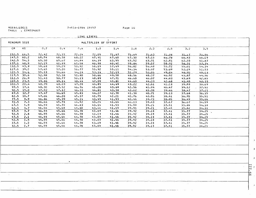
MGEAK.LOGjl 7 -F E d -19 B4 19: 'J 7 TABLE • CO~TINUED
LONG LINERS . MINIMU~ SIZE MULTIPLIER OF EFFORT
eM KG 0.2 0.4 0.6 1.0 1.4
152.5 66.5 72..42 72.33 72.24 72.05 711t:i7 147.5 60.2 68.54 68.38 68.22 67.91 67.60 142.5 54.3 65.30 65.07 64.84 64.39 b3.95 137.5 48.9 !>2.1q 61. tiS 61.58 60.98 60.40 132.5 1,3.8 59.68 59.29 53.92 58.19 57.49 127.5 39.0 57.65 57.20 56.77 55.92 55.11 122.5 34.6 55.18 5't.66 ':>4.14 53.14 52.19 117.5 30.6 52.98 52.38 51.80 50.66 49.58 112.5 26.9 51.43 50.77 50.13 48.89 47.71 107.5 23.5 49.86 49.14 48.44 47.09 45.81 102.5 20 .. 4 48.79 48.03 47.28 45.85 44.49
97.5 17.6 46.30 47.52 46.76 45.28 43.88 92.5 15.0 41.92 47.12 46.33 't4.81 43.36 87.5 12.1 47.41 46.65 45.83 't4.27 42.18 82.5 10.7 47.06 46.20 't5.37 43.15 42.21 11.5 8.9 46.86 45.99 45.l't 't3.49 41.93 12.5 7.3 46.66 45.78 44.92 't3.24 41.64 67.5 5.9 46.59 45.70 44.83 -43.1't 41.53 62.5 4.1 46.56 45.68 4't.BO 't3.11 41.49 57.5 3.1 46.55 45.66 4't.76 't3.09 41. 't6 52.5 2.8 46.55 45.66 44.76 't3.0~ 'tl.46 41.5 2.1 46.55 45.66 4't.78 43.09 41.46 42.5 1.5 -46.55 45.66 4't.18 't3.09 41.46 37.5 1.0 46.55 45.66 44.78 't3.u9 41.46 32.5 0.7 46.55 45.66 4't.7a 43.09 'tl.46
. '!
I
Page 10
1. !:i 2.:) 2.5
71! b9 11.b;) 11.36 67.30 67.15 6b.7fi 63.52 63.31 62.81 59.84 59157 58.92 56.82 56.4~ 55.72 54.34 53.~7 53.09 51.29 50.~~ 49.84 48.56 48.J7 46.92 46.60 46.07 44.83 44.60 44. ;)3 42.68 't3.22 42.61 41.18 42.56 41.9't 40.41 42.02 41. 3~ 39.t)6 41.38 40.71 39.13 40.76 'tV.O~ 38.'tl 'to.1t't 39.73 38.05 'tu.13 39.4) 37.67 39.9Y 39.2, 31.51 39.9, 39.21 31 ... 5 39.92 39.18 31.41 3'1.92 39.1~ 37.41 39.92 39.1~ 37.41 39.92 39.18 37.41 39.92 3'-}.19 37.41 39.92 39.13 37.41
3.0
11.!1 66.43 62.:n 58.31 ~5.01
52.28 48.90 4 'j.B7 43.b9 41.45 39.88 39.12 -38~4~ 37.68 36.90 36.49 36.07 35.8/j 35.82 35.77 35.71 35.77 35.71 35.77 35.77
3.5
lu.2b 66.09 61.ti7 51. lit 54.34 51.53 48.0,3 "t4.9u 42.6S 4v.33 3d.69 37.9J ~7~2.1 36.35 35.51 35.06 3't.59 31t.38 3At.)1 34.25 34.£ 5 34.25 34.25 34.25 34.25
~
I I I
H H H
0\ ~
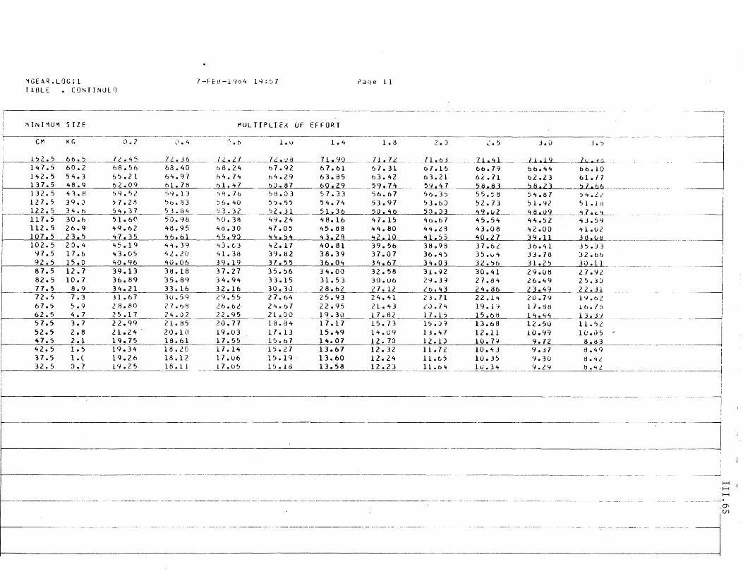
"'GEAR.LOG;l T~BLE • CONTINUEO
:-IINI.'1U'" SIZE
:."l.?
1~2.'J 66.; 72. ~ <)
147.5 60.2 68.56 142.5 54.3 6~.21
137.5 48.9 62.09 132. 5 43.H 59.52 127.5 39.J '>7.28 122.5 34.6 ~4.37
117.5 30.6 51.60 112.5 26.9 49.62 107.5 23.5 47.35 102.5 20.4 45.19 97.5 17.6 43.05 92.5 15.0 40.96 87.5 12.7 39.13 82.5 10.7 36.89 77.5 8.9 34.21 72.5 7.3 31.67 67.5 5.9 28.80 62.5 4.7 25.17 57.5 3.7 22.99 52.5 2.8 21.24 . 47.5 2.1 19.75 42.5 1.5 19.34 37.5 1.( 19.26 32.5 0.7 14.25
7-FEl1-190~ 19:";,7 t>age 11
-- ------- -~- .,~---
~ULTIPLIE~ UF EFFORT
(\.4 '-.• b 1.0 1.4 1.ti 2. ) ~.5 3.0 3. :>
72..36 _72 • .LL.... Jt!..'JO 71.90 __ ll~ __ _ LL~__ _~_ 71.19 _____ ~ 68.40 68.24 67.92 67.61 67.31 07.16 66.79 66.44 66.10 6~.97 n4.74 b4.29 63.85 63.42 63.21 62.71 62.23 61.17 61.78 _ 01.47 b Q • 87 60 • 29 59 • 74 59 • 4 7 55 • 8 3 !> 8 .2 3 __ ~!;L_ 5<).13 5>;.76 ~~.Q3 57.33 56.67 56.35 55.~8 54.ti7 ?4.2~ 'Jt>.83 ')6.40 5j.55 54.74 53.97 53.6) 52.73 51.~2 51.1d 53.84 _2~ 52.31 51.36 5Q.46 50.:23 49.lt2 45.09 .~ 50.98 ">0.31:1 4~.24 48.16 itl.15 40.67 45.54 44.52 43.59 48.95 48.30 47.05 45.88 44.80 44.23 43.08 42.00 ~1.02 46.61 45.9;l 44 • ~_'t3_~2Jl ~ 2 .. 1 Q_ It 1 • , 5 40. 2 7 39 • 11 3 8. (., tj 44.39 it3.b3 42.17 40.81 39.56 38.98 37.62 36.41 3?33 42.20 41. 3H 39.62 38.39 37.07 36.4~ 35.v4 33.75 32.66 40.06 39.19 37.55 36.04 34.67 34.03 32.56 31.2? 30.11 36.18 37.27 35.56 34.00 32.58 31.92 30.41 29.05 27.42 35.89 34.94 33.15 31.53 30.06 29.39 27.84 26.49 25.30 33.16 32.16 30.30 28.62 27.12 26.43 24.86 23.49 22.31 30.59 29.55 27.64 25.93 24.41 2j.71 22.14 20.79 1~.6Z 27.I:JB Z. 6.62, 24.67 22.95 21.43 ~J.74 19.1~ 17.tltl 16.1:>
~J
I -------!
!
-""-"'-'-----'-___ 2_1_._0_0_ 19.30 17.82 17.1:> 15.6tl 14.44 ___ 13.J-i _________ _ Zit.02 22·Q"i I
I 21.H5 20.77 18.84 17.17 15.73 l~.Jj 13.68 12.50 11.~L 20.10 19.03 17.13 15.49 14.09 13.47 12.11 10.99 10.05 18.61 17.55 15.67 14.07 12.7::> 12.1) 10.7=:J 9.72 H.d) 18.20 17.14 15.27 13.67 12.32 11.72 10.43 4.37 0.49 18.12 17.U6 15.19 13.60 12.24 11.65 10.35 9.30 d.4~ 18.11 17.05 1 ~. 1 d 13. 58 12 • 2 3 _____ ~~ 1 U • 3 it 9. 2. ~ e .4 L
. ---"---_."------------------- - ------ "-_. __ ._--.- ------ "-- --.. - .. _-- - - - -----.---- -----------.-------~- -- _._--_. ---------
- - -_._----- -_._-_ .. -
I
I -------1
I I
... ---~
--- - ._---- ----------
I
i
I I
------J H
'H H
,0'\
j~
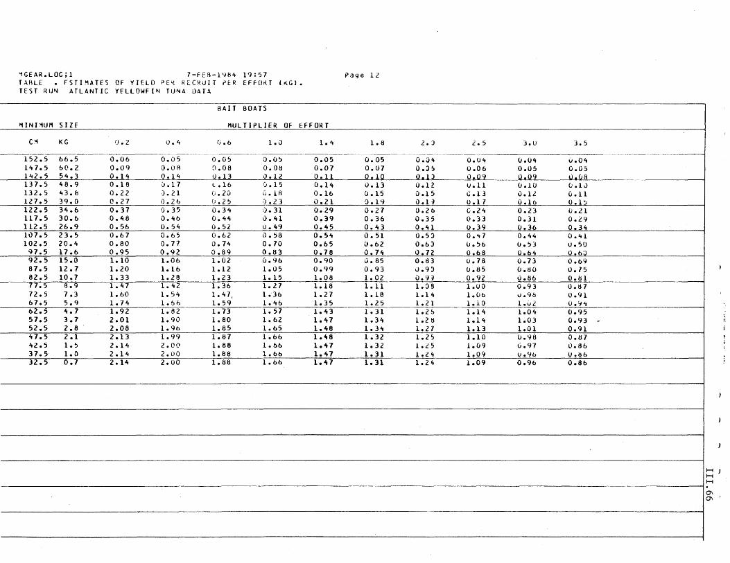
~GEAR.LOG;l 7-FEB-l~B4 19:57 T~ALE • FSTIMATES OF YIELD PE~ RECRUIT ~ER EFFO~T '~G).
TEST RU~ ATLANTIC YfLLOWFIN TUNA OATA
BAIT BOATS
I1INPIUt1 SIlt MU L TIP LIE R OF EFF OR T
C~ KG Q.2 0.4 0.6 1.u 1.4
152.5 66.5 0.06 0.05 0.05 O.O~ 0.05 141.5 60.2 0.09 0.08 0.08 O.OB 0.01 142.5 54.3 0.14 0.14 0.13 0.12 0.11 137.5 48.9 0.18 0.17 l .16 0.15 0.14 132.5 43.8 0.22 ).21 (i.20 0.18 0.16 121.5 )9.0 0.27 0.2'-> (i. 2? 0.23 0.21 122.5 34.6 0.37 1).35 0.34 0.31 0.29 117.5 30.6 0.48 0.46 0.44 0.41 0.39 112.5 26.9 0.56 0.54 0.52 0.49 0.45 101.5 23.5 0.67 0.65 0.62 0.58 0.54 102.5 20.4 0.80 0.77 0.74 0.70 0.65 91.5 17.6 0.95 0.92 0.89 0.83 0.78 92.5 15.0 1.10 1.06 1.02 0.96 0.90 87.5 12.7 1.20 1.16 1.12 1.05 0.99 82.5 10.1 1.33 1.28 1.23 1.15 1.08 77.5 8.9 1.47 1.42 1.36 1.27 1.18 12.5 7.3 1.60 1.54 1.47. 1.36 1.21 61.5 5.9 1.74 1.66 1.59 1.46 1.35 62.5 4.7 1.92 1.82 1.73 1.57 1.43 57.5 3.7 2.01 1.90 1.60 1.62 1.47 52.5 2.8 2.08 1.96 1.65 1.65 1.48 47.5 2.1 2.13 1.99 1.87 1.66 1.48 42.5 l.~ 2.14 2.00 1.86 1.66 1.47 37.5 1.0 2.14 2.00 1.88 1.6b 1.47 32.5 0.1 2.14 2.00 1.86 1.66 1.47
Page 12
1.8 2.) 2. 5
0.05 O.O't 0.04 0.01 O.J~ 0.06 0.10 0.1) 0.09 0.13 0.12 v.l1 (.I .15 0.15 O.ll 0.19 0.1~ 0.11 0.21 0.2 b C.24 0.36 0.35 0.33 0.43 0.41 0.39 0.51 0.5) 0.47 0.62 0.6:> v.56 0.14 0.12 0.68 0.85 0.83 0.18 0.93 "'.9:> 0.85 1.02 O.9J 0.92 1.11 1.::>9 1.UO 1.18 1.11t 1.(Jb 1.25 1.21 1.10 1.31 1.26 1.14 1.34 1. 2 ~ 1.14 1.34 1.27 1.13 1.3l 1.25 1.10 1.32 l.i5 1.09 1.31 1.21t 1.09 1.31 1.21t 1.09
3.u
(J.04 0.05 0.09 (J.I0 O.ll O.lb 0.23 0.31 0.36 0.44 U.53 0.64 0.73 O.liO v.66 0.93 v.98 1.02 1.04 1.03 1.01 0.98 0.97 u.9b 0.96
3.5
v.04 0.05 ~IQ8 0.10 (Jell O.l~
0.21 0.l9 0.34 (J.41 0.50 0.60 0.69 0.75 O.til 0.li7 0.91 V.94 0.95 0.93 0.91 0.87 0.86 U.b6 0.86
~
H H H
0\ 0\
)
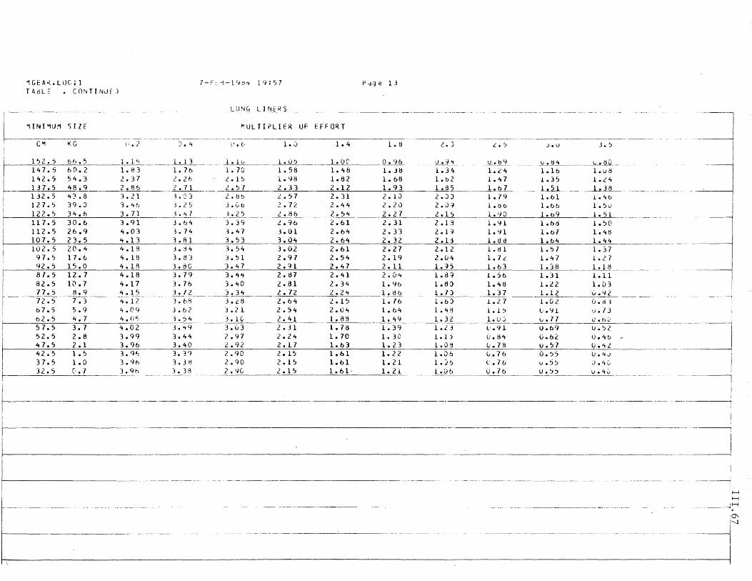
"1 G E A ~ • L I) G ; 1 7-F."..'1-14t1"t 19: l) 7 T A clL c . CO~TINJEJ
LU~G LINERS - - -~------~----+ - -.-~.---------
L-"1INI'1U.'1 SllE KULTIPLIER
------ -- ----- .- --+-------- ----
C'1 KG \i.2 i).4 (I. t. 1.0
152.5 b6.5 1.1-'1 ----~---. --- ~-~-- l.u? 147.') 60.2 1. 83 1. 76 1. 70 1.58 142.5 54.3 2..37 2.26 ~. 1 ~ 1.98 137.5 48.9 2.86 hLL_. __ 2.':;7 2.33 132.5 43.8 3.2.1 Le1j 2.bb ~.57
127.5 39.0 3.46 L 25 3.(,b 2..72 122.5 34.6 3.71 L"t 7 3.25 2.86 117.5 30.6 3.91 3. 64 3.39 L.96 112.5 26.9 4.03 3.74 3.47 3.01 107.5 23.5 4.13 3.81 j. 53 3.04 102.5 20.4 4.18 3. !H 3.54 3.02 97.5 17.6 4.18 3. 8 J 3.51 2.97 92.5 15.0 4.18 3.8C 3.47 2.~1
87.5 12.7 4.18 3.79 3.ltlt 2.ti7 82.5 10.7 4.17 3.76 3.40 2.81 77.5 8.9 4.15 3.72 3.34 2. 72 72.5 7.3 4. 12 3.68 3.~8 2.64 b7.5 5.9 4.09 3. b 2 j • Z 1 2.54 62.5 4.7 4.05 3. 54 3. lei 2.41 5 7.5 3.7 4.02
. --------~-
3.03 2.31 52.5 2.8 3.99 3.44 2.97 2.24 47.5 2.1 3.96 3.40 2.92 2.17 42.5 1.5 3.ql-; 3. 3 9 2.90 2. 15 37.5 1.0 3.9h 3.3tl 2.90 2.1'J 32.5 C· • 7 3.9b '1. 38 2.9C 2.15
---.---~-.-----
--- - -- --- -~- ~---.. ---- .
P dg e 1.3
- -----------
UF E FF OR T
1.4 108 ~. )
1.00 __ h~ 0.~4 _ 1.48 1.j8 1.34 1.82 1.68 1.b2 2.12 1. 93 1.135 2.31 2. 1 J 2.0) 2.44 2.20 2.iB 2.54 2.27 2.1~
2.61 2.31 2.13 2.64 2.33 2.1~
2.64 2.32 2.1l 2.61 2.27 2.12 2.54 2019 2.04 2.47 2. 11 1.~5
2.41 2.0 .. 1. 8~ 2.34 1.9b 1.8C) 2.24 1. ob 1. 7) 2.15 1. 76 l.t» 2.04 1.64 1. 4 9 1.88 1. 49 1.32 1.78 1.39 1. 2.3 1.70 1.30 i.15 1.63 1.23 1.05 1.61 1.22 1.Db 1.61 1.21 1.J~
1.61· 1.21 i.Db
---------- -- ------- -------
-- ----------------- --- -_. -.~-. -- - --
.~ .-.- -------~ ----------------------i. ~ JOV .3. ~
I _.1!...!M _ ~--------~--
I
10.( 4 1.16 1.iJti
~~ 1. 47 1.35 1.24 1.b7 1.51 1. 38 1. 79 l.bl 1.4b l.!jb l.ob 1.50 1. 90 1.b9 ~ 1.91 l.btl 1.50 1.Y1 1.b7 1.48 l.dd 1.64 1.44 ----------.---------- -- - -
1. /j 1 1.57 1.37 1.7L i.47 1. L 7 1.63 1.38 1 • 1 Ii. ___ . ____ . 1.~6 1.31 1.11 1.4tl 1.;U 1.03 1.37 1.12 '0. '-j 2 1.2. l 1.02 G.d] 1.1 ? l.Y1 v.l3 1. u.:J \).77 U.O"I
l'.91 U.69 u.~2
---~ V.li4 O.6~ O.4b u.78 u.'J7 0.42 v.76 O.~5 o."J
i l'.76 v.S~ 0.40 I
0.76 U.~'J v.40 I --~
I
I I
---------------- --~----- --------_._--
H H
___ --------J H
I~
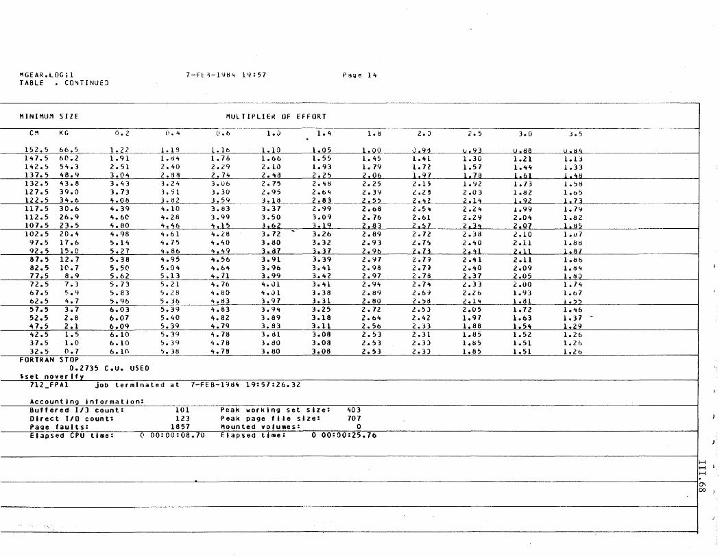
"'GEAR.LOG;l 7-FE~-1484 19:57 P ag e lit TABLE • CONTINUEJ
MIN I MU.'1 S II E MUlTIPLIE~ OF EFFORT
eM KG 0.2 (I. 4 0.6 1.0 1.It 1.8 . 152.5 66.5 1.22 1.lS 1.16 1.10 1~Q5 l~QO 1lt7.5 60.2 1.91 1.d4 1.78 1.66 1.55 1.45 142.5 54.3 2.51 2.40 2.29 2.10 1.93 1. 79 137.5 48.9 3.0lt 2.88 2.74 2.1t3 2.25 Z!Q6 132.5 43.8 3.43 3.24 3.0b 2.75 2.48 2.25 127.5 39.0 3.73 3.51 3.30 2.95 2.64 2.39 122.5 34.6 4.08 3.82 3.59 3.18 2.83 2.55 111.5 30.6 4.39 4.10 3.tU 3.37 2.99 2.68 112.5 26.9 4.60 4.28 3.99 3.50 3.09 2.76 107.5 23.5 4.80 1t.46 4.15 3.62 3.19 2.83 102.5 20.4 4.98 4.61 4.it! 3.72
... 3.26 2.89
97.5 17.6 5.11t 4.75 't.40 3.80 3.32 2.93 92.5 15.0 5.27 4.86 4.49 3.37 3.37 2.96 87.5 12.7 5.38 4.95 4.56 3.91 3.39 2.'17 82.5 1(\.7 5.5(\ 5.04 4.64 3.96 3.lt1 2.98 77.5 8.9 5.62 5.13 4.71 3.99 3.42 2.97 12.5 7.3 5.73 5.21 4.76 4. ,)1 3.41 2.'14 67.5 5.9 5.83 5.28 4.8() 4.,:)1 3.38 2.89 62.5 4.7 5.96 5.36 4.83 3.97 3.31 2.80 57.5 3.7 6.03 5.39 4.63 3.94 3.25 2.12 52.5 2.8 b.07 5.40 4.82 3.89 3.18 2.64 Je 7.5 2.1 6.09 5.39 4.79 3.63 3.11 2.56 42.5 1.5 6.10 5.39 4.78 3.81 3.08 2.53 31.5 1.0 6.10 ,.39 4.76 3.dO 3.08 2.53 32.5 0.7 6.10 5.31:J 4.16 3.60 3.08 2.53
FORTRAN STOP 0.2735 C.U. USEO
'set noverlly 112_FPAl Job terminated at 7-FEB-19dlt 19:57:26.32
Accounting information: Buftered II) count: 101 Peak working set size: 403 Olrect 1/0 count: 123 Peak page f"e size: 707 Page taults: 1851 Mounted volumes: 0 Elapsed CPU time: o 00:00:08.10 Elapsed time: o 00:00:25.76
" ----
2.:> 2.5 3.0
Qdl:i !.i II ~t3 U.de 1.4l. 1.30 1.21 1.72 1.57 1.44 1.97 1.7fj 1.Ql l.l' 1.92 1.13 2.2~ 2.03 1.d2 2.42 2.14 1.92 2.54 2.24 .1..99 2.61 2.29 2.0't 2.,;}7 2.34 2.07 2.72 2.38 2.10 2.7':> 2.40 2.11 ,.73 ,.41 '~ll 2.7j 2.41 2.11 2.7~ 2.40 2.09 2.76 2.31 2.05 2.74 2.33 2.00 2.b~ 2.26 1.93 2.58 2.14 1.81 2.5) 2.05 1.72 2.42 1.97 1.63 2.33 1.88 1.51t 2.31 1.85 1.52 2.3) 1.b5 1.51 2.3) 1.85 1.51
-~--.-------.--.-- _ ... -
j.5
U.!H 1.13 1.33 l.~d 1.58 1.b5 1.73 1.7f.J 1.82 1.d5 1.d7 1.Bd l~~l 1.b6 1.B4 1.8:> 1.14 1.b7 1.j5 1.46 1.37 .. 1.29 1.26 1.26 1.2b
-------_ .. _-
I I I
H H H
I
I
Q\ 00
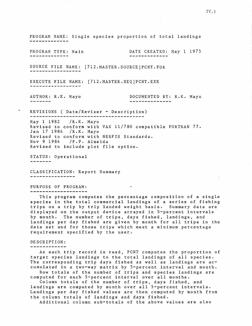
PROGRAM NAME: Single species proportion of total landings
PROGRAM TYPE: Main DATE CREATED: May 1 1975
SOURCE FILE NAME: [712.MASTER.SOURCE]PCNT.FOR
EXECUTE FILE NAME: [712.MASTER.XEQ]PCNT.EXE
AUTHOR: R.K. Mayo DOCUMENTED BY: R.K. Mayo
REVISIONS ( Date/Reviser - Description)
May 1 1982 /R.K. Revised to conform Jan 17 1984 /R.K. Revised to conform Nov 9 1984 IF.P. Revised to include
STATUS: Operational
Mayo with VAX 11/780 compatible FORTRAN 77. Mayo with NERFIS Standards. Almeida plot file option.
CLASSIFICATION: Report Summary
PURPOSE OF PROGRAM:
IV.1
This program computes the percentage composition of a single species in the total commercial landings of a series of fishing trips on a trip by trip landed weight basis. Summary data are displayed on the output device arrayed in 5-percent intervals by month. The number of trips, days fished, landings, and landings per day fished are given by month for all trips in the data set and for those trips which meet a minimum percentage requirement specified by the user.
DESCRIPTION:
As each trip record is read, PCNT computes the proportion of target species landings t~ the total landings of all species. The corresponding trip days fished as well as landings are accumulated in a two-way matrix by 5-percent interval and month.
Row totals of the number of trips and species landings are computed for each 5-percent interval over all months.
Column totals of the number of trips, days fished, and landings are computed by month over all 5-percent intervals. Landings per day fished values are then computed by 'month from the column totals of landings and days fished.
Additional column sub-totals of the above values are also
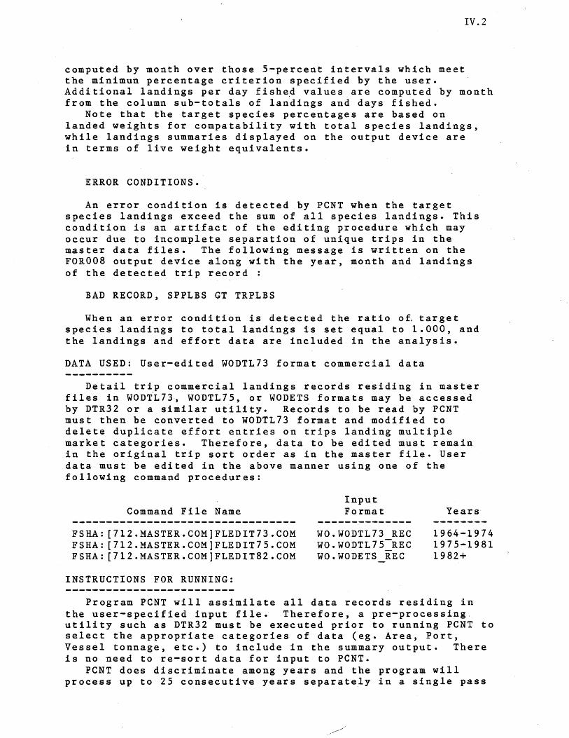
IV.2
computed by month over those 5-percent intervals which meet the minimun percentage criterion specified by the user. Additional landings per day fish~d values are computed by month from the column sub-totals of landings and days fished.
Note that the target species percentages are based on landed weights for compatability with total species landings, while landings summaries displayed on the output device are in terms of live weight equivalents.
ERROR CONDITIONS.
An error condition is detected by PCNT when the target species landings exceed the sum of all species landings. This condition is an artifact of the editing procedure which may occur due to incomplete separation of unique trips in the master data files. The following message is written on the FOR008 output device along with the year, month and landings of the detected trip record :
BAD RECORD, SPPLBS GT TRPLBS
When an error condition is detected the ratio o£ target species landings to total landings is set equal to 1.000, and the landings and effort data are included in the analysis.
DATA USED: User-edited WODTL73 format commercial data
Detail trip commercial landings records residing in master files in WODiL73, WODTL75, or WODETS formats may be accessed by DTR32 or a similar utility. Rec6rds to be read by PCNT must then be converted to WODTL73 format and modified to delete duplicate effort entries on trips landing multiple market categories. Therefore, data to be edited must remain in the original trip sort order as in the master file. User data must be edited in the above manner using one of the following command procedures:
Command File Name
FSHA: [712.MASTER.COM]FLEDIT73.COM FSHA: [712.MASTER.COM]FLEDIT75.COM FSHA: [712.MASTER.COM]FLEDIT82.COM
INSTRUCTIONS FOR RUNNING:
Input Format
WO.WODTL73 REC WO.WODTL75-REC WO.WODETS REC
Years
1964-1974 1975-1981 1982+
Program PCNT will assimilate all data records residing in the user-specified input file. Therefore, a pre-processing, utility such as DTR32 must be executed prior to running PC NT to select the appropriate categories of data (eg. Area, Port, Vessel tonnage, etc.) to include in the summary output. There is no need to re-sort data for input to PCNT.
PCNT does discriminate among years and the program will process up to 25 consecutive years separately in a single pass
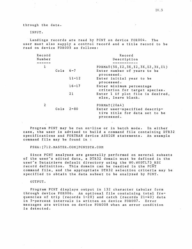
IV.3
through the data.
INPUT.
Landings records are read by PCNT on device FOR004. The user must also supply a control record and a title record to be read on device FOR005 as follows:
Record Number ------
1 Cols 6-7
11-12
16-17
21
2 Cols 2-80
Record Description
FORMAT(5X,I2,3X,I2,3X,I2,3X,I1) Enter number of years to be
processed. Enter initial year to be
processed. Enter minimum percentage criterion for target species.
Enter 1 if plot file is desired, else, leave blank.
FORMAT(20A4) Enter user-specifie~ descriptive title for data set to be processed.
Program PCNT may be run on-line or in batch mode. In either case, the user is advised to build a command file containing DTR32 specifications and FORTRAN device ASSIGN statements. An example command file may be found in :
FSHA: [712.MASTER.COM]PCNTDTR.COM
Since PCNT analyses are generally performed on several subsets of the user's edited data, a DTR32 domain must be defined in the user's Datatrieve default directory using the WO.WODTL73 REC record definition. This domain can be readied in the PCNT command file, and the appropriate DTR32 selection criteria may be specified to obtain the data subset to be analyzed by PCNT.
OUTPUT.
Program PCNT displays output in 132 character tabular form through device FOR006. An optional file containing total frequencies of trip (records 1-20) and catch (records 21-40) data in 5-percent intervals is written on device FOR007. Error messages are written on device FOR008 when an error condition is detected.
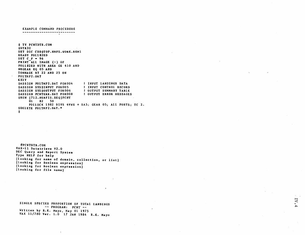
EXAMPLE COMMAND PROCEDURE
$ TY PCNTDTR.COM $DTR32 SET DIC CDD$TOP.NMFS.WORK.RKMI READY POl182ED SET C P - 96 PRINT-All IMAGE (-) OF POl182ED WITH AREA GE 410 AND NEGEAR EQ 05 AND TONNAGE BT 22 AND 25 ON POITMP2.DAT EXIT $ASSIGN POITMP2.DAT FOR004 $ASSIGN SYS$INPUT FOROOS $ASSIGN SYS$OUTPUT FOR006 $ASSIGN PCNTERR.DAT FOR008 $RUN [712.NERFIS.XEQ]PCNT
01 82 50
INPUT LANDINGS DATA INPUT CONTROL RECORD OUTPUT SUMMARY TABLE OUTPUT ERROR MESSAGES
POllOCK 1982 DIVS 4VWX + SA5; GEAR 05; All PORTS; TC 2. $DEIETE POITMP2.DAT.* $
@PCNTDTR.COH VAX-II Datatrieve V2.0 DEC Query and Report System Type HELP for help [looking for name of domain-, collection, or list] [looking for Boolean expression] [looking for Boolean expression] [looking for file name]
SINGLE SPECIES PROPORTION OF TOTAL lANDINGS -- PROGRAM: PCNT>--
Written by R.K. Mayo, May 01 1975 VAX 11/780 Ver. 1.0 17 JAN 1984 R.K. Mayo
H <: .j:::..
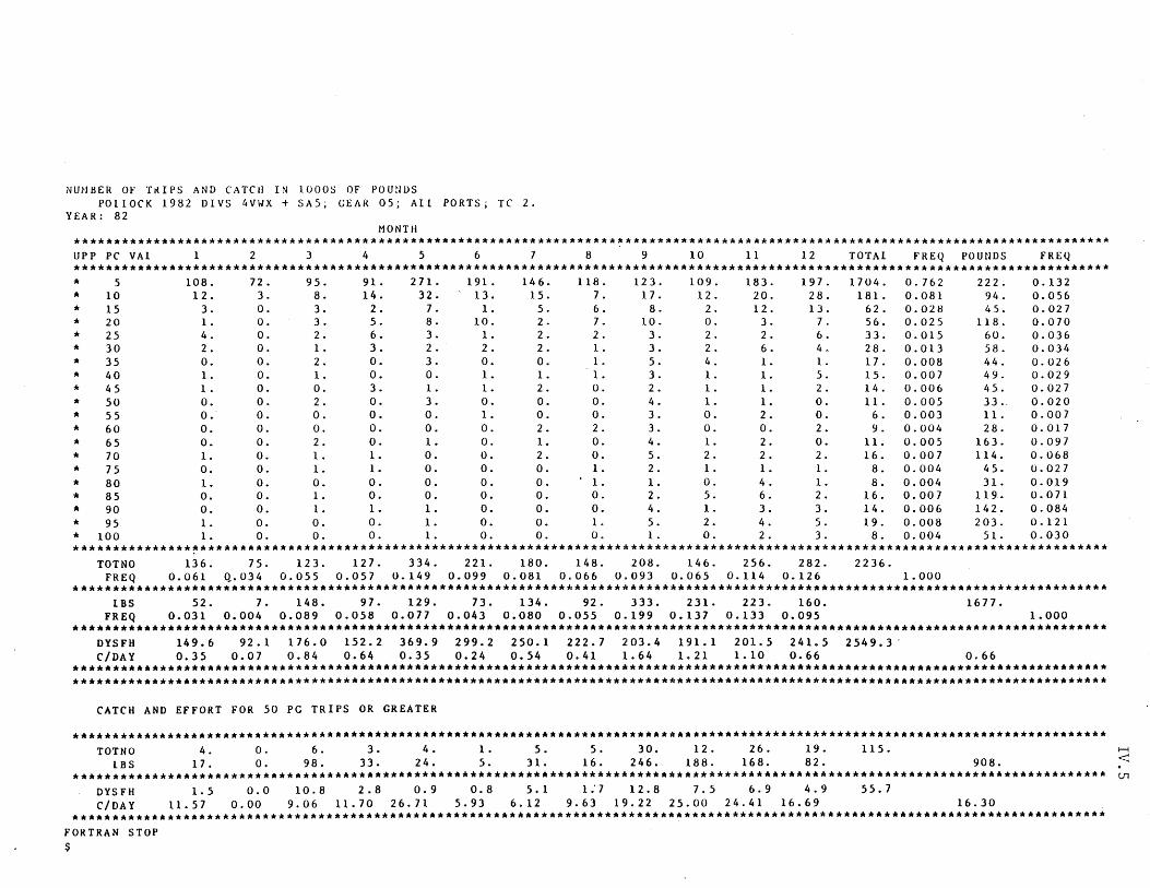
NUMBER OF TKIPS AND CATCH IN 1000S OF POUNUS POLLOCK 1982 DIVS 4VWX + SA5; GEAR OS; AIL PORTS; TC 2.
YEAR: 82 MONTH
********************************************************************************************************************************** UPP PC VAL 2 3 4 5 6 7 8 9 10 11 12 TOTAL FREQ POUNDS FREQ *******************************************.* ••• ************.***************************** ••• *****************.**.**.***** •• ** •• ** * • * * * * * * * • * * * * * * * * • *
5 10 15 20 25 30 35 40 45 50 55 60 65 70 75 80 85 90 95
100
108. 12.
3. 1. 4. 2. O. 1. 1-O. O. o. O. 1. O. 1. O. O. 1. 1.
72. 3. O. O. o. o. o. o. o. o. o. o. o. o. o. o. o. o. o. o.
95. 8. 3. 3. 2. 1. 2. 1. O. 2. O. O. 2. 1. 1-O. 1-1-O. O.
91. 14.
2. 5. 6. 3. O. O. 3. O. o. o. O. 1-1-O. O. 1-O. O.
271-32.
1-8. 3. 2. 3. O. 1. 3. O. O. 1. O. O. o. O. l. 1-1.
191. 13.
1. 10.
1. 2. O. 1. 1. O. 1. O. O. O. O. O. O. O. O. O.
146. 15.
5. 2. 2. 2. O. 1. 2. O. O. 2. 1. 2. O. O. o. O. O. o.
118. 7. 6. 7. 2. 1. l. 1. O. O. O. 2. O. O. 1.
. 1. O. O. 1. O.
123. 17.
8. 10.
3. 3. 5. 3. 2. 4. 3. 3. 4. 5. 2. 1. 2. 4. 5. 1.
109. 12.
2. O. 2. 2. 4. 1. 1. 1. O. O. 1. 2. 1. O. 5. 1. 2. O.
183. 20. 12.
3. 2. 6. 1. 1. 1. 1. 2. O. 2. 2. 1. 4. 6. 3. 4. 2.
197. 28. 13.
7. 6. 4. 1. 5. 2. O. O. 2. O. 2. 1. 1. 2. 3. 5. 3.
1704. 181.
62. 56. 33. 28. 17. 15. 14. 11.
6. 9.
11. 16.
8. 8.
16. 14. 19.
8.
0.762 0.081 0.028 0.025 0.015 0.013 0.008 0.007 0.006 0.005 0.003 0.004 0.005 0.007 0.004 0.004 0.007 0.006 0.008 0.004
222. 94. 45.
118. 60. 58. 44. 49. 45. 33 .. 11. 28.
163. 114.
45. 31.
119. 142. 203.
51.
0.132 0.056 0.027 0.070 0.036 0.034 0.026 0.029 0.027 0.020 0.007 0.017 0.097 0.068 0.027 0.019 0.071 0.084 0.121 0.030
.*****.** ••• * •• ~****.**.*********.************************************************************************************.*****.***** TOTNO 136. 75. 123. 127. 334. 221. 180. 148. 208. 146. 256. 282. 2236.
FREQ 0.061 Q.034 0.055 0.057 0.149 0.099 0.081 0.066 0.093 0.065 0.114 0.126 1.000 **********.*********.****.*******.****.*** •••••• **.*********.* •• **.******************************.*******.*********************.**
IBS 52. 7. 148. 97. 129. 73. 134. 92. 333. 231. 223. 160. 1677. FREQ 0.031 0.004 0.089 0.058 0.077 0.043 0.080 0.055 0.199 0.137 0.133 0.095 1.000
********.*********.**********************************.**.**** •• * •••• ****.* •• ****.**.***************** •• ** •• * •••••••••••• **** •• * ••• DYSFH 149.6 92.1 176.0 152.2 369.9 299.2 250.1 222.7 203.4 191.1 201.5 241.5 2549.3' CIDAY 0.35 0.07 0.84 0.64 0.35 0.24 0.54 0.41 1.64 1.21 1.10 0.66 0.66
** ••••••••• *.* •• **.***.*** •• *.******* ••• **.** •• ****** ••••• ** •••• ** •• *.**.************** ••••• *.** ••• ********* •• ****.***.*.******.** *** •• *******************.**.**.******.****.* •• *****.*************************.***** •• *.* •• ******************.********.***********.
CATCH AND EFFORT FOR 50 PC TRIPS OR GREATER
* •• * ••• * •• ****.*.********************* •• * •••• *.****.** ••• ********************.**** •• ***.****.**.*.**.*.**.************************ TOTNO 4. O. 6. 3. 4. 1. 5. 5. 30. 12. 26. 19. 115.
IBS 17. O. 98. 33. 24. 5. 31. 16. 246. 188. 168. 82. 908. ***.*****.**.**.**.**********************************.*****.** •••••• *.* ••• ***.* •••• *.** ••••• *.** ••• * •• *.***.** •• ***.****.**.****.*
DYSFH 1.5 0.0 10.8 2.8 0.9 0.8 5.1 1:7 12.8 7.5 6.9 4.9 55.7 C/DAY 11.57 0.00 9.06 11.70 26.71 5.93 6.12 9.63 19.22 25.00 24.41 16.69 16.30
*.********.******************.* •• *.******.***.**********.*************************.**************.*.*.******.** ••• *.**.**.******.* FORTRAN STOP $
H
-< Ul
PROGRAM NAME: Relative Fishing Power Estimator
PROGRAM TYPE: Main DATE CREATED: Jan 1 1971
SOURCE FILK NAME: FSHA: [7l2.MASTER.SOURCE]FPOW.FOR
EXECUTE FILE NAME: FSHA: [7l2.MASTER.XEQ]FPOW.EXE
AUTHOR: C. Berude and N.J. Abramson
DOCUMENTED BY: S.A. Murawski
REVISIONS ( Date/Reviser - Description)
May 30 1984 /S.A. Murawski Revised to conform with VAX 11/780 FORTRAN77
S TAT US: 0 p e, rat ion a 1
CLASSIFICATION: Analytical Model
PURPOSE OF PROGRAM:
Estimates of relative fishing power and relative population density are obtained utilizing analysis of variance.
DESCRIPTION:
Analysis of variance as a method for estimating relative fishing power was suggested by Robson (1966). FPOW utilizes this method in estimating relative fishing power, relative population density, approximate confidence intervals and corrections for bias in the parameter estimates.
A simple development of the method may be outlined as follows. The basic model assumed is:
C(ij) = q(i)f(ij)P(j)E(ij) ( 1 )
IV.6
where: C(ij) = the catch of the ith fishing treatment in the jth area-date stratum,
q(i) = the catchability coefficient of the ith treatment, f(ij) = the amount of fishing effort expended by the ith
treatment in the jth area-date, p(j) = the average p~pulation size in the jth area-date,
E(ij) = a log-normally distributed random variable.
The i treatments may be different vessels, horsepower, ves,sel types or their attributes (e. g. length, horsepower, tonnage), gear types or characteristics (e.g. gill nets, purse seines, soak times, trawl footrope lengths), or any other way of designating
IV.7
classes within the fishing fleet. It is assumed that (1) effort is measured such that within each treatment q(i) is constant, (2) the units of effort operate independently, and (3) there is no interaction between the treatments and area-dates.
Dividing through equation (1) by effort and taking natural logarithms we have:
1n(C(ij) / f(ij» 1nq(i) + 1nP(j) + 1nE(ij)
which may be written as:
Y(ij) = a1pha(i) + beta(j) + E' (ij) (2)
Equation (2) may be recognized as a linear two-factor analysis of variance model where the E'(ij) are assumed to be approximately N(O,var). If the a1pha(i) and beta(j) were estimable one would have estimates of the logarithms of the catchabi1ity coefficients and population densities directly. Since the design matrix is singular and therefore no solution exists, one must re-parameterize the model and obtain estimates of relative catchabi1ity, called relative fishing power, rho(i); and relative population density, D(j), where:
rho(i)
D (j )
q(i) / q(s)
p(j) / p(s)
and s designates the treatment and area-date selected to be the standard. Standardized fishing effort is obtained by:
such that:
f(sj) = ~ rho(i)f(ij) 1
C(j) = q(s)f(sj)P(j),
the desired relation with a single catchabi1ity coefficient. Detailed descriptions of the equations on which the method is based are given in the FAO manual on computer programs for fish stock assessment.
DATA USED: Catch/effort data by vessel and area-date
INSTRUCTIONS FOR RUNNING:
(1) a) The treatments (called Boats by FPOW) may be given any numeric designation. However, FPOW will always select the smallest numeric value as standard.
b) The AREA-DATES also may be given any numeric designation. FPOW will select as the standard that AREA-DATE with the lowest numeri"c value in which the standard BOAT first occurs.
c) Since the variances of the estimates include the variance of the standard, that BOAT which appears in the most AREA-DATES should be selected as the standard and be given the lowest numeric designation in order to
rV.8
obtain the smallest variances of estimates.
(2) Each BOAT need not appear in every AREA-DATE and zero catch observations may be entered.
(3) CATCH PER UNIT EFFORT values are the data entered into the program, but FPOW calls them CATCH.
(4) FPOW computes the expected catch per unit effort for the standard BOAT in the standard AREA-BOAT. Therefore, standardized catch per unit effort may be obtained by multiplying~the expected value times each of the estimates of relative density. However, unless the amount of effort for each BOAT-type is relatively uniform within each AREADATE, this procedure is not recommended. The major drawback to this program is that the estimates are not weighted by the amount of effort. With greater effort the variance of the observation is likely to be smaller. One can do nothing about the estimates of relative fishing power, but better estimates of standardized catch per unit of effort may be obtained in the long manner of mUltiplying each BOAT's effort by its relative fishing power estimate, summing up the standardized effort and dividing it into the catch.
(5) Another drawback is that an analysis of variance is not performed and there is no provision for testing for interaction. Also one cannot use alternative ANOVA models such as nested designs which often may be the appropriate ones. BMDP or SPSS ANOVA programs may be used prior to FPOW to examine interaction or alternative designs.
(6 ) Input data can be from a file (recommended) entered interactivly. Input data files are device FOR005. Output is to device FOR006. records are included in the input file:
or can be assigned to
The following
Record Number -------
1 Co Is. 1-80 2 Co Is. 1-80
3 Co Is. 1-3
5-7
4 Co Is. 1-80 5 Da ta records,
agree wi th 4 Field 1 Field 2 Field 3
6
Record Descrip tion
Title record, appears on each table. Sub-title record, appears only above
summa ry. YES for covariance matrix, NO otherwise,
lef t- j us tif ied, YES if want biased estimates, NO other-wise, left-justified,
Data format (variable 'F' format), as many as necessary, (format must above) An alpha(i), where i=1,2, •.. k BOATS, A beta(j), where j=1,2, •.• n AREA-DATES, A catch per unit effort. A blank card to end run.
To run the program, submit the following commands:
REFERENCES:
$ASSIGN [directory]datafile.DAT FOR005 $ASSIGN SYS$OUTPUT FOR006 $RUN FSHA: [7l2.MASTER.XEQ]FPOW
IV.9
Robson, D.S. 1966. Estimation of the relative fishing power of individual ships. ICNAF Res. Bull. 3:5-14.
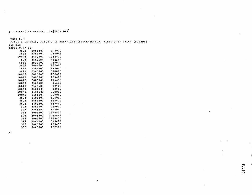
$ T FSHA: [712.MASTER.DATA)FPOW.DAT
TEST RUN FIELD 1 IS BOAT, FIELD 2 IS AREA-DATE (BLOCK-YR-MO), FIELD 3 IS CATCH (POUNDS)
YES YES (2FI0.0,F7.0)
3621 2006501 945000 3621 2566507 216045
10043 2406501 1332000 592 2566507 843600
3621 2006501 720000 3621 2006501 837000 3621 2566507 197000 3621 2566507 320000
10043 2006501 100000 10043 2006501 135670 10043 2006501 125690 10043 2566507 14670 10043 2566507 32900 10043 2566507 23900 10043 2466507 360000 10043 2466507 329000
3621 2406501 100000 3621 2406501 128970 3621 2406501 115900
592 2566507 789000 592 2566507 657000 592 2006501 1298000 592 2006501 1568999 592 2006501 1789600 592 2466507 345678 592 2466507 283456 592 2466507 187900
$
H
< ~
o
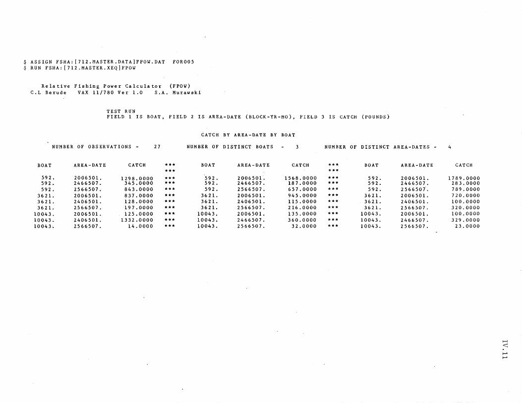
$ ASSIGN FSHA: [712.MASTER.DATA)FPOW.DAT FOR005 $ RUN FSHA: [712.MASTER.XEQ]FPOW
Relative Fishing Power Calculator (FPOW) C.L Berude VAX 11/780 Ver 1.0 S.A. Murawski
TEST RUN FIELD 1 IS BOAT, FIELD 2 IS AREA-DATE (BLOCK-YR-MO), FIELD 3 IS CATCH (POUNDS)
CATCH BY AREA-DATE BY BOAT
NUMBER OF OBSERVATIONS - 27 NUMBER OF DISTINCT BOATS 3 NUMBER OF DISTINCT AREA-DATES
BOAT AREA-DATE CATCH *** BOAT AREA-DATE CATCH *** BOAT AREA-DATE *** ***
592. 2006501. 1298.0000 *** '592. 2006501'. 1568.0000 *** 592. 2006501. 592. 2466507. 345.0000 *** 592. 2466507. 187.0000 *** 592. 2466507. 592. 2566507. 843.0000 *** 592. 2566507. 657.0000 *** 592. 256650i.
362l. 2006501. 837.0000 *** 362l. 200650l. 945.0000 *** 362l. 2006501. 362l. 2406501. 128.0000 *** 3621. 2406501. 115.0000 *** 3621. 2406501. 3621. 2566507. 197.0000 *** 362l. 2566507. 216.0000 *** 362l. 2566507.
10043. 2006501. 125.0000 *** 10043. 2006501. 135.0000 *** 10043. 2006501. 10043. 2406501. 1332.0000 *** 10043. 2466507. 360.0000 *** 10043. 2466507. 10043. 2566507. 14.0000 *** 10043. 2566507. 32.0000 *** 10043. 2566507.
- 4
CATCH
1789.0000 283.0000 789.0000 720.0000 100.0000 320.0000 100.0000 329.0000
23.0000
H
< f-..I. f-..I.
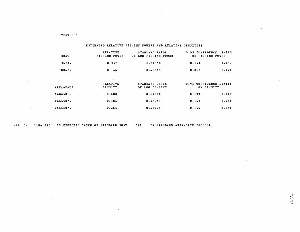
*** C= 1184.216
TEST RUN
ESTIMATED RELATIVE FISHING POWERS AND RELATIVE DENSITIES
BOAT
3621.
10043.
AREA-DATE
2406501.
2466507.
2566507.
RELATIVE FISHING POWER
0.352
0.146
RELATIVE DENSITY
0.400
0.386
0.264
IS EXPECTED CATCH OF STANDARD BOAT
STANDARD ERROR OF LOG FISHING POWER
0.54358
0.48568
STANDARD ERROR OF LOG DENSITY
0.64394
0.58959
0.47795
0.95 CONFIDENCE LIMITS ON FISHING POWER
0.141 1. 187
0.063 0.426
0.95 CONFIDENCE LIMITS ON DENSITY
0.139 1. 740
0.145 1.461
0.116 0.756
592. IN STANDARD AREA-DATE 2006501 ••
H <: I-l N
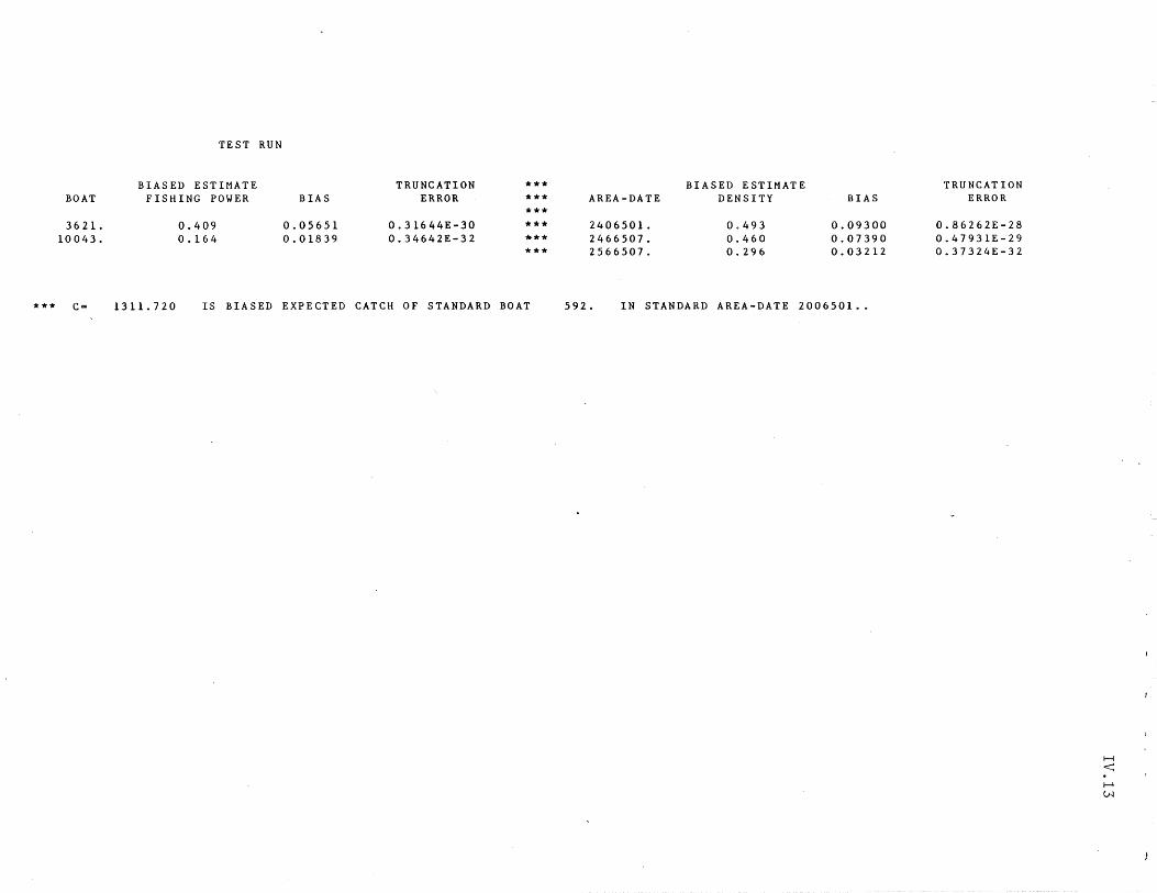
BOAT
3621. 10043.
*** C=
TEST RUN
BIASED ESTIMATE FISHING POWER
0.409 0.164
BIAS
0.05651 0.01839
TRUNCATION *** ERROR ***
*** 0.31644E-30 *** 0.34642E-32 ***
***
1311. 720 IS BIASED EXPECTED CATCH OF STANDARD BOAT
BIASED ESTIMATE AREA-DATE DENSITY BIAS
2406501. 0.493 0.09300 2466507. 0.460 0.07390 2566507. 0.296 0.03212
592. IN STANDARD AREA-DATE 2006501 ..
TRUNCATION ERROR
0.86262E-28 0.47931E-29 0.37324E-32
H
< ........ V-l
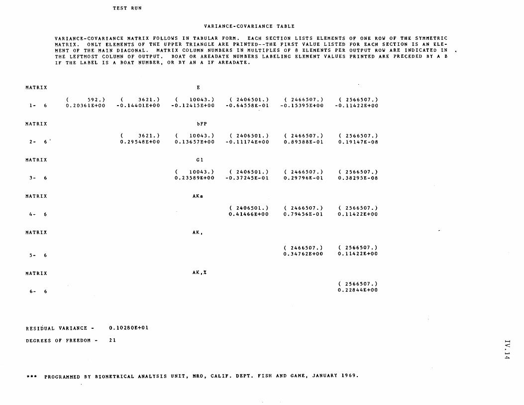
MATRIX
1- 6
MATRIX
2- 6 >
MATRIX
3- 6
MATRIX
4- 6
MATRIX
5- 6
MATRIX
6- 6
TEST RUN
VARIANCE-COVARIANCE TABLE
VARIANCE-COVARIANCE MATRIX FOLLOWS IN TABULAR FORM. EACH SECTION LISTS ELEMENTS OF ONE ROW OF THE SYMMETRIC MATRIX. ONLY ELEMENTS OF THE UPPER TRIANGLE ARE PRINTED--THE FIRST VALUE LISTED FOR EACH SECTION IS AN ELEMENT OF THE MAIN DIAGONAL. MATRIX COLUMN NUMBERS IN MULTIPLES OF 8 ELEMENTS PER OUTPUT ROW ARE INDICATED IN THE LEFTMOST COLUMN OF OUTPUT. BOAT OR AREADATE NUMBERS LABELING ELEMENT VALUES PRINTED ARE PRECEDED BY A B IF THE LABEL IS A BOAT NUMBER, OR BY AN A IF AREADATE.
E
( 592.) ( 3621. ) ( 10043.) ( 2406501.) ( 2466507.) ( 2566507.) 0.20361E+00 -0.14401E+00 -0.12415E+00 -0.64558E-01 -0.15395E+00 -0.11422E+00
bFP
3621. ) 10043.) ( 2406501.) ( 2466507.) ( 2566507.) 0.29548E+00 0.13657E+00 -0.11174E+00 0.89388E-01 0.19147E-08
G1
( 10043.) ( 2406501.) ( 2466507.) ( 2566507.) 0.23589E+00 -0.37245E-01 0.29796E-01 0.38295E-08
AKa
( 2406501.) ( 2466507.) ( 2566507.) 0.41466E+00 0.79456E-01 0.11422E+00
AK,
( 2466507.) ( 2566507.) 0.34762E+00 0.11422E+00
AK,%
( 2566507.) 0.22844E+00
RESIDUAL VARIANCE - 0.10280E+01
DEGREES OF FREEDOM - 21
*** PROGRAMMED BY BIOMETRICAL ANALYSIS UNIT, MRO, CALIF. DEPT. FISH AND GAME, JANUARY 1969.
H
< ~
.,f:::>.
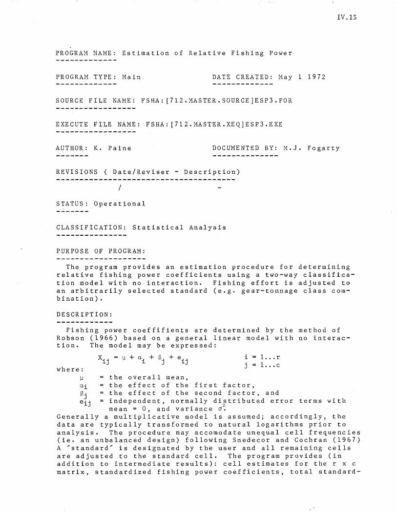
IV.1S
PROGRAM NAME: Estimation of Relative Fishing Power
PROGRAM TYPE: Main DATE CREATED: May 1 1972
SOURCE FILE NAME: FSHA: [712.MASTER.SOURCE]ESP3.FOR
EXECUTE FILE NAME: FSHA: [712.MASTER.XEQ]ESP3.EXE
AUTHOR: K. Paine DOCUMENTED BY: M.J. Fogarty
REVISIONS ( Date/Reviser - Description)
/
STATUS: Operational
CLASSIFICATION: Statistical Analysis
PURPOSE OF PROGRAM:
The program provides an estimation procedure for determining relative fishing power coefficients using a two-way classification model with no interaction. Fishing effort is adjusted to an arbitrarily selected standard (e.g. gear-tonnage class combination).
DESCRIPTION:
Fishing power coeffifients are determined by the method of Robson (1966) based on a general linear model with no interaction. The model may be expressed:
where: 11
X •• = 11 + a. + 13. + e .. 1J 1 J 1J
the overall mean,
i j
the effect of the first factor,
1 .•• r 1 ... c
the effect of the second factor, and independent, normally distributed error terms with mean = 0, and variance cr~
Generally a multiplicative model is assumed; accordingly, the data are typically transformed to natural logarithms prior to analysis. The procedure may accomodate unequal cell frequencies (ie. an unbalanced design) following Snedecor and Cochran (1967) A 'standard' is designated by the user and all remaining cells are adjusted to the standard cell. The program provides (in addition to intermediate results): cell estimates for the r x c matrix, standardized fishing power coefficients, total standard-
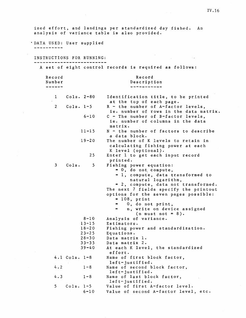
IV.16
ized effort, and landings per standardized day fished. An analysis of variance table is also provided.
"DATA USED: User supplied
INSTRUCTIONS FOR RUNNING:
A set of eight control records is required as follows:
Record Number ------
1 Cols. 2-80
2 Cols. 1-5
6-10
11-15
19-20
25
3 Cols. 5
8-10 13-15 18-20 23-25 28-30 33-35 39-40
4.1 Cols. 1-8
4.2 1-8
4.3 1-8
5 Cols. 1-5 6-10
Record Description
Identification title, to be printed at the top of each page.
R - the number of A-factor levels, ie. number of rows in the data matrix.
C - The number of B-factor levels, ie. number of columns in the data matrix.
N - the number of factors to describe a data block.
The number of K levels to retain in calculating fishing power at each K level (optional).
Enter 1 to get each input record printed.
Fishing power equation: = 0, do not: compute, = 1, compute, data transformed to
natural logarithm, = 2, compute, data not transformed.
The next 7 fields specify the printout options for the seven pages possible:
= 108, print 0, do not print,
= n, write on device assigned (n must not = 8).
Analysis of variance. Estimators. Fishing power and standardization. Equations. Data matrix 1. Data matrix 2. At each K level, the standardized effort.
Name of first block factor, left-justified.
Name of second block factor, left-justified.
Name of last block factor, left-justified.
Value of first A-factor level. Value of second A-factor level, etc.

6 Cols. 1-5 6-10
IV.17
for all levels, 12 to a record. Continue on more records if necessary. After the last A-factor level, in the next 5 column field, specify the value of the A-factor of the standard cell in fishing power estimates.
Value of first B-factor level. Value of second B-factor level, etc. as
above for A-factor levels. After last B-factor level, in the next 5 column field, specify the the value of the B-factor of the standard cell in fishing power estimates.
6A Cols. 1-60 Values of K. Data saved at each K level in recalculating fishing power. (5 column fields, 12/record)
7
8
Col. 5 Compress matrix option. If = 0, the matrix is not compressed and empty columns will cause the matrix to be singular. If = 1, empty rows and columns are excluded from calculations.
10 0, no action. = 1, if there is any row or column with
only 1 observation, that observation will be excluded from the calculations, and the row or column excluded.
15 n 0, no action.
20
n > 0, any data block with less than n observations will not be calculated.
n 0, no action. n > 0, any data block with observations
for less than n B-Ievels will no be calculated.
Cols. 2 1, y 2, y 3, y 4, y
In(tons/day fished).
4
5-80
n = 0, n > 0,
tons/day fished. In(catch); days fished catch; days fished = 1.
1 observation per record. the number of observations specified ,per data record.
1 •
Data record format, for the following list of variables, in order: 1) A-factor level. 2) B-factor level. 2a) K-Ievel (indicate dummy if not
used) . 3) number of days fished (indicate
dummy if not used). 4) catch. 5) block factors, in same order as type
4 records. 6) number of observations (even if col.
4 = 0, provision must be made. In-
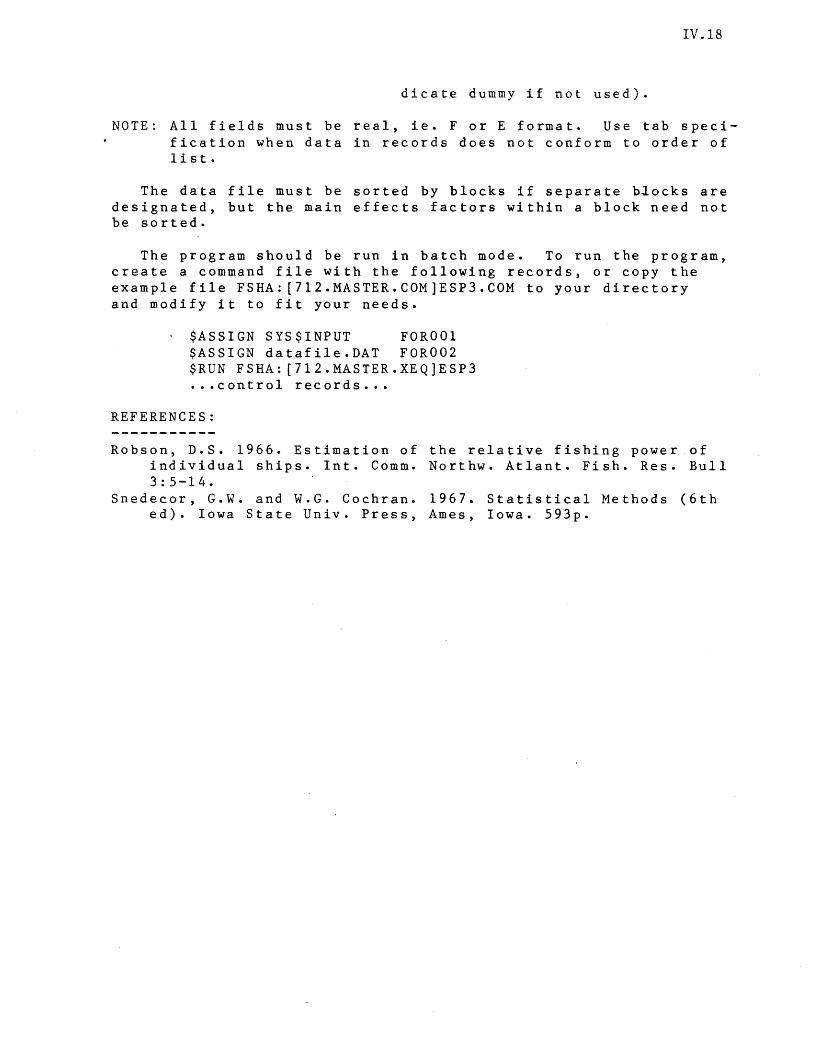
IV.18
dicate dummy if not used).
NOTE: All fields must be real, ie. F or E format. Use tab specification when data in records does not conform to order of list.
The data file must be sorted by blocks if separate blocks are designated, but the main effects factors within a block need not be sorted.
The program should be run in batch mode. To run the program, create a command file with the following records, or copy the example file FSHA:[712.MASTER.COM]ESP3.COM to your directory and modify it to fit your needs.
$ASSIGN SYS$INPUT FOR001 $ASSIGN datafile.DAT FOR002 $RUN FSHA:[712.MASTER.XEQ]ESP3 ••• control records .••
REFERENCES:
Robson, D.S. 1966. Estimation of the relative fishing power of individual ships. Int. Comma Northw. Atlant. Fish. Res. Bull 3:5-14.
Snedecor, G.W. and W.G. Cochran. 1967. Statistical Methods (6th ed). Iowa State Univ. Press, Ames, Iowa. 593p.
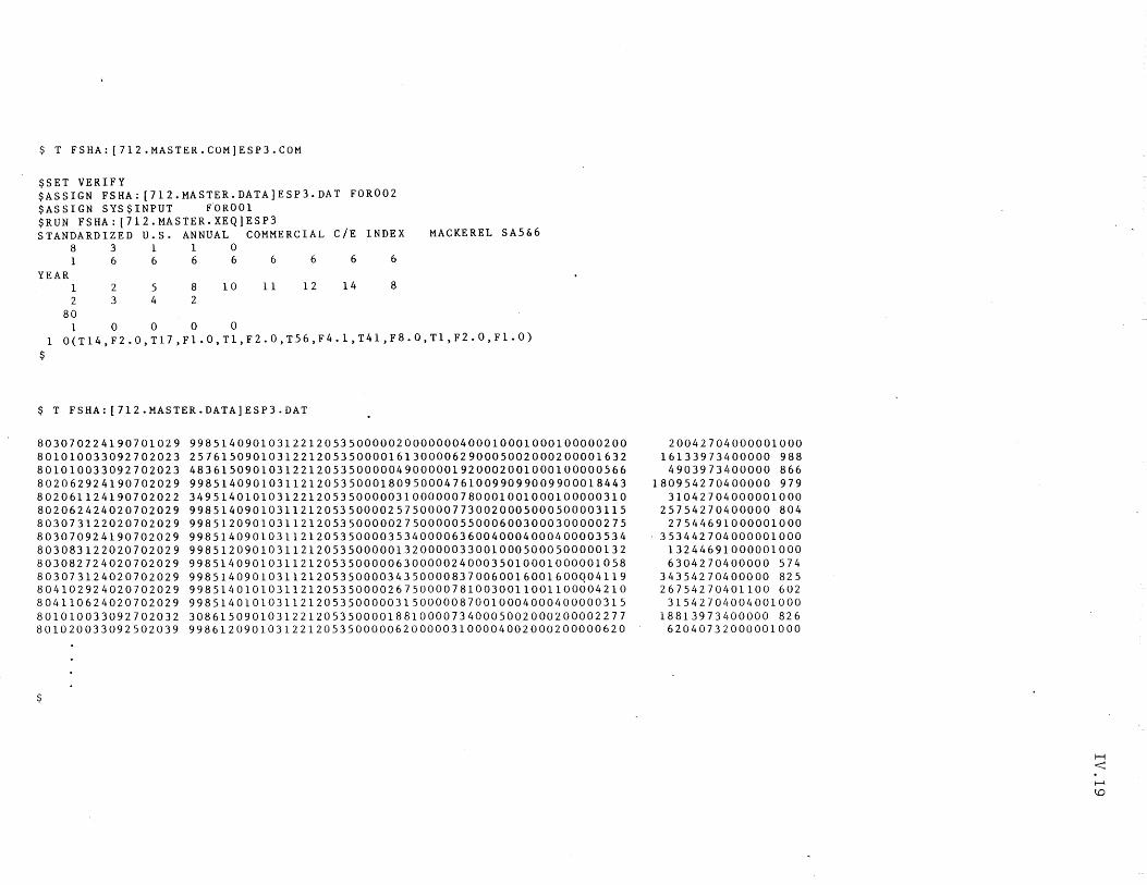
$ T FSHA:[712.MASTER.COM]ESP3.COM
$SET VERIFY $ASSIGN FSHA: [712.MASTER.DATA]ESP3.DAT FOR002 $ASSIGN SYS$INPUT ~OR001 $RUN FSHA: [712.MASTER.XEQ]ESP3 STANDARDIZED U.S. ANNUAL COMMERCIAL C/E INDEX MACKEREL SA5&6
8 3 110 1 6 6 666 6 6 6
YEAR 1 2 5 8 10 11 12 14 8 2 342
80 1 0 0 0 0
1 0(T14,F2.0,T17,F1.0,T1,F2.0,T56,F4.1,T41,F8.0,T1,F2.0,F1.0)
$
$ T FSHA: [712.MASTER.DATA]ESP3.DAT
803070224190701029 9985140901031221205350000020000000400010001000100000200 801010033092702023 2576150901031221205350000161300006290005002000200001632 801010033092702023 4836150901031221205350000049000001920002001000100000566 802062924190702029 9985140901031121205350001809500047610099099009900018443 802061124190702022 3495140101031221205350000031000000780001001000100000310 802062424020702029 9985140901031121205350000257500007730020005000500003115 803073122020702029 9985120901031121205350000027500000550006003000300000275 803070924190702029 9985140901031121205350000353400006360040004000400003534 803083122020702029 9985120901031121205350000013200000330010005000500000132 803082724020702029 9985140901031121205350000063000002400035010001000001058 803073124020702029 9985140901031121205350000343500008370060016001600004119 804102924020702029 9985140101031121205350000267500007810030011001100004210 804110624020702029 9985140101031121205350000031500000870010004000400000315 801010033092702032 3086150901031221205350000188100007340005002000200002277 801020033092502039 9986120901031221205350000062000003100004002000200000620
$
20042704000001000 16133973400000 988
4903973400000 866 180954270400000 979
31042704000001000 25754270400000 804
27544691000001000 353442704000001000
13244691000001000 6304270400000 574
34354270400000 825 26754270401100 602
31542704004001DOO 18813973400000 826
62040732000001000
H <: I--' \..0
, ~FSHA:[712.MASTER.COMJESP3
tASSIGN FSHA:[712.MASTER.DATAJESP3.DAT FOR002 $ASSIGN SYSSINPUT FOROO! SRUN FSHA:[712.HASTER.XEQ]ESP3
Estimation of Relative FishinS Power Version 1.0 K. Paine 1/V/72
Vax Version 1.3 O.Jackson 11/1/84
,"
H
< N o
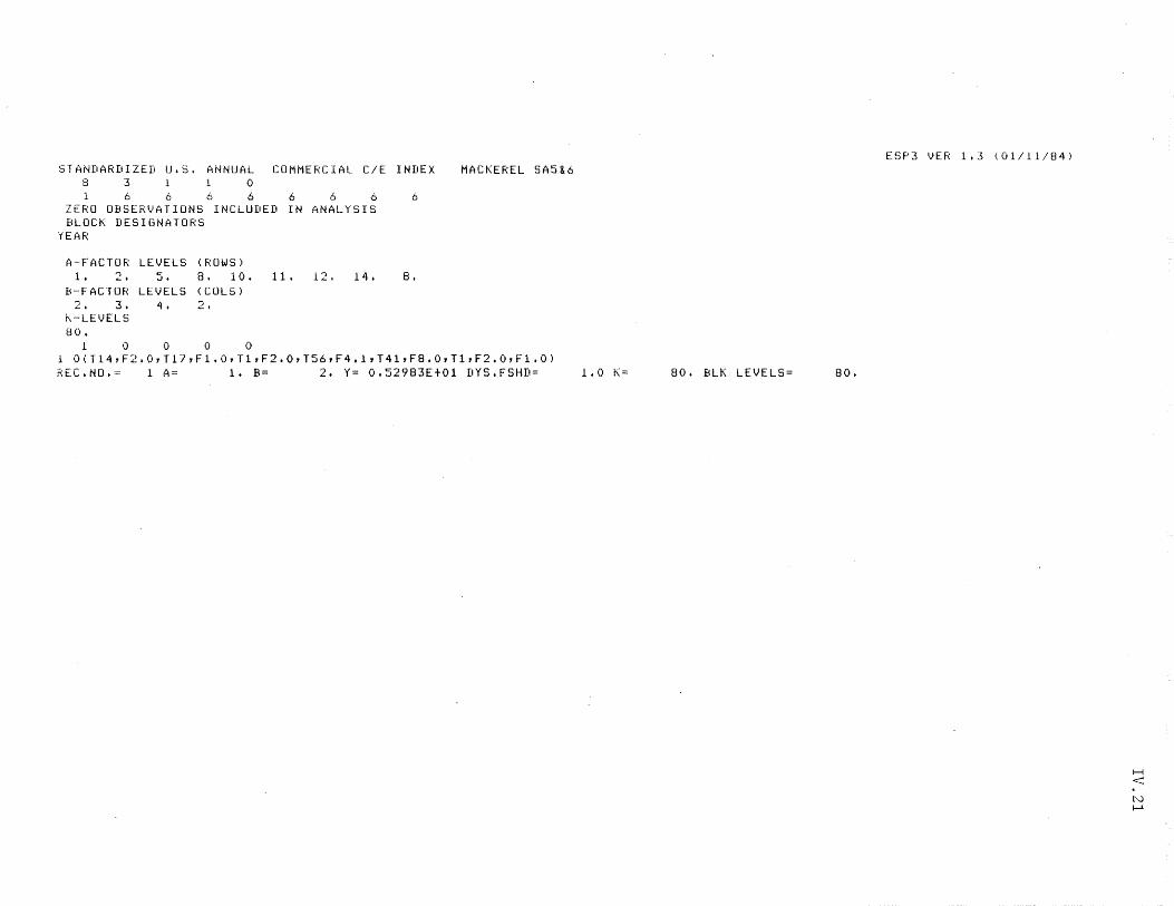
STANDARDIZED U.S. ANNUAL COMMERCIAL CIE INDEX 8 3 1 0 1 6 666 6 666
ZERO OBSERVATIONS INCLUDED IN ANALYSIS BLOCK DESIGNATORS
YEAR
A-FACTOR LEVELS (ROWS) 1. 2. r 8. 1O. 11. 12. 14. .J.
B-FACTOR lEVELS (COlS) 2. 3. 4. 2.
K-LEVElS 80.
1 0 0 0 0
8.
MACKEREL SA5&6
1 O(T14,F2.0,T17,F1.0,Tl,F2.0,T56,F4.1,T41,F8.0,Tl,F2.0,Fl.O) REC.NO.= 1 A= 1. B= 2. Y= O.52983EtOl DYS.FSHD= 1.0 K= 80. BLK lEVElS= 80.
ESP3 VER 1.3 (01/11/84)
H
< N f--l
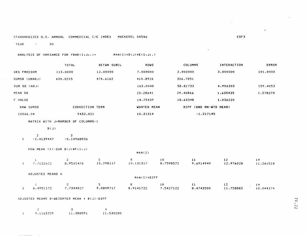
STANDARDIZED U.S. ANNUAL COMMERCIAL C/E INDEX MACKEREL SA5&6
YEAR 80
ANALYSIS OF VARIANCE FOR YBAR(I,J,.)= MtA(I>tB(J)tE(I,J,.)
TOTAL BETWN SUBCL
[lEG FREEDOM 113.0000 12.00000
SUMsa (UNADJ) 634.0215 474.6162
SUM sa (ADJ)
MEAN sa
F VALUE
RAW SUMSO CORRECTION TERM
10066.04 9432.021
MATRIX WITH J=NUMBER OF COLUMNS-1
1
B(J)
2 -2.4139447
3 -0.14968836
ROW MEAN (I)-SUM BCJ>*PCI,J)
7.7122622
ADJUSTED MEANS A
6.4951172
2 8.9515476
2 7.7344027
5 10.298117
5 9.0809717
ADJUSTED MEANS B=WEIGHTED MEAN t B(J)-DIFF
2
9.1163359
", \, ,','- " "\ \ '
3 11.380591
4 11.530280
ROWS
7.000000
410.8926
163.0048
23.28641
14.75439
WGHTED MEAN
10.31314
MtA (1)
8 10.131317
MtA(I)tDIFF
8 8.9141722
ESP3
COLUMNS INTERACTION
2.000000 3.000000
306.7051
58.81733 4.906303
29.40866 1.635435
18.63348 1.036220
DIFF (GND MN-WTD MEAN>
10 8.7598572
10 7.5427122
-1.217145
11 9.6914949
11 8.4743500
12 12.976028
12 11.758883
ERROR
101.0000
159.4053
1.578270
14 11.261518
14 10.044374
H
< N N
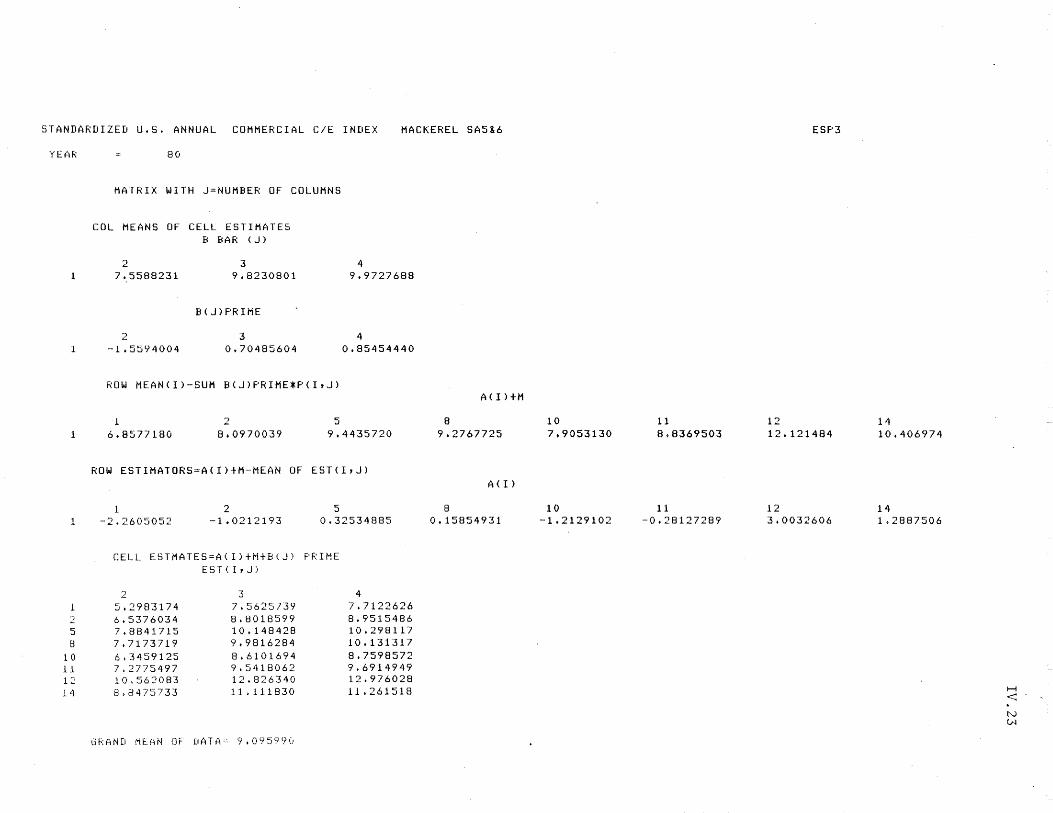
STANDARDIZED U.S. ANNUAL COMMERCIAL CIE INDEX MACKEREL SA5&6
YEAR
1
2 5 8
10 11 12 14
80
MATRIX WITH J=NUMBER OF COLUMNS
COL MEANS OF CELL ESTIMATES B BAR (J)
2 7.5588231
2 -1.5594004
3 9.8230801
B(J)PRIME
3 0.70485604
ROW MEAN(I)-SUM B(J)PRIME*P(I,J)
2 5
4 9.9727688
4 0.85454440
1
6.8577180 8.0970039 9.4435720
ROW ESTIMATORS=A(I)tM-MEAN OF EST(I,J)
1 -2.2605052
2 -1.0212193
5 0.32534885
CELL ESTMATES=A(I)tMtB(J) PRIME EST(I,J)
2 3 4 5.2983174 7.5625739 7.7122626 6.5376034 8.8018599 8.9515486 7.8841715 10.148428 10.298117 7.7173719 9.9816284 10.131317 6.3459125 8.6101694 8.7598572 7.2775497 9.5418062 9.6914949 10.562083 12.826340 12.976028 8.8475733 11.111830 11.261518
GRAND M~~N OF DATA~ 9.095990
A(I)tM
8 9.2767725
A(I)
8 0.15854931
10 7.9053130
10 -1.2129102
11 8.8369503
11 -0.28127289
ESP3
12 12.121484
12 3.0032606
14 10.406974
14 1.2887506
H <: N (.N
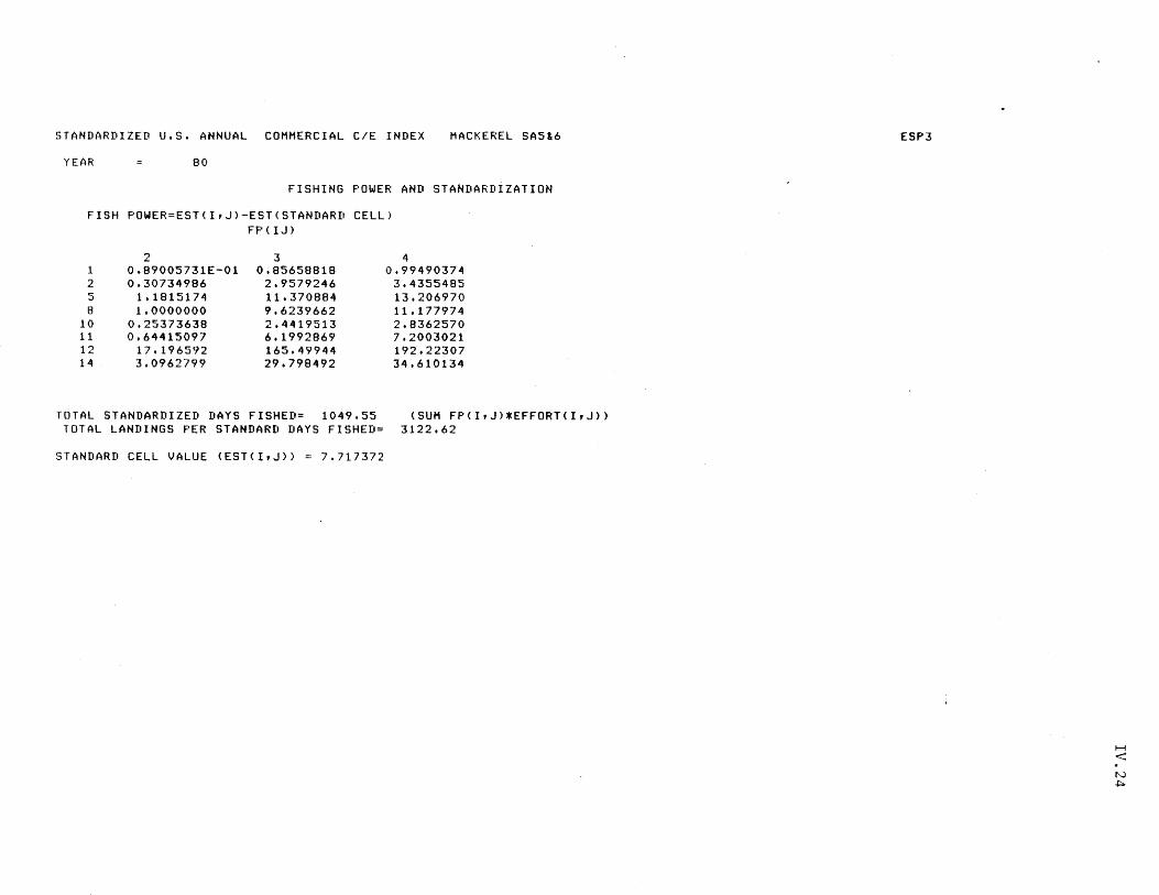
STANDARDIZED U.S. ANNUAL COMMERCIAL C/E INDEX MACKEREL SA5&6
YEAR 80
FISHING POWER AND STANDARDIZATION
FISH POWER=EST(I,J)-EST(STANDARD CELL) FP(IJ)
2 3 4 1 0.89005731E-01 0.85658818 0.9949037-\ 2 0.30734986 2.9579246 3.4355485 5 1.1815174 11.370884 13.206970 8 1.0000000 9.6239662 11.177974
10 0.25373638 2.4419513 2.8362570 11 0.64415097 6.1992869 7.2003021 12 17.196592 165.49944 192.22307 14 3.0962799 29.798492 34.610134
TOTAL STANDARDIZED DAYS FISHED= 1049.55 (SUM FP(I,J)*EFFORT(I,J» TOTAL LANDINGS PER STANDARD DAYS FISHED= 3122.62
STANDARD CELL VALUE (EST(I,J» 7.717372
ESP3
H
< N ..j::>.
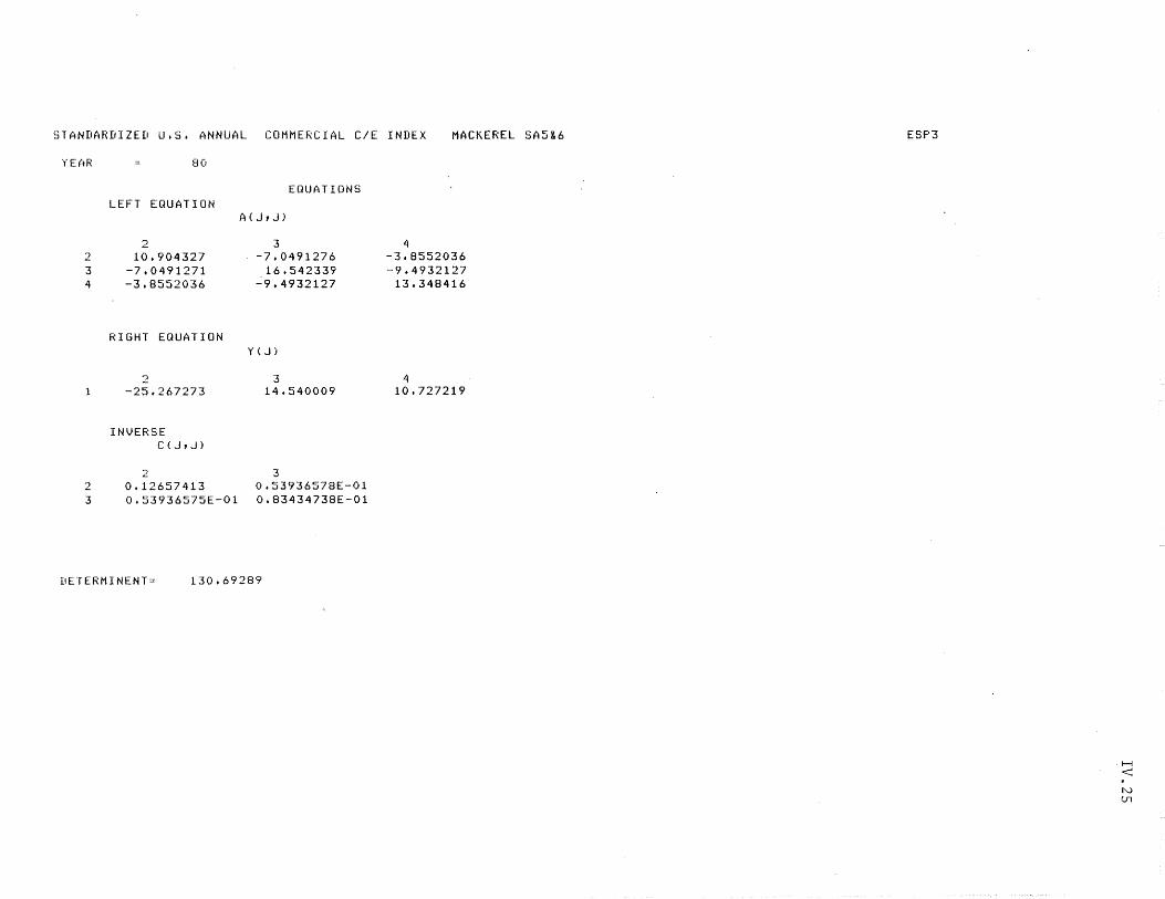
STANDARDIZED U.S. ANNUAL COMMERCIAL CIE INDEX MACKEREL SA5&6
YE(~R 80
EQUATIONS LEFT EQUATION
A(J,J)
2 3 4 2 10.904327 -7.0491276 -3.8552036 3 -7.0491271 16.542339 -9.4932127 4 -3.8552036 -9.4932127 13.348416
RIGHT EQUATION Y(J)
2 3 4 -25.267273 14.540009 10.727219
INVERSE C(J,J)
2 3 2 0.12657413 0.53936578E-01 3 0.53936575E-01 0.83434738E-01
DETERMINENT= 130.69289
ESF'3
·H <: N Ul
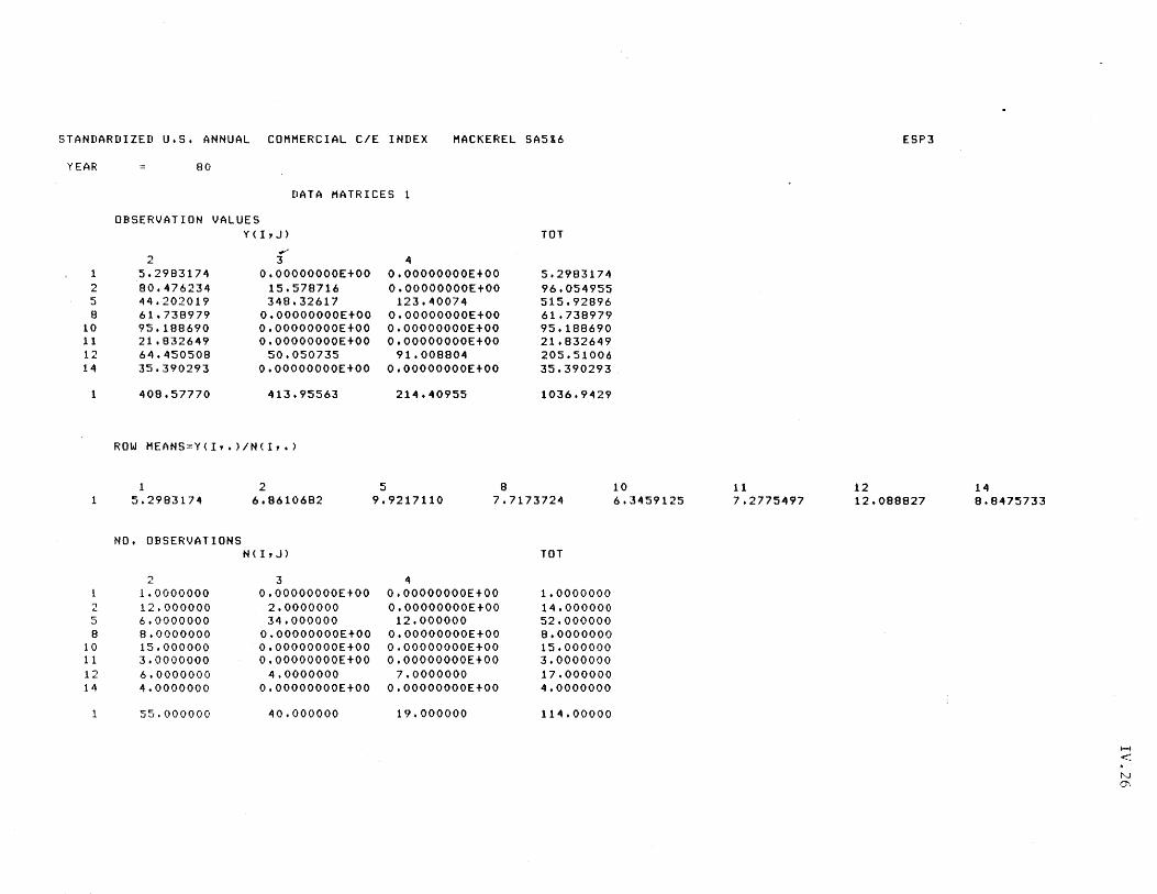
STANDARDIZED U.S. ANNUAL COMMERCIAL CIE INDEX MACKEREL SA5&6
YEAR
1 2 5 8
10 11 12 14
1
2 5 8
10 11 12 14
1
80
DATA MATRICES 1
OBSERVATION VALUES Y(I,J)
..y 2 3
5.2983174 O.OOOOOOOOE+OO 80.476234 15.578716 44.202019 348.32617 61.738979 O.OOOOOOOOE+OO 95.188690 O.OOOOOOOOE+OO 21.832649 O.OOOOOOOOE+OO 64.450508 50.050735 35.390293 O.OOOOOOOOE+OO
408.57770 413.95563
ROW MEANS=Y (I, • ) IN (I, • )
1 5.2983174
NO. OBSERVATIONS
2 1.0000000 12.000000 6.0000000 8.0000000 15.000000 3.0000000 6.0000000 4.0000000
55.000000
2 6.8610682
N(I,J)
3 O.OOOOOOOOE+OO
2.0000000 34.000000
O.OOOOOOOOE+OO O.OOOOOOOOE+OO O.OOOOOOOOE+OO
4.0000000 O.OOOOOOOOE+OO
40.000000
TOT
4 O.OOOOOOOOE+OO 5.2983174 O.OOOOOOOOE+OO 96.054955
123.40074 515.92896 O.OOOOOOOOE+OO 61.738979 O.OOOOOOOOE+OO 95.188690 O.OOOOOOOOE+OO 21.832649
91.008804 205.51006 O.OOOOOOOOE+OO 35.390293 ,
214.40955 1036.9429
5 9.9217110
8 7.7173724
TOT
4 O.OOOOOOOOE+OO 1.0000000 O.OOOOOOOOE+OO 14.000000 12.000000 52.000000
O.OOOOOOOOE+OO 8.0000000 O.OOOOOOOOE+OO 15.000000 O.OOOOOOOOE+OO 3.0000000
7.0000000 17.000000 O.OOOOOOOOE+OO 4.0000000
19.000000 114.00000
10 6.3459125
11 7.2775497
ESP3
12 12.088827
14 8.8475733
H
< N Q\
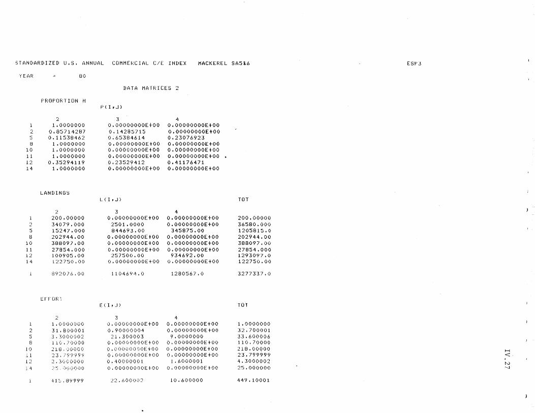
STANDARDIZED U.S. ANNUAL COMMERCIAL CIE INDEX MACKEREL SA5&6 ESP3
YUiR 80
DATA MATRICES 2
PROPORTION N P(I,J)
2 3 4 1.0000000 O.OOOOOOOOE+OO O.OOOOOOOOE+OO
2 0.85714287 0.14285715 O.OOOOOOOOE+OO 5 0.11538462 0.65384614 0.23076923 8 1.0000000 O.OOOOOOOOE+OO O.OOOOOOOOE+OO
10 1.0000000 O.OOOOOOOOE+OO O.OOOOOOOOE+OO 11 1.0000000 O.OOOOOOOOE+OO O.OOOOOOOOE+OO . 12 0.35294119 0.23529412 0.41176471 14 1.0000000 O.OOOO()OOOE+OO O.OOOOOOOOE+OO
LANDINGS L (l, J) TOT
2 3 4 200.00000 O.OOOOOOOOE+OO O.OOOOOOOOE+OO 200.00000
2 34079.000 2501.0000 O.OOOOOOOOE+OO 36580.000 5 15247.000 844693.00 345875.00 1205815.0 8 202944.00 O.OOOOOOOOE+OO O.OOOOOOOOE+OO 202944.00
10 388097.00 O.OOOOOOOOE+OO O.OOOOOOOOE+OO 388097.00 11 27854.000 O.OOOOOOOOE+OO O.OOOOOOOOE+OO 27854.000 12 100905.00 257500.00 934692.00 1293097.0 14 122750.00 O.OOOOOOOOE+OO O.OOOOOOOOE+OO 122750.00
892076.00 1104694.0 1280567.0 3277337.0
EFFOR-l E (I, J) TOT
2 3 4 1.0000000 O.OOOOOOOOE+OO O.OOOOOOOOE+OO 1.0000000
2 31.800001 0.90000004 O.OOOOOOOOE+OO 32.700001 5 3.3000002 21.300003 9.0000000 33.600006 8 110.70000 O.OOOOOOOOE+OO O.OOOOOOOOE+OO 110.70000
10 218, ')0000 O.OOOOOOOOE+OO O.OOOOOOOOE+OO 218.00900 H 11 :23./9999'1' O.OOOOOOOOE+OO O.OOOOOOOOE+OO 23.799999 <-12 :2.3('00000 0.40000001 1.6000001 4.3000002 .
N 1. 4 25,'-)00000 O.OOOOOOOOE+OO O.OOOOOOOOE+OO 25.000000 '-l
41:,,8Y999 22.600002 10.600000 449.10001
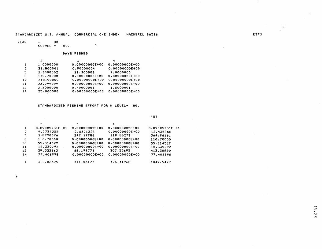
STANDARDIZED U.S. ANNUAL COMMERCIAL CIE INDEX MACKEREL SA516
i
YEAR 80 "LEVEL 80.
2 5 8
10 11 12 14
2 1.0000000 31.800001 3.3000002 110.70000 218.00000 23.799999 2.3000000 25.000000
DAYS FISHED
3 O.OOOOOOOOE+OO 0.9000000~
21.300003 O.OOOOOOOOE+OO O.OOOOOOOOE+OO O.OOOOOOOOE+OO 0.40000001 O.OOOOOOOOE+OO
4 O.OOOOOOOOE+OO O.OOOOOOOOE+OO
9.0000000 O.OOOOOOOOE+OO O.OOOOOOOOE+OO O.OOOOOOOOE+OO
1.6000001 O.OOOOOOOOE+OO
STANDARDIZED FISHING EFFORT FOR K LEVEL~ 80.
2 3 4 0.89005731E-Ol O.OOOOOOOOE+OO O.OOOOOOOOE+OO
2 9.7737255 2.6621323 O.OOOOOOOOE+OO 5 3.8990076 2-42.19986 118.86273 8 110.70000 O.OOOOOOOOE+OO O.OOOOOOOOE+OO
10 55.31-4529 O.OOOOOOOOE+OO O.OOOOOOOOE+OO 11 15.330792 O.OOOOOOOOE+OO O.OOOOOOOOE+OO 12 39.552162 66.199776 307.55695 14 77.406998 O.OOOOOOOOE+OO O.OOOOOOOOE+OO
312.06625 311.06177 426.41968
TOT
0.89005731E-Ol 12.-435858 36-4.96161 110.70000 55.314529 15.330792 -413.30890 77.-406998
1049.5477
ESP3
...... < t.J :;0
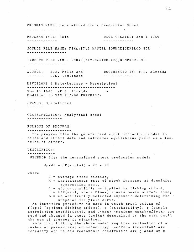
V.l
PROGRAM NAME: Generalized Stock Production Model
PROGRAM TYPE: Main DATE CREATED: Jan 1 1969
SOURCE FILE NAME: FSHA: [7l2.MASTER.SOURCE]GENPROD.FOR
EXECUTE FILE NAME: FSHA: [7l2.MASTER.XEQ]GENPROD.EXE
AUTHOR: J.J. Pella and P.K. Tomlinson
DOCUMENTED BY: F.P. Almeida
REVISIONS ( Date/Reviser - Description)
Nov 14 1983 /F.P. Almeida Modified to VAX 11/780 FORTRAN77
STATUS: Operational
CLASSIFICATION: Analytical Model
PURPOSE OF PROGRAM:
The program fits the generalized stock production model to catch and effort data and estimates equilibrium yield as a function of effort.
DESCRIPTION:
GENPROD fits the generalized stock production model:
where:
dp/dt = HP(exp(m» - KP - FP
P average stock biomass, K instantaneous rate of stock increase at densities
approaching zero, F qf, catchability multiplied by fishing effort, H K/P(max), where P(max) equals maximum stock size, m an arbitrarily selected exponent determining the
shape of the yield curve. An iterative procedure is used in which trial values of
f(opt) (optimum fishing effort), q (catchability), r (simple correlation coefficient), and U(max) (maximum catch/effort) are read and changed in steps (delta) determined by the user until the sum of squares is minimized.
Note that fitting the above model requires estimation of a number of parameters; consequently, numerous iterations are necessary and unless reasonable constraints are placed on m
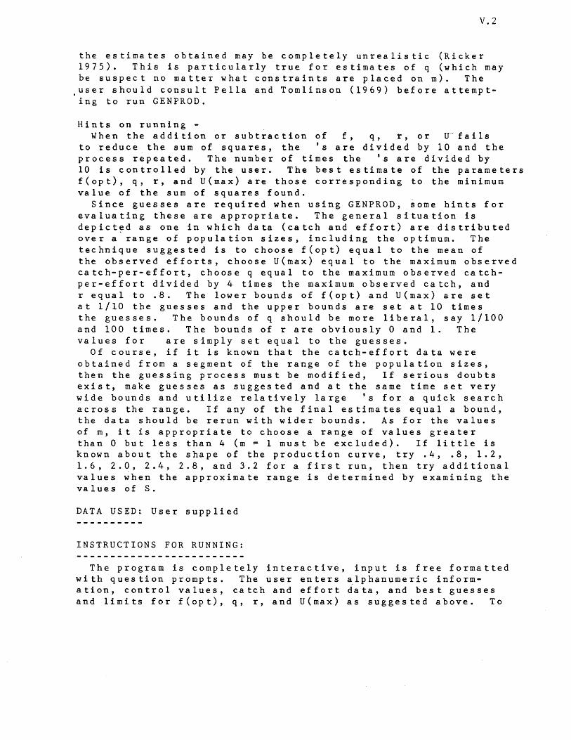
V.2
the estimates obtained may be completely unrealistic (Ricker 1975). This is particularly true for estimates of q (which may be suspect no matter what constraints are placed on m). The user should consult Pella and Tomlinson (1969) before attempting to run GENPROD.
Hints on running -When the addition or subtraction of f, q, r, or U-fails
to reduce the sum of squares, the's are divided by 10 and the process repeated. The number of times the's are divided by 10 is controlled by the user. The best estimate of the parameters f(opt), q, r, and U(max) are those corresponding to the minimum value of the sum of squares found.
Since guesses are required when using GENPROD, some hints for evaluating these are appropriate. The general situation is depict~d as one in which data (catch and effort) are distributed over a range of population sizes, including the optimum. The technique suggested is to choose f(opt) equal to the mean of the observed efforts, choose U(max) equal to the maximum observed catch-per-effort, choose q equal to the maximum observed catchper-effort divided by 4 times the maximum observed catch, and r equal to .8. The lower bounds of f(opt) and U(max) are set at 1/10 the guesses and the upper bounds are set at 10 times the guesses. The bounds of q should be more liberal, say 1/100 and 100 times. The bounds of r are obviously 0 and 1. The values for are simply set equal to the guesses.
Of course, if it is known that the catch-effort data were obtained from a segment of the range of the population sizes, then the guessing process must be modified, If serious doubts exist, make guesses as suggested and at the same time set very wide bounds and utilize relatively large's for a quick search across the range. If any of the final estimates equal a bound, the data should be rerun with wider bounds. As for the values of m, it is appropriate to choose a range of values greater than 0 but less than 4 (m = 1 must be excluded). If little is known about the shape of the production curve, try .4, .8, 1.2, 1.6, 2.0, 2.4, 2.8, and 3.2 for a first run, then try additional values when the approximate range is determined by examining the values of S.
DATA USED: User supplied
INSTRUCTIONS FOR RUNNING:
The program is completely interactive, input is free formatted with question prompts. The user enters ~lphanumeric information, control values, catch and effort data, and best guesses and limits for f(opt), q, r, and U(max) as suggested above. To
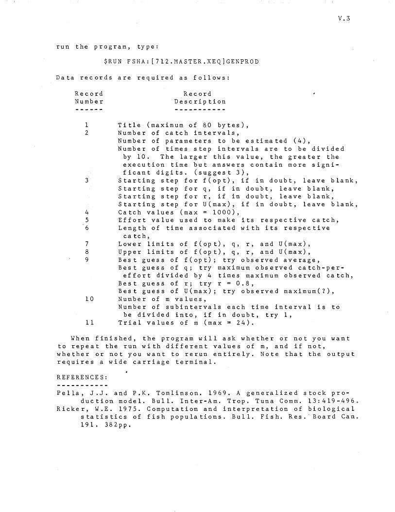
V.3
run the program, type:
$RUN FSHA: [712.MASTER.XEQ]GENPROD
Data records are required as follows:
Record Record Number Description
1 Title (maximum of 80 bytes), 2 Number of catch intervals,
Number of parameters to be estimated (4), Number of times step intervals are to be divided
by 10. The larger this value, the greater the execution time but answers contain more significant digits. (suggest 3),
3 Starting step for f(opt), if in doubt, leave blank, Starting step for q, if in doubt, leave blank, Starting step for r, if in doubt, leave blank, Starting step for U(max), if in doubt, leave blank,
4 Catch values (max = 1000), 5 Effort value used to make its respective catch, 6 Length of time associated with its respective
catch, 7 Lower limits of f(opt), q, r, and U(max), 8 Upper limits of f(opt), q, r, and U(max), 9 Best guess of f(opt); try observed average,
Best guess of q; try maximum observed catch-pereffort divided by 4 times maximum observed catch,
Best guess of r; try r = 0.8, Best guess of U(max); try observed maximum(?),
10 Number of m values, Number of subintervals each time interval is to
be divided into, if in doubt, try 1, 11 Trial values of m (max = 24).
When finished, the program will ask whether or not you want to repeat the run with different values of m, and if not, whether or not you want to rerun entirely. Note that the output requires a wide carriage terminal.
REFERENCE S:
Pella, J.J. and P.K. Tomlinson. 1969. A generalized stock production model. Bull. Inter-Am. Trop. Tuna Comm. 13:419-496.
Ricker, W.E. 1975. Computation and interpretation of biological statistics of fish populations. Bull. Fish. Res.' Board Can. 191. 382pp.
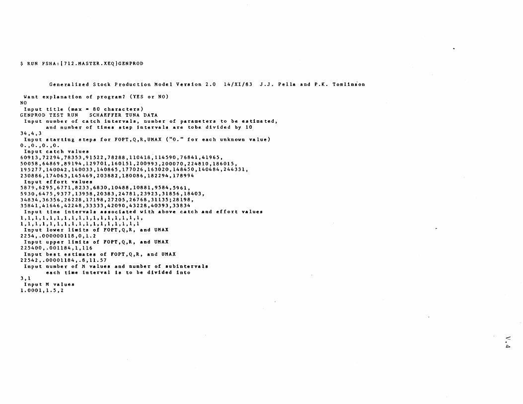
$ RUN FSHA:[712.MASTER.XEQ)GENPROD
Generalized Stock Production Model Version 2.0 14/XI/83 J.J. Pella and P.K. Tomlinson
Want explanation of program? (YES or NO) NO Input title (max - 80 characters)
GENPROD TEST RUN SCHAEFFER TUNA DATA Input number of catch intervals, number of parameters to be estimated,
and number of times step intervals are tobe divided by 10 34,4,3
Input starting steps for FOPT,Q,R,UMAX ("0." for each unknown value) O. ,0. ,0. ,0.
Input catch values 60913,72294,78353,91522,78288,110418,114590,76841,41965, 50058,64869,89194,129701,160151,200993,200070,224810,186015, 195277,140042,140033,140865,177026,163020,148450,140484,244331, 230886,174063,145469,203882,180086,182294,178994 Input effort values
5879,6295,6771,8233,6830,10488,10881,9584,5961, 5930,6475,9377,13958,20383,24781,23923,31856,18403, 34834,36356,26228,17198,27205,26768,31135;28198, 35841,41646,42248,33333,42090,43228,40393,33834
Input time intervals associated with above catch and effort values 1,1,1,1,1,1,1,1,1,1,1,1,1,1,1,1,1, 1,1,1,1,1,1,1,1,1,1,1,1,1,1,1,1,1 Input lower limits of FOPT,Q,R, and UMAX
2254,.000000118,0,1.2 Input upper limits of FOPT,Q,R, and UMAX
225400,.001184,1,116 Input best estimates of FOPT,Q,R, and UMAX
22542,.00001184,.8,11.57 Input number of H values and number of subintervals
each time interval is to be divided into 3, 1 Input M values
1.0001,1.5,2
< +:;..
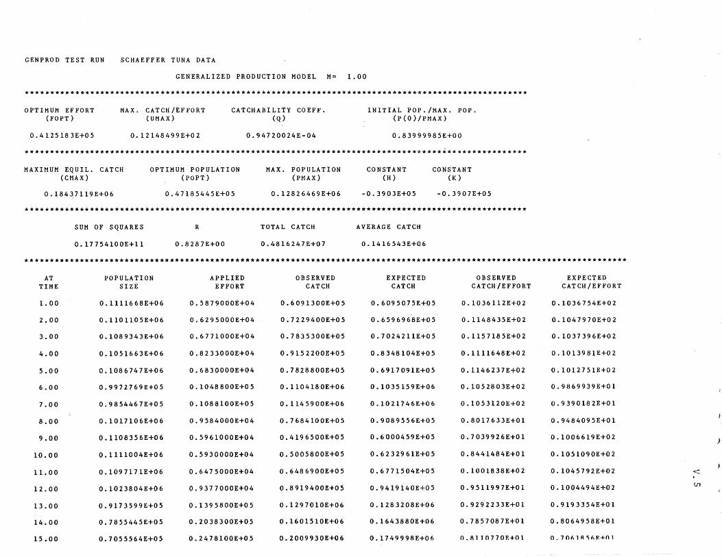
GENPROD TEST RUN SCHAEFFER TUNA DATA
GENERALIZED PRODUCTION MODEL M= 1.00
****************************************************************************************************
OPTIMUM EFFORT (FOPT)
0.4125183E+05
MAX. CATCH/EFFORT (UMAX)
0.12148499E+02
CATCHABILITY COEFF. (Q)
0.94720024E-04
INITIAL POP./MAX. POP. (P(O)/PMAX)
0.83999985E+OO
****************************************************************************************************
MAXIMUM EQUIL. CATCH (CMAX)
o .18437119E+06
OPTIMUM POPULATION (POPT)
0.47185445E+05
MAX. POPULATION (PMAX)
0.12826469E+06
CONSTANT (H)
-0.3903E+05
CONSTANT (K)
-0.3907E+05
****************************************************************************************************
SUM OF SQUARES R TOTAL CATCH AVERAGE CATCH
0.17754100E+l1 0.8287E+00 0.4816247E+07 0.1416543E+06
************************************************************************************************************************
AT POPULATION APPLIED OBSERVED EXPECTED OBSERVED EXPECTED TIME SIZE EFFORT CATCH CATCH CATCH/EFFORT CATCH/EFFORT
1. 00 0.1111668E+06 0.5879000E+04 0.6091300E+05 0.6095075E+05 0.1036112E+02 0.1036754E+02
2.00 0.1101105E+06 0.6295000E+04 0.7229400E+05 0.6596968E+05 0.1148435E+02 0.1047970E+02
3.00 0.1089343E+06 0.6771000E+04 0.7835300E+05 0.7024211E+05 0.1157185E+02 0.1037396E+02
4.00 0.1051663E+06 0.8233000E+04 0.9152200E+05 0.8348104E+05 0.1111648E+02 0.1013981E+02
5.00 0.1086747E+06 0.6830000E+04 0.7828800E+05 0.6917091E+05 0.1146237E+02 0.1012751E+02
6.00 0.9972769E+05 0.1048800E+05 0.1104180E+06 0.1035159E+06 0.1052803E+02 0.9869939E+Ol
7.00 0.9854467E+05 0.1088100E+05 0.1145900E+06 0.1021746E+06 0.1053120E+02 0.93901B2E+Ol
8.00 0.1017106E+06 0.9584000E+04 0.7684100E+05 0.9089556E+05 0.8017633E+Ol 0.9484095E+Ol
9.00 0.1108356E+06 0.5961000E+04 0.4196500E+05 0.6000459E+05 0.7039926E+01 0.1006619E+02
10.00 0.1111004E+06 0.5930000E+04 0.5005800E+05 0.6232961E+05 0.8441484E+01 0.1051090E+02
11. 00 0.1097171E+06 0.6475000E+04 0.6486900E+05 0.6771504E+05 0.1001838E+02 0.1045792E+02
12.00 0.1023804E+06 0.9377000E+04 0.8919400E+05 0.9419140E+05 0.9511997E+01 0.1004494E+02
13.00 0.9173599E+05 0.1395800E+05 0.1297010E+06 0.1283208E+06 0.9292233E+01 0.9193354E+Ol
14.00 0.7855445E+05 0.2038300E+05 0.1601510E+06 0.1643880E+06 0.7857087E+Ol 0.8064958E+Ol
15.00 0.7055564E+05 0.2478100E+05 0.2009930E+06 0.1749998E+06 O.8110770E+Ol O.70f,lR'if,F.+Ol
)
< Ul
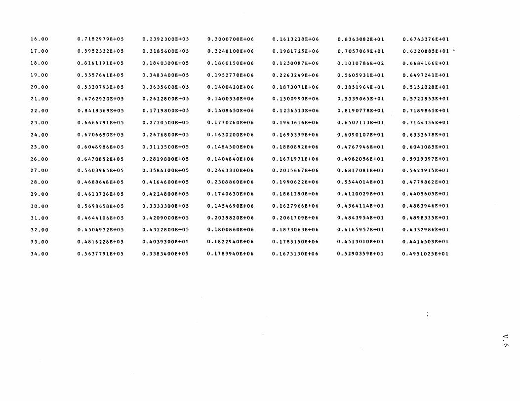
16.00 0.7182979E+05 0.2392300E+05 0.2000700E+06
17.00 0.5952332E+05 0.3185600E+05 0.2248100E+06
18.00 0.8161191E+05 0.1840300E+05 0.1860150E+06
19.00 0.5557641E+05 0.3483400£+05 0.1952770E+06
20.00 0.5320793E+05 0.3635600E+05 0.1400420E+06
21. 00 0.6762930£+05 0.2622800E+05 0.1400330E+06
22.00 0.8418369E+05 0.1719800E+05 0.1408650E+06
23.00 0.6666791E+05 0.2720500E+05 0.1770260E+06
24.00 0.6706680E+05 0.2676800E+05 0.1630200E+06
25.00 0.6048986E+05 0.3113500E+05 0.1484500£+06
26.00 0.6470852E+05 0.2819800E+05 0.1404840E+06
27.00 0.5403965E+05 0.3584100E+05 0.2443310E+06
28.00 0.4688648E+05 0.4164600E+05 0.2308860E+06
29.00 0.4613726E+05 0.4224800E+05 0.1740630E+06
30.00 0.5698658E+05 0.3333300E+05 0.1454690E+06
31. 00 0.4644106E+05 0.4209000E+05 0.2038820E+06
32.00 0.4504932E+05 0.4322800E+05 0.1800860E+06
33.00 0.4816228E+05 0.4039300E+05 0.1822940E+06
34.00 0.5637791E+05 0.3383400E+05 0.1789940E+06
0.1613218E+06 0.8363082E+01
0.1981725E+06 0.7057069E+01
0.1230087E+06 0.1010786E+02
0.2263249E+06 0.5605931£+01
0.1873071E+06 0.3851964E+01
0.1500990E+06 0.5339065E+01
0.1236513E+06 0.8190778E+01
0.1943616E+06 0.6507113E+01
0.1695399E+06 0.6090107E+01
0.1880892E+06 0.4767946E+01
0.1671971E+06 0.4982056E+01
0.2015667E+06 0.6817081E+01
0.1990622E+06 0.5544014E+01
0.1861280E+06 0.4120029E+01
0.1627966E+06 0.4364114E+01
0.2061709E+06 0.4843954E+01
0.1873063E+06 0.4165957E+01
0.1783150E+06 0.4513010E+01
0.1675130E+06 0.5290359E+01
0.6743376E+01
O. 6220885 E+O 1 •
0.6684166£+01
0.6497241E+01
0.5152028E+01
0.5722853£+01
0.7189865E+01
0.7144334E+01
0.6333678E+01
0.6041085E+01
0.5929397E+01
0.5623915E+01
0.4779862E+01
0.4405605E+01
0.4883946E+Ol
0.4898335£+01
0.43329861:+01
0.4414503E+01
0.4951025E+01
< 0\
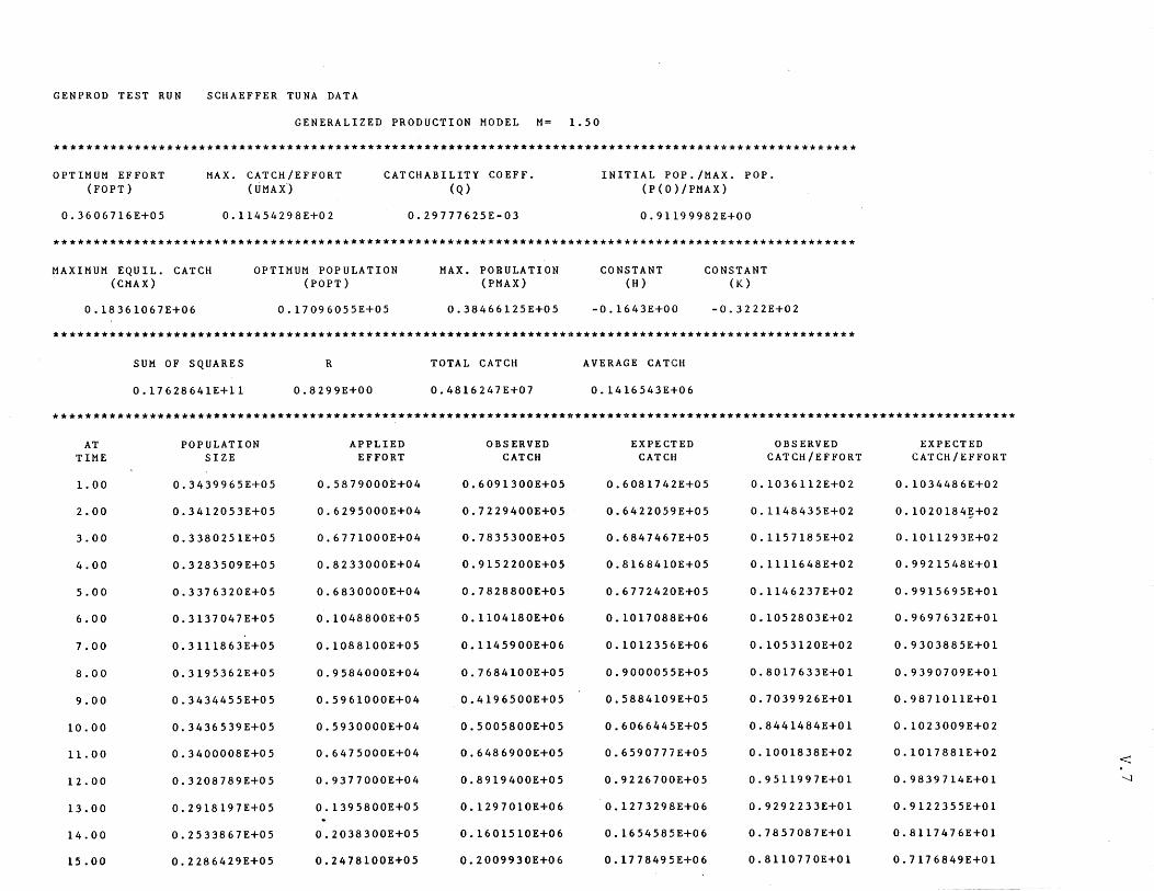
GENPROD TEST RUN SCHAEFFER TUNA DATA
GENERALIZED PRODUCTION MODEL M= 1.50
****************************************************************************************************
OPTIMUM EFFORT (FOPT)
0.3606716E+05
MAX. CATCH/EFFORT (tiMAX,)
0.11454298E+02
CATCHABILITY COEFF. (Q)
0.2977762SE-03
INITIAL POP./MAX. POP. (P(O)/PMAX)
0.91199982E+00
****************************************************************************************************
MAXIMUM EQUIL. CATCH (CMAX)
0.18361067E+06
OPTIMUM POPULATION (POPT)
0.1709605SE+OS
MAX. POBULATION (PMAX)
0.38466125E+OS
CONSTANT (H)
-0.1643E+00
CONSTANT (K)
-0.3222E+02
****************************************************************************************************
SUM OF SQUARES R TOTAL CATCH AVERAGE CATCH
0.17628641E+ll 0.8299E+00 0.4816247E+07 0.1416S43E+06
************************************************************************************************************************
AT TIME
1. 00
2.00
3.00
4.00
S.OO
6.00
7.00
8.00
9.00
10.00
11. 00
12.00
13.00
14.00
lS.00
POPULATION SIZE
0.343996SE+OS
0.34120S3E+OS
0.33802S1E+OS
0.3283509E+OS
0.3376320E+05
O.3137047E+05
0.3111863E+05
0.319S362E+OS
0.343445SE+05
O.3436539E+05
0.3400008E+OS
0.3208789E+OS
0.2918197E+OS
0.2S33867E+OS
0.2286429E+05
APPLIED EFFORT
0.5879000E+04
0.629S000E+04
0.6771000E+04
0.8233000E+04
0.6830000E+04
0.1048800E+05
0.1088100E+OS
0.9584000E+04
0.5961000E+04
O.5930000E+04
0.6475000E+04
0.9377000E+04
0.1395800E+OS
0.2038300E+OS
0.2478100E+OS
OBSERVED CATCH
0.6091300E+OS
0.7229400E+OS
0.783S300E+OS
0.91S2200E+OS
0.7828800E+05
0.1104180E+06
0.114S900E+06
0.7684100E+OS
0.4196500E+OS
0.SOOS800E+OS
0.6486900E+05
0.8919400E+05
0.1297010E+06
0.1601S10E+06
0.2009930E+06
EXPECTED CATCH
0.6081742E+05
0.64220S9E+05
0.6847467E+05
0.8168410E+OS
0.6772420E+OS
0.1017088E+06
0.1012356E+06
0.900005SE+05
0.S884109E+OS
0.6066445E+OS
0.6S90777E+OS
0.9226700E+05
0.1273298E+06
0.1654585E+06
O.1778495E+06
OBSERVED CATCH/EFFORT
0.1036112E+02
0.1148435E+02
0.1157185E+02
0.1111648E+02
0.1146237E+02
0.10S2803E+02
0.1053120E+02
0.8017 633E+0 1
0.7039926E+Ol
O.8441484E+Ol
0.l001838E+02
0.9511997E+01
0.9292233E+Ol
O.7857087E+Ol
O.8110770E+Ol
EXPECTED CATCH/EFFORT
0.1034486E+02
0.1020184~+02
0.1011293E+02
0.9921548E+Ol
0.991S695E+Ol
0.9697632E+Ol
0.9303885E+01
O.9390709E+Ol
0.9871011E+Ol
0.1023009E+02
O.1017881E+02
O.9839714E+Ol
0.91223S5E+Ol
0.8117476E+Ol
0.7176849E+Ol
< '-l
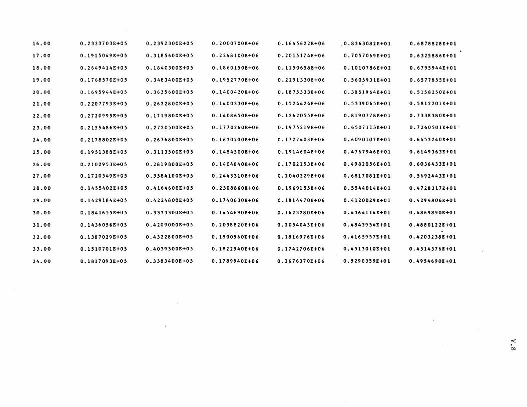
16.00 0.2333703E+05 0.2392300E+05 0.2000700E+06 0.1645622E+06 0.8363082E+01 0.6878828E+01
17.00 0.1915049E+05 0.3185600E+05 0.2248100E+06 O. 201517 4 E+O 6 0.7057069E+01 0.6325886£+01
18.00 0.2649414E+05 0.1840300E+05 0.1860150E+06 0.1250658E+06 0.1010786E+02 0.6795944E+Ol
19.00 0.1768570E+05 0.3483400E+05 0.1952770E+06 0.2291330E+06 0.5605931E+01 0.6577855E+01
20.00 0.1695944E+05 0.3635600E+05 0.1400420E+06 0.1875333E+06 0.3851964E+01 0.5158250E+01
21. 00 0.2207793E+05 0.2622800E+05 0.1400330E+06 0.1524424E+06 0.5339065E+01 0.5812201E+01
22.00 0.2720995E+05 0.1719800E+05 0.1408650E+06 0.1262055E+06 0.8190778E+01 0.7338380E+01
23.00 0.2155486E+05 0.2720500E+05 0.1770260E+06 0.1975219E+06 0.6507113E+01 0.7260501E+01'
24.00 0.2178802E+05 0.2676800E+05 0.1630200E+06 0.1727403E+06 0.6090107E+01 0.6453240£+01
25.00 0.1951388E+05 0.3113500E+05 0.1484500E+06 0.1914604E+06 0.4767946E+01 0.6149363£+01
26.00 0.2102953E+05 0.2819800E+05 0.1404840E+06 0.1702153E+06 0.4982056E+01 0.6036433E+01
27.00 0.1720349E+05 0.3584100E+05 0.2443310E+06 0.2040229E+06 0.6817081E+01 0.5692443E+01
28.00 0.1455402E+05 0.4164600E+05 0.2308860E+06 0.1969155E+06 0.5544014E+01 0.4728317E+01
29.00 0.1429184E+05 0.4224800E+05 0.1740630E+06 0.1814470E+06 0.4120029E+01 0.4294806E+01
30.00 0.1841655E+05 0.3333300E+05 0.1454690E+06 0.1623280£+06 0.4364114E+01 0.4869890E+01
31. 00 0.1436056E+05 0.4209000E+05 0.2038820E+06 0.2054043E+06 0.4843954E+01 0.4880122E+01
32.00 0.1387029E+05 0.4322800E+05 0.1800860E+06 0.1816976E+06 0.4165957E+01 0.4203238E+01
33.00 0.1510701E+05 0.4039300E+05 0.1822940E+06 0.1742706E+06 0.4513010E+01 0.4314376E+01
34.00 0.1817093E+05 0.3383400E+05 0.1789940E+06 0.1676370E+06 0.5290359E+01 0.4954690E+01
< 00
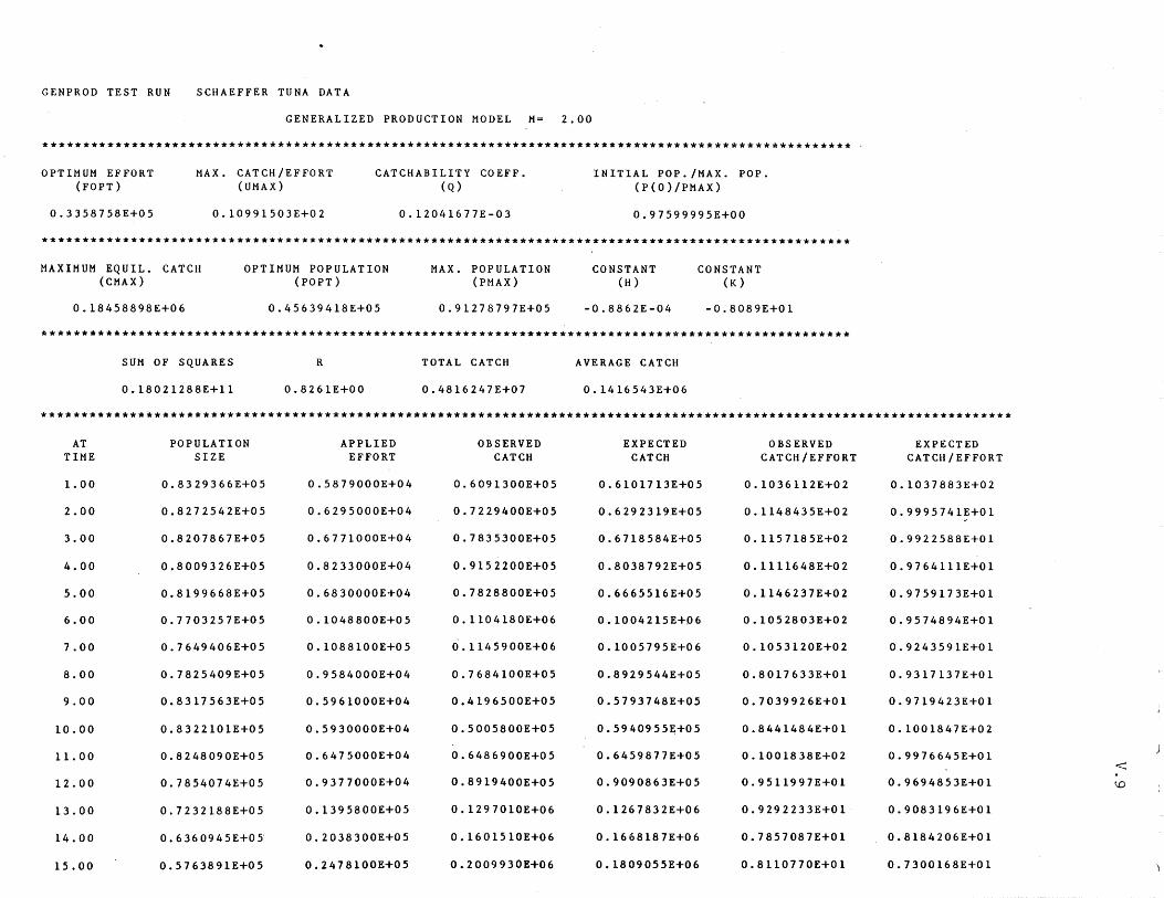
GENPROD TEST RUN SCHAEFFER TUNA DATA
GENERALIZED PRODUCTION MODEL M= 2.00
****************************************************************************************************
OPTIMUM EFFORT (FOPT)
0.3358758E+05
MAX. CATCH/EFFORT (UMAX)
0.10991503E+02
CATCHABILITY COEFF. (Q)
0.12041677E-03
INITIAL POP./MAX. POP. (P(O)/PMAX)
0.97599995E+00
****************************************************************************************************
MAXIMUM EQUIL. CATCH (CMAX)
0.18458898E+06
.oPTIMUM P.oPULATION (POPT)
0.45639418E+05
MAX. POPULATI.oN (PMAX)
0.91278797E+05
C.oNSTANT (H)
-0.8862E-04
C.oNSTANT (K)
-0.8089E+01
****************************************************************************************************
SUM OF SQUARES R T.oTAL CATCH AVERAGE CATCH
0.18021288E+11 .o.8261E+.o.o .o.4816247E+.o7 .o.1416543E+06
************************************************************************************************************************
AT P.oPULATI.oN APPLIED OBSERVED EXPECTED OBSERVED EXPECTED TIME SIZE EFF.oRT CATCH CATCH CATCH/EFF.oRT CATCH/EFFORT
1. .0.0 .o.8329366E+.o5 .o.5879.o.o.oE+.o4 .o.6.o913.o.oE+05 0.61.o1713E+.o5 .o.1.o36112E+.o2 .o.1.o37883E+.o2
2..0.0 .o.8272542E+05 0.6295000E+04 0.7229400E+05 .o.6292319E+05 0.1148435E+02 0.9995741E+01 ~
3 . .0.0 0.82.o7867E+.o5 .o.67710.o.oE+04 .o.78353.o.oE+.o5 .o.6718584E+.o5 .o.1157185E+.o2 .o.9922588E+.o1
4.00 0.8009326E+05 0.8233000E+04 0.9152200E+05 0.8038792E+05 .o.1111648E+02 0.9764111E+01
5.00 0.8199668E+05 0.6830000E+04 0.78288.oOE+05 0.6665516E+05 0.1146237E+02 0.9759173E+01
6 • .0.0 .o.77.o3257E+.o5 .o.l.o48800E+.o5 .o.11.o418.oE+.o6 .o.1.o.o4215E+.o6 .o.1.o528.o3E+.o2 .o.9574894E+.o1
7 . .00 0.7649406E+05 0.l.o881.o.oE+.o5 .o.1145900E+06 .o.1.o.o5795E+06 0.105312.oE+.o2 .o.9243591E+01
8 • .00 .o.78254.o9E+.o5 .o.9584000E+.o4 .o.76841.o.oE+.o5 .o.8929544E+.o5 .o.8.o17633E+.ol .o.9317137E+.o1
9.0.0 .o.8317563E+05 .o.5961.o.oOE+.o4 0.41965.oOE+05 .o.5793748E+.o5 .o.7.o39926E+01 .o.9719423E+.o1
10.00 .o.8322101E+05 .o.593.oO.o.oE+.o4 .o.5.o.o58.oOE+.o5 .o.5940955~+.o5 .o.8441484E+.o1 0.lD.o1847E+.o2
11. .0.0 0.824809DE+05 .o.6475.o.o.oE+.o4 .o.64869.o.oE+.o5 .o.6459877E+D5 .o.l.o01838E+.o2 D.9976645E+Dl
12. DO D.7854D74E+05 0.9377DO.oE+D4 0.891940.oE+.o5 D.9D9.o863E+D5 .o.9511997E+D1 D.9694853E+.ol
13.00 0.7232188E+D5 D.139580DE+05 0.1297.o10E+D6 0.1267832E+06 D.9292233E+01 0.9D83196E+D1
14 • .00 0.636D945E+D5- 0.2038300E+D5 0.160151.oE+06 D.1668187E+06 D.7857D87E+Ol 0.8184206E+.ol
15 • .0.0 .o.5763891E+05 .o.24781.oDE+.o5 D.2.oD9930E+D6 .o.18.o9D55E+06 .o.811D77.oE+Ol 0.73D.o168E+.o1
< (.0
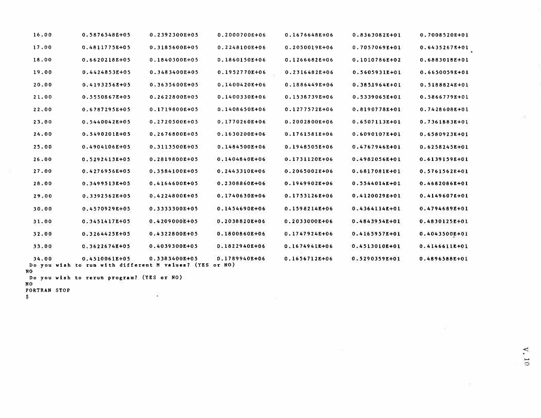
16.00 0.5876548E+05 0.2392300E+05 0.2000700E+06
17.00 0.4811775E+05 0.3185600E+05 0.2248100E+06
18.00 0.6620218E+05 0.1840300E+05 0.1860150E+06
19.00 0.4424853E+05 0.3483400E+05 0.1952770E+06
20.00 0.4193256E+05 0.3635600E+05 0.1400420E+06
21.00 0.5550867E+05 0.2622800E+05 0.1400330E+06
22.00 0.6787295E+05 0.1719800E+05 0.1408650E+06
23.00 0.5440042E+05 0.2720500E+05 0.1770260E+06
24.00 0.5490201E+05 0 .. 2676800E+05 0.1630200E+06
25.00 0.4904106E+05 0.3113500E+05 0.1484500E+06
26.00 0.5292413E+05 0.2819800E+05 0.1404840E+06
27.00 0.4276956E+05 0.3584100E+05 0.2443310E+06
28.00 0.3499513E+05 0.4164600E+05 0.2308860E+06
29.00 0.3392562£+05 0.4224800£+05 0.1740630£+06
30.00 0.4570929£+05 0.3333300E+05 0.1454690E+06
31.00 0.3451417E+05 0.4209000E+05 0.2038820E+06
32.00 0.3264425E+05 0.4322800E+05 0.1800860E+06
33.00 0.3622674E+05 0.4039300E+05 0.1822940E+06
34.00 0.4510061E+05 0.3383400E+05 0.1789940E+06 Do you wish to run with different M values? (YES or NO)
NO Do you wish to rerun program? (YES or NO)
NO FORTRAN STOP $
0.1676648E+06 0.8363082E+Ol
0.2050019E+06 0.7057069E+Ol
0.1266682E+06 0.1010786E+02
0.2316482E+06 0.5605931E+Ol
0.1886449E+06 0.385~964E+Ol
0.1538739E+06 0.5339065E+Ol
0.1277572E+06 0.8190778E+Ol
0.2002800E+06 0.6507113E+Ol
0.1761581E+06 0.6090107E+Ol
0.1948505E+06 0.4767946E+Ol
0.1731120E+06 0.4982056E+Ol
0.2065002E+06 0.6817081E+Ol
0.1949902E+06 0.5544014E+Ol
0.1753126£+06 0.4120029£+01
0.1598214E+06 0.4364114£+01
0.2033000E+06 0.4843954E+Ol
0.1747924E+06 0.4165957E+Ol
0.1674941E+06 0.4513010E+Ol
0.1656712E+06 0.5290359E+Ol
0.7008520E+Ol
0.6435267E+Ol
0.6883018E+Ol
0.6650059E+Ol
0.5188824E+Ol
0.5866779E+Ol
0.7428608E+Ol
0.7361883E+Ol
0.6580923E+Ol
0.6258245E+Ol
0.6139159E+Ol
0.5761562E+Ol
0.4682086£+01
0.4149607£+01
0.4794689E+Ol
0.4830125E+Ol
0.4043500~+01
0.4146611E+Ol
0.4896588E+Ol
< i-'
o
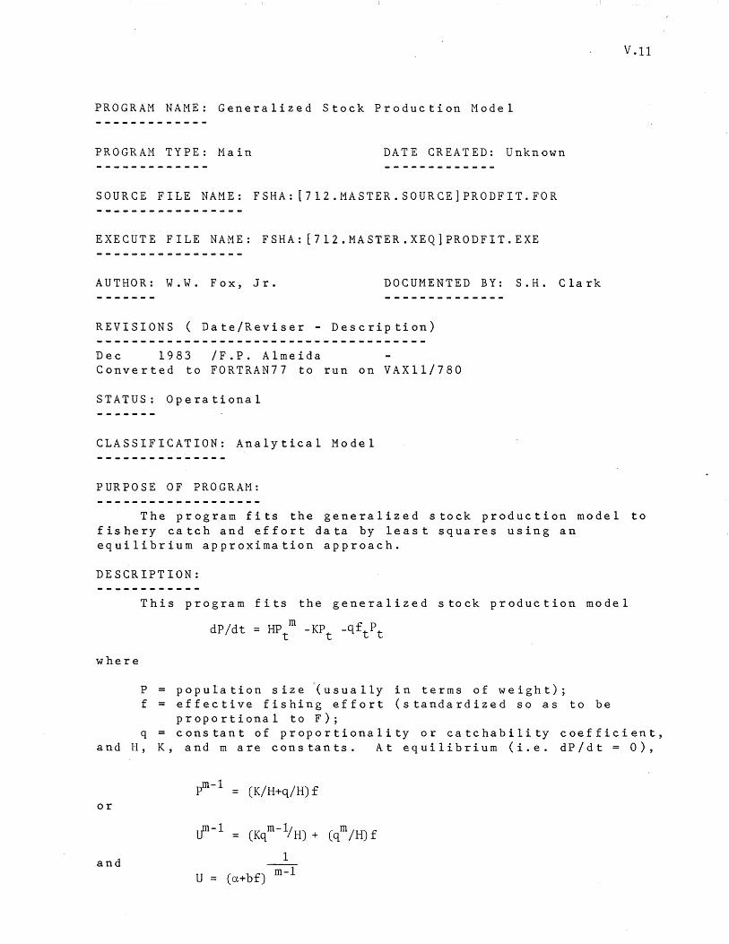
V.ll
PROGRAM NAME: Generalized Stock Production Model
PROGRAM TYPE: Main DATE CREATED: Unknown
SOURCE FILE NAME: FSHA: [712.MASTER.SOURCE]PRODFIT.FOR
EXECUTE FILE NAME: FSHA: [712.MASTER.XEQ]PRODFIT.EXE
AUTHOR: W.W. Fox, Jr. DOCUMENTED BY: S.H. Clark
REVISIONS ( Date/Reviser - Description)
Dec 1983 /F.P. Almeida Converted to FORTRAN77 to run on VAXll/780
STATUS: Operational
CLASSIFICATION: Analytical Model
PURPOSE OF PROGRAM:
The program fits the generalized stock production model to fishery catch and effort data by least squares using an equilibrium approximation approach.
DESCRIPTION:
where
This program fits the generalized stock production model
dP/dt = HPtffi -KPt _qftPt
P population size (usually in terms of weight); f effective fishing effort (standardized so as to be
proportional to F); q constant of proportionality or catchability coefficient,
and H, K, and m are constants. At equilibrium (i.e. dP/dt = 0),
ffi-l (K/H+q/H)f P = or
om- l = (Kqffi-~H)+ (qffi/H)f
1
U = (a+bf) m-l and
where U is the catch per unit effort. The program also estimates the following:
-L __ Urnax = a
m-1
1
Uopt = (a/m)m-1
Fopt = (a/b) (1/m-1) 1
Ymax m-1 = (a/b) (1/m-1) (a/m)
where:
Umax = relative poulation density. before exploitation; Uopt = relative population density providing maximum
sustainable yield; fopt = amount of fishing effort providing maximum
sustainable yield, and Ymax = maximum sustainable yield.
V.12
The program first adjusts fishing effort to approximate equilibrium conditions by computing weighted or unweighted averages by year over some previous number of years (K) corresponding to the number of year classes making a significant contribution to the catch. The resulting 1i values are used with corresponding catch values to derive a data set of (Ui, £i) pairs which are then utilized to estimate the parameters in the model. Note that K - 1 data points at the beginning of the data set are lost unless some information about these years prior to the data set can be entered and that K can vary throughout the time series. PRODFIT provides leastsquares estimates for the parameters a, b, and m by minimizing the function:
s = n L
i=l
" 2 W. (U. -U. ) 111
where the Wi values are statistical weights derived by assuming a multiplicative error structure and the Ui values are predicted from the fitted model.
Output from PRODFIT includes a listing of the input data, initial parameter estimates, final estimates for a, b, m, Umax, Uopt, fopt, and Ymax and their variability indices, observed and predicted values and error terms, estimates of the catchability coefficient q and a tables of equilibrium values.
Program PRODFIT provides the user with different options for data entry, calculation of parameter estimates, model configuration and weighting of effort data. These
V.13
can be summarized as follows:
Data Entry: The user may enter catch (Ci) and fishing effort (fi) values for i = 1 n years together with a vector of significant year class contribution numbers for averaging purposes (zero values are permitted if they are real and do not simply reflect a lack of information). Alternatively, a constant number of years may be entered for averaging purposes. If the data represent an equilibrium situation, or if the user wishes to calculate the averaged effort vector by procedures other than those used by the program, then catch per unit effort (Ui) and effort (fi) values are entered directly. No estimate of q can be made in the latter option.
Parameter Estimation: Parameter estimates may be calculated directly by the program without use of trial values in the majority of cases. Occasionally the data are so variable that compatible starting values cannot be obtained, and in this case (or in any case) the user may opt to enter initial parameter estimates directly.
Model Configuration: The user may allow PRODFIT to estimate m to any desired precision. Frequently, however, data are so variable that no significant reduction in the residual sum of squares can be obtained by varying m. The user then has the option to fix m at 2, the logistic model (Schaefer 1957); at 1, the Gompertz model (Fox 1970); or at zero, the asymptotic yield model.
Weighting: The user may select statistical weights assuming a multiplicative error structure or may choose not to weight the individual observations, i.e. Wi = 1 for all i.
DATA USED: User supplied
INSTRUCTIONS FOR RUNNING:
Input values are free - formatted; data values should be entered separated by commas. Output requires a wide carriage terminal. To run the program, type:
$RUN FSHA: [7l2.MASTER.XEQ]PRODFIT
The user is then prompted for an identifier title (80 byte maximum), control data/specifications, and catch and effort data (or catch per unit effort and effort data if data represent equilibrium). In the former case numbers of significant year classes must also be entered. Alternatively, the user may create a data file and use the following:
$ASSIGN datafile.DAT FOR005 $RUN FSHA: [7l2.MASTER.XEQ]PRODFIT
Res tric tions: Number of data points cannot exceed 99.
V.14
REFERENCES:
F:0x, W.W., Jr. 1970. An exponential surplus - yield model for op timizing exploi ted fish popu1a tions. Trans. Am. Fish. Soc. 99:80-88.
Fox, W. W., Jr. 1975. Fitting the generalized stock production model by least squares and equilibrium approximation. Fish. Bull., U.S., 73:23-37.
Schaefer, M. B. 1957. A study of the dynamics of the fishery for ye110wfin tuna in the eastern tropical Pacific Ocean. Inter - Am. Trop. Tuna Comm., Bull. 2:245-285.
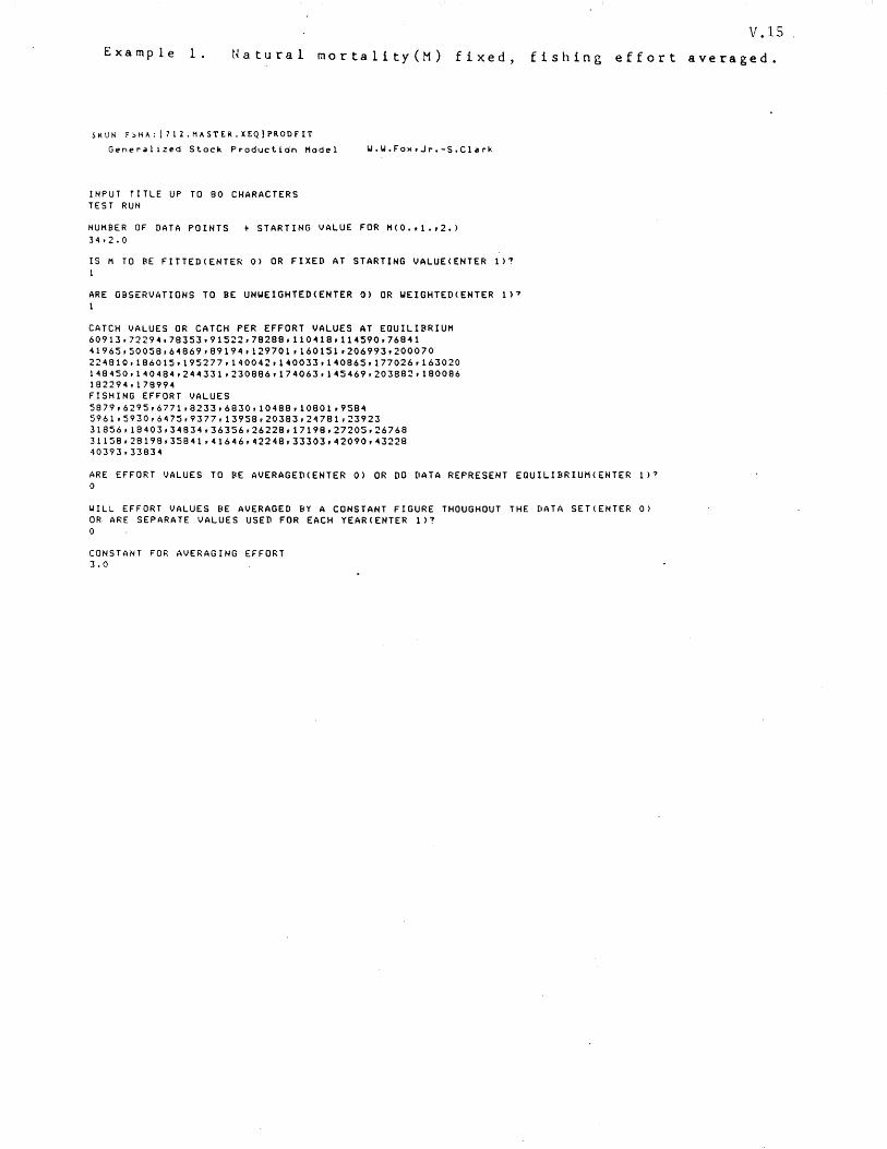
Example 1. V.IS
Natural mortality(H) fixed, fishing effort averaged.
$KUN fSHA; (7l2.HASTER.XEQ)PRODfIT
Gener~lized Stock Production Hodel
INPUT TITLE UP TO 90 CHARACTERS TEST RUN
~.U.Fo~.Jr.-S.Clark
NUHBER OF DATA POINTS + STARTING VALUE FOR H(0.,1.,2.) 34,2.0
IS H TO BE FITTED(ENTER 0) OR FIXED AT STARTING VALUE(ENTER 1)?
ARE OBSERVATIONS TO BE UNWEIGHTED(ENTER 0) OR WEIGHTED(ENTER 1)7
CATCH VALUES OR CATCH PER EFFORT VALUES AT EQUILIBRIUH 60913,7229~,78353,91522,78288,110~18,11~S90,768~1
~1965,50058,6~969,89194,129701,160151,206993,200070
224810,18601S,19S277,140042,140033,1~0965,177026,163020
1484S0,14048~,244331,230986,174063,145469,203892,180096
18229~.178994
FISHING EFFORT VALUES 5879.6295.6771.9233.6830.10488,10801,9584 5961,5930,6475,9377.13958.20383,24781,23923 31856,18403,34834,36356,26228,17198,27205,26768 31158,28199,35841,41646,42248,33303,42090,43229 40393,33834
ARE EFFORT VALUES TO BE AVERAGED(ENTER 0) OR DO DATA REPRESENT EQUILIBRIUH(ENTER 1)7 o
WILL EFFORT VALUES BE AVERAGED BY A CONSTANT FIGURE THOUGHOUT THE DATA SET(ENTER 0) OR ARE SEPARATE VALUES USED FOR EACH YEAR(ENTER I)? o
CONSTANT FOR AVERAGING EFFORT 3.0
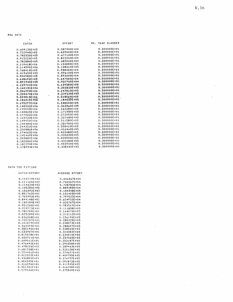
V.16
RAW DATA
CATCH EFFORT NO. YEAR CLASSES
0.609130EtOS 0.587900EtO~ 0.300000E+01 0.722940E+05 0.629500£+004 0.300000£+01 0.783530E+05 0.677100Et004 0.300000001 0.915220E+05 0.823300E+004 0.300000Et01 0.782680E+05 0.683000E+004 0.300000Et01 0.1100418Et06 0.1004680EtO:; 0.300000Et01 0.1104S90E+06 0.108010Et05 0.300000E+01 0.76841 OE+OS 0.9580400Et04 0.300000Et01 0.4196S0Et05 0.:S96100EtO~ 0.300000E+01 0.500580E+05 0.S93000£+004 0.300000E+Ol 0.648690E+OS 0.6USOOE+04 0.300000Et01 0.891940E+05 0.937700E+04 0.300000E+01
0.129701E+06 0.139S80E+OS 0.300000E+Ol 0.1601S1E+06 0.203930E+05 0.300000E+Ol 0.206993E+06 0.247810E+05 0.300000EtOl 0.200070E+06 0.239230Et05 0,300000E+Ol 0.224810E+06 0.318560Et05 0.300000E+Ol 0.196015E~6· O. IB40-:f~~+OS O. 300000EtOi··
o .195277Et06 0.3483-40Et05 0,300000EtOl 0.140042E+06 0.363560£+OS 0.300000E+01 0.140033E+06 0.262280E+05 0.300000E+01 0.140865Et06 0.171980E+05 0.300000E+01 0.177026E+06 0.2720S0E+05 0.300000E+01 0.163020E+06 0.267680E+OS 0.300000E+01 0.148450E+06 0.311580E+05 0.300000E+01 0.140484E+06 0.281980Et05 0.300000E+01 0.244331E+06 0.358410EtOS 0.300000E+01 0.230886E+06 0.416460E+OS O. 300000EtO 1 0.174063E+06 0.422480E+05 0.300000E+01 0.145469Et06 0.333030E+05 0.300000E+01 0.203882E+06 0.420900Et05 0.300000E+01 0.180086E+06 0.0432280Et05 0.300000Et01 0.182294E+06 0.403930E+05 0.300000Et01 0.178994E+06 0.338340E+OS 0.300000Et01
DATA FOR FITTING
C(1TCH/EFFORT AVERAGE EFFORT
0.115719Et02 0.646367E+04 0.111165Et02 0.742267E+04 0.114624E+02 0.728783Et04 0.105280E+0'.2 0.889283E+04 0.106092E+02 0.100348Et05 0.801763E+01 0.101"103E+05 0.703993E+01 0.797533£+04 0.844148E+01 0.6504933E+04 0.100184E+02 0.620767E+04 0.951200E+01 0.783517E+04 0.929223E+01 0.111838E+05 0.785709E+01 0.164070E+05 0.835289E+01 0.215112Et05 0.836308E+01 0.236190E+05 0.705707E+01 0.28032~E+0:S
0.101079E+02 0.238073£+05 0.560593E+01 0.288607Et05 0.385196E+01 0.32856SE+05 0.533907Et01 0.310383E+05 0.819078E+01 0.234010E+05 0.650711Et01 0.237065E+05 0.609011E+01 0.2S3187E+05 0.476443E+01 0.290358£+05 0.498206E+01 0.289463E+05 0.681708E+01 0.325128E+05 0.~~4401EtOl 0.374697Et05 0.412003E+01 0.409795E+05 0.436804E+01 0.376752Et05 0.484395E+01 0.391873E+05 0.416596E+01 0.411945E+05 0.451301Et01 0.416208E+05 0.~29036E+01 0.375860E+05
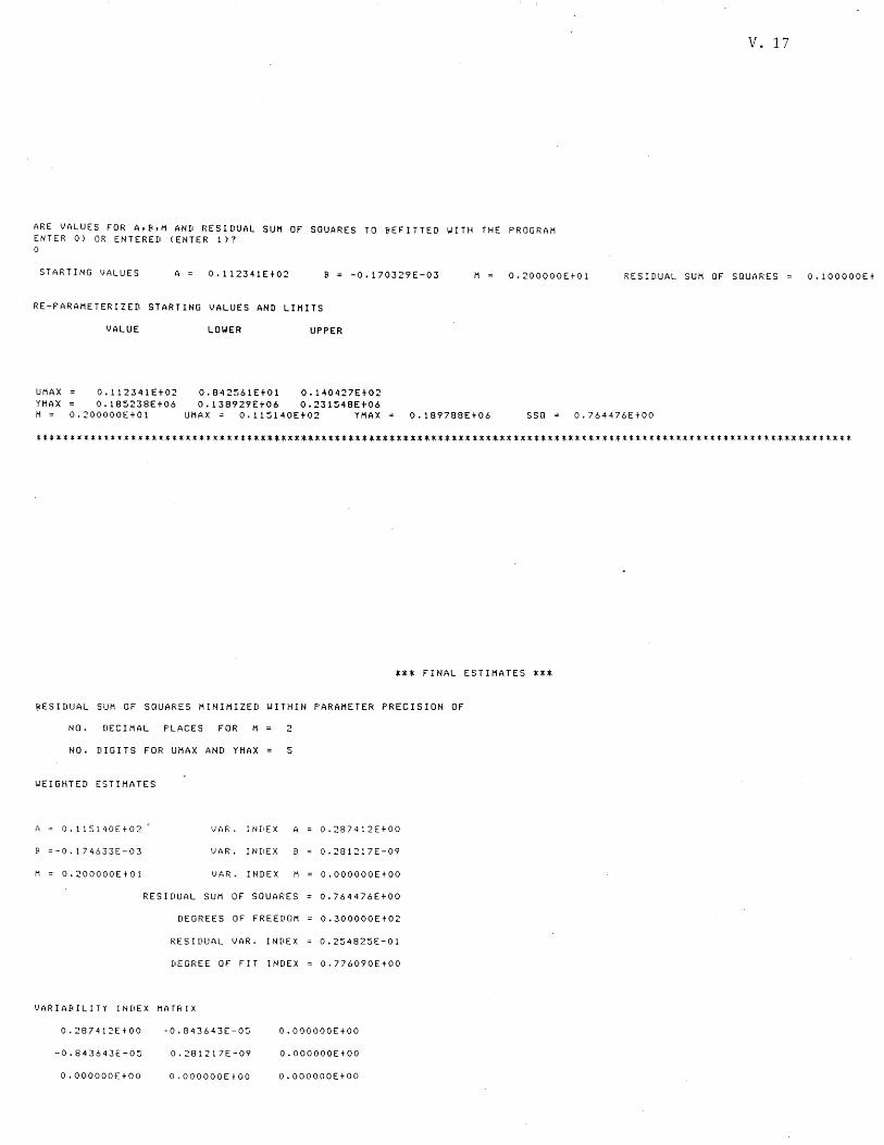
ARE VALUES FOR A,B,M AND RESIDUAL SUM OF SQUARES TO BEFITTED WITH THE PROGRAM ENTER 0) OR ENTERED (ENTER 1~? o
v. 17
STARTING VALUES A 0.112341E+02 B -0.170329E-03 M 0.200000E+01 RESIDUAL SUM OF SQUARES
RE-PARAMETERIZED STARTING VALUES AND LIMITS
UMAX YMAX M =
VALUE
0.112341E+02 0.185238E+06
0.200000£+01
LOWER UPPER
0.842561E+01 0.140427E+02 0.138929E+06 0.231548E+06
UMAX = 0.115140E+02 YMAX 0.189788E+06 SSQ = 0.764476E+00
0.100000E+
********************************************* •• * •• **************.*********.**.**.******.**.**.**** •••• *****.************
*** FINAL ESTIMATES ***
8ESIDUAL SUM OF SQUARES MINIMIZED WITHIN PARAMETER PRECISION OF
NO. DECIMAL PLACES FOR M 2
NO. DIGITS FOR UMAX AND YMAX 5
WEIGHTED ESTIMATES
H = 0.115140E+02 VAR. INDEX A 0.287412E+00
B =-0. 174633E-03 VAR. INDEX B 0.281217E-09
M 0.200000E+01 VAR. INDEX M O.OOOOOOE+OO
RESIDUAL SUM OF SQUARES 0.764476E+00
DEGREES OF FREEDOM 0.300000E+02
RESIDUAL VAR. INDEX 0.254825E-01
DEGREE OF FIT INDEX 0.776090E+00
VARIABILITY INDEX MATRIX
0.287412E+00 -0.843643E-05 O.OOOOOOE+OO
-0.843643E-05 0.281217E-09 O.OOOOOOE+OO
0.000000£+00 O.OOOOOOE+OO O.OOOOOOE+OO
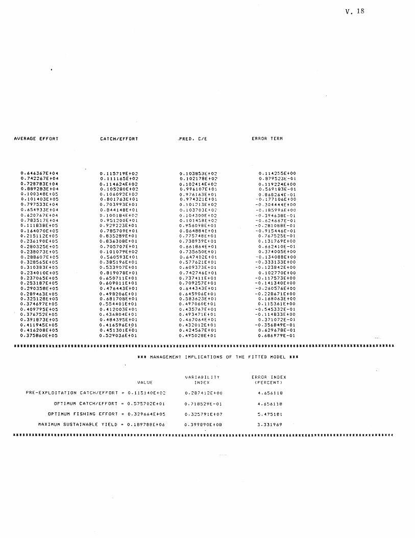
V. 18
AVERAGE EFFORT CATCH/EFFORT .PRED. C/[ ERROR TERM
0.646367E+04 0.115719E+02 0.103853EtO:! O. 114 2~j5E tOO 0.742267E+04 0.111165E+02 0.102178EtO:- 0.879523[-01 0.728783[+04 0.114624Et02 0.102414E+02 0.119224E+00 0.889283[+04 0.105280[+02 0.996107[t01 0.569183E-01 0.100348[t05 0.106092[t02 0.976163EtOI 0.868264[-01 0.101403E+05 0.801763[t01 0.974321Et01 -0.177106[tOO 0.797533E+04 0.703993[+01 0.101213[+02 -0.304444E+00 0.654933Et04 0.844148E+Ol 0.103703[+0:.' -0.185996EtOO 0.620767E+04 0.10018/1E+02 0.104300E+02 -0.39/1638E-Ol 0.783517E+04 0.951200EtOI 0.101458Et02 -0.624667E-01 0.111838E+05 0.929223E+Ol 0.956098E+Ol -0.281088E-01 0.164070E+05 0.785709Et01 0.864884EtOI -0.915446E-01 0.215112E+05 0.835289E+Ol 0.775748EtOI 0.767525E-Ol 0.236190E+05 0.836308E+Ol 0.738939EtOI 0.131769EtOO 0.280325Et05 0.705707Et01 0.661864E+01 0.662410E-Ol 0.238073Et05 0.101079E+02 0.735650E+Ol 0.374005E+00 0.288607Et05 0.560593E+01 0.647402EtOI -0.134088EtOO 0.328565E+05 0.385196E+Ol 0.577621EtOl -0.333133E+00 0.310383E+05 0.533907EtOI 0.609373EtOI -0.123842E+00 0.234010E+05 0.819078Et01 0.742746EtOI 0.102770E+00 0.237065E+05 0.650711E+01 0.737411EtOI -0.117573E+00 0.253187Et05 0.609011E+01 0.709257E+Ol -0.141340EtOO 0.290358E+05 0.476443E+01 0.644343EtOI -0.260576E+00 0.289463E+05 0.498206E+Ol 0.645906E+01 -0.228671E+00 0.325128E+05 0.681708E+01 0.583623EtOl 0.168063EtOO 0.37<\697E+05 0.554401E+01 0.497060E+01 0.115361E+00 0.409795E+05 0.412003E+01 0.435767E+01 -0.545332E-01 0.376752E+05 0.436804E+01 0.493471E+Ol -0.114833E+00 0.391873E+05 0.484395E+01 0.467064[t01 0.371072E-01 0.411945E+05 0.416596[+.01 0.432012E'l-01 -0.356849E-01 0.416208E+05 0.451301E+Ol 0.424567Et01 0.629678E-Ol 0.375860E+05 0.529036E+01 0.495028E+Ol 0.686979E-01
*** MANAGEMENT IMPLICATIONS OF THE FITTED MODEL ***
VARIABILITY ERROR INDEX VALUE INDEX (PERCENT)
PRE-EXPLOITATION CATCH/EFFORT 0.115140Et02 0.:'8741:'E+00 4.656118
OPTI MUM CATCH/EFFORT 0.575702E+01 0.7185:'9[-01 4.656118
OPTIMUM FISHING EFFORT 0.329664E+05 0.325791E+07 5.475181
MAXIMUM SUSTAINABLE Y I EUI 0.189788E+06 0.399890E+08 3.331969
*********************************_.*************************************************************************************
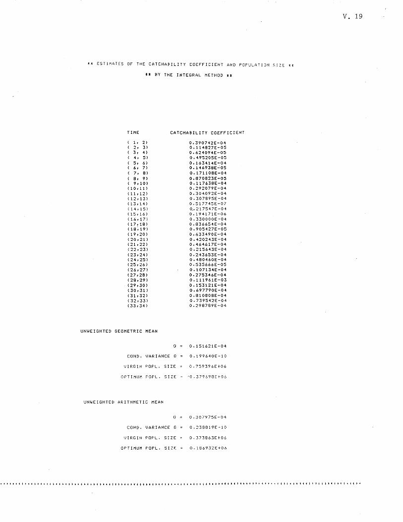
** ESTIMATES OF THE CATCHABILITY COEFFICIENT AND POPULATION SIZE **
** BY THE INTEGRAL HETHOD **
TIME CATCHABILITY COEFFICIENT
1. 2) 2. 3) 3. 4) 4, 5) 5. 6) 6, 7) 7, 8) 8, 9) 9.10)
(10.11> (11.12) (12.13) (13.14 ) (14.15) ( 15.16) (16.17) (17.18) (18~19) (19.20) (20,21> (21,22) (22,23) (23,24) (24,25) (25,26) (26,27> (27,28) (28,29) (29,30) (30,31> (31.32) (32,33) (33,34)
UNWEIGHTED GEOMETRIC HEAN
Q
CONDo VARIANCE Q
VIRGIN POPL. SIZE
OPTIMUM POPL. SIZE
UNWEIGHTED ARITHMETIC MEAN
Q
CONDo VARIANCE Q
VIRGIN POPL. SIZE
OPTIMUM POPL. SIZE
0.390742E-04 0.114827E-05 0.624094E-05 0.495205E-05 0.163H4E-04 0.146938E"';05 0.171108E-04 0.870823E-05 0.117638E-04 0.292079E-04 0.304092E-04 0.307895E-04 0.517745E-07 0,.217547E-04 0.194171E-06 0.330000E-04 0.836654E-04 0.905427E-05 0.633490E-04 0.420243E-04 0.464617E-04 0.215643E-04 0.243653E-04 0.480460E-04 0.535666E-05 0.107134E-04 0.275346E-04 0.111961E-03 0.153121E-04 0.697790E-04 0.810808E-04 0.739542E-04 0.298789E-04
0.151621E-04
0.199640[-10
0.759396E+06
'0.379698E+06
0.307975E-04
0.238819E-10
0.373863E+06
0.186932E+06
v. 19
•• I I • I • I •••••••• I I •• I I • I • I 1 ..... I •••• 1 t ••• 1 t I' • + ....... tit I • + • I ••• \ • I •••••• * •• + I ••• I ••• I- •••• + •• I • I •• I t I I r • I I I.' ! •• \ I I • + •
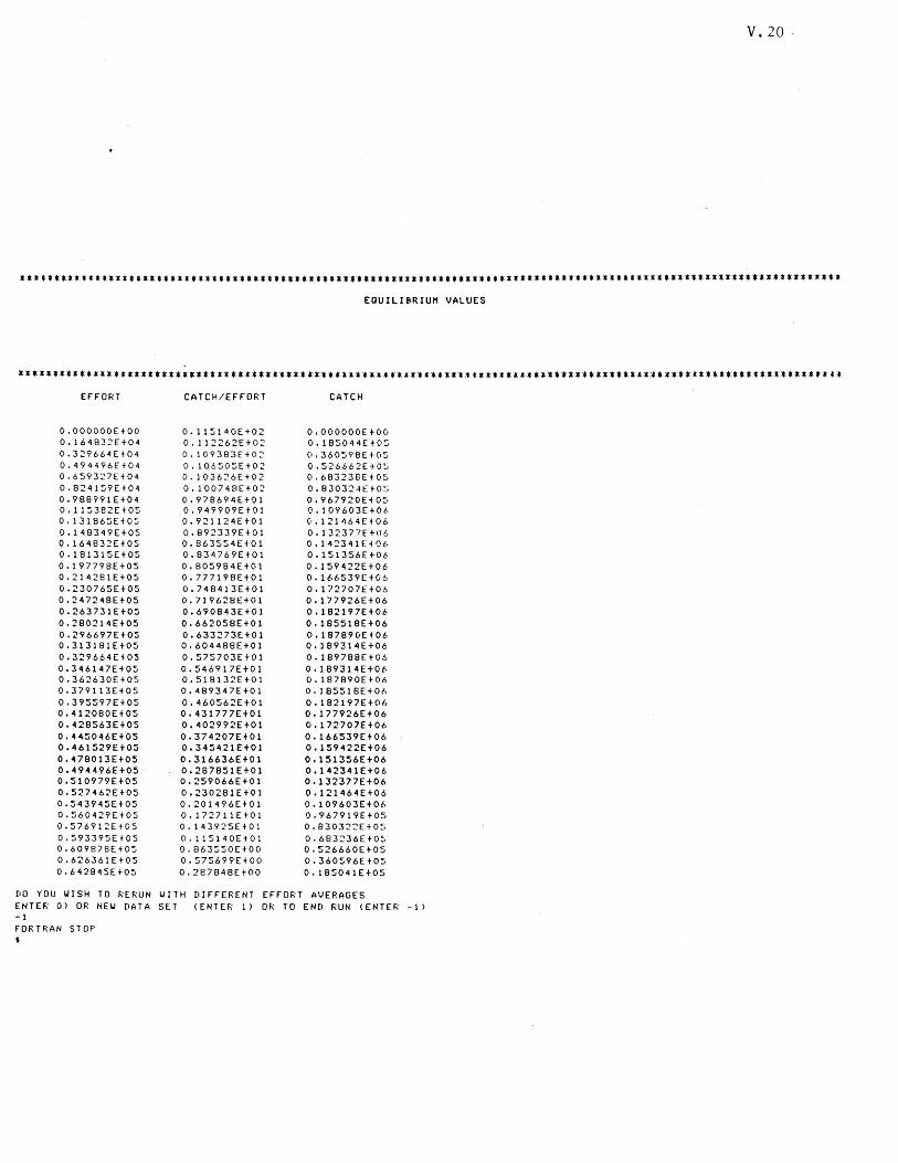
V. 20 .
i'.""'.'*" •• """""".'.""" ••••••• "i ••• i ••• ,ii'i'i"' •• ii' •• i,,' ••• 'i, •••••••••••••• i."'.""""iii' •• i.iii* EOUILIBRIUM VALUES
iiiiii*.*.ii***'*'***.**.**** •• ***** •• i"***i***** ••• *'*****i*l*i*.iiii***ii*i*ii*i.**i*****~**"******i**i**i***iiii._. EFFORT CATCH/EFFORT CATCH
0.000000£+00 0.115140£+02 0.000000£+00 0.164832£+04 0.112262£+02 0.185044E+05 0.329664£+04 0.109383£+02 0.360598E+05 0.494496£+04 0.106505E+02 O. 526662E+O~J 0.659327£+04 0.103626E+02 0.683238E+O~
0.824159E+04 0.100748E+02 O. 830324t: t-O~.i 0.988991£+04 0.978694E+01 0.967920E10::' 0.115382E+05 0.949909E+01 0.109603E+0t. 0.131865E+05 0.921124E+01 0.121464E+06 0.148349Et05 0.892339EtOl 0.132377ft06 0.164832Et05 0.863554E+01 0.142341U06 0.181315Et05 0.834769Et01 0.151356E+06 0.197798E+05 0.805984Et01 0.159422Et06 0.214281£t05 0.777198£t01 0.166539[t06 0.230765Et05 0.748413Et01 0.172707£tO.'.> 0.247248£t05 0.719628Et01 0.177926Et06 0.263731E+05 0.690843Et01 0.182197Et06 0.280214Et05 0.662058Et01 0.185518Et06 0.296697Et05 0.633273Et01 0.187890E+06 0.313181Et05 0.604488E+01 0.189314Et06 0.329664EtO:5 0.575703Et01 0.189788Et06 0.346147Et05 0.546917EtOl 0.189314EtOt. 0.362630Et05 0.518132Et01 0.187890E+06 0.379113Et05 0.489347EtOl 0.185516Et06 0.395597Et05 0.460562Et01 0.182197E+06 0.412080Et05 0.431777Et01 0.177926Et06 0.428563Et05 0.402992Et01 o .172707£t06 0.445046Et05 0.374207Et01 0.166539Et06 0.461529Et05 0.345421Et01 0.159422Et06 0.478013E+05 0.316636Et01 0.151356£t06 0.494496Et05 0.287851£t01 0.142341Et06 0.510979Et05 0.259066EtOl 0.132377Et06 0.527462E+05 0.230281EtOl 0.121464Et06 0.543945Et05 0.201496EtOl 0.109603Et06 0.560429E+05 0.172711EtOl 0.967919E+05 0.576912E+05 0.143925EtOI 0.830322E+05 0.593395E+05 0.115140E+Ol 0.683236E+0~ 0.609878Et05 0.863550EtOO 0.526660Et05 0.626361E+05 0.575699EtOO 0.360596Et05 0.642845Et05 0.287848EtOO 0.185041Et05
DO YOU YISH TO RERUN WITH DIFFERENT EFFORT AVERAGES ENTER 0) OR NEW DATA SET (ENTER 1) OR TO END RUN (ENTER -1) -1
FORTRAN STOP
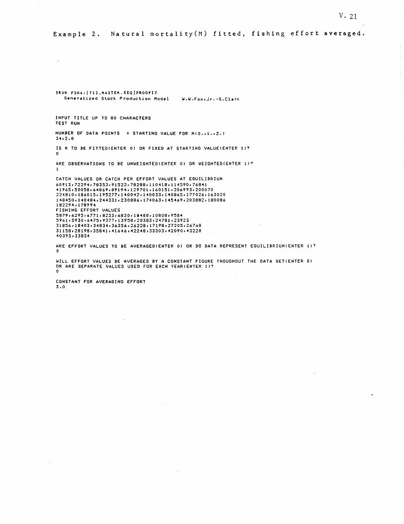
V·21
Example 2. Natural mortality(M) fitted, fishing effort averaged.
$RUH rSHA:(712.HASTER.XEQ)PRoorIT G.n.r~liz@d Stock Production Hodel
INPUT TITLE UP TO 80 CHARACTERS TEST RUN
W.U.Fox,Jr.-S.CI~rk
NUHBER OF DATA POINTS + STARTING VALUE FOR H<0.,I.,2.) 3~.2.0
IS H TO BE FITTED(ENTER 0) OR FIXED AT STARTING VALUE<ENTER 1)7 o
ARE OBSERVATIONS TO BE UNUEIGHTED(ENTER 0) OR WEIGHTED(ENTER 1)7
CATCH VALUES OR CATCH PER EFFORT VALUES AT EQUILIBRIUH 60913.7229~,78353,91522.78288.110418.114590,76841 ~1965,50058,6~869.89194,129701.160151.206993.200070
224810.186015.195277.1400~2,1~0033.140865,177026,163020
1~8450,140484,244331,230886,174063,145469,203882,180086
18229~,178994
FISHING EFFORT VALUES 5879,6295,6771,8233,6830,10488,10808,9584 5961,5930,6~75,9377~13958,20383,24781,23923
31856,18403,34834,36356,26228,17198.27205,26768 31158,28198.35841,41646,42248,33303,42090,43228 40393,33834
ARE EFFORT VALUES TO BE AVERAGED(ENTER 0) OR DO DATA REPRESENT EQUILIBRIUH(ENTER 1)7 o
WILL EFFORT VALUES BE -AVERAGED BY A CONSTANT FIGURE THOUGHOUT THE DATA SET(ENTER 0) OR ARE SEPARATE VALUES USED FOR EACH YEAR(ENTER 1)~ o
CONSTANT FOR AVERAGING EFFORT 3.0
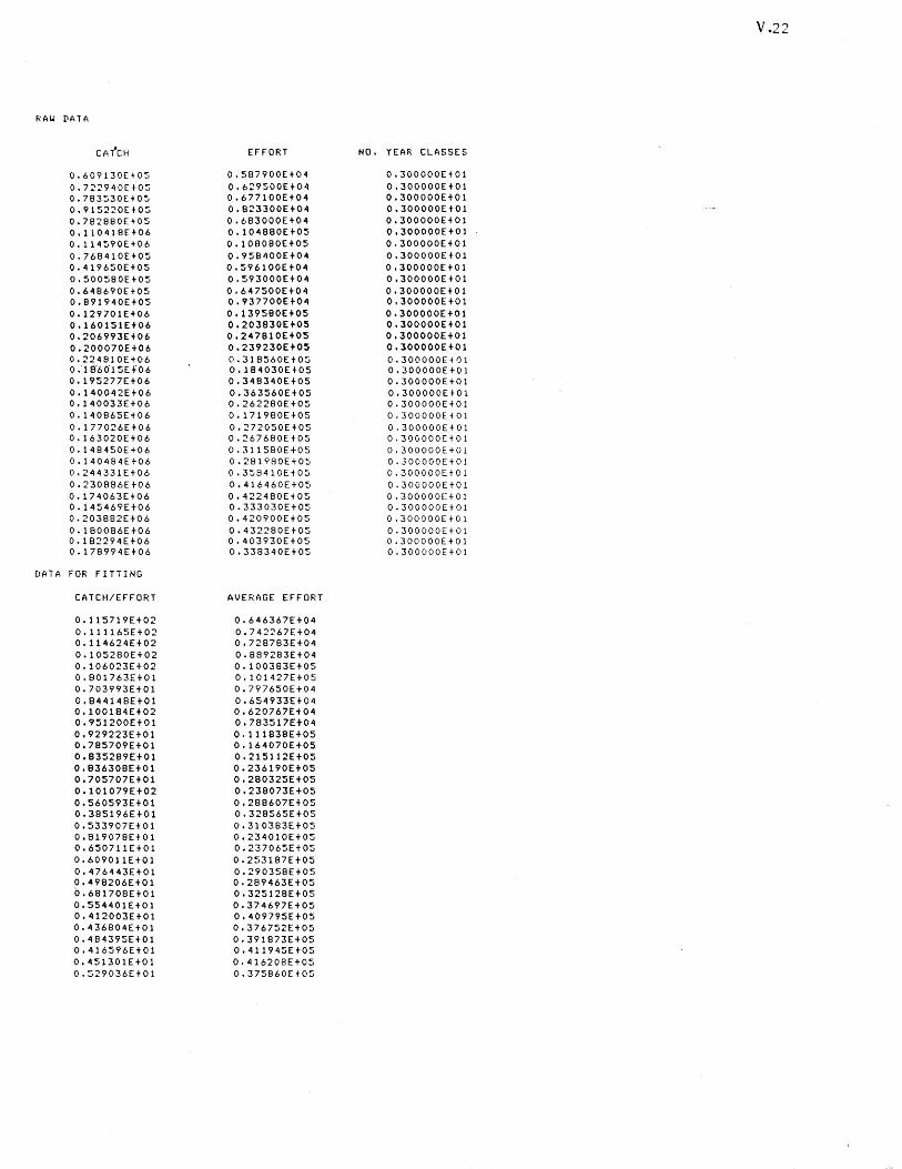
V.22
RAW DATA
CATCH EFFORT NO. YEAR CLASSES
0.609130E+05 0.587900E+04 0.300000E+01 0.722940E+05 0.629500Et04 0.300000E+01 0.783530Et05 0.677100Et04 0.300000Et01 0.915220[+05 0.823300E+0.o\ 0.300000Et01 0.782880E+05 0.683000Et04 0.300000Et01 0.110.q18E+06 0.104880E+05 0.300000E+01 0.114590[+06 0.108080E+05 0.300000E+01 0.768410E+05 0.958'100EtO.o\ 0.300000E+01 0.419650E+05 0.596100E+0.o\ 0.300000E+01 0.500580[+05 0.593000E+0.o\ 0.300000EtOl 0.6.o\8690E+05 0.647500E+04 0.300000E+01 0.891940[+05 0.937700E+0.o\ 0.300000E+01 0.129701E+06 0.139580E+05 0.300000E+01 0.160151E+06 0.203830E+05 0.300000Et01 0.206993E+06 0.247810E+05 0.300000Et01 0.200070[+06 0.239230E+05 0.300000E+01 0.224810E+06 0.318560E+05 0.300000E+01 0.-1S-60-15Ef06 0.184030E+05 0.300000E+01 0.195277E+06 0.348340E+05 0.300000E+01 0.140042E+06 0.363560E+05 0.300000Et01 0.140033Et06 0.262280E+05 0.300000E+01 0.140865E+06 0.171980E+05 0.300000EtOl 0.177026E+06 0.272050E+05 0.300000E+01 0.163020[+06 0.267680E+05 0.300000E+01 0.148450E+06 0.311580E+05 0.300000E+01 0.140484E+06 0.281980E+05 0.300000E+01 0.244331E+06 0.358410E+05 0.300000E+01 0.230886E+06 0.416460E+05 0.300000E+01 0.174063E+06 0.422480E+05 0.300000E+01 0.145469[+06 0.333030E+05 0.300000E+01 0.203882Et06 0.420900E+05 0.300000E+01 0.180086E+06 0.432280Et05 0.300000E+01 0.182294E+06 0.403930E+05 0.300000E+01 0.178994E+06 0.338340E+05 0.300000E+01
DATA FOR FITTING
CATCH/EFFORT AVERAGE EFFORT
0.115719E+02 0.646367E+04 0.111165E+02 0.742267E+04 0.114624E+02 0.728783E+04 0.105280E+02 0.889283E+04 0.106023E+02 0.100383E+05 0.801763E+01 0.101427E+05 0.703993E+01 0.797650E+04 0.844148E+01 0.654933E+04 0.100184Et02 0.620767Et04 0.951200E+01 0.783517E+04 0.929223E+01 0.111838Et05 0.785709Et01 0.164070E+05 0.835289E+01 0.215112Et05 0.836308Et01 0.236190Et05 0.705707E+01 0.280325E+05 0.101079E+02 0.238073E+05 0.560593Et01 0.288607E+05 0.385196E+01 0.328565E+05 0.533907E+01 0.310383E+05 0.819078E+01 0.234010E+05 0.650711E+01 0.237065E+05 0.609011E+01 0.253187E+05 0.476443E+01 0.290358E+05 0.-498206E+01 0.289463E+05 0.681708E+01 0.325128E+05 0.554401E+01 0.374697E+05 0.412003E+01 0.409795E+05 0.436804E+01 0.376752E+05 O. 484395E+0 1 0.391873E+05 0.416596E+01 0.411945Et05 0.451301E+01 0.416208E+05 0.529036E+01 0.375860E+05
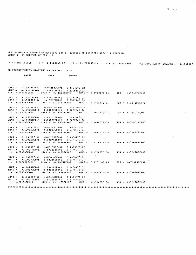
ARE VALUES FOR A,B,M AND RESIDUAL SUM OF SQUARES TO BEFITTED WITH THE PROGRAM ENTER 0) OR ENTERED (ENTER 1)? o
v. 23
STARTING VALUES A 0.112336E+02 B -0.170315E-03 M 0.200000E+01 RESIDUAL SUM OF SQUARES
RE-PARAHETERIZED STARTING VALUES AND LIHITS
VALUE LOWER UPPER
UHAX 0.112336E+02 0.842523E+01 0.140420E+02 YHAX 0.185237E+06 0.138928E+06 0.231546E+06 M :: 0.200000E+01 UMAX :: 0.115336E+02 YMAX O.190~37E+06 SSG 0.764496E+00
UMAX 0.115336E+02 0.865023E+01 0.144170Et02 YHAX 0.190237E+06 0.142678E+06 0.237796Et06 H = 0.210000E+01 UMAX = 0.114336E+02 YMf~X O. 190~37E t06 SSG 0.764589E+00
UHAX 0.115336E+02 0.865023E+01 0.144170E+0:' YHAX 0.190237E+06 0.142678E+06 0.237796E+06 M = 0.190000E+01 UHAX :: 0.116336E+02 YMAX 0.189237E+06 SSG 0.765273E+00
UMAX 0.115336E+02 0.865023E+01 0.144170E+02 YHAX 0.190237E+06 0.142678E+06 0.237796E+06 H :: 0.201000E+01 UHAX :: 0.115047E+02 YHAX 0.189837E+06 SSQ 0.764314E+00
UHAX 0.115047E+02 0.862855E+01 0.143809E+02 YMAX 0.189837E+06 0.142378E+06 0.237296E+06 M = 0.202000E+01 UMAX = 0.114937E+02 YMAX 0.189937E+06 SSG 0.764292E+00
UHAX 0.114937E+02 0.862030E+01 0.143672E+02 YHAX 0.189937E+06 0.142453E+06 0.237421E+06 H = 0.203000E+01 UHAX = o .114847E+02 YHAX 0.190017E+06 SSG 0.764281E+00
UHAX o .114847E+02 0.861355E+01 0.143559E+02 YHAX 0.190017E+06 0.142513E+06 0.237521E+06 H = 0.204000E+01 UHAX = 0.114757E+02 YHAX 0.190077E+06 SSG 0.764280E+00
UHAX 0.114757E+02 0.860680E+01 0.143447E+02 YHAX 0.190077E+06 0.142558E+06 0.237596E+06 H = 0.205000E+01 UHAX = o ',114657E+02 YHAX 0.190166E+06 SSQ 0.764289E+00
UHAX '" o .114757E+02 0.860680E+01 0.143447E+02 YHAX . 0.190077E+06 0.142558E+06 0.237596E+06 H .. 0.203000E+01 UHAX = 0.114847E+02 YHAX 0.189997E+06 SSQ 0.764281E+00
UHAX 0.114757E+02 0.860680E+01 0.143447E+02 YHAX = 0.190077E+06 0.142558E+06 0.237596E+06 M :: 0.204000E+01 UHAX :: 0.114757E+02 YMAX 0.190077E+06 SSQ :: 0.764280E+00
0.100000E+
**************************************************************************************************************.*********
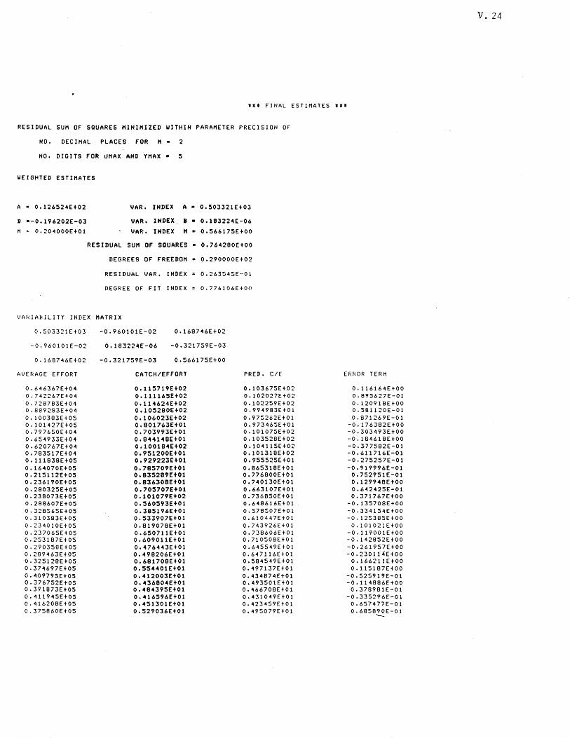
t** FINAL ESTIMATES ***
RESIDUAL SUM OF SQUARES MIHIMIZED WITHIH PARAMETER PRECISION OF
NO. DECIMAL PLACES fOR M· 2
NO. DIGITS FO~ uHAX AND YHAX· ~
WEIGHTED ESTIMATES
A • 0.126524H02
B --0.196202E-03
M 0.:!04000£+01
VAR. INDEX A· 0.~03321E+OJ
VAR. INDEX. B • 0.183224E-06
VAR. INDEX M· 0.566175E+00
RESIDUAL SUM OF SQUARES • 0.764280E+00
DEGREES OF FREEDOM • 0.290000E+02
RESIDUAL VAR. IND£X 0.263545E-01
DEGREE OF FIT INDEX 0.776106E+0()
VARIABILITY INDEX MATRIX
0.503321E+03
-0.960101E-02
0.168746E+02
AVERAGE EFFORT
0.646367E+04 0.742267£+04 0.728783E+04 0.889283E+04 0.100383E+05 0.101427E+05 0.797650£+04 0.654933E+04 0.620767£+04 0.783517E+04 0.111838E+05 0.164070H05 0.215112E+05 0.236190£+05 0.280325E+05 0.238073E+05 0.288607E+05 0.328565E+05 0.310383E+05 0.23'1010E+05 0.237065E+05 0.253187E+05 0.290358E+05 0.289463E+05 0.325128E+05 0.37.&\697E+05 0.409795£+05 0.376752E+05 0.391873E+05 0.411945£+05 0.416208E+05 0.375860E+05
-0.960101£-02 0.168746E+02
0.183224£-06 -0.321759E-03
-0.321759£-03 0.566175E+00
CATCH/EFFORT
0.115719£+02 0.111165£+02 0.114624£+02 0.105280£+02 0.106023£+02 0.801763£+01 0.703993£+01 0.844148E+01 0.100184£+02 0.951200Et01 0.929223£+01 0.785709£+01 0.835289E+01 0.836308E+01 0.70:5707E+01 0.101079£+02 0.560593E+01 0.385196£+01 0.533907£+01 0.819078Et01 0.650711E+01 0.609011E+01 0.476443E+01 0.498206£+01 0.681708£+01 0.:5:54401E+01 0 • .u2003E+01 0.436804£+01 0.484395E+Ol 0.416596E+Ol 0.451301£+01 0.529036Et01
PRED. C/£
0.103675E+02 0.102027E+02 0.102259£+02 0.994983£+01 0.975262E+01 0.97346~E+Ol
0.101075E+02 0.103528£+02 0.104115Et02 0.101318£+02 0.955525E+01 0.865318E+01 0.77 6800EtO 1 0.7-40130E+01 0.663107£+01 0.736850£+01 0.648616E+01 0.578507E+01 0.610447E+01 0.743926E+01 0.738606E+01 0.710508E+01 0.645549£+01 0.647116E+01 0.584549E+01 0.497137E+01 0.434874£+01 0.493501£+01 0.466708£+01 0.4310'l9E+01 0.423459E+01 O. 495079E+0 1
ERROR TERM
0.116164E+00 0.895627E-01 0.120918E+00 0.581120£-01 0.871269E-01
-0.176382£+00 -0.303493E+00 -0.184618E+00 -0.377582E-01 -0.611716E-Ol -0.275257E-01 -0.919996E-01
0.752951E-01 0.129948E+00 0.642425E-01 0.371767E+00
-0.135708E+00 -0.334154£+00 -0.125385E+00
0.101021£+00 -0.119001E+00 -0.142852£+00 -0.261957£+00 -0.230114E+00
0.166211E+00 0.115187E+00
-0.525919E-01 -0.114886E+00 0.378981E-01
-0.335296E-01 0.657477E-01 0.685890£-01
'--...
V. 24
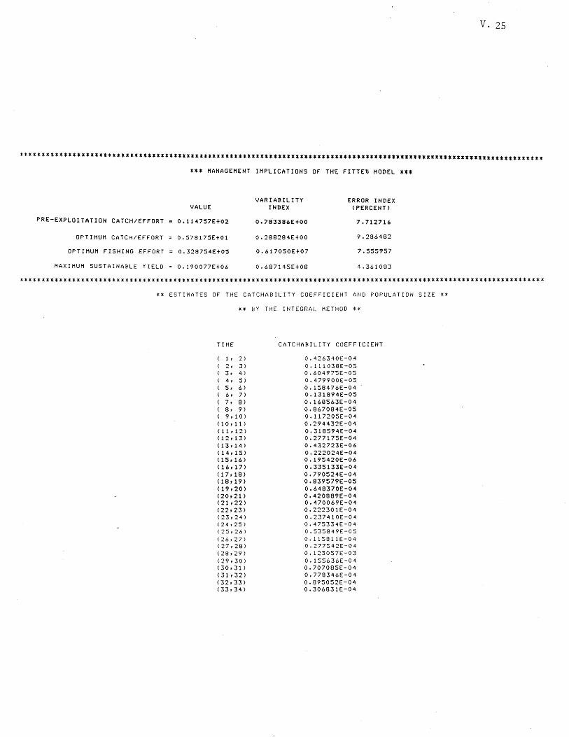
v. 2S
*t**********************************************t******tttt***t*****************************t****ttt*tttt*****t**t****** t** HANAGEHENT IHPLICATIONS OF TH£ FITTEO HODEL ***
VAR I ABIL!TY ERROR INDEX VALUE INDEX (PERCENT)
PRE-EXPLOITATION CATCH/EFFORT .. 0.11"757E+02 0.78'3386E+00 7.712716
OPTIMUM CATCH/EFFORT 0.578175E+Ol 0.288284E+00 9.286482
OPTIMUM FISHING EFFORT 0.328754E+05 0.617050E+07 7.555957
MAXIMUM SUSTAINABLE YIELD 0.190077E+06 0.687145E+08 4.361083
*t********************************************************tt***************************************************t*t****** ** ESTIMATES OF THE CATCHABILITY COEFFICIENT AND POPULATION SIZE _.
** BY THE INTEGRAL METHOD *«
TIME
1 , 2 ) 2, 3) 3, 4 ) 4 , 5) 5, 6 ) 6 , 7) 7 , 8) 8 , 9 ) 9,10)
(10.11> (11.12) (12.13) (13.14) ( 14,15) (15.16) (16.17) (17.18) (18.19) (19,20) (20,21> (21,22) (22,23) (23,24) (24,25) (25,26) (26,27) (27,28) (28,29) (29,30) (30,31> (31,32) (32,33) (33,34)
CATCHABILITY COEFFICIENT
0.426340E-0~
0.111038E-05 0.604975E-05 0.479900£-05 0.158476E-04 0.131994E-05 0.168563E-04 0.867084E-05 0.117205E-04 0.294432E-04 0.318594E-04 0.277175E-04 0.432723£-06 0.222024E-04 0.195420E-06 0.335133E-04 0.790524E-04 0.839579E-05 0.648370E-04 0.420889E-04 0.470069E-04 0.222301E-04 0.237410E-04 0.475334E-04 0.535849E-05 0.115811E-04 0.277542E-04 0.123057E-03 0.155636E-04 0.707085E-04 0.778346E-04 0.895052E-04 0.306831E-04
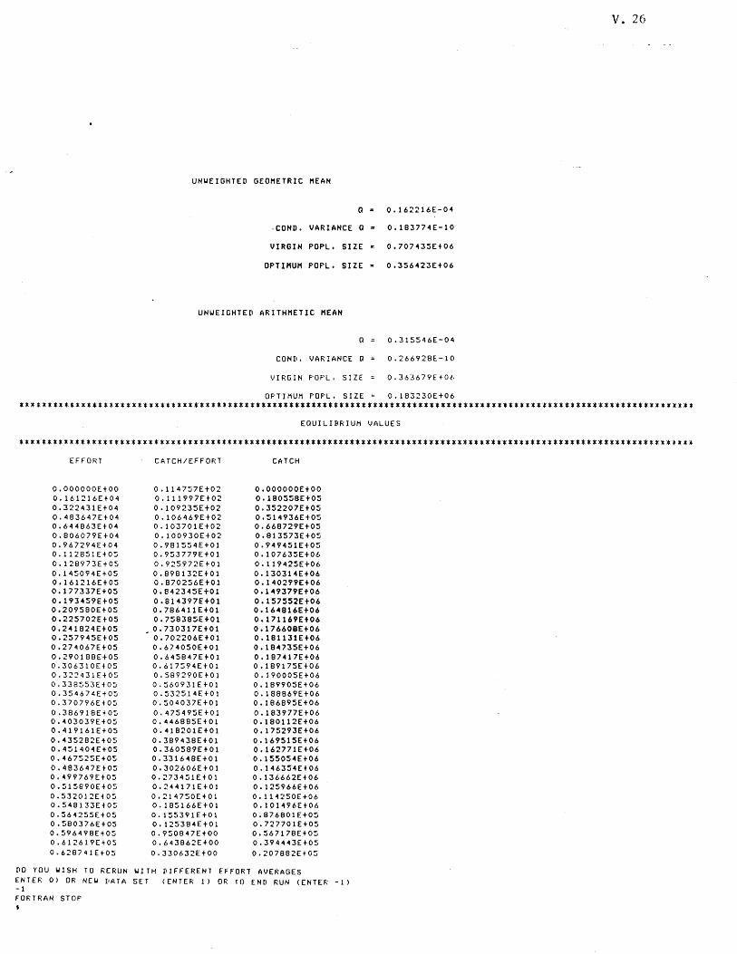
v. 26
UNWEIGHTED GEOMETRIC MEAN
o ~ 0.162216E-04
.COND. VARIANCE Q: 0.183774E-10
VIRGIN POPl. SIZE = 0.707435E+06
OPTIMUM POPl. SIZE· 0.356423E+06
UNWEIGHTED ARITHMETIC MEAN
0.315546E-04
COND. VARIANCE 0 0.266928E-10
VIRGIN POPL. SIZE 0.363679E+Ol.
OPTIMUM POPL. SIZE 0.183230E+06
**********t**********************************'*'*********************************************~**************t***********
EOUIlIBRIUM VALUES
tt*t*t****'*******************************************************************************************************l*~**~
EFFORT CATCH/EFFORT CATCH
O.OOOOOOE+OO 0.114757E+02 O.OOOOOOE+OO 0.161216E+04 0.111997E+02 0.180558E+05 0.322431E+04 0.109235E+02 0.352207E+05 0.483647E+04 0.106469E+02 0.514936E+05 0.644863E+04 0.103701E+02 0.668729E+05 0.806079E+04 0.100930E+02 0.813573E+05 0.967294E+04 0.981554E+01 0.949451E+05 0.112851E+05 O. 953779E+0 1 0.107635E+06 0.128973E+05 0.925972E+01 0.119425E+06 0.145094E+05 0.898132E+Ol 0.130314E+06 0.161216E+05 0.870256E+01 0.140299E+06 o .177337E+05 0.842345E+01 0.149379E+06 0.193459E+05 0.814397E+01 0.157552E+06 0.209580E+05 0.786411E+01 0.164816E+06 0.225702E+05 0.758385E+01 0.171169E+06 0.241824E+05 0.730317E+01 0.176608E+06 0.257945E+05 0.702206E+01 0.181131E+06 0.274067E+05 0.674050E+01 0.184735E+06 0.290188E+05 0.645847E+01 0.187417E+06 0.306310E+05 0.617594E+01 0.189175E+06 0.322431E+05 0.589290E+Ol 0.190005E+06 0.338553E+05 0.560931E+01 0.189905E+06 0.354674E+05 0.532514E+01 0.188869E+06 0.370796E+05 0.504037E+Ol 0.186895Et06 0.386918E+05 0.475495E+01 0.183977E+06 0.~03039E+05 0.446885E+Ol 0.180112E+06 0.419161E+05 0.418201E+Ol 0.175293E+06 0.-435282E+05 0.389438E+Ol 0.169515E+06 0.45140.o\E+05 0.360589E+Ol 0.162771E+06 0.-467525E+05 0.331648E+01 0.155054E+06 0.483647E+05 0.302606E+Ol O. 1 ~6354E+06 0.~99769E+05 0.273451E+Ol 0.136662Et06 0.515890E+05 0.2.o\4171E+Ol 0.125966E+06 0.532012E+05 0.21-4750E+01 0.114250E+06 0.548133E+05 0.185166E+01 0.101496£+06 0.564255E+05 0.155391E+Ol 0.876801E+05 0.580376E+05 0.125384E+Ol 0.727701E+05 0.596"'198E+05 0.9508-47E+00 0.567178E+05 0.612619[+05 0.6-43862E+00 0.3944-43E+05 0.628741E+05 0.330632E+00 0.207882E+05
DO YOU ~ISH TO RERUN WITH DIFFERENT fFFORl AVERAGES ENTER 0) OR NEU DATA SET (ENTER 1) OR ro END RUN (ENTER -1) -1 FORTRAN STOP
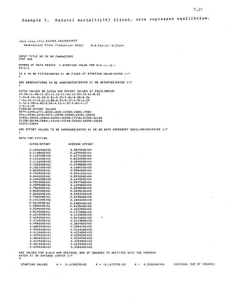
V.27
Example 3. Natural mortality(H) fitted, data represent equilibrium.
SRUN FSHA: (712.HASTER.Xt:QlpROOFIT
Generalized Stock Production Hodel
INPUT TITLE UP TO 80 CHARACTERS TEST RUN
NUHBER OF DATA POINTS + STARTING VALUE FOR H(0.,1.,2.) 34,2.0
IS H TO BE FITTED<ENTER 0) OR FIXED AT STARTING VALUE(ENTER 1)7 o
ARE OBSERVATIONS TO BE UNWEIGHTED(ENTER 0) OR WEIGHTED(ENTER 1)1 1
CATCH VALUES OR CATCH PER EFFORT VALUES AT EQUILIBRIUH 10.36,11.48,11.~7,11.12,11.46,10.53,10.61'B.02 7.04,8.44,10.02,9.~1,9.29,7.B6,8.35,8.36 7.06,10.11,5.61,3.8~,5.34,8.19,6.51,6.09 4.76,4.98,6.82,5.54,4.12,4.37,4.84,4.17 4.51,5.29 FISHING EFFORT VALUES 5879,6295,6771,8233,6830,10488,10801,9584 5961,5930,6475,9377,13958,20383,24781,23923 31856,18403,34834,36356,26228,17198,27205,26768 31158,28198,35841,41646,42248,33303,42090,43228 40393,33834
ARE EFFORT VALUES TO BE AVERAGED(ENTER 0) OR DO DATA REPRESENT EQUILIBRIUHCENTER 1)1 1
DATA FOR FITTING
CATCH/EFFORT
0.103600E+02 o • 114800E+02 0.115700E+02 0.111200E+02 0.114600E+02 0.105300E+02 0.106100E+02 0.802000E+Ol 0.704000£+01 0.844000E+01 0.100200E+02 0.951000E+Ol 0.929000E+01 0.786000E+01 0.835000E+01 0.836000E+01 0.706000E+Ol 0.101100E+02 0.561000E+01 0.38~000E+Ol 0.534000E+01 0.819000E+01 0.651000E+01 0.609000E+01 0.476000E+01 0.4 98000EtO 1 0.682000E+01 0.554000E+01 0.412000E+01 0.437000E+01 0.484000E+01 0.417000E+01 0.451000E+01
. O. 529000E+0 1
AVERAGE EFFORT
0.:587900E+04 0.629500E+04 0.677100E+04 0.823300E+04 0.683000E+04 0.104880E+05 0.108010E+05 0.958400E+04 0.596100E+04 0.593000E+04 0.647500E+04 0.937700E+04 0.139580Et0:5 0.203830E+05 0.247810E+05 0.239230E+05 0.318560E+05 0.184030E+05 0.348340E+05 0.363560E+05 0.262280E+05 0.171980E+05 0.272050E+05 0.267680Et05 0.311580Et05 0.281980E+05 0.358410E+05 0.4U400E+0~
0.422480E+0~
0.333030E+05 0.420900E+05 0.432280E+05 0.403930E+05 0.338340E+05
ARE VALUES FOR A,a,H AND RESIDUAL SUH OF SQUARES TO BEFITTED WITH THE PROGRAH ENTER 0) OR ENTERED (ENTER 1)1 o
STARTING VALUES A 00113057E+02 a z -0.167279E-03 0.200000E+01 RESIDUAL SUH OF SQUARES
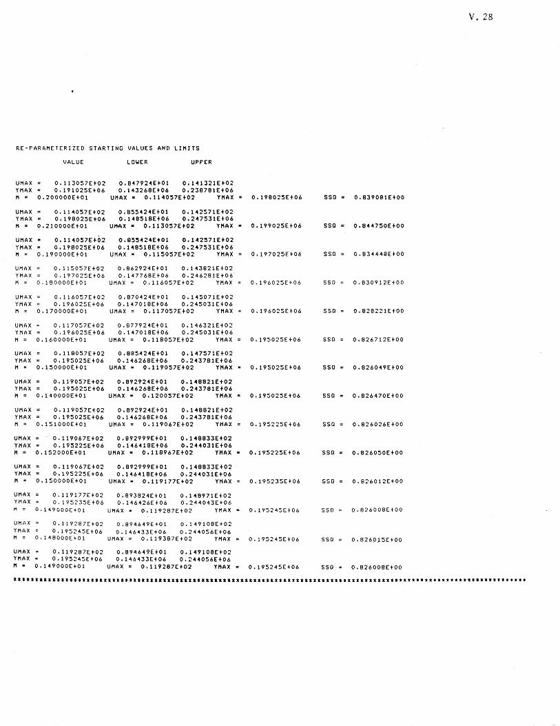
V.28
F:E-PARAHETERIZED STARTING VALUES AND LIMITS
VALUE lOIolER UPPER
UHAX 0.113057E+02 0.847924E+01 0.1U321Et02 YHAX .. 0.191025E+06 0.143268E+06 0.238781E+06 11 "" 0.200000E+Ol UHAX II: 0.114057E+02 YMAX "" 0.198025E+06 sse .. 0.839081E+00
UHAX 0.114057E+02 O. 85~H24E+Ol 0.142571E+02 YHAX :: 0.198025E+06 0.148518E+06 0.247531E+06 11 "" 0.210000E+01 UI'tAX .. 0.113057E+02 YMAX lit 0.199025E+06 sse '" 0.S44750E+00
UHAX 0.114057E+02 0.855424E+01 0.142571E+02 YHAX '" 0.198025E+06 0.148518E+06 0.247531E+06 M :: 0.190000EtOI UHAX '" 0.115057E+02 YMAX 0.197025E+06 sse 0.834448EtOO
UHAX 0.115057E+02 0.862924E+Ol 0.143821E+02 ,(HAX 0.197025Et06 0.147768E+06 0.246281E+06 H :: 0.180000Et01 UMAX :: 0.116057Et02 YMAX 0.196025Et06 SSQ 0.830912E+00
UHAX 0.116057E+02 0.870424E+01 o .145071E+02 YMAX 0.196025E+06 0.147018E+06 0.245031E+06 M = 0.170000Et01 UMAX = 0.117057E+02 YMAX 0.196025E+06 SSQ 0.828221E+00
UHAX 0.117057E+02 0.877924E+Ol 0.146321E+02 YMAX 0.196025E+06 0.147018E+06 0.245031Et06 M = 0.160000Et01 UHAX :: 0.118057E+02 YMAX 0.195025E+06 SSQ 0.826712EtOO
UMAX 0.118057E+02 0.885424E+01 0.147571E+02 YMAX 0.195025E+06 0.146268E+06 0.243781E+06 H :: 0.150000E+01 UMAX .. 0.119057E+02 YHAX .. 0.195025E+06 sse 0.S26049E+00
UHAX 0.119057E+02 0.892924E+01 0.1.,8821Et02 ,(HAX 0.195025E+06 0.146268E+06 0.243781E+06 11 :: o .140000Et01 UMAX .. 0.120057E+02 YI1AX :: 0.195025Et06 sse 0.826470E+00
UHAX 0.119057E+02 0.892924E+01 0.14S821E+02 YHAX 0.195025Et06 0.1 <46268E+06 0.243781E+06 H :: o .151000Et01 UHAX :: 0.119067E+02 YMAX 0.195225E+06 SSO 0.826026E+00
UMAX 0.119067E+02 0.892999Et01 0.148833E+02 YHAX 0.195225E+06 0.I46H8E+06 0.2.,.,031E+06 Ii '" 0.152000EtOI UHAX .. 0.118967E+02 YHAX . 0.195225E+06 SSQ 0.826050E+00
UHAX 0.119067E+02 0.892999E+Ol 0.148833E+02 YMAX 0.19522~EtOb 0.140418E+06 0.244031E+06 Ii :: 0.150000E+01 UI1AX .. 0.119177E+02 YMAX 0.195235Et06 sse 0.8:!6012EtOO
UMAX 0.119177E+02 0.893924E+01 0.148971E+02 YI1AX 0.195235E+06 0.1046426E+06 0.244043E+06 H = 0.149000E+01 UMAX . 0.119287E+02 YHAX - 0.1'7'5245E+06 SSQ 0.826009E+00
UMAX 0.119287E+02 0.894649E+01 0.149108E+02 YHAX 0.195245Et06 0.146433E+06 0.244056E+06 11 = 0.148000Et01 UHAX = 0.119387Et02 YHAX 0.195245E+06 sse 0.8269.15E+00
UHAX 0.119287Et02 0.894649E+01 0.149108E+02 YMAX 0.195245Et06 0.146433E+06 0.244056E+06 11 • 0.1049000E+01 UMAX .. 0.119287E+02 YMAX '" 0.195245E+06 SSQ :: 0.826008E+00
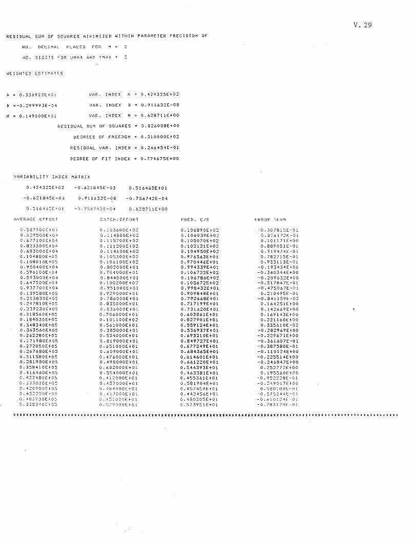
RESIDUAL SUM OF SOUARES MINIMIZED ~ITHIN PARAMETER PRECISION OF
NO. DECIMAL PLACES FOR M s 2
NO. DIGITS FOR UMAX AND YMAX" 5
WEIGHTED ESTIMATES
A '" 0.336922E+01 \JAR. INDEX A 0.424325E+02
B =-0.299993E-04 VAR. INDEX B = 0.911632E-08
H 0.14 9000EtO 1 VAR. INDEX M 0.628711E+00
RESIDUAL SUM OF SQUARES = 0.826008E+00
liEGREES OF FREEDOM " 0.310000E+02
RESIDUAL VAR. INDEX' 0.266454E-01
DEGREE OF FIT INDEX 0.774675E+00
VARIABILITY INDEX MATRIX
0.424325E+02 -0.621845E-03 0.516465E+01
-0.621845£-03
0.516465Et01
(,\"ERAGE EFFORT
0.587900Et04 o . 6 2 9 5 0 0 E + 0 ·1
0.677100E+04 0.823300E+04 0.683000E+04 o .104880Et05 0.108010E+05 0.958400E+04 0.596100E+04 0.593000E+04 0.647500E+04 0.937700E+04 0.139580E+05 0.203830£+05 0.247810£+05 0.239230Et05 0.318560£+05 o • 1 8 4 0 3 0 £of 0 5 0.348340£+05 0.363560£+05 0.262280£+05 0.171980£+05 0.272050£+05 0.267680£+05 0.311580£+05 0.281980E+05 0.358410E+05 0.416460£+05 0.422480E+05 0.333030E+05 0.420900Et05 0.432280Et05 0.403930E+05 0.3383<10Et05
0.911632E-08 -0.756742E-04
-0.756742E-04 0.628711E+00
CATCH/EFFORT
0.103600E+02 0.114800E+02 0.115700£+02 0.111200E+02 0.114600E+02 0.105300E+02 0.106100E+02 0.802000£+01 0.704000E+01 0.844000E+01 0.100200£+02 0.~51000£+01
0.929000E+01 0.786000E+01 0.835000£+01 0.836000E+01 0.706000E+01 0.101100£+02 0.561000E+01 0.385000E+01 0.534000E+01 0.819000E+01 0.651000£+01 0.609000E+01 0.476000E+01 0.498000E+01 0.682000£+01 0.554000E+01 0.412000E+01 0.437000E+01 O. -184000E+01 0.417000E+01 o . ·1 5 1 000 E t 0 1 O. 5~9000E+01
t=·RED. C/E
0.106890E+02 0.106039E+0:2 0.105070E+02 0.102121£+02 0.104950E+02 0.976563E+01 0.970446E+01 0.994339E+01 0.106722E+02 0.106786E+02 0.105672E+02 0.998432E+01 0.909848E+01 0.792668E+01 0.717199E+01 0.731620E+01 0.603861E+01 0.827901E+01 0.559124E+01 0.536937E+01 0.693210E+01 0.849727E+01 0.677249E+01 0.684365E+01 0.614601E+01 0.661220E+01 0.544393E+01 0.463381E+01 0.455361£+01 0.581904£+01 0.457459£+01 0.442456£+01 0.480305£+01 0.573951£+01
-0.307815E-01 0.8::617:::'1':-01 0.101171E+00 0.889051E-01 0.919474E--01 0.782715£-01 0.933113E-01
-0.193434£+00 -0.340344£+00 -0.209632£+00 -0.517847E-01 -0.475067E-01 0.210495£-01
-0.841159E.-02 0.164251E+00 0.142669E+00 0.169143£+00 0.221160E+00 0.335610E-02
-0.282969£+00 -0.229671E+00 -0.361607E-01 -0.387580E-01 -0.110124E+00 -0.225514E+00 -0.246847£+00
0.252772E+00 0.195560E+00
-0.952228E-01 -0.249017EtOO
0.580108[--01 -0.57534'n:-')1 -0.61012·1[-01 -0.783178E-Ol
V. 29
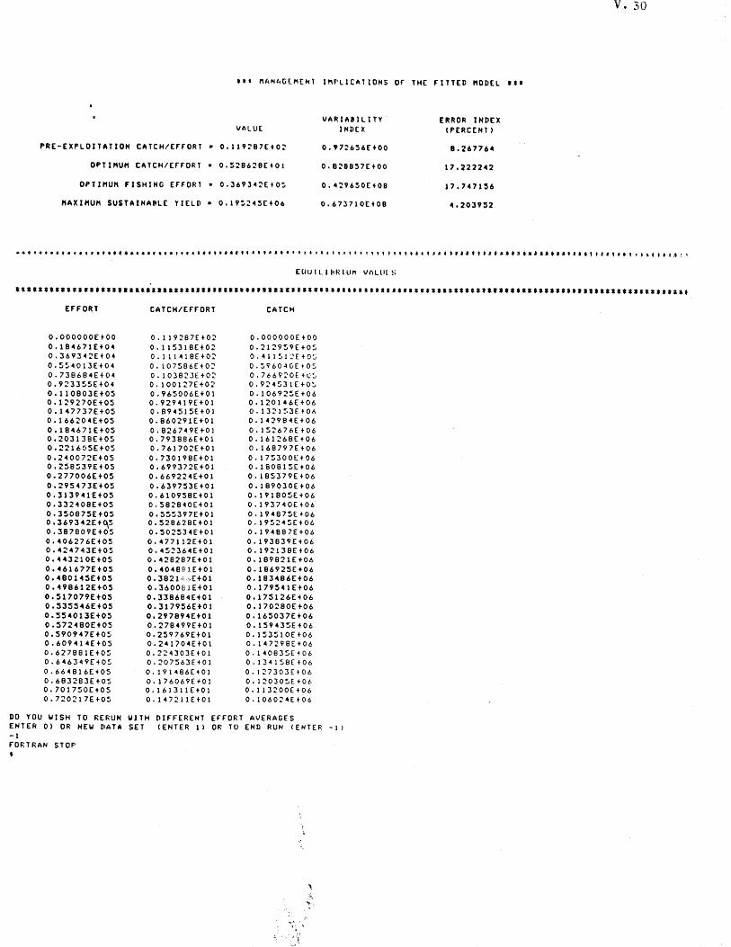
V .. 30
tt. M~NAG[M[Ht IMrlJC~tIONS or THE fITTED MODEL •••
VARIABILITY EPtROR INDEX VALUE INDEX (PERCENT)
PRE-EXPLOITATION CATCH/EHORT .0.119287£t02 0.,n656EtOO 8.26776~
OPTI MUH CATCH/EFFORt - 0.5:!B62B[tOl O. B:!8B57E+00 17.222242
OPTIMUM fiSHING EFFORT . 0.J693'12E.0~ O. '129650E+08 17.'471:56
MAXIMUM SUSTAIHA~LE ¥lUll- 0.19~2'15E+06 0.673710EtOB 4.203952
• • .............. , ............... , ••••••••• " ••• • t , , ••••• , • , t • , , .• , t • , t t , I , • t.' • , , .f , • l t .... , • .t • " .. t :t .. 1\1 ................. , I • t , •• , ••• t , , , .t : •
HItJ I L I ~R 1 Un vnUIL S
......................................................................................................................... EFFO~T CATCH/EFFORT CATCH
O.OOOOOO£tOO 0.119287[+02 O.OOOOOOE+OO 0.18'1671£+0'1 0.11~318Et02 0.2129~9E+0~ 0.3693'12E+O'l 0.111'118£+02 O. 'Ill :'1 ::'E + O:i 0.!;S'I013£t004 0.107!;86E+0:' 0.!.'i'604(iEt05 0.738684£tO'l 0.103823E+02 O. 7e-69:;'OE +1:'::' 0.9233!;S£+0" 0.100127[+02 0.92'1:'3lE+0~
0.110803Et05 0.965006E+Ol 0.106925E+06 0.129270£+05 0.929419£+01 0.1201'16E+06 0.1 U73 7E+05 0.89'1515E+Ol 0.1321~3E+Of,
0.16620'1£+05 0.860291£+01 0.l'l:?984E+06 0.184671Et05 0.8267"9[tOI 0.1!.2676[+06 0.203138£tO~ 0.793886£+01 0.161268(+06 O.:nI605Et05 0.761702EtOI 0.168797E+06 0.240072£+05 0.730198EtOI 0.1 7=>300!:::+ 06 0.2S8=>39Et05 0.699372E+Ol 0.18081:5(+06 O. 277006EtO~ 0.6692241£+01 0.185379Et06 O. 29~4I 73HOS O.6397~3E+Ol 0.189030(+06 0.313941Et05 0.6109~8(tOl 0.191805E+06 0.3320409E+0~ 0.582840(+01 0.193740(+06 0.3S0875Et05 0.5::;::;397E+Ol 0.194875E+06 O. 36930\2Et~~ 0.528628£+01 0.19:5245£+06 0.387809EtO:5 0.5025341E+Ol 0.194887£+06 0.406276£+05 0.4177112£+01 0.193839Et06 0.4247<43£tO:5 0.4:5~3641(+01 0.192138E+06 0.'143210E+05 0.428287£+01 0.189821E+06 0.461677E+05 O. 4I048!H EtO 1 0.186925E+06 0.4I801415E+05 0.3821 '~,E+Ol 0.183486£t06 0.n8612Et05 0.3600tilE+Ol 0.179541£t06 0.517079Et05 0.338684EtOI 0.175126Et06 0.53:55'-6Et05 0.317956£+01 0.170280Et06 0.554013Et05 0.297894EtOI 0.165037£+06 0.572480E+05 0.278499£+01 0.1590::;E+06 0.590947£+05 0.259769£+01 0.1~3:510E+06 0.6094114£t05 0.241704(tOI 0.147298(+06 0.627881£+0:5 0.22003[+01 0.14083!;(+O6 0.6'16349E+05 0.207:563E+Ol 0.13~158Et06
0.66'1816E+05 0.191'186E+Ol 0.127303[t06 0.683283£+0:; 0.176069E+Ol 0.120305£+06 0.701750E+05 0.161311(+01 0.113200[+06 0.n0217Et05 0.147211£+01 0.106024[+ 06
DO YOU UISH TO ~E~UN UITH DIFFERENT ErFORT AVERAGES ENTER 0) OR NEU DATA SET (£NTER 1) OR TO END RUN (ENT(R -I) -1 FORTRAN STOP
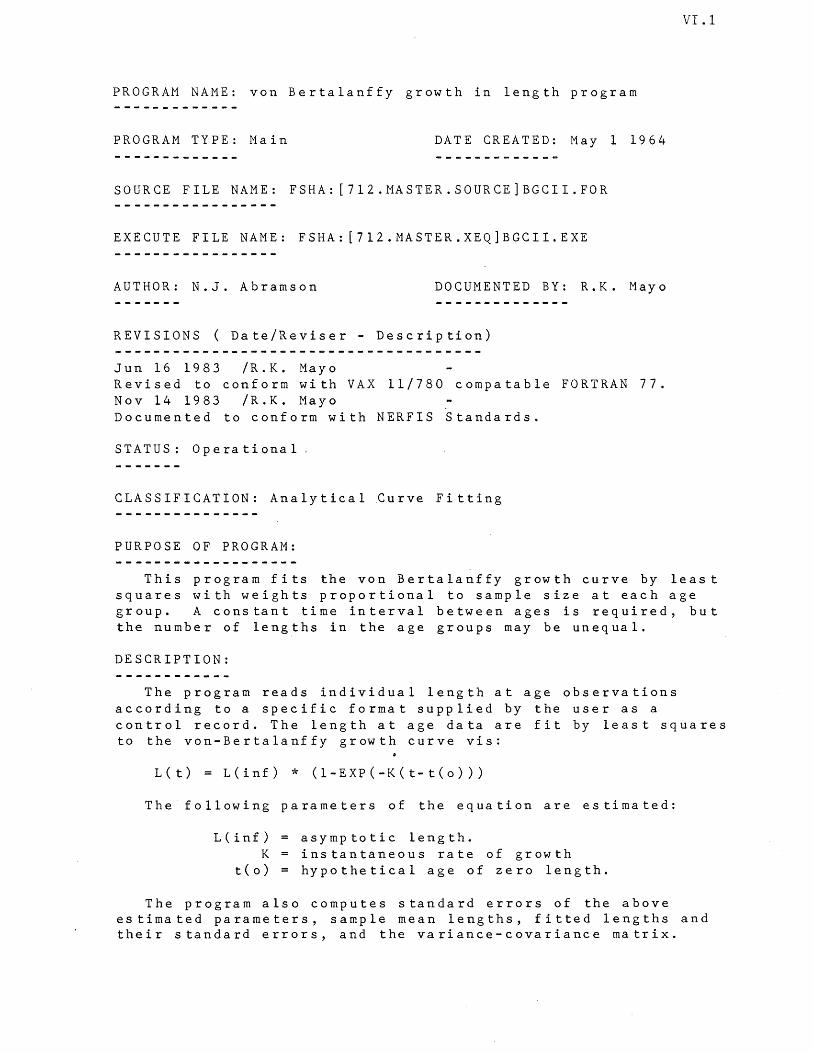
VI.l
PROGRAM NAME: von Bertalanffy growth in length program
PROGRAM TYPE: Main DATE CREATED: May 1 1964
SOURCE FILE NAME: FSHA: [7l2.MASTER.SOURCE]BGCII.FOR
EXECUTE FILE NAME: FSHA: [7l2.MASTER.XEQ]BGCII.EXE
AUTHOR: N.J. Abramson DOCUMENTED BY: R.K. Mayo
REVISIONS ( Date/Reviser - Description)
Jun 16 1983 /R.K. Mayo Revised to conform with VAX 11/780 compatable FORTRAN 77. Nov 14 1983 /R.K. Mayo . Documented to conform with NERFIS Standards.
STATUS: Operational,
CLASSIFICATION: Analytical Curve Fitting
PURPOSE OF PROGRAM:
This program fits the von Bertalanffy growth curve by least squares with weights proportional to sample size at each age group. A constant time interval between ages is required, but the number of lengths in the age groups may be unequal.
DESCRIPTION:
The program reads individual length at age observations according to a specific format supplied by the user as a control record. The length at age data are fit by least squares to the von-Bertalanffy growth curve vis:
L(t) = L(inf) * (l-EXP(-K(t-t(o)))
The following parameters of the equation are estimated:
L(inf) K
t(o)
asymptotic length. instantaneous rate of growth hypothetical age of zero length.
The program also computes standard errors of the above estimated parameters, sample mean lengths, fitted lengths and their standard errors, and the variance-covariance matrix.
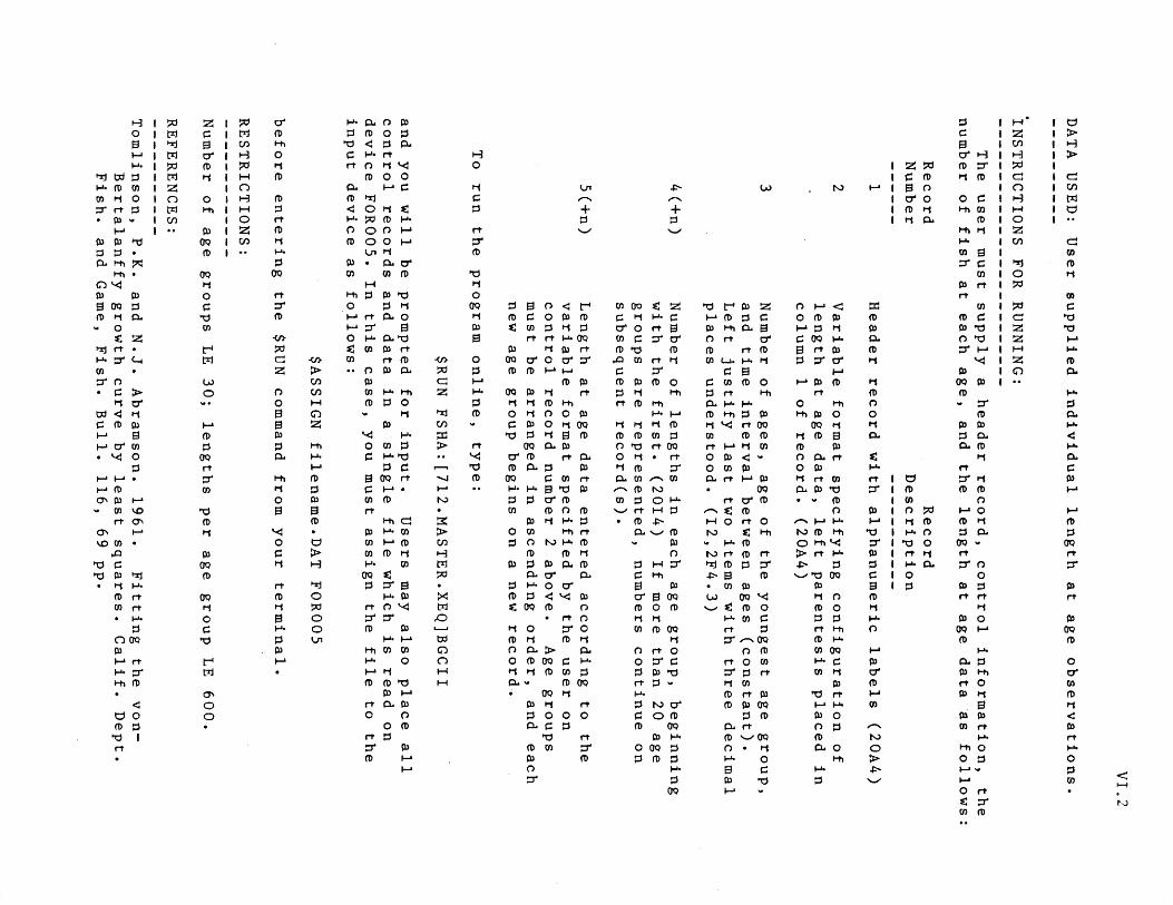
VI.2
DA
TA
U
SE
D:
Use
r su
pp
lied
in
div
idu
al
len
gth
at
ag
e
ob
serv
atio
ns .
. INS
TR
UC
TIO
NS
FO
R
RU
NN
ING
:
Th
e
user
mu
st su
pp
ly
a h
ead
er
reco
rd,
co
ntr
ol
info
rmatio
n,
the
nu
mb
er
of
fis
h
at
each
ag
e,
an
d
the
len
gth
at
ag
e
data
as
follo
ws:
Reco
rd
Nu
mb
er
1 2 3 4(+
n)
5(+
n)
Reco
rd
Descrip
tion
Head
er
reco
rd
with
alp
han
um
eric
la
bels
(2
0A
4)
Varia
ble
fo
rmat
sp
ecify
ing
co
nfig
uratio
n
of
len
gth
at
ag
e
data
, le
ft
paren
tesis
p
laced
in
co
lum
n
1 o
f re
co
rd.
(20
A4
)
Nu
mb
er o
f ag
es,
ag
e
of
the
yo
un
gest
ag
e
gro
up
, an
d
time
inte
rv
al
betw
een
ag
es
(co
nsta
nt)
. L
eft
justif
y la
st
two
ite
ms
with
th
ree
decim
al
pla
ces
un
ders
too
d.
(I2,2
F4
.3)
Nu
mb
er o
f le
ng
ths
in
each
ag
e
gro
up
, b
eg
inn
ing
w
ith
the first.
(20
14
) If
mo
re
than
2
0
ag
e
gro
up
s
are
re
pre
sen
ted
, n
um
bers
co
ntin
ue
on
su
bseq
uen
t reco
rd
(s).
Len
gth
at
ag
e
data
en
tere
d
acco
rdin
g
to
the
varia
ble
fo
rmat
sp
ecif
ied
b
y
the
user
on
co
ntr
ol
reco
rd
nu
mb
er
2 ab
ov
e.
Ag
e g
rou
ps
mu
st b
e
arra
ng
ed
in
ascen
din
g
ord
er,
an
d
each
n
ew
ag
e
gro
up
b
eg
ins
on
a
new
re
co
rd.
To
ru
n
the
pro
gra
m
on
line,
typ
e:
$RU
N
FS
HA
: [71
2.M
AS
TE
R.X
EQ
]BG
CII
an
d
yo
u w
ill b
e
pro
mp
ted
fo
r in
pu
t. U
sers
m
ay
als
o
pla
ce all
co
ntr
ol
reco
rds
an
d
data
in
a
sin
gle
file
w
hic
h
is
read
o
n
dev
ice
FO
R0
05
. In
th
is
case,
yo
u
mu
st assig
n
the
file
to
th
e
inp
ut
dev
ice
as
follo
ws:
$A
SS
IGN
file
nam
e.D
AT
F
OR
00
5
befo
re
en
terin
g
the
$RU
N
com
man
d
from
y
ou
r te
rm
inal.
RE
ST
RIC
TIO
NS
:
Nu
mb
er o
f ag
e
gro
up
s
LE
3
0;
len
gth
s
per
ag
e
gro
up
L
E
60
0.
RE
FE
RE
NC
ES
:
To
mlin
so
n,
P.K
. an
d
N.J
. A
bra
mso
n.
19
61
. F
itting
th
e
vo
n
Berta
lan
ffy
g
row
th
cu
rve
by
le
ast
sq
uare
s.
Calif
. D
ep
t. F
ish
. an
d
Gam
e, F
ish
. B
ull.
11
6,
69
p
p.
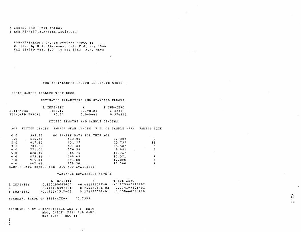
$ ASSIGN BGCII.DAT FOR005 $ RUN FSHA: [712.MASTER.XEQ]BGCII
VON-BERTALANFY GROWTH PROGRAM --BGC II Written by N.J. Abramson, Cal. F+G, May 1964 VAX 11/780 Ver. 1.0 14 Nov 1983 R.K. Mayo
VON BERTALANFFY GROWTH IN LENGTH CURVE
BGCII SAMPLE PROBLEM TEST DECK
ESTIMATED PARAMETERS AND STANDARD ERRORS
L INFINITY ESTIMATES 1102.17 STANDARD ERRORS 90.84
K 0.190181 0.049441
T SUB-ZERO -2.3232
0.574846
FITTED LENGTHS AND SAMPLE LENGTHS
AGE FITTED LENGTH SAMPLE MEAN LENGTH S . E. OF SAMPLE MEAN SAMPLE SIZE
0.0 393.62 NO SAMPLE DATA FOR THIS AGE 1.0 516.34 512.00 2.0 617.80 631.27 3.0 701.69 671.83 4.0 771.04 770.56 5.0 828.39 848.75 6.0 875.81 869.43 7.0 915.01 893.80 8.0 947.43 978.50
SAMPLE DATA BEYOND AGE 8.0 NOT AVAILABLE
VARIANCE-COVARIANCE MATRIX
L INFINITY K L INFINITY 0.82519908E+04 -0.44147839E+01 K -0.44147839E+01 0.24443913E-02 T SUB-ZERO -0.47356251E+02 0.27419950E-01
STANDARD ERROR OF ESTIMATE-- 43.7393
PROGRAMMED BY - BIOMETRICAL ANALYSIS UNIT MRO, CALIF. FISH AND GAME MAY 1964 - BGC II
$ $
17.302 15.737 18.582
9.982 11. 747 13.571 17.028 14.500
T SUB-ZERO -0.47356251E+02 0.27419950E-01 0.33044823E+00
.9 11
6 9
8 7 5 2
< H
<.N
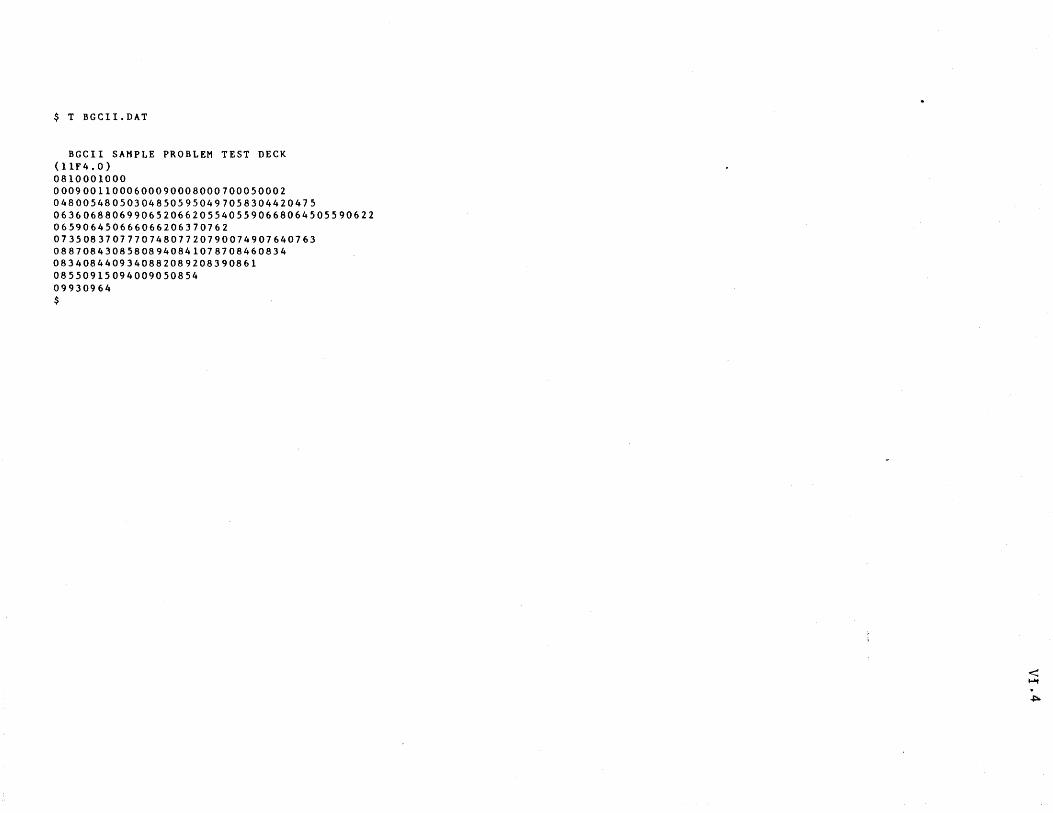
$ T BGClI.DAT
BGCll SAMPLE PROBLEM TEST DECK (11F4.0) 0810001000 00090011000600090008000700050002 048005480503048505950497058304420475 06360688069906520662055405590668064505590622 065906450666066206370762 073508370777074807720790074907640763 08870843085808940841078708460834 0834084409340882089208390861 08550915094009050854 09930964 $
< ..... .;::..
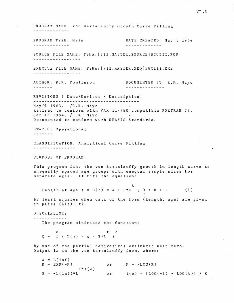
PROGRAM NAME: von Bertalanffy Growth Curve Fitting
PROGRAM TYPE: Main DATE CREATED: May 1 1964
SOURCE FILE NAME: FSHA: [712.MASTER.SOURCE]BGCIII.FOR
EXECUTE FILE NAME: FSHA: [712.MASTER.XEQ]BGCIII.EXE
AUTHOR: P.K. Tomlinson DOCUMENTED BY: R:K. Mayo
REVISIONS ( Date/Reviser - Description)
MayOl 1983. /R.K. Mayo. Revised to conform with VAX 11/780 compatible FORTRAN 77. Jan 16 1984. /R.K. Mayo. Documented to conform with NERFIS Standards.
STATUS: Operational
CLASSIFICATION: Analytical Curve Fitting
PURPOSE OF PROGRAM:
VI.5
This program fits the von Bertalanffy growth in length curve to unequally spaced age groups with unequal sample sizes for separate ages. It fits the equation:
t Length at age t = D(t) = A + B*R o < R < 1 ( 1 )
by least squares when data of the form (length, ag"e) are given in pairs (L( t), t).
DESCRIPTION:
The program minimizes the function:
n t 2 Q = L: ~ L ( t) - A - B *R )
by use of the partial derivatives evaluated near zero. Output is in the von Bertalanffy form, where:
A L ( i nf ) R EXP(-K) or K = -LOG(R)
K*t(o) B -L(inf)*L or t(o) = [LOG(-B) LOG (A) ] / K
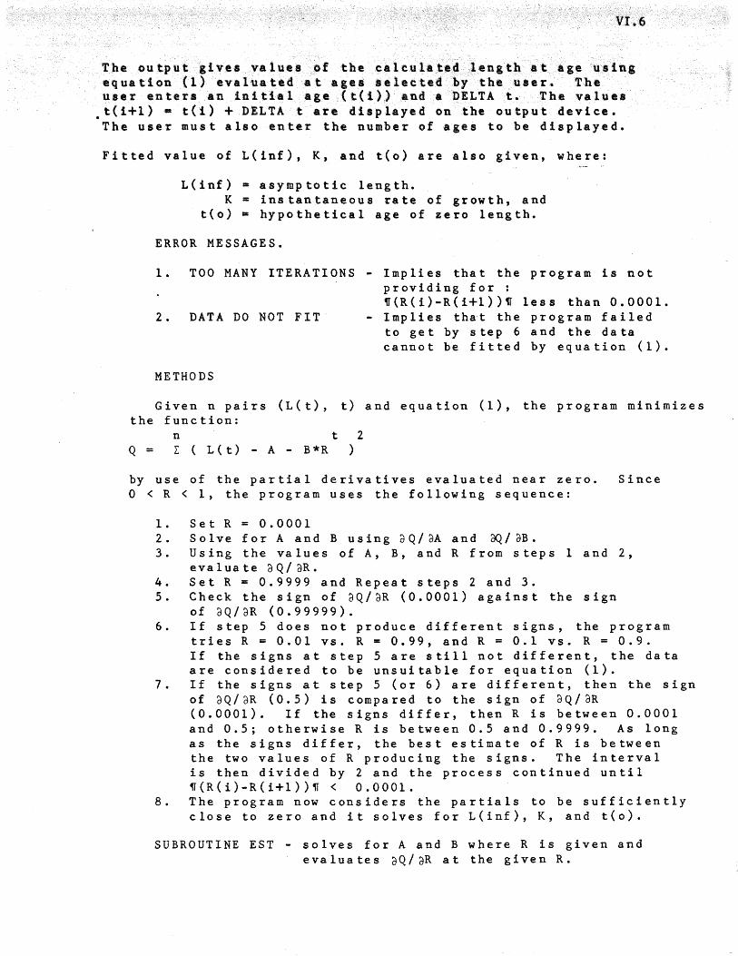
VI.6
The output gives values of the calculated length4lt ageuaina equation (1) evaluated at agel aelected by the user. The userenters an initial age (t(i»and a DELTA t. The values
.t(i+l) • tel) + DELTA t are displayed on the output device. The user must also enter the number of ages to be di~played.
Fitted value of L(inf), K, and t(o) are also given, where:
L(inf) • asymptotic length. K • instantaneous rate of growth, and
t(o) • hypothetical age of zero length.
ERROR MESSAGES.
1. TOO MANY ITERATIONS - Implies that the program is not providing for : '(R(i)-R(i+l»V less than 0.0001 •
2. DATA DO NOT FIT • Implies that the program failed to get by step 6 and the data cannot be fitted by equation (1).
METHODS
Given n pairs (L(t), t) and equation (1), the program minimizes the function:
n t 2 Q = L ( L(t) . A - B*R )
by use of the partial derivatives evaluated near zero. o < R < 1, the program uses the following sequence:
1. Set R = 0.0001 2. Solve for A and Busing 'dQ/aA and dQ/aB.
Since
3. Using the values of A, B, and R from steps 1 and 2, e val u ate a Q / aR.
4. Set R = 0.9999 and Repeat steps 2 and 3. 5. Check the sign of aQ/aR (0.0001) against the sign
of aQ/aR (0.99999). 6. If step 5 does not produce different signs, the program
tries R = 0.01 vs. R = 0.99, and R = 0.1 vs. R = 0.9. If the signs at step 5 are still not different, the data are considered to be unsuitable for equation (1).
7. If the signs at step 5 (or 6) are different, then the sign of aQ/aR (0.5) is compared to the sign of aQ/dR (0.0001). If the signs differ, then R is between 0.0001 and 0.5; otherwise R is between 0.5 and 0.9999. As long as the signs differ, the best estimate of R is between the two values of R producing the signs. The interval is then divided by 2 and the process continued until ~(R(i)-R(i+l»~ < 0.0001.
8. The program now considers the partials to be sufficiently close to zero and it solves for L(inf), K, and teo).
SUBROUTINE EST - solves for A and B where R is given and evaluates aQ/aR at the given R.
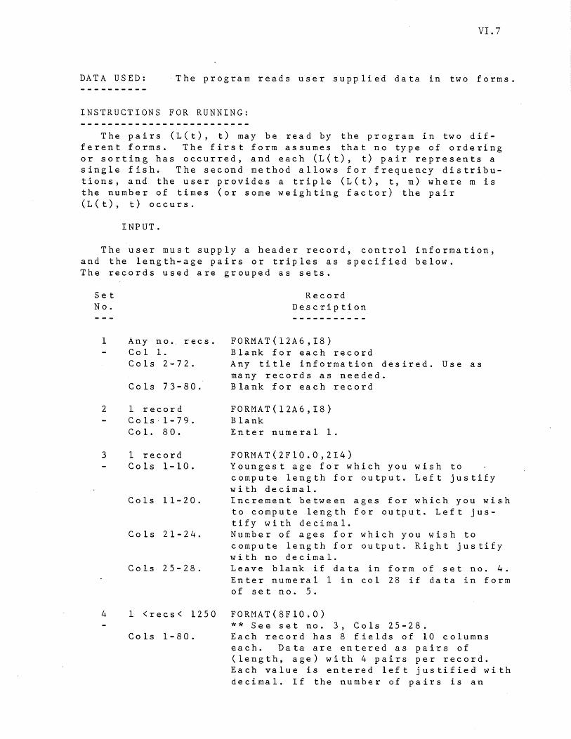
VI.7
DATA USED: The program reads user supplied data in two forms.
INSTRUCTIONS FOR RUNNING:
The pairs (L(t), t) may be read by the program in two different forms. The first form assumes that no type of ordering or sorting has occurred, and each (L(t), t) pair represents a single fish. The second method allows for frequency distributions, and the user provides a trip 1e (L (t), t, m) where m is the number of times (or some weighting factor) the pair (L(t), t) occurs.
INPUT.
The user must supply a header record, control information, and the length-age pairs or triples as specified below. The records used are grouped as sets.
Set No.
1
2
3
Any no. recs. Co 1 1. Co1s 2-72.
Co1s 73-80.
1 record Co1s·1-79. Col. 80.
1 record Co1s 1-10.
Co1s 11-20.
Co1s 21-24.
Co1s 25-28.
Record Description
FORMAT(12A6,I8) Blank for each record Any title information desired. Use as many records as needed. Blank for each record
FORMAT(12A6,I8) Blank Enter numeral 1.
FORMAT(2F10.0,2I4) Youngest age for which you wish to compute length for output. Left justify with decimal. Increment between ages for which you wish to compute length for output. Left justify with decimal. Number of ages for which you wish to compute length for output. Right justify with no decimal. Leave blank if data in form of set no. 4. Enter numeral 1 in col 28 if data in form of set no. 5.
4 1 <recs< 1250 FORMAT(8F10.0)
Co1s 1-80. ** See set no. 3, Co1s 25-28. Each record has 8 fields of 10 columns each. Data are entered as pairs of (length, age) with 4 pairs per record. Each value is entered left justified with decimal. If the number of pairs is an
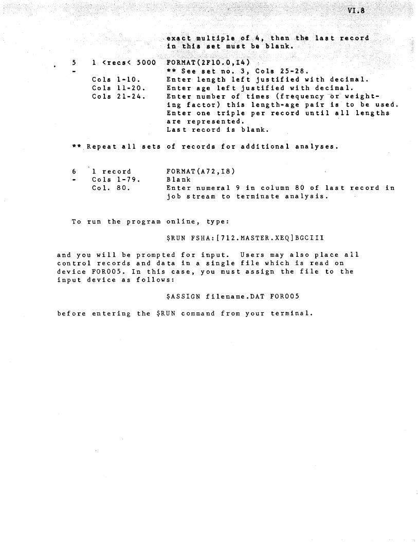
ex.c~ multiple of4, then the lastrecor4 lnt.hi. let must be blank..
5 1 ( r e c s < 5 000 '0 aKA T ( 2 F 10 .0 ,14 )
Cols 1-10. Cols 11-20. Cols 21-24.
**See set no. 3, Cola 25-28. Enter length left justified with decimal. Enter age left justified with decimal. Enter number of times (frequency ~rweight-ing factor) this length-age pair is to be used. Enter one triple per record until all lengths are represented. Last record is blank.
** Repeat all sets of records for additional analyses.
6 1 record Cols 1-79. Col. 80.
FORMAT(A72,I8) Blank Enter numeral 9 in column 80 of last record in job stream to terminate analysis.
To run the program online, type:
$RUN FSHA:[7l2.MASTER.XEQ]BGCIII
and you will be prompted for input. Users may also place all control records and data in a single file which is read on device FOR005. In this case, you must assign the file to the input device as follows:
$ASSIGN filename.DAT FOR005
before entering the $RUN command from your terminal.
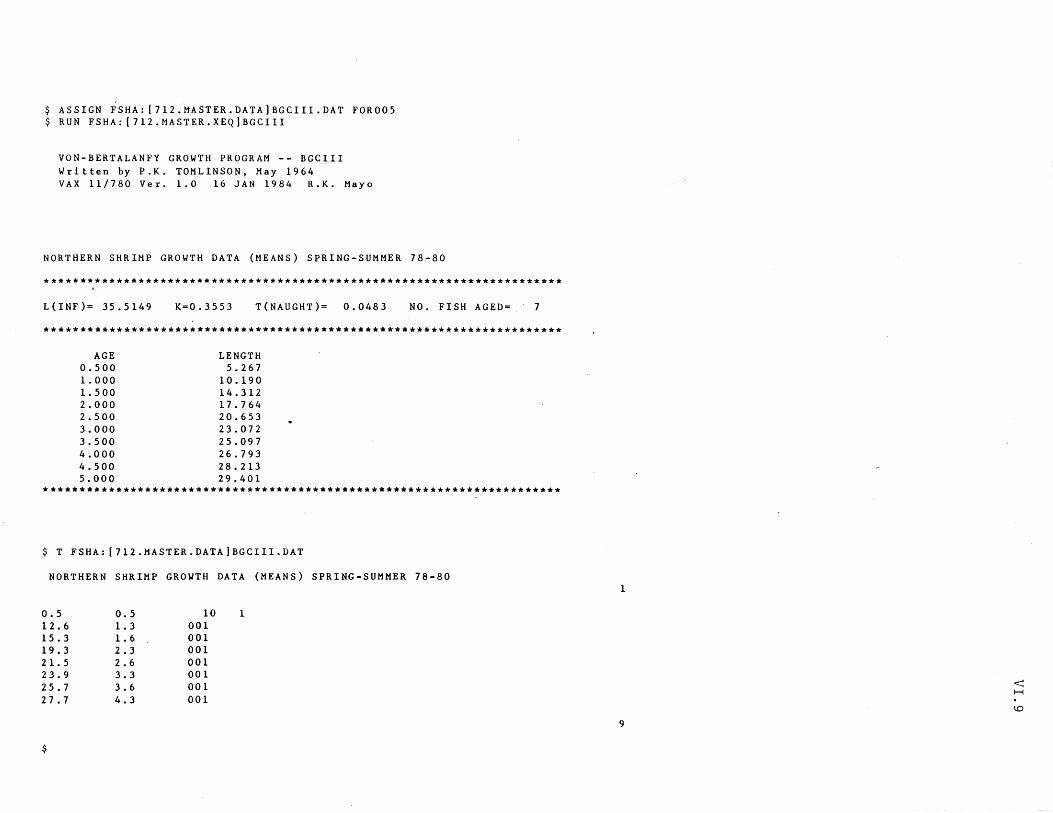
$ ASSIGN FSHA: [712.MASTER.DATA]BGCIII.DAT FOR005 $ RUN FSHA: [712.MASTER.XEQ]BGCIII
VON-BERTALANFY GROWTH PROGRAM -- BGCIII Written by P.K. TOMLINSON, May 1964 VAX 11/780 Ver. 1.0 16 JAN 1984 R.K. Mayo
NORTHERN SHRIMP GROWTH DATA (MEANS) SPRING-SUMMER 78-80
***********************************************************************
L(INF)= 35.5149 K=0.3553 T(NAUGHT)= 0.0483 NO. FISH AGED= . 7
***********************************************************************
AGE 0.500 1.000 1.500 2.000 2. 500 3.000 3.500 4.000 4.500 5.000
LENGTH 5.267
10.190 14.312 17 .. 764 20.653 23.072 25.097 26.793 28.213 29.401
***********************************************************************
$ T FSHA: [712.MASTER.DATA]BGCIII.DAT
NORTHERN SHRIMP GROWTH DATA (MEANS) SPRING-SUMMER 78-80
0.5 0.5 10 1 12.6 1.3 001 15.3 1.6 001 19.3 2.3 001 21.5 2.6 001 23.9 3.3 001 25.7 3.6 001 27.7 4.3 001
$
1
9
< H
!,Q
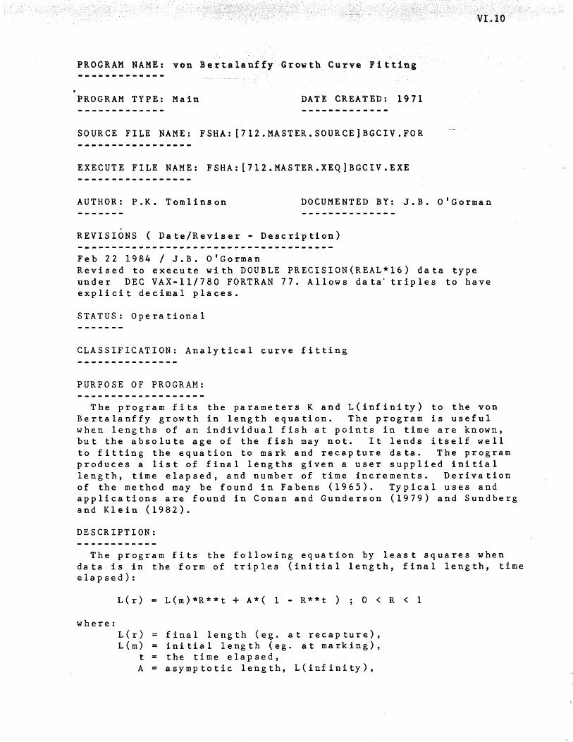
VI.10
PROGRAM NAME: von Bertalanffy Growth Curve Flttlni
PROGRAM TYPE: Main DATE CREATED: 1971
SOURCE FILE NAME: FSHA: [712.MASTER.SOURCE]BGCIV;FOR
EXECUTE FILE NAME: FSHA:[712.MASTER.XEQ]BGCIV.EXE
AUTHOR: P.K. Tomlinson DOCUMENTED BY: J.B. O'Gorman
REVISIONS ( Date/Reviser - Description)
Feb 22 1984 / J.B. O'Gorman Revised to execute with DOUBLE PRECISION(REAL*16) data type under DEC VAX-11/780 FORTRAN 77. Allows data" triples to have explicit decimal places.
STATUS: Operational
CLASSIFICATION: Analytical curve fitting
PURPOSE OF PROGRAM:
The program fits the parameters K and L(infinity) to the von Bertalanffy growth in length equation. The program is useful when lengths of an individual fish at points in time are known, but the absolute age of the fish may not. It lends itself well to fitting the equation to mark and recapture data. The program produces a list of final lengths given a user supplied initial length, time elapsed, and number of time increments. Derivation of the method may be found in Fabens (1965). Typical uses and applications are found in Conan and Gunderson (1979) and Sundberg and Klein (1982).
DESCRIPTION:
The program fits the following equation by least squares when data is in the form of triples (initial length, final length, time elapsed):
where:
L(r) = L(m)*R**t + A*( 1 - R**t ) o < R < 1
L(r) = final length (eg. at recapture), L(m) = initial length (eg. at marking),
t the time elapsed, A = asymptotic length, L(infinity),
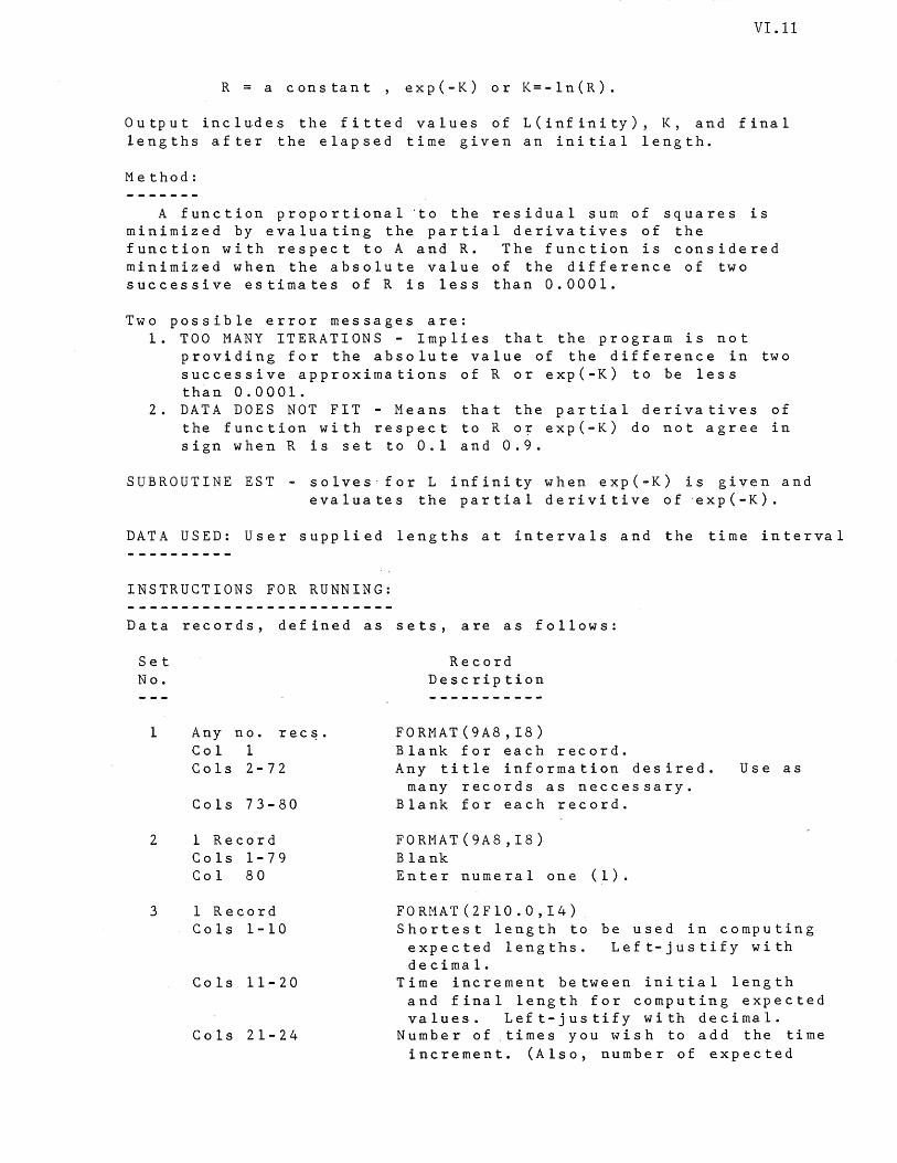
VI.II
R = a constant, exp(-K) or K=-ln(R).
Output incllldes the fitted values of L(infinity), K, and final lengths after the elapsed time given an initial length.
Method:
A function proportional 'to the residual sum of squares is minimized by evaluating the partial derivatives of the function with respect to A and R. The function is considered minimized when the absolute value of the difference of two successive estimates of R is less than 0.0001.
Two possible error messages are: 1. TOO MANY ITERATIONS - Implies that the program is not
providing for the absolute value of the difference in two successive approximations of R or exp(-K) to be less than 0.0001.
2. DATA DOES NOT FIT - Means that the partial derivatives of the function with respect to R or exp(-K) do not agree in sign when R is set to 0.1 and 0.9.
SUBROUTINE EST solves-for L infinity when exp(-K) is given and evaluates the partial derivitive of ·exp(-K).
DATA USED: User supplied lengths at intervals and the time interval
INSTRUCTIONS FOR RUNNING:
Data records, defined as sets, are as follows:
Set No.
1
2
3
Any no. r e c ~ . Col 1 Cols 2-72
Cols 73-80
1 Record Cols 1-79 Col 80
1 Record Cols 1-10
Cols 11-20
Cols 21-24
Record Descrip tion
FORMAT(9A8,I8) Blank for each record. Any title information desired.
many records as neccessary. Blank for each record.
FORMAT(9A8,I8) Blank Enter numeral one (1).
FORMAT(2F10.0,I4)
Use as
Shortest length to be used in computing expected lengths. Left-justify with dec i ma 1 .
Time increment between initial length and final length for computing expected values. Left-justify with decimal.
Number of .times you wish to add the time increment. (Also, number of expected
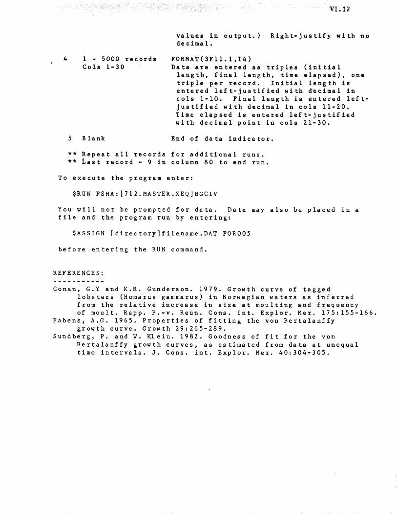
4 1 - 5000 records Cola 1-30
5 Blank
VI.,12
value. in output.) Right-justify with no decimal.
FORMAT(3Fll.l,I4) Data are entered as triples (initial
length, final length, time elapsed), one triple per record. Initial length is entered left-justified with d'ec~mal in cols 1-10. Final length is entered leftjustified with decimal in cols 11-20. Time elapsed is entered left-justified with decimal point in cols 21-30.
End of data indicator.
** Repeat all records for additional runs. ** Last record - 9 in column 80 to end run.
To execute the program enter:
$RUN FSHA:[712.MASTER.XEQ]BGCIV
You will not be prompted for data. Data may also be placed in a file and the program run by entering:
$ASSIGN [directory]filename.DAT FOR005
before entering the RUN command.
REFERENCES:
Conan, G.Y and K.R. Gunderson. 1979. Growth curve of tagged lobsters (Homarus gammarus) in Norwegian waters as inferred from the relative increase in size at moulting and frequency of moult. Rapp. P.-v. Reun. Cons. into Explor. Mer. 175: 155-166.
Fabens, A.G. 1965. Properties of fitting the von Bertalanffy growth curve. Growth 29:265-289.
Sundberg, P. and W. Klein. 1982. Goodness of fit for the von Bertalanffy growth curves, as estimated from data at unequal time intervals. J. Cons. into Explor. Mer. 40:304-305.
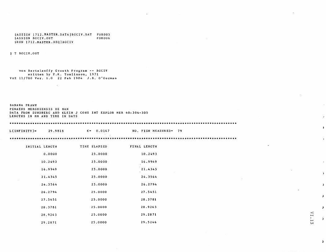
$ASSIGN L712.MASTER.DATA]BGCIV.DAT $ASSIGN BGCIV.OUT $RUN L712.MASTER.XEQ]BGCIV
$ T BGCIV.OUT
FOR005 FOR006
von Bertalanffy Growth Program -- BGCIV written by P.K. Tomlinson, 1971
VAX 11/780 Vera 1.0 22 Feb 1984 J.B. O'Gorman
BANANA PRAWN PENAEUS MERGUIENSIS DE MAN DATA FROM SUNDBERG AND KLEIN J CONS INT EXPLOR MER 40:304-305 LENGTHS IN MM AND TIME IN DAYS
****************************************************************************************************
L(INFINITY)-= 29.9818 K= 0.0167 NO. FISH MEASURED= 79
***************************;************************************************************************
INITIAL LENGTH TIME ELAPSED FINAL LENGTH
0.0000 25.0000 10.2493
10.2493 25.0000 16.9949
16.9949 25.0000 21.4345
21.4345 25.0000 24.3564
24.3564 25.0000 26.2794-
26.2794 25.0000 27.5451
27.5451 25.0000 28.3781
28.3781 25.0000 28.9263
28.9263 25.0000 29.2871
29.2871 25.0000 29.5246
)
)
< H
f-I. Vl
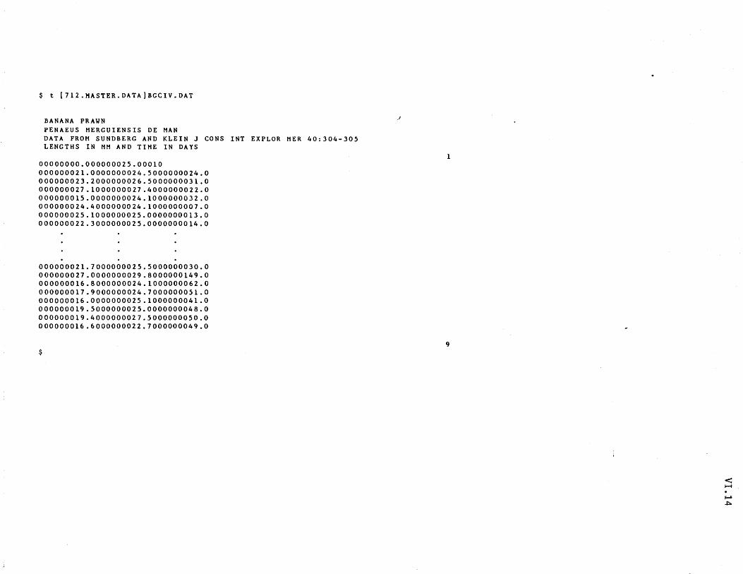
$ t [712.HASTER.DATA)BGCIV.DAT
BANANA PRAWN PENAEUS MERGUIENSIS DE MAN DATA FROM SUNDBERG AND KLEIN J CONS INT EXPLOR MER 40:304-305 LENGTHS IN HH AND TIME IN DAYS
00000000.000000025.00010 000000021.0000000024.5000000024.0 000000023.2000000026.5000000031.0 000000027.1000000027.4000000022.0 000000015.0000000024.1000000032.0 000000024.4000000024.1000000007.0 000000025.1000000025.0000000013.0 000000022.3000000025.0000000014.0
000000021.7000000025.5000000030.0 000000027.0000000029.8000000149.0 000000016.8000000024.1000000062.0 000000017.9000000024.7000000051.0 000000016.0000000025.1000000041.0 000000019.5000000025.0000000048.0 000000019.4000000027.5000000050.0 000000016.6000000022.7000000049.0
$
.J
1
9
< H
'""" ~
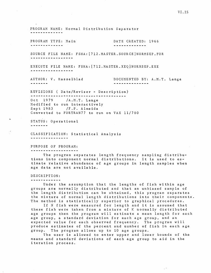
VI.IS
PROGRAM NAME: Normal Distribution Separator
PROGRAM TYPE: Main DATE CREATED: 1966
SOURCE FILE NAME: FSHA: [712.MASTER.SOURCE]NORMSEP.FOR
EXECUTE FILE NAME: FSHA: [712.MASTER.XEQ]NORMSEP.EXE
AUTHOR: V. Hasse1b1ad DOCUMENTED BY: A.M.T. Lange
REVISIONS ( Date/Reviser - Description)
Oct 1979 /A.M.T. Lange Modified to run interactively Sept 1983 /F.P. Almeida Converted to FORTRAN77 to run on VAX 11/780
STATUS: Operation&l
CLASSIFICATION: Statistical Analysis
PURPOSE OF PROGRAM:
The program separates length frequency sampling distributions into component normal distributions. It is used to estimate relative abundance of age groups in length samples when age data are not available.
DESCRIPTION:
Under the assumption that the lengths of fish within age groups are normally distributed and that an unbiased sample of the length distribution can be obtained, this program separates the mixture of normal length distributions into their components. The method is statistically superior to graphical procedures.
If N fish were measured for length and it is assumed that these fish were taken from a mixture of K normally distributed age groups then the program will estimate a mean length for each age group, a standard deviation for each age group, and an expected value for each observed frequency. The program will produce estimates of the percent and number of fish in each age group. The program allows up to 10 age groups.
The user is allowed to enter upper and lower bounds of the means and standard deviations of each age group to aid in the iteration process.
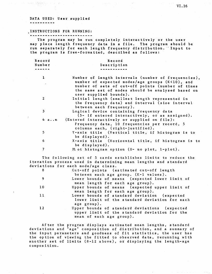
VI.16
DATA USED: User supplied
INSTRUCTIONS FOR RUNNING:
The program may be run completely interactively or the user may place length frequency data in a file. The program should be run s epa rat ely for e a c h 1 eng t h f r e que n c y dis t rib uti 0 n. ','- 1 n put to the program is free-formatted, described as follows:
Record Number
1
2
3
4 a .• n
5
6
7
Record Description
Number of length intervals (number of frequencies), n~mber of expected modes/age groups (K<lO), and number of sets of cut-off points (number of times the same set of modes should be analysed based on user supplied bounds).
Initial length (smallest length represented in the frequency data) and interval (size interval between each frequency).
Logical device containing frequency data (5- if entered interactively, or as assigned).
(Entered interactively or supplied on file): Frequency data, 10 frequencies per record, 5 columns each, (right-justified).
Y-axis title (Vertical title, if histogram is to be displayed).
X-axis title (Horizontal title, if histogram is to be displayed).
Plot his tog ram 0 p t ion (O - n 0 p lot, 1 - P lot) •
The following set of 5 cards establishes limits to reduce the iteration process used in determining mean lengths and standard deviations for each mode/age class.
8 Cut-off points (estimated cut-off length b e tw e en e a c hag e g r 0 up. ( K - 1 val u e s ) •
9 Lower bounds of means (expected lower limit of mean length for each age group).
10 Upper bounds of means (expected upper limit of mean length for each age group).
11 Lower bounds of standard deviation (expected lower limit of the standard deviation for each age group).
12 Upper bounds of standard deviations (expected upper limit of the standard deviation for the mean of each age group).
After the program displays estimated mean lengths, standard deviations and 'age' composition of distribution, and a summary of the input parameters and goodness of fit statistics, the user has the option of viewing the fitted to observed data, rerunning with another set of limits (8-12 above), or displaying the length-age composition.
VI.17
To run the program interactively, type:
$RUN FSHA: [7l2.MASTER.XEQ]NORMSEP
and you will be prompted for all values, or create a data file with the frequency data (4 a .. n) and use:
$ASSIGN datafile.DAT FOR $RUN FSHA: [712.MASTER.XEQ]NORMSEP
( represents the logical device number your data file will be assigned in the program.)
REFERENCES:
Tomlinson, P.K. 1971. Program name - NORMSEP. Programmed by V. Hasselblad. In N.J. Abramson (compiler). Computer programs f o. r f ish s to c k ass e ssm e n t. lOp. F AO, F ish. T e c h. Pap. 101.
Hasselblad, V. 1966. Estimation of parameters for a mixture of mixed normal distributions. Technometrics 8(3):431-444.
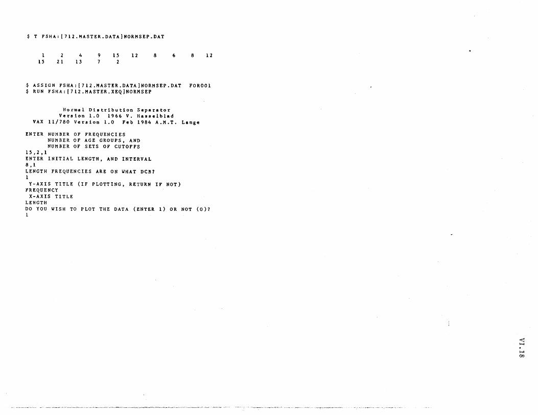
$ T FSHA: [712.HASTER.DATAINORHSEP.DAT
1 15
2 21
4 13
9 7
15 2
12 8 6 8 12
$ ASSIGN FSHA:[712.HASTER.DATAjNORHSEP.DAT FOR001 $ RUN FSHA:[712.HASTER.XEQ]NORHSEP
Normal Distribution Separator Version 1.0 1966 V. Hasse1b1ad
VAX 11/780 Version 1.0 Feb 1984 A.H.T. Lange
ENTER NUMBER OF FREQUENCIES NUMBER OF AGE GROUPS, AND NUMBER OF SETS OF CUTOFFS
15,2 ,1 ENTER INITIAL LENGTH, AND INTERVAL 8,1 LENGTH FREQUENCIES ARE ON WHAT DC!? 1
Y-AXIS TITLE (IF PLOTTING, RETURN IF NOT) FREQUENCY
X-AXIS TITLE LENGTH DO YOU WISH TO PLOT THE DATA (ENTER 1) OR NOT (0)1 1
..-.::; H
~
00
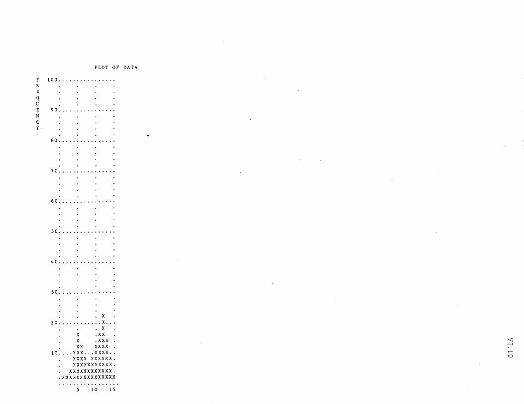
< Eo-<
< CI
"" 0 Eo-< 0 ....:I 0...
o o .-4
o CO
o ,.... o If')
X
VI.1
9
X X
X
X
X X
X
XX
X
'X
x •
·XX
X
x x
X X
X
X
X
X
xxx
xxx
xx
x x
x x
x x
xx x
xx x
0 .-4
x •
If')
x x
• .-4
X
X
X X
x
x xx ·0
xx
xx
xx
Xx
xx
If')
xx
xx
·X
x
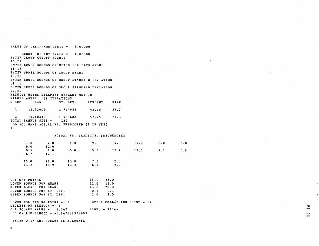
VALUE OF LEFT-HAND LIMIT
LENGTH OF INTERVALS ENTER GROUP CUTOFF POINTS 15,22
8.00000
1.00000
ENTER LOWER BOUNDS OF MEANS FOR EACH GROUP. 11,18 ENTER UPPER BOUNDS OF GROUP MEANS 13,20 ENTER LOWER BOUNDS OF GROUP STANDARD DEVIATION .1, .1 ENTER UPPER BOUNDS OF GROUP STANDARD DEVIATION 2. ,2. RESULTS USING STEEPEST DESCENT METHOD VALUES AFTER 29 ITERATIONS GROUP MEAN
1 12.92605
2 19.10436 TOTAL SAMPLE SIZE
ST. DEV.
1. 754952
1.583688 135
PERCENT
42.75
57.25
DO YOU WANT ACTUAL VS. PREDICTED (1 IF YES) 1
SIZE
57.7
77.3
ACTUAL VS. PREDICTED FREQUENCIES
1.0 2.0 8.0 12.0 0.5 2.0 6.7 12.1
15.0 21.0 18.2 18.9
CUT-OFF POINTS LOWER BOUNDS FOR MEANS UPPER BOUNDS FOR MEANS LOWER BOUNDS FOR ST. DEV. UPPER BOUNDS FOR ST. DEV.
4.0
5.0
13.0 13.2
9.0
9.4
7.0 6.2
15.0 11.0 13.0 0.1 2.0
15.0
12. 7
23.0 18.0 20.0
0.1 2.0
2.0 2.0
12.0
12. 5
LOWER COLLAPSING POINT = 3 UPPER COLLAPSING POINT DEGREES OF FREEDOM = 6 CHI SQUARE VALUE = 1.747 PROBe =.94144 LOG OF LIKELIHOOD = -0.14768233E+03
ENTER 0 IF CHI SQUARE IS ADEQUATE
o
8.0
9.1
14
6.0
5.9
-< H
N o
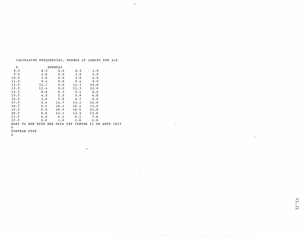
CALCULATED FREQUENCIES, NUMBER AT LENGTH PER AGE
X NUMBERS B.5 0.5 0.0 0.5 1.0 9.5 2.0 0.0 2.0 2.0
10.5 5.0 0.0 5.0 4.0 11.5 9.4 0.0 9.4 9.0 12.5 12.7 0.0 12.7 15.0 13.5 12.4 0.0 12.5 12.0 14.5 B.B 0.3 9.1 B.O 15.5 4.5 1.5 5.9 6.0 16.5 1.6 5.0 6.7 B.O 17.5 0.4 11. 7 12.1 12.0 lB.5 0.1 lB.1 1B.2 15.0 19.5 0.0 1B.9 1B.9 21.0 20.5 0.0 13.2 13.2 13.0 21.5 0.0 6.2 6.2 7.0 22. 5 0.0 2.0 2.0 2.0 WANT TO RUN WITH NEW DATA SET (ENTER 1 ) OR QUIT (0)1 0 FORTRAN STOP $
< H
N f-4
Related Documents