11007386.pdf - Enlighten: Theses - University of Glasgow

https://theses.gla.ac.uk/

Theses Digitisation:

https://www.gla.ac.uk/myglasgow/research/enlighten/theses/digitisation/

This is a digitised version of the original print thesis.

Copyright and moral rights for this work are retained by the author

A copy can be downloaded for personal non-commercial research or study,

without prior permission or charge

This work cannot be reproduced or quoted extensively from without first

obtaining permission in writing from the author

The content must not be changed in any way or sold commercially in any

format or medium without the formal permission of the author

When referring to this work, full bibliographic details including the author,

title, awarding institution and date of the thesis must be given

Enlighten: Theses

https://theses.gla.ac.uk/

[email protected]

NEW METHODS IN GRAVITATIONAL AND SEISMIC REFLECTION EXPLORATION

XIN QUAN MA B. sc.

A thesis submitted fo r the degree o f Doctor o f Philosophy at the Department o f Geology & Applied Geology, University o f Glasgow.

ProQuest Number: 11007386

All rights reserved

INFORMATION TO ALL USERS The quality of this reproduction is dependent upon the quality of the copy submitted.

In the unlikely event that the author did not send a com p le te manuscript and there are missing pages, these will be noted. Also, if material had to be removed,

a note will indicate the deletion.

uestProQuest 11007386

Published by ProQuest LLC(2018). Copyright of the Dissertation is held by the Author.

All rights reserved.This work is protected against unauthorized copying under Title 17, United States C ode

Microform Edition © ProQuest LLC.

ProQuest LLC.789 East Eisenhower Parkway

P.O. Box 1346 Ann Arbor, Ml 48106- 1346

Dedicated to my parents

Contents

Declaration

Acknowledgements

Preface

Summary

List of Figures

List of Tables

P a rt one: G ravity

Chapter 1 Automatic Terrain Correction Method for Regional Gravity Survey

1.1 Introduction ............................................................................................................... 1

1. 2 New approach to an automatic terrain correction method .................................. 3

1.3 Distant zone contribution ........................................................................................ 4

1.4 Intermediate zone contribution .............................................................................. 7

1.5 Near zone 2 contribution ........................................................................................ 8

1.6 Near zone 1 contribution ......................................................................................... 11

1.7 Fortran-77 program MATERRAIN ...................................................................... 21

1. 8 Real gravity data test and accuracy consideration ........................................... 23

1.9 Summary .................................................................................................................... 30

P art tw o: Reflection Seismology

Chapter 2 Methodology and Approach of New Seismic Reflection Experiment

2.1 Introduction ............................................................................................................. 34

2.2 Review of noise problems on basalt-covered areas studied by previous authors 34

2.3 Array design ............................................................................................................ 36

2.4 Three-component seismic data acquisition ........................................................ 39

2.4.1 Area chosen for the investigation ............................................................... 39

2.4.2 Instrum entation ............................................................................................. 39

2.4.3 Field survey .................................................................................................. 43

2.4.4 Field work preparation ............................................................................. 44

I I

2.4.5 Field work procedures ................................................................................. 46

2.5 Interaction with the seismic data processing package SKS ................................. 48

2.5.1 Introduction to the SKS package ............................................................... 48

2.5.2 Change of SEG-Y format into free ASCII-coded format ............................ 49

2.6 Three-component data transformation ................................................................ 53

2.6.1 Theory and method for transformation ...................................................... 53

2.6.2 Fortran-77 program MATRAN ................................................................... 55

2.7 Seismic data display using the UNIRAS package ............................................. 57

2.7.1 Introduction to the UNIRAS package .......................................................... 57

2.7.2 Plotting seismic traces in the normal way ................................................... 58

2.7.3 Combination of a gain control program with the plotting package .............. 58

2.8 Static correction ............................................................. 61

Chapter 3 Characterization of 3-component Seismic Data from a

Basalt-covered Area

3.1 Introduction ................................................................................................................ 65

3.2 Correlation between the penetration of seismic energy and charge size ............... 65

3.3 Characteristics of seismic reflection data in a basalt-covered area ..................... 67

3.4 Detection of energy distribution using spatial directional filtering .................... 75

3.4.1 Introduction to a spatial directional filter (SDF) ...................................... 75

3.4.2 Design of the spatial directional filter ....................................................... 76

3.4.3 Fortran-77 program MASDF ......................................................................... 78

3.4.4 Application of the MASDF filter for analysis of 3-component data .......... 80

3.5 Summary ..................................................................................................................... 87

Chapter 4 Data Processing and Interpretation

4.1 Introduction ............................................................................................................... 88

4.2 Pre-editing 3-component seismic data .................................................................. 88

4.3 Frequency filtering .................................................................................................. 89

4.4 Predictive deconvolution filtering ........................................................................ 91

4.5 Signal enhancement polarisation filtering (SEPF) ............................................. 92

4.5.1 Introduction to the SEPT filter .................................................................... 92

4.5.2 Design of the SEPF filter .............................................................................. 95

I l l

4.5.3 Fortran-77 program MASEPF ..................................................................... 98

4.5.4 Program test using noise and field 3-component data .............................. 101

4.5.5 Selection of an appropriate window length for filtering .......................... 103

4.5.6 Application of the MASEPF to the data from the basalt-covered a re a 105

4.6 Other data processing ............................................................................................ 110

4.7 Interpretation ............................................................................................................ 110

4.8 Summary .................................................................................................................... I l l

Chapter 5: Further Testing of the Polarisation Filter and Optimisation of

Array Designing Using Synthetic 3-component Seismic Data

5.1 Introduction ............................................................................................................... 112

5.2 Filter testing using the data in an isotropic medium .......................................... 112

5.2.1 Introduction to the modelling package "SEIS83" ..................................... 112

5.2.2 Geological model in an isotropic medium ................................................. 113

5.2.3 Generating and filtering "one shot - one receiver" data along a

profile line ......................................................................................................... 114

5.2.4 Generating the data based on the aerial ’RAZOR' array in an

isotropic medium ........................................................................................... 118

5.2.5 Processing the data based on the aerial array in an isotropic m edium 120

5.3 Filter testing using the data in an anisotropic medium ........................................ 124

5.3.1 Introduction to the modelling package "ANISEIS" .................................. 124

5.3.2 Geological model 1 in an anisotropic medium ............................. 125

5.3.3 Processing the data based on mode 1 in the anisotropic medium ............... 127

5.3.4 Geological model 2 in an anisotropic medium ............................ 130

5.3.5 Processing the data based on model 2 in the anisotropic medium ............... 131

5.4 Effect of characteristics of noise on filtering ........................................................ 131

5.5 Summary ...................................................................................................................... 134

Chapter 6 Imaging structure by slant-slack processing

6.1 Introduction ................................................................................................................ 137

6.2 Introduction to conventional slant-stack processing ............................................ 137

6.3 Imaging structure by slant-stack processing ........................................................ 139

6.4 Fortran-77 program MASSP ................................................................................... 144

6.5 Implementation of slant-stack processing on synthetic data to image structure .. 146

IV

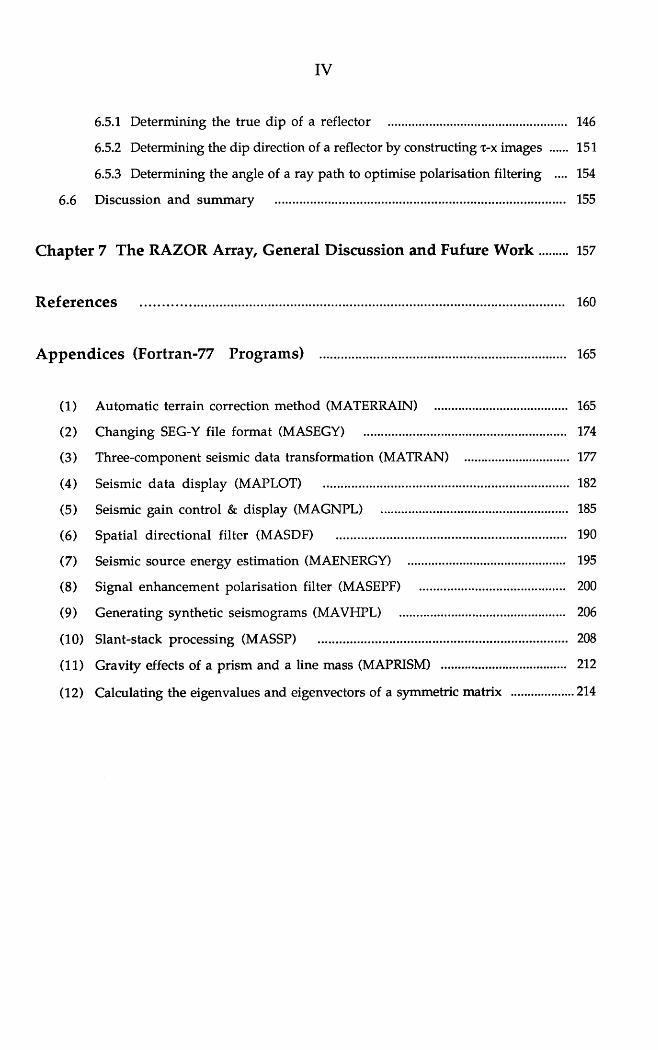
6.5.1 Determining the true dip of a reflector ..................................................... 146

6.5.2 Determining the dip direction of a reflector by constructing t - x images ..... 151

6.5.3 Determining the angle of a ray path to optimise polarisation filtering .... 154

6.6 Discussion and summ ary ...................................................................................... 155

Chapter 7 The RAZOR Array, General Discussion and Future W ork 157

R e f e re n c e s ............................................................................................................................... 160

A p p e n d ic e s (F o rtra n -7 7 P ro g ra m s ) .......................................................................... 165

(1) Automatic terrain correction method (MATERRAIN) ...................................... 165

(2) Changing SEG-Y file format (MASEGY) ........................................................... 174

(3) Three-component seismic data transformation (MATRAN) .............................. 177

(4) Seismic data display (MAPLOT) ......................................................................... 182

(5) Seismic gain control & display (MAGNPL) ....................................................... 185

(6) Spatial directional filter (MASDF) .................................................................... 190

(7) Seismic source energy estimation (MAENERGY) .............................................. 195

(8) Signal enhancement polarisation filter (MASEPF) .......................................... 200

(9) Generating synthetic seismograms (MAVHPL) ................................................ 206

(10) Slant-stack processing (MASSP) .......................................................................... 208

(11) Gravity effects of a prism and a line mass (MAPRISM) .................................... 212

(12) Calculating the eigenvalues and eigenvectors of a symmetric matrix .................. 214

V

D e c l a r a t i o n

The m aterial presented herein is the result o f my independent research

undertaken between April 1987 and April 1990 at the Department of Geology &

Applied Geology, University o f Glasgow. It has not previously been submitted

for any degree.

Any published or unpublished resu lts o f o ther w orkers have been

given full acknowledgm ent in the text.

April 1990.

VI

A c k n o w l e d g m e n t s

This research was carried out at the Department o f Geology & Applied

Geology, University of Glasgow. I am indebted to Professor B. E. Leake, the head

of the departm ent, for allowing me the use of the facilities o f the departm ent

during th is research.

I would like to thank my supervisor Dr. Doyle R. W atts for his guidance

and support especially on gravity work. His considerable help in conducting

the seism ic survey in the field , in providing constructive com m ents and

criticism s on seism ic work, and in correcting the drafts o f this thesis are

invaluable. His friendliness and hospitality at all times made me feel very

much at home. This project would have never completed on time without his

h e lp .

I would like to thank my supervisor Professor Dave K. Smythe for his

in itia ting and superv ising seism ic work. His patien t guidance, s tim ulating

discussion and encouragem ent and assistance with field work from the second

year of the project are extremely im portant for this research. His correcting

the drafts of this thesis greatly improves the grammar.

This project has benefited much from comments and suggestions by Dr.

J. J. Doody of the department. His assistance in computing and in field work is

acknow ledged with thanks.

My appreciation goes to the technical staff at the Department o f Geology

& Applied Geology; in particular to Eddie Spiers and Kenny Roberts for their

assistance throughout many long, often wet, windy and cold, days o f field

work, to G eorge Gordon for designing, m ain tain ing and repa iring field

equipm ent and to Roddy M orrison and Bob C um berland fo r e ffic ien tly

supplying the maps and other m aterials.

My thanks are due to my postgraduate student colleagues and some

undergraduate students of the Department of Geology & Applied geology,

VII

University of Glasgow; in particular, Fawzy Ahmed, Zayd Kamaliddin, Emil Said,

M ohammed Boulfoul, Paul N icholson and M organ Sullivan, who helped me in

the field work.

My g ra titu d e is ex ten d ed to the B ritish G eo lo g ica l Survey ,

N ottingham shire, for generously providing the gravity data o f the Northern

Britain, and to the British Geological Survey, Edinburgh, for allowing me the

use o f their seism ic m odelling package. The project has also benefited from

Mr. M in Lou, a postgraduate student in the BGS who helped me generate

synthetic seism ic data.

Britoil pic (now BP Exploration pic) in Glasgow helped me demutilplex

seism ic data. The Signal Processing D ivision of E lectrical and E lectronic

E ngineering D epartm ent, U niversity o f Strathclyde allowed me to access the

computer, in particular Dr. J. L. Bowie in the Division helped me to use the

seism ic data processing package. They are all here acknowledged with thanks.

The field work was carried out only with kind perm ission of landowners

throughout the survey area. I am also grateful to them.

I would like to thank the China National Oil & Gas Cooperation for

financing my study in Glasgow.

I am grateful to my wife Aiping for her love and encouragem ent and

also to my daughter M aning who spent hours with me at the department.

V II I

P r e f a c e

The o rig ina l p ro jec t w as defined as "G rav ita tiona l and Seism ic

Investigations in the Southern Uplands of Scotland". That was to develop a new

terrain correction method, reprocess and model gravity data, and to conduct a

seism ic refraction survey to derive crustal structure in the Southern Uplands

o f S cotland . H ow ever, the seism ic refraction survey was obstructed by

infrequent quarry blasts and the lack of cooperation o f quarry m anagers on

notification o f times o f blasting, so that the research had to be redirected to

another field .

In February 1988, it was agreed that my research could be redirected

towards the new field as "New Methods in Gravitational and Seismic Reflection

E xploration", which then forms the present thesis.

IX

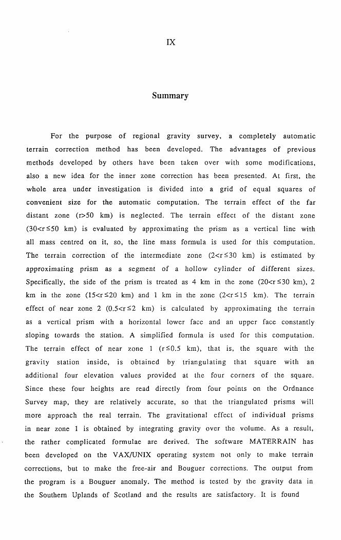
Summary

For the purpose o f regional gravity survey, a com pletely autom atic

terrain correction m ethod has been developed. The advantages o f previous

m ethods developed by others have been taken over with some m odifications,

also a new idea for the inner zone correction has been presented. At first, the

whole area under investigation is divided into a grid o f equal squares of

convenient size for the autom atic com putation. The terrain effect o f the far

d istant zone (r>50 km) is neglected. The terrain effect of the distant zone

(3 0 < r^ 5 0 km) is evaluated by approximating the prism as a vertical line with

all mass centred on it, so, the line mass formula is used for this compulation.

The terrain correction o f the interm ediate zone (2 < r^ 3 0 km) is estimated by

approxim ating prism as a segment of a hollow cylinder o f d ifferent sizes.

Specifically, the side of the prism is treated as 4 km in the zone (20<r^30 km), 2

km in the zone (15<r^20 km) and 1 km in the zone (2<r<15 km). The terrain

effect of near zone 2 (0 .5< r^2 km) is calculated by approxim ating the terrain

as a vertical prism with a horizontal lower face and an upper face constantly

sloping towards the station. A simplified formula is used for this computation.

The terrain effect of near zone 1 ( r^ 0 .5 km), that is, the square with the

gravity station inside, is obtained by triangu la ting that square with an

additional four elevation values provided at the four corners of the square.

Since these four heights are read directly from four points on the Ordnance

Survey map, they are relatively accurate, so that the triangulated prisms will

more approach the real terrain. The gravitational effect of individual prism s

in near zone 1 is obtained by integrating gravity over the volume. As a result,

the rather complicated form ulae are derived. The software M ATERRAIN has

been developed on the VAX/UNIX operating system not only to make terrain

corrections, but to make the free-air and Bouguer corrections. The output from

the program is a Bouguer anomaly. The method is tested by the gravity data in

the Southern Uplands of Scotland and the results are satisfactory. It is found

X

th a t som e of the orig inal terrain corrections provided by the BGS are

underestim ated and need to be m odified. The method is entirely automatic and

easy to use.

W ith respect to reflection seismology, a new experim ent was conducted

aim ed at understanding the wave propagation in volcanic rocks, finding new

m eans o f obtain ing conventional reflection seism ic data, and extracting the

weak signals in the presence o f noise. To accom modate this, a new areal

'RAZOR' array was designed. Three-com ponent geophones lie on one of two

concentric circles o f radii 75 and 130 m. The determ ination of the array

dim ension is based on several factors such as the wavelength o f signal, the

true dip o f deep reflectors. Three-com ponent seismic data were acquired over

the basalt in the Midland Valley of Scotland using an MDS-10 Data System. The

SEG-Y data were transformed into an ASCII-coded format and then rotated onto

a new coordinate system. The study of characteristics of field data shows that

3-com ponent seism ogram s are characterised by strong reverberations lasting

as long as 500 ms. The reverberation patterns vary from station to station. The

horizon tal com ponents exhibit larger am plitudes and low er frequency than

the vertica l com ponent. Furtherm ore, the data from the inner stations are

believed to be more affected by surface conditions than the data from the outer

stations. The display of the vertical and radial components from the outer

stations shows a line of reflection events at about 420 ms; there are no clear

events on the transverse section. By applying a spatial directional filter to

each component of seismic data, it is shown that there is more information in

the h o rizo n ta l com ponent passing through the f ilte r than the vertical

com ponent. This is attributed to the far larger amplitudes o f the horizontal

com ponents, w hich may dom inate the p o larisa tion d irec tion o f partic le

m otions. The energy variation diagram of each shot shows quantitatively that

the radial com ponent receives much more energy than the others.

In order to extract weak signals in the presence o f noise, a bandpass

frequency filter with a low cut-off of 20 Hz and a slope of 30 dB/octave, and a

high cut-off o f 60 Hz and a slope of 70 dB/octave is applied. The filtered data

reveal that the filter can reject part of the low frequency reverberations (<20

XI

Hz) and high frequency noise. For m ost of high reverberations within the

bandw idth, the filter does little to improve the data. Predictive deconvolution

f ilte rin g show s that it is very good at com pressing the w avelets and

a tten u a tin g the am plitude o f rev erb era tio n s . S ince both m u ltip les and

reflections are not clear on the sections, the predictive deconvolution filter

has to be used with great care, otherwise it degrades the useful signals. A

signal enhancem ent polarisation filte r was developed, based on a covariance

m atrix method. Both random noise and field data tests demonstrate that it can

be used to rem ove the random noise and part of the surface waves arriving

from different directions. From the interpretation point of view, the base of

the Clyde Plateau Lavas in the area investigated is found to be at about 930 m

below the surface.

To test the newly developed signal enhancem ent polarisation filter and

the optim isation o f array designing, synthetic 3-com ponent seism ic data were

generated in both isotropic and anisotropic m edia. The application of the

signal enhancem ent polarisation filter to those data is successful in terms of

suppressing random noise and enhancing signals. In addition, stacking the

filtered data based on the areal 'RAZOR' array provides a highly resolved

seism ic section. The study o f effect of added random noise on filtering shows

that, if the noise en tirely changes the po larisa tion d irection o f particle

m otions of reflection wavelets. The filter may thus not be able to extract very

weak signals from noise, however, by reducing the root mean square variance

o f random noise to a certain degree such that the noise mixed data exhibit a

better polarisation, the filter can then extract very weak signals.

A new approach of using slan t-slack processing to im age structure

based on the areal array has been dem onstrated using synthetic data from a

sim ple geological model. The result further proves that the dim ension of the

aerial array is appropriate for receiving the reflected plane waves from deep

interfaces. The true dip and dip direction of a reflector can possibly be derived

from x-p images and x-x images respectively, supposing that the velocity of the

upper layer is known. This m ethod can additionally be used to optim ise the

po larisa tion filte rin g , which keeps and enhances com pressional waves of

interest according to the polarisation directions of waves.

5

6

7

9

13

17

20

21

22

26

27

28

28

32

33

37

XII

List of Figures

1Division of topography for the computerized terrain correction. The station

is at the centre (o).................................................................................................

Diagram showing gravity in mGal of a prism and a line mass.

Both have the same m ass...................................................................................

Comparison of the terrain effect of a prism and a line mass, g l is the

gravity effect from a vertical prism, g3 from a line mass...............................

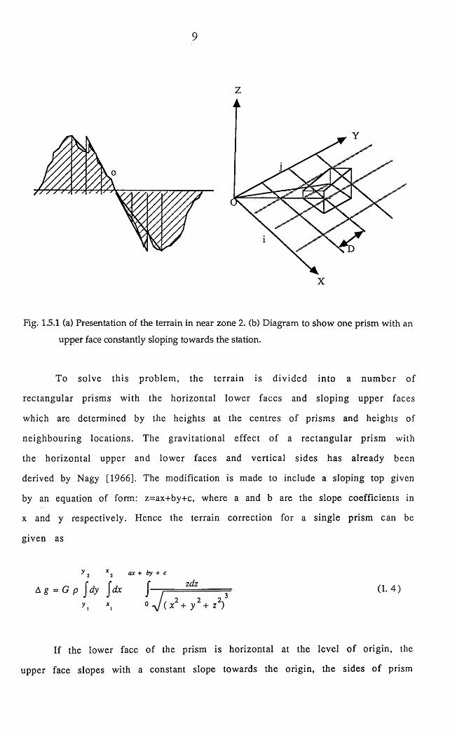
(a) Presentation of the terrain in near zone 2. (b) Diagram to show one prism

with an upper face constantly sloping towards the station............................ .

(a) Triangulation of near zone 1 in perspective views when P1Z1, P2Z2,

P3Z3 and P4Z4 are positive, (b) Projection of (a) onto the X-Y plane............

(a) Triangulation of near zone 1 when P1Z1 is negative, (b) Projection of

(a) onto the X-Y plane.......................................................................................

16 cases of possible terrain near the station in near zone 1 and their

corresponding formulae......................................................................................

Flow chart of possible terrain for the computer to choose appropriate

form ulae.....................................................................................................................

Flow chart of Fortran-77 program MATERRAIN.............................................

Geological map of the Southern Uplands of Scotland, showing the sites of

three density profile lines a, b and c................................................................

(a) Density profile 1 in the Southern Uplands of Scotland..............................

(b) Density profile 2 in the Southern Uplands of Scotland..............................

(c) Density profile 3 in the Southern Uplands of Scotland...............................

(a) The original Bouguer anomaly map of the Southern Uplands of

Scotland provided by the BGS............................................................................

(b) The new Bouguer anomaly map of the Southern Uplands of

Scotland, produced using the new terrain computation method.....................

2Field areal 'RAZOR' array pattern for seismic survey....................................

Geometry of a normal-incidence ray from a lower crustal re fleet or dipping

at 0. Plane wavefront is incident across an array of receiver-. < >i horizontal

XIII

dimension x............................................................................................................... 37

Fig. 2.4.1 Geological map of part of the Midland Valley, showing the site of

the seismic experiment in the rectangle to the South-west of Glasgow 40

Fig. 2.4.2 MDS-10 Data System Units, Rack-mounted........................................................ 40

Fig. 2.4.3 MDS-10 Data System block diagram ................................................................... 43

Fig. 2.4.4 Junction Box designed to connect geophones to the MDS-10.............................. 44

Fig. 2.4.5 Field lay-out and connections of the aerial array experiment........................... 46

Fig. 2.5.1 SEG-Y tape form at.................................................................................................. 50

Fig. 2.6.1 Two coordinate system with origins at the same point...................................... 54

Fig. 2.6.2 Flow diagram of Fortran-77 program MATRAN................................................. 56

Fig. 2.7.1 (a) Original unsealed seismic traces from shot 2. (b) Scaled seismic traces

after a gain is applied, (c) The gain functions.....................................................60

Fig. 2.8.1 Definitions of source and receiver static corrections. ......................................62

Fig. 2.8.2 The topography along the main profile line........................................................ 63

Chapter 3Fig. 3.2.1 (a) Six vertical traces (channels 1, 3, 5, 7, 9,11) from stations 1, 2, 6, 8, 9,10 at

shot 1 and six vertical traces (channels 2,4, 6, 8,10,12) for shot 2 (shot 1 and

shot 2 are test shots at the same location), (b) Same data as those

in (a) after gain functions are applied............................................................... 66

Fig. 3.3.1 (a) Three component seismic traces from station 8 at shot 6 (V - vertical,

N - North, E - East)................................................................................................ 68

(b) The amplitude spectra of two time series- vertical (V) and

horizontal (N) components as shown in (a)........................................................ 68

Fig. 3.3.2 Four groups of seismic traces. They are from shots 2, 3, 6,8 respectively.

The first 3 components in each group are from the inner station, the

second 3 components are from the outer station.................................................. 70

Fig. 3.3.3 The auto-correlation of a horizontal component (North) from station 6

at shot 4. It shows the periodicity of organised noise....................................... 71

Fig. 3.3.4 (a) The radial components from 10 shots. The traces from the inner stations

are on channels 1-60, those from the outer stations are on channels 61-120.........72

(b) The transverse components from 10 shots. The traces from the inner

stations are on channels 1-60, those from the outer stations are in channels

61-120........................................................................................................................... 73

(c) The vertical components from 10 shots. The traces from the inner stations

are on channels 1-60, those from the outer stations are on channels 61-120......... 74

Fig. 3.4.1 Principle of spatial directional filtering along the V-direction. The

XIV

polarisation axis E ^b of the response AB is near the V-direction, therefore,

part AB will be kept. Part BC will be rejected since its polarisation axis

Egc is almost perpendicular to the V-direction (From Cliet, 1987).................. 78

Fig. 3.4.2 Flow diagram of Fortran-77 program MASDF...................................................... 80

Fig. 3.4.3 The three-component sections of shot 6 after application of the spatial

directional filter. The time window for filtering is 84 ms, threshold angles

are 15°, 30°, 45°, 60°, and 75°................................................................................82

Fig. 3.4.4 The relationships between the number of windows within which the

data have passed through the filter and threshold angles. The number

of windows is expressed in percent. The data from 9 shots are presented 84

Fig. 3.4.5 Energy variation of each component expressed in percent as a function of

threshold angle. The data from 9 shots are presented...................................... 85

Chapter 4Fig. 4.3.1 (a) The original 3-component seismograms (1-3) from station 7 at shot 6,

and the bandpass frequency filtered seismograms (4-6). (b) The original

3-component seismograms (1-3) from station 10 at shot 5, and the frequency

filtered seismograms (4-6). Bandpass frequency bandwidth is 20/30-60/70

(Corner frequency/slope in dB /oct).................................................................... 90

Fig. 4.4.1 Five vertical seismograms (1-5) from stations 15, 21, 28, 34 and 40 at shot 6

and the deconvolved seismograms (6-10). Prediction lag d=24 ms,

the maximum operator length L=150 ms............................................................ 93

Fig. 4.5.1 (a) Polarisation diagram of random noise RL=0.1745.

(b) Polarisation diagram of field data RL=0.9198........................................... 97

Fig. 4.5.2 Flow Diagram of Fortran-77 program MASEPF................................................. 100

Fig. 4.5.3 (a) Random noise (1-3) and the polarisation filtered traces (4-6). (b) The

field 3-components (1-3) from station 2 at shot 2 and the polarisation filtered

traces (4-6). (c) Noise-enhanced field data (1-3) and the polarisation

filtered noise-enhanced data (4-6)...................................................................... 102

Fig. 4.5.4 Illustration of the effect of different time window length on polarisation

filtering. Traces 1-3 are noise mixed synthetic data. Rest are the filtered

noise-mixed synthetic data with varied window length. They are (from

left to right) 12, 36, 60, 84,124, 180, 244, 324, and 404 ms................................. 104

Fig. 4.5.5 (a) The frequency filtered vertical traces from stations 3, 5, 7, 9 at shot 5.

(b) The same data as in (a) after application of a polarisation filter............ 106

Fig. 4.5.6 (a) The polarisation filtered radial components from 10 shots. Those from

the inner circles are plotted on channels 1-60. Those from the outer circles

are on channels 61-120. The test shot is also included (1-6, 61-66).................... 107

XV

(b) The polarisation filtered transverse components from 10 shots. Those

from the inner circles are plotted on channels 1-60. Those from the outer

circles are on channels 61-120. The test shot is also included (1-6, 61-66)....... 108

(c) The polarisation filtered vertical components from 10 shots. Those

from the inner circles are plotted on channels 1-60. Those from the outer

circles are on channels 61-120. The test shot is also included (1-6, 61-66)....... 109

Chapter 5Fig. 5.2.1 Geological model of an isotropic medium ............................................................. 114

Fig. 5.2.2 (a) The original (channels 1-20), noise-mixed (channels 21-40) and

polarisation filtered (channels 41-60) seismograms for the vertical

components. The synthetic seismograms are for the model (2D) in an

isotropic m edium ..................................................................................................... 116

(b) The original (channels 1-20), noise-mixed (channels 21-40) and

polarisation filtered (channels 41-60) seismograms for the horizontal

components. The synthetic seismograms are for the model (2D) in

an isotropic m edium .............................................................................................. 117

Fig. 5.2.3 Array pattern for generating synthetic seismograms......................................... 119

Fig. 5.2.4 The geometries of a dipping reflector related to a line of different

azimuths and the new 2D models constructed, (a), (c) and (e) are 3D

models, (b), (d) and (f) are new 2D models constructed for the modelling

program SEIS83....................................................................................................... 121

Fig. 5.2.5 The synthetic seismograms based on the areal array of 3 dimensions.

The horizontal components are on the left-hand side. The vertical

components are on the right-hand side. The centre of the areal 'RAZOR'

array lies at the middle point of the model shown in Fig. 5.2.1, i.e. it is 2.5 km

away from the west along the profile line. Channel numbers correspond to

the station numbers marked in Fig. 5.2.3......................................................... 122

Fig. 5.2.6 The polarisation filtered and stacked seismograms (channels 1-20 for

the horizontal components, channels 21-40 for the vertical components) 123

Fig. 5.3.1 The geological model 1 in an anisotropic medium............................................. 126

Fig. 5.3.2 The original (channels 1-12), noise-mixed (channels 13-24) and polarisation

filtered (channels 25-36) seismograms (explosive source) at 4 stations (1, 2,

4,5) for model 1 in an anisotropic m edium . The order of the traces is the

radial, transverse and vertical............................................................................... 128

Fig. 5.3.3 The original (channels 1-12), noise-mixed (channels 13-24) and polarisation

filtered (channels 25-36) seismograms (SH source) at 4 stations (1, 2,4, 5)

XVI

for model 1 in an anisotropic medium. The order of the traces is the

radial, transverse and vertical............................................................................. 129

Fig. 5.3.4 The original (channels 1-12), noise-mixed (channels 13-24) and polarisation

filtered (channels 25-36) seismograms (explosive source) for model at 4

stations (1,2,4,5) in an anisotropic medium. The order of the traces is

the radial, transverse and vertical........................................................................ 132

Fig. 5.3.5 The original (channels 1-12), noise-mixed (channels 13-24) and polarisation

filtered (channels 25-36) seismograms (SH source) at 4 stations (1, 2,4, 5)

for model 2 in an anisotropic medium. The order of the traces is the

radial, transverse and vertical............................................................................ 133

Fig. 5.3.6 (a) The polarisation diagram of the original data from channel 3 in

Fig. 5.3.4. (b) The polarisation diagram of the noise-mixed data (root

mean square variance of noise is 60). (c) The polarisation diagram of the

noise-mixed data (root mean square variance os noise is 36)........................... 135

Fig. 5.3.7 Noise-mixed and filtered seismograms. Channel 1 is for the original data,

channel 2 for the noise-mixed data (root mean square variance of noise is

60), channel 3 for the filtered trace 2, channel 4 for the noise-mixed data

(root mean square variance of noise is 36), channel 5 for filtered trace 4........ 135

Chapter 6Fig. 6.2.1 The geometry of plane wavefront and a time delay associated with 2

receivers on the surface........................................................................................ 138

Fig. 6.2.2 A hyperbola in t - x domain maps onto an ellipse in T-p domain........................ 139

Fig. 6.3.1 Geological model for generating synthetic seismogram. (Horizontal scale is

exaggerated, the true dip \|/=26.6°).................................................................... 140

Fig. 6.3.2 Twelve vertical components generated by SEIS83. The data are based

on the model in Fig. 6.3.1. Channel numbers correspond to station numbers........ 142

Fig. 6.3.3 The contour map of two way travel time associated with the areal array. ... 142

Fig. 6.3.4 Construction of a projection line L with an azimuth a=0°. Two concentric

circles indicate that 2 stations are projected at the same point........................ 143

Fig. 6.3.5 Seven seismograms from stations 3,4,2,1,12,10,11 on the projection line L. .. 143Fig. 6.4.1 Flow diagram of Fortran-77 program MASSP..................................................... 146

Fig. 6.5.1 Nine T-p images based on nine projection lines with different azimuths............. 148

Fig. 6.5.2 Illustration of t - x images with 3 different azimuths. The ray parameter

in each diagram is constant.................................................................................... 152

Fig. 6.5.3 A t - x image constructed by synthetic data based on the model in Fig. 6.3.1.

Six shots are presented. The ray parameter p is 1.778 x lO '4 s /m ........................153

Fig. 6.5.4 (a) Geometry of a ray path showing the polarisation of a compressional

XVII

wave P. (b) Polarisation direction P of a compressional wave obtained

by slant-slack method and polarisation direction E of particle motions

obtained by the matrix method....................................................................... 155

XVIII

List of Tables

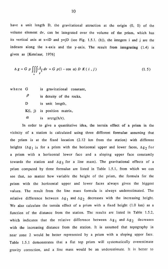
Chapter 1Table 1.5.1 Terrain corrections for prisms of 1 x i km2 with different heights by three

different formulae. The prism is located at r=2.12 km. %=100 x(Ag^-

Ag2)/A g i. .................................................................................................. 11

Table 1.5.2 Terrain corrections for prisms of 1 x i km2 with a fixed height (1.0 km) at

different distances from the station. %=100 x(Agi-Ag2 ) /A g j....................... 11

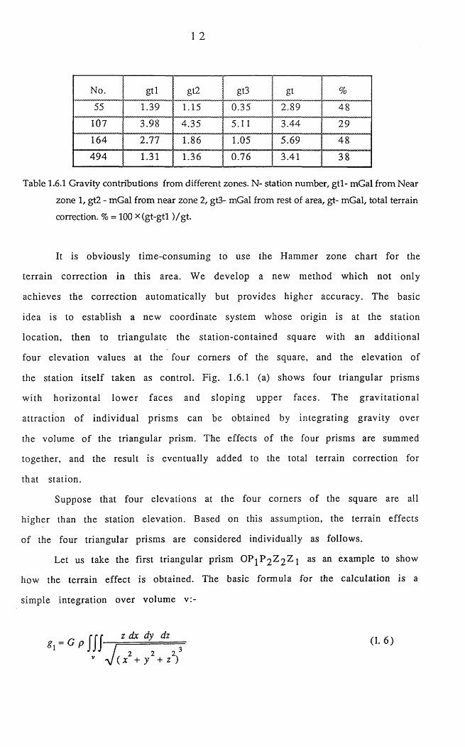
Table 1.6.1 Gravity contributions from different zones. N - station number, g tl-

mGal from Near zone 1, gt2 - mGal from near zone 2, gt3 - mGal from

rest of area, gt - total terrain correction. % = 100 x (g t-g tl ) /g t ...................... 12

Table 1.7.1 The station data file format. The actual observed gravity value is

(980000+gob) mGal............................................................................................ 22

Table 1.7.2 Block file data format......................................................................................... 23

Table 1.7.3 Format of output file OUTPUT. The actual normal gravity is (980000+go)

mGal. The actual observed gravity value is (980000+gob) mGal.................. 24

Table 1.7.4 Format of output file CONTBN........................................................................ 24

Table 1.8.1 Comparison of new corrections with old ones, gt (old) is provided by the

BGS, gt (new) is produced by the new terrain computation method............. 30

Table 1.8.2 Comparison of terrain correction among the old, Hammer and new values... 30

Chapter 2Table 2.5.1 Output data format from the program MASEGY..............................................52

Table 2.6.1 The angles of 12 radial directions from North................................................. 55

Table 2.6.2 Transformed data format from the program MATRAN................................. 57

Table 2.8.1 Static corrections applied to all the stations (st-station number; sp-shot

number; -distance between a receiver to the datum plane; t -time shift

in milliseconds)................................................................................................... 64

Chapter 5Table 5.2.1 The parameters of a model in an isotropic medium........................................ 114

Table 5.3.1 The parameters of model 1 in an anisotropic medium..................................... 126

Table 5.3.2 The parameters of model 2 in an anisotropic medium.................................... 130

1

PART ONE: GRAVITY

Chapter 1 Automatic Terrain Correction Method for

Regional Gravity Survey

1.1 Introduction

In general, the Bouguer anomaly is determined by

& b a ~ & 0b ~ 8 o + & f ~ & b + %t (1* 1)

w h e r e gba is Bouguer anomaly,

g0 b is observed gravity value,

g0 is normal gravity calculated by an international formula,

g f is free-air correction,

g b is Bouguer correction,

g t is terrain correction.

The values g , gf, gb can easily be determined, if all gravity station data such as

coordinates, elevations and rock densities are available. However, determ ining

the terrain correction gt is the most tedious task and is a very important part

of the Bouguer anomaly, especially in rugged terrain. Because of that, many

au thors have placed m ore em phasis on developing various m ethods to

calculate the terrain correction since the 1950's.

Bott pioneered m ethods o f terrain correction using the electronic

d igital com puter [Bott, 1958]. His method was to divide the region under

investiga tion into a grid o f equal squares o f convenient size, take the

elevations at the centres of the squares as the average heights of these prisms,

determ ine the gravity attraction o f a prism at a station by calculating the

2

gravity value produced by a segment of a hollow vertical cylinder, sum the

increm ental contributions from all squares except those less than 1 km from

the station. The corrections from the inner squares are calculated using the

Ham m er zone chart m ethod and finally added to the com puter correction

value. This method was a milestone for calculations made by computer, which

not only increased accuracy but also saved tim e. H ow ever, the m ain

disadvantage is the tim e-consuming terrain correction for the inner squares.

Karlemo [1963] developed a similar method mainly used for local gravity

investigation on the condition that the points o f observation are regularly

d istribu ted in a definite system and the distance betw een points is rather

sm all. He used a sym m etrical pattern of radial elevation p ro files , each

representing a sector of the terrain. The gravity attraction in the inner zone

(r<250 m ) is estimated by calculating the value produced by 68 segments. The

terrain corrections for the interm ediate and distant zones are estim ated in a

sim ilar way, but the spacing of points in these zones is increased in order to

reduce the calculation time. The form ulae used for calcu lation are very

com plicated. Such a m ethod seems very accurate and reliable for small scale

prospecting. However, it is rather im practical for regional gravity surveys;

here stations are irregularly and sparsely d istributed, because o f logistical

problem s which make data collection in a regular grid difficult.

Blais and Ferland [1983] approximated a distant prism as a vertical line

with the total mass of the prism, so the line mass formula is used to give the

gravim etric terrain correction. The intermediate zones are treated in the same

way as the distant zones, except for using the rigorous rectangular prism

form ula for regular flat-top prisms centred at the grid points. The inner zones

with regular elevation data are treated as a. num ber of sm aller prism s with

horizontal low er faces and sloping upper faces. The zones w ith irregular

elevation data have to be triangulated, the corresponding boundary definition

for triangulation is determ ined using contribution levels o f the individual

flat-top rectangular prism s. The gravim etric terrain corrections are obtained

by calcu lating the effects from the triangular prism s with sloping upper

3

faces. This method uses a rigorous rectangular prism form ula which increases

accuracy for the interm ediate zone contributions. However, the com putation

time will be increased by the 24-term formula. Above all, the boundary for

triangulation defined by the con tribu tion levels of the individual flat-top

rectangular prisms is not accurate enough since the heights o f the prism s are

often read from contour maps, for instance, the Ordnance Survey map with a

scale o f 1:25000 in Britain, and are average values partly depending on a

person's subjective judgm ent. The maximum height difference in a hilly area

read by different persons can som etim es reach 30 m, which o f course will

affect the total correction value.

Lagios [1978] approxim ated the inner zones by fitting m ultiquadric

surfaces or paraboloids to additional heights read from a map and height of a

station taken as control. The more heights that are provided, the more closely

does the fitting surface approach the real topography. He calcu lated the

terrain correction for a 100x100 m block with a horizontal upper face using

the approximated formula for a segment of a hollow cylinder whose height is

decided by fitting surface equations to the station at the centre. The accuracy

of this com putation largely depends on the number of heights provided for

fitting the surfaces. In practice, however, it is difficult to give a large number

o f elevation data for the neighborhood of stations, especially in regional

gravity surveys, in which there may be thousands of stations to process.

In this chapter, an autom atic terrain correction m ethod is presented

which is partly based on the previous methods, with more refined calculations

for the inner zone corrections.

1.2 New approach to an automatic terrain correction method

The advantages of previous m ethods developed by others have been

taken over with some m odifications, with a new contribution for the inner

zone correction being presented. The basic procedures are sim ilar to the

others. That is, the whole area under investigation is divided into a grid of

equal squares o f convenient size for the autom atic com putation. The terrain

4

effect of the far distant zone (r>50 km) is neglected. The terrain effect of the

distant zone (30 < r^5 0 km) is evaluated by approxim ating the prism as a

vertical line with all mass centred on it, so, the line mass formula is used for

this com putation. The terrain correction of the intermediate zone (2 < r^ 3 0 km)

is estim ated by approxim ating a prism as a segment of a hollow cylinder of

different sizes. Specifically, the size of the prism is treated as 4 km in the zone

where 2 0 < r^ 3 0 km, 2 km in the zone where 15<r^20 km and 1 km in the zone

where 2 < r ^ l5 km. The terrain effect of near zone 2 (0 .5< r^2 km) is calculated

by approxim ating the terrain as a vertical prism with a horizontal lower face

and an upper face constantly sloping towards the station. A sim plified formula

is used for this computation. The terrain effect of near zone 1 (r^ 0 .5 km), that

is, the square with the gravity station inside, is obtained by triangulating that

square with an additional four elevation values provided at the four comers of

the square. Since these fo u r . heights are read directly from four points on the

O rdnance Survey m ap, the values are rela tively accurate, so that the

triangulated prisms will more closely approach the real terrain.

1.3 D istant zone contribution

To achieve the terrain correction by computer, the terrain has to be

divided into a grid of equal squares of convenient size. For instance, in Great

Britain, the size of a square for the computation is usually adapted the same as

the N ational Grid square, which is one square kilom etre. The g rav ita tio n a l

effect is usually obtained by summing the incremental contributions from the

individual prism s. W ith respect to the computation time and accuracy, the

terra in is again divided by d ifferen t zones, w ithin each zone d ifferen t

approxim ations of terrain and formulae are applied (see Fig. 1.3.1).

The definition of the distant zone given by the author means the area

which is 30 km or further from a station. For regional gravity surveys, the

terrain effect caused by this large area is certainly significant. On the other

hand, according to Newton's gravitational law, the gravity attraction of any

mass to a certain point is inversely proportional to the square o f the distance

5

from the mass to the point, in other words, the further the mass from the

point, the less gravity attraction it will exert. So, we investigate what kind of

formula is acceptable for the corrections in this distant zone. Let us suppose

that the distant zone consists o f a number of vertical flat-top prisms, in order

to choose the appropriate form ula for shortening the calculation tim e, but

without losing much accuracy, the vertical line mass form ula (1.2) and the

rigorous form ula o f a right rectangular prism given by Nagy [1966], which

contains 24-term m athem atical expressions, are studied.

4 km ^ ►

0

Fig. 1.3.1 Division of topography for the computerized terrain correction. The station is at the

centre (o).

A g = G p A j ! 1 ^ = G p A ( T ~ - I ) .......r > (1' 2 )7 + h

W h e re r is distance from station to centre of square,

h is height difference between square and station,

A is area of square,

P is density of the rocks.

We calculate the gravitational effect of a height-fixed, vertical prism as

6

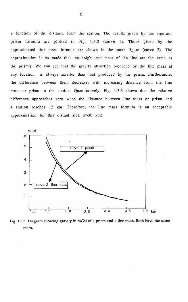
a function of the distance from the station. The results given by the rigorous

prism form ula are p lotted in Fig. 1.3.2 (curve 1). Those given by the

approxim ated line mass formula are shown in the same figure (curve 2). The

approximation is so made that the height and mass of the line are the same as

the prism's. We can see that the gravity attraction produced by the line mass at

any location is always sm aller than that produced by the prism. Furtherm ore,

the difference between them decreases with increasing distance from the line

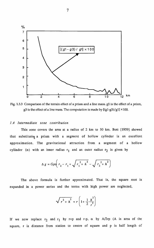
mass or prism to the station. Quantitatively, Fig. 1.3.3 shows that the relative

difference approaches zero when the distance between line mass or prism and

a station reaches 12 km. Therefore, the line mass form ula is an acceptable

approxim ation for this distant area (r>30 km).

mGal6

5 curve 1- prism

4

3

curve 2- line mass2

1

4.0 km3.0 3.52.0 2.5

Fig. 1.3.2 Diagram showing gravity in mGal of a prism and a line mass. Both have the same

mass.

7

%7

4

2

3

5

6

0

Fig. 1.3.3 Comparison of the terrain effect of a prism and a line mass, g l is the effect of a prism,

g3 is the effect of a line mass. The computation is made by [(gl-g3)/gl] x 100.

1.4 In term ediate zone contribution

This zone covers the area at a radius of 2 km to 30 km. Bott [1959] showed

that s u b s ti tu te a prism with a segment o f hollow cylinder is an excellent

approxim ation . The grav itational attraction from a segm ent o f a hollow

cylinder (a ) with an inner radius r^ and an outer radius ^ is given by

The above form ula is further approximated. That is, the square root is

expanded in a power series and the terms with high power are neglected,

If we now replace r2 and r j by r+p and r-p, a by A/2rp (A is area of the

square, r is distance from station to centre o f square and p is half length of

A g = Gp

8

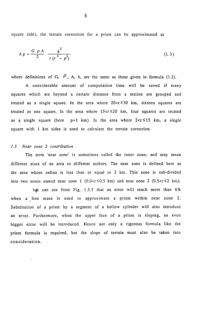
square side), the terrain correction for a prism can be approximated as

G p A hA g = — | --------- - 5 ------K (1 .3 )

z r ( r - p )

where definitions of G, P , A, h, are the same as those given in formula (1.2).

A considerable amount o f com putation tim e will be saved if many

squares which are beyond a certain distance from a station are grouped and

treated as a single square. In the area where 20< r^30 km, sixteen squares are

treated as one square. In the area where 15<r^20 km, four squares are treated

as a single square (here p = l km). In the area where 2 < r^ l5 km, a single

square with 1 km sides is used to calculate the terrain correction.

1.5 Near zone 2 contribution

The term 'near zone' is sometimes called the inner zone, and may mean

different sizes of an area to different authors. The near zone is defined here as

the area whose radius is less than or equal to 2 km. This zone is sub-divided

into two zones named near zone 1 (0.0<r<0.5 km) and near zone 2 (0 .5<r^2 km).

\Ap can see from Fig. 1.3.3 that an error will reach more than 6%

when a line mass is used to approxim ate a prism w ithin near zone 2.

Substitution of a prism by a segment of a hollow cylinder will also introduce

an error. Furtherm ore, when the upper face of a prism is sloping, an even

bigger error will be introduced. Hence not only a rigorous form ula like the

prism form ula is required, but the slope of terrain must also be taken into

c o n s id e ra t io n .

9

ZA

Y

X

Fig. 1.5.1 (a) Presentation of the terrain in near zone 2. (b) Diagram to show one prism with an

upper face constantly sloping towards the station.

To solve this problem , the terrain is d iv ided into a num ber of

rectangular prisms with the horizontal low er faces and sloping upper faces

which are determined by the heights at the centres of prisms and heights of

neighbouring locations. The gravitational effect of a rectangular prism with

the horizontal upper and lower faces and vertical sides has already been

derived by Nagy [1966]. The modification is made to include a sloping top given

by an equation of form: z=ax+by+c, where a and b are the slope coefficients in

x and y respectively. Hence the terrain correction for a single prism can be

given as

If the lower face of the prism is horizontal at the level o f origin, the

upper face slopes with a constant slope towards the origin, the sides o f prism

y 2 x 2 ax + by + c

(1 .4 )

10

have a unit length D, the gravitational attraction at the origin (0, 0) of the

volume element dv, can be integrated over the volume of the prism, which has

its vertical axis at x=iD and y=jD (see Fig. 1.5.1. (b)), the integers i and j are the

indexes along the x-axis and the y-axis. The result from integrating (1.4) is

given as [Ketelaar, 1976]

A g = G p = G p ( l - cos a) D K ( i , j ) (1. 5)

w h e r e G is gravitational constant,

P is density of the rocks,

D is unit length,

K(i, j) is position matrix,

a is a rctg(h/r).

In order to give a quantitative idea, the terrain effect of a prism in the

vicinity of a station is calculated using three different formulae assuming that

the prism is at the fixed location (2 . 1 2 km from the station) with different

heights (A g | is for a prism with the horizontal upper and lower faces, Ag 2 f o r

a prism with a horizontal lower face and a sloping upper face constantly

towards the station and Agg for a line mass). The gravitational effects of a

prism computed by three formulae are listed in Table 1.5.1, from which we can

see that, no matter how variable the height of the prism, the formula for the

prism with the horizontal upper and lower faces always gives the biggest

values. The result from the line mass formula is always underestimated. The

relative difference between A gj and Ag 2 decreases with the increasing height.

We also calculate the terrain effect of a prism with a fixed height (1.0 km) as a

function of the distance from the station. The results are listed in Table 1.5.2,

which indicates that the relative difference between A g j and A g 2 decreases

with the increasing distance from the station. It is assumed that topography in

near zone 2 would be better represented by a prism with a sloping upper face.

Table 1.5.1 demonstrates that a flat top prism will systematically overestimate

gravity correction, and a line mass would be an underestimate. It is better to

11

use a prism with a sloping upper face to approximate real terrain in near zone

2 , although problems may arise for areas of very rapid changes of topography.

h 0.5 0 . 8 1 . 0 1.5 2 . 0 3.0 km

A g _ * 1 .... 0.246 0.589 0 . 8 6 8 1.643 2.411 3.689

A g 6 2

0.228 0.552 0.819 1.574 2.336 3.626

0.226 0.546 0.811 1.558 2.313 3.589

% 7.100 6.300 5.700 4.200 3.100 1.700

Table 1.5.1 Terrain corrections for prisms of 1 x i km^ with different heights by three different

formulae. The prism is located at r=2.12 km. %=100 x(Agi-Ag2 )/Agp

r 1.41 2 . 1 2 2.83 3.54 4.24 6.36 km

A * 12.657 0 . 8 6 8 0.380 0.198 0.116 0.003

A ^ 22.396 0.819 0.366 0.193 0.113 0.003

A * 3 2.337 0.811 0.364 0.192 0.113 0.003

% 9.800 5.700 3.600 2.400 1.700 0.900

Table 1.5.2 Terrain corrections for prisms of 1 x i km^ with a fixed height (1.0 km) at different

distances from the station. % = 1 0 0 x(Ag^-Ag2 )/Ag^.

1.6 Near zone 1 contribution

This zone covers the area with a radius of less than or equal to 0.5 km.

The gravity effect of this near zone is extremely important. Table 1.6.1 lists the

gravity contributions o f 4 stations from 3 different zones in the Southern

Uplands of Scotland. We can see that although it occupies a small area, its

gravity effect is significant. Station 55 shows that the gravity effect of near

zone 1 contributes up to 48 % of the total terrain correction.

No. gtl gt2 gt3 gt %

55 1.39 1.15 0.35 2.89 48

107 3.98 4.35 5.11 3.44 29

164 2.77 1 . 8 6 1.05 5.69 48

494 1.31 1.36 0.76 3.41 38

Table 1.6.1 Gravity contributions from different zones. N- station number, gtl- mGal from Near

zone 1, gt2 - mGal from near zone 2 , gt3- mGal from rest of area, gt- mGal, total terrain

correction. % = 1 0 0 x(gt-gtl )/gt.

It is obviously time-consuming to use the Hammer zone chart for the

terrain correction in this area. We develop a new method which not only

achieves the correction automatically but provides higher accuracy. The basic

idea is to establish a new coordinate system whose origin is at the station

location, then to triangulate the station-contained square with an additional

four elevation values at the four comers of the square, and the elevation of

the station itself taken as control. Fig. 1.6.1 (a) shows four triangular prisms

with horizontal lower faces and sloping upper faces. The gravitational

attraction of individual prisms can be obtained by integrating gravity over

the volume of the triangular prism. The effects of the four prisms are summed

together, and the result is eventually added to the total terrain correction for

that station.

Suppose that four elevations at the four corners of the square are all

higher than the station elevation. Based on this assumption, the terrain effects

of the four triangular prisms are considered individually as follows.

Let us take the first triangular prism OP 1 P 2 Z 2 Z 1 as an example to show

how the terrain effect is obtained. The basic formula for the calculation is a

simple integration over volume v:-

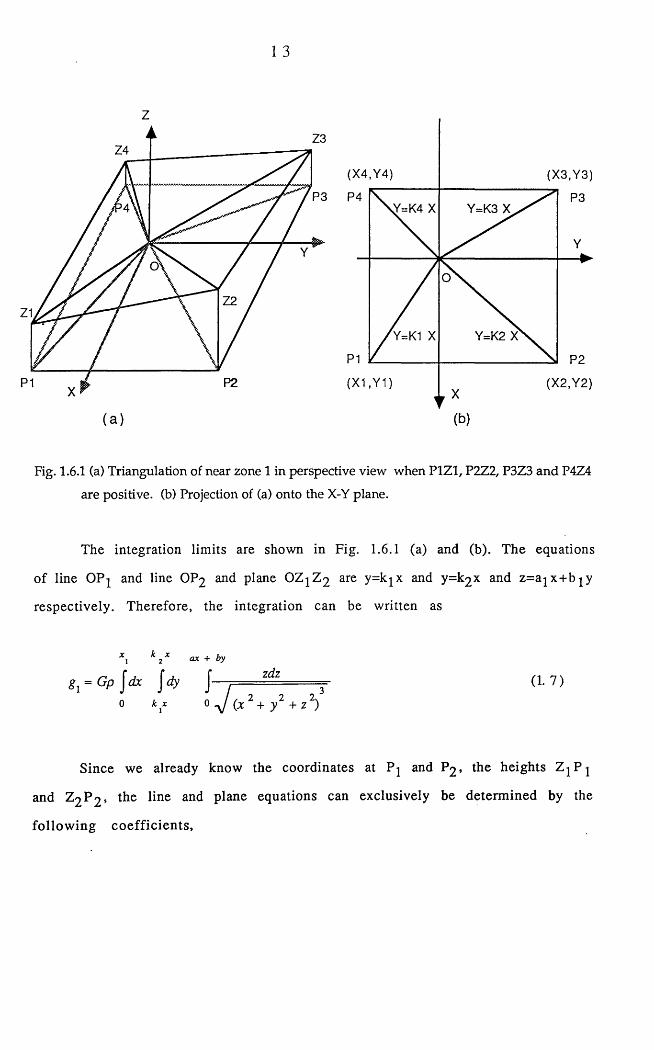
Fig. 1.6.1 (a) Triangulation of near zone 1 in perspective view when P1Z1, P2Z2, P3Z3 and P4Z4

are positive, (b) Projection of (a) onto the X-Y plane.

The integration limits are shown in Fig. 1.6.1 (a) and (b). The equations

of line O P | and line OP2 and plane O Z jZ 2 are y=k^x and y=k2 X and z = a ^ x + b |y

respectively. Therefore, the integration can be written as

X k 2X ax + by

(1 .7)

Since we already know the coordinates at P j and P2 , the heights Z j P j

and Z2 P 2 * the line and plane equations can exclusively be determined by the

fo llowing coefficients,

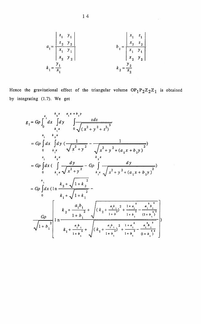
1 4

*i =

Z 1 ? 1 X l z i

Z 2 ^ 2 h X 2 z 2

* 1 ? 1 X l

* 2 ? 2 X 2 y 2> 1

* 1k 2 = -

y 2 X 2

Hence the gravitational effect o f the triangular volume OP 1 P 2 Z 2 Z 1

by integrating (1.7). We get

k x a x + 6 y 2 1 1

« , = G p | d x j d y Jz d z

k x 1

x k x

°7= G p J d x j d y i - j - l

0 k X

x k x1 2

V x 2 -t-y 2 2 2x + y + ( a xx + b xy )k x

= G p j d x ( J d y

7. 2 20 k W X + y

- G p Jd y

2 2k ix J x + ( a l x + b xy )

= G p j d x ( I n k l ^ j 2

0 k i + J 1 + k i

Gp

7 i + 6 1:

Q , b . I a b 2 I + a a bk 2 + — L-L? + l ( . k , + -d -L ) + 1

1 + 6

2 ' 2 ' 2 2 21 + 6 1 + 6 (1 + 6 )

1 na b 1 1 1& j + 2

1 + 61

2 2 2< 2 6 2 1 + a < 2 61/1 1 1 V 1 1 1

+ / ( k 1 + $■) + -1 + 6 1 + 6 (1 + 6 )

is obtained

)

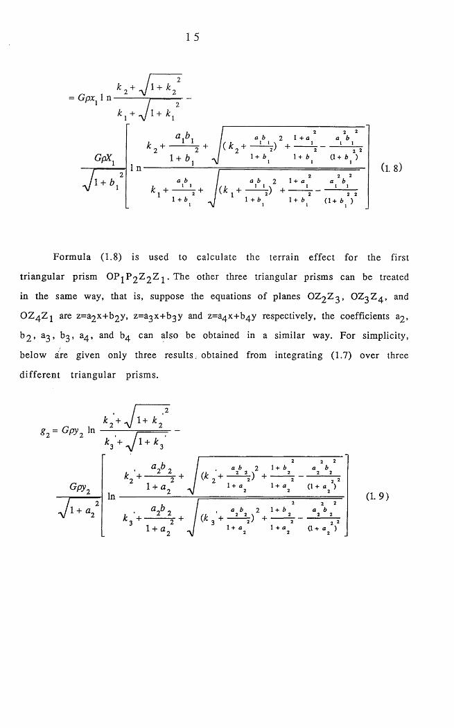
Formula (1.8) is used to calculate the terrain effect for the first

triangular prism O P J P 2 Z 2 Z ^ . The other three triangular prisms can be treated

in the same way, that is, suppose the equations of planes O Z 2 Z 3 , O Z 3 Z 4 , and

O Z 4 Z 1 are z=a2 X+b2 y, z=a3 X+b3 y and z=a4 X+b4 y respectively, the coefficients a2 ,

^ 2 ’ a3* ^ 3 ’ a4 ’ anc* ^4 can a*so obtained in a similar way. For simplicity,

below are given only three results, obtained from integrating (1.7) over three

d iffe ren t tr iangular prisms.

1 6

3 = —Gp* 3 I nk 3 + J l + k 3

G p x ,

a 3^3 I a3b 3 2 1+ bk „ + - + I (k Q + r) +

2 2 <2 6

3 3

I n

3 ' 2

3

3 ' 2 -J 1 + a

1 2 2 2

1 + f l 35 3

1 + a. a3b 3 I a3 3 2 l+b3k 4 + -------------T + / ^ 4 + ^ > +1 + a. 1 + a 1 + a

2 2 a 6 3 3

2 2 ( 1 + * 3 )

( 1. 10)

«4 = - Gpyi toi + J 1+ki

: i + J

JGpyx

1 + k.

• a J>Ak l + 2 +

1 + b .In

1 + bk A +

a. b4 4

1 + b

, a b 2 1 + a

(*1 + - ^ + -----1 + b A A

2 2 2 1 + 6 (1 + b )

2 2 2, a 6 2 1 + a a 6

+ ' ( * 4 + - ^ ) + — *7— M r1 + 6 1 + 6 (1 + 6 )

( 1 . ID

Where and k - ^ l / k g .

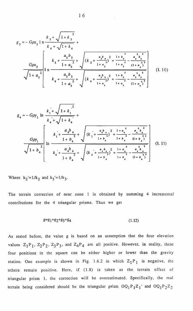
The terrain correction of near zone 1 is obtained by summing 4 incremental

contributions for the 4 triangular prisms. Thus we get

g=gl+g2+S3+S4 (1.12)

As stated before, the value g is based on an assumption that the four elevation

values Z j P j , Z2 P 2 » Z3 P 3 , an(l Z4 P 4 are a^ positive. However, in reality, these

four positions in the square can be either higher or lower than the gravity

station. One example is shown in Fig. 1.6.2 in which Z j P j is negative, the

others remain positive. Here, if (1.8) is taken as the terrain effect of

triangular prism 1, the correction will be overestimated. Specifically, the real

terrain being considered should be the triangular prism O Q j P j Z j ' and OQ 1 P 2 Z 2

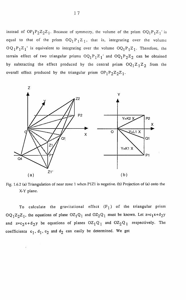
instead of O P 1 P 2 Z 2 Z J. Because of symmetry, the volume of the prism O Q j P ^ Z j ' is

equal to that of the prism O Q j P j Z ^ , that is, integrating over the volume

O Q j P j Z j ' is equivalent to integrating over the volume O Q j P j Z | . Therefore, the

terrain effect of two triangular prisms O Q j P j Z j ' and OQ 1 P 2 Z 2 can be obtained

by subtracting the effect produced by the central prism O Q j Z j Z 2 from the

overall effect produced by the triangular prism OP 1 P 2 Z 2 Z 1 .

Z

72

P2

04

ZV

Y

Y=K2 P2

=L1 X

Y=K1 X

Fig. 1.6.2 (a) Triangulation of near zone 1 when P1Z1 is negative, (b) Projection of (a) onto the

X-Y plane.

To calculate the gravitational effect (F^) of the triangular prism

O Q J Z 2 ZJ , the equations of plane OZ j Q j and OZ2 Qi must be known. Let z=C!X+d2y

and z=C2 X + d 2 Y be equations of planes O Z j Q j and OZ2 Q 1 respectively. The

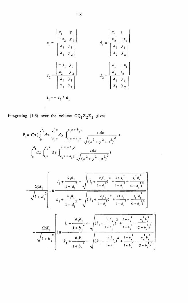
coefficients c j , d j , C2 and d2 can easily be determined. We get

1 8

c i =

zi y i x i z i

~ zi y 2 d. -x 2 - z 2

* 1 ? i

* 2 ? 2

* 1 ? 1

* 2 * 2

~ z i y i X — Z 1 1

z 2 y 2 A -

X z 2 2

2*i

2* 1 ? !

-

* 2

c i> d x

* 2 y 2

Integrating (1.6) over the volume O Q |Z 2 Z j gives

l x a x + b yi r i r i i

F1= Gp{J d x f d y J z d zk X C X

+ v J -

f ' d x j * d y \ l 1 — JJn x J c x + d y /

2 2 V

k x a x + b yl l

, 2 2 2 ' (X + y + Z )

z d z i/ 2 2 2 . ( x + y + z )

GfXl

c . di - i i , , c,d , 2 i + e -

1+ d. 1 + d2 2 2

1 + d (1 + d )

I n

k i +c . d. I c d 2 1 + C

- 2 - ^ + / ( ^ i + _ L J . ) +

1 + d . - / 1+<*

2 2 C if

1 12 2 2

1 + d (1 + d )

V i + 6 . ‘

1 n

* I 2 2 2£Z,0, / a £> 2 1+a a 6T 1 1 //I i i \ •

/ + f + / ^ 1 + 2 + S’" 2 21 + fcj ^ 1 + 6 , 1 + 6 , (1 + 6 , )

1 + b (1 + b )1 + b

1 9

GpK+ — )----- i— I n

/ 2J l + d 2

2 2

2 2

( 1 13)

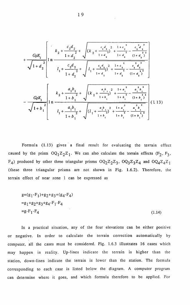
Formula (1.13) gives a final result for evaluating the terrain effect

caused by the prism O Q j Z 2 Z j . We can also calculate the terrain effects (F2 , F3 ,

F 4 ) produced by other three triangular prisms OQ2 Z 2 Z 3 , OQ3 Z 3 Z 4 and OQ4 Z 4 Z j

(these three triangular prisms are not shown in Fig. 1.6.2). Therefore, the

terrain effect of near zone 1 can be expressed as

In a practical situation, any of the four elevations can be either positive

or negative. In order to calculate the terrain correction automatically by

computer, all the cases must be considered. Fig. 1.6.3 illustrates 16 cases which

may happen in reality. Up-lines indicate the terrain is h igher than the

station, down-lines indicate the terrain is lower than the station. The formula

corresponding to each case is listed below the diagram. A computer program

can determine where it goes, and which formula therefore to be applied. For

g = ( g l - F l ) + g 2 + S3+ (g 4-F4)

=gl+g2+g3+g4-F r F4

=g-Fr F4 (1.14)

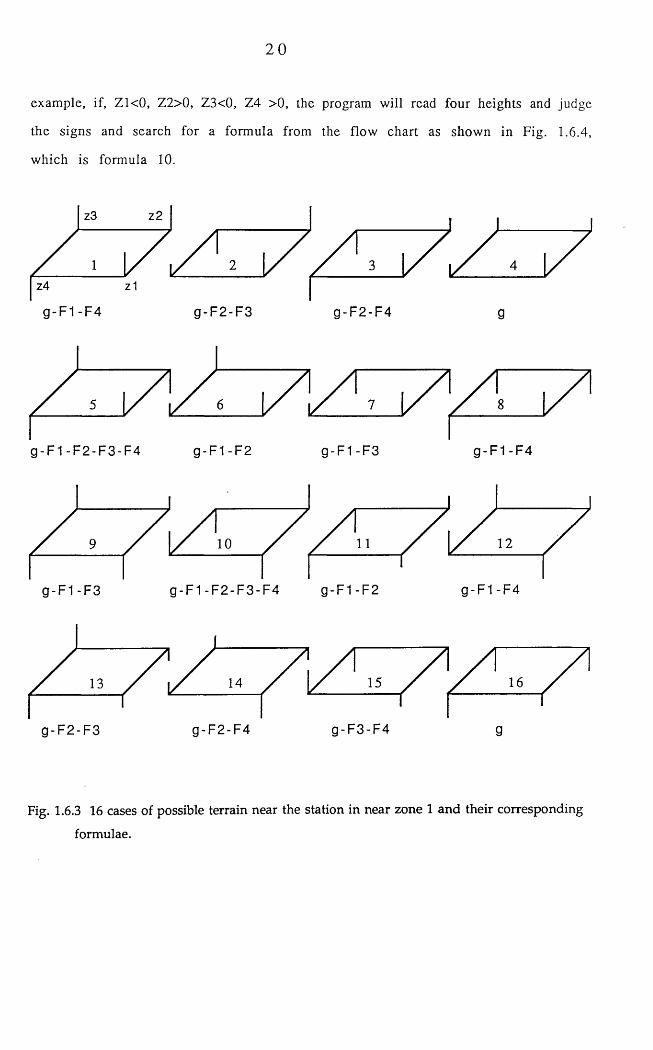
2 0

example, if, Z1<0, Z2>0, Z3<0, Z4 >0, the program will read four heights and judge

the signs and search for a formula from the flow chart as shown in Fig. 1.6.4,

which is formula 1 0 .

g-F1-F2-F3-F4 g-F1-F2 g-F1-F3 g-F1-F4

g-F1-F3 g-F1-F2-F3-F4 g-F1-F2 g-F1-F4

g-F2-F3 g-F2-F4 g-F3-F4 g

Fig. 1.6.3 16 cases of possible terrain near the station in near zone 1 and their corresponding

formulae.

21

z 1 > 0

z 1 < 0

z 2 < 0 z 2 > 0 z 2 < 0 z 2 > 0

z3<0 kz3>0 z3< z3>0 z3<0 3>0 z3<0 z3>0

z4>0 z4>0 z4>0 z4>0 z4>0 z4>0 z4>0 z4>0

6 15 13 14 1 1 10 9 1 2 8 7 6 35 2 1 4

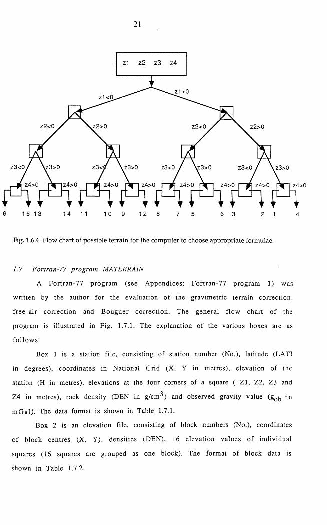
Fig. 1.6.4 Flow chart of possible terrain for the computer to choose appropriate formulae.

1.7 Fortran-77 program MATERRAIN

A Fortran-77 program (see Appendices; Fortran-77 program 1) was

written by the author for the evaluation of the gravimetric terrain correction,

free-air correction and Bouguer correction. The general flow chart of the

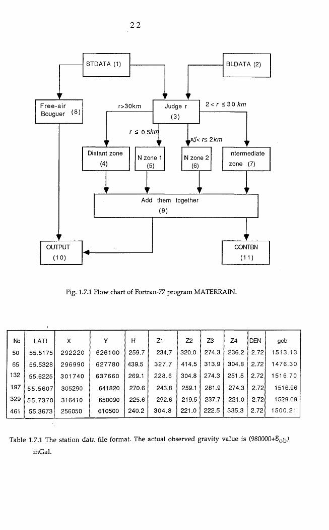
program is illustrated in Fig. 1.7.1. The explanation of the various boxes are as

fo llows.

Box 1 is a station file, consisting of station number (No.), latitude (LATI

in degrees), coordinates in National Grid (X, Y in metres), elevation of the

station (H in metres), elevations at the four comers of a square ( Z I, Z2, Z3 and'i

Z4 in metres), rock density (DEN in g/cmJ ) and observed gravity value (gob in

m G al). The data format is shown in Table 1.7.1.

Box 2 is an elevation file, consisting of block numbers (No.), coordinates

of block centres (X, Y), densities (DEN), 16 elevation values of individual

squares (16 squares are grouped as one block). The format of block data is

shown in Table 1.7.2.

22

2 < r < 3 0 kmr>30km

r < 0 .5km,dJ< r< 2 km

N zone 2N zone 1

OUTPUT

( 1 0 )

STD ATA (1)

Judge r

BLDATA (2)

Distant zone intermediate

zone (7)

F ree -a ir Bouguer (®)

Add them together

Fig. 1.7.1 Flow chart of Fortran-77 program MATERRAIN.

No LATI X Y H Z1 Z2 Z3 Z4 DEN gob

50 55.5175 2 9 2 2 2 0 6 2 6 1 0 0 259.7 234.7 320.0 274.3 236.2 2.72 151 3 .1 3

65 55.5328 2 9 6 9 9 0 6 2 7 7 8 0 439.5 3 2 7 .7 414.5 313.9 304.8 2.72 1476 .3 0

132 55.6225 3 0 1 7 4 0 6 3 7 6 6 0 269.1 2 2 8 .6 304.8 274.3 251.5 2.72 151 6 .70

197 5 5 .5 6 0 7 305290 641820 270.6 243.8 259.1 281.9 274.3 2.72 1516.96

329 5 5 .7 3 7 0 316410 650090 225.6 292.6 219.5 237.7 2 2 1 . 0 2.72 1529.09

461 55.3673 256050 610500 ! 240.2 304 .8 2 2 1 . 0 222.5 335.3 2.72 1500.21

Table 1.7.1 The station data file format. The actual observed gravity value is (980000+Sot,)

mGal.

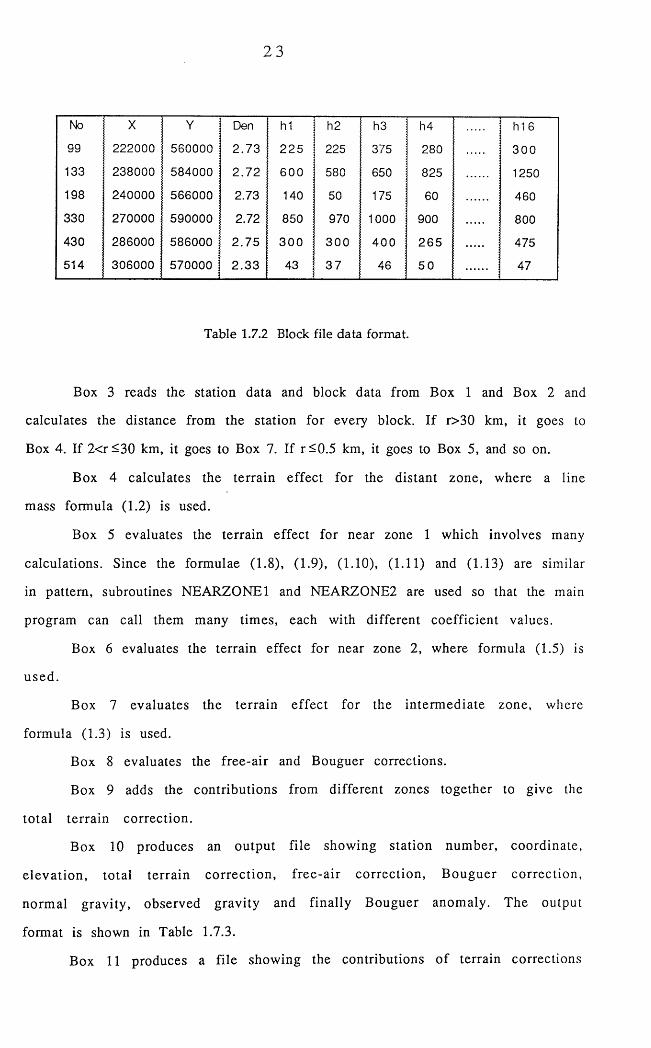
23

No X Y Den hi h2 h3 h4 hi 6

99 2 2 2 0 0 0 560000 2 .7 3 2 2 5 225 375 280 3 0 0

133 238000 584000 2 .7 2 6 0 0 580 650 825 1250

198 240000 566000 2.73 140 50 175 60 460

330 270000 590000 2.72 850 970 1 0 0 0 900 800

430 286000 586000 2 .7 5 3 0 0 3 0 0 4 0 0 2 6 5 475

514 306000 570000 2 .3 3 43 3 7 46 5 0 47

Table 1.7.2 Block file data format.

Box 3 reads the station data and block data from Box 1 and Box 2 and

calculates the distance from the station for every block. If r>30 km, it goes to

Box 4. If 2<r^30 km, it goes to Box 7. If r^0 .5 km, it goes to Box 5, and so on.

Box 4 calculates the terrain effect for the distant zone, where a line

mass formula ( 1 .2 ) is used.

Box 5 evaluates the terrain effect for near zone 1 which involves many

calculations. Since the formulae (1.8), (1.9), (1.10), (1.11) and (1.13) are similar

in pattern, subroutines NEARZONE 1 and NEARZONE2 are used so that the main

program can call them many times, each with different coefficient values.

Box 6 evaluates the terrain effect for near zone 2, where formula (1.5) is

used.

Box 7 evaluates the terrain effect for the intermediate zone, where

formula (1.3) is used.

Box 8 evaluates the free-air and Bouguer corrections.

Box 9 adds the contributions from different zones together to give the

total terrain correction.

Box 10 produces an output file showing station number, coordinate,

elevation, total terrain correction, free-air correction, Bouguer correction,

normal gravity, observed gravity and finally Bouguer anomaly. The output

format is shown in Table 1.7.3.

Box 11 produces a file showing the contributions of terrain corrections

24

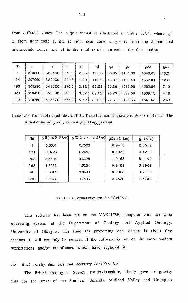
from different zones. The output format is illustrated in Table 1.7.4, where gtl

is from near zone 1, gt2 is from near zone 2, gt3 is from the distant and

intermediate zones, and gt is the total terrain correction for that station.

No X Y H gt gt gb go gob gba

1 273350 6 2 5 4 6 0 516.9 2 .3 5 159.52 58.95 1460.00 1549.63 13.31

64 297960 6 2 9 0 6 0 384.7 1.89 118.72 43.87 1488.40 1552.81 12.25

196 305290 6 4 1 8 2 0 270.6 0 . 1 2 83.51 30.86 1516.96 1562.56 7.13

328 316410 6 5 0 0 9 0 225.6 0 .37 6 9 .6 2 25.73 1529.09 1569.13 4.19

1131 319750 6 1 3 8 7 0 677.9 5 .5 2 2 .9 .2 0 77.31 1406.86 1541.63 2.63

Table 1.7.3 Format of output file OUTPUT. The actual normal gravity is (980000+go) mGal. The

actual observed gravity value is (980000+go^) mGal.

No gt\(r <0. 5 km) gt2(0. 5 < r < 2 km) gt3(r>2 km) gt (total)

1 0.6531 0.7503 0 .9 4 7 3 2 .3 5 1 2

131 0.0723 0.2457 0 .1 0 3 0 0 .4 2 1 0

2 0 8 2.8616 3.3325 1 .9163 8 .1 1 0 4

2 6 3 1.3266 1.5234 0 .9 4 6 9 3 .7 9 6 9

3 9 5 0.0014 0.0693 0 .2 0 0 3 0 .2 7 1 0

5 0 0 0.3674 0.7596 0 .4 5 2 0 1 .5 7 8 0

Table 1.7.4 Format of output file CONTBN.

This software has been run on the VAX11/750 computer with the Unix

opera ting system at the Department o f Geology and Applied Geology,

University of Glasgow. The time for processing one station is about five

seconds. It will certainly be reduced if the software is run on the more modem

workstations and/or mainframes which have replaced it.

1.8 Real gravity data test and accuracy consideration

The British Geological Survey, Nottinghamshire, kindly gave us gravity

data for the areas of the Southern Uplands, Midland Valley and Grampian

25

Highlands. For the purpose of testing the new method, 4526 gravity station in

the western Southern Uplands, which occupies 11,000 km2 , were read from the

magnetic tape. The area was digitized for the terrain correction. There are in

total 11,328 elevation data read from the Ordnance Survey (OS) map for 708

blocks, each block having 16 squares inside. In addition, 18,104 more elevation

data were also read from the OS map in order to calculate the terrain

correction for near zone 1. The organisation of elevation data is shown in

Table 1.7.1 and Table 1.7.2.

In creating block file BLDATA, the densities in the fourth column are

adapted from previous papers by Mansfield [1963], Bott [1960] and Parslow &

Randall [1973]. Specifically, the density for lower Palaeozoic rocks is 2.72-2.73

g / c m^ , 2.33 g/cm^ for New Red Sandstone rocks, 2.62 g/cm^ for granite, 1.03

g / c m ^ for sea water. In order to check these densities determined by the

sample measurement, Nettleton's method [1939] is used here for three areas in

the Southern Uplands where there are simple rock types and low relief

topography. According to Nettleton's theory, the correct density is measured

simply by making a special t r a - v e r s e of gravimetric stations across the

topographic feature, reducing these stations for several densities and finding

the density value for which the reduced curve has a minimum correlation

with the topography. A Fortran-77 program was written by the author to pick

up those stations which have to be not only along a short straight profile line,

but also in places where the geology is simple. The first density profile,

passing through the National Grid NX39 (see Fig. 1.8.1, line a), lies in the

northern belt of the Southern Uplands. The area is composed of greywackes

and shales (Ordovician). The second and third profile lines, passing through

NX77, NX87, NX8 8 , and NX76, NX87 respectively. Both trend NE-SW and lie in the

central belt of the Southern Uplands (see Fig. 1.8.1, lines b and c). Rock

exposures are greywackes, shales and sandstone (Silurian). The relief of the

topography along three lines is in the region of 60-190 m. The correct

densities from three figures seem to be in the region of 2.70-2.73 g/cm^

because the curves reduced by those densities are nearly horizontal,

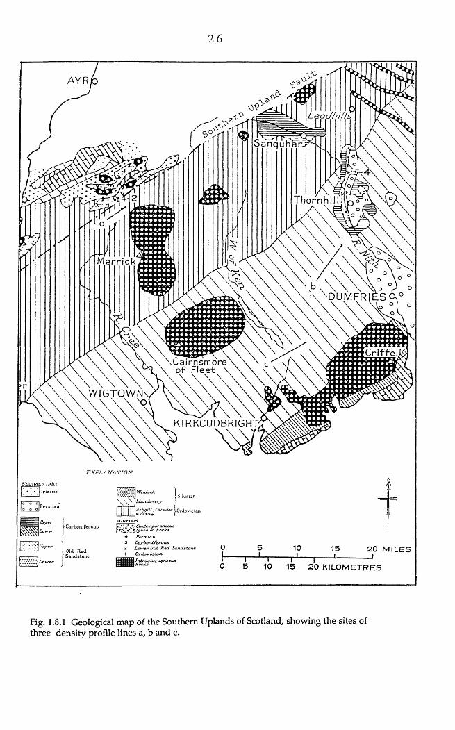
26

Leodh ills

Sanau i a r.

lo rnh il l :

e r r i c k

\ D U M F R I E S

rnsmore

W I G T O W N

KIRKCUDBRIGHT

E X P L A N A T I O N

S E D IM E N T A R Y

• Triassic

\U ppc> C arbon ife rous

Upper jOld R ed

I S a n d s to n e

WcnJLo <Jc ]J* S ilurian

L laJ idovery j

A shgU l. Cartuiac 1 q rcJ o c jaj* A A r e n ig j

IGNEOUSL C o n tem poraneous1 ‘ f ./y '• -T1 Ig n e o u s R o c k s

4 P erm ia n .3 C a r b o n if e r o u s 2 Lo>*‘c r Old- R ed . S a n d s to n e I O r d o v ic ia n .

10

10I

15

15_ l _

J Lh i

2 0 M IL E S

2 0 K ILO M E TR E S

Fig. 1.8.1 Geological map of the Southern Uplands of Scotland, showing the sites of three density profile lines a, b and c.

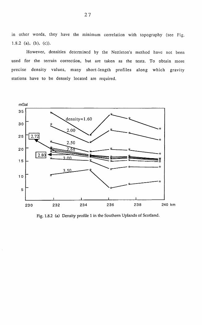
27

in other words, they have the minimum correlation with topography (see Fig.

1 .8 . 2 (a), (b), (c)).

However, densities determined by the Nettleton's method have not been

used for the terrain correction, but are taken as the tests. To obtain more

prec ise density values, many short-length profiles along which gravity

stations have to be densely located are required.

mGal

35

density=1.6030

2.001 2.7:25

2.5020

2.80

240 km238236234232230

Fig. 1.8.2 (a) Density profile 1 in the Southern Uplands of Scotland.

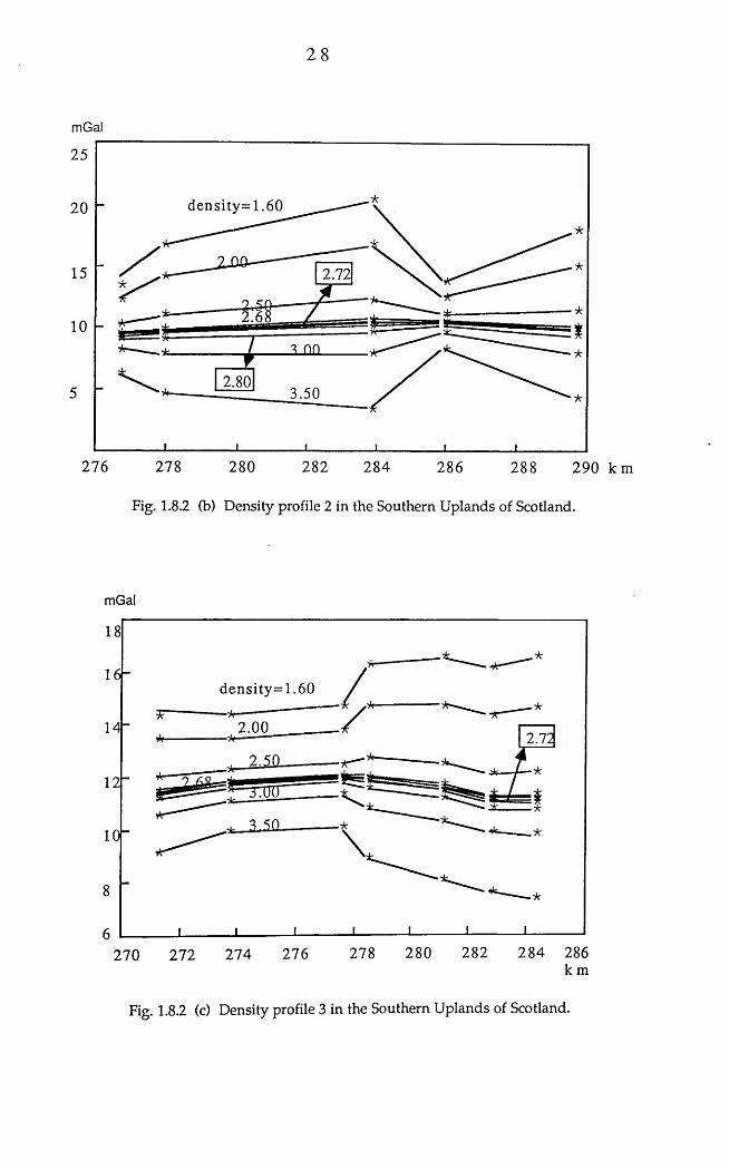
28

mGal

25

density=1.6020

2.6

2.803.50

276 278 280 282 284 286 288 290 k m

Fig. 1.8.2 (b) Density profile 2 in the Southern Uplands of Scotland.

mGal

density=1.60

2.00

282 284 286280278276274270 272

Fig. 1.8.2 (c) Density profile 3 in the Southern Uplands of Scotland.

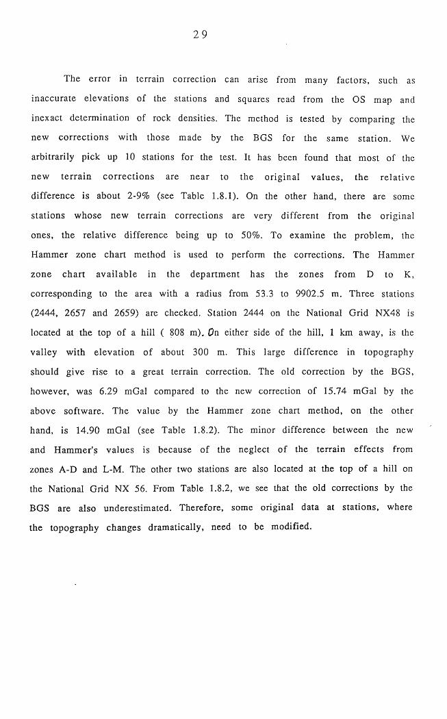
29

The error in terrain correction can arise from many factors, such as

inaccurate elevations of the stations and squares read from the OS map and

inexact determination of rock densities. The method is tested by comparing the

new corrections with those made by the BGS for the same station. We

arbitrarily pick up 10 stations for the test. It has been found that most of the

new terra in correc tions are near to the original values, the relative

difference is about 2-9% (see Table 1.8.1). On the other hand, there are some

stations whose new terrain corrections are very different from the original

ones, the relative difference being up to 50%. To examine the problem, the

Hammer zone chart method is used to perform the corrections. The Hammer

zone chart available in the department has the zones from D to K,

corresponding to the area with a radius from 53.3 to 9902.5 m. Three stations

(2444, 2657 and 2659) are checked. Station 2444 on the National Grid NX48 is

located at the top of a hill ( 808 m). On either side of the hill, 1 km away, is the

valley with elevation of about 300 m. This large difference in topography

should give rise to a great terrain correction. The old correction by the BGS,

however, was 6.29 mGal compared to the new correction of 15.74 mGal by the

above software. The value by the Hammer zone chart method, on the other

hand, is 14.90 mGal (see Table 1.8.2). The minor difference between the new

and Hammer's values is because of the neglect of the terrain effects from

zones A-D and L-M. The other two stations are also located at the top of a hill on

the National Grid NX 56. From Table 1.8.2, we see that the old corrections by the

BGS are also underestimated. Therefore, some original data at stations, where

the topography changes dramatically, need to be modified.

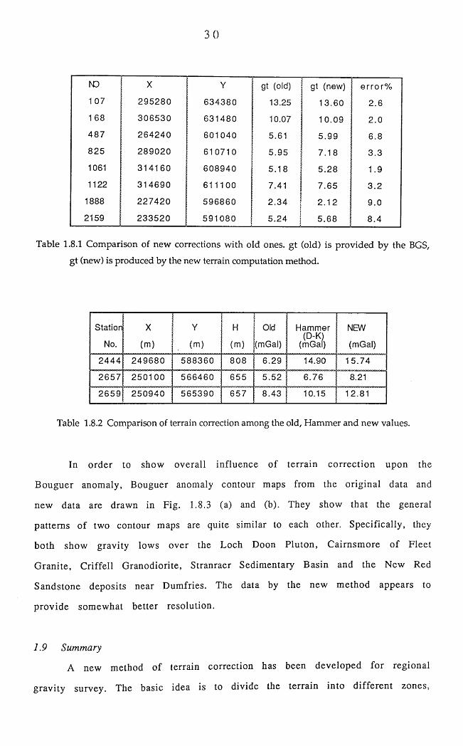
30

l\D X Y gt (old) gt (new) e rro r%

1 07 2 9 5 2 8 0 6 3 4 3 8 0 13.25 1 3 .60 2.61 68 3 0 6 5 3 0 6 3 1 4 8 0 10.07 10 .09 2.04 8 7 2 6 4 2 4 0 6 0 1 0 4 0 5.61 5 .9 9 6.88 2 5 2 8 9 0 2 0 6 1 0 7 1 0 5 .9 5 7 .1 8 3 .3

1061 3 1 4 1 6 0 6 0 8 9 4 0 5 .18 5 .2 8 1.9

1122 3 1 4 6 9 0 6 1 1 1 0 0 7.41 7 .6 5 3 .2

1888 2 2 7 4 2 0 5 9 6 8 6 0 2 .3 4;

2.12 9 .0

2159 2 3 3 5 2 0 5 9 1 0 8 0 5 .2 4 5 .6 8 8 .4

Table 1.8.1 Comparison of new corrections with old ones, gt (old) is provided by the BGS,

gt (new) is produced by the new terrain computation method.

Station

No.

X

(m)

Y

(m)

H

(m)

Old

(mGal)

Hammer(D-K)

(mGal)

NEW

(mGal)

2 4 4 4 2 4 9 6 8 0 5 8 8 3 6 0 80 8 6 .29 14.90 15 .7 4

2 6 5 7 2 5 0 1 0 0 5 6 6 4 6 0 655 5 .52 6 .7 6 8.21

2 6 5 9 2 5 0 9 4 0 5 6 5 3 9 0 65 7 8 .43 10.15 12.81

Table 1.8.2 Comparison of terrain correction among the old, Hammer and new values.

In order to show overall influence of terrain correction upon the

Bouguer anomaly, Bouguer anomaly contour maps from the original data and

new data are drawn in Fig. 1.8.3 (a) and (b). They show that the general

patterns of two contour maps are quite similar to each other. Specifically, they

both show gravity lows over the Loch Doon Pluton, Cairnsmore of Fleet

Granite, Criffell Granodiorite, Stranraer Sedimentary Basin and the New Red

Sandstone deposits near Dumfries. The data by the new method appears to

provide somewhat better resolution.

1.9 Summary

A new method of terrain correction has been developed for regional

gravity survey. The basic idea is to divide the terrain into different zones,

3 1

within each zone, different formulae with certain approximations are applied.

The main contributions to the old methods are made particularly for the near

zone 1 correction, where new formulae are derived from integrations. The

software MATERRAIN is tested by the gravity data in the Southern Uplands of

Scotland. It has been found that some of the old corrections by the BGS are

likely to be underestimated. The new method is entirely automatic and easy to

use .

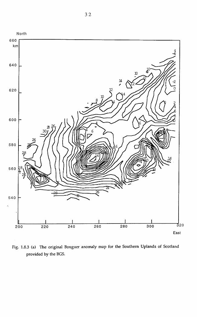
3 2

6 0 0 h

North

4

Q

0

5 8 0 L

5 6 0

5 4 0 h

Fig. 1.8.3 (a) The original Bouguer anomaly map for the Southern Uplands of Scotland

provided by the BGS.

3 3

North

6 0 0 -

J

6

0

0

5 8 0

56 0

5 4 0 “

Fig. 1.8.3 (b) New Bouguer anomaly map for the Southern Uplands of Scotland, produced using

the new terrain correction computation method.

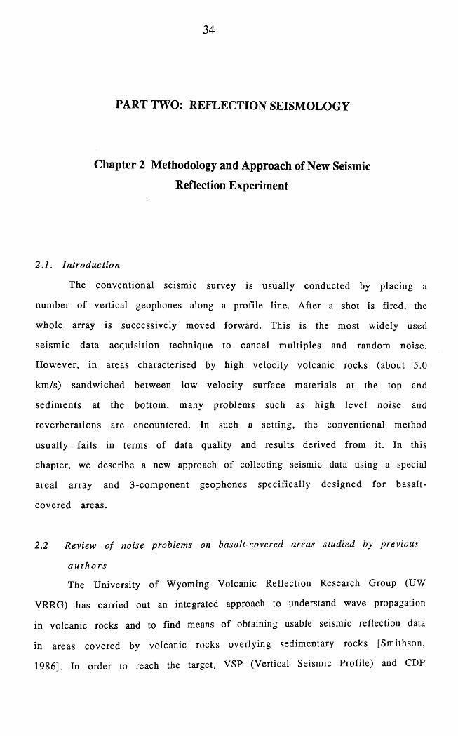
34

PART TWO: REFLECTION SEISMOLOGY

Chapter 2 Methodology and Approach of New Seismic

Reflection Experiment

2.1. In troduction

The conventional seismic survey is usually conducted by placing a

number of vertical geophones along a profile line. After a shot is fired, the

whole array is successively moved forward. This is the most widely used

seismic data acquisition technique to cancel multiples and random noise.

However, in areas characterised by high velocity volcanic rocks (about 5.0

km/s) sandwiched between low velocity surface materials at the top and

sedim ents at the bottom, many problems such as high level noise and

reverberations are encountered. In such a setting, the conventional method

usually fails in terms of data quality and results derived from it. In this

chapter, we describe a new approach of collecting seismic data using a special

areal array and 3 -component geophones specifically designed for basalt-

covered areas.

2.2 Review o f noise problems on basalt-covered areas studied by previous

a u th o r s

The University of Wyoming Volcanic Reflection Research Group (UW

VRRG) has carried out an integrated approach to understand wave propagation

in volcanic rocks and to find means of obtaining usable seismic reflection data

in areas covered by volcanic rocks overlying sedimentary rocks [Smithson,

1986]. In order to reach the target, VSP (Vertical Seismic Profile) and CDP

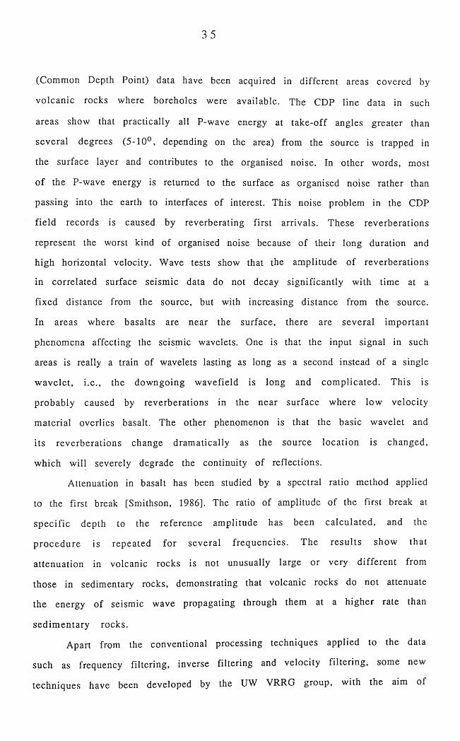
35

(Common Depth Point) data have been acquired in different areas covered by

volcanic rocks where boreholes were available. The CDP line data in such

areas show that practically all P-wave energy at take-off angles greater than

several degrees (5-10°, depending on the area) from the source is trapped in

the surface layer and contributes to the organised noise. In other words, most

of the P-wave energy is returned to the surface as organised noise rather than

passing into the earth to interfaces of interest. This noise problem in the CDP

field records is caused by reverberating first arrivals. These reverberations

represent the worst kind of organised noise because of their long duration and

high horizontal velocity. Wave tests show that the amplitude of reverberations

in correlated surface seismic data do not decay significantly with time at a

fixed distance from the source, but with increasing distance from the source.

In areas where basalts are near the surface, there are several important

phenomena affecting the seismic wavelets. One is that the input signal in such

areas is really a train of wavelets lasting as long as a second instead of a single

wavelet, i.e., the downgoing wavefield is long and complicated. This is

probably caused by reverberations in the near surface where low velocity

material overlies basalt. The other phenomenon is that the basic wavelet and

its reverberations change dramatically as the source location is changed,

which will severely degrade the continuity of reflections.

Attenuation in basalt has been studied by a spectral ratio method applied

to the first break [Smithson, 1986]. The ratio of amplitude of the first break at

specific depth to the reference amplitude has been calculated, and the

p rocedure is repeated for several frequencies. The results show that

attenuation in volcanic rocks is not unusually large or very different from

those in sedimentary rocks, demonstrating that volcanic rocks do not attenuate

the energy of seismic wave propagating through them at a higher rate than

sedim entary rocks.

Apart from the conventional processing techniques applied to the data

such as frequency filtering, inverse filtering and velocity filtering, some new

techniques have been developed by the UW VRRG group, with the aim of

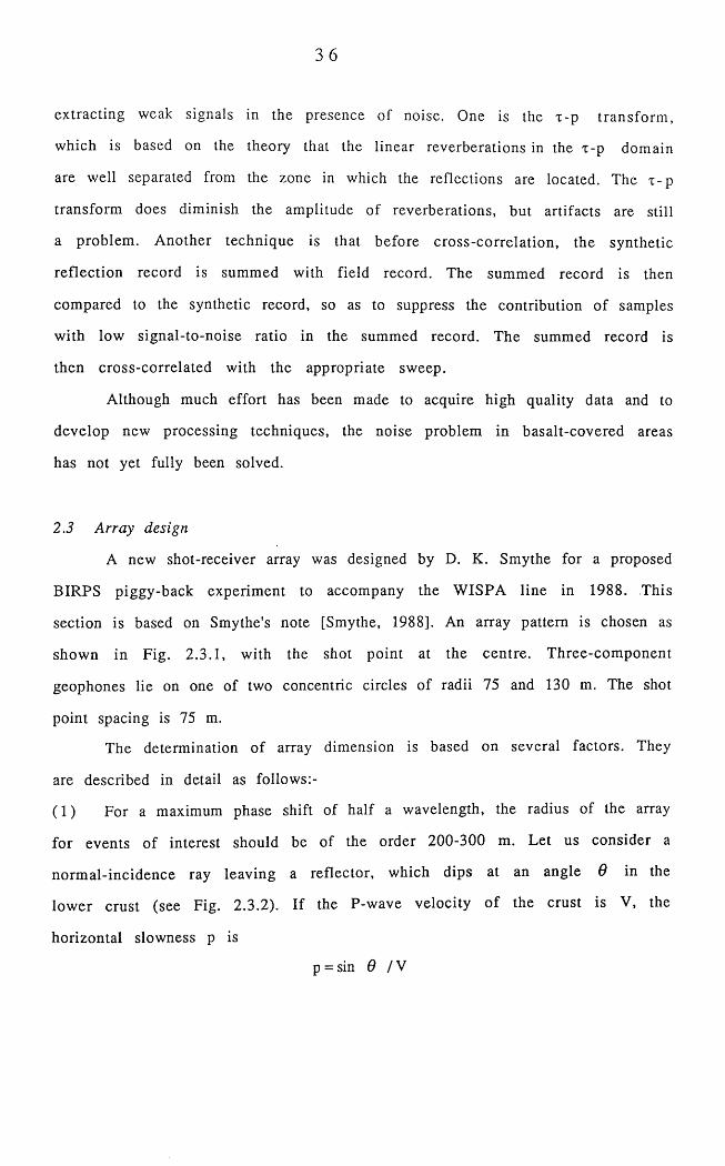
36

extracting weak signals in the presence of noise. One is the x-p transform ,

which is based on the theory that the linear reverberations in the x-p domain

are well separated from the zone in which the reflections are located. The x-p

transform does diminish the amplitude of reverberations, but artifacts are still

a problem. Another technique is that before cross-correlation, the synthetic

reflection record is summed with field record. The summed record is then

compared to the synthetic record, so as to suppress the contribution of samples

with low signal-to-noise ratio in the summed record. The summed record is

then cross-correlated with the appropriate sweep.

Although much effort has been made to acquire high quality data and to

develop new processing techniques, the noise problem in basalt-covered areas

has not yet fully been solved.

2.3 Array design

A new shot-receiver array was designed by D. K. Smythe for a proposed

BIRPS piggy-back experiment to accompany the WISPA line in 1988. This

section is based on Smythe's note [Smythe, 1988]. An array pattern is chosen as

shown in Fig. 2.3.1, with the shot point at the centre. Three-component

geophones lie on one of two concentric circles of radii 75 and 130 m. The shot

point spacing is 75 m.

The determination of array dimension is based on several factors. They

are described in detail as follows:-

(1 ) For a maximum phase shift of half a wavelength, the radius of the array

for events of interest should be of the order 200-300 m. Let us consider a

normal-incidence ray leaving a reflector, which dips at an angle 6 in the

lower crust (see Fig. 2.3.2). If the P-wave velocity of the crust is V, the

horizontal slowness p is

p = sin 6 / V

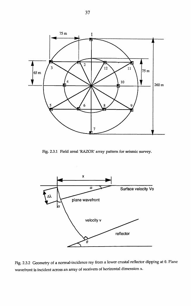
37

75 m

175 m65 m

260 m

— ________ f.....

Fig. 2.3.1 Field areal 'RAZOR1 array pattern for seismic survey.

Surface velocity Vo

plane wavefront

velocity v

reflector

Fig. 2.3.2 Geometry of a normal-incidence ray from a lower crustal reflector dipping at 0. Plane

wavefront is incident across an array of receivers of horizontal dimension x.

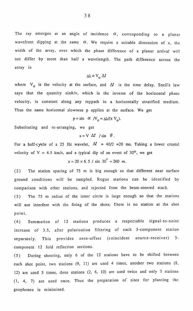
3 8

The ray emerges at an angle of incidence CC, corresponding to a planar

wavefront dipping at the same a . We require a suitable dimension of x, the

width of the array, over which the phase difference of a planar arrival will

not differ by more than half a wavelength. The path difference across the

array is

AX = V0 A t

where VQ is the velocity at the surface, and At is the time delay. Snell's law

says that the quantity sin0 /v, which is the inverse of the horizontal phase

velocity, is constant along any raypath in a horizontally stratified medium.

Thus the same horizontal slowness p applies at the surface. We get

P = sin a /V0 = AX/(x Vq).

Substituting and re-arranging, we get

x = V At /sin 6 .

For a half-cycle of a 25 Hz wavelet, Af = 40/2 =20 ms. Taking a lower crustal

velocity of Y = 6.5 km/s, and a typical dip of an event of 30°, we get

x = 20 x 6 . 5 / sin 30 = 260 m.

(2 ) The station spacing of 75 m is big enough so that different near surface

ground conditions will be sampled. Rogue stations can be identified by

comparison with other stations, and rejected from the beam-steered stack.

(3 ) The 75 m radius of the inner circle is large enough so that the stations

will not interfere with the firing of the shots; there is no station at the shot

po i n t .

( 4) Sum m ation of 12 stations produces a respectable s ignal-to-noise

increase of 3.5, after polarisation filtering of each 3-com ponent station

separa te ly . This provides ze ro -o ffse t (co inc iden t s o u rc e - re c e iv e r) 3-

component 1 2 fold reflection sections.

(5 ) During shooting, only 6 of the 12 stations have to be shifted between

each shot point, two stations (9, 11) are used 4 times, another two stations (8 ,

12) are used 3 times, three stations (2, 6 , 10) are used twice and only 3 stations

(1, 4, 7) are used once. Thus the preparation of sites for planting the

geophones is minimised.

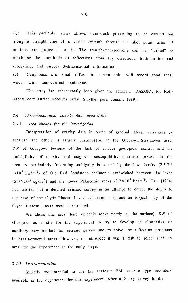
3 9

( 6 ) This particular array allows slant-stack processing to be carried out

along a straight line of a varied azimuth through the shot point, after 1 2

stations are projected on it. The transformed-sections can be "turned" to

maximise the amplitude of reflections from any directions, both in-line and

cross-line, and supply 3-dimensional information.

(7) Geophones with small offsets to a shot point will record good shear

waves with near-vertical incidence.

The array has subsequently been given the acronym "RAZOR", for Roll-

Along Zero Offset Receiver array [Smythe, pers. comm., 1989].

2.4 Three-component seismic data acquisition

2.4.1 Area chosen fo r the investigation

Interpretation of gravity data in terms of gradual lateral variations by

McLean and others is largely unsuccessful in the Greenock-Strathaven area,

SW of Glasgow, because of the lack of surface geological control and the

m ultiplicity of density and magnetic susceptibility contrasts present in the

area. A particularly frustrating ambiguity is caused by the low density (2.3-2 . 6

x l O^ k g / m ^ ) of Old Red Sandstone sediments sandwiched between the lavas

(2.7 x 1 0^ k g / m^ ) and the lower Palaeozoic rocks (2.7 x l O^ kg/m^). Hall [1974]

had carried out a detailed seismic survey in an attempt to detect the depth to

the base of the Clyde Plateau Lavas. A contour map and an isopach map of the

Clyde Plateau Lavas were constructed.

We chose this area (hard volcanic rocks nearly at the surface), SW of

Glasgow, as a site for the experiment to try to develop an alternative or

auxiliary new method for seismic survey and to solve the reflection problems

in basalt-covered areas. However, in retrospect it was a risk to select such an

area for the experiment at the early stage.

2.4.2 Instrum entation

Initially we intended to use the analogue FM cassette type recorders

available in the department for this experiment. After a 2 day survey in the

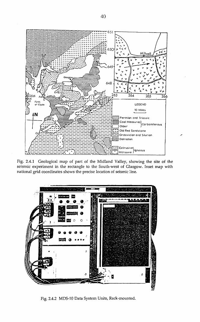
40

Millwell

G lasg o w

LEGEND

10 Miles

:*:■■■& P e r m i a n and TriassicCoal M e a s u re s ]

□ /C a rb o n i fe ro u sO ld e r J

|* Old Red S a n d s t o n e|~1ZTC| O rd o v ic ia n and Silurian

S Dalradian

F.W .j E x t ru s iv e ]Igneous

Fig. 2.4.1 Geological map of part of the Midland Valley, showing the site of the seismic experiment in the rectangle to the South-west of Glasgow. Inset map with national grid coordinates shows the precise location of seismic line.

Fig. 2.4.2 MDS-10 Data System Units, Rack-mounted.

4 1

area, we collected data from two shots with different sizes of explosive using

these recorders in early June, 1988. Twelve vertical component traces were

recorded from each shot.

The recordings obtained from the seismometers were played back using

an analogue facility and converted to digital form. Arrivals were picked up

from the analogue playbacks and arrival times were calculated using the MSF

pulses as a time scale. By inspecting the collected data carefully, we found that

the seismic signals were overloaded, and the time error of up to 2 0 ms was

unacceptable if the data are to be stacked. In fact, to image structure from the

time difference introduced by the dipping of reflectors, we require that the

error brought by the equipment should be less than 5 ms, otherw ise this

experim ent would lose its significance.

The departm ent subsequently acquired a second-hand MDS-10 (see Fig.

2.4.2) in 1988. This equipment can meet our requirements. The basic electronic

modules of the MDS-10 Seismic Data System are the printed circuit plug-in

cards containing an assemblage of linear and digital integrated circuits. These

cards are housed in modular card racks which may be mounted in several

different configurations depending on the type o f exploration work required.

The basic modules of Preamp, IFP Amplifier, Digital Controller, Power Supply,

and Tape Transport form the core of a Seismic Data Acquisition System. System

capabilities are expandable to 96 data channels by the addition of a second

Preamp module, and to field data stacking by the addition of a Mass Memory

Unit and card modules in the Digital Control Unit (Service Manual, 1977).

The Preamp Unit (see Fig. 2.4.3) is the analog input to the system. It is

capable of handling up to 96 seismic inputs. The seismic input is normally

channelled to the Preamp Unit by an input switching unit to allow for needed

functions such as geophone testing, leakage testing, CDP switching, etc. In the

operating mode of this Input Unit, the Preamps are connected directly to the

g eophones. The functions perform ed by the P ream p U nit in c lu d e ,

am plification of the signal, low-cut filtering, 50/60 Hz notch filtering, an ti­

aliasing filtering, and multiplexing of the data channels to the IFP Unit.

The IFP Amplifier Unit contains: the Track & Hold circuit which samples

the m ultiplexed signals from the Preamp, the IFP Amplifier which raises the

held sample to an analog level near full scale of the converter, and the

A nalog-to-D igital Converter which converts the analog signal to 14 bits plus

s ig n .

The Digital Control Unit contains the system master clock and associated

logic for system tim ing and control functions. Primary data flow concerns

movement of the converted data bits from the A/D converter and gain bits

from the IFP C ontroller Logic to the Tape Form atter. Data are arranged

according to the SEG-B Format and written to tape under the control of the

Tape Controller Logic in the Digital Unit. Other functions performed by the

D igital C ontroller include I/O signals for operation of remote firing system,

defloating and conversion circuits for driving a M onitor Camera, form atting

and con tro lling a D igital . C orrela tor for display of v ibroseis data, and

form atting and controlling a Mass Memory device for data stacking, when the

optional stacking features are ordered with the system.

The geophones used here have a natural frequency of 7.5 Hz. The coil

resistance is 600 ohms. To obtain uniform coupling, the 3 geophones (two

horizon tal and one vertica l) were fixed in one cluster, the horizontal

geophones being oriented towards North and East respectively. Twelve such

clusters were used.

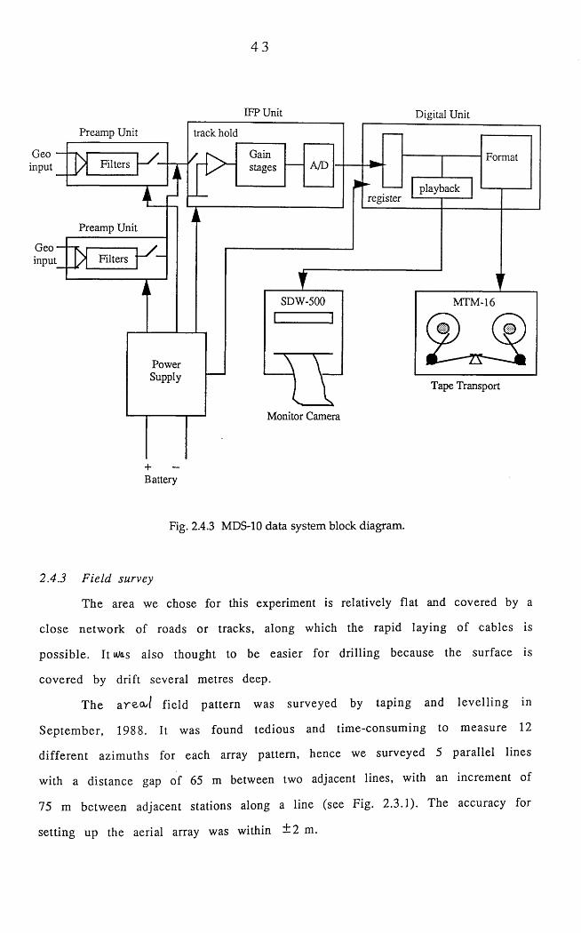
4 3

IFP Unit Digital UnitPreamp Unit track hold

Geoinput

Gainstages

FormatFilters A/D

playbackregister

Preamp Unit

Geo • input Filters

SDW-500 MTM-16

PowerSupply

Tape Transport

Monitor Camera

+Battery

Fig. 2.4.3 MDS-10 data system block diagram.

2.4.3 F ield survey

The area we chose for this experiment is relatively flat and covered by a

close netw ork of roads or tracks, along which the rapid laying of cables is

possible. It idas also thought to be easier for drilling because the surface is

covered by drift several metres deep.

The areoo/ field pattern was surveyed by taping and levelling in

Septem ber, 1988. It was found tedious and tim e-consuming to m easure 12

different azim uths for each array pattern, hence we surveyed 5 parallel lines

with a distance gap of 65 m between two adjacent lines, with an increment of

75 m between adjacent stations along a line (see Fig. 2.3.1). The accuracy for

setting up the aerial array was within ± 2 m.

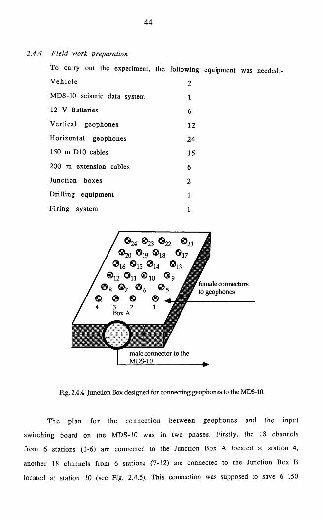
44

2.4.4 F ield work preparation

To carry out the experiment, the following equipment was needed:-

V e h ic le 2

MDS-10 seismic data system 1

12 V Batteries 6

V ertica l geophones 1 2

H orizon ta l geophones 24

150 m DIO cables 15

2 0 0 m extension cables 6

Junction boxes 2

D rilling equipm ent 1

F iring system 1

female connectors to geophones

Box A

male connector to the MDS-10 ______

Fig. 2.4.4 Junction Box designed for connecting geophones to the MDS-10.

The p lan fo r the connection betw een geophones and the input

sw itching board on the MDS-10 was in two phases. Firstly, the 18 channels

from 6 stations (1-6) are connected to the Junction Box A located at station 4,

another 18 channels from 6 stations (7-12) are connected to the Junction Box B

located at station 10 (see Fig. 2.4.5). This connection was supposed to save 6 150

45

m DIO cables; that is, the 3 channels from station 4 and another 3 channels

from station 10 are directly connected to the Junction Box A and Box B

resp e c tiv e ly w ithou t using ex tra cables for the connections betw een

geophones to the Junction Boxes. Secondly, the Junction Boxes were connected

to the input switching board by the extension cables which can be extended up

to 600 m (see Fig. 2.4.5).

The MDS-10 Data System testing was in two phases. First, it was tested by

writing pulses and sine waves with different frequencies to tape in the SEG-B

format and then displaying the demultiplexed data to see if they are as

expected. In addition, we tested the system by completing the circuits from

geophones to the input switching board. The geophones were set on supports

in the corridor, and a hammer was used as a seismic source. By inspecting the

playback from .the m onitor camera, we could isolate the dead traces, identify

problem s e ither in the MDS-10 recorder, cables or geophones. Secondly,

testing o f the blaster was carried out in the field.

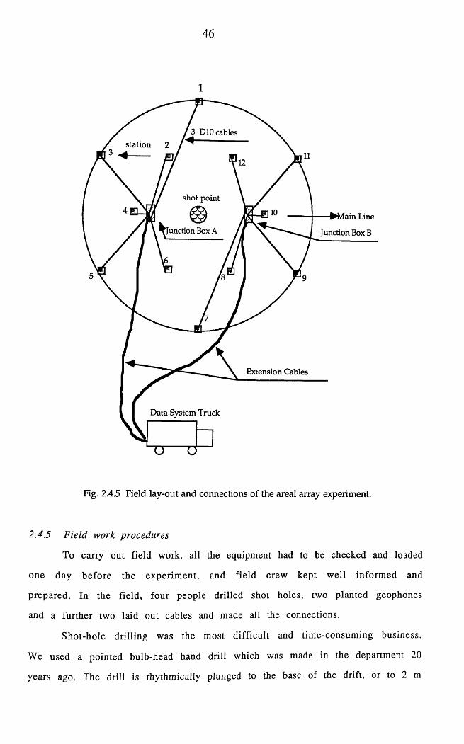
46

1

3 DIO cablesstation

f shot point

^Junction Box A►Main Line

Junction Box B

Extension Cables

Data System Truck

Fig. 2.4.5 Field lay-out and connections of the areal array experiment.

2.4.5 F ield work procedures

To carry out field work, all the equipment had to be checked and loaded

one day before the experim ent, and field crew kept well inform ed and

prepared. In the field, four people drilled shot holes, two planted geophones

and a further two laid out cables and made all the connections.

Shot-hole drilling was the most difficult and time-consuming business.

We used a pointed bulb-head hand drill which was made in the department 20

years ago. The drill is rhythmically plunged to the base of the drift, or to 2 m

47

length o f the drill shaft by means of a hand percussion bore and filled, after

loading, with mud and water. The 4 cm diameter drill head makes a hole wide

enough to take the 3 cm wide gelignite inserting device which comprises an

opcn-bottom ed sleeve to hold the stick, within which there is a plunger to

push the stick out at the bottom of the shot hole. Four holes in a polygonal

pattern about 1 m apart are drilled and made ready for loading dynamite.

Sticks or part sticks of I.C.I polar ammon gelignite, about 20 cm in

length and 3 cm in diameter, are placed individually in holes drilled to the

base o f the drift at the depth of about 2 m. The test was first conducted at the

same location by different sizes of explosive, say 4 half sticks in 4 holes and 2

half sticks in 2 holes. By comparison of the seismograms from the two shots, it

was found the first shot did not look any better than the second shot (see the

details in chapter 3). Therefore, two half sticks were used in the majority of

sh o ts .

The HS-200 blaster was used as a remote firing system which is

connected to the Digital Control Unit on the MDS-10 system. The firing signal

comes from the main system after pressing the "start" button, the blaster then

generates a 150-V firing pulse, which is conducted along a firing cable to the

series-connected detonators. Two 200 m-long twin core steel cables with a total

resistance of 40 ohms were used to complete the circuit. The blast creates a

cavity around the shot which is filled and flattened im m ediately after

s h o o tin g .

Two people planted the geophones. A shallow hole of about 50 cm in

depth was dug, and one geophone cluster was planted in the hole. A compass

was used to orient one of the horizontal geophones towards North, and the

other towards East. The holes were usually filled with soft clay afterwards.

The D10 cables were divided into two groups according to their length

(100 m or 150 m) having been tested and marked in the laboratory. Therefore,

six long cables could be used to connect stations 1 and 7 at the far ends, 30

short cables could be used t o connect other 10 stations around ihe stations 4

and 10 where the two Junction Boxes were placed. The person who

48

made all the connections had to be sure that all the stations had been

connected to the proper channels marked on the Junction Boxes. If one of the

connections was found to be faulty, he had to either swap the channels on the

Junction Box or take down the m is-connected channels for later change by

software. It was found that channel 24 did not work properly, so that this

channel had to be jumped over. In the field, channels 6-23 and channels 25-42

were used.

The MDS-10 operator is the key person in charge of the field work. He is

responsible for directing the field crew, testing the connections, giving the

signals to the firing system operator and to an observer who is stationed in the

vicinity o f the shot to warn the shooter of any hazard. Generally speaking, if

everything went all right in the field, it would take at least 3 hours to finish

one shot. In fact, we never succeeded in firing two shots in one day at the

beginning o f the experiment, although the second shot would only take half

the time of the first. The work was slowed down by many factors; for instance,

checking the dead channels again and again, and repairing the tape transport

and firing systems. These unexpected problems had to be sorted out in the

field. Som etimes, the weather before Christmas was too bad to proceed the

w o rk .

2.5 Interaction with the seismic data processing package SKS

2.5.1 Introduction to the SKS package

The collected seismic data were processed partly with the SKS (Seismic

Kernel System) package, so that it is necessary to give a brief introduction to

the package.

The Merlin SKS system consists of over 60 standard seismic processors,

which are called using MGL, Merlin Geophysical Language. MGL is a seismic

data processing language in which the geophysicist codes requests for seismic

data processes to be performed on seismic data. It has sophisticated plain-

English definition and comprehensive error reporting facilities, and includes

fac ilities to recognize the various kinds of block processing which are

49

required in seism ic data processing.

A seismic job coded in MGL is translated into the ESSR, Execution Stage

Seism ic Run, by MGLTRAN, the M erlin Geophysical Language Translator.

MGLTRAN is a four pass compiler which is able to recognize a wide number of

incorrect setups as well as optimize inefficient ones, and convert the requests

in the seism ic job into a Fortran-77 program which is then compiled and run

in the normal way.

A seism ic processor in SKS consists of two subroutines: (a) PPS (Pre­

processing Subroutine), which is loaded by the translator, M GLTRAN, in

response to the appearance of the corresponding processor name in seismic

job coded in MGL. Each processor has a number of verbs which define the

various functions of the processor. The PPS checks for the presence of the

verbs and the values of their arguments given in the seismic job. The PPS then

defines the system requirements for the SPS, and sets or resets variables in the

process comm on blocks, (b) SPS (Seismic Processing Subroutine) which does

the actual processing of the seismic data is executed as a subroutine call from

within the Fortran-77 program produced as the output of MGLTRAN.

The SKS package used was that installed in the Signal Processing

D ivision, D epartm ent o f Electrical & Electronic Engineering, U niversity of

Strathclyde, by kind permission of Professor T. Durrani.

2.5.2 Change o f SEG-Y form at into free ASCII-coded form at

A m ajor problem is dealing with various tape formats. Seismic field

tapes are recorded in a number of standard formats, SEG-A, SEG-B, SEG-C, and

SEG-D, corresponding to the A, B, C and D formats of the Society of Exploration

Geophysicist's (SEG). Different machines with different software use different

formats. However, all formats are simple if the computer on which the tape is

being read is an IBM machine, as both the characters and numeric formats are

based on IBM standards. A SEG-Y file, which is commonly used in the

exp lora tion industry is a file that contains a num ber o f traces stored

sequentially . Each trace contains a number of data samples. A SEG-Y file

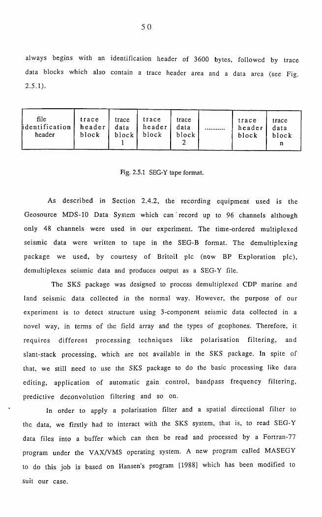
50

always begins with an identification header of 3600 bytes, followed by trace

data blocks which also contain a trace header area and a data area (see Fig.

2.5.1).

file t r a c e trace tra c e trace t r a c e traceid e n t if ic a t io n h e a d e r da ta h e a d e r da ta h e a d e r d a ta

header b lo c k b lo ck b lo ck b lo ck b lo c k b lo c k1 2 n

Fig. 2.5.1 SEG-Y tape format.

As described in Section 2.4.2, the recording equipment used is the

Geosource MDS-10 Data System which c a n ' record up to 96 channels although

only 48 channels were used in our experiment. The time-ordered m ultiplexed

seism ic data were written to tape in the SEG-B format. The dem ultiplexing

package we used, by courtesy of Britoil pic (now BP E xploration pic),

demultiplexes seismic data and produces output as a SEG-Y file.

The SKS package was designed to process demultiplexed CDP marine and

land seism ic data collected in the normal way. However, the purpose o f our

experiment is to detect structure using 3-component seismic data collected in a

novel way, in terms of the field array and the types of geophones. Therefore, it

requ ires d iffe ren t p rocessing techniques like po larisa tion filte rin g , and

slant-stack processing, which are not available in the SKS package. In spite of

that, we still need to use the SKS package to do the basic processing like data

editing, application of automatic gain control, bandpass frequency filtering,

predictive deconvolution filtering and so on.

In order to apply a polarisation filter and a spatial directional filter to

the data, we firstly had to interact with the SKS system, that is, to read SEG-Y

data files into a buffer which can then be read and processed by a Fortran-77

program under the VAX/VMS operating system. A new program called MASEGY

to do this job is based on Hansen's program [1988] which has been modified to

suit our case.

5 1

The program MASEGY uses the SKS subroutines to open, read, decode and

close SEG-Y files. The subroutines are as follows:-

DDKOPN opens the SEGY file in such way as to guarantee being able to

read the reel number, but not necessarily be able to read the data traces.

DSKHED reads the reel header, decodes it into a work common block and

then determines the required number of traces and record length for this file.

The file is autom atically closed and reopened with the correct record length

p a ra m e te r s .

DSKTIN reads the trace headers and traces into arrays in the required

fo rm a ts .

DSKFMT decodes the trace from tape into an array HOST(K).

MASEGY sets the data in the HOST(K) into another array BUFFER(I, J) and

then writes them into a new file in a required format.

The program MASEGY (see Appendices; Fortran-77 program 2) has

several advantages over ISAN (an interactive program with facilities for the

m anipulation and analysis o f time series and frequency dom ain data) and

other packages, in that it can read any number of traces in any part of a data

file and read any number of samples in any part of a trace. When we run the

program, it shows the length of header, number of traces in the file, and

number o f samples in one trace. Several questions then have to be answered,

as shown by the following example. Program prompts follow the $ sign.

$ INPUT QUALIFIER

MA

$ INPUT FILE NAME

RAGCDT

$ TRACE COMMON LENGTH (UIRCLN) = 160

$ LENGTH OF TRACE HEADER (RHWTHL)= 100

$ SAMPLES PER TRACE = 501

$ NUMBER OF TRACES IN FILE (RHWNRC)=192$ INPUT FIRST TRACE YOU WANT TO READ

45$ INPUT LAST TRACE YOU WANT TO READ

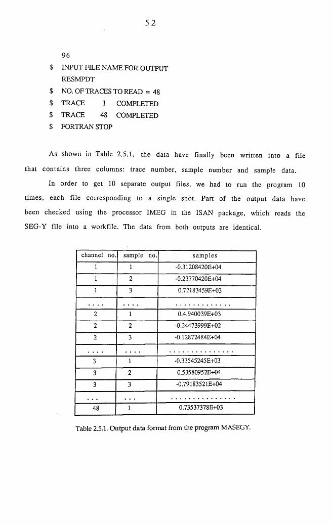
5 2

96

$ INPUT FILE NAME FOR OUTPUT

RESMPDT

$ NO. OF TRACES TO READ = 48

$ TRACE 1 COMPLETED

$ TRACE 48 COMPLETED

$ FORTRAN STOP

As shown in Table 2.5.1, the data have finally been written into a file

that contains three columns: trace number, sample number and sample data.

In order to get 10 separate output files, we had to run the program 10

times, each file corresponding to a single shot. Part of the output data have

been checked using the processor IMEG in the ISAN package, which reads the

SEG-Y file into a workfile. The data from both outputs are identical.

channel no. sample no. samples

1 1 -0.31208420E+04

1 2 -0.23770420E+04

1 3 0.72183459E+03

. . . . . . . .2 1 0.4.940039E+03

2 2 -0.24473999E+02

2 3 -0.12872484E+04

. . . . . . . .3 1 -0.33545245E+03

3 2 0.53580952E+04

3 3 -0.79183521E+04

. • * . . .48 1 0.73537378E+03

Table 2.5.1. Output data format from the program MASEGY.

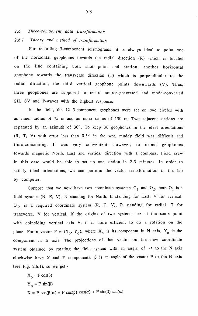
53

2.6 Three-component data transformation

2.6.1 Theory and method o f transformation

For recording 3-component seismograms, it is always ideal to point one

o f the horizontal geophones towards the radial direction (R) which is located

on the line containing both shot point and sta tion , another horizon tal

geophone towards the transverse direction (T) which is perpendicular to the

radial direction, the third vertical geophone points downw ards (V). Thus,

three geophones are supposed to record source-generated and m ode-converted

SH, SV and P-waves with the highest response.

In the field, the 12 3-component geophones were set on two circles with

an inner radius of 75 m and an outer radius of 130 m. Two adjacent stations are

separated by an azimuth of 30°. To keep 36 geophones in the ideal orientations

(R, T, V) with error less than 0.5° in the wet, muddy field was difficult and

tim e-consum ing . It was very convenient, how ever, to o rien t geophones

towards magnetic North, East and vertical direction with a compass. Field crew

in this case would be able to set up one station in 2-3 minutes. In order to

satisfy ideal orientations, we can perform the vector transform ation in the lab

by computer.

Suppose that we now have two coordinate systems Oj and 0 2 , here Oj is a

field system (N, E, V), N standing for North, E standing for East, V for vertical.

O 2 is a required coordinate system (R, T, V), R standing for radial, T for

transverse, V for vertical. If the origins of two systems are at the same point

with coinciding vertical axis V, it is more efficient to do a rotation on the

plane. For a vector F = (XQ, YQ), where XQ is its component in N axis, YQ is the

com ponent in E axis. The projections of that vector on the new coordinate

system obtained by rotating the field system with an angle of & to the N axis

clockwise have X and Y components. (3 is an angle of the vector F to the N axis

(see Fig. 2.6.1), so we get:-

X0 = Fcos(P)

Y 0 = F sin(P)

X = F cos(p-a) = F cos(p) cos(a) + F sin(P) sin(a)

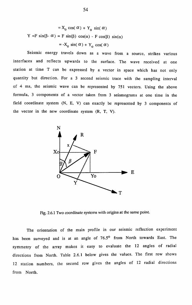
54

= x 0 cos( cc) + Y0 sin( a )

Y =F sin(P- a ) = F sin(P) cos(cc) - F cos(P) sin(a)

= -XQ sin( a ) + Y0 cos( a )

Seism ic energy travels down as a wave from a source, strikes various

in terfaces and reflects upwards to the surface. The wave received at one

station at tim e T can be expressed by a vector in space which has not only

quantity but direction. For a 3 second seismic trace with the sampling interval

of 4 ms, the seismic wave can be represented by 751 vectors. Using the above

formula, 3 components of a vector taken from 3 seismograms at one time in the

field coordinate system (N, E, V) can exactly be represented by 3 components of

the vector in the new coordinate system (R, T, V).

N

Xo

► EYo

Fig. 2.6.1 Two coordinate systems with origins at the same point.

The orientation of the main profile in our seismic reflection experiment

has been surveyed and is at an angle of 76.5° from North towards East. The

sym m etry o f the array makes it easy to evaluate the 1 2 angles o f radial

directions from North. Table 2.6.1 below gives the values. The first row shows

1 2 station num bers, the second row gives the angles of 1 2 radial directions

from North.

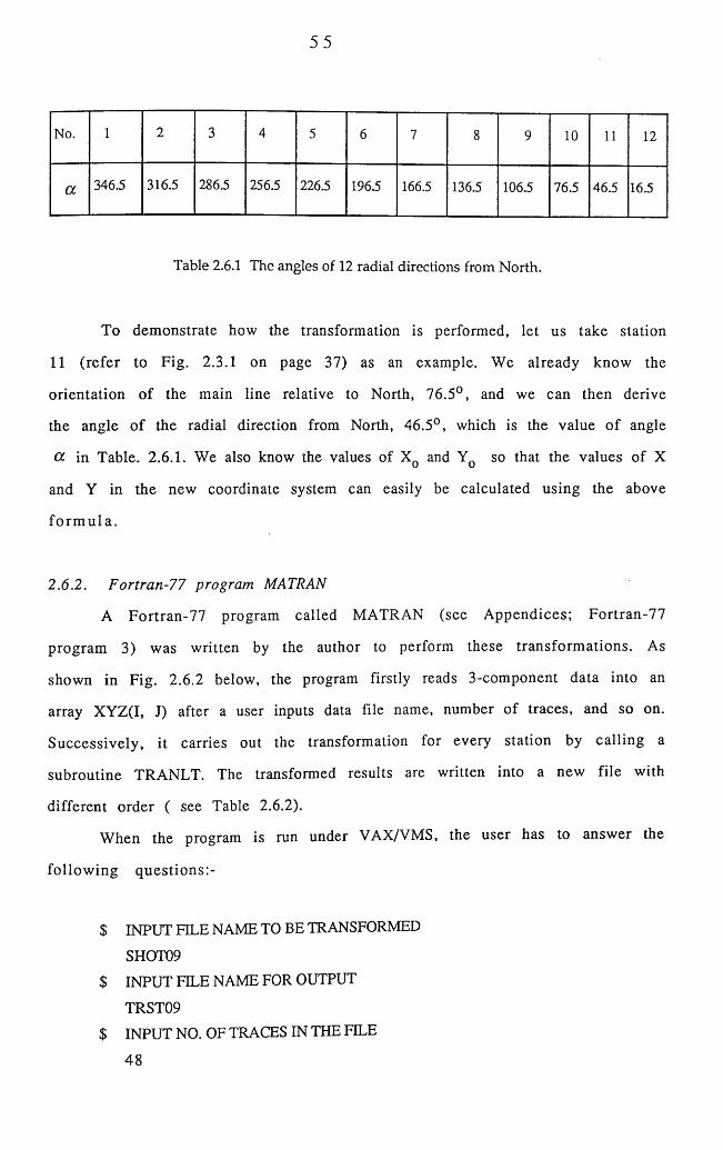
5 5

No. l 2 3 4 5 6 7 8 9 1 0 11 1 2

a 346.5 316.5 286.5 256.5 226.5 196.5 166.5 136.5 106.5 76.5 46.5 16.5

Table 2.6.1 The angles of 12 radial directions from North.

To demonstrate how the transformation is performed, let us take station

11 (refer to Fig. 2.3.1 on page 37) as an example. We already know the

orientation o f the main line relative to North, 76.5°, and we can then derive

the angle o f the radial direction from North, 46.5°, which is the value o f angle

cc in Table. 2.6.1. We also know the values of XQ and YQ so that the values of X

and Y in the new coordinate system can easily be calculated using the above

fo rm u la .

2.6.2. Fortran-77 program MATRAN

A Fortran-77 program called MATRAN (see A ppendices; Fortran-77

program 3) was written by the author to perform these transform ations. As

shown in Fig. 2.6.2 below, the program firstly reads 3-component data into an

array XYZ(I, J) after a user inputs data file name, number of traces, and so on.

Successively, it carries out the transformation for every station by calling a

subroutine TRANLT. The transformed results are written into a new file with

different order ( see Table 2.6.2).

W hen the program is run under VAX/VMS, the user has to answer the

fo llow ing questions:-

$ INPUT FILE NAME TO BE TRANSFORMED

SHOT09

$ INPUT FILE NAME FOR OUTPUT

TRST09$ INPUT NO. OF TRACES IN THE FILE

48

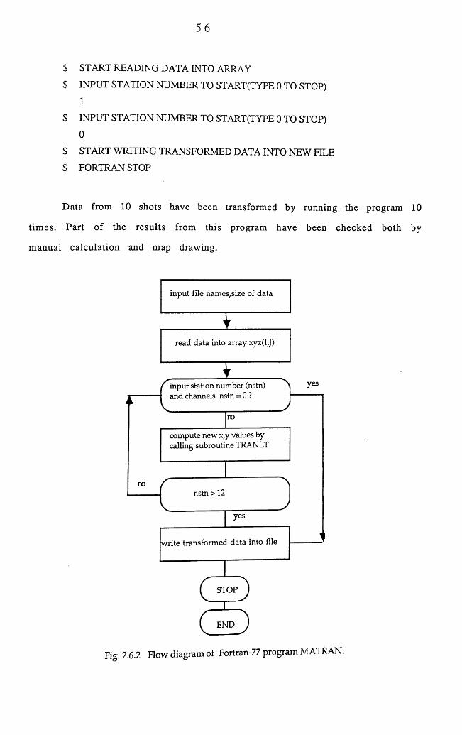
56

$ START READING DATA INTO ARRAY

$ INPUT STATION NUMBER TO START(TYPE 0 TO STOP)

1

$ INPUT STATION NUMBER TO START(TYPE 0 TO STOP)

0

$ START WRITING TRANSFORMED DATA INTO NEW FILE

$ FORTRAN STOP

Data from 10 shots have been transformed by running the program 10

tim es. Part of the results from this program have been checked both by

m anual calculation and map drawing.

yesinput station number (nstn) and channels nstn = 0?

no

nonstn > 12

yes

input file names,size of data

• read data into array xyz(I,J)

compute new x,y values by calling subroutine TRANLT

write transformed data into file

Fig. 2.6.2 How diagram of Fortran-77 program M ATR AN.

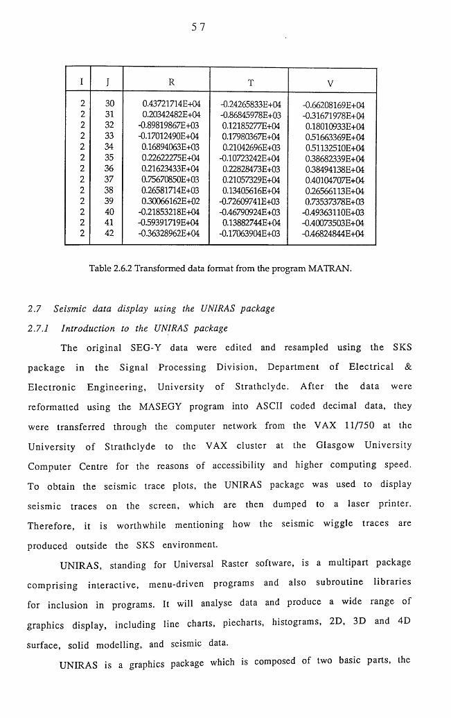
5 7

I J R T V

2 30 0.43721714E+04 -0.24265833E+04 -0.66208169E+042 31 0.20342482E+04 -0.86845978E+03 -0.31671978E+042 32 -0.89819867E+03 0.12185277E+04 0.18010933E+042 33 -0.17012490E+04 0.17980367E+04 0.51663369E+042 34 0.16894063E+03 0.21042696E+03 0.51132510E+042 35 0.22622275E+04 -0.10723242E+04 0.38682339E+042 36 0.21623433E+04 0.22828473E+03 0.38494138E+042 37 0.75670850E+03 0.21057329E+04 0.40104707E+042 38 0.26581714E+03 0.13405616E+04 0.26566113E+042 39 0.30066162E+02 -0.72609741E+03 0.73537378E+032 40 -0.21853218E+04 -0.46790924E+03 -0.49363110E+032 41 -0.59391719E+04 0.13882744E+04 -0.40073503E+042 42 -0.36328962E+04 -0.17063904E+03 -0.46824844E+04

Table 2.6.2 Transformed data format from the program MATRAN.

2.7 Seismic data display using the UNIRAS package

2.7.1 Introduction to the UNIRAS package

The original SEG-Y data were edited and resampled using the SKS

package in the Signal Processing D ivision, Departm ent o f E lec trica l &

E lectron ic E ngineering , U niversity of S trathclyde. A fter the data were

reform atted using the MASEGY program into ASCII coded decimal data, they

were transferred through the computer network from the VAX 11/750 at the

U niversity o f Strathclyde to the VAX cluster at the Glasgow U niversity

Com puter Centre for the reasons of accessibility and higher computing speed.

To obtain the seism ic trace plots, the UNIRAS package was used to display

seism ic traces on the screen, which are then dumped to a laser printer.

Therefore, it is worthwhile m entioning how the seismic wiggle traces are

produced outside the SKS environment.

UNIRAS, standing for Universal Raster software, is a m ultipart package

com prising in teractive, m enu-driven programs and also subroutine lib raries

for inclusion in programs. It will analyse data and produce a wide range of

graphics display, including line charts, piecharts, histograms, 2D, 3D and 4D

surface, solid modelling, and seismic data.

UNIRAS is a graphics package which is composed of two basic parts, the

58

first being the interactive programs. These provide facilities to draw charts

and maps of all kinds without the need to write your own program. UNIGRAPH

is for draw ing charts and graphs, while UNIMAP is for contour maps and

surface view s etc. The third interactive is UNIEDIT which allows pictures

drawn by the other two to be modified. The second main section of UNIRAS is

the subroutine libraries which are routines which can be called from a user's

own program in the similar manner to the NAG Graphics Library. Two levels

of subroutine library exist, one for high level routines which correspond to

the interactive programs, and a low level library. SEISPAK is a subroutine

library for the display of seismic data.

SEISPAK consists of many library subroutines which can be called in a

user's own program to display many kinds of seismic record sections. It can

display seism ic traces, variable area traces in vertical or horizontal direction

as a user requires. It can drive many kinds of term inals and plotters.

Furtherm ore, the seismic data can also be displayed in colour if a colour

terminal and a colour plotter are available. The package itself can enhance a

seism ic section either by reprocessing data or by using colours. F inally,

SEISPAK can also display seismic data in 3 dimensions.

2.7.2 Plotting seismic traces in the normal way

In order to make use of available packages for our own purposes, the

author has w ritten a Fortran-77 program called MAPLOT (see Appendices;

Fortran - 7 7 program 4 ) to display 3 -component seismic data in various kinds of

ways. The program permits the display of any one trace of 3-component data

which exists as one of 3 columns in a data file. It can display traces or variable

area wiggle traces and filled wiggle variable area without wiggle lines.

2.7.3 Combination o f a gain control program with the plotting package

Seism ic reflection data collected in our experim ent exhibit different

characteristics, as we deliberately selected the complex area with the intention

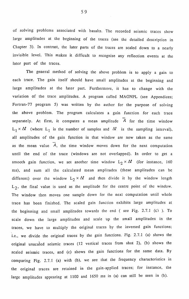
of solving problems associated with basalts. The recorded seismic traces show

large am plitudes at the beginning of the traces (see the detailed description in

Chapter 3). In contrast, the later parts of the traces are scaled down to a nearly

invisible level. This makes it difficult to recognise any reflection events at the

later part o f the traces.

The general method of solving the above problem is to apply a gain to

each trace. The gain itself should have small amplitudes at the beginning and

large am plitudes at the later part. Furthermore, it has to change with the

variation of the trace amplitudes. A program called MAGNPL (see Appendices;

Fortran-77 program 5) was written by the author for the purpose of solving

the above problem . The program calculates a gain function for each trace

separately. At first, it computes a mean amplitude A for the time window

L | x At (where L j is the number of samples and At is the sampling interval),

all amplitudes o f the gain function in that window are now taken as the same

as the mean value A, the time window moves down for the next computation

until the end of the trace (windows are not overlapped). In order to get a

smooth gain function, we set another time window L2 x A/ (for instance, 160

ms), and sum all the calculated mean amplitudes (these am plitudes can be

different) over the window L2 x Af and then divide it by the window length

L 2 , the final value is used as the amplitude for the centre point of the window.

The window then moves one sample down for the next computation until whole

trace has been finished. The scaled gain function exhibits large amplitudes at

the beginning and small amplitudes towards the end ( see Fig. 2.7.1 (c) ). To

scale down the large amplitudes and scale up the small am plitudes in the

traces, we have to multiply the original traces by the inversed gain functions;

i.e., we divide the original traces by the gain functions. Fig. 2.7.1 (a) shows the

original unsealed seismic traces ( 1 2 vertical traces from shot 2 ), (b) shows the

scaled seism ic traces, and (c) shows the gain functions for the same data. By

comparing Fig. 2.7.1 (a) with (b), we see that the frequency characteristics in

the original traces are retained in the gain-applied traces, for instance, the

large amplitudes appearing at 1100 and 1650 ms in (a) can still be seen in (b).

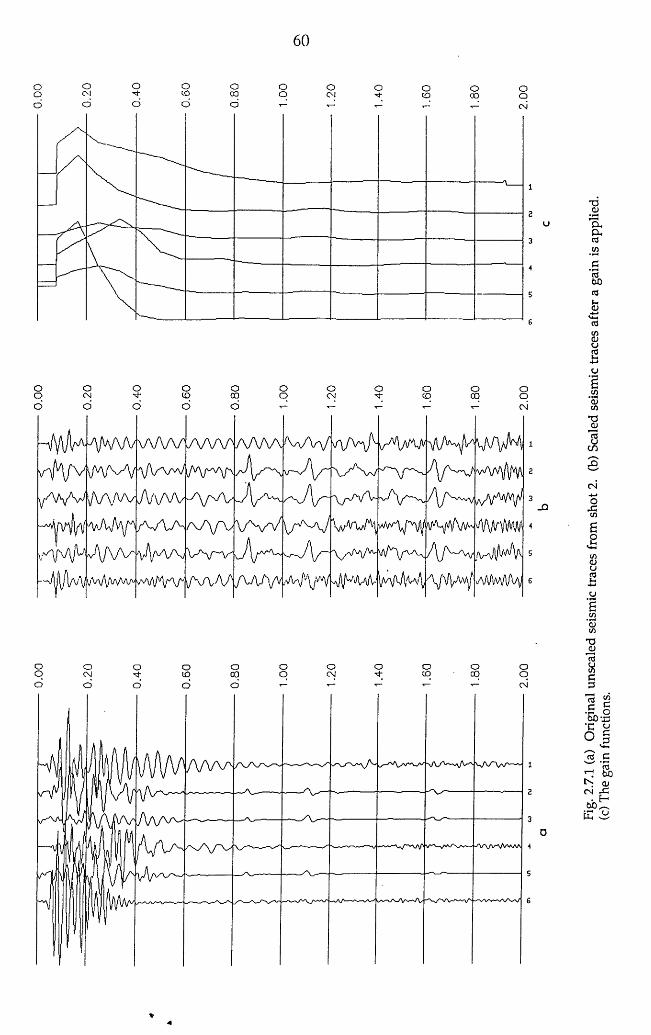
60

O O O O O t - ^ — t— t- t— CM

oo o<Nd

o otod

ooo oCM

O•M" OCO

ooCM

l / A v f / \ A / v V W

vA M l^

Mm /

\ h A A !

\IV \ AA/

J \ f \ M

(A'v/y'AAA/'' V

y w w

y \A /w

A A A

A A A A

/ATAA

A A O

V \ r - V

A /W V A aA a / A A n A AVAA''

'vA/v\ft A

./AAVV

w V i v / ^ ^ a / V v w ^ '-v ^ V ^ / V” v A a - ^ i f A # w

■ v ^ i A ' 'aA a ^ A A ^ /W iAAa

AAVN'V^ AAva IhAM, W A s jm m

A vA/w ^ ' -

Fig.

2.7.

1 (a)

O

rigin

al u

nsea

led

seism

ic tra

ces

from

shot

2.

(b) S

caled

se

ismic

tra

ces

after

a

gain

is ap

plie

d,

(c) T

he

gain

func

tions

.

61

The window lengths are empirically determined to produce the optimum

coherence o f seism ic events.

The combination of the gain-control program with the plotting package

saves m uch com puter memory, since there are no temporary files needed for

output from the gain-control program. This program reads the data, scales and

plots the data in one program run, which makes it possible for the user

quickly to examine the data. The program can also display seism ic data in

various ways, such as wiggle line display, variable area plus wiggle line

display or variable area display without wiggle lines.

2.8 Static correction

In order to obtain a seismic section which shows seism ic reflectors

representing the actual geological structure, reflection times must be reduced

to a defined reference datum. This is normally taken to correspond to a

horizon tal plane fixed at a certain known elevation. Static correction is

essen tia lly a tim e-sh ift introduced to each trace, reducing the observed

reflection time to the chosen datum plane.

The value of total static correction ( At ) depends on the following

factors [Al-Sadi, 1980]:-

(1) The vertical distance of the source from the datum plane.

(2) The surface topography, that is the vertical distance of the detector

from the datum.

(3) The velocity variation of the surface layer along the seismic line.

(4) Thickness variation of the surface layer.

The total static correction Af (Fig. 2.8.1) is made up of two parts, the

source correction At and the receiver correction At f , whereds + d r - 2 d r d 2

At = A t s + At r = y + -p ~o 1

^ s Source static correction,

^ r R eceiver static correction,

dg D istance between the source location at the surface and datum

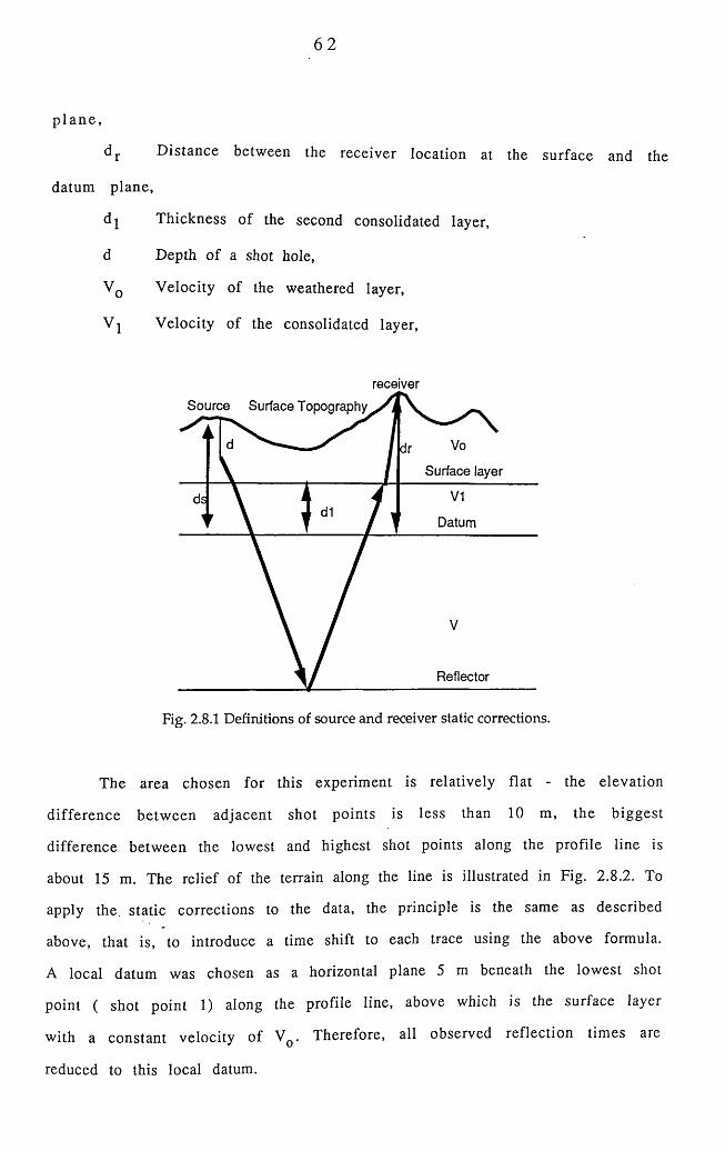
62

p la n e ,

d r D istance between the receiver location at the surface and the

datum plane,

d j Thickness of the second consolidated layer,

d Depth of a shot hole,

VQ Velocity of the weathered layer,

V | Velocity of the consolidated layer,

receiver

Source Surface Topography

Surface layer

Datum

Reflector

Fig. 2.8.1 Definitions of source and receiver static corrections.

The area chosen for this experiment is relatively flat - the elevation

d ifference betw een adjacent shot points is less than 1 0 m, the biggest

difference between the lowest and highest shot points along the profile line is

about 15 m. The relief of the terrain along the line is illustrated in Fig. 2.8.2. To

apply the. static corrections to the data, the principle is the same as described

above, that is, to introduce a time shift to each trace using the above formula.

A local datum was chosen as a horizontal plane 5 m beneath the lowest shot

point ( shot point 1 ) along the profile line, above which is the surface layer

with a constant velocity of VQ. Therefore, all observed reflection times are

reduced to this local datum.

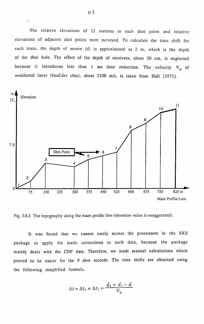
The relative elevations of 12 stations to each shot point and relative

elevations o f adjacent shot points were surveyed. To calculate the time shift for

each trace, the depth of source (d) is approximated as 2 m, which is the depth

of the shot hole. The effect of the depth of receivers, about 50 cm, is neglected

because it introduces less than 1 ms time reduction. The velocity VQ of

weathered layer (boutder clay), about 2100 m/s, is taken from Hall [1971].

Elevation

7.5-

Shot Point

750600 675 825 m450 525300 375150 22575Main Profile Line

Fig. 2.8.2 The topography along the main profile line (elevation value is exaggerated).

It was found that we cannot easily access the processors in the SKS

package to apply the static corrections to such data, because the package

mainly deals with the CDP data. Therefore, we made manual calculations which

proved to be easier for the 9 shot records. The time shifts are obtained using

the following simplified formula,

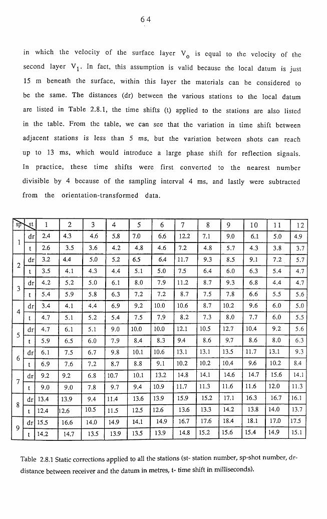
64

in which the velocity of the surface layer VQ is equal to the velocity of the

second layer V j. In fact, this assumption is valid because the local datum is just

15 m beneath the surface, within this layer the materials can be considered to

be the same. The distances (dr) between the various stations to the local datum

are listed in Table 2.8.1, the time shifts (t) applied to the stations are also listed

in the table. From the table, we can see that the variation in time shift between

adjacent stations is less than 5 ms, but the variation between shots can reach

up to 13 ms, which would introduce a large phase shift for reflection signals.

In practice, these tim e shifts were first converted to the nearest number

divisible by 4 because of the sampling interval 4 ms, and lastly were subtracted

from the orientation-transform ed data.

1 2 3 4 5 6 7 8 9 1 0 1 1 1 2

1dr 2.4 4.3 4.6 5.8 7.0 6 . 6 1 2 . 2 7.1 9.0 6 . 1 5.0 4.9

t 2 . 6 3.5 3.6 4.2 4.8 4.6 7.2 4.8 5.7 4.3 3.8 3.7

2dr 3.2 4.4 5.0 5.2 6.5 6.4 11.7 9.3 8.5 9.1 7.2 5.7

t 3.5 4.1 4.3 4.4 5.1 5.0 7.5 6.4 6 . 0 6.3 5.4 4.7

3dr 4.2 5.2 5.0 6 . 1 8 . 0 7.9 1 1 . 2 8.7 9.3 6 . 8 4.4 4.7

t 5.4 5.9 5.8 6.3 7.2 7.2 8.7 7.5 7.8 6 . 6 5.5 5.6

4dr 3.4 4.1 4.4 6.9 9.2 1 0 . 0 1 0 . 6 8.7 1 0 . 2 9.6 6 . 0 5.0

t 4.7 5.1 5.2 5.4 7.5 7.9 8 . 2 7.3 8 . 0 7.7 6 . 0 5.5

5dr 4.7 6 . 1 5.1 9.0 1 0 . 0 1 0 . 0 1 2 . 1 10.5 12.7 10.4 9.2 5.6

t 5.9 6.5 6 . 0 7.9 8.4 8.3 9.4 8 . 6 9.7 8 . 6 8 . 0 6.3

6dr 6 . 1 7.5 6.7 9.8 1 0 . 1 1 0 . 6 13.1 13.1 13.5 11.7 13.1 9.3

t 6.9 7.6 7.2 8.7

oo oo 9.1 1 0 . 2 1 0 . 2 10.4 9.6 1 0 . 2 8.4

7dr 9.2 9.2 6 . 8 10.7 1 0 . 1 13.2 14.8 14.1 14.6 14.7 15.6 14.1

t 9.0 9.0 7.8 9.7 9.4 10.9 11.7 11.3 1 1 . 6 1 1 . 6 1 2 . 0 11.3

8dr 13.4 13.9 9.4 11.4 13.6 13.9 15.9 15.2 17.1 16.3 16.7 16.1

t 12.4 1 2 . 6 10.5 11.5 12.5 1 2 . 6 13.6 13.3 14.2 13.8 14.0 13.7

9dr 15.5 16.6 14.0 14.9 14.1 14.9 16.7 17.6 18.4 18.1 17.0 17.5

t 14.2 14.7 13.5 13.9 13.5 13.9 14.8 15.2 15.6 15.4 14.9 15.1

Table 2.8.1 Static corrections applied to all the stations (st- station number, sp shot number, dr-

distance between receiver and the datum in metres, t- time shift in milliseconds).

65

Chapter 3 Characterization of 3-component Seismic Data

from a Basalt-covered Area

3.1 Introduction

Seism ic reflection CDP and VSP data are often of poor quality when

recorded in areas where volcanic rocks are present at or near the surface.

They are bo th characterised by large-am plitude reverberations caused by

seism ic energy trapped in the upper layers [Pujol, 1989]. In this chapter, we

present the m ajor characteristics of seismic reflection data recorded using the

areal array and 3-com ponent geophones in a basalt-covered area o f the

M idland V alley o f Scotland. We then investigate the energy distribution on

geophones at different orientations by applying a specially designed filter.

3.2. Correlation between the penetration o f seismic energy and charge size

As it is the first trial of shooting in a basalt-covered area, we had to

carry out some tests before the real experiment started. One of the tests was to

find out the correlation between the penetration of seismic energy and size of

explosive. This test aims at determining the minimum size of explosive without

substantial signal degradation. As described in Section 2.4.5, there is a limit to

the num ber of shots that can be fired together due to the properties of the

blaster and firing lines. The size of a cavity produced by a blast which is

proportional to size of explosive, and therefore has to be minimised. The total

resistance of the firing circuit should be kept to below 75 ohms to maintain the

current of about 2 A to fire seismic detonators. Therefore, it is advised to shoot

fewer than five charges together.

Four half-sticks of dynamite (each weighing 1/8 kg), in four holes,

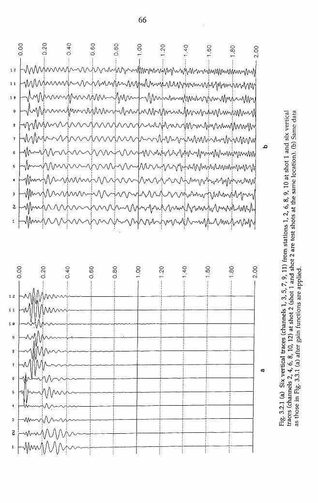
66

ooo<N

don-o

oto oco oo oCNJ

oto o00

oqCN

d M / \ / V W w ^

-W\

^\A/W\Av^ wc ^A NA/ J vyVJVvq|/ /\/\/\AA

A M / W W AAa a ^v W V tM N W '

A /V V V A a j Vv/'/^yv7';'

^ v y w v / v ^ w ^ j ^ ^ ^

/ \ n M i v A / v y v w y ^

¥

A\AMaaA^VH^A

oo oCN

ooN"o

oto

oCO

oo oCNJ

oNj- oCO

ooo oqCNJ

1 2

1 1

1 0

9

8

7

6

5

3

2

i

« JSU TOr ^QJ <D► £X CO•55 ^g enJ ^

r H C^ O O OrC COo5 cj .*-. °ton ^2 £ON “

v 01

00 SNO j_ .

v toCN t/Jrn' og - s

.2 «m saaj *4-'In CJ£ *o CNJ£ ~X °£ « -d

- *o . 2

tc* S:K r~l1 to10 n <u K O )_ CO X TO

„c/> fN §S J 1s * 5 §-*—• V4_TO _ u C'« 3 &jy — ( hr\rt o '

0 0 COCu ^ -v

•£ ^ -5U *>o

•2 » -^ CL) bb-q £ E-S § c3 S *>CN w t/iCO w o v * n \

toQJ

■ CO

Qj rCH-.

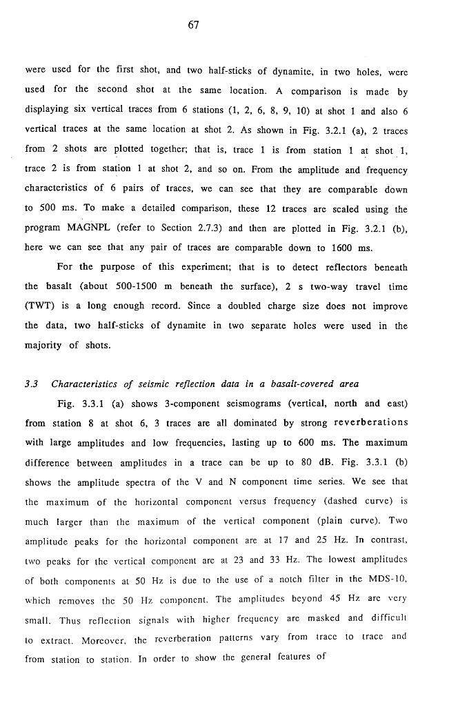
67

were used for the first shot, and two half-sticks of dynamite, in two holes, were

used for the second shot at the same location. A comparison is made by

displaying six vertical traces from 6 stations ( 1 , 2 , 6 , 8 , 9 , 1 0 ) at shot 1 and also 6

vertical traces at the same location at shot 2. As shown in Fig. 3.2.1 (a), 2 traces

from 2 shots are plotted together; that is, trace 1 is from station 1 at shot 1 ,

trace 2 is from station 1 at shot 2, and so on. From the amplitude and frequency

characteristics o f 6 pairs of traces, we can see that they are comparable down

to 500 ms. To make a detailed comparison, these 12 traces are scaled using the

program MAGNPL (refer to Section 2.7.3) and then are plotted in Fig. 3.2.1 (b),

here we can see that any pair of traces are comparable down to 1600 ms.

For the purpose of this experiment; that is to detect reflectors beneath

the basalt (about 500-1500 m beneath the surface), 2 s two-way travel time

(TWT) is a long enough record. Since a doubled charge size does not improve

the data, two half-sticks of dynamite in two separate holes were used in the

m ajority of shots.

3.3 Characteristics o f seismic reflection data in a basalt-covered area

Fig. 3.3.1 (a) shows 3-component seismograms (vertical, north and east)

from station 8 at shot 6 , 3 traces are all dominated by strong r e v e r b e r a t io n s

with large amplitudes and low frequencies, lasting up to 600 ms. The maximum

difference between amplitudes in a trace can be up to 80 dB. Fig. 3.3.1 (b)

shows the amplitude spectra of the V and N component time series. We see that

the maximum of the horizontal component versus frequency (dashed curve) is

much larger than the maximum of the vertical component (plain curve). Two

amplitude peaks for the horizontal component are at 17 and 25 Hz. In contrast,

two peaks for the vertical component are at 23 and 33 Hz. The lowest amplitudes

of both components at 50 Hz is due to the use of a notch filter in the MDS-10,

which removes the 50 Hz component. The amplitudes beyond 45 Hz arc very

small. Thus reflection signals with higher frequency are masked and difficult

to extract. M oreover, the reverberation patterns vary from trace to trace and

from station to station. In order to show the general features of

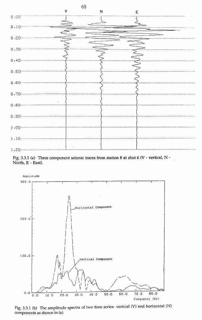
E0 -00

0 - 2 0

0 .3 0

0-50

0 -6 0

0 =70

0 -8 0

0-90

1 -00

Fig. 3.3.1 (a) Three component seismic traces from station 8 at shot 6 (V - vertical, N - North, E - East).

Amplitude

Horizontal Component

1 0 0 . 0,Vertical Component

70-0 80-0Frequency (Hz)

60-050-030-02 0 - 0

Fig. 3.3.1 (b) The amplitude spectra of two time series- vertical (V) and horizontal (N) components as shown in (a).

69

such data, several traces from different shots are plotted together (Fig. 3.3.2).

H alf o f them are from the stations in the inner circles and half are from the

stations in the outer circles (refer to Fig. 2.3.1). It was found that the data from

the inner circles all have much larger amplitudes than those from the outer

circles in the same time region. It is likely that the data from the inner circles

are m uch m ore affected by organised noise than those from the outer circles.

In fact, the attenuation difference by spherical divergence and absorption in

seismic energy reflected from the deep layers, say 2 km, is m inor between the

stations with small distance (say 65 m). Thus the great attenuation between two

offsets cannot be attributed to spherical divergence and absorption. It is,

how ever, caused by surface conditions in the area where basalt is near the

surface. S trong reverberations, as trapped modes in the upper layer, are

generated . The reverberations are attenuated dram atically w ith increase of

the d istance from a shot point. In other words, the data from small offset

sta tions (75 m) are obscured more severely than those from long offset

sta tions. A dditionally , two horizontal components are m ore noisy than the

vertica l com ponent, and their reverberation duration lasts longer than the

vertical component. In fact, the basalt at the shallow depth gives rise to a

critical angle o f less than 2 0 ° , and a corresponding distance at the surface is

less than 50 m. Therefore, stations in this area are all located beyond the

critical distance from a shot point, which may cause the data degradation.

S e i s m i c re f l ec t io n s igna ls are be l ieved to be ran d o m . T h e o r g a n i s e d

n o i s e - r e v e r b e r a t i o n s , h ow eve r , m ig h t be periodic. A u t o - c o r r e l a t i o n o f se i s m ic

t races is u s e d he re to invest igate the periodici ty o f o rganised noise. Therefore ,

a n u m b e r o f s e i s m i c t r a c e s in c l u d i n g both the v e r t i c a l an d h o r i z o n t a l

c o m p o n e n t s a re a u t o - c o r r e l a t e d . T h e a u t o - c o r r e l a t i o n f u n c t i o n s s h o w a

s t r ik in g c h a n g e in s t rength and per iod of reverberat ions , thi s m u s t be related

to su r f a c e e f f ec t s at the source. Fig. 3.3.3 shows one o f the au to -cor re la t i on

f u n c t i o n s w h i c h mos t ly repre sen ts the per iod ic i ty (40 ms) or the f r equency

(25 Hz) of such organised noise in such a basal t -covered area. T h e f requency

of such noise var ies with traces and stations; the general band is at 15-30 Hz.

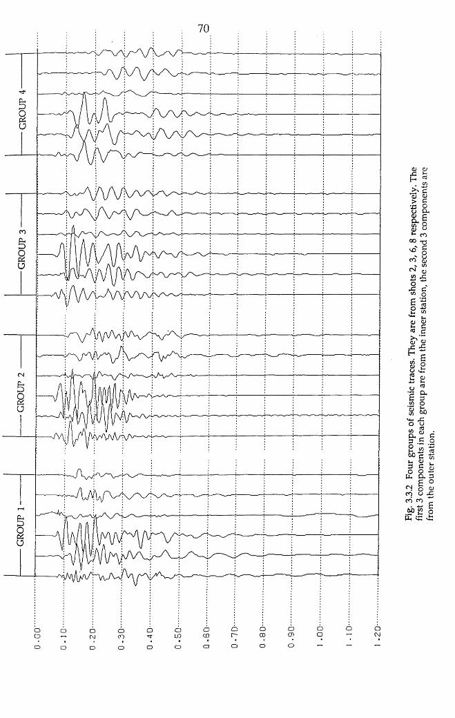
GROU

P 1

GROU

P 2

GR

OUP

3

GROU

P 4

oCT>OCO

OoLOoCO

D CDoooaoo oo

Fig.

3.3.

2 Fo

ur

grou

ps

of se

ismic

trace

s. Th

ey

are

from

shot

s 2,

3, 6, 8

res

pect

ivel

y. T

he

first

3 co

mpo

nent

s in

each

gr

oup

are

from

the

inne

r st

atio

n, t

he

seco

nd

3 co

mpo

nent

s ar

e

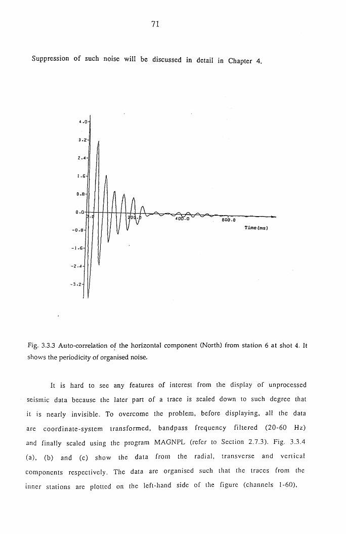
71

Suppression o f such noise will be discussed in detail in Chapter 4.

4 . 0 -

3 . 2 -

2 . 4 -

0 . 8 -

0 . 0

6 0 0 . 0

Time (ms)- 0 . 8 -

- 1 . 6 -

-2.4-

- 3 . 2 -

Fig. 3.3.3 Auto-correlation of the horizontal component (North) from station 6 at shot 4. It

shows the periodicity of organised noise.

It is hard to see any features of interest from the display of unprocessed

seismic data because the later part of a trace is scaled down to such degree that

it is nearly invisible. To overcome the problem, before displaying, all the data

are coordinate-system transform ed, bandpass frequency filtered (20-60 Hz)

and finally scaled using the program MAGNPL (refer to Section 2.7.3). Fig. 3.3.4

(a), (b) and (c) show the data from the radial, transverse and vertical

components respectively. The data are organised such that the traces from the

inner stations are plotted on the left-hand side of the figure (channels 1-60),

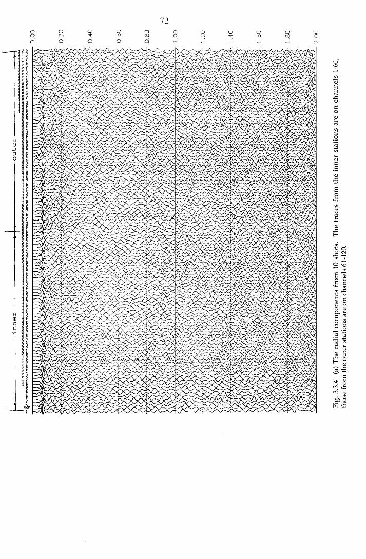
inne

r

*-4—«

------

------

------

------

---ou

ter

72

Fig.

3.3.

4 (a)

Th

e ra

dial

com

pone

nts

from

10 sh

ots.

Th

e tra

ces

from

the

inne

r st

atio

ns

are

on ch

anne

ls

1-60

, th

ose

from

the

oute

r st

atio

ns

are

on ch

anne

ls

61-1

20.

inne

r

> I -c-——

ou

ter

ooo

73o o o o oOJ •'t to co o

T- v-' oi

Fig.

3.3.

4 (b)

The

tra

nsve

rse

com

pone

nts

from

10 sh

ots.

The

trace

s fro

m the

in

ner

statio

ns

are

on ch

anne

ls 1-

60,

thos

e fro

m the

ou

ter

statio

ns

are

on ch

anne

ls 61

-120

.

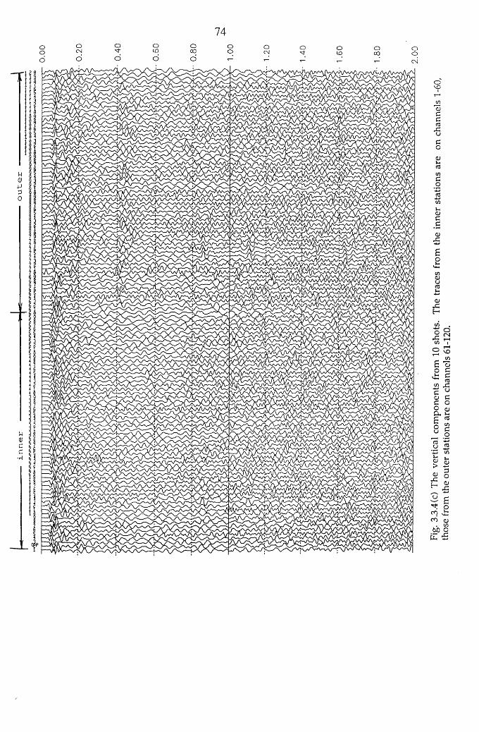
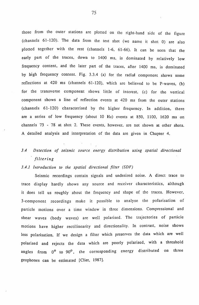
75

those from the outer stations are plotted on the right-hand side of the figure

(channels 61-120). The data from the test shot (we name it shot 0) are also

plotted together with the rest (channels 1-6, 61-66). It can be seen that the

early part o f the traces, down to 1400 ms, is dominated by relatively low

frequency content, and the later part of the traces, after 1400 ms, is dominated

by high frequency content. Fig. 3.3.4 (a) for the radial component shows some

reflections at 420 ms (channels 61-120), which are believed to be P-waves, (b)

for the transverse com ponent shows little of interest, (c) for the vertical

component shows a line of reflection events at 420 ms from the outer stations

(channels 61-120) characterised by the higher frequency. In addition, there

are a series of low frequency (about 10 Hz) events at 850, 1100, 1620 ms on

channels 73 - 78 at shot 2. These events, however, are not shown at other shots.

A detailed analysis and interpretation of the data are given in Chapter 4.

3.4 Detection o f seismic source energy distribution using spatial directional

f i l t e r i n g

3.4.1 Introduction to the spatial directional filter (SDF)

Seismic recordings contain signals and undesired noise. A direct trace to

trace display hardly shows any source and receiver characteristics, although

it does tell us roughly about the frequency and shape of the traces. However,

3-com ponent record ings make it possible to analyse the po larisa tion o f

particle m otions over a time window in three dimensions. Compressional and

shear waves (body waves) are well polarised. The trajectories o f particle

motions have higher rectilinearity and directionality. In contrast, noise shows

less polarisation. If we design a filter which preserves the data which are well

polarised and rejects the data which are poorly polarised, with a threshold

angles from 0 ° to 9 0 ° , the corresponding energy d istribu ted on three

geophones can be estimated [Cliet, 1987].

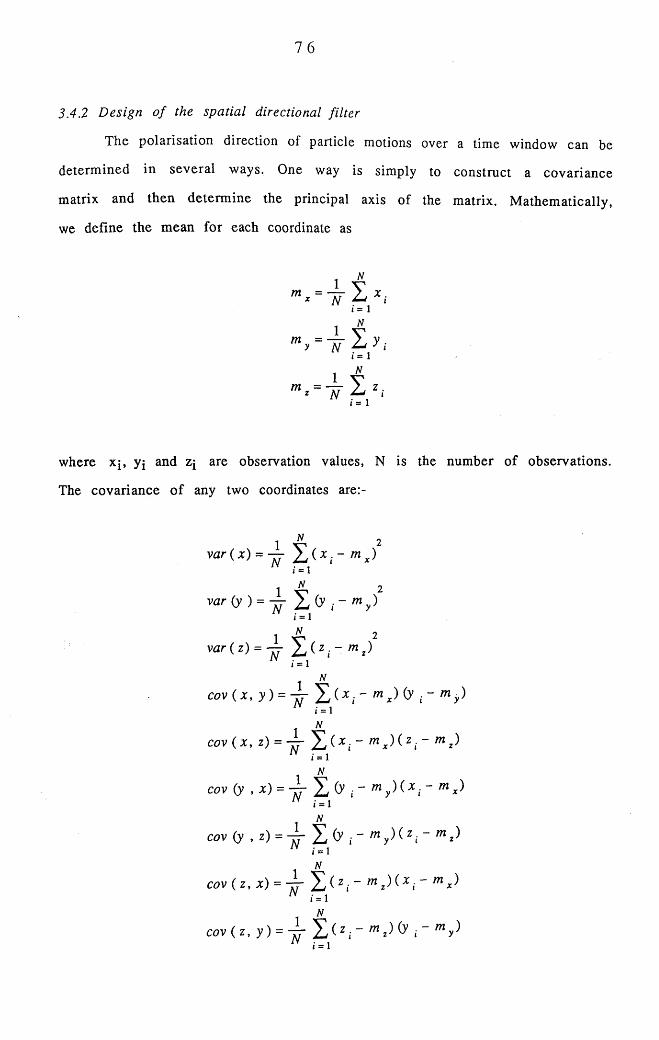
76

3.4.2 Design o f the spatial directional filter

The polarisation direction of particle motions over a time window can be

determ ined in several ways. One way is simply to construct a covariance

m atrix and then determ ine the principal axis of the matrix. M athem atically,

we define the mean for each coordinate as

1 V

i = l

1 N

i= 1

N

•=i

where x j, yj and z\ are observation values, N is the number o f observations.

The covariance o f any two coordinates are:-

1 N 2 v ar ( x) = — ^ ( x . - m j= 1 N

var( y ) = - ^ £ (y m y )N r . i

N

N t . i1 Ncov ( x , y ) = j j - l , ( x r m x ) (y m y )

= 1 N

N t . iN

cov(y , x ) = 4 r £ ( y r m y)(-x r m *)N t . i

N

cov (y , z) = ^ ( y { - rny) ( z iN

Ncov ( z , x) = i ~ m X) ( x . m X)

NN

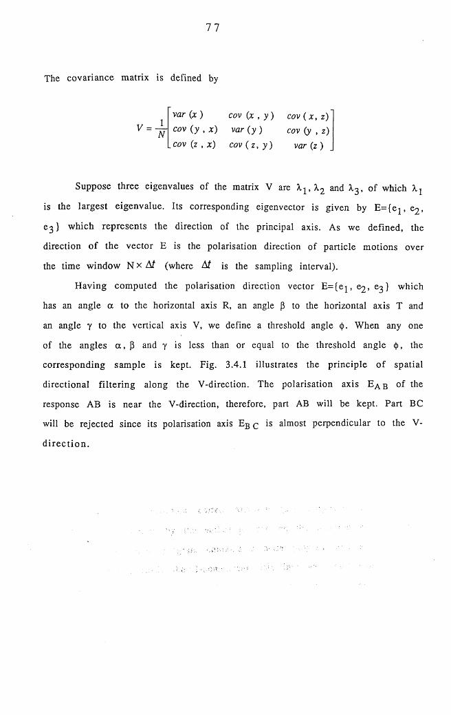
77

The covariance matrix is defined by

cov ( x , z) cov (y , z)

var ( z )

Suppose three eigenvalues of the matrix V are X j, X2 and X3 , o f which Xj

is the largest eigenvalue. Its corresponding eigenvector is given by E = { e j, e2 ,

6 3 } which represents the direction of the principal axis. As we defined, the

direction o f the vector E is the polarisation direction of particle motions over

the time window N x At (where At is the sampling interval).

H aving computed the polarisation direction vector E = {e j, e2 , 0 3 ) which

has an angle a to the horizontal axis R, an angle p to the horizontal axis T and

an angle y to the vertical axis V, we define a threshold angle <{>. When any one

of the angles a , p and y is less than or equal to the threshold angle <p, the

corresponding sam ple is kept. Fig. 3.4.1 illustrates the principle o f spatial

directional filtering along the V-direction. The polarisation axis E ^ b ° f the

response AB is near the V-direction, therefore, part AB will be kept. Part BC

will be rejected since its polarisation axis Eg q is almost perpendicular to the V-

d ire c tio n .

var (x ) cov (x , y )cov (y , x) var {y )

_cov (z , x) cov ( z, y )

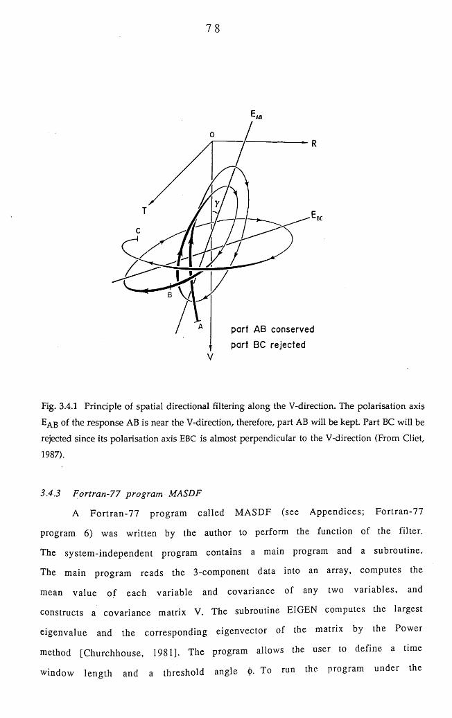
7 8

part AB conserved

part BC rejectedV

Fig. 3.4.1 Principle of spatial directional filtering along the V-direction. The polarisation axis

EAB of the response AB is near the V-direction, therefore, part AB will be kept. Part BC will be

rejected since its polarisation axis EBC is almost perpendicular to the V-direction (From Cliet,

1987).

3.4.3 Fortran-77 program MASDF

A F ortran-77 program called MASDF (see A ppendices; Fortran-77

program 6 ) was written by the author to perform the function of the filter.

The system -independent program contains a main program and a subroutine.

The main program reads the 3 -component data into an array, computes the

mean value o f each variable and covariance of any two variables, and

constructs a covariance matrix V. The subroutine EIGEN computes the largest

eigenvalue and the corresponding eigenvector of the matrix by the Power

method [Churchhouse, 1981]. The program allows the user to define a time

window length and a threshold angle <|>. To run the program under the

79

VAX/VMS operating system, the program (see Fig. 3.4.2) is modified to call a

NAG library routine for calculating the largest eigenvalue and corresponding

eigenvector. The data from 12 stations can be processed for each run. A user

has to reply to several questions:-

$ INPUT FILE NAME FOR FILTERING

TRST02

$ INPUT NUMBER OF STATIONS IN THE FILE

12

$ INPUT NUMBER OF SAMPLES IN ONE TRACE

501

$ INPUT FILE NAME FOR OUTPUT

EOUT02

$ START READING DATA INTO ARRAY

$ INPUT THRESHOLD ANGLE IN DEGREE

45

$ INPUT STATION NUMBER TO START (TYPE 0 TO STOP)

1

0

$ START WRITING FILTERED DATA INTO OUTPUT FILE

$ FORTRAN STOP

For the purpose of a clearer display of the filtered data, we set 0 as a

result w ithin the window in which angles oc, P and y are greater than a given

threshold angle <j), but set a constant 1 for the window in which angles a , P and

y are less than a given threshold angle <|>.

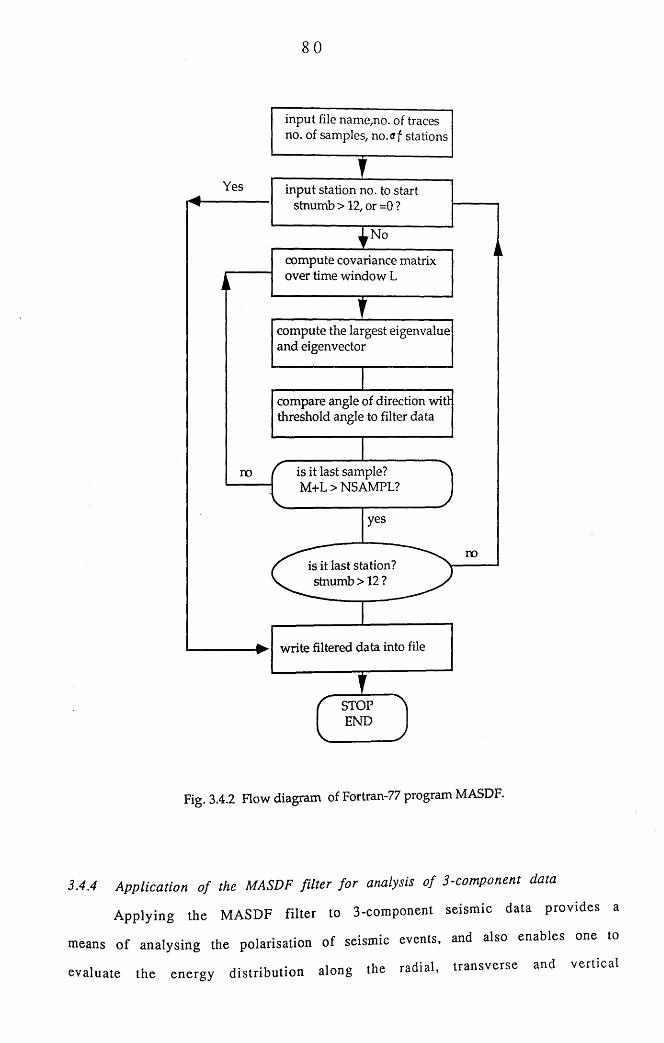
80

Yes

No

r is it last sample? M+L > NSAMPL?

no

yes

nois it last station? stnumb > 1 2 ?

STOPEND

compare angle of direction witl threshold angle to filter data

compute the largest eigenvalue and eigenvector

compute covariance matrix over time window L

input station no. to start stnumb > 1 2 , or = 0 ?

input file name,no. of traces no. of samples, no.t»f stations

write filtered data into file

Fig. 3.4.2 Flow diagram of Fortran-77 program MASDF.

3.4.4 Application o f the MASDF filter fo r analysis o f 3-component data

A pplying the MASDF filter to 3 -component seism ic data provides a

means o f analysing the polarisation of seismic events, and also enables one to

evaluate the energy distribution along the radial, transverse and vertical

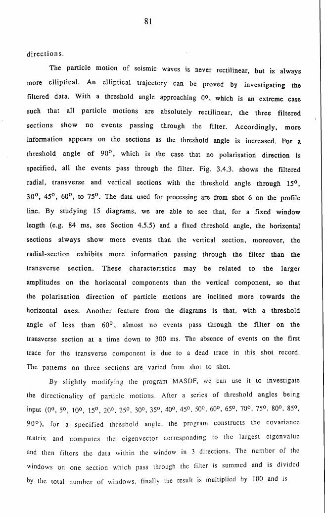
81

d ire c tio n s .

The particle motion of seismic waves is never rectilinear, but is always

more e llip tica l. An ellip tical trajectory can be proved by investigating the

filtered data. W ith a threshold angle approaching 0°, which is an extreme case

such that all p a rtic le m otions are absolutely rectilinear, the three filtered

sections show no events passing through the filter. A ccordingly , m ore

information appears on the sections as the threshold angle is increased. For a

threshold angle o f 9 0 ° , which is the case that no polarisation direction is

specified, all the events pass through the filter. Fig. 3.4.3. shows the filtered

radial, transverse and vertical sections with the threshold angle through 15°,

30°, 45°, 60°, to 75°. The data used for processing are from shot 6 on the profile

line. By studying 15 diagrams, we are able to see that, for a fixed window

length (e.g. 84 ms, see Section 4.5.5) and a fixed threshold angle, the horizontal

sections alw ays show m ore events than the vertical section, m oreover, the

radial-section exhib its more information passing through the filte r than the

transverse sec tio n . These characteristics may be related to the larger

amplitudes on the horizontal components than the vertical component, so that

the polarisation direction o f particle motions are inclined more tow ards the

horizontal axes. A nother feature from the diagrams is that, with a threshold

angle o f less than 6 0 ° , alm ost no events pass through the filte r on the

transverse section at a time down to 300 ms. The absence of events on the first

trace for the transverse component is due to a dead trace in this shot record.

The patterns on three sections are varied from shot to shot.

By slightly m odifying the program MASDF, we can use it to investigate

the directionality o f particle motions. After a series of threshold angles being

input (0°, 5°, 10°, 15°, 20°, 25°, 30°, 35°, 40°, 45°, 50°, 60°, 65°, 70°, 75°, 80°, 85°,

9 0 °) , for a specified threshold angle, the program constructs the covariance

matrix and com putes the eigenvector corresponding to the largest eigenvalue

and then filters the data within the window in 3 directions. The number of the

windows on one section which pass through the filter is summed and is divided

by the total number of windows, finally the result is multiplied by 1 0 0 and is

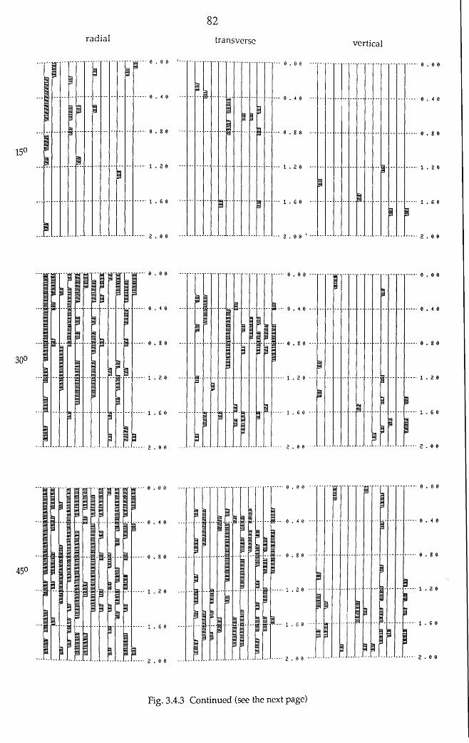
radial transverse vertical

Fig. 3.4.3 Continued (see the next page)

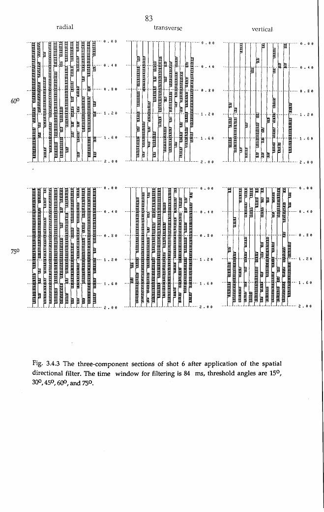
rad ial83

transverse vertical

Fig. 3.4.3 The three-component sections of shot 6 after application of the spatial directional filter. The time window for filtering is 84 ms, threshold angles are 15°, 30°, 45°, 60°, and 75°.

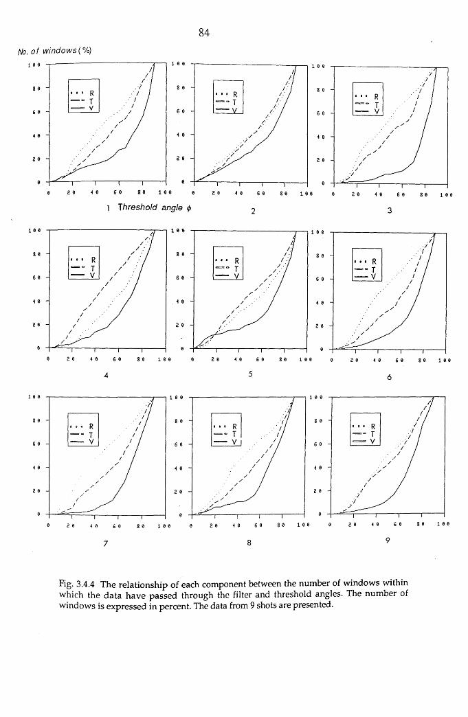
84No. of windows(%)

e

e

e

e

e

0

0 2 0 4 0 6 0 8 0 1 0 0 0 2 0 8 0 1 0 0

1

8 0

6 0

2 0

8 06 02 0

1 Threshold angle <p

1 0 0 1 0 0

8 0

6 0

2 0

0 2 0 6 0 8 0 2 01 0 0 0 4 0 6 0 8 0 0 0 8 0

1 0 0

10 0806 008 00 6 O08 0

Fig. 3.4.4 The relationship of each component between the number of windows within which the data have passed through the filter and threshold angles. The number of windows is expressed in percent. The data from 9 shots are presented.

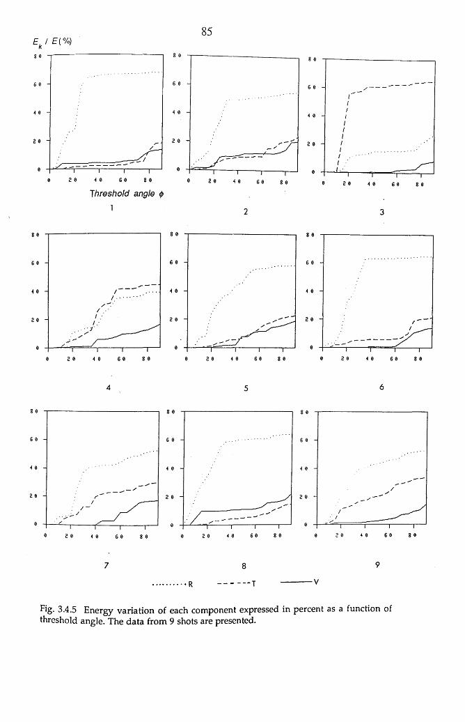
85Ek /E(%)

2 0

0 4 0 6 0 8 0

8 0

0

2 0

0

S 0 8 00

2 0

0 2 0 6 0 8 0

Threshold angle <p

8 0

6 0

4 0

8 02 0 6 00

8 0

6 0

2 0 6 0 8 00

8 0

6 0

2 0

2 00 g 0 8 0

4 5 6

8 0 8 0 0

g 0 0

0

2 0

0

g 0p 8 00 8 0g 0 0 04 02 008 0g 0

8

Fig. 3.4.5 Energy variation of each component expressed in percent as a function of threshold angle. The data from 9 shots are presented.

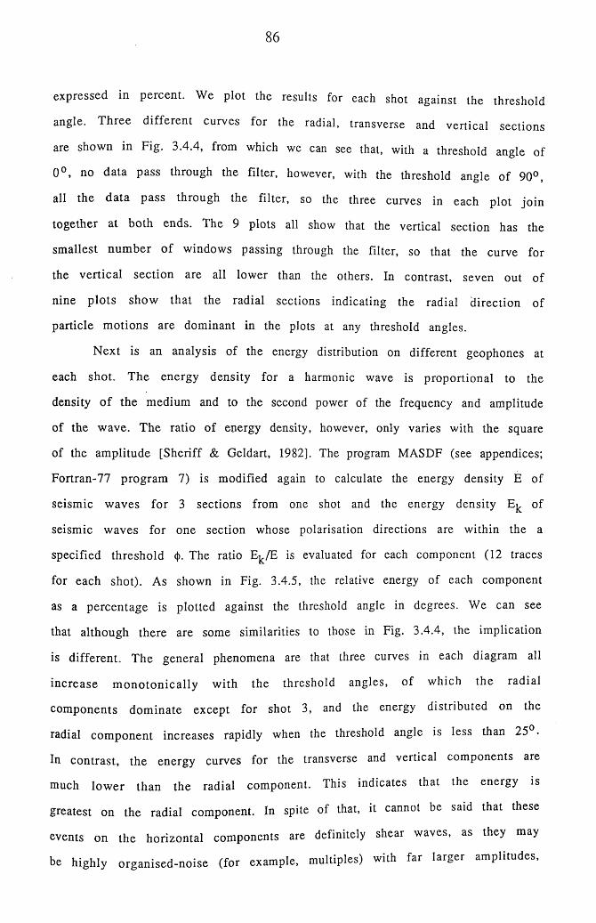
86

expressed in percent. We plot the results for each shot against the threshold

angle. Three different curves for the radial, transverse and vertical sections

are shown in Fig. 3.4.4, front which we can see that, with a threshold angle of

0 ° , no data pass through the filter, however, with the threshold angle of 90°,

all the data pass through the filter, so the three curves in each plot jo in

together at both ends. The 9 plots all show that the vertical section has the

smallest num ber o f windows passing through the filter, so that the curve for

the vertical section are all lower than the others. In contrast, seven out of

nine p lots show that the radial sections indicating the radial direction of

particle m otions are dominant in the plots at any threshold angles.

Next is an analysis of the energy distribution on different geophones at

each shot. The energy density for a harmonic wave is proportional to the

density o f the medium and to the second power of the frequency and amplitude

of the wave. The ratio of energy density, however, only varies with the square

of the amplitude [Sheriff & Geldart, 1982]. The program MASDF (see appendices;

Fortran-77 program 7) is modified again to calculate the energy density E of

seismic waves for 3 sections from one shot and the energy density of

seismic waves for one section whose polarisation directions are within the a

specified threshold 4>. The ratio E^/E is evaluated for each component (12 traces

for each shot). As shown in Fig. 3.4.5, the relative energy of each component

as a percentage is plotted against the threshold angle in degrees. We can see

that although there are some similarities to those in Fig. 3.4.4, the implication

is different. The general phenomena are that three curves in each diagram all

increase m ono ton ica lly w ith the threshold angles, of which the radial

components dom inate except for shot 3, and the energy distributed on the

radial com ponent increases rapidly when the threshold angle is less than 25 •

In contrast, the energy curves for the transverse and vertical components are

much low er than the radial component. This indicates that the energy is

greatest on the radial component. In spite of that, it cannot be said that these

events on the horizontal components are definitely shear waves, as they may

be highly organised-noise (for example, multiples) with far larger amplitudes,

87

which may dom inate the polarisation direction.

3.5. Summary

The test shot shows that a doubled size of dynamite in our experiment

does not produce better data, indicating that the correlation between the

penetration o f seism ic energy and charge size is not simply linear. Three-

component seismic data recorded in a basalt-covered area are characterised by

strong reverberations lasting as long as 500 ms. The reverberation patterns

vary from sta tion to station. The horizontal com ponents exhibit larger

amplitudes and lower frequency than the vertical component. By performing

auto-correlations of seismic traces, the frequency of such organised noise is

evaluated as about 15-30 Hz. Furthermore, the data from the inner stations are

believed to be more affected by surface conditions than the data from the outer

stations. The display of the vertical components from the outer stations shows

a line of reflection events at about 420 ms. There are no clear events on the

transverse section.

By applying the spatial directional filter to each component of seismic

data, it is shown that there are more events in the horizontal components

passing through the filter than the vertical component. This is attributed to

the far larger amplitudes o f the horizontal components, which may dominate

the polarisation direction of particle motions. The energy variation diagram of

each shot shows quantitatively that the radial component receives much more

energy than the others.

88

Chapter 4 Data Processing and Interpretation

4.1 In troduction

Seism ic reflection data are usually contaminated with various kinds of

noise such as coherent noise (direct wave, refracted wave, diffracted wave and

m ultip les) and random noise. Those data recorded in basalt-covered areas

exhib it a very special behaviour, being mixed with high reverberations

lasting as long as a second or so. As a result, the reflection signals are severely

masked by such organized noise. In order to extract the weak signals from the

data in the p resence o f noise, special processing techniques have to be

developed in addition to the existing conventional methods. In this chapter, we

firstly attem pt to apply the standard processing methods such as frequency

filtering and p red ic tive deconvolution filtering to the data, and then we

design and apply a signal enhancement polarisation filter. Lastly we present

the results o f filtering, and give an interpretation.

4.2 Pre-editing 3 -component seismic data

On recording 3-component seismic data in the field, some channels were

improperly m ixed up. For instance, the vertical component was connected to

the channel for the horizontal component. Some channels were open-circuit,

which caused the dead traces. The electrical connections of some traces were

inverted by m istake so that the peak-trough sense of such traces comes out

reversed in comparison with the rest of the recording. The SKS package (refer

to Section 2 .5 . 1 ) is used here to zero dead traces and to reverse the polarity of

some traces.

The original record length is 5 s with the sampling interval of 1 ms. To

89

save the storage, the data were re-sampled to 4 ms and data length is reduced to

2 s.

4.3 Frequency fil tering

An explosive source also generates unwanted noise. Ground-roll has a

frequency low er than 20-25 Hz and its amplitude is very high especially on

short-offset records. The air-wave usually has a frequency higher than 50 Hz.

A constan t zero-phase bandpass frequency filter is used here to attenuate

ground-roll and other high-frequency random noise.

The seism ic spectrum is subject to absorption along the propagation

path because o f the intrinsic attenuation of the earth. The higher frequency

com ponents are usually attenuated faster by absorption and other natural

filtering, so that higher frequency bands of useful signals are confined to the

shallow part o f the section. In contrast, the lower frequency band of useful

signals is confined to the later part of the section. In the exploration industry,

a tim e-variant bandpass filter is commonly used to obtain a cleaner section.

However, for our shallow seismic recordings, a constant bandpass filter (20/30

- 60/70) with a low cut-off of 20 Hz and a slope of 30 dB/octave, and a high cut­

off o f 60 Hz and a slope of 70 dB/octave is used to avoid the difficulties of

correlation from record to record induced by varying frequency and phase

changes o f different filters. Most importantly, the application of a polarisation

filter (refer to Section 4.5) to the data requires that frequency filtering 3

co m p o n en ts from one s ta tio n should not change the p o la risa tio n

characteristics o f particle motions of useful signals.

We take the data from shots 5 and 6 as an example, and perform

frequency filtering to see how the data are affected. Fig. 4.3.1 (a) shows the

unfiltered data (channels 1-3) and filtered data (channels 4-6) from station 7

at shot 6 , and Fig. 4.3.1 (b) shows the data from station 10 at shot 5. We can see

that high frequency noise, say at 100-200 ms on channel 3 in (a) has been

removed. The filte red traces have become smooth. Additionally, the lower

frequency components (<20 Hz) have also been removed. Hence the amplitudes

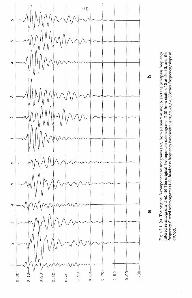
o

m

ro

CN

o

co

CN

OOoCDO

ODCDCO

O CDC \Jo

oooo D

Fig.

4.3.

1 (a)

Th

e or

igin

al 3

-com

pone

nt s

eism

ogra

ms

(1-3

) fro

m sta

tion

7 at

shot

6, a

nd

the

band

pass

fr

eque

ncy

filter

ed

seis

mog

ram

s (4

-6).

(b) T

he

orig

inal

3-c

ompo

nent

sei

smog

ram

s (1

-3)

from

statio

n 10

at sh

ot 5

, an

d th

e fre

quen

cy

filter

ed

seis

mog

ram

s (4

-6).

Band

pass

fre

quen

cy

band

wid

th

is 20

/30-

60/7

0 (C

orne

r fr

eque

ncy/

slop

e in

dB

/oct

).

91

of filtered data, say channel 5 in (a), have been suppressed. However, for those

components w ithin the frequency bandwidth, the filter does little to the data.

The unfiltered data (channels 1-3) and filtered data (channels 4-6 in Fig. 4.3.1

(b)) look rather the same because the frequencies of reverberation at this

station are higher than 20 Hz.

4.4 Predictive deconvolution filtering

D econvolution is a general term for data processing methods designed to

im prove the tem poral resolution of seismic data by com pressing the basic

seism ic w avelet (spiking deconvolution) and to remove effects which tend to

m ask the p rim ary reflected events on a seism ogram such as absorption,

reverbera tion , ghosting and m ultiple reflections (pred ictive deconvolu tion).

The form er process is based on W iener optimality which states that the seismic

w avele t can be res to red to any pre-defined shape. The p red ic tiv e

deconvolution is particularly based on the assumption that the reflectivity is a

random uncorrelated series, but that the reverberation has a fixed periodicity.

Hence the autocorrelation of seismic data is the same as the autocorrelation of

the reverbera tion w aveform . From the autocorrelation o f the reverberation

w aveform , a p red ic tio n operator can be com puted. This opera to r w ith

prediction d istance d will closely predict the reverberation com ponent o f the

waveform. Therefore, by subtracting the delayed predicted waveform from the

received w aveform , we can eliminate the reverberation com ponent. However,

the above two processes are limited in practical use unless the follow ing

conditions are met (Yilmaz, 1988):-

(1 ) The earth is made up of horizontal layers of constant velocity.

(2 ) The source generates a compressional plane wave that im pinges on

layer boundaries at normal incidence. Under such circum stances, no shear

waves are generated.

(3) The source waveform does not change as it travels in the subsurface.

(4) The noise component is zero.

(5) Reflectivity is a random process.

92

(6 ) The seism ic wavelet is minimum phase. Therefore, it has a minimum

phase inverse .

The seism ic data recorded in our experiment tend to be minimum phase.

A dditionally, the offset is relatively small. Therefore, we apply a predictive

deconvolution filter to the data from shot 6 as an example to show how the

predictive deconvolution filter affects the data. When the maximum operator

length L, which is sum of a prediction lag and length of operator, is 150 ms and

a p red ic tion lag d is 4 ms (sampling interval), the seismic w avelets are

com pressed, which is usually called spiking deconvolution. M eanw hile, the

amplitudes of high reverberation are also suppressed. When d= 8 or 16 ms, the

filtering does not make additional improvement. When d=24 ms, the filter best

attenuates reverberations. With a further increase of the prediction lag d, the

vertical reso lu tion is decreased. When d > 60 ms, the filtered data seem

untouched. Next, we use a fixed prediction lag d=24 ms, and change the L as 100,

125, 150, 175, 200 ms. The results show that shorter length of L such as 100 and

125 ms introduce "ringing" into the data, and the high reverberations are not

adequately suppressed. When the L is too long (> 250 ms), there is no additional

im provem ent. Fig. 4.4.1 (a) and (b) illustrate the orig inal 6 vertica l

com ponents and deconvolved components respectively. The maximum operator

length is chosen to be 150 ms, and the prediction lag 24 ms. We can see that the

high am plitudes at early part of the traces are suppressed in addition to the

com pressed w avelets. However, whether the filtering degrades the useful

signal is unknown because the reflections are not clear on the section. In

practice, we should test the autocorrelation of each component to choose

appropriate param eters. The deconvolution filtering for the vertica l and

horizontal com ponents should be applied separately.

4.5 Signal enhancement polarisation filtering (SEPF)

4.5.1 Introduction to the SEPF filter

As stated in Section 4.2 and 4.3, a frequency filter can be used to

suppress the noise outside the required frequency band. Deconvolution can be

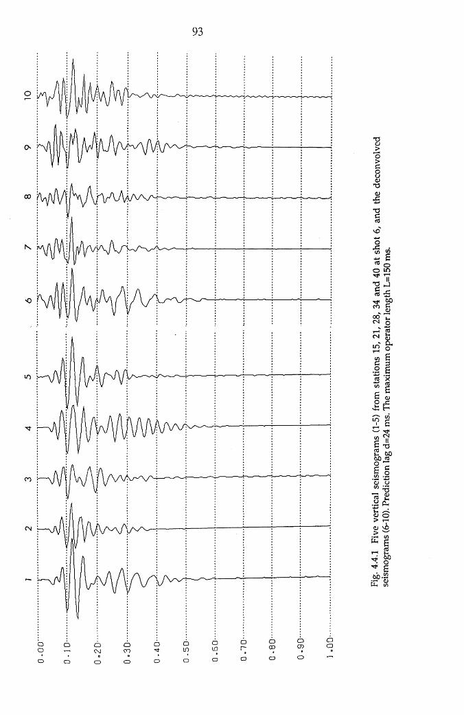
93

CO

CN

aao

CDoooa

coo aCs) in

oooOCDO OD OCD

Fig.

4.4.

1 Fi

ve

verti

cal

seis

mog

ram

s (1

-5)

from

statio

ns

15,

21,

28,

34 an

d 40

at sh

ot 6

, and

the

de

conv

olve

d se

ism

ogra

ms

(6-1

0).

Pred

ictio

n lag

d=

24

ms.

The

max

imum

op

erat

or l

engt

h L=

150

ms.

94

used to compress a seismic wavelet and also to attenuate multiples. However, its

usage is lim ited by several assumptions, and in practice, field seismic data do

not always meet the requirements. Therefore, a predictive deconvolution filter

has to be used with great care, otherwise, filtering will have a deleterious

effect on data. Velocity filtering has been successfully used to discrim inate

between prim ary reflection and multiple reflection or ground-roll. As a result,

the low velocity component can be excluded by applying a velocity filter.

H ow ever, ve locity filte ring requires the data to be recorded from an

appropriate number of stations with different offsets from a shot point. This is

because m ultiples and prim aries have no significant m oveout difference at

near o ffse ts . R egarding the 3-com ponent seism ic data recorded in our

experiment, it is impossible to apply the velocity filter to such near offset data.

In order to suppress the noise which exhibits sim ilar spectral characteristics

and sim ilar velocity band to primary reflections, other processing techniques

have to be developed. In this section, a signal enhancement polarisation filter

is designed and implemented for that purpose.

S ignal enhancem ent polarisation filtering is based on the m ultiple

com ponent reco rd ings o f ground m otions. The theory is that both

compressional and shear waves (body waves) exhibit a high degree of linear

polarisation. Noise may also be polarised, but the direction of polarisation is

random in nature. Furthermore, surface waves consist of mutually interfering

propagation m odes arriving from different directions which are also poorly

polarised. Three-component recording of ground motions makes it possible to

represent the direction of polarisation by the amplitudes of 3 components -

vertical, radial and transverse- over a specified time window N At , (where N is

number o f samples and A/ is the sampling interval). Hence by using various

characteristics o f polarised particle trajectories, a polarisation filter can be

designed to preserve or enhance the data when they are linearly polarised,

and to attenuate the data when they are randomly polarised [Kanasewich,

1975].

95

4.5.2 Design o f the SEPF filter

In order to m easure the rectilinearity and directionality o f particle

motions, we construct a covariance matrix of N points taken from each of the 3

components o f ground m otions and then compute the largest eigenvalue, the

second largest eigenvalue and the eigenvector corresponding to the largest

eigenvalue o f the matrix.

The construction of a covariance matrix follows the same procedures asv

stated in Chapter 3. We firstly define the mean values of N observations of the

random variables x and y,

! N

i = 1

m y = j j - ' L y ii= l

The covariance between N observations of two variables x and y is given byN

( * . > 0 = 4 - £ ( * , • - m x) (y m )C0V N i ,I = 1

The autocovariance between N observations of the same variable is defined asN 2

v a r (x ) = c o v ( x , x) = 4 r 2 / * , - “ m JN t . i

The three variables x, y and z correspond to the amplitudes of the radial,

transverse and vertica l com ponents respectively. From the autocovariance

and covariance o f above variables, we can construct a covariance m atrix V

given by

V = — N

var (x ) cov (x , y ) cov ( * , z) cov ( y , x) var (y ) cov (y , z)

.cov (z , x) cov ( z, y ) var (z ) .

If the tim e window N Af and the amplitudes of 3 traces are given, the

covariance m atrix V can be found. Thereafter, the rectilinearity of the

particle m otion trajectory over the specified time window can be estim ated

from the ratio of principal axes of this matrix, and the direction of polarisation

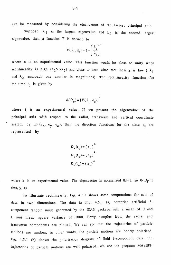
96

can be m easured by considering the eigenvector of the largest principal axis.

S uppose X l is the largest eigenvalue and X2 is the second largest

eigenvalue, then a function F is defined by

F (X V X2) = l -

where n is an experimental value. This function would be close to unity when

rectilinearity is high (A,j>>A,2 ) and close to zero when rectilinearity is low (

and X2 approach one another in magnitudes). The rectilinearity function for

the time tQ is given by

RL( tQ) = [ F ( X v A2) ] '

where j is an experim ental value. If we present the eigenvalue o f the

principal axis w ith respect to the radial, transverse and vertical coordinate

system by E = (ex , ey , ez ), then the direction functions for the tim e tQ are

represented by

D x (t0) = ( e x )

0 7<ro)-(*,)

where k is an experimental value. The eigenvector is normalized IEI=1, so 0<D^< 1

(i=x, y, z).

To illustrate rectilinearity, Fig. 4.5.1 shows some computations for sets of

data in two dim ensions. The data in Fig. 4.5.1 (a) comprise artificial 3-

component random noise generated by the ISAN package with a mean of 0 and

a root mean square variance of 1000. Forty samples from the radial and

transverse components are plotted. We can see that the trajectories of particle

motions are random, in other words, the particle motions are poorly polarised.

Fig. 4 .5 . 1 (b) shows the polarisation diagram of field 3 -component data, the

trajectories of particle motions are well polarised. We use the program MASEPF

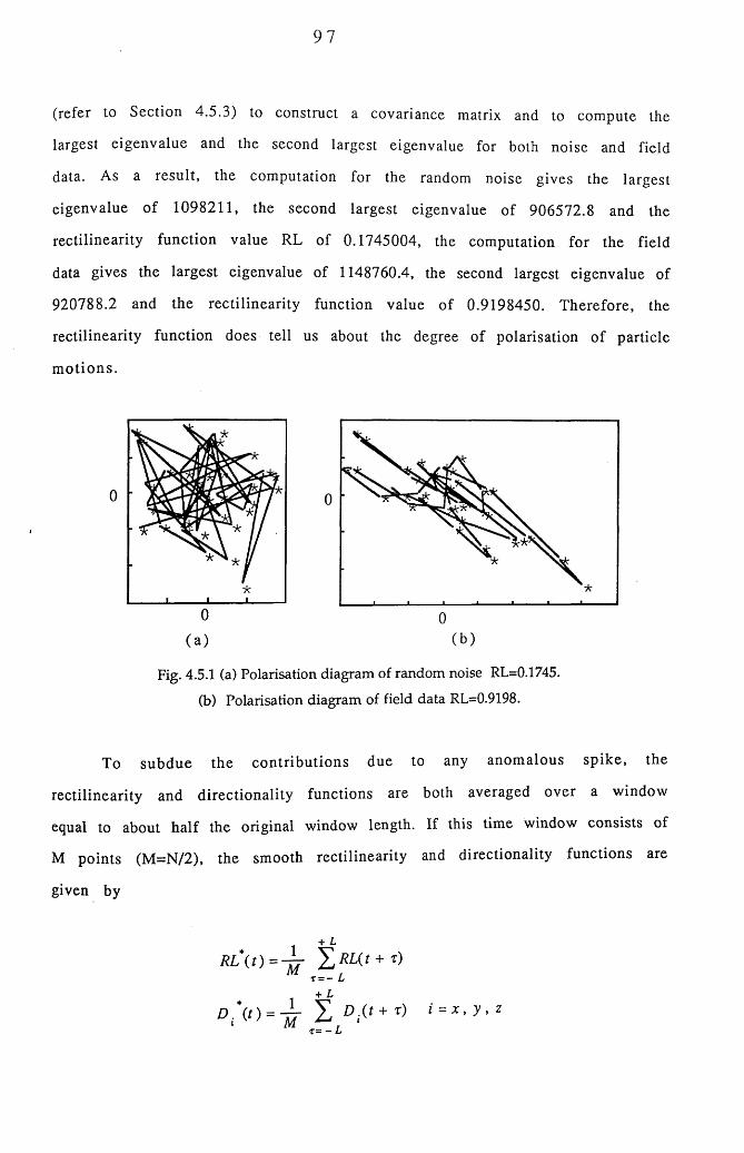
97

(refer to Section 4.5.3) to construct a covariance matrix and to compute the

largest eigenvalue and the second largest eigenvalue for both noise and field

data. As a result, the computation for the random noise gives the largest

eigenvalue o f 1098211, the second largest eigenvalue of 906572.8 and the

rectilinearity function value RL of 0.1745004, the computation for the field

data gives the largest eigenvalue of 1148760.4, the second largest eigenvalue of

920788.2 and the rectilinearity function value of 0.9198450. Therefore, the

rectilinearity function does tell us about the degree of polarisation of particle

m otions.

To subdue the con tribu tions due to any anom alous sp ike, the

rectilinearity and directionality functions are both averaged over a window

equal to about half the original window length. If this time window consists of

M points (M =N/2), the smooth rectilinearity and directionality functions are

given by

0

0

( a )0

(b )

Fig. 4.5.1 (a) Polarisation diagram of random noise RL=0.1745.

(b) Polarisation diagram of field data RL=0.9198.

D \ t ) = - L £ D X t + t) i = x , y , z « M W , 1

98

where L, t, and z are in ms, but in a program they are sample numbers L=(M-

l)/2 . Finally we have the filter operators as follows :-

F x = RL*(t). D x \ t )

F y - RL*(t) • D y *(t)

F z = RL*(t) ■ D *{t)

The filtered three seismograms are obtained by multiplying the filter

operators by the original seismograms, so we get

N x = x ( t ) - F x (t)

N y = y ( t ) - F y (t )

N z = z ( t ) - F z (t )

4.5.3 Fortran-77 program MASEPF

A Fortran-77 program called MASEPF was written by the author. As

shown in Fig. 4.5.2 below, the program reads 3-component seismic data into

arrays XX(I), YY(I) and ZZ(I), computes the covariance and autocovariance for

various variables over a specified time window, and constructs a covariance

m atrix V. The largest eigenvalue and a corresponding norm alized eigenvector

are com puted by calling the subroutine EIGEN1 which uses a Power method

[Churchhouse, 1981]. The Power method is actually an iterative m ethod in

which an arbitrary first approxim ation to the eigenvector corresponding to

the dom inan t e igenvalue is successively im proved until some requ ired

precision is reached. The second largest eigenvalue of the matrix is obtained

using the same Power method applied to a new m atrix B(2, 2) which is

construc ted from the original m atrix, its dom inant e igenvalue and the

corresponding eigenvector in such a way that it essentially contains only the

rem aining unknown eigenvalues of the original matrix. A system dependent

program (see Appendices; Fortran-77 program 8 ) was also w ritten by the

99

author which is run on the VAX/VMS operating system. Here a NAG routine

F02A BF is used to calcu la te the largest eigenvalue, the second largest

eigenvalue and the corresponding eigenvectors.

Having found the eigenvalues and the eigenvectors of the matrix V, the

program then constructs the rectilinearity and d irectionality functions for

the specified time window. The time window now moves one sample down for

the next window until the last sample is reached. However, for the first (N -l)/2

samples and last (N -l)/2 samples, (where N is the num ber of samples within

the w indow), there are no computed rectilinearity and directionality values,

thus the values are taken as the same as those at (N -l)/2 point, and NSAMPL-

(N -l)/2 point (NSAMPL is the total number of samples in one trace). The filter

operators are obtained by m ultip ly ing the rec tilinearity functions by the

directionality functions. A fter finishing one station, the program turns to the

next station and repeats the com putation until the last station has been

finished. The final filtered data are obtained by m ultiplying the original data

by the filte r operators and are w ritten into a new file. M eanwhile, the

operator functions can also be written into a file at the user's request.

To run the program , we have to answ er several questions at the

beginning (The $ is the command level prompt)

$ INPUT FILE NAME FOR FILTERING

DATA

$ INPUT NUMBER OF STATIONS

12$ INPUT NUMBER OF SAMPLES IN ONE TRACE

501

$ INPUT FILE NAME FOR OUTPUT

OUT

$ START READING DATA INTO ARRAY

$ INPUT TIME WINDOW FOR FILTERING(NO. OF SAMPLES)

21$ INPUT STATION NUMBER TO START (INPUT 0 TO STOP)

1$ INPUT STATION NUMBER TO START (INPUT 0 TO STOP)

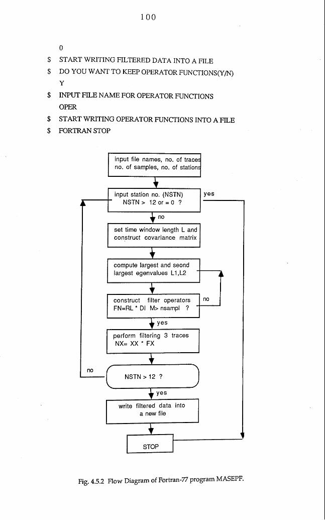
100

0

$ START WRITING FILTERED DATA INTO A FILE

$ DO YOU WANT TO KEEP OPERATOR FUNCTIONS(Y/N) Y

$ INPUT FILE NAME FOR OPERATOR FUNCTIONS

OPER

$ START WRITING OPERATOR FUNCTIONS INTO A FILE

$ FORTRAN STOP

yes

no

no

yes

noNSTN > 1 2 ?

yes

STOP

compute largest and seond largest egenvalues L1,L2

input station no. (NSTN) NSTN > 12 or = 0 ?

set time window length L and construct covariance matrix

input file names, no. of traces no. of samples, no. of stations

construct filter operators FN=RL * Dl M> nsampl ?

perform filtering 3 traces NX= XX * FX

write filtered data into a new file

Fig. 4.5.2 Flow Diagram of Fortran-77 program MASEPF.

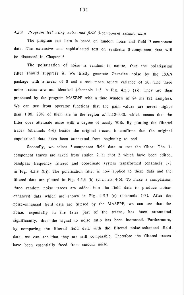
101

4.5.4 Program test using noise and fie ld 3-component seismic data

The program test here is based on random noise and field 3-component

data. The extensive and sophisticated test on synthetic 3-com ponent data will

be discussed in Chapter 5.

The polarisation of noise is random in nature, thus the polarisation

filte r should suppress it. We firstly generate Gaussian noise by the ISAN

package with a mean of 0 and a root mean square variance o f 50. The three

noise traces are not identical (channels 1-3 in Fig. 4.5.3 (a)). They are then

processed by the program MASEPF with a time window of 84 ms (21 samples).

We can see from operator functions that the gain values are never higher

than 1.00, 80% of them are in the region of 0.10-0.40, which means that the

filter does attenuate noise with a degree of nearly 70%. By plotting the filtered

traces (channels 4-6) beside the original traces, it confirms that the original

unpolarised data have been attenuated from beginning to end.

Secondly, we select 3-component field data to test the filter. The 3-

component traces are taken from station 2 at shot 2 which have been edited,

bandpass frequency filtered and coordinate system transform ed (channels 1-3

in Fig. 4.5.3 (b)). The polarisation filter is now applied to these data and the

filtered data are plotted in Fig. 4.5.3 (b) (channels 4-6). To make a comparison,

three random noise traces are added into the field data to produce noise-

enhanced data which are shown in Fig. 4.5.3 (c) (channels 1-3). After the

noise-enhanced field data are filtered by the MASEPF, we can see that the

noise, especially in the later part o f the traces, has been a ttenuated

significantly, thus the signal to noise ratio has been increased. Furtherm ore,

by com paring the filtered field data with the filtered noise-enhanced field

data, we can see that they are still comparable. Therefore the filtered traces

have been essentially freed from random noise.

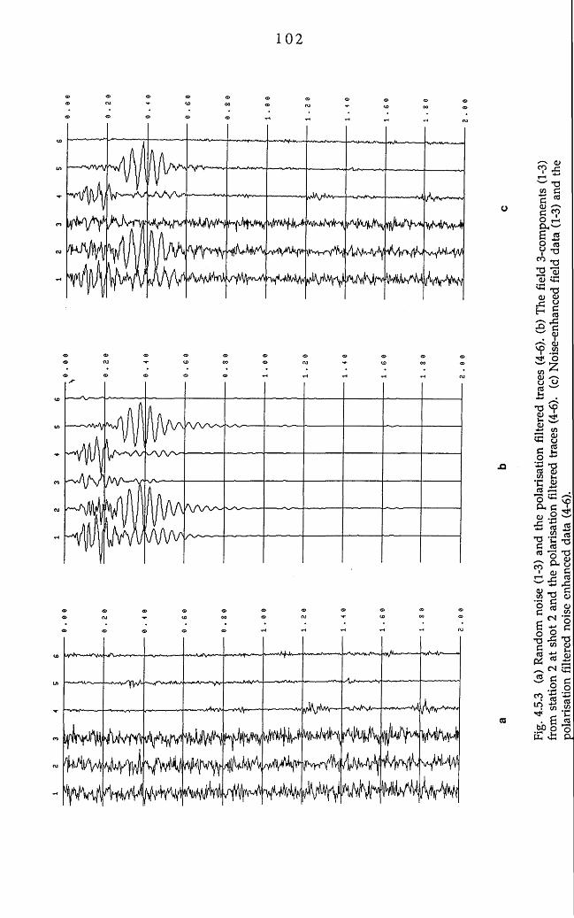
102

V

fA ^ V -

r'VMAH

«(lhtMt\ l rv rvA' AMv*V 1 V-yW /1/

A vV w

o o

u>

OJ

<£> 00 O OJ

'M'W

p^/HV

4MM

yAir^v

^vjkMh^

A*V'a'vwv

TyMlAvv ? Fig.

4.5.

3 (a)

Ra

ndom

no

ise

(1-3

) an

d the

po

laris

atio

n fil

tere

d tra

ces

(4-6

). (b)

Th

e fie

ld 3-

com

pone

nts

(1-3

) fro

m sta

tion

2 at

shot

2

and

the

pola

risat

ion

filter

ed

trace

s (4

-6).

(c) N

oise

-enh

ance

d fie

ld da

ta (1

-3)

and

the

pola

risat

ion

filter

ed

noise

en

hanc

ed

data

(4-6

).___

____

____

____

____

____

____

____

____

____

____

____

____

____

_

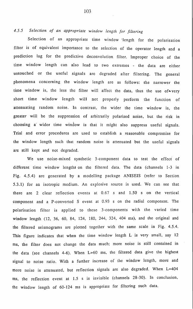
103

4.5.5 Selection o f an appropriate window length fo r filtering

Selection o f an appropriate time window 'length for the polarisation

filter is o f equivalent importance to the selection of the operator length and a

prediction lag for the predictive deconvolution filter. Improper choice of the

time w indow length can also lead to two extremes - the data are either

untouched or the useful signals are degraded after filtering. The general

phenom ena concerning the window length are as follows: the narrow er the

time window is, the less the filter will affect the data, thus the use of*very

short tim e w indow length w ill not properly perform the function of

attenuating random noise. In contrast, the wider the tim e window is, the

greater will be the suppression o f arbitrarily polarised noise, but the risk in

choosing a' w ider time window is that it might also suppress useful signals.

Trial and error procedures are used to establish a reasonable compromise for

the window length such that random noise is attenuated but the useful signals

are still kept and not degraded.

We use noise-m ixed synthetic 3-component data to test the effect of

different tim e window lengths on the filtered data. The data (channels 1-3 in

Fig. 4 .5.4) are generated by a m odelling package ANISEIS (refer to Section

5.3.1) for an isotropic medium. An explosive source is used. We can see that

there are 2 clear reflection events at 0.67 s and 1.50 s on the vertical

component and a P-converted S event at 0.93 s on the radial component. The

polarisation filte r is applied to these 3-components with the varied time

window length (12, 36, 60, 84, 124, 180, 244, 324, 404 ms), and the original and

the filtered seismograms are plotted together with the same scale in Fig. 4.5.4.

This figure indicates that when the time window length L is very small, say 12

ms, the filter does not change the data much; more noise is still contained in

the data (see channels 4-6). When L=60 ms, the filtered data give the highest

signal to noise ratio. With a further increase of the window length, more and

more noise is attenuated, but reflection signals are also degraded. When L=404

ms, the reflection event at 1.5 s is invisible (channels 28-30). In conclusion,

the window length of 60-124 ms is appropriate for filtering such data.

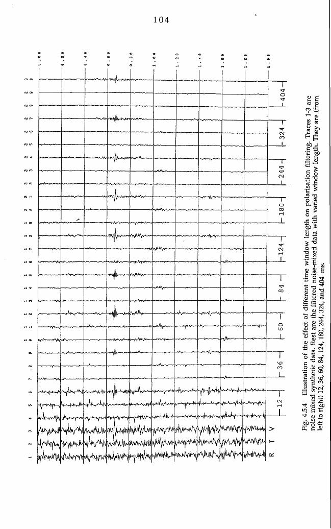
104

*~v4—

tJt vyA^V'1

v H l r ^

' /Vv'- «yMA^

Yv/ a—- ^ yf- wA-yW--h~Wp-“V yvJiVuA*'

yyl/iu y— *>V-4'VV'

VHI/fH

i A W \

\ } f \ } H ^

> m hHvj0 fkA

a gCO O

0) ro ue l 4

60,^ •c fo c^ jy® £ § O .2 T3■S c■s £O Si^■{3 c >° xX X 60 £ S iS

1— 1 CO5> •o

5 e

ocTJ<l»

*H• r**-n N O CO u-, c$ vO ^ r t — CJ ^" COjyVMv -c ■*-; O to <U

O' CO( j j 1 1

JB«■*■5 « s'-M vO « f.., ^ oo o .2 o *j aS ^ h ’B 'Qto C «*>a1—1 T3 ^

QJ _S.§ ^ c ’C

^ a) o. CO

60 'q XE § .2

lo

105

4.5.6 Application o f the SEPF filter to the data from the basalt-covered area

The signal enhancem ent polarisation filter is used here to attenuate

surface waves and random noise contained in the data. The tim e window

length is set to 68 ms (17 samples). Ten shot data including the test shot are all

processed by the SEPF filter. To illustrate how the filter works on field data, we

select 4 vertical traces from the outer stations (3, 5, 7, 9) at shot 5 as an

example. Fig. 4.5.5 (a) shows the unfiltered vertical traces. They exhibit not

only large amplitudes but complexity in wavelets. Fig. 4.5.5 (b) shows the same

data as the above after the application of the polarisation filter. The plotting

scale for the filtered data is smaller than for the unfiltered data. We can see

that the amplitudes of the filtered data are smaller than the unfiltered data at

the sam e tim e, i.e ., the strong reverberations have been a ttenuated .

Furtherm ore, the wavelets of filtered data become sim ple and clear, which

indicates that random noise has also been attenuated.

Fig. 4.5.6 (a) shows the processed and scaled radial com ponents. All

radial components from the inner circles are plotted on the left-hand side of

the figure (channels 1-60), those from the outer circles are plotted on the

right-hand side of the figure (channels 61-120). Fig. 4.5.6 (b) and (c) show the

processed and scaled transverse and vertical components respectively. We can

see from 3 figures that random noise has been attenuated significantly , the

processed sections are clearer than the unprocessed sections (refer to Fig.

3.4.4). A line o f reflection events at about 420 ms on the vertical section

(channels 61-120) are more conspicuous, so are the reflection events on the

radial section (channels 61-120). Why the reflections are not in phase may be

because o f velocity com plexity, low-frequency geophones, inaccurate static

corrections and m ost im portantly dipping reflectors (refer to Section 6.3

which states that a dipping layer at a great depth will introduce enormous time

delays among 12 vertical traces). As stated in Section 3.4, appearance of

reflection events on the radial section at the same time as on the vertical

section indicates that they are actually P-waves which are projected on the

radial components. The reflection event is not a single wavelet but a train of

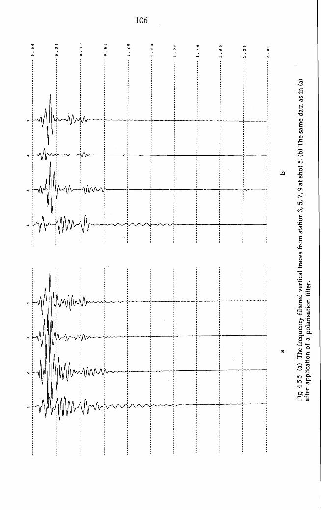
106

© ® o o ®

Fig.

4.5.

5 (a)

Th

e fre

quen

cy

filter

ed

verti

cal

trace

s fro

m sta

tion

3, 5,

7, 9

at sh

ot 5

. (b)

The

sa

me

data

as in

(a)

afte

r ap

plic

atio

n of

a po

laris

atio

n fil

ter.

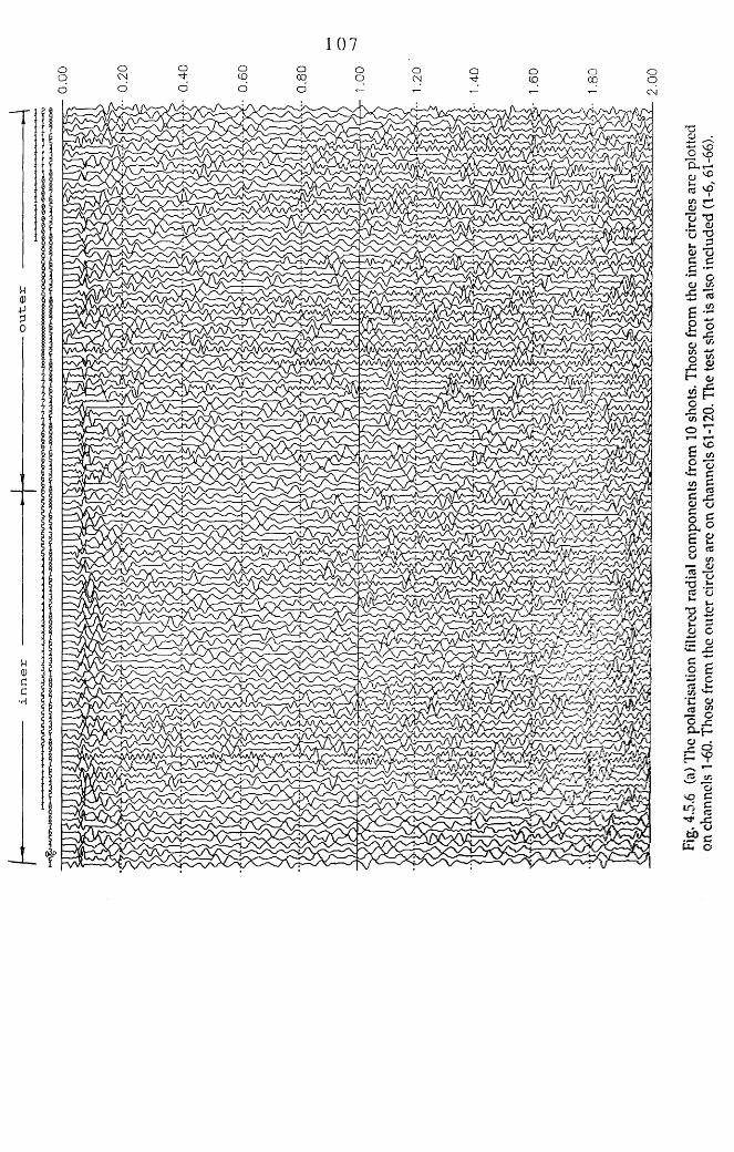
inne

r

ou

ter

107

'\/-< S * r:

lA'.Vuv\

>—Jn f^ j-— —"v V v /'»/la \/Vvv<

v'V .A

■J-xfiC-S-

W i

\yvv7f/^rJ)5

■u—■- «,/ •-*-' v // “ *v/ v v V.1^ /r ^ Y /c l/a C tW S’ y-f/ j'*j- / W

Vl/W/UA

Fig.

4.5.

6 (a)

The

po

laris

atio

n fil

tered

ra

dial

com

pone

nts

from

10 sh

ots.

Thos

e fro

m the

in

ner

circle

s are

pl

otte

d on

chan

nels

1-60

. Th

ose

from

the

oute

r cir

cles

are

on ch

anne

ls 61

-120

. Th

e tes

t sh

ot i

s als

o in

clud

ed

(1-6

,61-

66).

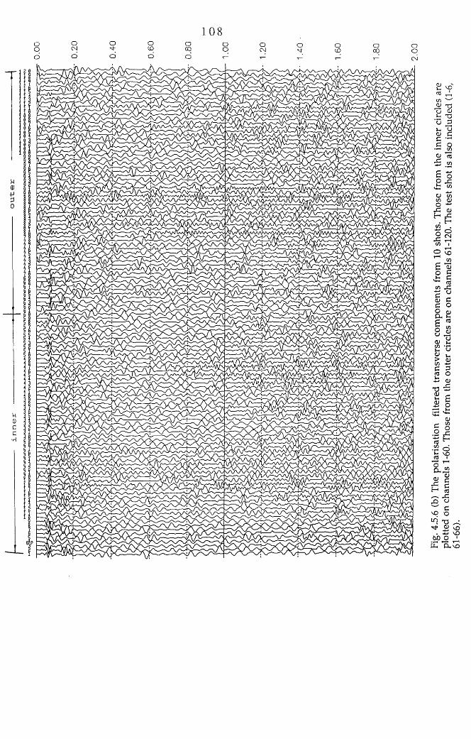
oute

r

108o o o O o o oo CM M" CO cq o CMo o Q d d r— v~

u VO« AC/2 '—cj xsu Cl »- X5 ‘u J3 u ’y a» C C —. £ 8GJ *cO

»G rn

5 ° 2 •c4: mOJ 1/2 c/2 0) OX 0)

H cG

OCM

O KO C/2

I I* gcn XC e 0/ G G O O o P-£ *£ cn0/

P u2 *-> ID C/2GCO

oVO

o t—1CX C/2

O)X

l i /c

H 03X

rQ <J

GvO oLO TS0» vO

vOt>b o i

E Ph vO

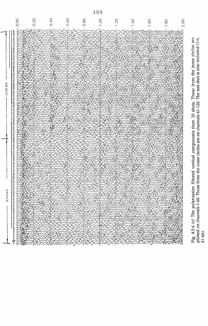
inne

r

^'

1 <

ou

ter

109

o o o oto CO o OJd d .—*

Fig.

4.5.

6 (c)

Th

e po

laris

atio

n fil

tere

d ve

rtica

l co

mpo

nent

s fro

m 10

shot

s. Th

ose

from

the

inne

r ci

rcles

ar

e pl

otte

d on

chan

nels

1-60

. Th

ose

from

the

oute

r cir

cles

are

on ch

anne

ls

61-1

20.

The

test

shot

is

also

incl

uded

(1

-6,

61-6

6).

110

w avelets , its shape and phase vary from sta tion to s ta tion . The transverse

section show s little o f in terest.

4.6 O ther data processing

In addition to the techniques stated in the above sections, o ther m ethods

w ere also d eve loped and p rogram m ed. One o f them is to use only two

com ponen ts (R and V) to iden tify the P-w aves by co n stru c tin g the cross-

product o f two com ponents over a tim e window. The theory is that, for a P-

wave, the horizon tal and vertical com ponents would be exactly in phase i f the

earth w ere a un ifo rm h a lf-sp ace , the cross-p roduct w ill have a b ig value

w hich gives a m easure o f the rectilinearity and the total signal pow er. F or S-

w aves and random noise, the signs o f two com ponents are irregu lar, so the

cross-product w ill be near to zero or have a small value [Shim shoni, 1964]. The

filte red seism ogram s are ob tained by m ultiplying the o rig inal seism ogram s by

the c ro ss-p roduct functions. This m ethod how ever is not im plem ented here.

A fter the various o f filtering , the 12 vertical com ponents from a single

shot are supposed to be stacked together so as to obtain a signal-to-noise ratio

im provem ent o f 3.5. The resu lt o f sum m ation is not show n here because the

num ber o f shots is not adequate enough to draw any conclusions on geological

s tru c tu re . To o b ta in the s tru c tu re inform ation , m any m ore sho ts w ould be

required . N evertheless, this sm all-scale shooting is only an experim ent m ostly

for develop ing new techniques. The large-scale field work can be conducted in

the fu tu re .

4 .7 In terpreta tion

The m ost in teresting param eters to be obtained from a seism ic survey in

this area are velocities o f form ations and the depth of the base o f the Clyde

Plateau Lavas (CPL). The present techniques based on this areal 'RAZOR' array

how ever cannot derive the interval velocity although it may be possib le to do

so in the fu ture with the developm ent of this experim ent. From the velocity

survey conducted by Hall [1974] in the adjacent area, the in terval velocity of

111

the CPL was given as 4420 m/s. We identify a line of events at 420 ms in Fig.

4.5.6 (c) as the primary reflections from the base of the CPL based on the

higher frequency of the wavelets compared with those upper and below the

wavelets o f interest, together with the inverse polarities of wavelets related to

the reflections from the top of the CPL (nearly at the surface). This may also

indicate an inverse velocity contrast between the CPL and the Old Red

S an d sto n e .

From the two-way travel time 420 ms, we can calculate the depth (or

thickness in this case) of the CPL HCPL=928 m below the surface, which is near

to 915 m (depth) from the contour map of the base of the CPL and to 900 m

(thickness) from the isopach map of the CPL provided by Hall [1974].

4.8 Summary

A bandpass frequency filter is tested and reveals that it can reject part

of the low frequency reverberations (<20 Hz) and high frequency noise. For

most o f high reverberations within the bandwidth, the filte r does little to

improve the data. Predictive deconvolution filtering test shows that it is very

good at com pressing the w avelets and attenuating the am plitude of

reverberations. Since both m ultiples and reflections are not clear on the

section, the predictive deconvolution filter has to be used with great care,

otherwise, it degrades the useful signals. The newly developed polarisation

Filter can be used to remove the random noise and part of the surface waves

arriving from different directions. This filter can also be used to process

conventional CDP data, if they are multi-components.

From the interval velocity and the two way travel time, the base of the

CPL is found to be at about 928 m below the surface.

112

Chapter 5 Further Testing of the Polarisation Filter and

Optimisation of Array Designing Using Synthetic 3-

component Seismic Data

5.1 In troduction

The signal enhancem ent polarisation filter (SEPF) has been developed

and simply tested using the field data as described in chapter 4. To test the

filter more thoroughly, there is a need for good quality seismic data in an area

w ith sim ple geology. In this chapter, we generate synthetic 3-com ponent

seism ic data in isotropic and anisotropic media by two m odelling packages.

Random noise has been added to the synthetic data and the noise-m ixed data

are then filtered by the SEPF filter. We will see how the signal to noise ratio is

increased after filtering and stacking.

5.2 F ilter testing using the data in an isotropic medium

5.2.1 Introduction to the modelling package "SEIS83"

The program SEIS83 was designed by Vlastislav Cerveny and Ivan

Psencik in Charles University, Czechoslovakia for the computation of rays of

seism ic waves which arrive at a system of receivers distributed regularly or

irregu larly along the earth 's surface. The generation o f waves is sem i­

au tom atic . At rece ivers , corresponding travel tim es are au to m atica lly

determ ined. Optionally, amplitudes and phase shifts may be evaluated (effects

of slight absorption may also be considered). All these quantities are stored

and may be optionally plotted or used for the com putation o f synthetic

se ism o g ra m s.

The m odel is 2D, with laterally inhom ogenous, curved in terfaces.

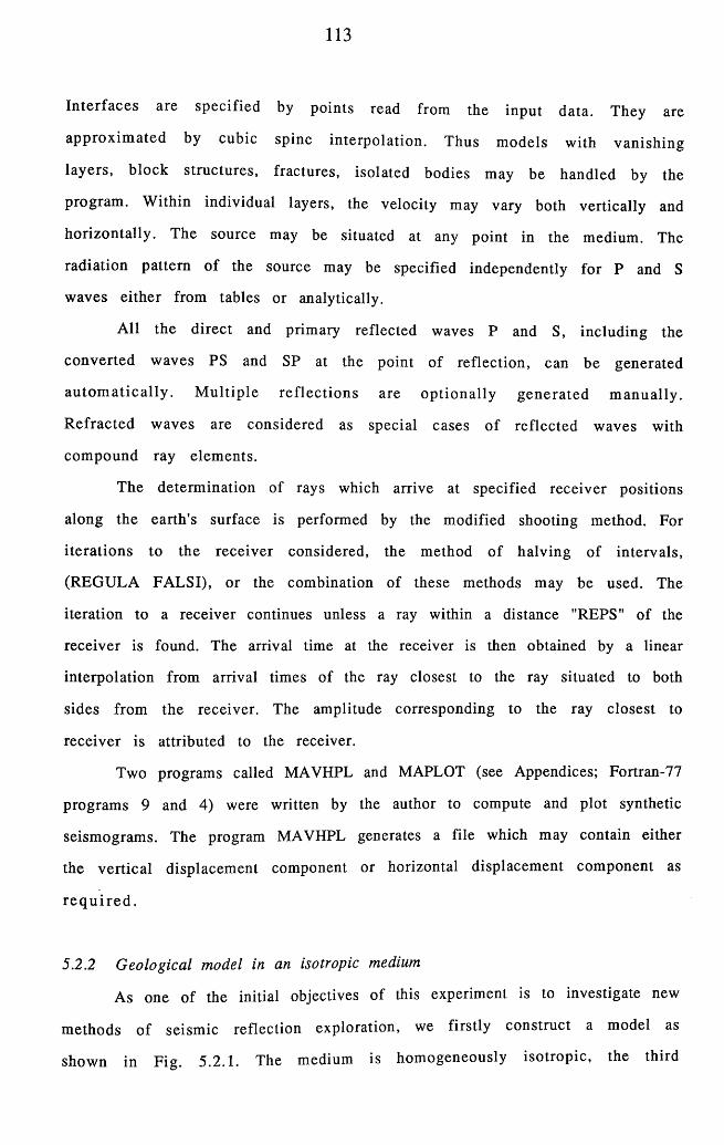
113

In te rfaces are specified by points read from the input data. They are

approx im ated by cubic spine in terpolation . Thus m odels w ith vanish ing

layers, b lock structures, fractures, isolated bodies may be handled by the

program . W ithin individual layers, the velocity may vary both vertically and

horizontally . The source may be situated at any point in the medium. The

radiation pattern o f the source may be specified independently for P and S

waves either from tables or analytically.

A ll the d irect and prim ary reflected waves P and S, including the

converted w aves PS and SP at the point of reflection, can be generated

a u to m a tic a lly . M u ltip le re flec tio n s are o p tiona lly g enera ted m anually .

R efracted w aves are considered as special cases o f reflected waves with

com pound ray elem ents.

The determ ination of rays which arrive at specified receiver positions

along the earth 's surface is performed by the m odified shooting method. For

ite rations to the receiver considered, the m ethod of halving of intervals,

(REGULA FA LSI), or the combination of these methods may be used. The

iteration to a receiver continues unless a ray within a distance "REPS" of the

receiver is found. The arrival time at the receiver is then obtained by a linear

interpolation from arrival times of the ray closest to the ray situated to both

sides from the receiver. The amplitude corresponding to the ray closest to

receiver is attributed to the receiver.

Two programs called MAVHPL and MAPLOT (see Appendices; Fortran-77

program s 9 and 4) were written by the author to compute and plot synthetic

seism ogram s. The program MAVHPL generates a file which may contain either

the vertical displacem ent component or horizontal displacem ent com ponent as

r e q u i r e d .

5.2.2 Geological model in an isotropic medium

As one of the initial objectives of this experiment is to investigate new

m ethods o f seism ic reflection exploration, we firstly construct a model as

shown in Fig. 5.2.1. The medium is hom ogeneously iso tropic, the third

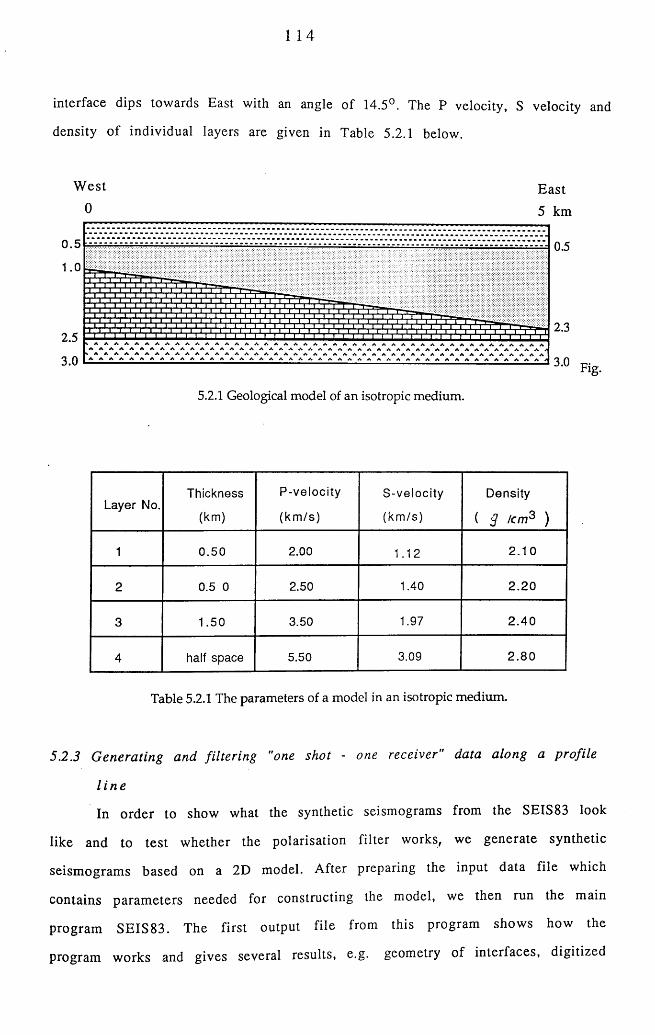
1 14

interface dips towards East with an angle of 14.5°. The P velocity, S velocity and

density of individual layers are given in Table 5.2.1 below.

W est East

5.2.1 Geological model of an isotropic medium.

Layer No.Thickness

(km)

P-velocity

(k m /s )

S-velocity

(km /s )

Density

( $ Icm^ )

1 0 .5 0 2 . 0 0 1 . 1 2 2 . 1 0

2 0.5 0 2.50 1.40 2 . 2 0

3 1 .50 3.50 1.97 2 .4 0

4 half space 5.50 3.09 2 .8 0

Table 5.2.1 The parameters of a model in an isotropic medium.

5.2.3 G enerating and filtering "one shot - one receiver" data along a profile

l i n e

In order to show what the synthetic seismograms from the SEIS83 look

like and to test whether the polarisation filter works, we generate synthetic

seism ogram s based on a 2D model. After preparing the input data file which

contains param eters needed for constructing the model, we then run the main

program SEIS83. The first output file from this program shows how the

program works and gives several results, e.g. geometry of interfaces, digitized

115

velocities, elem entary modes, travel times and phases. The second output file

from this program , which corresponds to either the vertical com ponent or

horizontal com ponent, gives wave modes, travel tim es, am plitudes, phase

shifts, initial angles and so on. This data file is an input file for the program

MAVHPL, which generates synthetic seism ogram s. One shot produces two

seismograms (vertical and horizontal) from one station with an offset o f 75 m

from the shot point. The shot spacing is 75 m. Data for 20 shots along the

profile line eastwards have been generated corresponding to a distance o f 1.5

km at the surface. The main parameters for a synthetic seismogram are as

fo llo w s:-

Seismic source type: explosive source

Frequency o f source signal: 35 Hz

Length o f recording: 4 s

Sam pling in terval: 4 ms

Due to the explosive source used in generating synthetic seismograms,

there are P-waves, S-waves and P-S converted waves on the vertical and radial

components. Let us take the data from shot 1 as an example to inspect the

characteristics of the data. As shown on the left-hand sides of Fig. 5.2.2 (a) and

Fig. 5.2.2 (b), we can see that there are three P-reflections at 0.50 s, 1.07 s and

1.81 s on the vertical component (channel 1 in Fig. 5 .2 .2 .(a)), and three S-

reflections at 0.89 s, 1.91 s and 3.22 s, and three P-S converted waves at 0.70 s,

1.49 s and 2.52 s on the radial component (channel 1 in Fig. 5 .2 .2 .(b)).

M eanwhile, the signals on both components are projected on each other but

with relatively small amplitudes. Looking at the 20 horizontal and 20 vertical

seismograms together, we see clear images of 3 layers in the time and distance

domain, with the middle one dipping towards East.

To apply the polarisation filter to the data, there have to be 3-

component seism ogram s at one station which are received at three different

orientations. The present package however can generate only one o f the

horizontal components. To satisfy the conditions, the transverse component is

constructed by filling pure random noise.

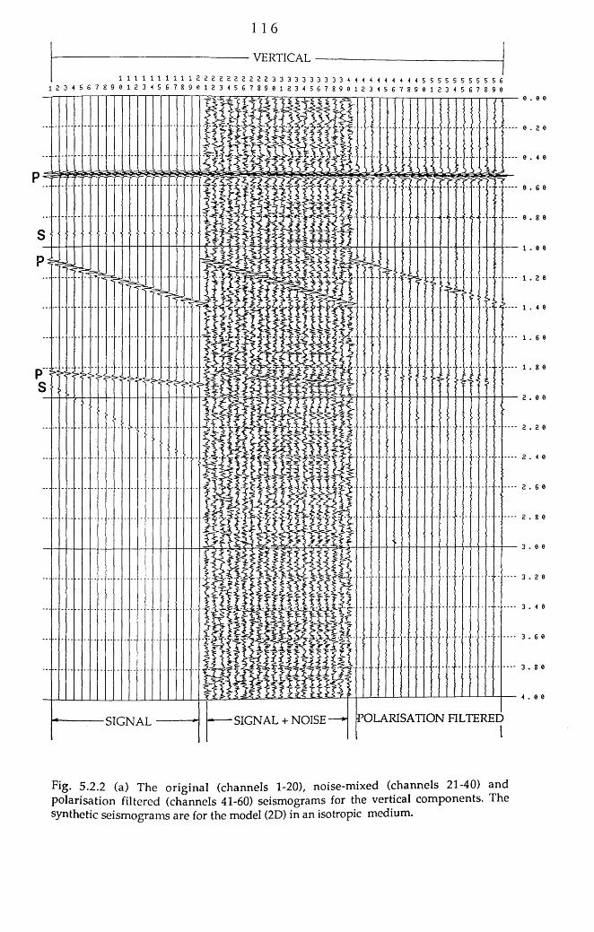
1 16

------------------------------------------- — VERTICAL -------------------------------------

1 1 1 1 1 1 1 1 1 1 a 2 2 2 E 2 2 2 2 2 3 3 3 3 3 3 3 3 3 3 n H H 4 4 H 5 5 5 5 5 5 5 5 5 5 6 1 2 3 4 5 6 7 8 9 9 1 2 3 4 5 6 7 8 9 e 1 2 3 4 5 6 7 8 9 6 1 2 3 4 5 6 7 8 9 0 1 2 3 4 5 G 7 8 9 0 1 2 3 4 5 6 7 8 9 e

t f l ' f

POLARISATION FILTEREDSIGNAL + NOISESIGNAL

0 0

2 0

4 0

6 0

8 0

0 0

2 0

4 0

6 0

8 0

0 0

2 0

4 0

S 0

8 0

0 0

2 0

4 0

6 0

8 0

0 0

Fig. 5.2.2 (a) The original (channels 1-20), noise-mixed (channels 21-40) and polarisation filtered (channels 41-60) seismograms for the vertical components. The synthetic seismograms are for the model (2D) in an isotropic medium.

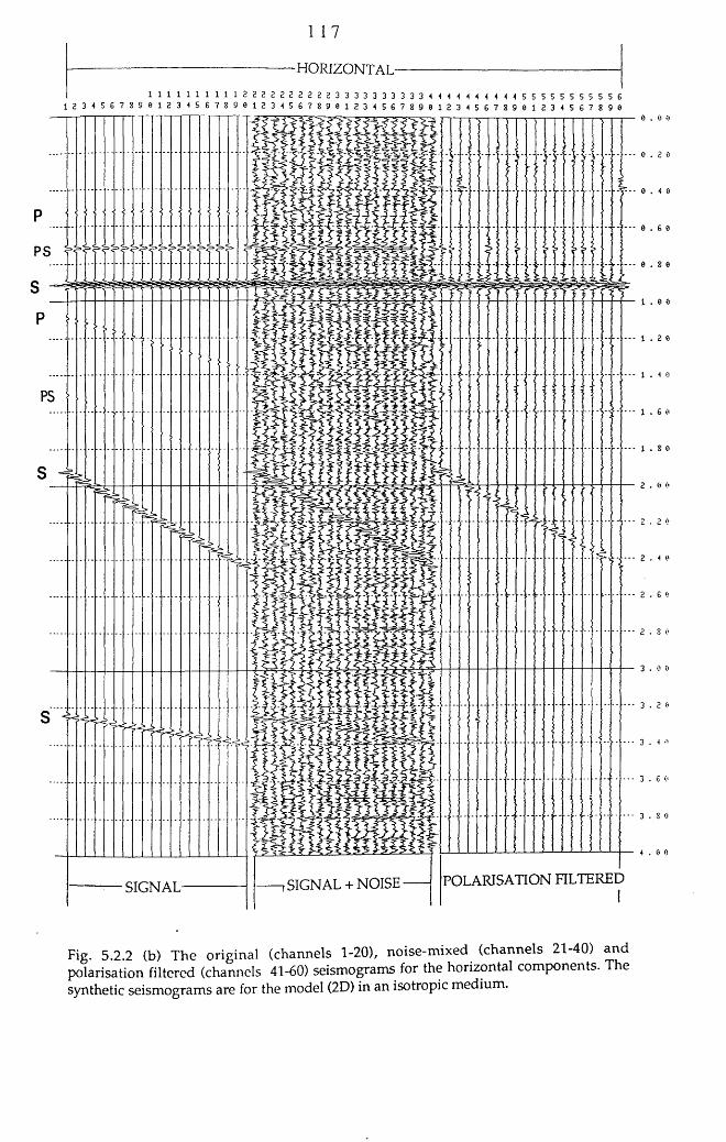
1 17

HORIZONTAL-

1 1 1 1 1 1 1 1 1 1 2 2 2 2 2 2 2 2 2 2 3 3 3 3 3 3 3 3 3 3 4 4 4 4 4 4 4 4 4 4 S S 5 5 5 S 5 5 5 5 6 1 2 3 4 S 6 ? S 9 9 1 2 3 4 5 6 7 8 9 e 1 2 3 4 S 6 ? 8 9 « 1 2 3 4 5 6 7 8 9 0 1 2 3 < 5 6 7 8 9 « 1 2 3 4 S 6 ? 8 9 «

PS

POLARISATION FILTEREDSIGNAL + NOISESIGNAL-

0

0

0

0

0

1

1

1

1

1

2

2

2

2

2

3

3

3

3

3

4

Fig. 5.2.2 (b) The original (channels 1-20), noise-mixed (channels 21-40) and polarisation filtered (channels 41-60) seismograms for the horizontal components. The synthetic seismograms are for the model (2D) in an isotropic medium.

118

Pure random noise with a mean of 0 and a root mean square variance of

120, generated by the package ISAN, is added to the vertical and radial

components, producing noise-mixed data. We can see from the middle panels of

Fig. 5.2.2 (a) and Fig. 5.2.2 (b) (channels 21-40) that the signal to noise ratio

has been decreased considerably.

The SEPF filter is applied to the 3-component data, the time window for

filtering is set to 23 samples (92 ms). The filtered seismograms are plotted on

the right-hand sides of Fig. 5.2.2 (a) and Fig. 5.2.2 (b) (channels 41-60). For the

horizontal com ponent section, two S-wave and one P-S converted images have

been kept, and the P-wave image at 0.50 s has been removed after filtering.

However, the S-waves at 3.20-3.40 s are not well separated from noise. It may be

because a large scale is used to produce the figure, the S-wave events are then

scaled down to an invisible level. Another possibility is that the added noise

en tirely changes the polarisation direction of particle m otions o f reflection

w avelets, which makes the polarisation filter unable to extract the S-waves (

see Section 5.4). For the vertical section, three P wave images have been kept,

all the S-wave and P-S converted images are removed because the polarisation

directions o f these waves are horizontal. By comparing 3 different data - the

original, noise-m ixed and filtered - in both figures, we can see that the added

noise has been attenuated remarkably. The signal, on the other hand, has not

been degraded after filtering.

5.2.4 Generating the data based on the areal 'RAZOR' array in an isotropic

m e d i u m

The areal 'RAZOR' array pattern and its dimensions were described in

Chapter 2. For the convenience, the array pattern is shown again in Fig. 5.2.3.

We generate synthetic seismograms based on this 3D model to test both the

SEPF filter and the optimisation of designing of such an array.

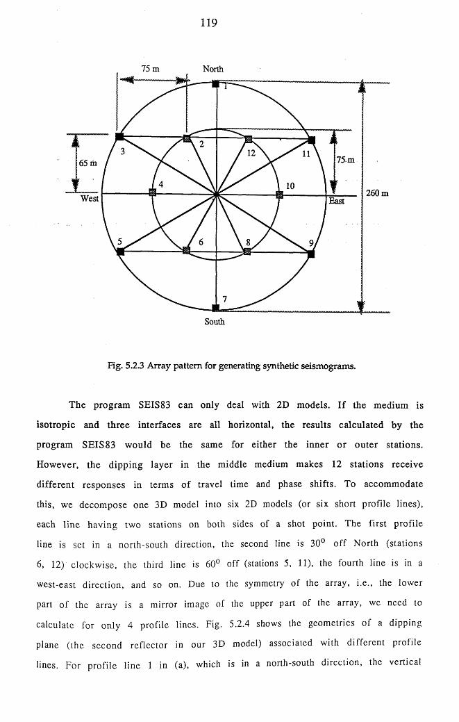
119

75 m North

75 m65 m

260 mWest East

South

Fig. 5.2.3 Array pattern for generating synthetic seismograms.

The program SEIS83 can only deal with 2D models. I f the medium is

isotropic and three interfaces are all horizontal, the results calculated by the

program SEIS83 would be the same for either the inner or outer stations.

However, the dipping layer in the middle medium makes 12 stations receive

different responses in terms of travel time and phase shifts. To accommodate

this, we decompose one 3D model into six 2D models (or six short profile lines),

each line having two stations on both sides of a shot point. The first profile

line is set in a north-south direction, the second line is 30° off North (stations

6, 12) clockwise, the third line is 60° off (stations 5, 11), the fourth line is in a

west-east direction, and so on. Due to the symmetry of the array, i.e., the lower

part of the array is a mirror image of the upper part of the array, we need to

calculate for only 4 profile lines. Fig. 5.2.4 shows the geometries of a dipping

plane (the second reflector in our 3D model) associated with different profile

lines. For profile line 1 in (a), which is in a north-south direction, the vertical

120

distance of the line to the plane is hz , the normal distance is h. Thus a new 2D

model in (b) is constructed such that the vertical distance to a planar reflector

is h. For profile line 4 in (c), which is in a west-east direction, a new 2D model

is shown in (d), here y is the true dip of the reflector. For profile line 2 and 3

in (e), the geometry of the new models is complicated. The plane OO'N, which is

the incident plane o f seismic waves, is normal to the dipping plane R, the

apparent dip <J> changes from y -0° (\\r is the true dip of the plane R in the 3D

model) when the azimuth a of a profile line X changes from 0 °-9 0 ° (an azimuth

of a line is defined as an angle measured clockwise from the west-east line).

Hence a new model in (f) for either line 2 or 3 is constructed such that the true

dip o f a reflector is <j> and the vertical distance of the line from a shot point at

the surface to the reflector is hx , the normal distance being h. Therefore, by

running the program SEIS83 4 times based on different input files, while

keeping the source condition untouched, the synthetic data for the 3D model

can be generated. Fig. 5.2.5 shows 12 horizontal traces and 12 vertical traces

for a shot. We can see a small fluctuation of seismic wavelets between adjacent

traces which is introduced by the dipping reflector.

5.2.5 Processing the data based on the areal 'RAZOR' array in the isotropic

m e d i u m

In this section, we will show how the polarisation filter works on noise-

mixed 3-com ponent data based on the areal 'RAZOR' array and how such an

array pattern is optimally chosen. At the first stage, we generate the synthetic

seismograms in the way described above. The data for 20 shots are generated

corresponding to a distance of 1.5 km at the surface. We then add the pure

random noise to the data and filter them by the polarisation filter. These

original, noise-m ixed and filtered data are not presented here, but they look

like the data shown in Fig. 5.2.5. At the second stage, we add the filtered

seismograms from each shot together so as to increase the signal to noise ratio

by 3.5. Specifically , 12 vertical components are stacked together and 12

horizontal components are stacked together for each shot, this stacking will

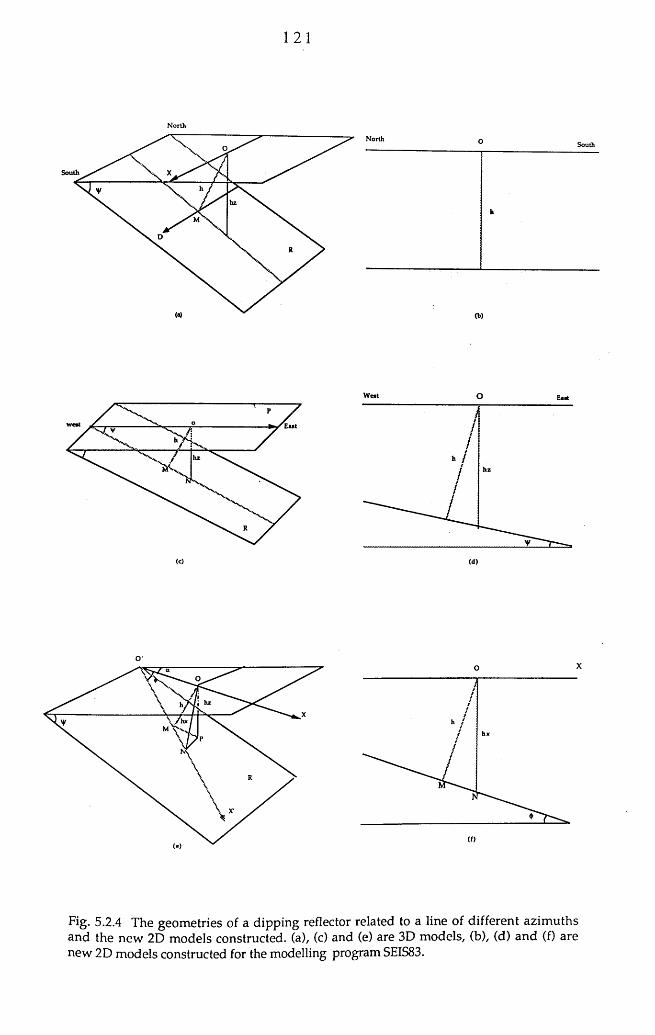
121

N o rth

South

hz

O'

(e)

O

Fig. 5.2.4 The geometries of a dipping reflector related to a line of different azimuths and the new 2D models constructed, (a), (c) and (e) are 3D models, (b), (d) and (f) are new 2D models constructed for the modelling program SEIS83.

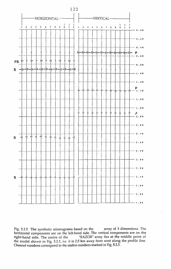
1 2 2

■HORIZONTAL' -VERTICAL -1 1 1

9 9 1 2 1 2 3 4 5 6 ?1 1 1

9 0 1 2

PS 5 - 5 5

j i i j r1 "" r * l " i " ( I T " ? " " ^ " " " 7 ' t " T — 1 - 4 0

1 . 2

T T t f f r t r f f f f ?— 2.00

3 . 6 0

3 . 8 0

Fig. 5.2.5 The synthetic seismograms based on the array of 3 dimensions. The horizontal components are on the left-hand side. The vertical components are on the right-hand side. The centre of the "RAZOR" array lies at the middle point of the model shown in Fig. 5.2.1, i.e. it is 2.5 km away from west along the profile line. Channel numbers correspond to the station numbers marked in Fig. 5.2.3.

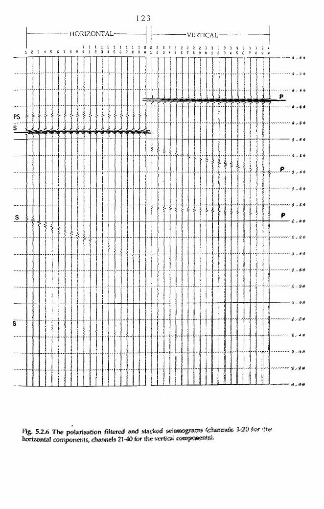
123

HORIZONTAL— ■VERTICAL'

1 1 1 1 1 1 1 1 1 1 2 2 2 2 2 2 2 2 2 2 3 3 3 3 3 3 3 3 3 3 4 1 2 3 4 5 6 ? 8 9 0 1 2 3 4 5 £ ? 8 9 0 1 2 3 4 5 G 7 £ 9 0 1 2 3 4 5 6 7 2 9 A

Fig. 5-2-6 The polarisation filtered and stacked seism ^am s fetaweife lh25) ffar -the horizontal components/ channels 21-40 for the vertical oomporoeMlS)).-

124

produce two final composite traces. By carrying out the same process, 20

composite vertical and 20 composite horizontal traces are obtained. They are

plotted in Fig. 5.2.6. From this figure, we can see that the residual random noise

has been cancelled out after stacking. In contrast, the reflection events from

the first horizontal interface are remarkably enhanced; not only because they

have large am plitudes but because they are in phase. The later reflections

from interfaces 2 and 3 are also revealed and show a better resolution than the

section in Fig. 5.2.2.

5.3 Filter testing using the data in an anisotropic medium

5.3.1 Introduction to the modelling package "ANISEIS"

AN ISEIS is a flexible com puter m odelling system for calcu la ting

synthetic seism ogram s from point sources in anisotropic and cracked plane-

layers. V ertical seismic profiles, surface to surface reflections, and cross-hole

shooting are some of the model geometries that can be accommodated.

The m ethods used in ANISEIS are based on plane wave analysis and

involve use o f the reflectivity method or propagator m atrix m ethod and

accum ulation of plane waves along summation paths in both the complex

horizontal slowness and complex PHI planes ( slowness is the inverse of phase

velocity and PHI is an angle in the horizontal plane, m easured from the

vertical plane which contains the source and geophones). This plane, the (X,

Z) plane in a system of right-handed co-ordinates with the Z-axis downwards,

will be referred to as the sagittal plane.

The calculation is performed for each of a range of frequencies and the

results recorded in the table which the user can update or extend if he wishes

to improve the results or add higher frequencies. It is also possible to run

frequencies one at a time and to compare results for successive calculations. It

is facilities such as this which make interactive use of ANISEIS valuable. While

a whole run of 50 to 200 frequencies through a model may be a major computer

exerc ise , the runn ing o f one frequency through a s im p lif ie d but

representative model is quickly performed. This feature allows the user to test

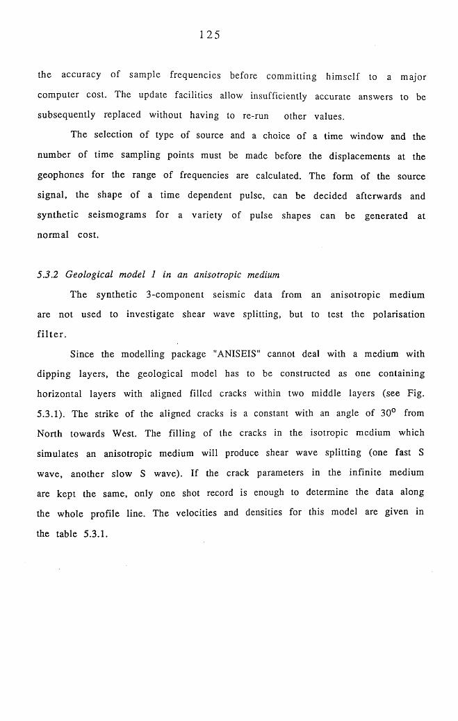
125

the accuracy o f sam ple frequencies before com m itting him self to a m ajor

com puter cost. The update facilities allow insufficiently accurate answers to be

subsequently replaced without having to re-run other values.

The selection o f type of source and a choice of a time window and the

num ber of time sampling points must be made before the displacements at the

geophones for the range o f frequencies are calculated. The form of the source

signal, the shape o f a tim e dependent pulse, can be decided afterwards and

synthetic seism ogram s for a variety of pulse shapes can be generated at

norm al cost.

5.3.2 Geological model 1 in an anisotropic medium

The synthetic 3-com ponent seismic data from an anisotropic medium

are not used to investigate shear wave splitting, but to test the polarisation

f i l t e r .

Since the modelling package "ANISEIS" cannot deal with a medium with

dipping layers, the geological model has to be constructed as one containing

horizontal layers with aligned filled cracks within two middle layers (see Fig.

5.3.1). The strike of the aligned cracks is a constant with an angle of 30° from

North towards W est. The filling of the cracks in the isotropic medium which

sim ulates an anisotropic medium will produce shear wave splitting (one fast S

wave, another slow S wave). If the crack parameters in the infinite medium

are kept the same, only one shot record is enough to determine the data along

the whole profile line. The velocities and densities for this model are given in

the table 5.3.1.

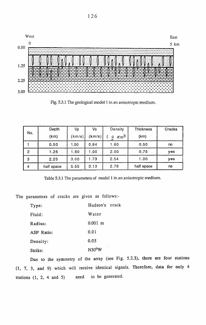
126

West East0 5 km

0.00

1.25

2.25

3.00

Fig. 5.3.1 The geological model 1 in an anisotropic medium.

No.Depth

(km )

Vp

(km /s )

Vs

(k m /s )

Density

( Km ^

Thickness

(km)

Cracks

1 0 .5 0 1.50 0 .84 1 .60 0 .5 0 no

2 1 .2 5 1 .80 1.00 2.00 0 .7 5 yes

3 2 .2 5 3 .0 0 1 .73 2 .5 4 1.00 yes

4 half space 5 .55 3 .1 3 2 .7 8 half space no

Table 5.3.1 The parameters of model 1 in an anisotropic medium.

The param eters o f cracks are given as follows:-

Type: Hudson's crack

Fluid: W ate r

R ad ius: 0.001 m

ASP Ratio: 0.01

D ensity : 0.05

Strike: N30°W

Due to the symmetry of the array (see Fig. 5.2.3), there are four stations

(1, 7, 3, and 9) which will receive identical signals. Therefore, data for only 4

stations (1, 2, 4 and 5) need to be generated.

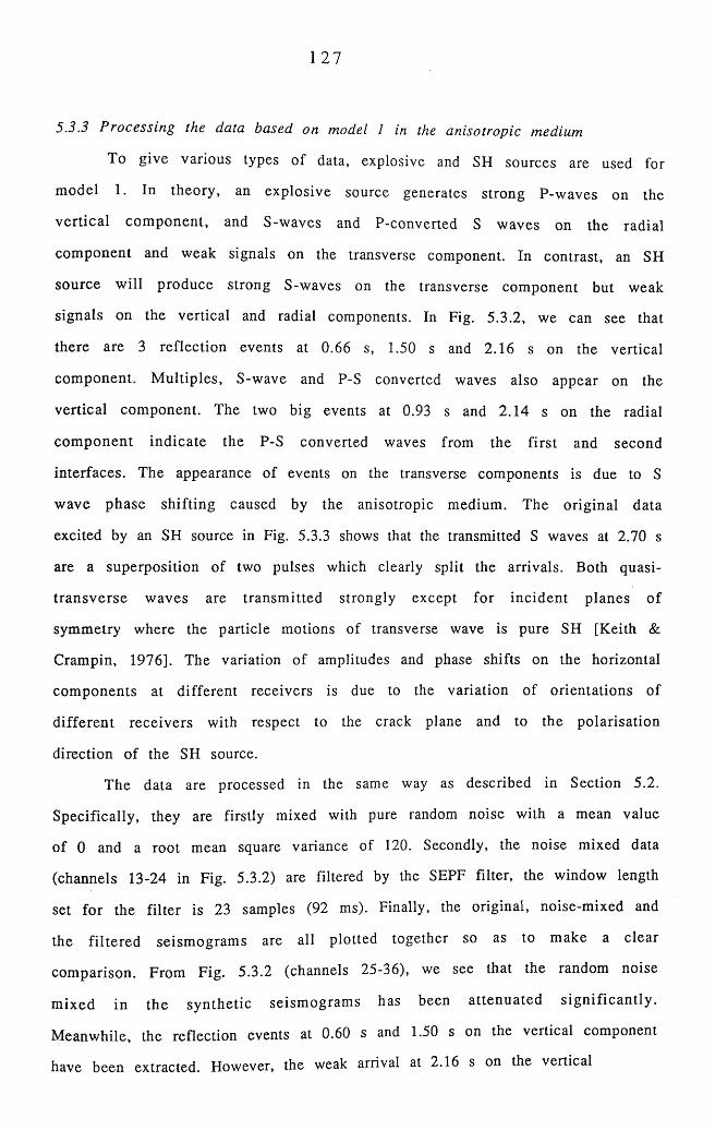
127

5.3.3 Processing the data based on model 1 in the anisotropic medium

To give various types o f data, explosive and SH sources are used for

m odel 1. In theory, an explosive source generates strong P-waves on the

vertica l com ponent, and S-waves and P-converted S waves on the radial

com ponent and weak signals on the transverse component. In contrast, an SH

source w ill produce strong S-waves on the transverse com ponent but weak

signals on the vertical and radial components. In Fig. 5.3.2, we can see that

there are 3 reflection events at 0.66 s, 1.50 s and 2.16 s on the vertical

com ponent. M ultiples, S-wave and P-S converted waves also appear on the

vertical com ponent. The two big events at 0.93 s and 2.14 s on the radial

com ponent ind icate the P-S converted waves from the first and second

interfaces. The appearance of events on the transverse components is due to S

wave phase shifting caused by the anisotropic medium. The original data

excited by an SH source in Fig. 5.3.3 shows that the transmitted S waves at 2.70 s

are a superposition of two pulses which clearly split the arrivals. Both quasi-

tran sverse w aves are transm itted strongly except fo r incident planes o f

symmetry where the particle motions of transverse wave is pure SH [Keith &

Crampin, 1976]. The variation of amplitudes and phase shifts on the horizontal

com ponents at different receivers is due to the variation of orientations of

d ifferen t receivers with respect to the crack plane and to the polarisation

direction of the SH source.

The data are processed in the same way as described in Section 5.2.

Specifically, they are firstly mixed with pure random noise with a mean value

of 0 and a root mean square variance of 120. Secondly, the noise mixed data

(channels 13-24 in Fig. 5.3.2) are filtered by the SEPF filter, the window length

set for the filter is 23 samples (92 ms). Finally, the original, noise-mixed and

the filte red seism ogram s are all plotted together so as to m ake a clear

com parison. From Fig. 5.3.2 (channels 25-36), we see that the random noise

m ixed in the syn thetic seism ogram s has been attenuated sign ifican tly .

M eanwhile, the reflection events at 0.60 s and 1.50 s on the vertical component

have been extracted. However, the weak arrival at 2.16 s on the vertical

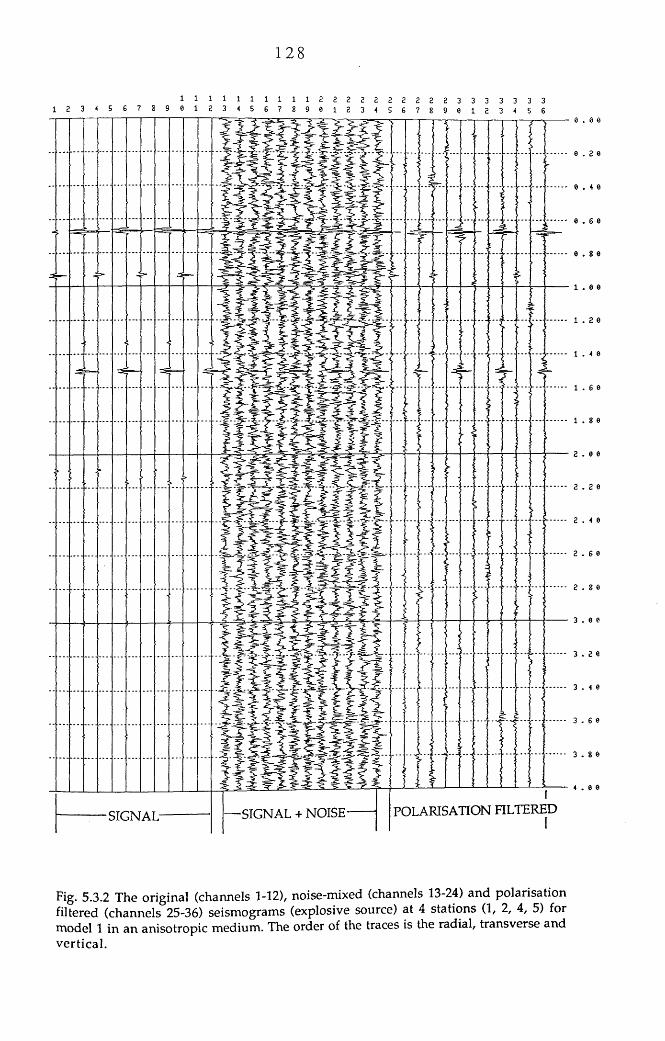
1 . z

- 3 - .......... 1 . 4

SIGNAL + NOISESIGNAL

. 2 0

- - 0 . 4

0 . 6

6 0

POLARISATION FILTERED

Fig. 5.3.2 The original (channels 1-12), noise-mixed (channels 13-24) and polarisation filtered (channels 25-36) seismograms (explosive source) at 4 stations (1, 2, 4, 5) for model 1 in an anisotropic medium. The order of the traces is the radial, transverse and vertical.

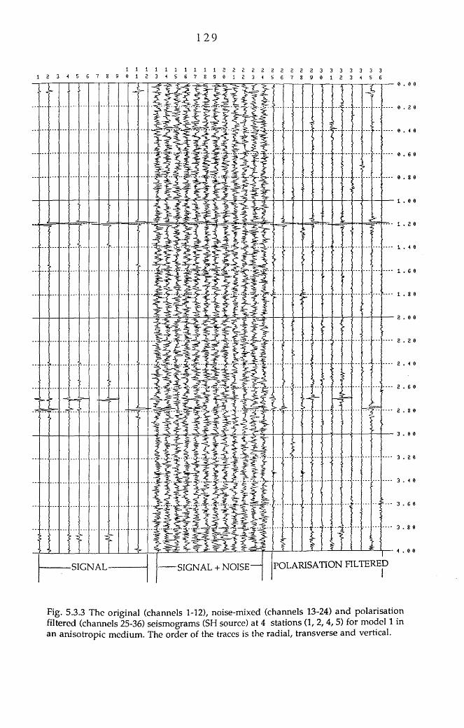
129

- - 0 . 6 0

2.60

2.60

SIGNAL SIGNAL + NOISE— POLARISATION FILTERED

Fig. 5.3.3 The original (channels 1-12), noise-mixed (channels 13-24) and polarisation filtered (channels 25-36) seismograms (SH source) at 4 stations (1, 2, 4, 5) for model 1 in an anisotropic medium. The order of the traces is the radial, transverse and vertical.

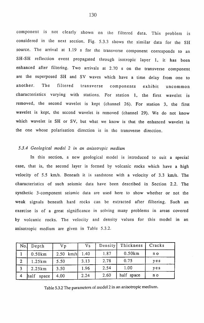
130

com ponent is not clearly shown on the filtered data. This problem is

considered in the next section. Fig. 5.3.3 shows the sim ilar data for the SH

source. The arrival at 1.19 s for the transverse component corresponds to an

SH-SH reflection event propagated through isotropic layer 1, it has been

enhanced after filtering. Two arrivals at 2.70 s on the transverse com ponent

are the superposed SH and SV waves which have a time delay from one to

a n o th e r . T he f i l te re d tra n sv e rse co m p o n en ts e x h ib i t u n co m m o n

charac te ris tics varying with stations. For station 1, the firs t w avelet is

rem oved, the second wavelet is kept (channel 26). For station 3, the first

wavelet is kept, the second wavelet is removed (channel 29). We do not know

which wavelet is SH or SV, but what we know is that the enhanced wavelet is

the one whose polarisation direction is in the transverse direction.

5.3.4 Geological model 2 in an anisotropic medium

In this section, a new geological model is introduced to suit a special

case, that is, the second layer is formed by volcanic rocks which have a high

velocity of 5.5 km/s. Beneath it is sandstone with a velocity of 3.3 km/s. The

characteristics of such seismic data have been described in Section 2.2. The

synthetic 3-component seismic data are used here to show whether or not the

weak signals beneath hard rocks can be extracted after filtering. Such an

exercise is of a great significance in solving many problems in areas covered

by volcanic rocks. The velocity and density values for this model in an

anisotropic medium are given in Table 5.3.2.

No. D ep th Vp Vs D ensity T h ic k n e ss C racks

1 0.50km 2.50 km/s 1.40 1.87 0.50km n o

2 1.25km 5.50 3.13 2.78 0.75 y e s

3 2.25km 3.50 1.96 2.54 1.00 y e s

4 half space 4.00 2.24 2.60 half space n o

Table 5.3.2 The parameters of model 2 in an anisotropic medium.

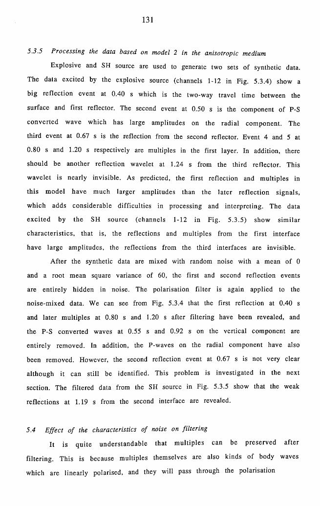
131

5.3.5 Processing the data based on model 2 in the anisotropic medium

Explosive and SH source are used to generate two sets of synthetic data.

The data excited by the explosive source (channels 1-12 in Fig. 5.3.4) show a

big reflection event at 0.40 s which is the two-way travel time between the

surface and first reflector. The second event at 0.50 s is the component of P-S

converted wave which has large amplitudes on the radial com ponent. The

third event at 0.67 s is the reflection from the second reflector. Event 4 and 5 at

0.80 s and 1.20 s respectively are multiples in the first layer. In addition, there

should be another reflection wavelet at 1.24 s from the third reflector. This

w avelet is nearly invisible. As predicted, the first reflection and m ultiples in

th is m odel have m uch larger amplitudes than the later reflection signals,

w hich adds considerable difficulties in processing and interpreting. The data

exc ited by the SH source (channels 1-12 in Fig. 5 .3 .5) show sim ilar

characteristics, that is, the reflections and m ultiples from the first interface

have large amplitudes, the reflections from the third interfaces are invisible.

A fter the synthetic data are mixed with random noise with a mean of 0

and a root mean square variance of 60, the first and second reflection events

are entirely hidden in noise. The polarisation filter is again applied to the

noise-m ixed data. We can see from Fig. 5.3.4 that the first reflection at 0.40 s

and later m ultiples at 0.80 s and 1.20 s after filtering have been revealed, and

the P-S converted waves at 0.55 s and 0.92 s on the vertical component are

entirely removed. In addition, the P-waves on the radial component have also

been removed. However, the second reflection event at 0.67 s is not very clear

although it can still be identified. This problem is investigated in the next

section. The filtered data from the SH source in Fig. 5.3.5 show that the weak

reflections at 1.19 s from the second interface are revealed.

5.4 E ffect o f the characteristics o f noise on filtering

It is qu ite understandable that m ultip les can be p reserved after

filtering. This is because m ultiples themselves are also kinds of body waves

which are linearly polarised, and they will pass through the polarisation

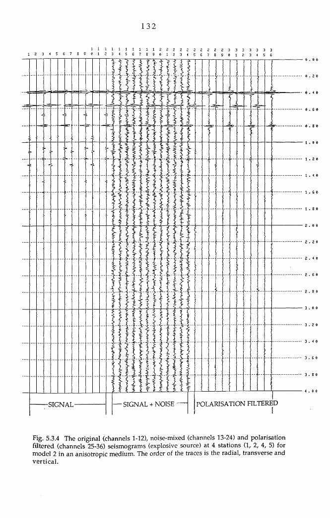
132

1 1 1 1 1 1 1 1 1 1 2 2 2 2 2 2 2 2 2 2 3 3 3 3 3 3 31 2 3 4 5 6 7 8 9 0 1 2 3 4 5 6 7 8 9 6 1 2 3 4 5 6 7 8 9 0 1 2 3 4 5 6

POLARISATION FILTERED— SIGNAL + NOISESIGNAL

0 . 2

. 2 0

. 6 0

. 8 0

•" 2.8

3 . 2 0

3 . 8

Fig. 5.3.4 The original (channels 1-12), noise-mixed (channels 13-24) and polarisation filtered (channels 25-36) seismograms (explosive source) at 4 stations (1, 2, 4, 5) for model 2 in an anisotropic medium. The order of the traces is the radial, transverse and vertical.

1 3 3

l l : l 1 1 1 1 1 1 1 2 2 2 2 2 2 2 2 2 2 3 3 3 3 3 3 31 2 3 4 5 6 7 8 9 0 1 2 3 4 5 6 7 8 9 8 1 2 3 4 5 6 7 8 9 0 1 2 3 4 5 6

POLARISATION FILTEREDSIGNAL + NOISESIGNAL

Fig. 5.3.5 The original (channels 1-12), noise-mixed (channels 13-24) and polarisation filtered (channels 25-36) seismograms (SH source) at 4 stations (1, 2,4, 5) for model 2 in an anisotropic medium. The order of the traces is the radial, transverse and vertical.

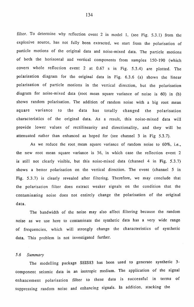
134

filter. To determine why reflection event 2 in model 1, (see Fig. 5.3.1) from the

explosive source, has not fully been extracted, we start from the polarisation of

particle motions of the original data and noise-mixed data. The particle motions

o f both the horizontal and vertical components from samples 150-190 (which

covers whole reflection event 2 at 0.67 s in Fig. 5.3.4) are plotted. The

polarisation diagram for the original data in Fig. 6.3.6 (a) shows the linear

polarisation of particle motions in the vertical direction, but the polarisation

diagram for noise-mixed data (root mean square variance o f noise is 60) in (b)

shows random polarisation. The addition of random noise with a big root mean

sq u a re v a ria n ce to the data has to ta lly changed the p o la r isa tio n

characteristics of the original data. As a result, this noise-m ixed data will

provide low er values of rectilinearity and directionality , and they will be

attenuated rather than enhanced as hoped for (see channel 3 in Fig 5.3.7).

As we reduce the root mean square variance of random noise to 60%, i.e.,

the new root mean square variance is 36, in which case the reflection event 2

is still not clearly visible, but this noise-mixed data (channel 4 in Fig. 5.3.7)

shows a better polarisation on the vertical direction. The event (channel 5 in

Fig. 5.3.7) is clearly revealed after filtering. Therefore, we may conclude that

the polarisation filter does extract weaker signals on the condition that the

contam inating noise does not entirely change the polarisation o f the original

d a ta .

The bandwidth of the noise may also affect filtering because the random

noise as we use here to contaminate the synthetic data has a very wide range

of frequencies, which will strongly change the characteristics o f synthetic

data. This problem is not investigated further.

5.6 Summary

The m odelling package SEIS83 has been used to generate synthetic 3-

component seismic data in an isotropic medium. The application o f the signal

enhancem ent polarisation filte r to these data is successfu l in term s o f

suppressing random noise and enhancing signals. In addition, stacking the

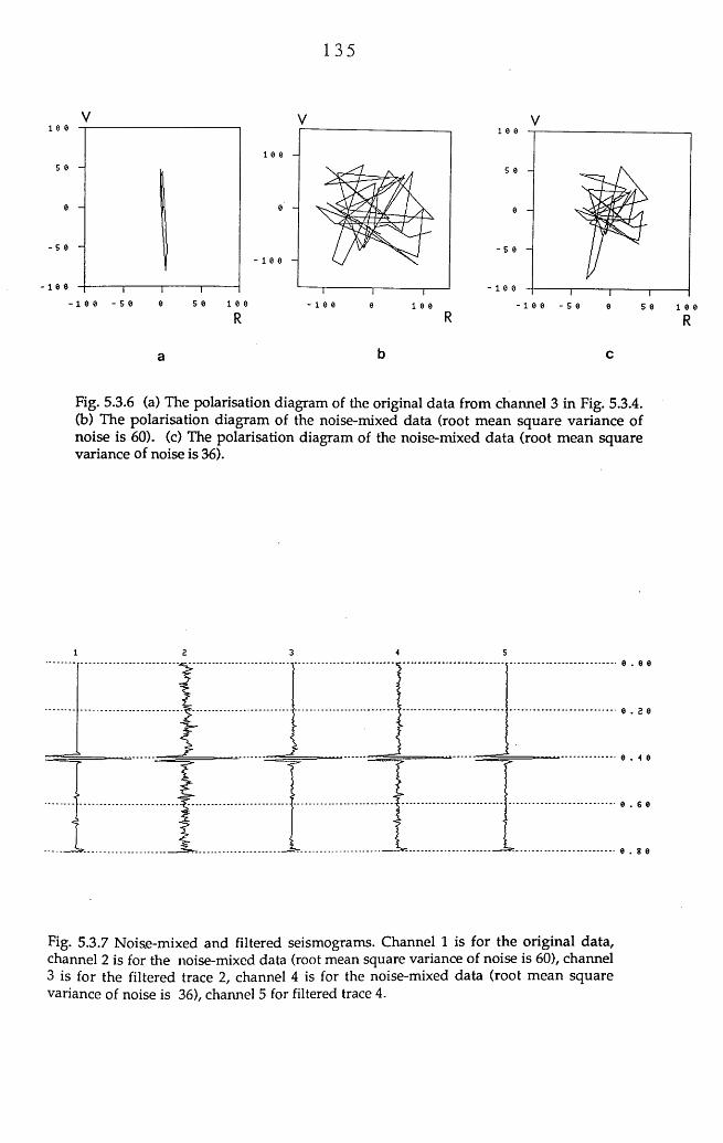
135

1 00

1 005 0

0 0

5 0

1 00

10 05 010 0 5 0 0 1 00 10 0 0 10 0

V1 00

5 0

0

5 0

10 01 00 5 0 0 5 0 10 0

Fig. 5.3.6 (a) The polarisation diagram of the original data from channel 3 in Fig. 5.3.4.(b) The polarisation diagram of the noise-mixed data (root mean square variance of noise is 60). (c) The polarisation diagram of the noise-mixed data (root mean square variance of noise is 36).

0 . a 0

Fig. 5.3.7 Noise-mixed and filtered seismograms. Channel 1 is for the original data, channel 2 is for the noise-mixed data (root mean square variance of noise is 60), channel 3 is for the filtered trace 2, channel 4 is for the noise-mixed data (root mean square variance of noise is 36), channel 5 for filtered trace 4.

136

filtered data based on the RAZOR array provides a highly resolved

section.

To generate 3-com ponent seismograms in an anisotropic medium by the

ANISEIS, two geological models are constructed for both a normal case (no

reversed v e loc ity con tras t) and a special case (low velocity sedim ents

sandwiched between lava at the top and hard rock beneath). The application of

the polarisation filter to data based on model 1 gives a good result. However,

filtering the data based on model 2 indicates a problem which is investigated

by changing amount o f noise in the data. The study shows that if the added

noise en tire ly changes the polarisation direction of particle m otions of

reflection w avelets, the filter may not be able to extract very weak signals

from noise, and by reducing the root mean square variance of random noise to

a certain degree such that the noise-mixed data exhibit a better polarisation,

the filtering w ill extract the weaker signals.

137

Chapter 6 Imaging Structure by Slant-stack Processing

6.1 Introduction

At the later stage of conventional seismic data processing, the data are

m igrated so as to determine the true reflection point. As a result, structural

im ages in the tim e-offset dom ain are obtained by d isp lay ing zero-offset

seism ic traces. In this chapter, we present a new idea of imaging structure in

3-dim ensions using synthetic data based on the areal 'RAZOR' array. The

method can in theory be used to determine the true dip and dip direction of a

deep reflec to r.

6.2 In troduction to conventional slant-stack processing

The s la n t-s ta ck , also called the x -p tra n s fo rm , p lan e w ave

decom position, beam-steering etc, is based on the model o f a downward moving

plane wave. A plane wave propagating at an angle from the vertical can be

generated by placing a line of point sources on the surface, exciting the point

sources in succession with a time delay and superimposing the responses that

are in the form of spherical wavefronts. The transformation of the tim e-offset

domain into the x-p domain and its usages have been discussed extensively by

many authors [Bessonova et al 1974, Stoffa & Buhl 1981, Diebold & stoffa 1981,

Treitel el al 1982, Biswell & Konty 1984, Brysk & McCowan 1986, Hake 1986,

M ithal & Vera 1987]. Here is a generalized description of how the x-p transform

is performed. As shown in Fig. 6.2.1, a plane wave with an angle 0 from the

vertical comes up from an interface. The time delay associated with the plane

wave is given by

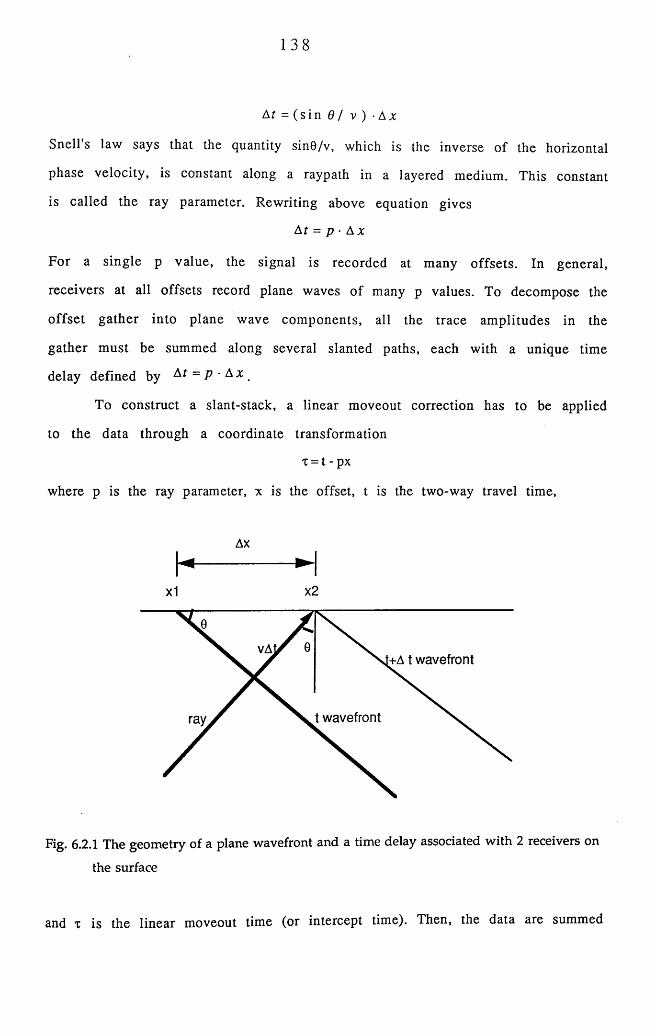
138

Ar = ( s i n 6 / v ) •A x

Snell's law says that the quantity sin0/v, which is the inverse of the horizontal

phase velocity, is constant along a raypath in a layered medium. This constant

is called the ray parameter. Rewriting above equation gives

At = p • A x

For a single p value, the signal is recorded at many offsets. In general,

receivers at all offsets record plane waves o f many p values. To decompose the

offset gather into plane wave com ponents, all the trace am plitudes in the

gather must be summed along several slanted paths, each with a unique time

delay defined by At = p ■ A x

To construct a slant-stack, a linear moveout correction has to be applied

to the data through a coordinate transform ation

x = t - px

where p is the ray parameter, x is the offset, t is the two-way travel time,

Ax

h Hx2x1

VA't+A t w avefront

t w avefrontray

Fig. 6.2.1 The geometry of a plane wavefront and a time delay associated with 2 receivers on

the surface

and x is the linear moveout time (or intercept time). Then, the data are summed

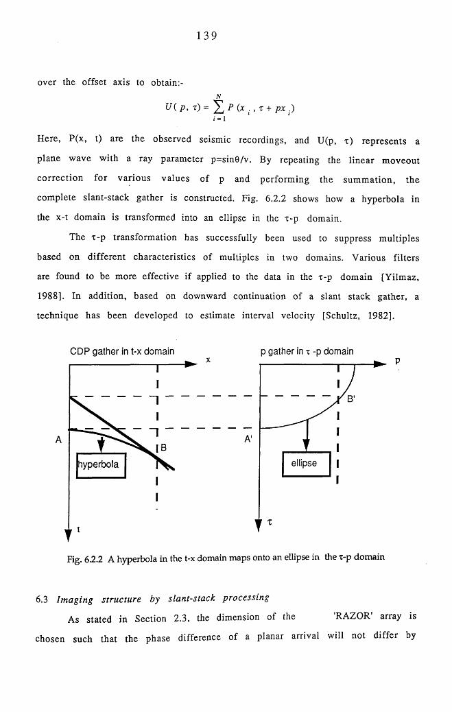
139

over the offset axis to obtain:-N

U( P> t) = ^ P (x . , X + px .)1 = 1 1

Here, P(x, t) are the observed seismic recordings, and U(p, x) represents a

plane wave with a ray param eter p=sin0/v. By repeating the linear m oveout

co rrec tion fo r various values of p and perform ing the sum m ation, the

complete slant-stack gather is constructed. Fig. 6.2.2 shows how a hyperbola in

the x-t domain is transformed into an ellipse in the x-p domain.

The x-p transform ation has successfully been used to suppress m ultiples

based on different characteristics of multiples in two domains. Various filters

are found to be more effective if applied to the data in the x-p dom ain [Yilmaz,

1988]. In addition, based on downward continuation of a slant stack gather, a

technique has been developed to estimate interval velocity [Schultz, 1982].

CDP gather in t-x domain p gather in x -p domain

1 ”A

ellipsehyperbola

Fig. 6.2.2 A hyperbola in the t-x domain maps onto an ellipse in the x-p domaindomainP

6.3 Im aging structure by slant-stack processing

As stated in Section 2.3, the dimension of the RAZOR array is

chosen such that the phase difference of a planar arrival will not d iffer by

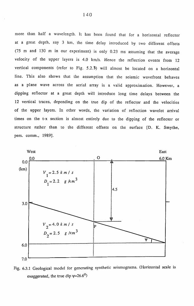
140

more than half a wavelength. It has been found that for a horizontal reflector

at a great depth, say 3 km, the time delay introduced by two different offsets

(75 m and 130 m in our experiment) is only 0.23 ms assuming that the average

velocity o f the upper layers is 4.0 km/s. Hence the reflection events from 12

vertical components (refer to Fig. 5 .2 3 ) will almost be located on a horizontal

line. This also shows that the assumption that the seismic wavefront behaves

as a plane wave across the aerial array is a valid approximation. However, a

dipping reflector at a great depth will introduce long time delays between the

12 vertical traces, depending on the true dip of the reflector and the velocities

of the upper layers. In other words, the variation of reflection wavelet arrival

times on the t-x section is almost entirely due to the dipping of the reflector or

structure rather than to the different offsets on the surface [D. K. Smythe,

pers. comm., 1989].

West East

0.0 6.0 Km0.0

(km)

4.5

3.0

6.0

7.0

Fig. 6.3.1 Geological model for generating synthetic seismograms. (Horizontal scale is

exaggerated, the true dip \\f=26.6°)

141

We generate synthetic seism ic data based on a m odel shown in Fig. 6.3.1

using a seism ic m odelling package SEIS83 (refer to Section 5.2.1). The m odel

com prises only one in terface which dips tow ards East. The true dip o f the

in terface is 26 .6°. The vertical depth from shot point O on the surface to a point

P on the dipping interface is 4.5 km. The upper and low er layers have constant

velocities o f 2.5 km /s and 4.0 km/s, and constant densities o f 2.2 g/cm^ and 2.5

g /c m ^ respectively. This model is used to generate 12 vertical com ponents. The

m ethod used to decom pose such a 3D model into 6 2D models is the same as that

described in Section 5.2.4. The 12 vertical com ponents are p lo tted in Fig. 6.3.2

in the o rder o f station num bers m arked in Fig. 5.2.3. W e can see from the

figure that the reflection events behave like a cosine wave on the section due

to the c irc u la r c o n fig u ra tio n o f the array . A d d itio n a lly , the tim e delay

betw een two stations, say, stations 3 and 9, reaches up to 40.6 m s, which is more

than tw ice as much as the 20 ms period of a reflection signal (50 Hz). A contour

m ap o f tw o-w ay travel tim e associated w ith 12 station positions is m ade and

show n in F ig . 6 .3 .3 . T his figure ind ica tes th a t the tw o-w ay trav e l tim e

increases tow ards the dip direction.

W e arb itra rily select a stra igh t line L through the shot po in t at the

centre o f the array, say, a west-east line, and define the azim uth o f a line as an

angle m easured anticlockw ise from x axis (or from East). Here the azim uth of

line L is 0 ° . Then, we "project" 12 stations onto the line L. "Projection" here

m eans tha t the order o f 12 sta tions is reorganised and th e ir o ffsets are re ­

c a lc u la te d , bu t the 12 seism ic traces them selves are kep t un touched . F or

exam ple, sta tions 3 and 5 are projected onto the line L, th e ir new offsets are

g iven by

x 3 = x 5 = 130 • cos 30° = 112. 12 m

likew ise, the new offsets for station 2 and 6 are given by

x 2 = x 6 = 75 ■ cos 60° = 37. 50 m

T herefore, a new "profile line" (or projection line) is constructed w ith 12

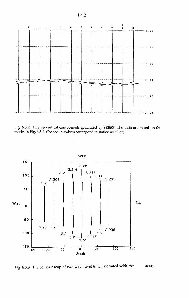
1 4 2

9 el l

l

3 . 2 6

3 . 4

Fig. 6.3.2 Twelve vertical components generated by SEIS83. The data are based on the model in Fig. 6.3.1. Channel numbers correspond to station numbers.

North

1 5 03. 22

3.2153. 215

3. 233 . 2353 . 205

3.20

50

EastWest

- 5 0

3.20 3.2053. 235

-100 3.233.213.2153 . 215

3.22

-150 15010050-50-150 -100South

Fig. 6.3.3 The contour map of two way travel time associated with the array.

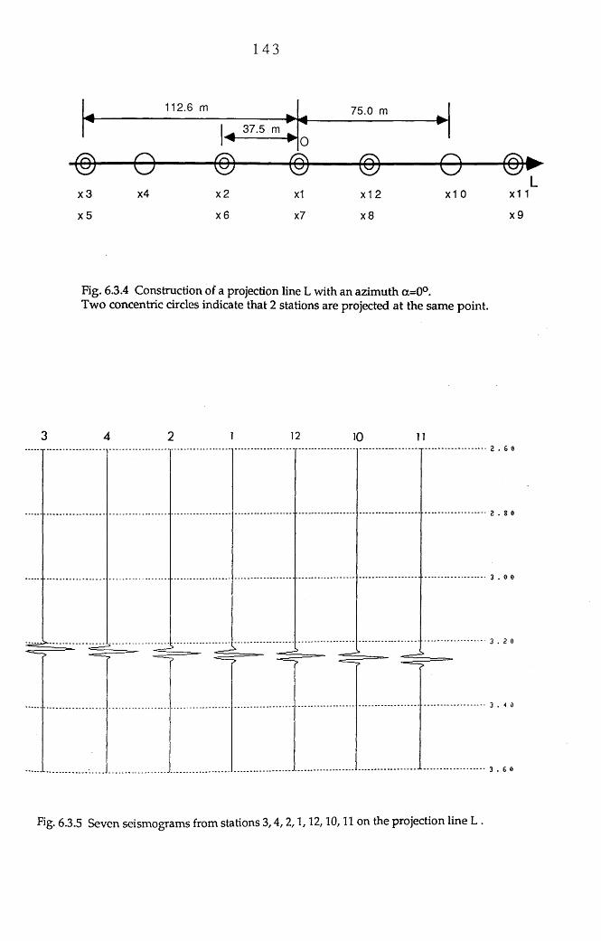
1 4 3

1 1 2 . 6 m ............. ^ 75.0 m

I 37.5 m^ ^

0■ ----------w

© — © ---------- © © © ---------© — ©L

x 3

x 5

x4 x 2

x 6

x1

x7

x1 2

x8

x 1 0 x 1 1

x 9

Fig. 6.3.4 Construction of a projection line L with an azimuth a=0°.Two concentric circles indicate that 2 stations are projected at the same point.

3 4 2 1 12 10 11T T T 2.60

2 . 8 0

3 . 0

3 . 2 0

3 . 6 0

Fig. 6.3.5 Seven seismograms from stations 3,4,2,1,12,10,11 on the projection line L .

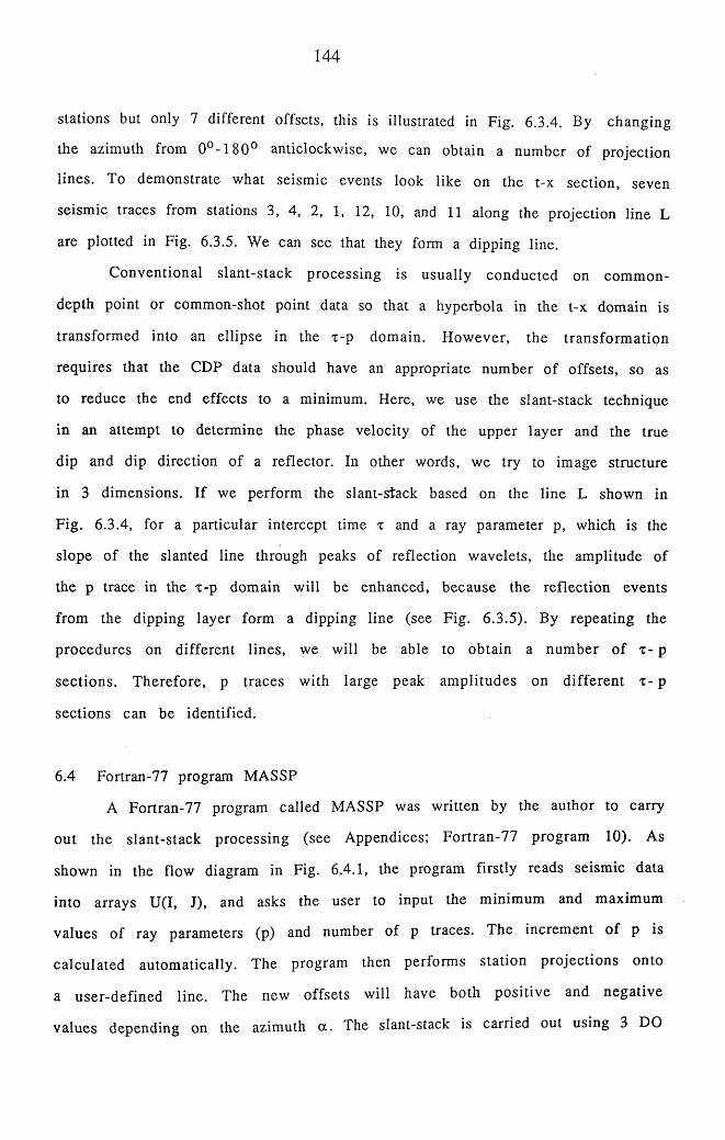
144

stations but only 7 different offsets, this is illustrated in Fig. 6.3.4. By changing

the azimuth from 0 ° -1 8 0 ° anticlockwise, we can obtain a number of projection

lines. To demonstrate what seismic events look like on the t-x section, seven

seismic traces from stations 3, 4, 2, 1, 12, 10, and 11 along the projection line L

are plotted in Fig. 6.3.5. We can see that they form a dipping line.

Conventional slant-stack processing is usually conducted on common-

depth point or common-shot point data so that a hyperbola in the t-x domain is

transform ed into an ellipse in the x-p domain. How ever, the transform ation

requires that the CDP data should have an appropriate number of offsets, so as

to reduce the end effects to a minimum. Here, we use the slant-stack technique

in an attempt to determine the phase velocity of the upper layer and the true

dip and dip direction of a reflector. In other words, we try to image structure

in 3 dimensions. If we perform the slant-stack based on the line L shown in

Fig. 6.3.4, for a particular intercept time x and a ray parameter p, which is the

slope o f the slanted line through peaks of reflection wavelets, the amplitude of

the p trace in the x-p domain will be enhanced, because the reflection events

from the dipping layer form a dipping line (see Fig. 6.3.5). By repeating the

procedures on different lines, we will be able to obtain a num ber o f x- p

sections. Therefore, p traces with large peak am plitudes on different x- p

sections can be identified.

6.4 Fortran-77 program MASSP

A Fortran-77 program called MASSP was written by the author to carry

out the slant-stack processing (see Appendices; Fortran-77 program 10). As

shown in the flow diagram in Fig. 6.4.1, the program firstly reads seismic data

into arrays U(I, J), and asks the user to input the minimum and maximum

values of ray parameters (p) and number of p traces. The increment o f p is

calculated autom atically. The program then performs station projections onto

a user-defined line. The new offsets will have both positive and negative

values depending on the azimuth c l . The slant-stack is carried out using 3 DO

145

loops and the results are saved in a new file. To run the program on the

VAX/VMS operating system, a user has to reply to several questions as shown

in the following example.

$ INPUT FILE NAME FOR SLANT-STACK

SHOTDT1

$ INPUT A FILE NAME FOR OUTPUT

TPOUT

$ INPUT THE MINIMUM AND MAXIMUM RAY PARAMETERS

-6.6667E-04 +6.667E-04

$ INPUT THE NUMBER OF THE RAY PARAMETERS

3

$ INPUT AN AZIMUTH FOR PROJECTIONS (IN DEGREES)

30

$ START SLANT-STACK PROCESSING

$ RAY PARAMETER 1 COMPLETED

$ RAY PARAMETER 2 COMPLETED

$ RAY PARAMETER 3 COMPLETED

$ FORTRAN STOP

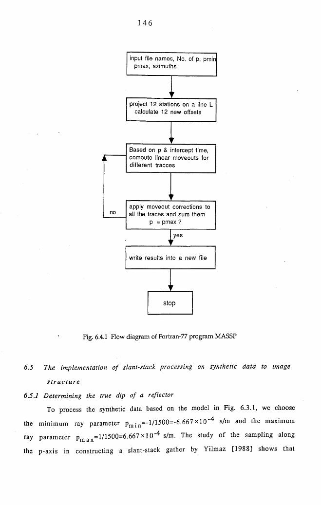
146

no

yes

stop

write results into a new file

project 12 stations on a line L calculate 12 new offsets

input file names, No. of p, pmin pmax, azimuths

apply moveout corrections to all the traces and sum them

p = pmax ?

Based on p & intercept time, compute linear moveouts for different tracces

Fig. 6.4.1 Flow diagram of Fortran-77 program MASSP

6.5 The implementation o f slant-stack processing on synthetic data to image

s tr u c tu r e

6.5.1 Determining the true dip o f a reflector

To process the synthetic data based on the model in Fig. 6.3.1, we choose

the minimum ray param eter pm j n= -l/1500= -6 .667x lO 4 s/m and the maximum

ray param eter pm ax =l/1500=6.667 x l O'4 s/m. The study o f the sampling along

the p-axis in constructing a slant-stack gather by Yilmaz [1988] shows that

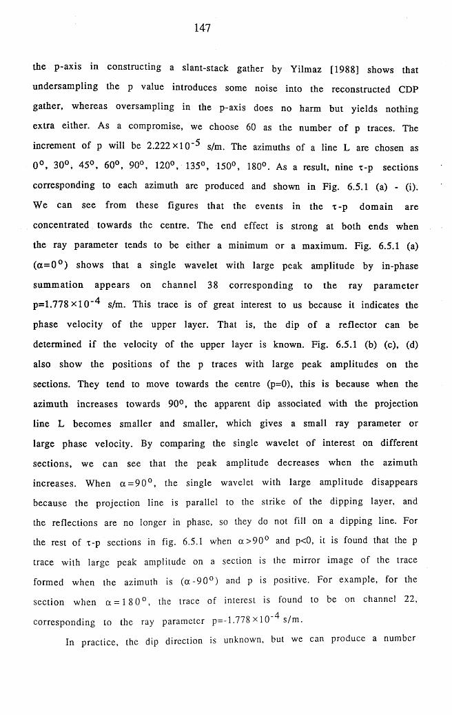
147

the p-axis in constructing a slant-stack gather by Yilmaz [1988] shows that

undersam pling the p value introduces some noise into the reconstructed CDP

gather, w hereas oversam pling in the p-axis does no harm but yields nothing

extra either. As a compromise, we choose 60 as the number o f p traces. The

increment o f p will be 2.222x1 O '5 s/m. The azimuths of a line L are chosen as

0 ° , 30°, 45°, 60°, 90°, 120°, 135°, 150°, 180°. As a result, nine x-p sections

corresponding to each azimuth are produced and shown in Fig. 6.5.1 (a) - (i).

W e can see from these figures that the events in the x -p dom ain are

concentrated tow ards the centre. The end effect is strong at both ends when

the ray param eter tends to be either a minimum or a maximum. Fig. 6.5.1 (a)

( a = 0 ° ) shows that a single wavelet with large peak am plitude by in-phase

sum m ation appears on channel 38 corresponding to the ray param eter

p = 1 .7 7 8 x l0 " 4 s/m. This trace is of great interest to us because it indicates the

phase velocity o f the upper layer. That is, the dip o f a reflector can be

determ ined if the velocity of the upper layer is known. Fig. 6.5.1 (b) (c), (d)

also show the positions o f the p traces with large peak am plitudes on the

sections. They tend to move towards the centre (p=0), this is because when the

azim uth increases towards 90°, the apparent dip associated with the projection

line L becom es sm aller and smaller, which gives a small ray param eter or

large phase velocity. By comparing the single wavelet o f interest on different

sections, we can see that the peak amplitude decreases when the azim uth

increases. W hen a = 9 0 ° , the single wavelet with large am plitude disappears

because the projection line is parallel to the strike of the dipping layer, and

the reflections are no longer in phase, so they do not fill on a dipping line. For

the rest of x-p sections in fig. 6.5.1 when a > 90° and p<0, it is found that the p

trace with large peak amplitude on a section is the mirror image of the trace

formed when the azimuth is ( a - 90° ) and p is positive. For example, for the

section when ot = 1 8 0 ° , the trace of interest is found to be on channel 22,

corresponding to the ray parameter p = -l.778 x10 ^ s /m.

In practice, the dip direction is unknown, but we can produce a number

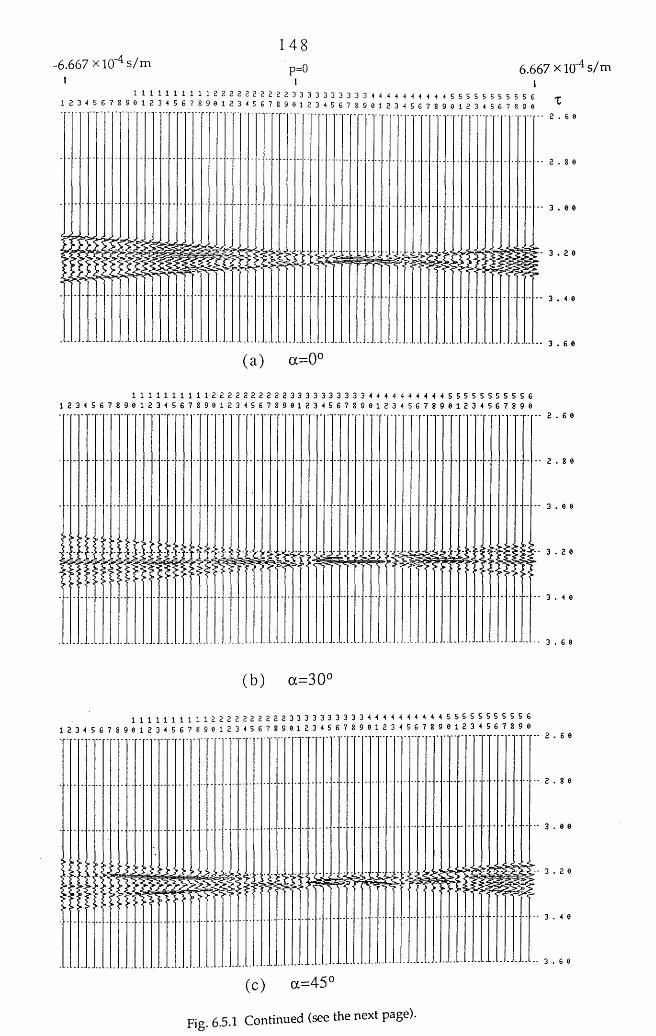
148-6.667 xiO"4 s /m • p=Q

' i i1 1 1 1 1 1 1 1 1 1 2 2 2 a 2 2 2 2 2 2 3 3 3 3 3 3 3 3 3 3 ( H H < H H 5 5 5 5 5 5 5 5 5 5 6

1 2 3 < 5 S 7 8 9 6 1 2 3 5 6 7 8 9 0 1 2 3 < 5 6 7 8 9 e 1 2 3 4 5 G ? 2 9 e i 2 3 4 5 6 7 8 9 0 1 2 3 4 5 6 7 8 9

6.667 x iO ^ s /m

T

3

2 . 6

3 . 0

3 . 4 6

1 1 1 1 1 1 1 1 1 1 2 2 2 2 2 2 2 2 2 2 3 3 3 3 3 3 3 3 3 3 4 4 4 4 4 4 4 4 4 4 5 5 5 5 5 5 5 5 5 5 61 2 3 4 5 6 7 8 9 6 1 2 3 4 5 6 7 8 9 6 1 2 3 4 5 6 7 8 9 0 1 2 3 4 5 6 7 8 9 6 1 2 3 4 5 6 7 8 9 6 1 2 3 4 5 6 7 8 9 6

im ii 4-

3

2.66

2.80

3 . 6

(b) a=30°

1 1 1 1 1 1 1 1 1 1 2 2 2 2 2 2 2 2 2 2 3 3 3 3 3 3 3 3 3 3 4 4 4 4 4 4 4 4 4 4 5 5 5 5 5 5 5 5 5 5 61 2 3 4 5 6 7 8 9 0 1 2 3 4 5 6 7 8 9 0 1 2 3 4 5 6 7 8 9 0 1 2 3 4 5 6 7 8 9 0 1 2 3 4 5 6 7 8 9 0 1 2 3 4 5 6 7 8 9 6

g j /

2 . 6 6

3 . 0

(c) a=45°

Fig. 6.5.1 Continued (see the next page).

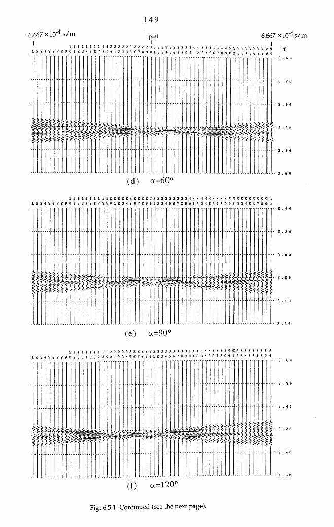
149

-6.667 x iO '4 s /m p = ° 6.667 x iq -4 s /mI 1 I

1 1 1 1 1 1 1 1 1 1 2 2 2 2 2 2 2 2 2 2 3 3 3 3 3 3 3 3 3 3 ^ U H H H 5 5 5 5 5 5 5 5 5 5 G <T

1 2 3 4 5 6 7 8 H 1 2 3 4 5 6 7 8 9 8 1 2 3 4 5 6 7 8 9 0 1 2 3 < 5 6 7 8 9 6 1 2 3 < 5 6 7 8 9 0 1 2 3 < 5 6 7 8 9 02 . G

3 . 2

3 . G 0

(d) oc=60°

1 1 1 1 1 1 1 1 1 1 2 2 2 2 2 2 2 2 2 2 3 3 3 3 3 3 3 3 3 3 4 4 4 4 4 4 4 4 4 4 5 5 5 5 5 5 5 5 5 5 6 1 2 3 4 5 G 7 8 9 0 1 2 3 4 5 G 7 8 9 0 1 2 3 4 5 G 7 8 9 0 1 2 3 4 5 G 7 8 9 0 1 2 3 4 5 G 7 8 9 0 1 2 3 4 5 G 7 8 9 0

3

2 . 8

3 . 0 6

3 . 4

3 . G

1 1 1 1 1 1 1 1 1 1 2 2 2 2 2 2 2 2 2 2 3 3 3 3 3 3 3 3 3 3 4 4 4 4 4 4 4 4 4 4 5 5 5 5 5 5 5 5 5 5 G 1 2 3 4 5 G 7 8 9 0 1 2 3 4 5 6 7 8 9 0 1 2 3 4 5 6 7 8 9 0 1 2 3 4 5 G 7 8 9 0 1 2 3 4 5 6 7 8 9 0 1 2 3 4 5 G 7 8 9 0

l i

Fig. 6.5.1 Continued (see the next page).

150

-6.667 x KT4 s/m p=0 6.667 x 10-4 s/m1 1 1 1 1 1 1 1 1 1 2 2 2 2 2 2 2 2 2 2 3 3 3 3 3 3 3 3 3 3 H H ^ H ( H 5 5 5 5 5 5 5 5 5 5 £

1 H 3 4 5 6 7 8 9 0 1 2 3 4 5 6 7 8 9 0 1 2 3 4 S 6 7 8 9 0 1 2 3 4 S 6 7 8 9 0 1 2 3 4 5 6 7 8 9 0 1 2 3 4 5 6 7 8 9 0

> f

3 .

1 1 1 1 1 1 1 1 1 1 2 2 2 2 2 2 2 2 2 2 3 3 3 3 3 3 3 3 3 3 4 4 4 4 4 4 4 4 4 4 5 5 5 5 5 5 5 5 5 5 6 1 2 3 4 5 6 7 8 9 0 1 2 3 4 5 6 7 8 9 0 1 2 3 4 5 6 7 8 9 0 1 2 3 4 5 6 7 8 9 0 1 2 3 4 5 6 7 8 9 0 1 2 3 4 5 6 7 8 9 0

2.80

1 1 1 1 1 1 1 1 1 1 2 2 2 2 2 2 2 2 2 2 3 3 3 3 3 3 3 3 3 3 4 4 4 4 4 4 4 4 4 4 5 5 5 5 5 5 5 5 5 5 61 2 3 4 5 6 7 8 9 0 1 2 3 4 5 6 7 8 9 0 1 2 3 4 5 6 7 8 9 0 1 2 3 4 5 6 7 8 9 0 1 2 3 4 5 6 7 8 9 0 1 2 3 4 5 6 7 8 9 0

Fig. 6.5.1 Nine x-p images based on nine projection lines with different azimuths.

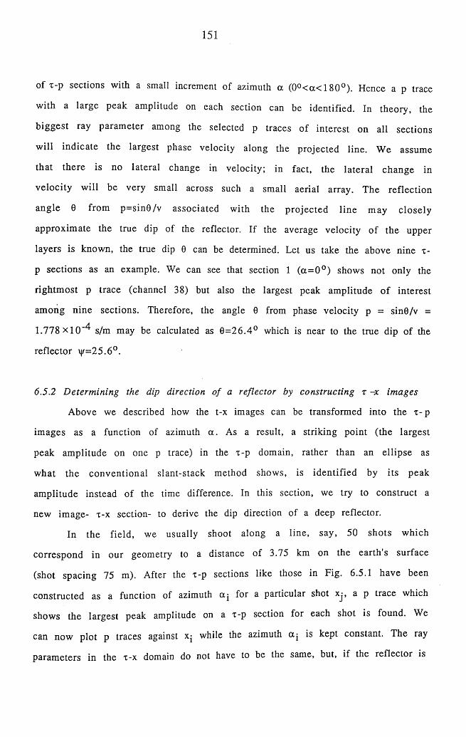
151

of x-p sections with a small increment of azimuth a (0°< a< 180°). Hence a p trace

with a large peak amplitude on each section can be identified. In theory, the

biggest ray param eter among the selected p traces of interest on all sections

will indicate the largest phase velocity along the projected line. We assume

that there is no lateral change in velocity; in fact, the lateral change in

velocity will be very small across such a small aerial array. The reflection

angle 0 from p=sin0 /v associated with the projected line m ay closely

approxim ate the true dip of the reflector. If the average velocity of the upper

layers is known, the true dip 0 can be determined. Let us take the above nine x-

p sections as an example. We can see that section 1 (a = 0 ° ) shows not only the

rightm ost p trace (channel 38) but also the largest peak amplitude o f interest

among nine sections. Therefore, the angle 0 from phase velocity p = sin0/v =

1 .778x10"^ s/m may be calculated as 0= 26 .4° which is near to the true dip of the

reflector \j/=25.6°.

6.5.2 Determining the dip direction o f a reflector by constructing x -x images

Above we described how the t-x images can be transformed into the x -p

images as a function of azimuth a . As a result, a striking point (the largest

peak amplitude on one p trace) in the x-p domain, rather than an ellipse as

what the conventional slant-stack method shows, is identified by its peak

amplitude instead of the time difference. In this section, we try to construct a

new image- x-x section- to derive the dip direction of a deep reflector.

In the field, we usually shoot along a line, say, 50 shots which

correspond in our geometry to a distance of 3.75 km on the earth 's surface

(shot spacing 75 m). After the x-p sections like those in Fig. 6.5.1 have been

constructed as a function of azimuth ocj for a particular shot xj, a p trace which

shows the largest peak amplitude on a x-p section for each shot is found. We

can now plot p traces against xj while the azimuth ocj is kept constant. The ray

parameters in the x-x domain do not have to be the same, but, if the reflector is

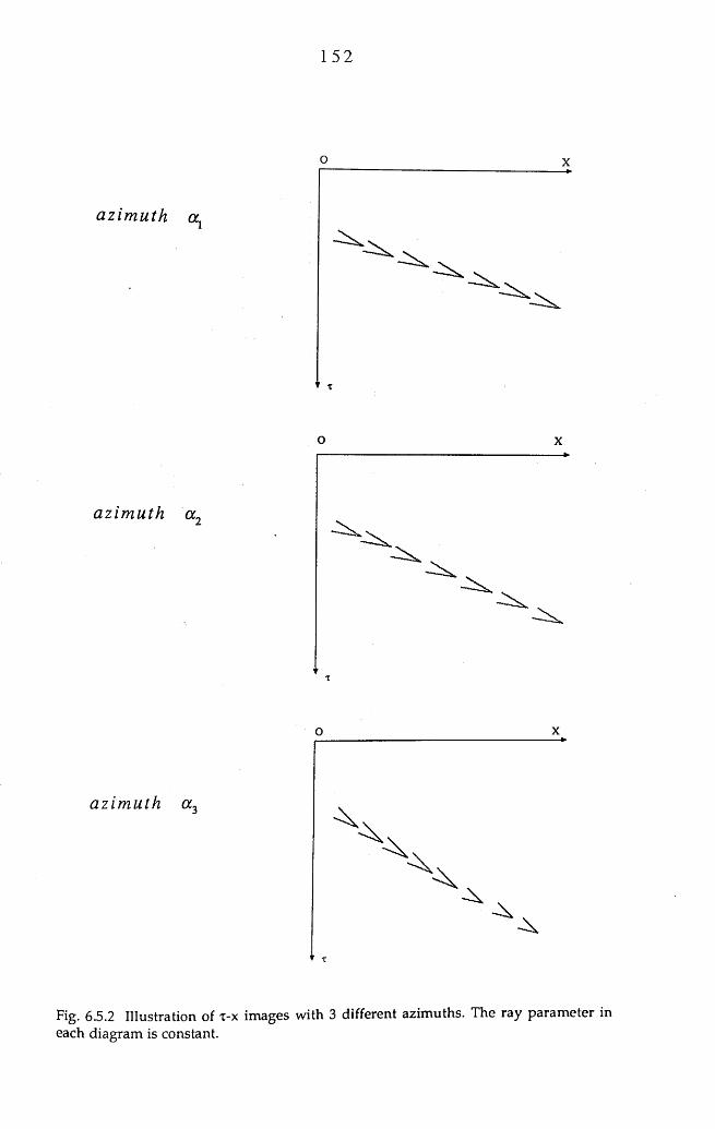
152

a z i m u t h a .,

a z i m u t h a„

o x

a z i m u t h a«

Fig. 6.5.2 Illustration of x-x images with 3 different azimuths. The ray parameter in each diagram is constant.

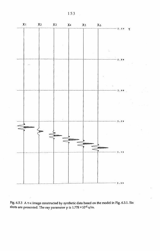
153

Xl X2 X3 X4 X5 X6

Fig. 6.5.3 A x-x image constructed by synthetic data based on the model in Fig. 6.3.1. Six shots are presented. The ray parameter p is 1.778 x itH s/m.

154

absolutely planar, the p values will be identical. Fig. 6.5.2 illustrates what the

final t -x images look like. Three t-x sections associated with azimuths a j , ot2

and oc ^ are produced, each showing a line of events with dips at different

amounts. The largest dip, as shown in Fig. 6.5.2 (c) is most likely to be the true

dip o f the reflector assuming that the velocity effect has been corrected.

Based on the model in Fig. 6.3.1, we generate 6-shot data and perform the

slan t-stack processing individually . A azimuth 0° is used as an example to

produce 6 T-p images. The first image for shot 1 is shown in Fig. 6.5.1 (a),

others are not shown here, but they look rather similar, except for the time

difference of the p gather. The p traces from 6 T-p sections are all on channel

38 which corresponds to a ray param eter p = 1 .7 7 8 x l0 " 4 s/m so that they are

picked up and plotted against offsets. Fig. 6.5.3 tells us about the dip direction

of the reflector which is towards East.

6.5.3 Determining the angle o f a ray path to optimise polarisation filtering

For a simple geological model with only one layer, the reflection angle 0

of a ray can be determined by the method described in Section 6.5.1. If the

angle is near to the true dip of a reflector, the polarisation direction P o f a

compressive wave can be derived as illustrated in Fig. 6.5.4 (a). On the other

hand, by constructing a covariance matrix over a time window and calculating

the e igenvalues and eigenvectors of the m atrix, we can determ ine the

p o la risa tio n d irec tion E o f partic le m otions recorded by 3-com ponent

geophones (refer to Section 3.4). Fig. 6.5.4 (b) shows the polarisation directions

P and E. The vector E is constructed by 3-component recordings. It can

represent the polarisation direction either of a shear wave or a compressional

wave, depending on seismic source type and geological conditions.

To preserve those trajectory parts whose polarisation direction is the

same as or near to the vector P, we define a fixed cone around the vector P.

Thus P is the cone's axis and the desired filtering direction. The vertex half

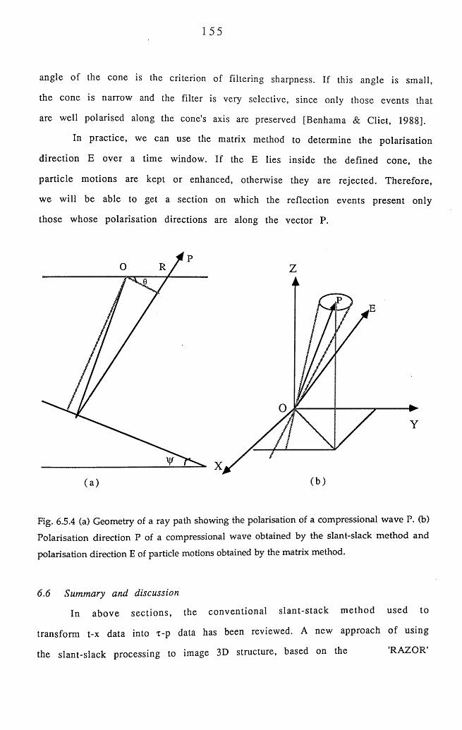
155

angle o f the cone is the criterion of filtering sharpness. If this angle is small,

the cone is narrow and the filter is very selective, since only those events that

are well polarised along the cone's axis are preserved [Benhama & Cliet, 1988].

In practice, we can use the matrix method to determine the polarisation

direction E over a time window. If the E lies inside the defined cone, the

particle m otions are kept or enhanced, otherwise they are rejected. Therefore,

we will be able to get a section on which the reflection events present only

those whose polarisation directions are along the vector P.

X(b )

Fig. 6.5.4 (a) Geometry of a ray path showing the polarisation of a compressional wave P. (b)

Polarisation direction P of a compressional wave obtained by the slant-slack method and

polarisation direction E of particle motions obtained by the matrix method.

6.6 Summary and discussion

In above sections, the conventional s lan t-stack m ethod used to

transform t-x data into x-p data has been reviewed. A new approach o f using

the slant-slack processing to image 3D structure, based on the RAZOR

156

array, has been demonstrated by synthetic data. The result further proves that

the dimension of the array is appropriate for receiving reflected plane

waves from deep interfaces. The true dip and dip direction of a reflector may

be derived from x-p images and x-x images respectively, assum ing that the

velocity of the upper layer is known. The com puter program MASSP was

designed to perform the slant-stack processing from the original t-x data. The

plotting program can display either T-p images or x-x images in various ways.

This m ethod can additionally be used to optim ise the polarisation filtering,

which keeps and enhances the compressional waves o f interest according to

the polarisation directions of waves.

In reality, the geological conditions are com plicated. There will be

many reflectors, with dips in different directions, and the velocities of layers

are no longer constant but are a function of depth. Nevertheless, we can treat

the geology as a model consisting of several layers, within each layer the

velocity can be considered as constant. Thus the slant-stack processing will

produce more than one line of events on both x-p image and x-x image. The

angle 0 derived from the phase velocity can no longer represent the true dip

or apparent dip of an individual layer but a contribution of several layers. The

true dip of individual layers can also be determined, if corrections are made.

T herefo re , this s lan t-stack m ethod, d iffe ren t from the conven tional, is

potentially of great importance for imaging complex structure.

157

Chapter 7 The RAZOR Array, General Discussion

and Future Work

The RAZOR array, a new array for acquiring seismic reflection data, has

been tested in a basalt-covered area. The radius of the outer circle is an

appropriate dim ension for recording the weak reflection events from below

basalts because Ground-roll and reverberations can be suppressed. The study

o f the characteristics of seismic reflection data from a basalt-covered area not

only confirm s with the results by other workers, but also reveals additional

c h a rac te ris tic s . The horizontal com ponents exhib it larger am plitudes and

low er frequency than the vertical com ponent. A pplica tion o f a new ly

designed spatial directional filter to the three component of seismic data shows

that m ore inform ation passes through the filter on the horizontal component.

The energy variation diagram for each shot shows that the radial component

receives m uch m ore energy than the others. The newly developed signal

enhancem ent polarisation filter can be used to suppress random noise and a

portion o f reverberations. The synthetic data based on this array demonstrates

that seism ic wavefronts can reasonably be considered as planes, which allows

slant-stacking to be carried out. As a result, the true dip and dipping direction

of a deep reflector can possibly derived. This method can also be used to

op tim ise the po larisa tion filtering , which passes com pressional w aves of

interest according to the polarisation directions of the waves.

However, the field data from the inner stations were very poor. One

explanation could be that these data are more severely affected by the surface

m aterials than the data from the outer stations. Other possibilities are that the

radius o f the inner circle is too small, the inner stations interfere with the

firing o f the shots, or the MDS-10 channels are overloaded because of

explosive charges close to geophones. From the data processing point of view,

the co n v en tio n a l m ethods such as frequency f ilte rin g and p red ic tive

158

deconvolution filtering cannot be applied with the same degree o f success

com pared to conventional seism ic reflection data. The po larisa tion filte r

cannot com pletely cancel all reverberations, especially when the data quality

is so poor that the the polarisation of the useful signals is lost in the presence

o f noise. Apart from the above, it is dangerous to stack the data across the

array , because problem s may arise by sum m ing reflec tion events w ith

d ifferen t phases when reflectors are very deep and the dipping angles are

large. The technique of imaging geological structure in 3 dimensions is only

based on the synthetic data of a simple model. To test the method thoroughly,

there is a need to use the data from a more com plicated m odel, and more

sophisticated processing methods need to be developed.

W ith the further development of techniques, the areal RAZOR array will

have its great potential in im aging geological structure. Below are listed

several areas for future work:

(a ) We need to modify the dimensions of the RAZOR array and to test the

developed techniques for commercial use. We should em pirically determ ine

the appropriate radius of the inner circle of the array and acquire seismic

reflection data in an area of simple geology (a normal case). The shot hole

should be drilled as deep as possible into bedrock. The size of explosive charge

for each hole should also be determined em pirically. It is hoped that good

shear waves can be received from an explosive source, so that some lithology

information of the crust can be obtained as it is indicated by Vp/Vs.

( b ) Instead of stacking data across the array, we can fire a number of shots,

say 10, at one location, and then stack the individual channels. Thus, we face

no danger o f stacking reflection signals with different phases. Random noise

will be greatly attenuated.

( c ) We can generate the synthetic data based on a more complicated model

to test the new techniques stated in Chapter 6, using more than one interface,

with different layer velocities. Software can be produced to determine the true

dips and dipping directions of reflectors after correction are made. Various

kinds of images such as x-t, x-p, x-x and offset-depth can be displayed on

159

m odern Sun W orkstations.

( d ) H aving been fully tested by the field data from an area o f simple

geology, this m ethod can then be applied to the area covered by volcanic

rocks. In addition to the existing processing m ethods (frequency filtering ,

d eco n v o lu tio n filte rin g , po larisa tion filte rin g , x-p transform , e tc .), m ore

advanced processing techniques need to be developed for extracting the weak

signals in the presence of noise.

( e ) It is well known that the study of shear wave splitting is o f great

potential in exploration geophysics. With the further development, we can use

3 -com ponent geophones and an S source to record very good shear waves. The

an iso trop ic characteristics of the crust can system atically be analysed by

study ing shear wave splitting. In addition to using po larisa tion diagram s

which are the main tools at present to characterise the data, we can develop a

new m eans o f processing 3-component data to identify the orientations of

aligned cracks in the crust. One possibility is to study the energy distribution

on the 3-com ponents as a function o f o rien tation o f geophones. The

co rre la tio n betw een them may help us to derive the crack orien tations.

Another possibility is to construct a new domain in which shear wave splitting

shows a great anomaly, from which further information may be obtained.

The RAZOR array, with further m odification and development, will have

a prom ising future.

160

References

Agocs, W. B., 1951. Least squares residual anomaly determination, Geophysics, Vol. 16, 686-696.Al-Sadi, H. N. 1980. Seismic Exploration Technique and Processing. Birkhauser Verlag Basel.Arnold, M. E., 1977. Beam forming with vibrator arrays. Geophysics, Vol. 42, No. 7,1321 - 1338.Benhama, A. and Cliet, C., 1988. Study and application of spatial directional filtering in

three-component recordings. Geophysical Prospecting, 36,591-613.Benoliel, S. D., 1987. Frequency wavenumber approach of the x-p transform: Some applications

in seismic data processing. Geophysical Prospecting, 35,517-538.Bessonova, E. N. and Fishman, V. M., 1974. The tau method for inversion of travel times- I.

Deep seismic sounding data. Geophy. J. Astr. Soc. 36,377-398.Biswell, D. E. and Konty, L. F., 1984. A geophone subarray beam-steering process. Geophysics,

Vol. 49, No. 11,1838 - 1849.Blais, J. A. R., Lodwick, G. D. and Ferland.R., 1983. Gravimetric terrain corrections in west

Canada. Can. J. Earth Sci. 20, 259-265.Blais, J. A. D. and Ferland, R. 1984. Optimization in gravimetric terrain corrections. Can. J.

Earth Sci. 21, 505-515.Bott, M. H. P., 1959. The use of electronic digital computers for the evaluation of gravimetric

terrain corrections. Geophysical Prospecting 8 45-54.Bott, M. H. P. and Masson-smith, D., 1960. A gravity survey of the Criffell granodiorite and

the New Red Sandstone deposits near Dumfries. Proceedings of the Yorkshire Geological Society. 32, 317-332.

Bott, M. H. P., 1962. A simple criterion for interpreting negative gravity anomalies.Geophysics, Vol. 27, 376-381.

Bott, M. H. P., 1964. Gravity measurements in the North-Eastern part of the Irish Sea. Quart. J. Geol. Soc. Lond. 120, 369-396.

Bott, M. H. P. and Smithson, S. B., 1967. Gravity investigations of subsurface shape and mass distributions of Granite Batholiths. Geological Society of America Bulletin, Vol. 78,

859-878.Brysk, H. and McCowan, D. W., 1986. A slant-stack procedure for point-source data.

Geophysics, Vol. 51, No. 7,1370-1386.Carrion, P. M. and Hassanzadeh, S., 1985. Direct estimation of shear-wave interval velocities

from seismic data. Geophysics, Vol 50, No. 4, 530-538.Cerveny, V. and Psencik, I., 1983. Numerical modelling of seismic wavefield in 2-D laterally

varying layered structures by the ray method (Manual).Churchhouse R. F., 1981. Handbook of Applicable Mathematics. Volume 3 Numerical Methods

John Wiley & sons.Cliet, C. and Dubesset, M., 1987. Three-component recordings: Interest for land seismic source

study. Geophysics, Vol. 52, No. 8, 1408-1059.Darby, E. K. and Davies, E. B., 1967. The analysis and design of two-dimensional filters for

two-dimensional data, Geophysical Prospecting, Vol. XV, No. 3, 383-406.Danes, Z. F., 1960. On a successive approximation method for interpreting gravity anomalies.

161

Geophysics, Vol. XXV, No. 6, 1215-1228.

Danes, Z. F. and Oncley, L. A., 1962. An analysis of some second derivative methods.Geophysics, Vol. XXVII, No. 5, 611-615.

Dankbaar, J. W. M., 1987. Vertical seismic profiling-separation of P- and S-waves.Geophysical Prospecting, 35, 803-814.

Dankbaar, J. W. M., 1985. Separation of P- and S-waves. Geophysical Prospecting, 33, 970-986. Diebold J. B. and Stoffa, P. L., 1981. The traveltime equation, tau-p mapping, and inversion of

common midpoint data. Geophysics, Vol. 46, No. 3,238 - 254.Dobrin, M. B., 1988. Introduction to Geophysical Prospecting. Fourth Edition. McGraw-hill

Book Company.

Dohr, G. and Janel, FI., 1980. Improvements in the observation of shear waves. Geophysical Prospecting, 28, 208-220.

Douma, J. and Helbig, K., 1987. What can the polarization of shear waves tell us. First Break, Vol. 5, No. 3.

Evan, R., 1984. Effects of the free surface on shear wavetrains. Geophys. J. R. Soc., 76, 165-172. Elkins, T. A., 1951. The second derivative method of gravity interpretation. Geophysics, Vol.

16, 29-50.Evjen, H. M., 1936. The place of the vertical gradient in gravitational interpretations.

Geophysics, Vol. 1, 127-136.Faddeev D. K. and Faddeeva V. N., 1963. Computational Methods of Linear Algebra.

Translated by Robert C. Williams.Fertig, J., 1984. Shear waves by an explosive point-source: The Earth surface as a generator of

converted P-S waves. Geophysical Prospecting, 32, 1-17.Flinn, E. A., 1965. Signal analysis using rectilinearity and direction of particle motion.

Proceedings of the IEEE (December).Geldart, L. P., Gill, D. E. and Sharma, B., 1966. Gravity anomalies of two dimensional faults.

Geophysics, Vol. XXI, No. 2, 372-397.Granar L., 1966-1967. On topographic correction. Geoexploration, 4-5, 65-70.Granser, H., 1987. Topographic reduction of gravity measurements by numerical Integration of

boundary integrals. Geophysical Prospecting, 35, 71-82.Grant, F. S., 1954. A theory for the regional correction of potential filed data. Geophysics, Vol.

1, 23-45.Grant, F., 1957. A problem in the analysis of geophysical data. Geophysics, Vol. XXII, No. 2,

309-344.Grant, F. S. and Elsahaty, A. F.,1962. Bouguer gravity corrections using a variable density.

Geophysics, Vol. XXVII, No. 5, 616-626.Grant, F. S., 1972. Review of data processing and interpretation methods in gravity and

magnetics, 1964-71. Geophysics, 37, 647-661.Green, R., 1976. Accurate determination of the dip angle of a geological contact using the

gravity method, Geophysical Prospecting 24, 265-272.Hake, H., 1986. Slant stacking and its significance for anisotropy. Geophysical Prospecting, 34,

595-608.

162

Hall, J. 1970. The correlation of seismic velocities with formations on the South-west of Scotland. Geophysical Prospecting 18, 134-148.

Hall, J., 1971. Seismic studies in the region of the Firth of Clyde, University of Glasgow, Ph. D. Thesis.

Hall, J., 1974. A seismic reflection survey of the Clyde Plateau Lavas in North Airshire and Renfrewshire. Scottish J. of Geology, 9 (4) 253-279.

Hammer, S., 1939. Terrain corrections for gravimeter stations. Geophysics, Vol. 4,184-194. Hansen, O., 1988. Signal-noise-ratio estimation and image processing of seismograms using two-

dimensional coherence techniques. M. Sc thesis in information technology systems. University of Strathclyde.

Hatton, L., Worthington, M. H. and Makin, J., 1986. Seismic Data Processing: Theory and Practice. Oxford Blackwell Scientific.

Helbig, K. and Mesdag, C. S., 1982. The potential of shear-wave observations. Geophysical Prospecting, 30, 413-431.

Henderson, R. G., 1960. A comprehensive system of automatic computation in magnetic and gravity interpretation. Geophysics, Vol. XXV, No. 3, 569-585.

Hipkin, R. G. and Hussain, A., 1983. Regional gravity anomalies. 1 Northern Britain. Report 82/10. Institute of Geological Sciences, NERC.

Kane, M. F., 1962. A comprehensive system of terrain corrections using a digital computer.Geophysics, 27, 455-462.

Kanasewich, E. R., 1975. Time sequence analysis in Geophysics. Edmonton University of Alberta Press.

Kantas, K, and Zych, D., 1967. Reduction of gravity observations with digital computer. Pure and Applied physics. 68, 12-18.

Karlemo B., 1963. Calculation of terrain correction in gravity studies using the electric computer. Geoexploration, 1 (1), 56-66.

Kelamis, P. G. and Mitchell, A. R., 1989. Slant-stacking process. First Break, Vol. 7, No. 2, 43-54.

Ketelaar, A. C. R., 1976. A system for computer-calculation of the terrain correction.Geoexploration, 14, 57-65.

Ketelaar, A. C. R., 1987. Terrain correction for gravity measurement, using a digital terrain model (DTM). Geoexploration, 24, 109-124.

Lagios, E., 1979. Gravity and other geophysical studies relating to the crustal structure of South-east Scotland. PhD Thesis, University of Edinburgh.

Lagios, E. and Hipkin, R. G., 1981. Gravity measurements in South-east Scotland. Geophys. J.

R. Astr. Soc., 65,505-506.Lagios, E. and Hipkin, R. G., 1979. The Tweeddale Granite- a newly discovered batholith in

the Southern Uplands. Nature, Vol. 280, 672-675.Lash, C. C., 1985. Shear waves produced by explosive sources. Geophysics, Vol. 50, No. 9,

1399-1409.Linsser, H., 1965. A generalized form of Nettleton’s density determination, Geophysical

Prospecting 13, 245-258.Linsser, H., 1967. Investigation of tectonics by gravity detailing. Geophysical Prospecting, Vol.

163

XV, No. 3, 480-515.

Lu, J. M., 1982. The principle of seismic exploration (in Chinese). Published by the Petroleum Industry Press, Beijing.

Malzac, J. and Rousseau, A., 1978. A "processing density" to calculate marine Bouguer gravity free of topographic variations in case of unknown bottom density, Geophysical Prospecting, 26, 853-867.

Mansfield, J., and Kennett. P. 1963. A gravity survey of the Stranraer sedimentary basin.Proceedings of the Yorkshire Geological Society, 34, 139-151.

Mclean, A. C. and Qureshi, I. R., 1964-1965. Regional gravity anomalies in the Western Midland Valley of Scotland. Trans. Roy. Soc. Edin., Vol. LXVI., No. 11.

Mcmechan, G. A. and Ottolini, R., 1980. Direct observation of a p-t curve in a slant stacked wave field. Bulletin of the SEIS. Soci. America. Vol. 70, NO. 3, 775-789.

McMechan, G. A., 1983. p-x imaging by localized slant stacks of t-x data. Geophys. J. R. astr.Soc. 72. 213-221.

Merlin Geophysical (Research) Ltd. SKS Users Manual.Mithal, R. and Vera, E. E., 1987. Comparison of plane-wave decomposition and slant stacking

of point-source seismic data. Geophysics, Vol. 52, No. 12,1631-1638.Mu, Y. G., 1981. Seismic data processing methods (in Chinese). Published by the Petroleum

Industry Press, Beijing.Nagy, D., 1966. The gravitational attraction of a right rectangular prism. Geophysics, 31,

362-371.Nettleton, L. L., 1939. Determination of density for reduction of gravimeter observations.

Geophysics, 4, 176-183.Nettleton, L. L., 1954. Regionals, residuals, and structures. Geophysics, Vol. XIX, No. 1, 1- 23. Oldham, C. H. G., 1954. The correlation between Pre-cambrain rock densities and Bouguer

gravity anomalies near parry sound, Ontario. Geophysics, Vol. 1, 76-88.Parslow, G. R. and Randall, B. A. O., 1973. A gravity survey of the Cairnsmore of Fleet granite

and its environs. Scott. J. Geol. 9 (3), 219- 231.Pujol, J. and Fuller. B. N., 1989. Interpretation of a vertical seismic profile conducted in the

Columbia Plateau basalts. Geophysics, Vol. 54, No. 10, 1258-1266.Rene, R. M., et al, 1986. Multicomponent seismic studies using complex trace analysis.

Geophysics, Vol. 51, No. 6, 1235-1251.Robinson, E. A. and Durrani, T. S., 1986. Geophysical Signal Processing. The University Press,

Cambridge.Rosenbach, O., 1953. Quantitative studies concerning the vertical gradient and second

derivative methods of gravity interpretation. Geophysical Prospecting, II, 128-138. Rosenbach, O., 1953. A contribution to the computation of the "second derivative" from gravity

data. Geophysics, Vol. 18, 894-912 Sandberg, C. H., 1958. Terrain corrections for an inclined plane in gravity computations.

Geophysics,18, 701-711.Schultz, P. S., 1982. A method for direct estimation of interval velocities. Geophysics, Vol. 47,

No. 12, 1657-1671.

164

Selem. A. M. and Monnet, C., 1953. Application of vertical gradients and comparison ofdifferent geophysical methods in a difficult area. Geophysical Prospecting, Vol. 1, No.3, 208-219.

Shimshoni, M. and Smith, S. W., 1964. Seismic signal enhancement with three-component detectors. Geophysics, Vol. XXIX, No. 5, 664-671.

Simpson, S. M., 1954. Least squares polynomial fitting to gravitational data and density plotting by digital computers. Geophysics, Vol. 19, 255-269.

Sissons, B. A., 1981. Densities determined from surface and subsurface gravity measurements.Geophysics, Vol. 46, No. 11, 1568-1571.

Smithson, S. B., Fuller, B., Pujol, J. and Woods, T., 1986. Final Report for 1985. University of Wyoming Volcanic Reflection Research Project.

Smythe, D. K., 1988. A note on BIRPS S-wave experiment 1988 - Field layout of the Glasgow piggyback experiment (unpublished).

Stoffa, L. P. and Buhl, P., 1981. Direct mapping of seismic data to the domain of intercept time and ray parameter- A plane-wave decomposition. Geophysics, Vol. 46, No. 3, 255 - 267.

Swartz, C. A., 1954. Some geometrical properties of residual maps. Geophysics, Vol. 1, 46-70. Takin, M. and Talwani, M., 1966. Rapid computation of the gravitation attraction of

topography on a spherical earth. Geophysical Prospecting, Vol. XIV, 119-142.Talwani, M., Worzel, J. L. and Landisman, M., 1959. Rapid gravity computations for two-

dimensional bodies with application to the Mendocino Submarine Fracture Zone. J. of Geophysical research, Vol. 64, No. 1, 49-59 .

Talwani, M. and Ewing, M., 1960. Rapid computation of gravitational attraction of three- dimensional bodies of arbitrary shape. Geophysics, Vol. XXV, No. 1, 203-225.

Taner, M. T., et al, 1979. Complex seismic trace analysis. Geophysics, Vol. 44, No. 6,1041-1063. Tatham, R. H., et al, 1976. Vp/Vs - A potential hydrocarbon indicator. Geophysics, Vol. 41,

No. 5, 837-849.Tatham, R. H., 1982. Vp/Vs and lithology. Geophysics, Vol. 47, No. 3, 336-344.Tatham, R. H., et al, 1983. Seismic shear-wave observations in a physical model experiment.

Geophysics, Vol. 48, No. 6, 688-701.Tatham, R. H., et al, 1984. Separation of S-wave and P-wave reflections offshore western

Florida. Geophysics, Vol. 49, No. 5, 493-508.Tompkins, C. B. and Willson W. L. 1969. Elementary Numerical Analysis.Treitel, S., Gutowski, P. R. andWagner, D. E., 1982. Plane-wave decomposition of seismograms.

Geophysics, Vol. 47, No. 10,1375-1401.Trejo, C. A., 1954. A note on downward continuation of gravity. Geophysics, Vol. 1, 71-75.Vajk, R., 1956. Bouguer corrections with varying surface density. Geophysics, Vol. XXI, No. 4,

1004-1020.Waters. K. H., 1978. Reflection seismology. A tool for energy resource exploration. A Wiley-

interscience Publication.Wiggins, R. A., 1967. Use of expected error in the design of least-squares optimum filters.

Geophysical Prospecting, Vol. XV, No. 2, 288-296.Yilmaz, O., 1988. Seismic data processing. (Investigation in Geophysics, Volume 2), Society of

Exploration Geophysicists.

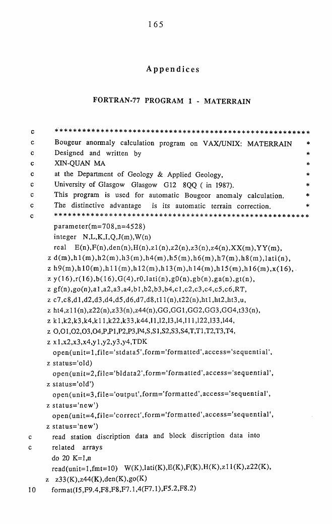
165

A p p e n d i c e s

FORTRAN-77 PROGRAM 1 - M ATERRAIN

c * * * * * * * * * * * * * * * * * * * * * * * * * * * * * * * * * * * * * * * * * * * * * * * * * * * * * * * *

ccc

ccc

c Bougeur anormaly calculation program on VAX/UNIX: MATERRAIN Designed and written by XIN-QUAN MA

at the Department of Geology & Applied Geology,University of Glasgow Glasgow G12 8QQ ( in 1987).This program is used for automatic Bougeor anomaly calculation. The distinctive advantage is its automatic terrain correction.* * * * * * * * * * * * * * * * * * * * * * * * * * * * * * * * * * * * * * * * * * * * * * * * * * * * * * * *

param eter(m = 708 ,n= 4528 ) integer N ,L,K ,I,Q ,J(m ),W (n)

real E (n ),F (n ),d en (n ),H (n ),z l(n ),z2 (n ),z3 (n ),z4 (n ),X X (m ),Y Y (m ), z d (m ) ,h l(m ) ,h 2 (m ) ,h 3 (m ) ,h 4 (m ) ,h 5 (m ) ,h 6 (m ) ,h 7 (m ) ,h 8 (m ) ,la t i (n ) , z h 9 (m ) ,h l0 (m ) ,h l I (m ) ,h l2 ( m ) ,h l3 ( m ) ,h l4 (m ) ,h l5 ( m ) ,h l6 ( m ) ,x ( 1 6 ) , z y (1 6 ) ,r (1 6 ) ,b ( l6 ) ,G (4 ) ,rO ,la ti(n ) ,g O (n ) ,g b (n ) ,g a (n ) ,g t(n ) , z g f(n ) ,g o (n ) ,a l,a 2 ,a 3 ,a 4 ,b l,b 2 ,b 3 ,b 4 ,c l,c2 ,c 3 ,c 4 ,c 5 ,c6 ,R T , z C 7 ,c 8 ,d l,d 2 ,d 3 ,d 4 ,d 5 ,d 6 ,d 7 ,d 8 ,tlI(n ),t2 2 (n ),h tl,h t2 ,h t3 ,u , z h t4 ,zll(n),z22(n),z33(n),z44(n),G G ,G G l,G G 2,G G 3,G G 4,t33(n), z k l,k 2 ,k 3 ,k 4 ,k lI ,k 2 2 ,k 3 3,k44,l 1,12,13,14,111,122,133,144, z 0,01,02,03,04,P,P1,P2,P3,P4,S,S1,S2,S3,S4,T,T1,T2,T3,T4, z x l,x2 ,x3,x4,yl,y2,y3,y4,TD K

o p e n (u n it= l ,f i le = ,s td a ta 5 ',fo rm = 'fo rm a tte d ',a c c e ss= 'se q u e n tia r ,

z s ta tus= 'o ld )o p e n (u n it= 2 ,f ile = ,b ld a ta 2 ,,fo rm = ,fo rm a tted ,,a c c e s s= 'se q u e n tia r ,

z s ta tu s= 'o ld ')o p e n (u n it= 3 ,f ile = 'o u tp u t ',fo rm = ,fo rm a tted ,,a c c e s s= 'se q u e n tia r ,

z s ta tu s= 'n e w ')o p e n (u n it= 4 ,f ile = ,c o rre c t,,fo rm = lfo rm a tte d ',a c c e ss= ,se q u e n tia l ',

z s ta tu s= 'n e w ')c read station discription data and block discription data into

c related arraysdo 20 K=l,nread(unit= l,fm t= 10) W (K ),lati(K ),E(K ),F(K ),H (K ),zl l(K ),z22(K ),

z z33(K ),z44(K),den(K ),go(K)10 form at(I5,F9.4,F8,F8,F7.1,4(F7.1),F5.2,F8.2)

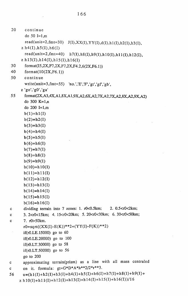
166

20 c o n t in u edo 50 1=1,m

read(un it= 2 ,fm t= 30) J (I) ,X X (I),Y Y (I),d (I) ,h l(I),h 2 (I) ,h 3 (I) , z h 4 ( I ) ,h 5 ( I ) ,h 6 ( I )

read (u n it= 2 ,fm t= 4 0 ) h 7 (I) ,h 8 (I) ,h 9 (I) ,h lO (I) ,h l 1 ( I ) ,h l2 ( I ) , z h l 3 ( I ) ,h l 4 ( I ) ,h l5 ( I ) ,h l 6 ( I )

30 format(I5,2X,F7,2X,F7,2X,F4.2,6(2X,F6.1 ))40 fo rm at(10(2X ,F 6 .1))50 c o n t in u e

w rite(unit=3 ,fm t= 55) 'no .’. 'E '. 'F '/g t '. 'g f /g b ', z 'goV gO V ga '

55 format(2X,A3,4X,Al,8X,Al,9X,A2,6X,A2,7X,A2,7X,A2,8X,A2,9X,A2) do 300 K =l,ndo 200 1=1,mb (1 )= h 1 (I)b (2 )= h 2 (I)b (3 )= h 3 (I)b (4 )= h 4 (I)b (5 )= h 5 (I)b (6 )= h 6 (I)b (7 )= h 7 (I)b (8 )= h 8 (I)b (9 )= h 9 (I)b( 10 )= h 10(1)b ( l l ) = h l 1(1)b( 12 )= h 12(1)b( 13 )=h 13(1)b (1 4 )= h l4 (I )b( 15)=h 15(1)b (1 6 )= h l6 (I )

c dividing terrain into 7 zones: 1. r0<0.5km; 2. 0.5<r0<2km;c 3. 2<r0<15km; 4. 15<r0<20km; 5. 20<r0<30km; 6. 30<i0<50km;

c 7. r0>50km.rO =sqrt((X X (I)-E (K ))**2+ (Y Y (I)-F (K ))**2)

if(rO.LE. 15000) go to 60if(rO.LE.20000) go to 100if(rO.LT.30000) go to 58if(r0.LT.50000) go to 56go to 200

c approxim ating terrain(prism) as a line with all mass centraledc on it. formula: gt=G*D*A*h**2/2*r**3.56 u = (h l( I )+ h 2 (I )+ h 3 (I)+ h 4 (I )+ h 5 (I )+ h 6 (I)+ h 7 (I )+ h 8 (I)+ h 9 (I )+

z h 1 0 (I)+ h l l ( I ) + h l2 ( I ) + h l 3(I)+ h 14(I)+h 1 5 (I)+ h l 6 ( I ) ) /1 6

167

T D K = ab s(3 3 3 6 * 1 6 * d (I)* (u -H (K ))* * 2 /r0 * * 3 ) t3 3 (K)=t3 3 (K)+TDK

gt(K)=gt(K)+TDK go to 200

c approxim ating terrain as prism with 4km long sides,c form ula: g t=G *D *A *h**2/2*r**3-r*4E 06).

58 u = (h l( I )+ h 2 (I )+ h 3 ( I )+ h 4 (I )+ h 5 ( I )+ h 6 ( I )+ h 7 (I )+ h 8 ( I )+ h 9 (I )+z h lO ( I)+ h l I ( l ) + h l2 ( l ) + h l3 ( l ) + h l4 ( l ) + h l5 ( l ) + h l6 ( l ) ) /1 6

T D K = ab s(3 3 3 6 * 1 6 * d (I)* (u -H (K ))* * 2 /(r0 * * 3 -r0 * 4 E 6 )) t3 3 (K)=t3 3 (K)+TDK gt(K)=gt(K)+TDK go to 200

60 x(l)=X X (I)-1500y (l)= Y Y (I)-1 5 0 0r ( l )= s q r t( (x ( l) -E (K ))* * 2 + (y ( l) -F (K ) )* * 2 )x(2)=XX(I)-500y(2)=Y Y (I)-1500r(2 )= sq r t((x (2 )-E (K ))* * 2 + (y (2 )-F (K ))* * 2 )x(3)=XX(I)-1500y(3)= Y Y (I)-500r(3 )= sq r t((x (3 )-E (K ))* * 2 + (y (3 )-F (K ))* * 2 )x(4)=XX(I)-500y(4)= Y Y (I)-500r(4 )= sq rt((x (4 )-E (K ))* * 2 + (y (4 )-F (K ))* * 2 )x(5)=XX(I)+500y(5)=Y Y (I)-1500r(5 )= sq rt((x (5 )-E (K ))* * 2 + (y (5 )-F (K ))* * 2 )x(6)=XX(I)+1500y(6)=Y Y (I)-1500r(6 )= sq rt((x (6 )-E (K ))* * 2 + (y (6 )-F (K ))* * 2 )x(7)=XX(I)+500y(7)= Y Y (I)-500r(7 )= sq rt((x (7 )-E (K ))* * 2 + (y (7 )-F (K ))* * 2 )

x(8)=XX(I)+1500y(8)= Y Y (I)-500r(8 )= sq rt((x (8 )-E (K ))* * 2 + (y (8 )-F (K ))* * 2 )

x(9)=XX(I)-1500y(9)=Y Y (I)+500r(9 )= sq rt((x (9 )-E (K ))* * 2 + (y (9 )-F (K ))* * 2 )

x(10)=XX(I)-500y(10)=Y Y (I)+500r(1 0 )= sq rt((x (1 0 )-E (K ))* * 2 + (y (1 0 )-F (K ))* * 2 )

168

x(ll)= X X (I)-1500y (ll)= Y Y (I)+ 1 5 0 0

r ( l l )= s q r t ( ( x ( l l ) - E ( K ) ) * * 2 + ( y ( l l ) - F ( K ) ) * * 2 )x(12)=XX(I)-500y(12)=Y Y (I)+1500

r (1 2 )= sq r t((x (1 2 )-E (K ))* * 2 + (y (1 2 )-F (K ))* * 2 )x(13)=XX(I)+500y(13)=Y Y (I)+500

r (1 3 )= sq r t((x (1 3 )-E (K ))* * 2 + (y (1 3 )-F (K ))* * 2 )x( 14)=XX(I)+1500y(14)=Y Y (I)+500

r(1 4 )= sq rt((x (1 4 )-E (K ))* * 2 + (y (1 4 )-F (K ))* * 2 )x(15)=XX(I)+500y(15)=Y Y (I)+1500r(1 5 )= sq rt((x (1 5 )-E (K ))* * 2 + (y (1 5 )-F (K ))* * 2 )x( 16)=XX(I)+1500y(16)=Y Y (I)+1500r(1 6 )= sq rt((x (1 6 )-E (K ))* * 2 + (y (1 6 )-F (K ))* * 2 ) do 80 Q=l,16if(E(K).GT.(x(Q)-500).AND.E(K).LT.(x(Q)+500).AND.

z F(K).GT.(y(Q)-500).AND.F(K).LT.(y(Q)+500)) go to 85 if(r(Q).GE.2000) go to 83

c calculating terrain correction in the inner zone(0.5<r0<2 km)c approximate terrain to a vertical prism with horizontal lowerc face and slopping upper surface whose slop is constant towardc the station point,c form ula: g=G *p*(l-cosa)*D *K (i,j)c 1 -co sa= 0 .5 * tan (a)* * 2

T D K = 6672*d(I)* ( l/r (Q )-l/sq rt((b (Q )-H (K ))* * 2 + r(Q )* * 2 ))t22(K)=t22(K)+TDKgt(K)=gt(K)+TDKgo to 80

83 T D K =3336*d(I)*(b(Q )-H (K ))**2/(r(Q )**3-r(Q )*2.5E 05)t33(K)=t33(K)+TDK gt(K)=gt(K)+TDK go to 80

c calculating terrain correction for the most inner zone(r0<0.5km ) by c dividing square into four triangle prisms.85 z l(K )= a b s(z l 1(K)-H(K))

z2(K )=abs(z22(K )-H (K )) z3(K )=abs(z33(K )-H (K )) z4(K )=abs(z44(K )-H (K )) x l=x(Q)-E(K)+500

169

y l=y(Q )-F(K )-500 x2=xly2=500+y(Q )-F(K)x3=x(Q)-E(K)-500y3=y2x4=x3

y4=y ia l= (z l(K )* y 2 -z 2 (K )* y l ) / (x l* y 2 -x 2 * y 1)b l= (x l* z 2 (K )-x 2 * z l(K )) /(x l* y 2 -x 2 * y 1)a2 = (z2 (K )* y 3 -z3 (K )* y 2 )/(x 2 * y 3 -x 3 * y 2 )b2= (x 2 * z3 (K )-x 3 * z2 (K ))/(x 2 * y 3 -x 3 * y 2 )a3 = (z3 (K )* y 4 -z4 (K )* y 3 )/(x 3 * y 4 -x 4 * y 3 )b3= (x 3 * z4 (K )-x 4 * z3 (K ))/(x 3 * y 4 -x 4 * y 3 )a4= (z4 (K ) * y 1- z 1 (K )*y4)/(x4*y 1 -x 1 *y4)b 4 = (x 4 * z l(K )-x l *z4(K ))/(x4*y l -x l* y 4 )c l= (z l(K )* y 2 + z 2 (K )* y l) / (x l* y 2 -x 2 * y 1)d l= ( - x l * z 2 (K )-x 2 * z l(K ))/(x l* y 2 -x 2 * y 1)c 2 = (-z l(K )* y 2 -z 2 (K )* y l ) / ( x l *y2-x2*y 1)d 2 = (x l* z 2 (K )+ x 2 * z l(K )) /(x l* y 2 -x 2 * y 1)c3 = (z2 (K )*y3+ z3 (K )*y2 )/(x2*y3 -x3*y2 )d3 = (-x2*z3 (K )-x3*z2 (K ))/(x2*y3 -x3*y2 )c4 = (-z2 (K )* y 3 -z3 (K )* y 2 )/(x 2 * y 3 -x 3 * y 2 )d4= (x2*z3(K )+ x3*z2(K ))/(x2*y3-x3*y2)c5 = (z3 (K )*y4+ z4 (K )*y3 )/(x3*y4 -x4*y3 )d 5= (-x3*z4 (K )-x4*z3 (K ))/(x3*y4 -x4*y3 )c6 = (-z3 (K )* y 4 -z4 (K )* y 3 )/(x 3 * y 4 -x 4 * y 3 )d6= (x3*z4(K )+ x4*z3(K ))/(x3*y4-x4*y3)c 7 = (z 4 (K )* y l+ z l(K )* y 4 )/(x 4 * y 1 -x l* y 4 )d 7 = (-x 4 * z l(K )-x 1 *z4(K ))/(x4*y l -x l* y 4 )c8 = (-z4 (K )* y l-z l(K )* y 4 ) /(x 4 * y l -x l* y 4 )d 8 = (x 4 * z l(K )+ x l *z4(K ))/(x4*y l -x l* y 4 )

k l= y 1 /x lk 2 = y 2 /x lk3= y2/x3k4= y4/x3k 11 = 1 /k 1k 2 2 = l/k 2k33 = l/k 3k 4 4 = l/k 4l l = - c l / d l12=-c3/d313=-c5/d5

170

14=-c7/d7 111 = 1/11

122= 1/12

133 = 1/13144=1/14

c using subroutines to calculate terrain correction produced byc four triangle prismsc triangle prism 1.

call IN N E R Z O N E l(al,b l,k2 ,kl,x l,G G l) c triangle prism 2.

call INNERZONEl(b2,a2,k22,k33,y2,GG2) c triangle prism 3.

call INNERZONEl(a3,b3,k3,k4,x3,GG3) c triangle prism 4.

call INNERZONE1 (b4,a4,k 11 ,k44,y 1 ,GG4)GG=GG1+GG2+GG3+GG4

c considering symboles of four height values in the four connersc o f that square,overestim ated terrain correction must be substractedc by the values resulting from central triangle prisms,c central triangle prism 1.

call INNERZONE2 (c l ,d l ,l l ,k l,x l ,P l) call INNERZONE2 (a l,b l,ll ,k l,x l,P 2 ) call INNERZONE2 (c2,d2,k2,ll,xl,P3) call INNERZONE2 (a l,b l,k2 ,ll,x l,P 4 )P=P1-P2+P3-P4

c central triangle prism 2.call INNERZONE2 (d4,c4,122,k33,y2,01) call INNERZONE2 (b2,a2,122,k33,y2,02) call INNERZONE2 (d3,c3,k22,122,y2,03) call INNERZONE2 (b2,a2,K22,122,y2,04)0=01-02+03-04

c central triangle prism 3.call INNERZ0NE2 (c6,d6,13,k4,x3,Sl) call INNERZ0NE2 (a3,b3,13,k4,x3,S2) call INNERZ0NE2 (c5,d5,k3,13,x3,S3) call INNERZ0NE2 (a3,b3,k3,13,x3,S4)S=S1-S2+S3-S4

c central triangle prism 4.call INNERZ0NE2 (d7,c7,144,k44,yl,Tl) call INNERZ0NE2 (b4,a4,144,k44,yl,T2) call INNERZ0NE2 (d8,c8,kll,144,yl,T3) call INNERZ0NE2 (b4.a4.kl 1,144,yl,T4)

T=T1-T2+T3-T4

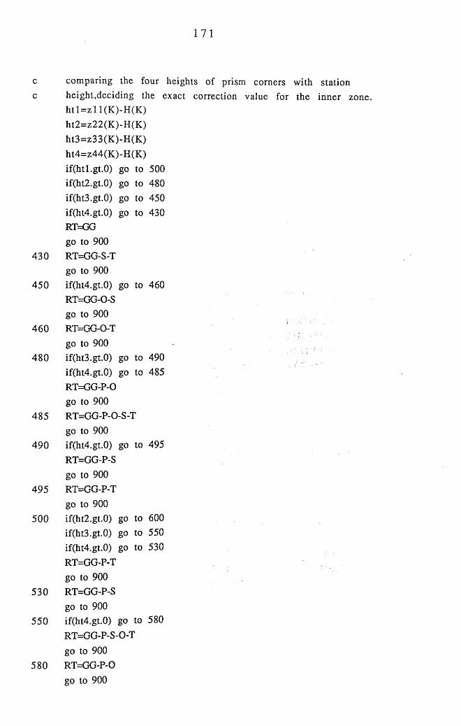
171

c com paring the four heights of prism corners with stationc height,deciding the exact correction value for the inner zone.

h t l= z l 1(K)-H(K) ht2=z22(K )-H (K ) ht3=z33(K )-H (K ) ht4=z44(K )-H (K ) if(htl.gt.O) go to 500if(ht2.gt.O) go to 480if(ht3.gt.0) go to 450if(ht4.gt.0) go to 430RT=GG go to 900

430 RT=GG-S-Tgo to 900

450 if(ht4.gt.0) go to 460RT=GG-0-S go to 900

460 RT=GG-0-Tgo to 900

480 if(ht3.gt.0) go to 490 /if(ht4.gt.0) go to 485RT=GG-P-0 go to 900

485 RT=GG-P-0-S-T go to 900

490 if(ht4.gt.0) go to 495RT=GG-P-S go to 900

495 RT=GG-P-Tgo to 900

500 if(ht2.gt.O) go to 600if(ht3.gt.O) go to 550if(ht4.gt.0) go to 530RT=GG-P-T go to 900

530 RT=GG-P-Sgo to 900

550 if(ht4.gt.0) go to 580RT=GG-P-S-0-T

go to 900 580 RT=GG-P-0

go to 900

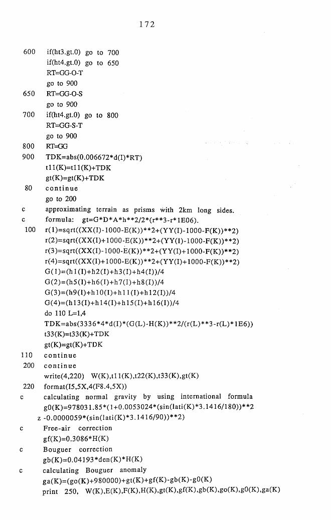
172

600 if(ht3.gt.0) go to 700if(ht4.gt.0) go to 650 RT=GG-0-T go to 900

650 RT=GG-0-Sgo to 900

700 if(ht4.gt.0) go to 800RT=GG-S-T go to 900

800 RT=GG

900 TD K =abs(0.006672*d(I)*RT)t i l (K )=tl 1 (K)+TDK gt(K)=gt(K)+TDK

80 c o n t in u ego to 200

c approxim ating terrain as prisms with 2km long sides,c form ula: g t= G *D *A *h**2/2*(r**3-r* lE 06).

100 r (l)= sq rt((X X (I)-1 0 0 0 -E (K ))* * 2 + (Y Y (I)-1 0 0 0 -F (K ))* * 2 )r(2 )= sq rt((X X (I)+ 1 0 0 0 -E (K ))* * 2 + (Y Y (I)-1 0 0 0 -F (K ))* * 2 )

r(3 )= sq rt((X X (I)-1 0 0 0 -E (K ))* * 2 + (Y Y (I)+ 1 0 0 0 -F (K ))* * 2 ) r(4 )= sq rt((X X (I)+ 1 0 0 0 -E (K ))* * 2 + (Y Y (I)+ 1 0 0 0 -F (K ))* * 2 ) G (l)= ( h l( I ) + h 2 (I )+ h 3 (I )+ h 4 ( I ) ) /4 G (2 )= (h 5 (I )+ h 6 (I )+ h 7 (I )+ h 8 (I ) ) /4 G (3 )= (h 9 (I )+ h lO (I )+ h l l ( I )+ h l2 ( I ) ) /4 G (4 ) = ( h l3 ( I ) + h l4 ( I ) + h l5 ( I ) + h l6 ( I ) ) /4 do 110 L =l,4

T D K = ab s(3 3 3 6 * 4 * d (I)* (G (L )-H (K ))* * 2 /(r(L )* * 3 -r(L )* lE 6 )) t33(K)=t33(K)+TDK gt(K)=gt(K)+TDK

110 c o n t in u e200 c o n t in u e

w rite(4,220) W (K ),tl l(K ),t22(K ),t33(K ),gt(K )220 form at(I5,5X ,4(F8.4,5X ))

c calculating normal gravity by using international form ulag0 (K )= 978031.85 *(1+0.0053 024* (sin (la ti(K ) *3.1416/180))* *2

z -0 .0 0 0 0 0 5 9 * (s in (la ti(K )* 3 .1 4 1 6 /9 0 ))* * 2 )

c F ree -a ir correctiongf(K )=0.3086*H (K )

c B ouguer correctiongb(K )= 0.04193*den(K )*H (K )

c calcu lating Bouguer anomalyga(K )= (go(K )+ 980000)+ g t(K )+ gf(K )-gb(K )-g0(K )prin t 250, W (K ),E (K ),F (K ),H (K ),g t(K ),g f(K ),gb(K ),go(K ),gO (K ),ga(K )

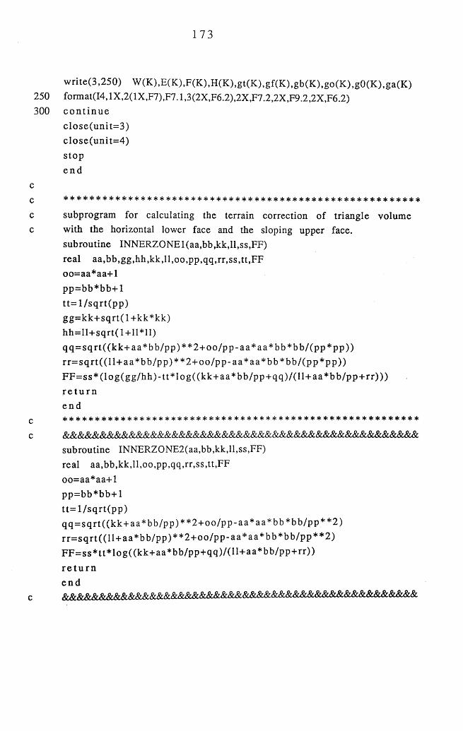
173

w rite(3 ,250) W (K ),E (K ),F(K ),H (K ),gt(K ),gf(K ),gb(K ),go(K ),gO (K ),ga(K ) 250 format(I4>lX ,2(lX ,F7),F7.1,3(2X ,F6.2),2X ,F7.2,2X ,F9.2,2X ,F6.2)300 c o n t in u e

c lo se (u n it= 3 )c lo se (u n it= 4 )s to pe n d

cq * * * * * * * * * * * * * * * * * * * * * * * * * * * * * * * * * * * * * * * * * * * * * * * * * * * * * * * *

c subprogram for calculating the terrain correction o f triangle volumec with the horizontal lower face and the sloping upper face,

subroutine INNERZO NEl(aa,bb,kk,ll,ss,FF) real aa ,bb ,gg ,hh ,kk ,ll,oo ,pp ,qq ,rr,ss ,tt,F F oo= aa*aa+ l p p = b b * b b + l t t= l / s q r t ( p p ) g g = k k + sq r t( l+ k k * k k ) h h = ll+ s q r t ( l+ ll* ll )q q = s q r t( (k k + a a * b b /p p )* * 2 + o o /p p -a a * a a * b b * b b /(p p * p p ))r r= s q r t ( ( l l+ a a * b b /p p )* * 2 + o o /p p -a a * a a * b b * b b /(p p * p p ) )F F = s s * ( lo g (g g /h h ) - t t* lo g ( (k k + a a * b b /p p + q q ) / ( l l+ a a * b b /p p + r r ) ) )r e t u r ne n d

q * * * * * * * * * * * * * * * * * * * * * * * * * * * * * * * * * * * * * * * * * * * * * * * * * * * * * * * *

subroutine INNERZONE2(aa,bb,kk,ll,ss,FF)real aa ,bb ,kk ,ll,oo ,pp ,qq ,rr,ss,tt,FF

oo= aa*aa+ lp p = b b * b b + lt t= l / s q r t ( p p )q q = s q r t( (k k + a a * b b /p p )* * 2 + o o /p p -a a * a a * b b * b b /p p * * 2 )r r= s q r t( ( l l+ a a * b b /p p )* * 2 + o o /p p -a a * a a * b b * b b /p p * * 2 )F F = s s * tt* lo g ((k k + a a * b b /p p + q q )/( l l+ a a * b b /p p + rr) )

r e t u r ne n d

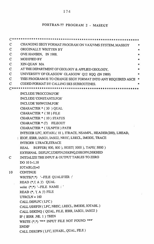
174

FORTRAN-77 PROGRAM 2 - MASEGY

C CHANGING SEGY FORMAT PROGRAM ON VAX/VMS SYSTEM, MASEGY *C ORIGINALLY WRITTEN BY *C OVE HANSEN, IN 1988. *C MODIFIED BY *C XIN-QUAN MA *

C AT THE DEPARTMENT OF GEOLOGY & APPLIED GEOLOGY, *C UNIVERSITY OF GLASGOW GLASGOW Q12 8QQ (IN 1989) *C THIS PROGRAM IS TO CHANGE SEGY FORMAT INTO ANY REQUIRED ASCII *C CODED FORMAT BY CALLING SKS SUBROUTINES. *c * * * * * * * * * * * * * * * * * * * * * * * * * * * * * * * * * * * * * * * * * * * * * * * * * * * * * * * * * * * *

INCLUDE PROCCOM.FOR’INCLUDE'CONSTANTS.FOR'INCLUDE 'RHWCOM.FOR'CHARACTER * ( 30 ) QUAL CHARACTER * ( 30 ) FILE CHARACTER * ( 10 ) STATUS CHARACTER * (7) FELEOUT CHARACTER * ( ULNPTH ) PATHINTEGER LFC, IOTABL( 18 ), ITRACE, NSAMPL, HEADER(200), LHEAD,

: IEOF, IERR, IASG1, IASG2, NREC, LRECL, IMODE, TRACE INTEGER LTRACE.STRACEREAL BUFFER( 800, 800 ), HOST( 5000 ), TAPE( 5000 )EXTERNAL DEFLFC,UDEFIN,DSKINQ,DSKOPN,DSKHED

C INITIALIZE THE INPUT & OUTPUT TABLES TO ZERO

DO 101=1,18 IOTABL(I)=0

10 CONTINUEWRITE(*,*) '-F IL E QUALIFIER READ (*,’( A )') QUAL write (*,*) '-F IL E NAME : 'READ (*, '( A )’) FILE UTRCLN = 160 CALL DEFLFC( LFC)CALL UDEFIN ( LFC, NREC, LRECL, IMODE, IOTABL )CALL DSKINQ ( QUAL, FILE, IERR, IASG1, IASG2 )

IF ( IERR .NE. 1 ) THENWRITE (*,*) '*** INPUT FILE NOT FOUND ***'

END IFCALL DSKOPN ( LFC, IOTABL, QUAL, FILE)

175

CALL DSKHED ( LFC, IOTABL, QUAL, FILE, HEADER, RHWLEN ) WRITE(*,*) 'TRACE COMMON LENGTH (UTRCLN)=',UTRCLN WRITE(*,*) 'LENGTH OF TRACE HEADER(RHWTHL)=',RHWTHL

WRITE(*,*) 'SAMPLES PER TRACE(RHWNSM) = ',RHWNSM WRITE(*,*) 'NUMBER OF TRACES IN FILE(RHWNRC) = ',RHWNRC IF ( RHWTHL .GT. 160 ) THEN

WRITE(*,*) 'NON-STANDARD HEADER LENGTH(>160) ’ERROR = .TRUE.END IF

WRITE(*,*) ’-INPU T FIRST TRACE NUMBER YOU WANT TO READ’READ ( * * ) ITRACE

NTRACE = RHWNRC - ITRACE + 1STRACE - ITRACE

WRITE(*,*) '-INPUT LAST TRACE NUMBER YOU WANT TO READ ’ READ(*, *) LTRACE

WRITE(*,*) ' -INPU T FIRST SAMPLE YOU WANT TO READ 1 READ ( *, * ) ISAMPL NSAMPL = RHWNSM - ISAMPL + 1 JTRACE = ITRACE - 1 ITRACE = ITRACE - 1

100 ITRACE = ITRACE + 1CALL DSKTIN ( LFC, IOTABL, ITRACE, HOST, TAPE, RHWNSM,

: IEOF, HEADER)CALL DSKFMT ( HOST, TAPE, RHWNSM )

DO 200 I = 1, NSAMPL BUFFER ( ITRACE - JTRACE, I ) =

: HOST ( I + ISAMPL - 1)

200 CONTINUEIF ( IEOF .EQ. 0 .AND. ITRACE .GE. LTRACE) GO TO 999

GO TO 100C WRITE DATA IN THE BUFFER INTO FILE999 WRITE(*,*) ’-INPU T FILE NAME FOR OUTPUT'

READ(*,'(A)') FILEOUTOPEN( 1 ,FTLE=FILEOUT,FORM='FORMATTED',ST ATUS='NEW')

PRINT*,'NO. OF TRACES TO WRITE=',LTRACE-STRACE+1

PRINT*,'NSAMPL=',NSAMPL

DO 888 1= 1 ,LTRACE-STRACE+1

DO 777 J=l,NSAMPL W RITE(1,889) I,J,BUFFER(I,J)

889 FORMAT( 215,E l8.8)

777 CONTINUEPRINT*,’ THE TRACE ', I, ' COMPLETED'

176

888 CONTINUE CLOSE( 1 ) STOP END

177

FORTRAN-77 PROGRAM 3 - MATRAN

£2 5lesl«sjes(esl«>l=s4«3(«5j«9(=s(«9(e9ies}esies(eajes(esfeajes4es(!:^es(e9(es(esfesjesfes}esjes(es|e9(e9(esjes(esleslc»fe9(es4es(eslesje9(es(e9jea(es(es(es(cs(e34es(esie

C THREE-COMPONENT SEISMIC DATA ROTATION PROGRAM ON *C THE VAX/VM S SYSTEM: MATRAN *C DESIGNED AND WRITTEN BY *C XIN-QUAN MA *

C AT THE DEPARTMENT OF GEOLOGY & APPLIED GEOLOGY *

C UNIVERSITY OF GLASGOW GLASGOW G12 8QQ (IN 1989) *C THE PURPOSE OF THIS PROGRAM IS TO TRANSFORM FEILD COORDINATE *C SYSTEM (VERT, NORTH, EAST) INTO A REQUIRED SYSTEM (VERTICAL, *C RADIAL,TRANSVERSE). VERTICAL TRACE IS KEPT INTACT. THE OTHER *C TRACES AS A VECTOR AT A SPECIFIC TIME HAVE BEEN PROJECTED *C ONTO NEW SYSTEM. FOR ONE SHOTPOINT, 12 ANGLES OF RADIAL LINES *C TO MAGNETIC NORTH ARE SET IN THE PROGRAM. AFTER THE OLD DATA *C HAVE BEEN INPUT, THE NEW DATA IN THE DIFFERENT ORDER ARE THE *

C OUTPUTS. *

REAL XYZ(100,800),XX(20,800),YY(20,800),ZZ(20,800)REAL ALPHA,PIINTEGER STNUMB ,NORTHCH,EASTCH,VERTCH,NSAMPL,NTRACE

INTEGER IIICHARACTER * 8 INFILE,OUTFELEPRINT*,'-INPUT RLE NAME TO BE TRANSLATED'READ(*,'(A)') INFILE

NTRACE = 48 NSAMPL = 501OPEN(l,HLE=INFILE,STATUS='OLD’)PRINT*,'-INPUT FILE NAME FOR OUTPUT'

READ(*,’(A)’) OUTFILE OPEN(2,FILE=OUTHLE,STATUS-NEW')PRINT*,’-STAR T READING DATA INTO ARRAY '

C READ THE 3-COMPONENT DATA INTO ARRAY XYZ(I,J)C THE DATA IN THE ARRAY XYZ(I,J) ARE PRODUCED BY PROGRAM

C MARDDISK.FOR, I IS CHANNEL, J IS SAMPLE

DO 2001=1, NTRACE

DO 100 J=l, NSAMPL

READ(1,50) M, N, XYZ(I,J)50 FORMAT(2I5,E18.8)

100 CONTINUE200 CONTINUE

178

P I= 3 .14159/180 C INPUT STATION NUMBER

111=0

99 PRINT*,'-INPUT STATION NUMBER(TYPE "0" TO STOP) 'READ*, STNUMB

111= 111+ 1EF(STNUMBJEQ.l) GO TO 300

IF(STNUMB .EQ.2) GO TO 400

LF(STNUMB.EQ.3) GO TO 500 EF(STNUMB .EQ.4) GO TO 600

IF(STNUMB .EQ.5) GO TO 700

IF(STNUMB .EQ. 6) GO TO 800

IF(STNUMB.EQ.7) GO TO 900

EF(STNUMB.EQ.8) GO TO 1000

IF(STNUMB.EQ.9) GO TO 1100 IF(STNUMB.EQ.IO) GO TO 1200

IF(STNUMB.EQ.ll) GO TO 1300 IF(STNUMB.EQ. 12) GO TO 1400

IF(STNUMB .EQ.0) GO TO 9999300 PRINT*,'-INPUT VERTICAL,NORTH,EAST TRACE NUMBERS'C THE ORIGINAL DATA HAVE SEQUENCES FROM VERTICAL,NORTHJEASTC WHICH ARE CORRESPONDING FIELD CHANNEL SEQUENCES.C REMEMBER INPUTING DATA IN CORRECT ORDER.

READ*, VERTCH,NORTHCH,EASTCH C A IS ANGLE OF ROTATION IN THE POSITIVE DIRECTION

ALPH A=346.5*PI DO 350 J=l,NSAMPLCALL TRANSLT(ALPHA,XYZ(NORTHCH,J),XYZ(EASTCH,J),XX(STNUMB,J),

Z YY(STNUMB.J))ZZ(STNUMB,J)=XYZ(VERTCH,J)

350 CONTINUE

GO TO 99400 PRINT*,’-INPU T VERTICAL NORTH AND EAST TRACE NUMBER’

READ*, VERTCH,NORTHCH,EASTCH C A IS ANGLE OF ROTATION IN THE POSITIVE DIRECTION

ALPHA = 316.5*PI DO 450 J = l,NSAMPLCALL TRANSLT(ALPHA,XYZ(NORTHCH,J),XYZ(EASTCH,J),XX(STNUMB,J),

Z YY(STNUMB,J))ZZ(STNUMB, J)=XYZ(VERTCH, J)

450 CONTINUE

GO TO 99500 PRINT*,'-INPUT VERTICAL NORTH AND EAST TRACE NUMBER'

179

READ*, VERTCH,NORTHCH,EASTCH

C A IS ANGLE OF ROTATION IN THE POSITIVE DIRECTION ALPHA = 286.5*PI

DO 550 J=l,NSAMPL

CALL TRANSLT( ALPHA,XYZ(NORTHCH,J),XYZ(EASTCH,J),XX(STNUMB,J), Z YY(STNUMB,J))

ZZ(STNUMB ,J)=XYZ(VERTCH,J)550 CONTINUE

GO TO 99

600 PRINT*,'-INPUT VERTICAL NORTH AND EAST TRACE NUMBER'READ*, VERTCH,NORTHCH,EASTCH

C A IS ANGLE OF ROTATION IN THE POSITIVE DIRECTIONALPHA = 256.5*PI

DO 650 J=l,NSAMPL

CALL TRANSLT(ALPHA,XYZ(NORTHCH,J),XYZ(EASTCH,J),XX(STNUMB,J), Z YY(STNUMB,J))

ZZ(STNUMB,J)=XYZ(VERTCH,J)650 CONTINUE

GO TO 99700 PRINT*,'-INPUT VERTICAL NORTH AND EAST TRACE NUMBER’

READ*, VERTCH,NORTHCH,EASTCH C A IS ANGLE OF ROTATION IN THE POSITIVE DIRECTION

ALPHA = 226.5*PI

DO 750 J=l,NSAMPLCALL TRANSLT(ALPHA,XYZ(NORTHCH,J),XYZ(EASTCH,J),XX(STNUMB,J),

Z YY(STNUMB,J))ZZ(STNUMB,J)=XYZ(VERTCH,J)

750 CONTINUE

GO TO 99800 PRINT*,'-INPUT VERTICAL NORTH AND EAST TRACE NUMBER'

READ*, VERTCH,NORTHCH,EASTCH C A IS ANGLE OF ROTATION IN THE POSITIVE DIRECTION

ALPHA = 196.5*PI

DO 850 J=l,NSAMPLCALL TRANSLT(ALPHA,XYZ(NORTHCH,J),XYZ(EASTCH,J),XX(STNUMB,J),

Z YY(STNUMB,J))ZZ(STNUMB, J)=XYZ(VERTCH, J)

850 CONTINUE

GO TO 99900 PRINT*,'-INPUT VERTICAL NORTH AND EAST TRACE NUMBER'

READ*, VERTCH,NORTHCH,EASTCH

C A IS ANGLE OF ROTATION IN THE POSITIVE DIRECTION

180

ALPHA = 166.5*PI

DO 950 J=1,NSAMPL

CALL TRANSLT(ALPHA,XYZ(NORTHCH,J),XYZ(EASTCH,J),XX(STNUMB,J), Z YY(STNUMBJ))

ZZ(STNUMB ,J)=X YZ(VERTCH, J)950 CONTINUE

GO TO 99

1000 PRINT*,'-INPUT VERTICAL NORTH AND EAST TRACE NUMBER’READ*, VERTCH,NORTHCH,EASTCH

C A IS ANGLE OF ROTATION IN THE POSITIVE DIRECTIONALPHA = 136.5*PI

DO 1050 J=1,NSAMPL

CALL TRANSLT(ALPHA,XYZ(NORTHCH,J),XYZ(EASTCH,J),XX(STNUMB,J), Z YY(STNUMB,J))

ZZ(STNUMB ,J)=XYZ( VERTCH, J)1050 CONTINUE

GO TO 99

1100 PRINT*,’-INPU T VERTICAL NORTH AND EAST TRACE NUMBER’READ*, VERTCH, NORTHCH.EASTCH

C A IS ANGLE OF ROTATION IN THE POSITIVE DIRECTIONALPHA = 106.5*PI

DO 1150 J=1,NSAMPLCALL TRANSLT(ALPHA,XYZ(NORTHCH,J),XYZ(EASTCH,J),XX(STNUMB,J),

Z YY(STNUMB,J))ZZ(STNUMB, J)=X YZ(VERTCH, J)

1150 CONTINUE

GO TO 991200 PRINT*,’-INPUT VERTICAL NORTH AND EAST TRACE NUMBER’

READ*, VERTCH,NORTHCH,EASTCH

C A IS ANGLE OF ROTATION IN THE POSITIVE DIRECTION

ALPH A=76.5*PI DO 1250 J=1,NSAMPLCALL TRANSLT(ALPHA,XYZ(NORTHCH,J),XYZ(EASTCH,J),XX(STNUMB,J),

Z YY(STNUMB,J))ZZ(STNUMB,J)=XYZ(VERTCH,J)

1250 CONTINUE GO TO 99

1300 PRINT*,’-INPUT VERTICAL NORTH AND EAST TRACE NUMBER’READ*, VERTCH,NORTHCH,EASTCH

C A IS ANGLE OF ROTATION IN THE POSITIVE DIRECTION

ALPH A=46.5*PI DO 1350 J=1,NSAMPLCALL TRANSLT(ALPHA,XYZ(NORTHCH,J),XYZ(EASTCH,J),XX(STNUMB,J),

181

Z YY(STNUMB,J))ZZ(STNUMB ,J)=XYZ(VERTCH,J)

1350 CONTINUE

GO TO 99

1400 PRINT*,'-INPUT VERTICAL NORTH AND EAST TRACE NUMBER'READ*, VERTCH,NORTHCH,EASTCH

C A IS ANGLE OF ROTATION IN THE POSITIVE DIRECTIONALPHA = 16.5*PI

DO 1450 J=1,NSAMPL

CALL TRANSLT(ALPHA,XYZ(NORTHCH,J),XYZ(EASTCH,J),XX(STNUMB,J),Z YY(STNUMB,J))

ZZ(STNUMB, J)=XYZ( VERT CH, J)1450 CONTINUE

GO TO 99

9999 PRINT*,'-START WRITING DATA INTO FILE ’C THE SEQUENCES OF OUTPUT DATA HAVE BEEN CHANGED INTO XX.YY/Z C WHICH ARE IMPORTANT FOR NEXT PROGRAM TO KEEP THEM SAME.

DO 8888 1=1, III-lDO 8888 J=1,NSAMPLW RITE(2,7777) I,J,XX(I,J),YY(I,J),ZZ(I,J)

7777 FORMAT(2I5,E18.8,E18.8,E18.8)8888 CONTINUE

STOP END

C^p ^ ^ p ^ <4^ 4 ) ^ 4 ) 4 ) ^ *4^ «4> «4> «4> «}> «4> «4> ^ *4) <4) 1^ *4 *4 »4 ^ ^ ^ *4 ^

C @@@@@@@@2^^

C THE NEW COORDINATE SYSTEM IS THAT X AXIS POINTS TO THEC RADICAL DIRECTION FROM THE SHOT POINT, Y AXIS ISC PERPENDICULAR TO THE X AXIS 90 DEGREE ANTICLOCKWISE FROM IT

C THE ROTATING FORMULA IS

C X=XO COS A + YO SIN AC Y=-XO SIN A + YO COS A

SUBROUTINE TRANSLT ( A, XXO,YYO,XXN,YYN)REAL A,XXO,YYO,XXN,YYN,B,C XXN=XXO*COS(A)+YYO*SIN(A)YYN=-XXO*SIN(A)+YY 0*COS(A)

RETURN

END

(§)(§

) (§

>(§>

(§)

(§)

182

FORTRAN-77 PROGRAM 4 - MAPLOT

^ * * * * * * * * * * * * * * * * * * * * * * * * * * * * * * * * * * * * * * * * * * * * * * * * * * * * * * * *

C SEISMIC DATA DISPLAY PROGRAM ON VAX/VMS: MAPLOT *C DESIGNED AND WDRRTEN BY *C XIN-QUAN MA *

C AT THE DEPARTMENT OF GEOLOGY & APPLIED GELOGY, *C UNIVERSITY OF GLASGOW GLASGOW G12 8QQ(IN 1989) *C THIS PROGRAM IS TO PLOT SEISMIC DATA AS VAIABLE AREA WIGGLE *C TRACES USING POWERFUL UNIRAS GRAPHICS FLIBRARYN ROUTINES *C WHICH IC MOUNTED ON VAX/VMS AT THE COMPUTER CENTRE, *C UNVERSITY OF GLASGOW. *C THE PROGRAM IS DESIGNED TO DISPLAY 3-COMPONENT SEISMIC DATA *

C WHICH ARE STORED IN FREE ASCII-CODED FORMAT. THE CHOICE FOR *C X, Y, Z DATA DISPLAY IS DETERMINED BY THE USER. *Q * * * * * * * * * * * * * * * * * * * * * * * * * * * * * * * * * * * * * * * * * * * * * * * * s ( e ^ « ^ c * * ^ e * *

REAL TRACD,X(501),Y(501),Z(501)CHARACTER* 8 COMP,INFILE INTEGER KTYPE,KSLINEPRINT*,’-IN PU T DATA FILE NAME FOR DISPLAY'READ(*,’(A)’) INFILE OPEN(l,FILE=INFILE,STATUS='OLD')

11 PRINT*,’-D O YOU WANT TO PLOT WIGGLE LINE WITH VAIABLE 'PRINT*,’ AREA, INPUT 0 FOR YES, 1 FOR JUST LINE ’

READ*, KTYPE

IF(KTYPE.EQ.O) GO TO 18 IF(KTYPE.EQ.l) GO TO 21PRINT*,’-Y O U INPUT A WRONG INTEGER, TRY AGAIN!’

GOTO 1118 PRINT*,'-DO YOU WANT TO KEEP LINE AND VAIABLE AREA,'

PRINT*,’ INPUT 0 FOR LINE & AREA, 1 FOR ONLY AREA, NO LINE'

READ*, KSLINEIF((KSLINE.EQ.l).OR.(KSLINE.EQ.O)) GO TO 21

PRINT*,'-YOU INPUT A WRONG INTEGER, TRY AGAIN!'

GOTO 1821 PRINT*,'-INPUT SCALLING VALUE E.G 999.999'

READ*, TRACDC DATA FILE CONSISTS OF 4 COLUMNS I,X,Y,Z22 PRINT*,'-INPUT DATA COMPONENT FOR DISPLAY(X,Y.OP Z)'

READ(*,'(A)') COMPIF(COMP.EQ.'X) GO TO 156 EF(COMP.EQ.'Y') GO TO 250

183

IF(COMP.EQ.'Z') GO TO 350

PRINT*,'-YOU INPUT A WRONG CHARACTER, TRY IT AGAIN!' GOTO 22

156 CALL GROUTE ('S VT4014;E')CALL GMSLEV(T,’ ',' ’)

CALLGOPEN

CALL SPRIM A(l)CALL SDIR(1,-1)

CALL SSMPSI( 10.0,0.40,TRACD)CALL STYPEW(KTYPE, 1 ,KSLINE)DO 200 1=1, 12

READ(1,100) X 100 FORMAT(5X,E12.4)

CALL SWIGG(X,501)CALL STRNMB(I)

200 CONTINUE

CALL SWIGG(X,9999)CALL SNUM BS(-l)GO TO 999

250 CALL GROUTE ('S VT4014;E’)CALL GMSLEV(T,’ ’,' ',' ’)CALLGOPEN CALL SPRIMA(l)CALL SDIR(1,-1)CALL SSMPSI(10.0,0.40,TRACD)CALL STYPEW(KTYPE, 1 ,KSLINE)

DO 2101= 1,12

READ(1,190) Y 190 FORMAT(17X,E12.4)

CALL SWIGG(Y,501)CALL STRNMB(I)

210 CONTINUECALL SWIGG(Y,9999)

GO TO 999 350 CALL GROUTE ('S VT4014;E')

CALL GMSLEVCI',' ',' ')

CALLGOPEN CALL SPRIMA(l)

CALL SDIR(1,-1)CALL SSMPSI(10.0,0.40,TRACD)CALL STYPEW(KTYPE,1,KSLINE)

DO 310 1=1, 12

184

READ(1,180) Z

180 FORM AT(29X,E 12.4)CALL SWIGG(Z,501)CALL STRNMB(I)

310 CONTINUE

CALL SWIGG(Z,9999)999 CALL STIMEE(l.O.l.O)

CALL GDASH(4)

CALL STIMEL(0.0,0.2,50,2)CALLGCLOSE

STOP

END

185

FORTRAN-77 PROGRAM 5 - M AGNPL

+ s |e s(« >|e s |<sk 5(t 5 |« ^«5| j + + 5 | c s |c ^ t^ c ^ < ^ c } |c ^ c s |c ^{ ^c jjc ^t )jc ^c 5(c ))e 5jc jjc jjc jje j|c ^c jjc ^c jj( j(c j jc jjc j |e j jc jjc j|e j je j|c jje jj5 j |e j jc j je j |c j jc j je j |{

C SCALLING SEISMIC TRACE PROGRAM ON THE VAX/VMS: MAGNPL *C DESIGNED AND WRIITEN BY *C XIN-QUAN MA *

C AT THE DEPERTMENT OF GEOLOGY & APPLIED GEOLOGY, *

C UNIVERSITY OF GLASGOW GLASGOW G12 8QQ (IN 1989) *

C THIS PROGRAM IS TO DESIGN A GAIN FUNCTION FOR EACH TRACE, *C WHICH VARIES WITH THE AMPLITUDES IN A TRACE. THE SCALED TRACE *C IS OBTAINED BY MULTIPLYING THE ORIGINAL TRACE BY THE GAIN *C FUNCTIONS. THE NUMBER OF TRACES FOR PROCESSING CAN BE DEFINED *C AS REQUIRED. *

cINTEGER T,II,JJ,NSTN,NSAMPL

PARAMETER(NSTN=12, NSAMPL=501)

REAL X(7000),Y(7000),Z(7000)REAL XX(NSTN,NSAMPL),YY(NSTN,NSAMPL),ZZ(NSTN,NSAMPL) REAL DX(NSTN,NSAMPL),DY(NSTN,NSAMPL),DZ(NSTN,NSAMPL) REAL FX(NSTN,NSAMPL),FY(NSTN,NSAMPL),FZ(NSTN,NSAMPL) REAL MX,MY,MZCHARACTER* 8 INFILE,OUTFILE,COMP

INTEGER KTYPE,KSLINEPRINT*,'-INPUT THE FILE NAME TO BE PLOTTED'

READ (*,'(A)') INFILE OPEN(l,FILE=INFILE,STATUS='OLD')

L = 21C READ 3- COMPONENT DATA INTO ARRAYC THE DATA ARE OUTPUT FROM PROGRAM MATRSFM.FOR WHICH ARE

C IN ORDER OF XX,YY,ZZ

DO 15 I=1,NSTN DO 25 J=1,NSAMPL RE AD (1,222) XX(I,J),YY(I,J),ZZ(I,J)

222 FORMAT(5X,3E12.4)

25 CONTINUE15 CONTINUE

PRINT*,'-START SCALLING TRACES'

DO 991 I=1,NSTN,2

M=0

100 M=M+L

186

MX=0

MY=0MZ=0DO 150 J=M-L+1, M MX=MX+AB S (XX(I, J))

M Y=M Y+ AB S( Y Y (I, J))

MZ=MZ+ABS(ZZ(I,J))150 CONTINUE

DO 160 J=M-L+1, M FX(I,J)=MX/L

FY (I,J)=M Y /L

FZ(I,J)=M Z/L 160 CONTINUE

IF(M.LE.(NSAMPL-L)) GO TO 100

C COMPUTE MEAN VALUES FOR LAST (NSAMPL-M) SAMPLES MX=0

MY=0

MZ=0DO 250 J=M+1, NSAMPL

MX=MX+AB S (XX(I, J))M Y=M Y+ABS (Y Y (I, J))MZ=MZ+ABS(ZZ(I,J))

250 CONTINUE

DO 350 J=M+1, NSAMPL FX(I,J)=MX/L

FY (I,J)=M Y /L

FZ(I,J)=M Z/L

350 CONTINUE

991 CONTINUEC TO WEIGHT OPERATOR FUNCTION

DO 666 I=1,NSTN,2

DO 555 J=l,NSAMPL

DX(I,J)=0 DY(I,J)=0

DZ(I,J)=0 555 CONTINUE

N = (4 1 - l) /2DO 434 J= l+ (41-l)/2 , NSAM PL-(41-l)/2

DO 433 T=-N,N DX(I,J)=DX(I,J)+FX(I,J+T)

D Y (I, J)=D Y (I, J)+FY (I, J+T)DZ(I,J)=DZ(I,J)+FZ(I,J+T)

433 CONTINUE

187

DX(I,J)=DX(I,J)/41 D Y (I,J)=D Y (I,J)/41 DZ(I,J)=DZ(I,J)/41

434 CONTINUE 666 CONTINUE

DO 567 I=1,NSTN,2

DO 567 J= l,(41-l)/2 DX(I,J)=FX(I,J)/1

D Y (I,J)=FY (I,J)/1

DZ(I,J)=FZ(I,J)/1567 CONTINUE

DO 568 I=1,NSTN,2

DO 568 J=NS AMPL-(41 -1 )/2 , NSAMPL DX(I,J)=FX(I,J)/1

D Y (I, J)=FY (I, J )/l DZ(I,J)=FZ(I,J)/1

568 CONTINUE

K = 0DO 700 I=1,NSTN,2

DO 700 J=l,NSAMPL

K = K + 1

X(K)=XX(I,J)/DX(I,J)Y (K )=Y Y (I, J)/D Y (I, J)

Z(K)=ZZ(I,J)/DZ(I,J)700 CONTINUE

PRINT*,’ '

PRINT*,’-START PLOTTING TRACES’PRINT*, ’ ’PRINT*,’-INPU T GAIN FOR SCALLING(E.G.999.999)‘READ*, TRACD

11 PRINT*,’-D O YOU WANT TO PLOT WIGGLE LINE WITH VAIABLE"PRINT*,’ AREA, INPUT 0 FOR YES, 1 FOR JUST LINE *

READ*, KTYPE

IF(KTYPE.EQ.O) GO TO 18 IF(KTYPE.EQ.l) GO TO 22PRINT*,’-Y O U INPUT A WRONG INTEGER, TRY AGAIN!"

GOTO 1118 PRINT*,-DO YOU WANT TO KEEP LINE AND VAIABLE AREA,"

PRINT*,’ INPUT 0 FOR LINE & AREA, 1 FOR ONLY AREA, NO LINE"

READ*, KSLINEIF((KSLINE.EQ. 1).OR,(KSLINE.EQ.O)) GO TO 22

PRINT*,’-Y O U INPUT A WRONG INTEGER, TRY AGAIN!"

188

GOTO 18C DATA FILE CONSISTS OF 4 COLUMNS I,X,Y,Z22 PRINT*,'-INPUT DATA COMPONENT FOR DISPLAY(X,Y,OR Z)'

READ(*,'(A)') COMP

IF(COMP.EQ.'X’) GO TO 156

IF(COMP.EQ.'Y') GO TO 251 EF(COMP.EQ.'Z') GO TO 351

PRINT*,’-Y O U INPUT A WRONG CHARACTER, TRY IT AGAIN!’ GOTO 22

156 CALL GROUTE (’S VT4014;E’)CALL GMSLEV(T,' ’,' ')CALLGOPEN CALL SPRIM A(l)CALL S D IR (l.-l)CALL SSMPSI(12.0,0.45,TRACD)CALL STYPEW(KTYPE, 1 ,KSLINE)

K = 0DO 200 1=1, NSTN.2 IF(I.GT.l) K=K+501

CALL SWIGG(X(K),501)CALL STRNMB(I)

200 CONTINUECALL SWIGG(X,9999)

GO TO 999 251 CALL GROUTE (’S VT4014;E')

CALL GMSLEV(T,’ ’,’ ’,’ ')

CALLGOPEN CALL SPRIM A(l)

CALL SDIR(1,-1)CALL SSMPSI(12.0,0.45,TRACD)CALL STYPEW(KTYPE,1,KSLINE)

K = 0DO 210 1=1, NSTN,2 IF(I.GT.l) K=K+501 CALL SWIGG(Y(K),501)

CALL STRNMB(I)

210 CONTINUECALL SWIGG(Y,9999)

GO TO 999 351 CALL GROUTE (’S VT4014;E')

CALL GMSLEV(T,' ’,' ')CALLGOPEN CALL SPRIMA(O)

189

CALL GVPORT(32.0, 5.0, 200.0,200.0) CALL SNTRAC(12)

CALL SDIR(1,1)CALL SSMPSI(10.0,0.40,TRACD)

CALL STYPEW(KTYPE,-1,KSLINE)K = 0DO 310 1=1, NSTN,2 IF(I.GT.l) K=K+501

CALL SWIGG(Z(K),501)CALL SNUM BS(-l)CALL STRNMB(I)

310 CONTINUECALL SWIGG(Z,9999)CALL SNUM BS(l)

999 CALL GDASH(2)CALL STIMEL(0.0,0.2,50,2)CALL GDASH(O)CALL STIMEL(0.0,1.0,250,2)CALLGCLOSE

STOPEND

190

FORTRAN-77 PROGRAM 6 - MASDF

^ 3ie3ie3j<:{c9fc9|ci)c:{c9|c;je9|ci{c3|c :{c3{c3|e9je 3 |c:jc;|c 3|e9fe9{c ; | ' 9jc ;{c9fc9jc ,|c j|c ; | ' }|c9| ' 9jc : jc3 |c9jc ,j(3 |e i jc9|e9 |e9jc9jc3 je} |e3 |e9|e9 |e9|e9 | ' 9|c : je9j ' ijc9 j'

C SPATIAL DIRECTION FILTER ON VAX/VMS: MASDF *C DEDSIGNED AND WRITTEN BY *C XIN-QUAN MA, *C DEPARTMENT OF GEOLOGY & APPLIED GEOLOGY, *C UNIVERSITY OF GLASGOW.(IN 1988) *C THIS PROGRAM IS TO FILTER THE DATA WHICH POLARIZE IN THE *C DEFINED DIRECTIONS BY EVALUATING THE LARGEST EIGENVECOTOR OF *C A MATRIX OVER A TIME WINDOW. *Q * * * * * * * * * * * * * * * * * * * * * * * * * * * * * * * * * * * * * * * * * * * * * * * * * * * * * * * *

INTEGER NN,CHANN1,CHANN2.CHANN3,IF AIL,IV,NSTN,NTRACE,NSAMPL DOUBLE PRECISION XX(20,1500),YY(20,1500),ZZ(20,1500),X(1500),

Z Y(1500),Z(1500),AL,BL,CL,DL,RR,R(3),V(3,3),T(3),MX,MY,Z M Z,A(3,3)

CHARACTER * 8 INFILE, OUTFILE EXTERNAL F02ABF PRINT*,' 'PRINT* 'PRINT* 1 * * 1PR IN T*,' * SPATIAL DIRECTIONAL FILTERING * 'PR IN T *,’ * * ’PRINT* 'PRINT*,’ 'PRINT*,’-IN PU T THE FILE NAME TO BE FILTERED’READ (*,’(A)’) INFILEOPEN(l ,FILE=INFILE,ST ATUS-OLD’)PRINT*,’-IN PU T FILE NAME FOR OUTPUT’READ(*,'(A)’) OUTFILE OPEN(2,FILE=OUTFILE,STATUS-NEW’)PRINT*,’-IN PUT NUMBER OF STATIONS IN THE FILE’

READ*, NSTNPRINT*,’-IN PU T NUMBER OF SAMPLES PER TRACE'

READ*, NSAMPLPRINT*,’-IN PUT THE LENGTH OF TIME WINDOW(NO.OF SAMPLES)’

READ*, LPRINT*,’-START READING DATA INTO ARRAY’

C READ 3- COMPONENT DATA INTO ARRAYC THE DATA ARE OUTPUT FROM PROGRAM MATRSFM.FOR WHICH ARE

C ORDER OF XX,YY,ZZDO 151=1,NSTN

191

DO 25 J=l,NSAMPLREAD( 1,222) IU J,X X (U ),Y Y (I,J),ZZ(I,J)

222 FORMAT(2I5,3E18.8)25 CONTINUE15 CONTINUEC INPUT A THRESHOLD ANGLE IN DEGREE

PRINT*,'-INPUT A THRESHOLD ANGLE IN DEGREE' READ*, DL

DL=D L*3.1416/180 999 PRINT*,’-INPUT THE STATION NUMBER TO START'

READ*, IIF(I.EQ.O .OR. I.GT.NSTN) GO TO 9999

C TO CREATE A MATRIX A(3,3)M=0

100 NN=M/L + 1 M=M+L

C SET MX,MY,MZ INTO ZEROSMX=0 MY=0 MZ=0DO 45 J=M-L+1,M MX=MX+XX(I,J)MY=MY+YY (I, J)MZ=MZ+ZZ(I,J)

45 CONTINUEMX=MX/L MY=MY/L M L-M LfL

C SET MATRIX A INTO ZERO

DO 455 J=l,3 DO 455 K=l,3 A(J,K)=0

455 CONTINUEDO 60 J=M-L+1,MA (1, 1)=A(1,1)+(XX(I,J)-MX)**2A( 1,2)=A( 1,2)+(XX(I,J)-M X)*(YY(I,J)-M Y)A(1,3)=A(1,3)+(XX(I,J)-MX)*(ZZ(I,J)-MZ) A(2,1)=A(2,1)+(YY(I,J)-MY)*(XX(I,J)-MX)

A (2,2)=A (2,2)+(Y Y (I,J)-M Y )**2A(2,3)=A(2,3)+(YY(I,J)-MY)*(ZZ(I,J)-MZ) A(3,1 )=A(3,1 )+(ZZ(I, J)-MZ)*(XX(I, J)-MX) A(3,2)=A(3,2)+(ZZ(I,J)-MZ)*(YY(I,J)-MY)

192

A (3,3)=A (3,3)+(ZZ(I,J)-M Z)**2 60 CONTINUE

DO 70 J=l,3 DO 70 K=l,3 A (J,K )=A (J,K )/L

70 CONTINUEC £ £ £ £ £ £ £ £ £ £ £ £ £ £ £ £ £ £ £ £ £ £ £ £ £ £ £ £ £ £ £ £ £ £ £ £ £ £ £ £ £ £ £ £ £ £ £ £ £ £ £ £ £ £ £

C AFTER CREATING A MATRIX A, THEN COMPUTE THE EIGENVECTOR £C CORRESPONDING TO THE LARGEST EIGENVALUE OF MATRIX A(3,3) £C THAT VECTOR IN THEORY IS CONSIDERED AS A DIRECTIONAL VECTOR £C OF MAIN POLARIZATION AXIS DURING A PERIOD OF TIME. £C £ £ £ £ £ £ £ £ £ £ £ £ £ £ £ £ £ £ £ £ £ £ £ £ £ £ £ £ £ £ £ £ £ £ £ £ £ £ £ £ £ £ £ £ £ £ £ £ £ £ £ £ £ £ £ £C % % % % % % % % % % % % % % % % % % % % % % % % % % % % % % % % % % % % % % %C NAG ROUTINE F02ABF CALCULATES EIGENVALUES AND EIGENVECTORSC OF SYMMETRIC MATRIX. HEREC A(3,3) STANDING FOR SYMMETRIC MATRICC R(3) STANDING FOR 3 EIGENVALUESC V(3,3) STANDING FOR 3 EIGENVECTORS

IA = 3 N = 3 IFAIL = 1 IV = 3CALL F02ABF(A,IA,N,R,V,IV,E,IFAIL)R (l) = ABS(R(1))R(3) = ABS(R(3))

C TO FIND OUT THE LARGEST EIGENVALUE AMONG 3 AND EIGENVECTORC CORRESPONDING TO THE LARGEST EIGENVALUE.

IF(R(3).LT.R(1)) THEN T (l) = ABS(V(1,1))T(2) = ABS(V(2,1))T(3) = ABS(V(3,1))ELSET (l) = ABS(V(1,3))T(2) = ABS(V(2,3))T(3) = ABS(V(3,3))END IF

C % % % % % % % % % % % % % % % % % % % % % % % % % % % % % % % % % % % % % % %c * * * * * * * * * * * * * * * * * * * * * * * * * * * * * * * * * * * * * * * * * * * * * * * * * * * * * * *

C AFTER THE DIRECTIONAL VECTOR OF MAIN POLARIZATION AXIS *C {T(1),T(2),T(3)} HAS BEEN FOUND, WE CALCULATE THE ANGLES *C OF POLARIZATION AXIS WITH THREE AXISES, MATHEMATICALLY *

C (COSAL)**2 + (COSBL)**2 + (COSCL)**2 = 1 *C CO SAL=T(l)/SQ RT(T(l)**2+T(2)**2+T(3)**2) *

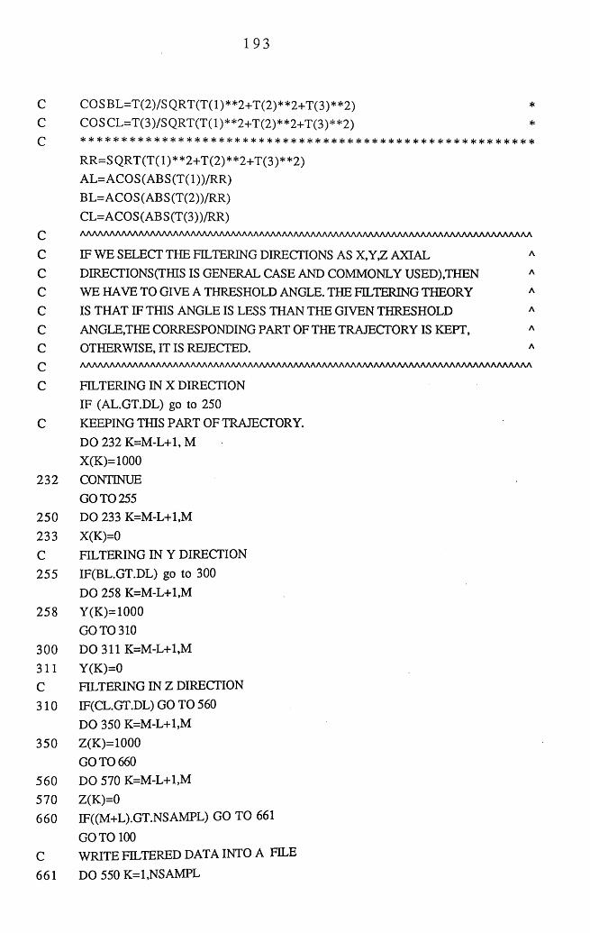
193

C COSBL=T(2)/SQRT(T(l)**2+T(2)**2+T(3)**2) *C COSCL=T(3)/SQRT(T(l)**2+T(2)**2+T(3)**2) *

RR=SQRT(T(1)**2+T(2)**2+T(3)**2)AL=ACO S (AB S (T( 1 ))/RR)BL=ACOS(ABS(T(2))/RR)CL=ACOS(ABS(T(3))/RR)

Q A A A A A A A A A A A A A A A A A A A A A A A A A A A A A A A A A A A A A A A A A A A A A A A A A A A A A A A A A A A A A A A A A A A A A A A A A A A A A A

C IF WE SELECT THE FILTERING DIRECTIONS AS X,Y,Z AXIAL AC DIRECTIONS(THIS IS GENERAL CASE AND COMMONLY USED),THEN AC WE HAVE TO GIVE A THRESHOLD ANGLE. THE FILTERING THEORY AC IS THAT IF THIS ANGLE IS LESS THAN THE GIVEN THRESHOLD AC ANGLE,THE CORRESPONDING PART OF THE TRAJECTORY IS KEPT, AC OTHERWISE, IT IS REJECTED. AQ A A A A A A A A A A A A A A A A A A A A A A A A A A A A A A A A A A A A A A A A A A A A A A A A A A A A A A A A A A A A A A A A A A A A A A A A A A A A A A

C FILTERING IN X DIRECTIONIF (AL.GT.DL) go to 250

C KEEPING THIS PART OF TRAJECTORY.DO 232 K=M-L+1, M X(K)=1000

232 CONTINUE GO TO 255

250 DO 233 K=M-L+1,M233 X(K)=0C FILTERING IN Y DIRECTION255 IF(BL.GT.DL) go to 300

DO 258 K=M-L+1,M 258 Y(K)=1000

GO TO 310 300 DO 311 K=M-L+1,M311 Y(K)=0C FILTERING IN Z DIRECTION310 IF(CL.GT.DL) GO TO 560

DO 350 K=M-L+1,M 350 Z(K)=1000

GO TO 660 560 DO 570 K=M-L+1,M570 Z(K)=0660 IF((M+L).GT.NSAMPL) GO TO 661

GOTO 100C WRITE FILTERED DATA INTO A FILE

661 DO 550 K=l,NSAMPL

194

WRITE(2,500) K,X(K),Y(K),Z(K) 500 FORMAT(I5,3E12.4)550 CONTINUE

GO TO 999 9999 STOP

END

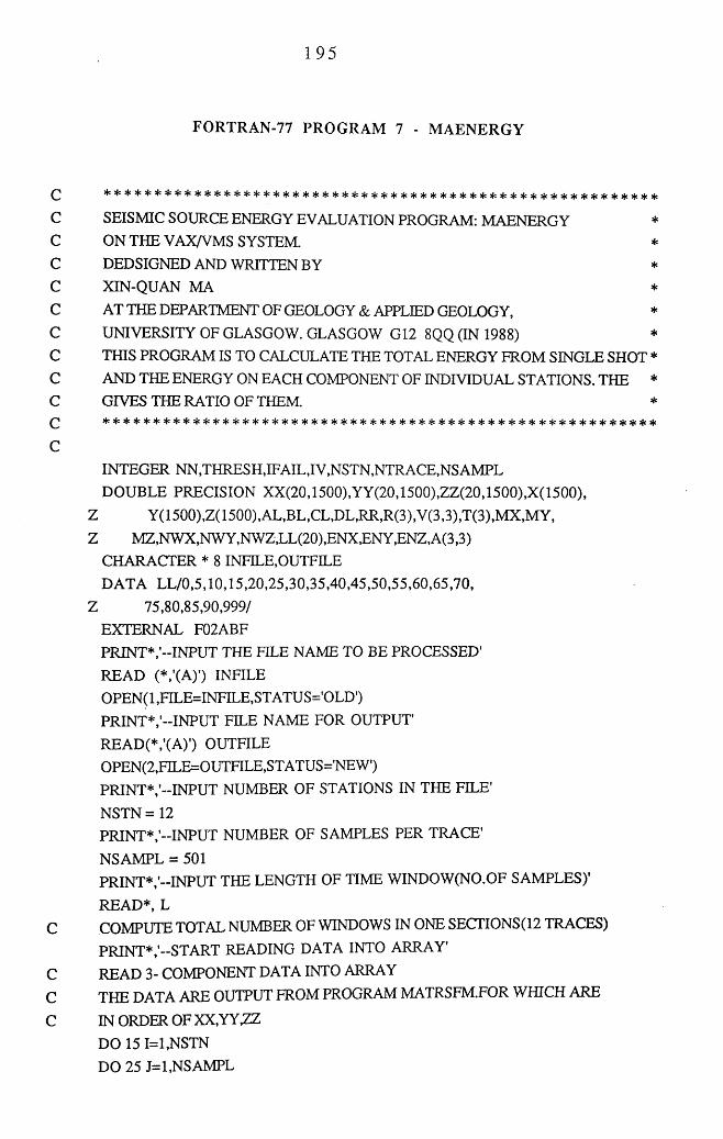
195

FORTRAN-77 PROGRAM 7 - M AENERGY

C SEISMIC SOURCE ENERGY EVALUATION PROGRAM: MAENERGY *C ON THE VAX/VMS SYSTEM. *C DEDSIGNED AND WRITTEN BY *C XIN-QUAN MA *C AT THE DEPARTMENT OF GEOLOGY & APPLIED GEOLOGY, *C UNIVERSITY OF GLASGOW. GLASGOW G12 8QQ (IN 1988) *C THIS PROGRAM IS TO CALCULATE THE TOTAL ENERGY FROM SINGLE SHOT *C AND THE ENERGY ON EACH COMPONENT OF INDIVIDUAL STATIONS. THE *C GIVES THE RATIO OF THEM. *Q s i c * * * * * * * * * * * * * * * * * * * * * * * * * * * * * * * * * * * * * * * * * * * * * * * * * * * * * * *

cINTEGER NN,THRESH,IFAIL,IV,NSTN,NTRACE,NSAMPL DOUBLE PRECISION XX(20,1500),YY(20,1500),ZZ(20,1500),X(1500),

Z Y(1500),Z(1500),AL,BL,CL,DL,RR,R(3),V(3,3),T(3),MX,MY,Z MZ,NWX,NWY,NWZ,LL(20),ENX,ENY,ENZ,A(3,3)

CHARACTER * 8 INFILE,OUTFILEDATA LL/0,5,10,15,20,25,30,35,40,45,50,55,60,65,70,

Z 75,80,85,90,999/EXTERNAL F02ABFPRINT*,'-INPUT THE FILE NAME TO BE PROCESSED’READ (*,'(A)') INFILEOPEN( 1 ,FILE=INFILE,STATU S-OLD')PRINT*,'-INPUT FILE NAME FOR OUTPUT'READ(*,'(A)') OUTFILE OPEN(2,FILE=OUTFILE,STATUS-NEW')PRINT*,'-INPUT NUMBER OF STATIONS IN THE FILE’

NSTN =12PRINT*,’-IN PUT NUMBER OF SAMPLES PER TRACE'

NSAMPL = 501PRINT*,'-INPUT THE LENGTH OF TIME WINDOW(NO.OF SAMPLES)'

READ*, LC COMPUTE TOTAL NUMBER OF WINDOWS IN ONE SECTIONS(12 TRACES)

PRINT*,'-START READING DATA INTO ARRAY'C READ 3- COMPONENT DATA INTO ARRAYC THE DATA ARE OUTPUT FROM PROGRAM MATRSFM.FOR WHICH ARE

C IN ORDER OF XX,YY,ZZDO 15 1=1,NSTN DO 25 J=l,NSAMPL

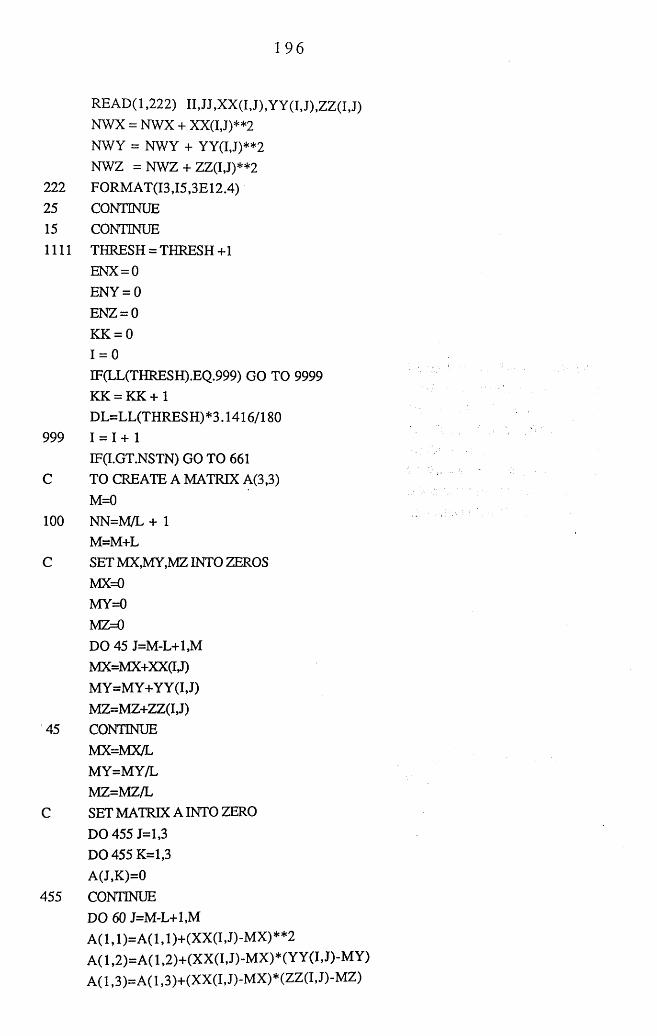
196

READ( 1,222) II,JJ,XX(I,J),YY(I,J),ZZ(I,J) NWX = NWX + XX(I,J)**2 NWY = NWY + YY(I,J)**2 NWZ = NWZ + ZZ(I,J)**2

222 FORMAT(I3,I5,3E12.4)25 CONTINUE15 CONTINUE1111 THRESH = THRESH+1

ENX = 0 ENY = 0 ENZ = 0 KK = 0 1 = 0IF(LL(THRESH).EQ.999) GO TO 9999 KK = KK + 1DL=LL(THRESH)*3.1416/180

999 1 = 1 + 1IF(I.GT.NSTN) GO TO 661

C TO CREATE A MATRIX A(3,3)M=0

100 NN=M/L + 1 M=M+L

C SET MX,MY,MZ INTO ZEROSMX=0 MY=0 MZ=0DO 45 J=M-L+1,M MX=MX+XX(IJ)MY=M Y+YY (I, J)MZ=MZ+ZZ(I,J)

45 CONTINUEMX=MX/L MY=MY/L MZ=MZ/L

C SET MATRIX A INTO ZERO

DO 455 J=l,3 DO 455 K=l,3 A(J,K)=0

455 CONTINUEDO 60 J=M-L+1,M A(1,1)=A(1,1)+(XX(I,J)-M X)**2 A( 1,2)=A( 1,2)+(XX(I, J)-MX)*(YY (I, J)-MY) A( 1,3)=A( 1,3)+(XX(I, J)-MX)*(ZZ(I, J)-MZ)

197

A(2,1)=A (2,1)+(Y Y(I,J)-M Y )*(XX (I,J)-M X)A (2,2)=A (2,2)+(Y Y (I,J)-M Y )**2A (2,3)=A (2,3)+(Y Y (I,J)-M Y )*(ZZ(I,J)-M Z)A(3,1)=A(3,1)+(ZZ(I,J)-M Z)*(XX(I,J)-M X)A(3,2)=A (3,2)+(ZZ(I,J)-M Z)*(Y Y (I,J)-M Y )A(3,3)=A (3,3)+(ZZ(I,J)-M Z)**2

60 CONTINUE DO 70 J=l,3 DO 70 K=l,3 A (J,K )=A (J,K )/L

70 CONTINUECC &&&<SC AFTER CREATING A MATRIX A, THEN COMPUTE THE EIGENVECTOR &C CORRESPONDING TO THE LARGEST EIGENVALUE OF MATRIX A(3,3) &C THAT VECTOR IN THEORY IS CONSIDERED AS A DIRECTIONAL VECTOR &C OF MAIN POLARIZATION AXIS DURING A PERIOD OF TIME. &C # # # # # # # # # # # # # # # # # # # # # # # # # # # # # # # # # # # # # # # # # # # # # # # # #c %%%%%%%%%%%%%%%%%%%%%%%%%%%%%%%%%%%%%%%C NAG ROUTINE F02ABF CALCULATES EIGENVALUES AND EIGENVECTORSC OF SYMMETRIC MATRIX. HEREC A(3,3) STANDING FOR SYMMETRIC MATRICC R(3) STANDING FOR 3 EIGENVALUESC V(3,3) STANDING FOR 3 EIGENVECTORS

IA = 3 N = 3 IFAIL = 1 IV = 3CALL F02ABF(A,IA,N,R,V,IV,E»IFAIL)

R (l) = ABS(R(1))R(3) = ABS(R(3))

C TO FIND OUT THE LARGEST EIGENVALUE AMONG 3 AND EIGENVECTORC CORRESPONDING TO THE LARGEST EIGENVALUE.

IF(R(3).LT.R(1)) THEN T (l) = ABS(V(1,1))T(2) = ABS(V(2,1))T(3) = ABS(V(3,1))ELSET (l) = ABS(V(1,3))T(2) = ABS(V(2,3))T(3) = ABS(V(3,3))END IF

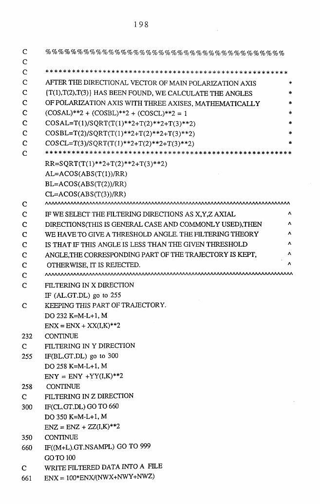
198

C % % % % % % % % % % % % % % % % % % % % % % % % % % % % % % % % % % % % % %c

C AFTER THE DIRECTIONAL VECTOR OF MAIN POLARIZATION AXIS *C {T(1),T(2),T(3)} HAS BEEN FOUND, WE CALCULATE THE ANGLES *C OF POLARIZATION AXIS WITH THREE AXISES, MATHEMATICALLY *C (COSAL)**2 + (COSBL)**2 + (COSCL)**2 = 1 *C CO SAL=T(l)/SQ RT(T(l)**2+T(2)**2+T(3)**2) *C COSBL=T(2)/SQRT(T(l)**2+T(2)**2+T(3)**2) *C COSCL=T(3)/SQRT(T(l)**2+T(2)**2+T(3)**2) *

RR=SQRT(T(1)**2+T(2)**2+T(3)**2)AL=ACO S (AB S (T( 1 ))/RR)BL=ACOS (AB S (T(2))/RR)CL=ACOS(ABS(T(3))/RR)

Q A A A A A A A A A A A A A A A A A A A A A A A A A A A A A A A A A A A A A A A A A A A A A A A A A A A A A A A A A A A A A A A A A A A A A A A A A A A A A A

C IF WE SELECT THE FILTERING DIRECTIONS ASX, Y,Z AXIAL AC DIRECTIONS(THIS IS GENERAL CASE AND COMMONLY USED),THEN AC WE HAVE TO GIVE A THRESHOLD ANGLE. THE FILTERING THEORY AC IS THAT IF THIS ANGLE IS LESS THAN THE GIVEN THRESHOLD AC ANGLE,THE CORRESPONDING PART OF THE TRAJECTORY IS KEPT, AC OTHERWISE, IT IS REJECTED. AQ A A A A A A A A A A A A A A A A A A A A A A A A A A A A A A A A A A A A A A A A A A A A A A A A A A A A A A A A A A A A A A A A A A A A A A A A A A A A A A A

C FILTERING IN X DIRECTIONIF (AL.GT.DL) go to 255

C KEEPING THIS PART OF TRAJECTORY.DO 232 K=M-L+1, M ENX = ENX + XX(I,K)**2

232 CONTINUEC FILTERING IN Y DIRECTION255 IF(BL.GT.DL) go to 300

DO 258 K=M-L+1, M ENY = ENY +YY(I,K)**2

258 CONTINUEC FILTERING IN Z DIRECTION300 IF(CL.GT.DL) GO TO 660

DO 350 K=M-L+1, M ENZ = ENZ + ZZ(I,K)**2

350 CONTINUE660 IF((M+L).GT.NSAMPL) GO TO 999

GOTO 100C WRITE FILTERED DATA INTO A FILE661 E N X = 100*EN X /(N W X +N W Y +NW Z )

199

ENY = 100 *EN Y/(NWX+N W Y+NWZ)ENZ = 100*ENZ/(NWX+NWY+NWZ)WRITE(2,500) THRESH,LL(THRESH),ENX,ENY,ENZ

500 FORMAT(I5,F6.2,3E12.4)GOTO 1111

9999 STOP END

200

FORTRAN-77 PROGRAM 8 - M ASEPF

£ * * * * * * * * * * * * * * * * s | e i i c s ) < * * * * s f e s | c s | e J ( c 5 ) « * s f e > | c 5 ( t s | e s | e s ) « s f e : l t s J c j ( c s | t s | t j | e s ( e : f c j | c : | c s ) c s | e s ( t a ( e 3 | c : | < j | c s | e : J « j | e

C SIGNAL ENHANCEMENT POLARISATION FILTER: MASEPF *C ON THE VAX/VMS SYSEM *C DESIGNED AND WRITTEN BY *C XIN-QUAN MA *C AT THE DEPARTMENT OF GEOLOGY & APPLIED GEOLOGY, *C UNIVERSITY OF GLASGOW GLASGOW G12 8QQ (IN 1988) *C THIS S OFTWARE COMPUTES THE COVARIANCE MATRIX OVER A TIME *C WINDOW AND THEN CALCULATES THE LARGEST AND THE SECOND *C LARGEST EIGENVALUES OF THIS MATRIX AND THE EIGENVECTOR *C CORRESPONDING THE LARGEST EIGENVALUE BY CALLING NAG ROUTINE *C F02ABF. THE REACTILINEARITY AND DIRECTIONALITY FUNCTIONS *C ARE CONSTRUCTED, WHICH FORMS THE FILTER OPERATORS. THE *C FILTERED SEISMOGRAMS ARE OBTAINED BY MULTIPLYING THE *C ORIGINAL SEISMOGRAMS BY FILTER OPERATORS. *C * * * * * * * * * * * * * * * * * * * * * * * * * * * * * * * * * * * * * * * * * * * * * * * * * * * * * * * *

CINTEGER MN,LL,T,L,II,IJK,III,NN,KK,JJ,JJJ,WW,NSTN,NSAMPL,

Z MM,LTH,RN,CN,IFAIL,IV,N,IA,QQ PARAMETER (RN=15,CN=1500)DOUBLE PRECISION A(3,3),F(2),G(3),MX,MY,MZ,V(3,3),E(3),R(3),

ZP(3),FTN(RN,CN),RLL(RN,CN),XX(RN,CN),YY(RN,CN),ZZ(RN,CN),Z FF,FNT(RN,CN),RL(RN,CN),DX(RN,CN),DY (RN,CN),DZ(RN,CN),Z FX(RN,CN),FY(RN,CN),FZ(RN,CN),NX(RN,CN),NY(RN,CN), ZNZ(RN,CN),DXX(RN,CN),DYY(RN,CN),DZZ(RN,CN)

CHARACTER*8 INFILE,OUTFILE,OPHLE.YORN

EXTERNAL F02ABF PRINT*,' 'PRINT*,' ’PRIN T* ' ******************************************

PRINT*,' * * 'PRINT*,' * SIGNAL ENHANCEMENT POLARISATION FILTER * '

PRINT*,' * * 'PRINT* ' ******************************************

PRINT*,' 'PRINT*,' 'PRINT*,'--INPUT DATA FILE NAME FOR FILTERING '

READ(*,'(A)') INFILEOPEN( 1 ,FILE=INFILE,STATUS-OLD')PRINT*,'--INPUT NUMBER OF STATIONS IN THE FILE'

201

NSTN = 1

PRINT*,'-INPUT THE NUMBER OF SAMPLES IN ONE TRACE 'NSAMPL = 1001PRINT*,'-INPUT THE FILE NAME FOR OUTPUT 'READ(*,'(A)') OUTFILE OPEN(2,FILE=OUTFILE,STATUS='NEW')

C INPUT THE TIME WINDOW ( NO OF SAMPLES )555 PRINT*,'-INPUT TIME WINDOW(NO.OF SAMPLES) '

READ*, LPRINT*,'-START READING DATA INTO ARRAY '

C READ THE 3-COMPONENT DATA INTO ARRAY XX(I,J),YY(I,J),ZZ(I,J)C THE DATA ARE OUTPUT FROM PROGRAM MATRSFM.FOR WHICH HAS ORDERC OFX,Y,Z.

DO 333 1=1, NSTNDO 222 J= l, NSAMPLREAD(1,111) QQ, XX(I,J),YY(I,J), ZZ(I,J)

111 FORMAT(I5,3E12.4)222 CONTINUE 333 CONTINUE7777 PRINT*,'-INPUT STATION NUMBER FOR FTLTERING(TYPE 0 TO STOP) '

READ*, I IJK=IJK+1IF((I.EQ.O) .OR. (I.GT.NSTN)) GO TO 8888

C TO CREATE COVARIANCE MATRIX A OVER THE TIME L*DT.

LL=L 27 LL=LL+1

MX=0 MY=0 MZ=0DO 33 J= LL-L, LL-1 MX=MX+XX(I,J)MY=M Y+YY (I, J)MZ=MZ+ZZ(I,J)

33 CONTINUEMX=MX/L MY=MY/L MZ=MZ/L

C SET ELEMENTS OF MATRIX INTO ZEROS

DO 6112 J=l,3 DO 6112 K=l,3 A(J,K) = 0

6112 CONTINUE

20 2

DO 44 J=LL-L,LL-1

A(1,1)=A(1,1)+(XX(I,J)-M X)**2A( 1,2)=A( 1,2)+(XX (I,J)-M X)*( YY(I, J)-M Y)A(1,3)=A(1,3)+(XX(I,J)-MX)*(ZZ(I,J)-MZ)A(2,1)=A(2,1)+(YY(I,J)-M Y)*(XX(I,J)-M X)A (2,2)=A (2,2)+(Y Y (I,J)-M Y )**2A(2,3)=A(2,3)+(YY(I,J)-M Y)*(ZZ(I,J)-M Z)A (3,1 )=A (3,1 )+(ZZ(I,J)-M Z) *(XX(I,J)-MX) A (3,2)=A (3,2)+(ZZ(I,J)-M Z)*(Y Y (I,J)-M Y )A (3,3)=A (3,3)+(ZZ(I,J)-M Z)**2

44 CONTINUE DO 55 J=l,3 DO 55 K=l,3 A (J,K )=A (J,K )/L

55 CONTINUEC !!!!!!!!!!!!!!!!!!!!!!!!!!!!!!!!!!!!!!!!!!!!!!!!!!!!!!!!!!!!!!!!!!!!!!!!!!!!!!!!!!!!!!!!!!!!!!!!!!!!!!!!!!!!!!!!!!!!!!!!!!!!!!!!!!!Q s|* * * * * * * * * * * * * * * * * * * * * * * * * * * * * * * * * * * * * * * * * * * * * * * * * * * * * * * *

C AFTER CREATING MATRIX A(3,3), THE NAG ROUTINE F02ABF IS *C USED TO CALCULATE THREE EIGENVALUES AND CORRESPONDING THREE *C EIGENVECTORS .HOWEVER, ONLY THE LARGEST AND THE SECOND *C LARGEST EIGENVALUES ARE USED IN THIS PROGRAM. SO IS THE *C EIGENVECTOR CORRESPONDING THE LARGEST EIGENVALUE. *C NAG ROUTINE F02ABF CALCULATES EIGENVALUES AND EIGENVECTORS *C OF SYMMETRIC MATRIX. HERE *C A(3,3) STANDING FOR SYMMETRIC MATRIX *C R(3) STANDING FOR 3 EIGENVALUES *C V(3,3) STANDING FOR 3 EIGENVECTORS *£ * * * * * * * * * * * * * * * * * * * * * * * * * * * * * * * * * * * * * * * * * * * * * * * * * * * * * * * *

IA = 3 N = 3 IFAIL = 1 IV = 3CALL F02ABF(A,IA,N,R,V,IV,E,IFAIL)R (l) = ABS(R(1))R(2) = ABS(R(2))R(3) = ABS(R(3))

C TO FIND OUT THE LARGEST EIGENVALUE AMONG 3 AND EIGENVECTORC CORRESPONDING TO THE LARGEST EIGENVALUE.

IF(R(3).LT.R(1)) THEN

F (l) = R (l)G (l) = ABS(V(1,1))G(2) = ABS(V(2,1))G(3) = ABS(V(3,1))

203

F(R(2).LT.R(3)) GO TO 6109 F(2) = R(2)GO TO 7009

6109 F(2) = R(3)7009 CONTINUE

ELSEF (l) = R(3)G (l) = ABS(V(1,3))G(2) = ABS(V(2,3))G(3) = ABS(V(3,3))IF(R(2).LT.R( 1)) GO TO 7109 F(2) = R(2)GOTO 7209

7109 F(2) = R (l)7209 ENDIF

C !!!!!!!!!!!!!!!!!!!!!!!!!!!!!!!!!!!!!!!!!!!!!!!!!!!!!!!!!!!!!!!!!!!!!!!!!!!!!!!!!!!!!!!!!!!!!!!!!!!!!!!!!!!!!!!!!!!!!!!!!!!!!!!!!!!! C AFTER FINDING THE LARGEST AND SECOND LARGEST EIGENVALUESC WE NOW CONSTRUCT A FUNCTION CALLED FTN.

I I= L L - l- (L - l ) /2NN=1JJ=1KK=1F T N (I,II)= 1-(F (2)/F (1))**N N

C TO MEASURE THE RECTILINEARITY AT TIME To, A NEW FUNC-C TION CALLED RL IS NOW CONSTRUCTED.

R L (I,II)= F T N (I,II)**JJ C TO CREATE THE DIRECTION FUNCTIONS AT TIME To, WE CONS-C TRUCT DX,DY AND DZ.

DX(I,II) = G(1)**KK DY(I,II) = G(2)**KK DZ(I,II) = G(3)**KK IF(II.LE.(NSAMPL-(L-l)/2)) GO TO 27

C NOTICE THAT WE CAN NOT OBTAIN THE FILTER OPERATORS FORC FIRST (L/2 -1) POINTS, BUT TAKEN THEM AS SAME AT THAT OF

C POINT L/2.III= 1+ (L -1 )/2 DO 888 N =l,(L-l)/2 R L (I,N )= R L (I,III)DX(I,N)=DX(I,III)D Y (I,N )=DY (I,III)DZ(I,N)=DZ(I,III)

888 CONTINUE

2 0 4

C NOTICE THAT WE CAN NOT OBTAIN THE FILTER OPERATORS FORC THE LAST (L-l)/2 POINTS, BUT TAKEN THEM AS SAME AS THATC OF POINT (MN-(L-l)/2).C JJJ IS LT CENTRE POINT IN ABOVE LOOP

JJJ=II-1DO 950 MM=II,NSAMPL R L(I,M M )=R L(I,JJJ)DX(I,MM)=DX(I,JJJ)DY(I,M M )=DY(I,JJJ)DZ(I,MM)=DZ(I,JJJ)

950 CONTINUEC TO WEIGHT OPERATOR FUNCTIONSC TO SET WINDOW LENGTH FOR SMOOTHING THE FUCTIONS.

LTH =11 M = (L T H -l)/2DO 434 J=l+(LTH-l)/2, NSAMPL-(LTH-l)/2 DO 433 T=-M,M R LL(I,J)=R LL(I,J)+R L(I,J+T)DXX(I,J)=DXX(I,J)+DX(I,J+T)D YY (I, J)=DY Y (I, J)+D Y (I, J+T)DZZ(I,J)=DZZ(I,J)+DZ(I,J+T)

433 CONTINUE R L (I,J)=R L L(I,J)/LTH DX(I,J)=DXX(I,J)/LTH DY(I,J)=DYY(I,J)/LTH DZ(I,J)=DZZ(I,J)/LTH

434 CONTINUEC OPERATOR FUNCTIONS FX,FY,FZ

DO 553 J=l,NSAMPL FX(I,J)=RL(I,J)*DX(I,J)FY (I,J)=R L (I,J)*D Y (I,J)FZ(I,J)=RL(I,J)*D Z(I,J)

553 CONTINUEC THE GAIN FUNCTIONS FX,FY AND FZ ARE CONSIDERED AS THEC FILTER OPERATORS. THE FILTERED SEISMOGRAMS ARE OBTAINEDC BY MULTIPLYING THE ORIGINAL SEISMIGRAMS BY FILTER OPERATORS.

DO 890 J= 1, NSAMPL NX(I,J)=XX(I,J)*FX(I,J)N Y (I,J)=Y Y (I,J)*FY (I,J)NZ(I,J)=ZZ(I,J)*FZ(I,J)

890 CONTINUEC SO FAR, THE 3 TRACES FOR ONE STATION HAVE BEEN FILTEREDC NEXT IS IF COMMAND ASKING FOR NEXT TRACES TRACES TO BE

205

C FILTERED.GO TO 7777

C AFTER NSTRN STATIONS HAVE BEEN FINISHED, THIS PROGRAM IS TOC WIRIT FILTERED DATA INTO FILE8888 PRINT*,'-START WRITING FILTERED DATA INTO FILE '

DO 8890 J = 1, UK-1DO 8890 K = 1, NSAMPL WRITE(2,8889) K, NX(J,K),NY(J,K),NZ(J,K)

8889 FORMAT( 15, )8890 CONTINUE444 PRINT*,'-DO YOU WANT TO KEEP OPERATOR FUNCTIONS(Y/N)’

READ(*,’(A)') YORN EF(YORN.EQ.’N') GO TO 9999 IF(YORN.EQ.'Y') GO TO 666PRINT*,’-Y O U INPUT A WRONG LETTER,TRY AGAIN!’GO TO 444

666 PRINT*,’-IN PUT FILE NAME FOR OPERATOR FUNCTIONS 'READ(*,’(A)') OPFILE OPEN(3,FILE=OPFILE,STATUS-NEW')PRINT*,'-START WRITING FILTER FUNCTIONS INTO FILE 'DO 7790 J = 1, UK-1DO 7790 K = l , NSAMPLWRITE(3,7789) K, FX(J,K),FY(J,K),FZ(J,K)

7789 FORMAT( 15, 3E12.4)7790 CONTINUE 9999 CLOSE(2)

CLOSE(3)STOPEND

206

FORTRAN-77 PROGRAM 9 - M AVHPL

C * * * * * * * * * * * * * * * * * * * * * * * * * * * * * * * * * * * * * * * * * * * * * * * * * * * * * * * *

C GENERATION SYNTHETIC SEISMOGRAM PROGRAM: MAVHPL *C ON THE VAX/VMS SYSTEM. *C DESIGNED AND WRIITEN BY *C XIN-QUAN MA *C AT THE DEPARTMENT OF GEOLOGY & APPLIED GEOLOGY, *C UNIVERSITY OF GLASGOW GLASGOW G12 8QQ (IN 1989) *C THIS PROGRAM IS USED IN CONJUNCTION WITH MODELLING PACKAGE *C SEIS83 AND VERTPL. TRACE LENGTH IS 4 SEC, SAMPLING RATE IS 4 MS. *C * * * * * * * * * * * * * * * * * * * * * * * * * * * * * * * * * * * * * * * * * * * * * * * * * * * * * * * *

CREAL TO,LI ,L2,NP,Y(200,20)INTEGER LO,NN,NO,X(200,20)CHARACTER* 10 INFILE,OUTFELE CHARACTER* 70 BOPEN(l,FILE='SEISGRAM',STATUS-OLD')OPEN (2 ,FILE='VMA' ,ST ATUS-NEW')DO 30 1=1,3 READ(1,89),B

89 FORMAT(A70)30 CONTINUE

NN = 0 333 NN = NN +1

IF(NN.EQ.3) STOPC TO IS THE TIME OF THE FIRST POINT IN SYNTHETIC SEISMOGRAM.C NP IS NUMBER OF POINTS IN SYNTHETIC SEISMOGRAM.

READ(1,90) TO.NP90 FORMAT(25X, F10.5, F5.0)

NO = NINT(TO/0.004)LI = NP/18L2 = ANINT(NP/18)IF((L1-L2).GT.0.0) THEN LO = NINT(L2) + 1 ELSELO = NINT(L2)END IF

5 DO 1001=1 J^OREAD(1,10) X(I,1),X(I,2),X(I,3),X(I,4),X(I,5),

Z X(I,6),X(I,7),X(I,8),X(I,9),X(I,10),Z X(I,n),X(I,12),X(I,13),X(I,14),X(I,15),

20 7

Z X(1,16),X(1,17),X(1,18)Y (1,1) = X(I,1)Y(I,2) = X(I,2)

Y(I,3) = X(I,3)Y(I,4) = X(I,4)Y(I,5) = X(I,5)Y(I,6) = X(I,6)Y(I,7) = X(I,7)Y(I,8) = X(I,8)Y(I,9) = X(I,9)Y(I,10) = X(I,10)Y(I,11) = X(I,11)Y(I,12) = X(I,12)Y(I,13) = X(I,13)Y(I,14) = X(I,14)Y(I,15) = X(I,15)Y(I,16) = X(I,16)Y(I,17) = X(I,17)Y(I,18) = X(I,18)

10 FORMAT(18I4)100 CONTINUE

DO 260 1 = 1, NO-1 WRITE(2,200) I, 0.0

260 CONTINUE K = NO-1 DO 3001=14.0 DO 300 J=l,18 K=K+1WRITE(2,200) K,Y(I,J)

200 FORMAT(I5,E12.4)300 CONTINUE

DO 3601 = NO+LO*18, 1001 WRITE(2,200) I, 0.0

360 CONTINUE GO TO 333

99 CLOSE(UNIT=2)

STOPEND

208

FORTRAN-77 PROGRAM 10 - MASSP

C * * * * * * * * * * * * * * * * * * * * * * * * * * * * * * * * * * * * * * * * * * * * * * * * * * * * * * * *

C SLANT-STACK PROCESSING PROGRAM ON THE VAX/VMS SYSTEM: MASSP *C DESIGNED AND WRITTEN BY *C XIN-QUAN MA *C AT THE DEPARTMENT OF GEOLOGY & APPLIED GEOLOGY, *C UNIVERSITY OF GLASGOW, GLASGOW G12 8QQ (IN 1989) *C THIS PROGRAM IS TO PROJECT ALL THE 12 STATIONS TO A *C SPECIFIED LINE WITH CERTAIN ANGLE TO THE EAST DEFINED *C BY THE USER AND THEN TO CALCULATE THE NEW OFFSETS OF *C DIFFERET STATIONS ACCORDING TO ARRAY GEOMETRY.FINALLY, *C TO CARRY OUT SLANT STACKING OR BEAM STEERING PROCESS. *C THE ARRAY CONSISTS OF 12 3-CONPONENT GEOPHONES WITH *C UNIT DIMENSION D. *

C

REAL D,RATE,UPDJLOD,ALPHA,U(100,5000),Z(20,5000)REAL B(12),DT(12),P(100),UPP,PIC,TAU,LOP,PIINTEGER NP,TA,NSAMPLCHARACTER* 8 FILEOUT.FILEIN,YONDATA B /90 ,120,150,180,210,240,270,300,330,0,30,60/PRINT*,' 'PRINT*,' ’PR IN T* ' ******************************************** '

PRINT*,' * * ’PRINT*,' * SLANT STACKING FORTRAN PROGRAM * '

PRINT* ' * * 'PR IN T* ' *********************************************

PRINT*,’ 'PRINT*,’ 'DO 789 1= 1,12 DO 789 J=2002,3000 Z(I,J) = 0.00000

789 CONTINUEPRINT*,'-INPUT FILE NAME FOR PROCESS PLEASE!'

READ(*,'(A)') FILEINOPEN(l,FILE=FILEIN,FORM='FORMATTED',STATUS-OLD')

C INPUT THE ALL PARAMETERS NSAMPL = 2001 LOP =-6.66667E-4 UPP = 6.66667E-4

2 0 9

PRINT*,'-INPUT NUMBER OF RAY PARAMETERS YOU NEED PLEASE!’ READ*,NP

C CALCULATE THE RAY PARAMETER INCREMENT PICPIC=(UPP-LO P)/N P D = 75

C DEFINE A 2-DIMENSION ARRAY,INPUT 12 TRACE SEISMIC DATAC INTO THIS ARRAY-Z(I,J)

PRINT*,' '

PRINT*, '-START READING 12-TRACE DATA INTO ARRAY U(I,J)' PRINT*,' ’DO 1001= 1, 12 DO 100 J = 1, 2001 READ(1,50) Z(I,J)

50 FORMAT(5X,E12.4)100 CONTINUE

GO TO 889776 PRINT*,’-DO YOU WANT TO TRY MORE ALPHA(Y/N)EG."Y" OR "N T777 READ(*,’(A)’),Y ON

EF(YON.EQ.’N’) GO TO 999 EF(YON.EQ.’Y') GO TO 889PRINT*,'-YOU INPUT A WRONG CHARACTER,TRY AGAIN!'GO TO 777

889 PRINT*, '-INPUT ARIMUTH ALPHA PLEASE!'READ*, ALPHAPRINT*,'-INPUT FILE NAME FOR OUTPUT PLEASE! ' READ(*,'(A)'),FILEOUTOPEN(2,FELE=FlLEOUT,FORM='FORMATTED',STATUS='NEW')

C CALCULATE THE OFFSET DISTANCE OF THE FIRST GEOPHONE

PRINT*,’ 'PRINT*,’-START COMPUTE OFFSET DISTANCES(PROJECTION)’

PRINT*,' 'LOD=D UPD = 130 PI = 3.1416/180DT(1) = UPD*COS((ALPHA-B(l))*PI)DT(2) = LOD*COS((ALPHA-B(2))*PI)DT(3) = UPD*COS((ALPHA-B(3))*PI)DT(4) = LOD*COS((ALPHA-B(4))*PI)DT(5) = UPD*COS((ALPHA-B(5))*PI)DT(6) = LOD*COS((ALPHA-B(6))*PI)DT(7) = UPD*COS((ALPHA-B(7))*PI)DT(8) = LOD*COS((ALPHA-B(8))*PI)

210

DT(9) = UPD*COS((ALPHA-B(9))*PI)DT(10) = LOD*COS((ALPHA-B(10))*PI)D T (ll) = UPD*C0S((ALPHA-B(11))*PI)DT(12) = LOD*COS((ALPHA-B( 12))*PI)

C FOR THIS SHOT POINT, 12 STATIONS HAVE BEEN PROJECTED INTOC A LINE WITH ANGLE ALPHA DEFINED BY USER. THE 12 OFFSETC DISTANCES HAVE BEEN OBTAINED X01.X02.X03.......X11.X12.C TO CARRY OUT BEAM STEERING WE NEED RAY PARAMETER p.AND OFFSETC TIME TAU.IT MEANS THAT WE SUM ALL WAVE APLITUDE WITH SLOPE PC OFFSET TIME TA U -A DECLINED LINE.C THE FORMULA IS AS FOLLOWING:C U(P,TAU)= SIGMA (U(Xj,T=TAU+P*Xj))C IN THIS PROGRAM WE USE THREE LOOPS TO SUM THE VALUES.

PRINT*,' 'PRINT*,'-START SLANT STACKING PROCESS'PRINT*,' 'P(0)=LOP

C THE FIRST LOOP DEFINES NUMBER OF P TRACES,IT ALSO MEANSC NO. OF DIFFERENT SLOPES GIVEN.

DO 500 1=1,NP P (I)= P (I-1 )+ P IC

C THIS LOOP DEFINES INTERCEPT TIME VALUES-TAU FOR PROCESSING.TAU = 0.0DO 300 J=l,NSAMPL TAU=TAU+2*0.001 TA = TAU/(2*0.001)

C TO INITIALIZE COUNTERM

M=0DO 200 K=l,12N =T A U /(2*0.001)+N IN T((P(I)*D T(K ))/(2*0.001))

M=M+196 U(I,TA)=U(I,TA)+Z(K,N)200 CONTINUEC TO NORMOLIZE STACKED DATA— THE SUMMED DATA DIVIDED BY

C NUMBER OF TRACES(M)97 U(I,TA )=U (I,TA )/M300 CONTINUE

DO 101 J = 1301, 180198 W RITE(2,99) J.U(I.J)99 FORMAT(I5,E12.4)

101 CONTINUEPRINT*,'-RAY PARAMETER',I,' COMPLETED'

500 CONTINUE

211

PRINT*,' 'GO TO 776

999 PRINT*,’-CALCULATION COMPLETED'CLOSE(2)STOPEND

FORTRAN-77 PROGRAM 11 - M APRISM

* * * * * * * * * * * * * * * * * * * * * * * * * * * * * * * * * * * * * * * * * * * * * * * * * * * * * *

Computing the gravity effect of a prism, a line mass and sylinder on VAX/UNIX: MAPRISM W ritten by XIN-QUAN MAat the Department of Geology & Applied Geology,Univrsity of Glasgow, Glasgow G12 8QQ (in 1987)This program calculates the gravity effect from a vertical prism with horizontal upper and lower faces, expressed by a 24-term formula; from a prism with a horizontal lower face and a sloping upper face; from a line mass; and from a sector o f a hollow sylinder. * * * * * * * * * * * * * * * * * * * * * * * * * * * * * * * * * * * * * * * * * * * * * * * * * * * * * *

real x l,x 2 ,y I,y 2 ,h ,tl,t2 ,t3 ,t4 ,t5 ,t6 ,t7 ,t8 ,t9 ,1 0 ,tll ,tl2 ,F z ,i,j ,K ,g l,g 2 ,g 3 ,c ,c o sa ,r ,P ,g 4p rin t* ,'in p u t x l ,y l ,h 'r e a d * ,x l ,y l ,hx2=x1+1000y2=yl+1000tl= lo g ((y 2 + sq rt(x 2 * x 2 + y 2 * y 2 )) /(y 2 + sq rt(x 2 * x 2 + y 2 * y 2 + h * h ))) t2 = lo g ((y l+ sq r t(x 2 * * 2 + y 1 * *2 ))/(y l+ sq rt(x 2 * * 2 + y 1 **2+ h**2))) t3 = lo g ((y 2 + sq rt(x 1 * * 2 + y 2 * * 2 ))/(y 2 + sq rt(x l* * 2 + y 2 * * 2 + h * * 2 ))) t4 = lo g ((y l+ s q r t ( x l **2+y 1 **2 ))/(y l+ s q r t(x l* * 2 + y 1 **2+ h**2))) t5 = lo g ((x 2 + sq rt(x 2 * * 2 + y 2 * * 2 ))/(x 2 + sq rt(x 2 * * 2 + y 2 * * 2 + h * * 2 ))) t6 = lo g ((x l+ sq r t(x 1 * * 2 + y 2 * * 2 ))/(x l+ sq rt(x 1 **2+ y2**2+ h**2))) t7 = lo g ((x 2 + sq rt(x 2 * * 2 + y 1 * * 2 ))/(x2+ sq rt(x2**2+ y 1 **2+ h**2))) t8 = lo g ((x l+ s q r t(x 1 **2+y 1 * * 2 ) ) /(x l+ s q r t(x l **2+y 1 **2+ h**2))) t9 = a s in ((y 2 * * 2 + h * * 2 + y 2 * sq rt(x 2 * * 2 + y 2 * * 2 + h * * 2 ))/((y 2 + s q r t(x 2 * * 2 + y 2 * * 2 + h * * 2 ))* sq r t(y 2 * * 2 + h * * 2 )))1 1 0 = a sin ((y 2 * * 2 + h * * 2 + y 2 * sq rt(x l* * 2 + y 2 * * 2 + h * * 2 ))/((y 2 + s q r t ( x l * * 2 + y 2 * * 2 + h * * 2 ))* sq rt(y 2 * * 2 + h * * 2 ))) t l l= a s in ((y 1 **2+ h**2+ y 1 * sq rt(x2**2+ y 1 * * 2 + h * * 2 ))/((y 1 + sq rt(x 2 * * 2 + y 1 * * 2 + h * * 2 ))* sq rt(y l* * 2 + h * * 2 ))) t l 2 = asin ((y 1 ** 2 + h * * 2 +y 1 * s q rt(x l* * 2 + y l* * 2 + h * * 2 )) /( (y 1 +

s q rt(x 1 **2+y 1 * * 2 + h * * 2 ))* sq rt(y 1 * * 2 + h * * 2 ))) F z = x 2 * (tl- t2 )-x l* ( t3 -t4 )+ y 2 * (t5 - t6 )-y l* ( t7 - t8 )+

h * ( t9 - t l0 - t l l+ t l2 ) p rin t* ,'F z= ',F z i= (x l+ 500)/1000 j= (y l+ 5 0 0 )/1 0 0 0r= sq rt((x l+ 500)**2+(y l+ 500)**2)

213

c = sq r t( r* * 2 + h * * 2 )c o s a = r /c

K = (i+ 0 .5 )* log ((j+ 0 .5 )+ sq rt((i+ 0 .5 )**2+ (j+ 0 .5 )**2 )) z - ( i-0 .5 )* lo g (( j+ 0 .5 )+ sq rt(( i-0 .5 )* * 2 + (j+ 0 .5 )* * 2 )) z + (j+ 0 .5 )* lo g ((i+ 0 .5 )+ sq rt((i+ 0 .5 )* * 2 + (j+ 0 .5 )* * 2 )) z - ( j+ 0 .5 )* lo g (( i-0 .5 )+ sq rt(( i-0 .5 )* * 2 + (j+ 0 .5 )* * 2 )) z - ( i+ 0 .5 )* lo g (( j-0 .5 )+ sq rt(( i+ 0 .5 )* * 2 + (j-0 .5 )* * 2 )) z + ( i-0 .5 )* lo g (( j-0 .5 )+ sq r t( ( i-0 .5 )* * 2 + (j-0 .5 )* * 2 )) z - ( j-0 .5 )* lo g (( i+ 0 .5 )+ sq rt(( i+ 0 .5 )* * 2 + (j-0 .5 )* * 2 )) z + G -0 .5 )* lo g ((i-0 .5 )+ sq rt(( i-0 .5 )* * 2 + (j-0 .5 )* * 2 ))

P = l/s q r t( i* * 2 + j* * 2 ) p rin t* , 'K = \K p r in t* , ’P = ',P print*,1 'g l= a b s (0 .006672*2.70*Fz)g2= 6 .672*2 .7 0 * (l-co sa )* Kg3 = 6 6 7 2 * 2 .7 0 * ( l / r - l /c )g 4 = 3 3 3 6 * 2 .7 0 * h * * 2 /(r* * 3 -r* 2 .5 E 0 5 )p r in t* , 'r = ’,rp r in t* , 'p r i s m = ',g lp rin t* ,'s lo p p in g p rism = ',g2p rin t* ,'lin e m ass= ',g3p r in t* , 's y l in d e r= ’,g4s tope n d

214

FORTRAN-77 PROPGRAM 12 - MAEIGEN

Q H e * * * * * * * * * * * * * * * * * * * * * * * * * * * * * * * * * * * * * * * * * * * * * * * * * * * * * *

C THE FOLLOWING TWO SUNROUTINES ARE USED TO CALCULATE THE *C EIGENVALUES AND EIGENVECTORS OF A SYMMETRIC MATRIX. THE *C EIGENVALUES ARE, ON OUPUT, IN DECEANT ORDER.C *Q * * * * * * * * * * * * * * * * * * * * * * * * * * * * * * * * * * * * * * * * * * * * * * * * * * * * * * *

SUBROUTINE JACOBI(A,N,NP,D,V,NROT)PARAMETER (NMAX=100)DIMENSION A(NP,NP),D(NP),V(NP,NP),B(NMAX),Z(NMAX)DO 12 IP=1,N DO 11 IQ=1,N V(IP,IQ)=0.

11 CONTINUE V (IP ,IP )= 1.

12 CONTINUE DO 13 IP=1,N B (IP )= A (IP ,IP )D (IP)=B (IP)Z(IP)=0.

13 CONTINUE NROT=0 DO 24 1=1,50 SM=0.DO 15 IP=1,N-1 DO 14 IQ=IP+1,N SM=SM+ABS(A(IP,IQ))

14 CONTINUE15 CONTINUE

IF(SM.EQ.O.)RETURN IF(I.LT.4) THEN THRESH=0.2*SM /N**2 ELSETHRESH=0.ENDIFDO 22 IP=1,N-1 DO 21 IQ=IP+1,N G=100.*ABS(A(IP,IQ))IF((I.GT.4) .AND. (ABS(D(IP))+G .EQ.ABS(D(IP)))* .AND. (ABS(D(IQ))+G .EQ. ABS(D(IQ)))) THEN

A(IP,IQ)=0.ELSE IF(ABS(A(IP,IQ)).GT.THRESH)THEN

215

H=D(IQ)-D(IP)IF(ABS(H)+G .EQ. ABS(H))THENT=A(IP,IQ)/HELSETHETA=0.5*H/A(IP,IQ)T= 1./(AB S (THET A)+S QRT( 1. +THET A* *2))IF(THETA.LT.O.)T=-TEND IF

C=1./SQRT(1+T**2)S=T*CTAU=S/(1.+C)H=T*A(IP,IQ)Z(IP)=Z(IP)-HZ(IQ)=Z(IQ)+HD(IP)=D(IP)-HD(IQ)=D(IQ)+HA(IP,IQ)=0.DO 16 J=1,IP-1 G=A(J,IP)H=A(J ,IQ)A(J,IP)=G-S*(H+G*TAU)A(J,IQ)=H+S * (G-H*TAU)

16 CONTINUEDO 17 J=IP+1,IQ-1 G=A(IP,J)H=A(J,IQ)A(IP,J)=G-S*(H+G*TAU)A(J JQ)=H+S *(G-H*TAU)

17 CONTINUE DO 18 J=IQ+1,N G=A(IP,J)H=A(IQ,J)A(IP,J)=G-S*(H+G*TAU)A(IQ,J)=H+S*(G-H*TAU)

18 CONTINUE DO 19 J=1,N G=V(J,IP)H=V(J,IQ)V(J,IP)=G-S*(H+G*TAU)V(J,IQ)=H+S*(G-H*TAU)

19 CONTINUE NROT=NROT+l

21 6

ENDIF21 CONTINUE22 CONTINUE

DO 23 IP-1,NB (IP)=B (IP)+Z(IP)D(IP)=B(IP)Z(IP)=0.

23 CONTINUE24 CONTINUE

PAUSE '50 ITERATIONS SHOULD NEVER HAPPEN'RETURNEND

cSUBROUTINE EIGSRT(D,V,N,NP)DIMENSION D(NP),V(NP,NP)DO 13 1=1, N-lK=IP=D(I)DO 11 J=I+1,N IF(D(J).GE.P) THEN K=J P=D(J)ENDIF

11 CONTINUE IF(K.NE.I)THEN D(K)=D(I)D(I)=PDO 12 J=1,N P=V(J,I)V(J,I)=V(J,K)V(J,K)=P

12 CONTINUE ENDIF

13 CONTINUE RETURN END