1 Prediction of Oil Production With Confidence Intervals* James Glimm 1,2, Shuling Hou 3, Yoon-ha Lee 1, David H. Sharp 3, Kenny Ye 1 1. SUNY at Stony.

1

Prediction of Oil Production With Confidence Intervals*

James Glimm1,2, Shuling Hou3, Yoon-ha Lee1,David H. Sharp3, Kenny Ye1

1. SUNY at Stony Brook2. Brookhaven National Laboratory3. Los Alamos National Laboratory

*Supported in part by the Department of Energy and National Science Foundation

2

Application of Prediction Theory

Reservoir Development Choices, for example Sizing of Production Equipment Location of Infill Drilling

During Early Development Stages Risk high Payoff high

3

Basic Idea: I

History match with probability of error

Start with geostatistical probability model for permeability, etc.

Observe production rates, etc.

4

Basic Idea: II

Multiple simulations from ensemble

(Re)Assign probabilities based on data, degree of mismatch of simulation to history

5

Basic Idea: III

Redefine probabilities and ensemble to be consistent with:

(a) data

(b) probable errors in simulation and data

6

Basic Idea: IV

New ensemble of geologies = Posterior

Prediction = sample from posterior

Confidence intervals come from

- posterior probabilities

- errors in forward simulation

7

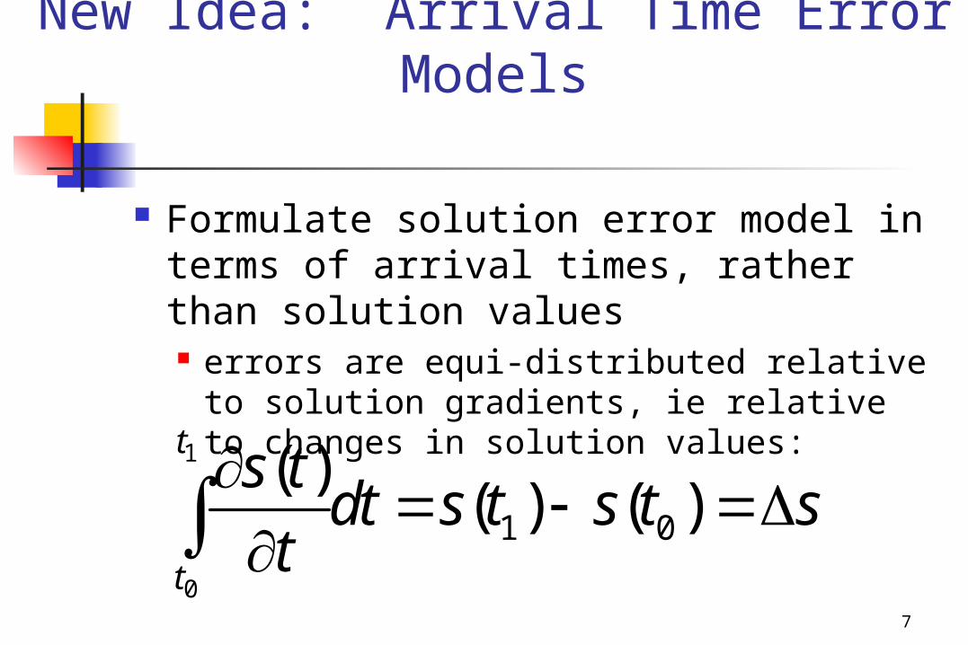
New Idea: Arrival Time Error Models

Formulate solution error model in terms of arrival times, rather than solution values errors are equi-distributed relative to

solution gradients, ie relative to changes in solution values:1

0

1 0

( )( ) ( )

t

t

s tdt s t s t s

t

8

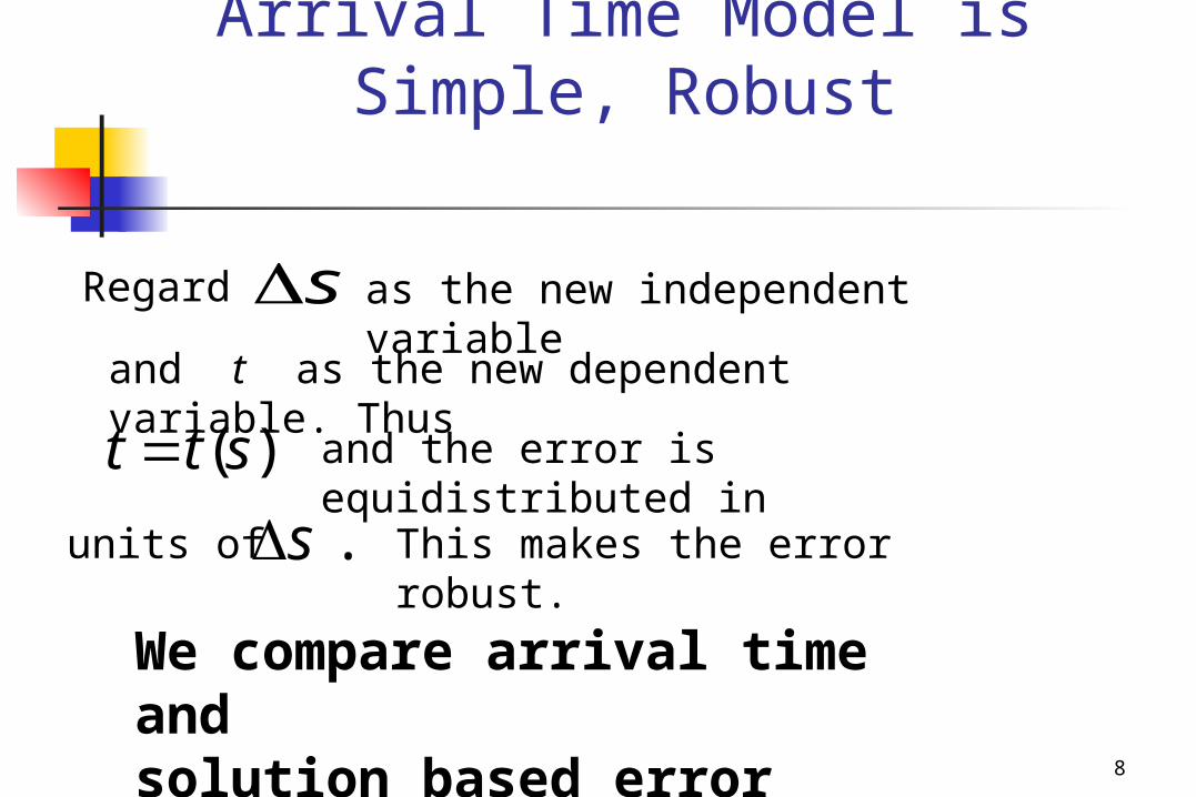
Arrival Time Model is Simple, Robust

Regard s as the new independent variable

and t as the new dependent variable. Thus

( ) t t s and the error is equidistributed in

units of .s This makes the error robust.

We compare arrival time and solution based error models

9

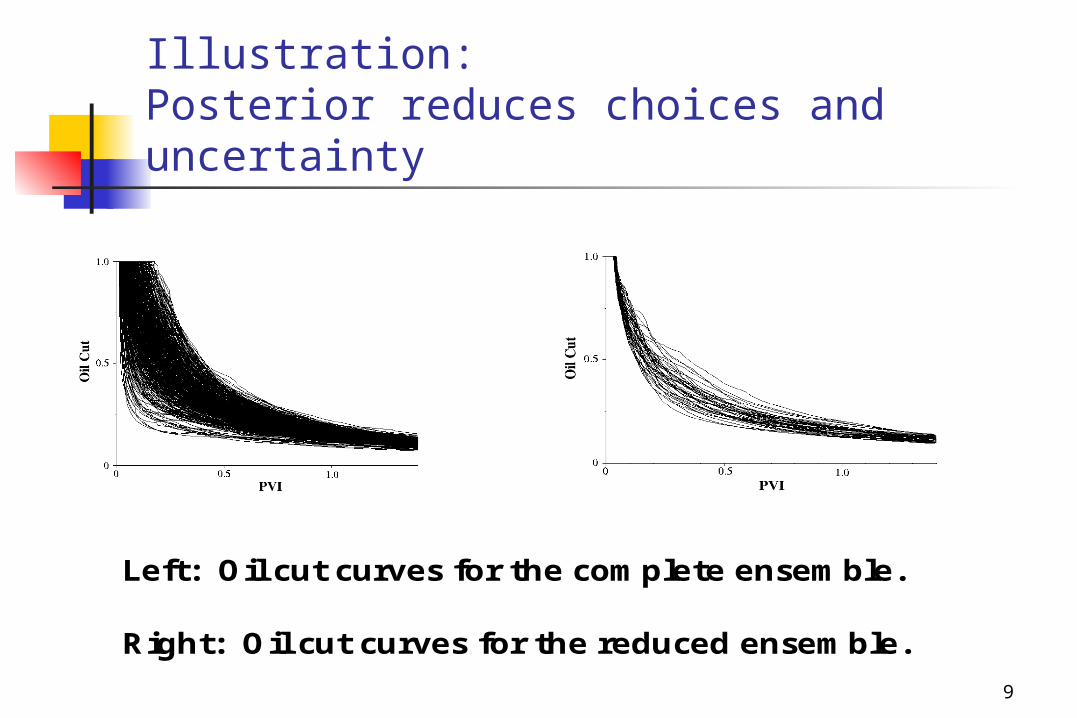
Illustration:Posterior reduces choices and uncertainty

Left: Oil cut curves for the complete ensemble.

Right: Oil cut curves for the reduced ensemble.

10

New Result: Predict outcomes and risk

Risk is predicted quantitatively

Risk prediction is based on

- formal probabilities of errors

in data and simulation

- methods for simulation error analysis

- Rapid simulation (upscale) allowing

exploration of many scenarios

11

Problem Formulation

Simulation study:

Line drive, 2D reservoir

Random permeability field

log normal, random correlation length

),( yxK

12

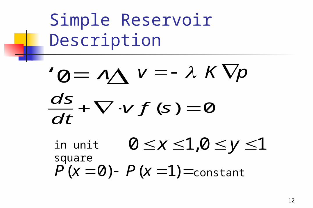
Simple Reservoir Description

pKv

0)( sfvdt

ds

in unit square

10,10 yx

)1()0( xPxP constant

, 0 v

13

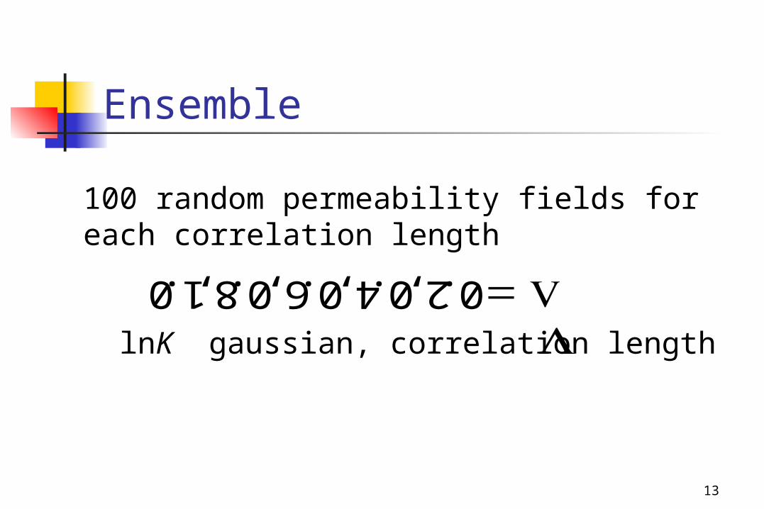
Ensemble

100 random permeability fields for each correlation length

lnK gaussian, correlation length

0. 1, 8. 0, 6. 0, 4. 0, 2. 0

14

Upscaling

Solution from fine grid

100 x 100 grid

Solution by upscaling

20 x 20, 10 x 10, 5 x 5

Upscaled grids

15

Upscaling by

Wallstrom, Hou, Christie, Durlofsky,

Sharp

1. Computational Geoscience 3:69-87

(1999)

2. SPE 51939

3. Transport in Porous Media (submitted)

Upscaling References

16

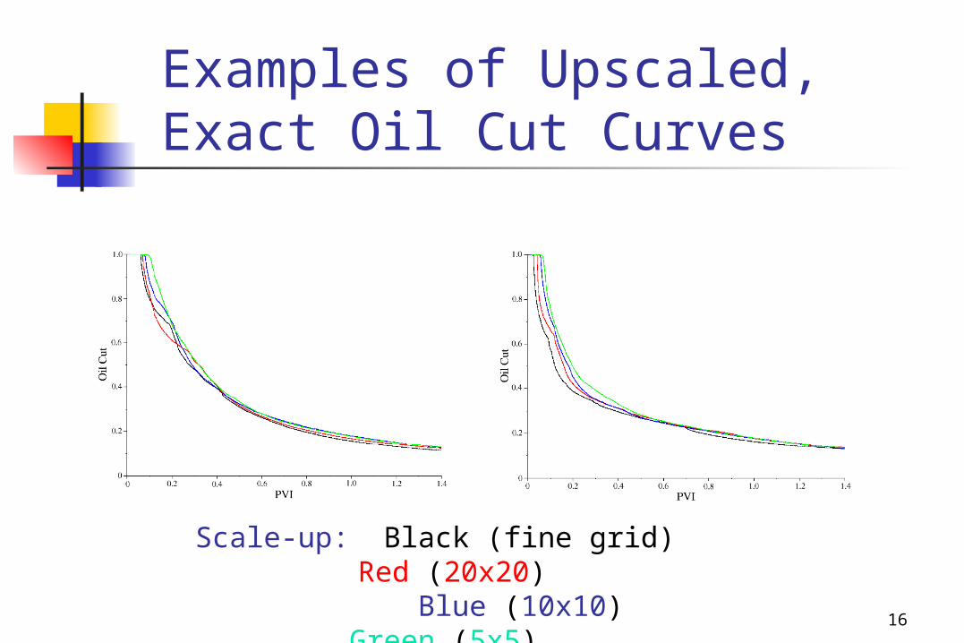
Examples of Upscaled, Exact Oil Cut Curves

Scale-up: Black (fine grid) Red (20x20)

Blue (10x10) Green (5x5)

17

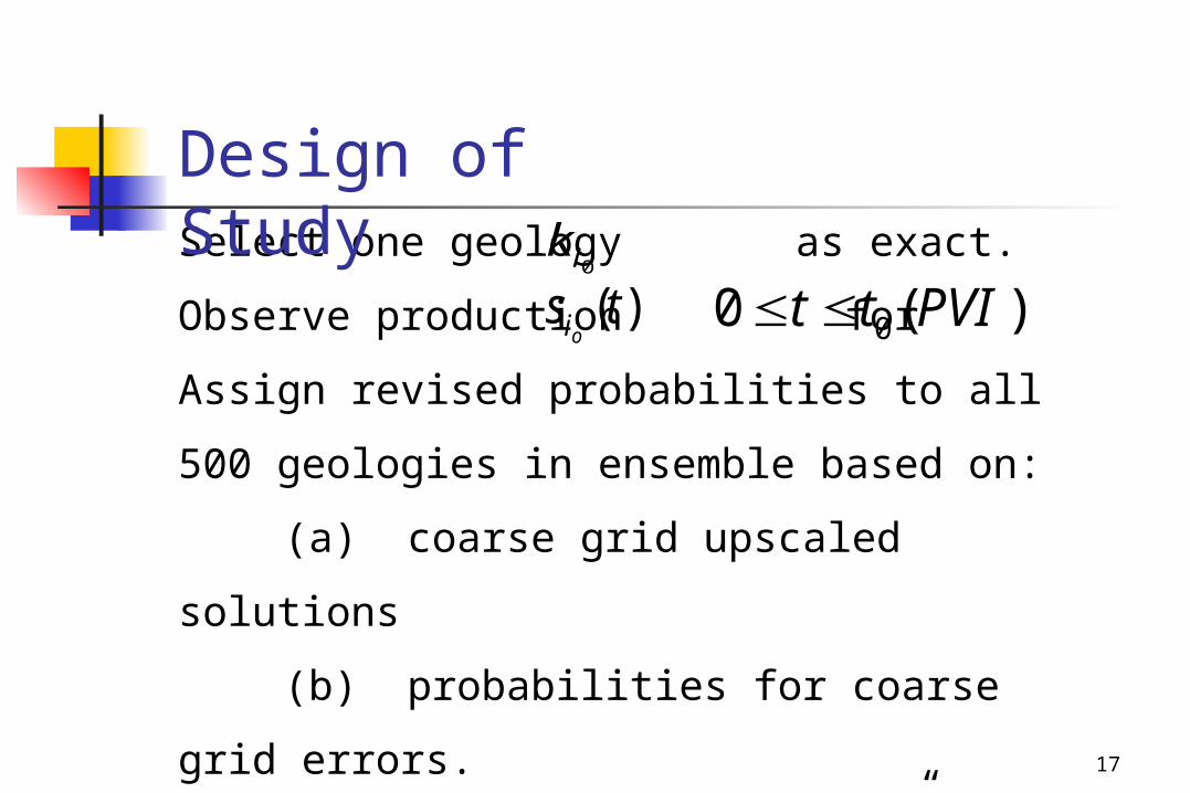
Select one geology as exact.

Observe production for

Assign revised probabilities to all

500 geologies in ensemble based on:

(a) coarse grid upscaled solutions

(b) probabilities for coarse grid

errors.

Compared to data (from “exact” geology)

0ik

)(tsoi

)(0 0 PVItt

Design of Study

18

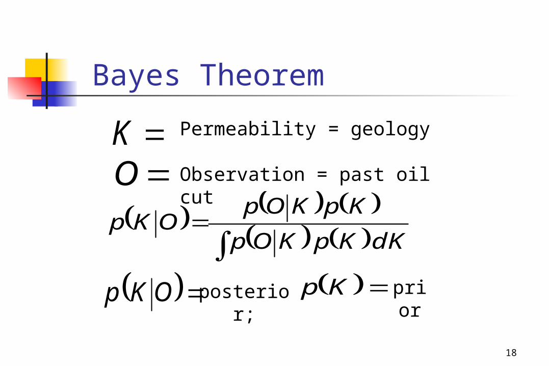
Bayes Theorem

K Permeability = geology

Observation = past oil cutO

dKKpKOp

KpKOpOKp

OKp posterior; Kp prior

19

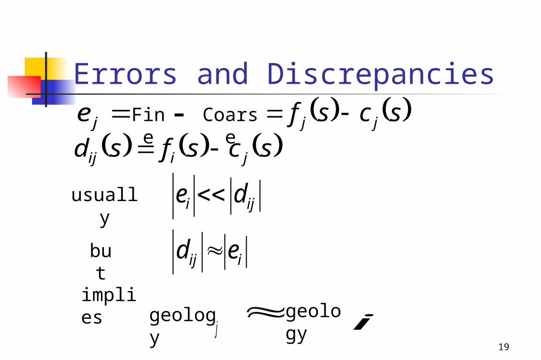
Errors and Discrepanciesje scsf jj scsfsd jiij

usually iji de

but iij ed

impliesgeology geolog

yj i

Fine

Coarse

20

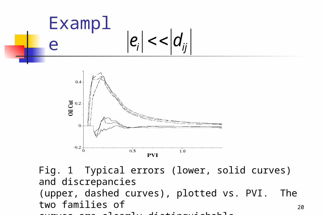
Example

Fig. 1 Typical errors (lower, solid curves) and discrepancies(upper, dashed curves), plotted vs. PVI. The two families of curves are clearly distinguishable.

iji de

21

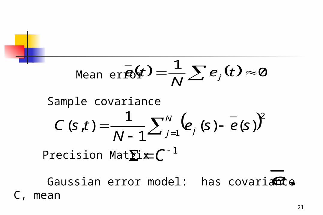
Mean error

Sample covariance

Precision Matrix

Gaussian error model: has covariance C, mean

01

teN

te j

21

)()(1

1),(

N

j j seseN

tsC

1 C

.e

22

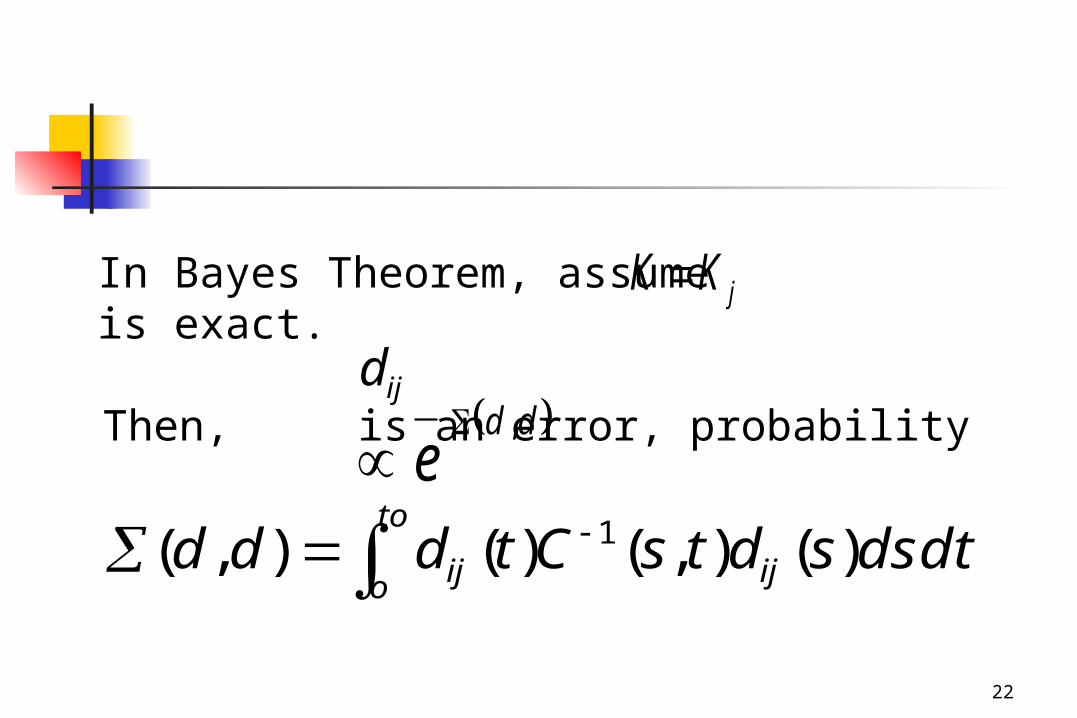
In Bayes Theorem, assume is exact.

Then, is an error, probability

jKK

ijd dd

e,

to

o ijij dtdssdtsCtddd )(),()(),( 1

23

For arrival time error models, the

formulation is identical, except that the

independent variables s and t now

denote the solution values, and not the

time values, while the error e(s)

denotes an error in the time of arrival

of the solution value s.

24

Model Reduction:

Limited data on solution errors

Don’t over fit data

Replace by finite matrix

,C

25

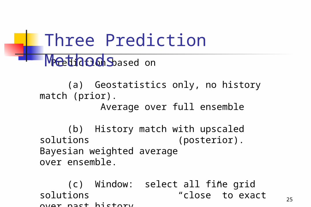
Prediction based on

(a) Geostatistics only, no history match (prior).

Average over full ensemble

(b) History match with upscaled solutions (posterior). Bayesian weighted

average over ensemble.

(c) Window: select all fine grid solutions “close” to exact over past

history. Average over restricted ensemble.

Three Prediction Methods

26

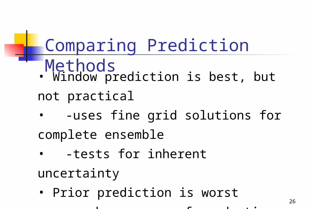
• Window prediction is best, but not

practical

• -uses fine grid solutions for

complete ensemble

• -tests for inherent uncertainty

• Prior prediction is worst

• - makes no use of production data.

Comparing Prediction Methods

27

Prediction error reduction, asper cent of prior prediction

choose present time to be oil cut of 0.6

Error Reduction

28

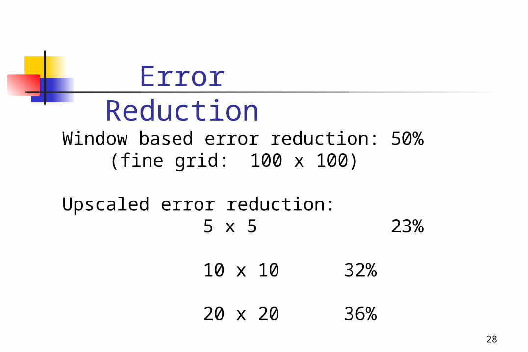
Window based error reduction: 50%(fine grid: 100 x 100)

Upscaled error reduction: 5 x 5 23%

10 x 10 32%

20 x 20 36%

Error Reduction

29

Confidence Intervals

5% - 95% interval in future oil production

Excludes extreme high-low values with 5%probability of occurrence

Expressed as a per cent of predicted production

30

s0 = oil cut at present time.

t0 = present time.

Compute 5%--95% confidence intervals for

future oil production, based on posterior and

forward prediction using upscaled simulation.

Result is a random variable. We express

confidence intervals as a percent of predicted

production, and take mean of this statistic.

Confidence Intervals

31

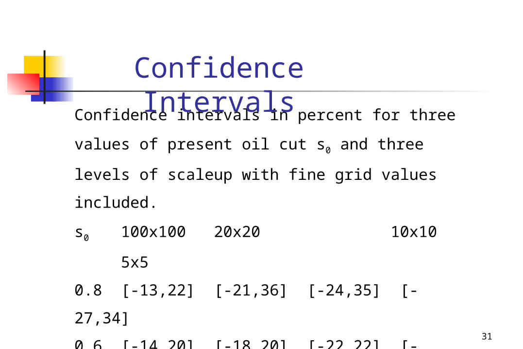
Confidence intervals in percent for three values

of present oil cut s0 and three levels of scaleup

with fine grid values included.

s0 100x100 20x20 10x10

5x5

0.8 [-13,22] [-21,36] [-24,35] [-

27,34]

0.6 [-14,20] [-18,20] [-22,22] [-

29,25]

0.4 [-14,17] [-18,18] [-24,21] [-

33,23]

Confidence Intervals

32

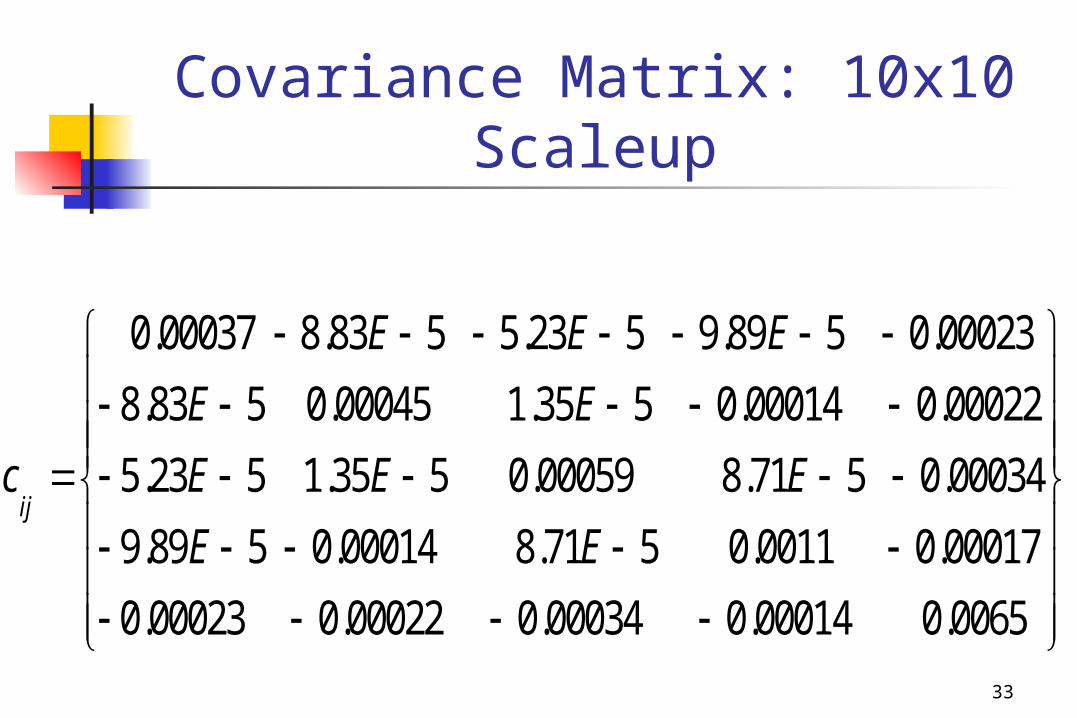
Arrival Time Error Analysis

Error Model defined by 5 solution values:s = 1- (Breakthrough), 0.8, 0.6, 0.4, 0.2.

Covariance is a 5 x 5 matrix, diagonallydominant, and neglecting diagonal terms,thus has 5 degrees of freedom. Thus it is simple.

Covariance is basically independent of thegeology correlation length. Thus it is robust.

33

Covariance Matrix: 10x10 Scaleup

0.00037 8.83 5 5.23 5 9.89 5 0.00023

8.83 5 0.00045 1.35 5 0.00014 0.00022

5.23 5 1.35 5 0.00059 8.71 5 0.00034

9.89 5 0.00014 8.71ij

E E E

E E

c E E E

E E

5 0.0011 0.00017

0.00023 0.00022 0.00034 0.00014 0.0065

34

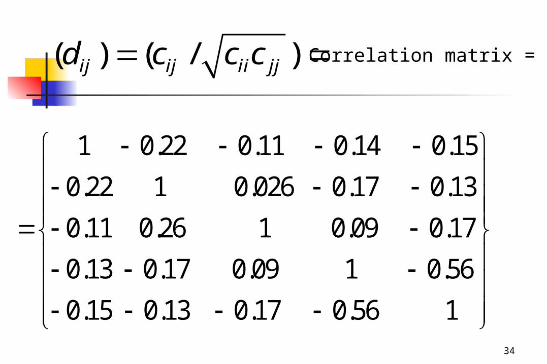
( ) ( / )ij ij ii jjd c c c

1 0.22 0.11 0.14 0.15

0.22 1 0.026 0.17 0.13

0.11 0.26 1 0.09 0.17

0.13 0.17 0.09 1 0.56

0.15 0.13 0.17

0.56 1

Correlation matrix =

35

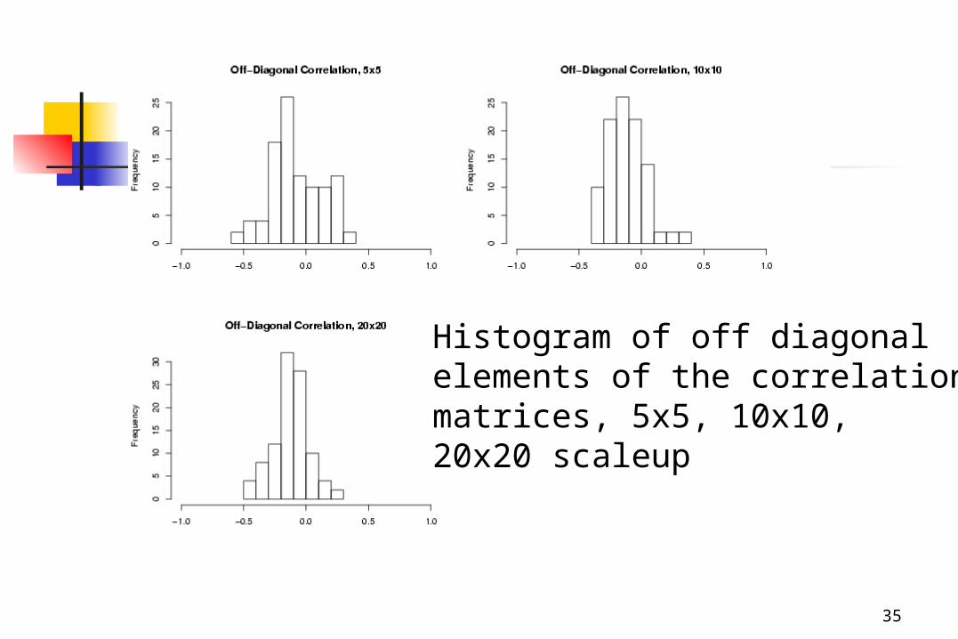
Histogram of off diagonal elements of the correlationmatrices, 5x5, 10x10,20x20 scaleup

36

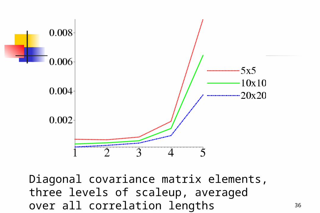
Diagonal covariance matrix elements, three levels of scaleup, averaged over all correlation lengths

37

Error covariance for arrival time

error model is proportional

to the degree of scale up

38

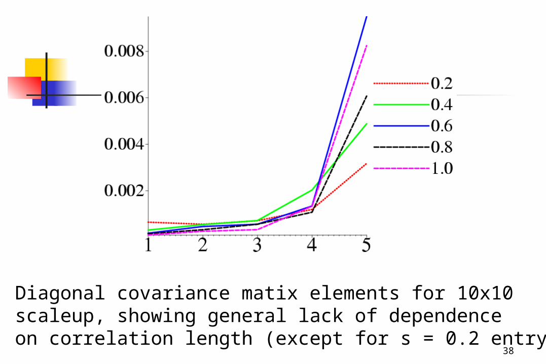
Diagonal covariance matix elements for 10x10scaleup, showing general lack of dependence on correlation length (except for s = 0.2 entry)

39

Covariance matrix diagonal entries

for arrival time error model are

independent of correlation length,

except for final (s = 0.2) entry.

40

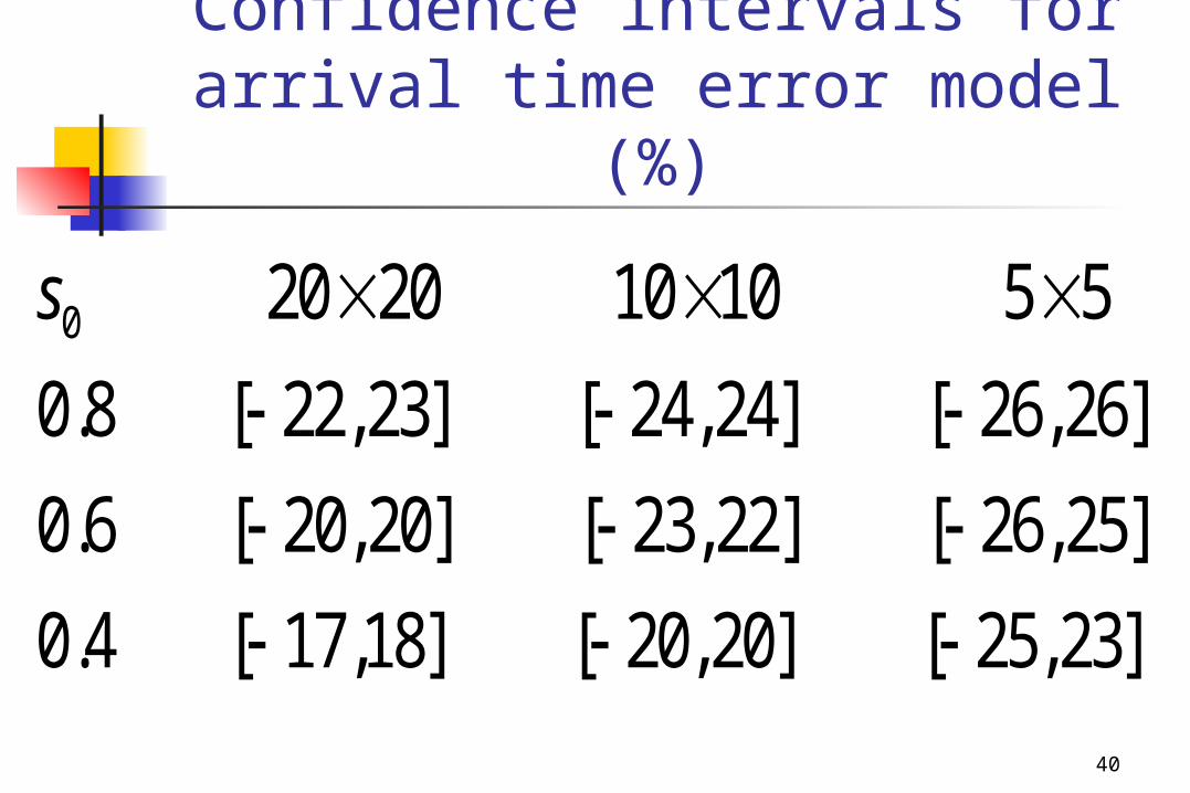
Confidence intervals for arrival time error model (%)

0 20 20 10 10 5 5

0.8 [ 22,23] [ 24,24] [ 26,26]

0.6 [ 20,20] [ 23,22] [ 26,25]

0.4 [ 17,18] [ 20,20] [ 25,23

s ]

41

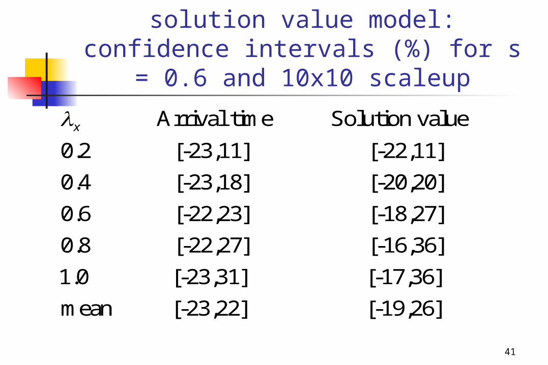
Arrival time error model vs. solution value model: confidence intervals (%) for s = 0.6 and 10x10 scaleup

Arrival time Solution value

0.2 [-23,11] [-22,11]

0.4 [-23,18] [-20,20]

0.6 [-22,23]

x

[-18,27]

0.8 [-22,27] [-16,36]

1.0 [-23,31] [-17,36]

mean [-23,22] [-19,26]

42

Summary and Conclusions New method to assess risk in

prediction of future oil production New methods to assess errors in

simulations as probabilities New upscaling allows consideration

of ensemble of geology scenarios Bayesian framework provides formal

probabilities for risk and uncertainty

43

References J. Glimm, S. Hou, H. Kim, D. H. Sharp, “A Probability

Model for Errors in the Numerical Solutions of a Partial Differential Equation”. Computational Fluid Dynamics Journal, Vol. 9, 485-493 (2001).

J. Glimm, S. Hou, Y. Lee, D. H. Sharp, “Prediction of Oil Production with Confidence Intervals”, SPE reprint SPE66350 (2001).

J. Glimm, S. Hou, H. Kim, D. H. Sharp, K. Ye, W. Zhu, “Risk Management for Petroleum Reservoir Production”, J. Comp. Geosciences, to appear.

J. Glimm, Y. Lee, K. Ye, “A Simple Model for Scale Up Error” Cont. Math. 2002 (to appear).