1 Ka-fu Wong University of Hong Kong Some Final Words.

1

Ka-fu WongUniversity of Hong Kong

Some Final Words

2

Unobserved components model of time series

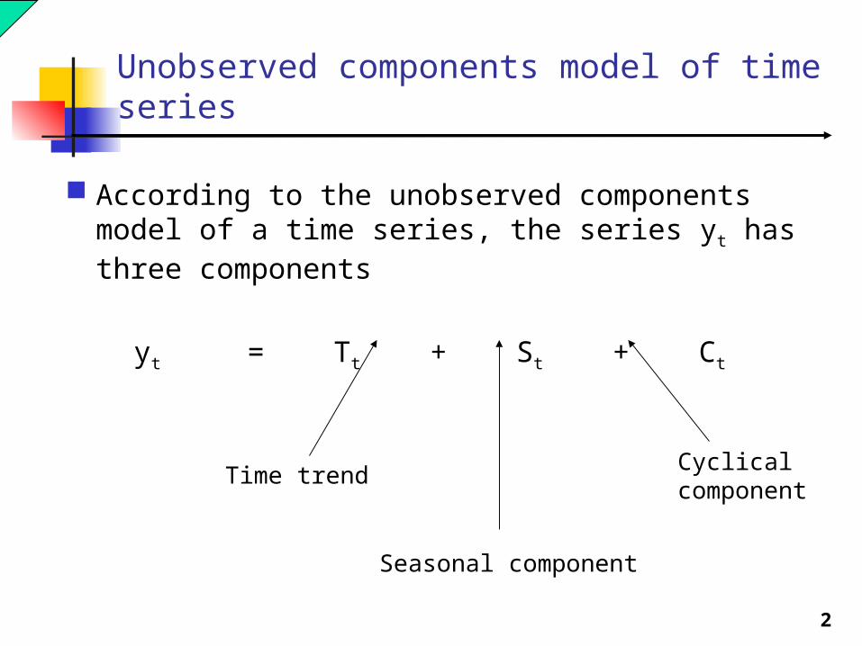
According to the unobserved components model of a time series, the series yt has three components

yt = Tt + St + Ct

Time trend

Seasonal component

Cyclical component

3

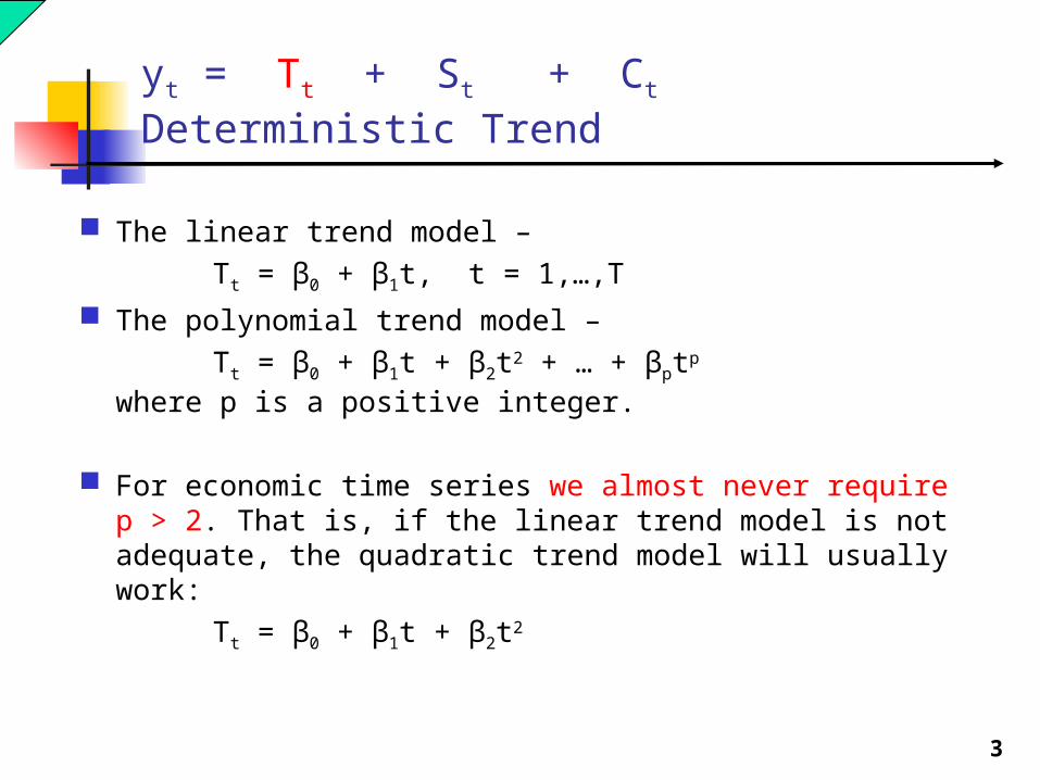
yt = Tt + St + Ct Deterministic Trend

The linear trend model –Tt = β0 + β1t, t = 1,…,T

The polynomial trend model –Tt = β0 + β1t + β2t2 + … + βptp

where p is a positive integer.

For economic time series we almost never require p > 2. That is, if the linear trend model is not adequate, the quadratic trend model will usually work:

Tt = β0 + β1t + β2t2

4

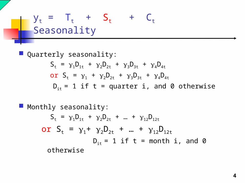
yt = Tt + St + Ct Seasonality

Quarterly seasonality:St = 1D1t + 2D2t + 3D3t + 4D4t

or St = 1 + 2D2t + 3D3t + 4D4t

Dit = 1 if t = quarter i, and 0 otherwise

Monthly seasonality:St = 1D1t + 2D2t + … + 12D12t

or St = 1+ 2D2t + … + 12D12t

Dit = 1 if t = month i, and 0 otherwise

5

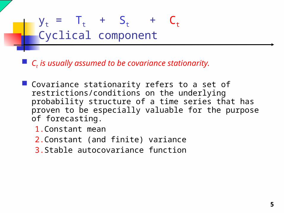
yt = Tt + St + Ct Cyclical component

Ct is usually assumed to be covariance stationarity.

Covariance stationarity refers to a set of restrictions/conditions on the underlying probability structure of a time series that has proven to be especially valuable for the purpose of forecasting.1.Constant mean2.Constant (and finite) variance3.Stable autocovariance function

6

Wold’s theorem

According to Wold’s theorem, if yt is a zero mean covariance stationary process than it can be written in the form:

...221100

ttt

iitit bbbby

where the ε’s are (i) WN(0,σ2), (ii) b0 = 1, and (iii)

0

2

iib

In other words, each yt can be expressed in terms of a single linear function of current and (possibly an infinite number of) past drawings of the white noise process, εt.

If yt depends on an infinite number of past ε’s, the weights on these ε’s, i.e., the bi’s must be going to zero as i gets large (and they must be going to zero at a fast enough rate for the sum of squared bi’s to converge).

7

Innovations

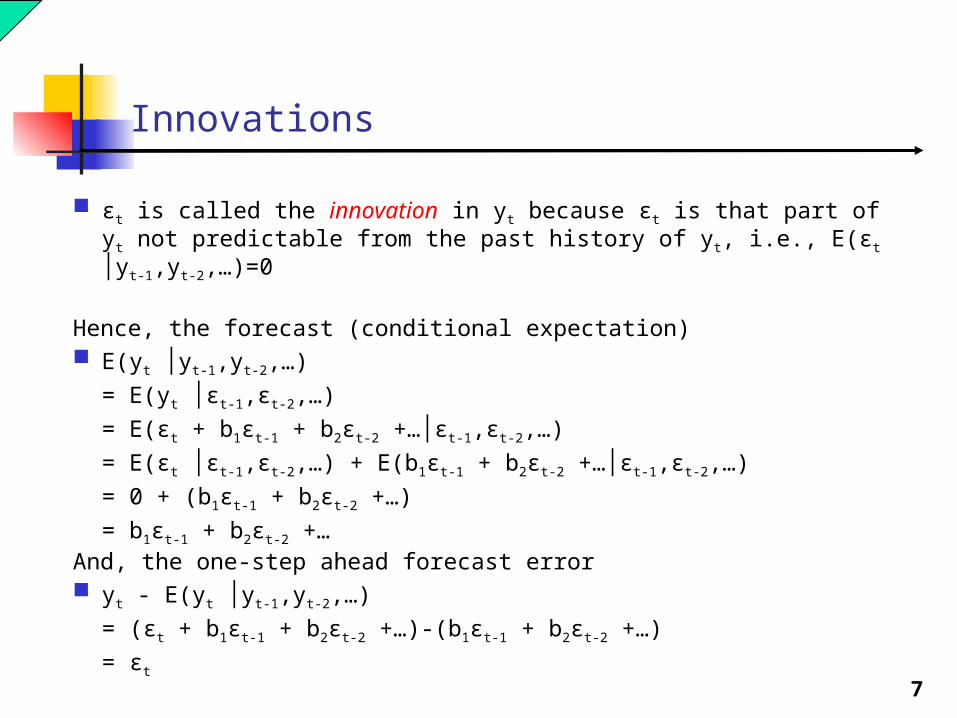
εt is called the innovation in yt because εt is that part of yt not predictable from the past history of yt, i.e., E(εt │yt-1,yt-2,…)=0

Hence, the forecast (conditional expectation) E(yt │yt-1,yt-2,…)

= E(yt │εt-1,εt-2,…)

= E(εt + b1εt-1 + b2εt-2 +…│εt-1,εt-2,…)

= E(εt │εt-1,εt-2,…) + E(b1εt-1 + b2εt-2 +…│εt-1,εt-2,…)

= 0 + (b1εt-1 + b2εt-2 +…)

= b1εt-1 + b2εt-2 +…And, the one-step ahead forecast error yt - E(yt │yt-1,yt-2,…)

= (εt + b1εt-1 + b2εt-2 +…)-(b1εt-1 + b2εt-2 +…)

= εt

8

Mapping Wold to a variety of models

It turns out that the Wold representation can usually be well-approximated by a variety of models that can expressed in terms of a very small number of parameters. the moving-average (MA) models, the autoregressive (AR) models, and the autoregressive moving-average (ARMA) models.

9

Mapping Wold to a variety of models

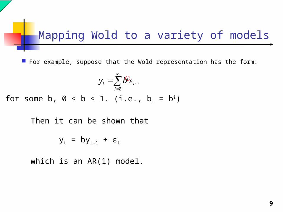
For example, suppose that the Wold representation has the form:

0iit

it by

for some b, 0 < b < 1. (i.e., bi = bi)

Then it can be shown that

yt = byt-1 + εt

which is an AR(1) model.

10

Moving Average (MA) Models

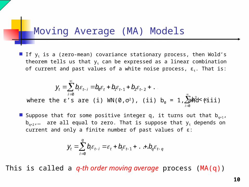
If yt is a (zero-mean) covariance stationary process, then Wold’s theorem tells us that yt can be expressed as a linear combination of current and past values of a white noise process, εt. That is:

...221100

ttt

iitit bbbby

where the ε’s are (i) WN(0,σ2), (ii) b0 = 1, and (iii)

0

2

iib

Suppose that for some positive integer q, it turns out that bq+1, bq+2,… are all equal to zero. That is suppose that yt depends on current and only a finite number of past values of ε:

qtqtt

q

iitit bbby

...11

0

This is called a q-th order moving average process (MA(q))

11

Autoregressive Models (AR(p))

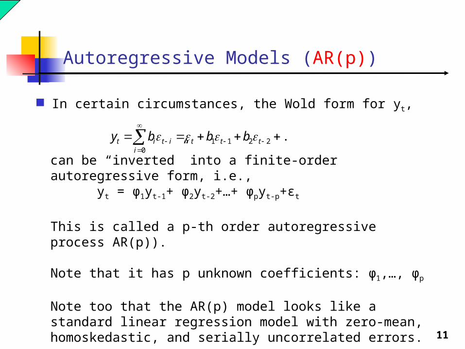
In certain circumstances, the Wold form for yt,

...22110

ttt

iitit bbby

can be “inverted” into a finite-order autoregressive form, i.e.,

yt = φ1yt-1+ φ2yt-2+…+ φpyt-p+εt

This is called a p-th order autoregressive process AR(p)).

Note that it has p unknown coefficients: φ1,…, φp

Note too that the AR(p) model looks like a standard linear regression model with zero-mean, homoskedastic, and serially uncorrelated errors.

12

AR(p): yt = φ1yt-1+ φ2yt-2+…+ φpyt-p+εt

The coefficients of the AR(p) model of a covariance stationary time series must satisfy the stationarity condition: Consider the values of x that solve the equation

1-φ1x-…-φpxp = 0

These x’s must all be greater than 1 in absolute value.

For example, if p = 1 (the AR(1) case), consider the solutions to

1- φx = 0The only value of x that satisfies this equation is x = 1/φ, which will be greater than one in absolute value if and only if the absolute value of φ is less than one. So, │φ│< 1 is the stationarity condition for the AR(1) model.The condition guarantees that the impact of εt on yt+

decays to zero as increases.

13

AR(p): yt = φ1yt-1+ φ2yt-2+…+ φpyt-p+εt

The autocovariance and autocorrelation functions, () and ρ(), will be non-zero for all . Their exact shapes will depend upon the signs and magnitudes of the AR coefficients, though we know that they will be decaying to zero as goes to infinity.

The partial autocorrelation function, p(), will be equal to 0 for all > p.

The exact shape of the pacf for 1 < < p will depend on the signs and magnitudes of φ1,…, φp.

14

Approximation

Any MA process may be approximated by an AR(p) process, for sufficient large p. And the residuals will appear white noise.

Any AR process may be approximated by a MA(q) process, for sufficient large q. And the residuals will appear white noise.

In fact, if an AR(p) process can be written exactly as a MA(q) process, the AR(p) process is called invertible.

Similarly, if a MA(q) process can be written exactly as an AR(p) process, the MA(q) process is called invertible.

15

Choice of ARMA(p,q) models

Estimate a low-order ARMA model and check the autocorrelation and partial autocorrelation of the residuals. If the model is a good approximation, the residuals should exhibit properties of white noise in the autocorrelation and partial autocorrelation.

Estimate ARMA models with various combination of p and q. Choose the model with the smallest AIC or SIC. When they are in conflict, choose the parsimonious one.

16

Has the probability structure remained same throughout the sample?

Check parameter constancy if we are suspicious.

Allow for breaks if they are known.

If we know breaks exist but do not know exactly where the break point should be, try to identify the breaks.

17

Assessing Model Stability Using Recursive Estimation and Recursive Residuals

Forecast: If the model’s parameters are different during the forecast period than they were during the sample period, then the model we estimated will not be very useful , regardless of how well it was estimated.

Model: If the model’s parameters were unstable over the sample period, then model was not even a good representation of how the series evolved over the sample period.

18

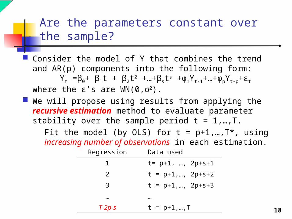
Are the parameters constant over the sample?

Consider the model of Y that combines the trend and AR(p) components into the following form:

Yt =β0+ β1t + β2t2 +…+βsts +φ1Yt-1+…+φpYt-p+εt

where the ε’s are WN(0,σ2). We will propose using results from applying the recursive

estimation method to evaluate parameter stability over the sample period t = 1,…,T.

Fit the model (by OLS) for t = p+1,…,T*, using increasing number of observations in each estimation.

Regression Data used

1 t= p+1, …, 2p+s+1

2 t = p+1,…, 2p+s+2

3 t = p+1,…, 2p+s+3

… …

T-2p-s t = p+1,…,T

19

Recursive estimation

The recursive estimation yield parameter estimates for each T*:

and for i = 1,..,s, j = 1,…,p and T* = 2p+s+1,…,T.

If the model is stable over time then what we should find is that as T* increases the recursive parameter estimates should stabilize at some level.

A model parameter is unstable if it does not appear to stabilize as T* increases or if there appears to be a sharp break in the behavior of the sequence before and after some T*.

*,ˆTi *,ˆ Tj

20

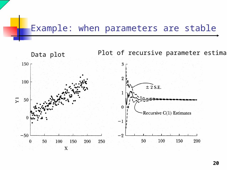
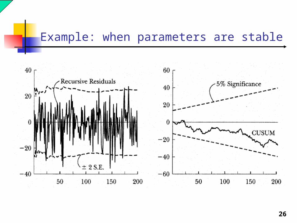
Example: when parameters are stable

Data plot Plot of recursive parameter estimates

21

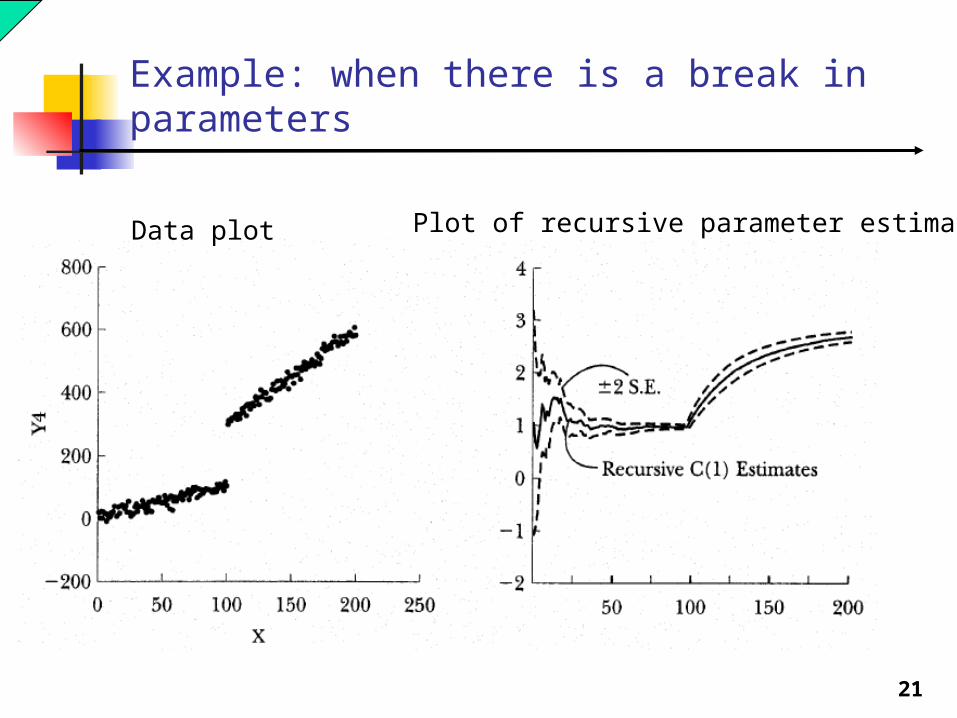
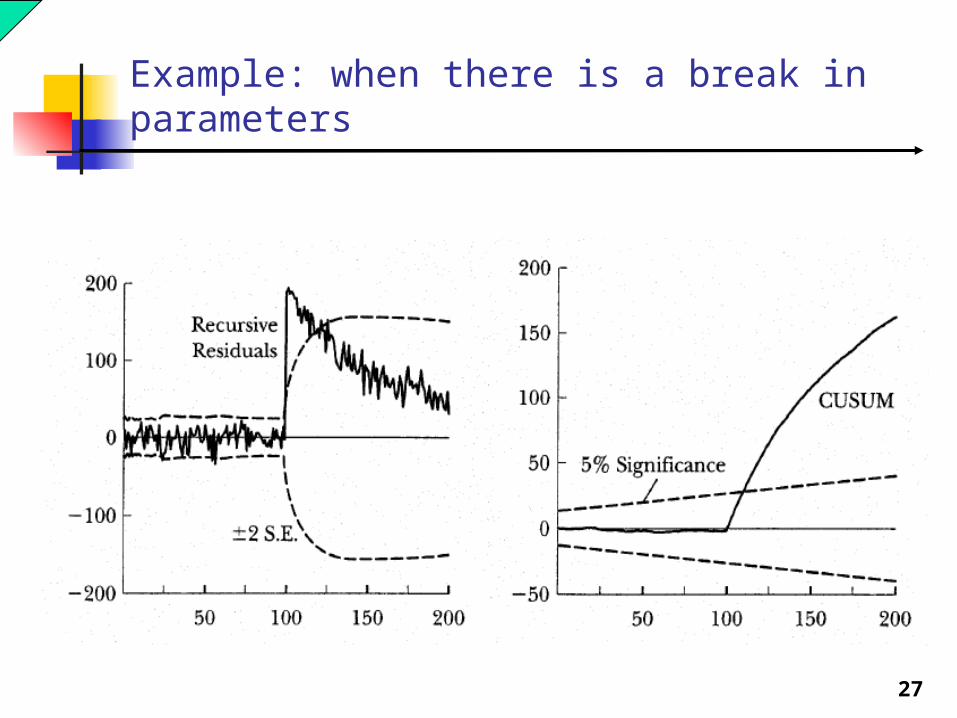
Example: when there is a break in parameters

Data plot Plot of recursive parameter estimates

22

Recursive Residuals and the CUSUM Test

The CUSUM (“cumulative sum”) test is often used to test the null hypothesis of model stability, based on the residuals from the recursive estimates. The CUSUM statistic is calculated for each t. Under the

null hypothesis of stability, the statistic follows the CUSUM distribution.

If the calculated CUSUM statistics appear to be too large to have been drawn from the CUSUM distribution, we reject the null hypothesis (of model stability).

23

CUSUM

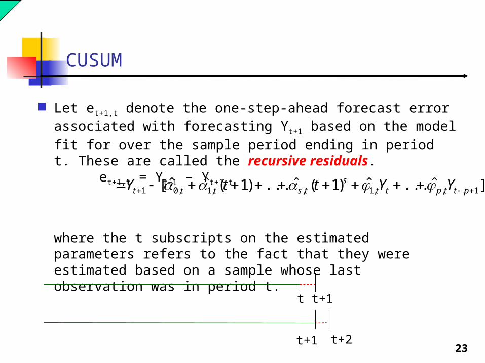
Let et+1,t denote the one-step-ahead forecast error associated with forecasting Yt+1 based on the model fit for over the sample period ending in period t. These are called the recursive residuals.

et+1,t = Yt+1 – Yt+1,t

where the t subscripts on the estimated parameters refers to the fact that they were estimated based on a sample whose last observation was in period t.

]ˆ...ˆ)1(ˆ...)1(ˆˆ[ 1,,1,,1,01 pttptts

tsttt YYttY

t t+1

t+1 t+2

24

CUSUM

Let σ1,t denote the standard error of the one-step ahead forecast of Y formed at time t, i.e,

σ1,t = sqrt(var(et+1,t))

Define the standardized recursive residuals, wt+1,t, according to

wt+1,t = et+1,t/σ1,t

Fact: Under our maintained assumptions, including model homogeneity,

wt+1,t ~ i.i.d. N(0,1).

Note that there will be a set of standardized recursive residuals for each sample.

25

CUSUM

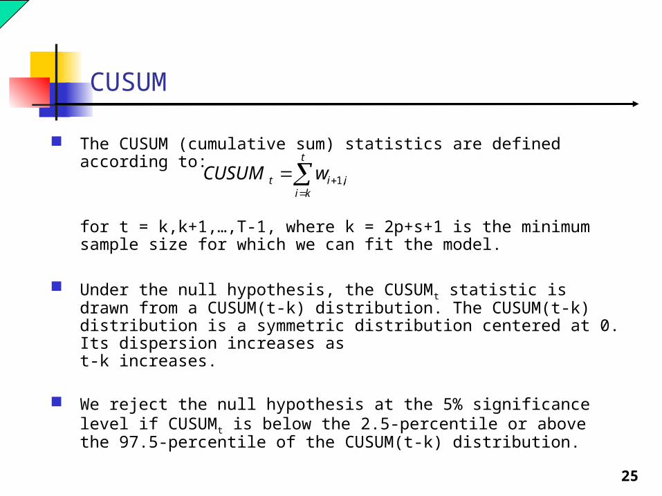
The CUSUM (cumulative sum) statistics are defined according to:

for t = k,k+1,…,T-1, where k = 2p+s+1 is the minimum sample size for which we can fit the model.

Under the null hypothesis, the CUSUMt statistic is drawn from a CUSUM(t-k) distribution. The CUSUM(t-k) distribution is a symmetric distribution centered at 0. Its dispersion increases as t-k increases.

We reject the null hypothesis at the 5% significance level if CUSUMt is below the 2.5-percentile or above the 97.5-percentile of the CUSUM(t-k) distribution.

t

kiiit wCUSUM ,1

26

Example: when parameters are stable

27

Example: when there is a break in parameters

28

Accounting for a structural break

Suppose it is known that there is a structural break in the trend of a series in 1998 – due to Asian Financial Crisis.

29

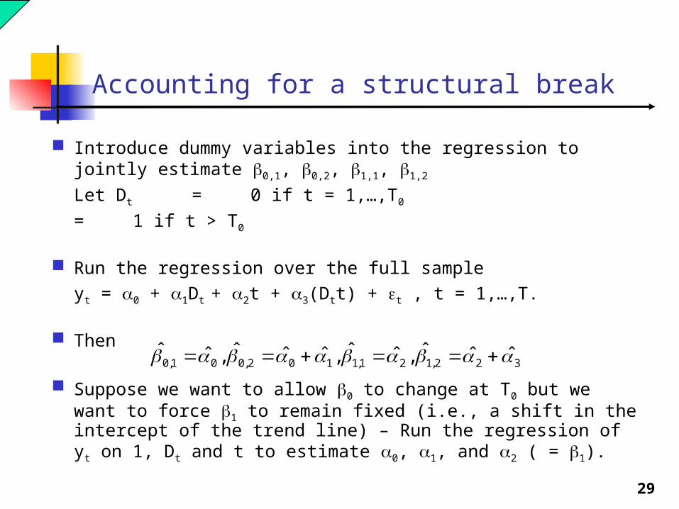
Accounting for a structural break

Introduce dummy variables into the regression to jointly estimate 0,1, 0,2, 1,1, 1,2

Let Dt = 0 if t = 1,…,T0

= 1 if t > T0

Run the regression over the full sampleyt = 0 + 1Dt + 2t + 3(Dtt) + t , t = 1,…,T.

Then

Suppose we want to allow 0 to change at T0 but we want to force 1 to remain fixed (i.e., a shift in the intercept of the trend line) – Run the regression of yt on 1, Dt and t to estimate 0, 1, and 2 ( = 1).

322,121,1102,001,0 ˆˆˆ,ˆˆ,ˆˆˆ,ˆˆ

30

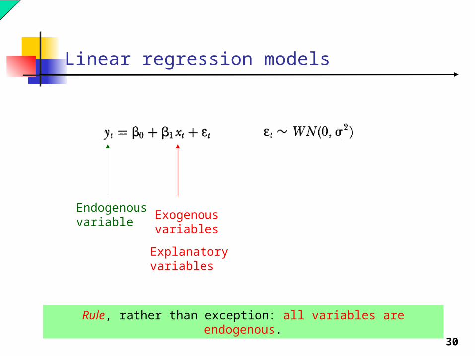
Linear regression models

Endogenous variable

Exogenous variables

Explanatory variables

Rule, rather than exception: all variables are endogenous.

31

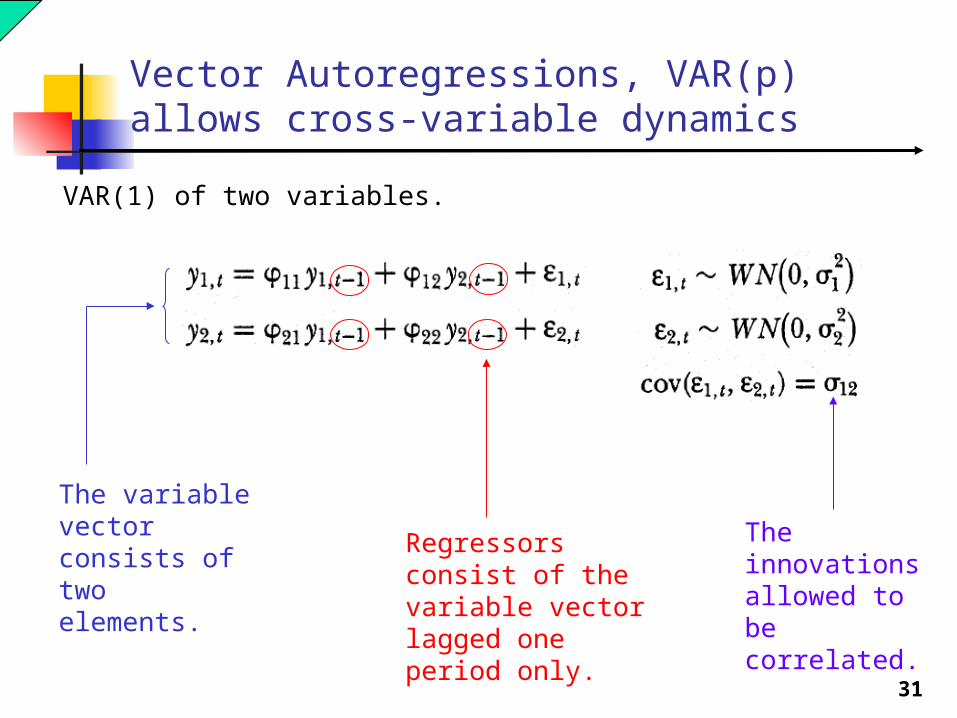
Vector Autoregressions, VAR(p)allows cross-variable dynamics

VAR(1) of two variables.

The variable vector consists of two elements.

Regressors consist of the variable vector lagged one period only.

The innovations allowed to be correlated.

32

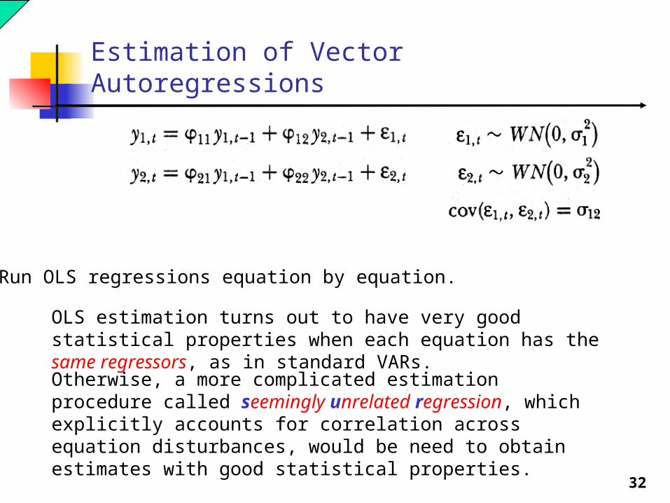
Estimation of Vector Autoregressions

Run OLS regressions equation by equation.

OLS estimation turns out to have very good statistical properties when each equation has the same regressors, as in standard VARs.Otherwise, a more complicated estimation procedure called seemingly unrelated regression, which explicitly accounts for correlation across equation disturbances, would be need to obtain estimates with good statistical properties.

33

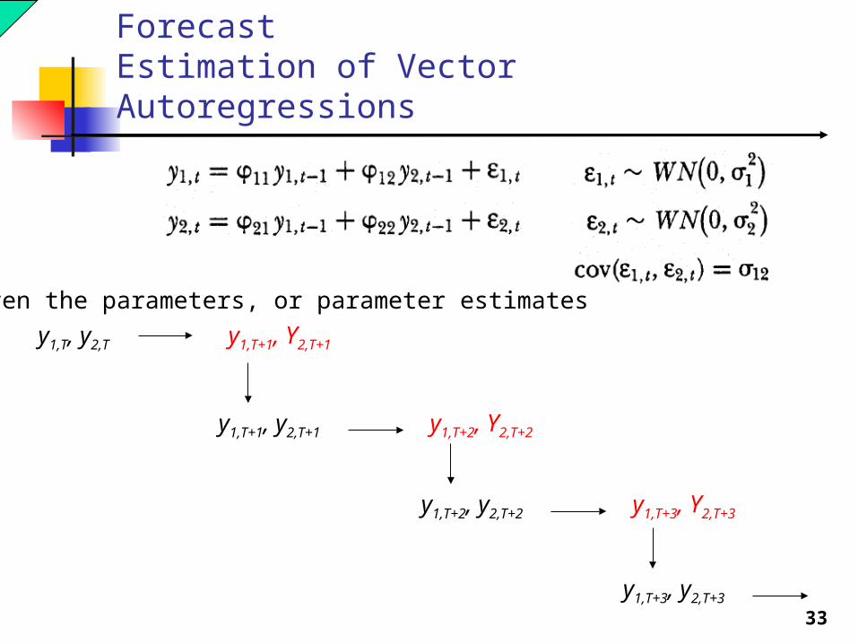
Forecast Estimation of Vector Autoregressions

y1,T, y2,T

y1,T+1, y2,T+1

y1,T+1, Y2,T+1

y1,T+2, Y2,T+2

y1,T+2, y2,T+2 y1,T+3, Y2,T+3

y1,T+3, y2,T+3

Given the parameters, or parameter estimates

34

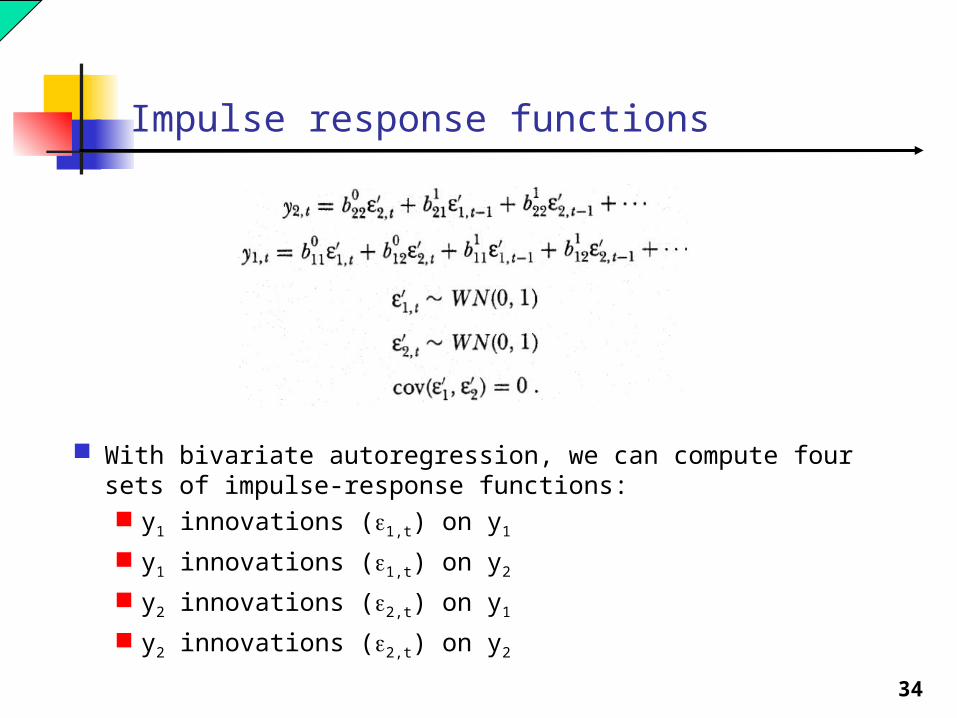
Impulse response functions

With bivariate autoregression, we can compute four sets of impulse-response functions: y1 innovations (1,t) on y1

y1 innovations (1,t) on y2

y2 innovations (2,t) on y1

y2 innovations (2,t) on y2

35

Variance decomposition

How much of the h-step-ahead forecast error variance of variable i is explained by innovations to variable j, for h=1,2,…. ?

With bivariate autoregression, we can compute four sets of variance decomposition: y1 innovations (1,t) on y1

y1 innovations (1,t) on y2

y2 innovations (2,t) on y1

y2 innovations (2,t) on y2

36

Assessing optimality with respect to an information setThe Mincer-Zarnowitz regression

Consider the regression yt+h = 0 + 1 yt+h,t + ut

If the forecast yt+h,t is optimal, we should have (0,1) =(0,1). That is yt+h = 0 + 1 yt+h,t + ut

et+h,t = yt+h - yt+h,t = 0 + 0 yt+h,t + ut

et+h,t = yt+h - yt+h,t = 0 + 1 yt+h,t + ut

where (0,1) =(0,0)

37

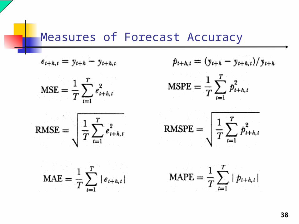
Measures of Forecast Accuracy

38

Measures of Forecast Accuracy

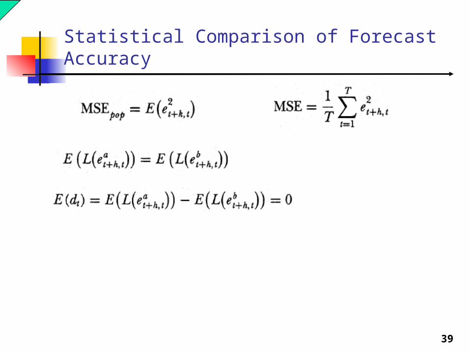
39

Statistical Comparison of Forecast Accuracy

40

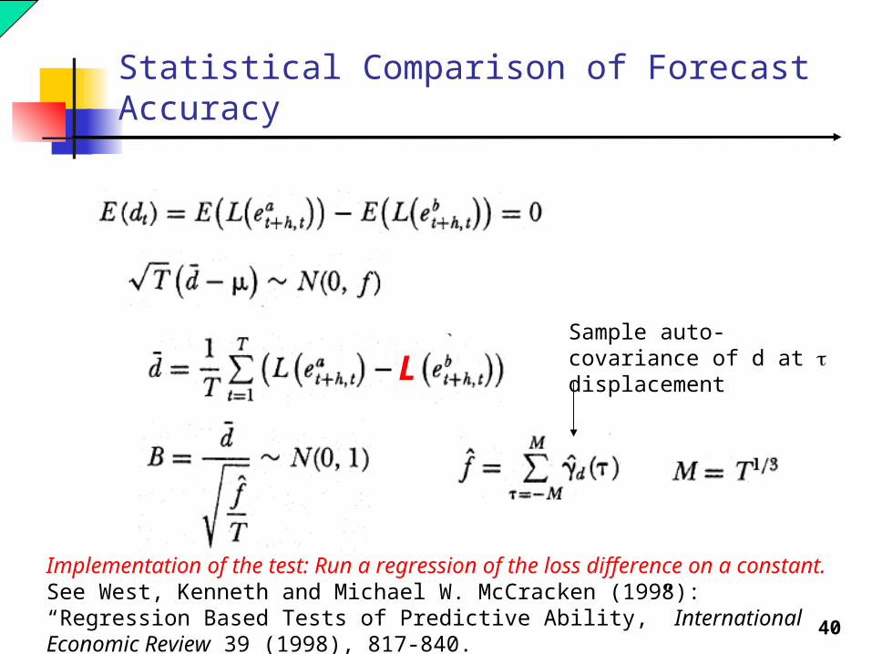
Statistical Comparison of Forecast Accuracy

Sample auto-covariance of d at displacementL

Implementation of the test: Run a regression of the loss difference on a constant. See West, Kenneth and Michael W. McCracken (1998): “Regression Based Tests of Predictive Ability,” International Economic Review 39 (1998), 817-840.

41

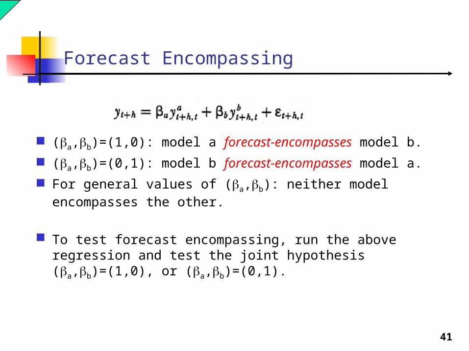
Forecast Encompassing

(a,b)=(1,0): model a forecast-encompasses model b.

(a,b)=(0,1): model b forecast-encompasses model a.

For general values of (a,b): neither model encompasses the other.

To test forecast encompassing, run the above regression and test the joint hypothesis (a,b)=(1,0), or (a,b)=(0,1).

42

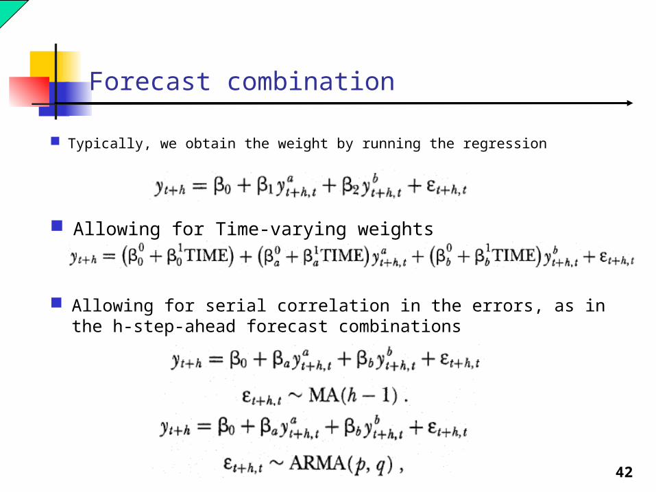
Forecast combination

Typically, we obtain the weight by running the regression

Allowing for Time-varying weights

Allowing for serial correlation in the errors, as in the h-step-ahead forecast combinations

43

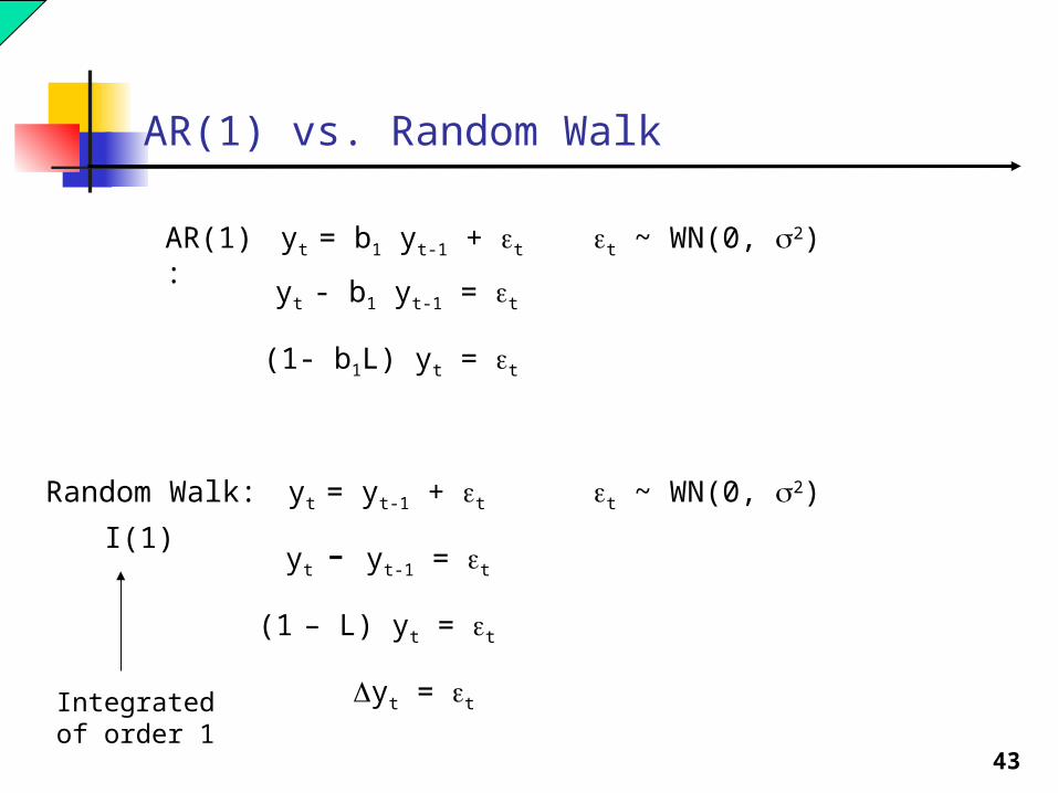
AR(1) vs. Random Walk

yt = b1 yt-1 + t t ~ WN(0, 2)

yt = yt-1 + t t ~ WN(0, 2)

AR(1):

Random Walk:

yt - b1 yt-1 = t

(1- b1L) yt = t

yt - yt-1 = t

(1 – L) yt = t

yt = t

I(1)

Integrated of order 1

44

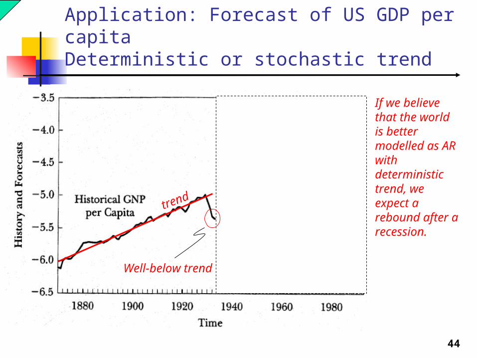
Application: Forecast of US GDP per capitaDeterministic or stochastic trend

trend

reverts back to trend

If we believe that the world is better modelled as AR with deterministic trend, we expect a rebound after a recession.

Well-below trend

45

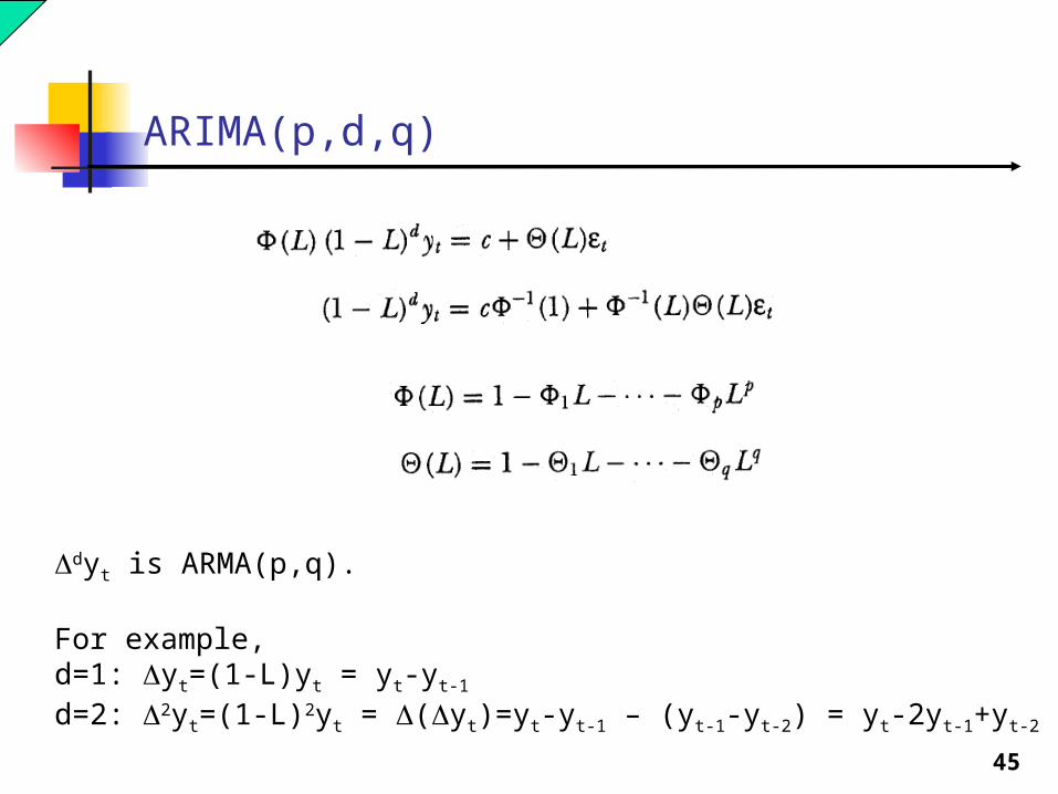
ARIMA(p,d,q)

dyt is ARMA(p,q).

For example,d=1: yt=(1-L)yt = yt-yt-1

d=2: 2yt=(1-L)2yt = (yt)=yt-yt-1 – (yt-1-yt-2) = yt-2yt-1+yt-2

46

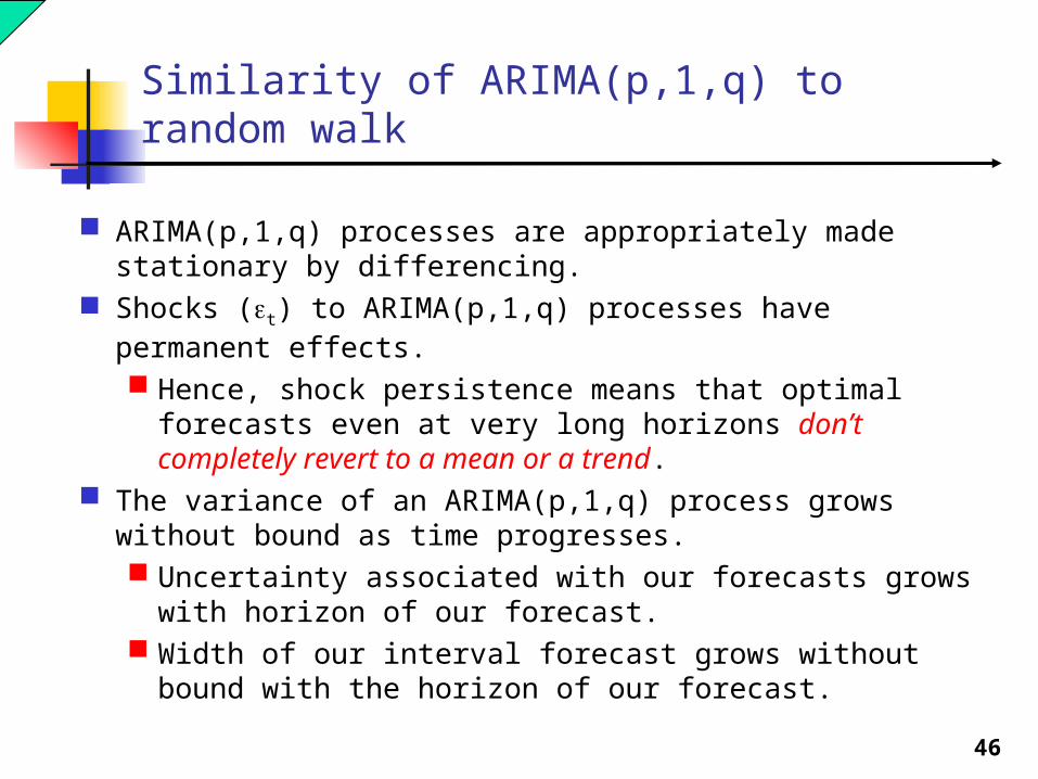
Similarity of ARIMA(p,1,q) to random walk

ARIMA(p,1,q) processes are appropriately made stationary by differencing.

Shocks (t) to ARIMA(p,1,q) processes have permanent effects. Hence, shock persistence means that optimal forecasts

even at very long horizons don’t completely revert to a mean or a trend.

The variance of an ARIMA(p,1,q) process grows without bound as time progresses. Uncertainty associated with our forecasts grows with

horizon of our forecast. Width of our interval forecast grows without bound with

the horizon of our forecast.

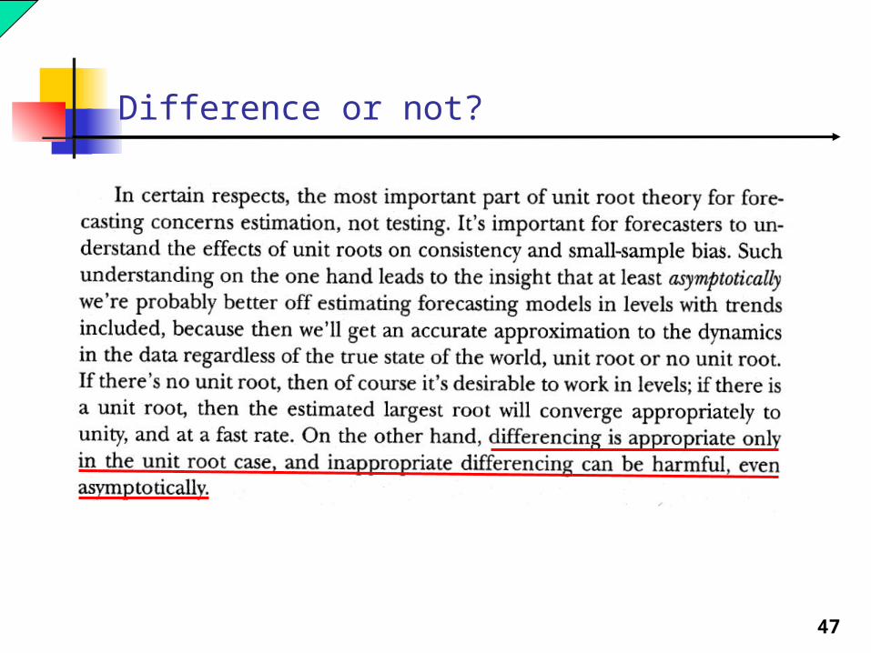
47

Difference or not?

48

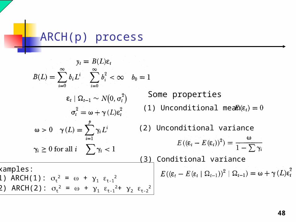
ARCH(p) process

Examples:(1)ARCH(1): t

2 = + 1 t-12

(2) ARCH(2): t2 = + 1 t-1

2+ 2 t-22

(1) Unconditional mean

(2) Unconditional variance

(3) Conditional variance

Some properties

49

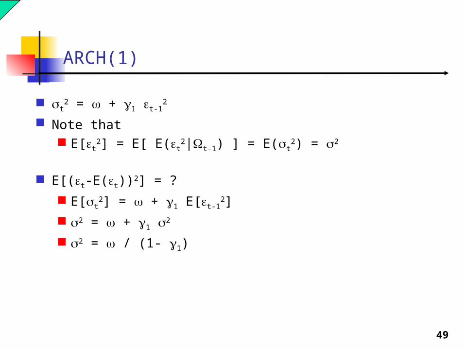
ARCH(1)

t2 = + 1 t-1

2

Note that E[t

2] = E[ E(t2|t-1) ] = E(t

2) = 2

E[(t-E(t))2] = ?

E[t2] = + 1 E[t-1

2]

2 = + 1 2

2 = / (1- 1)

50

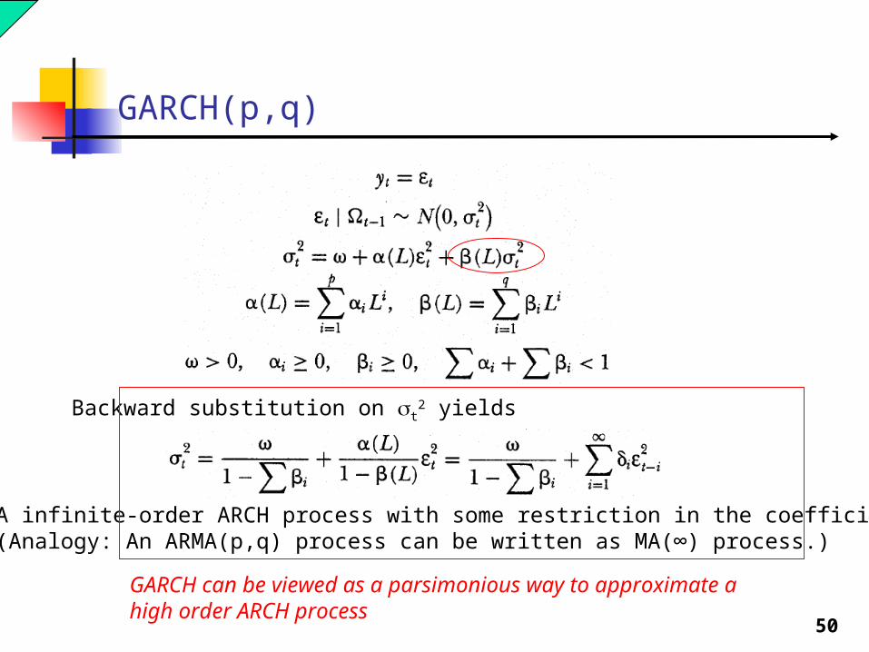
GARCH(p,q)

Backward substitution on t2 yields

A infinite-order ARCH process with some restriction in the coefficients.(Analogy: An ARMA(p,q) process can be written as MA(∞) process.)

GARCH can be viewed as a parsimonious way to approximate a high order ARCH process

51

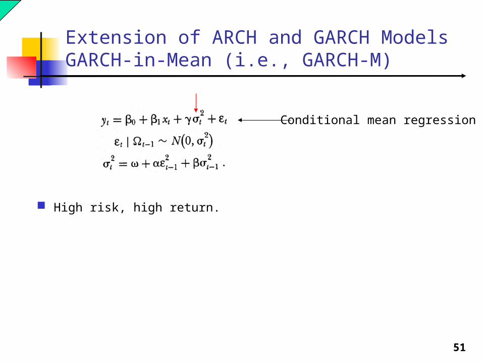
Extension of ARCH and GARCH ModelsGARCH-in-Mean (i.e., GARCH-M)

High risk, high return.

Conditional mean regression

52

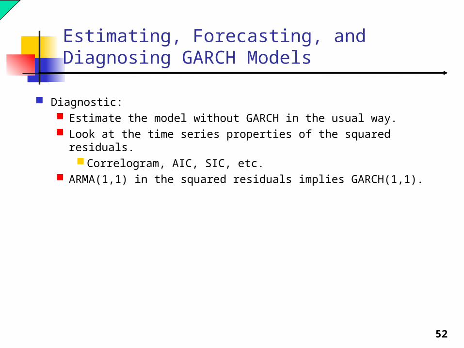
Estimating, Forecasting, and Diagnosing GARCH Models

Diagnostic: Estimate the model without GARCH in the usual way. Look at the time series properties of the squared residuals.

Correlogram, AIC, SIC, etc. ARMA(1,1) in the squared residuals implies GARCH(1,1).

53

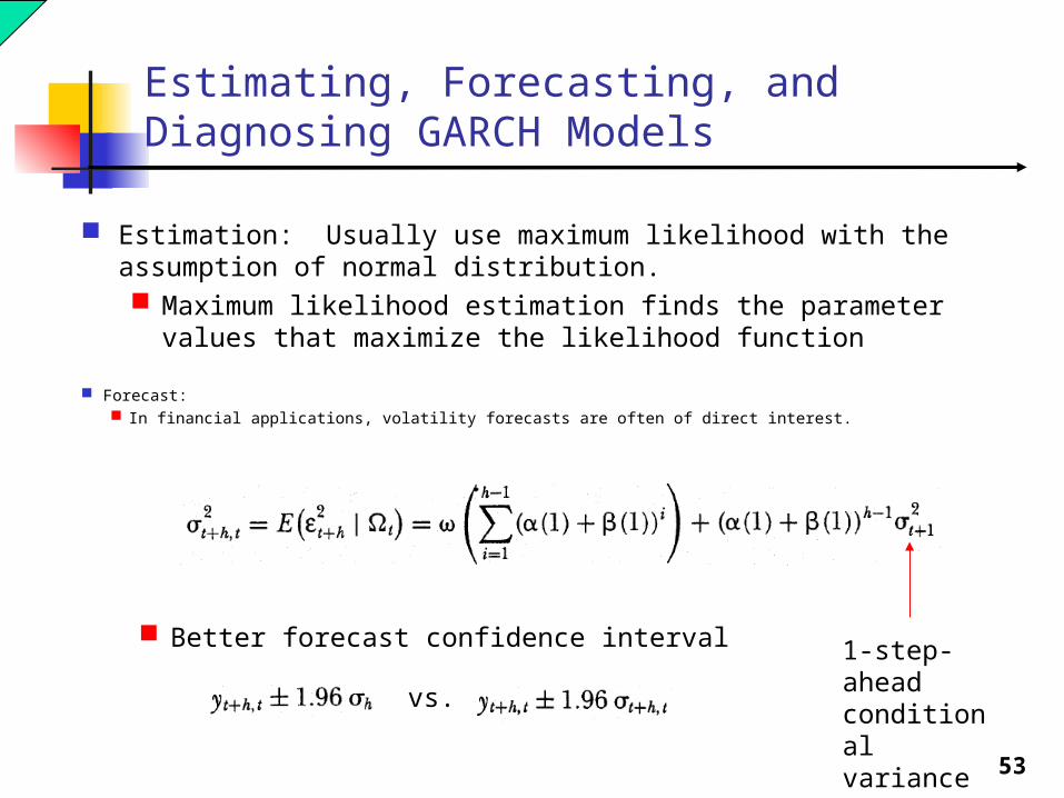
Estimating, Forecasting, and Diagnosing GARCH Models

Estimation: Usually use maximum likelihood with the assumption of normal distribution. Maximum likelihood estimation finds the parameter values

that maximize the likelihood function

Forecast: In financial applications, volatility forecasts are often of direct interest.

1-step-ahead conditional variance

Better forecast confidence interval

vs.

54

Does Anything Beat A GARCH(1,1) out of sample?

No. So, use GARCH(1,1) if no other information is available.

55

Additional interesting topics / references

Forecasting turning points.Lahiri, Kajal and Geoffrey H. Moore (1991): Leading Economic Indicators: New Approaches and Forecasting Records, Cambridge University Press.

Forecasting cycles:Niemira, Michael P. and Philip A. Klein (1994): Forecasting Financial and Economic Cycles, John Wiley and Sons.

56

Forecasting yt

Using past values of yt

Using other variables xt

Linear regression of yt on xt

Vector autoregressions of yt and xt

ARMA(p,q)

Deterministic elements

Trend

Seasonality

57

Forecasting volatility

Stochastic volatility models

GARCH models

58

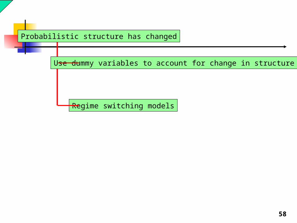
Probabilistic structure has changed

Regime switching models

Use dummy variables to account for change in structure

59

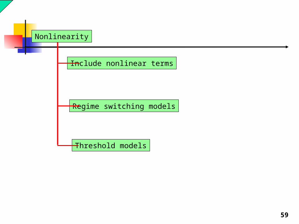
Nonlinearity

Regime switching models

Include nonlinear terms

Threshold models

60

Using models as an approximation of the real world.

No one knows what the true model should be.

Even if we know the true model, we may need to include too many variables, which are not feasible.

61

End