Ka-fu Wong © 2003 Chap 2-1 Dr. Ka-fu Wong ECON1003 Analysis of Economic Data

Ka-fu Wong © 2003 Chap 2-1 Dr. Ka-fu Wong ECON1003 Analysis of Economic Data.
Dec 21, 2015
Welcome message from author
This document is posted to help you gain knowledge. Please leave a comment to let me know what you think about it! Share it to your friends and learn new things together.
Transcript
Ka-fu Wong © 2003 Chap 2-1
Dr. Ka-fu Wong
ECON1003Analysis of Economic Data
Ka-fu Wong © 2003 Chap 2-2
Chapter TwoDescriptive StatisticsDescriptive Statistics
GOALS
1. Organize data into a frequency distribution.
2. Plots: Histogram, stem-and-leaf display.
3. Measures of central tendency
4. Measures of dispersion
5. Some properties of mean and standard deviations
Ka-fu Wong © 2003 Chap 2-3
Frequency Distribution
A Frequency distribution is a grouping of data into mutually exclusive categories showing the number of observations in each class.
Ka-fu Wong © 2003 Chap 2-4
Construction of a Frequency Distribution
1. Question to be addressed.
2. Collect data (raw data).
3. Organize data. Frequency distribution
4. Present data.
5. Draw conclusion.
Ka-fu Wong © 2003 Chap 2-5
Terms Related to Frequency Distribution
In constructing a frequency distribution, data are divided into exhaustive and mutually exclusive classes.
Mid-point: A point that divides a class into two equal parts. This is the average of the upper and lower class limits.
Class frequency: The number of observations in each class.
Class interval: The class interval is obtained by subtracting the lower limit of a class from the lower limit of the next class.
Ka-fu Wong © 2003 Chap 2-6
Four steps to construct frequency distribution
1. Decide on the number of classes. 2. Determine the class interval or width.3. Set the individual class limits.4. Tally the data into the classes and count
the number of items in each.
For illustration, it is convenient to carry an example with us – example 1.
Ka-fu Wong © 2003 Chap 2-7
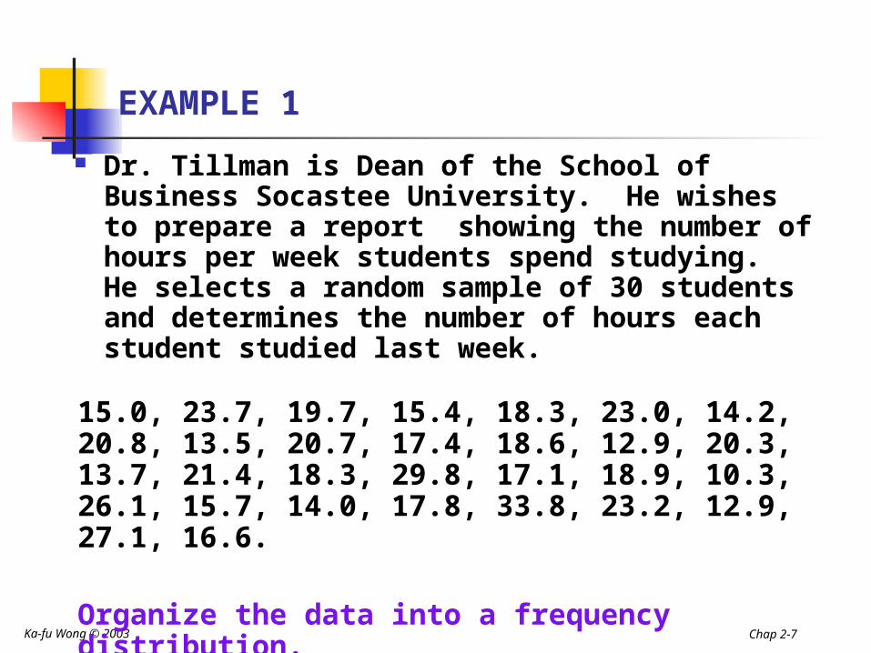
EXAMPLE 1
Dr. Tillman is Dean of the School of Business Socastee University. He wishes to prepare a report showing the number of hours per week students spend studying. He selects a random sample of 30 students and determines the number of hours each student studied last week.
15.0, 23.7, 19.7, 15.4, 18.3, 23.0, 14.2, 20.8, 13.5, 20.7, 17.4, 18.6, 12.9, 20.3, 13.7, 21.4, 18.3, 29.8, 17.1, 18.9, 10.3, 26.1, 15.7, 14.0, 17.8, 33.8, 23.2, 12.9, 27.1, 16.6.
Organize the data into a frequency distribution.
Ka-fu Wong © 2003 Chap 2-8
Step 1: Decide on the number of classes.
The goal is to use just enough groupings or classes to reveal the shape of the distribution.
“Just enough” Recipe –“2 to the k rule” Select the smallest number (k) for the
number of classes such that 2k is greater than the number of observations (n).
Ka-fu Wong © 2003 Chap 2-9
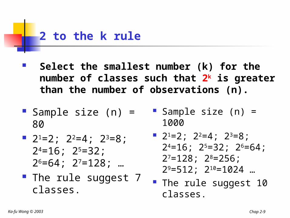
2 to the k rule
Sample size (n) = 80 21=2; 22=4; 23=8;
24=16; 25=32; 26=64; 27=128; …
The rule suggest 7 classes.
Sample size (n) = 1000
21=2; 22=4; 23=8; 24=16; 25=32; 26=64; 27=128; 28=256; 29=512; 210=1024 …
The rule suggest 10 classes.
Select the smallest number (k) for the number of classes such that 2k is greater than the number of observations (n).

Ka-fu Wong © 2003 Chap 2-10
2 to the k rule
Sample size (n)=10000
21=2; 22=4; 23=8; 24=16; 25=32; 26=64; 27=128; …,213=8192; 214 = 16384
The rule suggest 14.
Sample size (n)=100000
22=4; 23=8; 24=16; 25=32; 26=64; 27=128; …
Select the smallest number (k) for the number of classes such that 2k is greater than the number of observations (n).
Ka-fu Wong © 2003 Chap 2-11
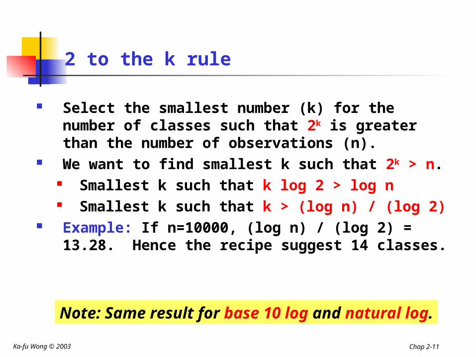
2 to the k rule
Select the smallest number (k) for the number of classes such that 2k is greater than the number of observations (n).
We want to find smallest k such that 2k > n. Smallest k such that k log 2 > log n Smallest k such that k > (log n) / (log 2)
Example: If n=10000, (log n) / (log 2) = 13.28. Hence the recipe suggest 14 classes.
Note: Same result for base 10 log and natural log.
Ka-fu Wong © 2003 Chap 2-12
Step 1: Decide on the number of classes.
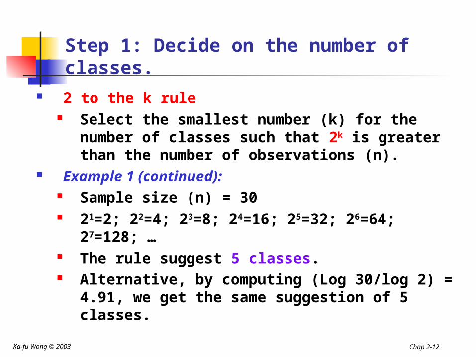
2 to the k rule Select the smallest number (k) for the
number of classes such that 2k is greater than the number of observations (n).
Example 1 (continued): Sample size (n) = 30 21=2; 22=4; 23=8; 24=16; 25=32; 26=64;
27=128; … The rule suggest 5 classes. Alternative, by computing (Log 30/log 2) =
4.91, we get the same suggestion of 5 classes.
Ka-fu Wong © 2003 Chap 2-13
Step 2: Determine the class interval or width.
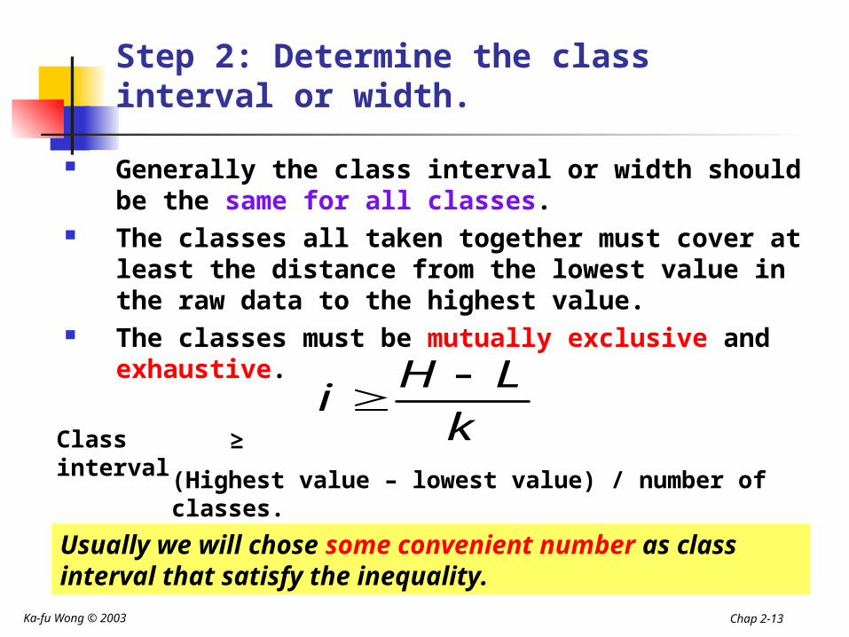
Generally the class interval or width should be the same for all classes.
The classes all taken together must cover at least the distance from the lowest value in the raw data to the highest value.
The classes must be mutually exclusive and exhaustive.
Class interval
≥
(Highest value – lowest value) / number of classes.
k
LHi
Usually we will chose some convenient number as class interval that satisfy the inequality.
Ka-fu Wong © 2003 Chap 2-14
Step 2: Determine the class interval or width.
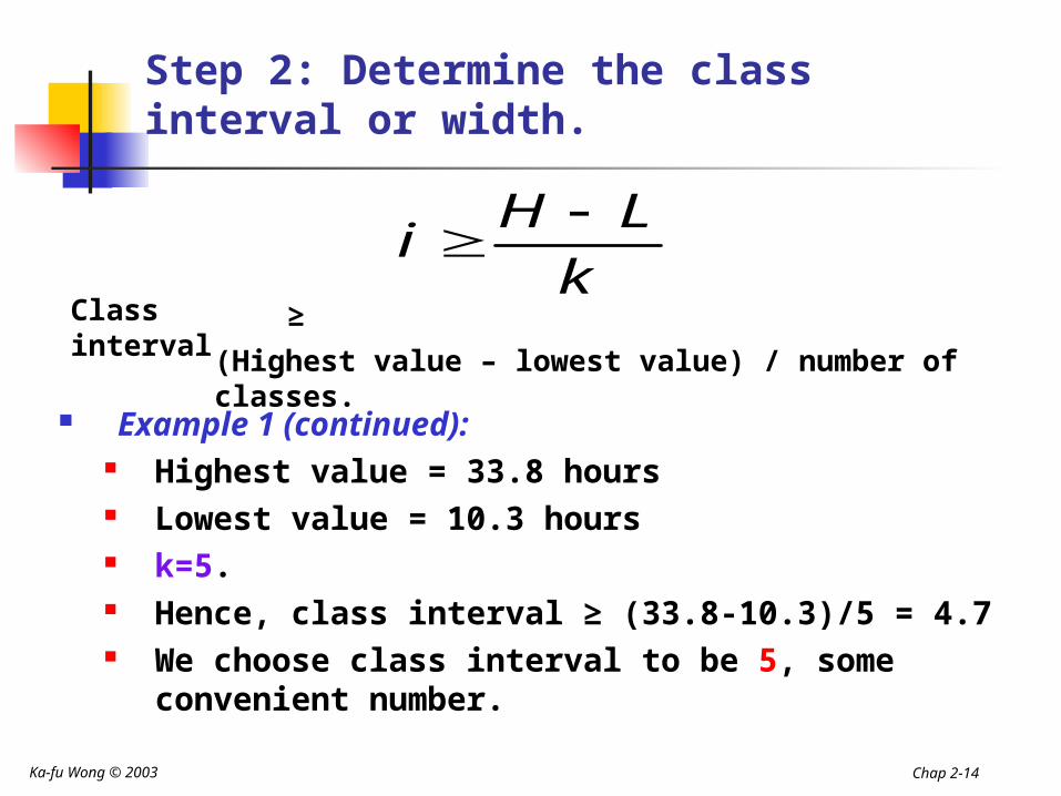
Example 1 (continued): Highest value = 33.8 hours Lowest value = 10.3 hours k=5. Hence, class interval ≥ (33.8-10.3)/5 = 4.7 We choose class interval to be 5, some
convenient number.
Class interval
≥
(Highest value – lowest value) / number of classes.
k
LHi
Ka-fu Wong © 2003 Chap 2-15
Step 3: Set the individual class limits
The class limits must be set so that the classes are mutually exclusive and exhaustive.
Round up to some convenient numbers.
Ka-fu Wong © 2003 Chap 2-16
Step 3: Set the individual class limits
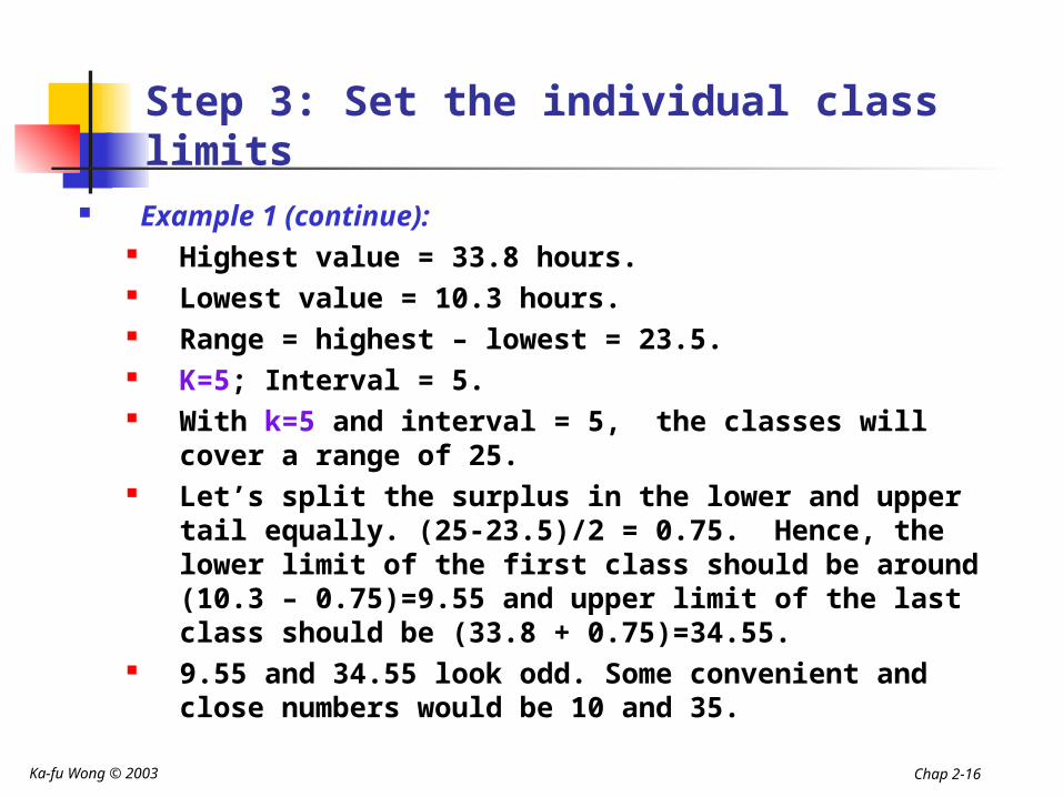
Example 1 (continue): Highest value = 33.8 hours. Lowest value = 10.3 hours. Range = highest – lowest = 23.5. K=5; Interval = 5. With k=5 and interval = 5, the classes will cover
a range of 25. Let’s split the surplus in the lower and upper tail
equally. (25-23.5)/2 = 0.75. Hence, the lower limit of the first class should be around (10.3 – 0.75)=9.55 and upper limit of the last class should be (33.8 + 0.75)=34.55.
9.55 and 34.55 look odd. Some convenient and close numbers would be 10 and 35.
Ka-fu Wong © 2003 Chap 2-17
Step 3: Set the individual class limits
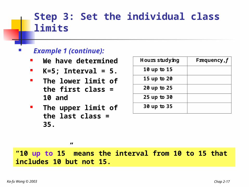
Example 1 (continue): We have
determined K=5; Interval = 5. The lower limit of
the first class = 10 and
The upper limit of the last class = 35.
Hours studying Frequency, f
10 up to 15
15 up to 20
20 up to 25
25 up to 30
30 up to 35
“10 up to 15” means the interval from 10 to 15 that includes 10 but not 15.
Ka-fu Wong © 2003 Chap 2-18
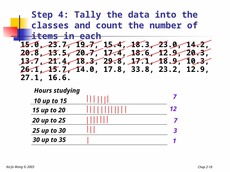
Step 4: Tally the data into the classes and count the number of items in each
10 up to 15
Hours studying
15 up to 20
20 up to 25
25 up to 3030 up to 35
15.0, 23.7, 19.7, 15.4, 18.3, 23.0, 14.2, 20.8, 13.5, 20.7, 17.4, 18.6, 12.9, 20.3, 13.7, 21.4, 18.3, 29.8, 17.1, 18.9, 10.3, 26.1, 15.7, 14.0, 17.8, 33.8, 23.2, 12.9, 27.1, 16.6.
7
12
7
3
1
Ka-fu Wong © 2003 Chap 2-19
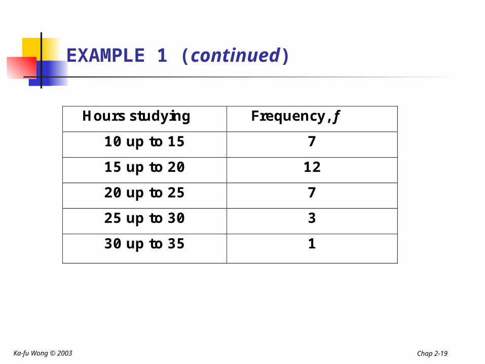
EXAMPLE 1 (continued)
Hours studying Frequency, f
10 up to 15 7
15 up to 20 12
20 up to 25 7
25 up to 30 3
30 up to 35 1
Ka-fu Wong © 2003 Chap 2-20
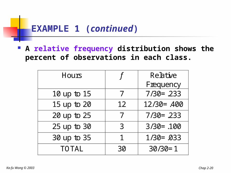
EXAMPLE 1 (continued)
A relative frequency distribution shows the percent of observations in each class.
Hours f Relative Frequency
10 up to 15 7 7/30=.233 15 up to 20 12 12/30=.400
20 up to 25 7 7/30=.233
25 up to 30 3 3/30=.100
30 up to 35 1 1/30=.033
TOTAL 30 30/30=1
Ka-fu Wong © 2003 Chap 2-21
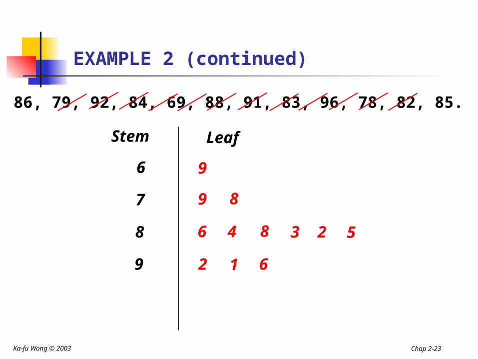
Stem-and-leaf Displays
Stem-and-leaf display: A statistical technique for displaying a set of data. Each numerical value is divided into two parts: the leading digits become the stem and the trailing digits the leaf.
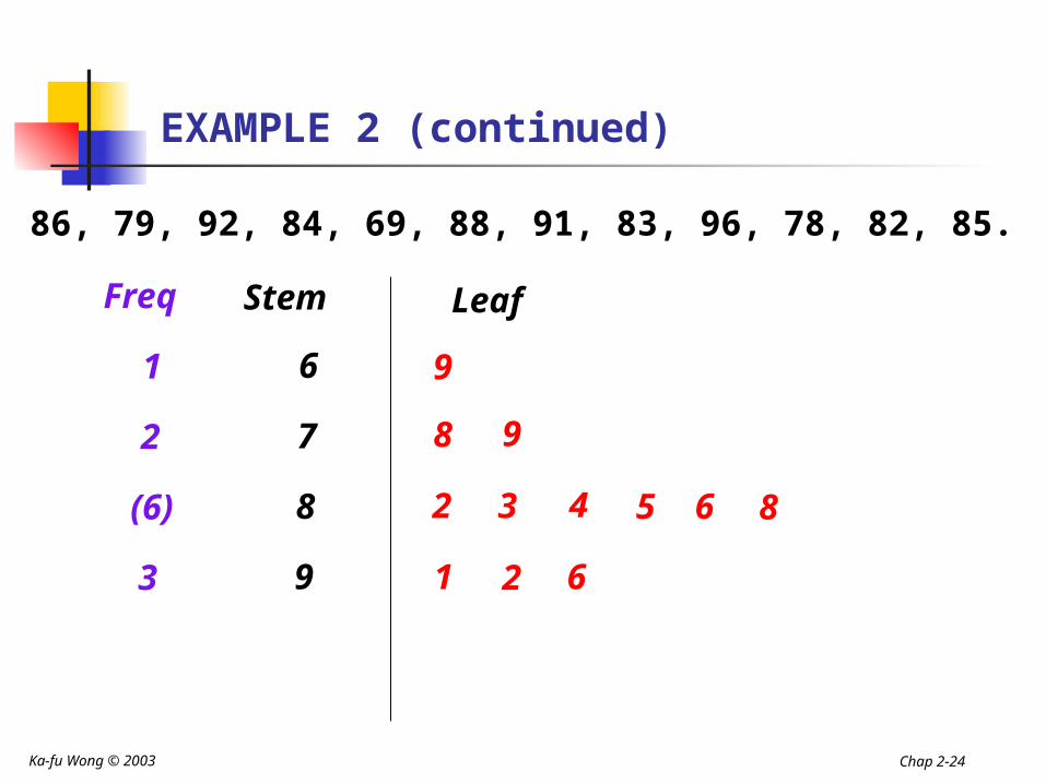
Note: An advantage of the stem-and-leaf
display over a frequency distribution is we do not lose the identity of each observation.
An disadvantage is that it is not good for large data sets.
Ka-fu Wong © 2003 Chap 2-22
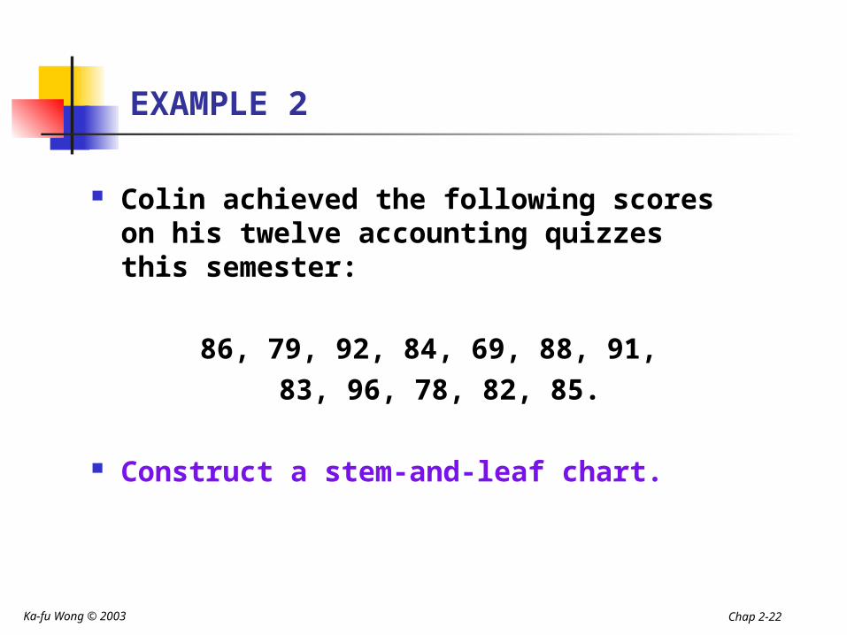
EXAMPLE 2
Colin achieved the following scores on his twelve accounting quizzes this semester:
86, 79, 92, 84, 69, 88, 91, 83, 96, 78, 82, 85.
Construct a stem-and-leaf chart.
Ka-fu Wong © 2003 Chap 2-23
EXAMPLE 2 (continued)
86, 79, 92, 84, 69, 88, 91, 83, 96, 78, 82, 85.
Stem Leaf
6
7
8
9
6
9
2
4
9
8
1
3
6
8
2 5
Ka-fu Wong © 2003 Chap 2-24
EXAMPLE 2 (continued)
86, 79, 92, 84, 69, 88, 91, 83, 96, 78, 82, 85.
Stem Leaf
6
7
8
9
2
8
1
3
9
4
2
5
6
9
6 8
1
2
(6)
3
Freq
Ka-fu Wong © 2003 Chap 2-25
Graphic Presentation of a Frequency Distribution
The three commonly used graphic forms are histograms, frequency polygons, and a cumulative frequency distribution.
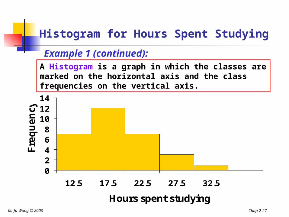
A Histogram is a graph in which the classes are marked on the horizontal axis and the class frequencies on the vertical axis. The class frequencies are represented by
the heights of the bars and the bars are drawn adjacent to each other.
Ka-fu Wong © 2003 Chap 2-26
Graphic Presentation of a Frequency Distribution
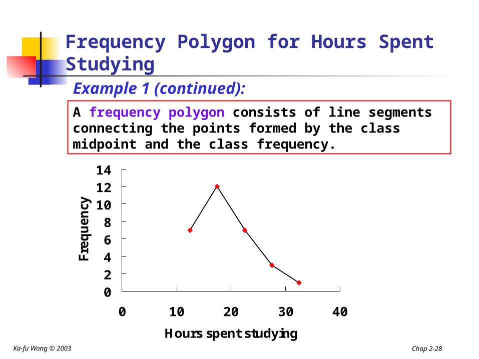
A frequency polygon consists of line segments connecting the points formed by the class midpoint and the class frequency.
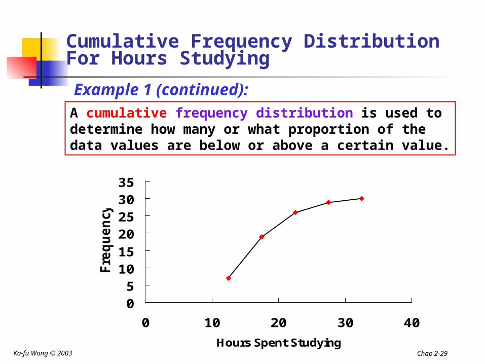
A cumulative frequency distribution is used to determine how many or what proportion of the data values are below or above a certain value.
Ka-fu Wong © 2003 Chap 2-27
Histogram for Hours Spent Studying
02468
101214
12.5 17.5 22.5 27.5 32.5
Hours spent studying
Fre
quency
Example 1 (continued):A Histogram is a graph in which the classes are marked on the horizontal axis and the class frequencies on the vertical axis.
Ka-fu Wong © 2003 Chap 2-28
Frequency Polygon for Hours Spent Studying
02468
101214
0 10 20 30 40
Hours spent studying
Freq
uen
cyExample 1 (continued):
A frequency polygon consists of line segments connecting the points formed by the class midpoint and the class frequency.
Ka-fu Wong © 2003 Chap 2-29
Cumulative Frequency Distribution For Hours Studying
05
101520253035
0 10 20 30 40
Hours Spent Studying
Fre
quency
Example 1 (continued):A cumulative frequency distribution is used to determine how many or what proportion of the data values are below or above a certain value.
Ka-fu Wong © 2003 Chap 2-30
Bar Chart
A bar chart can be used to depict any of the levels of measurement (nominal, ordinal, interval, or ratio).

Ka-fu Wong © 2003 Chap 2-31
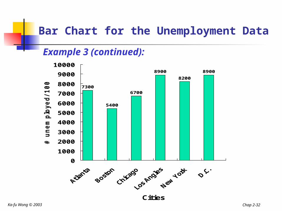
Example 3
Construct a bar chart for the number of unemployed per 100,000 population for selected cities during 2001
City Number of unemployed per 100,000 population
Atlanta, GA 7300
Boston, MA 5400
Chicago, IL 6700
Los Angeles, CA 8900
New York, NY 8200
Washington, D.C. 8900
Ka-fu Wong © 2003 Chap 2-32
Bar Chart for the Unemployment Data
7300
5400
6700
8900
8200
8900
0
1000
2000
3000
4000
5000
6000
7000
8000
9000
10000
Cities
# u
nem
plo
yed/100,0
00 .
Example 3 (continued):
Ka-fu Wong © 2003 Chap 2-33
Pie Chart
A pie chart is useful for displaying a relative frequency distribution. A circle is divided proportionally to the relative frequency and portions of the circle are allocated for the different groups.
Ka-fu Wong © 2003 Chap 2-34
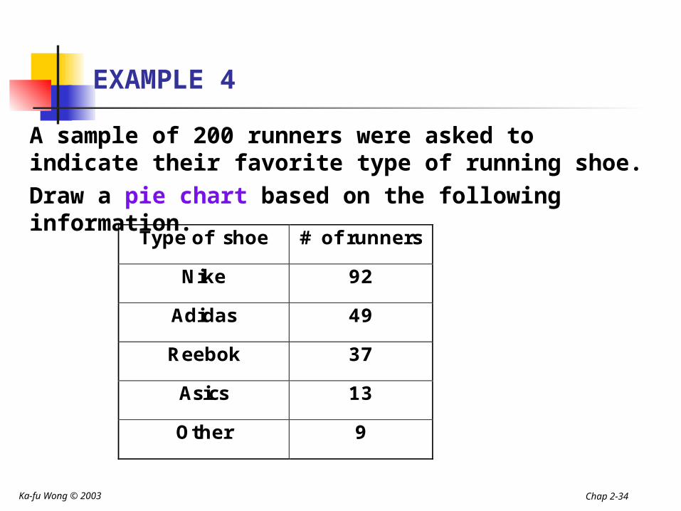
EXAMPLE 4
Type of shoe # of runners
Nike 92
Adidas 49
Reebok 37
Asics 13
Other 9
A sample of 200 runners were asked to indicate their favorite type of running shoe. Draw a pie chart based on the following information.
Ka-fu Wong © 2003 Chap 2-35
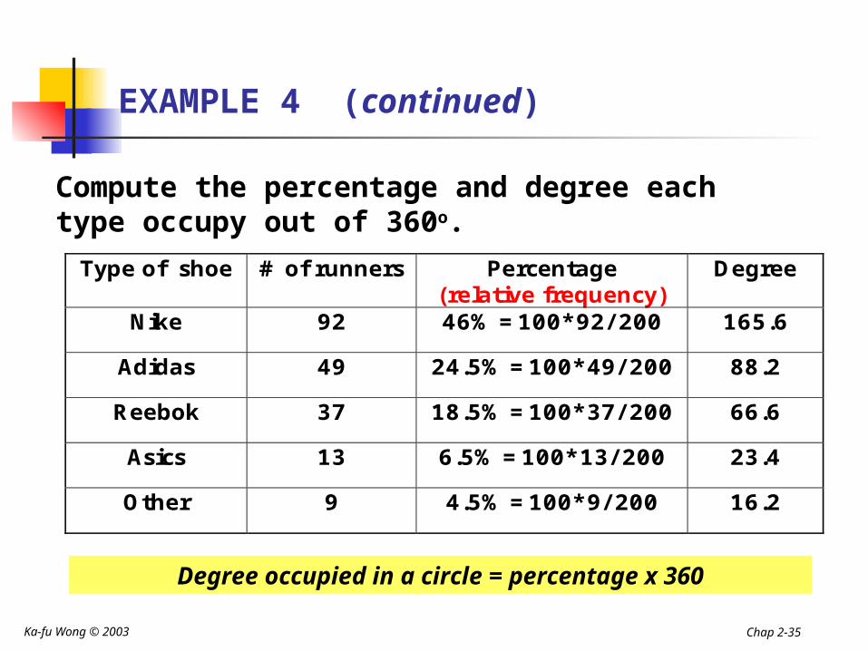
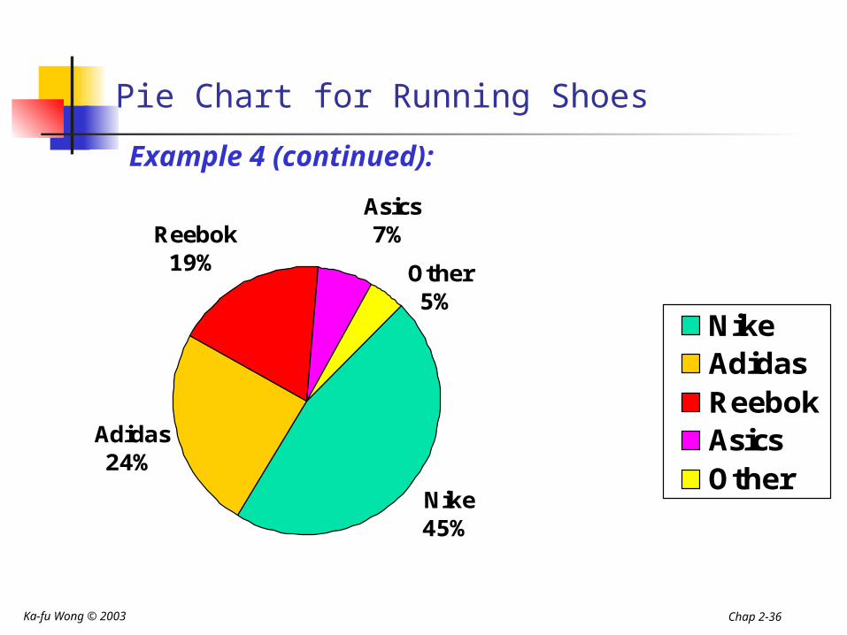
EXAMPLE 4 (continued)
Type of shoe # of runners Percentage (relative frequency)
Degree
Nike 92 46% =100*92/ 200 165.6
Adidas 49 24.5% =100*49/ 200 88.2
Reebok 37 18.5% =100*37/ 200 66.6
Asics 13 6.5% =100*13/ 200 23.4
Other 9 4.5% =100*9/ 200 16.2
Compute the percentage and degree each type occupy out of 360o.
Degree occupied in a circle = percentage x 360
Ka-fu Wong © 2003 Chap 2-36
Pie Chart for Running Shoes
Adidas24%
Reebok19%
Asics7%
Other5%
Nike45%
NikeAdidasReebokAsicsOther
Example 4 (continued):
Ka-fu Wong © 2003 Chap 2-37
Measures of Central Tendency
1. Mean2. Median3. Mode
Ka-fu Wong © 2003 Chap 2-38
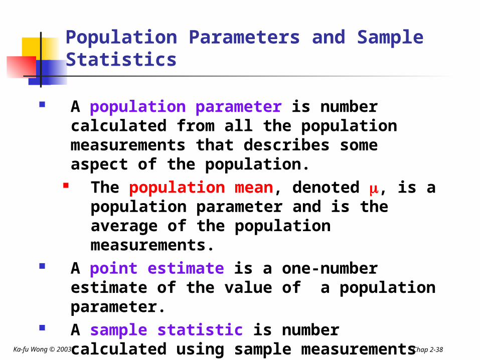
Population Parameters and Sample Statistics
A population parameter is number calculated from all the population measurements that describes some aspect of the population.
The population mean, denoted , is a population parameter and is the average of the population measurements.
A point estimate is a one-number estimate of the value of a population parameter.
A sample statistic is number calculated using sample measurements that describes some aspect of the sample.
Ka-fu Wong © 2003 Chap 2-39
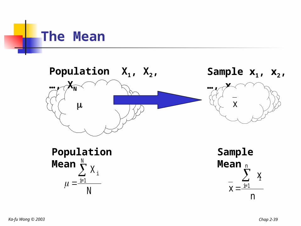
The Mean
Population X1, X2, …, XN
Population Mean
N
X
N
1=ii
Sample x1, x2, …, xn
Sample Mean
n
xx
n
1=ii
x
Ka-fu Wong © 2003 Chap 2-40
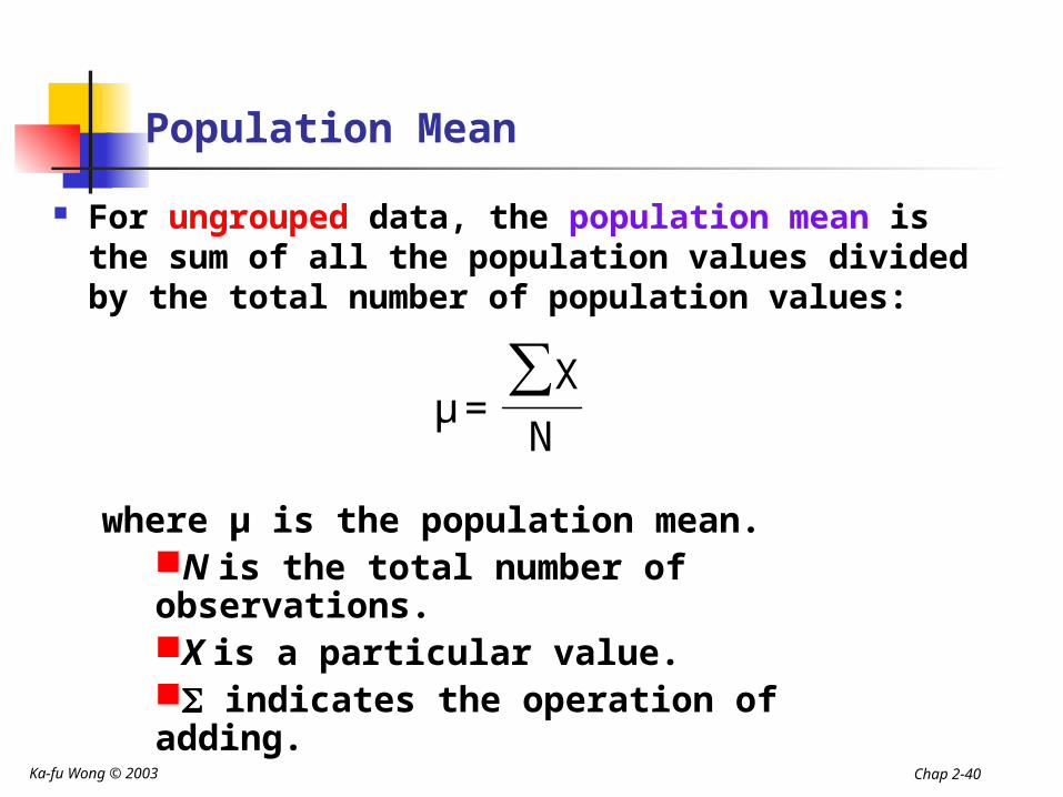
Population Mean
For ungrouped data, the population mean is the sum of all the population values divided by the total number of population values:
N
X=μ
∑
where µ is the population mean.N is the total number of observations.X is a particular value. indicates the operation of adding.
Ka-fu Wong © 2003 Chap 2-41
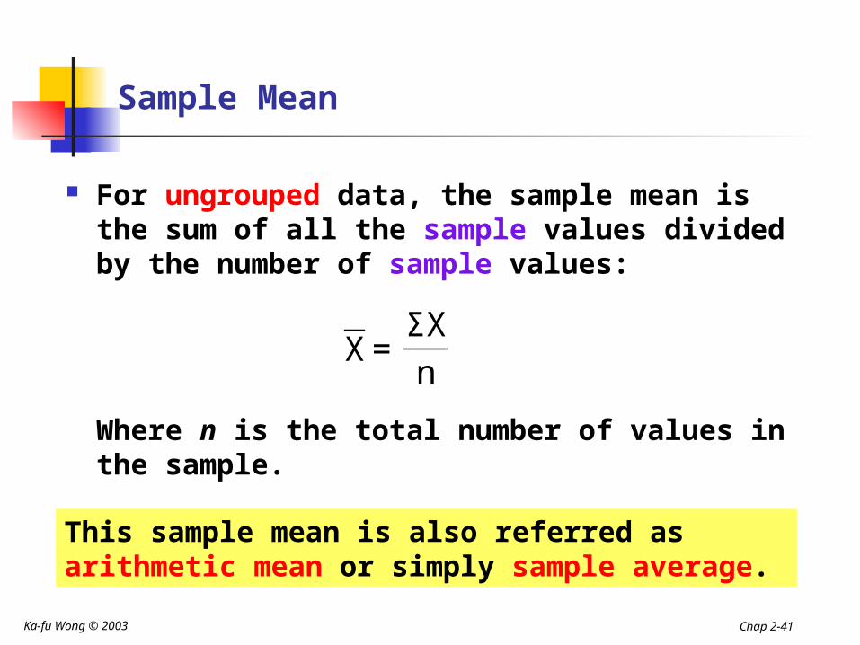
Sample Mean
For ungrouped data, the sample mean is the sum of all the sample values divided by the number of sample values:
Where n is the total number of values in the sample.
nΣX
=X
This sample mean is also referred as arithmetic mean or simply sample average.
Ka-fu Wong © 2003 Chap 2-42
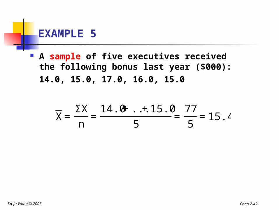
EXAMPLE 5
A sample of five executives received the following bonus last year ($000):
14.0, 15.0, 17.0, 16.0, 15.0
15.4=577
=5
15.0+...+14.0=
nΣX
=X
Ka-fu Wong © 2003 Chap 2-43
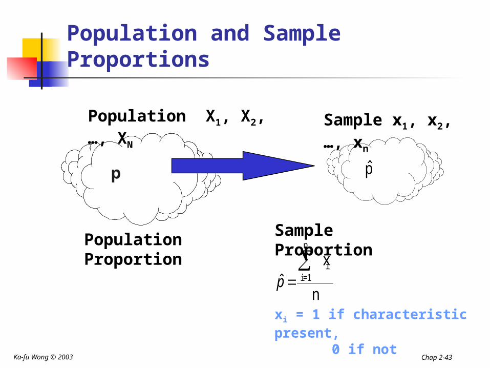
Population and Sample Proportions
Population X1, X2, …, XN
p
Population Proportion
Sample x1, x2, …, xn
Sample Proportion
n
xˆ
n
1=ii
p
p̂
xi = 1 if characteristic present, 0 if not
Ka-fu Wong © 2003 Chap 2-44
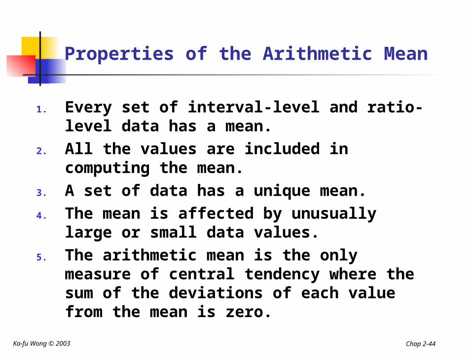
Properties of the Arithmetic Mean
1. Every set of interval-level and ratio-level data has a mean.
2. All the values are included in computing the mean.
3. A set of data has a unique mean.4. The mean is affected by unusually large
or small data values.5. The arithmetic mean is the only
measure of central tendency where the sum of the deviations of each value from the mean is zero.
Ka-fu Wong © 2003 Chap 2-45
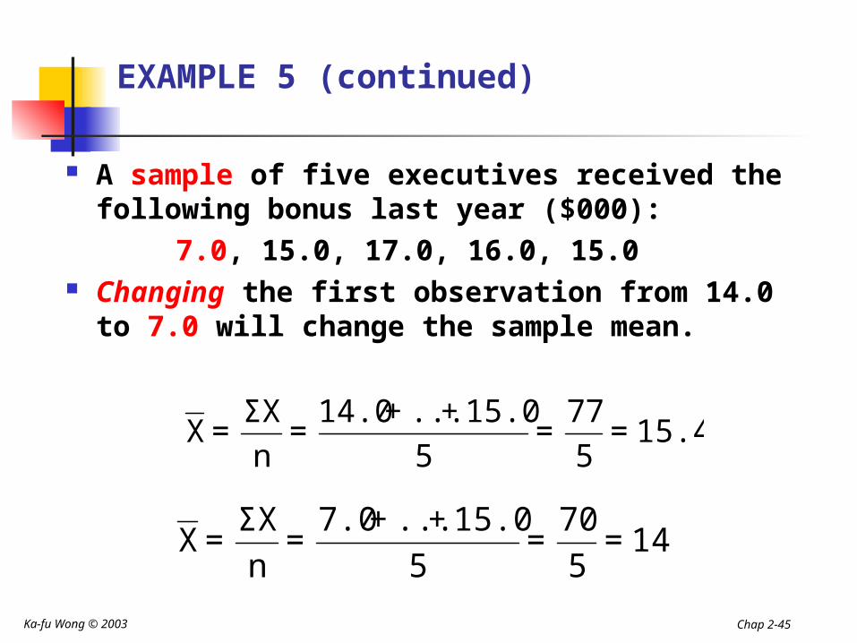
EXAMPLE 5 (continued)
A sample of five executives received the following bonus last year ($000):
7.0, 15.0, 17.0, 16.0, 15.0 Changing the first observation from 14.0 to
7.0 will change the sample mean.
14=570
=5
15.0+...+7.0=
nΣX
=X
15.4=577
=5
15.0+...+14.0=
nΣX
=X
Ka-fu Wong © 2003 Chap 2-46
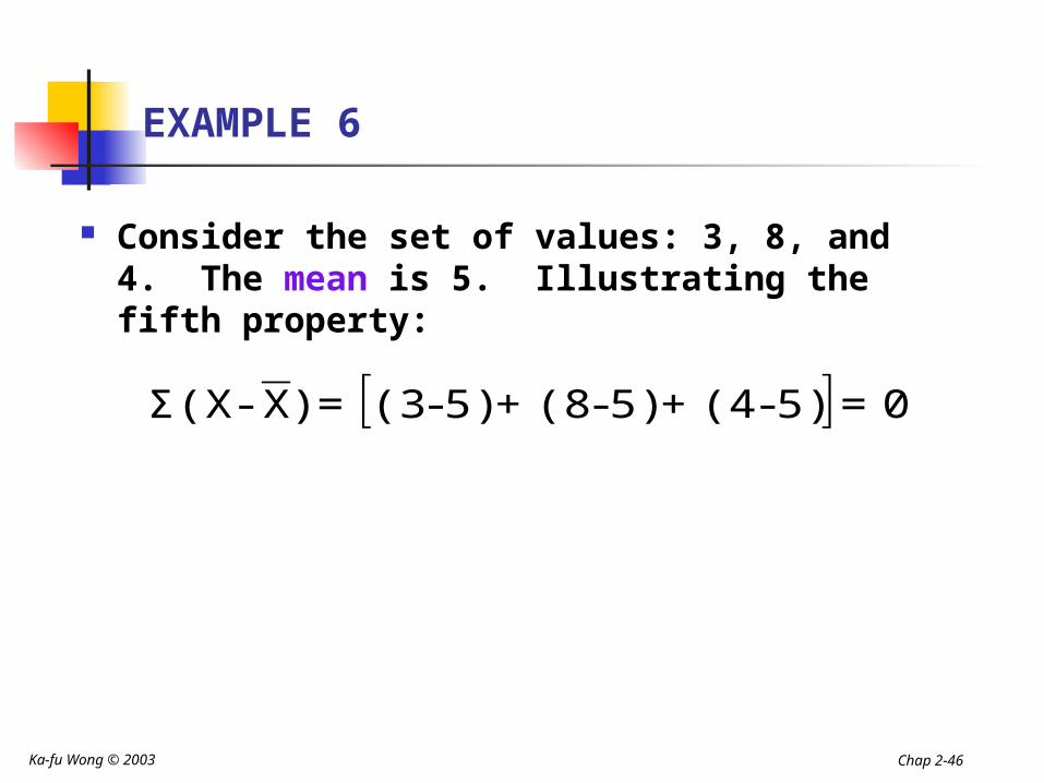
EXAMPLE 6
Consider the set of values: 3, 8, and 4. The mean is 5. Illustrating the fifth property:
0=5)(4+5)(8+5)(3=)X -Σ(X ---
Ka-fu Wong © 2003 Chap 2-47
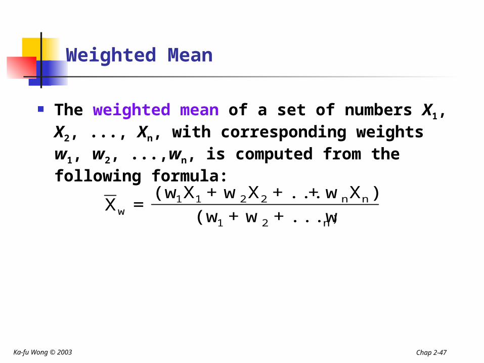
Weighted Mean
The weighted mean of a set of numbers X1, X2, ..., Xn, with corresponding weights w1, w2, ...,wn, is computed from the following formula:
)n21
nn2211w ...w+w+(w
)Xw+...+Xw+X(w=X
Ka-fu Wong © 2003 Chap 2-48
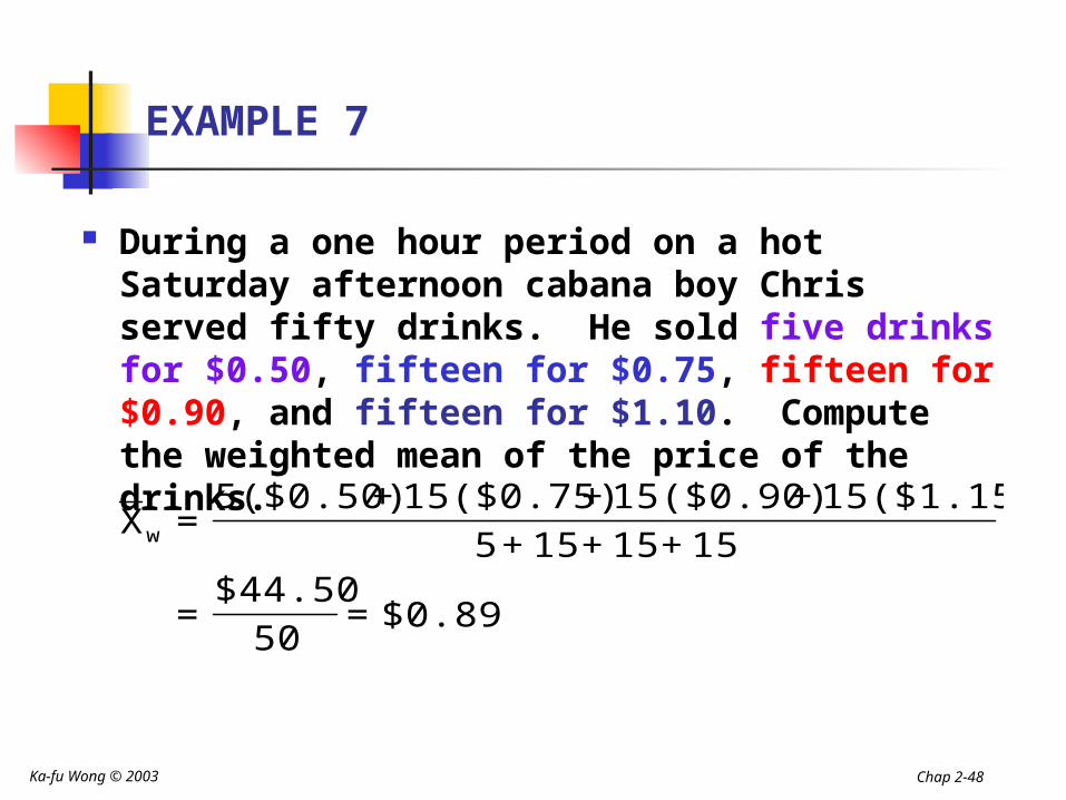
EXAMPLE 7
During a one hour period on a hot Saturday afternoon cabana boy Chris served fifty drinks. He sold five drinks for $0.50, fifteen for $0.75, fifteen for $0.90, and fifteen for $1.10. Compute the weighted mean of the price of the drinks.
$0.89=50
$44.50=
15+15+15+515($1.15)+15($0.90)+15($0.75)+5($0.50)
=Xw
Ka-fu Wong © 2003 Chap 2-49
The Median
The Median is the midpoint of the values after they have been ordered from the smallest to the largest.
There are as many values above the median as below it in the data array.
For an even set of values, the median will be the arithmetic average of the two middle numbers.
Ka-fu Wong © 2003 Chap 2-50
EXAMPLE 8
The ages for a sample of five college students are:
21, 25, 19, 20, 22 Arranging the data in ascending order
gives: 19, 20, 21, 22, 25. Thus the median is 21.
The heights of four basketball players, in inches, are: 76, 73, 80, 75
Arranging the data in ascending order gives: 73, 75, 76, 80. Thus the median is 75.5
Ka-fu Wong © 2003 Chap 2-51
Properties of the Median
1. There is a unique median for each data set.
2. It is not affected by extremely large or small values and is therefore a valuable measure of central tendency when such values occur.
3. It can be computed for ratio-level, interval-level, and ordinal-level data.
4. It can be computed for an open-ended frequency distribution if the median does not lie in an open-ended class.
Ka-fu Wong © 2003 Chap 2-52
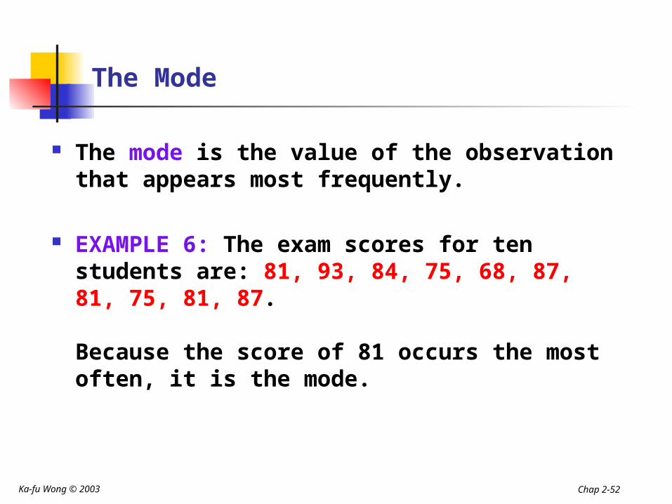
The Mode
The mode is the value of the observation that appears most frequently.
EXAMPLE 6: The exam scores for ten students are: 81, 93, 84, 75, 68, 87, 81, 75, 81, 87.
Because the score of 81 occurs the most often, it is the mode.
Ka-fu Wong © 2003 Chap 2-53
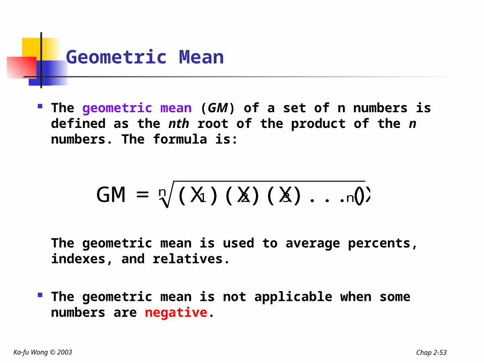
Geometric Mean
The geometric mean (GM) of a set of n numbers is defined as the nth root of the product of the n numbers. The formula is:
The geometric mean is used to average percents, indexes, and relatives.
The geometric mean is not applicable when some numbers are negative.
n n321 ))...(X)(X)(X(X=GM
Ka-fu Wong © 2003 Chap 2-54
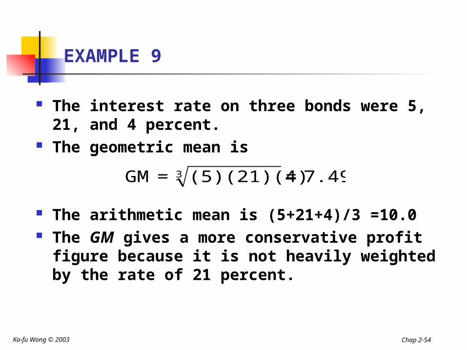
EXAMPLE 9
The interest rate on three bonds were 5, 21, and 4 percent.
The geometric mean is
The arithmetic mean is (5+21+4)/3 =10.0 The GM gives a more conservative profit
figure because it is not heavily weighted by the rate of 21 percent.
7.49=(5)(21)(4)=GM 3
Ka-fu Wong © 2003 Chap 2-55
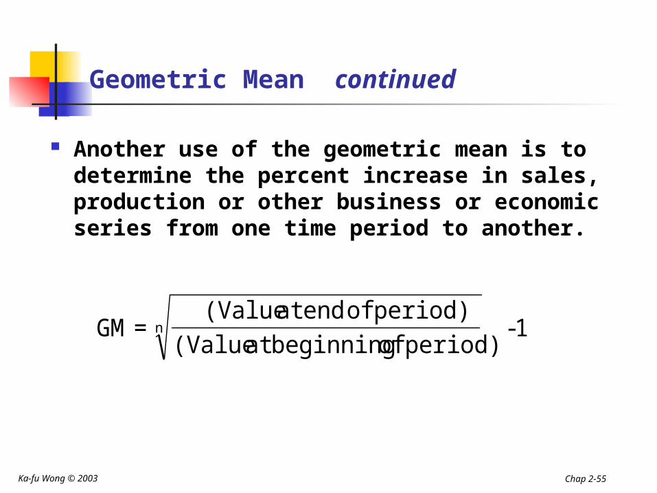
Geometric Mean continued
Another use of the geometric mean is to determine the percent increase in sales, production or other business or economic series from one time period to another.
1period) of beginningat (Value
period) of endat (Value=GM n -
Ka-fu Wong © 2003 Chap 2-56
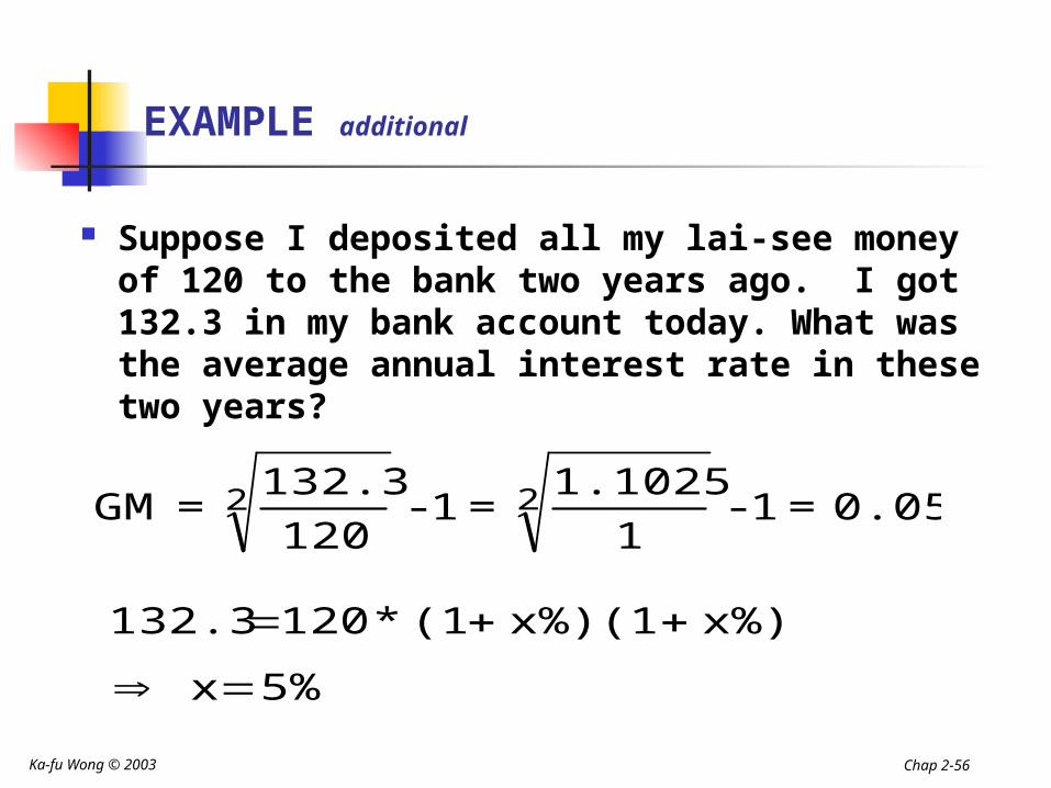
EXAMPLE additional
Suppose I deposited all my lai-see money of 120 to the bank two years ago. I got 132.3 in my bank account today. What was the average annual interest rate in these two years?
0.05 =1 - 1
1.1025=1 -
120
132.3=GM 22
5% x
x%)x%)(1(1*120 132.3
Ka-fu Wong © 2003 Chap 2-57
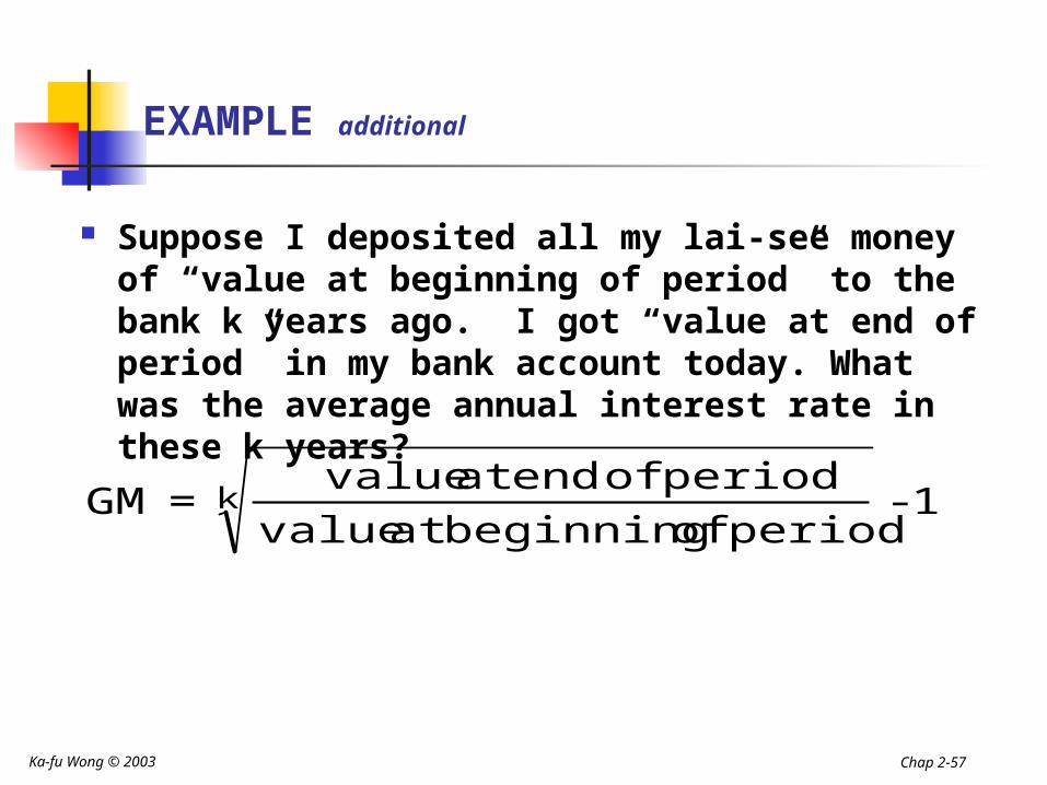
EXAMPLE additional
Suppose I deposited all my lai-see money of “value at beginning of period” to the bank k years ago. I got “value at end of period” in my bank account today. What was the average annual interest rate in these k years?
1 - period of beginningat value
period of endat value=GM k
Ka-fu Wong © 2003 Chap 2-58
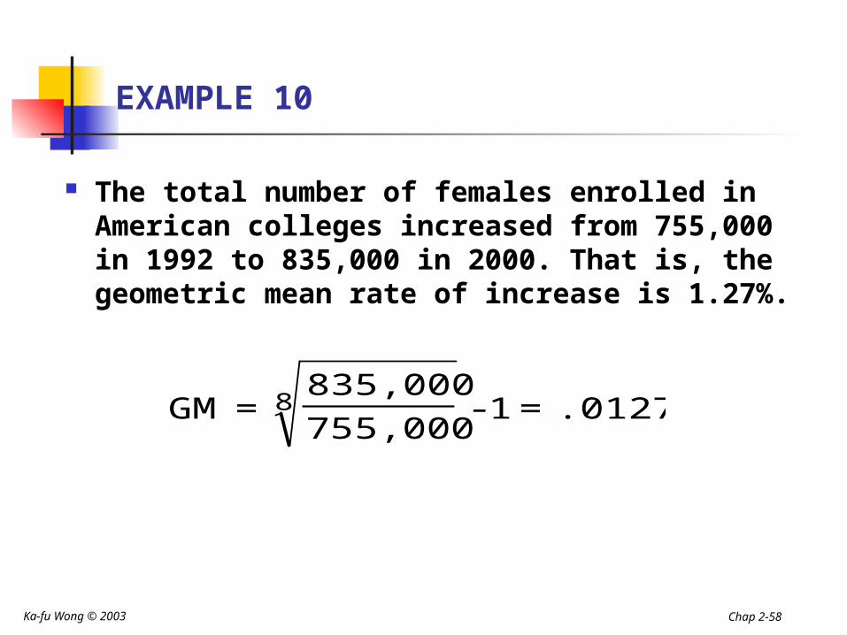
EXAMPLE 10
The total number of females enrolled in American colleges increased from 755,000 in 1992 to 835,000 in 2000. That is, the geometric mean rate of increase is 1.27%.
.0127=1 - 755,000
835,000=GM 8
Ka-fu Wong © 2003 Chap 2-59
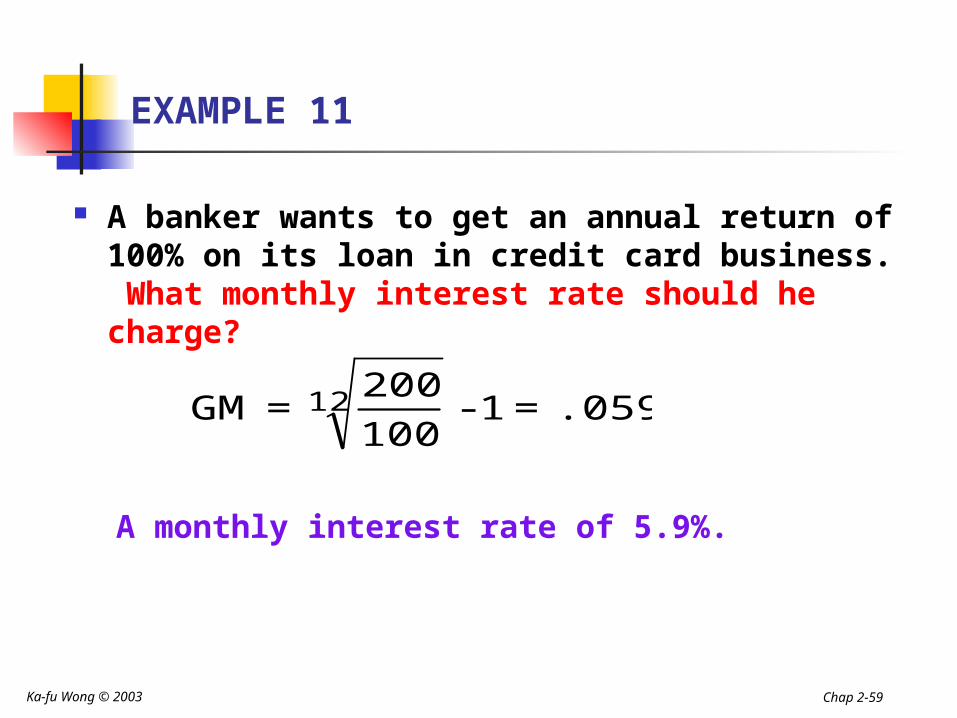
EXAMPLE 11
A banker wants to get an annual return of 100% on its loan in credit card business. What monthly interest rate should he charge?
.059=1 - 100
200=GM 12
A monthly interest rate of 5.9%.
Ka-fu Wong © 2003 Chap 2-60
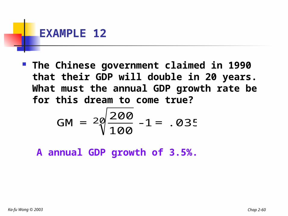
EXAMPLE 12
The Chinese government claimed in 1990 that their GDP will double in 20 years. What must the annual GDP growth rate be for this dream to come true?
.035=1 - 100
200=GM 20
A annual GDP growth of 3.5%.
Ka-fu Wong © 2003 Chap 2-61
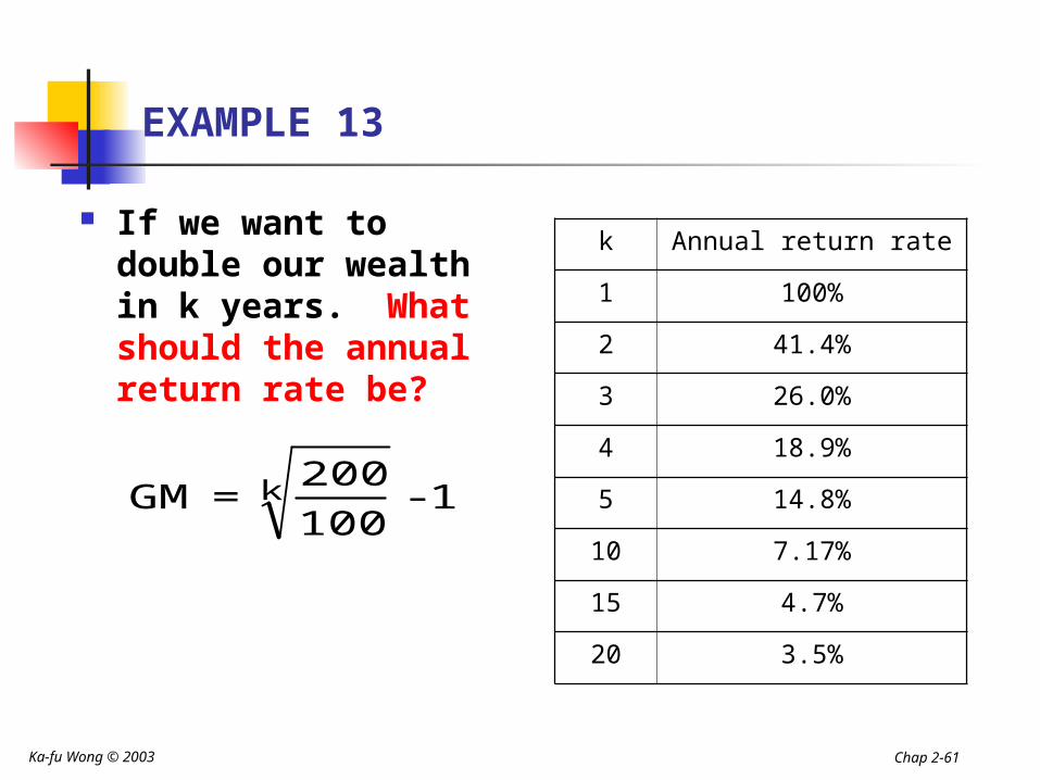
EXAMPLE 13
If we want to double our wealth in k years. What should the annual return rate be?
1 - 100
200=GM k
k Annual return rate
1 100%
2 41.4%
3 26.0%
4 18.9%
5 14.8%
10 7.17%
15 4.7%
20 3.5%
Ka-fu Wong © 2003 Chap 2-62
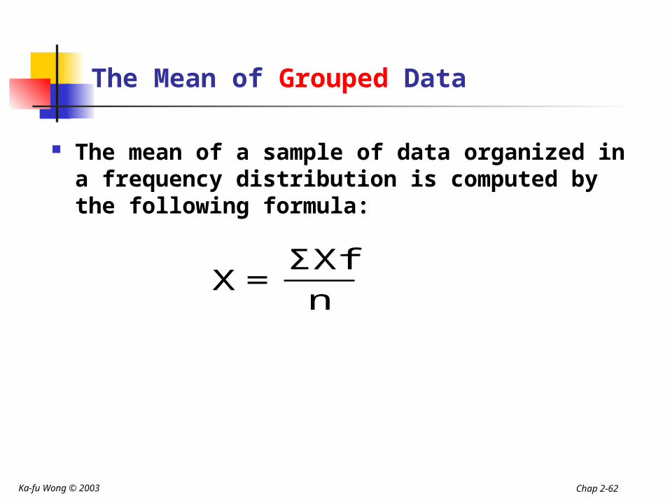
The Mean of Grouped Data
The mean of a sample of data organized in a frequency distribution is computed by the following formula:
nΣXf
=X
Ka-fu Wong © 2003 Chap 2-63
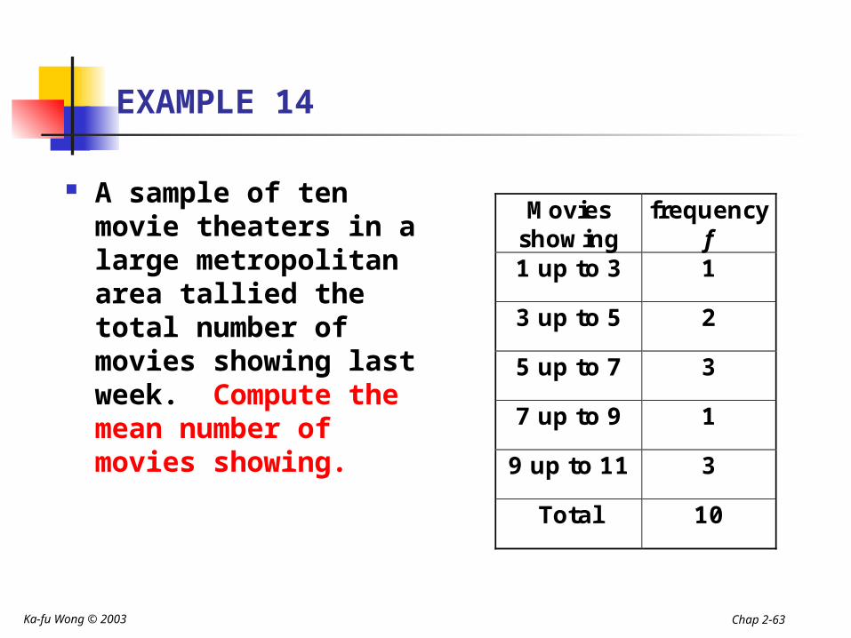
EXAMPLE 14
A sample of ten movie theaters in a large metropolitan area tallied the total number of movies showing last week. Compute the mean number of movies showing.
Movies showing
frequency f
1 up to 3 1
3 up to 5 2
5 up to 7 3
7 up to 9 1
9 up to 11 3
Total 10
Ka-fu Wong © 2003 Chap 2-64
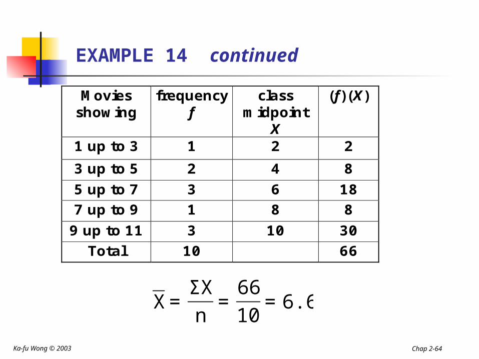
EXAMPLE 14 continued
Movies showing
frequency f
class midpoint
X
(f)(X)
1 up to 3 1 2 2
3 up to 5 2 4 8
5 up to 7 3 6 18 7 up to 9 1 8 8
9 up to 11 3 10 30
Total 10 66
6.6=1066
=nΣX
=X
Ka-fu Wong © 2003 Chap 2-65
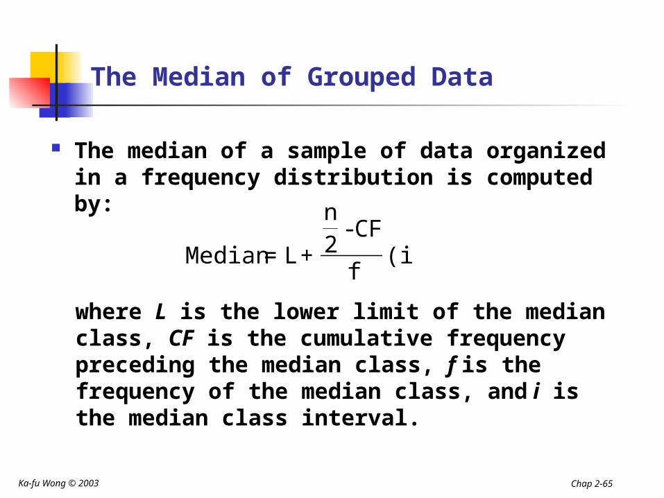
The Median of Grouped Data
The median of a sample of data organized in a frequency distribution is computed by:
(i)
f
CF2n
+L=Median -
where L is the lower limit of the median class, CF is the cumulative frequency preceding the median class, f is the frequency of the median class, and i is the median class interval.
Ka-fu Wong © 2003 Chap 2-66
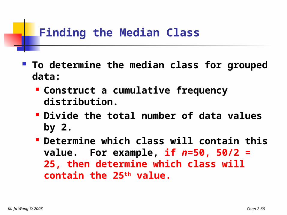
Finding the Median Class
To determine the median class for grouped data: Construct a cumulative frequency
distribution. Divide the total number of data values by
2. Determine which class will contain this
value. For example, if n=50, 50/2 = 25, then determine which class will contain the 25th value.
Ka-fu Wong © 2003 Chap 2-67
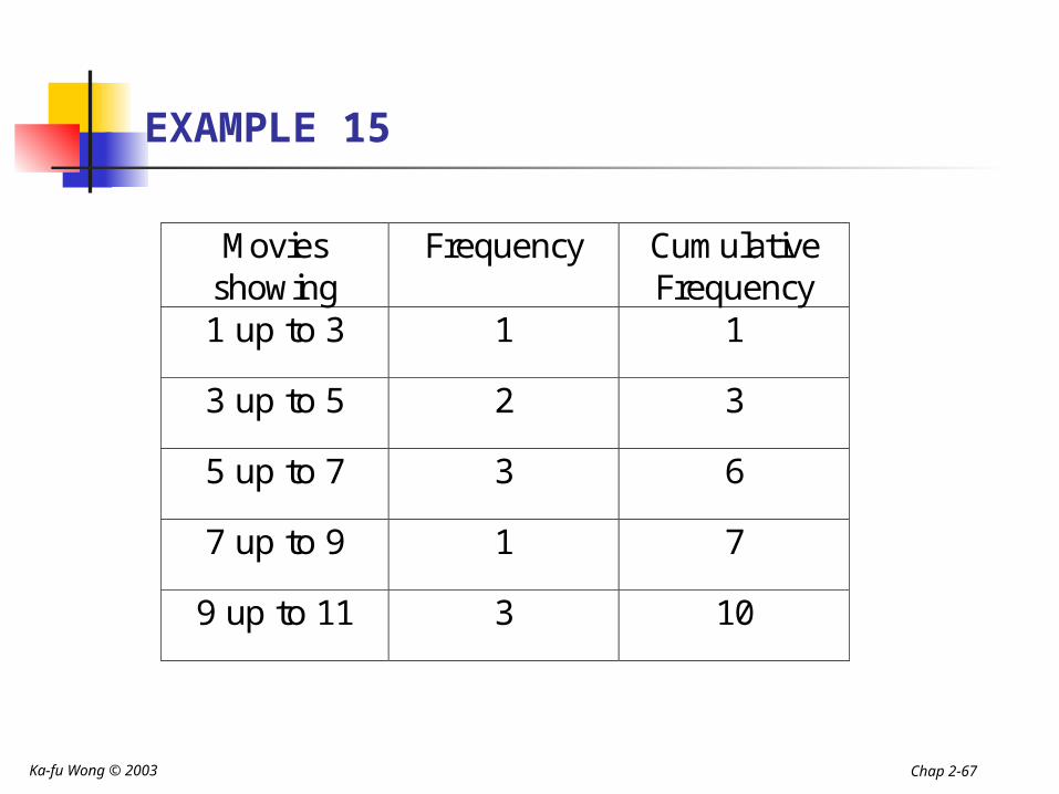
EXAMPLE 15
Movies showing
Frequency Cumulative Frequency
1 up to 3 1 1
3 up to 5 2 3
5 up to 7 3 6
7 up to 9 1 7
9 up to 11 3 10
Ka-fu Wong © 2003 Chap 2-68
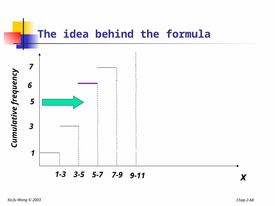
The idea behind the formula
x
Cu
mu
lati
ve f
req
uen
cy
1-3 3-5 5-7 7-9 9-11
1
3
6
7
5
Ka-fu Wong © 2003 Chap 2-69
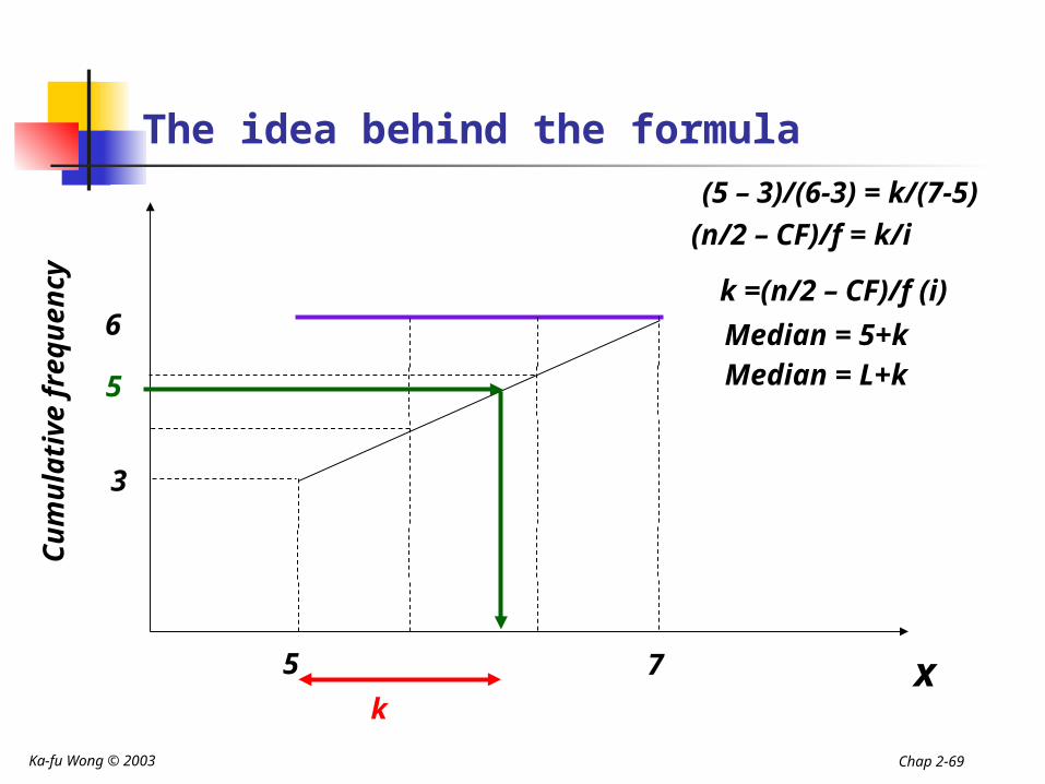
The idea behind the formula
x
Cu
mu
lati
ve f
req
uen
cy
5 7
3
6
5
(5 – 3)/(6-3) = k/(7-5)(n/2 – CF)/f = k/i
k =(n/2 – CF)/f (i)
k
Median = 5+kMedian = L+k
Ka-fu Wong © 2003 Chap 2-70
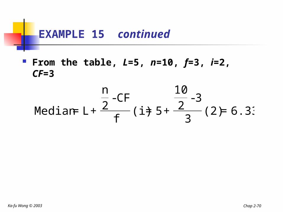
EXAMPLE 15 continued
From the table, L=5, n=10, f=3, i=2, CF=3
6.33=(2)3
32
10
+5=(i)f
CF2n
+L=Median - -
Ka-fu Wong © 2003 Chap 2-71
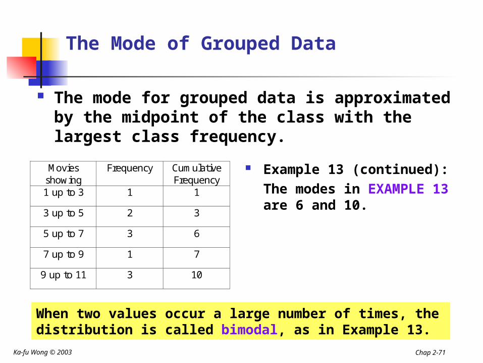
The Mode of Grouped Data
The mode for grouped data is approximated by the midpoint of the class with the largest class frequency.
Example 13 (continued): The modes in EXAMPLE 13 are 6 and 10.
Movies showing
Frequency Cumulative Frequency
1 up to 3 1 1
3 up to 5 2 3
5 up to 7 3 6
7 up to 9 1 7
9 up to 11 3 10
When two values occur a large number of times, the distribution is called bimodal, as in Example 13.
Ka-fu Wong © 2003 Chap 2-72
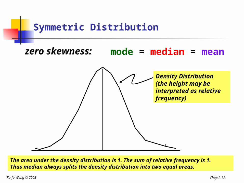
Symmetric Distribution
zero skewness: mode = median = mean
Density Distribution(the height may be interpreted as relative frequency)
The area under the density distribution is 1. The sum of relative frequency is 1.Thus median always splits the density distribution into two equal areas.
Ka-fu Wong © 2003 Chap 2-73
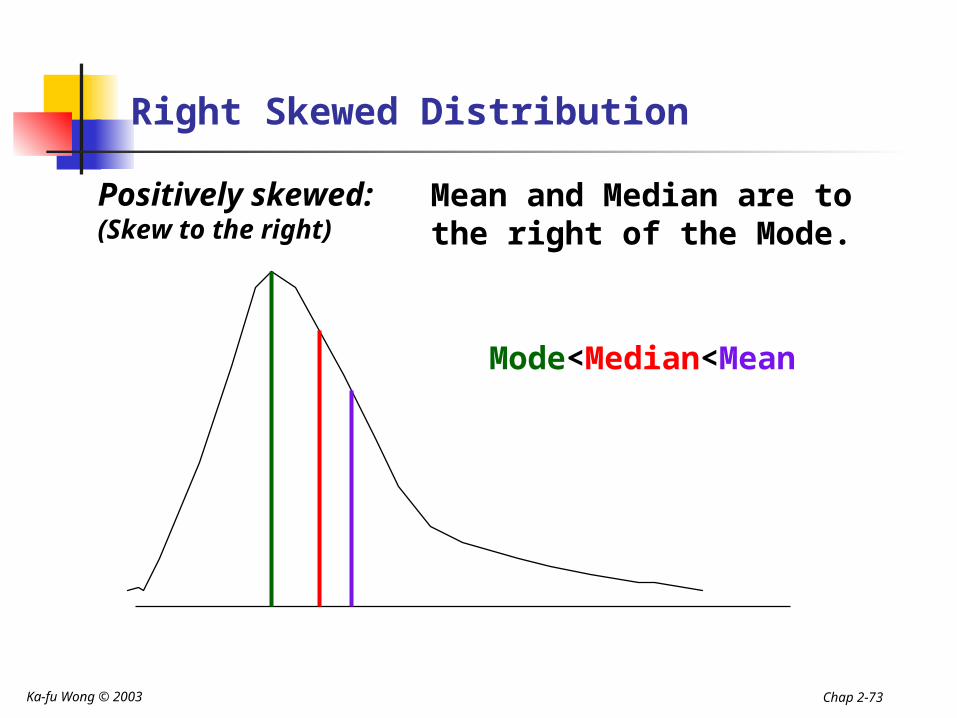
Right Skewed Distribution
Positively skewed: (Skew to the right)
Mean and Median are to the right of the Mode.
Mode<Median<Mean
Ka-fu Wong © 2003 Chap 2-74
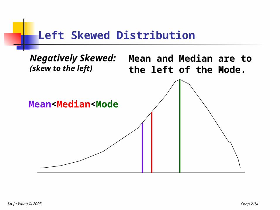
Left Skewed Distribution
Negatively Skewed:(skew to the left)
Mean and Median are to the left of the Mode.
Mean<Median<Mode
Ka-fu Wong © 2003 Chap 2-75
Measures of dispersionMeasures of dispersion
l
1. Range2. Mean Deviation3. Variance and standard deviation4. Coefficient of variation5. Box plots.
Ka-fu Wong © 2003 Chap 2-76
Range
The range is the difference between the largest and the smallest value.
Only two values are used in its calculation. It is influenced by an extreme value. It is easy to compute and understand.
Ka-fu Wong © 2003 Chap 2-77
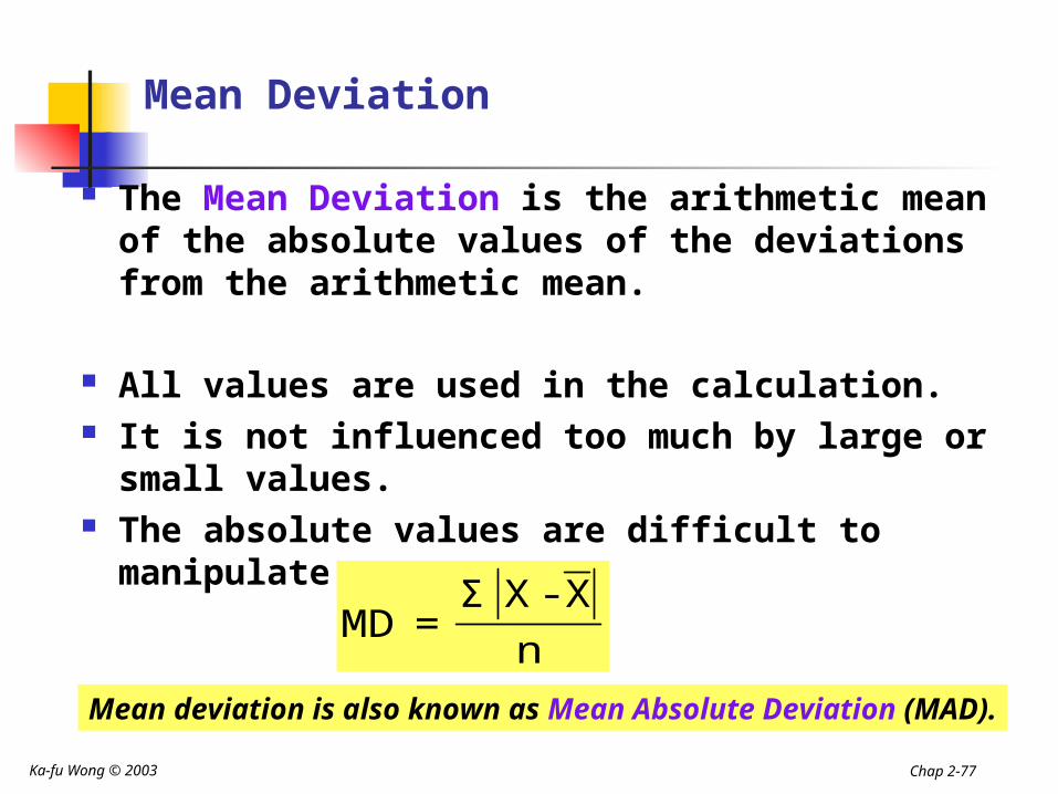
Mean Deviation
The Mean Deviation is the arithmetic mean of the absolute values of the deviations from the arithmetic mean.
All values are used in the calculation. It is not influenced too much by large or
small values. The absolute values are difficult to
manipulate.
Mean deviation is also known as Mean Absolute Deviation (MAD).
n
X-X Σ=MD
Ka-fu Wong © 2003 Chap 2-78
EXAMPLE 16
The weights of a sample of crates containing books for the bookstore (in pounds ) are:
103, 97, 101, 106, 103Find the range and the mean deviation.
Range = 106 – 97 = 9
Ka-fu Wong © 2003 Chap 2-79
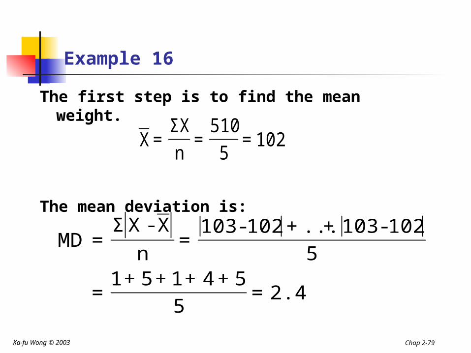
Example 16
The first step is to find the mean weight.
The mean deviation is:
102=5
510=
nΣX
=X
2.4=5
5+4+1+5+1=
5102-103+...+102-103
=n
X-X Σ=MD
Ka-fu Wong © 2003 Chap 2-80
Population Variance
The population variance is the arithmetic mean of the squared deviations from the population mean.
All values are used in the calculation. More likely to be influenced by extreme
values than mean deviation. The units are awkward, the square of the
original units.
Ka-fu Wong © 2003 Chap 2-81
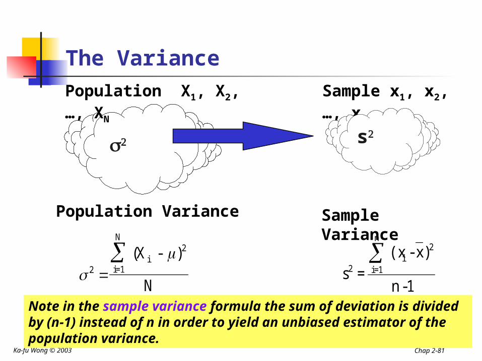
The VariancePopulation X1, X2, …, XN
Population Variance
(X - )
N2
i2
i=1
N
Sample x1, x2, …, xn
Sample Variance
1-n
)x - (x =s
n
1=i
2i
2
s
Note in the sample variance formula the sum of deviation is divided by (n-1) instead of n in order to yield an unbiased estimator of the population variance.
Ka-fu Wong © 2003 Chap 2-82
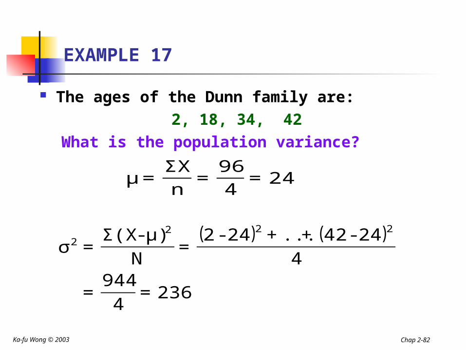
EXAMPLE 17
The ages of the Dunn family are: 2, 18, 34, 42
What is the population variance?
24=496
=nΣX
=μ
( ) ( )
236=4
944=
424-42+...+24-2
=N
μ)-Σ(X=σ
2222
Ka-fu Wong © 2003 Chap 2-83
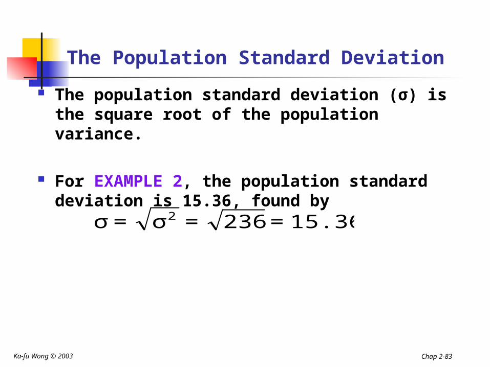
The Population Standard Deviation
The population standard deviation (σ) is the square root of the population variance.
For EXAMPLE 2, the population standard deviation is 15.36, found by
15.36=236=σ=σ 2
Ka-fu Wong © 2003 Chap 2-84
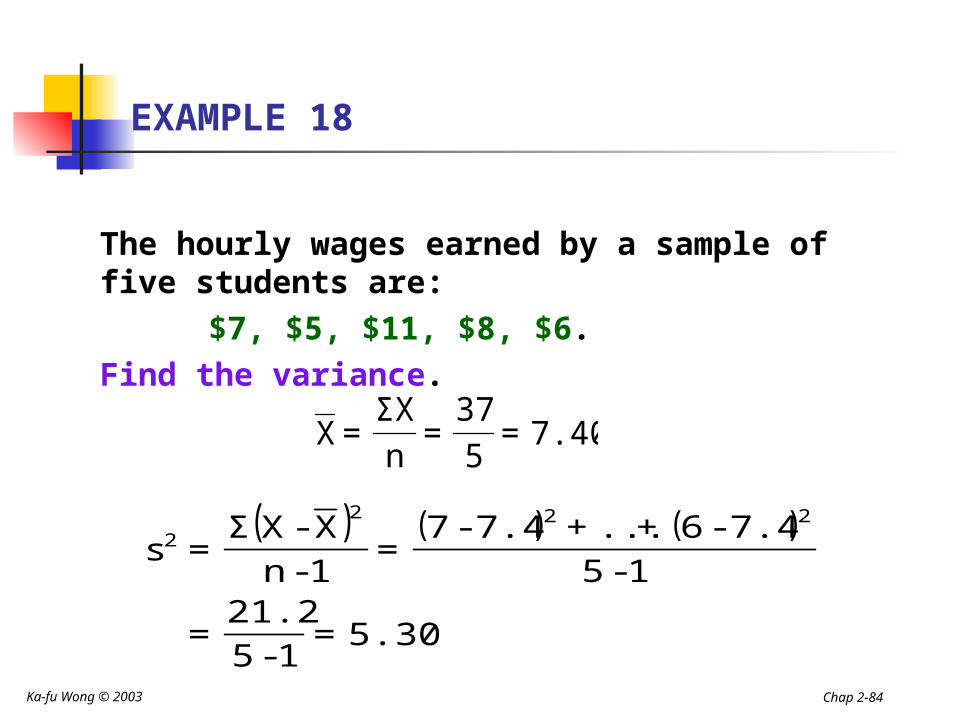
EXAMPLE 18
The hourly wages earned by a sample of five students are:
$7, $5, $11, $8, $6. Find the variance.
7.40=537
=nΣX
=X
( ) ( ) ( )
5.30=1-5
21.2=
1-57.4-6+...+7.4-7
=1-nX-XΣ
=s222
2
Ka-fu Wong © 2003 Chap 2-85
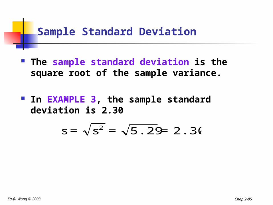
Sample Standard Deviation
The sample standard deviation is the square root of the sample variance.
In EXAMPLE 3, the sample standard deviation is 2.30
2.30=5.29=s=s 2
Ka-fu Wong © 2003 Chap 2-86
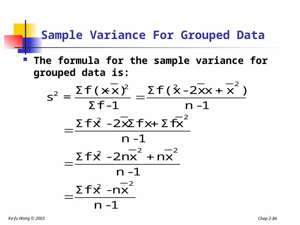
Sample Variance For Grouped Data
The formula for the sample variance for grouped data is:
1-n
xn-Σfx
1-n
xnx2n-Σfx
1-n
xΣfΣfxx2-Σfx
1-n
)xxx2-Σf(x
1-Σf
)x-Σf(x=s
22
222
22
2222
Ka-fu Wong © 2003 Chap 2-87
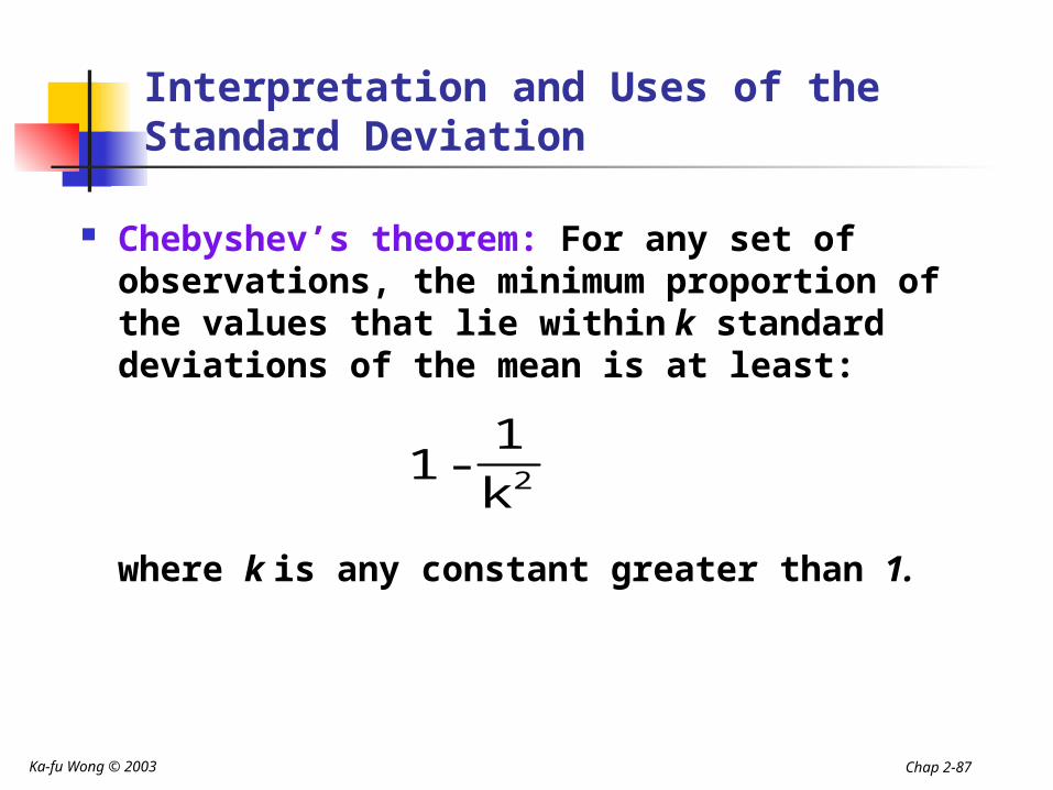
Interpretation and Uses of the Standard Deviation
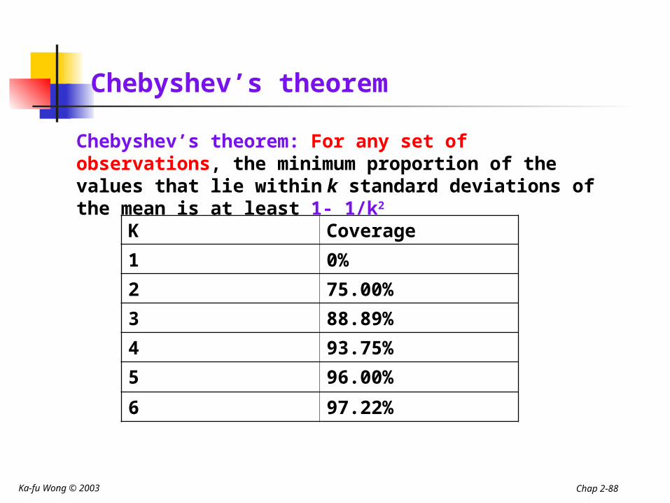
Chebyshev’s theorem: For any set of observations, the minimum proportion of the values that lie within k standard deviations of the mean is at least:
where k is any constant greater than 1.
2k1
-1
Ka-fu Wong © 2003 Chap 2-88
Chebyshev’s theorem
K Coverage
1 0%
2 75.00%
3 88.89%
4 93.75%
5 96.00%
6 97.22%
Chebyshev’s theorem: For any set of observations, the minimum proportion of the values that lie within k standard deviations of the mean is at least 1- 1/k2
Ka-fu Wong © 2003 Chap 2-89
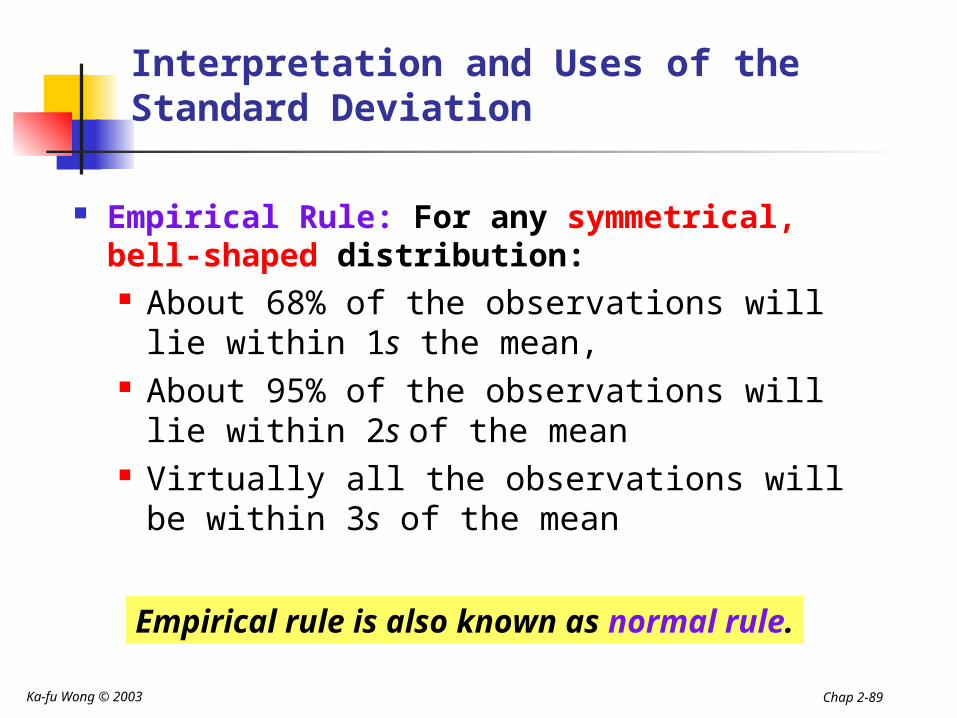
Interpretation and Uses of the Standard Deviation
Empirical Rule: For any symmetrical, bell-shaped distribution: About 68% of the observations will lie within
1s the mean, About 95% of the observations will lie within
2s of the mean Virtually all the observations will be within
3s of the mean
Empirical rule is also known as normal rule.
Ka-fu Wong © 2003 Chap 2-90
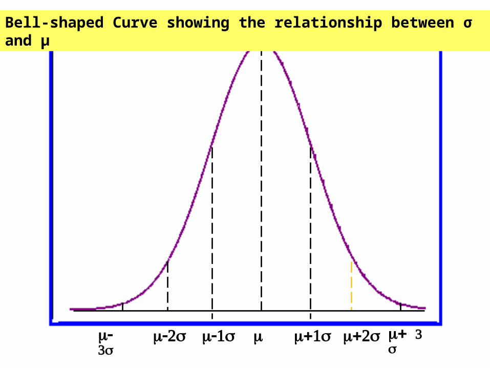
Bell-shaped Curve showing the relationship between σ and μ
Ka-fu Wong © 2003 Chap 2-91
Why are we concern about dispersion?
Dispersion is used as a measure of risk. Consider two assets of the same expected
(mean) returns. -2%, 0%,+2% -4%, 0%,+4%
The dispersion of returns of the second asset is larger then the first. Thus, the second asset is more risky.
Thus, the knowledge of dispersion is essential for investment decision. And so is the knowledge of expected (mean) returns.
Ka-fu Wong © 2003 Chap 2-92
Relative Dispersion
The coefficient of variation is the ratio of the standard deviation to the arithmetic mean, expressed as a percentage:
(100%)X
s=CV
Ka-fu Wong © 2003 Chap 2-93
Sharpe Ratio and Relative Dispersion
Sharpe Ratio is often used to measure the performance of investment strategies, with an adjustment for risk.
If X is the return of an investment strategy in excess of the market portfolio, the inverse of the CV is the Sharpe Ratio.
An investment strategy of a higher Sharpe Ratio is preferred.
http://www.stanford.edu/~wfsharpe/art/sr/sr.htm
Ka-fu Wong © 2003 Chap 2-94
Skewness
Skewness is the measurement of the lack of symmetry of the distribution.
The coefficient of skewness can range from 3.00 up to 3.00.
A value of 0 indicates a symmetric distribution.
It is computed as follows:
Smedian)-x3(
=sk
3
s
xx
2)-1)(n-(nn
=skOr
Ka-fu Wong © 2003 Chap 2-95
Why are we concerned about skewness?
Skewness measures the degree of asymmetry in risk. Upside risk Downside risk
Consider the distribution of asset returns: Right skewed implies higher upside risk
than downside risk. Left skewed implies higher downside risk
than upside risk.
Ka-fu Wong © 2003 Chap 2-96
Percentiles and Quartiles
For a set of measurements arranged in increasing order, the pth percentile is a value such that p percent of the measurements fall at or below the value and (100-p) percent of the measurements fall at or above the value.
The first quartile Q1 is the 25th percentile The second quartile (or median) Md is the
50th percentile The third quartile Q3 is the 75th percentile. The interquartile range IQR is Q3 - Q1
Ka-fu Wong © 2003 Chap 2-97
Example: Quartiles
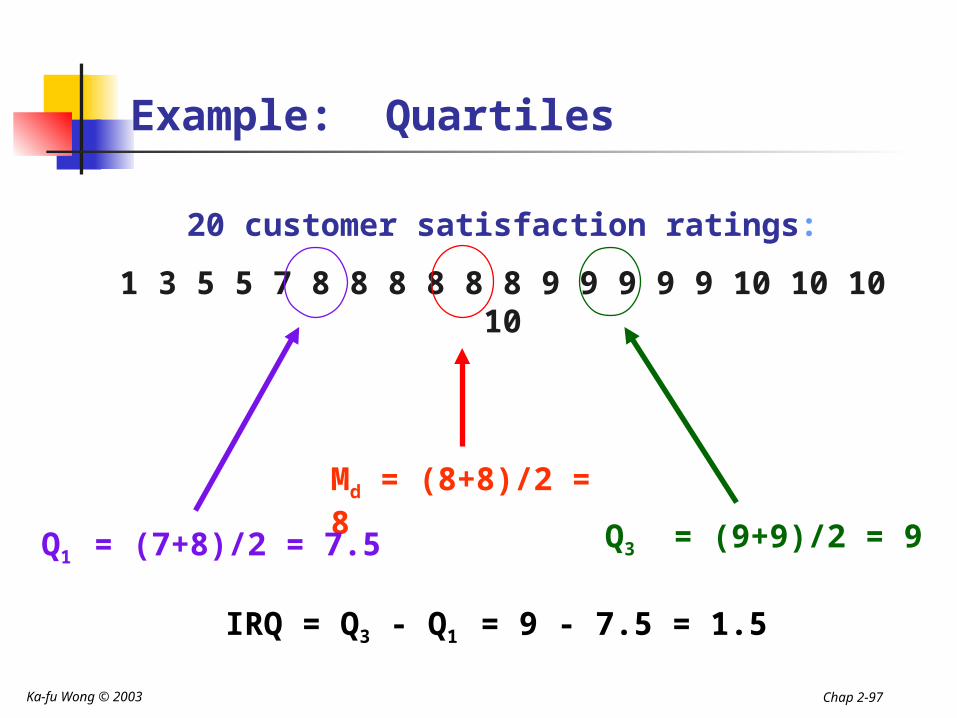
20 customer satisfaction ratings:
1 3 5 5 7 8 8 8 8 8 8 9 9 9 9 9 10 10 10 10
Md = (8+8)/2 = 8
Q1 = (7+8)/2 = 7.5 Q3 = (9+9)/2 = 9
IRQ = Q3 - Q1 = 9 - 7.5 = 1.5
Ka-fu Wong © 2003 Chap 2-98
Box Plots
A box plot is a graphical display, based on quartiles, that helps to picture a set of data.
Five pieces of data are needed to construct a box plot: the Minimum Value, the First Quartile, the Median, the Third Quartile, and the Maximum Value.
Ka-fu Wong © 2003 Chap 2-99
EXAMPLE 19
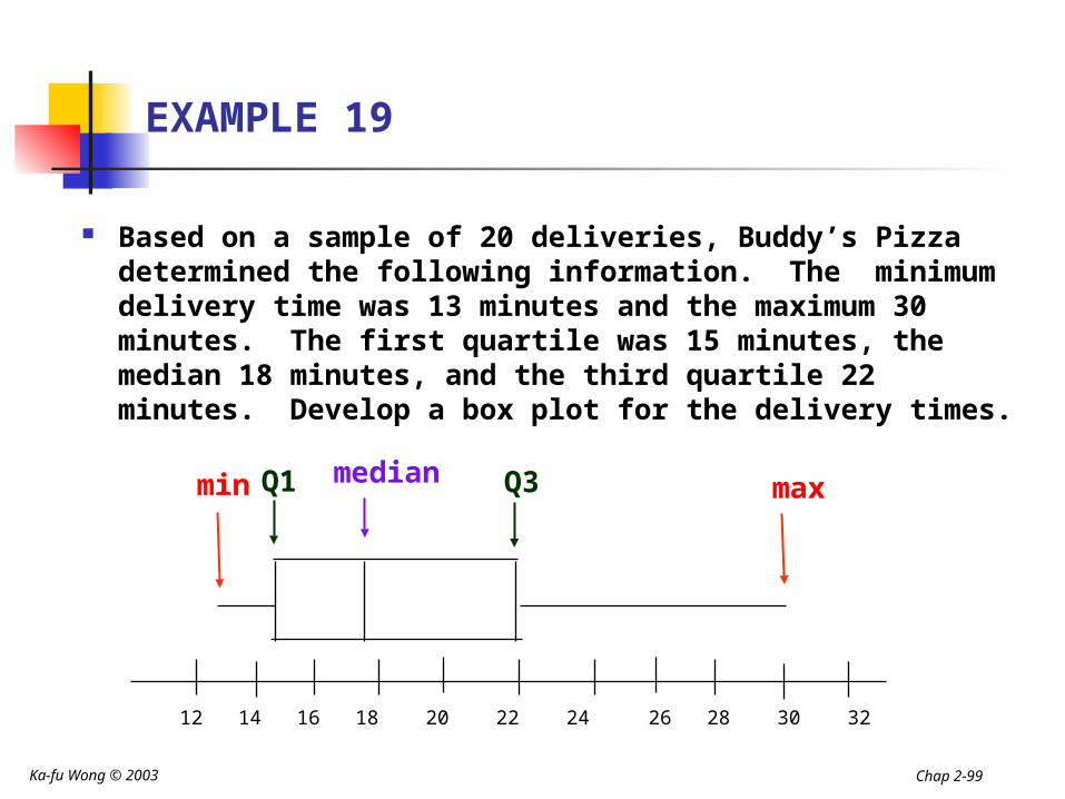
Based on a sample of 20 deliveries, Buddy’s Pizza determined the following information. The minimum delivery time was 13 minutes and the maximum 30 minutes. The first quartile was 15 minutes, the median 18 minutes, and the third quartile 22 minutes. Develop a box plot for the delivery times.
12 14 16 18 20 22 24 26 28 30 32
min maxmedianQ1 Q3
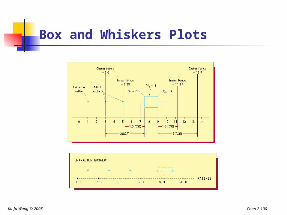
Ka-fu Wong © 2003 Chap 2-100
Box and Whiskers Plots
Ka-fu Wong © 2003 Chap 2-101
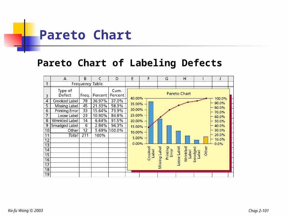
Pareto Chart
Pareto Chart of Labeling Defects
Ka-fu Wong © 2003 Chap 2-102
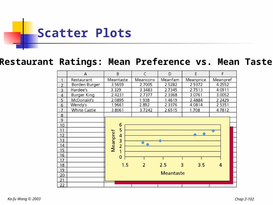
Scatter Plots
Restaurant Ratings: Mean Preference vs. Mean Taste
Ka-fu Wong © 2003 Chap 2-103
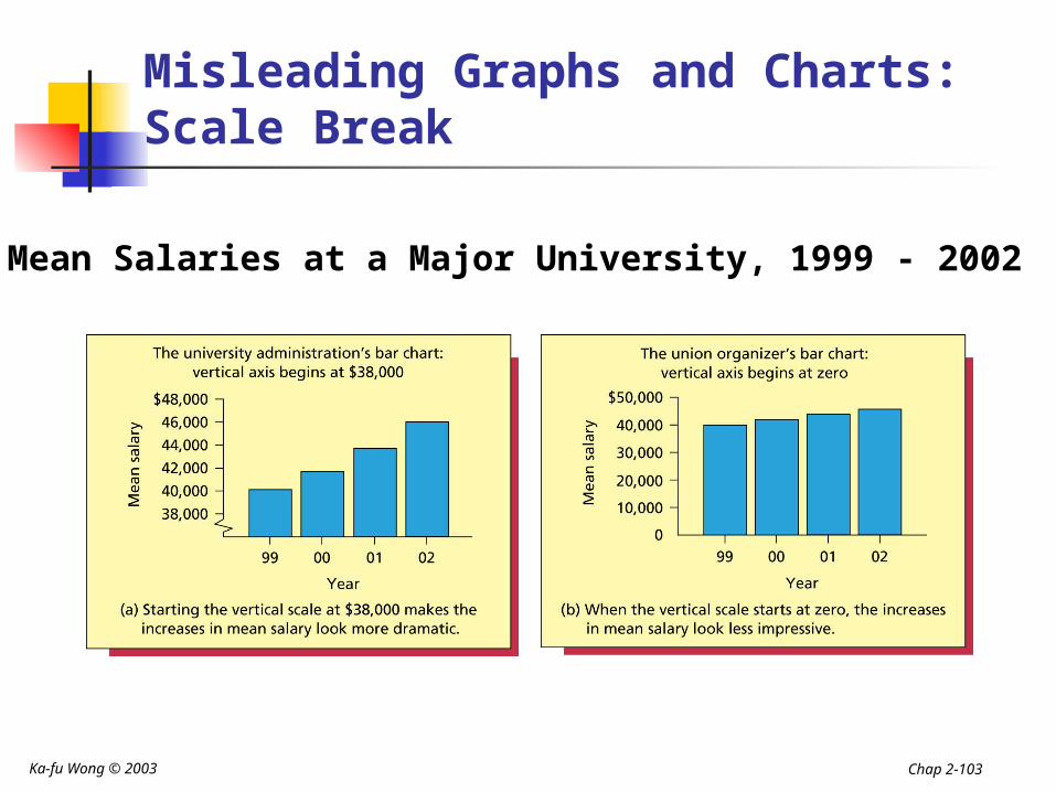
Misleading Graphs and Charts:Scale Break
Mean Salaries at a Major University, 1999 - 2002
Ka-fu Wong © 2003 Chap 2-104
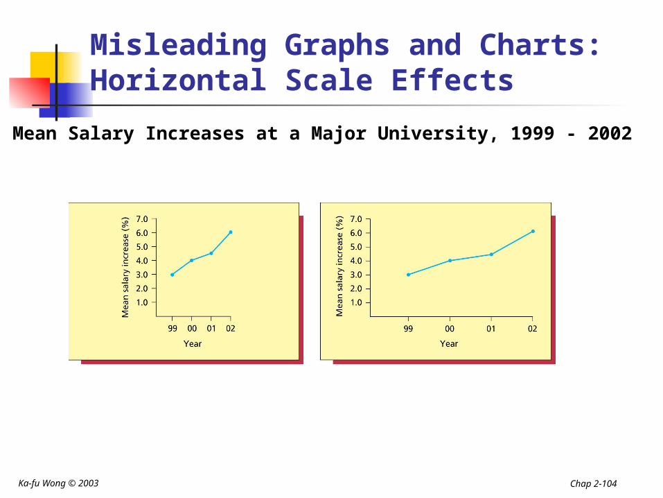
Misleading Graphs and Charts:Horizontal Scale Effects
Mean Salary Increases at a Major University, 1999 - 2002
Ka-fu Wong © 2003 Chap 2-105
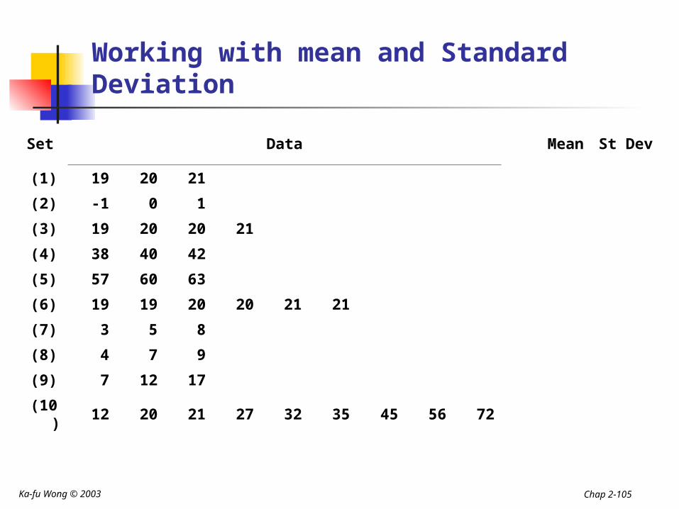
Working with mean and Standard Deviation
Set DataMea
nSt Dev
(1) 19 20 2120.0
0 0.82
(2) -1 0 1 0.00 0.82
(3) 19 20 20 2120.0
0 0.71
(4) 38 40 4240.0
0 1.63
(5) 57 60 6360.0
0 2.45
(6) 19 19 20 20 21 2120.0
0 0.82
(7) 3 5 8 5.33 2.05
(8) 4 7 9 6.67 2.05
(9) 7 12 1712.0
0 4.08
(10)
12 20 21 27 32 35 45 56 7235.5
6 18.04
Ka-fu Wong © 2003 Chap 2-106
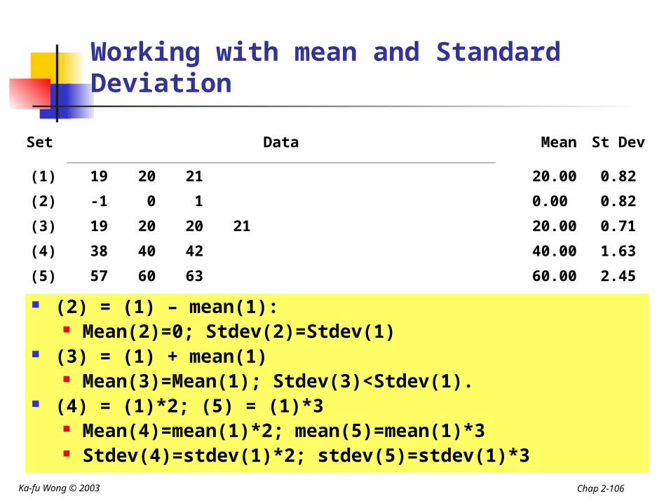
(2) = (1) – mean(1): Mean(2)=0; Stdev(2)=Stdev(1)
(3) = (1) + mean(1) Mean(3)=Mean(1); Stdev(3)<Stdev(1).
(4) = (1)*2; (5) = (1)*3 Mean(4)=mean(1)*2; mean(5)=mean(1)*3 Stdev(4)=stdev(1)*2; stdev(5)=stdev(1)*3
Working with mean and Standard Deviation
Set DataMea
nSt Dev
(1) 19 20 2120.0
0 0.82
(2) -1 0 1 0.00 0.82
(3) 19 20 20 2120.0
0 0.71
(4) 38 40 4240.0
0 1.63
(5) 57 60 6360.0
0 2.45
Ka-fu Wong © 2003 Chap 2-107
Working with mean and Standard Deviation
Set DataMea
nSt Dev
(1) 19 20 2120.0
0 0.82
(6) 19 19 20 20 21 2120.0
0 0.82
(7) 3 5 8 5.33 2.05
(8) 4 7 9 6.67 2.05
(9) 7 12 1712.0
0 4.08
(10)
12 20 21 27 32 35 45 56 7235.5
6 18.04
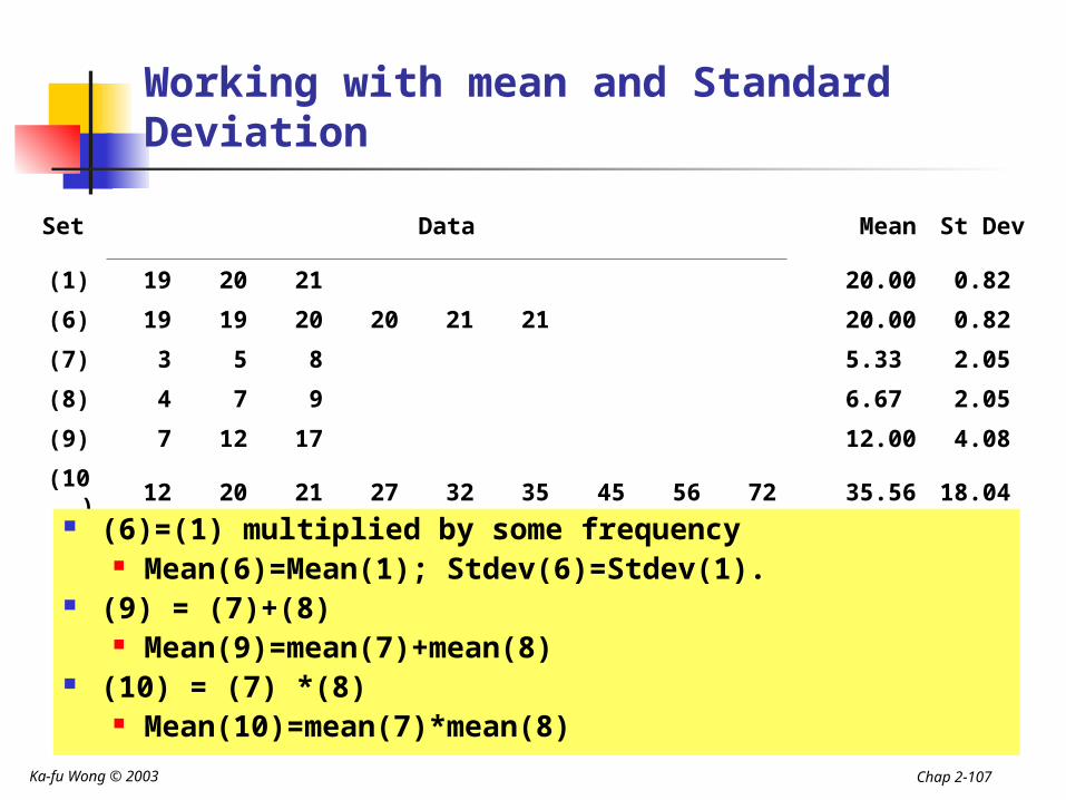
(6)=(1) multiplied by some frequency Mean(6)=Mean(1); Stdev(6)=Stdev(1).
(9) = (7)+(8) Mean(9)=mean(7)+mean(8)
(10) = (7) *(8) Mean(10)=mean(7)*mean(8)
Ka-fu Wong © 2003 Chap 2-108
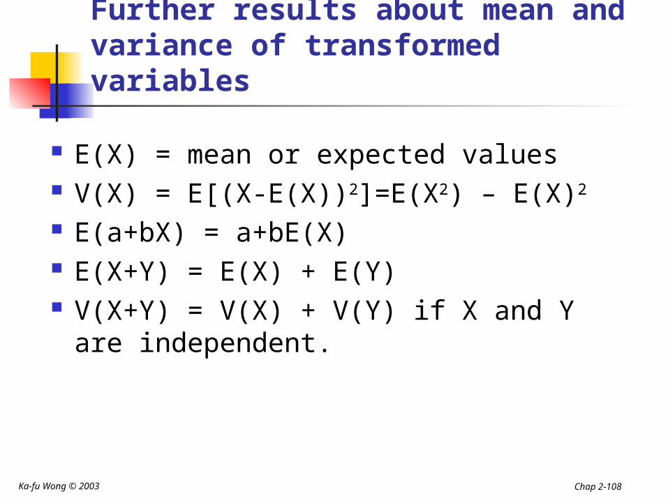
Further results about mean and variance of transformed variables
E(X) = mean or expected values V(X) = E[(X-E(X))2]=E(X2) – E(X)2 E(a+bX) = a+bE(X) E(X+Y) = E(X) + E(Y) V(X+Y) = V(X) + V(Y) if X and Y are
independent.
Ka-fu Wong © 2003 Chap 2-109
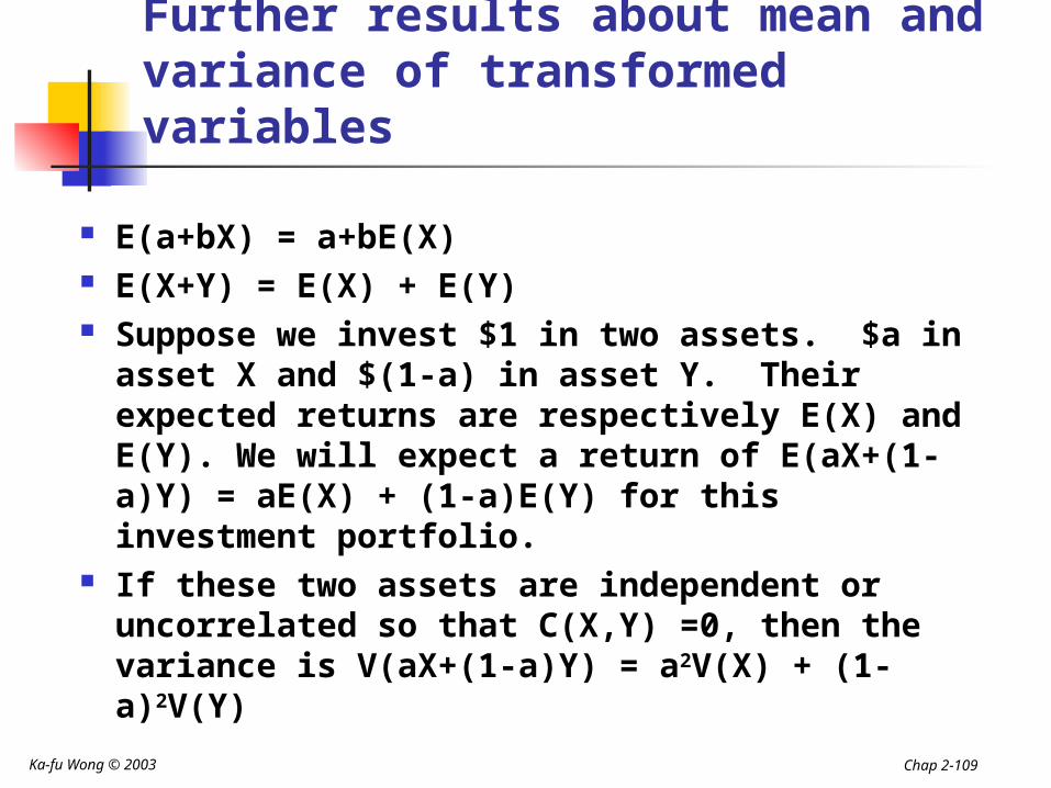
Further results about mean and variance of transformed variables
E(a+bX) = a+bE(X) E(X+Y) = E(X) + E(Y) Suppose we invest $1 in two assets. $a in
asset X and $(1-a) in asset Y. Their expected returns are respectively E(X) and E(Y). We will expect a return of E(aX+(1-a)Y) = aE(X) + (1-a)E(Y) for this investment portfolio.
If these two assets are independent or uncorrelated so that C(X,Y) =0, then the variance is V(aX+(1-a)Y) = a2V(X) + (1-a)2V(Y)
Ka-fu Wong © 2003 Chap 2-110
- END -
Chapter TwoDescriptive StatisticsDescriptive Statistics
Related Documents