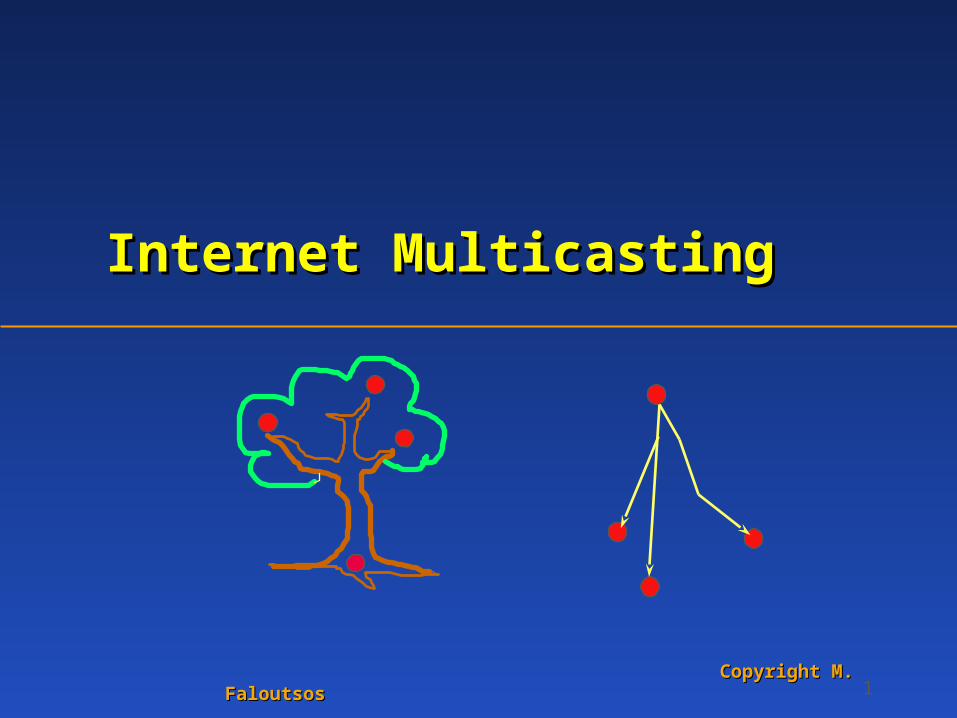
1 Internet Multicasting Internet Multicasting Copyright M. Copyright M. Faloutsos Faloutsos

1 Internet Multicasting Copyright M. Faloutsos Copyright M. Faloutsos.
Dec 22, 2015
Welcome message from author
This document is posted to help you gain knowledge. Please leave a comment to let me know what you think about it! Share it to your friends and learn new things together.
Transcript
1
Internet MulticastingInternet Multicasting
Copyright M. FaloutsosCopyright M. Faloutsos
2U. of Toronto Michalis Faloutsos
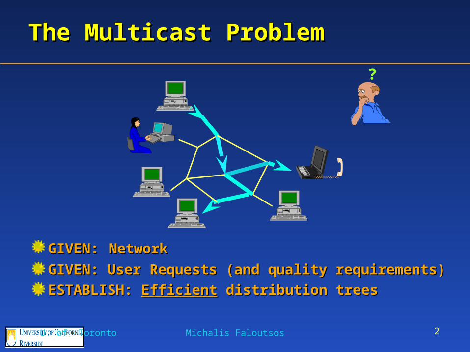
The Multicast ProblemThe Multicast Problem
GIVEN:GIVEN: NetworkNetwork
GIVEN: User Requests (and quality requirements)GIVEN: User Requests (and quality requirements)
ESTABLISH: ESTABLISH: EfficientEfficient distribution trees distribution trees
?
3
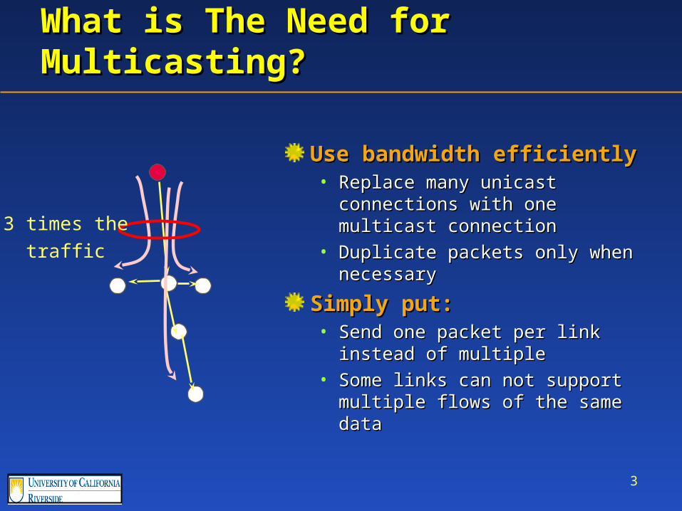
What is The Need for Multicasting?What is The Need for Multicasting?
Use bandwidth efficientlyUse bandwidth efficiently• Replace many unicast connections Replace many unicast connections
with one multicast connectionwith one multicast connection• Duplicate packets only when Duplicate packets only when
necessarynecessary
Simply put:Simply put:• Send one packet per link instead of Send one packet per link instead of
multiplemultiple• Some links can not support multiple Some links can not support multiple
flows of the same dataflows of the same data
3 times thetraffic
4
What Is Efficient?What Is Efficient?
ScalableScalable• Multicast stateMulticast state• Number of control messagesNumber of control messages
Use network resources efficientlyUse network resources efficiently
Meet end-to-end performance requirementsMeet end-to-end performance requirements• E2e Delay: from source to destinationsE2e Delay: from source to destinations
5
Some Theory on Multicast RoutingSome Theory on Multicast Routing
6
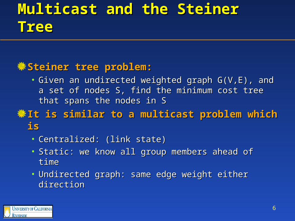
Multicast and the Steiner TreeMulticast and the Steiner Tree
Steiner tree problem: Steiner tree problem: • Given an undirected weighted graph G(V,E), and a Given an undirected weighted graph G(V,E), and a
set of nodes S, find the minimum cost tree that spans set of nodes S, find the minimum cost tree that spans the nodes in Sthe nodes in S
It is similar to a multicast problem which isIt is similar to a multicast problem which is• Centralized: (link state)Centralized: (link state)• Static: we know all group members ahead of timeStatic: we know all group members ahead of time• Undirected graph: same edge weight either directionUndirected graph: same edge weight either direction
7
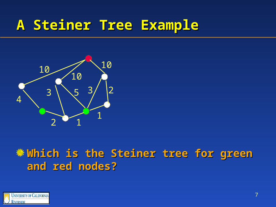
A Steiner Tree ExampleA Steiner Tree Example
Which is the Steiner tree for green and red Which is the Steiner tree for green and red nodes?nodes?
1010
10
2
11
4
2
53 3
8
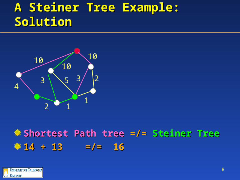
A Steiner Tree Example: SolutionA Steiner Tree Example: Solution
Shortest Path treeShortest Path tree =/= =/= Steiner TreeSteiner Tree
14 + 13 =/= 16 14 + 13 =/= 16
1010
10
2
11
4
2
53 3
9U. of Toronto Michalis Faloutsos
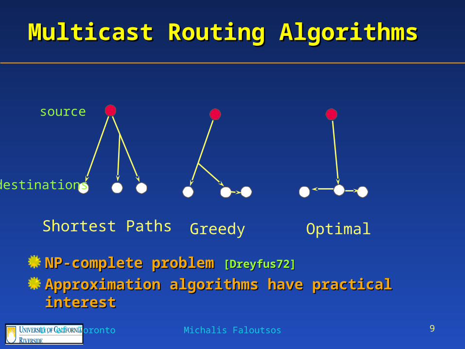
Multicast Routing AlgorithmsMulticast Routing Algorithms
NP-complete problem NP-complete problem [Dreyfus72][Dreyfus72]
Approximation algorithms have practical interestApproximation algorithms have practical interest
Shortest Paths Greedy Optimal
source
destinations
10
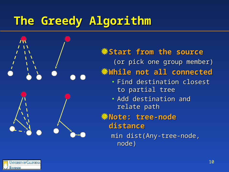
The Greedy AlgorithmThe Greedy Algorithm
Start from the sourceStart from the source(or pick one group member)(or pick one group member)
While not all connectedWhile not all connected• Find destination closest to Find destination closest to
partial treepartial tree• Add destination and relate Add destination and relate
pathpath
Note: tree-node distanceNote: tree-node distancemin dist(Any-tree-node, node)min dist(Any-tree-node, node)
11
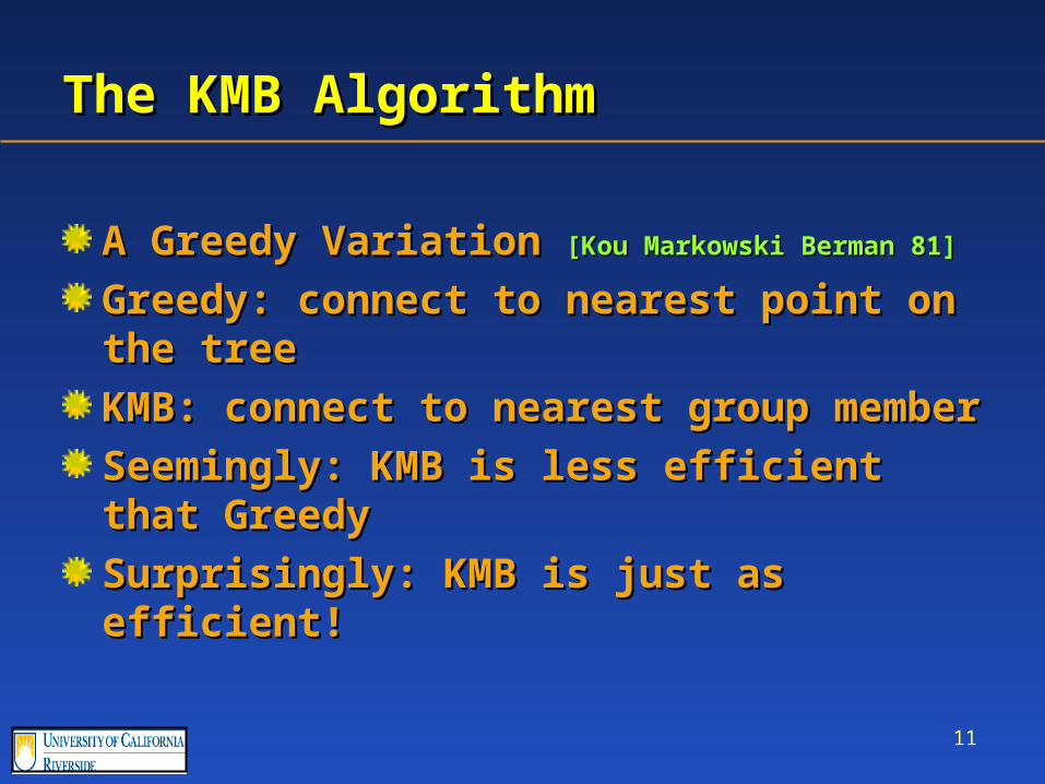
The KMB AlgorithmThe KMB Algorithm
A Greedy Variation A Greedy Variation [Kou Markowski Berman 81][Kou Markowski Berman 81]
Greedy: connect to nearest point on the treeGreedy: connect to nearest point on the tree
KMB: connect to nearest group memberKMB: connect to nearest group member
Seemingly: KMB is less efficient that GreedySeemingly: KMB is less efficient that Greedy
Surprisingly: KMB is just as efficient!Surprisingly: KMB is just as efficient!
12
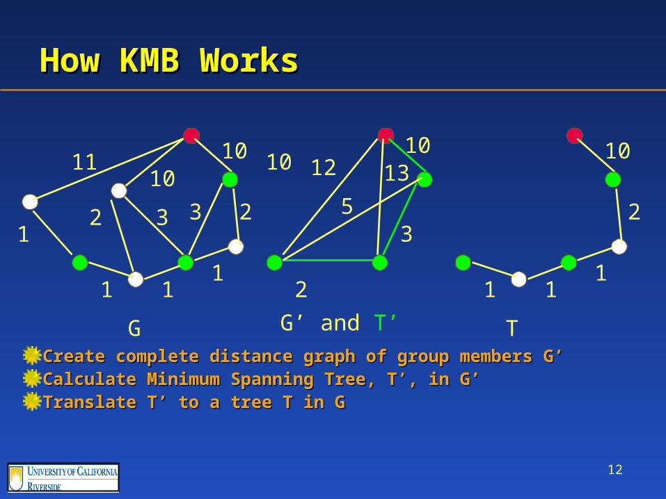
How KMB WorksHow KMB Works
Create complete distance graph of group members G’Create complete distance graph of group members G’Calculate Minimum Spanning Tree, T’, in G’Calculate Minimum Spanning Tree, T’, in G’Translate T’ to a tree T in GTranslate T’ to a tree T in G
1110
10
2
11
1
1
32 3
10 1210
3
2
5
1310
11
1
2
G G’ and T’ T
13
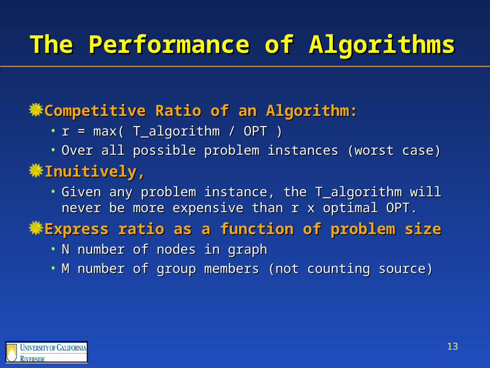
The Performance of AlgorithmsThe Performance of Algorithms
Competitive Ratio of an Algorithm: Competitive Ratio of an Algorithm: • r = max( T_algorithm / OPT )r = max( T_algorithm / OPT )• Over all possible problem instances (worst case)Over all possible problem instances (worst case)
Inuitively,Inuitively,• Given any problem instance, the T_algorithm will Given any problem instance, the T_algorithm will
never be more expensive than r x optimal OPT.never be more expensive than r x optimal OPT.
Express ratio as a function of problem sizeExpress ratio as a function of problem size• N number of nodes in graphN number of nodes in graph• M number of group members (not counting source)M number of group members (not counting source)
14
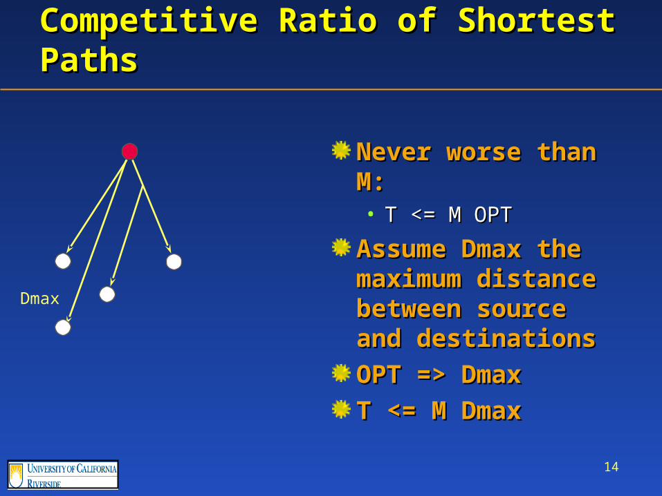
Competitive Ratio of Shortest PathsCompetitive Ratio of Shortest Paths
Never worse than M:Never worse than M:• T <= M OPTT <= M OPT
Assume Dmax the Assume Dmax the maximum distance maximum distance between source and between source and destinationsdestinations
OPT => DmaxOPT => Dmax
T <= M DmaxT <= M Dmax
Dmax
15
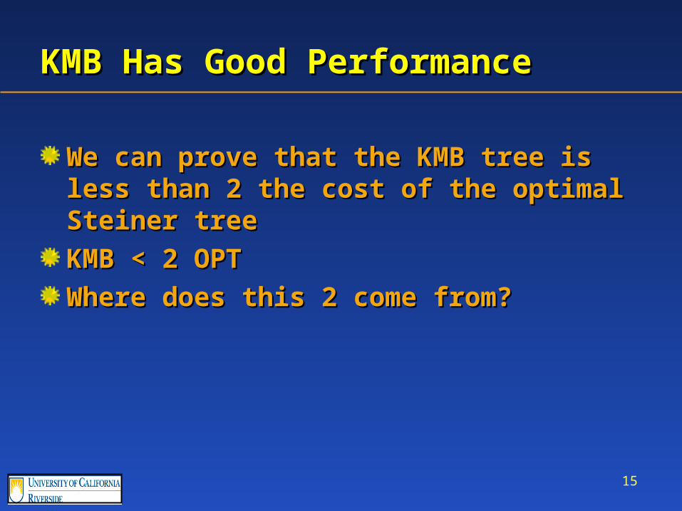
KMB Has Good PerformanceKMB Has Good Performance
We can prove that the KMB tree is less than 2 We can prove that the KMB tree is less than 2 the cost of the optimal Steiner treethe cost of the optimal Steiner tree
KMB < 2 OPTKMB < 2 OPT
Where does this 2 come from?Where does this 2 come from?
16
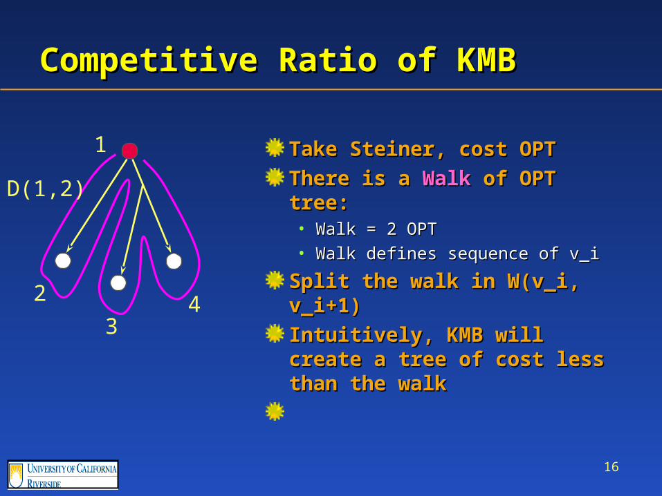
Competitive Ratio of KMBCompetitive Ratio of KMB
Take Steiner, cost OPTTake Steiner, cost OPT
There is a There is a Walk Walk of OPT tree:of OPT tree:• Walk = 2 OPTWalk = 2 OPT• Walk defines sequence of v_iWalk defines sequence of v_i
Split the walk in W(v_i, v_i+1)Split the walk in W(v_i, v_i+1)
Intuitively, KMB will create a Intuitively, KMB will create a tree of cost less than the walktree of cost less than the walk
1
2
34
D(1,2)
17
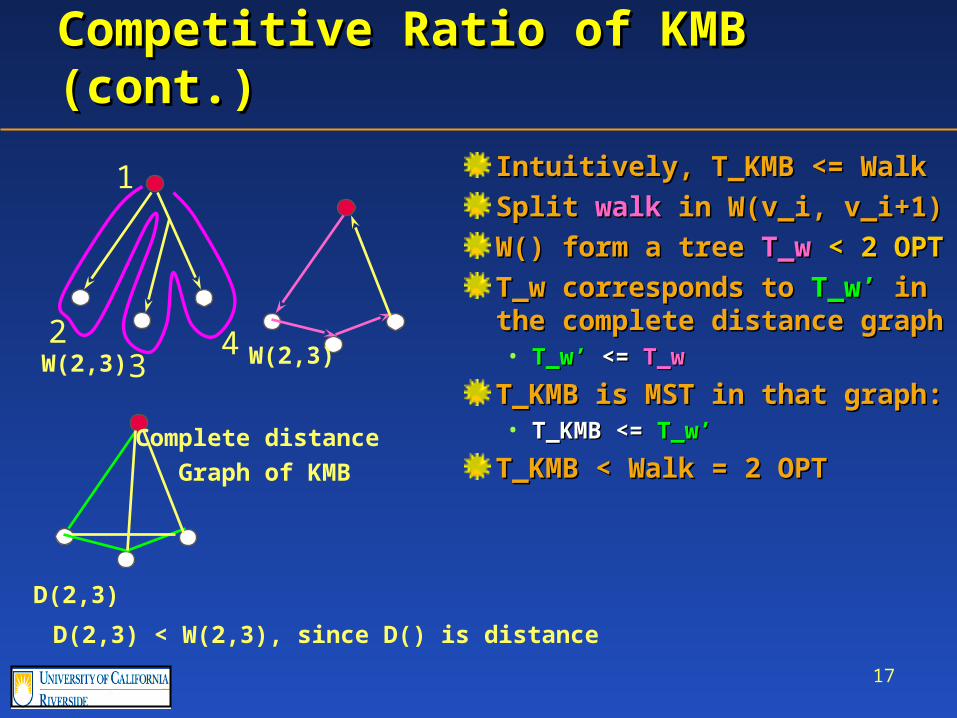
Competitive Ratio of KMB (cont.)Competitive Ratio of KMB (cont.)
Intuitively, T_KMB <= Walk Intuitively, T_KMB <= Walk
Split Split walkwalk in W(v_i, v_i+1) in W(v_i, v_i+1)
W() form a tree W() form a tree T_w T_w < 2 OPT< 2 OPT
T_w corresponds to T_w corresponds to T_w’T_w’ in in the complete distance graphthe complete distance graph• T_w’T_w’ <= <= T_wT_w
T_KMB is MST in that graph:T_KMB is MST in that graph:• T_KMB <= T_KMB <= T_w’T_w’
T_KMB < Walk = 2 OPTT_KMB < Walk = 2 OPT
1
23
4W(2,3) W(2,3)
D(2,3) < W(2,3), since D() is distance
D(2,3)
Complete distance Graph of KMB
18U. of Toronto Michalis Faloutsos
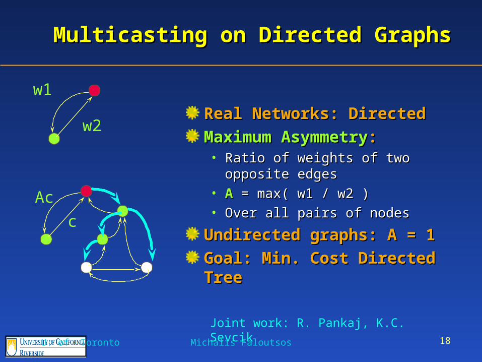
Multicasting on Directed Graphs Multicasting on Directed Graphs
Real Networks: DirectedReal Networks: Directed
Maximum AsymmetryMaximum Asymmetry: : • Ratio of weights of two opposite edgesRatio of weights of two opposite edges• AA = max( w1 / w2 ) = max( w1 / w2 ) • Over all pairs of nodesOver all pairs of nodes
Undirected graphs: A = 1Undirected graphs: A = 1
Goal: Min. Cost Directed TreeGoal: Min. Cost Directed Tree
Joint work: R. Pankaj, K.C. Sevcik
c
Ac
w2
w1
19
Multicast BoundsMulticast Bounds
Bounds for Greedy and Sh. Paths w.r.t.:Bounds for Greedy and Sh. Paths w.r.t.:• Maximum asymmetry: Maximum asymmetry: AA• Number of join requests: Number of join requests: MM• Competitive Ratio of tree cost: Algorithm/OptimalCompetitive Ratio of tree cost: Algorithm/Optimal
Problem Variations:Problem Variations:• Static: members know ahead of timeStatic: members know ahead of time• Join-Only: members join randomlyJoin-Only: members join randomly• Join-Leave: members join and leave randomlyJoin-Leave: members join and leave randomly
20
Performance On Undirected GraphsPerformance On Undirected Graphs
Shortest Path: tighlty bounded by MShortest Path: tighlty bounded by M• Where M the number of destinationsWhere M the number of destinations
Greedy and KMB: Greedy and KMB: • Static: bounded by 2Static: bounded by 2• Join-only: log MJoin-only: log M• Join-leave: 2^M (or N)Join-leave: 2^M (or N)
21Michalis Faloutsos
Overview of Theoretical ResultsOverview of Theoretical Results
Short. Paths:Short. Paths:• tight bound in all variationstight bound in all variations
Greedy:Greedy:• Static: Tight bound (2 A) Static: Tight bound (2 A) • Join-Only: Near-optimal online bound (A log M)Join-Only: Near-optimal online bound (A log M)
Greedy is no more than log M from Greedy is no more than log M from any onlineany online algorithm algorithm• Join-Leave: Large lower bound (A or 2^M)Join-Leave: Large lower bound (A or 2^M)
[Faloutsos et al SIROCCO’97][Faloutsos et al SIROCCO’97]
22Michalis Faloutsos
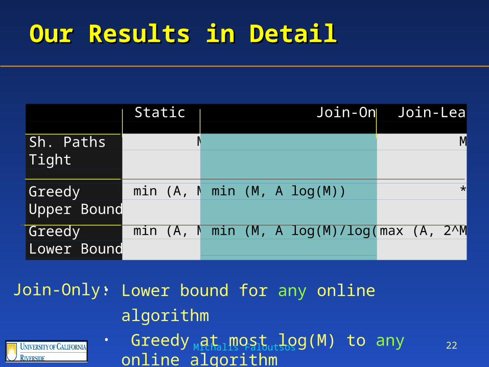
Our Results in DetailOur Results in Detail
Static Join-Only Join-Leave
Sh. PathsTight
M M M
GreedyUpper Bound
min (A, M) min (M, A log(M)) *
GreedyLower Bound
min (A, M) min (M, A log(M)/log(A+1))max (A, 2^M)
• Lower bound for any online algorithm • Greedy at most log(M) to any online algorithm
Join-Only:
23U. of Toronto Michalis Faloutsos
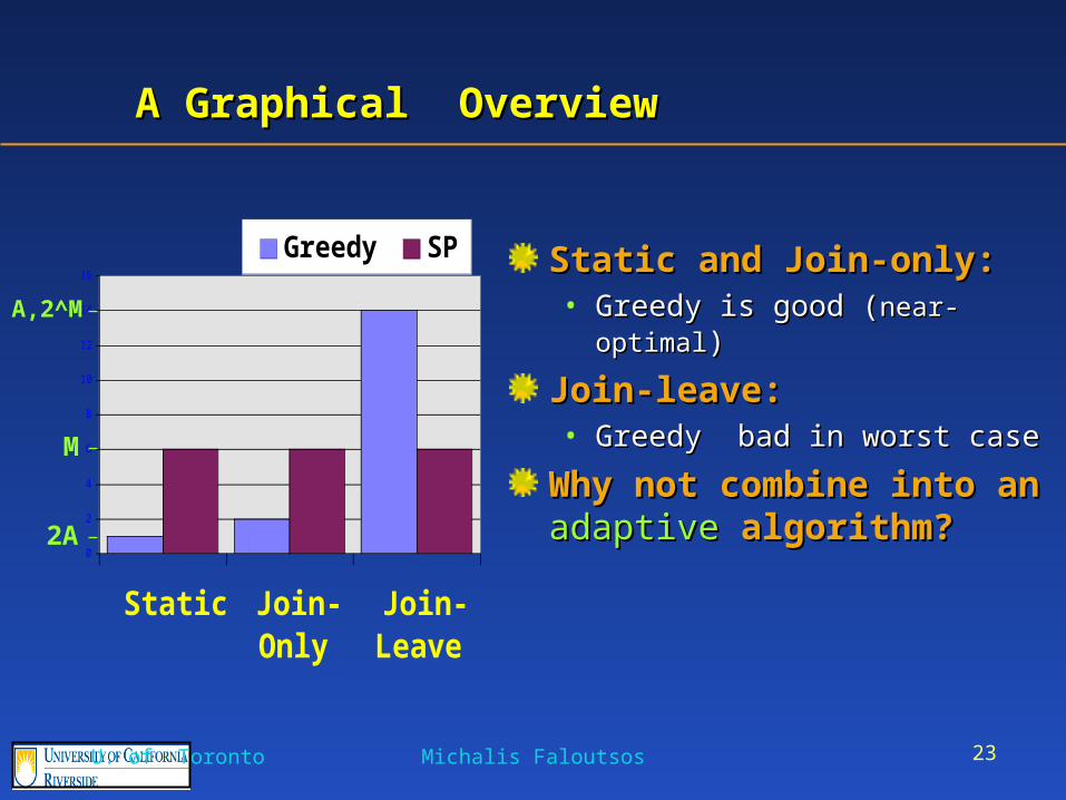
A Graphical OverviewA Graphical Overview
0
2
4
6
8
10
12
14
16
Static Join-Only
Join-Leave
Greedy SP Static and Join-only:Static and Join-only:• Greedy is good (Greedy is good (near-optimalnear-optimal))
Join-leave:Join-leave:• Greedy bad in worst caseGreedy bad in worst case
Why not combine into an Why not combine into an adaptiveadaptive algorithm? algorithm?
2A
M
A,2^M
25Michalis Faloutsos
Desirable Protocol PropertiesDesirable Protocol Properties
ScalableScalable
Easy to implement and deployEasy to implement and deploy
Provide high QoSProvide high QoS
Use network resources efficientlyUse network resources efficiently• Create efficient treesCreate efficient trees• Use little bandwidthUse little bandwidth• Minimize required stateMinimize required state
Adaptive - FlexibleAdaptive - Flexible
26
Internet Multicasting: ProtocolsInternet Multicasting: Protocols
27
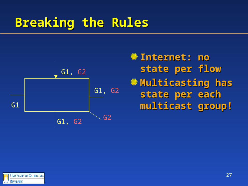
Breaking the RulesBreaking the Rules
Internet: no state Internet: no state per flowper flow
Multicasting has Multicasting has state per each state per each multicast group!multicast group!
G1, G2
G1, G2
G1, G2
G1
G2
28
What Are The Issues?What Are The Issues?
RoutingRouting• Intra-domainIntra-domain• Inter-domainInter-domain
Reliable multicastingReliable multicasting
Secure multicastingSecure multicasting
Address space allocationAddress space allocation
Multicast state aggregationMulticast state aggregation
Modeling and Simulating: realistic modelsModeling and Simulating: realistic models
29
What Is The Real IssueWhat Is The Real Issue
ISPs do not want/care to deploy multicastISPs do not want/care to deploy multicast
Chicken and egg problemChicken and egg problem• Customers do not ask for multicasting,Customers do not ask for multicasting,
because there are no multicast applications,because there are no multicast applications,
because none builds multicast applications,because none builds multicast applications,
because there is no support for multicastingbecause there is no support for multicasting
Multicast researchers:Multicast researchers:• Be careful in what topic you chooseBe careful in what topic you choose
30
MBone: The multicast backboneMBone: The multicast backbone
Some routers are multicast enabledSome routers are multicast enabled
These routers connect to each other with These routers connect to each other with virtual edges (encapsulation)virtual edges (encapsulation)
Multicast protocols and applications can be Multicast protocols and applications can be deployed on the MBonedeployed on the MBone
31
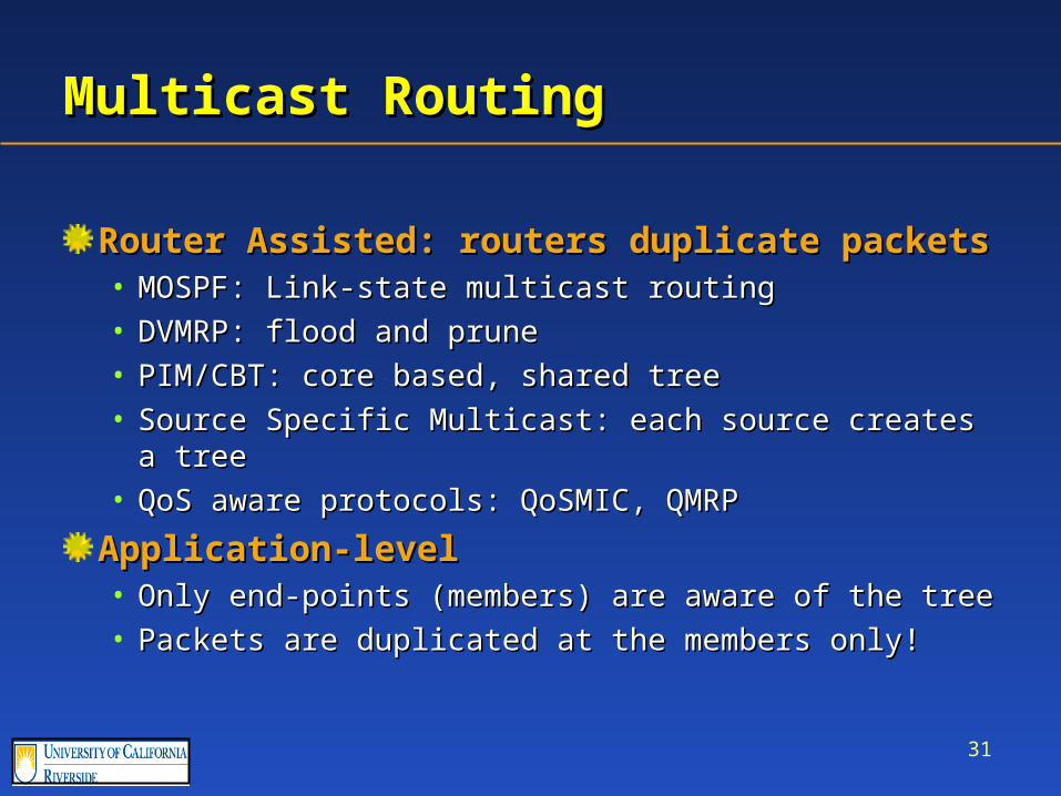
Multicast Routing Multicast Routing
Router Assisted: routers duplicate packetsRouter Assisted: routers duplicate packets• MOSPF: Link-state multicast routingMOSPF: Link-state multicast routing• DVMRP: flood and pruneDVMRP: flood and prune• PIM/CBT: core based, shared treePIM/CBT: core based, shared tree• Source Specific Multicast: each source creates a treeSource Specific Multicast: each source creates a tree• QoS aware protocols: QoSMIC, QMRPQoS aware protocols: QoSMIC, QMRP
Application-levelApplication-level• Only end-points (members) are aware of the treeOnly end-points (members) are aware of the tree• Packets are duplicated at the members only!Packets are duplicated at the members only!
32
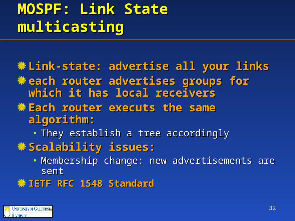
MOSPF: Link State multicastingMOSPF: Link State multicasting
Link-state: advertise all your linksLink-state: advertise all your linkseach router advertises groups for which it each router advertises groups for which it has local receivershas local receiversEach router executs the same algorithm:Each router executs the same algorithm:• They establish a tree accordinglyThey establish a tree accordingly
Scalability issues: Scalability issues: • Membership change: new advertisements are Membership change: new advertisements are
sentsentIETF RFC 1548 StandardIETF RFC 1548 Standard
33
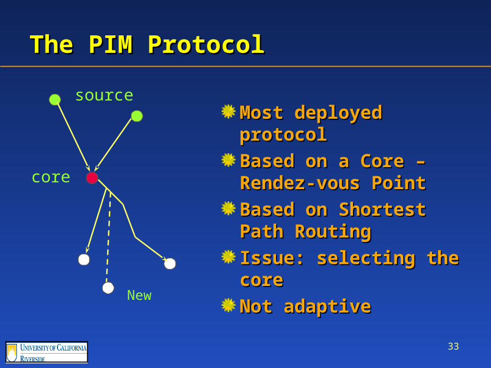
The PIM ProtocolThe PIM Protocol
Most deployed protocolMost deployed protocol
Based on a Core – Based on a Core – Rendez-vous PointRendez-vous Point
Based on Shortest Path Based on Shortest Path RoutingRouting
Issue: selecting the coreIssue: selecting the core
Not adaptiveNot adaptiveNew
source
core
34Michalis Faloutsos
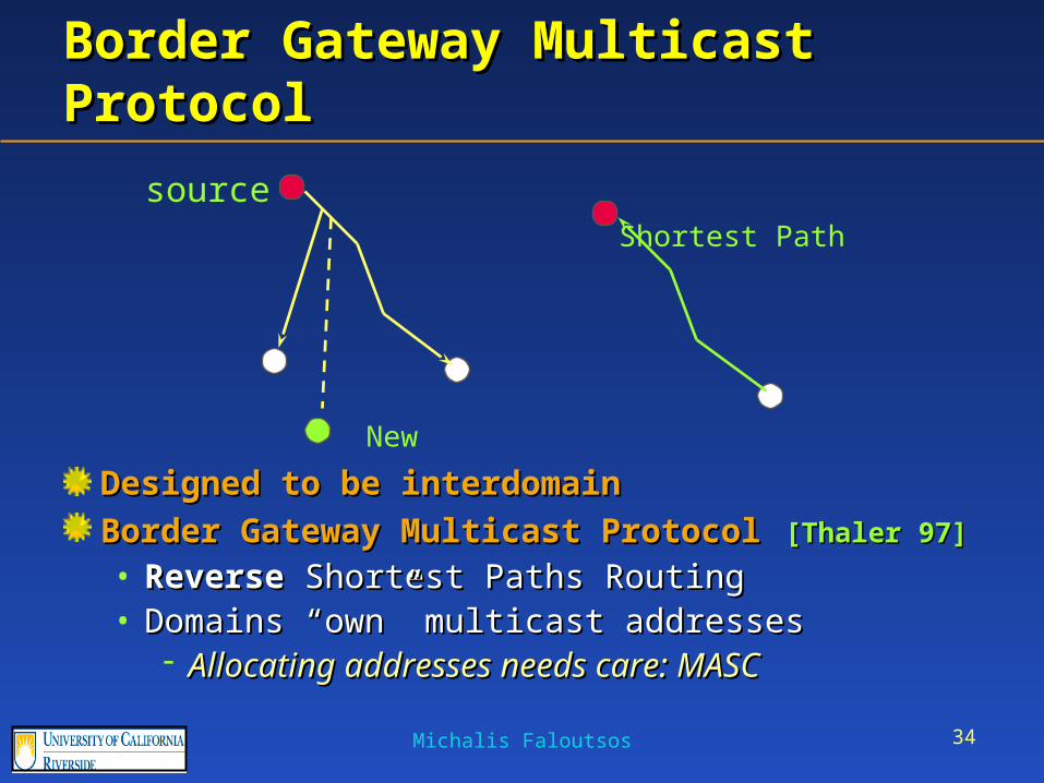
Border Gateway Multicast ProtocolBorder Gateway Multicast Protocol
Designed to be interdomainDesigned to be interdomain
Border Gateway Multicast ProtocolBorder Gateway Multicast Protocol [Thaler 97][Thaler 97]
• Reverse Reverse Shortest Paths Routing Shortest Paths Routing • Domains “own” multicast addressesDomains “own” multicast addresses
Allocating addresses needs care: MASCAllocating addresses needs care: MASC
New
Shortest Path
source
35U. of Toronto Michalis Faloutsos
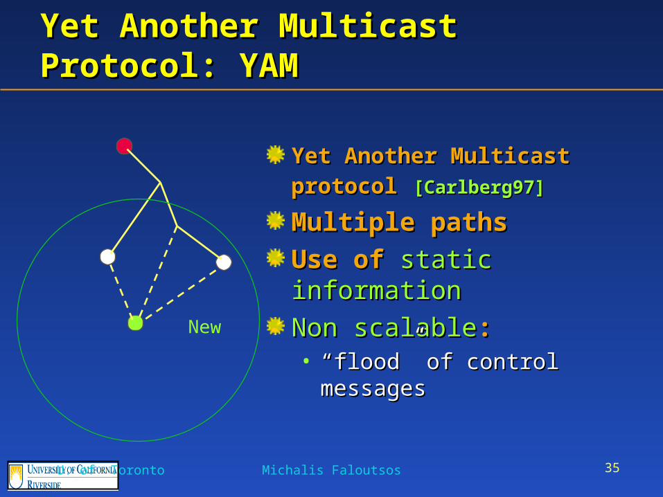
Yet Another Multicast Protocol: YAMYet Another Multicast Protocol: YAM
Yet Another Multicast protocolYet Another Multicast protocol [Carlberg97][Carlberg97]
Multiple pathsMultiple paths
Use of Use of static informationstatic information
Non scalableNon scalable::• ““flood” of control messagesflood” of control messagesNew
36Michalis Faloutsos
Our Protocol: QoSMICOur Protocol: QoSMIC
QoSQoS MMulticast ulticast IInternet protonternet protoCCol ol [SIGCOMM’98][SIGCOMM’98]
Supports QoS Supports QoS
Uses dynamic informationUses dynamic information
ScalableScalable
37U. of Toronto Michalis Faloutsos
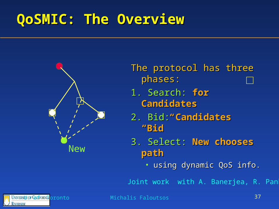
QoSMIC: The OverviewQoSMIC: The Overview
The protocol has three phases:The protocol has three phases:
1. Search: 1. Search: for Candidatesfor Candidates
2. Bid: 2. Bid: Candidates “Bid”Candidates “Bid”
3. Select: 3. Select: New chooses pathNew chooses path• using dynamic QoS info.using dynamic QoS info.
Joint work with A. Banerjea, R. Pankaj
New
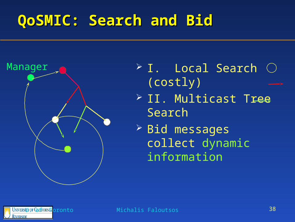
38U. of Toronto Michalis Faloutsos
I. Local Search (costly) II. Multicast Tree Search Bid messages collect
dynamic information
QoSMIC: Search and BidQoSMIC: Search and Bid
Manager
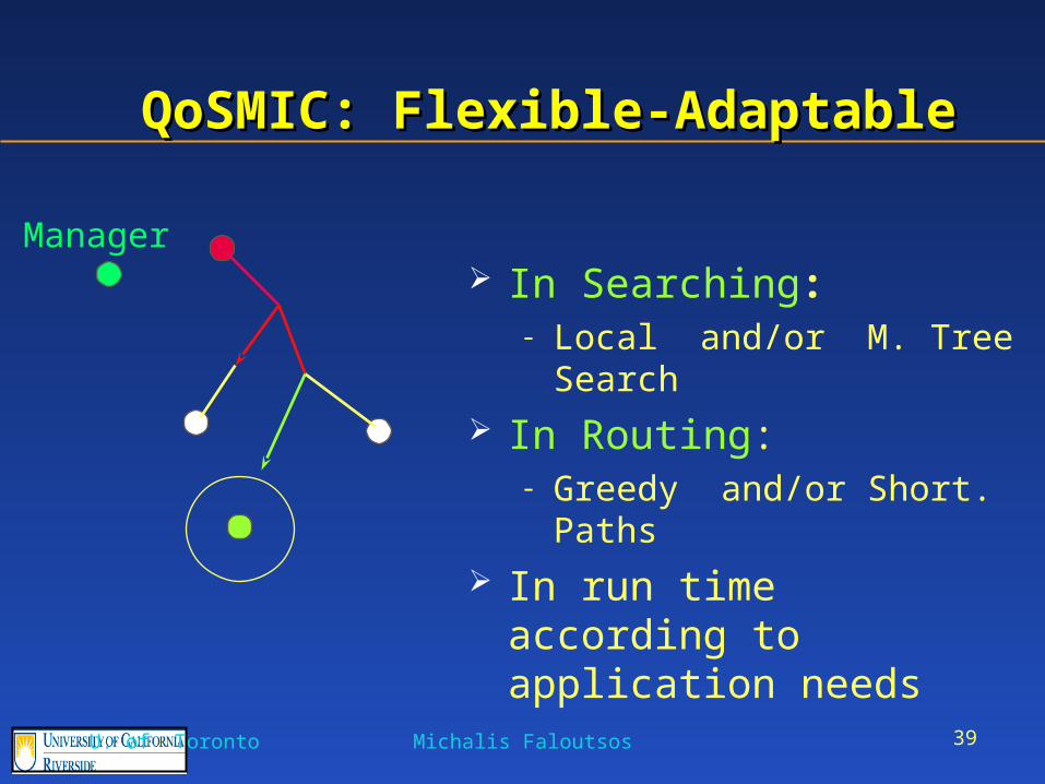
39U. of Toronto Michalis Faloutsos
In Searching: - Local and/or M. Tree Search
In Routing:- Greedy and/or Short. Paths
In run time according to application needs
QoSMIC: Flexible-AdaptableQoSMIC: Flexible-Adaptable
Manager
40U. of Toronto Michalis Faloutsos
Some SimulationsSome Simulations
Compare routing efficiency with BGMPCompare routing efficiency with BGMP• Tree cost = Sum of link-weights Tree cost = Sum of link-weights
Compare message complexity with YAMCompare message complexity with YAM• Number of control messages of search phase Number of control messages of search phase
41U. of Toronto Michalis Faloutsos
The Simulation Set-upThe Simulation Set-up
Build a simulatorBuild a simulator
Real Graph: Major Internet routers Real Graph: Major Internet routers [[Casner93Casner93]]
Weighted asymmetric graphWeighted asymmetric graph
Simulation Precision:Simulation Precision:• 95%-confidence interval <10% of shown values95%-confidence interval <10% of shown values
42U. of Toronto Michalis Faloutsos
The Simulated AlgorithmsThe Simulated Algorithms
Offline: greedy for referenceOffline: greedy for reference• At any snapshot, run greedy from scratchAt any snapshot, run greedy from scratch
SP: Shortest PathsSP: Shortest Paths
BGMP: Reverse Shortest PathsBGMP: Reverse Shortest Paths
QoSMICQoSMIC
43U. of Toronto Michalis Faloutsos
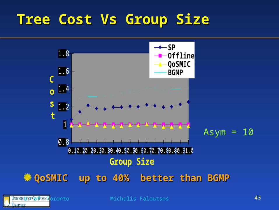
Tree Cost Vs Group SizeTree Cost Vs Group Size
0.8
1
1.2
1.4
1.6
1.8
0.1 0.2 0.2 0.3 0.3 0.4 0.5 0.5 0.6 0.7 0.7 0.8 0.8 0.9 1.0
Group Size %
Cost
SPOfflineQoSMICBGMP
QoSMIC up to 40% better than BGMP QoSMIC up to 40% better than BGMP
Asym = 10
44U. of Toronto Michalis Faloutsos
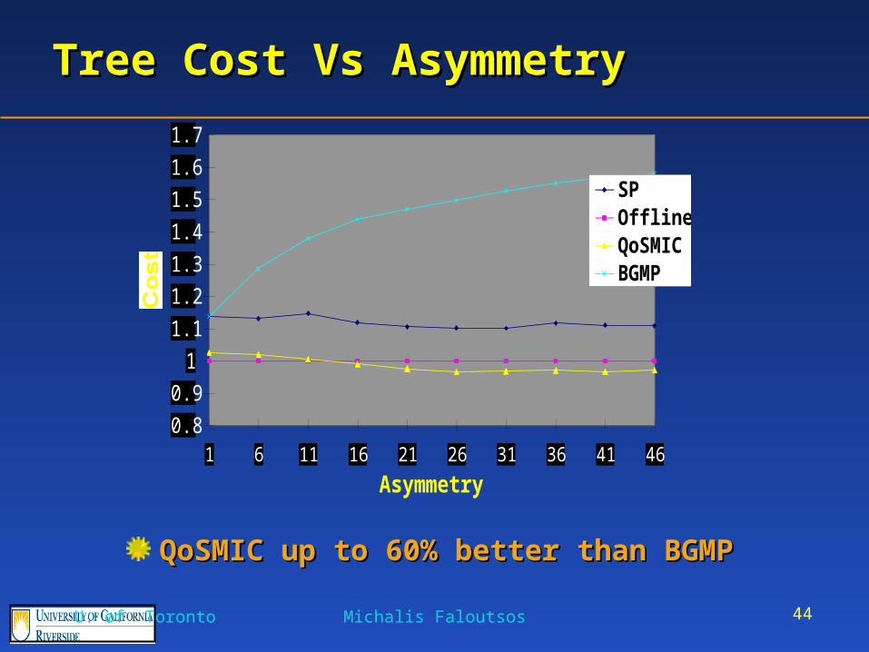
Tree Cost Vs AsymmetryTree Cost Vs Asymmetry
QoSMIC up to 60% better than BGMPQoSMIC up to 60% better than BGMP
0.8
0.9
1
1.1
1.2
1.3
1.4
1.5
1.6
1.7
1 6 11 16 21 26 31 36 41 46
Asymmetry
Cost
SPOfflineQoSMICBGMP
45U. of Toronto Michalis Faloutsos
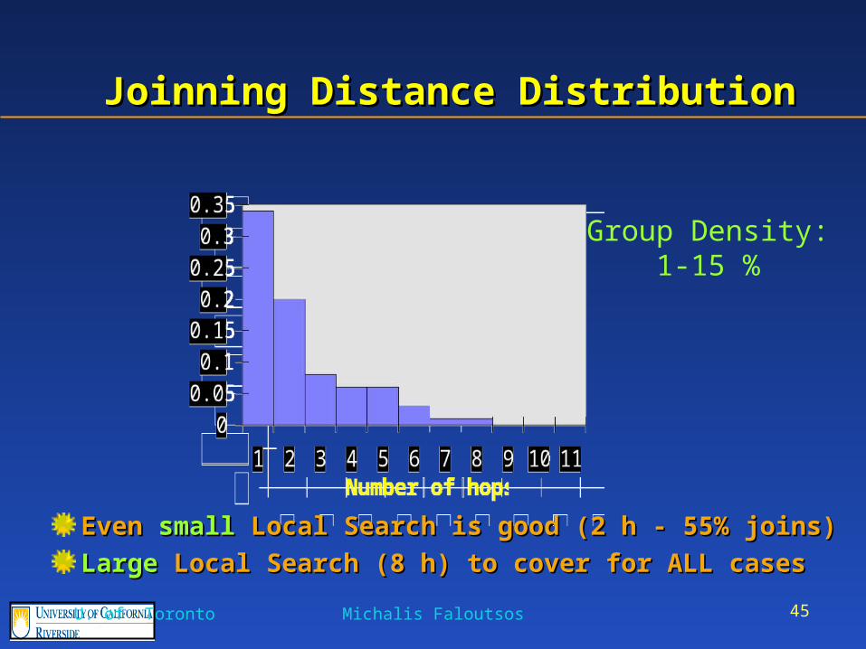
Joinning Distance DistributionJoinning Distance Distribution
Even Even smallsmall Local Search is good (2 h - 55% joins) Local Search is good (2 h - 55% joins)
Large Large Local Search (8 h) to cover for ALL casesLocal Search (8 h) to cover for ALL cases
Group Density:1-15 %
46U. of Toronto Michalis Faloutsos
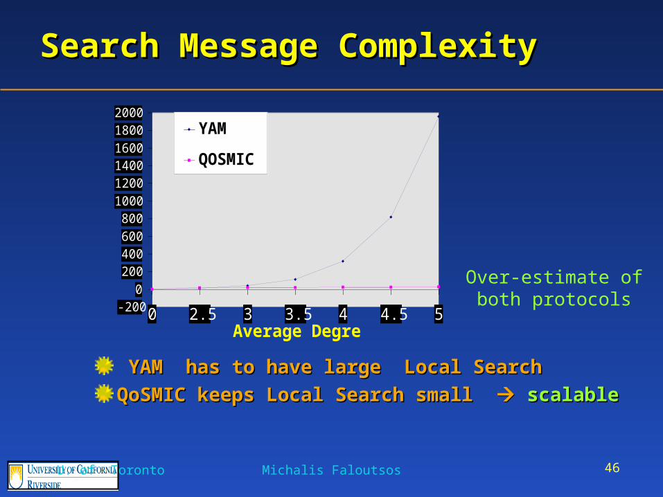
Search Message ComplexitySearch Message Complexity
-2000
200400600800
100012001400160018002000
0 2.5 3 3.5 4 4.5 5Average Degree
Messages per Join
YAM
QOSMIC
YAM has to have large Local SearchYAM has to have large Local Search
QoSMIC keeps Local Search small QoSMIC keeps Local Search small scalablescalable
Over-estimate of both protocols
47U. of Toronto Michalis Faloutsos
QoSMIC: The ClaimQoSMIC: The Claim
<< QoSMIC routes in a QoS-sensitive way, and is more efficient even than the non QoS-sensitive protocols >>
48
Why Isn’t QoSMIC the Standard?Why Isn’t QoSMIC the Standard?
Implementation complexityImplementation complexity
Scalability and message complexityScalability and message complexity
Needs industry and IETF supportNeeds industry and IETF support
Timeliness:Timeliness:• Now people look at other issuesNow people look at other issues
49
Generalizing QoSMICGeneralizing QoSMIC
QoSMIC as a set of searching proceduresQoSMIC as a set of searching procedures• Local flooding: receiver drivenLocal flooding: receiver driven• Indirect search: through designated routerIndirect search: through designated router
A mechanism to search for points of interestA mechanism to search for points of interest• Servers, caches etcServers, caches etc
Possible applicationsPossible applications• Web server locationWeb server location• Ad-hoc networks: searching for a destinationAd-hoc networks: searching for a destination
50
Multicasting: The ResurrectionMulticasting: The Resurrection
Can we do multicasting without the need of Can we do multicasting without the need of router support?router support?
51
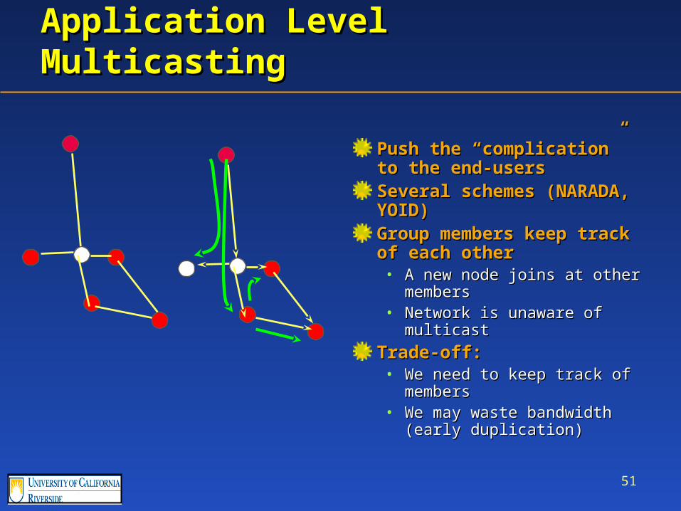
Application Level MulticastingApplication Level Multicasting
Push the “complication” to Push the “complication” to the end-usersthe end-usersSeveral schemes (NARADA, Several schemes (NARADA, YOID)YOID)Group members keep track of Group members keep track of each othereach other• A new node joins at other A new node joins at other
membersmembers• Network is unaware of Network is unaware of
multicastmulticast
Trade-off:Trade-off:• We need to keep track of We need to keep track of
membersmembers• We may waste bandwidth We may waste bandwidth
(early duplication)(early duplication)
52
Application Layer Multicast:Application Layer Multicast:PerformancePerformance
A-L multicast implements the KMB version of A-L multicast implements the KMB version of the greedy algorithm!the greedy algorithm!
Thus routing performance is not that bad!Thus routing performance is not that bad!• In theory: cost of an edge is fixedIn theory: cost of an edge is fixed
The real concern:The real concern:• We overload the last-mile of the networkWe overload the last-mile of the network
I.e. imagine 3 copies of video uploadedI.e. imagine 3 copies of video uploaded
53
Application Layer Multicasting:Application Layer Multicasting:Pros and ConsPros and Cons
Pros:Pros:
Easy to deployEasy to deploy
Adaptive to changeAdaptive to change
Good routing Good routing
Cons:Cons:
Need to track group membersNeed to track group members
Member-changes alter the treeMember-changes alter the tree
Bad bandwidth utilizationBad bandwidth utilization
More message overheadMore message overhead
54
Application Layer Multicasting:Application Layer Multicasting:ApplicationsApplications
Ad hoc networks:Ad hoc networks:• Paths are changing rapidly, faster than membersPaths are changing rapidly, faster than members
Nodes need to keep dynamic routing state Nodes need to keep dynamic routing state anywayanyway
55
Aggregating Multicast StateAggregating Multicast State
56
Large Routing State is a ProblemLarge Routing State is a Problem
Internet scalability: based on stateless Internet scalability: based on stateless routingrouting
IP multicast: state on each tree router per IP multicast: state on each tree router per group (group = connection)group (group = connection)
Routing State: proportional to # groupsRouting State: proportional to # groups
57
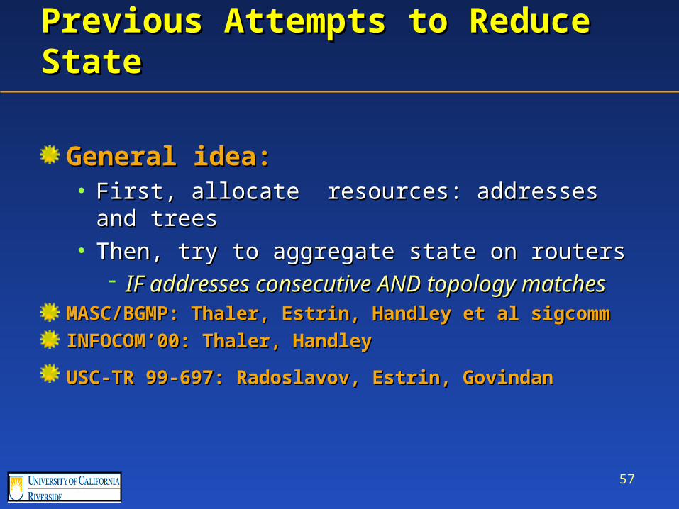
Previous Attempts to Reduce StatePrevious Attempts to Reduce State
General idea:General idea:• First, allocate resources: addresses and treesFirst, allocate resources: addresses and trees• Then, try to aggregate state on routersThen, try to aggregate state on routers
IF addresses consecutive AND topology matchesIF addresses consecutive AND topology matchesMASC/BGMP: Thaler, Estrin, Handley et al sigcommMASC/BGMP: Thaler, Estrin, Handley et al sigcomm
INFOCOM’00: Thaler, HandleyINFOCOM’00: Thaler, Handley
USC-TR 99-697: Radoslavov, Estrin, GovindanUSC-TR 99-697: Radoslavov, Estrin, Govindan
58
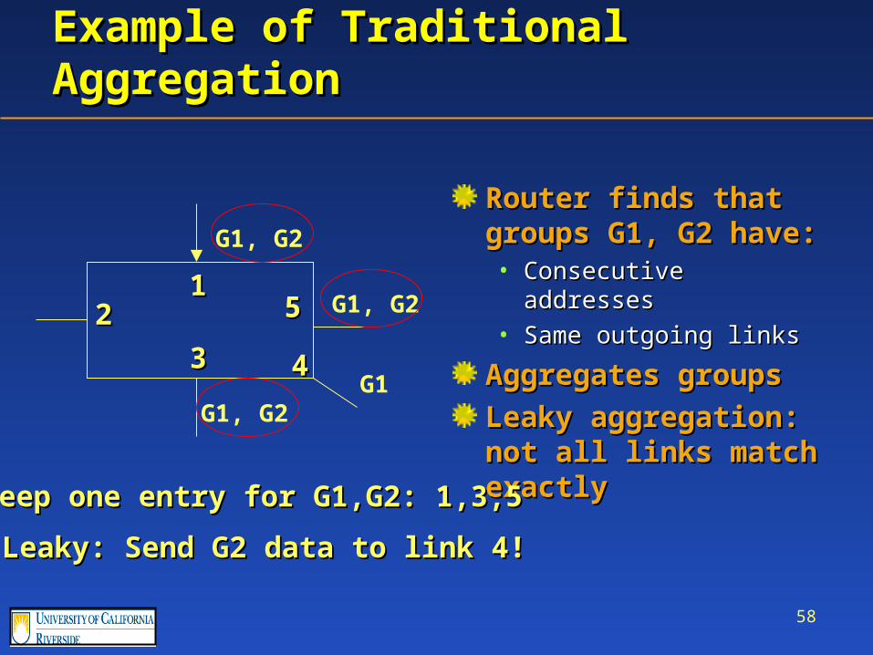
Example of Traditional AggregationExample of Traditional Aggregation
Router finds that Router finds that groups G1, G2 have:groups G1, G2 have:• Consecutive addressesConsecutive addresses• Same outgoing linksSame outgoing links
Aggregates groupsAggregates groups
Leaky aggregation: not Leaky aggregation: not all links match exactlyall links match exactly
G1, G2
G1, G2
G1, G2
Keep one entry for G1,G2: 1,3,5Keep one entry for G1,G2: 1,3,5
G1
Leaky: Send G2 data to link 4!Leaky: Send G2 data to link 4!
1122
33 44
55
59
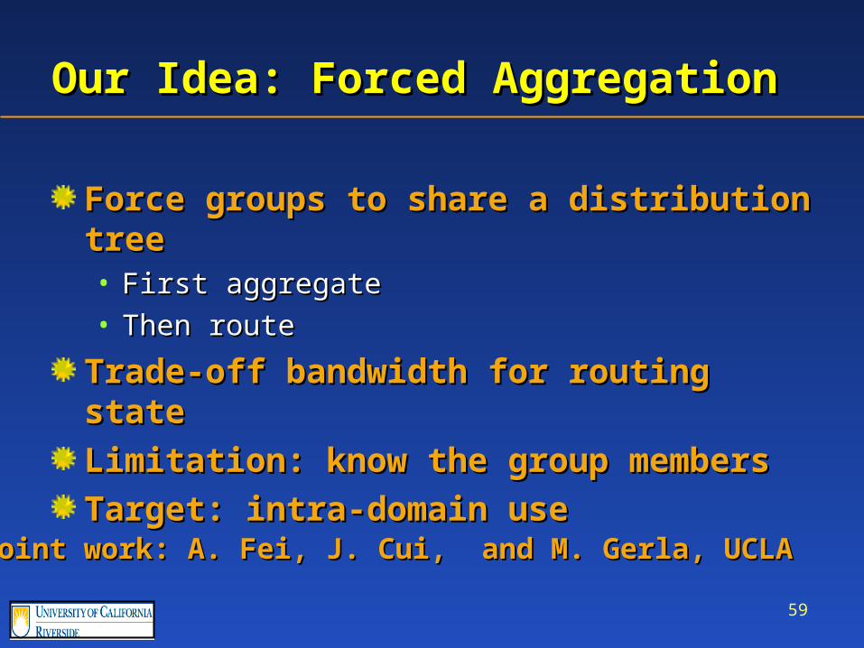
Our Idea: Forced AggregationOur Idea: Forced Aggregation
Force groups to share a distribution treeForce groups to share a distribution tree• First aggregateFirst aggregate• Then routeThen route
Trade-off bandwidth for routing stateTrade-off bandwidth for routing state
Limitation: know the group membersLimitation: know the group members
Target: intra-domain useTarget: intra-domain use
•Joint work: A. Fei, J. Cui, and M. Gerla, UCLAJoint work: A. Fei, J. Cui, and M. Gerla, UCLA
60
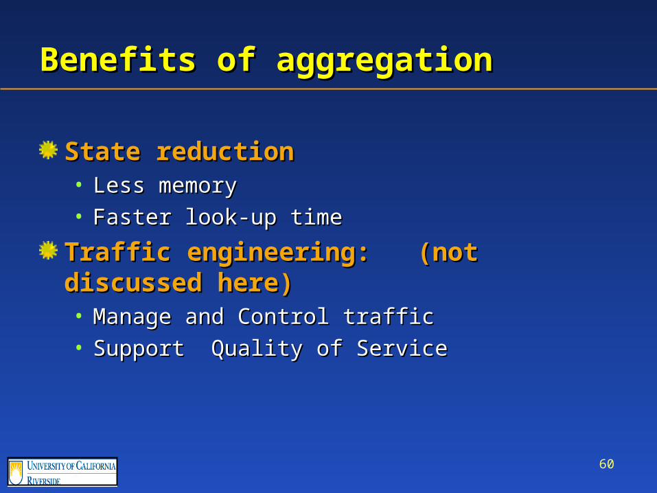
Benefits of aggregationBenefits of aggregation
State reductionState reduction• Less memoryLess memory• Faster look-up timeFaster look-up time
Traffic engineering: (not discussed here)Traffic engineering: (not discussed here)• Manage and Control trafficManage and Control traffic• Support Quality of ServiceSupport Quality of Service
61
RoadmapRoadmap
IntroductionIntroduction
Our approach in more detailOur approach in more detail
Implementation issuesImplementation issues
Analytical results Analytical results
Simulations resultsSimulations results
ConclusionsConclusions
62
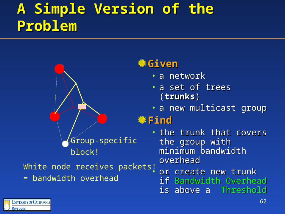
A Simple Version of the ProblemA Simple Version of the Problem
GivenGiven• a network a network • a set of trees (a set of trees (trunkstrunks))• a new multicast groupa new multicast group
Find Find • the trunk that covers the the trunk that covers the
group with minimum group with minimum bandwidth overheadbandwidth overhead
• or create new trunk if or create new trunk if Bandwidth OverheadBandwidth Overhead is is above a above a ThresholdThreshold
White node receives packets!= bandwidth overhead
Group-specificblock!
63
Subtle Points and VariationsSubtle Points and Variations
We need to know the group members at least We need to know the group members at least approximatelyapproximatelyOff-line versus on-line version of the problemOff-line versus on-line version of the problem• Know all groups ahead of timeKnow all groups ahead of time
Perfect versus leaky match:Perfect versus leaky match:• Trunk and group have the same leavesTrunk and group have the same leaves
Group specific blocks in the trunkGroup specific blocks in the trunk• Block unwanted traffic on a per Block unwanted traffic on a per sourcesource/group basis/group basis
64
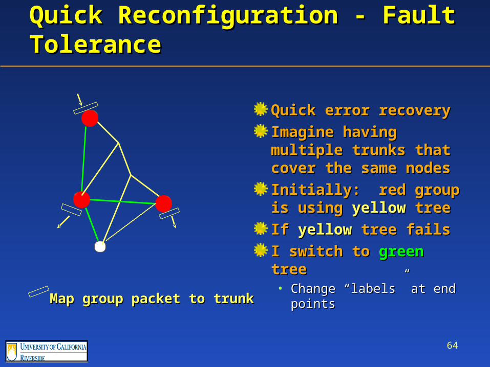
Quick Reconfiguration - Fault Quick Reconfiguration - Fault ToleranceTolerance
Quick error recoveryQuick error recovery
Imagine having multiple Imagine having multiple trunks that cover the trunks that cover the same nodessame nodes
Initially: red group is Initially: red group is using using yellowyellow tree tree
If If yellowyellow tree fails tree fails
I switch to I switch to greengreen tree tree• Change “labels” at end Change “labels” at end
pointspointsMap group packet to trunkMap group packet to trunk
65
Implementation IssuesImplementation Issues
We need controlled and centralised We need controlled and centralised operationoperation• Some nodes should keep track of trunks and groupsSome nodes should keep track of trunks and groups
How can we force a group on a tree?How can we force a group on a tree?• IP EncapsulationIP Encapsulation• Multi Protocol Label Switching (MPLS)Multi Protocol Label Switching (MPLS)• Home-made solutions are being consideredHome-made solutions are being considered
66
Aggregation Performance MetricsAggregation Performance Metrics
Average aggregation degree:Average aggregation degree:• #groups / #trunks#groups / #trunks
Routing state reduction ratio, r_as: Routing state reduction ratio, r_as: • 1 – N_agg /N_non-agg1 – N_agg /N_non-agg
Non-reducible state: Non-reducible state: • the state that leaf nodes maintain the state that leaf nodes maintain
Reducible state reduction ratio, r_rs:Reducible state reduction ratio, r_rs:• As r_as without considering the non-reducible stateAs r_as without considering the non-reducible state
67
Preliminary Simulation ResultsPreliminary Simulation Results
Goal: examine trade-offGoal: examine trade-off• aggregation vs bandwidth overheadaggregation vs bandwidth overhead
Used Abilene network topology Used Abilene network topology
Random selection of group membersRandom selection of group members• No assumption of localityNo assumption of locality
We did not consider group-specific blockingWe did not consider group-specific blocking
Group size: 2-10 nodes uniformlyGroup size: 2-10 nodes uniformly
68
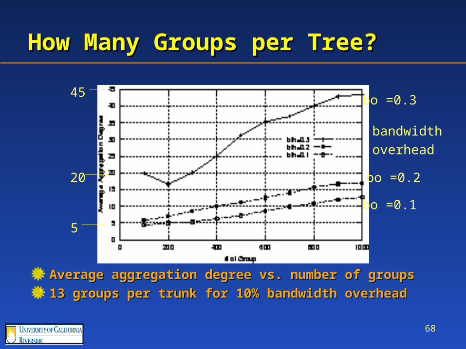
How Many Groups per Tree?How Many Groups per Tree?
Average aggregation degree vs. number of groupsAverage aggregation degree vs. number of groups
13 groups per trunk for 10% bandwidth overhead13 groups per trunk for 10% bandwidth overhead
5
20
45bo =0.3
bo =0.2
bo =0.1
bandwidthoverhead
69
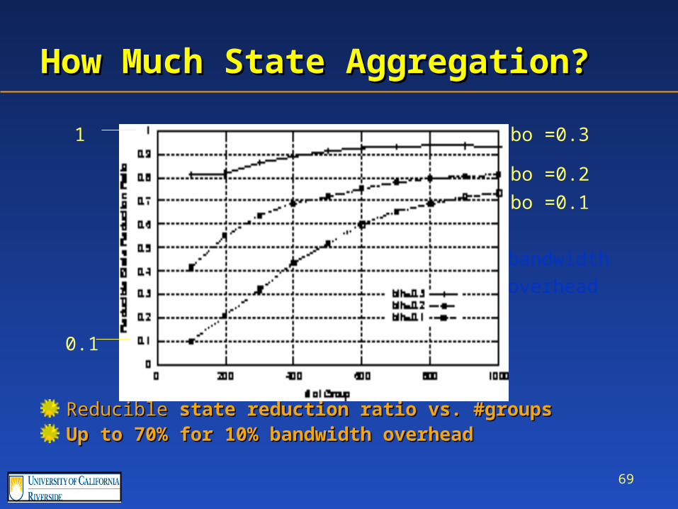
How Much State Aggregation?How Much State Aggregation?
ReducibleReducible state reduction ratio vs. #groups state reduction ratio vs. #groupsUp to 70% for 10% bandwidth overheadUp to 70% for 10% bandwidth overhead
bo =0.3
bo =0.2
bo =0.1
bandwidthoverhead
0.1
1
70
SummarySummary
A novel idea, “forced” aggregate multicast:A novel idea, “forced” aggregate multicast:• First aggregate, then routeFirst aggregate, then route
We examined the trade-off:We examined the trade-off:• Aggregation versus bandwidth overheadAggregation versus bandwidth overhead
Initial simulations are promising Initial simulations are promising
71
Future WorkFuture Work
Analytical boundsAnalytical bounds
Simulation with large ISP topologiesSimulation with large ISP topologies
Consider user localityConsider user locality• Find a realistic model for membershipFind a realistic model for membership• Examine its effect on aggregation (positive)Examine its effect on aggregation (positive)
Consider group-specific blocksConsider group-specific blocks
Evaluate different implementationsEvaluate different implementations
72
End of MulticastEnd of Multicast
73
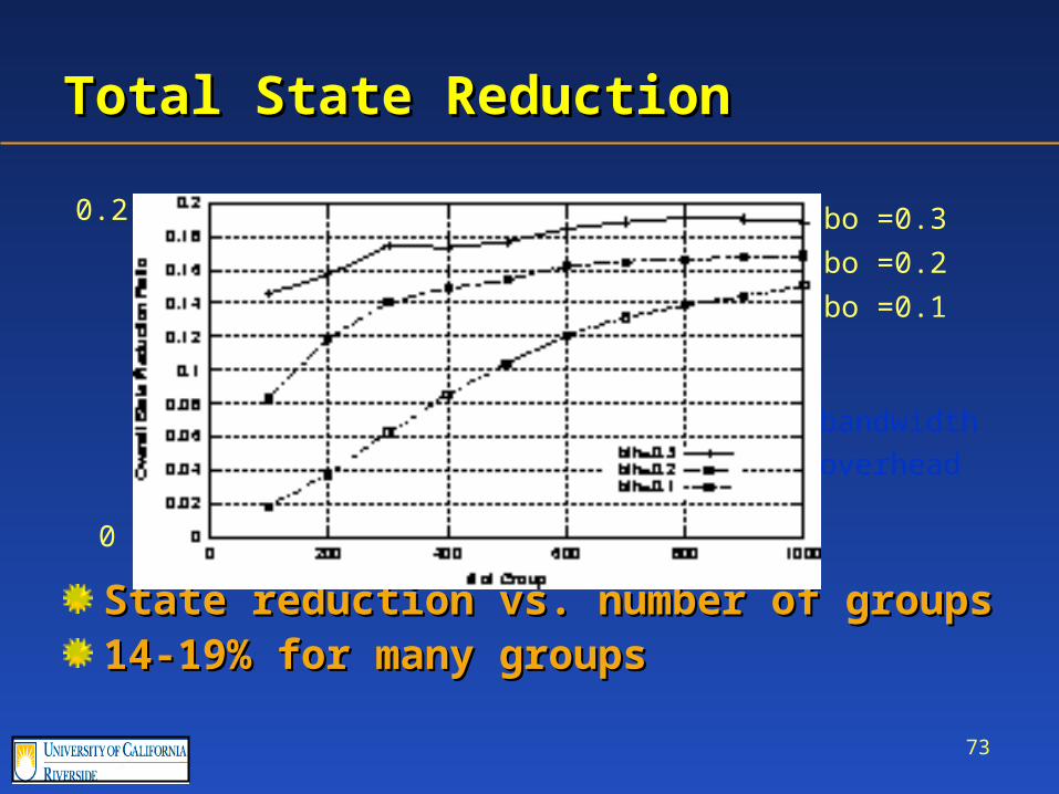
Total State ReductionTotal State Reduction
State reduction vs. number of groupsState reduction vs. number of groups14-19% for many groups14-19% for many groups
0.2
0
bo =0.3
bo =0.2
bo =0.1
bandwidthoverhead

74
Aggregate Multicast for Traffic Aggregate Multicast for Traffic EngineeringEngineering
Customer wants QoS Customer wants QoS guarantees through a guarantees through a networknetwork
Allocate a tree + Allocate a tree + resourcesresources
Customer can utilize Customer can utilize the resource as she the resource as she wantswants
ISP network
7522Michalis Faloutsos
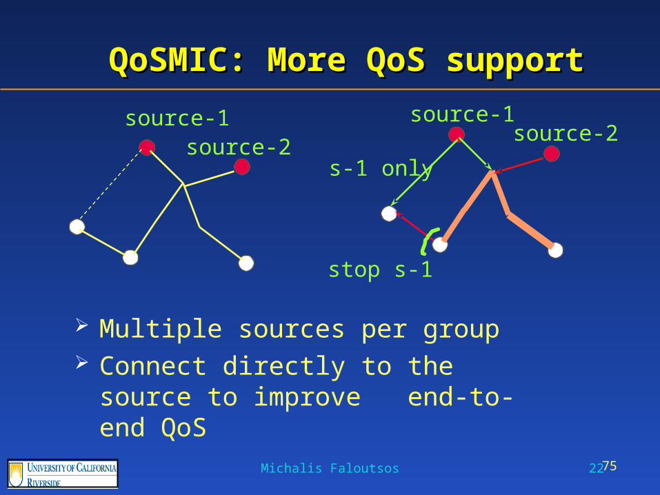
QoSMIC: More QoS supportQoSMIC: More QoS support
Multiple sources per group Connect directly to the source to improve
end-to-end QoS
source-1source-2
s-1 only
stop s-1
source-1source-2
76
Then, why is not QoSMIC deployed?Then, why is not QoSMIC deployed?
Need for industrial supportNeed for industrial support
Complicated implementationComplicated implementation
Timeliness: too lateTimeliness: too late
The QoS taint: some people are “against” QoSThe QoS taint: some people are “against” QoS
77
QoSMIC II: The return of the living QoSMIC II: The return of the living deaddead
QoSMIC as a collection of procedures for QoSMIC as a collection of procedures for searchingsearching• Flood locallyFlood locally• Indirection globallyIndirection globally
Possible applicationsPossible applications• Wireless ad hoc networksWireless ad hoc networks• Peer-to-peer networksPeer-to-peer networks
Related Documents