Management of Uncertainty
Yossi Sheffi
ESD.260J/1.260J/15.770J

2
Outline
ForecastingManaging uncertaintyAggregation/risk poolingPostponementMixed strategiesLead time management

3
Supply Chains are Tough to ManageSupply Chains are Tough to Manage
• Supply chains are difficult to manage – regardless of industry clockspeed (although more difficult in fast clockspeed industries)
• Managing inventory is one of the difficulties, ranging from shortages as we see for Goodyear racing tires to excess inventory as we see in Cisco’s high-tech networking products. The impact of the inventory challenges affectemployment levels as we see how GM used layoffs to adjust inventoryproduct price; as we see Palm cut prices to deal with excess inventoryprofits; as we see USX’s net income sink
• It is a cyclical problem that has extremes as we see in Intel’s case, going fromshortages and backlogs to chip gluts back to shortages
• Supply chains are tough to manage even if you are the dominant player.

4
Four Rules of Forecasting
1.2.3.4.

5
Why is the World Less Certain
Aggravated bullwhip; higher variance; irrelevant historyMuch more difficult to forecast

6
Managing Uncertainty
1. Point forecasts are invariably wrong
2. Aggregate forecasts are more accurate
3. Longer term forecasts are less accurate
4. In many cases somebody else knows what is going to happen
Plan for forecast range – use flexible contracts to go up/downAggregate the forecast -postponement/risk pooling
Shorten forecasting horizons –multiple orders; early detectionCollaborate

7
Managing Uncertainty
Centralized inventory (aggregation, risk pooling) – less safety stock
Pronounced with high variability and negative correlation
PostponementReduction in forecast horizon beyond the pivot pointRisk pooling in “core” productBuilt-to-order
Lead time reductionProximity; process re-engineering, I/T
8
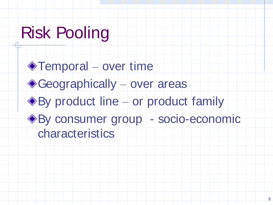
Risk Pooling
Temporal – over timeGeographically – over areasBy product line – or product familyBy consumer group - socio-economic characteristics
9
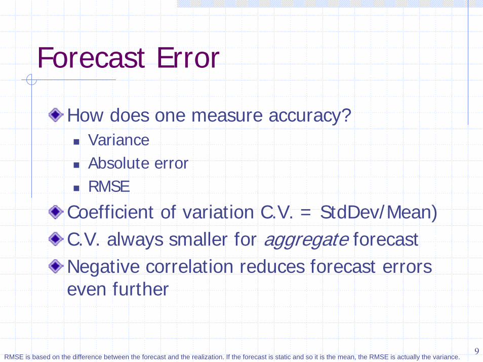
Forecast Error
How does one measure accuracy?VarianceAbsolute errorRMSE
Coefficient of variation C.V. = StdDev/Mean)C.V. always smaller for aggregate forecastNegative correlation reduces forecast errors even further
RMSE is based on the difference between the forecast and the realization. If the forecast is static and so it is the mean, the RMSE is actually the variance.
10
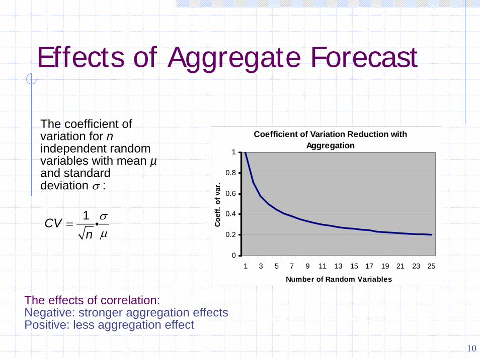
Effects of Aggregate Forecast
Coefficient of Variation Reduction with Aggregation
0
0.2
0.4
0.6
0.8
1
1 3 5 7 9 11 13 15 17 19 21 23 25
Number of Random Variables
Coef
f. of
var
.
The coefficient of variation for nindependent random variables with mean µand standard deviation σ :
1CVnσµ
= i
The effects of correlation:Negative: stronger aggregation effectsPositive: less aggregation effect

11
Risk PoolingWhy do “big box” stores do well?Imagine an urban area with nine store
Each store sells a mean of µ = 50/wk with a standard deviation of σ = 35/wkLead time = 2 weeks For 97.5% service, Store Safety Stock= 1.96•35•1.41=97 itemsTotal safety stock = 9•97=873 items
Now replace these stores with a single super-storeThe super-store sells a mean of µ = 450/wk with a standard deviation of σ = 3•35/wk = 105/wkFor 97.5% service, The super-store Safety Stock= 1.96•105•1.41=291 items
Note: the inventory required to cover the lead time does not change (900 units). The difference is in the safety stock.
(√2 = 1.41)

12
Big StoreAdvantages:
Disadvantages:

13
Centralized Inventory
Plant
DC
DC DC
DCCDC
20 stores (5 per DC)LOS: 97.5%Store Demand = 50±35Replenishment time = 1 week
Each DC Demand = 5•50±SQRT(5)•35 = 250±78CDC Demand = 20•50±SQRT(20)•35 = 1,000±156
Total safety stock at stores = 20•(50+1.96•35) = 2,372Total safety stock at DC-s = 4•(250+1.96•78) = 1,612Total safety stock at CDC = 1,000+1.96•156 = 1,306

14
Aggregation with a Single OrderEach of 4 stores:Price: $150Cost : $50Salvage: $25Mean: 500Std. Dev: 150
Each:Q* = NORMINV(0.8, 500, 150) = 626Profits = $44,7514 independents: $179,003CombinedQ* = NORMINV(0.8, 2000, 300)= 2,252Profits = $189,501
Effect of Std. Dev (n=4)
100,000
125,000
150,000
175,000
200,000
0.2 0.3 0.4 0.5 0.6 0.7 0.8 0.9 1 1.1Coefficient of Variation
Expe
cted
Pro
fit
IndependentOutletsCombinedInventory
Big change:# sold items up 1.73%# unsold items dn 50.00%

15
United Colors of Benetton
Shirt PostponementRegular operation: import shirts from the far East (4 wks lead time)Need: LOS = 97.5%
Postponement: bring Greige colors and dye to order
Mean Std DevColor shirts/wk shirts/wk
Red 1,500 500Blue 1,200 450Green 600 250Black 2,500 700
DemandTransit safety Total
Inv Stock Inv6,000 1,960 7,9604,800 1,764 6,5642,400 980 3,380
10,000 2,744 12,744
23,200 7,448 30,648Total (Individual Shirts)
23,200 3,930 27,130Total (postponed) 5,800 1,002
•Safety stock•Owned inventory

16
Uncertainty Management:
Examples: Risk Pooling and PostponementCadillac automobiles in Florida
Benetton for sweaters and T-shirts
HP European printers
Gillette for blades in Europe
Sherwin Williams paint
Motorola modems
Zara Fabrics
Dell build-to-order

17
Build-to-Order
The ultimate postponementDell/Gateway build-to-order
Better response to changes in demandBetter response to changes in component pricing/availabilityAbility to direct customers to products including existing components
The “Pivot” point: from BTS to BTOPushing the customization/commitment later in the supply chain

18
United Colors of Benetton
Postponement
Mean demand = 800Standard deviation = 400Price = $40Cost = $18Salvage = $5
Order size for each color = 931 sweatersTotal order = 3,724 sweatersExpected profit for each color = $12,301Total profit = $49,230
Make “Griege” sweaters and die to demand
Mean demand = 3,200Standard deviation = 800Cost = $21Salvage = $5
Order size for each color = 3,286 sweatersExpected total profit = $53,327
2,790 sold; 934 unsold 3,026 sold; 260 unsold

19
A Mixed StrategyIdea: order some pre-colored sweaters and sell those firstOrder also some griege sweaters and sell them as demand materializesQuestion: how many of each to maximize profitUse: simulationAnswer:
Only colored: order 931 of each 3,724 Tot.): Exp. profit: $49,230Only griege: order 3,280: Exp. Profit: $53,327600 colored each and 1,100 griege: Exp. profit: $54,487
20
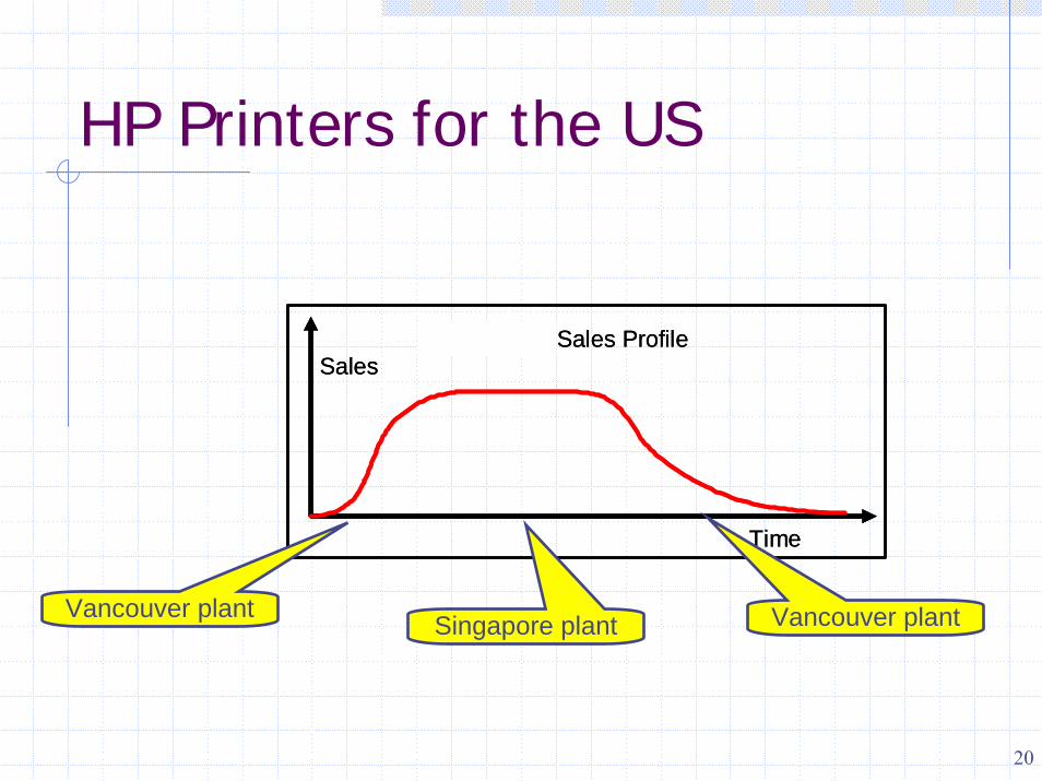
HP Printers for the US
Time
SalesFigure 16.5 Sales Profile
Time
SalesFigure 16.5 Sales Profile
Vancouver plant Vancouver plantSingapore plant

21
Multiple Orders (QR)Price $120
Cost $40
Salvage $25
Mean (1 period) 50
Std. Dev 25
Order once for the whole period:Mean = 100; Std. Dev = 35.4Q* = 135Exp. Profits = $7,190
Order at the beginning & again in mid period:2nd period: Mean = 50; Std. Dev = 25Order “up to”: = 75How much in 1st period?
10 Simulations
4000
4500
5000
5500
6000
6500
7000
7500
8000
0 50 100 150 2001sr Period Order
Exp.
Pro
fits
4000
4500
5000
5500
6000
6500
7000
7500
8000
15 30 45 60 75 90 105 120 135 150 165 180
Q* ≅ 104; Exp Profits = $7,450

22
Asymmetric Aggregation
You can always upgrade to keep consumers happyExample: two-cars automobile rental company: Buick and CadillacAssume: equal demand (order 500 each for independent demand)For upgrade option: order more Cadillacs and less Buicks
23
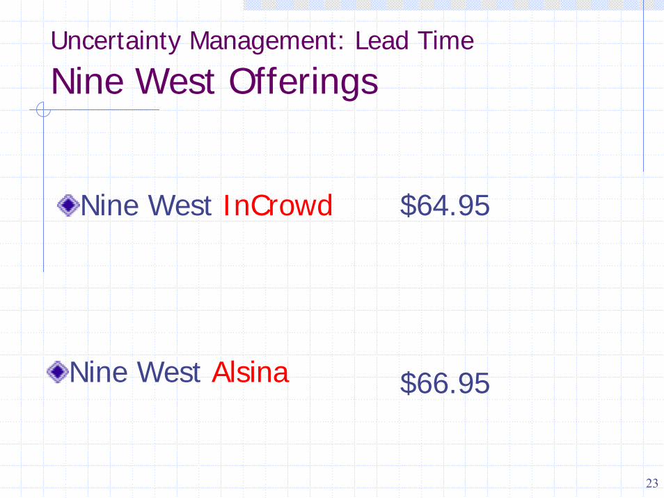
Uncertainty Management: Lead Time
Nine West Offerings
Nine West InCrowd $64.95
Nine West Alsina $66.95

24
NINE WEST
Traditional Supply Chain
Shoe sampleordered
from factory
Send to 2nd or3rd channel at
a loss
Sell-out orMark-downs
Samples OK& production
orderedProduction
DeliveryTo
storesSales? Yes
Poor
Very well Stock-out

25
NINE WEST
Improved Supply Chain
1000 Shoesample
ordered
productionordered
Samples air-freighted to5 US stores
Sales intest
stores?No change
to planYes
Very well Increaseproduction
Poor Decreaseproduction
ProductionProduction
Delivery to2nd or 3rd
channel
Deliveryto stores

26
Any Questions?
Yossi Sheffi


![YOAV ZURIEL, GALI SHEFFI, arXiv:1909.02852v2 [cs.DC] 9 Sep 2019 · 128:2 Yoav Zuriel, Michal Friedman, Gali Sheffi, Nachshon Cohen, and Erez Petrank may change the order in which](https://static.cupdf.com/doc/110x72/60501e3ade9bf70b8c714ca0/yoav-zuriel-gali-sheffi-arxiv190902852v2-csdc-9-sep-2019-1282-yoav-zuriel.jpg)