1
Wireless Broadcast Using Network CodingDong Nguyen, Tuan Tran, Thinh Nguyen, Bella Bose
School of EECS, Oregon State University
Corvallis, OR 97331, USA
{nguyendo, trantu, thinhq}@eecs.oregonstate.edu; [email protected]
Abstract
Traditional approaches to transmit information reliably over an error-prone network employ either
Forward Error Correction (FEC) or retransmission techniques. In this paper we propose some network
coding schemes to reduce the number of broadcast transmissions from one sender to multiple receivers.
The main idea is to allow the sender to combine and retransmit the lost packets in a certain way, so
that with one transmission, multiple receivers are able to recover their own lost packets. For comparison,
we derive a few theoretical results on the bandwidth efficiencies of the proposed network coding and
traditional Automatic Repeat-reQuest (ARQ) schemes. Both simulations and theoretical analysis confirm
the advantages of the proposed network coding schemes over the Automatic Repeat-reQuest (ARQ) ones.
I. INTRODUCTION
Broadcast is a mechanism for disseminating identical information from a sender to multiple receivers. It
is widely employed in many applications, ranging from satellite communications to Wireless Local Area
Network (WLAN). Reliable broadcast requires that every receiver must receive the correct information
sent by the sender. When the communication channels between a sender and receivers are lossy, some
appropriate error control schemes must be used to provide reliable transmissions. Depending on applica-
tions, these schemes can be classified into two main approaches: Automatic Repeat ReQuest (ARQ) and
Forward Error Correction (FEC).
Using the ARQ approach, the sender may have to rebroadcast the lost packet to all the receivers, even
though there may be only one receiver that did not receive that packet correctly. The ARQ approach
assumes that a feedback channel is available so that the receiver can communicate to the sender on
whether or not it receives the correct data. On the other hand, using the pure FEC approach, the sender
generates some redundancies, then broadcasts both redundant and original information to the receivers
[1]. If the amount of lost data is sufficiently small (less than the redundant data), a receiver can recover
the lost data using some decoding schemes.
For satellite TV applications, the TV signals are broadcast from a satellite to potentially millions of
TVs, making the probability of any TV not receiving the correct signal at any time close to 1. Therefore, it
is extremely inefficient to employ an ARQ protocol for retransmissions since most of the bandwidth will
be used for retransmissions. Furthermore, the lack of TV-to-satellite channels makes the retransmission
approach infeasible. In these scenarios, it is preferable to employ a pure FEC technique.
In other settings, e.g., WLAN, there are relatively few devices and the communication channel is
relatively reliable. Therefore, the retransmission approach may be more bandwidth-efficient than that
of the FEC approach since redundant information is not added in every transmission. Furthermore, in
practice, FEC alone cannot guarantee reliable delivery due to a non-zero chance that a receiver may not
be able to recover the data from a single transmission.
That said, this paper explores the efficient retransmission-based broadcast schemes in single-hop wireless
networks. Efficient schemes can be used in WLAN to reduce the time required to copy a large file from
one computer to multiple computers simultaneously. It can also be used to broadcast music or important
announcements in multiple rooms in a small building, even though a highly reliable audio signal is
probably not needed in most situations. In addition, an efficient retransmission-based wireless broadcast
scheme might be beneficial to the emerging wireless standard WiMAX (Worldwide Interoperability for
Microwave Access). WiMAX aims to enable wireless data transmissions over long distances, and can
potentially provide wireless broadband access as an alternative to cable and DSL. In this WiMAX setting,
at any point in time, a few homes may want to watch the same broadcast digital TV program through
the Internet, i.e., these homes may want to receive the same TV signals. Therefore, a WiMAX broadcast
station can view the data delivery as multiple wireless broadcast sessions (TV channels) with each session
involving a few homes. By optimizing these wireless broadcast sessions, the wireless bandwidth can be
efficiently used. To this end, we propose some broadcast schemes that combine network coding and
retransmission to utilize bandwidth efficiently.
a
a a1 2
b b b34RR1 R2
(a)
ba b
a 1 2 b
a b a b
b=a (a b) a=b (a b)
RR1 R2
3
(b)
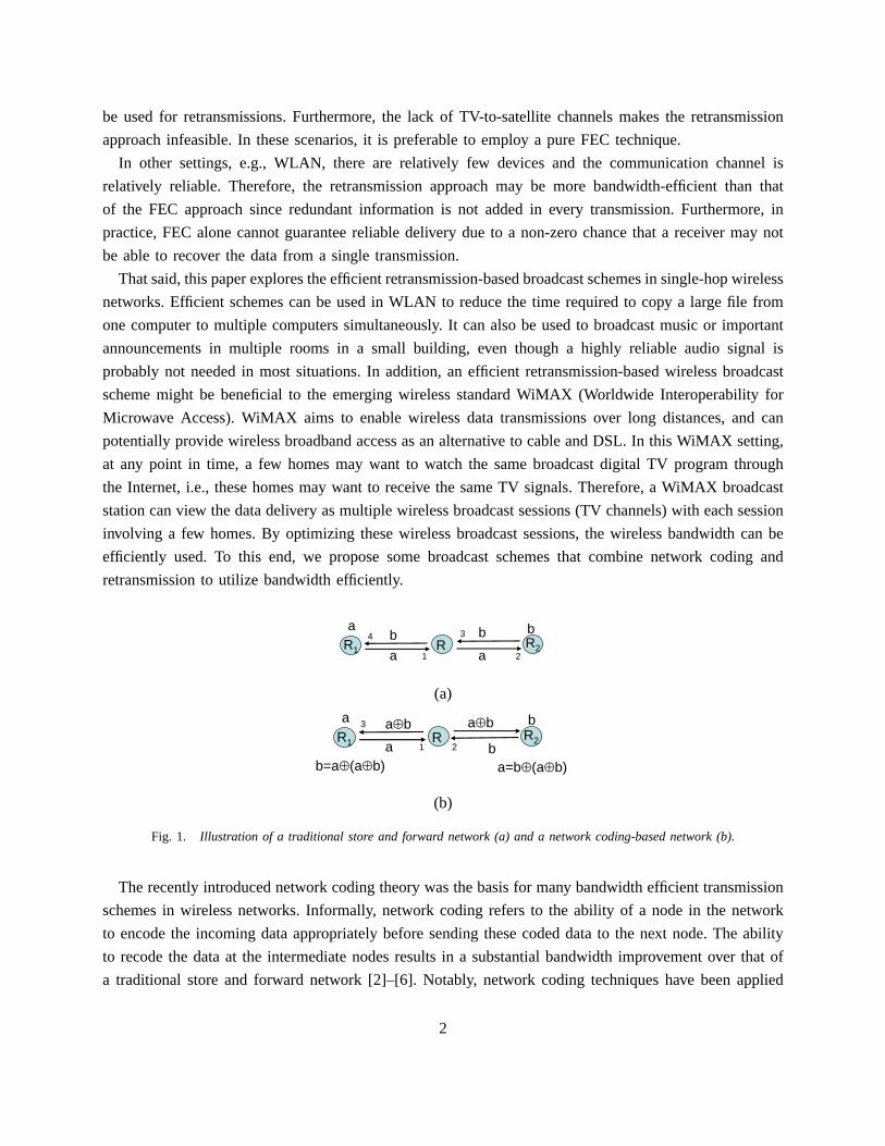
Fig. 1. Illustration of a traditional store and forward network (a) and a network coding-based network (b).
The recently introduced network coding theory was the basis for many bandwidth efficient transmission
schemes in wireless networks. Informally, network coding refers to the ability of a node in the network
to encode the incoming data appropriately before sending these coded data to the next node. The ability
to recode the data at the intermediate nodes results in a substantial bandwidth improvement over that of
a traditional store and forward network [2]–[6]. Notably, network coding techniques have been applied
2
to increase bandwidth efficiency in wireless ad hoc networks [7]–[11]. As an illustration, Fig. 1 shows
an example of packet exchange between nodes R1 and R2 via node R in a wireless ad hoc network.
As shown in Fig. 1 (a), without network coding, node R simply relays packet a from R1 to R2 and
packet b from R2 to R1. As a result, the total number of transmissions required for R1 and R2 to exchange
their packets is 4. On the other hand, when network coding is used, the intermediate node R is allowed to
generate and send a new packet out, based on the packets it receives from nodes R1 and R2. As shown in
Fig. 1 (b), since both nodes R1 and R2 can hear the transmission from R, R can generate a new packet
by XORing the bits in packets a and b, then broadcasts this new packet a⊕ b to both R1 and R2. Upon
receiving a ⊕ b, R1 can recover b as a ⊕ (a ⊕ b), R2 can recover a as b ⊕ (a ⊕ b). Clearly, in this case,
only 3 transmissions are required for R1 and R2 to exchange their packets.
Instead of employing network coding for packet exchange in wireless ad hoc networks, our proposed
schemes are designed for broadcast in single-hop wireless networks. The main idea for the proposed
schemes is based on the observation that, at a certain point in time, many receivers may have disjoint lost
packets. Thus, the sender may XOR these lost packets together and broadcast it to all the receivers. Upon
receiving this XOR packet, a receiver will be able to recover its lost packet by XORing the XOR packet
with the certain packets that it has received previously. As such, one transmission from the sender will
enable multiple receivers to recover their lost packets, thus efficiently utilizing the wireless bandwidth.
We will elaborate on how to do this shortly and show that this approach can reduce the transmission
bandwidth significantly. We note that part of this work has been presented in [12] and [13].
The organization of our paper is as follows. We first discuss related work in Section II. In Section III,
we describe different retransmission-based broadcast schemes with and without network coding. We then
analyze their performances in terms of bandwidth utilization in Section IV. In particular, we derive a few
results that show the reduced transmission bandwidth when network coding is employed under different
network conditions. Section V presents the simulation results that confirm our theoretical predictions.
II. RELATED WORK
Wireless broadcast is a well-explored problem. In his seminal work, Cover [14] modeled a broadcast
channel as multiple binary channels, each with a given channel capacity. He found the lower and upper
bounds on the capacity regions of jointly achievable transmission rates. Subsequently, there has been much
research on using broadcast bandwidth efficiently. Recently, network coding has been applied successfully
to many wireless broadcast and multicast applications. Lun et al. [15] proved that the problem of minimum-
energy multicast in infrastructureless networks can be solved exactly in polynomial time when employing
network coding. This is in contrast with the traditional routing approaches in [16]–[18] that result in non-
polynomial time solutions. In addition, Li et al. [19], [20] proved that network coding could provide some
benefits over the non-network coding approaches. Lun et al. [21] showed a capacity-approaching coding
scheme for unicast or multicast over lossy packet networks, in which all nodes perform opportunistic
coding by constructing the encoded packets with random linear combinations of previously received
packets.
3
Our work is rooted in the recent development of network coding for wireless ad hoc networks [7],
[22], [23], [10]. In [7], Wu et al. proposed the basic scheme that uses XOR of packets to increase the
bandwidth efficiency of a wireless mesh network. In [22], Katti et al. implemented a XOR-based scheme
in a wireless mesh network and showed a substantial bandwidth improvement over the current approach.
Unlike existing approaches, the focus of our work is on the analysis of the reliable wireless broadcast
problem in a single-hop wireless network such as WLAN or WiMAX networks. Eryilmaz et al. [24]
also recently proposed a similar model. In this work, Eryilmaz et al. employed a random network coding
scheme for multiple users downloading a single file or multiple files from a wireless base station. Rather
than using XOR operations, their scheme encodes every packet using coefficients taken randomly from a
sufficiently large finite field [25], [26]. This scheme guarantees that the receivers can decode the original
data with high probability. Another work somewhat related to ours is that of Ghaderi et al. [27]. In [27],
the authors analyzed the reliability benefit of network coding for reliable multicast by computing the
expected number of transmissions using link-by-link ARQ compared to network coding.
Last but not least, there exist standard error control techniques for reliable wireless transmission that
employ either FEC, ARQ, or hybrid-ARQ [28]. For example, A. Shiozaki et al. [29] and M. Nakamura
et al. [30] investigated hybrid error control broadcast models which incorporate the ARQ with FEC
techniques to achieve higher throughputs to all receivers.
III. BROADCAST SCHEMES
To describe our proposed schemes, we make the following assumptions for all the broadcast schemes:
1) There are one sender and M > 1 receivers.
2) Data is sent in packets, and each packet is sent in a time slot of fixed duration.
3) The sender has access to the information on packet losses of all the receivers at any time slot. This
can be accomplished through the use of positive and negative acknowledgments (ACK/NAKs). For
simplicity, we assume that all the ACK/NAKs are instantaneous, i.e. the sender knows (a) whether
or not a packet is lost and (b) the identity of the receiver with the lost packet instantaneously. This
implicitly assumes that ACK/NAKs are never lost. This assumption is not critical since one can
easily incorporate the delay and bandwidth used by ACK/NAKs into the analysis. One can also
consider an alternative view in which, if an ACK or NAK is lost, the corresponding data packet
is also considered lost. Thus, the assumption of reliable ACK/NAK messages can be relaxed by
changing the packet loss probabilities at the receivers to reflect the loss rates in both data and
feedback channels.
4) Packet loss at a receiver i follows a Bernoulli trial with parameter pi. This model is clearly insuffi-
cient to describe many real-world scenarios. However, this model is only intended for capturing the
essence of wireless broadcast. One can develop a more accurate model, at the cost of complicated
analysis. In fact, we will provide some results when using a slightly more accurate model that
reflects the correlated losses among the receivers in Section IV-C. We will also provide simulation
results using a simple two-state Markov model to characterize packet losses.
4
A. Broadcast Schemes without Network Coding
Scheme A (Memoryless receiver). In this scenario, a receiver sends a NAK immediately whenever
there is a packet loss in the current time slot, regardless of whether it has received this packet correctly
in some previous time slots (hence memoryless). This situation arises when a receiver receives a correct
packet, but this packet was lost at some other receivers at some previous time slots. Hence, the sender
has to retransmit this packet. If this packet is now lost in the current time slot, a memoryless receiver
would automatically request a retransmission, even though it has previously received that packet. This
scheme is clearly suboptimal in terms of bandwidth utilization as it implies that the sender has to resend
a packet until all the receivers receive this packet correctly and simultaneously.
Scheme B (Typical ARQ scheme). In this scenario, the receiver sends a NAK immediately only if there
is a packet loss in the current time slot and this packet has not been received correctly in any previous
time slot. This scheme is clearly superior to scheme A in terms of bandwidth utilization since it never
requests a retransmission for a packet that it already received successfully.
B. Broadcast Schemes with Network Coding
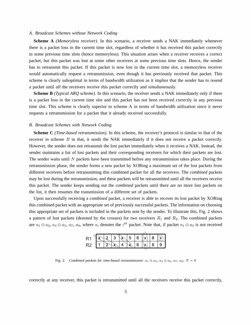
Scheme C (Time-based retransmission). In this scheme, the receiver’s protocol is similar to that of the
receiver in scheme B in that, it sends the NAK immediately if it does not receive a packet correctly.
However, the sender does not retransmit the lost packet immediately when it receives a NAK. Instead, the
sender maintains a list of lost packets and their corresponding receivers for which their packets are lost.
The sender waits until N packets have been transmitted before any retransmission takes place. During the
retransmission phase, the sender forms a new packet by XORing a maximum set of the lost packets from
different receivers before retransmitting this combined packet for all the receivers. The combined packets
may be lost during the retransmission, and these packets will be retransmitted until all the receivers receive
this packet. The sender keeps sending out the combined packets until there are no more lost packets on
the list, it then resumes the transmission of a different set of packets.
Upon successfully receiving a combined packet, a receiver is able to recover its lost packet by XORing
this combined packet with an appropriate set of previously successful packets. The information on choosing
this appropriate set of packets is included in the packets sent by the sender. To illustrate this, Fig. 2 shows
a pattern of lost packets (denoted by the crosses) for two receivers R1 and R2. The combined packets
are a1 ⊕ a3, a4 ⊕ a5, a7, a9, where ai denotes the ith packet. Note that, if packet a1 ⊕ a3 is not received
98x6x4x21
x8x65x32x
98x6x4x21
x8x65x32xR1
R2
Fig. 2. Combined packets for time-based retransmission: a1 ⊕ a3, a4 ⊕ a5, a7, a9; N = 9
correctly at any receiver, this packet is retransmitted until all the receivers receive this packet correctly,
5
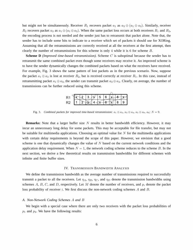
but might not be simultaneously. Receiver R1 recovers packet a1 as a3 ⊕ (a1 ⊕ a3). Similarly, receiver
R2 recovers packet a3 as a1 ⊕ (a1 ⊕a3). When the same packet loss occurs at both receivers R1 and R2,
the encoding process is not needed and the sender just has to retransmit that packet alone. Note that, the
sender has to include some bits to indicate to a receiver which set of packets it should use for XORing.
Assuming that all the retransmissions are correctly received at all the receivers at the first attempt, then
clearly the number of retransmissions for this scheme is only 4 while it is 6 for scheme B.
Scheme D (Improved time-based retransmission). Scheme C is suboptimal because the sender has to
retransmit the same combined packet even though some receivers may receive it. An improved scheme is
to have the sender dynamically changes the combined packets based on what the receivers have received.
For example, Fig. 3 shows the same pattern of lost packets as in the previous scenario. Now, suppose
the packet a1 ⊕ a3 is lost at receiver R2, but is received correctly at receiver R1. In this case, instead of
retransmitting packet a1 ⊕ a3, the sender can transmit packet a3 ⊕ a4. Clearly, on average, the number of
transmissions can be further reduced using this scheme.
98x6x4x21
x8x65x32x
98x6x4x21
x8x65x32xR1
R2
Fig. 3. Combined packets for improved time-based retransmission: a1 ⊕ a3, a3 ⊕ a4, a5 ⊕ a9, a6; N = 9.
Remarks: Note that a larger buffer size N results in better bandwidth efficiency. However, it may
incur an unnecessary long delay for some packets. This may be acceptable for file transfer, but may not
be suitable for multimedia applications. Choosing an optimal value for N for the multimedia applications
with certain delay requirements is beyond the scope of this paper. However, we envision that a good
scheme is one that dynamically changes the value of N based on the current network conditions and the
application delay requirement. When N = 1, the network coding scheme reduces to the scheme B. In the
next section, we derive a few theoretical results on transmission bandwidths for different schemes with
infinite and finite buffer sizes.
IV. TRANSMISSION BANDWIDTH ANALYSIS
We define the transmission bandwidth as the average number of transmissions required to successfully
transmit a packet to all the receivers. Let ηA, ηB , ηC , and ηD denote the transmission bandwidths using
schemes A, B, C, and D, respectively. Let M denote the number of receivers, and pi denote the packet
loss probability of receiver i. We first discuss the non-network coding schemes A and B.
A. Non-Network Coding Schemes A and B
We begin with a special case where there are only two receivers with the packet loss probabilities of
p1 and p2. We have the following results:
6
Proposition 4.1: The transmission bandwidth of scheme A with two receivers is
ηA =1
(1 − p1)(1 − p2)(1)
and using scheme B is
ηB =1
1 − p1+
11 − p2
− 11 − p1p2
. (2)
Proof: For scheme A, the proof is simple. As described in Section III, the sender has to retransmit the
packets until both receivers receive the correct packets simultaneously. Since the packet loss is independent
and uncorrelated between the receivers (Bernoulli trial), the number of transmission attempts before both
receivers correctly receive the data follows the geometric distribution with the parameter (1−p1)(1−p2).Therefore, the average number of transmissions per successful event is 1
(1−p1)(1−p2).
For scheme B, let X1, X2 be the random variables denoting the numbers of attempts to successfully
deliver a packet to R1 and R2, respectively. Then, the number of transmissions needed to successfully
deliver a packet to both receivers is the random variable Y = max{X1, X2}. We have
P [Y ≤ k] = P [max{X1, X2} ≤ k] =2∏
i=1
P [Xi ≤ k] =2∏
i=1
(1 − pki ). (3)
Therefore,
P [Y = k] =2∏
i=1
(1 − pki ) −
2∏i=1
(1 − pk−1i ) (4)
and the average number of transmissions per successful packet is
ηB = E[Y ] =∞∑
k=1
k
(2∏
i=1
(1 − pki ) −
2∏i=1
(1 − pk−1i )
)
=∞∑
k=1
k(pk−11 − pk
1) +∞∑
k=1
k(pk−12 − pk
2) +∞∑
k=1
k(pk1p
k2 − pk−1
1 pk−12 )
=1
1 − p1+
11 − p2
− 11 − p1p2
. (5)
Theorem 4.1: The transmission bandwidth of scheme A with M receivers is
ηA =1∏M
i=1 (1 − pi)(6)
and using scheme B is
ηB =∑
i1,i2,...,iM
(−1)i1+i2+...iM−1
1 − pi11 pi2
2 ...piM
M
, (7)
where i1, i2, ..., iM ∈ {0, 1}, ∃ij �= 0.
Proof: For scheme A, using the same argument for two receivers, the number of transmissions
before all M receivers correctly receive a packet follows the geometric distribution with the parameter∏Mi=1(1− pi). Therefore, the average number of transmissions per successful packet is ηA = 1∏M
i=1(1−pi)
.
7
For scheme B, let R1, R2, ..., RM denote the receivers with the corresponding packet loss probabil-
ities p1, p2, ..., pM , respectively. The number of transmissions needed to successfully deliver a packet
to all receivers is the random variable Y = maxi∈{1,..,M}{Xi}, where Xi is the random variable
denoting the number of attempts to successfully deliver a packet to Ri. We know that P [Y ≤ k] =P
[maxi∈{1,..,M}{Xi} ≤ k
]=
∏Mi=1(1 − pk
i ). Therefore,
P [Y = k] = P [Y ≤ k] − P [Y ≤ k − 1] =M∏i=1
(1 − pki ) −
M∏i=1
(1 − pk−1i ). (8)
Thus the average number of transmissions per successful packet is
ηB = E[Y ] =∞∑
k=1
kP [Y = k] =∞∑
k=1
k
(M∏i=1
(1 − pki ) −
M∏i=1
(1 − pk−1i )
)
=∞∑
k=1
k
((−pk
1 + pk−11 ) + ... + (−pk
M + pk−1M ) + (−1)1((pk
1pk2 − pk−1
1 pk−12 ) + ...
+ (pkM−1p
kM−2 − (pk−1
M−1pM−2)k−1) + ... + (−1)M (pk1p
k2...p
kM − pk−1
1 p2...pk−1M )
)
=∑
i1,i2,...,iM
(−1)i1+i2+...+iM−1
1 − pi11 pi2
2 ...piM
M
, (9)
where i1, i2, ..., iM ∈ {0, 1} and ∃ij �= 0.
Note that, with p1 = p2 = ... = pM = p,
ηB =M∑
k=1
(−1)k−1(M
k
)1 − pk
. (10)
B. Network Coding Schemes C and D
Unlike the schemes A and B, scheme C has one additional parameter, namely, the size of the buffer
used to maintain a list of receivers and their corresponding lost packets. When a small buffer is used,
there may not be sufficiently many lost packets for generating the combined packets, which can reduce the
bandwidth efficiency. On the other hand, when a large buffer is used, the bandwidth efficiency improves at
the expense of increased delays for some packets. This approach is acceptable for file transfer applications.
We now provide an asymptotic result when the buffer size N and the number of packets to be sent T
are sufficiently large. Since it is not beneficial to have N > T , we assume T = N and N is sufficiently
large. We have the following results for two receivers.
Proposition 4.2: The transmission bandwidth of scheme C with two receivers where p1 ≤ p2 and N
is sufficiently large is
ηC = 1 +p1
1 − p1+
p2
1 − p2− p1
1 − p1p2. (11)
Proof: The key to our proof is the following observation. The transmission bandwidth depends on
how many pairs of lost packets one can find in order to generate the combined packets. When the number
8
of packets to be sent is sufficiently large, the probability that the number of lost packets at the receiver
R1 is smaller than that of receiver R2 is arbitrarily close to 1. Furthermore, the average numbers of lost
packets for R1 and R2 are Np1 and Np2, respectively. This implies that on average, one can combine
Np1 pairs of lost packets since Np1 ≤ Np2. As a result, there are Np2 − Np1 lost packets from R2
that need to be retransmitted alone. Therefore, the total number of transmissions required to successfully
deliver all N packets to two receivers is simply
n = N + Np1E[X1] + N(p2 − p1)E[X2], (12)
where X1 and X2 are the random variables denoting the numbers of transmission attempts before a
successful transmission for the combined and non-combined packets. Now, E[X2] = 11−p2
since X2
follows the geometric distribution. From Proposition 4.1, we have
E[X1] =1
1 − p1+
11 − p2
− 11 − p1p2
.
Replace E[X1] and E[X2] in Equation (12) and divide n by N , we arrive at Proposition 4.2.
We can generalize the result to M receivers.
Theorem 4.2: The transmission bandwidth of scheme C with M receivers and sufficiently large N is
ηC = 1 + p1ϕM +M−1∑j=1
(pj+1 − pj)ϕM−j , (13)
where
ϕM =∑
i1,i2,...,iM
(−1)i1+i2+...+iM−1
1 − pi11 pi2
2 ...piM
M
(14)
and i1, i2, ...iM ∈ {0, 1}, ∃ij �= 0, p1 ≤ p1 ≤ ... ≤ pM .
Proof: After a sufficiently large number of transmissions N , the number of lost packets at receivers
R1, R2, ..., RM are Np1, Np2, ..., NpM , respectively. Since p1 ≤ p2 ≤ ... ≤ pM , we have Np1 ≤ Np2 ≤... ≤ NpM . We can conceptually count the number of combinations for XORing the lost packets and
transmit these packets in different rounds. In particular, in round 1, there are Np1 lost packets of R1 that
can be combined with the lost packets of R2, R3, ..., RM . After these combinations, the numbers of lost
packets remain for R1, R2, R3, ..., RM are 0, N(p2−p1), N(p3−p1), ..., N(pM −p1), respectively. Next
in round 2, the remaining N(p2 − p1) lost packets at R2 are combined with the remaining lost packets
at R3, R4, ... RM . Thus, the remaining lost packets for receivers R1 to RM are now 0, 0, N(p3 − p2),...,N(pM − pM−1). The same reasoning applies until there are no more lost packets. Therefore, the average
number of transmissions required to successfully deliver all N packets to all the receivers equals
n = N + Np1φ1 + N(p2 − p1)φ2 + N(p3 − p2)φ3 + ... + N(pM − pM−1)φM , (15)
where φi denotes the average number of transmissions required to successfully transmit a combined packet
in round i.
9
Now, using Theorem 4.1, the average number of transmission attempts in order for all K receivers to
correctly receive a packet is
ϕK =∑
i1,i2,...iK
(−1)i1+i2+...+iK−1
1 − pi11 pi2
2 ...piK
K
, (16)
where i1, i2, ..., iK ∈ {0, 1}, ∃ij �= 0, and p1 ≤ p2 ≤ ... ≤ pK . Set φi = ϕM+1−i and divide n by N , the
proof follows directly.
Theorem 4.3: The transmission bandwidth of scheme D with M receivers and sufficiently large N is
ηD =1
1 − maxi∈{1,..,M}{pi} . (17)
Proof: We begin with the case of two receivers. Without loss of generality, we assume that p1 ≤ p2.
As discussed in Section III, the combined packets in scheme D are dynamically formed based on the
feedback from the receivers. If a combined packet is correctly received at one receiver, but not at the
other, a new combined packet is generated to ensure that the receivers with the correct packet will be able
to obtain the new data using the new combined packet. This implies that, in the long run, the number of
losses will be dominated by the number of losses at the receiver with the largest error probability (R2).
Therefore, the total number of transmissions to successfully deliver N packets to two receivers equals the
number of transmissions to successfully deliver N packets to R2 alone, i.e. N1−p2
or N1−max{p1,p2} . Using
a similar argument, we can generalize this result to the case with M receivers:
n =N
1 − maxi∈{1,..,M}{pi} . (18)
Therefore, the transmission bandwidth is
ηD =n
N=
11 − maxi∈{1,..,M}{pi} . (19)
For many real-time applications, it is necessary to reduce to the packet delay. This implies that the
retransmission of lost packets from the sender to the receivers must be done promptly, i.e., N should be
sufficiently small. However, by doing so, the chance of combining the lost packets decreases. Thus, we
want to quantify the bandwidth efficiency for scheme D with finite buffer size N . We have the following
theorem:
Theorem 4.4: The transmission bandwidth of scheme D with M receivers and buffer size N is
ηND =
∞∑k=N
k( M∏
j=1
k−N∑i=0
Qij −M∏
j=1
k−N−1∑i=0
Qij)
N, (20)
where
Qij =
{pi
j(1 − pj)N ∑il=1
(Nl
)(i−1l−1
)with i ≤ N
pij(1 − pj)
N ∑Nl=1
(Nl
)(i−1l−1
)with i > N
and pj is the loss probability at receiver Rj .
10
Proof: The proof is provided in the Appendix.
Note that we have not been able to obtain a reasonable closed-form expression for the transmission
bandwidth of scheme C with a finite buffer. Thus, we omit the analysis for this case.
C. Receivers with Correlated Loss
The previous results are obtained based on a simple Bernoulli model for packet loss in a wireless
medium. In many scenarios, packet losses at different receivers are highly correlated. For example, if
two wireless receivers are located closely to each other, and behind an obstacle, then most likely they
will have correlated losses. Thus, the assumption on independent packet losses among the receivers is
no longer accurate. In this section, we would like to investigate the performance gain of network coding
schemes under such scenarios. In particular, we first assume that packet losses at different receivers in a
given time slot can be correlated, and their loss probabilities are given by a joint probability. Second, we
assume that packet losses in different time slots are uncorrelated. We now have the following results on
transmission bandwidth for M receivers with correlated losses.
Theorem 4.5: The transmission bandwidth for an M-receiver scenario with correlated losses and
sufficiently large buffer using scheme B is
ηBcor =
∞∑k=1
kP [YM = k] (21)
and using scheme C is
ηCcor = 1 +
M−1∑l=0
∞∑k=1
k(pl+1 − pl)P [YM−l = k] , (22)
where p1 ≤ p2 ≤ ... ≤ pM , p0 = 0 and P [YM−l = k] is the probability that the sender needs k
transmissions to deliver a packet to all M − l receivers Rl, Rl+1, ..., RM successfully.
Proof: The proof can be found in the Appendix.
The theorem above indicate that to compute the transmission bandwidth, one needs to compute the
probabilities P [YM = k] and P [YM−l = k]. We show how to compute these probabilities in the Appendix.
The transmission bandwidth with correlated losses in Scheme D is the same as that in the case of
independent receivers, i.e.,
ηDcor =
11 − maxi∈{1,..,M}{pi} .
This is because, in the long run, regardless of whether the packet losses are correlated or not, the number
of transmissions to successfully deliver N packets to M receivers will be dominated by the one with the
largest loss probability.
D. Remarks on Network Coding Gain
In the previous section, we analyzed the transmission bandwidths of different schemes. We now define
the coding gain of one scheme over the other by the ratio of their transmission bandwidths. In particular,
11
the coding gains of schemes C and D over scheme B for two receivers are
GC =ηB
ηC=
11−p1
+ 11−p2
− 11−p1p2
1 + p1
1−p1+ p2
1−p2− p1
1−p1p2
(23)
and
GD =ηB
ηD=
11−p1
+ 11−p2
− 11−p1p2
11−max{p1,p2}
. (24)
For the case p1 = p2 = p, Equations (23) and (24) become
GC =1 + 2p
1 + p + p2(25)
and
GD =1 + 2p
1 + p. (26)
Note that, when p1 or p2 is equal to zero, Equations (23) and (24) indicate no gain for network coding
schemes, e.g., GC = GD = 1. However, this scenario is only true when considering only two receivers.
A typical scenario is likely to involve more users with different packet loss rates. Even in the presence
of lossless receivers, if there are a few lossy receivers (more than 1), our schemes still provide higher
bandwidth efficiency. We will continue this discussion in the next section.
V. SIMULATION RESULTS AND DISCUSSION
We use simulations to (a) verify the analytical derivations for the transmission bandwidths and (b)
to set light on the typical performances of different broadcast schemes for real world settings. Instead
of using Raleigh fading parameters to characterize the wireless channel, we use packet loss rates which
is sufficiently characterize the overall health of the channel. For interested readers, in [31], we provide
some analysis of our proposed techniques with a detail consideration on the modulation and channel
parameters. However, such analysis is beyond the scope of this paper. Also, our simulations do not take
into account the interaction between the MAC protocol and the higher layer protocol such as TCP. Under
some settings, this interaction may reduce the coding gain for the proposed schemes. Recently, Dong
et al. [32] provide a discussion on possible performance degradation of network coding when TCP is
employed in wireless ad hoc network. As such, the authors provide a loop coding scheme that improves
both network throughput and TCP throughput simultaneously. Modeling such a complex interaction is
very useful, however it is beyond the scope of this paper.
That said, the simulations are divided into four categories. In category one, packet losses are assumed
to be independent and uncorrelated across the receivers. In category two, packet losses are also assumed
independent across the time slots, but they are correlated among the receivers. In both of these categories,
we attempt to model a realistic performance of the proposed scheme by using the simulated packet loss
rates for the IEEE 802.11 standard as reported in the literature. In particular, the reported packet loss rates
(before the MAC protocol retransmissions) range from 0.5% to 20% [33]. Similar packet loss rates are
12
confirmed in [34]. In category three, we model the channel as a two-state Markov chain to capture the
burst losses. Finally, in category four, we employ trace-driven simulations. The traces are collected from
measurements of packet losses in IEEE 802.11 based network [33]. We now begin with the simulations
for category one.
A. Independent and Uncorrelated Packet Loss Model
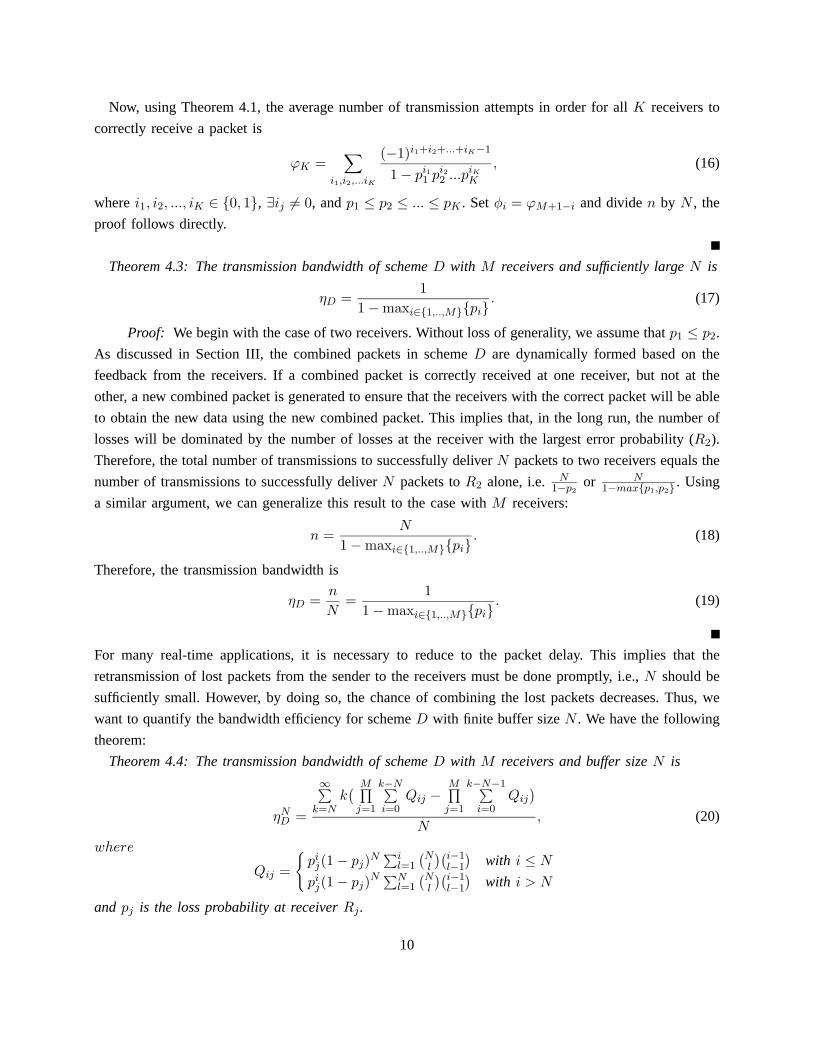
Fig. 4 shows the simulation and theoretical results on the transmission bandwidths (e.g., the average
number of transmissions per successful packet) of schemes A, B, C, and D for the scenario consisting of
one sender and two receivers R1 and R2 with independent and uncorrelated packet losses. For schemes
C and D, we use the buffer size N = 1000 packets, which sufficiently simulates an infinite size buffer in
this setting. The packet loss probability of R1 varies as shown on the x-axis while that of R2 remains at
10%. As seen, the simulation and theoretical curves match all most exactly for all the schemes, verifying
the results of our derivations. Furthermore, the number of transmissions per successful packet in scheme
D is the smallest while that of scheme A is the largest, which confirms our earlier intuitions about
these schemes. We note that although scheme D is slightly more efficient than scheme C, the hardware
implementation of scheme D might be little more complex than that of scheme C due to its dynamic
selection of the retransmitted packets.
0 0.05 0.1 0.15 0.21.1
1.15
1.2
1.25
1.3
1.35
1.4
1.45
1.5
Loss probability p1
Tra
nsm
issi
on b
andw
idth
Loss probability p2=0.1
Scheme−A: TheoryScheme−A: SimulationScheme−B: TheoryScheme−B: SimulationScheme−C: TheoryScheme−C: SimulationScheme−D: TheoryScheme−D: Simulation
Fig. 4. Transmission bandwidth versus packet loss probability.
We now show the coding gains of different schemes. Ideally, scheme A has the worst performance
and should be used as the baseline for comparison. However, most wireless devices with limited memory
will be able to implement scheme B. Furthermore, scheme B is the traditional ARQ scheme. Therefore,
we compare our proposed schemes C and D against scheme B by examining their coding gains over
scheme B. Fig. 5 shows the coding gains of schemes C and D as functions of packet loss probability
of R1. It is interesting to note that the gain is largest when both loss probabilities of R1 and R2 are
equal to each other. This is intuitively plausible as in this special case, the maximum number of lost
13
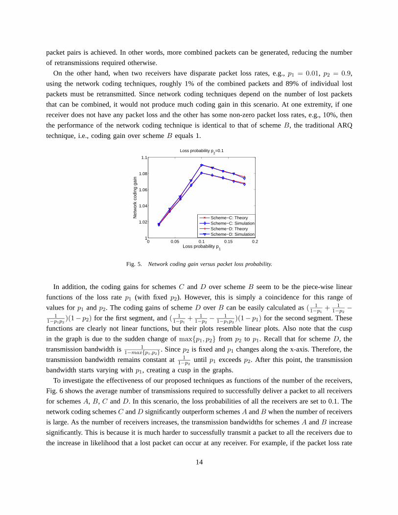
packet pairs is achieved. In other words, more combined packets can be generated, reducing the number
of retransmissions required otherwise.
On the other hand, when two receivers have disparate packet loss rates, e.g., p1 = 0.01, p2 = 0.9,
using the network coding techniques, roughly 1% of the combined packets and 89% of individual lost
packets must be retransmitted. Since network coding techniques depend on the number of lost packets
that can be combined, it would not produce much coding gain in this scenario. At one extremity, if one
receiver does not have any packet loss and the other has some non-zero packet loss rates, e.g., 10%, then
the performance of the network coding technique is identical to that of scheme B, the traditional ARQ
technique, i.e., coding gain over scheme B equals 1.
0 0.05 0.1 0.15 0.21
1.02
1.04
1.06
1.08
1.1
Loss probability p1
Net
wor
k co
ding
gai
n
Loss probability p2=0.1
Scheme−C: TheoryScheme−C: SimulationScheme−D: TheoryScheme−D: Simulation
Fig. 5. Network coding gain versus packet loss probability.
In addition, the coding gains for schemes C and D over scheme B seem to be the piece-wise linear
functions of the loss rate p1 (with fixed p2). However, this is simply a coincidence for this range of
values for p1 and p2. The coding gains of scheme D over B can be easily calculated as ( 11−p1
+ 11−p2
−1
1−p1p2)(1− p2) for the first segment, and ( 1
1−p1+ 1
1−p2− 1
1−p1p2)(1− p1) for the second segment. These
functions are clearly not linear functions, but their plots resemble linear plots. Also note that the cusp
in the graph is due to the sudden change of max{p1, p2} from p2 to p1. Recall that for scheme D, the
transmission bandwidth is 11−max{p1,p2} . Since p2 is fixed and p1 changes along the x-axis. Therefore, the
transmission bandwidth remains constant at 11−p2
until p1 exceeds p2. After this point, the transmission
bandwidth starts varying with p1, creating a cusp in the graphs.
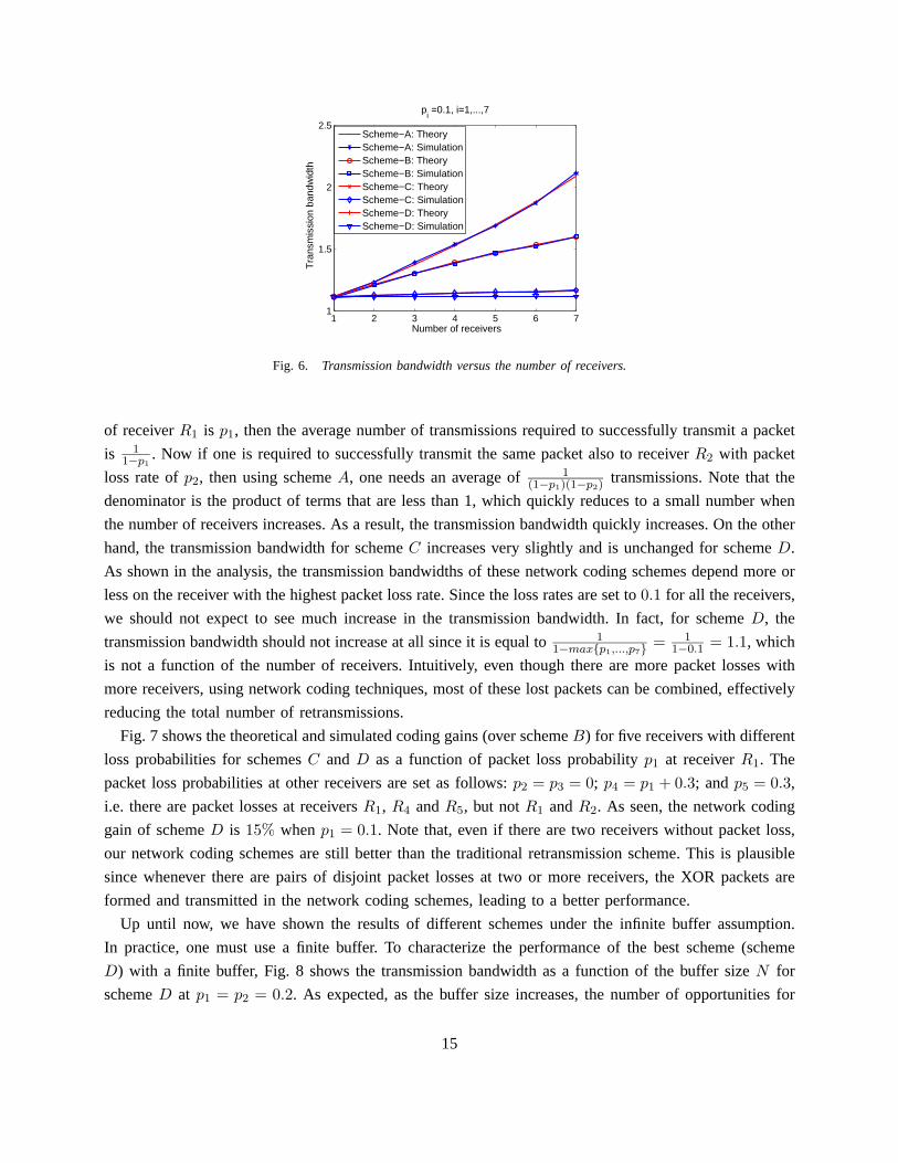
To investigate the effectiveness of our proposed techniques as functions of the number of the receivers,
Fig. 6 shows the average number of transmissions required to successfully deliver a packet to all receivers
for schemes A, B, C and D. In this scenario, the loss probabilities of all the receivers are set to 0.1. The
network coding schemes C and D significantly outperform schemes A and B when the number of receivers
is large. As the number of receivers increases, the transmission bandwidths for schemes A and B increase
significantly. This is because it is much harder to successfully transmit a packet to all the receivers due to
the increase in likelihood that a lost packet can occur at any receiver. For example, if the packet loss rate
14
1 2 3 4 5 6 71
1.5
2
2.5
Number of receivers
Tra
nsm
issi
on b
andw
idth
pi =0.1, i=1,...,7
Scheme−A: TheoryScheme−A: SimulationScheme−B: TheoryScheme−B: SimulationScheme−C: TheoryScheme−C: SimulationScheme−D: TheoryScheme−D: Simulation
Fig. 6. Transmission bandwidth versus the number of receivers.
of receiver R1 is p1, then the average number of transmissions required to successfully transmit a packet
is 11−p1
. Now if one is required to successfully transmit the same packet also to receiver R2 with packet
loss rate of p2, then using scheme A, one needs an average of 1(1−p1)(1−p2)
transmissions. Note that the
denominator is the product of terms that are less than 1, which quickly reduces to a small number when
the number of receivers increases. As a result, the transmission bandwidth quickly increases. On the other
hand, the transmission bandwidth for scheme C increases very slightly and is unchanged for scheme D.
As shown in the analysis, the transmission bandwidths of these network coding schemes depend more or
less on the receiver with the highest packet loss rate. Since the loss rates are set to 0.1 for all the receivers,
we should not expect to see much increase in the transmission bandwidth. In fact, for scheme D, the
transmission bandwidth should not increase at all since it is equal to 11−max{p1,...,p7} = 1
1−0.1 = 1.1, which
is not a function of the number of receivers. Intuitively, even though there are more packet losses with
more receivers, using network coding techniques, most of these lost packets can be combined, effectively
reducing the total number of retransmissions.
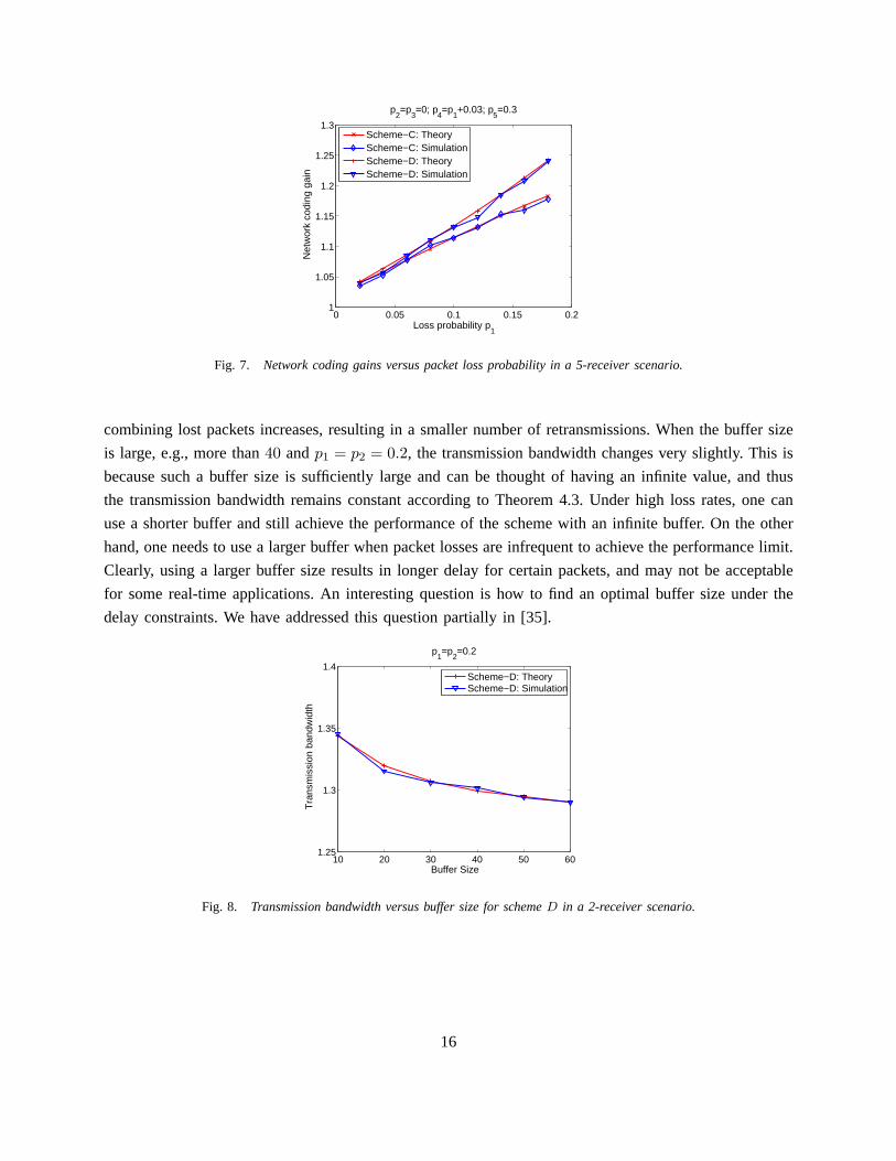
Fig. 7 shows the theoretical and simulated coding gains (over scheme B) for five receivers with different
loss probabilities for schemes C and D as a function of packet loss probability p1 at receiver R1. The
packet loss probabilities at other receivers are set as follows: p2 = p3 = 0; p4 = p1 + 0.3; and p5 = 0.3,
i.e. there are packet losses at receivers R1, R4 and R5, but not R1 and R2. As seen, the network coding
gain of scheme D is 15% when p1 = 0.1. Note that, even if there are two receivers without packet loss,
our network coding schemes are still better than the traditional retransmission scheme. This is plausible
since whenever there are pairs of disjoint packet losses at two or more receivers, the XOR packets are
formed and transmitted in the network coding schemes, leading to a better performance.
Up until now, we have shown the results of different schemes under the infinite buffer assumption.
In practice, one must use a finite buffer. To characterize the performance of the best scheme (scheme
D) with a finite buffer, Fig. 8 shows the transmission bandwidth as a function of the buffer size N for
scheme D at p1 = p2 = 0.2. As expected, as the buffer size increases, the number of opportunities for
15
0 0.05 0.1 0.15 0.21
1.05
1.1
1.15
1.2
1.25
1.3
Loss probability p1
Net
wor
k co
ding
gai
n
p2=p
3=0; p
4=p
1+0.03; p
5=0.3
Scheme−C: TheoryScheme−C: SimulationScheme−D: TheoryScheme−D: Simulation
Fig. 7. Network coding gains versus packet loss probability in a 5-receiver scenario.
combining lost packets increases, resulting in a smaller number of retransmissions. When the buffer size
is large, e.g., more than 40 and p1 = p2 = 0.2, the transmission bandwidth changes very slightly. This is
because such a buffer size is sufficiently large and can be thought of having an infinite value, and thus
the transmission bandwidth remains constant according to Theorem 4.3. Under high loss rates, one can
use a shorter buffer and still achieve the performance of the scheme with an infinite buffer. On the other
hand, one needs to use a larger buffer when packet losses are infrequent to achieve the performance limit.
Clearly, using a larger buffer size results in longer delay for certain packets, and may not be acceptable
for some real-time applications. An interesting question is how to find an optimal buffer size under the
delay constraints. We have addressed this question partially in [35].
10 20 30 40 50 601.25
1.3
1.35
1.4
Buffer Size
Tra
nsm
issi
on b
andw
idth
p1=p
2=0.2
Scheme−D: TheoryScheme−D: Simulation
Fig. 8. Transmission bandwidth versus buffer size for scheme D in a 2-receiver scenario.
16
B. Independent but Correlated Packet Loss Model
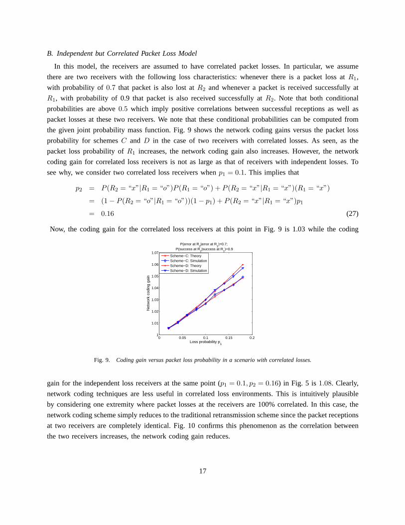
In this model, the receivers are assumed to have correlated packet losses. In particular, we assume
there are two receivers with the following loss characteristics: whenever there is a packet loss at R1,
with probability of 0.7 that packet is also lost at R2 and whenever a packet is received successfully at
R1, with probability of 0.9 that packet is also received successfully at R2. Note that both conditional
probabilities are above 0.5 which imply positive correlations between successful receptions as well as
packet losses at these two receivers. We note that these conditional probabilities can be computed from
the given joint probability mass function. Fig. 9 shows the network coding gains versus the packet loss
probability for schemes C and D in the case of two receivers with correlated losses. As seen, as the
packet loss probability of R1 increases, the network coding gain also increases. However, the network
coding gain for correlated loss receivers is not as large as that of receivers with independent losses. To
see why, we consider two correlated loss receivers when p1 = 0.1. This implies that
p2 = P (R2 = “x”|R1 = “o”)P (R1 = “o”) + P (R2 = “x”|R1 = “x”)(R1 = “x”)
= (1 − P (R2 = “o”|R1 = “o”))(1 − p1) + P (R2 = “x”|R1 = “x”)p1
= 0.16 (27)
Now, the coding gain for the correlated loss receivers at this point in Fig. 9 is 1.03 while the coding
0 0.05 0.1 0.15 0.21
1.01
1.02
1.03
1.04
1.05
1.06
1.07
Loss probability p1
Net
wor
k co
ding
gai
n
P(error at R2|error at R
1)=0.7;
P(success at R2|success at R
1)=0.9
Scheme−C: TheoryScheme−C: SimulationScheme−D: TheoryScheme−D: Simulation
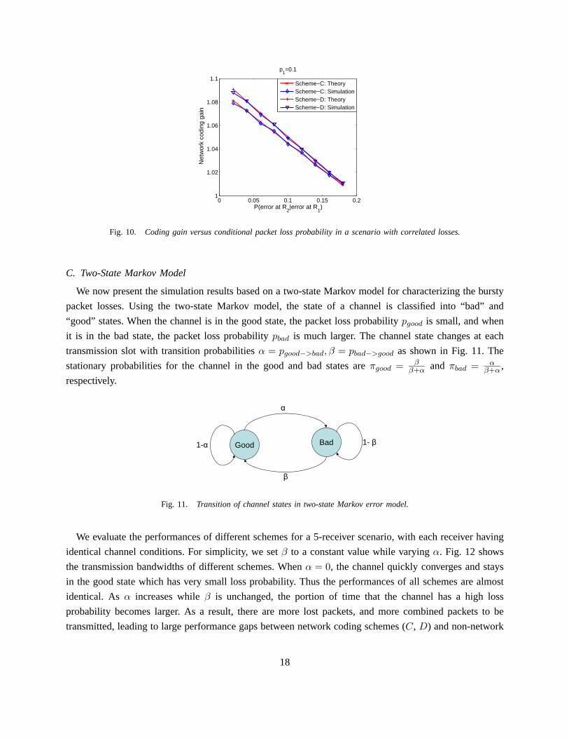
Fig. 9. Coding gain versus packet loss probability in a scenario with correlated losses.
gain for the independent loss receivers at the same point (p1 = 0.1, p2 = 0.16) in Fig. 5 is 1.08. Clearly,
network coding techniques are less useful in correlated loss environments. This is intuitively plausible
by considering one extremity where packet losses at the receivers are 100% correlated. In this case, the
network coding scheme simply reduces to the traditional retransmission scheme since the packet receptions
at two receivers are completely identical. Fig. 10 confirms this phenomenon as the correlation between
the two receivers increases, the network coding gain reduces.
17
0 0.05 0.1 0.15 0.21
1.02
1.04
1.06
1.08
1.1
P(error at R2|error at R
1)
Net
wor
k co
ding
gai
n
p1=0.1
Scheme−C: TheoryScheme−C: SimulationScheme−D: TheoryScheme−D: Simulation
Fig. 10. Coding gain versus conditional packet loss probability in a scenario with correlated losses.
C. Two-State Markov Model
We now present the simulation results based on a two-state Markov model for characterizing the bursty
packet losses. Using the two-state Markov model, the state of a channel is classified into “bad” and
“good” states. When the channel is in the good state, the packet loss probability pgood is small, and when
it is in the bad state, the packet loss probability pbad is much larger. The channel state changes at each
transmission slot with transition probabilities α = pgood−>bad, β = pbad−>good as shown in Fig. 11. The
stationary probabilities for the channel in the good and bad states are πgood = ββ+α and πbad = α
β+α ,
respectively.
Good Bad 1-1-
Fig. 11. Transition of channel states in two-state Markov error model.
We evaluate the performances of different schemes for a 5-receiver scenario, with each receiver having
identical channel conditions. For simplicity, we set β to a constant value while varying α. Fig. 12 shows
the transmission bandwidths of different schemes. When α = 0, the channel quickly converges and stays
in the good state which has very small loss probability. Thus the performances of all schemes are almost
identical. As α increases while β is unchanged, the portion of time that the channel has a high loss
probability becomes larger. As a result, there are more lost packets, and more combined packets to be
transmitted, leading to large performance gaps between network coding schemes (C, D) and non-network
18
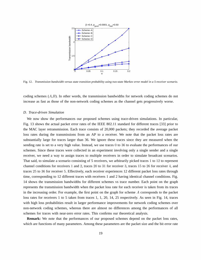
0 0.05 0.1 0.15 0.21
1.5
2
2.5
α
Tra
nsm
issi
on b
andw
idth
β =0.4, pgood
=0.0001, pbad
=0.50
Scheme−AScheme−BScheme−CScheme−D
Fig. 12. Transmission bandwidth versus state transition probability using two-state Markov error model in a 5-receiver scenario.
coding schemes (A,B). In other words, the transmission bandwidths for network coding schemes do not
increase as fast as those of the non-network coding schemes as the channel gets progressively worse.
D. Trace-driven Simulation
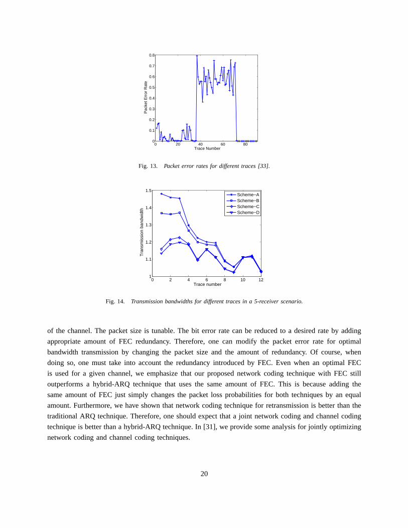
We now show the performances our proposed schemes using trace-driven simulations. In particular,
Fig. 13 shows the actual packet error rates of the IEEE 802.11 standard for different traces [33] prior to
the MAC layer retransmission. Each trace consists of 20,000 packets; they recorded the average packet
loss rates during the transmissions from an AP to a receiver. We note that the packet loss rates are
substantially large for traces larger than 36. We ignore these traces since they are measured when the
sending rate is set to a very high value. Instead, we use traces 0 to 36 to evaluate the performances of our
schemes. Since these traces were collected in an experiment involving only a single sender and a single
receiver, we need a way to assign traces to multiple receivers in order to simulate broadcast scenarios.
That said, to simulate a scenario consisting of 5 receivers, we arbitrarily picked traces 1 to 12 to represent
channel conditions for receivers 1 and 2, traces 20 to 31 for receiver 3, traces 15 to 26 for receiver 4, and
traces 25 to 36 for receiver 5. Effectively, each receiver experiences 12 different packet loss rates through
time, corresponding to 12 different traces with receivers 1 and 2 having identical channel conditions. Fig.
14 shows the transmission bandwidths for different schemes vs trace number. Each point on the graph
represents the transmission bandwidth when the packet loss rate for each receiver is taken from its traces
in the increasing order. For example, the first point on the graph for scheme A corresponds to the packet
loss rates for receivers 1 to 5 taken from traces 1, 1, 20, 14, 25 respectively. As seen in Fig. 14, traces
with high loss probabilities result in larger performance improvements for network coding schemes over
non-network coding schemes, whereas there are almost no differences among the performances of all
schemes for traces with near-zero error rates. This confirms our theoretical analysis.
Remark: We note that the performances of our proposed schemes depend on the packet loss rates,
which are functions of many parameters. Among these parameters are the packet size and the bit error rate
19
0 20 40 60 800
0.1
0.2
0.3
0.4
0.5
0.6
0.7
0.8
Trace NumberP
acke
t Err
or R
ate
Fig. 13. Packet error rates for different traces [33].
0 2 4 6 8 10 121
1.1
1.2
1.3
1.4
1.5
Trace number
Tra
nsm
issi
on b
andw
idth
Scheme−AScheme−BScheme−CScheme−D
Fig. 14. Transmission bandwidths for different traces in a 5-receiver scenario.
of the channel. The packet size is tunable. The bit error rate can be reduced to a desired rate by adding
appropriate amount of FEC redundancy. Therefore, one can modify the packet error rate for optimal
bandwidth transmission by changing the packet size and the amount of redundancy. Of course, when
doing so, one must take into account the redundancy introduced by FEC. Even when an optimal FEC
is used for a given channel, we emphasize that our proposed network coding technique with FEC still
outperforms a hybrid-ARQ technique that uses the same amount of FEC. This is because adding the
same amount of FEC just simply changes the packet loss probabilities for both techniques by an equal
amount. Furthermore, we have shown that network coding technique for retransmission is better than the
traditional ARQ technique. Therefore, one should expect that a joint network coding and channel coding
technique is better than a hybrid-ARQ technique. In [31], we provide some analysis for jointly optimizing
network coding and channel coding techniques.
20
VI. CONCLUSION
In this paper we propose some network coding techniques to increase the bandwidth efficiency of reliable
broadcast in a wireless network. Our proposed schemes combine different lost packets from different
receivers in such a way that multiple receivers are able to recover their lost packets with one transmission
by the sender. The advantages of the proposed schemes over the traditional wireless broadcast are shown
through simulations and theoretical analysis. Specifically, we provide a few results on the transmission
bandwidths of the proposed schemes under different channel conditions. We are currently investigating
a joint approach of network coding, retransmission, and FEC in order to further increase the bandwidth
utilization.
REFERENCES
[1] G. C. Clark and J. B. Cain, Error-Correction Coding for Digital Communications, New York: Plenum, 1982.
[2] R. Ahlswede, N. Cai, R. Li, and R. W. Yeung, “Network information flow,” IEEE Transactions on Information Theory,
vol. 46, pp. 1204–1216, July 2000.
[3] R. Koetter and M. Medard, “Beyond routing: An algebraic approach to network coding,” in Proc. of the IEEE Infocom,
June 2002, vol. 1, pp. 122–130.
[4] P. Chou, Y. Wu, and K. Jain, “Practical network coding,” in Proc. of 41st Allerton Conference on Communication, Control
and Computing Monticello, October 2003.
[5] C. Chekuri, C. Fragouli, and E. Soljanin, “On average throughput and alphabet size in network coding,” IEEE Transactions
on Information Theory, vol. 52, pp. 2410–2424, June 2005.
[6] C. Gkantsidis and P. Rodriguez, “Network coding for large scale content distribution,” in INFOCOM 2005, 24th Annual
Joint Conference of the IEEE Computer and Communications Societies, August 2005, pp. 2235–2245.
[7] Y. Wu, P. A. Chou, and S.-Y. Kung, “Information exchange in wireless networks with network coding and physical-layer
broadcast,” in 39th Annual Conference on Information Sciences and Systems (CISS), March 2005.
[8] S. Katti, H. Rahul, W. Hu, D. Katabi, M. Medard, and J. Crowcroft, “Xors in the air: Practical wireless network coding,”
in ACM SIGCOMM Computer Communication Review, October 2006, vol. 36, pp. 243–254.
[9] Y. Wu, P. A. Chou, and S.-Y. Kung, “Minimum-energy multicast in mobile ad hoc networks using network coding,” in
IEEE Information Theory Workshop, October 2004.
[10] S. Deb, M. Effros, T. Ho, D. R. Karger, R. Koetter, D. S. Lun, M. Medard, and N. Ratnakar, “Network coding for wireless
applications: A brief tutorial,” in Proc. of International Workshop on Wireless Ad-hoc and Sensor Networks, May 2005.
[11] J. Liu, D. Goeckel, and D. Towsley, “The throughput order of ad hoc networks employing network coding and broadcasting,”
in Military Communications Conference, MILCOM 2006, pp. 1–7.
[12] D. Nguyen, T. Nguyen, and B. Bose, “Wireless broacast using newtork coding,” in NetCod Workshop, January 2007.
[13] D. Nguyen, “Wireless broadcast with network coding,” Technical Report: OSU-TR-2006-06, Oregon State University, June
2006.
[14] T. Cover, “Broadcast channels,” IEEE Transactions on Information Theory, vol. IT-18, pp. 2–14, January 1972.
[15] D. S. Lun, M. Medard, and R. Koetter, “Efficient operation of wireless packet networks using network coding,” in
International Workshop on Convergent Technologies, June 2005.
[16] M. Cagalj, J. Hubaux, and C. Enz, “Minimum-energy broadcast in all-wireless networks: NP-completeness and distribution
issues,” in ACM/IEEE Mobicom, September 2002, pp. 172–182.
[17] W. Liang, “Constructing minimum energy broadcast trees in wireless ad hoc networks,” in Proc. of 3rd ACM International
Symposium on Mobile Ad Hoc Networking and Computing (MobiHoc), Lausanne, Switzerland, June 2002, pp. 112–122.
[18] A. Ahluwalia, E. Modiano, and L. Shu, “On the complexity and distributed construction of energy-efficient broadcast trees
in static ad hoc wireless networks,” IEEE Transactions on Wireless Communications, vol. 4, pp. 2136–2147, September
2005.
21
[19] Z. Li and B. Li, “On increasing end-to-end thoughput in wireless ad hoc networks,” in Conference on Quality of Service
in Heterogeneous Wired/Wireless Networks (QShine), 2005.
[20] Z. Li and B. Li, “Network coding: the case for multiple unicast sessions,” in Allerton Conference on Communications,
2004.
[21] D. Lun, M. Medard, R. Koetter, and M. Effros, “On coding for reliable communication over packet networks,” in Proc.
42nd Annual Allerton Conference on Communication, Control, and Computing Monticello, IL, October 2004.
[22] S. Katti, D. Katabi, W. Hu, H. Rahul, and M. Medard, “The importance of being opportunistic: Practical network coding
for wireless environments,” in Proc. of 43rd Annual Allerton Conference on Communication, September 2005.
[23] C. Fragouli, J. L. Boudec, and J. Widmer, “Network coding: An instant primer,” in ACM SIGCOMM Computer
Communication Review, January 2006, vol. 36, pp. 63–68.
[24] A. Eryilmaz, A. Ozdaglar, and M. Medard, “On delay performance gains from network coding,” in 40th Annual Conference
on Information Sciences and Systems, March 2006, pp. 864–870.
[25] T. Ho, M. Medard, J. Shi, M. Effros, and D. R. Karger, “On randomized network coding,” in Proc. of 41st Annual Allerton
Conference on Communication, Control, and Computing, October 2003.
[26] T. Ho, M. Medard, D. R. Karger, M. Effros, J. Shi, and B. Leong, “A random linear network coding approach to multicast,”
IEEE Transaction on Information Theory, 2004.
[27] M. Ghaderi, D. Towsley, and Jim Kurose, “Reliability benefit of network coding,” Technical Report 07-08, Computer
Science Department, University of Massachusetts Amherst, February 2007.
[28] Stephen Wicker, Error Control Systems for Digital Communication and Storage, Prentice-Hall, 1995.
[29] A. Shiozaki, “Adaptive type-II hybrid broadcast ARQ system,” IEEE Transactions on Communications, vol. 44, pp.
420–422, April 1996.
[30] M. Nakamura and T. Kodama, “An efficient hybrid ARQ scheme for broadcast data transmission systems (in Japanese),”
IEICE Transactions, vol. J73-A, pp. 277–283, February 1990.
[31] T. Tran, T. Nguyen, and B. Bose, “A joint network-channel coding technique for single-hop wireless networks,” to appear
in NetCod Workshop, January 2008.
[32] Q. Dong, J. Wu, W. Hu, and J. Crowcroft, “Practical network coding in wireless networks,” in Proceedings of the 13th
annual ACM international conference on Mobile computing and networking, 2007.
[33] A. Willig, M. Kubisch, and A. Wolisz, “Result of bit error rate measurements with an IEEE 802.11 compliant PHY,”
Technical Report: TKN-00-08, Technical University Berlin, p. 40, September 2000.
[34] C. H. Nam, S. C. Liew, and C. P. Fu, “An experimental study of ARQ protocol in 802.11b Wireless LAN,” in Wireless
Personal Multimedia Communications (WPMC’02), October 2002.
[35] D. Nguyen, T. Nguyen, and X. Yang, “Wireless multimedia transmission with network coding,” to appear in Packet Video
2007, November 2007.
APPENDIX
Proof of Theorem 4.4: We consider the scenario with one sender and one receiver. Let X denote the number
of transmissions for the receiver to get N packets successfully. X can be N , N + 1, N + 2, ... .We compute the
probabilities for different values of X .
If exactly N transmissions are required, then there must be no loss during transmitting N packets. We have
P [X = N ] =(
N
0
)p0(1 − p)N .
If N + 1 transmissions are required, then there must be only one lost packet and one successful retransmission. We
have
P [X = N + 1] =[(
N
1
)p(1 − p)N−1
](1 − p) =
(N
1
)p(1 − p)N .
22
If N + 2 transmissions are required, then there could be one loss during the transmissions of the first N packets
and two retransmissions before the lost packet is successfully received, or there could be two losses during the
transmissions of the first N packets and two successful retransmissions, one for each lost packet. We have
P [X = N + 2] =[(
N
1
)p(1 − p)N−1
]p(1 − p) +
[(N
2
)p2(1 − p)N−2
](1 − p)2
=[(
N
1
)+
(N
2
)]p2(1 − p)N . (A.28)
Similarly, one can show that
P [X = N + i] =
{pi(1 − p)N
∑il=1
(Nl
)(i−1l−1
)with i ≤ N
pi(1 − p)N ∑Nl=1
(Nl
)(i−1l−1
)with i > N.
(A.29)
Now, we consider the case of one sender and two receivers.
The number of transmissions using network coding to guarantee that both receivers receive N packets successfully
is Y = maxj∈{1,2}{Xj} where Xj is a random variable denoting the number of transmissions for receiver j to get
N packets successfully. Then,
P [Y ≤ k] =2∏
j=1
k−N∑i=0
P [Xj = i + N ]. (A.30)
Next,
P [Y = k] =2∏
j=1
k−N∑i=0
Qij −2∏
j=1
k−N−1∑i=0
Qij , (A.31)
where Qij = P [Xj = N + i], which can be computed from (A.29).
The average number of transmissions so that both receivers receive a packet successfully is
ηND = E[Y ] =
∞∑k=N
kP [Y = k] =∞∑
k=N
k
⎛⎝ 2∏
j=1
k−N∑i=0
Qij −2∏
j=1
k−N−1∑i=0
Qij
⎞⎠. (A.32)
Without much difficulty, we can generalize the result for the case with M receivers as
E[Y ] =∞∑
k=N
k
⎛⎝ M∏
j=1
k−N∑i=0
Qij −M∏
j=1
k−N−1∑i=0
Qij
⎞⎠ , (A.33)
where
Qij =
{pi
j(1 − pj)N∑i
l=1
(Nl
)(i−1l−1
)with i ≤ N
pij(1 − pj)
N ∑Nl=1
(Nl
)(i−1l−1
)with i > N
and pj is the probability that the packet is lost at receiver Rj .
Proof of Theorem 4.5 Scheme B (outline): We start with the case of two receivers, then generalize to M
receivers. Denote X1 and X2 the number of attempts needed to successfully deliver a packet to receiver R1 and R2
respectively, and Y = maxi∈{1,2}{Xi}. We have
P [Y ≤ k] =k∑
i=1
k∑j=1
P [X1 = i,X2 = j]. (A.34)
23
Next,
P [Y = k] =k∑
i=1
k∑j=1
P [X1 = i,X2 = j] −k−1∑i=1
k−1∑j=1
P [X1 = i,X2 = j]
=k∑
i=1
P [X1 = i,X2 = k] +k−1∑i=1
P [X1 = k,X2 = i]. (A.35)
Number of attempts 1 2 … i-1 i i+1 … k-1 kR1 x x … x o - …
x-
R2 x x … x-xx … o
Fig. 15. Number of attempts to deliver a packet to both receivers successfully: R1 needs i while R2 needs k attempts (“x”
and “o” indicate an unsuccessful and successful attempt, respectively).
Fig. 15 shows that after X1 = i and X2 = k attempts (i ≤ k), a packet is received successfully at R1 and R2
respectively. Assume that we know the joint packet loss probability. Let us denote pxx, pxo, pox, and poo as the
probabilities that a packet is lost at both receivers, a packet is lost at R1 but received at R2, a packet is received at
R1 but lost at R2, and a packet is received at both receivers, respectively. We have
P [X1 = i,X2 = j] ={
pi−1xx pox(pox + pxx)j−i−1(poo + pxo) with i ≤ j
pj−1xx pxo(pxo + pxx)i−j−1(poo + pox) with i > j.
(A.36)
Therefore, the average number of transmissions required to send a packet successfully to both receivers is
E[Y ] =∞∑
k=1
k∑i=1
kP [X1 = i,X2 = k] +∞∑
k=1
k−1∑i=1
kP [X1 = k,X2 = i]
=∞∑
k=1
k∑i=1
kpi−1xx pox(pox + pxx)k−i−1(poo + pxo)
+∞∑
k=1
k−1∑i=1
kpi−1xx pxo(pxo + pxx)k−i−1(poo + pox). (A.37)
Now examine the case of M receivers. Let Xi denote the number of attempts for a packet to be received
successfully at receiver Ri, YM = maxi∈{1,...,M}{Xi}, and P [j1, j2, ..., jM ] = P [X1 = j1,X2 = j2, ...,XM = jM ].We have
P [YM = k] =∑
j1,...,jM∈Zk
P [j1, j2, ..., jM ] −∑
j1,...,jM∈Zk−1
P [j1, j2, ..., jM ],
(A.38)
where Zk = {1, ..., k} and Zk−1 = {1, ..., k − 1}. Note that Zk and Zk−1 are defined to make k largest among
j1, j2, ...jM .
Now, we can compute P [j1, j2, ...jM ] in terms of the joint packet loss probabilities. Let the vector (a1a2...aM )denote the status reception of a packet at all the receivers; ah = “o” and ah = “x′′ indicate successful and unsuccessful
receptions at receiver Ri, respectively. Let pa1a2...aMdenote the probability of this event, then:
24
∑j1,...,jM∈Zk
P [j1, j2, ..., jM ] =∑
j1,...,jM∈Zk
(pi1
x1x2...xMpo1x1...xM
M−1∏h=1
( ∑ah∈{oh,xh}
pa1...ahxh+1...xM
)lh+1−lh−1
( ∑ah∈{oh,xh}
pa1...ahoh+1xh+2...xM
))(A.39)
where the sequence {l1, l2, ..., lM} is is an ascending sorted sequence of {j1, j2, ..., jM}. For instance, if {j1, j3, j2}is the ascending sorted sequence of {j1, j2, j3}, then then l1 = j1, l2 = j3, and l3 = j2.
The key is to obtain the above equation is to set up a table as shown in Fig. 15 and multiply out the joint
probability as it was done in Equation (A.36) for the 2-receiver case.
Given P [YM = k], the transmission bandwidth for M receivers with correlated losses using scheme B is
ηBcor = E[Y ] =
∞∑k=1
kP [YM = k] (A.40)
Proof of Theorem 4.5 Scheme C: Consider the 2-receiver scenarios. We use the same notations above and
assume that p1 ≤ p2. In the long run, the average number of lost packets at receiver 2 with be larger than that at
receiver 1. Then average number of transmissions to successfully deliver a packet to two receivers is
ηCcor = 1 + p1E[max{X1,X2}] + (p2 − p1)E[X2], (A.41)
where E[max{X1,X2}] is obtained from equation A.37 and E[X2] = 11−p2
.
For the general case of M receivers, we also assume that pi ≤ pj for all i < j. Similarly, in the long run, the
number of lost packets at receiver i is smaller than that of receiver j. Using the same argument for the case of 2receivers we can derive the average number of transmissions required to successfully deliver a packet to M receivers
as
ηCcor = 1 + p1E[ max
i∈{1,..,M}{Xi}] + (p2 − p1)E[ max
i∈{2,..,M}{Xi}] + ... + (pM − pM−1)E[XM ]
= 1 +M−1∑l=0
(pl+1 − pl)∞∑
k=1
kP [YM−l = k]
= 1 +M−1∑l=0
∞∑k=1
k(pl+1 − pl)P [YM−l = k] , (A.42)
where p0 = 0 and P [YM−l = k] is the probability that the sender needs k transmissions to deliver a packet to all
M − l receivers Rl, Rl+1, ..., and RM successfully. P [YM−l = k] can be computed using Equation (A.39). Note
that, to shorten the notation, we add a virtual receiver R0 with p0 = 0.
25