


VLOOKUP CONTROL THE EXCEL POWER
www.Experiglot.com
2
Table of Contents
Intro ............................................................................................................. 3
How to use VLOOKUP in Excel ..................................................................... 6
Some Tips & Advanced Excel Tricks............................................................ 12
Using Vlookup And Nested If In Excel For Golf Scoring ............................... 27
Too Many Options, Which One Should I Use? ............................................ 30
Combining Excel Sumif, Vlookup, If Is Error Functions, etc ......................... 33
Vlookup or "Relationships" In Excel 2013 .................................................. 37
Learning Vlookup is Only the Beginning ..................................................... 39
VLOOKUP CONTROL THE EXCEL POWER
www.Experiglot.com
3 Intro
Hey people!
My name is Pete and I am the owner of Experiments in
Finance as of 2011. This blog was once half about
personal finance and half about Excel tutorials. It seems
that most people here are more interested in Excel than
personal finance so I've decided to switch it completely
to the usage of Excel. This is also the reason why you
have this book in your hand… or on your computer!
Thank you for registering to my newsletter where I will share all my Excel
tips I’ve learned over the years. I promise to never spam you with irrelevant
ads and only provide you with Excel tutorial oriented content.
How Excel Earned me a Promotion
I first started my career working for a bank in the financial industry. I was
23 and eager to work and get a promotion as soon as possible. I rapidly
noticed my boss was having a problem with keeping up with his
department stats.
We were a team of 7 employees logging our sales in separate excel
spreadsheets. Since he used to receive his stats every quarter from the
“stats department from the bank” , he wanted to get a closer look at his
VLOOKUP CONTROL THE EXCEL POWER
www.Experiglot.com
4 daily business. This is why, once a week, he had to ask for them by email
and compile the results manually. It was time consuming and not very
accurate.
After discussing this problem with one of my friend, he showed me how to
use Excel to automatically compile the data, make graphs and trends out of
it. After a few hours of computing, I’ve had generated a powerful stats
tracking system for my boss.
No more emails sent to employees – He could get stats at any time
in the day without asking anybody!
No more hours spent compiling stats manually – a Simple click on
the macro button and the compilation was made within seconds!
No more data errors – All stats were tracked and packaged by Excel,
data became exempt from human errors!
The time I’ve saved my boss with this “simple” Excel spreadsheet had been
the key for my first promotion. Everybody on the floor heard about my
system and how productive I was as an employee. In addition to my
promotion, I’ve earned credibility instantly.
VLOOKUP CONTROL THE EXCEL POWER
www.Experiglot.com
5 Most People Don’t Know How To Use Excel at Work – Be The Star!
You don’t need to master Excel inside out to be the hero at work; you
simply have to know how to use formulas that will help YOU being more
productive. Saving time and hassles to your boss is definitely the best way
to become indispensable at work and earn the next promotion.
I’m here to show you how to achieve this goal by using the power of Excel.
So let’s start with this book that will show you VLOOKUP inside out. If you
use Excel much at your job, sooner or later, you're bound to need to look
up values in a table. One of the most useful functions in Excel,
called vlookup, does exactly that. The "V" in vlookup stands for "vertical"
and "lookup" is pretty self explanatory. This function allows you to look up
values in a table that are listed in column format (how most tables are laid
out), given another value (let's call this the "key"). Excel also has a sister
function called hlookup (h = horizontal) that can be used to look up values
in rows.
VLOOKUP CONTROL THE EXCEL POWER
www.Experiglot.com
6 How to use VLOOKUP in Excel
Sadly, as most companies seem to rely on Excel as a poor-man's database
of sorts (a totally unscalable solution and prone to errors with every
revision, but don't get me started), once you know vlookup, it's likely to
become one of your most often used Excel functions.
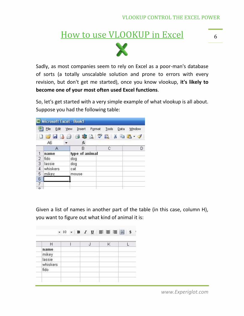
So, let's get started with a very simple example of what vlookup is all about.
Suppose you had the following table:
Given a list of names in another part of the table (in this case, column H),
you want to figure out what kind of animal it is:
VLOOKUP CONTROL THE EXCEL POWER
www.Experiglot.com
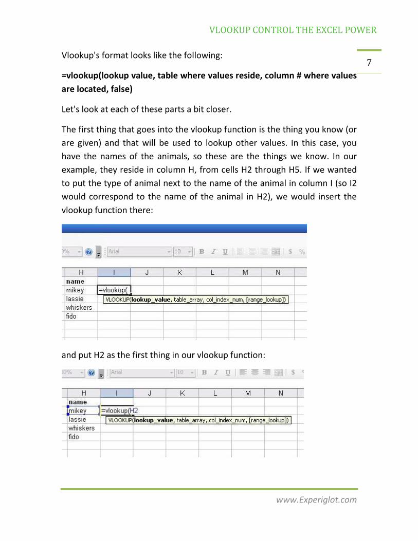
7 Vlookup's format looks like the following:
=vlookup(lookup value, table where values reside, column # where values
are located, false)
Let's look at each of these parts a bit closer.
The first thing that goes into the vlookup function is the thing you know (or
are given) and that will be used to lookup other values. In this case, you
have the names of the animals, so these are the things we know. In our
example, they reside in column H, from cells H2 through H5. If we wanted
to put the type of animal next to the name of the animal in column I (so I2
would correspond to the name of the animal in H2), we would insert the
vlookup function there:
and put H2 as the first thing in our vlookup function:
VLOOKUP CONTROL THE EXCEL POWER
www.Experiglot.com
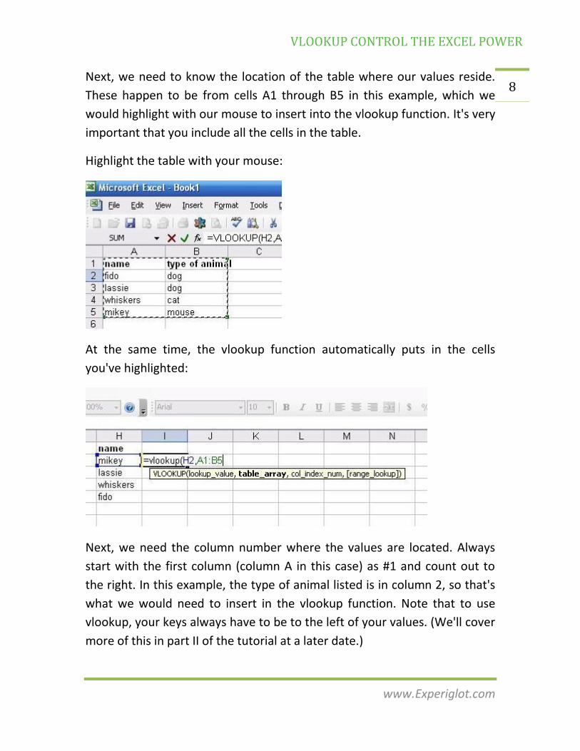
8 Next, we need to know the location of the table where our values reside.
These happen to be from cells A1 through B5 in this example, which we
would highlight with our mouse to insert into the vlookup function. It's very
important that you include all the cells in the table.
Highlight the table with your mouse:
At the same time, the vlookup function automatically puts in the cells
you've highlighted:
Next, we need the column number where the values are located. Always
start with the first column (column A in this case) as #1 and count out to
the right. In this example, the type of animal listed is in column 2, so that's
what we would need to insert in the vlookup function. Note that to use
vlookup, your keys always have to be to the left of your values. (We'll cover
more of this in part II of the tutorial at a later date.)
VLOOKUP CONTROL THE EXCEL POWER
www.Experiglot.com
9
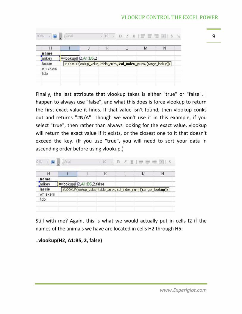
Finally, the last attribute that vlookup takes is either "true" or "false". I
happen to always use "false", and what this does is force vlookup to return
the first exact value it finds. If that value isn't found, then vlookup conks
out and returns "#N/A". Though we won't use it in this example, if you
select "true", then rather than always looking for the exact value, vlookup
will return the exact value if it exists, or the closest one to it that doesn't
exceed the key. (If you use "true", you will need to sort your data in
ascending order before using vlookup.)
Still with me? Again, this is what we would actually put in cells I2 if the
names of the animals we have are located in cells H2 through H5:
=vlookup(H2, A1:B5, 2, false)
VLOOKUP CONTROL THE EXCEL POWER
www.Experiglot.com
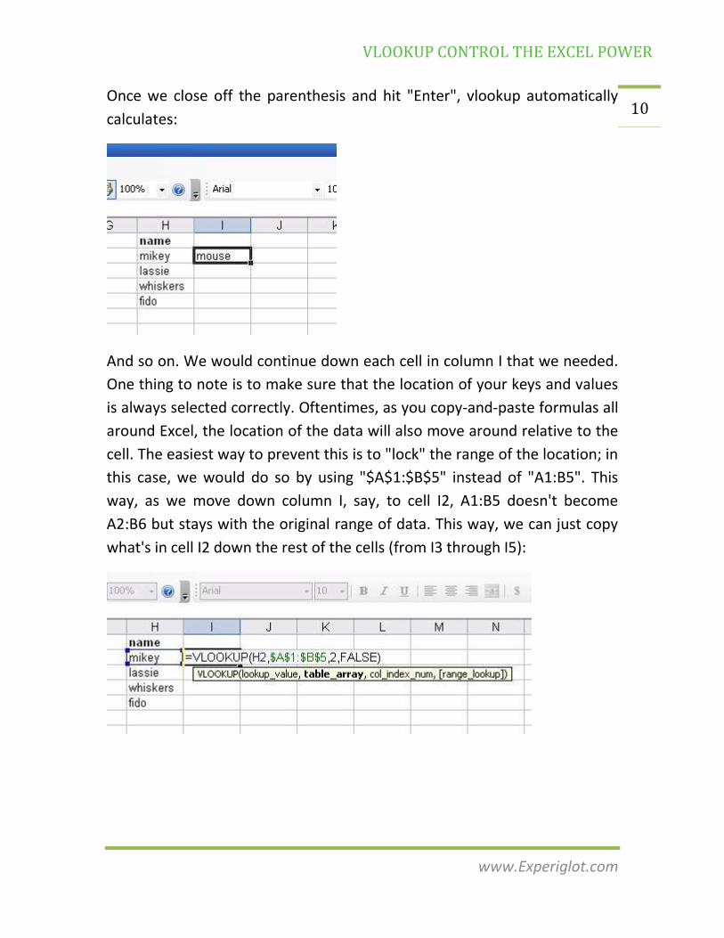
10 Once we close off the parenthesis and hit "Enter", vlookup automatically
calculates:
And so on. We would continue down each cell in column I that we needed.
One thing to note is to make sure that the location of your keys and values
is always selected correctly. Oftentimes, as you copy-and-paste formulas all
around Excel, the location of the data will also move around relative to the
cell. The easiest way to prevent this is to "lock" the range of the location; in
this case, we would do so by using "$A$1:$B$5" instead of "A1:B5". This
way, as we move down column I, say, to cell I2, A1:B5 doesn't become
A2:B6 but stays with the original range of data. This way, we can just copy
what's in cell I2 down the rest of the cells (from I3 through I5):

VLOOKUP CONTROL THE EXCEL POWER
www.Experiglot.com
11 Finally, here's our result, after making the "$" changes and copying and
pasting the formula down the rest of the column:
This has been a really simple example of vlookup, and I'll cover a bit more in
part II with another example, still simple, but with slightly more data.
Although in practice, vlookup is usually used between Excel sheets and
workbooks, once you understand this example (which has been done
within a single sheet), using vlookup outside the same sheet shouldn't be
much harder.
VLOOKUP CONTROL THE EXCEL POWER
www.Experiglot.com
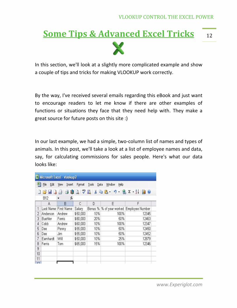
12 Some Tips & Advanced Excel Tricks
In this section, we'll look at a slightly more complicated example and show
a couple of tips and tricks for making VLOOKUP work correctly.
By the way, I've received several emails regarding this eBook and just want
to encourage readers to let me know if there are other examples of
functions or situations they face that they need help with. They make a
great source for future posts on this site :)
In our last example, we had a simple, two-column list of names and types of
animals. In this post, we'll take a look at a list of employee names and data,
say, for calculating commissions for sales people. Here's what our data
looks like:
VLOOKUP CONTROL THE EXCEL POWER
www.Experiglot.com
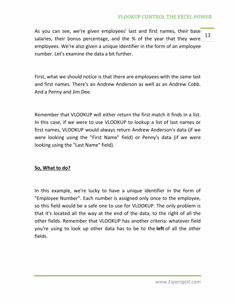
13 As you can see, we're given employees' last and first names, their base
salaries, their bonus percentage, and the % of the year that they were
employees. We're also given a unique identifier in the form of an employee
number. Let's examine the data a bit further.
First, what we should notice is that there are employees with the same last
and first names. There's an Andrew Anderson as well as an Andrew Cobb.
And a Penny and Jim Dee.
Remember that VLOOKUP will either return the first match it finds in a list.
In this case, if we were to use VLOOKUP to lookup a list of last names or
first names, VLOOKUP would always return Andrew Anderson's data (if we
were looking using the "First Name" field) or Penny's data (if we were
looking using the "Last Name" field).
So, What to do?
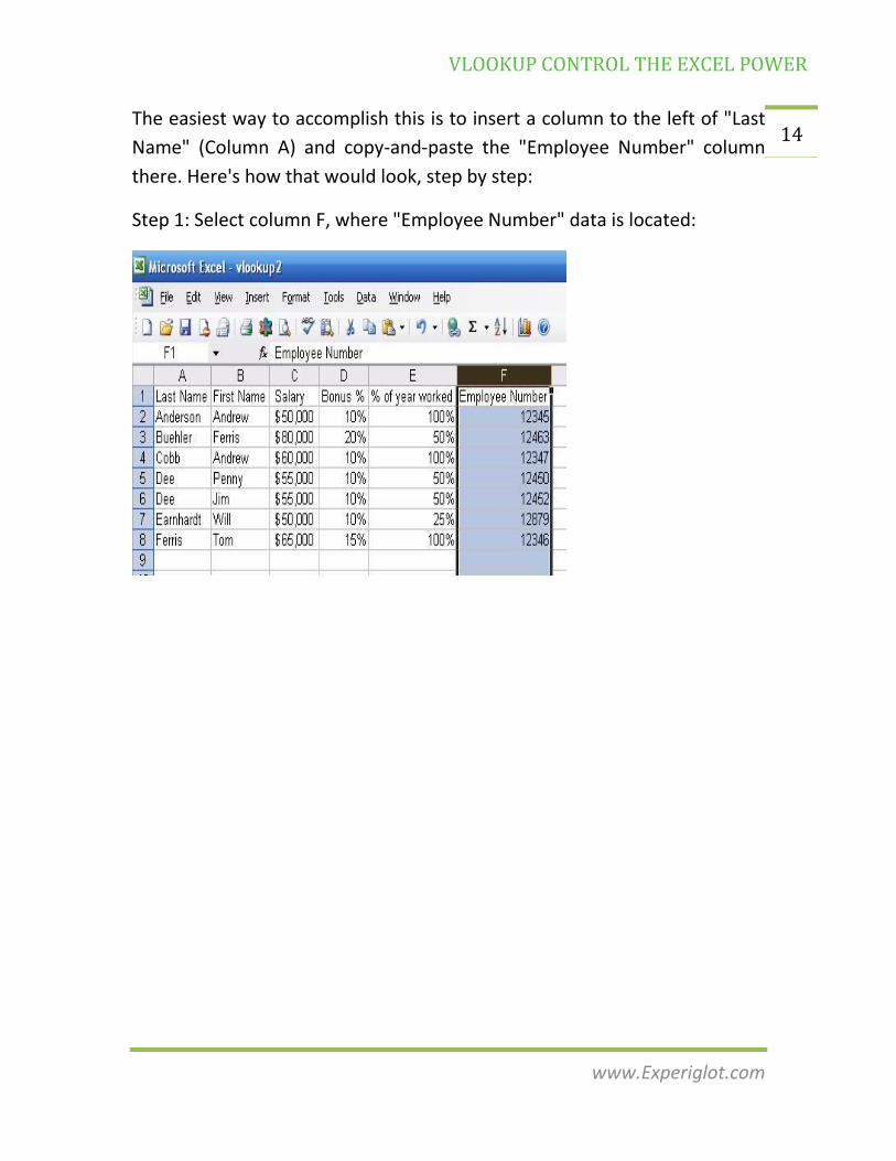
In this example, we're lucky to have a unique identifier in the form of
"Employee Number". Each number is assigned only once to the employee,
so this field would be a safe one to use for VLOOKUP. The only problem is
that it's located all the way at the end of the data, to the right of all the
other fields. Remember that VLOOKUP has another criteria: whatever field
you're using to look up other data has to be to the left of all the other
fields.
VLOOKUP CONTROL THE EXCEL POWER
www.Experiglot.com
14 The easiest way to accomplish this is to insert a column to the left of "Last
Name" (Column A) and copy-and-paste the "Employee Number" column
there. Here's how that would look, step by step:
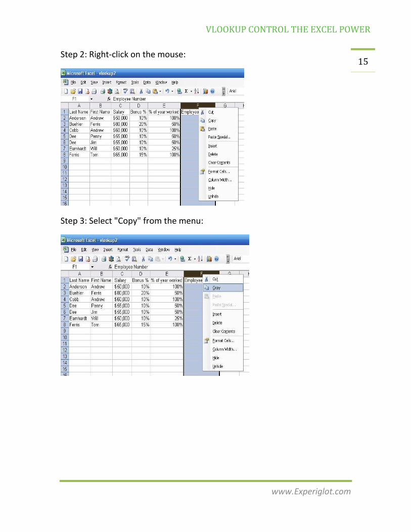
Step 1: Select column F, where "Employee Number" data is located:
VLOOKUP CONTROL THE EXCEL POWER
www.Experiglot.com
15 Step 2: Right-click on the mouse:
Step 3: Select "Copy" from the menu:
VLOOKUP CONTROL THE EXCEL POWER
www.Experiglot.com
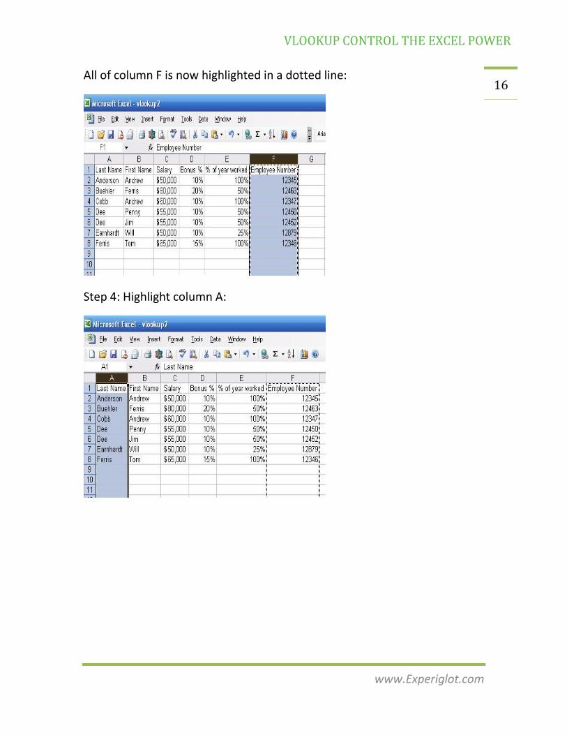
16 All of column F is now highlighted in a dotted line:
Step 4: Highlight column A:
VLOOKUP CONTROL THE EXCEL POWER
www.Experiglot.com
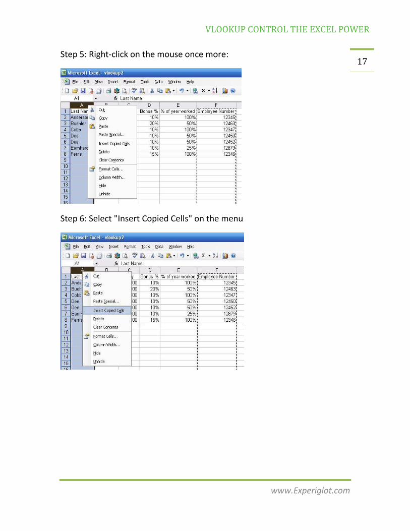
17 Step 5: Right-click on the mouse once more:
Step 6: Select "Insert Copied Cells" on the menu
VLOOKUP CONTROL THE EXCEL POWER
www.Experiglot.com
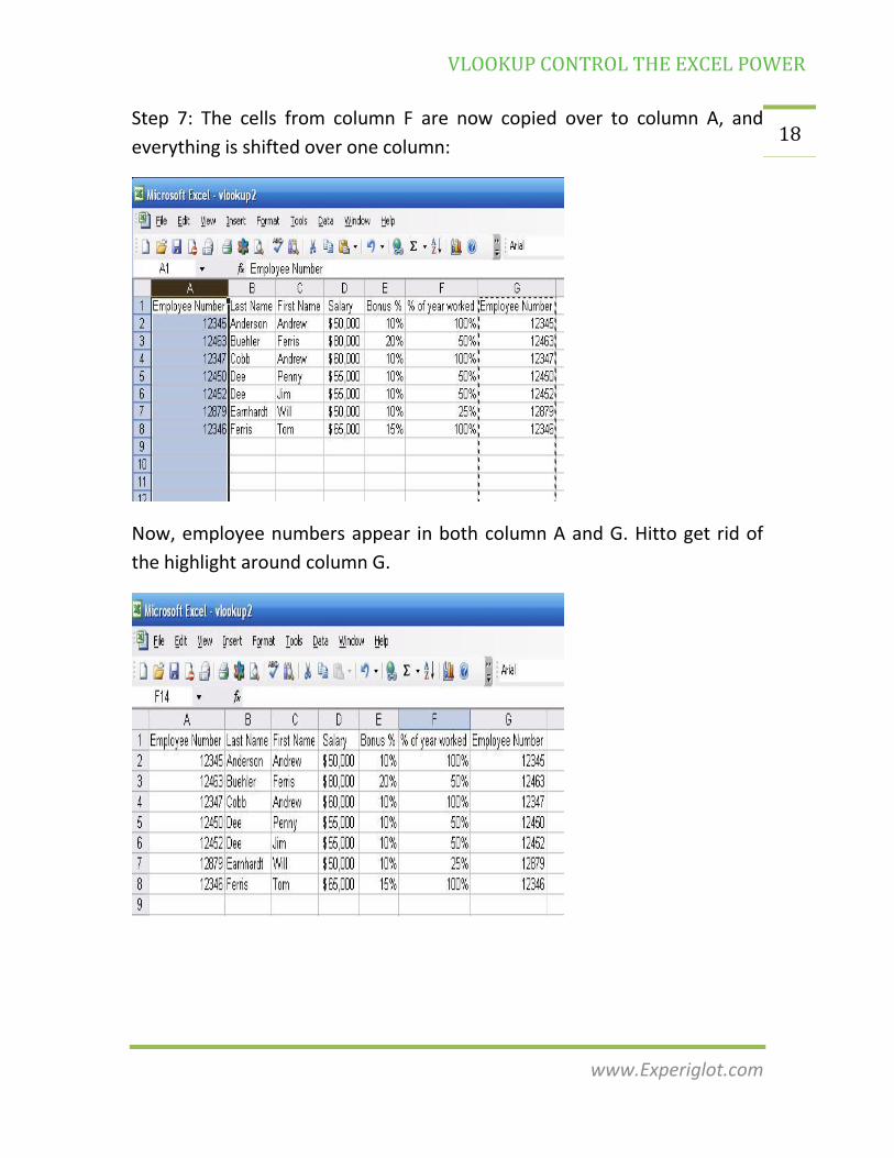
18 Step 7: The cells from column F are now copied over to column A, and
everything is shifted over one column:
Now, employee numbers appear in both column A and G. Hitto get rid of
the highlight around column G.

VLOOKUP CONTROL THE EXCEL POWER
www.Experiglot.com
19 We're now good to go!
By the way, if you had not had unique identifiers like employee numbers
readily available, you could potentially use the CONCATENATE or "&"
function in Excel to "create" unique identifiers. CONCATENATE is a function
that just munges two fields together. In this case, creating a unique
identifier out of concatenating last name and first name would probably
work.
Back to the tutorial. Suppose we had a second sheet that had a list of
employee numbers for the four employees who had worked less than 100%
during the year, and we wanted to calculate their bonuses for the year.
Notice we swapped first and last name orders in this sheet and put the
employee numbers in a different order:
We just want to fill in the data from the other source (possibly from
another Excel sheet or workbook) in order to do the calculation. Here, I've
left the original data in "Sheet1" and am pulling the data into "Sheet2".
VLOOKUP CONTROL THE EXCEL POWER
www.Experiglot.com
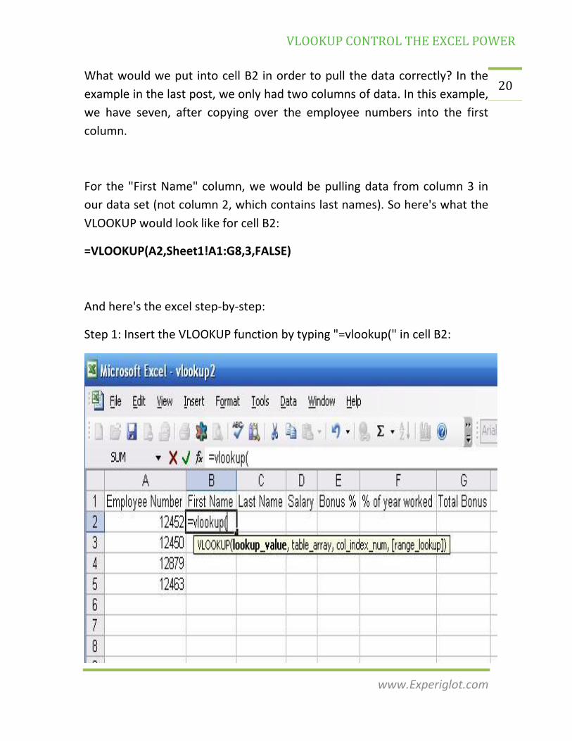
20 What would we put into cell B2 in order to pull the data correctly? In the
example in the last post, we only had two columns of data. In this example,
we have seven, after copying over the employee numbers into the first
column.
For the "First Name" column, we would be pulling data from column 3 in
our data set (not column 2, which contains last names). So here's what the
VLOOKUP would look like for cell B2:
=VLOOKUP(A2,Sheet1!A1:G8,3,FALSE)
And here's the excel step-by-step:
Step 1: Insert the VLOOKUP function by typing "=vlookup(" in cell B2:
VLOOKUP CONTROL THE EXCEL POWER
www.Experiglot.com
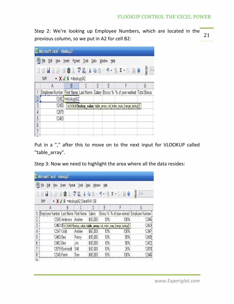
21 Step 2: We're looking up Employee Numbers, which are located in the
previous column, so we put in A2 for cell B2:
Put in a "," after this to move on to the next input for VLOOKUP called
"table_array".
Step 3: Now we need to highlight the area where all the data resides:
VLOOKUP CONTROL THE EXCEL POWER
www.Experiglot.com
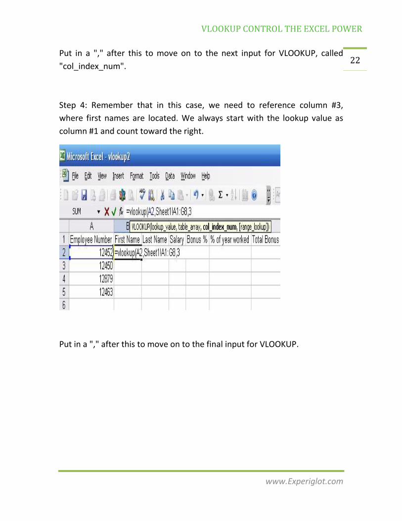
22 Put in a "," after this to move on to the next input for VLOOKUP, called
"col_index_num".
Step 4: Remember that in this case, we need to reference column #3,
where first names are located. We always start with the lookup value as
column #1 and count toward the right.
Put in a "," after this to move on to the final input for VLOOKUP.

VLOOKUP CONTROL THE EXCEL POWER
www.Experiglot.com
23 Step 5: Finally, we want to put in "false" as the final input into VLOOKUP to
tell it to look for exact matches.
Now close off the parenthesis to VLOOKUP, and the cell is automatically
populated with the data we need.
VLOOKUP CONTROL THE EXCEL POWER
www.Experiglot.com
24 The key now is to populate the rest of the cells. Can you figure out how to
do this? One way would be to go through each cell and repeat the steps
above. For example, to populate cell C2, we would write:
=VLOOKUP(A2,Sheet1!A1:G8,2,FALSE)
and so on, referencing each column where the data resides. ("Salary"
resides in column 4, "bonus" in column 5, etc.) Another way would be to
use Excel's anchoring mechanism so that we could copy and paste formulas
a bit more efficiently.
For example, for the rest of the cells under "First Name", what we could do
is write the following instead in B2:
=VLOOKUP($A2,Sheet1!$A$1:$G$8,3,FALSE)
What putting a "$" sign does in front of cell coordinates is to "lock" them in
place. By putting $A2 instead of A2 in the first input section, we lock "A" in
place (because all our employee numbers are in column A) and let the "2"
change as we go down the row.
By putting "$A$1:$G$8" instead of "A1:G8" as we originally had, we lock in
the entire A1 to G8 cells in place and keep that section "locked" no matter
where we put the formula.
VLOOKUP CONTROL THE EXCEL POWER
www.Experiglot.com
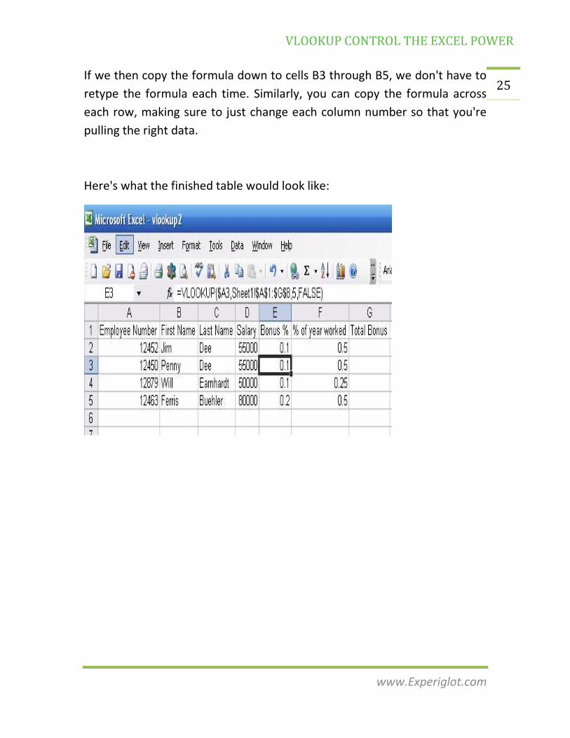
25 If we then copy the formula down to cells B3 through B5, we don't have to
retype the formula each time. Similarly, you can copy the formula across
each row, making sure to just change each column number so that you're
pulling the right data.
Here's what the finished table would look like:
VLOOKUP CONTROL THE EXCEL POWER
www.Experiglot.com
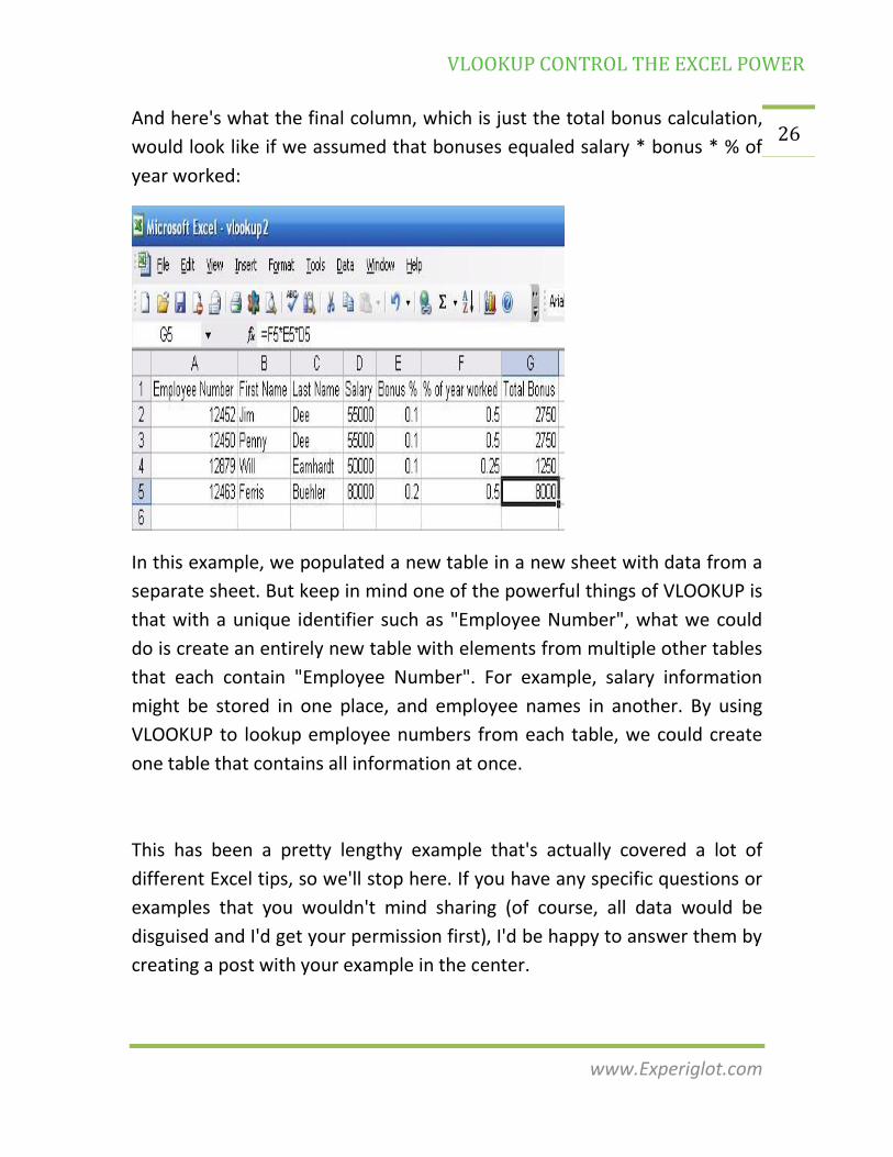
26 And here's what the final column, which is just the total bonus calculation,
would look like if we assumed that bonuses equaled salary * bonus * % of
year worked:
In this example, we populated a new table in a new sheet with data from a
separate sheet. But keep in mind one of the powerful things of VLOOKUP is
that with a unique identifier such as "Employee Number", what we could
do is create an entirely new table with elements from multiple other tables
that each contain "Employee Number". For example, salary information
might be stored in one place, and employee names in another. By using
VLOOKUP to lookup employee numbers from each table, we could create
one table that contains all information at once.
This has been a pretty lengthy example that's actually covered a lot of
different Excel tips, so we'll stop here. If you have any specific questions or
examples that you wouldn't mind sharing (of course, all data would be
disguised and I'd get your permission first), I'd be happy to answer them by
creating a post with your example in the center.
VLOOKUP CONTROL THE EXCEL POWER
www.Experiglot.com
27 Using Vlookup And Nested If In Excel
For Golf Scoring
Showing Excel tutorials is great but I always like real life examples to show
you how you can use Excel functions for almost everything. I’ve received a
very interesting email from a retired member of the military asking some
help with a golf scoring issue. Needless to say that on so many levels I was
more than happy to help out. While my blog is about "Experiments in
Finance, it's fair to say that many finance lovers like to play golf as well. It's
not the easiest problem to explain but hopefully with his comment and a
preview of his spreadsheet you will get the idea. Here we go:
"I need help with writing an "IF" formula in Excel. Background: I run a local
golf league with 40 to 70 golfers playing each week. Instead of using strokes
and keeping up with the handicaps, I use a point system. Each week I have
to manually calculate each man's score, plus or minus, from his required
points.
Example: For myself I currently am required to make 45 points. If I make
within plus or minus 2 of the 45 points there is no change to my next weeks
requirement. However, if I make minus 3 or more points, my score will drop
1 point(to 44). If on the other hand, I score 3 or 4 points above 45, my new
point requirement increases by 1 point, if I score 5 or 6 points above, my
requirement increases by 2 points, if I score 7 or more points, my
requirement increases to 3 points. I currently use an excel spreadsheet,
listing the players. I enter their that days point total and then manually do
VLOOKUP CONTROL THE EXCEL POWER
www.Experiglot.com
28 the math and enter their new point requirement. I can continue to do the
math...but in this day and age I would like to work "smarter not harder""
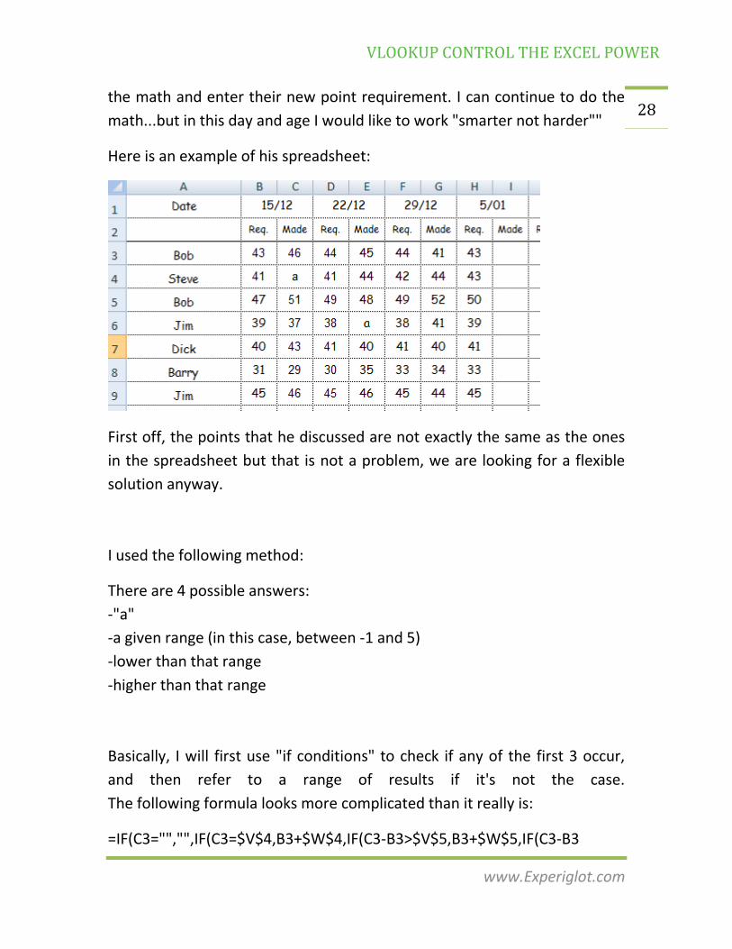
Here is an example of his spreadsheet:
First off, the points that he discussed are not exactly the same as the ones
in the spreadsheet but that is not a problem, we are looking for a flexible
solution anyway.
I used the following method:
There are 4 possible answers:
-"a"
-a given range (in this case, between -1 and 5)
-lower than that range
-higher than that range
Basically, I will first use "if conditions" to check if any of the first 3 occur,
and then refer to a range of results if it's not the case.
The following formula looks more complicated than it really is:
=IF(C3="","",IF(C3=$V$4,B3+$W$4,IF(C3-B3>$V$5,B3+$W$5,IF(C3-B3

VLOOKUP CONTROL THE EXCEL POWER
www.Experiglot.com
29 Basically, it checks if the previous score made is filled, if it the result is
either "a", higher than the range, lower than the range and applies the
adjustment depending on those.
If none of those conditions are met, it simply checks the range.
You can modify the range or values at any time by changing columns "U"
and "V". You can also simply copy the blue cells to a new column "req". try
copying from P3:P22 to R3:R22.
Here is what the new spreadsheet looks like:
I also invite you to download the spreadsheet to see for yourself!
VLOOKUP CONTROL THE EXCEL POWER
www.Experiglot.com
30 Too Many Options, Which One Should I
Use?
Excel Nested If Condition With Vlookup
One of the challenges about resolving issues in excel is that there are
usually so many different ways to resolve a given problem. It's all about
understanding the exact need and trying to find an optimal solution that
will be:
As easy as possible to create and modify later on
Quick and efficient to use
As light as possible
Etc.
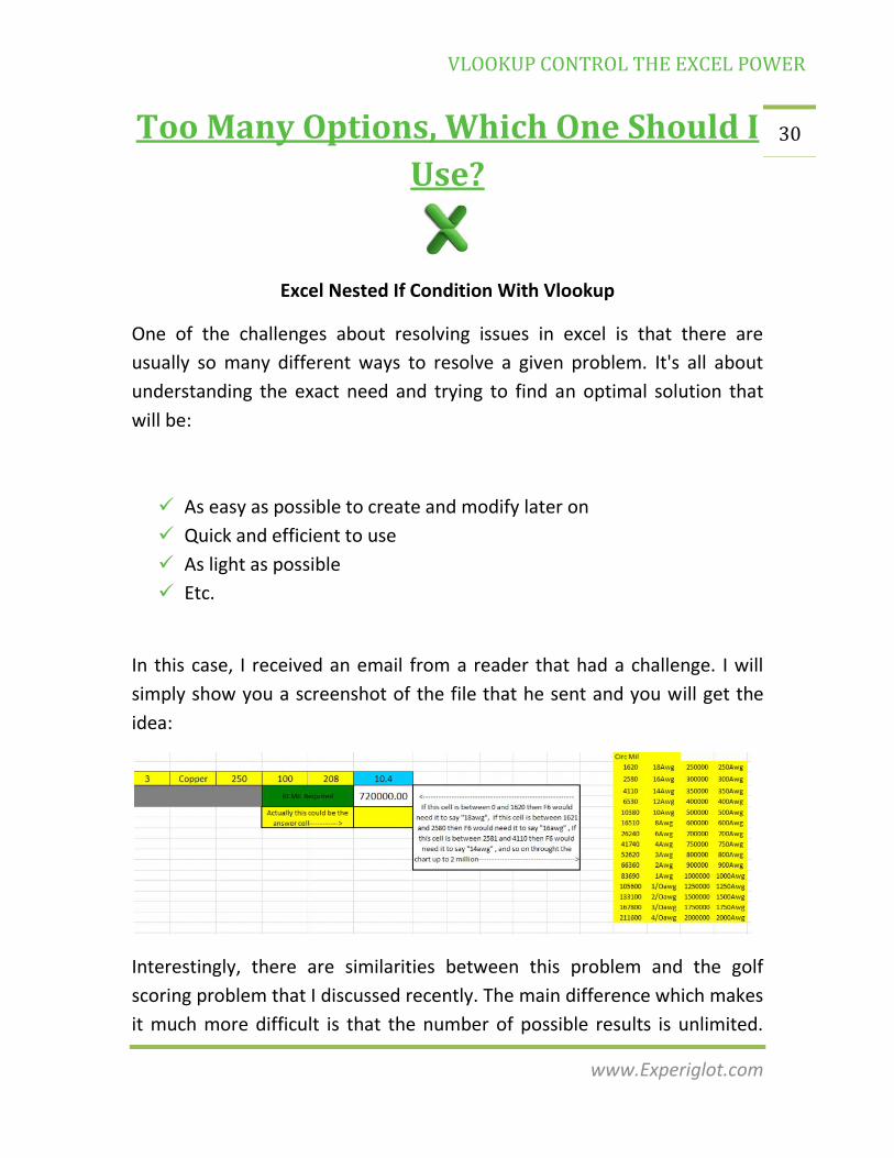
In this case, I received an email from a reader that had a challenge. I will
simply show you a screenshot of the file that he sent and you will get the
idea:
Interestingly, there are similarities between this problem and the golf
scoring problem that I discussed recently. The main difference which makes
it much more difficult is that the number of possible results is unlimited.
VLOOKUP CONTROL THE EXCEL POWER
www.Experiglot.com
31 That makes it challenging on many levels and makes it impossible to use a
simple vlookup. I wasn't quite sure how to tackle this specific problem. As is
always the case, using a macro was certainly an interesting option. Using a
nested if statement could have worked, or even a combination of a few of
those but given the number of possible outcomes, it would be very difficult
to work with, and even more tricky to modify later on. Why?
Imagine using an If(xxx,y,if(xxx,y,if(xxx,……. Etc)
This would have gone on and on. My next reflex was to ask the reader if
this would be used for multiple lines at a time. If so, that would make things
even more difficult. Thankfully, in this specific case, it was going to be done
one at a time. This meant that I could simply verfiy (with a nested if
statement for each line if that specific answer was the correct one.
In O2 I added:
=IF(AND($F$4>M2,$F$4
And in P2 I added:
=IF(AND($F$4>M2,$F$4
I dragged both formulas and then added the following in F7:8:
=VLOOKUP("YES",O:P,2,FALSE)
VLOOKUP CONTROL THE EXCEL POWER
www.Experiglot.com
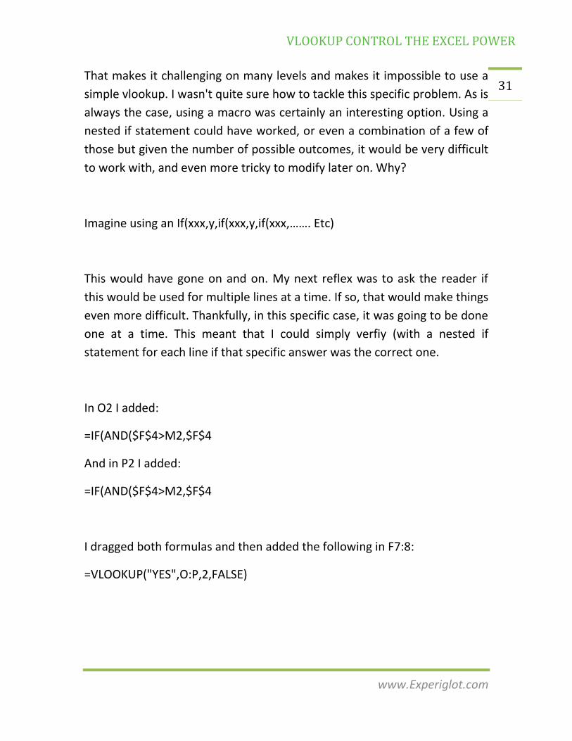
32 You can see the result here:
And you can download the spreadsheet off course:)
VLOOKUP CONTROL THE EXCEL POWER
www.Experiglot.com
33 Combining Excel Sumif, Vlookup, If Is
Error Functions, etc
I’ve received another interesting question by email which I wanted to share
in this book since it was not the first time I had received this type of
question. In this specific case, it required me to use several of the functions
that I have been writing about on this blog so I thought it would make an
interesting case. First, let me explain what the user asked for. You will not
have the exact same problem but I think that trying to understand it can
help you a great deal. Basically, this user has a list of documents that you
can see in column A. Then, there is a reference for that document and a
date in columns B and C. What this reader would like is:
-For each document number, get the reference number for the most recent
modification
The tricky part here is that most documents appear several times (because
they were modified on several dates)
Alternatives
Problems like this are so interesting because there so many different ways
to get them done. One way would have been to do a macro with a loop as I
did a few weeks ago. I will however do it without a macro for this time, it
should be as simple.
VLOOKUP CONTROL THE EXCEL POWER
www.Experiglot.com
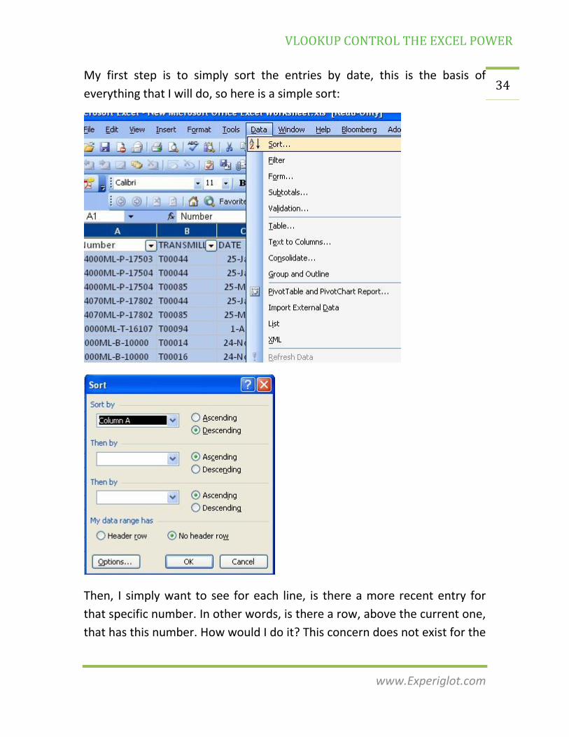
34 My first step is to simply sort the entries by date, this is the basis of
everything that I will do, so here is a simple sort:
Then, I simply want to see for each line, is there a more recent entry for
that specific number. In other words, is there a row, above the current one,
that has this number. How would I do it? This concern does not exist for the
VLOOKUP CONTROL THE EXCEL POWER
www.Experiglot.com
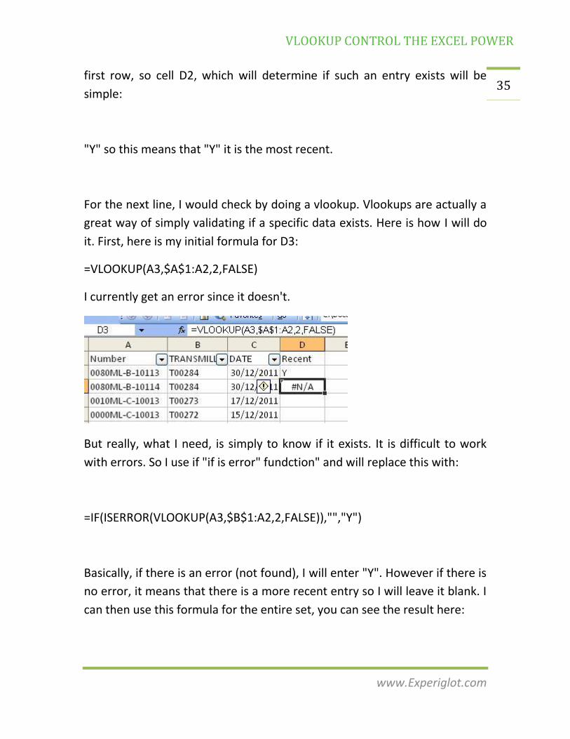
35 first row, so cell D2, which will determine if such an entry exists will be
simple:
"Y" so this means that "Y" it is the most recent.
For the next line, I would check by doing a vlookup. Vlookups are actually a
great way of simply validating if a specific data exists. Here is how I will do
it. First, here is my initial formula for D3:
=VLOOKUP(A3,$A$1:A2,2,FALSE)
I currently get an error since it doesn't.
But really, what I need, is simply to know if it exists. It is difficult to work
with errors. So I use if "if is error" fundction" and will replace this with:
=IF(ISERROR(VLOOKUP(A3,$B$1:A2,2,FALSE)),"","Y")
Basically, if there is an error (not found), I will enter "Y". However if there is
no error, it means that there is a more recent entry so I will leave it blank. I
can then use this formula for the entire set, you can see the result here:
VLOOKUP CONTROL THE EXCEL POWER
www.Experiglot.com
36
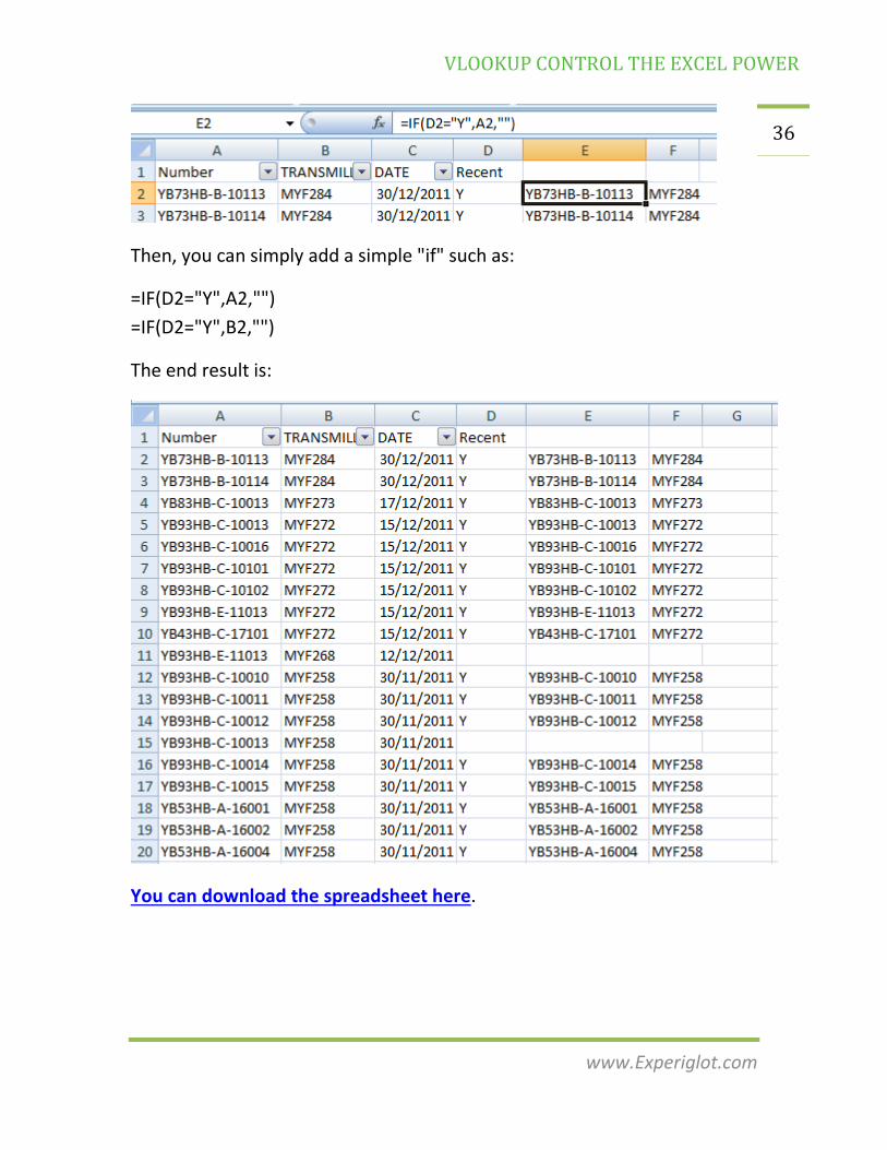
Then, you can simply add a simple "if" such as:
=IF(D2="Y",A2,"")
=IF(D2="Y",B2,"")
The end result is:
You can download the spreadsheet here.
VLOOKUP CONTROL THE EXCEL POWER
www.Experiglot.com
37 Vlookup or "Relationships" In Excel
2013
Vlookup functions are difficult to understand initially and while they
become very powerful once you do fully understand how to use them, I can
tell you from the dozens of requests that I get every month that the
concept remains very difficult to understand. Microsoft is trying to make
life easier for users by changing the concept again. Here is the direct quote
from CFO's excel 2013 preview:
Relationships instead of VLOOKUP. If you add your worksheets to the
pedestrian “Data Model” feature, you can use the Relationships icon to
define that CustID in your million row transaction worksheet is related to
CustNumber in your customer worksheet. Now, without doing millions of
VLOOKUPs, you can create pivot tables from the data on both worksheets.
Whether you’re sick of people who feel superior because they can do
VLOOKUP, or someone who does VLOOKUP in their sleep, no one can argue
that creating a relationship in 3 clicks is faster than waiting for a million
VLOOKUPs to recalculate.

VLOOKUP CONTROL THE EXCEL POWER
www.Experiglot.com
38 This might work although it will simply make other parts more difficult. I'm
assuming that having the right column headers will become very important
as Excel 2013 will try to guess how data interacts with each other. It will
certainly be very interesting to see. I'm curious, do you expect to upgrade
to Excel 2013 as soon as possible? I will certainly start moving soon
although I do use cloud computing a lot more than I did just a few months
ago so it will only impact my more complex spreadsheets. If ever you'd like
to access a preview version, you can try going here.
VLOOKUP CONTROL THE EXCEL POWER
www.Experiglot.com
39 Learning Vlookup is Only the
Beginning
First, I hope you enjoyed this book and you learned a few tricks on how to
use Vlookup properly. If you are still struggling with this function, send me
an email at [email protected]. It will be my pleasure to assist you with
your problems.
Now, you are ready for the next step. As you know, Vlookup is only the
beginning of what Excel can do for you. This function certainly doesn’t
answer all your questions. This is why I’ve created a master resource to
learn everything useful about Excel. You will find several tutorials
(including this one) showing you how to:
Automate your daily tasks, save time or money
Resolve all your problems and stop staring at your computer with an
upset face ;-)
Create your own spreadsheets & functions
Make your time 100% productive
Learn from “real life” examples
Download numerous useful spreadsheets ready to use
This is an evolving eBook. This means that buy purchasing the eBook; you
will receive updated versions (probably once a year) with additional
content and other bonuses. All this for no additional charges!
VLOOKUP CONTROL THE EXCEL POWER
www.Experiglot.com
40 Download “Taking Your Excel Skills to
Another Level”
How much is it? Only $9.95
Why You Should Buy Now
Microsoft Excel is in a way like a
human brain, as most of us only use a
tiny part of it. Why? Mostly because we do not know enough about
everything that is possible. This eBook is meant to share with you the
summaries of my answers to hundreds of different excel related questions
that were asked on this website,
“Your eBook was great. I’ve been looking for ways to improve my excel skills
for months and I feel like I am now making significant progress” – Anton
Download “Taking Your Excel Skills to Another Level”
Then again, if you need me for any questions don’t be shy and send me an
email!
Best,
Pete
www.Experiglot.com


![VLOOKUP(otsitav väärtus; massiiv; veeru indeks; [vastendustüüp])download.microsoft.com/download/f/7/7/f776bdfe-6d16-4183... · 2018-10-17 · Microsoft Excel Funktsiooni VLOOKUP](https://static.cupdf.com/doc/110x72/5f1612dd3aa6032cb806d300/vlookupotsitav-vrtus-massiiv-veeru-indeks-vastendustp-2018-10-17.jpg)


![Microsoft Excel 2019 Advanced - CustomGuide · The Vlookup Function: The Vlookup function =VLOOKUP(lookup_value, table_array, col_index_num, [range_lookup]) looks for a value you](https://static.cupdf.com/doc/110x72/5e696095634ca420fd60c532/microsoft-excel-2019-advanced-customguide-the-vlookup-function-the-vlookup-function.jpg)
