Valuation of Ecosystem Services, Karnataka State, India
Report of the NCAVES Project
2
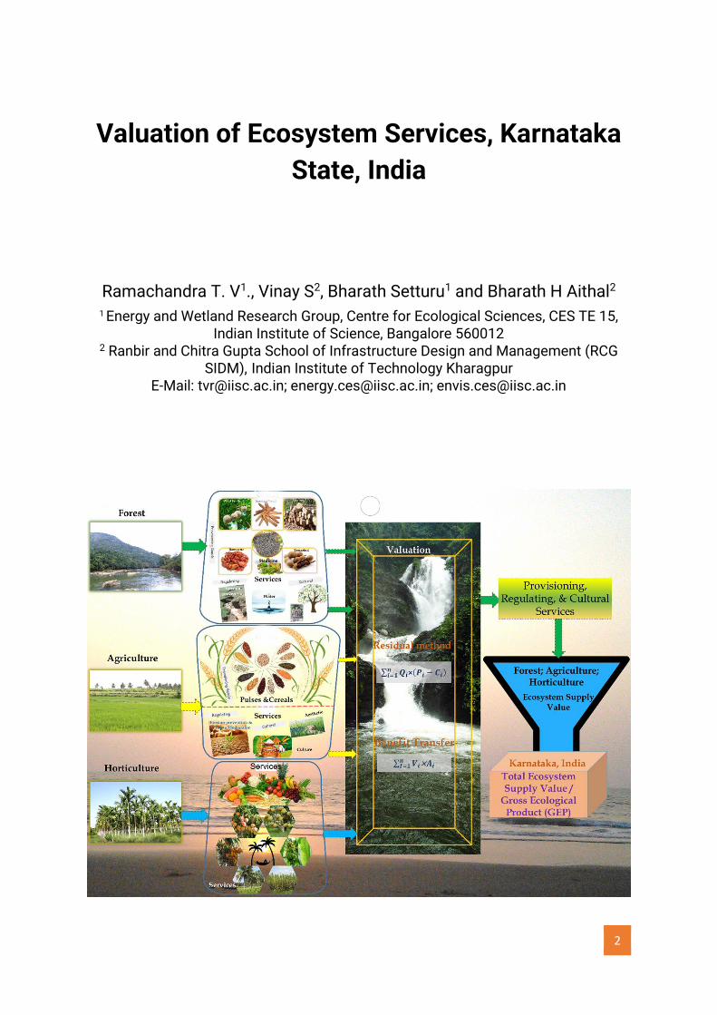
Valuation of Ecosystem Services, Karnataka
State, India
Ramachandra T. V1., Vinay S2, Bharath Setturu1 and Bharath H Aithal2
1 Energy and Wetland Research Group, Centre for Ecological Sciences, CES TE 15, Indian Institute of Science, Bangalore 560012
2 Ranbir and Chitra Gupta School of Infrastructure Design and Management (RCG SIDM), Indian Institute of Technology Kharagpur
E-Mail: [email protected]; [email protected]; [email protected]
3
Valuation of Ecosystem Services, Karnataka State, India
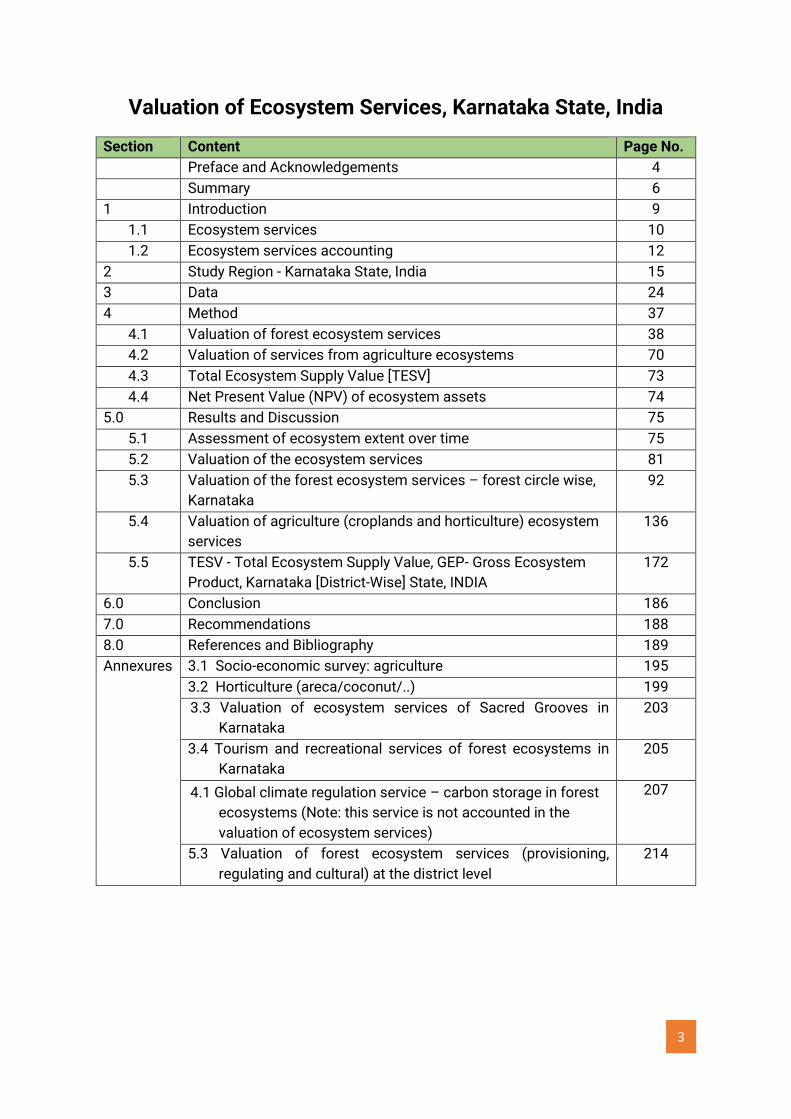
Section Content Page No.
Preface and Acknowledgements 4
Summary 6
1 Introduction 9
1.1 Ecosystem services 10
1.2 Ecosystem services accounting 12
2 Study Region - Karnataka State, India 15
3 Data 24
4 Method 37
4.1 Valuation of forest ecosystem services 38
4.2 Valuation of services from agriculture ecosystems 70
4.3 Total Ecosystem Supply Value [TESV] 73
4.4 Net Present Value (NPV) of ecosystem assets 74
5.0 Results and Discussion 75
5.1 Assessment of ecosystem extent over time 75
5.2 Valuation of the ecosystem services 81
5.3 Valuation of the forest ecosystem services – forest circle wise,
Karnataka
92
5.4 Valuation of agriculture (croplands and horticulture) ecosystem
services
136
5.5 TESV - Total Ecosystem Supply Value, GEP- Gross Ecosystem
Product, Karnataka [District-Wise] State, INDIA
172
6.0 Conclusion 186
7.0 Recommendations 188
8.0 References and Bibliography 189
Annexures 3.1 Socio-economic survey: agriculture 195
3.2 Horticulture (areca/coconut/..) 199
3.3 Valuation of ecosystem services of Sacred Grooves in
Karnataka
203
3.4 Tourism and recreational services of forest ecosystems in
Karnataka
205
4.1 Global climate regulation service – carbon storage in forest
ecosystems (Note: this service is not accounted in the
valuation of ecosystem services)
207
5.3 Valuation of forest ecosystem services (provisioning,
regulating and cultural) at the district level
214
4
PREFACE AND ACKNOWLEDGEMENTS
This report focusing on Karnataka, India, was commissioned by the United Nations
Environment Programme (UNEP) as part of the international, EU-funded Natural
Capital Accounting and Valuation of Ecosystem Services (NCAVES) project. The
NCAVES project was carried out as a collaboration between UNEP, the United Nations
Statistics Division (UNSD), the Ministry of Statistics and Programme Implementation
(MoSPI), Government of India and ENVIS Division, The Ministry of Environment
Forests and Climate Change (MoEF&CC), Government of India.
Acknowledgments go to the European Union for funding the NCAVES Project and the
Delegation of the European Union to India for supporting its implementation in
Karnataka State, India, and the UNSD and UNEP for leading the NCAVES Project
globally and supporting its implementation and management in Karnataka State,
India.
UNSD and UNEP commissioned Dr. T V Ramachandra, Co-ordinator, Energy &
Wetlands Research Group, CES TE15 at the Indian Institute of Science through a Small
Scale funding agreement (SSFA/2019/1502), to pilot the compilation of selected
ecosystem accounts in physical and monetary terms based on policy priorities and to
contribute to policy mainstreaming.
The Energy & Wetlands Research Group, CES TE 15 at the Indian Institute of Science
(IISc) Bangalore appreciates the contributions of Dr. Shailja Sharma, Dr. Awadhesh
Kumar Mishra, Smt. P Bhanumati, Mr. Rakesh Kumar Maurya, Dr. Sudeepta Ghosh of
the Ministry of Statistics and Programme Implementation (MoSPI), Government of
India (GoI); Dr. Anandi Subramnyam, Dr. James Mathew, and Mr. Kumar Rajnish of the
Ministry of Environment, Forests and Climate Change (MoEFCC), GoI in developing the
ecosystem services account. Thanks to (i) Dr. Prabhuraj, Director, Karnataka State
Remote Sensing Centre (KSRSAC), Government of Karnataka (GoK), Bangalore, for
providing spatial data of the district administrative boundaries, stream and river
network, population data; (ii) Dr. Hemanth Kumar, Executive Secretary, Karnataka
State Council for Science and Technology (KSCST), GoK for providing spatial data
related to geology, lithology, etc. (iii) Director, National Remote Sensing Centre,
Department of Space, GoI, Hyderabad and (iii) Director, Department of Agriculture,
GoK for providing soil health data – district wise for Karnataka.
The Energy & Wetlands Research Group, IISc acknowledges the efforts of Mr. Karthik
Naik and Mr. Vinayka Bhatta (for assisting in field data collection and district wise
remote sensing data analyses – extent and fragmentation analyses), Ms. Madhumita
Dey (for assistance in the computation of Land surface temperature analyses), Mr.
Rakesh D.R (soil quality analyses), Mr. Chandan M (for the assistance in agent-based
modelling and geo-visualisation), Ms. Harita (for help in compiling data related to
5
biodiversity), Ms. Minsa (for compiling data related to fauna), Dr. G R Rao, Mr. Vishnu
Mukri and Mr. Shrikanth Naik (for assistance in field data collection related to flora
and fauna in 5 districts of Western Ghats), Mr. Vrijulal and Dr. M D Subash Chandran
(for verification of data – flora and fauna). Ms. Sincy V, Ms. Asulabha K S, Ms. Deepthi
H, Ms. Saranya G and Mr. Sudarshan Bhat assisted with the ecosystems’ economic
valuation and compiling the accounts.
The work was carried out using (i) field data, (ii) collateral data compiled KSRSAC,
GoK; KSCST, GoK; Department of Agriculture, GoK, Karnataka Forest Department, GoK
and (iii) spatial data (Landsat series available in the public domain) and (iv) spatial
data (IRS LISS Data) procured from the National Remote Sensing Centre, GoI,
Hyderabad.
The study benefitted from the review inputs of Dr. William Speller of UNEP, Dr. Bram
Edens of UNSD, Dr. Anshu Singh and Dr. Prerna of Statistics division, the Ministry of
Environment, Forests and Climate Change, Government of India, Officers of the
Ministry of Statistics and Programme Implementation, GoI, and the members of the
UN Technical Committee on the SEEA EA and its working groups.
The views, thoughts, and opinions expressed in the text are not necessarily those of
the United Nations, European Union, or other agencies involved. The designations
employed and the presentation of material including on any map in this work do not
imply the expression of any opinion whatsoever on the part of the United Nations or
European Union concerning the legal status of any country, territory, city or area or its
authorities, or concerning the delimitation of its frontiers or boundaries.
Citation: Ramachandra, T.V., Vinay, S., Bharath, Setturu, and Bharath, H. Aithal (2022).
Valuation of Ecosystem Services, Karnataka State, India. Available at:
http://wgbis.ces.iisc.ernet.in/energy/NCAVES
Funded by the European Union
6
VALUATION OF ECOSYSTEM SERVICES, KARNATAKA STATE, INDIA
SUMMARY
India is trying to accelerate economic growth and relax environmental laws, and there
is tremendous pressure to divert natural systems to other uses. Hence, there is a
pressing need to undertake the natural capital accounting and valuation of the
ecosystem services, especially intangible benefits, provided by ecosystems in India.
This report focuses on ecosystem services in forest and agricultural ecosystems in
Karnataka for 2005 and 2019.
This report follows the SEEA Ecosystem Accounting (SEEA EA), which constitutes the
statistical framework for natural capital accounting and organizes data on
ecosystems and the services they provide. The UN Statistical Commission adopted
the SEEA EA framework in 2021, and it forms the underlying conceptual framework of
the accounts developed in this report. Ecosystem services in the SEEA EA are defined
as the contributions of ecosystems to the benefits that are used in economic and
other human activities. Within the SEEA EA, valuation of ecosystem services (VES)
allows for adjusted national accounts which reflect the output of ecosystem services
as well as the depletion of natural resources and the degradation costs (externalized
costs of the loss of ecosystem services) of ecosystems in economic terms, which will
help raise awareness and provide a quantitative tool to evaluate the sustainability of
policies. It provides an unbiased and dependable national framework to value so far
unaccounted ecosystem benefits and helps develop meaningful policy interventions.
The value of all ecosystem services, including the degradation costs, needs to be
understood for developing appropriate policies toward the conservation and
sustainable use and management of ecosystems. Scientific efforts during the past
decade have refined the understanding of ecosystem function and demonstrated the
links between functions and the provision of ecosystem services. This knowledge
needs to be communicated effectively to decision-makers and the public, which will
lead to the development of policies that adequately consider the trade-offs between
the conservation of ecosystems and natural resources and economic growth. In order
to accurately assess trade-offs, natural capital accounts are needed to incorporate
the economic worth of natural capital found in ecosystems such as forests to
measure the wealth of a region.
For this report, ecosystem services were quantified following the valuation principles
of the SEEA. This means that only the contribution of the ecosystem to the benefit is
measured, not the benefit itself. This can be achieved, for instance, through the
7
residual value method by taking the gross value of the final marketed good to which
the ecosystem service provides input and then deducting the cost of all other inputs,
including labor, produced assets, and intermediate inputs (as per the SEEA Central
Framework).
This report focuses on ecosystem services in forest and agricultural ecosystems for
2005 and 2019. Values of 2005 were adjusted through the consumer price index or
gross domestic product (GDP) deflator. These values reflect the actual measures of
ecosystem services, which could be compared with ecosystem services of 2019.
Comparison of values of services in 2019 with 2005 highlights that there has been a
considerable decline in ecosystem services in Karnataka– a 28.5% reduction in
provisioning services (51.6% reduction in forest ecosystems), a 21% reduction in
regulatory services (mainly in forest ecosystems - 27.1% reduction), and a 1.9%
reduction in cultural services during 2005 to 2019.
Ecosystem services were aggregated to compute the Total Ecosystem Supply Value
(TESV). This aggregate measure is also referred to as Gross Ecosystem Product
(GEP), which equals the sum of all final ecosystem services (i.e., by monetary values
of those services) from ecosystem assets. The TESV of forest and agricultural
ecosystems in Karnataka was 3620 billion INR in 2005 (forest ecosystems: 2841
billion INR and agricultural ecosystems: 779 billion INR). However, overall, TESV
declined in 2019 to 2912 billion rupees, with forest ecosystems driving this decline
with a 35% decline in TESV. The TESV was also compared to the GDP of Karnataka,
which is about 10128 billion rupees. TESV of the forest ecosystem is equivalent to
18.1% of the GDP, and the TESV from agriculture ecosystems is equivalent to about
10.6% of the GDP in Karnataka.
There has been a 35.4% reduction in the TESV of forest ecosystems from 2005 to
2019, mainly due to the degradation of ecosystems. The decline in the TESV highlights
the degradation of forest ecosystem assets from 2005 to 2019, as shown by the
reduction of ecosystem extent and ecosystem condition (Ramachandra et al., 2021a,
b). The decrease in value is also demonstrated by a fall in the net present value (NPV)
of expected future returns of the ecosystem services supplied by forest ecosystem
assets. The NPV of the assessed ecosystems based on 2005 ecosystem flows is
about 93130 billion INR (forest ecosystem: 73099 billion INR, agriculture ecosystem:
20031 billion INR). However, the NPV of ecosystems in Karnataka, based on 2019
flows, indicates 74938 billion INR (forest ecosystem: 47214 billion INR, agriculture
ecosystem: 27724 billion INR). This highlights that there has been a decline of 35.4%
in the asset value of forest ecosystems with the transition of forest ecosystems to
croplands or horticulture (agriculture ecosystems), which is correlated to an increase
in NPV of agriculture ecosystems by 38%.
8
Ecosystem accounts make the value of ecosystem services visible, allowing them to
be internalized into decision-making. This enables an assessment of trade-offs
between economic development and environmental conservation and restoration,
resulting in better-informed decisions. It also allows strengthening the economic case
for conserving forests in states in India and developing countries where there can be
great pressure to relax forest laws and divert forests to non-forest uses without proper
consideration of the sustainability of such actions.
The ecosystem services computed for Karnataka State also support the viability of
markets for particular ecosystem services. The development of such markets requires
additional institutional reforms such as changes with respect to property rights and
reforms in land and labor markets. The main policy challenge of the future concerns
is to promote conservation and develop such markets so that those bearing the cost
of conservation can be adequately compensated.
Based on the experiences gained in the current pilot, it is estimated that the exercise
of natural capital accounting and valuation of ecosystem services could be replicated
in any region (of 10000 to 12000 sq. km) as per the SEEA-EA framework in a period of
15 months, involving field data collection with a team consisting of multidiscipline
expertise. It requires (i) all para-state agencies sharing the data of biophysical
variables as the primary data collection is a time-consuming endeavor, (ii) organizing
orientation programs and hands-on training to enhance the capability of the team to
undertake spatial analyses, collecting biophysical variables from the government
agencies and the field, data integration and validation, analyses of the data and
interpretation, (iii) addressing the gaps in the existing biophysical models (adapting to
local conditions). Thus, the valuation of ecosystem services done in Karnataka State
can be replicated in other states so that the accounts can play a vital role in
conservation planning and ecosystem-based management across India.
9
VALUATION OF ECOSYSTEM SERVICES, KARNATAKA STATE, INDIA
1.0 Introduction
Humans depend on the environment for their basic needs, such as food, fuel, minerals, water,
air, etc. In developing countries, nearly 80% of the labor force is engaged in agricultural or
resource-based activities, contributing significantly to the GDP (World Bank 1998, 2001). The
dependency on the natural resources, over the years, has led to their degradation and
depletion owing to the unsustainable practices involved in their extraction. Burgeoning
unplanned development activities to cater to the demands of the increasing population have
put tremendous pressure on the natural resources, leading to environmental degradation
(Kulkarni and Ramachandra 2009). An increased surge in developmental and technological
activities over the last two decades, with no regard to their ecological implications, has led to
indiscriminate disposal of wastes (liquid and solid), contributing to the degradation of the
natural ecosystems. This has resulted in a substantial and largely irreversible loss in the
diversity of life on Earth (MEA 2005). And yet, unsustainable utilization of land and other
natural resources persists, despite the increasing understanding of the impacts that human
activities have on the environment, (Euliss Jr et al., 2010). Linkages between the health of the
environment and the sustenance of humankind make it imperative to maintain a balance
considering the carrying capacity of the environment and the availability of natural resources.
Conservation of natural ecosystems has long-term benefits for humans in utilitarian terms
through their provision of food, timber, minerals, and a variety of valuable resources that have
provided the backbone for economic development. Going beyond utilitarian values, natural
ecosystems have also been a source for maintaining gene pools, biodiversity, and other
potentially useful factors that are of indirect use to humans. Hence, ecosystems’ intrinsic,
anthropocentric, instrumental, and relational values should be considered in the policy design
and consider resources exploited for human settlement, food, and energy production.
In this regard, a statistical framing of data on ecosystems plays a vital role in incorporating at
least some parts of the wider value of ecosystems as a regular component of decision-
making. The SEEA Ecosystem Accounting (SEEA EA) provides such a framework. Adopted by
the United Nations Statistical Commission in 2021, the SEEA EA constitutes an integrated and
comprehensive statistical framework for organizing ecosystem data, measuring ecosystem
services, and tracking ecosystem changes. In addition, the data on ecosystems is linked to
information on economic and other activities, as the SEEA EA uses many of the same
concepts, definitions, and classifications as the System of National Accounts (SNA). Finally,
the SEEA EA enables high-quality and consistent measurement over time by using agreed
concepts, definitions, and classifications. Providing relevant time series and trend data on the
environment-economy nexus is crucial for effective policy design, decision-making, and
evaluation.
The dilemma associated with rapid land-use changes for accommodating the growing
demand for natural resources is impacting and degrading the ecosystems (Foley et
10
al., 2005, Ramachandra et al., 2007). The ecosystem service approach capturing the
full range of environmental impacts systematically offers a way to understand and
deal with the feedback that is created when ecosystems are used up to meet
humankind’s own needs (Rodríguez et al., 2006). The objectives of the current study
are to (i) to assess the ecosystem services values for the forest, agriculture, and
horticulture ecosystem types, district-wise for Karnataka State, India (ii) the
computation of the total ecosystem supply value (TESV), and (iii) Net present value
(NPV) of ecosystem assets. The report focuses on data for the years 2005 and 2019.
It should be noted that the SEEA EA focuses on values of anthropocentric origin – i.e.,
values that are centered on human beings. Further, the measurement focus of the
SEEA EA is on instrumental (is the value attributed to something as a means to
achieve a particular end) or use values because these interactions are most readily
quantified and because, from a monetary valuation perspective, these values are most
readily reflected in monetary terms. From a policy perspective, the focus on
anthropocentric, instrumental values may also be considered of high relevance since
they concern the types of human interactions with the environment that can place the
most pressure on ecosystems (SEEA EA 2021).
The outline of this report is as follows: the following section (Section 1) defines
ecosystem services and accounting for ecosystem services in the context of the SEEA
EA. Section 2 describes the study region – Karnataka State, India and provides socio-
economic context. Section 3 explains data sources, and Section 4 presents methods
adopted for valuation. Section 5 describes the results: of ecosystem services
accounting for forest ecosystems and agriculture ecosystems. Section 5 concludes
with recommendations. Ecosystem-wise services (physical as well as monetary)
computed district-wise are presented in Annexures 5.3 for forest ecosystems.
1.1. Ecosystem services
In the SEEA EA, ecosystem services are the contributions of ecosystems to the
benefits that are used in economic and other human activities. In this definition, use
incorporates direct physical consumption, passive enjoyment, and indirect receipt of
services.
An ecosystem services approach to foster an understanding of the relationship
between humans and the environment has been emphasized in various initiatives,
including The Economics of Ecosystems and Biodiversity initiative (Costanza et al.,
1997, 2014; Markandya et al., 2002; MEA 2005; Van der et al., 2010; TEEB 2010a, b;
Ten Brink 2011; De Groot et al., 2012, 2017, 2020; Perelet et al., 2014), the Mapping
and Assessment of Ecosystems and their Services (MAES) framework (Maes et al.,
2013, 2016, 2018, 2020); the Natural Capital Project at Stanford University; the
11
Integrated System for Natural Capital Accounting (INCA) project (Vallecillo et al.,
2019); and the Intergovernmental Science-Policy Platform on Biodiversity and
Ecosystem Services (IPBES) (Diaz et al., 2015), etc.
Most resource management decisions are influenced by ecosystem services (ESs)
entering markets; thus, the non-marketed benefits often remain unaccounted. Both
renewable resources (water supply, air quality, etc.) and non-renewable resources
(mineral deposits, some soil nutrients, fossil fuels, etc.) are capital assets and provide
the backbone for numerous economic activities that account for the development of
a region. Yet, traditional national accounts do not include measures of resource
depletion or their degradation. GDP, a measure of the current economic well-being of
a population, based on the market exchange of material well-being, will indicate
resource depletion/degradation only through a positive gain in the economy and will
not represent the decline in these assets (wealth) at all. Thus, the existing GDP growth
percentages used as yardsticks to measure the development and well-being of
citizens in decision-making processes are substantially misleading, and yet they are
being used (De Groot et al., 2002; Haripriya et al., 2006). GDP cannot be a true measure
of the country’s sustained economic wealth and cannot be a proxy for understanding
its future economic well-being. Quantitative evidence on the economic value of such
assets is thereby necessary for most of these services, most of which are not traded
in the markets and hence do not have a market value. The monetary valuation of
ecosystem services can help in building a better understanding of their influence on
well-being and can further facilitate information-driven decisions and policy reforms
that align with the Sustainable Development Goals (SDGs). Environmental accounting
systems seek to determine a region’s environmental and economic assets and can be
used to assess whether economic development is consistent with sustainable
development or to help ensure optimal use of natural resources and the environment.
Recent efforts, especially the System of Environmental-Economic Accounting, Central
Framework (SEEA CF), and Ecosystem Accounting (SEEA EA), aim to extend and
integrate the national accounts for environmental and ecosystem assets (SEEA 2017;
SEEA EA 2021).
Ecosystem services encompass all forms of interaction between ecosystems and
people, including both in situ and remote interactions. The supply of an ecosystem
service is associated with an ecosystem structure or process or a combination of
ecosystem structures and processes that reflect the biological, chemical, and physical
interactions among ecosystem components. In the SEEA EA, ecosystem services are
broadly categorized as (i) provisioning services, which are those ecosystem services
representing the contributions to benefits that are extracted or harvested from
ecosystems; (ii) regulating and maintenance services, which are those ecosystem
services resulting from the ability of ecosystems to regulate biological processes and
to influence climate, hydrological and biochemical cycles, and thereby maintain
12
environmental conditions beneficial to individuals and society; and (iii) cultural
services, which are experiential and intangible services related to the perceived or
actual qualities of ecosystems whose existence and functioning contributes to a
range of cultural benefits. There is a range of other benefits, for example, concerning
relational and intrinsic values, that are not captured in the above categories.
Ecosystem services serve as the connecting concept between ecosystem assets
(contiguous spaces of a specific ecosystem type, i.e., individual ecosystems) and the
production and consumption activities as per the SEEA EA. The key concepts of the
SEEA EA related to ecosystem services concern (i) the supply of ecosystem services
to users; and (ii) the contribution of ecosystem services to benefits (i.e., the goods
and services ultimately used and enjoyed by people and society). Further, ecosystem
services encompass all forms of interaction between ecosystems and people,
including both in situ and remote interactions. A key feature of ecosystem accounting
is its capacity to integrate spatially referenced data about ecosystems, i.e., data about
the location, size, and condition of ecosystems within a given area and how these are
changing over time. Recording these stocks and changes in stocks in a coherent and
mutually exclusive manner supports the derivation of indicators. Understanding the
size and location of ecosystems also supports the measurement of ecosystem
conditions and the quantification and valuation of many ecosystem services, the flows
of which will vary from ecosystem to ecosystem.
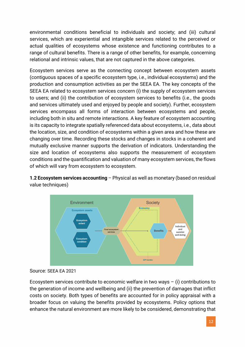
1.2 Ecosystem services accounting – Physical as well as monetary (based on residual
value techniques)
Source: SEEA EA 2021
Ecosystem services contribute to economic welfare in two ways – (i) contributions to
the generation of income and wellbeing and (ii) the prevention of damages that inflict
costs on society. Both types of benefits are accounted for in policy appraisal with a
broader focus on valuing the benefits provided by ecosystems. Policy options that
enhance the natural environment are more likely to be considered, demonstrating that
13
investing in natural capital can make economic sense. There is considerable
complexity in understanding and assessing the underlying links between a policy, its
effects on ecosystems and related services, and valuing its impacts in economic
terms. Collaboration between those working in policy, science, and economics
disciplines is essential in implementing this approach in practice. The critical
importance of the links to scientific analysis, which form the basis for valuing
ecosystem services, needs to be recognized. The SEEA EA emphasizes the need to
consider the ecosystem as a whole and underlines those changes or impacts on one
part of an ecosystem have consequences for the whole system. Therefore,
considering the scale and scope of the services to be valued is vital to arrive at any
meaningful values.
The key stages in the valuation of ecosystem services in the SEEA EA are: (i) setting a
scope and baseline through ecosystem extent and condition accounts, (ii) physical
quantification of services, and (iii) valuation of ecosystem services, including changes
over time. Monetary accounts can further inform a qualitative assessment of the
potential impacts of policy options on ecosystem services and quantification of the
impacts of policy options on specific ecosystem services, and evaluation of the
effects on human welfare.
There is a growing interest in ecosystem services (ESs), and ES conservation
management strategies, and the valuation of ecosystem services would help equip
society with the means to incorporate the values of nature into decision-making at all
levels. It also provides a baseline for evaluating management changes. This helps
evaluate and prioritize different policies, evaluate potential trade-offs in management
decisions, and assess the damages caused by natural disturbances. Apart from these,
other benefits are (i) enhanced communication with stakeholders about the economic
benefits and costs of potential changes in forest management, as communities’
preferences for different ecosystem services may be affected by estimates of
economic performance; (ii) a baseline for evaluating management changes. This
helps policymakers to take into account the value of ecosystems in development
planning and resource allocations and take adequate measures for conservation to
ensure the sustenance of the flow of ecosystem services.
The United Nations Statistical Commission (UNSC) endorsed the SEEA-Experimental
Ecosystem Accounting (SEEA-EEA in 2013 (System of Environmental-Economic
Accounting-Experimental Ecosystem Accounting) as the basis for commencing
testing and further development of a common statistical framework for ecosystem
accounting. The UNSC also encouraged the use and experimentation of the SEEA-EEA
by international and regional agencies (SEEA 2017; SEEA EA 2021). The various
research publications from the scientific community on the valuation of ecosystem
services have substantially grown to address the several challenges and for proposing
common frameworks. The expansion of a worldwide research base with a
14
multidisciplinary scope of ecosystem services is resolving issues that arise in
quantification, terminology, classification systems, research methods, and reporting
requirements (Polasky et al., 2015; Mengist and Soromessa 2019).
The ecosystem accounts in this report have been developed for Karnataka State, India,
as per the SEEA Ecosystem Accounting (SEEA EA) framework. Valuation of
ecosystem services is the third report in a series of four, which follow Ecosystem
Extent Accounts (Ramachandra et al., 2021a) and Ecosystem Condition
(Ramachandra et al., 2021b)
The objective of the current analysis is to pilot the ecosystem services flow accounts
in physical and monetary terms, as well as the monetary asset account. The
ecosystem service accounts were developed using spatially explicit estimates of the
supply of ecosystem services in physical terms and their contributions to benefits in
monetary terms for major ecosystems (forests and agriculture) despite the
constraints (time and also unfortunate situation with restrictions on travel due to
lockdown with the global pandemic COVID19). The following set of services is
covered:
(i) Provisioning services
• forest ecosystems - timber, bamboo, fodder, fuelwood, non-timber
forest produce, fish and other aquatic products provisioning
services, medicine, water supply service, and genetic material
service for forest ecosystems
• agriculture ecosystems - food (cereals, pulses, oilseeds, vegetables,
and commercial crops), fodder, and wood
(ii) Regulating services (global climate regulation services/carbon
sequestration, local (micro and meso) climate regulation services,
pollination service, soil conservation, groundwater recharge, water
purification, waste treatment (for forest ecosystem), carbon fixation, soil
carbon, ground water recharge, nitrogen fixation, soil fertility, remediation –
organic and inorganic materials, genetic diversity, biological control (for
agriculture ecosystem), air filtration services, and
(iii) Cultural services (aesthetic, recreational, spiritual and historical, artistic and
culture, education, scientific and research).
15
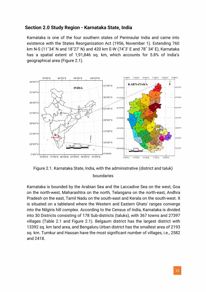
Section 2.0 Study Region - Karnataka State, India
Karnataka is one of the four southern states of Peninsular India and came into
existence with the States Reorganization Act (1956, November 1). Extending 760
km N-S (11˚34’ N and 18˚27’ N) and 420 km E-W (74˚3’ E and 78˚ 34’ E), Karnataka
has a spatial extent of 1,91,846 sq. km, which accounts for 5.8% of India’s
geographical area (Figure 2.1).
Figure 2.1. Karnataka State, India, with the administrative (district and taluk)
boundaries
Karnataka is bounded by the Arabian Sea and the Laccadive Sea on the west, Goa
on the north-west, Maharashtra on the north, Telangana on the north-east, Andhra
Pradesh on the east, Tamil Nadu on the south-east and Kerala on the south-west. It
is situated on a tableland where the Western and Eastern Ghats' ranges converge
into the Nilgiris hill complex. According to the Census of India, Karnataka is divided
into 30 Districts consisting of 178 Sub-districts (taluks), with 367 towns and 27397
villages (Table 2.1 and Figure 2.1). Belgaum district has the largest district with
13392 sq. km land area, and Bengaluru Urban district has the smallest area of 2193
sq. km. Tumkur and Hassan have the most significant number of villages, i.e., 2582
and 2418.
16
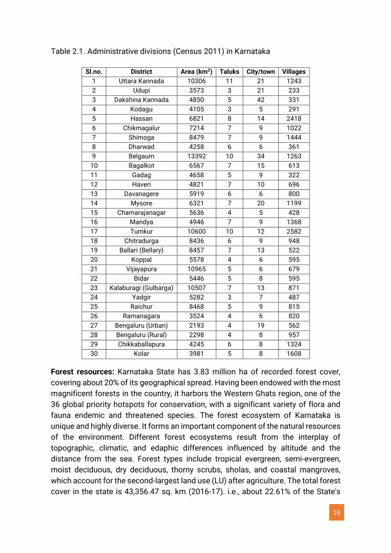
Table 2.1. Administrative divisions (Census 2011) in Karnataka
Sl.no. District Area (km2) Taluks City/town Villages
1 Uttara Kannada 10306 11 21 1243
2 Udupi 3573 3 21 233
3 Dakshina Kannada 4850 5 42 331
4 Kodagu 4105 3 5 291
5 Hassan 6821 8 14 2418
6 Chikmagalur 7214 7 9 1022
7 Shimoga 8479 7 9 1444
8 Dharwad 4258 6 6 361
9 Belgaum 13392 10 34 1263
10 Bagalkot 6567 7 15 613
11 Gadag 4658 5 9 322
12 Haveri 4821 7 10 696
13 Davanagere 5919 6 6 800
14 Mysore 6321 7 20 1199
15 Chamarajanagar 5636 4 5 428
16 Mandya 4946 7 9 1368
17 Tumkur 10600 10 12 2582
18 Chitradurga 8436 6 9 948
19 Ballari (Bellary) 8457 7 13 522
20 Koppal 5578 4 6 595
21 Vijayapura 10965 5 6 679
22 Bidar 5446 5 8 595
23 Kalaburagi (Gulbarga) 10507 7 13 871
24 Yadgir 5282 3 7 487
25 Raichur 8468 5 9 815
26 Ramanagara 3524 4 6 820
27 Bengaluru (Urban) 2193 4 19 562
28 Bengaluru (Rural) 2298 4 8 957
29 Chikkaballapura 4245 6 8 1324
30 Kolar 3981 5 8 1608
Forest resources: Karnataka State has 3.83 million ha of recorded forest cover,
covering about 20% of its geographical spread. Having been endowed with the most
magnificent forests in the country, it harbors the Western Ghats region, one of the
36 global priority hotspots for conservation, with a significant variety of flora and
fauna endemic and threatened species. The forest ecosystem of Karnataka is
unique and highly diverse. It forms an important component of the natural resources
of the environment. Different forest ecosystems result from the interplay of
topographic, climatic, and edaphic differences influenced by altitude and the
distance from the sea. Forest types include tropical evergreen, semi-evergreen,
moist deciduous, dry deciduous, thorny scrubs, sholas, and coastal mangroves,
which account for the second-largest land use (LU) after agriculture. The total forest
cover in the state is 43,356.47 sq. km (2016-17). i.e., about 22.61% of the State's
17
1 One lakh is equal to a hundred thousand. 2 One crore is equal to ten million, or one hundred lakhs
geographical area is under forest cover. Of the total forests, reserve forest
constitutes 15.48%, protected forest constitutes 1.85%, village forest constitutes
0.03%, unclassified forest constitutes 5.23% and private forest constitutes 0.03%.
Forest resources in the State are under severe pressure, with a drastic fall in dense
forest cover areas between 2001 and 2015. The state's forest cover has slightly
declined compared to the country's forest cover during the period. Increased
deforestation and degradation of the environmental resources have severe
implications for the ecosystem's production and resilience. The loss of forest cover
is a serious threat to the environment, sustainable development, and the livelihoods
of millions of people in the state. Forest resources significantly contribute to the
State's GDP by being a major source of timber, medicinal plants, non-timber forest
products (NTFPs), grazing, recreational activities, carbon sequestration, watershed
provisions, etc. The state has formed 4467 Biodiversity Management Committees
at the Grama Panchayat level as per the Biological Diversity Act of 2002 (BDA 2002,
Government of India) to protect and monitor biodiversity. Biodiversity heritage sites
(such as the 400-year-old tamarind grove at Nallur, Devanahalli taluk) are being
protected to conserve and develop unique genetic biodiversity.
Karnataka has a repository of rich biodiversity with more than 1.2 lakh1 known
species, including 4,500 flowering plants, 800 fishes, 600 birds, 160 reptiles, 120
mammals, and 1,493 medicinal plants. Fifty percent of the Western Ghats’
biodiversity is present in Karnataka. These forests support a wide range of flora and
fauna (biodiversity) through a network of well-connected and protected Wildlife
Sanctuaries and National Parks. The State has five national parks and 30 wildlife
sanctuaries covering an area of 9,586.02 km square. Apart from the national parks
and sanctuaries, the State has 15 conservation reserves and one community reserve
comprising 652.369 km square. All these areas form 23.59% of the total forest area.
These are spread over evergreen to scrub forests, representing different
ecosystems with rare and endangered species of plants, animals, and birds. The
State has been active in formulating and implementing various programs to develop
forests and protect its natural environment. Among the Forest Department's
schemes concerning wildlife and national parks, long-term measures to mitigate
‘Man-Animal Conflict’ incurred an expenditure of 24.80%, Project Tiger 30.40%,
Integrated Development of Wildlife Habitats 2.47%, nature conservation activities
attracted 13.38% and Rs. 27.50 crores2 of total expenditure were incurred towards
voluntary rehabilitation of families from tiger reserves and national parks during
2016-17.
18
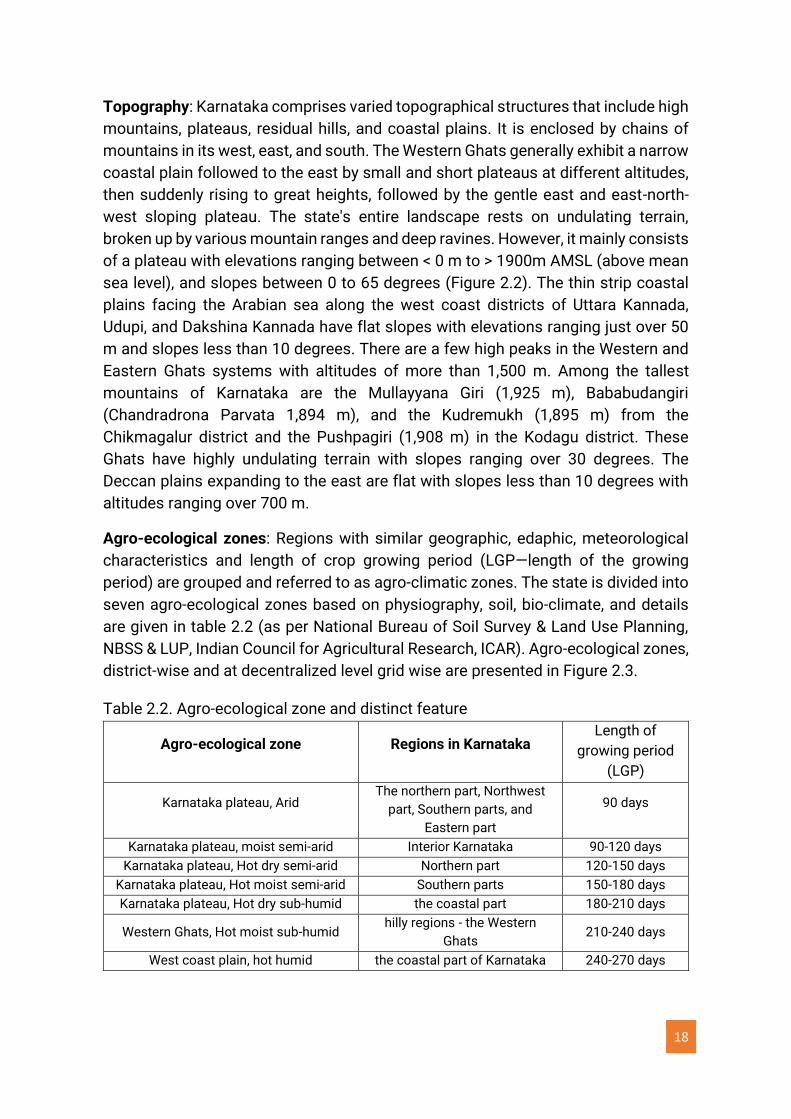
Topography: Karnataka comprises varied topographical structures that include high
mountains, plateaus, residual hills, and coastal plains. It is enclosed by chains of
mountains in its west, east, and south. The Western Ghats generally exhibit a narrow
coastal plain followed to the east by small and short plateaus at different altitudes,
then suddenly rising to great heights, followed by the gentle east and east-north-
west sloping plateau. The state's entire landscape rests on undulating terrain,
broken up by various mountain ranges and deep ravines. However, it mainly consists
of a plateau with elevations ranging between < 0 m to > 1900m AMSL (above mean
sea level), and slopes between 0 to 65 degrees (Figure 2.2). The thin strip coastal
plains facing the Arabian sea along the west coast districts of Uttara Kannada,
Udupi, and Dakshina Kannada have flat slopes with elevations ranging just over 50
m and slopes less than 10 degrees. There are a few high peaks in the Western and
Eastern Ghats systems with altitudes of more than 1,500 m. Among the tallest
mountains of Karnataka are the Mullayyana Giri (1,925 m), Bababudangiri
(Chandradrona Parvata 1,894 m), and the Kudremukh (1,895 m) from the
Chikmagalur district and the Pushpagiri (1,908 m) in the Kodagu district. These
Ghats have highly undulating terrain with slopes ranging over 30 degrees. The
Deccan plains expanding to the east are flat with slopes less than 10 degrees with
altitudes ranging over 700 m.
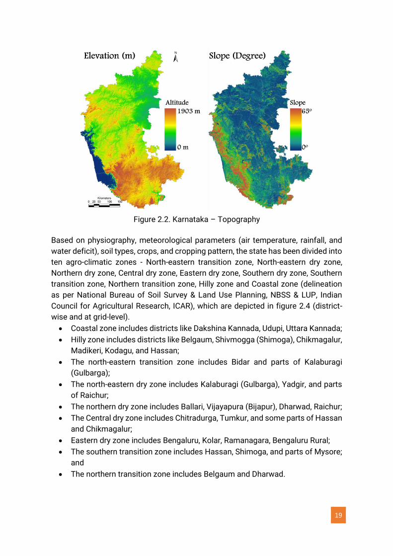
Agro-ecological zones: Regions with similar geographic, edaphic, meteorological
characteristics and length of crop growing period (LGP—length of the growing
period) are grouped and referred to as agro-climatic zones. The state is divided into
seven agro-ecological zones based on physiography, soil, bio-climate, and details
are given in table 2.2 (as per National Bureau of Soil Survey & Land Use Planning,
NBSS & LUP, Indian Council for Agricultural Research, ICAR). Agro-ecological zones,
district-wise and at decentralized level grid wise are presented in Figure 2.3.
Table 2.2. Agro-ecological zone and distinct feature
Agro-ecological zone Regions in Karnataka Length of
growing period
(LGP)
Karnataka plateau, Arid The northern part, Northwest
part, Southern parts, and
Eastern part
90 days
Karnataka plateau, moist semi-arid Interior Karnataka 90-120 days
Karnataka plateau, Hot dry semi-arid Northern part 120-150 days
Karnataka plateau, Hot moist semi-arid Southern parts 150-180 days
Karnataka plateau, Hot dry sub-humid the coastal part 180-210 days
Western Ghats, Hot moist sub-humid hilly regions - the Western
Ghats 210-240 days
West coast plain, hot humid the coastal part of Karnataka 240-270 days
19
Figure 2.2. Karnataka – Topography
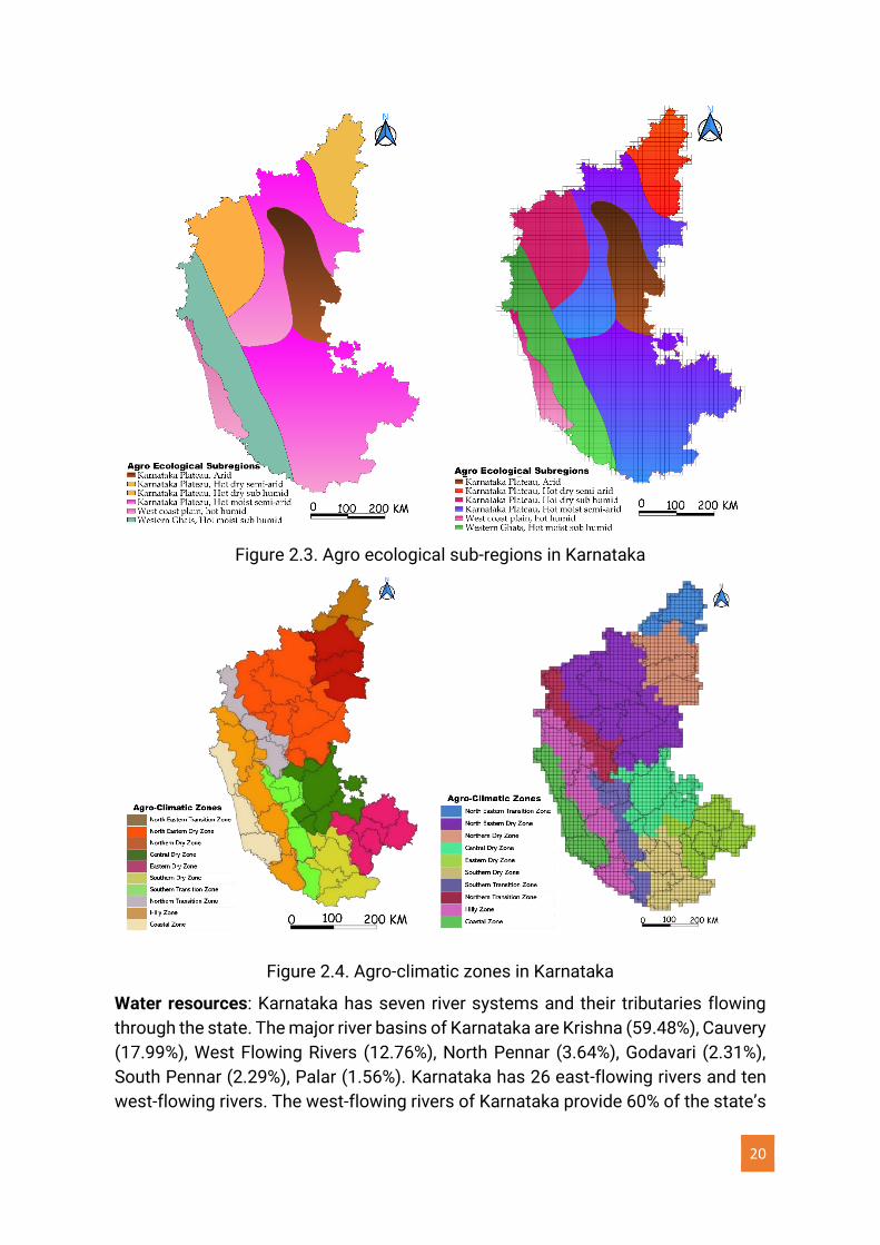
Based on physiography, meteorological parameters (air temperature, rainfall, and
water deficit), soil types, crops, and cropping pattern, the state has been divided into
ten agro-climatic zones - North-eastern transition zone, North-eastern dry zone,
Northern dry zone, Central dry zone, Eastern dry zone, Southern dry zone, Southern
transition zone, Northern transition zone, Hilly zone and Coastal zone (delineation
as per National Bureau of Soil Survey & Land Use Planning, NBSS & LUP, Indian
Council for Agricultural Research, ICAR), which are depicted in figure 2.4 (district-
wise and at grid-level).
• Coastal zone includes districts like Dakshina Kannada, Udupi, Uttara Kannada;
• Hilly zone includes districts like Belgaum, Shivmogga (Shimoga), Chikmagalur,
Madikeri, Kodagu, and Hassan;
• The north-eastern transition zone includes Bidar and parts of Kalaburagi
(Gulbarga);
• The north-eastern dry zone includes Kalaburagi (Gulbarga), Yadgir, and parts
of Raichur;
• The northern dry zone includes Ballari, Vijayapura (Bijapur), Dharwad, Raichur;
• The Central dry zone includes Chitradurga, Tumkur, and some parts of Hassan
and Chikmagalur;
• Eastern dry zone includes Bengaluru, Kolar, Ramanagara, Bengaluru Rural;
• The southern transition zone includes Hassan, Shimoga, and parts of Mysore;
and
• The northern transition zone includes Belgaum and Dharwad.
20
Figure 2.3. Agro ecological sub-regions in Karnataka
Figure 2.4. Agro-climatic zones in Karnataka
Water resources: Karnataka has seven river systems and their tributaries flowing
through the state. The major river basins of Karnataka are Krishna (59.48%), Cauvery
(17.99%), West Flowing Rivers (12.76%), North Pennar (3.64%), Godavari (2.31%),
South Pennar (2.29%), Palar (1.56%). Karnataka has 26 east-flowing rivers and ten
west-flowing rivers. The west-flowing rivers of Karnataka provide 60% of the state’s
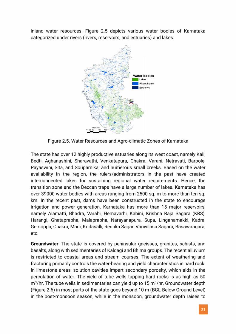
21
inland water resources. Figure 2.5 depicts various water bodies of Karnataka
categorized under rivers (rivers, reservoirs, and estuaries) and lakes.
Figure 2.5. Water Resources and Agro-climatic Zones of Karnataka
The state has over 12 highly productive estuaries along its west coast, namely Kali,
Bedti, Aghanashini, Sharavathi, Venkatapura, Chakra, Varahi, Netravati, Barpole,
Payaswini, Sita, and Souparnika, and numerous small creeks. Based on the water
availability in the region, the rulers/administrators in the past have created
interconnected lakes for sustaining regional water requirements. Hence, the
transition zone and the Deccan traps have a large number of lakes. Karnataka has
over 39000 water bodies with areas ranging from 2500 sq. m to more than ten sq.
km. In the recent past, dams have been constructed in the state to encourage
irrigation and power generation. Karnataka has more than 15 major reservoirs,
namely Alamatti, Bhadra, Varahi, Hemavarhi, Kabini, Krishna Raja Sagara (KRS),
Harangi, Ghataprabha, Malaprabha, Narayanapura, Supa, Linganamakki, Kadra,
Gersoppa, Chakra, Mani, Kodasalli, Renuka Sagar, Vanivilasa Sagara, Basavaragara,
etc.
Groundwater: The state is covered by peninsular gneisses, granites, schists, and
basalts, along with sedimentaries of Kaldagi and Bhima groups. The recent alluvium
is restricted to coastal areas and stream courses. The extent of weathering and
fracturing primarily controls the water-bearing and yield characteristics in hard rock.
In limestone areas, solution cavities impart secondary porosity, which aids in the
percolation of water. The yield of tube wells tapping hard rocks is as high as 50
m3/hr. The tube wells in sedimentaries can yield up to 15 m3/hr. Groundwater depth
(Figure 2.6) in most parts of the state goes beyond 10 m (BGL-Below Ground Level)
in the post-monsoon season, while in the monsoon, groundwater depth raises to
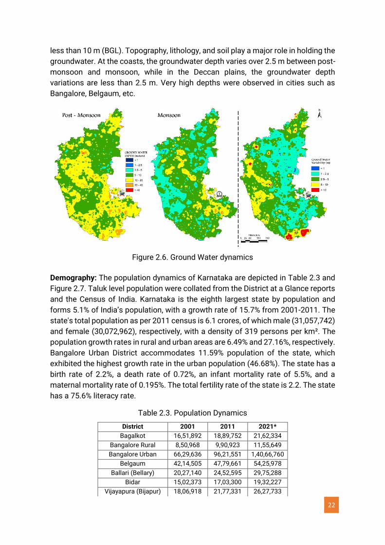
22
less than 10 m (BGL). Topography, lithology, and soil play a major role in holding the
groundwater. At the coasts, the groundwater depth varies over 2.5 m between post-
monsoon and monsoon, while in the Deccan plains, the groundwater depth
variations are less than 2.5 m. Very high depths were observed in cities such as
Bangalore, Belgaum, etc.
Figure 2.6. Ground Water dynamics
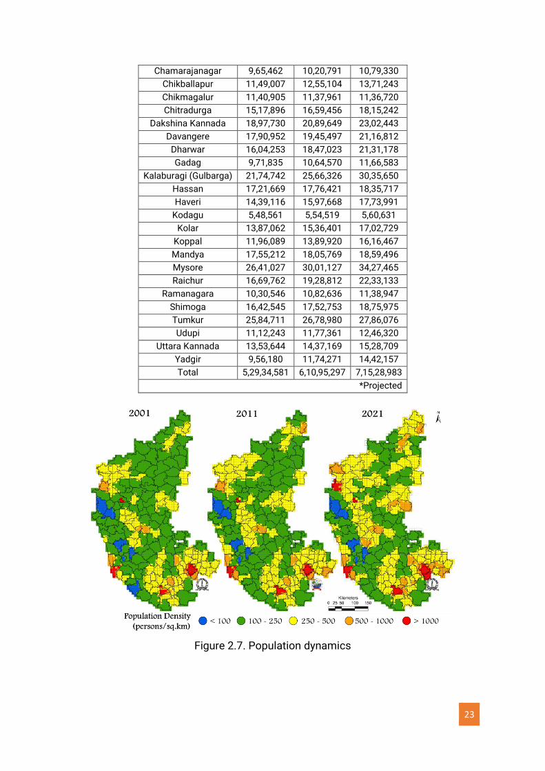
Demography: The population dynamics of Karnataka are depicted in Table 2.3 and
Figure 2.7. Taluk level population were collated from the District at a Glance reports
and the Census of India. Karnataka is the eighth largest state by population and
forms 5.1% of India’s population, with a growth rate of 15.7% from 2001-2011. The
state's total population as per 2011 census is 6.1 crores, of which male (31,057,742)
and female (30,072,962), respectively, with a density of 319 persons per km². The
population growth rates in rural and urban areas are 6.49% and 27.16%, respectively.
Bangalore Urban District accommodates 11.59% population of the state, which
exhibited the highest growth rate in the urban population (46.68%). The state has a
birth rate of 2.2%, a death rate of 0.72%, an infant mortality rate of 5.5%, and a
maternal mortality rate of 0.195%. The total fertility rate of the state is 2.2. The state
has a 75.6% literacy rate.
Table 2.3. Population Dynamics
District 2001 2011 2021*
Bagalkot 16,51,892 18,89,752 21,62,334
Bangalore Rural 8,50,968 9,90,923 11,55,649
Bangalore Urban 66,29,636 96,21,551 1,40,66,760
Belgaum 42,14,505 47,79,661 54,25,978
Ballari (Bellary) 20,27,140 24,52,595 29,75,288
Bidar 15,02,373 17,03,300 19,32,227
Vijayapura (Bijapur) 18,06,918 21,77,331 26,27,733
23
Chamarajanagar 9,65,462 10,20,791 10,79,330
Chikballapur 11,49,007 12,55,104 13,71,243
Chikmagalur 11,40,905 11,37,961 11,36,720
Chitradurga 15,17,896 16,59,456 18,15,242
Dakshina Kannada 18,97,730 20,89,649 23,02,443
Davangere 17,90,952 19,45,497 21,16,812
Dharwar 16,04,253 18,47,023 21,31,178
Gadag 9,71,835 10,64,570 11,66,583
Kalaburagi (Gulbarga) 21,74,742 25,66,326 30,35,650
Hassan 17,21,669 17,76,421 18,35,717
Haveri 14,39,116 15,97,668 17,73,991
Kodagu 5,48,561 5,54,519 5,60,631
Kolar 13,87,062 15,36,401 17,02,729
Koppal 11,96,089 13,89,920 16,16,467
Mandya 17,55,212 18,05,769 18,59,496
Mysore 26,41,027 30,01,127 34,27,465
Raichur 16,69,762 19,28,812 22,33,133
Ramanagara 10,30,546 10,82,636 11,38,947
Shimoga 16,42,545 17,52,753 18,75,975
Tumkur 25,84,711 26,78,980 27,86,076
Udupi 11,12,243 11,77,361 12,46,320
Uttara Kannada 13,53,644 14,37,169 15,28,709
Yadgir 9,56,180 11,74,271 14,42,157
Total 5,29,34,581 6,10,95,297 7,15,28,983
*Projected
Figure 2.7. Population dynamics
24
Section 3.0 Data
Ecosystem extent account: An important foundation for estimating ecosystem
services is the ecosystem extent account (Ramachandra et al., 2021a). Table 3.1 lists
the spatial data used for assessing the spatial extent of ecosystems in Karnataka.
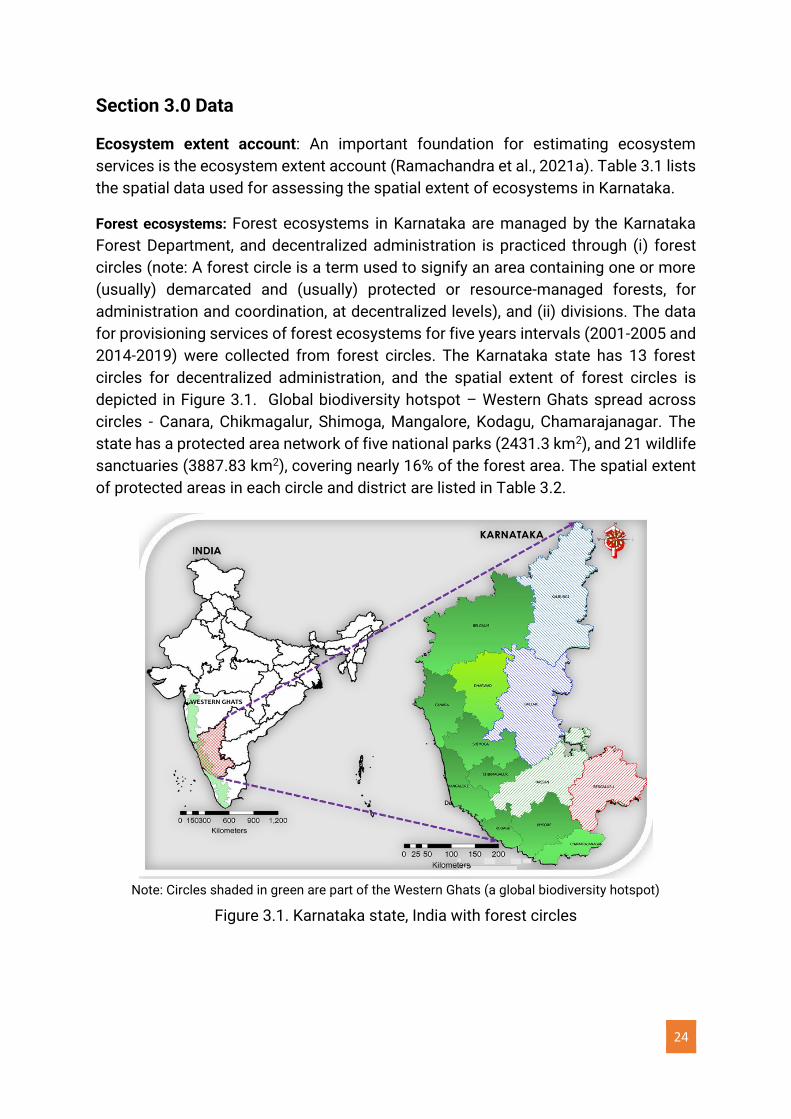
Forest ecosystems: Forest ecosystems in Karnataka are managed by the Karnataka
Forest Department, and decentralized administration is practiced through (i) forest
circles (note: A forest circle is a term used to signify an area containing one or more
(usually) demarcated and (usually) protected or resource-managed forests, for
administration and coordination, at decentralized levels), and (ii) divisions. The data
for provisioning services of forest ecosystems for five years intervals (2001-2005 and
2014-2019) were collected from forest circles. The Karnataka state has 13 forest
circles for decentralized administration, and the spatial extent of forest circles is
depicted in Figure 3.1. Global biodiversity hotspot – Western Ghats spread across
circles - Canara, Chikmagalur, Shimoga, Mangalore, Kodagu, Chamarajanagar. The
state has a protected area network of five national parks (2431.3 km2), and 21 wildlife
sanctuaries (3887.83 km2), covering nearly 16% of the forest area. The spatial extent
of protected areas in each circle and district are listed in Table 3.2.
Note: Circles shaded in green are part of the Western Ghats (a global biodiversity hotspot)
Figure 3.1. Karnataka state, India with forest circles
25
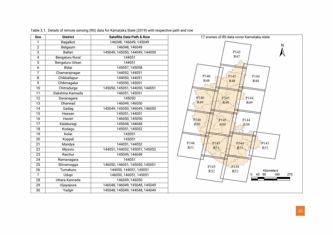
Table 3.1. Details of remote sensing (RS) data for Karnataka State (2019) with respective path and row
Sno District Satellite Data Path & Row 17 scenes of RS data cover Karnataka state
1 Bagalkot 146048, 146049, 145049
2 Belgaum 146048, 146049
3 Ballari 145049, 145050, 144049, 144050
4 Bengaluru Rural 144051
5 Bengaluru Urban 144051
6 Bidar 145057, 145058
7 Chamarajnagar 144052, 144051
8 Chikballapur 144050, 144051
9 Chikmagalur 145050, 145051
10 Chitradurga 145050, 145051, 144050, 144051
11 Dakshina Kannada 146051, 145051
12 Davanagere 145050
13 Dharwad 146049, 146050
14 Gadag 145049, 145050, 146049, 146050
15 Hassan 145051, 144051
16 Haveri 146050, 145050
17 Kalaburagi 145048, 144048
18 Kodagu 145051, 145052
19 Kolar 143051
20 Koppal 145051
21 Mandya 144051, 144052
22 Mysuru 144051, 144052, 145051, 145052
23 Raichur 145049, 144049
24 Ramanagara 144051
25 Shivamogga 146050, 146051, 145050, 145051
26 Tumakuru 144050, 144051, 145051
7 Udupi 146050, 146051, 145051
28 Uttara Kannada 146049, 146050
29 Vijayapura 146048, 146049, 145048, 145049
30 Yadgir 145048, 145049, 144048, 144049
26
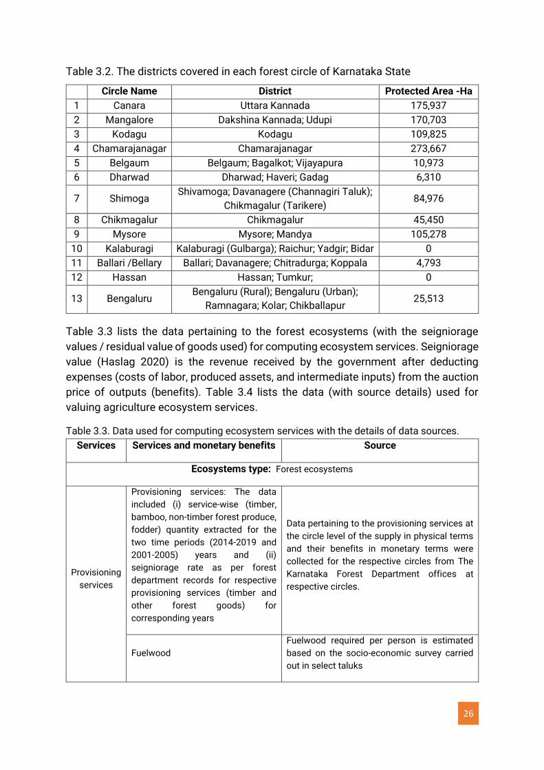
Table 3.2. The districts covered in each forest circle of Karnataka State
Circle Name District Protected Area -Ha
1 Canara Uttara Kannada 175,937
2 Mangalore Dakshina Kannada; Udupi 170,703
3 Kodagu Kodagu 109,825
4 Chamarajanagar Chamarajanagar 273,667
5 Belgaum Belgaum; Bagalkot; Vijayapura 10,973
6 Dharwad Dharwad; Haveri; Gadag 6,310
7 Shimoga Shivamoga; Davanagere (Channagiri Taluk);
Chikmagalur (Tarikere) 84,976
8 Chikmagalur Chikmagalur 45,450
9 Mysore Mysore; Mandya 105,278
10 Kalaburagi Kalaburagi (Gulbarga); Raichur; Yadgir; Bidar 0
11 Ballari /Bellary Ballari; Davanagere; Chitradurga; Koppala 4,793
12 Hassan Hassan; Tumkur; 0
13 Bengaluru Bengaluru (Rural); Bengaluru (Urban);
Ramnagara; Kolar; Chikballapur 25,513
Table 3.3 lists the data pertaining to the forest ecosystems (with the seigniorage
values / residual value of goods used) for computing ecosystem services. Seigniorage
value (Haslag 2020) is the revenue received by the government after deducting
expenses (costs of labor, produced assets, and intermediate inputs) from the auction
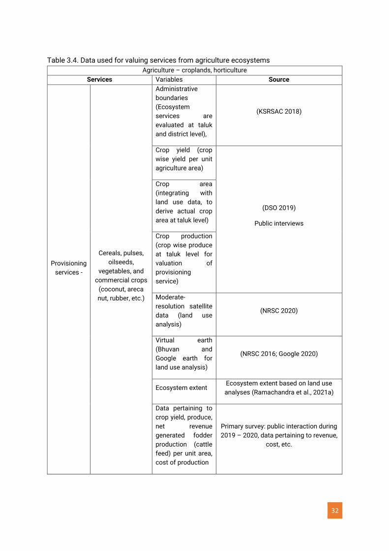
price of outputs (benefits). Table 3.4 lists the data (with source details) used for
valuing agriculture ecosystem services.
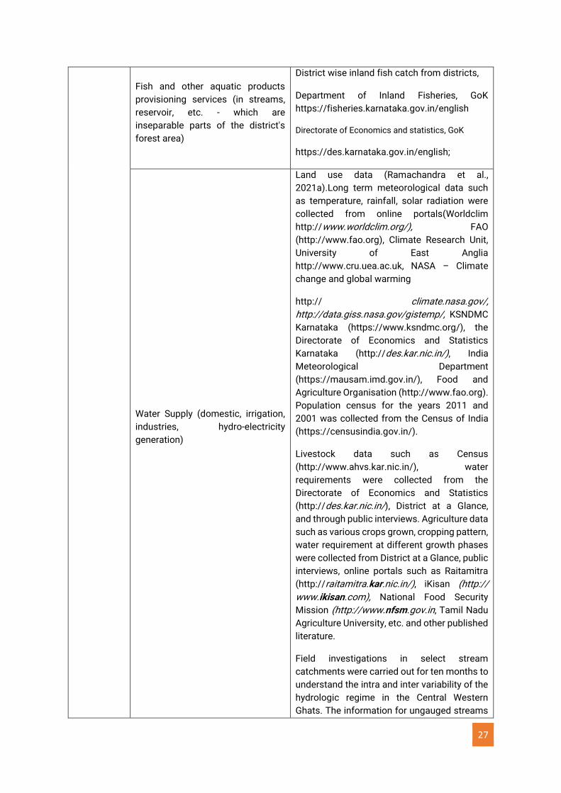
Table 3.3. Data used for computing ecosystem services with the details of data sources.
Services Services and monetary benefits Source
Ecosystems type: Forest ecosystems
Provisioning
services
Provisioning services: The data
included (i) service-wise (timber,
bamboo, non-timber forest produce,
fodder) quantity extracted for the
two time periods (2014-2019 and
2001-2005) years and (ii)
seigniorage rate as per forest
department records for respective
provisioning services (timber and
other forest goods) for
corresponding years
Data pertaining to the provisioning services at
the circle level of the supply in physical terms
and their benefits in monetary terms were
collected for the respective circles from The
Karnataka Forest Department offices at
respective circles.
Fuelwood
Fuelwood required per person is estimated
based on the socio-economic survey carried
out in select taluks
27
Fish and other aquatic products
provisioning services (in streams,
reservoir, etc. - which are
inseparable parts of the district's
forest area)
District wise inland fish catch from districts,
Department of Inland Fisheries, GoK https://fisheries.karnataka.gov.in/english
Directorate of Economics and statistics, GoK
https://des.karnataka.gov.in/english;
Water Supply (domestic, irrigation,
industries, hydro-electricity
generation)
Land use data (Ramachandra et al.,
2021a).Long term meteorological data such
as temperature, rainfall, solar radiation were
collected from online portals(Worldclim
http://www.worldclim.org/), FAO
(http://www.fao.org), Climate Research Unit,
University of East Anglia
http://www.cru.uea.ac.uk, NASA – Climate
change and global warming
http:// climate.nasa.gov/,
http://data.giss.nasa.gov/gistemp/, KSNDMC
Karnataka (https://www.ksndmc.org/), the
Directorate of Economics and Statistics
Karnataka (http://des.kar.nic.in/), India
Meteorological Department
(https://mausam.imd.gov.in/), Food and
Agriculture Organisation (http://www.fao.org).
Population census for the years 2011 and
2001 was collected from the Census of India
(https://censusindia.gov.in/).
Livestock data such as Census
(http://www.ahvs.kar.nic.in/), water
requirements were collected from the
Directorate of Economics and Statistics
(http://des.kar.nic.in/), District at a Glance,
and through public interviews. Agriculture data
such as various crops grown, cropping pattern,
water requirement at different growth phases
were collected from District at a Glance, public
interviews, online portals such as Raitamitra
(http://raitamitra.kar.nic.in/), iKisan (http://
www.ikisan.com), National Food Security
Mission (http://www.nfsm.gov.in, Tamil Nadu
Agriculture University, etc. and other published
literature.
Field investigations in select stream
catchments were carried out for ten months to
understand the intra and inter variability of the
hydrologic regime in the Central Western
Ghats. The information for ungauged streams
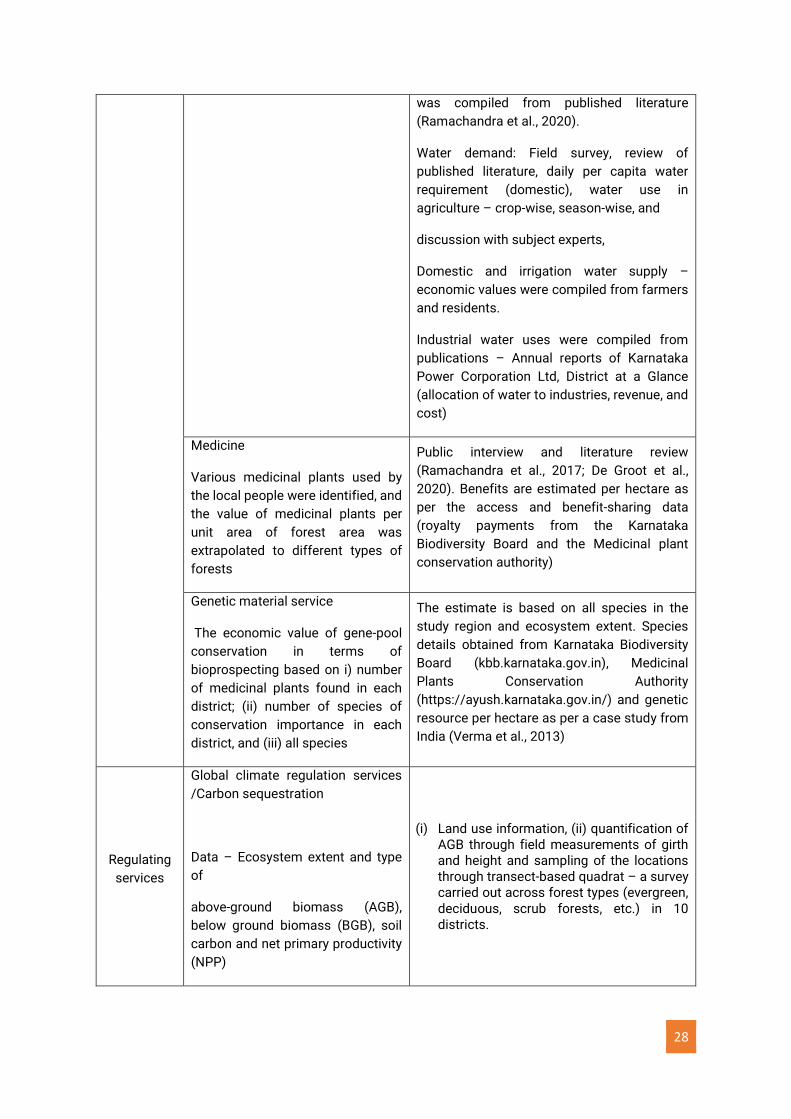
28
was compiled from published literature
(Ramachandra et al., 2020).
Water demand: Field survey, review of
published literature, daily per capita water
requirement (domestic), water use in
agriculture – crop-wise, season-wise, and
discussion with subject experts,
Domestic and irrigation water supply –
economic values were compiled from farmers
and residents.
Industrial water uses were compiled from
publications – Annual reports of Karnataka
Power Corporation Ltd, District at a Glance
(allocation of water to industries, revenue, and
cost)
Medicine
Various medicinal plants used by
the local people were identified, and
the value of medicinal plants per
unit area of forest area was
extrapolated to different types of
forests
Public interview and literature review
(Ramachandra et al., 2017; De Groot et al.,
2020). Benefits are estimated per hectare as
per the access and benefit-sharing data
(royalty payments from the Karnataka
Biodiversity Board and the Medicinal plant
conservation authority)
Genetic material service
The economic value of gene-pool
conservation in terms of
bioprospecting based on i) number
of medicinal plants found in each
district; (ii) number of species of
conservation importance in each
district, and (iii) all species
The estimate is based on all species in the
study region and ecosystem extent. Species
details obtained from Karnataka Biodiversity
Board (kbb.karnataka.gov.in), Medicinal
Plants Conservation Authority
(https://ayush.karnataka.gov.in/) and genetic
resource per hectare as per a case study from
India (Verma et al., 2013)
Regulating
services
Global climate regulation services
/Carbon sequestration
Data – Ecosystem extent and type
of
above-ground biomass (AGB),
below ground biomass (BGB), soil
carbon and net primary productivity
(NPP)
(i) Land use information, (ii) quantification of AGB through field measurements of girth and height and sampling of the locations through transect-based quadrat – a survey carried out across forest types (evergreen, deciduous, scrub forests, etc.) in 10 districts.

29
Soil conservation and soil fertility –
Data: soil characteristics, land use
characteristics, vegetation
characteristics, farming practices,
topographic effects, etc
Annual rainfall, monthly rainfall,
quick flows, historical climate data
bioclimatic variables, long term
weather data, daily rainfall data
Ecosystem entent assessment (Ramachandra
et al., 2021a), Ecosystem condition -soil
(Ramachandra et al., 2021b; Ma et al., 2019),
IMD, GoI (https://mausam.imd.gov.in/), NASA
Portal (https://gpm.nasa.gov/data),
Worldclim (https://www.worldclim.org/),
KSNDMC (www.ksndmc.org)
Ground water recharge
Precipitation, overland flow,
infiltration, evapotranspiration,
maximum and minimum
temperature along with the solar
radiation
Overland flow (runoff) – field measurements –
four river basins in Uttara Kannada and two
river basins in Shimoga districts using a
current meter (water velocity measurement –
three consecutive days, monthly), IMD, GoI
(https://mausam.imd.gov.in/), NASA Portal
(https://gpm.nasa.gov/data), Worldclim
(https://www.worldclim.org/), KSNDMC
(www.ksndmc.org)
Water purification
Economic values of water purification and
waste treatment are estimated per hectare as
per a case study from India (Verma et al., 2013,
Ramachandra et al., 2017)
Pollination service
Ecosystem extent, and type.
Natural forest regeneration and
afforestation (replacement) cost
Ecosystem extent based on land use analyses
and literature (Ramachandra et al., 2021a).
Comparative assessment of natural
regeneration of forest patches (with fencing
protection from external pressures (Ray et al.,
2015) and afforestation cost. The estimates of
natural forest regeneration in all forest types
are adjusted according to the forest
regeneration in plantations (NAP 2009;
Ollerton et al., 2011; Hipólito et al., 2019)
Air filtration services – extent of
forest ecosystem
Air filtration regulation service
values per hectare is based on
published literature from India
(Ninan and Kontoleon, 2016, Joshi G
and Negi GCS, 2011)
Ecosystem extent based on land use analyses
(Ramachandra et al., 2021a) and
Air filtration regulation service values per
hectare based on published literature from
India (Ninan and Kontoleon, 2016, Joshi G and
Negi GCS, 2011) which are comparable to
global studies -– global ecosystem service
valuation database (ESVD) for tropical forests,
and mangroves.
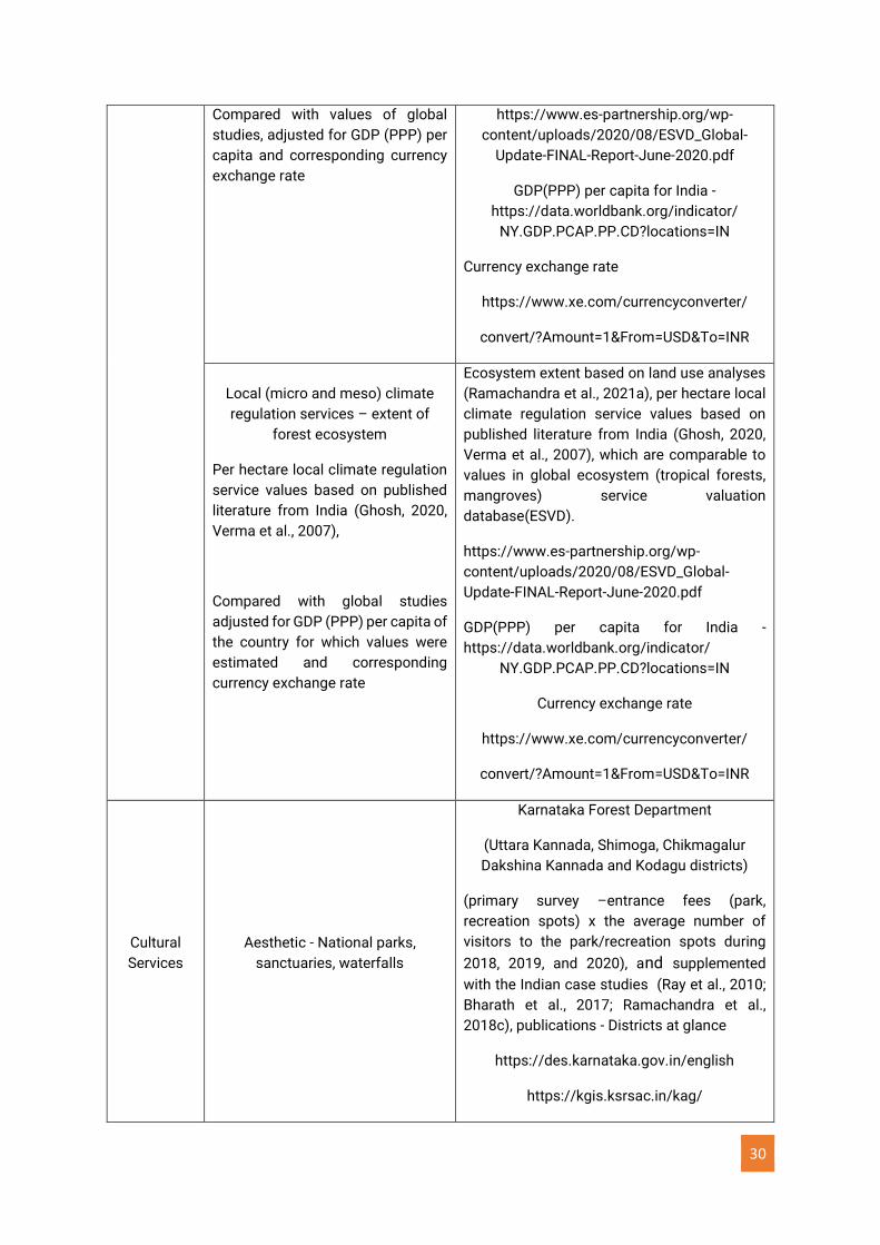
30
Compared with values of global
studies, adjusted for GDP (PPP) per
capita and corresponding currency
exchange rate
https://www.es-partnership.org/wp-
content/uploads/2020/08/ESVD_Global-
Update-FINAL-Report-June-2020.pdf
GDP(PPP) per capita for India -
https://data.worldbank.org/indicator/
NY.GDP.PCAP.PP.CD?locations=IN
Currency exchange rate
https://www.xe.com/currencyconverter/
convert/?Amount=1&From=USD&To=INR
Local (micro and meso) climate
regulation services – extent of
forest ecosystem
Per hectare local climate regulation
service values based on published
literature from India (Ghosh, 2020,
Verma et al., 2007),
Compared with global studies
adjusted for GDP (PPP) per capita of
the country for which values were
estimated and corresponding
currency exchange rate
Ecosystem extent based on land use analyses
(Ramachandra et al., 2021a), per hectare local
climate regulation service values based on
published literature from India (Ghosh, 2020,
Verma et al., 2007), which are comparable to
values in global ecosystem (tropical forests,
mangroves) service valuation
database(ESVD).
https://www.es-partnership.org/wp-
content/uploads/2020/08/ESVD_Global-
Update-FINAL-Report-June-2020.pdf
GDP(PPP) per capita for India -
https://data.worldbank.org/indicator/
NY.GDP.PCAP.PP.CD?locations=IN
Currency exchange rate
https://www.xe.com/currencyconverter/
convert/?Amount=1&From=USD&To=INR
Cultural
Services
Aesthetic - National parks,
sanctuaries, waterfalls
Karnataka Forest Department
(Uttara Kannada, Shimoga, Chikmagalur
Dakshina Kannada and Kodagu districts)
(primary survey –entrance fees (park,
recreation spots) x the average number of
visitors to the park/recreation spots during
2018, 2019, and 2020), and supplemented
with the Indian case studies (Ray et al., 2010;
Bharath et al., 2017; Ramachandra et al.,
2018c), publications - Districts at glance
https://des.karnataka.gov.in/english
https://kgis.ksrsac.in/kag/

31
Spiritual and Historic - Distribution
of sacred groves (relic forests -
protected due to belief and
customs)
Rituals are performed by devotees and the
amount is paid for performing rituals (either
visiting the grove or in absentia). Also, there is
a practice of donating money during birthday
celebrations or in the name of elders (or
departed soul). Data pertaining to the annual
collection and expenses were compiled from
the administrative / management committees
of select groves in Shimoga, Uttara Kannada,
and Kodagu districts. Residual method was
used (annual collection for rituals and
deducting costs – priest salary and ritual
expenses).
In groves, where annual collection details were
not available, the travel cost method is used
for valuation, considering the number of
visitors (visiting groves) for annual rituals,
festivals, and other religious activities. This is
done through primary surveys of select groves
in Uttara Kannada, Shimoga, and Kodagu
districts, and supplemented with case-studies
from India using the benefit transfer method
(Ramachandra et al., 2012; Ray et al., 2014b,
2015; Ramachandra et al., 2016, 2017, 2019a)
Tourism and recreational services
Travel cost method (primary survey – benefits
to travel operators, entrance fees (park,
recreation spots) x the average number of
visitors to the park during 2020) is used,
supplemented with the Indian case studies.
Benefit transfer method -(Ramachandra et al.,
2019b; Badola et al., 2017; Gunarekha and
Binoy 2017; Sinclair et al., 2020)
Education, science, and research
Researchers need to obtain prior permission
from the Forest Department to undertake
research (and long-term monitoring). Details
of the research, duration, project budget (for
field research) and research team were
compiled from the Karnataka Forest
Department.
This information is supplemented with the
data compilation through discussion with
researchers and relevant literature of field-
based research (ecology, medicinal plants,
etc.) (Chandran et al., 2010; Ray and
Ramachandra 2010; Gould et al., 2014; Ray et
al., 2014a; Dorji et al., 2019; Kreye et al., 2019).
32
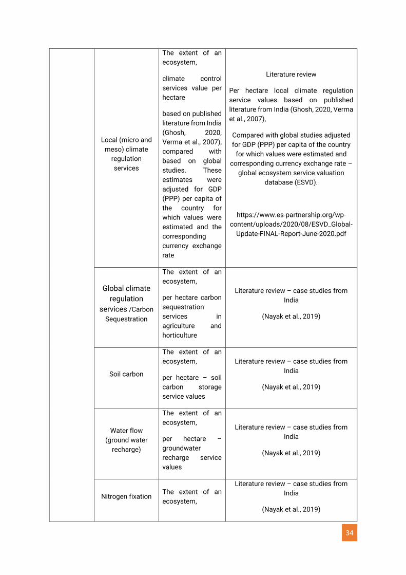
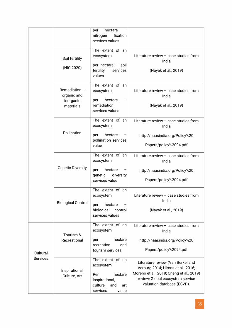
Table 3.4. Data used for valuing services from agriculture ecosystems
Agriculture – croplands, horticulture
Services Variables Source
Provisioning
services -
Cereals, pulses,
oilseeds,
vegetables, and
commercial crops
(coconut, areca
nut, rubber, etc.)
Administrative
boundaries
(Ecosystem
services are
evaluated at taluk
and district level),
(KSRSAC 2018)
Crop yield (crop
wise yield per unit
agriculture area)
(DSO 2019)
Public interviews
Crop area
(integrating with
land use data, to
derive actual crop
area at taluk level)
Crop production
(crop wise produce
at taluk level for
valuation of
provisioning
service)
Moderate-
resolution satellite
data (land use
analysis)
(NRSC 2020)
Virtual earth
(Bhuvan and
Google earth for
land use analysis)
(NRSC 2016; Google 2020)
Ecosystem extent Ecosystem extent based on land use
analyses (Ramachandra et al., 2021a)
Data pertaining to
crop yield, produce,
net revenue
generated fodder
production (cattle
feed) per unit area,
cost of production
Primary survey: public interaction during
2019 – 2020, data pertaining to revenue,
cost, etc.
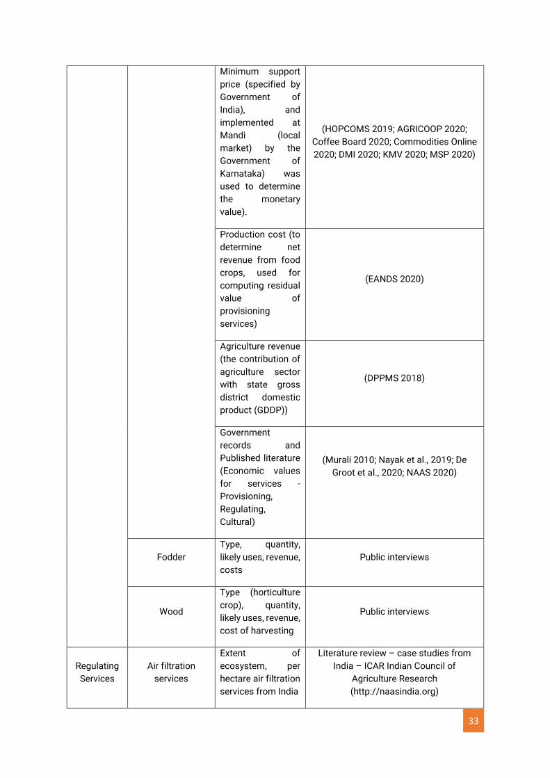
33
Minimum support
price (specified by
Government of
India), and
implemented at
Mandi (local
market) by the
Government of
Karnataka) was
used to determine
the monetary
value).
(HOPCOMS 2019; AGRICOOP 2020;
Coffee Board 2020; Commodities Online
2020; DMI 2020; KMV 2020; MSP 2020)
Production cost (to
determine net
revenue from food
crops, used for
computing residual
value of
provisioning
services)
(EANDS 2020)
Agriculture revenue
(the contribution of
agriculture sector
with state gross
district domestic
product (GDDP))
(DPPMS 2018)
Government
records and
Published literature
(Economic values
for services -
Provisioning,
Regulating,
Cultural)
(Murali 2010; Nayak et al., 2019; De
Groot et al., 2020; NAAS 2020)
Fodder
Type, quantity,
likely uses, revenue,
costs
Public interviews
Wood
Type (horticulture
crop), quantity,
likely uses, revenue,
cost of harvesting
Public interviews
Regulating
Services
Air filtration
services
Extent of
ecosystem, per
hectare air filtration
services from India
Literature review – case studies from
India – ICAR Indian Council of
Agriculture Research
(http://naasindia.org)
34
Local (micro and
meso) climate
regulation
services
The extent of an
ecosystem,
climate control
services value per
hectare
based on published
literature from India
(Ghosh, 2020,
Verma et al., 2007),
compared with
based on global
studies. These
estimates were
adjusted for GDP
(PPP) per capita of
the country for
which values were
estimated and the
corresponding
currency exchange
rate
Literature review
Per hectare local climate regulation
service values based on published
literature from India (Ghosh, 2020, Verma
et al., 2007),
Compared with global studies adjusted
for GDP (PPP) per capita of the country
for which values were estimated and
corresponding currency exchange rate –
global ecosystem service valuation
database (ESVD).
https://www.es-partnership.org/wp-
content/uploads/2020/08/ESVD_Global-
Update-FINAL-Report-June-2020.pdf
Global climate
regulation
services /Carbon
Sequestration
The extent of an
ecosystem,
per hectare carbon
sequestration
services in
agriculture and
horticulture
Literature review – case studies from
India
(Nayak et al., 2019)
Soil carbon
The extent of an
ecosystem,
per hectare – soil
carbon storage
service values
Literature review – case studies from
India
(Nayak et al., 2019)
Water flow
(ground water
recharge)
The extent of an
ecosystem,
per hectare –
groundwater
recharge service
values
Literature review – case studies from
India
(Nayak et al., 2019)
Nitrogen fixation The extent of an
ecosystem,
Literature review – case studies from
India
(Nayak et al., 2019)
35
per hectare –
nitrogen fixation
services values
Soil fertility
(NIC 2020)
The extent of an
ecosystem,
per hectare – soil
fertility services
values
Literature review – case studies from
India
(Nayak et al., 2019)
Remediation –
organic and
inorganic
materials
The extent of an
ecosystem,
per hectare –
remediation
services values
Literature review – case studies from
India
(Nayak et al., 2019)
Pollination
The extent of an
ecosystem,
per hectare –
pollination services
value
Literature review – case studies from
India
http://naasindia.org/Policy%20
Papers/policy%2094.pdf
Genetic Diversity
The extent of an
ecosystem,
per hectare –
genetic diversity
services value
Literature review – case studies from
India
http://naasindia.org/Policy%20
Papers/policy%2094.pdf
Biological Control
The extent of an
ecosystem,
per hectare –
biological control
services values
Literature review – case studies from
India
(Nayak et al., 2019)
Cultural
Services
Tourism &
Recreational
The extent of an
ecosystem,
per hectare
recreation and
tourism services
Literature review – case studies from
India
http://naasindia.org/Policy%20
Papers/policy%2094.pdf
Inspirational,
Culture, Art
The extent of an
ecosystem,
Per hectare
inspirational,
culture and art
services value
Literature review (Van Berkel and
Verburg 2014; Hirons et al., 2016;
Moreno et al., 2018; Cheng et al., 2019)
review; Global ecosystem service
valuation database (ESVD).
36
based on global
studies. These
estimates were
adjusted for GDP
(PPP) per capita of
the country for
which values were
estimated and the
corresponding
currency exchange
rate
https://www.es-partnership.org/wp-
content/uploads/2020/08/ESVD_Global-
Update-FINAL-Report-June-2020.pdf
GDP(PPP) per capita for India -
https://data.worldbank.org/indicator/
NY.GDP.PCAP.PP.CD?locations=IN
Currency exchange rate
https://www.xe.com/currencyconverter/
convert/?Amount=1&From=USD&To=INR
Note: Annexures 3.1, and 3.2 provide the questionnaires used for data
compilation (crop yield, cost, revenue) through public interviews for agriculture
(cropland and horticulture) ecosystems.
Annexures 3.3 and 3.4 provide the details of the data collected from the surveyed
sacred groves and tourism locations.
37
Section 4.0 Method
Ecosystem services are accounted for through the (i) residual value method, (ii)
benefit transfer method, and (iii) biophysical models- InVEST, depending on the
availability of data and time constraints.
Residual value method: Provisioning services of ecosystems are accounted for
through the residual value (or resource rent) method. The residual value method has
been used to estimate a value for an ecosystem service by taking the gross value of
the final marketed good (to which the ecosystem service provides input) and then
deducting the cost of all non-ecosystem inputs, including labour, produced assets and
intermediate inputs (as per SEEA Central Framework, given below).
Net return on environmental assets = resource rent - depletion
Resource rent = gross operating surplus - consumption of fixed capital
(depreciation) - return on produced assets - labour of self-employed persons
Gross operating surplus = Output - intermediate consumption - compensation of
employees - other taxes on production + other subsidies on production
Economic rent is the surplus value accruing to the extractor or user of an asset
calculated after all costs, and normal returns have been considered. The measure of
resource rent (i.e., surplus-value of environmental assets) provides a gross measure
of the returns to the environmental asset as a direct capital value, giving a reasonable
approximation of the market price of the service.
The benefit transfer method or unit value transfer refers to applying economic value
estimates from one location to a similar site in another place. Values for ecosystem
services at a study site, expressed as a value per unit (usually per unit of area or
beneficiary), combined with information on the number of units at the policy site, are
used to estimate policy site values. Unit values from the study site are multiplied by
the number of units at the policy site. When using the benefit transfer method, unit
values are adjusted to reflect differences between the study and policy sites. In this
report, ecosystem services values are based on case studies from India, which are
compared with the global ecosystem service valuation database (ESVD)
[https://www.es-partnership.org/wp-content/uploads/2020/08/ESVD_Global-Update-FINAL-
Report-June-2020.pdf] and published literature (of case studies from India) considering
GDP (PPP) per capita for India (https://data.worldbank.org/indicator/NY.GDP.PCAP. PP.
CD? locations=IN) and the currency exchange rate (https://www.xe.com/ currencyconverter/
convert/?Amount=1&From=USD&To =INR).
InVEST: InVEST (Integrated Valuation of Ecosystem Services and Trade-offs) is a
suite of models used to map and value ecosystem services. It helps explore how
38
changes in ecosystems can lead to changes in the flows of many different benefits
to people. InVEST returns results in either biophysical terms (e.g., tons of carbon
sequestered) or economic terms (e.g., the net present value of that sequestered
carbon). InVEST (https://naturalcapitalproject.stanford.edu/software/invest) models
are spatially explicit, using maps as information sources and producing maps as
outputs.
4.1 Valuation of forest ecosystem services
Provisioning services from forest ecosystem: The provisioning services derived from
the forests in this report include:
• Timber: Forests are the prime source of timber for the local people. Timber includes
wood for making furniture, agricultural implements, fencing wood and wood poles, and
planks for roofs. Timber provides revenue and constitutes an essential component of
value on forest land properties. Timber is a readily available goods, which has a
marketable value from the forests. However, strict rules and regulations are in
operation from the State Government to extract timber from the protected forests.
In many cases, the value of the timber can be several times the value of the land.
Timber includes rosewood, teak wood, jungle wood, etc. Timber is mainly prominent
in deciduous forests, while it is found in less amount in evergreen forest patches.
Plantation forests primarily consist of timber-producing trees like acacia, teak, etc.
Forest-based industries depend on the produce from the forest, which includes round
wood, softwood, matchwood, etc. The data regarding the quantity of timber harvested
and seigniorage values (residual value) were obtained from the Karnataka Forest
Department. As per the Karnataka Forest Department records, the seigniorage values
remain the same for all provisioning services for 2005 and 2019.
▪ The ecosystem supply value of Rosewood is 140,017 Rs/Ha/yr (2005) and
140,998 Rs/Ha/yr (2019) based on the data collected across the circles from
Karnataka Forest Department.
▪ Teakwood is 79,881 Rs/Ha/yr (2005) and 79,961 Rs/Ha/yr (2019).
▪ Eucalyptus wood is 4,304, and 4,265 Rs/Ha/yr for 2005, 2019 respectively.
▪ Other kinds of timber are 4,644 and 4,297 Rs/Ha/yr for 2005, 2019.
▪ Pulpwood is 3,369 Rs/Ha/yr (2005) and 3381Rs/Ha/yr (2019).
▪ Round poles wood is assessed as 4,434, and 4,261 Rs/Ha/yr for 2005, and
2019.
▪ Sandalwood is accounted as 4,573, and 4,652 Rs/Ha/yr for 2005, and 2019
respectively.
▪ Bamboo for the Karnataka state is assessed as 3,938, and 4,402 Rs/Ha/yr for
2005 and 2019.
• Fuelwood: Fuelwood is the most important forest product in Karnataka. Fuelwood is
the energy source for cooking in most parts of rural India, and 50% of the total
fuelwood consumed comes from the forests. The yield of fuelwood depends on the
39
ease of access to the forests. The total value of fuelwood includes the value of
fuelwood used for domestic purposes, i.e., for cooking and water heating, and also the
fuelwood used for various industrial and commercial purposes like jaggery making,
areca processing, cashew processing, restaurants, and bakery, parboiling, cremation,
etc. Local people collect fallen wood/dry tree branches from the forests. An
exploratory survey focusing on fuelwood requirements was initially conducted in
various taluks of the agro-climatic zones and through a review of literature based on
our earlier work (Ramachandra et al., 2000d). Socio-economic and energy data was
collected from randomly selected samples in the Sirsi, Siddapur, Kumta, and Ankola
taluks of Uttara Kannada district. The fuelwood required for various other purposes
(large scale jaggery making, drying of agro products such as cardamom, etc.) were
based on field experiments (Ramachandra et al., 2000c, 2017; Ramachandra and
Bharath 2019a). The preliminary results of the survey in households using fuel-
efficient stoves in the Sirsi and Kumta taluks showed fuelwood requirements for
cooking (kg/person/day) to be 1.80 and 1.78 (summer) and 2.25 and 1.98 (monsoon),
respectively. Villagers are permitted to collect fuelwood from the nearby forests, and
the collection fee is collected by the forest department. Based on these data, the forest
circle-wise fuelwood requirement is assessed and quantified in physical (tons) and
monetary values (million INR). The ecosystem supply value of fuelwood is assessed
as 5,097, and 23,623 Rs/Ha/yr for 2005 and 2019 based on the fuelwood consumption
data collected for the Karnataka state.
• Non-timber forest products: Non-timber forest products play a significant role in the
livelihoods of the local communities and often contribute significantly towards the
family income of the forest-dependent communities. The Forest Department gains
significant revenue (over 50%) from NTFP extractions, and 75-80% of forest export
income comes from NTFP exports. Over 275 million of the rural population (27% of
India total) are engaged in collecting NTFP (Bhattacharya and Hayat 2009), resulting
in a revenue of 6000 crores to rural communities (Planning Commission 2011).
Traditional, non-destructive methods of extraction of NTFPs are practiced by the
villagers. In many places, due to the commercial players, traditional harvesting has
been replaced by destructive/excessive harvesting. The data on the harvesting of
NTFP was obtained from the Forest Department. The total value of NTFP includes the
value of a) NTFPs extracted by Forest Department, b) NTFPs collected by households,
and c) bamboo extracted by the Karnataka Forest Department. Twenty-two varieties
of food products derived from the forest were identified, and the value of food
extracted per unit area of forest was obtained from literature was extrapolated to the
total forest area. Household honey collection, which is a critical provisioning service
from forests, was quantified based on the earlier field studies (Ramachandra et al.,
2012, 2018a)) for all talukas and valued based on the quantity and benefits.
• Fodder: Fodder is the most important source of nutrients for livestock. A significant
proportion of cattle reared grazes from the forested landscapes. Tree leaves and
ground herbage (grass) are collected from the forests to feed the livestock, and fallen
leaves are used to prepare compost and mulching in gardens. Leaf litter from the
40
forest floor is collected by the local people and used as cattle beds for some time and
is then transferred to compost pits; once turned into compost, it is then transported to
crop fields to replenish soil fertility. The livestock dependent on forests for fodder
requirements is estimated, and the cost-adjusted price of fodder is also evaluated
considering the unit market price of the fodder and the cost for collecting fodder. The
total value of fodder supplied from the forest was quantified using field data and data
from the earlier studies (Prasad et al., 1987; Ramachandra et al., 2000d) on herb layer
productivity in different types of forests and the extent of different types of forest.
Based on these inputs, per hectare value for fodder was assessed, and total values
were computed based on market prices, assuming 10% cost factor, with a standard
daily fodder requirement of 22 kg/CU/day and the existing livestock. The ecosystem
supply value of fodder is 7,736 and 15,476 Rs/Ha/yr for 2005 and 2019, respectively.
• Fish and other aquatic products provisioning services: Fish is one of the primary
sources of animal protein globally, and inland fishing is an important economic activity
in the forest ecosystem. Inland fishing happens in rivers, rivulets, streams, reservoirs,
lakes, etc., which are inseparable parts of the district's forest area. Fish are harvested
by locals and for commercial purposes in the streams, lakes, and reservoirs of
Karnataka. The inland fish quantity harvested for the years 2005 and 2019 has been
compiled from the published reports of the Karnataka Inland Fisheries Department,
Government of Karnataka. The revenue generated is quantified by using fishermen's
share value per ton. The fishermen's share in consumers' rupee (%) is estimated from
the net price received by the fishermen over the price paid by consumers (Aswathy et
al., 2014). The fishermen generally receive 56% of the share from the consumers' end
price (Piumsombun 2001; Kumar et al., 2008; Aswathy et al., 2014). Economic values
for the ecosystem’s contribution were determined (65,000 Rs/Ha/yr for 2005 and
2019) based on the residual value considering revenue and cost of harvesting.
• Water supply service: The accessibility and quality of water are intensely influenced
by forests, which regulate water flows and control the availability of water resources
(Ramachandra et al., 2020). The misconception of evapotranspiration,
misinterpretations, and misinformation about vegetation in catchments has resulted
in ad-hoc policies (Calder et al., 2008).
Most of the water resources come from forested catchments. Hydrological services
are quantified by the quantity of domestic water utilization, water for irrigation
purposes (Ramachandra et al., 2001), water for industrial use, and water used for
power generation (hydropower stations and nuclear power stations). Point-based daily
rainfall data from various rain gauge stations in and around the study area between
1901 and 2019 were considered for the analyses of spatial and temporal patterns of
rainfall (Ramachandra et al., 1999, 2020). Run-off (surface flow and sub-surface flow),
infiltration, and groundwater recharge were quantified based on field measurement
(Ramachandra et al., 1999, 2020). The field data reveal a correlation between water
supply and the quality of forests as follows: (i) moderate overland flow with the
substantial local recharge in catchments dominated by native vegetation, (ii) higher
41
overland flow, and reduced local water recharge in catchments with vegetation cover
< 30%. Local water recharge helps in sustaining water in streams and wells during the
post-monsoon season. Societal demand depends on the availability of water in
streams and wells in the region. Streams are perennial (with 12 months flow) when
their catchment is dominated by vegetation (> 60%) of native species. This is mainly
due to infiltration or percolation in the catchment as the soil is porous with the
presence of native species. Diverse microorganisms interact with plant roots, and soil
helps in the transfer of nutrients from the soil to plants, and the soil is porous. Analyses
of soil samples from the catchments of perennial, intermittent streams reveal that
soils in perennial streams catchment have the highest moisture content (61.47 to
61.57%), higher nutrients (C, N, and K), lower bulk density (0.50 to 0.57 g/cc).
Compared to this, a catchment of intermittent and seasonal streams had higher bulk
density (0.87 – 1.53 g/cc) and relatively lower nutrients. Due to this, water infiltrates
and fills the underlying zones, namely saturated zone, and vadose zones, which is
crucial for the sustenance of water in the streams during lean seasons. This
emphasizes that forest vegetation helps in retarding the water flow in the catchment
by allowing infiltration. Contiguous forests of native species moderate the local
climate (through transpiration) and also act as a sponge by retaining the water, which
is slowly released to the streams during the lean seasons, thereby sustaining the water
availability in the catchment to meet biotic needs throughout the year. Water
availability for four months is observed in the streams of the degraded catchment, with
vegetation cover less than 30%.
Domestic water demand is assessed as the function of water requirement per person
per day, population, and season. Water required per person includes water required for
bathing, washing, drinking, and other basic needs. Household surveys were conducted
with structured questionnaires to understand the agricultural cropping pattern and
water needed for various crops in the catchment. Livestock population details were
obtained from the district statistics office, and water requirements for different
animals were quantified based on the interviews. The crop water requirement for
various crops was estimated considering their growth phase and details of the
cropping pattern in the catchment (based on the data compiled from household
surveys and discussion with the subject experts, review of published publications.
Water used for electricity generation are compiled from the Annual reports of
Karnataka Power Corporation Ltd and the District at a Glance (allocation of water to
industries, revenue, and cost). Water supply services are accounted sector wise
(domestic, croplands, horticulture, industries, and electricity generation) considering
the quantum of water and residual value (revenue and cost details as per the Water
Resources Development Organisation, Government of Karnataka
(http://waterresources.kar.nic.in), Department of Minor Irrigation
(https://minorirrigation.karnataka.gov.in/english), Karnataka Power Corporation
(http://karnatakapower.com/), districts at a glance (kgis.ksrsac.in/kag/), Directorate
of Economics and Statistics Karnataka (http://des.kar.nic.in/), etc. The water supply
services accounts to 2,61,360 ₹/Ha/Yr (medium density forests: MDF) to 4,80,315
42
₹/Ha/Yr (very dense forests: VDF), which is comparable to the earlier reports (values
are within ±10% as per Ravindranath and Ostwald 2008, de Groot et al., 2020b).
• Medicine: Medicinal plants act as a prime source for healing in forest areas, with
widespread usage in recent times, even in urban areas. The people of India have an
ancient history of using medicinal plants as codified and non-codified healing
systems. As per the Botanical Survey of India, about 255 modern medicines are
derived from forest medicinal plants. Forest ecosystems in Karnataka are endowed
with 1838 species of medicinal plants (http://envis.frlht.org/checklist/karna.pdf). The
demand for medicinal plant-based raw materials is growing at the rate of 15 to 25
percent annually. According to the World Health Organisation (WHO) estimate, the
demand for medicinal plants is likely to increase from the current $14 billion a year to
$5 trillion in 2050.
A sampling of medicinal plants has been done through (i) field-based measurements
collected across the forests of Karnataka using transect-based quadrat sampling
techniques (see below) and (ii) published literature on an inventory of medicinal plants.
The study region (Karnataka State) was divided into 2597 grids of 5’ × 5’ (or 9 km x 9
km) grids corresponding to grids of 1:50000 topographic maps of the Survey of India.
Select grids corresponding to agro-climatic zones were chosen for field investigations.
The field estimations were done across the varied forest types covering around 424
transects in Uttara Kannada, Shimoga, Chikmagalur, Kodagu, Dakshina Kannada,
Udupi, Dharwad, etc. The number of quadrats per transects varied between 3 and 5
depending on species occurrence in the sampling locality. The opportunistic survey
was also carried out to list out species not recorded in transect studies to get the total
medicinal plant species count. Per hectare population was also calculated for
important medicinal plant (trees, shrubs, and herbs) species. The medicinal plants in
the region were identified based on the available secondary literature (Rao et al., 2014,
2015; Ramachandra et al., 2015). Medicinal plants used by the local people were
identified (Ramachandra et al., 2017), and the value of these medicinal plants per unit
area of forest area was computed, based on public interviews, discussion with the
local experts (with the knowledge of traditional uses of plants) and the review of
literature review (Ramachandra et al., 2017; Chanda and Ramachandra 2019a, b).
Highly traded medicinal plants such as Salacia chinensis, Nothapodytes foetida,
Embelia ribes, Coscinium fenestratum, Cinnamomum malabathrum, Myristica
malabarica, Costus speciosus and Garcinia spp. were found to be well represented in
the study area.
Medicinal plants being used at local levels and details of plants, details of use for
treating ailments, and likely market value were compiled through the public interviews,
discussion with the experts, and literature review (Ramachandra et al., 2017; De Groot
et al., 2020). Medicinal plants have commercial value (in addition to local uses), and
as per the norms (Biodiversity Act, 2002, Government of India (http://nbaindia.org/)
and norms of access and benefit-sharing as per Article 15 of the Convention on
Biological Diversity (CBD)), industries are required to pay the royalty to the government
43
on an annual basis. Medicinal plants harvested (type/species, quantity extracted per
season, and royalty/revenue) with the access and benefit-sharing details are obtained
from (from Karnataka Biodiversity Board (https://kbbwebportal.karnataka.gov.in/
default.aspx), Karnataka Forest Department (https://aranya.gov.in/;
http://envis.frlht.org/mpcas) and Medicinal Plants Conservation Authority
(https://ayush.karnataka.gov.in/). Medicine services of forest ecosystems were
quantified based on the spatial extent of forests, quantity of medicinal plants
harvested, and residual value (revenue and costs). The medicinal plants' services of
forest ecosystems ranging from 221 Rs/Ha/Year (MDF) to 445 Rs/Ha/Year (VDF) and
are comparable to studies from India (Verma et al., 2013) and international (De Groot
et al., 2020) studies (adjusted for GDP (PPP) per capita and the currency exchange
rate).
• Genetic material service: Forests aid as gene pools and play a significant role in
conserving biodiversity, which is being explored for various purposes (medicine,
conservation, species richness, biodiversity, etc.) and is increasingly recognized. The
economic value of gene-pool conservation in terms of bioprospecting is based on i)
the number of medicinal plants found in each district, (ii) the number of species of
conservation importance in each district, and (iii) all species. The estimate is based on
all species in the district and ecosystem extent. Species details were obtained from
the Karnataka Biodiversity Board (kbb.karnataka.gov.in), Karnataka Forest
Department (https://aranya.gov.in/; http://envis.frlht.org/mpcas), and the Medicinal
Plants Conservation Authority (https://ayush.karnataka.gov.in/). The genetic material
services of forest ecosystems in Karnataka is estimated considering the spatial extent
of forest patches (with the distribution of endemic species and species of
conservation importance) through benefit transfer technique (Verma et al., 2013),
which ranges from 2,25,856 Rs/Ha/Year (evergreen forests, VDF), 1,79,680
Rs/Ha/Year (evergreen, MDF), 1,09,940 Rs/Ha/Year (moist deciduous) and 67,852
Rs/Ha/Year (dry deciduous) based on studies from India.
Regulating services from forest ecosystems: Forests provide several intangible
benefits such as regulating local and global climate, protecting watersheds,
controlling soil erosion, nutrient cycling, etc., that are often ignored in policy contexts
since these values do not register in conventional markets or are challenging to
measure. Valuation studies have uncovered the significance of forest resources and
provided a deeper understanding of many ways in which forest resources benefit
humankind (De Groot et al., 2002, 2020; Amirnejad et al., 2006; Costanza et al., 2014;
Zarandian et al., 2016). However, regulating services, unlike provisioning services,
pose much more significant challenges in valuation as they are seldomly marketed.
In the present study, regulating services were quantified through the benefit transfer
method (Ramachandra et al., 2000b, 2010, 2017, 2018b; Ramachandra and Bharath
2021). Regulating services considered are:
• Global climate regulation services/ Carbon sequestration: Forests sequester CO2, which
aids in mitigating climate change impacts. However, degradation of forest ecosystems
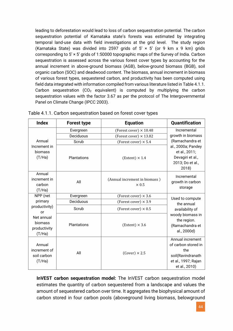
44
leading to deforestation would lead to loss of carbon sequestration potential. The carbon
sequestration potential of Karnataka state’s forests was estimated by integrating
temporal land-use data with field investigations at the grid level. The study region
(Karnataka State) was divided into 2597 grids of 5’ × 5’ (or 9 km x 9 km) grids
corresponding to 5’ × 5’ grids of 1:50000 topographic maps of the Survey of India. Carbon
sequestration is assessed across the various forest cover types by accounting for the
annual increment in above-ground biomass (AGB), below-ground biomass (BGB), soil
organic carbon (SOC) and deadwood content. The biomass, annual increment in biomass
of various forest types, sequestered carbon, and productivity has been computed using
field data integrated with information compiled from various literature listed in Table 4.1.1.
Carbon sequestration (CO2 equivalent) is computed by multiplying the carbon
sequestration values with the factor 3.67 as per the protocol of The Intergovernmental
Panel on Climate Change (IPCC 2003).
Table 4.1.1. Carbon sequestration based on forest cover types
Index Forest type Equation Quantification
Annual
Increment in
biomass
(T/Ha)
Evergreen (Forest cover) × 10.48 Incremental
growth in biomass
(Ramachandra et
al., 2000a; Pandey
et al., 2011;
Devagiri et al.,
2013; Do et al.,
2018)
Deciduous (Forest cover) × 13.82
Scrub (Forest cover) × 5.4
Plantations (Extent) × 1.4
Annual
increment in
carbon
(T/Ha)
All (Annual increment in biomass )
× 0.5
Incremental
growth in carbon
storage
NPP (net
primary
productivity)
or
Net annual
biomass
productivity
(T/Ha)
Evergreen (Forest cover) × 3.6 Used to compute
the annual
availability of
woody biomass in
the region.
(Ramachandra et
al., 2000d)
Deciduous (Forest cover) × 3.9
Scrub (Forest cover) × 0.5
Plantations (Extent) × 3.6
Annual
increment of
soil carbon
(T/Ha)
All (Cover) × 2.5
Annual increment
of carbon stored in
the
soil(Ravindranath
et al., 1997; Rajan
et al., 2010)
InVEST carbon sequestration model: The InVEST carbon sequestration model
estimates the quantity of carbon sequestered from a landscape and values the
amount of sequestered carbon over time. It aggregates the biophysical amount of
carbon stored in four carbon pools (aboveground living biomass, belowground
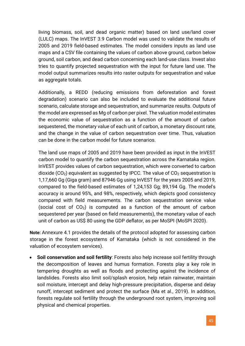
45
living biomass, soil, and dead organic matter) based on land use/land cover
(LULC) maps. The InVEST 3.9 Carbon model was used to validate the results of
2005 and 2019 field-based estimates. The model considers inputs as land use
maps and a CSV file containing the values of carbon above ground, carbon below
ground, soil carbon, and dead carbon concerning each land-use class. Invest also
tries to quantify projected sequestration with the input for future land use. The
model output summarizes results into raster outputs for sequestration and value
as aggregate totals.
Additionally, a REDD (reducing emissions from deforestation and forest
degradation) scenario can also be included to evaluate the additional future
scenario, calculate storage and sequestration, and summarize results. Outputs of
the model are expressed as Mg of carbon per pixel. The valuation model estimates
the economic value of sequestration as a function of the amount of carbon
sequestered, the monetary value of each unit of carbon, a monetary discount rate,
and the change in the value of carbon sequestration over time. Thus, valuation
can be done in the carbon model for future scenarios.
The land use maps of 2005 and 2019 have been provided as input in the InVEST
carbon model to quantify the carbon sequestration across the Karnataka region.
InVEST provides values of carbon sequestration, which were converted to carbon
dioxide (CO2) equivalent as suggested by IPCC. The value of CO2 sequestration is
1,17,660 Gg (Giga gram) and 87946 Gg using InVEST for the years 2005 and 2019,
compared to the field-based estimates of 1,24,153 Gg; 89,194 Gg. The model's
accuracy is around 95%, and 98%, respectively, which depicts good consistency
compared with field measurements. The carbon sequestration service value
(social cost of CO2) is computed as a function of the amount of carbon
sequestered per year (based on field measurements), the monetary value of each
unit of carbon as US$ 80 using the GDP deflator, as per MoSPI (MoSPI 2020).
Note: Annexure 4.1 provides the details of the protocol adopted for assessing carbon
storage in the forest ecosystems of Karnataka (which is not considered in the
valuation of ecosystem services).
• Soil conservation and soil fertility: Forests also help increase soil fertility through
the decomposition of leaves and humus formation. Forests play a key role in
tempering droughts as well as floods and protecting against the incidence of
landslides. Forests also limit soil/splash erosion, help retain rainwater, maintain
soil moisture, intercept and delay high-pressure precipitation, disperse and delay
runoff, intercept sediment and protect the surface (Ma et al., 2019). In addition,
forests regulate soil fertility through the underground root system, improving soil
physical and chemical properties.
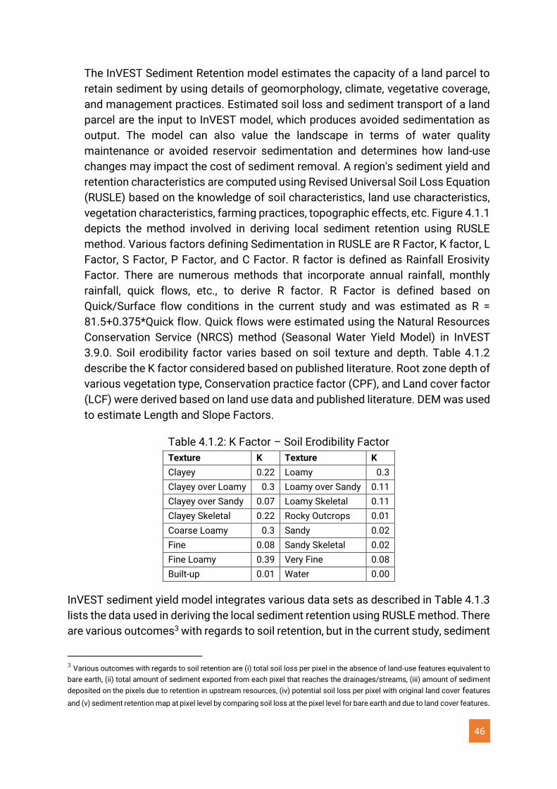
46
The InVEST Sediment Retention model estimates the capacity of a land parcel to
retain sediment by using details of geomorphology, climate, vegetative coverage,
and management practices. Estimated soil loss and sediment transport of a land
parcel are the input to InVEST model, which produces avoided sedimentation as
output. The model can also value the landscape in terms of water quality
maintenance or avoided reservoir sedimentation and determines how land-use
changes may impact the cost of sediment removal. A region's sediment yield and
retention characteristics are computed using Revised Universal Soil Loss Equation
(RUSLE) based on the knowledge of soil characteristics, land use characteristics,
vegetation characteristics, farming practices, topographic effects, etc. Figure 4.1.1
depicts the method involved in deriving local sediment retention using RUSLE
method. Various factors defining Sedimentation in RUSLE are R Factor, K factor, L
Factor, S Factor, P Factor, and C Factor. R factor is defined as Rainfall Erosivity
Factor. There are numerous methods that incorporate annual rainfall, monthly
rainfall, quick flows, etc., to derive R factor. R Factor is defined based on
Quick/Surface flow conditions in the current study and was estimated as R =
81.5+0.375*Quick flow. Quick flows were estimated using the Natural Resources
Conservation Service (NRCS) method (Seasonal Water Yield Model) in InVEST
3.9.0. Soil erodibility factor varies based on soil texture and depth. Table 4.1.2
describe the K factor considered based on published literature. Root zone depth of
various vegetation type, Conservation practice factor (CPF), and Land cover factor
(LCF) were derived based on land use data and published literature. DEM was used
to estimate Length and Slope Factors.
Table 4.1.2: K Factor – Soil Erodibility Factor
Texture K Texture K
Clayey 0.22 Loamy 0.3
Clayey over Loamy 0.3 Loamy over Sandy 0.11
Clayey over Sandy 0.07 Loamy Skeletal 0.11
Clayey Skeletal 0.22 Rocky Outcrops 0.01
Coarse Loamy 0.3 Sandy 0.02
Fine 0.08 Sandy Skeletal 0.02
Fine Loamy 0.39 Very Fine 0.08
Built-up 0.01 Water 0.00
InVEST sediment yield model integrates various data sets as described in Table 4.1.3
lists the data used in deriving the local sediment retention using RUSLE method. There
are various outcomes3 with regards to soil retention, but in the current study, sediment
3 Various outcomes with regards to soil retention are (i) total soil loss per pixel in the absence of land-use features equivalent to
bare earth, (ii) total amount of sediment exported from each pixel that reaches the drainages/streams, (iii) amount of sediment
deposited on the pixels due to retention in upstream resources, (iv) potential soil loss per pixel with original land cover features
and (v) sediment retention map at pixel level by comparing soil loss at the pixel level for bare earth and due to land cover features.
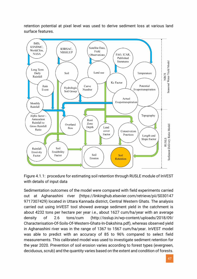
47
retention potential at pixel level was used to derive sediment loss at various land
surface features.
Figure 4.1.1: procedure for estimating soil retention through RUSLE module of InVEST
with details of input data
Sedimentation outcomes of the model were compared with field experiments carried
out at Aghanashini river (https://linkinghub.elsevier.com/retrieve/pii/S030147
9717307429) located in Uttara Kannada district, Central Western Ghats. The analysis
carried out using InVEST tool showed average sediment yield in the catchment is
about 4232 tons per hectare per year i.e., about 1627 cum/ha/year with an average
density of 2.6 tons/cum (http://isslup.in/wp-content/uploads/2018/09/
Characterisation-Of-Soils-Of-Western-Ghats-In-Dakshina.pdf), whereas observed yield
in Aghanashini river was in the range of 1367 to 1567 cum/ha/year. InVEST model
was able to predict with an accuracy of 85 to 96% compared to select field
measurements. This calibrated model was used to investigate sediment retention for
the year 2020. Prevention of soil erosion varies according to forest types (evergreen,
deciduous, scrub) and the quantity varies based on the extent and condition of forests.
48
InVEST provides the quantum of soil (sediment) retained within the natural forested
areas, and considering Rs 48.8 per ton retention of sediments and on the condition of
forests (Verma et al., 2013), soil retention services values range from 9064 INR/Ha/yr
(dry deciduous, medium-density forests) to 19436 INR/Ha/Yr (evergreen, very dense
forests). Analyses of sediment yield based on vegetation type and canopy cover reveal
that sediment retention in evergreen forests ranges from 150 tons per hectare (MDF)
to 1000 tons per hectare per year (VDF), and soil retention services range from 7320
Rs/ha/year (Open canopy forests) to more than 48800 Rs/Ha/year (VDF) in evergreen
forests. Similarly, in deciduous forests, sediment retention ranges between 15 tons
per hectare per year to 350 tons per hectare per year (VDF), and soil retention services
range from 732 Rs/ha/year (open forests) to 17080 Rs/Ha/year (VDF).
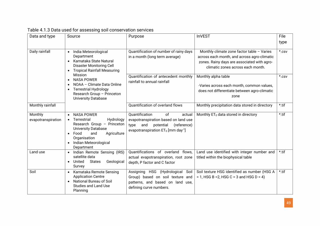
49
Table 4.1.3 Data used for assessing soil conservation services
Data and type Source Purpose InVEST File
type
Daily rainfall
• India Meteorological Department
• Karnataka State Natural Disaster Monitoring Cell
• Tropical Rainfall Measuring Mission
• NASA POWER
• NOAA – Climate Data Online
• Terrestrial Hydrology Research Group – Princeton University Database
Quantification of number of rainy days
in a month (long term average)
Monthly climate zone factor table – Varies
across each month, and across agro-climatic
zones. Rainy days are associated with agro-
climatic zones across each month.
*.csv
Quantification of antecedent monthly
rainfall to annual rainfall
Monthly alpha table
-Varies across each month, common values,
does not differentiate between agro-climatic
zone
*.csv
Monthly rainfall Quantification of overland flows Monthly precipitation data stored in directory *.tif
Monthly
evapotranspiration
• NASA POWER
• Terrestrial Hydrology Research Group – Princeton University Database
• Food and Agriculture Organisation
• Indian Meteorological Department
Quantification of actual
evapotranspiration based on land use
type and potential (reference)
evapotranspiration ET0 [mm day-1]
Monthly ET0 data stored in directory *.tif
Land use • Indian Remote Sensing (IRS) satellite data
• United States Geological Survey
Quantifications of overland flows,
actual evapotranspiration, root zone
depth, P factor and C factor
Land use identified with integer number and
titled within the biophysical table
*.tif
Soil • Karnataka Remote Sensing Application Centre
• National Bureau of Soil Studies and Land Use Planning
Assigning HSG (Hydrological Soil
Group) based on soil texture and
patterns, and based on land use,
defining curve numbers.
Soil texture HSG identified as number (HSG A
= 1, HSG B =2, HSG C = 3 and HSG D = 4)
*.tif
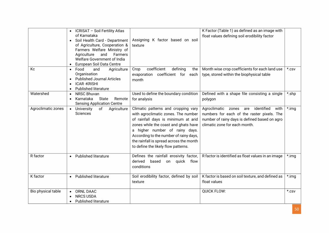
50
• ICRISAT – Soil Fertility Atlas of Karnataka
• Soil Health Card - Department of Agriculture, Cooperation & Farmers Welfare Ministry of Agriculture and Farmers Welfare Government of India
• European Soil Data Centre
Assigning K factor based on soil
texture
K Factor (Table 1) as defined as an image with
float values defining soil erodibility factor
Kc • Food and Agriculture Organisation
• Published Journal Articles
• ICAR -KRISHI
• Published literature
Crop coefficient defining the
evaporation coefficient for each
month
Month wise crop coefficients for each land use
type, stored within the biophysical table
*.csv
Watershed • NRSC Bhuvan
• Karnataka State Remote Sensing Application Centre
Used to define the boundary condition
for analysis
Defined with a shape file consisting a single
polygon
*.shp
Agroclimatic zones • University of Agriculture Sciences
Climatic patterns and cropping vary
with agroclimatic zones. The number
of rainfall days is minimum at arid
zones while the coast and ghats have
a higher number of rainy days.
According to the number of rainy days,
the rainfall is spread across the month
to define the likely flow patterns.
Agroclimatic zones are identified with
numbers for each of the raster pixels. The
number of rainy days is defined based on agro
climatic zone for each month.
*.img
R factor • Published literature Defines the rainfall erosivity factor,
derived based on quick flow
conditions
R factor is identified as float values in an image *.img
K factor • Published literature Soil erodibility factor, defined by soil
texture
K factor is based on soil texture, and defined as
float values
*.img
Bio physical table • ORNL DAAC
• NRCS USDA
• Published literature
QUICK FLOW: *.csv
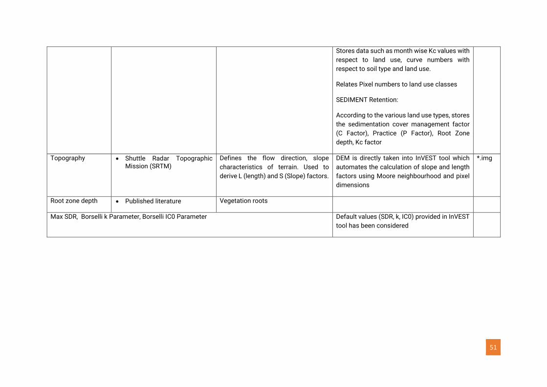
51
Stores data such as month wise Kc values with
respect to land use, curve numbers with
respect to soil type and land use.
Relates Pixel numbers to land use classes
SEDIMENT Retention:
According to the various land use types, stores
the sedimentation cover management factor
(C Factor), Practice (P Factor), Root Zone
depth, Kc factor
Topography • Shuttle Radar Topographic Mission (SRTM)
Defines the flow direction, slope
characteristics of terrain. Used to
derive L (length) and S (Slope) factors.
DEM is directly taken into InVEST tool which
automates the calculation of slope and length
factors using Moore neighbourhood and pixel
dimensions
*.img
Root zone depth • Published literature Vegetation roots
Max SDR, Borselli k Parameter, Borselli IC0 Parameter Default values (SDR, k, IC0) provided in InVEST
tool has been considered
52
• Water regulation and groundwater recharge: Forests in the watershed help
retain water supplied from precipitation in underground aquifers just as water
is stored in human-made reservoirs. They simplify in increasing the efficient
water available, improving water quality, and decreasing water runoff. The
quantity of water conserved depends on several parameters: evaporation and
runoff rates, interception ratios, tree and forest characteristics, nature and
intensity of rainfall, geographic and soil conditions, etc. (Ramachandra et al.,
2020). Forests help regulate the hydrological regime locally and sustain water
flow in the streams due to their sponge-like effect. Vegetation in the catchment
helps in retarding the water flow in the catchment by allowing infiltration.
Water regulation services are the ecosystem contributions to the regulation of
river flows and groundwater and lake water tables. They are derived from the
ability of ecosystems to absorb and store water, and gradually release water
during dry seasons or periods through evapotranspiration and hence secure a
regular flow of water. This is recorded as a final or intermediate ecosystem
service. Peak flow mitigation services will be supplied together with river flood
mitigation services to provide the benefit of flood protection, a final ecosystem
service. Field investigations in four river basins of Uttara Kannada district
reveal that water infiltrates and fills the underlying zones, namely saturated
zone, and vadose zones, in the catchments of streams. The region receives rain
for about four months, and the surface run-off during the monsoon is due to
the precipitation (after saturation of underlying regions). After the monsoon
recedes, the water stored in the vadose regions, and saturated zones flow
laterally towards the streams for about 6-8 months (as pipe flow in the post-
monsoon period of 4 months and base flow during summer). Water infiltration
allows water storage in the saturated and vadose zones, which is crucial for
water sustenance in the streams during lean seasons. Catchments with > 65%
vegetation of native species have perennial streams, higher soil moisture, and
groundwater than the catchment dominated by degradation.
InVEST Seasonal Water Yield Model: the model integrates various data sets as
described in Table 4.1.4. A Natural Resource Conservation Series (NRCS)
model or SCS model uses the curve number functions-based soil
characteristics, land use characteristics, climate characteristics, etc. Figure
4.1.3 depicts the method involved in deriving local water recharge using NRCS
curve number method. The method uses the water balance equation to derive
the unknown parameter (Precipitation = Overland Flow + Infiltration +
Evapotranspiration). The local infiltration parameter defines local water
recharge. The NRCS curve number model utilizes various parameters to derive
the overland flow; FAO recommends the Penman Monteith / Modified
Hargreaves method to derive the potential evapotranspiration (ET0). In the
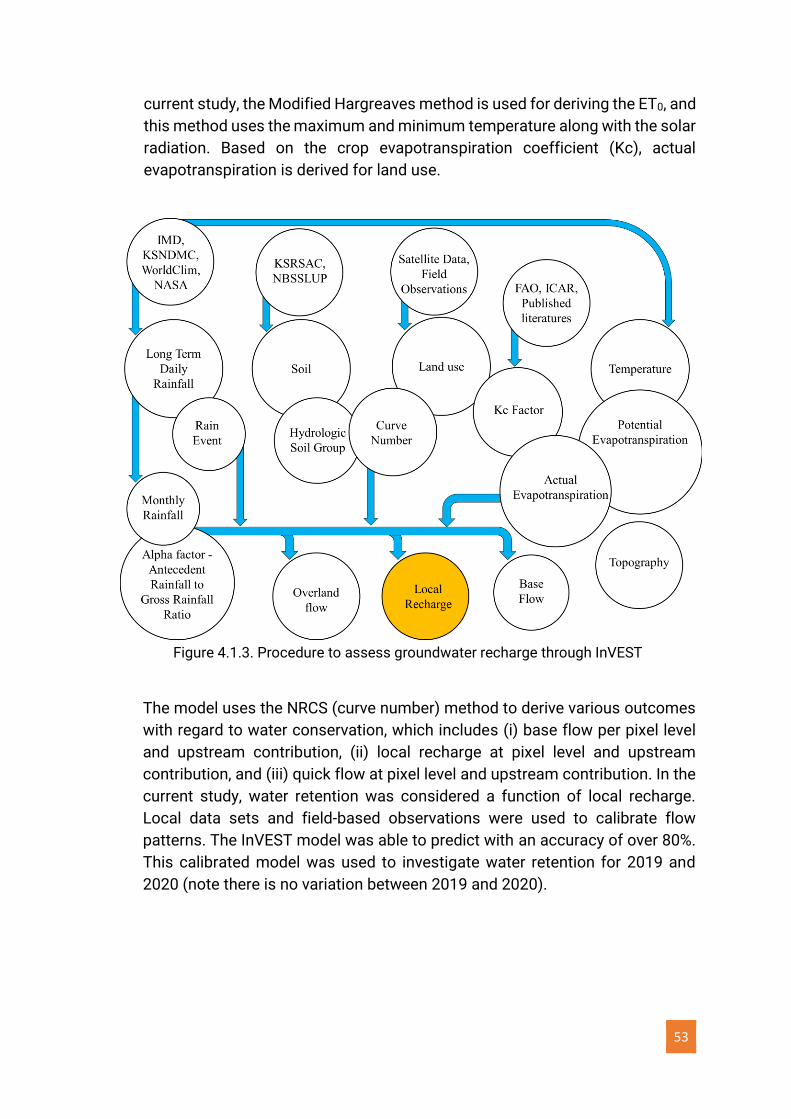
53
current study, the Modified Hargreaves method is used for deriving the ET0, and
this method uses the maximum and minimum temperature along with the solar
radiation. Based on the crop evapotranspiration coefficient (Kc), actual
evapotranspiration is derived for land use.
Figure 4.1.3. Procedure to assess groundwater recharge through InVEST
The model uses the NRCS (curve number) method to derive various outcomes
with regard to water conservation, which includes (i) base flow per pixel level
and upstream contribution, (ii) local recharge at pixel level and upstream
contribution, and (iii) quick flow at pixel level and upstream contribution. In the
current study, water retention was considered a function of local recharge.
Local data sets and field-based observations were used to calibrate flow
patterns. The InVEST model was able to predict with an accuracy of over 80%.
This calibrated model was used to investigate water retention for 2019 and
2020 (note there is no variation between 2019 and 2020).
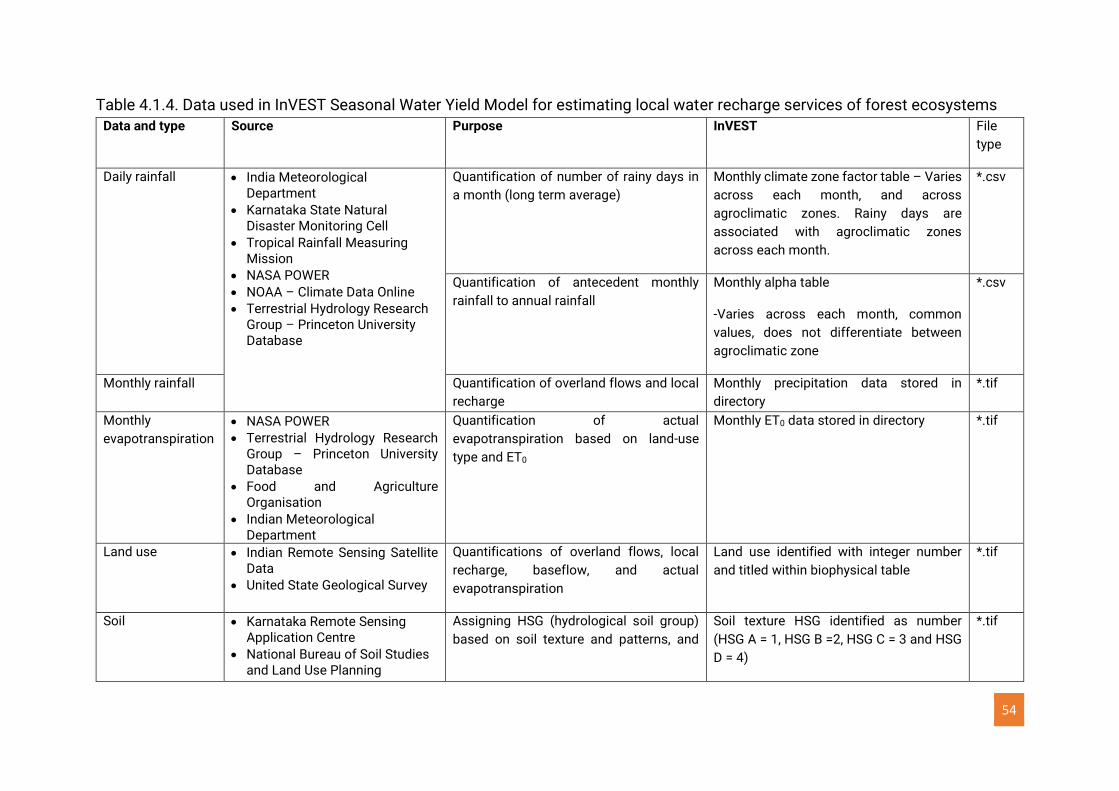
54
Table 4.1.4. Data used in InVEST Seasonal Water Yield Model for estimating local water recharge services of forest ecosystems
Data and type Source Purpose InVEST File
type
Daily rainfall • India Meteorological Department
• Karnataka State Natural Disaster Monitoring Cell
• Tropical Rainfall Measuring Mission
• NASA POWER
• NOAA – Climate Data Online
• Terrestrial Hydrology Research Group – Princeton University Database
Quantification of number of rainy days in
a month (long term average)
Monthly climate zone factor table – Varies
across each month, and across
agroclimatic zones. Rainy days are
associated with agroclimatic zones
across each month.
*.csv
Quantification of antecedent monthly
rainfall to annual rainfall
Monthly alpha table
-Varies across each month, common
values, does not differentiate between
agroclimatic zone
*.csv
Monthly rainfall Quantification of overland flows and local
recharge
Monthly precipitation data stored in
directory
*.tif
Monthly
evapotranspiration
• NASA POWER
• Terrestrial Hydrology Research Group – Princeton University Database
• Food and Agriculture Organisation
• Indian Meteorological Department
Quantification of actual
evapotranspiration based on land-use
type and ET0
Monthly ET0 data stored in directory *.tif
Land use • Indian Remote Sensing Satellite Data
• United State Geological Survey
Quantifications of overland flows, local
recharge, baseflow, and actual
evapotranspiration
Land use identified with integer number
and titled within biophysical table
*.tif
Soil • Karnataka Remote Sensing Application Centre
• National Bureau of Soil Studies and Land Use Planning
Assigning HSG (hydrological soil group)
based on soil texture and patterns, and
Soil texture HSG identified as number
(HSG A = 1, HSG B =2, HSG C = 3 and HSG
D = 4)
*.tif
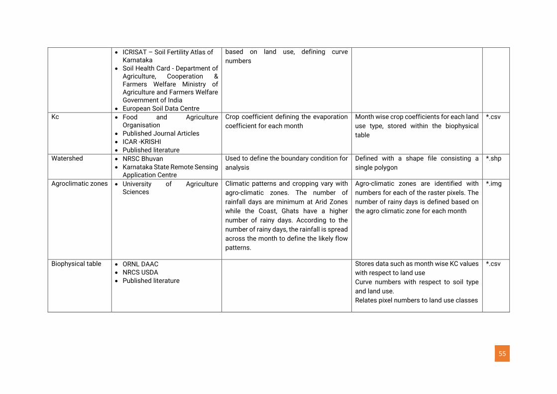
55
• ICRISAT – Soil Fertility Atlas of Karnataka
• Soil Health Card - Department of Agriculture, Cooperation & Farmers Welfare Ministry of Agriculture and Farmers Welfare Government of India
• European Soil Data Centre
based on land use, defining curve
numbers
Kc • Food and Agriculture Organisation
• Published Journal Articles
• ICAR -KRISHI
• Published literature
Crop coefficient defining the evaporation
coefficient for each month
Month wise crop coefficients for each land
use type, stored within the biophysical
table
*.csv
Watershed • NRSC Bhuvan
• Karnataka State Remote Sensing Application Centre
Used to define the boundary condition for
analysis
Defined with a shape file consisting a
single polygon
*.shp
Agroclimatic zones • University of Agriculture Sciences
Climatic patterns and cropping vary with
agro-climatic zones. The number of
rainfall days are minimum at Arid Zones
while the Coast, Ghats have a higher
number of rainy days. According to the
number of rainy days, the rainfall is spread
across the month to define the likely flow
patterns.
Agro-climatic zones are identified with
numbers for each of the raster pixels. The
number of rainy days is defined based on
the agro climatic zone for each month
*.img
Biophysical table • ORNL DAAC
• NRCS USDA
• Published literature
Stores data such as month wise KC values
with respect to land use
Curve numbers with respect to soil type
and land use.
Relates pixel numbers to land use classes
*.csv
56
Groundwater was the major source for irrigation apart from the canal irrigation
system. Water contained in the voids of the geologic materials supports needs
of irrigation, both domestic and from industries. The groundwater storage
available annually is estimated based on area and depth of fluctuation in the
groundwater table and specific yield factors. The groundwater storage in the
aquifer depends on the input components such as precipitation; seepage, and
return flow (Chatterjee 2011).
InVEST provides the quantum of water recharge within the natural forested
areas. The forest of Karnataka locally recharges about 27.2 billion cubic meters
of water to the ground, which later flows as base flows. The economic value of
groundwater (after deducting costs) is about 262.5 Rs/kilo cum of water.
Based on this, local recharge in evergreen forests ranges between 1000 mm
(medium-density forests: MDF) to more than 4000 mm (very dense forests:
VDF), and the economic value of groundwater recharge services for evergreen
forests ranges from 2600 Rs/ha/year (MDF) to more than 5000 Rs/ha/year
(VDF). Similarly, local recharge in deciduous forests ranges from 25 mm (MDF)
to 1500 mm (VDF). The economic value of groundwater recharge services for
deciduous forests ranges from 663 Rs/Ha/year to more than 3700 Rs/ha/year.
• Water purification and waste treatment: Forests, their diversity, and native
vegetation, control all hydrological events such as flow, recharge, and
precipitation, etc. Forest soils and root systems, and microorganisms present
in soil and water help filter and absorb contaminants and bacteria from the
water received from precipitation. In fact, the water obtained from rainfall in
forest areas that drips through streams and springs is rich in mineral nutrients
and highly valued for its purity and medicinal value (Chatterjee 2011; Terrado
et al., 2014; Zawadzka et al., 2019; Ramachandra et al., 2020). Diverse
microorganisms interact with plant roots, and soil helps in the transfer of
nutrients from the soil to plants which aids in the remediation of water. Soil and
water conservation and water purification are interrelated, as these are
different services provided by forest ecosystems.
Forest ecosystems have multifunctional potential in terms of water and
wastewater treatment, thereby supporting natural processes of ecosystem
services supply. Forests aid as sink and support treatment (bioremediation),
which depend on the spatial extent, and condition of ecosystems (Zawadzka et
al., 2019). Economic values of water purification and waste treatment by forest
ecosystems in Karnataka are estimated through the benefit transfer method
based on case studies from India. An average of 2,950 Rs/ha/yr was
considered as a water purification service from forests (Verma et al., 2013).
57
Waste treatment is estimated at 4,716 Rs/ha/yr (Ramachandra et al., 2017,
Verma et al., 2013), and values are comparable to the studies across the globe
(De Groot et al., 2020) after adjusting for GDP (PPP) per capita for India and
currency exchange value.
• Pollination service: The natural processes of regeneration of the forest,
fruiting, and food production from landscapes are due to pollination and seed
dispersal from various agents. Pollination is a key service that governs
biological production, and the maintenance of biodiversity. Most flowering
plants (approximately 78%) depend on pollinators to reproduce and survive
(Ollerton et al.,, 2011). Pollinator abundance will increase the ecosystem supply
value through enhanced production levels by improving qualitative aspects of
fruit and seed yields, nutritional content, and general appearance, including fruit
size (Potts et al., 2016; Balachandran et al., 2017; Porto et al., 2020). This
contribution can be well assessed through services such as pollination and
seed dispersal (Hipólito et al., 2019), which directly affects the food security of
human populations (Potts et al., 2016).
Pollination services are accounted for through the comparative assessment of
natural regeneration of forest patches (with fencing protection from external
pressures: (Balachandran et al., 2017; Ray et al., 2015) and afforestation cost.
The estimates of natural forest regeneration in all forest types are adjusted
according to the forest regeneration in plantations (NAP 2009; Ollerton et al.,
2011; Hipólito et al., 2019). The economic value of pollination has been
estimated in the current study based on benefit transfer method considering
case studies from India (Verma et al., 2013) of natural forest regeneration and
its replacement cost if done artificially as recommended by the National
Afforestation Programme Guidelines (NAP 2009) and based on the success
stories of National Beekeeping & Honey Mission (NBHM 2019). The pollination
services vary with forest type, and canopy cover and values range from 10167
INR/Ha/Yr (MDF) to 11907 INR/Ha/Yr (VDF) (Verma et al., 2013) with regard to
forest regeneration, excluding the contribution to agricultural production. The
estimates of natural forest regeneration in all forest types are further adjusted
according to the forest regeneration in plantations. The economic value so
estimated is limited only to the value of artificially replacing the process of
natural forest regeneration and covers partly the economic value of forest
succession.
• Air filtration services: Forests moderate air quality and reduce pollution that
affects human health and well-being, ecosystem health, crops, climate, etc.
Forests remove gaseous air pollutants and improve the quality primarily by
uptake via leaf stomata (Nowak et al., 2014) and provide clean air by capturing
58
the dust. Densely forested regions can remove air pollution, accounting for
around 16%; moderately dense forests can remove up to 4.5%; and sparse
cover can remove up to 1%, depending on the meteorological conditions
(Nowak et al., 2006). The air quality service value of forest ecosystems ranges
from 8,368 INR/Ha/Yr (MDF) to 22,617 INR/Ha/Yr (VDF) based on published
literature from case studies in India (Ninan and Kontoleon, 2016, Joshi G and
Negi GCS, 2011) which are comparable to tropical forest ecosystems in the
global ecosystem service valuation database (ESVD) adjusted for GDP (PPP)
per capita for India and the prevailing currency exchange rate (March 2020).
• Local (micro and meso) climate regulation services: Forest vegetation plays a
crucial role in moderating the local climate. The presence of native vegetation
improves the living conditions, regulates ambient atmospheric conditions for
the people, and supports economic production. Forests also contribute to local
atmospheric climatic moderation, humidity, and rainfall. Local climate
regulation services value ranges from 17,933 INR/Ha/Yr (MDF) to 48,468
INR/Ha/Yr (VDF) quantified through benefit transfer method based on
published literature from case studies in India (Ghosh, 2020, Verma et al.,
2007), which are comparable to values for tropical forests in global ecosystem
service valuation database (ESVD) adjusted for GDP (PPP) and currency
exchange rate as on March 2020 (USD to INR).
Cultural ecosystem services from forest ecosystem: Cultural ecosystem services are
the contributions to benefits and wellbeing people gain from their interactions with
different environmental areas, which can be valued in terms of monetary, qualitative,
quantitative methods. Cultural services generally reflect social connections, sensory
experiences, symbolic importance, and identity. The forest has a high cultural value;
the main reason can be attributed to the aesthetic beauty, recreational benefit,
spiritual and historic (Kan forests, which are the sacred groves present in the district)
values. Sacred groves are communally protected forest fragments with significant
religious connotations (Ramachandra et al., 2010, 2017; Ray et al., 2010). Protected
areas in Karnataka are Bannerghatta National Park, Anshi National Park,
Bandipur National park, Kudremukh National Park, Arabithittu Wildlife Sanctuary,
Bhadra Wildlife Sanctuary, Bhimgad Wildlife Sanctuary, Biligiri Rangaswamy Temple
(BRT) Wildlife Sanctuary.
Further, recreational benefits provided by the forest include gaming, trekking,
swimming, walking, hunting, etc. The aesthetic beauty of the forest is valuable; the
presence of waterfalls and caves adds to the aesthetic value of the district. Education,
scientific, and research value provided by the forest are indispensable as many long-
term ecological monitoring research stations are set up by the major science and
research institutes and organizations.
59
• Aesthetic - National parks, sanctuaries, waterfalls: Data pertaining to the entry
fees (park, recreation spots), and details of visitors were compiled from the
forest divisions (Uttara Kannada, Shimoga, Chikmagalur Dakshina Kannada,
and Kodagu districts) of the Karnataka Forest Department. Valuation of
aesthetic services is computed considering entrance fees (park, recreation
spots) x the average number of visitors to the park/recreation spots during
2018, 2019, and 2020), supplemented with the Indian case studies (Ray et al.,
2010; Bharath et al., 2017; Ramachandra et al., 2018c) and travel expenses
associated to the travel, based on the address of visitors and considering the
connectivity (road/train) and additional details collected from the service
providers on revenue during the past three years. The data collected from the
service operators include (i) cost (labor, fuel, and maintenance) and (ii) annual
revenue. The aesthetic value is computed based on these (travel expenses,
entrance fee, maintenance cost and benefits to service operators), which
accounts for 1500±250 ₹/Ha/Yr and an average value of Rs 1500 ₹/Ha/Yr was
considered for accounting for the aesthetic cultural services from forest
ecosystems in Karnataka.
• Spiritual and historic - Distribution of sacred groves (relic forests - protected
due to belief and customs): Sacred groves or kan forests of Central Western
Ghats of Karnataka are climax evergreen forests, preserved through
generations as sacred forests by the village communities of Malnadu regions.
Patches of forests are dedicated to deities and used for worship and cultural
activities by the local communities. In the past, kans numbered in the
thousands, each kan measuring originally from a few hectares to several
hundred hectares in area. They were characteristic of the traditional land use
of Shimoga, Uttara Kannada, and Chikmagalur districts especially, and were
equivalent to the devarakadus of Kodagu region. Kan forests functioned as
important sources of perennial streams and springs used for irrigation crops
and domestic needs. However, the curtailment of community rights in the kans,
in districts of the central Western Ghats, including heavier taxation for
collection of forest produce, resulted in the abandonment of many of them,
causing various hardships to the villagers (Chandran et al., 2010; Ramachandra
et al., 2012, 2016, 2017, 2019a; Ray et al., 2014b, 2015).
Sacred groves or devarakadu in Kodagu district, Karnataka: Sacred groves or
devarakadu or kan forests are culturally protected patches of forests that
continue to thrive as a living tradition in Kodagu district. The district has the
highest density of groves in the world. The extent of sacred groves in Kodagu
is 2,500 hectares, i.e., around 2% of the land area in the district, with at least
one grove for every 300-hectares. The groves are owned by the Forest
Department and declared as Protected Forests, but are managed by local
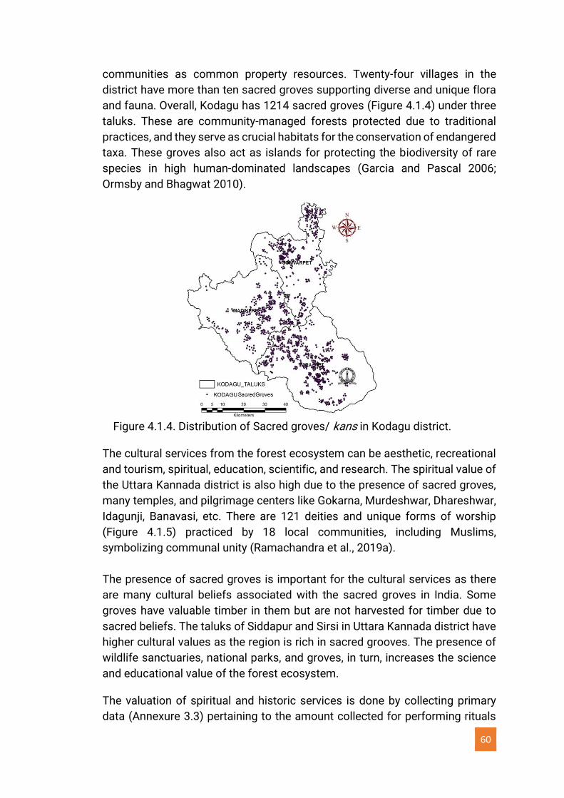
60
communities as common property resources. Twenty-four villages in the
district have more than ten sacred groves supporting diverse and unique flora
and fauna. Overall, Kodagu has 1214 sacred groves (Figure 4.1.4) under three
taluks. These are community-managed forests protected due to traditional
practices, and they serve as crucial habitats for the conservation of endangered
taxa. These groves also act as islands for protecting the biodiversity of rare
species in high human-dominated landscapes (Garcia and Pascal 2006;
Ormsby and Bhagwat 2010).
Figure 4.1.4. Distribution of Sacred groves/ kans in Kodagu district.
The cultural services from the forest ecosystem can be aesthetic, recreational
and tourism, spiritual, education, scientific, and research. The spiritual value of
the Uttara Kannada district is also high due to the presence of sacred groves,
many temples, and pilgrimage centers like Gokarna, Murdeshwar, Dhareshwar,
Idagunji, Banavasi, etc. There are 121 deities and unique forms of worship
(Figure 4.1.5) practiced by 18 local communities, including Muslims,
symbolizing communal unity (Ramachandra et al., 2019a).
The presence of sacred groves is important for the cultural services as there
are many cultural beliefs associated with the sacred groves in India. Some
groves have valuable timber in them but are not harvested for timber due to
sacred beliefs. The taluks of Siddapur and Sirsi in Uttara Kannada district have
higher cultural values as the region is rich in sacred grooves. The presence of
wildlife sanctuaries, national parks, and groves, in turn, increases the science
and educational value of the forest ecosystem.
The valuation of spiritual and historic services is done by collecting primary
data (Annexure 3.3) pertaining to the amount collected for performing rituals
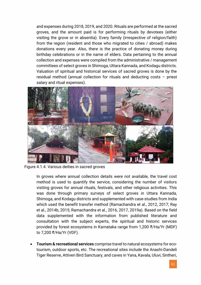
61
and expenses during 2018, 2019, and 2020. Rituals are performed at the sacred
groves, and the amount paid is for performing rituals by devotees (either
visiting the grove or in absentia). Every family (irrespective of religion/faith)
from the region (resident and those who migrated to cities / abroad) makes
donations every year. Also, there is the practice of donating money during
birthday celebrations or in the name of elders. Data pertaining to the annual
collection and expenses were compiled from the administrative / management
committees of select groves in Shimoga, Uttara Kannada, and Kodagu districts.
Valuation of spiritual and historical services of sacred groves is done by the
residual method (annual collection for rituals and deducting costs – priest
salary and ritual expenses).
Figure 4.1.4. Various deities in sacred groves
In groves where annual collection details were not available, the travel cost
method is used to quantify the service, considering the number of visitors
visiting groves for annual rituals, festivals, and other religious activities. This
was done through primary surveys of select groves in Uttara Kannada,
Shimoga, and Kodagu districts and supplemented with case-studies from India
which used the benefit transfer method (Ramachandra et al., 2012, 2017; Ray
et al., 2014b, 2015; Ramachandra et al., 2016, 2017, 2019a). Based on the field
data supplemented with the information from published literature and
consultation with the subject experts, the spiritual and historic services
provided by forest ecosystems in Karnataka range from 1,200 ₹/Ha/Yr (MDF)
to 7,200 ₹/Ha/Yr (VDF).
• Tourism & recreational services comprise travel to natural ecosystems for eco-
tourism, outdoor sports, etc. The recreational sites include the Anashi-Dandeli
Tiger Reserve, Attiveri Bird Sanctuary, and caves in Yana, Kavala, Uluvi, Sintheri,
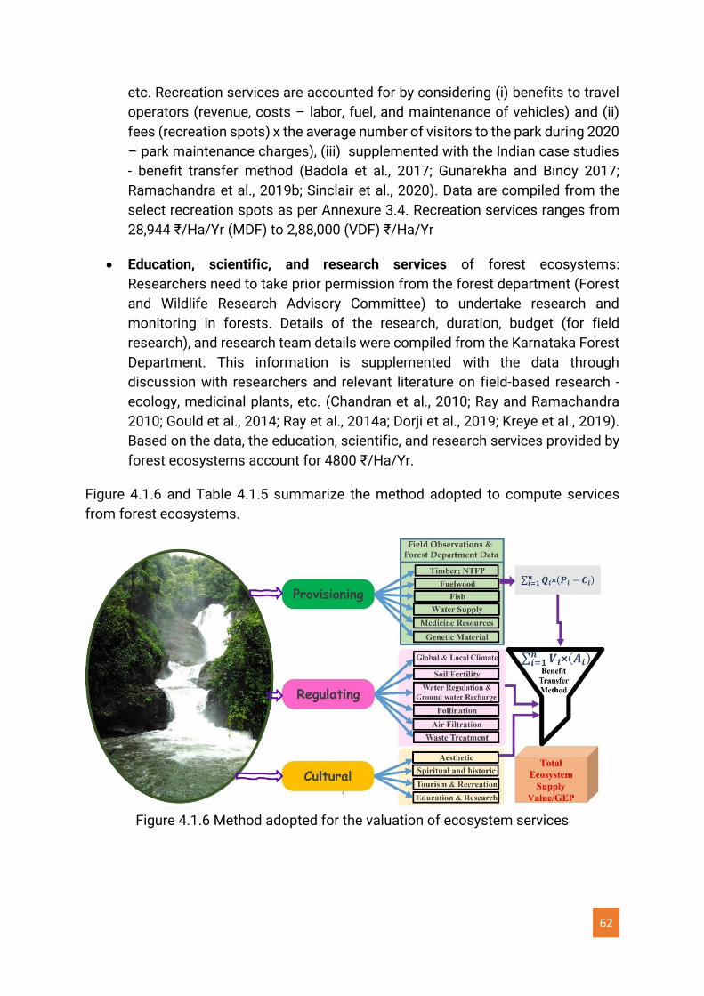
62
etc. Recreation services are accounted for by considering (i) benefits to travel
operators (revenue, costs – labor, fuel, and maintenance of vehicles) and (ii)
fees (recreation spots) x the average number of visitors to the park during 2020
– park maintenance charges), (iii) supplemented with the Indian case studies
- benefit transfer method (Badola et al., 2017; Gunarekha and Binoy 2017;
Ramachandra et al., 2019b; Sinclair et al., 2020). Data are compiled from the
select recreation spots as per Annexure 3.4. Recreation services ranges from
28,944 ₹/Ha/Yr (MDF) to 2,88,000 (VDF) ₹/Ha/Yr
• Education, scientific, and research services of forest ecosystems:
Researchers need to take prior permission from the forest department (Forest
and Wildlife Research Advisory Committee) to undertake research and
monitoring in forests. Details of the research, duration, budget (for field
research), and research team details were compiled from the Karnataka Forest
Department. This information is supplemented with the data through
discussion with researchers and relevant literature on field-based research -
ecology, medicinal plants, etc. (Chandran et al., 2010; Ray and Ramachandra
2010; Gould et al., 2014; Ray et al., 2014a; Dorji et al., 2019; Kreye et al., 2019).
Based on the data, the education, scientific, and research services provided by
forest ecosystems account for 4800 ₹/Ha/Yr.
Figure 4.1.6 and Table 4.1.5 summarize the method adopted to compute services
from forest ecosystems.
Figure 4.1.6 Method adopted for the valuation of ecosystem services
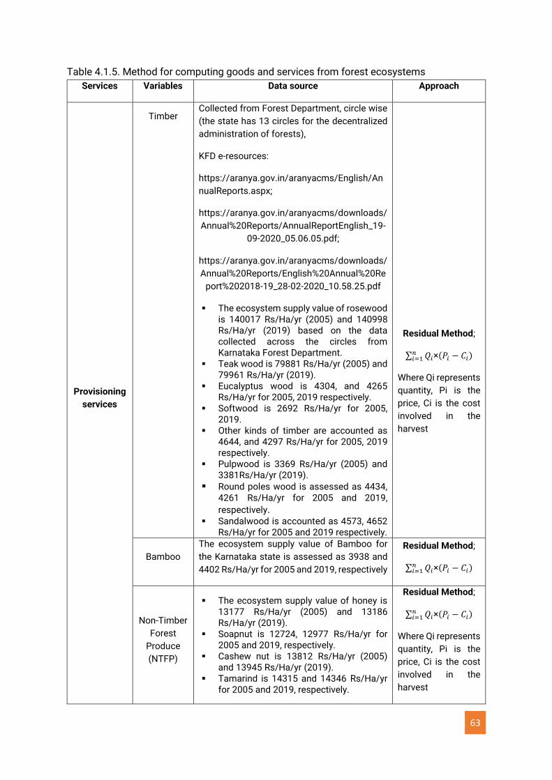
63
Table 4.1.5. Method for computing goods and services from forest ecosystems
Services Variables Data source Approach
Provisioning
services
Timber
Collected from Forest Department, circle wise
(the state has 13 circles for the decentralized
administration of forests),
KFD e-resources:
https://aranya.gov.in/aranyacms/English/An
nualReports.aspx;
https://aranya.gov.in/aranyacms/downloads/
Annual%20Reports/AnnualReportEnglish_19-
09-2020_05.06.05.pdf;
https://aranya.gov.in/aranyacms/downloads/
Annual%20Reports/English%20Annual%20Re
port%202018-19_28-02-2020_10.58.25.pdf
▪ The ecosystem supply value of rosewood is 140017 Rs/Ha/yr (2005) and 140998 Rs/Ha/yr (2019) based on the data collected across the circles from Karnataka Forest Department.
▪ Teak wood is 79881 Rs/Ha/yr (2005) and 79961 Rs/Ha/yr (2019).
▪ Eucalyptus wood is 4304, and 4265 Rs/Ha/yr for 2005, 2019 respectively.
▪ Softwood is 2692 Rs/Ha/yr for 2005, 2019.
▪ Other kinds of timber are accounted as 4644, and 4297 Rs/Ha/yr for 2005, 2019 respectively.
▪ Pulpwood is 3369 Rs/Ha/yr (2005) and 3381Rs/Ha/yr (2019).
▪ Round poles wood is assessed as 4434, 4261 Rs/Ha/yr for 2005 and 2019,
respectively. ▪ Sandalwood is accounted as 4573, 4652
Rs/Ha/yr for 2005 and 2019 respectively.
Residual Method;
∑ 𝑄𝑖𝑛𝑖=1 ×(𝑃𝑖 − 𝐶𝑖)
Where Qi represents
quantity, Pi is the
price, Ci is the cost
involved in the
harvest
Bamboo
The ecosystem supply value of Bamboo for
the Karnataka state is assessed as 3938 and
4402 Rs/Ha/yr for 2005 and 2019, respectively
Residual Method;
∑ 𝑄𝑖𝑛𝑖=1 ×(𝑃𝑖 − 𝐶𝑖)
Non-Timber
Forest
Produce
(NTFP)
▪ The ecosystem supply value of honey is 13177 Rs/Ha/yr (2005) and 13186 Rs/Ha/yr (2019).
▪ Soapnut is 12724, 12977 Rs/Ha/yr for 2005 and 2019, respectively.
▪ Cashew nut is 13812 Rs/Ha/yr (2005) and 13945 Rs/Ha/yr (2019).
▪ Tamarind is 14315 and 14346 Rs/Ha/yr for 2005 and 2019, respectively.
Residual Method;
∑ 𝑄𝑖𝑛𝑖=1 ×(𝑃𝑖 − 𝐶𝑖)
Where Qi represents
quantity, Pi is the
price, Ci is the cost
involved in the
harvest
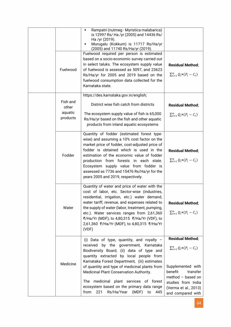
64
▪ Rampatri (nutmeg - Myristica malabarica) is 12997 Rs/ Ha /yr (2005) and 14436 Rs/ Ha /yr (2019).
▪ Murugalu (Kokkum) is 11717 Rs/Ha/yr (2005) and 11740 Rs/Ha/yr (2019).
Fuelwood
Fuelwood required per person is estimated
based on a socio-economic survey carried out
in select taluks. The ecosystem supply value
of fuelwood is assessed as 5097, and 23623
Rs/Ha/yr for 2005 and 2019 based on the
fuelwood consumption data collected for the
Karnataka state.
Residual Method;
∑ 𝑄𝑖𝑛𝑖=1 ×(𝑃𝑖 − 𝐶𝑖)
Fish and
other
aquatic
products
https://des.karnataka.gov.in/english;
District wise fish catch from districts
The ecosystem supply value of fish is 65,000
Rs/Ha/yr based on the fish and other aquatic
products from inland aquatic ecosystems
Residual Method;
∑ 𝑄𝑖𝑛𝑖=1 ×(𝑃𝑖 − 𝐶𝑖)
Fodder
Quantity of fodder (estimated forest type-
wise) and assuming a 10% cost factor on the
market price of fodder, cost-adjusted price of
fodder is obtained which is used in the
estimation of the economic value of fodder
production from forests in each state.
Ecosystem supply value from fodder is
assessed as 7736 and 15476 Rs/Ha/yr for the
years 2005 and 2019, respectively.
Residual Method;
∑ 𝑄𝑖𝑛𝑖=1 ×(𝑃𝑖 − 𝐶𝑖)
Water
Quantity of water and price of water with the
cost of labor, etc. Sector-wise (industries,
residential, irrigation, etc.) water demand,
water tariff, revenue, and expenses related to
the supply of water (labor, treatment, pumping,
etc.). Water services ranges from 2,61,360
₹/Ha/Yr (MDF), to 4,80,315 ₹/Ha/Yr (VDF), to
2,61,360 ₹/Ha/Yr (MDF), to 4,80,315 ₹/Ha/Yr
(VDF)
Residual Method;
∑ 𝑄𝑖𝑛𝑖=1 ×(𝑃𝑖 − 𝐶𝑖)
Medicine
(i) Data of type, quantity, and royalty –
received by the government, Karnataka
Biodiversity Board, (ii) data of type and
quantity extracted by local people from
Karnataka Forest Department, (iii) estimates
of quantity and type of medicinal plants from
Medicinal Plant Conservation Authority.
The medicinal plant services of forest
ecosystem based on the primary data range
from 221 Rs/Ha/Year (MDF) to 445
Residual Method;
∑ 𝑄𝑖𝑛𝑖=1 ×(𝑃𝑖 − 𝐶𝑖)
Supplemented with
benefit transfer
method – based on
studies from India
(Verma et al., 2013)
and compared with
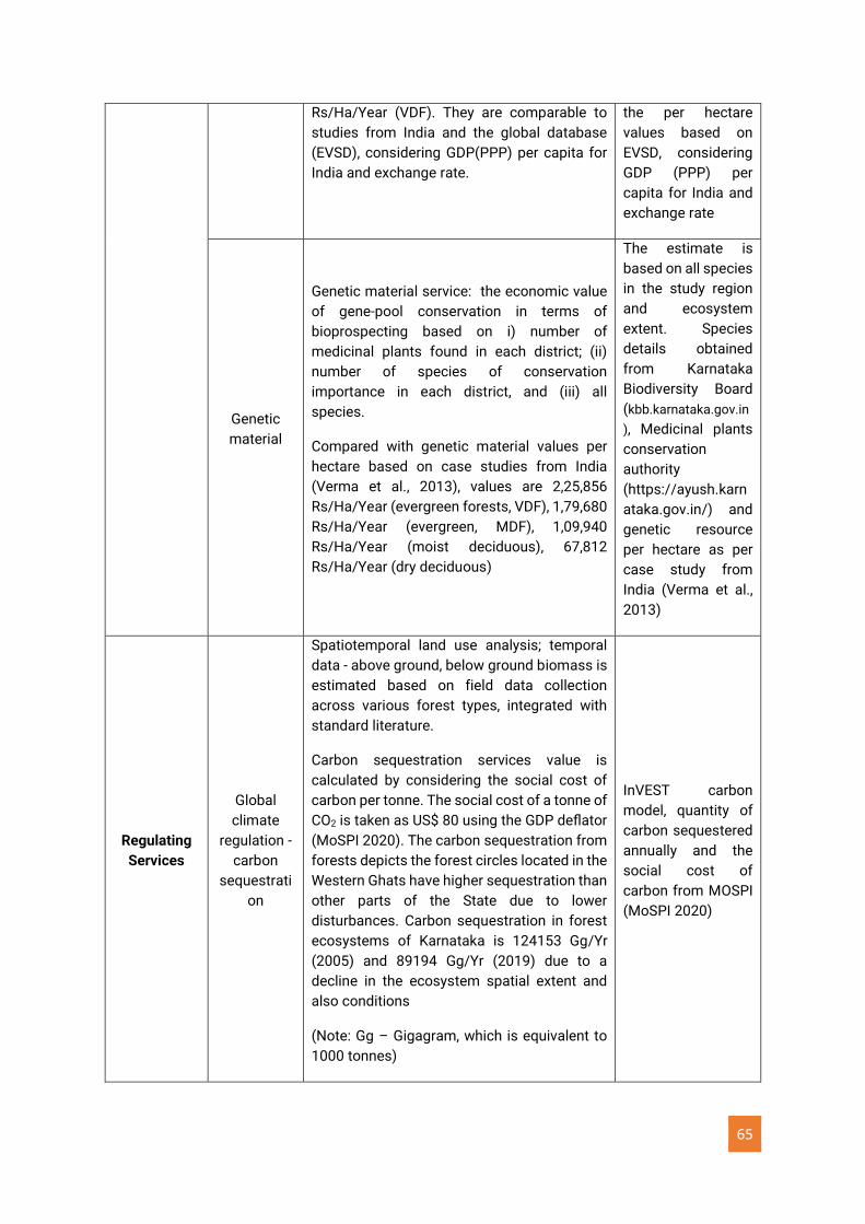
65
Rs/Ha/Year (VDF). They are comparable to
studies from India and the global database
(EVSD), considering GDP(PPP) per capita for
India and exchange rate.
the per hectare
values based on
EVSD, considering
GDP (PPP) per
capita for India and
exchange rate
Genetic
material
Genetic material service: the economic value
of gene-pool conservation in terms of
bioprospecting based on i) number of
medicinal plants found in each district; (ii)
number of species of conservation
importance in each district, and (iii) all
species.
Compared with genetic material values per
hectare based on case studies from India
(Verma et al., 2013), values are 2,25,856
Rs/Ha/Year (evergreen forests, VDF), 1,79,680
Rs/Ha/Year (evergreen, MDF), 1,09,940
Rs/Ha/Year (moist deciduous), 67,812
Rs/Ha/Year (dry deciduous)
The estimate is
based on all species
in the study region
and ecosystem
extent. Species
details obtained
from Karnataka
Biodiversity Board
(kbb.karnataka.gov.in
), Medicinal plants
conservation
authority
(https://ayush.karn
ataka.gov.in/) and
genetic resource
per hectare as per
case study from
India (Verma et al.,
2013)
Regulating
Services
Global
climate
regulation -
carbon
sequestrati
on
Spatiotemporal land use analysis; temporal
data - above ground, below ground biomass is
estimated based on field data collection
across various forest types, integrated with
standard literature.
Carbon sequestration services value is
calculated by considering the social cost of
carbon per tonne. The social cost of a tonne of
CO2 is taken as US$ 80 using the GDP deflator
(MoSPI 2020). The carbon sequestration from
forests depicts the forest circles located in the
Western Ghats have higher sequestration than
other parts of the State due to lower
disturbances. Carbon sequestration in forest
ecosystems of Karnataka is 124153 Gg/Yr
(2005) and 89194 Gg/Yr (2019) due to a
decline in the ecosystem spatial extent and
also conditions
(Note: Gg – Gigagram, which is equivalent to
1000 tonnes)
InVEST carbon
model, quantity of
carbon sequestered
annually and the
social cost of
carbon from MOSPI
(MoSPI 2020)
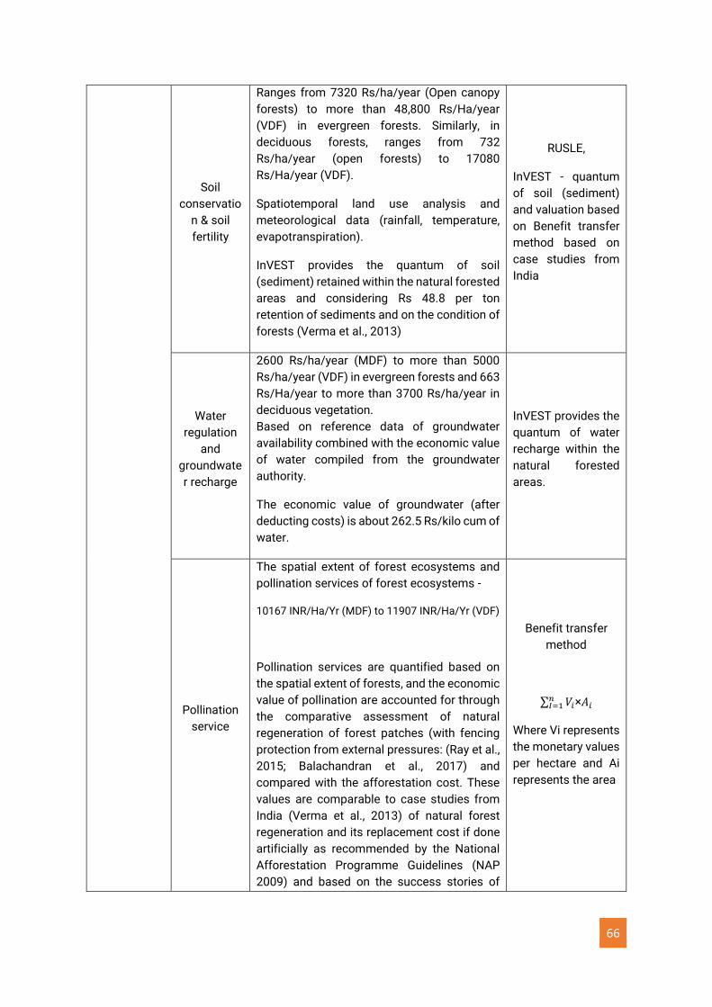
66
Soil
conservatio
n & soil
fertility
Ranges from 7320 Rs/ha/year (Open canopy
forests) to more than 48,800 Rs/Ha/year
(VDF) in evergreen forests. Similarly, in
deciduous forests, ranges from 732
Rs/ha/year (open forests) to 17080
Rs/Ha/year (VDF).
Spatiotemporal land use analysis and
meteorological data (rainfall, temperature,
evapotranspiration).
InVEST provides the quantum of soil
(sediment) retained within the natural forested
areas and considering Rs 48.8 per ton
retention of sediments and on the condition of
forests (Verma et al., 2013)
RUSLE,
InVEST - quantum
of soil (sediment)
and valuation based
on Benefit transfer
method based on
case studies from
India
Water
regulation
and
groundwate
r recharge
2600 Rs/ha/year (MDF) to more than 5000
Rs/ha/year (VDF) in evergreen forests and 663
Rs/Ha/year to more than 3700 Rs/ha/year in
deciduous vegetation.
Based on reference data of groundwater
availability combined with the economic value
of water compiled from the groundwater
authority.
The economic value of groundwater (after
deducting costs) is about 262.5 Rs/kilo cum of
water.
InVEST provides the
quantum of water
recharge within the
natural forested
areas.
Pollination
service
The spatial extent of forest ecosystems and
pollination services of forest ecosystems -
10167 INR/Ha/Yr (MDF) to 11907 INR/Ha/Yr (VDF)
Pollination services are quantified based on
the spatial extent of forests, and the economic
value of pollination are accounted for through
the comparative assessment of natural
regeneration of forest patches (with fencing
protection from external pressures: (Ray et al.,
2015; Balachandran et al., 2017) and
compared with the afforestation cost. These
values are comparable to case studies from
India (Verma et al., 2013) of natural forest
regeneration and its replacement cost if done
artificially as recommended by the National
Afforestation Programme Guidelines (NAP
2009) and based on the success stories of
Benefit transfer
method
∑ 𝑉𝑖𝑛𝐼=1 ×𝐴𝑖
Where Vi represents
the monetary values
per hectare and Ai
represents the area
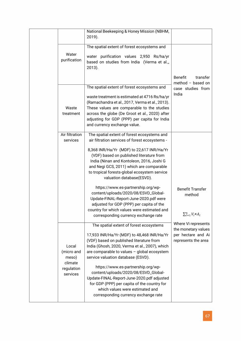
67
National Beekeeping & Honey Mission (NBHM,
2019).
Water
purification
The spatial extent of forest ecosystems and
water purification values 2,950 Rs/ha/yr
based on studies from India (Verma et al.,,
2013).
Benefit transfer
method – based on
case studies from
India
Waste
treatment
The spatial extent of forest ecosystems and
waste treatment is estimated at 4716 Rs/ha/yr
(Ramachandra et al., 2017, Verma et al., 2013).
These values are comparable to the studies
across the globe (De Groot et al., 2020) after
adjusting for GDP (PPP) per capita for India
and currency exchange value.
Air filtration
services
The spatial extent of forest ecosystems and
air filtration services of forest ecosystems -
8,368 INR/Ha/Yr (MDF) to 22,617 INR/Ha/Yr
(VDF) based on published literature from
India (Ninan and Kontoleon, 2016, Joshi G
and Negi GCS, 2011) which are comparable
to tropical forests-global ecosystem service
valuation database(ESVD).
https://www.es-partnership.org/wp-
content/uploads/2020/08/ESVD_Global-
Update-FINAL-Report-June-2020.pdf were
adjusted for GDP (PPP) per capita of the
country for which values were estimated and
corresponding currency exchange rate
Benefit Transfer
method
∑ 𝑉𝑖𝑛𝐼=1 ×𝐴𝑖
Where Vi represents
the monetary values
per hectare and Ai
represents the area
Local
(micro and
meso)
climate
regulation
services
The spatial extent of forest ecosystems
17,933 INR/Ha/Yr (MDF) to 48,468 INR/Ha/Yr
(VDF) based on published literature from
India (Ghosh, 2020, Verma et al., 2007), which
are comparable to values – global ecosystem
service valuation database (ESVD).
https://www.es-partnership.org/wp-
content/uploads/2020/08/ESVD_Global-
Update-FINAL-Report-June-2020.pdf adjusted
for GDP (PPP) per capita of the country for
which values were estimated and
corresponding currency exchange rate
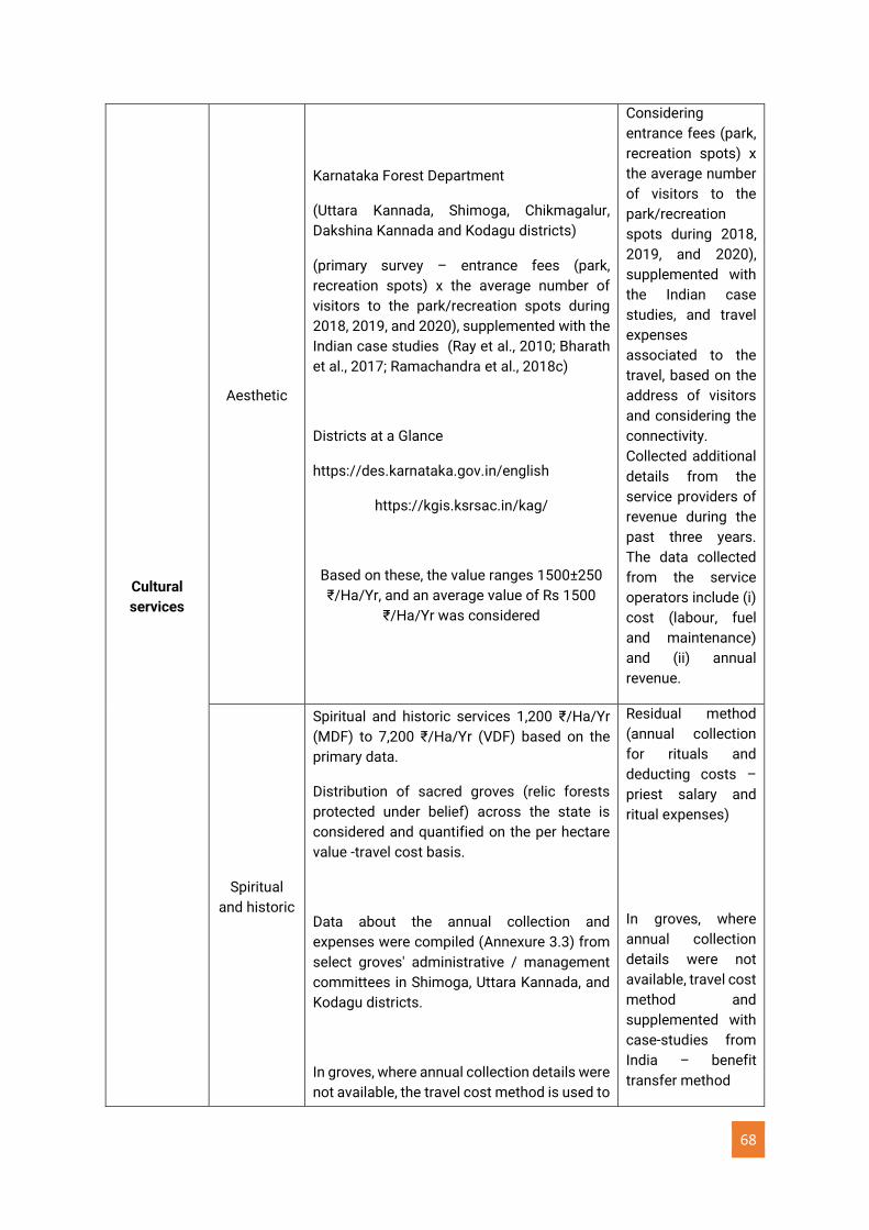
68
Cultural
services
Aesthetic
Karnataka Forest Department
(Uttara Kannada, Shimoga, Chikmagalur,
Dakshina Kannada and Kodagu districts)
(primary survey – entrance fees (park,
recreation spots) x the average number of
visitors to the park/recreation spots during
2018, 2019, and 2020), supplemented with the
Indian case studies (Ray et al., 2010; Bharath
et al., 2017; Ramachandra et al., 2018c)
Districts at a Glance
https://des.karnataka.gov.in/english
https://kgis.ksrsac.in/kag/
Based on these, the value ranges 1500±250
₹/Ha/Yr, and an average value of Rs 1500
₹/Ha/Yr was considered
Considering
entrance fees (park,
recreation spots) x
the average number
of visitors to the
park/recreation
spots during 2018,
2019, and 2020),
supplemented with
the Indian case
studies, and travel
expenses
associated to the
travel, based on the
address of visitors
and considering the
connectivity.
Collected additional
details from the
service providers of
revenue during the
past three years.
The data collected
from the service
operators include (i)
cost (labour, fuel
and maintenance)
and (ii) annual
revenue.
Spiritual
and historic
Spiritual and historic services 1,200 ₹/Ha/Yr
(MDF) to 7,200 ₹/Ha/Yr (VDF) based on the
primary data.
Distribution of sacred groves (relic forests
protected under belief) across the state is
considered and quantified on the per hectare
value -travel cost basis.
Data about the annual collection and
expenses were compiled (Annexure 3.3) from
select groves' administrative / management
committees in Shimoga, Uttara Kannada, and
Kodagu districts.
In groves, where annual collection details were
not available, the travel cost method is used to
Residual method
(annual collection
for rituals and
deducting costs –
priest salary and
ritual expenses)
In groves, where
annual collection
details were not
available, travel cost
method and
supplemented with
case-studies from
India – benefit
transfer method
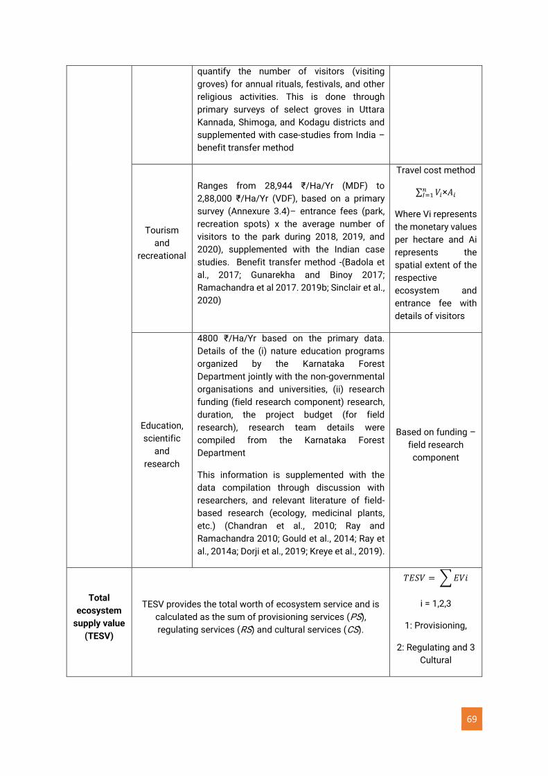
69
quantify the number of visitors (visiting
groves) for annual rituals, festivals, and other
religious activities. This is done through
primary surveys of select groves in Uttara
Kannada, Shimoga, and Kodagu districts and
supplemented with case-studies from India –
benefit transfer method
Tourism
and
recreational
Ranges from 28,944 ₹/Ha/Yr (MDF) to
2,88,000 ₹/Ha/Yr (VDF), based on a primary
survey (Annexure 3.4)– entrance fees (park,
recreation spots) x the average number of
visitors to the park during 2018, 2019, and
2020), supplemented with the Indian case
studies. Benefit transfer method -(Badola et
al., 2017; Gunarekha and Binoy 2017;
Ramachandra et al 2017. 2019b; Sinclair et al.,
2020)
Travel cost method
∑ 𝑉𝑖𝑛𝐼=1 ×𝐴𝑖
Where Vi represents
the monetary values
per hectare and Ai
represents the
spatial extent of the
respective
ecosystem and
entrance fee with
details of visitors
Education,
scientific
and
research
4800 ₹/Ha/Yr based on the primary data.
Details of the (i) nature education programs
organized by the Karnataka Forest
Department jointly with the non-governmental
organisations and universities, (ii) research
funding (field research component) research,
duration, the project budget (for field
research), research team details were
compiled from the Karnataka Forest
Department
This information is supplemented with the
data compilation through discussion with
researchers, and relevant literature of field-
based research (ecology, medicinal plants,
etc.) (Chandran et al., 2010; Ray and
Ramachandra 2010; Gould et al., 2014; Ray et
al., 2014a; Dorji et al., 2019; Kreye et al., 2019).
Based on funding –
field research
component
Total
ecosystem
supply value
(TESV)
TESV provides the total worth of ecosystem service and is
calculated as the sum of provisioning services (PS),
regulating services (RS) and cultural services (CS).
𝑇𝐸𝑆𝑉 = ∑ 𝐸𝑉𝑖
i = 1,2,3
1: Provisioning,
2: Regulating and 3
Cultural
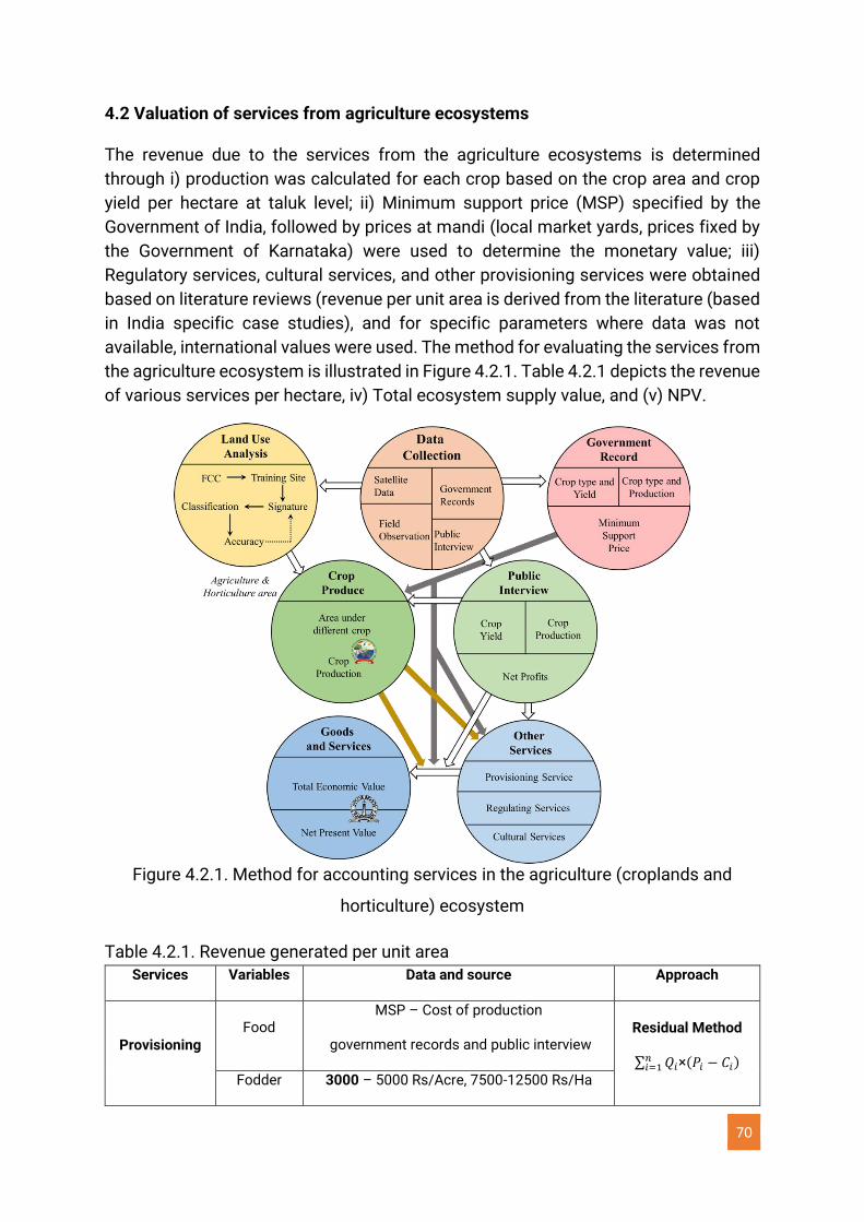
70
4.2 Valuation of services from agriculture ecosystems
The revenue due to the services from the agriculture ecosystems is determined
through i) production was calculated for each crop based on the crop area and crop
yield per hectare at taluk level; ii) Minimum support price (MSP) specified by the
Government of India, followed by prices at mandi (local market yards, prices fixed by
the Government of Karnataka) were used to determine the monetary value; iii)
Regulatory services, cultural services, and other provisioning services were obtained
based on literature reviews (revenue per unit area is derived from the literature (based
in India specific case studies), and for specific parameters where data was not
available, international values were used. The method for evaluating the services from
the agriculture ecosystem is illustrated in Figure 4.2.1. Table 4.2.1 depicts the revenue
of various services per hectare, iv) Total ecosystem supply value, and (v) NPV.
Figure 4.2.1. Method for accounting services in the agriculture (croplands and
horticulture) ecosystem
Table 4.2.1. Revenue generated per unit area
Services Variables Data and source Approach
Provisioning Food
MSP – Cost of production
government records and public interview Residual Method
∑ 𝑄𝑖𝑛𝑖=1 ×(𝑃𝑖 − 𝐶𝑖)
Fodder 3000 – 5000 Rs/Acre, 7500-12500 Rs/Ha
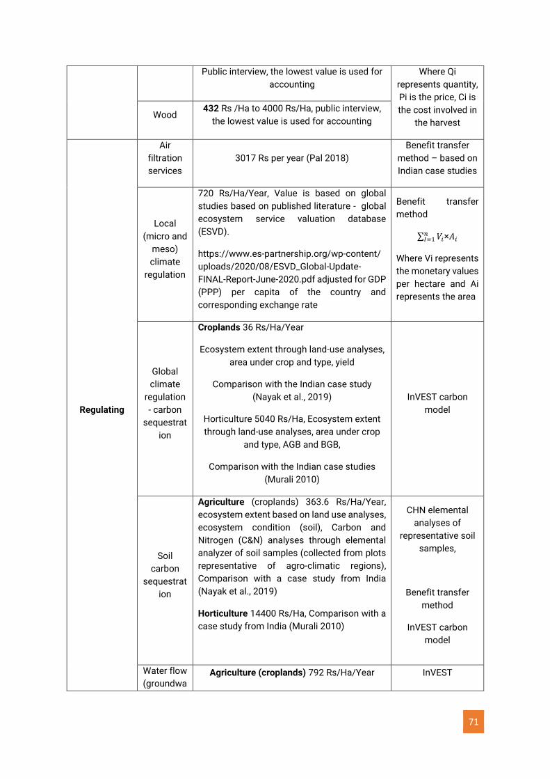
71
Public interview, the lowest value is used for
accounting
Where Qi
represents quantity,
Pi is the price, Ci is
the cost involved in
the harvest Wood
432 Rs /Ha to 4000 Rs/Ha, public interview,
the lowest value is used for accounting
Regulating
Air
filtration
services
3017 Rs per year (Pal 2018)
Benefit transfer
method – based on
Indian case studies
Local
(micro and
meso)
climate
regulation
720 Rs/Ha/Year, Value is based on global
studies based on published literature - global
ecosystem service valuation database
(ESVD).
https://www.es-partnership.org/wp-content/
uploads/2020/08/ESVD_Global-Update-
FINAL-Report-June-2020.pdf adjusted for GDP
(PPP) per capita of the country and
corresponding exchange rate
Benefit transfer
method
∑ 𝑉𝑖𝑛𝐼=1 ×𝐴𝑖
Where Vi represents
the monetary values
per hectare and Ai
represents the area
Global
climate
regulation
- carbon
sequestrat
ion
Croplands 36 Rs/Ha/Year
Ecosystem extent through land-use analyses,
area under crop and type, yield
Comparison with the Indian case study
(Nayak et al., 2019)
Horticulture 5040 Rs/Ha, Ecosystem extent
through land-use analyses, area under crop
and type, AGB and BGB,
Comparison with the Indian case studies
(Murali 2010)
InVEST carbon
model
Soil
carbon
sequestrat
ion
Agriculture (croplands) 363.6 Rs/Ha/Year,
ecosystem extent based on land use analyses,
ecosystem condition (soil), Carbon and
Nitrogen (C&N) analyses through elemental
analyzer of soil samples (collected from plots
representative of agro-climatic regions),
Comparison with a case study from India
(Nayak et al., 2019)
Horticulture 14400 Rs/Ha, Comparison with a
case study from India (Murali 2010)
CHN elemental
analyses of
representative soil
samples,
Benefit transfer
method
InVEST carbon
model
Water flow
(groundwaAgriculture (croplands) 792 Rs/Ha/Year InVEST
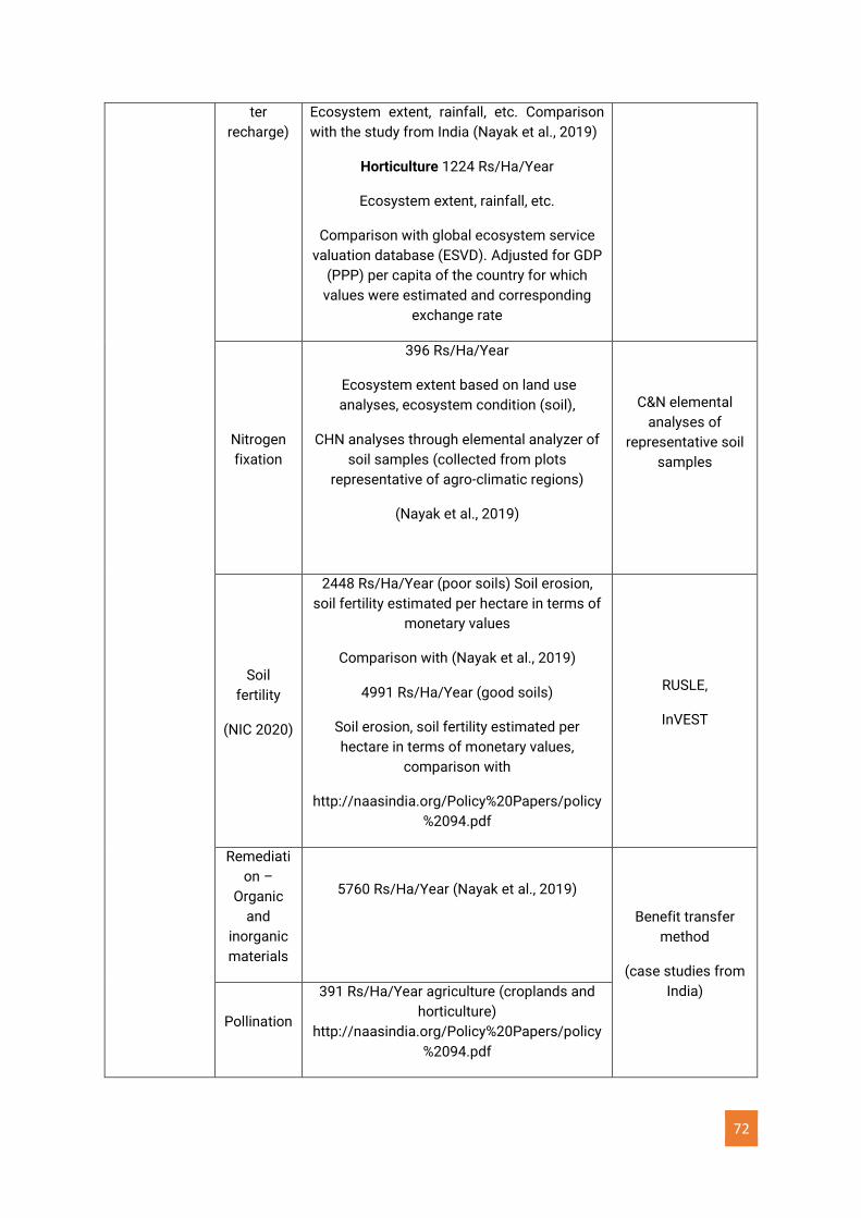
72
ter
recharge)
Ecosystem extent, rainfall, etc. Comparison
with the study from India (Nayak et al., 2019)
Horticulture 1224 Rs/Ha/Year
Ecosystem extent, rainfall, etc.
Comparison with global ecosystem service
valuation database (ESVD). Adjusted for GDP
(PPP) per capita of the country for which
values were estimated and corresponding
exchange rate
Nitrogen
fixation
396 Rs/Ha/Year
Ecosystem extent based on land use
analyses, ecosystem condition (soil),
CHN analyses through elemental analyzer of
soil samples (collected from plots
representative of agro-climatic regions)
(Nayak et al., 2019)
C&N elemental
analyses of
representative soil
samples
Soil
fertility
(NIC 2020)
2448 Rs/Ha/Year (poor soils) Soil erosion,
soil fertility estimated per hectare in terms of
monetary values
Comparison with (Nayak et al., 2019)
4991 Rs/Ha/Year (good soils)
Soil erosion, soil fertility estimated per
hectare in terms of monetary values,
comparison with
http://naasindia.org/Policy%20Papers/policy
%2094.pdf
RUSLE,
InVEST
Remediati
on –
Organic
and
inorganic
materials
5760 Rs/Ha/Year (Nayak et al., 2019)
Benefit transfer
method
(case studies from
India)
Pollination
391 Rs/Ha/Year agriculture (croplands and
horticulture)
http://naasindia.org/Policy%20Papers/policy
%2094.pdf
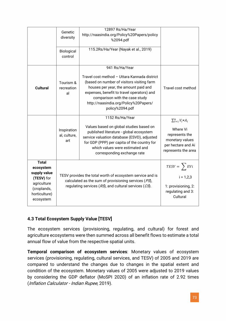
73
Genetic
diversity
12897 Rs/Ha/Year
http://naasindia.org/Policy%20Papers/policy
%2094.pdf
Biological
control
115.2Rs/Ha/Year (Nayak et al., 2019)
Cultural
Tourism &
recreation
al
941 Rs/Ha/Year
Travel cost method – Uttara Kannada district
(based on number of visitors visiting farm
houses per year, the amount paid and
expenses, benefit to travel operators) and
comparison with the case study
http://naasindia.org/Policy%20Papers/
policy%2094.pdf
Travel cost method
Inspiration
al, culture,
art
1152 Rs/Ha/Year
Values based on global studies based on
published literature - global ecosystem
service valuation database (ESVD), adjusted
for GDP (PPP) per capita of the country for
which values were estimated and
corresponding exchange rate
∑ 𝑉𝑖𝑛𝐼=1 ×𝐴𝑖
Where Vi
represents the
monetary values
per hectare and Ai
represents the area
Total
ecosystem
supply value
(TESV) for
agriculture
(croplands,
horticulture)
ecosystem
TESV provides the total worth of ecosystem service and is
calculated as the sum of provisioning services (PS),
regulating services (RS), and cultural services (CS).
𝑇𝐸𝑆𝑉 = ∑ 𝐸𝑉𝑖
i = 1,2,3
1: provisioning, 2:
regulating and 3:
Cultural
4.3 Total Ecosystem Supply Value [TESV]
The ecosystem services (provisioning, regulating, and cultural) for forest and
agriculture ecosystems were then summed across all benefit flows to estimate a total
annual flow of value from the respective spatial units.
Temporal comparison of ecosystem services: Monetary values of ecosystem
services (provisioning, regulating, cultural services, and TESV) of 2005 and 2019 are
compared to understand the changes due to changes in the spatial extent and
condition of the ecosystem. Monetary values of 2005 were adjusted to 2019 values
by considering the GDP deflator (MoSPI 2020) of an inflation rate of 2.92 times
(Inflation Calculator - Indian Rupee, 2019).
74
4.4 Net Present Value (NPV) of ecosystem assets:
The net present value (NPV) is the value of an asset determined by estimating the
stream of income expected to be earned in the future and then discounting the future
income back to the present accounting period. (SEEA, 2021). In ecosystem
accounting, it is applied by aggregating the NPV of expected future returns for each
ecosystem service supplied by an ecosystem asset. The use of an NPV approach
implies that their value will be related to the capacity to supply ecosystem services
and how this capacity is expected to change in the future.
NPV is based on the measurement of (i) the ecosystem services supplied by the asset,
and the monetary values of these services (ii) estimation of pattern of future flows of
each ecosystem service, taking into account expected degradation/enhancement and
demand (iii) expected future prices for each ecosystem service; (iv) expected
institutional arrangements; and (v) expected asset life. In addition, NPV requires a
discount rate, which adjusts the value of a stream of future flows to account for time
preferences and attitudes to risk. Discount rates are required to convert the expected
future ecosystem services flows into a current period estimate of overall value. In this
report, a social discount rate (as opposed to individual discount rate) has been used,
as most of the ecosystem services contribute to collective benefits.
Net present value is calculated using equation 4.1 and applied at the level of individual
ecosystem services, and the resulting discounted values are aggregated to derive the
monetary value of the ecosystem asset.
NPV = ∑ESt
(1+r)tTt=1 --------------------- 4.1
Where, t – Number of years ranging between 1 to T.
T - Number of years for which this annual benefit from the asset will accrue.
This is closely linked to the length of time needed to regenerate the same
type and quality of forests. The Hon’ble Supreme Court of India in the
Judgement of 26th September 2005 (Page 10, Para 4) has suggested that
the basis for calculation of NPV should be the economic value spread over
a period of 50 years, which is the period for forest regeneration
ESt –Ecosystem services at time t
r – Social rate of discount for capital returns. As per the norms in India and
Hon’ble Supreme Court, a social discount rate of 4% is applied for renewables
and 2% for non-renewable resources. Hence, for forest ecosystems, 3% is
considered that is the weighted average of renewable and non-renewable.
NPV of ecosystems (forests, agriculture) in Karnataka is computed using TESV -the
total value of ecosystem flow based on a social discount rate of 3% and a period of
50 years. The ecosystem service values are determined based on government
records, and prices were considered to remain the same with no inflations for 50 years
(w.r.t 2019).
75
Section 5.0 Results and Discussion
Valuation of ecosystem services entails the computation of spatial extent and
conditions of the respective ecosystems, and quantification of services in physical
and monetary units. The spatial extent (Ramachandra et al., 2021a) and the condition
of forests (Ramachandra et al., 2021b) assessed district-wise earlier for Karnataka
(Ramachandra et al., 2021a, b) were used for computing the value of the provisioning
services per hectare. Forests have been reclassified as VDF (very dense forests), MDF
(medium dense forests), and open forests (OF) based on the condition (computed
through the fragmentation analyses), comparable to the classification approach
adopted by the Karnataka Forest Department (based on the forest type and their
canopy cover). A similar approach was adopted earlier to compute ecosystem
services from forest ecosystems in India (Verma et al., 2013).
The following subsections present (i) the extent of ecosystems in Karnataka, (ii)
valuation of ecosystem services, (iii) computation of TESV: Total ecosystem supply
value and NPV of ecosystem assets
5.1 Assessment of ecosystem extent over time
An assessment of ecosystem extent was performed, using land use and land cover as
proxies. The spatiotemporal land cover/use analysis was carried out from 1985 to
2019 using remote sensing data through a supervised classifier based on the
Gaussian maximum likelihood algorithm.
The state witnessed large-scale land-use transitions post-1990s due to globalization
and the consequent spurt in industrialization and urbanization, as well as an increase
of horticulture crops and the conversion of croplands (cereals, pulses, etc.) to market-
based cash crops (coffee, sugarcane, areca nut, etc. with higher economic values),
etc.
Temporal land cover/use analyses reveal the decline of forest cover in Karnataka from
1985 to 2019 (Figure 5.1). Districts of the Western Ghats region have a higher forest
cover than other districts, as depicted in Figure 5.1. Currently, 15% of the State’s
geographical area is forested, compared to 21% in 1985 (Table 5.1). Large-scale
developmental activities such as constructing a series of reservoirs and dams,
creating special economic zones, townships, and land conversion for built-up areas
have led to the loss of large tracts of forests. The forest cover now is confined to
major conservation reserves such as protected areas, national parks, and wildlife
sanctuaries. Natural forests show a decline of evergreen forests from 7.5% (1985) to
5.7% (by 2019), moist deciduous forests from 5.7% (1985) to 4.1% (by 2019), and dry
deciduous forests from 4.0% (1985) to 2.2 % (2019).
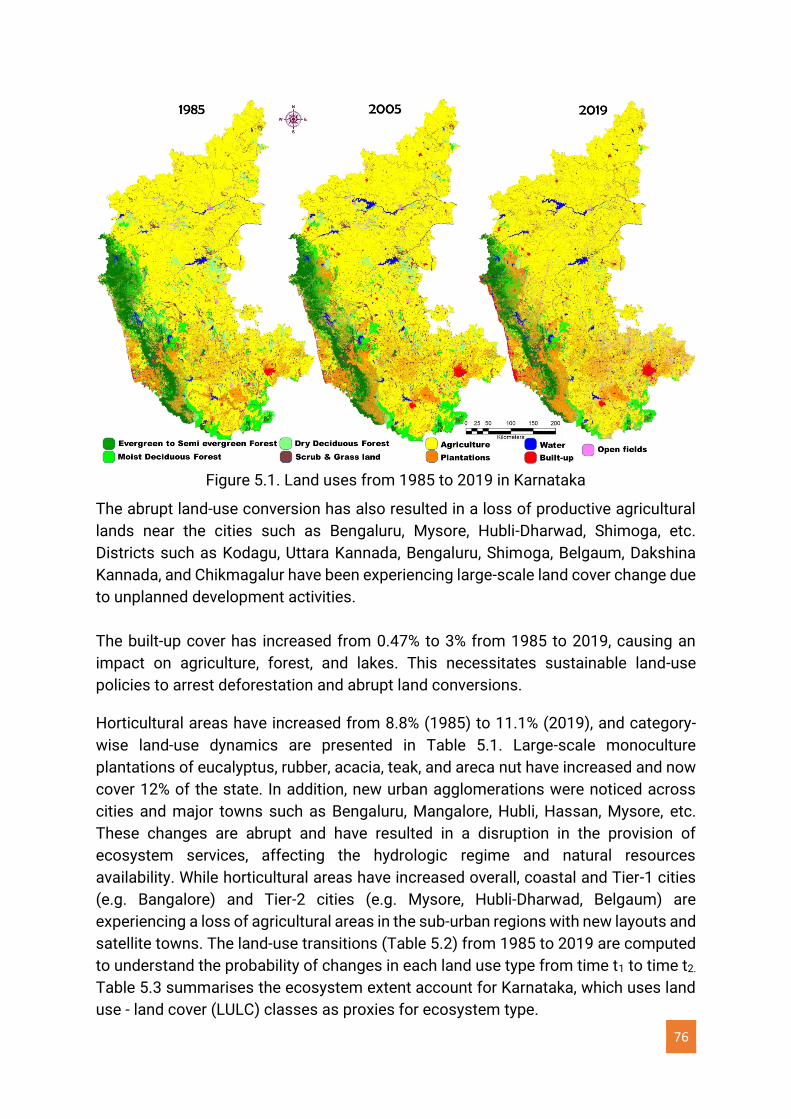
76
Figure 5.1. Land uses from 1985 to 2019 in Karnataka
The abrupt land-use conversion has also resulted in a loss of productive agricultural
lands near the cities such as Bengaluru, Mysore, Hubli-Dharwad, Shimoga, etc.
Districts such as Kodagu, Uttara Kannada, Bengaluru, Shimoga, Belgaum, Dakshina
Kannada, and Chikmagalur have been experiencing large-scale land cover change due
to unplanned development activities.
The built-up cover has increased from 0.47% to 3% from 1985 to 2019, causing an
impact on agriculture, forest, and lakes. This necessitates sustainable land-use
policies to arrest deforestation and abrupt land conversions.
Horticultural areas have increased from 8.8% (1985) to 11.1% (2019), and category-
wise land-use dynamics are presented in Table 5.1. Large-scale monoculture
plantations of eucalyptus, rubber, acacia, teak, and areca nut have increased and now
cover 12% of the state. In addition, new urban agglomerations were noticed across
cities and major towns such as Bengaluru, Mangalore, Hubli, Hassan, Mysore, etc.
These changes are abrupt and have resulted in a disruption in the provision of
ecosystem services, affecting the hydrologic regime and natural resources
availability. While horticultural areas have increased overall, coastal and Tier-1 cities
(e.g. Bangalore) and Tier-2 cities (e.g. Mysore, Hubli-Dharwad, Belgaum) are
experiencing a loss of agricultural areas in the sub-urban regions with new layouts and
satellite towns. The land-use transitions (Table 5.2) from 1985 to 2019 are computed
to understand the probability of changes in each land use type from time t1 to time t2.
Table 5.3 summarises the ecosystem extent account for Karnataka, which uses land
use - land cover (LULC) classes as proxies for ecosystem type.
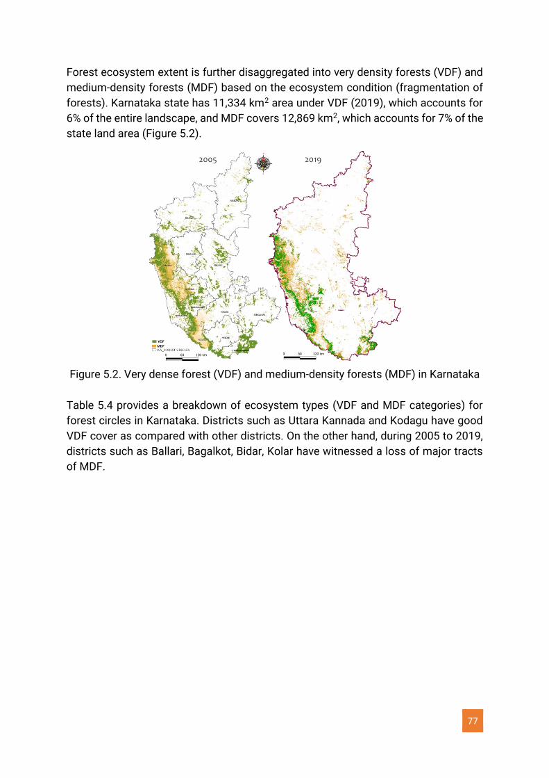
77
Forest ecosystem extent is further disaggregated into very density forests (VDF) and
medium-density forests (MDF) based on the ecosystem condition (fragmentation of
forests). Karnataka state has 11,334 km2 area under VDF (2019), which accounts for
6% of the entire landscape, and MDF covers 12,869 km2, which accounts for 7% of the
state land area (Figure 5.2).
Figure 5.2. Very dense forest (VDF) and medium-density forests (MDF) in Karnataka
Table 5.4 provides a breakdown of ecosystem types (VDF and MDF categories) for
forest circles in Karnataka. Districts such as Uttara Kannada and Kodagu have good
VDF cover as compared with other districts. On the other hand, during 2005 to 2019,
districts such as Ballari, Bagalkot, Bidar, Kolar have witnessed a loss of major tracts
of MDF.
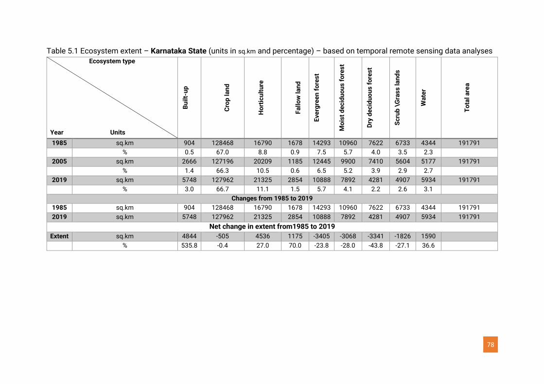
78
Table 5.1 Ecosystem extent – Karnataka State (units in sq.km and percentage) – based on temporal remote sensing data analyses
Ecosystem type
Year Units
Bu
ilt-
up
Cro
p l
an
d
Ho
rtic
ult
ure
Fa
llo
w l
an
d
Ev
erg
ree
n f
ore
st
Mo
ist
de
cid
uo
us
fo
res
t
Dry
de
cid
uo
us
fo
res
t
Sc
rub
\G
ras
s l
an
ds
Wa
ter
To
tal
are
a
1985 sq.km 904 128468 16790 1678 14293 10960 7622 6733 4344 191791 % 0.5 67.0 8.8 0.9 7.5 5.7 4.0 3.5 2.3
2005 sq.km 2666 127196 20209 1185 12445 9900 7410 5604 5177 191791 % 1.4 66.3 10.5 0.6 6.5 5.2 3.9 2.9 2.7
2019 sq.km 5748 127962 21325 2854 10888 7892 4281 4907 5934 191791 % 3.0 66.7 11.1 1.5 5.7 4.1 2.2 2.6 3.1
Changes from 1985 to 2019
1985 sq.km 904 128468 16790 1678 14293 10960 7622 6733 4344 191791
2019 sq.km 5748 127962 21325 2854 10888 7892 4281 4907 5934 191791
Net change in extent from1985 to 2019
Extent sq.km 4844 -505 4536 1175 -3405 -3068 -3341 -1826 1590
% 535.8 -0.4 27.0 70.0 -23.8 -28.0 -43.8 -27.1 36.6
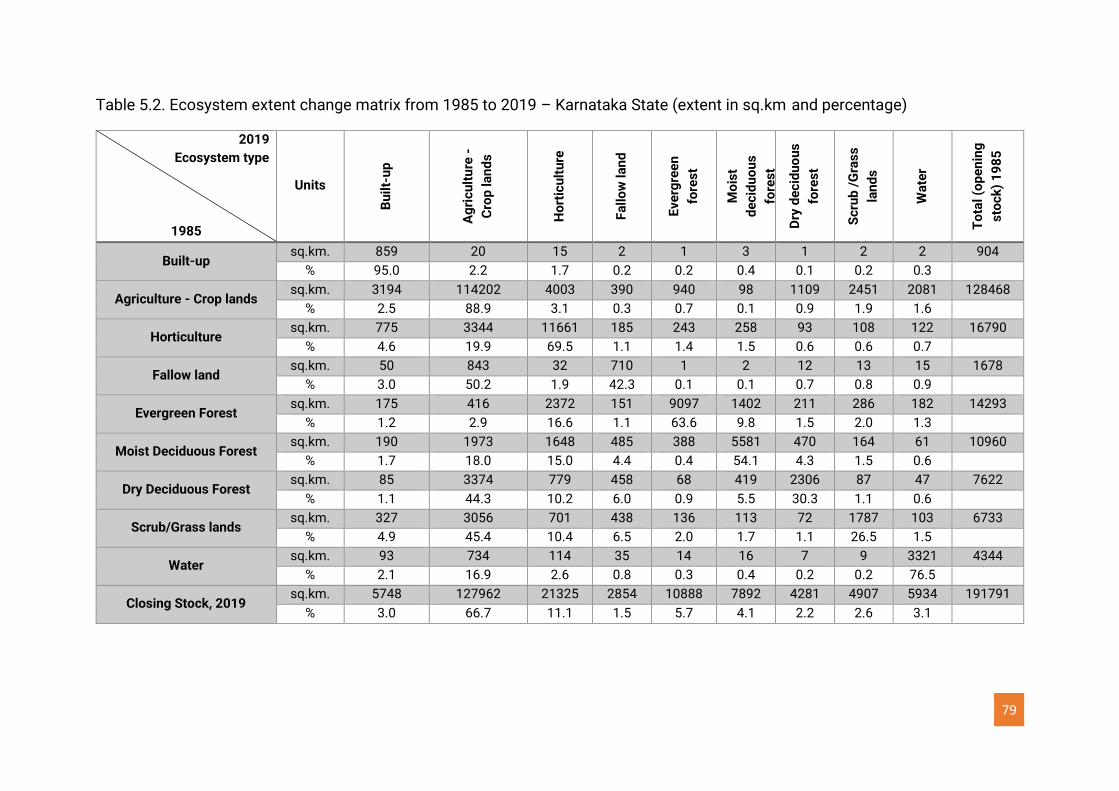
79
Table 5.2. Ecosystem extent change matrix from 1985 to 2019 – Karnataka State (extent in sq.km and percentage)
2019
Ecosystem type
1985
Units
Bu
ilt-
up
Ag
ric
ult
ure
-
Cro
p l
an
ds
Ho
rtic
ult
ure
Fa
llo
w l
an
d
Ev
erg
ree
n
fore
st
Mo
ist
de
cid
uo
us
fore
st
Dry
de
cid
uo
us
fore
st
Sc
rub
/G
ras
s
lan
ds
Wa
ter
To
tal
(op
en
ing
sto
ck
) 1
98
5
Built-up sq.km. 859 20 15 2 1 3 1 2 2 904
% 95.0 2.2 1.7 0.2 0.2 0.4 0.1 0.2 0.3
Agriculture - Crop lands sq.km. 3194 114202 4003 390 940 98 1109 2451 2081 128468
% 2.5 88.9 3.1 0.3 0.7 0.1 0.9 1.9 1.6
Horticulture sq.km. 775 3344 11661 185 243 258 93 108 122 16790
% 4.6 19.9 69.5 1.1 1.4 1.5 0.6 0.6 0.7
Fallow land sq.km. 50 843 32 710 1 2 12 13 15 1678
% 3.0 50.2 1.9 42.3 0.1 0.1 0.7 0.8 0.9
Evergreen Forest sq.km. 175 416 2372 151 9097 1402 211 286 182 14293
% 1.2 2.9 16.6 1.1 63.6 9.8 1.5 2.0 1.3
Moist Deciduous Forest sq.km. 190 1973 1648 485 388 5581 470 164 61 10960
% 1.7 18.0 15.0 4.4 0.4 54.1 4.3 1.5 0.6
Dry Deciduous Forest sq.km. 85 3374 779 458 68 419 2306 87 47 7622
% 1.1 44.3 10.2 6.0 0.9 5.5 30.3 1.1 0.6
Scrub/Grass lands sq.km. 327 3056 701 438 136 113 72 1787 103 6733
% 4.9 45.4 10.4 6.5 2.0 1.7 1.1 26.5 1.5
Water sq.km. 93 734 114 35 14 16 7 9 3321 4344
% 2.1 16.9 2.6 0.8 0.3 0.4 0.2 0.2 76.5
Closing Stock, 2019 sq.km. 5748 127962 21325 2854 10888 7892 4281 4907 5934 191791
% 3.0 66.7 11.1 1.5 5.7 4.1 2.2 2.6 3.1
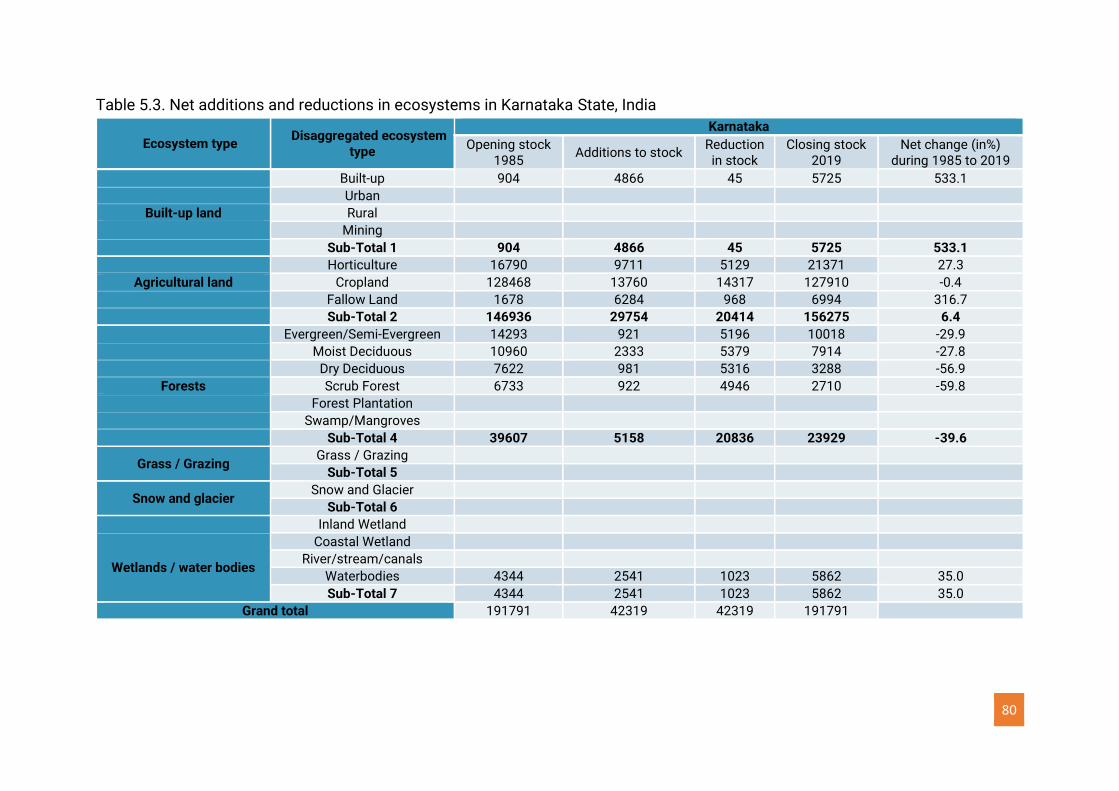
80
Table 5.3. Net additions and reductions in ecosystems in Karnataka State, India
Ecosystem type Disaggregated ecosystem
type
Karnataka
Opening stock 1985
Additions to stock Reduction in stock
Closing stock 2019
Net change (in%) during 1985 to 2019
Built-up 904 4866 45 5725 533.1 Urban
Built-up land Rural
Mining
Sub-Total 1 904 4866 45 5725 533.1 Horticulture 16790 9711 5129 21371 27.3
Agricultural land Cropland 128468 13760 14317 127910 -0.4 Fallow Land 1678 6284 968 6994 316.7 Sub-Total 2 146936 29754 20414 156275 6.4 Evergreen/Semi-Evergreen 14293 921 5196 10018 -29.9 Moist Deciduous 10960 2333 5379 7914 -27.8 Dry Deciduous 7622 981 5316 3288 -56.9
Forests Scrub Forest 6733 922 4946 2710 -59.8 Forest Plantation
Swamp/Mangroves
Sub-Total 4 39607 5158 20836 23929 -39.6
Grass / Grazing Grass / Grazing
Sub-Total 5
Snow and glacier Snow and Glacier
Sub-Total 6
Inland Wetland
Wetlands / water bodies
Coastal Wetland
River/stream/canals
Waterbodies 4344 2541 1023 5862 35.0
Sub-Total 7 4344 2541 1023 5862 35.0
Grand total 191791 42319 42319 191791
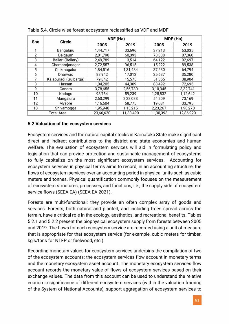
81
Table 5.4. Circle wise forest ecosystem reclassified as VDF and MDF
Sno Circle VDF (Ha) MDF (Ha)
2005 2019 2005 2019
1 Bengaluru 1,44,717 33,696 37,213 63,035
2 Belgaum 2,01,790 60,393 78,388 87,360
3 Ballari (Bellary) 2,49,789 13,514 64,122 92,697
4 Chamarajanagar 2,72,557 96,515 15,222 89,538
5 Chikmagalur 1,84,516 1,31,484 37,230 64,794
6 Dharwad 83,942 17,012 25,637 35,280
7 Kalaburagi (Gulbarga) 79,842 15,575 51,355 38,904
8 Hassan 1,04,205 44,309 88,492 72,695
9 Canara 3,78,655 2,56,730 3,10,345 3,32,741
10 Kodagu 93,764 59,239 1,25,832 1,12,642
11 Mangaluru 2,60,299 2,23,033 54,209 73,169
12 Mysore 1,16,604 68,775 19,081 33,795
13 Shivamogga 1,95,940 1,13,215 2,23,267 1,90,270
Total Area 23,66,620 11,33,490 11,30,393 12,86,920
5.2 Valuation of the ecosystem services
Ecosystem services and the natural capital stocks in Karnataka State make significant
direct and indirect contributions to the district and state economies and human
welfare. The evaluation of ecosystem services will aid in formulating policy and
legislation that can provide protection and sustainable management of ecosystems
to fully capitalize on the most significant ecosystem services. Accounting for
ecosystem services in physical terms aims to record, in an accounting structure, the
flows of ecosystem services over an accounting period in physical units such as cubic
meters and tonnes. Physical quantification commonly focuses on the measurement
of ecosystem structures, processes, and functions, i.e., the supply side of ecosystem
service flows (SEEA EA) (SEEA EA 2021).
Forests are multi-functional: they provide an often complex array of goods and
services. Forests, both natural and planted, and including trees spread across the
terrain, have a critical role in the ecology, aesthetics, and recreational benefits. Tables
5.2.1 and 5.2.2 present the biophysical ecosystem supply from forests between 2005
and 2019. The flows for each ecosystem service are recorded using a unit of measure
that is appropriate for that ecosystem service (for example, cubic meters for timber,
kg’s/tons for NTFP or fuelwood, etc.).
Recording monetary values for ecosystem services underpins the compilation of two
of the ecosystem accounts: the ecosystem services flow account in monetary terms
and the monetary ecosystem asset account. The monetary ecosystem services flow
account records the monetary value of flows of ecosystem services based on their
exchange values. The data from this account can be used to understand the relative
economic significance of different ecosystem services (within the valuation framing
of the System of National Accounts), support aggregation of ecosystem services to
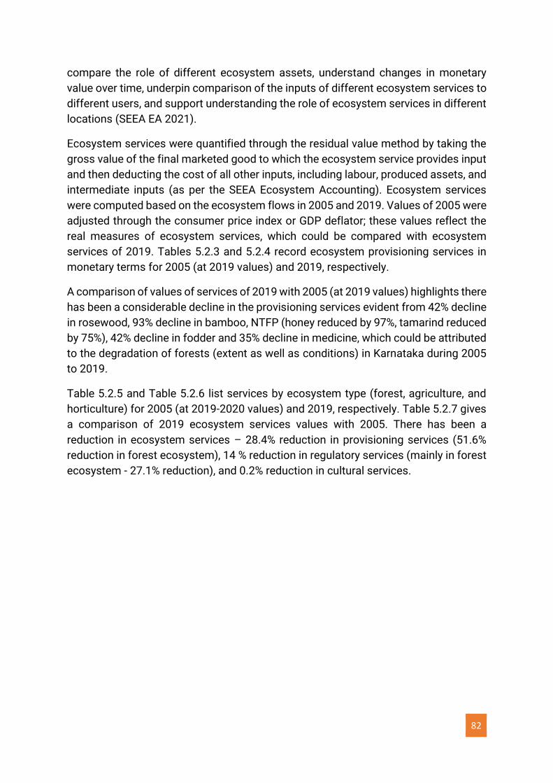
82
compare the role of different ecosystem assets, understand changes in monetary
value over time, underpin comparison of the inputs of different ecosystem services to
different users, and support understanding the role of ecosystem services in different
locations (SEEA EA 2021).
Ecosystem services were quantified through the residual value method by taking the
gross value of the final marketed good to which the ecosystem service provides input
and then deducting the cost of all other inputs, including labour, produced assets, and
intermediate inputs (as per the SEEA Ecosystem Accounting). Ecosystem services
were computed based on the ecosystem flows in 2005 and 2019. Values of 2005 were
adjusted through the consumer price index or GDP deflator; these values reflect the
real measures of ecosystem services, which could be compared with ecosystem
services of 2019. Tables 5.2.3 and 5.2.4 record ecosystem provisioning services in
monetary terms for 2005 (at 2019 values) and 2019, respectively.
A comparison of values of services of 2019 with 2005 (at 2019 values) highlights there
has been a considerable decline in the provisioning services evident from 42% decline
in rosewood, 93% decline in bamboo, NTFP (honey reduced by 97%, tamarind reduced
by 75%), 42% decline in fodder and 35% decline in medicine, which could be attributed
to the degradation of forests (extent as well as conditions) in Karnataka during 2005
to 2019.
Table 5.2.5 and Table 5.2.6 list services by ecosystem type (forest, agriculture, and
horticulture) for 2005 (at 2019-2020 values) and 2019, respectively. Table 5.2.7 gives
a comparison of 2019 ecosystem services values with 2005. There has been a
reduction in ecosystem services – 28.4% reduction in provisioning services (51.6%
reduction in forest ecosystem), 14 % reduction in regulatory services (mainly in forest
ecosystem - 27.1% reduction), and 0.2% reduction in cultural services.
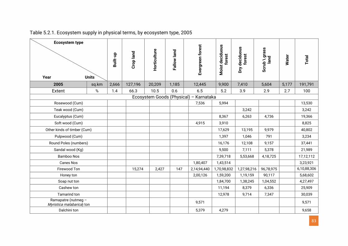
83
Table 5.2.1. Ecosystem supply in physical terms, by ecosystem type, 2005
Ecosystem type
Year Units
Bu
ilt-
up
Cro
p l
an
d
Ho
rtic
ult
ure
Fa
llo
w l
an
d
Ev
erg
ree
n f
ore
st
Mo
ist
de
cid
uo
us
f
ore
st
Dry
de
cid
uo
us
f
ore
st
Sc
rub
\ g
ras
s
lan
d
Wa
ter
To
tal
2005 sq.km 2,666 127,196 20,209 1,185 12,445 9,900 7,410 5,604 5,177 191,791
Extent % 1.4 66.3 10.5 0.6 6.5 5.2 3.9 2.9 2.7 100
Ecosystem Goods (Physical) – Karnataka
Rosewood (Cum) 7,536 5,994 13,530
Teak wood (Cum) 3,242 3,242
Eucalyptus (Cum) 8,367 6,263 4,736 19,366
Soft wood (Cum) 4,915 3,910 8,825
Other kinds of timber (Cum) 17,629 13,195 9,979 40,802
Pulpwood (Cum) 1,397 1,046 791 3,234
Round Poles (numbers) 16,176 12,108 9,157 37,441
Sandal wood (Kg) 9,500 7,111 5,378 21,989
Bamboo Nos 7,39,718 5,53,668 4,18,725 17,12,112
Canes Nos 1,80,407 1,43,514 3,23,921
Firewood Ton 15,274 2,427 147 2,14,94,440 1,70,98,832 1,27,98,216 96,78,975 6,10,88,306
Honey ton 2,00,126 1,59,200 1,19,159 90,117 5,68,602
Soap nut ton 1,84,700 1,38,245 1,04,552 4,27,497
Cashew ton 11,194 8,379 6,336 25,909
Tamarind ton 12,978 9,714 7,347 30,039
Ramapatre (nutmeg – Myristica malabarica) ton
9,571 9,571
Dalchini ton 5,379 4,279 9,658
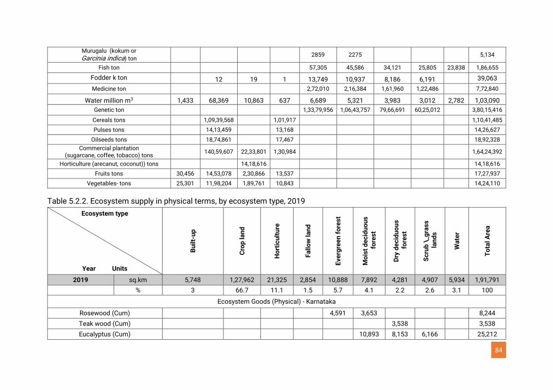
84
Murugalu (kokum or
Garcinia indica) ton 2859 2275 5,134
Fish ton 57,305 45,586 34,121 25,805 23,838 1,86,655
Fodder k ton 12 19 1 13,749 10,937 8,186 6,191 39,063
Medicine ton 2,72,010 2,16,384 1,61,960 1,22,486 7,72,840
Water million m3 1,433 68,369 10,863 637 6,689 5,321 3,983 3,012 2,782 1,03,090
Genetic ton 1,33,79,956 1,06,43,757 79,66,691 60,25,012 3,80,15,416
Cereals tons 1,09,39,568 1,01,917 1,10,41,485
Pulses tons 14,13,459 13,168 14,26,627
Oilseeds tons 18,74,861 17,467 18,92,328
Commercial plantation (sugarcane, coffee, tobacco) tons
140,59,607 22,33,801 1,30,984 1,64,24,392
Horticulture (arecanut, coconut)) tons 14,18,616 14,18,616
Fruits tons 30,456 14,53,078 2,30,866 13,537 17,27,937
Vegetables- tons 25,301 11,98,204 1,89,761 10,843 14,24,110
Table 5.2.2. Ecosystem supply in physical terms, by ecosystem type, 2019
Ecosystem type
Year Units
Bu
ilt-
up
Cro
p l
an
d
Ho
rtic
ult
ure
Fa
llo
w l
an
d
Ev
erg
ree
n f
ore
st
Mo
ist
de
cid
uo
us
f
ore
st
Dry
de
cid
uo
us
f
ore
st
Sc
rub
\_g
ras
s
la
nd
s
Wa
ter
To
tal
Are
a
2019 sq.km 5,748 1,27,962 21,325 2,854 10,888 7,892 4,281 4,907 5,934 1,91,791 % 3 66.7 11.1 1.5 5.7 4.1 2.2 2.6 3.1 100
Ecosystem Goods (Physical) - Karnataka
Rosewood (Cum) 4,591 3,653 8,244
Teak wood (Cum) 3,538 3,538
Eucalyptus (Cum) 10,893 8,153 6,166 25,212
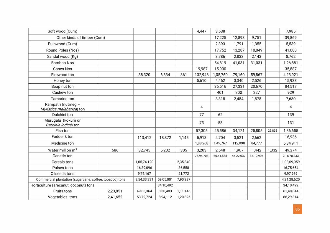
85
Soft wood (Cum) 4,447 3,538 7,985
Other kinds of timber (Cum) 17,225 12,893 9,751 39,869
Pulpwood (Cum) 2,393 1,791 1,355 5,539
Round Poles (Nos) 17,752 13,287 10,049 41,088
Sandal wood (Kg) 3,786 2,833 2,143 8,762
Bamboo Nos 54,819 41,031 31,031 1,26,881
Canes Nos 19,987 15,900 35,887
Firewood ton 38,320 6,834 861 132,948 1,05,760 79,160 59,867 4,23,921
Honey ton 5,610 4,462 3,340 2,526 15,938
Soap nut ton 36,516 27,331 20,670 84,517
Cashew ton 401 300 227 929
Tamarind ton 3,318 2,484 1,878 7,680
Rampatri (nutmeg – Myristica malabarica) ton
4 4
Dalchini ton 77 62 139
Murugalu (kokum or Garcinia indica) ton
73 58 131
Fish ton 57,305 45,586 34,121 25,805 23,838 1,86,655
Fodder k ton 113,412 18,872 1,145 5,913 4,704 3,521 2,662 16,936
Medicine ton 1,88,268 1,49,767 112,098 84,777 5,34,911
Water million m3 686 32,745 5,202 305 3,203 2,548 1,907 1,442 1,332 49,374
Genetic ton 75,94,703 60,41,588 45,22,037 34,19,905 2,15,78,233
Cereals tons 1,05,74,120 2,35,840 1,08,09,959
Pulses tons 16,39,096 36,558 16,75,654
Oilseeds tons 9,76,167 21,772 9,97,939
Commercial plantation (sugarcane, coffee, tobacco) tons 3,54,33,331 59,05,001 7,90,287 4,21,28,620
Horticulture (arecanut, coconut) tons 34,10,492 34,10,492
Fruits tons 2,23,851 49,83,364 8,30,483 1,11,146 61,48,844
Vegetables- tons 2,41,652 53,72,724 8,94,112 1,20,826 66,29,314
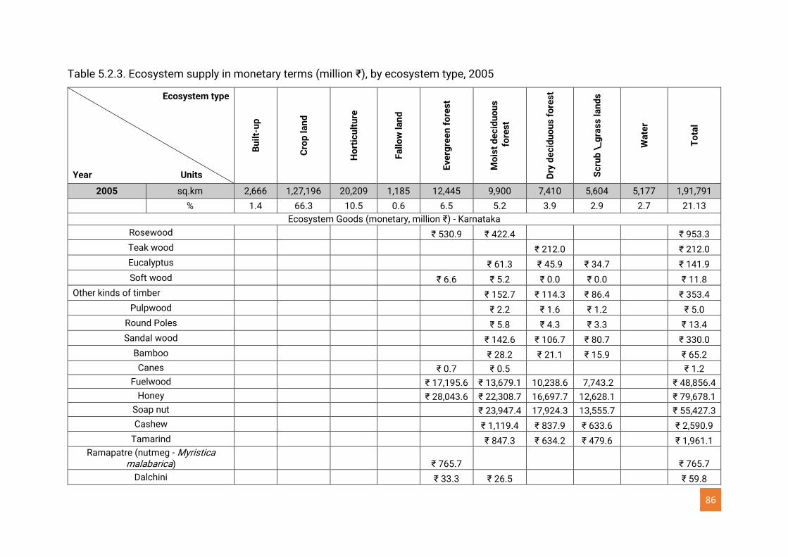
86
Table 5.2.3. Ecosystem supply in monetary terms (million ₹), by ecosystem type, 2005
Ecosystem type
Year Units
Bu
ilt-
up
Cro
p l
an
d
Ho
rtic
ult
ure
Fa
llo
w l
an
d
Ev
erg
ree
n f
ore
st
Mo
ist
de
cid
uo
us
f
ore
st
Dry
de
cid
uo
us
fo
res
t
Sc
rub
\_g
ras
s l
an
ds
Wa
ter
To
tal
2005 sq.km 2,666 1,27,196 20,209 1,185 12,445 9,900 7,410 5,604 5,177 1,91,791 % 1.4 66.3 10.5 0.6 6.5 5.2 3.9 2.9 2.7 21.13
Ecosystem Goods (monetary, million ₹) - Karnataka
Rosewood ₹ 530.9 ₹ 422.4 ₹ 953.3
Teak wood ₹ 212.0 ₹ 212.0
Eucalyptus ₹ 61.3 ₹ 45.9 ₹ 34.7 ₹ 141.9
Soft wood ₹ 6.6 ₹ 5.2 ₹ 0.0 ₹ 0.0 ₹ 11.8
Other kinds of timber ₹ 152.7 ₹ 114.3 ₹ 86.4 ₹ 353.4
Pulpwood ₹ 2.2 ₹ 1.6 ₹ 1.2 ₹ 5.0
Round Poles ₹ 5.8 ₹ 4.3 ₹ 3.3 ₹ 13.4
Sandal wood ₹ 142.6 ₹ 106.7 ₹ 80.7 ₹ 330.0
Bamboo ₹ 28.2 ₹ 21.1 ₹ 15.9 ₹ 65.2
Canes ₹ 0.7 ₹ 0.5 ₹ 1.2
Fuelwood ₹ 17,195.6 ₹ 13,679.1 10,238.6 7,743.2 ₹ 48,856.4
Honey ₹ 28,043.6 ₹ 22,308.7 16,697.7 12,628.1 ₹ 79,678.1
Soap nut ₹ 23,947.4 17,924.3 13,555.7 ₹ 55,427.3
Cashew ₹ 1,119.4 ₹ 837.9 ₹ 633.6 ₹ 2,590.9
Tamarind ₹ 847.3 ₹ 634.2 ₹ 479.6 ₹ 1,961.1
Ramapatre (nutmeg - Myristica malabarica) ₹ 765.7 ₹ 765.7
Dalchini ₹ 33.3 ₹ 26.5 ₹ 59.8
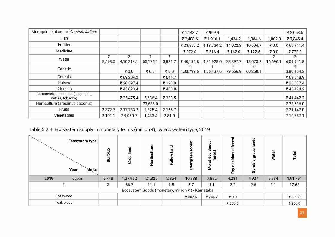
87
Murugalu (kokum or Garcinia indica) ₹ 1,143.7 ₹ 909.9 ₹ 2,053.6
Fish ₹ 2,408.6 ₹ 1,916.1 1,434.2 1,084.6 1,002.0 ₹ 7,845.4
Fodder ₹ 23,550.2 ₹ 18,734.2 14,022.3 10,604.7 ₹ 0.0 ₹ 66,911.4
Medicine ₹ 272.0 ₹ 216.4 ₹ 162.0 ₹ 122.5 ₹ 0.0 ₹ 772.8
Water ₹
8,598.0 ₹
4,10,214.1 ₹
65,175.1 ₹
3,821.7 ₹ 40,135.8 ₹ 31,928.0 23,897.7
18,073.2 ₹
16,696.1 ₹
6,09,941.8
Genetic ₹ 0.0 ₹ 0.0 ₹ 0.0
₹ 1,33,799.6
₹ 1,06,437.6
₹ 79,666.9
₹ 60,250.1
₹ 3,80,154.2
Cereals ₹ 69,204.2 ₹ 644.7 ₹ 69,848.9
Pulses ₹ 20,397.4 ₹ 190.0 ₹ 20,587.4
Oilseeds ₹ 43,023.4 ₹ 400.8 ₹ 43,424.2 Commercial plantation (sugarcane,
coffee, tobacco) ₹ 35,475.4 5,636.4 ₹ 330.5 ₹ 41,442.2
Horticulture (arecanut, coconut) 73,636.0 ₹ 73,636.0
Fruits ₹ 372.7 ₹ 17,783.2 2,825.4 ₹ 165.7 ₹ 21,147.0
Vegetables ₹ 191.1 ₹ 9,050.7 1,433.4 ₹ 81.9 ₹ 10,757.1
Table 5.2.4. Ecosystem supply in monetary terms (million ₹), by ecosystem type, 2019
Ecosystem type
Year Units
Bu
ilt-
up
Cro
p l
an
d
Ho
rtic
ult
ure
Fa
llo
w l
an
d
Ev
erg
ree
n f
ore
st
Mo
ist
de
cid
uo
us
fo
res
t
Dry
de
cid
uo
us
fo
res
t
Sc
rub
\_g
ras
s l
an
ds
Wa
ter
To
tal
2019 sq.km 5,748 1,27,962 21,325 2,854 10,888 7,892 4,281 4,907 5,934 1,91,791
% 3 66.7 11.1 1.5 5.7 4.1 2.2 2.6 3.1 17.68
Ecosystem Goods (monetary, million ₹ ) - Karnataka
Rosewood ₹ 307.6 ₹ 244.7 ₹ 0.0 ₹ 552.3
Teak wood ₹ 230.0 ₹ 230.0
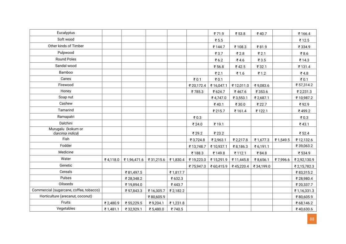
88
Eucalyptus ₹ 71.9 ₹ 53.8 ₹ 40.7 ₹ 166.4
Soft wood ₹ 5.5 ₹ 12.5
Other kinds of Timber ₹ 144.7 ₹ 108.3 ₹ 81.9 ₹ 334.9
Pulpwood ₹ 3.7 ₹ 2.8 ₹ 2.1 ₹ 8.6
Round Poles ₹ 6.2 ₹ 4.6 ₹ 3.5 ₹ 14.3
Sandal wood ₹ 56.8 ₹ 42.5 ₹ 32.1 ₹ 131.4
Bamboo ₹ 2.1 ₹ 1.6 ₹ 1.2 ₹ 4.8
Canes ₹ 0.1 ₹ 0.1 ₹ 0.1
Firewood ₹ 20,172.4 ₹ 16,047.1 ₹ 12,011.0 ₹ 9,083.6 ₹ 57,314.2
Honey ₹ 785.3 ₹ 624.7 ₹ 467.6 ₹ 353.6 ₹ 2,231.3
Soap nut ₹ 4,747.0 ₹ 3,553.1 ₹ 2,687.1 ₹ 10,987.2
Cashew ₹ 40.1 ₹ 30.0 ₹ 22.7 ₹ 92.9
Tamarind ₹ 215.7 ₹ 161.4 ₹ 122.1 ₹ 499.2
Ramapatri ₹ 0.3 ₹ 0.3
Dalchini ₹ 24.0 ₹ 19.1 ₹ 43.1
Murugalu (kokum or Garcinia indica) ₹ 29.2 ₹ 23.2 ₹ 52.4
Fish ₹ 3,724.8 ₹ 2,963.1 ₹ 2,217.8 ₹ 1,677.3 ₹ 1,549.5 ₹ 12,132.6
Fodder ₹ 13,748.7 ₹ 10,937.1 ₹ 8,186.3 ₹ 6,191.1 ₹ 39,063.2
Medicine ₹ 188.3 ₹ 149.8 ₹ 112.1 ₹ 84.8 ₹ 534.9
Water ₹ 4,118.0 ₹ 1,96,471.6 ₹ 31,215.6 ₹ 1,830.4 ₹ 19,223.0 ₹ 15,291.9 ₹ 11,445.8 ₹ 8,656.1 ₹ 7,996.6 ₹ 2,92,130.9
Genetic ₹ 75,947.0 ₹ 60,415.9 ₹ 45,220.4 ₹ 34,199.0 ₹ 2,15,782.3
Cereals ₹ 81,497.5 ₹ 1,817.7 ₹ 83,315.2
Pulses ₹ 28,348.2 ₹ 632.3 ₹ 28,980.4
Oilseeds ₹ 19,894.0 ₹ 443.7 ₹ 20,337.7
Commercial (sugarcane, coffee, tobacco) ₹ 97,843.3 ₹ 16,305.7 ₹ 2,182.2 ₹ 1,16,331.3
Horticulture (arecanut, coconut) ₹ 80,605.9 ₹ 80,605.9
Fruits ₹ 2,480.9 ₹ 55,229.5 ₹ 9,204.1 ₹ 1,231.8 ₹ 68,146.2
Vegetables ₹ 1,481.1 ₹ 32,929.1 ₹ 5,480.0 ₹ 740.5 ₹ 40,630.6
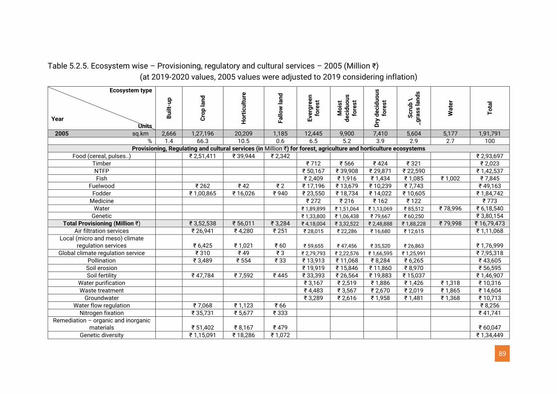
89
Table 5.2.5. Ecosystem wise – Provisioning, regulatory and cultural services – 2005 (Million ₹)
(at 2019-2020 values, 2005 values were adjusted to 2019 considering inflation)
Ecosystem type
Year Units
Bu
ilt-
up
Cro
p l
an
d
Ho
rtic
ult
ure
Fa
llo
w l
an
d
Ev
erg
ree
n
fore
st
Mo
ist
de
cid
uo
us
fo
res
t
Dry
de
cid
uo
us
fo
res
t
Sc
rub
\
_gra
ss
la
nd
s
Wa
ter
To
tal
2005 sq.km 2,666 1,27,196 20,209 1,185 12,445 9,900 7,410 5,604 5,177 1,91,791
% 1.4 66.3 10.5 0.6 6.5 5.2 3.9 2.9 2.7 100
Provisioning, Regulating and cultural services (in Million ₹) for forest, agriculture and horticulture ecosystems
Food (cereal, pulses..) ₹ 2,51,411 ₹ 39,944 ₹ 2,342 ₹ 2,93,697
Timber ₹ 712 ₹ 566 ₹ 424 ₹ 321 ₹ 2,023
NTFP ₹ 50,167 ₹ 39,908 ₹ 29,871 ₹ 22,590 ₹ 1,42,537
Fish ₹ 2,409 ₹ 1,916 ₹ 1,434 ₹ 1,085 ₹ 1,002 ₹ 7,845
Fuelwood ₹ 262 ₹ 42 ₹ 2 ₹ 17,196 ₹ 13,679 ₹ 10,239 ₹ 7,743 ₹ 49,163
Fodder ₹ 1,00,865 ₹ 16,026 ₹ 940 ₹ 23,550 ₹ 18,734 ₹ 14,022 ₹ 10,605 ₹ 1,84,742
Medicine ₹ 272 ₹ 216 ₹ 162 ₹ 122 ₹ 773
Water ₹ 1,89,899 ₹ 1,51,064 ₹ 1,13,069 ₹ 85,512 ₹ 78,996 ₹ 6,18,540
Genetic ₹ 1,33,800 ₹ 1,06,438 ₹ 79,667 ₹ 60,250 ₹ 3,80,154
Total Provisioning (Million ₹) ₹ 3,52,538 ₹ 56,011 ₹ 3,284 ₹ 4,18,004 ₹ 3,32,522 ₹ 2,48,888 ₹ 1,88,228 ₹ 79,998 ₹ 16,79,473
Air filtration services ₹ 26,941 ₹ 4,280 ₹ 251 ₹ 28,015 ₹ 22,286 ₹ 16,680 ₹ 12,615 ₹ 1,11,068
Local (micro and meso) climate regulation services
₹ 6,425 ₹ 1,021 ₹ 60 ₹ 59,655 ₹ 47,456 ₹ 35,520 ₹ 26,863 ₹ 1,76,999
Global climate regulation service ₹ 310 ₹ 49 ₹ 3 ₹ 2,79,793 ₹ 2,22,576 ₹ 1,66,595 ₹ 1,25,991 ₹ 7,95,318
Pollination ₹ 3,489 ₹ 554 ₹ 33 ₹ 13,913 ₹ 11,068 ₹ 8,284 ₹ 6,265 ₹ 43,605
Soil erosion ₹ 19,919 ₹ 15,846 ₹ 11,860 ₹ 8,970 ₹ 56,595
Soil fertility ₹ 47,784 ₹ 7,592 ₹ 445 ₹ 33,393 ₹ 26,564 ₹ 19,883 ₹ 15,037 ₹ 1,46,907
Water purification ₹ 3,167 ₹ 2,519 ₹ 1,886 ₹ 1,426 ₹ 1,318 ₹ 10,316
Waste treatment ₹ 4,483 ₹ 3,567 ₹ 2,670 ₹ 2,019 ₹ 1,865 ₹ 14,604
Groundwater ₹ 3,289 ₹ 2,616 ₹ 1,958 ₹ 1,481 ₹ 1,368 ₹ 10,713
Water flow regulation ₹ 7,068 ₹ 1,123 ₹ 66 ₹ 8,256
Nitrogen fixation ₹ 35,731 ₹ 5,677 ₹ 333 ₹ 41,741
Remediation – organic and inorganic materials
₹ 51,402 ₹ 8,167 ₹ 479 ₹ 60,047
Genetic diversity ₹ 1,15,091 ₹ 18,286 ₹ 1,072 ₹ 1,34,449
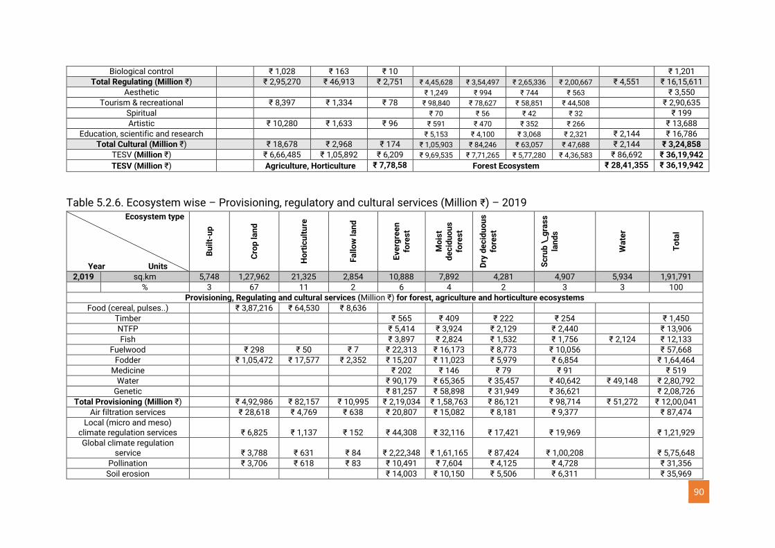
90
Biological control ₹ 1,028 ₹ 163 ₹ 10 ₹ 1,201
Total Regulating (Million ₹) ₹ 2,95,270 ₹ 46,913 ₹ 2,751 ₹ 4,45,628 ₹ 3,54,497 ₹ 2,65,336 ₹ 2,00,667 ₹ 4,551 ₹ 16,15,611
Aesthetic ₹ 1,249 ₹ 994 ₹ 744 ₹ 563 ₹ 3,550
Tourism & recreational ₹ 8,397 ₹ 1,334 ₹ 78 ₹ 98,840 ₹ 78,627 ₹ 58,851 ₹ 44,508 ₹ 2,90,635
Spiritual ₹ 70 ₹ 56 ₹ 42 ₹ 32 ₹ 199
Artistic ₹ 10,280 ₹ 1,633 ₹ 96 ₹ 591 ₹ 470 ₹ 352 ₹ 266 ₹ 13,688
Education, scientific and research ₹ 5,153 ₹ 4,100 ₹ 3,068 ₹ 2,321 ₹ 2,144 ₹ 16,786
Total Cultural (Million ₹) ₹ 18,678 ₹ 2,968 ₹ 174 ₹ 1,05,903 ₹ 84,246 ₹ 63,057 ₹ 47,688 ₹ 2,144 ₹ 3,24,858
TESV (Million ₹) ₹ 6,66,485 ₹ 1,05,892 ₹ 6,209 ₹ 9,69,535 ₹ 7,71,265 ₹ 5,77,280 ₹ 4,36,583 ₹ 86,692 ₹ 36,19,942
TESV (Million ₹) Agriculture, Horticulture ₹ 7,78,58 Forest Ecosystem ₹ 28,41,355 ₹ 36,19,942
Table 5.2.6. Ecosystem wise – Provisioning, regulatory and cultural services (Million ₹) – 2019 Ecosystem type
Year Units
Bu
ilt-
up
Cro
p l
an
d
Ho
rtic
ult
ure
Fa
llo
w l
an
d
Ev
erg
ree
n
fore
st
Mo
ist
de
cid
uo
us
fo
res
t
Dry
de
cid
uo
us
fo
res
t
Sc
rub
\_g
ras
s
lan
ds
Wa
ter
To
tal
2,019 sq.km 5,748 1,27,962 21,325 2,854 10,888 7,892 4,281 4,907 5,934 1,91,791 % 3 67 11 2 6 4 2 3 3 100
Provisioning, Regulating and cultural services (Million ₹) for forest, agriculture and horticulture ecosystems
Food (cereal, pulses..) ₹ 3,87,216 ₹ 64,530 ₹ 8,636
Timber ₹ 565 ₹ 409 ₹ 222 ₹ 254 ₹ 1,450
NTFP ₹ 5,414 ₹ 3,924 ₹ 2,129 ₹ 2,440 ₹ 13,906
Fish ₹ 3,897 ₹ 2,824 ₹ 1,532 ₹ 1,756 ₹ 2,124 ₹ 12,133
Fuelwood ₹ 298 ₹ 50 ₹ 7 ₹ 22,313 ₹ 16,173 ₹ 8,773 ₹ 10,056 ₹ 57,668
Fodder ₹ 1,05,472 ₹ 17,577 ₹ 2,352 ₹ 15,207 ₹ 11,023 ₹ 5,979 ₹ 6,854 ₹ 1,64,464
Medicine ₹ 202 ₹ 146 ₹ 79 ₹ 91 ₹ 519
Water ₹ 90,179 ₹ 65,365 ₹ 35,457 ₹ 40,642 ₹ 49,148 ₹ 2,80,792
Genetic ₹ 81,257 ₹ 58,898 ₹ 31,949 ₹ 36,621 ₹ 2,08,726
Total Provisioning (Million ₹) ₹ 4,92,986 ₹ 82,157 ₹ 10,995 ₹ 2,19,034 ₹ 1,58,763 ₹ 86,121 ₹ 98,714 ₹ 51,272 ₹ 12,00,041
Air filtration services ₹ 28,618 ₹ 4,769 ₹ 638 ₹ 20,807 ₹ 15,082 ₹ 8,181 ₹ 9,377 ₹ 87,474
Local (micro and meso) climate regulation services
₹ 6,825 ₹ 1,137 ₹ 152 ₹ 44,308 ₹ 32,116 ₹ 17,421 ₹ 19,969 ₹ 1,21,929
Global climate regulation service
₹ 3,788 ₹ 631 ₹ 84 ₹ 2,22,348 ₹ 1,61,165 ₹ 87,424 ₹ 1,00,208 ₹ 5,75,648
Pollination ₹ 3,706 ₹ 618 ₹ 83 ₹ 10,491 ₹ 7,604 ₹ 4,125 ₹ 4,728 ₹ 31,356
Soil erosion ₹ 14,003 ₹ 10,150 ₹ 5,506 ₹ 6,311 ₹ 35,969
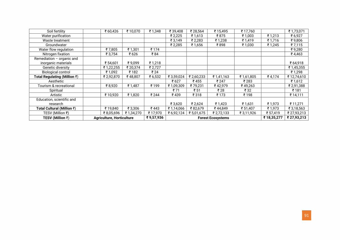
91
Soil fertility ₹ 60,426 ₹ 10,070 ₹ 1,348 ₹ 39,408 ₹ 28,564 ₹ 15,495 ₹ 17,760 ₹ 1,73,071
Water purification ₹ 2,225 ₹ 1,613 ₹ 875 ₹ 1,003 ₹ 1,213 ₹ 6,927
Waste treatment ₹ 3,149 ₹ 2,283 ₹ 1,238 ₹ 1,419 ₹ 1,716 ₹ 9,806
Groundwater ₹ 2,285 ₹ 1,656 ₹ 898 ₹ 1,030 ₹ 1,245 ₹ 7,115
Water flow regulation ₹ 7,805 ₹ 1,301 ₹ 174 ₹ 9,280
Nitrogen fixation ₹ 3,754 ₹ 626 ₹ 84 ₹ 4,463
Remediation – organic and inorganic materials
₹ 54,601 ₹ 9,099 ₹ 1,218 ₹ 64,918
Genetic diversity ₹ 1,22,255 ₹ 20,374 ₹ 2,727 ₹ 1,45,355
Biological control ₹ 1,092 ₹ 182 ₹ 24 ₹ 1,298
Total Regulating (Million ₹) ₹ 2,92,870 ₹ 48,807 ₹ 6,532 ₹ 3,59,024 ₹ 2,60,233 ₹ 1,41,163 ₹ 1,61,805 ₹ 4,174 ₹ 12,74,610
Aesthetic ₹ 627 ₹ 455 ₹ 247 ₹ 283 ₹ 1,612
Tourism & recreational ₹ 8,920 ₹ 1,487 ₹ 199 ₹ 1,09,309 ₹ 79,231 ₹ 42,979 ₹ 49,263 ₹ 2,91,388
Spiritual ₹ 71 ₹ 51 ₹ 28 ₹ 32 ₹ 181
Artistic ₹ 10,920 ₹ 1,820 ₹ 244 ₹ 439 ₹ 318 ₹ 173 ₹ 198 ₹ 14,111
Education, scientific and research
₹ 3,620 ₹ 2,624 ₹ 1,423 ₹ 1,631 ₹ 1,973 ₹ 11,271
Total Cultural (Million ₹) ₹ 19,840 ₹ 3,306 ₹ 443 ₹ 1,14,066 ₹ 82,679 ₹ 44,849 ₹ 51,407 ₹ 1,973 ₹ 3,18,563
TESV (Million ₹) ₹ 8,05,696 ₹ 1,34,270 ₹ 17,970 ₹ 6,92,124 ₹ 5,01,675 ₹ 2,72,133 ₹ 3,11,926 ₹ 57,419 ₹ 27,93,213
TESV (Million ₹) Agriculture, Horticulture ₹ 9,57,936 Forest Ecosystems ₹ 18,35,277 ₹ 27,93,213

92
5.3 Valuation of the forest ecosystem services – forest circle wise, Karnataka
The forest provisioning services (physical values), area of extraction, and seigniorage
value (revenue) for two five-year periods (2001-2005 and 2015-2019) were compiled
from the respective forest circles of the Karnataka Forest Department. Averages of
five years of goods were used to quantify goods in physical terms for 2005 and 2019.
Forests are managed by the Karnataka Forest Department, Government of Karnataka
(KFD 2020). Decentralized administration and management of forests in Karnataka
state are through forest circles, and there are 13 forest circles. Temporal data of 5
years period helped accounting for variability across the study period (years). The
seigniorage represents the residual value of the respective goods after deducting the
cost involved (harvesting, transportation, etc.). Seigniorage is expressed as revenue
received by the government (Haslag 2020) after deducting all expenses from the
auction amount of the respective provisioning services.
Provisioning services of forest ecosystems in Karnataka
The provisioning services - timber (rosewood (Dalbergia latifolia), teak wood (Tectona
grandis, Terminalia arjuna Terminalia elliptica, Anogeissus latifolia, etc.), eucalyptus
(Eucalyptus globulus), soft wood (Artocarpus hirsutus, Ailanthus excelsa, etc.), round
poles, pulp wood, sandal wood, other timber), bamboo (Bambusa arundinacea,
Dendrocalamus strictus, etc.), cane (Calamus neelagiricus, C. vattayila, C.
pseudofeanus, etc.), NTFP (honey, soap nut (Sapindus saponaria), cashew nut
(Anacardium occidentale), tamarind (Tamarindus indica), dalchini (cinnamon -
Cinnamomum malabatrum, Cinnamomum verum); rampatri (nutmeg - Myristica
malabarica); murgalu (kokum or Garcinia indica)); fuelwood; fodder, etc. extracted (in
physical units) with seigniorage values from each circle are provided in Tables 5.3.1
to 5.3.3, and Figures 5.3.1 to 5.3.3 presents circle wise provisioning services. The
seigniorage value for 2005 and 2019 are the same for all provisioning services, as per
the forest department reports.
Timber: Timber includes rosewood, teak wood, eucalyptus, softwood, round pole, etc.
The provisioning services (monetary) of all timber wood products extracted from each
circle are assessed considering the respective seigniorage value of individual forest
goods are listed in Table 5.3.4. Based on the extraction area, per hectare values of
each timber type are computed, which are listed in Table 5.3.5. Figures 5.3.3 and 5.3.4
depict the spatial variability of the ecosystem value of timber goods in Karnataka. The
total provisioning value of timber extracted from Karnataka state is 2,023, and 1,445
billion rupees, respectively, for 2005 and 2019. The rosewood is available only in
specific circles, which are part of the Western Ghats. Shimoga, Kodagu, and Canara
circles have higher ecosystem supply value as compared with other circles. The
ecosystem supply value of rosewood is 140,017 Rs/Ha/yr (2005) and 140,998
Rs/Ha/yr (2019). The maximum value is observed as 240,571 Rs/Ha/yr in the Canara
93
circle, and the minimum value is observed in Dharwad as 60,909 Rs/Ha/yr for the year
2005. In 2019 maximum value is observed from the Canara circle as 240,656 Rs/Ha/yr
and the minimum value as 60,909 Rs/Ha/yr from the Dharwad circle.
Teakwood: Teakwood is extracted in large quantities from Canara, Shimoga, Kodagu,
and Chikmagalur circles. The ecosystem supply value of teak wood shows 79,881
Rs/Ha/yr (2005) and 79,961 Rs/Ha/yr (2019) as per the collected data. Maximum and
minimum values are observed as 157,744, 41,302 Rs/Ha/yr (2005) for the circles
Kodagu, Dharwad respectively, whereas for the year 2019, maximum and minimum
values accounted as 158,134, 41,231 Rs/Ha/yr for the circles Kodagu, Dharwad
respectively. The average teak wood values are observed as 79,881, 79,961 Rs/Ha/yr
for the years 2005, and 2019 respectively.
Eucalyptus: The revenue from eucalyptus is high in Bengaluru, and Mysore circles.
Sandalwood is extracted in large quantities from Dharwad, Hassan circles. These
values are comparable to the earlier studies in India (Verma et al., 2013). Overall, the
circles such as Belgaum, Mysore, Ballari (Bellary) have lower timber services for 2019
compared to 2005. The ecosystem supply value of Eucalyptus wood is 4,304 and
4,265 Rs/Ha/yr for the data collected for the years 2005, 2019 respectively. The
maximum value observed is 9,246 Rs/Ha/yr in Hassan, and the minimum value is in
the Canara circle as 1,302 Rs/Ha/yr for the year 2005. In 2019 maximum value is
observed from the Hassan circle as 9235 Rs/Ha/yr and the minimum value as 1,302
Rs/Ha/yr from the Kodagu circle.
Softwood: The ecosystem supply value of softwood is 2,692 Rs/Ha/yr as per the
collected data for 2005, and 2019. Maximum and minimum values are 3,864 and 1,303
Rs/Ha/yr (2005) for Mangalore, Canara circles, respectively, whereas for the year
2019, maximum and minimum values accounted for 158,134, and 41,231 Rs/Ha/yr for
the circles Kodagu, Dharwad respectively.
Other timber: The ecosystem supply value of other kinds of timber is 4,644 and 4,297
Rs/Ha/yr for the data collected for the years 2005, 2019 respectively. The maximum
value is 9,276 Rs/Ha/yr in Hassan, and the minimum value is in Canara, Kodagu circles
as 1,302 Rs/Ha/yr for the year 2005. In 2019 maximum value from the Mysore circle
is 9,241 Rs/Ha/yr, and the minimum value is 1,302 Rs/Ha/yr from Canara and Kodagu
circles.
Pulpwood: The ecosystem supply value of pulpwood is 3,369 Rs/Ha/yr (2005) and
3,381Rs/Ha/yr (2019) based on the data collected across the circles from Karnataka
Forest Department. The maximum value is 4,272 Rs/Ha/yr in the Bangalore circle, and
the minimum value is in Chikmagalur as 3,830 Rs/Ha/yr for 2005. In 2019 maximum
value from the Bangalore circle is 4,295 Rs/Ha/yr, and the minimum value is 3,829
Rs/Ha/yr from the Chikmagalur circle.
94
Round poles: The ecosystem supply value of round poles wood is assessed as 4,434
and 4,261 Rs/Ha/yr for 2005, and 2019, respectively. The maximum value is 10,788
Rs/Ha/yr in Hassan, and the minimum value is in the Canara circle as 1,303 Rs/Ha/yr
for the year 2005. In 2019 maximum value from the Mysore circle is 9,224 Rs/Ha/yr
and the minimum value is 1,304 Rs/Ha/yr from the Canara circle.
Sandalwood: The ecosystem supply value of sandalwood is accounted as 4,573, and
4,652 Rs/Ha/yr for 2005, and 2019 respectively. The maximum value is 9,237 Rs/Ha/yr
in Hassan, and the minimum value is in Canara circles as 1,302 Rs/Ha/yr for the year
2005. In 2019 maximum value from Hassan circle is 9,240 Rs/Ha/yr and the minimum
value is 1,302 Rs/Ha/yr from the Canara circle.
Bamboo and Cane Production: Timber and biomass of bamboo and cane production
have been assessed from the forest inventory. The ecosystem supply value from
bamboo and canes was estimated (Table 5.3.6, Figure 5.3.5). Circles such as Canara
and Mangalore are getting higher revenue from bamboo, and Bengaluru, Canara
Dharwad, and Mangalore are getting high revenue from canes. The ecosystem supply
value of bamboo has reduced for the year 2019 might be attributed to the degradation
in the forest ecosystem with the reduced bamboo cover.
The ecosystem supply value of Bamboo for the Karnataka state is assessed as 3,938
and 4,402 Rs/Ha/yr for the years 2005 and 2019, respectively. The maximum value is
9,283 Rs/Ha/yr in Mysore, and the minimum value is observed in Canara circles as
1,302 Rs/Ha/yr for 2005. In 2019 maximum value from the Hassan circle is 8,911
Rs/Ha/yr, and the minimum value is 1,303 Rs/Ha/yr from the Canara circle.
Fodder Production: Table 5.3.7 lists circle-wise fodder in physical and monetary
values per hectare per year. Figure 5.3.6 depicts the circle-wise ecosystem value for
fodder, and values are 66,911 and 39,063 million rupees for 2005 and 2019,
respectively. The reduction in fodder availability could be attributed to the degradation
of forest ecosystems in the State. Canara, Shimoga, Mangalore, and Chamarajanagar
contribute higher compared to the Dharwad circle (least). Ecosystem supply value
from fodder for Karnataka state is assessed 7,736, and 15,476 Rs/Ha/yr for the years
2005 and 2019. The maximum value is 8,988 Rs/Ha/yr in Chamarajanagar, and the
minimum value is in the Kodagu circle as 6,583 Rs/Ha/yr for the year 2005. In 2019
maximum value is witnessed from the Chamarajanaga circle as 20,050 Rs/Ha/yr and
the minimum value as 12,779 Rs/Ha/yr from the Ballari circle.
Non-Timber Forest Produce / Non-Wood Forest Produce: The quantity of harvested
NTFP in physical quantities is assessed and listed category-wise in Table 5.3.8 for
2005 and 2019. The spatial variability is depicted in Figure 5.3.7. These are
comparable to a study from India (Verma et al., 2013). Table 5.3.9 lists NTFP values
for various forest types per hectare per year. Figure 5.3.8 depicts circle-wise the
ecosystem values from NTFP in a million rupees. Ecosystem value from NTFP is
95
estimated as 13,906 million rupees, in which Mysore, Shimoga, circles show higher
values, and Mangalore, Chikmagalur show lower values. The quantity of NTFP
extraction is higher in 2005 compared with 2019. The reduction is due to the
degradation of the forest cover and the non-availability of labor (discussion with
farmers during field investigations) for the sustainable extraction of NTFP.
▪ The ecosystem supply value of honey is 13,177 Rs/Ha/yr (2005) and 13,186 Rs/Ha/yr
(2019) based on the data collected across the circles from Karnataka Forest
Department. The maximum value is 13,411 Rs/Ha/yr in the Chamarajanagar circle and
the minimum value is 13,059 Rs/Ha/yr for the year 2005 in the Shimoga circle. In 2019,
the maximum value of 13,413 Rs/Ha/yr is in the Chamarajanagar circle, and the
minimum value is 13,060 Rs/Ha/yr in the Shimoga circle.
▪ Soapnut is 12,724 and 12,977 Rs/Ha/yr for the years 2005 and 2019, respectively. The
maximum value of 16,757 Rs/Ha/yr is in the Chamarajanagar circle for 2005 and 2019.
The minimum value of 11,714 Rs/Ha/yr is in Kodagu, Mangalore, and Shimoga circles
for 2005 and Kodagu circle in 2019.
▪ Cashew nut is 13,812 Rs/Ha/yr (2005) and 13,945 Rs/Ha/yr (2019). The maximum
value is 17,029 Rs/Ha/yr in the Bangalore circle, and the minimum is in Belgaum of
11,714 Rs/Ha/yr for 2005. In 2019, the maximum value of 17,048 Rs/Ha/yr in the
Bangalore circle and the minimum value of 11,715 Rs/Ha/yr was from the Belgaum
circle.
▪ Tamarind is 14,315 and14,346 Rs/Ha/yr for 2005 and 2019, respectively. The
maximum values of 17,044 and 17,049 Rs/Ha/yr are in the Ballari circle for 2005 and
2019. Minimum values of 11,423, and 11,575 Rs/Ha/yr are in the Kalaburagi circle for
2005 and 2019.
▪ Rampatri (nutmeg - Myristica malabarica) is 12,997 Rs/ Ha /yr (2005) and 14,436 Rs/
Ha /yr (2019). The maximum value of 16,891 Rs/ Ha /yr is in the Hassan circle, and
the minimum value is in Canara with 11,667 Rs/ Ha /yr for the year 2005. In 2019, the
maximum value of 16,842 Rs/ Ha /yr is in the Hassan circle, and the minimum value is
12,030 Rs/Ha/yr from the Canara circle.
▪ Dalchini (Cinnamon) is 13,333 Rs/Ha/yr (2005) and 13,478 Rs/Ha/yr (2019), based on
the data collected across the circles from Karnataka Forest Department.
▪ Murugalu (Kokkum) is 11,717 Rs/Ha/yr (2005) and 11,740 Rs/Ha/yr (2019). The
maximum value is 11,722 Rs/Ha/yr in the Shimoga circle, and the minimum value of
11,714 Rs/Ha/yr for the year 2005 is in the Canara circle. In 2019 maximum value is
observed from the Chikmagalur circle as 11,765 Rs/Ha/yr and the minimum value of
11,715 Rs/Ha/yr is in the Canara circle.
Overall, Canara, Shimoga, Kodagu, and Chamarajanagar circles provide provisioning
services in significant quantities, while Chikmagalur, Belgaum, Hassan, Mangalore,
Ballari, Dharwad, and Bengaluru provide moderate amounts, and the least amount is
provided by Gulbarga circle.
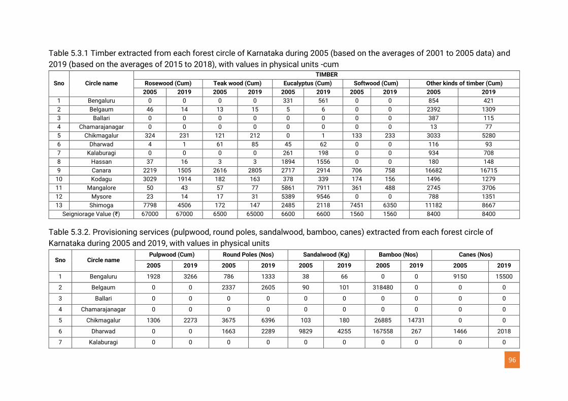
96
Table 5.3.1 Timber extracted from each forest circle of Karnataka during 2005 (based on the averages of 2001 to 2005 data) and
2019 (based on the averages of 2015 to 2018), with values in physical units -cum
Sno Circle name
TIMBER
Rosewood (Cum) Teak wood (Cum) Eucalyptus (Cum) Softwood (Cum) Other kinds of timber (Cum)
2005 2019 2005 2019 2005 2019 2005 2019 2005 2019
1 Bengaluru 0 0 0 0 331 561 0 0 854 421
2 Belgaum 46 14 13 15 5 6 0 0 2392 1309
3 Ballari 0 0 0 0 0 0 0 0 387 115
4 Chamarajanagar 0 0 0 0 0 0 0 0 13 77
5 Chikmagalur 324 231 121 212 0 1 133 233 3033 5280
6 Dharwad 4 1 61 85 45 62 0 0 116 93
7 Kalaburagi 0 0 0 0 261 198 0 0 934 708
8 Hassan 37 16 3 3 1894 1556 0 0 180 148
9 Canara 2219 1505 2616 2805 2717 2914 706 758 16682 16715
10 Kodagu 3029 1914 182 163 378 339 174 156 1496 1279
11 Mangalore 50 43 57 77 5861 7911 361 488 2745 3706
12 Mysore 23 14 17 31 5389 9546 0 0 788 1351
13 Shimoga 7798 4506 172 147 2485 2118 7451 6350 11182 8667
Seigniorage Value (₹) 67000 67000 6500 65000 6600 6600 1560 1560 8400 8400
Table 5.3.2. Provisioning services (pulpwood, round poles, sandalwood, bamboo, canes) extracted from each forest circle of
Karnataka during 2005 and 2019, with values in physical units
Sno Circle name Pulpwood (Cum) Round Poles (Nos) Sandalwood (Kg) Bamboo (Nos) Canes (Nos)
2005 2019 2005 2019 2005 2019 2005 2019 2005 2019
1 Bengaluru 1928 3266 786 1333 38 66 0 0 9150 15500
2 Belgaum 0 0 2337 2605 90 101 318480 0 0 0
3 Ballari 0 0 0 0 0 0 0 0 0 0
4 Chamarajanagar 0 0 0 0 0 0 0 0 0 0
5 Chikmagalur 1306 2273 3675 6396 103 180 26885 14731 0 0
6 Dharwad 0 0 1663 2289 9829 4255 167558 267 1466 2018
7 Kalaburagi 0 0 0 0 0 0 0 0 0 0
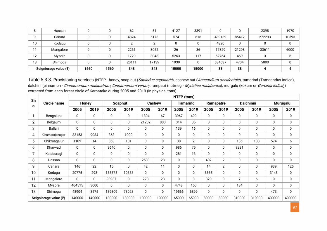
97
8 Hassan 0 0 62 51 4127 3391 0 0 2398 1970
9 Canara 0 0 4824 5173 574 616 489139 85412 272293 10393
10 Kodagu 0 0 2 2 0 0 4820 0 0 0
11 Mangalore 0 0 2261 3052 26 36 17829 21298 33611 6000
12 Mysore 0 0 1720 3048 5263 117 52764 469 3 6
13 Shimoga 0 0 20111 17139 1939 0 634637 4704 5000 0
Seigniorage value (₹) 1560 1560 348 348 15000 15000 38 38 4 4
Table 5.3.3. Provisioning services (NTFP - honey, soap nut (Sapindus saponaria), cashew nut (Anacardium occidentale), tamarind (Tamarindus indica),
dalchini (cinnamon - Cinnamomum malabatrum, Cinnamomum verum); rampatri (nutmeg - Myristica malabarica); murgalu (kokum or Garcinia indica))
extracted from each forest circle of Karnataka during 2005 and 2019 (in physical tons)
Sn
o Circle name
NTFP (tons)
Honey Soapnut Cashew Tamarind Ramapatre Dalchinni Murugalu
2005 2019 2005 2019 2005 2019 2005 2019 2005 2019 2005 2019 2005 2019
1 Bengaluru 0 0 0 0 1804 67 3967 490 0 0 0 0 0 0
2 Belgaum 0 0 0 0 21282 800 314 35 0 0 0 0 0 0
3 Ballari 0 0 0 0 0 0 139 16 0 0 0 0 0 0
4 Chamarajanagar 33153 9034 868 1000 0 0 0 0 0 0 0 0 0 0
5 Chikmagalur 1109 14 853 101 0 0 38 2 0 0 186 133 574 6
6 Dharwad 0 0 3640 0 0 0 986 75 0 0 9281 0 0 0
7 Kalaburagi 0 0 0 0 0 0 281 13 0 0 0 0 0 0
8 Hassan 0 0 0 0 2508 28 0 0 402 2 0 0 0 0
9 Canara 146 22 15 0 42 11 0 0 14 2 0 0 939 125
10 Kodagu 20775 293 188375 10388 0 0 0 0 8835 0 0 0 3148 0
11 Mangalore 0 0 93937 0 273 23 0 0 320 0 7 6 0 0
12 Mysore 464515 3000 0 0 0 0 4748 150 0 0 184 0 0 0
13 Shimoga 48904 3575 139809 73028 0 0 19566 6899 0 0 0 0 473 0
Seigniorage value (₹) 140000 140000 130000 130000 100000 100000 65000 65000 80000 80000 310000 310000 400000 400000
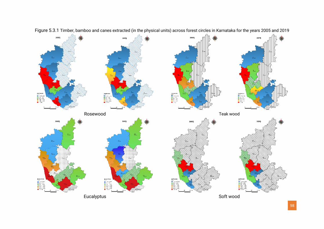
98
Figure 5.3.1 Timber, bamboo and canes extracted (in the physical units) across forest circles in Karnataka for the years 2005 and 2019
Rosewood Teak wood
Eucalyptus Soft wood
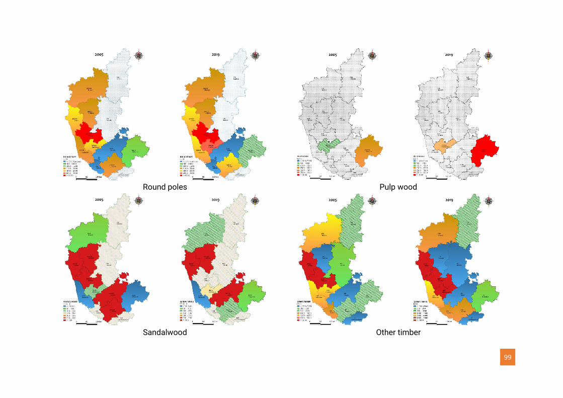
99
Round poles Pulp wood
Sandalwood Other timber
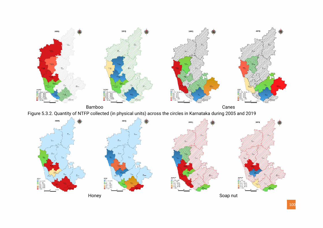
100
Bamboo Canes
Figure 5.3.2. Quantity of NTFP collected (in physical units) across the circles in Karnataka during 2005 and 2019
Honey Soap nut
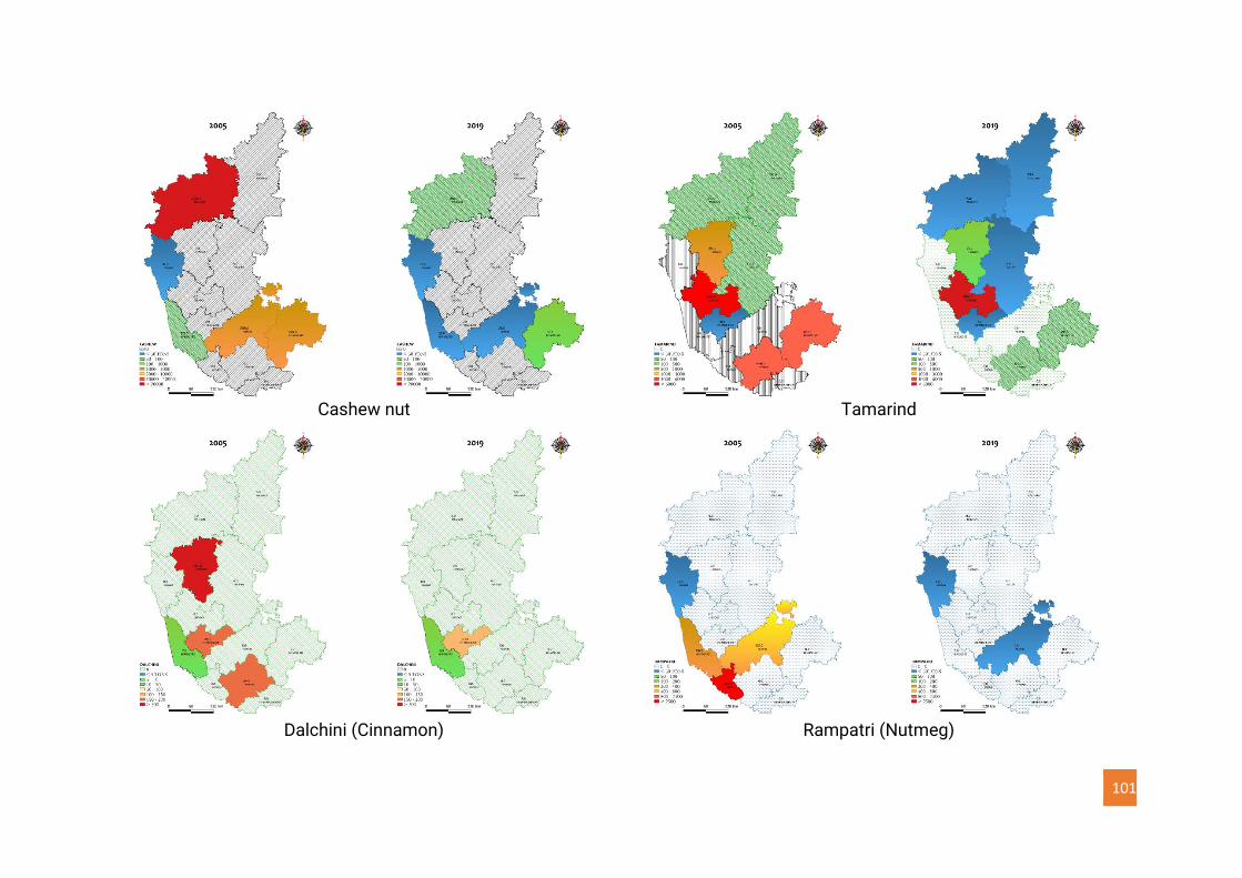
101
Cashew nut Tamarind
Dalchini (Cinnamon) Rampatri (Nutmeg)
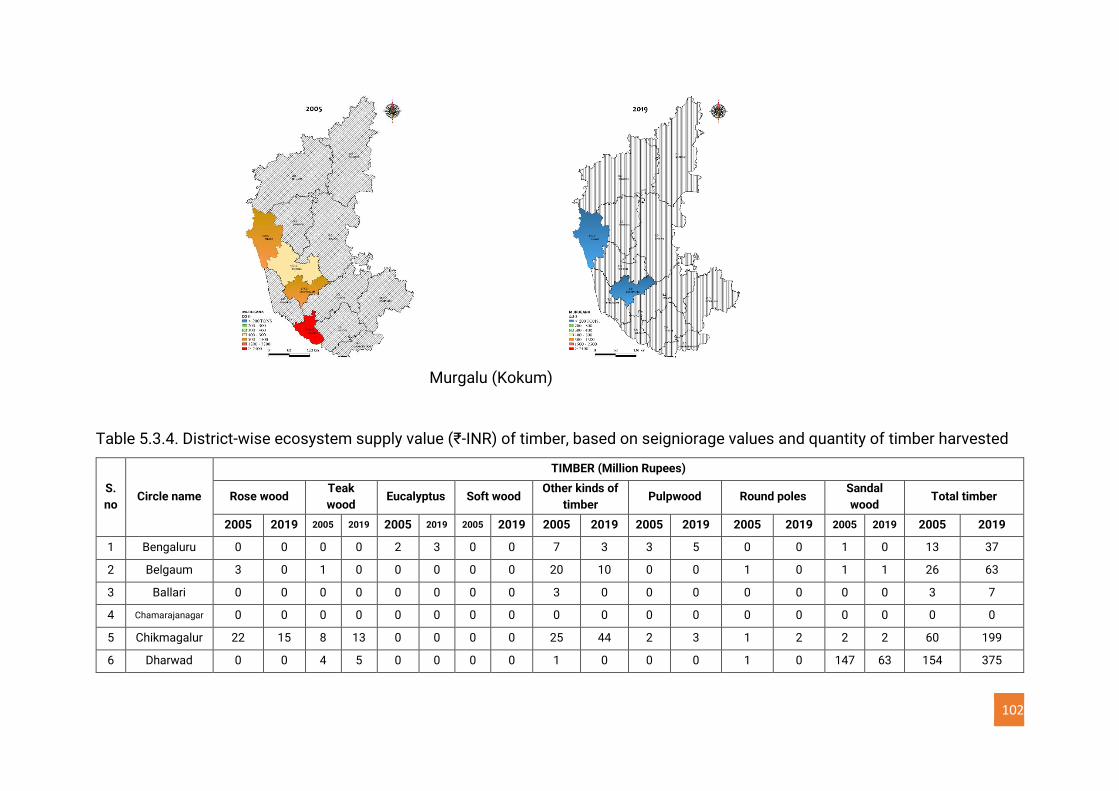
102
Murgalu (Kokum)
Table 5.3.4. District-wise ecosystem supply value (₹-INR) of timber, based on seigniorage values and quantity of timber harvested
S.
no Circle name
TIMBER (Million Rupees)
Rose wood Teak
wood Eucalyptus Soft wood
Other kinds of
timber Pulpwood Round poles
Sandal
wood Total timber
2005 2019 2005 2019 2005 2019 2005 2019 2005 2019 2005 2019 2005 2019 2005 2019 2005 2019
1 Bengaluru 0 0 0 0 2 3 0 0 7 3 3 5 0 0 1 0 13 37
2 Belgaum 3 0 1 0 0 0 0 0 20 10 0 0 1 0 1 1 26 63
3 Ballari 0 0 0 0 0 0 0 0 3 0 0 0 0 0 0 0 3 7
4 Chamarajanagar 0 0 0 0 0 0 0 0 0 0 0 0 0 0 0 0 0 0
5 Chikmagalur 22 15 8 13 0 0 0 0 25 44 2 3 1 2 2 2 60 199
6 Dharwad 0 0 4 5 0 0 0 0 1 0 0 0 1 0 147 63 154 375
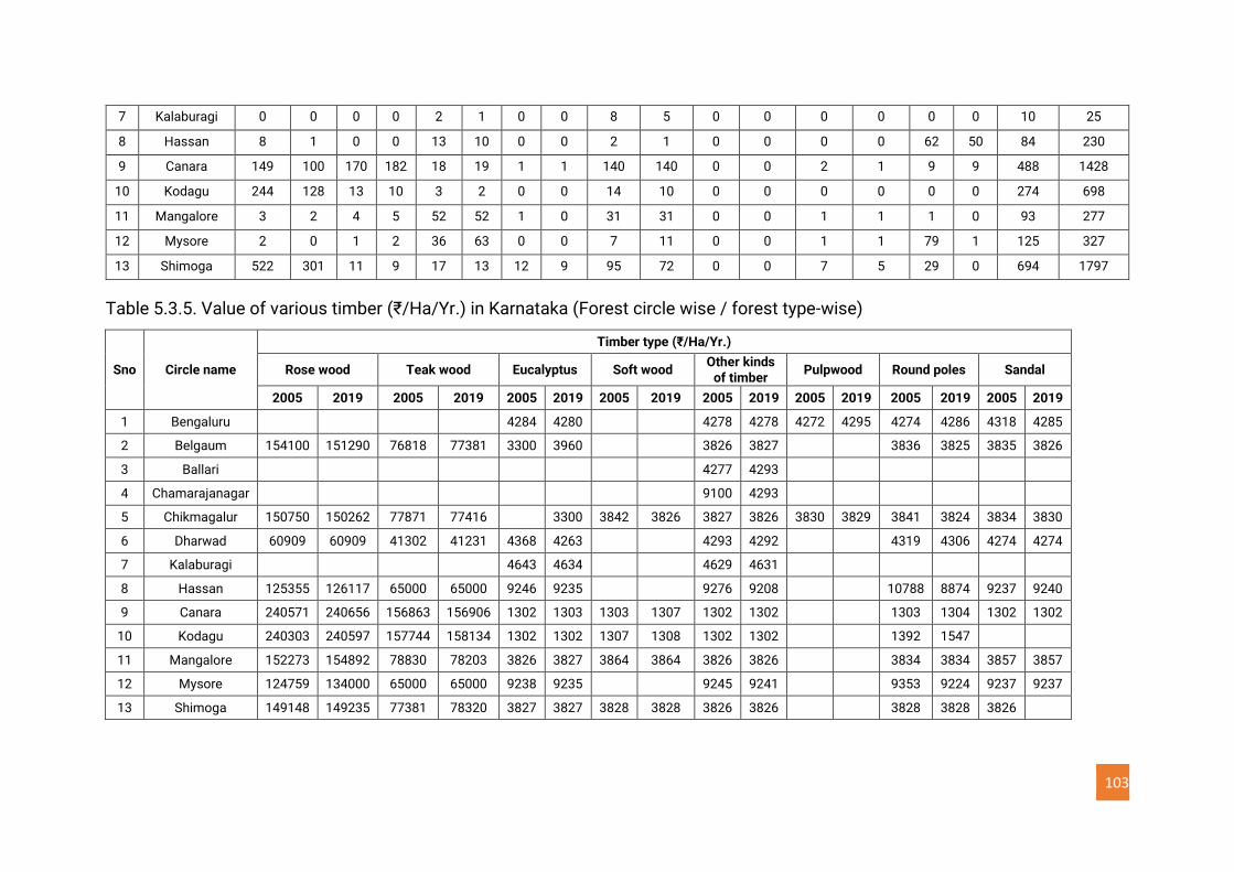
103
7 Kalaburagi 0 0 0 0 2 1 0 0 8 5 0 0 0 0 0 0 10 25
8 Hassan 8 1 0 0 13 10 0 0 2 1 0 0 0 0 62 50 84 230
9 Canara 149 100 170 182 18 19 1 1 140 140 0 0 2 1 9 9 488 1428
10 Kodagu 244 128 13 10 3 2 0 0 14 10 0 0 0 0 0 0 274 698
11 Mangalore 3 2 4 5 52 52 1 0 31 31 0 0 1 1 1 0 93 277
12 Mysore 2 0 1 2 36 63 0 0 7 11 0 0 1 1 79 1 125 327
13 Shimoga 522 301 11 9 17 13 12 9 95 72 0 0 7 5 29 0 694 1797
Table 5.3.5. Value of various timber (₹/Ha/Yr.) in Karnataka (Forest circle wise / forest type-wise)
Sno Circle name
Timber type (₹/Ha/Yr.)
Rose wood Teak wood Eucalyptus Soft wood Other kinds
of timber Pulpwood Round poles Sandal
2005 2019 2005 2019 2005 2019 2005 2019 2005 2019 2005 2019 2005 2019 2005 2019
1 Bengaluru 4284 4280 4278 4278 4272 4295 4274 4286 4318 4285
2 Belgaum 154100 151290 76818 77381 3300 3960 3826 3827 3836 3825 3835 3826
3 Ballari 4277 4293
4 Chamarajanagar 9100 4293
5 Chikmagalur 150750 150262 77871 77416 3300 3842 3826 3827 3826 3830 3829 3841 3824 3834 3830
6 Dharwad 60909 60909 41302 41231 4368 4263 4293 4292 4319 4306 4274 4274
7 Kalaburagi 4643 4634 4629 4631
8 Hassan 125355 126117 65000 65000 9246 9235 9276 9208 10788 8874 9237 9240
9 Canara 240571 240656 156863 156906 1302 1303 1303 1307 1302 1302 1303 1304 1302 1302
10 Kodagu 240303 240597 157744 158134 1302 1302 1307 1308 1302 1302 1392 1547
11 Mangalore 152273 154892 78830 78203 3826 3827 3864 3864 3826 3826 3834 3834 3857 3857
12 Mysore 124759 134000 65000 65000 9238 9235 9245 9241 9353 9224 9237 9237
13 Shimoga 149148 149235 77381 78320 3827 3827 3828 3828 3826 3826 3828 3828 3826

104
Figure 5.3.3. Ecosystem supply value (INR) of various timber across the circles for 2005 and 2019
Rosewood Teak wood
Eucalyptus Soft wood
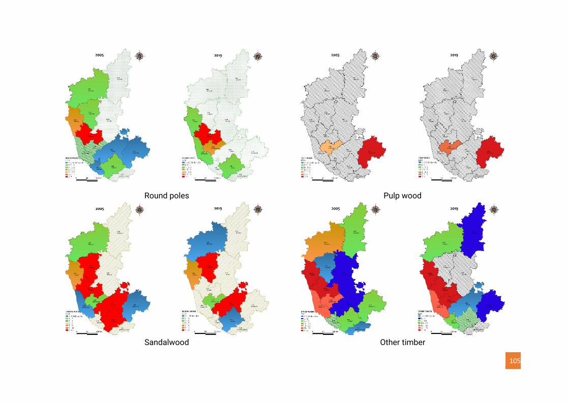
105
Round poles Pulp wood
Sandalwood Other timber
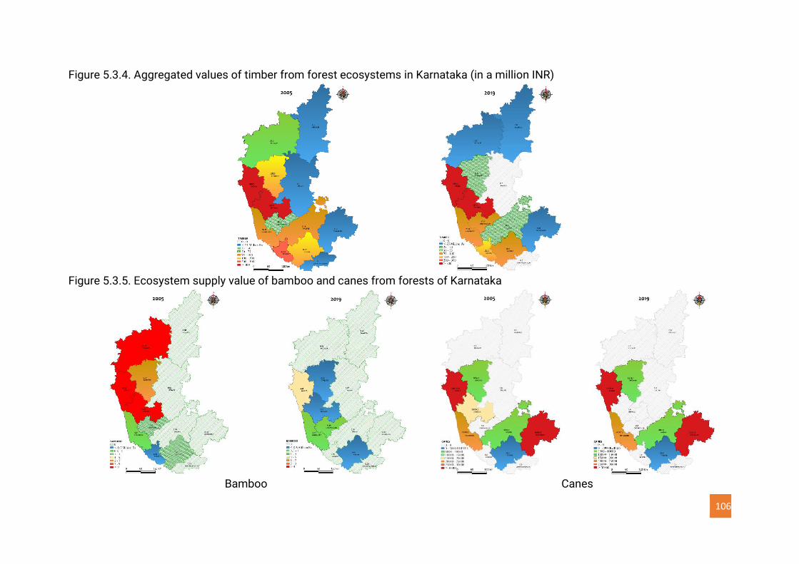
106
Figure 5.3.4. Aggregated values of timber from forest ecosystems in Karnataka (in a million INR)
Figure 5.3.5. Ecosystem supply value of bamboo and canes from forests of Karnataka
Bamboo Canes
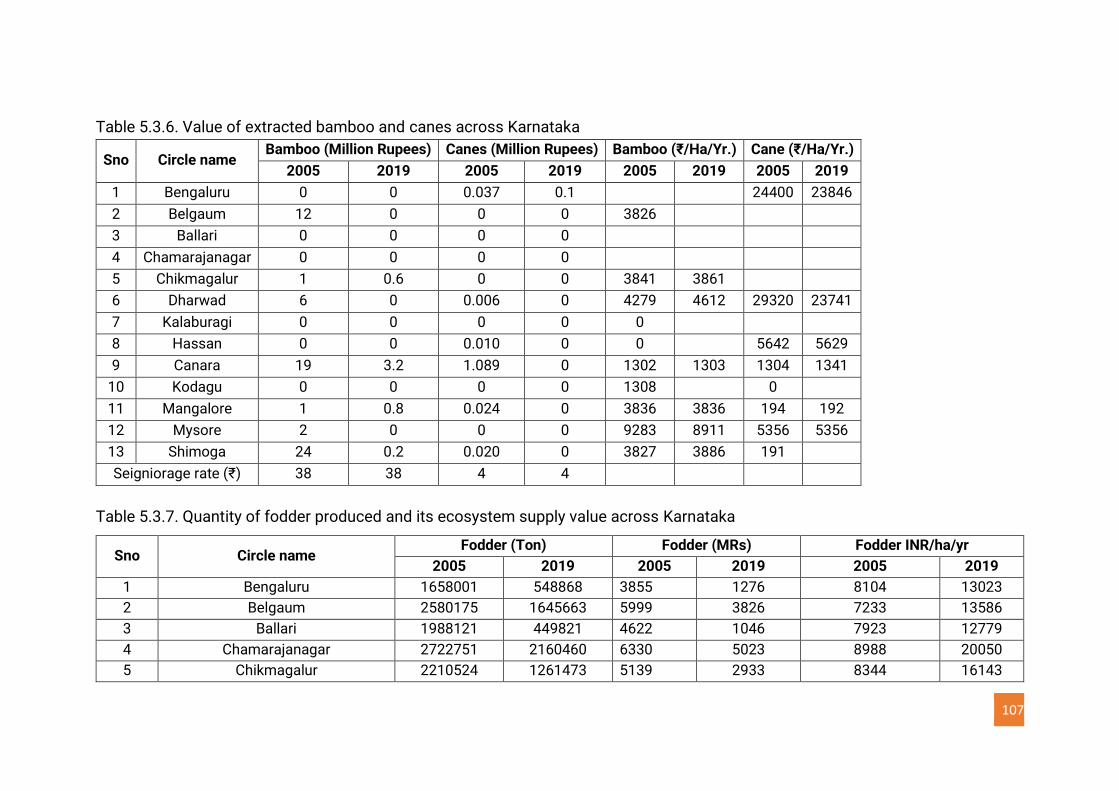
107
Table 5.3.6. Value of extracted bamboo and canes across Karnataka
Sno Circle name Bamboo (Million Rupees) Canes (Million Rupees) Bamboo (₹/Ha/Yr.) Cane (₹/Ha/Yr.)
2005 2019 2005 2019 2005 2019 2005 2019
1 Bengaluru 0 0 0.037 0.1 24400 23846
2 Belgaum 12 0 0 0 3826
3 Ballari 0 0 0 0
4 Chamarajanagar 0 0 0 0
5 Chikmagalur 1 0.6 0 0 3841 3861
6 Dharwad 6 0 0.006 0 4279 4612 29320 23741
7 Kalaburagi 0 0 0 0 0
8 Hassan 0 0 0.010 0 0 5642 5629
9 Canara 19 3.2 1.089 0 1302 1303 1304 1341
10 Kodagu 0 0 0 0 1308 0
11 Mangalore 1 0.8 0.024 0 3836 3836 194 192
12 Mysore 2 0 0 0 9283 8911 5356 5356
13 Shimoga 24 0.2 0.020 0 3827 3886 191
Seigniorage rate (₹) 38 38 4 4
Table 5.3.7. Quantity of fodder produced and its ecosystem supply value across Karnataka
Sno Circle name Fodder (Ton) Fodder (MRs) Fodder INR/ha/yr
2005 2019 2005 2019 2005 2019
1 Bengaluru 1658001 548868 3855 1276 8104 13023
2 Belgaum 2580175 1645663 5999 3826 7233 13586
3 Ballari 1988121 449821 4622 1046 7923 12779
4 Chamarajanagar 2722751 2160460 6330 5023 8988 20050
5 Chikmagalur 2210524 1261473 5139 2933 8344 16143
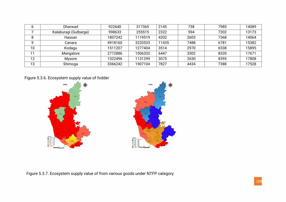
108
6 Dharwad 922640 317365 2145 738 7985 14089
7 Kalaburagi (Gulbarga) 998633 255515 2322 594 7202 13173
8 Hassan 1807242 1119519 4202 2603 7368 14064
9 Canara 4918160 3220533 11435 7488 6781 15382
10 Kodagu 1511207 1277404 3514 2970 6538 15895
11 Mangalore 2772886 1506332 6447 3502 8320 17671
12 Mysore 1322496 1131299 3075 2630 8395 17808
13 Shimoga 3366242 1907104 7827 4434 7388 17528
Figure 5.3.6. Ecosystem supply value of fodder
Figure 5.3.7. Ecosystem supply value of from various goods under NTFP category
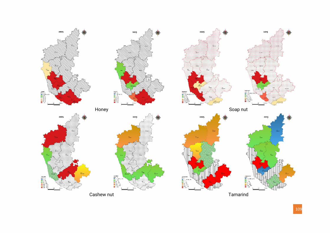
109
Honey Soap nut
Cashew nut Tamarind
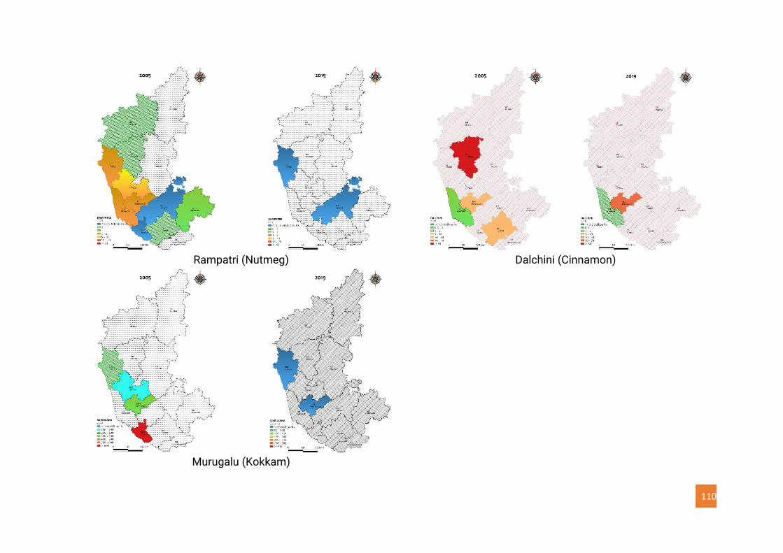
110
Rampatri (Nutmeg) Dalchini (Cinnamon)
Murugalu (Kokkam)
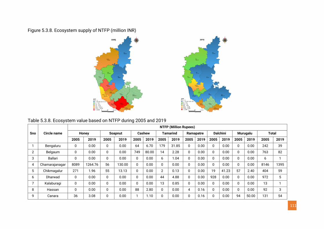
111
Figure 5.3.8. Ecosystem supply of NTFP (million INR)
Table 5.3.8. Ecosystem value based on NTFP during 2005 and 2019
Sno Circle name
NTFP (Million Rupees)
Honey Soapnut Cashew Tamarind Ramapatre Dalchini Murugalu Total
2005 2019 2005 2019 2005 2019 2005 2019 2005 2019 2005 2019 2005 2019 2005 2019
1 Bengaluru 0 0.00 0 0.00 64 6.70 179 31.85 0 0.00 0 0.00 0 0.00 242 39
2 Belgaum 0 0.00 0 0.00 749 80.00 14 2.28 0 0.00 0 0.00 0 0.00 763 82
3 Ballari 0 0.00 0 0.00 0 0.00 6 1.04 0 0.00 0 0.00 0 0.00 6 1
4 Chamarajanagar 8089 1264.76 56 130.00 0 0.00 0 0.00 0 0.00 0 0.00 0 0.00 8146 1395
5 Chikmagalur 271 1.96 55 13.13 0 0.00 2 0.13 0 0.00 19 41.23 57 2.40 404 59
6 Dharwad 0 0.00 0 0.00 0 0.00 44 4.88 0 0.00 928 0.00 0 0.00 972 5
7 Kalaburagi 0 0.00 0 0.00 0 0.00 13 0.85 0 0.00 0 0.00 0 0.00 13 1
8 Hassan 0 0.00 0 0.00 88 2.80 0 0.00 4 0.16 0 0.00 0 0.00 92 3
9 Canara 36 3.08 0 0.00 1 1.10 0 0.00 0 0.16 0 0.00 94 50.00 131 54
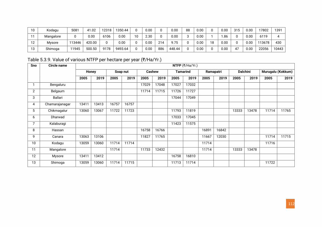
112
10 Kodagu 5081 41.02 12318 1350.44 0 0.00 0 0.00 88 0.00 0 0.00 315 0.00 17802 1391
11 Mangalore 0 0.00 6106 0.00 10 2.30 0 0.00 3 0.00 1 1.86 0 0.00 6119 4
12 Mysore 113446 420.00 0 0.00 0 0.00 214 9.75 0 0.00 18 0.00 0 0.00 113678 430
13 Shimoga 11945 500.50 9178 9493.64 0 0.00 886 448.44 0 0.00 0 0.00 47 0.00 22056 10443
Table 5.3.9. Value of various NTFP per hectare per year (₹/Ha/Yr.) Sno
Circle name
NTFP (₹/Ha/Yr.)
Honey Soap nut Cashew Tamarind Ramapatri Dalchini Murugalu (Kokkum)
2005 2019 2005 2019 2005 2019 2005 2019 2005 2019 2005 2019 2005 2019
1 Bengaluru
17029 17048 17027 17032
2 Belgaum
11714 11715 11726 11727
3 Ballari
17044 17049
4 Chamarajanagar 13411 13413 16757 16757
5 Chikmagalur 13060 13067 11722 11723
11793 11819
13333 13478 11714 11765
6 Dharwad
17033 17045
7 Kalaburagi
11423 11575
8 Hassan
16758 16766
16891 16842
9 Canara 13063 13106
11827 11765 11667 12030
11714 11715
10 Kodagu 13059 13060 11714 11714
11714
11716
11 Mangalore
11714 11733 12432 11714 13333 13478
12 Mysore 13411 13412
16758 16810
13 Shimoga 13059 13060 11714 11715
11713 11714
11722
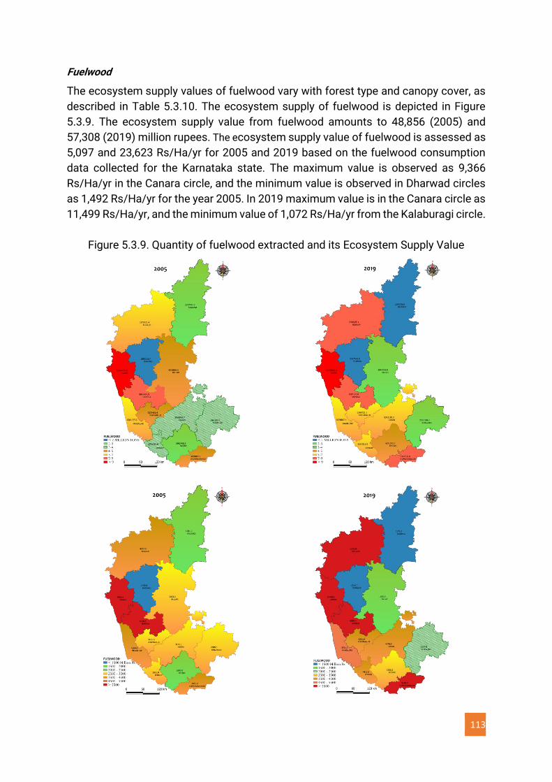
113
Fuelwood
The ecosystem supply values of fuelwood vary with forest type and canopy cover, as
described in Table 5.3.10. The ecosystem supply of fuelwood is depicted in Figure
5.3.9. The ecosystem supply value from fuelwood amounts to 48,856 (2005) and
57,308 (2019) million rupees. The ecosystem supply value of fuelwood is assessed as
5,097 and 23,623 Rs/Ha/yr for 2005 and 2019 based on the fuelwood consumption
data collected for the Karnataka state. The maximum value is observed as 9,366
Rs/Ha/yr in the Canara circle, and the minimum value is observed in Dharwad circles
as 1,492 Rs/Ha/yr for the year 2005. In 2019 maximum value is in the Canara circle as
11,499 Rs/Ha/yr, and the minimum value of 1,072 Rs/Ha/yr from the Kalaburagi circle.
Figure 5.3.9. Quantity of fuelwood extracted and its Ecosystem Supply Value
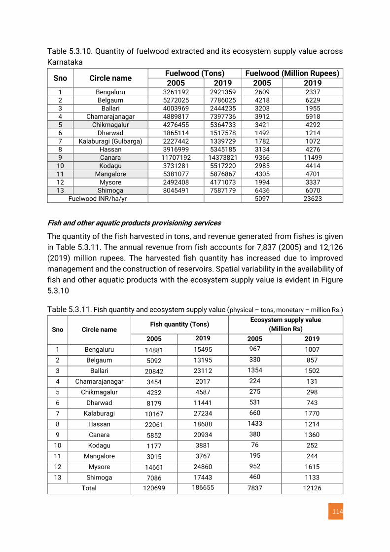
114
Table 5.3.10. Quantity of fuelwood extracted and its ecosystem supply value across
Karnataka
Sno Circle name Fuelwood (Tons) Fuelwood (Million Rupees) 2005 2019 2005 2019
1 Bengaluru 3261192 2921359 2609 2337
2 Belgaum 5272025 7786025 4218 6229
3 Ballari 4003969 2444235 3203 1955
4 Chamarajanagar 4889817 7397736 3912 5918
5 Chikmagalur 4276455 5364733 3421 4292
6 Dharwad 1865114 1517578 1492 1214
7 Kalaburagi (Gulbarga) 2227442 1339729 1782 1072
8 Hassan 3916999 5345185 3134 4276
9 Canara 11707192 14373821 9366 11499
10 Kodagu 3731281 5517220 2985 4414
11 Mangalore 5381077 5876867 4305 4701
12 Mysore 2492408 4171073 1994 3337
13 Shimoga 8045491 7587179 6436 6070
Fuelwood INR/ha/yr 5097 23623
Fish and other aquatic products provisioning services
The quantity of the fish harvested in tons, and revenue generated from fishes is given
in Table 5.3.11. The annual revenue from fish accounts for 7,837 (2005) and 12,126
(2019) million rupees. The harvested fish quantity has increased due to improved
management and the construction of reservoirs. Spatial variability in the availability of
fish and other aquatic products with the ecosystem supply value is evident in Figure
5.3.10
Table 5.3.11. Fish quantity and ecosystem supply value (physical – tons, monetary – million Rs.)
Sno Circle name Fish quantity (Tons)
Ecosystem supply value
(Million Rs)
2005 2019 2005 2019
1 Bengaluru 14881 15495 967 1007
2 Belgaum 5092 13195 330 857
3 Ballari 20842 23112 1354 1502
4 Chamarajanagar 3454 2017 224 131
5 Chikmagalur 4232 4587 275 298
6 Dharwad 8179 11441 531 743
7 Kalaburagi 10167 27234 660 1770
8 Hassan 22061 18688 1433 1214
9 Canara 5852 20934 380 1360
10 Kodagu 1177 3881 76 252
11 Mangalore 3015 3767 195 244
12 Mysore 14661 24860 952 1615
13 Shimoga 7086 17443 460 1133
Total 120699 186655 7837 12126
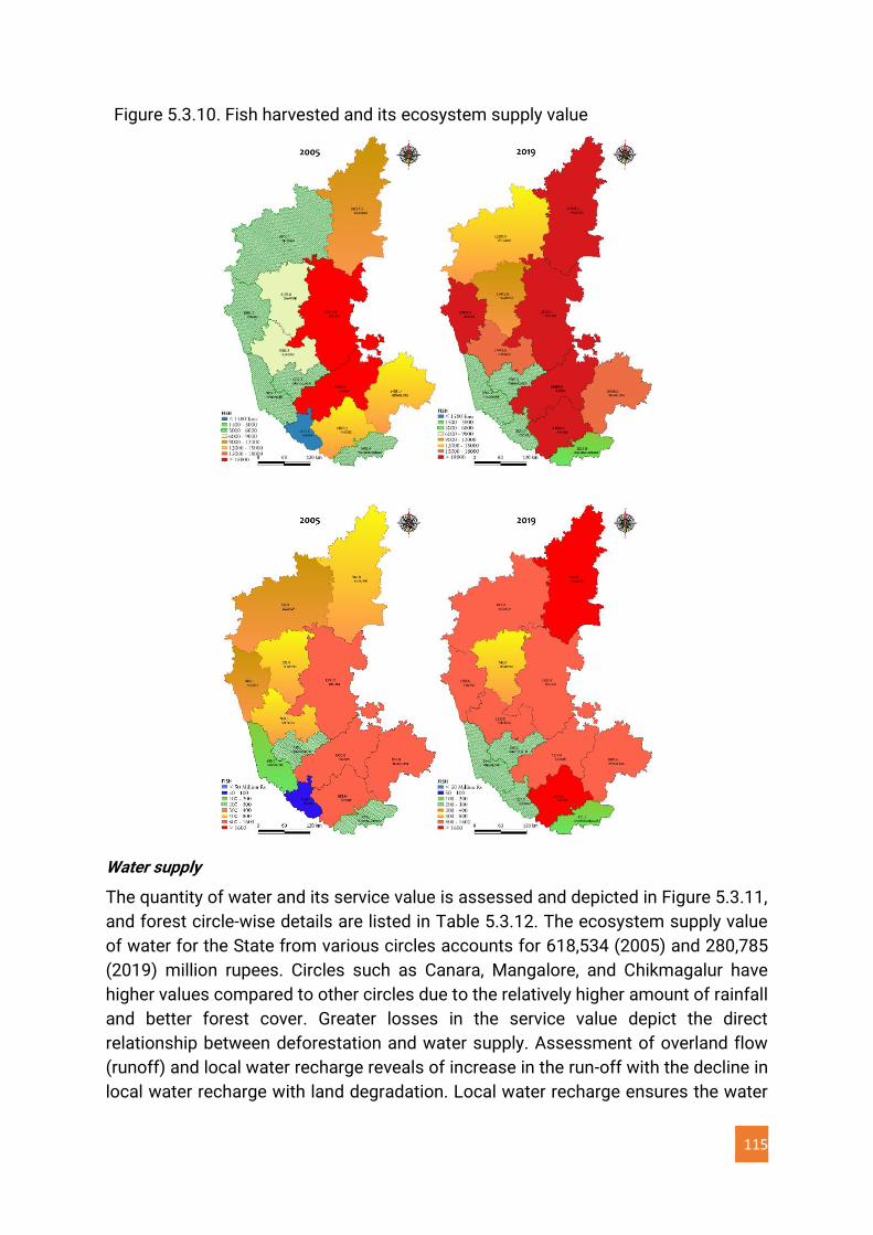
115
Figure 5.3.10. Fish harvested and its ecosystem supply value
Water supply
The quantity of water and its service value is assessed and depicted in Figure 5.3.11,
and forest circle-wise details are listed in Table 5.3.12. The ecosystem supply value
of water for the State from various circles accounts for 618,534 (2005) and 280,785
(2019) million rupees. Circles such as Canara, Mangalore, and Chikmagalur have
higher values compared to other circles due to the relatively higher amount of rainfall
and better forest cover. Greater losses in the service value depict the direct
relationship between deforestation and water supply. Assessment of overland flow
(runoff) and local water recharge reveals of increase in the run-off with the decline in
local water recharge with land degradation. Local water recharge ensures the water
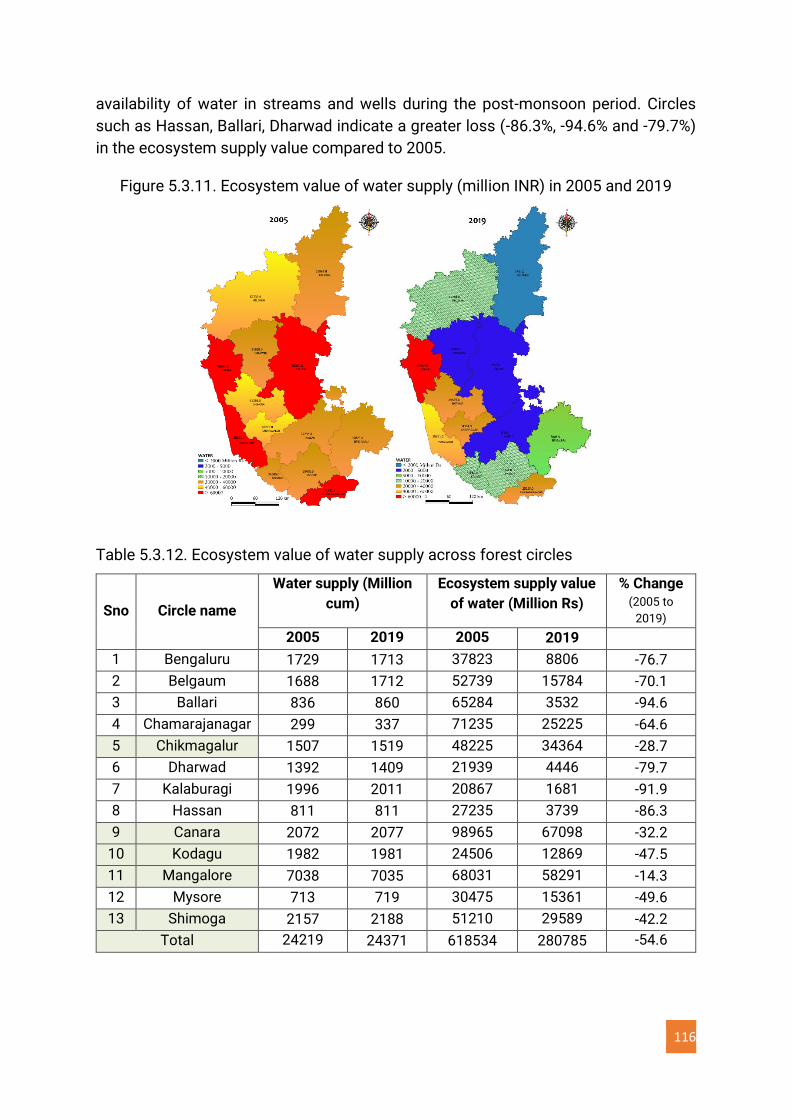
116
availability of water in streams and wells during the post-monsoon period. Circles
such as Hassan, Ballari, Dharwad indicate a greater loss (-86.3%, -94.6% and -79.7%)
in the ecosystem supply value compared to 2005.
Figure 5.3.11. Ecosystem value of water supply (million INR) in 2005 and 2019
Table 5.3.12. Ecosystem value of water supply across forest circles
Sno Circle name
Water supply (Million
cum)
Ecosystem supply value
of water (Million Rs)
% Change (2005 to
2019)
2005 2019 2005 2019
1 Bengaluru 1729 1713 37823 8806 -76.7
2 Belgaum 1688 1712 52739 15784 -70.1
3 Ballari 836 860 65284 3532 -94.6
4 Chamarajanagar 299 337 71235 25225 -64.6
5 Chikmagalur 1507 1519 48225 34364 -28.7
6 Dharwad 1392 1409 21939 4446 -79.7
7 Kalaburagi 1996 2011 20867 1681 -91.9
8 Hassan 811 811 27235 3739 -86.3
9 Canara 2072 2077 98965 67098 -32.2
10 Kodagu 1982 1981 24506 12869 -47.5
11 Mangalore 7038 7035 68031 58291 -14.3
12 Mysore 713 719 30475 15361 -49.6
13 Shimoga 2157 2188 51210 29589 -42.2
Total 24219 24371 618534 280785 -54.6
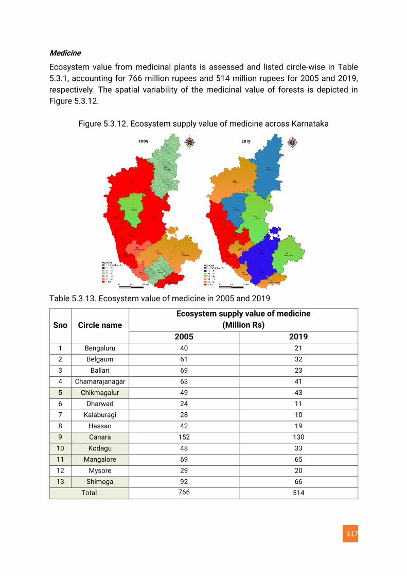
117
Medicine
Ecosystem value from medicinal plants is assessed and listed circle-wise in Table
5.3.1, accounting for 766 million rupees and 514 million rupees for 2005 and 2019,
respectively. The spatial variability of the medicinal value of forests is depicted in
Figure 5.3.12.
Figure 5.3.12. Ecosystem supply value of medicine across Karnataka
Table 5.3.13. Ecosystem value of medicine in 2005 and 2019
Sno Circle name
Ecosystem supply value of medicine
(Million Rs)
2005 2019
1 Bengaluru 40 21
2 Belgaum 61 32
3 Ballari 69 23
4 Chamarajanagar 63 41
5 Chikmagalur 49 43
6 Dharwad 24 11
7 Kalaburagi 28 10
8 Hassan 42 19
9 Canara 152 130
10 Kodagu 48 33
11 Mangalore 69 65
12 Mysore 29 20
13 Shimoga 92 66
Total 766 514
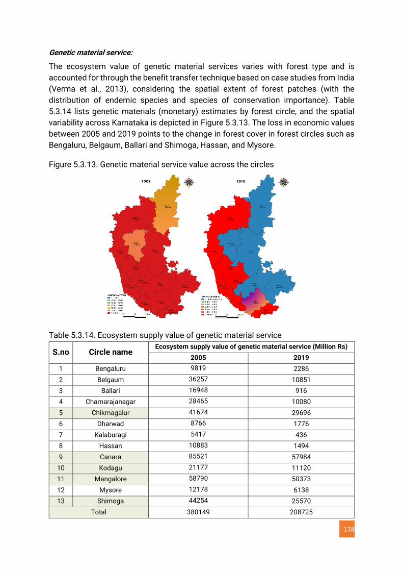
118
Genetic material service:
The ecosystem value of genetic material services varies with forest type and is
accounted for through the benefit transfer technique based on case studies from India
(Verma et al., 2013), considering the spatial extent of forest patches (with the
distribution of endemic species and species of conservation importance). Table
5.3.14 lists genetic materials (monetary) estimates by forest circle, and the spatial
variability across Karnataka is depicted in Figure 5.3.13. The loss in economic values
between 2005 and 2019 points to the change in forest cover in forest circles such as
Bengaluru, Belgaum, Ballari and Shimoga, Hassan, and Mysore.
Figure 5.3.13. Genetic material service value across the circles
Table 5.3.14. Ecosystem supply value of genetic material service
S.no Circle name Ecosystem supply value of genetic material service (Million Rs)
2005 2019
1 Bengaluru 9819 2286
2 Belgaum 36257 10851
3 Ballari 16948 916
4 Chamarajanagar 28465 10080
5 Chikmagalur 41674 29696
6 Dharwad 8766 1776
7 Kalaburagi 5417 436
8 Hassan 10883 1494
9 Canara 85521 57984
10 Kodagu 21177 11120
11 Mangalore 58790 50373
12 Mysore 12178 6138
13 Shimoga 44254 25570
Total 380149 208725
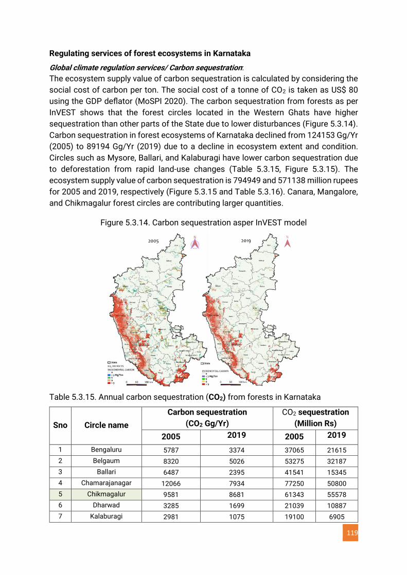
119
Regulating services of forest ecosystems in Karnataka
Global climate regulation services/ Carbon sequestration:
The ecosystem supply value of carbon sequestration is calculated by considering the
social cost of carbon per ton. The social cost of a tonne of CO2 is taken as US$ 80
using the GDP deflator (MoSPI 2020). The carbon sequestration from forests as per
InVEST shows that the forest circles located in the Western Ghats have higher
sequestration than other parts of the State due to lower disturbances (Figure 5.3.14).
Carbon sequestration in forest ecosystems of Karnataka declined from 124153 Gg/Yr
(2005) to 89194 Gg/Yr (2019) due to a decline in ecosystem extent and condition.
Circles such as Mysore, Ballari, and Kalaburagi have lower carbon sequestration due
to deforestation from rapid land-use changes (Table 5.3.15, Figure 5.3.15). The
ecosystem supply value of carbon sequestration is 794949 and 571138 million rupees
for 2005 and 2019, respectively (Figure 5.3.15 and Table 5.3.16). Canara, Mangalore,
and Chikmagalur forest circles are contributing larger quantities.
Figure 5.3.14. Carbon sequestration asper InVEST model
Table 5.3.15. Annual carbon sequestration (CO2) from forests in Karnataka
Sno Circle name
Carbon sequestration
(CO2 Gg/Yr)
CO2 sequestration
(Million Rs)
2005 2019 2005 2019
1 Bengaluru 5787 3374 37065 21615
2 Belgaum 8320 5026 53275 32187
3 Ballari 6487 2395 41541 15345
4 Chamarajanagar 12066 7934 77250 50800
5 Chikmagalur 9581 8681 61343 55578
6 Dharwad 3285 1699 21039 10887
7 Kalaburagi 2981 1075 19100 6905
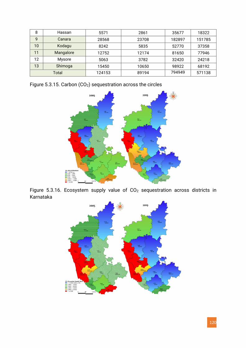
120
8 Hassan 5571 2861 35677 18322
9 Canara 28568 23708 182897 151785
10 Kodagu 8242 5835 52770 37358
11 Mangalore 12752 12174 81650 77946
12 Mysore 5063 3782 32420 24218
13 Shimoga 15450 10650 98922 68192
Total 124153 89194 794949 571138
Figure 5.3.15. Carbon (CO2) sequestration across the circles
Figure 5.3.16. Ecosystem supply value of CO2 sequestration across districts in
Karnataka
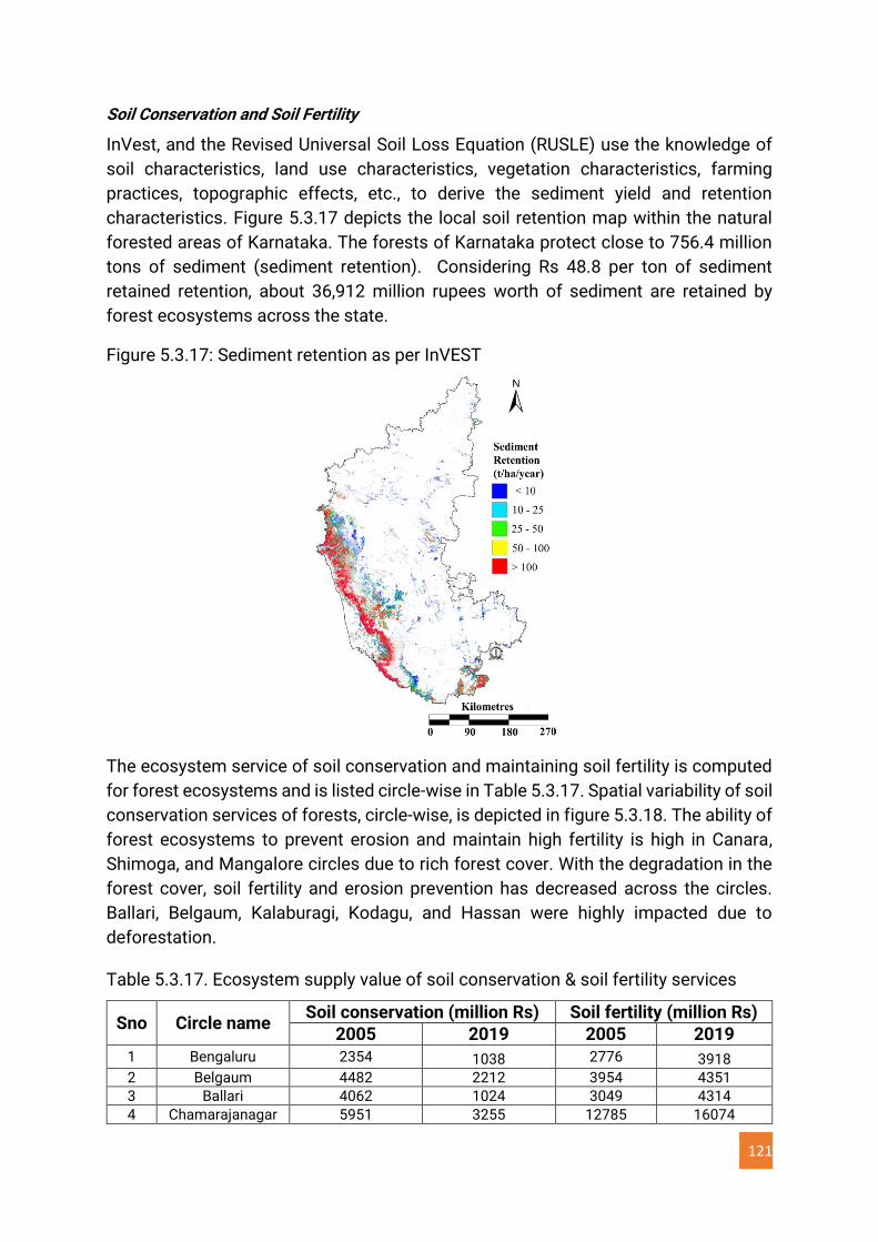
121
Soil Conservation and Soil Fertility
InVest, and the Revised Universal Soil Loss Equation (RUSLE) use the knowledge of
soil characteristics, land use characteristics, vegetation characteristics, farming
practices, topographic effects, etc., to derive the sediment yield and retention
characteristics. Figure 5.3.17 depicts the local soil retention map within the natural
forested areas of Karnataka. The forests of Karnataka protect close to 756.4 million
tons of sediment (sediment retention). Considering Rs 48.8 per ton of sediment
retained retention, about 36,912 million rupees worth of sediment are retained by
forest ecosystems across the state.
Figure 5.3.17: Sediment retention as per InVEST
The ecosystem service of soil conservation and maintaining soil fertility is computed
for forest ecosystems and is listed circle-wise in Table 5.3.17. Spatial variability of soil
conservation services of forests, circle-wise, is depicted in figure 5.3.18. The ability of
forest ecosystems to prevent erosion and maintain high fertility is high in Canara,
Shimoga, and Mangalore circles due to rich forest cover. With the degradation in the
forest cover, soil fertility and erosion prevention has decreased across the circles.
Ballari, Belgaum, Kalaburagi, Kodagu, and Hassan were highly impacted due to
deforestation.
Table 5.3.17. Ecosystem supply value of soil conservation & soil fertility services
Sno Circle name Soil conservation (million Rs) Soil fertility (million Rs)
2005 2019 2005 2019 1 Bengaluru 2354 1038 2776 3918
2 Belgaum 4482 2212 3954 4351
3 Ballari 4062 1024 3049 4314
4 Chamarajanagar 5951 3255 12785 16074
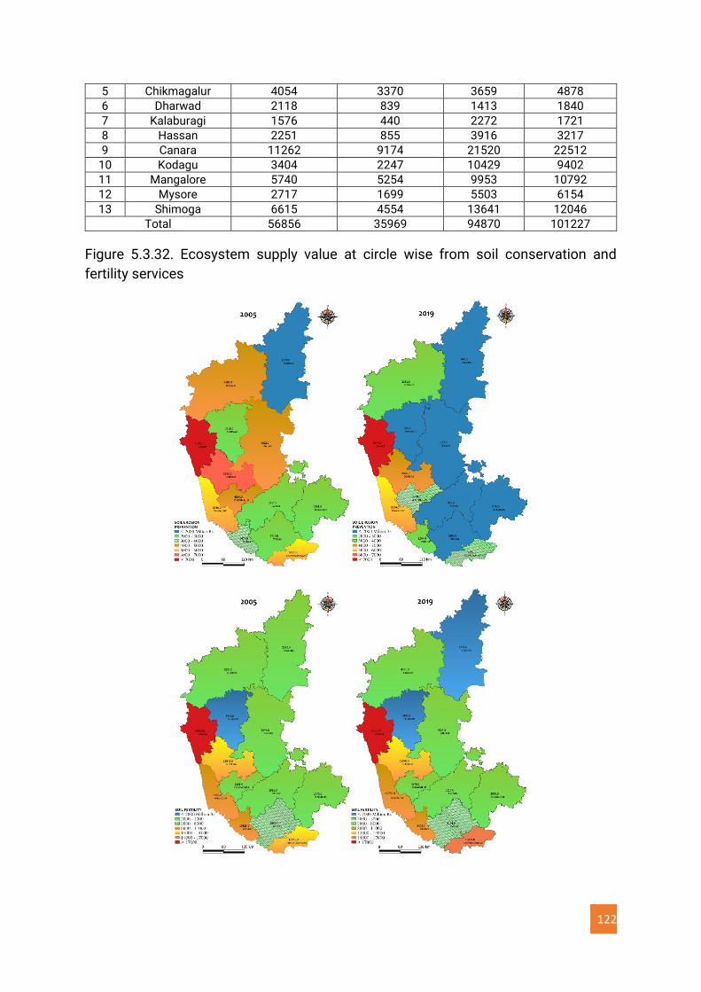
122
5 Chikmagalur 4054 3370 3659 4878
6 Dharwad 2118 839 1413 1840
7 Kalaburagi 1576 440 2272 1721
8 Hassan 2251 855 3916 3217
9 Canara 11262 9174 21520 22512
10 Kodagu 3404 2247 10429 9402
11 Mangalore 5740 5254 9953 10792
12 Mysore 2717 1699 5503 6154
13 Shimoga 6615 4554 13641 12046
Total 56856 35969 94870 101227
Figure 5.3.32. Ecosystem supply value at circle wise from soil conservation and
fertility services
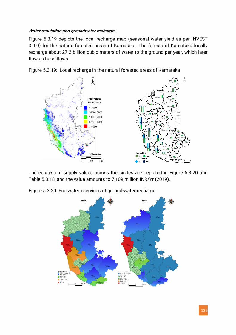
123
Water regulation and groundwater recharge:
Figure 5.3.19 depicts the local recharge map (seasonal water yield as per INVEST
3.9.0) for the natural forested areas of Karnataka. The forests of Karnataka locally
recharge about 27.2 billion cubic meters of water to the ground per year, which later
flow as base flows.
Figure 5.3.19: Local recharge in the natural forested areas of Karnataka
The ecosystem supply values across the circles are depicted in Figure 5.3.20 and
Table 5.3.18, and the value amounts to 7,109 million INR/Yr (2019).
Figure 5.3.20. Ecosystem services of ground-water recharge
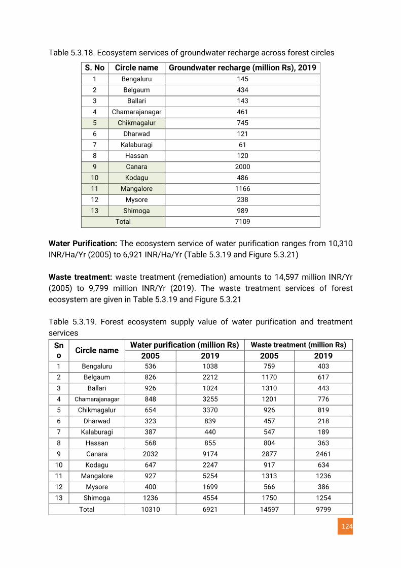
124
Table 5.3.18. Ecosystem services of groundwater recharge across forest circles
S. No Circle name Groundwater recharge (million Rs), 2019
1 Bengaluru 145
2 Belgaum 434
3 Ballari 143
4 Chamarajanagar 461
5 Chikmagalur 745
6 Dharwad 121
7 Kalaburagi 61
8 Hassan 120
9 Canara 2000
10 Kodagu 486
11 Mangalore 1166
12 Mysore 238
13 Shimoga 989
Total 7109
Water Purification: The ecosystem service of water purification ranges from 10,310
INR/Ha/Yr (2005) to 6,921 INR/Ha/Yr (Table 5.3.19 and Figure 5.3.21)
Waste treatment: waste treatment (remediation) amounts to 14,597 million INR/Yr
(2005) to 9,799 million INR/Yr (2019). The waste treatment services of forest
ecosystem are given in Table 5.3.19 and Figure 5.3.21
Table 5.3.19. Forest ecosystem supply value of water purification and treatment
services
Sno
Circle name Water purification (million Rs) Waste treatment (million Rs)
2005 2019 2005 2019 1 Bengaluru 536 1038 759 403
2 Belgaum 826 2212 1170 617
3 Ballari 926 1024 1310 443
4 Chamarajanagar 848 3255 1201 776
5 Chikmagalur 654 3370 926 819
6 Dharwad 323 839 457 218
7 Kalaburagi 387 440 547 189
8 Hassan 568 855 804 363
9 Canara 2032 9174 2877 2461
10 Kodagu 647 2247 917 634
11 Mangalore 927 5254 1313 1236
12 Mysore 400 1699 566 386
13 Shimoga 1236 4554 1750 1254
Total 10310 6921 14597 9799
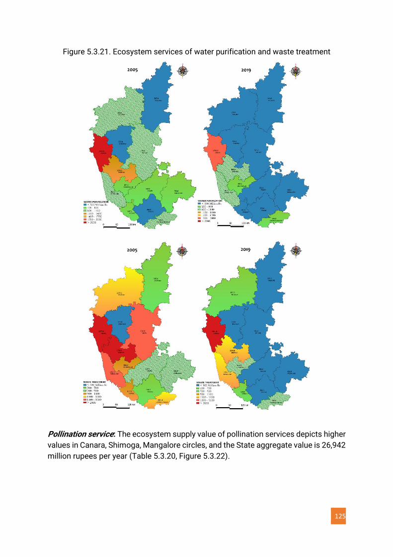
125
Figure 5.3.21. Ecosystem services of water purification and waste treatment
Pollination service: The ecosystem supply value of pollination services depicts higher
values in Canara, Shimoga, Mangalore circles, and the State aggregate value is 26,942
million rupees per year (Table 5.3.20, Figure 5.3.22).
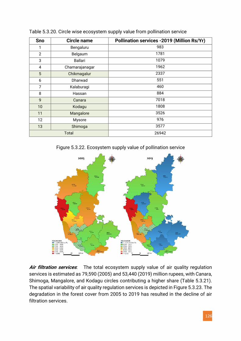
126
Table 5.3.20. Circle wise ecosystem supply value from pollination service
Sno Circle name Pollination services -2019 (Million Rs/Yr)
1 Bengaluru 983
2 Belgaum 1781
3 Ballari 1079
4 Chamarajanagar 1962
5 Chikmagalur 2337
6 Dharwad 551
7 Kalaburagi 460
8 Hassan 884
9 Canara 7018
10 Kodagu 1808
11 Mangalore 3526
12 Mysore 976
13 Shimoga 3577
Total 26942
Figure 5.3.22. Ecosystem supply value of pollination service
Air filtration services: The total ecosystem supply value of air quality regulation
services is estimated as 79,590 (2005) and 53,440 (2019) million rupees, with Canara,
Shimoga, Mangalore, and Kodagu circles contributing a higher share (Table 5.3.21).
The spatial variability of air quality regulation services is depicted in Figure 5.3.23. The
degradation in the forest cover from 2005 to 2019 has resulted in the decline of air
filtration services.

127
Table 5.3.21. Ecosystem supply value from air filtration service
S.no Circle name Air filtration services (Million Rs)
2005 2019
1 Bengaluru 4140 2201
2 Belgaum 6377 3363
3 Ballari 7144 2417
4 Chamarajanagar 6550 4234
5 Chikmagalur 5047 4467
6 Dharwad 2494 1190
7 Kalaburagi 2986 1031
8 Hassan 4385 1980
9 Canara 15682 13416
10 Kodagu 4998 3456
11 Mangalore 7158 6741
12 Mysore 3088 2106
13 Shimoga 9541 6838
Total 79590 53440
Figure 5.3.23. Air quality regulation services from forest ecosystems in Karnataka
Local (micro and meso) climate regulation services: The ecosystem value of
moderating climate listed in Table 5.3.22 accounts for 169,487 (2005) and 113,807
(2019) million rupees. Canara, Shimoga, Mangalore, and Kodagu circles contribute a
higher share due to good forest cover, which is responsible for moderating the climate
(Figure 5.3.24). All forest circles show a decline in local climate regulation ecosystem
value due to the loss of forest cover.
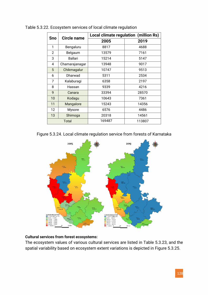
128
Table 5.3.22. Ecosystem services of local climate regulation
Sno Circle name Local climate regulation (million Rs)
2005 2019
1 Bengaluru 8817 4688
2 Belgaum 13579 7161
3 Ballari 15214 5147
4 Chamarajanagar 13948 9017
5 Chikmagalur 10747 9513
6 Dharwad 5311 2534
7 Kalaburagi 6358 2197
8 Hassan 9339 4216
9 Canara 33394 28570
10 Kodagu 10643 7361
11 Mangalore 15243 14356
12 Mysore 6576 4486
13 Shimoga 20318 14561
Total 169487 113807
Figure 5.3.24. Local climate regulation service from forests of Karnataka
Cultural services from forest ecosystems:
The ecosystem values of various cultural services are listed in Table 5.3.23, and the
spatial variability based on ecosystem extent variations is depicted in Figure 5.3.25.
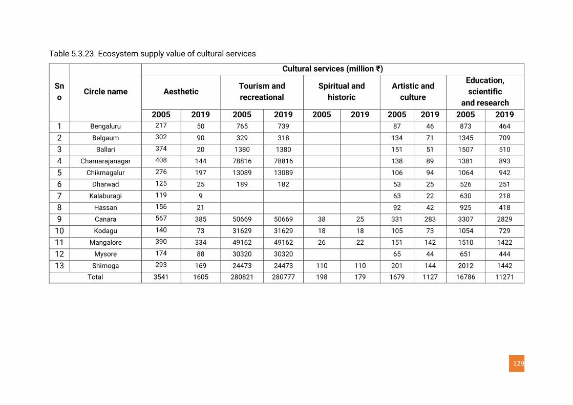
129
Table 5.3.23. Ecosystem supply value of cultural services
Sn
o Circle name
Cultural services (million ₹)
Aesthetic Tourism and
recreational
Spiritual and
historic
Artistic and
culture
Education,
scientific
and research
2005 2019 2005 2019 2005 2019 2005 2019 2005 2019
1 Bengaluru 217 50 765 739 87 46 873 464
2 Belgaum 302 90 329 318 134 71 1345 709
3 Ballari 374 20 1380 1380 151 51 1507 510
4 Chamarajanagar 408 144 78816 78816 138 89 1381 893
5 Chikmagalur 276 197 13089 13089 106 94 1064 942
6 Dharwad 125 25 189 182 53 25 526 251
7 Kalaburagi 119 9 63 22 630 218
8 Hassan 156 21 92 42 925 418
9 Canara 567 385 50669 50669 38 25 331 283 3307 2829
10 Kodagu 140 73 31629 31629 18 18 105 73 1054 729
11 Mangalore 390 334 49162 49162 26 22 151 142 1510 1422
12 Mysore 174 88 30320 30320 65 44 651 444
13 Shimoga 293 169 24473 24473 110 110 201 144 2012 1442
Total 3541 1605 280821 280777 198 179 1679 1127 16786 11271
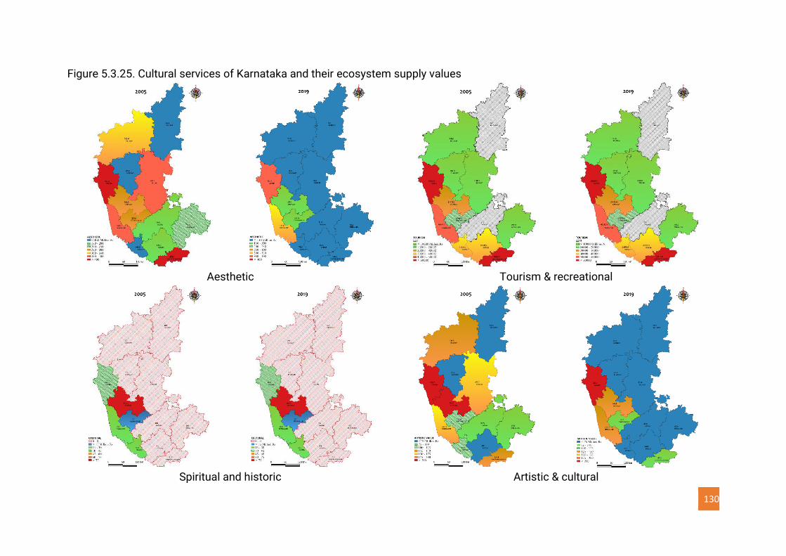
130
Figure 5.3.25. Cultural services of Karnataka and their ecosystem supply values
Aesthetic Tourism & recreational
Spiritual and historic Artistic & cultural
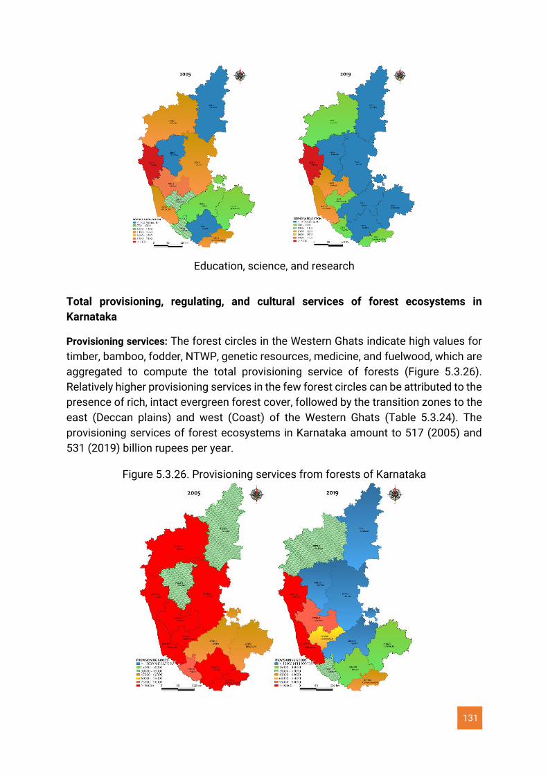
131
Education, science, and research
Total provisioning, regulating, and cultural services of forest ecosystems in
Karnataka
Provisioning services: The forest circles in the Western Ghats indicate high values for
timber, bamboo, fodder, NTWP, genetic resources, medicine, and fuelwood, which are
aggregated to compute the total provisioning service of forests (Figure 5.3.26).
Relatively higher provisioning services in the few forest circles can be attributed to the
presence of rich, intact evergreen forest cover, followed by the transition zones to the
east (Deccan plains) and west (Coast) of the Western Ghats (Table 5.3.24). The
provisioning services of forest ecosystems in Karnataka amount to 517 (2005) and
531 (2019) billion rupees per year.
Figure 5.3.26. Provisioning services from forests of Karnataka
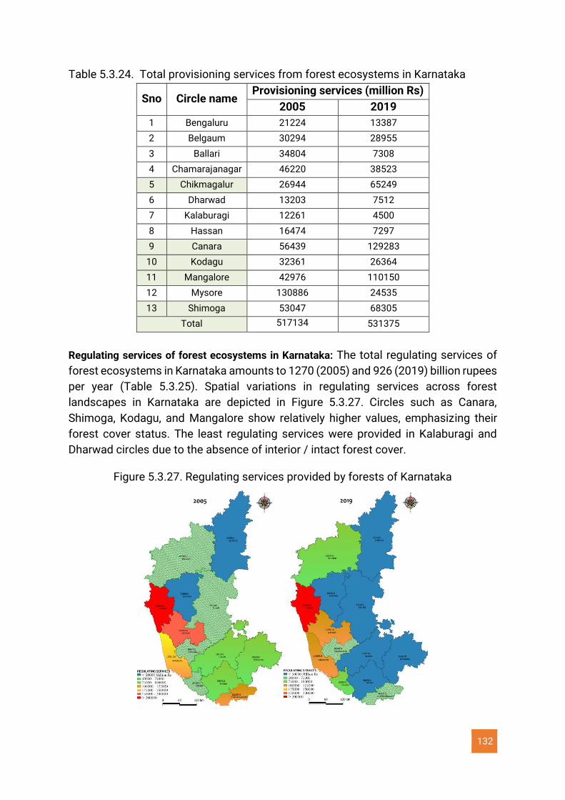
132
Table 5.3.24. Total provisioning services from forest ecosystems in Karnataka
Sno Circle name Provisioning services (million Rs)
2005 2019
1 Bengaluru 21224 13387
2 Belgaum 30294 28955
3 Ballari 34804 7308
4 Chamarajanagar 46220 38523
5 Chikmagalur 26944 65249
6 Dharwad 13203 7512
7 Kalaburagi 12261 4500
8 Hassan 16474 7297
9 Canara 56439 129283
10 Kodagu 32361 26364
11 Mangalore 42976 110150
12 Mysore 130886 24535
13 Shimoga 53047 68305
Total 517134 531375
Regulating services of forest ecosystems in Karnataka: The total regulating services of
forest ecosystems in Karnataka amounts to 1270 (2005) and 926 (2019) billion rupees
per year (Table 5.3.25). Spatial variations in regulating services across forest
landscapes in Karnataka are depicted in Figure 5.3.27. Circles such as Canara,
Shimoga, Kodagu, and Mangalore show relatively higher values, emphasizing their
forest cover status. The least regulating services were provided in Kalaburagi and
Dharwad circles due to the absence of interior / intact forest cover.
Figure 5.3.27. Regulating services provided by forests of Karnataka
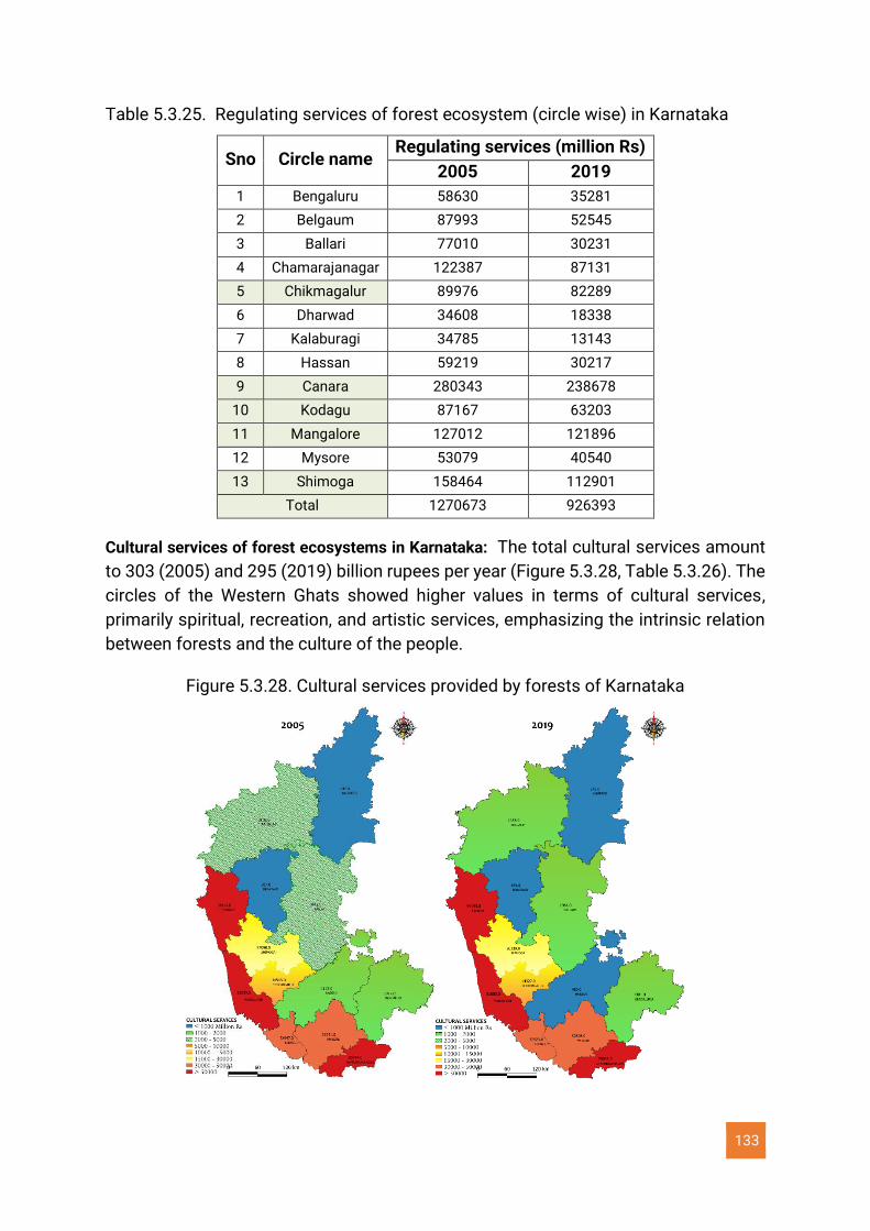
133
Table 5.3.25. Regulating services of forest ecosystem (circle wise) in Karnataka
Sno Circle name Regulating services (million Rs)
2005 2019
1 Bengaluru 58630 35281
2 Belgaum 87993 52545
3 Ballari 77010 30231
4 Chamarajanagar 122387 87131
5 Chikmagalur 89976 82289
6 Dharwad 34608 18338
7 Kalaburagi 34785 13143
8 Hassan 59219 30217
9 Canara 280343 238678
10 Kodagu 87167 63203
11 Mangalore 127012 121896
12 Mysore 53079 40540
13 Shimoga 158464 112901
Total 1270673 926393
Cultural services of forest ecosystems in Karnataka: The total cultural services amount
to 303 (2005) and 295 (2019) billion rupees per year (Figure 5.3.28, Table 5.3.26). The
circles of the Western Ghats showed higher values in terms of cultural services,
primarily spiritual, recreation, and artistic services, emphasizing the intrinsic relation
between forests and the culture of the people.
Figure 5.3.28. Cultural services provided by forests of Karnataka
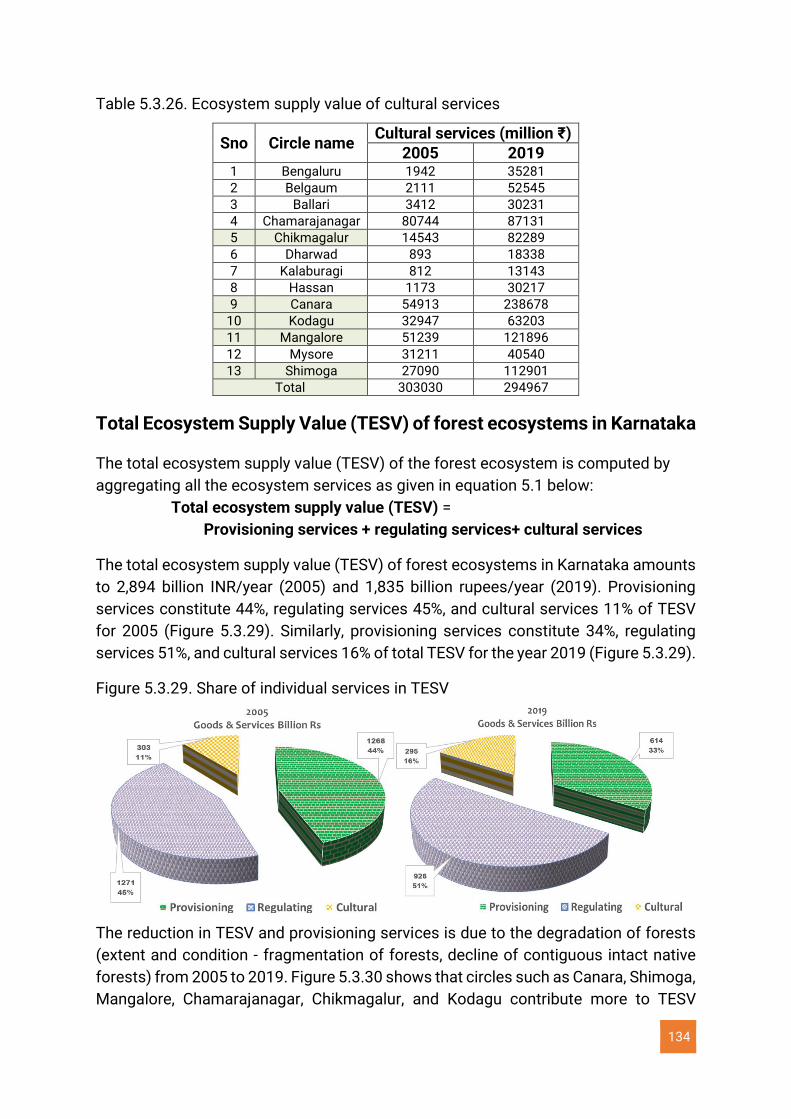
134
Table 5.3.26. Ecosystem supply value of cultural services
Sno Circle name Cultural services (million ₹)
2005 2019 1 Bengaluru 1942 35281
2 Belgaum 2111 52545
3 Ballari 3412 30231
4 Chamarajanagar 80744 87131
5 Chikmagalur 14543 82289
6 Dharwad 893 18338
7 Kalaburagi 812 13143
8 Hassan 1173 30217
9 Canara 54913 238678
10 Kodagu 32947 63203
11 Mangalore 51239 121896
12 Mysore 31211 40540
13 Shimoga 27090 112901
Total 303030 294967
Total Ecosystem Supply Value (TESV) of forest ecosystems in Karnataka
The total ecosystem supply value (TESV) of the forest ecosystem is computed by
aggregating all the ecosystem services as given in equation 5.1 below:
Total ecosystem supply value (TESV) =
Provisioning services + regulating services+ cultural services
The total ecosystem supply value (TESV) of forest ecosystems in Karnataka amounts
to 2,894 billion INR/year (2005) and 1,835 billion rupees/year (2019). Provisioning
services constitute 44%, regulating services 45%, and cultural services 11% of TESV
for 2005 (Figure 5.3.29). Similarly, provisioning services constitute 34%, regulating
services 51%, and cultural services 16% of total TESV for the year 2019 (Figure 5.3.29).
Figure 5.3.29. Share of individual services in TESV
The reduction in TESV and provisioning services is due to the degradation of forests
(extent and condition - fragmentation of forests, decline of contiguous intact native
forests) from 2005 to 2019. Figure 5.3.30 shows that circles such as Canara, Shimoga,
Mangalore, Chamarajanagar, Chikmagalur, and Kodagu contribute more to TESV
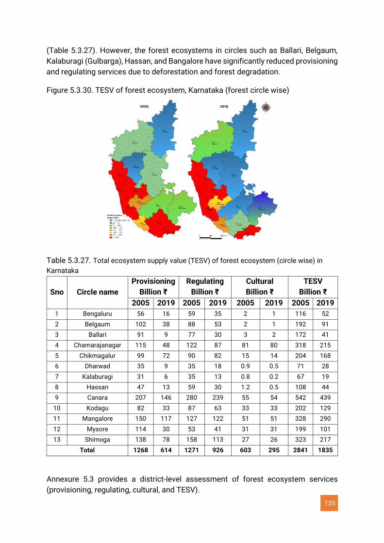
135
(Table 5.3.27). However, the forest ecosystems in circles such as Ballari, Belgaum,
Kalaburagi (Gulbarga), Hassan, and Bangalore have significantly reduced provisioning
and regulating services due to deforestation and forest degradation.
Figure 5.3.30. TESV of forest ecosystem, Karnataka (forest circle wise)
Table 5.3.27. Total ecosystem supply value (TESV) of forest ecosystem (circle wise) in
Karnataka
Sno Circle name
Provisioning
Billion ₹
Regulating
Billion ₹
Cultural
Billion ₹
TESV
Billion ₹
2005 2019 2005 2019 2005 2019 2005 2019
1 Bengaluru 56 16 59 35 2 1 116 52
2 Belgaum 102 38 88 53 2 1 192 91
3 Ballari 91 9 77 30 3 2 172 41
4 Chamarajanagar 115 48 122 87 81 80 318 215
5 Chikmagalur 99 72 90 82 15 14 204 168
6 Dharwad 35 9 35 18 0.9 0.5 71 28
7 Kalaburagi 31 6 35 13 0.8 0.2 67 19
8 Hassan 47 13 59 30 1.2 0.5 108 44
9 Canara 207 146 280 239 55 54 542 439
10 Kodagu 82 33 87 63 33 33 202 129
11 Mangalore 150 117 127 122 51 51 328 290
12 Mysore 114 30 53 41 31 31 199 101
13 Shimoga 138 78 158 113 27 26 323 217
Total 1268 614 1271 926 603 295 2841 1835
Annexure 5.3 provides a district-level assessment of forest ecosystem services
(provisioning, regulating, cultural, and TESV).
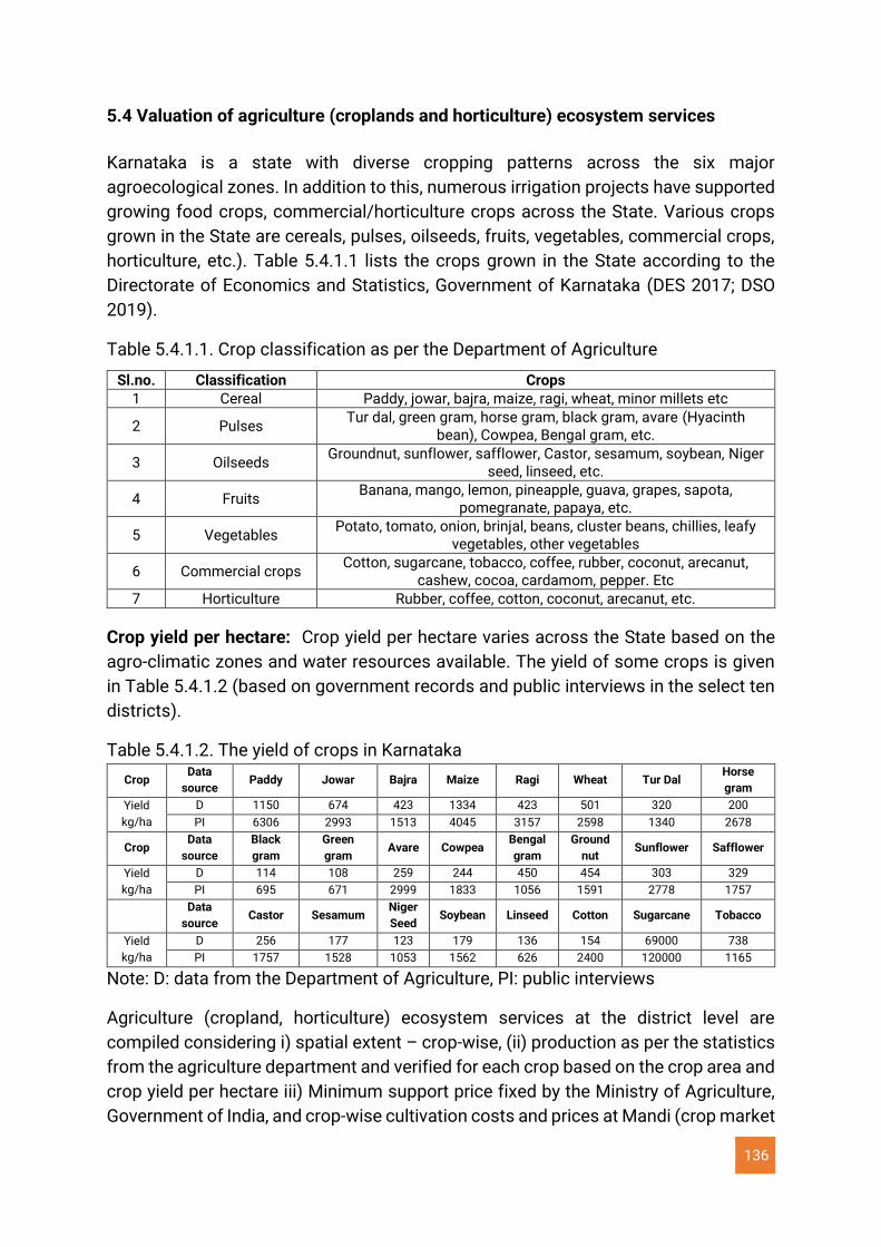
136
5.4 Valuation of agriculture (croplands and horticulture) ecosystem services
Karnataka is a state with diverse cropping patterns across the six major
agroecological zones. In addition to this, numerous irrigation projects have supported
growing food crops, commercial/horticulture crops across the State. Various crops
grown in the State are cereals, pulses, oilseeds, fruits, vegetables, commercial crops,
horticulture, etc.). Table 5.4.1.1 lists the crops grown in the State according to the
Directorate of Economics and Statistics, Government of Karnataka (DES 2017; DSO
2019).
Table 5.4.1.1. Crop classification as per the Department of Agriculture
Sl.no. Classification Crops
1 Cereal Paddy, jowar, bajra, maize, ragi, wheat, minor millets etc
2 Pulses Tur dal, green gram, horse gram, black gram, avare (Hyacinth
bean), Cowpea, Bengal gram, etc.
3 Oilseeds Groundnut, sunflower, safflower, Castor, sesamum, soybean, Niger
seed, linseed, etc.
4 Fruits Banana, mango, lemon, pineapple, guava, grapes, sapota,
pomegranate, papaya, etc.
5 Vegetables Potato, tomato, onion, brinjal, beans, cluster beans, chillies, leafy
vegetables, other vegetables
6 Commercial crops Cotton, sugarcane, tobacco, coffee, rubber, coconut, arecanut,
cashew, cocoa, cardamom, pepper. Etc
7 Horticulture Rubber, coffee, cotton, coconut, arecanut, etc.
Crop yield per hectare: Crop yield per hectare varies across the State based on the
agro-climatic zones and water resources available. The yield of some crops is given
in Table 5.4.1.2 (based on government records and public interviews in the select ten
districts).
Table 5.4.1.2. The yield of crops in Karnataka
Crop Data
source Paddy Jowar Bajra Maize Ragi Wheat Tur Dal
Horse
gram
Yield
kg/ha
D 1150 674 423 1334 423 501 320 200
PI 6306 2993 1513 4045 3157 2598 1340 2678
Crop Data
source
Black
gram
Green
gram Avare Cowpea
Bengal
gram
Ground
nut Sunflower Safflower
Yield
kg/ha
D 114 108 259 244 450 454 303 329
PI 695 671 2999 1833 1056 1591 2778 1757
Data
source Castor Sesamum
Niger
Seed Soybean Linseed Cotton Sugarcane Tobacco
Yield
kg/ha
D 256 177 123 179 136 154 69000 738
PI 1757 1528 1053 1562 626 2400 120000 1165
Note: D: data from the Department of Agriculture, PI: public interviews
Agriculture (cropland, horticulture) ecosystem services at the district level are
compiled considering i) spatial extent – crop-wise, (ii) production as per the statistics
from the agriculture department and verified for each crop based on the crop area and
crop yield per hectare iii) Minimum support price fixed by the Ministry of Agriculture,
Government of India, and crop-wise cultivation costs and prices at Mandi (crop market
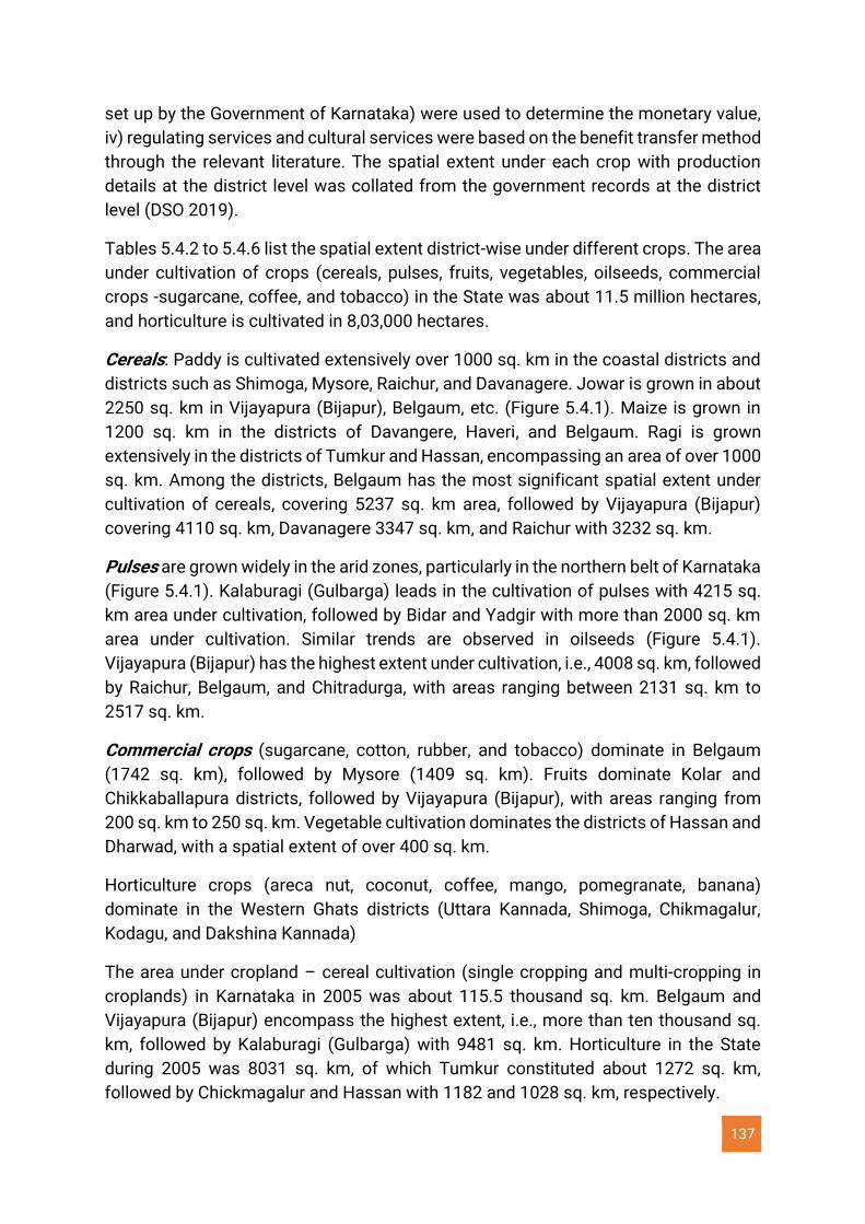
137
set up by the Government of Karnataka) were used to determine the monetary value,
iv) regulating services and cultural services were based on the benefit transfer method
through the relevant literature. The spatial extent under each crop with production
details at the district level was collated from the government records at the district
level (DSO 2019).
Tables 5.4.2 to 5.4.6 list the spatial extent district-wise under different crops. The area
under cultivation of crops (cereals, pulses, fruits, vegetables, oilseeds, commercial
crops -sugarcane, coffee, and tobacco) in the State was about 11.5 million hectares,
and horticulture is cultivated in 8,03,000 hectares.
Cereals: Paddy is cultivated extensively over 1000 sq. km in the coastal districts and
districts such as Shimoga, Mysore, Raichur, and Davanagere. Jowar is grown in about
2250 sq. km in Vijayapura (Bijapur), Belgaum, etc. (Figure 5.4.1). Maize is grown in
1200 sq. km in the districts of Davangere, Haveri, and Belgaum. Ragi is grown
extensively in the districts of Tumkur and Hassan, encompassing an area of over 1000
sq. km. Among the districts, Belgaum has the most significant spatial extent under
cultivation of cereals, covering 5237 sq. km area, followed by Vijayapura (Bijapur)
covering 4110 sq. km, Davanagere 3347 sq. km, and Raichur with 3232 sq. km.
Pulses are grown widely in the arid zones, particularly in the northern belt of Karnataka
(Figure 5.4.1). Kalaburagi (Gulbarga) leads in the cultivation of pulses with 4215 sq.
km area under cultivation, followed by Bidar and Yadgir with more than 2000 sq. km
area under cultivation. Similar trends are observed in oilseeds (Figure 5.4.1).
Vijayapura (Bijapur) has the highest extent under cultivation, i.e., 4008 sq. km, followed
by Raichur, Belgaum, and Chitradurga, with areas ranging between 2131 sq. km to
2517 sq. km.
Commercial crops (sugarcane, cotton, rubber, and tobacco) dominate in Belgaum
(1742 sq. km), followed by Mysore (1409 sq. km). Fruits dominate Kolar and
Chikkaballapura districts, followed by Vijayapura (Bijapur), with areas ranging from
200 sq. km to 250 sq. km. Vegetable cultivation dominates the districts of Hassan and
Dharwad, with a spatial extent of over 400 sq. km.
Horticulture crops (areca nut, coconut, coffee, mango, pomegranate, banana)
dominate in the Western Ghats districts (Uttara Kannada, Shimoga, Chikmagalur,
Kodagu, and Dakshina Kannada)
The area under cropland – cereal cultivation (single cropping and multi-cropping in
croplands) in Karnataka in 2005 was about 115.5 thousand sq. km. Belgaum and
Vijayapura (Bijapur) encompass the highest extent, i.e., more than ten thousand sq.
km, followed by Kalaburagi (Gulbarga) with 9481 sq. km. Horticulture in the State
during 2005 was 8031 sq. km, of which Tumkur constituted about 1272 sq. km,
followed by Chickmagalur and Hassan with 1182 and 1028 sq. km, respectively.
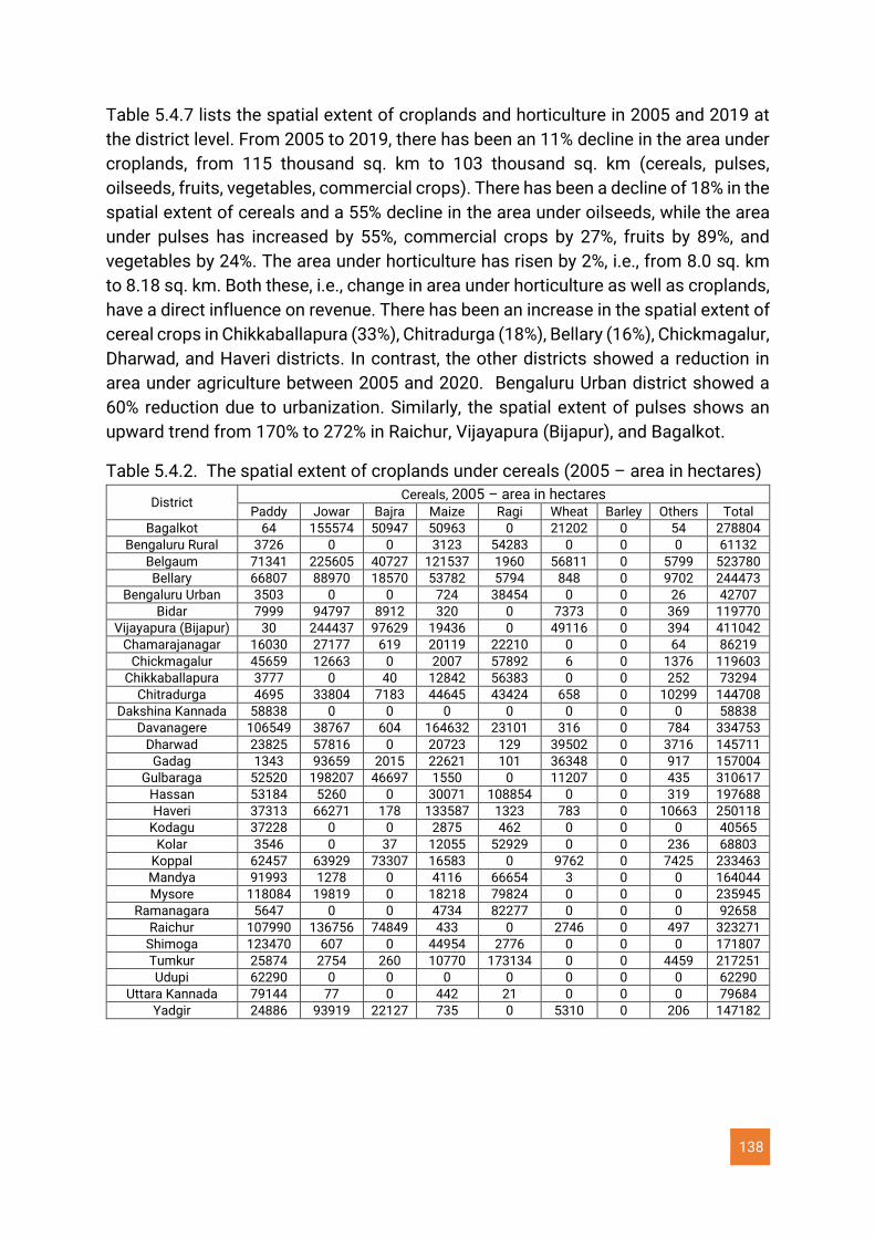
138
Table 5.4.7 lists the spatial extent of croplands and horticulture in 2005 and 2019 at
the district level. From 2005 to 2019, there has been an 11% decline in the area under
croplands, from 115 thousand sq. km to 103 thousand sq. km (cereals, pulses,
oilseeds, fruits, vegetables, commercial crops). There has been a decline of 18% in the
spatial extent of cereals and a 55% decline in the area under oilseeds, while the area
under pulses has increased by 55%, commercial crops by 27%, fruits by 89%, and
vegetables by 24%. The area under horticulture has risen by 2%, i.e., from 8.0 sq. km
to 8.18 sq. km. Both these, i.e., change in area under horticulture as well as croplands,
have a direct influence on revenue. There has been an increase in the spatial extent of
cereal crops in Chikkaballapura (33%), Chitradurga (18%), Bellary (16%), Chickmagalur,
Dharwad, and Haveri districts. In contrast, the other districts showed a reduction in
area under agriculture between 2005 and 2020. Bengaluru Urban district showed a
60% reduction due to urbanization. Similarly, the spatial extent of pulses shows an
upward trend from 170% to 272% in Raichur, Vijayapura (Bijapur), and Bagalkot.
Table 5.4.2. The spatial extent of croplands under cereals (2005 – area in hectares)
District Cereals, 2005 – area in hectares
Paddy Jowar Bajra Maize Ragi Wheat Barley Others Total
Bagalkot 64 155574 50947 50963 0 21202 0 54 278804
Bengaluru Rural 3726 0 0 3123 54283 0 0 0 61132
Belgaum 71341 225605 40727 121537 1960 56811 0 5799 523780
Bellary 66807 88970 18570 53782 5794 848 0 9702 244473
Bengaluru Urban 3503 0 0 724 38454 0 0 26 42707
Bidar 7999 94797 8912 320 0 7373 0 369 119770
Vijayapura (Bijapur) 30 244437 97629 19436 0 49116 0 394 411042
Chamarajanagar 16030 27177 619 20119 22210 0 0 64 86219
Chickmagalur 45659 12663 0 2007 57892 6 0 1376 119603
Chikkaballapura 3777 0 40 12842 56383 0 0 252 73294
Chitradurga 4695 33804 7183 44645 43424 658 0 10299 144708
Dakshina Kannada 58838 0 0 0 0 0 0 0 58838
Davanagere 106549 38767 604 164632 23101 316 0 784 334753
Dharwad 23825 57816 0 20723 129 39502 0 3716 145711
Gadag 1343 93659 2015 22621 101 36348 0 917 157004
Gulbaraga 52520 198207 46697 1550 0 11207 0 435 310617
Hassan 53184 5260 0 30071 108854 0 0 319 197688
Haveri 37313 66271 178 133587 1323 783 0 10663 250118
Kodagu 37228 0 0 2875 462 0 0 0 40565
Kolar 3546 0 37 12055 52929 0 0 236 68803
Koppal 62457 63929 73307 16583 0 9762 0 7425 233463
Mandya 91993 1278 0 4116 66654 3 0 0 164044
Mysore 118084 19819 0 18218 79824 0 0 0 235945
Ramanagara 5647 0 0 4734 82277 0 0 0 92658
Raichur 107990 136756 74849 433 0 2746 0 497 323271
Shimoga 123470 607 0 44954 2776 0 0 0 171807
Tumkur 25874 2754 260 10770 173134 0 0 4459 217251
Udupi 62290 0 0 0 0 0 0 0 62290
Uttara Kannada 79144 77 0 442 21 0 0 0 79684
Yadgir 24886 93919 22127 735 0 5310 0 206 147182
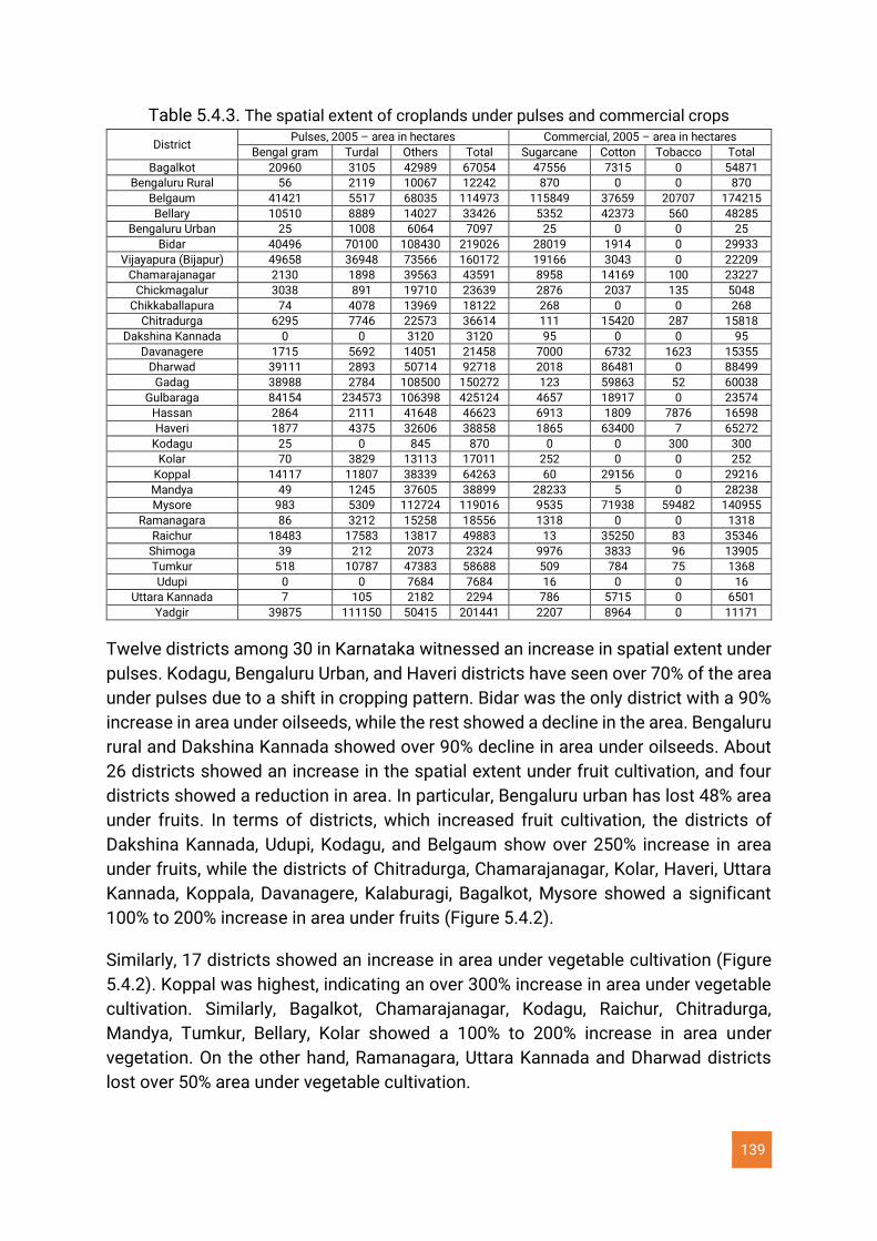
139
Table 5.4.3. The spatial extent of croplands under pulses and commercial crops
District Pulses, 2005 – area in hectares Commercial, 2005 – area in hectares
Bengal gram Turdal Others Total Sugarcane Cotton Tobacco Total
Bagalkot 20960 3105 42989 67054 47556 7315 0 54871
Bengaluru Rural 56 2119 10067 12242 870 0 0 870
Belgaum 41421 5517 68035 114973 115849 37659 20707 174215
Bellary 10510 8889 14027 33426 5352 42373 560 48285
Bengaluru Urban 25 1008 6064 7097 25 0 0 25
Bidar 40496 70100 108430 219026 28019 1914 0 29933
Vijayapura (Bijapur) 49658 36948 73566 160172 19166 3043 0 22209
Chamarajanagar 2130 1898 39563 43591 8958 14169 100 23227
Chickmagalur 3038 891 19710 23639 2876 2037 135 5048
Chikkaballapura 74 4078 13969 18122 268 0 0 268
Chitradurga 6295 7746 22573 36614 111 15420 287 15818
Dakshina Kannada 0 0 3120 3120 95 0 0 95
Davanagere 1715 5692 14051 21458 7000 6732 1623 15355
Dharwad 39111 2893 50714 92718 2018 86481 0 88499
Gadag 38988 2784 108500 150272 123 59863 52 60038
Gulbaraga 84154 234573 106398 425124 4657 18917 0 23574
Hassan 2864 2111 41648 46623 6913 1809 7876 16598
Haveri 1877 4375 32606 38858 1865 63400 7 65272
Kodagu 25 0 845 870 0 0 300 300
Kolar 70 3829 13113 17011 252 0 0 252
Koppal 14117 11807 38339 64263 60 29156 0 29216
Mandya 49 1245 37605 38899 28233 5 0 28238
Mysore 983 5309 112724 119016 9535 71938 59482 140955
Ramanagara 86 3212 15258 18556 1318 0 0 1318
Raichur 18483 17583 13817 49883 13 35250 83 35346
Shimoga 39 212 2073 2324 9976 3833 96 13905
Tumkur 518 10787 47383 58688 509 784 75 1368
Udupi 0 0 7684 7684 16 0 0 16
Uttara Kannada 7 105 2182 2294 786 5715 0 6501
Yadgir 39875 111150 50415 201441 2207 8964 0 11171
Twelve districts among 30 in Karnataka witnessed an increase in spatial extent under
pulses. Kodagu, Bengaluru Urban, and Haveri districts have seen over 70% of the area
under pulses due to a shift in cropping pattern. Bidar was the only district with a 90%
increase in area under oilseeds, while the rest showed a decline in the area. Bengaluru
rural and Dakshina Kannada showed over 90% decline in area under oilseeds. About
26 districts showed an increase in the spatial extent under fruit cultivation, and four
districts showed a reduction in area. In particular, Bengaluru urban has lost 48% area
under fruits. In terms of districts, which increased fruit cultivation, the districts of
Dakshina Kannada, Udupi, Kodagu, and Belgaum show over 250% increase in area
under fruits, while the districts of Chitradurga, Chamarajanagar, Kolar, Haveri, Uttara
Kannada, Koppala, Davanagere, Kalaburagi, Bagalkot, Mysore showed a significant
100% to 200% increase in area under fruits (Figure 5.4.2).
Similarly, 17 districts showed an increase in area under vegetable cultivation (Figure
5.4.2). Koppal was highest, indicating an over 300% increase in area under vegetable
cultivation. Similarly, Bagalkot, Chamarajanagar, Kodagu, Raichur, Chitradurga,
Mandya, Tumkur, Bellary, Kolar showed a 100% to 200% increase in area under
vegetation. On the other hand, Ramanagara, Uttara Kannada and Dharwad districts
lost over 50% area under vegetable cultivation.
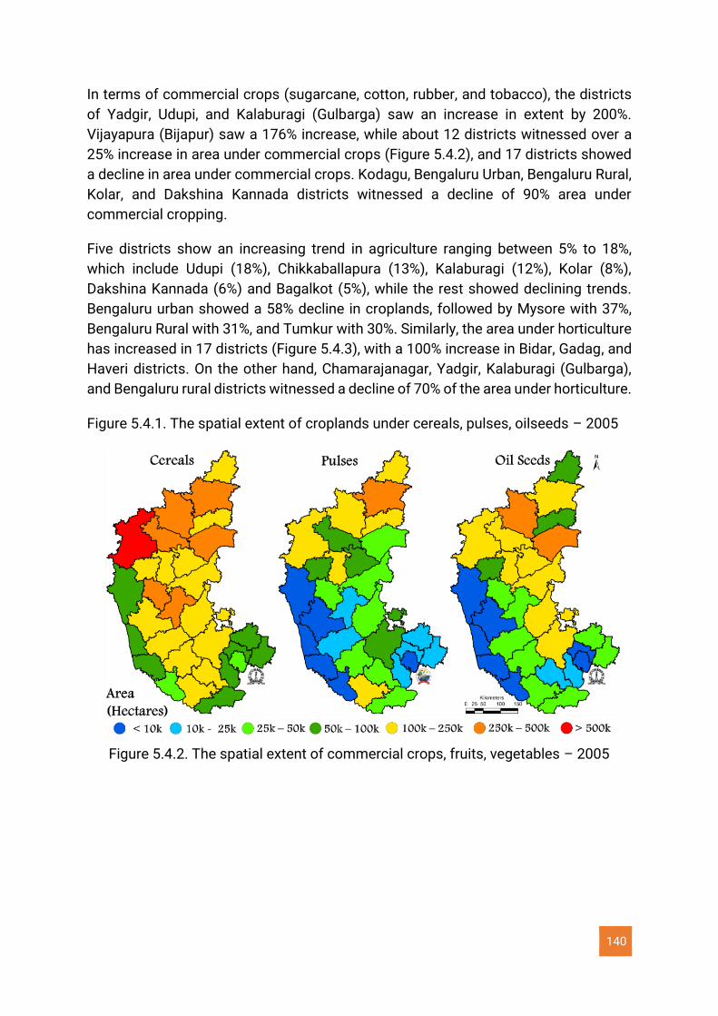
140
In terms of commercial crops (sugarcane, cotton, rubber, and tobacco), the districts
of Yadgir, Udupi, and Kalaburagi (Gulbarga) saw an increase in extent by 200%.
Vijayapura (Bijapur) saw a 176% increase, while about 12 districts witnessed over a
25% increase in area under commercial crops (Figure 5.4.2), and 17 districts showed
a decline in area under commercial crops. Kodagu, Bengaluru Urban, Bengaluru Rural,
Kolar, and Dakshina Kannada districts witnessed a decline of 90% area under
commercial cropping.
Five districts show an increasing trend in agriculture ranging between 5% to 18%,
which include Udupi (18%), Chikkaballapura (13%), Kalaburagi (12%), Kolar (8%),
Dakshina Kannada (6%) and Bagalkot (5%), while the rest showed declining trends.
Bengaluru urban showed a 58% decline in croplands, followed by Mysore with 37%,
Bengaluru Rural with 31%, and Tumkur with 30%. Similarly, the area under horticulture
has increased in 17 districts (Figure 5.4.3), with a 100% increase in Bidar, Gadag, and
Haveri districts. On the other hand, Chamarajanagar, Yadgir, Kalaburagi (Gulbarga),
and Bengaluru rural districts witnessed a decline of 70% of the area under horticulture.
Figure 5.4.1. The spatial extent of croplands under cereals, pulses, oilseeds – 2005
Figure 5.4.2. The spatial extent of commercial crops, fruits, vegetables – 2005
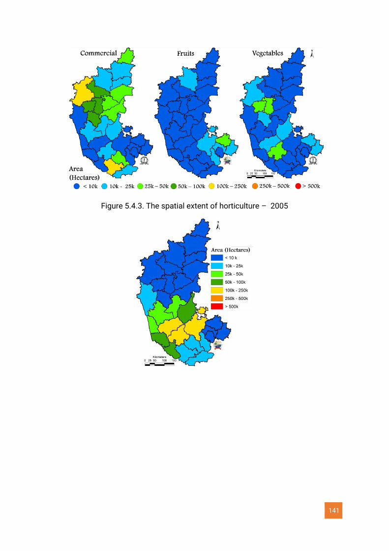
141
Figure 5.4.3. The spatial extent of horticulture – 2005
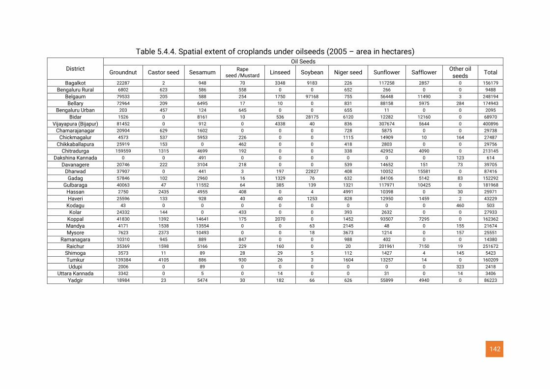
142
Table 5.4.4. Spatial extent of croplands under oilseeds (2005 – area in hectares)
District Oil Seeds
Groundnut Castor seed Sesamum Rape
seed /Mustard Linseed Soybean Niger seed Sunflower Safflower Other oil
seeds Total
Bagalkot 22287 2 948 70 3348 9183 226 117258 2857 0 156179
Bengaluru Rural 6802 623 586 558 0 0 652 266 0 0 9488
Belgaum 79533 205 588 254 1750 97168 755 56448 11490 3 248194
Bellary 72964 209 6495 17 10 0 831 88158 5975 284 174943
Bengaluru Urban 203 457 124 645 0 0 655 11 0 0 2095
Bidar 1526 0 8161 10 536 28175 6120 12282 12160 0 68970
Vijayapura (Bijapur) 81452 0 912 0 4338 40 836 307674 5644 0 400896
Chamarajanagar 20904 629 1602 0 0 0 728 5875 0 0 29738
Chickmagalur 4573 537 5953 226 0 0 1115 14909 10 164 27487
Chikkaballapura 25919 153 0 462 0 0 418 2803 0 0 29756
Chitradurga 159559 1315 4699 192 0 0 338 42952 4090 0 213145
Dakshina Kannada 0 0 491 0 0 0 0 0 0 123 614
Davanagere 20746 222 3104 218 0 0 539 14652 151 73 39705
Dharwad 37907 0 441 3 197 22827 408 10052 15581 0 87416
Gadag 57846 102 2960 16 1329 76 632 84106 5142 83 152292
Gulbaraga 40063 47 11552 64 385 139 1321 117971 10425 0 181968
Hassan 2750 2435 4955 408 0 4 4991 10398 0 30 25971
Haveri 25596 133 928 40 40 1253 828 12950 1459 2 43229
Kodagu 43 0 0 0 0 0 0 0 0 460 503
Kolar 24332 144 0 433 0 0 393 2632 0 0 27933
Koppal 41830 1392 14641 175 2070 0 1452 93507 7295 0 162362
Mandya 4171 1538 13554 0 0 63 2145 48 0 155 21674
Mysore 7623 2373 10493 0 0 18 3673 1214 0 157 25551
Ramanagara 10310 945 889 847 0 0 988 402 0 0 14380
Raichur 35369 1598 5166 229 160 0 20 201961 7150 19 251672
Shimoga 3573 11 89 28 29 5 112 1427 4 145 5423
Tumkur 139384 4105 886 930 26 3 1604 13257 14 0 160209
Udupi 2006 0 89 0 0 0 0 0 0 323 2418
Uttara Kannada 3342 0 5 0 14 0 0 31 0 14 3406
Yadgir 18984 23 5474 30 182 66 626 55899 4940 0 86223
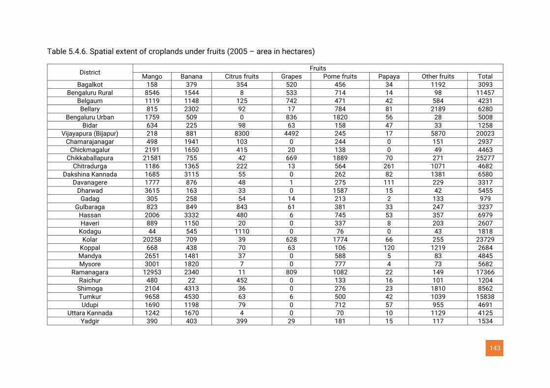
143
Table 5.4.6. Spatial extent of croplands under fruits (2005 – area in hectares)
District Fruits
Mango Banana Citrus fruits Grapes Pome fruits Papaya Other fruits Total
Bagalkot 158 379 354 520 456 34 1192 3093
Bengaluru Rural 8546 1544 8 533 714 14 98 11457
Belgaum 1119 1148 125 742 471 42 584 4231
Bellary 815 2302 92 17 784 81 2189 6280
Bengaluru Urban 1759 509 0 836 1820 56 28 5008
Bidar 634 225 98 63 158 47 33 1258
Vijayapura (Bijapur) 218 881 8300 4492 245 17 5870 20023
Chamarajanagar 498 1941 103 0 244 0 151 2937
Chickmagalur 2191 1650 415 20 138 0 49 4463
Chikkaballapura 21581 755 42 669 1889 70 271 25277
Chitradurga 1186 1365 222 13 564 261 1071 4682
Dakshina Kannada 1685 3115 55 0 262 82 1381 6580
Davanagere 1777 876 48 1 275 111 229 3317
Dharwad 3615 163 33 0 1587 15 42 5455
Gadag 305 258 54 14 213 2 133 979
Gulbaraga 823 849 843 61 381 33 247 3237
Hassan 2006 3332 480 6 745 53 357 6979
Haveri 889 1150 20 0 337 8 203 2607
Kodagu 44 545 1110 0 76 0 43 1818
Kolar 20258 709 39 628 1774 66 255 23729
Koppal 668 438 70 63 106 120 1219 2684
Mandya 2651 1481 37 0 588 5 83 4845
Mysore 3001 1820 7 0 777 4 73 5682
Ramanagara 12953 2340 11 809 1082 22 149 17366
Raichur 480 22 452 0 133 16 101 1204
Shimoga 2104 4313 36 0 276 23 1810 8562
Tumkur 9658 4530 63 6 500 42 1039 15838
Udupi 1690 1198 79 0 712 57 955 4691
Uttara Kannada 1242 1670 4 0 70 10 1129 4125
Yadgir 390 403 399 29 181 15 117 1534

144
Table 5.4.7. Spatial extent of croplands under vegetables,
Total croplands and horticulture (2005 – area in hectares)
District Vegetable Total
croplands Horticulture
Potato Tapioca Sweet potato Onion Others Total Rubber Coffee Cashew Coconut Arecanut Total
Bagalkot 0 0 57 6986 1667 8710 569166 0 1 0 452 2 455
Bengaluru Rural 660 85 8 19 2155 2928 106871 5 80 19 7866 785 8755
Belgaum 5336 0 2164 6967 6660 21127 1087671 0 0 544 599 8 1151
Bellary 0 0 0 3761 2468 6229 514931 0 1 3 1259 32 1295
Bengaluru Urban 204 0 13 90 2838 3145 62818 0 10 0 2498 233 2741
Bidar 47 0 0 441 1887 2375 441386 0 0 30 24 0 54
Vijayapura 0 0 5 5436 1538 6979 1021499 0 0 0 178 0 178
Chamarajanagar 13 0 0 2547 1148 3708 202771 0 686 195 12161 309 13351
Chickmagalur 4051 36 177 5608 2449 12321 310860 709 69526 326 31122 16616 118299
Chikkaballapura 2078 0 0 777 12946 15801 164810 0 0 1181 1084 28 2293
Chitradurga 0 0 0 13134 1317 14451 487294 0 15 9 43354 14498 57876
Dakshina Kannada 0 698 537 0 2370 3605 155525 10113 82 29585 15684 27209 82673
Davanagere 3 0 0 5459 1888 7350 455984 0 20 33 11978 22015 34046
Dharwad 284 0 0 38112 2345 40741 461096 0 0 114 431 11 556
Gadag 0 0 0 30434 1256 31690 552900 0 0 0 622 3 625
Gulbaraga 3 0 21 1302 2343 3669 948687 0 0 0 498 0 498
Hassan 36151 0 68 107 5154 41480 438160 5 38219 16 61098 3483 102821
Haveri 1 0 0 10372 4405 14778 416743 0 0 17 1147 717 1881
Kodagu 0 9 12 0 91 112 134214 1926 83205 2198 1331 1386 90046
Kolar 1950 0 0 730 12153 14833 154714 0 0 1109 1017 26 2152
Koppal 3 0 0 960 2062 3025 495357 0 0 0 344 0 344
Mandya 115 4 14 414 3938 4485 281576 0 85 262 18165 879 19391
Mysore 15 0 0 5 3672 3692 551119 0 26 172 19404 676 20278
Ramanagara 1000 130 12 29 3267 4437 161987 8 121 29 11923 1190 13271
Raichur 0 0 0 1429 1031 2460 664277 0 0 0 441 0 441
Shimoga 0 10 0 20 352 382 240984 881 464 1473 6613 29150 38581
Tumkur 22 28 18 201 1596 1865 582441 0 6 82 110937 16197 127222
Udupi 0 66 439 4 1580 2089 120173 2295 0 19207 14464 5019 40985
Uttara Kannada 0 0 28 77 241 346 117023 6 11 2087 6276 12287 20667
Yadgir 1 0 10 617 1110 1738 449525 0 0 0 236 0 236
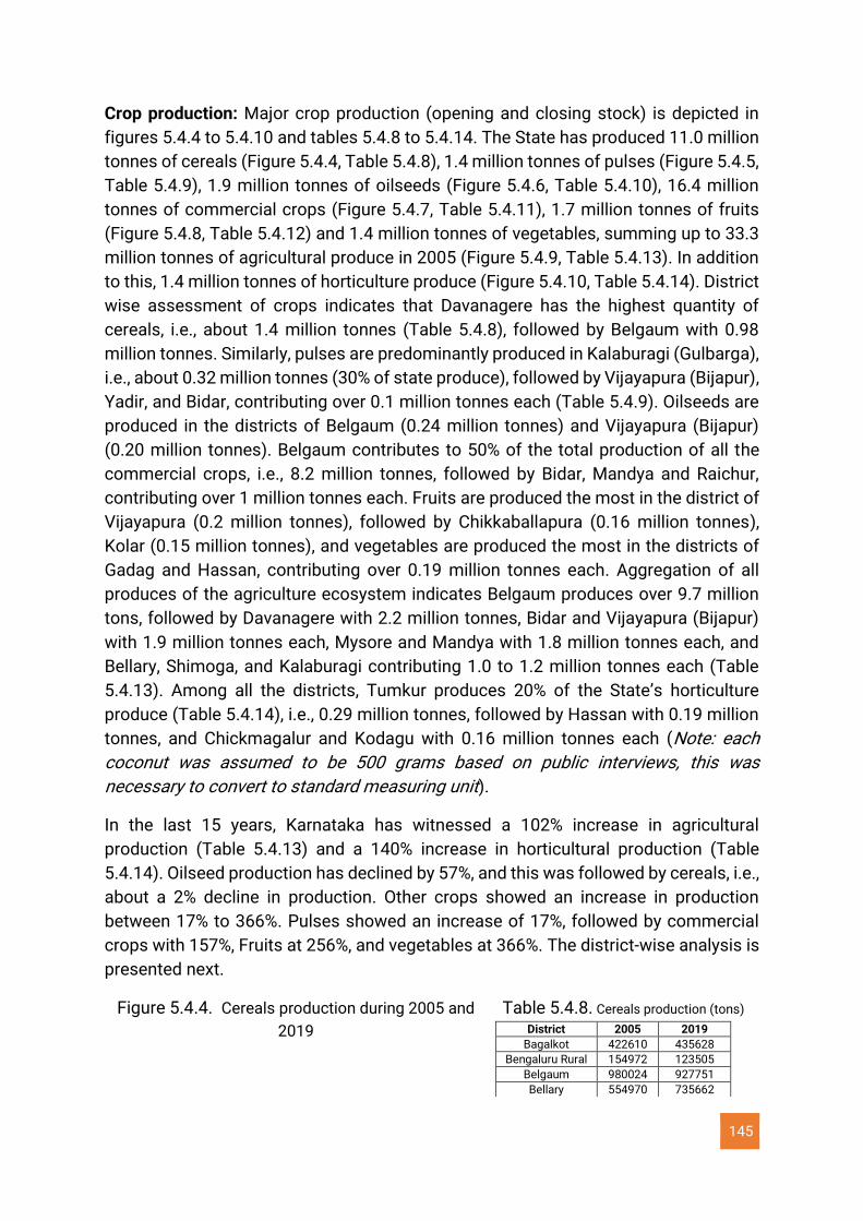
145
Crop production: Major crop production (opening and closing stock) is depicted in
figures 5.4.4 to 5.4.10 and tables 5.4.8 to 5.4.14. The State has produced 11.0 million
tonnes of cereals (Figure 5.4.4, Table 5.4.8), 1.4 million tonnes of pulses (Figure 5.4.5,
Table 5.4.9), 1.9 million tonnes of oilseeds (Figure 5.4.6, Table 5.4.10), 16.4 million
tonnes of commercial crops (Figure 5.4.7, Table 5.4.11), 1.7 million tonnes of fruits
(Figure 5.4.8, Table 5.4.12) and 1.4 million tonnes of vegetables, summing up to 33.3
million tonnes of agricultural produce in 2005 (Figure 5.4.9, Table 5.4.13). In addition
to this, 1.4 million tonnes of horticulture produce (Figure 5.4.10, Table 5.4.14). District
wise assessment of crops indicates that Davanagere has the highest quantity of
cereals, i.e., about 1.4 million tonnes (Table 5.4.8), followed by Belgaum with 0.98
million tonnes. Similarly, pulses are predominantly produced in Kalaburagi (Gulbarga),
i.e., about 0.32 million tonnes (30% of state produce), followed by Vijayapura (Bijapur),
Yadir, and Bidar, contributing over 0.1 million tonnes each (Table 5.4.9). Oilseeds are
produced in the districts of Belgaum (0.24 million tonnes) and Vijayapura (Bijapur)
(0.20 million tonnes). Belgaum contributes to 50% of the total production of all the
commercial crops, i.e., 8.2 million tonnes, followed by Bidar, Mandya and Raichur,
contributing over 1 million tonnes each. Fruits are produced the most in the district of
Vijayapura (0.2 million tonnes), followed by Chikkaballapura (0.16 million tonnes),
Kolar (0.15 million tonnes), and vegetables are produced the most in the districts of
Gadag and Hassan, contributing over 0.19 million tonnes each. Aggregation of all
produces of the agriculture ecosystem indicates Belgaum produces over 9.7 million
tons, followed by Davanagere with 2.2 million tonnes, Bidar and Vijayapura (Bijapur)
with 1.9 million tonnes each, Mysore and Mandya with 1.8 million tonnes each, and
Bellary, Shimoga, and Kalaburagi contributing 1.0 to 1.2 million tonnes each (Table
5.4.13). Among all the districts, Tumkur produces 20% of the State’s horticulture
produce (Table 5.4.14), i.e., 0.29 million tonnes, followed by Hassan with 0.19 million
tonnes, and Chickmagalur and Kodagu with 0.16 million tonnes each (Note: each
coconut was assumed to be 500 grams based on public interviews, this was
necessary to convert to standard measuring unit).
In the last 15 years, Karnataka has witnessed a 102% increase in agricultural
production (Table 5.4.13) and a 140% increase in horticultural production (Table
5.4.14). Oilseed production has declined by 57%, and this was followed by cereals, i.e.,
about a 2% decline in production. Other crops showed an increase in production
between 17% to 366%. Pulses showed an increase of 17%, followed by commercial
crops with 157%, Fruits at 256%, and vegetables at 366%. The district-wise analysis is
presented next.
Figure 5.4.4. Cereals production during 2005 and
2019
Table 5.4.8. Cereals production (tons) District 2005 2019
Bagalkot 422610 435628
Bengaluru Rural 154972 123505
Belgaum 980024 927751
Bellary 554970 735662
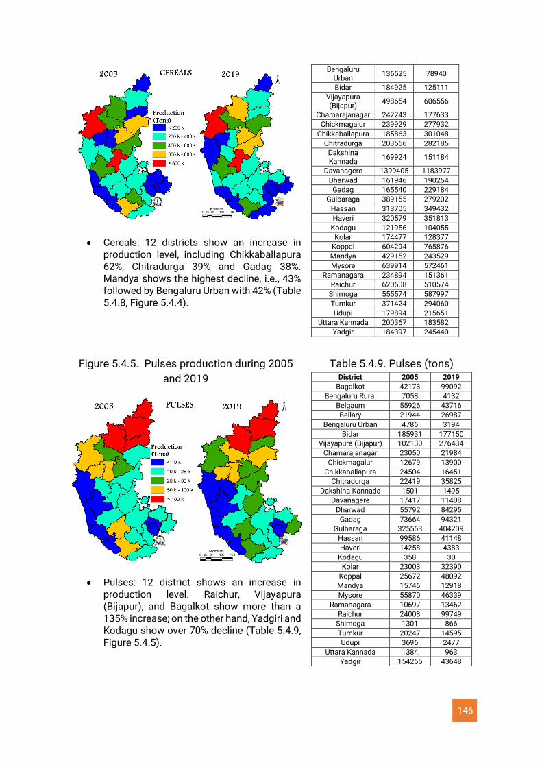
146
• Cereals: 12 districts show an increase in production level, including Chikkaballapura 62%, Chitradurga 39% and Gadag 38%. Mandya shows the highest decline, i.e., 43% followed by Bengaluru Urban with 42% (Table 5.4.8, Figure 5.4.4).
Bengaluru Urban
136525 78940
Bidar 184925 125111
Vijayapura (Bijapur)
498654 606556
Chamarajanagar 242243 177633
Chickmagalur 239929 277932
Chikkaballapura 185863 301048
Chitradurga 203566 282185
Dakshina Kannada
169924 151184
Davanagere 1399405 1183977
Dharwad 161946 190254
Gadag 165540 229184
Gulbaraga 389155 279202
Hassan 313705 349432
Haveri 320579 351813
Kodagu 121956 104055
Kolar 174477 128377
Koppal 604294 765876
Mandya 429152 243529
Mysore 639914 572461
Ramanagara 234894 151361
Raichur 620608 510574
Shimoga 555574 587997
Tumkur 371424 294060
Udupi 179894 215651
Uttara Kannada 200367 183582
Yadgir 184397 245440
Figure 5.4.5. Pulses production during 2005
and 2019
• Pulses: 12 district shows an increase in production level. Raichur, Vijayapura (Bijapur), and Bagalkot show more than a 135% increase; on the other hand, Yadgiri and Kodagu show over 70% decline (Table 5.4.9, Figure 5.4.5).
Table 5.4.9. Pulses (tons) District 2005 2019
Bagalkot 42173 99092
Bengaluru Rural 7058 4132
Belgaum 55926 43716
Bellary 21944 26987
Bengaluru Urban 4786 3194
Bidar 185931 177150
Vijayapura (Bijapur) 102130 276434
Chamarajanagar 23050 21984
Chickmagalur 12679 13900
Chikkaballapura 24504 16451
Chitradurga 22419 35825
Dakshina Kannada 1501 1495
Davanagere 17417 11408
Dharwad 55792 84295
Gadag 73664 94321
Gulbaraga 325563 404209
Hassan 99586 41148
Haveri 14258 4383
Kodagu 358 30
Kolar 23003 32390
Koppal 25672 48092
Mandya 15746 12918
Mysore 55870 46339
Ramanagara 10697 13462
Raichur 24008 99749
Shimoga 1301 866
Tumkur 20247 14595
Udupi 3696 2477
Uttara Kannada 1384 963
Yadgir 154265 43648
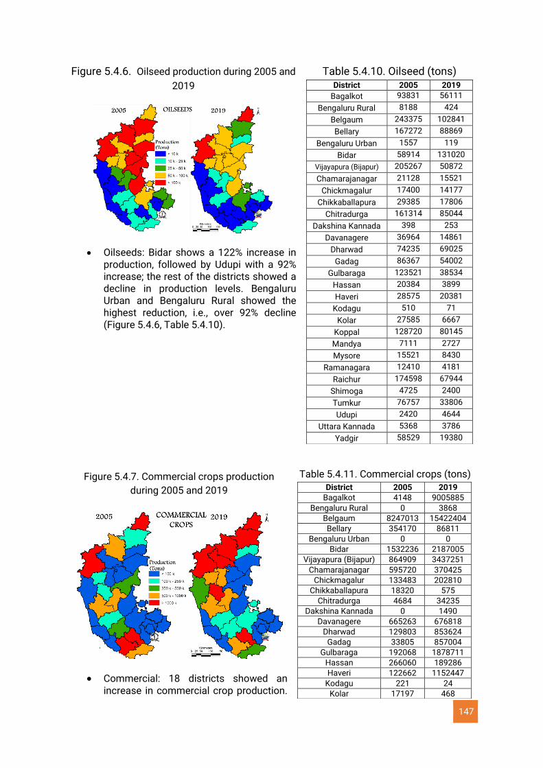
147
Figure 5.4.6. Oilseed production during 2005 and
2019
• Oilseeds: Bidar shows a 122% increase in production, followed by Udupi with a 92% increase; the rest of the districts showed a decline in production levels. Bengaluru Urban and Bengaluru Rural showed the highest reduction, i.e., over 92% decline (Figure 5.4.6, Table 5.4.10).
Table 5.4.10. Oilseed (tons) District 2005 2019
Bagalkot 93831 56111
Bengaluru Rural 8188 424
Belgaum 243375 102841
Bellary 167272 88869
Bengaluru Urban 1557 119
Bidar 58914 131020
Vijayapura (Bijapur) 205267 50872
Chamarajanagar 21128 15521
Chickmagalur 17400 14177
Chikkaballapura 29385 17806
Chitradurga 161314 85044
Dakshina Kannada 398 253
Davanagere 36964 14861
Dharwad 74235 69025
Gadag 86367 54002
Gulbaraga 123521 38534
Hassan 20384 3899
Haveri 28575 20381
Kodagu 510 71
Kolar 27585 6667
Koppal 128720 80145
Mandya 7111 2727
Mysore 15521 8430
Ramanagara 12410 4181
Raichur 174598 67944
Shimoga 4725 2400
Tumkur 76757 33806
Udupi 2420 4644
Uttara Kannada 5368 3786
Yadgir 58529 19380
Figure 5.4.7. Commercial crops production
during 2005 and 2019
• Commercial: 18 districts showed an increase in commercial crop production.
Table 5.4.11. Commercial crops (tons)
District 2005 2019
Bagalkot 4148 9005885
Bengaluru Rural 0 3868
Belgaum 8247013 15422404
Bellary 354170 86811
Bengaluru Urban 0 0
Bidar 1532236 2187005
Vijayapura (Bijapur) 864909 3437251
Chamarajanagar 595720 370425
Chickmagalur 133483 202810
Chikkaballapura 18320 575
Chitradurga 4684 34235
Dakshina Kannada 0 1490
Davanagere 665263 676818
Dharwad 129803 853624
Gadag 33805 857004
Gulbaraga 192068 1878711
Hassan 266060 189286
Haveri 122662 1152447
Kodagu 221 24
Kolar 17197 468
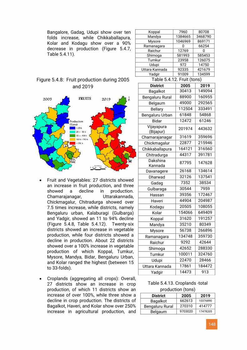
148
Bangalore, Gadag, Udupi show over ten folds increase, while Chikkaballapura, Kolar and Kodagu show over a 90% decrease in production (Figure 5.4.7, Table 5.4.11).
Koppal 7960 80708
Mandya 1384665 3468790
Mysore 1046969 869171
Ramanagara 0 66254
Raichur 12769 0
Shimoga 581993 585453
Tumkur 23958 126075
Udupi 972 14750
Uttara Kannada 92335 421679
Yadgir 91009 134599
Figure 5.4.8: Fruit production during 2005
and 2019
• Fruit and Vegetables: 27 districts showed an increase in fruit production, and three showed a decline in production. Chamarajanagar, Uttarakannada, Chickmagalur, Chitradurga showed over 7.5 times increase, while districts, namely Bengaluru urban, Kalaburagi (Gulbarga) and Yadgir, showed an 11 to 94% decline (Figure 5.4.8, Table 5.4.12). Twenty-six districts showed an increase in vegetable production, while four districts showed a decline in production. About 22 districts showed over a 100% increase in vegetable production of which Koppal, Tumkur, Mysore, Mandya, Bidar, Bengaluru Urban, and Kolar ranged the highest (between 15 to 33-folds).
Table 5.4.12. Fruit (tons)
District 2005 2019
Bagalkot 30413 149094
Bengaluru Rural 88900 160955
Belgaum 49000 292565
Bellary 112504 333491
Bengaluru Urban 61848 54868
Bidar 12472 61246
Vijayapura (Bijapur)
201974 443632
Chamarajanagar 31619 359696
Chickmagalur 22877 215946
Chikkaballapura 164121 316560
Chitradurga 44317 391781
Dakshina Kannada
87795 147628
Davanagere 26168 134614
Dharwad 32126 137541
Gadag 7352 38534
Gulbaraga 30544 7959
Hassan 39356 172467
Haveri 44904 204987
Kodagu 20505 108055
Kolar 154066 649409
Koppal 31620 191257
Mandya 35210 80349
Mysore 56738 266896
Ramanagara 134748 359730
Raichur 9292 42644
Shimoga 42652 288330
Tumkur 100011 324760
Udupi 22470 28466
Uttara Kannada 17861 184472
Yadgir 14473 913
• Croplands (aggregating all crops): Overall, 27 districts show an increase in crop production, of which 11 districts show an increase of over 100%, while three show a decline in crop production. The districts of Bagalkot, Haveri, and Kolar show over 250% increase in agricultural production, and
Table 5.4.13. Croplands -total
production (tons)
District 2005 2019
Bagalkot 662613 10376890
Bengaluru Rural 270310 414777
Belgaum 9703020 17478205
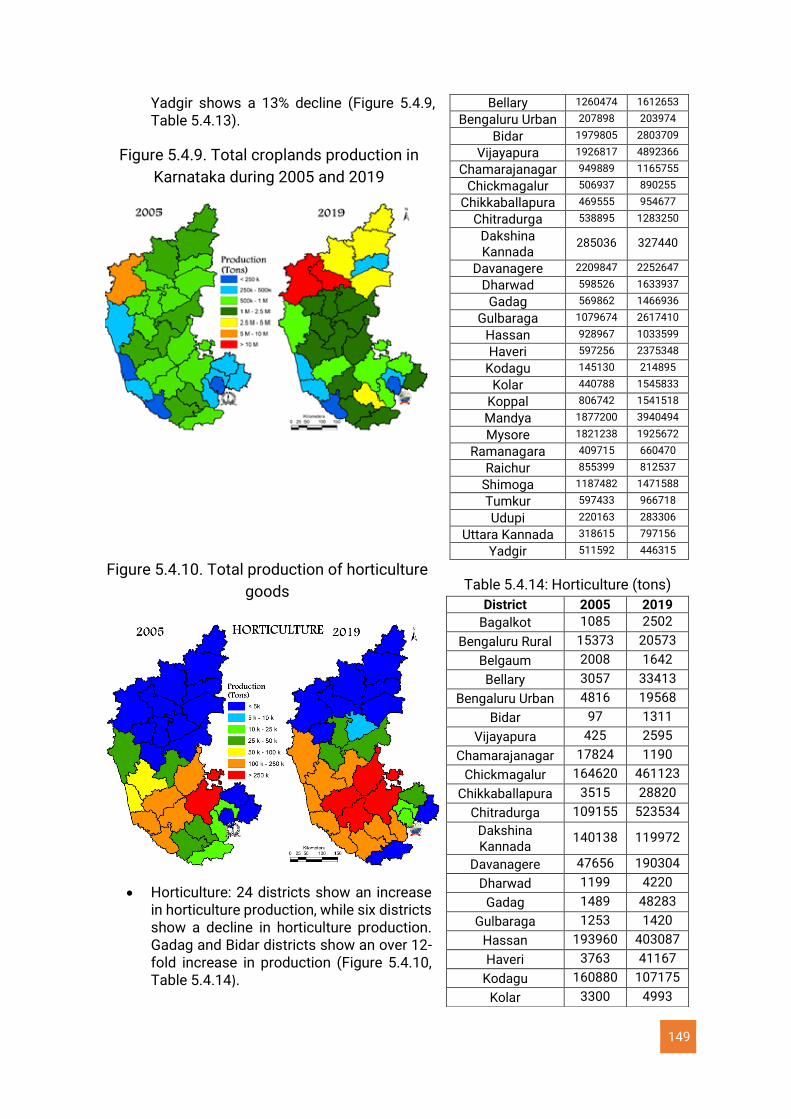
149
Yadgir shows a 13% decline (Figure 5.4.9, Table 5.4.13).
Figure 5.4.9. Total croplands production in
Karnataka during 2005 and 2019
Bellary 1260474 1612653
Bengaluru Urban 207898 203974
Bidar 1979805 2803709
Vijayapura 1926817 4892366
Chamarajanagar 949889 1165755
Chickmagalur 506937 890255
Chikkaballapura 469555 954677
Chitradurga 538895 1283250
Dakshina Kannada
285036 327440
Davanagere 2209847 2252647
Dharwad 598526 1633937
Gadag 569862 1466936
Gulbaraga 1079674 2617410
Hassan 928967 1033599
Haveri 597256 2375348
Kodagu 145130 214895
Kolar 440788 1545833
Koppal 806742 1541518
Mandya 1877200 3940494
Mysore 1821238 1925672
Ramanagara 409715 660470
Raichur 855399 812537
Shimoga 1187482 1471588
Tumkur 597433 966718
Udupi 220163 283306
Uttara Kannada 318615 797156
Yadgir 511592 446315
Figure 5.4.10. Total production of horticulture
goods
• Horticulture: 24 districts show an increase in horticulture production, while six districts show a decline in horticulture production. Gadag and Bidar districts show an over 12-fold increase in production (Figure 5.4.10, Table 5.4.14).
Table 5.4.14: Horticulture (tons)
District 2005 2019
Bagalkot 1085 2502
Bengaluru Rural 15373 20573
Belgaum 2008 1642
Bellary 3057 33413
Bengaluru Urban 4816 19568
Bidar 97 1311
Vijayapura 425 2595
Chamarajanagar 17824 1190
Chickmagalur 164620 461123
Chikkaballapura 3515 28820
Chitradurga 109155 523534
Dakshina Kannada
140138 119972
Davanagere 47656 190304
Dharwad 1199 4220
Gadag 1489 48283
Gulbaraga 1253 1420
Hassan 193960 403087
Haveri 3763 41167
Kodagu 160880 107175
Kolar 3300 4993
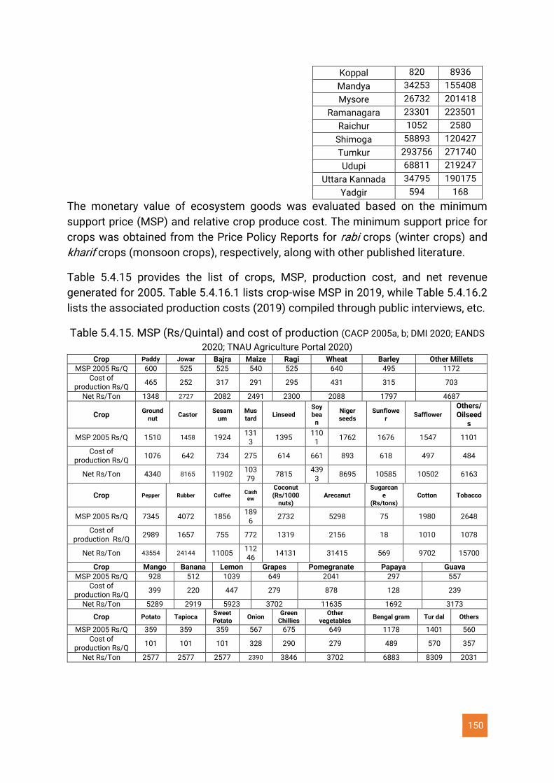
150
Koppal 820 8936
Mandya 34253 155408
Mysore 26732 201418
Ramanagara 23301 223501
Raichur 1052 2580
Shimoga 58893 120427
Tumkur 293756 271740
Udupi 68811 219247
Uttara Kannada 34795 190175
Yadgir 594 168
The monetary value of ecosystem goods was evaluated based on the minimum
support price (MSP) and relative crop produce cost. The minimum support price for
crops was obtained from the Price Policy Reports for rabi crops (winter crops) and
kharif crops (monsoon crops), respectively, along with other published literature.
Table 5.4.15 provides the list of crops, MSP, production cost, and net revenue
generated for 2005. Table 5.4.16.1 lists crop-wise MSP in 2019, while Table 5.4.16.2
lists the associated production costs (2019) compiled through public interviews, etc.
Table 5.4.15. MSP (Rs/Quintal) and cost of production (CACP 2005a, b; DMI 2020; EANDS
2020; TNAU Agriculture Portal 2020) Crop Paddy Jowar Bajra Maize Ragi Wheat Barley Other Millets
MSP 2005 Rs/Q 600 525 525 540 525 640 495 1172
Cost of production Rs/Q
465 252 317 291 295 431 315 703
Net Rs/Ton 1348 2727 2082 2491 2300 2088 1797 4687
Crop Ground
nut Castor
Sesamum
Mustard
Linseed Soybea
n
Niger seeds
Sunflower
Safflower
Others/ Oilseed
s
MSP 2005 Rs/Q 1510 1458 1924 131
3 1395
1101
1762 1676 1547 1101
Cost of production Rs/Q
1076 642 734 275 614 661 893 618 497 484
Net Rs/Ton 4340 8165 11902 10379
7815 439
3 8695 10585 10502 6163
Crop Pepper Rubber Coffee Cashew
Coconut (Rs/1000
nuts) Arecanut
Sugarcane
(Rs/tons) Cotton Tobacco
MSP 2005 Rs/Q 7345 4072 1856 189
6 2732 5298 75 1980 2648
Cost of production Rs/Q
2989 1657 755 772 1319 2156 18 1010 1078
Net Rs/Ton 43554 24144 11005 11246
14131 31415 569 9702 15700
Crop Mango Banana Lemon Grapes Pomegranate Papaya Guava
MSP 2005 Rs/Q 928 512 1039 649 2041 297 557
Cost of production Rs/Q
399 220 447 279 878 128 239
Net Rs/Ton 5289 2919 5923 3702 11635 1692 3173
Crop Potato Tapioca Sweet Potato
Onion Green
Chillies Other
vegetables Bengal gram Tur dal Others
MSP 2005 Rs/Q 359 359 359 567 675 649 1178 1401 560
Cost of production Rs/Q
101 101 101 328 290 279 489 570 357
Net Rs/Ton 2577 2577 2577 2390 3846 3702 6883 8309 2031
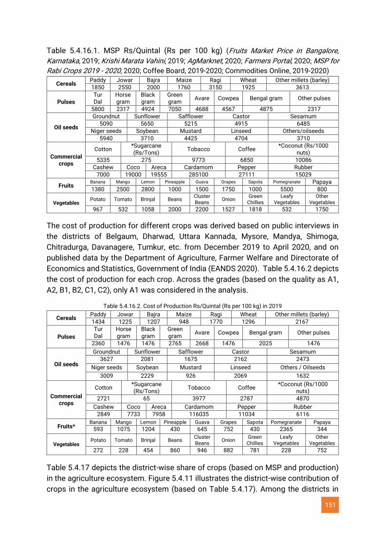
151
Table 5.4.16.1. MSP Rs/Quintal (Rs per 100 kg) (Fruits Market Price in Bangalore,
Karnataka, 2019; Krishi Marata Vahini, 2019; AgMarknet, 2020; Farmers Portal, 2020; MSP for
Rabi Crops 2019 - 2020, 2020; Coffee Board, 2019-2020; Commodities Online, 2019-2020)
Cereals Paddy Jowar Bajra Maize Ragi Wheat Other millets (barley)
1850 2550 2000 1760 3150 1925 3613
Pulses Tur Dal
Horse gram
Black gram
Green gram
Avare Cowpea Bengal gram Other pulses
5800 2317 4924 7050 4688 4567 4875 2317
Oil seeds
Groundnut Sunflower Safflower Castor Sesamum
5090 5650 5215 4915 6485
Niger seeds Soybean Mustard Linseed Others/oilseeds
5940 3710 4425 4704 3710
Commercial crops
Cotton *Sugarcane (Rs/Tons)
Tobacco Coffee *Coconut (Rs/1000
nuts)
5335 275 9773 6850 10086
Cashew Coco Areca Cardamom Pepper Rubber
7000 19000 19555 285100 27111 15029
Fruits Banana Mango Lemon Pineapple Guava Grapes Sapota Pomegranate Papaya
1380 2500 2800 1000 1500 1750 1000 5500 800
Vegetables Potato Tomato Brinjal Beans
Cluster Beans
Onion Green
Chillies Leafy
Vegetables Other
Vegetables
967 532 1058 2000 2200 1527 1818 532 1750
The cost of production for different crops was derived based on public interviews in
the districts of Belgaum, Dharwad, Uttara Kannada, Mysore, Mandya, Shimoga,
Chitradurga, Davanagere, Tumkur, etc. from December 2019 to April 2020, and on
published data by the Department of Agriculture, Farmer Welfare and Directorate of
Economics and Statistics, Government of India (EANDS 2020). Table 5.4.16.2 depicts
the cost of production for each crop. Across the grades (based on the quality as A1,
A2, B1, B2, C1, C2), only A1 was considered in the analysis.
Table 5.4.16.2. Cost of Production Rs/Quintal (Rs per 100 kg) in 2019
Cereals Paddy Jowar Bajra Maize Ragi Wheat Other millets (barley)
1434 1225 1207 948 1770 1296 2167
Pulses
Tur Dal
Horse gram
Black gram
Green gram
Avare Cowpea Bengal gram Other pulses
2360 1476 1476 2765 2668 1476 2025 1476
Oil seeds
Groundnut Sunflower Safflower Castor Sesamum
3627 2081 1675 2162 2473
Niger seeds Soybean Mustard Linseed Others / Oilseeds
3009 2229 926 2069 1632
Commercial crops
Cotton *Sugarcane (Rs/Tons)
Tobacco Coffee *Coconut (Rs/1000
nuts)
2721 65 3977 2787 4870
Cashew Coco Areca Cardamom Pepper Rubber
2849 7733 7958 116035 11034 6116
Fruits* Banana Mango Lemon Pineapple Guava Grapes Sapota Pomegranate Papaya
593 1075 1204 430 645 752 430 2365 344
Vegetables Potato Tomato Brinjal Beans
Cluster Beans
Onion Green
Chillies Leafy
Vegetables Other
Vegetables
272 228 454 860 946 882 781 228 752
Table 5.4.17 depicts the district-wise share of crops (based on MSP and production)
in the agriculture ecosystem. Figure 5.4.11 illustrates the district-wise contribution of
crops in the agriculture ecosystem (based on Table 5.4.17). Among the districts in
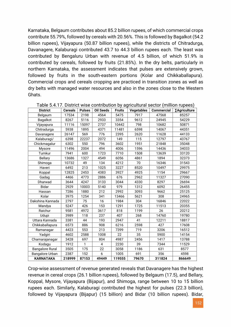
152
Karnataka, Belgaum contributes about 85.2 billion rupees, of which commercial crops
contribute 55.79%, followed by cereals with 20.56%. This is followed by Bagalkot (54.2
billion rupees), Vijayapura (50.87 billion rupees), while the districts of Chitradurga,
Davanagere, Kalaburagi contributed 43.7 to 44.3 billion rupees each. The least was
contributed by Bengaluru Urban with revenue of 4.5 billion, of which 51.9% is
contributed by cereals, followed by fruits (21.85%). In the dry belts, particularly in
northern Karnataka, the assessment indicates that pulses are extensively grown,
followed by fruits in the south-eastern portions (Kolar and Chikkaballapura).
Commercial crops and cereals cropping are practiced in transition zones as well as
dry belts with managed water resources and also in the zones close to the Western
Ghats.
Table 5.4.17. District wise contribution by agricultural sector (million rupees) District Cereals Pulses Oil Seeds Fruits Vegetables Commercial ∑Agriculture
Belgaum 17534 2198 4564 5475 7917 47568 85257
Bagalkot 8267 5116 2933 3354 9612 24945 54229
Vijayapura 11116 15097 2737 10442 798 10682 50871
Chitradurga 5938 1895 4371 11481 6598 14067 44351
Davanagere 26147 569 776 2395 2620 11628 44133
Kalaburagi/ 6398 22237 2072 149 115 12797 43767
Chickmagalur 6302 550 796 3602 1951 21848 35048
Mysore 11496 2004 494 4006 1596 14436 34033
Tumkur 7941 600 1723 7710 1508 13639 33120
Bellary 13686 1327 4549 6056 4861 1894 32373
Shimoga 10732 49 134 4212 70 16346 31543
Haveri 6492 213 1025 3227 8520 10497 29975
Koppal 12825 2453 4383 3927 4925 1154 29667
Gadag 4466 4773 2886 676 2962 11327 27090
Dharwad 3644 4247 3133 3044 4330 8297 26694
Bidar 2929 10003 5140 979 1312 6092 26455
Hassan 7286 1880 212 2992 3093 9662 25125
Kolar 3975 1254 341 13466 5621 308 24965
Dakshina Kannada 2797 75 16 1984 304 16846 22022
Mandya 5247 426 153 1291 1725 11513 20355
Raichur 9581 4972 3617 818 1199 26 20212
Udupi 3989 118 237 407 268 14760 19780
Uttara Kannada 3381 44 193 2947 41 12211 18817
Chikkaballapura 6573 886 908 6216 2598 427 17608
Ramanagar 4423 553 213 7399 719 3206 16512
Yadgiri 4602 2588 1008 22 35 5900 14154
Chamarajanagar 3428 697 804 4987 2456 1417 13788
Kodagu 1912 1 4 2230 39 7344 11529
Bangalore Rural 3505 175 22 3058 1186 631 8577
Bangalore Urban 2387 152 6 1005 691 356 4598
KARNATAKA 218999 87153 49449 119555 79670 311824 866649
Crop-wise assessment of revenue generated reveals that Davanagere has the highest
revenue in cereal crops (26.1 billion rupees), followed by Belgaum (17.5), and Bellary,
Koppal, Mysore, Vijayapura (Bijapur), and Shimoga, range between 10 to 15 billion
rupees each. Similarly, Kalaburagi contributed the highest for pulses (22.3 billion),
followed by Vijayapura (Bijapur) (15 billion) and Bidar (10 billion rupees). Bidar,
153
Belgaum, Bellary, Koppal, Chitradurga contributed to oilseeds with 4.3 to 5.1 billion
rupees each. Districts Kolar, Chitradurga, and Vijayapura (Bijapur) contribute to fruits
with a 10.4 to 13.4 billion rupees revenue each. Vegetables contributed by Bagalkot,
Haveri, and Belgaum amounted to between 7.9 billion to 9.6 billion rupees each.
Belgaum contributes about 47.5 billion rupees through commercial crops, followed by
Bagalkot (21.8), Chickmagalur (24.9 billion rupees), followed by Dakshina Kannada
and Shimoga, each with 16 billion rupees.
The annual revenue (in 2019) from the cropland ecosystem in Karnataka State
amounts to 866 billion (Figure 5.4.12). Commercial crops contribute to 36.1% (311.8
billion), followed by cereal crops (25.3%, 218.9 billion), fruits (13.8%, 119.5 billion),
pulses (10.1%, 87.1 billion), vegetables (9.2%, 79.6 billion) and oilseeds (5.7%, 49.4
billion).
Total revenue (based on the crop production and MSP) generated in a district was
compared with the GDDP (Gross District Domestic product) to understand the
agriculture sector's contribution to the State economy. Table 5.4.18 lists district-wise
GDDP obtained from the Economic Survey of Karnataka, 2018-19. Figure 5.4.13
indicates district-wise total revenue generated through agriculture, GDDP, and the
proportion of revenue generated from the agriculture sector compared to the GDDP.
The total GSDP (Gross State Domestic Product) of Karnataka State is 10128 billion
rupees. The revenue generated from croplands is 866 billion rupees, which is 8.5% of
the GSDP. Among districts, Bangalore urban has the highest GDDP of 3535.6 billion
rupees (agriculture share is 0.13%), followed by Dakshina Kannada with GDDP of 587
billion rupees (agriculture contributes 3.75%). Agriculture contributes 27% in GDDP of
Vijayapura district, followed by Chitradurga (26%), Koppal (25%), Gadag (25%),
Kalaburagi (22%), Davanagere (22%), and Bagalkot (20%).
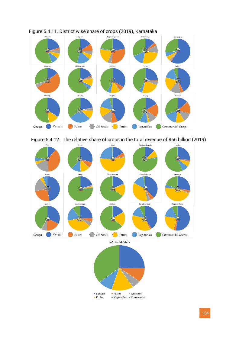
154
Figure 5.4.11. District wise share of crops (2019), Karnataka
Figure 5.4.12. The relative share of crops in the total revenue of 866 billion (2019)
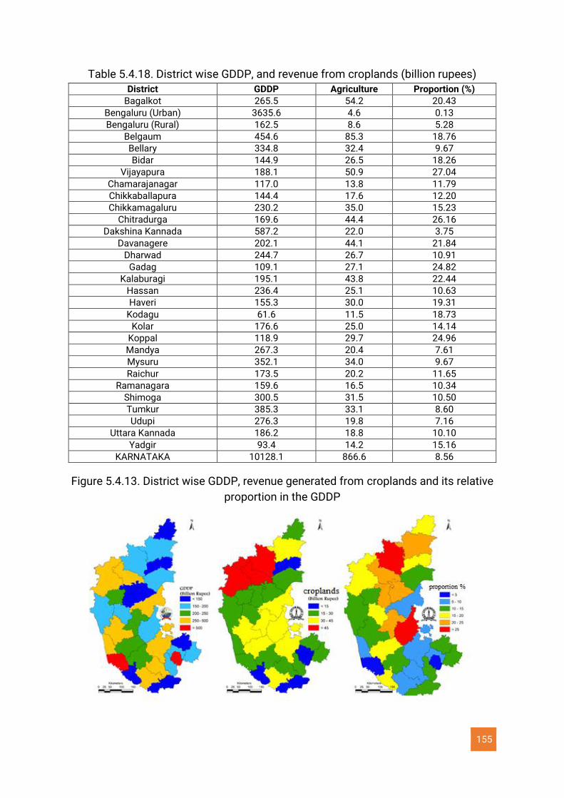
155
Table 5.4.18. District wise GDDP, and revenue from croplands (billion rupees)
District GDDP Agriculture Proportion (%)
Bagalkot 265.5 54.2 20.43
Bengaluru (Urban) 3635.6 4.6 0.13
Bengaluru (Rural) 162.5 8.6 5.28
Belgaum 454.6 85.3 18.76
Bellary 334.8 32.4 9.67
Bidar 144.9 26.5 18.26
Vijayapura 188.1 50.9 27.04
Chamarajanagar 117.0 13.8 11.79
Chikkaballapura 144.4 17.6 12.20
Chikkamagaluru 230.2 35.0 15.23
Chitradurga 169.6 44.4 26.16
Dakshina Kannada 587.2 22.0 3.75
Davanagere 202.1 44.1 21.84
Dharwad 244.7 26.7 10.91
Gadag 109.1 27.1 24.82
Kalaburagi 195.1 43.8 22.44
Hassan 236.4 25.1 10.63
Haveri 155.3 30.0 19.31
Kodagu 61.6 11.5 18.73
Kolar 176.6 25.0 14.14
Koppal 118.9 29.7 24.96
Mandya 267.3 20.4 7.61
Mysuru 352.1 34.0 9.67
Raichur 173.5 20.2 11.65
Ramanagara 159.6 16.5 10.34
Shimoga 300.5 31.5 10.50
Tumkur 385.3 33.1 8.60
Udupi 276.3 19.8 7.16
Uttara Kannada 186.2 18.8 10.10
Yadgir 93.4 14.2 15.16
KARNATAKA 10128.1 866.6 8.56
Figure 5.4.13. District wise GDDP, revenue generated from croplands and its relative
proportion in the GDDP
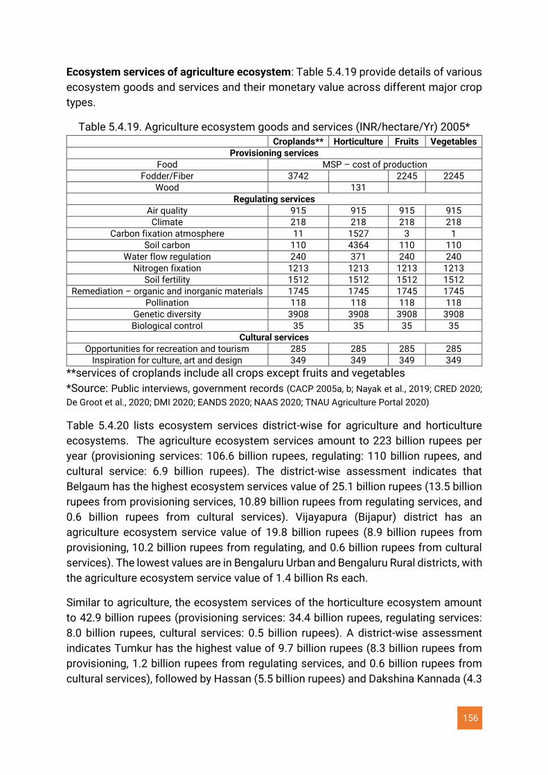
156
Ecosystem services of agriculture ecosystem: Table 5.4.19 provide details of various
ecosystem goods and services and their monetary value across different major crop
types.
Table 5.4.19. Agriculture ecosystem goods and services (INR/hectare/Yr) 2005* Croplands** Horticulture Fruits Vegetables
Provisioning services
Food MSP – cost of production
Fodder/Fiber 3742 2245 2245
Wood 131
Regulating services
Air quality 915 915 915 915
Climate 218 218 218 218
Carbon fixation atmosphere 11 1527 3 1
Soil carbon 110 4364 110 110
Water flow regulation 240 371 240 240
Nitrogen fixation 1213 1213 1213 1213
Soil fertility 1512 1512 1512 1512
Remediation – organic and inorganic materials 1745 1745 1745 1745
Pollination 118 118 118 118
Genetic diversity 3908 3908 3908 3908
Biological control 35 35 35 35
Cultural services
Opportunities for recreation and tourism 285 285 285 285
Inspiration for culture, art and design 349 349 349 349
**services of croplands include all crops except fruits and vegetables
*Source: Public interviews, government records (CACP 2005a, b; Nayak et al., 2019; CRED 2020;
De Groot et al., 2020; DMI 2020; EANDS 2020; NAAS 2020; TNAU Agriculture Portal 2020)
Table 5.4.20 lists ecosystem services district-wise for agriculture and horticulture
ecosystems. The agriculture ecosystem services amount to 223 billion rupees per
year (provisioning services: 106.6 billion rupees, regulating: 110 billion rupees, and
cultural service: 6.9 billion rupees). The district-wise assessment indicates that
Belgaum has the highest ecosystem services value of 25.1 billion rupees (13.5 billion
rupees from provisioning services, 10.89 billion rupees from regulating services, and
0.6 billion rupees from cultural services). Vijayapura (Bijapur) district has an
agriculture ecosystem service value of 19.8 billion rupees (8.9 billion rupees from
provisioning, 10.2 billion rupees from regulating, and 0.6 billion rupees from cultural
services). The lowest values are in Bengaluru Urban and Bengaluru Rural districts, with
the agriculture ecosystem service value of 1.4 billion Rs each.
Similar to agriculture, the ecosystem services of the horticulture ecosystem amount
to 42.9 billion rupees (provisioning services: 34.4 billion rupees, regulating services:
8.0 billion rupees, cultural services: 0.5 billion rupees). A district-wise assessment
indicates Tumkur has the highest value of 9.7 billion rupees (8.3 billion rupees from
provisioning, 1.2 billion rupees from regulating services, and 0.6 billion rupees from
cultural services), followed by Hassan (5.5 billion rupees) and Dakshina Kannada (4.3
157
billion rupees). Districts with the lowest values include Bidar (3 million rupees),
Chikkaballapura (14 million rupees), and Vijayapura (Bijapur) (14 million rupees).
Figures 5.4.14 and 5.4.15 provide the monetary value of agriculture (croplands and
horticulture) ecosystem services in 2005. The ecosystem services of agriculture are
about 266 billion rupees. Belgaum contributes the highest at 25.1 billion rupees,
followed by Hassan (21 billion rupees) and Tumkur (21 billion rupees), and Vijayapura
(Bijapur) (19.8 billion rupees).
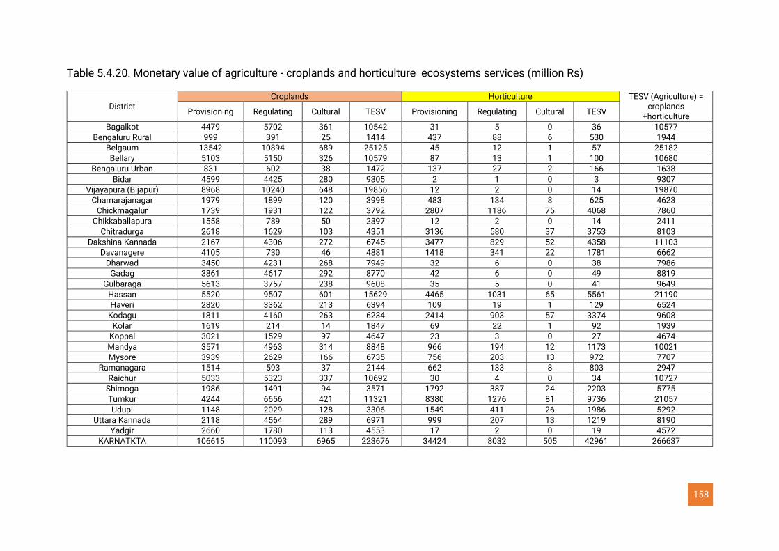
158
Table 5.4.20. Monetary value of agriculture - croplands and horticulture ecosystems services (million Rs)
District Croplands Horticulture TESV (Agriculture) =
croplands +horticulture
Provisioning Regulating Cultural TESV Provisioning Regulating Cultural TESV
Bagalkot 4479 5702 361 10542 31 5 0 36 10577
Bengaluru Rural 999 391 25 1414 437 88 6 530 1944
Belgaum 13542 10894 689 25125 45 12 1 57 25182
Bellary 5103 5150 326 10579 87 13 1 100 10680
Bengaluru Urban 831 602 38 1472 137 27 2 166 1638
Bidar 4599 4425 280 9305 2 1 0 3 9307
Vijayapura (Bijapur) 8968 10240 648 19856 12 2 0 14 19870
Chamarajanagar 1979 1899 120 3998 483 134 8 625 4623
Chickmagalur 1739 1931 122 3792 2807 1186 75 4068 7860
Chikkaballapura 1558 789 50 2397 12 2 0 14 2411
Chitradurga 2618 1629 103 4351 3136 580 37 3753 8103
Dakshina Kannada 2167 4306 272 6745 3477 829 52 4358 11103
Davanagere 4105 730 46 4881 1418 341 22 1781 6662
Dharwad 3450 4231 268 7949 32 6 0 38 7986
Gadag 3861 4617 292 8770 42 6 0 49 8819
Gulbaraga 5613 3757 238 9608 35 5 0 41 9649
Hassan 5520 9507 601 15629 4465 1031 65 5561 21190
Haveri 2820 3362 213 6394 109 19 1 129 6524
Kodagu 1811 4160 263 6234 2414 903 57 3374 9608
Kolar 1619 214 14 1847 69 22 1 92 1939
Koppal 3021 1529 97 4647 23 3 0 27 4674
Mandya 3571 4963 314 8848 966 194 12 1173 10021
Mysore 3939 2629 166 6735 756 203 13 972 7707
Ramanagara 1514 593 37 2144 662 133 8 803 2947
Raichur 5033 5323 337 10692 30 4 0 34 10727
Shimoga 1986 1491 94 3571 1792 387 24 2203 5775
Tumkur 4244 6656 421 11321 8380 1276 81 9736 21057
Udupi 1148 2029 128 3306 1549 411 26 1986 5292
Uttara Kannada 2118 4564 289 6971 999 207 13 1219 8190
Yadgir 2660 1780 113 4553 17 2 0 19 4572
KARNATKTA 106615 110093 6965 223676 34424 8032 505 42961 266637
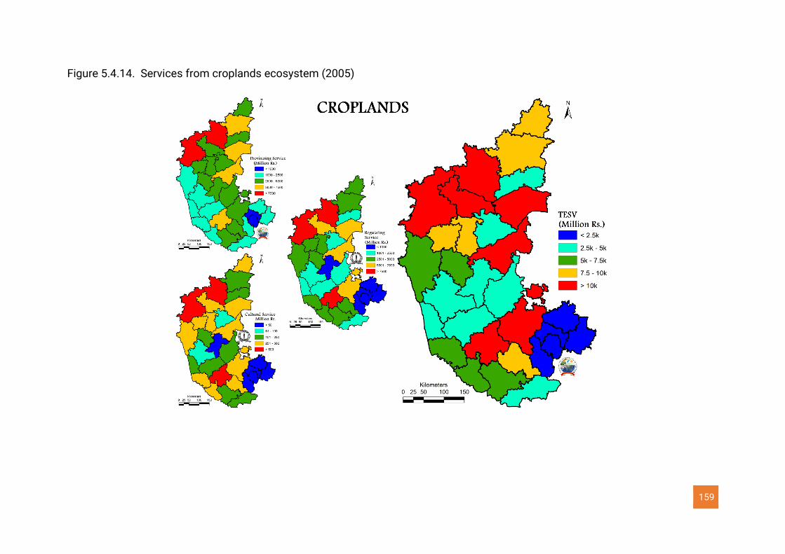
159
Figure 5.4.14. Services from croplands ecosystem (2005)
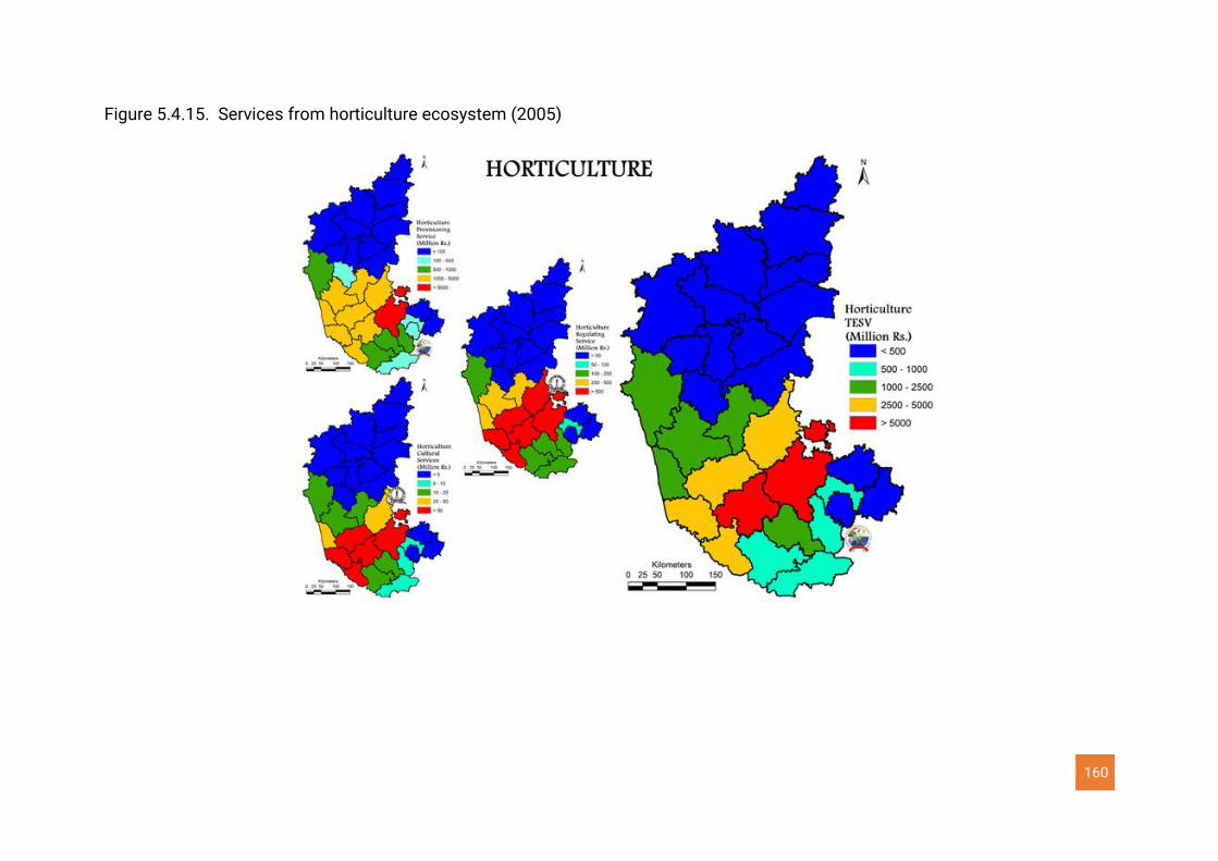
160
Figure 5.4.15. Services from horticulture ecosystem (2005)
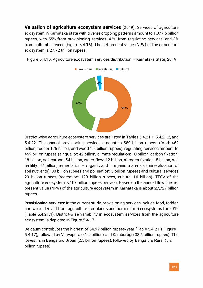
161
Valuation of agriculture ecosystem services (2019): Services of agriculture
ecosystem in Karnataka state with diverse cropping patterns amount to 1,077.6 billion
rupees, with 55% from provisioning services, 42% from regulating services, and 3%
from cultural services (Figure 5.4.16). The net present value (NPV) of the agriculture
ecosystem is 27.72 trillion rupees.
Figure 5.4.16. Agriculture ecosystem services distribution – Karnataka State, 2019
District-wise agriculture ecosystem services are listed in Tables 5.4.21.1, 5.4.21.2, and
5.4.22. The annual provisioning services amount to 589 billion rupees (food: 462
billion, fodder:125 billion, and wood 1.5 billion rupees), regulating services amount to
459 billion rupees (air quality: 42 billion, climate regulation: 10 billion, carbon fixation:
18 billion, soil carbon: 54 billion, water flow: 12 billion, nitrogen fixation: 5 billion, soil
fertility: 47 billion, remediation – organic and inorganic materials (mineralization of
soil nutrients): 80 billion rupees and pollination: 5 billion rupees) and cultural services
29 billion rupees (recreation: 123 billion rupees, culture: 16 billion). TESV of the
agriculture ecosystem is 107 billion rupees per year. Based on the annual flow, the net
present value (NPV) of the agriculture ecosystem in Karnataka is about 27,727 billion
rupees.
Provisioning services: In the current study, provisioning services include food, fodder,
and wood derived from agriculture (croplands and horticulture) ecosystems for 2019
(Table 5.4.21.1). District-wise variability in ecosystem services from the agriculture
ecosystem is depicted in Figure 5.4.17.
Belgaum contributes the highest of 64.99 billion rupees/year (Table 5.4.21.1, Figure
5.4.17), followed by Vijayapura (41.9 billion) and Kalaburagi (38.6 billion rupees). The
lowest is in Bengaluru Urban (2.5 billion rupees), followed by Bengaluru Rural (5.2
billion rupees).
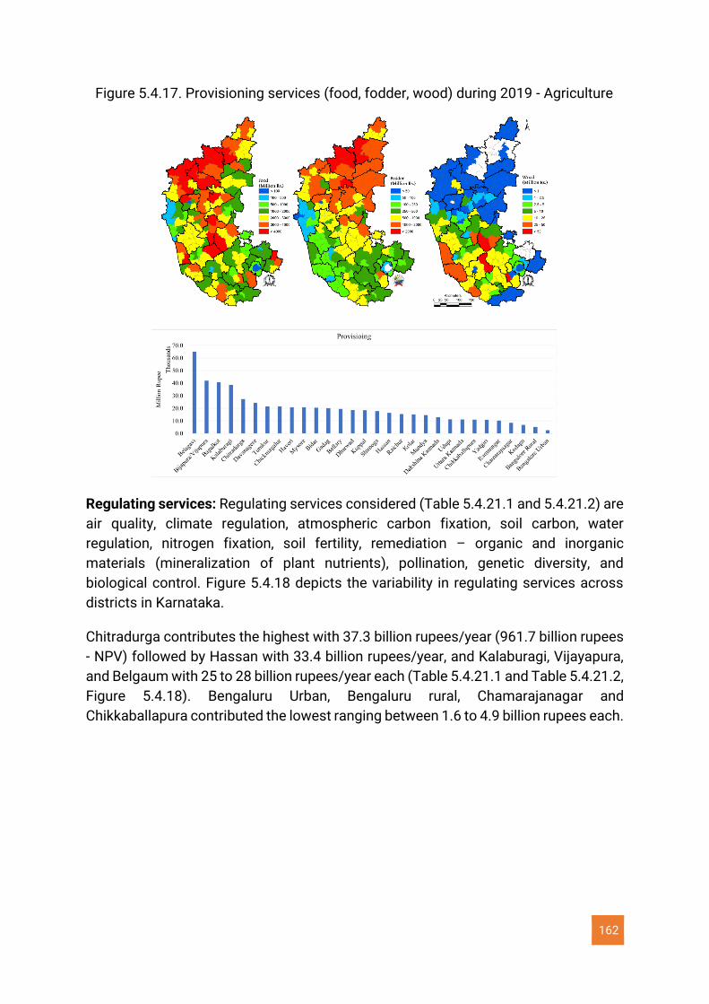
162
Figure 5.4.17. Provisioning services (food, fodder, wood) during 2019 - Agriculture
Regulating services: Regulating services considered (Table 5.4.21.1 and 5.4.21.2) are
air quality, climate regulation, atmospheric carbon fixation, soil carbon, water
regulation, nitrogen fixation, soil fertility, remediation – organic and inorganic
materials (mineralization of plant nutrients), pollination, genetic diversity, and
biological control. Figure 5.4.18 depicts the variability in regulating services across
districts in Karnataka.
Chitradurga contributes the highest with 37.3 billion rupees/year (961.7 billion rupees
- NPV) followed by Hassan with 33.4 billion rupees/year, and Kalaburagi, Vijayapura,
and Belgaum with 25 to 28 billion rupees/year each (Table 5.4.21.1 and Table 5.4.21.2,
Figure 5.4.18). Bengaluru Urban, Bengaluru rural, Chamarajanagar and
Chikkaballapura contributed the lowest ranging between 1.6 to 4.9 billion rupees each.
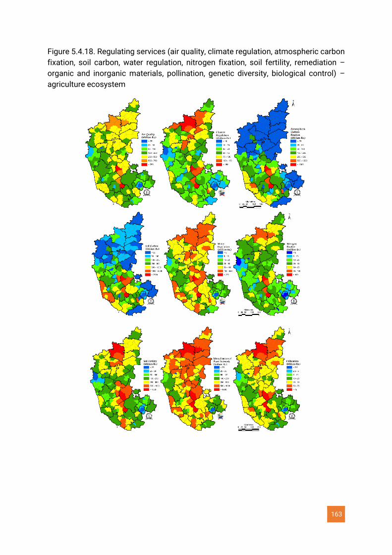
163
Figure 5.4.18. Regulating services (air quality, climate regulation, atmospheric carbon
fixation, soil carbon, water regulation, nitrogen fixation, soil fertility, remediation –
organic and inorganic materials, pollination, genetic diversity, biological control) –
agriculture ecosystem
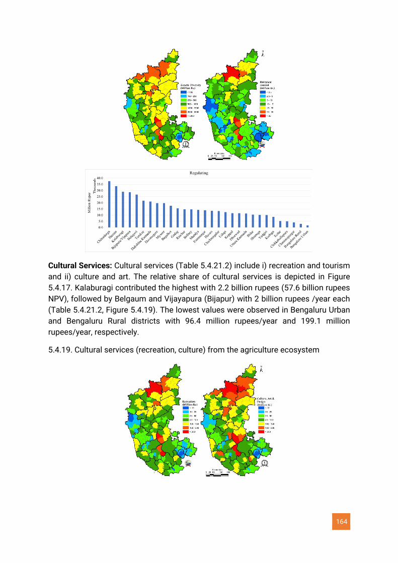
164
Cultural Services: Cultural services (Table 5.4.21.2) include i) recreation and tourism
and ii) culture and art. The relative share of cultural services is depicted in Figure
5.4.17. Kalaburagi contributed the highest with 2.2 billion rupees (57.6 billion rupees
NPV), followed by Belgaum and Vijayapura (Bijapur) with 2 billion rupees /year each
(Table 5.4.21.2, Figure 5.4.19). The lowest values were observed in Bengaluru Urban
and Bengaluru Rural districts with 96.4 million rupees/year and 199.1 million
rupees/year, respectively.
5.4.19. Cultural services (recreation, culture) from the agriculture ecosystem
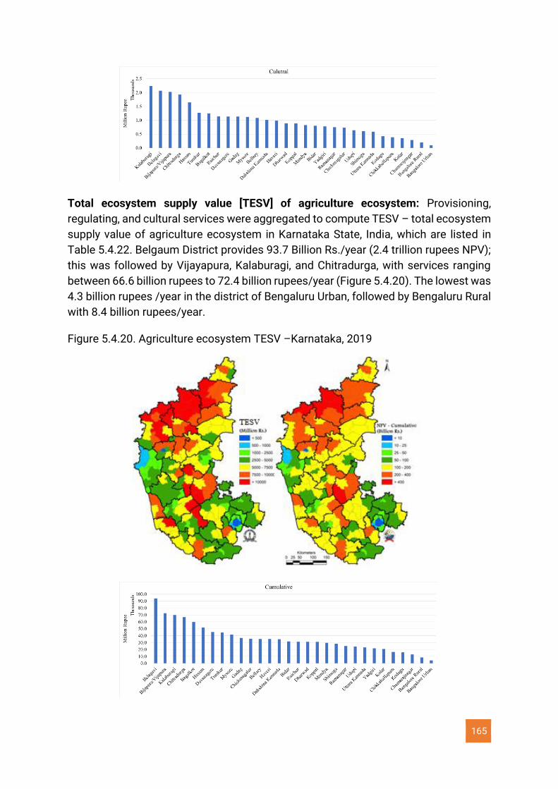
165
Total ecosystem supply value [TESV] of agriculture ecosystem: Provisioning,
regulating, and cultural services were aggregated to compute TESV – total ecosystem
supply value of agriculture ecosystem in Karnataka State, India, which are listed in
Table 5.4.22. Belgaum District provides 93.7 Billion Rs./year (2.4 trillion rupees NPV);
this was followed by Vijayapura, Kalaburagi, and Chitradurga, with services ranging
between 66.6 billion rupees to 72.4 billion rupees/year (Figure 5.4.20). The lowest was
4.3 billion rupees /year in the district of Bengaluru Urban, followed by Bengaluru Rural
with 8.4 billion rupees/year.
Figure 5.4.20. Agriculture ecosystem TESV –Karnataka, 2019
166
Temporal comparison of agriculture ecosystem services: Monetary values of
ecosystem services (provisioning, regulating, cultural services, and TSEV) of 2005 and
2019 are compared to understand the changes due to changes in the spatial extent
and condition of the ecosystem. Monetary values of 2005 were adjusted to 2019
values by considering the GDP deflator (MoSPI 2020) of an inflation rate of 2.92 times
(Inflation Calculator - Indian Rupee, 2019). Tables 5.4.23 and 5.4.24 list district-wise
comparative assessments of various goods and services of 2005 (at 2019 price) with
goods and services of 2019 for agriculture and horticulture ecosystems.
Croplands Ecosystem: Tables 5.4.23 indicates that there has been an increase in the
provisioning goods of 193 billion rupees (311 billion rupees in 2005 (at 2019 price)
increased to 505 billion rupees in 2019, an increase of 62%), a decline in regulating
services of 31 billion rupees (321 billion rupees in 2005 declined to 290 billion rupees
in 2019, a drop of 10%), a marginal increase in cultural services of 1.5 billion rupees
(20.3 billion rupees in 2005 increased to 21.8 billion rupees, an increase of 8%) and an
increase in TESV of 164 billion rupees (653 billion rupees in 2005 increased to 817
billion rupees in 2019, an increase of 25%). However, a TESV decline of 24% to 80% is
noticed during 2005 to 2019 in Mandya, Bengaluru Urban, Tumkur, Udupi, Hassan,
Raichur, Uttara Kannada, Dakshina Kannada, and Kodagu districts, due to the
conversion of agriculture lands to commercial plantations, built-up areas, etc. On the
other hand, there has been an increase in TESV of 125% in Ramanagara, Kolar,
Chitradurga, Kalaburagi (Gulbarga), Chikkaballapura, and Koppal districts, owing to an
increase in the spatial extent of cropland.
Horticulture ecosystem: There has been a decline of 19 billion rupees (Tables 5.4.24)
in provisioning services (100 billion rupees in 2005 (at 2019 price), decreased to 80.9
billion rupees in 2019, a decline of 19%), an increase in regulating services of 15 billion
rupees (23 billion rupees in 2005 increased to 38 billion rupees in 2019, an increase
of 65%), 0.2 billion rupees increase in cultural services (1.5 billion rupees in 2005
increased to 1.7 billion rupees in 2019, an increase of 16%) and decline of 4 billion
rupees in TESV (125 billion in 2005 declined to 121 billion rupees in 2019, a drop of
3%). An increase in TESV is noticed in 14 districts, while the rest showed a declining
trend. About a 125% increase in TESV is seen in the Uttara Kannada, Gadag,
Chikkaballapura, and Bidar districts, while a 78% decline in the districts of Raichur,
Chamarajanagar, Bagalkot, Yadgir, and Kalaburagi (Gulbarga) was seen during 2005
to 2019.
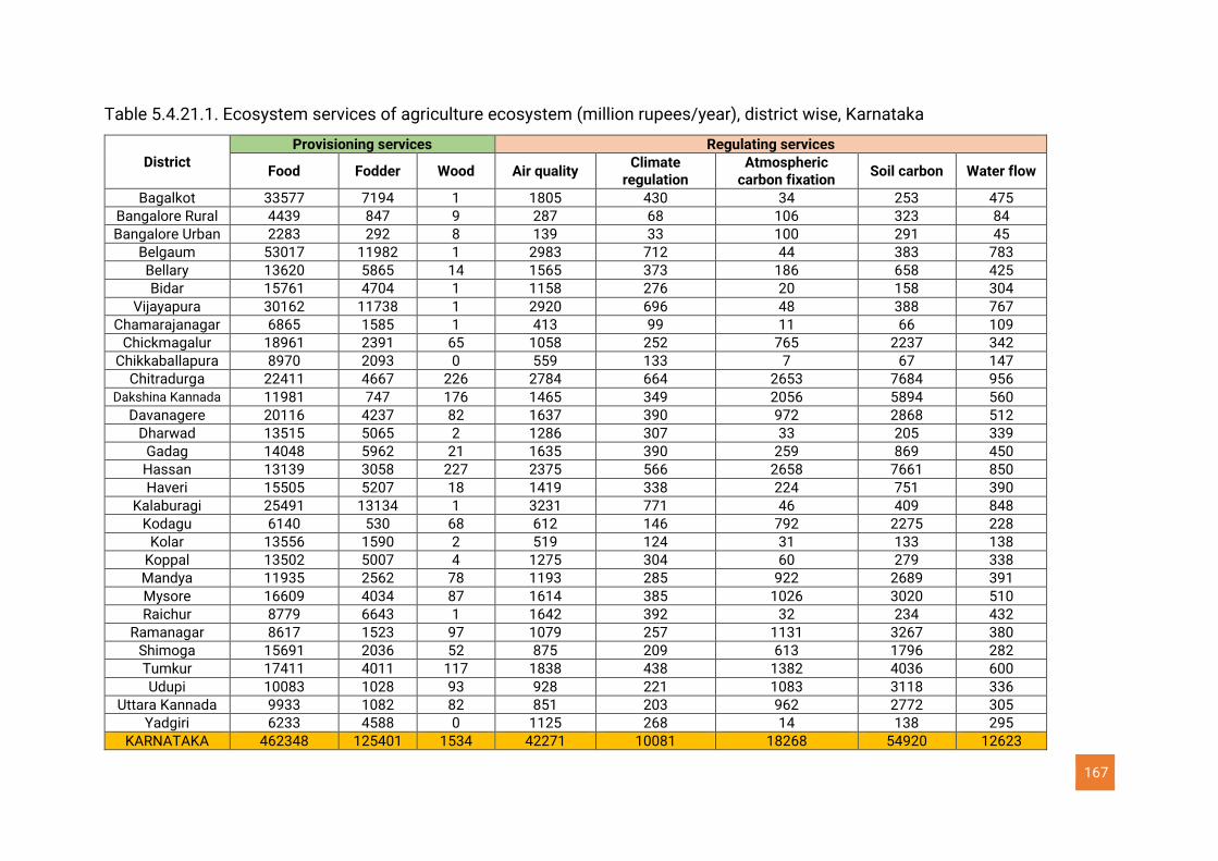
167
Table 5.4.21.1. Ecosystem services of agriculture ecosystem (million rupees/year), district wise, Karnataka
District Provisioning services Regulating services
Food Fodder Wood Air quality Climate
regulation Atmospheric
carbon fixation Soil carbon Water flow
Bagalkot 33577 7194 1 1805 430 34 253 475
Bangalore Rural 4439 847 9 287 68 106 323 84
Bangalore Urban 2283 292 8 139 33 100 291 45
Belgaum 53017 11982 1 2983 712 44 383 783
Bellary 13620 5865 14 1565 373 186 658 425
Bidar 15761 4704 1 1158 276 20 158 304
Vijayapura 30162 11738 1 2920 696 48 388 767
Chamarajanagar 6865 1585 1 413 99 11 66 109
Chickmagalur 18961 2391 65 1058 252 765 2237 342
Chikkaballapura 8970 2093 0 559 133 7 67 147
Chitradurga 22411 4667 226 2784 664 2653 7684 956 Dakshina Kannada 11981 747 176 1465 349 2056 5894 560
Davanagere 20116 4237 82 1637 390 972 2868 512
Dharwad 13515 5065 2 1286 307 33 205 339
Gadag 14048 5962 21 1635 390 259 869 450
Hassan 13139 3058 227 2375 566 2658 7661 850
Haveri 15505 5207 18 1419 338 224 751 390
Kalaburagi 25491 13134 1 3231 771 46 409 848
Kodagu 6140 530 68 612 146 792 2275 228
Kolar 13556 1590 2 519 124 31 133 138
Koppal 13502 5007 4 1275 304 60 279 338
Mandya 11935 2562 78 1193 285 922 2689 391
Mysore 16609 4034 87 1614 385 1026 3020 510
Raichur 8779 6643 1 1642 392 32 234 432
Ramanagar 8617 1523 97 1079 257 1131 3267 380
Shimoga 15691 2036 52 875 209 613 1796 282
Tumkur 17411 4011 117 1838 438 1382 4036 600
Udupi 10083 1028 93 928 221 1083 3118 336
Uttara Kannada 9933 1082 82 851 203 962 2772 305
Yadgiri 6233 4588 0 1125 268 14 138 295
KARNATAKA 462348 125401 1534 42271 10081 18268 54920 12623
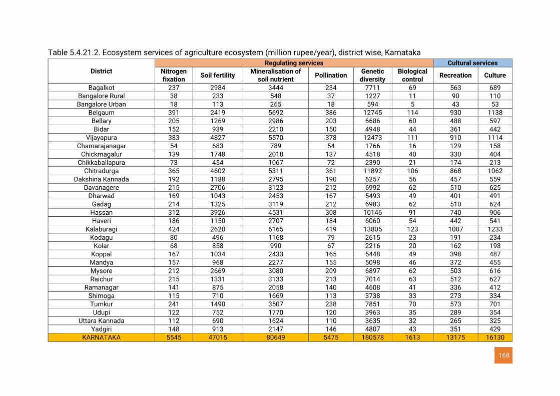
168
Table 5.4.21.2. Ecosystem services of agriculture ecosystem (million rupee/year), district wise, Karnataka
District Regulating services Cultural services
Nitrogen fixation
Soil fertility Mineralisation of
soil nutrient Pollination
Genetic diversity
Biological control
Recreation Culture
Bagalkot 237 2984 3444 234 7711 69 563 689
Bangalore Rural 38 233 548 37 1227 11 90 110
Bangalore Urban 18 113 265 18 594 5 43 53
Belgaum 391 2419 5692 386 12745 114 930 1138
Bellary 205 1269 2986 203 6686 60 488 597
Bidar 152 939 2210 150 4948 44 361 442
Vijayapura 383 4827 5570 378 12473 111 910 1114
Chamarajanagar 54 683 789 54 1766 16 129 158
Chickmagalur 139 1748 2018 137 4518 40 330 404
Chikkaballapura 73 454 1067 72 2390 21 174 213
Chitradurga 365 4602 5311 361 11892 106 868 1062
Dakshina Kannada 192 1188 2795 190 6257 56 457 559
Davanagere 215 2706 3123 212 6992 62 510 625
Dharwad 169 1043 2453 167 5493 49 401 491
Gadag 214 1325 3119 212 6983 62 510 624
Hassan 312 3926 4531 308 10146 91 740 906
Haveri 186 1150 2707 184 6060 54 442 541
Kalaburagi 424 2620 6165 419 13805 123 1007 1233
Kodagu 80 496 1168 79 2615 23 191 234
Kolar 68 858 990 67 2216 20 162 198
Koppal 167 1034 2433 165 5448 49 398 487
Mandya 157 968 2277 155 5098 46 372 455
Mysore 212 2669 3080 209 6897 62 503 616
Raichur 215 1331 3133 213 7014 63 512 627
Ramanagar 141 875 2058 140 4608 41 336 412
Shimoga 115 710 1669 113 3738 33 273 334
Tumkur 241 1490 3507 238 7851 70 573 701
Udupi 122 752 1770 120 3963 35 289 354
Uttara Kannada 112 690 1624 110 3635 32 265 325
Yadgiri 148 913 2147 146 4807 43 351 429
KARNATAKA 5545 47015 80649 5475 180578 1613 13175 16130
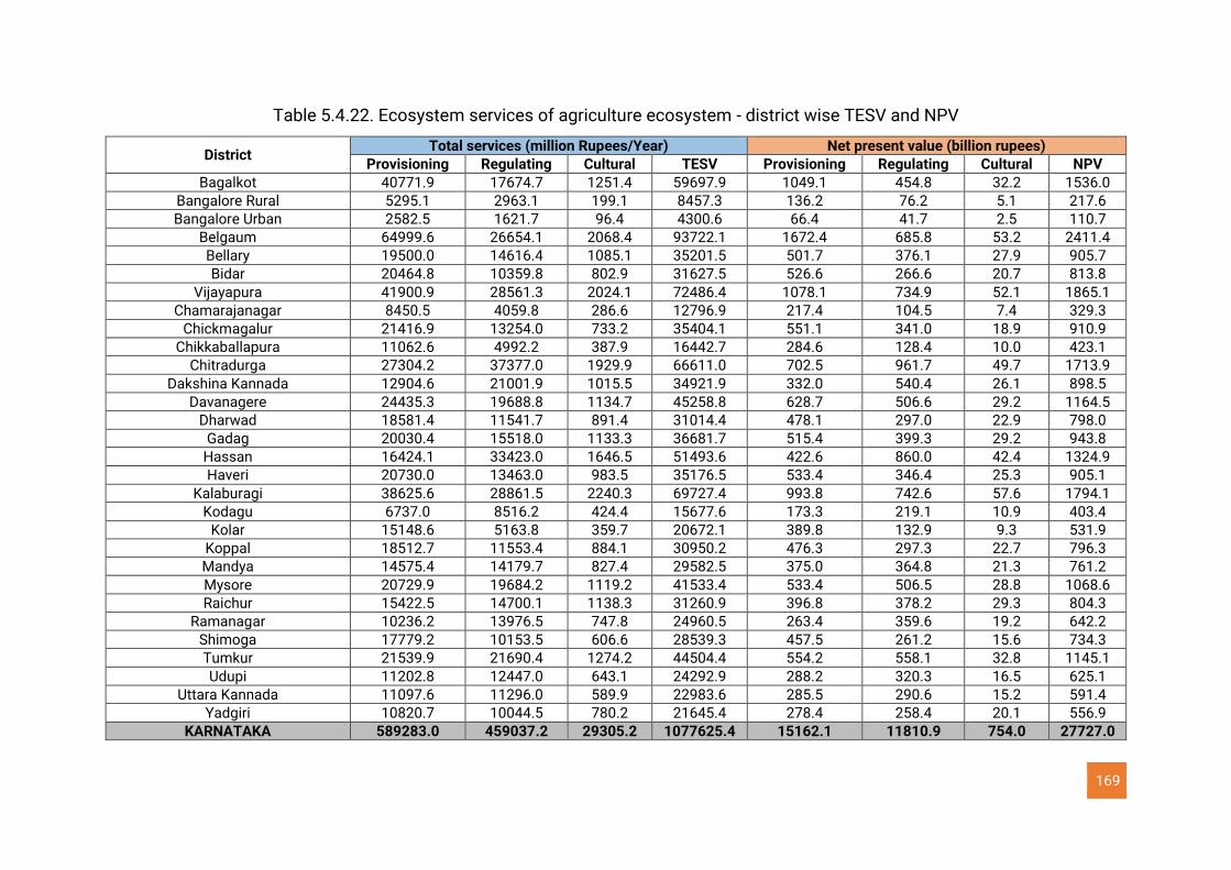
169
Table 5.4.22. Ecosystem services of agriculture ecosystem - district wise TESV and NPV
District Total services (million Rupees/Year) Net present value (billion rupees)
Provisioning Regulating Cultural TESV Provisioning Regulating Cultural NPV
Bagalkot 40771.9 17674.7 1251.4 59697.9 1049.1 454.8 32.2 1536.0
Bangalore Rural 5295.1 2963.1 199.1 8457.3 136.2 76.2 5.1 217.6
Bangalore Urban 2582.5 1621.7 96.4 4300.6 66.4 41.7 2.5 110.7
Belgaum 64999.6 26654.1 2068.4 93722.1 1672.4 685.8 53.2 2411.4
Bellary 19500.0 14616.4 1085.1 35201.5 501.7 376.1 27.9 905.7
Bidar 20464.8 10359.8 802.9 31627.5 526.6 266.6 20.7 813.8
Vijayapura 41900.9 28561.3 2024.1 72486.4 1078.1 734.9 52.1 1865.1
Chamarajanagar 8450.5 4059.8 286.6 12796.9 217.4 104.5 7.4 329.3
Chickmagalur 21416.9 13254.0 733.2 35404.1 551.1 341.0 18.9 910.9
Chikkaballapura 11062.6 4992.2 387.9 16442.7 284.6 128.4 10.0 423.1
Chitradurga 27304.2 37377.0 1929.9 66611.0 702.5 961.7 49.7 1713.9
Dakshina Kannada 12904.6 21001.9 1015.5 34921.9 332.0 540.4 26.1 898.5
Davanagere 24435.3 19688.8 1134.7 45258.8 628.7 506.6 29.2 1164.5
Dharwad 18581.4 11541.7 891.4 31014.4 478.1 297.0 22.9 798.0
Gadag 20030.4 15518.0 1133.3 36681.7 515.4 399.3 29.2 943.8
Hassan 16424.1 33423.0 1646.5 51493.6 422.6 860.0 42.4 1324.9
Haveri 20730.0 13463.0 983.5 35176.5 533.4 346.4 25.3 905.1
Kalaburagi 38625.6 28861.5 2240.3 69727.4 993.8 742.6 57.6 1794.1
Kodagu 6737.0 8516.2 424.4 15677.6 173.3 219.1 10.9 403.4
Kolar 15148.6 5163.8 359.7 20672.1 389.8 132.9 9.3 531.9
Koppal 18512.7 11553.4 884.1 30950.2 476.3 297.3 22.7 796.3
Mandya 14575.4 14179.7 827.4 29582.5 375.0 364.8 21.3 761.2
Mysore 20729.9 19684.2 1119.2 41533.4 533.4 506.5 28.8 1068.6
Raichur 15422.5 14700.1 1138.3 31260.9 396.8 378.2 29.3 804.3
Ramanagar 10236.2 13976.5 747.8 24960.5 263.4 359.6 19.2 642.2
Shimoga 17779.2 10153.5 606.6 28539.3 457.5 261.2 15.6 734.3
Tumkur 21539.9 21690.4 1274.2 44504.4 554.2 558.1 32.8 1145.1
Udupi 11202.8 12447.0 643.1 24292.9 288.2 320.3 16.5 625.1
Uttara Kannada 11097.6 11296.0 589.9 22983.6 285.5 290.6 15.2 591.4
Yadgiri 10820.7 10044.5 780.2 21645.4 278.4 258.4 20.1 556.9
KARNATAKA 589283.0 459037.2 29305.2 1077625.4 15162.1 11810.9 754.0 27727.0
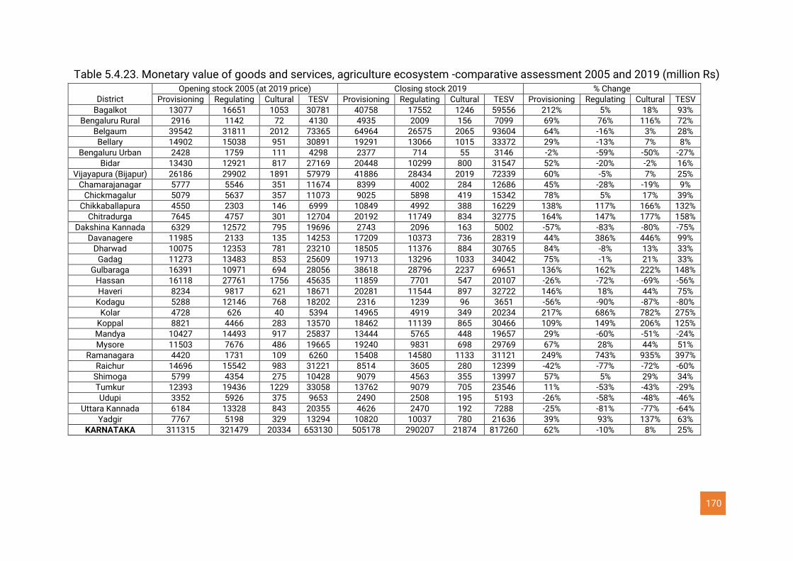
170
Table 5.4.23. Monetary value of goods and services, agriculture ecosystem -comparative assessment 2005 and 2019 (million Rs)
District Opening stock 2005 (at 2019 price) Closing stock 2019 % Change
Provisioning Regulating Cultural TESV Provisioning Regulating Cultural TESV Provisioning Regulating Cultural TESV
Bagalkot 13077 16651 1053 30781 40758 17552 1246 59556 212% 5% 18% 93%
Bengaluru Rural 2916 1142 72 4130 4935 2009 156 7099 69% 76% 116% 72%
Belgaum 39542 31811 2012 73365 64964 26575 2065 93604 64% -16% 3% 28%
Bellary 14902 15038 951 30891 19291 13066 1015 33372 29% -13% 7% 8%
Bengaluru Urban 2428 1759 111 4298 2377 714 55 3146 -2% -59% -50% -27%
Bidar 13430 12921 817 27169 20448 10299 800 31547 52% -20% -2% 16%
Vijayapura (Bijapur) 26186 29902 1891 57979 41886 28434 2019 72339 60% -5% 7% 25%
Chamarajanagar 5777 5546 351 11674 8399 4002 284 12686 45% -28% -19% 9%
Chickmagalur 5079 5637 357 11073 9025 5898 419 15342 78% 5% 17% 39%
Chikkaballapura 4550 2303 146 6999 10849 4992 388 16229 138% 117% 166% 132%
Chitradurga 7645 4757 301 12704 20192 11749 834 32775 164% 147% 177% 158%
Dakshina Kannada 6329 12572 795 19696 2743 2096 163 5002 -57% -83% -80% -75%
Davanagere 11985 2133 135 14253 17209 10373 736 28319 44% 386% 446% 99%
Dharwad 10075 12353 781 23210 18505 11376 884 30765 84% -8% 13% 33%
Gadag 11273 13483 853 25609 19713 13296 1033 34042 75% -1% 21% 33%
Gulbaraga 16391 10971 694 28056 38618 28796 2237 69651 136% 162% 222% 148%
Hassan 16118 27761 1756 45635 11859 7701 547 20107 -26% -72% -69% -56%
Haveri 8234 9817 621 18671 20281 11544 897 32722 146% 18% 44% 75%
Kodagu 5288 12146 768 18202 2316 1239 96 3651 -56% -90% -87% -80%
Kolar 4728 626 40 5394 14965 4919 349 20234 217% 686% 782% 275%
Koppal 8821 4466 283 13570 18462 11139 865 30466 109% 149% 206% 125%
Mandya 10427 14493 917 25837 13444 5765 448 19657 29% -60% -51% -24%
Mysore 11503 7676 486 19665 19240 9831 698 29769 67% 28% 44% 51%
Ramanagara 4420 1731 109 6260 15408 14580 1133 31121 249% 743% 935% 397%
Raichur 14696 15542 983 31221 8514 3605 280 12399 -42% -77% -72% -60%
Shimoga 5799 4354 275 10428 9079 4563 355 13997 57% 5% 29% 34%
Tumkur 12393 19436 1229 33058 13762 9079 705 23546 11% -53% -43% -29%
Udupi 3352 5926 375 9653 2490 2508 195 5193 -26% -58% -48% -46%
Uttara Kannada 6184 13328 843 20355 4626 2470 192 7288 -25% -81% -77% -64%
Yadgir 7767 5198 329 13294 10820 10037 780 21636 39% 93% 137% 63%
KARNATAKA 311315 321479 20334 653130 505178 290207 21874 817260 62% -10% 8% 25%
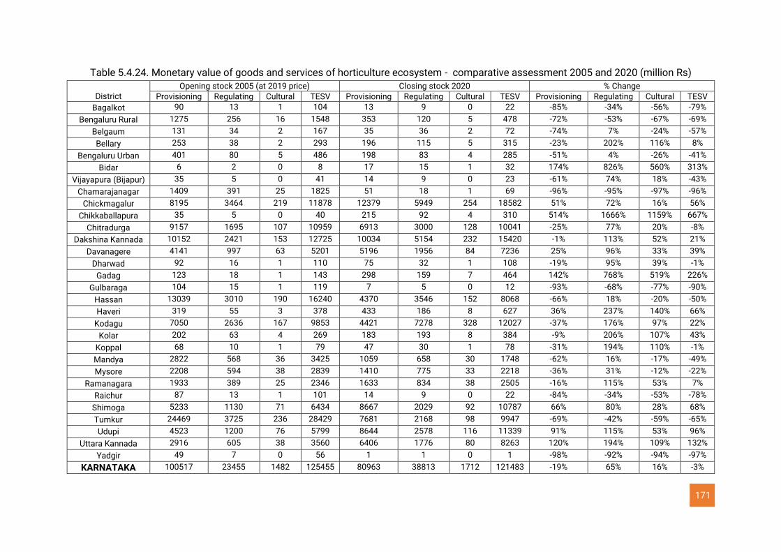
171
Table 5.4.24. Monetary value of goods and services of horticulture ecosystem - comparative assessment 2005 and 2020 (million Rs)
District
Opening stock 2005 (at 2019 price) Closing stock 2020 % Change
Provisioning Regulating Cultural TESV Provisioning Regulating Cultural TESV Provisioning Regulating Cultural TESV
Bagalkot 90 13 1 104 13 9 0 22 -85% -34% -56% -79%
Bengaluru Rural 1275 256 16 1548 353 120 5 478 -72% -53% -67% -69%
Belgaum 131 34 2 167 35 36 2 72 -74% 7% -24% -57%
Bellary 253 38 2 293 196 115 5 315 -23% 202% 116% 8%
Bengaluru Urban 401 80 5 486 198 83 4 285 -51% 4% -26% -41%
Bidar 6 2 0 8 17 15 1 32 174% 826% 560% 313%
Vijayapura (Bijapur) 35 5 0 41 14 9 0 23 -61% 74% 18% -43%
Chamarajanagar 1409 391 25 1825 51 18 1 69 -96% -95% -97% -96%
Chickmagalur 8195 3464 219 11878 12379 5949 254 18582 51% 72% 16% 56%
Chikkaballapura 35 5 0 40 215 92 4 310 514% 1666% 1159% 667%
Chitradurga 9157 1695 107 10959 6913 3000 128 10041 -25% 77% 20% -8%
Dakshina Kannada 10152 2421 153 12725 10034 5154 232 15420 -1% 113% 52% 21%
Davanagere 4141 997 63 5201 5196 1956 84 7236 25% 96% 33% 39%
Dharwad 92 16 1 110 75 32 1 108 -19% 95% 39% -1%
Gadag 123 18 1 143 298 159 7 464 142% 768% 519% 226%
Gulbaraga 104 15 1 119 7 5 0 12 -93% -68% -77% -90%
Hassan 13039 3010 190 16240 4370 3546 152 8068 -66% 18% -20% -50%
Haveri 319 55 3 378 433 186 8 627 36% 237% 140% 66%
Kodagu 7050 2636 167 9853 4421 7278 328 12027 -37% 176% 97% 22%
Kolar 202 63 4 269 183 193 8 384 -9% 206% 107% 43%
Koppal 68 10 1 79 47 30 1 78 -31% 194% 110% -1%
Mandya 2822 568 36 3425 1059 658 30 1748 -62% 16% -17% -49%
Mysore 2208 594 38 2839 1410 775 33 2218 -36% 31% -12% -22%
Ramanagara 1933 389 25 2346 1633 834 38 2505 -16% 115% 53% 7%
Raichur 87 13 1 101 14 9 0 22 -84% -34% -53% -78%
Shimoga 5233 1130 71 6434 8667 2029 92 10787 66% 80% 28% 68%
Tumkur 24469 3725 236 28429 7681 2168 98 9947 -69% -42% -59% -65%
Udupi 4523 1200 76 5799 8644 2578 116 11339 91% 115% 53% 96%
Uttara Kannada 2916 605 38 3560 6406 1776 80 8263 120% 194% 109% 132%
Yadgir 49 7 0 56 1 1 0 1 -98% -92% -94% -97%
KARNATAKA 100517 23455 1482 125455 80963 38813 1712 121483 -19% 65% 16% -3%
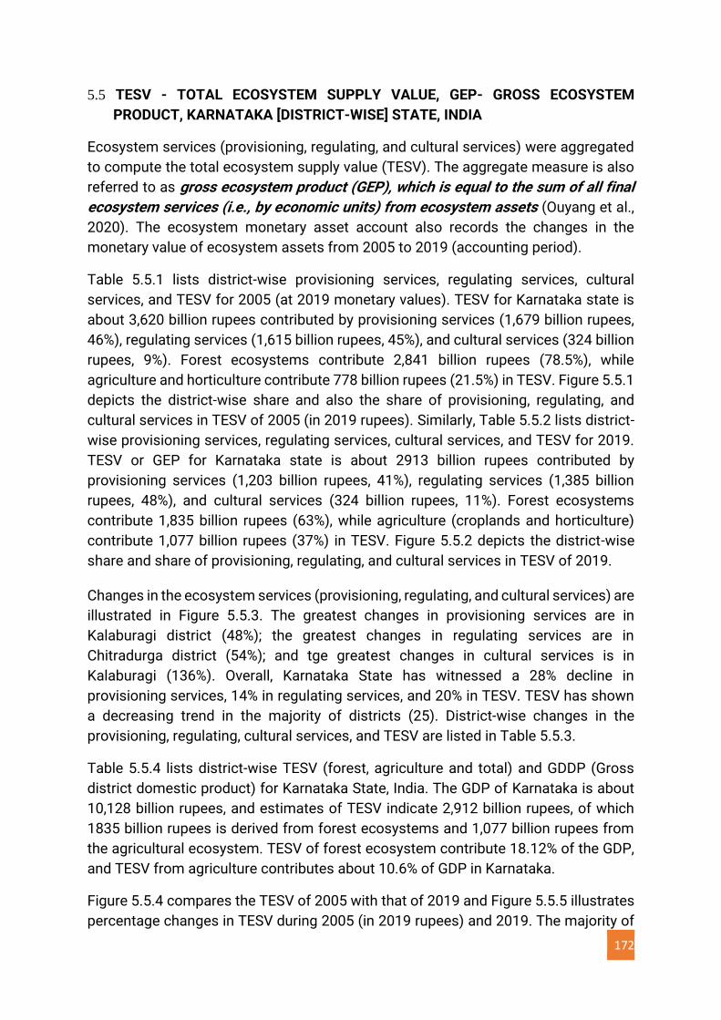
172
5.5 TESV - TOTAL ECOSYSTEM SUPPLY VALUE, GEP- GROSS ECOSYSTEM
PRODUCT, KARNATAKA [DISTRICT-WISE] STATE, INDIA
Ecosystem services (provisioning, regulating, and cultural services) were aggregated
to compute the total ecosystem supply value (TESV). The aggregate measure is also
referred to as gross ecosystem product (GEP), which is equal to the sum of all final
ecosystem services (i.e., by economic units) from ecosystem assets (Ouyang et al.,
2020). The ecosystem monetary asset account also records the changes in the
monetary value of ecosystem assets from 2005 to 2019 (accounting period).
Table 5.5.1 lists district-wise provisioning services, regulating services, cultural
services, and TESV for 2005 (at 2019 monetary values). TESV for Karnataka state is
about 3,620 billion rupees contributed by provisioning services (1,679 billion rupees,
46%), regulating services (1,615 billion rupees, 45%), and cultural services (324 billion
rupees, 9%). Forest ecosystems contribute 2,841 billion rupees (78.5%), while
agriculture and horticulture contribute 778 billion rupees (21.5%) in TESV. Figure 5.5.1
depicts the district-wise share and also the share of provisioning, regulating, and
cultural services in TESV of 2005 (in 2019 rupees). Similarly, Table 5.5.2 lists district-
wise provisioning services, regulating services, cultural services, and TESV for 2019.
TESV or GEP for Karnataka state is about 2913 billion rupees contributed by
provisioning services (1,203 billion rupees, 41%), regulating services (1,385 billion
rupees, 48%), and cultural services (324 billion rupees, 11%). Forest ecosystems
contribute 1,835 billion rupees (63%), while agriculture (croplands and horticulture)
contribute 1,077 billion rupees (37%) in TESV. Figure 5.5.2 depicts the district-wise
share and share of provisioning, regulating, and cultural services in TESV of 2019.
Changes in the ecosystem services (provisioning, regulating, and cultural services) are
illustrated in Figure 5.5.3. The greatest changes in provisioning services are in
Kalaburagi district (48%); the greatest changes in regulating services are in
Chitradurga district (54%); and tge greatest changes in cultural services is in
Kalaburagi (136%). Overall, Karnataka State has witnessed a 28% decline in
provisioning services, 14% in regulating services, and 20% in TESV. TESV has shown
a decreasing trend in the majority of districts (25). District-wise changes in the
provisioning, regulating, cultural services, and TESV are listed in Table 5.5.3.
Table 5.5.4 lists district-wise TESV (forest, agriculture and total) and GDDP (Gross
district domestic product) for Karnataka State, India. The GDP of Karnataka is about
10,128 billion rupees, and estimates of TESV indicate 2,912 billion rupees, of which
1835 billion rupees is derived from forest ecosystems and 1,077 billion rupees from
the agricultural ecosystem. TESV of forest ecosystem contribute 18.12% of the GDP,
and TESV from agriculture contributes about 10.6% of GDP in Karnataka.
Figure 5.5.4 compares the TESV of 2005 with that of 2019 and Figure 5.5.5 illustrates
percentage changes in TESV during 2005 (in 2019 rupees) and 2019. The majority of
173
districts reveal declining TESV, except districts Kalaburagi (48%), Bangalore urban
(10%), Ramnagara (6%), Chitradurga (4%), and Haveri (2%), which show an increase
in TESV.
Higher NPV values in the Western Ghats districts – Uttara Kannada (NPV: 11,885
billion), Chikmagalur (5,875), Chamarjanagar (5,858), Dakshina Kannada (5,205),
Shimoga (5,062), Udupi (3,787), Kodagu (3,721), Belagavi (3,445), and Mysore (2,527)
highlight the role of a forest ecosystem with native species of vegetation in supporting
rich endemic biodiversity, sustaining water availability during all seasons to meet
biotic demands, and supporting the livelihood of people. Understanding these linkages
would help the planners/decision-makers with valuable knowledge for integrated
ecosystem management. The study highlights the vital ecological function of the
Western Ghats, one among 36 global biodiversity hotspots, in sustaining the
hydrologic regime and livelihood of local people. Hence, the premium should be
towards conserving the forests with native species to sustain water and biotic
diversity, which are vital for food security. There still exists a chance to restore the lost
natural evergreen to semi-evergreen forests through appropriate conservation and
management practices in Karnataka State.
Figure 5.5.6 depicts the district-wise share of TESV in GDDP. The district-wise
assessment indicates TESV of Bengaluru urban and rural districts are the lowest,
amounting to <10% of GDDP. In contrast, forest-rich Western Ghats districts (mainly
Uttara Kannada of Canara forest circle, Kodagu of Kodagu forest circle, and
Chamarajanagar and Chamarajanagar circle) provide TESV that is about 200% of the
respective district GDDP. The presence of rich forests in these districts contributes to
higher TESV, highlighting that TESV share in GDDP (Gross District Domestic Product)
is correlated with the extent and conditions of forest ecosystems in the respective
districts.
Table 5.5.5 lists TESV or GEP for Karnataka considering forest, and agriculture
(croplands and horticulture) ecosystems. The TESV of these ecosystems is 3620
billion rupees in 2005 (forest ecosystem: 2,841 billion rupees and agriculture
(croplands and horticulture) ecosystem: 779 billion rupees). Similarly, TESV computed
for 2019 indicates 2,912 billion rupees (forest ecosystem: 1,835 billion rupees and
agriculture 1,077: billion rupees). There has been a 35.4% reduction in TESV of forest
ecosystems from 2005 to 2019, mainly due to the degradation of ecosystems.
The decline of TESV highlights the degradation of forest ecosystem assets from 2005
to 2019 due to the reduction of ecosystem extent and condition. The decrease in value
is also demonstrated by a fall in the net present value of expected future returns of
the ecosystem services supplied by forest ecosystem assets, as shown through the
ecosystem monetary asset account.
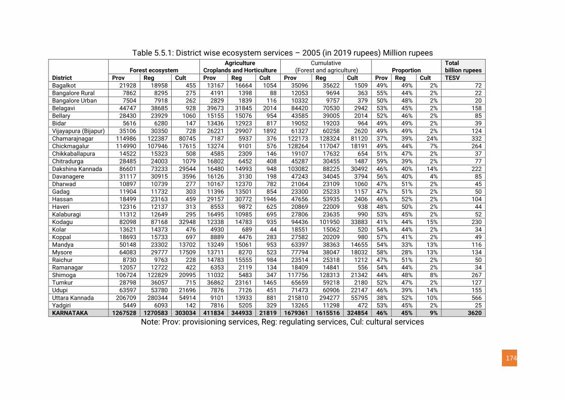
174
Table 5.5.1: District wise ecosystem services – 2005 (in 2019 rupees) Million rupees
District
Forest ecosystem Agriculture
Croplands and Horticulture Cumulative
(Forest and agriculture) Proportion Total billion rupees
Prov Reg Cult Prov Reg Cult Prov Reg Cult Prov Reg Cult TESV
Bagalkot 21928 18958 455 13167 16664 1054 35096 35622 1509 49% 49% 2% 72
Bangalore Rural 7862 8295 275 4191 1398 88 12053 9694 363 55% 44% 2% 22
Bangalore Urban 7504 7918 262 2829 1839 116 10332 9757 379 50% 48% 2% 20
Belagavi 44747 38685 928 39673 31845 2014 84420 70530 2942 53% 45% 2% 158
Bellary 28430 23929 1060 15155 15076 954 43585 39005 2014 52% 46% 2% 85
Bidar 5616 6280 147 13436 12923 817 19052 19203 964 49% 49% 2% 39
Vijayapura (Bijapur) 35106 30350 728 26221 29907 1892 61327 60258 2620 49% 49% 2% 124
Chamarajnagar 114986 122387 80745 7187 5937 376 122173 128324 81120 37% 39% 24% 332
Chickmagalur 114990 107946 17615 13274 9101 576 128264 117047 18191 49% 44% 7% 264
Chikkaballapura 14522 15323 508 4585 2309 146 19107 17632 654 51% 47% 2% 37
Chitradurga 28485 24003 1079 16802 6452 408 45287 30455 1487 59% 39% 2% 77
Dakshina Kannada 86601 73233 29544 16480 14993 948 103082 88225 30492 46% 40% 14% 222
Davanagere 31117 30915 3596 16126 3130 198 47243 34045 3794 56% 40% 4% 85
Dharwad 10897 10739 277 10167 12370 782 21064 23109 1060 47% 51% 2% 45
Gadag 11904 11732 303 11396 13501 854 23300 25233 1157 47% 51% 2% 50
Hassan 18499 23163 459 29157 30772 1946 47656 53935 2406 46% 52% 2% 104
Haveri 12316 12137 313 8553 9872 625 20869 22009 938 48% 50% 2% 44
Kalaburagi 11312 12649 295 16495 10985 695 27806 23635 990 53% 45% 2% 52
Kodagu 82098 87168 32948 12338 14783 935 94436 101950 33883 41% 44% 15% 230
Kolar 13621 14373 476 4930 689 44 18551 15062 520 54% 44% 2% 34
Koppal 18693 15733 697 8889 4476 283 27582 20209 980 57% 41% 2% 49
Mandya 50148 23302 13702 13249 15061 953 63397 38363 14655 54% 33% 13% 116
Mysore 64083 29777 17509 13711 8270 523 77794 38047 18032 58% 28% 13% 134
Raichur 8730 9763 228 14783 15555 984 23514 25318 1212 47% 51% 2% 50
Ramanagar 12057 12722 422 6353 2119 134 18409 14841 556 54% 44% 2% 34
Shimoga 106724 122829 20995 11032 5483 347 117756 128313 21342 44% 48% 8% 267
Tumkur 28798 36057 715 36862 23161 1465 65659 59218 2180 52% 47% 2% 127
Udupi 63597 53780 21696 7876 7126 451 71473 60906 22147 46% 39% 14% 155
Uttara Kannada 206709 280344 54914 9101 13933 881 215810 294277 55795 38% 52% 10% 566
Yadgiri 5449 6093 142 7816 5205 329 13265 11298 472 53% 45% 2% 25
KARNATAKA 1267528 1270583 303034 411834 344933 21819 1679361 1615516 324854 46% 45% 9% 3620
Note: Prov: provisioning services, Reg: regulating services, Cul: cultural services
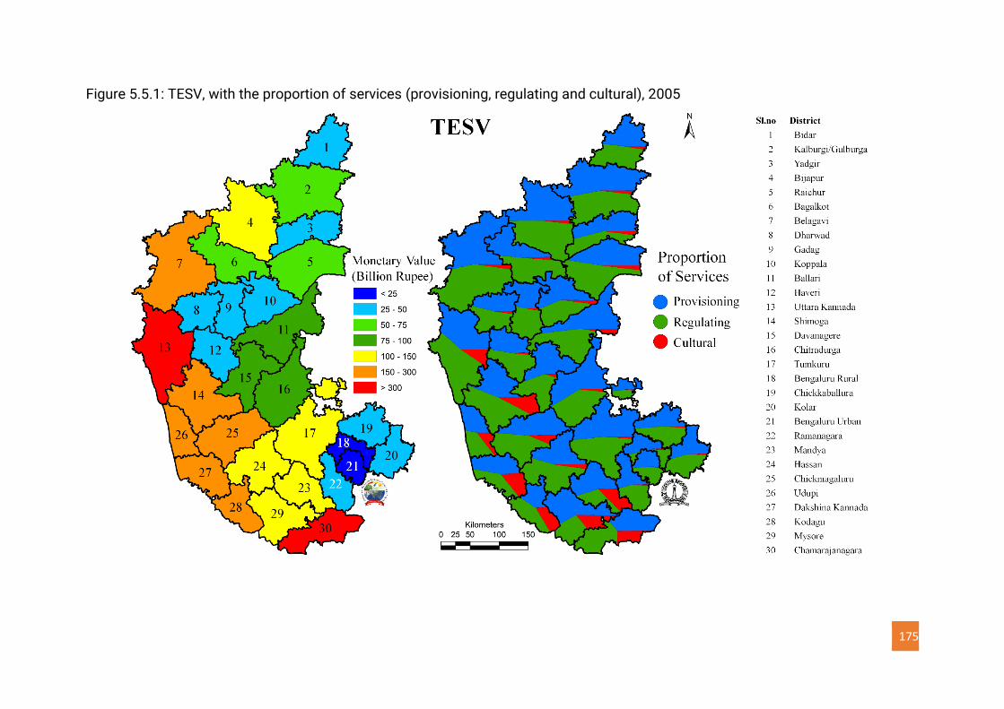
175
Figure 5.5.1: TESV, with the proportion of services (provisioning, regulating and cultural), 2005
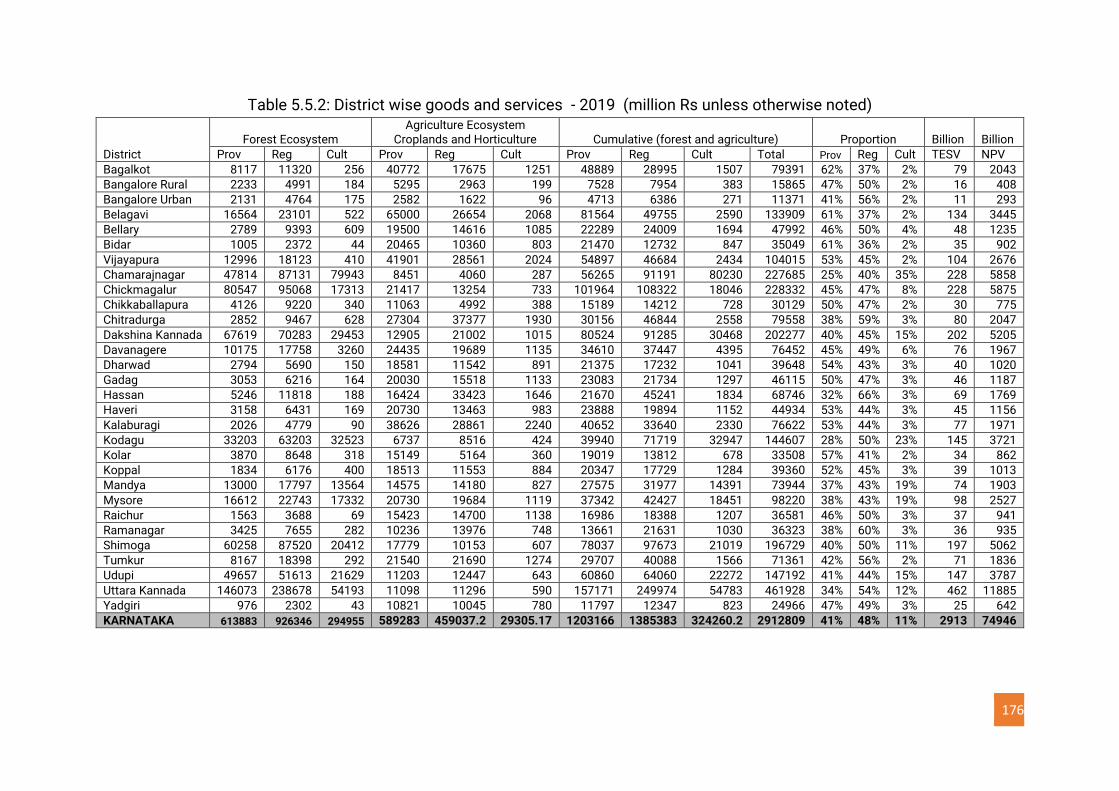
176
Table 5.5.2: District wise goods and services - 2019 (million Rs unless otherwise noted)
District
Forest Ecosystem Agriculture Ecosystem
Croplands and Horticulture Cumulative (forest and agriculture) Proportion Billion Billion
Prov Reg Cult Prov Reg Cult Prov Reg Cult Total Prov Reg Cult TESV NPV
Bagalkot 8117 11320 256 40772 17675 1251 48889 28995 1507 79391 62% 37% 2% 79 2043
Bangalore Rural 2233 4991 184 5295 2963 199 7528 7954 383 15865 47% 50% 2% 16 408
Bangalore Urban 2131 4764 175 2582 1622 96 4713 6386 271 11371 41% 56% 2% 11 293
Belagavi 16564 23101 522 65000 26654 2068 81564 49755 2590 133909 61% 37% 2% 134 3445
Bellary 2789 9393 609 19500 14616 1085 22289 24009 1694 47992 46% 50% 4% 48 1235
Bidar 1005 2372 44 20465 10360 803 21470 12732 847 35049 61% 36% 2% 35 902
Vijayapura 12996 18123 410 41901 28561 2024 54897 46684 2434 104015 53% 45% 2% 104 2676
Chamarajnagar 47814 87131 79943 8451 4060 287 56265 91191 80230 227685 25% 40% 35% 228 5858
Chickmagalur 80547 95068 17313 21417 13254 733 101964 108322 18046 228332 45% 47% 8% 228 5875
Chikkaballapura 4126 9220 340 11063 4992 388 15189 14212 728 30129 50% 47% 2% 30 775
Chitradurga 2852 9467 628 27304 37377 1930 30156 46844 2558 79558 38% 59% 3% 80 2047
Dakshina Kannada 67619 70283 29453 12905 21002 1015 80524 91285 30468 202277 40% 45% 15% 202 5205
Davanagere 10175 17758 3260 24435 19689 1135 34610 37447 4395 76452 45% 49% 6% 76 1967
Dharwad 2794 5690 150 18581 11542 891 21375 17232 1041 39648 54% 43% 3% 40 1020
Gadag 3053 6216 164 20030 15518 1133 23083 21734 1297 46115 50% 47% 3% 46 1187
Hassan 5246 11818 188 16424 33423 1646 21670 45241 1834 68746 32% 66% 3% 69 1769
Haveri 3158 6431 169 20730 13463 983 23888 19894 1152 44934 53% 44% 3% 45 1156
Kalaburagi 2026 4779 90 38626 28861 2240 40652 33640 2330 76622 53% 44% 3% 77 1971
Kodagu 33203 63203 32523 6737 8516 424 39940 71719 32947 144607 28% 50% 23% 145 3721
Kolar 3870 8648 318 15149 5164 360 19019 13812 678 33508 57% 41% 2% 34 862
Koppal 1834 6176 400 18513 11553 884 20347 17729 1284 39360 52% 45% 3% 39 1013
Mandya 13000 17797 13564 14575 14180 827 27575 31977 14391 73944 37% 43% 19% 74 1903
Mysore 16612 22743 17332 20730 19684 1119 37342 42427 18451 98220 38% 43% 19% 98 2527
Raichur 1563 3688 69 15423 14700 1138 16986 18388 1207 36581 46% 50% 3% 37 941
Ramanagar 3425 7655 282 10236 13976 748 13661 21631 1030 36323 38% 60% 3% 36 935
Shimoga 60258 87520 20412 17779 10153 607 78037 97673 21019 196729 40% 50% 11% 197 5062
Tumkur 8167 18398 292 21540 21690 1274 29707 40088 1566 71361 42% 56% 2% 71 1836
Udupi 49657 51613 21629 11203 12447 643 60860 64060 22272 147192 41% 44% 15% 147 3787
Uttara Kannada 146073 238678 54193 11098 11296 590 157171 249974 54783 461928 34% 54% 12% 462 11885
Yadgiri 976 2302 43 10821 10045 780 11797 12347 823 24966 47% 49% 3% 25 642
KARNATAKA 613883 926346 294955 589283 459037.2 29305.17 1203166 1385383 324260.2 2912809 41% 48% 11% 2913 74946
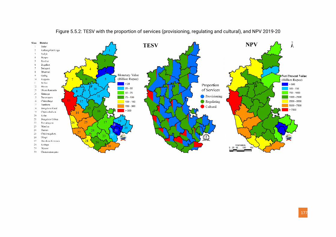
177
Figure 5.5.2: TESV with the proportion of services (provisioning, regulating and cultural), and NPV 2019-20
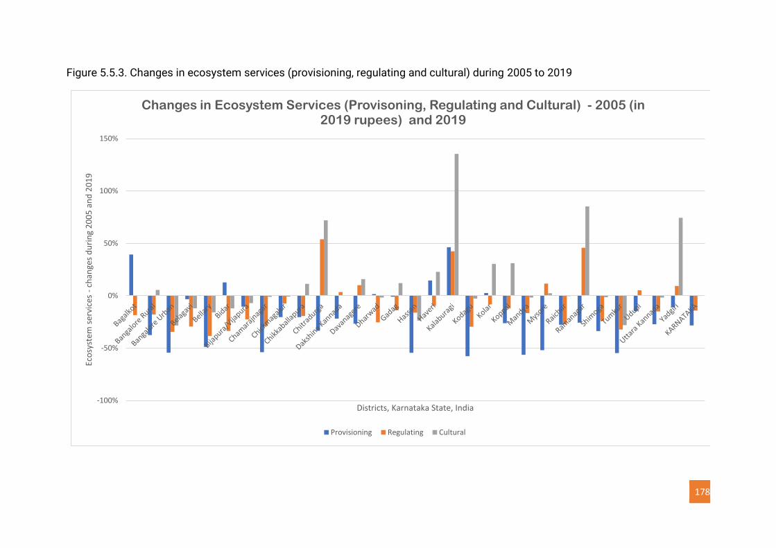
178
Figure 5.5.3. Changes in ecosystem services (provisioning, regulating and cultural) during 2005 to 2019
-100%
-50%
0%
50%
100%
150%
Eco
syst
em s
ervi
ces
-ch
ange
s d
uri
ng
20
05
an
d 2
01
9
Districts, Karnataka State, India
Changes in Ecosystem Services (Provisoning, Regulating and Cultural) - 2005 (in 2019 rupees) and 2019
Provisioning Regulating Cultural
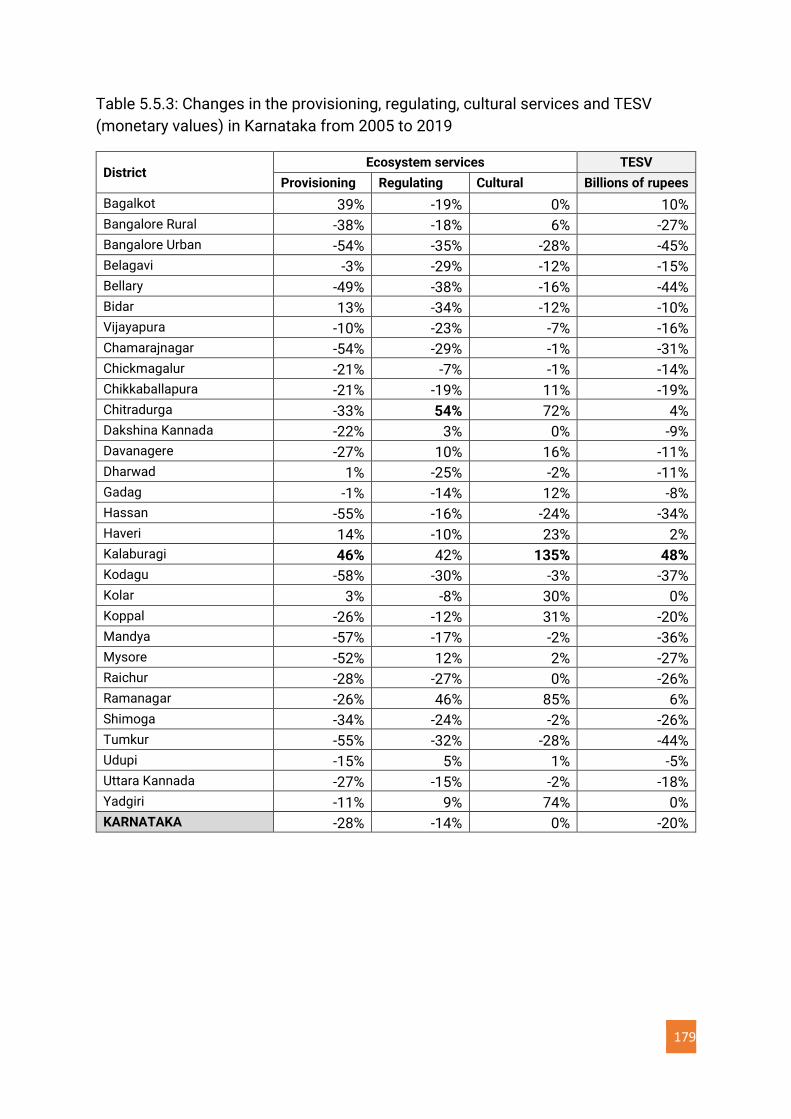
179
Table 5.5.3: Changes in the provisioning, regulating, cultural services and TESV
(monetary values) in Karnataka from 2005 to 2019
District Ecosystem services TESV
Provisioning Regulating Cultural Billions of rupees
Bagalkot 39% -19% 0% 10%
Bangalore Rural -38% -18% 6% -27%
Bangalore Urban -54% -35% -28% -45%
Belagavi -3% -29% -12% -15%
Bellary -49% -38% -16% -44%
Bidar 13% -34% -12% -10%
Vijayapura -10% -23% -7% -16%
Chamarajnagar -54% -29% -1% -31%
Chickmagalur -21% -7% -1% -14%
Chikkaballapura -21% -19% 11% -19%
Chitradurga -33% 54% 72% 4%
Dakshina Kannada -22% 3% 0% -9%
Davanagere -27% 10% 16% -11%
Dharwad 1% -25% -2% -11%
Gadag -1% -14% 12% -8%
Hassan -55% -16% -24% -34%
Haveri 14% -10% 23% 2%
Kalaburagi 46% 42% 135% 48%
Kodagu -58% -30% -3% -37%
Kolar 3% -8% 30% 0%
Koppal -26% -12% 31% -20%
Mandya -57% -17% -2% -36%
Mysore -52% 12% 2% -27%
Raichur -28% -27% 0% -26%
Ramanagar -26% 46% 85% 6%
Shimoga -34% -24% -2% -26%
Tumkur -55% -32% -28% -44%
Udupi -15% 5% 1% -5%
Uttara Kannada -27% -15% -2% -18%
Yadgiri -11% 9% 74% 0%
KARNATAKA -28% -14% 0% -20%
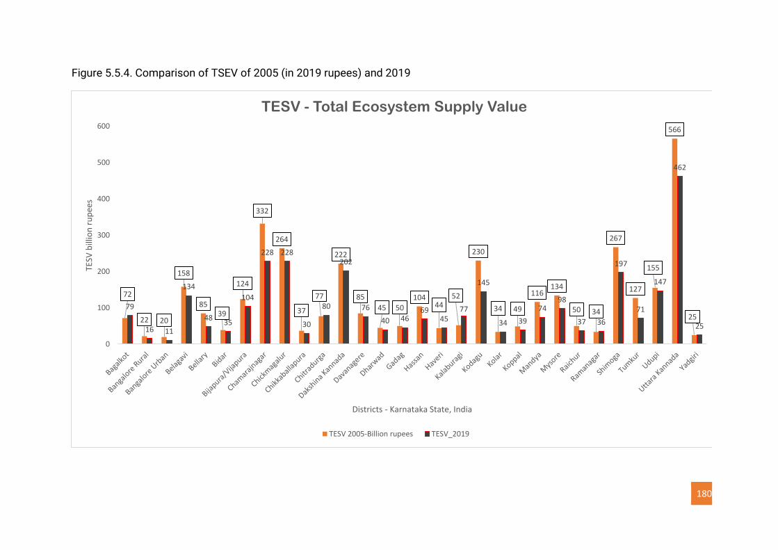
180
Figure 5.5.4. Comparison of TSEV of 2005 (in 2019 rupees) and 2019
72
22 20
158
8539
124
332
264
37
77
222
85
45 50104
4452
230
34 49
116134
50 34
267
127
155
566
2579
16 11
134
4835
104
228 228
30
80
202
76
40 4669
4577
145
34 39
7498
37 36
197
71
147
462
25
0
100
200
300
400
500
600
TESV
bill
ion
ru
pee
s
Districts - Karnataka State, India
TESV - Total Ecosystem Supply Value
TESV 2005-Billion rupees TESV_2019
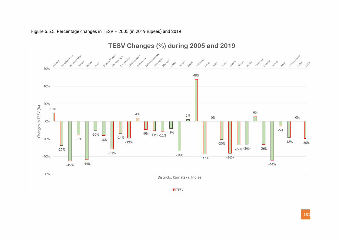
181
Figure 5.5.5. Percentage changes in TESV – 2005 (in 2019 rupees) and 2019
10%
-27%
-45%
-15%
-44%
-10%
-16%
-31%
-14%
-19%
4%
-9% -11% -11%-8%
-34%
2%
48%
-37%
0%
-20%
-36%
-27% -26%
6%
-26%
-44%
-5%
-18%
0%
-20%
-60%
-40%
-20%
0%
20%
40%
60%
Ch
ange
s in
TES
V (
%)
Districts, Karnataka, Indiae
TESV Changes (%) during 2005 and 2019
TESV
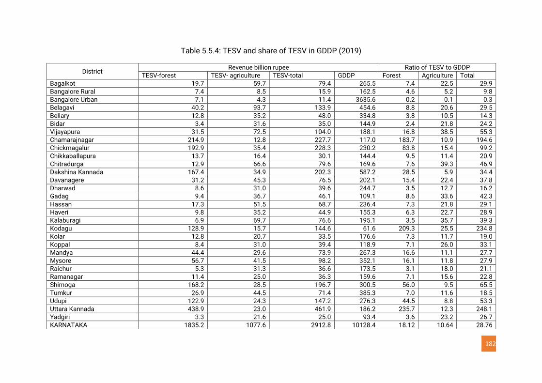
182
Table 5.5.4: TESV and share of TESV in GDDP (2019)
District Revenue billion rupee Ratio of TESV to GDDP
TESV-forest TESV- agriculture TESV-total GDDP Forest Agriculture Total
Bagalkot 19.7 59.7 79.4 265.5 7.4 22.5 29.9
Bangalore Rural 7.4 8.5 15.9 162.5 4.6 5.2 9.8
Bangalore Urban 7.1 4.3 11.4 3635.6 0.2 0.1 0.3
Belagavi 40.2 93.7 133.9 454.6 8.8 20.6 29.5
Bellary 12.8 35.2 48.0 334.8 3.8 10.5 14.3
Bidar 3.4 31.6 35.0 144.9 2.4 21.8 24.2
Vijayapura 31.5 72.5 104.0 188.1 16.8 38.5 55.3
Chamarajnagar 214.9 12.8 227.7 117.0 183.7 10.9 194.6
Chickmagalur 192.9 35.4 228.3 230.2 83.8 15.4 99.2
Chikkaballapura 13.7 16.4 30.1 144.4 9.5 11.4 20.9
Chitradurga 12.9 66.6 79.6 169.6 7.6 39.3 46.9
Dakshina Kannada 167.4 34.9 202.3 587.2 28.5 5.9 34.4
Davanagere 31.2 45.3 76.5 202.1 15.4 22.4 37.8
Dharwad 8.6 31.0 39.6 244.7 3.5 12.7 16.2
Gadag 9.4 36.7 46.1 109.1 8.6 33.6 42.3
Hassan 17.3 51.5 68.7 236.4 7.3 21.8 29.1
Haveri 9.8 35.2 44.9 155.3 6.3 22.7 28.9
Kalaburagi 6.9 69.7 76.6 195.1 3.5 35.7 39.3
Kodagu 128.9 15.7 144.6 61.6 209.3 25.5 234.8
Kolar 12.8 20.7 33.5 176.6 7.3 11.7 19.0
Koppal 8.4 31.0 39.4 118.9 7.1 26.0 33.1
Mandya 44.4 29.6 73.9 267.3 16.6 11.1 27.7
Mysore 56.7 41.5 98.2 352.1 16.1 11.8 27.9
Raichur 5.3 31.3 36.6 173.5 3.1 18.0 21.1
Ramanagar 11.4 25.0 36.3 159.6 7.1 15.6 22.8
Shimoga 168.2 28.5 196.7 300.5 56.0 9.5 65.5
Tumkur 26.9 44.5 71.4 385.3 7.0 11.6 18.5
Udupi 122.9 24.3 147.2 276.3 44.5 8.8 53.3
Uttara Kannada 438.9 23.0 461.9 186.2 235.7 12.3 248.1
Yadgiri 3.3 21.6 25.0 93.4 3.6 23.2 26.7
KARNATAKA 1835.2 1077.6 2912.8 10128.4 18.12 10.64 28.76
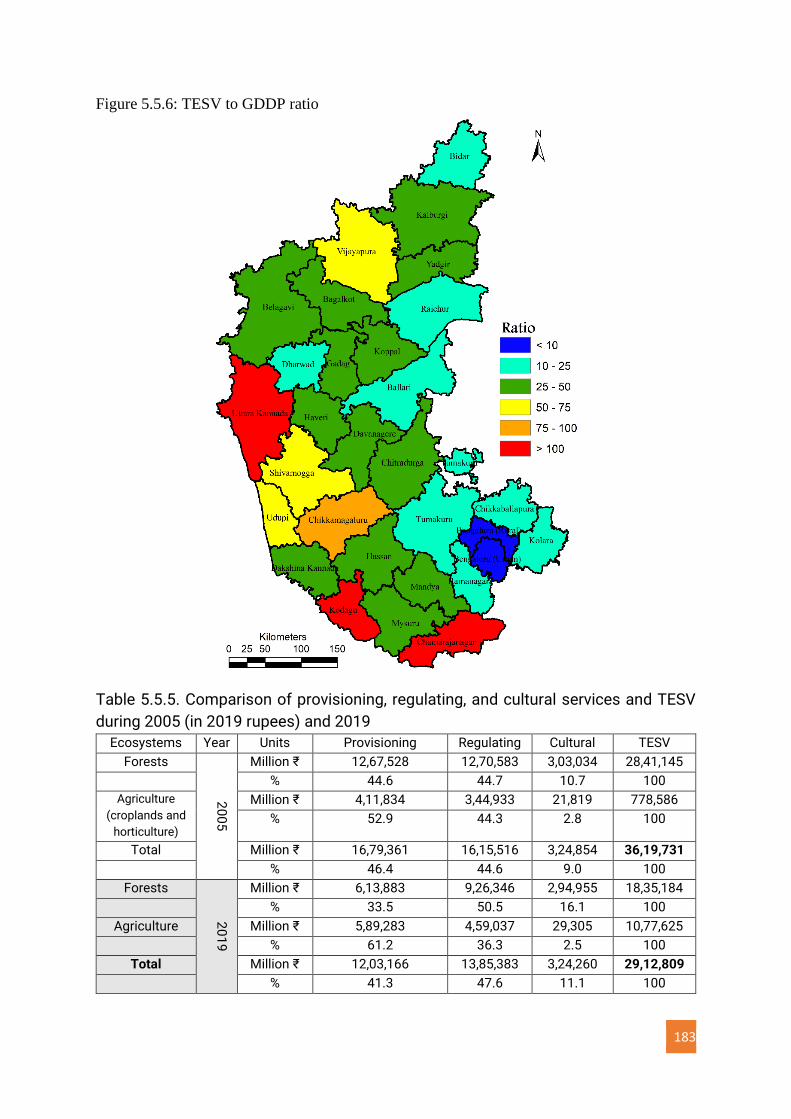
183
Figure 5.5.6: TESV to GDDP ratio
Table 5.5.5. Comparison of provisioning, regulating, and cultural services and TESV
during 2005 (in 2019 rupees) and 2019
Ecosystems Year Units Provisioning Regulating Cultural TESV
Forests
20
05
Million ₹ 12,67,528 12,70,583 3,03,034 28,41,145
% 44.6 44.7 10.7 100
Agriculture
(croplands and
horticulture)
Million ₹ 4,11,834 3,44,933 21,819 778,586
% 52.9 44.3 2.8 100
Total Million ₹ 16,79,361 16,15,516 3,24,854 36,19,731
% 46.4 44.6 9.0 100
Forests
20
19
Million ₹ 6,13,883 9,26,346 2,94,955 18,35,184
% 33.5 50.5 16.1 100
Agriculture Million ₹ 5,89,283 4,59,037 29,305 10,77,625
% 61.2 36.3 2.5 100
Total Million ₹ 12,03,166 13,85,383 3,24,260 29,12,809
% 41.3 47.6 11.1 100
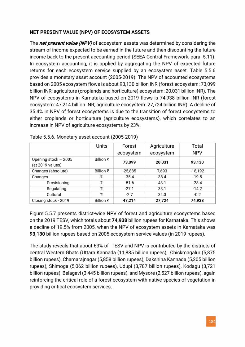
184
NET PRESENT VALUE (NPV) OF ECOSYSTEM ASSETS
The net present value (NPV) of ecosystem assets was determined by considering the
stream of income expected to be earned in the future and then discounting the future
income back to the present accounting period (SEEA Central Framework, para. 5.11).
In ecosystem accounting, it is applied by aggregating the NPV of expected future
returns for each ecosystem service supplied by an ecosystem asset. Table 5.5.6
provides a monetary asset account (2005-2019). The NPV of accounted ecosystems
based on 2005 ecosystem flows is about 93,130 billion INR (forest ecosystem: 73,099
billion INR; agriculture (croplands and horticulture) ecosystem: 20,031 billion INR). The
NPV of ecosystems in Karnataka based on 2019 flows is 74,938 billion INR (forest
ecosystem: 47,214 billion INR; agriculture ecosystem: 27,724 billion INR). A decline of
35.4% in NPV of forest ecosystems is due to the transition of forest ecosystems to
either croplands or horticulture (agriculture ecosystems), which correlates to an
increase in NPV of agriculture ecosystems by 23%.
Table 5.5.6. Monetary asset account (2005-2019)
Units Forest
ecosystem
Agriculture
ecosystem
Total
NPV
Opening stock – 2005
(at 2019 values)
Billion ₹ 73,099 20,031 93,130
Changes (absolute) Billion ₹ -25,885 7,693 -18,192
Changes % -35.4 38.4 -19.5
Provisioning % -51.6 43.1 -28.4
Regulating % -27.1 33.1 -14.2
Cultural % -2.7 34.3 -0.2
Closing stock - 2019 Billion ₹ 47,214 27,724 74,938
Figure 5.5.7 presents district-wise NPV of forest and agriculture ecosystems based
on the 2019 TESV, which totals about 74,938 billion rupees for Karnataka. This shows
a decline of 19.5% from 2005, when the NPV of ecosystem assets in Karnataka was
93,130 billion rupees based on 2005 ecosystem service values (in 2019 rupees).
The study reveals that about 63% of TESV and NPV is contributed by the districts of
central Western Ghats (Uttara Kannada (11,885 billion rupees), Chickmagalur (5,875
billion rupees), Chamarajnagar (5,858 billion rupees), Dakshina Kannada (5,205 billion
rupees), Shimoga (5,062 billion rupees), Udupi (3,787 billion rupees), Kodagu (3,721
billion rupees), Belagavi (3,445 billion rupees), and Mysore (2,527 billion rupees), again
reinforcing the critical role of a forest ecosystem with native species of vegetation in
providing critical ecosystem services.
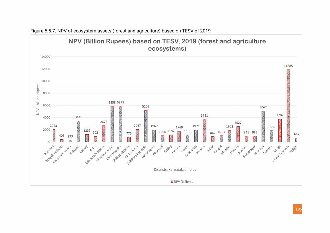
185
Figure 5.5.7. NPV of ecosystem assets (forest and agriculture) based on TESV of 2019
2043
408 293
3445
1235902
2676
5858 5875
775
2047
5205
1967
1020 11871769
1156
1971
3721
862 1013
19032527
941 935
5062
1836
3787
11885
642
0
2000
4000
6000
8000
10000
12000
14000
NP
V -
bill
ion
ru
pee
s
Districts, Karnataka, Indiae
NPV (Billion Rupees) based on TESV, 2019 (forest and agriculture ecosystems)
NPV (billion…
186
6.0 Conclusion
The compilation of ecosystem extent, service, and asset accounts using the SEEA EA
has enabled a thorough analysis of the changes in the provision of ecosystem services
in Karnataka between 2005 and 2019. The comparison of the values of goods of 2019
with 2005 highlights there has been a considerable reduction in ecosystem services
– a 28.5% reduction in provisioning services (including a 51.6% reduction in forest
ecosystem), a 21 % reduction in regulatory services (mainly in forest ecosystem -
27.1% reduction), and a 1.9% reduction in cultural services. In terms of the reductions
in provisioning services, these included a 93% decline in bamboo, a decline in NTFP
(honey reduced by 97%, tamarind reduced by 75%), a 42% decline in fodder and a 35%
decline in medicine. The large decreases in provisioning and regulatory services can
be attributed to the degradation of forests (extent and conditions) in Karnataka from
2005 to 2019.
Ecosystem services were aggregated to compute TESV. This aggregate measure is
also referred to as gross ecosystem product (GEP), equal to the sum of all final
ecosystem services (i.e., used by economic units) from ecosystem assets. The TESV
of ecosystems was 3620 billion INR in 2005 (forest ecosystem: 2,841 billion INR and
agriculture ecosystem: 779 billion INR). However, the TESV computed for 2019
indicates 2,793 billion INR (forest ecosystem: 1,835 billion INR and agriculture 958
billion INR). While the TESV for agricultural ecosystems increased by 179 billion INR
between 2005 and 2019, there was a much larger decrease in TESV for forest
ecosystems, which amounted to 1,006 billion INR. This 35.4% reduction in TESV of
forest ecosystems can again be attributed to the degradation of ecosystems.
The relationship between the SEEA EA and the System of National Accounts also
means that TESV can be compared to GDP. The GDP of Karnataka is about 10,128
billion rupees. Therefore, the TESV of the forest ecosystem is equivalent to 18.1% of
the GDP, and TESV from agriculture is equivalent to about 10.6% of GDP in Karnataka.
The district-wise assessment indicates that the TESV of Bengaluru’s urban and rural
districts are the smallest, with <10% of GDDP (Gross District Domestic Product). In
contrast, forest-rich Western Ghats districts (mainly Uttara Kannada, Kodagu, and
Chamarajanagar) provide TESV that is about 200% of the respective district GDDP.
The presence of rich forests in these districts contributes to higher TESV, highlighting
that TESV share in GDDP is correlated with the extent and conditions of forest
ecosystems in the respective districts.
The decline of TESV highlights the degradation of forest ecosystem assets from 2005
to 2019 due to the deterioration of ecosystem extent and ecosystem condition. The
decrease in value is also reflected in a fall in the NPV of expected future returns of the
ecosystem services supplied by forest ecosystem assets. The NPV of forest and
agriculture ecosystems based on 2005 ecosystem flows is about 93,130 billion INR
187
(forest ecosystem: 73,099 billion INR; agriculture ecosystem: 20,031 billion INR).
Similarly, the NPV of ecosystems in Karnataka based on 2019 flows indicates 74,938
billion INR (forest ecosystem: 47,214 billion INR, agriculture ecosystem: 27,724 billion
INR). This indicates a decline of 35.4% in NPV of forest ecosystems, largely due to the
transition of forest ecosystems to either croplands or horticulture (agriculture
ecosystems). These ecosystem conversions have led to an increase in the NPV of
agriculture ecosystems by 23% between 2005 and 2019.
The drivers behind the land-use change and the decline of forest resources in
Karnataka are mainly the expansion of agricultural activities coupled with
industrialization and rapid urbanization. However, the increase in the values of
agricultural TESV and NPV at the expense of a decrease in the values of forest TESV
and NPV points to the need for an adequate assessment of trade-offs in land use
policy. Hence, the current study emphasizes the need for the valuation of services of
all ecosystems, capitalizing on the advances in geoinformatics, availability of spatial
data at regular intervals to estimate the economic value of ecosystems forests, and,
in particular, reflect the value of forests in policy decisions.
The overall assessment of the ecological services provides information for prioritizing
ecosystems for sustainable land-use practices, promoting off-farm incomes to the
dependent communities, restoring degraded sites, biodiversity conservation, water
resources, etc., while promoting community-based prudent management of natural
resources. There is a need to enhance awareness for the protection of the
environment, especially the maintenance of native forest cover, which is crucial for
balanced economic and social progress in the country. Over the last few decades,
though India has evolved legislation, policies, and programs for environmental
protection and conservation of natural resources, there has been an uneven
implementation of these policies and programs. Thus, ecosystem accounting can play
a role in two ways. First, ecosystem accounts can help policymakers factor in
ecosystem service benefits when making economic policies that impact natural
resources and ecosystems. Second, ecosystem accounts, which are regularly
compiled, can be used to help monitor the impact of these policies over time and
ensure that they are being implemented properly.
Finally, it should be noted that the ecosystem accounts compiled for Karnataka have
a large potential to be used for payment for ecosystem services schemes. The
Supreme Court of India (2006) directed the national government to set up
compensatory payments for the conversion of different types of forested land to non-
forest uses and use these payments to improve India’s forest cover. The SEEA EA
accounts can provide important information on the values of ecosystems and their
services which can help in creating transparent criteria with which to reward states.
Afforestation in the degraded landscape would aid in mitigating changes in the
climate due to global warming while sustaining people’s livelihood through (i)
188
provision of ecosystem services, (ii) improvements in the crop yield, ii) sustenance of
water in the landscape, etc.
7.0 Recommendations
The ecosystem services computed for Karnataka State support the viability of
markets for particular ecosystem services. Developing such markets requires
additional institutional reforms such as changes with respect to property rights and
reforms in land and labor markets. Hence, ecosystem services need to be internalized
in decision-making, strengthening the economic case for conserving forests in all
states in India and developing countries, as there is great pressure to relax forest laws
and divert forests to non-forest uses with the illusion of boosting long-term economic
growth. The main policy challenge is to promote conservation and develop such
markets so that those bearing the cost of conservation are adequately compensated.
The valuation of ecosystem services done in Karnataka State and replicating this
exercise in other states will undoubtedly play a vital role in conservation planning
and ecosystem-based management in India. This requires:
i) Strengthening biophysical research on ecosystem services, with a focus on those that
would seem to have the highest economic value potential (e.g., changes in the climatic,
hydrologic regime, etc.);
ii) Inventorying, mapping, and monitoring ecosystems' spatial extent and conditions
through the use of advanced spatial technologies with temporal remote sensing data;
iii) Promoting valuation studies reveals current incentives, i.e., the existing distribution of
net ecosystem benefits/opportunity costs across stakeholders, which will aid for
internalizing in the regional policies; and
iv) Developing land-use policies which take into account the provision of ecosystem
services across different ecosystem types.
The exercise of compiling physical and monetary SEEA EA could be replicated in any
region (of 10000 to 20000 sq. km) in a period of 15 months, with a team of
multidisciplinary expertise. It requires (i) all para-state agencies sharing biophysical
data, as primary data collection is a time-consuming endeavor, (ii) Training
programmes and workshops - orientation programs, (iii) hands-on training to enhance
the capability of the team to undertake spatial analyses, (iv) collecting biophysical
data from the government agencies and in the field, (v) performing data integration
and validation, and conducting analyses of the data and interpretation, and (vi)
addressing gaps in existing biophysical models (i.e., adapting them to the local
context).
Extending this exercise in Karnataka or other states could help evolve strategies to
conserve ecosystems to support people's livelihood. As shown in this report,
ecosystem accounts can provide insights into the social, economic, and
environmental benefits of various levels of biodiversity that might be achieved under
different ecosystem management options at various scales. The economic valuation
189
of forest ecosystem services and biodiversity can help clarify trade-offs among
conflicting environmental, social, and economic goals in the development and
implementation of policies and to improve management in order to sustain
biodiversity. At the same time, there is a need to communicate more effectively the
research results on these issues to decision-makers and other stakeholders.
8.0 References and Bibliography
AGRICOOP (2020) Farmers Portal. In: Dep. Agric. Coop. Farmers Welf. Minist. Agric. Farmers Welfare, Gov. India
Amirnejad H, Khalilian S, Assareh MH, Ahmadian M (2006) Estimating the existence value of north forests of Iran by using a contingent valuation method. Ecol Econ 58:665–675
Aswathy N, Narayanakumar R, Harshan NK (2014) Marketing costs, margins and efficiency of domestic marine fish marketing in Kerala. Indian J Fish 61:97–102
Badola R, Hussain SA, Dobriyal P, et al (2017) Assessment of recreational services of natural landscapes in third world tropics using the travel cost method. Wilderness Wildl Tour 17
Balachandran. C., Chandran, M. D. S., Vinay. S., Shrikant, N., Ramachandra. T. V., 2017, Pollinator diversity and foraging dynamics on monsoon crop of cucurbits in a traditional landscape of South Indian west coast, Biotropia 24(1):16-27
Bharath S, Nimish G, Ramachandra T V (2017) Visualization and prediction of landscape dynamics in the protected areas of Karnataka. IJRET Int J Res Eng Technol 06:2321–7308. https://doi.org/10.15623/ijret.2017.0614011
Bhattacharya P, Hayat SF (2009) Sustainable NTFP management for livelihood and income generation of tribal communities: a case from Madhya Pradesh, India. Non timber For Prod Conserv Manag Policy Trop Ed By Shaanker R Uma, Ankita J Hiremath, Gladwin C Joseph Nitin D Rai Publ by ATTREE Univ Agric Sci Bangalore 21–34
Chanda S, Ramachandra T V (2019a) A review on some Therapeutic aspects of Phytochemicals present in Medicinal plants. Int J Pharm \& Life Sci 10:
Chanda S, Ramachandra T V (2019b) Sacred Groves—Repository of Medicinal Plant Resources: A Review. Res \& Rev J Ecol 8:12–20
Chandran MDS, Rao GR, Gururaja KV, Ramachandra TV (2010) Ecology of the Swampy Relic Forests of Kathalekan from Central Western Ghats , India. Bioremediation, Biodivers Bioavailab 4:54–68
Chatterjee R (2011) Groundwater resources estimation—case studies from India. J Geol Soc India 77:201–204
Cheng X, Van Damme S, Li L, Uyttenhove P (2019) Evaluation of cultural ecosystem services: A review of methods. Ecosyst Serv 37:100925
Coffee Board (2020) Daily Coffee Market Report. In: Gov. India, Minist. Commer. Ind. Commodities Online (2020) Mandi Rates Costanza R, D’Arge R, De Groot R, et al (1997) The value of the world’s ecosystem services and natural
capital. Nature. https://doi.org/10.1038/387253a0 Costanza R, De Groot R, Sutton P, et al (2014) Changes in the global value of ecosystem services. Glob
Environ Chang 26:152–158 Dadhwal VK, Singh S, Patil P (2009) Assessment of phytomass carbon pools in forest ecosystems in
India. NNRMS Bull 41–57 De Groot R, Brander L, Van Der Ploeg S, et al (2012) Global estimates of the value of ecosystems and
their services in monetary units. Ecosyst Serv 1:50–61 De Groot R, Luke B, Solomonides S (2020) Ecosystem Services Valuation Database (ESVD) Version
June 2020 De Groot RS, Leon B, Costanza R (2017) A short history of the ecosystem services concept. Mapp
Ecosyst Serv 31 De Groot RS, Wilson MA, Boumans RMJ (2002) A typology for the classification, description and
valuation of ecosystem functions, goods and services. Ecol Econ 41:393–408 Devagiri GM, Money S, Singh S, et al (2013) Assessment of above ground biomass and carbon pool in
different vegetation types of south western part of Karnataka, India using spectral modeling. Trop Ecol 54:149–165
190
Diaz S, Demissew S, Carabias J, et al (2015) The IPBES Conceptual Framework—connecting nature and people. Curr Opin Environ Sustain 14:1–16
DMI (2020) AgMarknet. In: Dir. Mark. Insp. (DMI),Ministry Agric. Farmers Welfare, Gov. India Do T Van, Trung PD, Yamamoto M, et al (2018) Aboveground biomass increment and stand dynamics
in tropical evergreen broadleaved forest. J Sustain For 37:1–14. https://doi.org/10.1080/10549811.2017.1375959
Dorji T, Brookes JD, Facelli JM, et al (2019) Socio-cultural values of ecosystem services from Oak Forests in the Eastern Himalaya. Sustainability 11:2250
DPPMS (2018) Economic Survey of Karnataka 2017 - 2018 DSO (2019) District Statistics at a Glance, District Statistical Office. Bengaluru EANDS (2020) Cost of Cultivation/Production and related data. In: Dir. Econ. Stat. Dep. Agric. Coop.
Farmers Welfare. Minist. Agric. Farmers Welfare, Govt. India Euliss Jr NH, Smith LM, Liu S, et al (2010) The need for simultaneous evaluation of ecosystem services
and land use change Foley JA, DeFries R, Asner GP, et al (2005) Global consequences of land use. Science (80- ) 309:570–
574 Garcia CA, Pascal JP (2006) Sacred forests of Kodagu: Ecological value and social role. In: Cederlof G,
Sivaramakrishnan K (eds) Ecological Nationalisms: Nature, livelihoods, and identities in south Asia. University of Washington Press, Seattle and London, pp 199–229
Ghosh N, 2020. Promoting a ‘GDP of the Poor’: The Imperative of Integrating Ecosystems Valuation in
Development Policy, ORF Occasional Paper No. 239, March 2020, Observer Research
Foundation.
Google (2020) Google Earth, http://google.com/earth Gould RK, Ardoin NM, Woodside U, et al (2014) The forest has a story: cultural ecosystem services in
Kona, Hawai ‘i. Ecol Soc 19: Gunarekha BS, Binoy TA (2017) Community based sustainable tourism development in Karnataka: A
study on Mysuru district. Asia Pacific J Res 1:121–126 Haripriya G, Sanyal S, Sinha R, Sukhdev P (2006) Green Accounting for Indian States Project. TERI Press,
New Delhi, New Delhi Haslag JH (2020) Seigniorage revenue and monetary policy. In: Handbook of Monetary Policy.
Routledge, pp 347–362 Hipólito J, Sousa B dos SB, Borges RC, et al (2019) Valuing nature’s contribution to people: The
pollination services provided by two protected areas in Brazil. Glob Ecol Conserv 20:e00782 Hirons M, Comberti C, Dunford R (2016) Valuing cultural ecosystem services. Annu Rev Environ Resour
41:545–574 HOPCOMS (2019) Fruits market Price in Bangalore, Karnataka Inflation (2021) Inflation calculator - Indian Rupee. In: Inflat. tool. https://www.inflationtool.com/indian-
rupee KFD (2020), Karnataka Forest Department, https://aranya.gov.in/aranyacms/ English/Home.aspx KMV (2020) Krishi Marata Vahini. In: Deparment Agric. Mark. Karnataka State Agric. Mark. Board Kreye MM, Adams DC, Ghimire R, et al (2019) Forest Ecosystem Services: Cultural Values KSRSAC (2018) Karnataka Geographical Information System. In: Gov. Karnataka Joshi J., Negi GCS (2011) Quantification and valuation of forest ecosystem services in the western
Himalayan region of India, International Journal of Biodiversity Science, Ecosystem Services & Management, 7:1, 2-11, DOI: 10.1080/21513732.2011.598134
Kulkarni V, Ramachandra T V (2009) Environmental management, Commonwealth of learning, Canada and Indian Institute of Science, Bangalore
Lal R, Smith P, Jungkunst HF, et al (2018) The carbon sequestration potential of terrestrial ecosystems. J Soil Water Conserv 73:. https://doi.org/10.2489/jswc.73.6.145A
Ma E, Feng Z, Zheng Y (2019) The Effect of Forest on Soil Erosion Control Based on Remote Sensing Technology. Ekoloji Derg
Maes J, Czúcz B, Keith H, et al (2020) A review of ecosystem condition accounts: lessons learned and options for further development
Maes J, Teller A, Erhard M, et al (2013) Mapping and Assessment of Ecosystems and their Services. An Anal Framew Ecosyst assessments under action 5:1–58
Maes J, Teller A, Erhard M, et al (2018) Mapping and Assessment of Ecosystems and their Services: An analytical framework for ecosystem condition. Publ Off Eur Union, Luxemb 1–78
191
Maes J, Zulian G, Thijssen M, et al (2016) Mapping and Assessment of Ecosystems and their Services: Urban ecosystems. Publ Off Eur Union, Luxemb 4:
Markandya A, Harou P, Bellu LG, et al (2002) Environmental economics for sustainable growth: A handbook for practitioners. Edward Elgar Publishing Ltd
MEA (2005) Ecosystems and human well-being. Island Press Washington, DC Mengist W, Soromessa T (2019) Assessment of forest ecosystem service research trends and
methodological approaches at global level: a meta-analysis. Environ Syst Res 8:22. https://doi.org/10.1186/s40068-019-0150-4
Moreno G, Aviron S, Berg S, et al (2018) Agroforestry systems of high nature and cultural value in Europe: provision of commercial goods and other ecosystem services. Agrofor Syst 92:877–891
MoSPI (2021) Ecosystem Accounts for India - Report of the NCAVES Project. New Delhi MoSPI (2020), Forests - the Climate Protectors (Chapter 3),
https://mospi.gov.in/documents/213904//649960//1614147361232_b3_ES2_2020.pdf http://mospi.nic.in/sites/default/files/reports_and_publication/statistical_publication/EnviStats2/ES2_2020_Complete_revised%20on%204_11_2020.pdf
MSP (2020) MSP for Rabi Crops 2019 - 2020. In: Minist. Agric. Farmers Welfare, Gov. India Murali G (2010) Opportunity to Sustain Coconut Ecosystem Services through Recycling of the Palm
Leaf Litter as Vermicompost: Indian Scenario (A Technology/ Research Note). CORD 26:14. https://doi.org/10.37833/cord.v26i2.130
NAAS (2020) Payment for Ecosystem Services in Agriculture. New Delhi Nair PKR, Nair VD, Kumar BM, Haile SG (2009) Soil carbon sequestration in tropical agroforestry
systems: a feasibility appraisal. Environ Sci Policy 12:1099–1111. https://doi.org/10.1016/j.envsci.2009.01.010
NAP (2009) National Afforestation Programme Revised Operational Guidelines. New Delhi Nayak AK, Shahid M, Nayak AD, et al (2019) Assessment of ecosystem services of rice farms in eastern
India. Ecol Process 8:35. https://doi.org/10.1186/s13717-019-0189-1 NIC (2020) Soil Health Maps. In: Deparment Agric. Coop. Farmers Welfare, Gov. India Ninan KN, Kontoleon A (2016) Valuing forest ecosystem services and disservices – Case study of a
protected area in India, Ecosystem Services, 20 (2016): 1-14, ISSN 2212-0416, https://doi.org/10.1016/j.ecoser.2016.05.001.
NRSC (2020) National Remote Sensing Centre-IRS data products. In: Indian Sp. Res. Organ. Gov. India NRSC (2016) Bhuvan-National Remote Sensing Centre. In: Indian Sp. Res. Organ. Gov. India Ollerton J, Winfree R, Tarrant S (2011) How many flowering plants are pollinated by animals? Oikos
120:321–326 Ormsby AA, Bhagwat SA (2010) Sacred forests of India: a strong tradition of community-based natural
resource management. Environ Conserv 320–326 Pal S (2018) Agriculture and Ecosystem Services. ICAR-National Institute of Agricultural Economics
and Policy Research, New Delhi, New Delhi Pandey R, Rawat GS, Kishwan J (2011) Changes in Distribution of Carbon in Various Forest Types of
India from 1995-2005 Changements dans la Distribution du Carbone dans Différents Types de Forêts en Inde. Silva Lusit 19:41–54
Perelet R, Mason P, Markandya A, Taylor T (2014) Dictionary of environmental economics. Routledge Planning Commission (2011) Report of the sub-group II on NTFP and their sustainable management in
the 12th five year plan. A Rep Submitt under Plan Comm Work Gr For Nat Resour Manag Polasky S, Tallis H, Reyers B (2015) Setting the bar: Standards for ecosystem services. Proc Natl Acad
Sci 112:7356–7361. https://doi.org/10.1073/pnas.1406490112 Prasad SN, Hedge M, Hedge MS (1987) Fuel Consumption and Conservation Method in Urban Centres
of Uttara Kannada, CES Technical Report 25,. Bangalore Rai SN, Proctor J (1986) Ecological Studies on Four Rainforests in Karnataka , India. J Ecol 74:439–454 Rajan K, Natarajan A, Anil Kumar KS, et al (2010) Soil organic carbon - the most reliable indicator for
monitoring land degradation by soil erosion. Curr Sci 99:823–827 Ramachandra T., Joshi N., Subramanian D. (2000a) Present and prospective role of bioenergy in
regional energy system. Renew Sustain Energy Rev 4:375–430. https://doi.org/10.1016/S1364-0321(00)00002-2
Ramachandra T. V, Chandran, M D S, Bharath S, et al (2018a) Forest Ecosystem: Goods and Services, ENVIS Technical Report 142, Sahyadri Conservation Series 79,. Bangalore
Ramachandra T, Bharath S, Vinay S, et al (2019a) Grid Based Monitoring of Natural Resources in the Ecologically Fragile Regions of Kodagu, Karnataka, ENVIS Technical Report 156, Sahyadri

192
Conservation Series 83. Bangalore Ramachandra T, Vinay S, Bharath S, Shashishankar A (2018b) Eco-Hydrological Footprint of a River
Basin in Western Ghats. Yale Journal of Biology and Medicine Inc. Ramachandra TV, Bharath S (2019a) Global Warming Mitigation Through Carbon Sequestrations in the
Central Western Ghats. Remote Sens Earth Syst Sci 2:39–63. https://doi.org/10.1007/s41976-019-0010-z
Ramachandra TV, Bharath S (2021) Carbon Footprint of Karnataka: Accounting of Sources and Sinks. In: Carbon Footprint Case Studies. Springer, pp 53–92
Ramachandra TV, Bharath S (2019b) Carbon Sequestration Potential of the Forest Ecosystems in the Western Ghats, a Global Biodiversity Hotspot. Nat Resour Res 29:2753–2771. https://doi.org/10.1007/s11053-019-09588-0
Ramachandra TV, Bharath S, Gupta N (2018c) Modelling landscape dynamics with LST in protected areas of Western Ghats, Karnataka. J. Environ. Manage. 1253–1262
Ramachandra TV, Bharath S, Vinay S (2019b) Visualisation of impacts due to the proposed developmental projects in the ecologically fragile regions- Kodagu district, Karnataka. Prog Disaster Sci 3:100038. https://doi.org/10.1016/j.pdisas.2019.100038
Ramachandra TV, Bharath S, Vinay S, Bharath HA (2021a) Ecosystem Extent Account for Karnataka. Bangalore
Ramachandra TV, Bharath S, Vinay S, Bharath HA (2021b) Ecosystem Condition Account for Karnataka. Bangalore
Ramachandra TV, Chandran MDS, Gururaja KV, Sreekantha (2007) Cumulative environmental impact assessment. Nova Science Publishers, New York, NY (United States)
Ramachandra TV, Chandran MDS, Rao GR, et al (2015) Floristic diversity in Uttara Kannada district, Karnataka, Chapter 1, In Biodiversity in India. Regency publications, New Delhi
Ramachandra TV, Chandran MDS, Vinay S, et al (2016) Sacred Groves (Kan forests) of Sagara taluk, Shimoga district, Sahyadri Conservation Series: 54, ENVIS Technical Report 102,. BANGALORE
Ramachandra TV, Soman D, Naik AD, Chandran MDS (2017) Appraisal of Forest Ecosystems Goods and Services: Challenges and Opportunities for Conservation. J Biodivers 8:12–33. https://doi.org/10.1080/09766901.2017.1346160
Ramachandra TV, Subramanian DK, Joshi NV, et al (2000b) Domestic energy consumption patterns in Uttara Kannada District, Karnataka State, India. Energy Convers Manag 41:775–831. https://doi.org/10.1016/S0196-8904(99)00151-X
Ramachandra TV, Vinay S, Bharath S, et al (2020) Insights into riverscape dynamics with the hydrological, ecological and social dimensions for water sustenance. Curr Sci 113891:118
Ramachandra T V., Chandran MDS, Ananth A, et al (2012) Tragedy of the Kan Sacred Forests of Shimoga District: Need for Urgent Policy Interventions for Conservation, CES Technical Report: 128,. Bangalore
Ramachandra T V., Joshi N V., Subramanian DK (2000c) Present and prospective role of bioenergy in regional energy system. Renew Sustain Energy Rev 4:375–430. https://doi.org/10.1016/S1364-0321(00)00002-2
Ramachandra T V., Subramanian DK, Joshi N V., et al (2000d) Domestic energy consumption patterns in Uttara Kannada District, Karnataka State, India. Energy Convers Manag 41:775–831. https://doi.org/10.1016/S0196-8904(99)00151-X
Ramachandra T V, Chandran MDS, Harish BR, et al (2010) Biodiversity, Ecology and Socio Economic Aspects of Gundia River Basin in the Context of Proposed Mega Hydro Electric Power Project, CES Technical Report 122. BENGALURU
Ramachandra T V, Subramanian DK, Joshi N V (2001) A decision support system for optimal design of hydroelectric projects in Uttara Kannada. Energy Sustain Dev 5:14–31
Ramachandra T V, Subramanian DK, Joshi N V (1999) Hydroelectric resource assessment in Uttara Kannada district, Karnataka state, India. J Clean Prod 7:195–211
Rao G, Krishnakumar G, Sumesh Dudani N, Ramachandra T V et al (2013) Vegetation Changes along Altitudinal Gradients in Human Disturbed Forests of Uttara Kannada, Central Western Ghats. J Biodivers 4:61–68
Rao GR, Chandran MDS, Ramachandra T V. (2015) Diversity and Regeneration Status of Medicinal Plants in Medicinal Plants Conservation Area (MPCA) at Shirgunji of Uttara Kannada District, Central Western Ghats. MyForest 51:85–99
Rao GR, Krishnakumar G, Dudani SN, et al (2014) Diversity and Regeneration Aspects of Medicinal Plants at Devimane, Uttara Kannada District, Karnataka, Central Western Ghats. J Biodivers
193
Manag For 8:2 Ravindranath NH, Ostwald M (2008) Carbon inventory methods: a handbook for greenhouse gas
inventory, carbon mitigation and roundwood production projects. Advances in Global Change Research. Carbon Invent methods a Handb Greenh gas Invent carbon Mitig roundwood Prod Proj Adv Glob Chang Res 237–270. https://doi.org/10.1007/978-1-4020-6547-7_10
Ravindranath NH, Somashekhar BS, Gadgil M (1997) Carbon flow in Indian forests. Clim Change 35:297–320. https://doi.org/10.1023/A:1005303405404
Ray R, Bharath S, Ramachandra T V (2014a) Biodiversity Conservation in Humanised Landscape–Challenges and Opportunity. In: LAKE 2014. EWRG, CES, IISc, Bangalore
Ray R, Chandran MDS, Ramachandra T V (2015) Hydrological importance of sacred forest fragments in Central Western Ghats of India. Trop Ecol 56:87–99
Ray R, Chandran MDS, Ramachandra T V (2014b) Biodiversity and ecological assessments of Indian sacred groves. J For Res 25:21–28
Ray R, Ramachandra T V (2010) Small sacred groves in local landscape: are they really worthy for conservation? Curr Sci 98:1178–1180
Ray R, Subash Chandran MD, Ramachandra T V (2010) Ecosystem services from sacred groves of Uttar Kannada: A case study. In: Bangalore: LAKE 2010 Conference 22nd-24th December
Rodríguez JP, Beard Jr TD, Bennett EM, et al (2006) Trade-offs across space, time, and ecosystem services. Ecol Soc 11:
SEEA (2017) System of Environmental Economic Accounting 2012: Central Framework. International Monetary Fund
SEEA EA (2021) System of Environmental-Economic Accounting—Ecosystem Accounting, Final Draft, Version 5,. Department Of Economic And Social Affairs, Statistics Division, United NationsISION, UNITED NATIONS
Sinclair M, Mayer M, Woltering M, Ghermandi A (2020) Valuing nature-based recreation using a crowdsourced travel cost method: A comparison to onsite survey data and value transfer. Ecosyst Serv 45:101165
Swamy HR (1992) Organic productivity, nutrient cycling and small watershed hydrology of natural forests and monoculture plantations in Chikmagalur District, Karnataka. John Wiley and Sons, Inc., New York, NY (United States)
TEEB (2010a) The Economics of Ecosystems and Biodiversity, Ecological and Economic Foundations. Earthscan, London and Washington.
TEEB (2010b) Mainstreaming the Economics of Nature: A Synthesis of the Approach, Conclusions and Recommendations of TEEB. TEEB
Ten Brink P (2011) The economics of ecosystems and biodiversity in national and international policy making. Routledge
Terrado M, Acuña V, Ennaanay D, et al (2014) Impact of climate extremes on hydrological ecosystem services in a heavily humanized Mediterranean basin. Ecol Indic 37:199–209
Vallecillo S, La Notte A, Zulian G, et al (2019) Ecosystem services accounts: Valuing the actual flow of nature-based recreation from ecosystems to people. Ecol Modell 392:196–211
Van Berkel DB, Verburg PH (2014) Spatial quantification and valuation of cultural ecosystem services in an agricultural landscape. Ecol Indic 37:163–174
Van der P, De Groot RS, Wang Y (2010) The TEEB Valuation Database: overview of structure, data and results. Wageningen, the Netherlands
Verma M, Joshi S, Godbole G., Singh A. (2007) Valuation of Ecosystem Services and Forest Governance
- A scoping study from Uttarakhand, LEAD India, New Delhi
Verma M, Negandhi D, Wahal AK, Kumar R (2013) Revision of rates of NPV applicable for different class/category of forests. AcademiaEdu 143
World Bank (1998) The World Bank annual report 1998 (English). Washington, D.C. World Bank (2001) The World Bank annual report 2001 : Year in review (English). Washington, D.C. Zarandian A, Baral H, Yavari AR, et al (2016) Anthropogenic decline of ecosystem services threatens
the integrity of the unique Hyrcanian (Caspian) forests in Northern Iran. Forests 7:51 Zawadzka J, Gallagher E, Smith H, Corstanje R (2019) Ecosystem services from combined natural and
engineered water and wastewater treatment systems: Going beyond water quality enhancement. Ecol Eng X 2:100006. https://doi.org/10.1016/j.ecoena.2019.100006
194
Annexures
3.1 Socio-economic survey: agriculture
3.2 Horticulture (areca/coconut/..)
3.3 Valuation of ecosystem services of Sacred Grooves in Karnataka
3.4 Tourism and recreational services of forest ecosystems in Karnataka
4.1 Global climate regulation service – carbon storage in forest ecosystems
(Note: this service is not accounted in the valuation of ecosystem services)
5.3 Valuation of forest ecosystem services (provisioning, regulating and cultural) at the
district level
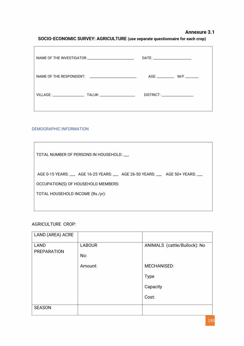
195
Annexure 3.1
SOCIO-ECONOMIC SURVEY: AGRICULTURE (use separate questionnaire for each crop)
NAME OF THE INVESTIGATOR ____________________________ DATE: _______________________
NAME OF THE RESPONDENT: ____________________________ AGE: __________ M/F ________
VILLAGE: ___________________ TALUK: _____________________ DISTRICT: ___________________
DEMOGRAPHIC INFORMATION
TOTAL NUMBER OF PERSONS IN HOUSEHOLD: ___
AGE 0-15 YEARS: ___ AGE 16-25 YEARS: ___ AGE 26-50 YEARS: ___ AGE 50+ YEARS: ___
OCCUPATION(S) OF HOUSEHOLD MEMBERS:
TOTAL HOUSEHOLD INCOME (Rs./yr):
AGRICULTURE CROP:
LAND (AREA) ACRE
LAND
PREPARATION
LABOUR
No:
Amount:
ANIMALS (cattle/Bullock): No
MECHANISED:
Type
Capacity
Cost:
SEASON

196
SEED TYPE
QUANTITY
COST
SOWING
LABOUR
AMOUNT:
ADDITIONAL WORK –
DEWEEDING
LABOUR
AMOUNT
TRANSPLANTATION
(FOR PADDY)
LABOUR
TYPE
COST
MANURE /Fertiliser Frequency:
Type:
Quantity
Cost:
IRRIGATION TYPE:
Frequency
Electricity
Motor (HP)
Duration
Cost
PESTS
PROTECTION (WILD
PIG, BANDICOT,
MONKEY, …)
PEST Type
DAMAGE EXTENT
PROTECTION
TYPE
Cost
PESTICIDE / Type Labour
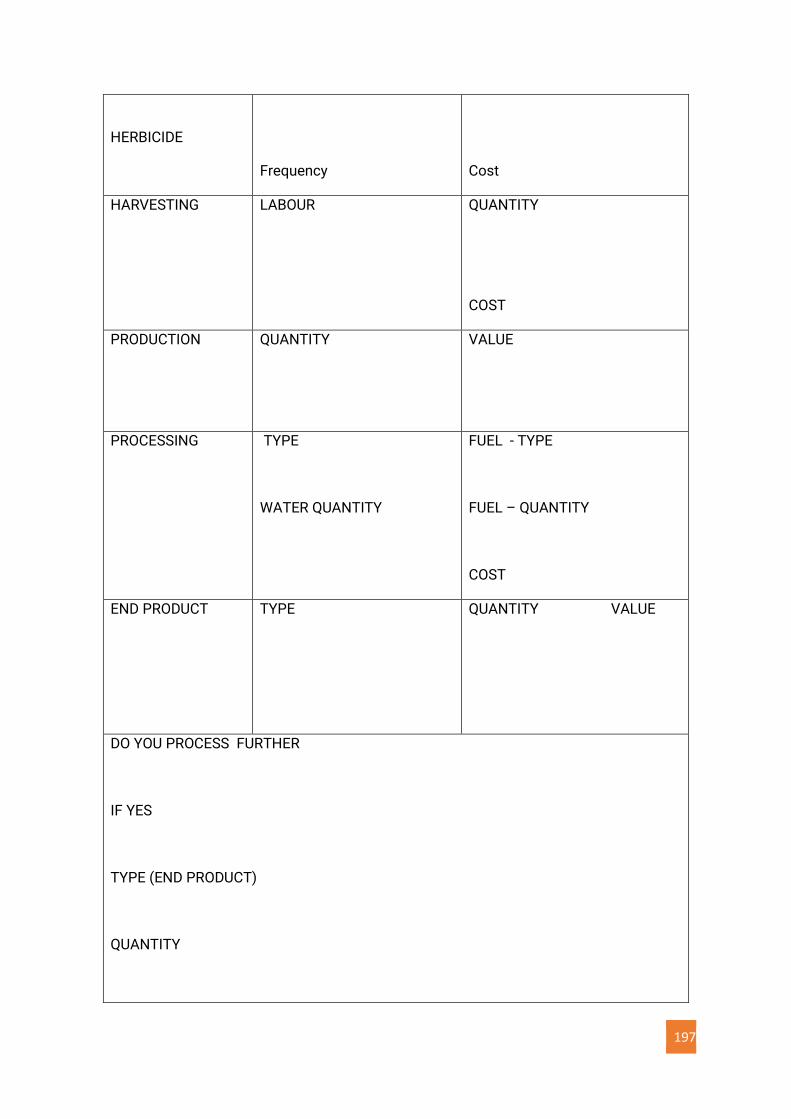
197
HERBICIDE
Frequency
Cost
HARVESTING LABOUR
QUANTITY
COST
PRODUCTION QUANTITY VALUE
PROCESSING
TYPE
WATER QUANTITY
FUEL - TYPE
FUEL – QUANTITY
COST
END PRODUCT TYPE
QUANTITY VALUE
DO YOU PROCESS FURTHER
IF YES
TYPE (END PRODUCT)
QUANTITY
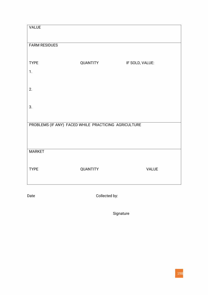
198
VALUE
FARM RESIDUES
TYPE QUANTITY IF SOLD, VALUE:
1.
2.
3.
PROBLEMS (IF ANY) FACED WHILE PRACTICING AGRICULTURE
MARKET
TYPE QUANTITY VALUE
Date Collected by:
Signature
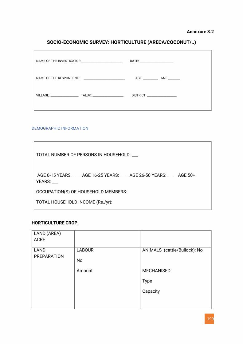
199
Annexure 3.2
SOCIO-ECONOMIC SURVEY: HORTICULTURE (ARECA/COCONUT/..)
NAME OF THE INVESTIGATOR ____________________________ DATE: _______________________
NAME OF THE RESPONDENT: ____________________________ AGE: __________ M/F ________
VILLAGE: ___________________ TALUK: _____________________ DISTRICT: ____________________
DEMOGRAPHIC INFORMATION
TOTAL NUMBER OF PERSONS IN HOUSEHOLD: ___
AGE 0-15 YEARS: ___ AGE 16-25 YEARS: ___ AGE 26-50 YEARS: ___ AGE 50+
YEARS: ___
OCCUPATION(S) OF HOUSEHOLD MEMBERS:
TOTAL HOUSEHOLD INCOME (Rs./yr):
HORTICULTURE CROP:
LAND (AREA)
ACRE
LAND
PREPARATION
LABOUR
No:
Amount:
ANIMALS (cattle/Bullock): No
MECHANISED:
Type
Capacity
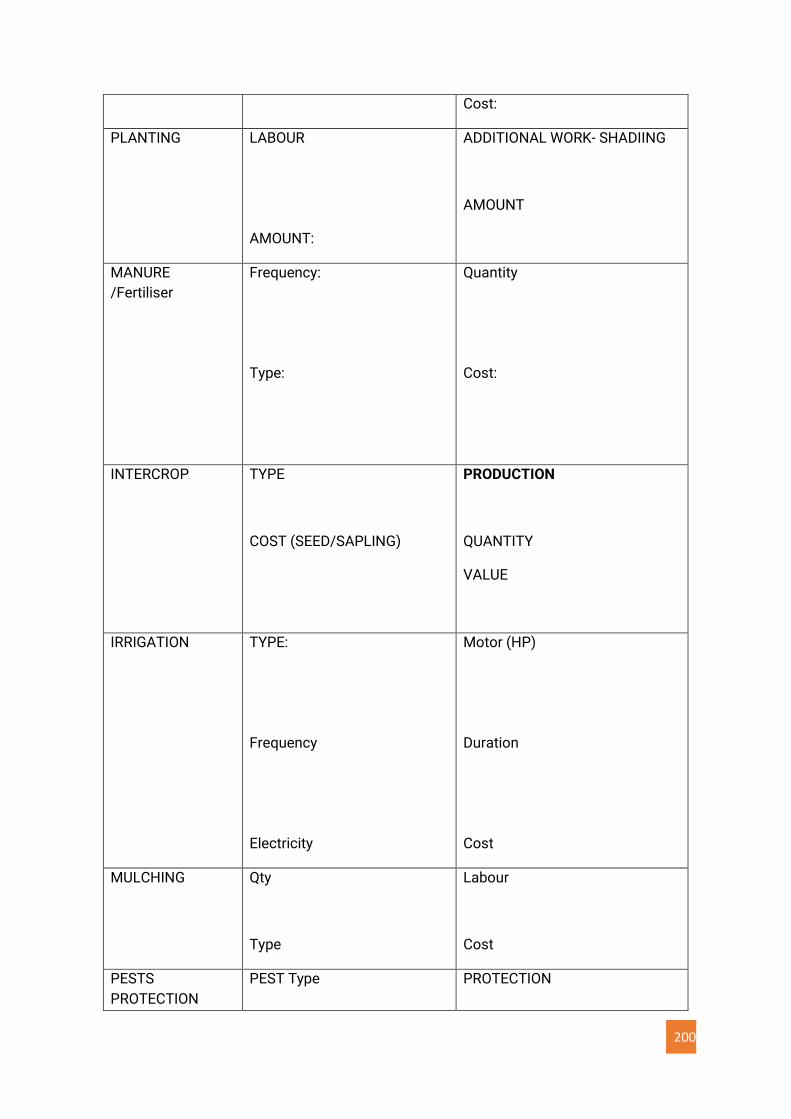
200
Cost:
PLANTING
LABOUR
AMOUNT:
ADDITIONAL WORK- SHADIING
AMOUNT
MANURE
/Fertiliser
Frequency:
Type:
Quantity
Cost:
INTERCROP
TYPE
COST (SEED/SAPLING)
PRODUCTION
QUANTITY
VALUE
IRRIGATION TYPE:
Frequency
Electricity
Motor (HP)
Duration
Cost
MULCHING Qty
Type
Labour
Cost
PESTS
PROTECTION
PEST Type PROTECTION
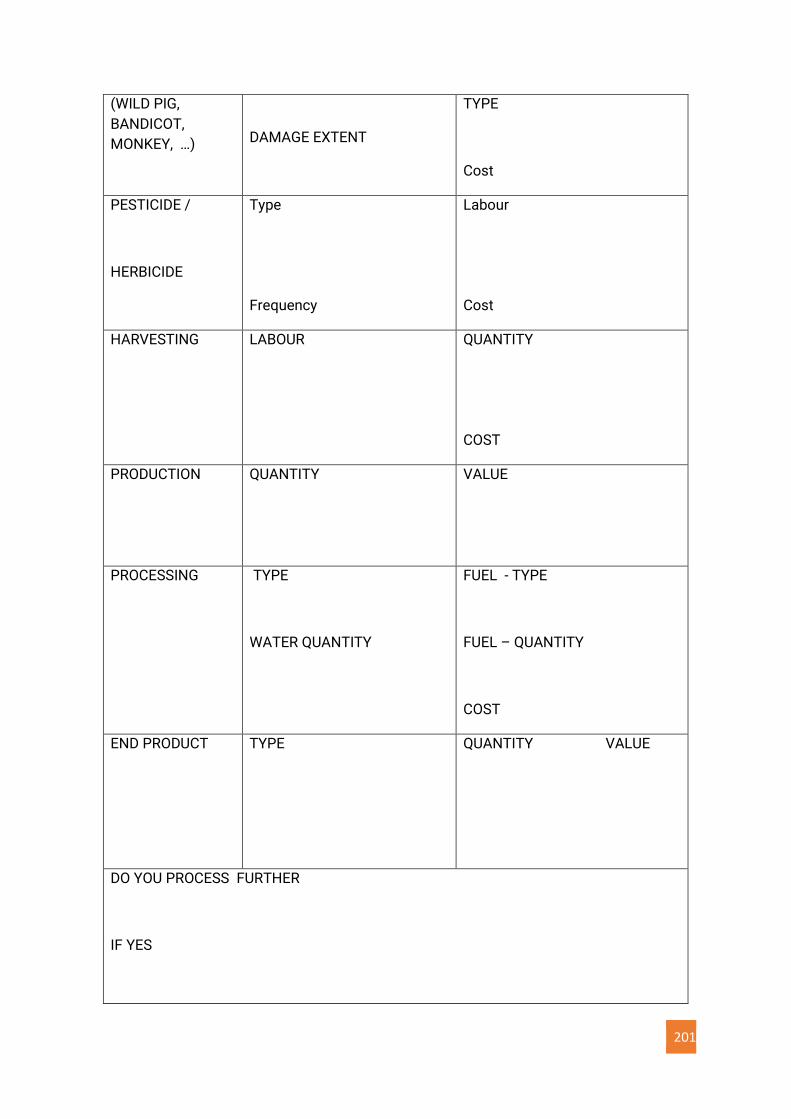
201
(WILD PIG,
BANDICOT,
MONKEY, …)
DAMAGE EXTENT
TYPE
Cost
PESTICIDE /
HERBICIDE
Type
Frequency
Labour
Cost
HARVESTING LABOUR
QUANTITY
COST
PRODUCTION QUANTITY VALUE
PROCESSING
TYPE
WATER QUANTITY
FUEL - TYPE
FUEL – QUANTITY
COST
END PRODUCT TYPE
QUANTITY VALUE
DO YOU PROCESS FURTHER
IF YES
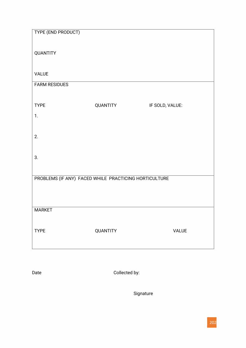
202
TYPE (END PRODUCT)
QUANTITY
VALUE
FARM RESIDUES
TYPE QUANTITY IF SOLD, VALUE:
1.
2.
3.
PROBLEMS (IF ANY) FACED WHILE PRACTICING HORTICULTURE
MARKET
TYPE QUANTITY VALUE
Date Collected by:
Signature
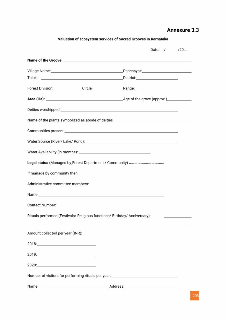
203
Annexure 3.3
Valuation of ecosystem services of Sacred Grooves in Karnataka
Date: / /20….
Name of the Groove:
Village Name: Panchayat:
Taluk: District:
Forest Division: Circle: Range:
Area (Ha): Age of the grove (approx.)
Deities worshipped:
Name of the plants symbolized as abode of deities
Communities present:
Water Source (River/ Lake/ Pond):
Water Availability (in months):
Legal status (Managed by Forest Department / Community) ……………………………….
If manage by community then,
Administrative committee members:
Name:
Contact Number:
Rituals performed (Festivals/ Religious functions/ Birthday/ Anniversary):
Amount collected per year (INR):
2018:
2019:
2020:
Number of visitors for performing rituals per year:
Name: Address:
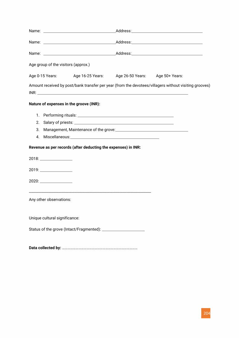
204
Name: Address:
Name: Address:
Name: Address:
Age group of the visitors (approx.)
Age 0-15 Years: Age 16-25 Years: Age 26-50 Years: Age 50+ Years:
Amount received by post/bank transfer per year (from the devotees/villagers without visiting grooves)
INR:
Nature of expenses in the groove (INR):
1. Performing rituals:
2. Salary of priests:
3. Management, Maintenance of the grove:
4. Miscellaneous:
Revenue as per records (after deducting the expenses) in INR:
2018:
2019:
2020:
--------------------------------------------------------------------------------------------------------------
Any other observations:
Unique cultural significance:
Status of the grove (Intact/Fragmented):
Data collected by: …………………………………………………………………………
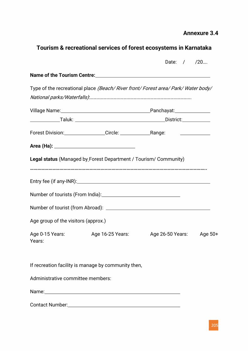
205
Annexure 3.4
Tourism & recreational services of forest ecosystems in Karnataka
Date: / /20….
Name of the Tourism Centre:
Type of the recreational place (Beach/ River front/ Forest area/ Park/ Water body/
National parks/Waterfalls):……………………………………………………………………………….
Village Name: Panchayat:
Taluk: District:
Forest Division: Circle: Range:
Area (Ha):
Legal status (Managed by Forest Department / Tourism/ Community)
……………………………………………………………………………………………………………………………..
Entry fee (if any-INR):
Number of tourists (From India):
Number of tourist (from Abroad):
Age group of the visitors (approx.)
Age 0-15 Years: Age 16-25 Years: Age 26-50 Years: Age 50+
Years:
If recreation facility is manage by community then,
Administrative committee members:
Name:
Contact Number:
206
Accommodation status:……………………………………………….
If available then,
Type of the accommodation:…………………………………………
Price per day (INR):……………………………………
Peak season of tourism activities (Monsson/Summer): ……………………….
Gross Revenue generated per year (INR):
2018:
2019:
2020:
Nature of expenses (INR):
1. Maintenance of the location:
2. Salary of the employers:
3. Miscellaneous:
Revenue as per records (after deducting the expenses) in INR:
2018:
2019:
2020:
--------------------------------------------------------------------------------------------------------------
Any other observations:
Uniqueness of the region:
Status of the environment:
Data collected by: …………………………………………………………………………
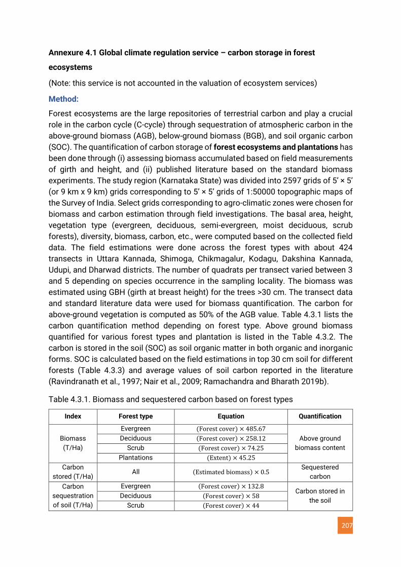
207
Annexure 4.1 Global climate regulation service – carbon storage in forest
ecosystems
(Note: this service is not accounted in the valuation of ecosystem services)
Method:
Forest ecosystems are the large repositories of terrestrial carbon and play a crucial
role in the carbon cycle (C-cycle) through sequestration of atmospheric carbon in the
above-ground biomass (AGB), below-ground biomass (BGB), and soil organic carbon
(SOC). The quantification of carbon storage of forest ecosystems and plantations has
been done through (i) assessing biomass accumulated based on field measurements
of girth and height, and (ii) published literature based on the standard biomass
experiments. The study region (Karnataka State) was divided into 2597 grids of 5’ × 5’
(or 9 km x 9 km) grids corresponding to 5’ × 5’ grids of 1:50000 topographic maps of
the Survey of India. Select grids corresponding to agro-climatic zones were chosen for
biomass and carbon estimation through field investigations. The basal area, height,
vegetation type (evergreen, deciduous, semi-evergreen, moist deciduous, scrub
forests), diversity, biomass, carbon, etc., were computed based on the collected field
data. The field estimations were done across the forest types with about 424
transects in Uttara Kannada, Shimoga, Chikmagalur, Kodagu, Dakshina Kannada,
Udupi, and Dharwad districts. The number of quadrats per transect varied between 3
and 5 depending on species occurrence in the sampling locality. The biomass was
estimated using GBH (girth at breast height) for the trees >30 cm. The transect data
and standard literature data were used for biomass quantification. The carbon for
above-ground vegetation is computed as 50% of the AGB value. Table 4.3.1 lists the
carbon quantification method depending on forest type. Above ground biomass
quantified for various forest types and plantation is listed in the Table 4.3.2. The
carbon is stored in the soil (SOC) as soil organic matter in both organic and inorganic
forms. SOC is calculated based on the field estimations in top 30 cm soil for different
forests (Table 4.3.3) and average values of soil carbon reported in the literature
(Ravindranath et al., 1997; Nair et al., 2009; Ramachandra and Bharath 2019b).
Table 4.3.1. Biomass and sequestered carbon based on forest types
Index Forest type Equation Quantification
Biomass
(T/Ha)
Evergreen (Forest cover) × 485.67
Above ground
biomass content
Deciduous (Forest cover) × 258.12
Scrub (Forest cover) × 74.25
Plantations (Extent) × 45.25
Carbon
stored (T/Ha) All (Estimated biomass) × 0.5
Sequestered
carbon
Carbon
sequestration
of soil (T/Ha)
Evergreen (Forest cover) × 132.8 Carbon stored in
the soil Deciduous (Forest cover) × 58
Scrub (Forest cover) × 44
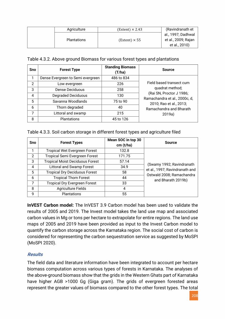
208
Agriculture (Extent) × 2.43 (Ravindranath et
al., 1997; Dadhwal
et al., 2009; Rajan
et al., 2010)
Plantations (Extent) × 55
Table 4.3.2. Above ground Biomass for various forest types and plantations
Sno Forest Type Standing Biomass
(T/ha) Source
1 Dense Evergreen to Semi evergreen 486 to 834
Field based transect cum
quadrat method;
(Rai SN, Proctor J 1986;
Ramachandra et al., 2000c, d,
2010; Rao et al., 2013;
Ramachandra and Bharath
2019a)
2 Low evergreen 226
3 Dense Deciduous 258
4 Degraded Deciduous 130
5 Savanna Woodlands 75 to 90
6 Thorn degraded 40
7 Littoral and swamp 215
8 Plantations 45 to 126
Table 4.3.3. Soil carbon storage in different forest types and agriculture filed
Sno Forest Types Mean SOC in top 30
cm (t/ha) Source
1 Tropical Wet Evergreen Forest 132.8
(Swamy 1992; Ravindranath
et al., 1997; Ravindranath and
Ostwald 2008; Ramachandra
and Bharath 2019b)
2 Tropical Semi Evergreen Forest 171.75
3 Tropical Moist Deciduous Forest 57.14
4 Littoral and Swamp Forest 34.9
5 Tropical Dry Deciduous Forest 58
6 Tropical Thorn Forest 44
7 Tropical Dry Evergreen Forest 33
8 Agriculture Fields 4
9 Plantations 55
InVEST Carbon model: The InVEST 3.9 Carbon model has been used to validate the
results of 2005 and 2019. The Invest model takes the land use map and associated
carbon values in Mg or tons per hectare to extrapolate for entire regions. The land use
maps of 2005 and 2019 have been provided as input to the Invest Carbon model to
quantify the carbon storage across the Karnataka region. The social cost of carbon is
considered for representing the carbon sequestration service as suggested by MoSPI
(MoSPI 2020).
Results
The field data and literature information have been integrated to account per hectare
biomass computation across various types of forests in Karnataka. The analyses of
the above-ground biomass show that the grids in the Western Ghats part of Karnataka
have higher AGB >1000 Gg (Giga gram). The grids of evergreen forested areas
represent the greater values of biomass compared to the other forest types. The total
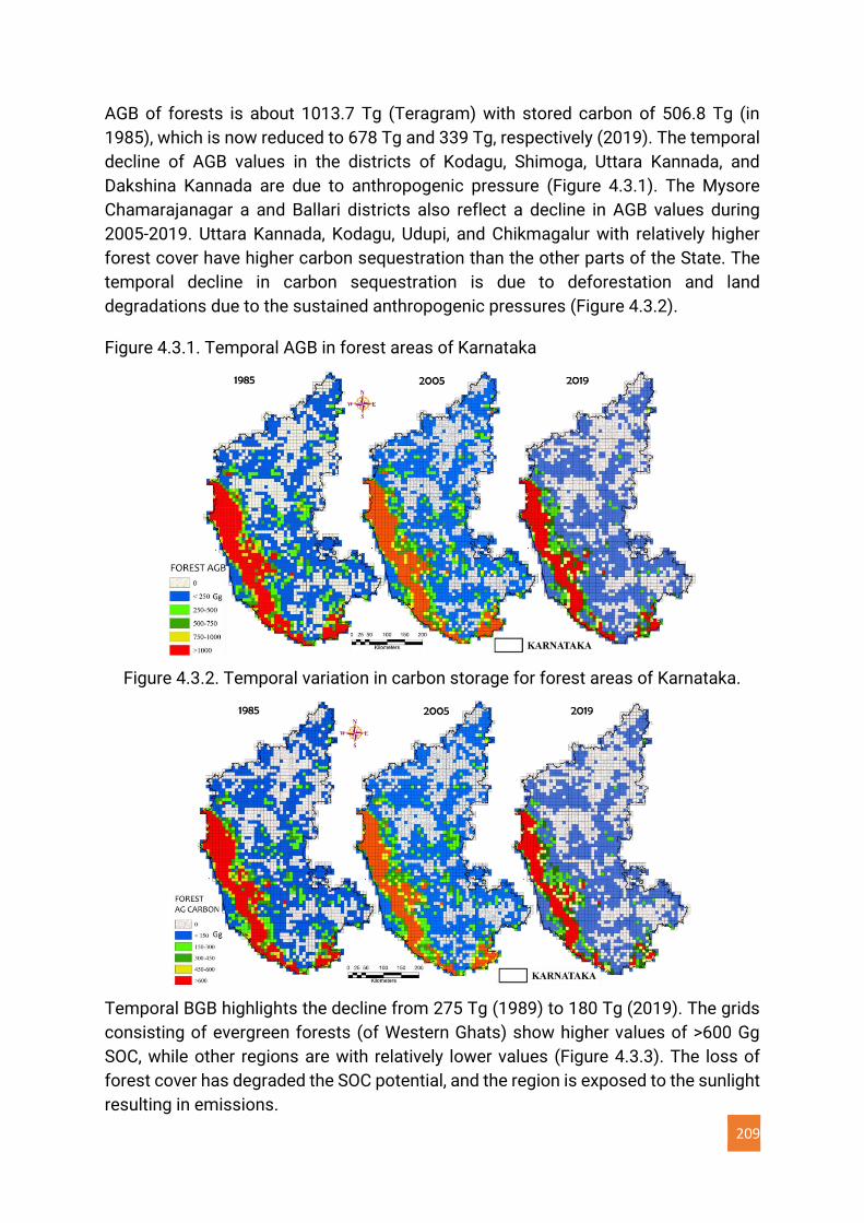
209
AGB of forests is about 1013.7 Tg (Teragram) with stored carbon of 506.8 Tg (in
1985), which is now reduced to 678 Tg and 339 Tg, respectively (2019). The temporal
decline of AGB values in the districts of Kodagu, Shimoga, Uttara Kannada, and
Dakshina Kannada are due to anthropogenic pressure (Figure 4.3.1). The Mysore
Chamarajanagar a and Ballari districts also reflect a decline in AGB values during
2005-2019. Uttara Kannada, Kodagu, Udupi, and Chikmagalur with relatively higher
forest cover have higher carbon sequestration than the other parts of the State. The
temporal decline in carbon sequestration is due to deforestation and land
degradations due to the sustained anthropogenic pressures (Figure 4.3.2).
Figure 4.3.1. Temporal AGB in forest areas of Karnataka
Figure 4.3.2. Temporal variation in carbon storage for forest areas of Karnataka.
Temporal BGB highlights the decline from 275 Tg (1989) to 180 Tg (2019). The grids
consisting of evergreen forests (of Western Ghats) show higher values of >600 Gg
SOC, while other regions are with relatively lower values (Figure 4.3.3). The loss of
forest cover has degraded the SOC potential, and the region is exposed to the sunlight
resulting in emissions.
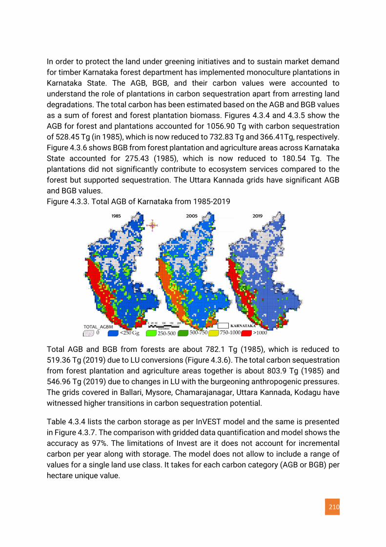
210
In order to protect the land under greening initiatives and to sustain market demand
for timber Karnataka forest department has implemented monoculture plantations in
Karnataka State. The AGB, BGB, and their carbon values were accounted to
understand the role of plantations in carbon sequestration apart from arresting land
degradations. The total carbon has been estimated based on the AGB and BGB values
as a sum of forest and forest plantation biomass. Figures 4.3.4 and 4.3.5 show the
AGB for forest and plantations accounted for 1056.90 Tg with carbon sequestration
of 528.45 Tg (in 1985), which is now reduced to 732.83 Tg and 366.41Tg, respectively.
Figure 4.3.6 shows BGB from forest plantation and agriculture areas across Karnataka
State accounted for 275.43 (1985), which is now reduced to 180.54 Tg. The
plantations did not significantly contribute to ecosystem services compared to the
forest but supported sequestration. The Uttara Kannada grids have significant AGB
and BGB values.
Figure 4.3.3. Total AGB of Karnataka from 1985-2019
Total AGB and BGB from forests are about 782.1 Tg (1985), which is reduced to
519.36 Tg (2019) due to LU conversions (Figure 4.3.6). The total carbon sequestration
from forest plantation and agriculture areas together is about 803.9 Tg (1985) and
546.96 Tg (2019) due to changes in LU with the burgeoning anthropogenic pressures.
The grids covered in Ballari, Mysore, Chamarajanagar, Uttara Kannada, Kodagu have
witnessed higher transitions in carbon sequestration potential.
Table 4.3.4 lists the carbon storage as per InVEST model and the same is presented
in Figure 4.3.7. The comparison with gridded data quantification and model shows the
accuracy as 97%. The limitations of Invest are it does not account for incremental
carbon per year along with storage. The model does not allow to include a range of
values for a single land use class. It takes for each carbon category (AGB or BGB) per
hectare unique value.
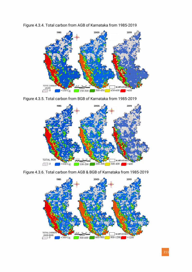
211
Figure 4.3.4. Total carbon from AGB of Karnataka from 1985-2019
Figure 4.3.5. Total carbon from BGB of Karnataka from 1985-2019
Figure 4.3.6. Total carbon from AGB & BGB of Karnataka from 1985-2019
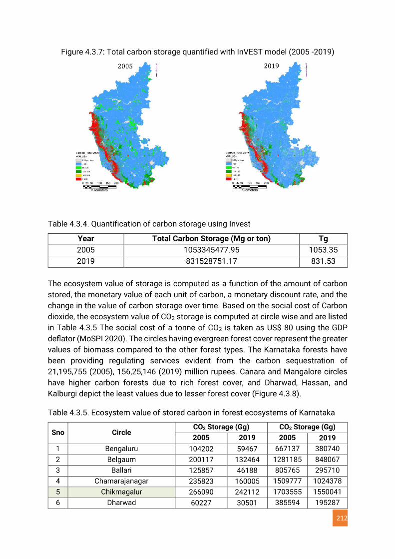
212
Figure 4.3.7: Total carbon storage quantified with InVEST model (2005 -2019)
Table 4.3.4. Quantification of carbon storage using Invest
Year Total Carbon Storage (Mg or ton) Tg
2005 1053345477.95 1053.35
2019 831528751.17 831.53
The ecosystem value of storage is computed as a function of the amount of carbon
stored, the monetary value of each unit of carbon, a monetary discount rate, and the
change in the value of carbon storage over time. Based on the social cost of Carbon
dioxide, the ecosystem value of CO2 storage is computed at circle wise and are listed
in Table 4.3.5 The social cost of a tonne of CO2 is taken as US$ 80 using the GDP
deflator (MoSPI 2020). The circles having evergreen forest cover represent the greater
values of biomass compared to the other forest types. The Karnataka forests have
been providing regulating services evident from the carbon sequestration of
21,195,755 (2005), 156,25,146 (2019) million rupees. Canara and Mangalore circles
have higher carbon forests due to rich forest cover, and Dharwad, Hassan, and
Kalburgi depict the least values due to lesser forest cover (Figure 4.3.8).
Table 4.3.5. Ecosystem value of stored carbon in forest ecosystems of Karnataka
Sno Circle CO2 Storage (Gg) CO2 Storage (Gg)
2005 2019 2005 2019
1 Bengaluru 104202 59467 667137 380740
2 Belgaum 200117 132464 1281185 848067
3 Ballari 125857 46188 805765 295710
4 Chamarajanagar 235823 160005 1509777 1024378
5 Chikmagalur 266090 242112 1703555 1550041
6 Dharwad 60227 30501 385594 195287
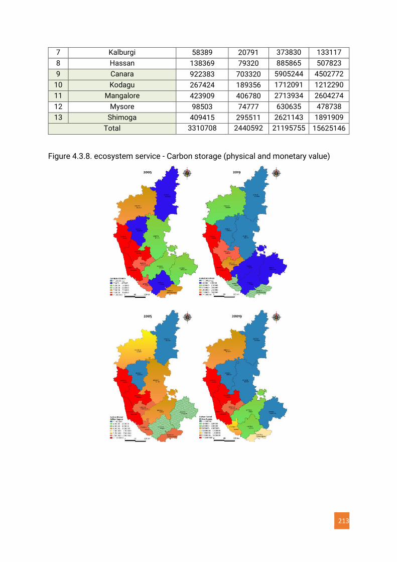
213
7 Kalburgi 58389 20791 373830 133117
8 Hassan 138369 79320 885865 507823
9 Canara 922383 703320 5905244 4502772
10 Kodagu 267424 189356 1712091 1212290
11 Mangalore 423909 406780 2713934 2604274
12 Mysore 98503 74777 630635 478738
13 Shimoga 409415 295511 2621143 1891909
Total 3310708 2440592 21195755 15625146
Figure 4.3.8. ecosystem service - Carbon storage (physical and monetary value)
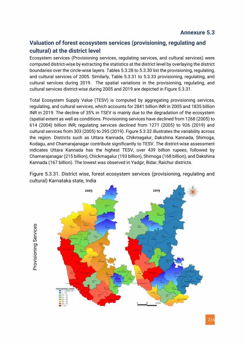
214
Annexure 5.3
Valuation of forest ecosystem services (provisioning, regulating and
cultural) at the district level Ecosystem services (Provisioning services, regulating services, and cultural services) were
computed district-wise by extracting the statistics at the district level by overlaying the district
boundaries over the circle-wise layers. Tables 5.3.28 to 5.3.30 list the provisioning, regulating,
and cultural services of 2005. Similarly, Table 5.3.31 to 5.3.33 provisioning, regulating, and
cultural services during 2019. The spatial variations in the provisioning, regulating, and
cultural services district-wise during 2005 and 2019 are depicted in Figure 5.3.31.
Total Ecosystem Supply Value (TESV) is computed by aggregating provisioning services,
regulating, and cultural services, which accounts for 2841 billion INR in 2005 and 1835 billion
INR in 2019. The decline of 35% in TSEV is mainly due to the degradation of the ecosystem
(spatial extent as well as conditions. Provisioning services have declined from 1268 (2005) to
614 (2004) billion INR; regulating services declined from 1271 (2005) to 926 (2019) and
cultural services from 303 (2005) to 295 (2019). Figure 5.3.32 illustrates the variability across
the region. Districts such as Uttara Kannada, Chikmagalur, Dakshina Kannada, Shimoga,
Kodagu, and Chamarajanagar contribute significantly to TESV. The district-wise assessment
indicates Uttara Kannada has the highest TESV, over 439 billion rupees, followed by
Chamarajanagar (215 billion), Chickmagalur (193 billion), Shimoga (168 billion), and Dakshina
Kannada (167 billion). The lowest was observed in Yadgir, Bidar, Raichur districts.
Figure 5.3.31. District wise, forest ecosystem services (provisioning, regulating and
cultural) Karnataka state, India
Pro
vis
ion
ing
Se
rvic
es
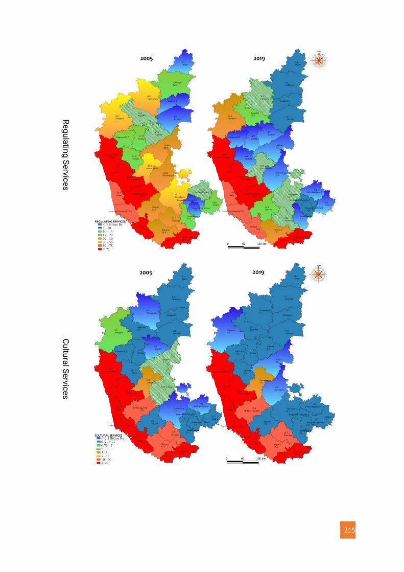
215
Re
gu
latin
g S
ervic
es
Cu
ltura
l Se
rvice
s
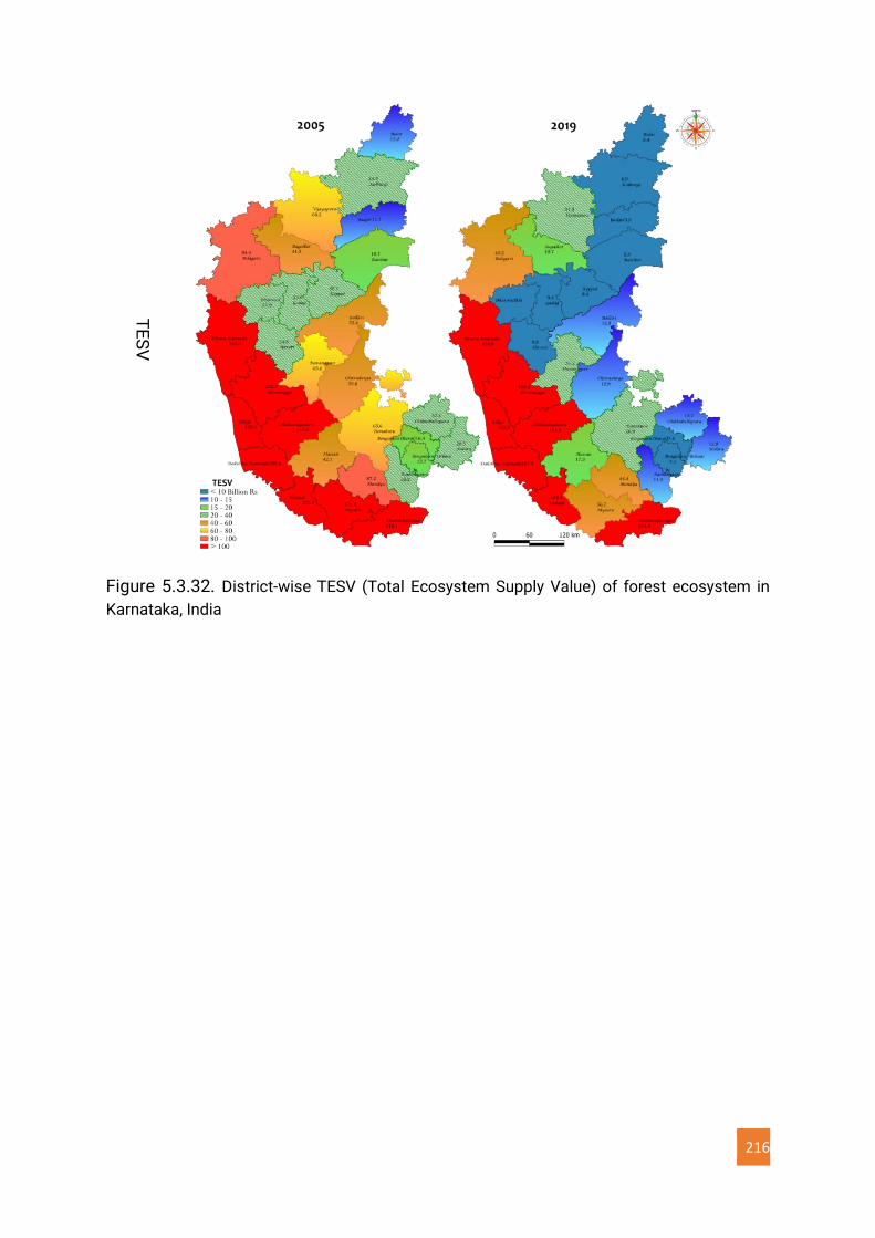
216
TE
SV
Figure 5.3.32. District-wise TESV (Total Ecosystem Supply Value) of forest ecosystem in
Karnataka, India
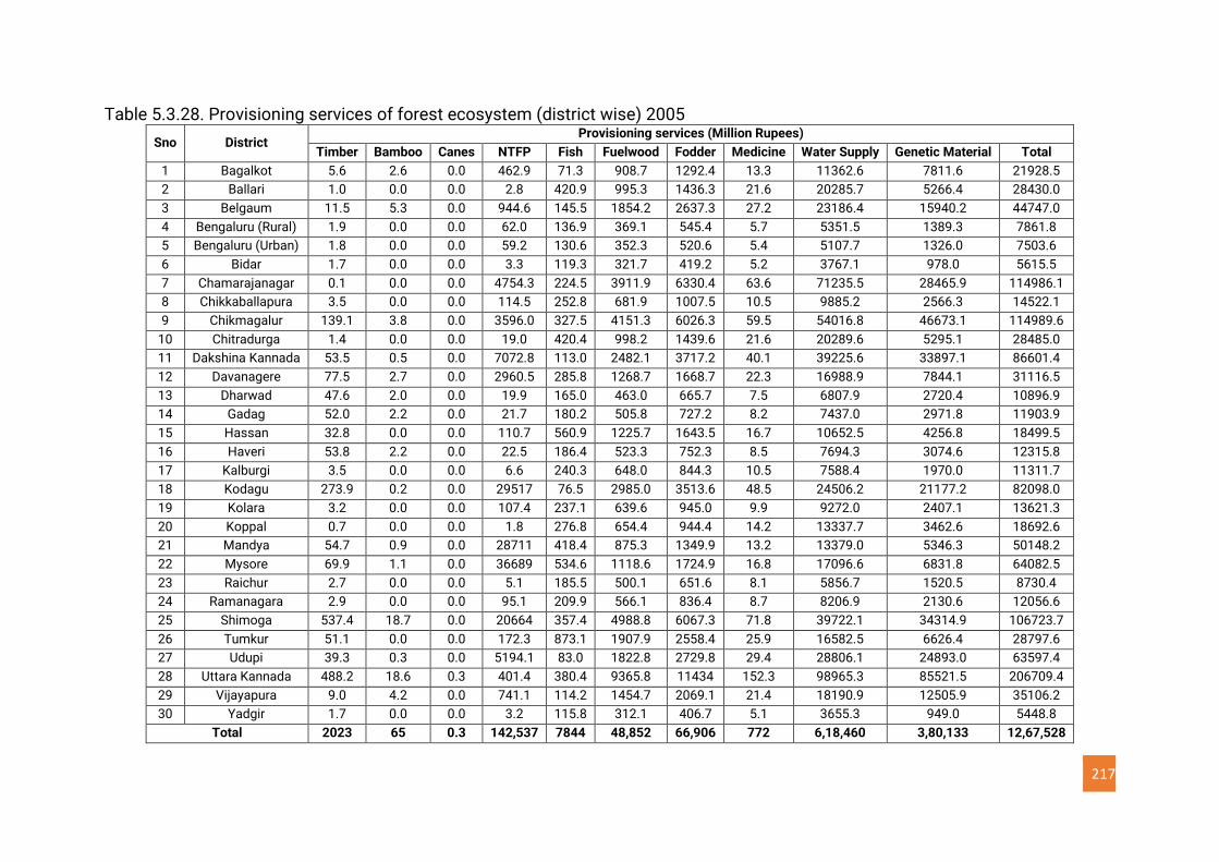
217
Table 5.3.28. Provisioning services of forest ecosystem (district wise) 2005
Sno District Provisioning services (Million Rupees)
Timber Bamboo Canes NTFP Fish Fuelwood Fodder Medicine Water Supply Genetic Material Total
1 Bagalkot 5.6 2.6 0.0 462.9 71.3 908.7 1292.4 13.3 11362.6 7811.6 21928.5
2 Ballari 1.0 0.0 0.0 2.8 420.9 995.3 1436.3 21.6 20285.7 5266.4 28430.0
3 Belgaum 11.5 5.3 0.0 944.6 145.5 1854.2 2637.3 27.2 23186.4 15940.2 44747.0
4 Bengaluru (Rural) 1.9 0.0 0.0 62.0 136.9 369.1 545.4 5.7 5351.5 1389.3 7861.8
5 Bengaluru (Urban) 1.8 0.0 0.0 59.2 130.6 352.3 520.6 5.4 5107.7 1326.0 7503.6
6 Bidar 1.7 0.0 0.0 3.3 119.3 321.7 419.2 5.2 3767.1 978.0 5615.5
7 Chamarajanagar 0.1 0.0 0.0 4754.3 224.5 3911.9 6330.4 63.6 71235.5 28465.9 114986.1
8 Chikkaballapura 3.5 0.0 0.0 114.5 252.8 681.9 1007.5 10.5 9885.2 2566.3 14522.1
9 Chikmagalur 139.1 3.8 0.0 3596.0 327.5 4151.3 6026.3 59.5 54016.8 46673.1 114989.6
10 Chitradurga 1.4 0.0 0.0 19.0 420.4 998.2 1439.6 21.6 20289.6 5295.1 28485.0
11 Dakshina Kannada 53.5 0.5 0.0 7072.8 113.0 2482.1 3717.2 40.1 39225.6 33897.1 86601.4
12 Davanagere 77.5 2.7 0.0 2960.5 285.8 1268.7 1668.7 22.3 16988.9 7844.1 31116.5
13 Dharwad 47.6 2.0 0.0 19.9 165.0 463.0 665.7 7.5 6807.9 2720.4 10896.9
14 Gadag 52.0 2.2 0.0 21.7 180.2 505.8 727.2 8.2 7437.0 2971.8 11903.9
15 Hassan 32.8 0.0 0.0 110.7 560.9 1225.7 1643.5 16.7 10652.5 4256.8 18499.5
16 Haveri 53.8 2.2 0.0 22.5 186.4 523.3 752.3 8.5 7694.3 3074.6 12315.8
17 Kalburgi 3.5 0.0 0.0 6.6 240.3 648.0 844.3 10.5 7588.4 1970.0 11311.7
18 Kodagu 273.9 0.2 0.0 29517 76.5 2985.0 3513.6 48.5 24506.2 21177.2 82098.0
19 Kolara 3.2 0.0 0.0 107.4 237.1 639.6 945.0 9.9 9272.0 2407.1 13621.3
20 Koppal 0.7 0.0 0.0 1.8 276.8 654.4 944.4 14.2 13337.7 3462.6 18692.6
21 Mandya 54.7 0.9 0.0 28711 418.4 875.3 1349.9 13.2 13379.0 5346.3 50148.2
22 Mysore 69.9 1.1 0.0 36689 534.6 1118.6 1724.9 16.8 17096.6 6831.8 64082.5
23 Raichur 2.7 0.0 0.0 5.1 185.5 500.1 651.6 8.1 5856.7 1520.5 8730.4
24 Ramanagara 2.9 0.0 0.0 95.1 209.9 566.1 836.4 8.7 8206.9 2130.6 12056.6
25 Shimoga 537.4 18.7 0.0 20664 357.4 4988.8 6067.3 71.8 39722.1 34314.9 106723.7
26 Tumkur 51.1 0.0 0.0 172.3 873.1 1907.9 2558.4 25.9 16582.5 6626.4 28797.6
27 Udupi 39.3 0.3 0.0 5194.1 83.0 1822.8 2729.8 29.4 28806.1 24893.0 63597.4
28 Uttara Kannada 488.2 18.6 0.3 401.4 380.4 9365.8 11434 152.3 98965.3 85521.5 206709.4
29 Vijayapura 9.0 4.2 0.0 741.1 114.2 1454.7 2069.1 21.4 18190.9 12505.9 35106.2
30 Yadgir 1.7 0.0 0.0 3.2 115.8 312.1 406.7 5.1 3655.3 949.0 5448.8
Total 2023 65 0.3 142,537 7844 48,852 66,906 772 6,18,460 3,80,133 12,67,528
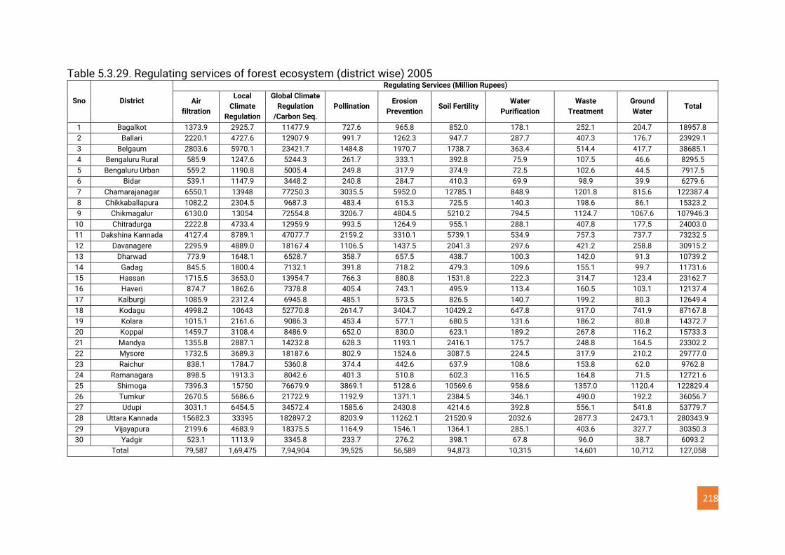
218
Table 5.3.29. Regulating services of forest ecosystem (district wise) 2005
Sno District
Regulating Services (Million Rupees)
Air
filtration
Local
Climate
Regulation
Global Climate
Regulation
/Carbon Seq.
Pollination Erosion
Prevention Soil Fertility
Water
Purification
Waste
Treatment
Ground
Water Total
1 Bagalkot 1373.9 2925.7 11477.9 727.6 965.8 852.0 178.1 252.1 204.7 18957.8
2 Ballari 2220.1 4727.6 12907.9 991.7 1262.3 947.7 287.7 407.3 176.7 23929.1
3 Belgaum 2803.6 5970.1 23421.7 1484.8 1970.7 1738.7 363.4 514.4 417.7 38685.1
4 Bengaluru Rural 585.9 1247.6 5244.3 261.7 333.1 392.8 75.9 107.5 46.6 8295.5
5 Bengaluru Urban 559.2 1190.8 5005.4 249.8 317.9 374.9 72.5 102.6 44.5 7917.5
6 Bidar 539.1 1147.9 3448.2 240.8 284.7 410.3 69.9 98.9 39.9 6279.6
7 Chamarajanagar 6550.1 13948 77250.3 3035.5 5952.0 12785.1 848.9 1201.8 815.6 122387.4
8 Chikkaballapura 1082.2 2304.5 9687.3 483.4 615.3 725.5 140.3 198.6 86.1 15323.2
9 Chikmagalur 6130.0 13054 72554.8 3206.7 4804.5 5210.2 794.5 1124.7 1067.6 107946.3
10 Chitradurga 2222.8 4733.4 12959.9 993.5 1264.9 955.1 288.1 407.8 177.5 24003.0
11 Dakshina Kannada 4127.4 8789.1 47077.7 2159.2 3310.1 5739.1 534.9 757.3 737.7 73232.5
12 Davanagere 2295.9 4889.0 18167.4 1106.5 1437.5 2041.3 297.6 421.2 258.8 30915.2
13 Dharwad 773.9 1648.1 6528.7 358.7 657.5 438.7 100.3 142.0 91.3 10739.2
14 Gadag 845.5 1800.4 7132.1 391.8 718.2 479.3 109.6 155.1 99.7 11731.6
15 Hassan 1715.5 3653.0 13954.7 766.3 880.8 1531.8 222.3 314.7 123.4 23162.7
16 Haveri 874.7 1862.6 7378.8 405.4 743.1 495.9 113.4 160.5 103.1 12137.4
17 Kalburgi 1085.9 2312.4 6945.8 485.1 573.5 826.5 140.7 199.2 80.3 12649.4
18 Kodagu 4998.2 10643 52770.8 2614.7 3404.7 10429.2 647.8 917.0 741.9 87167.8
19 Kolara 1015.1 2161.6 9086.3 453.4 577.1 680.5 131.6 186.2 80.8 14372.7
20 Koppal 1459.7 3108.4 8486.9 652.0 830.0 623.1 189.2 267.8 116.2 15733.3
21 Mandya 1355.8 2887.1 14232.8 628.3 1193.1 2416.1 175.7 248.8 164.5 23302.2
22 Mysore 1732.5 3689.3 18187.6 802.9 1524.6 3087.5 224.5 317.9 210.2 29777.0
23 Raichur 838.1 1784.7 5360.8 374.4 442.6 637.9 108.6 153.8 62.0 9762.8
24 Ramanagara 898.5 1913.3 8042.6 401.3 510.8 602.3 116.5 164.8 71.5 12721.6
25 Shimoga 7396.3 15750 76679.9 3869.1 5128.6 10569.6 958.6 1357.0 1120.4 122829.4
26 Tumkur 2670.5 5686.6 21722.9 1192.9 1371.1 2384.5 346.1 490.0 192.2 36056.7
27 Udupi 3031.1 6454.5 34572.4 1585.6 2430.8 4214.6 392.8 556.1 541.8 53779.7
28 Uttara Kannada 15682.3 33395 182897.2 8203.9 11262.1 21520.9 2032.6 2877.3 2473.1 280343.9
29 Vijayapura 2199.6 4683.9 18375.5 1164.9 1546.1 1364.1 285.1 403.6 327.7 30350.3
30 Yadgir 523.1 1113.9 3345.8 233.7 276.2 398.1 67.8 96.0 38.7 6093.2
Total 79,587 1,69,475 7,94,904 39,525 56,589 94,873 10,315 14,601 10,712 127,058
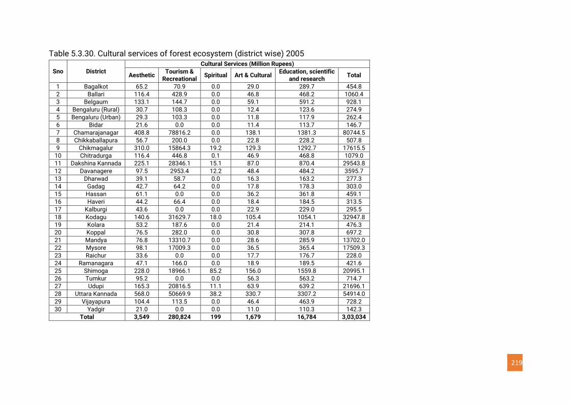
219
Table 5.3.30. Cultural services of forest ecosystem (district wise) 2005
Sno District
Cultural Services (Million Rupees)
Aesthetic Tourism &
Recreational Spiritual Art & Cultural
Education, scientific and research
Total
1 Bagalkot 65.2 70.9 0.0 29.0 289.7 454.8
2 Ballari 116.4 428.9 0.0 46.8 468.2 1060.4
3 Belgaum 133.1 144.7 0.0 59.1 591.2 928.1
4 Bengaluru (Rural) 30.7 108.3 0.0 12.4 123.6 274.9
5 Bengaluru (Urban) 29.3 103.3 0.0 11.8 117.9 262.4
6 Bidar 21.6 0.0 0.0 11.4 113.7 146.7
7 Chamarajanagar 408.8 78816.2 0.0 138.1 1381.3 80744.5
8 Chikkaballapura 56.7 200.0 0.0 22.8 228.2 507.8
9 Chikmagalur 310.0 15864.3 19.2 129.3 1292.7 17615.5
10 Chitradurga 116.4 446.8 0.1 46.9 468.8 1079.0
11 Dakshina Kannada 225.1 28346.1 15.1 87.0 870.4 29543.8
12 Davanagere 97.5 2953.4 12.2 48.4 484.2 3595.7
13 Dharwad 39.1 58.7 0.0 16.3 163.2 277.3
14 Gadag 42.7 64.2 0.0 17.8 178.3 303.0
15 Hassan 61.1 0.0 0.0 36.2 361.8 459.1
16 Haveri 44.2 66.4 0.0 18.4 184.5 313.5
17 Kalburgi 43.6 0.0 0.0 22.9 229.0 295.5
18 Kodagu 140.6 31629.7 18.0 105.4 1054.1 32947.8
19 Kolara 53.2 187.6 0.0 21.4 214.1 476.3
20 Koppal 76.5 282.0 0.0 30.8 307.8 697.2
21 Mandya 76.8 13310.7 0.0 28.6 285.9 13702.0
22 Mysore 98.1 17009.3 0.0 36.5 365.4 17509.3
23 Raichur 33.6 0.0 0.0 17.7 176.7 228.0
24 Ramanagara 47.1 166.0 0.0 18.9 189.5 421.6
25 Shimoga 228.0 18966.1 85.2 156.0 1559.8 20995.1
26 Tumkur 95.2 0.0 0.0 56.3 563.2 714.7
27 Udupi 165.3 20816.5 11.1 63.9 639.2 21696.1
28 Uttara Kannada 568.0 50669.9 38.2 330.7 3307.2 54914.0
29 Vijayapura 104.4 113.5 0.0 46.4 463.9 728.2
30 Yadgir 21.0 0.0 0.0 11.0 110.3 142.3
Total 3,549 280,824 199 1,679 16,784 3,03,034
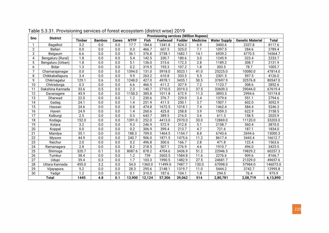
220
Table 5.3.31. Provisioning services of forest ecosystem (district wise) 2019
Sno District Provisioning services (Million Rupees)
Timber Bamboo Canes NTFP Fish Fuelwood Fodder Medicine Water Supply Genetic Material Total
1 Bagalkot 3.2 0.0 0.0 17.7 184.6 1341.8 824.3 6.9 3400.6 2337.8 8117.6
2 Ballari 0.0 0.0 0.0 0.3 466.7 607.5 325.0 7.1 1097.5 284.6 2789.4
3 Belgaum 6.6 0.0 0.0 36.1 376.8 2738.1 1682.1 14.1 6939.2 4770.5 16564.7
4 Bengaluru (Rural) 1.8 0.0 0.0 5.4 142.5 330.7 180.6 3.0 1245.9 323.4 2233.7
5 Bengaluru (Urban) 1.8 0.0 0.0 5.1 136.0 315.6 172.3 2.8 1189.2 308.7 2131.9
6 Bidar 1.3 0.0 0.0 0.2 319.5 193.3 107.2 1.8 303.5 78.7 1005.7
7 Chamarajanagar 0.0 0.0 0.0 1394.0 131.0 5918.0 5023.1 41.0 25225.0 10080.0 47814.0
8 Chikkaballapura 3.4 0.0 0.0 9.9 263.2 610.8 333.5 5.5 2301.5 597.5 4126.0
9 Chikmagalur 129.1 0.6 0.0 1248.0 427.0 4978.1 3435.1 50.5 37697.9 32576.8 80547.0
10 Chitradurga 0.3 0.0 0.0 6.6 466.5 611.2 327.9 7.2 1123.7 308.6 2852.6
11 Dakshina Kannada 53.6 0.5 0.0 2.3 140.7 2710.5 2019.3 37.5 33609.3 29044.0 67619.4
12 Davanagere 45.9 0.0 0.0 1158.3 385.8 1011.8 672.9 11.3 3893.5 2994.6 10174.8
13 Dharwad 22.0 0.0 0.0 1.2 230.6 376.7 229.0 3.4 1379.6 551.1 2794.6
14 Gadag 24.1 0.0 0.0 1.4 251.9 411.5 250.1 3.7 1507.1 602.0 3052.9
15 Hassan 24.6 0.0 0.0 0.8 474.8 1672.5 1018.1 7.4 1462.4 584.4 5246.3
16 Haveri 24.9 0.0 0.0 1.4 260.6 425.8 258.8 3.9 1559.3 622.9 3158.5
17 Kalburgi 2.5 0.0 0.0 0.3 643.7 389.5 216.0 3.6 611.3 158.5 2025.9
18 Kodagu 152.0 0.0 0.0 1391.0 252.0 4413.0 2970.0 33.0 12869.0 11120.0 33203.0
19 Kolara 3.2 0.0 0.0 9.3 246.9 572.9 312.8 5.1 2158.7 560.4 3870.0
20 Koppal 0.0 0.0 0.0 0.2 306.9 399.4 213.7 4.7 721.6 187.1 1834.0
21 Mandya 35.1 0.0 0.0 188.3 709.0 1464.5 1154.7 8.8 6743.6 2694.6 13000.3
22 Mysore 44.9 0.0 0.0 240.7 906.0 1871.5 1475.6 11.2 8617.4 3443.4 16612.7
23 Raichur 2.0 0.0 0.0 0.2 496.8 300.6 166.7 2.8 471.8 122.4 1563.6
24 Ramanagara 2.8 0.0 0.0 8.2 218.5 507.1 276.9 4.6 1910.7 496.0 3425.5
25 Shimoga 320.7 0.1 0.0 8087.6 878.2 4704.6 3436.9 51.2 22946.5 19829.2 60257.3
26 Tumkur 38.4 0.0 0.0 1.2 739 2603.5 1584.8 11.6 2276.6 909.6 8166.7
27 Udupi 39.4 0.3 0.0 1.7 103.3 1990.5 1482.9 27.5 24681.7 21329.0 49657.6
28 Uttara Kannada 455.0 3.2 0.0 54.0 1360.0 11499.0 7487.7 130.0 67098.0 57984.0 146073.0
29 Vijayapura 5.2 0.0 0.0 28.3 295.6 2148.1 1319.7 11.0 5444.2 3742.7 12995.8
30 Yadgir 1.2 0.0 0.0 0.1 310.0 187.6 104.1 1.8 294.5 76.4 975.9
Total 1445 4.8 0.1 13,900 12,124 57,306 39,062 514 2,80,781 2,08,719 6,13,890
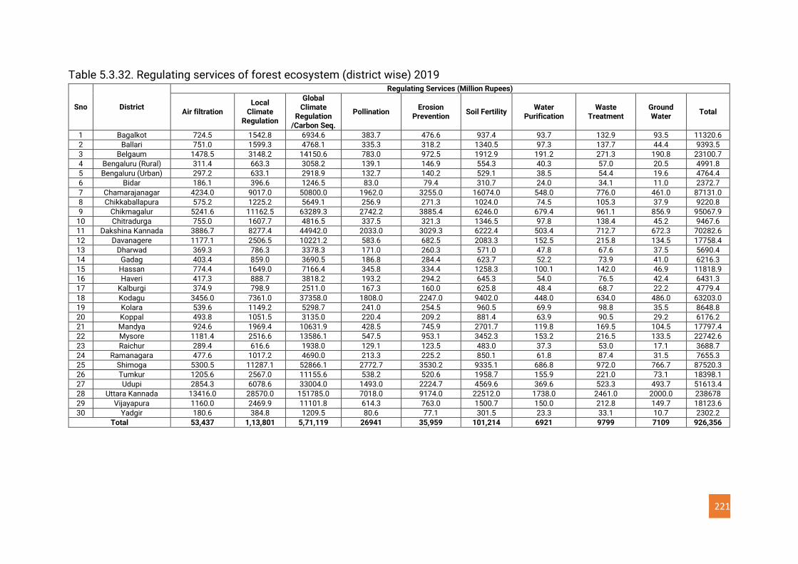
221
Table 5.3.32. Regulating services of forest ecosystem (district wise) 2019
Sno District
Regulating Services (Million Rupees)
Air filtration Local
Climate Regulation
Global Climate
Regulation /Carbon Seq.
Pollination Erosion
Prevention Soil Fertility
Water Purification
Waste Treatment
Ground Water
Total
1 Bagalkot 724.5 1542.8 6934.6 383.7 476.6 937.4 93.7 132.9 93.5 11320.6
2 Ballari 751.0 1599.3 4768.1 335.3 318.2 1340.5 97.3 137.7 44.4 9393.5
3 Belgaum 1478.5 3148.2 14150.6 783.0 972.5 1912.9 191.2 271.3 190.8 23100.7
4 Bengaluru (Rural) 311.4 663.3 3058.2 139.1 146.9 554.3 40.3 57.0 20.5 4991.8
5 Bengaluru (Urban) 297.2 633.1 2918.9 132.7 140.2 529.1 38.5 54.4 19.6 4764.4
6 Bidar 186.1 396.6 1246.5 83.0 79.4 310.7 24.0 34.1 11.0 2372.7
7 Chamarajanagar 4234.0 9017.0 50800.0 1962.0 3255.0 16074.0 548.0 776.0 461.0 87131.0
8 Chikkaballapura 575.2 1225.2 5649.1 256.9 271.3 1024.0 74.5 105.3 37.9 9220.8
9 Chikmagalur 5241.6 11162.5 63289.3 2742.2 3885.4 6246.0 679.4 961.1 856.9 95067.9
10 Chitradurga 755.0 1607.7 4816.5 337.5 321.3 1346.5 97.8 138.4 45.2 9467.6
11 Dakshina Kannada 3886.7 8277.4 44942.0 2033.0 3029.3 6222.4 503.4 712.7 672.3 70282.6
12 Davanagere 1177.1 2506.5 10221.2 583.6 682.5 2083.3 152.5 215.8 134.5 17758.4
13 Dharwad 369.3 786.3 3378.3 171.0 260.3 571.0 47.8 67.6 37.5 5690.4
14 Gadag 403.4 859.0 3690.5 186.8 284.4 623.7 52.2 73.9 41.0 6216.3
15 Hassan 774.4 1649.0 7166.4 345.8 334.4 1258.3 100.1 142.0 46.9 11818.9
16 Haveri 417.3 888.7 3818.2 193.2 294.2 645.3 54.0 76.5 42.4 6431.3
17 Kalburgi 374.9 798.9 2511.0 167.3 160.0 625.8 48.4 68.7 22.2 4779.4
18 Kodagu 3456.0 7361.0 37358.0 1808.0 2247.0 9402.0 448.0 634.0 486.0 63203.0
19 Kolara 539.6 1149.2 5298.7 241.0 254.5 960.5 69.9 98.8 35.5 8648.8
20 Koppal 493.8 1051.5 3135.0 220.4 209.2 881.4 63.9 90.5 29.2 6176.2
21 Mandya 924.6 1969.4 10631.9 428.5 745.9 2701.7 119.8 169.5 104.5 17797.4
22 Mysore 1181.4 2516.6 13586.1 547.5 953.1 3452.3 153.2 216.5 133.5 22742.6
23 Raichur 289.4 616.6 1938.0 129.1 123.5 483.0 37.3 53.0 17.1 3688.7
24 Ramanagara 477.6 1017.2 4690.0 213.3 225.2 850.1 61.8 87.4 31.5 7655.3
25 Shimoga 5300.5 11287.1 52866.1 2772.7 3530.2 9335.1 686.8 972.0 766.7 87520.3
26 Tumkur 1205.6 2567.0 11155.6 538.2 520.6 1958.7 155.9 221.0 73.1 18398.1
27 Udupi 2854.3 6078.6 33004.0 1493.0 2224.7 4569.6 369.6 523.3 493.7 51613.4
28 Uttara Kannada 13416.0 28570.0 151785.0 7018.0 9174.0 22512.0 1738.0 2461.0 2000.0 238678
29 Vijayapura 1160.0 2469.9 11101.8 614.3 763.0 1500.7 150.0 212.8 149.7 18123.6
30 Yadgir 180.6 384.8 1209.5 80.6 77.1 301.5 23.3 33.1 10.7 2302.2
Total 53,437 1,13,801 5,71,119 26941 35,959 101,214 6921 9799 7109 926,356
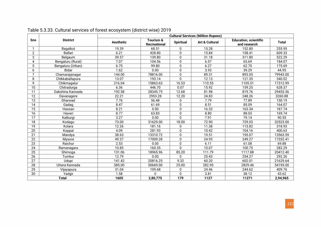
222
Table 5.3.33. Cultural services of forest ecosystem (district wise) 2019
Sno District Cultural Services (Million Rupees)
Aesthetic Tourism &
Recreational Spiritual Art & Cultural
Education, scientific and research
Total
1 Bagalkot 19.39 68.51 0 15.28 152.80 255.95
2 Ballari 6.21 428.80 0 15.84 158.41 609.33
3 Belgaum 39.57 139.80 0 31.18 311.80 522.29
4 Bengaluru (Rural) 7.07 104.56 0 6.57 65.69 184.07
5 Bengaluru (Urban) 6.75 99.80 0 6.27 62.70 175.69
6 Bidar 1.62 0.00 0 3.93 39.29 44.95
7 Chamarajanagar 144.00 78816.00 0 89.31 893.05 79943.00
8 Chikkaballapura 13.07 193.14 0 12.13 121.35 340.02
9 Chikmagalur 216.04 15863.63 16.53 110.55 1105.51 17312.99
10 Chitradurga 6.36 446.70 0.07 15.92 159.25 628.37
11 Dakshina Kannada 192.58 28345.75 12.68 81.98 819.76 29453.36
12 Davanagere 22.21 2953.28 12.20 24.83 248.26 3260.88
13 Dharwad 7.76 56.48 0 7.79 77.89 150.19
14 Gadag 8.47 61.69 0 8.51 85.09 164.07
15 Hassan 8.21 0.00 0 16.33 163.34 187.74
16 Haveri 8.77 63.83 0 8.80 88.03 169.74
17 Kalburgi 3.27 0.00 0 7.91 79.14 90.55
18 Kodagu 73.00 31629.00 18.00 72.90 729.03 32523.00
19 Kolara 12.26 181.16 0 11.38 113.82 318.93
20 Koppal 4.09 281.93 0 10.42 104.16 400.63
21 Mandya 38.63 13310.72 0 19.51 195.07 13563.59
22 Mysore 49.37 17009.28 0 24.93 249.27 17332.41
23 Raichur 2.53 0.00 0 6.11 61.08 69.88
24 Ramanagara 10.85 160.35 0 10.07 100.75 282.29
25 Shimoga 131.06 18965.96 85.20 111.79 1117.88 20412.40
26 Tumkur 12.79 0.00 0 25.43 254.27 292.26
27 Udupi 141.42 20816.25 9.32 60.20 602.01 21629.64
28 Uttara Kannada 385.00 50669.00 25.00 282.95 2829.46 54193.00
29 Vijayapura 31.04 109.68 0 24.46 244.62 409.76
30 Yadgir 1.58 0 0 3.81 38.12 43.62
Total 1605 2,80,775 179 1127 11271 2,94,965
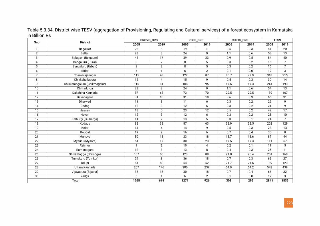
223
Table 5.3.34. District wise TESV (aggregation of Provisioning, Regulating and Cultural services) of a forest ecosystem in Karnataka in Billion Rs
Sno District PROVG_BRS REGS_BRS CULTS_BRS TESV
2005 2019 2005 2019 2005 2019 2005 2019
1 Bagalkot 22 8 19 11 0.5 0.3 41 20
2 Ballari 28 3 24 9 1.1 0.6 53 13
3 Belagavi (Belgaum) 45 17 39 23 0.9 0.5 84 40
4 Bengaluru (Rural) 8 2 8 5 0.3 0.2 16 7
5 Bengaluru (Urban) 8 2 8 5 0.3 0.2 16 7
6 Bidar 6 1 6 2 0.1 0.0 12 3
7 Chamarajanagar 115 48 122 87 80.7 79.9 318 215
8 Chikkaballapura 15 4 15 9 0.5 0.3 30 14
9 Chikkamagaluru (Chikmagalur) 115 81 108 95 17.6 17.3 241 193
10 Chitradurga 28 3 24 9 1.1 0.6 54 13
11 Dakshina Kannada 87 68 73 70 29.5 29.5 189 167
12 Davanagere 31 10 31 18 3.6 3.3 66 31
13 Dharwad 11 3 11 6 0.3 0.2 22 9
14 Gadag 12 3 12 6 0.3 0.2 24 9
15 Hassan 18 5 23 12 0.5 0.2 42 17
16 Haveri 12 3 12 6 0.3 0.2 25 10
17 Kalburgi (Gulbarga) 11 2 13 5 0.3 0.1 24 7
18 Kodagu 82 33 87 63 32.9 32.5 202 129
19 Kolar 14 4 14 9 0.5 0.3 28 13
20 Koppal 19 2 16 6 0.7 0.4 35 8
21 Mandya 50 13 23 18 13.7 13.6 87 44
22 Mysuru (Mysore) 64 17 30 23 17.5 17.3 111 57
23 Raichur 9 2 10 4 0.2 0.1 19 5
24 Ramanagara 12 3 13 8 0.4 0.3 25 11
25 Shivamogga (Shimoga) 107 60 123 88 21.0 20.4 251 168
26 Tumakuru (Tumkur) 29 8 36 18 0.7 0.3 66 27
27 Udupi 64 50 54 52 21.7 21.6 139 123
28 Uttara Kannada 207 146 280 239 54.9 54.2 542 439
29 Vijayapura (Bijapur) 35 13 30 18 0.7 0.4 66 32
30 Yadgir 5 1 6 2 0.1 0.0 12 3
Total 1268 614 1271 926 303 295 2841 1835
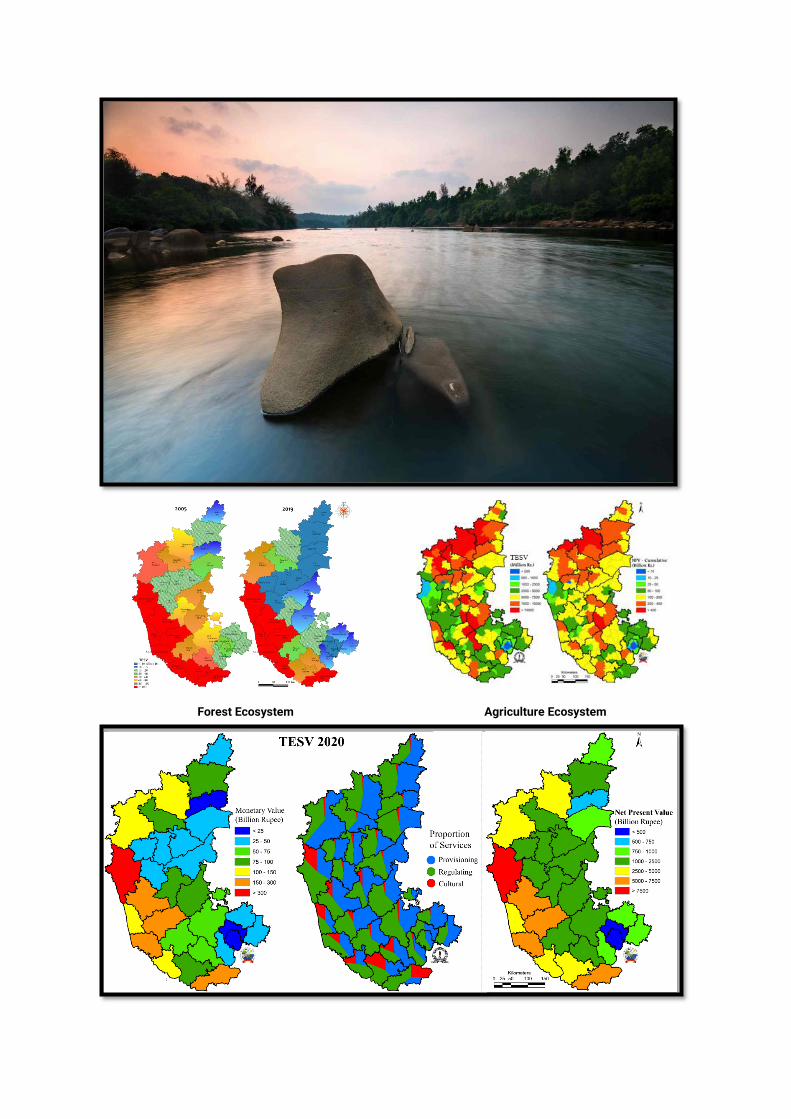
Forest Ecosystem Agriculture Ecosystem