IDEA AND
PERSPECT IVE Using landscape history to predict biodiversity patterns in
fragmented landscapes
Robert M. Ewers,1* Raphael K.
Didham,2,3 William D. Pearse,1,4,5
V�eronique Lefebvre,1 Isabel M. D.
Rosa,1 Jo~ao M. B. Carreiras,6
Richard M. Lucas7 and Daniel C.
Reuman1,8*
AbstractLandscape ecology plays a vital role in understanding the impacts of land-use change on biodiversity, but it
is not a predictive discipline, lacking theoretical models that quantitatively predict biodiversity patterns from
first principles. Here, we draw heavily on ideas from phylogenetics to fill this gap, basing our approach on
the insight that habitat fragments have a shared history. We develop a landscape ‘terrageny’, which repre-
sents the historical spatial separation of habitat fragments in the same way that a phylogeny represents evo-
lutionary divergence among species. Combining a random sampling model with a terrageny generates
numerical predictions about the expected proportion of species shared between any two fragments, the
locations of locally endemic species, and the number of species that have been driven locally extinct. The
model predicts that community similarity declines with terragenetic distance, and that local endemics are
more likely to be found in terragenetically distinctive fragments than in large fragments. We derive
equations to quantify the variance around predictions, and show that ignoring the spatial structure of
fragmented landscapes leads to over-estimates of local extinction rates at the landscape scale. We argue that
ignoring the shared history of habitat fragments limits our ability to understand biodiversity changes in
human-modified landscapes.
KeywordsDistance-dissimilarity curve, habitat fragmentation, habitat loss, landscape divergence hypothesis, nested
communities, neutral model, random sampling, spatial autocorrelation, spatial insurance, vicariance model.
Ecology Letters (2013) 16: 1221–1233
INTRODUCTION
The historical pattern of habitat cover has an impact on present-
day biodiversity patterns in fragmented landscapes (Harding et al.
1998; Kuussaari et al. 2009; Krauss et al. 2010; Wearn et al. 2012).
This temporal effect occurs because habitat loss and fragmentation
may not directly kill individuals of a species, and it can therefore
take a number of generations for populations to go extinct after
habitat loss. This ‘ghost of land-use past’ (Harding et al. 1998) can
be a powerful force that explains patterns of present-day diversity
better than present-day patterns of habitat cover, with the implica-
tion that landscape history must now be considered in conservation
planning (Schrott et al. 2005; Dauber et al. 2006; Kuussaari et al.
2009).
Such legacy effects can be detected by correlating present-day
biodiversity patterns to present and historical patterns of habitat
cover (Kuussaari et al. 2009), with historical impacts inferred when
there are significant correlations to previous habitat cover patterns.
This approach, however, treats the ‘past’ and the ‘present’ as being
distinct and separate categories. It implicitly assumes that habitat
change is a process that used to happen but stopped at an unde-
fined point in time, rather than being a cumulative process that
operates over many decades and culminates in the present-day land-
scape. Predicting the magnitude of biodiversity loss arising from this
temporal trajectory of land-use change represents a difficult chal-
lenge that is exacerbated by failure to consider the cumulative nat-
ure of landscape dynamics (Wearn et al. 2012). The most commonly
applied analytical approach to the problem thus far has been the
empirical species–area relationship (SAR) for discrete estimates of
total habitat loss (Pimm & Askins 1995; Pimm & Raven 2000); the
approach can be adjusted to include habitat change as a cumulative
rather than a binary process (Wearn et al. 2012). However, these
models still ignore the spatial distribution of species within habitat
(He & Hubbell 2011), the geometry of habitat loss in relation to
the spatial pattern of species distributions (Pereira et al. 2012), and
the spatial structure of the habitat itself within landscapes. This is
despite knowing that habitat fragmentation strongly influences the
spatial patterning of biodiversity (Ewers & Didham 2006), and that
1Department of Life Sciences, Imperial College London, Silwood Park Campus,
Buckhurst Road, Ascot, SL5 7PY, UK2School of Animal Biology, University of Western Australia, 35 Stirling
Highway, Crawley, WA, 6009, Australia3CSIRO Ecosystem Sciences, Centre for Environment and Life Sciences,
Underwood Ave, Floreat, WA, 6014, Australia4Department of Ecology, Evolution, and Behavior, University of Minnesota,
100 Ecology Building, 1987 Upper Buford Circle, Saint Paul, Minnesota,
55108, USA
5NERC Centre for Ecology and Hydrology, Wallingford, Oxfordshire, OX10
8BB, UK6Tropical Research Institute (IICT), Travessa do Conde da Ribeira, 9, Lisbon,
1400-142, Portugal7Institute of Geography and Earth Sciences, Aberystwyth University,
Aberystwyth, Ceredigion, SY23 3DB, Wales8Laboratory of Populations, Rockefeller University, 1230 York Avenue,
New York, NY, 10065, USA
*Correspondence: E-mail: [email protected]; [email protected]
© 2013 The Authors. Ecology Letters published by John Wiley & Sons Ltd and CNRSThis is an open access article under the terms of the Creative Commons Attribution License, which permits use,
distribution and reproduction in any medium, provided the original work is properly cited.
Ecology Letters, (2013) 16: 1221–1233 doi: 10.1111/ele.12160
the accumulation of fine-scale fragmentation effects dictates biodi-
versity patterns at the landscape scale (Ewers et al. 2010).
Within a fragmented landscape, the total number of species that
persist is a function of how species are distributed among isolated
habitat fragments. Any given fragment will likely hold only a subset
of all species present in the landscape, and many species will be
present in more than one fragment. On this basis, the total number
of species that persist in the landscape reflects both the species
richness of individual fragments and how many of those species are
shared among fragments, with other features of the landscape such
as connectivity among fragments also influencing the number of
species present in any individual fragment. Species richness within
individual fragments in a fragmented landscape can be approxi-
mated well by the SAR (Drakare et al. 2006), but predicting the spa-
tial pattern of shared species among habitat fragments is much
more problematic.
An informative neutral model that predicts spatial patterns of bio-
diversity is an important requirement for inferring the relative
importance of non-neutral biological processes (Rosindell et al.
2011), but despite considerable advances in landscape ecology since
the advent of island biogeography theory (Laurance 2008; Fahrig
2003; Didham et al. 2012), there is still no generalised model that
generates neutral predictions of the pattern of shared species in
fragmented landscapes. Such neutral predictions are necessary for
quantifying the importance of biological processes such as dispersal,
and the role of species traits such as body size and trophic level;
these are expected to influence the responses of species and com-
munities to habitat loss and fragmentation (Henle et al. 2004; Ewers
& Didham 2006). We demonstrate that explicitly accounting for the
history of habitat change within a landscape leads naturally to
predictions of shared species among habitat fragments, and these
predictions scale up to provide estimates of the number of species
expected to be driven extinct from fragmented landscapes given a
particular amount and spatial pattern of habitat loss.
Here, we develop a method for quantifying the history of a land-
scape by treating it as a cumulative rather than a two-step process.
We draw heavily on phylogenetic approaches to the evolution of spe-
cies, treating habitat as a set of ‘lineages’ that have shared ‘ancestry’
that we quantify by recording the historical patterns of connectedness
among fragments. This approach generates a ‘terrageny’ of habitat
fragments within a landscape that is analogous to a phylogeny of spe-
cies. Terragenies are developed for two Amazonian landscapes and
we adapt phylogenetic metrics to demonstrate the ability to statisti-
cally quantify differences in the historical patterns of land-use change
between landscapes. We then combine terragenies with a nested ran-
dom sampling model to generate neutral predictions about biodiver-
sity patterns in fragmented landscapes, including the proportion of
species that will go extinct from a given landscape, be shared
between any pair of habitat fragments, or be locally endemic to a
single fragment. Differences in terragenetic histories are shown to
propagate through fragment lineages to generate differences in the
expected patterns of biodiversity in the present day. Importantly, we
also derive numeric predictions for the variance around each of these
predictions and test the terragenetic model using a data set on leaf-lit-
ter beetle communities from an Amazonian landscape. We conclude
by discussing the set of assumptions that are implicit within the
model and the likely impact of relaxing those assumptions on the
predictions that arise from the terragenetic model.
QUANTIFYING LANDSCAPE HISTORY IN A TERRAGENY
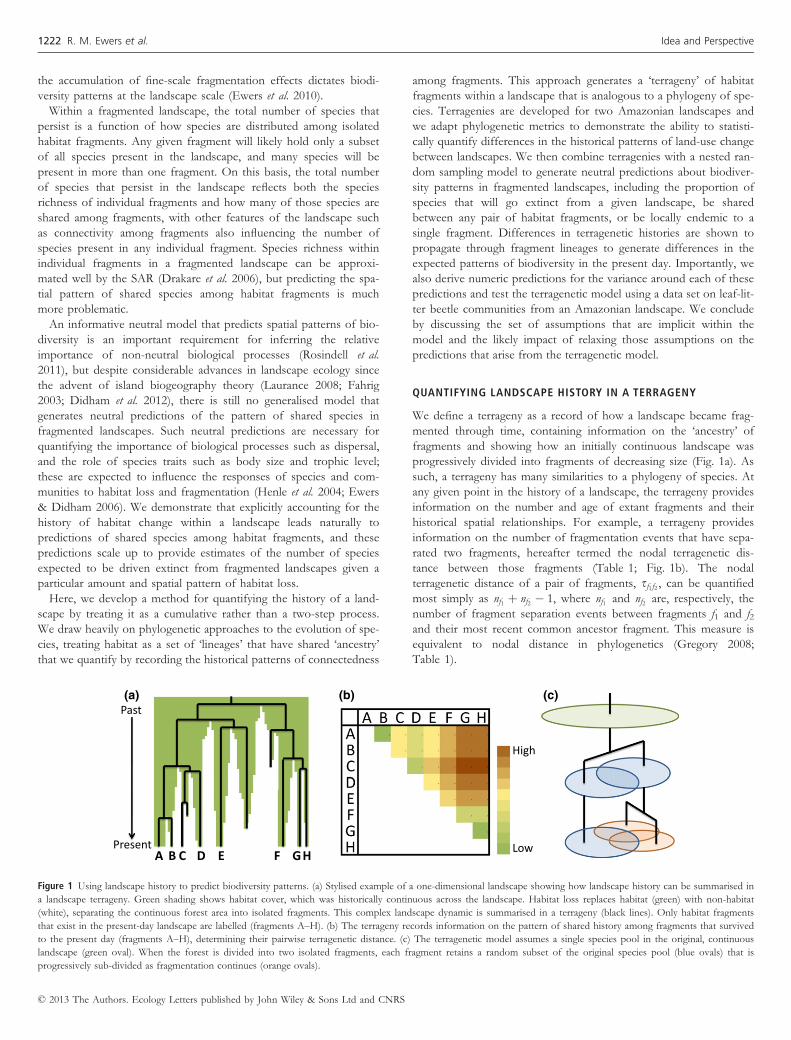
We define a terrageny as a record of how a landscape became frag-
mented through time, containing information on the ‘ancestry’ of
fragments and showing how an initially continuous landscape was
progressively divided into fragments of decreasing size (Fig. 1a). As
such, a terrageny has many similarities to a phylogeny of species. At
any given point in the history of a landscape, the terrageny provides
information on the number and age of extant fragments and their
historical spatial relationships. For example, a terrageny provides
information on the number of fragmentation events that have sepa-
rated two fragments, hereafter termed the nodal terragenetic dis-
tance between those fragments (Table 1; Fig. 1b). The nodal
terragenetic distance of a pair of fragments, sf1 f2 , can be quantified
most simply as nf1 þ nf2 � 1, where nf1 and nf2 are, respectively, the
number of fragment separation events between fragments f1 and f2and their most recent common ancestor fragment. This measure is
equivalent to nodal distance in phylogenetics (Gregory 2008;
Table 1).
A B C D E F GH
Past
Present Low
High
(a) (b) (c)
Figure 1 Using landscape history to predict biodiversity patterns. (a) Stylised example of a one-dimensional landscape showing how landscape history can be summarised in
a landscape terrageny. Green shading shows habitat cover, which was historically continuous across the landscape. Habitat loss replaces habitat (green) with non-habitat
(white), separating the continuous forest area into isolated fragments. This complex landscape dynamic is summarised in a terrageny (black lines). Only habitat fragments
that exist in the present-day landscape are labelled (fragments A–H). (b) The terrageny records information on the pattern of shared history among fragments that survived
to the present day (fragments A–H), determining their pairwise terragenetic distance. (c) The terragenetic model assumes a single species pool in the original, continuous
landscape (green oval). When the forest is divided into two isolated fragments, each fragment retains a random subset of the original species pool (blue ovals) that is
progressively sub-divided as fragmentation continues (orange ovals).
© 2013 The Authors. Ecology Letters published by John Wiley & Sons Ltd and CNRS
1222 R. M. Ewers et al. Idea and Perspective
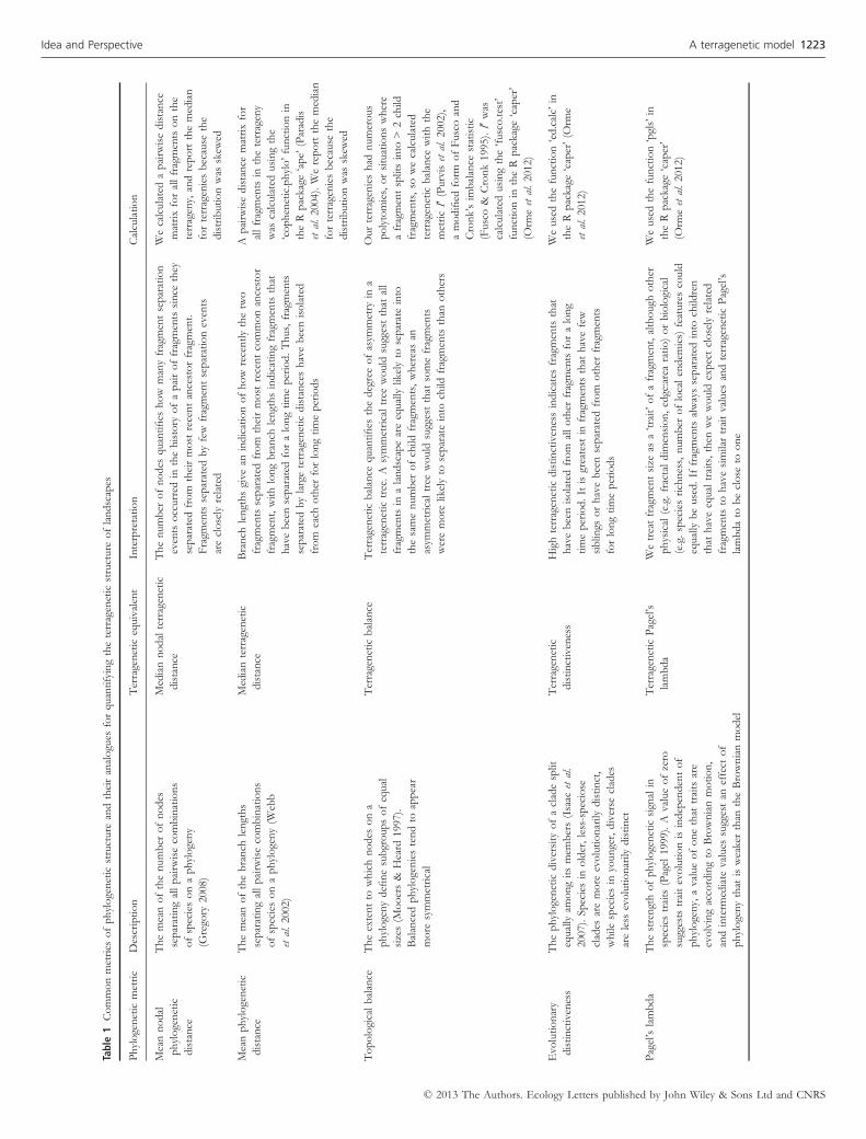
Table
1Commonmetrics
ofphylogeneticstructure
andtheiranalogues
forquantifyingtheterrageneticstructure
oflandscapes
Phylogeneticmetric
Description
Terrageneticequivalent
Interpretation
Calculation
Meannodal
phylogenetic
distance
Themeanofthenumber
ofnodes
separatingallpairwisecombinations
ofspeciesonaphylogeny
(Gregory
2008)
Mediannodalterragenetic
distance
Thenumber
ofnodes
quantifies
how
manyfragmentseparation
eventsoccurred
inthehistory
ofapairoffragmentssince
they
separated
from
theirmostrecentancestorfragment.
Fragm
entsseparated
byfewfragmentseparationevents
arecloselyrelated
Wecalculatedapairwisedistance
matrixforallfragmentsonthe
terrageny,andreportthemedian
forterrageniesbecause
the
distributionwas
skew
ed
Meanphylogenetic
distance
Themeanofthebranch
lengths
separatingallpairwisecombinations
ofspeciesonaphylogeny(W
ebb
etal.2002)
Medianterragenetic
distance
Branch
lengthsgive
anindicationofhowrecentlythetwo
fragmentsseparated
from
theirmostrecentcommonancestor
fragment,withlongbranch
lengthsindicatingfragmentsthat
havebeenseparated
foralongtimeperiod.Thus,fragments
separated
bylargeterrageneticdistanceshavebeenisolated
from
each
other
forlongtimeperiods
Apairwisedistance
matrixfor
allfragmentsin
theterrageny
was
calculatedusingthe
‘cophenetic.phylo’functionin
theRpackage‘ape’(Paradis
etal.2004).Wereportthemedian
forterrageniesbecause
the
distributionwas
skew
ed
Topologicalbalance
Theextentto
whichnodes
ona
phylogenydefinesubgroupsofequal
sizes(M
ooers&
Heard
1997).
Balancedphylogeniestendto
appear
more
symmetrical
Terrageneticbalance
Terrageneticbalance
quantifies
thedegreeofasym
metry
ina
terragenetictree.A
symmetricaltree
would
suggestthat
all
fragmentsin
alandscapeareequallylikelyto
separateinto
thesamenumber
ofchild
fragments,whereasan
asym
metricaltree
would
suggestthat
somefragments
weremore
likelyto
separateinto
child
fragmentsthan
others
Ourterragenieshad
numerous
polytomies,orsituationswhere
afragmentsplitsinto
>2child
fragments,so
wecalculated
terrageneticbalance
withthe
metricI′(Purvisetal.2002),
amodified
form
ofFuscoand
Cronk’simbalance
statistic
(Fusco&
Cronk1995).I′was
calculatedusingthe‘fusco.test’
functionin
theRpackage
‘caper’
(Orm
eetal.2012)
Evolutionary
distinctiveness
Thephylogeneticdiversity
ofacladesplit
equallyam
ongitsmem
bers(Isaac
etal.
2007).Speciesin
older,less-speciose
clades
aremore
evolutionarily
distinct,
while
speciesin
younger,diverse
clades
areless
evolutionarily
distinct
Terragenetic
distinctiveness
Highterrageneticdistinctivenessindicates
fragmentsthat
havebeenisolatedfrom
allother
fragmentsforalong
timeperiod.Itisgreatestin
fragmentsthat
havefew
siblings
orhavebeenseparated
from
other
fragments
forlongtimeperiods
Weusedthefunction‘ed.calc’in
theRpackage‘caper’(O
rme
etal.2012)
Pagel’slambda
Thestrengthofphylogeneticsignalin
speciestraits(Pagel1999).A
valueofzero
suggeststraitevolutionisindependentof
phylogeny,avalueofonethat
traitsare
evolvingaccordingto
Brownianmotion,
andinterm
ediate
values
suggestan
effect
of
phylogenythat
isweakerthan
theBrownianmodel
TerrageneticPagel’s
lambda
Wetreatfragmentsize
asa‘trait’ofafragment,although
other
physical(e.g.fractaldimension,edge:arearatio)orbiological
(e.g.speciesrichness,number
oflocalendem
ics)featurescould
equallybeused.If
fragmentsalwaysseparated
into
children
that
haveequaltraits,then
wewould
expectcloselyrelated
fragmentsto
havesimilartraitvalues
andterrageneticPagel’s
lambdato
beclose
toone
Weusedthefunction‘pgls’in
theRpackage‘caper’
(Orm
eetal.2012)
© 2013 The Authors. Ecology Letters published by John Wiley & Sons Ltd and CNRS
Idea and Perspective A terragenetic model 1223

To demonstrate how terragenies generate quantitative estimates
of landscape history that can provide informative comparisons
among landscapes, we constructed terragenies for two landscapes in
the Brazilian Amazon and adapted phylogenetic metrics to quantify
the terragenetic structure of the two landscapes. Statistical differ-
ences in the phylogenetic metrics among the two landscapes are
interpreted in light of a detailed understanding of the differences in
their land-use history.
Terragenetic trees in Amazonian landscapes
We constructed terragenies for a 1254 km2 landscape in each of the
municipalities of Machadinho d’Oeste and Manaus, both in the Bra-
zilian Amazon (Figs 2, 3 and S1). The two landscapes were of the
same spatial extent (33 9 38 km) and resolution (grid size
150 9 150 m), and, in both, more than 99% of the landscape was
covered by forest prior to human encroachment. In both land-
scapes, we used land cover maps derived from time series of Land-
sat sensor data following the methods of Prates-Clark et al. (2009),
with maps showing observed forest cover at 23 points in time
between 1973 and 2011 in Manaus and at 21 points in time
between 1984 and 2011 in Machadinho d’Oeste. While we recognise
the role of regrowth in retaining biodiversity, such forests were not
included in this analysis and instead we assumed all deforested areas
to have remained as such for the duration of the time series.
Deforestation in Manaus began in the early 1970s, accelerated in
the mid-1980s and then slowed from the 1990s onwards, resulting
in the conversion of 21% of the landscape and the creation of 94
extant forest fragments by 2011 (Fig. 2a). Deforestation in Machad-
inho d’Oeste started in the 1980s, but has progressed more rapidly,
leaving a landscape that was 60% deforested with 446 extant forest
fragments in 2011 (Fig. 2b). The number of habitat fragments in
Manaus increased through time in an approximately sigmoidal pat-
tern, although there was a period in the early 2000s when a large
number of small fragments were destroyed (Fig. 2c). In contrast,
forest fragments in Machadinho d’Oeste continue to be created rap-
idly (Fig. 2d).
The median size of fragments in the present day does not differ
between the two landscapes (Table 2; Wilcoxon test, W = 21 992,
nominal P = 0.442) and neither does the size-distribution of forest
(a)
(b)
020
4060
8010
0
0.0
0.2
0.4
0.6
0.8
1.0
For
est c
over
Num
ber
of fr
agm
ents
(c)
1970 1980 1990 2000 2010
010
020
030
040
0
0.0
0.2
0.4
0.6
0.8
1.0
For
est c
over
Year
Num
ber
of fr
agm
ents
(d)
010
2030
4050
Geo
grap
hic
dist
ance
(km
)
(e)
0 5 10 15 20
010
2030
4050
Geo
grap
hic
dist
ance
(km
)
Nodal terragenetic distance
(f)
Figure 2 Terragenetic patterns in the Manaus (top row) and Machadinho d’Oeste (bottom row) landscapes. (a,b) Maps of the study landscapes show the present-day
(2011) distribution of primary forest (green). Both landscapes are 1254 km2 (33 9 38 km). (c,d) Temporal dynamics of the study landscapes through time, as
reconstructed from time series maps of land cover. Panels show the number of forest fragments (black line, left axis) and the proportion of forest cover (grey line, right
axis) through time. Dashed lines indicate values that were not directly observed. Internal tick marks on the x-axis represent time points when land cover was observed.
(e,f) Correlation between nodal terragenetic distance and geographical distance as measured by the distance between fragment centroids. Points are semi-transparent, so
darker areas correspond to higher point density.
© 2013 The Authors. Ecology Letters published by John Wiley & Sons Ltd and CNRS
1224 R. M. Ewers et al. Idea and Perspective

fragments (Kolmogorov–Smirnov test, D = 0.0743, nominal
P = 0.784; these are nominal P-values because fragment sizes are
not independent and, as such, they function as descriptive statistics
only, with no probabilistic meaning). Thus, any differences in
1980 1990 2000 2010
Year Size TD
0 1 2
Endemic
Figure 3 Terrageny for the Manaus landscape. Each horizontal line represents a
fragment, with vertical lines connecting sibling fragments to their immediate
ancestor. Only the 94 fragments that were present in 2011 are represented.
Circles represent log10-transformed, present-day size of the forest fragments;
triangles represent the terragenetic distinctiveness (TD) of fragments (larger
triangles are more terragenetically distinct); the bar chart represents the predicted
number of local endemics in each fragment (values were generated using a z-
value for the SAR of 0.25 and a pool of s0 = 1000 species). Full terragenies that
include all fragments that were destroyed in the Manaus and Machadinho
d’Oeste landscapes are presented in Fig. S1.
Table 2 Summary statistics describing terragenetic structure and biodiversity pat-
terns predicted from the terragenetic model in two landscapes located in the Bra-
zilian Amazon. The tilde (~) represents statistical models with the response
variable to the left and predictor variable to the right. LM represents a linear
regression model and PGLS represents a phylogenetic generalised least squares
model
StatisticLandscape
Manaus
Machadinho
d’Oeste
Fragment size (ha) in 2011 median = 4.5
IQR = 2.3–19.7median = 4.5
IQR = 2.3–18.0Fragment age (years) in 2011 �x = 11.9
SD = 7.6
�x = 5.9
SD = 4.0
Nodal terragenetic distance (s) median = 7
IQR = 4–10median = 9
IQR = 7–12Terragenetic distance median = 44
IQR = 40–46median = 28
IQR = 26–30Pagel’s lambda (k) onlog10(fragment size) (ha)
k = 0.0 k = 0.0
Nodal terragenetic distance (s) ~geographical distance (Mantel test)
r = 0.08
P < 0.001
r = 0.11
P < 0.001
Terragenetic balance (I′) �x = 0.95
P < 0.001
�x = 0.95
P < 0.001
Terragenetic distinctiveness (TD) median = 6.6
IQR = 5.4–10.8median = 4.4
IQR = 2.7–6.6Community similarity (U) ~ nodal
terragenetic distance (s)(Mantel test)
r = �0.06
P < 0.001
r = �0.16
P < 0.001
Community similarity (U) ~geographical distance (Mantel test)
r = �0.07
P < 0.001
r = �0.17
P < 0.001
Local endemics (uk) ~ fragment
creation date (test = PGLS)
F2,92 = 27.0
P < 0.001
k = 0.88
R2 = 0.23
F2,444 = 37.5
P < 0.001
k = 0.00
R2 = 0.08
Local endemics (uk) ~ fragment
creation date (test = LM)
F1,92 = 16.9
P < 0.001
R2 = 0.16
F1,444 = 37.5
P < 0.001
R2 = 0.08
Local endemics (uk) ~ fragment
separation events (k) (test = PGLS)
F2,92 = 28.6
P < 0.001
k = 0.85
R2 = 0.20
F2,444 = 63.8
P < 0.001
k = 0.00
R2 = 0.13
Local endemics (uk) ~ fragment
separation events (k) (test = LM)
F1,92 = 16.5
P < 0.001
R2 = 0.15
F1,444 = 63.8
P < 0.001
R2 = 0.13
Local endemics (uk) ~ terragenetic
distinctiveness (TD) (test = PGLS)
F2,92 = 110
P < 0.001
k = 1.0
R2 = 0.54
F2,444 = 114
P < 0.001
k = 0.0
R2 = 0.20
Local endemics (uk) ~ terragenetic
distinctiveness (TD) (test = LM)
F1,92 = 71.1
P < 0.001
R2 = 0.44
F1,444 = 114.0
P < 0.001
R2 = 0.20
Local endemics (uk) ~ log10(fragment
size) (ha) (test = PGLS)
F2,92 = 0.23
P = 0.792
k = 0.59
R2 < 0.01
F2,444 = 1.00
P = 0.369
k = 0.00
R2 < 0.01
Local endemics (uk) ~ log10(fragment
size) (test = LM)
F1,92 = 0.1
P = 0.762
R2 < 0.01
F1,444 = 1.0
P = 0.318
R2 < 0.01
IQR, interquartile range; SD, standard deviation.
© 2013 The Authors. Ecology Letters published by John Wiley & Sons Ltd and CNRS
Idea and Perspective A terragenetic model 1225
terragenetic structure between the landscapes will reflect informa-
tion about landscape structure that is beyond the information con-
tained in present-day distributions of fragment size.
Applying metrics of phylogenetic structure to terragenetic trees
We adapted and applied standard measures of phylogenetic structure
to the two terragenies: terragenetic distance, terragenetic balance, ter-
ragenetic Pagel’s lambda and terragenetic distinctiveness (Table 1;
Figs 3 and S1). All measures were calculated on terragenetic trees
that retained only fragments present in the landscape in 2011.
The frequency distribution of nodal terragenetic distances
between fragments (s) was right-skewed in both landscapes, mean-
ing that most fragments within a landscape have relatively high ter-
ragenetic relatedness with a smaller number of more distantly
related fragments (Table 2). Median terragenetic distance was higher
in Manaus than in Machadinho d’Oeste, showing that fragments in
Machadinho d’Oeste tend to be more closely related than those in
Manaus (Table 2). This is likely a consequence of fragmentation
having occurred more recently in Machadinho d’Oeste, and hence
the median time periods separating habitat fragments were shorter.
Fragments separated by a high nodal terragenetic distance tended
to be more widely separated in space (Table 2; Fig. 2e,f). This
occurs because fragment separation creates descendent fragments
that are nested within the spatial bounds of the ancestor fragment,
so closely related fragments on a terrageny are likely to be, on
average, closer geographically than fragments separated by a large
terragenetic distance. There is, however, a large amount of scatter
around the relationship, showing that terragenies contain informa-
tion that cannot be inferred from current geography alone.
Both terragenies had significantly unbalanced topologies
(Table 2), suggesting that when fragment separation events occur,
the child fragments tend to have unequal numbers of descendent
fragments. Terragenetic Pagel’s lambda on the log10-transformed
fragment sizes had values of k = 0 in both landscapes, indicating
that fragment size is not related to terragenetic history (Table 2).
Finally, fragments in Manaus had significantly higher median
terragenetic distinctiveness than in Machadinho d’Oeste (Table 2;
Wilcoxon test, W = 31 934, nominal P < 0.001), reflecting the
longer history of deforestation in the landscape and the fact that
individual fragments tend to be older in Manaus (Wilcoxon test,
W = 30 909, nominal P < 0.001; Table 2).
FROM LANDSCAPE HISTORY TO SPATIAL PATTERNS OF
BIODIVERSITY
We here develop a neutral model that uses the history of a frag-
mented landscape, summarised in a terrageny, to predict biodiversity
patterns and the variance around those patterns. Predictions are gen-
erated for the two Amazonian landscape terragenies presented above,
allowing us to demonstrate how differences in historical patterns of
habitat loss and fragmentation accumulate through fragment lineages
to generate predicted differences in the spatial patterns of biodiver-
sity in the present-day landscapes. We use the term ‘neutral’ to high-
light the fact that we make an assumption of ecological equivalence,
as done in other models which have collectively come to be known
as ‘neutral’ models (sensu Gotelli & McGill 2006). In our model,
neutrality is at the level of species, as it is in the Theory of Island
Biogeography (MacArthur & Wilson 1967; Gotelli & McGill 2006),
rather than at the level of individuals as in the Unified Neutral
Theory of Biodiversity and Biogeography (Hubbell 2001).
Our goal is to overlay a random sampling model onto a terrageny
to build a neutral expectation for the proportions of species that
will go extinct from a given landscape, be shared between any pair
of habitat fragments, or be locally endemic to a single fragment
(Fig. 1c). To predict biodiversity patterns, we use a single biological
parameter, a z-value for the SAR of 0.25, which is commonly
employed to predict species responses to habitat loss and fragmen-
tation (Pimm & Askins 1995; Pimm & Raven 2000; Venter et al.
2009; Wearn et al. 2012). Formal derivations of all equations are
presented in the Online Appendices (Supporting Information).
The model begins with a single species pool that is present in a
continuous landscape (Fig. 1c). As habitat loss and fragmentation
progress, the continuous landscape is divided into isolated ‘child’
fragments and we use the SAR to predict the proportion of the spe-
cies pool that will persist in each fragment. The total number of
species that persist in the fragmented landscape is given by the sum
of species richness in each fragment, minus the species that are
shared among fragments. Because habitat has been lost, the total
number of species persisting in the fragments is lower than it was
in the original species pool, meaning local extinctions have
occurred. We assume species are randomly distributed among child
fragments, and that a ‘grandchild’ fragment can only inherit species
from its parent. Through repeated fragment separation events that
more finely divide the habitat within the landscape, this repeated
random sampling from parent fragments can lead to species being
confined to a single fragment within the landscape, becoming ende-
mic to that particular fragment.
Variance around extinction estimates following habitat loss
The SAR predicts that the number of species a given habitat frag-
ment can support is determined by its size (Rosenzweig 1995), typi-
cally via a relationship of the form s0 ¼ caz0 where s0 is number of
species, a0 is fragment size, and c and z are constants (Drakare et al.
2006). Following habitat loss, habitat area is reduced to the propor-
tion a/a0 of the original area a0, and the proportion s/s0 = (a/a0)z
of the species originally present in the landscape persist (Pimm &
Askins 1995). Under this model, the proportion of species retained
in the modified landscape is fixed and there is zero variance, reflect-
ing the assumption that the species ‘capacity’ of the reduced
amount of habitat is fixed and therefore that the probability of a
particular species being retained is not independent of the probabil-
ity of all other species (i.e. if one species persists, then it increases
the probability that another species will not persist).
In a fully neutral model, we might assume that each species has
an independent probability of persisting in the modified landscape
(Didham et al. 2012), with that probability given by re-interpreting
the z-value of the SAR as the accumulation of species-level events
rather than a community-level constant. Under this interpretation,
the probability of any given species surviving following habitat loss
is given by p = (a/a0)z. Each species in the original landscape now
represents an independent Bernoulli trial, Fi, with a probability of
success p and a probability of failure q = 1 � p, and species
richness is measured in positive integers rather than as a proportion
of the original species pool. This follows a binomial distribution,
with the number of species persisting following habitat loss,
Sl, given by the sum Sl ¼Ps0
i¼1 Fi . This has expected value s0p and
© 2013 The Authors. Ecology Letters published by John Wiley & Sons Ltd and CNRS
1226 R. M. Ewers et al. Idea and Perspective
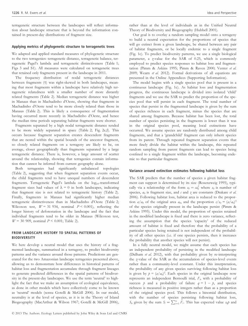
variance s0p(1 � p). Substituting p = (a/a0)z, we obtain the original
expectation that s0(a/a0)z species will persist following habitat loss,
but with the benefit of having now obtained the variance around
that expectation as VarðSl Þ ¼ s0ða=a0Þzð1� ða=a0ÞzÞ (Appendix
A3). When z = 0.25, variance is highest when c. 95% of the original
habitat has been lost (Fig. 4).
Predicting extinction in fragmented landscapes
For a fragment fk, there is a proportion of species that were in fkbut are not in any present-day descendant fragments of fk: they go
extinct from the fragment lineage of fk before the present day. If frag-
ment fk splits into child fragments fkþ1ð1Þ ; fkþ1ð2Þ ; . . .; fkþ1ðnkþ1Þ then the
expected proportions ek (respectively, ekþ1ð1Þ ; ekþ1ð2Þ ; . . .; ekþ1ðnkþ1Þ ) of
species in fk (respectively, in fkþ1ð1Þ ; fkþ1ð2Þ ; . . .; fkþ1ðnkþ1Þ ) that go
extinct by the present day follow the recursive formula
ek ¼Ynkþ1
c¼1
1� akþ1ðcÞ
ak
� �z� �þ akþ1ðcÞ
ak
� �zekþ1ðcÞ
� �
whereakþ1ðcÞak
is the proportion of the area of fk that remains in fkþ1ðcÞ
(Appendix A7). The sum in the brackets is the expected proportion
of species in fk that do not survive to occupy fkþ1ðcÞ , plus those that
do, but subsequently go extinct from the lineage of fkþ1ðcÞ .These
sums must be multiplied because extinction from the lineage of fkrequires the species to either not be present in, or go extinct from,
each of the fragment lineages descending from fk. The recursive
base case, in which fragment fkþ1ðcÞ does not split into any child
fragments, corresponds to ekþ1ðcÞ ¼ 0. The expected proportion of
species that go extinct from the full landscape is obtained by setting
fk to the fragment that represents the entire landscape, f0, at the
root of the terrageny. The variance around e0, the expected propor-
tion of species in the original landscape that go extinct, can be
quantified by considering extinction as a sum of Bernoulli trials
across the s0 species that are present in f0, and equals e0ð1� e0Þ=s0(Appendix A7).
Predicted local extinctions in the Manaus and Machadinho d’Oeste
landscapes were very low, because the pattern of shared species
among non-randomly distributed habitat fragments generates a form
of spatial insurance (Loreau et al. 2003). For a taxon with s0 = 1000
species in the original landscapes, the model predicted that habitat
loss and fragmentation would have caused the local extinction of just
3.2% (95% confidence interval 2.2–4.4%) of the original species pool
from the Manaus landscape and 5.1% (95% CI 3.8–6.5%) in the Ma-
chadinho d’Oeste landscape. These values are lower than the 5.7%
(95% CI 4.3–7.2%) and 20.5% (95% CI 18.0–23.0%) loss predicted
from applying the SAR to the total amount of habitat in the two
landscapes, respectively, and highlight the importance of considering
the fate of biodiversity within individual fragments (Ewers et al.
2010). The confidence intervals of the terragenetic and landscape
SAR predictions overlap in Manaus but not in Machadinho d’Oeste,
suggesting that the importance of modelling landscape history
becomes more pronounced in more fragmented landscapes.
Predicting shared species among habitat fragments
If fk and fh are two fragments with most recent common ancestor
fragment fr, and if ak, ah, and ar are the areas of these fragments,
then the fragments fk and fh are expected to share a proportion
ðakarÞzðah
arÞz of the species that were present in fr (Appendix A4). The
proportion
1� 1� ak
ar
� �z� �1� ah
ar
� �z� �¼ ak
ar
� �zþ ah
ar
� �z� ak
ar
� �zah
ar
� �zof the species in fr will be retained in one or the other of the frag-
ments (Appendix A5), and hence the expected proportion of the
species that are shared between the two fragments is
Ufk fh ¼azka
zh
azka
zr þ a
zh a
zr � a
zka
zh
(Appendix A6). This is directly equivalent to Jaccard similarity, a
commonly used measure of overlap in community composition
(Magurran 2003; Chao et al. 2005). Variance around this expectation
is also available online (Appendix A6).
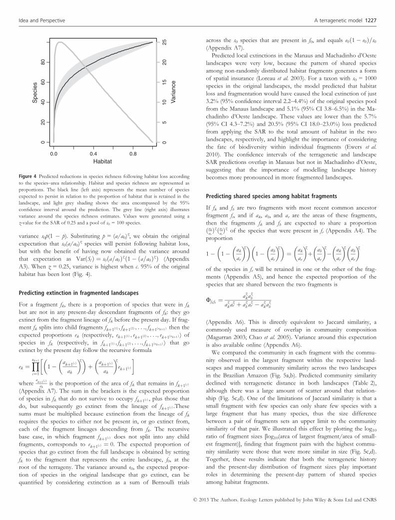
We compared the community in each fragment with the commu-
nity observed in the largest fragment within the respective land-
scapes and mapped community similarity across the two landscapes
in the Brazilian Amazon (Fig. 5a,b). Predicted community similarity
declined with terragenetic distance in both landscapes (Table 2),
although there was a large amount of scatter around that relation-
ship (Fig. 5c,d). One of the limitations of Jaccard similarity is that a
small fragment with few species can only share few species with a
large fragment that has many species, thus the size difference
between a pair of fragments sets an upper limit to the community
similarity of that pair. We illustrated this effect by plotting the log10ratio of fragment sizes [log10(area of largest fragment/area of small-
est fragment)], finding that fragment pairs with the highest commu-
nity similarity were those that were more similar in size (Fig. 5c,d).
Together, these results indicate that both the terragenetic history
and the present-day distribution of fragment sizes play important
roles in determining the present-day pattern of shared species
among habitat fragments.
0.0 0.4 0.8
020
4060
80
Habitat
Spe
cies
05
1015
2025
Var
ianc
eFigure 4 Predicted reductions in species richness following habitat loss according
to the species–area relationship. Habitat and species richness are represented as
proportions. The black line (left axis) represents the mean number of species
expected to persist in relation to the proportion of habitat that is retained in the
landscape, and light grey shading shows the area encompassed by the 95%
confidence interval around the prediction. The grey line (right axis) illustrates
variance around the species richness estimates. Values were generated using a
z-value for the SAR of 0.25 and a pool of s0 = 100 species.
© 2013 The Authors. Ecology Letters published by John Wiley & Sons Ltd and CNRS
Idea and Perspective A terragenetic model 1227
Spatial autocorrelation and community turnover
As the communities of descendent fragments are nested subsets of
the community in the ancestor fragment, the terragenetic model
predicts that closely related fragments will have more species in
common than fragments widely separated on the terrageny (Fig. 5c,
d). Moreover, closely related fragments also tend to be close in geo-
graphical space (Fig. 2e,f), so the terragenetic model should also
predict that fragments located close together in space are likely to
have more species in common than fragments widely separated in
space. This negative correlation was statistically significant in both
landscapes (Table 2), with the terragenetic model predicting a very
rapid decline in community similarity over small spatial scales fol-
lowed by low similarities over larger distances (Fig. 5e,f). Combined
with the nested structure of communities in descendent fragments,
this pattern may help explain the landscape divergence phenomenon
(Laurance et al. 2007), in which communities inhabiting fragments
within the same landscape (i.e. close together) appear to have con-
vergent species compositions whereas those in different landscapes
tend to be divergent.
The location of locally endemic species
We define a locally endemic species as a species that is present in
just one habitat fragment within the landscape. Information on the
likely locations of local endemics is of immediate conservation inter-
est at local scales in much the same way as the locations of globally
endemic species are important for identifying areas of conservation
priority at global scales (Wilson et al. 2006). The terragenetic model
predicts the expected proportion, uk, of species from the original,
full landscape, f0, that end up locally endemic to a present-day frag-
ment, fk, that is separated from f0 by k fragmentation events. If
event t (t = 1,…,k) consists of a single separation into fragment
ft ð1Þ , the direct ancestor of fk, and the siblings of ft ð1Þ , here denoted
ft ðcÞ for c = 2,3,…,nt, then
uk ¼Ykt¼1
at ð1Þ
at�1ð1Þ
� �z�Yntc¼2
1� at ðcÞ
at�1ðcÞ
� �z� �þ at ðcÞ
at�1ðcÞ
� �zet ðcÞ
� �" #
where at ðcÞ is the area of ft ðcÞ (Appendix A8). The left product is over
all separation events leading to fk because in order for a species to
0.0 0.5 1.0
0.0
0.2
0.4
0.6
0.8
123
(c)(a)
(b)
0 5 10 15 20
0.0
0.2
0.4
0.6
0.8
Nodal terragenetic distance
123
(d)
0.0
0.2
0.4
0.6
0.8
(e)
0 10 20 30 40 50
0.0
0.2
0.4
0.6
0.8
Geographic distance (km)
(f)
Com
mun
ity s
imila
rity
Com
mun
ity s
imila
rity
Com
mun
ity s
imila
rity
Com
mun
ity s
imila
rity
Figure 5 Predicted biodiversity patterns arising from the terragenetic model in the Manaus (top row) and Machadinho d’Oeste (bottom row) landscapes. Predictions were
made using a z-value for the species–area relationship of 0.25. (a,b) Spatial pattern in community similarity among habitat fragments. Colours represent the proportion of
species shared with the largest fragment in each landscape (grey circle), and are plotted at the centroid of each fragment. The size of points reflects log10-transformed
fragment size. (c,d) Predicted community similarity against nodal terragenetic distance, with point size reflecting the log10 ratio of fragment sizes. (e,f) Predicted
community similarity against geographical distance. Geographical distance is measured as the distance between fragment centroids and points are semi-transparent, so
darker areas correspond to a higher density of points. In panels c–f, community similarity is represented as Jaccard similarity and represents the proportion of species that
are common to any given pair of habitat fragments.
© 2013 The Authors. Ecology Letters published by John Wiley & Sons Ltd and CNRS
1228 R. M. Ewers et al. Idea and Perspective

be endemic in fk it must have survived, on each fragmentation
event, t, leading to fk, to occupy ft ð1Þ (probability given by the term
ð atð1Þ
at�1ð1Þ
Þz ). The species must also have failed to survive to the present
day in the lineages descending from the sibling fragments ft ðcÞ (prob-
ability given by the product in the bracket). The product in the
bracket resembles the extinction equation of an earlier section and
follows a similar logic. Variance around the expectation given above
is also available online (Appendix A8).
Estimates of uk are always greater than zero, but median values
were very low (< 1 9 10�4) for our two landscapes (Figs 3 and
S1), suggesting few fragments in either landscape are likely to have
locally endemic species. The highest predicted values were 0.002 in
a single fragment in Manaus, and 0.004 and 0.001 in two frag-
ments, respectively, in Machadinho d’Oeste. These values suggest
that for diverse taxa such as invertebrates with s0 = 1000 species
within the landscape, there is one fragment in Manaus that is
expected to contain two locally endemic species, while in Machad-
inho d’Oeste one fragment is expected to contain four local en-
demics and another is expected to contain one. Other fragments
with lower values of uk may also contain local endemics, each with
low probability.
We used phylogenetic generalised least squares to account for the
non-independence of related fragments to examine the correlates of
predicted local endemic species richness. Phylogenetic generalised
least squares models were calculated using the function ‘pgls’ in the
R package ‘caper’ (Orme et al. 2012). We found that the number of
predicted local endemics was higher in fragments that arose earlier
in the terrageny and in fragments that had fewer fragment separa-
tion events in their history (Table 2). As expected, we found that
more terragenetically distinct fragments were more likely to contain
more local endemics in both landscapes (Table 2). In contrast, the
proportion of local endemics was not significantly related to log10-
transformed fragment size (Table 2), suggesting that the presence of
local endemics is related more to the temporal dynamics of histori-
cal patterns of habitat change than it is to the present-day structure
of habitat in the landscape.
Interestingly, the phylogenetic analyses in the Manaus landscape
had k values approaching one, whereas the k values in Machadinho
d’Oeste were zero (Table 2). Values approaching k = 1 indicate that
model residuals show significant terragenetic structuring, suggesting
that in the Manaus landscape standard statistical methods such as
linear regression, which treats fragments as independent replicates
for analysis, would incorrectly estimate the model parameters.
Indeed, linear regression models testing the same relationships
above always had lower explanatory power than phylogenetic gener-
alised least squares models in the Manaus landscape, but there was
no difference among linear and phylogenetic models fitted in the
Machadinho d’Oeste landscape (Table 2).
Model validation
We tested the ability of the terragenetic model to predict
biodiversity patterns using data collected on leaf-litter beetle
(Coleoptera) communities at the Biological Dynamics of Forest
Fragments Project (Didham et al. 1998a) located within the Man-
aus landscape modelled above. Although the beetle data are not
an ideal complete census of many fragments within the landscape,
the full data set did encompass 8494 individuals from 993 species
collected in seven fragments ranging in area from one hectare
through to continuous forest. Using these data, we estimated the
z-value of the SAR to be 0.11, which was the value employed to
make all terragenetic predictions in this case. Beetle communities
were sampled in 1994, and thus we trimmed our terrageny to
make terragenetic predictions for the landscape as it was in the
year 1994. Data on beetle communities were available for just
four of the 1994 fragments represented in the historical land-use
terrageny for Manaus (out of a total of seven fragments in the
original beetle data set – the remaining three were so small they
were below the mapping resolution used to construct the terrage-
nies), giving a combined sample size of 7976 beetles from 947
species. Even with these large sample sizes, the observed number
of species per fragment was less than 60% of the number of
species predicted to be present by the Chao1 diversity index
(range 24–60%), and this undersampling influences the calculation
of similarity indices and the estimation of numbers of locally
endemic species in this data set (Didham et al. 1998b). To miti-
gate this, we used rarefaction to generate estimates of community
composition for a standardised sample size. We randomly
assigned 500 individuals to species within each fragment, with
assignations weighted by the observed relative abundance of the
species within that fragment. We repeated this process 1000
times, and we tested the terragenetic predictions for each of the
1000 rarefied site 9 species matrices using Pearson correlations.
This process allowed us to generate mean and 95% confidence
intervals around the correlation coefficients used to test the terra-
genetic predictions.
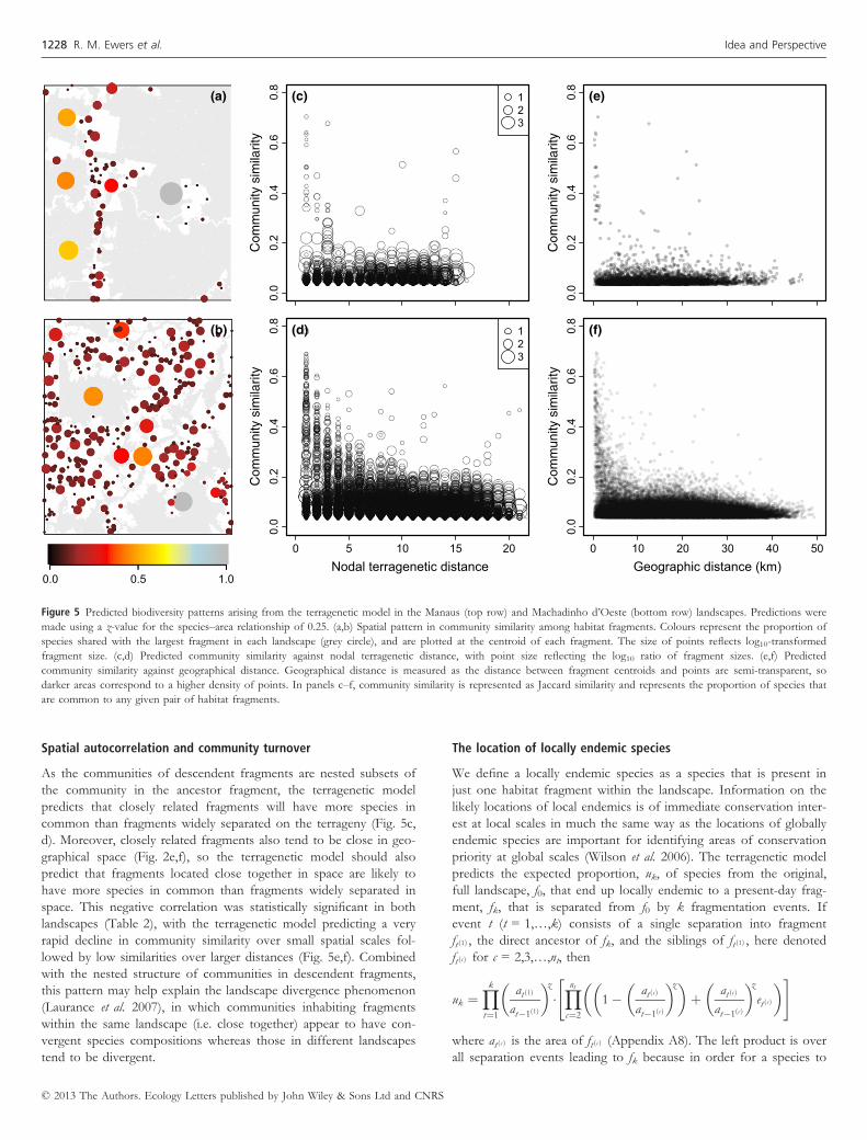
As expected under the terragenetic model, we found a positive
correlation between predicted and observed community similarity
(�r = 0.25, 95% CI = �0.07 to 0.54; Fig. 6a) and a strong, negative
correlation between observed community similarity and terragenetic
distance (�r = �0.28, 95% CI = �0.51 to �0.01; Fig. 6c). Contrary
to the terragenetic predictions, we found a positive correlation
between community similarity and geographical space (�r = 0.52,
95% CI = 0.28 to 0.72; Fig. 6d), although the slope was near-zero
(slope = 0.003) and, with just four fragments, we were unable to
reject the hypothesis that the observed slope was zero (linear
regression: F1,4 = 1.66, P = 0.27). Furthermore, this pattern may
have been an artefact of a weak negative correlation between
geographical distance and the log-ratio of fragment sizes for the
four fragments in this analysis (Mantel test: r = �0.08, P = 0.58).
We also detected a negative correlation between observed and
predicted local endemic species richness (�r = �0.92, 95%
CI = �0.96 to �0.87; Fig. 6b). However, the slope of this
relationship was also near-zero (slope = �0.002) and observed
numbers of endemic species were several orders of magnitude
higher than the predictions, likely an artefact of sampling just four
fragments incompletely. Many species deemed locally endemic in
our empirical data will be shared with fragments that were not
sampled, and this undersampling of fragments will greatly inflate
the observed number of local endemics. Undersampling of the
beetle communities within the fragments probably also contributes
to the inflated estimates of endemic species. This interpretation is
supported by the low values of observed community similarity in
the beetle data (Didham et al. 1998b), with observations being
consistently lower than the values predicted under the terragenetic
model.
© 2013 The Authors. Ecology Letters published by John Wiley & Sons Ltd and CNRS
Idea and Perspective A terragenetic model 1229

DISCUSSION
The terragenetic model is a tree-based model that is neutral at the
level of species and allows us to predict the spatial patterns of bio-
diversity in human-modified landscapes, providing a mathematical
representation of how historical habitat change can leave a spatial
signature on present-day biodiversity. It is more informative as a
null model than MacArthur & Wilson’s (1967) Theory of Island
Biogeography because it predicts spatially explicit patterns of shared
species among fragments rather than species richness within frag-
ments alone. Unlike the Unified Neutral Theory of Biodiversity and
Biogeography (Hubbell 2001), it does not predict the species abun-
dance distribution, and neutrality in the terragenetic model is at the
level of species rather than individuals.
A terrageny represents a quantitative measure of landscape his-
tory. It combines the amount of habitat loss, the patterns of
habitat fragmentation and the historical changes in both of these
features into a single, unique description of landscape structure.
We believe this is particularly important given the interrelated
nature of habitat loss and habitat fragmentation (Fahrig 2003;
Didham et al. 2012). The approach of representing landscape his-
tory as a terrageny integrates these dual processes and patterns,
and provides a natural position from which to make predictions
about their joint effects on biodiversity. Importantly, the terrage-
nies quantified differences between the landscapes despite land-
scape statistics such as the size-distribution of habitat fragments
suggesting there was no difference, and provided information
about individual fragments that was additional to that obtained
from examining physical features such as fragment size and
geographical proximity to neighbouring fragments. These differ-
ences propagate through the terragenetic model to change our
expectation of extinction rates in fragmented landscapes, and gen-
erate predictions about the possible locations of locally endemic
species.
Using the species–area relationship to predict extinction rates
By applying SAR predictions at the scale of individual fragments
rather than the landscape as a whole, the terragenetic model retains
the basic philosophy of SAR-based approaches to estimating extinc-
tion rates. The fundamental difference in approach mirrors the dif-
ference between continental and island-based SARs (Rosenzweig
1995; Drakare et al. 2006): landscape-based SARs rely on a conti-
nental SAR and effectively combine all remnant habitat into a single
estimate of habitat amount, whereas the terragenetic model is built
from an island SAR that estimates the number of species retained
0.0 0.2 0.4 0.6 0.8
0.0
0.2
0.4
0.6
0.8
Observed community similarity
Pre
dict
ed c
omm
unity
sim
ilarit
y (a)
0.0 0.1 0.2 0.3
0.0
0.1
0.2
0.3
Observed local endemic species
Pre
dict
ed lo
cal e
ndem
ic s
peci
es
(b)
0 5 10 15 20
0.0
0.2
0.4
0.6
0.8
Nodal terragenetic distance
Obs
erve
d co
mm
unity
sim
ilarit
y (c)
0 10 20 30 40 50
0.0
0.2
0.4
0.6
0.8
Geographic distance (km)
Obs
erve
d co
mm
unity
sim
ilarit
y (d)
Figure 6 Empirical validations of the ability of the terragenetic model to predict patterns of leaf-litter beetle community composition in the Manaus landscape. (a)
Observed vs. predicted community similarity and (b) observed vs. predicted proportion of locally endemic species. Grey dashed line shows the 1 : 1 relationship that
would be followed if the model made perfect predictions. Observed community similarity (c) declines with increasing terragenetic distance between fragments but (d)
increases with geographical distance between fragments. In all panels, black dashed lines show the relationship fitted using linear regression. Error bars represent the 95%
confidence interval around predicted and observed values. Terragenetic predictions were generated using a z-value for the SAR of 0.11. Community similarity is
represented as Jaccard similarity and represents the proportion of species that are common to any given pair of habitat fragments.
© 2013 The Authors. Ecology Letters published by John Wiley & Sons Ltd and CNRS
1230 R. M. Ewers et al. Idea and Perspective

in individual habitat fragments. The terragenetic model thereby
retains biologically relevant information on the size-distribution of
fragments within landscapes as it makes its predictions (Ewers et al.
2010).
The continental SAR has been criticised for over-estimating
extinction rates that may be better approximated by an endemics–area relationship (EAR) (He & Hubbell 2011). However, whether
the SAR or EAR is most appropriate may depend on the geometry
of habitat loss and how that intersects the spatial distribution of
species (Pereira et al. 2012). Both of these approaches make the
unrealistic assumption that all remnant habitat is spatially discrete,
whereas the terragenetic model allows for fragmented landscapes to
have complex spatial patterns consisting of multiple habitat rem-
nants. Importantly, the terragenetic approach also provides much
more information than a landscape-scale application of the conti-
nental SAR or EAR. The continental SAR and EAR predict the
total number of species that should be retained in a landscape
assuming all remnant habitat is continuous, and cannot be down-
scaled to predict the distribution of species within a landscape. In
contrast, the terragenetic model uses the island SAR to predict the
spatial distribution of species among the various fragments that
comprise the habitat retained within the landscape, and can be up-
scaled to predict the total number of species persisting within a
landscape. Moreover, we obtain these additional predictions without
having to add additional biological parameters to the model.
We also re-interpreted the SAR as providing a species-level prob-
ability rather than a community-level quantity, thereby allowing us
to calculate the variance around all of our predictions of biodiver-
sity patterns (Online Appendices). SAR-based estimates of extinc-
tion are sometimes accompanied with variance estimates, but only
by assuming there is variance in the z-value itself (e.g. Venter et al.
2009; Wearn et al. 2012). In contrast, we assumed that z reflects the
community-level outcome of a stochastic process that operates at
the level of individual species. This allowed us to predict the level
of variance around SAR-based extinction estimates, a new approach
that may help provide resolution on debates about the utility of
large-scale estimates of extinction made using the SAR (Pimm &
Askins 1995; Pimm & Raven 2000; He & Hubbell 2011; Wearn
et al. 2012).
Assumptions of the terragenetic model
We constructed the terragenetic model using a set of simplifying
assumptions, of which we believe four are particularly important.
First, we assumed that all species were distributed randomly across
the pre-fragmentation landscape. However, pre-existing environmen-
tal heterogeneity and species turnover make this unlikely and are
known to influence the outcomes of SAR-based predictions of
extinction (He & Hubbell 2011; Pereira et al. 2012). This will likely
lead to communities sharing less species than predicted by the terra-
genetic model. Second, the model has assumed that fragment size is
a constant until such a time as it separates into two sibling frag-
ments. But we know that accounting for cumulative habitat loss
that gradually erodes the size of an individual fragment can impact
predicted extinction rates (Wearn et al. 2012). A related issue is that
we assumed species richness reaches equilibrium instantaneously
when in fact this process can take many decades and can be depen-
dent on the size of the fragment (Brooks et al. 1999; Ferraz et al.
2003; Halley & Iwasa 2011). If a fragment separates before equilib-
rium species richness is reached, it will pass on more species to its
descendent fragments than accounted for in our models, and by
ignoring this extinction debt the model may underestimate the num-
ber of species that remain in landscapes undergoing rapid change.
Third, dispersal among fragments is a key component of biodiver-
sity persistence in fragmented landscapes (Hanski 1998) and results
in species occupancy patterns shifting among fragments, but was
not incorporated in the model. Over long time periods, continuous
dispersal may erase any terragenetic signature from patterns of
shared species. Finally, the terragenetic model assumed neutrality at
the level of species, so non-random patterns of species susceptibility
to habitat loss and fragmentation might generate nested communi-
ties (Henle et al. 2004; Ewers & Didham 2006; Watling & Donnelly
2006) that are more similar than predicted by the terragenetic
model. Similarly, we made the simplifying assumption that all spe-
cies were habitat specialists and did not persist in, or disperse
through, the matrix, despite considerable evidence to the contrary
for some groups (Kupfer et al. 2006).
Testing the terragenetic model
We used pre-existing data on leaf-litter beetle communities to vali-
date the terragenetic model, relying on one of the largest existing
data sets on the responses of invertebrate communities to habitat
fragmentation collected in the tropics (Didham et al. 1998a). Even
this data set, however, had relatively little power to test the terrage-
netic model for two reasons. First, beetles were sampled at 44 dif-
ferent locations in the Manaus landscape, but that corresponded to
just four separate fragments for which we also had terragenetic data.
This arose because samples were collected along edge gradients
within fragments and because the four control sites used in the
original study were all located within different regions of the same
continuous area of forest. Second, the difficulties of fully censusing
such diverse communities ensured the communities in all fragments
were undersampled (Didham et al. 1998b), reducing the certainty
with which patterns of relative community composition can be
quantified. Notwithstanding these issues, it was encouraging to note
that the observed spatial patterns of among-fragment community
similarity and similarity declines with terragenetic distance were
broadly consistent with the predictions of the terragenetic model.
Testing the predictions of the terragenetic model with higher res-
olution empirical data represents a challenging, but achievable, exer-
cise for future work. The basic unit of biodiversity information that
is predicted by the model is community similarity in the form of
Jaccard similarity. This measure lends itself to field validation,
although it can be difficult to rigorously quantify as it would ideally
require a complete census of the community inhabiting each frag-
ment, as demonstrated by our preliminary validation attempt. Jac-
card similarity is also limited by the size-difference of the fragments
being compared, but remains the most parsimonious metric for use
in the terragenetic model. The terragenetic model does not predict
the abundance of species so abundance-based similarity indices can-
not be used, and Jaccard similarity is more easily interpreted than
the widely used Sørensen similarity index that is monotonically
related to Jaccard (Chao et al. 2005). Field-based studies of habitat
fragmentation typically subsample communities rather than census
them (Nufio et al. 2009; Stork et al. 2009), although methods do
exist to use abundance data to account for undersampling when
communities have not been fully censused (Chao et al. 2005). Even
© 2013 The Authors. Ecology Letters published by John Wiley & Sons Ltd and CNRS
Idea and Perspective A terragenetic model 1231
so, it will be necessary to heavily sample a large number of frag-
ments across an entire landscape to gain enough among-fragment
comparisons of shared species to provide a meaningful test of the
model. The size of the landscape itself should also be carefully
defined to ensure that terragenetic predictions are being made at
spatial scales that are appropriate to the particular taxon being stud-
ied. The sampled fragments in field studies are themselves chosen
to examine gradients of features such as landscape habitat amount
and fragment size, but to test the terragenetic model it will be nec-
essary to structure the collection of field data in different ways to
encompass gradients of terragenetic distance.
Implications for landscape ecology
One of the most important implications of the terragenetic model
is that individual fragments are not independent units to use in
comparative analyses because they have shared histories. This non-
independence of fragment communities may demand a new
approach to analysing the distribution of species across fragmented
landscapes, just as recognition of the shared history of species
demanded a new approach to analysing the distribution of species
traits across phylogenies (Felsenstein 1985) and patterns of extinc-
tion threat across species (reviewed by Purvis 2008). The similar
nature of terragenies and phylogenies ensures that the toolbox of
statistical methods developed to quantify and analyse phylogenies
and phylogenetically correlated data may now provide an excellent
resource for landscape ecologists.
The use of landscape maps is fundamental in landscape ecology,
both for modelling biodiversity patterns within fragmented land-
scapes and for scaling up those models to estimate the total
impact of habitat loss and fragmentation on species and communi-
ties (Ewers et al. 2010). Historical maps of habitat cover have
already proven invaluable in understanding present-day patterns of
biodiversity (Harding et al. 1998; Kuussaari et al. 2009; Wearn et al.
2012), but one implication arising from terragenetic models is that
accurate prediction of biodiversity patterns will require time series
maps of habitat cover. Ideally, historical data on habitat change
through time would always be used to construct a terrageny, but,
in most contexts, detailed historical records will not be available.
In these cases, an alternative approach may be to infer the form
of the terrageny from present-day patterns of habitat distribution
combined with spatially explicit models of historical habitat
change. This in turn suggests that landscape ecologists will need
to more closely integrate their ecological studies with studies on
the dynamics of landscapes themselves, which are driven by
social and economic, rather than ecological, concerns (Lambin &
Meyfroidt 2011).
CONCLUSIONS
As with any model, the usefulness of the terragenetic model will be
in both its ability to accurately describe patterns in data, and its abil-
ity to fail in informative ways (Hubbell 2001; Rosindell et al. 2011).
The importance of biological processes is revealed by comparing
real-world patterns to those of a neutral baseline (Rosindell et al.
2011), and we anticipate this will be the primary role of the terrage-
netic model. Obvious examples include quantifying the role of dis-
persal ability and other species traits in explaining biodiversity
patterns in landscapes that have undergone habitat loss and
fragmentation. Nonetheless, the terragenetic approach to predicting
biodiversity did generate spatial patterns of community composition
that are broadly consistent with expected ecological patterns. The
model retains predictions of the SAR such that large fragments
typically have more species than small fragments, and it predicts dis-
tance-decay in the similarity of communities across space, with the
pattern emerging naturally from an understanding of the history of
a landscape. Predictions of extinction are lower than those arising
from applying the SAR to landscape-scale habitat loss which is in
line with expectation (He & Hubbell 2011), and although we did
not explore it here, the terragenetic model also makes numerical
predictions about patterns of community nestedness along gradients
of fragment size (Watling & Donnelly 2006). Working with terrage-
nies also provides non-intuitive predictions that do not arise from
looking at the geographical distribution of fragments or the distribu-
tion of fragment sizes alone, such as locally endemic species occur-
ring in terragenetically distinct fragments rather than in large
fragments.
Accounting for landscape history and quantifying it in a terrageny,
and by combining a terrageny with a single biological parameter, the
z-value of the SAR, we were able to derive a diverse set of predic-
tions about biodiversity patterns in fragmented landscapes. In the
same way that ignoring evolutionary history limited our ability to
understand patterns of extinction risk among species (Purvis 2008),
we suggest that ignoring the spatio-temporal patterns of landscape
history may limit our ability to understand the biological conse-
quences of habitat loss and fragmentation.
ACKNOWLEDGEMENTS
RME and VL are supported by European Research Council Project
number 281986; RME by the Sime Darby Foundation; RKD by
Australian Research Council Future Fellowship FT100100040;
WDP by a NERC CASE PhD studentship; IMDR by Microsoft
Research and the Grantham Institute for Climate Change; JMBC
by the Foundation for Science and Technology (FCT, Portugal)
REGROWTH-BR Project (Ref. PTDC/AGR-CFL/114908/2009);
and DCR by UK Natural Environment Research Council grants
NE/H020705/1, NE/I010963/1 and NE/I011889/1. J. Jones con-
tributed to the mapping, and A. Bradley, W. Laurance, M. Pfeifer
and J. Rosindell provided comments on the manuscript.
AUTHORSHIP
RME designed the study; RME, DCR and VF developed the math-
ematics; RME, RKD, WDP, DCR and IMDR conducted the analy-
ses; RKD, JMBC and RML collected data; RME wrote the first
draft of the manuscript, and all authors contributed substantially to
revisions.
REFERENCES
Brooks, T.M., Pimm, S.L. & Oyugi, J.O. (1999). Time lag between deforestation
and bird extinction in tropical forest fragments. Conserv. Biol., 13, 1140–1150.Chao, A., Chazdon, R.L., Colwell, R.K. & Shen, T.J. (2005). A new statistical
approach for assessing similarity of species composition with incidence and
abundance data. Ecol. Lett., 8, 148–159.Dauber, J., Bengtsson, J. & Lenoir, L. (2006). Evaluating effects of habitat loss
and land-use continuity on ant species richness in seminatural grassland
remnants. Conserv. Biol., 20, 1150–1160.
© 2013 The Authors. Ecology Letters published by John Wiley & Sons Ltd and CNRS
1232 R. M. Ewers et al. Idea and Perspective
Didham, R.K., Lawton, J.H., Hammond, P.M. & Eggleton, P. (1998a). Trophic
structure stability and extinction dynamics of beetles (Coleoptera) in tropical
forest fragments. Philos. Trans. R. Soc. B-Biol. Sci., 353, 437–451.Didham, R.K., Hammond, P.M., Lawton, J.H., Eggleton, P. & Stork, N.E.
(1998b). Beetle species responses to tropical forest fragmentation. Ecol.
Monogr., 68, 295–323.Didham, R.K., Kapos, V. & Ewers, R.M. (2012). Rethinking the conceptual
foundations of habitat fragmentation research. Oikos, 121, 161–170.Drakare, S., Lennon, J.J. & Hillebrand, H. (2006). The imprint of the
geographical, evolutionary and ecological context on species-area relationships.
Ecol. Lett., 9, 215–227.Ewers, R.M. & Didham, R.K. (2006). Confounding factors in the detection of
species responses to habitat fragmentation. Biol. Rev., 81, 117–142.Ewers, R.M., Marsh, C.J. & Wearn, O.R. (2010). Making statistics biologically
relevant in fragmented landscapes. Trends Ecol. Evol., 25, 699–704.Fahrig, L. (2003). Effects of habitat fragmentation on biodiversity. Annu. Rev.
Ecol. Evol. Syst., 34, 487–515.Felsenstein, J. (1985). Phylogenies and the comparative method. Am. Nat., 125,
1–15.Ferraz, G., Russell, G.J., Stouffer, P.C., Bierregaard, R.O. Jr, Pimm, S.L. &
Lovejoy, T.E. (2003). Rates of species loss from Amazonian forest fragments.
Proc. Natl Acad. Sci. USA, 100, 14069–14073.Fusco, G. & Cronk, Q.C.B. (1995). A new method for evaluating the shape of
large phylogenies. J. Theor. Biol., 175, 235–243.Gotelli, N.J. & McGill, B.J. (2006). Null versus neutral models: what’s the
difference? Ecography, 29, 793–800.Gregory, T.R. (2008). Understanding evolutionary trees. Evol. Educ. Outreach, 1,
121–137.Halley, J.M. & Iwasa, Y. (2011). Neutral theory as a predictor of avifaunal
extinctions after habitat loss. Proc. Natl Acad. Sci. USA, 108, 2316–2321.Hanski, I. (1998). Metapopulation dynamics. Nature, 396, 41–49.Harding, J.S., Benfield, E.F., Bolstad, P.V., Helfman, G.S. & Jones, E.D.B. III
(1998). Stream biodiversity: the ghost of land use past. Proc. Natl Acad. Sci.
USA, 95, 14843–14947.He, F. & Hubbell, S.P. (2011). Species-area relationships always overestimate
extinction rates from habitat loss. Nature, 473, 368–371.Henle, K., Davies, K.F., Kleyer, M., Margules, C.R. & Settele, J. (2004).
Predictors of species sensitivity to fragmentation. Biodiv. Conserv., 13, 207–251.Hubbell, S.P. (2001). The Unified Neutral Theory of Biodiversity and Biogeography.
Princeton University Press, Princeton.
Isaac, N.J.B., Turvey, S.T., Collen, B., Waterman, C. & Bailie, J.E.M. (2007).
Mammals on the EDGE: conservation priorities based on threat and
phylogeny. PLoS ONE, 2, e296.
Krauss, J., Bommarco, R., Guardiola, M., Heikkinen, R.K., Helm, A., Kuussaari,
M. et al. (2010). Habitat fragmentation causes immediate and time-delayed
biodiversity loss at different trophic levels. Ecol. Lett., 13, 597–605.Kupfer, J.A., Malanson, G.P. & Franklin, S.B. (2006). Not seeing the ocean for
the islands: the mediating influence of matrix-based processes on forest
fragmentation effects. Global Ecol. Biogeog., 15, 8–20.Kuussaari, M., Bommarco, R., Heikkinen, R.K., Helm, A., Krauss, J., Lindborg,
R. et al. (2009). Extinction debt: a challenge for biodiversity conservation.
Trends Ecol. Evol., 24, 564–571.Lambin, E.F. & Meyfroidt, P. (2011). Global land use change, economic
globalization, and the looming land scarcity. Proc. Natl Acad. Sci. USA, 108,
3465–3472.Laurance, W.F. (2008). Theory meets reality: how habitat fragmentation
research has transcended island biogeographic theory. Biol. Conserv., 141,
1731–1744.Laurance, W.F., Nascimento, H.E.M., Laurance, S.G., Andrade, A., Ewers, R.M.,
Harms, K.E. et al. (2007). Habitat fragmentation, variable edge effects, and the
landscape-divergence hypothesis. PLoS ONE, 2, e1017.
Loreau, M., Mouquet, N. & Gonzalez, A. (2003). Biodiversity as spatial
insurance in heterogeneous landscapes. Proc. Natl Acad. Sci. USA, 100, 12765–12770.
MacArthur, R.H. & Wilson, E.O. (1967). The Theory of Island Biogeography.
Princeton University Press, Princeton.
Magurran, A.E. (2003). Measuring Biological Diversity. Blackwell Science Ltd,
Oxford.
Mooers, A.O. & Heard, S.B. (1997). Inferring evolutionary process from
phylogenetic tree shape. Quarterly Rev, Biol., 72, 31–54.Nufio, C.R., McClenahan, J.L. & Thurston, E.G. (2009). Determining the effects
of habitat fragment area on grasshopper species density and richness: a
comparison of proportional and uniform sampling methods. Insect. Conserv.
Divers., 2, 295–304.Orme, C.D.L., Freckleton, R.P., Thomas, G., Petzoldt, T., Fritz, S. & Isaac,
N.J.B. (2012). caper: Comparative analyses of phylogenetics and evolution in
R, R package version 0.5. Available at: http://caper.r-forge.r-project.org/.
Pagel, M. (1999). Inferring the historical patterns of biological evolution. Nature,
401, 877–884.Paradis, E., Claude, J. & Strimmer, K. (2004). APE: analyses of phylogenetics
and evolution in R language. Bioinformatics, 20, 289–290.Pereira, H.M., Borda-de-Agua, L. & Martins, I.S. (2012). Geometry and scale in
species-area relationships. Nature, 482, E3–E4.Pimm, S.L. & Askins, R.A. (1995). Forest losses predict bird extinctions in
eastern North America. Proc. Natl Acad. Sci. USA, 92, 9343–9347.Pimm, S.L. & Raven, P. (2000). Extinction by numbers. Nature, 403, 843–845.Prates-Clark, C.D.C., Lucas, R.M. & dos Santos, J.R. (2009). Implications of
land-use history for forest regeneration in the Brazilian Amazon. Can. J.
Remote Sens., 35, 534–553.Purvis, A. (2008). Phylogenetic approaches to the study of extinction. Annu. Rev.
Ecol. Evol. Syst., 39, 301–319.Purvis, A., Katzourakis, A. & Agapow, P.-M. (2002). Phylogenetic tree shape:
two modifications to Fusco and Cronk’s method. J. Theor. Biol., 214, 93–103.Rosenzweig, M.L. (1995). Species Diversity in Space and Time. Cambridge University
Press, Cambridge.
Rosindell, J., Hubbell, S.P. & Etienne, R.S. (2011). The unified neutral theory of
biodiversity and biogeography at age ten. Trends Ecol. Evol., 26, 340–348.Schrott, G.R., With, K.A. & King, A.W. (2005). On the importance of landscape
history for assessing extinction risk. Ecol. Appl., 15, 493–506.Stork, N.E., Coddington, J.A., Colwell, R.K., Chazdon, R.L., Dick, C.W., Peres,
C.A. et al. (2009). Vulnerability and resilience of tropical forest species to
land-use change. Conserv. Biol., 23, 1438–1447.Venter, O., Laurance, W.F., Iwamura, T., Wilson, K.A., Fuller, R.A. &
Possingham, H.P. (2009). Harnessing carbon payments to protect biodiversity.
Science, 326, 1368.
Watling, J.I. & Donnelly, M.A. (2006). Fragments as islands: a synthesis of faunal
responses to habitat patchiness. Conserv. Biol., 20, 1016–1025.Wearn, O.R., Reuman, D.C. & Ewers, R.M. (2012). Extinction debt and
windows of conservation opportunity in the Brazilian Amazon. Science, 337,
228–232.Webb, C.O., Ackerly, D.D., McPeek, M.A. & Donoghue, M.J. (2002).
Phylogenies and community ecology. Annu. Rev. Ecol. Syst., 33, 475–505.Wilson, K.A., McBride, M.F., Bode, M. & Possingham, H.P. (2006). Prioritizing
global conservation efforts. Nature, 440, 337–340.
SUPPORTING INFORMATION
Additional Supporting Information may be downloaded via the online
version of this article at Wiley Online Library (www.ecologyletters.com).
Editor, Michael Bonsall
Manuscript received 1 February 2013
First decision made 12 March 2013
Second decision made 20 May 2013
Manuscript accepted 28 June 2013
© 2013 The Authors. Ecology Letters published by John Wiley & Sons Ltd and CNRS
Idea and Perspective A terragenetic model 1233