University of Sheffield
a thesis submitted in fulfilment of the requirements for
the degree of Doctor of Philosophy
Understanding the Dynamic LeakageBehaviour of Longitudinal Slits in
Viscoelastic Pipes
Author:
Samuel Fox
Supervisor:
Dr. Richard Collins
Prof. Joby Boxall
Pennine Water Group
Department of Civil and Structural Engineering
February 2016
UNIVERSITY OF SHEFFIELD
Executive Summary
Polyethylene pipes, and other polymeric materials, are a popular choice in the water in-
dustry due to their advertised but exaggerated leak resistance. When leaks do occur in
this pipe material, the complex leakage behaviour (time and pressure dependent) presents
a challenge in accurately modelling the representative response. The presented research
aimed to quantify the leak behaviour of longitudinal slits in viscoelastic water distribution
pipes, considering the dynamic interaction of hydraulic conditions and the pipe section
characteristics. A methodology was developed to create synergy between novel physical
investigations and numerical simulations, evaluating the synchronous pressure, leakage
flow-rate and leak area to understand the interdependence of the leakage and structural
dynamics. The synchronous leak area was confirmed as the critical parameter defining
the leak response and is in turn dependent on the leak and pipe geometry, loading condi-
tions and viscoelastic material properties. The theoretical discharge coefficient was shown
to remain constant, thereby establishing that the structural response, i.e. the change of
leak area, can be determined by quantifying the leakage flow-rate and the pressure head
alone. Derivation of a generalised leakage model effectively captured the dynamic leakage
behaviour. However, the model may provide an erroneous estimate of the true response
due to the exclusion of the influence of ground conditions. These were shown to result in a
significant increase in slit face loading dependent on the specific soil matrix properties, si-
multaneously altering the structural deformation and net leakage. Alongside the advances
in fundamental understanding, the research also has implications for leakage management
strategies. The short term behaviour may severely hinder the effectiveness of leak local-
isation technologies and the quantification of risk associated with contaminant ingress.
However, it was shown that current leakage modelling practice over relatively long time
periods are not adversely affected by the existence of such dynamic leaks.
ii
Dedication
“To my wife Soph, who now knows as much about leakage management as I do...without
ever wanting to. Thank you for all your love and support!”
Contents
Executive Summary i
List of Figures vi
List of Tables ix
List of Abbreviations x
List of Symbols xii
1 Introduction 1
2 Literature Review 3
2.1 The Water Distribution System . . . . . . . . . . . . . . . . . . . . . . . . . 3
2.2 Polyethylene pipes - The leak free alternative? . . . . . . . . . . . . . . . . 7
2.2.1 Composition and Structure . . . . . . . . . . . . . . . . . . . . . . . 7
2.2.2 Viscoelasticity . . . . . . . . . . . . . . . . . . . . . . . . . . . . . . 8
2.2.3 Modelling Viscoelasticity . . . . . . . . . . . . . . . . . . . . . . . . 9
Maxwell Model . . . . . . . . . . . . . . . . . . . . . . . 10
Kelvin-Voigt Model . . . . . . . . . . . . . . . . . . . . . 11
Standard Linear Solid Model . . . . . . . . . . . . . . . . 11
Burgers Model . . . . . . . . . . . . . . . . . . . . . . . . 12
Maxwell-Wiechert Model . . . . . . . . . . . . . . . . . . 13
Generalised Kelvin-Voigt Model . . . . . . . . . . . . . . 14
2.2.4 Manufacture and Residual Stresses . . . . . . . . . . . . . . . . . . . 15
2.2.5 Deterioration and Failure . . . . . . . . . . . . . . . . . . . . . . . . 17
2.3 Leak Hydraulics . . . . . . . . . . . . . . . . . . . . . . . . . . . . . . . . . 18
2.3.1 The Orifice Equation . . . . . . . . . . . . . . . . . . . . . . . . . . . 18
2.3.2 Discharge Coefficient (Head Losses) . . . . . . . . . . . . . . . . . . 19
2.3.3 Porous Media (Soil Head Losses) . . . . . . . . . . . . . . . . . . . . 22
2.4 Leakage Modelling . . . . . . . . . . . . . . . . . . . . . . . . . . . . . . . . 25
2.4.1 Structural Behaviour . . . . . . . . . . . . . . . . . . . . . . . . . . . 28
2.4.1.1 Theoretical Investigations . . . . . . . . . . . . . . . . . . . 29
2.4.1.2 Empirical Investigations . . . . . . . . . . . . . . . . . . . . 31
2.5 Leakage Control and Localisation . . . . . . . . . . . . . . . . . . . . . . . . 34
2.6 Summary . . . . . . . . . . . . . . . . . . . . . . . . . . . . . . . . . . . . . 36
iii

Contents iv
3 Aims and Objectives 38
3.1 Research Aim . . . . . . . . . . . . . . . . . . . . . . . . . . . . . . . . . . . 38
3.2 Research Objectives . . . . . . . . . . . . . . . . . . . . . . . . . . . . . . . 38
3.3 Research Structure . . . . . . . . . . . . . . . . . . . . . . . . . . . . . . . . 39
4 Physical study exploring the interaction between structural behaviourand leak hydraulics for dynamic leakage 40
4.1 Overview . . . . . . . . . . . . . . . . . . . . . . . . . . . . . . . . . . . . . 40
4.1.1 Journal Submission Details . . . . . . . . . . . . . . . . . . . . . . . 41
4.2 Abstract . . . . . . . . . . . . . . . . . . . . . . . . . . . . . . . . . . . . . . 42
4.3 Introduction . . . . . . . . . . . . . . . . . . . . . . . . . . . . . . . . . . . . 42
4.4 Background . . . . . . . . . . . . . . . . . . . . . . . . . . . . . . . . . . . . 43
4.5 Viscoelastic Characterisation . . . . . . . . . . . . . . . . . . . . . . . . . . 45
4.6 Investigation Aims . . . . . . . . . . . . . . . . . . . . . . . . . . . . . . . . 47
4.7 Experimental Setup . . . . . . . . . . . . . . . . . . . . . . . . . . . . . . . 47
4.7.1 Laboratory Facility . . . . . . . . . . . . . . . . . . . . . . . . . . . . 47
4.7.2 Test Section Preparation . . . . . . . . . . . . . . . . . . . . . . . . . 48
4.7.3 Structural Response Measurements . . . . . . . . . . . . . . . . . . . 49
4.7.4 Experimental Procedure . . . . . . . . . . . . . . . . . . . . . . . . . 50
4.8 Experimental Results . . . . . . . . . . . . . . . . . . . . . . . . . . . . . . . 52
4.9 Analysis . . . . . . . . . . . . . . . . . . . . . . . . . . . . . . . . . . . . . . 55
4.9.1 Leak Hydraulics . . . . . . . . . . . . . . . . . . . . . . . . . . . . . 56
4.9.2 Structural Response and Leakage Model . . . . . . . . . . . . . . . . 57
4.10 Discussion . . . . . . . . . . . . . . . . . . . . . . . . . . . . . . . . . . . . . 59
4.11 Conclusion . . . . . . . . . . . . . . . . . . . . . . . . . . . . . . . . . . . . 63
5 A dynamic leakage model: derivation and validation of a leakage modelfor longitudinal slits in viscoelastic pipe 65
5.1 Overview . . . . . . . . . . . . . . . . . . . . . . . . . . . . . . . . . . . . . 65
5.1.1 Journal Submission Details . . . . . . . . . . . . . . . . . . . . . . . 66
5.2 Abstract . . . . . . . . . . . . . . . . . . . . . . . . . . . . . . . . . . . . . . 67
5.3 Introduction . . . . . . . . . . . . . . . . . . . . . . . . . . . . . . . . . . . . 67
5.4 Background . . . . . . . . . . . . . . . . . . . . . . . . . . . . . . . . . . . . 68
5.4.1 Theoretical Studies . . . . . . . . . . . . . . . . . . . . . . . . . . . . 69
5.4.2 Empirical Investigations . . . . . . . . . . . . . . . . . . . . . . . . . 70
5.4.3 Polyethylene Pipes . . . . . . . . . . . . . . . . . . . . . . . . . . . . 71
5.5 Research Aim . . . . . . . . . . . . . . . . . . . . . . . . . . . . . . . . . . . 72
5.6 Research Method . . . . . . . . . . . . . . . . . . . . . . . . . . . . . . . . . 73
5.7 Linear-elastic Finite Element Analysis . . . . . . . . . . . . . . . . . . . . . 74
5.7.1 Model and Boundary Conditions . . . . . . . . . . . . . . . . . . . . 74
5.7.2 Meshing and Validation . . . . . . . . . . . . . . . . . . . . . . . . . 76
5.8 Simulation Results . . . . . . . . . . . . . . . . . . . . . . . . . . . . . . . . 77
5.8.1 Slit Face Loading . . . . . . . . . . . . . . . . . . . . . . . . . . . . . 77
5.8.2 Residual Stress . . . . . . . . . . . . . . . . . . . . . . . . . . . . . . 78
5.9 Derivation of Leak Area Model . . . . . . . . . . . . . . . . . . . . . . . . . 79
5.10 Synergistic linear-viscoelastic calibration . . . . . . . . . . . . . . . . . . . . 82
5.11 Experimental validation - dynamic Leakage . . . . . . . . . . . . . . . . . . 84
Contents v
5.12 Discussion . . . . . . . . . . . . . . . . . . . . . . . . . . . . . . . . . . . . . 87
5.12.1 Application . . . . . . . . . . . . . . . . . . . . . . . . . . . . . . . . 90
5.13 Conclusion . . . . . . . . . . . . . . . . . . . . . . . . . . . . . . . . . . . . 90
6 Physical investigation into the significance of ground conditions on dy-namic leakage behaviour 91
6.1 Overview . . . . . . . . . . . . . . . . . . . . . . . . . . . . . . . . . . . . . 91
6.1.1 Journal Submission Details . . . . . . . . . . . . . . . . . . . . . . . 92
6.2 Abstract . . . . . . . . . . . . . . . . . . . . . . . . . . . . . . . . . . . . . . 93
6.3 Introduction . . . . . . . . . . . . . . . . . . . . . . . . . . . . . . . . . . . . 93
6.4 Background . . . . . . . . . . . . . . . . . . . . . . . . . . . . . . . . . . . . 94
6.5 Aim and Hypothesis . . . . . . . . . . . . . . . . . . . . . . . . . . . . . . . 96
6.6 CFD Analysis . . . . . . . . . . . . . . . . . . . . . . . . . . . . . . . . . . . 97
6.7 Experimental Setup . . . . . . . . . . . . . . . . . . . . . . . . . . . . . . . 99
6.7.1 Laboratory Facility . . . . . . . . . . . . . . . . . . . . . . . . . . . . 99
6.8 Experimental Results . . . . . . . . . . . . . . . . . . . . . . . . . . . . . . . 101
6.9 Discussion . . . . . . . . . . . . . . . . . . . . . . . . . . . . . . . . . . . . . 106
6.10 Conclusion . . . . . . . . . . . . . . . . . . . . . . . . . . . . . . . . . . . . 109
7 Analysis and Discussion 111
7.1 Dynamic leak area . . . . . . . . . . . . . . . . . . . . . . . . . . . . . . . . 111
7.1.1 Effective leak area . . . . . . . . . . . . . . . . . . . . . . . . . . . . 113
7.2 Strain-area relationship . . . . . . . . . . . . . . . . . . . . . . . . . . . . . 114
7.3 Influence of ground conditions . . . . . . . . . . . . . . . . . . . . . . . . . . 115
7.4 Generalised leak area model . . . . . . . . . . . . . . . . . . . . . . . . . . . 116
7.5 Application in Leakage Management . . . . . . . . . . . . . . . . . . . . . . 118
7.5.1 Leakage Assessment . . . . . . . . . . . . . . . . . . . . . . . . . . . 118
7.5.2 Hysteresis Analysis . . . . . . . . . . . . . . . . . . . . . . . . . . . . 120
7.5.3 Leakage Exponent . . . . . . . . . . . . . . . . . . . . . . . . . . . . 123
7.5.4 Leakage Localisation and Control . . . . . . . . . . . . . . . . . . . . 124
8 Conclusions 127
8.1 Further Work Proposals . . . . . . . . . . . . . . . . . . . . . . . . . . . . . 130
A Finite Element Analysis Details 131
A.1 Finite Element Verification and Validation . . . . . . . . . . . . . . . . . . . 131
A.2 Parameter Analysis . . . . . . . . . . . . . . . . . . . . . . . . . . . . . . . . 134
B Experimental Methodologies - Additional Information 136
B.1 Leak Area Measurement . . . . . . . . . . . . . . . . . . . . . . . . . . . . . 136
B.1.1 Threshold Analysis . . . . . . . . . . . . . . . . . . . . . . . . . . . . 137
B.2 Experimental Process for Fill Placement . . . . . . . . . . . . . . . . . . . . 138
References 139

List of Figures
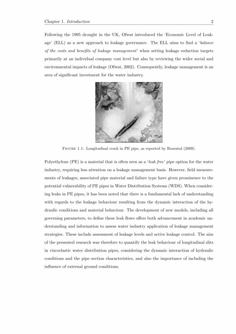
1.1 Longitudinal crack in PE pipe, as reported by Rozental (2009). . . . . . . . 2
2.1 Sample DMA flow-rate and pressure head time series, highlighting MinimumNight Flow (maximum leakage) approximately between 02:00 and 06:00. . . 27
4.1 Schematic of the Generalised Kelvin-Voigt Model . . . . . . . . . . . . . . . 46
4.2 Contaminant Ingress into Distribution Systems laboratory schematic andimage of the test setup. . . . . . . . . . . . . . . . . . . . . . . . . . . . . . 48
4.3 a) Camera setup for image capture (3 fps) of horizontally orientated 60x1 mmlongitudinal slit b) Raw image c) Processed binary image of slit . . . . . . . 50
4.4 Cylindrical coordinate system for strain gauge location (see Table 4.1) wherethe centre of the leak area is located at (31.5,0,0). . . . . . . . . . . . . . . 51
4.5 Experimental procedure flowchart, defining the pressurisation (8 hr phase)and recovery (16 hr phase) stages used to capture the creep and recoveryresponses respectively. . . . . . . . . . . . . . . . . . . . . . . . . . . . . . . 52
4.6 Compiled 5-day measurements of leak area, axial strain, leak flow-rate andpressure head for TS601a at 20 m initial pressure head. . . . . . . . . . . . 53
4.7 Compiled 3-day measurements of leak area, axial strain, leak flow-rate andpressure head for TS601b at 20 m initial pressure head. Plotted on thesame axis as Figure 4.6 to aid comparison. . . . . . . . . . . . . . . . . . . . 54
4.8 Compiled 3-day measurements of leak area, axial strain, leak flow-rate andpressure head for TS601c at 20 m initial pressure head. Plotted on the sameaxis as Figure 4.6 to aid comparison. . . . . . . . . . . . . . . . . . . . . . . 55
4.9 Leak area and strain relationship as measured for TS601a, TS601b andTS601c. Measurements of leak area and axial strain during the recoveryphase only are presented for TS601b and c. . . . . . . . . . . . . . . . . . . 56
4.10 Calculated discharge coefficients for TS601a, TS601b and TS601c at 20 mpressure head, from left to right. . . . . . . . . . . . . . . . . . . . . . . . . 57
4.11 Comparison of measured and modelled leakage from TS601a for 3 day pres-sure tests (downsampled to 1Hz). Quasi-steady state pressure heads of10 m, 20 m and 25 m in ascending order in plot. . . . . . . . . . . . . . . . 59
5.1 Finite element model boundary conditions; plane of symmetry fixed againstdisplacement in x-direction (hatched area), pipe ends fixed against displace-ment in all directions. . . . . . . . . . . . . . . . . . . . . . . . . . . . . . . 75
5.2 Standardised mesh distribution for Finite Element Analysis. Example shownis 60x1 mm longitudinal slit highlighting the mesh detail in the proximityof the slit opening. . . . . . . . . . . . . . . . . . . . . . . . . . . . . . . . . 76
5.3 Mesh Invariance analysis for finite element model. Dashed vertical lineindicates chosen mesh resolution. . . . . . . . . . . . . . . . . . . . . . . . . 77
vi

List of Figures vii
5.4 Comparison of the slit edge deflection (Ux) of a 20x1mm FE model subjectto three discrete slit face load cases. . . . . . . . . . . . . . . . . . . . . . . 78
5.5 Longitudinal slit areas from FE simulation of residual stress analysis forthree discrete test sections. . . . . . . . . . . . . . . . . . . . . . . . . . . . 79
5.6 Coefficient (C1) analysis from Finite Element data. . . . . . . . . . . . . . . 81
5.7 Measured and modelled leakage for 60x1 mm test section, including theassociated Cd error. Quasi-steady state pressure heads of 10 m, 20 m and25 m in ascending order in plot. . . . . . . . . . . . . . . . . . . . . . . . . . 85
5.8 Measured and modelled leakage for 20x1 mm test section, including theassociated Cd error. Quasi-steady state pressure head of 20 m. . . . . . . . 86
5.9 Measured and modelled leakage for 40x1 mm test section, including theassociated Cd error. Quasi-steady state pressure head of 20 m. . . . . . . . 86
5.10 Histograms of the ratio of numerically simulated using FEA (Asim) andpredicted (Apred) leak areas of longitudinal slits in pressurised pipes. (Left)Equation 5.4 prediction of leak area of longitudinal slits in thin walled pipesusing parameters from Cassa and van Zyl (2008). (Right) Expression fromCassa and van Zyl (2011) of leak area of longitudinal slits in thick walledpipes using parameters from Table 5.1. . . . . . . . . . . . . . . . . . . . . . 88
6.1 Investigation to explore the interdependence of three fundamentals princi-ples; leak hydraulics, structural behaviour and soil hydraulics. . . . . . . . . 97
6.2 Velocity streamlines (left) and static pressure contour on central slit plane(right) from CFD simulation of 60x1 mm longitudinal slit leaking into afully submerged test section box. Plane of interest shown as transparentsurface on velocity streamline plot. . . . . . . . . . . . . . . . . . . . . . . . 98
6.3 Velocity streamlines (left) and static pressure contour on central slit plane(right) from CFD simulation of 60x1 mm longitudinal slit leaking into a fullysubmerged test section box containing compact gravel. Plane of interestshown as transparent surface on velocity streamline plot. . . . . . . . . . . . 99
6.4 Contaminant Ingress into Distribution Systems Laboratory Facility . . . . . 100
6.5 Leakage flow-rate through a 60x1 mm longitudinal slit at three discretepressure heads into water (blue line) and geotexile fabric (black line). . . . . 102
6.6 Axial strain measured parallel to a 60x1 mm longitudinal slit in MDPEpipe at three discrete pressure heads for test cases into water (blue line)and geotexile fabric (black line). . . . . . . . . . . . . . . . . . . . . . . . . 103
6.7 Time series of evaluated discharge coefficients (Cd) for 60x1 mm longitudinalslit in MDPE pipe at three discrete pressure heads for test cases into water(blue line) and geotexile fabric (black line). . . . . . . . . . . . . . . . . . . 104
6.8 Axial strain for a 60x1 mm longitudinal slit in MDPE pipe at 26 m pressurehead for test cases into water (blue line), geotexile fabric (black line) andmixed gravel (gray line). . . . . . . . . . . . . . . . . . . . . . . . . . . . . . 105
6.9 Leakage flow rate for a 60x1 mm longitudinal slit in MDPE pipe at 26 mpressure head for test cases into water (blue line), geotexile fabric (blackline) and mixed gravel (gray line). . . . . . . . . . . . . . . . . . . . . . . . 105
7.1 Centre of 60x1 mm longitudinal slit deflection across pipe wall thickness(s=6.5 mm), at a range of applied pressure heads (H ), with diagram ofreference plane through pipe. Width equal to 0 mm represents symmetryline from FEA model (see Chapter 5). . . . . . . . . . . . . . . . . . . . . . 112

List of Figures viii
7.2 The variation of effective leak area with pressure head for a 90x2 mm lon-gitudinal slit in 93.3 mm diameter HDPE pipe (Massari et al., 2012). . . . . 113
7.3 (Left) Dependence on leak age of fitted leakage exponent (Right) Leak agedependence of percentage difference between viscoelastic leak flow data andfitted model predictions . . . . . . . . . . . . . . . . . . . . . . . . . . . . . 119
7.4 Influence of pressure regimes on daily change in net leakage flow-rate forarbitrary longitudinal slit in viscoelastic pipe. Varied mean pressure (left)and varied pressure range with equal mean pressures (right). . . . . . . . . 121
7.5 Hysteresis offset analysis where S=0.0626 for left hand figure with J5=1.3E-09 Pa and S=0.1356 for right hand figure with J5=5E-09 Pa. . . . . . . . . 121
7.6 Pressure-leakage hysteresis cycles of arbitrary longitudinal slit, for discretepressure ranges (details listed in Table 7.3). . . . . . . . . . . . . . . . . . . 123
A.1 Finite element analysis summary of geometrical parameters influence on therelative change of longitudinal slit area. . . . . . . . . . . . . . . . . . . . . 131
A.2 Relationship between axial strain and leak area taken from Finite ElementAnalyses for 20x1, 40x1 and 60x1 mm longitudinal slits. . . . . . . . . . . . 132
A.3 Relative axial strain measurements parallel to a longitudinal slit at 18 mmdistance from leak centre. . . . . . . . . . . . . . . . . . . . . . . . . . . . . 133
A.4 Relative axial strain measurements perpendicular to a longitudinal slit. Ori-gin at centre of slit length on the edge of the opening. . . . . . . . . . . . . 133
A.5 Finite element analysis summary of geometrical parameters influence on therelative change of longitudinal slit area. . . . . . . . . . . . . . . . . . . . . 134
A.6 Finite element analysis summary of material and loading conditions influ-ence on the relative change of longitudinal slit area. . . . . . . . . . . . . . 135
List of Tables
2.1 Example of typical ranges of discharge coefficient (Cd) for sharp-edged ori-fices as summarised in Brater et al. (1996). . . . . . . . . . . . . . . . . . . 19
2.2 Table of leakage exponents for individual leaks taken from experimental data. 26
2.3 Summary table of key leakage research papers identified from literaturereview listing the type and focus of the research. (The. - Theoretical Study;Exp. - Experimental Study; and Num. - Numerical Study) . . . . . . . . . . 37
4.1 Summary table of test sections and details of axial strain gauge locations. . 49
4.2 Linear fitting parameters for the explicit strain-area relationship for threediscrete test sections. . . . . . . . . . . . . . . . . . . . . . . . . . . . . . . . 56
4.3 Non-linear least squares calibration of creep compliance components fortime-dependent axial strain for TS601a. . . . . . . . . . . . . . . . . . . . . 58
5.1 Summary table of Finite Element Analysis variables. . . . . . . . . . . . . . 74
5.2 Results of statistical analysis of FEA parameter significance using multipleregression. . . . . . . . . . . . . . . . . . . . . . . . . . . . . . . . . . . . . . 80
5.3 Non-linear least squares calibration of creep compliance components fortime-dependent elastic modulus for TS601a at three discrete experimentalpressure heads. . . . . . . . . . . . . . . . . . . . . . . . . . . . . . . . . . . 83
6.1 Summary table of results from 60x1 mm slit at three discrete pressuresleaking into water and geotextile fabric. Net leakage refers to volume ofleakage flow over 1 hr pressurisation phase. . . . . . . . . . . . . . . . . . . 102
7.1 Relative creep compliance components (J ′n = Jn/Jmax) from Chapters 4and 5 for the explicit and generalised leak area models. . . . . . . . . . . . . 115
7.2 Pipe and longitudinal slit dimensions for modelling study. . . . . . . . . . . 119
7.3 Summary of test cases from Figure 7.6 and associated hysteresis descriptorsof enclosed area (EA) and characteristic offset (S ). . . . . . . . . . . . . . . 122
8.1 Summary of research outputs and outcomes. . . . . . . . . . . . . . . . . . . 129
ix

List of Abbreviations
CFD Computational Fluid Dynamics
DAQ Data Acquisition Device
DMA District Metered Area
DMZ District Metered Zone
ELL Economic Level of Leakage
FAVAD Fixed And Variable Area Discharge
FEA Finite Element Analysis
GKV Generalised Kelvin Voigt
HDPE High Density Polyethylene
ITA Inverse Transient Analysis
KV Kelvin Voigt
LDPE Low Density Polyethylene
LED Light Emitting Diode
MDPE Medium Density Polyethylene
IWA Internation Water Association
MNF Minimum Night Flow
NRV Non Revenue Water
Ofwat Office of Water Services
OS Orifice Soil number
PE PolyEthylene
RMSE Root Mean Squared Error
SDR Standard Dimension Ratio
SELL Sustainable Economic Level of Leakage
SG Strain Gauge
SLS Standard Linear Solid
x

List of Abbreviations xi
UARL Unavoidable Annual Real Losses
uPVC unplasticised Polyvinyl Chloride
WDS Water Distribution Systems

List of Symbols
A0 initial area m2
AE effective leak area m2
AL laek area m2
c leakage coefficient
Cd discharge coefficient
C0 constant coefficient
C1 dimensionless coefficient
dA change of leak area m2
D pipe diameter m
DH hydraulic diameter m
E Young’s modulus Pa
g gravitational acceleration = 9.81m/s2
G relaxation modulus Pa
ho orifice head loss m
hs soil head loss m
H pressure head m
Ps slit face pressure Pa
J creep compliance 1/Pa
L slit length m
Q discharge/flow-rate m3/s
P pressure Pa
r radial coordinate m
Re Reynolds number
s pipe wall thickness m
S relative hysteresis offset
xii

List of Symbols xiii
t time s
T temperature oC
v flow velocity m/s
W slit width m
∆P differential pressure Pa
(= Pipe Fluid Pressure - Depth of Water External to leak)
ε strain
η viscosity Pa s
λ leakage exponent (or N1)
ν Poisson ratio
ρ density kg/m3
σ stress N/m2
σr residual stress Pa
τ retardation time s
Chapter 1
Introduction
The transportation of potable water from supplier to consumer is a vital infrastructure
that continues to develop in an effort to meet regulatory standards of both water quality
and delivery performance. Figures published by the Department for Environment, Food
and Rural Affairs (Defra, 2011) in 2011 estimated that the water distribution system
required a capacity of over 8,500 mega-litres per day, across the 34 privately-owned water
companies regulated by the Office of Water Services (Ofwat, 2013), to supply the UK’s
population who consumed between 100 and 160 litres per person per day (Defra, 2011).
The delivery of clean and safe drinking water is therefore essential both from a water
quality and economic viewpoint.
Leakages within the distribution network are a well-documented challenge that water com-
panies must confront in order to meet standards set by Ofwat. During the period of 2009-11
the industry average level of leakage within the UK was estimated at 133.1 litres per prop-
erty per day, which equates to 24% of the delivered supply pipe volume (Ofwat, 2010).
1
Chapter 1. Introduction 2
Following the 1995 drought in the UK, Ofwat introduced the ‘Economic Level of Leak-
age’ (ELL) as a new approach to leakage governance. The ELL aims to find a ‘balance
of the costs and benefits of leakage management ’ when setting leakage reduction targets
primarily at an individual company cost level but also by reviewing the wider social and
environmental impacts of leakage (Ofwat, 2002). Consequently, leakage management is an
area of significant investment for the water industry.
Figure 1.1: Longitudinal crack in PE pipe, as reported by Rozental (2009).
Polyethylene (PE) is a material that is often seen as a ‘leak free’ pipe option for the water
industry, requiring less attention on a leakage management basis. However, field measure-
ments of leakages, associated pipe material and failure type have given prominence to the
potential vulnerability of PE pipes in Water Distribution Systems (WDS). When consider-
ing leaks in PE pipes, it has been noted that there is a fundamental lack of understanding
with regards to the leakage behaviour resulting from the dynamic interaction of the hy-
draulic conditions and material behaviour. The development of new models, including all
governing parameters, to define these leak flows offers both advancement in academic un-
derstanding and information to assess water industry application of leakage management
strategies. These include assessment of leakage levels and active leakage control. The aim
of the presented research was therefore to quantify the leak behaviour of longitudinal slits
in viscoelastic water distribution pipes, considering the dynamic interaction of hydraulic
conditions and the pipe section characteristics, and also the importance of including the
influence of external ground conditions.
Chapter 2
Literature Review
2.1 The Water Distribution System
Food, water and shelter; the basic needs of human beings for a secure existence. The ever
increasing global population continues to put a strain on these fundamental requirements
with new technologies geared to supplement potential food shortages across the globe,
novel building techniques employed to minimise cost and maximise the use of limited
space and a focus on reliable sourcing, treatment and distribution of potable water.
The water distribution system (WDS) plays a crucial role in the daily lives of every member
of our society. A failure to provide a secure and reliable source of potable water does not
only have potential ramifications for health and well-being, but can also have an impact
on economic prosperity for dependent commercial and industrial consumers in addition to
the reliance of residential occupants. In the United Kingdom an estimated population of
60 million are connected to a constant supply of water by over 340,000 km of pipe lines,
provided by the group of private water companies. Whilst operating within a business
framework, the water companies have a more important responsibility to ensure that one
of the most basic needs for human existence is met, providing clean and safe drinking
water. To ensure that this is done whilst maximising the efficiency and cost-effectiveness
of the supply chain, the water industry have emphasised a focus on sustainability through
investment.
3

Chapter 2. Literature Review 4
The ambiguity and over-use of the term ‘sustainability’ can often detract from its signif-
icance. In the context of the water industry, consideration of health and safety, environ-
mental and economic aspects are used to evaluate the sustainability of the WDS. On a
global level, some of the critical factors affecting the sustainability of the water supply
include; increasing population, water scarcity (possibly due to global warming) and the
increase in industry/manufacturing demand. At a more localised level, critical factors
include; water quality, utility security, energy costs (treatment and transport) as well as
real and apparent losses (real losses are bursts and background leaks, with apparent losses
covering unauthorised consumption). All of these factors can increase the operating cost
for water suppliers, a cost that is subsequently passed onto consumers. Well-documented
and publicised problems faced by the water industry are the real losses, i.e. leaks and
bursts, from distribution pipes. As water is fast becoming one of the most valuable global
resources, the economic impact in addition to the environmental consequences of these
losses is serious.
Leaks and leakages are a common issue for water suppliers. Leaks, the structural failings
through which leakage may result, manifest in a variety of different forms. Leaks include
joint failures, holes (corrosion and impact) and cracks, with the specific failure mechanism
often dependent on factors such as material type, manufacturing process, installation pro-
cedure, external environmental conditions and structural loading. In the UK, the Water
Services Regulation Authority (Ofwat) published leakage statistics from 2013 showed that
the current level of leakage stands at 172 mega-litres per day, equivalent to approximately
452,000 Olympic size swimming pools worth of water lost every year (Ofwat, 2013). Fol-
lowing the 1995 drought in the UK, Ofwat introduced the Economic Level of leakage
(ELL), which has now been superseded by the Sustainable Economic Level of Leakage
(SELL), aimed at reducing the environmental and social impacts of leakage including the
supply cost to customers and businesses, new water resources and the threat of lost water
supply (Ofwat, 2002). The aim of the targets were to ensure that water companies ‘fix
leaks, as long as the cost of doing so is less than the cost of not fixing the leak ’ (Ofwat,
2002). The term ‘cost’ referred to both the cost of treating and transporting water to
supplement the losses from the system, but also accounts for the environmental damage
that leaks may cause, such as flooding, erosion etc. The effectiveness of the SELL targets
are often reviewed, with an SMC report stating that changes could be made to account
for ‘average and extreme years’ as opposed to the current standard to base calculations on

Chapter 2. Literature Review 5
an average year (Strategic Management Consultants, 2012). Such reviews aim to drive the
sustainability of the WDS forward, encouraging further investment from water companies
across the UK with particular attention given to the implementation of successful leakage
management strategies and those that require further attention and development.
Typical leakage management strategies aim to reduce leakage whilst meeting the require-
ments of the SELL targets. There are reviews and guidelines that outline the current
state of the art concerning leakage management strategies within the water industry in
detail; e.g. Farley (2001) and Puust et al. (2010). Puust et al. (2010) categorised the
existing and developing methods into i) leakage assessment ii) leakage detection and iii)
leakage control. Leakage assessment focuses on the effective methods of quantifying the
losses from distribution systems through the use of appropriate models to interpret real-
network data (pressure and flow-rates). Such models require a fundamental understanding
of system characteristics including the system demand, network configuration and also the
behaviour of different leak types. Leakage detection technologies are aimed at highlighting
‘leakage hotspots’ as well as determining localised sections containing significant leaks or
bursts. Finally, leakage control focuses on methods to control current and future levels of
leakage through techniques such as pressure management and also consideration of asset
maintenance and renewal. There is also an increasing awareness and understanding of
the impact of diurnal pressure variations (Farley, 2001) and the interaction of leaks and
dynamic pressures within WDS (Fox et al., 2014b).
Water companies continue to explore a variety of different approaches to manage the real
losses from their systems. These include novel leak detection technologies and advanced
pressure management schemes. A major change over the past few decades has been the
selection of pipeline material used, with careful consideration given to material cost, design
limits, serviceability and durability. This has seen a shift in the use of pipes from more
traditional materials such as cast and ductile iron towards plastics including PVC and
polyethylene. Alongside the benefits of plastic pipes in terms of their ease of on-site
handling (continuous pipe coils up to 150 m in length can be delivered and installed)
and overall costs (reduce whole life costs by up to 45% compared to other materials
according to GPSUK (2014a)), polyethylene pipes in particular are often perceived to
be ‘leak free’ alternatives for the water industry. Field data provides evidence to the
contrary (UKWIR, 2008). Fundamental understanding of the behaviour of individual leaks
is crucial to the effective implementation of leakage management strategies. Consideration

Chapter 2. Literature Review 6
of the dependent behaviour under different hydraulic and environmental loading conditions
may have significant consequences for the development and implementation of leakage
assessment, leakage detection and leakage control alike.
Chapter 2. Literature Review 7
2.2 Polyethylene pipes - The leak free alternative?
Polyethylene (PE) was invented by accident in 1933 following an explosion at the ICI
Laboratories in the United Kingdom (Grann-Meyer, 2005). Following its discovery, its
use as a hydraulic pipeline material has grown steadily since the 1950s when the earliest
generations of low and high density polyethylene were first created. The market for the
PE pipes is ever growing, especially in Western Europe as supported by figures published
by TEPPFA and Association (2007), with the production of HDPE measured at over
1000ktons/year in 2002 with a forecast growth of 5% (Grann-Meyer, 2005). This growing
market, supplying both the water and gas industry, is fuelled by the publicised ‘leak
free’ capacity of PE pipelines (Pepipe.org, 2013) and the subsequent economic benefits of
utilising such a material.
2.2.1 Composition and Structure
Polyethylene is a thermoplastic, defined as having the ability to soften on heating and re-
harden on cooling (Bilgin et al., 2008) which has a significant consequence on the mechan-
ical properties. Polyethylene is formed from the chemical bonding of ethylene molecules
to form long linear macromolecular chains, with the length and degree of the crystallinity
determining the molecular weight and hence the toughness of the material (Grann-Meyer,
2005). As a semi-crystalline polymer, polyethylene can be categorised into high, medium
and low densities which are dependent on the level of crystallinity and subsequent density
(Grann-Meyer, 2005). Low Density Polyethylene (LDPE) is formed at high pressure (at
approximately 1000 bar) with High Density Polyethylene (HDPE) formed at relatively
low pressures (at approximately 50 bar) resulting in lower level branching of the structure
which increases the material density (Lepoutre, 2013). O’Connor (2011) describes how
LDPE was first discovered in the early 1950s followed shortly afterwards by 1st generation
HDPE. Medium Density Polyethylene (MDPE) and the 2nd generation of HDPE were
then manufactured in the 1960s and 1970s respectively with the development of PE con-
tinuing through to the current day. The composition and structure of the different classes
of PE define the mechanical properties of the materials and are therefore significant when
considering the performance of PE hydraulic pipes in operation.

Chapter 2. Literature Review 8
2.2.2 Viscoelasticity
Materials are often described as displaying a linear or non-linear structural response to
an applied loading. Representative material models may infer that liquids exhibit pure
Newtonian viscosity and solids exhibit pure Hookean elastic behaviour. In reality materials
exhibit a combination of these characteristics and may therefore be classified for example
as elastic, plastic or viscoelastic.
Viscoelastic materials show an ‘interdependence of stress and strain with time’ (Benham
et al., 1996) with polymer viscoelasticity focussing on the ‘interrelationships among elas-
ticity, flow and molecular motion’ (Sperling, 1992). There are three important phases
when considering the structural response of viscoelastic materials, namely; creep, relax-
ation and recovery. Creep is defined as the time and temperature dependent strain of a
material for a constant stress. Stress relaxation is the time and temperature decrease in
stress at a constant applied strain. Recovery is the time and temperature dependent strain
recovery following removal of an applied stress. These viscoelastic phenomena result from
the molecular structure and activity of the material (commonly polymeric) and may be
placed into five general categories/modes (Tobolsky, 1960), which may independently or
collectively contribute to the observed behaviour;
1. Chain Scission
2. Bond Interchange
3. Viscous Flow
4. Thirion Relaxation
5. Molecular Relaxation
PE is classified as a viscoelastic material due to the composition and structure of the ma-
terial, where the long chain branching and molecular weight distribution directly influence
the viscoelastic characteristics (Wood-Adams et al., 2000).

Chapter 2. Literature Review 9
2.2.3 Modelling Viscoelasticity
There are many varied academic and industry applications which necessitate the use of
analytical viscoelastic models including biomechanics, fluid mechanics and polymer sci-
ence/engineering. The applied models are derived from constitutive equations, typically
considering linear viscoelastic behaviour which infers the employment of infinitesimal strain
theory (Ferry, 1961). Infinitesimal strain theory deals with small/infinitesimal deforma-
tions of a continuum body, generally observed in civil and mechanical engineering activities
(Banks et al., 2011). Moore and Zhang (1998) confirmed the applicability of linear vis-
coelasticity if the material strain does not exceed 0.01 (specifically for HDPE). Pittman
and Farah (1997) also found that models based on this assumption of linear viscoelastic
theory were applicable for polyethylene pipes (MDPE) for strain magnitudes less than
2%. Non-linear viscoelasticity, which concerns the time-dependent response of materials
to large and rapid changes in strain, is far more complicated and requires application of
fundamental continuum (Dealy, 2014). The linear viscoelastic constitutive equations are
based upon the effects of sequential changes in strain or stress, assuming that all changes
are additive (Ferry, 1961). Often referred to as the Boltzmann superposition principle,
this theoretical approach assumes that the net response is the summation of the full load-
ing history comprised of individual load steps. Also known as the ‘rheological equation
of state’, the equations deal with the time dependent relation between stress and strain
(Ferry, 1961). Equation 2.1, convolution integral for stress, expresses this relationship
with respect to the shear rate and the theoretical relaxation modulus of the material, G.
σ(t) =
∫ t
−∞G(t− t′)dε
dt(t′)dt′ (2.1)
Another formulation of the constitutive equation, shown in equation 2.2 as the convolu-
tion integral for strain, defines the time-dependent strain in terms of the loading history
(applied stress) and the theoretical material creep compliance, J.
ε(t) =
∫ t
−∞J(t− t′)dσ
dt(t′)dt′ (2.2)
The implementation of the alternative constitutive equations is dependent on the indi-
vidual analysis scenario, i.e. whether creep, relaxation or recovery phenomena are being
assessed. In order to implement the theoretical ‘rheological equations of state’ a method
Chapter 2. Literature Review 10
to calibrate the material responses (e.g. creep compliance) is required. The constitutive
equations for viscoelasticity may therefore be conceptualised as a series of springs, repre-
sentative of the linear-elastic response, and dashpots, representative of the time-dependent
viscous response of a material (Lemaitre et al., 1996). There are a range of mathematical
representations of viscoelasticity which involve different configurations of these two com-
ponents, with six typical formulations summarised below with examples of their utilised
applications.
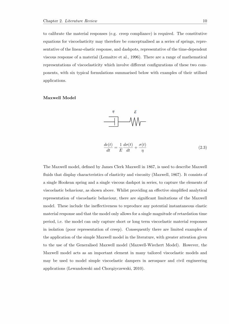
Maxwell Model
dε(t)
dt=
1
E
dσ(t)
dt+σ(t)
η(2.3)
The Maxwell model, defined by James Clerk Maxwell in 1867, is used to describe Maxwell
fluids that display characteristics of elasticity and viscosity (Maxwell, 1867). It consists of
a single Hookean spring and a single viscous dashpot in series, to capture the elements of
viscoelastic behaviour, as shown above. Whilst providing an effective simplified analytical
representation of viscoelastic behaviour, there are significant limitations of the Maxwell
model. These include the ineffectiveness to reproduce any potential instantaneous elastic
material response and that the model only allows for a single magnitude of retardation time
period, i.e. the model can only capture short or long term viscoelastic material responses
in isolation (poor representation of creep). Consequently there are limited examples of
the application of the simple Maxwell model in the literature, with greater attention given
to the use of the Generalised Maxwell model (Maxwell-Wiechert Model). However, the
Maxwell model acts as an important element in many tailored viscoelastic models and
may be used to model simple viscoelastic dampers in aerospace and civil engineering
applications (Lewandowski and Chorazyczewski, 2010).

Chapter 2. Literature Review 11
Kelvin-Voigt Model
σ(t) = Eε(t) + ηdε(t)
dt(2.4)
The Kelvin-Voigt (KV) model, named after physicists Lord Kelvin and Woldemar Voigt
(Fung, 1981), consists of a single Hookean spring and a single viscous dashpot in parallel
and describes the characteristic behaviour of a simple viscoelastic solid. The result of this
configuration is that the strain in each component is equal and tends towards a constant
limit within the linear viscoelastic range. This is in contrast to the Maxwell model which
assumes an unbounded linear relationship between strain and time, thus representing a
viscoelastic fluid (Marques and Creus, 2012). As with the Maxwell model, the simple
form of the model inhibits the effectiveness for the representation of realistic viscoelastic
behaviour. Therefore the KV model is commonly used as an element within more detailed
models, including the Generalised Kelvin-Voigt model, capturing all the characteristics of
linear viscoelastic behaviour.
Standard Linear Solid Model
dε(t)
dt=
1
E1 + E2
(dσ(t)
dt+E2
ησ(t)− E1E2
ηε(t)
)(2.5)

Chapter 2. Literature Review 12
The Standard Linear Solid (SLS) model was developed as a means to overcome the limi-
tations of both the Maxwell and KV models, i.e. the ineffectiveness to capture creep and
relaxation behaviour respectively. The SLS, or Zener model, consists of a single Hookean
spring and a Maxwell element in parallel and is therefore the simplest mathematical rep-
resentation that accounts for creep, relaxation and recovery. As a result the SLS model
has been employed to simplify the definition of the viscoelastic behaviour of complex ma-
terials such as carbon nanotube fibres (Lekawa-Raus et al., 2014). Whilst the simplicity
of the model provides an effective computationally lightweight solution for approximating
viscoelastic behaviour, this also limits the accuracy of the modelled material response due
to the complex reality of viscoelastic material behaviour.
Burgers Model
ε =σ
E1+
σ
E2
(1− exp
(−E1
η1.t
))+
σ
E2.t (2.6)
The Burgers model was developed by Johannes Martinus Burgers to incorporate elements
from both the Maxwell and KV viscoelastic models (Burgers, 1935). The effect of this
configuration is that instantaneous elastic responses, time-dependent viscous responses
and non-recoverable creep flow are all accounted for at a basic level. Examples of the
use of Burgers model include application within the simulation of ice behaviour (Yazarov,
2012) and geotechnical work considering the viscoelastic response of soil beds (Dey and
Basudhar, 2010). Like the Maxwell model, Burgers model is an effective tool to describe
the response of viscoelastic fluids as the stress tends to zero during stress relaxation and
there is unbounded deformation during the creep phase (Shepherd et al., 2012). However,
it therefore presents a poor representation of viscoelastic solids.
Chapter 2. Literature Review 13
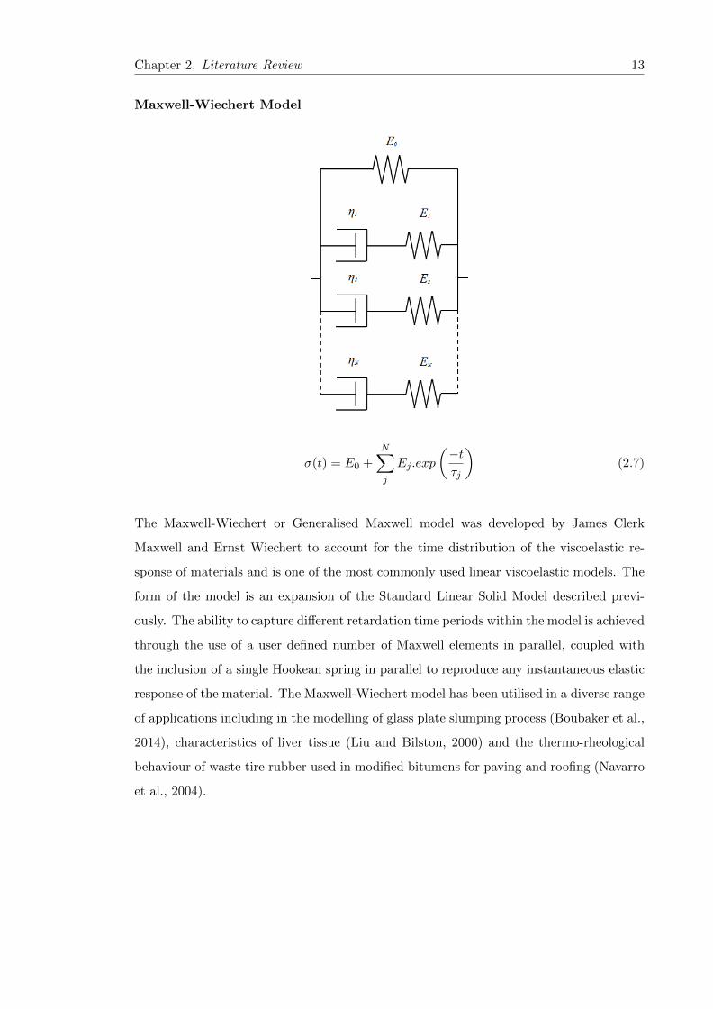
Maxwell-Wiechert Model
σ(t) = E0 +N∑j
Ej .exp
(−tτj
)(2.7)
The Maxwell-Wiechert or Generalised Maxwell model was developed by James Clerk
Maxwell and Ernst Wiechert to account for the time distribution of the viscoelastic re-
sponse of materials and is one of the most commonly used linear viscoelastic models. The
form of the model is an expansion of the Standard Linear Solid Model described previ-
ously. The ability to capture different retardation time periods within the model is achieved
through the use of a user defined number of Maxwell elements in parallel, coupled with
the inclusion of a single Hookean spring in parallel to reproduce any instantaneous elastic
response of the material. The Maxwell-Wiechert model has been utilised in a diverse range
of applications including in the modelling of glass plate slumping process (Boubaker et al.,
2014), characteristics of liver tissue (Liu and Bilston, 2000) and the thermo-rheological
behaviour of waste tire rubber used in modified bitumens for paving and roofing (Navarro
et al., 2004).

Chapter 2. Literature Review 14
Generalised Kelvin-Voigt Model
ε(t) = σ(t)J0 +
∫ t
0σ(t− t′)dJ
dt′(t′)dt′ (2.8)
The Generalised Kelvin-Voigt model (GKV) consists of a single Hookean spring and a
user-defined number of KV elements in series. The term J is the creep compliance, equal
to the inverse of the elastic modulus (E ). As with the Maxwell-Wiechert model, the GKV
enables the implementation of an infinite number of retardation time periods, significant
for modelling materials such as foam which necessitate the use of a large range of time con-
stants (Singh et al., 2003). Subsequently, the increased size of model increases the accuracy
of the model but also increases the computational demand to solve the defined convolution
integral. The GKV is commonly used when modelling the behaviour of polymeric mate-
rials in hydraulic systems, with particular attention given to the effect of viscoelasticity
on pressure transients within water distribution pipes (Bergant et al., 2003; Covas et al.,
2004, 2005).
Generalised viscoelastic models including the Maxwell-Wiechert and GKV models pro-
vide a powerful tool to calibrate the characterstic response of a viscoelastic material (fluid
or solid) from experimental data. The level of accuracy is dependent on the number of
components within a given representation, whereby the larger the model the greater the
potential accuracy. However, this is limited as increasing the number of components in-
creases the complexity in calibrating the contribution of each individual part. The need
for multiple time periods to be represented within viscoelastic solid models may be rea-
soned as resulting from the characteristic behaviour of different molecular lengths of a
given material for example, although it is not feasible to relate individual analytical con-
stants to specific rheological phenomena (Purkayastha and Peleg, 1984). Such (calibrated)
Chapter 2. Literature Review 15
generalised models must therefore be assessed as numerically accurate but not physically
quantitative at a molecular level.
The Maxwell-Wiechert and GKV models provide the most comprehensive representations
of the complex behaviour of viscoelastic materials due to the inclusion of an indefinite
number of individual components. Researchers using such models, have commented that
whilst providing powerful tools to calibrate and represent viscoelastic behaviour, the pur-
pose of the model must be evaluated so that the size and accuracy of the proposed scheme
does not exceed the requirements of the application and the available computational re-
sources (Vıtkovsky et al., 2007; Giustolisi et al., 2012). In other words, a valid parsimo-
nious model may provide the optimal solution containing less potential sources of error
for implementation by academics and industry alike. A mathematical representation of
the viscoelastic behaviour of polyethylene can therefore be formulated and calibrated to a
given degree of accuracy based on the specific application. The are no definite criteria to
aid the selection of the most appropriate model to use (Purkayastha and Peleg, 1984), e.g.
Maxwell-Wiechert or GKV. Experience, historical case studies and preliminary modelling
trials appear to be the most direct methods to aid this choice.
2.2.4 Manufacture and Residual Stresses
Alongside the material rheology, the manufacture process also has a direct influence of
the inherent properties of PE pipe, most notably the stresses within the material. The
molten polymer is fed through an annular die and cooled rapidly, typically with water
applied to the external surface (Hutar et al., 2012). This results in differential cooling of
the internal and external surfaces of the pipe, where the outer surface solidifies preventing
the material contracting as further cooling occurs through the pipe wall thickness (Guan
and Boot, 2004). The conflict between the solidified external surface and the cooling
interior of the pipe wall creates a through wall stress distribution, termed the residual
stress. The requirement to account for this residual stress distribution has been noted in
several studies quantifying the behaviour and design life of polyethylene pipes subject to
hydraulic loading (Covas et al., 2004; Krishnaswamy et al., 2004; Frank et al., 2009). Guan
and Boot (2004) summarise three methods for quantifying the residual stresses within the
pipe;
Chapter 2. Literature Review 16
• Linear Approximate Method, a qualitative method to analyse the residual stresses
taken from Water Authorities Association Information and Guidance (WAA, 1987)
• Hole Drilling Method, applicable to elastic materials but not as reliable within anal-
ysis of plastics (Maxwell and Turnbull, 2003)
• Layer Removal and Subsequent Slitting Method (LRSS), to determine circumferen-
tial residual stresses (Williams et al., 1981)
The application of these methodologies is well developed within the metal industry, but al-
ternative techniques to analyse residual stresses in plastics have also been developed. Doshi
(1989) developed a prediction tool for estimating the residual stresses in plastic pipe using
a similar technique to the LRSS method. This technique is based on an understanding of
the material shrinkage and the quenching method, conceptualising the pipe as a series of
layers in order to determine the residual hoop stresses. The analysis was validated against
experimental results from another study, which did not provide the creep modulus, and
therefore only a qualitative assessment of the accuracy of the proposed method was pos-
sible (Doshi, 1989). Guan and Boot (2004) took the analysis of residual stress a stage
further, developing a model to not only analyse the residual hoop stresses in plastic pipes
but the tri-axial residual stress distribution. A polynomial function was used to predict
the stress distribution based on the measurements of the stress in the extreme fibres (Guan
and Boot, 2004). Comparison of the model output against physical data collected by Beech
et al. (1988) concluded that for large diameter MDPE (SDR 11) the proposed polynomial
function provided a good fit to the true stress distribution. Stresses of approximately
2 MPa to -2 MPa were quantified in both studies for the internal face and external face of
the pipe respectively. A study by Frank et al. (2009) investigating the remaining lifetime
of older PE pipes in situ, measured the axial and circumferential residual stress of pipes
greater than 30 years old. A typical range of approximately 3.0 to 4.0 MPa was found
for the residual stresses in the circumferential direction (although no clear indication is
given as to the location of the measurement), indicating that the inherent stresses do not
alter significantly with time. This finding is in contrast to a WAA (1987) report which
presupposed that residual stresses found in the material post-production may decay over
time, inferring that older plastic pipes may not be so susceptible to the effects of these
stresses.

Chapter 2. Literature Review 17
The results of the studies all concluded that the manufacturing process, in particular the
rate of cooling of the extruded polymer, have a significant influence on the magnitude
of the material residual stresses. Methods to quantify the non-linear through wall stress
distribution continue to develop for plastic pipes, but it is generally accepted that for
polyethylene pipes, a typical range of 2.0 to 5.0 MPa may be assumed for both compressive
and tensile stresses on the internal and external pipe faces respectively.
2.2.5 Deterioration and Failure
Polyethylene pipes are considered as having three typical modes of failure based on hy-
drostatic pressure testing; 1) ductile failure, 2) brittle failure and 3) brittle/chemical fail-
ure. These modes of failure (modes I, II and III) manifest themselves as large-scale plas-
tic deformations, creep rupture and plastic degradation and embrittlement respectively
(O’Connor, 2012). A relatively common failure type in polyethylene pipes are longitudi-
nal cracks, which form in the direction of extrusion (Grann-Meyer, 2005; O’Connor, 2011).
The formation of longitudinal cracks may be viewed as a mode II failure, resulting from
the propagation of slow-crack growth, but may also result from other external influences
such as impact loading and manufacturing issues for example. Oxidation of the plastic
due to the interaction with chlorine dioxide in the transported potable water has also been
cited as a potential cause of the instigation of through wall cracks in PE pipe (Colin et al.,
2009). Polyethylene pipes are not infallible, although they do offer superior performance to
many other pipe materials used by the water industry. Careful consideration of the inher-
ent material properties are important when understanding and quantifying losses through
potential failure openings in this time and pressure dependent viscoelastic material.

Chapter 2. Literature Review 18
2.3 Leak Hydraulics
2.3.1 The Orifice Equation
Leakage modelling refers to the quantification of flow through an individual leak using
a theoretical model derived from physical tests. Evangelista Torricelli used a series of
experiments, considering an orifice in the side of a filled reservoir to demonstrate that the
velocity of a jet exiting an orifice is proportional to the square root of the head above the
orifice (Massey and Ward-Smith, 2012). This relationship is shown in Equation 2.9 which
assumes zero energy losses. Typical leakage models used to evaluate the estimated physical
losses from individual bursts/leaks use some approximation of the Orifice Equation (Walski
et al., 2006), given in Equation 2.10. Proper application of the orifice flow equation for
leakage modelling purposes requires accurate definition of a discharge coefficient which
may be based on the ratio of actual and ideal discharge.
v =√
2gH (2.9)
Q = ALCd√
2gH (2.10)
An orifice is defined as ‘an opening with the thickness in the direction of flow, very small
in comparison with other measurements’ (Massey and Ward-Smith, 2012). The pathway
through which a fluid moves through may however be classified as an orifice, tube or pipe
based on the dimensionless ratio of flow length and hydraulic diameter. Orifices encompass
an l/d ratio less than 2, tubes fall in the l/d range of 2 to 3 with pipes having a l/d ratio
greater than 3 (Brater et al., 1996). Orifice and tube flow may be analytically modelled
using the Orifice Equation, whereas pipe flows require application of the traditional Darcy
Weisbach equation considering all secondary losses (Coetzer et al., 2006). By viewing
a snapshot of the common distribution and service pipes used in the United Kingdom,
it may be concluded that on average pipes are thin walled (D/s < 20) with relatively
large standard dimension ratios (UKWIR, 2008). The significance of this is that most
common failure types (crack, slits, holes and failed joints) may therefore be classified as
orifice or tube like pathways due to the relatively small magnitude of the flow length,
i.e. wall thickness. It is therefore a reasonable approximation to use the Orifice Equation
for analytically modelling the flow through failure openings in distribution system pipes.

Chapter 2. Literature Review 19
The limiting ratio stated by Brater et al. (1996) for type of flow therefore assumes that
relatively small leaks in thick-walled pipes do not behave as orifices. For example, any
crack length less than 35 mm in a pipe with 6.5 mm wall thickness (assuming a crack
width of 1 mm and a hydraulic diameter (DH) as given in Equation 2.11), exceeds the l/d
ratio of 2.
d = DH =4ab
2ab=
2ab
a+ b(2.11)
where a is the crack length and b is the crack width.
The applicability of the Orifice Equation to cracks exceeding this criteria is unclear, but
it is also questionable as to whether the hydraulic diameter adopted for use within the l/d
ratio is an appropriate measure.
2.3.2 Discharge Coefficient (Head Losses)
The coefficient of discharge (Cd) is defined as the ratio between the actual and ideal
discharge through an orifice, taking into the account the energy losses due to the effects of
friction and contraction (Massey and Ward-Smith, 2012). Experimental data is typically
used to quantify the value of this coefficient but as previous work has shown, a single
value is not valid for all cases of flow through an orifice. Values of some of the typical
discharge coefficients for different sharp-edged leak types (shapes) taken from published
literature are summarised in Table 2.1. The difficulty in determining and applying a truly
representative value of discharge coefficient is reflected in the disagreement of published
values (ranges given in Table 2.1) by different authors for identical leak configurations
(Brater et al., 1996).
Table 2.1: Example of typical ranges of discharge coefficient (Cd) for sharp-edged orificesas summarised in Brater et al. (1996).
Orifice Type Cd
Circular 0.592-0.657
Square 0.598-0.661
Rectangular 0.601-0.646

Chapter 2. Literature Review 20
Flow classification, i.e. whether the flow is laminar or turbulent (or transitional), has a
significant influence on the associated discharge coefficient. Lambert (2001) presented the
effect of increasing the flow Reynolds Number (Re) on the quantified value of Cd after
measuring the discharge through a 1 mm hole in the side of a 15 mm diameter copper
pipe. Reynolds number, given in equation 2.12, is a dimensionless parameter that may
be used to determine the state of flow, defining the relationship between the inertia and
viscous forces (Fox and McDonald, 1978).
Re =ρV D
µ=ρV
ν(2.12)
The data, provided courtesy of Effective Fluid Engineering for Lambert (2001), highlighted
the sensitivity of the discharge coefficient to the flow regime. Fully turbulent flows do not
result in significant change of Cd, however for laminar flows, Cd was found to increase as Re
increased, with the relatively large oscillations of Cd accounted for by the transition from
laminar to turbulent flows. The author notes that this shows that small leaks with low
Re values may therefore be very sensitive to changes in pressure because of the change in
Cd (Lambert, 2001). Clayton and van Zyl (2007) derived several expressions defining the
maximum laminar and transitional flow rates for circular and rectangular leaks. For fully
laminar orifice flow, very small flows were required, with the authors therefore concluding
that losses within the distribution system were unlikely to occur in the fully laminar zone
(Clayton and van Zyl, 2007). The flow regime is not the only influencing factor on the
discharge coefficient variance, the ratio of the orifice and pipe diameter also has a significant
effect (Jan and Nguyen, 2010).
Experimental studies (Johansen, 1930; Yoon et al., 2008; Rahman et al., 2009; Jan and
Nguyen, 2010) assessing the definition of a discharge coefficient for use within orifice flow
meters have shown how the ratio between the orifice diameter (or hydraulic diameter) and
the pipe diameter (termed beta, β, ratio by Rahman et al. (2009)) also effects the definition
of this coefficient. Rahman et al. (2009) conducted tests using five different sized orifice
plates (relating to a range of β values) and five flow levels (controlled with an upstream
valve), concluding that there was a positive linear relationship between the beta ratio and
Cd, and that lower flow rates are more sensitive to changes in the beta ratio. The finding
related to the sensitivity of the discharge coefficient to changes in the ratio between the
orifice and pipe diameter is corroborated in studies conducted by Johansen (1930) and
Chapter 2. Literature Review 21
Yoon et al. (2008). The flow regime (laminar or turbulent) along with the geometry of the
orifice and the pipe must therefore be considered when defining the theoretical discharge
coefficient.
Considering the equation of motion and momentum balance, the jet angle from an orifice
is significant when accounting for the head loss across a leak. This is important when
defining the differential pressure head used within the implementation of leakage (demand)
in water distribution network modelling. This characteristic was explored by researchers
investigating discharge behaviour of crack-like fractures in pipes, where they noted the
jet angle was dependent on the ratio between the upstream flow in the pipe and the leak
flow (Osterwalder and Wirth, 1985). A recent physical study of the jet angle through a
longitudinal slit in pressurised pipe, conducted at the University of Perugia, confirmed
this phenomenon and described the limitations of applying momentum balance assuming
flow through the orifice is perpendicular to the flow in the pipe (Ferrante et al., 2012b).
The investigators in both studies agreed on the significance of jet angle when estimating
specific leakage hydraulics parameters, with Osterwalder and Wirth (1985) concluding that
the discharge coefficient is a function of the jet angle and dependent on two geometrical
parameters, namely the ratio of leak area and pipe cross-sectional area and the length
to width ratio of the leak (rupture). Ferrante et al. (2012b) therefore advocated the
use of an effective area (product of leak area and discharge coefficient) to account for
any uncertainty in the exact leak area and discharge coefficient, an approach previously
adopted by Al-khomairi (2005) whilst analysing the leakage behaviour of a range of leak
types. The uncertainty surrounding the interdependence of the leakage hydraulics and
structural dynamics continues to limit our fundamental understanding of the behaviour of
‘sensitive’ leaks. This is reflected in the dimensionless analysis conducted by Franchini and
Lanza (2014) who simply apply a correction factor to the derived and validated generalised
Torricelli equation describing leaks in different elastic materials, diameter and orifice shape
rather than isolating the influence of the theoretical discharge coefficient and variable leak
area.
Modelling the flow through an opening classed as an orifice may be achieved through the
application of the Torricelli theorem and definition of an individual dependent discharge
coefficient. In defining this coefficient to account for the head loss across the orifice consid-
eration of the flow regime, geometry and momentum balance is required. This approach
Chapter 2. Literature Review 22
provides a model of leakage flow through an idealised orifice (i.e. leak into air or wa-
ter). However in practice distribution system pipes containing leaks and bursts are buried
and therefore an understanding of the influence of an external porous media on the leak
hydraulics is also necessary.
2.3.3 Porous Media (Soil Head Losses)
The external media (bedding and sidefill materials) surrounding a buried hydraulic pipeline
has a significant influence on the pipe due to its structural bearing capacity and the asso-
ciated soil hydraulics. Guidance on the bedding and sidefill materials for buried pipelines
from the Water Research Centre (WRc) highlight the importance on the choice of mate-
rial used based on the categorisation of the pipe (flexible or rigid) and the pipe material
(WRc, 1994). Rigid pipes, such as concrete pipes, have an ‘inherent load carrying capabil-
ity ’ whereas flexible pipes, such as uPVC and PE pipes, do not. Inappropriate selection
of bedding and sidefill materials can therefore impact on the performance and design life
of the pipeline, in particular for flexible pipe where the backfill material aids the control
of the deformation of the pipe under loading. The impact of the chemical properties of
certain bedding and sidefill materials must also be considered. Air cooled blast furnace
slag, for example, can bring about damaging corrosion with ductile iron and steel pipelines
increasing the risk of a leakage or burst event (WRc, 1994). Alongside the structural in-
fluence on distribution pipelines, external media may also influence the leakage behaviour,
should a pipe integrity failure occur. Therefore, the soil hydraulics have a marked influence
when considering the real losses through a leak in a buried pipe (Clayton and van Zyl,
2007).
Traditionally the flow of a fluid within a porous medium is described analytically using
Darcy’s Law given in Equation 2.13; considering the permeability of the medium, viscosity
of the fluid and the pressure head drop over a given distance. Integration of this empir-
ically derived equation within leakage modelling applications infers that the leakage of
behaviour from pressurised pipes into different porous media will differ dependent on the
specific properties of the medium surrounding a leaking orifice; a phenomena observed by
Coetzer et al. (2006). A study into the influence of porous media conducted by Walski
et al. (2006) aimed to highlight the need for better predictors within leakage modelling.
Chapter 2. Literature Review 23
The investigators utilised an experimental programme to validate the use of the theoret-
ically derived Orifice/Soil number, which may be used to determine whether orifice head
losses or soil matrix head losses are the dominant feature when considering the total leak-
age. This non-dimensional indicator for the type of flow was derived from Darcy’s Law
(equation 2.13) and the Orifice Equation (equation 2.10).
Q = KA
(hsLs
)(2.13)
The OS number is defined in equation 2.14 with the output values indicating the sig-
nificance of soil and orifice losses on the leak discharge. OS values of 1 indicate equal
importance of the soil and orifice losses, values less than 0.1 indicate the soil losses are
dominant and values greater than 10 indicate that the orifice losses are dominant (Walski
et al., 2006).
OS =KAQ
2gLs
(1
CdA0
)2
=hohs
(2.14)
The results of the testing, using a test section buried in sand, along with ‘real-world’ anal-
yses of leaks showed that the use of the OS number is an effective means to determine the
dominant head loss feature. It was concluded that for large OS numbers, when consider-
ing circular orifices, the application of the Orifice Equation (Equation 2.10) is appropriate.
However, further analysis of the pressure-leakage relationship showed divergence from the
theoretical square-root relationship for lower OS values (less than 1). The investigators
were able to constrain the soil to prevent fluidisation, which refers to when the inter-
particle forces within a granular material are negligible and allow the particles to move
freely (van Zyl et al., 2013). Fluidisation has the effect of changing the characteristics of
the flow through the porous media, and it was concluded that in order for the soil matrix
head loss to control leakage, this phenomenon must not occur (Walski et al., 2006). van
Zyl et al. (2013) investigated the effect of fluidisation of a porous media (glass ballotini)
external to a leaking orifice concluding that the fluidised zone contributed to the majority
of the head loss in the soil as opposed to Darcy flow head loss. Significantly under flu-
idised conditions, the pressure-leakage relationship adheres to the square-root relationship
defined within the Orifice Equation.

Chapter 2. Literature Review 24
The work presented by Walski et al. (2006) provides a platform to determine the dom-
inant head loss feature when considering the leakage behaviour from a pressurised pipe
into a porous media and subsequently redefine the pressure-leakage relationship when the
soil is constrained (prevented from fluidising). Collins and Boxall (2013) conducted a se-
ries of experiments, building upon the findings of Computational Fluid Dynamic analyses
(Collins et al., 2011), exploring the influence of different soils and ground water conditions
on intrusion. A novel experimental methodology was created to quantify the intrusion rate
through a leak orifice into a pipe surrounded by various porous media. A small diameter
pipe, containing a circular leak (1, 2 or 10 mm diameter), ran through a large diameter
outer pipe which was capped at both ends, allowing for the enclosed volume (volume be-
tween the large outer pipe and the smaller internal pipe) to be filled with water, gravel,
or BBs and measurements of the intrusion rate to be recorded.
Q =1√
k′ + d0g√GB
6
πd204
√2g∆h (2.15)
An analytical expression, Equation 2.15, to describe the intrusion process was derived
and validated considering the viscous and inertial effects of the media and is theoretically
reversible to account for leakage (Collins and Boxall, 2013). The model effectively defines
a reformulated discharge coefficient accounting for the soil head loss, integrated within
the traditional Orifice Equation. Through the development of an experimentally validated
leakage/intrusion model, the work again highlighted the need to consider both the orifice
and soil effects (head losses) when modelling leakage and intrusion whilst offering a means
to quantify the leakage behaviour into a range of different porous media assuming zero
fluidisation.
Work in the geotechnical arena has investigated the impact of soil conditions and pipe
installation methods on the structural performance of viscoelastic water pipes (Cholewa
et al., 2011). However, there remains a distinct deficiency in empirical data that may
be used to quantify the coupled effects of leak and soil hydraulics on the total leakage
behaviour of leaks in live distribution systems. Analysis, for example, of whether laminar
flow within the porous media surrounding a leak (as utilised by Walski et al. (2006)) is
a valid modelling assumption in all cases, and details on the frequency in occurrence of
fluidisation of porous media external to a leak, would further the understanding of this
dynamic hydraulic interaction.
Chapter 2. Literature Review 25
2.4 Leakage Modelling
The Orifice Equation, as presented in Equation 2.10, defines the association between the
pressure head across an opening and the resulting flow through as a simple square-root
relationship. Application of this analytical model within leakage modelling therefore as-
sumes consistency of the leak area (rigid material) and a constant theoretical discharge
coefficient for a given leak, and may be utilised for analysis of losses from individual leaks.
However, it is now accepted that leaks are more sensitive to changes in pressure than is
described by the Orifice Equation. Within the water industry, a generalised form of the
Orifice Equation is often adopted to quantify the pressure dependent discharge through a
leak in a pipe or the net leakage from an isolated section of distribution network. The gen-
eralised form of the Orifice Equation utilises a leakage coefficient and leakage exponent,
as shown in Equation 2.16, allowing the evaluation of the leaks sensitivity to pressure
(Clayton and van Zyl, 2007). The theoretical leakage exponent, λ or N1, is equal to 0.5
for leaks that may be characterised using the traditional Orifice Equation. The coefficient,
c, accounts for the leak area, discharge coefficient and gravitational acceleration and is
commonly fitted simultaneously with the leakage exponent to develop an accurate model
characterising the leakage behaviour for a discrete test case.
Q = chλ (2.16)
There is a relative abundance of data concerning the associated leakage exponents of
individual leaks tested under laboratory conditions compared to field data of District
Metered Area (DMA) level leakage exponents (Schwaller and van Zyl, 2014). Table 2.2
summarises leakage exponents evaluated for different leaks in a range of pipe materials
by researchers around the world. The results emphasise the true sensitivity of leaks to
changes in pressure where λ is significantly greater than 0.5, with the highest leakage
exponents associated with the most sensitive leaks (corrosion clusters and longitudinal
cracks). An additional study conducted by De Paola and Giugni (2012) investigated the
leakage exponents of a range of different leak types in steel and ductile iron pipes. However
the experimental setup, which involved the use of brass nozzles to simulate the different
leaks, invalidated the conclusions drawn regarding the leakage exponents of leaks in steel
and ductile iron pipe due to the use of different orifice materials. The inclusion of a branch
section for attachment of the leak apertures also undermines the results of the experimental

Chapter 2. Literature Review 26
investigation as the head loss through the section must be considered when quantifying
the leakage flow-rate, thus the results are not included in the summary Table 2.21.
Table 2.2: Table of leakage exponents for individual leaks taken from experimental data.
Reference Pipe Material Leak Classification Leakage Exponent
Avila Rangel and Gonzalez Barreto (2006) PVC Longitudinal crack 1.40 - 2.01
Greyvenstein and van Zyl (2006) Asbestos-cement Longitudinal crack 0.78 - 1.04
Steel Corrosion cluster 1.90 - 2.30
Steel Round hole 0.52
uPVC Circumferential crack 0.40 - 0.52
uPVC Longitudinal crack 1.50 - 1.85
Ferrante (2012) Steel Longitudinal crack 0.5-0.61
Quantifying the total real losses from a given DMA is necessary to understand where
operational changes (e.g. asset investment, leakage control, water metering) are required to
improve the sustainability of the network. Leakage assessment may be segregated into two
categories; top-down and bottom-up approaches (Puust et al., 2010). Minimum Night Flow
(MNF) analysis is a common bottom-up approach that uses DMA flow and pressure data
from a window of minimum legitimate usage to evaluate the theoretical leakage coefficient
and leakage exponent in the Generalised Orifice Equation. These system descriptors may
then be used to estimate the total leakage (real losses) from the isolated DMA using the
average system time series pressure for a specified duration (e.g. pressure measurements
for 24 hour period at 15 minute intervals). Figure 2.1 is an example of data used for such
MNF calculations. The minimum flow is between approximately 02:00 to 06:00 (typically
between 02:00 and 04:00 (Mutikanga et al., 2013)) where the legitimate usage is at a
minimum. The pressure and flow data for this time period alongside the Generalised
Orifice Equation, Equation 2.16, is used to fit the leakage coefficient and exponent and
extrapolate to estimate the net leakage over a larger time period.
Field tests based around this methodology at DMA level from studies in Brazil, Japan
and the United Kingdom showed that the combined effect of single and multiple leak
points may result in leakage exponents in the range of 0.52 to 2.79 (Farely and Trow,
2003). The quantifiable benefit of utilising the Generalised Orifice Equation to define the
system characteristics (leakage behaviour) at DMA level is in understanding the specific
1van Zyl (2012) also made this point within an interactive comment in response to the published paperby De Paola and Giugni (2012).
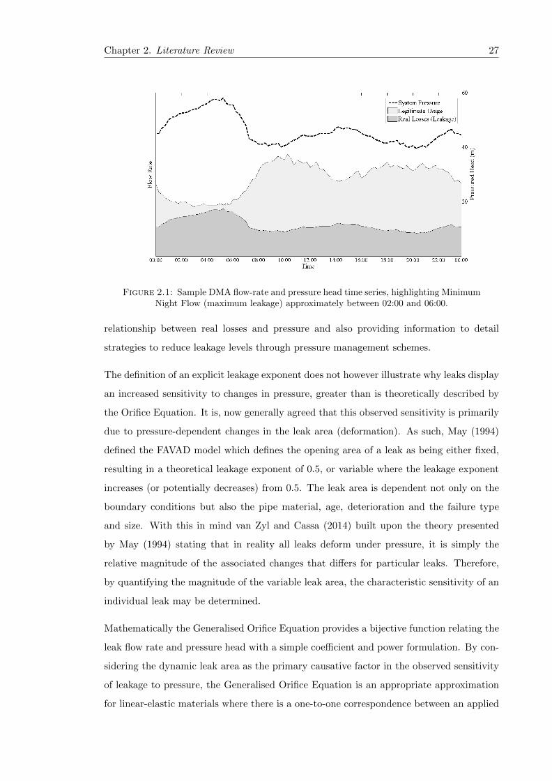
Chapter 2. Literature Review 27
Figure 2.1: Sample DMA flow-rate and pressure head time series, highlighting MinimumNight Flow (maximum leakage) approximately between 02:00 and 06:00.
relationship between real losses and pressure and also providing information to detail
strategies to reduce leakage levels through pressure management schemes.
The definition of an explicit leakage exponent does not however illustrate why leaks display
an increased sensitivity to changes in pressure, greater than is theoretically described by
the Orifice Equation. It is, now generally agreed that this observed sensitivity is primarily
due to pressure-dependent changes in the leak area (deformation). As such, May (1994)
defined the FAVAD model which defines the opening area of a leak as being either fixed,
resulting in a theoretical leakage exponent of 0.5, or variable where the leakage exponent
increases (or potentially decreases) from 0.5. The leak area is dependent not only on the
boundary conditions but also the pipe material, age, deterioration and the failure type
and size. With this in mind van Zyl and Cassa (2014) built upon the theory presented
by May (1994) stating that in reality all leaks deform under pressure, it is simply the
relative magnitude of the associated changes that differs for particular leaks. Therefore,
by quantifying the magnitude of the variable leak area, the characteristic sensitivity of an
individual leak may be determined.
Mathematically the Generalised Orifice Equation provides a bijective function relating the
leak flow rate and pressure head with a simple coefficient and power formulation. By con-
sidering the dynamic leak area as the primary causative factor in the observed sensitivity
of leakage to pressure, the Generalised Orifice Equation is an appropriate approximation
for linear-elastic materials where there is a one-to-one correspondence between an applied
Chapter 2. Literature Review 28
load (stress) and deformation (strain) for a single leak. With regards to pipe materials
used by the water industry, this includes steel, cast and ductile iron and asbestos cement.
The current and growing use of viscoelastic materials (e.g. polymeric materials including
PVC and PE) within the water distribution system means that this approach is poten-
tially not applicable in all cases. Massari et al. (2012) demonstrated the hysteresis type
behaviour of leakage from artificially manufactured slits in polyethylene pipe, where a one-
to-one relationship between pressure and leakage does not exist but is dependent on the
loading history. The longitudinal slits investigated within the study present a challenge
in deriving an accurate model to describe the leakage behaviour due to both the observed
sensitivity of this failure type, as shown for linear-elastic pressurised pipes (Avila Rangel
and Gonzalez Barreto, 2006; Greyvenstein and van Zyl, 2006), and the complex inherent
material rheology.
2.4.1 Structural Behaviour
Leaks within the water distribution system are commonplace in the United Kingdom and
manifest themselves in a diverse range of shapes and sizes. Some of the most common
failure types in the United Kingdom are pin holes, longitudinal cracks, circumferential
cracks and joint failures (UKWIR, 2008). The structural behaviour of a leak is a critical
parameter influencing the specific leakage performance. The significance of this behaviour
may be qualitatively assessed by evaluating the leakage exponent defining the pressure-
leakage relationship. With reference to Table 2.2, the most sensitive leaks, in other words
the leaks that may be surmised as having the greatest dependence on pressure with regards
to the instantaneous leak area, are corrosion clusters and longitudinal cracks. This is
notable for longitudinal cracks in plastic pipes which are inherently less stiff than equivalent
steel or iron pipes. In order to accurately define leakage models for application in both
academic and industrial contexts a detailed understanding of the structural dynamics of
different leaks is required.
The observed sensitivity of the pressure-leakage relationship is generally agreed to be due
to the dynamic nature of leaks, i.e. the pressure dependent leak area. As a results of
this a number of investigatory studies have been conducted to quantify the structural
behaviour of leaks in pressurised pipe. A significant majority of this work has focussed
Chapter 2. Literature Review 29
on the performance of highly sensitive failure types in linear-elastic materials for different
leak types, as listed below;
• Longitudinal Cracks/Slits - Grebner and Strathmeier (1984); Bhandari and Leroux
(1993); Avila Rangel and Gonzalez Barreto (2006); Al-khomairi (2005); Cassa and
van Zyl (2011); De Miranda et al. (2012); Ferrante (2012)
• Circumferential Cracks/Slits - Rahman et al. (1998); Takahashi (2002); Cassa and
van Zyl (2011)
The studies listed adopt different approaches for the assessment and quantification of the
leak structural dynamics. These approaches may be categorised into theoretical investi-
gations (based on fundamental governing principles) and empirical investigations (based
on physical observations). It must also be noted that there are a considerable number
of studies evaluating the behaviour of leaks considering the leak-before-break framework.
These studies consider the formation of through wall cracks whereas the highlighted work
herein presumes the existence of a failure opening without considering the specific cause.
2.4.1.1 Theoretical Investigations
With regards to theoretical analyses considering the structural behaviour of leaks in pres-
surised pipes, fundamental structural principles are used to derive frameworks to evaluate
the behaviour of stable cracks. These studies do not take into account fracture mechanics
and crack propagation, and therefore assume that the leak area remains constant before
and after an applied loading. Wuthrich (1983) demonstrated the application of shell-
theory with respect to crack opening. The methodology utilised a conversion between the
calculated deformation of a crack in a flat plate to an equivalent failure in a curved sur-
face or cylindrical pipe. Shell theory is applicable to any linear-elastic material assuming
a relatively small wall thickness. However, a significant proportion of distribution pipes
are now classified as thick-walled due to the continuing growth in use of plastic pipes
in particular, and therefore the use of shell theory is not universally applicable due to
this modelling assumption. Another theoretical approach was adopted by De Miranda
et al. (2012) who discretised the physical mechanisms define the structural behaviour of
longitudinal slits in pressurised pipe. Using stiffness coefficients and boundary and in-
terface loading conditions for a beam with elastic constraints, the theoretical model was
Chapter 2. Literature Review 30
validated using finite element analysis results. The methodology adopted by De Miranda
et al. (2012) provided a detailed assessment of the physical mechanisms controlling the
structural behaviour by simplifying them into individual contributory components. How-
ever, as with the previously discussed shell theory methodology, this theoretical approach
does not consider the effect of shear deformation that may occur in thick-walled pipes.
The attempted validation of the ‘beam model’ against thick-walled finite element models
emphasises this limitation. There is a noticeable increasing offset between the predicted
and modelled leak area as the d/s ratio increases, in other words as the modelled pipes
tend towards a thick-walled classification. The authors state that the developed model
provides a simple and easy-to-use application for leakage management practitioners. The
requirement to solve ordinary differential equations using pre-defined boundary-interface
conditions potentially counters this ambition, as any initial error in boundary condition
definition for example, would ultimately result in significant final solution error.
Most modelling approaches to the problem of defining the pressure-leakage relationship
for individual leaks consider a single leak type. On the other hand, Franchini and Lanza
(2014) developed a theoretical approach based on the application of the Buckingum π
theorem to establish the basis for a dimensionless generalised leakage model. This frame-
work considered different elastic materials, pipe and leak geometries to account for the
dependence of the leak area and discharge coefficient. The dimensionless analysis offers
a very robust generalised tool to derive a single pressure leakage relationship for failures
in linear-elastic materials. However, the adopted approach does not isolate the explicit
deformation of individual leaks. Rather, experimental data is used to calibrate the dimen-
sionless theoretical model utilising a correction factor for the coupled effect of the dynamic
leak area and discharge coefficient.
Observations from physical investigations are vital for the validation of governing prin-
ciples and derived models but are often expensive and time consuming. Validated finite
element analyses (FEA) have been adopted as a rigorous tool to explore the structural
behaviour of leaks in an efficient and cost effective manner through the implementation
of theoretical structural principles. FEA provides a means to investigate the structural
behaviour of a limitless range of failure types in different pipe sizes and materials under
various loading conditions, whilst quantifying macroscopic and microscopic material re-
sponses. The definition of suitably fine mesh sizing and appropriate boundary conditions
are essential to develop accurate simulations however. Cassa and van Zyl (2011) used
Chapter 2. Literature Review 31
FEA to investigate the significance of different parameters on the leak behaviour of three
types of leaks; longitudinal, circumferential and spiral cracks. The FEA results compiled
were used to statistically derive an equation defining the dependent change of area for
each leak type, subsequently input into a reformulation of the Fixed and Variable Area
Discharge (FAVAD) model defined by May (1994). The finalised leakage model presented
by van Zyl and Cassa (2014) provides an effective and simple methodology to quantify
the pressure-dependent leak area and hence predict an explicit leakage exponent value
using the pressure head-area slope parameter m. The non-dimensionally homogeneous
nature of the derived expression means that no physical meaning can be attached to the
components of the predictive model. Despite this, the derived expressions were used to
make an important point with regards to the suitability of the Generalised Orifice Equa-
tion in characterising the overall behaviour of these dynamic leaks. van Zyl and Cassa
(2014) showed that leakage exponent is dependent on the loading conditions. This em-
phasises that the Generalised Orifice Equation must be seen as an approximation of the
characteristic leakage behaviour and cannot comprehensively capture the coupled pressure
dependent leak area and orifice flow phenomena. The authors offer the Leakage Number
as an alternative and ‘convenient ’ means of defining the instantaneous leakage exponent
based on the loading conditions and leak characteristics (van Zyl and Cassa, 2014) without
extensive analysis of simultaneous empirical leak flow-rates and pressure heads.
2.4.1.2 Empirical Investigations
Empirical data refers to the collection of information through investigatory experiments
and/or observations. Such information provides a powerful platform to develop rigorous
and validated models in a wide range of applications. Within the field of leakage mod-
elling, experimental data from real and artificially manufactured leaks have been utilised
to verify and validate the application of existing leakage models (Orifice Equation) and
novel theoretically derived models (De Miranda et al., 2012; Franchini and Lanza, 2014).
Experimental investigations allow for the isolation of specific variables and physical mech-
anisms. In order to quantify the dynamic leak area of a range of different failure types
including circular orifices and longitudinal slits under representative loading conditions,
Buckley (2007) designed and used a test rig incorporating a hydraulic pressurised blad-
der. The setup allowed for isolation of the structural behaviour of the leaks, without the
need to consider the interdependence of the leak hydraulics and the potential structural
Chapter 2. Literature Review 32
implications. Based on a qualitative assessment of the presented results, the importance
of the viscoelastic behaviour of PVC pipes was not considered. This time and pressure
dependent phenomena is thought to be evident in the trend line fitting error observable
in the presented results. A non-linear association between the applied pressure and mea-
sured leak area is the dominant feature for the uPVC test results of longitudinal cracks.
Nevertheless, the work provided an important insight into the influence of different pa-
rameters on the leak opening area, in particular the significance of slit length on the scale
of deformation under an applied loading.
Buckley (2007) and Cassa and van Zyl (2011) focussed on PVC pipes, relevant due to
the frequent use of plastic pipes by the water industry. The investigations concluded
a linear relationship between the internal pressure and the leak area. When analysing
polymeric materials, such as PVC, the material rheology must also be considered, i.e.
the viscoelastic material characteristics (Meissner and Franke, 1977). Time-dependent
viscoelastic behaviour may be seen as a secondary feature compared to the dominant
structural influencing parameters presented by Cassa and van Zyl (2008) within the struc-
tural performance of leaks in PVC pipe. However when analysing the equivalent behaviour
of leaks in polyethylene pipe, another common pipe material found in water distribution
systems, understanding and quantifying the material rheology is critical (Massari et al.,
2012). Currently, research into the behaviour of leaks in viscoelastic pipes is limited to
preliminary observations of the time and pressure dependent leakage response by Ferrante
et al. (2011) and Massari et al. (2012). Mathematical representations of the viscoelastic
behaviour (Maxwell-Wiechert and Generalised Kelvin-Voigt models) were calibrated and
utilised to fit the pressure-leakage relationship with positive results, but this did not ac-
count for the actual dynamic leak area rather the effective leak area (coupled leak area
and discharge coefficient). Radial strain measurements (thought to be circumferential
strain measurements in reality) allude once again to the dynamic leak area as the primary
factor resulting in the observed time and pressure-dependent leakage response. Massari
et al. (2012) reiterates that a ‘formula linking QL [leak flow-rate] with all the parameters it
depends on...is still an open issue’, in particular for viscoelastic materials as demonstrated.
The work reviewed regarding the structural behaviour of leaks in pressurised pipes all
focussed on the definition of theoretically or empirically derived models, appropriate for
practical application in leakage management strategies and the development of academic
Chapter 2. Literature Review 33
understanding. The solution of ordinary differential equations and multi-component ex-
pressions can be computationally demanding, especially when you consider the non-static
nature of typical water distribution system pressures (Fox et al., 2014b). An effective
model should therefore not only recognise the significance of the fundamental mechanisms
it is accounting for, but also the adequacy and efficiency for its defined practical usage
(e.g. leakage control).
Chapter 2. Literature Review 34
2.5 Leakage Control and Localisation
Leakage control can be grouped into two areas; passive (reactive) leakage control where
leaks are identified and fixed following customer contacts/complaints, and active leakage
control which involves water companies actively seeking out and resolving the source of
leakage events (Gopan et al., 2010). This is in slight contrast to the categories defined
by Puust et al. (2010) who separate Leakage Control and Leak Detection. Active leakage
control, pressure management, the speed/quality of repairs and the overall management of
water distribution system pipelines and assets, make up the four components of a successful
leakage management policy as outlined by the IWA (Liemberger and Farley, 2004).
Gopan et al. (2010) categorise active leakage control into five sections; pressure control,
regular sounding, district metering, waste metering and combined waste metering. Regu-
lar sounding, an acoustic detection methodology, is the most conventional method for leak
detection and localisation but is limited by the skill of the operator, background noise, the
acoustic properties of the pipe material and the operational intensiveness of the method-
ology. As such, this method is ineffective for locating leaks in plastic pipes which have
minimal acoustic transmission. An example of a method that continues to develop and
gain recognition is inverse-transient analysis (Pudar and Liggett, 1992; Liggett and Chen,
1995) which was a novel concept that used pressure measurements to determine some
unknown parameters such as pipe roughness and leaks, in contrast to the forward prob-
lem solution previously adopted, that assumed knowledge of such parameters (Colombo
et al., 2009). The Orifice Equation is incorporated into this inverse analysis to allow for
the location and magnitude of the leak to be calculated (Wang et al., 2002). Utilising
an analytical expression, equivalent to the Orifice Equation, which better describes the
variability of the time and pressure-dependent orifice leak flow, as highlighted previously,
would allow for further refinement of existing transient based leak localisation methods.
On the other hand, leak detection methodologies which are primarily used to identify the
existence of leaks in a network do not necessitate the use of specific leak characteristics
but rather note the change in signal response of a pressure transient or acoustic reflection
(Covas and Ramos, 2010). A limitation of using pressure transients as a leak localisation
tool is the potential reluctance of service providers to inputting these dynamic pressures
into their systems. This may be due to potential resulting water quality issues (e.g. con-
taminant ingress (Fox et al., 2014b) and discolouration (Lehtola et al., 2006)) as well as the
Chapter 2. Literature Review 35
structural impact of rapidly changing pressures to the pipe (e.g. pipe bursts (Starczewska
et al., 2014)).
A well established leakage reduction methodology is pressure management which considers
the direct relationship between leakage and pressure (Nazif et al., 2009). This relationship,
based on the FAVAD concept first proposed by May (1994), is given in Equation 2.17
and provides the means for a simple analysis of a pressure management scheme where the
relative leakage reduction may be calculated based on the change of average DMA pressure
(Lambert, 2001).
Q1
Q0=
(P1
P0
)λ(2.17)
The subscripts 0 and 1 refer to the pre and post flow change (Q) and pressure head change
(P) conditions respectively. Pressure management is typically conducted using pump con-
trol, flow modulated valves and fixed outlet control valves (Thornton et al., 2008). The
effectiveness of the FAVAD based model is limited by the accuracy of the defined value of
leakage exponent (λ). Evaluation of the leakage exponent is often conducted using Min-
imum Night Flow analysis (District Metered Area flows and pressures between 02:00hrs
and 04:00hrs), as detailed previously (Mutikanga et al., 2012). The approximation of a
single leakage exponent for an entire DMA may be inadequate if the DMA consists of a
diverse range of pipe materials and leak types, thereby under or over-estimating the poten-
tial benefits of pressure reduction. However, one clear strength of pressure management is
in the capability of reducing background leakage levels, i.e. leaks that may be impractical
to locate using traditional methods.
Leak localisation and pressure management are just two examples of leakage management
tools. Mutikanga et al. (2012) present a detailed review of a wider range of current and
developing methodologies utilised by the water industry. The ability to minimise the total
real losses from WDS is based on the fundamental understanding of leakage behaviour
and the accuracy of theoretical and physically derived models used for leakage assessment.
Improving current modelling practices based on improved principal knowledge, will have
quantifiable sustainability benefits (financial in particular), which may be passed directly
from suppliers to consumers.
Chapter 2. Literature Review 36
2.6 Summary
An extensive review of the relevant literature regarding real losses from water distribution
systems and the phenomenon of dynamic leakage has been completed. Three fundamental
areas of research have been highlighted within the remit of the presented literature review;
leakage hydraulics, structural dynamics and soil hydraulics. Table 2.3 lists the leading
topical papers summarising the type of work presented in each and the fundamental sub-
ject areas addressed. Most studies focus on either theoretical, experimental or numerical
investigatory methodologies in isolation which often limits the research scope breadth and
potential outputs. A pronounced finding is the scarcity of research into the interaction
of leakage and soil hydraulics (and structural dynamics to an even greater extent), a
significant omission for a traditionally buried infrastructure. The general acceptance of
the importance of the structural dynamics on the observed pressure-leakage sensitivity
for leaks in distribution pipes has resulted in several studies exploring the behaviour of
leaks in traditional linear elastic materials. Polymeric pipe materials such as uPVC and
polyethylene present a distinctly more complex problem however.
Polyethylene pipes are not invulnerable to failures. Failures such as cracks in the direction
of extrusion demonstrate a high level of sensitivity to changes in pressure, temperature
and time, due to the viscoelastic material rheology. A rigorous understanding of the
interaction between the structural behaviour and the leak hydraulics for these dynamic
leaks is currently lacking, particularly considering all the significant determining factors
of the behavioural response. Furthermore, investigations into the influence of an external
porous media on both the structural and leakage performance have yet to be considered.
Hypothetically, well established leakage management strategies such as leakage assess-
ment, pressure management and active leakage control technologies may benefit from the
inclusion of suitable time-dependent leakage models accounting for the distinct leakage
response.

Chapter 2. Literature Review 37
Table 2.3: Summary table of key leakage research papers identified from literaturereview listing the type and focus of the research.
(The. - Theoretical Study; Exp. - Experimental Study; and Num. - Numerical Study)
References The. Exp. Num. Leak Hydraulics Structural Dynamics Soil Hydraulics
Al-khomairi (2005) X X
Avila Rangel and Gonzalez Barreto (2006) X X
Buckley (2007) X X X
Cassa and van Zyl (2008) X X
Cassa and van Zyl (2011) X X
Coetzer et al. (2006) X X X
Collins and Boxall (2013) X X X X X
De Miranda et al. (2012) X X X
De Paola and Giugni (2012) X X
De Paola et al. (2014) X X X
Ferrante et al. (2011) X X X
Ferrante (2012) X X
Ferrante et al. (2012b) X X X
Fox et al. (2012) X X
Franchini and Lanza (2014) X X X
Grebner et al. (1984) X X
Greyvenstein and van Zyl (2006) X X X
Ilunga et al. (2008) X X
Johansen (1930) X X
Kim et al. (2002) X X
Massari et al. (2012) X X X
Matsumoto et al. (1991) X X
May (1994) X X
Meniconi et al. (2013) X X
Osterwalder and Wirth (1985) X X
Rahman et al. (1998) X X X
Schwaller and van Zyl (2014) X X X X
Takahashi (2002) X X
Thornton and Lambert (2005) X X
van Zyl and Cassa (2011) X X X
van Zyl and Cassa (2014) X X
van Zyl et al. (2013) X X
Walski et al. (2006) X X X X
Wuthrich (1983) X X
Chapter 3
Aims and Objectives
3.1 Research Aim
The headline aim for the research was to quantify the leak behaviour of longitudinal slits in
thick-walled viscoelastic pipes, considering the dynamic interaction of hydraulic conditions
and the pipe section characteristics. The proposed research methodology took advantage
of both physical and numerical investigatory techniques, creating synergy between these
research tools to explore and quantify all the influencing effects (leak hydraulics, structural
dynamics and soil hydraulics). Fundamentally, the work looked to explore three charac-
teristics of the nature of an individual leak; the leak flow rate (Q), system pressure (H)
and the leak area (AL), evaluating their interdependence.
The term ’dynamic’ in the context of the presented research, was used to emphasise the
complexity of the characteristic leakage behaviour considered (time and pressure depen-
dent) relative to the ’simpler’ behaviour observed for linear-elastic type leaks for example.
3.2 Research Objectives
In developing a methodology to achieve the desired level of understanding, a clear and
achievable set of objectives was outlined for the research.
38
Chapter 3. Aims and Objectives 39
1. To physically quantify the time dependent leak area, flow rate and pressure head
across longitudinal slits in polyethylene pipes, exploring the interaction between
leak hydraulics and the pipe structure.
2. To numerically explore the material behavioural response of linear elastic pipes con-
taining longitudinal slits in order to derive a dimensionally homogeneous leak area
model incorporating constitutive viscoelastic theory.
3. To calibrate the viscoelastic response of the leak area from experimental data, for
integration into a validated dynamic leakage model.
4. To explore the effects of an external porous media on the material and leakage
behavioural response of longitudinal slits in polyethylene pipes.
5. To assess the effectiveness of current leakage management strategies using the devel-
oped analytical leakage model.
3.3 Research Structure
The presented thesis has been structured into three distinct results chapters which are
based on three separate journal publications. This has been done in order to provide a
concise and logical narrative of the investigation which consisted of three discrete but de-
pendent methodologies and results. The first of these chapters (Chapter 4) focusses on the
quantitative assessment of the behaviour of the discussed leak type, capturing a unique
dataset for characterisation and validation of the leakage behaviour. The second chapter
(Chapter 5) assesses the dependent variables dictating the observed leakage response, for-
mulating a means to describe the complex interdependent leakage behaviour. Finally, the
third chapter (Chapter 6) looks to address the noted deficiency in understanding of the
interaction of a dynamic leak with an external porous media, highlighting the implication
of this interaction in leakage modelling applications. A discussion of specific methodolo-
gies and results are contained within each chapter, with a comprehensive analysis and
discussion of all the results and findings presented in Chapter 7. It should also be noted
that in the context of the presented investigation, the term ‘crack’ refers specifically to
natural failures in pipes and ‘slit’ refers to an artificially manufactured failure opening
where material is removed from the pipe to form a leak opening.

Chapter 4
Physical study exploring the
interaction between structural
behaviour and leak hydraulics for
dynamic leakage
“One can state, without exaggeration, that the observation of and the search for
similarities and differences are the basis of all human knowledge.”
Alfred Nobel (1896)
4.1 Overview
Observations provide a unique insight into the true interdependencies of physical phe-
nomena, provided data can be acquired of the individual contributing components. This
chapter presents the work evaluating and quantifying the significance of the structural
dynamics on the leakage behaviour, in particular the theoretical discharge coefficient and
the leakage flow-rate, using a novel experimental setup. The physical observations aimed
to capture the synchronous leakage flow-rate, pressure head and leak area to quantify the
interdependence of these fundamental parameters characterising the leakage behaviour.
An assessment of the effectiveness of orifice theory (Torricelli theorem) for characterising
40

Chapter 4. Physical observations of dynamic leakage 41
the leakage flow-rate of time and pressure dependent longitudinal slits in viscoelastic pipe,
yielded the definition of an explicit leakage model integrating the dynamic leak area into
the Orifice Equation.
The data collected within the experimental investigation was not only aimed to calibrate
an explicit leakage model describing the leakage behaviour of a single leak, but also to
provide a platform to calibrate a generalised leakage model. It was necessary to define
a methodology that was consistent and repeatable, providing sufficiently accurate data
to complete a detailed calibration procedure. The experimental work also provided an
initial insight into the influence of the leak geometry on the observed sensitivity of the
pressure-leakage relationship. This chapter addressed the goals set out in Objective 1 in
Chapter 3.
4.1.1 Journal Submission Details
The chapter is the manuscript submitted to the American Society of Civil Engineers
(ASCE) Journal of Hydraulic Engineering. The original submission date was 29/05/2015.
The Journal of Hydraulic Engineering was chosen due to the focus on flow in closed
conduits and advancement in the understanding of leakage hydraulics presented within
the paper. Additionally the journal reputation within the field of water engineering was
considered (Impact Factor at time of submission: 1.26). The work builds on previous
publications within the Journal of Hydraulic Engineering which offered initial observa-
tions of the complex behaviour of leaks in viscoelastic polyethylene pipes (Ferrante et al.,
2011; Ferrante, 2012) and the viscoelastic nature of polyethylene pipes in the water dis-
tribution system (Covas et al., 2004). The topics and conclusions presented within the
paper are relevant to a wide range of applications within the field of hydraulic engineer-
ing, in particular the findings on the nature of the theoretical discharge coefficient and
effectiveness of the Orifice Equation in leakage modelling applications. Experimental data
is at a premium with regards to leakage modelling studies due to the cost of conducting
such investigations. The work may therefore present a significant resource for the research
community for model validation and/or development of experimental practice, focussing
on the interaction between leakage and structural dynamics.
Chapter 4. Physical observations of dynamic leakage 42
4.2 Abstract
Strategies for managing leakage from water distribution systems require the ability to ef-
fectively evaluate such real losses through the understanding of the behaviour of individual
leaks, including their response to changes in pressure regime due to demand or management
strategies. This paper presents the results from an innovative experimental investigation
aimed at understanding the response of longitudinal slits in pressurised viscoelastic pipes,
specifically considering the interaction between the structural and leakage dynamics. For
the first time, leakage flow-rate, pressure, leak area and material strain were recorded si-
multaneously, providing new knowledge of the complex interaction of these factors. The
work shows that strain and area are directly related, hence it is possible to employ strain
as a predictor of leak area, calculated using a calibrated viscoelastic model. Using such an
approach, the leakage flow-rates under a range of quasi-static pressures were accurately
predicted and validated. Overall the work demonstrates that the Orifice Equation, with a
constant coefficient of discharge, is suitable for accurately estimating dynamic leakage flow
rates from longitudinal slits, provided that the leak area is suitably incorporated.
4.3 Introduction
Leakage remains a key sustainability issue faced by water utilities around the world. Esti-
mates for the level of leakage in the United Kingdom alone highlight the significance of the
problem, with OFWAT published figures estimating that 23.6% of the total distributed
water was lost through bursts and background leakage between 2012 and 2013 (Ofwat,
2013). This figure has remained static for a decade or more under the current Economic
Levels of Leakage (ELL) directive (Strategic Management Consultants, 2012). Leakage
management strategies aimed at addressing this issue range from the development of leak
detection technologies to advanced pressure management schemes. Likewise, the selec-
tion of pipe material is also targeted at improving the durability and cost effectiveness
of distribution systems by minimising the occurrence of pipe failures. Polyethylene pipes
in particular offer cost benefits due to their inherent durability and flexibility resulting in
ease of installation and tolerance to potential ground movement (GPSUK, 2014b). Plastic

Chapter 4. Physical observations of dynamic leakage 43
pipes are often perceived as a ‘leak free’ option; however this is not evident in practice. Un-
derstanding the leakage behaviour of leaks that occur in plastic pipes is crucial in planning
and implementing effective active leakage control strategies.
4.4 Background
Leakage modelling plays a major part in the process of leakage management in water
distribution systems. This includes the quantification and/or estimation of leakage levels
in operational systems (Thornton and Lambert, 2005; Cheung et al., 2010), application of
leakage detection methodologies (Pudar and Liggett, 1992; Vıtkovsky et al., 2000; Koppel
et al., 2009) and the development of effective pressure management schemes (Awad et al.,
2008; Nazif et al., 2009). Such tools and techniques use leakage flow rate estimation based
on Equation 4.1, known as the Orifice Equation. The effectiveness of this equation has
been reviewed by several authors who explore the variability of the relationship between
pressure and leakage using a generalised form of the equation, also given in Equation 4.1
(May, 1994; Thornton and Lambert, 2005; Clayton and van Zyl, 2007).
Q = ALCd√
2gH = chλ (4.1)
The power term, λ, is theoretically constant equal to 0.5. However field data and analyses
at District Metered Area level (DMAs are manageable divisions of a larger distribution
networks), as summarised by Farely and Trow (2003), found that the leakage exponents in
Brazil, Japan and United Kingdom lay in the range 0.52 to 2.79. In addition, experimental
investigations isolating individual leaks have shown that the theoretical value (λ = 0.5)
is not appropriate or accurate in all cases. Greyvenstein and van Zyl (2006) conducted a
series of tests on failed pipe sections from real systems and determined leakage exponent
values ranging from 0.40 to 2.30. Leakage exponent values greater than 1.0 were noted
predominantly for longitudinal cracks and corrosion clusters emphasising the sensitivity of
these particular leak types to changes in pressure. Similarly Avila Rangel and Gonzalez
Barreto (2006) evaluated leakage exponents between 1.40 and 2.01 for manufactured lon-
gitudinal slits in PVC pipe. For the purpose of this paper, cracks are defined as naturally
occurring pipe failures, whilst slits are artificially manufactured openings. The conclusion
drawn from these studies was that leaks are more sensitive to pressure than is described
Chapter 4. Physical observations of dynamic leakage 44
by the simple Orifice Equation but that the additional pressure dependent behaviour can
be modelled by the definition of a single leakage exponent once the leak specific behaviour
is known. This approach reflects the Fixed and Variable Area Discharge (FAVAD) model
proposed by May (1994), with the observed sensitivity surmised to be predominantly in-
fluenced by the pressure-dependence of leak opening areas (Clayton and van Zyl, 2007).
Ferrante et al. (2012a) consider the consequence of quantifying the behaviour of single
or multiple (global leaks), numerically confirming that the mean global leakage exponent
is typically higher than the equivalent single leakage exponent as it account for all the
quantities affecting the distributed leakage.
An understanding of the effect of the dynamic nature of opening area on leak hydraulics,
specifically the definition of a coefficient of discharge, is a relatively unexplored topic within
the literature. The effective leak area (AE = CdAL), which captures the coupled definition
of both the leak area and discharge coefficient, is often used. Theoretical and experimental
investigations using this approach, for different failures, highlighted the pressure depen-
dence of the effective leak area most notably for longitudinal cracks (Al-khomairi, 2005;
Ferrante et al., 2011; Franchini and Lanza, 2014). However this methodology does not
facilitate assessment of the fundamental interdependence of the leak area and the coef-
ficient of discharge. In other words, is the theoretical coefficient of discharge dependent
on pressure and the dynamic leak area? Definition of the synchronous pressure, leak area
and subsequent leakage flow rate is necessary to evaluate the associated coefficient of dis-
charge and fully validate the effectiveness of using the Orifice Equation when integrating
the pressure dependent leak area.
Commonly used pipe materials found in water distribution systems include steel, concrete
and ductile iron which behave as linear-elastic materials. However polymeric materials
such as Medium Density Polyethylene (MDPE) are viscoelastic in nature. The use of
such polymeric materials drives a need to understand the phenomena of viscoelasticity,
which manifests as pressure, time and temperature dependent behaviour. A relatively
common failure type in viscoelastic pipes such as polyethylene are longitudinal cracks
(axial direction), a brittle failure mode, which form in the direction of extrusion (Grann-
Meyer, 2005; O’Connor, 2011). Longitudinal cracks have been shown to be highly sensitive
to changes in pressure in linear-elastic materials (Al-khomairi, 2005; Greyvenstein and van
Zyl, 2006; Cassa and van Zyl, 2011) therefore the coupled effect of the crack sensitivity and
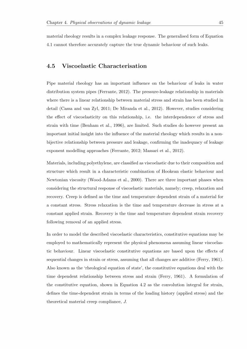
Chapter 4. Physical observations of dynamic leakage 45
material rheology results in a complex leakage response. The generalised form of Equation
4.1 cannot therefore accurately capture the true dynamic behaviour of such leaks.
4.5 Viscoelastic Characterisation
Pipe material rheology has an important influence on the behaviour of leaks in water
distribution system pipes (Ferrante, 2012). The pressure-leakage relationship in materials
where there is a linear relationship between material stress and strain has been studied in
detail (Cassa and van Zyl, 2011; De Miranda et al., 2012). However, studies considering
the effect of viscoelasticity on this relationship, i.e. the interdependence of stress and
strain with time (Benham et al., 1996), are limited. Such studies do however present an
important initial insight into the influence of the material rheology which results in a non-
bijective relationship between pressure and leakage, confirming the inadequacy of leakage
exponent modelling approaches (Ferrante, 2012; Massari et al., 2012).
Materials, including polyethylene, are classified as viscoelastic due to their composition and
structure which result in a characteristic combination of Hookean elastic behaviour and
Newtonian viscosity (Wood-Adams et al., 2000). There are three important phases when
considering the structural response of viscoelastic materials, namely; creep, relaxation and
recovery. Creep is defined as the time and temperature dependent strain of a material for
a constant stress. Stress relaxation is the time and temperature decrease in stress at a
constant applied strain. Recovery is the time and temperature dependent strain recovery
following removal of an applied stress.
In order to model the described viscoelastic characteristics, constitutive equations may be
employed to mathematically represent the physical phenomena assuming linear viscoelas-
tic behaviour. Linear viscoelastic constitutive equations are based upon the effects of
sequential changes in strain or stress, assuming that all changes are additive (Ferry, 1961).
Also known as the ‘rheological equation of state’, the constitutive equations deal with the
time dependent relationship between stress and strain (Ferry, 1961). A formulation of
the constitutive equation, shown in Equation 4.2 as the convolution integral for strain,
defines the time-dependent strain in terms of the loading history (applied stress) and the
theoretical material creep compliance, J.
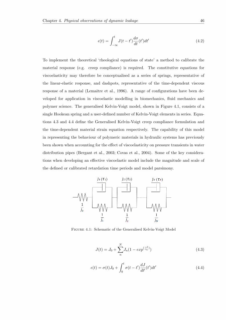
Chapter 4. Physical observations of dynamic leakage 46
ε(t) =
∫ t
−∞J(t− t′)dσ
dt(t′)dt′ (4.2)
To implement the theoretical ‘rheological equations of state’ a method to calibrate the
material response (e.g. creep compliance) is required. The constitutive equations for
viscoelasticity may therefore be conceptualised as a series of springs, representative of
the linear-elastic response, and dashpots, representative of the time-dependent viscous
response of a material (Lemaitre et al., 1996). A range of configurations have been de-
veloped for application in viscoelastic modelling in biomechanics, fluid mechanics and
polymer science. The generalised Kelvin-Voigt model, shown in Figure 4.1, consists of a
single Hookean spring and a user-defined number of Kelvin-Voigt elements in series. Equa-
tions 4.3 and 4.4 define the Generalised Kelvin-Voigt creep compliance formulation and
the time-dependent material strain equation respectively. The capability of this model
in representing the behaviour of polymeric materials in hydraulic systems has previously
been shown when accounting for the effect of viscoelasticity on pressure transients in water
distribution pipes (Bergant et al., 2003; Covas et al., 2004). Some of the key considera-
tions when developing an effective viscoelastic model include the magnitude and scale of
the defined or calibrated retardation time periods and model parsimony.
Figure 4.1: Schematic of the Generalised Kelvin-Voigt Model
J(t) = J0 +
N∑n
Jn(1− exp(−tτn
)) (4.3)
ε(t) = σ(t)J0 +
∫ t
0σ(t− t′)dJ
dt′(t′)dt′ (4.4)

Chapter 4. Physical observations of dynamic leakage 47
4.6 Investigation Aims
The aim of the research reported here was to understand the behaviour of longitudinal slits
in pressurised viscoelastic pipes, specifically the interaction between the structural dynam-
ics and leak hydraulics, through physical observations. Experiments were conducted to
quantitatively assess whether leak area is the primary independent parameter influencing
the sensitivity of leakage to pressure, confirming the suitability of the Orifice Equation in
describing such dynamic leaks. Ultimately the objective of the study was to utilise the de-
veloped knowledge and quantitative experimental data to produce an explicit empirically
calibrated leakage model for a longitudinal slit in a viscoelastic pipe.
4.7 Experimental Setup
A series of experiments were undertaken, which recorded for the first time the synchronous
pressure head, leak flow rate, leak area and material strain under quasi steady-state condi-
tions (slowly changing) for engineered longitudinal slits in Medium Density Polyethylene
(MDPE) pipe. Repeatable test conditions were employed to characterise the long term
leakage behaviour, specifically the structural response and the associated leak hydraulics
under controlled conditions. Simultaneous measurements of the material axial strain and
leak area were employed to explore the theory that localised strain is a predictor of the
variable leak area.
4.7.1 Laboratory Facility
The laboratory investigation used the Contaminant Ingress into Distribution Systems
(CID) facility at the University of Sheffield, which is a 141 m length recirculating pipe
loop. The facility consists of 50 mm nominal diameter 12 bar rated MDPE pipe, tensile
yield stress of 15 MPa, with water fed from an upstream holding reservoir (volume of
0.95 m3) through a 3.5 kW Wilo MVIE variable speed pump. A 0.8 m removable section
of pipe, 62 m downstream of the system pump, allows for the inclusion of different test
sections housed within a 0.45 m3 capacity box containing a single side viewing window.
The flow-rate and pressure data are recorded using a single Arkon Flow System Mag-900
Electromagnetic Flow Meter located immediately downstream from the system pump and
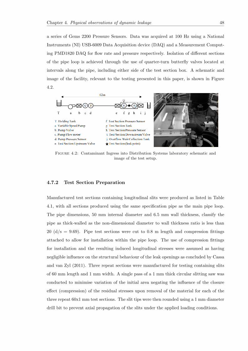
Chapter 4. Physical observations of dynamic leakage 48
a series of Gems 2200 Pressure Sensors. Data was acquired at 100 Hz using a National
Instruments (NI) USB-6009 Data Acquisition device (DAQ) and a Measurement Comput-
ing PMD1820 DAQ for flow rate and pressure respectively. Isolation of different sections
of the pipe loop is achieved through the use of quarter-turn butterfly valves located at
intervals along the pipe, including either side of the test section box. A schematic and
image of the facility, relevant to the testing presented in this paper, is shown in Figure
4.2.
Figure 4.2: Contaminant Ingress into Distribution Systems laboratory schematic andimage of the test setup.
4.7.2 Test Section Preparation
Manufactured test sections containing longitudinal slits were produced as listed in Table
4.1, with all sections produced using the same specification pipe as the main pipe loop.
The pipe dimensions, 50 mm internal diameter and 6.5 mm wall thickness, classify the
pipe as thick-walled as the non-dimensional diameter to wall thickness ratio is less than
20 (d/s = 9.69). Pipe test sections were cut to 0.8 m length and compression fittings
attached to allow for installation within the pipe loop. The use of compression fittings
for installation and the resulting induced longitudinal stresses were assumed as having
negligible influence on the structural behaviour of the leak openings as concluded by Cassa
and van Zyl (2011). Three repeat sections were manufactured for testing containing slits
of 60 mm length and 1 mm width. A single pass of a 1 mm thick circular slitting saw was
conducted to minimise variation of the initial area negating the influence of the closure
effect (compression) of the residual stresses upon removal of the material for each of the
three repeat 60x1 mm test sections. The slit tips were then rounded using a 1 mm diameter
drill bit to prevent axial propagation of the slits under the applied loading conditions.
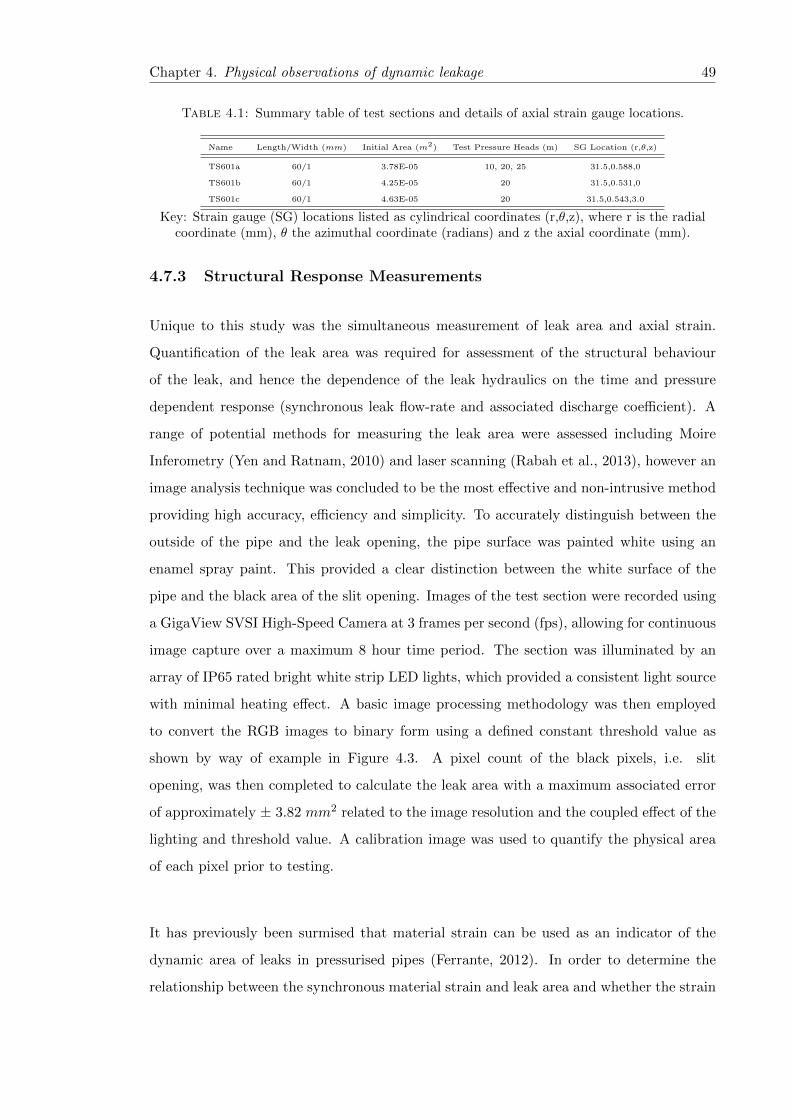
Chapter 4. Physical observations of dynamic leakage 49
Table 4.1: Summary table of test sections and details of axial strain gauge locations.
Name Length/Width (mm) Initial Area (m2) Test Pressure Heads (m) SG Location (r,θ,z)
TS601a 60/1 3.78E-05 10, 20, 25 31.5,0.588,0
TS601b 60/1 4.25E-05 20 31.5,0.531,0
TS601c 60/1 4.63E-05 20 31.5,0.543,3.0
Key: Strain gauge (SG) locations listed as cylindrical coordinates (r,θ,z), where r is the radialcoordinate (mm), θ the azimuthal coordinate (radians) and z the axial coordinate (mm).
4.7.3 Structural Response Measurements
Unique to this study was the simultaneous measurement of leak area and axial strain.
Quantification of the leak area was required for assessment of the structural behaviour
of the leak, and hence the dependence of the leak hydraulics on the time and pressure
dependent response (synchronous leak flow-rate and associated discharge coefficient). A
range of potential methods for measuring the leak area were assessed including Moire
Inferometry (Yen and Ratnam, 2010) and laser scanning (Rabah et al., 2013), however an
image analysis technique was concluded to be the most effective and non-intrusive method
providing high accuracy, efficiency and simplicity. To accurately distinguish between the
outside of the pipe and the leak opening, the pipe surface was painted white using an
enamel spray paint. This provided a clear distinction between the white surface of the
pipe and the black area of the slit opening. Images of the test section were recorded using
a GigaView SVSI High-Speed Camera at 3 frames per second (fps), allowing for continuous
image capture over a maximum 8 hour time period. The section was illuminated by an
array of IP65 rated bright white strip LED lights, which provided a consistent light source
with minimal heating effect. A basic image processing methodology was then employed
to convert the RGB images to binary form using a defined constant threshold value as
shown by way of example in Figure 4.3. A pixel count of the black pixels, i.e. slit
opening, was then completed to calculate the leak area with a maximum associated error
of approximately ± 3.82 mm2 related to the image resolution and the coupled effect of the
lighting and threshold value. A calibration image was used to quantify the physical area
of each pixel prior to testing.
It has previously been surmised that material strain can be used as an indicator of the
dynamic area of leaks in pressurised pipes (Ferrante, 2012). In order to determine the
relationship between the synchronous material strain and leak area and whether the strain
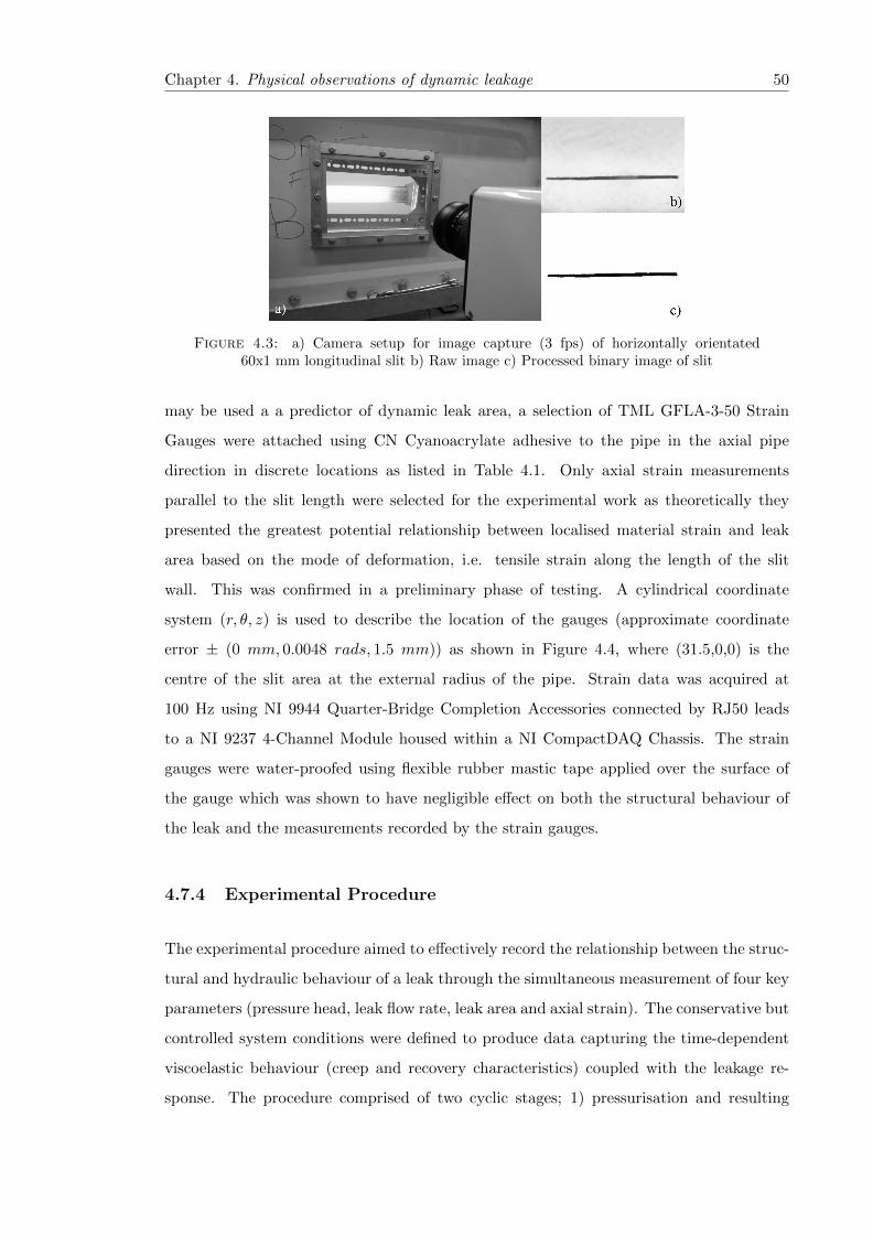
Chapter 4. Physical observations of dynamic leakage 50
Figure 4.3: a) Camera setup for image capture (3 fps) of horizontally orientated60x1 mm longitudinal slit b) Raw image c) Processed binary image of slit
may be used a a predictor of dynamic leak area, a selection of TML GFLA-3-50 Strain
Gauges were attached using CN Cyanoacrylate adhesive to the pipe in the axial pipe
direction in discrete locations as listed in Table 4.1. Only axial strain measurements
parallel to the slit length were selected for the experimental work as theoretically they
presented the greatest potential relationship between localised material strain and leak
area based on the mode of deformation, i.e. tensile strain along the length of the slit
wall. This was confirmed in a preliminary phase of testing. A cylindrical coordinate
system (r, θ, z) is used to describe the location of the gauges (approximate coordinate
error ± (0 mm, 0.0048 rads, 1.5 mm)) as shown in Figure 4.4, where (31.5,0,0) is the
centre of the slit area at the external radius of the pipe. Strain data was acquired at
100 Hz using NI 9944 Quarter-Bridge Completion Accessories connected by RJ50 leads
to a NI 9237 4-Channel Module housed within a NI CompactDAQ Chassis. The strain
gauges were water-proofed using flexible rubber mastic tape applied over the surface of
the gauge which was shown to have negligible effect on both the structural behaviour of
the leak and the measurements recorded by the strain gauges.
4.7.4 Experimental Procedure
The experimental procedure aimed to effectively record the relationship between the struc-
tural and hydraulic behaviour of a leak through the simultaneous measurement of four key
parameters (pressure head, leak flow rate, leak area and axial strain). The conservative but
controlled system conditions were defined to produce data capturing the time-dependent
viscoelastic behaviour (creep and recovery characteristics) coupled with the leakage re-
sponse. The procedure comprised of two cyclic stages; 1) pressurisation and resulting

Chapter 4. Physical observations of dynamic leakage 51
Figure 4.4: Cylindrical coordinate system for strain gauge location (see Table 4.1) wherethe centre of the leak area is located at (31.5,0,0).
creep phase, and 2) de-pressurisation and resulting recovery phase. Stage 1 provided data
on the time dependent leak behaviour following the assumed instantaneous pressurisation
and ensuing quasi steady-state conditions at a predefined initial pressure head, with stage
2 providing data on the leak opening area behaviour following the assumed instantaneous
de-pressurisation and material recovery. Three to five repeats were conducted for TS601a
at predetermined initial pressures of 10, 20 and 25 m head, each of which included an 8 hr
pressurisation phase and 16 hr recovery phase. Figure 4.5 summarises the experimental
procedure implemented for the pressurisation and recovery phases.
The length of time for the pressurisation and de-pressurisation stages were chosen due to
the observed time periods of measurable structural creep and recovery during preliminary
testing. The repeated test sections, TS601b and TS601c, were both tested at 20 m initial
pressure head only, primarily for assessment of experimental repeatability. The pressures
utilised within the experimental work represent relatively low pressures compared to op-
erational WDS pressures but were set due the physical constraints (e.g. size of overflow
weir) of the laboratory facility.
After the installation of the individual test sections within the pipe loop, the system was
left dormant for two days to allow equilibration of the material strain. A null offset for all
the attached strain gauges was executed prior to testing assuming the test sections were
at rest (zero stress and strain). The pressurisation phase was conducted by starting the

Chapter 4. Physical observations of dynamic leakage 52
Figure 4.5: Experimental procedure flowchart, defining the pressurisation (8 hr phase)and recovery (16 hr phase) stages used to capture the creep and recovery responses re-
spectively.
pump at a predetermined speed to achieve the necessary initial system pressure head. A
manual opening of the upstream test section box valve (item e) whilst the downstream
test section box valve remained closed was completed resulting in a step pressure change
in the test sections. The subsequent leakage flow-rate was allowed to overflow the box into
the collection tank before being returned to the main system holding tank by a separate
automated submersible pump, thus maintaining a constant water level within the test
section tank (Hw = 0.45 m). After the defined 8 hr creep period, the upstream valve
was closed resulting in a step change de-pressurisation and isolation of the test section.
The test sections were then left to complete the 16 hr recovery phase before repeating the
process. Tests were conducted between 3 and 5 days to allow for a detailed assessment of
the effect of the loading time-history on the material response.
4.8 Experimental Results
The leakage behaviour of the longitudinal slits in MDPE pipe were characterised using four
synchronous measurements of leak area, material strain, pressure head and subsequent
leakage flow rate. The results for the three test sections investigated (as described in
Table 4.1) are presented in Figures 4.6, 4.7 and 4.8, showing the 5-day response to a series
of equal 20 m pressure head pressurisations and de-pressurisations for TS601a and the
equivalent 3-day responses for TS601b and c. Each figure shows the measured leak area
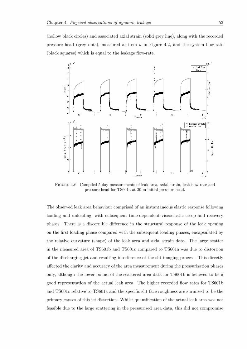
Chapter 4. Physical observations of dynamic leakage 53
(hollow black circles) and associated axial strain (solid grey line), along with the recorded
pressure head (grey dots), measured at item h in Figure 4.2, and the system flow-rate
(black squares) which is equal to the leakage flow-rate.
Figure 4.6: Compiled 5-day measurements of leak area, axial strain, leak flow-rate andpressure head for TS601a at 20 m initial pressure head.
The observed leak area behaviour comprised of an instantaneous elastic response following
loading and unloading, with subsequent time-dependent viscoelastic creep and recovery
phases. There is a discernible difference in the structural response of the leak opening
on the first loading phase compared with the subsequent loading phases, encapsulated by
the relative curvature (shape) of the leak area and axial strain data. The large scatter
in the measured area of TS601b and TS601c compared to TS601a was due to distortion
of the discharging jet and resulting interference of the slit imaging process. This directly
affected the clarity and accuracy of the area measurement during the pressurisation phases
only, although the lower bound of the scattered area data for TS601b is believed to be a
good representation of the actual leak area. The higher recorded flow rates for TS601b
and TS601c relative to TS601a and the specific slit face roughness are surmised to be the
primary causes of this jet distortion. Whilst quantification of the actual leak area was not
feasible due to the large scattering in the pressurised area data, this did not compromise
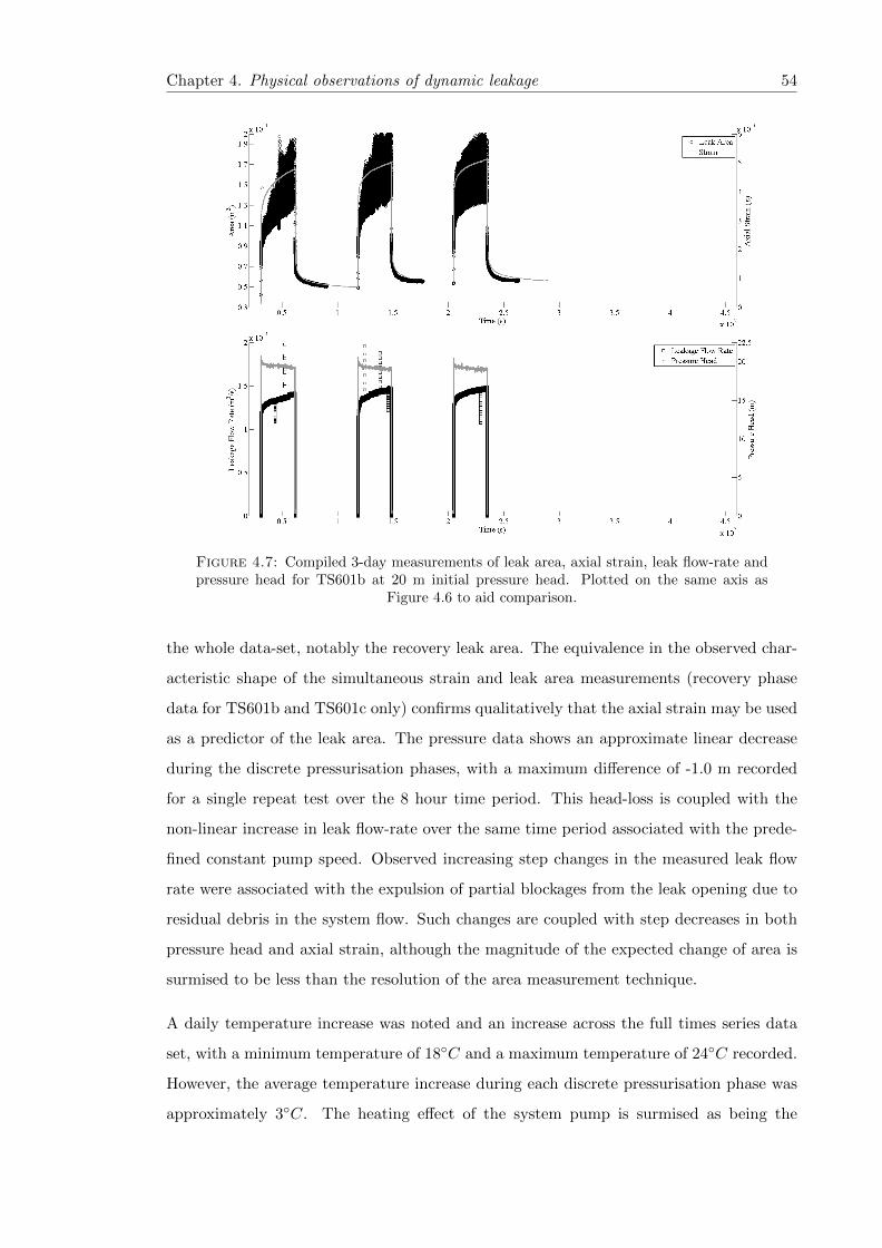
Chapter 4. Physical observations of dynamic leakage 54
Figure 4.7: Compiled 3-day measurements of leak area, axial strain, leak flow-rate andpressure head for TS601b at 20 m initial pressure head. Plotted on the same axis as
Figure 4.6 to aid comparison.
the whole data-set, notably the recovery leak area. The equivalence in the observed char-
acteristic shape of the simultaneous strain and leak area measurements (recovery phase
data for TS601b and TS601c only) confirms qualitatively that the axial strain may be used
as a predictor of the leak area. The pressure data shows an approximate linear decrease
during the discrete pressurisation phases, with a maximum difference of -1.0 m recorded
for a single repeat test over the 8 hour time period. This head-loss is coupled with the
non-linear increase in leak flow-rate over the same time period associated with the prede-
fined constant pump speed. Observed increasing step changes in the measured leak flow
rate were associated with the expulsion of partial blockages from the leak opening due to
residual debris in the system flow. Such changes are coupled with step decreases in both
pressure head and axial strain, although the magnitude of the expected change of area is
surmised to be less than the resolution of the area measurement technique.
A daily temperature increase was noted and an increase across the full times series data
set, with a minimum temperature of 18◦C and a maximum temperature of 24◦C recorded.
However, the average temperature increase during each discrete pressurisation phase was
approximately 3◦C. The heating effect of the system pump is surmised as being the
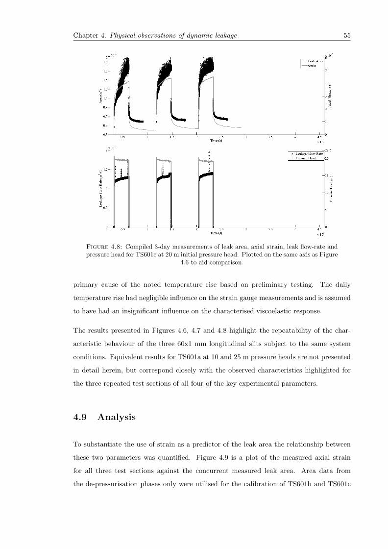
Chapter 4. Physical observations of dynamic leakage 55
Figure 4.8: Compiled 3-day measurements of leak area, axial strain, leak flow-rate andpressure head for TS601c at 20 m initial pressure head. Plotted on the same axis as Figure
4.6 to aid comparison.
primary cause of the noted temperature rise based on preliminary testing. The daily
temperature rise had negligible influence on the strain gauge measurements and is assumed
to have had an insignificant influence on the characterised viscoelastic response.
The results presented in Figures 4.6, 4.7 and 4.8 highlight the repeatability of the char-
acteristic behaviour of the three 60x1 mm longitudinal slits subject to the same system
conditions. Equivalent results for TS601a at 10 and 25 m pressure heads are not presented
in detail herein, but correspond closely with the observed characteristics highlighted for
the three repeated test sections of all four of the key experimental parameters.
4.9 Analysis
To substantiate the use of strain as a predictor of the leak area the relationship between
these two parameters was quantified. Figure 4.9 is a plot of the measured axial strain
for all three test sections against the concurrent measured leak area. Area data from
the de-pressurisation phases only were utilised for the calibration of TS601b and TS601c

Chapter 4. Physical observations of dynamic leakage 56
due to the interference in the image leak area definition as previously described. The
mean relationships between the measured axial strain and leak area may be represented
by simple linear equations for each test section, as listed in Table 4.2.
Table 4.2: Linear fitting parameters for the explicit strain-area relationship for threediscrete test sections.
Test Section Gradient Intercept RMSE
(m2) (m2)
TS601a 0.0176 2.8E-05 2.25
TS601b 0.0199 3.6E-05 0.57
TS601c 0.0197 5.1E-05 0.50
The use of recovery phase (de-pressurisation) data only for the fitting procedure for TS601b
and TS601c results in relatively low RMSE due to the lower range of area and axial strain
magnitude. The equations describing the association between strain and area allow for
further analysis of the interaction of the structural behaviour and leak hydraulics where
there is uncertainty with regards to the leak area during pressurisation.
Figure 4.9: Leak area and strain relationship as measured for TS601a, TS601b andTS601c. Measurements of leak area and axial strain during the recovery phase only are
presented for TS601b and c.
4.9.1 Leak Hydraulics
Figure 4.10 shows the evaluated discharge coefficients using the Orifice Equation (λ=0.5)
and the recorded laboratory data (synchronous leak flow rate, leak area and pressure), for
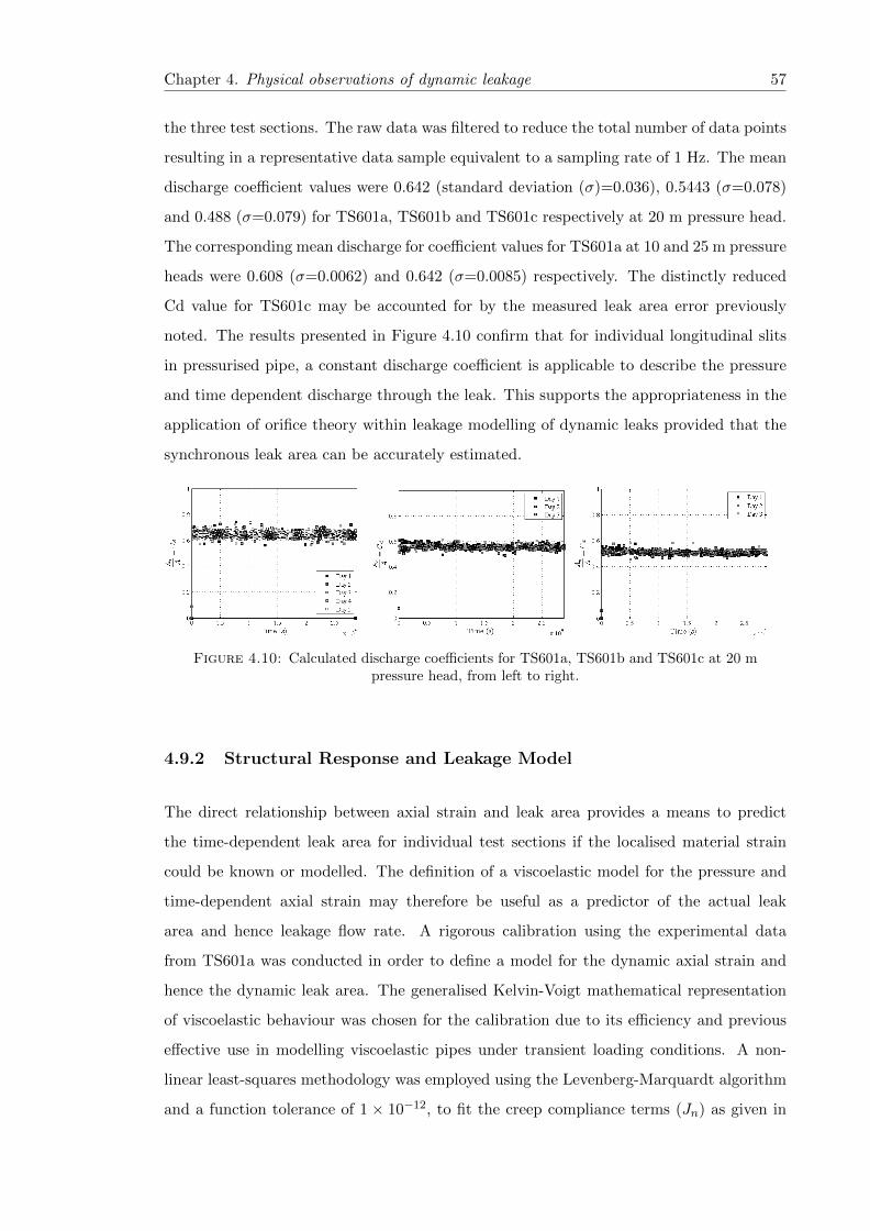
Chapter 4. Physical observations of dynamic leakage 57
the three test sections. The raw data was filtered to reduce the total number of data points
resulting in a representative data sample equivalent to a sampling rate of 1 Hz. The mean
discharge coefficient values were 0.642 (standard deviation (σ)=0.036), 0.5443 (σ=0.078)
and 0.488 (σ=0.079) for TS601a, TS601b and TS601c respectively at 20 m pressure head.
The corresponding mean discharge for coefficient values for TS601a at 10 and 25 m pressure
heads were 0.608 (σ=0.0062) and 0.642 (σ=0.0085) respectively. The distinctly reduced
Cd value for TS601c may be accounted for by the measured leak area error previously
noted. The results presented in Figure 4.10 confirm that for individual longitudinal slits
in pressurised pipe, a constant discharge coefficient is applicable to describe the pressure
and time dependent discharge through the leak. This supports the appropriateness in the
application of orifice theory within leakage modelling of dynamic leaks provided that the
synchronous leak area can be accurately estimated.
Figure 4.10: Calculated discharge coefficients for TS601a, TS601b and TS601c at 20 mpressure head, from left to right.
4.9.2 Structural Response and Leakage Model
The direct relationship between axial strain and leak area provides a means to predict
the time-dependent leak area for individual test sections if the localised material strain
could be known or modelled. The definition of a viscoelastic model for the pressure and
time-dependent axial strain may therefore be useful as a predictor of the actual leak
area and hence leakage flow rate. A rigorous calibration using the experimental data
from TS601a was conducted in order to define a model for the dynamic axial strain and
hence the dynamic leak area. The generalised Kelvin-Voigt mathematical representation
of viscoelastic behaviour was chosen for the calibration due to its efficiency and previous
effective use in modelling viscoelastic pipes under transient loading conditions. A non-
linear least-squares methodology was employed using the Levenberg-Marquardt algorithm
and a function tolerance of 1 × 10⁻¹², to fit the creep compliance terms (Jn) as given in

Chapter 4. Physical observations of dynamic leakage 58
Equation 4.3, using the measured strain, pressure head data and the convolution integral,
Equation 4.4. Calibration of the discrete daily leakage response and the 5-day response
were evaluated. The results of the calibration program considering the full time-history
(5-day response) are summarised in Table 4.3. The retardation times (τn), were assigned
prior to the calibration to capture the discrete time period material response. These pre-
determined values were used to represent the time periods in increasing orders of magnitude
(multiples of 10 s) covered by the long term response of the structural behaviour captured
within the experimental program. This methodology reflected the method used by Covas
et al. (2005) when considering the calibration of the short-term viscoelastic response of
pipes to transient propagation.
Table 4.3: Non-linear least squares calibration of creep compliance components fortime-dependent axial strain for TS601a.
Jn( 1Pa
) : J0 J1 J2 J3 J4 J5 J6 J7 StdError
τn (s): 10 100 1000 10000 100000 1000000 10000000
3 Comps. 8.50E-0.9 1.26E-08 0 0 0 0 0 0 5.16E-04
5 Comps. 8.50E-0.9 1.00E-11 1.26E-08 0 0 0 0 0 5.08E-04
7 Comps. 8.50E-0.9 1.28E-09 1.00E-11 1.17E-08 0 0 0 0 4.53E-04
9 Comps. 8.50E-0.9 2.00E-09 5.46E-09 1.22E-11 7.46E-09 0 0 0 2.90E-04
11 Comps. 8.50E-0.9 2.14E-09 2.84E-09 4.09E-09 1.84E-09 8.42E-09 0 0 1.92E-04
13 Comps. 8.50E-0.9 2.04E-09 3.02E-09 3.89E-09 2.15E-09 6.68E-09 6.13E-09 0 8.31E-05
15 Comps. 8.50E-0.9 2.81E-09 2.85E-09 2.99E-09 2.66E-09 5.93E-09 7.80E-09 1.26E-11 8.49E-05
Employing the 11-component parameter model as detailed in Table 4.3, the strain data was
converted to time-dependent modelled leak area (AL(t)) using the calibration for TS601a
given above. The 11-component model was assessed to be the optimal model selection
based on computational efficiency and modelling accuracy (standard error representative
of approximately 11.3% of the experimental recorded standard deviation). The mean value
for the evaluated discharge coefficient (Cd = 0.64), based on the analysis presented in
Figure 4.10, the measured differential pressure head across the leak opening and the mod-
elled leak area were input into Equation 4.5, a modified time-dependent form of the Orifice
equation (Equation 4.1) to evaluate the leakage through the longitudinal slit. Equation
4.6 is the leak area model using the calibrated creep compliance model (where J11 is the 11
component creep compliance model, Equation 4.3, using components listed in Table 4.3)
and the linear strain-area relationship for TS601a where C1 = 0.01765 and C2 = 2.8×10⁻⁵.
Figure 4.11 presents results from this procedure for TS601a at three discrete quasi steady
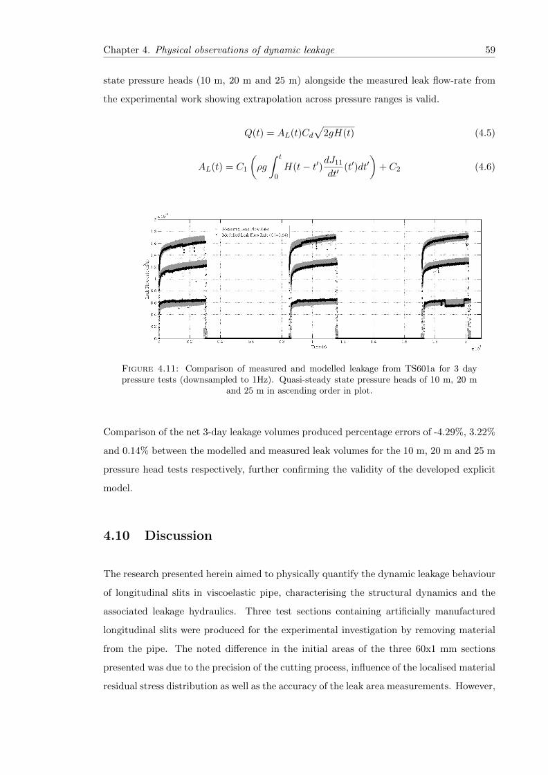
Chapter 4. Physical observations of dynamic leakage 59
state pressure heads (10 m, 20 m and 25 m) alongside the measured leak flow-rate from
the experimental work showing extrapolation across pressure ranges is valid.
Q(t) = AL(t)Cd√
2gH(t) (4.5)
AL(t) = C1
(ρg
∫ t
0H(t− t′)dJ11
dt′(t′)dt′
)+ C2 (4.6)
Figure 4.11: Comparison of measured and modelled leakage from TS601a for 3 daypressure tests (downsampled to 1Hz). Quasi-steady state pressure heads of 10 m, 20 m
and 25 m in ascending order in plot.
Comparison of the net 3-day leakage volumes produced percentage errors of -4.29%, 3.22%
and 0.14% between the modelled and measured leak volumes for the 10 m, 20 m and 25 m
pressure head tests respectively, further confirming the validity of the developed explicit
model.
4.10 Discussion
The research presented herein aimed to physically quantify the dynamic leakage behaviour
of longitudinal slits in viscoelastic pipe, characterising the structural dynamics and the
associated leakage hydraulics. Three test sections containing artificially manufactured
longitudinal slits were produced for the experimental investigation by removing material
from the pipe. The noted difference in the initial areas of the three 60x1 mm sections
presented was due to the precision of the cutting process, influence of the localised material
residual stress distribution as well as the accuracy of the leak area measurements. However,

Chapter 4. Physical observations of dynamic leakage 60
the characteristic leakage behaviour was consistent for all three test sections with the
relative variance in leak flow-rate a function of the initial leak area. In reality longitudinal
cracks do not typically result from the removal of material but may occur due to chemical
degradation of the material (Duvall and Edwards, 2011), slow crack growth (Brown, 2007)
or fatigue (Nishimura et al., 1993), and would therefore have an imperceptible opening
area at zero pressure. It is not anticipated that the associated characteristic behaviour
would vary significantly from the observations made herein for cracks with zero area at
rest, although the localised crack tip stresses would be higher resulting in an increased
risk of crack propagation and structural failure of the pipe.
Analysis was conducted to evaluate the average maximum change of area for all the test
sections, during the first 8 hrs of the recovery phases; -6.38E-05 m2 (σ=2.76E-06 m2),
-6.10E-05 m2 (σ=1.50E-06 m2) and -5.99E-05 m2 (σ=1.79E-06 m2) for days one, two
and three respectively. The low standard deviations for the repeated test sections, infers
that the susceptibility and magnitude of longitudinal slits to deformation is dependent
primarily on the slit length not the width, which varied across the length of each manu-
factured slit resulting in different initial areas. This corresponds with the findings from
numerical simulations conducted by Cassa and van Zyl (2011) investigating the structural
behaviour of equivalent leaks in linear-elastic materials. The discrepancy in the relative
magnitude of strain for each test section corresponds to the distance of the strain gauge
from the slit edge. In other words, the material strain is a function of the proximity to
the slit. Further analysis of the axial strain distribution parallel and perpendicular to the
leak length through physical observations and numerical simulations would advance the
understanding of the mechanism of opening, i.e. whether deformations are due to localised
buckling or bulging of the material. An evaluation of the significance of the manufacturing
process on the inherent stresses within the extruded pipe, may also provide a greater level
of understanding of the observed phenomena.
The validated relationship between the measured leak area and the localised material axial
strain allows for evaluation of the synchronous dynamic leak area if the strain is known or
can be modelled. The simple fitted linear equations provide an alternative means to define
the time-dependent leak area if the leak is not visible, i.e. buried. The influence of the
external ground conditions on the leakage behaviour of dynamic leaks, (e.g. transferred
loading, soil hydraulics, additional flow resistance, ground temperature etc.) remains
a comparatively unexplored area of research. This unique dataset and the calibration
Chapter 4. Physical observations of dynamic leakage 61
between leak area and strain therefore provides an opportunity to develop a methodology
to explore the performance of buried leaking pipes, assessing the fluid-structure interaction
and the associated structural dynamics and leak hydraulics, addressing the limited current
knowledge on this topic.
The temperature range recorded during testing means that the magnitude of the observed
structural deformations may be considered as relatively more extreme than for pipes in-
situ due to the relationship between temperature and creep compliance, i.e. increasing
temperature reduces the stiffness of the material. The typical seasonal soil temperature
variations in the United Kingdom for pipe burial depths between 750 mm and 1350 mm
(Water Regulation No. 1148, 1999) lie between 4◦C and 21◦C (Banks, 2012).
It is generally agreed that the dynamic leak area is the dominant influence on the ob-
served sensitivity of leaks to pressure (Clayton and van Zyl, 2007; Cassa and van Zyl,
2011; Ferrante, 2012). This interpretation is qualitatively supported by the discernible
linear correlation between the measured leak area and flow-rate from the experimental
results. Studies have previously used an effective leak area when modelling leakage due
to the uncertainty of the changing leak area and the potential dependence of the associ-
ated leak discharge coefficient. Using the synchronous measurements of the leak flow-rate,
pressure head and leak area as presented in Figure 1.9, the time-dependent discharge co-
efficients for each test section were evaluated and found to remain constant over the full
range of testing (five discrete loading phases) despite a maximum change in leak area of
greater than 250% for TS601a at 20 m pressure head for example. Two additional test
sections with longitudinal slits of 20x1 mm and 40x1 mm were subsequently produced to
confirm this finding, with calculated mean discharge coefficients of 0.608 (σ=0.0091) and
0.610 (σ=0.0062) respectively. It may therefore be assumed that the theoretical discharge
coefficient is independent of the leak deformation but dependent on the orifice type. This
provides confirmation that the structural behaviour, namely the change of leak area, is the
most critical determining factor of the dynamic leakage behaviour. Ultimately this vali-
dates the inference made that accurate leakage models based on the Orifice Equation may
be utilised for this longitudinal slits in thick-walled viscoelastic pipes under fully turbu-
lent flow conditions. This is achievable by using a discrete constant discharge coefficient,
knowledge of the applied time-series pressure and the synchronous leak area quantified
from physical data or structural modelling. In reality, the actual leak area may not be
measurable. However, knowledge that the discharge coefficient is independent from the

Chapter 4. Physical observations of dynamic leakage 62
dynamic structural leak behaviour may therefore allow an approximation of the leak type
and area to be made based on the observed pressure and leakage relationship. Further
work to confirm this observation (constant discharge coefficient) for other leak types in
different pipe materials, is still required but remains a commonly adopted assumption (e.g.
Cassa et al. (2010)).
A generalised Kelvin-Voigt creep compliance formulation (Equation 4.4) was employed
within the viscoelastic calibration due to the effectiveness of this mathematical represen-
tation in capturing both the instantaneous elastic and time-dependent creep and recovery
material responses over specified time periods. As may be expected, the results of the
calibration show that the greater the number of creep compliance components the better
the fit to the experimental data, highlighting the importance of employing both the short
and long-term components to define a model that considers the full loading-history and
the time dependent creep and recovery responses. Smaller separate models (< 11 total
components) are capable of accurately predicting the daily strain response in isolation
without considering the full loading history. Application of an 11 component model was
determined to be the minimum requirement to effectively replicate the observed structural
behaviour as five discrete retardation time periods were identified from the time depen-
dent structural response. This therefore represents an accurate and parsimonious model
essential in the development of computationally efficient tools for use within both aca-
demic and industrial applications. Separation of the daily standard errors indicated that
the calibration goodness-of-fit was weakest for the first day. This highlights a potential
limitation of mathematical representations in accurately predicting the total physical re-
sponse of viscoelastic structures to applied loading, emphasising that such models are only
ever approximations of the true behaviour. This modelling error is inconsequential with
regards to the modelling error for application in real systems, as it is not anticipated that
in reality a leak would either exist in newly laid pipeline that is pressurised for the first
time or be present in a pipe that has been fully de-pressurised for a time greater than
the total material recovery time. The investigation highlights the need to consider the
entire loading history, or alternatively a time period greater than the time required for the
material to reach a quasi-steady state. Figure 4.11 confirms the effectiveness of Equation
4.5, a time and pressure-dependent form of the Orifice Equation, as a means of modelling
the leakage behaviour of discrete longitudinal slits in MDPE pipe considering the loading
history and the interdependence of the structural behaviour and the leak hydraulics.
Chapter 4. Physical observations of dynamic leakage 63
Leakage exponent based analyses are often used as a means to assess the sensitivity of leaks
to pressure. The results presented within this paper question the validity of such an ap-
proach when considering viscoelastic materials which not only display pressure-dependence
but also time-dependence. The impact of this is in reducing the effectiveness and benefits
of leakage assessment and control techniques using the FAVAD (or similar) leakage model
for predominantly viscoelastic material based systems. In order to understand the benefits
of pressure-management in reducing the total losses in a system comprised of polyethy-
lene pipe, an appreciation of the complex dynamic nature of the leaks in this material
must be considered. The explicit leakage modelling technique developed within this paper
allows for accurate calculations of time-dependent leakage based on pressure head data
and a leak area model calibrated from recorded axial strain data. A leakage model for
longitudinal slits in viscoelastic pipe based on the characterisation and calibration within
this paper, considering all parameters including geometry, material rheology and loading
conditions will provide a means to develop a generalised leakage model considering all
the significant influencing parameters. The methodology presented for characterising the
leakage behaviour may be developed for assessing the equivalent short-term response of
leaks subject to dynamic pressures, e.g. pressure transients due to valve closures, pump
shut-down or changes in demand (Collins et al., 2012). Focus on the short-term response
has significance for the assessment of contaminant ingress risk associated to the existence
of low or negative pressures in water distribution pipes. Likewise, active leakage control
techniques such as leak detection and localisation based on inverse transient analysis may
be greatly enhanced by the inclusion of the pressure and time-dependent Orifice Equation.
4.11 Conclusion
An experimental investigation was conducted to quantify the leakage behaviour of longi-
tudinal slits in MDPE pipe due to changing pressure regime, providing a unique dataset
measuring the synchronous leak flow-rate, pressure, leak area and material strain. The
time and pressure dependent leak area, due to the viscoelastic behaviour of the material,
is shown to be the critical factor defining the observed dynamic leakage response of the
failure type examined. It was shown that localised axial strain measurements may be used
as a predictor of the variable leak area. Hence using a mathematical representation of
the linear viscoelastic constitutive equations to characterise the strain, a means to model

Chapter 4. Physical observations of dynamic leakage 64
the dynamic leak area is provided. Integrating such estimation of the time and pressure
dependent leak geometry into the Orifice Equation yields an effective means to model the
leakage flow rate, in which the coefficient of discharge remains constant. The knowledge
gained is relevant to better inform the development of leakage management strategies,
including pressure management and other active leakage control technologies, aimed at
reducing the real losses from water distribution systems.
Chapter 5
A dynamic leakage model:
derivation and validation of a
leakage model for longitudinal slits
in viscoelastic pipe
“Once we accept our limits, we go beyond them.”
Albert Einstein (1955)
5.1 Overview
Physical observations provide a detailed insight into the true dynamic nature of a leak and
the dependent leak area. A key question is, what are the primary governing parameters
defining this behaviour? Isolation of the structural dependencies through physical exper-
iments can be a long and protracted process, whereas numerical simulations allow for an
efficient interrogation of the structural variables. A methodology for describing leakage
behaviour in a generalised form was established utilising numerical modelling defining the
dependent leak area, and empirical data to characterise the viscoelastic behaviour. The
work builds upon the knowledge gained from the physical observations of the interdepen-
dence of the structural and leak dynamics.
65
Chapter 5. Dynamic leakage model 66
The numerical simulations to capture the structural behaviour are particularly significant
as they go beyond the scope of previous work that has focussed primarily on leaks in
thin walled pipes. The need to understand the response of leaks in thick walled pipes
continues to develop as the use of plastic pipes such as MDPE and HDPE increases. This
chapter addressed the goals set out in Objectives 2 and 3 in Chapter 3. The concept of
the methodology presented in this chapter to define a generalised leakage model was;
• to identify the primary governing parameters for the structural dynamics for slits in
linear elastic pipes from numerical simulations
• to derive a simple analytical model to describe this dynamic behaviour
• to calibrate the time dependent elastic modulus from empirical data
• to integrate this model of structural dynamics into the previously validated modified
Orifice Equation and validate this for quantifying leakage
5.1.1 Journal Submission Details
This chapter is the manuscript intended for submission to the American Society of Civil
Engineers (ASCE) Journal of Hydraulic Engineering. As a result of the reference to the
physical experimental research presented in Chapter 4, submission was placed on hold
until confirmation of acceptance of the previous chapter had been achieved.
The generalised leakage model developed within this chapter describes the leak behaviour
of longitudinal slits in polyethylene pipe for the first time. The investigation builds on the
work of van Zyl and Cassa (2014) regarding the leakage behaviour of elastically deforming
leaks, and the previously described work presented by Ferrante et al. (2011) observing
the complex nature of leaks in viscoelastic pipes. Publication of Chapters 4 and 5 in the
Journal of Hydraulic Engineering therefore provide a strong narrative regarding the quan-
tification of the behaviour of different leak types in a single publication. The derived and
validated leakage model provides a unique tool to assess the impact of such complex leaks
in the water distribution systems, in particular the effectiveness of current and developing
leakage management strategies, building upon the understanding of the interdependence
of leak and structural dynamics.

Chapter 5. Dynamic leakage model 67
5.2 Abstract
Accurate models describing the characteristic response of complex leaks that may occur in
pressurised water distribution pipes are crucial in improving the understanding of leak-
age behaviour. Such knowledge allows for the enhancement of the ability to assess and
mitigate the real losses through these failure openings. A synergistic methodology was
formulated whereby numerical and physical experimental data was used to develop a gen-
eralised model quantifying both the structural and leak dynamics of longitudinal slits in
thick-walled viscoelastic pipes. The parsimonious and dimensionally homogeneous time
and pressure dependent leakage model was validated using experimental data, independent
from the physical observations utilised for the viscoelastic calibration. It was shown to be
an effective tool to predict the distinct short and long term response of the evaluated test
cases.
5.3 Introduction
Real losses from Water Distribution Systems (WDS), as a result of background leakage and
bursts, have a significant effect on the overall sustainability of this vital infrastructure, both
economically and environmentally. In the UK, the Water Services Regulation Authority
(Ofwat) published leakage statistics from 2013, showed that the current level of leakage
stands at 172 mega-litres per day (Ofwat, 2013). This value has remained approximately
static for over a decade. The ability to assess, analyse and mitigate the impact of such losses
is dependent on new fundamental understanding of the behaviour of individual leaks and
the capability to predict their behaviour. Studies, such as Greyvenstein and van Zyl (2006),
have emphasised the need to consider the sensitivity of leakage to pressure primarily due to
the dynamic nature of leak areas (changing leak area) of different failure types in a range
of commonly used pipe materials. Dynamic leak areas result in potentially high sensitivity
of leakage flow-rates with regards to changes in pressure, greater than the traditional
relationship defined in the Orifice Equation. This has been observed both in field studies
at District Metered Area (DMA) level and in laboratory tests of individual leaks (Thornton
and Lambert, 2005; Avila Rangel and Gonzalez Barreto, 2006; Greyvenstein and van Zyl,
2006).
Chapter 5. Dynamic leakage model 68
Plastic pipes are a popular choice for hydraulic pipelines due to their durability and cost
effectiveness. However, leaks occurring in this type of pipe, in particular longitudinal
cracks/slits a dominant failure mode in plastic pipes, result in a complex leakage behaviour
due to the inherent material rheology. Quantifying the dependent structural response of
leaks in these viscoelastic pipes and the interdependence with the leak hydraulics is crucial
in predicting the time and pressure-dependent leakage.
5.4 Background
Leaks occur in a diverse range of shapes and sizes, dependent on factors including pipe
material, loading case, ground conditions, age, and manufacturing process. Leakage flow-
rates are often estimated using the Orifice Equation which assumes a constant leak area
and a square root relationship between pressure and flow-rate. The Generalised Orifice
Equation (Equation 5.1) is used to characterise the leakage behaviour of isolated systems
where the size of the leak (or leaks) opening is unknown. Field studies have recorded
leakage exponent values in the range of 0.52 to 2.79 (Farely and Trow, 2003), deviating from
the theoretical constant of 0.5 described in the traditional Orifice Equation. A selection
of common failure types were investigated by Greyvenstein and van Zyl (2006) who found
corrosion clusters and longitudinal cracks displayed the highest sensitivity to changes in
pressures represented by leakage exponents greater than 0.5. It was surmised that this
was primarily due to the variability of the leak area under different hydraulic pressures
within the pipe, a qualitative assessment that is generally recognised and accepted (Clayton
and van Zyl, 2007; Cassa and van Zyl, 2011; Ferrante, 2012). Experimental studies have
confirmed that the leak area is the primary causative factor of this observed behaviour,
also highlighting the insensitivity of the theoretical discharge coefficient (Chapter 4).
Q = chλ (5.1)
The importance of understanding the dynamic nature of leaks has resulted in a number of
studies investigating their structural behaviour. Much of this work has focussed on failures
in linear-elastic materials, in particular longitudinal cracks (Grebner and Strathmeier,
1984; Bhandari and Leroux, 1993; Avila Rangel and Gonzalez Barreto, 2006; Al-khomairi,
2005; De Miranda et al., 2012) and circumferential cracks (Rahman et al., 1998; Takahashi,

Chapter 5. Dynamic leakage model 69
2002). Different approaches have been adopted, all considering the pressure-dependent leak
area of failures. These may be categorised as theoretical or empirically based studies.
5.4.1 Theoretical Studies
Theoretical analyses utilise fundamental structural principles to derive frameworks to eval-
uate the behaviour of stable cracks (no propagation). The application of shell theory with
respect to crack opening behaviour has been effectively demonstrated, allowing the conver-
sion between the calculated deformation of a crack in a flat plate to an equivalent failure
in a curved surface or cylindrical pipe (Wuthrich, 1983). The use of shell theory assumes a
relatively small wall thickness of the modelled plate. This approach is therefore not univer-
sally applicable to leaks in water distribution pipes as a significant proportion are classified
as thick-walled, most notably regarding polyethylene pipes (over 10% of UK WDS pipes
(UKWIR, 2008)). De Miranda et al. (2012) presented a method to describe the dynamic
structural behaviour of longitudinal slits1 in pressurised pipes using a validated analytical
model based on a beam with elastic constraints. This approach provided a detailed assess-
ment of the physical mechanisms/ components controlling the structural behaviour. As
with shell theory, this theoretical approach did not consider the effect of shear deformation
that may occur in thick-walled pipes, emphasising this limitation within the attempted
validation from thick-walled finite element models. Application of the model requires so-
lution of ordinary differential equations using pre-defined boundary-interface conditions,
hindering the simplicity and ease of use for leakage management practitioners as desired.
Franchini and Lanza (2014) developed a theoretical approach based on the application
of the Buckingum π theorem to establish the basis for a dimensionless leakage model.
This considered different elastic materials, and pipe and leak geometries to account for
the dependence of the leak area and discharge coefficient. The work offers a very robust
tool, calibrated with experimental data, to derive a single pressure leakage relationship
for failures in linear-elastic materials. However the approach did not isolate the explicit
deformation of individual leaks which is necessary for exploring the interdependence of the
structural behaviour and leak hydraulics.
Numerical simulations including validated finite element analyses (FEA) have been adopted
as a powerful tool to explore the structural behaviour of leaks. FEA provides a means
1Within this paper, ’cracks’ refer to naturally occurring leak apertures in pipes, and ’slits’ refer toartificially manufactured failure apertures.

Chapter 5. Dynamic leakage model 70
to investigate the structural behaviour of a limitless range of failure types in different
pipe sizes and materials under various loading conditions, whilst quantifying macroscopic
and microscopic material responses. The definition of suitably fine mesh sizing and ap-
propriate boundary conditions are essential to develop accurate simulations. Cassa and
van Zyl (2011) used FEA to investigate the significance of different parameters on the
leak behaviour of three types of leaks; longitudinal, circumferential and spiral slits. The
FEA results compiled were used to statistically derive an equation defining the dependent
change of area for each leak type, subsequently input into a reformulation of the Fixed and
Variable Area Discharge (FAVAD) model defined by May (1994). The finalised leakage
model presented by van Zyl and Cassa (2014) provides an effective and simple method-
ology to quantify the pressure-dependent leak area and hence predict an explicit leakage
exponent value. The non-dimensionally equal nature of the derived expression means that
no physical meaning can be attached to the components of the predictive model.
Definition of accurate boundary conditions are critical to the validity of numerical sim-
ulations. Alongside the significance of fixed boundary conditions defining the degree of
freedom of a given model, the variable boundary conditions (e.g. the applied loadings)
are also important. Methods to simulate the pressure loading due to hydraulic conditions
are well practised (Rahman et al., 1998; Cassa and van Zyl, 2008; De Miranda et al.,
2012). However, there is still uncertainty with regards to the magnitude, and hence the
significance, of the slit face loading for a given leak. Such localised pressures are there-
fore commonly excluded from analyses due to the uncertainty in the definition of the true
pressure distribution (Takahashi, 2002).
5.4.2 Empirical Investigations
Empirical data is a powerful platform to develop rigorous and validated models in a wide
range of applications. Within the field of leakage modelling, experimental data from real
and artificially manufactured leaks has been utilised to verify and validate the application
of existing leakage models (Orifice Equation) and novel theoretically derived models (De
Miranda et al., 2012; Franchini and Lanza, 2014). Buckley (2007) explored the dynamic
leak area of a range of different failure types including circular orifices and longitudinal slits
under representative loading conditions using a hydraulic pressurised bladder. The work
provided an insight into the influence of different parameters on the leak opening area, in

Chapter 5. Dynamic leakage model 71
particular the significance of slit length on the scale of deformation under applied loading.
However, the work did not consider the significance of the viscoelastic behaviour of PVC
pipes, observable in the presented results, compromising the fitted linear pressure-area
relationships. When analysing polymeric materials, such as PVC, the material rheology
must also be considered, i.e. the viscoelastic material characteristics (Meissner and Franke,
1977).
Time-dependent viscoelastic behaviour may be seen as a secondary feature compared to
the dominant structural influencing parameters presented by Cassa and van Zyl (2008)
and Buckley (2007) within the structural performance of leaks in PVC pipes. However
when quantifying the equivalent behaviour of leaks in polyethylene pipes, another common
pipe material found in water distribution systems, understanding the material rheology
is critical. Massari et al. (2012) presented results from a series of physical observations
of the behaviour of longitudinal slits in High-Density Polyethylene (HDPE) emphasising
the time and pressure dependence of the localised strain around the leak and the ‘effective
leak area’, which is the coupled discharge coefficient and leak area.
5.4.3 Polyethylene Pipes
Polyethylene (PE) pipes are frequently used in the water industry due to the cost benefits
offered by the inherent durability and flexibility of the material (GPSUK, 2014b). Standard
PE pipe sections used by the water industry in the United Kingdom range from 20 mm
to 1000 mm external diameter (British Standards Institution, 2011), with typical service
pipes for cold water service found to be between 20 mm and 63 mm external diameter
based on BS 6572:1985 (British Standards Institution (1985) withdrawn in 2003). All
sections within the range of 20-1000 mm diameter are classed as thick-walled pipes, where
the ratio of external diameter to wall thickness (d/s) is less than 20. This is in contrast
to typical steel, PVC and some cast iron pipes where the d/s ratio is commonly greater
than 20, classifying such pipes as thin-walled. The spatially dependent cross sectional
stress distributions and the viscoelastic nature of PE results in a complex behaviour of
failures in the pipe primarily due to the time, temperature and pressure dependence of
the structural response. Additionally, the extrusion based manufacturing process tends
to result in the formation of residual stresses within the material due to the differential
cooling of the internal and external faces (Hutar et al., 2012). The average measured
Chapter 5. Dynamic leakage model 72
residual stresses may be simply approximated as a tensile stress on the external face and
a compressive stress on the internal face in the range of 2.0 to 5.0 MPa, with a non-linear
distribution across the wall-thickness (Guan and Boot, 2004; Frank et al., 2009). The
residual stresses are important when quantifying the material behaviour under hydraulic
loading conditions, and more critically when quantifying the structural behaviour of pipe
failures such as longitudinal slits.
The performance of longitudinal slits (a common failure mode in the direction of the pipe
extrusion (O’Connor, 2011)), have been shown to demonstrate complex leakage behaviour
(Massari et al., 2012). There remains, a need to determine all of the key parameters
controlling the time-dependent leakage behaviour of such longitudinal slits in viscoelastic
pipes, equivalent to studies of linear elastic pipes. In particular, investigating the struc-
tural parameters influencing the variable leak area in order to understand the observed
dynamic behaviour is important (as also noted by Ferrante (2012)). Previous experimental
observations concluded, significantly, that the dynamic leakage behaviour may be simply
modelled by quantifying the variable leak area and applying this within a modified form of
the Orifice Equation (Chapter 4). The absolute leak area is therefore the dominant influ-
encing factor on the resulting leak-flow rate and has negligible impact on the assumption
and application of a constant discharge coefficient.
5.5 Research Aim
The aim of the investigation was to derive a simple dimensionally homogeneous model
to quantify the generalised dynamic leak area of stable longitudinal slits in pressurised
Medium Density Polyethylene (MDPE) pipes. The research looked to investigate the
influence of geometrical characteristics, material properties and loading conditions, whilst
also qualitatively assessing the significance of the development of a slit face loading on the
observed structural deformations. Ultimately the research intended to validate the use of
an analytical model integrating this dependent leak area expression into a modified form
of the Orifice Equation, to describe the leakage behaviour of this sensitive leak type.

Chapter 5. Dynamic leakage model 73
5.6 Research Method
The methodology to develop a generalised analytical model to describe the leakage be-
haviour of stable longitudinal slits, built on the synergy between numerical simulations
and experimental data. The steps taken were i) numerical simulations quantifying the
variable leak area, ii) derivation of linear-elastic variable leak area model from simula-
tion results, iii) calibration of characteristic viscoelastic response from empirical data and
finally, iv) validation of dynamic leakage model against physical observations.
Considering the fundamental structural behaviour of polyethylene pipes, theoretically a
constant elastic modulus may be replaced by an empirically calibrated time-dependent
elastic modulus to capture the dependent linear-viscoelastic structural response. This
corresponds with the constitutive linear-viscoelastic equations which define the relationship
between stress and strain using a Volterra integral equation, where time is the variable
limit of integration. Utilising the created synergy between numerical simulations and
physical observations, the objective was to produce a leak area model of the form shown
in Equation 5.2, accounting for the combined contribution of the variables of geometry,
material properties and loading conditions respectively.
A(t) = A0 + dA = A0 +K(Geometry,Material, Loading) (5.2)
Finite element analyses were utilised to empirically derive an expression based on Equation
5.2 defining the dependent variable leak area of longitudinal slits in thick walled linear-
elastic pipes. The simplest and a dimensionally homogenous form was targeted within the
analysis, to provide a functional and efficient model. Experimental data of the synchronous
leakage flow-rate, pressure head and leak area data for longitudinal slits in Medium Den-
sity Polyethylene (MDPE) was subsequently used to calibrate the time-dependent elastic
modulus. The final dynamic leakage model was then validated against supplementary
experimental data.
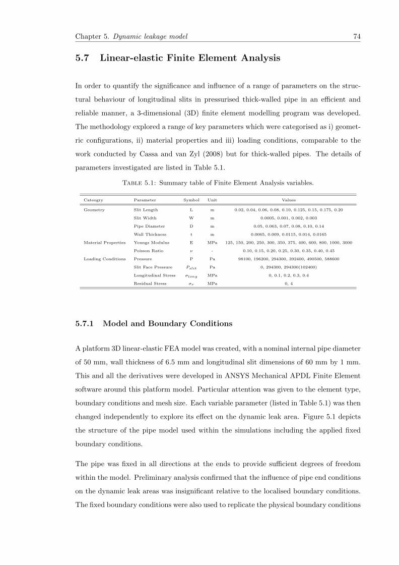
Chapter 5. Dynamic leakage model 74
5.7 Linear-elastic Finite Element Analysis
In order to quantify the significance and influence of a range of parameters on the struc-
tural behaviour of longitudinal slits in pressurised thick-walled pipe in an efficient and
reliable manner, a 3-dimensional (3D) finite element modelling program was developed.
The methodology explored a range of key parameters which were categorised as i) geomet-
ric configurations, ii) material properties and iii) loading conditions, comparable to the
work conducted by Cassa and van Zyl (2008) but for thick-walled pipes. The details of
parameters investigated are listed in Table 5.1.
Table 5.1: Summary table of Finite Element Analysis variables.
Cateogry Parameter Symbol Unit Values
Geometry Slit Length L m 0.02, 0.04, 0.06, 0.08, 0.10, 0.125, 0.15, 0.175, 0.20
Slit Width W m 0.0005, 0.001, 0.002, 0.003
Pipe Diameter D m 0.05, 0.063, 0.07, 0.08, 0.10, 0.14
Wall Thickness t m 0.0065, 0.009, 0.0115, 0.014, 0.0165
Material Properties Youngs Modulus E MPa 125, 150, 200, 250, 300, 350, 375, 400, 600, 800, 1000, 3000
Poisson Ratio ν - 0.10, 0.15, 0.20, 0.25, 0.30, 0.35, 0.40, 0.45
Loading Conditions Pressure P Pa 98100, 196200, 294300, 392400, 490500, 588600
Slit Face Pressure Pslit Pa 0, 294300, 294300(102400)
Longitudinal Stress σlong MPa 0, 0.1, 0.2, 0.3, 0.4
Residual Stress σr MPa 0, 4
5.7.1 Model and Boundary Conditions
A platform 3D linear-elastic FEA model was created, with a nominal internal pipe diameter
of 50 mm, wall thickness of 6.5 mm and longitudinal slit dimensions of 60 mm by 1 mm.
This and all the derivatives were developed in ANSYS Mechanical APDL Finite Element
software around this platform model. Particular attention was given to the element type,
boundary conditions and mesh size. Each variable parameter (listed in Table 5.1) was then
changed independently to explore its effect on the dynamic leak area. Figure 5.1 depicts
the structure of the pipe model used within the simulations including the applied fixed
boundary conditions.
The pipe was fixed in all directions at the ends to provide sufficient degrees of freedom
within the model. Preliminary analysis confirmed that the influence of pipe end conditions
on the dynamic leak areas was insignificant relative to the localised boundary conditions.
The fixed boundary conditions were also used to replicate the physical boundary conditions

Chapter 5. Dynamic leakage model 75
Figure 5.1: Finite element model boundary conditions; plane of symmetry fixed againstdisplacement in x-direction (hatched area), pipe ends fixed against displacement in all
directions.
utilised within Chapter 4 laboratory investigations. In doing so, an accurate comparison
and subsequent calibration of the structural behaviour may be achieved between both sets
of empirical data. A plane of symmetry was used to reduce the model size and consequently
the required simulation time, achieved by splitting the model in half along the axial length
of the pipe (Z-direction) through the centre of the longitudinal slit. Preliminary analysis
against a whole pipe model confirmed this had negligible impact on the observed dynamic
leak area. The model was then fixed in the X-direction along the line of symmetry as
can be seen in Figure 5.1. The 3D model consisted of 20-node 3D SOLID186 elements
which have the capability to accurately model large deflections and strains. The element
type is classified as a ‘Current-technology-element’ as opposed to the ‘Legacy’ elements
which therefore allows for use of tools including inistate, an effective means to simulate
the residual pipe stresses.
The internal pipe pressure was simulated by applying a nodal pressure loading. The range
of simulated pressures investigated are representative of typical operating pressures in
water distribution pipes in the United Kingdom. Pressure loading was done sequentially
to prevent extremely large deformations from occurring within the model, i.e. pressure
loading steps equivalent to pressure heads of 10, 20, 30, 40, 50 and 60 m were implemented.
Non-linear geometry effects were activated within the static structural solution of the
models to account for any large deformations. Preliminary simulations indicated that this
had negligible effect on the resultant leak areas measured.
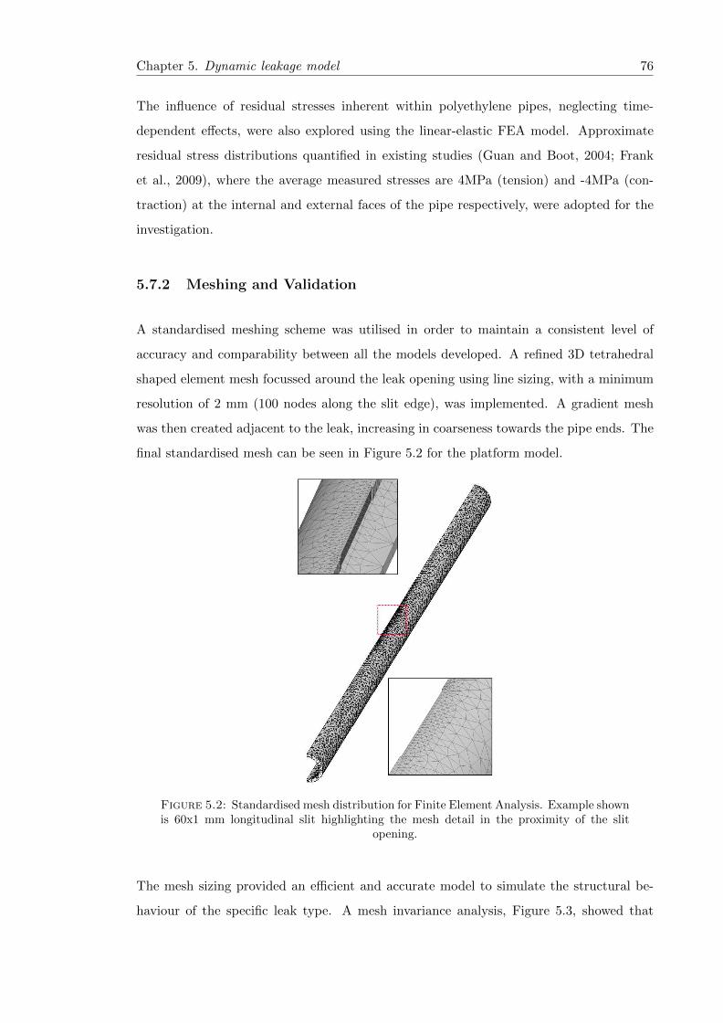
Chapter 5. Dynamic leakage model 76
The influence of residual stresses inherent within polyethylene pipes, neglecting time-
dependent effects, were also explored using the linear-elastic FEA model. Approximate
residual stress distributions quantified in existing studies (Guan and Boot, 2004; Frank
et al., 2009), where the average measured stresses are 4MPa (tension) and -4MPa (con-
traction) at the internal and external faces of the pipe respectively, were adopted for the
investigation.
5.7.2 Meshing and Validation
A standardised meshing scheme was utilised in order to maintain a consistent level of
accuracy and comparability between all the models developed. A refined 3D tetrahedral
shaped element mesh focussed around the leak opening using line sizing, with a minimum
resolution of 2 mm (100 nodes along the slit edge), was implemented. A gradient mesh
was then created adjacent to the leak, increasing in coarseness towards the pipe ends. The
final standardised mesh can be seen in Figure 5.2 for the platform model.
Figure 5.2: Standardised mesh distribution for Finite Element Analysis. Example shownis 60x1 mm longitudinal slit highlighting the mesh detail in the proximity of the slit
opening.
The mesh sizing provided an efficient and accurate model to simulate the structural be-
haviour of the specific leak type. A mesh invariance analysis, Figure 5.3, showed that
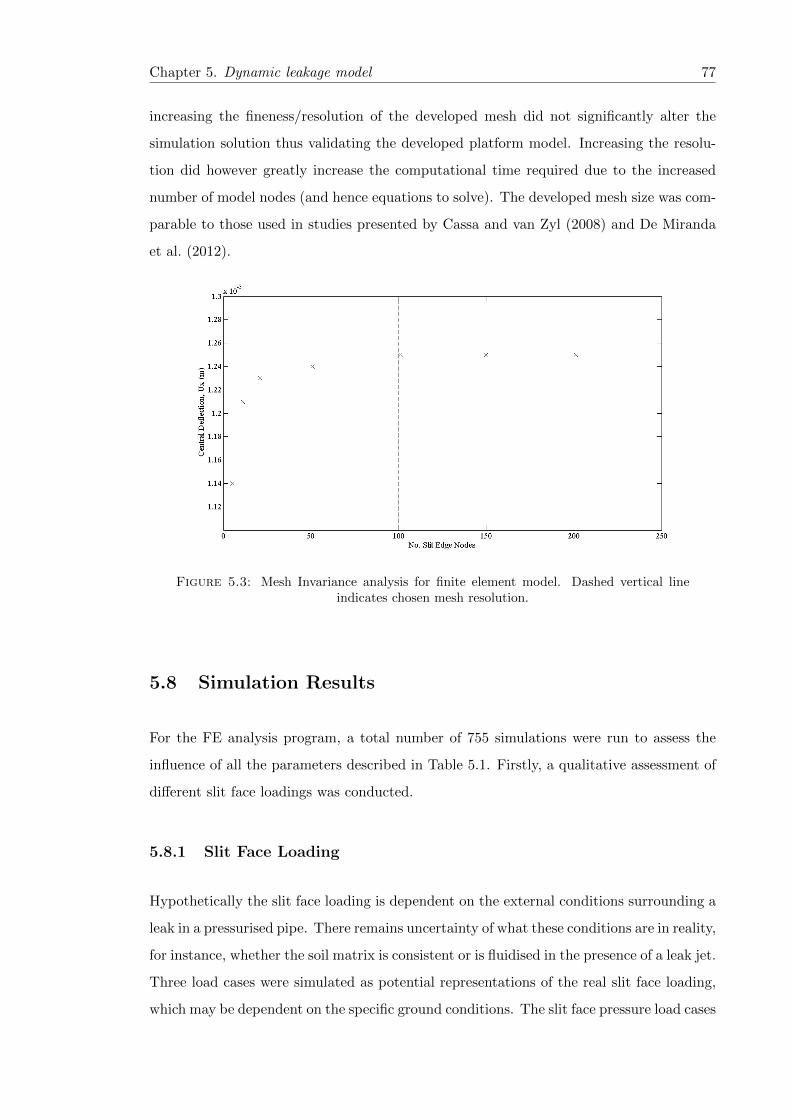
Chapter 5. Dynamic leakage model 77
increasing the fineness/resolution of the developed mesh did not significantly alter the
simulation solution thus validating the developed platform model. Increasing the resolu-
tion did however greatly increase the computational time required due to the increased
number of model nodes (and hence equations to solve). The developed mesh size was com-
parable to those used in studies presented by Cassa and van Zyl (2008) and De Miranda
et al. (2012).
Figure 5.3: Mesh Invariance analysis for finite element model. Dashed vertical lineindicates chosen mesh resolution.
5.8 Simulation Results
For the FE analysis program, a total number of 755 simulations were run to assess the
influence of all the parameters described in Table 5.1. Firstly, a qualitative assessment of
different slit face loadings was conducted.
5.8.1 Slit Face Loading
Hypothetically the slit face loading is dependent on the external conditions surrounding a
leak in a pressurised pipe. There remains uncertainty of what these conditions are in reality,
for instance, whether the soil matrix is consistent or is fluidised in the presence of a leak jet.
Three load cases were simulated as potential representations of the real slit face loading,
which may be dependent on the specific ground conditions. The slit face pressure load cases

Chapter 5. Dynamic leakage model 78
were; Load Case A) zero loading, Load Case B) constant slit loading (Pslit = 294300 Pa)
and Load Case C) linear gradient loading (Pslit = −2.95E + 07(sn) + 2.943E + 05 Pa,
where sn is the discretised wall thickness over n steps). An example from the results
of the analysis, using a 20x1 mm slit, is presented in Figure 5.4 where the percentage
increase in central deflection of Load Cases B and C relative to Load Case A were 12.25%
and 7.28% respectively. The results indicate that the slit face loading is significant with
Figure 5.4: Comparison of the slit edge deflection (Ux) of a 20x1mm FE model subjectto three discrete slit face load cases.
respect to the change of leak area. However, the explicit relationship between this pressure
distribution and the pipe geometry and external boundary conditions are beyond the scope
of the investigation. This parameter was therefore not included within any further analysis
aimed at deriving an analytical leak area model as a quantification of the actual slit face
pressure distribution is required.
5.8.2 Residual Stress
Following completion of the simulation program, the contribution of individual parameters
to the observed dynamic leak area behaviour were evaluated. Firstly the significance of
the approximated residual stress was analysed. Using the residual stress distribution pre-
viously described, the leak areas were quantified and compared with ‘No Residual Stress’
models for a range of pressures. A selection of results from the analyses are presented in
Figure 5.5 for 40, 60 and 80x1 mm slit models. It can be seen that the residual stresses
resulted in a relative offset (reduction) of the measured leak area which was approximately
constant for each discrete test case. In other words, the change of area remained constant

Chapter 5. Dynamic leakage model 79
for simulations with and without an applied residual stress. This result indicates that the
effect of residual stresses may be directly integrated within a leak area model by the inclu-
sion of the initial area (A0) which is a function of the inherent residual stress distribution.
Consequently the residual stress parameter was not included within the derivation of the
leak area model.
Figure 5.5: Longitudinal slit areas from FE simulation of residual stress analysis forthree discrete test sections.
5.9 Derivation of Leak Area Model
The objective of the analysis was to develop an dimensionally consistent analytical model
in its simplest form, to provide an efficient and practical tool for the assessment of the
structural behaviour of such dynamic leaks. In order to assess the impact of each parameter
on the structural behaviour, a single power-term based analytical expression was evaluated
using statistical multiple regression analysis. The power term formulation was utilised for
the analysis, akin to the work conducted by Cassa and van Zyl (2011), but primarily due to
the approximate power relationships observed within preliminary independent component
analyses (i.e. relationship between each parameter and the relative change of area). The
isolated parameter analysis is not presented herein as the net structural behaviour is not
deemed to be based on the individual effect of different components, but rather the coupled
effect of all the significant parameters, identifiable from the regression analysis. The results
of the fitting process (associated power term values) are given in Table 5.2.
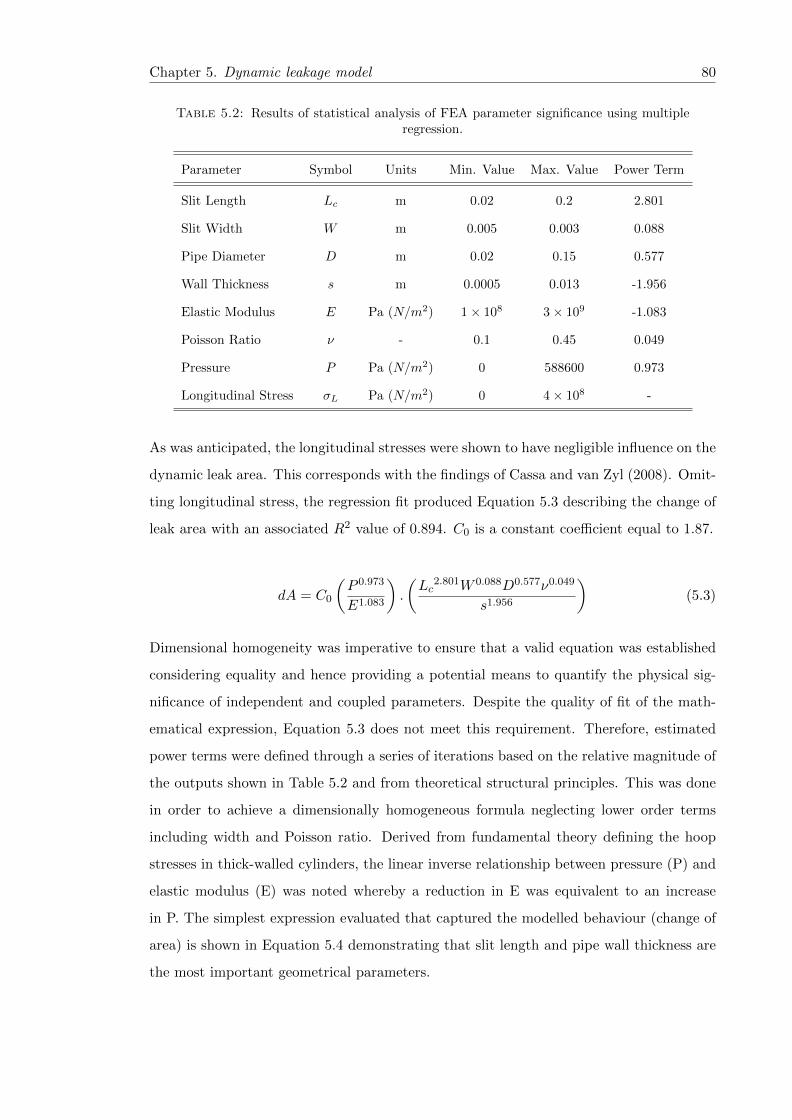
Chapter 5. Dynamic leakage model 80
Table 5.2: Results of statistical analysis of FEA parameter significance using multipleregression.
Parameter Symbol Units Min. Value Max. Value Power Term
Slit Length Lc m 0.02 0.2 2.801
Slit Width W m 0.005 0.003 0.088
Pipe Diameter D m 0.02 0.15 0.577
Wall Thickness s m 0.0005 0.013 -1.956
Elastic Modulus E Pa (N/m2) 1× 10⁸ 3× 10⁹ -1.083
Poisson Ratio ν - 0.1 0.45 0.049
Pressure P Pa (N/m2) 0 588600 0.973
Longitudinal Stress σL Pa (N/m2) 0 4× 10⁸ -
As was anticipated, the longitudinal stresses were shown to have negligible influence on the
dynamic leak area. This corresponds with the findings of Cassa and van Zyl (2008). Omit-
ting longitudinal stress, the regression fit produced Equation 5.3 describing the change of
leak area with an associated R2 value of 0.894. C0 is a constant coefficient equal to 1.87.
dA = C0
(P 0.973
E1.083
).
(Lc
2.801W 0.088D0.577ν0.049
s1.956
)(5.3)
Dimensional homogeneity was imperative to ensure that a valid equation was established
considering equality and hence providing a potential means to quantify the physical sig-
nificance of independent and coupled parameters. Despite the quality of fit of the math-
ematical expression, Equation 5.3 does not meet this requirement. Therefore, estimated
power terms were defined through a series of iterations based on the relative magnitude of
the outputs shown in Table 5.2 and from theoretical structural principles. This was done
in order to achieve a dimensionally homogeneous formula neglecting lower order terms
including width and Poisson ratio. Derived from fundamental theory defining the hoop
stresses in thick-walled cylinders, the linear inverse relationship between pressure (P) and
elastic modulus (E) was noted whereby a reduction in E was equivalent to an increase
in P. The simplest expression evaluated that captured the modelled behaviour (change of
area) is shown in Equation 5.4 demonstrating that slit length and pipe wall thickness are
the most important geometrical parameters.

Chapter 5. Dynamic leakage model 81
dA = C1
(P
E
).
(L4c
s2
)(5.4)
The term C1 represents a dimensionless coefficient that was simultaneously evaluated with
the parameter exponents given in Equation 5.4. This was done to maximise the model
accuracy. A range of dimensionless parameters based on reasonable engineering judgement
were investigated to determine the definition of this coefficient. The ratio of crack length
(Lc) and pipe circumference (πD) is a commonly used dimensionless parameter utilised in
structural mechanics to define the relative size of a crack in a pipe or pressurised vessel
(primarily for circumferential cracks). Employing this term and plotting the relationship
with the coefficient term C1 as shown in Figure 5.6, highlights the capacity of LcπD as a
predictor of C1. Equation 5.5 was fitted to the data in Figure 5.6 for integration into the
final dimensionally homogeneous formulation (Equation 5.4). This relationship is true for
slit length to pipe circumference ratios less than 1, indicating that large slits in relative
small diameter pipe will be over-predicted by the proposed model. In reality such large
scale slits may result in the total structural integrity failure of the pipe, meaning the elastic
deformation of the slit is inconsequential. Equation 5.4 was shown to provide a very good
fit to all the collated data with a mean AreamodelAreameasured
ratio of 1.01 and standard deviation
of 0.12 (excluding data for slit length to pipe circumference ratio greater than 1).
Figure 5.6: Coefficient (C1) analysis from Finite Element data.
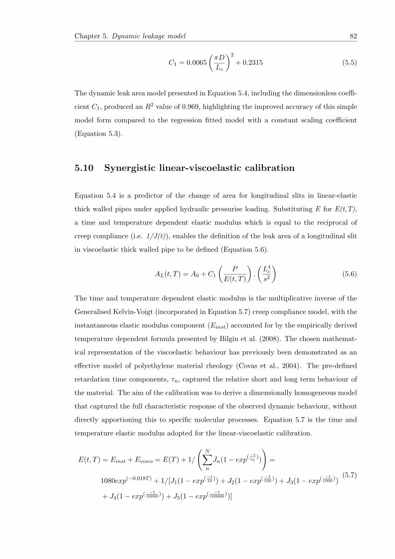
Chapter 5. Dynamic leakage model 82
C1 = 0.0065
(πD
Lc
)2
+ 0.2315 (5.5)
The dynamic leak area model presented in Equation 5.4, including the dimensionless coeffi-
cient C1, produced an R2 value of 0.969, highlighting the improved accuracy of this simple
model form compared to the regression fitted model with a constant scaling coefficient
(Equation 5.3).
5.10 Synergistic linear-viscoelastic calibration
Equation 5.4 is a predictor of the change of area for longitudinal slits in linear-elastic
thick walled pipes under applied hydraulic pressurise loading. Substituting E for E(t,T),
a time and temperature dependent elastic modulus which is equal to the reciprocal of
creep compliance (i.e. 1/J(t)), enables the definition of the leak area of a longitudinal slit
in viscoelastic thick walled pipe to be defined (Equation 5.6).
AL(t, T ) = A0 + C1
(P
E(t, T )
).
(L4c
s2
)(5.6)
The time and temperature dependent elastic modulus is the multiplicative inverse of the
Generalised Kelvin-Voigt (incorporated in Equation 5.7) creep compliance model, with the
instantaneous elastic modulus component (Einst) accounted for by the empirically derived
temperature dependent formula presented by Bilgin et al. (2008). The chosen mathemat-
ical representation of the viscoelastic behaviour has previously been demonstrated as an
effective model of polyethylene material rheology (Covas et al., 2004). The pre-defined
retardation time components, τn, captured the relative short and long term behaviour of
the material. The aim of the calibration was to derive a dimensionally homogeneous model
that captured the full characteristic response of the observed dynamic behaviour, without
directly apportioning this to specific molecular processes. Equation 5.7 is the time and
temperature elastic modulus adopted for the linear-viscoelastic calibration.
E(t, T ) = Einst + Evisco = E(T ) + 1/
(N∑n
Jn(1− exp(−tτn
))
)=
1080exp(−0.018T ) + 1/[J1(1− exp(−t10
)) + J2(1− exp(−t100
)) + J3(1− exp(−t
1000))
+ J4(1− exp(−t
10000)) + J5(1− exp(
−t100000
))]
(5.7)
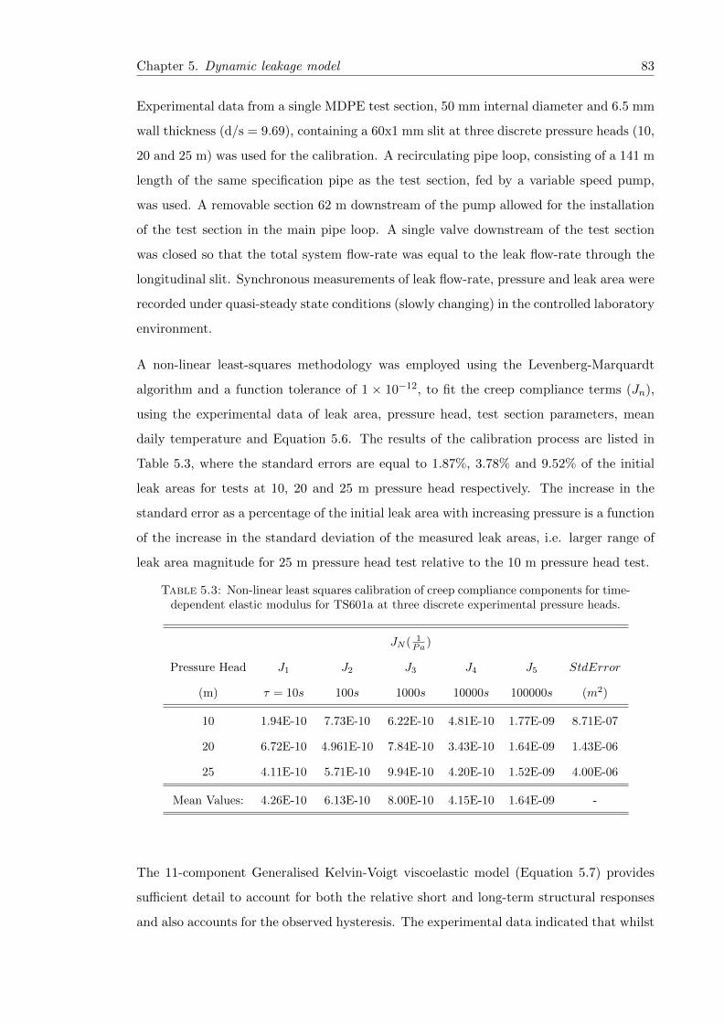
Chapter 5. Dynamic leakage model 83
Experimental data from a single MDPE test section, 50 mm internal diameter and 6.5 mm
wall thickness (d/s = 9.69), containing a 60x1 mm slit at three discrete pressure heads (10,
20 and 25 m) was used for the calibration. A recirculating pipe loop, consisting of a 141 m
length of the same specification pipe as the test section, fed by a variable speed pump,
was used. A removable section 62 m downstream of the pump allowed for the installation
of the test section in the main pipe loop. A single valve downstream of the test section
was closed so that the total system flow-rate was equal to the leak flow-rate through the
longitudinal slit. Synchronous measurements of leak flow-rate, pressure and leak area were
recorded under quasi-steady state conditions (slowly changing) in the controlled laboratory
environment.
A non-linear least-squares methodology was employed using the Levenberg-Marquardt
algorithm and a function tolerance of 1 × 10⁻¹², to fit the creep compliance terms (Jn),
using the experimental data of leak area, pressure head, test section parameters, mean
daily temperature and Equation 5.6. The results of the calibration process are listed in
Table 5.3, where the standard errors are equal to 1.87%, 3.78% and 9.52% of the initial
leak areas for tests at 10, 20 and 25 m pressure head respectively. The increase in the
standard error as a percentage of the initial leak area with increasing pressure is a function
of the increase in the standard deviation of the measured leak areas, i.e. larger range of
leak area magnitude for 25 m pressure head test relative to the 10 m pressure head test.
Table 5.3: Non-linear least squares calibration of creep compliance components for time-dependent elastic modulus for TS601a at three discrete experimental pressure heads.
JN ( 1Pa )
Pressure Head J1 J2 J3 J4 J5 StdError
(m) τ = 10s 100s 1000s 10000s 100000s (m2)
10 1.94E-10 7.73E-10 6.22E-10 4.81E-10 1.77E-09 8.71E-07
20 6.72E-10 4.961E-10 7.84E-10 3.43E-10 1.64E-09 1.43E-06
25 4.11E-10 5.71E-10 9.94E-10 4.20E-10 1.52E-09 4.00E-06
Mean Values: 4.26E-10 6.13E-10 8.00E-10 4.15E-10 1.64E-09 -
The 11-component Generalised Kelvin-Voigt viscoelastic model (Equation 5.7) provides
sufficient detail to account for both the relative short and long-term structural responses
and also accounts for the observed hysteresis. The experimental data indicated that whilst
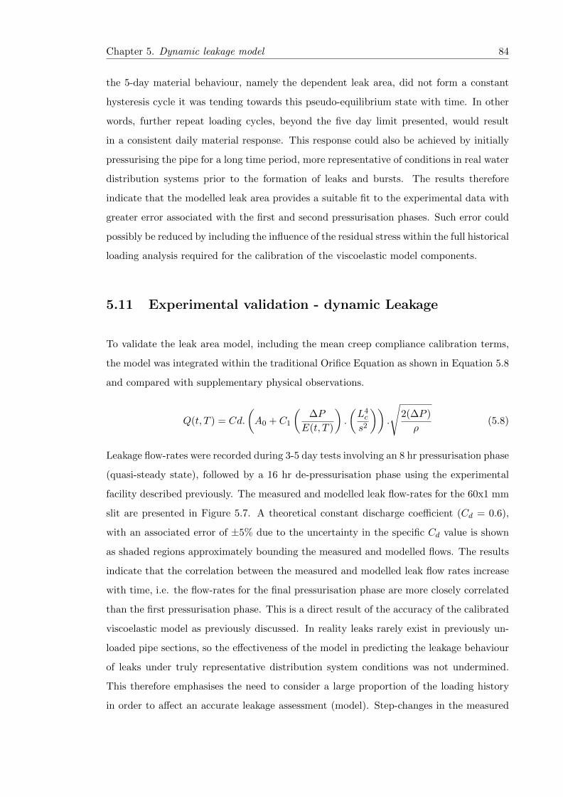
Chapter 5. Dynamic leakage model 84
the 5-day material behaviour, namely the dependent leak area, did not form a constant
hysteresis cycle it was tending towards this pseudo-equilibrium state with time. In other
words, further repeat loading cycles, beyond the five day limit presented, would result
in a consistent daily material response. This response could also be achieved by initially
pressurising the pipe for a long time period, more representative of conditions in real water
distribution systems prior to the formation of leaks and bursts. The results therefore
indicate that the modelled leak area provides a suitable fit to the experimental data with
greater error associated with the first and second pressurisation phases. Such error could
possibly be reduced by including the influence of the residual stress within the full historical
loading analysis required for the calibration of the viscoelastic model components.
5.11 Experimental validation - dynamic Leakage
To validate the leak area model, including the mean creep compliance calibration terms,
the model was integrated within the traditional Orifice Equation as shown in Equation 5.8
and compared with supplementary physical observations.
Q(t, T ) = Cd.
(A0 + C1
(∆P
E(t, T )
).
(L4c
s2
)).
√2(∆P )
ρ(5.8)
Leakage flow-rates were recorded during 3-5 day tests involving an 8 hr pressurisation phase
(quasi-steady state), followed by a 16 hr de-pressurisation phase using the experimental
facility described previously. The measured and modelled leak flow-rates for the 60x1 mm
slit are presented in Figure 5.7. A theoretical constant discharge coefficient (Cd = 0.6),
with an associated error of ±5% due to the uncertainty in the specific Cd value is shown
as shaded regions approximately bounding the measured and modelled flows. The results
indicate that the correlation between the measured and modelled leak flow rates increase
with time, i.e. the flow-rates for the final pressurisation phase are more closely correlated
than the first pressurisation phase. This is a direct result of the accuracy of the calibrated
viscoelastic model as previously discussed. In reality leaks rarely exist in previously un-
loaded pipe sections, so the effectiveness of the model in predicting the leakage behaviour
of leaks under truly representative distribution system conditions was not undermined.
This therefore emphasises the need to consider a large proportion of the loading history
in order to affect an accurate leakage assessment (model). Step-changes in the measured

Chapter 5. Dynamic leakage model 85
Figure 5.7: Measured and modelled leakage for 60x1 mm test section, including theassociated Cd error. Quasi-steady state pressure heads of 10 m, 20 m and 25 m in
ascending order in plot.
leakage during each test phase (not including the initial pressurisation) are surmised to
be result of the sensitivity of the slits to blockages from system debris. This was observed
to be most significant for the 10 m pressure head tests where there is less driving force
to allow for expulsion of any debris reducing the cross-sectional leak area. It must also
be noted that pressure heads of 10 m or less are extremely conservative compared to real
system pressures due to minimum service pressure requirements outlined by Ofwat (2008)
to ensure a minimum pressure of 7.14 m (0.7 bar) is maintained at consumer taps.
To confirm the validity of the generalised leakage model, the leakage flow rates from two
supplementary test sections were modelled. The test sections contained 20x1 mm and
40x1 mm artificially manufactured longitudinal slits in the same specification pipe as
the 60x1 mm test section previously described. The results of the model validation are
presented in Figures 5.8 and 5.9, also using a theoretical constant discharge coefficient of
0.6.
The results presented in Figures 5.8 and 5.9 correspond with those in Figure 5.7 whereby
the correlation between the measured and modelled flows increase with time, accounting for
the offset between the measured and modelled leakage flow-rate. This offset is speculated
to be a result of the under-prediction of the leak area from Equation 5.4 due to initial leak
area from the experimental data (measurement error ±3.82 mm2). It may also be inferred
from the observations that the relative change of leak flow rate over time decreases as the

Chapter 5. Dynamic leakage model 86
Figure 5.8: Measured and modelled leakage for 20x1 mm test section, including theassociated Cd error. Quasi-steady state pressure head of 20 m.
Figure 5.9: Measured and modelled leakage for 40x1 mm test section, including theassociated Cd error. Quasi-steady state pressure head of 20 m.
initial slit length is reduced. This may be explained by the knowledge that the relative
change of area over time decreases as the slit length decreases, as is described in Equation
5.6, due to the increased structural stiffness. All the results presented confirm the validity
and effectiveness of the developed model in capturing the dependent leakage behaviour of
longitudinal slits in thick-walled viscoelastic pipe.

Chapter 5. Dynamic leakage model 87
5.12 Discussion
The methodology and results presented here aimed to develop a generalised analytical
model to describe the leakage behaviour of stable longitudinal slits in thick-walled vis-
coelastic pipe through the synergy of numerical simulations and experimental data. Ini-
tially a model form was sought that could accurately capture the structural behaviour of
longitudinal slits in linear-elastic pipes in the simplest dimensionally homogeneous way,
prior to calibration of the viscoelastic components (time-dependent elastic modulus). The
qualitative statistical evaluation of the results indicated the most dominant parameters
(slit length, pipe diameter, wall thickness, pressure and elastic modulus) in the observed
structural behaviour, allowing less significant parameters (slit width, longitudinal stress,
Poisson ratio) to be removed from further analysis, thus simplifying the model definition.
The integration of the dimensionless coefficient C1 within the analytical model improved
the statistical fit to the data compared to the fitted parameters from the multiple regres-
sion. This coefficient integrated the pipe diameter into the model, which was shown to
be significant in the initial regression analysis. It is surmised that were the structural
descriptor of the relative size of a leak (πDL ) input into the original regression, an im-
proved R2 term would be evaluated. This highlights the limitation of the original model
form, Equation 5.3, utilising a constant numerical coefficient. Equation 5.4 represents the
simplest and most computationally efficient expression to describe the dependent dynamic
leak area. This is particularly important when incorporating the time-dependent viscoelas-
tic behaviour, which would otherwise require extreme levels of data processing had other
derived models (e.g. De Miranda et al. (2012)) been used. An interesting finding was the
triviality of the slit width, which was shown to directly influence the initial area only. Sim-
ilarly, a maximum relative slit length limit was highlighted within the analysis, whereby
test sections with a slit length to pipe circumference ratio greater than 1 deviated from the
derived model predictions. In cases with extreme values of slit length and width however,
it may be assumed that plastic deformation and/or structural failure would occur rapidly,
rather than recoverable elastic deformation.
The fundamental difference between the leak area models for longitudinal slits in linear-
elastic pipes, as presented in Equation 5.6 and the expression from van Zyl and Cassa
(2014), are that they are derived from thick walled and thin walled FEA respectively.
Comparison of the predictive capabilities of the two models in Figure 5.10 highlights the
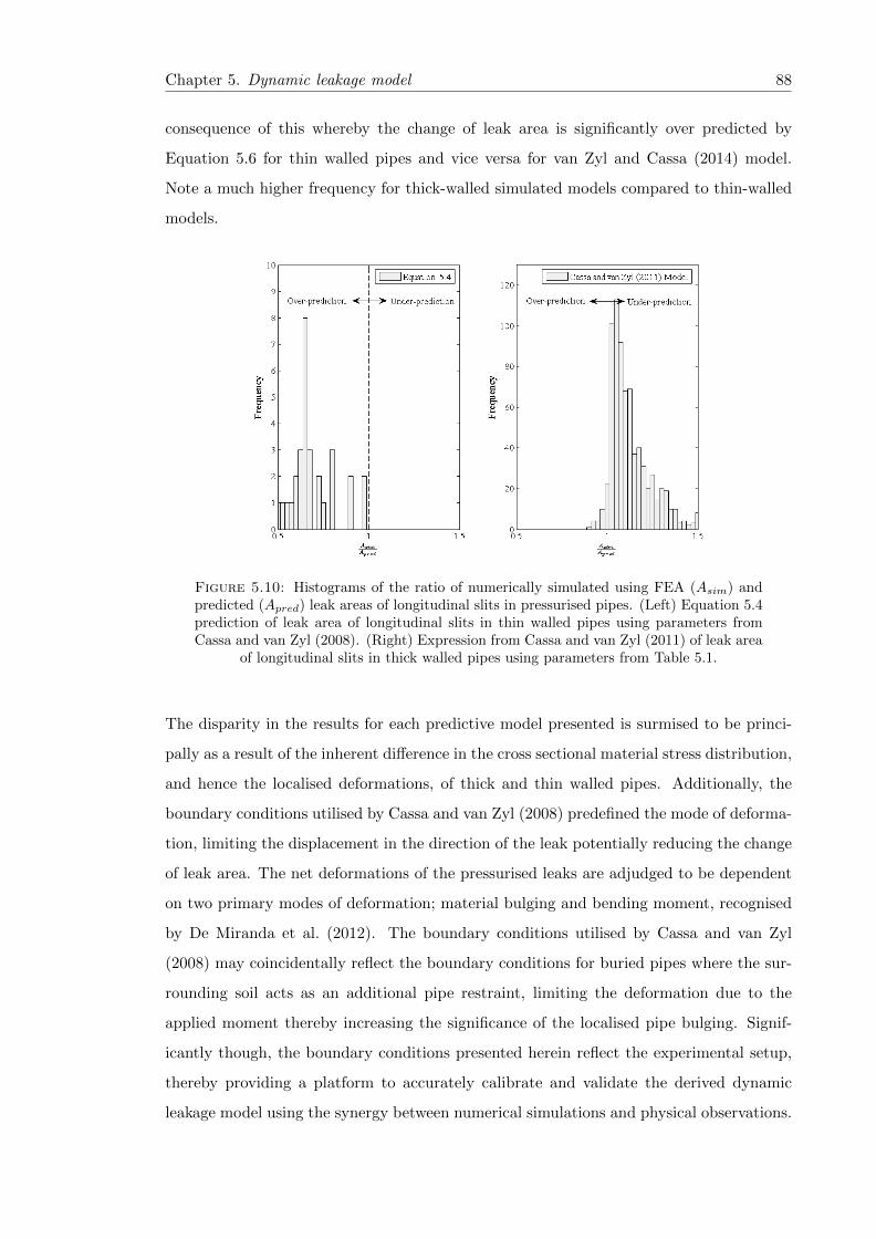
Chapter 5. Dynamic leakage model 88
consequence of this whereby the change of leak area is significantly over predicted by
Equation 5.6 for thin walled pipes and vice versa for van Zyl and Cassa (2014) model.
Note a much higher frequency for thick-walled simulated models compared to thin-walled
models.
Figure 5.10: Histograms of the ratio of numerically simulated using FEA (Asim) andpredicted (Apred) leak areas of longitudinal slits in pressurised pipes. (Left) Equation 5.4prediction of leak area of longitudinal slits in thin walled pipes using parameters fromCassa and van Zyl (2008). (Right) Expression from Cassa and van Zyl (2011) of leak area
of longitudinal slits in thick walled pipes using parameters from Table 5.1.
The disparity in the results for each predictive model presented is surmised to be princi-
pally as a result of the inherent difference in the cross sectional material stress distribution,
and hence the localised deformations, of thick and thin walled pipes. Additionally, the
boundary conditions utilised by Cassa and van Zyl (2008) predefined the mode of deforma-
tion, limiting the displacement in the direction of the leak potentially reducing the change
of leak area. The net deformations of the pressurised leaks are adjudged to be dependent
on two primary modes of deformation; material bulging and bending moment, recognised
by De Miranda et al. (2012). The boundary conditions utilised by Cassa and van Zyl
(2008) may coincidentally reflect the boundary conditions for buried pipes where the sur-
rounding soil acts as an additional pipe restraint, limiting the deformation due to the
applied moment thereby increasing the significance of the localised pipe bulging. Signif-
icantly though, the boundary conditions presented herein reflect the experimental setup,
thereby providing a platform to accurately calibrate and validate the derived dynamic
leakage model using the synergy between numerical simulations and physical observations.
Chapter 5. Dynamic leakage model 89
Mathematical representations of viscoelasticity are powerful tools to capture composite be-
haviour. There are no clear means to determine the most effective representation to use,
or ability to compare creep compliance constants evaluated using different model forms
(Purkayastha and Peleg, 1984). The decision criterion is therefore based on the most ef-
ficient model to describe the observed physical behaviour. The Generalised Kelvin-Voigt
mathematical representation was demonstrated to be an effective means of predicting the
structural response of such dynamic leaks. The calibrated creep compliances only give
an indication of the significance of each retardation time period on the net structural be-
haviour as opposed to being directly relatable to a physical mechanism. It is not therefore
feasible to directly equate the calibrated components for different viscoelastic materials
including different grades of MDPE, high density polyethylene (HDPE) or PVC. However,
the methodology presented is transferable for longitudinal slits in different material thick-
walled pipes provided they adhere to the traditional constitutive relationships between
stress and strain in both linear and visco-elastic materials.
The qualitative assessment of the slit face loading highlighted the need to fully understand
the independent variables influencing this pressure distribution due to distinct increase in
associated leak area opening. An appreciation of the external ground conditions and the
interaction between any potential porous media and the leak hydraulics is necessary to
fully explore this phenomenon. As such, the current leakage model (Equation 5.8) presents
an idealised representation of the leakage behaviour of fully submerged longitudinal slits
in MDPE pipe, assuming negligible external loading, and is therefore not truly represen-
tative of leaks found in real water distribution systems. Further work is required to fully
understand the behaviour of buried leaking pipes. Such work would advance the level of
understanding from an idealised formulation to a realistic platform. Consideration of the
structural interaction between an external media and the pipe as well as the effects on the
leakage hydraulics will further enhance the ability to accurately quantify the behaviour of
this particular failure type. The dimensionally homogeneous model does however provide
a unique insight into the fundamental structural behaviour of this failure type, considering
the time and pressure dependent characteristics dictating the dynamic leakage response.

Chapter 5. Dynamic leakage model 90
5.12.1 Application
The presented leakage model (Equation 5.8) offers potential benefits to developing active
leakage control technologies such as pressure management where the current simple leakage
exponent approach does not accurately reflect the true complexity of the pressure-leakage
relationship observed in viscoelastic pipes. Leak detection/localisation, through the reverse
engineering of pressure transient signals, commonly use a form of the Orifice Equation.
Integration of the proposed leakage model alongside the damping effect of viscoelastic
pipe walls on transient pressures, has the potential to further improve the accuracy of
this technology. In addition, the investigation highlighted the importance in considering
a loading time-history several orders of magnitude greater than the time period utilised
for any transient analysis in order to capture the true response of leaks in viscoelastic
pipe. An 11-component viscoelastic model was necessary to accurately describe both the
short and long term structural response of the leak; instantaneous elastic and retarded
viscous components. If only the long term response (e.g. the leak area opening after
24 hrs) is required, it would be possible to simplify the model by removing the lower
order retardation time components. However, this would greatly reduce the capacity of
the model to accurately quantify the total daily leakage volume for example.
5.13 Conclusion
A generalised analytical model to describe the structural response and subsequent leakage
through a longitudinal slit in thick-walled viscoelastic polyethylene pipe has been devel-
oped and validated through the synergistic use of numerical simulations and experimental
data. The derivation of a dimensionally homogeneous expression defined the structural
dynamics of a leak in a linear elastic pipe material, with experimental data utilised to
calibrate the time dependent elastic modulus in PE pipe. The proposed model provides
a means to assess the time-dependent leakage response for this failure type for a range of
different parameters, excluding the effect of a solid external porous media such as gravel
or sand, but including; leak geometry, pipe dimensions and hydraulic loading conditions.
This fundamental understanding of how leaks behave in water distribution systems is cru-
cial in improving on current leakage levels through new and improved leakage management
strategies.

Chapter 6
Physical investigation into the
significance of ground conditions
on dynamic leakage behaviour
“Models, even those of science, are by their very nature simplifications and as such are
not one hundred per cent accurate.”
Byron Jennings (2014)
6.1 Overview
The derived dynamic leakage model has been demonstrated to effectively approximate the
true nature of highly sensitive longitudinal slits in pressurised viscoelastic pipes; but how
representative is this of the behaviour found for leaks in the real world? The modelling
assumptions utilised thus far have created an idealised scenario of a leak into water only,
excluding the influence of external ground conditions. Water distribution system pipes are
typically buried and therefore overlooking the effect of the ground conditions on the leakage
behaviour will potentially increase the associated modelling error. Physically investigating
how the soil hydraulics alter the leak and structural dynamics was therefore of great
importance and addressed a proportion of the noted deficiency with regards to research
into the interaction of leaks and surrounding ground conditions highlighted in Table 2.3.
91

Chapter 6. Influence of Porous Media 92
The work presented in this chapter considers the assumed boundary conditions from the
experimental and numerical investigations in Chapters 4 and 5. The idealised conditions
that were utilised within these phases of the investigation negated the influence of the slit
face loading due to the head loss across the leak. The implications of such a simplifica-
tion are analysed and discussed, highlighting potential avenues of further work to fully
quantify the influence of ground conditions on leakage behaviour using the experimental
methodology described. This chapter addressed the research goals set out in Objective 4
in Chapter 3.
Models may only ever be approximations but every effort should be made to make them
as accurate representations of the phenomena that they are attempting to describe.
6.1.1 Journal Submission Details
This chapter is the manuscript submission to the International Water Association (IWA)
Journal of Water Supply: Research and Technology—AQUA. The original submission date
was 9/06/2015.
The Journal of Water Supply: Research and Technology—AQUA was chosen due to the
focus on the development of technologies in the water industry through novel research
approaches in the publication. The work presented in this chapter concentrates on the im-
portance of considering the ground conditions on the observed dynamic leakage behaviour
and the impact this has on existing leakage models and their application.
Chapter 6. Influence of Porous Media 93
6.2 Abstract
Effective leakage models are crucial for leakage assessment and control strategies to improve
the sustainability of vital water distribution, and other pipeline, infrastructure. This paper
evaluated the interdependence of leak hydraulics, structural dynamics and soil hydraulics,
particularly considering the significance of the soil conditions external to longitudinal slits
in viscoelastic pipe. Initial numerical exploration and unique physical experimental results
are presented exploring this complex physical phenomenon. The existence of an idealised
fully restrained porous medium was shown to significantly increase the pressure and time
dependent leak opening area whilst reducing the leak flow-rate, compared to a leak into
water only. The research highlights the limitation of existing dynamic leakage modelling
approaches which greatly simplify or neglect the influence of the soil conditions. Incorpo-
ration of this understanding into leakage modelling will enable more accurate estimation
of leakage rates and hence the effects of management and control strategies.
6.3 Introduction
The capacity to numerically represent physical phenomena is dependent on our ability
to determine all the causative factors for a given scenario and incorporate these within
a verifiable model. Leakage models play a pivotal role in assessing and controlling the
total real losses from water distribution systems, forming the fundamental development
platforms for leakage management approaches including leakage assessment and pressure
management. The definition of the sensitivity of leaks to changes in pressure, specifically
the pressure dependence of the leak area, has been identified as a key research topic aimed
at improving current leakage modelling practice. Select investigations explore idealised
model parameters where the pipe is not buried in a soil or other porous media, contrary
to the typical conditions found for this typically buried infrastructure. Consequently
the significance of the interdependence of the soil and leak hydraulics with the pipe and
soil structural behaviour are generally omitted from developed leakage models. A basic
understanding of the influence of a representative porous media on the structural loading
conditions and subsequent leakage magnitude will potentially have a direct impact on
improving leakage management applications and hence the overall sustainability of water
distribution systems.

Chapter 6. Influence of Porous Media 94
6.4 Background
Fundamentally, leakage studies consider the relationship between pressure and flow-rate
from individual failure apertures. Leaks in typical water distribution pipes have been
shown to exhibit orifice type flow and may theoretically be characterised using the Orifice
Equation (Greyvenstein and van Zyl, 2006). The observed sensitivity of different leaks
to changes in pressure has led to the adoption and application of the Generalised Orifice
Equation which accounts for the dynamic nature of many leaks (Schwaller and van Zyl,
2014). Leakage behaviour may be quantified based on the knowledge and understanding of
structural dynamics, leak hydraulics and soil hydraulics. When evaluating the performance
of system leakage at District Metered Area level, the temporal water demand must also
be considered (Clayton and van Zyl, 2007).
Recent studies have concluded that pipe structural behaviour, specifically the pressure
dependent leak area, is the primary causative factor for the marked leakage sensitivity.
Generally, leaks behave in two distinct manners dependent on the inherent pipe material
properties. Failures in linear elastic materials such as cast iron and steel, display a sim-
ple pressure-dependent leakage response, whereas equivalent leaks in viscoelastic materials
such as polyethylene, display a more complex time and pressure dependent response (Fer-
rante, 2012). In Chapter 4 it was demonstrated that despite the dynamic nature of highly
sensitive longitudinal slits in viscoelastic pipes, a modified Orifice Equation accounting
for the time and pressure dependent leak area was an effective tool in modelling the re-
sulting leakage behaviour. Significantly, the impact of such geometrical transformations
was shown to have a negligible effect on the definition of a constant theoretical discharge
coefficient. The study built upon the understanding of the effect of flow classification
(laminar and turbulent orifice flow), reasoning that constant discharge coefficients applied
in numerical modelling studies evaluating the leakage behaviour of leaks in linear-elastic
materials were valid (Cassa and van Zyl, 2011). However, such studies neglected the effect
of external ground conditions and the influence of soil hydraulics on the observed dynamic
leak behaviour.
The association between structural performance and leak hydraulics has a significant influ-
ence on the net leakage behaviour of failures in pressurised pipes. In most cases, numerical
and physical studies simplify the analysis of leakage behaviour by eliminating the influence
Chapter 6. Influence of Porous Media 95
of porous media external to a pipe. Clayton and van Zyl (2007) emphasised the complex-
ity of integrating the non-linear coupled soil and orifice hydraulics into leakage models.
The consideration of soil hydraulics offers the potential to further our understanding of
the physical mechanisms controlling leaks in buried pipes. Walski et al. (2006) derived
and validated the theoretical Orifice Soil (OS) number to define the dominant head loss
components for leaks in buried pipe using the energy equation. Small circular orifices
were used for the experimental work, which are relatively insensitive to changes in pres-
sure and therefore allow for the assumption of a constant leak area. Experimental results
demonstrated the effectiveness of the OS number as a tool for defining the orifice or soil
matrix head losses as the dominant factor defining the pressure-leakage relationship. How-
ever, the investigation results are limited to Darcy soil flow (no mobilisation of the soil)
and laminar flow conditions, thereby assuming negligible turbulent hydraulic effects in the
soil. Lambert (2001) highlighted the sensitivity and variability of the leakage exponent for
small leaks in the laminar region, therefore hindering the conclusion drawn by Walski et al.
(2006) that the static soil matrix head losses are solely dominant at low flow rates without
consideration of the coupled dynamic orifice hydraulics. Fluidisation, or the mobilisation
of soil particulate, results in a distinct hydraulic behaviour that differs from idealised
Darcy flow explored by Walski et al. (2006). Initial experimental results presented by van
Zyl et al. (2013) showed that the majority of measured head loss may be accounted for
by fluidised zones, not the static zones, when considering leaks into unconstrained porous
media. The fluidised soil behaved as an energy dissipation mechanism but had only a small
effect on the pressure-leakage relationship observed primarily due to the increased external
pressure. Theoretically though, less mobile soils compared to the spherical ballotini used
by van Zyl et al. (2013) may result in occlusion of the leak aperture directly affecting the
hydraulic and structural loading of the leak orifice. The characteristics of porous media,
namely the soil matrix composition/rigidity and the hydraulic conductivity (permeabil-
ity), and the coupled effect with the leak hydraulics can therefore directly influence the
observed leakage performance. This effect may be theoretically modelled using a modified
Orifice Equation, accounting for both soil and orifice losses assuming a fixed orifice area
and no soil fluidisation (Collins and Boxall, 2013).
Both the coupled effects of the structural behaviour and leak hydraulics as well as the
soil and leak hydraulics have been examined within the available literature. The interde-
pendence of all three of these fundamental principles remains an important but relatively
Chapter 6. Influence of Porous Media 96
unexplored area of research. For example, what effect do the soil hydraulics have on the
structural behaviour and the resulting leak response? The effect of the soil matrix external
to a leaking pipe on the net head losses have been investigated to varying degrees of detail.
The impact this has on the loading state of a pressurised pipe, in particular the head loss
across the orifice length in the direction of the leak flow, has not been quantified. The
effectiveness of numerical studies aimed at defining the structural behaviour of dynamic
leaks in pressurised pipes using finite element analyses (e.g. Rahman et al. (1998); Cassa
and van Zyl (2011); De Miranda et al. (2012)) are dependent on the accuracy of modelled
boundary and loading conditions. For hydraulic pipelines, the primary loading component
is the pressure applied to the internal pipe face from the fluid. For highly sensitive leaks
such as slits in the circumferential or longitudinal direction, the slit face loading is an ad-
ditional component that has a significant influence on the scale of deformation of the leak
(Lewis and Wang, 2008). This is of particular significance for pipes defined as thick-walled,
where the ratio of pipe diameter to wall thickness is less than 20. Such localised pressures
are commonly excluded from analyses due to uncertainty in the definition of the true pres-
sure distribution (Takahashi, 2002), with authors stating that detailed fluid and thermal
analyses are required before accurate definition (Kim et al., 2002). It may be inferred that
the magnitude of the slit face pressure distribution is dependent on the external conditions
surrounding the leak and the orifice flow, therefore necessitating a detailed understanding
of the soil and leak hydraulics. Existing leak area models excluding the effect of slit face
loading may therefore be seen as conservative. Without considering the interdependence
of the leak and soil hydraulics and the structural behaviour of dynamic leaks, models may
over or under predict the true leakage behaviour of individual leaks.
6.5 Aim and Hypothesis
The aim of the research was to investigate the influence of an idealised (invariable) external
porous media on the dynamic leakage behaviour of longitudinal slits in polyethylene pipe,
through some initial numerical studies and then a series of novel physical experiments.
Three fundamental, interacting, principles were investigated; structural behaviour and
leak and soil hydraulics, as summarised in Figure 6.1.
From considering the interdependence of leak and soil hydraulics it may be expected
that the existence of a fully constrained/consolidated porous media external to a leaking
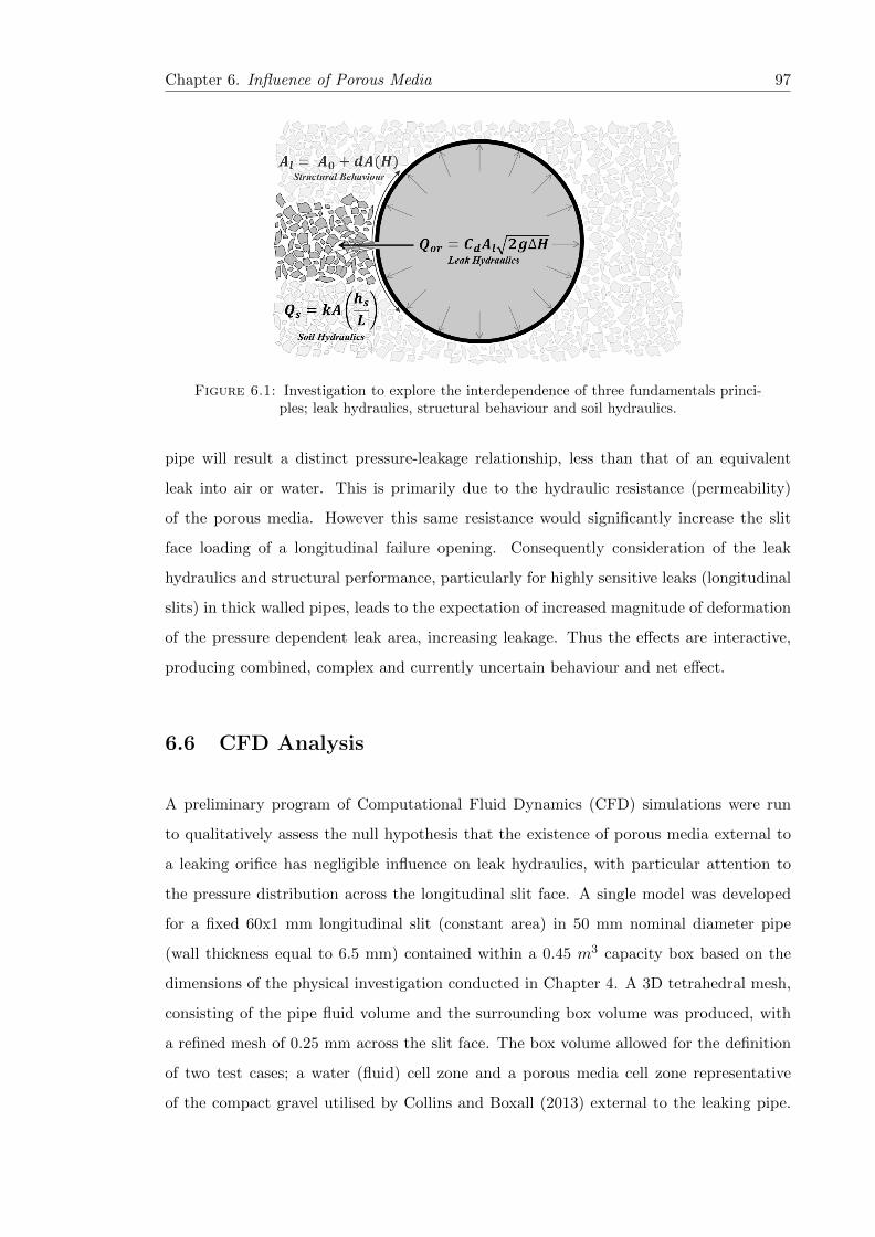
Chapter 6. Influence of Porous Media 97
Figure 6.1: Investigation to explore the interdependence of three fundamentals princi-ples; leak hydraulics, structural behaviour and soil hydraulics.
pipe will result a distinct pressure-leakage relationship, less than that of an equivalent
leak into air or water. This is primarily due to the hydraulic resistance (permeability)
of the porous media. However this same resistance would significantly increase the slit
face loading of a longitudinal failure opening. Consequently consideration of the leak
hydraulics and structural performance, particularly for highly sensitive leaks (longitudinal
slits) in thick walled pipes, leads to the expectation of increased magnitude of deformation
of the pressure dependent leak area, increasing leakage. Thus the effects are interactive,
producing combined, complex and currently uncertain behaviour and net effect.
6.6 CFD Analysis
A preliminary program of Computational Fluid Dynamics (CFD) simulations were run
to qualitatively assess the null hypothesis that the existence of porous media external to
a leaking orifice has negligible influence on leak hydraulics, with particular attention to
the pressure distribution across the longitudinal slit face. A single model was developed
for a fixed 60x1 mm longitudinal slit (constant area) in 50 mm nominal diameter pipe
(wall thickness equal to 6.5 mm) contained within a 0.45 m3 capacity box based on the
dimensions of the physical investigation conducted in Chapter 4. A 3D tetrahedral mesh,
consisting of the pipe fluid volume and the surrounding box volume was produced, with
a refined mesh of 0.25 mm across the slit face. The box volume allowed for the definition
of two test cases; a water (fluid) cell zone and a porous media cell zone representative
of the compact gravel utilised by Collins and Boxall (2013) external to the leaking pipe.

Chapter 6. Influence of Porous Media 98
For each test case a constant pipe inlet pressure head of 20 m (196200 Pa) and zero pipe
outlet velocity (system flow equal to leak flow-rate) was used and solved using a standard
k − ε viscous model with enhanced wall functions. The k − ε viscous model provides an
efficient and effective solver for near wall treatment and turbulent flow simulations (Oon
et al., 2013). Figures 6.2 and 6.3 show the results of the simulations, focussing on the leak
jet formation and the slit face pressure distribution.
Figure 6.2: Velocity streamlines (left) and static pressure contour on central slit plane(right) from CFD simulation of 60x1 mm longitudinal slit leaking into a fully submergedtest section box. Plane of interest shown as transparent surface on velocity streamline
plot.
A clear distinction between the leak jet dispersion is evident from the simulation results
of the velocity streamlines, with a reduced flow-rate of 0.43 l/s evaluated for the leak into
gravel compared to 0.87 l/s for the equivalent flow into water. Crucially, there was also
a quantifiable difference in the simulated slit face loading conditions. A horizontal plane
through the centre of the slit, parallel to the longitudinal axis, was used to evaluate the slit
face pressure. The mean slit face pressure for the water case was 4710 Pa (equivalent to
0.48 m pressure head) and 147150 Pa (equivalent to 15 m pressure head) for the compact
gravel case. The basic CFD simulations assumed a constant leak area thereby isolating the
leak and soil hydraulics from the structural dynamics for the analysis. The findings of the
qualitative CFD analysis therefore rejected the null hypothesis and supported the theory
that the existence of an idealised porous media external to a leak significantly increases the
slit face loading (greater than one order of magnitude) and reduces the magnitude of the

Chapter 6. Influence of Porous Media 99
leak flow-rate due to the hydraulic resistance of the media. In order to determine whether
the results of these idealised numerical simulations reflect the real physical phenomena
experienced by leaks in buried pipes, a series of physical experiments were designed and
implemented.
Figure 6.3: Velocity streamlines (left) and static pressure contour on central slit plane(right) from CFD simulation of 60x1 mm longitudinal slit leaking into a fully submergedtest section box containing compact gravel. Plane of interest shown as transparent surface
on velocity streamline plot.
6.7 Experimental Setup
A series of experiments were undertaken, which recorded the synchronous pressure head,
leak flow rate, leak area and material strain under quasi steady-state conditions (slowly-
changing) for an engineered longitudinal slit in Medium Density Polyethylene (MDPE)
pipe leaking into water and a porous medium.
6.7.1 Laboratory Facility
The laboratory investigation utilised the Contaminant Ingress into Distribution Systems
(CID) facility at the University of Sheffield, which is a 141 m length recirculating pipe
loop. The facility consists of 50 mm nominal diameter 12 bar rated MDPE pipe with
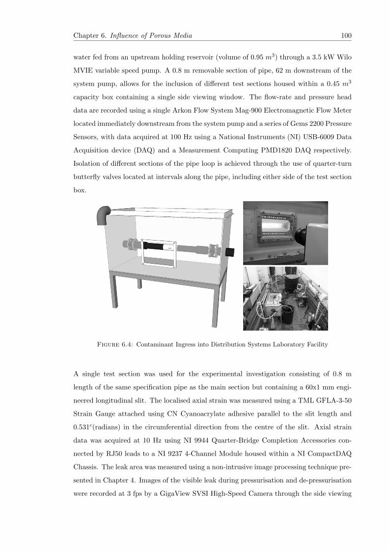
Chapter 6. Influence of Porous Media 100
water fed from an upstream holding reservoir (volume of 0.95 m3) through a 3.5 kW Wilo
MVIE variable speed pump. A 0.8 m removable section of pipe, 62 m downstream of the
system pump, allows for the inclusion of different test sections housed within a 0.45 m3
capacity box containing a single side viewing window. The flow-rate and pressure head
data are recorded using a single Arkon Flow System Mag-900 Electromagnetic Flow Meter
located immediately downstream from the system pump and a series of Gems 2200 Pressure
Sensors, with data acquired at 100 Hz using a National Instruments (NI) USB-6009 Data
Acquisition device (DAQ) and a Measurement Computing PMD1820 DAQ respectively.
Isolation of different sections of the pipe loop is achieved through the use of quarter-turn
butterfly valves located at intervals along the pipe, including either side of the test section
box.
Figure 6.4: Contaminant Ingress into Distribution Systems Laboratory Facility
A single test section was used for the experimental investigation consisting of 0.8 m
length of the same specification pipe as the main section but containing a 60x1 mm engi-
neered longitudinal slit. The localised axial strain was measured using a TML GFLA-3-50
Strain Gauge attached using CN Cyanoacrylate adhesive parallel to the slit length and
0.531c(radians) in the circumferential direction from the centre of the slit. Axial strain
data was acquired at 10 Hz using NI 9944 Quarter-Bridge Completion Accessories con-
nected by RJ50 leads to a NI 9237 4-Channel Module housed within a NI CompactDAQ
Chassis. The leak area was measured using a non-intrusive image processing technique pre-
sented in Chapter 4. Images of the visible leak during pressurisation and de-pressurisation
were recorded at 3 fps by a GigaView SVSI High-Speed Camera through the side viewing
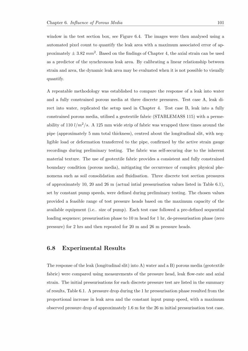
Chapter 6. Influence of Porous Media 101
window in the test section box, see Figure 6.4. The images were then analysed using a
automated pixel count to quantify the leak area with a maximum associated error of ap-
proximately ± 3.82 mm2. Based on the findings of Chapter 4, the axial strain can be used
as a predictor of the synchronous leak area. By calibrating a linear relationship between
strain and area, the dynamic leak area may be evaluated when it is not possible to visually
quantify.
A repeatable methodology was established to compare the response of a leak into water
and a fully constrained porous media at three discrete pressures. Test case A, leak di-
rect into water, replicated the setup used in Chapter 4. Test case B, leak into a fully
constrained porous media, utilised a geotextile fabric (STABLEMASS 115) with a perme-
ability of 110 l/m2/s. A 125 mm wide strip of fabric was wrapped three times around the
pipe (approximately 5 mm total thickness), centred about the longitudinal slit, with neg-
ligible load or deformation transferred to the pipe, confirmed by the active strain gauge
recordings during preliminary testing. The fabric was self-securing due to the inherent
material texture. The use of geotextile fabric provides a consistent and fully constrained
boundary condition (porous media), mitigating the occurrence of complex physical phe-
nomena such as soil consolidation and fluidisation. Three discrete test section pressures
of approximately 10, 20 and 26 m (actual intial pressurisation values listed in Table 6.1),
set by constant pump speeds, were defined during preliminary testing. The chosen values
provided a feasible range of test pressure heads based on the maximum capacity of the
available equipment (i.e.. size of pump). Each test case followed a pre-defined sequential
loading sequence; pressurisation phase to 10 m head for 1 hr, de-pressurisation phase (zero
pressure) for 2 hrs and then repeated for 20 m and 26 m pressure heads.
6.8 Experimental Results
The response of the leak (longitudinal slit) into A) water and a B) porous media (geotextile
fabric) were compared using measurements of the pressure head, leak flow-rate and axial
strain. The initial pressurisations for each discrete pressure test are listed in the summary
of results, Table 6.1. A pressure drop during the 1 hr pressurisation phase resulted from the
proportional increase in leak area and the constant input pump speed, with a maximum
observed pressure drop of approximately 1.6 m for the 26 m initial pressurisation test case.
Chapter 6. Influence of Porous Media 102
Table 6.1: Summary table of results from 60x1 mm slit at three discrete pressuresleaking into water and geotextile fabric. Net leakage refers to volume of leakage flow over
1 hr pressurisation phase.
Water Geotextile Fabric
Initial Pressure Net leakage Mean Cd Initial Pressure Net leakage Mean Cd
(m) (m3) (m) (m3)
i) 10.81 2.31 0.75 10.79 2.19 0.66
ii) 20.48 4.45 0.74 20.52 4.31 0.66
iii) 26.19 5.70 0.72 26.14 5.59 0.64
The results of the measured leak flow-rates for the two test cases are presented in Figure
6.5 where the data has been adjusted to t = 0s for the start of each discrete pressure test
case. The total measured volumes of flow (net leakage) through the leak were quantified by
integrating the time series flow-rate for the 1 hr pressurisation phase, with the results listed
in Table 6.1. It was observed that the flow-rate through the geotextile was significantly
less than the equivalent leak into water.
Figure 6.5: Leakage flow-rate through a 60x1 mm longitudinal slit at three discretepressure heads into water (blue line) and geotexile fabric (black line).
Alongside the measurements of fluid pressure and leak flow-rate, the synchronous struc-
tural behaviour of the leak opening was quantified. Axial strain measurements were
recorded for both the water and geotextile fabric test cases, with leak area also recorded
for the water case only. A fitting procedure between the measured leak area (mm2) and
material strain produced the linear relationship shown in Equation 6.1, assumed to be the
same for both the water and geotextile test cases. The fit produced an R2 value of 0.973
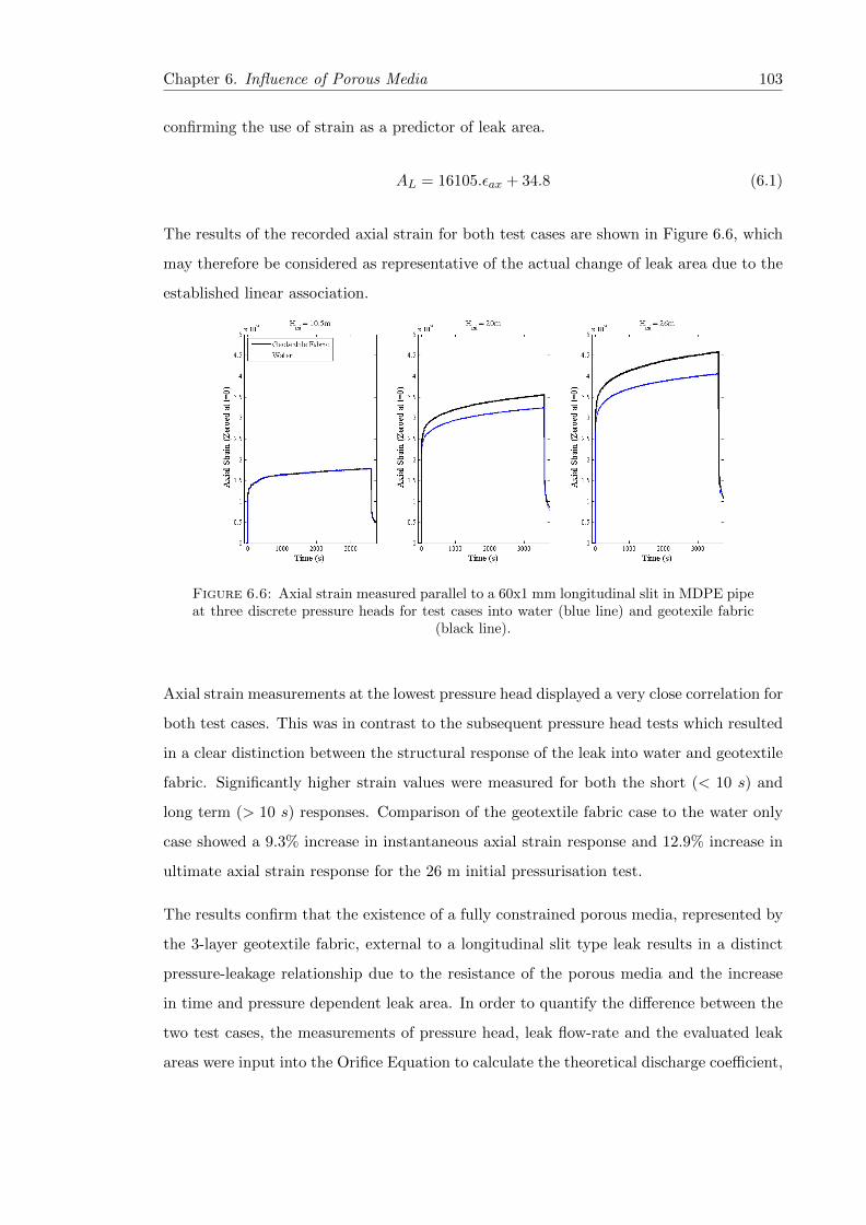
Chapter 6. Influence of Porous Media 103
confirming the use of strain as a predictor of leak area.
AL = 16105.εax + 34.8 (6.1)
The results of the recorded axial strain for both test cases are shown in Figure 6.6, which
may therefore be considered as representative of the actual change of leak area due to the
established linear association.
Figure 6.6: Axial strain measured parallel to a 60x1 mm longitudinal slit in MDPE pipeat three discrete pressure heads for test cases into water (blue line) and geotexile fabric
(black line).
Axial strain measurements at the lowest pressure head displayed a very close correlation for
both test cases. This was in contrast to the subsequent pressure head tests which resulted
in a clear distinction between the structural response of the leak into water and geotextile
fabric. Significantly higher strain values were measured for both the short (< 10 s) and
long term (> 10 s) responses. Comparison of the geotextile fabric case to the water only
case showed a 9.3% increase in instantaneous axial strain response and 12.9% increase in
ultimate axial strain response for the 26 m initial pressurisation test.
The results confirm that the existence of a fully constrained porous media, represented by
the 3-layer geotextile fabric, external to a longitudinal slit type leak results in a distinct
pressure-leakage relationship due to the resistance of the porous media and the increase
in time and pressure dependent leak area. In order to quantify the difference between the
two test cases, the measurements of pressure head, leak flow-rate and the evaluated leak
areas were input into the Orifice Equation to calculate the theoretical discharge coefficient,

Chapter 6. Influence of Porous Media 104
Cd. The results of the analysis are presented in Figure 6.7 for both the geotextile fabric
and water test cases.
Figure 6.7: Time series of evaluated discharge coefficients (Cd) for 60x1 mm longitudinalslit in MDPE pipe at three discrete pressure heads for test cases into water (blue line)
and geotexile fabric (black line).
The visible data spike at t=3600 s in Figure 6.7 is due to the small discrepancy in data ac-
quisition time stamping between the flow, pressure and leak area data (less than ±0.05 s).
The mean discharge coefficient values for each test case and discrete pressure tests are
summarised in Table 6.1. Additionally the total standard deviation for the three pressure
tests were evaluated as 0.0131 for the water test case and 0.0121 for the geotextile fabric
test case respectively. The results support the conclusion drawn in Chapter 4 that the
application of a tailored constant Cd value (mean value ±2.5%) for different longitudinal
slits is a valid approximation, despite the dynamic nature of the observed structural be-
haviour. A mean decrease of 11.3% for the geotextile fabric discharge coefficient compared
to the equivalent Cd value for the water case was evaluated emanating from the coupled
influence of the dynamic leak area and the fabric permeability.
Finally, a qualitative physical assessment of the influence of a porous media truly represen-
tative of those found in practice was conducted by burying the same test section in mixed
gravel. An identical test procedure as utilised for the water and geotextile fabric cases
was conducted, however the results of the final pressurisation test only are presented in
this paper as the leak became partially blocked during the first and second pressure tests.
The test section was buried under 0.45 m depth of mixed grade pea gravel (approximately
5-12 mm diameter) consistent with the British Standard for backfill material for plastic
pipework (BSI, 1973). The initial pressure head was recorded as 26.15 m with an observed

Chapter 6. Influence of Porous Media 105
total head loss of 1.53 m over the 1 hr pressurisation phase. The results for the measured
change of axial strain and leak flow-rate are shown in Figure 6.8 and 6.9 respectively.
The change of axial strain was utilised to account for the initial strain applied by the
mixed gravel during burial, considering the effects of both compression loading and tensile
bending.
Figure 6.8: Axial strain for a 60x1 mm longitudinal slit in MDPE pipe at 26 m pressurehead for test cases into water (blue line), geotexile fabric (black line) and mixed gravel
(gray line).
Figure 6.9: Leakage flow rate for a 60x1 mm longitudinal slit in MDPE pipe at 26 mpressure head for test cases into water (blue line), geotexile fabric (black line) and mixed
gravel (gray line).
Figure 6.8 indicates that there was an observable difference between the measured axial
strain, and hence the leak area, for all three test cases with the leak into water displaying
the smallest total structural deformation. The large positive offset between the axial strain

Chapter 6. Influence of Porous Media 106
for the geotextile fabric and the mixed gravel demonstrates that the fabric had a relatively
low permeability compared to the mixed gravel as may have been reasonably assumed.
The leak flow-rates for the geotextile fabric and mixed gravel correlate well together,
taking account of the step increase in flow-rate for the mixed gravel case at approximately
t = 1100 s which is surmised to be due to the expulsion of a partial blockage within the
cross-section of the leak opening. This correlation is considered as coincidental due to
the coupled effect of the porous media permeability and relative change of leak area for
both test cases. These qualitative results support the hypothesis that a porous media
external to a leak orifice will significantly influence both the hydraulics and the structural
behavioural response of the leak, increasing the relative magnitude of change of leak area
and simultaneously reducing the leak flow-rate due to the soil hydraulic resistance.
6.9 Discussion
The results of both the qualitative CFD simulations and the experimental investigation
confirmed that the existence of a porous media external to a longitudinal slit in a pres-
surised water pipe significantly influences the leak hydraulics, i.e. the magnitude of the
leak flow-rate. Compact gravel was simulated within the CFD model and resulted in a
constant slit face loading over 30 times larger than the equivalent loading for the simulated
leak into water, and 75% of the internal pipe fluid pressure. Whilst the CFD simulations
isolated the influence of the leak and soil hydraulics from the structural dynamics, the
magnitude of the quantified slit face loading implied that this load case would result in a
substantial increase in the relative total leak area.
The experimental work replicated the static soil zone using a geotextile fabric which allowed
for the assessment of the leak and soil hydraulics as well as the structural dynamics.
This idealised porous media resulted in a significant increase in leak area due to slit face
loading, as demonstrated by the recorded material strain (compared to the leak into water
case). However the effect of this (to increase the flow-rate) was countered by the hydraulic
resistance of the porous medium, resulting in lower overall leakage. It was shown that
the observed leakage behaviour may be described using a modified form of the Orifice
Equation, considering the measured time-dependent leak area, with a constant discharge
coefficient. A theoretical constant Cd is applicable despite the dynamic structural nature
of longitudinal slits in viscoelastic pipes, and includes the influence of the external soil

Chapter 6. Influence of Porous Media 107
hydraulics. The discharge coefficient may therefore be defined based on the explicit soil
properties, providing the soil matrix structure remains the same, and the leak opening
characteristics. Further work to determine whether this is also true for fluidised soil
conditions is still required.
Walski et al. (2006) stated that in the real world, orifice head losses will dominate over
the soil matrix head losses, thus dictating the leakage behaviour. Based on the results
presented in this chapter it is not feasible to confirm this statement as Walski et al. (2006)
did not consider the effect ground conditions have on the dynamic leak area. The complex
interdependence of the leak and soil hydraulics with the structural dynamics means that
it is not trivial to assign a primary head loss component. By way of an illustration, as the
pressure in a buried pipe increases the relative leak area will increase due to the slit face
pressure distribution. The soil hydraulic resistance will therefore alter as the area of flow
increases (based on assumption of Darcy flow), thus altering the resulting leak hydraulics.
Hypothetically this may result in equivalent leaks into water and porous media having the
same magnitude leakage flow-rate at a given pressure, but distinctly different leak areas.
The complex interdependence of the three parameters described is therefore critical in
defining the total leakage behaviour of buried leaks.
The magnitude of the influence a porous media external to a leaking orifice has on the
observed leakage behaviour is dependent on the explicit permeability and resistance to
fluidisation. The static geotextile fabric used within the experimental work represented an
extreme ‘no fluidisation’ case, highlighting the significance of the leak jet resistance on the
structural loading due to occlusion, as mentioned by van Zyl et al. (2013). The observed
difference in the strain and flow rate measurements presented in Figures 6.8 and 6.9 for
the quantitative water and geotextile fabric test cases and the qualitative results from
the gravel test case, show the variability in the influence of different porous media on the
leakage behaviour. The relatively close correlation between the strain measurements for
the water and gravel test cases at 26 m pressure head are surmised to be as a result of the
fluidisation of the mixed gravel surrounding the leak. This would result in a reduced slit
face loading as the fluidised zone acts as a means of dissipating the energy, reducing the
structural deformation relative to the non-fluidised geotextile fabric case. To fully quantify
this effect, the structural influence of the gravel loading on the external surface of the pipe
would need to be determined. In other words, the combined effect of the increased slit
face loading, soil self weight and surcharge loading need to be considered to truly quantify

Chapter 6. Influence of Porous Media 108
the behaviour of buried leaking pipes. However, the results do provide an initial insight
into the influence of conservative and extreme external conditions on dynamic leakage
behaviour. Neglecting the existence of porous media surrounding buried pipes can result
in inaccurate estimations of the true leakage behaviour.
Whilst the presented work does not directly address the need to quantify The presented
work shows the importance of including slit face loading within the assessment of struc-
tural dynamics for deformable leaks. The CFD simulations of idealised compact gravel
and the experimental results for the leak into a geotextile fabric present the worst case
scenario regarding the magnitude of the slit face loading. In reality, the complex nature
of soil structure and potential for void formation or fluidisation as a result of the presence
of a leak jet may lead to more conservative slit face loading values. The axial strain mea-
surements provided a unique opportunity to quantify the leak area of the longitudinal slits
when the pipe is buried or wrapped in a geotextile fabric. The demonstrated effectiveness
of this methodology therefore presents a potential tool for live asset monitoring in water
distribution systems. Although it is not feasible to utilise strain gauges to measure leak
areas in buried pipes, it may be possible to utilise them as a means of monitoring the
structural integrity of pipelines by recording the magnitude of strain changes. For exam-
ple, extreme changes in recorded strain may indicate the formation of a failure aperture
within the vicinity of the strain gauge. Realistically though, the relationship between ax-
ial strain and leak area and the effectiveness of using strain gauges for assessment of the
leak behaviour of buried pipes is more appropriate for further academic investigations of
structural behaviour.
The Generalised Orifice Equation is commonly applied to define the pressure-leakage re-
lationship for leaks within a District Metered Area (DMA). Results from field tests in
several countries have highlighted the greater sensitivity of DMA leakage to pressure than
described by the by the traditional Orifice Equation. The influence of different soil con-
ditions, by location, on this relationship is possibly an important further area of research.
Additionally, well constrained and consolidated soils reduce the relative leakage magni-
tude due to the inherent hydraulic resistance of the soil. However the increased structural
loading and subsequent increased deformation may lead to an increased risk of struc-
tural integrity failure. A detailed understanding of the influence of different soils on the
pressure-leakage relationship of individual leaks may therefore advance the accuracy of the
Chapter 6. Influence of Porous Media 109
interpretation of DMA leakage assessments and subsequent application of leakage man-
agement strategies. Current leakage models describing the behaviour of individual leaks
based on idealised conditions (neglecting the existence of an external porous media) may
under or over predict the net leakage volume dependent on the specific soil properties
(permeability, consolidation, degree of constraint and temperature) and interaction of this
with leak hydraulics and structural behaviour of the pipe.
6.10 Conclusion
The results of novel physical experimental studies into leakage are reported, exploring the
interdependence of leak hydraulics, structural behaviour of the pipe and the soil hydraulics.
A novel synchronous data set is presented demonstrating the use of strain measurement
as a direct proxy for leak area, enabling the measurement of dynamic leak area in buried
conditions. The results showed that the existence of an idealised, fully constrained repre-
sentative porous media (geotextile fabric) external to a longitudinal slit in a thick walled
pipe, directly affects the pressure-leakage relationship. There was a measured increase in
the time and pressure-dependent change of leak area (measured strain). The increased
deformation of the leak area was concluded as being a direct result of the increased mag-
nitude of the slit face loading (supported by numerical simulation) which is dependent
on the fluid pressure within the pipe and the external boundary conditions (porous me-
dia) affecting the head loss through the orifice. However the overall leak rate was only
increased by around five percent, as the increased leak area effect was counteracted by
the hydraulic resistance of the media. Conversely experimental results using mixed gravel
media external to the pipe showed only a marginal increase in axial strain, and hence leak
area compared to a water case, but overall leak flow rate approximated to the gravel case.
This lack of dynamic leak area change is assumed to be due to the formation of a small
void or fluidised zone immediately external to the leak, and the pressure dissipation ef-
fects provided by this providing significant pressure loss through the orifice. However, the
media further from the leak still provide substantial overall hydraulic resistance. Further
research is required into media effects, in particular void and fluidisation effects local to
leak orifices using representative media. Overall the research reported here shows that in
order to accurately model and capture the leakage behaviour of dynamic leaks in buried

Chapter 6. Influence of Porous Media 110
pipes the interacting effects of porous media permeability and slit face loading should be
considered.
Chapter 7
Analysis and Discussion
The results and discussions presented in the previous chapters highlighted some of the fun-
damental components that are required to accurately characterise and predict the leakage
behaviour of sensitive longitudinal slits in viscoleastic pipes. It is critical to understand
their significance and interdependence.
7.1 Dynamic leak area
Previous studies (Clayton and van Zyl, 2007; Cassa and van Zyl, 2011; Ferrante, 2012)
agree that the leak area is the most important parameter defining the leakage behaviour.
The work presented here has confirmed this for the first time by isolating the structural
behaviour and leak hydraulics through a unique set of physical observations and numerical
simulations. A modified form of the Orifice Equation, considering the pressure and time
dependent leak area, was subsequently demonstrated as a highly effective model to quantify
this response. This is feasible due to the invariable nature of the calculated discharge
coefficient, which was shown by using synchronous measurements of pressure, flow-rate
and leak area, for discharge into water. The use of orifice theory (i.e. application of the
modified Orifice Equation) was also shown to be applicable for a leak that, according to
Brater et al. (1996), was classed as a ‘pipe’ (20x1 mm longitudinal slits which have an
l/d ratio of 3.2). It is surmised that this is principally due to the inaccurate definition
of the leak hydraulic diameter but would require further investigatory confirmation. The
generalised leakage model was validated using a constant discharge coefficient of 0.6, for all
111
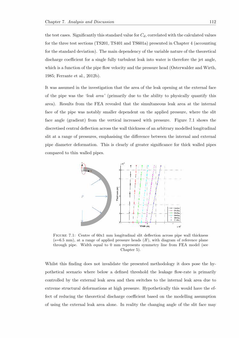
Chapter 7. Analysis and Discussion 112
the test cases. Significantly this standard value for Cd, correlated with the calculated values
for the three test sections (TS201, TS401 and TS601a) presented in Chapter 4 (accounting
for the standard deviation). The main dependency of the variable nature of the theoretical
discharge coefficient for a single fully turbulent leak into water is therefore the jet angle,
which is a function of the pipe flow velocity and the pressure head (Osterwalder and Wirth,
1985; Ferrante et al., 2012b).
It was assumed in the investigation that the area of the leak opening at the external face
of the pipe was the ‘leak area’ (primarily due to the ability to physically quantify this
area). Results from the FEA revealed that the simultaneous leak area at the internal
face of the pipe was notably smaller dependent on the applied pressure, where the slit
face angle (gradient) from the vertical increased with pressure. Figure 7.1 shows the
discretised central deflection across the wall thickness of an arbitrary modelled longitudinal
slit at a range of pressures, emphasising the difference between the internal and external
pipe diameter deformation. This is clearly of greater significance for thick walled pipes
compared to thin walled pipes.
Figure 7.1: Centre of 60x1 mm longitudinal slit deflection across pipe wall thickness(s=6.5 mm), at a range of applied pressure heads (H ), with diagram of reference planethrough pipe. Width equal to 0 mm represents symmetry line from FEA model (see
Chapter 5).
Whilst this finding does not invalidate the presented methodology it does pose the hy-
pothetical scenario where below a defined threshold the leakage flow-rate is primarily
controlled by the external leak area and then switches to the internal leak area due to
extreme structural deformations at high pressure. Hypothetically this would have the ef-
fect of reducing the theoretical discharge coefficient based on the modelling assumption
of using the external leak area alone. In reality the changing angle of the slit face may
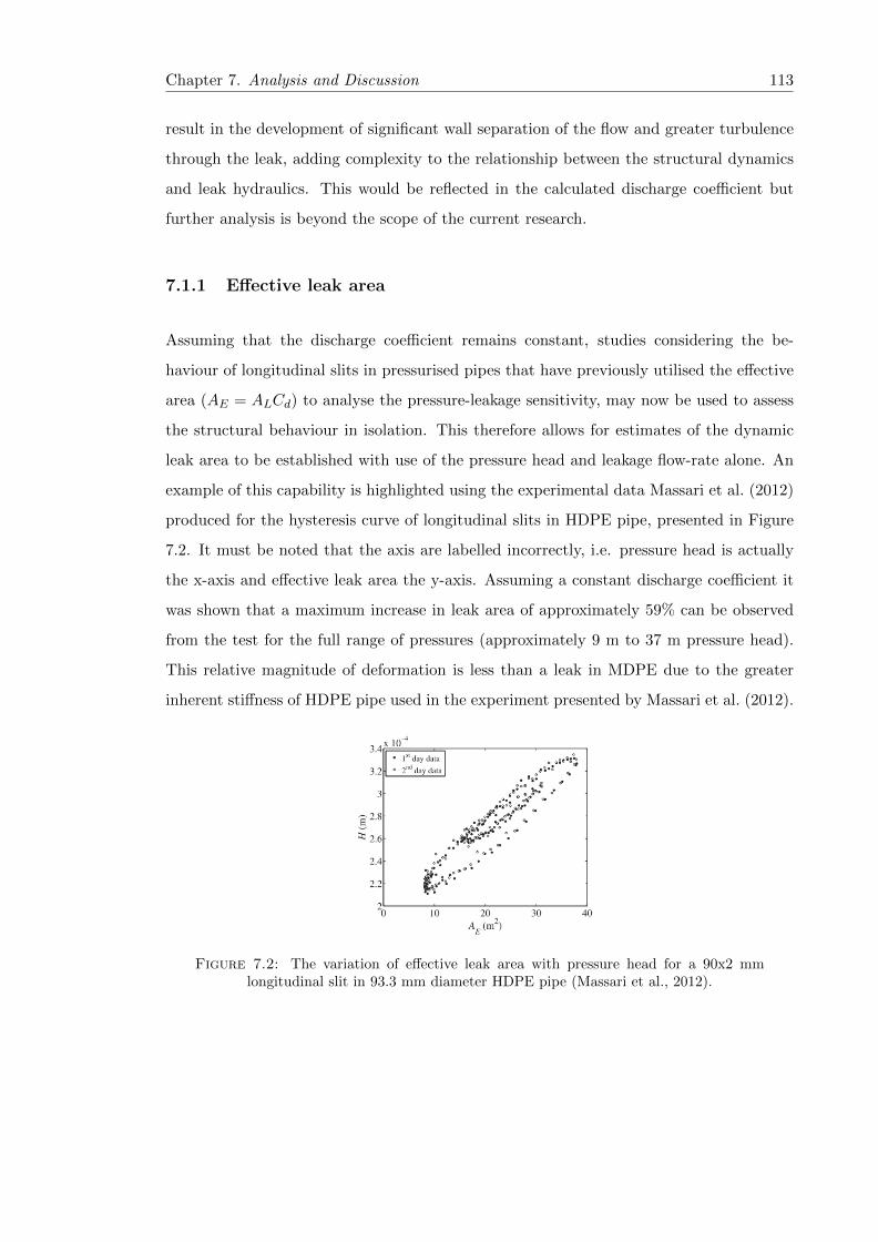
Chapter 7. Analysis and Discussion 113
result in the development of significant wall separation of the flow and greater turbulence
through the leak, adding complexity to the relationship between the structural dynamics
and leak hydraulics. This would be reflected in the calculated discharge coefficient but
further analysis is beyond the scope of the current research.
7.1.1 Effective leak area
Assuming that the discharge coefficient remains constant, studies considering the be-
haviour of longitudinal slits in pressurised pipes that have previously utilised the effective
area (AE = ALCd) to analyse the pressure-leakage sensitivity, may now be used to assess
the structural behaviour in isolation. This therefore allows for estimates of the dynamic
leak area to be established with use of the pressure head and leakage flow-rate alone. An
example of this capability is highlighted using the experimental data Massari et al. (2012)
produced for the hysteresis curve of longitudinal slits in HDPE pipe, presented in Figure
7.2. It must be noted that the axis are labelled incorrectly, i.e. pressure head is actually
the x-axis and effective leak area the y-axis. Assuming a constant discharge coefficient it
was shown that a maximum increase in leak area of approximately 59% can be observed
from the test for the full range of pressures (approximately 9 m to 37 m pressure head).
This relative magnitude of deformation is less than a leak in MDPE due to the greater
inherent stiffness of HDPE pipe used in the experiment presented by Massari et al. (2012).
Figure 7.2: The variation of effective leak area with pressure head for a 90x2 mmlongitudinal slit in 93.3 mm diameter HDPE pipe (Massari et al., 2012).

Chapter 7. Analysis and Discussion 114
7.2 Strain-area relationship
Identification of the relationship between the localised axial strain around a longitudinal
slit and the leak area means that strain may be used as a predictor of leak area. It
also allowed for an initial interrogation of the influence of porous media by providing
a tool to quantify the leak area when the leak is not visible. This novel methodology
is applicable for longitudinal slits in both linear elastic (confirmed through numerical
simulations) and viscoelastic materials (confirmed from physical observations) and is also
theoretically suited to other leak types. The mode of deformation of the longitudinal slits
was concluded to be a combination of material bulging and deformation due to an applied
moment, as supported by De Miranda et al. (2012). It was theorised that the existence of
a soil external to a leak would result in the reduction of deformation due to the applied
moment as a result of the restraint on the pipe. The derived relationship between strain
and area offers an opportunity to examine this phenomenon in greater detail, verifying the
true mode of deformation for leaks in buried pipes.
The strain-area relationship also provided a means to characterise the viscoelastic struc-
tural behaviour of individual test sections using the experimental data. Direct comparison
between the calibrated viscoelastic components from Chapter 4 and Chapter 5 cannot be
made as they refer to explicit and generalised leak area models respectively. The explicit
model is dependent on the strain gauge location and initial calibration (null offset), whereas
the generalised model is dependent on the geometry, material properties and loading con-
ditions. A comparison was made between the creep compliance components (Jn) relative
to the maximum component values, given in Table 7.1, for the two modelling approaches.
It was hypothesised that these relative values should be equal to the linear relationship
between strain and area that also relates the derivation of the explicit and generalised
models. As can be seen in Table 7.1, this hypothesis was confirmed, demonstrating the
validity of the highlighted linearity between the measured axial strain and leak area and
the effectiveness of the calibration methodology.

Chapter 7. Analysis and Discussion 115
Table 7.1: Relative creep compliance components (J ′n = Jn/Jmax) from Chapters 4 and
5 for the explicit and generalised leak area models.
J ′n : J ′
1 J ′2 J ′
3 J ′4 J ′
5
τn (s): 10 100 1000 10000 100000
Explicit Model (Chapter 4) 0.25 0.34 0.49 0.22 1.00
Generalised Model (Chapter 5) 0.26 0.37 0.49 0.25 1.00
7.3 Influence of ground conditions
It has been shown in this study (Chapter 6) that the existence of a fully consolidated and
constrained porous media external to a leaking longitudinal slit results in more extreme
structural deformations (change of leak area) due to the development of a slit face pres-
sure loading. The analyses conducted in Chapters 4 and 5 assumed idealised conditions
neglecting the influence of the ground conditions surrounding the leak, as was also done
by Cassa and van Zyl (2011) and De Miranda et al. (2012). Consequently, the dynamic
leak area model derived from the physical observations and numerical simulations does not
capture the true representative conditions of water distribution pipes that are typically
buried. It is not possible to determine whether the adopted modelling approach will under
or over estimate the actual structural dynamics without a detailed quantitative investiga-
tion. This is as a direct result of the coupled effect of the existence of soil surrounding a
leak increasing the slit face loading (therefore increasing the leak area) and the simultane-
ous external applied pressure loading on the pipe due to the soil self-weight and surcharge
loading, which acts to restrain such deformation.
The qualitative CFD simulation results presented in Figure 6.3 indicate that a constant slit
face-loading may be approximated assuming a fully constrained compact gravel is located
external to the leak. The simulations conducted in Chapter 5 demonstrated that for this
load case, a difference in leak area greater than 10% may be observed when compared
to a leak into water. This has a direct impact on the accuracy of the derived dynamic
leakage model for a leak in a buried pipe. The external load due to the soil self-weight may
approximated as a scaled negative internal pressure (based on the results of additional FEA
simulations) which may be integrated as a constant coefficient within Equation 5.6. The
differential pressure defined in the validated leakage model (Equation 5.8) is the difference
Chapter 7. Analysis and Discussion 116
between the fluid pressure in the pipe and the pressure head (depth) of water external to
the pipe. This is valid for the idealised case of a leak into water. However, for a leak in a
buried pipe, definition of this fluid differential pressure (alongside the structural loading)
is not trivial. This is primarily due to the explicit head loss of the jet out of the leak,
which is dependent on the properties of the soil matrix.
Integration of the influence of the slit face loading and the differential pressure across the
leak is surmised to be a complex procedure. This is due to the dependence on the leak
hydraulics, magnitude of leak area and the specific soil properties. As a result, a detailed
quantitative study of the influence of ground conditions on the dynamic leakage behaviour
is still required; considering the effects of the soil type, soil saturation (location of ground
water table), self weight, consolidation and constraint (in particular the potential for
fluidisation). The results and methodologies presented herein emphasise the significance
of this interdependence, offering a unique set of tool to investigate this phenomena further.
7.4 Generalised leak area model
The generalised leak area model for the time and pressure dependent behaviour of lon-
gitudinal slits in thick walled viscoelastic pipes was derived from the created synergy
between physical observations and numerical simulations. The model represents both a
dimensionally homogeneous and accessible formulation. This allowed for the development
in understanding of the fundamental interdependence of leak hydraulics and structural
dynamics, but also offers an easy-to-use model for academic and practical applications.
Attempts were made to derive the linear-elastic leak area model, Equation 5.4, based on
physical governing principles (e.g. hoop stress in thick-walled cylinders). However, no
simplified relationships were established (apart from PE ) and therefore the most efficient
and dimensionally consistent solution was sought. The final model therefore represents
a simplified formulation that may be assumed to account for the coupled and indepen-
dent parameters defining the structural behaviour. A similar approach was adopted for
the viscoelastic calibration. The Generalised Kelvin-Voigt model used is a mathematical
representation of the net characteristic behaviour and does not assert to be a represen-
tation of discrete physical mechanisms (e.g. elongation of specific polymeric molecules).
A parsimonious model was developed capturing both the short and long term creep and
Chapter 7. Analysis and Discussion 117
recovery material responses. The similarity in relative creep compliance components (Ta-
ble 7.1) indicates that the derived leak area model is an effective representation of the
true structural behaviour, previously captured by the strain-area measurements and the
observed linear relationship. The accuracy of this fitting approach was dependent on
the assumption of linear viscoelastic behaviour and negligible plastic deformation (stable
leak). Linear viscoelastic theory is applicable if the material strain does not exceed 0.01
(Moore and Zhang, 1998), a value that was not exceeded by any of the localised recorded
strains in the physical observations (see Chapter 4). However, the pressure range utilised
for the investigation was on the conservative side of the representative pressures found in
the water distribution system and therefore it may be inferred that in reality the existence
of higher pressures may result in notable plastic deformation. Based on supplementary
FEA observations and prior engineering knowledge, the maximum material stresses are
localised at the slit tips and may potentially result in non-recoverable deformation and
in a worst case scenario, lead to propagation of the slit length increasing the risk of total
structural integrity failure.
A purely experimental methodology would potentially have provided sufficient data to
reach the presented model. However the equivalent number of discrete test sections evalu-
ated in the numerical simulations would have made the investigation infeasible within the
time scale of the presented research. An additional complication would be the inability
to isolate the viscoelastic behaviour (time and pressure dependence), as was effectively
done within the finite element analyses. The available laboratory resources limited the
range of pressures that were utilised to calibrate and validate the dynamic leakage to 25 m
and below; low pressures relative to those found in live distribution systems. Although
the numerical simulations utilised a comparably higher pressure range, it would further
support the conclusions of the research if a suitable experimental setup were established
to physically verify the response at higher pressures. Nevertheless, the techniques devel-
oped within the presented research offer the potential to conduct further investigations
quantifying the influence of discrete soil conditions, higher pressures and the behaviour of
different leak types in viscoelastic (and linear elastic) materials.
The development of polymeric materials used for pressurised pipelines has progressed
rapidly over the last 80 years. Understanding the performance of existing materials can
inform the evolution of new products that are cheaper, more flexible, and have greater
durability (e.g. resistance to oxidation from potable water treatment chemicals (Duvall

Chapter 7. Analysis and Discussion 118
and Edwards, 2011)). Thick walled pipes such as MDPE are inherently less stiff than
thin walled pipes such as cast iron and steel. Failures in these plastic pipes are less com-
mon, potentially as a result of the typical pipe age, wall thickness and material flexibility.
However when leaks such as longitudinal slits form, the subsequent leakage behaviour is
more complex and dynamic than equivalent leaks in thin-walled linear elastic pipes due
primarily to the material rheology. The quantification of the leakage behaviour of these
highly sensitive leaks therefore allows for the assessment of the effectiveness of current
leakage management strategies aimed at reducing the real losses from water distribution
systems.
7.5 Application in Leakage Management
Leakage management within the water industry is a continually evolving practice as service
providers aim to meet governance targets whilst maximising their operational sustainabil-
ity; environmentally, socially and financially.
7.5.1 Leakage Assessment
The reporting of leakage levels (i.e. real losses from the water distribution system) are
fundamental in benchmarking the performance against ELL targets set by Ofwat in the
United Kingdom. Common bottom-up approaches include fitting of the Generalised Orifice
Equation, Equation 5.1, using Minimum Night Flow data accounting for the complex
nature of the diverse array of leakage mechanisms within a given isolated DMA. However,
this theoretical approach defines a one-to-one pressure-leakage relationship for any given
system. The observations made from the previous chapters highlighted the significance of
the material rheology on the time and pressure dependent leakage response. The question
that needed addressing was; how accurate is this methodology in estimating the leakage
levels in systems which are comprised wholly or in part, of viscoelastic plastic pipes?
In order to address this question, a series of simulations were run using the derived leakage
model for slits in viscoelastic pipe, Equation 5.8. Adopting the MNF analysis framework,
the accuracy of the leakage exponent fitting approach using Equation 5.1 was evaluated.
Three different test cases were assessed, as listed in Table 7.2, based on standard PE pipe
sections (British Standards Institution, 2011), alongside the influence of loading history
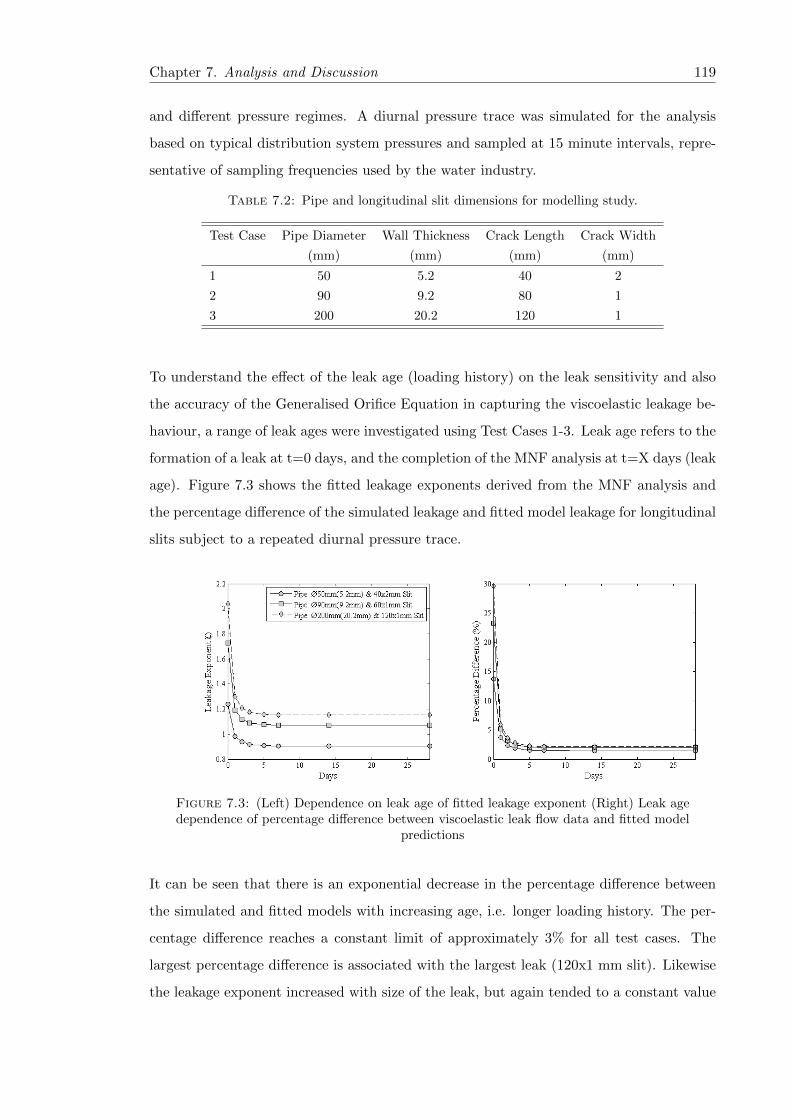
Chapter 7. Analysis and Discussion 119
and different pressure regimes. A diurnal pressure trace was simulated for the analysis
based on typical distribution system pressures and sampled at 15 minute intervals, repre-
sentative of sampling frequencies used by the water industry.
Table 7.2: Pipe and longitudinal slit dimensions for modelling study.
Test Case Pipe Diameter Wall Thickness Crack Length Crack Width
(mm) (mm) (mm) (mm)
1 50 5.2 40 2
2 90 9.2 80 1
3 200 20.2 120 1
To understand the effect of the leak age (loading history) on the leak sensitivity and also
the accuracy of the Generalised Orifice Equation in capturing the viscoelastic leakage be-
haviour, a range of leak ages were investigated using Test Cases 1-3. Leak age refers to the
formation of a leak at t=0 days, and the completion of the MNF analysis at t=X days (leak
age). Figure 7.3 shows the fitted leakage exponents derived from the MNF analysis and
the percentage difference of the simulated leakage and fitted model leakage for longitudinal
slits subject to a repeated diurnal pressure trace.
Figure 7.3: (Left) Dependence on leak age of fitted leakage exponent (Right) Leak agedependence of percentage difference between viscoelastic leak flow data and fitted model
predictions
It can be seen that there is an exponential decrease in the percentage difference between
the simulated and fitted models with increasing age, i.e. longer loading history. The per-
centage difference reaches a constant limit of approximately 3% for all test cases. The
largest percentage difference is associated with the largest leak (120x1 mm slit). Likewise
the leakage exponent increased with size of the leak, but again tended to a constant value

Chapter 7. Analysis and Discussion 120
after 7 days in all cases. In reality it is highly unlikely that a leakage assessment will cap-
ture a leak that has formed within the past 72 hours for example, the time period where
the error associated with the MNF and leakage exponent fitting methodology is at a max-
imum as highlighted in Figure 7.3. The effective stiffness of a dynamic leak increases with
time, resulting in a material response that tends towards a linear-elastic characterisation
over a long time period. In other words, the rate of change of the structural behaviour
decreases with time and reaches a pseudo-equilibrium state (approximately constant hys-
teresis cycle). The analysis confirms that the use of the Generalised Orifice Equation is an
effective estimator of the leakage response of a viscoelastic leak. The associated error is
not cumulative if the pressure-leakage relationship remains in a constant hysteresis cycle.
This in itself is dependent on the pressure regime and the material properties. Therefore
any significant changes in the diurnal pattern (pressure steps) and the viscoelastic prop-
erties of a failed pipe, may result in diversion from this pseudo-equilibrium state, thus
increasing the cumulative fitted model error. This correlates with the conclusions drawn
by van Zyl and Cassa (2014) who found that the definition of the leakage exponent was
dependent on the specific pressure range it was derived over. The Generalised Orifice
Equation given in Equation 5.1 merely represents a numerical likeness (simplified fit) of
the true coupled characteristic leakage behaviour for a given system. Again it must be
noted that the derived viscoelastic leakage model, Equation 5.8, describes the time and
pressure dependent behaviour of stable leaks in pressurised pipes. It may be assumed that
in practice the formation and development of such leaks is a more complex phenomena
than can be feasibly captured in a single analytical model.
7.5.2 Hysteresis Analysis
The concepts of a pseudo-equilibrium state and hysteresis offset for dynamic leaks in
viscoelastic pipe are significant in terms of the associated error with regards to leakage
assessment. The time required to reach this predictable state may be surmised to be a
function of the operating pressure regime, i.e. the maximum mean daily pressure and the
daily pressure range. Figure 7.4 presents the percentage difference in daily net simulated
leakage volume (e.g. percentage difference between Days 1 and 2) for Test Case 1 using
scaled diurnal pressure data. The results verify that the time taken to reach the pseudo-
equilibrium state is a function of the pressure regime and the initial error is primarily a
function of the magnitude of the mean pressure.
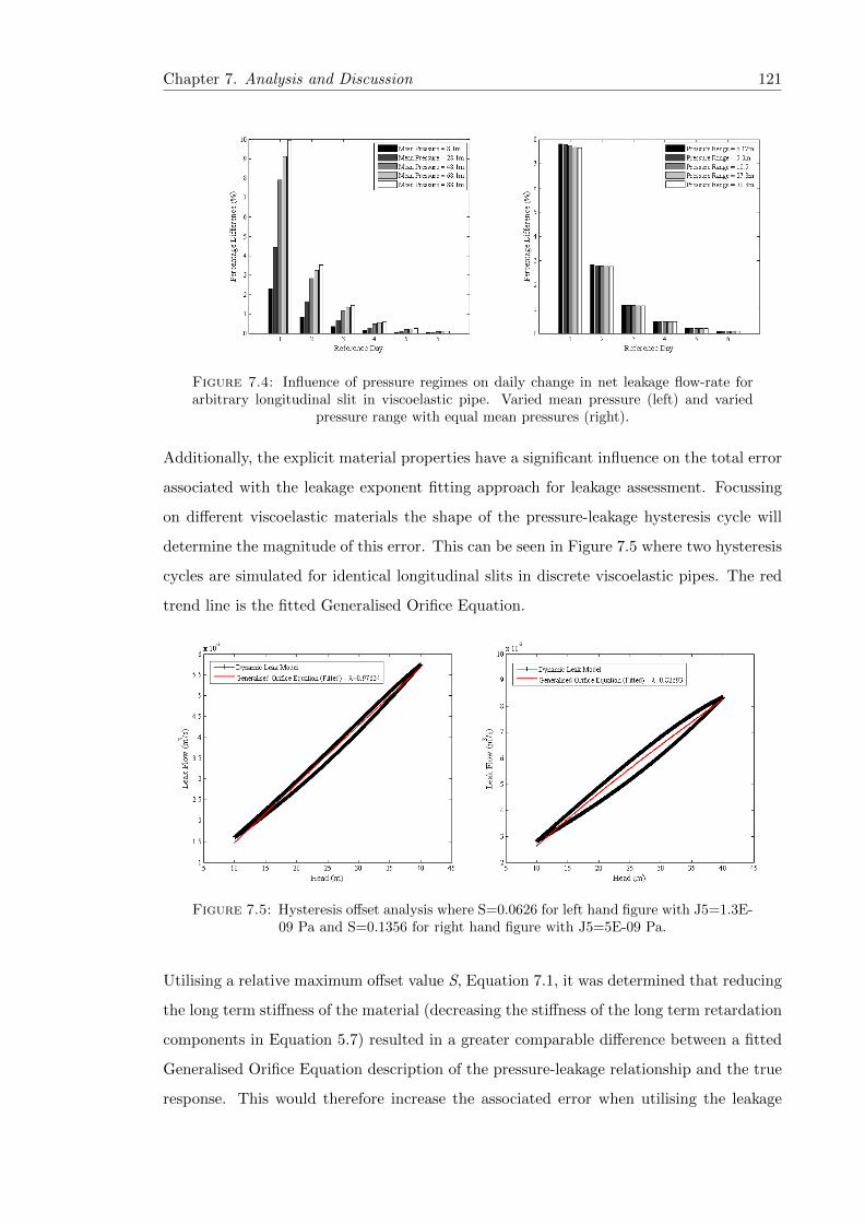
Chapter 7. Analysis and Discussion 121
Figure 7.4: Influence of pressure regimes on daily change in net leakage flow-rate forarbitrary longitudinal slit in viscoelastic pipe. Varied mean pressure (left) and varied
pressure range with equal mean pressures (right).
Additionally, the explicit material properties have a significant influence on the total error
associated with the leakage exponent fitting approach for leakage assessment. Focussing
on different viscoelastic materials the shape of the pressure-leakage hysteresis cycle will
determine the magnitude of this error. This can be seen in Figure 7.5 where two hysteresis
cycles are simulated for identical longitudinal slits in discrete viscoelastic pipes. The red
trend line is the fitted Generalised Orifice Equation.
Figure 7.5: Hysteresis offset analysis where S=0.0626 for left hand figure with J5=1.3E-09 Pa and S=0.1356 for right hand figure with J5=5E-09 Pa.
Utilising a relative maximum offset value S, Equation 7.1, it was determined that reducing
the long term stiffness of the material (decreasing the stiffness of the long term retardation
components in Equation 5.7) resulted in a greater comparable difference between a fitted
Generalised Orifice Equation description of the pressure-leakage relationship and the true
response. This would therefore increase the associated error when utilising the leakage
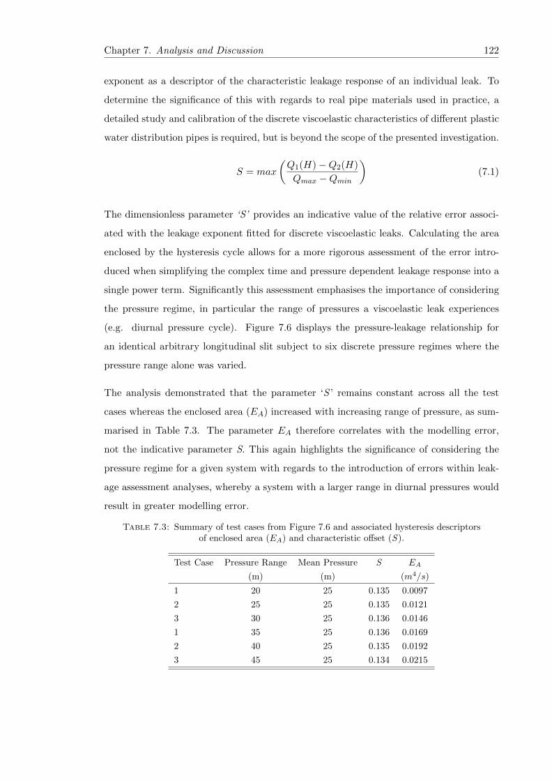
Chapter 7. Analysis and Discussion 122
exponent as a descriptor of the characteristic leakage response of an individual leak. To
determine the significance of this with regards to real pipe materials used in practice, a
detailed study and calibration of the discrete viscoelastic characteristics of different plastic
water distribution pipes is required, but is beyond the scope of the presented investigation.
S = max
(Q1(H)−Q2(H)
Qmax −Qmin
)(7.1)
The dimensionless parameter ‘S’ provides an indicative value of the relative error associ-
ated with the leakage exponent fitted for discrete viscoelastic leaks. Calculating the area
enclosed by the hysteresis cycle allows for a more rigorous assessment of the error intro-
duced when simplifying the complex time and pressure dependent leakage response into a
single power term. Significantly this assessment emphasises the importance of considering
the pressure regime, in particular the range of pressures a viscoelastic leak experiences
(e.g. diurnal pressure cycle). Figure 7.6 displays the pressure-leakage relationship for
an identical arbitrary longitudinal slit subject to six discrete pressure regimes where the
pressure range alone was varied.
The analysis demonstrated that the parameter ‘S ’ remains constant across all the test
cases whereas the enclosed area (EA) increased with increasing range of pressure, as sum-
marised in Table 7.3. The parameter EA therefore correlates with the modelling error,
not the indicative parameter S. This again highlights the significance of considering the
pressure regime for a given system with regards to the introduction of errors within leak-
age assessment analyses, whereby a system with a larger range in diurnal pressures would
result in greater modelling error.
Table 7.3: Summary of test cases from Figure 7.6 and associated hysteresis descriptorsof enclosed area (EA) and characteristic offset (S ).
Test Case Pressure Range Mean Pressure S EA
(m) (m) (m4/s)
1 20 25 0.135 0.0097
2 25 25 0.135 0.0121
3 30 25 0.136 0.0146
1 35 25 0.136 0.0169
2 40 25 0.135 0.0192
3 45 25 0.134 0.0215

Chapter 7. Analysis and Discussion 123
Figure 7.6: Pressure-leakage hysteresis cycles of arbitrary longitudinal slit, for discretepressure ranges (details listed in Table 7.3).
7.5.3 Leakage Exponent
The leakage exponent methodology for characterising the leakage response of an individual
leak or combination of leaks (e.g. both linear and viscoelastic leaks) may only be regarded
as an estimator of the true response. Equation 7.2 is an example of an arbitrary system
where the total losses are comprised of background leakage, leaks from fixed area orifices
and linear and viscoelastic type leaks (approximated by the Generalised Orifice Equation).
QL = QBackground+QOrifice+QLinear+QV isco = c1H0.5 +c2H
0.5 +c3H1.0 +c4H
1.1 (7.2)

Chapter 7. Analysis and Discussion 124
cHλ 6= c1H0.5 + c2H
0.5 + c3H1.0 + c4H
1.1 (7.3)
There is no equivalence between the Generalised Orifice Equation and Equation 7.2 as
shown in Equation 7.3, and therefore the Generalised Orifice Equation given merely rep-
resents a numerical likeness (simplified fit) of the true coupled characteristic leakage be-
haviour. This fitting methodology only provides a good representation of the actual re-
sponse for a localised fit, i.e. specific pressure or small range of pressures. Nevertheless in
practice this approach has been demonstrated, herein and in other published work, as a
highly effective and efficient assessment tool for leakage management practitioners in the
water industry for distribution systems that consist of linear elastic or viscoelastic pipes
(or a combination of both). Integrating the derived dynamic leakage area model within
the proposed Leakage Number by van Zyl and Cassa (2014) may also offer a means to as-
sess the theoretical implications of different leaks types and sizes on the pressure-leakage
relationship, characterised by the leakage exponent. Approximation of a system leakage
exponent also allows for the assessment of the benefit of pressure reduction on the total
losses in an isolated DMA, in particular the levels of background leakage. Attention must
however be given to the influence of the viscoelastic nature of longitudinal slits in plas-
tic pipes which have been shown to be highly dependent not only on the instantaneous
pressure but also the full loading time history. Significant errors may be introduced into
theoretical pressure management studies without effective application of the understand-
ing presented regarding the dynamic leakage behaviour of such leaks and the subsequent
pressure dependence of the theoretical leakage exponent.
7.5.4 Leakage Localisation and Control
Leakage assessment and pressure management refer to the relative long time period charac-
teristics of the pressure-leakage relationship. Honing in on the short time period response,
in particular the performance of leaks subject to pressure transients, the material rheology
takes on greater significance. The creep and recovery structural behaviour due to rapidly
changing pressures appears to be less dependent of the loading history based on the devel-
oped leakage model. However the leakage model calibrated in Chapter 5 is not deemed to
be of sufficiently accurate resolution to capture the true short term dynamic behaviour of a
slit in viscoelastic pipe due to the magnitude of the modelled retardation time components.
The minimum time period utilised was 10 s compared to time components utilised in other

Chapter 7. Analysis and Discussion 125
studies of the short term viscoelastic response of polyethylene pipes which utilised a range
from 0.05 s to 10 s (Covas et al., 2005). Whether an integrated model incorporating the
calibrated long and short term viscoelastic modelling components would be adequate to
describe the total material behaviour remains an unanswered question.
A detailed understanding of the leakage response of viscoelastic leaks to pressure tran-
sients is of particular importance in the development of leak localisation methodologies.
Characterising the time and pressure dependent response in order to quantify the damping
of a generated pressure transient will greatly improve the ability to locate and size the leak
using methodologies such as that described by Wang et al. (2002). An alternative method-
ology for leak localisation utilises time-domain reflectometry (TDR) and offers a means
of locating leaks without specific consideration of the leak size, evaluating the arrival of
the reflected transient wave from a leak source (an example of the development of this
technique is a study by Vıtkovsky et al. (2007)). The complexity of the time and pressure
dependent response of leaks, including longitudinal slits in PE pipe, would therefore not
impact the effectiveness of this methodology as severely as those considering the damping
rate of transients. However, attention to the viscoelastic properties (most significantly, the
wave speed) of the pipe are fundamental to the accuracy of the ‘leak-free’ numerical tran-
sient models (or historical data) that are used for comparison with the acquired transient
leak data used by the TDR methodology. On the other hand, leak detection techniques
primarily identify the existence of a leak (Covas and Ramos, 2010) and do not necessar-
ily require definition of the precise leakage response as they effectively only consider the
relative change in signal response/reflection. However, a fundamental appreciation of the
characteristic behaviour of viscoelastic leaks may allow for more detailed signal processing
by understanding the expected time and pressure dependent response and integrating this
within isolation from contributing system noise for example.
The response of sensitive leaks to rapid changes in pressure also has great significance
for the quantification of risk regarding contaminant intrusion into the water distribution
system. Provided a contaminant source, pathway into a pipe and a driving force (low or
negative pressure during pressure transient event) exist simultaneously, there is a risk of
contaminant ingress (Lindley and Buchberger, 2002). The magnitude of the contamination
event is therefore dependent on the size of the driving force, contaminant concentration
and the size of the leak. As a result of this, assuming a leak has a fixed or variable area
will significantly alter the calculated risk. The viscoelastic behaviour of longitudinal slits

Chapter 7. Analysis and Discussion 126
in plastic pipes for example would result in a proportionally higher leak area compared to
a similar leak in linear elastic pipe due to the material recovery time period, previously
demonstrated by Fox et al. (2012). A negative pressure wave or sudden reduction in
pressure is equivalent to the de-pressurisation conducted in Chapter 4 but over a shorter
time period. Building on the understanding of the mechanism of contaminant intrusion
(Fox et al., 2014a) using the derived dynamic leakage model, a more accurate measure of
the risk of contaminant ingress and subsequent threat to public health may be established.
Chapter 8
Conclusions
The presented research sought to quantify the leakage behaviour of longitudinal slits in
thick-walled viscoelastic water distribution pipes, considering the interaction of the leak
and structural dynamics. This aim was achieved through the development of a validated
dynamic leakage model (Equation 8.1) describing the dependent leakage response, derived
from the created synergy between a unique set of physical observations, numerical simu-
lations and application of linear viscoelastic theory.
Q(t, T ) = Cd.
(A0 + C1
(∆P
E(t, T )
).
(L4c
s2
)).
√2(∆P )
ρ(8.1)
The experimental investigations captured the synchronous leakage flow rate, pressure head,
leak area and material strain for the first time. Consequently the time and pressure depen-
dent leak area was conclusively established to be the critical factor defining the observed
dynamic leakage, also confirming the invariable nature of the discharge coefficient. Deriva-
tion of an explicit leakage flow rate model provided a powerful tool to predict the response
of a single leak test case. The definition of a generalised model however contributed to a
greater level of understanding of the parameters governing the leakage behaviour of this
failure type for different geometries, material properties and loading conditions.
The significance of the slit face loading on the dynamic leak area was demonstrated. The
slit face loading is dependent on the external ground conditions. Therefore, to accurately
model and capture the leakage behaviour of dynamic leaks in buried pipes the porous
media permeability, consolidation, constraint and self-weight must be considered. This
127
Chapter 8. Conclusions 128
is so as not to provide conservative estimates of the risks posed by the magnitude of
the structural dynamics in particular. The experimental and numerical methodologies
demonstrated within the investigation offer exciting opportunities to further knowledge in
this area, in particular the use of strain as a predictor of the leak area.
Finally the dynamic leakage model, was used to assess the effectiveness of some traditional
leakage management strategies. Significantly, the short term behaviour of the dynamic
leaks may severely hinder the effectiveness of some active leakage control methods and the
quantification of risk associated with contaminant ingress. It was also shown that cur-
rent leakage modelling practice over relatively long time periods (e.g. leakage assessment
techniques) were not adversely affected by the existence of viscoelastic leaks.
In addition to the primary output of the research (i.e. the dynamic leakage model), the
other key outputs and resulting outcomes are summarised in Table 8.1.
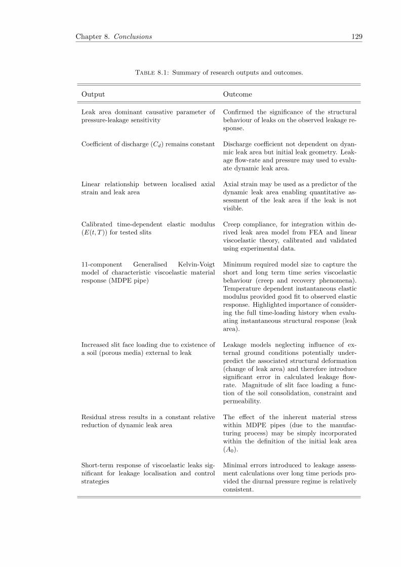
Chapter 8. Conclusions 129
Table 8.1: Summary of research outputs and outcomes.
Output Outcome
Leak area dominant causative parameter ofpressure-leakage sensitivity
Confirmed the significance of the structuralbehaviour of leaks on the observed leakage re-sponse.
Coefficient of discharge (Cd) remains constant Discharge coefficient not dependent on dyan-mic leak area but initial leak geometry. Leak-age flow-rate and pressure may used to evalu-ate dynamic leak area.
Linear relationship between localised axialstrain and leak area
Axial strain may be used as a predictor of thedynamic leak area enabling quantitative as-sessment of the leak area if the leak is notvisible.
Calibrated time-dependent elastic modulus(E(t, T )) for tested slits
Creep compliance, for integration within de-rived leak area model from FEA and linearviscoelastic theory, calibrated and validatedusing experimental data.
11-component Generalised Kelvin-Voigtmodel of characteristic viscoelastic materialresponse (MDPE pipe)
Minimum required model size to capture theshort and long term time series viscoelasticbehaviour (creep and recovery phenomena).Temperature dependent instantaneous elasticmodulus provided good fit to observed elasticresponse. Highlighted importance of consider-ing the full time-loading history when evalu-ating instantaneous structural response (leakarea).
Increased slit face loading due to existence ofa soil (porous media) external to leak
Leakage models neglecting influence of ex-ternal ground conditions potentially under-predict the associated structural deformation(change of leak area) and therefore introducesignificant error in calculated leakage flow-rate. Magnitude of slit face loading a func-tion of the soil consolidation, constraint andpermeability.
Residual stress results in a constant relativereduction of dynamic leak area
The effect of the inherent material stresswithin MDPE pipes (due to the manufac-turing process) may be simply incorporatedwithin the definition of the initial leak area(A0).
Short-term response of viscoelastic leaks sig-nificant for leakage localisation and controlstrategies
Minimal errors introduced to leakage assess-ment calculations over long time periods pro-vided the diurnal pressure regime is relativelyconsistent.
Chapter 8. Conclusions 130
8.1 Further Work Proposals
A comprehensive list of aims and objectives was established for the presented research
based on an extensive review of available literature regarding the modelling of complex
leaks in water distribution system pipes. Following on from the subsequent analysis and
discussion, a proposed list of future work that has not been addressed within the scope of
the current research has been outlined and summarised in the following list.
• Quantitative study of the influence of soil conditions on leakage behaviour - the
work may involve the development of a programme of work to better understand
the influence of soil grades, degree of consolation, fluidisation and burial depth for
example. The research methods developed within the presented thesis could be effec-
tively utilised to further quantify the interaction of soil and leakage behaviour. These
tools include the CFD modelling approach (potentially incorporating structural dy-
namics modelling, i.e. pressure/time dependent leak area), the observed strain:area
relationship, image analysis methodology and other experimental techniques.
• Characterisation of the short term viscoelastic behaviour - developing the presented
investigatory research methodologies to quantify the leakage behaviour of similar leak
types subject to rapidly varying pressure oscillations. This work could also include
the assessment of the suitability of a coupled short and long term viscoelastic model
to mathematically represent the ’total ’ structural behaviour.
• Viscoelastic characterisation of different polyethylene pipe materials using described
methodology (e.g. HDPE pipe).
• Implementation of dynamic leakage model into commercial WDS network modelling
tools.
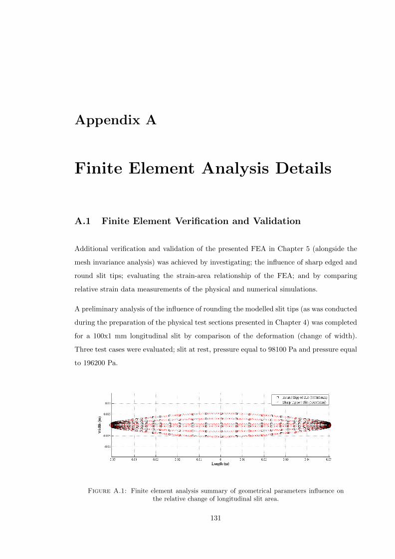
Appendix A
Finite Element Analysis Details
A.1 Finite Element Verification and Validation
Additional verification and validation of the presented FEA in Chapter 5 (alongside the
mesh invariance analysis) was achieved by investigating; the influence of sharp edged and
round slit tips; evaluating the strain-area relationship of the FEA; and by comparing
relative strain data measurements of the physical and numerical simulations.
A preliminary analysis of the influence of rounding the modelled slit tips (as was conducted
during the preparation of the physical test sections presented in Chapter 4) was completed
for a 100x1 mm longitudinal slit by comparison of the deformation (change of width).
Three test cases were evaluated; slit at rest, pressure equal to 98100 Pa and pressure equal
to 196200 Pa.
Figure A.1: Finite element analysis summary of geometrical parameters influence onthe relative change of longitudinal slit area.
131
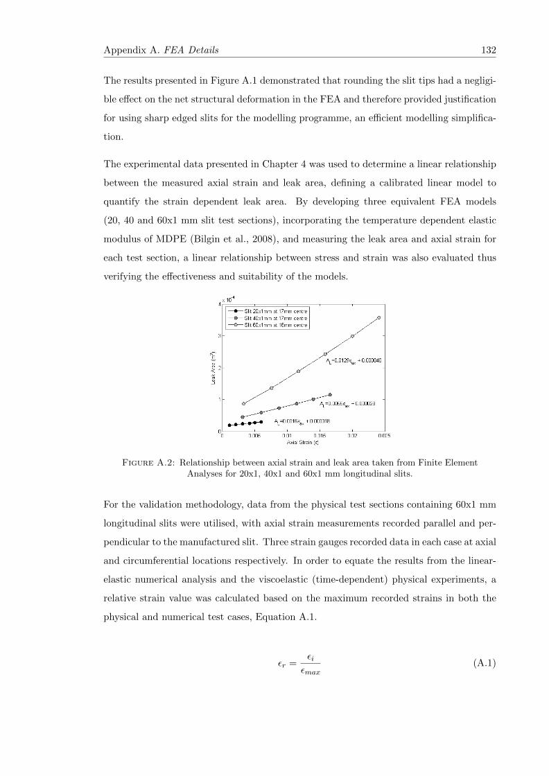
Appendix A. FEA Details 132
The results presented in Figure A.1 demonstrated that rounding the slit tips had a negligi-
ble effect on the net structural deformation in the FEA and therefore provided justification
for using sharp edged slits for the modelling programme, an efficient modelling simplifica-
tion.
The experimental data presented in Chapter 4 was used to determine a linear relationship
between the measured axial strain and leak area, defining a calibrated linear model to
quantify the strain dependent leak area. By developing three equivalent FEA models
(20, 40 and 60x1 mm slit test sections), incorporating the temperature dependent elastic
modulus of MDPE (Bilgin et al., 2008), and measuring the leak area and axial strain for
each test section, a linear relationship between stress and strain was also evaluated thus
verifying the effectiveness and suitability of the models.
Figure A.2: Relationship between axial strain and leak area taken from Finite ElementAnalyses for 20x1, 40x1 and 60x1 mm longitudinal slits.
For the validation methodology, data from the physical test sections containing 60x1 mm
longitudinal slits were utilised, with axial strain measurements recorded parallel and per-
pendicular to the manufactured slit. Three strain gauges recorded data in each case at axial
and circumferential locations respectively. In order to equate the results from the linear-
elastic numerical analysis and the viscoelastic (time-dependent) physical experiments, a
relative strain value was calculated based on the maximum recorded strains in both the
physical and numerical test cases, Equation A.1.
εr =εiεmax
(A.1)
Appendix A. FEA Details 133
where the subscript r denotes the relative strain and i the discretised axial strain mea-
surement at location i in the FEA analysis. The results of the relative strain validation
analyses are shown in Figure A.3 and A.4 which clearly depict the same strain distribu-
tion in both numerical and physical cases, validating the developed FE models against
empirical lab data.
Figure A.3: Relative axial strain measurements parallel to a longitudinal slit at 18 mmdistance from leak centre.
The angularity of the curve shown in Figure A.3 for the parallel axial strain measurement
results is as a result of the coarseness of the mesh. It may be surmised that refining
the mesh about the slit would alter the localised shape (rounded corners) of this curve.
However it is not thought that this would alter the overall form of the results, as was
shown in the mesh invariance analysis.
Figure A.4: Relative axial strain measurements perpendicular to a longitudinal slit.Origin at centre of slit length on the edge of the opening.
Appendix A. FEA Details 134
A.2 Parameter Analysis
To qualitatively demonstrate the significance of each variable, the range of parameter val-
ues were plotted against the relative change of area. All simulations, with the exception
of the pressure dependent simulations, were run at a static pressure of 196200 Pa. Fig-
ure A.5 summarises the results for the geometrical parameters explored, and Figure A.6
summarises the material and loading conditions parameters considered.
Figure A.5: Finite element analysis summary of geometrical parameters influence onthe relative change of longitudinal slit area.
As described in Chapter 5, this analysis does not offer a quantitative insight into the
significance of each parameter on the dynamic leak behaviour, as the physical phenomena
was surmised to be dependent on the coupled influence of select parameters. However it
does provide a clear qualitative judgement of which parameters are the most dominant
variables on the observed behaviour. Based on this, it was be concluded that the slit length,
pipe diameter, wall thickness, pressure head and elastic modulus are the key parameters.
The influence of slit width, longitudinal stress and Poisson’s ratio were therefore adjudged
to be negligible.
Appendix A. FEA Details 135
Figure A.6: Finite element analysis summary of material and loading conditions influ-ence on the relative change of longitudinal slit area.
Appendix B
Experimental Methodologies -
Additional Information
B.1 Leak Area Measurement
A range of methods for physically quantifying the leak area during the experimental in-
vestigations, were explored. These included;
• Strain gauge measurements
• Moire interferometry
• Physical gauges – micrometers directly attached to pipe
• Image capture and analysis
It was desirable to utilise a method that minimised any external influence on the leak
hydraulics and structural response. Therefore, the image analysis technique was taken
forward for development due to the ability to quantify the leak area in a non-intrusive
manner.
The defined methodology used a simple conversion process from an RGB image recorded
using the high speed camera described in Chapter 4 to a binary black and white image.
The steps taken in the setup and processing of the recorded images were as follows;
136
Appendix B. Methodologies 137
1. Camera setup and calibration – use of calibration sheet placed directly onto leak to
define the image pixel height/width. Algorithm defined to evaluate the pixel size
based on line width measurements recorded from calibration sheet (5.2 mm printed
lines).
2. Record images – see Experimental Procedure in Chapter 4 for further details
3. Download images from camera – converted all recorded images to .jpg files for further
analysis
4. Process recorded images – algorithm defined to convert RGB images to binary image
based on threshold value (see Threshold Analysis section).
5. Area measurement – leak area defined by pixel count of black pixels (leak area).
6. Output file – data output to single file with measured area and time stamp for all
data analysed
B.1.1 Threshold Analysis
The threshold definition for the conversion between RGB colour images and binary black
and white images was fundamental to the accurate definition of the leak area. A range
of different methods were explored, including wavelet analysis and histogram processing.
However, it was concluded that ultimately a user defined threshold value was always
required. Consequently an approach was taken whereby the camera set-up and lighting
was kept constant for each test section experimental programme, to ensure that all results
were comparable based on a single threshold value. Further analysis (invariance testing)
of the influence of the threshold value was also incorporated within the definition of the
measurement error defined within the discussion of the methodology presented in Chapter
4.
A limiting factor of the leak area measurement accuracy was the resolution of the images.
A compromise was met between image resolution and acquisition frequency. In order to
capture the required 8 hr test phase, a lower resolution image of the leak was required to
enable the recording frequency defined in Chapter 4 to be implemented.

Appendix B. Methodologies 138
B.2 Experimental Process for Fill Placement
The following section briefly summarises the methodology implemented within the exper-
imental investigations carried out in Chapter 6, specifically the placement of the porous
media within the test section box.
The test section box, presented in Figure 6.4 was lined with a single drainage layer (typi-
cally used for green roof drainage layers) to provide a permeable boundary condition whilst
restraining the porous media. Mixed grade pea gravel (approximately 3 to 8 mm in size)
was used as the porous media within the test, and was placed and compacted within the
box and around the pipe in approximately 100 mm depth layers. This was conducted to
minimise the potential occurrence of fluidisation of the gravel around the leak orifice. The
gravel beneath the pipe was compacted as thoroughly as possible to minimise the impact
of biased loading of the pipe, which may have resulted in an adverse bending moment of
the pipe, altering the observed structural response.
The lead wires for the strain gauges were wrapped prior to burial to prevent any damage
from the compacted media. This was shown to have negligible influence on the recorded
strain values. During the burial phase of the test set-up, the strain gauge readings were
recorded to measure the structural impact of the applied loading from the gravel media.

References
Al-khomairi, A. (2005). Use of the steady-state orifice equation in the computation of
transient flow through pipe leaks. The Arabian Journal for Science and Engineering,
30(1):33–45.
Albert Einstein (1879-1955). http://www.brainyquote.com/quotes/quotes/a/alberteins118979.html
- Last Viewed- 05/07/2015.
Alfred Nobel (1833-1896). http://www.brainyquote.com/quotes/quotes/a/alfrednobe556200.html
- Last Viewed- 05/07/2015.
Avila Rangel, H. & Gonzalez Barreto, C. (2006). Determinacion de parametros de fuga
para fallas longitudinales , en conexiones domiciliarias y en uniones de tuberıas en PVC.
Revista de Ingenierıa, 24:15–22.
Awad, H., Kapelan, Z., & Savic, D. (2008). Analysis of pressure management economics
in water distribution systems. In: 10th Annual Water Distribution Systems Analysis
Conference, pages 520–531.
Banks, D. (2012). An Introduction to Thermogeology: Ground Source Heating and Cooling.
Wiley-Blackwell.
Banks, H., Hu, S., & Kenz, Z. (2011). A brief review of elasticity and viscoelasticity.
Advances in Applied Mathematics and Mechanics, 3:1–51.
Beech, S., Burley, C., & Bunn, H. (1988). Residual stress in large diameter MDPE pipe. In:
PRI-Proceedings of the VII International Conference on Plastic Pipes, pages 15/1–15/9.
Benham, P., Crawford, R., & Armstrong, C. (1996). Mechanics of Engineering Materials,
(2 ed.). Pearson.
139
References 140
Bergant, A., Tijsseling, A., Vıtkovsky, J., Covas, D., Simpson, A., Lambert, M., &
Litostroj, E. I. (2003). Further investigation of parameters affecting water hammer wave
attenuation, shape and time. Part 1: Mathematical tools. Technical report, Eindhoven
University of Technology.
Bhandari, S. & Leroux, J. (1993). Evaluation of crack opening times and leakage areas for
longitudinal cracks in a pressurized pipe Part I . Model for maximum leak areas and its
validation. Nuclear Engineering and Design, 142:15–19.
Bilgin, O., Stewart, H., & O’Rourke, T. (2008). Thermal and Mechanical Properties of
Polyethylene Pipes. Journal of Materials in Civil Engineering, 19(12):1043–1052.
Boubaker, M., Le Corre, B., Meshaka, Y., & Jeandel, G. (2014). Finite element simulation
of the slumping process of a glass plate using 3D generalized viscoelastic Maxwell model.
Journal of Non-Crystalline Solids, 405:45–54.
Brater, E., King, H., Lindell, J., & Wei, C. (1996). Handbook of Hydraulics, (7 ed.).
McGraw-Hill.
British Standards Institution (1985). BS 6572:1985 : Blue polyethylene pipes up to nominal
size 63 for below ground use for potable water.
British Standards Institution (2011). BS EN 12201-2:2011 : Plastic piping systems for wa-
ter supply, and for drainage and sewerage under pressure — Polyethylene (PE) drainage
and Part 2 : Pipes.
Brown, N. (2007). Intrinsic lifetime of polyethylene pipelines. Polymer Engineering &
Science, 47(4):477–480.
BSI, B. S. I. (1973). CP 312-1:1973 Code of Practice for Plastics pipework (thermoplastics
material)- Part 1: General principles and choice of material.
Buckley, R. (2007). Theoretical investigation and experimentatioin into the expansion of
round holes and cracks within pressurised pipes. PhD thesis, University of Johannesburg.
Burgers, J. (1935). Mechanical considerations - model systems - phenomenological theories
of relaxation and of viscosity. In: First Report on Viscosity and Plasticity. Nordemann
Publishing Company.

References 141
Byron Jennings (2014). http://www.quantumdiaries.org/2014/07/04/wrong/ - Last
Viewed- 05/07/2015.
Cassa, A. & van Zyl, J. (2008). A numerical investigation into the behaviour of cracks
in uPVC pipes under pressure. In: 10th Annual Water Distribution Systems Analysis,
pages 1–8. American Society of Civil Engineers.
Cassa, A. & van Zyl, J. (2011). Predicting the head-area slopes and leakage exponents of
cracks in pipes. In: Urban Water Management: Challenges and Oppurtunities, CCWI
2011, pages 485–491.
Cassa, A. M., van Zyl, J. E., & Laubscher, R. F. (2010). A numerical investigation into
the effect of pressure on holes and cracks in water supply pipes. Urban Water Journal,
7(2):109–120.
Cheung, P., Guilherme, V., Abe, N., & Propato, M. (2010). Night flow analysis and mod-
eling for leakage estimation in a water distribution system. Integrating Water Systems,
pages 509–513.
Cholewa, J., Brachman, R., & Moore, I. (2011). Axial stress-strain response of HDPE from
whole pipes and coupons. Journal of Materials in Civil Engineering, 23(10):1377–1386.
Clayton, C. & van Zyl, J. (2007). The effect of pressure on leakage in water distribution
systems. Proceedings of the ICE - Water Management, 160(2):109–114.
Coetzer, A., van Zyl, J., & Clayton, C. (2006). An experimental investigation into the
turbulent-flow hydraulics of small circular holes in plastic pipes. In: Water Distribution
Systems Analysis Symposium, pages 1–9. American Society of Civil Engineers.
Colin, X., Audouin, L., Verdu, J., Rozental-Evesque, M., Rabaud, B., Martin, F., &
Bourgine, F. (2009). Aging of polyethylene pipes transporting drinking water disinfected
by cholirne dioxide. Part II- Lifetime prediction. Polymer Engineering and Science,
49(8):1642–1652.
Collins, R. & Boxall, J. (2013). Influence of ground conditions on intrusion flows through
apertures in distribution pipes. Journal of Hydraulic Engineering, 139(October):1052–
1061.
References 142
Collins, R., Boxall, J., Besner, M.-C., Beck, S., & Karney, B. (2011). Intrusion modelling
and the effect of ground water conditions. In: Water Distribution Systems Analysis
2010, pages 585–594. American Society of Civil Engineers.
Collins, R., Fox, S., Beck, S., Saul, A., & Boxall, J. (2012). Intrusion and leakage through
cracks and slits in plastic (MDPE) pipes. In: Proceedings of 14th Water Distribution
Systems Analysis Conference.
Colombo, A., Lee, P., & Karney, B. (2009). A selective literature review of transient-based
leak detection methods. Journal of Hydro-environment Research, 2(4):212–227.
Covas, D. & Ramos, H. (2010). Case Studies of Leak Detection and Location in Water
Pipe Systems by Inverse Transient Analysis. Journal of Water Resources Planning and
Management, 136(2):248–257.
Covas, D., Stoianov, I., Mano, J., Ramos, H., Graham, N., & Maksimovic, C. (2004). The
dynamic effect of pipe-wall viscoelasticity in hydraulic transients . Part I — experimental
analysis and creep characterization. Journal of Hydraulic Engineering, 42(5):516–530.
Covas, D., Stoianov, I., Mano, J. F., Ramos, H., Graham, N., & Maksimovic, C. (2005).
The dynamic effect of pipe-wall viscoelasticity in hydraulic transients . Part II — model
development , calibration and verification. Journal of Hydraulic Research, 43(1):56–70.
De Miranda, S., Molari, L., Scalet, G., & Ubertini, F. (2012). Simple Beam Model to
Estimate Leakage in Longitudinally Cracked Pressurized Pipes. Journal of Structural
Engineering, 138:1065–1074.
De Paola, F., Galdiero, E., Giugni, M., Papa, R., & Urciuoli, G. (2014). Experimental
Investigation on a Buried Leaking Pipe. Procedia Engineering, 89:298–303.
De Paola, F. & Giugni, M. (2012). Leakages and pressure relation: an experimental
research. Drinking Water Engineering and Science, 5(1):59–65.
Defra (2011). Water for Life. The Stationary Office (TSO).
Dey, A. & Basudhar, P. (2010). Applicability of burger model in predicting the response of
viscoelastic soil beds. In: GeoFlorida 2010: Advances in Analysis, Modeling & Design,
pages 2611–2620.
References 143
Doshi, S. (1989). Prediction of residual stress distribution in plastic pipe extrusion. Journal
of Vinyl Technology, 11(4):190–194.
Duvall, D. & Edwards, D. (2011). Field Failure Mechanisms in HDPE Potable Water Pipe.
In: ANTEC, 2011.
Farely, M. & Trow, S. (2003). Losses in Water Distribution Networks: A Practitioner’s
Guide to Assessment, Monitoring and Control. IWA Publishing.
Farley, M. (2001). Leakage management and control: A best practice training manual.
World Health Organisation.
Ferrante, M. (2012). Experimental investigation of the effects of pipe material on the leak
head-discharge relationship. Journal of Hydraulic Engineering, 138:736–743.
Ferrante, M., Massari, C., Brunone, B., & Meniconi, S. (2011). Experimental Evidence
of Hysteresis in the Head-Discharge Relationship for a Leak in a Polyethylene Pipe.
Journal of Hydraulic Engineering, 137(1):775–780.
Ferrante, M., Meniconi, S., & Brunone, B. (2012a). Local and global leak laws. The
relationship between pressure and leakage for a single leak and for a district with leaks.
Water Resources Management, 28(11):3761–3782.
Ferrante, M., Todini, E., Massari, C., Brunone, B., & Meniconi, S. (2012b). Experimental
investigation of the leak hydraulics. Journal of Hydroinformatics, 15(3):666–675.
Ferry, J. (1961). Viscoelastic properties of polymers. John Wiley & Sons, Inc.
Fox, R. & McDonald, A. (1978). Introduction to fluid mechanics, (2nd ed.). John Wiley
& Sons, Inc.
Fox, S., Collins, R., & Boxall, J. (2012). Time dependent area of leaks in MDPE pipes
during transient events. In: 11th International Conference on Pressure Surges, pages
113–125.
Fox, S., Collins, R., & Boxall, J. (2014a). Dynamic Leakage: Physical Study of the Leak
Behaviour of Longitudinal Slits in MDPE Pipe. Procedia Engineering, 89:286–289.
Fox, S., Shepherd, W., Collins, R., & Boxall, J. (2014b). Experimental proof of con-
taminant ingress into a leaking pipe during a transient event. Procedia Engineering,
70:668–677.
References 144
Franchini, M. & Lanza, L. (2014). Leakages in pipes: generalizing Torricelli’s equation to
dela with different elastic materials, diameters and orifice shape and dimensions. Urban
Water Journal, 11:678–695.
Frank, A., Pinter, G., & Lang, R. (2009). Prediction of the remaining lifetime of polyethy-
lene pipes after up to 30 years in use. Polymer Testing, 28(7):737–745.
Fung, Y. (1981). Use of Viscoelastic Models. In: Biomechanics: Mechanical Properties of
Living Tissues, pages 50–56. Springer-Verlag New York Inc.
Giustolisi, O., Walski, T., & Asce, F. (2012). Demand Components in Water Distri-
bution Network Analysis. Journal of Water Resources Planning and Management,
138(August):356–367.
Gopan, A., Suja, R., & Letha, J. (2010). Pressure Control for Leakage Minimization In
Water Distribution Network.
GPSUK (2014a). GPS PE Pipe Systems UK. URL:
http://www.gpsuk.com/content/1/126/quality-control.html - Last Viewed- 01/06/2014,
pages Quality– Quality Control.
GPSUK (2014b). GPS PE Pipe Systems UK. URL
http://www.gpsuk.com/articles/3/19/plastic-pipes–number-one-choice-for-water—
sewerage-applications.html - Last Viewed- 10/12/2014, page Plastic Pipes: Number
One Choice for Water & Sewerage Applications.
Grann-Meyer, E. (2005). Polyethylene pipes in applied engineering. TOTAL PETRO-
CHEMICALS.
Grebner, H. & Strathmeier, U. (1984). Elastic-plastic finite element calculation with
ADINA of leak areas of a longitudinal crack in a pipe. International Journal of Fracture,
25:77–81.
Greyvenstein, B. & van Zyl, J. (2006). An experimental investigation into the pressure
leakage relationship of some failed water pipes. Journal of Water Supply: Research and
Technology – AQUA, 56(2):117–124.
Guan, Z. & Boot, J. (2004). A method to predict triaxial residual stresses in plastic pipes.
Polymer Engineering and Science, 44(10):1828–1838.
References 145
Hutar, P., Sevcik, M., Zouhar, M., Nahlık, L., & Kucera, J. (2012). The effect of residual
stresses on crack shape in polymer pipes. In: Crack Paths, CP 2012, pages 489–496.
Ilunga, D., van Zyl, J., & Dundu, M. (2008). The effect of the pipe material in the
behaviour of longitudinal cracks under pressure. In: 10th Annual Water Distribution
Systems Analysis, volume 1, pages 777–781. American Society of Civil Engineers.
Jan, C. & Nguyen, Q. (2010). Discharge Coefficient for a Water Flow through a Bot-
tom Orifice of a Conical Hopper. Journal of Irrigation and Drainage Engineering,
136(August):567–572.
Johansen, F. (1930). Flow through Pipe Orifices at Low Reynolds Numbers. Proceedings
of the Royal Society A: Mathematical, Physical and Engineering Sciences, 126(801):231–
245.
Kim, Y., Shim, D., Huh, N., & Kim, Y. (2002). Plastic limit pressures for cracked pipes
using finite element limit analyses. International Journal of Pressure Vessels and Piping,
79:321–330.
Koppel, T., Vassiljev, a., Lukjanov, D., & Annus, I. (2009). Use of Pressure Dynamics for
Calibration of Water Distribution System and Leakage Detection. Water Distribution
Systems Analysis 2008, pages 1–12.
Krishnaswamy, R., Lamborn, M., & Phillips, C. (2004). The Influence of Process History
on the Ductile Failure of Polyethylene Pipes Subject to Continuous Hydrostatic Pressure.
Advances in Polymer Technology, 24(3):226–232.
Lambert, A. (2001). What do we know about pressure:leakage relationships in distribution
systems? In: IWA Conference on System Approach to Leakage Control and Water
Distribution Systems Management, pages 1–8.
Lehtola, M., Miettinen, I., Hirvonen, A., Vartiainen, T., & Martikainen, P. (2006). Resus-
pension of biofilms and sediments to water from pipelines as a result of pressure shocks
in drinking water distribution system. In: International Conference (IWA) Biofilm
Systems VI, pages CD–ROM.
Lekawa-Raus, A., Koziol, K., & Windle, A. (2014). Piezoresistive Effect in Carbon Nan-
otube Fibers. ACS Nano, 8(11):11214–11224.
References 146
Lemaitre, J., Ikegami, K., Rahouadj, R., Cunat, C., & Schapery, R. (1996). Handbook of
Materials Behaviour Models: Volume I. World Scientific.
Lepoutre, P. (2013). The manufacture of polyethylene. URL:
http://nzic.org.nz/ChemProcesses/polymers/10J.pdf - Last Viewed- 09/10/2013.
Lewandowski, R. & Chorazyczewski, B. (2010). Identification of the parameters of the
Kelvin–Voigt and the Maxwell fractional models, used to modeling of viscoelastic
dampers. Computers & Structures, 88(1-2):1–17.
Lewis, T. & Wang, X. (2008). The T-stress solutions for through-wall circumferential
cracks in cylinders subjected to general loading conditions. Engineering Fracture Me-
chanics, 75(10):3206–3225.
Liemberger, R. & Farley, M. (2004). Developing a Non-Revenue Water Reduction Strategy
Part 1 : Investigating and Assessing Water Losses. In: IWA Congress.
Liggett, J. & Chen, L. (1995). Inverse transient analysis in pipe networks. Journal of
Hydraulic Engineering, 120(8):934–955.
Lindley, T. & Buchberger, S. (2002). Assessing intrusion susceptibility in distribution
systems. Journal American Water Works Association, 94(6):66–79.
Liu, Z. & Bilston, L. (2000). On the viscoelastic character of liver tissue: experiments and
modelling of the linear behaviour. Biorheology, 37(3):191–201.
Marques, S. & Creus, G. (2012). Computational Viscoelasticity. In: SpringerBriefs in
Applied Sciences and Technology, pages 11–21. Springer.
Massari, C., Ferrante, M., Brunone, B., & Meniconi, S. (2012). Is the leak head-discharge
relationship in polyethylene pipes a bijective function? Journal of Hydraulic Research,
50(4):409–417.
Massey, B. & Ward-Smith, J. (2012). Mechanics of Fluids, (9 ed.). Spon Press.
Maxwell, A. & Turnbull, A. (2003). Measurement of residual stress in engineering plastics
using the hole-drilling technique. Polymer Testing, 22(2):231–233.
Maxwell, J. (1867). On the Dynamical Theory of Gases. Philosophical Transactions of the
Royal Society of London, 157(January):49–88.

References 147
May, J. (1994). Leakage, pressure and control. In: BICS International Conference on
Leakage Control.
Meissner, E. & Franke, G. (1977). Influence of pipe material on the dampening of water
hammer. In: Proceedings of the 17th Congress of the International Association for
Hydraulic Research.
Moore, I. & Zhang, C. (1998). Nonlinear predictions for HDPE pipe response under parallel
plate loading. Journal of Transportation Engineering, 124(3):286–292.
Mutikanga, H., Sharma, S., & Vairavamoorthy, K. (2012). Review of Methods and Tools for
Managing Losses in Water Distribution Systems. Journal of Water Resources Planning
and Management, 139(2):166–174.
Mutikanga, H., Sharma, S., & Vairavamoorthy, K. (2013). Methods and Tools for Man-
aging Losses in Water Distribution Systems. Journal of Water Resources Planning and
Management, 139(April):166–174.
Navarro, F., Partal, P., Martınez-Boza, F., & Gallegos, C. (2004). Thermo-rheological
behaviour and storage stability of ground tire rubber-modified bitumens. Fuel, 83(14-
15):2041–2049.
Nazif, S., Karamouz, M., Tabesh, M., & Moridi, A. (2009). Pressure Management Model
for Urban Water Distribution Networks. Water Resources Management, 24(3):437–458.
Nishimura, H., Nakashiba, A., Nakakura, M., & Sasai, K. (1993). Fatigue behavior of
medium-density polyethylene pipes for gas distribution. Polymer Engineering & Science,
33(14):895–900.
O’Connor, C. (2011). Plastics Today. URL: http://www.plasticstoday.com/mpw/articles/the-
nature-of-polyethylene-pipe-failure - Last Viewed- 09/10/2013.
O’Connor, C. (2012). Polyethylene pipeline system- Avoid-
ing the pitfalls of fusion welding. URL: http://www.pipeline-
conference.com/sites/default/files/papers/ptc 2012 OConnor.pdf - Last Viewed-
11/07/2013, pages 1–12.
Ofwat (2002). Best practice principles in the economic level of leakage calculation. URL:
http://www.ofwat.gov.uk/publications/commissioned/rpt com tripartitestudybstpractprinc.pdf
- Last Viewed- 04/07/2013.
References 148
Ofwat (2008). The guaranteed standards scheme ( GSS ).
Ofwat (2010). Service and delivery – performance of the water compa-
nies in England and Wales 2009-10 report Supporting information. URL:
http://www.ofwat.gov.uk/regulating/reporting/rpt los 2009-10supinfo.pdf - Last Viewed-
05/07/2013.
Ofwat (2013). Industry Overview. URL: http://www.ofwat.gov.uk/regulating/overview -
Last Viewed- 05/07/2013.
Oon, C., Togun, H., Kazi, S., Badarudin, A., & Sadeghinezhad, E. (2013). Computational
simulation of heat transfer to separation fluid flow in an annular passage. International
Communications in Heat and Mass Transfer, 46:92–96.
Osterwalder, J. & Wirth, C. (1985). Experimental investigations of discharge behaviour
of crack-like fractures in pipes. Journal of Hydraulic Research, 23(3):37–41.
Pepipe.org (2013). Alliance for pe pipe: Case studies. URL:
http://www.pepipe.org/index.php?page=indianapolis-in - Last Viewed- 11/07/2013.
Pittman, J. & Farah, I. (1997). A linear viscoelastic model for solid polyethylene. Rheo-
logica Acta, 36(4):462–471.
Pudar, R. & Liggett, J. (1992). Leaks in pipe networks. Journal of Hydraulic Engineering,
118(7):1031–1046.
Purkayastha, S. & Peleg, M. (1984). Rheologica Acta Presentation of the creep curves
of solid biological materials by a simplified mathematical version of the generalized
Kelvin-Voigt model. Rheologica Acta, 563:556–563.
Puust, R., Kapelan, Z., Savic, D., & Koppel, T. (2010). A review of methods for leakage
management in pipe networks. Urban Water Journal, 7(1):25–45.
Rabah, M., Elhattab, A., & Fayad, A. (2013). Automatic concrete cracks detection and
mapping of terrestrial laser scan data. NRIAG Journal of Astronomy and Geophysics,
2(2):250–255.
Rahman, M., Biswas, R., & Mahfuz, W. (2009). Effects of Beta Ratio and Reynold’s
Number on Coefficient of Discharge of Orifice Meter. Journal of Agriculture and Rural
Development, 7(June):151–156.
References 149
Rahman, S., Brust, F., Ghadiali, N., & Wilkowski, G. (1998). Crack-opening-area analyses
for circumferential through-wall cracks in pipes- Part I: analytical models. International
Journal of Pressure Vessels and Piping, 75:357–373.
Rozental, M. (2009). The life-cycle of polyethylene. In: ASTEE - Suez Environment, Nice,
ed., page Presentation Slides.
Schwaller, J. & van Zyl, J. (2014). Modeling the Pressure-Leakage Response of Water
Distribution Systems Based on Individual Leak Behavior. Journal of Hydraulic Engi-
neering, 141(5).
Shepherd, T., Zhang, J., Ovaert, T., Roeder, R., & Niebur, G. (2012). Direct comparison
of nanoindentation and macroscopic measurements of bone viscoelasticity. Journal of
the Mechanical Behaviour of Biomedical Materials, 4(8):2055–2062.
Singh, R., Davies, P., & Bajaj, A. (2003). Estimation of the dynamical properties of
polyurethane foam through use of Prony series. Journal of Sound and Vibration,
264:1005–1043.
Sperling, L. (1992). Introduction to physical polymer science, (2nd ed.). John Wiley &
Sons, Inc.
Starczewska, D., Collins, R., & Boxall, J. (2014). Transient behavior in complex distribu-
tion network : a case study. Procedia Engineering, 70:1582—-1591.
Strategic Management Consultants (2012). Review of the calculation of sustainable eco-
nomic level of leakage and its integration with water resource management planning-
Contract 26777. Technical report, SMC.
Takahashi, Y. (2002). Evaluation of leak-before-break assessment methodology for pipes
with a circumferential through-wall crack. Part III: estimation of crack opening area.
International Journal of Pressure Vessels and Piping, 79(7):525–536.
TEPPFA, T. E. P. P. & Association, F. (2007). First european pipe survey of ex-
isting networks. URL: http://www.teppfa.com/pdf/absorptionfinal.pdf - Last Viewed-
09/10/2013.
Thornton, J. & Lambert, A. (2005). Progress in practical prediction of pressure : leakage
, pressure : burst frequency and pressure : consumption relationships. In: IWA Special
Conference - Leakage 2005, pages 1–10.
References 150
Thornton, J., Sturm, R., & Kunkel, G. (2008). Water Loss Control, (second ed.). The
McGraw-Hill Companies, Inc.
Tobolsky, A. V. (1960). Properties and Structure of Polymers. Wiley.
UKWIR (2008). National Sewers and Water Mains Failure Database (08/RG/05/26).
Technical report, UKWIR.
van Zyl, J. (2012). Interactive comment on “ Leakages and pressure relations: an exper-
imental research ” by F. De Paola and M. Giugni. Drinking Water Engineering and
Science Discussions, 7(2010):C150–C151.
van Zyl, J., Alsaydalani, M., Clayton, C., Bird, T., & Dennis, A. (2013). Soil fluidisation
outside leaks in water distribution pipes – preliminary observations. Water Management,
166(WM10):546–555.
van Zyl, J. & Cassa, A. (2011). Linking the power and FAVAD equations for modelling
the effect of pressure on leakage. In: Urban Water Management: Challenges and Op-
purtunities, CCWI 2011, pages 551–557.
van Zyl, J. & Cassa, A. (2014). Modeling elastically deforming leaks in water distribution
pipes. Journal of Hydraulic Engineering, 140(2):182–189.
Vıtkovsky, J., Lambert, M., Simpson, A., & Liggett, J. (2007). Experimental Observa-
tion and Analysis of Inverse Transients for Pipeline Leak Detection. Journal of Water
Resources Planning and Management, 133(6):519–530.
Vıtkovsky, J., Simpson, A., & Lambert, M. (2000). Leak detection and calibration using
transients and genetic algorithms. Journal of Water Resources Planning and Manage-
ment, 126(1):262–265.
WAA (1987). Specificatioin for blue Polyethylene (PE) pressure pipe for cold potable
water, Information and Guidance Note 4-32-03. Technical report, Water Authorities
Asssociation.
Walski, T., Bezts, W., Poslusny, E., Weir, M., & Whitman, B. (2006). Modeling leak-
age reduction through pressure control. Journal American Water Works Association,
98(4):147–155.
References 151
Wang, X., Lambert, M., Simpson, A., Liggett, J., & Vıtkovsky, J. (2002). Leak Detection
in Pipelines using the Damping of Fluid Transients. Journal of Hydraulic Engineering,
128(7):697–711.
Water Regulation No. 1148 (1999). No.1148 WATER INDUSTRY, ENGLAND AND
WALES- The Water Supply (Water Fittings) Regulations 1999.
Williams, J., M, H. J., & Gray, A. (1981). The determination of residual stresses in plastic
pipe and their role in fracture. Polymer Engineering & Science, 21(13):822–828.
Wood-Adams, P., Dealy, J., Willem, A., & Redwine, O. (2000). Effect of Molecular Struc-
ture on the Linear Viscoelastic Behavior of Polyethylene. Macromolecules, 33(20):7489–
7499.
WRc (1994). Bedding and sidefill materials for buried pipelines, Water Industry Informa-
tion and Guidance Note (IGN 4-08-01). Technical Report 4, WRc plc.
Wuthrich, C. (1983). Crack opening areas in pressure vessels and pipes. Engineering
Fracture Mechanics, 18(5):1049–1057.
Yazarov, M. (2012). One-Dimensional Viscoelastic Simulation of Ice Behaviour in relation
to Dynamic Ice Action. Masters thesis, Norwgian University of Science and Technology.
Yen, K. & Ratnam, M. (2010). 2-D crack growth measurement using circular grating moire
fringes and pattern matching. Structural Control and Health Monitoring, 18(4):404–415.
Yoon, J., Sung, N., & Lee, C. (2008). Discharge coefficient equation of a segmental wedge
flowmeter. Proceedings of the Institution of Mechanical Engineers, Part E: Journal of
Process Mechanical Engineering, 222(1):79–83.