November 9, 2005 11:49 WSPC/102-IDAQPRT 00211
Infinite Dimensional Analysis, Quantum Probabilityand Related TopicsVol. 8, No. 4 (2005) 573–591c© World Scientific Publishing Company
TWO-PHOTON ABSORPTION AND EMISSION PROCESS
FRANCO FAGNOLA
Dipartimento di Matematica “F. Brioschi”, Politecnico di Milano,
Piazza Leonardo da Vinci 32, I-20133 Milano, Italy
ROBERTO QUEZADA
Departamento de Matematicas, UAM-Iztapalapa,
Av. San Rafael Atlixco 186, Col Vicentina,
09340 Mexico D.F., Mexico
Received 25 March 2005Communicated by L. Accardi
We analyze the two-photon absorption and emission process and characterize the sta-tionary states at zero and positive temperature. We show that entangled stationarystates exist only at zero temperature and, at positive temperature, there exists infinitelymany commuting invariant states satisfying the detailed balance condition.
Keywords: Quantum dynamical semigroup; detailed balance; KMS condition.
AMS Subject Classification: 46L55, 82C10, 60J27
1. Introduction
The two-photon absorption and emission process is one of the most basic radiation-
matter interaction mechanisms. The first steps in the development of the physical
theory go back to the work of M. Goppert-Mayer17 in 1931 but the phenomenon of
two-photon absorption was not observed until 1961 (see Ref. 16), after the advent
of the laser, in fact two-photon absorption is one of the first phenomena demon-
strated with the aid of laser radiation. Since then, this phenomenon has been studied
intensively. Gilles and Knight,15 introduced a model based on a quantum Markov
semigroup and found nonclassical stationary states. Here we consider a general-
ization of this model. In Sec. 8 we outline the deduction of our model for the
two-photon absorption or absorption and emission processes, from the stochastic
limit of the evolution of the system (one-mode EM field) weakly coupled with a
boson reservoir (see Ref. 3 for the general theory of the stochastic limit).
573

November 9, 2005 11:49 WSPC/102-IDAQPRT 00211
574 F. Fagnola & R. Quezada
The main features of our model are the following: nonclassical (entangled) sta-
tionary states exist only at zero temperature; there exist infinitely many commuting
invariant states at positive temperature and all of them satisfy the detailed balance
condition; it is possible to determine explicitly the attraction domain of any invari-
ant state.
The paper is organized as follows. In Sec. 2 we define the formal Lindblad gen-
erator of the model and prove the conservativity of the corresponding minimal
quantum dynamical semigroup. In Sec. 4 we show that there are two natural in-
variant subspaces for our evolution, namely the space of states supported by even
or odd number states, and discuss the ergodicity of the restricted even and odd
evolutions. Later in Sec. 5 we discuss the detailed balance condition with respect
to a family of invariant states and show, in Sec. 6, that these are the only invariant
states at positive temperature. In Sec. 7 we discuss the approach to equilibrium,
i.e., the convergence of any initial state to some invariant state and determine the
attraction domain of every invariant state.
2. The Model
In this section we introduce the Lindbladian for the two-photon creation and anni-
hilation process.
Let h be the Hilbert space h = `2(N) and let a, a+ and N be the annihilation
and creation operators. Denote by (ek)k≥0 the canonical orthonormal basis of h.
Let G be the operator defined on the domain Dom(N 2) of the square of the number
operator by
G = −λ2
2a2a+2 − µ2
2a+2a2 − iωa+2a2
with λ ≥ 0, µ > 0, ω ∈ R and let L1, L2 be the operators defined on Dom(N) by
L1 = µa2 , L2 = λa+2 .
Clearly G generates a strongly continuous semigroup of contractions (Pt)t≥0 with
Pt = e−t(λ2(N+1)(N+2)+(µ2+2iω)N(N−1))/2 .
For every x ∈ B(h) the Lindblad formal generator is a sesquilinear form defined by
L−(x)[u, v] = 〈Gu, xv〉 +
2∑
`=1
〈L`u, xL`v〉 + 〈u, xGv〉 , (2.1)
for u, v ∈ Dom(G) = Dom(N2). One can easily check that conditions for construct-
ing the minimal quantum dynamical semigroup (QDS) associated with the above
G, L1, L2 ((H-min) in Ref. 7) hold and this semigroup T = (Tt)t≥0 satisfies the so
called Lindblad equation
〈v, Tt(x)u〉 = 〈v, P ∗t xPtu〉 +
2∑
`=1
∫ t
0
〈L`Pt−sv, Ts(x)L`Pt−su〉ds , (2.2)
for all u, v ∈ Dom(G).

November 9, 2005 11:49 WSPC/102-IDAQPRT 00211
Two-Photon Absorption and Emission Process 575
We have that L−(N + 1) ≤ 4µ2(N + 1) if λ ≤ µ, therefore L− satisfies a well-
known criterion for conservativity, see Ref. 7. Moreover, for λ > µ the formal
generator satisfies a simple criterion for nonconservativity, see Ref. 14, Example 2.
Then the minimal QDS is Markov (or conservative) if and only if λ ≤ µ. It follows
from conservativity that the minimal QDS is the unique solution of Eq. (2.2).
Moreover, an operator x ∈ B(h) belongs to the domain of the generator L if and
only if the sesquilinear form L−(x) is bounded (see Ref. 8 Lemma 1.1, or Ref. 7
Proposition 3.33). It follows that the action of L on the linear manifold M =
span{|ej〉〈ek| : j, k ≥ 0} of finite range operators is given by
L(x) = iω∑
j,k
(j[j − 1] − k[k − 1])xjk |ej〉〈ek|
+∑
j,k
|ej〉〈ek|(
µ2k1
2 [k − 1]1
2 j1
2 [j − 1]1
2 xj−2k−2 −µ2
2(k[k − 1] + j[j − 1])xjk
+ λ2(k + 1)1
2 (k + 2)1
2 (j + 1)1
2 (j + 2)1
2 xj+2k+2 − λ2
2((j + 1)(j + 2)
+ (k + 1)(k + 2))xjk
)
, (2.3)
where [k − 1] = max{k − 1, 0}, [j − 1] = max{j − 1, 0}.
3. Invariant States
When ν = λ/µ < 1 we can easily find two invariant states. Indeed, a straightforward
computation yields the states ρe, ρo defined by
ρe = (1 − ν2)∑
k≥0
ν2k|e2k〉〈e2k| , ρo = (1 − ν2)∑
k≥0
ν2k|e2k+1〉〈e2k+1| .
Proposition 3.1. The states ρe and ρo are invariant.
Proof. Let L∗ be the generator of the predual semigroup T∗ = (T∗t)t≥0, acting on
the Banach space L1(h) of trace class operators on h. Consider the approximations
ρe,n = (1 − ν2)∑n
k=0 ν2k |e2k〉〈e2k|, of ρe by finite range operators.
The operators ρe,n belong to the domain of L∗ and we have L∗(ρe,n) = λ2(2n+
1)(2n+2)ν2n(|e2n+1〉〈e2n+1|− |e2n〉〈e2n|). Thus, for all m < n, we have ‖L∗(ρe,n −ρe,m)‖1 = 2λ2((2n+1)(2n+2)ν2n +(2m+1)(2m+2)ν2m) which converges to zero
as n, m → ∞ since ν < 1. Similar computations and conclusion hold for ρo,n. This
proves that ρe, ρo ∈ Dom(L∗) and L∗(ρe) = 0 = L∗(ρo).
In Sec. 6 we shall prove that, when λ > 0, all the invariant states are convex
combination of ρo and ρe. When λ = 0, we can easily find all the invariant states.
November 9, 2005 11:49 WSPC/102-IDAQPRT 00211
576 F. Fagnola & R. Quezada
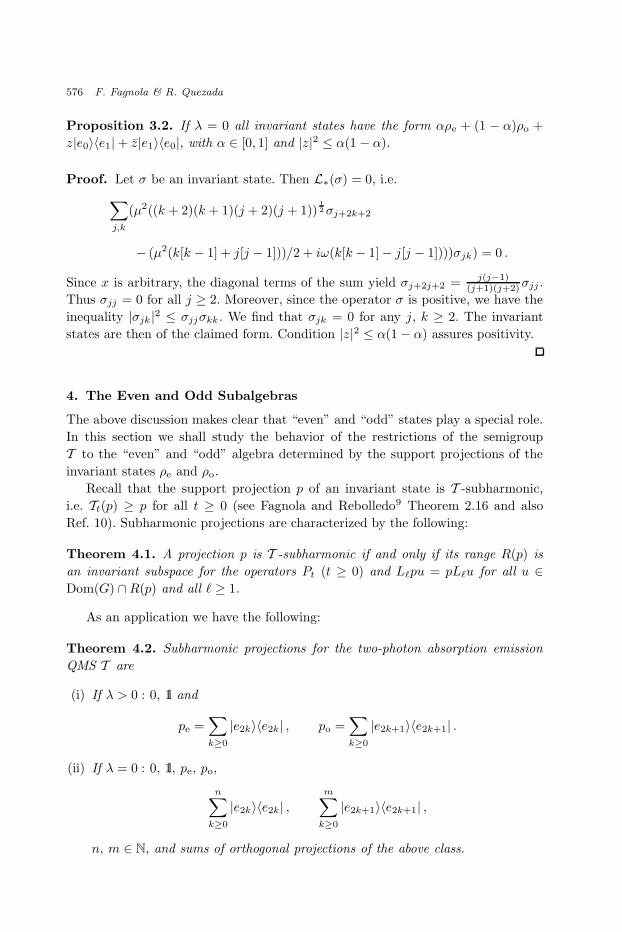
Proposition 3.2. If λ = 0 all invariant states have the form αρe + (1 − α)ρo +
z|e0〉〈e1| + z|e1〉〈e0|, with α ∈ [0, 1] and |z|2 ≤ α(1 − α).
Proof. Let σ be an invariant state. Then L∗(σ) = 0, i.e.
∑
j,k
(µ2((k + 2)(k + 1)(j + 2)(j + 1))1
2 σj+2k+2
− (µ2(k[k − 1] + j[j − 1]))/2 + iω(k[k − 1] − j[j − 1])))σjk) = 0 .
Since x is arbitrary, the diagonal terms of the sum yield σj+2j+2 = j(j−1)(j+1)(j+2)σjj .
Thus σjj = 0 for all j ≥ 2. Moreover, since the operator σ is positive, we have the
inequality |σjk |2 ≤ σjjσkk . We find that σjk = 0 for any j, k ≥ 2. The invariant
states are then of the claimed form. Condition |z|2 ≤ α(1 − α) assures positivity.
4. The Even and Odd Subalgebras
The above discussion makes clear that “even” and “odd” states play a special role.
In this section we shall study the behavior of the restrictions of the semigroup
T to the “even” and “odd” algebra determined by the support projections of the
invariant states ρe and ρo.
Recall that the support projection p of an invariant state is T -subharmonic,
i.e. Tt(p) ≥ p for all t ≥ 0 (see Fagnola and Rebolledo9 Theorem 2.16 and also
Ref. 10). Subharmonic projections are characterized by the following:
Theorem 4.1. A projection p is T -subharmonic if and only if its range R(p) is
an invariant subspace for the operators Pt (t ≥ 0) and L`pu = pL`u for all u ∈Dom(G) ∩ R(p) and all ` ≥ 1.
As an application we have the following:
Theorem 4.2. Subharmonic projections for the two-photon absorption emission
QMS T are
(i) If λ > 0 : 0, 1l and
pe =∑
k≥0
|e2k〉〈e2k| , po =∑
k≥0
|e2k+1〉〈e2k+1| .
(ii) If λ = 0 : 0, 1l, pe, po,
n∑
k≥0
|e2k〉〈e2k| ,m∑
k≥0
|e2k+1〉〈e2k+1| ,
n, m ∈ N, and sums of orthogonal projections of the above class.

November 9, 2005 11:49 WSPC/102-IDAQPRT 00211
Two-Photon Absorption and Emission Process 577
In both cases the projections pe and po are T -invariant and the hereditary sub-
algebras Ae = peApe, the even subalgebra, and Ao = poApo, the odd subalgebra, are
T -invariant.
Proof. Any invariant subspace of a normal compact operator is generated by eigen-
vectors (e.g. by Theorem 4, p. 272 in Ref. 19). The operators (Pt)t≥0 are clearly
compact and normal, and all the ek’s are eigenvectors. Therefore any invariant
subspace IK is generated by a collection {ek : k ∈ K} where K ⊂ N.
Assume λ > 0. If K contains only even (resp. odd) numbers, then IK is invariant
under L1 = µa2 and L2 = λa+2 if and only if K contains all the even (resp. odd)
numbers. On the other hand, if K contains at least an odd and an even number, it
is clear that IK is invariant under L1 and L2 if and only if it coincides with h.
If λ = 0 and K contains only even (resp. odd) numbers, then the action of
a2pK (pK denotes the projection onto IK) moves the indices two places backward,
while pKa2pK moves the indices two places backward and kills the smallest index.
Therefore IK is invariant under L1 if and only if K is finite of the form K =
{0, 2, . . . , 2n} (resp. {1, 3, . . . , 2m + 1}) with n ≥ 1, or K coincides with N, 2N or
2N + 1.
This proves (i) and (ii). Moreover, a simple and straightforward computation
yields L−(po) = L−(pe) = 0. Therefore, by Lemma 1.1, p. 563 of Ref. 8, both po and
pe belong to the domain of L and we have Tt(po) = po, Tt(pe) = pe.
Finally, for all self-adjoint x ∈ B(h), we have
−‖x‖pe = Tt(−‖x‖pe) ≤ Tt(pexpe) ≤ Tt(‖x‖pe) = ‖x‖pe .
It follows that Tt(pexpe) belongs to Ae for all t ≥ 0. By decomposing an arbitrary
x ∈ B(h) into its self-adjoint and anti-self-adjoint parts we find that Tt(Ae) ⊆ Ae
for all t ≥ 0. The invariance of Ao is proved in the same way.
Denote by T e and T o the restrictions of T to Ae and Ao, respectively.
In the remaining part of this section we establish the asymptotic behavior of T e
and T o. To this end first recall the following results (see Frigerio and Verri11,13):
Theorem 4.3. Let S be a QMS on a von Neumann algebra A with a faithful
normal invariant state ω and let F(S), N (S) be the von Neumann subalgebras of
A
F(S) = {x ∈ A|St(x) = x, ∀ t ≥ 0} ,
N (S) = {x ∈ A|St(x∗x) = St(x
∗)St(x),St(xx∗) = St(x)St(x∗), ∀ t ≥ 0} .
Then:
(i) F(S) is contained in N (S),
(ii) if F(S) = N (S), then limt→∞ S∗t(σ) exists for all normal state σ on A,
(iii) if F(S) = C 1l, then ω is the unique S-invariant state,

November 9, 2005 11:49 WSPC/102-IDAQPRT 00211
578 F. Fagnola & R. Quezada
(iv) if N (S) = F(S) = C 1l, then limt→∞ S∗t(σ) = ω for all normal state σ
on A.
The following result by Fagnola and Rebolledo,8,9 allows us to determine easily
F(T e), F(T o), N (T e) and N (T o) and apply Theorem 4.3.
Theorem 4.4. Suppose that both minimal QDS T associated with the operators
G, L` and T associated with the operators G∗, L` are Markov. Moreover, suppose
that there exists D ⊂ h dense which is a common core for G and G∗ such that the
sequence (nG∗(n − G)−1)u)n≥1 converges for all u ∈ D. Then N (T ) = {Lk, L∗k :
k ≥ 1}′ and F(T ) = {H, Lk, L∗k : k ≥ 1}′.
Here the {X1, X2, . . .}′ denotes the generalized commutator of the (possibly
unbounded) operators X1, X2, . . .. This is the subalgebra of B(h) of all the operators
y such that yXk ⊆ Xky (i.e. Dom(Xk) ⊆ Dom(Xky) and yXku = Xkyu for all
u ∈ Dom(Xk)) for all k ≥ 1.
We can now prove the main result of this section
Theorem 4.5. Let T e (resp. T o) be the restriction of the QMS T to the subalgebra
Ae (resp. Ao). Then N (T e) = N (T e) = C 1l (resp. N (T o) = N (T o) = C 1l). It
follows that, for any even state σe on Ae (resp. odd state σo on Ao), we have
limt→∞
T e∗t(σe) = ρe , lim
t→∞T o∗t(σo) = ρo .
Proof. Let us prove that N (T e) = C 1l. The proof of N (T o) = C 1l is identical. If
x ∈ N (T e) is a self-adjoint operator we have that xmn = 0 for all odd m, n ≥ 0.
Moreover, if a2x ⊂ xa2 and a+2x ⊂ xa+2, after simple computations we obtain
((2m)!)1
2 〈e2m, xe2n〉 = 〈e0, a2mxen〉 = 〈e0, xa2men〉 = 0
for all n < m. Being self-adjoint, this proves that x is diagonal. Now for any m,
n ≥ 0 after direct computations we obtain
(2m + 2)1
2 (2m + 1)1
2 x2m+22n = 〈e2m, a2xe2n〉
= 〈e2m, xa2e2n〉 = (2n − 1)1
2 (2n)1
2 x2m2n−2 ,
hence with n = m + 1 we obtain that x2n2n = x2n−22n−2 for all n ≥ 1. This proves
that x is a multiple of the identity operator. For a general element x ∈ N (T e) we
can use its decomposition as a linear combination of self-adjoint operators both in
N (T e). Then we have that F(T e) = N (T e) = C 1l. The conclusion follows then
from Theorem 4.3(iv).
5. Detailed Balance
A QMS T with a faithful normal invariant state ρ satisfies the quantum detailed
balance condition introduced by Frigerio, Gorini, Kossakowski and Verri12 if there
exists another QMS T such that
tr(ρyTt(x)) = tr(ρTt(y)x)

November 9, 2005 11:49 WSPC/102-IDAQPRT 00211
Two-Photon Absorption and Emission Process 579
for all x, y ∈ B(h). The QMS T , in our case, is the QMS associated with G∗, L1,
L2 therefore it has the same generator as T up to the sign of ω. In particular, for
all x ∈ M, the generators satisfy
L(x) − L(x) = 2iω[a+2a2, x] . (5.1)
In this section we shall prove that the two-photon absorption and emission QMS
with λ > 0 satisfies the quantum detailed balance with respect to any invariant state
ρα = αρe + (1 − α)ρo , α ∈ ]0, 1[ . (5.2)
Indeed, we will show that, for all θ ∈ [0, 1], x, y ∈ B(h), we have
tr(ρ1−θα yρθ
αTt(x)) = tr(ρ1−θα Tt(y)ρθ
αx) . (5.3)
The identity (5.1) follows from a simple algebraic computation. However, since
we do not know whether M is an essential domain for both L and L, or even if
these operators have a common essential domain we cannot deduce (5.3) directly
from (5.1). In order to circumvent this difficulty we associate with our QMS certain
semigroups on the Hilbert space L2(h) of Hilbert–Schmidt operators on h endowed
with the scalar product 〈y, x〉 = tr(y∗x). For each ρα with α ∈ ]0, 1[ define the
embedding of B(h) into L2(h),
ι : B(h) → L2(h) , ι(x) = ρθ
2
αxρ1−θ
2
α .
The map ι is an injective contraction with a dense range and it is a completely
positive map for θ = 1/2. We now define T αt (ι(x)) = ι(Tt(x)) for every t ≥ 0 and
x ∈ B(h). The operators T αt can be extended to the whole L2(h) and they define
a unique strongly continuous contraction semigroup T α = (T αt )t≥0 on L2(h) (see
Carbone,5 Theorem 2.0.3). Moreover, if Lα is the infinitesimal generator of T α,
then ι(D(L)) is contained in the domain of Lα and
Lα(
ρθ
2
αxρ1−θ
2
α
)
= ρθ
2
αL(x)ρ1−θ
2
α
for every x in the domain D(L) of L. Notice that T α∗t (ρ
1
2
α) = ρ1
2
α for t ≥ 0, indeed
tr(ρ1
2
αT αt (ι(x))) = tr(ραTt(x)) = tr(ραx) = tr(ρ
1
2
α ι(x)) ,
for all x ∈ B(h). The generator Lα is characterized as follows.
Proposition 5.1. The linear manifold ι(M) is contained in the domain of Lα and
is a core for Lα.
Proof. The linear manifold M is contained in the domain of L, thus the weak∗
limit for t → 0+ of t−1(Tt(x) − x) exists. Exploiting this fact it is easy to check
that, for each x ∈ M, the weak limit of t−1(T αt (ι(x)) − ι(x)) for t → 0+ exists. It
follows that ι(x) belongs to the domain of Lα.

November 9, 2005 11:49 WSPC/102-IDAQPRT 00211
580 F. Fagnola & R. Quezada
In order to show that ι(M) is a core for Lα we construct a sequence Lαn (n ≥ 1)
of bounded approximations such that, calling Mn the submanifold of M generated
by the |ej〉〈ek| with 0 ≤ j, k ≤ 2n, we have
Lαn(ι(Mn)) ⊆ ι(Mn+1) , ‖(Lα − Lα
n)|ι(Mn)‖ ≤ 8λµn .
Then, since Lα is dissipative and closed as the generator of a contraction semigroup,
it follows from Theorem 3.1.34, p. 193 of Ref. 4 that ι(M) = ∪n≥1ι(Mn) is a core
for Lα.
For each n ≥ 1 we denote by Nn the bounded approximation of the number
operator N ∧ (2n) of the number operator defined by truncation, i.e. Nnek = kek
for k ≤ 2n and Nnek = 2nek for k > 2n. Let an, a+n be the bounded approximations
of creation and annihilation operators
an = S∗N1/2n , a+
n = N1/2n S .
Let Ln be the approximated Lindblad generator defined as in (2.1) replacing a and
a+ by an and a+n . The operator Ln is bounded and, moreover, L(Mn) is contained
in Mn+1 for all n ≥ 1. A straightforward computation shows that, for all x ∈ Mn,
we have
Lα(ι(x)) − Lαn(ι(x)) = µ2ρ
θ
2
α (a+2xa2 − a+2n xa2
n)ρ1−θ
2
α .
Since x =∑
0≤j,k≤2n xjk |ej〉〈ek|, the operator a+2xa2 − a+2n xa2
n can be written as
2n∑
j=2n−1
2n−2∑
k=0
xjk((k + 1)(k + 2))1/2(((j + 1)(j + 2))1/2 − 2n)|ej+2〉〈ek+2|
+
2n∑
k=2n−1
2n−2∑
j=0
xjk((j + 1)(j + 2))1/2(((k + 1)(k + 2))1/2 − 2n)|ej+2〉〈ek+2|
+
2n∑
j=2n−1
2n∑
k=2n−2
xjk(((j + 1)(j + 2)(k + 1)(k + 2))1/2 − 4n2)|ej+2〉〈ek+2| .
Then the elementary inequalities,∣
∣((k + 1)(k + 2))1/2(((j + 1)(j + 2))1/2 − 2n)∣
∣ ≤ 2(3n + 1) ,∣
∣((j + 1)(j + 2)(k + 1)(k + 2))1/2 − 4n2∣
∣ ≤ 2(3n + 1)
for 2n − 1 ≤ j, k ≤ 2n lead to the estimate∥
∥
∥ρθ
2
α (a∗2xa2 − a∗2n xa2
n)ρ1−θ
2
α
∥
∥
∥
2
2≤ 4ν2(3n + 1)2‖ι(x)‖2
2 .
Now, since 2(3n+1) ≤ 8n for n ≥ 1, we can apply Theorem 3.1.34, p. 193 of Ref. 4
to conclude.
Starting from T , we can define in the same way T α and Lα by T αt (ρ
1−θ
2
α xρθ
2
α ) =
ρ1−θ
2
α Tt(x)ρθ
2
α . The linear manifold ι(M) is also a core for Lα (Lα and Lα differ only
by the sign of ω).
November 9, 2005 11:49 WSPC/102-IDAQPRT 00211
Two-Photon Absorption and Emission Process 581
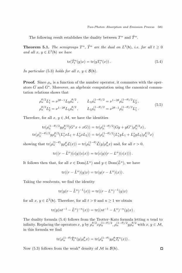
The following result establishes the duality between T α and T α.
Theorem 5.1. The semigroups T α, T α are the dual on L2(h), i.e. for all t ≥ 0
and all x, y ∈ L2(h) we have
tr(T αt (y)x) = tr(yT α
t (x)) . (5.4)
In particular (5.3) holds for all x, y ∈ B(h).
Proof. Since ρα is a function of the number operator, it commutes with the oper-
ators G and G∗. Moreover, an algebraic computation using the canonical commu-
tation relations shows that
ρθ/2α L∗
1 = ν2θ−1L2ρθ/2α , L1ρ
(1−θ)/2α = ν1−2θρ
(1−θ)/2α L∗
2 ,
ρθ/2α L∗
2 = ν1−2θL1ρθ/2α , L1ρ
(1−θ)/2α = ν2θ−1ρ
(1−θ)/2α L∗
1 .(5.5)
Therefore, for all x, y ∈ M, we have the identities
tr(ρ(1−θ)/2α yρθ/2
α (G∗x + xG)) = tr(ρ(1−θ)/2α (Gy + yG∗)ρθ/2
α x) ,
tr(ρ(1−θ)/2α yρθ/2
α (L∗1xL1 + L∗
2xL2)) = tr(ρ(1−θ)/2α (L∗
1yL1 + L∗2yL2)ρ
θ/2α x)
showing that tr(ρ(1−θ)α yρθ
αL(x)) = tr(ρ(1−θ)α L(y)ρθ
αx) and, for all r > 0,
tr((r − Lα)(ι(y))ι(x)) = tr(ι(y)(r − Lα)(ι(x))) .
It follows then that, for all x ∈ Dom(Lα) and y ∈ Dom(Lα), we have
tr((r − Lα)(y)x) = tr(y(r − Lα)(x)) .
Taking the resolvents, we find the identity
tr(y(r − Lα)−1(x)) = tr((r − Lα)−1(y)x)
for all x, y ∈ L2(h). Therefore, for all t > 0 and n ≥ 1 we obtain
tr(y(nt−1 − Lα)−n(x)) = tr((nt−1 − Lα)−n(y)x) .
The duality formula (5.4) follows from the Trotter–Kato formula letting n tend to
infinity. Replacing the operators x, y by ρθ/2α xρ
(1−θ)/2α , ρ
(1−θ)/2α yρ
θ/2α with x, y ∈ M,
in this formula we find
tr(ρ(1−θ)α T α
t (y)ρθαx) = tr(ρ(1−θ)
α yρθαT α
t (x)) .
Now (5.3) follows from the weak* density of M in B(h).

November 9, 2005 11:49 WSPC/102-IDAQPRT 00211
582 F. Fagnola & R. Quezada
6. Characterization of the Invariant States for λ > 0
In this section we show that ρe and ρo determine all invariant states of T . Indeed,
we prove the following
Theorem 6.1. If λ > 0, then all invariant states of T are convex linear combina-
tions of ρe and ρo.
Let σ a fixed normal T -invariant state and let (σjk)j,k≥0 be its matrix elements
in the canonical orthonormal basis. As a first step we show that the diagonal part
of σ has the desired form.
Lemma 6.1. Let σ be a normal T -invariant state. Then we have
peσpe = tr(σpe)ρe , poσpo = tr(σpo)ρo . (6.1)
As a consequence, the diagonal part σd =∑
j σjj |ej〉〈ej | of σ is given by
σd = tr(σpe)ρe + tr(σpo)ρo .
Moreover, we have the inequalities |σjk | ≤ c(σ, ν)ν(j+k)/2 for all j, k, with c(σ, ν)
constant depending only on σ, ν.
Proof. We know from Theorem 4.5 that
w∗ − limt→∞
T et (pexpe) = tr(ρex)pe , w∗ − lim
t→∞T o
t (poxpo) = tr(ρox)po
for any x ∈ B(h) since Ae (resp. Ao) is the dual of states supported in pe (resp. po).
By the invariance of σ we have then
tr(σpexpe) = tr(σTt(pexpe)) = limt→∞
tr(σT et (pexpe)) = tr(ρex)tr(σpe) .
In the same way we find tr(σpoxpo) = tr(ρox)tr(σpo). Therefore, since x is arbitrary,
we obtain (6.1).
The positivity of σ implies |σjk |2 ≤ σjjσkk for all j, k. Therefore, since the
diagonal part of σ is a convex combination of ρe and ρo, the last claim follows.
We are now in a position to prove Theorem 6.1.
Proof of Theorem 6.1. Let σ be a T -invariant state. Then L∗(σ) = 0. Writing
σ =∑
j,k≥0 σjk |ej〉〈ek| we find
L∗(σ) =∑
j,k≥0
|ej〉〈ek|{
iω(k[k − 1] − j[j − 1])σjk − µ2
2(k[k − 1] + j[j − 1])σjk
+ µ2(k + 1)1
2 (k + 2)1
2 (j + 1)1
2 (j + 2)1
2 σj+2k+2
+ λ2k1
2 [k − 1]1
2 j1
2 [j − 1]1
2 σj−2k−2
− λ2
2((j + 1)(j + 2) + (k + 1)(k + 2))σjk)
}

November 9, 2005 11:49 WSPC/102-IDAQPRT 00211
Two-Photon Absorption and Emission Process 583
with the understanding that [k − 1] = max{(k − 1), 0}, [j − 1] = max{(j − 1), 0}.We shall prove that σjk = 0 for all j 6= k. Clearly, since σ is hermitian, it suffices
to check that σjk = 0 for all j > k. Letting j = k + n, with n ≥ 1, the identity
L∗(σ) = 0 yields
0 = −iωn(2k + n − 1)σk+n,k − µ2(k[k − 1] + (k + n)(k + n − 1))σk+n,k
−λ2((k + 1)(k + 2) + (k + n + 1)(k + n + 2))σk+nk
+ 2µ2(k + 1)1
2 (k + 2)1
2 (k + n + 1)1
2 (k + n + 2)1
2 σk+n+2k+2
+ 2λ2k1
2 [k − 1]1
2 (k + n)1
2 (k + n − 1)1
2 σk+n−2k−2
for all k, n ≥ 0. Fix n and put yk = ν−k/2σk+nk . Notice that the sequence (yk)k≥0
is square summable because, by Lemma 6.1, |yk| ≤ c(σ, ν)ν(k+n)/2. Multiplying by
yk, summing on k and taking the real part, the above equation reads as
0 = −µ2∑
k≥0
k[k − 1]|yk|2 − µ2∑
k≥0
(k + n)(k + n − 1)|yk|2
+ 2λµ Re∑
k≥0
(k + 1)1
2 (k + 2)1
2 (k + n + 1)1
2 (k + n + 2)1
2 ykyk+2
−λ2∑
k≥0
(k + 1)(k + 2)|yk|2 − λ2∑
k≥0
(k + n + 1)(k + n + 2)|yk|2
+ 2λµ Re∑
k≥0
k1
2 [k − 1]1
2 (k + n)1
2 (k + n − 1)1
2 ykyk−2
= −µ2n(n − 1)|y0|2 − µ2n(n + 1)|y1|2
−µ2∑
k≥2
k[k − 1]|yk|2 − µ2∑
k≥0
(k + n + 1)(k + n + 2)|yk+2|2
+ 2λµ Re∑
k≥0
(k + 1)1
2 (k + 2)1
2 (k + n + 1)1
2 (k + n + 2)1
2 ykyk+2
−λ2∑
k≥0
(k + 1)(k + 2)|yk|2 − λ2∑
k≥2
(k + n − 1)(k + n)|yk−2|2
+ 2λµ Re∑
k≥2
k1
2 [k − 1]1
2 (k + n)1
2 (k + n − 1)1
2 ykyk−2 .
Reconstructing a square from the three sums for k ≥ 0 and another from the three
sums on k ≥ 2 we find
0 = −µ2n(n − 1)|y0|2 − µ2n(n + 1)|y1|2
−∑
k≥0
∣
∣
∣λ(k + 1)
1
2 (k + 2)1
2 yk − µ(k + n + 1)1
2 (k + n + 2)1
2 yk+2
∣
∣
∣
2

November 9, 2005 11:49 WSPC/102-IDAQPRT 00211
584 F. Fagnola & R. Quezada
−∑
k≥2
∣
∣
∣λ(k + n − 1)1
2 (k + n)1
2 yk−2 − µk1
2 [k − 1]1
2 yk
∣
∣
∣
2
= −µ2n(n − 1)|y0|2 − µ2n(n + 1)|y1|2
−∑
k≥0
∣
∣
∣λ(k + 1)1
2 (k + 2)1
2 yk − µ(k + n + 1)1
2 (k + n + 2)1
2 yk+2
∣
∣
∣
2
−∑
k≥0
∣
∣
∣λ(k + n + 1)1
2 (k + n + 2)1
2 yk − µ(k + 2)1
2 (k + 1)1
2 yk+2
∣
∣
∣
2
.
Now, for n > 1, this implies y0 = y1 = 0 and then, by induction yk = 0 for all
k ≥ 0. If n = 1 then y1 = 0 and yk = 0 for all odd k’s by induction. Moreover, if
the two sums of squares are 0, then
yk+2 = ν(k + 1)1
2 (k + 3)−1
2 yk , yk+2 = ν(k + 1)−1
2 (k + 3)1
2 yk
for all k ≥ 0. This can happen only if yk = 0. Therefore σ is diagonal.
7. Approach to Equilibrium
In this section we study convergence of states T∗t(σ) towards an invariant state and
determine the domains of attraction of the invariant states. As a first step, with
the notation of Sec. 4, we prove the following.
Lemma 7.1. Suppose λ > 0. Then F(T ) = N (T ).
Proof. The QMS T has a faithful normal invariant state. Therefore the inclusion
F(T ) ⊆ N (T ) always holds. It suffices then to prove the opposite.
By Theorem 4.4 we have N (T ) = {a2, a+2}′ and F(T ) = {a2, a+2, a+2a2}′. A
x ∈ N (T ), satisfies then a2x ⊆ xa2 and a+2x ⊆ xa+2. It follows that
(a+2a2)x = a+2(a2x) ⊆ a+2(xa2) = (a+2x)a2 ⊆ (xa+2)a2 = x(a+2a2) .
Therefore x belongs also to F(T ).
Proposition 7.1. Suppose λ > 0. Then, for any normal state σ, we have
limt→∞
T∗t(σ) = tr(σpe)ρe + tr(σpo)ρo .
Proof. With the same notation as in the proof of Theorem 6.1 write σ = ασe +
(1 − α)σo + σr, where σe = peσpe and σo = poσpo are the even and odd diagonal
parts of σ, α = tr(peσ) ∈ [0, 1] and σr is the off-diagonal part of σ.
By Lemma 7.1 and Theorem 4.3(ii) the family of states T∗t(σ) converges to an
invariant state σ∞, which is diagonal, σ∞ = γρe + (1 − γ)ρo say, by Theorem 6.1.
Therefore by Theorem 4.5 and the Tt-invariance of pe we have
γ = tr(pe(γρe +(1−γ)ρo)) = limt→∞
tr(peT∗t(ασe +(1−α)σo +σr)) = αtr(peσe) = α .
November 9, 2005 11:49 WSPC/102-IDAQPRT 00211
Two-Photon Absorption and Emission Process 585
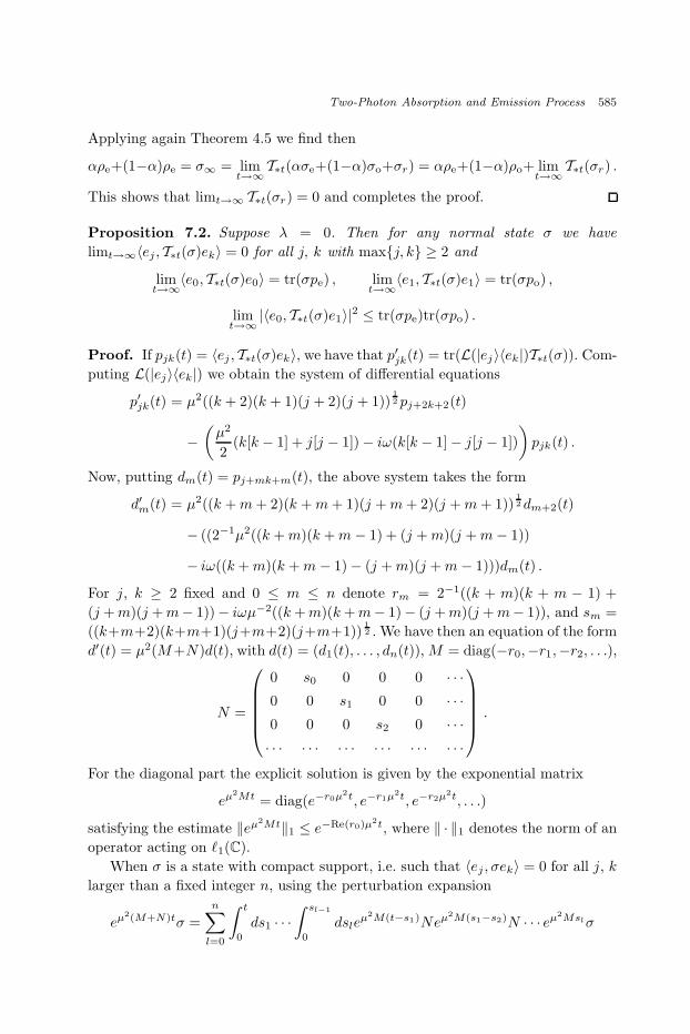
Applying again Theorem 4.5 we find then
αρe+(1−α)ρe = σ∞ = limt→∞
T∗t(ασe+(1−α)σo+σr) = αρe+(1−α)ρo+ limt→∞
T∗t(σr) .
This shows that limt→∞ T∗t(σr) = 0 and completes the proof.
Proposition 7.2. Suppose λ = 0. Then for any normal state σ we have
limt→∞〈ej , T∗t(σ)ek〉 = 0 for all j, k with max{j, k} ≥ 2 and
limt→∞
〈e0, T∗t(σ)e0〉 = tr(σpe) , limt→∞
〈e1, T∗t(σ)e1〉 = tr(σpo) ,
limt→∞
|〈e0, T∗t(σ)e1〉|2 ≤ tr(σpe)tr(σpo) .
Proof. If pjk(t) = 〈ej , T∗t(σ)ek〉, we have that p′jk(t) = tr(L(|ej〉〈ek|)T∗t(σ)). Com-
puting L(|ej〉〈ek|) we obtain the system of differential equations
p′jk(t) = µ2((k + 2)(k + 1)(j + 2)(j + 1))1
2 pj+2k+2(t)
−(
µ2
2(k[k − 1] + j[j − 1]) − iω(k[k − 1] − j[j − 1])
)
pjk(t) .
Now, putting dm(t) = pj+mk+m(t), the above system takes the form
d′m(t) = µ2((k + m + 2)(k + m + 1)(j + m + 2)(j + m + 1))1
2 dm+2(t)
− ((2−1µ2((k + m)(k + m − 1) + (j + m)(j + m − 1))
− iω((k + m)(k + m − 1) − (j + m)(j + m − 1)))dm(t) .
For j, k ≥ 2 fixed and 0 ≤ m ≤ n denote rm = 2−1((k + m)(k + m − 1) +
(j + m)(j + m− 1))− iωµ−2((k + m)(k + m− 1)− (j + m)(j + m− 1)), and sm =
((k+m+2)(k+m+1)(j+m+2)(j+m+1))1
2 . We have then an equation of the form
d′(t) = µ2(M+N)d(t), with d(t) = (d1(t), . . . , dn(t)), M = diag(−r0,−r1,−r2, . . .),
N =
0 s0 0 0 0 · · ·0 0 s1 0 0 · · ·0 0 0 s2 0 · · ·· · · · · · · · · · · · · · · · · ·
.
For the diagonal part the explicit solution is given by the exponential matrix
eµ2Mt = diag(e−r0µ2t, e−r1µ2t, e−r2µ2t, . . .)
satisfying the estimate ‖eµ2Mt‖1 ≤ e−Re(r0)µ2t, where ‖ · ‖1 denotes the norm of an
operator acting on `1(C).
When σ is a state with compact support, i.e. such that 〈ej , σek〉 = 0 for all j, k
larger than a fixed integer n, using the perturbation expansion
eµ2(M+N)tσ =
n∑
l=0
∫ t
0
ds1 · · ·∫ sl−1
0
dsleµ2M(t−s1)Neµ2M(s1−s2)N · · · eµ2Mslσ

November 9, 2005 11:49 WSPC/102-IDAQPRT 00211
586 F. Fagnola & R. Quezada
we obtain the estimate ‖e(M+N)t‖1 ≤ e−Re(r0)µ2t∑n
l=0(l!)−1(‖N‖1t)
l. Since
Re(r0) > 0, it follows that 〈ej , T∗t(σ)ek〉 → 0 as t → ∞, for any j, k ≥ 2. For
an arbitrary σ the conclusion follows by approximation with a compact support σ.
Now let us consider the matrix elements 〈ej , T∗t(σ)ek〉 with 0 ≤ j, k ≤ 1. By
Theorem 4.2 the subalgebras Ae and Ao are T -invariant. Therefore for a compactly
supported σe (since λ = 0 the support of T∗t(σe) is contained in that of σe for all
t ≥ 0) we have then
limt→∞
〈e0, T e∗t(σe)e0〉 = 1 − lim
t→∞
∑
k≥2
〈ek, T e∗t(σe)ek〉 = 1 .
This fact also holds for an arbitrary σe by approximation in trace norm
with a compact support σe. Moreover, in the same way we can prove that
limt→∞〈e1, T o∗t(σo)e1〉 = tr(σo) = 1.
Given an arbitrary σ we can write the decomposition σ = ασe + (1−α)σo + σr
with α = tr(σpe). It follows that
limt→∞
〈e0, T∗t(σ)e0〉 = α limt→∞
〈e0, T e∗t(σe)e0〉 = α ,
and limt→∞〈e1, T∗t(σ)e1〉 = (1 − α) limt→∞〈e1, T o∗t(σo)e1〉 = 1 − α. For the off-
diagonal terms we find ddt〈e0, T∗t(σ)e1〉 = 2
√3〈e2, T∗t(σ)e3〉, then, for all t, s > 0
|〈e0, (T∗t − T∗s)(σ)e1〉| ≤ 2√
3
∫ t
s
|〈e2, T∗τe3〉|adτ ≤ 2√
3(e−ksp(s) − e−ktp(t)) ,
where p is a polynomial and k a positive constant. Therefore there exists the limit
z = limt→∞〈e0, T∗t(σ)e1〉 and |z|2 ≤ α(1 − α), by positivity of limt→∞ T∗t(σ).
Proposition 7.3. Suppose λ = 0. The attraction domain of the invariant state
ρα,z = α|e0〉〈e0| + (1 − α)|e1〉〈e1| + z|e0〉〈e1| + z|e1〉〈e0| ,with |z|2 ≤ α(1 − α) is given by
D(ρα,z) =
σ = (σjk)|α =∑
m≥0
σ2m2m , z =∑
m≥0
c2m
√2m + 1σ2m2m+1
,
where c2m = 2−2m (2m)!m! Πm
j=1(j − iωµ2 )−1.
Proof. With the notation in the proof of Proposition 7.2 let θm(t) =√m + 1pmm+1(t), then θm satisfies the following differential equation
θ′m(t) = µ2(m + 2)(m + 1)θm+2(t) − (µ2m2 − 2iωm)θm(t) .
Since λ = 0, the linear manifold M is T∗t-invariant. Thus we can define for
σ ∈ M the function f(σ, t) =∑
m≥0 c2mθ2m(t), where c2m are coefficients to be
determined. We have that
f ′(σ, t) =∑
m≥0
(µ2c2m(2m + 2)(2m + 1) − c2m+2(µ2(2m + 2)2 − 4iω(m + 1)))θ2m ,
November 9, 2005 11:49 WSPC/102-IDAQPRT 00211
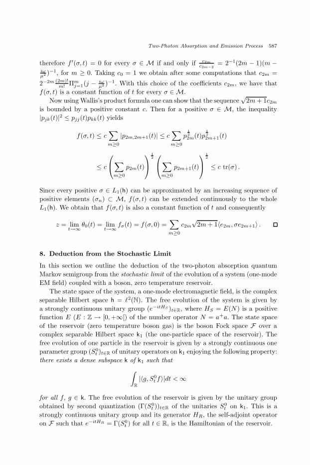
Two-Photon Absorption and Emission Process 587
therefore f ′(σ, t) = 0 for every σ ∈ M if and only if c2m
c2m−2
= 2−1(2m − 1)(m −iωµ2 )−1, for m ≥ 0. Taking c0 = 1 we obtain after some computations that c2m =
2−2m (2m)!m! Πm
j=1(j − iωµ2 )−1. With this choice of the coefficients c2m, we have that
f(σ, t) is a constant function of t for every σ ∈ M.
Now using Wallis’s product formula one can show that the sequence√
2m + 1c2m
is bounded by a positive constant c. Then for a positive σ ∈ M, the inequality
|pjk(t)|2 ≤ pjj(t)pkk(t) yields
f(σ, t) ≤ c∑
m≥0
|p2m,2m+1(t)| ≤ c∑
m≥0
p1
2
2m(t)p1
2
2m+1(t)
≤ c
∑
m≥0
p2m(t)
1
2
∑
m≥0
p2m+1(t)
1
2
≤ c tr(σ) .
Since every positive σ ∈ L1(h) can be approximated by an increasing sequence of
positive elements (σn) ⊂ M, f(σ, t) can be extended continuously to the whole
L1(h). We obtain that f(σ, t) is also a constant function of t and consequently
z = limt→∞
θ0(t) = limt→∞
fσ(t) = f(σ, 0) =∑
m≥0
c2m
√2m + 1〈e2m, σe2m+1〉 .
8. Deduction from the Stochastic Limit
In this section we outline the deduction of the two-photon absorption quantum
Markov semigroup from the stochastic limit of the evolution of a system (one-mode
EM field) coupled with a boson, zero temperature reservoir.
The state space of the system, a one-mode electromagnetic field, is the complex
separable Hilbert space h = `2(N). The free evolution of the system is given by
a strongly continuous unitary group (e−itHS )t∈R, where HS = E(N) is a positive
function E (E : Z → [0, +∞[) of the number operator N = a+a. The state space
of the reservoir (zero temperature boson gas) is the boson Fock space F over a
complex separable Hilbert space k1 (the one-particle space of the reservoir). The
free evolution of one particle in the reservoir is given by a strongly continuous one
parameter group (S0t )t∈R of unitary operators on k1 enjoying the following property:
there exists a dense subspace k of k1 such that
∫
R
|〈g, S0t f〉|dt < ∞
for all f, g ∈ k. The free evolution of the reservoir is given by the unitary group
obtained by second quantization (Γ(S0t ))t∈R of the unitaries S0
t on k1. This is a
strongly continuous unitary group and its generator HR, the self-adjoint operator
on F such that e−itHR = Γ(S0t ) for all t ∈ R, is the Hamiltonian of the reservoir.

November 9, 2005 11:49 WSPC/102-IDAQPRT 00211
588 F. Fagnola & R. Quezada
The evolution of the whole system is given by the unitary group generated by
the total Hamiltonian
Hλ = HS ⊗ 1F + 1S ⊗ HR + λV ,
where λ is a real positive parameter and V is an interaction operator such that Hλ
is self-adjoint for all λ > 0.
Suppose that the interaction operator (of dipole type) has the form
Vg = i(ad ⊗ A∗(g) − a+d ⊗ A(g)) ,
where d ∈ N∗, A(g), A∗(g) are creation and annihilation operators on F with g ∈ k1.
A straightforward computation using the commutation relations
eitE(N)ad = adeitE(N−d)
shows that generalized rotating wave approximation
eitHSade−itHS = e−iω0tad ,
where ω0 > 0 (see Ref. 3, Definition 4.10.1 on p. 125) holds, with ω0 = E(n− d)−E(n) for all n ∈ N if and only if E is linear. This is the case, for example, when
HS = a+a.
Suppose that the generalized rotating wave approximation holds. The sesquilin-
ear form on k
(f |g) :=
∫
R
〈g, S0t f〉dt
is positive (see Ref. 3). Therefore it defines a pre-scalar product on k. We denote
by K the Hilbert space obtained by quotient and completion; the scalar product
will be denoted by (·|·). Defining
U(λ)t = eitH0e−itHλ
a straightforward computation shows that the family of unitaries (U(λ)t )t≥0 on h⊗F
satisfies the differential equation
d
dtU
(λ)t = −iλVg(t)U
(λ)t , U
(λ)0 = 1l ,
where Vg(t) = i(D ⊗ A∗(Stg) − D∗ ⊗ A(Stg)) and St = eitω0S(0)t .
Let W (f) (f ∈ k1) denote the unitary Weyl operators on F acting on exponen-
tial vectors as
W (f1)e(f2) = e−‖f1‖2/2−〈f1,f2〉e(f1 + f2) .
The basic idea of Accardi, Frigerio and Lu1 was to study the result of small
interactions (λ → 0) on a large time scale (time goes to infinity). This was realized
by scaling time by λ2 and space by λ and letting λ tend to 0. As a result of the
limiting procedure, the state space of the whole system also changes.
The following result allows us to find the structure of the space of the limit
evolution.
November 9, 2005 11:49 WSPC/102-IDAQPRT 00211
Two-Photon Absorption and Emission Process 589
Proposition 8.1. For all n, n′ ∈ N and all f1, . . . , fn, f ′1, . . . , f
′n′ ∈ K,
s1, t1, . . . , sn, tn, s′1, t′1, . . . , s
′n′ , t′n′ ∈ R with sk ≤ tk, s′k ≤ t′k for all k denote
W (f1, . . . , fn) = W
(
λ
∫ λ−2t1
λ−2s1
Sr1f1dr1
)
· · ·W(
λ
∫ λ−2tn
λ−2sn
Srnfndrn
)
.
We have then
limλ→0
〈W (f1, . . . , fn)0, W (f ′1, . . . , f
′n)0〉
= 〈W (f1 ⊗ 1[s1,t1]) · · ·W (fn ⊗ 1[sn,tn])0 ,
W (f ′1 ⊗ 1[s′
1,t′
1]) · · ·W (f ′
n′ ⊗ 1[s′
n′,t′
n′])e(0)〉 ,
where W (f1 ⊗ 1[s1,t1]), . . . , W (f ′n′ ⊗ 1[sn′ ,tn′ ]) are Weyl operators in the boson Fock
space over L2(R+;K).
It follows that the state space of the limit evolution is the tensor product of the
initial space h with the boson Fock space Γ(L2(R+;K)). The limit of unitaries is
given in the following theorem.
Theorem 8.1. For all v, u ∈ h, n, n′ ∈ N and all f1, . . . , fn, f ′1, . . . , f
′n′ ∈ K, s1,
t1, . . . , sn, tn, s′1, t′1, . . . , s′n′ , t′n′ ∈ R with sk ≤ tk, s′k ≤ t′k we have
limλ→0
〈vW (f1, . . . , fn)e(0), U(λ)
λ−2tuW (f ′1, . . . , f
′n)e(0)〉
= 〈W (f1 ⊗ 1[s1,t1]) · · ·W (fn ⊗ 1[sn,tn])e(0) ,
UtuW (f ′1 ⊗ 1[s′
1,t′
1]) · · ·W (f ′
n′ ⊗ 1[s′
n′,t′
n′])e(0)〉 ,
where U is the unique unitary process satisfying the quantum stochastic differential
equation on h ⊗ Γ(L2(R+;K))
dUt = (addA∗t (g) − a+ddAt(g) − (g|g)−a+daddt)Ut , U0 =1l
with (g|g)− =∫ 0
−∞〈g, Stg〉dt. Moreover, for all x ∈ B(h), we have
limλ→0
〈vW (f1, . . . , fn)e(0), U(λ)∗λ−2t(x⊗ 1lF)U
(λ)λ−2tuW (f ′
1, . . . , f′n)e(0)〉
= 〈W (f1 ⊗ 1[s1,t1]) · · ·W (fn ⊗ 1[sn,tn])e(0) ,
U∗t (x⊗ 1lF)UtuW (f ′
1 ⊗ 1[s′
1,t′
1]) · · ·W (f ′
n′ ⊗ 1[s′
n′,t′
n′])e(0)〉 .
As a consequence, applying results on quantum stochastic differential equations
and quantum flows in Ref. 7, we have
Theorem 8.2. Suppose that HS = a+a. Then the quantum dynamical semigroup
of the quantum flow
jt(x) = U∗t (x⊗ 1lF )Ut
is the minimal quantum dynamical semigroup associated with
L−(x) = −(g|g)−a+dadx + 2 Re(g|g)−a+dxad − (g|g)−xa+dad .
November 9, 2005 11:49 WSPC/102-IDAQPRT 00211
590 F. Fagnola & R. Quezada
Several of the above assumptions (rotating wave approximation, boundedness
of D, . . .) can be removed or weakened. Moreover, other reservoirs and other types
of interaction can be studied. In particular, for d = 2, the stochastic limit of the
above system coupled with a boson reservoir at positive temperature leads to the
model introduced in Sec. 2. We refer to Ref. 3 for the proof.
Acknowledgments
The authors want to thank L. Accardi and J. C. Garcıa for several stimulat-
ing discussions. The financial support from the project Mexico-Italia “Dinamica
Estocastica”, the EU RTN Network “Quantum Probability with Applications to
Physics, Information Theory and Biology” and the Grant 37491-E of CONACYT-
Mexico, are gratefully acknowledged.
References
1. L. Accardi, A. Frigerio and Y. G. Lu, The weak coupling limit as a quantum functionalcentral limit, Commun. Math. Phys. 131 (1990) 537–570.
2. L. Accardi and S. Kozyrev, Lectures on quantum interacting particle systems, Quan-
tum Interacting Particle Systems, eds. L. Accardi and F. Fagnola (World Scientific,2002), p. 1–195.
3. L. Accardi, Y. G. Lu and I. Volovich, Quantum Theory and Its Stochastic Limit
(Springer-Verlag, 2002).4. O. Bratteli and D. W. Robinson, Operator Algebras and Quantum Statistical Mechan-
ics I (Springer-Verlag, 1979).5. R. Carbone, Exponential ergodicity of some quantum Markov semigroups, Ph.D. The-
sis, Universita degli Studi di Milano, 1–93 (2000).6. R. Carbone and F. Fagnola, Exponential L
2-convergence of quantum Markov semi-groups on B(h), Math. Notes 68 (2000) 452–463.
7. F. Fagnola, Quantum Markov semigroups and quantum Markov flows, Proyecciones
18 (1999) 1–144.8. F. Fagnola and R. Rebolledo, The approach to equilibrium of a class of quantum
dynamical semigroups, Inf. Dim. Anal. Quantum Probab. Rel. Topics 1 (1998) 561–572.
9. F. Fagnola and R. Rebolledo, Lectures on the qualitative analysis of quantum Markovsemigroups, Quantum Interacting Particle Systems, QP–PQ: Quantum Probab. WhiteNoise Anal., Vol. 14 (World Scientific, 2002).
10. F. Fagnola and R. Rebolledo, Subharmonic projections for a quantum Markov semi-group, J. Math. Phys. 43 (2002) 1074–1082.
11. A. Frigerio, Quantum dynamical semigroups and approach to equilibrium, Lett. Math.
Phys. 2 (1977) 79–87.12. A. Frigerio, A. Kossakowski, V. Gorini and M. Verri, Quantum detailed balance and
KMS condition, Commun. Math. Phys. 57 (1977) 97–110.13. A. Frigerio and M. Verri, Long-time asymptotic properties of dynamical semigroups
on W∗-algebras, Math. Z. 180 (1982) 275–286.
14. J. C. Garcıa and R. Quezada, Hille–Yosida estimate and nonconservativity criteriafor quantum dynamical semigroups, Inf. Dim. Anal. Quantum Probab. Rel. Topics 7
(2004) 383–394.
November 9, 2005 11:49 WSPC/102-IDAQPRT 00211
Two-Photon Absorption and Emission Process 591
15. L. Gilles and P. L. Knight, Two-photon and nonclassical states of light, Phys. Rev. A
48 (1993) 1582–1593.16. W. Kaiser and C. G. B. Garret, Two-photon Exitation in CaF2:Eu
2+, Phys. Rev.
Lett. 7 (1961) 229–231.17. M. Goppert-Mayer, Uber Elementarakte mit zwei Quantensprungen, Ann. Physics 9
(1931) 273–294.18. M. Reed and B. Simon, Methods of Modern Mathematical Physics, Vol. II, Fourier
Analysis, Selfadjointness (Academic Press, 1975).19. J. Wermer, On invariant subspaces of normal operators, Proc. Amer. Math. Soc. 3
(1952) 270–277.