Liquid Crystal Polarization Rotator (LCPR) calibration
Gerardo Capobianco, Luca Zangrilli, Silvano Fineschi
Report nr. 73 18-10-2005
Technical Report nr. 73 - LCPR Calibration 2
Index Abstract…………………………………………………………………………………………………………………….4 1. Introduction............................................................................................................................................................... 5 2. Set-up used for tests .................................................................................................................................................. 6 2.1 Light source ................................................................................................................................................................. 6 2.2 Monochromator and spectrograph ............................................................................................................................... 6 2.3 Optical power meter and Detector ............................................................................................................................... 7 2.4 Polarimetrics components............................................................................................................................................ 7 2.5 Setup and its preparation .............................................................................................................................................. 7 3. Data acquisition and data analysis............................................................................................................................. 9 4. Comparison with data supplied from the manufacturer .......................................................................................... 17 5. Results..................................................................................................................................................................... 18 Appendix A – Meadowlark D2040 voltage calibration test......................................................................................... 19 A.1 Introduction............................................................................................................................................................... 19 A.2 Set-up for voltage calibration tests............................................................................................................................ 19 A.3 Data acquisition and data analysis ............................................................................................................................ 20 A.4 Results ....................................................................................................................................................................... 25 Appendix B – Set-up Equipment Data Sheets .............................................................................................................. 26 B.1 Light source .............................................................................................................................................................. 26 B.2 Monochromator and Spectrograph............................................................................................................................ 27 B.3 Detector and Optical Power Meter............................................................................................................................ 29 B.4 Linear Polarizer......................................................................................................................................................... 31 B.5 LCPR ........................................................................................................................................................................ 32 Bibliography.................................................................................................................................................................... 33
Index of figure Figure 1-1-1 - Operation of Liquid Crystal Polarization Rotator showing complete rotation of a linearly polarized input
beam [1]. .................................................................................................................................................................... 5 Figure 2-5-1 - Outline of the set-up for the measure of the rotation of the LCPR in function of the applied voltage and
the wavelength. ........................................................................................................................................................... 8 Figure 3-1 - Luminous intensity in function of the voltage applied to LCPR at 5000 Å. .................................................... 9 Figure 3-2 - Luminous intensity in function of the voltage applied to LCPR at 5300 Å. .................................................... 9 Figure 3-3 - Luminous intensity in function of the voltage applied to LCPR at 6330 Å. .................................................. 10 Figure 3-4 – Rotation in function of the voltage applied to LCPR at 5000 Å. .................................................................. 10 Figure 3-5 - Rotation in function of the voltage applied to LCPR at 5300 Å.................................................................... 11 Figure 3-6 - Rotation in function of the voltage applied to LCPR at 6330 Å.................................................................... 11 Figure 3-7 - Rotation in function of the voltage applied to LCPR at different wavelengths. ............................................ 12 Figure 3-8 - Rotation in function of the voltage applied (0-1300mV) to LCPR at different wavelengths........................ 13 Figure 3-9 - Rotation in function of the voltage applied (1300-3100mV) to LCPR at different wavelengths.................. 13 Figure 3-10 - Rotation in function of the voltage applied (3000-10000mV) to LCPR at different wavelengths. ............. 14 Figure 3-11 - Rotation in function of the voltage applied to LCPR at 500 nm……………………………………………….15 Figure 3-12 - Rotation in function of the voltage applied to LCPR at 530 nm……………………………………………….15 Figure 3-13 - Rotation in function of the voltage applied to LCPR at 633 nm……………………………………………….16 Figure 3-14 - Rotation in function of the voltage applied for different wavelengths…………………………………...…….16 Figure 3-15 - Rotation in function of wavelength for different voltages………………………………………………………..17 Figure 4-1 – MLO Voltage-Rotation curve comparated with curve that we obtained. ..................................................... 17 Figure A-1-1 –Meadowlark D2040 voltage output........................................................................................................... 19 Figure A-2-1 – Set-up used for D2040 voltage calibration tests. ................................................................................... 20 Figure A-3-1 – Vout in ideal case (green curve) and in real case (red curve)................................................................... 22 Figure A-3-2 – Amplification coefficient in function of Vset…………………………………………………………………….23 Figure A-3-3 – Voffset in function of Vset. …………………………………..…………………………………………………….23 Figure A-3-4 – Voffset in function of Vset and relative fit…………………………………………………………………………..24 Figure B-1-1 – Spectral irradiance at 0.5m for light source ORIEL 6333 [2]................................................................. 26 Figure B-1-2 - Spectral irradiance at 0.5 m from the 6333 100 W QTH Lamp at different voltages. The lamp is rated for
100 W at 12 V [2] . ................................................................................................................................................... 26 Figure B-2-1 – Outline of the monochromator and spectrograph Lot Oriel MS257TM with our accessories [2]............ 28 Figure B-2-2 – Monochromator and spectrograph Lot Oriel MS257TM with our accessories [2]. ................................. 28

Technical Report nr. 73 - LCPR Calibration 3
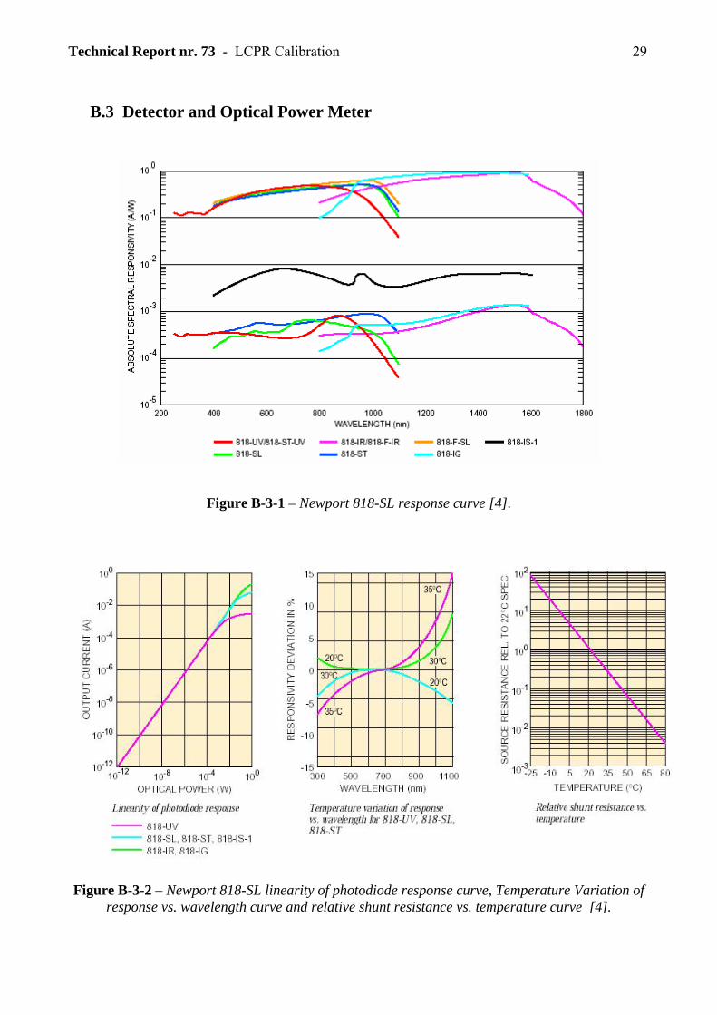
Figure B-3-1 – Newport 818-SL response curve [4]. ....................................................................................................... 29 Figure B-3-2 – Newport 818-SL linearity of photodiode response curve, Temperature Variation of response vs. wavelength curve and relative shunt resistance vs. temperature curve [4]…………………………………………………...29
Figure B-3-3 –Detector Specifications [4]…………………………………………………………………………………………30
Figure B-3-4 – Optical power meter Newport 1830-C with detector [4]……………....……………………………………...30
Figure B-3-5 – Optical Power Meter Specifications [4]………………………………………………………………………... 31
Figure B-4-1 – MLO Linear Polarizer Transmission curve [1]…………………………………………………………………31
Figure B-5-1 – MLO LCPR Specifications [1]…………………………………………………………………………………….32
Index of table Tab. 2-5-1 – Set-up properties 8 Tab. 5-1 – Best fit parameters at different wavelength 18
Tab. A-3-1 - −+ /
outV for Vset = 0V, 1V, 1.5V, 3V, 5V and 10V. 20
Tab. A-3-2 - −+ /
outV for Vset = 0.5V, 1.1V, 1.2V, 1.3V, 3.5V and 4V. 21
Tab. A-3-3 - −+ /
outV and relative error for every Vset. *We estimate strumental error equal to 10 mV. When standard deviation is less than this value, we assuming the error equal to10 mV. 21
Tab. A-3-4 – Amplification, offsetV and relative errors for every Vset. 22
Tab. B-2-1 – Monochromator Specifications 27
Technical Report nr. 73 - LCPR Calibration 4
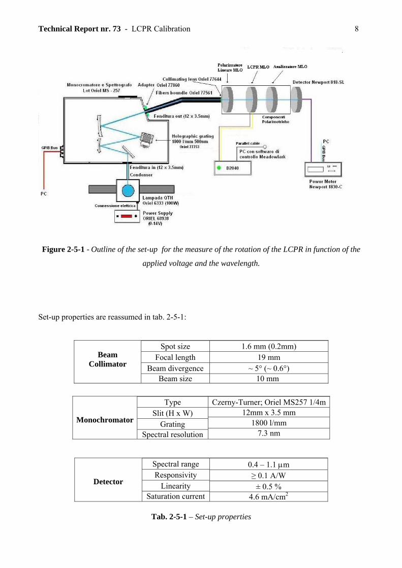
Abstract This technical report describes the preliminary tests on the chromatic polararization response of
the Meadowlark (MLO) Liquid Crystal Polarization Rotator (LCPR). The rotation of input linear
polarization as function of bias voltage has been measured at 500, 530 and 633 nm. The results
show that the MLO LCPR has a more stable and less chromatic response for bias voltage > 2500
mV.

Technical Report nr. 73 - LCPR Calibration 5
1. Introduction
The Liquid Crystal Polarization Rotator (LCPR) rotates electro-optically the polarization direction
of a linearly polarized input beam. The design consists of a Liquid Crystal Variable Retarder
(LCVR) whose birifrangence changes as a function of the applied potential bias, combined with a
zero order polymer quarter-wave retarder (fig. 1-1). The fast axes of the two retarders are 45° apart.
The linear polarize acting as output analyzer must be parallel to the quarter wave retarder slow axis.
Polarization rotation is achieved by electrically controlling the retardance of the LCVR. There is no
mechanical motion. The quarter-wave retarder converts elliptical polarization formed by the Liquid
Crystal Variable Retarder into linear polarization. The rotation angle is equal to half the retardance
change in the LCVR. Polarization purity is defined as the ratio of the rotated linear component to
the orthogonal component. A selected rotation is very sensitive to applied voltage and operating
temperature. On average, polarization purity, or contrast ratio is better than 150:1 [1].
Figure 1-1-1 - Operation of Liquid Crystal Polarization Rotator showing complete rotation of a
linearly polarized input beam [1].
The goal of our measurements has been the characterization of the LCPR Meadowlark Optics LPR-
200-VIS-DP-TSO (C001094, 01-288) as a function of the applied voltage, at different wavelengths.
The setup will be described in the next chapter. The control voltage control and temperature setting
of the LCPR are done through a digital controller, the Meadowlark D2040, programmable through
PC. In the tests, the control software supplied by Meadowlark Optics has been used. Temperatures
as not been monitored. Detailed information on the LCPR can be found in the official
documentation of the Meadowlark Optics [ 1 ].

Technical Report nr. 73 - LCPR Calibration 6
2. Set-up used for tests In this section we describe the setup used for the measurements carried out in date 16-12-2004 at
the Optical Laboratory of the Turin Astronomical Observatory (OATo).
2.1 Light source The source is an quartz-tungsten halogen lamp (QTH). In particular, the light source model is the
Oriel Photomax 6333, 100 W. This types of light sources are popular visible and near infrared
sources because of their smooth spectral curve and stable output. They do not have the sharp
spectral peaks that arc lamps exhibit, and they emit little UV radiation. QTH lamps use a doped
tungsten filament inside a quartz envelope. They are filled with a rare gas and a small amount of
halogen. Current flowing through the filament heats the tungsten to >3000 K. The filaments of this
light sources are dense planar structures for highest image brightness. The white light produced
radiates through the clear quartz envelope. In Appendix B.1 is reported the spectral irradiance for
this light source at 0.5m and the spectral irradiance from 250 to 500 nm for the 6333 100 W lamp at
different voltages. (The filament plane was parallel to the slit of the radiometer for maximum
irradiance.) As voltage is reduced, total output is reduced and the peak wavelength shifts only
slightly to the red. The output at a wavelength in the blue end of the spectrum can change
significantly with a slight change in voltage [2]. The lamp’s power supply is the Thermo Oriel
68938 with a voltage output from 0 to 14V. For other information see [2].
2.2 Monochromator and spectrograph A monochromator is used to select a spectral band or one determined frequency of the
electromagnetic spectrum. The monochromator’s type is a Czerny-Turner, model Lot Oriel
MS257TM. We report in figure B-2-1 the outline of this instrument. See Appendix B.2 for details.
During our tests, the wavelength selection was made with a LabVIEW1-based software piloting the
instrument through IEEE-488 interface.
For our measures, we used 12mm x 3.5mm slits and a 1800 l/mm grating (Lot-Oriel 77753).
Spectral resolution is ~73Å. The monochromator settings are summarized in Tab. 2-5-1.
1 LabVIEW is a development tool produced from National Instruments [3].

Technical Report nr. 73 - LCPR Calibration 7
2.3 Optical power meter and Detector Optical power meter is used for data acquisition. The model is a Newport 1830-C. Newport 1830-C
is a digital power meter with 0.1 pW resolution, used through IEEE-488 interface and controlled
with an acquisition system that realized in LabVIEW. The detector is a silicon diode Newport
(Newport 818-SL). The response curve is shown in figure B.3-1 (green curve). Additional
information are available in [4] and in Appendix B.3. The detector properties are summarized in
Tab. 2-5-1.
2.4 Polarimetric components Polarimetric components used for this tests are:
• 1 linear polarizer;
• 1 analyzer.
Both are supplied by Meadowlark Optics [1]. Appendix B.4 shows the transmission curve for the
linear polarizer.
2.5 Setup and its preparation The set-up used for the tests it is outlined in figure 2-5-1. The lamp focused the light on the entrance slit of the monochromator. A particular frequency is
selected. A fiber optic bundle from the exit slit feeds a collimator to illuminate the polarimetric
components of the set-up: the linear polarizer, then the LCPR and finally the linear analyzer, in
front of detector. The measured intensity follows the Malus law:
)]([cos20 VII Φ=
from which:
⎟⎟⎠
⎞⎜⎜⎝
⎛=Φ
0
arccos)(IIV (E.1)
where I is the value of read luminous intensity, I0 its maximum and Φ(V) the relative rotation.
Technical Report nr. 73 - LCPR Calibration 8
Figure 2-5-1 - Outline of the set-up for the measure of the rotation of the LCPR in function of the
applied voltage and the wavelength.
Set-up properties are reassumed in tab. 2-5-1:
Tab. 2-5-1 – Set-up properties
Beam
Collimator
Spot size Focal length
Beam divergence Beam size
1.6 mm (0.2mm) 19 mm
~ 5° (~ 0.6°) 10 mm
Monochromator
Type Slit (H x W)
Grating Spectral resolution
Czerny-Turner; Oriel MS257 1/4m 12mm x 3.5 mm
1800 l/mm 7.3 nm
Detector
Spectral range Responsivity
Linearity Saturation current
0.4 – 1.1 µm ≥ 0.1 A/W
± 0.5 % 4.6 mA/cm2

Technical Report nr. 73 - LCPR Calibration 9
3. Data acquisition and data analysis For three different wavelengths (5000, 5300 and 6330 Å), the intensity as a function of the voltage
applied to the LCPR has been measured. The lamps power at 8.5V is 60W. The slit width of the
monochromator was set at 3,5 millimetres.
The data acquired are plotted in the figures 3-1, 3-2 and 3-3.
Intensity vs Voltage at 500 nm
0,0000
0,0050
0,0100
0,0150
0,0200
0,0250
0 1000 2000 3000 4000 5000 6000 7000 8000 9000 10000
Voltage (mV)
Intensity (nW)
Figure 3-1 - Luminous intensity in function of the voltage applied to LCPR at 5000 Å.
Intensity vs Voltage at 530 nm
0,0000
0,0050
0,0100
0,0150
0,0200
0,0250
0,0300
0,0350
0,0400
0,0450
0 1000 2000 3000 4000 5000 6000 7000 8000 9000 10000
Voltage (mV)
Intensity (nW)
Figure 3-2 - Luminous intensity in function of the voltage applied to LCPR at 5300 Å.

Technical Report nr. 73 - LCPR Calibration 10
Intensity vs Voltage at 633 nm
0,0000
0,0100
0,0200
0,0300
0,0400
0,0500
0,0600
0,0700
0 1000 2000 3000 4000 5000 6000 7000 8000 9000 10000
Voltage (mV)
Intensity (nW)
Figure 3-3 - Luminous intensity in function of the voltage applied to LCPR at 6330 Å.
From the equation (E.1), the values of rotation in function of the voltage have been derived. The
results are plotted in figures 3-4, 3-5, and 3-6.
LCPR Rotation vs Voltage at 500 nm
-50
0
50
100
150
200
250
300
350
0 1000 2000 3000 4000 5000 6000 7000 8000 9000 10000
Voltage (mV)
Rotation (deg)
Figure 3-4 – Rotation in function of the voltage applied to LCPR at 5000 Å.

Technical Report nr. 73 - LCPR Calibration 11
LCPR Rotation vs Voltage at 530 nm
0
50
100
150
200
250
300
350
0 1000 2000 3000 4000 5000 6000 7000 8000 9000 10000Voltage (mV)
Rotation (deg)
Figure 3-5 - Rotation in function of the voltage applied to LCPR at 5300 Å.
LCPR Rotation vs Voltage at 633nm
0
50
100
150
200
250
300
350
0 1000 2000 3000 4000 5000 6000 7000 8000 9000 10000Voltage (mV)
Rotation (deg)
Figure 3-6 - Rotation in function of the voltage applied to LCPR at 6330 Å.

Technical Report nr. 73 - LCPR Calibration 12
The error bars in the rotation diagrams, have been obtained by error propagation, according to the
formula:
⎟⎟⎠
⎞⎜⎜⎝
⎛ ∆+
∆
⎥⎦
⎤⎢⎣
⎡+
=∆Φ0
0
0
0
12)(
II
II
II
II
V (E. 2)
Note that the error is inversely proportional to the luminous intensity. Therefore in the points of
low intensity, the error will be greater. Figure 3-7 shows the LCPR response curves for all three
wavelengths.
LCPR Rotation vs Voltage
-50
0
50
100
150
200
250
300
350
0 2000 4000 6000 8000 10000
Voltage (mV)
Rotation (deg)
500 nm530 nm633 nm
Figure 3-7 - Rotation in function of the voltage applied to LCPR at different wavelengths.
We can divide the response curve in 3 regions: the first one (from 0 to approximately 1300 mV)
where the rotation is approximately constant for varying voltage (fig. 3-8), the second region (1300
to approximately 3100 mV) where the rotation follows a logarithmic behavior (fig. 3-9) and a third
region, beyond the 3000 mV, where the rotation flattens, for large voltages (fig. 3-10). Therefore
the sensibility of the LCPR will be greater in the central region where, for small variations of the
voltage applied correspond large rotations. The third region shows more achromaticity. In figure
3-8, it can be noticed that for the curve at 633 nm, the error bars for 1000, 1100 and 1200 mV are

Technical Report nr. 73 - LCPR Calibration 13
much larger than those in all other points. This is probably due, to an error in the data
transcription.
LCPR Rotation vs Voltage
-50
0
50
100
150
200
250
300
350
0 100 200 300 400 500 600 700 800 900 1000 1100 1200 1300
Voltage (mV)
Rotation (deg)
500 nm530 nm633 nm
Figure 3-8 - Rotation in function of the voltage applied (0-1300mV) to LCPR at different wavelengths.
LCPR Rotation vs Voltage
0
50
100
150
200
250
300
350
1300 1600 1900 2200 2500 2800 3100Voltage (mV)
Rotation (deg)
500 nm530 nm633 nm
Figure 3-9 - Rotation in function of the voltage applied (1300-3100mV) to LCPR at different wavelengths.

Technical Report nr. 73 - LCPR Calibration 14
LCPR Rotation vs Voltage
200
220
240
260
280
300
320
340
3000 4000 5000 6000 7000 8000 9000 10000Voltage (mV)
Rotation (deg)
500 nm530 nm633 nm
Figure 3-10 - Rotation in function of the voltage applied (3000-10000mV) to LCPR at different wavelengths.
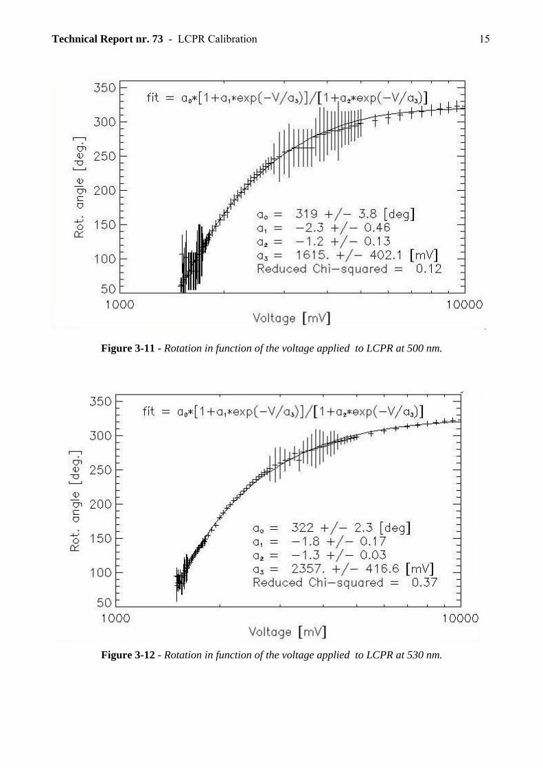
For every wavelength and for voltage values > 1500 mV, the data can be fit with a ‘logistic curve’.
The expression of this curve is given by:
⎟⎟⎠
⎞⎜⎜⎝
⎛ −⋅+
⎟⎟⎠
⎞⎜⎜⎝
⎛ −⋅+
⋅=Φ
32
31
0
exp1
exp1
aVa
aVa
a (E.3)
The fits are shown in figs: 3-11, 3-12 and 3-13:
Technical Report nr. 73 - LCPR Calibration 15
Figure 3-11 - Rotation in function of the voltage applied to LCPR at 500 nm.
Figure 3-12 - Rotation in function of the voltage applied to LCPR at 530 nm.

Technical Report nr. 73 - LCPR Calibration 16
Figure 3-13 - Rotation in function of the voltage applied to LCPR at 633 nm.
Figure 3-14 - Rotation in function of the voltage applied for different wavelengths.
In figure 3-14, we plot the fits for different wavelengths. In this figure, blue line is referred to 500
nm wavelength, violet line to 530 nm and yellow line to 633 nm.
Technical Report nr. 73 - LCPR Calibration 17
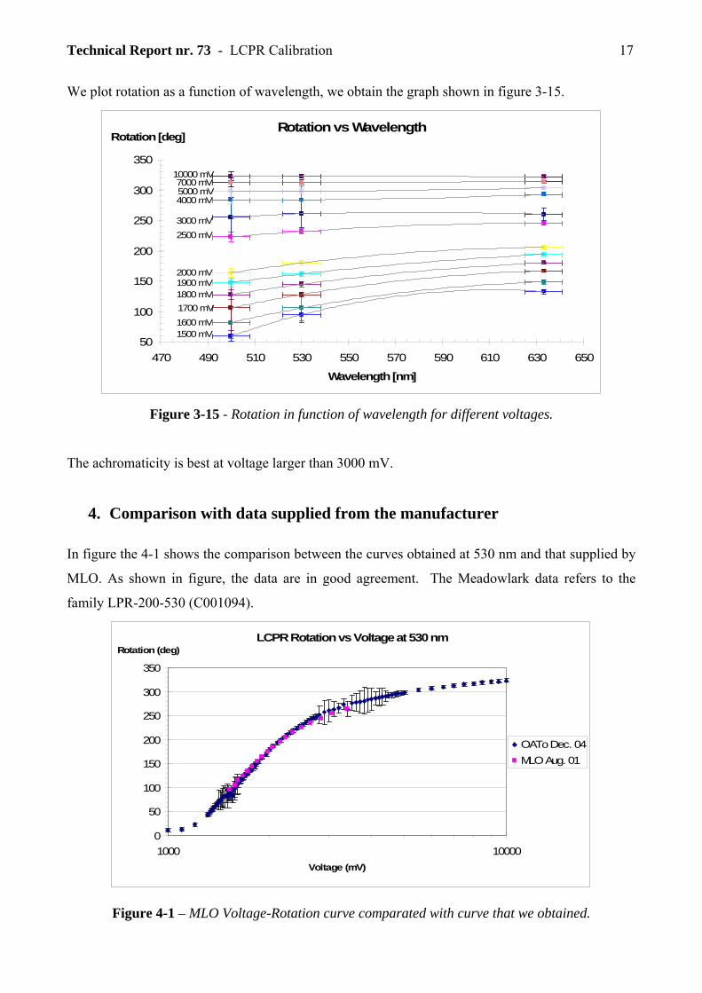
We plot rotation as a function of wavelength, we obtain the graph shown in figure 3-15.
Rotation vs Wavelength
1500 mV1600 mV1700 mV1800 mV1900 mV2000 mV
2500 mV3000 mV
4000 mV5000 mV7000 mV
10000 mV
50
100
150
200
250
300
350
470 490 510 530 550 570 590 610 630 650
Wavelength [nm]
Rotation [deg]
Figure 3-15 - Rotation in function of wavelength for different voltages.
The achromaticity is best at voltage larger than 3000 mV.
4. Comparison with data supplied from the manufacturer In figure the 4-1 shows the comparison between the curves obtained at 530 nm and that supplied by
MLO. As shown in figure, the data are in good agreement. The Meadowlark data refers to the
family LPR-200-530 (C001094).
LCPR Rotation vs Voltage at 530 nm
0
50
100
150
200
250
300
350
1000 10000Voltage (mV)
Rotation (deg)
OATo Dec. 04MLO Aug. 01
Figure 4-1 – MLO Voltage-Rotation curve comparated with curve that we obtained.

Technical Report nr. 73 - LCPR Calibration 18
5. Results From this preliminary analysis, we have characterized the LCPR response. In particular, at
different wavelengths, for voltages > 5000 mV, the rotation is weakly wavelength dependent [5].
The response curve is fit by logistic curve. This curves are defined by four parameters. The
parameters for the curves at three wavelengths measured are given in table 5-1. This curve is the
best fit for data distribution for voltages larger than 1500 mV. The 530 nm data are in good
agreement with MLO data.
a0 [deg] a1 a2 a3 [mV]
500 nm 319 ± 4 -2.3 ± 0.5 -1.2 ± 0.1 1615 ± 402
530 nm 322 ± 2 -1.8 ± 0.2 -1.3 ± 0.03 2357 ± 417
633 nm 320 ± 1 -1.8 ± 0.1 -1.2 ± 0.02 1872 ± 137
Tab. 5-1 – Best fit parameters at different wavelength.

Technical Report nr. 73 - LCPR Calibration 19
Appendix A – Meadowlark D2040 voltage calibration test
A.1 Introduction In this appendix we describe the Meadowlark (MLO) D2040 voltage calibration tests. D2040 is a
liquid crystal digital controller product from Meadowlark Optics [1] for LC-based optics driving. It
is programmable by parallel port and it has 2 outputs. The voltage output that is a BNC output and
the temperature output that is a 5 pin output. The voltage output set the LCVR voltage and the
temperature output read and set his temperature.
The voltage output is a square wave width 2kHz frequency and ± Vset voltage. If there is no signal
input, the voltage output has value 40Vp-p (Fig. A-1-1).
The voltage output has been measured with a digital oscilloscope for every voltage setting.
Figure A-1-1 –Meadowlark D2040 voltage output.
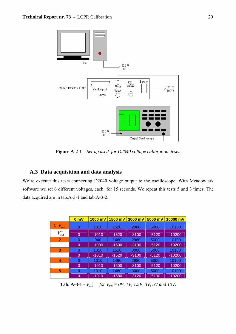
A.2 Set-up for voltage calibration tests The set-up used for voltage calibration tests is illustrated in Fig. A-2-1 and is comprised of:
• PC with operative system Windows 95 running in MS-DOS modality.
• Digital oscilloscope Tektronix TDS 3014.
• Meadowlark D2040 digital controller and MLO control software.
The D2040 voltage output is injected and sampled from digital oscilloscope. The temperature
control and monitoring is not connected.
Technical Report nr. 73 - LCPR Calibration 20
Figure A-2-1 – Set-up used for D2040 voltage calibration tests.
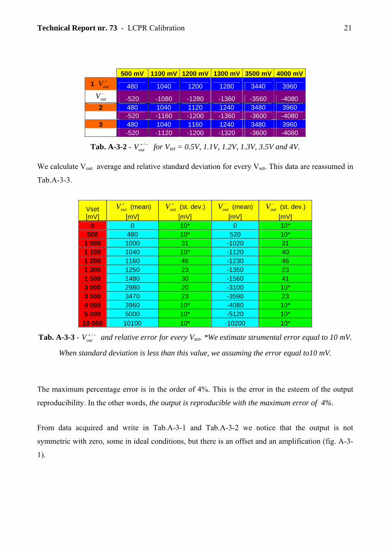
A.3 Data acquisition and data analysis We’re execute this tests connecting D2040 voltage output to the oscilloscope. With Meadowlark
software we set 6 different voltages, each for 15 seconds. We repeat this tests 5 and 3 times. The
data acquired are in tab.A-3-1 and tab.A-3-2:
0 mV 1000 mV 1500 mV 3000 mV 5000 mV 10000 mV 1 +
outV 0 1010 1520 2960 5000 10100 −
outV 0 -1010 -1520 -3100 -5120 -10200 2 0 940 1460 2960 5000 10100 0 -1080 -1600 -3100 -5120 -10200 3 0 1010 1510 3000 5000 10100 0 -1010 -1520 -3100 -5120 -10200 4 0 1010 1460 2980 5000 10100 0 -1010 -1600 -3100 -5120 -10200 5 0 1010 1460 3000 5000 10100 0 -1010 -1580 -3120 -5100 -10200
Tab. A-3-1 - −+ /outV for Vset = 0V, 1V, 1.5V, 3V, 5V and 10V.
Technical Report nr. 73 - LCPR Calibration 21
500 mV 1100 mV 1200 mV 1300 mV 3500 mV 4000 mV 1 +
outV 480 1040 1200 1280 3440 3960 −
outV -520 -1080 -1280 -1360 -3560 -4080 2 480 1040 1120 1240 3480 3960 -520 -1160 -1200 -1360 -3600 -4080 3 480 1040 1160 1240 3480 3960 -520 -1120 -1200 -1320 -3600 -4080
Tab. A-3-2 - −+ /outV for Vset = 0.5V, 1.1V, 1.2V, 1.3V, 3.5V and 4V.
We calculate Vout average and relative standard deviation for every Vset. This data are reassumed in
Tab.A-3-3.
Vset [mV]
+outV (mean)
[mV]
+outV (st. dev.)
[mV]
−outV (mean)
[mV]
−outV (st. dev.)
[mV] 0 0 10* 0 10*
500 480 10* 520 10* 1 000 1000 31 -1020 31 1 100 1040 10* -1120 40 1 200 1160 46 -1230 46 1 300 1250 23 -1350 23 1 500 1480 30 -1560 41 3 000 2980 20 -3100 10* 3 500 3470 23 -3590 23 4 000 3960 10* -4080 10* 5 000 5000 10* -5120 10*
10 000 10100 10* -10200 10*
Tab. A-3-3 - −+ /outV and relative error for every Vset. *We estimate strumental error equal to 10 mV.
When standard deviation is less than this value, we assuming the error equal to10 mV.
The maximum percentage error is in the order of 4%. This is the error in the esteem of the output
reproducibility. In the other words, the output is reproducible with the maximum error of 4%.
From data acquired and write in Tab.A-3-1 and Tab.A-3-2 we notice that the output is not
symmetric with zero, some in ideal conditions, but there is an offset and an amplification (fig. A-3-
1).

Technical Report nr. 73 - LCPR Calibration 22
Figure A-3-1 – Vout in ideal case (green curve) and in real case (red curve).
The equations that describes −+ /outV are the follows:
offsetsetout VVAV +⋅=+ (E. 4)
offsetsetout VVAV −⋅−=− (E. 5)
where:
setVVVA
⋅−
=−+
2 is the amplification coefficient, and
2
−+ +=
VVVoffset is the offset.
In table A-3-4 we calculate Voffset and A for every Vset.
setV [mV] A Aσ
offsetV
[mV] Voffsetσ
[mV] 0 1,00 1,00 0 10
500 1,00 0,02 -20 10 1 000 1,01 0,03 -10 31 1 100 0,98 0,02 -40 25 1 200 1,00 0,04 -35 46 1 300 1,00 0,02 -50 23 1 500 1,01 0,02 -40 35 3 000 1,013 0,005 -60 15 3 500 1,009 0,007 -60 23 4 000 1,005 0,002 -60 10 5 000 1,012 0,002 -60 10
10 000 1,015 0,001 -50 10
Tab. A-3-4 – Amplification, offsetV and relative errors for every Vset.
Plotting A in function of Vset we obtain the fig. A-3-2 graph.

Technical Report nr. 73 - LCPR Calibration 23
Amplification vs Vset
0,95
0,97
0,99
1,01
1,03
1,05
0 1000 2000 3000 4000 5000 6000 7000 8000 9000 10000
Vset [mV]
A
Figure A-3-2 – Amplification coefficient in function of Vset.
We fit this data distribution with a constant (green line).
01.1=A (E. 6)
This is the law for amplification (A) in function of Vset. Plotting Voffset in function of Vset we obtain the fig. A-3-3 graph.
Offset vs Vset
-100
-80
-60
-40
-20
0
20
40
0 1000 2000 3000 4000 5000 6000 7000 8000 9000 10000
Vset [mV]
Voffset [mV]
Figure A-3-3 – Voffset in function of Vset. We execute the fit with ‘logistic curve’, that is the best fit for this data distribution. The expression of this curve is the follow:

Technical Report nr. 73 - LCPR Calibration 24
⎟⎠⎞⎜
⎝⎛−⋅+
⎟⎠⎞⎜
⎝⎛−⋅+
⋅=
32
31
0
exp1
exp1
aVa
aVa
aVset
set
offset
Fit is reported in fig.A-3-4 and the parameter of this fit with errors is the follows:
⎪⎪⎪
⎩
⎪⎪⎪
⎨
⎧
=
±=±=±=
±−=
200.0
9775976.82
5.016.557
23
2
1
0
rid
mVaaa
mVa
χ
Figure A-3-4 – Voffset in function of Vset and relative fit.
The low for Voffset in function of Vset is the follow:
)597/(
)597/(
exp21exp157 Vset
Vset
offsetV −
−
⋅+⋅+
⋅−= (E.7)
From E.4, E.5, E.6 and E.7, we obtain:
)597/(
)597/(/
exp21exp157)01.1( Vset
Vset
setout VV −
−−+
⋅+⋅+
⋅⋅±= m (E.8)

Technical Report nr. 73 - LCPR Calibration 25
A.4 Results
In conclusions, after MLO D2040 calibration tests, we rewrite the −+ /outV with E.8 equations. From
this equations is possible to estimate the real D2040 voltage output in function of Vset.
For 2500>setV mV, the exponential terms of E.7 is approximately zero, and E.8 become:
mVVV setout 57)01.1(/ m⋅±=−+
The voltage output is reproducible with a good approximation (less or equal to 4% of Vset).

Technical Report nr. 73 - LCPR Calibration 26
Appendix B – Set-up Equipment Data Sheets
B.1 Light source
Figure B-1-1 – Spectral irradiance at 0.5m for light source ORIEL 6333 [2].
Figure B-1-2 - Spectral irradiance at 0.5 m from the 6333 100 W QTH Lamp at different voltages.
The lamp is rated for 100 W at 12 V [2] .

Technical Report nr. 73 - LCPR Calibration 27
B.2 Monochromator and Spectrograph
Tab. B-2-1 – Monochromator Specifications

Technical Report nr. 73 - LCPR Calibration 28
Figure B-2-1 – Outline of the monochromator and spectrograph Lot Oriel MS257TM with our accessories [2].
Figure B-2-2 – Monochromator and spectrograph Lot Oriel MS257TM with our accessories [2].
Technical Report nr. 73 - LCPR Calibration 29
B.3 Detector and Optical Power Meter
Figure B-3-1 – Newport 818-SL response curve [4].
Figure B-3-2 – Newport 818-SL linearity of photodiode response curve, Temperature Variation of response vs. wavelength curve and relative shunt resistance vs. temperature curve [4].

Technical Report nr. 73 - LCPR Calibration 30
Figure B-3-3 –Detector Specifications [4].
Figure B-3-4 – Optical power meter Newport 1830-C with detector [4].

Technical Report nr. 73 - LCPR Calibration 31
Figure B-3-5 – Optical Power Meter Specifications [4].
B.4 Linear Polarizer
Figure B-4-1 – MLO Linear Polarizer Transmission curve [1].

Technical Report nr. 73 - LCPR Calibration 32
B.5 LCPR
Figure B-5-1 – MLO LCPR Specifications [1].

Technical Report nr. 73 - LCPR Calibration 33
Bibliography [1] Meadowlark Optics
Official web page:
http://www.meadowlark.com
[2] Lot Oriel Italia
Official web page:
http://www.lot-oriel.com
[3] National Instruments
Official web page:
http://www.ni.com
[4] Newport Corporation
Official web page:
http://www.newport.com [5] S. Fineschi et al.
KPol: liquid crystal polarimeter for K-corona observations from the SCORE coronagraph
Proc. of SPIE Vol. 5901 , 59011I, (2005)