TIMETABLE SCHEDULING USING RULE-BASED TECHNIQUE
FIFDIL MAR WAN
A report submitted in partial fulfilment of the requirements for the award
of the degree of Bachelor of Computer Technology (Software Engineering)
Faculty of Computer Systems & Software Engineering
University College of Engineering & Technology Malaysia
MARCH, 2005

ABSTRACT
Timetablmg is a problem of allocating a timeslot for all lectures, lab and tutorials
in the problem instances within a limited number of permitted timeslots, in such a way
that none of the specified hard constraints are violated. In addition to the hard constraints,
there are often many soft constraints which are desirable to satisfy. In this study, the
timetable scheduling for Faculty of Computer System & Software Engineering (FSKKP)
of University College of Engineering & Technology Malaysia (KUKTEM) has been
studied to develop new prototype software for generating timetable. Basically, FSKKP is
still using human power in generating its timetable instead of using timetable scheduling
software. Since the timetable is configured manually, it is time-consumed as well as it
needs extra human resources to manage it. The university has its own system for
generating timetable which involving all of the faculties, but it is still in maintenance for
perfecting and enhancement since it still has weaknesses. In this project development, the
prototype will be implemented with rule-based approach as the solution to overcome the
timetable constraints and rules. The success of implementation and development of this
project is expected to help in reducing the time consumed and human power in generating
timetable for FSKKP. Indeed, it is also expected to generate a well-developed timetable
which giving the best solution in overcome the timetabling constraints and rules of
FSKKP.
V

ABSTRAK
Penjadualan merupakan satu masalah untuk menyusun semua aktiviti
pembelajaran seperti kuliah, bengkel dan tutorial mengikut masa dan tempat seterusnya
kemudian dimuat dan disusunkan dalam bentuk jadual tanpa melanggar atau
mengindarkan kengkangan utama seperti kekangan universiti dan fakulti. Dalam kajian
mi, penyusunan jadual waktu bagi Fakulti Sistem Komputer & Kejuruteraan Perisian
(FSKKP) di Kolej Umversiti Kejuruteraan & Teknologi Malaysia (KUKTEM) telah
dikaji untuk tujuan pembangunan model perisian yang mampu menyusunjadual
pembelajaran dengan berkesan. Penyusunanjadual pembelajaran di FSKKP masih lagi
dijalankan secara manual di mana ianya memakan-masa yang lama dan menggunakan
banyak tenaga manusia. Orgamsasi KUKTEM telah pun mempunyai sistem untuk
menyusun jadual pembelajaran yang melibatkan semua fakulti di universiti tersebut.
Namun demikian, sistem tersebut masih lagi dalam proses pembaikan disebabkan masih
lagi mempunyai kelemahan. Dalam projek mi, model yang dibangunkan menggunakan
teknik pangkalan peraturan dalam melaksanakan aktiviti penjadualan. Daripada projek
mi, diharap ía dapat mengurangkan masa dan tenaga manusia untuk pembangunan jadual
pembelajaran di FSKKP yang merupakan masalah utama yang perlu diatasi. Dengan
pembangunan projek nit juga, diharap ia dapat membma jadual yang berkesan dengan
menitik beratkan kengkangan-kengkangan yang perlu diambil kira.
VI-
TABLE OF CONTENTS
VII
CHAPTER
1
2
TITLE PAGE
Title Page
Declaration of Originality and Exclusiveness ii
Dedication iii
Acknowledgement iv
Abstract V
Abstrak vi
Table of Contents vii
List of Figures ix
List of Abbreviations x
List of Appendices xi
INTRODUCTION 1
1.1 Introduction 1
1.2 Problem Statement 2
1.2.1 Current System 2
1.2.2 Current System's Process 2
1.3 Objectives 2
1.4 Scopes
LITERATURE REVIEW 4
2.1 Introduction 4
2.2 Methodology in Timetabling 5
2.2.1 Rule-Based Approach 5
2.2.2 Fuzzy Logic Approach 8
2.2.3 Genetic Algorithm Approach 10
2.3 Selected Technique 18
2.4 Common Constraints in Timetabling 19
2.4.1 The Rooms Problem 19
2.4.2 Pre-allocations or Pre-assignments 19
2.4.3 Unavailability 19
2.4.4 Minimizing versus equitation 20
2.4.5 Preferences 20
2.4.6 Miscellaneous constraints. 21
2.5 Constraints in FSKKP Timetabling 21
3 METHODOLOGY 23
3.1 Introduction 23
3.2 Software Process 24
3.11 Analysis 24
3.2.2 Design 25
3.2.3 Development 26
3.2.4 Testing 27
33 Software and Hardware 31
4 RESULT AND DISCUSSION 32
4.1 introduction 32
4.2 Result and Discussion 32
4.3 Assumption and Further Research 33
4.4 Lesson Learnt 33
5 CONCLUSION 35
REFERENCES 36
APPENDICES A - F 39-68
VIII
LIST OF FIGURES
FIGURE NO TITLE PAGE
2.1 Forward-Chaining in Rule-based System 8
2.2 Fuzzy controller 9
2.3 Example of algorithm for Fuzzy logic 10
2.4 Genetic Algorithm 11
3.1 Rapid Application Development 24
3.2 Rule-based algorithm in the project 26
3.3 One of the exception handling in the software 27
3.4 Testing for duplicate subject code 28
3.5 Testing for duplicate room code 28
3.6 Testing for duplicate lecturer name 29
3.7 Testing for duplicate lecturer name 29
3.8 Testing for duplicate subject code 30
3.9 Sample of timetable report 30
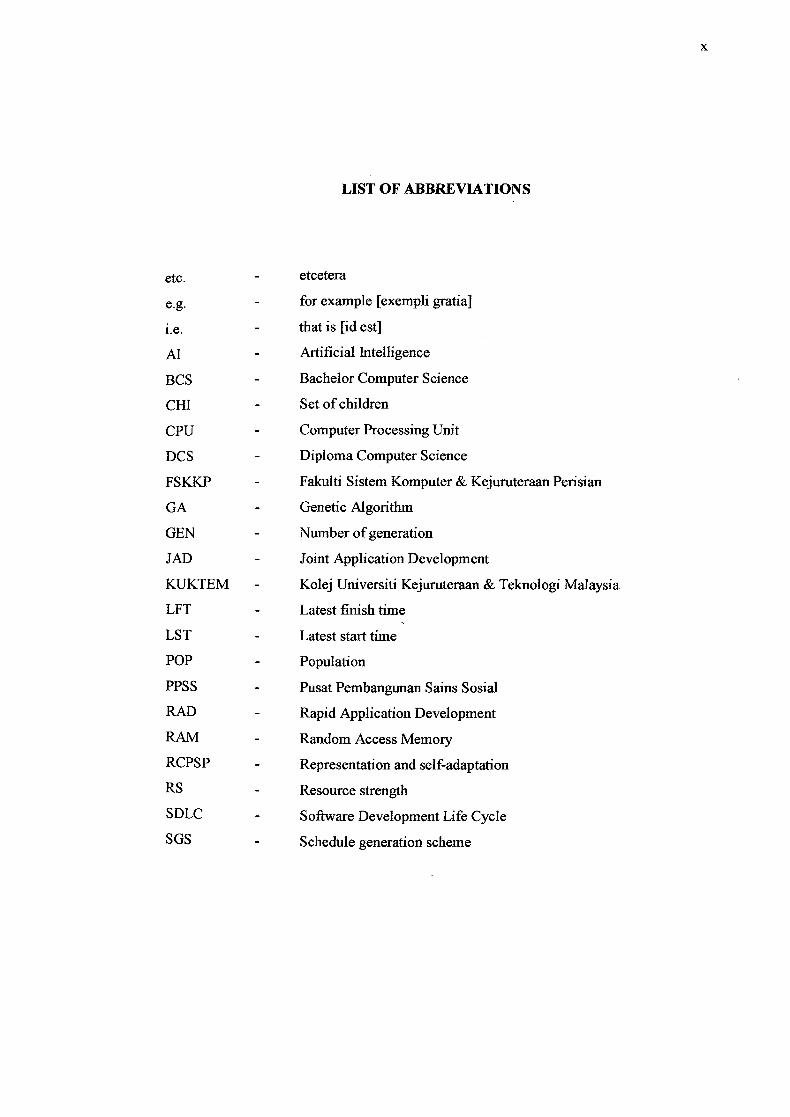
LIST OF ABBREVIATIONS
etc. - etcetera
e.g. - for example [exempli gratia]
i.e. - that is [id est]
Al - Artificial Intelligence
BCS - Bachelor Computer Science
CHI - Set of children
CPU - Computer Processing Unit
DCS - Diploma Computer Science
FSKKP - Fakulti Sistem Komputer & Kejuruteraan Perisian
GA - Genetic Algorithm
GEN - Number of generation
JAD - Joint Application Development
KUKTEM - Kolej Umversiti Kejuruteraan & Teknologi Malaysia
LFT - Latest finish time
LST - Latest start time
POP - Population
PPSS - Pusat Pembangunan Sains Sosial
RAD - Rapid Application Development
RAM - Random Access Memory
RCPSP - Representation and self-adaptation
RS - Resource strength
SDLC - Software Development Life Cycle
SGS - Schedule generation scheme
x
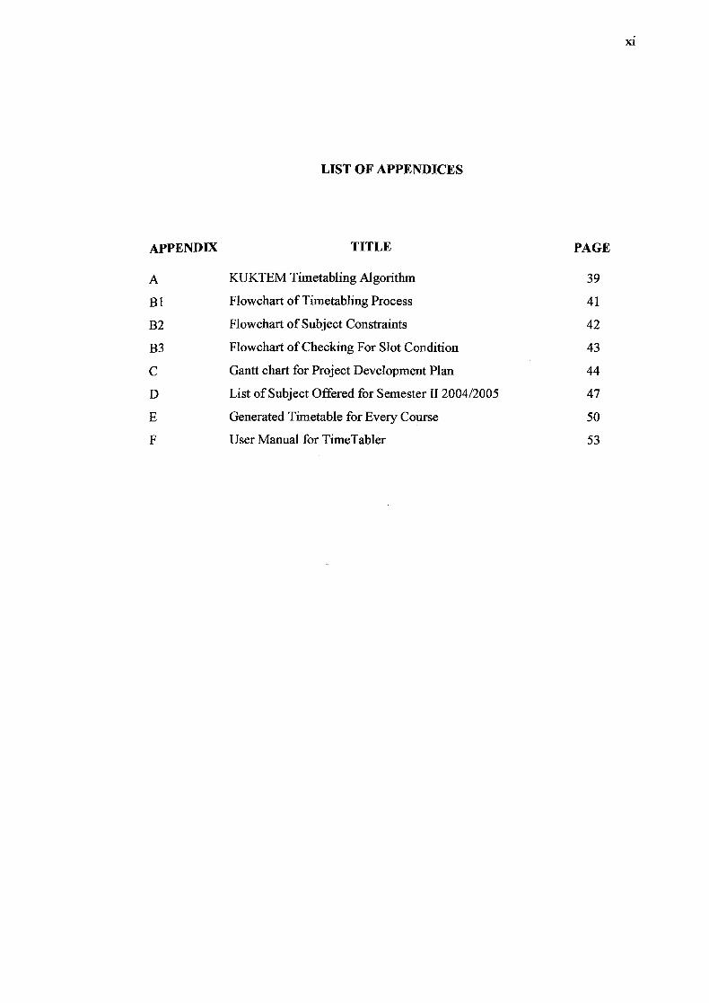
LIST OF APPENDICES
APPENDIX TITLE PAGE
A KUKTEM Timetabling Algorithm 39
B 1 Flowchart of Timetabling Process 41
B2 Flowchart of Subject Constraints 42
B3 Flowchart of Checking For Slot Condition 43
C Gantt chart for Project Development Plan 44
D List of Subject Offered for Semester 11 2004/2005 47
E Generated Timetable for Every Course 50
F User Manual for TimeTabler 53
xi
CHAPTER 1
INTRODUCTION
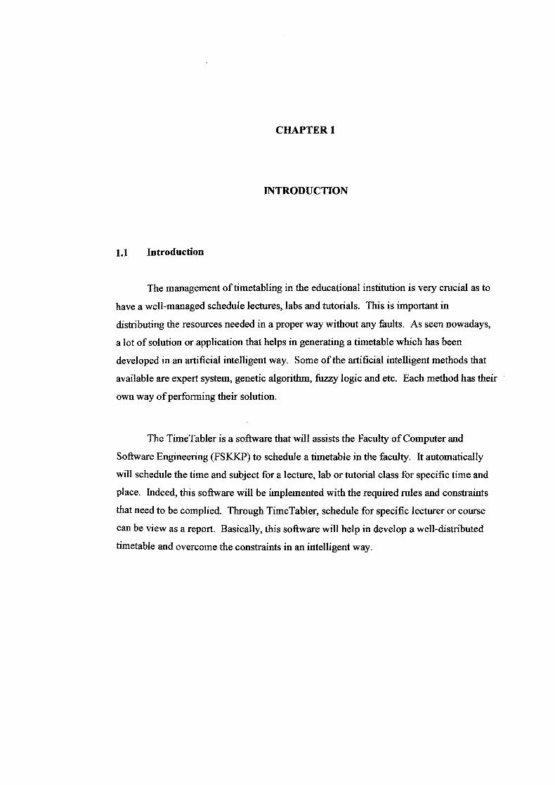
1.1 Introduction
The management of timetabling in the educational institution is very crucial as to
have a well-managed schedule lectures, labs and tutorials. This is important in
distributing the resources needed in a proper way without any faults. As seen nowadays,
a lot of solution or application that helps in generating a timetable which has been
developed in an artificial intelligent way. Some of the artificial intelligent methods that
available are expert system, genetic algorithm, fuzzy logic and etc. Each method has their
own way of performing their solution.
The TimeTabler is a software that will assists the Faculty of Computer and
Software Engineering (FSKKP) to schedule a timetable in the faculty. It automatically
will schedule the time and subject for a lecture, lab or tutorial class for specific time and
place. Indeed, this software will be implemented with the required rules and constraints
that need to be complied. Through TimeTabler, schedule for specific lecturer or course
can be view as a report. Basically, this software will help in develop a well-distributed
timetable and overcome the constraints in an intelligent way.

2
1.2 Problem Statement
1.2.1 Current System
The current system for timetablmg in the faculty manages to develop a timetable.
Based on the previous timetable, it is found that the system does not really helps in
scheduling timetable wisely. Therefore, there is still human power needed to configure
the timetable manually. Below are some of the problems faced by the current system:
(a) Classroom clashing between for two courses at the same time
(b) Classroom provided cannot support the number of student
(c) Timetable for courses in FSKKP takes approximately three days to be
manually-developed.
(d) Still in need for human power for timetable configuration.
1.2.2 Current System Process
For every algorithm, it is crucial to understand the flow of process on how it is
executed. This will determine the success of the algorithm implementation through
coding and logic programming. The process flow for KUKTEM timetablmg algorithm
can be referred in Appendix A.
1.3 Objectives
For every project development, it must have its aims so the project's success can
be measured into some extent. Therefore, below are the objectives of this project:
(a) TimeTabler is a prototype software for developing a well-distributed
timetable for every course in FSKKP.

3
(b) Provide a full report of timetable for every course in FSKKP
(c) Reduce the time consumed as well as the human power in arranging a
schedule and overcome the conventional way of managing a schedule
1.4 Scopes
Basically, this software is mainly developed for the FSKKP to manage and
establish a well-organized schedule. The courses that involved are Bachelor of Software
Engineering (BCS) and Diploma of Software Engineering (DCS) for each
batch. In this scheduling, it only involves with the subjects in the FSKKP and the
subjects from Pusat Pembangunan Sams Sosial (PPSS) for university subjects.
This project is going to be developed for Windows platform and it uses the data or
resources and subjects for semester 2 year 2004/2005. It will use the visual basic
programming as code generation and Microsoft Access as the database management.
The TimeTabler is well-designed rule-based application to comply the following
constraints that critically required to be emphasized:
(a) There will be no class or lecture that is clashing.
(b) The room for each class, tutorial or lab must be able to support the number
of student.
(c) Must satisfy the university constraints such as there should be no class at
8.am on every Monday, no subject is scheduled in the evening for every
Wednesday, and schedule should not have class at 1.00 pm and for faculty
meeting; on Tuesday 8 am to 10 am.
(d) The TimeTabler should be able to give a final report of timetable for every
course in the FSKKP.
CHAPTER 2
LITERATURE REVIEW
2.1 Introduction
Timetabling is a great importance for educational institutions and has to be solved
numerous times at each institution consuming expensive human and computer resources.
Timetabling can be defined as the problem of assigning a set of schedule into a given set
of classrooms over a limited number of time periods in such a way that there are no
conflicts between any two classes. That is no student should be required to attend two
classes at the same time and no two classes should be assigned to the same classroom
during overlapping time periods.. At the same time, it is also need to consider the capacity
of the room, lecturers that involved, time and some other constraints.
There are a lot of applications that has been developed and available in the market.
These applications aim is to generate a well-distributed timetable in respective way of
solution depending its method or artificial intelligent algorithm. A lot of algorithms or
methods available nowadays and widely used in the area of timetabling, such as genetic
algorithm, fuzzy logic, expert system and etc.
2.2 Methodology in Timetabling
2.2.1 Rule-Based Approach
2.2.1.1 Introduction to Rule-Based System
Rule-based system use a set of assertions, which collectively form the 'working
memory', and a set of rules that specify how to act on the assertion set, a rule-based
system can be created. Rule-based systems are fairly simplistic, consisting of little more
than a set of if-then statements, but provide the basis for so-called "expert systems" which
are widely used in many fields. The concept of an expert system is where the knowledge
of an expert is encoded into the rule set. When exposed to the same data, the expert
system will perform in a similar manner to the expert.
Rule-based systems are a relatively simple model that can be adapted to any
number of problems. As with any 'system, a rule-based system has its strengths as well as
limitations that must be considered before deciding if it's the right technique to use for a
given problem. Overall, rule-based systems are really only feasible for problems for
which any and all knowledge in the problem area can be written in the form of if-then
rules and for which this problem area is not large. If there are too many rules, the system
can become difficult to maintain and can suffer a performance hit. Basically, to create a
rule-based system for a given problem, the following must have (or created) [15]:
a) A set of facts to represent the initial working memory. This should be
anything relevant to the beginning state of the system.
b) A set of rules. This should encompass any and all actions that should be
taken within the scope of a problem, but nothing irrelevant. The number
of rules in the system can affect its performance, so you don't want any
that aren't needed.

C) A condition that determines that a solution has been found or that none
exists. This is necessary to terminate some rule-based systems that find
themselves in infinite loops otherwise.
2.2.1.2 Theory of Rule-Based Systems
The rule-based system itself uses a simple technique whereby it starts with a rule-
base, which contains all of the appropriate knowledge encoded into If-Then rules, and a
working memory, which may or may not initially contain any data, assertions or initially
known information. The system examines all the rule conditions (IF) and determines a
subset, the conflict set, of the rules whose conditions are satisfied based on the working
memory. Of this conflict set, one of those rules is triggered (fired).
Which one is chosen is based on a conflict resolution strategy. When the rule is
fired, any actions specified in its THEN clause are carried out. These actions can modify
the working memory, the rule-base itself, or do just about anything else the system
programmer decides to include. This loop of firing rules and performing actions
continues until one of two conditions is met: there are no more rules whose conditions are
satisfied or a rule is fired whose action specifies the program should terminate.
Which rule is chosen to fire is a function of the conflict resolution strategy.
Which strategy is chosen can be determined by the problem or it may be a matter of
preference. In any case, it is vital as it controls which of the applicable rules are fired and
thus how the entire system behaves. There are several different strategies, but here are a
few of the most common [15].
First Applicable: If the rules are in a specified order, firing the first applicable one
allows control over the order in which rules fire. This is the simplest strategy and has a
potential for a large problem: that of an infinite loop on the same rule. If the working
memory remains the same, as does the rule-base, then the conditions of the first rule have
not changed and it will fire again and again. To solve this, it is a common practice to
7
suspend a fired rule and prevent it from re-firing until the data in working memory, that
satisfied the rule's conditions, has changed.
Random: Though it doesn't provide the predictability or control of the first-applicable
strategy, it does have its advantages. For one thing, its unpredictability is an advantage in
some circumstances (such as games for example). A random strategy simply chooses a
single random rule to fire from the conflict set. Another possibility for a random strategy
is a fuzzy rule-based system in which each of the rules has a probability such that some
rules are more likely to fire than others.
Most Specific: This strategy is based on the number of conditions of the rules. From the
conflict set, the rule with the most conditions is chosen. This is based on the assumption
that if it has the most conditions then it has the most relevance to the existing data.
Least Recently Used: Each of the rules is accompanied by a time or step stamp, which
marks the last time it was used. This maximizes the number of individual rules that are
fired at least once. If all rules are needed for the solution of a given problem, this is a
perfect strategy.
"Best" rule: For this to work, each rule is given a 'weight,' which specifies how much it
should be considered over the alternatives. The rule with the most preferable outcomes is
chosen based on this weight.
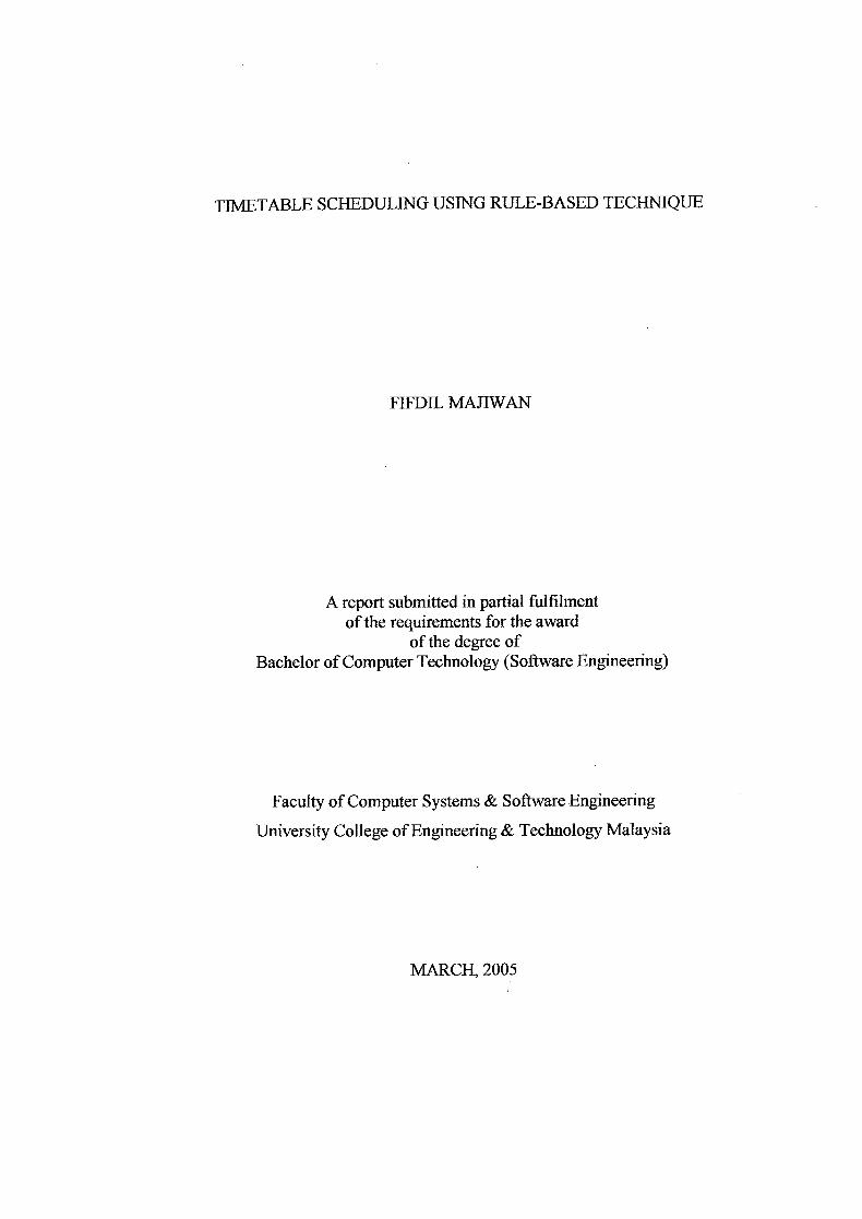
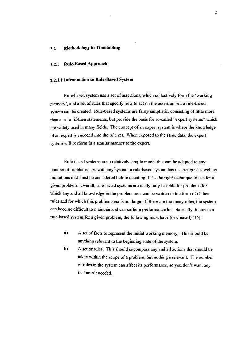
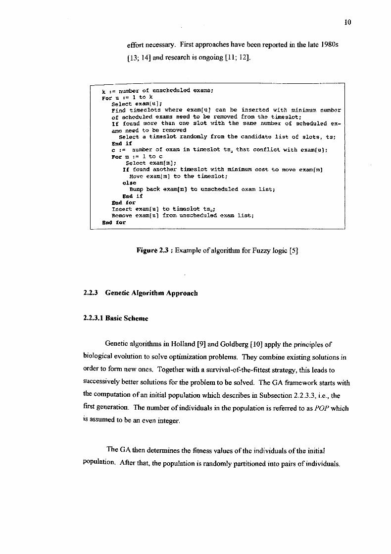
2.2.1.3 Forward-Chaining in Rule-Based Systems
Rule-based systems, as defined above, are adaptable to a variety of problems. In
some problems, information is provided with the rules and the Al follows them to see
where they lead. An example of this is a medical diagnosis in which the problem is to
diagnose the underlying disease based on a set of symptoms (the working memory). A
problem of this nature is solved using a forward-chaining, data-driven, system that
compares data in the working memory against the conditions (IF parts) of the rules and
determines which rules to fire.
Rule) I Determine possible Base rules to tire
Conflict Set Working Memory
SelectRule Fo I Resolution \Conflict
Strategy rule Fire RuI to fire
No Rule Found
I Exit
Figure 2.1: Forward-Chaining in Rule-based System [15]
2.2.2 Fuzzy Logic Approach
Fuzzy scheduling provides the possibility to deal with the inherent dynamic and
incompleteness of the scheduling area. It allows the representation (by fuzzy sets and
linguistic variables) and the inference (by fuzzy rules) from vaguely formulated
knowledge. The main types of imprecise scheduling information addressed by fuzzy sets
are:
(a) Vaguely defined dates or durations, e.g., due dates,
(b) Vague definitions of preferences, e.g., preferences between alternatives,
(c) Uncertainty about the value of scheduling parameters, e.g., process times,
(d) Aggregated knowledge, e.g., machine groups instead of individual
machines.
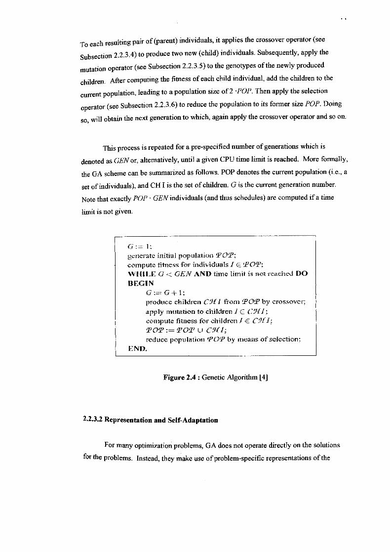
.1 knowledge Fuzzy-base Controller
fuzzifi- inference deflizzifl-cation engine cation
Output: crisp Input: crisp values values
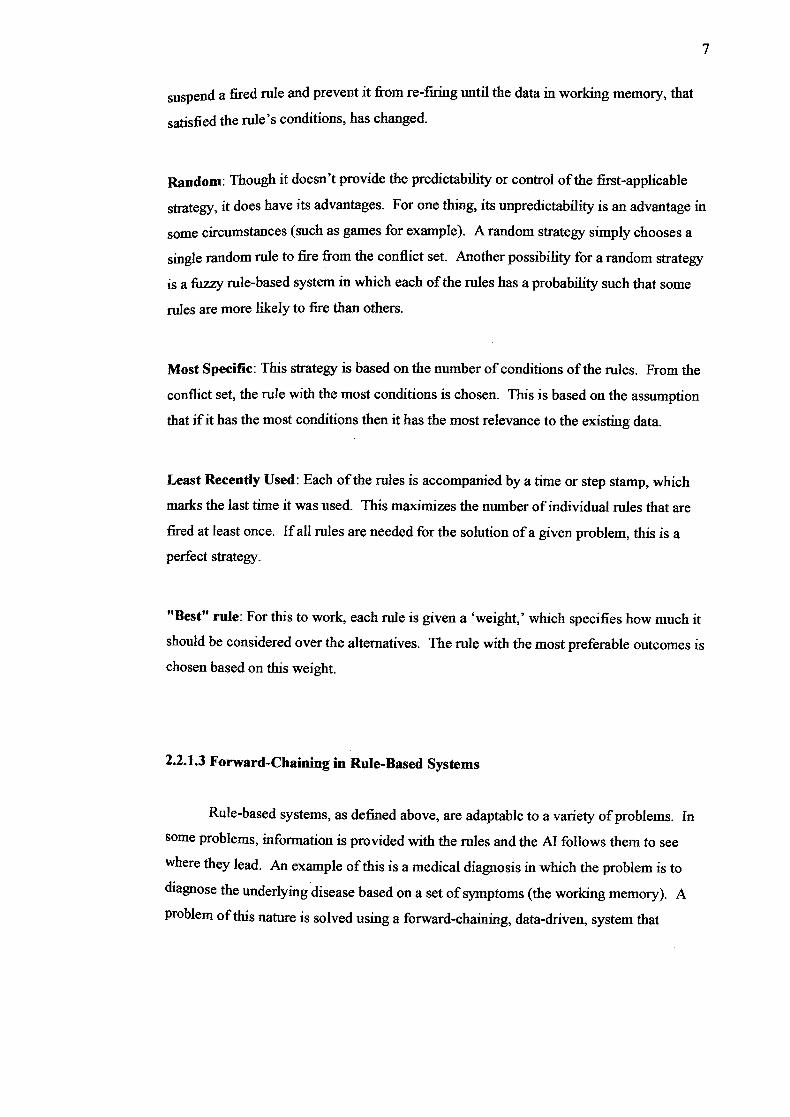
Figure 2.2 Fuzzy controller [16]
To handle the imprecise information with fuzzy controllers (Figure 2.2), the following
steps have to be performed:
(a) Transformation of scheduling data into a knowledge representation that
can be handled by a fuzzy controller (fuzzification). Imprecise knowledge
is represented by linguistic variables denoting the possible values, e.g.,
capacity of machine groups by (very low, low, normal, high, very high).
For each of the possible values a membership function (e.g., triangular) is
given, which is used in combining and processing the fuzzy sets.
(b) Processing of the fuzzy scheduling knowledge towards a decision by
means of given rules and integration of fuzzy arithmetic to deal with
imprecise or vague data. Fuzzy sets and rules are stored in the knowledge
base of the fuzzy controller.
(c) Transformation of the fuzzy scheduling decision into crisp scheduling data
(defuzzification), e.g., to determine concrete dates for operations. The
principal advantage of fuzzy scheduling is the possibility to focus on the
significant scheduling decisions; a main disadvantage is the computational
10
effort necessary. First approaches have been reported in the late 1980s
[13; 14] and research is ongoing [11; 12].
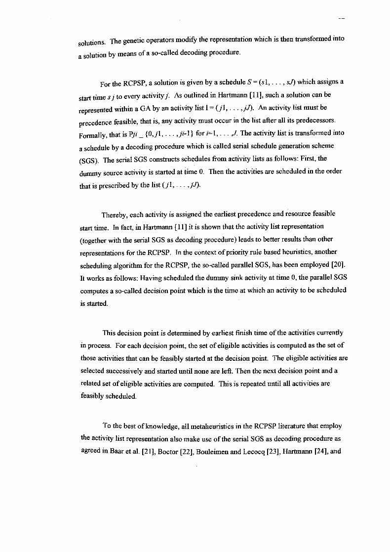
k number of unscheduled exam; For u I to k
Select exam[u]; Find timeslots where exam(uj can be inserted with minimum number of scheduled exams need to be removed from the timesiot; If found more than one slot with the same number of scheduled ex-ams need to be removed
Select a time-slot randomly from the candidate list of slots, ts; End if C number of exam in timeslot ts that conflict with examlu); For in : 1 to c
Select exam[m]; If found another timeslot with minimum cost to move examfm)
Move exam[ m] to the timeslot; else
Bump back exam(m) to unscheduled exam list; End if
End for Insert examlu) to timeslot ts,; Remove exam[ u) from unscheduled exam List;
End for
Figure 2.3 : Example of algorithm for Fuzzy logic [5]
2.2.3 Genetic Algorithm Approach
2.2.3.1 Basic Scheme
Genetic algorithms in Holland [9] and Goldberg [10] apply the principles of
biological evolution to solve optimization problems. They combine existing solutions in
order to form new ones. Together with a survival-of-the-fittest strategy, this leads to
successively better solutions for the problem to be solved. The GA framework starts with
the computation of an initial population which describes in Subsection 2.2.3.3, i.e., the
first generation. The number of individuals in the population is referred to as POP which
is assumed to be an even integer.
The GA then determines the fitness values of the individuals of the initial
Population. After that, the population is randomly partitioned into pairs of individuals.
To each resulting pair of (parent) individuals, it applies the crossover operator (see
Subsection 2.2.3.4) to produce two new (child) individuals. Subsequently, apply the
mutation operator (see Subsection 2.2.3.5) to the genotypes of the newly produced
children. After computing the fitness of each child individual, add the children to the
current population, leading to a population size of 2 POP. Then apply the selection
operator (see Subsection 2.2.3.6) to reduce the population to its former size POP. Doing
so, will obtain the next generation to which, again apply the crossover operator and so on.
This process is repeated for a pre-specified number of generations which is
denoted as GEN or, alternatively, until a given CPU time limit is reached. More formally,
the GA scheme can be summarized as follows. POP denotes the current population (i.e., a
set of individuals), and CH I is the set of children. G is the current generation number.
Note that exactly POP GEN individuals (and thus schedules) are computed if a time
limit is not given.
G:= I: generate initial population TOT; compute fitness for individuals I E !POfP:
W till E G < GE \ AND time limit is not reached 1)0 BEGIN
produce children C5{i from POT by crossover; apply mutation to children .1 E C51.i; compute fitness for children I E C511; POP: == TOT U CHI; reduce population POP by means of selection:
EN I).
Figure 2.4: Genetic Algorithm [4]
2.2.3.2 Representation and Self-Adaptation
For many optimization problems, GA does not operate directly on the solutions
for the problems. Instead, they make use of problem-specific representations of the
solutions. The genetic operators modify the representation which is then transformed into
a solution by means of a so-called decoding procedure.
For the RCPSP, a solution is given by a schedule S = (si,. . . , s.J) which assigns a
start time Sf to every activityj. As outlined in Hartmann [11], such a solution can be
represented within a GA by an activity list I = (jl,. . . ,jJ. M activity list must be
precedence feasible, that is, any activity must occur in the list after all its predecessors.
Formally, that is Pji - {0,jl,.. . ,ji-1} for 11,.. . J. The activity list is transformed into
a schedule by a decoding procedure which is called serial schedule generation scheme
(SGS). The serial SGS constructs schedules from activity lists as follows: First, the
dummy source activity is started at time 0. Then the activities are scheduled in the order
that is prescribed by the list (ii,. . . ,jJ).
Thereby, each activity is assigned the earliest precedence and resource feasible
start time. In fact, in Hartmann [11] it is shown that the activity list representation
(together with the serial SGS as decoding procedure) leads to better results than other
representations for the RCPSP. In the context of priority rule based heuristics, another
scheduling algorithm for the RCPSP, the so-called parallel SGS, has been employed [20].
It works as follows: Having scheduled the dummy sink activity at time 0, the parallel SGS
computes a so-called decision point which is the time at which an activity to be scheduled
is started.
This decision point is determined by earliest finish time of the activities currently
in process. For each decision point, the set of eligible activities is computed as the set of
those activities that can be feasibly started at the decision point. The eligible activities are
selected successively and started until none are left. Then the next decision point and a
related set of eligible activities are computed. This is repeated until all activities are
feasibly scheduled.
To the best of knowledge, all metaheuristics in the RCPSP literature that employ
the activity list representation also make use of the serial SGS as decoding procedure as
agreed in Baar et al. [21], Boctor [22], Bouleimen and Lecocq [23], Hartmann [24], and

Pinson et al. [25]. Usually, no reason for the selection of the serial SGS is given—the
serial SGS appears to be the "natural choice."
Thus, here it is proposed to use not only the serial but also the parallel SGS as
decoding procedure for the activity list representation. In fact, the parallel SGS can easily
be applied to activity lists: In each step, simply choose that activity from the eligible set
that has the lowest index in the activity list.
Now there are two possible decoding procedures for the activity list representation
of the RCPSP. This leads to the question which of them should be used. In fact, there is
no general answer to this question. This is due to the differences between the serial and
the parallel SGS: Whereas the serial SGS constructs so-called active schedules, the
parallel one constructs so-called non-delay schedules [27].
The set of the non-delay schedules is a (in most cases proper) subset of the set of
the active schedules. While the set of the active schedules always contains an optimal
schedule, this does not hold for the set of the non-delay schedules. Consequently, the
parallel SGS may miss an optimal schedule. On the other hand, it produces schedules of
good average quality because it tends to utilize the resources as early as possible, leading
to compact schedules.
These result in different behaviors of the SGS in computational experiments based
on Kolisch [20] and Hartmann and Kolisch [26]. On instances with many activities
and/or scarce resource capacities, the parallel SGS performs better than the serial one.
Moreover, if long computation times are allowed (i.e., if many schedules can be
computed), the serial SGS leads to better results than the parallel one.
These observations can be explained as follows: Many activities and scarce
resources imply larger search spaces, where the focus on compact, but often only
suboptimal non-delay schedules is a promising heuristic strategy. Longer computation
times may allow finding an optimal or a near optimal solution, which is typically only
possible if the serial SGS is used.
However, it is usually impossible to predict which of the SGS will perform better
for an arbitrary instance of the RCPSP. The idea is now to allow both SGS to be
employed as decoding procedures within the GA. To do so, define the genotype as
follows: An individual I = (l,SGS) consists of an activity list 1 and an indicator
SGS = 1 1, if activity list 1 is to be decoded by the serial SGS
0, if activity list 1 is to be decoded by the parallel SGS.
For a given individual, compute a schedule using the SGS specified in the
genotype. The fitness of the individual is defined as the make span of the schedule. That
is, a lower fitness implies a better individual and thus a higher chance to survive.
The extended representation proposed here includes an additional gene that
determines the SGS type to be used as decoding procedure for the related activity list. As
with all genes in GAs, also this one is subject to the genetic operators' crossover,
mutation, and selection. Therefore, the SGS type leading to better results will survive
while the other one will probably die over the generations. Thus the mechanism of
evolution decides for the specific instance currently to be solved which decoding
procedure is the more promising one. This enables the GA to adapt itself dynamically to
each instance, leading to what it is call a self-adapting GA.
2.2.3.3 Initial Population
In initial population, it is crucial to define how to determine an initial population
containing POP individuals of the genotype introduced above. Basically, it will proceed
in two steps. First, consider the construction of an activity list. Second, describe the
selection of the decoding procedure to be used, i.e., one of the two SGS. An activity list
is constructed by a modified priority rule based sampling heuristic [20]. The next activity
for the list is successively chosen from those unscheduled activities the predecessors of
which have already been selected for the list. This way, it will obtain a precedence
feasible activity list. The decision which activity is chosen next is made on the basis of
one of two well-known priority rules. Firstly, select the priority rule; either the LFT
(latest finish time) or the LST (latest start time) rule is chosen with a probability of 0.5
each.
From the resulting priority values of the activities, derive regret based biased
selection probabilities that are used to select the next activity (for details on the priority
rules and the regret based biased sampling approach, refer to Kolisch [20]). Using two
good priority rules and a randomized activity selection method leads to a diversified
initial population of good activity lists. Next, choose an SGS in order to make the current
activity list a complete genotype. Of course, both SGS must appear in the population
because the genetic algorithm needs to decide which of them is more promising. Then,
examined the following three alternative approaches:
a) The most straightforward method is to select each of the SGS types with a
probability ofp = 0.5.
b) The following idea was designed to lead to a good initial distribution of the
SGS types with respect to the project actually to be scheduled. It is
discussed above that, roughly explained, the serial SGS is more favorable
for smaller projects. This motivated the following approach where the
probability to select the serial SGS is defined asp serial = a J, where a is a
constant. Clearly, setp parallel = 1-p serial. This way, the more activities
it will have in a project, the higher the probability to select the parallel
SGS in the initial population.
C) Similarly, the parallel SGS is superior in case of scarce resource capacities.
A formal measure for the scarceness is the resource strength RS [28]. Low
resource strength implies scarce capacities. Thus, simply set p serial = RS.
Again, set parallel =1-p serial. Obviously, low resource strength leads
to a low probability for selecting the serial SGS (note that RS is between 0
and 1 by definition).

In computational experiments with a large number of test instances, these three
approaches gave similar results on the average. This indicates that the initial distribution
is not crucial for the evolution as long as both .SGS obtain a sufficient fraction in the
initial population. As none of the methods was clearly superior, select the simplest
approach (a).
2.2.3.4 Crossover
Let's assume that two individuals of the current population have been selected for
crossover. Thus, there will be mother individual M(1M,SGSIvI) and a father individual F
=(1F,SGSF). Now two child individuals have to be constructed, a daughter D =
(ID,SGSD) and a son S = (IS,SGSS).
First, start with a definition of the daughter D. In a first step, determine the
daughter's activity list ID. Combining the parent's activity lists, make sure that each
activity appears exactly once in the daughter's activity list. Therefore, adapt a general
crossover technique presented by Reeves [311 for permutation based genotypes. This
approach also secures that precedence feasibility is maintained. Perform a two-point
crossover for which will draw two random integers q 1 and q2 with 1 - q 1 <q2 - J. Now
the daughter's activity list ID is determined by taking the activity list of the positions i =
1,. . . ,q 1 from the mother, that is,
.M ii := J
The positions i=q 1 + 1,.. . ,q2 are derived from the father. However, the activities already
selected may not be considered again. Then, this will be obtained:
= j k where k is the lowest index such that ,. . • 'fi }
The remaining positions i = q2+1,. . .. ,J are again taken from the mother, that is,


![Mimosa Scheduling · PDF fileInvoke Mimosa Scheduling Software ... change the timetable you want to schedule next [Double-click] to schedule Press [F3] or click this button to find](https://static.cupdf.com/doc/110x72/5a9d61337f8b9abd058c807c/mimosa-scheduling-mimosa-scheduling-software-change-the-timetable-you-want-to.jpg)