
Three-dimensional (3D) three-component (3C)shallow seismicrefraction surveys across a shearzone associated with drylandsalinity at the Spicers Creek Catchment, New South Wales,Australia
Author:Nikrouz, Ramin
Publication Date:2005
DOI:https://doi.org/10.26190/unsworks/21772
License:https://creativecommons.org/licenses/by-nc-nd/3.0/au/Link to license to see what you are allowed to do with this resource.
Downloaded from http://hdl.handle.net/1959.4/20607 in https://unsworks.unsw.edu.au on 2022-07-21
Three-Dimensional (3D) Three-Component (3C) Shallow Seismic Refraction Surveys Across a Shear Zone Associated with Dryland Salinity at the Spicers
Creek Catchment, New South Wales, Australia
by
Ramin Nikrouz
B.Sc., Geology, IRAN M.Sc., Petrology, IRAN
A Thesis Submitted in Fulfillment of the Requirements for the Degree of
Doctor of Philosophy
School of Biological, Earth and Environmental Sciences The University of New South Wales
Sydney NSW 2052 Australia
April 2005

PLEASE TYPE THE UNIVERSITY OF NEW SOUTH WALES
Thesis/Project Report Sheet Surname or Family name:
First name:
Other name/s:
Abbreviation for degree as given in the University calendar:
School:
Faculty:
Title:
Abstract 350 words maximum: (PLEASE TYPE)
Declaration relating to disposition of project report/thesis I am fully aware of the policy of the University relating to the retention and use of higher degree project reports and theses, namely that the University retains the copies submitted for examination and is free to allow them to be consulted or borrowed. Subject to the provisions of the Copyright Act 1968, the University may issue a project report or thesis in whole or in part, in photostat or microfilm or other copying medium. I also authorise the publication by University Microfilms of a 350 word abstract in Dissertation Abstracts International (applicable to doctorates only). …………………………………………………………… Signature
……………………………………..……………… Witness
……….……………………...…….… Date
The University recognises that there may be exceptional circumstances requiring restrictions on copying or conditions on use. Requests for restriction for a period of up to 2 years must be made in writing to the Registrar. Requests for a longer period of restriction may be considered in exceptional circumstances if accompanied by a letter of support from the Supervisor or Head of School. Such requests must be submitted with the thesis/project report. FOR OFFICE USE ONLY
Date of completion of requirements for Award:
Registrar and Deputy Principal
THIS SHEET IS TO BE GLUED TO THE INSIDE FRONT COVER OF THE THESIS
N:\FLORENCE\ABSTRACT

To my wife Fariba and my son Amir

CERTIFICATE OF ORIGINALITY
I hereby declare that this submission is my own work and to the best of my
knowledge it contains no materials previously published or written by another
person, nor material which to a substantial extent has been accepted for the
award of any other degree or diploma at UNSW or any other educational
institution, except where due acknowledgement is made in the thesis. Any
contribution made to the research by others, with whom I have worked at
UNSW or elsewhere, is explicitly acknowledged in the thesis.
I also declare that the intellectual content of this thesis is the product of my own
work, except to the extent that assistance from others in the project’s design
and conception or in style, presentation and linguistic expression is
acknowledged.
……………………………………………….
Ramin Nikrouz
ABSTRACT
Three-dimensional (3D) three-component (3C) shallow seismic refraction
surveys were recorded over a shear zone at two sites associated with dryland
salinity in the Spicers Creek Catchment, near Dubbo in southeastern Australia.
The seismic data were recorded with the Australian National Seismic Imaging
Resources (ANSIR) 360-trace ARAM-24 seismic system and IVI MiniVibrator.
Dryland salinity occurs extensively throughout the Spicers Creek Catchment.
The high concentration of salt in the groundwater has led to a significant decline
in agricultural productivity and a reduction in native vegetation. Furthermore,
the saline groundwater in the surface soil has caused the destruction of the clay
and soil structure and as a result, large areas of the catchment have
experienced soil erosion and extensive alteration of the landscape.
The broad objective of this study was to use seismic refraction methods to map
in detail a shear zone, which is associated with the salination. Seismic
refraction methods were selected because of their potential ability to provide
greater lateral resolution of the narrow vertical shear zone, than is currently the
norm with electrical or electromagnetic methods. This situation was confirmed
with a number of resistivity depth images generated as part of this study.
The results of the seismic refraction surveys show that the shear zone occurs
as a narrow region with low seismic velocities and increased depths of
weathering. However, there were numerous ambiguities in generating
i
consistent parameters in the refractor between adjacent receiver lines.
Furthermore, these ambiguities were not resolved with the use refraction
tomography, because even major differences with the various starting models
still generated acceptable agreement with the traveltime data. Therefore, in
order to generate consistency between the results for the various receiver lines,
it was necessary to generate detailed starting models.
A major achievement of this study is the development of a smoothing method
which significantly removes the effects of the near surface irregularities.
Termed the GRM SSM (for statics smoothing method), it essentially generates
a time-depth model of the refracting interface for which the effects of the near
surface irregularities have been minimized, by taking an average of the time-
depth profiles for a range of XY values. The GRM SSM, which takes advantage
of the unique redundancy properties of the GRM computations, was a major
factor in deriving consistent detailed starting models for refraction inversion.
Furthermore, this consistency was achieved with both S-wave components, as
well as the P-wave results.
The major geological achievement, which was made possible with the GRM
SSM, was the demonstration that there were cross cutting features associated
with the major shear zone. Therefore, it appears that saline groundwater can
discharge at the surface where increased volumes of groundwater occur at the
intersection of different sets of shears. This model provides a useful
explanation for the discontinuous occurrence of salination along the major shear
zone.
ii

ACKNOWLEDGEMENTS
First and foremost, I would like to thank God for helping me to accomplish this
project which is going to affect my academic life for some time to come. This
accomplishment would not have been possible without the help and support of
my supervisor, Derecke Palmer, who acted as a source of inspiration and
practical scientific support. I am most grateful for his keen supervision,
continuous support and encouragement during my research study. The
geophysical knowledge which I have acquired as the result of the
accomplishment of this research project is indeed the result of his insight and
expertise. I have been inspired by his endurance and perseverance.
I would also like to acknowledge my indebtedness to Paul Lennox, my co-
supervisor, who saved no effort to keep me on track in my endeavors. A
special word of thanks also goes to one of my best friends and colleagues in
Australia, Andrew Spyrow, whose friendship I value most highly. He was
especially helpful and supportive in the many computing tasks associated with
this study. I also owe a word of gratitude to David Johnston and the ANSIR
team who made it possible for me to gather what was indeed the corner stone
of my project, the data of the study.
iii

On a different note, I would like to thank the officials in the Iranian Ministry of
Science, Research and Technology and the University of Urmia of which I am a
faculty member for the financial support they provided for my family and me.
Also, I need to acknowledge my sense of gratitude and indebtedness to my
wife, Fariba and my son, Amir. They served as a source of encouragement and
support for me and were commendably patient with me although due to the
requirements of my studies, I had less time to spend with them. I am also
thankful to my parents of whose encouragement and support I am always
appreciative.
I should also take this opportunity to express my most sincere thanks to my
fellow research students at UNSW and friends, Morteza Jami and Ahmad Reza
Mokhtari, for their support and encouragement throughout the study of my
research.
Last but not the least, I sincerely thank the staff of the School of Biological,
Earth, and Environmental Sciences at UNSW, for their continued support and
encouragement. I am also grateful to many others, whose names do not
appear here. Their help is greatly appreciated.
iv
CONTENTS
Abstract-------------------------------------------------------------------------------------- i Acknowledgements---------------------------------------------------------------------- iii Contents-------------------------------------------------------------------------------------- V Illustrations---------------------------------------------------------------------------------- xi
Chapter 1 Introduction--------------------------------------------------------------------------------- 1 1.1 - Recent Advances in the Resolution of Geophysical Data-------------- -- 1 1.2 - Three-Dimentional Shallow Seismic Refraction Methods----------------- 5 1.3 - Dryland Salinity---------------------------------------------------------------------- 8 1.4 - Detailed Mapping of Shear Zones---------------------------------------------- 10 1.5 - Objectives----------------------------------------------------------------------------- 12 1.6 - Problems Solved in this Study--------------------------------------------------- 15
Chapter 2 Dryland Salinity----------------------------------------------------------------------------- 17 2.1 - Summary------------------------------------------------------------------------------- 17 2.2 - Introduction---------------------------------------------------------------------------- 18 2.3 - Extent of Dryland Salinity in New South Wales------------------------------- 19 2.4 - Causes of Dryland Salinity--------------------------------------------------------- 23 2.5 - Dryland Salinity in the Spicers Creek Catchment---------------------------- 28 2.6 - Management of Dryland Salinity-------------------------------------------------- 33
Chapter 3 Shear Zones Characteristic------------------------------------------------------------ 43 3.1 - Summary------------------------------------------------------------------------------- 43 3.2 - Introduction---------------------------------------------------------------------------- 44 3.3 - Shear Zone Types------------------------------------------------------------------- 46 3.4 - Fluid Movement in Shear Zones------------------------------------------------- 51
v
3.5 - Shear Zone Evidences---------------------------------------------------------- 54 3.5.1 - Field Evidence------------------------------------------------------------------- 54 3.5.2 - Imaging Shear Zones with Geophysical Methods---------------------- 59
Chapter 4 Three Dimension Three Component Seismic Surveys-------------------- 61 4.1 - Summary---------------------------------------------------------------------------- 61 4.2 - The Seismic Refraction Method----------------------------------------------- 62 4.3 - Seismic Velocities in the Earth------------------------------------------------ 63 4.4 - Three Dimension Seismic Refraction Methods---------------------------- 65 4.5 - Three Component Seismic Refraction Surveys---------------------------- 68 4.6 - Shear Waves Versus P Waves------------------------------------------------ 70
Chapter 5 Geology and Geophysics------------------------------------------------------------ 74 5.1 - Summary----------------------------------------------------------------------------- 74 5.2 - Introduction------------------------------------------------------------------------- 75 5.3 - Tectonic Setting-------------------------------------------------------------------- 75
5.3.1 - Lachlan Fold Belt------------------------------------------------------------ 77 5.3.2 - Gunnedah Basin------------------------------------------------------------- 82 5.3.3 - Surat Basin-------------------------------------------------------------------- 88
5.4 - Regional Geology------------------------------------------------------------------ 91 5.4.1 - Introduction-------------------------------------------------------------------- 91 5.4.2 - Climate------------------------------------------------------------------------- 92 5.4.3 - Physiography----------------------------------------------------------------- 93 5.4.4 - Dubbo Area------------------------------------------------------------------- 95 5.4.5 - Geology------------------------------------------------------------------------ 99 5.4.6 - Metamorphism--------------------------------------------------------------- 103
5.5 - Local Geology---------------------------------------------------------------------- 105 5.5.1 - Introduction------------------------------------------------------------------- 105 5.5.2 - Climate------------------------------------------------------------------------- 107 5.5.3 - Stratigraphy------------------------------------------------------------------- 107
5.5.3.1 - Palaeozoic Units------------------------------------------------------- 110
vi
5.5.3.1.1 - Okdale Formation (θco)--------------------------------------- 110 5.5.3.1.2 - Ungrouped Ordovician Intrusions (θm)--------------------- 111 5.5.3.1.3 - Gleneski Formation (Sms)------------------------------------ 112 5.5.3.1.4 - Cuga Burga Volcanics (Dgc)--------------------------------- 112 5.5.3.1.5 - Early Permian Undifferentiated (Pe)------------------------ 114 5.5.3.1.6 - Dunedoo Formation (Pd)-------------------------------------- 114
5.5.3.2 - Mesozoic Units--------------------------------------------------------- 115 5.5.3.2.1 - Boulerwood Formation (Rb)---------------------------------- 115 5.5.3.2.2 - Napperby Formation (Rp)------------------------------------- 116
5.5.3.3 - Cainozoic unit---------------------------------------------------------- 117 5.5.3.3.1 - Alluvial deposits (Qa)------------------------------------------- 117
5.5.4 - Structure----------------------------------------------------------------------- 117 5.5.4.1 - Nindethana Fault------------------------------------------------------ 121 5.5.4.2 - Narragal Thrust Sheet------------------------------------------------ 123 5.5.4.3 - Macquarie Fault-------------------------------------------------------- 123 5.5.4.4 - Neurea Fault------------------------------------------------------------ 124
5.6 - Regional and Local Geophysics----------------------------------------------- 125 5.6.1 - Introduction------------------------------------------------------------------- 125 5.6.2 - Radiometric Methods------------------------------------------------------ 127
5.6.2.1 - Theory, Application--------------------------------------------------- 127 5.6.2.2 - Interpretation Methodology----------------------------------------- 128 5.6.2.3 - Regional Interpretation----------------------------------------------- 132
5.6.3 - Aeromagnetic Methods---------------------------------------------------- 136 5.6.3.1 - Theory, Application--------------------------------------------------- 136 5.6.3.2 - Interpretation Methodology----------------------------------------- 138 5.6.3.3 - Regional Interpretation---------------------------------------------- 139
5.6.4 - Gravity Methods------------------------------------------------------------ 142 5.6.4.1 - Theory, Application-------------------------------------------------- 142 5.6.4.2 - Interpretation Methodology---------------------------------------- 144 5.6.4.3 - Regional Interpretation--------------------------------------------- 145
vii
Chapter 6 Near-Surface Effect Corrections with the GRM------------------------------- 148 6.1 - Summary----------------------------------------------------------------------------- 148 6.2 - Introduction--------------------------------------------------------------------------- 149 6.3 - Correcting for Near-Surface Effects------------------------------------------- 150 6.4 - Model 1: Irregular Refractor with Flat Topography------------------------ 152 6.5 - Model 2: Irregular Refractor with Irregular Topography----------------- 159 6.6 - Applying Near-Surface Effect Corrections to Model 2------------------- 164
Chapter 7 Methodology and data acquisition------------------------------------------------- 174 7.1 - Summary----------------------------------------------------------------------------- 174 7.2 - Introduction-------------------------------------------------------------------------- 174 7.3 - Equipment--------------------------------------------------------------------------- 175
7.3.1 - ARAM 24 Seismic Recording System---------------------------------- 176 7.3.2 - Mini Vibrator------------------------------------------------------------------ 177 7.3.3 - Geophones-------------------------------------------------------------------- 181 7.3.4 - Explosive Source------------------------------------------------------------ 182
7.4 - Field Procedure-------------------------------------------------------------------- 183 7.4.1 - Setting up the Survey Spread-------------------------------------------- 184 7.4.2 - Conducting the Survey----------------------------------------------------- 186
7.4.2.1 - Site 1---------------------------------------------------------------------- 188 7.4.2.2 - Site 2---------------------------------------------------------------------- 192
7.5 - Data quality in Site 1 and Site 2------------------------------------------------ 196 7.6 – Magnetic Data Acquisition------------------------------------------------------ 198 7.7 – Resistivity Data Acquisition----------------------------------------------------- 198
Chapter 8 Processing--------------------------------------------------------------------------------- 199 8.1 - Summary----------------------------------------------------------------------------- 199 8.2 - Introduction--------------------------------------------------------------------------- 200 8.3 - Processing of Magnetic and Resistivity Data-------------------------------- 200
8.3.1 - MagMap 2000 Software----------------------------------------------------- 201
viii
8.3.2 - Res2DINV Software---------------------------------------------------------- 201
8.4 - Processing of Seismic Refraction Data---------------------------------------- 203 8.4.1 - Microsoft Excel----------------------------------------------------------------- 204 8.4.2 - Surfer 8--------------------------------------------------------------------------- 204 8.4.3 - Seismic UN*x Program------------------------------------------------------- 205 8.4.4 - Visual-SUNT Software-------------------------------------------------------- 206 8.4.5 - Rayfract Software---------------------------------------------------------------206
8.5 - The Generalized Reciprocal Method-------------------------------------------- 207 8.5.1 - Velocity Analysis Function--------------------------------------------------- 208 8.5.2 - Time-Depth Function---------------------------------------------------------- 209
8.6 - Procedure of the Data Processing---------------------------------------------- 213 8.6.1 - Pre-processing----------------------------------------------------------------- 213 8.6.2 - Refraction Convolution Sections (RCS)--------------------------------- 214 8.6.3 - First Arrival Picking----------------------------------------------------------- 220 8.6.4 - Traveltime Graphs------------------------------------------------------------ 223 8.6.5 - The GRM Refractor Velocity Analysis Function----------------------- 228 8.6.6 - Corrections for Surface Effects-------------------------------------------- 234 8.6.7 - Seismic Velocities in the Refractor--------------------------------------- 237 8.6.8 - The GRM Time-Depth and Depth Function------------------------------240 8.6.9 - Processing of the First Arrival Amplitudes------------------------------ 244 8.6.10 - Velocity Ratios--------------------------------------------------------------- 248 8.6.11 - Three-Dimensional Images---------------------------------------------- 249 8.6.12 - Traveltime Tomography--------------------------------------------------- 249
Chapter 9 Interpretation------------------------------------------------------------------------------ 253 9.1 - Summary------------------------------------------------------------------------------ 253 9.2 - Introduction--------------------------------------------------------------------------- 255 9.3 - Magnetic Data Interpretation----------------------------------------------------- 256 9.4 - Resistivity Data Interpretation---------------------------------------------------- 257 9.5 - 3D-3C Seismic Data interpretation---------------------------------------------- 265
9.5.1 - Refractor Seismic Images at the First Site----------------------------- 265
ix
9.5.2 - Refractor Seismic Images at the Second Site------------------------- 274 9.6 - Geology and Tectonic interpretation------------------------------------------- 282 Chapter 10 Conclusions------------------------------------------------------------------------------ 285 References-------------------------------------------------------------------------------- 290 Appendices Appendix A - Linear and Non-Linear Metod--------------------------------------- 307 Appendix B - Operation Reports------------------------------------------------------ 309 Appendix C - Specification for the Equipment------------------------------------ 312 Appendix D - Station and Shot Point Coordinates------------------------------ 315 Appendix E - Geophone Coordinates----------------------------------------------- 317 Appendix F - Comment Document From Observer------------------------------ 318 Appendix G - Assessment of Data Quality----------------------------------------- 322 Appendix H - Seismic Unix Shell Scripts and C Files--------------------------- 336 Appendix I - Trace Order--------------------------------------------------------------- 348 Appendix J - Refraction Convolution Images------------------------------------- 350 Appendix K - Refractor Seismic Velocities---------------------------------------- 362 Appendix L - Time-Depth and Depth Graphs------------------------------------- 374 Appendix M - Eavepath Eikonal Traveltime Inversion-------------------------- 390 Appendix N - Traveltime Tomography Errors------------------------------------- 395 Appendix O - Refractor Images------------------------------------------------------ 396 Appendix P - GRM Tomography Images------------------------------------------ 410 Appendix Q - GRM Statics for Shallow Refraction Data----------------------- 416 Q1 – Abstract---------------------------------------------------------------- 416 Q2 – Generating Detailed Refractor Model for Inversion--------- 417 Q3 – Non-Uniqueness in Determining Detailed Refractor Velocities-------------------------------------------------------------- 422 Q4 – “Statics” Corrections for Shallow Refraction Data – Model Study -------------------------------------------------------- 427 Q5 – “Statics” Corrections for Shallow Refraction Data – Case Study----------------------------------------------------------- 431 Q6 – Conclusions----------------------------------------------------------- 434 Q7 – References------------------------------------------------------------ 437 Q8 – Figure Captions------------------------------------------------------ 441 Q9 - Figures ----------------------------------------------------------------- 445
x
ILLUSTRATIONS FIGURES Figure 1 - 1: Improvements in the resolution of geological detail have been achieved by adopting a new generation of survey specifications and presenting the resulting grid as an image. This illustration is from an area of the Ebagoola 1:250 000 sheet in northern Queensland. Top: BMR survey flown (E-W) in 1973 at a mean terrain clearance of 150 m and a line spacing of 1500 m, presented as a contour map with contour interval 10 nT. Bottom: the same area flown (E-W) by Geoterrex in 1991 with 100 m terrain clearance and 400 m line spacing (Reeves, C.V., 1992)…………………………………………………………………2 Figure 1 - 2: Results from the 3-D Mt Bulga seismic refraction survey. Seismic velocities and interpreted faults are plotted over the contours of the time-depths in milliseconds. The bold arrows indicate the directions of the higher seismic velocity (Palmer 2001b)………………………………………………………………6 Figure 1 - 3: The standard 2-D refraction depth cross section obtained across a shear zone at Mt Bulga. The shear zone (between stations 54 and 60) exhibits a decrease in the seismic velocity and an increase in the depth of weathering (Palmer, 2001b)……………………………………………………………………….6 Figure 2 - 1: Dryland salinity hazards in New South Wales (taken from Bradd, et al. 1997). The area that is within each hazard category is approximately low 75,060,000 ha; moderate 4,250,000 ha; high 470,000 ha; and very high 310,000 ha…………………………………………………………………………….21 Figure 2 - 2: Dryland salinity risk in New South Wales 2000 (From National Land & Water Resources Audit, 2000)…………………………………………….22 Figure 2 - 3: Dryland salinity risk in New South Wales 2050 (From National Land & Water Resources Audit; 2000)…………………………………………….22 Figure 2 - 4: Map of the Spicers Creek catchment with the main town, road and drainage modified from Cobbora 1:50,000 topographic map……………………28 Figure 3 - 1: (A) Fault. (B) Fault zone. (C) Shear zone (From Hobbs et al, 1976)………………………………………………………………………………….46 Figure 3 - 2: Different types of shear zones from (Ramsay and Auber, 1983)….. …………………………………………………………………………………………47 Figure 3 - 3: Idealized active shear zones of Type I and II (right) and stress / shear strain curves for each material (left). Shaded areas are current, actively straining regions, at margins (m) or in interior (i) of zones of Type I and II, respectively. Stubby arrows indicate direction of migration over time of boundaries of straining regions. Ellipses represent finite-strain gradients (From Means, 1995)…………………………………………………………………………49 Figure 3 - 4: Finite shear strain vs. time curves (solid) for the three types of shear zones, for rock at the final zone margins (m) and in the interior (i). P (dashed line) represents some process-controlling parameter (like temperature or fluid chemistry) that is assumed to change over the shearing history. In Type II zones, the marginal and interior acquire their low-strain state at about the
xi

same time and p value (heavy dots). The marginal rocks, therefore, provide a good record of former low-strain state of the interior rocks. In zones of Types I and III, the corresponding dots are farther apart in time and p, so the marginal rocks provide a less reliable record of the former low-strain state of the interior rocks. The type III diagram has been drawn for the case where the marginal rocks begin straining at the same time as the interior rocks, but more slowly. In each diagram, the right-hand dotted line is drawn at the point along the m line where its slope (the marginal strain-rate) becomes zero. The horizontal position of this line, therefore, represents the time at which rock in the shear zone margins acquired its final state of (low) strain. The left-hand line represents the time at which rock in the shear zone interior passed through this same state of (low) strain (From Means, 1995)…………………………………………………..50 Figure 3 - 5: Different types of criteria used for the determination of shear sense in shear zones (From Ramsay and Auber, 1983)……………………….58 Figure 4 - 1: Snell’s Law…………………………………………………………..62 Figure 4 - 2: Seismic refraction wave raypaths…………………………………64 Figure 4 -3: Nine-component sections recorded by P-, SH-, and SV-geophones for P-, SH-, and SV sources. Without anisotropy the sections marked ? would be blank (From Tatham and McCormack, 1991)………………………………..69 Figure 5 - 1: Tectonic units within the Lachlan Fold Belt area (Modified from: Kingham, 1998)…………………………………………………………………….76 Figure 5 - 2: Structural map of the Lachlan Fold Belt in New South Wales (Suppel and Scheibner, 1990)……………………………………………………78 Figure 5 - 3: Tectonic model for the eastern Lachlan Fold Belt (Modified from Collins and Vernon (1994))………………………………………………………..83 Figure 5 - 4: The Sydney, Gunnedah and Bowen Basin in NSW (Tadros, 1993). ………………………………………………………………………………………..85 Figure 5 - 5: Lithostratigraphy of the Gunnedah Basin (Tadros, 1993)………87
Figure 5-6: Surat Basin Stratigraphy (From: www.minerals.unsw.gov.au/geosurvey/petrol)…………………………90 Figure 5 - 7: Locality map for the Dubbo 1:250,000 geological map sheet area, showing the six component 1:100,000 map sheets and geographical features (Meakin and Morgan, 1999)………………………………………………………91 Figure 5 - 8: Mean monthly maximum and minimum temperatures, mean monthly precipitation data and the average number of wet days for Dubbo and Dunedoo, pan evaporation data for Wellington is shown at the base of Figure (Schofield, 1998)……………………………………………………………………92 Figure 5 - 9: Topography, township and surface drainage map for the Dubbo and Cobbora 1:100,000 sheets……………………………………………………94 Figure 5 - 10: Schematic structure map of the Dubbo1:250 000 sheet area (Matson, 1975)………………………………………………………………………96 Figure 5 - 11: Simplified geological framework of the Dubbo 1:250,000 map sheet area (Meakin and Morgan, 1999)………………………………………….100 Figure 5 - 12: Dubbo 1:250,000 map sheet area showing the metamorphic zones (Meakin and Morgan, 1999)……………………………………………….104 Figure 5 - 13: The road map of the Dubbo area………………………………..106
xii
Figure 5 - 14: Geological map of study area from Cobbora 1:100,000 geological map with the two sites marked. The various units are described in Table 1…108 Figure 5 - 15: Structural zones defined by Scott (1997) across the Dubbo geological map sheet………………………………………………………………118 Figure 5 - 16: Structural map of the thrust sheet on the Cowra Zone and Molong Zone of the Dubbo geological sheet (Modified from Meakin and Morgan, 1999)…………………………………………………………………………………122 Figure 5 - 17: Location of the geophysical data sets supplied by AGSO and the selected area of interest for the interpretation of this data (Schofield, 1998)..125 Figure 5 - 18: The HSV colour model – H, S, and V represent hue, saturation, and value of colour intensity, respectively. According to this model, for a colour of constant hue and saturation, if its value is decreased it darkens towards black. For a colour of constant hue and value, if the saturation is decreased it becomes whiter (Milligan and Gunn, 1977)……………………………………..131 Figure 5 – 19: Red-green-blue composite radiometric image for Dubbo area (Meakin and Morgan, 1999)……………………………………………………….134 Figure 5 - 20: Gamma-ray image of an area south of Dubbo, showing the geochemically different signatures of a number of minor intrusions in the area. Some intrusions have dominant U+Th signatures, others dominant K+U or K+Th, and yet others are high in all three elements (Jaques et al., 1997)…..135
Figure 5 - 21: TMI aeromagnetic image for the Dubbo region ( Modified from Meakin and Morgan, 1999)……………………………………………………….141 Figure 5 - 22: Point located data for the Dubbo and Ballimore regions (Schofield, 1998)……………………………………………………………………142 Figure 5 - 23: Imaged gravity data for the Dubbo region (Modified from Meakin and Morgan, 1999)…………………………………………………………………146 Figure 5 - 24: Regional features that can be identified from a comparison of the gravity and magnetic images (Schofield, 1998)…………………………………147
Figure 6 - 1: Model with a plane horizontal ground surface and a highly irregular refractor. The vertical and horizontal scales are equal (Palmer, 1980)………153 Figure 6 - 2: Traveltime curves derived from the model in Figure 6 - 1……..153 Figure 6 - 3: Coincident velocity analysis functions for XY-values from 0 to 30 m (with same reciprocal time), derived from the traveltime data in Figure 6 - 2…. ……………………………………………………………………………………….155 Figure 6 - 4: Stacked velocity analysis functions for XY-values from 0 to 30 m (with different reciprocal time), derived from the traveltime data in Figure 6-2… ……………………………………………………………………………………….155 Figure 6 - 5: Average velocity analysis graph, derived from the traveltime curves in Figure 6 - 2………………………………………………………………156 Figure 6 - 6: Linear versus non-linear refractor velocities from Figure 6 - 2. 157 Figure 6 - 7: Time-depth for XY-values from 0 to 30 m……………………….158
xiii
Figure 6 - 8: Depth section which shows particularly for the depression at 225 m and for the fault at 50 m………………………………………………………158 Figure 6 - 9: Model with irregular ground and refractor surfaces. The vertical and horizontal scales are equal (Palmer, 1980)………………………………159 Figure 6 - 10: Traveltime curves derived from the model in Figure 6 - 9….160 Figure 6 - 11: Velocity analysis functions for XY-values from 0 to 30 m derived from the traveltime data in Figure 7-10. The data for a 15 m XY-value are judged the best……………………………………………………………………161 Figure 6 - 12: Average velocity analysis graph, derived from the traveltime curves in Figure 6 - 10……………………………………………………………162 Figure 6 - 13: Refractor seismic velocity graph derived from Figure 6 – 10.163 Figure 6 - 14: Stacked time-depth for XY-values from 0 to 30 m derived from the traveltime data in Figure 6 - 10………………………………………………163 Figure 6 - 15: Depth sections calculated from time-depth using 15-m XY-values……………………………………………………………………………….163 Figure 6 - 16: Traveltime curves derived from the model in Figure 7-10 after one correction………………………………………………………………………164 Figure 6 - 17: First raw traveltime correction……………………………………165 Figure 6 - 18: Velocity analysis functions for XY-values from 0 to 30 m derived from the traveltime data in Figure 6 - 10 after one correction…………………166 Figure 6 - 19: Average velocity analysis graph, derived from the traveltime curves in Figure 15, after one correction…………………………………………167 Figure 6 - 20: Refractor seismic velocity graph derived from Figure 6 - 16, after one correction………………………………………………………………………168 Figure 6 - 21: Stacked time-depth for XY-values from 0 to 30 m derived from the traveltime data in Figure 6 - 10 after 1 iteration……………………………168 Figure 6 - 22: Depth sections calculated from time-depth using 15-m XY-values after 1 iteration……………………………………………………………………..169 Figure 6 - 23: Traveltime curves derived from the model in Figure 6 – 10 after four corrections…………………………………………………………………….170 Figure 6 - 24: Fourth time-depth correction graph…………………………….171 Figure 6 - 25: Velocity analysis functions for XY-values from 0 to 30 m derived from the traveltime data in Figure 6 - 10 after four corrections……………….171 Figure 6 - 26: Average velocity analysis graph, derived from the traveltime curves in Figure 6 - 23, after four corrections……………………………………172 Figure 6 - 27: Refractor seismic velocity graph derived from Figure 6 - 23, after four corrections…………………………………………………………………….172 Figure 6 - 28: Stacked time-depth for XY-values from 0 to 30 m derived from the traveltime data in Figure 6 – 10 after four corrections…………………….173
xiv
Figure 6 - 29: Depth sections calculated from time-depth using 15-m XY-values after 4 iteration……………………………………………………………………173 Figure 7 - 1: P-wave versus S-wave comparison…………………………….179 Figure 7 - 2: Geophones and shot points layout at site 1……………………191 Figure 7 - 3: Geophones and shot points layout at site 2……………………195 Figure 7 - 4: P-wave shot record………………………………………………..197 Figure 8 - 1: Arrangement of the blocks used in a model together with the datum points in the pseudosection that generate by RES2DINV software…202 Figure 8 - 2: An illustration of the ray paths of the velocity analysis function. Ray paths are shown as solid lines when they are added, broken lines when they are subtracted and as broken-dashed lines when they cancel (Palmer, 2003b)………………………………………………………………………………209 Figure 8 - 3: A schematic summary of the ray paths used in the computation of the time-depth function for GRM (Palmer, 2003b)…………………………….210 Figure 8 - 4: The process of refraction migration. The offset distance (XG and YG) is the horizontal distances between the point of emergence of the ray on the refracting interface and the point of detection at the surface (top). Inversion methods which do not explicitly recognise the offset distance suffer refractor smoothing. The GRM accommodates the offset distance by calculating different values of horizontal distance between forward and reverse receivers, then selecting the XY value for which the forward and reverse rays leave the refractor at the same point and arrive at different detector positions at the surface (bottom)……………………………………………………………………212 Figure 8 - 5: Vertical shot record. The receivers on lines 1, 2, 3 and 4 are numbered 100-128, 200-228, 300-328 and 400-428 respectively. The four receiver lines are wrapped continuously in a ‘W’ shape, where the receivers for lines 2 and 4 are in the reverse order……………………………………………215 Figure 8 - 6: The shot record in Figure 1 split into individual receiver lines. The receivers on lines 1, 2, 3 and 4 are numbered 100-128, 200-228, 300-328 and 400-428 respectively. The trace order of lines 2 and 4 have been reversed..217 Figure 8 - 7: Refraction convolution section for a vertical (left) and orthogonal horizontal (right) component showing the refractor structure and amplitudes proportional to the square of the head coefficients………………………… …218 Figure 8 - 8: The enhancement of S-wave in horizontal records using records of opposite polarity. Subtraction results in the sum of the S-wave components and cancellation of P-wave components (bottom left) whilst addition results in the opposite (bottom right)…………………………………………………………….219 Figure 8 - 9: Muting and killing traces can improve the quality of first-arrival picking. The original cross line horizontal component shot record with considerable noise and dead traces (left). The same shot record after killing and muting above the first-arrivals (right)…………………………………………….220
xv
Figure 8 - 10: The picked first-arrival traveltimes overlayed on the shot records. ………………………………………………………………………………………222 Figure 8 - 11: Survey geometry with the source line offset from the receiver line. For a source point s and receiver r, when X is less than Y or when they are comparable there is a significant distortion of the traveltime curve at that point. When X is much greater than Y the distortion is negligible…………………..224 Figure 8 - 12: Traveltime graph for shot points inside the receiver spread. Since the shot points are offset from the receiver line, direct arrival traveltimes are shifted up in time and have a concave upward shape………………………..225 Figure 8 - 13: Corrected traveltime graphs for shot points inside the receiver spread. By geometric proportioning the traveltimes are changed so that the first arrival at each shot point occurs at zero time………………………………….226 Figure 8 - 14: Traveltime graph for P-wave (site1, line1) before correction..226 Figure 8 - 15: Corrected traveltime for P-wave (site1, line1) after correction.227 Figure 8 - 16: Using phantoming to combine traveltime graphs. Each traveltime curve is shifted downwards by the average separation between itself and the base traveltime graph. The average of these graphs is then taken to obtain the combined traveltime graph……………………………………………………….228 Figure 8 - 17: Forward and reverse velocity analysis graph for line1, site1, P-wave…………………………………………………………………………………229 Figure 8 - 18: The velocity analysis function calculated for different XY values and stacked. The optimum XY value can be determined by observing for which XY value the others are symmetric about, in this case a XY value of about 5 m. ………………………………………………………………………………………230 Figure 8 - 19: Forward and reverse velocity analysis graph for XY=5, P-wave, line1, site1………………………………………………………………………….231 Figure 8 - 20: Velocity analysis residuals are obtained by subtracting the average of the velocity analysis functions from the individual velocity analysis functions. Variations between the velocity analysis functions for the different XY values are generally less than 1.5 ms…………………………………………..232 Figure 8 - 21: Velocity analysis residual for P- and S-waves, site1…………233 Figure 8 - 22: Velocity analysis graph that show near surface effect……….234 Figure 8 - 23: Velocity analysis graph before correction. Notice to the line trends for V2 and V3………………………………………………………………236 Figure 8 - 24: Velocity analysis graph after correction. Notice to the line trends for V2 and V3………………………………………………………………………237 Figure 8 - 25: Lateral variations in S-wave velocities (in m/s) within the refractor…………………………………………………………………………….239 Figure 8 - 26: Traveltime of a refracted arrival at the shot point (S) (Palmer, 2003b)………………………………………………………………………………241
xvi
Figure 8 - 27: The time-depth function calculated for different XY values and stacked. The optimum XY value can be determined by observing for which XY value small irregularities in the time-depth function are most pronounced, in this case a XY value of about 5 m…………………………………………………….242 Figure 8 - 28: time-depth residuals are obtained by subtracting the average of the time-depth functions from the individual time-depth functions. Variations between the time-depth functions for the different XY values are generally less than 2 ms……………………………………………………………………………242 Figure 8 - 29: Forward and reverse distance P-wave amplitudes for shots 5 & 14 with calculating 1/X, 1/X^2 and 1/X^3. The large geometric spreading component dominates. The effects of geometric spreading have been reduced. ……………………………………………………………………………………….247 Figure 8 - 30: The product of forward and reverse amplitudes for various offset shot pair. There are gross similarities in the shape of the amplitude products for all the shot pairs, suggesting that the variations are related to variations in the seismic velocities in the refractor…………………………………………………247 Figure 8 - 31: Final sections from WET tomography. Section generated using 1D starting model with multiple layers of assumed constant vertical velocity gradients (top). Section generated using 2D starting model derived from the GRM (bottom). Despite the large differences in the sections both fit the field data to acceptable accuracy………………………………………………………252 Figure 9 - 1: 2D contour map of magnetic data at site 1………………………258 Figure 9 - 2: 2D contour map of magnetic data at site 2………………………258 Figure 9 - 3: The resistivity result at Site1-Line1……………………………….263 Figure 9 - 4: The resistivity result at Site1-line2………………………………..263 Figure 9 - 5: The resistivity result at Site1-Line3……………………………….264 Figure 9 - 6: The resistivity result at Site2………………………………………264 Figure 9 - 7: The possible P-wave undetected layer. A change from partially saturated to completely saturated sediment above the refractor will result in an increase in P-wave velocity. If this layer of completely saturated sediment is relatively thin, then it will be undetectable in the P-wave traveltime graphs, resulting in the refractor being imaged shallower than the true depth. Since S-waves do not propagate through liquids, the degree of saturation in the sediment will have no effect on its propagation, thus the S-waves will image the refractor at its true depth…………………………………………………………..267 Figure 9 - 8: Summary of the refractor velocities at site 1. The refractor can be separated into three distinct regions of different seismic velocities…………..269 Figure 9 - 9: Cross-cutting features at site1…………………………………….270 Figure 9 - 10: Amplitude product for P-wave at site1………………………….272 Figure 9 - 11: Wave-type conversion and the GRM. The forward and reverse traveltimes employed by the GRM algorithms include one set derived from SV-P-SV-waves and the other set from pure SV-waves. When this occurs, the refractor is shifted laterally and is imaged at a greater depth…………………276
xvii
Figure 9 - 12: Summary of the refractor velocities at site 2. Refractor can be separated into four distinct regions of different seismic velocities……………277 Figure 9 - 13: Cross-cutting features at site2…………………………………..280 Figure 9 - 14: Distinction among the particle-displacement vectors associated with the three fundamental modes, P, SH, and SV, which compose vector-wavefield seismic data (Hardage et al., 2003)………………………………….281 Figure 9 - 15: Simplified regional geology map of the Hill End Trough (Modified from David et al., 2003)……………………………………………………………284 TABLES Table 1- 1: Areas (hectares) with a high potential to develop dryland salinity in Australia (From: National Land and Water Resources Audit, 2001)………….9 Table 2 - 1: Summary of the local, intermediate and regional systems (Coram, 1998)…………………………………………………………………………………26 Table 2 - 2: Evaluation attributes for different dryland salinity management options (from Coram et al., 2001)…………………………………………………38 Table 2- 3: Land management recommendations for the Yass Valley (modified from Nicoll and Scown, 1993)……………………………………………………..40 Table 4 - 1: Some applications of refraction methods………………………….66 Table 5 - 1: Description of different rocks type in the Spicers Creek area (From Cobbora 100,000 geological map)………………………………………………..109 Table 5 - 2: Proposed deformation events affecting rocks across the Dubbo 1:250,000 geological sheet Scott (Morgan, 1997)………………………………119 Table 5 - 3: Survey parameters for the Gilgandra and Dubbo airborne surveys………………………………………………………………………………126 Table 5 - 4: IAEA (International Atomic Energy Agency) recommended windows for conventional 3-channel airborne gamma-ray spectrometry (IAEA, 1991).129
Table 5 - 5: Interpretation of relative concentration of K. Th, and U in rocks based on the RGB image (Morgan, 1997)……………………………………….130
40
Table 7 - 1: Trace to station relationship at site 1………………………………190 Table 7 - 2: Trace to station relationship at site 2………………………………194 Table 7 - 3: The number of shot recorded in site 1 and site 2…………………196 Table 9 - 1: Minimum, maximum and average time-depth and depth for each wave-type……………………………………………………………………………266 Table 9 - 2: Minimum, maximum and average time-depth and depth for each wave-type…………………………………………………………………..………..274
xviii
PHOTOS Photo 2 - 1: An artesian bore discharging saline groundwater. The severity of the soil erosion is evident. Note the difference between the top of the concrete collar on the casing and the existing ground surface……………………………31 Photo 2 - 2: A photo taken to the left of photo 1 (the tree and post appearing in both). The degree of soil erosion caused by saline groundwater destroying the soil structure is evident, especially along the far edge of the accumulated groundwater……………………………………………………………………….…31 Photo 2 - 3: 50 m downstream from the artesian bore in photo 1. Salt completely covers the soil around the stream, indicating the streamwater’s high salinity levels…………………………………………………………………………32 Photo 2 - 4: Upstream from photo 3 the amount of salt covering the soil is even greater. Also notice the soil erosion along the banks of the stream………..….32 Photo 7 - 1: The ARAM24 CRU………………………………………………….177 Photo 7 - 2: IVI Mini-vibrator Model T-15000…………………………………..179 Photo 7 - 3: The vibrator operating in P-wave mode. The actuator (the blue cylinder above the base plate) is positioned vertically…………………………180 Photo 7 - 4: The vibrator operating in S-wave mode. The actuator is positioned horizontally and is perpendicular to the axis of the truck………………………180 Photo 7 - 5: GS-20DM 14 Hz three component geophone. A bubble spirit level (the white circle) is used to plant the geophone in the correct orientation. Each component is transmitted through a separate cable (marked red, white and yellow)……………………………………………………………………………….181 Photo 7 - 6: A cartridge of anzomex, a high frequency explosive composed of TNT and PENT……………………………………………………………………..182 Photo 7 - 7: The Pelton Shot Pro dynamite firing system was used to remotely control detonation……………………………………………………………….….182 Photo 7 - 8: A successful detonation of a small charge……………………….187 Photo 7 - 9: four receiver lines at site 1…………………………………………189 Photo 7 - 10: One of the receiver lines ready for recording. Pin flags are first surveyed. Three receiver cables are then laid out. Receivers are planted next to the pin flags and connected to the cables. The station units are then connected to the cables………………………………………………………………………..190 Photo 7 - 11: Minivib recording at site 2…………………………………………193 Photo 7 - 12: Geophones and cable deployment at site 2…………………….193 Photo 7 - 13: A successful detonation of a small charge at site2…………….194
xix
Chapter 1
Introduction
1.1 Recent Advances in the Resolution of Geophysical Data
In the last twenty-five years, there have been significant advances in the spatial
resolution of most geophysical sets of data. Whereas geophysical data were
once commonly acquired along widely spaced profiles, it is now more usual to
obtain geophysical data along numerous closely spaced traverses. As a result,
the spatial sampling is now comparable in both horizontal directions and the
greater resolution has greatly improved the interpretation of geological features.
Figure 1-1, taken from Reeves (1992), illustrates the effects of improvements in
the spatial sampling. The upper contour map was derived from data acquired in
1973 with a fluxgate magnetometer with accuracy of ±10 nanoTeslas and a line
spacing of nominally 1.5 km. The lower grey scale image was derived from
data recorded in 1991 with a cesium vapour magnetometer with a resolution of
±1 nanoTesla and a line spacing of 400 metres. Despite the resolution ±10
nanoTeslas of the fluxgate magnetometer, it is still not possible to recognize
features such as the folds on the left hand side or the dykes on the right hand
side, in the contour map, even though they can be readily observed in the grey
scale image. The contouring process has the properties of a low pass filter, and
does not permit the retaining of the higher frequency components.
1
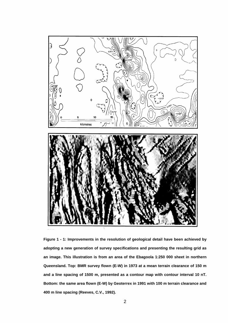
Figure 1 - 1: Improvements in the resolution of geological detail have been achieved by
adopting a new generation of survey specifications and presenting the resulting grid as
an image. This illustration is from an area of the Ebagoola 1:250 000 sheet in northern
Queensland. Top: BMR survey flown (E-W) in 1973 at a mean terrain clearance of 150 m
and a line spacing of 1500 m, presented as a contour map with contour interval 10 nT.
Bottom: the same area flown (E-W) by Geoterrex in 1991 with 100 m terrain clearance and
400 m line spacing (Reeves, C.V., 1992).
2
However, it is clear that the line spacing of 1.5 kilometres is too large to permit
confident correlation of subtle anomalies on adjacent profiles, and as a result,
only a low resolution result is possible. Therefore, it can be argued that despite
its format as a two-dimensional map, the contour map has essentially the same
resolution as a series of one-dimensional profiles. It is essential to employ
significantly closer line spacings, in order to achieve a genuine 2-D image.
Perhaps one of the most spectacular demonstrations of the benefits of
improved spatial resolution in both horizontal directions, has been three-
dimensional (3-D) seismic reflection methods. In the past twenty-five years,
high resolution 3-D seismic reflection methods have revolutionized the
investigation of the sedimentary basins (Weimer and Davis, 1996). The
fundamental problem facing two-dimensional (2-D) seismic methods is the fact
that most geological targets are three-dimensional. In the past, two-
dimensional methods have attempted to counter this problem by locating lines
with the strike and dips of the major features in mind, minimizing but rarely
eliminating the effect of the third dimension (Brown 1996).
French (1974) demonstrated that 3-D migration eliminates many of the lateral
correlation ambiguities which are caused by “sideswipes” and “blind structures”.
Structure maps derived from 3-D migration processing give a true and precise
picture of 3-D models, whereas the same data when processed using 2-D
migration, results in the mapped structures being distorted in shape. However,
the distortions can be reduced by increased coverage and careful interpretive
techniques (French, 1974). As a result, to obtain a precise image from seismic
3
data it is necessary to employ sampling densities and processing methods
which recognize and accommodate the three dimensions.
Furthermore, the geological targets studied in the near surface surveys often
display considerable variations in cross-line and in-line directions in terms of
depth to and seismic velocities within (Palmer, 2001b). This makes the
adoption of 3-D methods inevitable.
Perhaps one of the most compelling demonstrations of the benefits of 3-D
geophysical methods has been the study by Nestvold (1992) which
demonstrates that 3-D seismic reflection results are often significantly different
from 2-D seismic reflection results. In many cases, 2-D methods can provide
an incorrect rather than an incomplete picture of the subsurface structure. The
differences can be explained by the fact that the geological targets can vary
significantly in both horizontal directions, thereby requiring the adequate spatial
sampling obtained with 3-D methods. In other words, the incorrect subsurface
structure can often be the result of spatial aliasing. Furthermore, most seismic
reflection processing routines, especially imaging (also known as migration),
perform much better in three dimensions because they recognize and
accommodate out-of-plane signals.
4
1.2 Three-Dimensional Shallow Seismic Refraction Methods
While three-dimensional seismic refraction methods have been used in the
study of the deep earth’s crust (e.g. Miles, 1988; Bennett, 1999), they have not
been commonly applied to near surface targets. A major reason for this
situation is the fact that most shallow refraction field systems rarely consist of
more than twenty-four recording channels. As a result, the acquisition of
satisfactory volumes of data can be inconvenient.
Nevertheless, there have been several published examples which suggest that
3-D refraction methods may generate very useful results with genuine 3-D
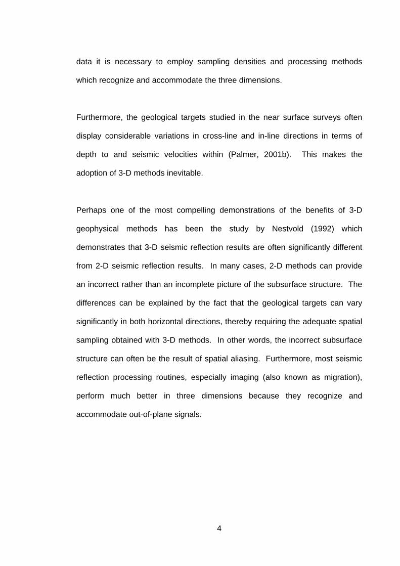
targets. In Palmer (2001b), a 3-D refraction survey was recorded across a
mapped shear zone at Mt. Bulga in southeastern Australia. These results
showed that there were important 3-D effects associated with the nominally 2-D
shear zone (Figure 1-2). They include cross-cutting orthogonal faults that had
not been detected with an earlier 2-D profile across the shear zone and a
change in the horizontal direction of approximately ninety degrees of the
azimuth of the highest seismic velocity in one region of the survey area.
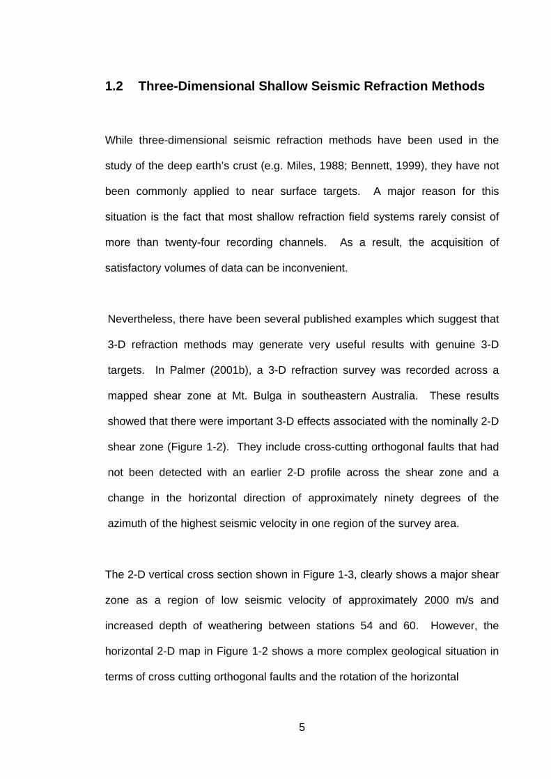
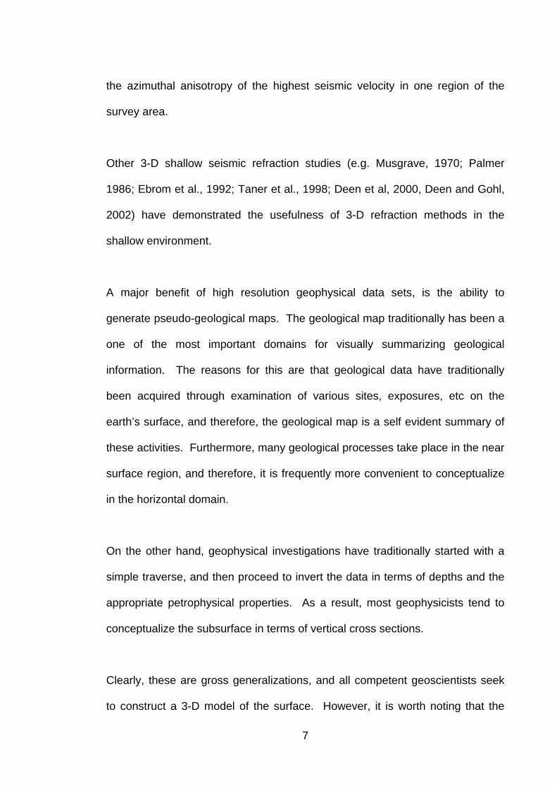
The 2-D vertical cross section shown in Figure 1-3, clearly shows a major shear
zone as a region of low seismic velocity of approximately 2000 m/s and
increased depth of weathering between stations 54 and 60. However, the
horizontal 2-D map in Figure 1-2 shows a more complex geological situation in
terms of cross cutting orthogonal faults and the rotation of the horizontal
5
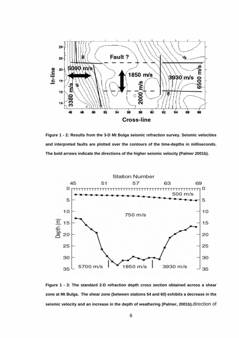
Figure 1 - 2: Results from the 3-D Mt Bulga seismic refraction survey. Seismic velocities
and interpreted faults are plotted over the contours of the time-depths in milliseconds.
The bold arrows indicate the directions of the higher seismic velocity (Palmer 2001b).
Figure 1 - 3: The standard 2-D refraction depth cross section obtained across a shear
zone at Mt Bulga. The shear zone (between stations 54 and 60) exhibits a decrease in the
seismic velocity and an increase in the depth of weathering (Palmer, 2001b).direction of
6
the azimuthal anisotropy of the highest seismic velocity in one region of the
survey area.
Other 3-D shallow seismic refraction studies (e.g. Musgrave, 1970; Palmer
1986; Ebrom et al., 1992; Taner et al., 1998; Deen et al, 2000, Deen and Gohl,
2002) have demonstrated the usefulness of 3-D refraction methods in the
shallow environment.
A major benefit of high resolution geophysical data sets, is the ability to
generate pseudo-geological maps. The geological map traditionally has been a
one of the most important domains for visually summarizing geological
information. The reasons for this are that geological data have traditionally
been acquired through examination of various sites, exposures, etc on the
earth’s surface, and therefore, the geological map is a self evident summary of
these activities. Furthermore, many geological processes take place in the near
surface region, and therefore, it is frequently more convenient to conceptualize
in the horizontal domain.
On the other hand, geophysical investigations have traditionally started with a
simple traverse, and then proceed to invert the data in terms of depths and the
appropriate petrophysical properties. As a result, most geophysicists tend to
conceptualize the subsurface in terms of vertical cross sections.
Clearly, these are gross generalizations, and all competent geoscientists seek
to construct a 3-D model of the surface. However, it is worth noting that the
7

greatly increased use of airborne geophysical methods for geological mapping
was more a result of improved methods of data presentation with image
processing software, rather than more detailed methods for depth inversion.
1.3 Dryland Salinity
Dryland salinity or secondary soil salinization is a form of land degradation
which seriously affects many parts of the Australian landscape. The problem of
salinity was first identified by Walter Earnest Woods in 1924, who investigated
the deterioration of land and watercourses in the Western Australia wheat belt
in the years following clearing of native vegetation for agricultural land-use
(English, 2002). The occurrence of dryland salinity has major implications for
agricultural, industrial and domestic activities as well as for the natural
environment. This form of land degradation leads to a decline in crop and
native plant growth, increase in soil erosion, and the pollution of rivers and
groundwater
Dryland salinity is a major problem in many parts of inland Australia. According
to the National Land and Water Resources Audit (2001), over the next fifty
years, the area at risk from dryland salinity in Australia will increase from a
current 5.7 million to 17 million hectares (Coram et al. 2001). The audit states
that as a result of this three-fold increase, the area of native vegetation at risk
will expand from a current 630,000 to potentially 2,000,000 hectares, and the
length of streams at risk will be over 20,000 kilometres. The economic cost of
8

repairing the more than 200 towns expected to suffer infrastructure damage
and the 52,000 kilometres of road facing damage is substantial.
The largest areas of dryland salinity are in the agriculture zone of south-west
Western Australia. Large areas are also at risk of dryland salinity in South
Australia, Victoria and New South Wales, mainly in the Murray-Darling Basin
where ground water levels are still rising (Bradd and Gates, 1996). In New
South Wales approximately 120,000 hectares of land are estimated to be
currently affected by salinity, of which over 90 per cent occur in the five
catchments of the Murray, Murrumbidgee, Lachlan, Macquarie and Hunter
rivers. Table 1-1 is shown the areas with a high potential to developed dryland
salinity in Australia (National Land and Water Resources Audit, 2001). The
Northern Territory and the Australian Capital Territory were not included as the
dryland salinity problem was considered to be very minor.
Table 1- 1: Areas (hectares) with a high potential to develop dryland salinity in Australia
(From: National Land and Water Resources Audit, 2001).
State/Territory 2000 2050
NSW 181000 1300000
Vic 670000 3110000
Qld not assessed 3100000
SA 390000 600000
WA 4363000 8800000
Tas 54000 90000
9

The extent and severity of salinity problems are sometimes measured in terms
of the area of land affected, value of lost agricultural production and the effect
on water quality. It has been estimated that approximately 16090 km of land
in the non-arid zone of Australia is affected by irrigation salting and 324090 km
affected by natural and man-induced dryland salting (ACIL, 1983). The latter
represents approximately 35 per cent of the total area of land in Australia
affected by some form of soil degradation.
2
2
Dryland salinity occurs extensively throughout the Spicers Creek Catchment in
central eastern New South Wales, Australia. The surface discharge of saline
groundwater at several locations has led to a decline in crop and native plant
growth, increase in soil erosion, and the pollution of rivers and groundwater. At
several of these locations the saline groundwater seepage zones are
geologically induced, correlating with a shear zone inferred from geological
mapping. These zones of fractured bedrock enable the saline groundwater,
contained within deep basement aquifers, to flow upwards, where they mix with
shallow groundwater and are eventually discharged at the ground surface
causing extensive soil salinisation.
1.4 Detailed Mapping of Shear Zones
A shear zone is defined by Bates and Jackson (1980) as “a tubular zone of rock
that has been crushed and brecciated by many parallel fractures due to shear
strain”. The general characteristics of shear zones can differ in the field. The
10
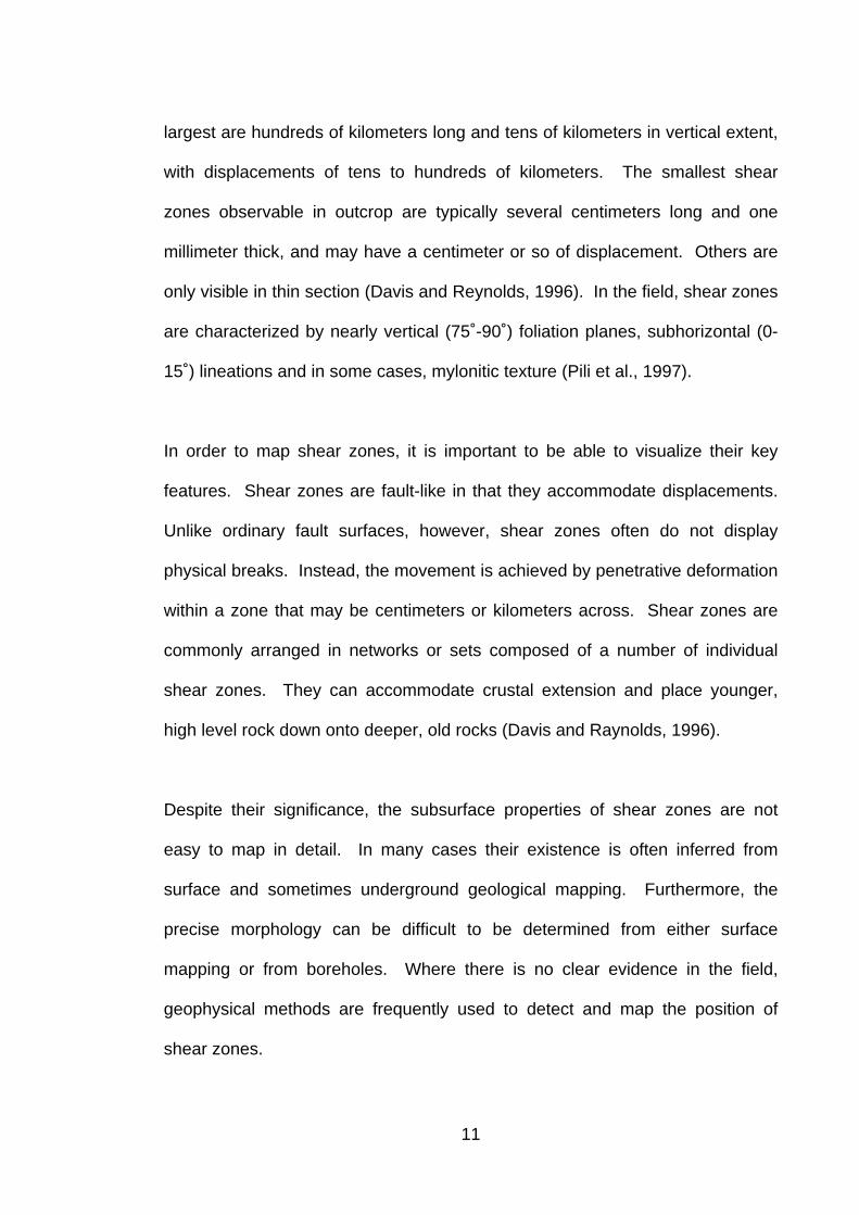
largest are hundreds of kilometers long and tens of kilometers in vertical extent,
with displacements of tens to hundreds of kilometers. The smallest shear
zones observable in outcrop are typically several centimeters long and one
millimeter thick, and may have a centimeter or so of displacement. Others are
only visible in thin section (Davis and Reynolds, 1996). In the field, shear zones
are characterized by nearly vertical (75˚-90˚) foliation planes, subhorizontal (0-
15˚) lineations and in some cases, mylonitic texture (Pili et al., 1997).
In order to map shear zones, it is important to be able to visualize their key
features. Shear zones are fault-like in that they accommodate displacements.
Unlike ordinary fault surfaces, however, shear zones often do not display
physical breaks. Instead, the movement is achieved by penetrative deformation
within a zone that may be centimeters or kilometers across. Shear zones are
commonly arranged in networks or sets composed of a number of individual
shear zones. They can accommodate crustal extension and place younger,
high level rock down onto deeper, old rocks (Davis and Raynolds, 1996).
Despite their significance, the subsurface properties of shear zones are not
easy to map in detail. In many cases their existence is often inferred from
surface and sometimes underground geological mapping. Furthermore, the
precise morphology can be difficult to be determined from either surface
mapping or from boreholes. Where there is no clear evidence in the field,
geophysical methods are frequently used to detect and map the position of
shear zones.
11
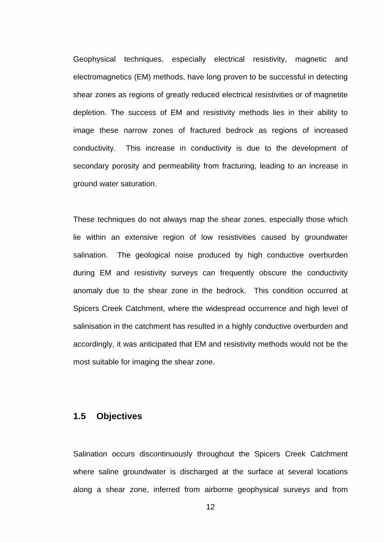
Geophysical techniques, especially electrical resistivity, magnetic and
electromagnetics (EM) methods, have long proven to be successful in detecting
shear zones as regions of greatly reduced electrical resistivities or of magnetite
depletion. The success of EM and resistivity methods lies in their ability to
image these narrow zones of fractured bedrock as regions of increased
conductivity. This increase in conductivity is due to the development of
secondary porosity and permeability from fracturing, leading to an increase in
ground water saturation.
These techniques do not always map the shear zones, especially those which
lie within an extensive region of low resistivities caused by groundwater
salination. The geological noise produced by high conductive overburden
during EM and resistivity surveys can frequently obscure the conductivity
anomaly due to the shear zone in the bedrock. This condition occurred at
Spicers Creek Catchment, where the widespread occurrence and high level of
salinisation in the catchment has resulted in a highly conductive overburden and
accordingly, it was anticipated that EM and resistivity methods would not be the
most suitable for imaging the shear zone.
1.5 Objectives
Salination occurs discontinuously throughout the Spicers Creek Catchment
where saline groundwater is discharged at the surface at several locations
along a shear zone, inferred from airborne geophysical surveys and from
12
subsequent regional geological mapping by the NSW Geological Survey.
However, there has been no confirmation of the exact location of the shear
zone or its precise correlation with saline groundwater discharges at the
surface.
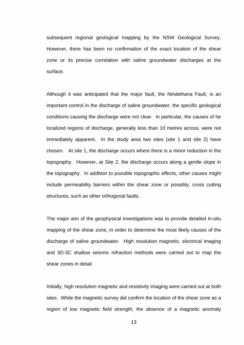
Although it was anticipated that the major fault, the Nindethana Fault, is an
important control in the discharge of saline groundwater, the specific geological
conditions causing the discharge were not clear. In particular, the causes of he
localized regions of discharge, generally less than 10 metres across, were not
immediately apparent. In the study area two sites (site 1 and site 2) have
chosen. At site 1, the discharge occurs where there is a minor reduction in the
topography. However, at Site 2, the discharge occurs along a gentle slope in
the topography. In addition to possible topographic effects, other causes might
include permeability barriers within the shear zone or possibly, cross cutting
structures, such as other orthogonal faults.
The major aim of the geophysical investigations was to provide detailed in-situ
mapping of the shear zone, in order to determine the most likely causes of the
discharge of saline groundwater. High resolution magnetic, electrical imaging
and 3D-3C shallow seismic refraction methods were carried out to map the
shear zones in detail.
Initially, high resolution magnetic and resistivity imaging were carried out at both
sites. While the magnetic survey did confirm the location of the shear zone as a
region of low magnetic field strength, the absence of a magnetic anomaly
13
precluded any detailed mapping of the internal features of the shear zone.
Also, resistivity imaging did not achieve satisfactory penetration through the
conductive overburden, sufficient to map the shear zone in detail.
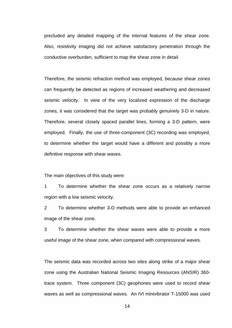
Therefore, the seismic refraction method was employed, because shear zones
can frequently be detected as regions of increased weathering and decreased
seismic velocity. In view of the very localized expression of the discharge
zones, it was considered that the target was probably genuinely 3-D in nature.
Therefore, several closely spaced parallel lines, forming a 3-D pattern, were
employed. Finally, the use of three-component (3C) recording was employed,
to determine whether the target would have a different and possibly a more
definitive response with shear waves.
The main objectives of this study were:
1 To determine whether the shear zone occurs as a relatively narrow
region with a low seismic velocity.
2 To determine whether 3-D methods were able to provide an enhanced
image of the shear zone.
3 To determine whether the shear waves were able to provide a more
useful image of the shear zone, when compared with compressional waves.
The seismic data was recorded across two sites along strike of a major shear
zone using the Australian National Seismic Imaging Resources (ANSIR) 360-
trace system. Three component (3C) geophones were used to record shear
waves as well as compressional waves. An IVI minivibrator T-15000 was used
14
as the main source of energy for the seismic survey although some explosive
charges in shallow shot holes were used for comparison. Data were processed
using the generalized reciprocal method (GRM, Palmer 1980, 1986), Seismic
Un*x freely distributed by the Centre for Wave Phenomena at the Colorado
School of Mines and Visual-SUNT 6, generously donated by W_Geosoft.
1.6 Problems Solved in this Study
This study demonstrates that 3D – 3C seismic refraction methods are able to
provide a good estimate of the structure or shape of the refracting interface. As
discussed in a previous section, there has been no evidence to confirm the
existence of the inferred shear zone or cross-cutting features at the sites in the
Spicers Creek Catchment. This study confirms that the Nindethana fault
occurs as a region of low seismic velocities and increased depths of
weathering, and that the regions of salination correspond with the occurrence
of cross-cutting faults along the Nindethana fault.
This study demonstrates the ability to generate a reasonably detailed model of
the shear zone in the Spicers Creek Catchment in the region of the discharge
of saline groundwater. As with the Mt Bulga case history described earlier, it is
clear that the three-dimensional seismic refraction method was used able to
image the important cross-cutting features, as well as the major shear zone,
which were not as readily detectable with two-dimensional methods.
15
However, it was necessary to process the data so that the seismic signature of
the shear zone was enhanced. This required the development of methods to
include most of the field data in order to improve the statistical reliability of the
data, as well as an effective method to correct for near surface irregularities.
The latter can often result in ambiguous interpretations of the field data and
therefore can adversely effect the determination of accurate seismic velocities
in the refractor.
A new method, which is described as part of this study, takes advantages of a
unique feature of the GRM to compensate for localized variations in the near
surface seismic velocities and/or topography, termed the GRM SSM for GRM
statics smoothing method. This method significantly improved the reliability
and consistency in determining seismic velocities in the refractor.
Furthermore, this study demonstrates the importance of generating robust
starting models for inversion. In recent years, the methods of model-based
inversion have been used to the analysis of refraction data and involve the
derivation of an initial or starting model (Smith and Ferguson, 2000; Palmer
2003a) and then refining that model until the traveltimes generated with the
model, match those of the recorded field data. Wavepath eikonal traveltime
(WET) tomography was used to generate a velocity-depth section of every line
for each wave type. Starting models were generated using both one
dimensional inversion methods, namely the delta-t-V method (Gebrande and
Miller 1985), and two-dimensional inversion algorithms with the GRM.
16

Chapter 2
Dryland Salinity
2.1 Summary
Large areas throughout Australia are currently at risk of being affected by
dryland salinity. In New South Wales, approximately 125 000 hectares of land
is currently affected. Dryland salinisation develops where a source of salt
exists. This salt can be contained within the colluvium, having accumulated
there due to rainfall, aeolian processes, and the weathering of soil and rock
minerals, or it can be derived deeper in the bedrock from saline groundwater in
an unconfined aquifer.
The extent of dryland salinity in the study area, the Spicers Creek Catchment,
has severely altered the landscape, having major environmental implications.
Large areas of the catchment have experienced soil erosion resulting from the
saline groundwater in the surface soil causing the destruction of clay and soil
structure. Saline groundwater is discharged at the surface at several locations.
A significant amount of the saline groundwater continuously discharges through
shallow alluvial/colluvial aquifers at intermittent locations along an extension of
the Nindethana fault, and forms a “saline plume” contaminating the soil down
gradient from the seepage zone.
17

2.2 Introduction
Salinity is a problem, which affects about one-third of the irrigated land around
the world (Reeve and Fireman, 1967). Salinity is believed to have been a
problem with Mesopotamian agriculture about 4500 years ago (Jacobsen and
Adams, 1958). Australia is one of the few countries which experience salinity in
non-irrigation (dryland) farmland (Peck et al., 1983). Dryland salinity or
secondary soil salinisation is associated with the movement of saline
groundwater, and it is an indication of a changing water balance in the
catchment. It is associated with particular land uses that cause groundwater
levels and salt contents to rise by allowing deep percolation of rainwater
through the soil. Dryland salinity is a form of land degradation, which seriously
affects many parts of Australian landscapes.
Dryland salinity is caused by a number of earth processes and the salts
involved have multiple sources. Dryland salinity can occur where soils contain
high levels of salt because of rising groundwater levels. Usually plants and soil
organisms are killed or their productivity is severely limited on affected lands.
The occurrence of dryland salinity has major implications for agricultural,
industrial and domestic activities as well as for the natural environment. This
form of land degradation leads to a decline in crop and native plant growth,
increase in soil erosion, and the pollution of rivers and groundwater
The water quality of river systems is adversely affected by dryland salinity.
Freshwater salinity is a by-product of dryland salinity whereby salt in the surface
18

soil eventually enters river systems, leading to an increase in water salinity.
This occurs via two mechanisms. Firstly, the salt can come from overland flow
where rainfall washes salt off the affected land and into river systems at the
bottom of catchments. This is especially the case when rivers are not lined with
native vegetation which filters incoming pollutants such as salt. Secondly, the
salt can enter river systems directly from the groundwater, especially where the
rivers are low. An increase in freshwater salinity can devastate the ecology of a
river system as well as reducing water quality for domestic, industrial and
agricultural purposes.
The extent of dryland salinity in the study area, Spicers Creek Catchment, has
severely altered the landscape, having major environmental implications. The
high concentration of salt in the groundwater has led to a significant decline in
agricultural productivity and a reduction in native vegetation. Large areas of the
catchment have experienced soil erosion resulting from the saline groundwater
in the surface soil causing the destruction of clay and soil structure.
2.3 Extent of Dryland Salinity in New South Wales
Dryland salinity is a major problem in many parts of inland Australia. Bradd et
al. (1997) mapped the spatial distribution of dryland salinity hazard throughout
NSW using a prediction tool based on the correlation between the current
occurrence of dryland salinity in NSW and specific combinations of land and
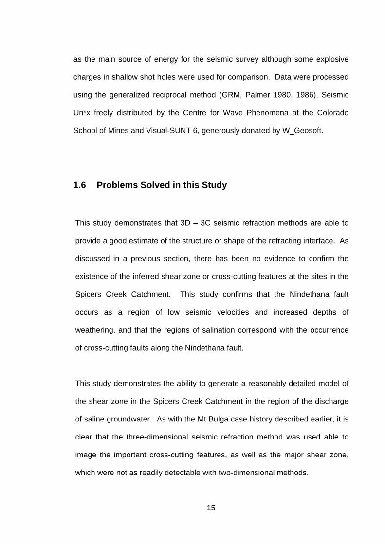
physiographic attributes (Figure 2-1). The results of their work suggest that up
19

to 5 million hectares of land has the potential of being affected by dryland
salinity with 4 250 000, 470 000, and 310 000 hectares of land in the
moderate, high and very high hazard categories respectively.
In New South Wales approximately 120,000 hectares of land are estimated to
be currently affected (Bradd and Gates, 1996), while a further 5,000,000
hectares are considered to be at risk on the basis of their physical
characteristics. In New South Wales some regions are more vulnerable to
dryland salinity such as the Lachlan, Murrumbidgee and the Macquarie river
basin. Areas of major concern with high to very high dryland salinity hazard
index are located in a north-south belt just north of Canberra (Yass River
Valley), and in the south-western part of the Lachlan River catchment, east of
Wagga Wagga in the Murrumbidgee River catchment, and east of Dubbo in the
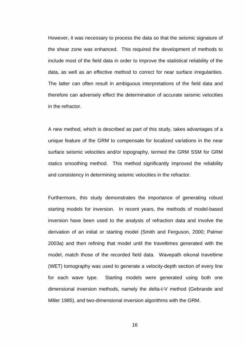
Macquarie River catchment. In the north of NSW, the potential for dryland
salinity is less (Coram, 1998). Figure 2-2 shows the dryland salinity risk in NSW
in 2001 and Figure 2-3 is predicted dryland salinity risk in NSW by 2050.
20
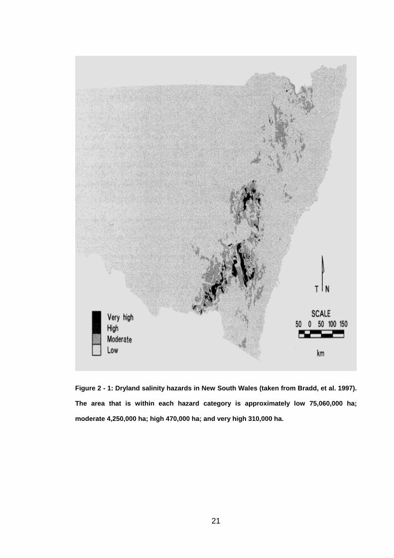
Figure 2 - 1: Dryland salinity hazards in New South Wales (taken from Bradd, et al. 1997).
The area that is within each hazard category is approximately low 75,060,000 ha;
moderate 4,250,000 ha; high 470,000 ha; and very high 310,000 ha.
21
Figure 2 - 2: Dryland salinity risk in New South Wales 2000 (From National Land & Water
Resources Audit, 2000).
Figure 2 - 3: Dryland salinity risk in New South Wales 2050 (From National Land & Water
Resources Audit; 2000).
22

2.4 Causes of Dryland Salinity
The general cause of dryland salinity is well known. It was described in
Australia as early as 1924 with the publication of ‘Increase in salt in soil and
streams following the destruction of native vegetation’ by Walter Wood in the
Journal of the Royal Society of Western Australia. Coram (1998) has
developed a national catchment classification system in Australia and proposed
that the broad features of common occurrences of salinisation can be described
by the fifteen hydrogeological models according to whether local, intermediate
or regional flow systems are present. The broad features of local, intermediate
and regional systems are summarized in Table 2-1. These fifteen
hydrogeological models are as below:
1) Local models:
a) Discharge over lower hydraulic conductivity structures.
b) Discharge from unweathered rock aquifers at the break of slope.
c) Discharge from weathered fractured rock aquifers at break of slope.
c) Discharge from colluvial/alluvial slopes.
d) Discharge controlled by stratigraphy (sediments/basalts).
e) Discharged from perched aquifer.
f) Discharge controlled by linear features of contrasting hydraulic
conductivity.
g) Discharge from low hydraulic conductivity aquifer.
2) Intermediate models:
23
a) Capillary discharge from unconfined aquifers in valley floors.
b) Discharge from semi-confined aquifers controlled by facies changes
and changes in aquifer geometry.
c) Discharge from unweathered fractured rock aquifer at break of slope.
d) Discharge across topographic divides controlled by large, transmissive
linear structures.
3) Regional models:
a) Regional confined and semi-confined aquifer discharge controlled by
structure.
b) Regional confined and semi-confined aquifer discharge controlled by
facies change.
c) Regional unconfined to semi-confined aquifer discharge controlled by
topography.
Coram (1998) has shown that the model 1(d) is applicable for the area around
Dubbo. In this model salinisation occurs in sedimentary sequences or basaltic
rocks because of groundwater discharging from local or perched systems where
high hydraulic conductivity layers terminate at erosional surfaces or at
faulted/unconformable contacts. Also discharge occurs from a permanent and
large saturated zone.
There are several sources of the dryland salinity in the Lachlan River catchment
in southern NSW. Acworth and Jankowski (2001) have carried out a detailed
study involving drilling, geophysics, hydrogeochemistry and groundwater
monitoring over a 10-year period at a small catchment in southeast of NSW
24
(Yass River) to investigate the sources of salt causing dryland salinity. They
demonstrated that there is no hydrogeochemical evidence to suggest
evaporative or transpirative concentration of salt in the groundwater and that
there is a likely windblown source for the salt.
Different mechanisms for controlling the development of dryland salinity have
been suggested in different parts of Australia by several authors. Knight et al.
(1989) demonstrated that there is a relationship between dryland salinisation
and saline groundwaters discharging through a fault zone. Lewis (1991)
suggested linear geological features such as dykes, fractures and shear fault
zones can be responsible for salinity.
Waltham (1997) described shear zones which were the result of drag of the salt
by the movement of the hanging wall. Dahlhaus et al. (2000) also described the
effect of discharge at a break in slope as a result of the differences in sediment
permeability. Acworth and Jankowski (2001) demonstrated that the saline
seepages originated from the fractured bedrock aquifer on the lower slopes and
valley floors, where the bedrock is close to the ground surface. Clarke et al.
(2002) illustrated the affect of geological structures on dryland salinity; and
finally the recent study by Morgan and Jankowski (2002) demonstrated that the
zone discharging salinity occurred near a fault.
25

Table 2 - 1: Summary of the local, intermediate and regional systems (Coram, 1998).
Local flow
system
Intermediate flow
system
Regional flow
system
Horizontal scale 1-3 Kilometers 5-10 kilometers >50 Kilometers
Geomorphology -Subcatchments in
higher relief on
edges of plateaus
and ranges
-Alluvial and occasionally,
glacial valley fill in foothills
and valleys
-Broad riverine
plains on
depositional basins
Geology -Fractured
metamorphics and
igneous rocks.
-Colluvial
sediments.
-Aeolian sediments
-Fractured metamorphic
and igneous rocks shallow
(<50 meters deep) alluvial
and colluvial sediments.
-Deep, interbedded
marine, alluvial and
Aeolian
sedimentary
sequences (several
hundreds of meters
deep).
Structural
features
influencing
groundwater flow
-Subsurface low
hydraulic
conductivity
features such as
bedrock highs and
dykes.
-Termination of
aquifer at erosional
surface.
-reduction in hydraulic
conductivity with distance
from sedimentary source or
aquifer weathering.
-Reductions in hydraulic
gradient or aquifer
thickness with shallowing of
the ground surface
-Subsurface low hydraulic
conductivity features such
as bedrock highs and
dykes.
-Reductions in
hydraulic
conductivity with
distance from
sedimentary source
or associated with
structural deforming
(faulting, folding).
-Reductions in
hydraulic gradient
or aquifer thickness
with shallowing of
the ground surface.
26

A more comprehensive list of salinity causes is as follows (Creelman, 2002):
Salt from the atmosphere: deflated from the sea or picked up from the land
surface, referred to as cyclical salts.
Salt from the interior of the continent: older cyclical salts that have been
accumulated in the interior of the continent, and can be transported by their
adherence to windborne dust.
Salt from anthropogenic sources: soluble products from industrial activities
such as combustion, industrial processes that use and then dispose of water.
Salt from relict seawater: this is salt that accumulates as enclosed marine
environments are evaporated. The salt is contained in the fluid inclusions within
the rocks and is partially the source of salts in basinal brines or evaporate
deposits.
Aeolian deposits and debris flow: related to geology and the hydrosphere
with atmospheric inputs.
Salt from rock weathering: altered rocks can contain over 100 times the
amount of chloride as unaltered rocks.
Salt elements exchange onto clay minerals: as seawater deposits the clays,
or as clays are deposited in seawater.
Dissolution of evaporates: within the drainage basin.
27
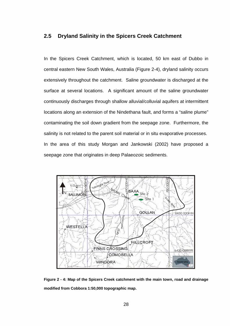
2.5 Dryland Salinity in the Spicers Creek Catchment
In the Spicers Creek Catchment, which is located, 50 km east of Dubbo in
central eastern New South Wales, Australia (Figure 2-4), dryland salinity occurs
extensively throughout the catchment. Saline groundwater is discharged at the
surface at several locations. A significant amount of the saline groundwater
continuously discharges through shallow alluvial/colluvial aquifers at intermittent
locations along an extension of the Nindethana fault, and forms a “saline plume”
contaminating the soil down gradient from the seepage zone. Furthermore, the
salinity is not related to the parent soil material or in situ evaporative processes.
In the area of this study Morgan and Jankowski (2002) have proposed a
seepage zone that originates in deep Palaeozoic sediments.
6420 000mN
700
000m
E
690
000m
E
6430 000mN
N BALLIMORE
680
000m
E
To DubboSpicers Creek
Talbragar River
Racec
ourseG
ully
Site 2
Site 1
Snake River
Figure 2 - 4: Map of the Spicers Creek catchment with the main town, road and drainage
modified from Cobbora 1:50,000 topographic map.
28
Previous work by Morgan and Jankowski (2004) has identified several areas in
the Spicers Creek Catchment where the discharge of saline groundwater at the
surface correlates with a north–south-trending shear zone which has been
inferred from airborne geophysical surveys and from subsequent regional
geological mapping. This zone of fractured bedrock enables the saline
groundwater, contained within deep basement aquifers, to flow upwards, mixing
with shallow groundwater within the colluvium, and eventually being discharged
at the ground surface causing extensive soil salinisation. However, there have
been no studies of the exact location of the shear zone and its correlation with
saline groundwater discharges at the surface.
The high concentration of salt in the groundwater has led to a significant decline
in agricultural productivity and a reduction in native vegetation. Large areas of
the catchment have experienced soil erosion resulting from the saline
groundwater in the surface soil causing the destruction of clay and soil
structure. The severity of soil erosion can be seen in photos 2-1 and 2-2 of an
artesian bore discharging saline groundwater. The difference between the top
of the concrete collar on the casing and the existing ground surface is
considerable. Photos 2-3 and 2-4 show the water flow approximately 50 metres
downstream from the artesian bore in photo 2-1. Salt completely covers the
majority of the stream bank, indicating the high concentrations of salt in the
stream.
At several sites, saline groundwater seepage zones are geologically induced
having formed adjacent to a north–south-trending shear zone. These zones of
29

fractured bedrock enable the saline groundwater, contained within deep
basement aquifers, to flow upwards, mixing with shallow groundwater within the
colluvium, and eventually being discharged at the ground surface causing
extensive soil salinisation.
The extent of dryland salinity in the Spicers Creek Catchment has severely
altered the landscape, having major environmental implications. The principal
land use in the Spicers Creek Catchment is agricultural. Large areas of land
are occupied by cereal cropping such as wheat, canola and legumes, whilst
sheep grazing occurs in areas of partly cleared native vegetation. The increase
in agricultural activities has resulted in the replacement of high-water use native
vegetation with low-water use crops, resulting in increased groundwater
recharge and rising water tables. This, together with the landscape’s naturally
saline environment, has led to large areas of the catchment developing dryland
salinisation. Fifty-two sites have been identified as affected (Jewel and
Associates, 2000).
30
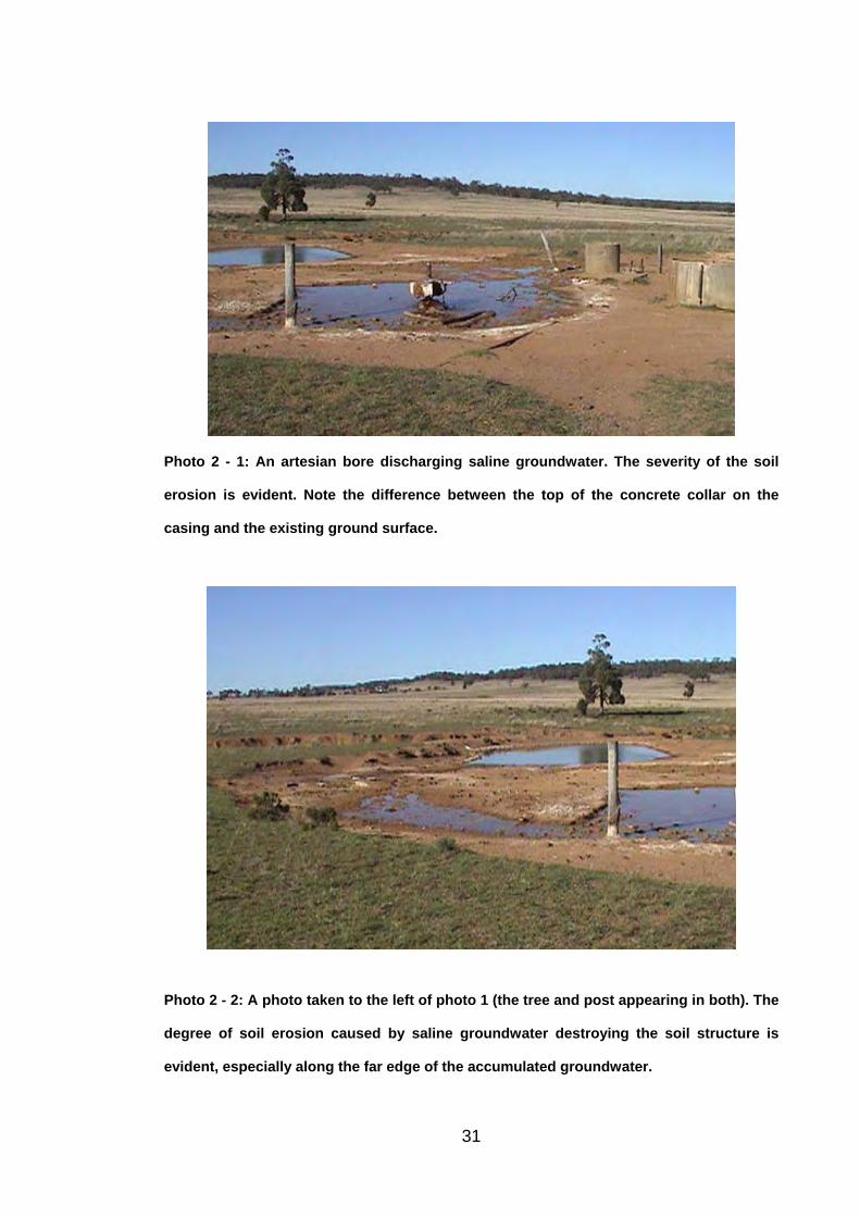
Photo 2 - 1: An artesian bore discharging saline groundwater. The severity of the soil
erosion is evident. Note the difference between the top of the concrete collar on the
casing and the existing ground surface.
Photo 2 - 2: A photo taken to the left of photo 1 (the tree and post appearing in both). The
degree of soil erosion caused by saline groundwater destroying the soil structure is
evident, especially along the far edge of the accumulated groundwater.
31
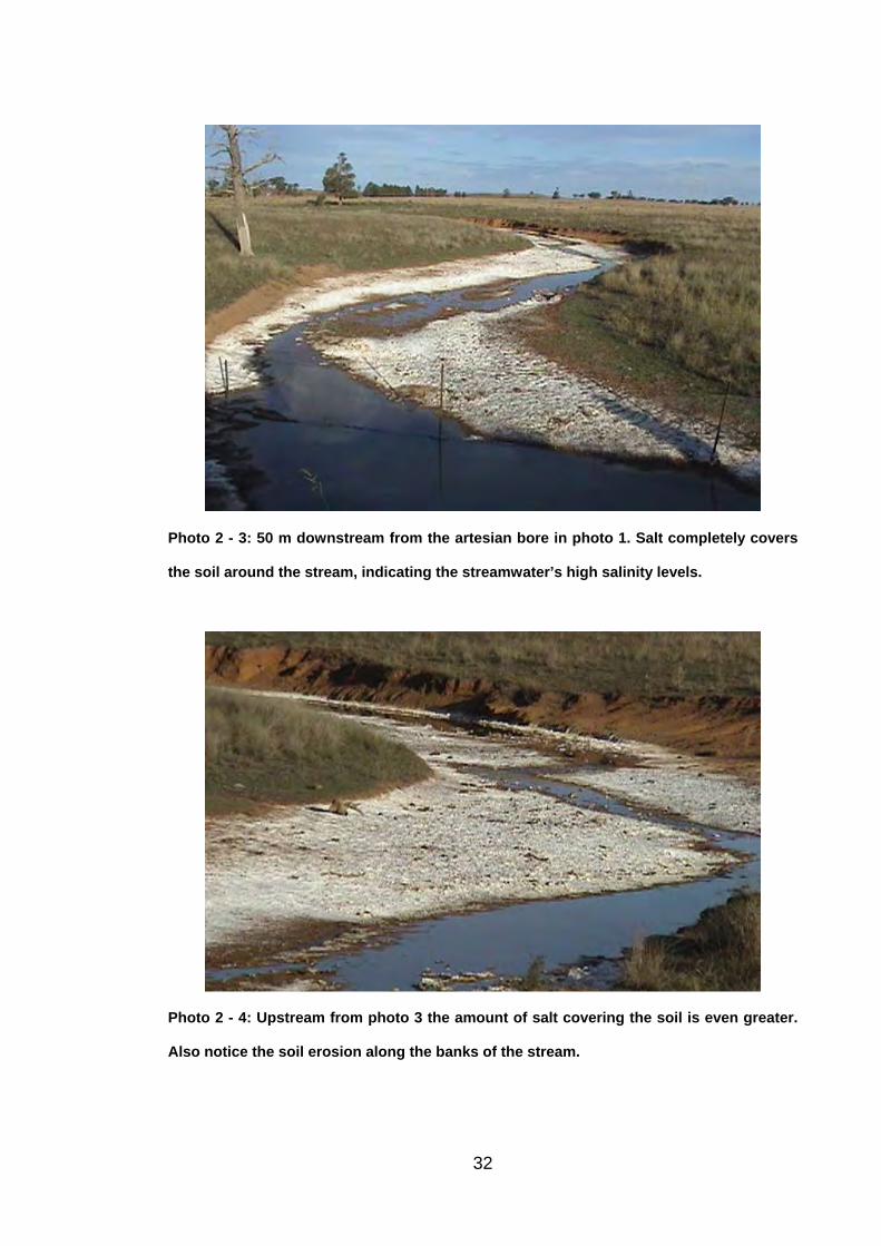
Photo 2 - 3: 50 m downstream from the artesian bore in photo 1. Salt completely covers
the soil around the stream, indicating the streamwater’s high salinity levels.
Photo 2 - 4: Upstream from photo 3 the amount of salt covering the soil is even greater.
Also notice the soil erosion along the banks of the stream.
32

2.6 Management of Dryland Salinity
Although many management options are recognized for dryland salinity, there is
little information available on the possible effectiveness of alternative actions for
salinity control in specific area. Peck et al. (1983) demonstrated that the
following specific data and information needs for salinity management in
Australia:
1 Data on the effect of land-forming on irrigation water use.
2 Data on water use by different plants and under different management to
estimate groundwater recharge rates.
3 Methods to establish location and rate of groundwater recharge and
present or potential discharge.
4 Definition of the hydrogeological situation in which a number of
representative salt seepages have developed.
5 Application of groundwater modeling techniques to areas with
representative hydrogeology to predict the effect of management options.
6 Field studies of the effectiveness of possible treatments and
combinations of treatments for control of groundwater recharge and discharge.
7 Treatments to be considered include diversion and control of surface
waters; chemical or physical modification of soil properties; biological
manipulation of plant growth patterns; subsurface drainage; selection of crops;
and shrubs or trees.
8 Salinity models and field methodology to provide an early warning of salt
discharge before land and water are degraded.
33

9 Estimate of the time-scale for development of salinity problems and for
their control by various management actions.
10 Methods to locate the most effective sites for de-watering bores.
11 Models of river water quality which take account of the effects of land
uses on groundwater flow to the river.
12 Models of river water quality to meet more than one management
objective.
13 Studies of the long term salt distribution patterns developed in
groundwater systems associated with evaporation basins, particularly in the
absence of commercial salt production from the basin.
Coram et al. (2001) showed that dryland salinity management options can be
broadly devided into four categories. These are prevention, treatment of
causes, amelioration of symptoms, and productive uses of saline resources.
Examples of these are shown in Table 2-2.
Prevention options include the retention of native vegetation, and employing
suitable agricultural techniques in order to keep land and surface waters free
from salinity. Based on their work in the Yass River Catchment, Nicoll and
Scown (1993) developed a technique for determining dryland salinity
management strategies which is mostly preventative in nature. Dryland salinity
has long been recognized in that area, with much of the landscape being
vulnerable. Eight land management classes were identified based on the
capability of the affected land, recognizing factors such as soil type, land use,
timber cover, and terrain slope (Table 2-3).
34

Options to reduce land and surface water salinisation by treatment of the cause
involve either reducing the intake of water at the recharge zone or intercepting
the groundwater prior to infiltration into the discharge zone. The former can be
accomplished by planting communities of deep rooted trees and shallower
rooted shrubs in strategic areas of recharge. The latter is accomplished
through engineering works based on active or passive drainage.
Amelioration is achieved through a range of approaches which seek to minimize
the impact the added salt has on affected land and water resources. Alternative
farming practices such as implementing raised beds in dryland cropping,
cultivating a mixture of salt tolerant and conventional crops, and minimizing
grazing by livestock enables continued agricultural productivity whilst
diminishing land and surface water salinisation. Land and surface water
salinisation can be further diminished by managing saline discharge through the
revegetation of target areas with salt tolerant native plants and trees.
Some management options are based on not seeking to prevent or reduce
dryland salinity but rather employing alternative and productive uses for the
saline land and water resources. Aquaculture, currently one of Australia’s
fastest growing primary industries has been implemented in inland areas using
saline groundwater. The successful breeding and cultivating of seawater
species such as tiger prawns, tuna, black bream, salmon, marron and redclaw
crayfish in saline groundwater suggests that an inland aquaculture industry is
viable (Sexton, 2003). Sustainable forestry is perhaps another viable use for
35

salt affected land. Experiments in selective breeding of tree species have
produced hybrids that have both a tolerance for saline water and produce
timber. The use of such trees in sustainable forestry will enable the
management of land for water movement and salinity, whilst at the same time
maximize the productive use of the land (Sexton, 2003).
A number of options are available for the prevention and remediation of dryland
salinity in the Spicers Creek Catchment. Most preventative options are based
on managing the vegetation in areas of risk so deep drainage does not
increase. Nicoll and Scown’s (1993) land management class six (LM 6) for
saline and potentially saline country in the Yass Valley could be readily applied
in areas of the Spicers Creek Catchment. For such country, they recommend
retaining existing trees; planting salt tolerant grasses, shrubs and trees; and to
straw mulch the area for better grass germination. They also recommend that
the area be fenced in, lightly grazed for short periods only when ground cover is
established, maintain a minimum of 70 % ground cover, and not to graze
pasture below 5 cm in height.
Due to the complex hydrogeological nature of the problem, strategies for the
remediation of dryland salinity are different for every catchment. In the Spicers
Creek Catchment, the successful remediation of salinisation lies in the ability to
obtain a reasonably detailed model of the possible shear zone that is
associated with the discharge of saline groundwater. Three-dimensional three-
component seismic refraction surveys were carried out at two sites of dryland
salinity in the Spicers Creek Catchment with the objective to provide this model.
36

Variables which would be useful in determining the possible remediation
measures at the Spicers Creek Catchment include the width of the shear zone
and a measure of the degree of fracturing in terms of porosity and permeability.
The possibility of grouting as a remediation option might arise if the shear zone
is quite narrow, possibly less than 10 m. Grouting along the extent of the shear
zone and the subsequent filling of the fractured bedrock would confine the
basement aquifers. This would prevent the saline groundwater from flowing
upwards in to the colluvium.
For a wider shear zone, the most suitable remediation option might be to
intercept and drain the saline groundwater before it reaches the surface soil.
This could be done with passive drainage if the shear zone is consistently
fractured, or with active drainage if it consists of a small number of large
fractures. The construction of a passive drainage system might involve setting
porous gravels at the water table along key areas of discharge and running a
drainage line underground to a collection dam. With active drainage, a number
of bore holes could be drilled into the water table above the large fractures in
order to pump the saline groundwater into a collection dam. Once in the dam,
the water could be evaporated leaving the salt to be collect and disposed.
37

Table 2 - 2: Evaluation attributes for different dryland salinity management options (from Coram et al., 2001).
Managementobjective
Strategy Outcome sought Recommended evaluation attributes
Per cent retention of native deep-rooted vegetation in high risk areasLong-term groundw ater level trendsLong-term stream salinity and salt load trendsExtent of land salinisedLand cover changeHydrogeological and soil characteristicsClimatic characteristics
Long-term groundw ater level trendsLong-term stream salinity and salt load trendsExtent of land salinisationLand cover changeHydrogeological and soil characteristicsClimatic characteristics
Long-term groundw ater level trendsLong-term stream salinity and salt load trendsExtent of land salinisationHydrogeological and soil characteristicsClimatic characteristics
Long-term stream salinity and salt load trendsExtent of land salinisationHydrogeological and soil characteristicsClimatic characteristics
Trea
tmen
t of c
ause
Prev
enta
tion
Land and surface w aters w ill remainfree from degradation from salinity
Land and surface w ater salinisationw ill diminish
Interception and disposal of salt, and reduction of groundw ater levels in transmissin zones
Land and surface w ater salinisationw ill diminish
Land and surface w ater salinisationw ill diminish
Reduce recharge to the groundw ater system by increasing vegetation w ater use through land management practices
Interception of w ater prior to infiltration or from groundw ater upgradient of discharge zone
Manage vegetation so deep drainagedoes not increase in high risk areas
38

Table 2- 2 (continued): Evaluation attributes for different dryland salinity management options (from Coram et al., 2001).
Managementobjective
Strategy Outcome sought Recommended evaluation attributes
Managing saline discharge Long-term stream salinity and salt load trendsHydrogeological and soil characteristicsClimatic characteristics
Application of soil treatments (ameliorants) Extent of land salinisationSoil w ater characteristicsHydrogeological and soil characteristicsClimatic characteristics
Establishment of salt tolerant land cover Extent of land salinisationLand cover changeIncrease in production of biomass
Extent of land salinisationLand cover change
Optimistation of the use of non-saline resources Land cover change
Alternative use of saline land and w aterresources
Productivity from non-salt affectedland w ill increase
Productivity from salt affected landand w ater w ill increase
Prod
uctiv
e us
es o
f sal
ine
reso
urce
s
Land and surface w ater salinisationw ill diminish
Agriculture production from saline landis increased
Amel
iora
tion
of
sym
ptom
s
Productivity from salt affected landw ill increase
39

Table 2- 3: Land management recommendations for the Yass Valley (modified from Nicoll and Scown, 1993)
Land managementclass
Land use Description Recommended technique Attributes of recommendedland management technique
cropping country deep soils land capable of regular cultivationw ell structured maintain soil structure by crop rotation
protect area w ith w indbreaksavoid long, bare fallow s, avoid fallow s on f lood prone areasuse legume break crops to replace fallow smanage area to produce maximum vegetative production
rotational cropping country deep soils land capable of regular cultivationw eak structure maintain soil structure by crop rotation
prevent soil erosion by use of soil conservation earthw orksuse direct drill or reduced tillage practisesavoid long, bare fallow s, avoid fallow s on f lood prone areasestablish perennial pastures after cropping phaseprotect area w ith w indbreaks
good grazing country moderately deep soils agroforestry techniques utilise high WT and good soilsestablish w indbreaks and treelotsretain all existing timberfertilise according to soil tests, on a regular basismaintain a minimum 70% groundcover all yearspread stock w atering points to ensure even pasture grazingdo not graze pasture below 4cm in height
improved perennial pastures, potentially agroforestry as technology develops
LM 3
conservative farmingtechniques
LM 1
LM 2
minimum 4 years perennial pasture phase betw een crops
40

Table 2- 3 (continued): Land management recommendations for the Yass Valley (modified from Nicoll and Scown, 1993).
Land managementclass
Land use Description Recommended technique Attributes of recommendedland management technique
seasonal grazing country seasonally w aterlogged should not be cultivated due to the high risk of soil erosionretain w ater tolerant perennial speciesestablish perennial improved pasturesgraze w hen soils are firmmaintain even cover of vegetation, not less than 70%do not graze pasture below 4cm in heightremove stock w hen soils become w aterloggedfence out actively eroding drainage lines
poor grazing country soils highly erodible most suited to native pastures encourage re-seeding of desirable native specieslow available moisture use deep rooting perennial grasses
apply fertilisers on a regular basisavoid set-stocking natve pasturesmaintain minimum 70% ground cover all yearestablish w indbreaks and treelotsspread stock w atering points to ensure even pasture grazingdo not graze pasture below 4cm in heightaim tow ards 20% tree cover
fence out arearetain existing treesplant salt tolerant grasses, shrubs and treesimplement earthw orks as required, to stop soil erosionstraw mulch area for better germination of grasseslighlty graze for short periods onlydo not graze w hen w aterloggeddo not graze pasture below 5 cm in heightmaintain minimum 70% ground cover all year
most suited to w ater tolerant pastures. Not suitable for cultivation
LM 4
LM 5
saline and potentially saline country
saline depending onw atertable depths andsalt sources
LM 6
suited to saltland agronomy, lands to be treated for saline discharge
41

Table 2- 3 (continued): Land management recommendations for the Yass Valley (modified from Nicoll and Scown, 1993).
Land managementclass
Land use Description Recommended technique Attributes of recommendedland management technique
steep, stony shallow soils retain mature forest cover and regrow thestablish block plantings of treesexclude livestock at critical periods of tree f low eringperiodically graze to reduce fire risksmaintain minimum 70% ground cover all yearselective thinning of trees is possible on slopes
non-agricultural land very steep slopes severe soil erosion hazardsrocky areas fence area to exclude livestock and feral animalsw ater bodies encourage native animals/habitat
encourage natural forest regeneration
best suited to natural vegetation, not suited to agricultural production
LM 8
suited to green timberproduction
best protected from soil erosion w ith trees, potentially high recharge areasLM 7
42
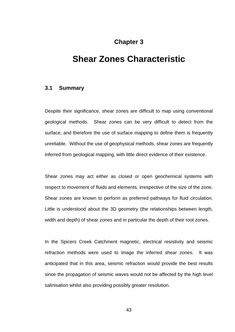
Chapter 3
Shear Zones Characteristic
3.1 Summary
Despite their significance, shear zones are difficult to map using conventional
geological methods. Shear zones can be very difficult to detect from the
surface, and therefore the use of surface mapping to define them is frequently
unreliable. Without the use of geophysical methods, shear zones are frequently
inferred from geological mapping, with little direct evidence of their existence.
Shear zones may act either as closed or open geochemical systems with
respect to movement of fluids and elements, irrespective of the size of the zone.
Shear zones are known to perform as preferred pathways for fluid circulation.
Little is understood about the 3D geometry (the relationships between length,
width and depth) of shear zones and in particular the depth of their root zones.
In the Spicers Creek Catchment magnetic, electrical resistivity and seismic
refraction methods were used to image the inferred shear zones. It was
anticipated that in this area, seismic refraction would provide the best results
since the propagation of seismic waves would not be affected by the high level
salinisation whilst also providing possibly greater resolution.
43
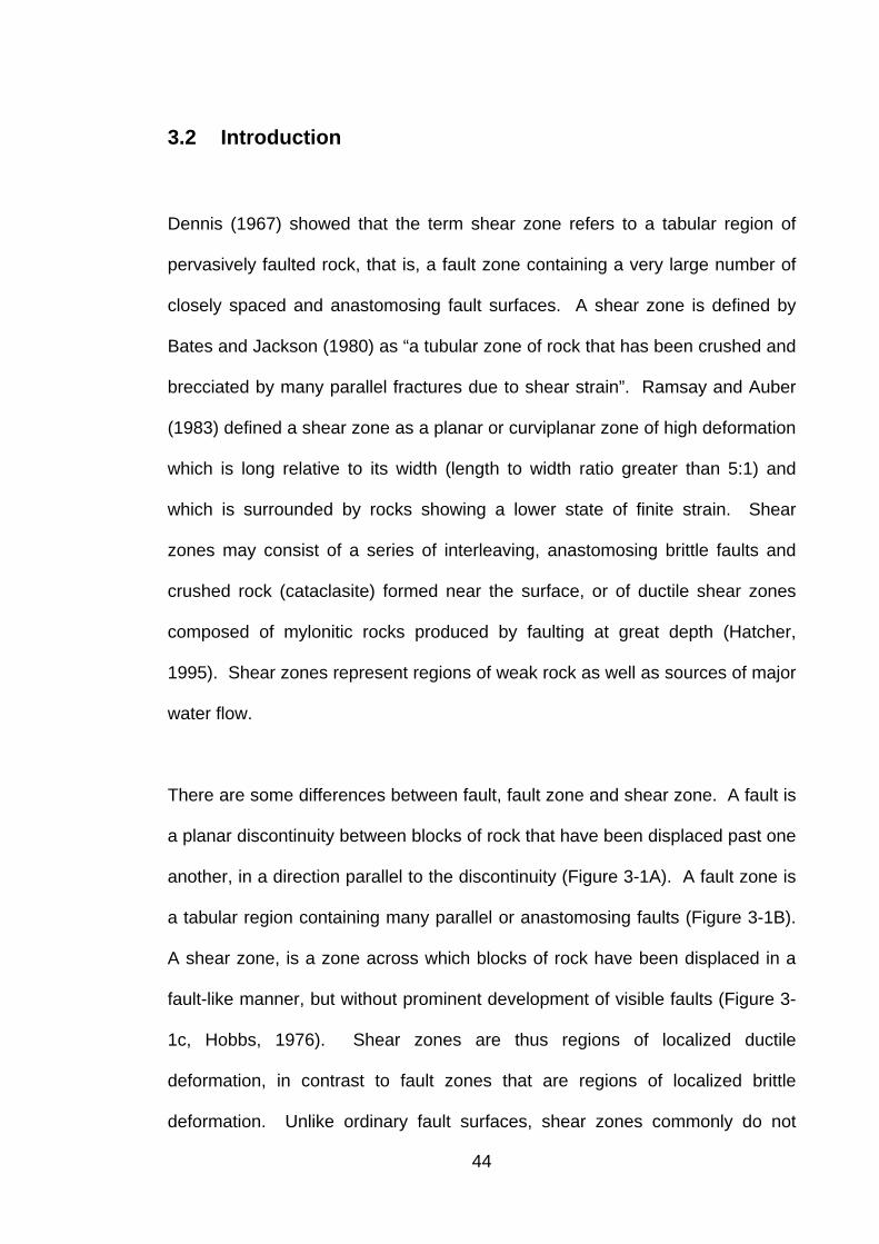
3.2 Introduction
Dennis (1967) showed that the term shear zone refers to a tabular region of
pervasively faulted rock, that is, a fault zone containing a very large number of
closely spaced and anastomosing fault surfaces. A shear zone is defined by
Bates and Jackson (1980) as “a tubular zone of rock that has been crushed and
brecciated by many parallel fractures due to shear strain”. Ramsay and Auber
(1983) defined a shear zone as a planar or curviplanar zone of high deformation
which is long relative to its width (length to width ratio greater than 5:1) and
which is surrounded by rocks showing a lower state of finite strain. Shear
zones may consist of a series of interleaving, anastomosing brittle faults and
crushed rock (cataclasite) formed near the surface, or of ductile shear zones
composed of mylonitic rocks produced by faulting at great depth (Hatcher,
1995). Shear zones represent regions of weak rock as well as sources of major
water flow.
There are some differences between fault, fault zone and shear zone. A fault is
a planar discontinuity between blocks of rock that have been displaced past one
another, in a direction parallel to the discontinuity (Figure 3-1A). A fault zone is
a tabular region containing many parallel or anastomosing faults (Figure 3-1B).
A shear zone, is a zone across which blocks of rock have been displaced in a
fault-like manner, but without prominent development of visible faults (Figure 3-
1c, Hobbs, 1976). Shear zones are thus regions of localized ductile
deformation, in contrast to fault zones that are regions of localized brittle
deformation. Unlike ordinary fault surfaces, shear zones commonly do not
44
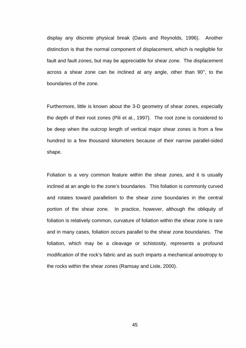
display any discrete physical break (Davis and Reynolds, 1996). Another
distinction is that the normal component of displacement, which is negligible for
fault and fault zones, but may be appreciable for shear zone. The displacement
across a shear zone can be inclined at any angle, other than 90°, to the
boundaries of the zone.
Furthermore, little is known about the 3-D geometry of shear zones, especially
the depth of their root zones (Pili et al., 1997). The root zone is considered to
be deep when the outcrop length of vertical major shear zones is from a few
hundred to a few thousand kilometers because of their narrow parallel-sided
shape.
Foliation is a very common feature within the shear zones, and it is usually
inclined at an angle to the zone’s boundaries. This foliation is commonly curved
and rotates toward parallelism to the shear zone boundaries in the central
portion of the shear zone. In practice, however, although the obliquity of
foliation is relatively common, curvature of foliation within the shear zone is rare
and in many cases, foliation occurs parallel to the shear zone boundaries. The
foliation, which may be a cleavage or schistosity, represents a profound
modification of the rock’s fabric and as such imparts a mechanical anisotropy to
the rocks within the shear zones (Ramsay and Lisle, 2000).
45
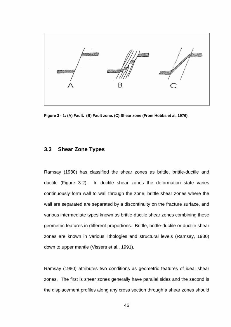
Figure 3 - 1: (A) Fault. (B) Fault zone. (C) Shear zone (From Hobbs et al, 1976).
3.3 Shear Zone Types
Ramsay (1980) has classified the shear zones as brittle, brittle-ductile and
ductile (Figure 3-2). In ductile shear zones the deformation state varies
continuously form wall to wall through the zone, brittle shear zones where the
wall are separated are separated by a discontinuity on the fracture surface, and
various intermediate types known as brittle-ductile shear zones combining these
geometric features in different proportions. Brittle, brittle-ductile or ductile shear
zones are known in various lithologies and structural levels (Ramsay, 1980)
down to upper mantle (Vissers et al., 1991).
Ramsay (1980) attributes two conditions as geometric features of ideal shear
zones. The first is shear zones generally have parallel sides and the second is
the displacement profiles along any cross section through a shear zones should
46
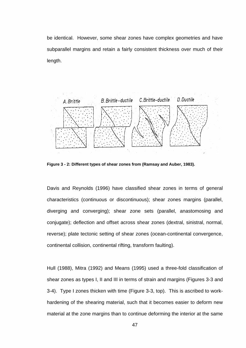
be identical. However, some shear zones have complex geometries and have
subparallel margins and retain a fairly consistent thickness over much of their
length.
Figure 3 - 2: Different types of shear zones from (Ramsay and Auber, 1983).
Davis and Reynolds (1996) have classified shear zones in terms of general
characteristics (continuous or discontinuous); shear zones margins (parallel,
diverging and converging); shear zone sets (parallel, anastomosing and
conjugate); deflection and offset across shear zones (dextral, sinistral, normal,
reverse); plate tectonic setting of shear zones (ocean-continental convergence,
continental collision, continental rifting, transform faulting).
Hull (1988), Mitra (1992) and Means (1995) used a three-fold classification of
shear zones as types I, II and III in terms of strain and margins (Figures 3-3 and
3-4). Type I zones thicken with time (Figure 3-3, top). This is ascribed to work-
hardening of the shearing material, such that it becomes easier to deform new
material at the zone margins than to continue deforming the interior at the same
47
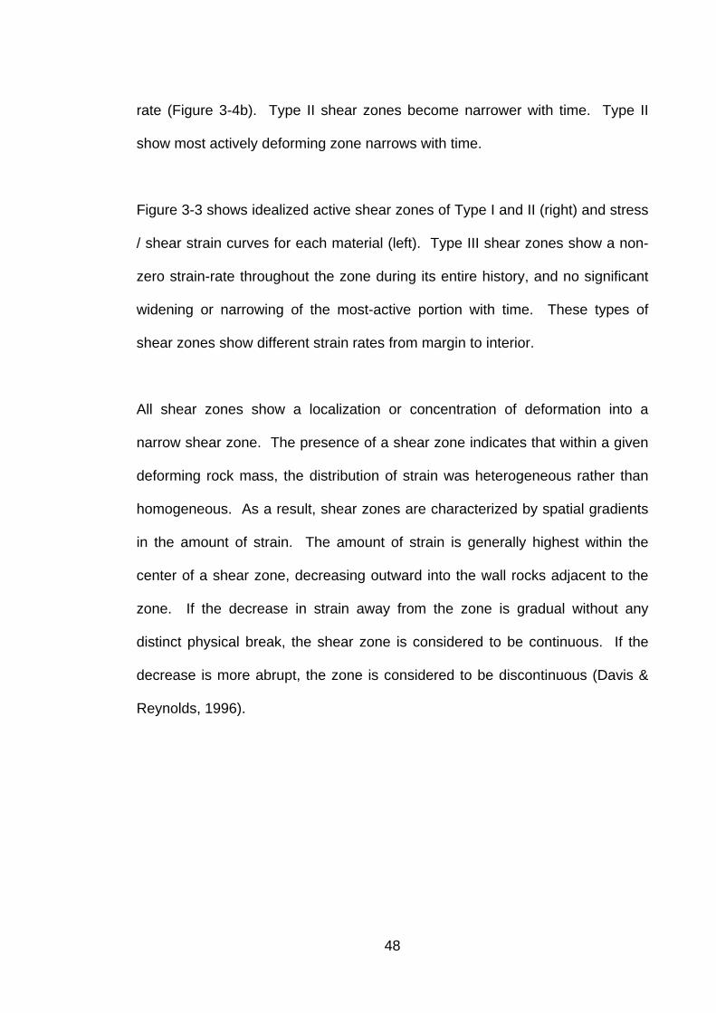
rate (Figure 3-4b). Type II shear zones become narrower with time. Type II
show most actively deforming zone narrows with time.
Figure 3-3 shows idealized active shear zones of Type I and II (right) and stress
/ shear strain curves for each material (left). Type III shear zones show a non-
zero strain-rate throughout the zone during its entire history, and no significant
widening or narrowing of the most-active portion with time. These types of
shear zones show different strain rates from margin to interior.
All shear zones show a localization or concentration of deformation into a
narrow shear zone. The presence of a shear zone indicates that within a given
deforming rock mass, the distribution of strain was heterogeneous rather than
homogeneous. As a result, shear zones are characterized by spatial gradients
in the amount of strain. The amount of strain is generally highest within the
center of a shear zone, decreasing outward into the wall rocks adjacent to the
zone. If the decrease in strain away from the zone is gradual without any
distinct physical break, the shear zone is considered to be continuous. If the
decrease is more abrupt, the zone is considered to be discontinuous (Davis &
Reynolds, 1996).
48
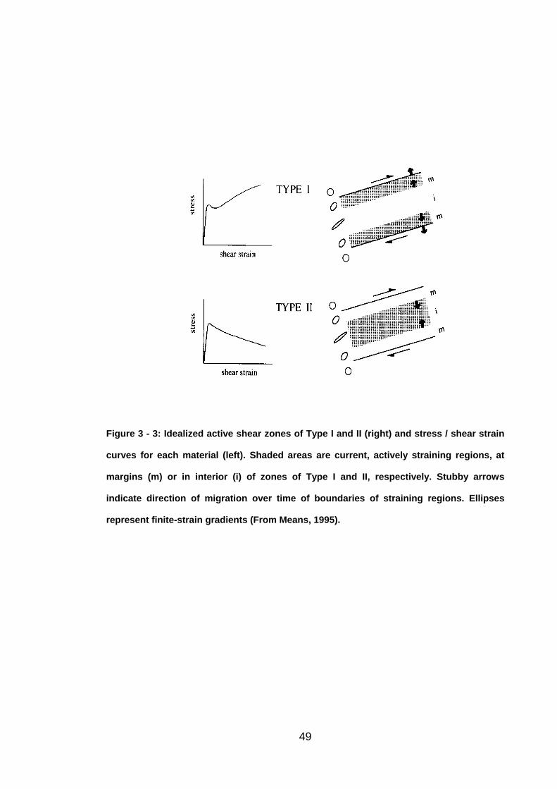
Figure 3 - 3: Idealized active shear zones of Type I and II (right) and stress / shear strain
curves for each material (left). Shaded areas are current, actively straining regions, at
margins (m) or in interior (i) of zones of Type I and II, respectively. Stubby arrows
indicate direction of migration over time of boundaries of straining regions. Ellipses
represent finite-strain gradients (From Means, 1995).
49
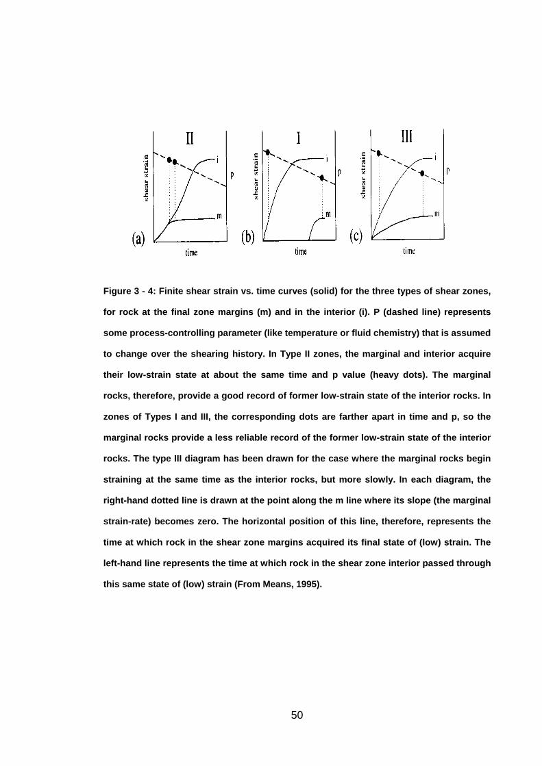
Figure 3 - 4: Finite shear strain vs. time curves (solid) for the three types of shear zones,
for rock at the final zone margins (m) and in the interior (i). P (dashed line) represents
some process-controlling parameter (like temperature or fluid chemistry) that is assumed
to change over the shearing history. In Type II zones, the marginal and interior acquire
their low-strain state at about the same time and p value (heavy dots). The marginal
rocks, therefore, provide a good record of former low-strain state of the interior rocks. In
zones of Types I and III, the corresponding dots are farther apart in time and p, so the
marginal rocks provide a less reliable record of the former low-strain state of the interior
rocks. The type III diagram has been drawn for the case where the marginal rocks begin
straining at the same time as the interior rocks, but more slowly. In each diagram, the
right-hand dotted line is drawn at the point along the m line where its slope (the marginal
strain-rate) becomes zero. The horizontal position of this line, therefore, represents the
time at which rock in the shear zone margins acquired its final state of (low) strain. The
left-hand line represents the time at which rock in the shear zone interior passed through
this same state of (low) strain (From Means, 1995).
50
3.4 Fluid Movement in Shear Zones
Fault zones can act both as barriers to fluid flow and as conduits along or
across which fluid flows ( Anderson et al., 1991, Anderson et al., 1994, Hooper,
1991, Knipe, 1993, Berg and Avery, 1995, Lopez and Smith, 1995, Heneberg,
1995, Sibson, 1996, Roberts et al., 1996, Yielding et al., 1997, Knipe, 1997,).
Faults and their movements play a key-controlling element in fluid flow systems
in geological settings. The direction of fluid flow through a rock mass is
governed by the maximum hydraulic gradient (not necessarily vertical), existing
permeability anisotropy (e.g. bedding, foliation), and superimposed structural
permeability (Sibson, 1996). Furthermore, the permeability of a fault zone
depends on additional factors such as juxtaposition of permeable units across
the fault, rock properties, stress field, the amount of sand, clay, or fault gouge in
the fault zone, the presence of material with high capillary entry pressure, and
the presence or absence of an open fracture network (Smith, 1980, Allan, 1989,
Miller, 1995, Sibson, 1996, Knipe, 1997). Philips (1991) demonstrated that
fractured rocks can have much larger permeabilities, and hence hydraulic
conductivity, than that of completely homogenous rocks. As a result,
permeability may vary by many orders of magnitudes, depending upon rock
type and the pressure-temperature conditions (Braun et al., 2003).
Shear zones have long been shown as preferential fluid pathways (Beach and
Fyfe, 1972). Shear zones may act both as closed or open geochemical
systems with respect to movement of fluids and elements, irrespective of the
size of the zone (Hatcher, 1995). Shear zones are known to perform as
51
preferred pathway for fluid circulation (Beach and Fyfe, 1972). Little is
understood about the 3D geometry (the relationships between length, width and
depth) of shear zones and in particular the depth of their root zones (Pili et al.,
1997).
For an understanding of the dynamics and rates of fluid motion around and
within faults, it is necessary to understand the behavior of hydrothermal
systems. Braun et al. (2003) presented the result of simple numerical
experiments of fluid flow around and within a permeable fault embedded in a
less permeable porous medium. They showed that fluid flow is controlled by
two timescales: and , where S is the specific storage
of the porous material, l the length of the fault, and and are the
hydraulic conductivities of the porous material and the fault, respectively.
Physically, the three conditions correspond to:
Ff KSl /2=τ MF KSl /2=τ
MK FK
If ( fττ < ), fluid rapidly travels through the fault driven by the initial vertical
pressure gradient (or hydraulic head);
If ( Ff τττ << ), the fluid flow in the fault leads to pressure changes in the rock at
both extremities of the fault that result in a decrease of the pressure gradient
between the extremities of the fault;
If ( Fττ < ), fluid flow in the matrix has adapted itself to the new permeability
structure and a steady-state pressure field has developed around the fault.
The first time constant fτ , is the time required by the fluid to travel inside the
fault. fτ is therefore a function of l and . The second time constant, FK Fτ , is
52
the time required by the fluid to reach a steady-state flow and associated
pressure gradient in the matrix in the vicinity of the fault. Fτ is therefore a
function of l and . For a 1 km-long fault, MK fτ varies between 30 years and
300 kyr, depending on the value of the hydraulic conductivity, whereas Fτ varies
between 3Myr and 30 Gyr. Braun et al. (2003) showed that the length of a fault
is the most important factor which determines the value of the two time
constants, fτ and Fτ .
It has been useful to find ‘steady-state flow’ in rocks, flow at constant stress,
constant temperature, constant strain rate and constant microstructure, so that
the flow law can be expressed in a strain-independent form that allows
separation of variables, thus (Rutter, 1999):
( ) ( ) ( )ST 321 ∫∫∫Α= σε
In which ε is strain rate, σ is flow stress, T is absolute temperature and is
some measure of rate controlling microstructure, which might be grain size. It is
widely recognized that fine-grained rocks can be weaker than their coarser-
grained counterparts at high temperature (Walker, et al., 1990), if grain size
sensitive flow processes were to be activated. As Rutter (1999) discussed,
rocks in shear zones are commonly tectonically reduced in grain size, an
observation which tends to reinforce the inference that shear zones are zones
of relative mechanical weakness.
S
53
3.5 Evidence of Shear Zones
Shear zones have certain characteristic to recognize them in the field, in thin
section, on geological maps and cross sections (Davis and Reynolds, 1996),
and geophysical methods. Geophysical methods are very useful when there is
no clear evidence of shear zones in the field. Shear zones exist at all scales
and their size depends on the conditions, such as brittle, ductile, or intermediate
conditions, under which they were formed.
3.5.1 Field Evidence
The following evidence for detecting shear zones (Ramsay and Auber, 1983;
Simpson and Schmid, 1983; Passchier and Simpson, 1986; Davis and
Reynolds, 1996) might be established in outcrops, in hand specimens or in thin
sections.
1 S-C band structure (Figure 3-5A): S-C fabrics consist of foliation (S-
surfaces) and shear bands (C-surfaces). The S and C surfaces are at an angle
to one another, indicating the sense of shear. In most S-C fabrics, the S-
surfaces are a typical foliation, being defined by flattened lenticular grains and
aggregates of grains. The oblique relationship of the two structures shows a
clear indication of the displacement sense. S-C fabrics can be divided into two
general types (Lister and Snoke, 1984). Type I are the dominant S-C fabric in
most mylonitic quartzofeldspathic rocks. Type II S-C fabrics are most common
in micaceous quartzite and some mylonites. In both types of S-C fabric, the C-
54

surfaces are commonly aligned parallel to the shear zone and are associated
with the same strain gradients as any continuous shear zone.
2 Rotation of porphyroblasts or porphyroclasts (Figure 3-5B): If the
large grains instead are new metamorphic grains that grew during or after
deformation, they are called porphyroblasts. Grains interpreted to be relics from
the protolith are called porphyroclasts because they commonly represent
fragments or clasts of original phenocrysts or detrital grains. In many
metamorphic rocks it is well known that large porphyroblasts can develop;
albite, garnet, staurolite are particularly useful for the determination of shear
sense. These crystals can roll like ball bearings and by matching the inclusion
trails they contain inside the crystal ( ) with those found outside ( ), the
rotation sense can be determined. Such crystals can grow as porphyroblasts
during the shear motion when they produce a “snowball structure”.
is es
3 σ -Structure (Figure 3-5C): This structure is found around
porphyroclasts, and relates to the form of the dynamically recrystallized
pressure shadow tail in relation to the porphyroclast. In this structure the
median line of the tail does not cross the tend of the average shistosity, and the
structure appears to form because the rotation rate of the tail is higher than that
of the porphyroclast. This structure is characteristic of shear zones with low
shear strains where the recrystallization rates are higher than the rotation rates.
4 δ - Structure (Figure 3-5D): This structure, like σ -structure, is
developed around porphyroclasts, but where the recrystallized pressure shadow
55
tail is strongly rotated by the porphyroclasts. This structure shows the
extremely curved and often embayed nature of the generally narrow tail, and
where the median line crosses the general trend of the schistosity. This type of
structure is particularly characteristic of origins of high shear strains where the
recrystallization rates are lower than the rotation rates.
5 Bookshelf sliding (Figure 3-5E): When broken crystals are subjected to
shear, the individual parts are rotated in the direction of shear, a feature which
sets up a contrary shear motion between the fragments much like a collapsing
set of books. Further shearing motion can lead to separation of the individual
fragments and the development of recrystallized pressure shadow zones
between the fragments.
6 Displaced crystals (Figure 3-5F): Where crystals possessing a well
developed crystal cleavage lie with this cleavage close to the shear plane, they
often become internally detached by gliding on this surface. In highly deformed
mylonites, for example, it is not uncommon to find individual mica fragments
connected by zonal films of phyllosilicates to form free “floating mica fish”.
7 Dynamic recrystallization (Figure 3-5G): Rocks that have been very
highly deformed by crystal plastic processes frequently show an intense
banding and schistosity. Within the more deformed crystal (especially with
quartz and calcite) the bands are crossed obliquely by small grains with a
marked individual alignment.
56

8 Preferred optical orientation (Figure 3-5H): Plastic flow of crystals
leads to a variety of different types of preferred alignment patterns of the optical
axes of the crystals in the rock aggregate. Many of these complications of
interpretation of preferred orientation patterns result from the nature of the
environmental conditions during deformation.
9 Protomylonite, mylonite, and ultramylonite: Mylonites are strongly
foliated metamorphic rocks that exhibit high ductile strain and incomplete
recrystallization or recovery. Mylonite contains 50 to 90 per cent matrix.
Mylonite is typical shear zones rock. The initial stages of mylonitization produce
a weakly to moderately mylonitic rock, called a protomylonite. Protomylonite
contains less than 50 per cent fine-grained matrix. Ultramylonite contains more
than 90 per cent matrix and less than 10 per cent relict grains. Some foliation in
mylonitic rocks is the expression of thin shear zones.
57
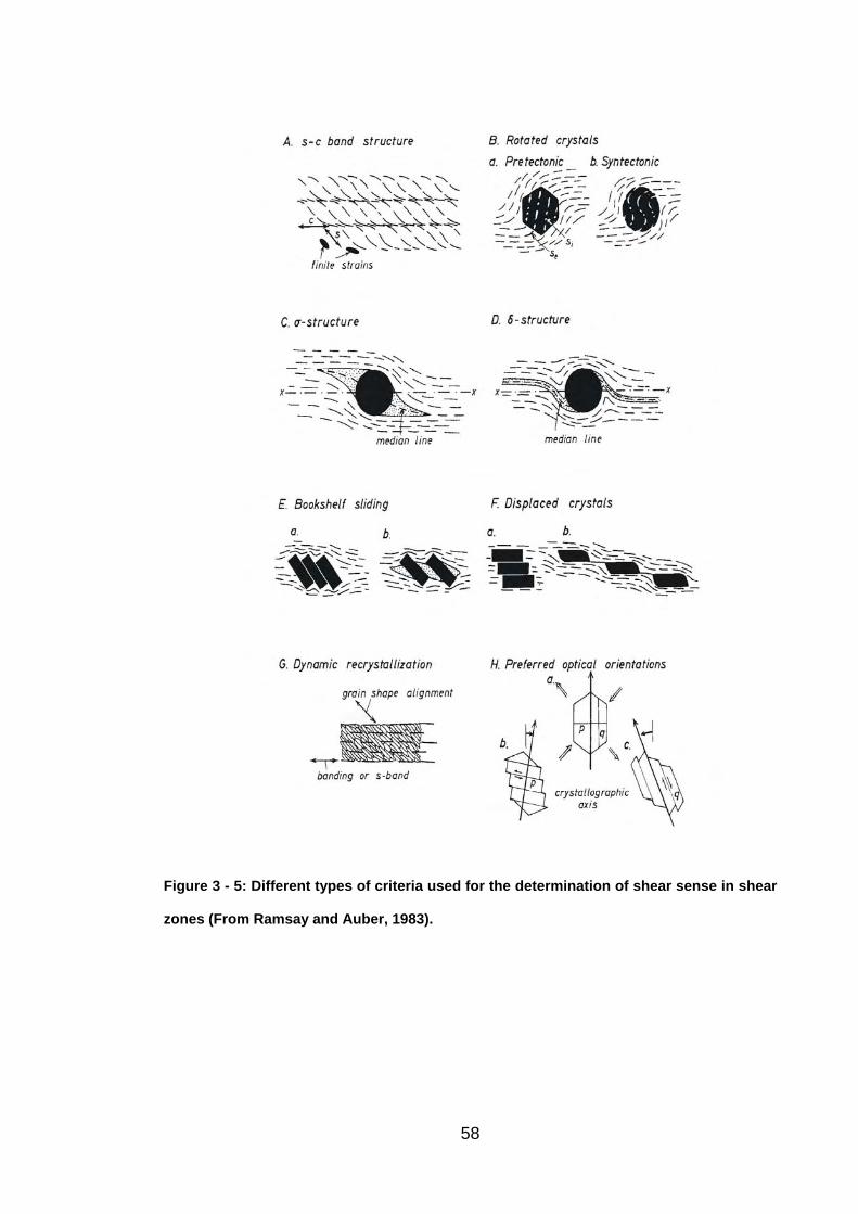
Figure 3 - 5: Different types of criteria used for the determination of shear sense in shear
zones (From Ramsay and Auber, 1983).
58
3.5.2 Imaging Shear Zones with Geophysical Methods
Despite their significance, shear zones can be difficult to map in detail using
conventional geological methods. However, their location can often be inferred
from topographic features or geophysical methods, such as electromagnetic
techniques. Shear zones can be difficult to detect from the surface, and
therefore the use of surface mapping to define them is often unreliable. Without
the use of geophysical methods, shear zones are frequently inferred from
geological mapping, often with little evidence of their existence either directly or
tectonically. It should be emphasized that detecting and studying shear zones
are not always a straightforward procedure.
Major faults and shear zones are routinely discovered by explorationists through
geophysical methods. Nowadays, integrated use of least two geophysical
methods with geological interpretation is important to obtain accurate geological
interpretation. For example Street and Engel (1990) showed that integrated use
of geophysical methods (magnetic and seismic refraction), drilling, and sample
analysis has hound geological controls on the location of dryland salinity in
Western Australia. The success of the electromagnetic and resistivity
geophysical methods in imaging shear zones lies in their ability to image these
narrow zones as regions of high conductivity. This increase in conductivity is
due to the development of secondary porosity and permeability from fracturing
which leads to an increase in groundwater saturation. The success of the
seismic refraction method lies in its ability to image the shear zone as a narrow
region of low seismic velocity and increased depths of weathering.
59

In the Spicers Creek Catchment magnetic, electrical resistivity and seismic
refraction methods were used to image the inferred shear zones. It was
anticipated that in this area, seismic refraction would provide the best results
since the propagation of seismic waves would not be affected by the high level
salinisation whilst also providing possibly greater resolution.
60
Chapter 4
Three-Dimension Three Component
Seismic Surveys
4.1 Summary
The objective of the seismic refraction method is to determine the velocity
distribution in the sub-surface. The seismic refraction method does have a
number of advantages over the reflection method, particularly in shallow
investigations such as in geotechnical, environmental and groundwater
applications. The seismic refraction methods seek to measure the spatial
variation of petrophysical parameters by using seismic velocity.
Many geological features in the subsurface are three-dimension (3-D) in nature,
and two-dimension (2-D) seismic section is a cross section of the 3-D seismic
wave field. Having a detailed image of the subsurface usually makes the
interpretation more reliable. The aim of using 3D-3C seismic data is to find
more information about rock properties with both P- and S-waves. The most
important parameters which can be extracted from P-wave and S-wave data are
the P-wave/S-wave velocity (Vp/Vs) ratio and Poisson’s ratio.
61
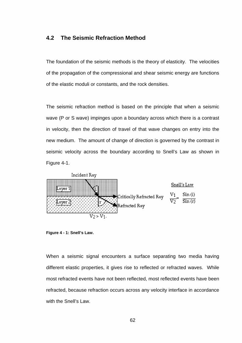
4.2 The Seismic Refraction Method
The foundation of the seismic methods is the theory of elasticity. The velocities
of the propagation of the compressional and shear seismic energy are functions
of the elastic moduli or constants, and the rock densities.
The seismic refraction method is based on the principle that when a seismic
wave (P or S wave) impinges upon a boundary across which there is a contrast
in velocity, then the direction of travel of that wave changes on entry into the
new medium. The amount of change of direction is governed by the contrast in
seismic velocity across the boundary according to Snell’s Law as shown in
Figure 4-1.
Figure 4 - 1: Snell’s Law.
When a seismic signal encounters a surface separating two media having
different elastic properties, it gives rise to reflected or refracted waves. While
most refracted events have not been reflected, most reflected events have been
refracted, because refraction occurs across any velocity interface in accordance
with the Snell’s Law.
62

4.3 Seismic Velocities in the Earth
The seismic velocity is generally used as a measure of earth elasticity, since P
and S seismic velocities can be derived from the elastic constants and the
density. Due to the variability of the near surface conditions, the seismic
velocities in shallow earth materials are also highly variable. The relevant
factors include major rock forming minerals, rock formation, the nature of the
cementing material, fracturing and weathering, structural deformation, etc. In
general, seismic velocities are less in unconsolidated materials.
Furthermore, the seismic velocities of earth materials usually increase with
depth, because of decreasing weathering, and increasing water saturation,
compaction and diagenesis with depth. The velocities of seismic waves in most
igneous and metamorphic rocks depend mainly on the elastic properties of the
minerals making up the rock material itself, since these rocks have little or no
porosity. In general, igneous rocks have seismic velocities which show a much
narrower range of variation than sedimentary or metamorphic rocks. The
average velocity for igneous rocks is higher than that for other types (Dobrin
and Savit, 1988).
Because the seismic velocities generally increase with depth, seismic energy is
systematically refracted away from the vertical, until it travels in a predominantly
horizontal direction. Furthermore, the horizontally traveling energy also radiates
energy back into the overlying layers. As a result, seismic energy which is
initiated at the surfaces propagates down into the subsurface and returns to the
63
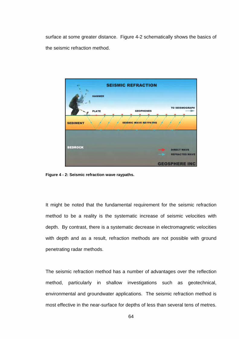
surface at some greater distance. Figure 4-2 schematically shows the basics of
the seismic refraction method.
Figure 4 - 2: Seismic refraction wave raypaths.
It might be noted that the fundamental requirement for the seismic refraction
method to be a reality is the systematic increase of seismic velocities with
depth. By contrast, there is a systematic decrease in electromagnetic velocities
with depth and as a result, refraction methods are not possible with ground
penetrating radar methods.
The seismic refraction method has a number of advantages over the reflection
method, particularly in shallow investigations such as geotechnical,
environmental and groundwater applications. The seismic refraction method is
most effective in the near-surface for depths of less than several tens of metres.
64
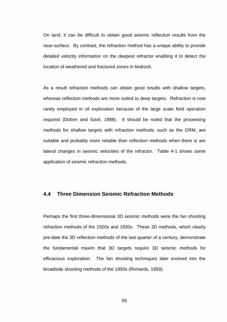
On land, it can be difficult to obtain good seismic reflection results from the
near-surface. By contrast, the refraction method has a unique ability to provide
detailed velocity information on the deepest refractor enabling it to detect the
location of weathered and fractured zones in bedrock.
As a result refraction methods can obtain good results with shallow targets,
whereas reflection methods are more suited to deep targets. Refraction is now
rarely employed in oil exploration because of the large scale field operation
required (Dobrin and Savit, 1988). It should be noted that the processing
methods for shallow targets with refraction methods, such as the GRM, are
suitable and probably more reliable than reflection methods when there is are
lateral changes in seismic velocities of the refractor. Table 4-1 shows some
application of seismic refraction methods.
4.4 Three Dimension Seismic Refraction Methods
Perhaps the first three-dimensional 3D seismic methods were the fan shooting
refraction methods of the 1920s and 1930s. These 3D methods, which clearly
pre-date the 3D reflection methods of the last quarter of a century, demonstrate
the fundamental maxim that 3D targets require 3D seismic methods for
efficacious exploration. The fan shooting techniques later evolved into the
broadside shooting methods of the 1950s (Richards, 1959).
65
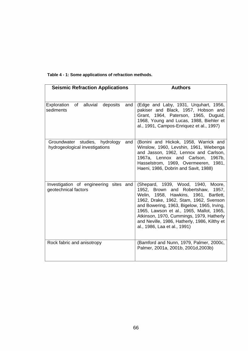
Table 4 - 1: Some applications of refraction methods.
Seismic Refraction Applications
Authors
Exploration of alluvial deposits and sediments
(Edge and Laby, 1931, Urquhart, 1956, pakiser and Black, 1957, Hobson and Grant, 1964, Paterson, 1965, Duguid, 1968, Young and Lucas, 1988, Biehler et al., 1991, Campos-Enriquez et al., 1997)
Groundwater studies, hydrology and hydrogeological investigations
(Bonini and Hickok, 1958, Warrick and Winslow, 1960, Levshin, 1961, Wiebenga and Jasson, 1962, Lennox and Carlson, 1967a, Lennox and Carlson, 1967b, Hasselstrom, 1969, Overmeeren, 1981, Haeni, 1986, Dobrin and Savit, 1988)
Investigation of engineering sites and geotechnical factors
(Shepard, 1939, Wood, 1940, Moore, 1952, Brown and Robertshaw, 1957, Welin, 1958, Hawkins, 1961, Bartlett, 1962, Drake, 1962, Stam, 1962, Svenson and Bowering, 1963, Bigelow, 1965, Irving, 1965, Lawson et al., 1965, Mallot, 1965, Atkinson, 1970, Cummings, 1979, Hatherly and Neville, 1986, Hatherly, 1986, Kilthy et al., 1986, Laa et al., 1991)
Rock fabric and anisotropy (Bamford and Nunn, 1979, Palmer, 2000c, Palmer, 2001a, 2001b, 2001d,2003b)
66
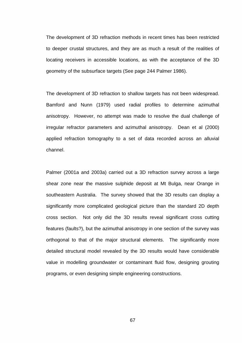
The development of 3D refraction methods in recent times has been restricted
to deeper crustal structures, and they are as much a result of the realities of
locating receivers in accessible locations, as with the acceptance of the 3D
geometry of the subsurface targets (See page 244 Palmer 1986).
The development of 3D refraction to shallow targets has not been widespread.
Bamford and Nunn (1979) used radial profiles to determine azimuthal
anisotropy. However, no attempt was made to resolve the dual challenge of
irregular refractor parameters and azimuthal anisotropy. Dean et al (2000)
applied refraction tomography to a set of data recorded across an alluvial
channel.
Palmer (2001a and 2003a) carried out a 3D refraction survey across a large
shear zone near the massive sulphide deposit at Mt Bulga, near Orange in
southeastern Australia. The survey showed that the 3D results can display a
significantly more complicated geological picture than the standard 2D depth
cross section. Not only did the 3D results reveal significant cross cutting
features (faults?), but the azimuthal anisotropy in one section of the survey was
orthogonal to that of the major structural elements. The significantly more
detailed structural model revealed by the 3D results would have considerable
value in modelling groundwater or contaminant fluid flow, designing grouting
programs, or even designing simple engineering constructions.
67
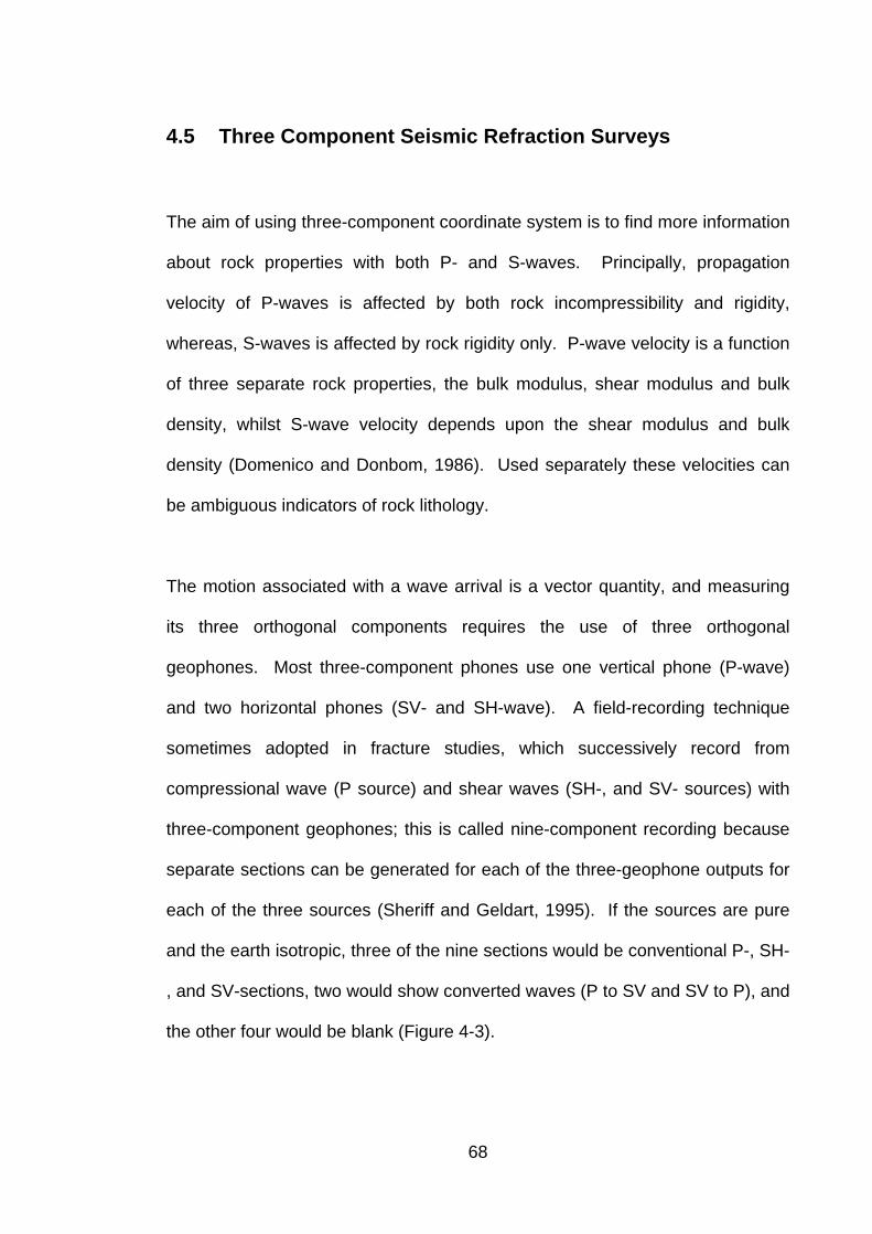
4.5 Three Component Seismic Refraction Surveys
The aim of using three-component coordinate system is to find more information
about rock properties with both P- and S-waves. Principally, propagation
velocity of P-waves is affected by both rock incompressibility and rigidity,
whereas, S-waves is affected by rock rigidity only. P-wave velocity is a function
of three separate rock properties, the bulk modulus, shear modulus and bulk
density, whilst S-wave velocity depends upon the shear modulus and bulk
density (Domenico and Donbom, 1986). Used separately these velocities can
be ambiguous indicators of rock lithology.
The motion associated with a wave arrival is a vector quantity, and measuring
its three orthogonal components requires the use of three orthogonal
geophones. Most three-component phones use one vertical phone (P-wave)
and two horizontal phones (SV- and SH-wave). A field-recording technique
sometimes adopted in fracture studies, which successively record from
compressional wave (P source) and shear waves (SH-, and SV- sources) with
three-component geophones; this is called nine-component recording because
separate sections can be generated for each of the three-geophone outputs for
each of the three sources (Sheriff and Geldart, 1995). If the sources are pure
and the earth isotropic, three of the nine sections would be conventional P-, SH-
, and SV-sections, two would show converted waves (P to SV and SV to P), and
the other four would be blank (Figure 4-3).
68

The coordinate system for measuring the three components of a P- or S-waves
can be rotated around any axis; in particular, they can be rotated into a natural
coordinate system. Such a coordinate rotation is sometimes called Alford
rotation or polarization filtering (Sheriff and Geldart, 1995).
Three-component recording can be employed to resolve fracture problems in a
3-D survey (Lewis et al., 1991). On the other hand, if the SH- and SV- sources
and geophones are not oriented parallel and perpendicular to the natural
orientation or azimuthal anisotropy is present, then shear wave splitting will
result in energy showing on all panels.
Conventional P-wave data
Conventional SH-wave data
Conventional SV-wave data
Mode conversion P to SV
Mode conversion P to SV
?
?
?
?
SV
SH
P
P SH SV
SOURCE MOTION
Figure 4 - 3: Nine-component sections recorded by P-, SH-, and SV-geophones for P-, SH-
, and SV sources. Without anisotropy the sections marked ? would be blank (From
Tatham and McCormack, 1991).
69
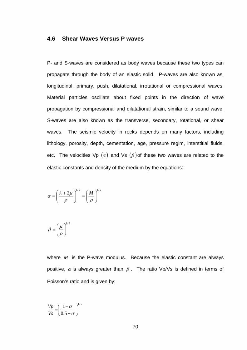
4.6 Shear Waves Versus P waves
P- and S-waves are considered as body waves because these two types can
propagate through the body of an elastic solid. P-waves are also known as,
longitudinal, primary, push, dilatational, irrotational or compressional waves.
Material particles oscillate about fixed points in the direction of wave
propagation by compressional and dilatational strain, similar to a sound wave.
S-waves are also known as the transverse, secondary, rotational, or shear
waves. The seismic velocity in rocks depends on many factors, including
lithology, porosity, depth, cementation, age, pressure regim, interstitial fluids,
etc. The velocities Vp ( )α and Vs ( )β of these two waves are related to the
elastic constants and density of the medium by the equations:
2/12/12
⎟⎟⎠
⎞⎜⎜⎝
⎛=⎟⎟
⎠
⎞⎜⎜⎝
⎛ +=
ρρµλα M
2/1
⎟⎟⎠
⎞⎜⎜⎝
⎛=
ρµβ
where M is the P-wave modulus. Because the elastic constant are always
positive, α is always greater than β . The ratio Vp/Vs is defined in terms of
Poisson’s ratio and is given by:
2/1
5.01
⎟⎠⎞
⎜⎝⎛
−−
=σσ
VsVp
70
As σ decreases from 0.5 to 0, Vs/Vp increases from 0 to its maximum value,
2/1 ; thus, the velocity of the S-wave ranges from 0 to 70% of the velocity of
the P-wave (Sheriff and Geldart, 1995). Meanwhile, for fluids, µ is zero and
hence β is zero also; and as a result S-waves do not propagate in fluids.
The Poission’s ratio is one of the most important parameters which can be
extracted from P-wave and S-wave data. This parameter is independent of
density, it is a much more diagnostic lithological and pore-fluid indicators and it
can also detect the degree of rock fracturing and seismic anisotropy (Dasios et
al, 1999). In terms of rock mechanics, Poisson’s ratio is equal to the ratio of
transverse and longitudinal strain and hence can provide information on
material elasticity. The nature of interstitial fluids can be determined using the
relationships between Vp/Vs ratio and Poisson’s ratio with pore pressure and
fluid type. For example, Vp/Vs ratio is sensitive to the pore fluids found in
sedimentary rocks, with the value being much lower for gas saturation than for
liquid saturation (Tatham, 1982). Furthermore, laboratory studies have shown
that at high differential pressures, Poisson’s ratio is constant, whilst at low
differential pressures, the ratio increases for saturated rocks and decreases for
dry rocks (Carcione and Cavallini, 2002). The Vp/Vs ratio is affected by changes
in porosity. For example, a relationship between the velocity ratio and the
shape of the pore space has been shown (Toksöz et al, 1976) with flat pore
spaces resulting from fracture porosity giving a different response from rounded
pore spaces resulting from primary or secondary porosity. The anisotropy of
strata can be detected by changes in Vp/Vs ratio in different azimuthal
71
directions. This is useful in fracture detection, where velocities can be affected
differently depending on the raypath orientation with respect to these fractures.
As the velocities of S-waves are slower than that of P-waves, for S- and P-
waves with comparable frequencies and hence shorter and longer wavelengths
respectively, it might be expected that the resolution of S-wave records would
be higher than that of P-wave records. However this resolution is often not
realisable, due to the difficulty in generating high frequency S-waves, their high
attenuation, and noise from surface and compressional waves. Due to the
effect of source to ground coupling, it is more difficult to generate S-waves than
P-waves of high frequency (Helbig, 1986). In general, the quality factor of S-
waves is lower than that of P-waves, limiting their useful length of travel to a few
hundred times its wavelength. S-wave records are contaminated by a high
degree of noise with lingering reverberations from P-waves often occurring at
the same time as S-wave arrivals (Pautet et al., 2001). Also the marginally
slower velocities of surface waves mean that their separation from S-waves can
be difficult (Helbig, 1986).
The enhancement of S-waves is possible if horizontal component seismic
records are generated using sources of opposite polarity (Xia et al, 2002). S-
wave energy can be enhanced by subtracting seismic records of opposite
polarity, resulting in the cancellation of P-wave components whilst leaving the
sum of the two S-wave components. Opposite polarity records may show
amplitude and phase differences due to changes in near-surface conditions. As
a result the subtraction procedure would not lead to S-wave enhancement
72

(Dasios et al, 1999). Appropriate amplitude and phase corrections must be
applied before these enhancement operations are performed.
73
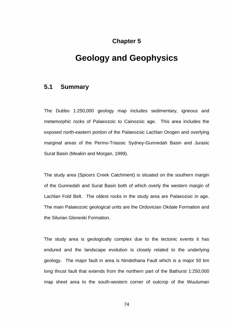
Chapter 5
Geology and Geophysics
5.1 Summary
The Dubbo 1:250,000 geology map includes sedimentary, igneous and
metamorphic rocks of Palaeozoic to Cainozoic age. This area includes the
exposed north-eastern portion of the Palaeozoic Lachlan Orogen and overlying
marginal areas of the Permo-Triassic Sydney-Gunnedah Basin and Jurasic
Surat Basin (Meakin and Morgan, 1999).
The study area (Spicers Creek Catchment) is situated on the southern margin
of the Gunnedah and Surat Basin both of which overly the western margin of
Lachlan Fold Belt. The oldest rocks in the study area are Palaeozoic in age.
The main Palaeozoic geological units are the Ordovician Okdale Formation and
the Silurian Gleneski Formation.
The study area is geologically complex due to the tectonic events it has
endured and the landscape evolution is closely related to the underlying
geology. The major fault in area is Nindethana Fault which is a major 50 km
long thrust fault that extends from the northern part of the Bathurst 1:250,000
map sheet area to the south-western corner of outcrop of the Wuuluman
74
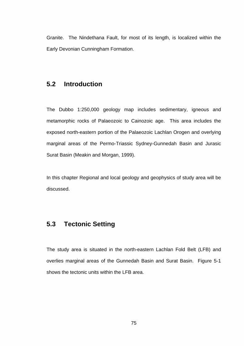
Granite. The Nindethana Fault, for most of its length, is localized within the
Early Devonian Cunningham Formation.
5.2 Introduction
The Dubbo 1:250,000 geology map includes sedimentary, igneous and
metamorphic rocks of Palaeozoic to Cainozoic age. This area includes the
exposed north-eastern portion of the Palaeozoic Lachlan Orogen and overlying
marginal areas of the Permo-Triassic Sydney-Gunnedah Basin and Jurasic
Surat Basin (Meakin and Morgan, 1999).
In this chapter Regional and local geology and geophysics of study area will be
discussed.
5.3 Tectonic Setting
The study area is situated in the north-eastern Lachlan Fold Belt (LFB) and
overlies marginal areas of the Gunnedah Basin and Surat Basin. Figure 5-1
shows the tectonic units within the LFB area.
75
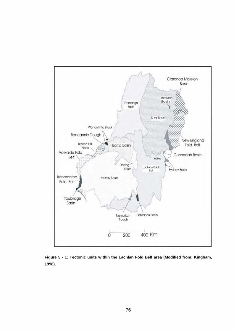
Figure 5 - 1: Tectonic units within the Lachlan Fold Belt area (Modified from: Kingham, 1998).
76
5.3.1 Lachlan Fold Belt
The Lachlan Fold Belt (LFB) is part of the eastern margin of Gondowanaland
and a major structural unit located on the eastern side of the Tasman Fold Belt
System. The LFB extends from eastern Tasmania through Victoria into New
South Wales (NSW), where it forms a large part of the state. In NSW the LFB is
bounded to the east by the younger New England Fold Belt, to the north by the
Thompson Fold Belt and to the west by the Kanmantoo Fold Belt.
The LFB is a complex orogenic belt, which according to most workers
developed from the Cambrian to the Early Carboniferous. The belt has been
subdivided into several stratotectonic units (Figure 5-2) termed anticlinorial and
synclinorial zones that reflect the geological development across the LFB
(Suppel and Scheibner, 1990).
Scheibner and Basden (1996) described the LFB as a ‘composite orogenic belt
composed of Early Cambrian to Early Devonian pre-cratonic complexes
developed over mixed ensialic (microcontinents) and ensiamatic (oceanic or
ophiolitic) basement’. Study of the stratigraphy shows that there have been four
main phases of folding as identified by stratigraphic relationships. It is probable
that tectonic activity was continuous for over 30 Ma from its commencement at
about the end of Ordovician until the Early Devonian, with significant phases in
the latest Ordovician to Early Silurian (Benambian) and Late Silurian to Early
Devonian (Bowning), followed by more discrete episodes in late Middle
77
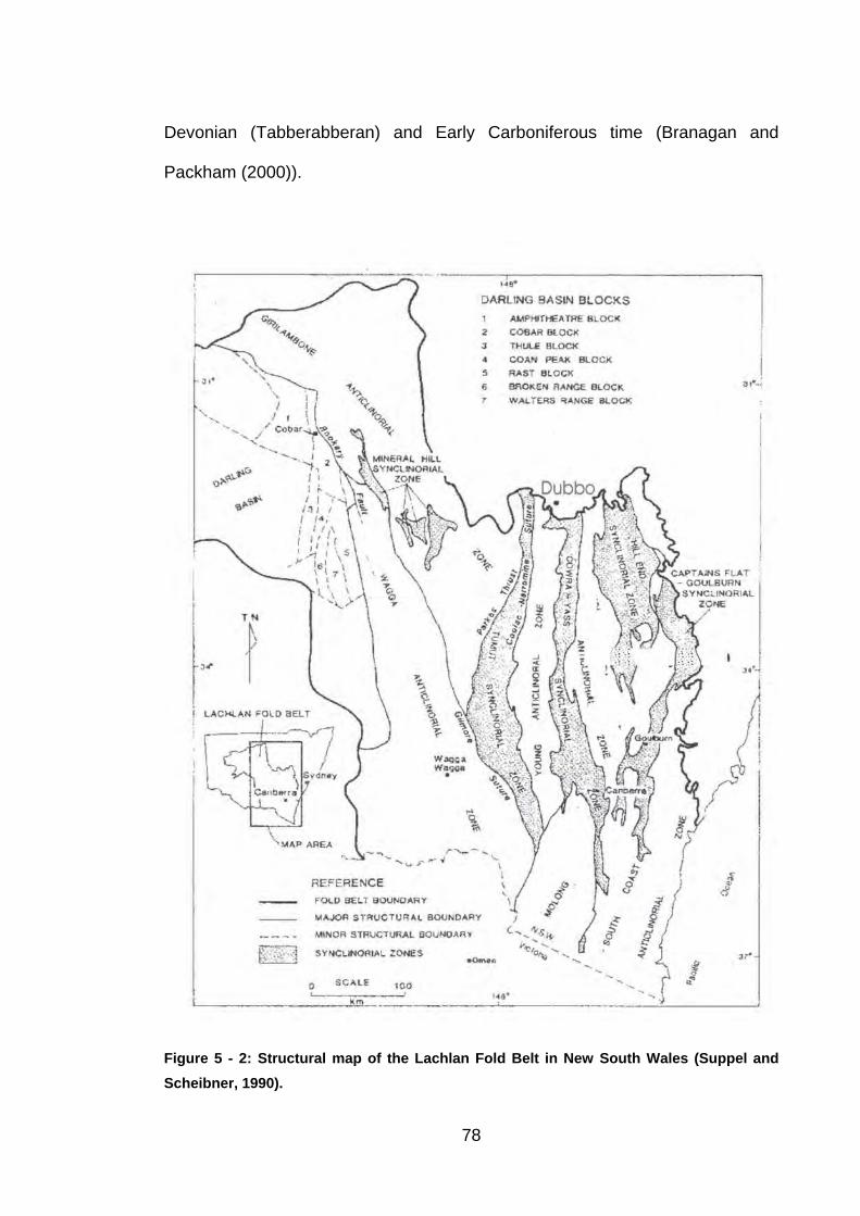
Devonian (Tabberabberan) and Early Carboniferous time (Branagan and
Packham (2000)).
Figure 5 - 2: Structural map of the Lachlan Fold Belt in New South Wales (Suppel and Scheibner, 1990).
78
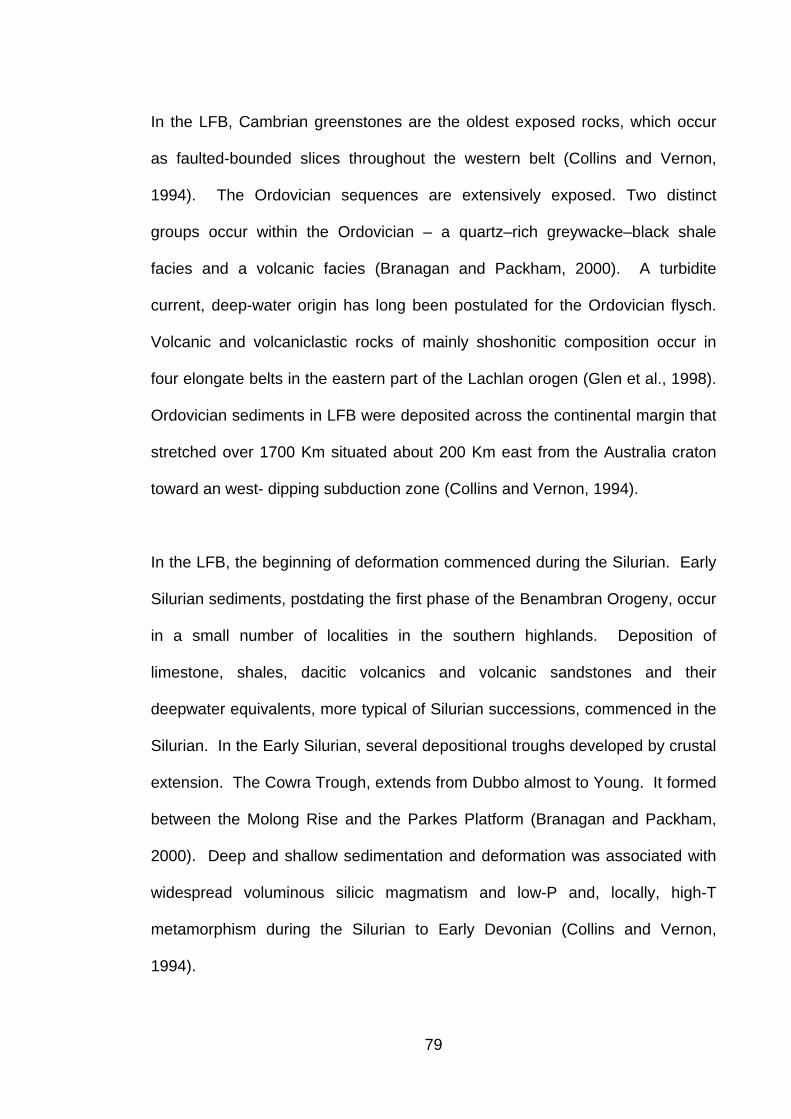
In the LFB, Cambrian greenstones are the oldest exposed rocks, which occur
as faulted-bounded slices throughout the western belt (Collins and Vernon,
1994). The Ordovician sequences are extensively exposed. Two distinct
groups occur within the Ordovician – a quartz–rich greywacke–black shale
facies and a volcanic facies (Branagan and Packham, 2000). A turbidite
current, deep-water origin has long been postulated for the Ordovician flysch.
Volcanic and volcaniclastic rocks of mainly shoshonitic composition occur in
four elongate belts in the eastern part of the Lachlan orogen (Glen et al., 1998).
Ordovician sediments in LFB were deposited across the continental margin that
stretched over 1700 Km situated about 200 Km east from the Australia craton
toward an west- dipping subduction zone (Collins and Vernon, 1994).
In the LFB, the beginning of deformation commenced during the Silurian. Early
Silurian sediments, postdating the first phase of the Benambran Orogeny, occur
in a small number of localities in the southern highlands. Deposition of
limestone, shales, dacitic volcanics and volcanic sandstones and their
deepwater equivalents, more typical of Silurian successions, commenced in the
Silurian. In the Early Silurian, several depositional troughs developed by crustal
extension. The Cowra Trough, extends from Dubbo almost to Young. It formed
between the Molong Rise and the Parkes Platform (Branagan and Packham,
2000). Deep and shallow sedimentation and deformation was associated with
widespread voluminous silicic magmatism and low-P and, locally, high-T
metamorphism during the Silurian to Early Devonian (Collins and Vernon,
1994).
79
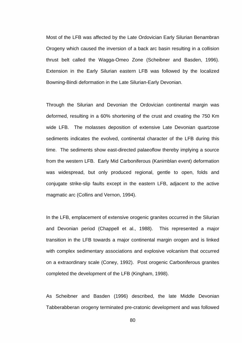
Most of the LFB was affected by the Late Ordovician Early Silurian Benambran
Orogeny which caused the inversion of a back arc basin resulting in a collision
thrust belt called the Wagga-Omeo Zone (Scheibner and Basden, 1996).
Extension in the Early Silurian eastern LFB was followed by the localized
Bowning-Bindi deformation in the Late Silurian-Early Devonian.
Through the Silurian and Devonian the Ordovician continental margin was
deformed, resulting in a 60% shortening of the crust and creating the 750 Km
wide LFB. The molasses deposition of extensive Late Devonian quartzose
sediments indicates the evolved, continental character of the LFB during this
time. The sediments show east-directed palaeoflow thereby implying a source
from the western LFB. Early Mid Carboniferous (Kanimblan event) deformation
was widespread, but only produced regional, gentle to open, folds and
conjugate strike-slip faults except in the eastern LFB, adjacent to the active
magmatic arc (Collins and Vernon, 1994).
In the LFB, emplacement of extensive orogenic granites occurred in the Silurian
and Devonian period (Chappell et al., 1988). This represented a major
transition in the LFB towards a major continental margin orogen and is linked
with complex sedimentary associations and explosive volcanism that occurred
on a extraordinary scale (Coney, 1992). Post orogenic Carboniferous granites
completed the development of the LFB (Kingham, 1998).
As Scheibner and Basden (1996) described, the late Middle Devonian
Tabberabberan orogeny terminated pre-cratonic development and was followed
80
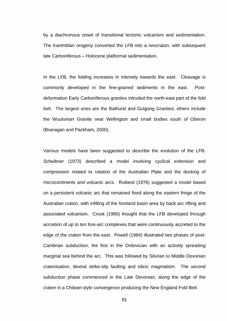
by a diachronous onset of transitional tectonic volcanism and sedimentation.
The Kanimblan orogeny converted the LFB into a neocraton, with subsequent
late Carboniferous – Holocene platformal sedimentation.
In the LFB, the folding increases in intensity towards the east. Cleavage is
commonly developed in the fine-grained sediments in the east. Post-
deformation Early Carboniferous granites intruded the north-east part of the fold
belt. The largest ones are the Bathurst and Gulgong Granites; others include
the Wuuluman Granite near Wellington and small bodies south of Oberon
(Branagan and Packham, 2000).
Various models have been suggested to describe the evolution of the LFB.
Scheibner (1973) described a model involving cyclical extension and
compression related to rotation of the Australian Plate and the docking of
microcontinents and volcanic arcs. Rutland (1976) suggested a model based
on a persistent volcanic arc that remained fixed along the eastern fringe of the
Australian craton, with infilling of the foreland basin area by back arc rifting and
associated volcanism. Crook (1980) thought that the LFB developed through
accretion of up to ten fore-arc complexes that were continuously accreted to the
edge of the craton from the east. Powell (1984) illustrated two phases of post-
Cambrian subduction, the first in the Ordovician with an actively spreading
marginal sea behind the arc. This was followed by Silurian to Middle Devonian
cratonisation, dextral strike-slip faulting and silicic magmatism. The second
subduction phase commenced in the Late Devonian, along the edge of the
craton in a Chilean-style convergence producing the New England Fold Belt.
81
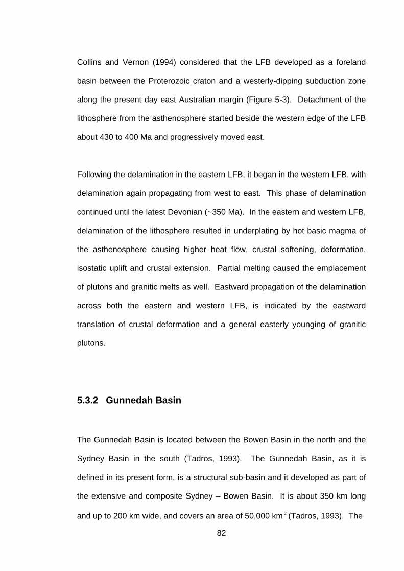
Collins and Vernon (1994) considered that the LFB developed as a foreland
basin between the Proterozoic craton and a westerly-dipping subduction zone
along the present day east Australian margin (Figure 5-3). Detachment of the
lithosphere from the asthenosphere started beside the western edge of the LFB
about 430 to 400 Ma and progressively moved east.
Following the delamination in the eastern LFB, it began in the western LFB, with
delamination again propagating from west to east. This phase of delamination
continued until the latest Devonian (~350 Ma). In the eastern and western LFB,
delamination of the lithosphere resulted in underplating by hot basic magma of
the asthenosphere causing higher heat flow, crustal softening, deformation,
isostatic uplift and crustal extension. Partial melting caused the emplacement
of plutons and granitic melts as well. Eastward propagation of the delamination
across both the eastern and western LFB, is indicated by the eastward
translation of crustal deformation and a general easterly younging of granitic
plutons.
5.3.2 Gunnedah Basin
The Gunnedah Basin is located between the Bowen Basin in the north and the
Sydney Basin in the south (Tadros, 1993). The Gunnedah Basin, as it is
defined in its present form, is a structural sub-basin and it developed as part of
the extensive and composite Sydney – Bowen Basin. It is about 350 km long
and up to 200 km wide, and covers an area of 50,000 km (Tadros, 1993). The 2
82
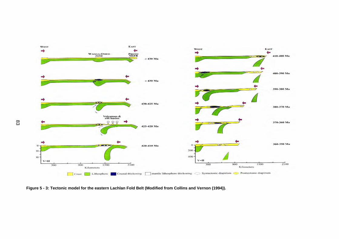
83
Figure 5 - 3: Tectonic model for the eastern Lachlan Fold Belt (Modified from Collins and Vernon (1994)).
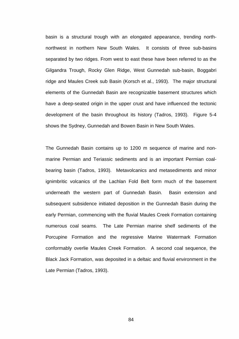
basin is a structural trough with an elongated appearance, trending north-
northwest in northern New South Wales. It consists of three sub-basins
separated by two ridges. From west to east these have been referred to as the
Gilgandra Trough, Rocky Glen Ridge, West Gunnedah sub-basin, Boggabri
ridge and Maules Creek sub Basin (Korsch et al., 1993). The major structural
elements of the Gunnedah Basin are recognizable basement structures which
have a deep-seated origin in the upper crust and have influenced the tectonic
development of the basin throughout its history (Tadros, 1993). Figure 5-4
shows the Sydney, Gunnedah and Bowen Basin in New South Wales.
The Gunnedah Basin contains up to 1200 m sequence of marine and non-
marine Permian and Teriassic sediments and is an important Permian coal-
bearing basin (Tadros, 1993). Metavolcanics and metasediments and minor
ignimbritic volcanics of the Lachlan Fold Belt form much of the basement
underneath the western part of Gunnedah Basin. Basin extension and
subsequent subsidence initiated deposition in the Gunnedah Basin during the
early Permian, commencing with the fluvial Maules Creek Formation containing
numerous coal seams. The Late Permian marine shelf sediments of the
Porcupine Formation and the regressive Marine Watermark Formation
conformably overlie Maules Creek Formation. A second coal sequence, the
Black Jack Formation, was deposited in a deltaic and fluvial environment in the
Late Permian (Tadros, 1993).
84
Figure 5 - 4: The Sydney, Gunnedah and Bowen Basin in NSW (Tadros, 1993).
85
Triassic sediments unconformably overlie the Permian sequences. Two
depositional sequences have been identified in the Digby Formation. The lower
stage consists of a conglomerate unit deposited by a braided steam system
after uplift of the adjacent New England Fold Belt. During the late stage sandy
sediments were deposited as the elevation of the New England source area
declined, and the system changed from a braided to a meander system. A
basin-wide palaeosol horizon caps the Digby Formation. The Napperby
depositional sequence represents the upper limit of the Gunnedah Basin
sequence, with a regional unconformity existing between the Triassic and
overlying Jurassic sediments of the Surat Basin north of Liverpool Ranges
(Tadros, 1993, Kingham, 1998).
The Gunnedah Basin sequence includes a number of basic intrusions of
Mesozoic and Tertiary rocks. These are associated with massive extrusions of
the Garrawilla Volcanic complex and the Liverpool, Warrumbungle and
Nandewar Ranges. Cretaceous sediments (Bungil Formation) occur under
Tertiary basalt in the western part of the Liverpool Range (Tadros, 1993). Figure
5-5 shows the lithostratigraphy of the Gunnedah Basin from(Tadros, 1993).
In addition to coal resources, the Gunnedah Basin also has potential for the
discovery of oil and gas, especially as good petroleum source rocks are
presented at several stratigraphic horizons. Sandstones with good to excellent
reservoir potential also occur at several stratigraphic levels and many are
sealed by regionally extensive clayey units (Tadros, 1993).
86
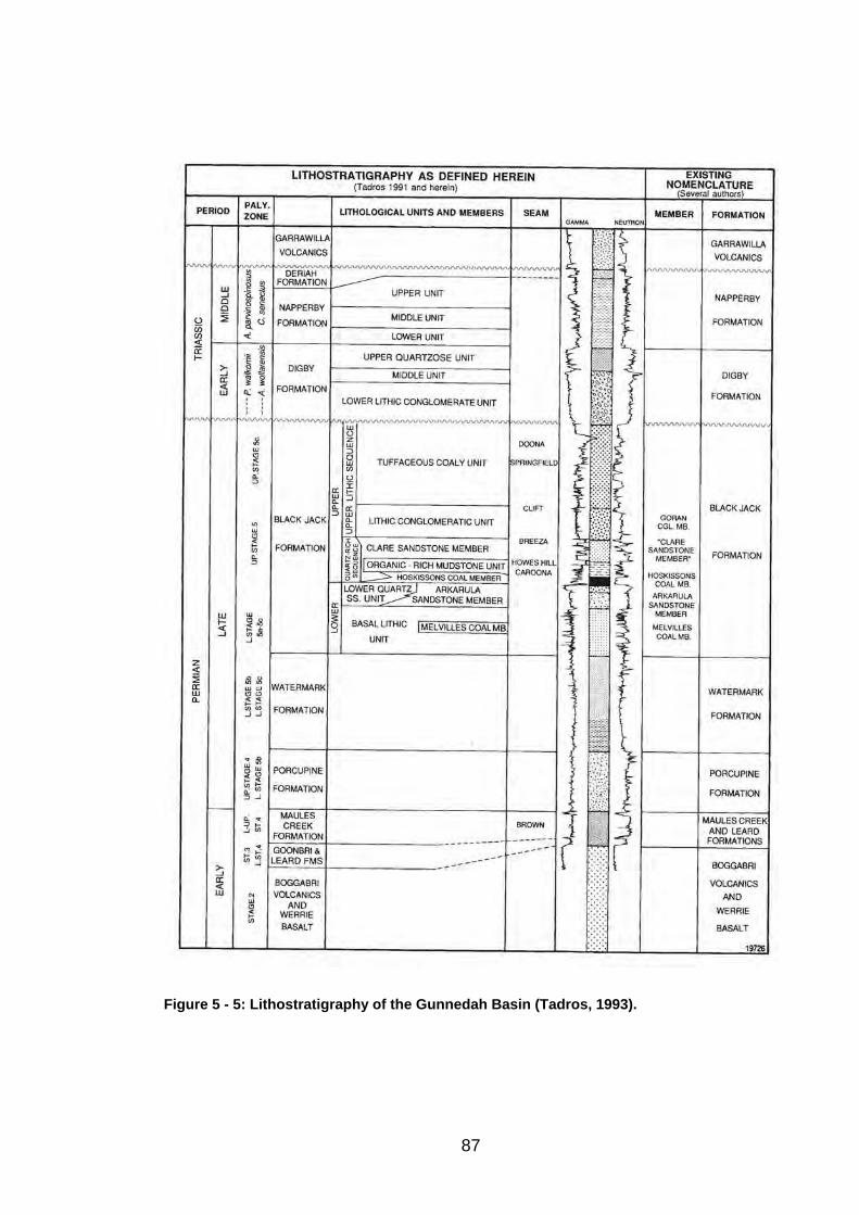
Figure 5 - 5: Lithostratigraphy of the Gunnedah Basin (Tadros, 1993).
87

5.3.3 Surat Basin
The Jurasic-Cretaceous Surat Basin is located on the eastern part of the Great
Australian Basin (Figure 5-1). The Great Australian Basin is a composite
structural basin that includes a relict group of major Jurassic-Cretaceous
epicratonic sedimentary basin occupying about 1.7 million square kilometers of
inland eastern Australia (Cramsie and Hawke, 1984). In New South Wales the
Surat Basin has been divided into six lower category units includes the Boomi
Trough, the Lightning Ridge Shelf, the Coonamble Embayment, the Oxley
Basin, the Rawdon Ridge and the Warialda Trough (Bourke et al., 1974; Hawke
and Cramsie, 1984; Scheibner and Basden, 1996). In NSW it is also separated
from the Eromanga Basin by the Nebine Ridge, which underlies the Cunnamulla
Shelf. To the east of this is the Lightning Ridge Shelf and the Boomi Trough, to
the south of these elements is the Coonamble Embayment.
The Surat Basin is asymmetric, being wedge-shaped in cross section with the
sedimentary section gradually thickening from the western margin to the axis of
the Jurassic-Cretaceous trough, the Mimosa Syncline, and thinning more
sharply farther east to Kumbarella Ridge (Power and Devine, 1970).
The Surat Basin includes 2500 metres of mainly Jurassic clastic continental
sedimentary rocks and lower Cretaceous marine beds largely obscured by
Cainozoic alluvium. During the Jurassic period, there were 5 cycles of
terrestrial deposition. Coarse sand braided stream deposits grading up into
finer sand and silt deposits of meandering streams represent these cycles.
88
Labile sand, silt, mud and coal were laid down in swamps, lakes, deltas and
shallow seas to complete the cycle of deposition. During the mid-late Jurassic,
much of the sediments were supplied by andesitic volcanic activity (Exon,
1976). Outcropping units laid down during the Jurassic period include the
Precipice Sandstone and Evergreen Formation, the Hutton Sandstone and
Walloon Coal Measures, the Springbok Sandstone and Westbourne Formation,
the Gubberamunda Sandstone and Orallo Formation, with the final terrestrial
cycle depositing the Mooga Sandstone and Bungil Formation (Kingham, 1998).
Hawke and Cramsie (1984) described the stratigraphy of the Surat Basin in
New South Wales, as divided into four main intervals. The lowest is an Early to
Middle Jurassic, predominantly fine-grained, terrestrial sequence on the eastern
side. This is overlain by fluvial sandstone sequences of Middle Jurasic to
Neocomian age. An overlying Neocomian to early Albian essentially fine-
grained transgressive/marine/regressive sequence is overlain in the deepest,
central part of the basin by Albian transgressive/regressive sequence.
The Early Cretaceous marine transgression ended the fluvial cycles and
initiated deposition of the Rolling Downs Group. This group includes the
Doncaster and Coreena members of the Wallumbilla Formation, the Surat
Siltstone and the Griman Creek Formation (Kingham, 1998). During the Late
Cretaceous and early Tertiary, there was a deep weathering profile. Basic
volcanic activity occurred during the Oligocene-Miocene and since this time the
Surat Basin has remained relatively stable, with extensive erosion occurring
89
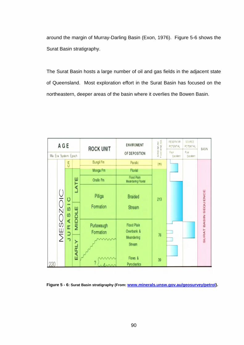
around the margin of Murray-Darling Basin (Exon, 1976). Figure 5-6 shows the
Surat Basin stratigraphy.
The Surat Basin hosts a large number of oil and gas fields in the adjacent state
of Queensland. Most exploration effort in the Surat Basin has focused on the
northeastern, deeper areas of the basin where it overlies the Bowen Basin.
Figure 5 - 6: Surat Basin stratigraphy (From: www.minerals.unsw.gov.au/geosurvey/petrol).
90
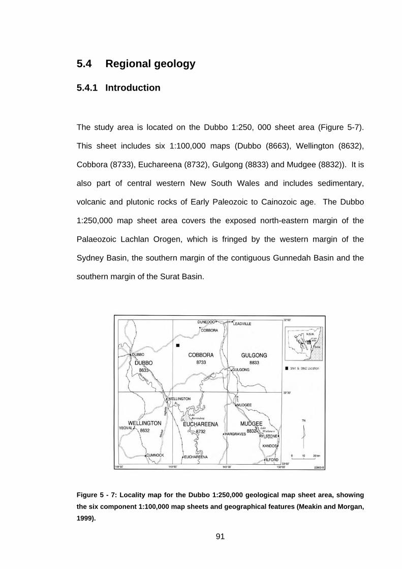
5.4 Regional geology
5.4.1 Introduction
The study area is located on the Dubbo 1:250, 000 sheet area (Figure 5-7).
This sheet includes six 1:100,000 maps (Dubbo (8663), Wellington (8632),
Cobbora (8733), Euchareena (8732), Gulgong (8833) and Mudgee (8832)). It is
also part of central western New South Wales and includes sedimentary,
volcanic and plutonic rocks of Early Paleozoic to Cainozoic age. The Dubbo
1:250,000 map sheet area covers the exposed north-eastern margin of the
Palaeozoic Lachlan Orogen, which is fringed by the western margin of the
Sydney Basin, the southern margin of the contiguous Gunnedah Basin and the
southern margin of the Surat Basin.
Figure 5 - 7: Locality map for the Dubbo 1:250,000 geological map sheet area, showing the six component 1:100,000 map sheets and geographical features (Meakin and Morgan, 1999).
91

5.4.2 Climate
Figure 5-8 shows the mean monthly maximum and minimum temperatures,
mean monthly precipitation data and the average number of wet days for Dubbo
and Dunedoo, and pan evaporation data for Wellington (Schofield, 1998). In
the Dubbo region rainfall is greatest in January, with an annual average of 584
mm reported on the Dubbo 1:100,000 sheet and 642 mm on the Cobbora
1:100,000 sheet. The annual distribution of rainfall is tilted toward the summer
months, but June is also a wet month. The climate is temperate with annual
mean temperatures ranging from 19 to 32 ˚C in summer, and 3 to 19˚C in winter
(Schofield, 1998).
Figure 5 - 8: Mean monthly maximum and minimum temperatures, mean monthly precipitation data and the average number of wet days for Dubbo and Dunedoo, pan evaporation data for Wellington is shown at the base of Figure (Schofield, 1998).
92

5.4.3 Physiography
The Dubbo 1:250,000 map area covers 15,600 square kilometers over parts of
the Shires of Cabonne, Wellington, Dubbo, Coolah, Mudgee, Merriwa and
Rylstone. The Western railway and several major roads, including the Mitchell
Highway, serve the area (Meakin and Morgan, 1999).
Topographically, the area falls from 740 m ASL in the east, to around 240 m
ASL near Dubbo (Figure 5-9). The topography in the Dubbo region has been
substantially reduced to a peneplain by erosion. This process mixes low-lying
lava flow relics with isolated topographic highs comprising plugs and earlier but
topographically inverted lava flows.
In the area there are three main drainage systems: Macquarie, Cudgegong and
Talbragar Rivers. The largest is the Macquarie River. The Macquarie River
flows from the western boundary of the study area to the NW through Dubbo.
The Talbragar flows in the north-west direction, through Dunedoo via Ballimore
to the Macquarie River. The two rivers link together 5 km north of Dubbo.
Talbragar River from east to west has 11 tributaries: Sandy Creek, Boomley
Creek, Spring Creek, Baragonumble Creek, Goan Creek, Spicers Creek, Back
Creek, Rocky Creek, Mitchells Creek, Jones Creek and Troy Creek. The
Gudgegong River flows in a southerly direction from the east side of Gulgong
town.
93
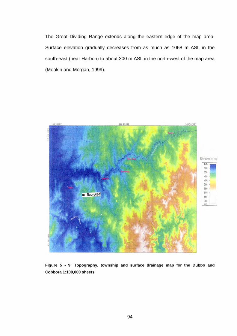
The Great Dividing Range extends along the eastern edge of the map area.
Surface elevation gradually decreases from as much as 1068 m ASL in the
south-east (near Harbon) to about 300 m ASL in the north-west of the map area
(Meakin and Morgan, 1999).
Figure 5 - 9: Topography, township and surface drainage map for the Dubbo and Cobbora 1:100,000 sheets.
94

5.4.4 Dubbo Area
The Dubbo 1:250,000 map sheet area covers the exposed north-eastern margin
of Lachlan Orogen. Meakin and Morgan (1999) divided the Lachlan Orogen
rocks into seven lithotectonic associations based on age, lithology and
depositional environment. These include the:
Early Ordovician to Late Ordovician generally deepwater, mafic to intermediate
volcanic and volcaniclastic rocks and intrusions;
?Early to Middle Ordovician quartz-rich turbidities;
late Early Silurian to Early Devonian shallow water to deepwater volcanic and
sedimentary sequences;
Early Devonian plutonic rocks;
Middle Devonian subaerial silicic volcanic sequences;
Late Devonian quartzose fluviatile to shallow marine sedimentary rocks; and
late Early to Late Carboniferous granite intrusions.
Figure 5-10 shows the schematic structural map of the Dubbo 1:250,000 sheet
area (Matson, 1975). During the Early Middle Ordovician, tensional forces
probably associated with rollback of the subduction zone towards the east
caused separation of a substantial part of the Girilambone flysch wedge (most
probably of Cambrian age) from the Australian Pate. The Wagga Marginal
Basin formed between the microcontinent and the major plate. In the Late
Ordovician and Early Silurian, further extension caused relatively minor splitting
between the microcontinent and the Molong Volcanic Rise such that the
95
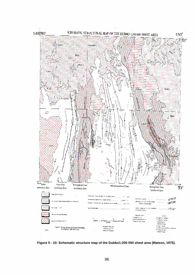
33˚
32˚
148˚30’ 150˚
Figure 5 - 10: Schematic structure map of the Dubbo1:250 000 sheet area (Matson, 1975).
96
western segment of the volcanic rise was left attached to the Parkes Terrace
that had developed over the microcontinent. The initiation of the Cowra Trough
probably represented the depression associated with this splitting (Matson,
1975)
At the end of Ordovician, following the extension, the Australian plate advanced
eastwards causing the Benambran Orogeny. Sedimentary material filling the
Wagga Marginal Basin was deformed and metamorphosed. During Silurian
times, after this Orogeny, tensional stress developed, probably caused by
rollback (Matson, 1975). The Qidongan Orogeny occurred in this period (Crook ,
1980).
The Oidongan Orogeny during the Silurian caused further folding and uplift of
the flysch and volcanic sequences to the east, and attached to, the Molong
Volcanic Rise. Following the Oidongan Orogeny, strong tensional stresses
caused splitting of the Molong Volcanic Rise and the formation of a new
marginal sea, the Hill End Trough, with other similar features in the Lachlan
Fold Zone. After this extension in the Middle Silurian, explosive acid volcanism
commenced. The acid volcanism is indicative of the commencement of the
Bowning Tectonic Stage (Matson, 1975). In the early Devonian, closure of the
Cowra Trough marked the end of sedimentation in this area. Flysch and
volcanic rocks was deposited in the Hill End Trough during the early Devonian.
Devonian sedimentation in the Hill End Trough reached 6100 m, much greater
than the thickness of the Silurian sequence. The Silurian to Middle Devonian
97
Rise was formed, due to formation of the Sofala Anticlinorium and the Sunny
Corner Synclinorium. The formation of the Forbes Anticlinorial Zone and the
Cowra – Yass Synclinorial Zone from the former Cowra Trough was completed
during the later Kanimblan Orogeny. Tabberabberan folding and uplift
cratonized the Hill End Trough and it is now represented by the Hill End
Synclinorial zone. Locally at Mount Frome, near Mudgee, Middle Devonian
formations and the Lambie Group are conformable, but elsewhere an
unconformity has been proven below the Lambie Group (Matson, 1975).
In the Early Carboniferous the Kanimblan Orogeny caused deformation of the
Late Devonian strata, producing the Catombal and Lambie Synclinoria, and the
Lachlan Fold Belt was cratonised. During the Middle to Late Carboniferous, the
post kinematic Bathurst granites were emplaced. Prior to this emplacement,
acid volcanism, which was probably related to the granite plutonism, occurred in
the Rylstone area.
In the Permian, plate interaction and extension resulted in the formation of the
Sydney – Bowen Basin as well as New England Mobile Zone. The Hunter
Orogeny deformed the New England Fold Belt during the late Early Permian.
Following this orogeny, the sediments of the Bowen and Hawkesbury Tectonic
Stages were deposited in the Sydney – Bowen Basin a fore-deep basin
(Matson, 1975).
In the early Triassic, extension followed by depression formed the Great
Australian Basin. In the Jurassic and Cretaceous the Tasman Epi-Cratonic
Province was established, and the main subsidence was transferred from the
98

Sydney Basin to the Great Australian Basin onlapping the previous fore-deep
sediments. Also, Triassic-Jurassic and Jurassic sediments onlapped the older
rocks to the west (Matson, 1975).
5.4.5 Geology
The Dubbo 1:250,000 geology map includes sedimentary, igneous and
metamorphic rocks of Palaeozoic to Cainozoic age (Figure 5-11). The oldest
rocks in the Dubbo area belong to the Macquarie Volcanic Arc and in particular,
to the early Ordovician Mitchell Formation, which is conformably overlain by the
deepwater Hensleigh Siltstone (Meakin and Morgan, 1999).
The Early Ordovician sequence contains volcanic and volcaniclastic rocks that
range in age from the Lancefieldian (or older) to the early Bendigonian.
Because of an hiatus the Early Ordovivian strata represent a separate volcanic
event from that of the overlying Middle Ordovician Cabonne Group.
During the late Middle to Late Ordovician igneous activity generated
intermediate to mafic, medium-K to shoshonitic volcanic and shallow rocks of
the Cabonne Group, with copper-gold mineralization. A quartz-rich fan system
(Adaminby Group) developed in the south-east part of the map area during this
time. Deformation of the Lachlan Orogen occurred in the Late Ordovician to
Early Silurian. Regional extension in the Early Silurian caused the Macquarie
Volcanic Arc to split and form separate belts (Meakin and Morgan, 1999).
99
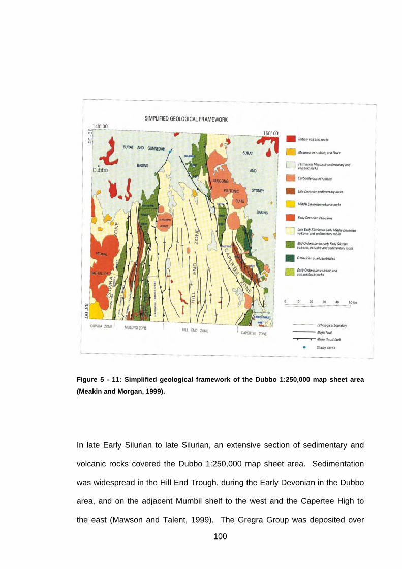
Figure 5 - 11: Simplified geological framework of the Dubbo 1:250,000 map sheet area (Meakin and Morgan, 1999).
In late Early Silurian to late Silurian, an extensive section of sedimentary and
volcanic rocks covered the Dubbo 1:250,000 map sheet area. Sedimentation
was widespread in the Hill End Trough, during the Early Devonian in the Dubbo
area, and on the adjacent Mumbil shelf to the west and the Capertee High to
the east (Mawson and Talent, 1999). The Gregra Group was deposited over 100
the Mumbil Shelf and extends into the adjacent Cowra and Hill End Troughs.
The subaerial and dominantly acid volcanic rocks of the Hyandra Creek Group
were deposited over a small area to the south of Dubbo (Meakin and Morgan,
1999). During this time, the Yeoval Batholith, consisting of I-type intrusive
igneous rocks and intermediate to mafic sills was intruded. The truncation of
folds and faults is caused by a pre-Late Devonian unconformity (Tabberabberan
event) on the Dubbo 1:250,000 map sheet.
The Carboniferous period is represented by some plutonic igneous rocks, which
range from monzodiorite to granite in composition. The Carboniferous granites
are clearly discordant with the pervasive north-south structural trends and may
indicate an extensional regime (Meakin and Morgan, 1999). The granites of the
Dubbo 1:250,000 map sheet area are largely I-type, but some phases in the
eastern part of the Gulgong plutonic suite show marginal S-type characteristics,
with the presence of common muscovite and biotite (Barron, 1997).
The Permian period is represented by reactivation of older faults and by
deposition of the Early Permian, silicic Rylstone Volcanics which host
epithermal and intrusion-related skarn mineralization. In the ?late
Carboniferous to Triassic sequence around the eastern and northern margins of
the Dubbo 1:250,000 map, early Permian sediments represent the base of the
Sydney-Gunnedah Basin. The Sydney-Gunnedah Basin is an elongated
structural basin that extends between the Lachlan Orogen to the west and the
New England Orogen to the east. Conversion of the Sydney Basin to a foreland
101
basin led to development of extensive Late Permian coal swamps (Meakin and
Morgan, 1999).
In Mesozoic age, igneous rocks extended across the Dubbo 1:250,000 map and
are commonly related to the Permian to Triassic sedimentary rocks of the
Sydney and Gunnedah Basin (Meakin and Morgan, 1999). Googodery
Trachyte is the only named Mesozoic igneous unit in this area. During this
period, fluvio-lacustrine quartzose sediments (Purlawaugh Formation, Pilliga
Sandstone) of the Surat Basin were deposited along the northern margin of the
area. They represent deposition due to erosion which commenced in the Late
Jurassic and continued into the Tertiary.
In the Cainozoic, deposits on the Dubbo 1:250,000 map are represented by
alluvial, colluvial and lacustrine sediments, basalt and duricrust. No formal
names have been applied to unconsolidated Quarternary units on the Dubbo
1:250,000 map sheet. Gravel deposition represents climatic change by high-
energy, braided river systems, which gradually diminished in energy with the
development of aridity in inland Australia. Tertiary basalt overlies and intrudes
all pre-Cretaceous rocks across the Dubbo 1:250,000 map sheet area, with
relict basalt preserved predominantly over the Mumbil Shelf and Capertee High
(Dubbo area and Liverpool Range), and also over the southern end of the Hill
End Trough (Meakin and Morgan, 1999).
102
5.4.6 Metamorphism
Figure 5-12 shows the metamorphic zones on the Dubbo 1:250,000 map sheet
area. There are four main metamorphic zones in the area (Pogson and
Watkins, 1998). The following is the four summary metamorphic zones:
M1 (blue): clay/carbonate, epidote, sericite, albite, with or without foliation.
M2 (green): prehnite/pumpellyite, normally without foliation.
M3 (purple): actinolite/biotite, with or without foliation.
MH (red): akin to the hornfels envelope surrounding an intrusion. This zone is
represented by the presence of metamorphic diopside or garnet, or other
phases such as cordierite, andalusite, or even other higher grade hornfels
assemblages.
The metamorphic map has been prepared from an assessment of the
metamorphic mineral assemblages of 1919 rocks corrected by the Geological
Survey of New South Wales from this sheet. Because of small data set, this
map is regarded as a preliminary attempt to reassess the metamorphic zones
published by (Smith, 1969). His work identified and showed the distribution of
six zones of differing metamorphic grade over the Buthurst-Dubbo region,
based on the presence or absence of key metamorphic minerals such as
carbonate, albite, chlorite, prehnite, pumpellyite, actinolite-tremolite and biotite.
Metamorphism can be seen adjacent to the intrusion on the Dubbo map. All the
Carboniferous plugs and plutons are altered to an M1 assemblage such as that
seen in the Yeoval Complex.
103
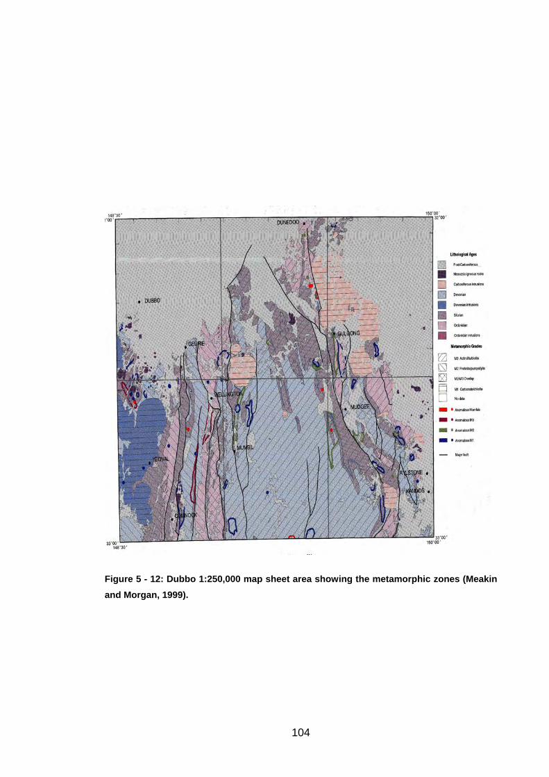
Figure 5 - 12: Dubbo 1:250,000 map sheet area showing the metamorphic zones (Meakin and Morgan, 1999).
104

5.5 Local Geology
5.5.1 Introduction
The study area is located in the Spicers Creek catchment within the Cobbora
1:100,000 map sheet area on the Dubbo 1:250,000 map (Figure 2-4). Spicers
Creek catchment is situated about 45 km from the city of Dubbo to the west, 20
km from the town of Cobbora to the east, 15 km from the town of Boomley to
the north and south 45 km to Wellington (Figure 5-13).
Cobbora region is situated in the north-eastern portion of the Lachlan Fold Belt
(LFB) and overlying marginal areas of the Gunnedah Basin and Surat Basin.
The basement rocks of the Lachlan Fold Belt have been regionally
metamorphosed and contain north-south trending faults, folds, and fractures.
The Gunnedah Basin Sequence includes a number of basic intrusions of
Mesozoic and Tertiary rocks. These are associated with massive extrusions of
Garrawilla Nolanic complex and the Liverpool, Warrumbungle and Nandewar
Ranges (Tadros, 1993). The Surat Basin contains 2500 metres of mainly
Jurrasic continental sedimentary rocks and lower Cretaceous marine beds
largely obscured by Cainozoic alluvium (Exon, 1976).
The area of study, is geologically complex due to the tectonic events it has
endured and the landscape evolution is closely related to the underlying
geology (Morgan and Jankowski, 2002). The Palaeozoic rocks range in age
from Ordovician through to Devonian. The depositional environments ranges
from marine to sub-marine (Schofield and Jankowski, 2000). Lithologies 105
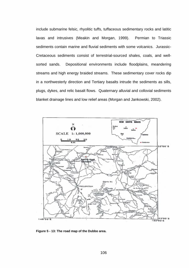
include submarine felsic, rhyolitic tuffs, tuffaceous sedimentary rocks and latitic
lavas and intrusives (Meakin and Morgan, 1999). Permian to Triassic
sediments contain marine and fluvial sediments with some volcanics. Jurassic-
Cretaceous sediments consist of terrestrial-sourced shales, coals, and well-
sorted sands. Depositional environments include floodplains, meandering
streams and high energy braided streams. These sedimentary cover rocks dip
in a northwesterly direction and Tertiary basalts intrude the sediments as sills,
plugs, dykes, and relic basalt flows. Quaternary alluvial and collovial sediments
blanket drainage lines and low relief areas (Morgan and Jankowski, 2002).
Figure 5 - 13: The road map of the Dubbo area.
106
5.5.2 Climate
In the Spicers Creek catchment the highest temperatures are January with
maximum mean of 33˚C and the lowest temperatures are in July with a
minimum mean of 1.8˚C. The mean average rainfall for the catchment was
measured as 563 mm. Summer is the wettest season receiving 31% of the
annual rainfall (Jewel, 2000, Morgan and Jankowski, 2002).
5.5.3 Stratigraphy
The rock units that are represented in the Cobbora area are categorized into
those relating to basement and those that constitute the cover rocks. The
Ordovician to Late Devonian, mainly marine basement rocks were deformed
during compressive Middle Devonian and Middle Carboniferous orogenic
episodes, whilst the mainly terrestrial Late Carboniferous to Late Jurassic cover
rocks were deposited in an extensional tectonic regime.
Figure 5-14 shows the geological map around the area are scale of 1:100,000.
Table 5-1 is a summary of the different rock types found in the area.
Throughout the following sections the characteristics of the geological units
around the study area are documented (Meakin and Morgan, 1999).
107
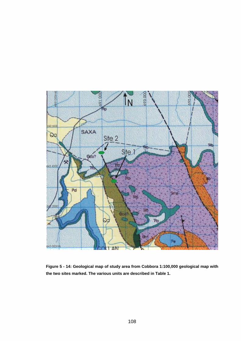
Figure 5 - 14: Geological map of study area from Cobbora 1:100,000 geological map with the two sites marked. The various units are described in Table 1.
108

Table 5 - 1: Description of different rocks type in the Spicers Creek area (From Cobbora 100,000 geological map).
Symbol from
fig 2-14
Rock
Formation
/Group
Age
Composition
Qa
--- Quaternary Alluvial silt, clay and sand, variable humic content,
sporadic pebble to cobble-sized unconsolidated
conglomeratic lenses.
Rp Napperby
Formation
Triassic Siltstone thinly interbedded with fine-medium grained,
lithic-quartz sandstone, minor conglomerate;
coarsening-up sequences.
Rb Boulderwood
Formation
Triassic Thick-bedded quartz-lithic conglomerate, coarse
pebbly quartz-lithic sandstone and siltstone.
Pd
Dunedoo
Formation
Permian
Pebbly quartz-lithic sandstone to conglomerate,
breccia, white claystone, thin coal seams.
Pe
---- Permian Carbonaceous siltstone, quartz lithic sandstone,
conglomerate and coal lenses rare varves.
Dgc Cuga Burga
Volcanics
Devonian Latitic, crystal-lithic sandstone, breccia, siltstone, tuff,
latite and lesser andesite, basalt, minor
allochthonous limestone, quartzose sandstone.
Sms Gleneski
Formation
Silurian Rhyolitic to latitic lava, intrusive and tuff and
volcaniclastic sandstone.
θm Ungrouped
Ordovician
Intrusions
Late
Ordovician
Monzonite and diorite to more felsic syenite and
granite.
θco Oakdale
Formation
Ordovician Basalt, basaltic andesite, latite lava and intrusions,
volcaniclastic breccia, conglomerate, sandstone and
siltstone, minor allochthonous limestone.
109
5.5.3.1 Palaeozoic units
The Palaeozoic rocks range in age from Ordovician through to Devonian. The
early Ordovician sequence represents the oldest strata on the Dubbo 1:250,000
map sheet area and the study area.
5.5.3.1.1 Oakdale Formation (θco)
The Oakdale Formation is one of the most widespread units of the Cabonne
Group. The Formation takes it name from the Oakdale property, at the
southern end of the Oakdale Anticline (Meakin and Morgan, 1999). It forms a
broad, structurally complex, largely fault–bounded belt about 120 km in strike
length which extends from 35 km north of Wellington to 20 km south-east of
Orange.
Constituent units contain a number of allochthonous, and possibly rarely
autochthonous, limestone bodies, as well as limestone breccia and calcareous
sandstone. Primary volcanic rocks of the Oakdale Formation include
predominantly shoshonite, basalt to basaltic andesite and less commonly latite
lavas and high level intrusions. Volcanoclastic breccia and conglomerate are
common in the Oakdale Formation, particularly in the area to the north of
Wellington. The units are interbedded with sandstone turbidite packages and
primary volcanic layers.
110
The units are massive to coarsely bedded, clast- to matrix-supported, poorly
sorted and range from 3 m to over 20 m in thickness. This formation is
unconformably overlain in the main belt by late Early to Late Silurian Mumbil
Shelf strata, represented south of Wellington by the Dripstone Formation, and
north of Wellington by the Narragal limestone and Gleneski Formation of the
Mumbil Group.
In the Oakdale Formation, graptolite and brachiopod fauna have been
described by a number of researchers from the siltstone units (Meakin and
Morgan, 1999).
5.5.3.1.2 Ungrouped Ordovician Intrusions (θm)
Many small intrusive bodies of presumed Ordovician age occur within the
Oakdale Formation. None of these units have been isotopically dated. The
intrusions range from monzonite and diorite to more felsic syenite and granite in
composition and the outcrops range in size from less than 100 metres up to 900
metres in diameter.
Metamorphism by these intrusions is generally limited to weak to moderate
development of chlorite-sericite-epidote alteration of plagioclase and
ferromagnesian minerals, indicating a lower greenshist grade (Meakin and
Morgan, 1999).
111
5.5.3.1.3 Gleneski Formation (Sms)
The formation takes it name from the Gleneski property north of the Macquarie
River (Meakin and Morgan, 1999). The Gleneski Formation is comprised
predominantly of felsic to rhyolitic tuff and tuffaceous sedimentary rocks, with
lesser rhyolitic to felsic to latitic lava and intrusions, shale, and minor limestone.
Massive felsite, quartz felsite, quartz latite and rhyolite lava and intrusions
locally are intercalated with the volcanoclastic rocks of the Gleneski Formation.
These lithologies are interbedded on a variety of scales. Rare limestone and
calcareous sandstone are interbedded with volcanoclastic rocks of the Gleneski
Formation.
The massive and graded beds, erosional bases and local cross bedding in
clastic rocks of the Gleneski Formation suggest that they were deposited
subaqueously by turbidity currents. The magma source for the Gleneski
Formation was acid, but both primary volcanic and pyroclastic rocks, as well as
volcanic and lithic fragments in tuffaceous units, are deficient in quartz
phenocrysts (Meakin and Morgan, 1999).
5.5.3.1.4 Cuga Burga Volcanics (Dgc)
The name is derived from Cuga Burga Creek, which cuts through the formation
to the south-east of the Oakdale Anticline (Meakin and Morgan, 1999). The
Cuga Burga Volcanics contains no autochthonous fossils and age constraints
for the formation are provided mainly by conodont data for overlying and 112
underlying formations. It consists mainly of shoshonitic latitic volcanic and
volcanoclastic rocks. A thick sequence of pillow lavas is well-exposed in the
representative section of this units. A low radiometric character characterizes
the Cuga Burga Volcanics, although locally, the formation has a strong
potassium (pink) response.
The belt of Cuga Burga Volcanics separating the Yeoval Complex from the
Yennora Granite in the western area shows a complex intrusive history. Many
dykes are present, varying in composition from microdiorite and graphic
microgranite to dacite and rhyolite to basalt. The Cuga Burga Volcanics
contains no authochthonous fossils and age constraints for the formation are
provided mainly by conodont data for the overlying and underlying formations
(Meakin and Morgan, 1999).
The Cuga Burga Volcanics is characterized by a low radiometric character (dark
signature on radiometric images), although locally, such as in the fault-bounded
belt north of The Gap, the formation has a strong potassium (pink) response.
The formation has an overall anomalous magnetic high signature on total
magnetic intensity images. Igneous rocks of the formation have a high magnetic
susceptibility while volcaniclastic rocks are more variable (Meakin and Morgan,
1999).
113
5.5.3.1.5 Early Permian Undifferentiated (Pe)
This unit is largely exposed in a series of north-west trending lobes which
extend northwards under the Late Permian to Jurassic sedimentary rocks of the
Gunnedah Basin and the overlying Great Australian Basin. It contains
carbonaceous siltstone, quartz lithic sandstone, conglomerate coal lenses and
rare varves. This unit is somewhat better exposed in the Spicers Creek. In the
Spicers Creek the basal Early Permian sequence consists of poorly sorted,
sedimentary polymictic breccia and conglomerate which contains subangular to
rounded clasts of sandstone, phyllite and quartz which range up to 40 cm in
size.
The undifferentiated Early Permian, a possible distal equivalent to the Rylstone
Volcanics, correlates with the Late Carboniferous to earliest Permian, thick non-
marine fluvio-glacial conglomerates of the Talaterang Group in the southern
Sydney Basin, and the fluvio-lacustrine sediments of the Seaham Formation
(Meakin and Morgan, 1999).
5.5.3.1.6 Dunedoo Formation (Pd)
The Dunedoo Formation forms a relatively thin unit in the area of study. It
unconformably overlies the undifferentiated Early Permian (Pe) sedimentary
rocks and is disconformably overlain by Early Triassic sedimentary rocks. The
Dunedoo Formation is only moderately exposed at scattered localities, mainly in
114

creeks or occasionally on steeper slopes immediately below the more resistant
overlying Boulderwood Formation.
The formation consists of breccia, conglomerate and fine – to coarse- grained
sandstone and pebbly sandstone of quartzose to quartz-lithic and
quartzofeldspathic composition with a dominantly kaolinitic matrix. The lower
section of this formation is generally only poorly exposed. Surface exposures of
the Dunedoo Formation range up to 60 m on the Cobbora 1:100,000 map sheet
area. Common fining-up sequences in the Dunedoo Formation reflect fluvial
deposition (Meakin and Morgan, 1999).
5.5.3.2 Mesozoic units
Igneous rocks of Mesozoic age are scattered across Dubbo 1:250 000 map
sheet area, and are commonly associated with Permian to Triassic sedimentary
rocks of the Sydney and Gunnedah Basins. The Mesozoic rocks in the Spicers
Creek area are limited to the Boulerwood Formation and the Napperby
Formation. They cover of a large part of the north of area.
5.5.3.2.1 Boulerwood Formation (Rb)
The name is derived from Boulderwood homestead (Meakin and Morgan,
1999). It is typically exposed at the margins of slightly elevated plateaus
capped by the early Jurrasic Purlawaugh Formation. This formation ovelies the
115

Dunedoo Formation with probably disconformity or slight angular unconformity
and is conformably overlain by the Napperby Formation.
The Boulderwood Formation consists of very coarse-grained pebbly to
conglomeratic, lithic-quartz sandstone and grit, together with subordinate flaggy,
planar laminated, white, medium-grained quartz sandstone, claystone and
siltstone. Clasts are subangular to subrounded and predominantly quartz, with
minor fine silicic volcanic fragments and other siliceous metasedimentary
basement lithologies. The formation was deposited by a fluvial system.
Channel floor, channel bar and point bar sequences are common (Meakin and
Morgan, 1999).
5.5.3.2.2 Napperby Formation (Rp)
The name is derived from calcareous sandstone and laminated mudstone
exposed on Napperby station, near the Pine Vala well on the Coonabarabran-
Mullaley road (Meakin and Morgan, 1999). It conformably overlies the
Boulderwood Formation.
The formation consists of white, fine – to medium-grained, moderately to poorly
sorted lithic-quartz and quartzose, often flaggy, ferruginous sandstone with a
white clayey matrix thinly interbedded or interlaminated with grey siltstone and
minor conglomerate lenses. The Napperby Formation represents lacustrine-
delta deposition (Meakin and Morgan, 1999).
116
5.5.3.3 Cainozoic Unit
In the area of study the Cainozoic deposits are represented by alluvial deposits.
5.5.3.3.1 Alluvial Deposits (Qa)
No formal names have been applied to unconsolidated Quarternary units.
Alluvial deposits are geomorphological units. They can be regarded as falling
into three distinct morpho-stratigraphic types: actively depositing Holocene
zones; inactive Holocene/Pleistocene zones; and relict/elevated Pleistocene
zones. Generalized lithologies for the alluvium consist of silt and clay, with a
variable humic content.
5.5.4 Structure
The Spicers Creek region is situated in the east of the Dubbo 1:250,000 map
sheet and in the west of the Cobbora 1:100,000 sheet. It includes four of the
structural entities of the LFB; including the Cowra Trough, Molong High, Hill End
Trough and Capertee High (see Figure 5-10). Scott (1997) re-defined the
structural entities of the northeastern LFB into the four zones including the
Cowra-Molong Zone, Nindethana Zone, Hill End Zone and Capertee Zone
(Figure 5-15). He proposed there were three deformation events affecting rocks
across the map sheets. These are summarized in Table 5-2.
117
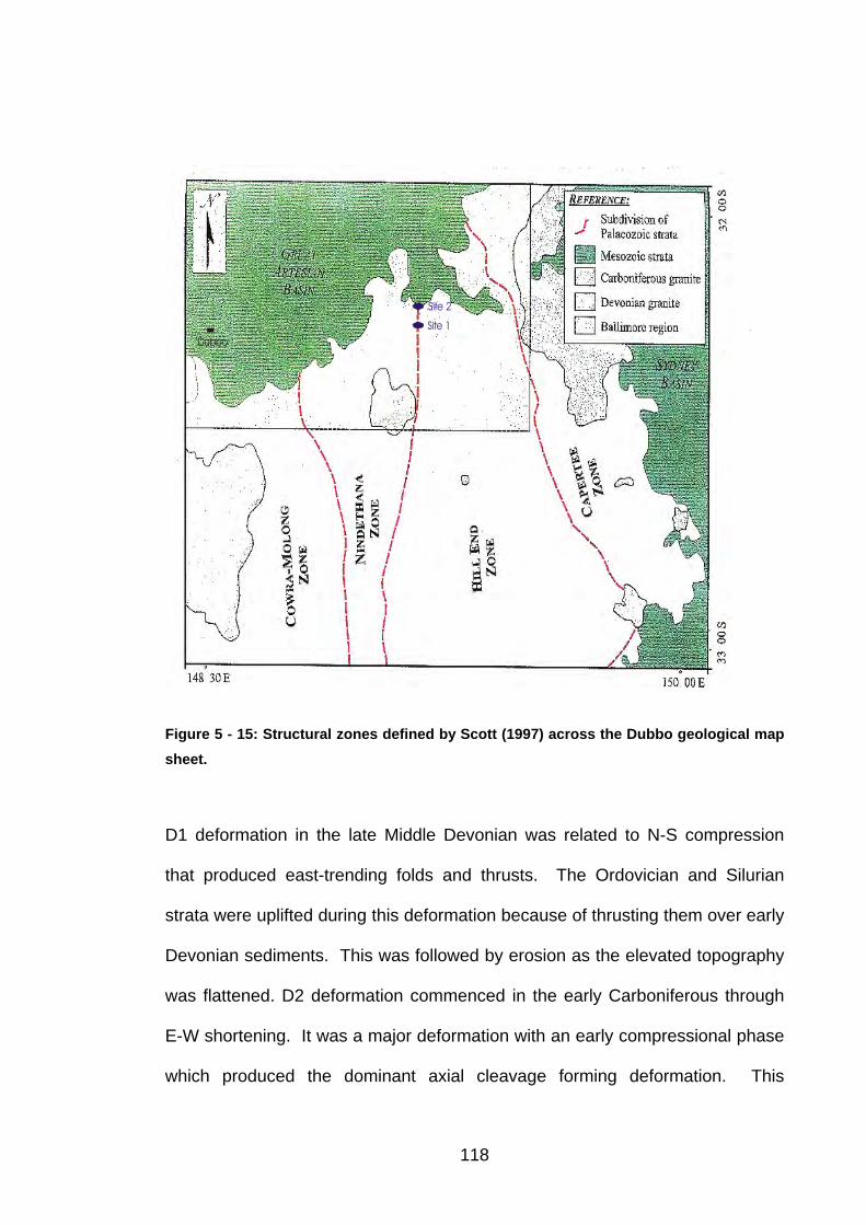
Site 2
Site 1Dubbo
Figure 5 - 15: Structural zones defined by Scott (1997) across the Dubbo geological map sheet.
D1 deformation in the late Middle Devonian was related to N-S compression
that produced east-trending folds and thrusts. The Ordovician and Silurian
strata were uplifted during this deformation because of thrusting them over early
Devonian sediments. This was followed by erosion as the elevated topography
was flattened. D2 deformation commenced in the early Carboniferous through
E-W shortening. It was a major deformation with an early compressional phase
which produced the dominant axial cleavage forming deformation. This
118
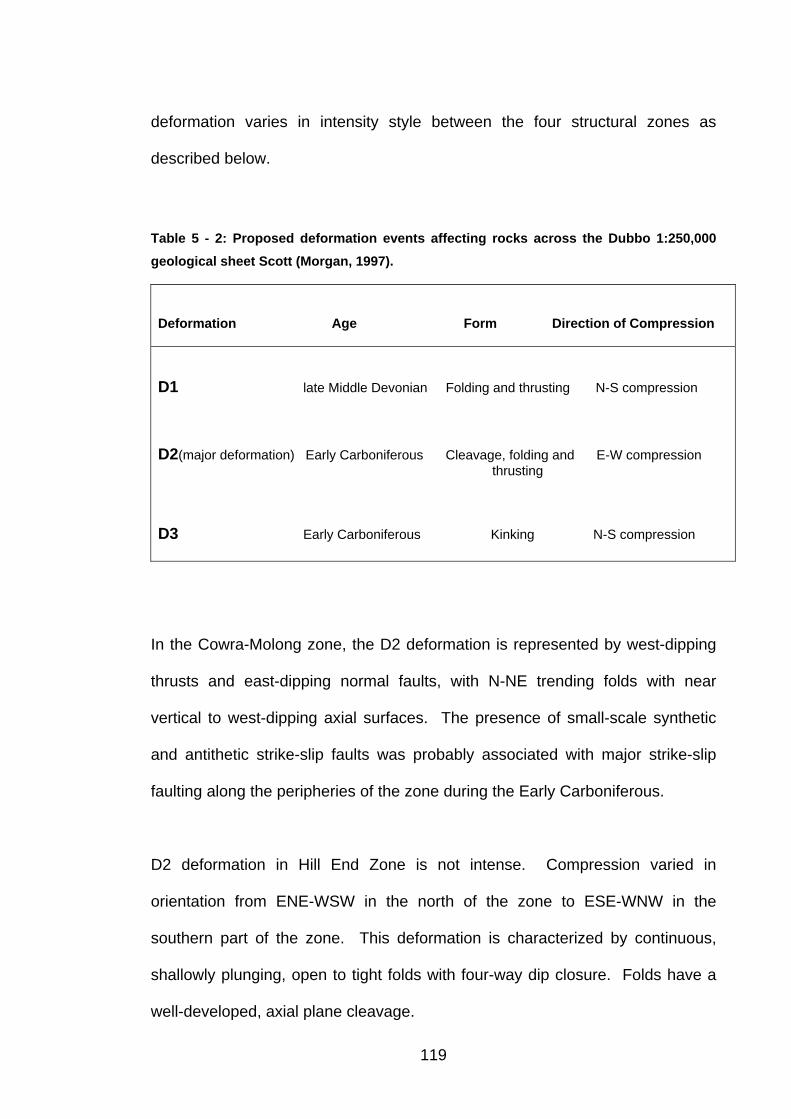
deformation varies in intensity style between the four structural zones as
described below.
Table 5 - 2: Proposed deformation events affecting rocks across the Dubbo 1:250,000 geological sheet Scott (Morgan, 1997).
Deformation Age Form Direction of Compression
D1 late Middle Devonian Folding and thrusting N-S compression
D2(major deformation) Early Carboniferous Cleavage, folding and E-W compression thrusting
D3 Early Carboniferous Kinking N-S compression
In the Cowra-Molong zone, the D2 deformation is represented by west-dipping
thrusts and east-dipping normal faults, with N-NE trending folds with near
vertical to west-dipping axial surfaces. The presence of small-scale synthetic
and antithetic strike-slip faults was probably associated with major strike-slip
faulting along the peripheries of the zone during the Early Carboniferous.
D2 deformation in Hill End Zone is not intense. Compression varied in
orientation from ENE-WSW in the north of the zone to ESE-WNW in the
southern part of the zone. This deformation is characterized by continuous,
shallowly plunging, open to tight folds with four-way dip closure. Folds have a
well-developed, axial plane cleavage.
119
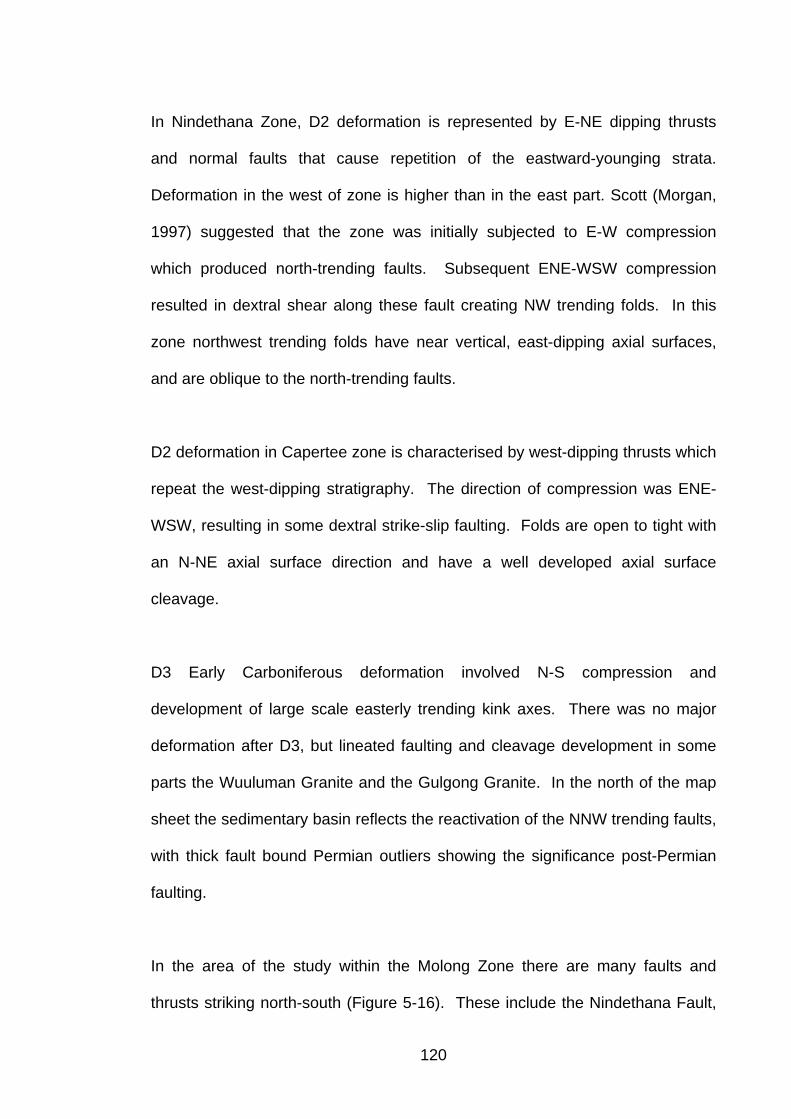
In Nindethana Zone, D2 deformation is represented by E-NE dipping thrusts
and normal faults that cause repetition of the eastward-younging strata.
Deformation in the west of zone is higher than in the east part. Scott (Morgan,
1997) suggested that the zone was initially subjected to E-W compression
which produced north-trending faults. Subsequent ENE-WSW compression
resulted in dextral shear along these fault creating NW trending folds. In this
zone northwest trending folds have near vertical, east-dipping axial surfaces,
and are oblique to the north-trending faults.
D2 deformation in Capertee zone is characterised by west-dipping thrusts which
repeat the west-dipping stratigraphy. The direction of compression was ENE-
WSW, resulting in some dextral strike-slip faulting. Folds are open to tight with
an N-NE axial surface direction and have a well developed axial surface
cleavage.
D3 Early Carboniferous deformation involved N-S compression and
development of large scale easterly trending kink axes. There was no major
deformation after D3, but lineated faulting and cleavage development in some
parts the Wuuluman Granite and the Gulgong Granite. In the north of the map
sheet the sedimentary basin reflects the reactivation of the NNW trending faults,
with thick fault bound Permian outliers showing the significance post-Permian
faulting.
In the area of the study within the Molong Zone there are many faults and
thrusts striking north-south (Figure 5-16). These include the Nindethana Fault,
120
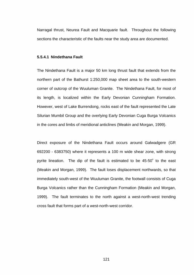
Narragal thrust, Neurea Fault and Macquarie fault. Throughout the following
sections the characteristic of the faults near the study area are documented.
5.5.4.1 Nindethana Fault
The Nindethana Fault is a major 50 km long thrust fault that extends from the
northern part of the Bathurst 1:250,000 map sheet area to the south-western
corner of outcrop of the Wuuluman Granite. The Nindethana Fault, for most of
its length, is localized within the Early Devonian Cunningham Formation.
However, west of Lake Burrendong, rocks east of the fault represented the Late
Silurian Mumbil Group and the overlying Early Devonian Cuga Burga Volcanics
in the cores and limbs of meridional anticlines (Meakin and Morgan, 1999).
Direct exposure of the Nindethana Fault occurs around Galwadgere (GR
692200 - 6383750) where it represents a 100 m wide shear zone, with strong
pyrite lineation. The dip of the fault is estimated to be 45-50˚ to the east
(Meakin and Morgan, 1999). The fault loses displacement northwards, so that
immediately south-west of the Wuuluman Granite, the footwall consists of Cuga
Burga Volcanics rather than the Cunningham Formation (Meakin and Morgan,
1999). The fault terminates to the north against a west-north-west trending
cross fault that forms part of a west-north-west corridor.
121
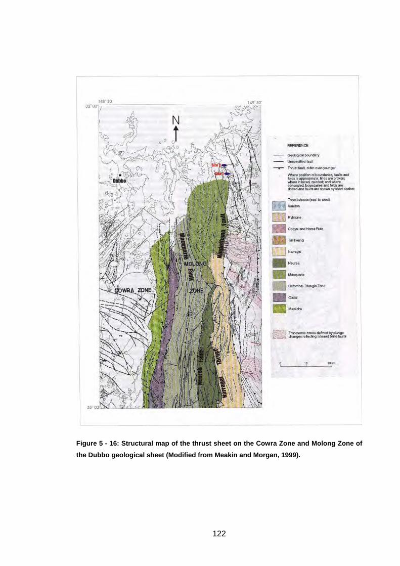
Figure 5 - 16: Structural map of the thrust sheet on the Cowra Zone and Molong Zone of the Dubbo geological sheet (Modified from Meakin and Morgan, 1999).
122

5.5.4.2 Narragal Thrust Sheet
The Narragal Thrust Sheet represents a combination of regional folds and
thrusts, and thus shows a structural transitional zone between the Molong Zone
to the west which is dominated by thrusts, and the Hill End Zone to the east that
is dominated by folds (Scott, 1997). This thrust sheet is bounded to the west
(below) by the east-dipping Narragal fault that marks the roof of Neurea Thrust
Sheet and to the east (end below) by the Nindethana Fault that also dips east.
The Narragal Thrust Sheet thus lies between two parallel thrusts (Meakin and
Morgan, 1999).
Cleavage in the Narragal Thrust Sheet dips steeply to the east and west and
swings in strike from NNW in the southern third of the map sheet area to NNE in
northern two third where it is approximately parallel in strike to fold axial traces.
The general obliquity with the meridonal bounding faults suggests a component
of left-lateral movement on them during deformation (Meakin and Morgan,
1999).
5.5.4.3 Macquarie Fault
The Macquarie Fault has a NNW trend and east dip. Its southern extent is
uncertain and it may disappear within the Garra Formation or link into a WNW
cross fault that cuts off the northern end of the Neurea Fault. This fault
juxtaposes Ordovician rocks in the hanging wall against the Late Devonian
Catombal Group in the Mount Arthur Syncline in the foot wall. The fault is
interpreted as one of a series of east-dipping thrusts with lesser displacement
123
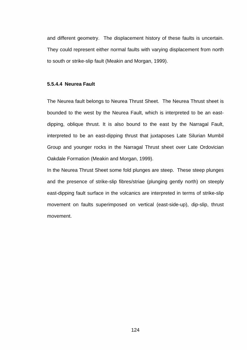
and different geometry. The displacement history of these faults is uncertain.
They could represent either normal faults with varying displacement from north
to south or strike-slip fault (Meakin and Morgan, 1999).
5.5.4.4 Neurea Fault
The Neurea fault belongs to Neurea Thrust Sheet. The Neurea Thrust sheet is
bounded to the west by the Neurea Fault, which is interpreted to be an east-
dipping, oblique thrust. It is also bound to the east by the Narragal Fault,
interpreted to be an east-dipping thrust that juxtaposes Late Silurian Mumbil
Group and younger rocks in the Narragal Thrust sheet over Late Ordovician
Oakdale Formation (Meakin and Morgan, 1999).
In the Neurea Thrust Sheet some fold plunges are steep. These steep plunges
and the presence of strike-slip fibres/striae (plunging gently north) on steeply
east-dipping fault surface in the volcanics are interpreted in terms of strike-slip
movement on faults superimposed on vertical (east-side-up), dip-slip, thrust
movement.
124
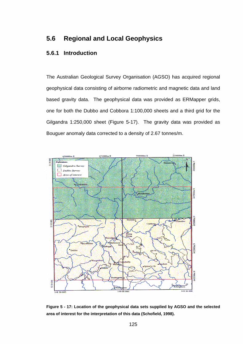
5.6 Regional and Local Geophysics
5.6.1 Introduction
The Australian Geological Survey Organisation (AGSO) has acquired regional
geophysical data consisting of airborne radiometric and magnetic data and land
based gravity data. The geophysical data was provided as ERMapper grids,
one for both the Dubbo and Cobbora 1:100,000 sheets and a third grid for the
Gilgandra 1:250,000 sheet (Figure 5-17). The gravity data was provided as
Bouguer anomaly data corrected to a density of 2.67 tonnes/m.
Figure 5 - 17: Location of the geophysical data sets supplied by AGSO and the selected area of interest for the interpretation of this data (Schofield, 1998).
125

The radiometric and magnetic data for the Gilgandra Map Sheet was acquired
in 1979. Its resolution is significantly lower than that of the data from the Dubbo
Map Sheet which was flown as part of the National Geoscience Mapping
Accord (NGMA) in 1991. The survey parameters are listed in Table 5-3.
Table 5 - 3: Survey parameters for the Gilgandra and Dubbo airborne surveys.
Gilgandra Survey Dubbo Survey
Operator New South Wales Department New South Wales Department
of Mineral Resources of Mineral Resources
Date 1979 1991
Line spacing 1,500m 400m
Altitude 150m 100m
Sampling interval 60m (magnetic) 7m (magnetic)
60m (radiometric) 67m (radiometric)
Line direction E-W E-W
Instruments ٠ MF57 Fluxgate ٠ Geometrics G833 helium
magnetometer vapour magnetometer
٠Four-channel gamma ray ٠Four-channel gamma ray
spectrometer (crystal spectrometer (crystal
volume 16.8 litres) volume 33.6 litres)
126
5.6.2 Radiometric Methods
5.6.2.1 Theory, Application
Elements whose atomic nuclei contain the same number of protons but different
numbers of neutrons are called isotopes. They are forms of the same element
with different atomic weights. Certain nuclei disintegrate spontaneously
emitting α particles (helium nuclei He) and β particles (electrons and positrons).
This is the phenomenon of radioactivity. These emissions alter the nuclear
charge, α by –2, β (positron) by –1 and β (electron) by +1. As a result the
disintegrating nucleus is transformed into a nucleus of another element.
The natural decay of radioactive elements produces a variety of types of
radiation (alpha, beta, gamma) at specific energy levels. Only gamma-ray
radiation has sufficient energy to be useful for geological mapping or
exploration. There are a large number of radioactive minerals, but the more
common are potassium (K), uranium (U), and thorium (Th). The gamma
radiation is emitted when these elements decay gradually through time (see
Telford et al., 1976), for a description of the individual decay process and
series).
Radiometric surveying is employed in the search for radioactive deposits and
also for deposits associated with radioactive elements such as zirconium and
titanium (Kearey and Brooks, 2001). Radiometric surveys used in geological
mapping as different rock types can be recognized from their distinctive
signature (Pires and Harthhill, 1989). It is an important source of information for
127
soil, regolith and geomorphological studies, including their mineralogy, texture,
chemistry and style of weathering (Wilford et al., 1997).
As Jaques et al. (1997) demonstrated gamma-ray spectrometry is an important
tool for distinguishing igneous rock bodies because of composition and degree
of differentiation, as U, Th and K. These elements are critical elements involved
in magmatic differentiation processes.
5.6.2.2 Interpretation Methodology
Airborne radiometric methods measure gamma radiation emitted from the
Earth’s surface and it is recorded using a gamma-ray spectrometer. The most
diagnostically valuable of these for geological mapping correspond to potassium
(1.46 MeV), bismuth-214 (1.765MeV) from the uranium-238 decay series, and
thallium-232 (2.614 MeV) from the thorium-232 decay series (Horsfall, 1997).
When K, U and Th decay they create gamma radiation of differing energy, K
producing the lowest and Th the highest (Table 5-4).
The sensor detects the energy levels of the gamma spectrum, and the relative
contribution of each band is recorded as a separate channel along with a total
signal channel (Horsfall, 1997). Modern airborne gamma-ray data acquisition
for regional mapping consists of a multichannel spectrometer be able to
measure at least 256 channels of data in the energy range 0-3 MeV (Minty,
1997).
128
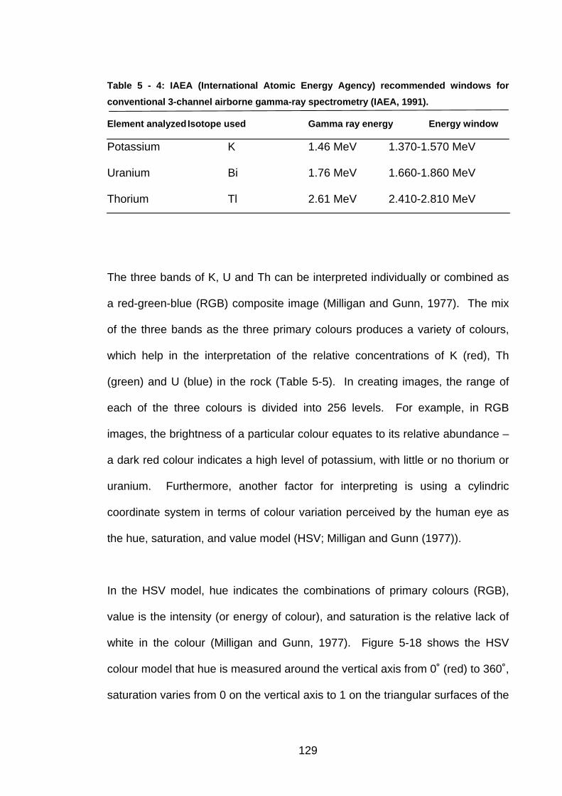
Table 5 - 4: IAEA (International Atomic Energy Agency) recommended windows for conventional 3-channel airborne gamma-ray spectrometry (IAEA, 1991).
Element analyzed Isotope used Gamma ray energy Energy window
Potassium K 1.46 MeV 1.370-1.570 MeV
Uranium Bi 1.76 MeV 1.660-1.860 MeV
Thorium Tl 2.61 MeV 2.410-2.810 MeV
The three bands of K, U and Th can be interpreted individually or combined as
a red-green-blue (RGB) composite image (Milligan and Gunn, 1977). The mix
of the three bands as the three primary colours produces a variety of colours,
which help in the interpretation of the relative concentrations of K (red), Th
(green) and U (blue) in the rock (Table 5-5). In creating images, the range of
each of the three colours is divided into 256 levels. For example, in RGB
images, the brightness of a particular colour equates to its relative abundance –
a dark red colour indicates a high level of potassium, with little or no thorium or
uranium. Furthermore, another factor for interpreting is using a cylindric
coordinate system in terms of colour variation perceived by the human eye as
the hue, saturation, and value model (HSV; Milligan and Gunn (1977)).
In the HSV model, hue indicates the combinations of primary colours (RGB),
value is the intensity (or energy of colour), and saturation is the relative lack of
white in the colour (Milligan and Gunn, 1977). Figure 5-18 shows the HSV
colour model that hue is measured around the vertical axis from 0˚ (red) to 360˚,
saturation varies from 0 on the vertical axis to 1 on the triangular surfaces of the
129

hexagonal, and value varies from 0 (black) through shades of grey along the
central axis to 1 (white) at the top. ( Milligan and Gunn, 1977).
Table 5 - 5: Interpretation of relative concentration of K. Th, and U in rocks based on the RGB image (Morgan, 1997).
K Th U Resultant colour
High Low Low Red
Low High Low Green
Low Low High Blue
High High Low Yellow
High Low High Purple
Low High High Light Blue
High High High White
An interpretation of gamma-ray data needs to incorporate many variables.
Besides the geometry and physical property contrasts of the radioactive source,
environmental effects can influence the interpretation of data. Environmental
factors include air temperature and pressure, soil moisture, non-radioactive
overburden, rainfall, vegetation and precipitation (Minty, 1997). Barren
overburden can reduce the radiation output from the Earth’s surface because of
its high density. In some areas, dense vegetation may shield the source of
radiation which would be equivalent to 50 m of air. The trunks of trees in dense
130
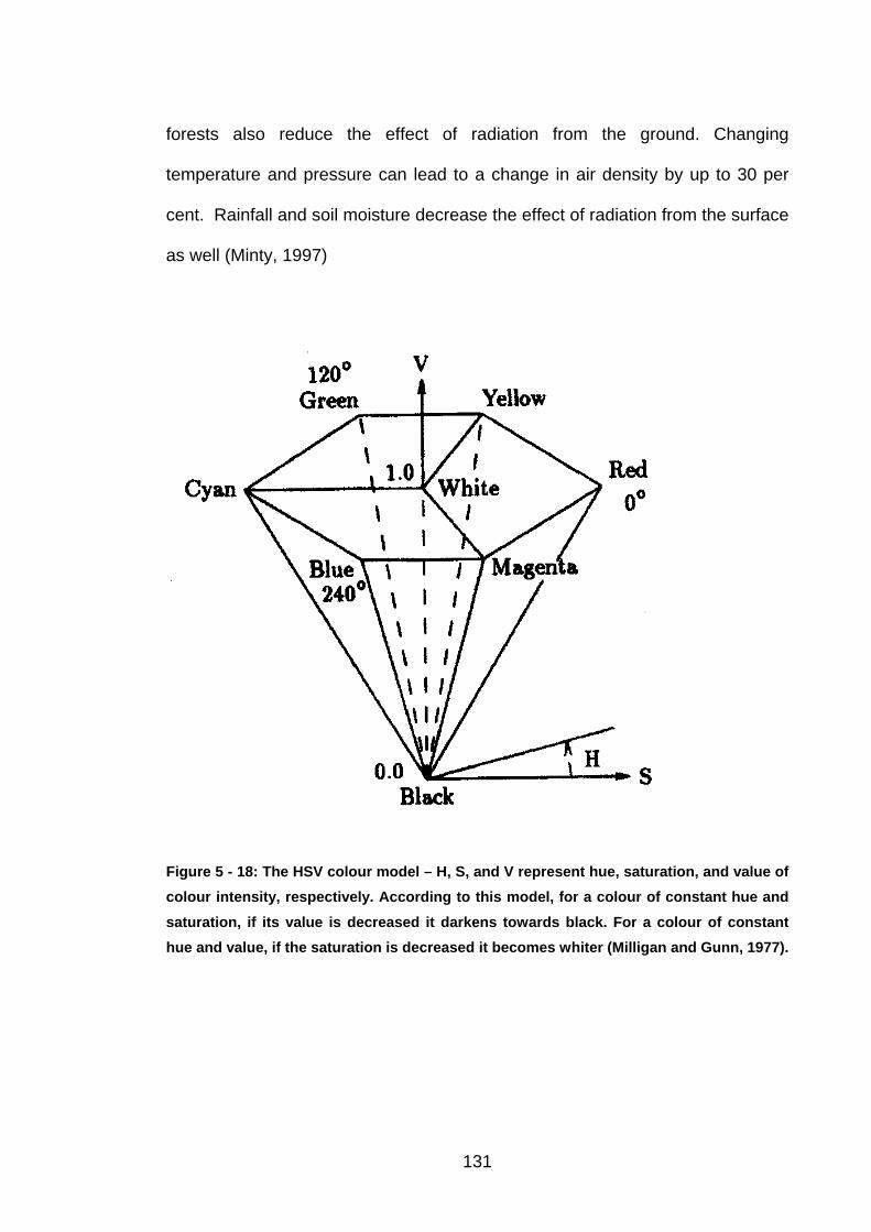
forests also reduce the effect of radiation from the ground. Changing
temperature and pressure can lead to a change in air density by up to 30 per
cent. Rainfall and soil moisture decrease the effect of radiation from the surface
as well (Minty, 1997)
Figure 5 - 18: The HSV colour model – H, S, and V represent hue, saturation, and value of colour intensity, respectively. According to this model, for a colour of constant hue and saturation, if its value is decreased it darkens towards black. For a colour of constant hue and value, if the saturation is decreased it becomes whiter (Milligan and Gunn, 1977).
131
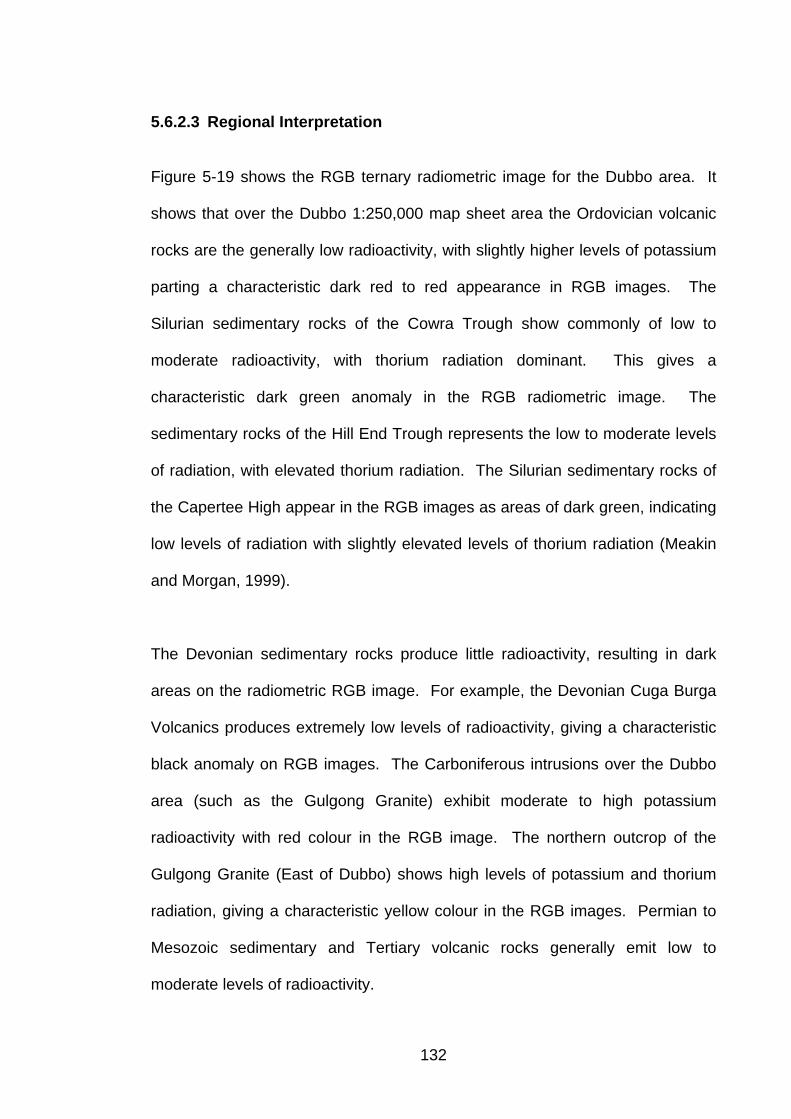
5.6.2.3 Regional Interpretation
Figure 5-19 shows the RGB ternary radiometric image for the Dubbo area. It
shows that over the Dubbo 1:250,000 map sheet area the Ordovician volcanic
rocks are the generally low radioactivity, with slightly higher levels of potassium
parting a characteristic dark red to red appearance in RGB images. The
Silurian sedimentary rocks of the Cowra Trough show commonly of low to
moderate radioactivity, with thorium radiation dominant. This gives a
characteristic dark green anomaly in the RGB radiometric image. The
sedimentary rocks of the Hill End Trough represents the low to moderate levels
of radiation, with elevated thorium radiation. The Silurian sedimentary rocks of
the Capertee High appear in the RGB images as areas of dark green, indicating
low levels of radiation with slightly elevated levels of thorium radiation (Meakin
and Morgan, 1999).
The Devonian sedimentary rocks produce little radioactivity, resulting in dark
areas on the radiometric RGB image. For example, the Devonian Cuga Burga
Volcanics produces extremely low levels of radioactivity, giving a characteristic
black anomaly on RGB images. The Carboniferous intrusions over the Dubbo
area (such as the Gulgong Granite) exhibit moderate to high potassium
radioactivity with red colour in the RGB image. The northern outcrop of the
Gulgong Granite (East of Dubbo) shows high levels of potassium and thorium
radiation, giving a characteristic yellow colour in the RGB images. Permian to
Mesozoic sedimentary and Tertiary volcanic rocks generally emit low to
moderate levels of radioactivity.
132

In the north-eastern part of Dubbo 1:250,000 map sheet, the basalts may be
mapped from the radiometric images but in the north-western part, the generally
lower radioactivity levels emitted by the Great Australian Basin (Surat Basin)
sedimentary rocks makes it more difficult to distinguish between the
sedimentary rocks and the basalts (Meakin and Morgan, 1999).
As Jaques et al. (1997) showed there are some associated intrusive bodies in
the south of Dubbo ( probably Mesozoic age) with the development of alteration
and rare-metal mineralisation such as Zr, Hf, Nb, Ta, light REE and Y. The
gamma-ray image shows that each intrusion has a different geochemical
signature. Some have dominant U+Th signatures, others dominant K+U or
K+Th, and some are high in all three elements (Figure 5-20).
133
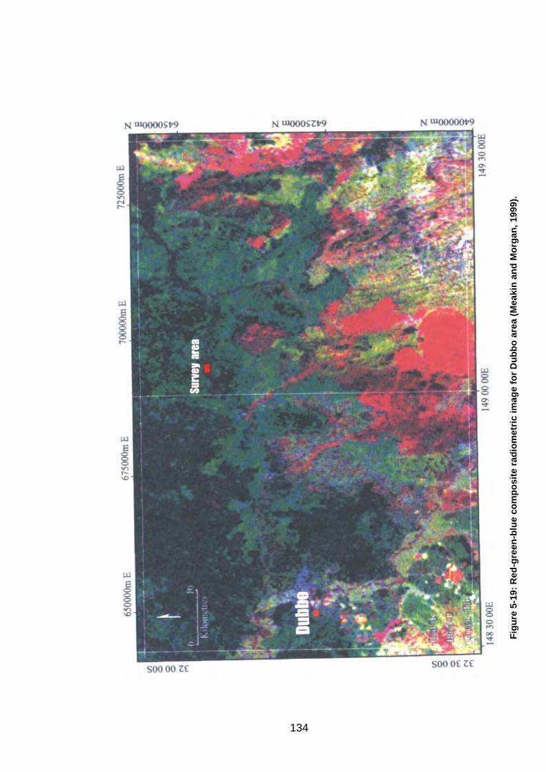
Figu
re 5
-19:
Red
-gre
en-b
lue
com
posi
te ra
diom
etric
imag
e fo
r Dub
bo a
rea
(Mea
kin
and
Mor
gan,
199
9).
134
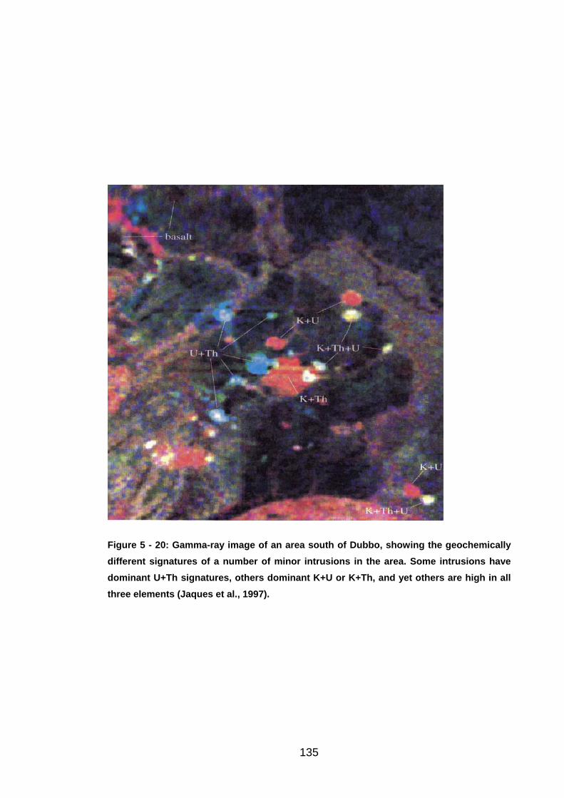
Figure 5 - 20: Gamma-ray image of an area south of Dubbo, showing the geochemically different signatures of a number of minor intrusions in the area. Some intrusions have dominant U+Th signatures, others dominant K+U or K+Th, and yet others are high in all three elements (Jaques et al., 1997).
135

5.6.3 Aeromagnetic Methods
5.6.3.1 Theory, Application
Magnetic surveys can be carried out in the air from helicopters or fixed wing
aircraft, because large areas can be covered in great detail and relatively
inexpensively. The operation is known as airborne magnetic surveying or
aeromagnetic surveying. Magnetic survey can also be carried out on the ground
for more detail. The instrument used to measure the magnetic field is called a
magnetometer.
Airborne magnetic surveys are used extensively to map regional geology in
areas of poor outcrop. The usual procedure is to record data continuously
along equally spaced parallel flight lines covering the survey area. In Australia,
airborne surveys are flown routinely at line spacings of 400-500 m and in areas
where greater detail is required, flight-line spacing is reduced to 200 m. For
regional mapping the flight line direction is usually oriented orthogonal to the
predominant strike of the geology. For more specific applications, such as
mineral exploration targets, the flight-line separation and direction will be
selected to maximise the magnetic signature (Horsfall, 1997).
Ferromagnetic minerals in the earth’s crust are the source of anomalous
magnetic field. The major magnetic minerals are magnetite, titanmagnetite,
titanhematite, maghemite, pyrrhotite and native iron. These minerals can show
magnetic anomalies, because of their abnormally large magnetic susceptibilities
or because they have high remnant magnetizations. Of the magnetic minerals
136

that are found in the nature, magnetite is the most abundant (Grant, 1984).
Igneous rocks have a higher content of magnetic minerals than sediments and
can be mapped in sedimentary basins from magnetic data (Gunn, 1997a).
The contrasting proportions of these minerals in different crustal rocks produce
the magnetic anomalies that are the targets of magnetometer surveying.
Airborne magnetic surveys measure the total magnetic field that includes
induced magnetism and remnant magnetism. Any rock containing magnetic
minerals may possess both induced and remanent magnetizations (Gunn and
Dentith, 1997).
When a material is placed in a magnetic field it may acquire a magnetization in
the direction of the field which is lost when the material is removed from the
field. This phenomenon is known as induced magnetization or magnetic
polarization. The inherited magnetization remaining after removal of the applied
field is known as remanent, or permanent, magnetization (Kearey and Brooks,
2001).
The magnetic field decreases approximately as the inverse of the square of the
distance from the magnetic source. Therefore to record small variations in the
field, surveys must be flown close to the ground. The survey attitude is usually
in the range 80-60 m. Surveys with 200 m line spacing are typically flown 80 m
above ground while surveys with 100 m line spacing may be flown at 60 m
above ground (Horsfall, 1997).
137

5.6.3.2 Interpretation Methodology
Rock magnetism results from the magnetic minerals they contain. Magnetic
minerals also belong to iron-titanium-oxygen solid solution series from
magnetite (FeO) to ulvospinel (FeTiO) or the iron-sulphur group pyrrhotite
(FeS). Magnetite can occur as either primary magmatic minerals or as
metamorphic minerals. Basic igneous rocks are usually highly magnetic due to
their relatively high magnetite content. In general magnetite concentrations
decrease with increasing acidity in magmatic rocks (Kearey and Brooks, 2001).
Magnetic anomalies range in amplitude from a few tens of nanoteslas over
deep metamorphic basement to several hundred nanoteslas over basic
intrusions and may reach an amplitude of several thousand nanoteslas over
magnetite ores. The magnetic field for typical magnetic bodies in the
subsurface decays rapidly away from its source (Kearey and Brooks, 2001). As
a result shallow bodies are subjected by high wavenumber components,
creating narrower relatively low amplitude anomalies, whereas deep bodies
produce broader, smoother anomalies (Schofield, 1998).
Ferromagnetic rocks or sediments show positive magnetic susceptibility
whereas diamagnetic rocks or sediments show negative magnetic susceptibility.
For example pure salt comprising hatite, gypsum and anhydrite, is diamagnetic
and it has a negative magnetic susceptibility and as a result represent a
negative magnetic contrast relative to surrounding sediments (Gunn, 1997b).
138

The aim of magnetic interpretation is to obtain geological information from
magnetic survey data (Gunn, 1997b). The results of magnetic survey are
usually presented as a map, or an image, of the magnetic anomalies. The
magnetic anomaly is the product of the susceptibility of the rock and the size of
the body or rock. A colour total magnetic intensity (TMI) image provides a
useful method for interpreting geological units and their structure. Boundaries
between different geological units are determined on the basis of their magnetic
response. Common causes of magnetic anomalies include dykes, faulted,
folded, magnetite ore bodies and metamorphic basement rocks (Kearey and
Brooks, 2001).
There are some environmental factors that can influence magnetic anomalies
include temperature and weathering. It is unusual to find magnetite in
unmetamorphosed sedimentary rocks except in very minor amounts. Magnetite
is unstable in the low-temperature, highly oxidizing environment of chemical
weathering and sedimentation. Four factors effect the chemical weathering and
sedimentation of iron covsist of chemical weathering, leaching, transportation
and compaction and early diagenesis (Grant, 1984). Figure 5-21 presented the
total magnetic intensity (TMI) image for the Dubbo region.
5.6.3.3 Regional Interpretation
Sedimentary rocks over the Dubbo area show low to medium magnetic
susceptibility, but contain indications of internal north-south structure. In the
western part of Dubbo, the Silurian sedimentary rocks in the Cowra Trough 139
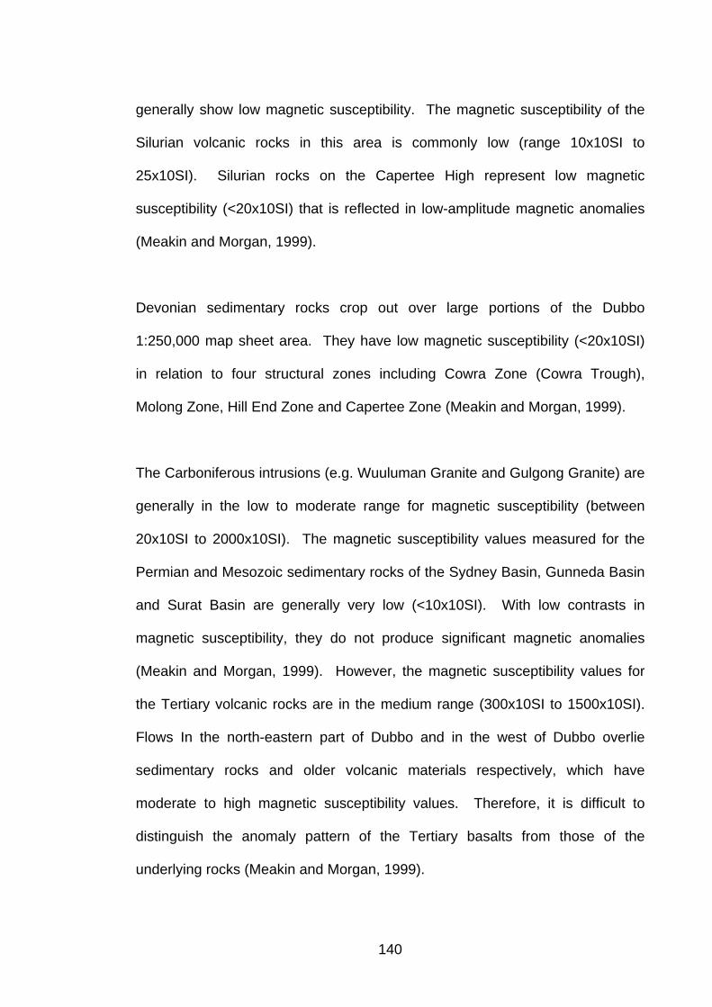
generally show low magnetic susceptibility. The magnetic susceptibility of the
Silurian volcanic rocks in this area is commonly low (range 10x10SI to
25x10SI). Silurian rocks on the Capertee High represent low magnetic
susceptibility (<20x10SI) that is reflected in low-amplitude magnetic anomalies
(Meakin and Morgan, 1999).
Devonian sedimentary rocks crop out over large portions of the Dubbo
1:250,000 map sheet area. They have low magnetic susceptibility (<20x10SI)
in relation to four structural zones including Cowra Zone (Cowra Trough),
Molong Zone, Hill End Zone and Capertee Zone (Meakin and Morgan, 1999).
The Carboniferous intrusions (e.g. Wuuluman Granite and Gulgong Granite) are
generally in the low to moderate range for magnetic susceptibility (between
20x10SI to 2000x10SI). The magnetic susceptibility values measured for the
Permian and Mesozoic sedimentary rocks of the Sydney Basin, Gunneda Basin
and Surat Basin are generally very low (<10x10SI). With low contrasts in
magnetic susceptibility, they do not produce significant magnetic anomalies
(Meakin and Morgan, 1999). However, the magnetic susceptibility values for
the Tertiary volcanic rocks are in the medium range (300x10SI to 1500x10SI).
Flows In the north-eastern part of Dubbo and in the west of Dubbo overlie
sedimentary rocks and older volcanic materials respectively, which have
moderate to high magnetic susceptibility values. Therefore, it is difficult to
distinguish the anomaly pattern of the Tertiary basalts from those of the
underlying rocks (Meakin and Morgan, 1999).
140
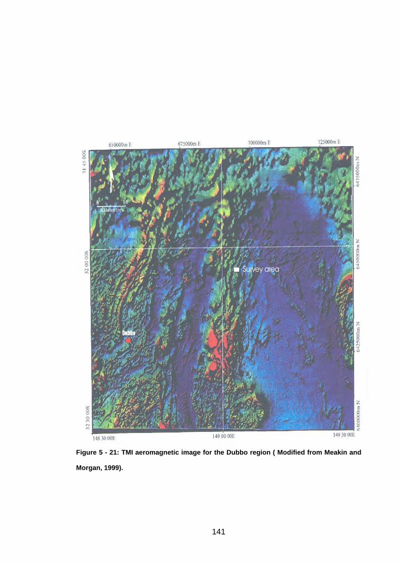
Survey area
Figure 5 - 21: TMI aeromagnetic image for the Dubbo region ( Modified from Meakin and
Morgan, 1999).
141
5.6.4 Gravity Methods
5.6.4.1 Theory, Application
Australian Geological Survey Organisation (AGSO) carried out numerous
traverses throughout the Dubbo and Ballimore region. The stations are on
average about 4 km apart. Figure 5-22 shows that the distribution of the
stations is not regular and accordingly parts of the area have dense coverage
while in others parts coverage is quite sparse. The gravity data are based on
the IGSN71 gravity datum and the ISOGAL84 scale.
Figure 5 - 22 Point located data for the Dubbo and Ballimore regions (Schofield, 1998).
142
Gravity surveying measures variations in the Earth’s gravitational field produced
by differences of density between subsurface rocks. The theory that explains
gravitational methods is based on Newton’s law. This law is expressing the
force of mutual attraction between two particles in terms of their masses and
separation. The force of attraction F between two masses m and m, that
dimensions are small with respect to the distance r between them, is given by
221
rmGmF =
where G is the Gravitational Constant.
The variation in gravity depends on lateral changes in the density of earth
materials in the vicinity of the measuring point (Dobrin and Savit, 1988). Gravity
method is a natural field method, which measure a bulk petrophysical property
such as density. Density depends on both composition and porosity. In
sedimentary rocks, porosity is the main cause of density variations and density
tends to increase with depth because of compaction, and with age due to
cementation. Igneous and metamorphic rocks have small porosity, and
composition is the main cause of density variation. In igneous rocks density
increase as acidity decreases.
Like radioactivity and magnetic methods, gravity is a natural source method in
which local variations in density of rocks near the surface cause small changes
in the main gravity field. Some applications of gravity surveying are in regional
geological studies, hydrocarbon exploration, geodesy, monitoring volcanoes
and archaeogeophysics (Kearey and Brooks, 2001). Gravity studies have
143

shown that the graben portions of the rift system correspond to narrow gravity
lows caused by low density sediments along the rift (Gunn, 1977a,Swain,
1992).
Gravity surveying can be particularly useful in the initial exploration of water
covered shelf areas, if there is no geological information (Dobrin and Savit,
1988). However gravity appears to have more limited applicability in mineral
exploration because of the good contrasts between the densities of base metal
sulphides and the host rocks. Some ores, like chromites, have a high density
compared with the material that surrounds them and gravity methods can be
used directly by detailed gravity surveys.
5.6.4.2 Interpretation Methodology
The geological interpretation of gravity data is more difficult and needs more
corrections (such as Bouguer, elevation, free air, hight correction, tide and drift
corrections) rather than magnetic methods. It is known that the gravity on the
Earth’s surface depends on five factors, latitude, elevation, topography of the
surrounding terrain, earth tides and variation in density in the subsurface.
Because of the variations in the density in the subsurface, the interpretation of
potential field anomalies for gravity data is inherently ambiguous (Kearey and
Brooks, 2001). One of the most difficult problems in gravity interpretation is the
separation of residual anomalies from the regional Bouguer gravity anomaly
(Mickus et al., 1991).
144
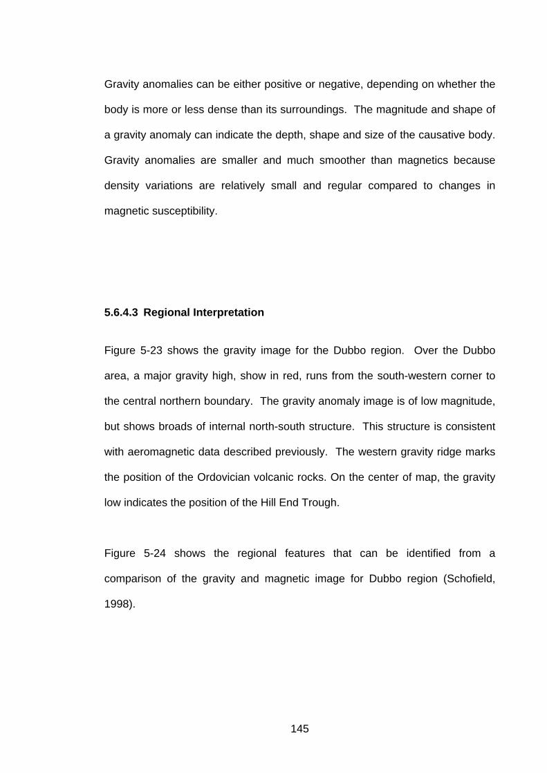
Gravity anomalies can be either positive or negative, depending on whether the
body is more or less dense than its surroundings. The magnitude and shape of
a gravity anomaly can indicate the depth, shape and size of the causative body.
Gravity anomalies are smaller and much smoother than magnetics because
density variations are relatively small and regular compared to changes in
magnetic susceptibility.
5.6.4.3 Regional Interpretation
Figure 5-23 shows the gravity image for the Dubbo region. Over the Dubbo
area, a major gravity high, show in red, runs from the south-western corner to
the central northern boundary. The gravity anomaly image is of low magnitude,
but shows broads of internal north-south structure. This structure is consistent
with aeromagnetic data described previously. The western gravity ridge marks
the position of the Ordovician volcanic rocks. On the center of map, the gravity
low indicates the position of the Hill End Trough.
Figure 5-24 shows the regional features that can be identified from a
comparison of the gravity and magnetic image for Dubbo region (Schofield,
1998).
145
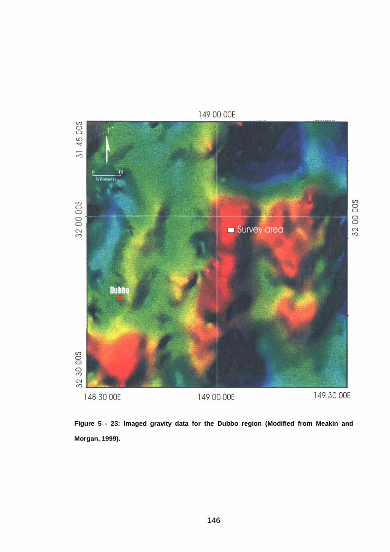
148 30 00E 149 00 00E 149 30 00E
32 0
0 00
S32
30
00S
31 4
5 00
S
149 00 00E
32 0
0 00
S
Survey area
Figure 5 - 23: Imaged gravity data for the Dubbo region (Modified from Meakin and
Morgan, 1999).
146
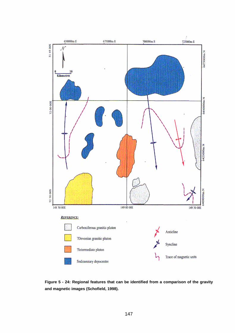
Figure 5 - 24: Regional features that can be identified from a comparison of the gravity and magnetic images (Schofield, 1998).
147
Chapter 6
Near-Surface Effect Corrections with the GRM
6.1 Summary
The determination of seismic velocities in the unweathered layer with shallow
seismic refraction methods is often an ill posed problem. Very small variations
in the parameters used to derive the seismic velocities in the refractor can result
in significant variations in the computed velocities. In many cases, where small
receiver spacings are employed to define very shallow targets, such as is
commonly the case with geotechnical investigations, the variations in the
computed time parameters are often as large as the errors in the traveltime data
(Palmer et al, 2005).
The standard methods for correcting for surface irregularities are usually not
practical where the very near surface irregularities are of limited lateral extent.
In such circumstances, the GRM smoothing statics method (SSM) is a simple
and robust approach, which can facilitate more accurate estimates of refractor
velocities (Palmer et al., 2005).
The Near-Surface Effect Corrections with the GRM generates a smoothing
“statics” correction by subtracting an average of the time-depths computed with
a range of XY values from the time-depths computed with a zero XY value
148
(where the XY value is the separation between the receivers used to compute
the time-depth). The time-depths to the deeper target refractors do not vary
greatly with varying XY values, and therefore an average is much the same as
the optimum value. However, the time-depths for the very near surface
irregularities migrate laterally with increasing XY values and they are
substantially reduced with the averaging process.
As a result, the time-depth profile averaged over a range of XY values is
effectively corrected for the near surface irregularities. Also, the time-depths
computed with a zero XY value are the sum of both the near surface effects and
the time-depths to the target refractor. Therefore, their subtraction generates
an approximate “statics” correction, which in turn, is subtracted from the
traveltimes.
6.2 Introduction
Variations in the topography and thickness of the near-surface soil layers can
have a major affect on traveltimes, because the very low seismic velocities,
often as low as 250 m/s, can result in large increases in traveltimes. These
layers can lead to significant problems with the detailed inversion of refraction
data, commonly as artefacts in the refractor velocities if no attempt is made to
recognize and remove their effects. As such, it is usually necessary to correct
for variations in the near surface, if a detailed model of the refractor is required
as a starting models for tomographic inversion.
149
With the traveltime data recorded at Spicers Creek, it was found that the
consistency between adjacent lines, which were only 10 m apart, was not
always immediately obvious, even though the traveltime data generated
excellent refraction tomograms. However, when the near surface effects were
satisfactorily accommodated, the consistency between adjacent lines was
improved considerably.
The near-surface corrections are adjustments to the original field seismic
refraction data, in order to remove the effects of varying topography or surface
velocities. As part of this study, a new method for correcting near-surface
effects based on the generalized reciprocal method (GRM, Palmer, 1980, 1986)
has been developed and has been applied to synthetic models as well as field
data. In general, the method, whilst being simple to implement, provides a
significantly more reliable measures of detailed refractor parameters.
6.3 Correcting for Near-Surface Effects
Most methods for correcting for near-surface effects attempt to model the near
surface irregularities and to calculate the traveltimes through these
irregularities. The corrections are usually computed with the first arrival
refraction data, if there is adequate coverage of these irregularities. The
standard methods of correcting for any near surface variations, using
traveltimes obtained with intermediate shot-to-receiver spacings is described in
Dobrin (1983, p. 334–336) and Palmer (1986, p.152–155). If these corrections
150
are not made, the determination of refractor velocities can be subject to
considerable ambiguity, especially where the detailed resolution of narrow
features, such as shear zones, is concerned.
However, where the irregularities do not extend over more than a few receiver
intervals, these deterministic methods cannot be employed, because there is
usually insufficient reversed traveltime data to define them accurately. In such
situations, an alternative approach is required.
The new method for correcting near-surface effects, which was developed as
part of this study, takes advantage of a unique feature of the GRM in which a
variable refraction migration distance, known as the XY distance, is employed.
Since the GRM time-depths computed with a range of XY values generally do
not exhibit large differences, the average of the time-depths for a range of XY
values is largely similar to that computed with the optimum XY value. However,
anomalies caused by surface irregularities propagate laterally throughout the
traveltimes and time-depths (Palmer, 1986, p.107-111). Therefore, when the
time-depths are averaged for a range of XY values, the time-depth anomalies
and hence the near-surface effects are averaged and reduced.
The average of these time-depths is then subtracted from the time-depths
computed with a zero XY. The result is generally a good estimate of the time-
depth anomalies caused by the near-surface variations. This difference is
subtracted from the traveltimes, thereby affecting a good correction for the near-
surface variations. This process can then be repeated on the updated
151
traveltimes iteratively until there is a significant improvement in the computed
seismic velocities in and the depth to the refractor.
The use of the GRM to remove near-surface effects from seismic refraction data
is shown in the following sections. The method is applied to various synthetic
models taken from Palmer (1980, pages 17-30) to illustrate its theoretical
performance over a range of near-surface variations. In some cases, the near
surface variations vary smoothly, while in other cases, the variations are large
and discontinuous. The first model consists of an irregular refractor with plane
topography whilst the second model introduces an irregular topography. The
method described has also been applied to the data acquired during the Spicers
Creek seismic refraction survey.
6.4 Model 1: Irregular Refractor with Flat Topography
The model shown in Figure 6-1 has a plane horizontal ground surface and a
highly irregular refractor with dips of approximately 18 degrees on the sloping
surfaces. The seismic velocity within the refractor changes laterally from 4000
to 5000 m/s at station 175, whilst the seismic velocity of the layers above the
refractor is constant at 1500 m/s. The first arrival traveltimes, shown in Figure
6-2, were obtained by wavefront construction. This method was used since it
conveniently accommodates dipping refractors, interfering head waves, and
diffractions (Palmer, 1974). Since the model has a plane horizontal topography,
there are no effects from variations in the near surface, thus no corrections
152
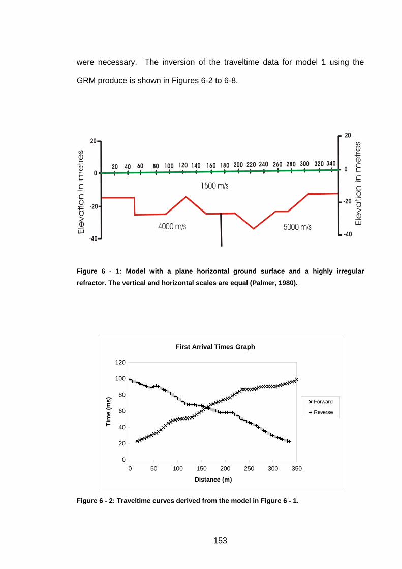
were necessary. The inversion of the traveltime data for model 1 using the
GRM produce is shown in Figures 6-2 to 6-8.
20 40 60 80 100 120 140 160 180 200 220 240 260 280 300 320 340
20
0
-40
-20
20
0
-20
-40
1500 m/s
4000 m/s 5000 m/s
Figure 6 - 1: Model with a plane horizontal ground surface and a highly irregular refractor. The vertical and horizontal scales are equal (Palmer, 1980).
First Arrival Times Graph
0
20
40
60
80
100
120
0 50 100 150 200 250 300 350
Distance (m)
Tim
e (m
s) Forward
Reverse
Figure 6 - 2: Traveltime curves derived from the model in Figure 6 - 1.
153
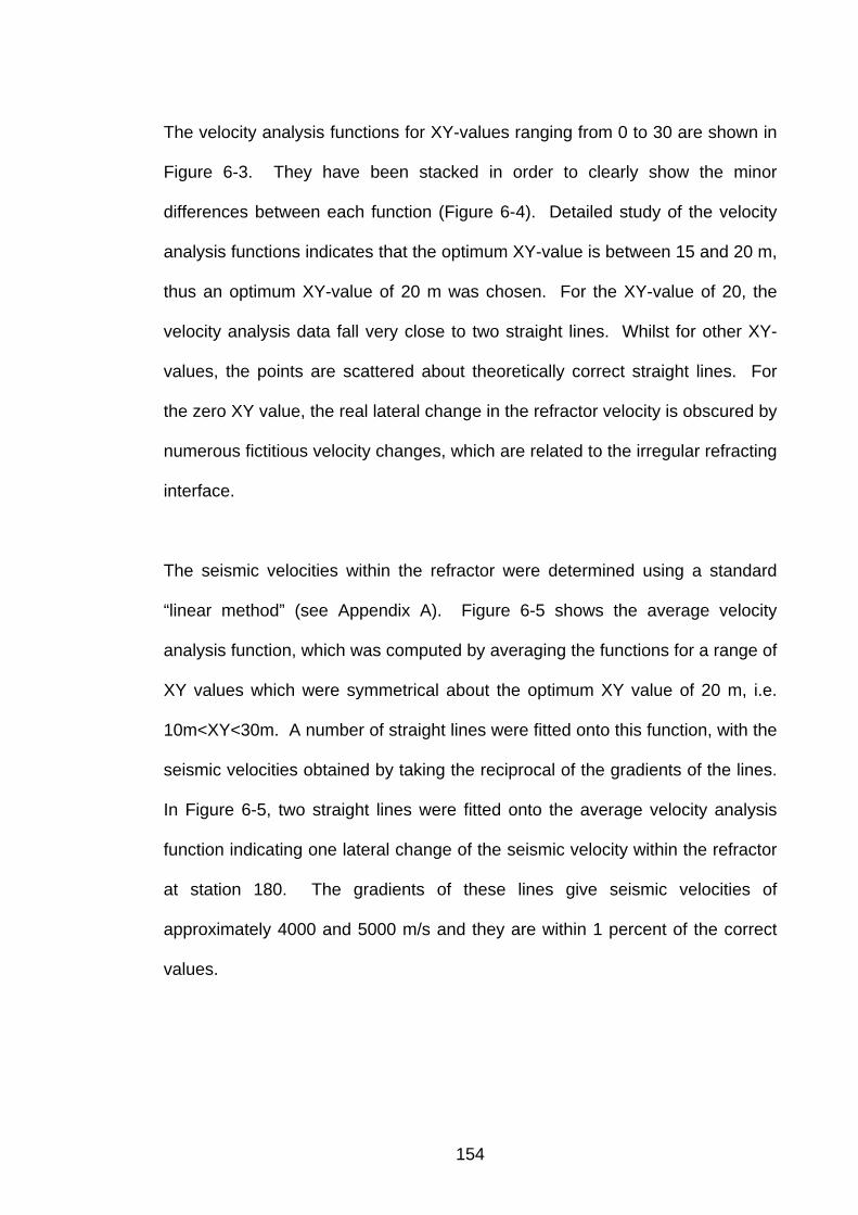
The velocity analysis functions for XY-values ranging from 0 to 30 are shown in
Figure 6-3. They have been stacked in order to clearly show the minor
differences between each function (Figure 6-4). Detailed study of the velocity
analysis functions indicates that the optimum XY-value is between 15 and 20 m,
thus an optimum XY-value of 20 m was chosen. For the XY-value of 20, the
velocity analysis data fall very close to two straight lines. Whilst for other XY-
values, the points are scattered about theoretically correct straight lines. For
the zero XY value, the real lateral change in the refractor velocity is obscured by
numerous fictitious velocity changes, which are related to the irregular refracting
interface.
The seismic velocities within the refractor were determined using a standard
“linear method” (see Appendix A). Figure 6-5 shows the average velocity
analysis function, which was computed by averaging the functions for a range of
XY values which were symmetrical about the optimum XY value of 20 m, i.e.
10m<XY<30m. A number of straight lines were fitted onto this function, with the
seismic velocities obtained by taking the reciprocal of the gradients of the lines.
In Figure 6-5, two straight lines were fitted onto the average velocity analysis
function indicating one lateral change of the seismic velocity within the refractor
at station 180. The gradients of these lines give seismic velocities of
approximately 4000 and 5000 m/s and they are within 1 percent of the correct
values.
154
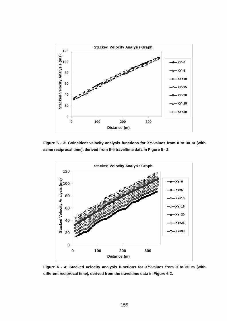
Stacked Velocity Analysis Graph
0
20
40
60
80
100
120
0 100 200 300
Distance (m)
Stac
ked
Velo
city
Ana
lysi
s (m
s)XY=0
XY=5
XY=10
XY=15
XY=20
XY=25
XY=30
Figure 6 - 3: Coincident velocity analysis functions for XY-values from 0 to 30 m (with same reciprocal time), derived from the traveltime data in Figure 6 - 2.
Stacked Velocity Analysis Graph
0
20
40
60
80
100
120
0 100 200 300Distance (m)
Stac
ked
Velo
city
Ana
lysi
s (m
s) XY=0
XY=5
XY=10
XY=15
XY=20
XY=25
XY=30
Figure 6 - 4: Stacked velocity analysis functions for XY-values from 0 to 30 m (with different reciprocal time), derived from the traveltime data in Figure 6-2.
155
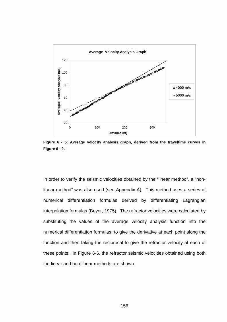
Average Velocity Analysis Graph
20
40
60
80
100
120
0 100 200 300
Distance (m)
Ave
rage
d V
eloc
ity A
naly
sis
(ms)
4000 m/s
5000 m/s
Figure 6 - 5: Average velocity analysis graph, derived from the traveltime curves in Figure 6 - 2.
In order to verify the seismic velocities obtained by the “linear method”, a “non-
linear method” was also used (see Appendix A). This method uses a series of
numerical differentiation formulas derived by differentiating Lagrangian
interpolation formulas (Beyer, 1975). The refractor velocities were calculated by
substituting the values of the average velocity analysis function into the
numerical differentiation formulas, to give the derivative at each point along the
function and then taking the reciprocal to give the refractor velocity at each of
these points. In Figure 6-6, the refractor seismic velocities obtained using both
the linear and non-linear methods are shown.
156
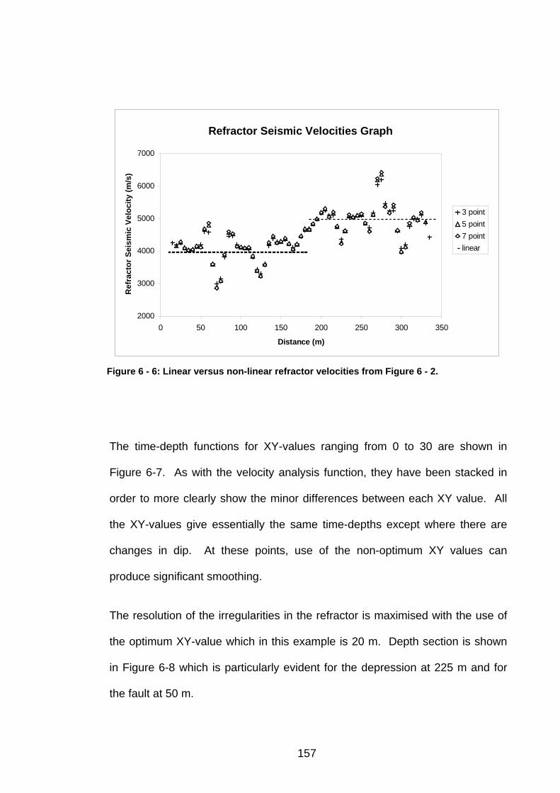
Refractor Seismic Velocities Graph
2000
3000
4000
5000
6000
7000
0 50 100 150 200 250 300 350
Distance (m)
Ref
ract
or S
eism
ic V
eloc
ity (m
/s)
3 point5 point7 pointlinear
Figure 6 - 6: Linear versus non-linear refractor velocities from Figure 6 - 2.
The time-depth functions for XY-values ranging from 0 to 30 are shown in
Figure 6-7. As with the velocity analysis function, they have been stacked in
order to more clearly show the minor differences between each XY value. All
the XY-values give essentially the same time-depths except where there are
changes in dip. At these points, use of the non-optimum XY values can
produce significant smoothing.
The resolution of the irregularities in the refractor is maximised with the use of
the optimum XY-value which in this example is 20 m. Depth section is shown
in Figure 6-8 which is particularly evident for the depression at 225 m and for
the fault at 50 m.
157
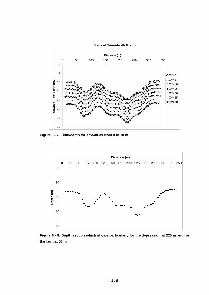
Stacked Time-depth Graph
0
5
10
15
20
25
30
35
0 50 100 150 200 250 300 350
Distance (m)St
acke
d Ti
me-
dept
h (m
s)
XY=0XY=5XY=10XY=15XY=20XY=25XY=30
Figure 6 - 7: Time-depth for XY-values from 0 to 30 m.
0
10
20
30
40
0 25 50 75 100 125 150 175 200 225 250 275 300 325 350
Distance (m)
Dep
th (m
)
Figure 6 - 8: Depth section which shows particularly for the depression at 225 m and for the fault at 50 m.
158
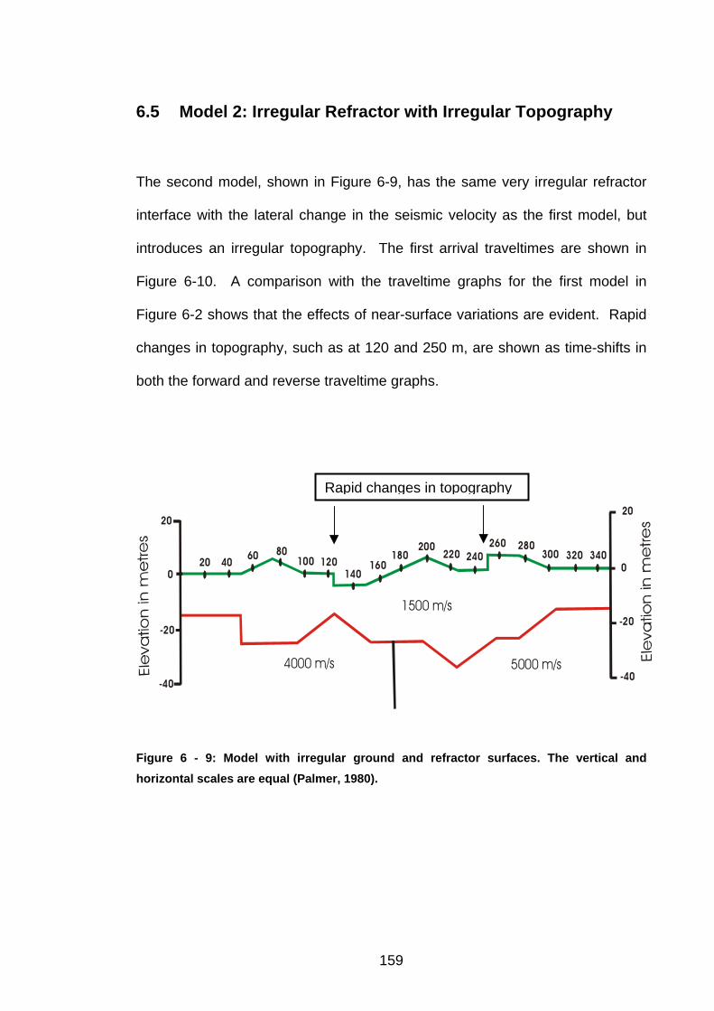
6.5 Model 2: Irregular Refractor with Irregular Topography
The second model, shown in Figure 6-9, has the same very irregular refractor
interface with the lateral change in the seismic velocity as the first model, but
introduces an irregular topography. The first arrival traveltimes are shown in
Figure 6-10. A comparison with the traveltime graphs for the first model in
Figure 6-2 shows that the effects of near-surface variations are evident. Rapid
changes in topography, such as at 120 and 250 m, are shown as time-shifts in
both the forward and reverse traveltime graphs.
20 4060 80
100 120140
160180
200220 240
260 280300 320 340
20
0
-40
-20
20
0
-20
-40
1500 m/s
4000 m/s 5000 m/s
Rapid changes in topography
Figure 6 - 9: Model with irregular ground and refractor surfaces. The vertical and horizontal scales are equal (Palmer, 1980).
159
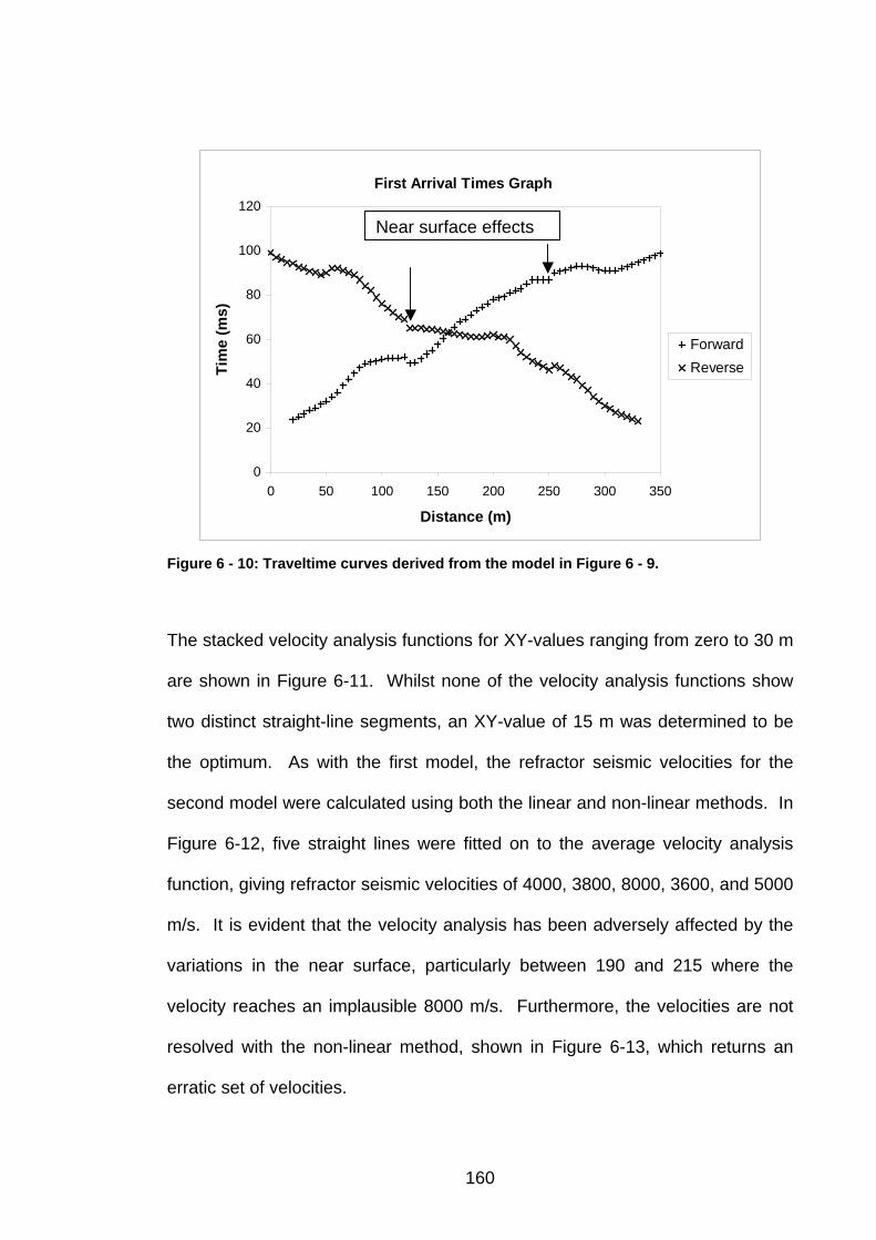
First Arrival Times Graph
0
20
40
60
80
100
120
0 50 100 150 200 250 300 350
Distance (m)
Tim
e (m
s)
ForwardReverse
Near surface effects
Figure 6 - 10: Traveltime curves derived from the model in Figure 6 - 9.
The stacked velocity analysis functions for XY-values ranging from zero to 30 m
are shown in Figure 6-11. Whilst none of the velocity analysis functions show
two distinct straight-line segments, an XY-value of 15 m was determined to be
the optimum. As with the first model, the refractor seismic velocities for the
second model were calculated using both the linear and non-linear methods. In
Figure 6-12, five straight lines were fitted on to the average velocity analysis
function, giving refractor seismic velocities of 4000, 3800, 8000, 3600, and 5000
m/s. It is evident that the velocity analysis has been adversely affected by the
variations in the near surface, particularly between 190 and 215 where the
velocity reaches an implausible 8000 m/s. Furthermore, the velocities are not
resolved with the non-linear method, shown in Figure 6-13, which returns an
erratic set of velocities.
160
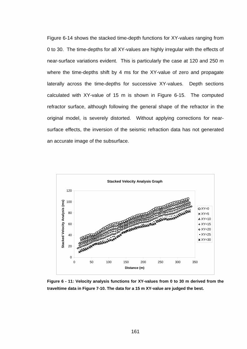
Figure 6-14 shows the stacked time-depth functions for XY-values ranging from
0 to 30. The time-depths for all XY-values are highly irregular with the effects of
near-surface variations evident. This is particularly the case at 120 and 250 m
where the time-depths shift by 4 ms for the XY-value of zero and propagate
laterally across the time-depths for successive XY-values. Depth sections
calculated with XY-value of 15 m is shown in Figure 6-15. The computed
refractor surface, although following the general shape of the refractor in the
original model, is severely distorted. Without applying corrections for near-
surface effects, the inversion of the seismic refraction data has not generated
an accurate image of the subsurface.
Stacked Velocity Analysis Graph
0
20
40
60
80
100
120
0 50 100 150 200 250 300 350
Distance (m)
Stac
ked
Velo
city
Ana
lysi
s (m
s)
XY=0XY=5XY=10XY=15XY=20XY=25XY=30
Figure 6 - 11: Velocity analysis functions for XY-values from 0 to 30 m derived from the traveltime data in Figure 7-10. The data for a 15 m XY-value are judged the best.
161
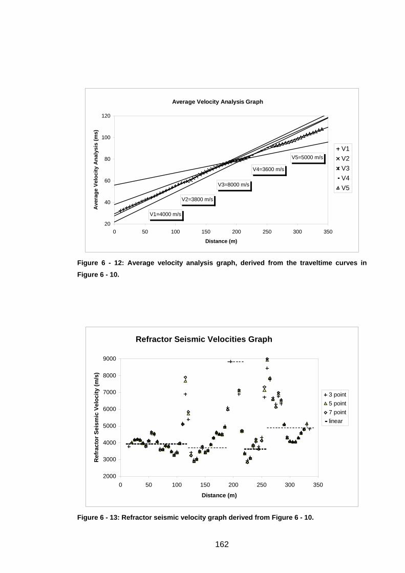
Average Velocity Analysis Graph
V1=4000 m/s
V2=3800 m/s
V3=8000 m/s
V4=3600 m/s
V5=5000 m/s
20
40
60
80
100
120
0 50 100 150 200 250 300 350
Distance (m)
Ave
rage
Vel
ocity
Ana
lysi
s (m
s)
V1V2V3V4V5
Figure 6 - 12: Average velocity analysis graph, derived from the traveltime curves in Figure 6 - 10.
Refractor Seismic Velocities Graph
2000
3000
4000
5000
6000
7000
8000
9000
0 50 100 150 200 250 300 350
Distance (m)
Ref
ract
or S
eism
ic V
eloc
ity (m
/s)
3 point5 point7 pointlinear
Figure 6 - 13: Refractor seismic velocity graph derived from Figure 6 - 10.
162
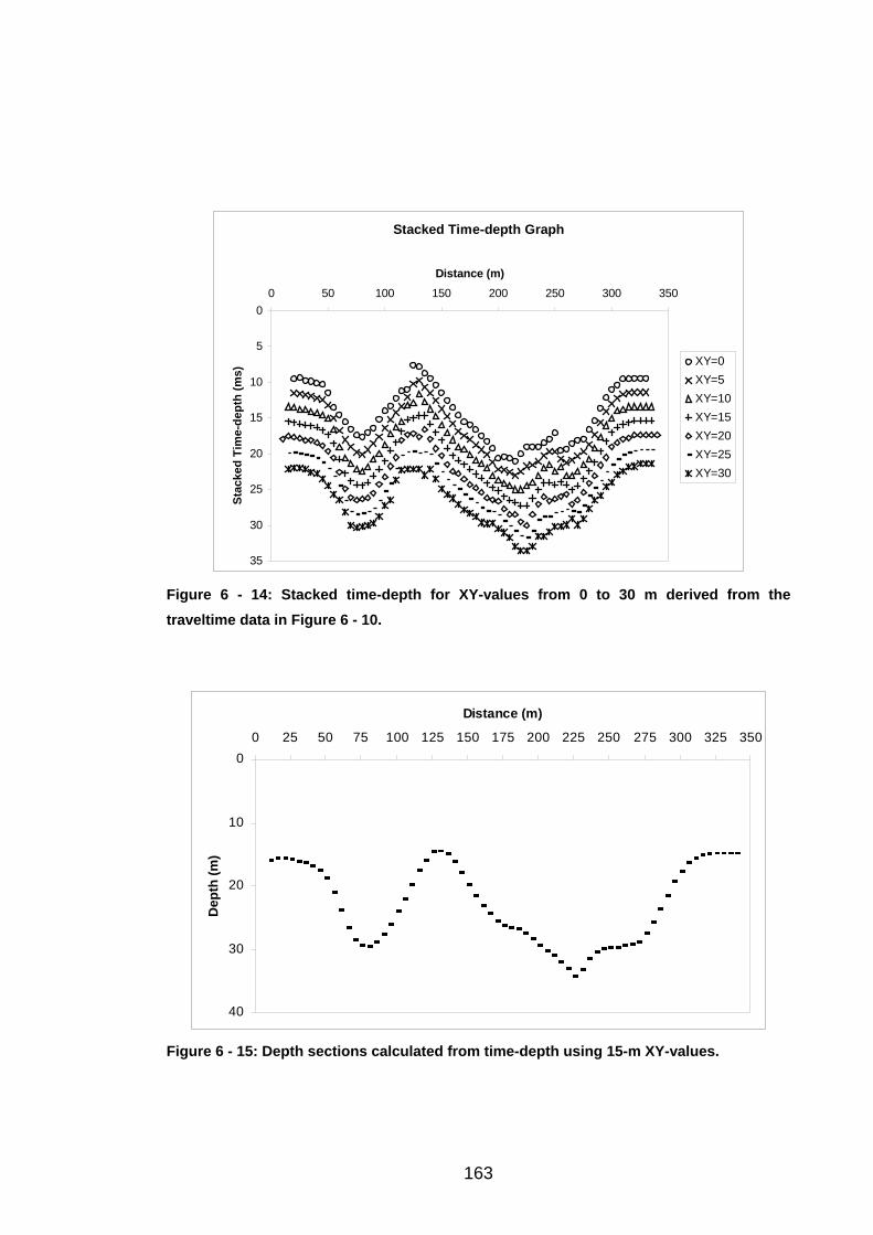
Stacked Time-depth Graph
0
5
10
15
20
25
30
35
0 50 100 150 200 250 300 350
Distance (m)
Stac
ked
Tim
e-de
pth
(ms)
XY=0XY=5XY=10XY=15XY=20XY=25XY=30
Figure 6 - 14: Stacked time-depth for XY-values from 0 to 30 m derived from the traveltime data in Figure 6 - 10.
0
10
20
30
40
0 25 50 75 100 125 150 175 200 225 250 275 300 325 350
Distance (m)
Dep
th (m
)
Figure 6 - 15: Depth sections calculated from time-depth using 15-m XY-values.
163
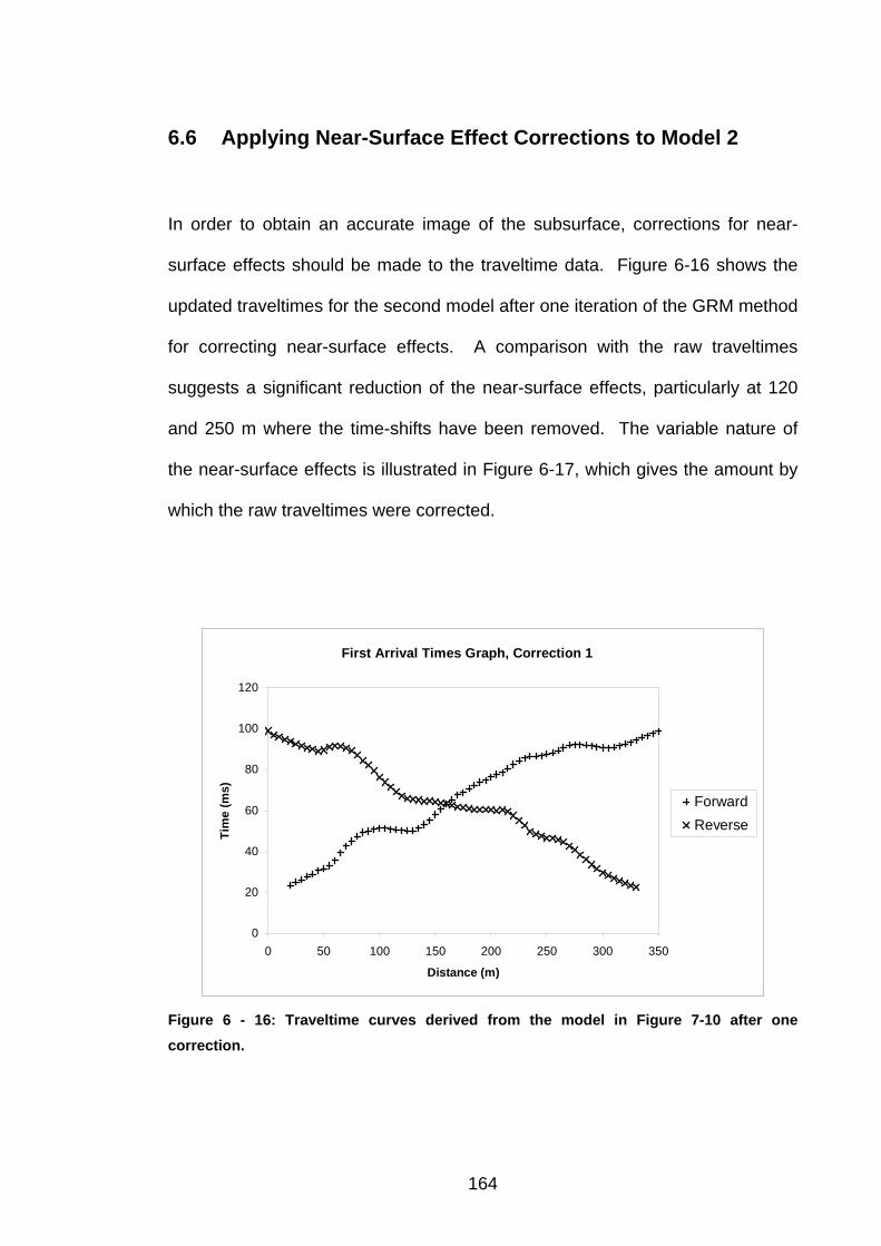
6.6 Applying Near-Surface Effect Corrections to Model 2
In order to obtain an accurate image of the subsurface, corrections for near-
surface effects should be made to the traveltime data. Figure 6-16 shows the
updated traveltimes for the second model after one iteration of the GRM method
for correcting near-surface effects. A comparison with the raw traveltimes
suggests a significant reduction of the near-surface effects, particularly at 120
and 250 m where the time-shifts have been removed. The variable nature of
the near-surface effects is illustrated in Figure 6-17, which gives the amount by
which the raw traveltimes were corrected.
First Arrival Times Graph, Correction 1
0
20
40
60
80
100
120
0 50 100 150 200 250 300 350
Distance (m)
Tim
e (m
s)
ForwardReverse
Figure 6 - 16: Traveltime curves derived from the model in Figure 7-10 after one correction.
164
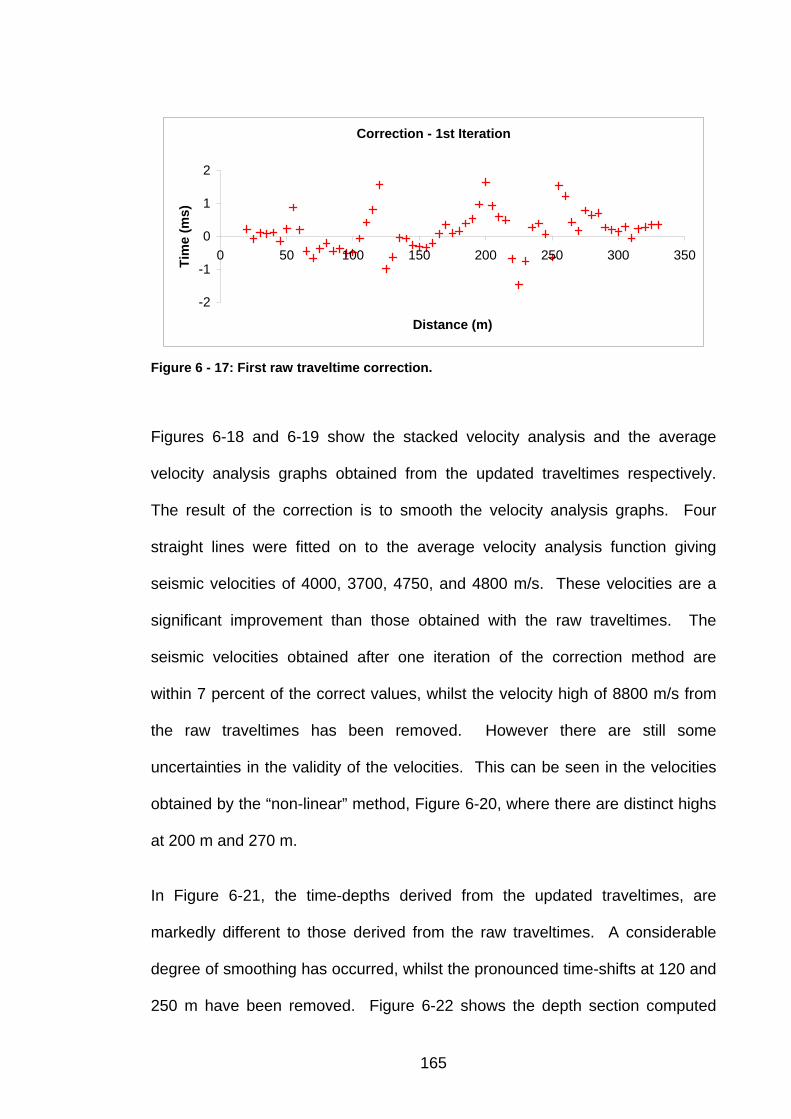
Correction - 1st Iteration
-2
-1
0
1
2
0 50 100 150 200 250 300 350
Distance (m)
Tim
e (m
s)
Figure 6 - 17: First raw traveltime correction.
Figures 6-18 and 6-19 show the stacked velocity analysis and the average
velocity analysis graphs obtained from the updated traveltimes respectively.
The result of the correction is to smooth the velocity analysis graphs. Four
straight lines were fitted on to the average velocity analysis function giving
seismic velocities of 4000, 3700, 4750, and 4800 m/s. These velocities are a
significant improvement than those obtained with the raw traveltimes. The
seismic velocities obtained after one iteration of the correction method are
within 7 percent of the correct values, whilst the velocity high of 8800 m/s from
the raw traveltimes has been removed. However there are still some
uncertainties in the validity of the velocities. This can be seen in the velocities
obtained by the “non-linear” method, Figure 6-20, where there are distinct highs
at 200 m and 270 m.
In Figure 6-21, the time-depths derived from the updated traveltimes, are
markedly different to those derived from the raw traveltimes. A considerable
degree of smoothing has occurred, whilst the pronounced time-shifts at 120 and
250 m have been removed. Figure 6-22 shows the depth section computed
165
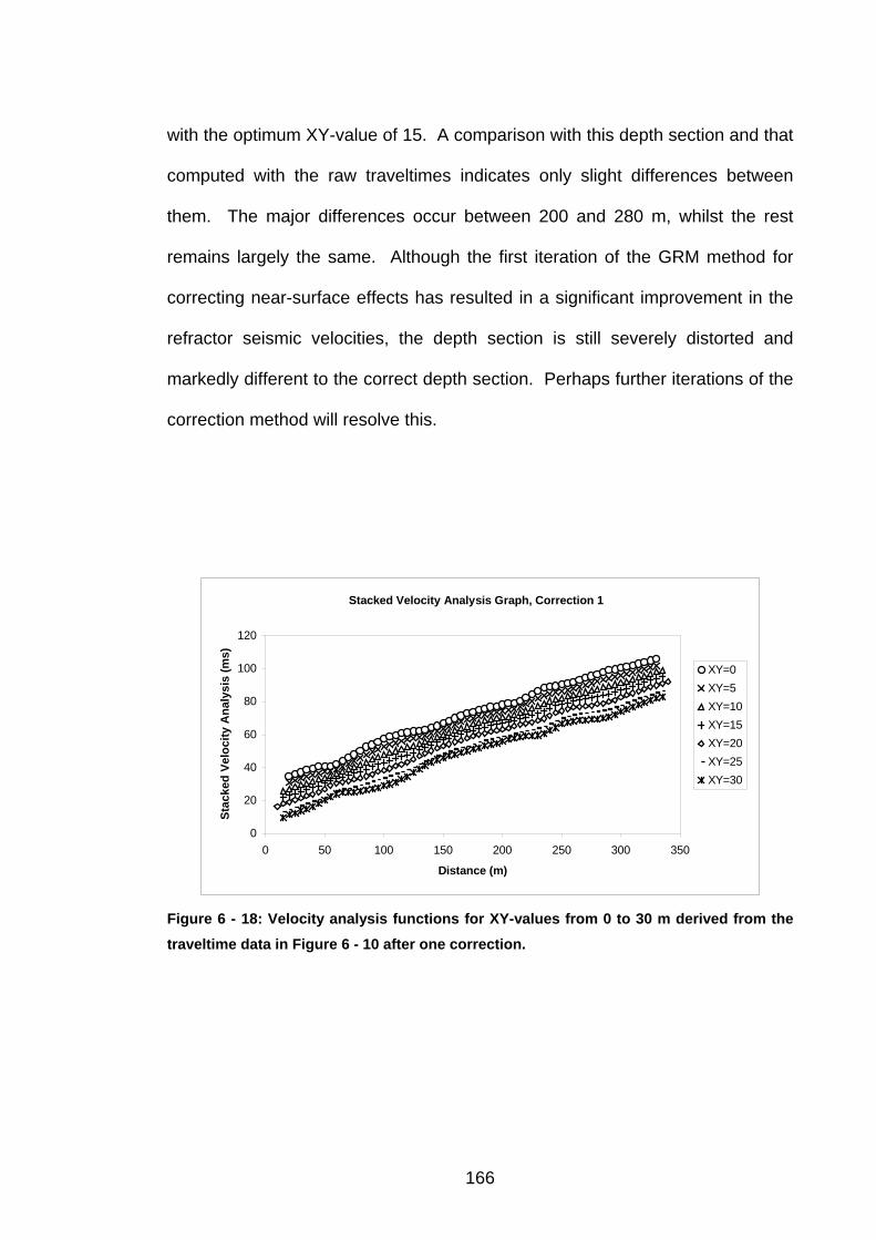
with the optimum XY-value of 15. A comparison with this depth section and that
computed with the raw traveltimes indicates only slight differences between
them. The major differences occur between 200 and 280 m, whilst the rest
remains largely the same. Although the first iteration of the GRM method for
correcting near-surface effects has resulted in a significant improvement in the
refractor seismic velocities, the depth section is still severely distorted and
markedly different to the correct depth section. Perhaps further iterations of the
correction method will resolve this.
Stacked Velocity Analysis Graph, Correction 1
0
20
40
60
80
100
120
0 50 100 150 200 250 300 350
Distance (m)
Stac
ked
Velo
city
Ana
lysi
s (m
s)
XY=0XY=5XY=10XY=15XY=20XY=25XY=30
Figure 6 - 18: Velocity analysis functions for XY-values from 0 to 30 m derived from the traveltime data in Figure 6 - 10 after one correction.
166
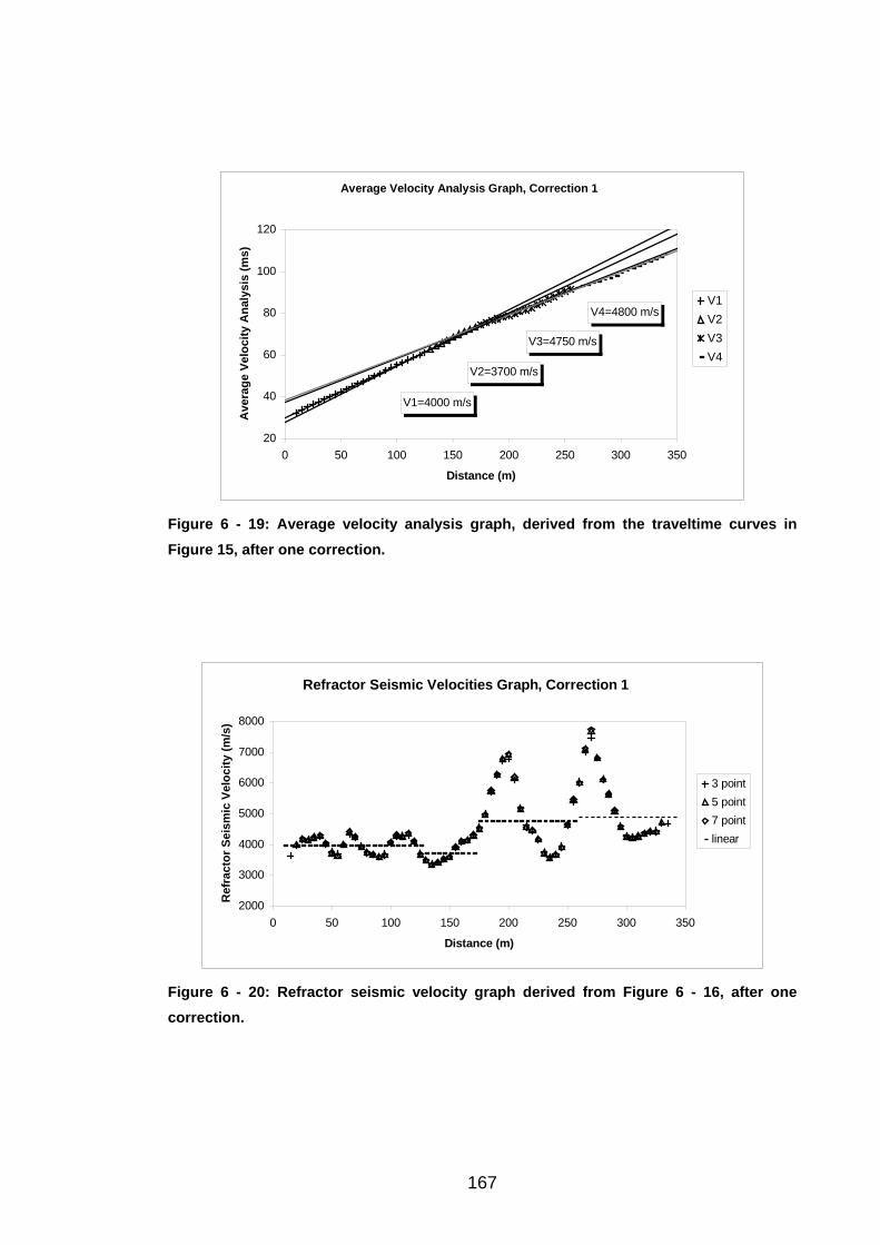
Average Velocity Analysis Graph, Correction 1
V2=3700 m/s
V3=4750 m/s
V4=4800 m/s
V1=4000 m/s
20
40
60
80
100
120
0 50 100 150 200 250 300 350
Distance (m)
Ave
rage
Vel
ocity
Ana
lysi
s (m
s)
V1V2V3V4
Figure 6 - 19: Average velocity analysis graph, derived from the traveltime curves in Figure 15, after one correction.
Refractor Seismic Velocities Graph, Correction 1
2000
3000
4000
5000
6000
7000
8000
0 50 100 150 200 250 300 350
Distance (m)
Ref
ract
or S
eism
ic V
eloc
ity (m
/s)
3 point5 point7 pointlinear
Figure 6 - 20: Refractor seismic velocity graph derived from Figure 6 - 16, after one correction.
167
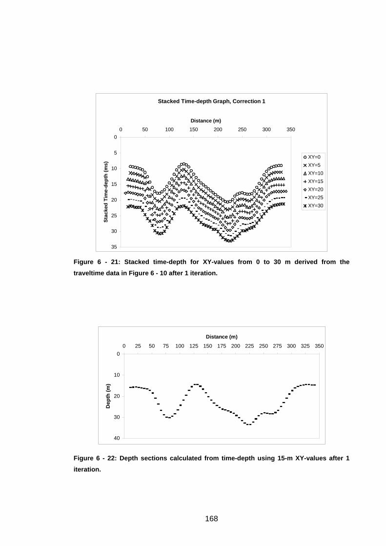
Stacked Time-depth Graph, Correction 1
0
5
10
15
20
25
30
35
0 50 100 150 200 250 300 350
Distance (m)
Stac
ked
Tim
e-de
pth
(ms)
XY=0XY=5XY=10XY=15XY=20XY=25XY=30
Figure 6 - 21: Stacked time-depth for XY-values from 0 to 30 m derived from the traveltime data in Figure 6 - 10 after 1 iteration.
0
10
20
30
40
0 25 50 75 100 125 150 175 200 225 250 275 300 325 350
Distance (m)
Dep
th (m
)
Figure 6 - 22: Depth sections calculated from time-depth using 15-m XY-values after 1 iteration.
168
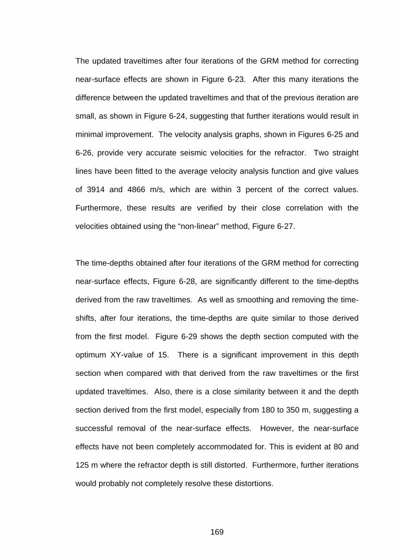
The updated traveltimes after four iterations of the GRM method for correcting
near-surface effects are shown in Figure 6-23. After this many iterations the
difference between the updated traveltimes and that of the previous iteration are
small, as shown in Figure 6-24, suggesting that further iterations would result in
minimal improvement. The velocity analysis graphs, shown in Figures 6-25 and
6-26, provide very accurate seismic velocities for the refractor. Two straight
lines have been fitted to the average velocity analysis function and give values
of 3914 and 4866 m/s, which are within 3 percent of the correct values.
Furthermore, these results are verified by their close correlation with the
velocities obtained using the “non-linear” method, Figure 6-27.
The time-depths obtained after four iterations of the GRM method for correcting
near-surface effects, Figure 6-28, are significantly different to the time-depths
derived from the raw traveltimes. As well as smoothing and removing the time-
shifts, after four iterations, the time-depths are quite similar to those derived
from the first model. Figure 6-29 shows the depth section computed with the
optimum XY-value of 15. There is a significant improvement in this depth
section when compared with that derived from the raw traveltimes or the first
updated traveltimes. Also, there is a close similarity between it and the depth
section derived from the first model, especially from 180 to 350 m, suggesting a
successful removal of the near-surface effects. However, the near-surface
effects have not been completely accommodated for. This is evident at 80 and
125 m where the refractor depth is still distorted. Furthermore, further iterations
would probably not completely resolve these distortions.
169
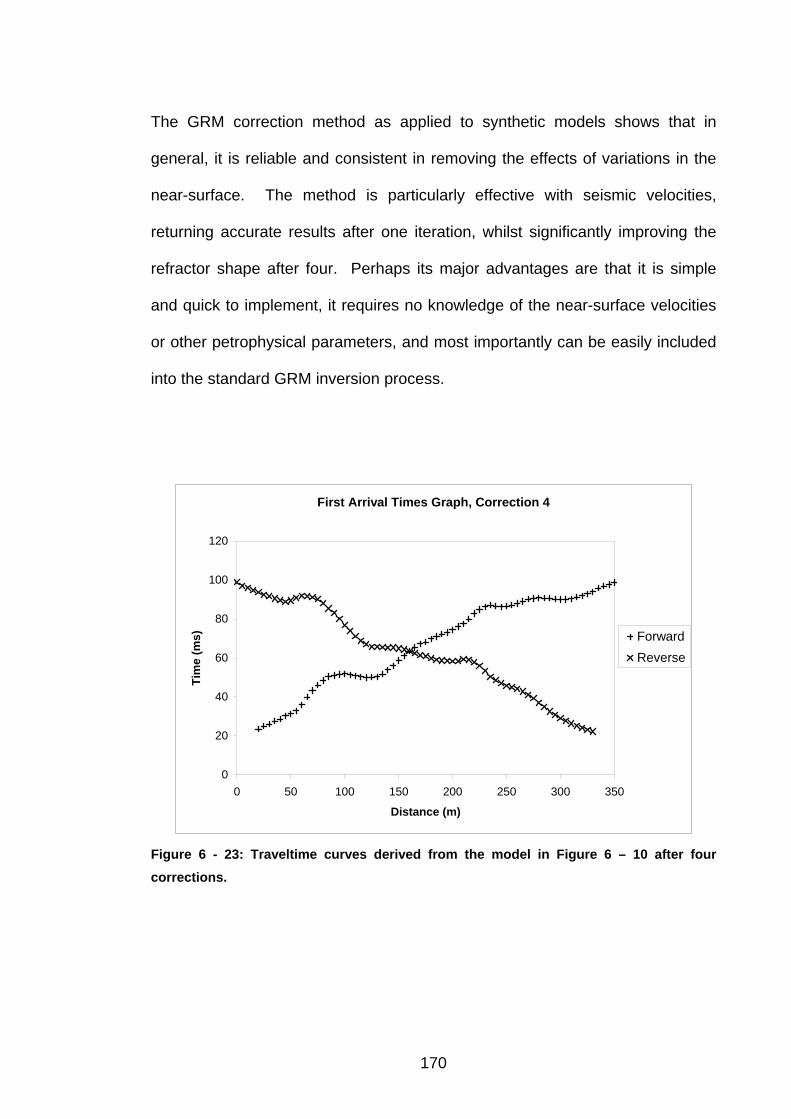
The GRM correction method as applied to synthetic models shows that in
general, it is reliable and consistent in removing the effects of variations in the
near-surface. The method is particularly effective with seismic velocities,
returning accurate results after one iteration, whilst significantly improving the
refractor shape after four. Perhaps its major advantages are that it is simple
and quick to implement, it requires no knowledge of the near-surface velocities
or other petrophysical parameters, and most importantly can be easily included
into the standard GRM inversion process.
First Arrival Times Graph, Correction 4
0
20
40
60
80
100
120
0 50 100 150 200 250 300 350
Distance (m)
Tim
e (m
s) ForwardReverse
Figure 6 - 23: Traveltime curves derived from the model in Figure 6 – 10 after four corrections.
170
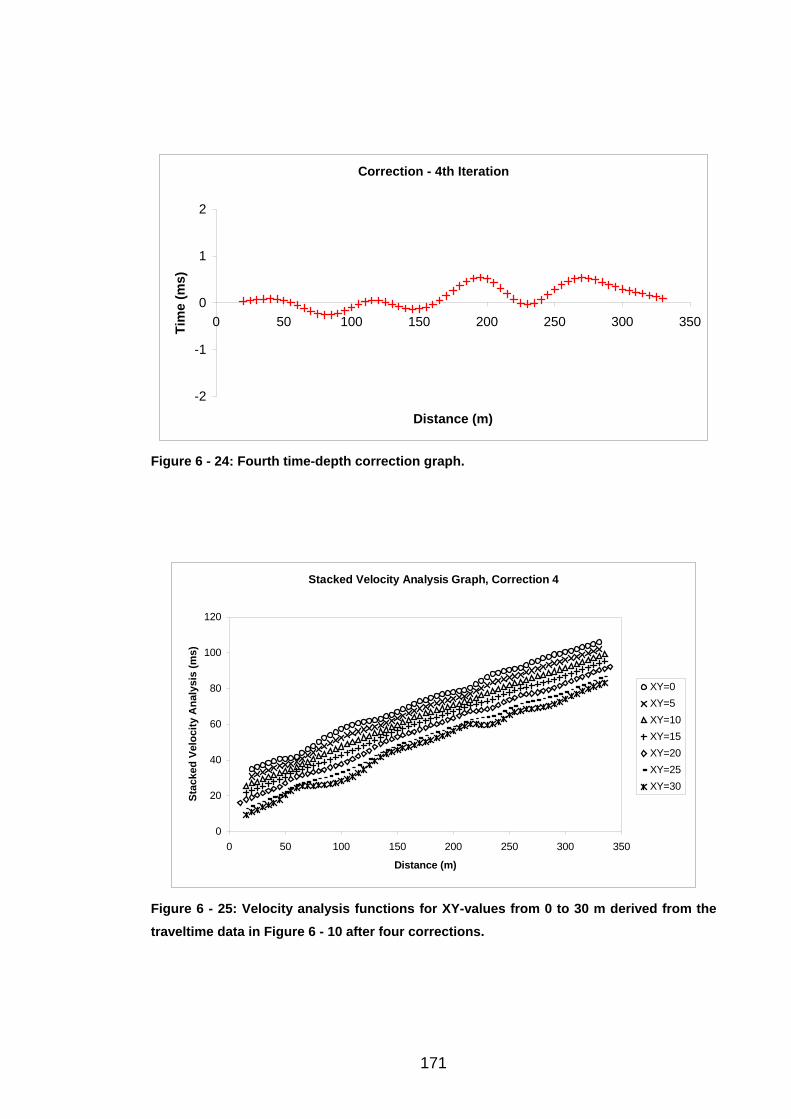
Correction - 4th Iteration
-2
-1
0
1
2
0 50 100 150 200 250 300 350
Distance (m)
Tim
e (m
s)
Figure 6 - 24: Fourth time-depth correction graph.
Stacked Velocity Analysis Graph, Correction 4
0
20
40
60
80
100
120
0 50 100 150 200 250 300 350
Distance (m)
Stac
ked
Velo
city
Ana
lysi
s (m
s)
XY=0XY=5XY=10XY=15XY=20XY=25XY=30
Figure 6 - 25: Velocity analysis functions for XY-values from 0 to 30 m derived from the traveltime data in Figure 6 - 10 after four corrections.
171
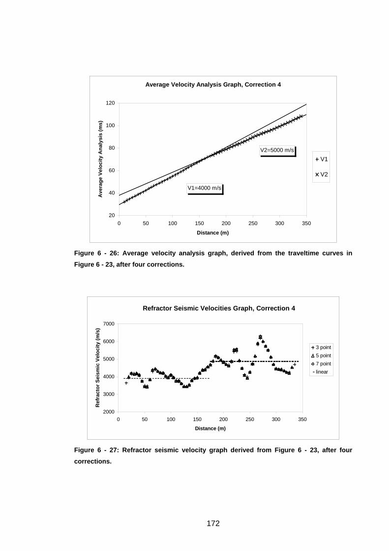
Average Velocity Analysis Graph, Correction 4
V2=5000 m/s
V1=4000 m/s
20
40
60
80
100
120
0 50 100 150 200 250 300 350
Distance (m)
Ave
rage
Vel
ocity
Ana
lysi
s (m
s)
V1
V2
Figure 6 - 26: Average velocity analysis graph, derived from the traveltime curves in Figure 6 - 23, after four corrections.
Refractor Seismic Velocities Graph, Correction 4
2000
3000
4000
5000
6000
7000
0 50 100 150 200 250 300 350
Distance (m)
Ref
ract
or S
eism
ic V
eloc
ity (m
/s)
3 point5 point7 pointlinear
Figure 6 - 27: Refractor seismic velocity graph derived from Figure 6 - 23, after four corrections.
172
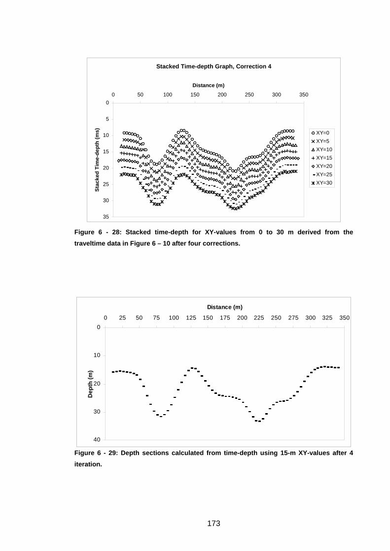
Stacked Time-depth Graph, Correction 4
0
5
10
15
20
25
30
35
0 50 100 150 200 250 300 350
Distance (m)
Stac
ked
Tim
e-de
pth
(ms) XY=0
XY=5XY=10XY=15XY=20XY=25XY=30
Figure 6 - 28: Stacked time-depth for XY-values from 0 to 30 m derived from the traveltime data in Figure 6 – 10 after four corrections.
0
10
20
30
40
0 25 50 75 100 125 150 175 200 225 250 275 300 325 350
Distance (m)
Dep
th (m
)
Figure 6 - 29: Depth sections calculated from time-depth using 15-m XY-values after 4 iteration.
173
Chapter 7
Methodology and Data Acquisition
7.1 Summary
Three-dimensional (3D) three-component (3C) shallow seismic refraction
surveys were recorded over a shear zone at two sites associated with dryland
salinity in the study area. The seismic data were recorded with the Australian
National Seismic Imaging Resources (ANSIR) 360-trace ARAM-24 seismic
system and IVI MiniVibrator. Survey geometry consisted of four parallel
receiver lines 10 m apart, set orthogonal to the inferred shear zone. Each line
consisted of 29 three-component geophones at 5 m intervals. 532 shots were
recorded during the two surveys resulting in around 1.5GB of data.
7.2 Introduction
The fieldwork was carried out at two sites in the Spicers Creek Catchment from
the 6th to the 12th of April 2003, using 360 trace ARAM24 seismic system and
IVI Minivib seismic energy source operated by Australian National Seismic
Imaging Resource (ANSIR). ANSIR is operated jointly by the Australian
Geological Survey Organisation (AGSO) and the Australian National University.
174
The Minivib can be conFigured in the field to generate P- and S-waves (see
Appendix B for an Operations Reports).
The field crew consisted of personnel from Geoscience Australia, including the
party manager, vibrator operator and geophone engineer, the observer from
Trace Energy Service, and field hands from UNSW.
The survey at site 2 was conducted first. The majority of the first day was spent
setting out the geophone spread and testing the system. Recording started on
the afternoon of the first day and continued for another two and a half days.
Recording at site 2 was completed on the morning of the fourth day. The
spread was retrieved and then re-deployed at site 1. Recording at site 1
commenced in the afternoon of the fourth day and continued till the end of the
sixth day, after which the spread was retrieved.
7.3 Equipment
The equipment listed below were used for recording data during the field
procedure
1) ARAM24 seismic recording system consisting of 360 channels.
2) IVI Minivib T-15000
3) 120 three component geophones GS-20DM (natural frequency, 14 HZ).
4) Dynamites (Dyno Nobel HDP 150).
175
5) Dynamite firing system (Shot Pro).
6) Cables for 5 m station separation.
7) Remote Acquisition Module (RAM) and batteries.
8) Plastic pin markers.
9) GPS (Gamin’s GPS 12 personal navigator).
10) Auger for digging shallow hole.
Appendix C shows the detail of specifications for the equipment.
7.3.1 ARAM24 Seismic Recording System
The seismic recorder was a 360-channel ARAM24 system manufactured by
Geo-X systems. The ARAM24 is a telemetry seismic recording system, which
is capable of 3D acquisition. It consists of a Central Recording Unit (CRU) from
which the system operated. The CRU is capable of data QC, vibroseis
correlation. The system was mounted in a purpose-built truck. The truck
served as mobile processing station. It contained the equipment shown in
photo 7-1 that includes from left to right: printer, ARAM24 processor, and
monitor for displaying data.
176
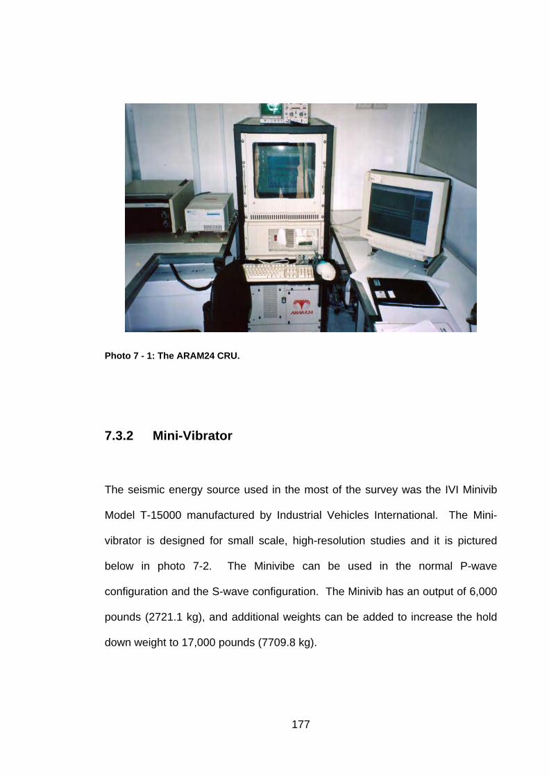
Photo 7 - 1: The ARAM24 CRU.
7.3.2 Mini-Vibrator
The seismic energy source used in the most of the survey was the IVI Minivib
Model T-15000 manufactured by Industrial Vehicles International. The Mini-
vibrator is designed for small scale, high-resolution studies and it is pictured
below in photo 7-2. The Minivibe can be used in the normal P-wave
configuration and the S-wave configuration. The Minivib has an output of 6,000
pounds (2721.1 kg), and additional weights can be added to increase the hold
down weight to 17,000 pounds (7709.8 kg).
177
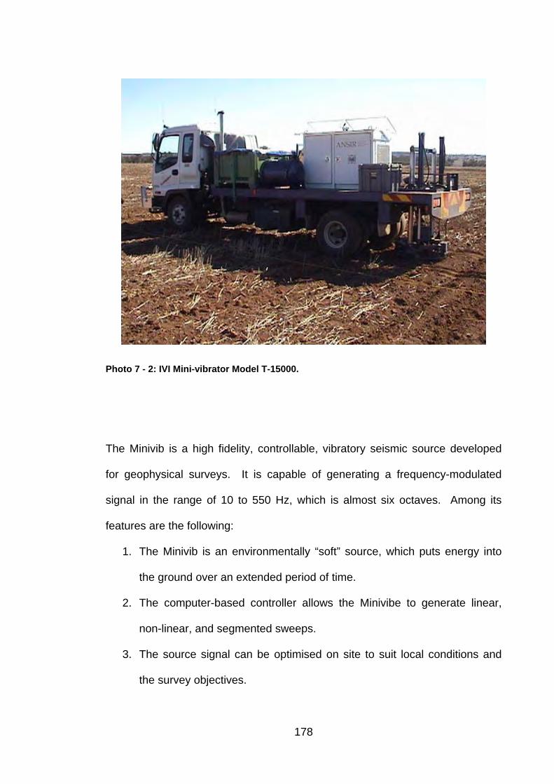
Photo 7 - 2: IVI Mini-vibrator Model T-15000.
The Minivib is a high fidelity, controllable, vibratory seismic source developed
for geophysical surveys. It is capable of generating a frequency-modulated
signal in the range of 10 to 550 Hz, which is almost six octaves. Among its
features are the following:
1. The Minivib is an environmentally “soft” source, which puts energy into
the ground over an extended period of time.
2. The computer-based controller allows the Minivibe to generate linear,
non-linear, and segmented sweeps.
3. The source signal can be optimised on site to suit local conditions and
the survey objectives.
178

The Minivib has the capability to rotate the vibrator mechanism from the vertical
to the horizontal, so that shear waves, as well as compressional waves can be
generated. Figure 7-1 shows the actuator in the two positions for the
generating of P- and S-waves. The vibrator in P-wave mode is shown in photo
7-3 with the actuator positioned vertically, whilst in photo 7-4 it is in S-wave
mode with the actuator positioned horizontally. This design also allows for the
rotation and positioning of the horizontally mounted actuator at any angle
relative to the line.
The ‘minivib’ P-waveconfiguration.
The ‘minivib’ S-wave configuration.
Figure 7 - 1: P-wave versus S-wave comparison.
179
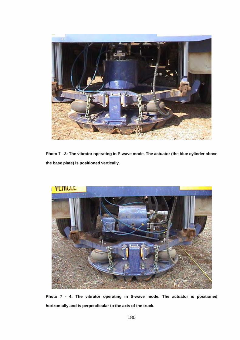
Photo 7 - 3: The vibrator operating in P-wave mode. The actuator (the blue cylinder above
the base plate) is positioned vertically.
Photo 7 - 4: The vibrator operating in S-wave mode. The actuator is positioned
horizontally and is perpendicular to the axis of the truck.
180
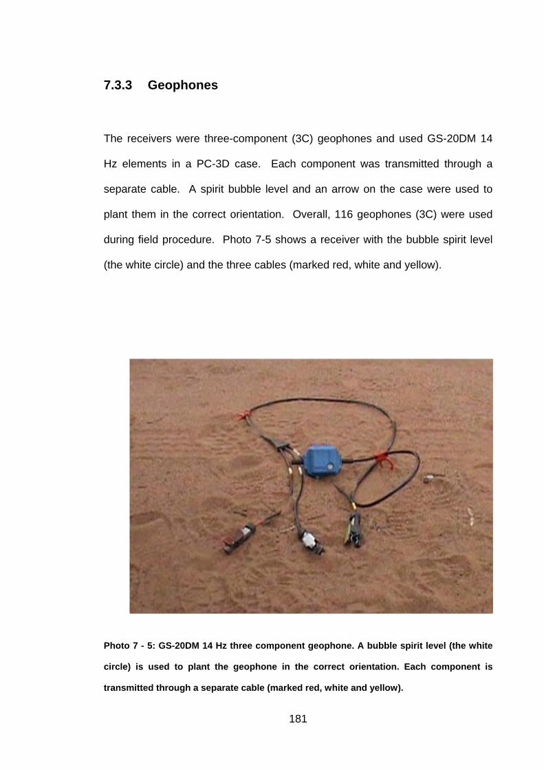
7.3.3 Geophones
The receivers were three-component (3C) geophones and used GS-20DM 14
Hz elements in a PC-3D case. Each component was transmitted through a
separate cable. A spirit bubble level and an arrow on the case were used to
plant them in the correct orientation. Overall, 116 geophones (3C) were used
during field procedure. Photo 7-5 shows a receiver with the bubble spirit level
(the white circle) and the three cables (marked red, white and yellow).
Photo 7 - 5: GS-20DM 14 Hz three component geophone. A bubble spirit level (the white
circle) is used to plant the geophone in the correct orientation. Each component is
transmitted through a separate cable (marked red, white and yellow).
181
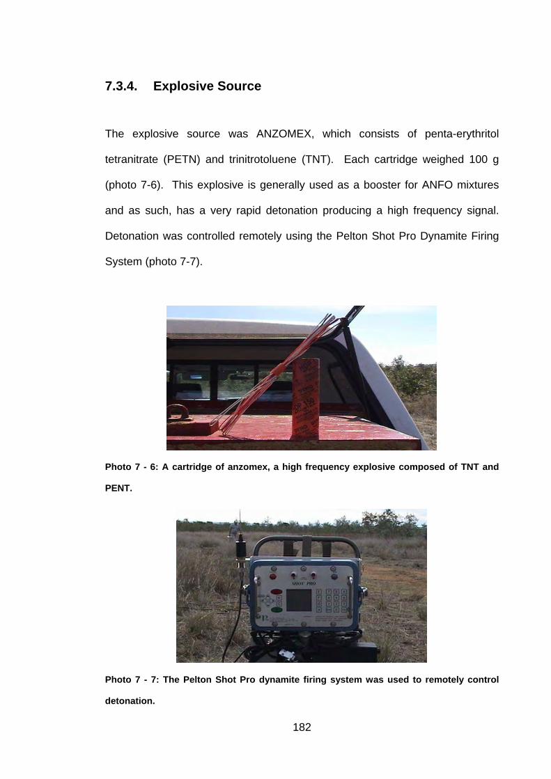
7.3.4. Explosive Source
The explosive source was ANZOMEX, which consists of penta-erythritol
tetranitrate (PETN) and trinitrotoluene (TNT). Each cartridge weighed 100 g
(photo 7-6). This explosive is generally used as a booster for ANFO mixtures
and as such, has a very rapid detonation producing a high frequency signal.
Detonation was controlled remotely using the Pelton Shot Pro Dynamite Firing
System (photo 7-7).
Photo 7 - 6: A cartridge of anzomex, a high frequency explosive composed of TNT and
PENT.
Photo 7 - 7: The Pelton Shot Pro dynamite firing system was used to remotely control
detonation.
182
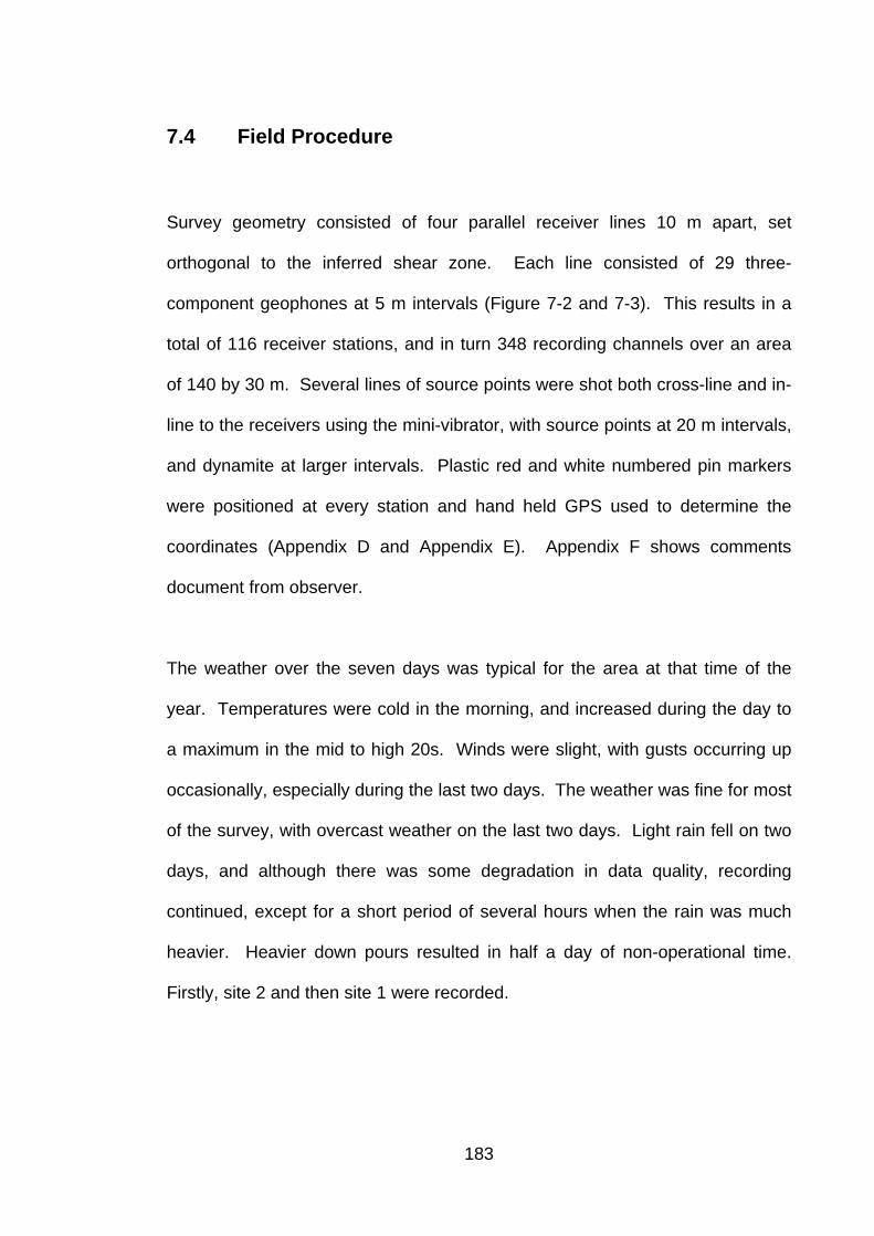
7.4 Field Procedure
Survey geometry consisted of four parallel receiver lines 10 m apart, set
orthogonal to the inferred shear zone. Each line consisted of 29 three-
component geophones at 5 m intervals (Figure 7-2 and 7-3). This results in a
total of 116 receiver stations, and in turn 348 recording channels over an area
of 140 by 30 m. Several lines of source points were shot both cross-line and in-
line to the receivers using the mini-vibrator, with source points at 20 m intervals,
and dynamite at larger intervals. Plastic red and white numbered pin markers
were positioned at every station and hand held GPS used to determine the
coordinates (Appendix D and Appendix E). Appendix F shows comments
document from observer.
The weather over the seven days was typical for the area at that time of the
year. Temperatures were cold in the morning, and increased during the day to
a maximum in the mid to high 20s. Winds were slight, with gusts occurring up
occasionally, especially during the last two days. The weather was fine for most
of the survey, with overcast weather on the last two days. Light rain fell on two
days, and although there was some degradation in data quality, recording
continued, except for a short period of several hours when the rain was much
heavier. Heavier down pours resulted in half a day of non-operational time.
Firstly, site 2 and then site 1 were recorded.
183
7.4.1 Setting Up the Survey Spread
The first step in the field procedure was to determine the shear zone’s location
and trend at the survey site. This was determined from previous magnetic and
resistivity surveys, its surface expression, such as saline groundwater discharge
and salt scalding, from the presence of salt resilient vegetation which were
planted in order to combat the dryland salinity, from the location of piezometers
which were used during previous studies, and from the 1:100 000 geological
map of the area.
Once the general location and trend of the shear zone was determined the
receiver lines were then set out. A measuring tape was used to measure 140 m
over the and along a bearing orthogonal to the inferred shear zone. Pin flags
were then placed at 5 m intervals along the tape. The pin flags were kept in line
with each other by forward and backward siting. The adjacent lines were offset
orthogonally from the first line by 10 m intervals, with pin flags being placed at 5
m intervals. The second, third and fourth lines were then set out in similar
manner to the first line. The first Receiver station was 100 and if, positioned on
the lower-right corner of the rectangle, then the last station, number 187, was
on the upper-left.
The source points were located with a 300 m length of rope with markings at 5
m intervals. The rope was laid along a number of different lines parallel,
perpendicular and oblique to the receiver lines with pin flags being placed at 20
m intervals.
184
The accuracy in setting out the receiver and source lines was generally quite
good. This can be seen in the GPS readings, which were taken at both ends
and at the centre of each receiver line and at every source point. For site 1,
from the GPS readings the distance between the receiver lines ranged from 9.8
to 10.6 m, whilst the distance between the source points was 20 +/- 1.8 m. Site
2 had less precise measurements with 10 +/- 1.8 m between the receiver lines,
and 20 +/- 2.6 m between the source points.
After the receiver lines were set out, receiver cables were laid out using the
geophone truck. Three cables were used, one for each component, going up
the first receiver line, then down the second, back up the third, and down the
fourth. These cables were then connected to the recording vehicle.
Since the seismic recorder only had 3D capabilities for 4 lines, it was decided to
use individual line inputs for each component, and to concatenate the four lines
on the ground into a single time.
The three component geophones were planted at 5m intervals along the
receiver lines and connected to the three cables. Horizontal planting of the
geophones was readily achieved with the aid of a bubble spirit level on the top
of each unit and correct orientation of the horizontal components was achieved
by ensuring that was orthogonal to the receiver lines. These two steps ensured
that the directions of each of the components were the same for every
geophone. When connecting the geophone outputs to the cables, care was
185
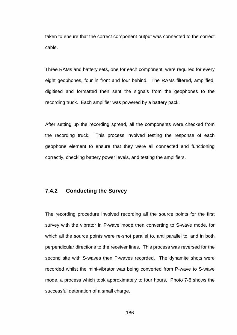
taken to ensure that the correct component output was connected to the correct
cable.
Three RAMs and battery sets, one for each component, were required for every
eight geophones, four in front and four behind. The RAMs filtered, amplified,
digitised and formatted then sent the signals from the geophones to the
recording truck. Each amplifier was powered by a battery pack.
After setting up the recording spread, all the components were checked from
the recording truck. This process involved testing the response of each
geophone element to ensure that they were all connected and functioning
correctly, checking battery power levels, and testing the amplifiers.
7.4.2 Conducting the Survey
The recording procedure involved recording all the source points for the first
survey with the vibrator in P-wave mode then converting to S-wave mode, for
which all the source points were re-shot parallel to, anti parallel to, and in both
perpendicular directions to the receiver lines. This process was reversed for the
second site with S-waves then P-waves recorded. The dynamite shots were
recorded whilst the mini-vibrator was being converted from P-wave to S-wave
mode, a process which took approximately to four hours. Photo 7-8 shows the
successful detonation of a small charge.
186
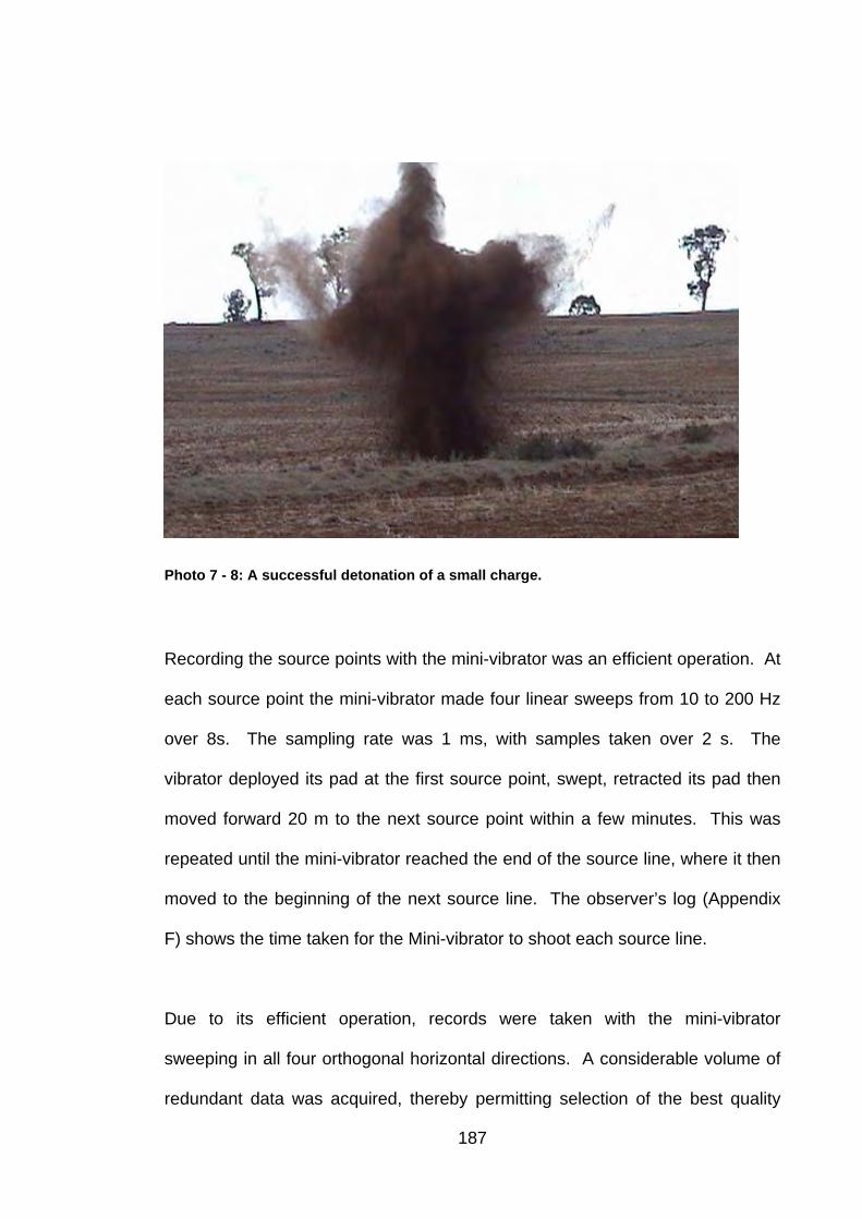
Photo 7 - 8: A successful detonation of a small charge.
Recording the source points with the mini-vibrator was an efficient operation. At
each source point the mini-vibrator made four linear sweeps from 10 to 200 Hz
over 8s. The sampling rate was 1 ms, with samples taken over 2 s. The
vibrator deployed its pad at the first source point, swept, retracted its pad then
moved forward 20 m to the next source point within a few minutes. This was
repeated until the mini-vibrator reached the end of the source line, where it then
moved to the beginning of the next source line. The observer’s log (Appendix
F) shows the time taken for the Mini-vibrator to shoot each source line.
Due to its efficient operation, records were taken with the mini-vibrator
sweeping in all four orthogonal horizontal directions. A considerable volume of
redundant data was acquired, thereby permitting selection of the best quality
187
shot records for processing. Over 540 shot records were obtained during the
two surveys resulting in approximately 1.5 GB of data.
7.4.2.1 Site 1
Site 1 was located in a ploughed paddock at grid coordinates 691500mE,
6433400mN (Map Grid of Australia, 149:02:36 East, 32:13:27 South) with the
receiver lines running at a bearing of 311 degrees. Lack of vegetation and
smooth topography resulted in precise survey setup and good accessibility for
the vibrator truck. The paddock sloped uphill to the north east of the survey.
This slope was gently and was not considered to have had an adverse effect on
acquisition. A dry erosional gully ran east west to the northwest of the receiver
lines, and it necessitated careful negotiation by the vibrator truck.
Due to the ploughing, a thin layer of loose soil, up to 5 cm thick was present
above a more compacted soil. Geophone ground coupling was not affected by
this, since the geophone spike was long enough to penetrate into the more
compacted soil especially after the removal of the surrounding loose soil.
Nevertheless, there were still some local variations in the near surface soil
properties, such as the moisture content, which affected the seismic velocities.
Those variations resulted in the development of a smoothing method, in order to
minimise their effect on the determination of the seismic velocities in the
refractor.
188
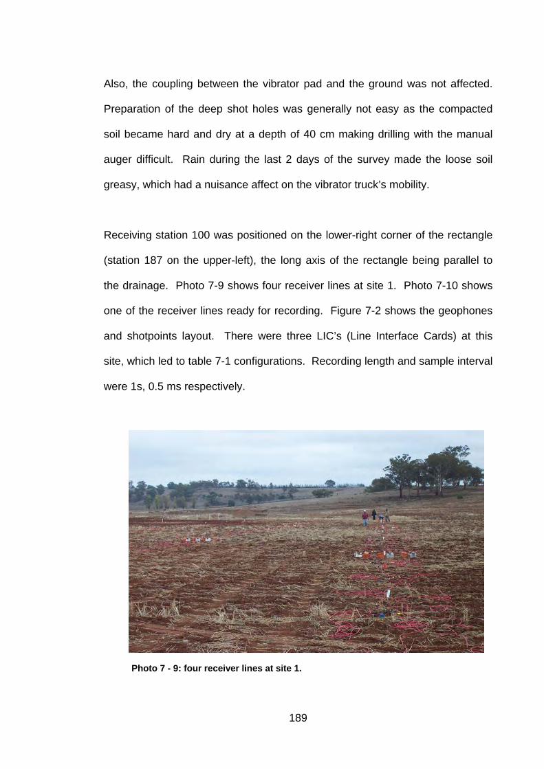
Also, the coupling between the vibrator pad and the ground was not affected.
Preparation of the deep shot holes was generally not easy as the compacted
soil became hard and dry at a depth of 40 cm making drilling with the manual
auger difficult. Rain during the last 2 days of the survey made the loose soil
greasy, which had a nuisance affect on the vibrator truck’s mobility.
Receiving station 100 was positioned on the lower-right corner of the rectangle
(station 187 on the upper-left), the long axis of the rectangle being parallel to
the drainage. Photo 7-9 shows four receiver lines at site 1. Photo 7-10 shows
one of the receiver lines ready for recording. Figure 7-2 shows the geophones
and shotpoints layout. There were three LIC’s (Line Interface Cards) at this
site, which led to table 7-1 configurations. Recording length and sample interval
were 1s, 0.5 ms respectively.
Photo 7 - 9: four receiver lines at site 1.
189
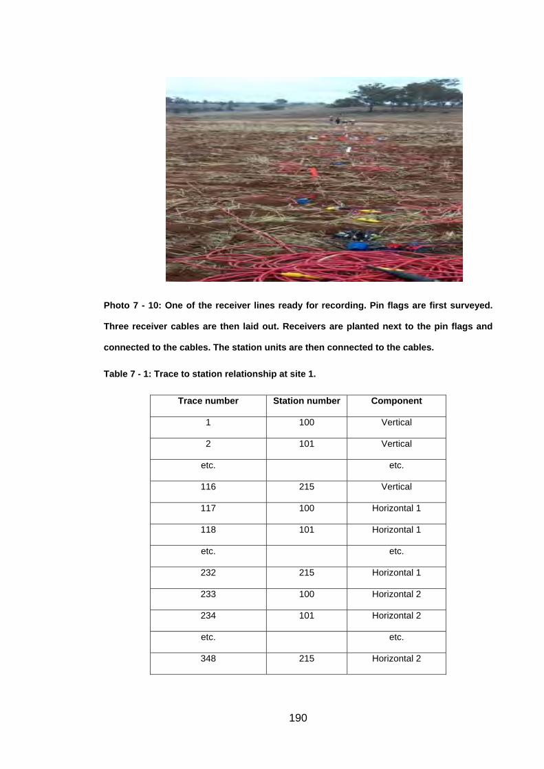
Photo 7 - 10: One of the receiver lines ready for recording. Pin flags are first surveyed.
Three receiver cables are then laid out. Receivers are planted next to the pin flags and
connected to the cables. The station units are then connected to the cables.
Table 7 - 1: Trace to station relationship at site 1.
Trace number Station number Component
1 100 Vertical
2 101 Vertical
etc. etc.
116 215 Vertical
117 100 Horizontal 1
118 101 Horizontal 1
etc. etc.
232 215 Horizontal 1
233 100 Horizontal 2
234 101 Horizontal 2
etc. etc.
348 215 Horizontal 2
190
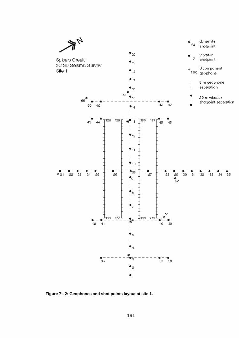
Figure 7 - 2: Geophones and shot points layout at site 1.
191
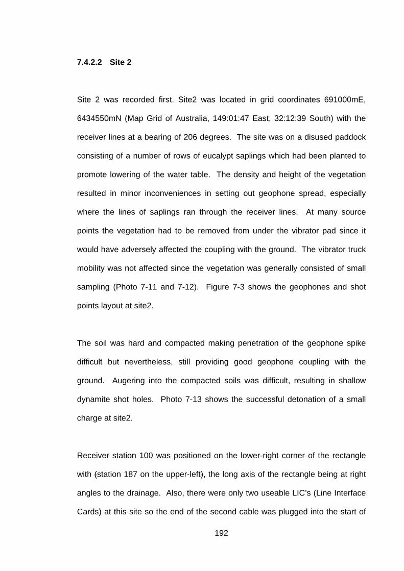
7.4.2.2 Site 2
Site 2 was recorded first. Site2 was located in grid coordinates 691000mE,
6434550mN (Map Grid of Australia, 149:01:47 East, 32:12:39 South) with the
receiver lines at a bearing of 206 degrees. The site was on a disused paddock
consisting of a number of rows of eucalypt saplings which had been planted to
promote lowering of the water table. The density and height of the vegetation
resulted in minor inconveniences in setting out geophone spread, especially
where the lines of saplings ran through the receiver lines. At many source
points the vegetation had to be removed from under the vibrator pad since it
would have adversely affected the coupling with the ground. The vibrator truck
mobility was not affected since the vegetation was generally consisted of small
sampling (Photo 7-11 and 7-12). Figure 7-3 shows the geophones and shot
points layout at site2.
The soil was hard and compacted making penetration of the geophone spike
difficult but nevertheless, still providing good geophone coupling with the
ground. Augering into the compacted soils was difficult, resulting in shallow
dynamite shot holes. Photo 7-13 shows the successful detonation of a small
charge at site2.
Receiver station 100 was positioned on the lower-right corner of the rectangle
with (station 187 on the upper-left), the long axis of the rectangle being at right
angles to the drainage. Also, there were only two useable LIC’s (Line Interface
Cards) at this site so the end of the second cable was plugged into the start of
192
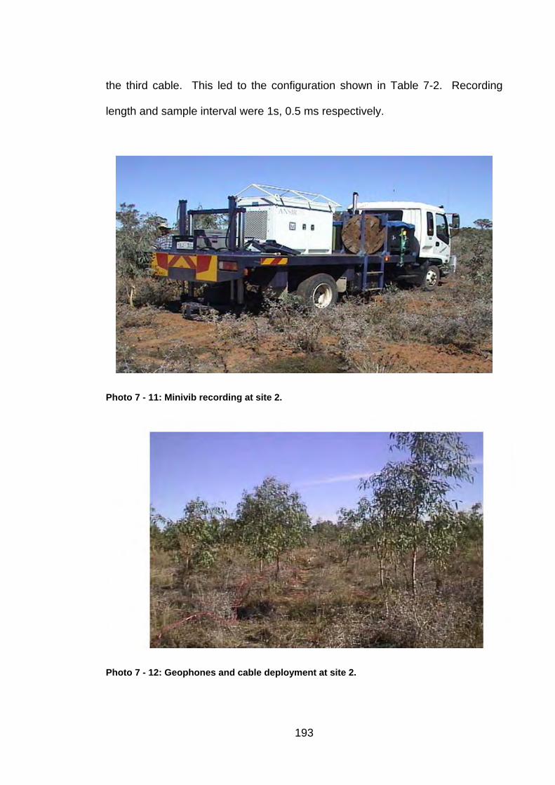
the third cable. This led to the configuration shown in Table 7-2. Recording
length and sample interval were 1s, 0.5 ms respectively.
Photo 7 - 11: Minivib recording at site 2.
Photo 7 - 12: Geophones and cable deployment at site 2.
193
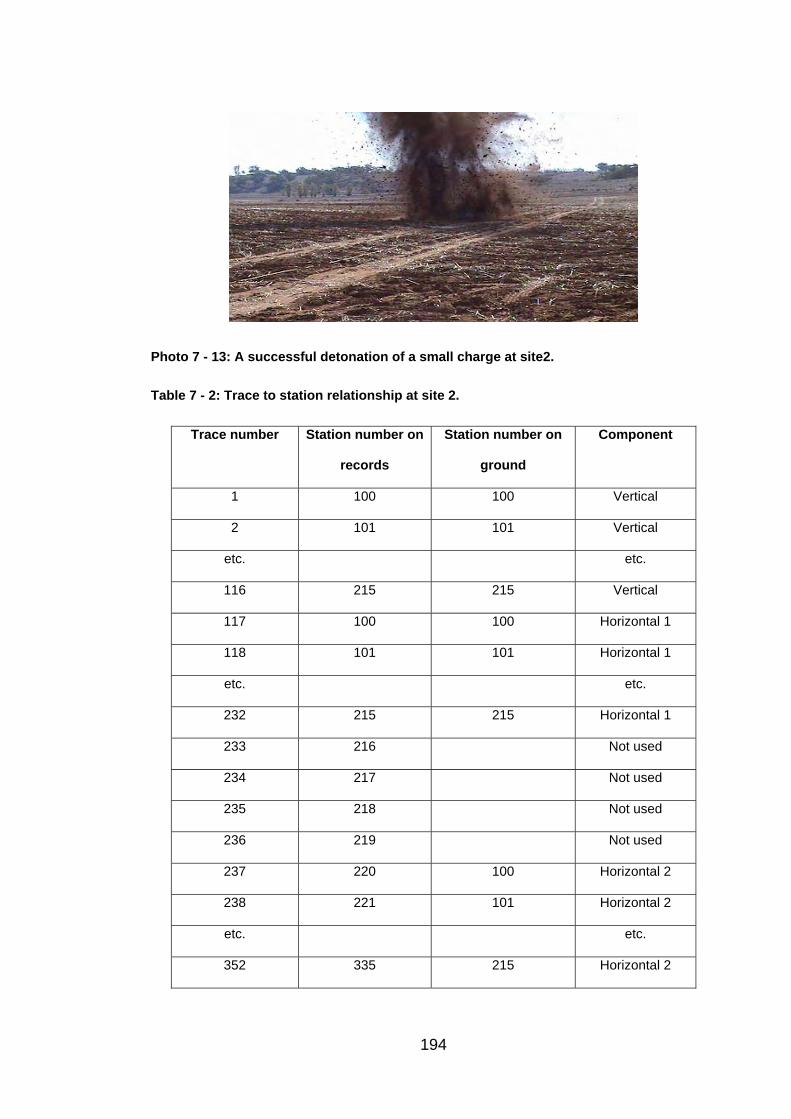
Photo 7 - 13: A successful detonation of a small charge at site2.
Table 7 - 2: Trace to station relationship at site 2.
Trace number Station number on
records
Station number on
ground
Component
1 100 100 Vertical
2 101 101 Vertical
etc. etc.
116 215 215 Vertical
117 100 100 Horizontal 1
118 101 101 Horizontal 1
etc. etc.
232 215 215 Horizontal 1
233 216 Not used
234 217 Not used
235 218 Not used
236 219 Not used
237 220 100 Horizontal 2
238 221 101 Horizontal 2
etc. etc.
352 335 215 Horizontal 2
194
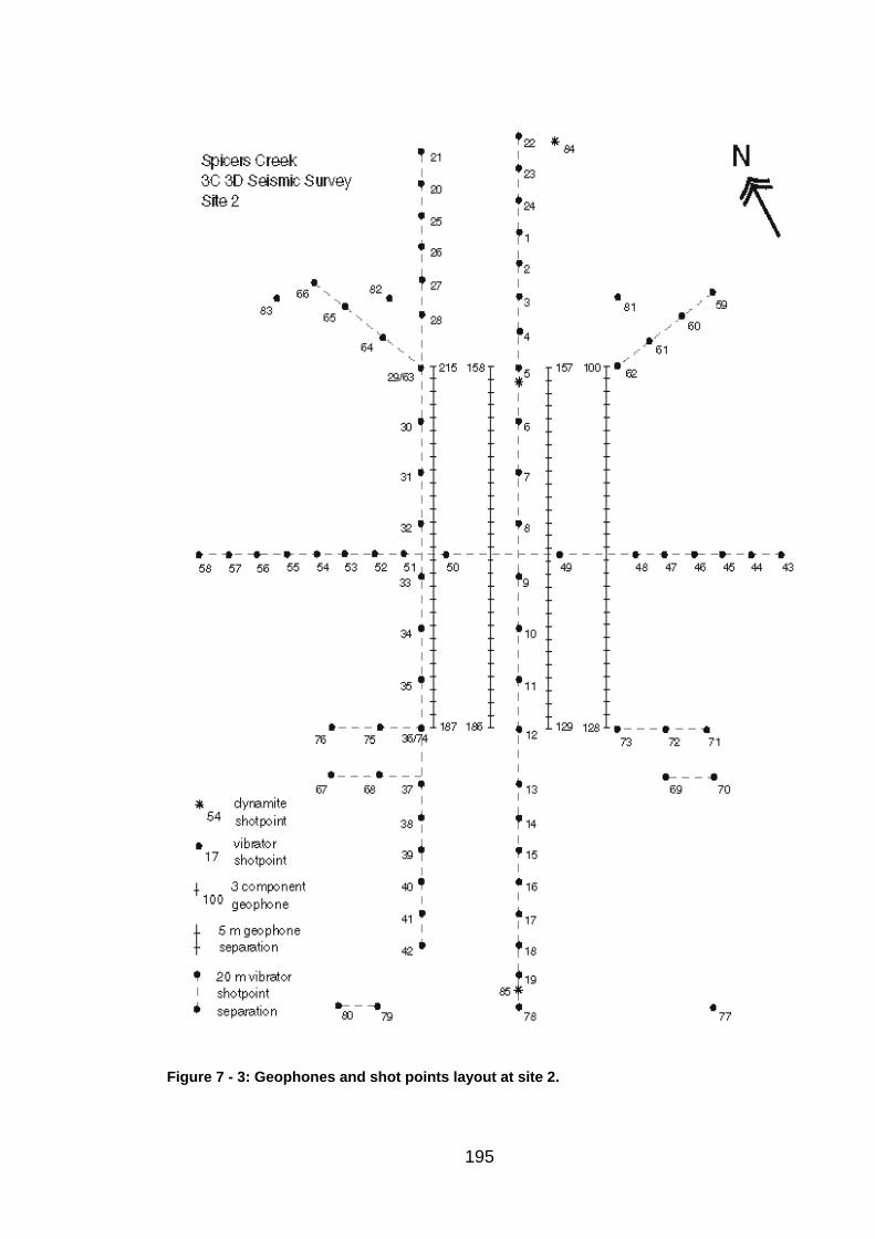
Figure 7 - 3: Geophones and shot points layout at site 2.
195
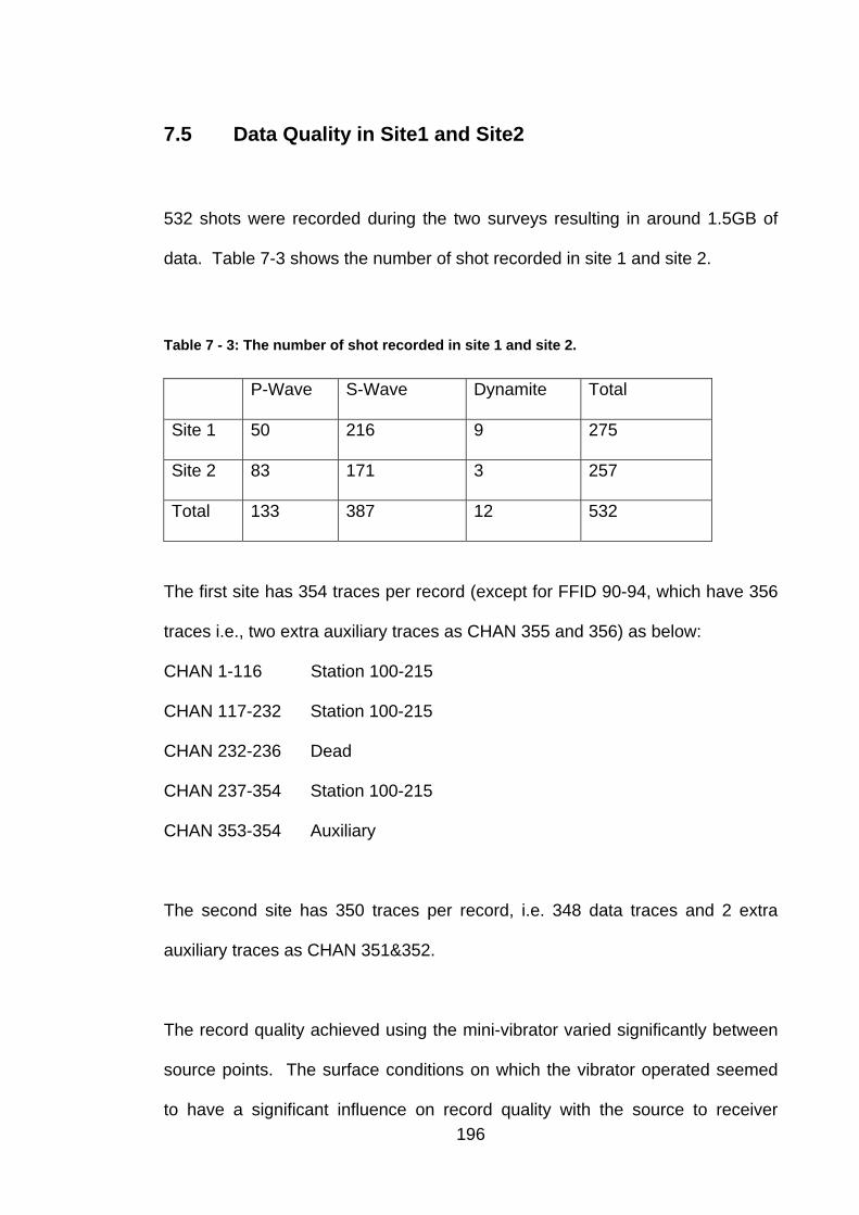
7.5 Data Quality in Site1 and Site2
532 shots were recorded during the two surveys resulting in around 1.5GB of
data. Table 7-3 shows the number of shot recorded in site 1 and site 2.
Table 7 - 3: The number of shot recorded in site 1 and site 2.
P-Wave S-Wave Dynamite Total
Site 1 50 216 9 275
Site 2 83 171 3 257
Total 133 387 12 532
The first site has 354 traces per record (except for FFID 90-94, which have 356
traces i.e., two extra auxiliary traces as CHAN 355 and 356) as below:
CHAN 1-116 Station 100-215
CHAN 117-232 Station 100-215
CHAN 232-236 Dead
CHAN 237-354 Station 100-215
CHAN 353-354 Auxiliary
The second site has 350 traces per record, i.e. 348 data traces and 2 extra
auxiliary traces as CHAN 351&352.
The record quality achieved using the mini-vibrator varied significantly between
source points. The surface conditions on which the vibrator operated seemed
to have a significant influence on record quality with the source to receiver 196
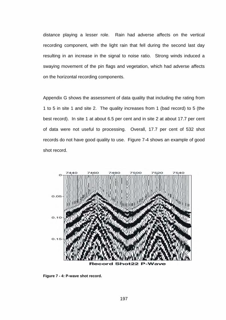
distance playing a lesser role. Rain had adverse affects on the vertical
recording component, with the light rain that fell during the second last day
resulting in an increase in the signal to noise ratio. Strong winds induced a
swaying movement of the pin flags and vegetation, which had adverse affects
on the horizontal recording components.
Appendix G shows the assessment of data quality that including the rating from
1 to 5 in site 1 and site 2. The quality increases from 1 (bad record) to 5 (the
best record). In site 1 at about 6.5 per cent and in site 2 at about 17.7 per cent
of data were not useful to processing. Overall, 17.7 per cent of 532 shot
records do not have good quality to use. Figure 7-4 shows an example of good
shot record.
Figure 7 - 4: P-wave shot record.
197
7.6 Magnetic Data Acquisition
The magnetic survey was acquired at the Spicers Creek Catchment using a G-
858 magnetometer. At the first site the survey consisted of 18 lines, 5 m apart
and 130 m in length and at the second site consisted of 40 lines, 10 m apart
and 100 m in length. Station spacing was approximately 0.25 m along each
line.
7.7 Resistivity Data Acquisition
At the Spicers Creek Catchment, the resistivity survey was acquired using an
ABEM Terrameter. Using a Wenner configuration, resistivity measurements
were acquired along three different lines (line 1 = 240m; line 2 = 260m; line 3 =
180m) at the first site and along one line (420 m) at the second site (refer to
chapter 8).
198
Chapter 8
Processing
8.1 Summary
Processing of the Spicers Creek Catchment survey was done using a number
of software packages for magnetic (Magmap 2000), resistivity (Res2DINV) and
seismic refraction data. The main stage was the processing of seismic
refraction data by using the Seismic Un*x program, developed by the Centre for
Wave Phenomena at the Colorado School of Mines, Visual-SUNT and Rayfract
softwares.
In particular these software packages were used to generate three-dimensional
images, perform the generalized reciprocal method, calculate velocity ratios of
P- and S-waves, the picking of first-arrival traveltimes, display the shot records,
processing on the full shot records and wave eikonal traveltime (WET)
tomography images.
The major challenges of the processing of the seismic refraction data were to
reduce the very large volume of data, primarily through averaging processes,
and to generate detailed starting models for tomographic inversion. Near
surface irregularities were a major cause of inconsistencies between adjacent
199
lines. The development of the GRM SSM (statics smoothing method) is a major
achievement of this study.
8.2 Introduction
Processing of the geophysical data was done in two stages, using a number of
software packages. The first stage involved the processing of magnetic and
resistivity data collected from 2 to 7 April 2002, using MagMap 2000 and
RES2DINV software. The second stage involved the processing of the seismic
refraction data collected from 6 April 2003 to 13 April 2003, with the generalized
reciprocal method (GRM; Palmer, 1980, 1986). Processing of these data was
done using Microsoft Excel, Surfer 8, Seismic Un*x, Visual_SUNT, and
RAYFRACT software.
8.3 Processing of Magnetic and Resistivity Data
Magnetic and electrical resistivity surveys were carried out to determine the
general location of the probable shear zones. These are the most common
geophysical methods for imaging shear zones in the near surface and they are
widely used in many geotechnical and environmental investigations. The
magnetic data was processed using MagMap 2000 and the resistivity data
using RES2DINV.
200
8.3.1 MagMap 2000 Software
High resolution magnetic data were acquired at two sites at Spicers Creek using
a Geometrics G858 magnetometer. MagMap 2000 (Geometrics software,
version 4.26) is a post acquisition processing software used to edit and correct
magnetic data from several models of Geometrics magnetometers. MagMap
2000 was used to initially download the data from the magnetometer. It was
then employed to perform various editing functions, include moving lines and
positions, changing the direction of lines, rotating lines, and deleting parts of
lines or entire lines. The MagMap 2000 software also enables the performing of
diurnal corrections, plotting the acquired magnetic field, and filtering for spikes
and dropouts. The results of processing are shown in Chapter 9.
8.3.2 RES2DINV Software
Electrical resistivity imaging surveys were carried out along four lines at the two
sites at Spicers Creek with an ABEM Terrameter. The data were processed
with RES2DINV. The two-dimensional (2-D) starting model consists of a
number of rectangular blocks loosely tied to the distribution of the data points in
the pseudosection (shown in Figure 8-1).
201
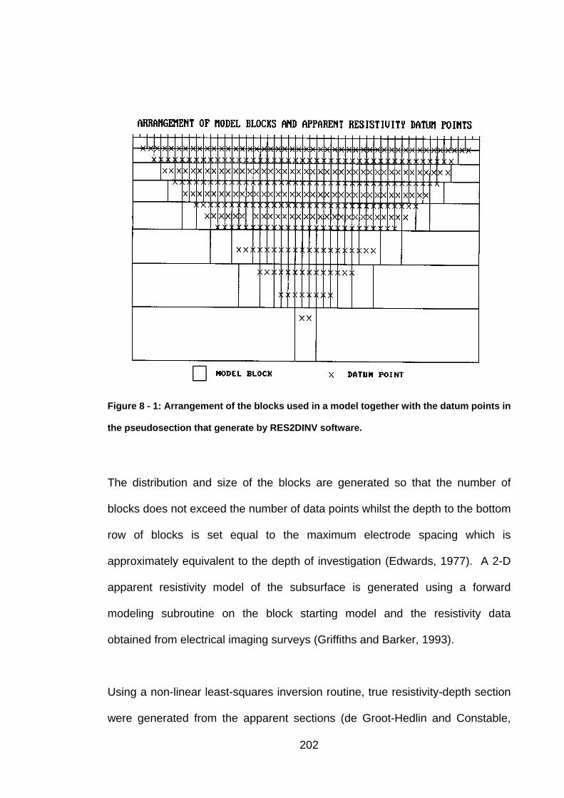
Figure 8 - 1: Arrangement of the blocks used in a model together with the datum points in
the pseudosection that generate by RES2DINV software.
The distribution and size of the blocks are generated so that the number of
blocks does not exceed the number of data points whilst the depth to the bottom
row of blocks is set equal to the maximum electrode spacing which is
approximately equivalent to the depth of investigation (Edwards, 1977). A 2-D
apparent resistivity model of the subsurface is generated using a forward
modeling subroutine on the block starting model and the resistivity data
obtained from electrical imaging surveys (Griffiths and Barker, 1993).
Using a non-linear least-squares inversion routine, true resistivity-depth section
were generated from the apparent sections (de Groot-Hedlin and Constable,
202
1990), the results of which are shown in Chapter 9. The inversion routine used
by the program is a smoothness-constrained least-squares optimization
technique (de Groot-Hedlin and Constable, 1990, Sasaki, 1992) and is based
on the following equation:
(J T J + µF)d = J g T
where: F=f f + f f XTX Z
TX
f = horizontal flatness filter X
f = vertical flatness filter Z
J= matrix of partial derivatives
µ= damping factor
d= model perturbation vector
g= discrepancy vector.
8.4 Processing of Seismic Refraction Data
The processing of the seismic refraction data was performed with a number of
software packages. The processing of the seismic data took more than a year
to carry out. Due to the considerable volume of data, an initial interpretation
was carried out in order to gain an initial understanding of the problems. It then
became apparent that the expressions of the shear zone were subtle, and
careful re-processing would be required. The processing, particularly the
picking of first-arrival traveltimes was done up to four times using different
methods in order to obtain accurate values.
203
8.4.1 Microsoft Excel
Microsoft Excel is powerful spreadsheet software used to efficiently evaluate
and revise data, calculate and compare numbers, and create charts and
graphs. This software was used to process the first-arrival traveltimes and their
amplitudes. In particular it was used to determine the degree of geometric
spreading; calculate amplitude products; review and combine traveltime curves;
perform the GRM analyses including the generation of velocity analysis, time-
depth and depth graphs, and the calculation of P- and S-wave velocities and
their ratios.
8.4.2 Surfer 8
Surfer by Golden Software is a grid-based graphics program. Surfer
interpolates irregularly spaced XYZ data into a regularly spaced grid using a
number of gridding algorithms. The grid is then used to produce different types
of maps including contour, vector, wireframe, image, shaded relief, and surface
maps. Maps can be displayed and enhanced in Surfer by the addition of
boundary information, posting data points, combining several maps, adding
drawing, and annotating with text. Surfer was used to generate three-
dimensional images of the refractor velocity and depth, and velocity-depth
sections.
204
The main statistical gridding algorithm used was kriging. This method is one of
the more flexible methods and is useful for gridding almost any type of data set,
producing visually appealing maps from irregularly spaced data. Triangulation
with linear interpolation was also used. This algorithm, based on optimal
Delaunay Triangulation creates triangles by drawing lines between data points.
The original points are connected so that none of the triangle’s edges are
intersected by others. Each triangle defines a plane over the grid nodes lying
within the triangle, with the tilt and elevation of the triangle determined by the
three original data points defining the triangle.
8.4.3 Seismic Un*x Program
The Seismic Un*x (SU) package is a seismic processing and research
environment developed by the Center for Wave Phenomena, Colorado School
of Mines and is distributed free with full source code. This package operates in
the UNIX or LINUX environments. For convenience, the LINUX environment
was created with the freeware package CYGWIN which operations within the
Microsoft Windows environment (Stockwell et al., 2000). Seismic Un*x was
used to prepare the seismic data before processing, pick first-arrival traveltimes
and amplitudes, display the shot records, and perform processing on the full
shot records.
205
8.4.4 Visual_SUNT Software
The picking of the first-arrival traveltimes and amplitudes from more complex
shot records were done using Visual_SUNT software developed by W_Geosoft.
This software reads seismic data in SU format. After picking the first-arrival
traveltimes and amplitudes with Visual_SUNT, the data was transferred to Excel
for further processing.
8.4.5 RAYFRACT Software
Traveltime tomography was performed using RAYFRACT by Intelligent
Resources, a Windows 32-bit software package. The tomographic algorithm is
based on wavepath eikonal traveltime inversion (Schuster and Quintus-Bosz,
1993) and is suited for processing of seismic profiles and interpretation of both
P- and S-waves. RAYFRACT performs the Wavefront method as an optimized
version of the GRM, with laterally varying and automatically estimated receiver
separation i.e. XY distance.
Wavepath Eikonal Traveltime (WET) tomography was used to generate a
velocity-depth section of every line for each wave type from the GRM initial
models. WET tomography accommodates multiple signal paths contributing to
each first break and is a computationally efficient and geophysically robust
method (for a brief discussion on WET theory see Appendix M).
206
8.5 The Generalized Reciprocal Method
The aim of this section is to give a general overview of generalized reciprocal
method (GRM) of seismic refraction inversion as described by Palmer (1980,
1981, 1986, 1990 and 2003b). Only those parts of the GRM that have been
used for the processing of the Spicers Creek refraction data are described.
The GRM is a seismic inversion method that uses the refracted arrival
traveltime data for both forward and reverse shots, and the reciprocal time. The
GRM is able to provide good estimates of the seismic velocities within the
refractor, and the structure or shape of the refracting interface.
The major difference between the GRM and other seismic refraction inversion
methods is that the former applies a variable refraction migration which can be
often be useful in resolving undetected layers, variable velocity media and
anisotropy under favourable conditions. With the GRM, a range of offset
distances is computed, usually from zero to a value in excess of the estimated
true value. The optimum value, for which the refractor velocity analysis function
displays a minimum of artifacts caused by the irregular refractor interface, is
selected by inspection of the graphs.
The GRM consists of two algorithms: the velocity analysis function from which
the refractor velocity is derived, and the time-depth function which is a measure
of the depth to the refractor in units of time. The two functions are calculated for
different values of the horizontal separation between forward and reverse
207
receivers (XY values), with the optimum value being determined from inspection
of the resulting functions.
8.5.1 Velocity Analysis Function
The GRM refractor velocity analysis function, t , is defined by: V
( )FRRXFYV tttt +−= 2/1 (1)
This equation is applied to pairs of reversed traveltimes at the receivers X and Y
which are located between the forward and reverse shot points F and R from
the same refractor. The computed value is referred to G which is the midpoint
between X and Y. The raypaths used to form this equation are shown
schematically in Figure 8-2.
For moderately dipping refractor, the traveltimes from Q to Y and from P to X
are approximately equal and hence cancel. Therefore, tV reduces to the
average of the traveltimes from F to P and from F to Q, or approximately from F
to R. This approximation is more reasonable when the XY separation is such
that P and Q are very close together. Since t is computed for successive
receiver locations, the increments represent the additional time required to
travel the additional receiver spacing in the refractor, and hence provides a
method for determining the seismic velocity within the refractor.
V
208
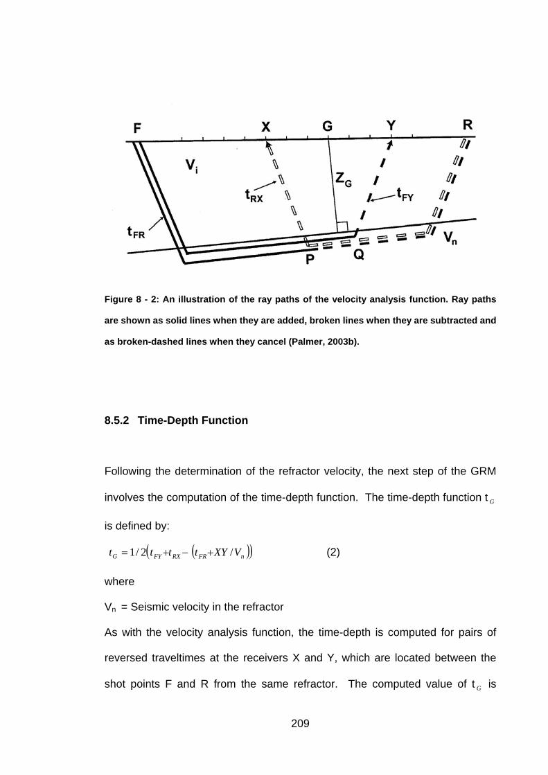
Figure 8 - 2: An illustration of the ray paths of the velocity analysis function. Ray paths
are shown as solid lines when they are added, broken lines when they are subtracted and
as broken-dashed lines when they cancel (Palmer, 2003b).
8.5.2 Time-Depth Function
Following the determination of the refractor velocity, the next step of the GRM
involves the computation of the time-depth function. The time-depth function t
is defined by:
G
( )( )nFRRXFYG VXYtttt /2/1 +−+= (2)
where
Vn = Seismic velocity in the refractor
As with the velocity analysis function, the time-depth is computed for pairs of
reversed traveltimes at the receivers X and Y, which are located between the
shot points F and R from the same refractor. The computed value of t is G
209
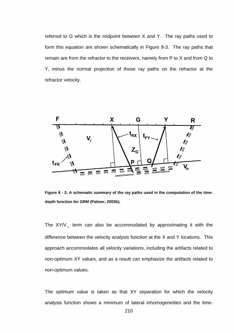
referred to G which is the midpoint between X and Y. The ray paths used to
form this equation are shown schematically in Figure 8-3. The ray paths that
remain are from the refractor to the receivers, namely from P to X and from Q to
Y, minus the normal projection of those ray paths on the refractor at the
refractor velocity.
Figure 8 - 3: A schematic summary of the ray paths used in the computation of the time-
depth function for GRM (Palmer, 2003b).
The XY/V term can also be accommodated by approximating it with the
difference between the velocity analysis function at the X and Y locations. This
approach accommodates all velocity variations, including the artifacts related to
non-optimum XY values, and as a result can emphasize the artifacts related to
non-optimum values.
n
The optimum value is taken as that XY separation for which the velocity
analysis function shows a minimum of lateral inhomogeneities and the time-
210
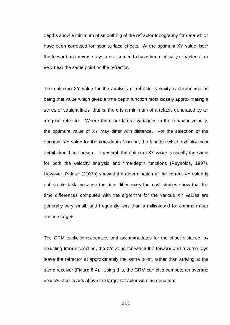
depths show a minimum of smoothing of the refractor topography for data which
have been corrected for near surface effects. At the optimum XY value, both
the forward and reverse rays are assumed to have been critically refracted at or
very near the same point on the refractor.
The optimum XY value for the analysis of refractor velocity is determined as
being that value which gives a time-depth function most closely approximating a
series of straight lines, that is, there is a minimum of artefacts generated by an
irregular refractor. Where there are lateral variations in the refractor velocity,
the optimum value of XY may differ with distance. For the selection of the
optimum XY value for the time-depth function, the function which exhibits most
detail should be chosen. In general, the optimum XY value is usually the same
for both the velocity analysis and time-depth functions (Reynolds, 1997).
However, Palmer (2003b) showed the determination of the correct XY value is
not simple task, because the time differences for most studies show that the
time differences computed with the algorithm for the various XY values are
generally very small, and frequently less than a millisecond for common near
surface targets.
The GRM explicitly recognizes and accommodates for the offset distance, by
selecting from inspection, the XY value for which the forward and reverse rays
leave the refractor at approximately the same point, rather than arriving at the
same receiver (Figure 8-4). Using this, the GRM can also compute an average
velocity of all layers above the target refractor with the equation:
211
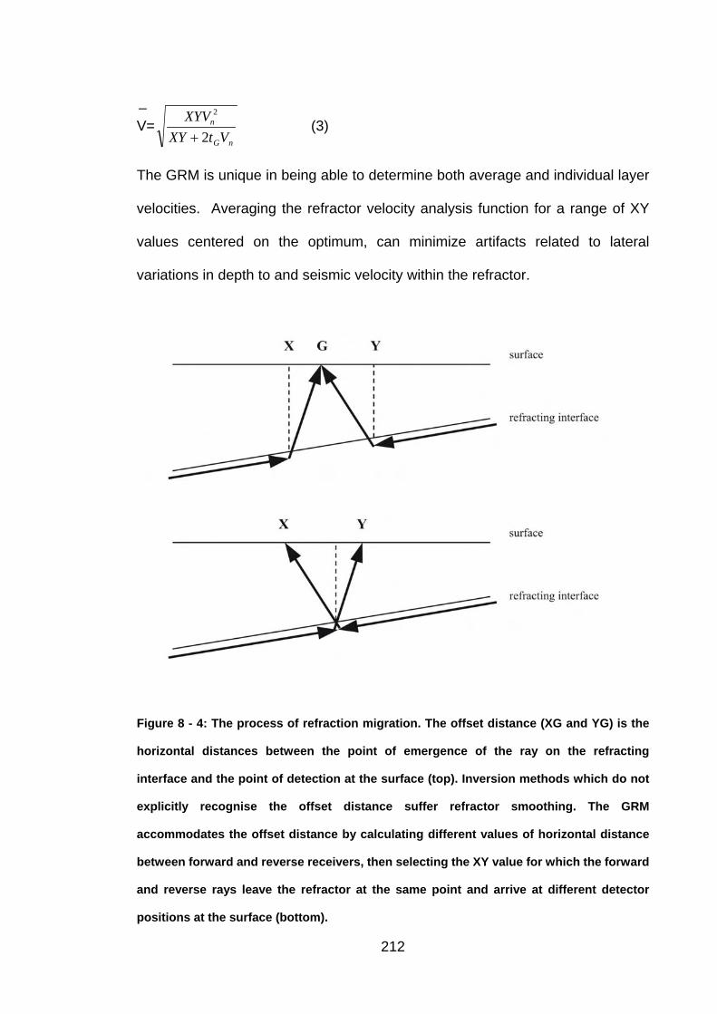
V=nG
n
VtXYXYV
2
2
+ (3)
_
The GRM is unique in being able to determine both average and individual layer
velocities. Averaging the refractor velocity analysis function for a range of XY
values centered on the optimum, can minimize artifacts related to lateral
variations in depth to and seismic velocity within the refractor.
Figure 8 - 4: The process of refraction migration. The offset distance (XG and YG) is the
horizontal distances between the point of emergence of the ray on the refracting
interface and the point of detection at the surface (top). Inversion methods which do not
explicitly recognise the offset distance suffer refractor smoothing. The GRM
accommodates the offset distance by calculating different values of horizontal distance
between forward and reverse receivers, then selecting the XY value for which the forward
and reverse rays leave the refractor at the same point and arrive at different detector
positions at the surface (bottom).
212
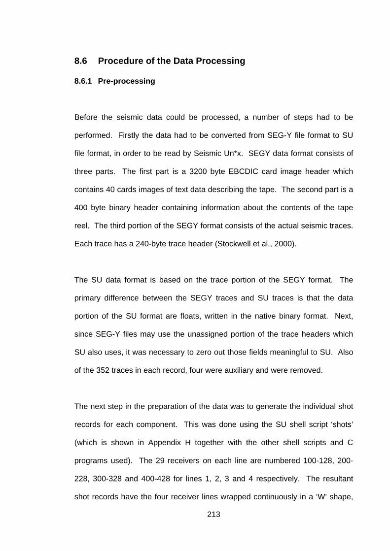
8.6 Procedure of the Data Processing
8.6.1 Pre-processing
Before the seismic data could be processed, a number of steps had to be
performed. Firstly the data had to be converted from SEG-Y file format to SU
file format, in order to be read by Seismic Un*x. SEGY data format consists of
three parts. The first part is a 3200 byte EBCDIC card image header which
contains 40 cards images of text data describing the tape. The second part is a
400 byte binary header containing information about the contents of the tape
reel. The third portion of the SEGY format consists of the actual seismic traces.
Each trace has a 240-byte trace header (Stockwell et al., 2000).
The SU data format is based on the trace portion of the SEGY format. The
primary difference between the SEGY traces and SU traces is that the data
portion of the SU format are floats, written in the native binary format. Next,
since SEG-Y files may use the unassigned portion of the trace headers which
SU also uses, it was necessary to zero out those fields meaningful to SU. Also
of the 352 traces in each record, four were auxiliary and were removed.
The next step in the preparation of the data was to generate the individual shot
records for each component. This was done using the SU shell script ‘shots’
(which is shown in Appendix H together with the other shell scripts and C
programs used). The 29 receivers on each line are numbered 100-128, 200-
228, 300-328 and 400-428 for lines 1, 2, 3 and 4 respectively. The resultant
shot records have the four receiver lines wrapped continuously in a ‘W’ shape,
213
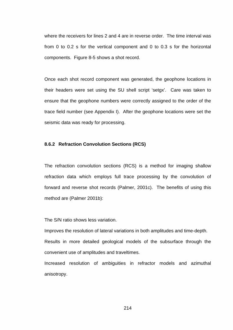
where the receivers for lines 2 and 4 are in reverse order. The time interval was
from 0 to 0.2 s for the vertical component and 0 to 0.3 s for the horizontal
components. Figure 8-5 shows a shot record.
Once each shot record component was generated, the geophone locations in
their headers were set using the SU shell script ‘setgx’. Care was taken to
ensure that the geophone numbers were correctly assigned to the order of the
trace field number (see Appendix I). After the geophone locations were set the
seismic data was ready for processing.
8.6.2 Refraction Convolution Sections (RCS)
The refraction convolution sections (RCS) is a method for imaging shallow
refraction data which employs full trace processing by the convolution of
forward and reverse shot records (Palmer, 2001c). The benefits of using this
method are (Palmer 2001b):
The S/N ratio shows less variation.
Improves the resolution of lateral variations in both amplitudes and time-depth.
Results in more detailed geological models of the subsurface through the
convenient use of amplitudes and traveltimes.
Increased resolution of ambiguities in refractor models and azimuthal
anisotropy.
214
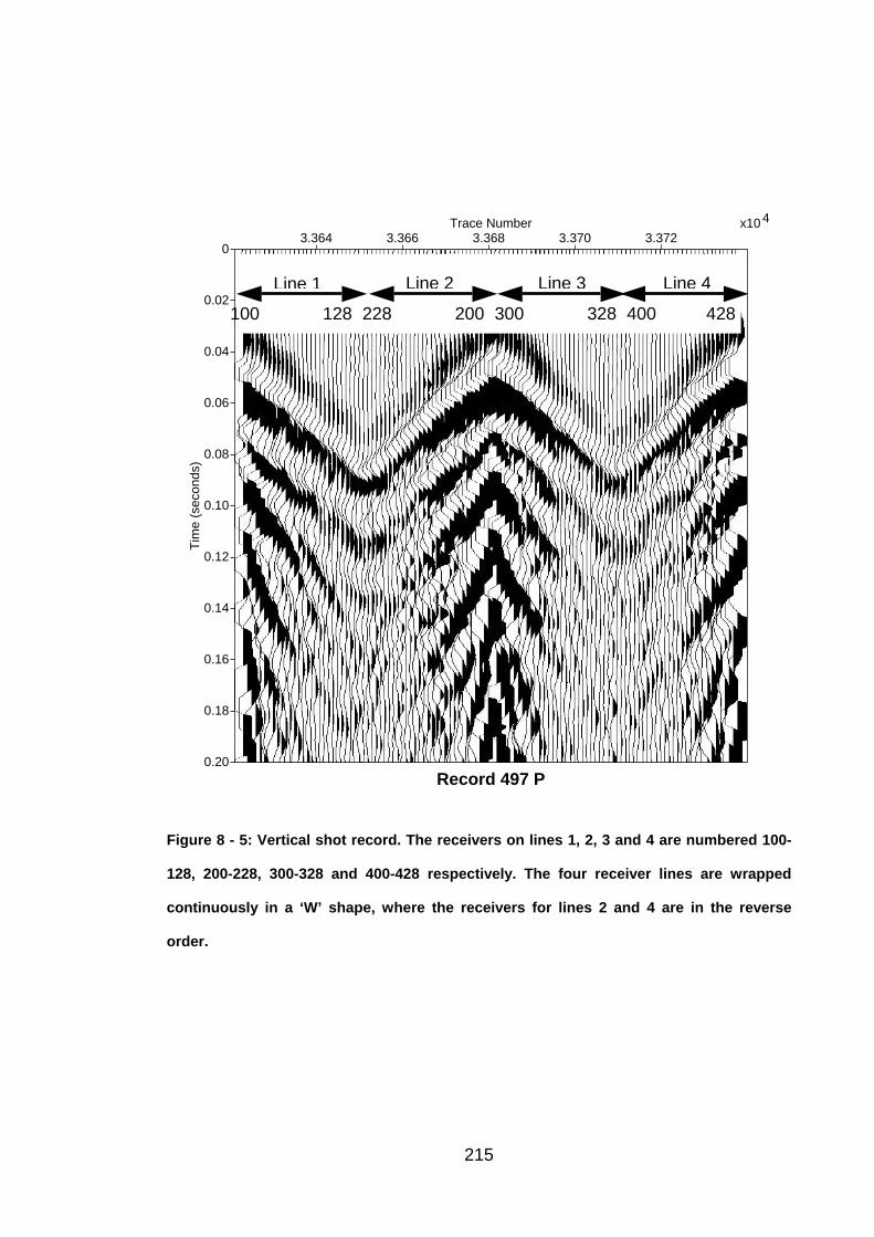
0
0.02
0.04
0.06
0.08
0.10
0.12
0.14
0.16
0.18
0.20
Tim
e (s
econ
ds)
3.364 3.366 3.368 3.370 3.372x10⁴Trace Number
Record 497 P
Line 1 Line 2 Line 3 Line 4
428400 328300200128 228100
Figure 8 - 5: Vertical shot record. The receivers on lines 1, 2, 3 and 4 are numbered 100-
128, 200-228, 300-328 and 400-428 respectively. The four receiver lines are wrapped
continuously in a ‘W’ shape, where the receivers for lines 2 and 4 are in the reverse
order.
215
It was necessary to split each shot record into the four individual receiver lines
and to reverse the trace order of the second and fourth lines. These two stages
were done using the SU shell script ‘linebreaker’ (see Appendix H). Figure 8-6
shows the result of this operation on the shot record in Figure 8-5. The
individual lines have been separated where the receivers on lines 1, 2, 3 and 4
are numbered 100-128, 200-228, 300-328 and 400-428 respectively. After
splitting the shot records into the four individual lines it was possible to generate
refraction convolution sections (see Appendix J).
The refraction convolution sections were generated by using the SU shell script
‘convolve’ which uses the SU program ‘surefcon’ to convolve pairs of forward
and reverse shot records. Figure 8-7 shows the results in the structure and
amplitudes of the refractor being displayed in a time cross-section.
Shot records were generated for horizontal sources of opposite polarity
enabling the enhancement of the S-wave energy. This operation was
performed by subtracting seismic records of opposite polarity, resulting in the
cancellation of P-wave components whilst leaving the sum of two S-wave
components (Helbig, 1986). Figure 8-8 shows the S-wave enhancement by
using the SU shell script ‘sumdiff’ (see Appendix H). These S-wave enhanced
waves are especially evident in the orthogonal components which generally had
poor convolution sections before this process.
216
0
0.05
0.10
0.15
Tim
e (s
econ
ds)
100 105 110 115 120 125Geophone
Record 497 P
0
0.05
0.10
0.15
Tim
e (s
econ
ds)
200 205 210 215 220 225Geophone
Record 497 P
0
0.05
0.10
0.15
Tim
e (s
econ
ds)
300 305 310 315 320 325Geophone
Record 497 P
0
0.05
0.10
0.15
Tim
e (s
econ
ds)
400 405 410 415 420 425Geophone
Record 497 P
Figure 8 - 6: The shot record in Figure 1 split into individual receiver lines. The receivers
on lines 1, 2, 3 and 4 are numbered 100-128, 200-228, 300-328 and 400-428 respectively.
The trace order of lines 2 and 4 have been reversed.
217
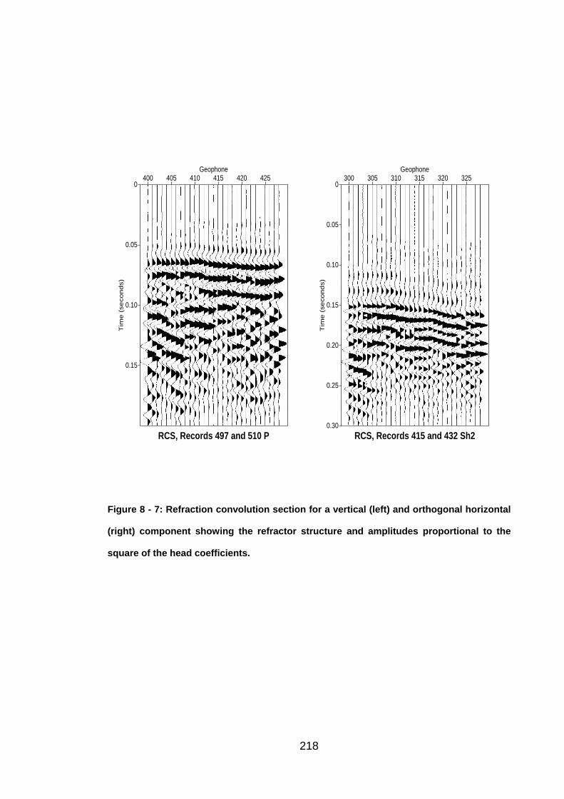
0
0.05
0.10
0.15
Tim
e (
seconds)
400 405 410 415 420 425Geophone
RCS, Records 497 and 510 P
0
0.05
0.10
0.15
0.20
0.25
0.30
Tim
e (
seconds)
300 305 310 315 320 325Geophone
RCS, Records 415 and 432 Sh2
Figure 8 - 7: Refraction convolution section for a vertical (left) and orthogonal horizontal
(right) component showing the refractor structure and amplitudes proportional to the
square of the head coefficients.
218
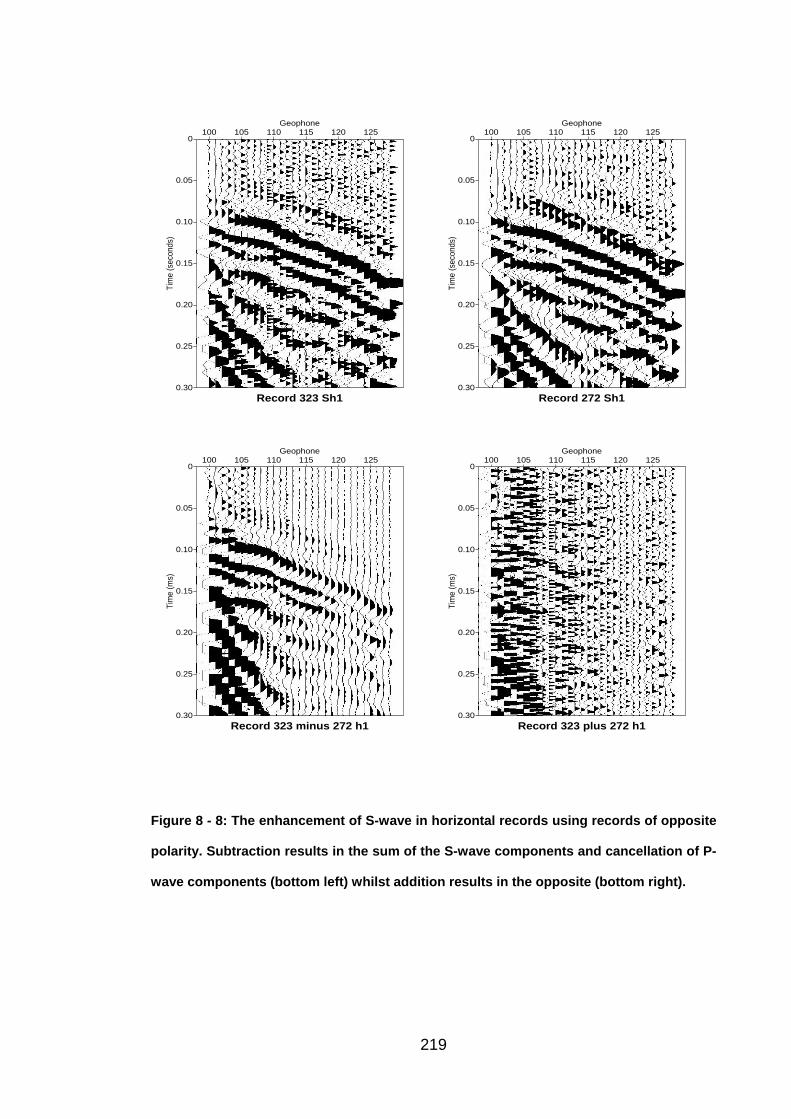
0
0.05
0.10
0.15
0.20
0.25
0.30
Tim
e (s
econ
ds)
100 105 110 115 120 125Geophone
Record 323 Sh1
0
0.05
0.10
0.15
0.20
0.25
0.30
Tim
e (s
econ
ds)
100 105 110 115 120 125Geophone
Record 272 Sh1
0
0.05
0.10
0.15
0.20
0.25
0.30
Tim
e (m
s)
100 105 110 115 120 125Geophone
Record 323 minus 272 h1
0
0.05
0.10
0.15
0.20
0.25
0.30
Tim
e (m
s)100 105 110 115 120 125
Geophone
Record 323 plus 272 h1
Figure 8 - 8: The enhancement of S-wave in horizontal records using records of opposite
polarity. Subtraction results in the sum of the S-wave components and cancellation of P-
wave components (bottom left) whilst addition results in the opposite (bottom right).
219
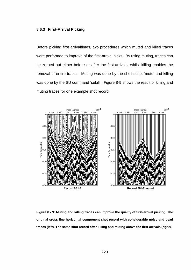
8.6.3 First-Arrival Picking
Before picking first arrivaltimes, two procedures which muted and killed traces
were performed to improve of the first-arrival picks. By using muting, traces can
be zeroed out either before or after the first-arrivals, whilst killing enables the
removal of entire traces. Muting was done by the shell script ‘mute’ and killing
was done by the SU command ‘sukill’. Figure 8-9 shows the result of killing and
muting traces for one example shot record.
0
0.05
0.10
0.15
0.20
0.25
0.30
Tim
e (
seco
nds)
3.388 3.390 3.392 3.394 3.396 3.398x10⁴Trace Number
Record 96 h2
0
0.05
0.10
0.15
0.20
0.25
0.30
Tim
e (
seco
nds)
3.388 3.390 3.392 3.394 3.396 3.398x10⁴Trace Number
Record 96 h2 muted
Figure 8 - 9: Muting and killing traces can improve the quality of first-arrival picking. The
original cross line horizontal component shot record with considerable noise and dead
traces (left). The same shot record after killing and muting above the first-arrivals (right).
220
After muting and killing, first arrivals from the shot records were picked to obtain
traveltimes by using a series of shell scripts in SU. The shell script ‘pics’ was
employed to display the individual shot records. The shell script ‘amps’ was
used to interpolate the maximum positive and negative amplitudes and their
times over the record within a specific time window, which was 20 ms, starting
at those points generated by ‘pics’ shell script. The quality of the interpolating
procedure in picking first-arrivals was checked using ‘plotAmps’ which displays
the shot records with first-arrivals overlayed.
Figures 8-10 show the result of the ‘plotAmps’. They show the varying quality of
the picking procedure in determining first-arrival traveltimes. In the record on
the top, the maximum negative first-arrivals (in white), form a smooth line, whilst
the maximum positive first-arrivals (in black) form an irregular line. In the record
on the bottom both the maximum negative and positive first-arrivals form fairly
smooth lines, although some irregularities do occur, such as between trace
numbers 5880 and 5900, and at 5920.
Due to poor record quality, picking first-arrivaltimes using Seismic Un*x was
often difficult (especially for many S-wave records). Instead Visual_SUNT was
used to pick the first-arrival times for those shot records with a complex set of
head-waves. With Visual_SUNT traces can be viewed individually, together
with every time increment in the sampling rate and their amplitudes. Once a
whole shot record was picked by this way, which was a lengthy process, the
quality of the picking could be checked using ‘plotAmps’ shell script. In some
shot records, both Seismic Un*x and Visual_SUNT were used.
221
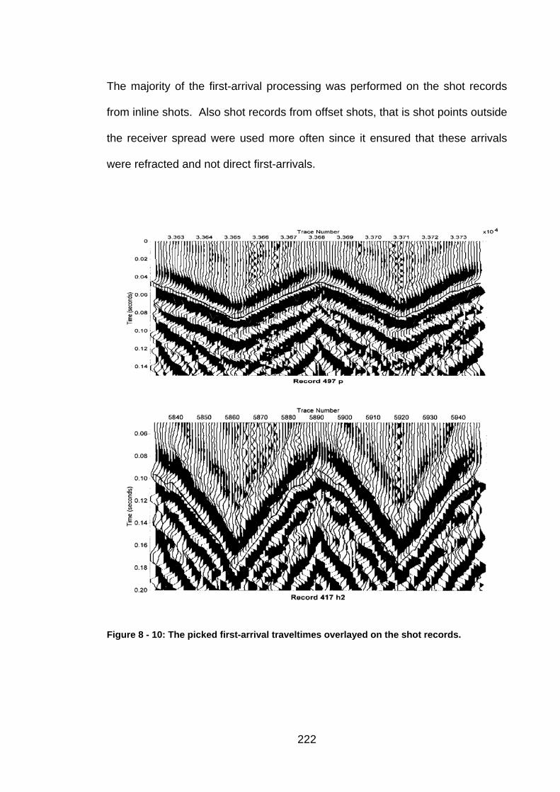
The majority of the first-arrival processing was performed on the shot records
from inline shots. Also shot records from offset shots, that is shot points outside
the receiver spread were used more often since it ensured that these arrivals
were refracted and not direct first-arrivals.
Figure 8 - 10: The picked first-arrival traveltimes overlayed on the shot records.
222
8.6.4 Traveltime Graphs
The first arrival traveltimes for each wave type (P-, SH-, SV-waves) were plotted
against distance to produce traveltime graphs. These graphs were then
checked to ensure that the minimum time of each in-spread traveltime graph
coincides with the shot point. The intercept times at each in-spread shot point
were also determined from the traveltime graphs using parallelism (Sjogren,
1980).
The traveltime graphs were distorted since the source lines were offset from the
receiver lines (Figure 8-11), due to the impracticality of operating the mini-vibe
next to the receivers. The distorting effect was most prominent for the receivers
near the source points, where the distance X along the line and Y the lateral
offset from the line are comparable, especially when X was less than Y. As a
result the traveltimes of direct arrivals were distorted significantly, such as in
Figure 6-12 where the traveltime graphs around the source points are shifted up
in time by over 20 ms and have a broad concave upward shape. For the
refracted arrivals the receivers are far from the source points, with Y being
much less than X, thus the distorting effect was less prominent on the
traveltimes of these arrivals.
The traveltime curves were corrected for the distortion effect using geometric
proportioning. Each traveltime was multiplied by the proportioning factor X/L,
where L is the direct and X is the inline distance between the source and
receiver for that traveltime (Figure 8-11). The factor X/L has a value of 0 when
223
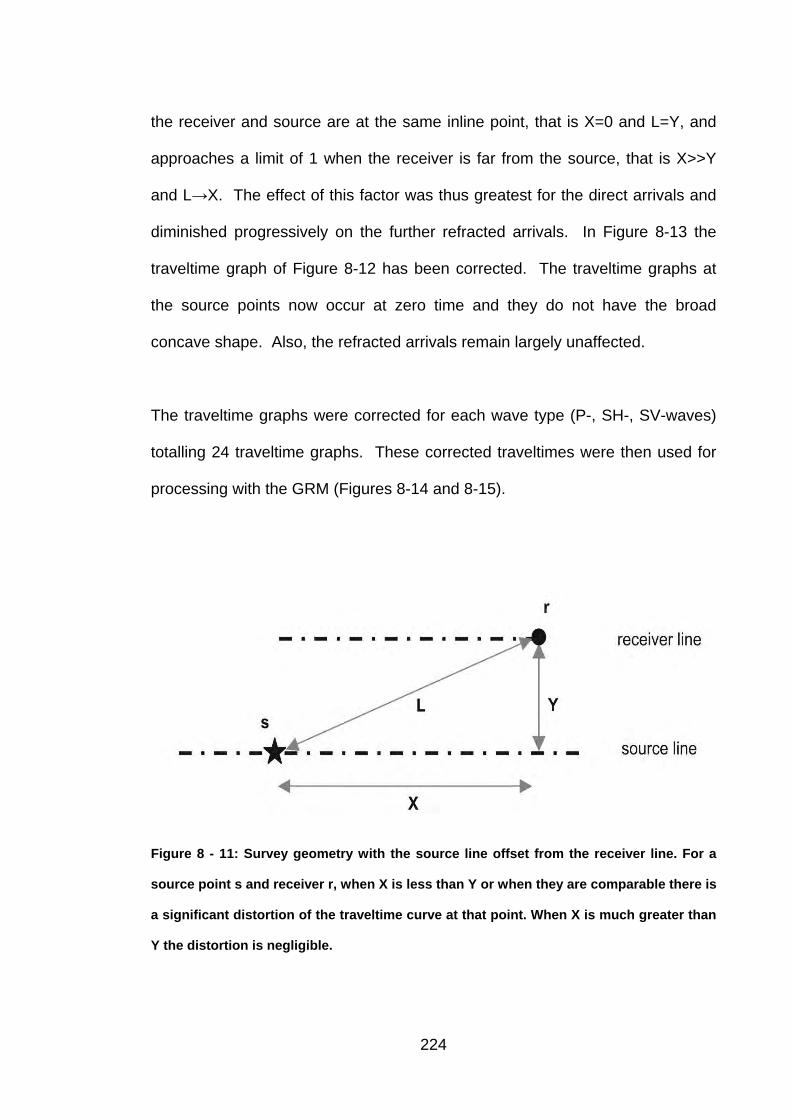
the receiver and source are at the same inline point, that is X=0 and L=Y, and
approaches a limit of 1 when the receiver is far from the source, that is X>>Y
and L→X. The effect of this factor was thus greatest for the direct arrivals and
diminished progressively on the further refracted arrivals. In Figure 8-13 the
traveltime graph of Figure 8-12 has been corrected. The traveltime graphs at
the source points now occur at zero time and they do not have the broad
concave shape. Also, the refracted arrivals remain largely unaffected.
The traveltime graphs were corrected for each wave type (P-, SH-, SV-waves)
totalling 24 traveltime graphs. These corrected traveltimes were then used for
processing with the GRM (Figures 8-14 and 8-15).
Figure 8 - 11: Survey geometry with the source line offset from the receiver line. For a
source point s and receiver r, when X is less than Y or when they are comparable there is
a significant distortion of the traveltime curve at that point. When X is much greater than
Y the distortion is negligible.
224
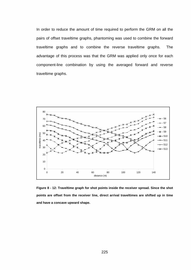
In order to reduce the amount of time required to perform the GRM on all the
pairs of offset traveltime graphs, phantoming was used to combine the forward
traveltime graphs and to combine the reverse traveltime graphs. The
advantage of this process was that the GRM was applied only once for each
component-line combination by using the averaged forward and reverse
traveltime graphs.
0
10
20
30
40
50
60
70
80
0 20 40 60 80 100 120 140distance (m)
trave
ltime
(ms)
S6
S7
S8
S9
S10
S11
S12
S13
Figure 8 - 12: Traveltime graph for shot points inside the receiver spread. Since the shot
points are offset from the receiver line, direct arrival traveltimes are shifted up in time
and have a concave upward shape.
225
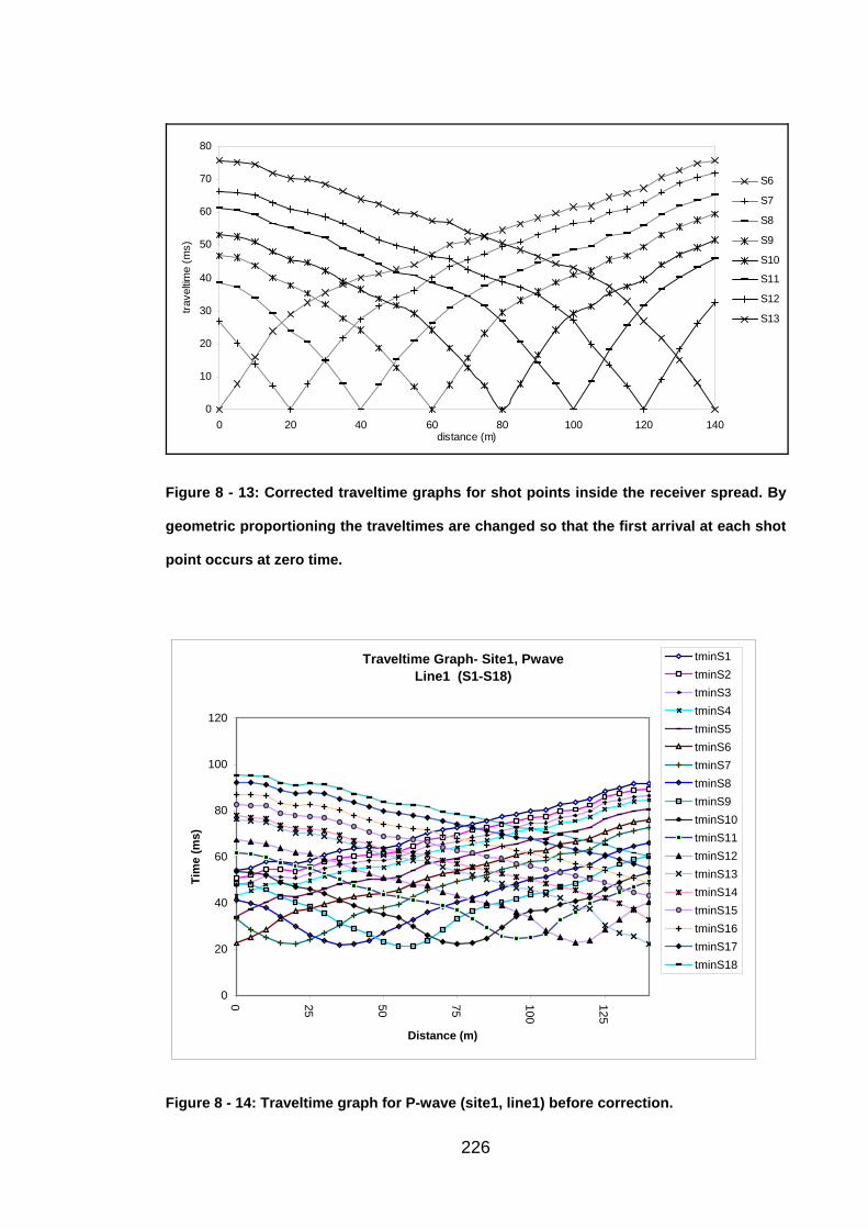
0
10
20
30
40
50
60
70
80
0 20 40 60 80 100 120 140distance (m)
trave
ltime
(ms)
S6
S7
S8
S9
S10
S11
S12
S13
Figure 8 - 13: Corrected traveltime graphs for shot points inside the receiver spread. By
geometric proportioning the traveltimes are changed so that the first arrival at each shot
point occurs at zero time.
Traveltime Graph- Site1, Pwave Line1 (S1-S18)
0
20
40
60
80
100
120
0 25 50 75 100
125
Distance (m)
Tim
e (m
s)
tminS1tminS2tminS3tminS4tminS5tminS6tminS7tminS8tminS9tminS10tminS11tminS12tminS13tminS14tminS15tminS16tminS17tminS18
Figure 8 - 14: Traveltime graph for P-wave (site1, line1) before correction.
226
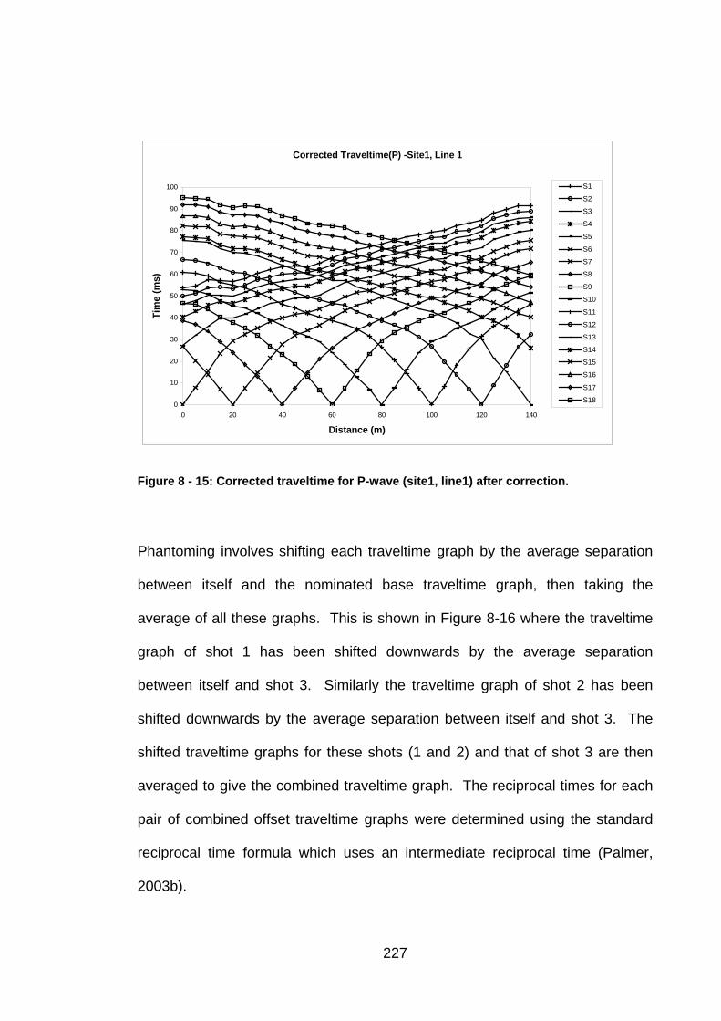
Corrected Traveltime(P) -Site1, Line 1
0
10
20
30
40
50
60
70
80
90
100
0 20 40 60 80 100 120 140
Distance (m)
Tim
e (m
s)
S1
S2
S3
S4
S5
S6
S7
S8
S9
S10
S11
S12
S13
S14
S15
S16
S17
S18
Figure 8 - 15: Corrected traveltime for P-wave (site1, line1) after correction.
Phantoming involves shifting each traveltime graph by the average separation
between itself and the nominated base traveltime graph, then taking the
average of all these graphs. This is shown in Figure 8-16 where the traveltime
graph of shot 1 has been shifted downwards by the average separation
between itself and shot 3. Similarly the traveltime graph of shot 2 has been
shifted downwards by the average separation between itself and shot 3. The
shifted traveltime graphs for these shots (1 and 2) and that of shot 3 are then
averaged to give the combined traveltime graph. The reciprocal times for each
pair of combined offset traveltime graphs were determined using the standard
reciprocal time formula which uses an intermediate reciprocal time (Palmer,
2003b).
227
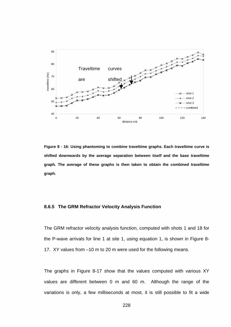
40
50
60
70
80
90
0 20 40 60 80 100 120 140distance (m)
trave
ltime
(ms)
shot 1
shot 2
shot 3
combined
Traveltime curves
are shifted
Figure 8 - 16: Using phantoming to combine traveltime graphs. Each traveltime curve is
shifted downwards by the average separation between itself and the base traveltime
graph. The average of these graphs is then taken to obtain the combined traveltime
graph.
8.6.5 The GRM Refractor Velocity Analysis Function
The GRM refractor velocity analysis function, computed with shots 1 and 18 for
the P-wave arrivals for line 1 at site 1, using equation 1, is shown in Figure 8-
17. XY values from –10 m to 20 m were used for the following means.
The graphs in Figure 8-17 show that the values computed with various XY
values are different between 0 m and 60 m. Although the range of the
variations is only, a few milliseconds at most, it is still possible to fit a wide
228
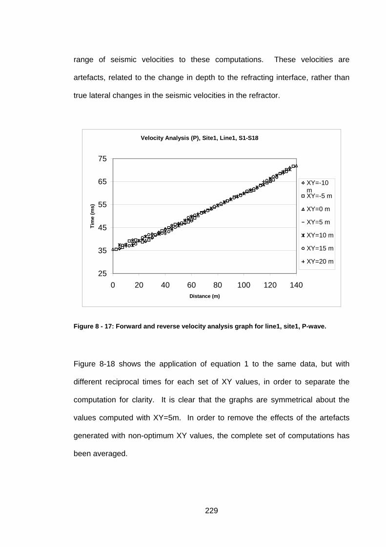
range of seismic velocities to these computations. These velocities are
artefacts, related to the change in depth to the refracting interface, rather than
true lateral changes in the seismic velocities in the refractor.
Velocity Analysis (P), Site1, Line1, S1-S18
25
35
45
55
65
75
0 20 40 60 80 100 120 140Distance (m)
Tim
e (m
s)
XY=-10mXY=-5 m
XY=0 m
XY=5 m
XY=10 m
XY=15 m
XY=20 m
Figure 8 - 17: Forward and reverse velocity analysis graph for line1, site1, P-wave.
Figure 8-18 shows the application of equation 1 to the same data, but with
different reciprocal times for each set of XY values, in order to separate the
computation for clarity. It is clear that the graphs are symmetrical about the
values computed with XY=5m. In order to remove the effects of the artefacts
generated with non-optimum XY values, the complete set of computations has
been averaged.
229
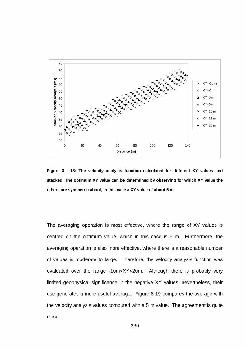
20
25
30
35
40
45
50
55
60
65
70
75
0 20 40 60 80 100 120 140
Distance (m)
Stac
ked
Velo
city
Ana
lysi
s (m
s)
XY=-10 m
XY=-5 m
XY=0 m
XY=5 m
XY=10 m
XY=15 m
XY=20 m
Figure 8 - 18: The velocity analysis function calculated for different XY values and
stacked. The optimum XY value can be determined by observing for which XY value the
others are symmetric about, in this case a XY value of about 5 m.
The averaging operation is most effective, where the range of XY values is
centred on the optimum value, which in this case is 5 m. Furthermore, the
averaging operation is also more effective, where there is a reasonable number
of values is moderate to large. Therefore, the velocity analysis function was
evaluated over the range -10m<XY<20m. Although there is probably very
limited geophysical significance in the negative XY values, nevertheless, their
use generates a more useful average. Figure 8-19 compares the average with
the velocity analysis values computed with a 5 m value. The agreement is quite
close.
230
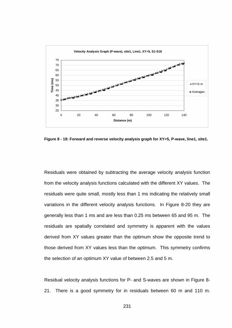
Velocity Analysis Graph (P-wave), site1, Line1, XY=5, S1-S18
2530354045505560657075
0 20 40 60 80 100 120 140
Distance (m)
Tim
e (m
s)
XY=5 m
Averages
Figure 8 - 19: Forward and reverse velocity analysis graph for XY=5, P-wave, line1, site1.
Residuals were obtained by subtracting the average velocity analysis function
from the velocity analysis functions calculated with the different XY values. The
residuals were quite small, mostly less than 1 ms indicating the relatively small
variations in the different velocity analysis functions. In Figure 8-20 they are
generally less than 1 ms and are less than 0.25 ms between 65 and 95 m. The
residuals are spatially correlated and symmetry is apparent with the values
derived from XY values greater than the optimum show the opposite trend to
those derived from XY values less than the optimum. This symmetry confirms
the selection of an optimum XY value of between 2.5 and 5 m.
Residual velocity analysis functions for P- and S-waves are shown in Figure 8-
21. There is a good symmetry for in residuals between 60 m and 110 m.
231
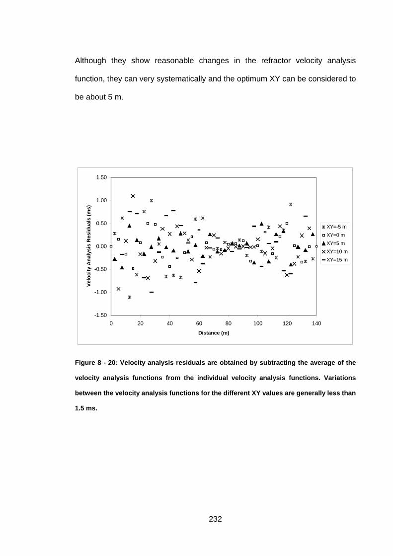
Although they show reasonable changes in the refractor velocity analysis
function, they can very systematically and the optimum XY can be considered to
be about 5 m.
-1.50
-1.00
-0.50
0.00
0.50
1.00
1.50
0 20 40 60 80 100 120 140
Distance (m)
Velo
city
Ana
lysi
s R
esid
uals
(ms)
XY=-5 mXY=0 mXY=5 mXY=10 mXY=15 m
Figure 8 - 20: Velocity analysis residuals are obtained by subtracting the average of the
velocity analysis functions from the individual velocity analysis functions. Variations
between the velocity analysis functions for the different XY values are generally less than
1.5 ms.
232
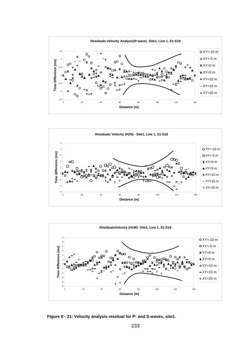
Residuals Velocity Analysis(P-wave) -Site1, Line 1, S1-S18
-1.5
-1
-0.5
0
0.5
1
1.5
0 20 40 60 80 100 120 140
Distance (m)
Tim
e di
ffere
nce
(ms)
XY=-10 m
XY=-5 m
XY=0 m
XY=5 m
XY=10 m
XY=15 m
XY=20 m
Residuals Velocity (H2N) - Site1, Line 1, S1-S18
-3
-2
-1
0
1
2
3
4
5
0 20 40 60 80 100 120 140
Distance (m)
Tim
e di
ffere
nce
(ms)
XY=-10 m
XY=-5 m
XY=0 m
XY=5 m
XY=10 m
XY=15 m
XY=20 m
ResidualsVelocity (H1W)- Site1, Line 1, S1-S18
-5
-4
-3
-2
-1
0
1
2
3
4
5
6
0 20 40 60 80 100 120 140
Distance (m)
Tim
e di
ffere
nce
(ms)
XY=-10 m
XY=-5 m
XY=0 m
XY=5 m
XY=10 m
XY=15 m
XY=20 m
Figure 8 - 21: Velocity analysis residual for P- and S-waves, site1.
233
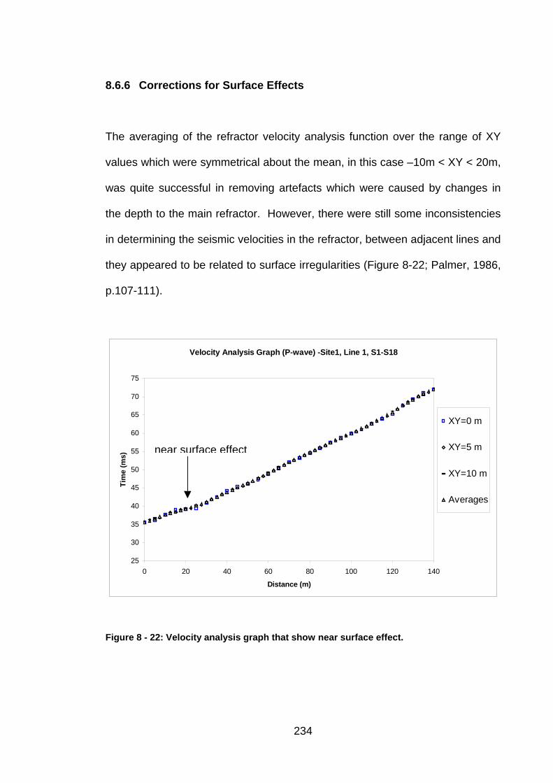
8.6.6 Corrections for Surface Effects
The averaging of the refractor velocity analysis function over the range of XY
values which were symmetrical about the mean, in this case –10m < XY < 20m,
was quite successful in removing artefacts which were caused by changes in
the depth to the main refractor. However, there were still some inconsistencies
in determining the seismic velocities in the refractor, between adjacent lines and
they appeared to be related to surface irregularities (Figure 8-22; Palmer, 1986,
p.107-111).
Velocity Analysis Graph (P-wave) -Site1, Line 1, S1-S18
25
30
35
40
45
50
55
60
65
70
75
0 20 40 60 80 100 120 140
Distance (m)
Tim
e (m
s)
XY=0 m
XY=5 m
XY=10 m
Averages
near surface effect
Figure 8 - 22: Velocity analysis graph that show near surface effect.
234
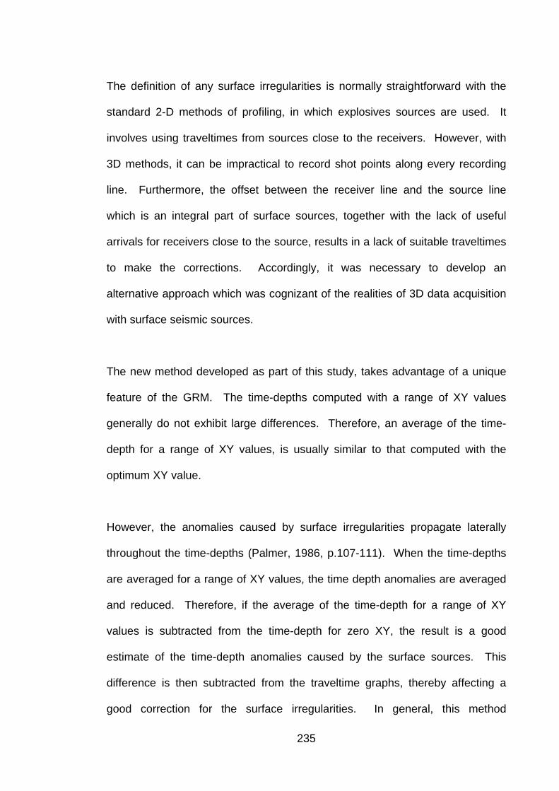
The definition of any surface irregularities is normally straightforward with the
standard 2-D methods of profiling, in which explosives sources are used. It
involves using traveltimes from sources close to the receivers. However, with
3D methods, it can be impractical to record shot points along every recording
line. Furthermore, the offset between the receiver line and the source line
which is an integral part of surface sources, together with the lack of useful
arrivals for receivers close to the source, results in a lack of suitable traveltimes
to make the corrections. Accordingly, it was necessary to develop an
alternative approach which was cognizant of the realities of 3D data acquisition
with surface seismic sources.
The new method developed as part of this study, takes advantage of a unique
feature of the GRM. The time-depths computed with a range of XY values
generally do not exhibit large differences. Therefore, an average of the time-
depth for a range of XY values, is usually similar to that computed with the
optimum XY value.
However, the anomalies caused by surface irregularities propagate laterally
throughout the time-depths (Palmer, 1986, p.107-111). When the time-depths
are averaged for a range of XY values, the time depth anomalies are averaged
and reduced. Therefore, if the average of the time-depth for a range of XY
values is subtracted from the time-depth for zero XY, the result is a good
estimate of the time-depth anomalies caused by the surface sources. This
difference is then subtracted from the traveltime graphs, thereby affecting a
good correction for the surface irregularities. In general, this method
235
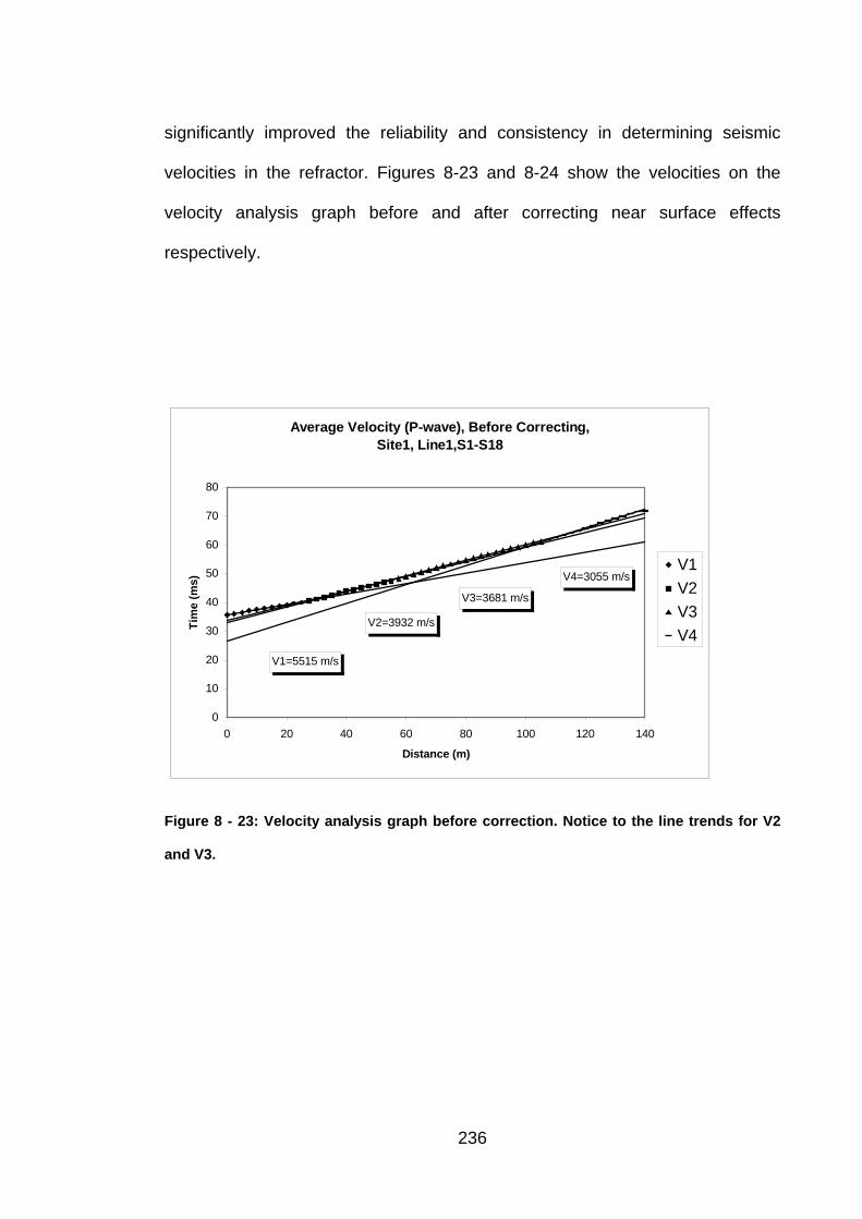
significantly improved the reliability and consistency in determining seismic
velocities in the refractor. Figures 8-23 and 8-24 show the velocities on the
velocity analysis graph before and after correcting near surface effects
respectively.
Average Velocity (P-wave), Before Correcting, Site1, Line1,S1-S18
V1=5515 m/s
V2=3932 m/s
V3=3681 m/s
V4=3055 m/s
0
10
20
30
40
50
60
70
80
0 20 40 60 80 100 120 140
Distance (m)
Tim
e (m
s)
V1V2V3V4
Figure 8 - 23: Velocity analysis graph before correction. Notice to the line trends for V2
and V3.
236
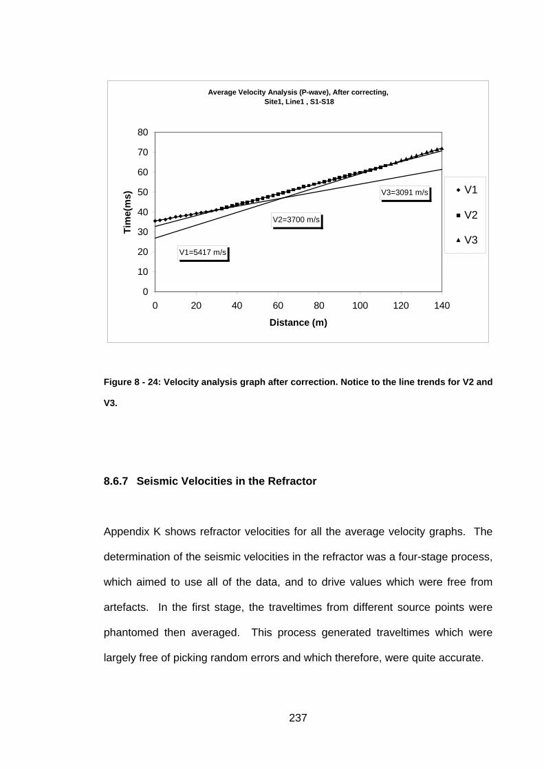
Average Velocity Analysis (P-wave), After correcting, Site1, Line1 , S1-S18
V1=5417 m/s
V2=3700 m/s
V3=3091 m/s
0
10
20
30
40
50
60
70
80
0 20 40 60 80 100 120 140
Distance (m)
Tim
e(m
s) V1
V2
V3
Figure 8 - 24: Velocity analysis graph after correction. Notice to the line trends for V2 and
V3.
8.6.7 Seismic Velocities in the Refractor
Appendix K shows refractor velocities for all the average velocity graphs. The
determination of the seismic velocities in the refractor was a four-stage process,
which aimed to use all of the data, and to drive values which were free from
artefacts. In the first stage, the traveltimes from different source points were
phantomed then averaged. This process generated traveltimes which were
largely free of picking random errors and which therefore, were quite accurate.
237
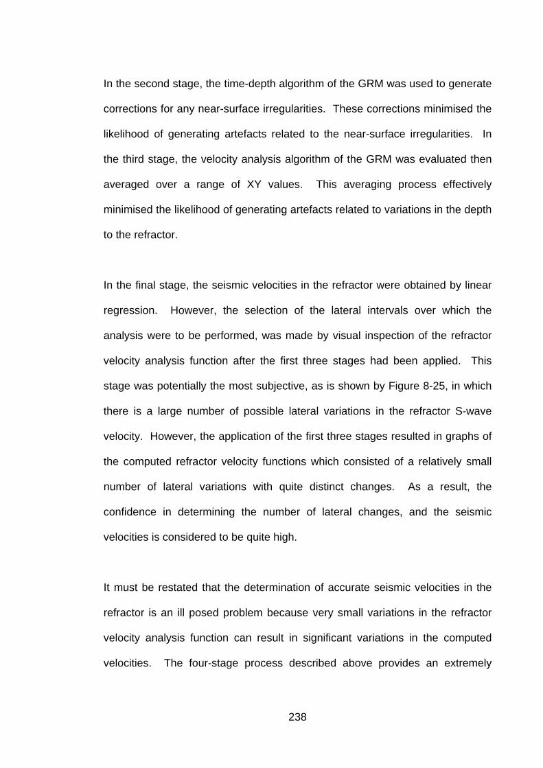
In the second stage, the time-depth algorithm of the GRM was used to generate
corrections for any near-surface irregularities. These corrections minimised the
likelihood of generating artefacts related to the near-surface irregularities. In
the third stage, the velocity analysis algorithm of the GRM was evaluated then
averaged over a range of XY values. This averaging process effectively
minimised the likelihood of generating artefacts related to variations in the depth
to the refractor.
In the final stage, the seismic velocities in the refractor were obtained by linear
regression. However, the selection of the lateral intervals over which the
analysis were to be performed, was made by visual inspection of the refractor
velocity analysis function after the first three stages had been applied. This
stage was potentially the most subjective, as is shown by Figure 8-25, in which
there is a large number of possible lateral variations in the refractor S-wave
velocity. However, the application of the first three stages resulted in graphs of
the computed refractor velocity functions which consisted of a relatively small
number of lateral variations with quite distinct changes. As a result, the
confidence in determining the number of lateral changes, and the seismic
velocities is considered to be quite high.
It must be restated that the determination of accurate seismic velocities in the
refractor is an ill posed problem because very small variations in the refractor
velocity analysis function can result in significant variations in the computed
velocities. The four-stage process described above provides an extremely
238
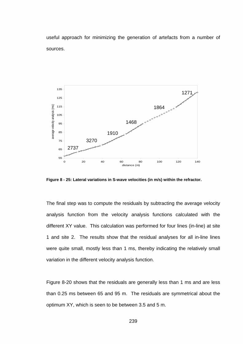
useful approach for minimizing the generation of artefacts from a number of
sources.
55
65
75
85
95
105
115
125
135
0 20 40 60 80 100 120 1distance (m)
aver
age v
elocit
y ana
lysis
(ms)
40
1271
1864
1468
19103270
2737
Figure 8 - 25: Lateral variations in S-wave velocities (in m/s) within the refractor.
The final step was to compute the residuals by subtracting the average velocity
analysis function from the velocity analysis functions calculated with the
different XY value. This calculation was performed for four lines (in-line) at site
1 and site 2. The results show that the residual analyses for all in-line lines
were quite small, mostly less than 1 ms, thereby indicating the relatively small
variation in the different velocity analysis function.
Figure 8-20 shows that the residuals are generally less than 1 ms and are less
than 0.25 ms between 65 and 95 m. The residuals are symmetrical about the
optimum XY, which is seen to be between 3.5 and 5 m.
239
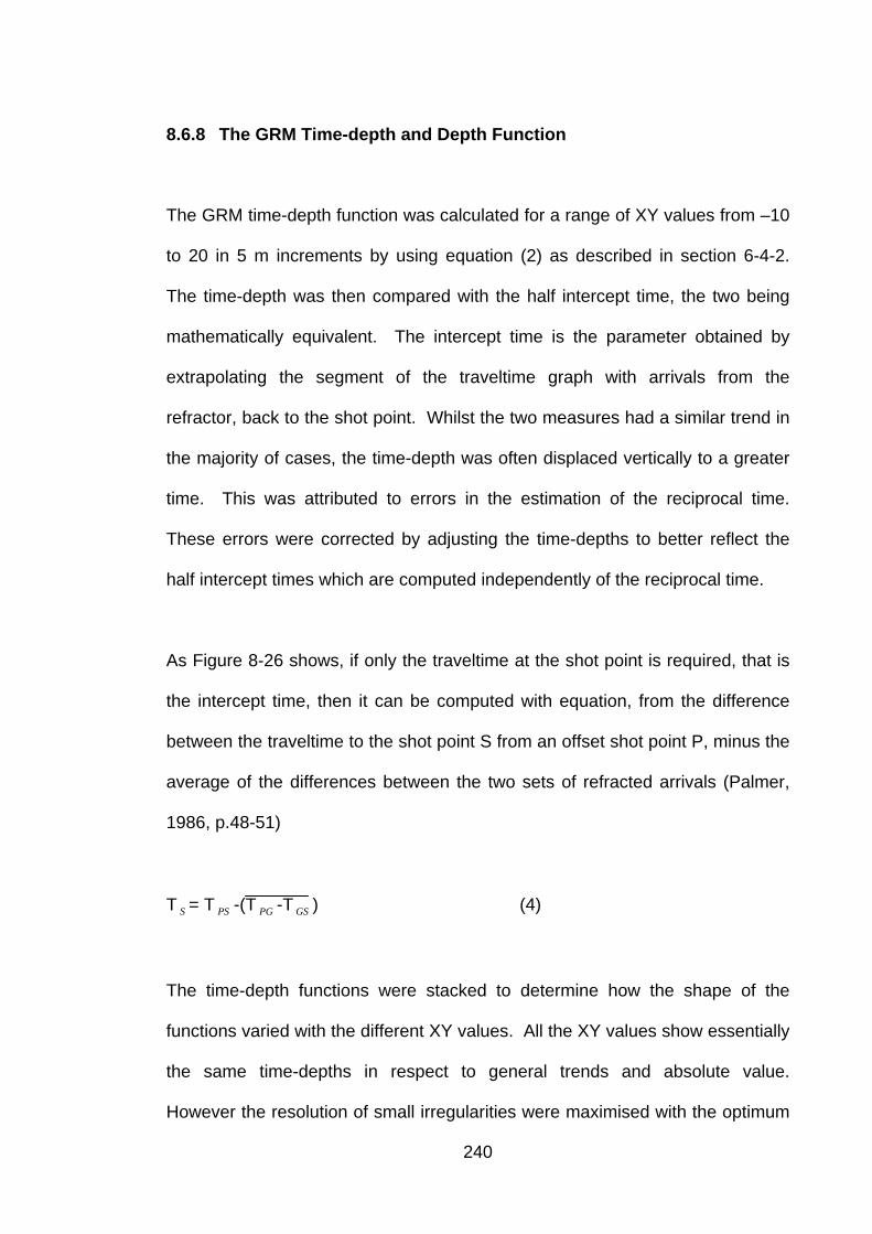
8.6.8 The GRM Time-depth and Depth Function
The GRM time-depth function was calculated for a range of XY values from –10
to 20 in 5 m increments by using equation (2) as described in section 6-4-2.
The time-depth was then compared with the half intercept time, the two being
mathematically equivalent. The intercept time is the parameter obtained by
extrapolating the segment of the traveltime graph with arrivals from the
refractor, back to the shot point. Whilst the two measures had a similar trend in
the majority of cases, the time-depth was often displaced vertically to a greater
time. This was attributed to errors in the estimation of the reciprocal time.
These errors were corrected by adjusting the time-depths to better reflect the
half intercept times which are computed independently of the reciprocal time.
As Figure 8-26 shows, if only the traveltime at the shot point is required, that is
the intercept time, then it can be computed with equation, from the difference
between the traveltime to the shot point S from an offset shot point P, minus the
average of the differences between the two sets of refracted arrivals (Palmer,
1986, p.48-51)
T = T -(T -T GS ) (4) S PS PG
The time-depth functions were stacked to determine how the shape of the
functions varied with the different XY values. All the XY values show essentially
the same time-depths in respect to general trends and absolute value.
However the resolution of small irregularities were maximised with the optimum
240
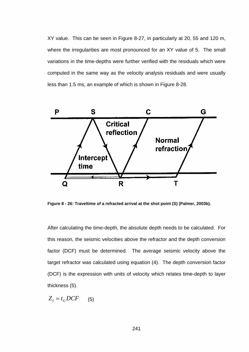
XY value. This can be seen in Figure 8-27, in particularly at 20, 55 and 120 m,
where the irregularities are most pronounced for an XY value of 5. The small
variations in the time-depths were further verified with the residuals which were
computed in the same way as the velocity analysis residuals and were usually
less than 1.5 ms, an example of which is shown in Figure 8-28.
Figure 8 - 26: Traveltime of a refracted arrival at the shot point (S) (Palmer, 2003b).
After calculating the time-depth, the absolute depth needs to be calculated. For
this reason, the seismic velocities above the refractor and the depth conversion
factor (DCF) must be determined. The average seismic velocity above the
target refractor was calculated using equation (4). The depth conversion factor
(DCF) is the expression with units of velocity which relates time-depth to layer
thickness (5).
DCFtZ G=1 (5)
241
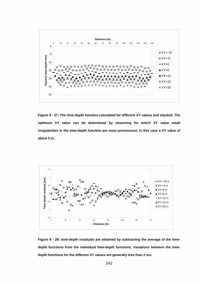
0
5
10
15
20
25
30
0 10 20 30 40 50 60 70 80 90 100 110 120 130 140
Distance (m)
Stac
ked
time-
dept
h (m
s)
XY=-10
XY=-5
XY=0
XY=5
XY=10
XY=15
XY=20
Figure 8 - 27: The time-depth function calculated for different XY values and stacked. The
optimum XY value can be determined by observing for which XY value small
irregularities in the time-depth function are most pronounced, in this case a XY value of
about 5 m.
-1.5
-1
-0.5
0
0.5
1
1.5
0 20 40 60 80 100 120 140
Distance (m)
Tim
e-de
oth
resi
dual
(ms)
XY=-10 mXY=-5 mXY=0 mXY=5 mXY=10 mXY=15 mXY=20 m
Figure 8 - 28: time-depth residuals are obtained by subtracting the average of the time-
depth functions from the individual time-depth functions. Variations between the time-
depth functions for the different XY values are generally less than 2 ms.
242
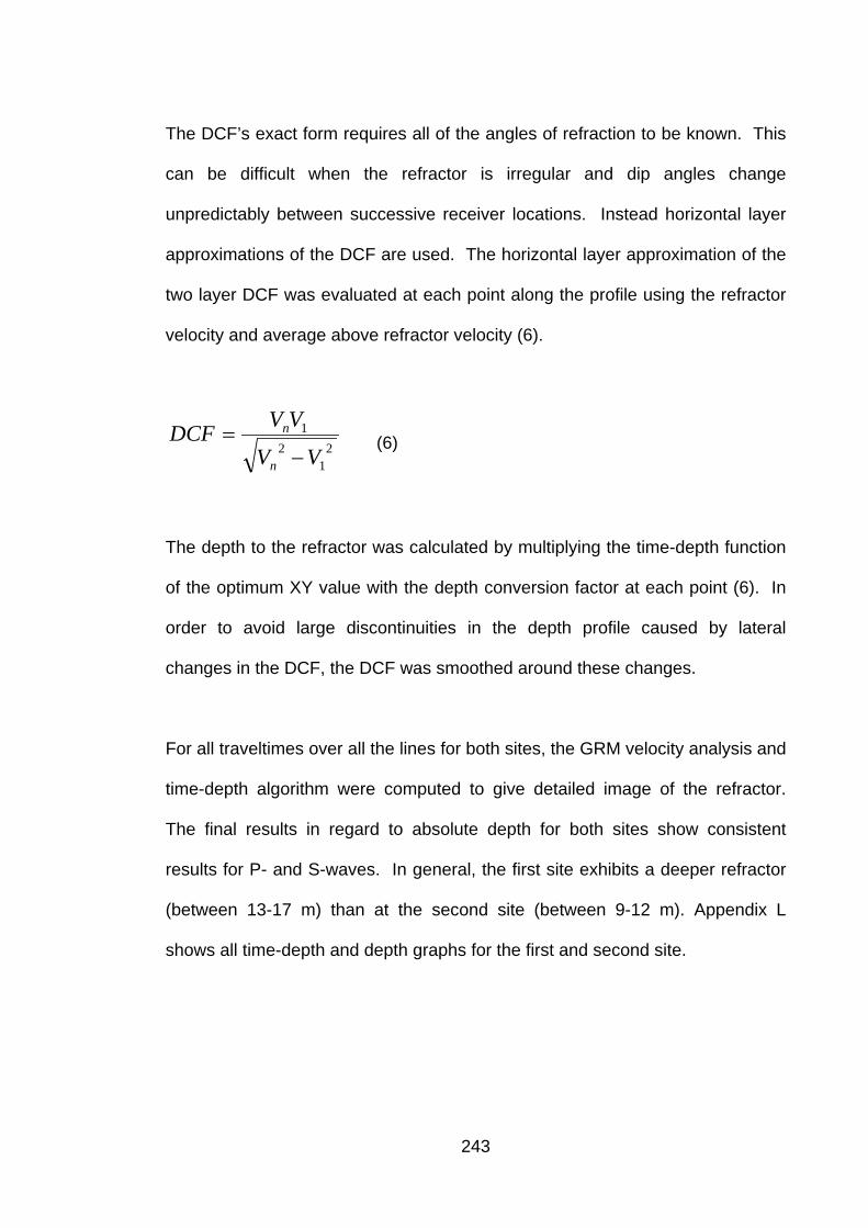
The DCF’s exact form requires all of the angles of refraction to be known. This
can be difficult when the refractor is irregular and dip angles change
unpredictably between successive receiver locations. Instead horizontal layer
approximations of the DCF are used. The horizontal layer approximation of the
two layer DCF was evaluated at each point along the profile using the refractor
velocity and average above refractor velocity (6).
21
21
VV
VVDCFn
n
−= (6)
The depth to the refractor was calculated by multiplying the time-depth function
of the optimum XY value with the depth conversion factor at each point (6). In
order to avoid large discontinuities in the depth profile caused by lateral
changes in the DCF, the DCF was smoothed around these changes.
For all traveltimes over all the lines for both sites, the GRM velocity analysis and
time-depth algorithm were computed to give detailed image of the refractor.
The final results in regard to absolute depth for both sites show consistent
results for P- and S-waves. In general, the first site exhibits a deeper refractor
(between 13-17 m) than at the second site (between 9-12 m). Appendix L
shows all time-depth and depth graphs for the first and second site.
243
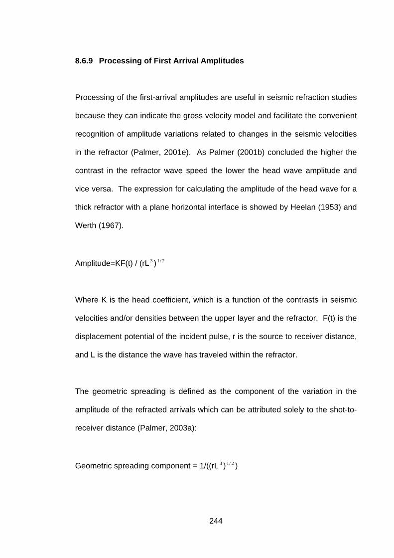
8.6.9 Processing of First Arrival Amplitudes
Processing of the first-arrival amplitudes are useful in seismic refraction studies
because they can indicate the gross velocity model and facilitate the convenient
recognition of amplitude variations related to changes in the seismic velocities
in the refractor (Palmer, 2001e). As Palmer (2001b) concluded the higher the
contrast in the refractor wave speed the lower the head wave amplitude and
vice versa. The expression for calculating the amplitude of the head wave for a
thick refractor with a plane horizontal interface is showed by Heelan (1953) and
Werth (1967).
Amplitude=KF(t) / (rL 3 ) 2/1
Where K is the head coefficient, which is a function of the contrasts in seismic
velocities and/or densities between the upper layer and the refractor. F(t) is the
displacement potential of the incident pulse, r is the source to receiver distance,
and L is the distance the wave has traveled within the refractor.
The geometric spreading is defined as the component of the variation in the
amplitude of the refracted arrivals which can be attributed solely to the shot-to-
receiver distance (Palmer, 2003a):
Geometric spreading component = 1/((rL ) ) 3 2/1
244
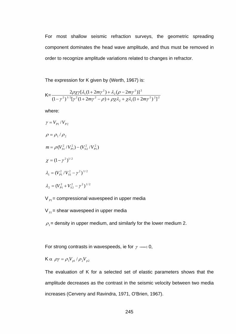
For most shallow seismic refraction surveys, the geometric spreading
component dominates the head wave amplitude, and thus must be removed in
order to recognize amplitude variations related to changes in refractor.
The expression for K given by (Werth, 1967) is:
K= 22212
222/12
222
21
])21()21([)1()]2()21([2
γχλρχλργγγγρλγλρχγ
mmmm
+++−+−−++
where:
21 / PP VV=γ
21 / ρρρ =
)/()/( 21
22
21
21 PSPS VVVVm −= ρ
2/12 )1( γχ −=
2/1221
211 )/( γλ −= SP VV
2/1222
212 )( γλ −+= SP VV
V = compressional wavespeed in upper media 1P
V = shear wavespeed in upper media 1S
1ρ = density in upper medium, and similarly for the lower medium 2.
For strong contrasts in wavespeeds, ie for γ ⎯→⎯ 0,
K α 2211 / pp VV ρργρ =
The evaluation of K for a selected set of elastic parameters shows that the
amplitude decreases as the contrast in the seismic velocity between two media
increases (Cerveny and Ravindra, 1971, O'Brien, 1967).
245

In order to recognize any amplitude variations related to the head coefficient, it
was necessary to reduce the effect of geometrical spreading. This was done by
computing the amplitude product for each forward and reverse shot pair
(Palmer, 2003b). The product of the forward and reverse shot amplitudes
largely compensates for the effects of geometric spreading and dipping
refractors (Palmer, 2003b, Palmer, 2001b). The amplitude product was
calculated only for the P-waves since the S-waves did not show good
consistency.
The effectiveness of this operation can be seen in Figure 8-29. The Figure
shows the large amount of geometric spreading from a shot pair 20 m from the
receiver spread, with the amplitudes decaying much faster than the reciprocal of
the distance squared. The product of this shot pair as well as a number of other
offset shot pairs is shown in Figure 8-30. The removal of the geometric
spreading component is most effective between 20 and 100 m. Also there are
gross similarities in the shape of the amplitude products for all the shot pairs.
This suggests that the variations are related to the head coefficient and hence
to variations in the seismic velocities in the refractor.
246
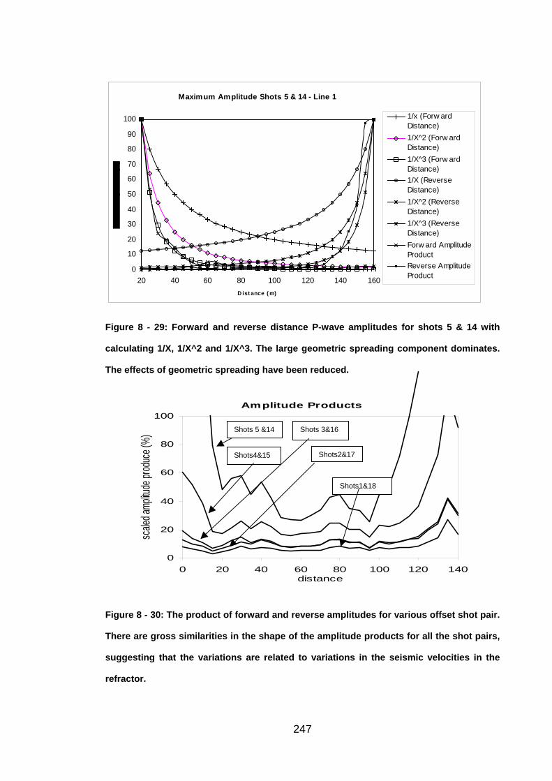
Maximum Amplitude Shots 5 & 14 - Line 1
0
10
20
30
40
50
60
70
80
90
100
20 40 60 80 100 120 140 160D ist ance ( m)
1/x (Forw ardDistance)1/X^2 (Forw ardDistance)1/X^3 (Forw ardDistance)1/X (ReverseDistance)1/X^2 (ReverseDistance)1/X^3 (ReverseDistance)Forw ard AmplitudeProductReverse AmplitudeProduct
Figure 8 - 29: Forward and reverse distance P-wave amplitudes for shots 5 & 14 with
calculating 1/X, 1/X^2 and 1/X^3. The large geometric spreading component dominates.
The effects of geometric spreading have been reduced.
Amplitude Products
0
20
40
60
80
100
0 20 40 60 80 100 120 140distance
scale
d amp
litude
prod
uce (
%)
Shots 5 &14
Shots4&15
Shots1&18
Shots2&17
Shots 3&16
Figure 8 - 30: The product of forward and reverse amplitudes for various offset shot pair.
There are gross similarities in the shape of the amplitude products for all the shot pairs,
suggesting that the variations are related to variations in the seismic velocities in the
refractor.
247
8.6.10 Velocity Ratios
Shear wave (S-wave) data can be readily combined with the interpretation of
conventional seismic compressional-wave (P-wave) data. After determining the
seismic velocities for both P- and S-waves, it was possible to calculate the
velocity ratio Vp/Vs or Poisson’s ratio along each profile. Although Poisson’s
ratio (σ) is not a constant of proportionality between stress and strain, it can be
expressed in terms of elastic constants, and is often used in the same context
as the elastic constants (Tatham, 1985).
The ratio Vp/Vs is defined in terms of Poisson’s ratio (σ) and is given by
(Reynolds, 1997):
2/1
2/11
⎟⎠⎞
⎜⎝⎛
−−
=σ
σVsVp
where:
2/13/4
⎟⎟⎠
⎞⎜⎜⎝
⎛ +=
ρµkVp
( ) 2/1/ ρµ=Vs
k=Bulk modulus
µ = Shear (rigidity) modulus
ρ = density
Note that µ =0 for a fluid, as fluids cannot support shear-waves, and the
maximum value of Poisson’s ratio is 0.5; σ % 0.05 for very hard rocks, %0.45 for
loose, unconsolidated sediments, average % 0.25.
248
8.6.11 Three-Dimensional Images
Three-dimensional images were generated by using the results from the
processing of the first-arrival traveltimes and amplitudes across the four lines at
the first and second site. Image maps in Surfur (8) were used to generate
three-dimensional images.
8.6.12 Traveltime Tomography
Wavepath eikonal traveltime (WET) tomography was used to generate a
velocity-depth section of every line for each wave type. WET tomography
accommodates multiple signal paths contributing to each first break and is a
computationally efficient and geophysically robust method. Wavepath eikonal
traveltime inversion is a high frequency traveltime tomographic method. It is a
computationally efficient method, being an order of magnitude faster than wave-
equation traveltime inversion (yet comparable in effectiveness) since only
solutions to the eikonal equation are involved. It models multiple signal
propagation paths contributing to one first-arrival and as such is superior to
conventional ray-tracing tomography which is limited to the modelling of just one
ray per first-arrival (for a brief discussion on WET theory see Appendix M).
The first step was to generate starting model by using both one and two
dimensional inversion methods. The delta-t-V method was used to generate 1D
starting models (Gebrande and Miller, 1985). This method is a pseudo-
249
tomographic method that yields one-dimensional velocity profiles for each
common midpoint (CMP). This turning ray inversion method delivers
continuous depth vs. velocity profiles for all profile stations. The first step of the
WET inversion algorithm is to propose an initial slowness model, which may be
generated assuming constant vertical velocity gradients such as with 1D tau-p
inversion (see Appendix M), or assuming discrete velocity changes such as with
the generalised reciprocal method (Palmer, 2003a). The depth sections and
seismic velocities obtained with the GRM (as discussed previously) were used
to generate 2-D starting models.
The starting models were then refined with WET tomography until ideally the
modelled traveltimes matched the field traveltimes. A perfect match between
the traveltimes however was never realised, with the mean unsigned error
around 2 ms (Appendix N). This was because after a certain number of
iterations in the WET tomography algorithm, the amount of change between the
updated velocity fields of consecutive iterations decreased, that is the rate of
convergence between the modelled and field traveltimes decreased. At this
point the WET algorithm was terminated.
The differences between the final models generated using the 1-D and 2-D
starting models were significant. Furthermore the errors between them and the
field data were both comparable and within the bounds of acceptable accuracy.
This non-uniqueness is illustrated in Figure 6-31, the top and bottom sections
being derived from 1-D and 2-D starting models respectively. Both fit the field
data to acceptable accuracy. However the differences between the two are
250
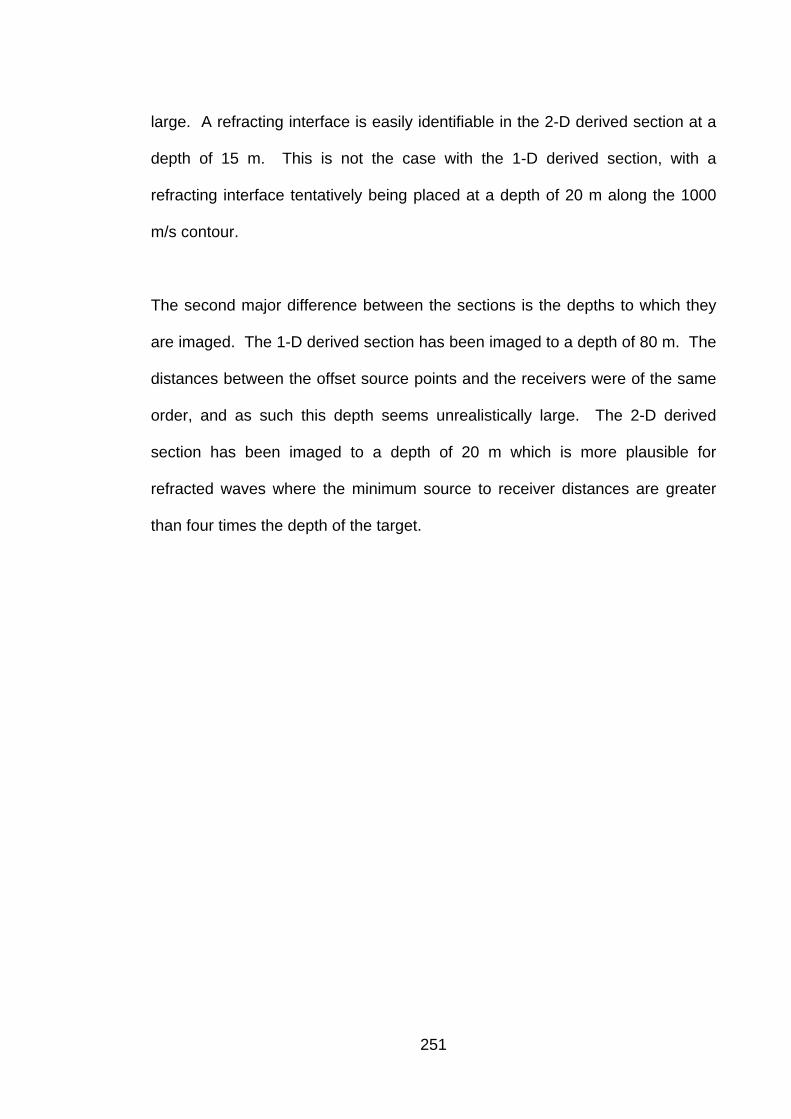
large. A refracting interface is easily identifiable in the 2-D derived section at a
depth of 15 m. This is not the case with the 1-D derived section, with a
refracting interface tentatively being placed at a depth of 20 m along the 1000
m/s contour.
The second major difference between the sections is the depths to which they
are imaged. The 1-D derived section has been imaged to a depth of 80 m. The
distances between the offset source points and the receivers were of the same
order, and as such this depth seems unrealistically large. The 2-D derived
section has been imaged to a depth of 20 m which is more plausible for
refracted waves where the minimum source to receiver distances are greater
than four times the depth of the target.
251
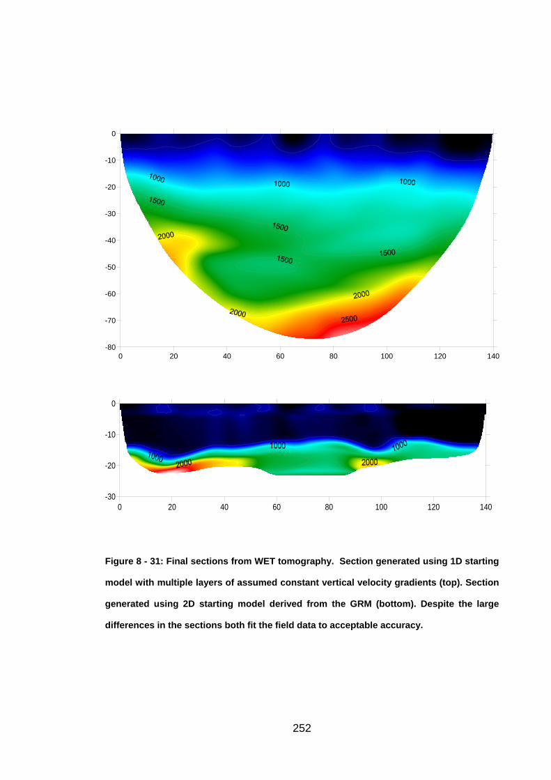
0 20 40 60 80 100 120 140-80
-70
-60
-50
-40
-30
-20
-10
0
0 20 40 60 80 100 120 140-30
-20
-10
0
Figure 8 - 31: Final sections from WET tomography. Section generated using 1D starting
model with multiple layers of assumed constant vertical velocity gradients (top). Section
generated using 2D starting model derived from the GRM (bottom). Despite the large
differences in the sections both fit the field data to acceptable accuracy.
252
Chapter 9
Interpretation
9.1 Summary
Three-dimensional three-component shallow seismic refraction surveys at two
sites of dryland salinity in the Spicers Creek Catchment New South Wales have
verified that the shear zone exists as a relatively narrow region of decreased
seismic velocity and increased depths of weathering. Refraction tomography
indicated that the shear zone’s seismic expression continued below the
refracting interface and into the bedrock.
Three-dimensional surveying provided an improvement in the structural imaging
capabilities of the refraction method. Despite showing gross trends along the
orthogonal two-dimensional profiles, variations in the in-line direction suggest
that shear zone has considerable lateral variations parallel to their strike. The
validity of these in-line variations are emphasised by their consistency in the
results of all the wave types. Furthermore, these variations are not predictable
on the basis of orthogonal two-dimensional profiles.
A detailed analysis of the refractor seismic velocities and amplitudes at two
sites, show a number of linear features parallel to and cross-cutting the shear
253
zone (Nikrouz and Palmer, 2004). These lineaments, on basis of the Dubbo
geological map, have been interpreted as a series of recent faults which cut the
older shear zone. The discharge of saline groundwater appears to occur along
the intersection of these faults with the shear zone.
At the first site the results show the seismic geophysical anomaly of half a shear
zone. The velocity-depth sections show that the shear zone’s seismic
expression extends below the refracting interface into the bedrock. All the
wave-types have similar spatial distribution in both time-depth and depth
images and have been interpreted as the boundary between bedrock and
overlying sediment. Changes in refractor seismic velocities occur in both the
cross-line and in-line directions. In the in-line direction, the velocities for all
wave-types show a general decreases with the refractor being separated into
three main regions of different velocities. Furthermore, the seismic velocities in
the refractor in the cross-line direction suggest the presence of a number of
cross cutting and parallel lineaments which have been interpreted to be a series
of faults.
At the second site, the results show the seismic response of a shear zone as a
narrow region of low seismic velocity and increased depth of weathering. The
P-wave/S-wave velocity ratios, which is quite sensitive to pore fluid saturant and
lithology, and Poisson’s ratios (σ ) show distinctive high values over the region.
This has been attributed to an increase in secondary porosity and permeability
from fracturing, leading to an increase in groundwater saturation. At site2, as at
site1, an interpretation of the refractor images of the seismic velocities and
254
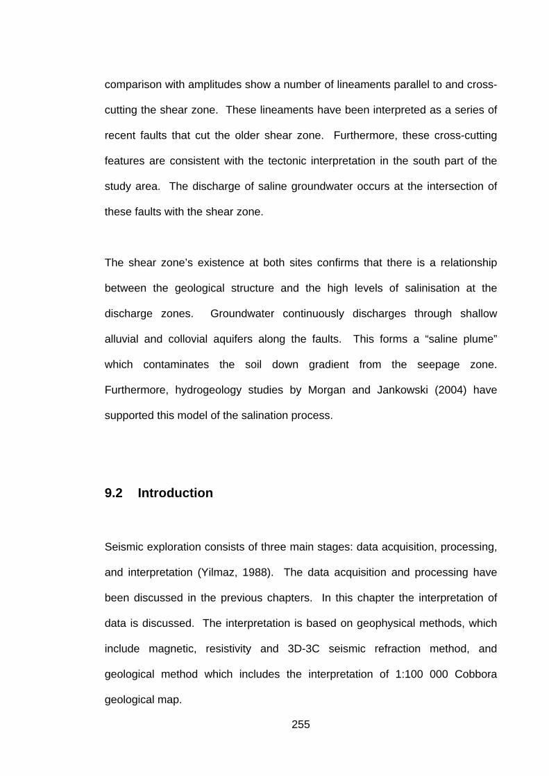
comparison with amplitudes show a number of lineaments parallel to and cross-
cutting the shear zone. These lineaments have been interpreted as a series of
recent faults that cut the older shear zone. Furthermore, these cross-cutting
features are consistent with the tectonic interpretation in the south part of the
study area. The discharge of saline groundwater occurs at the intersection of
these faults with the shear zone.
The shear zone’s existence at both sites confirms that there is a relationship
between the geological structure and the high levels of salinisation at the
discharge zones. Groundwater continuously discharges through shallow
alluvial and collovial aquifers along the faults. This forms a “saline plume”
which contaminates the soil down gradient from the seepage zone.
Furthermore, hydrogeology studies by Morgan and Jankowski (2004) have
supported this model of the salination process.
9.2 Introduction
Seismic exploration consists of three main stages: data acquisition, processing,
and interpretation (Yilmaz, 1988). The data acquisition and processing have
been discussed in the previous chapters. In this chapter the interpretation of
data is discussed. The interpretation is based on geophysical methods, which
include magnetic, resistivity and 3D-3C seismic refraction method, and
geological method which includes the interpretation of 1:100 000 Cobbora
geological map.
255

In the Spicers Creek Catchment magnetic, electrical resistivity and seismic
refraction methods were used to image the inferred shear zones. It was
anticipated that in this area, seismic refraction would provide the best results
since the propagation of seismic waves would not be affected by the high level
salinisation whilst also providing possibly greater resolution.
In general, the geophysical and geological interpretation show a consistent
result in terms of the being of shear zone and cross-cutting features at two sites
in the Spicers Creek Catchment.
9.3 Magnetic Data Interpretation
Figures 9-1 and 9-2 show the magnetic field in nanoteslas as a 2D contour plot
for the two sites. The magnetic results show reductions of approximately 2100
nanoteslas at site1 and 600 nanoteslas at site2 over the inferred zones of the
shear zones. The low magnetic values are inferred to be caused by the
enhanced oxidation of magnetite, the magnetite mineral, to hematite, goethite or
maghemite, resulting from fracturing of the rock associated with the shear zone.
Magnetite is unstable in the typically low temperature and highly oxidizing
environment of chemical weathering and sedimentation. Groundwater
containing CO causes the ferrous iron minerals to eventually break down with
Fe being slightly soluble in water containing CO . Meanwhile, the oxygen
fugacity sets the upper limit at which magnetite can exist as a stable compound.
2
+22
256

It is given by the fO2 vs T relationship that governs the oxidation of magnetite to
hematite (Grant, 1985):
)(32/1)(2 32243 hematiteOFeOmagnetiteOFe ⇔+
At the Spicers Creek Catchment, the magnetics show lows over the inferred
location of the shear zones. These magnetic lows are consistent with the
weathering of magnetite by the saline groundwater. Furthermore, the local
magnetic data is consistent with the airborne magnetic data obtained by AGSO
over the Dubbo 1:250,000 map (as discussed in chapter 5).
9.4 Resistivity Data Interpretation
Electrical resistivity survey methods have been employed for many decades to
image the near surface where they can provide useful information on geological
structure, lithologies and subsurface water resources. Resistivity methods are
widely employed in hydrogeological investigations (Kearey and Brooks, 2001),
because earth resistivity can be readily related to porosity and water quality.
2D resistivity imaging is a geophysical method which aims to generate a cross
section of the electrical properties of the subsurface by passing an electric
current along many different paths and measuring the associated potential
differences. This can be accomplished by connecting a linear array of
257
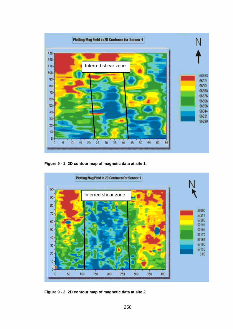
Figure 9 - 1: 2D contour map of magnetic data at site 1.
Inferred shear zone
Inferred shear zone
Figure 9 - 2: 2D contour map of magnetic data at site 2.
258

grounded electrodes through a multicore cable to a computer controlled
switching module and a resistivity meter. However, with the electrical resistivity
surveys at the Spicers Creek, the data were acquired with a traditional field
system using two current and two potential electrodes. A large number of
apparent resistivity measurements were made using differing combinations of
four electrodes along the array in a Wenner configuration. The apparent
resistivity measurements were used to plot pseudosections, which are
qualitatively related to the distribution of true resistivity. The pseudosections
are inverted using either a manual interactive approach or an automatic iterative
method to improve the detail and correctly scale the apparent resistivity image
giving a true resistivity-depth section (Griffiths and Barker, 1993).
The conductivity* of geological materials exhibits one of the largest ranges of all
physical properties (Reynolds, 1997). In a normal crust, from the surface to up
to 15 km depth, bulk conductivities are largely controlled by aqueous electrolytic
conduction (Ward, 1990). The major factors affecting the bulk electric
conductivity of soil or rock are (McNeill, 1990):
1. Porosity and permeability
2. Degree of saturation (fraction of pore space/fractures filled with moisture)
3. Presence of clays with moderate to high cation exchange capacity (CEC)
4. Conductivity of interstitial fluid
* Resistivity is the inverse of conductivity and has units of ohm-metres (Ωm). The following will refer to conductivity, which has units of siemens/metre (S/m). 259
Geological processes such as dissolution, faulting, shearing, and weathering
usually increase porosity and fluid permeability. Thus the result of such process
on a rock formation will be an increase in conductivity.
The fluid saturation of a rock formation is a direct influence on its conductivity.
A large proportion of pore spaces, fractures and other gaps filled with fluid in a
rock mass will enhance aqueous electrolytic conduction. In general, the
conductivity of a rock increases as the percent fluid saturation increases.
The presence of clay adds an additional component to conductivity, with clay
particles acting as separate conducting paths to the electrolyte path. Due to the
large cation-exchange capacity of clay, the cations of the diffuse layer are free
to move under the influence of an applied electric field. This leads to an
increase in the density of charge carriers and hence an increase in conductivity.
The salinity of interstitial fluid is perhaps the greatest factor determining the
conductivity of a rock. The ions that enable the flow of electric current in a fluid
result from the dissociation of salts, which occurs when salts are dissolved in
water. Since the quantity of charge that can be carried by an ion is finite, the
more ions available in a solution, the greater the total charge, and hence the
higher the conductivity. In general, a rock which contains water within its pores
will have a greater conductivity when the salinity of the water is high than when
it is low.
260
The resistivity of geological materials exhibits one of the largest ranges of all
physical properties, from m for native silver to m for pure
sulfur (Reynolds, 1997). In sedimentary rocks, the resistivity of the interstitial
fluid is probably more important than that the host rock. Archie (1942)
developed an empirical formula for the effective resistivity of a rock formation in
terms of the resistivity and volume of the pore water present as below:
Ω× −8106.1 Ω1610
wcb fa ρφρ −−=
Where φ is the porosity, the fraction of pores containing water of resistivity f
wρ and , and are empirical constants (a b c 5.0 5.2≤≤ a , , and
). Korvin (1982) has proposed a theoretical basis to account for Archie’s
Law. Salin groundwater may have a resistivity as low as 0.05 Ωm and some
groundwater can have resistivities in excess of 1000
5.23.1 ≤≤ m
2≈n
Ωm.
The 2D resistivity imaging results are shown in Figures 9-3 to 9-6. For each
Figure the top pseudosection is the measured apparent resistivity, whilst the
middle is the apparent resistivity starting model calculated by the inversion
software. The bottom is the resistivity-depth section resulting after three
iterations of the inversion program.
Evidence of the shear zone is not apparent in the resistivity-depth sections.
The sections do not show narrow vertical zones of low resistivity as would be
expected from the presence of the shear zone. Rather, they all show an
approximately layered subsurface with increasing resistivity with depth. The
very near surface does however show a degree of lateral variation in resistivity
261
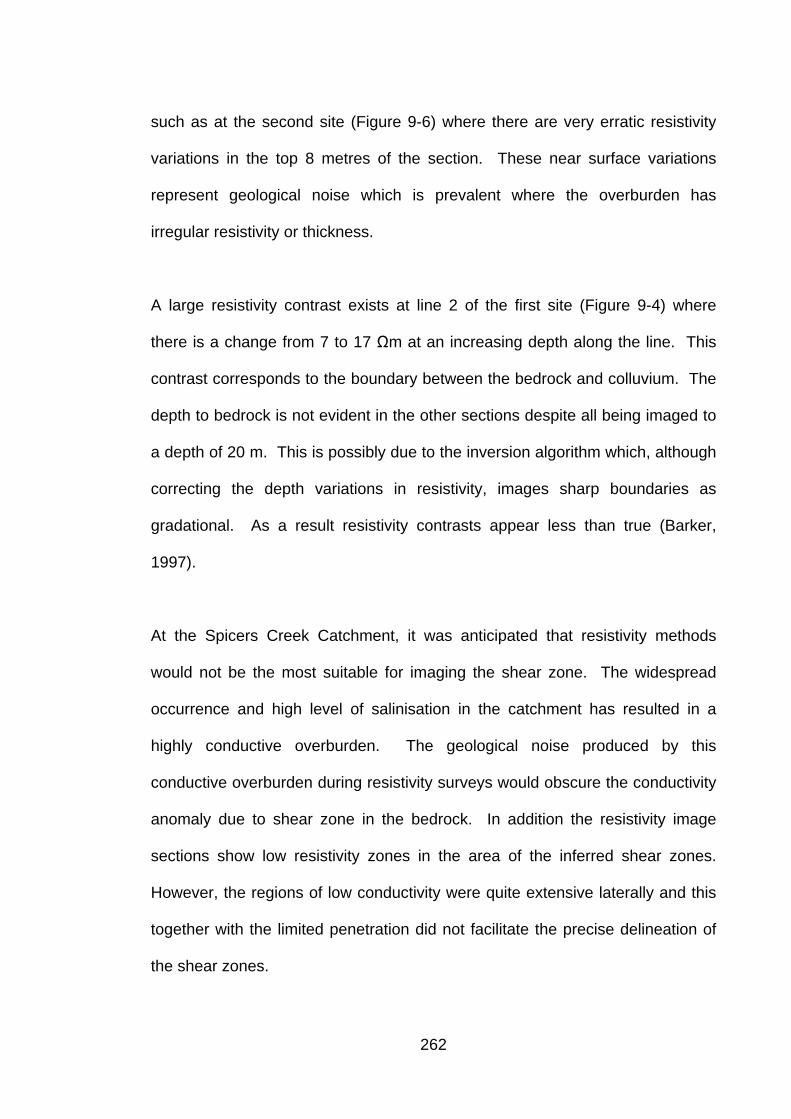
such as at the second site (Figure 9-6) where there are very erratic resistivity
variations in the top 8 metres of the section. These near surface variations
represent geological noise which is prevalent where the overburden has
irregular resistivity or thickness.
A large resistivity contrast exists at line 2 of the first site (Figure 9-4) where
there is a change from 7 to 17 Ωm at an increasing depth along the line. This
contrast corresponds to the boundary between the bedrock and colluvium. The
depth to bedrock is not evident in the other sections despite all being imaged to
a depth of 20 m. This is possibly due to the inversion algorithm which, although
correcting the depth variations in resistivity, images sharp boundaries as
gradational. As a result resistivity contrasts appear less than true (Barker,
1997).
At the Spicers Creek Catchment, it was anticipated that resistivity methods
would not be the most suitable for imaging the shear zone. The widespread
occurrence and high level of salinisation in the catchment has resulted in a
highly conductive overburden. The geological noise produced by this
conductive overburden during resistivity surveys would obscure the conductivity
anomaly due to shear zone in the bedrock. In addition the resistivity image
sections show low resistivity zones in the area of the inferred shear zones.
However, the regions of low conductivity were quite extensive laterally and this
together with the limited penetration did not facilitate the precise delineation of
the shear zones.
262
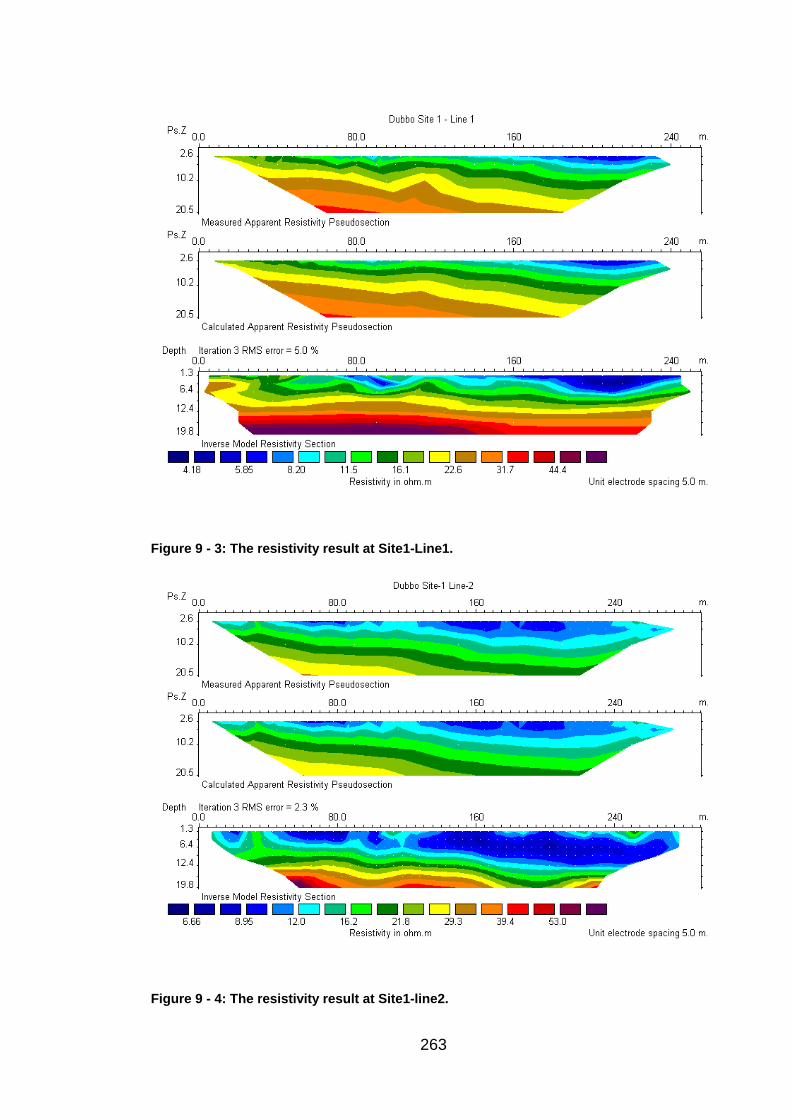
Figure 9 - 3: The resistivity result at Site1-Line1.
Figure 9 - 4: The resistivity result at Site1-line2.
263
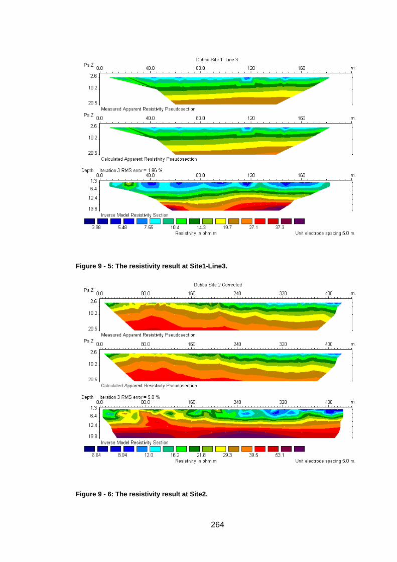
Figure 9 - 5: The resistivity result at Site1-Line3.
Figure 9 - 6: The resistivity result at Site2.
264
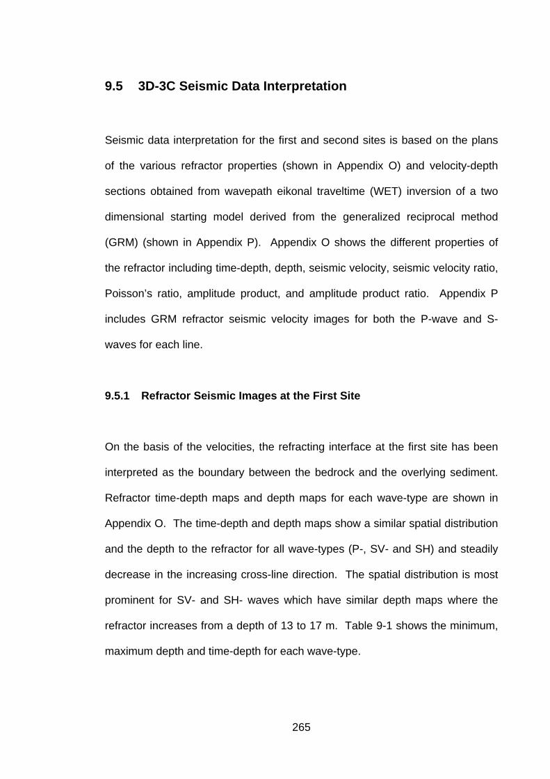
9.5 3D-3C Seismic Data Interpretation
Seismic data interpretation for the first and second sites is based on the plans
of the various refractor properties (shown in Appendix O) and velocity-depth
sections obtained from wavepath eikonal traveltime (WET) inversion of a two
dimensional starting model derived from the generalized reciprocal method
(GRM) (shown in Appendix P). Appendix O shows the different properties of
the refractor including time-depth, depth, seismic velocity, seismic velocity ratio,
Poisson’s ratio, amplitude product, and amplitude product ratio. Appendix P
includes GRM refractor seismic velocity images for both the P-wave and S-
waves for each line.
9.5.1 Refractor Seismic Images at the First Site
On the basis of the velocities, the refracting interface at the first site has been
interpreted as the boundary between the bedrock and the overlying sediment.
Refractor time-depth maps and depth maps for each wave-type are shown in
Appendix O. The time-depth and depth maps show a similar spatial distribution
and the depth to the refractor for all wave-types (P-, SV- and SH) and steadily
decrease in the increasing cross-line direction. The spatial distribution is most
prominent for SV- and SH- waves which have similar depth maps where the
refractor increases from a depth of 13 to 17 m. Table 9-1 shows the minimum,
maximum depth and time-depth for each wave-type.
265
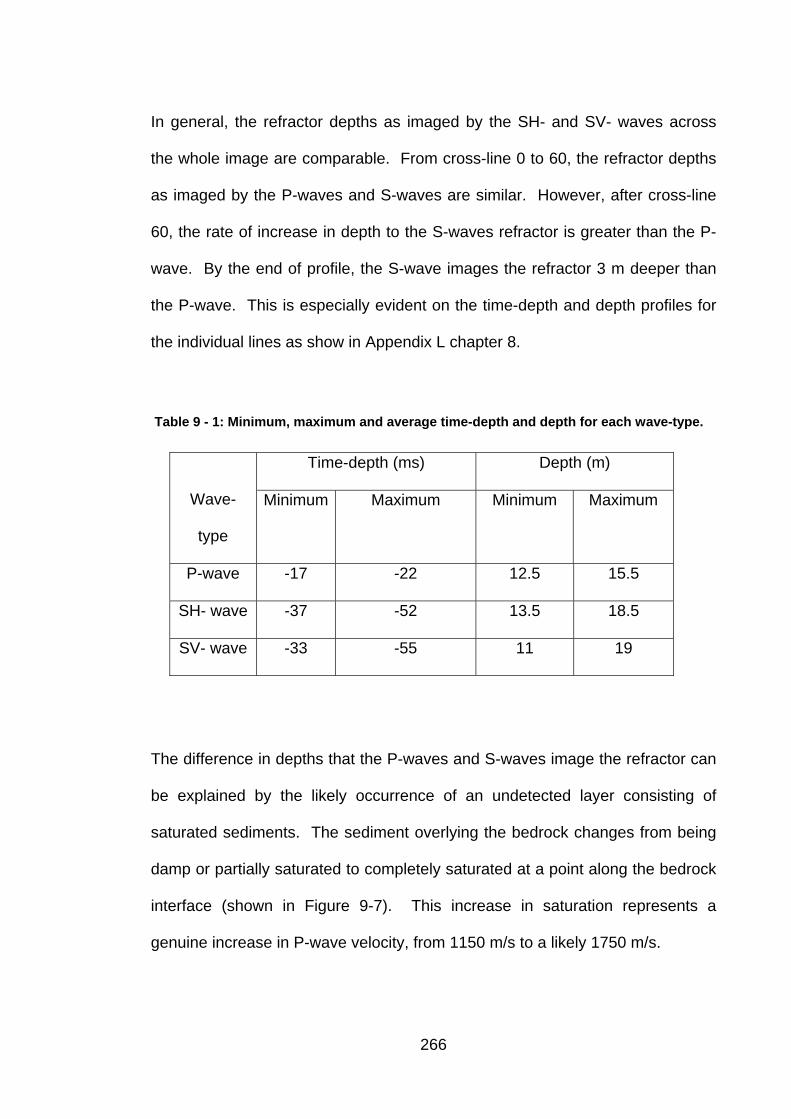
In general, the refractor depths as imaged by the SH- and SV- waves across
the whole image are comparable. From cross-line 0 to 60, the refractor depths
as imaged by the P-waves and S-waves are similar. However, after cross-line
60, the rate of increase in depth to the S-waves refractor is greater than the P-
wave. By the end of profile, the S-wave images the refractor 3 m deeper than
the P-wave. This is especially evident on the time-depth and depth profiles for
the individual lines as show in Appendix L chapter 8.
Table 9 - 1: Minimum, maximum and average time-depth and depth for each wave-type.
Time-depth (ms) Depth (m)
Wave-
type
Minimum Maximum Minimum Maximum
P-wave -17 -22 12.5 15.5
SH- wave -37 -52 13.5 18.5
SV- wave -33 -55 11 19
The difference in depths that the P-waves and S-waves image the refractor can
be explained by the likely occurrence of an undetected layer consisting of
saturated sediments. The sediment overlying the bedrock changes from being
damp or partially saturated to completely saturated at a point along the bedrock
interface (shown in Figure 9-7). This increase in saturation represents a
genuine increase in P-wave velocity, from 1150 m/s to a likely 1750 m/s.
266

Bedrock
Partially saturated sediment
Saturated sediment
Vp1Vs1
Vp2 > Vp1Vs2 = Vs1
Vp3 > Vp2Vs3 > Vs2
Figure 9 - 7: The possible P-wave undetected layer. A change from partially saturated to
completely saturated sediment above the refractor will result in an increase in P-wave
velocity. If this layer of completely saturated sediment is relatively thin, then it will be
undetectable in the P-wave traveltime graphs, resulting in the refractor being imaged
shallower than the true depth. Since S-waves do not propagate through liquids, the
degree of saturation in the sediment will have no effect on its propagation, thus the S-
waves will image the refractor at its true depth.
However, the saturated layer is not thick enough to generate refracted P-wave
first arrivals, and therefore is not recognisable in the traveltime graphs. The
result of this undetected layer is to image the P-wave refractor shallower than
its true depth. Furthermore, in this case the problem of the undetected layer is
not overcome by the use of an average seismic velocity above the refractor
derived with the GRM. This is because the saturated sediment is not present
along the whole profile and also progressively changes thickness.
267

Since S-waves do not propagate through liquids, the degree of saturation in the
sediments has no influence on the velocity of these waves. Thus the presence
of the completely saturated layer along part of the profile will have no effect on
the S-wave image of the refractor. The layer of saturated sediment is present
where the refractor is imaged at differing depths by the P-waves and S-waves,
and is absent where the refractor is imaged at the same depth by both waves.
The refractor images for all wave-types are shown in Appendix O. Changes in
refractor seismic velocities (Figure O3) occur in both the cross-line and the in-
line directions. In the in-line direction, the velocities for all wave-types show a
general decrease with the refractor being separated into three main regions of
different velocities (Figure 9-8). The P-wave velocities are between 4700-5300
m/s between 0 and 30 m, around 4000 m/s between 30m and 120m and 3000
m/s between 120m and 140m. The constant in seismic velocities between the
regions is not as large for the S-waves, with both the SV- and SH-waves having
velocities greater than 2500 m/s in the first region, 1700 for the second, and
around 1400 m/s for the third region. The consistent zoning of refractor
velocities for all wave-types is compelling evidence for genuine lateral changes
within the bedrock. At the first site, the existence of half of a shear zone is
evident from the first 40 m in the in-line direction (line AB on Figure 9-8). Line
AB is coincident with a major fault in the Spicers Creek Catchment as is
discussed in the geology section.
268
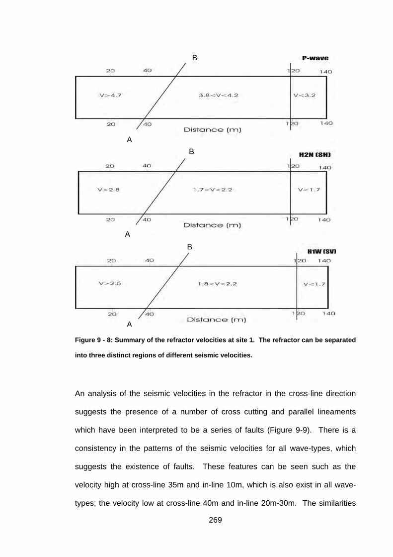
B
AB
A B
A
Figure 9 - 8: Summary of the refractor velocities at site 1. The refractor can be separated
into three distinct regions of different seismic velocities.
An analysis of the seismic velocities in the refractor in the cross-line direction
suggests the presence of a number of cross cutting and parallel lineaments
which have been interpreted to be a series of faults (Figure 9-9). There is a
consistency in the patterns of the seismic velocities for all wave-types, which
suggests the existence of faults. These features can be seen such as the
velocity high at cross-line 35m and in-line 10m, which is also exist in all wave-
types; the velocity low at cross-line 40m and in-line 20m-30m. The similarities
269
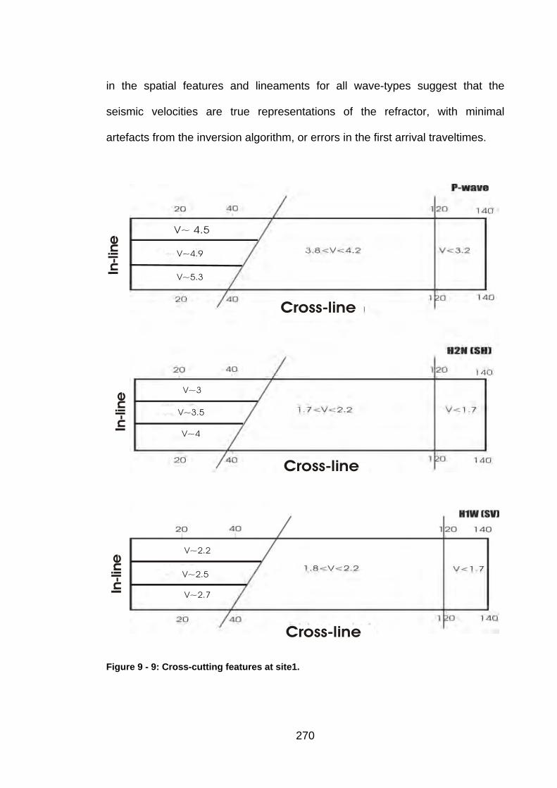
in the spatial features and lineaments for all wave-types suggest that the
seismic velocities are true representations of the refractor, with minimal
artefacts from the inversion algorithm, or errors in the first arrival traveltimes.
V~4.9
V~5.3
V~3
V~3.5
V~4
V~2.2
V~2.5
V~2.7
Cross-line
In-li
ne
Cross-line
In-li
ne
Cross-line
In-li
ne
Figure 9 - 9: Cross-cutting features at site1.
270
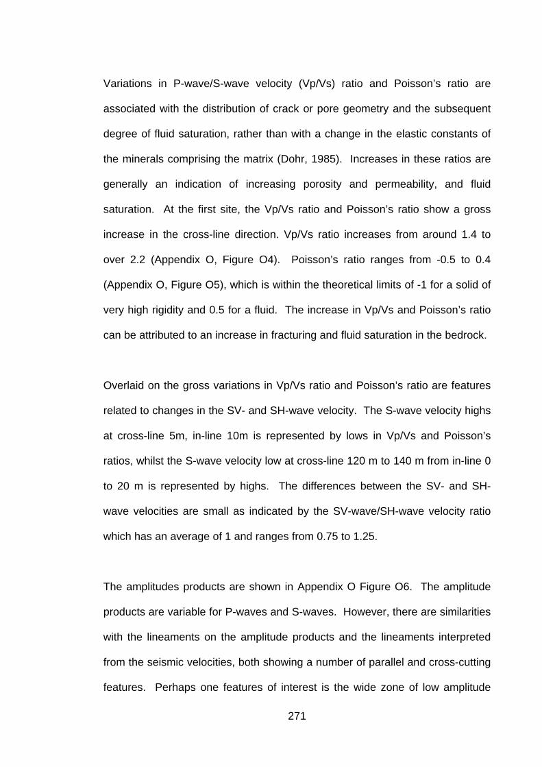
Variations in P-wave/S-wave velocity (Vp/Vs) ratio and Poisson’s ratio are
associated with the distribution of crack or pore geometry and the subsequent
degree of fluid saturation, rather than with a change in the elastic constants of
the minerals comprising the matrix (Dohr, 1985). Increases in these ratios are
generally an indication of increasing porosity and permeability, and fluid
saturation. At the first site, the Vp/Vs ratio and Poisson’s ratio show a gross
increase in the cross-line direction. Vp/Vs ratio increases from around 1.4 to
over 2.2 (Appendix O, Figure O4). Poisson’s ratio ranges from -0.5 to 0.4
(Appendix O, Figure O5), which is within the theoretical limits of -1 for a solid of
very high rigidity and 0.5 for a fluid. The increase in Vp/Vs and Poisson’s ratio
can be attributed to an increase in fracturing and fluid saturation in the bedrock.
Overlaid on the gross variations in Vp/Vs ratio and Poisson’s ratio are features
related to changes in the SV- and SH-wave velocity. The S-wave velocity highs
at cross-line 5m, in-line 10m is represented by lows in Vp/Vs and Poisson’s
ratios, whilst the S-wave velocity low at cross-line 120 m to 140 m from in-line 0
to 20 m is represented by highs. The differences between the SV- and SH-
wave velocities are small as indicated by the SV-wave/SH-wave velocity ratio
which has an average of 1 and ranges from 0.75 to 1.25.
The amplitudes products are shown in Appendix O Figure O6. The amplitude
products are variable for P-waves and S-waves. However, there are similarities
with the lineaments on the amplitude products and the lineaments interpreted
from the seismic velocities, both showing a number of parallel and cross-cutting
features. Perhaps one features of interest is the wide zone of low amplitude
271
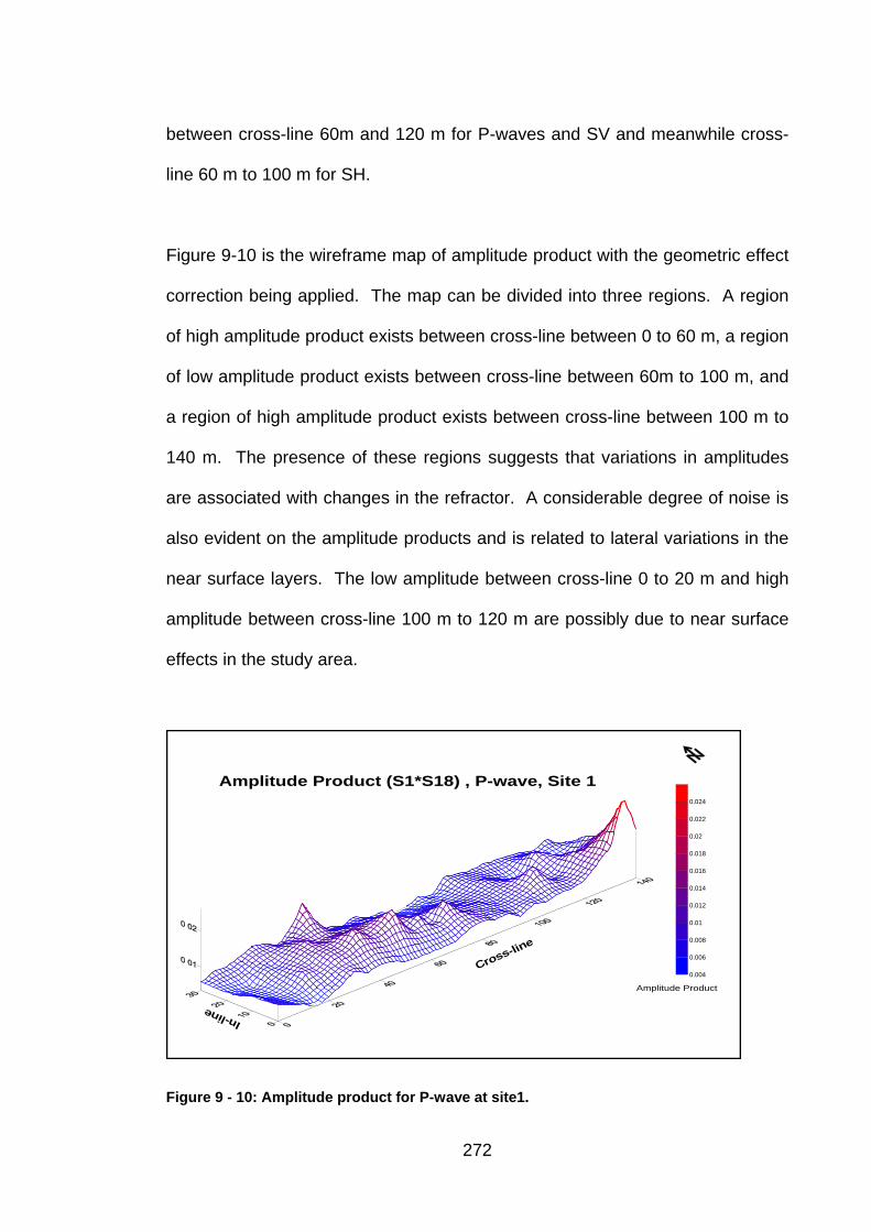
between cross-line 60m and 120 m for P-waves and SV and meanwhile cross-
line 60 m to 100 m for SH.
Figure 9-10 is the wireframe map of amplitude product with the geometric effect
correction being applied. The map can be divided into three regions. A region
of high amplitude product exists between cross-line between 0 to 60 m, a region
of low amplitude product exists between cross-line between 60m to 100 m, and
a region of high amplitude product exists between cross-line between 100 m to
140 m. The presence of these regions suggests that variations in amplitudes
are associated with changes in the refractor. A considerable degree of noise is
also evident on the amplitude products and is related to lateral variations in the
near surface layers. The low amplitude between cross-line 0 to 20 m and high
amplitude between cross-line 100 m to 120 m are possibly due to near surface
effects in the study area.
0.004
0.006
0.008
0.01
0.012
0.014
0.016
0.018
0.02
0.022
0.024
Amplitude Product (S1*S18) , P-wave, Site 1
Amplitude Product
Cross-line
In-line
Figure 9 - 10: Amplitude product for P-wave at site1.
272
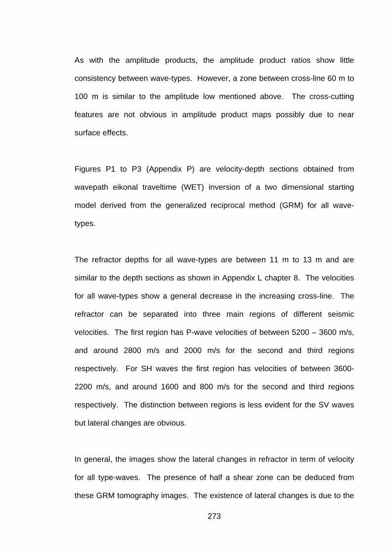
As with the amplitude products, the amplitude product ratios show little
consistency between wave-types. However, a zone between cross-line 60 m to
100 m is similar to the amplitude low mentioned above. The cross-cutting
features are not obvious in amplitude product maps possibly due to near
surface effects.
Figures P1 to P3 (Appendix P) are velocity-depth sections obtained from
wavepath eikonal traveltime (WET) inversion of a two dimensional starting
model derived from the generalized reciprocal method (GRM) for all wave-
types.
The refractor depths for all wave-types are between 11 m to 13 m and are
similar to the depth sections as shown in Appendix L chapter 8. The velocities
for all wave-types show a general decrease in the increasing cross-line. The
refractor can be separated into three main regions of different seismic
velocities. The first region has P-wave velocities of between 5200 – 3600 m/s,
and around 2800 m/s and 2000 m/s for the second and third regions
respectively. For SH waves the first region has velocities of between 3600-
2200 m/s, and around 1600 and 800 m/s for the second and third regions
respectively. The distinction between regions is less evident for the SV waves
but lateral changes are obvious.
In general, the images show the lateral changes in refractor in term of velocity
for all type-waves. The presence of half a shear zone can be deduced from
these GRM tomography images. The existence of lateral changes is due to the
273
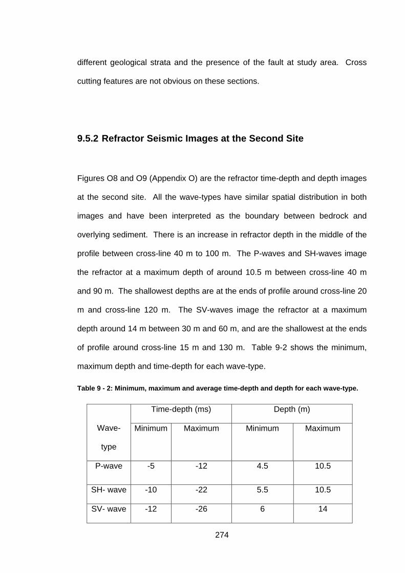
different geological strata and the presence of the fault at study area. Cross
cutting features are not obvious on these sections.
9.5.2 Refractor Seismic Images at the Second Site
Figures O8 and O9 (Appendix O) are the refractor time-depth and depth images
at the second site. All the wave-types have similar spatial distribution in both
images and have been interpreted as the boundary between bedrock and
overlying sediment. There is an increase in refractor depth in the middle of the
profile between cross-line 40 m to 100 m. The P-waves and SH-waves image
the refractor at a maximum depth of around 10.5 m between cross-line 40 m
and 90 m. The shallowest depths are at the ends of profile around cross-line 20
m and cross-line 120 m. The SV-waves image the refractor at a maximum
depth around 14 m between 30 m and 60 m, and are the shallowest at the ends
of profile around cross-line 15 m and 130 m. Table 9-2 shows the minimum,
maximum depth and time-depth for each wave-type.
Table 9 - 2: Minimum, maximum and average time-depth and depth for each wave-type.
Time-depth (ms) Depth (m)
Wave-
type
Minimum Maximum Minimum Maximum
P-wave -5 -12 4.5 10.5
SH- wave -10 -22 5.5 10.5
SV- wave -12 -26 6 14
274
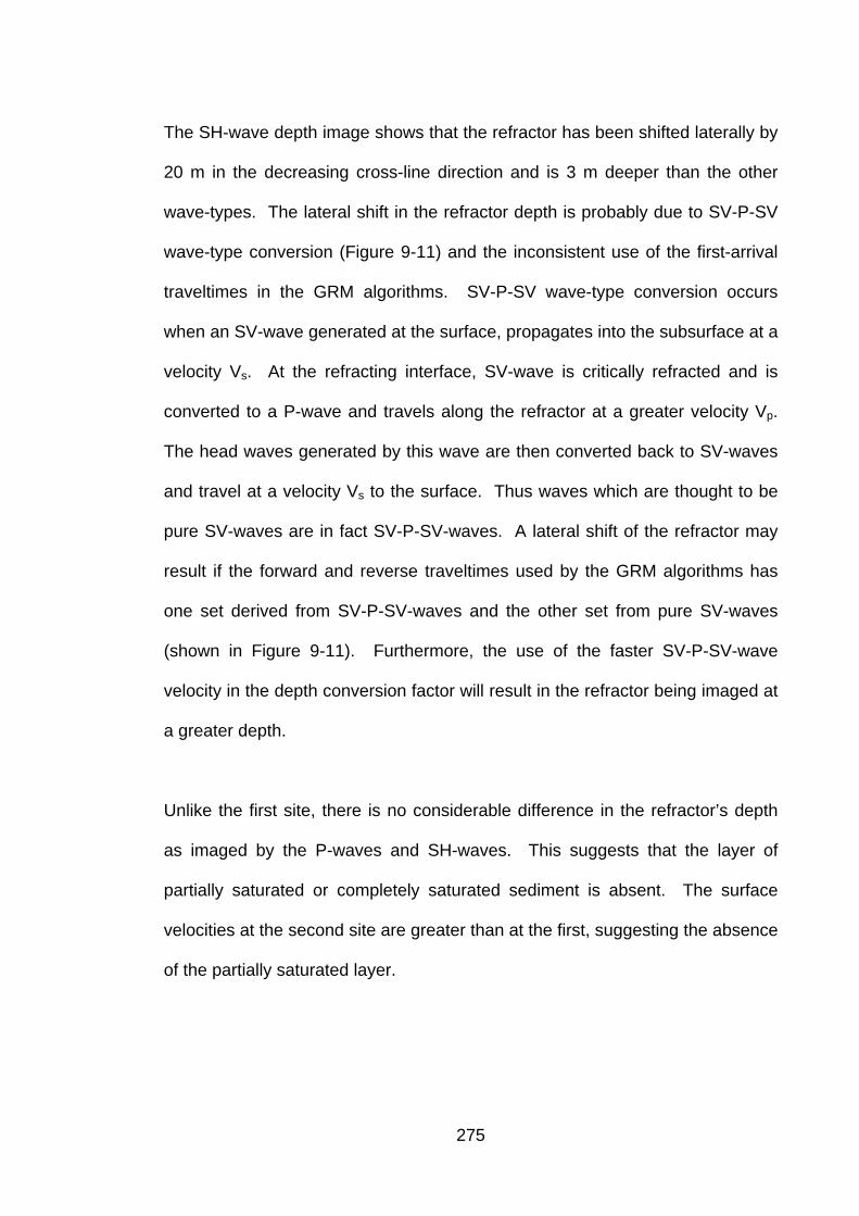
The SH-wave depth image shows that the refractor has been shifted laterally by
20 m in the decreasing cross-line direction and is 3 m deeper than the other
wave-types. The lateral shift in the refractor depth is probably due to SV-P-SV
wave-type conversion (Figure 9-11) and the inconsistent use of the first-arrival
traveltimes in the GRM algorithms. SV-P-SV wave-type conversion occurs
when an SV-wave generated at the surface, propagates into the subsurface at a
velocity Vs. At the refracting interface, SV-wave is critically refracted and is
converted to a P-wave and travels along the refractor at a greater velocity Vp.
The head waves generated by this wave are then converted back to SV-waves
and travel at a velocity Vs to the surface. Thus waves which are thought to be
pure SV-waves are in fact SV-P-SV-waves. A lateral shift of the refractor may
result if the forward and reverse traveltimes used by the GRM algorithms has
one set derived from SV-P-SV-waves and the other set from pure SV-waves
(shown in Figure 9-11). Furthermore, the use of the faster SV-P-SV-wave
velocity in the depth conversion factor will result in the refractor being imaged at
a greater depth.
Unlike the first site, there is no considerable difference in the refractor’s depth
as imaged by the P-waves and SH-waves. This suggests that the layer of
partially saturated or completely saturated sediment is absent. The surface
velocities at the second site are greater than at the first, suggesting the absence
of the partially saturated layer.
275
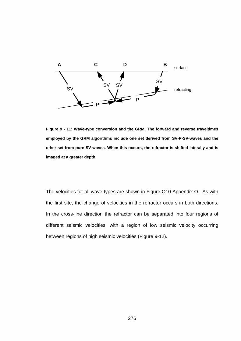
A C D Bsurface
SVSVSV
SV refracting
PP
Figure 9 - 11: Wave-type conversion and the GRM. The forward and reverse traveltimes
employed by the GRM algorithms include one set derived from SV-P-SV-waves and the
other set from pure SV-waves. When this occurs, the refractor is shifted laterally and is
imaged at a greater depth.
The velocities for all wave-types are shown in Figure O10 Appendix O. As with
the first site, the change of velocities in the refractor occurs in both directions.
In the cross-line direction the refractor can be separated into four regions of
different seismic velocities, with a region of low seismic velocity occurring
between regions of high seismic velocities (Figure 9-12).
276
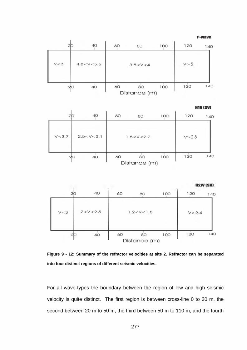
5
2.8
Figure 9 - 12: Summary of the refractor velocities at site 2. Refractor can be separated
into four distinct regions of different seismic velocities.
For all wave-types the boundary between the region of low and high seismic
velocity is quite distinct. The first region is between cross-line 0 to 20 m, the
second between 20 m to 50 m, the third between 50 m to 110 m, and the fourth
277
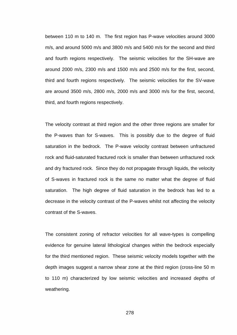
between 110 m to 140 m. The first region has P-wave velocities around 3000
m/s, and around 5000 m/s and 3800 m/s and 5400 m/s for the second and third
and fourth regions respectively. The seismic velocities for the SH-wave are
around 2000 m/s, 2300 m/s and 1500 m/s and 2500 m/s for the first, second,
third and fourth regions respectively. The seismic velocities for the SV-wave
are around 3500 m/s, 2800 m/s, 2000 m/s and 3000 m/s for the first, second,
third, and fourth regions respectively.
The velocity contrast at third region and the other three regions are smaller for
the P-waves than for S-waves. This is possibly due to the degree of fluid
saturation in the bedrock. The P-wave velocity contrast between unfractured
rock and fluid-saturated fractured rock is smaller than between unfractured rock
and dry fractured rock. Since they do not propagate through liquids, the velocity
of S-waves in fractured rock is the same no matter what the degree of fluid
saturation. The high degree of fluid saturation in the bedrock has led to a
decrease in the velocity contrast of the P-waves whilst not affecting the velocity
contrast of the S-waves.
The consistent zoning of refractor velocities for all wave-types is compelling
evidence for genuine lateral lithological changes within the bedrock especially
for the third mentioned region. These seismic velocity models together with the
depth images suggest a narrow shear zone at the third region (cross-line 50 m
to 110 m) characterized by low seismic velocities and increased depths of
weathering.
278
As with the first site, in the inline direction a detailed analysis of the seismic
velocities in the refractor suggests the presence of a number of cross cutting
and parallel lineaments which have been interpreted to be a series of faults
(Figure 9-13). There are a number of spatial similarities between all wave-types
velocities between cross-line 0 to 50 m, in-line 0 to 30 m, and between cross-
line 110 m to 140 m, in-line 0 to 30 m which seem to be related to the faults.
While The cross cutting features can be seen on both sides on the images for
all wave types, the SH-wave shows these features the best. This maybe due to
the direction of propagation SH-waves throughout the refractor. Figure 9-14
shows the direction of propagation for all wave-types.
There is a region of increased P-wave/SH-wave velocity ratio and associated
Poisson’s ratio between cross-lines 40 m and 110 m (Figure O11, O12,
Appendix O). The increase is considerable with a Vs/Vp ratio of 2.25 and
Poisson’s ratio of 0.35, contrasted with Vs/Vp ratio of 1.75 and Poisson’s ratio
of 0.3 in the surrounding regions. This increase correlates with the region of
low refractor velocity and is possibly related to an increase in porosity and
permeability, and a subsequent increase in fluid saturation.
The lateral variation in the SV-wave velocity can be resolved by examining the
velocity ratios. A P-wave/SV-wave velocity ratio high of greater than 2.25
occurs between cross-lines 20 m and 40 m, whilst the SV-wave/SH-wave
velocity ratio high of greater than 1.75 occurs between cross-lines 90 m and
110 m.
279
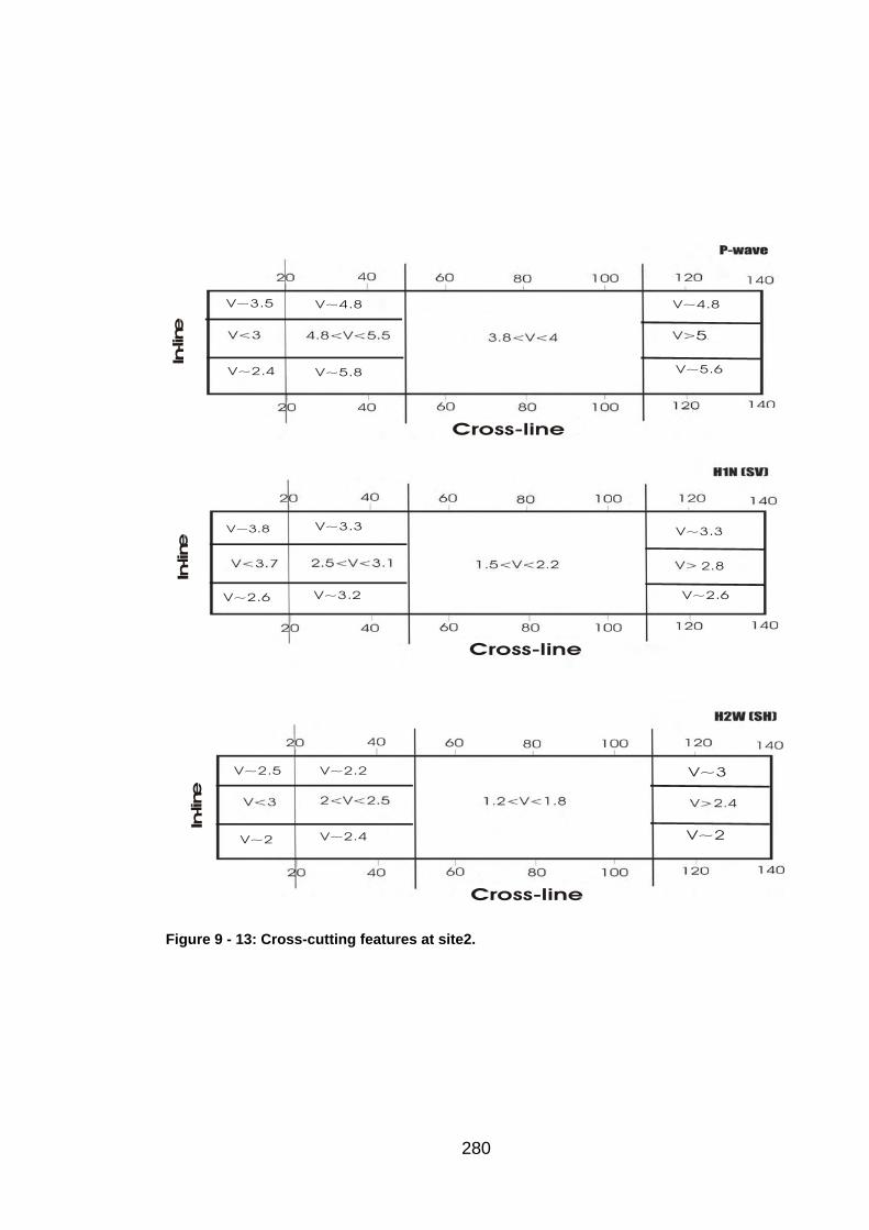
V~3.5
V~2.4
V~4.8
V~5.8
V~4.8
V~5.6
2.8
V~3.8 V~3.3
V~2.6 V~3.2
V~3.3
V~2.6
V~2.5
V~2
V~2.2
V~2.4
V~3
V~2
Cross-line
In-line
Cross-line
In-line
In-line
Cross-line
Figure 9 - 13: Cross-cutting features at site2.
280
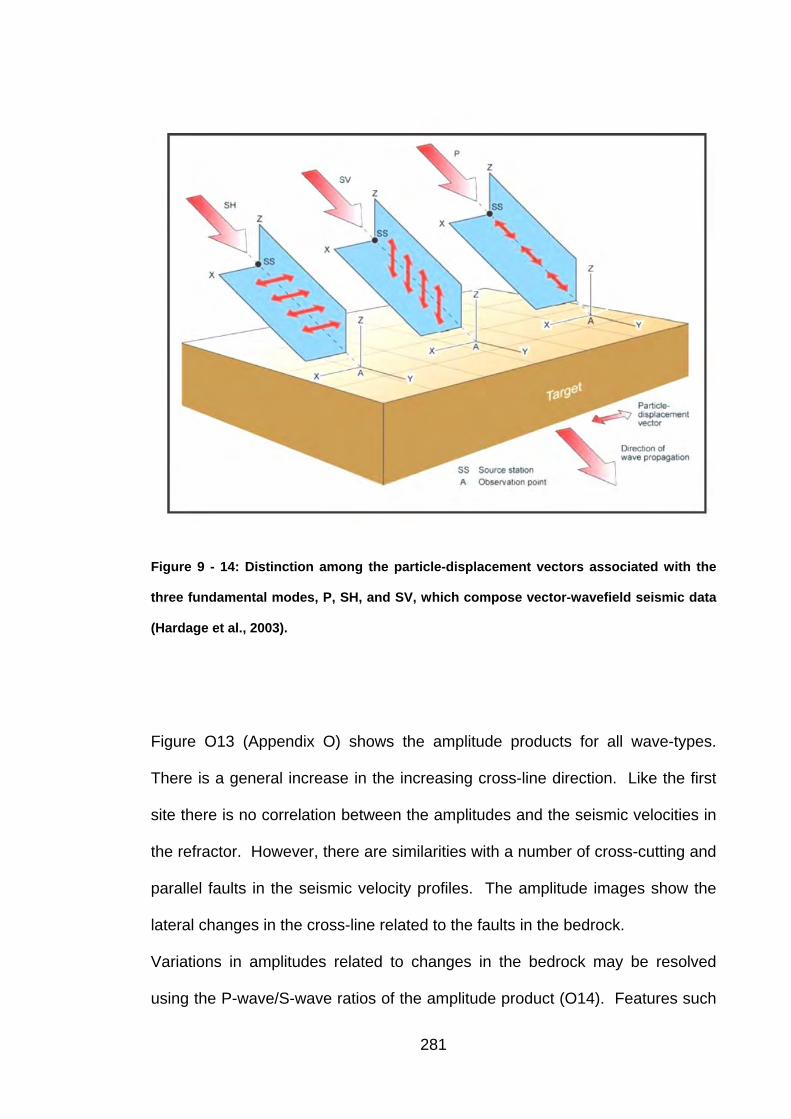
Figure 9 - 14: Distinction among the particle-displacement vectors associated with the
three fundamental modes, P, SH, and SV, which compose vector-wavefield seismic data
(Hardage et al., 2003).
Figure O13 (Appendix O) shows the amplitude products for all wave-types.
There is a general increase in the increasing cross-line direction. Like the first
site there is no correlation between the amplitudes and the seismic velocities in
the refractor. However, there are similarities with a number of cross-cutting and
parallel faults in the seismic velocity profiles. The amplitude images show the
lateral changes in the cross-line related to the faults in the bedrock.
Variations in amplitudes related to changes in the bedrock may be resolved
using the P-wave/S-wave ratios of the amplitude product (O14). Features such
281
as the high between cross-line 40 m and 100 m in the P-wave/SV-wave ratio,
and between 50 m and 110 m in the P-wave/SH-wave ratio, are clearly
detectable. This region of high P-wave amplitude and low S-wave amplitude
may be due a high degree of fracturing causing the preferential attenuation of
S-waves with respect to P-waves as S-waves are more directly affected by
changes in rigidity modulus and density.
Figures P4 to P6 (Appendix P) show the GRM velocity-depth sections for all
wave-types. The low velocity zone can be seen for most of images including P-
waves (line1 and line4), SH-waves (line1, line3, line4) and SV-waves (line4).
There is no obvious low velocity zone for some images because of the limited
penetration of some of the wave-types into the refractor. The low velocity zones
support a region of increased porosity and permeability, and the subsequent
increases in the degree of groundwater saturation, that correlates with the
presence of the shear zone at the second site.
9.6 Geology and Tectonic Interpretation
As discussed in the geology chapter, the study area is situated in the mid-
Silurian to Early Devonian Hill End Trough in the eastern Lachlan Fold Belt
(LFB) and overlies marginal areas of the Gunnedah Basin and Surat Basin.
The Hill End Trough is bounded to the south by the Carboniferous Buthurst
Batholith and the Lachlan Transverse Zone (Glen and Walshe, 1999) and to the
east and west by Ordovician volcanics that are overlain by thin Silurian-Early
282
Devonian rocks and intruded in part by Carboniferous granites (David et al.,
2003). Figure 9-15 shows the simplified regional geology map of the Hill End
Trough (David et al., 2003).
The geology and tectonic interpretation shows a detailed model of the cross-
cutting features at the first and second site. They confirm that there is a good
relationship between the interpretation of seismic data and that of the geology
at the Spicers Creek Catchment. The detection of lineaments and cross-cutting
features through the interpretation of the seismic velocities and amplitude
products was made possible via the use of three dimensional seismic refraction
methods.
283
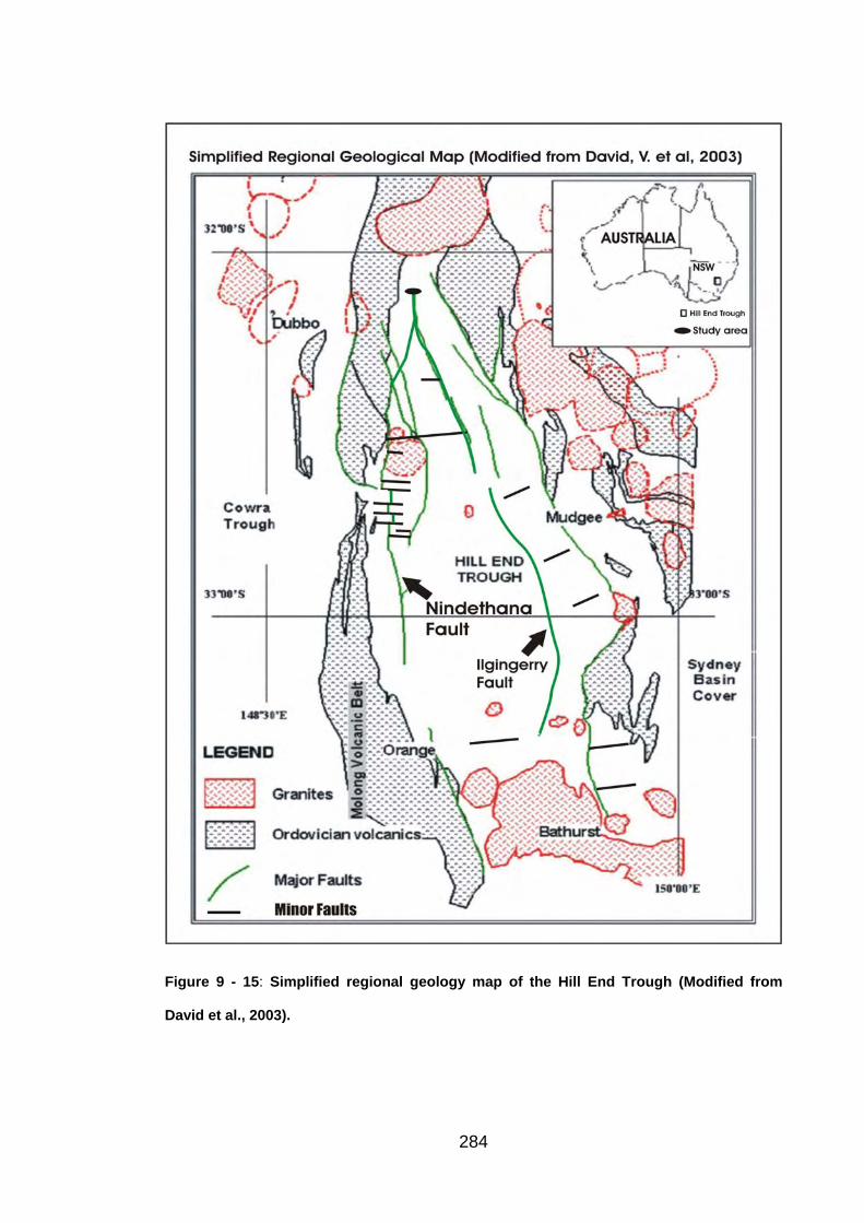
Figure 9 - 15: Simplified regional geology map of the Hill End Trough (Modified from
David et al., 2003).
284
Chapter 10
Conclusions
Three-dimensional (3D) three-component (3C) shallow seismic refraction
surveys were recorded over a shear zone at two sites associated with dryland
salinity in the Spicers Creek Catchment, near Dubbo in southeastern Australia.
The seismic data were recorded with the Australian National Seismic Imaging
Resources (ANSIR) 360-trace ARAM-24 seismic system and IVI MiniVibrator.
Dryland salinity occurs extensively throughout the Spicers Creek Catchment.
The high concentration of salt in the groundwater has led to a significant decline
in agricultural productivity and a reduction in native vegetation. Furthermore,
the saline groundwater in the surface soil has caused the destruction of the clay
and soil structure and as a result, large areas of the catchment have
experienced soil erosion and extensive alteration of the landscape.
The broad objective of this study was to use seismic refraction methods to map
in detail a shear zone, which is associated with the salination. Although the
shear zone had been recognized in airborne geophysical surveys and
subsequent regional geological mapping as the Nindethana Fault, the exact
geological factors which produced the discontinuous occurrences of saline
groundwater at the surface, were not known. Detailed ground magnetic surveys
carried out as part of this study, confirmed the location of the shear zone, but
285
they did not provide further explanation of the causes of salination. Therefore,
the detailed objectives were to map the extent of the shear zone as well as
other properties, such as the rock fabric.
Seismic refraction methods were selected because of their potential ability to
provide greater lateral resolution of the narrow vertical shear zone, than is
currently the norm with electrical or electromagnetic methods. This situation
was confirmed with a number of resistivity depth images generated as part of
this study. Furthermore, it was anticipated that the high electrical conductivities
of the near surface areas would have no significant impact on the depth of
investigation of the seismic energy. Finally it was also anticipated that the head
wave amplitude might provide a more detailed measure of the seismic velocities
as a function of azimuth and therefore of fracture porosity.
The 3D 3C survey was set out as four parallel lines 10 m apart with twenty-nine
3C geophones, 5 m apart, in each line. The source lines were located parallel
and orthogonal to the lines of geophones and passing through the geometric
centre of the receiver spread. Source points were nominally 10 m apart and
both P- and S-waves were generated.
The results of the seismic refraction surveys show that the shear zone occurs
as a narrow region with low seismic velocities and increased depths of
weathering. However, there were numerous ambiguities in generating
consistent parameters in the refractor between adjacent receiver lines.
Furthermore, these ambiguities were not resolved with the use refraction
286
tomography, because even moderate differences with the various starting
models still generated acceptable agreement with the traveltime data.
Therefore, in order to generate consistency between the results for the various
receiver lines, it was necessary to generate detailed starting models.
It was found that near surface irregularities of a very limited lateral extent were
the major sources of uncertainty in deriving detailed starting models. In the
Spicers Creek Catchment, the variations in the traveltimes caused by the near
surface irregularities, were frequently of a comparable magnitude to those
caused by the changes in depths and seismic velocities in the refractor. As a
result, the derivation of detailed parameters of the refractor using the
generalized reciprocal method (GRM) was subject to significant uncertainty
unless they are accommodated with the GRM SSM.
A major achievement of this study is the development of a smoothing method
which significantly removes the effects of the near surface irregularities.
Termed the GRM SSM (for statics smoothing method), it essentially generates
a time-depth model of the refracting interface for which the effects of the near
surface irregularities have been minimized, by taking an average of the time-
depth profiles for a range of XY values. Although the time-depths to the target
refractor show very little variation with changing XY distances, the traveltime
anomalies for the near surface irregularities migrate laterally through the time-
depths. Therefore, the average time-depth profile is largely free of the near
surface anomalies. When this averaged time-depth profile is subtracted from
that for zero XY, the result is essentially a set of corrections for the near surface
287
irregularities. These corrections are then subtracted from the field traveltimes,
and the GRM computations are then repeated with the corrected traveltimes.
The GRM SSM, which takes advantage of the unique redundancy properties of
the GRM computations, was a major factor in deriving consistent detailed
starting models for refraction inversion. Furthermore, this consistency was
achieved with both S-wave components, as well as the P-wave results.
The major geological achievement, which was made possible with the GRM
SSM, was the demonstration that there were cross cutting features associated
with the major shear zone. Therefore, it appears that saline groundwater can
discharge at the surface where increased volumes of groundwater occur at the
intersection of different sets of shears. This model provides a useful
explanation for the discontinuous occurrence of salination along the major shear
zone.
As is usually the case, increased numbers of recording channels would have
been beneficial. In particular, the four recording lines separated by 10 m did not
provide as high resolution in the cross-line direction as in the in-line direction.
Therefore, where cross cutting features are considered likely to occur and to be
significant, than re-deploying the recording spread in the orthogonal direction
provides an acceptable alternative to employing field systems with significantly
larger recording capacity.
The measurement of S-wave velocities provided a measure of Poisson’s ratio,
which is a useful elastic parameter. Although a detailed analysis of the head
288

wave amplitudes did not generate useful results, nevertheless, the fact that the
head wave amplitude is a function of the densities, as well as the seismic
velocities, suggests that the joint inversion of seismic refraction traveltimes and
head wave amplitudes, with detailed gravity profiles, should facilitate the
determination of both seismic velocity and density models, and in turn, the
derivation of elastic constants. It is likely that the detailed geotechnical
characterization of sites with 3D 3C seismic refraction methods, together with
detailed gravity profiles, could provide useful quantitative models for the
analysis of groundwater flow in fractured rock masses, as well as for the
traditional engineering construction site applications.
289
REFERENCES ACIL, Australia Pty Ltd, 1983, Causes, Extent and Effect of Salinity in Victoria:
A Report Prepared for the Salinity Committee of the Victorian Parliament, Melbourne, pp. 175.
Acworth, R. I. and Jankowski, J., 2001, Salt source for dryland salinity-evidence
from an upland catchment on the Southern Tablelands Of New South Wales: Aust. J.Soil.Res., 39, pp. 39-59.
Allan, U. S., 1989, Model for hydrocarbon migration and entrapment within
faulted structures: AAPG Bulletin, 73, pp. 803-811. Anderson, R. N., Flemings, P., Losh, S., Austin, J. and Woodhams, R., 1994,
Gulf of Mexico growth fault drilled, seen as oil, gas migration pathway: Oil and Gas J., 12, pp. 97-102.
Anderson, R. N., He, W., Hobart, M. A., Wilkinson, C. R. and Nelson, H. R.,
1991, Active fluid flow in the Eugene Island area, offshore Louisiana: The Leading Edge, 10, pp. 12-17.
Archie, G. E., 1942, The electrical resistivity log as an aid to determining some
reservoir characteristics: A.I.M.E., 146, pp. 389-406. Atkinson, T., 1970, Ground preparation by ripping in open pit mining: Mining
Magazine, 122, pp. 458-469. Bamford, D. and Nunn, K. R., 1979, In situ seismic measurements of crack
anisotropy in the carboniferous limestone of northwest England: Geophys. Prosp., 27, pp. 322-338.
Barker, R. D., 1997, Electrical imaging and its applications in engineering
investigations, In: McCann, D. M., Eddleston, M., Fenning, P.J., Reeves, G.M.(Ed): Modern geophysics in engineering geology, The Geological Society, London, pp. 37-43.
Barron, L. M., 1997, Igneous petrology overview of the Dubbo 1:250,000
geological sheet: Geological Survey of New South Wales, Report GS1997/080.
Bartlett, A. H., 1962, Refraction seismic survey in civil engineering: Australian
Road Research Board 1st Biennial Conference. Bates, R. L. and Jackson, J. A., 1980, Glossary of Geology: American
Geological Institute, U.S.A. Beach, A. and Fyfe, W. S., 1972, Fluid transport and shear zones at Scourie,
Sutherland: evidence for overthrusting?: Contrib.Mineral.Petrol., 36, pp. 175-180.
290
Bennett, G., 1999, 3-D seismic refraction for deep exploration targets: The Leading Edge, 18, pp. 186-191.
Berg, R. R. and Avery, A. H., 1995, Sealing properties of tertiary growth faults,
Texas Gulf Coast: AAPG Bulletin, 79, pp. 375-393. Beyer, W. H., 1975, Handbook of mathematical science, 5th edition: CRC
Press, Florida. Biehler, S., Ferguson, J., Baldridge, W. S., Jiracek, G. R., Aldren, J. L.,
Martinez, M., Fernandez, R., Romo, J., Gilpin, B., Braile, L. W., Hersey, D. R., Luyendyk, B. P. and Aiken, C. L., 1991, A geophysical model of the Espanol Basin, Rio Grande rift, New Mexico: Geophysics, 56, pp. 340-353.
Bigelow, N., 1965, Seismograph operations by marine state highway
commission: Highway Research Record No.81, Highway Research Board, Washington, pp. 9-15.
Bonini, E. W. and Hickok, E. A., 1958, Seismic refraction method in ground-
water exploration: AIME Trans., 211, pp. 485-488. Bourke, D. J., Hawke, J. M. and Scheibner, E., 1974, Structural subdivision of
the Great Australian Basin in New South Wales: Geological Survey of New South Wales, Quarterly Notes, 16, pp. 10-16.
Bradd, J. M. and Gates, G., 1996, Dryland salinity in New South Wales. A state
perspective: Department of Land and Water Conservation, Technical Report No. TS95.113.
Bradd, J. M., Milne-Home, W. A. and Gates, G., 1997, Overview of factors
leading to dryland salinity and its potential hazard in New South Wales, Australia: Hydrogeology Journal, 5, pp. 51-67.
Branagan, D. F. and Packham, G. H., 2000, Field geology of New South Wales:
Department of Mineral Resources New South Wales, Sydney, Australia. Braun, J., Munroe, S. and Cox, F., 2003, Transient fluid flow in and around a
fault: Geofluids, 3, pp. 81-87. Brown, A. R., 1996, Interpretation of three-dimensional seismic data: AAPG
Memoir, 42. Brown, P. D. and Robertshaw, J., 1957, Determining the thickness of
unconsolidated deposits overlying shallow mine working by seismic methods in methods and case histories in mining geophysics: Sixth Commonwealth Mining and Metallurgical Congress, Montreal.
291

Campos-Enriquez, J., Delgado-Redriguez, O., Chavez-Segura, R., Gomez-Contreras, P., Flores-Marquez, E. L. and Birch, F. S., 1997, The subsurface structure of the Chalco sub-basin (Mexico City) inferred from geophysical data: Geophysics, 62, pp. 23-35.
Carcione, J. M. and Cavallini, F., 2002, Poisson's ratio at high pore pressure.:
Geophysical Prospecting, 50, pp. 97-106. Cerveny, V. and Ravindra, R., 1971, Theory of seismic head waves: University
of Toronto Press. Cerveny, V., Molotkov, I.A., Psencik, I., 1977, Ray Method in Seismology:
Praha, Universita, Karlova. Chappell, B. W., White, A. J. R. and Hine, R., 1988, Granite provinces and
basement terranes in the Lachlan Fold Belt, Southeaster Australia: Australian Journal of Earth Sciences, 35, pp. 505-521.
Clarke, C. J., George, R. L., Bell, R. W. and Hatton, T. J., 2002, Dryland salinity
in south-western Australia: its origins, remedies and future research directions: Australian Journal of Soil Research, 40, pp. 93-113.
Collins, W. J. and Vernon, R. H., 1994, A rift-drift-delamination model of
continental evolution: Paleaozoic tectonic development of eastern Australia: Tectonophysics, 235, pp. 249-275.
Coney, P. J., 1992, The Lachlan belt of eastern Australia and Circum-Pacific
tectonic evolution: Tectonophysics, 214, pp. 1-25. Coram, J., 1998, National classification of catchments for land and river salinity
control: RIRDC Publication, No: 98/78. Coram, J., Dyson, P. and Evans, R., 2001, An evaluation framework for dryland
salinity: Department of Agriculture, Fisheries and Forestry Australia, Australian Government Publishing Service, Canberra.
Cramsie, J. N. and Hawke, J. M., 1984, Introduction In:Hawke, J. M. and
Cramsie, J. N.(Eds) Contribution to the geology of the Great Australian Basin in New South Wales: Geological survey of New South Wales, Department of Mineral Resources, Bulletin No.31, pp. 1-22.
Creelman, R., 2002, Reviewing the Science of Salinity: First Annual Symposium
on Salinity Assessment and Management, University of Sydney. Crook, K. A. W., 1980, Fore-arc evolution in the Tasman Geosyncline: the origin
of the southern Australia continental crust: Journal of the Geological Society of Australia, 27, pp. 215-232.
292
Cummings, D., 1979, Determination of depths an irregular interface in shallow refraction surveys using a pocket calculator: Geophysics, 44, pp. 1987-1998.
Dahlhaus, P. G., MacEwan, R. L., Nathan, L. and Morand, J., 2000, Salinity on
the southeastern Dundas Tableland, Victoria: Australian Journal of Earth Sciences, 47, pp. 3-11.
Dasios, A., McCann, C., Astin, T. R., McCann, D. M. and Fenning, P., 1999,
Seismic imaging of the shallow subsurface: shear-wave case histories: Geophysical Prospecting, 47, pp. 565-591.
David, V., 2003, Cross section four, Combo to Guntawang in Hill End Trough,
CD Geoscience Database: Geological Survey of New South Wales. David, V., Glen, R. A. and Spencer, R., 2003, Three-dimensional extension of
the Hill End Trough based on the modeling of the regional gravity data. In: Vassallo, J. J. G., R.A.(Ed), Evolution of the Hill End Trough: Hill End Trough CD Geoscience Data Package. Open File GS Report 2003/291, Geological Survey of New South Wales, Sydney, Australia, pp. 43-48.
Davis, H. D. and Reynolds, S. J., 1996, Structural geology of rocks and regions:
John Wiley & sons Inc., U.S.A. de Groot-Hedlin, C. and Constable, S., 1990, Occam's inversion to generate
smooth, two-dimensional models form magnetotelluric data: Geophysics, 55, pp. 1613-1624.
Deen, T. and Gohl, K., 2002, 3-D tomographic seismic inversion of a
paleochannel system in central New South Wales, Australia: Geophysics, 67, pp. 1364-1371.
Deen, T. J., Gohl, K., Leslie, C., Papp, E. and Wake-Dyster, K. D., 2000,
Seismic refraction inversion over a palaeochannel in the Lachlan fold belt, central NSW: Exploration Geophysics, 31, pp. 389-393.
Dennis, J. G., 1967, International tectonic dictionary: Am. Assoc. Pet. Geol.
Tusla, pp. 196. Dobrin, M. B., 1983, Introduction to geophysical prospecting: McGraw-Hill.Inc,
Japan. Dobrin, M. B. and Savit, C. H., 1988, Introduction to geophysical prospecting:
McGraw Hill. Dohr, G., 1985, Seismic shear waves: Geophysical Press, London. 293

Domenico, S. N. and Danbon, S. H., 1986, Shear-wave technology in petroleum exploration - past, current, and future In: Dunbom, S. H. and Domenico, S. N.(Eds) Shear wave exploration, Society of Exploration Geophysicists, pp. 3-18.
Drake, C. L., 1962, Geophysics, "Geophysics" and engineering: Geophysics,
27, pp. 193-197. Duguid, J. O., 1968, Refracted determination of water table depth and alluvium
thickness: Geophysics, 33, pp. 481-488. Ebrom, D., McDonald, J. and Tatham, B., 1992, Sideswipe in a 3-D, 3-C model
survey: The Leading Edge, 11, pp. 45-51. Edge, A. G. and Laby, T. H., 1931, The principles and practice of geophysical
prospecting: Cambridge University Press, London. Edwards, L. S., 1977, A modified pseudosection for resistivity and induced
polarization: Geophysics, 42, pp. 1020-1036. English, P., 2002, Overview of salinity research at CSIRO land and water: First
Annual Symposium on Salinity Assessment and Management, University of Sydney.
Exon, N. F., 1976, Geology of the Surat Basin: Australian Government
Publishing Service, Canberra, French, S. W., 1974, Two-dimensional and three-dimensional migration of
model-experiment reflection profiles: Geophysics, 39, pp. 265-277. Gebrande, H. and Miller, H., 1985, Refraction seismology In: Bender, F.(Ed),
Applied geoscience, methods of applied geophysics and mathematical procedures in geosinces, F.Enke Publishing House, Stuttgart, pp. 226-260.
Glen, R. A. and Walshe, J. L., 1999, Cross Structure in the Lachlan Orogen
Australia: the Lachlan Transverse Zone example: Australian Journal of Earth Sciences, 46, pp. 641-658.
Glen, R. A., Walshe, J. L., Barron, L. M. and Watkins, J. J., 1998, Ordovician
convergent-margin volcanism and tectonism in the Lachlan sector of east Gondwana: Geology, 26, pp. 751-754.
Glen, R. A. and Watkins, J. J., 1999, Implications of Middle Devonian
deformation of the eastern part of the Hill End Trough, Lachlan Orogen, New South Wales: Australian Journal of Earth Sciences, 46, pp. 35-52.
Grant, F. S., 1985, Aeromagnetics, geology and ore environments, I.Magnetite
in igneous, sedimentary and metamorphic rocks, An overview: Geoexploration, 23, pp. 303-333.
294
Griffiths, D. H. and Barker, R. D., 1993, Two-dimensional resistivity imaging and modelling in areas of complex geology: Journal of Applied Geophysics, 29, pp. 211-226.
Gunn, P. J., 1997a, Regional magnetic and gravity responses of extensional
sedimentary basins: AGSO Journal of Australian Geology and Geophysics, 17, pp. 115-131.
Gunn, P. J., 1997b, Application of aeromagnetic surveys to sedimentary basin
studies: AGSO Journal of Australian Geology and Geophysics, 17, pp. 133-144.
Gunn, P. J. and Dentith, M. C., 1997, Magnetic responses associated with
mineral deposits: AGSO Journal of Australian Geology and Geophysics, 17, pp. 145-158.
Haeni, F. P., 1986, Application of seismic refraction methods in groundwater
modeling studies in New England: Geophysics, 51, pp. 236-249. Hasselstrom, B., 1969, Water prospecting and rock-investigation by the seismic
refraction method: Geoexploration, 7, pp. 113-132. Hatcher, R. D., 1995, Structure geology: principles, concepts, and problems:
Prentice-Hall, Inc., U.S.A. Hatherly, P. J., 1986, Attenuation measurements on shallow seismic refraction
data: Geophysics, 51, pp. 250-254. Hatherly, P. J. and Neville, M. J., 1986, Experience with the generalized
reciprocal method of seismic refraction interpretation for shallow engineering site investigation: geophysics, 51, pp. 255-265.
Hawke, J. M. and Cramsie, J. N., 1984, Contribution to the Geology of the Great
Australian Basin in New South Wales: Geological Survey of New South Wales, Bulletine 31, pp. 259.
Hawkins, L. V., 1961, The reciprocal method of routine shallow seismic
refraction investigations: Geophysics, 26, pp. 806-819. Heelan, P. A., 1953, On the theory of head waves: Geophysics, 18, pp. 871-
893. Helbig, K., 1986, Shear-waves-what they are and how they can be used
In:Danbom, S. H., Domenico, S.N.(Ed), Shear-wave exploration: Society of Exploration Geophysicists, pp. 19-36.
Heneberg, W. C., 1995, Steady state groundwater flow across idealized faults:
Water Resources Research, 31, pp. 1815-1820. Hobbs, B. E., 1976, An outline of structural geology: Wiley & Sons, Inc, pp.571. 295
Hobson, G. D. and Grant, A. C., 1964, Tracing buried river valleys in the Kirkland Lake area of Ontario with a hammer seismograph: Canadian Mining Journal, pp. 79-83.
Hooper, E. C. D., 1991, Fluid migration along growth faults in compacting
sediments: Journal of Petroleum Geology, 14, pp. 161-180. Horsfall, K. R., 1997, Airborne magnetic and gamma-ray data acquisition:
AGSO Journal of Australian Geology and Geophysics, 17, pp. 23-30. Hull, J., 1988, Thickness-displacement relationships for deformation zones:
J.Struct.Geol., 10, pp. 431-435. IAEA, 1991, Airborne gamma ray spectrometer surveying: International Atomic
Energy Agency, Technical Reports Series, No. 323. Irving, F. R., 1965, Seismic surveying methods, equipment and costs in New
York State: Highway Research Record No.81, Highway Research Board, Washington, pp. 2-8.
Jacobsen, T. and Adams, R. M., 1958, Salt and silt in ancient Mesopotamian
agriculture: Science, 128, pp. 1251-1258. Jaques, A. L., Wellman, P., Whitaker, A. and Wyborn, D., 1997, High-resolution
geophysics in modern geological mapping: AGSO Journal of Australian Geology and Geophysics, 17, pp. 159-173.
Jewel, C. M. and Associates, 2000, Hydrogeological study for Spicers Ck /
Talbragar catchment: Jewel CM and Associates Pty Ltd Rep No A59967.4, April 2000.
Kearey, P. and Brooks, M., 2001, An introduction to geophysical exploration:
Blackwell Scientific Publications. Kilthy, K. T., Norris, R. A., McLamore, W. R., Hennon and K.P.Euge, K., 1986,
Seismic refraction at Horse Mesa Dam: an application of the generalized reciprocal method: Geophysics, 51, pp. 266-275.
Kingham, R., 1998, Geology of the Murray-Darling Basin - Simplified
Lithostratigraphic Groupings: Australian Geological Survey Organisation, Record 1998/21.
Knight, M. J., Saunders, B. J., Williams, R. M. and Hillier, J., 1989, Geologically
induced salinity at Yelarbon, Border River area, New South Wales, Queensland: BMR Journal of Australian Geology and Geophysics, 11, pp. 355-361.
Knipe, R. J., 1993, The influence of fault zone processes diagenesis on fluid
flow In:Horbury, A. D. and Robonson, A. G.(Eds), Diagenesis and basin development studies in geology: AAPG Bulletin, pp. 135-151.
296
Knipe, R. J., 1997, Juxtaposition and seal diagrams to help analyze fault seals in hydrocarbon reservoirs: AAPG Bulletin, 81, pp. 187-195.
Korsch, R. J., Wake-Dyster, K. D. and Johnstone, D. W., 1993, Deep seismic
reflection profiling in the Gunnedah basin: regional tectonics and basin responses In: Swarbick, G. J. and Morton, D. J. (Eds), Proceedings NSW Petroleum Symposium: Petroleum Exploration Society of Australia, NSW Branch.
Korvin, G., 1982, Axiomatic characterization of the general mixture rule:
Geoexploration, 19, 267-276. Laa, A., Winit, Y., Chalong, B., Pansak, W., Somyot, H. and Ladda, W., 1991,
Integrated geothecnical and geophysical investigations of the groundwater dam at Ban Wa, case study: Khon Kaen, Thailand,
Lawson, C. E., Foster, W. R. and Mitchell, R. E., 1965, Geophysical equipment
usage in the Wiscons in highway commission organization: Highway Research Record No.81, Highway Research Board, Washington, pp. 42-48.
Lecomte, I., Gjoystdal, H., Dahle, A., Pedersen, O.C., 2000, Improving modeling
and inversion in refraction seismics with a first-order Eikonal solver: Geophysical Prospecting, 48, 437-454.
Lennox, D. H. and Carlson, V., 1967a, Geophysical exploration for buried
valleys in an area north of Two Hills, Alberta: Geophysics, 32, pp. 331-362.
Lennox, D. H. and Carlson, V., 1967b, Integration of geophysical methods for
groundwater exploration in the Prarie provinces, Canada: Geol. Surv. Canada, Economic Geology Report No. 26, pp. 517-535.
Levshin, A. L., 1961, Determination of groundwater level by the seismic
methods: Akad. Nauk. SSSR Izv. Ser. Geofiz, 9, pp. 857-870 (Eng. Trans.).
Lewis, C., Davis, T. L. and Vuillermoz, C., 1991, Three-dimensional
multicomponent imaging of reservoir heterogeneity, Silo Field, Wyoming: Geophysics, 56, pp. 2048-56.
Lewis, M. F., 1991, Lineaments and salinity in western Australia - carriers or
barriers?: International Hydrology and Water Resource Symposium, Perth-Australia.
Lister, G. S. and Snoke, A. W., 1984, S-C mylonites: Journal of Structural
Geology, 6, pp. 617-638. 297
Lopez, D. L. and Smith, L., 1995, Fluid flow in fault zones: analysis of the interplay of convective circulation and topographically driven groundwater flow: Water Resources Research, 31, pp. 1489-1503.
Luo, Y., Schuster, G.T., 1991, Wave equation traveltime inversion: Geophysics,
56, 645-653. Mallot, D. F., 1965, Application of geophysics to highway engineering in
Michigan: Highway Research Record No.81, Highway Research Board, Washington, pp. 20-41.
Martelat, J. E., Vidal, G., Lardeaux, J. M., Nicollet, C. and Rakotondrazafy, R.,
1995, Images spatiales et tectoniques profoundes des continents, l`exemple du Sud-Ouest de Madagascar: C.R.Acad.Paris, 321, pp. 325-332, (Eng. Trans.).
Matson, C. R., 1975, Mine data sheets to accompany metallogenic map, Dubbo
1:250 000 sheet: Geological Survey of New South Wales. Mawson, R. and Talent, J. A., 1999, The Devonian of eastern Australia:
stratigraphic alignments, stage and series boundaries, and the transgression - regression pattern reconsidered: Courier Forschungsinstitute Senckenberg, 225, pp. 243-270.
McNeill, J. D., 1990, The use of electromagnetic methods for groundwater
studies In:Ward, S. H.(Ed), Geotechnical and environmental geophysics, Volume I review and tutorial: Society of Exploration Geophysicists, Tulsa, pp. 191-218.
Meakin, N. S. and Morgan, E. J. c., 1999, Dubbo Geological sheet 1:250,000,
S1/55-4 2nd ed. Explanatory Notes: Geological Survey of NSW, Sydney, Sydney.
Means, W. D., 1995, Shear zones and rock history: Tectonophysics, 274, pp.
157-160. Mickus, K. L., Aiken, C. L. and Kennedy, W. D., 1991, regional-residual gravity
anomaly separation using the minimum-curvature technique: Geophysics, 56, pp. 279-283.
Miles, D. R., 1988, Three-component seismic data: Researcher's toy or
interpreter's tool?: The Leading Edge, 7, pp. 28-31. Miller, T. W., 1995, New insight on natural hydraulic fractures induced by
abnormally high pore pressures: AAPG Bulletin, 79, pp. 1005-1018. Milligan, P. R. and Gunn, P. J., 1977, Enhancement and presentation of
airborne geophysical data: AGSO Journal of Australian Geology and Geophysics, 17, pp. 63-75.
298

Minty, B. R. S., 1997, Fundamentals of airborne gamma-ray spectrometry: AGSO Journal of Australian Geology and Geophysics, 17, pp. 39-50.
Mitra, G., 1992, Deformation of granitic basement rocks along fault zones at
shallow or intermediate crustal levels In:Mitra, S. and Fisher, G. W.(Eds), Structural geology of fold and thrust belts: Johns Hopkins University Press, Baltimore, MD, pp. 123-144.
Moore, R. W., 1952, Geophysical methods adapted to highway engineering
problems: Geophysics, 17, pp. 505-530. Morgan, E. J. E., 1997, Geology and Metallogenesis of the Fifield-Peak Hill-
Wellington-Gulgong-Mudgee Region of New South Wales: Narromine and Dubbo 1:250,000 Geological Sheets (New South Wales Geological Survey, Sydney): New South Wales Department of Mineral Resources, Unpublished Report No.1997/080.
Morgan, K. and Jankowski, J., 2002, Determination of the source of salinity
within the dryland salinity affected Spicers Creek catchment, central west, NSW, Australia: Proceedings of the 27th Hydrology and Water Resources Symposium, Melbourne, Australia.
Morgan, K. and Jankowski, J., 2004, Saline groundwater seepage zones and
their impact on soil and water resources in the Spicers Creek Catchment, central west, New South Wales, Australia: Environmental Geology, 46, pp. 273-285.
Musgrave, A. W., 1970, Seismic refraction prospecting: Society of Exploration
Geophysics, pp.604. National Land and Water Resources Audit, 2001, Dryland salinity in Australia: a
summary of the National Land and Water Resources Audit’s Australian Dryland Salinity Assessment 2000: extent, impacts, processes, monitoring and management options: National Land & Water Resources Audit, ACT, Australia.
Nestvold, E. O., 1992, 3-D Seismic: Is the promise fulfilled?: The Leading Edge,
11, pp. 12-19. Nicoll, C. and Scown, J., 1993, Dryland salinity in the Yass Valley, processes
and management: Department of Conservation and Land Management, Australian Government Publishing Service, Canberra.
Nikrouz, R. and Palmer, D., 2004, 3-D 3-C Seismic Refraction Imaging of Shear
Zone Sources of Dryland Salinity: 17th geophysical conference and exhibition, 15-19 August 2004, Sydney – Australia.
O'Brien, P. N. S., 1967, The use of amplitudes in seismic refraction survey In:
Musgrave, A. W.(Ed), Seismic refraction prospecting, Society of Exploration Geophysicists, Tulsa.
299
Overmeeren, R. A. V., 1981, A combination of electrical resistivity, seismic refraction, and gravity measurements for groundwater exploration in Sudan: Geophysics, 46, pp. 1304-1313.
Packham, G. H., 1968, The lower and middle Palaeozoic stratigraphy and
sedimentary tectonics of the Sofala- Hill End- Euchareena region, NSW.: Proceedings of the Linnean Society of New South Wales., pp. 111-163.
Packham, G. H., 1999, Radiometric evidence for Middle Devonian inversion of
the Hill End Trough, Northeast Lachlan fold belt.: Australian Journal of Earth Sciences, 46, pp. 23-33.
Packham, G. H., 2003, Hill End Trough : Genesis and fill In:Vassallo, J. J. and
Glen, R. A.(Eds), Evolution of the Hill End Trough: Hill End Trough CD Geoscience Data package. Open File GS Report 2003/291: Geological Survey of New South Wales, Sydney, Australia, pp. 1-11.
pakiser, L. C. and Black, R. A., 1957, Exploration for ancient channels with the
refraction seismograph: Geophysics, 22, pp. 32-47. Palmer, D., 1974, An application of the time section in shallow seismic
refraction studies: Master's thesis, The University of Sydney, pp. 157. Palmer, D., 1979, What is the future for seismic refraction methods?: Bull.
Austral. SEG, 10, pp. 215-217. Palmer, D., 1980, The generalized reciprocal method of seismic refraction
interpretation: Society of Exploration Geophysicists. Palmer, D., 1981, An introduction to generalized reciprocal method of seismic
refraction interpretation: Geophysics, 46, pp. 1508-1518. Palmer, D., 1986, Refraction seismic, The lateral resolution of structure and
seismic velocity: Geophysical press. Palmer, D., 1990, The generalized reciprocal method - an integrated approach
to shallow refraction seismology: Exploration Geophysics, 21, pp. 33-44. Palmer, D., 1991, The resolution of narrow low-velocity zones with the
generalized reciprocal method: Geophysical Prospecting, 39, pp. 1031-1060.
Palmer, D., 1992, Is forward modelling as efficacious as minimum variance for
refraction inversion?: Exploration Geophysics, 23, pp. 261-266. Palmer, D., 2000a, Can amplitude resolve ambiguities in refraction inversion?:
Exploration Geophysics, 31, pp. 304-309. 300
Palmer, D., 2000b, Can new acquisition methods improve signal-to-noise ratios with seismic refraction techniques?: Exploration Geophysics, 31, pp. 275-300.
Palmer, D., 2000c, The measurement of weak anisotropy with the generalized
reciprocal method: Geophysics, 65, pp. 1583-1591. Palmer, D., 2001a, Amplitude "statics" in shallow refraction seismology: ASEG
15th Geophysical Conference and Exhibition, Brisbane. Palmer, D., 2001b, Digital processing of shallow seismic refraction data with the
refraction convolution section: PhD’s thesis, School of Geology, New South Wales, Sydney, Australia, pp. 256.
Palmer, D., 2001c, Imaging refractors with the convolution section: Geophysics,
66, pp. 1582-1589. Palmer, D., 2001d, Measurement of rock fabric in shallow refraction seismology:
Exploration Geophysics, 32, 307-314. Palmer, D., 2001e, Resolving refractor ambiguities with amplitudes:
Geophysics, 66, pp. 1590-1593. Palmer, D., 2001f, Shallow refraction seismology for the new millennium: ASEG
15th Geophysical Conference and Exhibition, Brisbane. Palmer, D., 2001g, A simple approach to 3-D shallow refraction seismology:
ASEG 15th Geophysical Conference and Exhibition, Brisbane. Palmer, D., 2003a, Application of amplitudes in shallow seismic refraction
inversion: ASEG 16th Geophysical Conferences and Exhibition, Adelaide.
Palmer, D., 2003b, Processing and interpreting shallow seismic refraction data
with the GRM & the CRM, Unpublished: University of New South Wales, pp. 154.
Palmer, D., Goleby, B. and Drummond, B., 2000, The effect of spatial sampling
on refraction statics: Exploration Geophysics, 31, pp. 270-274. Palmer, D., Nikrouz, R. and Spyrou, A., 2005, Statics Corrections for Shallow
Seismic Refraction Data: In prep.. Passchier, C. W. and Simpson, C., 1986, Porphyroclast systems as kinematic
indicators: Journal of Structural Geology, 8, pp. 831-843. Paterson, N. R., 1965, Seismic wave propagation in porous granular media:
Geophysics, 21, pp. 691-714. 301

Peck, A. J., Thomas, J. F. and Williamson, D. R., 1983, Salinity Issues: Australian Government Publishing Service, Canberra.
Philips, O. M., 1991, Flow and Reaction in Permeable Rocks: Cambridge
University Press, Cambridge, UK. Pili, E., Ricard, Y., Lardeaux, J. M. and Sheppars, S. M. F., 1997, Lithospheric
shear zones and mantle-crust connections: Tectonophysics, 280, pp. 15-29.
Pires, A. C. B., Harthhill, N., 1989, Statistical analysis of airborne gamma-ray
data for geological mapping purposes: Crixas-Itapaci area, Goias, Brazil: Geophysics, 54, pp. 1326-32.
Pogson, D. J. and Watkins, J. J., 1998, Buthurst Geological sheet SI/55-8:
Explanatory Notes: Geological Survey of New South Wales, Sydney. Powell, C. M., 1984, Ordovician to earliest Silurian: marginal sea and island arc,
In: Veevers, J. J.(Ed), Phanerozoic of earth history of Australia: Clarendon Press, Oxford, pp. 290-309.
Powell, C. M., Edgecombe, D. R., Henry, N. M. and Jones, J. G., 1976, Timing
of regional deformation of the Hill End Trough: a reassessment: Journal of the Geological Society of Australia, 23, pp. 407-421.
Power, P. E. and Devine, S. B., 1970, Surat Basin, Australia-subsurface
stratigraphy, history, and petroleum: AAPG Bulletin, 54, pp. 2410-2437. Qin, F., Luo, Y., Olsen, K., Cai, W., Schuster, G., 1992, Finite-difference
solution of the eikonal equation along expanding wavefront: Geophysics, 57, pp.478-487.
Ramsay, J. G., 1980, Shear zone geometry, a review: Journal of Structural
Geology, 2, pp. 83-99. Ramsay, J. G. and Auber, M., 1983, Modern structural geology: Academic
Press, London. Ramsay, J. G. and Lisle, R. J., 2000, Modern structural geology (volume 3):
Academic Press, UK. Reeve, R. C. and Fireman, M., 1967, Salt problem in relation to irregation.
In:Hagan, R. M., Haise, H. R. and Edminister, T. W.(Eds), Irrigation of agriculture lands: American Society of Agronomy, USA.
Reeves, C. V., 1992, New horizons for airborne geophysics mapping:
Exploration Geophysics, 23, pp. 273-280. Reston, T. J., 1990, Mantle shear zones and the evolution of the northern North
Sea basin: Geology, 18, pp. 272-275. 302
Reynolds, M. R., 1997, An introduction to applied and environmental geophysics: John Wiley & Sons, Inc., New York, USA.
Richards, T.C., 1959, Broadside refraction shooting: Geophysics, 24, 725-748. Roberts, S. J., Nunn, J. A., Cathles, L. and Cipriani, F. D., 1996, Expulsion of
abnormally pressured fluids along faults: Journal of Geophysical Research, 101, pp. 28231-28252.
Rutland, R. W. R., 1976, Orogenic evolution of Australia: Earth Science
Reviews, 12, pp. 161-196. Rutter, E. H., 1999, On the relationship between the formation of shear zones
and the form of the flow law for rocks undergoing dynamic recrystalization: Tectonophysics, 303, pp. 147-158.
Sasaki, Y., 1992, Resolution of resistivity tomography inferred from numerical
simulation: Geophysical Prospecting, 40, pp. 453-464. Scheibner, E., 1973, A plate tectonic model of the palaeozoic teconic history of
New Souht Wales: Journal of the Geological Society of Australia, 20, pp. 405-426.
Scheibner, E. and Basden, H. e., 1996, Geology of New South Wales-
Synthesis. Volume 1 Structural Framework: Geological Survey of New South Wales, Memoir Geology, 13(1), pp. 295.
Schofield, S. and Jankowski, J., 2000, Hydrogeology of Billimore Region,
Central New South Wales, Australia. In: O.Sililo et al. (Eds): Proc. Cong. IAH, Cape Town, Africa.
Schofield, S. K., 1998, The geology, hydrogeology and hydrogeochemistry of
the Ballimore Region central New South Wales, Phd thesis: University of New South Wales, pp. 453.
Schuster, G. T. and Quintus-Bosz, A., 1993, Wavepath eikonal traveltime
inversion, Theory: Geophysics, 58, pp. 1314-1323. Scott, J. H., 1973, Seismic refraction modeling by computer: Geophysics, 38,
pp. 271-284. Scott, M. M., 1997, Structural development of the Dubbo sheet In:Morgan, E.
J.(Ed), Geology and Metallogenesis of the Fifield-Peak Hill-Wellington-Gulgong-Mudgee Region of New South Wales: Narromine and Dubbo 1:250,000 Geological Sheets (New South Wales Geological Survey, Sydney): New South Wales Department of Mineral Resources, Report 1997/080.
Sexton, M., 2003, Silent flood, Australia's salinity crisis: ABC books, Sydney. 303
Shepard, E. R., 1939, The seismic method of exploration applied to construcyion projects: The Military Engineer, 31.
Sheriff, R. E. and Geldart, L. P., 1995, Exploration Seismology: Cambridge
University Press, New York, USA. Sibson, R. H., 1996, Structural permeability of fluid-driven fault-fracture meshes:
Journal of Structural Geology, 18, pp. 1031-1042. Simpson, C. and Schmid, S. M., 1983, An evaluation of criteria to deduce the
sense of movement in sheared rocks: Geological Society of America Bulletin, 94, pp. 1281-1288.
Sjogren, B., 1980, The law of parallelism in refraction shooting: Geophysical
Prospecting, 28, pp. 716-743. Sjogren, B., 1984, Shallow refraction seismic: Chapman and Hall Ltd, New
York, USA. Smith, R.E, 1969, Zones of progressive regional burial metamorphism in part of
the Tasman Geosyncline, eastern Australia: Journal of Petrology, 10, 144-163.
Smith, D. A., 1980, Sealing and nonsealing faults in Louisiana Gulf Coast salt
basin: AAPG Bulletin, 64, pp. 145-172. Smith, D. N. and Ferguson, J. F., 2000, Constrained inversion of seismic
refraction data using the controlled random search: Geophysics, 65, pp. 1622-1630.
Stam, J. C., 1962, Modern developments in shallow seismic refraction
techniques: Geophysics, 27, pp. 198-212. Stockwell, J. W., Cohen, J. K. and Cohen, J., 2000, The New SU User's
Manual: The Society of Exploration Geophysicists, pp. 140. Street, G. J. and Engel, R., 1990, Geophysical Surveys of Dryland Salinity
In:Ward, S. H.(Ed), Geotechnical and environmental geophysics: Society of Exploration geophysicists.
Suppel, D. W. and Scheibner, E., 1990, Lachlan Fold Belt in New South Wales -
Regional Geology and Mineral Deposits In: Hughes, F. E.(Ed), Geology of the mineral Deposits of Australia and Papua New Guinea: The Australian Institute of Mining and Metallurgy, Melbourne, pp. 1321-1327.
Svenson, D. and Bowering, R. H., 1963, The engineering seismograph and its
use by the Snowy Mountain Authority: 4th Aust.-N.Z. Conf. Soil Mech. and Foundation Engineering.
304
Swain, C. J., 1992, The Kenya rift axial gravity high, a reinterpretation: Tectonophysics, 204, pp. 59-70.
Tadros, N. Z. E., 1993, The Gunnedah Basin, New South Wales: Geological
Survey of New South Wales, Memoir Geology 12, 649 pp. Taner, M. T., Wagner, D. E., Baysal, E. and Lu, L., 1998, A unified method for
the 2-D and 3-D refraction statics: Geophysics, 63, pp. 260-274. Tatham, R. H., 1982, Vp/Vs and lithology: Geophysics, 47, pp. 336-344. Tatham, R. H., 1985, Shear waves and lithology In:Helbig, K., Treitel, S.(Ed),
Seismic shear waves, Geophysical Press Limited, pp. 273. Tatham, R. H. and McCormack, M. D., 1991, Multicomponent Seismology in
Petroleum Exploration: Tusla: Society of Exploration Geophysicists. Telford, W. M., Geldart, L. P., Sheriff, R. E. and Keys, D. A., 1976, Applied
geophysics: Cambridge University Press, London. Toksoz, M. N., Cheng, C. H. and Timur, A., 1976, Velocities of seismic waves in
porous rocks: Geophysics, 47, pp. 621-645. Urquhart, D. F., 1956, The investigation of deep leads by the seismic refraction
method: Australia, Bureau of Mineral Resourses, 35. Vassalo, J. J., Glen, R. A. and David, V., 2003, Structural pathways and
locations of gold in the Hill End Trough, eastern Lachlan Orogen, NSW. In:Vassallo, J. J. and Glen, R. A.(Eds), Evolution of the Hill End Trough: Hill End Trough CD Geoscience Data package. Open File GS Report 2003/291: Geological Survey of New South Wales, Sydney, Australia, pp. 26-37.
Vidale, J., 1988, Finite-difference calculation of traveltimes: Bull.Sci.Soc.Am.,
78, 2062-2076. Vissers, R. L. M., Drury, M. R., Strating, E. H. H. and Van der Wal, D., 1991,
Shear zones in the upper mantle: a case study in an alpine type lherzolite massif: Geology, 19, pp. 990-993.
Walker, A. N., Rutter, E. H. and Brodie, K. H., 1990, Experimental study of grain
size sensetive flow of synthetic, host-pressed calcite rocks. In:Knipe, R. J. and Rutter, E. H.(Eds), Deformation Mechanisms, Rheology and Tectonics: Geol. Soc. London Spec. Publ., pp. 259-284.
Waltham, D., 1997, Why does salt start to move?: Tectonophysics, 282, pp.
117-128. Walton, G. G., 1972, Three-dimensional seismic method: Geophysics, 37, pp.
417-430. 305
Ward, S. H., 1990, Resistivity and induced polarisation methods In:Ward, S. H.(Ed), Geotechnical and environmental geophysics, Volume I review and tutorial: Society of Exploration Geophysicists, Tulsa, pp. 147-190.
Warrick, R. E. and Winslow, J. E., 1960, Application of seismic methods to a
groundwater problem in north-eastern Ohio: Geophysics, 25, pp. 505-519.
Weimer, P. and Davis, T. L., 1996, Applications of 3-D seismic data to
exploration and production: AAPG & SEG, Tulsa, Oklahoma, U.S.A. Welin, E., 1958, Seismic refraction survey of a hydro-electric plant in northern
Sweden, Geophysical surveys in mining, hydrological and engineering projects: E.A.E.G., pp. 262-270.
Werth, G. A., 1967, Method for calculating the amplitude of the refraction arrival
In:Musgrave, A. W.(Ed), Seismic refraction prospecting: Society of Exploration Geophysics, pp. 119-137.
Wiebenga, W. A. and Jasson, E. E., 1962, Geophysical exploration for
underground water: Burear of Mineral Resources, Australia, Record No.1962/172.
Wilford, J. R., Bierwirth, P. N. and Craig, M. A., 1997, Application of airborne
gamma-ray spectrometry in soil/regolith mapping and applied geomorphology: AGSO Journal of Australian Geology and Geophysics, 17, pp. 201-216.
Wood, A. E., 1940, Damsite surveying by seismograph: Engineering News-
Record, 124, pp. 438-441. Woodward, M., Rocca, F., 1988, Wave-equation tomography: 58th Ann.Internal.
Mtg., SEG, extended abstracts, 1232-1235. Xia, J., Miller, R. D., Park, C. B., Wightman, E. and Nigbor, R., 2002, A pitfall in
shallow shear-wave refraction surveying: Journal of Applied Geophysics, 51, 1, pp.1-19.
Yielding, G., Freeman, B. and Needham, D. T., 1997, Quantitative fault seal
prediction: AAPG Bulletin, 81, pp. 897-917. Yilmaz, O., 1988, Seismic data processing: Society of Exploration Geophysics. Young, R. A. and Lucas, J. E., 1988, Exploration beneath volcanics, Snake
River plain, Idaho: Geophysics, 53, pp. 444-452.
306
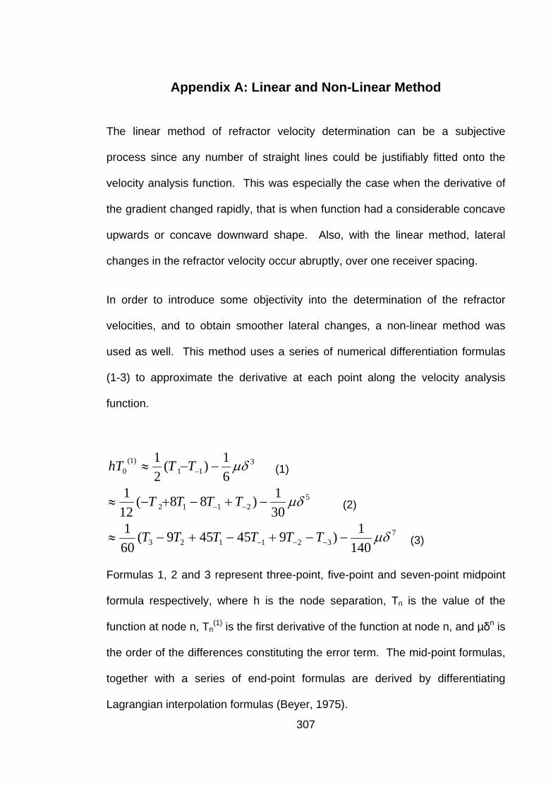
Appendix A: Linear and Non-Linear Method The linear method of refractor velocity determination can be a subjective
process since any number of straight lines could be justifiably fitted onto the
velocity analysis function. This was especially the case when the derivative of
the gradient changed rapidly, that is when function had a considerable concave
upwards or concave downward shape. Also, with the linear method, lateral
changes in the refractor velocity occur abruptly, over one receiver spacing.
In order to introduce some objectivity into the determination of the refractor
velocities, and to obtain smoother lateral changes, a non-linear method was
used as well. This method uses a series of numerical differentiation formulas
(1-3) to approximate the derivative at each point along the velocity analysis
function.
311
)1(0 6
1)(21 µδ−−≈ −TThT (1)
52112 30
1)88(121 µδ−+−+−≈ −− TTTT (2)
7321123 140
1)945459(601 µδ−−+−+−≈ −−− TTTTTT (3)
Formulas 1, 2 and 3 represent three-point, five-point and seven-point midpoint
formula respectively, where h is the node separation, Tn is the value of the
function at node n, Tn(1) is the first derivative of the function at node n, and µδn is
the order of the differences constituting the error term. The mid-point formulas,
together with a series of end-point formulas are derived by differentiating
Lagrangian interpolation formulas (Beyer, 1975).
307
308
With the non-linear method, refractor velocities were calculated by substituting
the values of the velocity analysis function into the different numerical
differentiation formulas, to give the derivative at each point along the function
and then taking the reciprocal to give the refractor velocity at each of these
points. For example using the three-point midpoint formula (1) the reciprocal of
the refractor velocity at a centre point T0(1) is approximately half the difference of
the velocity analysis function at the point to its right T1 and the point to its left T-1
divided by the point separation h. The velocities obtained using the different
formulas were similar, however the smoothness of the velocity trends tended to
increase as the number of points used in the formula increased.
Reference: Beyer, W. H., 1975, Handbook of mathematical science, 5th edition: CRC Press, Florida.

Appendix B: Operations Reports
Dates of Survey
Start date: 6 April, 2003
End date: 13 April, 2003
Days in field: 8
Days lost: 1.5 travelling
0.5 weather
Site 1
Coordinates: 691000 mE, 6433000 mN
Description: Recently ploughed paddock.
No vegetation.
Loose soil layer (up to 5cm) above
compacted soil.
Erosional gully trending east-west to
northwest near receiver lines.
Site 2
Coordinates: 690000 mE, 6434000 mN
Description: Disused paddock.
Moderately dense scrub.
Two tree lines trending east-west cutting
through lines.
Hard compacted soil.
309

Climate
Max mean temperature: 33 °C January
Min mean temperature: 1.8 °C July
Average annual rainfall: 523 mm
Survey Parameters
Number of receiver lines: 4
Receiver line spacing: 10 m
Receiver line bearing: 311 site 1
206 site 2
Receivers per line 29
Receiver spacing 5 m
Receiver sampling rate: 1 ms
Sweep frequency range: 10-200 Hz
Number of sweeps: 4
Sweep length: 8 ms
Source point spacing: 20 m
Number of source points: 50 P
100 S1
100 S2
9 explosive site 1
83 P
76 S1
95 S2
4 explosive site 2
310

Personnel
Party manager: David Johnson GA
Project leader: Derecke Palmer UNSW
Observer: Mike Bogor Trace Geophysics
Vibrator operator: Ian Crawford GA
Quality control: Leonie Jones GA
Field hands: Pete Taylor GA
Ramin Nikrouz UNSW
Andrew Spyrou UNSW
311

Appendix C: Specifications for the Equipment
Vibrator Source
Type: IVI Minivibe T-15000
Make: Industrial Vehicles International
Carrier: Isuzu 4WD
Controller software: Sweepware
Max peak force: 2.722 kgf
Frequency range: 10-550 Hz
Reaction mass weight: 141 kgf
Reaction mass stroke: 4.78 cm
Baseplate area: 65.67 cm2
Receivers
Type: GS-20DM 14 Hz
Make: GeoSpace
Casing: PC-3D
Height 2.64 cm
Diameter 2.22 cm
Weight 43 gr
Natural frequency (Fn): 14 Hz ± 5%
Max tilt for Fn: 20°
Moving mass: 7.8g ± 5%
Standard coil resistance 240 ohms ± 5%
Intrinsic voltage sensitivity 0.177 V/cm/s ± 7%
312

Damping constant 0.95 Rc
Operating temp range: -45 to 100 °C
Seismic Recording System
Type: ARAM24
Make: Geo-X Systems
Number of traces: 360
RAM units: 48 @ 8 channels per RAM
CRU line interface cards: 4
Line tap units: 5
Battery packs (24 V): 80
Telemetry cables: 46 8 takeouts @ 12.5 m
Telemetry baseline cable: 10 348 m
5 105 m
Explosive Source
Type: Anzomex
Appearance Roughly cylindrical shapes
Composition: Penta-erythritol tetranitrate (PENT, 30-
70%)
Trinitrotoluene (TNT, 70-30%)
Sodium nitrate (0-10%)
Inert fillers (0-10%)
Specific gravity 1.62 g/cc
313

Shot Firing System
Typ Pelton Shot Pro II
Height 11.4 cm
Length 28 cm
Width 22.2 cm
Weight 3.6 kg
Operating temperature range -40°C to +60°C
Firing accuracy ±20 microseconds
Firing current up to 30 amps
Vehicles
Recording truck Isuzu ANSIR
Mini-vibe truck Isuzu ANSIR
Geophone truck Toyota GA
Light ute Toyota UNSW
314
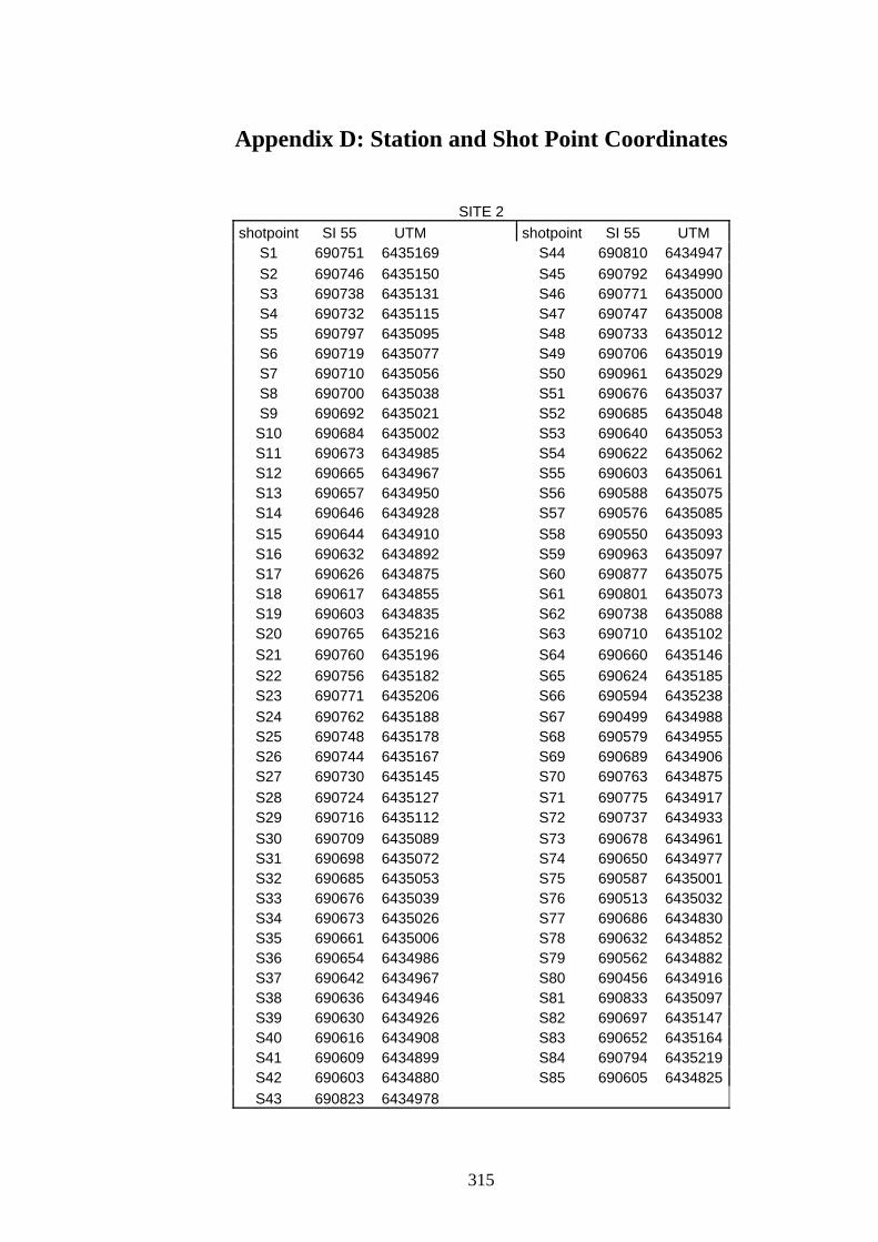
Appendix D: Station and Shot Point Coordinates
SITE 2 shotpoint SI 55 UTM shotpoint SI 55 UTM S1 690751 6435169 S44 690810 6434947 S2 690746 6435150 S45 690792 6434990 S3 690738 6435131 S46 690771 6435000 S4 690732 6435115 S47 690747 6435008 S5 690797 6435095 S48 690733 6435012 S6 690719 6435077 S49 690706 6435019 S7 690710 6435056 S50 690961 6435029 S8 690700 6435038 S51 690676 6435037 S9 690692 6435021 S52 690685 6435048 S10 690684 6435002 S53 690640 6435053 S11 690673 6434985 S54 690622 6435062 S12 690665 6434967 S55 690603 6435061 S13 690657 6434950 S56 690588 6435075 S14 690646 6434928 S57 690576 6435085 S15 690644 6434910 S58 690550 6435093 S16 690632 6434892 S59 690963 6435097 S17 690626 6434875 S60 690877 6435075 S18 690617 6434855 S61 690801 6435073 S19 690603 6434835 S62 690738 6435088 S20 690765 6435216 S63 690710 6435102 S21 690760 6435196 S64 690660 6435146 S22 690756 6435182 S65 690624 6435185 S23 690771 6435206 S66 690594 6435238 S24 690762 6435188 S67 690499 6434988 S25 690748 6435178 S68 690579 6434955 S26 690744 6435167 S69 690689 6434906 S27 690730 6435145 S70 690763 6434875 S28 690724 6435127 S71 690775 6434917 S29 690716 6435112 S72 690737 6434933 S30 690709 6435089 S73 690678 6434961 S31 690698 6435072 S74 690650 6434977 S32 690685 6435053 S75 690587 6435001 S33 690676 6435039 S76 690513 6435032 S34 690673 6435026 S77 690686 6434830 S35 690661 6435006 S78 690632 6434852 S36 690654 6434986 S79 690562 6434882 S37 690642 6434967 S80 690456 6434916 S38 690636 6434946 S81 690833 6435097 S39 690630 6434926 S82 690697 6435147 S40 690616 6434908 S83 690652 6435164 S41 690609 6434899 S84 690794 6435219 S42 690603 6434880 S85 690605 6434825 S43 690823 6434978
315
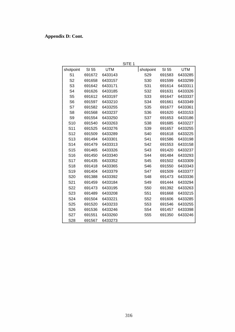
Appendix D: Cont.
SITE 1 shotpoint SI 55 UTM shotpoint SI 55 UTM S1 691672 6433143 S29 691583 6433285 S2 691658 6433157 S30 691599 6433299 S3 691642 6433171 S31 691614 6433311 S4 691626 6433185 S32 691631 6433326 S5 691612 6433197 S33 691647 6433337 S6 691597 6433210 S34 691661 6433349 S7 691582 6433255 S35 691677 6433361 S8 691568 6433237 S36 691620 6433153 S9 691554 6433250 S37 691653 6433186 S10 691540 6433263 S38 691685 6433227 S11 691525 6433276 S39 691657 6433255 S12 691509 6433289 S40 691618 6433225 S13 691494 6433301 S41 691586 6433198 S14 691479 6433313 S42 691553 6433158 S15 691465 6433326 S43 691420 6433237 S16 691450 6433340 S44 691484 6433293 S17 691435 6433352 S45 691502 6433309 S18 691418 6433365 S46 691550 6433343 S19 691404 6433379 S47 691509 6433377 S20 691388 6433392 S48 691473 6433336 S21 691459 6433184 S49 691444 6433294 S22 691473 6433195 S50 691392 6433263 S23 691489 6433208 S51 691668 6433215 S24 691504 6433221 S52 691606 6433285 S25 691520 6433233 S53 691546 6433255 S26 691536 6433246 S54 691457 6433398 S27 691551 6433260 S55 691350 6433246 S28 691567 6433273
316
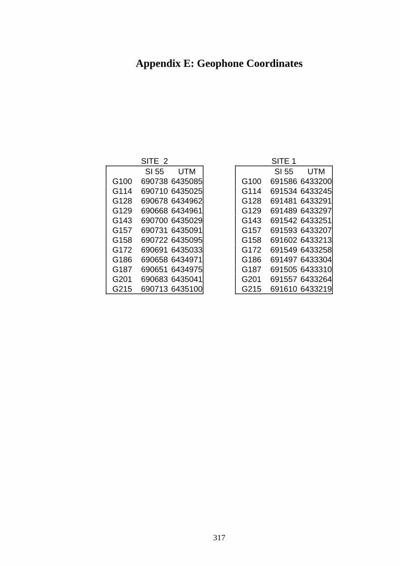
Appendix E: Geophone Coordinates
SITE 2 SITE 1 SI 55 UTM SI 55 UTM
G100 690738 6435085 G100 691586 6433200G114 690710 6435025 G114 691534 6433245G128 690678 6434962 G128 691481 6433291G129 690668 6434961 G129 691489 6433297G143 690700 6435029 G143 691542 6433251G157 690731 6435091 G157 691593 6433207G158 690722 6435095 G158 691602 6433213G172 690691 6435033 G172 691549 6433258G186 690658 6434971 G186 691497 6433304G187 690651 6434975 G187 691505 6433310G201 690683 6435041 G201 691557 6433264G215 690713 6435100 G215 691610 6433219
317
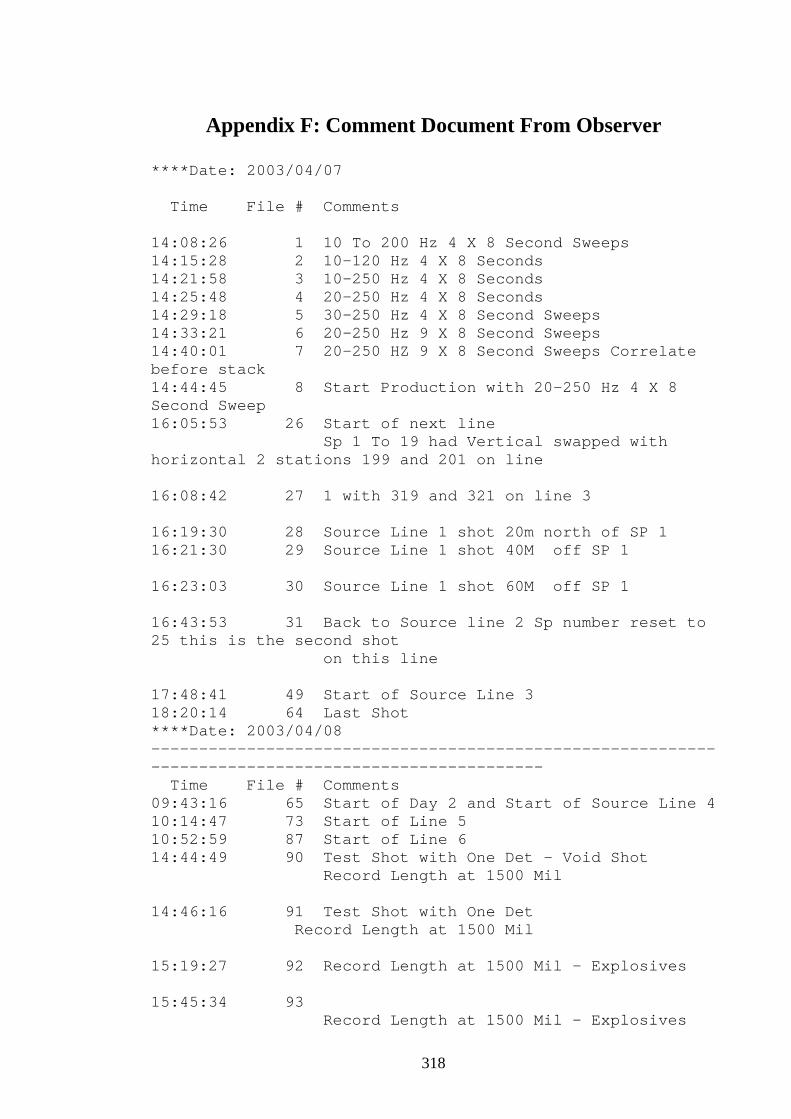
Appendix F: Comment Document From Observer
****Date: 2003/04/07 Time File # Comments 14:08:26 1 10 To 200 Hz 4 X 8 Second Sweeps 14:15:28 2 10-120 Hz 4 X 8 Seconds 14:21:58 3 10-250 Hz 4 X 8 Seconds 14:25:48 4 20-250 Hz 4 X 8 Seconds 14:29:18 5 30-250 Hz 4 X 8 Second Sweeps 14:33:21 6 20-250 Hz 9 X 8 Second Sweeps 14:40:01 7 20-250 HZ 9 X 8 Second Sweeps Correlate before stack 14:44:45 8 Start Production with 20-250 Hz 4 X 8 Second Sweep 16:05:53 26 Start of next line Sp 1 To 19 had Vertical swapped with horizontal 2 stations 199 and 201 on line 16:08:42 27 1 with 319 and 321 on line 3 16:19:30 28 Source Line 1 shot 20m north of SP 1 16:21:30 29 Source Line 1 shot 40M off SP 1 16:23:03 30 Source Line 1 shot 60M off SP 1 16:43:53 31 Back to Source line 2 Sp number reset to 25 this is the second shot on this line 17:48:41 49 Start of Source Line 3 18:20:14 64 Last Shot ****Date: 2003/04/08 ---------------------------------------------------------------------------------------------------- Time File # Comments 09:43:16 65 Start of Day 2 and Start of Source Line 4 10:14:47 73 Start of Line 5 10:52:59 87 Start of Line 6 14:44:49 90 Test Shot with One Det - Void Shot Record Length at 1500 Mil 14:46:16 91 Test Shot with One Det Record Length at 1500 Mil 15:19:27 92 Record Length at 1500 Mil - Explosives 15:45:34 93 Record Length at 1500 Mil - Explosives
318
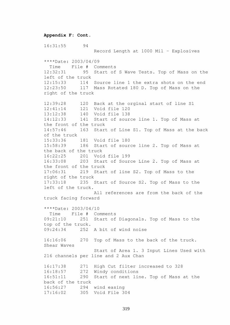
Appendix F: Cont. 16:31:55 94 Record Length at 1000 Mil - Explosives ****Date: 2003/04/09 Time File # Comments 12:32:31 95 Start of S Wave Tests. Top of Mass on the left of the truck 12:15:33 114 Source line 1 the extra shots on the end 12:23:50 117 Mass Rotated 180 D. Top of Mass on the right of the truck 12:39:28 120 Back at the orginal start of line S1 12:41:14 121 Void file 120 13:12:38 140 Void file 138 14:12:33 141 Start of source line 1. Top of Mass at the front of the truck 14:57:46 163 Start of Line S1. Top of Mass at the back of the truck 15:33:36 181 Void file 180 15:58:39 186 Start of source line 2. Top of Mass at the back of the truck 16:22:25 201 Void file 199 16:33:08 203 Start of Source Line 2. Top of Mass at the front of the truck 17:06:31 219 Start of line S2. Top of Mass to the right of the truck 17:33:18 235 Start of Source S2. Top of Mass to the left of the truck. All references are from the back of the truck facing forward ****Date: 2003/04/10 Time File # Comments 09:21:10 251 Start of Diagonals. Top of Mass to the top of the truck. 09:24:34 252 A bit of wind noise 16:16:06 270 Top of Mass to the back of the truck. Shear Waves Start of Area 1. 3 Input Lines Used with 216 channels per line and 2 Aux Chan 16:17:38 271 High Cut filter increased to 328 16:18:57 272 Windy conditions 16:51:11 290 Start of next line. Top of Mass at the back of the truck 16:56:27 294 wind easing 17:16:02 305 Void File 304
319
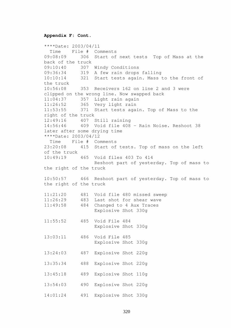
Appendix F: Cont. ****Date: 2003/04/11 Time File # Comments 09:08:09 306 Start of next tests Top of Mass at the back of the truck 09:10:40 307 Windy Conditions 09:36:34 319 A few rain drops falling 10:10:14 321 Start tests again. Mass to the front of the truck 10:56:08 353 Receivers 162 on line 2 and 3 were clipped on the wrong line. Now swapped back 11:04:37 357 Light rain again 11:26:52 365 Very light rain 11:53:55 371 Start tests again. Top of Mass to the right of the truck 12:49:16 407 Still raining 14:56:46 409 Void file 408 - Rain Noise. Reshoot 38 later after some drying time ****Date: 2003/04/12 Time File # Comments 23:20:08 415 Start of tests. Top of mass on the left of the truck 10:49:19 465 Void files 403 To 414 Reshoot part of yesterday. Top of mass to the right of the truck 10:50:57 466 Reshoot part of yesterday. Top of mass to the right of the truck 11:21:20 481 Void file 480 missed sweep 11:26:29 483 Last shot for shear wave 11:49:58 484 Changed to 4 Aux Traces Explosive Shot 330g 11:55:52 485 Void File 484 Explosive Shot 330g 13:03:11 486 Void File 485 Explosive Shot 330g 13:24:03 487 Explosive Shot 220g 13:35:34 488 Explosive Shot 220g 13:45:18 489 Explosive Shot 110g 13:54:03 490 Explosive Shot 220g 14:01:24 491 Explosive Shot 330g
320

14:15:01 492 Explosive Shot 440g 14:24:51 493 Explosive Shot 220g 14:44:26 494 Last Explosive Explosive Shot 220g 15:03:10 495 Start of P wave tests 16:16:34 544 End of Spicer Program
321

Appendix G: Assessment of Data Quality
Site 1 Source: Vertical
Rating (1-5) File
number Source Point #
Source Line #
SourceOrientation(V, S1, S2)
SourceLocation(in/out
spread)
Distance to
NearestDetector V H1 H2 Overall
Use (Yes/No)
495 1 S2 V out 100 4 3 2 3 Yes 496 2 S2 V out 80 4 3 2 3 Yes 497 3 S2 V out 60 4 2 2 3 Yes 498 4 S2 V out 40 4 2 2 3 Yes 499 5 S2 V out 20 4 2 2 3 Yes 500 6 S2 V in 5 4 2 2 3 Yes 501 7 S2 V in 5 4 2 1 2 Yes 502 8 S2 V in 5 3 1 1 2 Yes 503 9 S2 V in 5 3 2 1 2 Yes 504 10 S2 V in 5 4 4 3 4 Yes 505 11 S2 V in 5 4 2 1 2 Yes 506 12 S2 V in 5 4 2 2 3 Yes 507 13 S2 V in 5 4 3 3 3 Yes 508 14 S2 V out 20 4 3 3 3 Yes 509 15 S2 V out 40 4 3 3 3 Yes 510 16 S2 V out 60 3 2 2 2 Yes 511 17 S2 V out 80 3 3 3 3 Yes 512 18 S2 V out 100 3 2 2 2 Yes 513 19 S2 V out 120 3 3 2 3 Yes 514 20 S2 V out 140 3 2 2 2 Yes 515 21 S2 V out 100 1 1 2 1 Yes 516 22 S2 V out 80 1 1 2 1 Yes 517 23 S2 V out 60 2 1 1 1 Yes 518 24 S2 V out 40 2 1 1 1 Yes 519 25 S2 V out 20 3 1 1 2 Yes 520 26 S2 V in 0 4 1 1 2 Yes 521 27 S2 V in 0 4 2 1 2 Yes 522 28 S2 V out 20 4 1 1 2 Yes 523 29 S2 V out 40 3 1 2 2 Yes 524 30 S2 V out 60 3 1 1 2 Yes 525 31 S2 V out 80 3 1 1 2 Yes 526 32 S2 V out 100 3 1 1 2 Yes 527 33 S2 V out 120 3 1 1 2 Yes 528 34 S2 V out 140 3 2 2 2 Yes 529 35 S2 V out 160 3 2 2 2 Yes 530 36 S2 V out 60 4 3 3 3 Yes 531 37 S2 V out 60 4 3 3 3 Yes 532 38 S2 V out 60 3 2 2 2 Yes 533 39 S2 V out 20 3 2 2 2 Yes
322
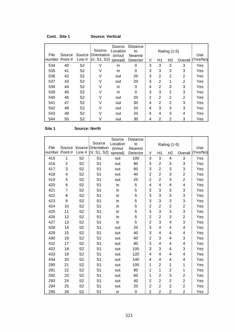
Cont. Site 1 Source: Vertical
Rating (1-5) File
number Source Point #
Source Line #
Source Orientation(V, S1, S2)
SourceLocation(in/out
spread)
Distance to
NearestDetector V H1 H2 Overall
Use (Yes/No)
534 40 S2 V in 0 3 3 3 3 Yes 535 41 S2 V in 0 3 3 3 3 Yes 536 42 S2 V out 20 3 2 2 2 Yes 537 43 S2 V out 20 3 2 1 2 Yes 538 44 S2 V in 0 4 2 3 3 Yes 539 45 S2 V in 0 3 3 2 3 Yes 540 46 S2 V out 20 2 2 2 2 Yes 541 47 S2 V out 30 4 2 2 3 Yes 542 48 S2 V out 20 4 3 3 3 Yes 543 49 S2 V out 20 4 4 3 4 Yes 544 50 S2 V out 30 4 2 2 3 Yes
Site 1 Source: North
Rating (1-5) File
number Source Point #
Source Line #
SourceOrientation(V, S1, S2)
SourceLocation(in/out
spread)
Distance to
NearestDetector V H1 H2 Overall
Use (Yes/No)
415 1 S2 S1 out 100 3 3 4 3 Yes 416 2 S2 S1 out 80 3 2 3 3 Yes 417 3 S2 S1 out 60 3 2 3 3 Yes 418 4 S2 S1 out 40 2 2 3 2 Yes 419 5 S2 S1 out 20 2 2 3 2 Yes 420 6 S2 S1 in 5 4 4 4 4 Yes 421 7 S2 S1 in 5 3 3 3 3 Yes 422 8 S2 S1 in 5 3 3 3 3 Yes 423 9 S2 S1 in 5 3 3 3 3 Yes 424 10 S2 S1 in 5 2 2 2 2 Yes 425 11 S2 S1 in 5 3 3 3 3 Yes 426 12 S2 S1 in 5 2 2 3 2 Yes 427 13 S2 S1 in 5 2 3 4 3 Yes 428 14 S2 S1 out 20 3 4 4 4 Yes 429 15 S2 S1 out 40 3 4 4 4 Yes 430 16 S2 S1 out 60 2 3 4 3 Yes 431 17 S2 S1 out 80 3 4 4 4 Yes 432 18 S2 S1 out 100 3 3 4 3 Yes 433 19 S2 S1 out 120 4 4 4 4 Yes 434 20 S2 S1 out 140 4 4 4 4 Yes 290 21 S2 S1 out 100 1 2 1 1 Yes 291 22 S2 S1 out 80 1 1 2 1 Yes 292 23 S2 S1 out 60 1 2 3 2 Yes 293 24 S2 S1 out 40 2 2 2 2 Yes 294 25 S2 S1 out 20 2 2 2 2 Yes 295 26 S2 S1 in 0 2 2 2 2 Yes
323
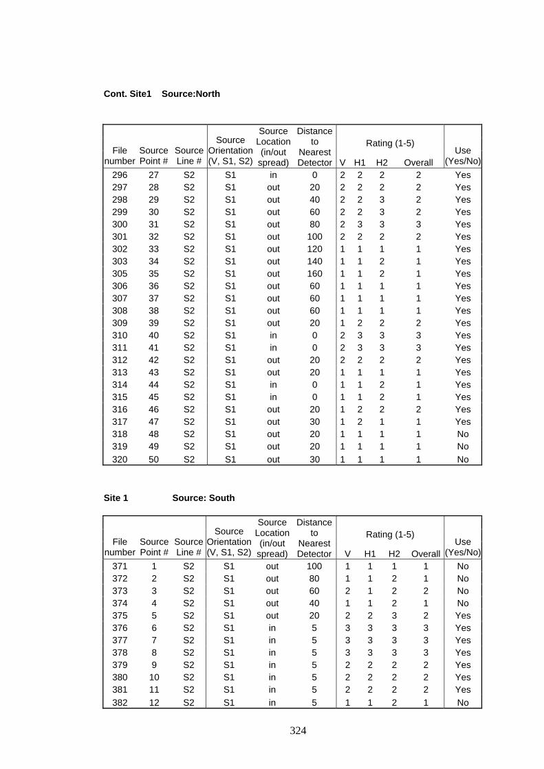
Cont. Site1 Source:North
Rating (1-5) File
number SourcePoint #
Source Line #
SourceOrientation(V, S1, S2)
SourceLocation(in/out
spread)
Distance to
NearestDetector V H1 H2 Overall
Use (Yes/No)
296 27 S2 S1 in 0 2 2 2 2 Yes 297 28 S2 S1 out 20 2 2 2 2 Yes 298 29 S2 S1 out 40 2 2 3 2 Yes 299 30 S2 S1 out 60 2 2 3 2 Yes 300 31 S2 S1 out 80 2 3 3 3 Yes 301 32 S2 S1 out 100 2 2 2 2 Yes 302 33 S2 S1 out 120 1 1 1 1 Yes 303 34 S2 S1 out 140 1 1 2 1 Yes 305 35 S2 S1 out 160 1 1 2 1 Yes 306 36 S2 S1 out 60 1 1 1 1 Yes 307 37 S2 S1 out 60 1 1 1 1 Yes 308 38 S2 S1 out 60 1 1 1 1 Yes 309 39 S2 S1 out 20 1 2 2 2 Yes 310 40 S2 S1 in 0 2 3 3 3 Yes 311 41 S2 S1 in 0 2 3 3 3 Yes 312 42 S2 S1 out 20 2 2 2 2 Yes 313 43 S2 S1 out 20 1 1 1 1 Yes 314 44 S2 S1 in 0 1 1 2 1 Yes 315 45 S2 S1 in 0 1 1 2 1 Yes 316 46 S2 S1 out 20 1 2 2 2 Yes 317 47 S2 S1 out 30 1 2 1 1 Yes 318 48 S2 S1 out 20 1 1 1 1 No 319 49 S2 S1 out 20 1 1 1 1 No 320 50 S2 S1 out 30 1 1 1 1 No
Site 1 Source: South
Rating (1-5) File
number Source Point #
Source Line #
SourceOrientation(V, S1, S2)
SourceLocation(in/out
spread)
Distance to
NearestDetector V H1 H2 Overall
Use (Yes/No)
371 1 S2 S1 out 100 1 1 1 1 No 372 2 S2 S1 out 80 1 1 2 1 No 373 3 S2 S1 out 60 2 1 2 2 No 374 4 S2 S1 out 40 1 1 2 1 No 375 5 S2 S1 out 20 2 2 3 2 Yes 376 6 S2 S1 in 5 3 3 3 3 Yes 377 7 S2 S1 in 5 3 3 3 3 Yes 378 8 S2 S1 in 5 3 3 3 3 Yes 379 9 S2 S1 in 5 2 2 2 2 Yes 380 10 S2 S1 in 5 2 2 2 2 Yes 381 11 S2 S1 in 5 2 2 2 2 Yes 382 12 S2 S1 in 5 1 1 2 1 No
324
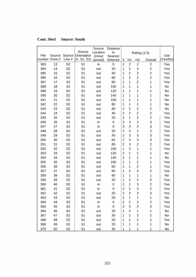
Cont. Site1 Source: South
Rating (1-5) File
number SourcePoint #
Source Line #
SourceOrientation(V, S1, S2)
SourceLocation(in/out
spread)
Distance to
NearestDetector V H1 H2 Overall
Use (Yes/No)
383 13 S2 S1 in 5 2 2 2 2 Yes 384 14 S2 S1 out 20 1 2 3 2 Yes 385 15 S2 S1 out 40 1 2 3 2 Yes 386 16 S2 S1 out 60 1 2 2 2 Yes 387 17 S2 S1 out 80 1 1 2 1 Yes 388 18 S2 S1 out 100 1 1 1 1 No 389 19 S2 S1 out 120 1 1 1 1 No 390 20 S2 S1 out 140 1 1 1 1 No 341 21 S2 S1 out 100 1 2 1 1 No 342 22 S2 S1 out 80 1 1 2 1 No 343 23 S2 S1 out 60 2 2 2 2 No 344 24 S2 S1 out 40 2 2 2 2 Yes 345 25 S2 S1 out 20 2 1 2 2 Yes 346 26 S2 S1 in 0 3 3 3 3 Yes 347 27 S2 S1 in 0 3 3 3 3 Yes 348 28 S2 S1 out 20 2 3 2 2 Yes 349 29 S2 S1 out 40 2 3 3 3 Yes 350 30 S2 S1 out 60 2 3 3 3 Yes 351 31 S2 S1 out 80 2 3 2 2 Yes 352 32 S2 S1 out 100 1 2 1 1 Yes 353 33 S2 S1 out 120 2 1 1 1 No 354 34 S2 S1 out 140 2 1 1 1 No 355 35 S2 S1 out 160 1 1 2 1 Yes 356 36 S2 S1 out 60 1 1 2 1 Yes 357 37 S2 S1 out 60 1 2 3 2 Yes 358 38 S2 S1 out 60 1 1 1 1 No 359 39 S2 S1 out 20 1 2 2 2 Yes 360 40 S2 S1 in 0 2 2 3 2 Yes 361 41 S2 S1 in 0 2 2 3 2 Yes 362 42 S2 S1 out 20 2 3 3 3 Yes 363 43 S2 S1 out 20 1 1 1 1 No 364 44 S2 S1 in 0 2 2 3 2 Yes 365 45 S2 S1 in 0 2 3 3 3 Yes 366 46 S2 S1 out 20 1 2 1 1 No 367 47 S2 S1 out 30 1 2 2 2 No 368 48 S2 S1 out 20 1 2 2 2 Yes 369 49 S2 S1 out 20 1 1 2 1 No 370 50 S2 S1 out 30 1 1 1 1 No
325
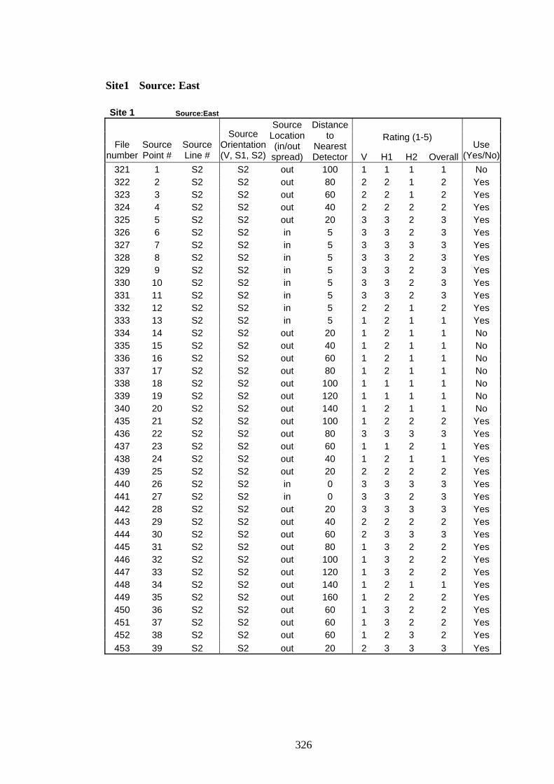
Site1 Source: East
Site 1 Source:East
Rating (1-5) File
number Source Point #
Source Line #
Source Orientation(V, S1, S2)
SourceLocation(in/out
spread)
Distance to
NearestDetector V H1 H2 Overall
Use (Yes/No)
321 1 S2 S2 out 100 1 1 1 1 No 322 2 S2 S2 out 80 2 2 1 2 Yes 323 3 S2 S2 out 60 2 2 1 2 Yes 324 4 S2 S2 out 40 2 2 2 2 Yes 325 5 S2 S2 out 20 3 3 2 3 Yes 326 6 S2 S2 in 5 3 3 2 3 Yes 327 7 S2 S2 in 5 3 3 3 3 Yes 328 8 S2 S2 in 5 3 3 2 3 Yes 329 9 S2 S2 in 5 3 3 2 3 Yes 330 10 S2 S2 in 5 3 3 2 3 Yes 331 11 S2 S2 in 5 3 3 2 3 Yes 332 12 S2 S2 in 5 2 2 1 2 Yes 333 13 S2 S2 in 5 1 2 1 1 Yes 334 14 S2 S2 out 20 1 2 1 1 No 335 15 S2 S2 out 40 1 2 1 1 No 336 16 S2 S2 out 60 1 2 1 1 No 337 17 S2 S2 out 80 1 2 1 1 No 338 18 S2 S2 out 100 1 1 1 1 No 339 19 S2 S2 out 120 1 1 1 1 No 340 20 S2 S2 out 140 1 2 1 1 No 435 21 S2 S2 out 100 1 2 2 2 Yes 436 22 S2 S2 out 80 3 3 3 3 Yes 437 23 S2 S2 out 60 1 1 2 1 Yes 438 24 S2 S2 out 40 1 2 1 1 Yes 439 25 S2 S2 out 20 2 2 2 2 Yes 440 26 S2 S2 in 0 3 3 3 3 Yes 441 27 S2 S2 in 0 3 3 2 3 Yes 442 28 S2 S2 out 20 3 3 3 3 Yes 443 29 S2 S2 out 40 2 2 2 2 Yes 444 30 S2 S2 out 60 2 3 3 3 Yes 445 31 S2 S2 out 80 1 3 2 2 Yes 446 32 S2 S2 out 100 1 3 2 2 Yes 447 33 S2 S2 out 120 1 3 2 2 Yes 448 34 S2 S2 out 140 1 2 1 1 Yes 449 35 S2 S2 out 160 1 2 2 2 Yes 450 36 S2 S2 out 60 1 3 2 2 Yes 451 37 S2 S2 out 60 1 3 2 2 Yes 452 38 S2 S2 out 60 1 2 3 2 Yes 453 39 S2 S2 out 20 2 3 3 3 Yes
326
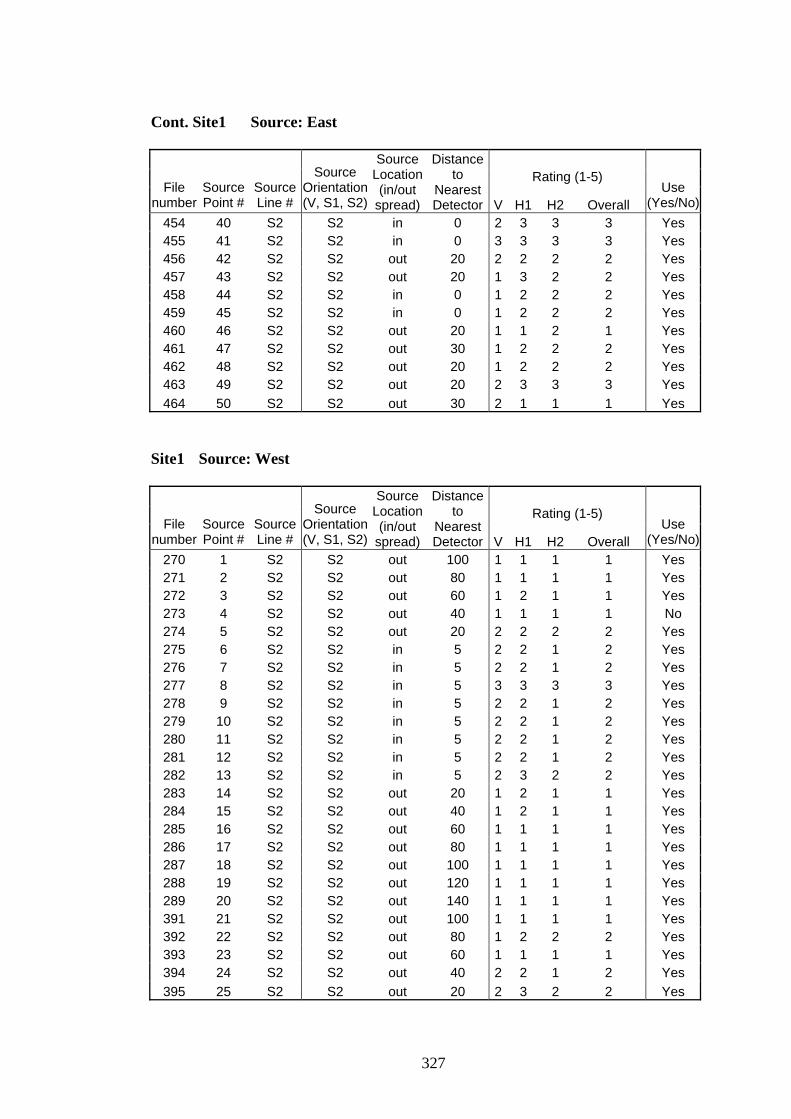
Cont. Site1 Source: East
Rating (1-5) File
number SourcePoint #
Source Line #
SourceOrientation(V, S1, S2)
SourceLocation(in/out
spread)
Distance to
NearestDetector V H1 H2 Overall
Use (Yes/No)
454 40 S2 S2 in 0 2 3 3 3 Yes 455 41 S2 S2 in 0 3 3 3 3 Yes 456 42 S2 S2 out 20 2 2 2 2 Yes 457 43 S2 S2 out 20 1 3 2 2 Yes 458 44 S2 S2 in 0 1 2 2 2 Yes 459 45 S2 S2 in 0 1 2 2 2 Yes 460 46 S2 S2 out 20 1 1 2 1 Yes 461 47 S2 S2 out 30 1 2 2 2 Yes 462 48 S2 S2 out 20 1 2 2 2 Yes 463 49 S2 S2 out 20 2 3 3 3 Yes 464 50 S2 S2 out 30 2 1 1 1 Yes
Site1 Source: West
Rating (1-5) File
number SourcePoint #
Source Line #
SourceOrientation(V, S1, S2)
SourceLocation(in/out
spread)
Distance to
NearestDetector V H1 H2 Overall
Use (Yes/No)
270 1 S2 S2 out 100 1 1 1 1 Yes 271 2 S2 S2 out 80 1 1 1 1 Yes 272 3 S2 S2 out 60 1 2 1 1 Yes 273 4 S2 S2 out 40 1 1 1 1 No 274 5 S2 S2 out 20 2 2 2 2 Yes 275 6 S2 S2 in 5 2 2 1 2 Yes 276 7 S2 S2 in 5 2 2 1 2 Yes 277 8 S2 S2 in 5 3 3 3 3 Yes 278 9 S2 S2 in 5 2 2 1 2 Yes 279 10 S2 S2 in 5 2 2 1 2 Yes 280 11 S2 S2 in 5 2 2 1 2 Yes 281 12 S2 S2 in 5 2 2 1 2 Yes 282 13 S2 S2 in 5 2 3 2 2 Yes 283 14 S2 S2 out 20 1 2 1 1 Yes 284 15 S2 S2 out 40 1 2 1 1 Yes 285 16 S2 S2 out 60 1 1 1 1 Yes 286 17 S2 S2 out 80 1 1 1 1 Yes 287 18 S2 S2 out 100 1 1 1 1 Yes 288 19 S2 S2 out 120 1 1 1 1 Yes 289 20 S2 S2 out 140 1 1 1 1 Yes 391 21 S2 S2 out 100 1 1 1 1 Yes 392 22 S2 S2 out 80 1 2 2 2 Yes 393 23 S2 S2 out 60 1 1 1 1 Yes 394 24 S2 S2 out 40 2 2 1 2 Yes 395 25 S2 S2 out 20 2 3 2 2 Yes
327
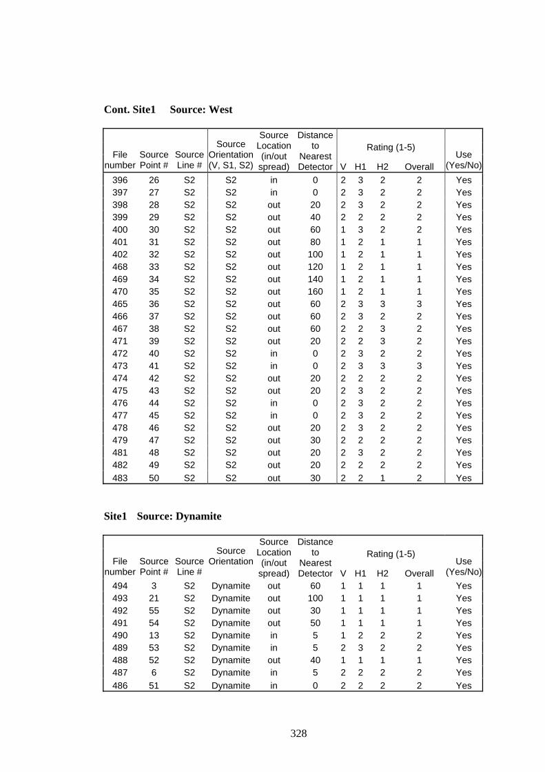
Cont. Site1 Source: West
Rating (1-5) File
number SourcePoint #
Source Line #
SourceOrientation(V, S1, S2)
SourceLocation(in/out
spread)
Distance to
NearestDetector V H1 H2 Overall
Use (Yes/No)
396 26 S2 S2 in 0 2 3 2 2 Yes 397 27 S2 S2 in 0 2 3 2 2 Yes 398 28 S2 S2 out 20 2 3 2 2 Yes 399 29 S2 S2 out 40 2 2 2 2 Yes 400 30 S2 S2 out 60 1 3 2 2 Yes 401 31 S2 S2 out 80 1 2 1 1 Yes 402 32 S2 S2 out 100 1 2 1 1 Yes 468 33 S2 S2 out 120 1 2 1 1 Yes 469 34 S2 S2 out 140 1 2 1 1 Yes 470 35 S2 S2 out 160 1 2 1 1 Yes 465 36 S2 S2 out 60 2 3 3 3 Yes 466 37 S2 S2 out 60 2 3 2 2 Yes 467 38 S2 S2 out 60 2 2 3 2 Yes 471 39 S2 S2 out 20 2 2 3 2 Yes 472 40 S2 S2 in 0 2 3 2 2 Yes 473 41 S2 S2 in 0 2 3 3 3 Yes 474 42 S2 S2 out 20 2 2 2 2 Yes 475 43 S2 S2 out 20 2 3 2 2 Yes 476 44 S2 S2 in 0 2 3 2 2 Yes 477 45 S2 S2 in 0 2 3 2 2 Yes 478 46 S2 S2 out 20 2 3 2 2 Yes 479 47 S2 S2 out 30 2 2 2 2 Yes 481 48 S2 S2 out 20 2 3 2 2 Yes 482 49 S2 S2 out 20 2 2 2 2 Yes 483 50 S2 S2 out 30 2 2 1 2 Yes
Site1 Source: Dynamite
Rating (1-5) File
number SourcePoint #
Source Line #
SourceOrientation
SourceLocation(in/out
spread)
Distance to
NearestDetector V H1 H2 Overall
Use (Yes/No)
494 3 S2 Dynamite out 60 1 1 1 1 Yes 493 21 S2 Dynamite out 100 1 1 1 1 Yes 492 55 S2 Dynamite out 30 1 1 1 1 Yes 491 54 S2 Dynamite out 50 1 1 1 1 Yes 490 13 S2 Dynamite in 5 1 2 2 2 Yes 489 53 S2 Dynamite in 5 2 3 2 2 Yes 488 52 S2 Dynamite out 40 1 1 1 1 Yes 487 6 S2 Dynamite in 5 2 2 2 2 Yes 486 51 S2 Dynamite in 0 2 2 2 2 Yes
328
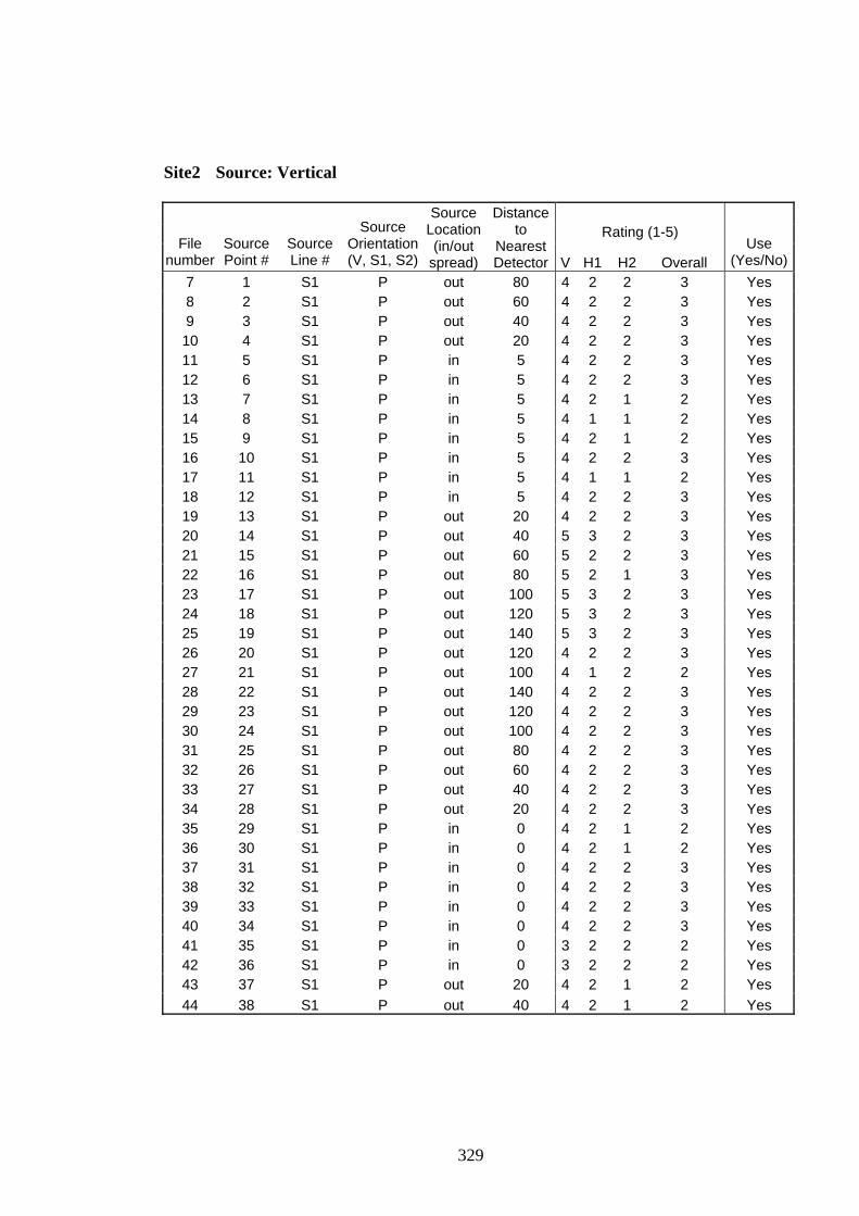
Site2 Source: Vertical
Rating (1-5) File
number Source Point #
Source Line #
Source Orientation(V, S1, S2)
SourceLocation(in/out
spread)
Distance to
NearestDetector V H1 H2 Overall
Use (Yes/No)
7 1 S1 P out 80 4 2 2 3 Yes 8 2 S1 P out 60 4 2 2 3 Yes 9 3 S1 P out 40 4 2 2 3 Yes 10 4 S1 P out 20 4 2 2 3 Yes 11 5 S1 P in 5 4 2 2 3 Yes 12 6 S1 P in 5 4 2 2 3 Yes 13 7 S1 P in 5 4 2 1 2 Yes 14 8 S1 P in 5 4 1 1 2 Yes 15 9 S1 P in 5 4 2 1 2 Yes 16 10 S1 P in 5 4 2 2 3 Yes 17 11 S1 P in 5 4 1 1 2 Yes 18 12 S1 P in 5 4 2 2 3 Yes 19 13 S1 P out 20 4 2 2 3 Yes 20 14 S1 P out 40 5 3 2 3 Yes 21 15 S1 P out 60 5 2 2 3 Yes 22 16 S1 P out 80 5 2 1 3 Yes 23 17 S1 P out 100 5 3 2 3 Yes 24 18 S1 P out 120 5 3 2 3 Yes 25 19 S1 P out 140 5 3 2 3 Yes 26 20 S1 P out 120 4 2 2 3 Yes 27 21 S1 P out 100 4 1 2 2 Yes 28 22 S1 P out 140 4 2 2 3 Yes 29 23 S1 P out 120 4 2 2 3 Yes 30 24 S1 P out 100 4 2 2 3 Yes 31 25 S1 P out 80 4 2 2 3 Yes 32 26 S1 P out 60 4 2 2 3 Yes 33 27 S1 P out 40 4 2 2 3 Yes 34 28 S1 P out 20 4 2 2 3 Yes 35 29 S1 P in 0 4 2 1 2 Yes 36 30 S1 P in 0 4 2 1 2 Yes 37 31 S1 P in 0 4 2 2 3 Yes 38 32 S1 P in 0 4 2 2 3 Yes 39 33 S1 P in 0 4 2 2 3 Yes 40 34 S1 P in 0 4 2 2 3 Yes 41 35 S1 P in 0 3 2 2 2 Yes 42 36 S1 P in 0 3 2 2 2 Yes 43 37 S1 P out 20 4 2 1 2 Yes 44 38 S1 P out 40 4 2 1 2 Yes
329
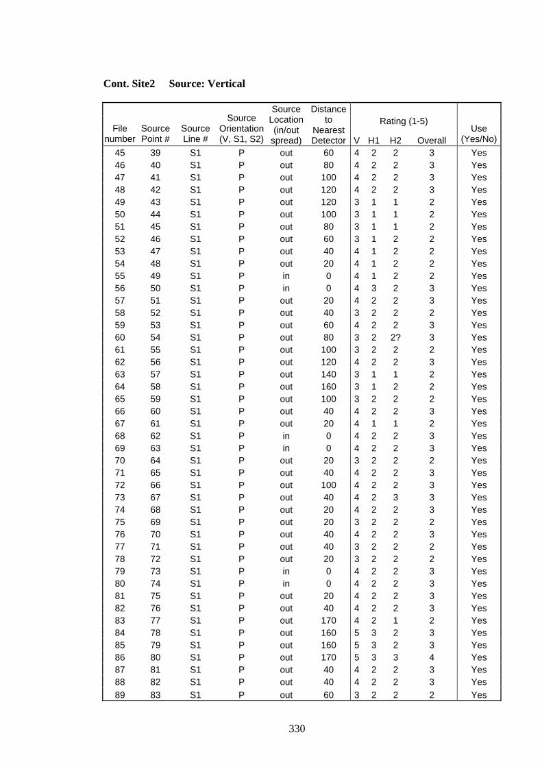
Cont. Site2 Source: Vertical
Rating (1-5) File
number Source Point #
Source Line #
Source Orientation(V, S1, S2)
SourceLocation(in/out
spread)
Distance to
NearestDetector V H1 H2 Overall
Use (Yes/No)
45 39 S1 P out 60 4 2 2 3 Yes 46 40 S1 P out 80 4 2 2 3 Yes 47 41 S1 P out 100 4 2 2 3 Yes 48 42 S1 P out 120 4 2 2 3 Yes 49 43 S1 P out 120 3 1 1 2 Yes 50 44 S1 P out 100 3 1 1 2 Yes 51 45 S1 P out 80 3 1 1 2 Yes 52 46 S1 P out 60 3 1 2 2 Yes 53 47 S1 P out 40 4 1 2 2 Yes 54 48 S1 P out 20 4 1 2 2 Yes 55 49 S1 P in 0 4 1 2 2 Yes 56 50 S1 P in 0 4 3 2 3 Yes 57 51 S1 P out 20 4 2 2 3 Yes 58 52 S1 P out 40 3 2 2 2 Yes 59 53 S1 P out 60 4 2 2 3 Yes 60 54 S1 P out 80 3 2 2? 3 Yes 61 55 S1 P out 100 3 2 2 2 Yes 62 56 S1 P out 120 4 2 2 3 Yes 63 57 S1 P out 140 3 1 1 2 Yes 64 58 S1 P out 160 3 1 2 2 Yes 65 59 S1 P out 100 3 2 2 2 Yes 66 60 S1 P out 40 4 2 2 3 Yes 67 61 S1 P out 20 4 1 1 2 Yes 68 62 S1 P in 0 4 2 2 3 Yes 69 63 S1 P in 0 4 2 2 3 Yes 70 64 S1 P out 20 3 2 2 2 Yes 71 65 S1 P out 40 4 2 2 3 Yes 72 66 S1 P out 100 4 2 2 3 Yes 73 67 S1 P out 40 4 2 3 3 Yes 74 68 S1 P out 20 4 2 2 3 Yes 75 69 S1 P out 20 3 2 2 2 Yes 76 70 S1 P out 40 4 2 2 3 Yes 77 71 S1 P out 40 3 2 2 2 Yes 78 72 S1 P out 20 3 2 2 2 Yes 79 73 S1 P in 0 4 2 2 3 Yes 80 74 S1 P in 0 4 2 2 3 Yes 81 75 S1 P out 20 4 2 2 3 Yes 82 76 S1 P out 40 4 2 2 3 Yes 83 77 S1 P out 170 4 2 1 2 Yes 84 78 S1 P out 160 5 3 2 3 Yes 85 79 S1 P out 160 5 3 2 3 Yes 86 80 S1 P out 170 5 3 3 4 Yes 87 81 S1 P out 40 4 2 2 3 Yes 88 82 S1 P out 40 4 2 2 3 Yes 89 83 S1 P out 60 3 2 2 2 Yes
330
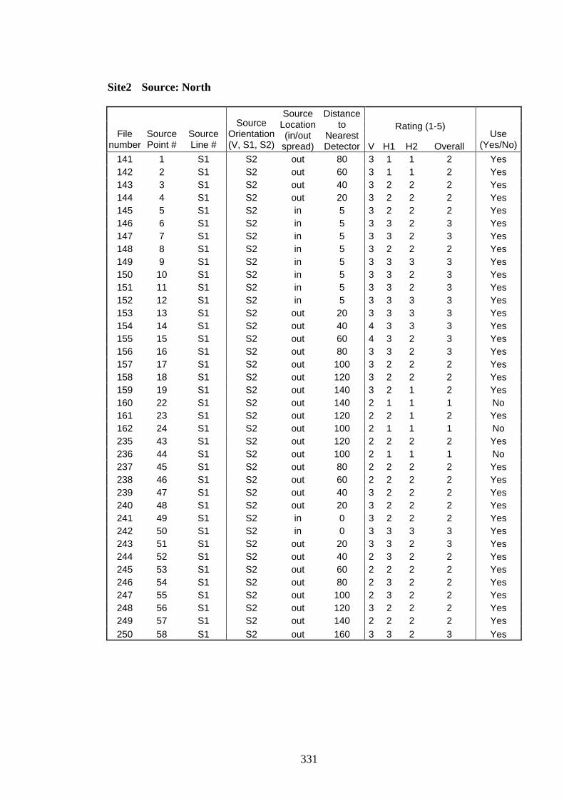
Site2 Source: North
Rating (1-5) File
number Source Point #
Source Line #
Source Orientation(V, S1, S2)
SourceLocation(in/out
spread)
Distance to
NearestDetector V H1 H2 Overall
Use (Yes/No)
141 1 S1 S2 out 80 3 1 1 2 Yes 142 2 S1 S2 out 60 3 1 1 2 Yes 143 3 S1 S2 out 40 3 2 2 2 Yes 144 4 S1 S2 out 20 3 2 2 2 Yes 145 5 S1 S2 in 5 3 2 2 2 Yes 146 6 S1 S2 in 5 3 3 2 3 Yes 147 7 S1 S2 in 5 3 3 2 3 Yes 148 8 S1 S2 in 5 3 2 2 2 Yes 149 9 S1 S2 in 5 3 3 3 3 Yes 150 10 S1 S2 in 5 3 3 2 3 Yes 151 11 S1 S2 in 5 3 3 2 3 Yes 152 12 S1 S2 in 5 3 3 3 3 Yes 153 13 S1 S2 out 20 3 3 3 3 Yes 154 14 S1 S2 out 40 4 3 3 3 Yes 155 15 S1 S2 out 60 4 3 2 3 Yes 156 16 S1 S2 out 80 3 3 2 3 Yes 157 17 S1 S2 out 100 3 2 2 2 Yes 158 18 S1 S2 out 120 3 2 2 2 Yes 159 19 S1 S2 out 140 3 2 1 2 Yes 160 22 S1 S2 out 140 2 1 1 1 No 161 23 S1 S2 out 120 2 2 1 2 Yes 162 24 S1 S2 out 100 2 1 1 1 No 235 43 S1 S2 out 120 2 2 2 2 Yes 236 44 S1 S2 out 100 2 1 1 1 No 237 45 S1 S2 out 80 2 2 2 2 Yes 238 46 S1 S2 out 60 2 2 2 2 Yes 239 47 S1 S2 out 40 3 2 2 2 Yes 240 48 S1 S2 out 20 3 2 2 2 Yes 241 49 S1 S2 in 0 3 2 2 2 Yes 242 50 S1 S2 in 0 3 3 3 3 Yes 243 51 S1 S2 out 20 3 3 2 3 Yes 244 52 S1 S2 out 40 2 3 2 2 Yes 245 53 S1 S2 out 60 2 2 2 2 Yes 246 54 S1 S2 out 80 2 3 2 2 Yes 247 55 S1 S2 out 100 2 3 2 2 Yes 248 56 S1 S2 out 120 3 2 2 2 Yes 249 57 S1 S2 out 140 2 2 2 2 Yes 250 58 S1 S2 out 160 3 3 2 3 Yes
331
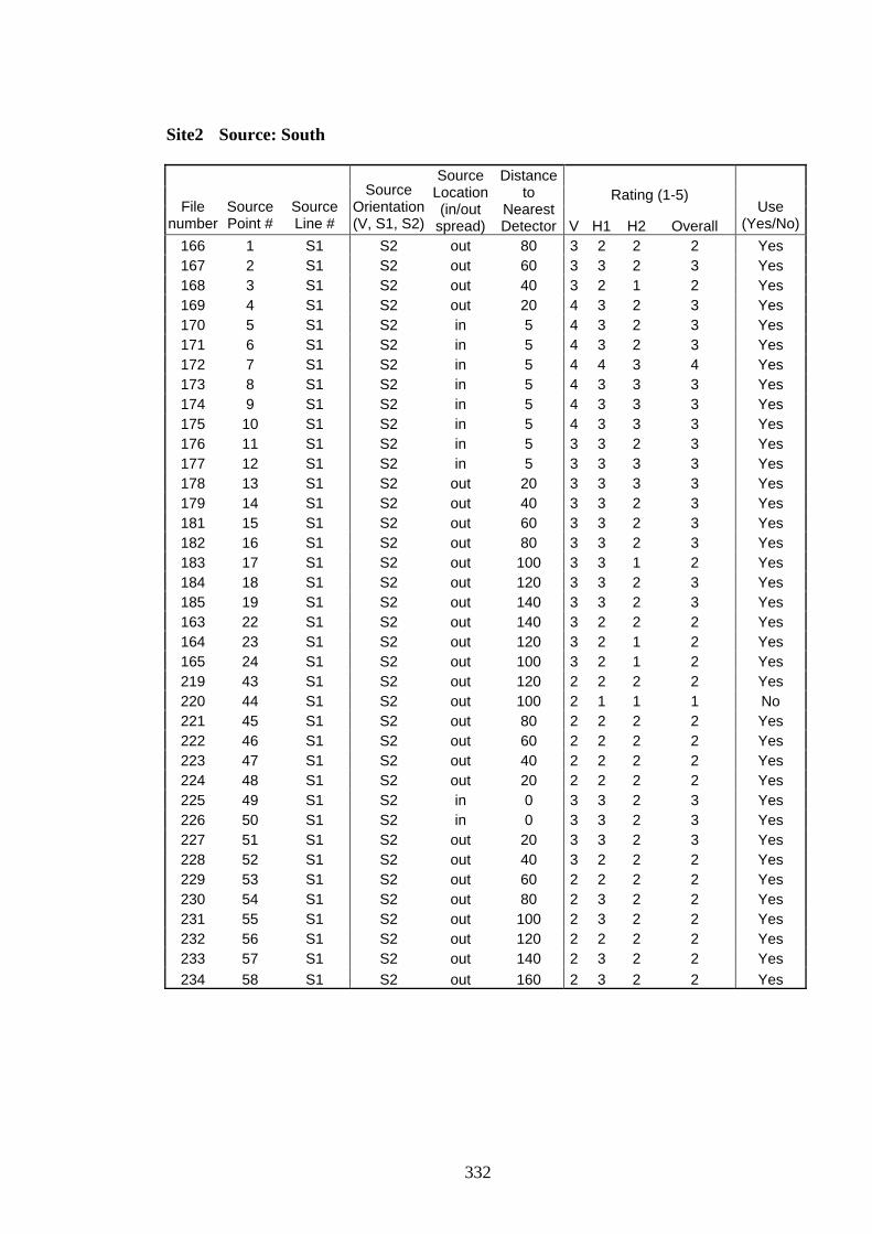
Site2 Source: South
Rating (1-5) File
number Source Point #
Source Line #
Source Orientation(V, S1, S2)
SourceLocation(in/out
spread)
Distance to
NearestDetector V H1 H2 Overall
Use (Yes/No)
166 1 S1 S2 out 80 3 2 2 2 Yes 167 2 S1 S2 out 60 3 3 2 3 Yes 168 3 S1 S2 out 40 3 2 1 2 Yes 169 4 S1 S2 out 20 4 3 2 3 Yes 170 5 S1 S2 in 5 4 3 2 3 Yes 171 6 S1 S2 in 5 4 3 2 3 Yes 172 7 S1 S2 in 5 4 4 3 4 Yes 173 8 S1 S2 in 5 4 3 3 3 Yes 174 9 S1 S2 in 5 4 3 3 3 Yes 175 10 S1 S2 in 5 4 3 3 3 Yes 176 11 S1 S2 in 5 3 3 2 3 Yes 177 12 S1 S2 in 5 3 3 3 3 Yes 178 13 S1 S2 out 20 3 3 3 3 Yes 179 14 S1 S2 out 40 3 3 2 3 Yes 181 15 S1 S2 out 60 3 3 2 3 Yes 182 16 S1 S2 out 80 3 3 2 3 Yes 183 17 S1 S2 out 100 3 3 1 2 Yes 184 18 S1 S2 out 120 3 3 2 3 Yes 185 19 S1 S2 out 140 3 3 2 3 Yes 163 22 S1 S2 out 140 3 2 2 2 Yes 164 23 S1 S2 out 120 3 2 1 2 Yes 165 24 S1 S2 out 100 3 2 1 2 Yes 219 43 S1 S2 out 120 2 2 2 2 Yes 220 44 S1 S2 out 100 2 1 1 1 No 221 45 S1 S2 out 80 2 2 2 2 Yes 222 46 S1 S2 out 60 2 2 2 2 Yes 223 47 S1 S2 out 40 2 2 2 2 Yes 224 48 S1 S2 out 20 2 2 2 2 Yes 225 49 S1 S2 in 0 3 3 2 3 Yes 226 50 S1 S2 in 0 3 3 2 3 Yes 227 51 S1 S2 out 20 3 3 2 3 Yes 228 52 S1 S2 out 40 3 2 2 2 Yes 229 53 S1 S2 out 60 2 2 2 2 Yes 230 54 S1 S2 out 80 2 3 2 2 Yes 231 55 S1 S2 out 100 2 3 2 2 Yes 232 56 S1 S2 out 120 2 2 2 2 Yes 233 57 S1 S2 out 140 2 3 2 2 Yes 234 58 S1 S2 out 160 2 3 2 2 Yes
332

Site2 Source: East
Rating (1-5) File
number Source Point #
Source Line #
Source Orientation(V, S1, S2)
SourceLocation(in/out
spread)
Distance to
NearestDetector V H1 H2 Overall
Use (Yes/No)
121 1 S1 S1 out 80 2 1 2 2 Yes 122 2 S1 S1 out 60 2 1 2 2 Yes 123 3 S1 S1 out 40 2 1 3 2 Yes 124 4 S1 S1 out 20 2 2 3 2 Yes 125 5 S1 S1 in 5 3 2 3 3 Yes 126 6 S1 S1 in 5 3 2 4 3 Yes 127 7 S1 S1 in 5 2 2 3 2 Yes 128 8 S1 S1 in 5 3 2 3 3 Yes 129 9 S1 S1 in 5 3 2 2 2 Yes 130 10 S1 S1 in 5 2 2 3 2 Yes 131 11 S1 S1 in 5 2 2 2 2 Yes 132 12 S1 S1 in 5 2 2 3 2 Yes 133 13 S1 S1 out 20 2 3 4 3 Yes 134 14 S1 S1 out 40 2 3 4 3 Yes 135 15 S1 S1 out 60 2 2 2 2 Yes 136 16 S1 S1 out 80 2 2 3 2 Yes 137 17 S1 S1 out 100 2 2 3 2 Yes 140 18 S1 S1 out 120 2 1 2 2 Yes 139 19 S1 S1 out 140 2 1 2 2 Yes 117 22 S1 S1 out 140 2 1 2 2 Yes 118 23 S1 S1 out 120 2 2 2 2 Yes 119 24 S1 S1 out 100 2 2 3 2 Yes 203 43 S1 S1 out 120 2 1 1 1 No 204 44 S1 S1 out 100 2 1 1 1 No 205 45 S1 S1 out 80 1 2 2 2 Yes 206 46 S1 S1 out 60 1 1 2 1 No 207 47 S1 S1 out 40 1 1 2 1 No 208 48 S1 S1 out 20 2 2 2 2 Yes 209 49 S1 S1 in 0 2 2 2 2 Yes 210 50 S1 S1 in 0 2 2 3 2 Yes 211 51 S1 S1 out 20 2 2 2 2 Yes 212 52 S1 S1 out 40 2 2 2 2 Yes 213 53 S1 S1 out 60 2 2 2 2 Yes 214 54 S1 S1 out 80 3 2 2 2 Yes 215 55 S1 S1 out 100 3 3 2 3 Yes 216 56 S1 S1 out 120 3 2 2 2 Yes 217 57 S1 S1 out 140 2 2 2 2 Yes 218 58 S1 S1 out 160 2 2 2 2 Yes
333
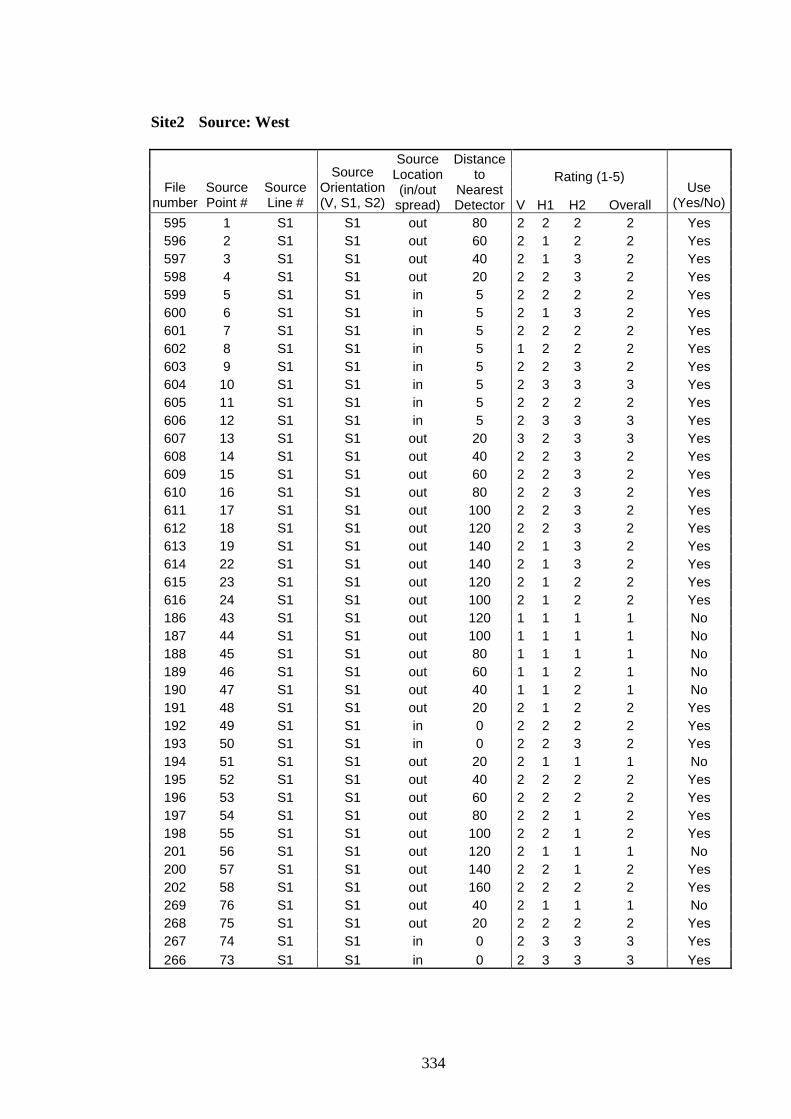
Site2 Source: West
Rating (1-5) File
number Source Point #
Source Line #
Source Orientation(V, S1, S2)
SourceLocation(in/out
spread)
Distance to
NearestDetector V H1 H2 Overall
Use (Yes/No)
595 1 S1 S1 out 80 2 2 2 2 Yes 596 2 S1 S1 out 60 2 1 2 2 Yes 597 3 S1 S1 out 40 2 1 3 2 Yes 598 4 S1 S1 out 20 2 2 3 2 Yes 599 5 S1 S1 in 5 2 2 2 2 Yes 600 6 S1 S1 in 5 2 1 3 2 Yes 601 7 S1 S1 in 5 2 2 2 2 Yes 602 8 S1 S1 in 5 1 2 2 2 Yes 603 9 S1 S1 in 5 2 2 3 2 Yes 604 10 S1 S1 in 5 2 3 3 3 Yes 605 11 S1 S1 in 5 2 2 2 2 Yes 606 12 S1 S1 in 5 2 3 3 3 Yes 607 13 S1 S1 out 20 3 2 3 3 Yes 608 14 S1 S1 out 40 2 2 3 2 Yes 609 15 S1 S1 out 60 2 2 3 2 Yes 610 16 S1 S1 out 80 2 2 3 2 Yes 611 17 S1 S1 out 100 2 2 3 2 Yes 612 18 S1 S1 out 120 2 2 3 2 Yes 613 19 S1 S1 out 140 2 1 3 2 Yes 614 22 S1 S1 out 140 2 1 3 2 Yes 615 23 S1 S1 out 120 2 1 2 2 Yes 616 24 S1 S1 out 100 2 1 2 2 Yes 186 43 S1 S1 out 120 1 1 1 1 No 187 44 S1 S1 out 100 1 1 1 1 No 188 45 S1 S1 out 80 1 1 1 1 No 189 46 S1 S1 out 60 1 1 2 1 No 190 47 S1 S1 out 40 1 1 2 1 No 191 48 S1 S1 out 20 2 1 2 2 Yes 192 49 S1 S1 in 0 2 2 2 2 Yes 193 50 S1 S1 in 0 2 2 3 2 Yes 194 51 S1 S1 out 20 2 1 1 1 No 195 52 S1 S1 out 40 2 2 2 2 Yes 196 53 S1 S1 out 60 2 2 2 2 Yes 197 54 S1 S1 out 80 2 2 1 2 Yes 198 55 S1 S1 out 100 2 2 1 2 Yes 201 56 S1 S1 out 120 2 1 1 1 No 200 57 S1 S1 out 140 2 2 1 2 Yes 202 58 S1 S1 out 160 2 2 2 2 Yes 269 76 S1 S1 out 40 2 1 1 1 No 268 75 S1 S1 out 20 2 2 2 2 Yes 267 74 S1 S1 in 0 2 3 3 3 Yes 266 73 S1 S1 in 0 2 3 3 3 Yes
334
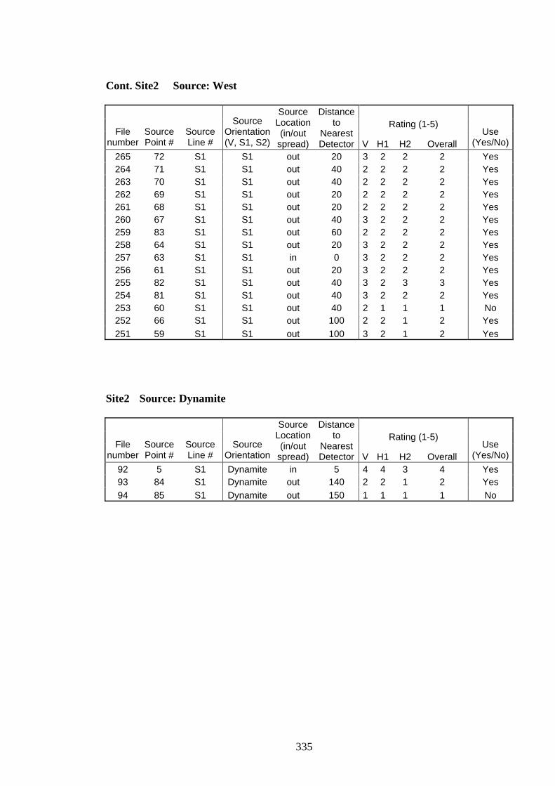
Cont. Site2 Source: West
Rating (1-5) File
number Source Point #
Source Line #
Source Orientation(V, S1, S2)
SourceLocation(in/out
spread)
Distance to
NearestDetector V H1 H2 Overall
Use (Yes/No)
265 72 S1 S1 out 20 3 2 2 2 Yes 264 71 S1 S1 out 40 2 2 2 2 Yes 263 70 S1 S1 out 40 2 2 2 2 Yes 262 69 S1 S1 out 20 2 2 2 2 Yes 261 68 S1 S1 out 20 2 2 2 2 Yes 260 67 S1 S1 out 40 3 2 2 2 Yes 259 83 S1 S1 out 60 2 2 2 2 Yes 258 64 S1 S1 out 20 3 2 2 2 Yes 257 63 S1 S1 in 0 3 2 2 2 Yes 256 61 S1 S1 out 20 3 2 2 2 Yes 255 82 S1 S1 out 40 3 2 3 3 Yes 254 81 S1 S1 out 40 3 2 2 2 Yes 253 60 S1 S1 out 40 2 1 1 1 No 252 66 S1 S1 out 100 2 2 1 2 Yes 251 59 S1 S1 out 100 3 2 1 2 Yes
Site2 Source: Dynamite
Rating (1-5) File
number Source Point #
Source Line #
Source Orientation
SourceLocation(in/out
spread)
Distance to
NearestDetector V H1 H2 Overall
Use (Yes/No)
92 5 S1 Dynamite in 5 4 4 3 4 Yes 93 84 S1 Dynamite out 140 2 2 1 2 Yes 94 85 S1 Dynamite out 150 1 1 1 1 No
335
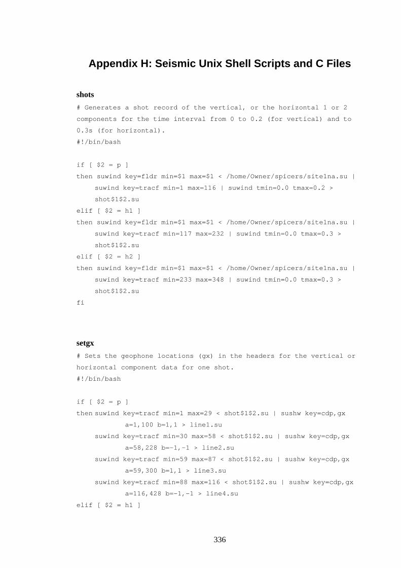
Appendix H: Seismic Unix Shell Scripts and C Files
shots # Generates a shot record of the vertical, or the horizontal 1 or 2
components for the time interval from 0 to 0.2 (for vertical) and to
0.3s (for horizontal).
#!/bin/bash
if [ $2 = p ]
then suwind key=fldr min=$1 max=$1 < /home/Owner/spicers/site1na.su |
suwind key=tracf min=1 max=116 | suwind tmin=0.0 tmax=0.2 >
shot$1$2.su
elif [ $2 = h1 ]
then suwind key=fldr min=$1 max=$1 < /home/Owner/spicers/site1na.su |
suwind key=tracf min=117 max=232 | suwind tmin=0.0 tmax=0.3 >
shot$1$2.su
elif [ $2 = h2 ]
then suwind key=fldr min=$1 max=$1 < /home/Owner/spicers/site1na.su |
suwind key=tracf min=233 max=348 | suwind tmin=0.0 tmax=0.3 >
shot$1$2.su
fi
setgx # Sets the geophone locations (gx) in the headers for the vertical or
horizontal component data for one shot.
#!/bin/bash
if [ $2 = p ]
then suwind key=tracf min=1 max=29 < shot$1$2.su | sushw key=cdp,gx
a=1,100 b=1,1 > line1.su
suwind key=tracf min=30 max=58 < shot$1$2.su | sushw key=cdp,gx
a=58,228 b=-1,-1 > line2.su
suwind key=tracf min=59 max=87 < shot$1$2.su | sushw key=cdp,gx
a=59,300 b=1,1 > line3.su
suwind key=tracf min=88 max=116 < shot$1$2.su | sushw key=cdp,gx
a=116,428 b=-1,-1 > line4.su
elif [ $2 = h1 ]
336
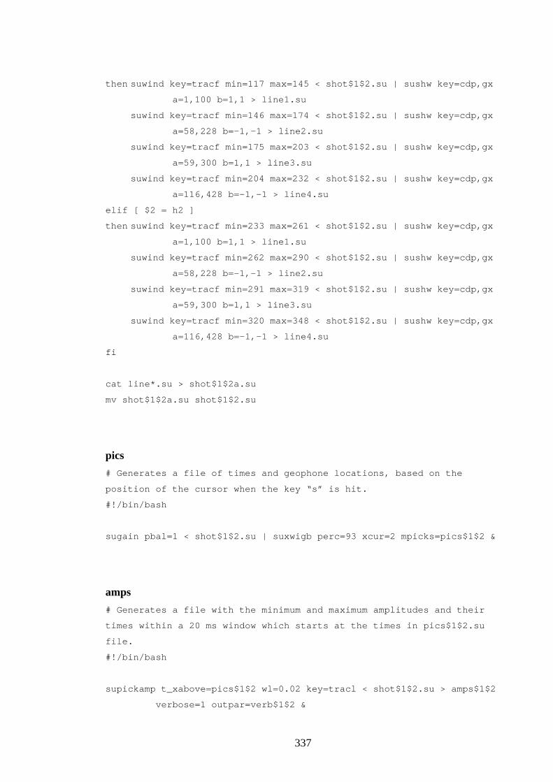
then suwind key=tracf min=117 max=145 < shot$1$2.su | sushw key=cdp,gx
a=1,100 b=1,1 > line1.su
suwind key=tracf min=146 max=174 < shot$1$2.su | sushw key=cdp,gx
a=58,228 b=-1,-1 > line2.su
suwind key=tracf min=175 max=203 < shot$1$2.su | sushw key=cdp,gx
a=59,300 b=1,1 > line3.su
suwind key=tracf min=204 max=232 < shot$1$2.su | sushw key=cdp,gx
a=116,428 b=-1,-1 > line4.su
elif [ $2 = h2 ]
then suwind key=tracf min=233 max=261 < shot$1$2.su | sushw key=cdp,gx
a=1,100 b=1,1 > line1.su
suwind key=tracf min=262 max=290 < shot$1$2.su | sushw key=cdp,gx
a=58,228 b=-1,-1 > line2.su
suwind key=tracf min=291 max=319 < shot$1$2.su | sushw key=cdp,gx
a=59,300 b=1,1 > line3.su
suwind key=tracf min=320 max=348 < shot$1$2.su | sushw key=cdp,gx
a=116,428 b=-1,-1 > line4.su
fi
cat line*.su > shot$1$2a.su
mv shot$1$2a.su shot$1$2.su
pics # Generates a file of times and geophone locations, based on the
position of the cursor when the key “s” is hit.
#!/bin/bash
sugain pbal=1 < shot$1$2.su | suxwigb perc=93 xcur=2 mpicks=pics$1$2 &
amps # Generates a file with the minimum and maximum amplitudes and their
times within a 20 ms window which starts at the times in pics$1$2.su
file.
#!/bin/bash
supickamp t_xabove=pics$1$2 wl=0.02 key=tracl < shot$1$2.su > amps$1$2
verbose=1 outpar=verb$1$2 &
337
plotAmps # Makes an EPS file of the shot record with the time for minimum and
maximum amplitudes overlayed.
#!/bin/bash
if [ $2 = p ]
then
tracemin=$(suwind key=tracf min=1 max=1 < shot$1$2.su | sugethw
key=tracl output=geom)
tracemax=$(suwind key=tracf min=116 max=116 < shot$1$2.su |
sugethw key=tracl output=geom)
elif [ $2 = h1 ]
then
tracemin=$(suwind key=tracf min=117 max=117 < shot$1$2.su |
sugethw key=tracl output=geom)
tracemax=$(suwind key=tracf min=232 max=232 < shot$1$2.su |
sugethw key=tracl output=geom)
elif [ $2 = h2 ]
then
tracemin=$(suwind key=tracf min=233 max=233 < shot$1$2.su |
sugethw key=tracl output=geom)
tracemax=$(suwind key=tracf min=348 max=348 < shot$1$2.su |
sugethw key=tracl output=geom)
fi
tracemin=`expr $tracemin - 2`
tracemax=`expr $tracemax + 2`
supickamp t_xabove=pics$1$2 arg1=tmax wl=0.02 key=tracl verbose=0 <
shot$1$2.su > tmax.ascii
supickamp t_xabove=pics$1$2 arg1=tmin wl=0.02 key=tracl verbose=0 <
shot$1$2.su > tmin.ascii
a2b < tmax.ascii n1=2 > tmax.bin
a2b < tmin.ascii n1=2 > tmin.bin
psgraph style=seismic linecolor=green labelsize=0 x1beg=0 x1end=0.2
x2beg=$tracemin x2end=$tracemax < tmax.bin n=116 > tmax.eps
psgraph style=seismic linecolor=red labelsize=0 x1beg=0 x1end=0.2
x2beg=$tracemin x2end=$tracemax < tmin.bin n=116 > tmin.eps
sugain pbal=1 < shot$1$2.su | supswigb perc=93 xcur=2 wbox=6 hbox=8
title="Record $1 $2" label1="Time (seconds)" label2="Trace Number"
> plota.eps
338
psmerge in=plota.eps in=tmax.eps in=tmin.eps > plot$1$2.eps
verbfixer.c // Takes max Amp, tmax, min Amp and tmin from verb file and reformats
// into tab delimited format, ready for excel.
// Usage: verbfixer -"option" < "input_verb_file" > "output"
// option: all
#include <string.h>
#include <stdio.h>
#include <ctype.h>
#include <stdlib.h>
float get1stnum(char line[])
char num1[20];
double num;
int i, j=0;
for(i=0; line[i] != '='; i++)
;
i++;
while(isspace(line[i]) == 0)
num1[j] = line[i];
i++;
j++;
num = atof(num1);
return num;
float get2ndnum(char line[])
char num1[20];
double num;
int i, j=0, len;
len = strlen(line);
339
for(i=0; line[i] != 't'; i++)
;
i++;
for(; line[i] != '='; i++)
;
i++;
while(i != len)
num1[j] = line[i];
i++;
j++;
num = atof(num1);
return num;
int main(int argc, char *argv[])
char line1[BUFSIZ], line2[BUFSIZ], line3[BUFSIZ], line4[BUFSIZ],
line5[BUFSIZ], line6[BUFSIZ], line7[BUFSIZ];
int j, mode=0;
double max, min, tmin, tmax, max2, min2, tmin2, tmax2;
if(argc == 2)
if(strcmp(argv[1],"-all") == 0)
mode = 1;
if(mode == 1)
printf("tracf\tAmp(max)\tAmax*1000\ttmax\ttmax*1000\tAmp(min)\tA
min*1000\ttmin\ttmin*1000\n");
else
printf("tracf\tAmp(max)\ttmax\tAmp(min)\ttmin\n");
for(j=1;j<=116;j++)
gets(line1);
gets(line2);
gets(line3);
gets(line4);
gets(line5);
gets(line6);
340
gets(line7);
max = get1stnum(line3);
tmax = get2ndnum(line3);
min = get1stnum(line4);
tmin = get2ndnum(line4);
if(mode == 1)
max2 = max * 1000;
min2 = min * 1000;
tmax2 = tmax * 1000;
tmin2 = tmin * 1000;
printf("%d\t%e\t%e\t%e\t%e\t%e\t%e\t%e\t%e\n",j,max,max2,tmax
,tmax2,min,min2,tmin,tmin2);
else
printf("%d\t%e\t%e\t%e\t%e\n",j,max,tmax,min,tmin);
return 0;
mute # mutes traces above ‘-above’ or below ‘-below’ or both ‘–all’ the
polygonal curve defined after picking.
# NOTE 1: You must have the C program "splitter.exe" in the directory.
# NOTE 2: For some reason the function a2b only works for even
numbers, thus mute will work only when there is an even number of
picks.
#!/bin/bash
sugain pbal=1 < shot$2$3.su | suxwigb perc=93 xcur=2 mpicks=picks
nmute=$(grep -c 0.* < picks)
./splitter 1 $nmute < picks > tfile.ascii
./splitter 2 $nmute < picks > xfile.ascii
a2b < tfile.ascii > tfile.bin
a2b < xfile.ascii > xfile.bin
if [ $1 = above ]
341
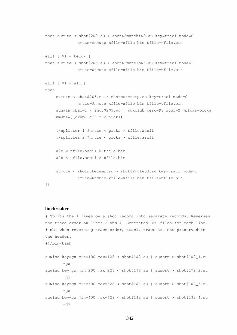
then sumute < shot$2$3.su > shot$2mutehi$3.su key=tracl mode=0
nmute=$nmute xfile=xfile.bin tfile=tfile.bin
elif [ $1 = below ]
then sumute < shot$2$3.su > shot$2mutelo$3.su key=tracl mode=1
nmute=$nmute xfile=xfile.bin tfile=tfile.bin
elif [ $1 = all ]
then
sumute < shot$2$3.su > shotmutetemp.su key=tracl mode=0
nmute=$nmute xfile=xfile.bin tfile=tfile.bin
sugain pbal=1 < shot$2$3.su | suxwigb perc=93 xcur=2 mpicks=picks
nmute=$(grep -c 0.* < picks)
./splitter 1 $nmute < picks > tfile.ascii
./splitter 2 $nmute < picks > xfile.ascii
a2b < tfile.ascii > tfile.bin
a2b < xfile.ascii > xfile.bin
sumute < shotmutetemp.su > shot$2mute$3.su key=tracl mode=1
nmute=$nmute xfile=xfile.bin tfile=tfile.bin
fi
linebreaker # Splits the 4 lines on a shot record into separate records. Reverses
the trace order on lines 2 and 4. Generates EPS files for each line.
# nb: when reversing trace order, tracl, tracr are not preserved in
the header.
#!/bin/bash
suwind key=gx min=100 max=128 < shot$1$2.su | susort > shot$1$2_1.su
-gx
suwind key=gx min=200 max=228 < shot$1$2.su | susort > shot$1$2_2.su
-gx
suwind key=gx min=300 max=328 < shot$1$2.su | susort > shot$1$2_3.su
-gx
suwind key=gx min=400 max=428 < shot$1$2.su | susort > shot$1$2_4.su
-gx
342
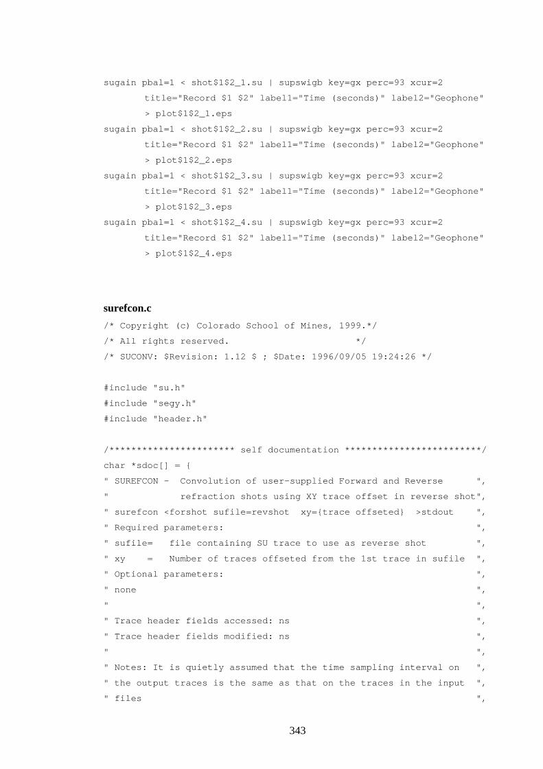
sugain pbal=1 < shot$1$2_1.su | supswigb key=gx perc=93 xcur=2
title="Record $1 $2" label1="Time (seconds)" label2="Geophone"
> plot$1$2_1.eps
sugain pbal=1 < shot$1$2_2.su | supswigb key=gx perc=93 xcur=2
title="Record $1 $2" label1="Time (seconds)" label2="Geophone"
> plot$1$2_2.eps
sugain pbal=1 < shot$1$2_3.su | supswigb key=gx perc=93 xcur=2
title="Record $1 $2" label1="Time (seconds)" label2="Geophone"
> plot$1$2_3.eps
sugain pbal=1 < shot$1$2_4.su | supswigb key=gx perc=93 xcur=2
title="Record $1 $2" label1="Time (seconds)" label2="Geophone"
> plot$1$2_4.eps
surefcon.c /* Copyright (c) Colorado School of Mines, 1999.*/
/* All rights reserved. */
/* SUCONV: $Revision: 1.12 $ ; $Date: 1996/09/05 19:24:26 */
#include "su.h"
#include "segy.h"
#include "header.h"
/*********************** self documentation *************************/
char *sdoc[] =
" SUREFCON - Convolution of user-supplied Forward and Reverse ",
" refraction shots using XY trace offset in reverse shot",
" surefcon <forshot sufile=revshot xy=trace offseted >stdout ",
" Required parameters: ",
" sufile= file containing SU trace to use as reverse shot ",
" xy = Number of traces offseted from the 1st trace in sufile ",
" Optional parameters: ",
" none ",
" ",
" Trace header fields accessed: ns ",
" Trace header fields modified: ns ",
" ",
" Notes: It is quietly assumed that the time sampling interval on ",
" the output traces is the same as that on the traces in the input ",
" files ",
343
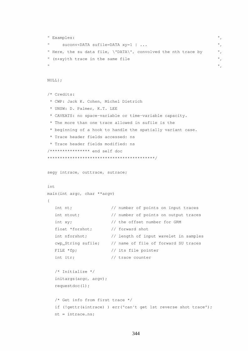
" Examples: ",
" suconv<DATA sufile=DATA xy=1 | ... ",
" Here, the su data file, \"DATA\", convolved the nth trace by ",
" (n+xy)th trace in the same file ",
" ",
NULL;
/* Credits:
* CWP: Jack K. Cohen, Michel Dietrich
* UNSW: D. Palmer, K.T. LEE
* CAVEATS: no space-variable or time-variable capacity.
* The more than one trace allowed in sufile is the
* beginning of a hook to handle the spatially variant case.
* Trace header fields accessed: ns
* Trace header fields modified: ns
/**************** end self doc
*******************************************/
segy intrace, outtrace, sutrace;
int
main(int argc, char **argv)
int nt; // number of points on input traces
int ntout; // number of points on output traces
int xy; // the offset number for GRM
float *forshot; // forward shot
int nforshot; // length of input wavelet in samples
cwp_String sufile; // name of file of forward SU traces
FILE *fp; // its file pointer
int itr; // trace counter
/* Initialize */
initargs(argc, argv);
requestdoc(1);
/* Get info from first trace */
if (!gettr(&intrace) ) err("can't get 1st reverse shot trace");
nt = intrace.ns;
344
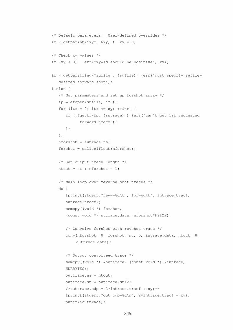
/* Default parameters; User-defined overrides */
if (!getparint("xy", &xy) ) xy = 0;
/* Check xy values */
if (xy < 0) err("xy=%d should be positive", xy);
if (!getparstring("sufile", &sufile)) err("must specify sufile=
desired forward shot");
else
/* Get parameters and set up forshot array */
fp = efopen(sufile, "r");
for (itr = 0; itr <= xy; ++itr)
if (!fgettr(fp, &sutrace) ) err("can't get 1st requested
forward trace");
;
;
nforshot = sutrace.ns;
forshot = ealloc1float(nforshot);
/* Set output trace length */
ntout = nt + nforshot - 1;
/* Main loop over reverse shot traces */
do
fprintf(stderr,"rev==%d\t , for=%d\t", intrace.tracf,
sutrace.tracf);
memcpy((void *) forshot,
(const void *) sutrace.data, nforshot*FSIZE);
/* Convolve forshot with revshot trace */
conv(nforshot, 0, forshot, nt, 0, intrace.data, ntout, 0,
outtrace.data);
/* Output convolveed trace */
memcpy((void *) &outtrace, (const void *) &intrace,
HDRBYTES);
outtrace.ns = ntout;
outtrace.dt = outtrace.dt/2;
/*outtrace.cdp = 2*intrace.tracf + xy;*/
fprintf(stderr,"out_cdp=%d\n", 2*intrace.tracf + xy);
puttr(&outtrace);
345
while ( gettr(&intrace) && fgettr(fp, &sutrace) );
;
return EXIT_SUCCESS;
convolve # Uses surefcon to generate a RCS from forward and reverse shot
records for each line. Generates EPS files for each RCS.
#!/bin/bash
surefcon sufile=shot$1$3_1.su < shot$2$3_1.su > conv$1-$2$3_1.su
surefcon sufile=shot$1$3_2.su < shot$2$3_2.su > conv$1-$2$3_2.su
surefcon sufile=shot$1$3_3.su < shot$2$3_3.su > conv$1-$2$3_3.su
surefcon sufile=shot$1$3_4.su < shot$2$3_4.su > conv$1-$2$3_4.su
supswigb < conv$1-$2$3_1.su key=gx perc=75 xcur=2 title="RCS, Records
$1 and $2 $3" label1="Time (seconds)" label2="Geophone" >
convplot$1-$2$3_1.eps
supswigb < conv$1-$2$3_2.su key=gx perc=75 xcur=2 title="RCS, Records
$1 and $2 $3" label1="Time (seconds)" label2="Geophone" >
convplot$1-$2$3_2.eps
supswigb < conv$1-$2$3_3.su key=gx perc=75 xcur=2 title="RCS, Records
$1 and $2 $3" label1="Time (seconds)" label2="Geophone" >
convplot$1-$2$3_3.eps
supswigb < conv$1-$2$3_4.su key=gx perc=75 xcur=2 title="RCS, Records
$1 and $2 $3" label1="Time (seconds)" label2="Geophone" >
convplot$1-$2$3_4.eps
sumdiff # Adds and subtracts shot records, used to combine out of phase
records. Generates the sum and difference shot records for each line
as a EPS file.
#!/bin/bash
suop2 shot$1$3_1.su shot$2$3_1.su op=diff > shot$1-$2$3_1.su
suop2 shot$1$3_1.su shot$2$3_1.su op=sum > shot$1+$2$3_1.su
suop2 shot$1$3_2.su shot$2$3_2.su op=diff > shot$1-$2$3_2.su
346
suop2 shot$1$3_2.su shot$2$3_2.su op=sum > shot$1+$2$3_2.su
suop2 shot$1$3_3.su shot$2$3_3.su op=diff > shot$1-$2$3_3.su
suop2 shot$1$3_3.su shot$2$3_3.su op=sum > shot$1+$2$3_3.su
suop2 shot$1$3_4.su shot$2$3_4.su op=diff > shot$1-$2$3_4.su
suop2 shot$1$3_4.su shot$2$3_4.su op=sum > shot$1+$2$3_4.su
supswigb < shot$1-$2$3_1.su key=gx perc=93 xcur=2 title="Record $1
minus $2 $3" label1="Time (seconds)" label2="Geophone" >
plotsum_1.eps
supswigb < shot$1+$2$3_1.su key=gx perc=93 xcur=2 title="Record $1
plus $2 $3" label1="Time (seconds)" label2="Geophone" >
plotdiff_1.eps
merge2 mode=landscape plotsum_1.eps plotdiff_1.eps >
plot$1op$2$3_1.eps
supswigb < shot$1-$2$3_2.su key=gx perc=93 xcur=2 title="Record $1
minus $2 $3" label1="Time (seconds)" label2="Geophone" >
plotsum_2.eps
supswigb < shot$1+$2$3_2.su key=gx perc=93 xcur=2 title="Record $1
plus $2 $3" label1="Time (seconds)" label2="Geophone" > plotdiff_2.eps
merge2 mode=landscape plotsum_2.eps plotdiff_2.eps >
plot$1op$2$3_2.eps
supswigb < shot$1-$2$3_3.su key=gx perc=93 xcur=2 title="Record $1
minus $2 $3" label1="Time (seconds)" label2="Geophone" >
plotsum_3.eps
supswigb < shot$1+$2$3_3.su key=gx perc=93 xcur=2 title="Record $1
plus $2 $3" label1="Time (seconds)" label2="Geophone" >
plotdiff_3.eps
merge2 mode=landscape plotsum_3.eps plotdiff_3.eps >
plot$1op$2$3_3.eps
supswigb < shot$1-$2$3_4.su key=gx perc=93 xcur=2 title="Record $1
minus $2 $3" label1="Time (seconds)" label2="Geophone" > plotsum_4.eps
supswigb < shot$1+$2$3_4.su key=gx perc=93 xcur=2 title="Record $1
plus $2 $3" label1="Time (seconds)" label2="Geophone" >
plotdiff_4.eps
merge2 mode=landscape plotsum_4.eps plotdiff_4.eps >
plot$1op$2$3_4.eps
347
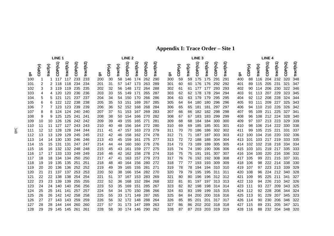
Appendix I: Trace Order – Site 1
gx CD
P(v)
trac
f(v)
CD
P(h1
)
trac
f(h1)
CD
P(h2
)
trac
f(h2)
gx CD
P(v)
trac
f(v)
CD
P(h1
)
trac
f(h1)
CD
P(h2
)
trac
f(h2)
gx CD
P(v)
trac
f(v)
CD
P(h1
)
trac
f(h1)
CD
P(h2
)
trac
f(h2)
gx CD
P(v)
trac
f(v)
CD
P(h1
)
trac
f(h1)
CD
P(h2
)
trac
f(h2)
100 1 1 117 117 233 233 200 30 58 146 174 262 290 300 59 59 175 175 291 291 400 88 116 204 232 320 348101 2 2 118 118 234 234 201 31 57 147 173 263 289 301 60 60 176 176 292 292 401 89 115 205 231 321 347102 3 3 119 119 235 235 202 32 56 148 172 264 288 302 61 61 177 177 293 293 402 90 114 206 230 322 346103 4 4 120 120 236 236 203 33 55 149 171 265 287 303 62 62 178 178 294 294 403 91 113 207 229 323 345104 5 5 121 121 237 237 204 34 54 150 170 266 286 304 63 63 179 179 295 295 404 92 112 208 228 324 344105 6 6 122 122 238 238 205 35 53 151 169 267 285 305 64 64 180 180 296 296 405 93 111 209 227 325 343106 7 7 123 123 239 239 206 36 52 152 168 268 284 306 65 65 181 181 297 297 406 94 110 210 226 326 342107 8 8 124 124 240 240 207 37 51 153 167 269 283 307 66 66 182 182 298 298 407 95 109 211 225 327 341108 9 9 125 125 241 241 208 38 50 154 166 270 282 308 67 67 183 183 299 299 408 96 108 212 224 328 340109 10 10 126 126 242 242 209 39 49 155 165 271 281 309 68 68 184 184 300 300 409 97 107 213 223 329 339110 11 11 127 127 243 243 210 40 48 156 164 272 280 310 69 69 185 185 301 301 410 98 106 214 222 330 338111 12 12 128 128 244 244 211 41 47 157 163 273 279 311 70 70 186 186 302 302 411 99 105 215 221 331 337112 13 13 129 129 245 245 212 42 46 158 162 274 278 312 71 71 187 187 303 303 412 100 104 216 220 332 336113 14 14 130 130 246 246 213 43 45 159 161 275 277 313 72 72 188 188 304 304 413 101 103 217 219 333 335114 15 15 131 131 247 247 214 44 44 160 160 276 276 314 73 73 189 189 305 305 414 102 102 218 218 334 334115 16 16 132 132 248 248 215 45 43 161 159 277 275 315 74 74 190 190 306 306 415 103 101 219 217 335 333116 17 17 133 133 249 249 216 46 42 162 158 278 274 316 75 75 191 191 307 307 416 104 100 220 216 336 332117 18 18 134 134 250 250 217 47 41 163 157 279 273 317 76 76 192 192 308 308 417 105 99 221 215 337 331118 19 19 135 135 251 251 218 48 40 164 156 280 272 318 77 77 193 193 309 309 418 106 98 222 214 338 330119 20 20 136 136 252 252 219 49 39 165 155 281 271 319 78 78 194 194 310 310 419 107 97 223 213 339 329120 21 21 137 137 253 253 220 50 38 166 154 282 270 320 79 79 195 195 311 311 420 108 96 224 212 340 328121 22 22 138 138 254 254 221 51 37 167 153 283 269 321 80 80 196 196 312 312 421 109 95 225 211 341 327122 23 23 139 139 255 255 222 52 36 168 152 284 268 322 81 81 197 197 313 313 422 110 94 226 210 342 326123 24 24 140 140 256 256 223 53 35 169 151 285 267 323 82 82 198 198 314 314 423 111 93 227 209 343 325124 25 25 141 141 257 257 224 54 34 170 150 286 266 324 83 83 199 199 315 315 424 112 92 228 208 344 324125 26 26 142 142 258 258 225 55 33 171 149 287 265 325 84 84 200 200 316 316 425 113 91 229 207 345 323126 27 27 143 143 259 259 226 56 32 172 148 288 264 326 85 85 201 201 317 317 426 114 90 230 206 346 322127 28 28 144 144 260 260 227 57 31 173 147 289 263 327 86 86 202 202 318 318 427 115 89 231 205 347 321128 29 29 145 145 261 261 228 58 30 174 146 290 262 328 87 87 203 203 319 319 428 116 88 232 204 348 320
LINE 1 LINE 2 LINE 3 LINE 4
348
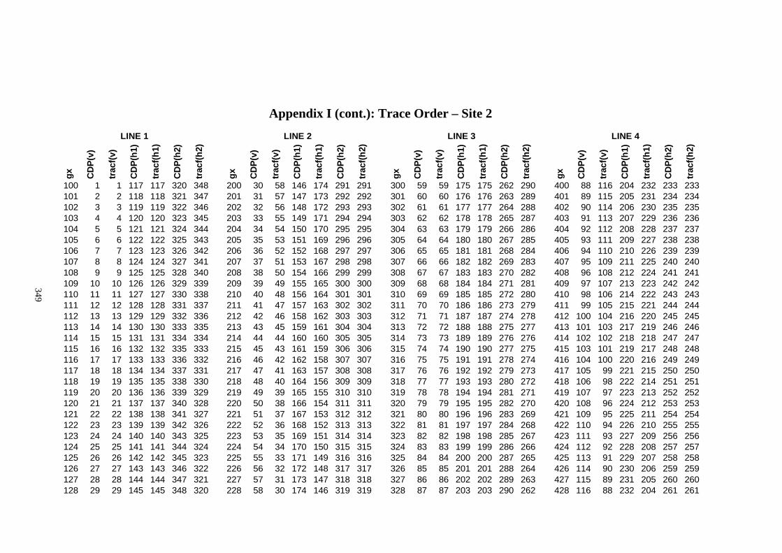
Appendix I (cont.): Trace Order – Site 2
gx CD
P(v)
trac
f(v)
CD
P(h1
)
trac
f(h1)
CD
P(h2
)
trac
f(h2)
gx CD
P(v)
trac
f(v)
CD
P(h1
)
trac
f(h1)
CD
P(h2
)
trac
f(h2)
gx CD
P(v)
trac
f(v)
CD
P(h1
)
trac
f(h1)
CD
P(h2
)
trac
f(h2)
gx CD
P(v)
trac
f(v)
CD
P(h1
)
trac
f(h1)
CD
P(h2
)
trac
f(h2)
100 1 1 117 117 320 348 200 30 58 146 174 291 291 300 59 59 175 175 262 290 400 88 116 204 232 233 233101 2 2 118 118 321 347 201 31 57 147 173 292 292 301 60 60 176 176 263 289 401 89 115 205 231 234 234102 3 3 119 119 322 346 202 32 56 148 172 293 293 302 61 61 177 177 264 288 402 90 114 206 230 235 235103 4 4 120 120 323 345 203 33 55 149 171 294 294 303 62 62 178 178 265 287 403 91 113 207 229 236 236104 5 5 121 121 324 344 204 34 54 150 170 295 295 304 63 63 179 179 266 286 404 92 112 208 228 237 237105 6 6 122 122 325 343 205 35 53 151 169 296 296 305 64 64 180 180 267 285 405 93 111 209 227 238 238106 7 7 123 123 326 342 206 36 52 152 168 297 297 306 65 65 181 181 268 284 406 94 110 210 226 239 239107 8 8 124 124 327 341 207 37 51 153 167 298 298 307 66 66 182 182 269 283 407 95 109 211 225 240 240108 9 9 125 125 328 340 208 38 50 154 166 299 299 308 67 67 183 183 270 282 408 96 108 212 224 241 241109 10 10 126 126 329 339 209 39 49 155 165 300 300 309 68 68 184 184 271 281 409 97 107 213 223 242 242110 11 11 127 127 330 338 210 40 48 156 164 301 301 310 69 69 185 185 272 280 410 98 106 214 222 243 243111 12 12 128 128 331 337 211 41 47 157 163 302 302 311 70 70 186 186 273 279 411 99 105 215 221 244 244112 13 13 129 129 332 336 212 42 46 158 162 303 303 312 71 71 187 187 274 278 412 100 104 216 220 245 245113 14 14 130 130 333 335 213 43 45 159 161 304 304 313 72 72 188 188 275 277 413 101 103 217 219 246 246114 15 15 131 131 334 334 214 44 44 160 160 305 305 314 73 73 189 189 276 276 414 102 102 218 218 247 247115 16 16 132 132 335 333 215 45 43 161 159 306 306 315 74 74 190 190 277 275 415 103 101 219 217 248 248116 17 17 133 133 336 332 216 46 42 162 158 307 307 316 75 75 191 191 278 274 416 104 100 220 216 249 249117 18 18 134 134 337 331 217 47 41 163 157 308 308 317 76 76 192 192 279 273 417 105 99 221 215 250 250118 19 19 135 135 338 330 218 48 40 164 156 309 309 318 77 77 193 193 280 272 418 106 98 222 214 251 251119 20 20 136 136 339 329 219 49 39 165 155 310 310 319 78 78 194 194 281 271 419 107 97 223 213 252 252120 21 21 137 137 340 328 220 50 38 166 154 311 311 320 79 79 195 195 282 270 420 108 96 224 212 253 253121 22 22 138 138 341 327 221 51 37 167 153 312 312 321 80 80 196 196 283 269 421 109 95 225 211 254 254122 23 23 139 139 342 326 222 52 36 168 152 313 313 322 81 81 197 197 284 268 422 110 94 226 210 255 255123 24 24 140 140 343 325 223 53 35 169 151 314 314 323 82 82 198 198 285 267 423 111 93 227 209 256 256124 25 25 141 141 344 324 224 54 34 170 150 315 315 324 83 83 199 199 286 266 424 112 92 228 208 257 257125 26 26 142 142 345 323 225 55 33 171 149 316 316 325 84 84 200 200 287 265 425 113 91 229 207 258 258126 27 27 143 143 346 322 226 56 32 172 148 317 317 326 85 85 201 201 288 264 426 114 90 230 206 259 259127 28 28 144 144 347 321 227 57 31 173 147 318 318 327 86 86 202 202 289 263 427 115 89 231 205 260 260128 29 29 145 145 348 320 228 58 30 174 146 319 319 328 87 87 203 203 290 262 428 116 88 232 204 261 261
LINE 3 LINE 4LINE 1 LINE 2
349
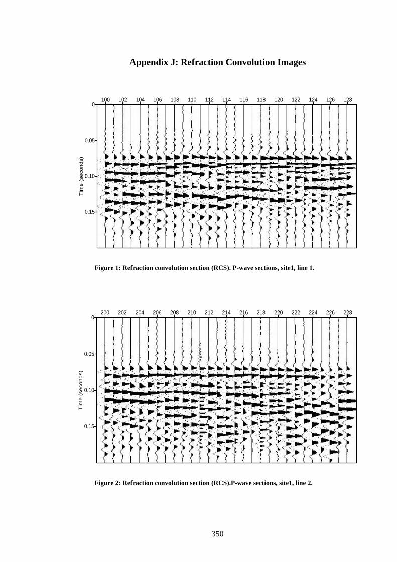
Appendix J: Refraction Convolution Images
0
0.05
0.10
0.15
Tim
e (
seco
nds)
100 102 104 106 108 110 112 114 116 118 120 122 124 126 128
Figure 1: Refraction convolution section (RCS). P-wave sections, site1, line 1.
0
0.05
0.10
0.15
Tim
e (
seco
nd
s)
200 202 204 206 208 210 212 214 216 218 220 222 224 226 228
Figure 2: Refraction convolution section (RCS).P-wave sections, site1, line 2.
350
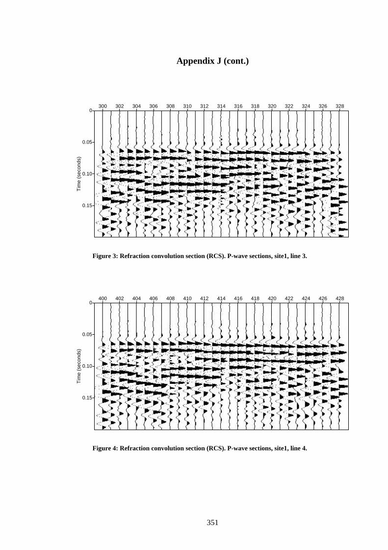
Appendix J (cont.)
0
0.05
0.10
0.15
Tim
e (s
econ
ds)
300 302 304 306 308 310 312 314 316 318 320 322 324 326 328
Figure 3: Refraction convolution section (RCS). P-wave sections, site1, line 3.
0
0.05
0.10
0.15
Tim
e (s
econ
ds)
400 402 404 406 408 410 412 414 416 418 420 422 424 426 428
Figure 4: Refraction convolution section (RCS). P-wave sections, site1, line 4.
351
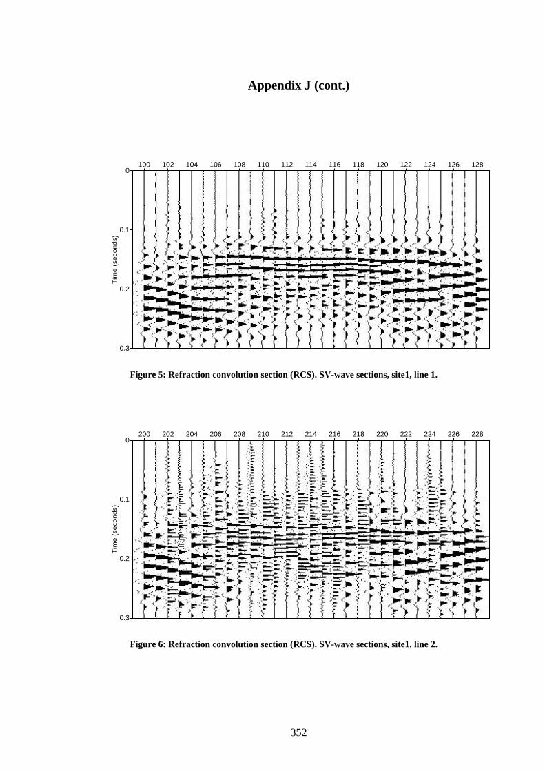
Appendix J (cont.)
0
0.1
0.2
0.3
Tim
e (s
econ
ds)
100 102 104 106 108 110 112 114 116 118 120 122 124 126 128
Figure 5: Refraction convolution section (RCS). SV-wave sections, site1, line 1.
0
0.1
0.2
0.3
Tim
e (s
econ
ds)
200 202 204 206 208 210 212 214 216 218 220 222 224 226 228
Figure 6: Refraction convolution section (RCS). SV-wave sections, site1, line 2.
352
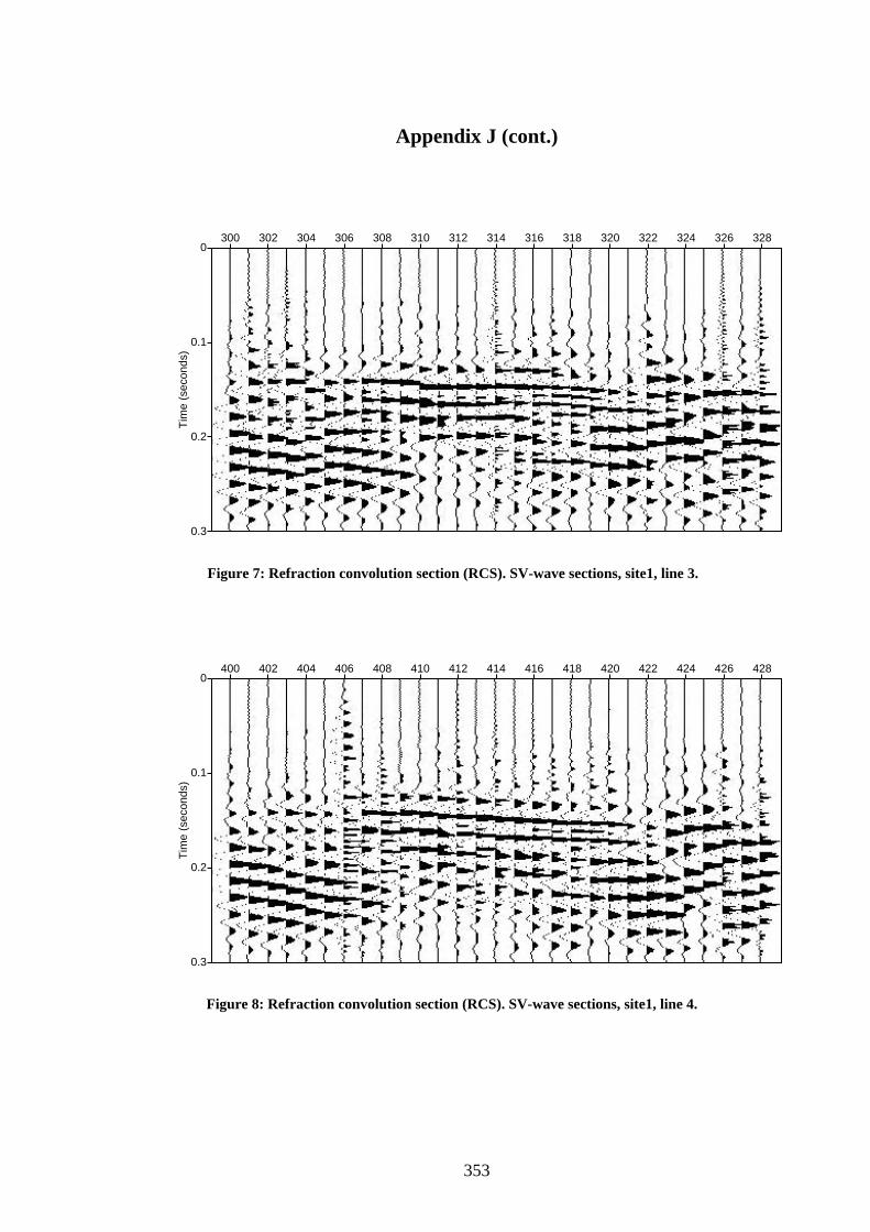
Appendix J (cont.)
0
0.1
0.2
0.3
Tim
e (s
econ
ds)
300 302 304 306 308 310 312 314 316 318 320 322 324 326 328
Figure 7: Refraction convolution section (RCS). SV-wave sections, site1, line 3.
0
0.1
0.2
0.3
Tim
e (s
econ
ds)
400 402 404 406 408 410 412 414 416 418 420 422 424 426 428
Figure 8: Refraction convolution section (RCS). SV-wave sections, site1, line 4.
353
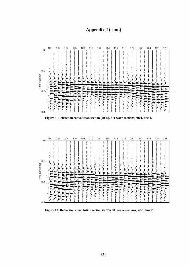
Appendix J (cont.)
0
0.1
0.2
0.3
Tim
e (s
econ
ds)
100 102 104 106 108 110 112 114 116 118 120 122 124 126 128
Figure 9: Refraction convolution section (RCS). SH-wave sections, site1, line 1.
0
0.1
0.2
0.3
Tim
e (s
econ
ds)
200 202 204 206 208 210 212 214 216 218 220 222 224 226 228
Figure 10: Refraction convolution section (RCS). SH-wave sections, site1, line 2.
354
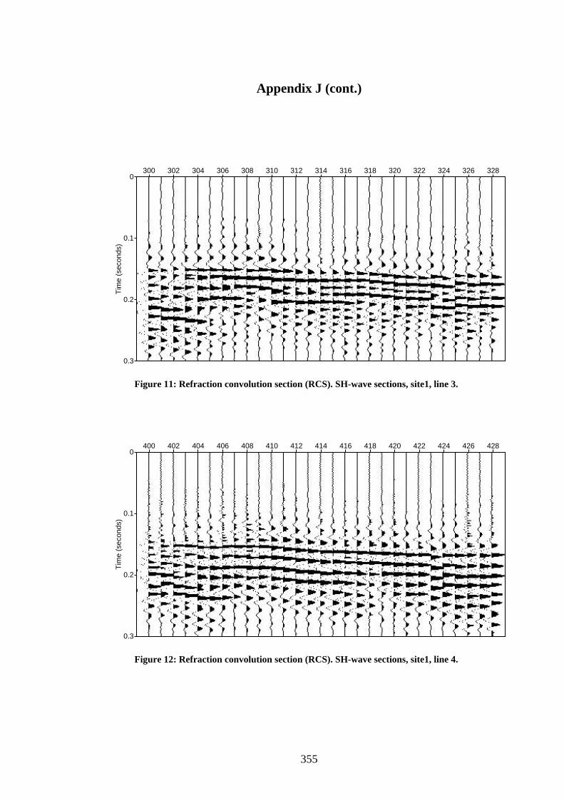
Appendix J (cont.)
0
0.1
0.2
0.3
Tim
e (s
econ
ds)
300 302 304 306 308 310 312 314 316 318 320 322 324 326 328
Figure 11: Refraction convolution section (RCS). SH-wave sections, site1, line 3.
0
0.1
0.2
0.3
Tim
e (s
econ
ds)
400 402 404 406 408 410 412 414 416 418 420 422 424 426 428
Figure 12: Refraction convolution section (RCS). SH-wave sections, site1, line 4.
355
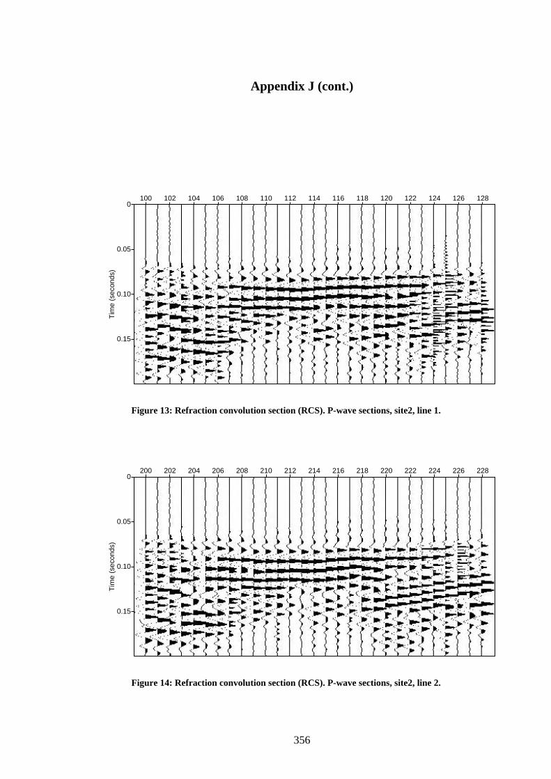
Appendix J (cont.)
0
0.05
0.10
0.15
Tim
e (s
econ
ds)
100 102 104 106 108 110 112 114 116 118 120 122 124 126 128
Figure 13: Refraction convolution section (RCS). P-wave sections, site2, line 1.
0
0.05
0.10
0.15
Tim
e (s
econ
ds)
200 202 204 206 208 210 212 214 216 218 220 222 224 226 228
Figure 14: Refraction convolution section (RCS). P-wave sections, site2, line 2.
356
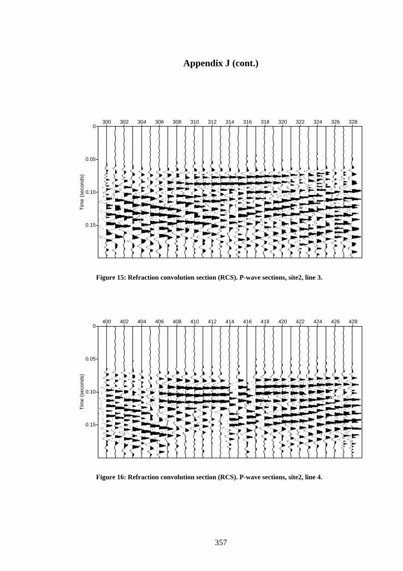
Appendix J (cont.)
0
0.05
0.10
0.15
Tim
e (s
econ
ds)
300 302 304 306 308 310 312 314 316 318 320 322 324 326 328
Figure 15: Refraction convolution section (RCS). P-wave sections, site2, line 3.
0
0.05
0.10
0.15
Tim
e (s
econ
ds)
400 402 404 406 408 410 412 414 416 418 420 422 424 426 428
Figure 16: Refraction convolution section (RCS). P-wave sections, site2, line 4.
357
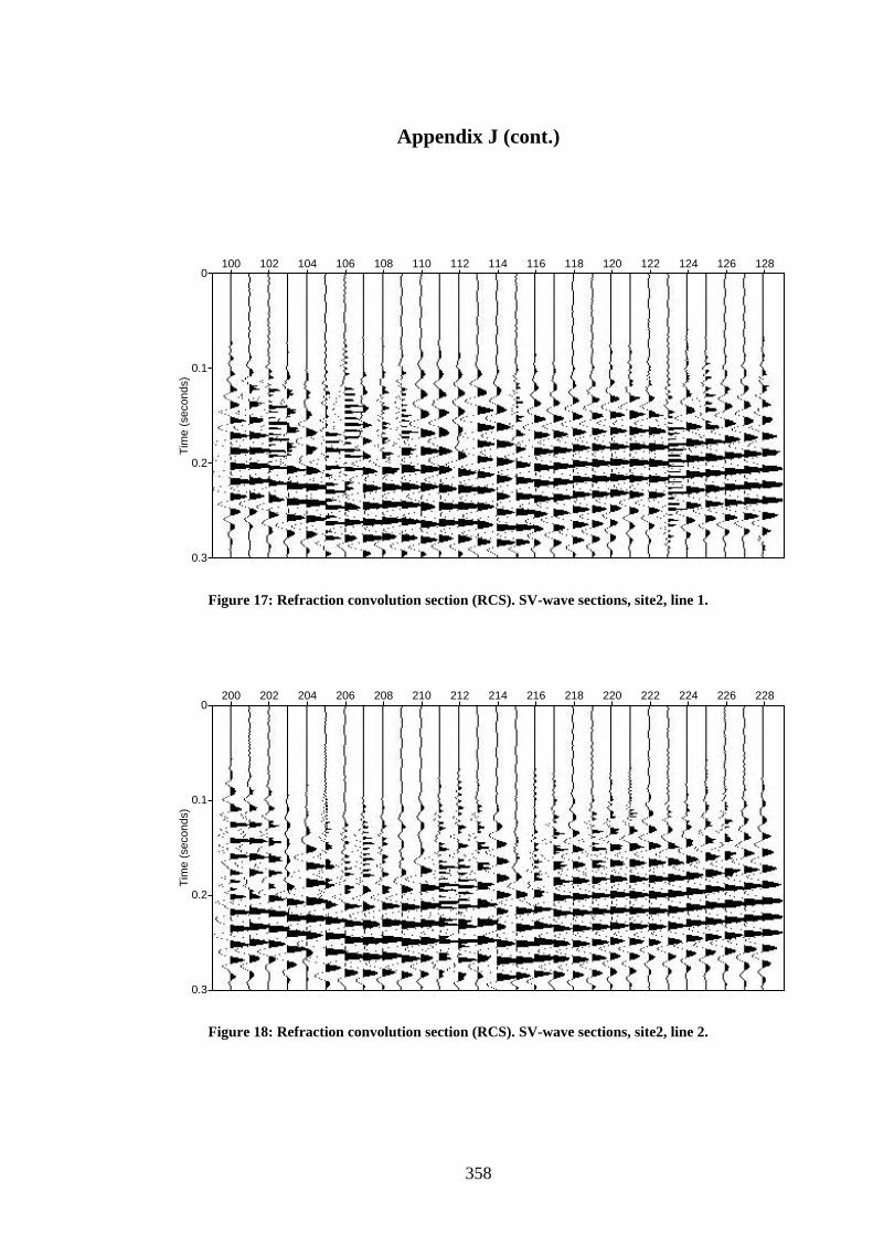
Appendix J (cont.)
0
0.1
0.2
0.3
Tim
e (s
econ
ds)
100 102 104 106 108 110 112 114 116 118 120 122 124 126 128
Figure 17: Refraction convolution section (RCS). SV-wave sections, site2, line 1.
0
0.1
0.2
0.3
Tim
e (s
econ
ds)
200 202 204 206 208 210 212 214 216 218 220 222 224 226 228
Figure 18: Refraction convolution section (RCS). SV-wave sections, site2, line 2.
358
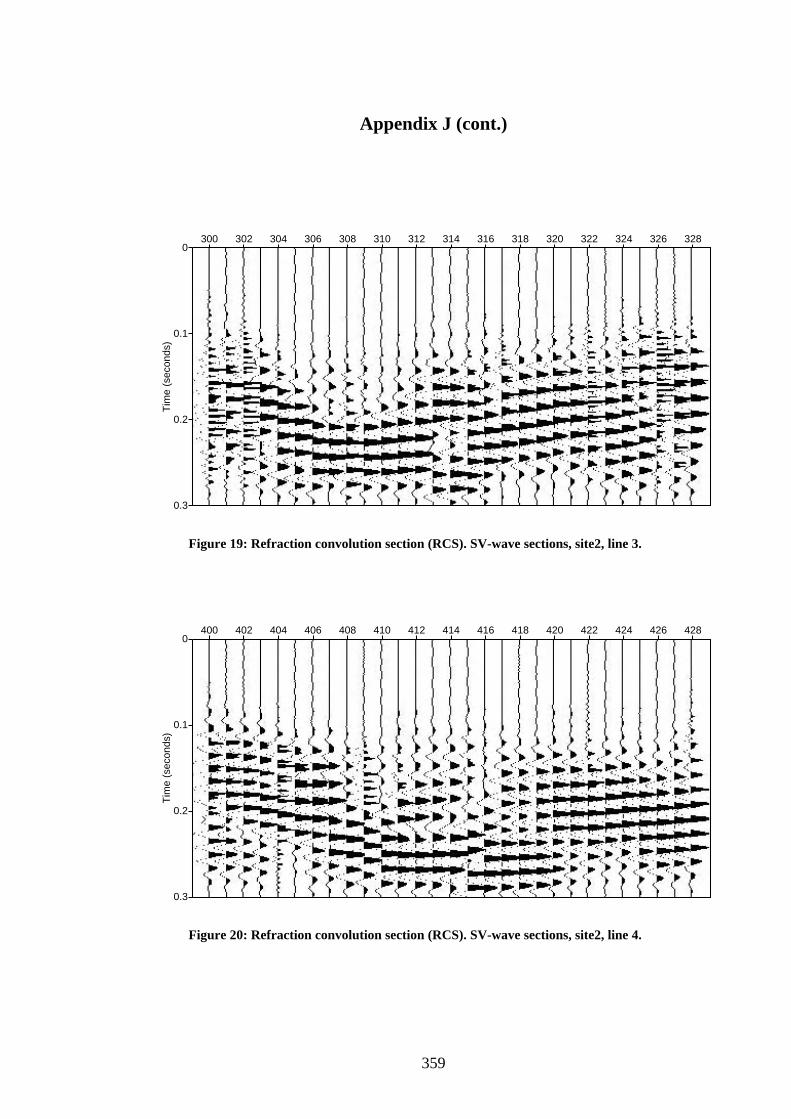
Appendix J (cont.)
0
0.1
0.2
0.3
Tim
e (s
econ
ds)
300 302 304 306 308 310 312 314 316 318 320 322 324 326 328
Figure 19: Refraction convolution section (RCS). SV-wave sections, site2, line 3.
0
0.1
0.2
0.3
Tim
e (s
econ
ds)
400 402 404 406 408 410 412 414 416 418 420 422 424 426 428
Figure 20: Refraction convolution section (RCS). SV-wave sections, site2, line 4.
359
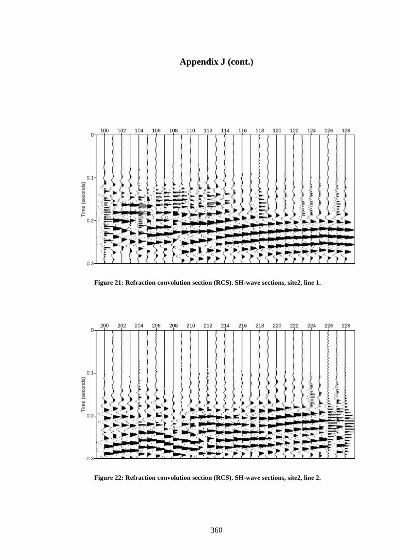
Appendix J (cont.)
0
0.1
0.2
0.3
Tim
e (s
econ
ds)
100 102 104 106 108 110 112 114 116 118 120 122 124 126 128
Figure 21: Refraction convolution section (RCS). SH-wave sections, site2, line 1.
0
0.1
0.2
0.3
Tim
e (s
econ
ds)
200 202 204 206 208 210 212 214 216 218 220 222 224 226 228
Figure 22: Refraction convolution section (RCS). SH-wave sections, site2, line 2.
360
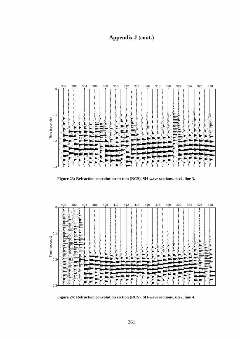
Appendix J (cont.)
0
0.1
0.2
0.3
Tim
e (s
econ
ds)
300 302 304 306 308 310 312 314 316 318 320 322 324 326 328
Figure 23: Refraction convolution section (RCS). SH-wave sections, site2, line 3.
0
0.1
0.2
0.3
Tim
e (s
econ
ds)
400 402 404 406 408 410 412 414 416 418 420 422 424 426 428
Figure 24: Refraction convolution section (RCS). SH-wave sections, site2, line 4.
361
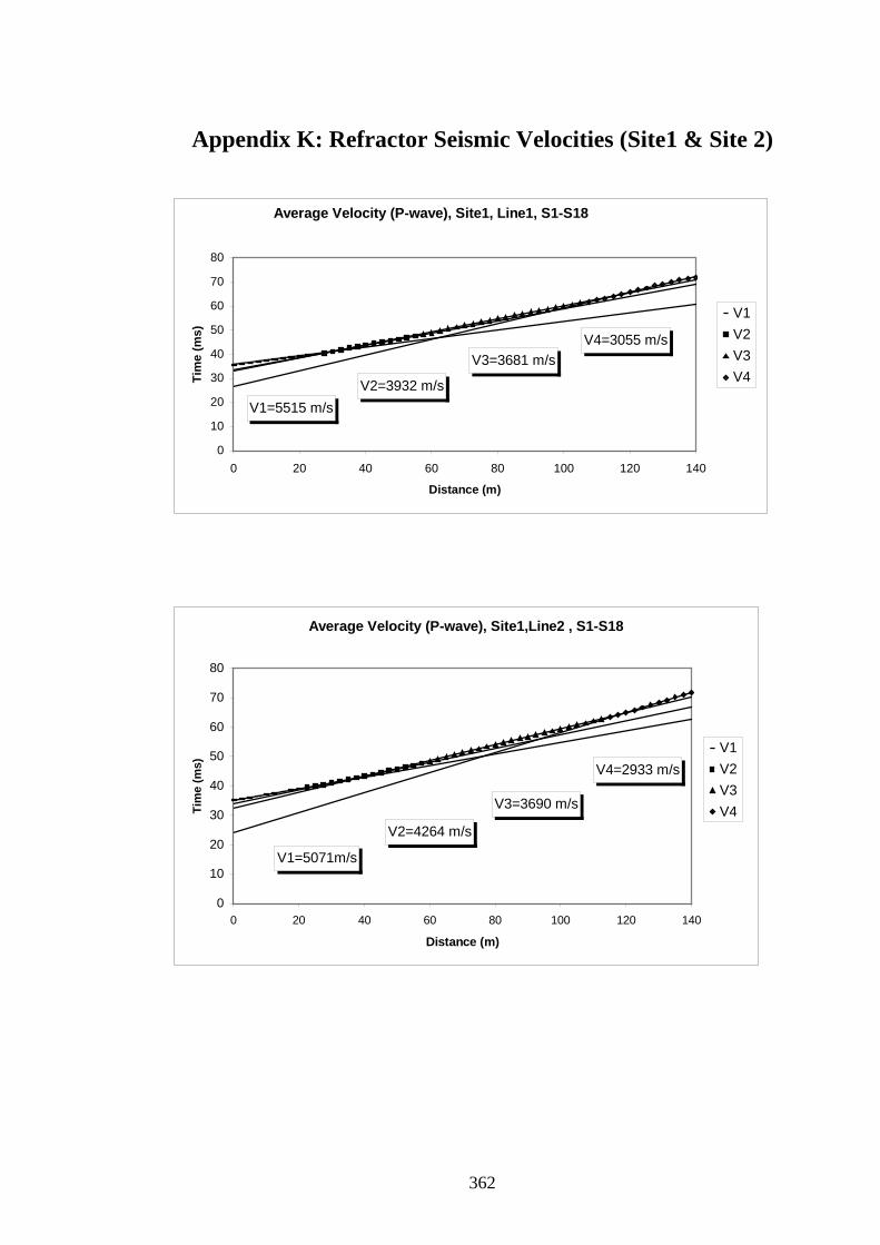
Appendix K: Refractor Seismic Velocities (Site1 & Site 2)
Average Velocity (P-wave), Site1, Line1, S1-S18
V1=5515 m/sV2=3932 m/s
V3=3681 m/sV4=3055 m/s
0
10
20
30
40
50
60
70
80
0 20 40 60 80 100 120 140
Distance (m)
Tim
e (m
s)
V1V2V3V4
Average Velocity (P-wave), Site1,Line2 , S1-S18
V1=5071m/s
V2=4264 m/s
V3=3690 m/s
V4=2933 m/s
0
10
20
30
40
50
60
70
80
0 20 40 60 80 100 120 140
Distance (m)
Tim
e (m
s)
V1V2V3V4
362
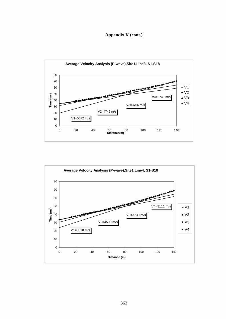
Appendix K (cont.)
Average Velocity Analysis (P-wave),Site1,Line3, S1-S18
V1=5672 m/s
V2=4742 m/s
V3=3706 m/s
V4=2749 m/s
0
10
20
30
40
50
60
70
80
0 20 40 60 80 100 120 140Distance(m)
Tim
e (m
s)
V1V2V3V4
Average Velocity Analysis (P-wave),Site1,Line4, S1-S18
V1=5018 m/s
V2=4500 m/s
V4=3111 m/s
V3=3730 m/s
0
10
20
30
40
50
60
70
80
0 20 40 60 80 100 120 140
Distance (m)
Tim
e (m
s) V1
V2
V3
V4
363
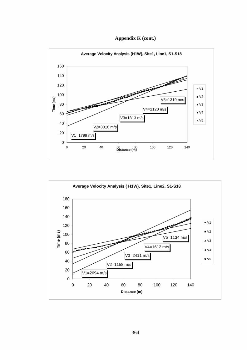
Appendix K (cont.)
Average Velocity Analysis (H1W), Site1, Line1, S1-S18
V1=1799 m/s
V2=3018 m/s
V3=1813 m/s
V4=2120 m/s
V5=1319 m/s
0
20
40
60
80
100
120
140
160
0 20 40 60 80 100 120 140Distance (m)
Tim
e (m
s)
V1
V2
V3
V4
V5
Average Velocity Analysis ( H1W), Site1, Line2, S1-S18
V1=2694 m/s
V2=1158 m/s
V3=2411 m/s
V4=1612 m/s
V5=1134 m/s
0
20
40
60
80
100
120
140
160
180
0 20 40 60 80 100 120 140Distance (m)
Tim
e (m
s)
V1
V2
V3
V4
V5
364
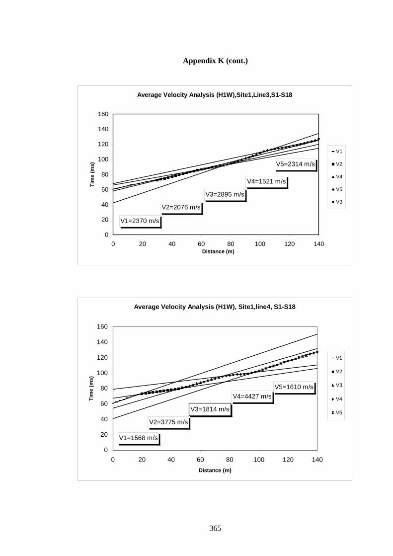
Appendix K (cont.)
Average Velocity Analysis (H1W),Site1,Line3,S1-S18
V3=2895 m/s
V4=1521 m/s
V5=2314 m/s
V2=2076 m/s
V1=2370 m/s
0
20
40
60
80
100
120
140
160
0 20 40 60 80 100 120 140Distance (m)
Tim
e (m
s)
V1
V2
V4
V5
V3
Average Velocity Analysis (H1W), Site1,line4, S1-S18
V1=1568 m/s
V2=3775 m/s
V3=1814 m/s
V4=4427 m/sV5=1610 m/s
0
20
40
60
80
100
120
140
160
0 20 40 60 80 100 120 140Distance (m)
Tim
e (m
s)
V1
V2
V3
V4
V5
365
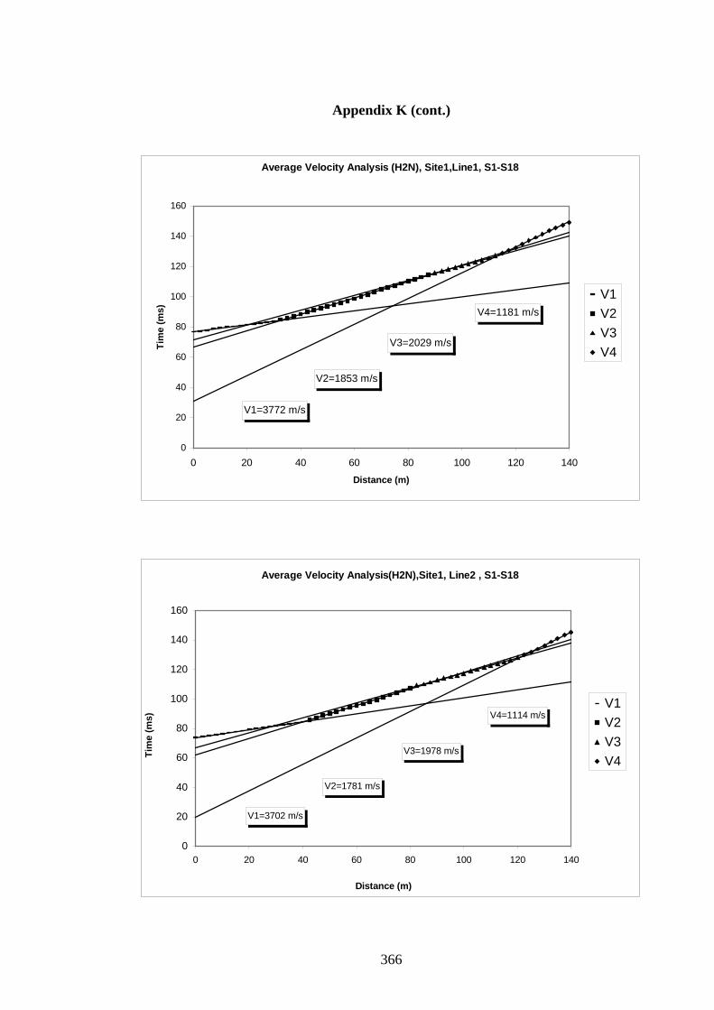
Appendix K (cont.)
Average Velocity Analysis (H2N), Site1,Line1, S1-S18
V1=3772 m/s
V2=1853 m/s
V3=2029 m/s
V4=1181 m/s
0
20
40
60
80
100
120
140
160
0 20 40 60 80 100 120 140
Distance (m)
Tim
e (m
s)
V1V2V3V4
Average Velocity Analysis(H2N),Site1, Line2 , S1-S18
V1=3702 m/s
V2=1781 m/s
V3=1978 m/s
V4=1114 m/s
0
20
40
60
80
100
120
140
160
0 20 40 60 80 100 120 140
Distance (m)
Tim
e (m
s)
V1V2V3V4
366
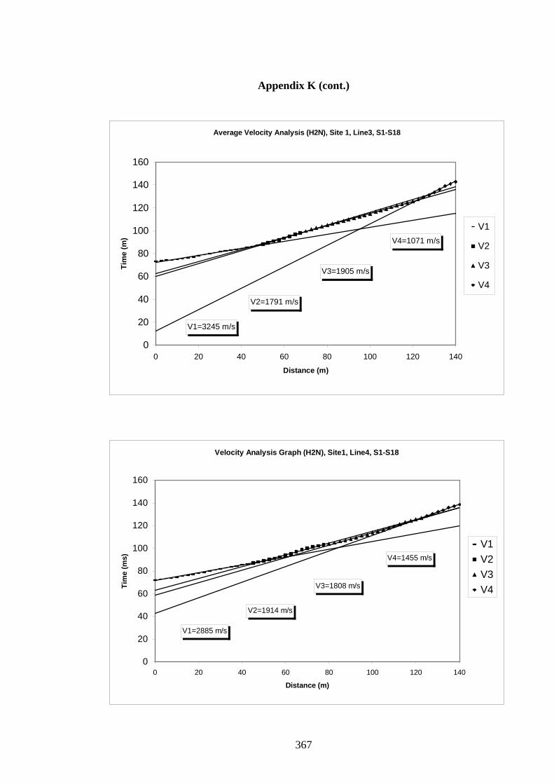
Appendix K (cont.)
Average Velocity Analysis (H2N), Site 1, Line3, S1-S18
V1=3245 m/s
V2=1791 m/s
V3=1905 m/s
V4=1071 m/s
0
20
40
60
80
100
120
140
160
0 20 40 60 80 100 120 140
Distance (m)
Tim
e (m
)
V1
V2
V3
V4
Velocity Analysis Graph (H2N), Site1, Line4, S1-S18
V2=1914 m/s
V3=1808 m/s
V1=2885 m/s
V4=1455 m/s
0
20
40
60
80
100
120
140
160
0 20 40 60 80 100 120 140
Distance (m)
Tim
e (m
s)
V1V2V3V4
367
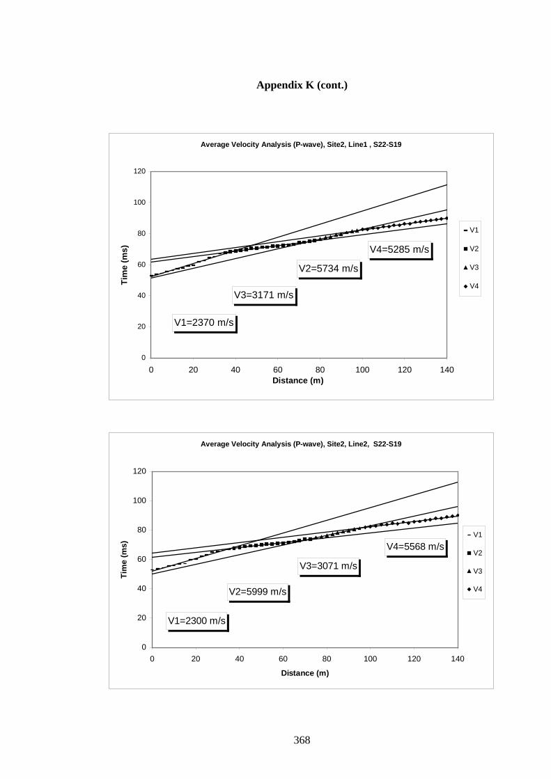
Appendix K (cont.)
Average Velocity Analysis (P-wave), Site2, Line1 , S22-S19
V1=2370 m/s
V2=5734 m/s
V3=3171 m/s
V4=5285 m/s
0
20
40
60
80
100
120
0 20 40 60 80 100 120 140Distance (m)
Tim
e (m
s)
V1
V2
V3
V4
Average Velocity Analysis (P-wave), Site2, Line2, S22-S19
V1=2300 m/s
V2=5999 m/s
V3=3071 m/s
V4=5568 m/s
0
20
40
60
80
100
120
0 20 40 60 80 100 120 140
Distance (m)
Tim
e (m
s)
V1
V2
V3
V4
368
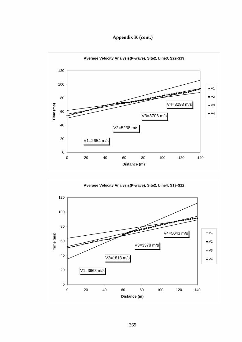
Appendix K (cont.)
Average Velocity Analysis(P-wave), Site2, Line3, S22-S19
V1=2654 m/s
V2=5238 m/s
V3=3706 m/s
V4=3293 m/s
0
20
40
60
80
100
120
0 20 40 60 80 100 120 140
Distance (m)
Tim
e (m
s)
V1
V2
V3
V4
Average Velocity Analysis(P-wave), Site2, Line4, S19-S22
V1=3663 m/s
V2=1818 m/s
V3=3378 m/s
V4=5043 m/s
0
20
40
60
80
100
120
0 20 40 60 80 100 120 140
Distance (m)
Tim
e (m
s) V1
V2
V3
V4
369
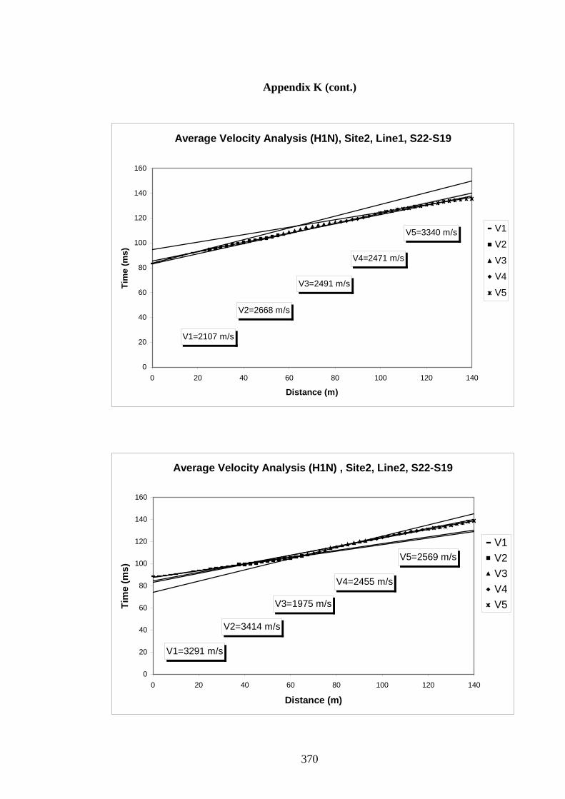
Appendix K (cont.)
Average Velocity Analysis (H1N), Site2, Line1, S22-S19
V1=2107 m/s
V3=2491 m/s
V4=2471 m/s
V2=2668 m/s
V5=3340 m/s
0
20
40
60
80
100
120
140
160
0 20 40 60 80 100 120 140
Distance (m)
Tim
e (m
s)
V1
V2
V3
V4
V5
Average Velocity Analysis (H1N) , Site2, Line2, S22-S19
V1=3291 m/s
V2=3414 m/s
V3=1975 m/s
V4=2455 m/s
V5=2569 m/s
0
20
40
60
80
100
120
140
160
0 20 40 60 80 100 120 140
Distance (m)
Tim
e (m
s)
V1V2V3V4V5
370
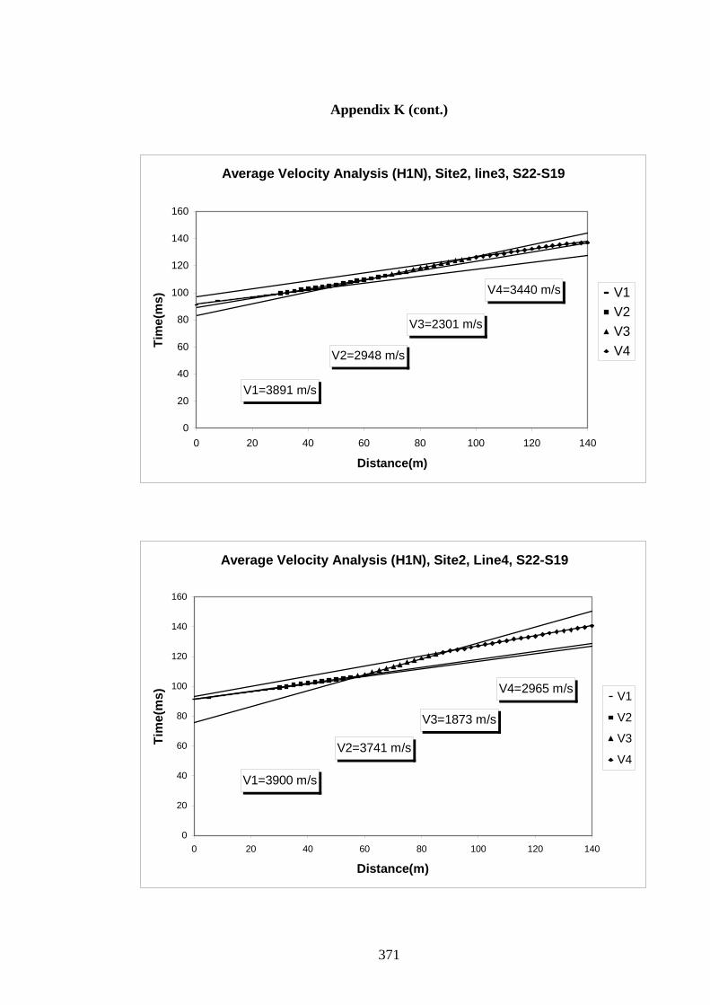
Appendix K (cont.)
Average Velocity Analysis (H1N), Site2, line3, S22-S19
V1=3891 m/s
V2=2948 m/s
V3=2301 m/s
V4=3440 m/s
0
20
40
60
80
100
120
140
160
0 20 40 60 80 100 120 140
Distance(m)
Tim
e(m
s) V1V2V3V4
Average Velocity Analysis (H1N), Site2, Line4, S22-S19
V1=3900 m/s
V2=3741 m/s
V3=1873 m/s
V4=2965 m/s
0
20
40
60
80
100
120
140
160
0 20 40 60 80 100 120 140
Distance(m)
Tim
e(m
s) V1
V2
V3
V4
371
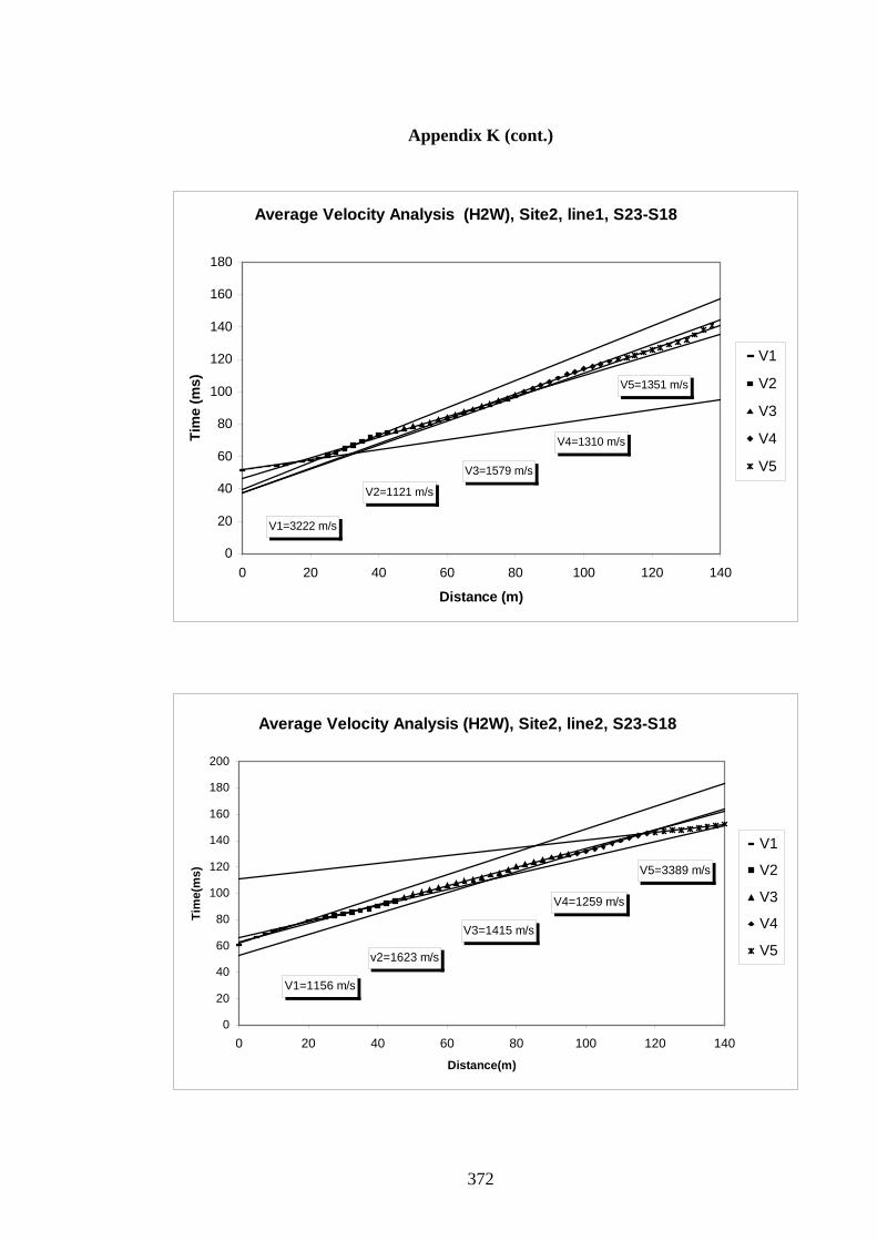
Appendix K (cont.)
Average Velocity Analysis (H2W), Site2, line1, S23-S18
V1=3222 m/s
V2=1121 m/s
V3=1579 m/s
V4=1310 m/s
V5=1351 m/s
0
20
40
60
80
100
120
140
160
180
0 20 40 60 80 100 120 140
Distance (m)
Tim
e (m
s)
V1
V2
V3
V4
V5
Average Velocity Analysis (H2W), Site2, line2, S23-S18
V1=1156 m/s
v2=1623 m/s
V3=1415 m/s
V4=1259 m/s
V5=3389 m/s
0
20
40
60
80
100
120
140
160
180
200
0 20 40 60 80 100 120 140
Distance(m)
Tim
e(m
s)
V1
V2
V3
V4
V5
372
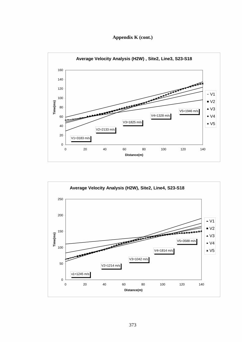
Appendix K (cont.)
Average Velocity Analysis (H2W) , Site2, Line3, S23-S18
V1=3183 m/s
V2=2133 m/s
V3=1825 m/s
V4=1328 m/sV5=1946 m/s
0
20
40
60
80
100
120
140
160
0 20 40 60 80 100 120 140
Distance(m)
Tim
e(m
s)
V1
V2
V3
V4
V5
Average Velocity Analysis (H2W), Site2, Line4, S23-S18
v1=1245 m/s
V2=1214 m/s
V3=1042 m/s
V4=1814 m/s
V5=3588 m/s
0
50
100
150
200
250
0 20 40 60 80 100 120 140
Distance(m)
Tim
e(m
s)
V1
V2
V3
V4
V5
373
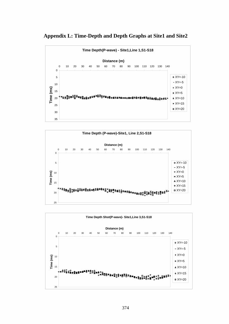
Appendix L: Time-Depth and Depth Graphs at Site1 and Site2
Time Depth(P-wave) - Site1,Line 1,S1-S18
0
5
10
15
20
25
30
35
0 10 20 30 40 50 60 70 80 90 100 110 120 130 140
Distance (m)
Tim
e (m
s)
XY=-10
XY=-5
XY=0
XY=5
XY=10
XY=15
XY=20
Time Depth (P-wave)-Site1, Line 2,S1-S18
0
5
10
15
20
25
0 10 20 30 40 50 60 70 80 90 100 110 120 130 140
Distance (m)
Tim
e (m
s)
XY=-10XY=-5XY=0XY=5XY=10XY=15XY=20
Time Depth Shot(P-wave)- Site1,Line 3,S1-S18
0
5
10
15
20
25
0 10 20 30 40 50 60 70 80 90 100 110 120 130 140
Distance (m)
Tim
e (m
s)
XY=-10
XY=-5
XY=0
XY=5
XY=10
XY=15
XY=20
374
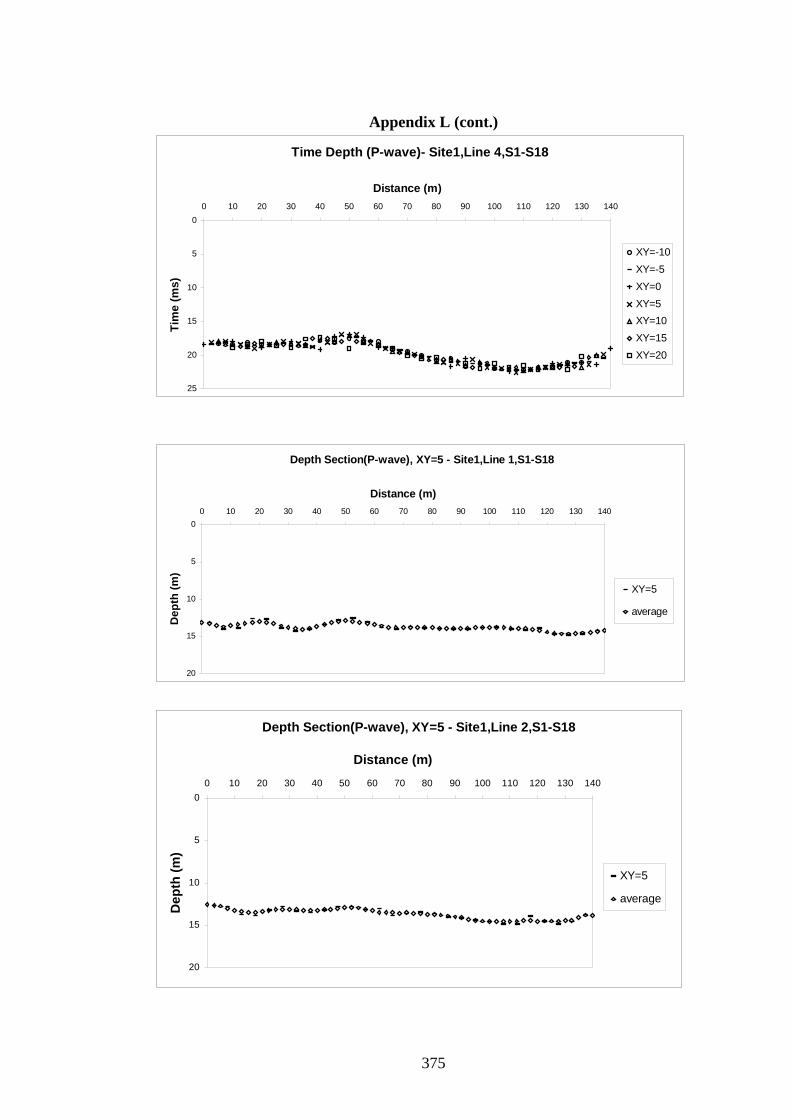
Appendix L (cont.)
Time Depth (P-wave)- Site1,Line 4,S1-S18
0
5
10
15
20
25
0 10 20 30 40 50 60 70 80 90 100 110 120 130 140
Distance (m)Ti
me
(ms)
XY=-10XY=-5XY=0XY=5XY=10XY=15XY=20
Depth Section(P-wave), XY=5 - Site1,Line 1,S1-S18
0
5
10
15
20
0 10 20 30 40 50 60 70 80 90 100 110 120 130 140
Distance (m)
Dep
th (m
)
XY=5
average
Depth Section(P-wave), XY=5 - Site1,Line 2,S1-S18
0
5
10
15
20
0 10 20 30 40 50 60 70 80 90 100 110 120 130 140
Distance (m)
Dep
th (m
)
XY=5
average
375
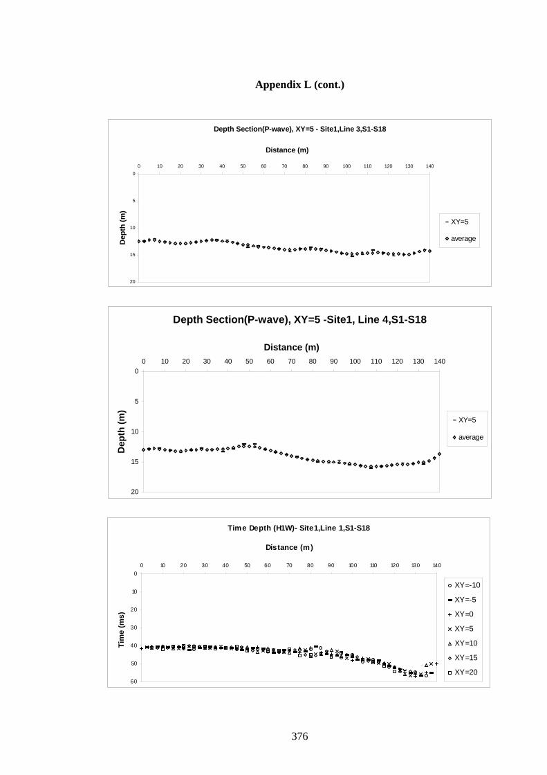
Appendix L (cont.)
Depth Section(P-wave), XY=5 - Site1,Line 3,S1-S18
0
5
10
15
20
0 10 20 30 40 50 60 70 80 90 100 110 120 130 140
Distance (m)
Dep
th (m
)
XY=5
average
Depth Section(P-wave), XY=5 -Site1, Line 4,S1-S18
0
5
10
15
20
0 10 20 30 40 50 60 70 80 90 100 110 120 130 140
Distance (m)
Dep
th (m
)
XY=5
average
Time Depth (H1W)- Site1,Line 1,S1-S18
0
10
20
30
40
50
60
0 10 20 30 40 50 60 70 80 90 100 110 120 130 140
Distance (m)
Tim
e (m
s)
XY=-10
XY=-5
XY=0
XY=5
XY=10
XY=15
XY=20
376
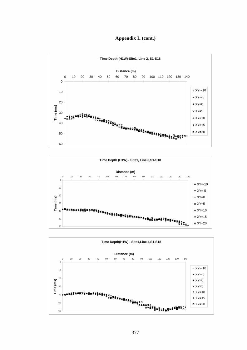
Appendix L (cont.)
Time Depth (H1W)-Site1, Line 2, S1-S18
0
10
20
30
40
50
60
0 10 20 30 40 50 60 70 80 90 100 110 120 130 140
Distance (m)
Tim
e (m
s)
XY=-10
XY=-5
XY=0
XY=5
XY=10
XY=15
XY=20
Time Depth (H1W) - Site1, Line 3,S1-S18
0
10
20
30
40
50
60
0 10 20 30 40 50 60 70 80 90 100 110 120 130 140
Distance (m)
Tim
e (m
s)
XY=-10
XY=-5
XY=0
XY=5
XY=10
XY=15
XY=20
Time Depth(H1W) - Site1,Line 4,S1-S18
0
10
20
30
40
50
60
0 10 20 30 40 50 60 70 80 90 100 110 120 130 140
Distance (m)
Tim
e (m
s)
XY=-10
XY=-5
XY=0
XY=5
XY=10
XY=15
XY=20
377
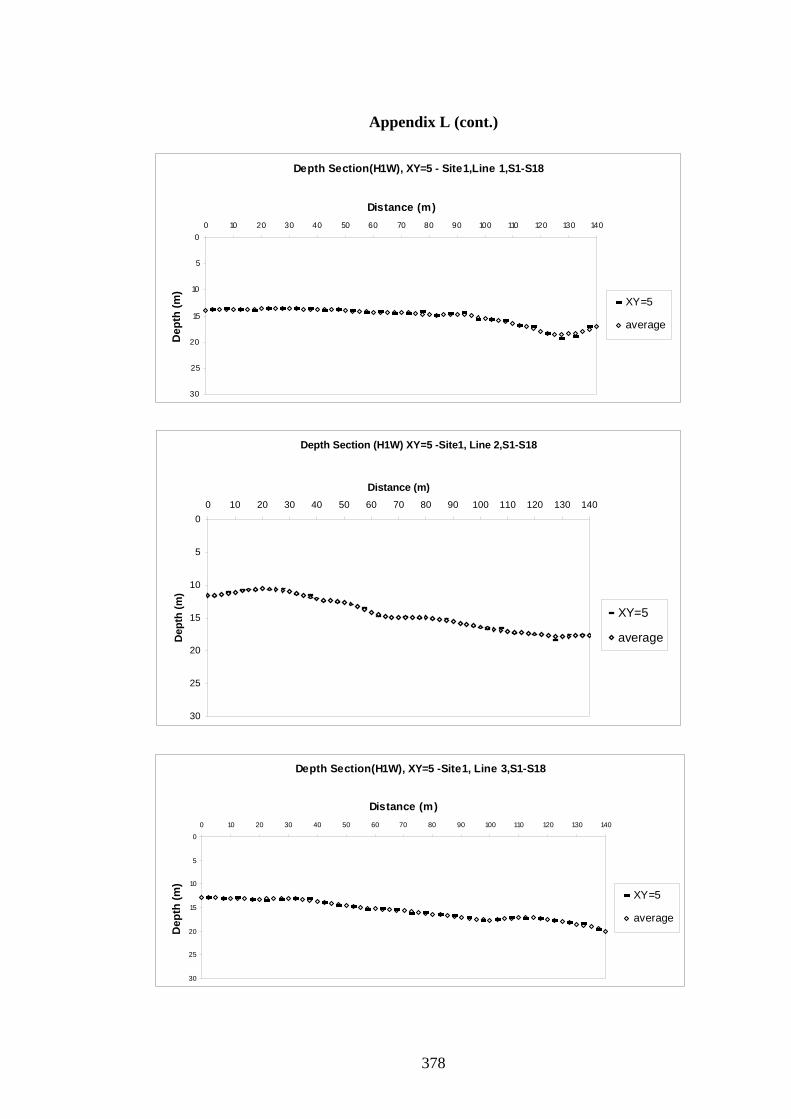
Appendix L (cont.)
Depth Section(H1W), XY=5 - Site1,Line 1,S1-S18
0
5
10
15
20
25
30
0 10 20 30 40 50 60 70 80 90 100 110 120 130 140
Distance (m)
Dep
th (m
)
XY=5
average
Depth Section (H1W) XY=5 -Site1, Line 2,S1-S18
0
5
10
15
20
25
30
0 10 20 30 40 50 60 70 80 90 100 110 120 130 140
Distance (m)
Dep
th (m
)
XY=5
average
Depth Section(H1W), XY=5 -Site1, Line 3,S1-S18
0
5
10
15
20
25
30
0 10 20 30 40 50 60 70 80 90 100 110 120 130 140
Distance (m)
Dep
th (m
)
XY=5
average
378
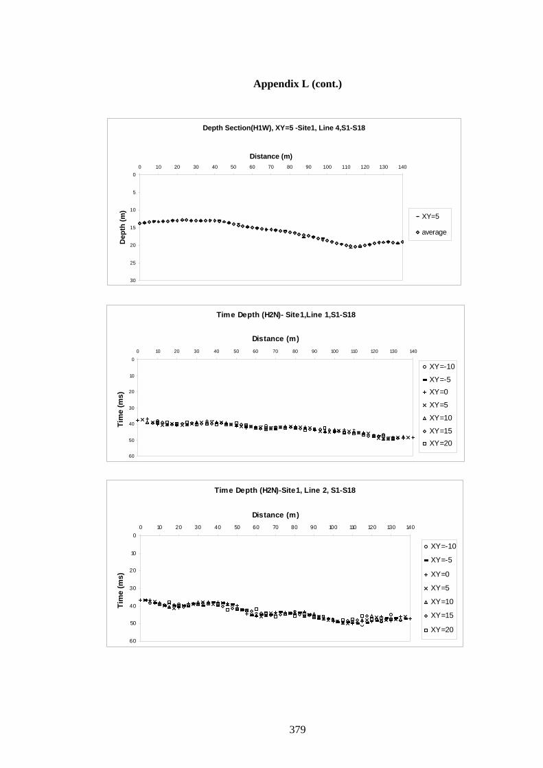
Appendix L (cont.)
Depth Section(H1W), XY=5 -Site1, Line 4,S1-S18
0
5
10
15
20
25
30
0 10 20 30 40 50 60 70 80 90 100 110 120 130 140
Distance (m)
Dep
th (m
)
XY=5
average
Time Depth (H2N)- Site1,Line 1,S1-S18
0
10
20
30
40
50
60
0 10 20 30 40 50 60 70 80 90 100 110 120 130 140
Distance (m)
Tim
e (m
s)
XY=-10
XY=-5XY=0
XY=5
XY=10
XY=15XY=20
Time Depth (H2N)-Site1, Line 2, S1-S18
0
10
20
30
40
50
60
0 10 20 30 40 50 60 70 80 90 100 110 120 130 140
Distance (m)
Tim
e (m
s)
XY=-10
XY=-5
XY=0
XY=5
XY=10
XY=15
XY=20
379
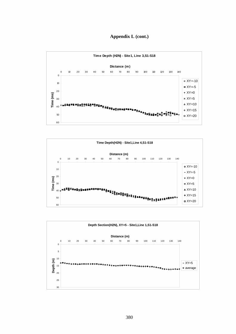
Appendix L (cont.)
Time Depth (H2N) - Site1, Line 3,S1-S18
0
10
20
30
40
50
60
0 10 20 30 40 50 60 70 80 90 100 110 120 130 140
Distance (m)
Tim
e (m
s)
XY=-10
XY=-5
XY=0
XY=5
XY=10
XY=15
XY=20
Time Depth(H2N) - Site1,Line 4,S1-S18
0
10
20
30
40
50
60
0 10 20 30 40 50 60 70 80 90 100 110 120 130 140
Distance (m)
Tim
e (m
s)
XY=-10
XY=-5
XY=0
XY=5
XY=10
XY=15
XY=20
Depth Section(H2N), XY=5 - Site1,Line 1,S1-S18
0
5
10
15
20
25
30
0 10 20 30 40 50 60 70 80 90 100 110 120 130 140
Distance (m)
Dep
th (m
)
XY=5average
380
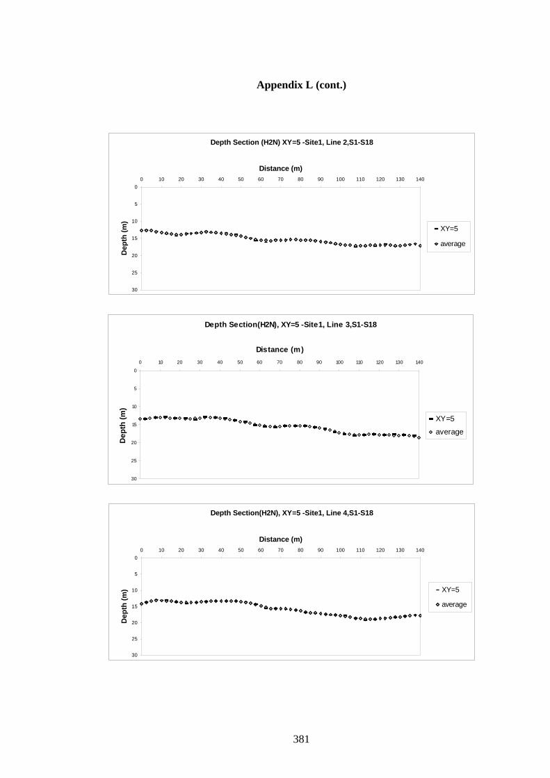
Appendix L (cont.)
Depth Section (H2N) XY=5 -Site1, Line 2,S1-S18
0
5
10
15
20
25
30
0 10 20 30 40 50 60 70 80 90 100 110 120 130 140
Distance (m)
Dep
th (m
)
XY=5
average
Depth Section(H2N), XY=5 -Site1, Line 3,S1-S18
0
5
10
15
20
25
30
0 10 20 30 40 50 60 70 80 90 100 110 120 130 140
Distance (m)
Dep
th (m
)
XY=5
average
Depth Section(H2N), XY=5 -Site1, Line 4,S1-S18
0
5
10
15
20
25
30
0 10 20 30 40 50 60 70 80 90 100 110 120 130 140
Distance (m)
Dep
th (m
) XY=5
average
381
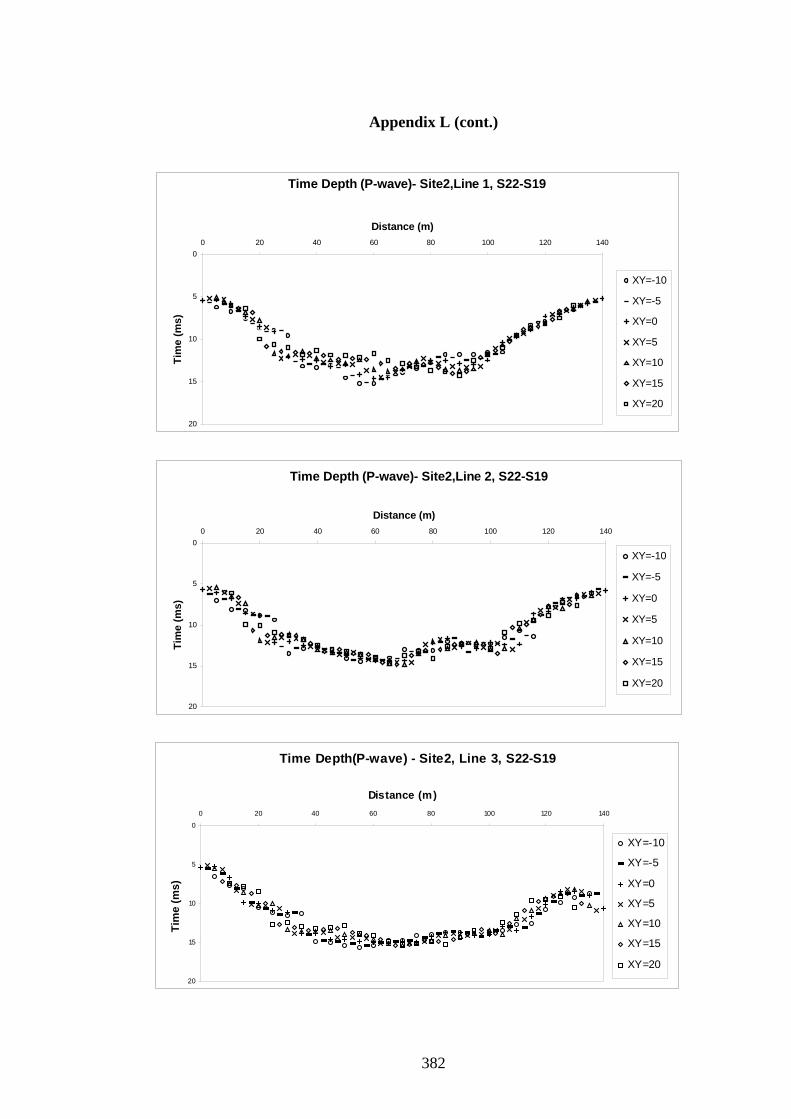
Appendix L (cont.)
Time Depth (P-wave)- Site2,Line 1, S22-S19
0
5
10
15
20
0 20 40 60 80 100 120 140
Distance (m)
Tim
e (m
s)
XY=-10
XY=-5
XY=0
XY=5
XY=10
XY=15
XY=20
Time Depth (P-wave)- Site2,Line 2, S22-S19
0
5
10
15
20
0 20 40 60 80 100 120 140
Distance (m)
Tim
e (m
s)
XY=-10
XY=-5
XY=0
XY=5
XY=10
XY=15
XY=20
Time Depth(P-wave) - Site2, Line 3, S22-S19
0
5
10
15
20
0 20 40 60 80 100 120 140
Distance (m)
Tim
e (m
s)
XY=-10
XY=-5
XY=0
XY=5
XY=10
XY=15
XY=20
382
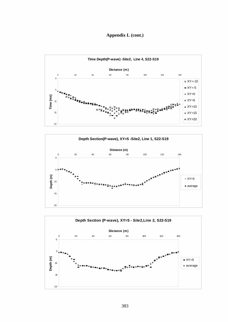
Appendix L (cont.)
Time Depth(P-wave) -Site2, Line 4, S22-S19
0
5
10
15
20
0 20 40 60 80 100 120 140
Distance (m)
Tim
e (m
s)
XY=-10
XY=-5
XY=0
XY=5
XY=10
XY=15
XY=20
Depth Section(P-wave), XY=5 -Site2, Line 1, S22-S19
0
5
10
15
20
0 20 40 60 80 100 120 140
Distance (m)
Dep
th (m
)
XY=5
average
Depth Section (P-wave), XY=5 - Site2,Line 2, S22-S19
0
5
10
15
20
0 20 40 60 80 100 120 140
Distance (m)
Dep
th (m
)
XY=5
average
383
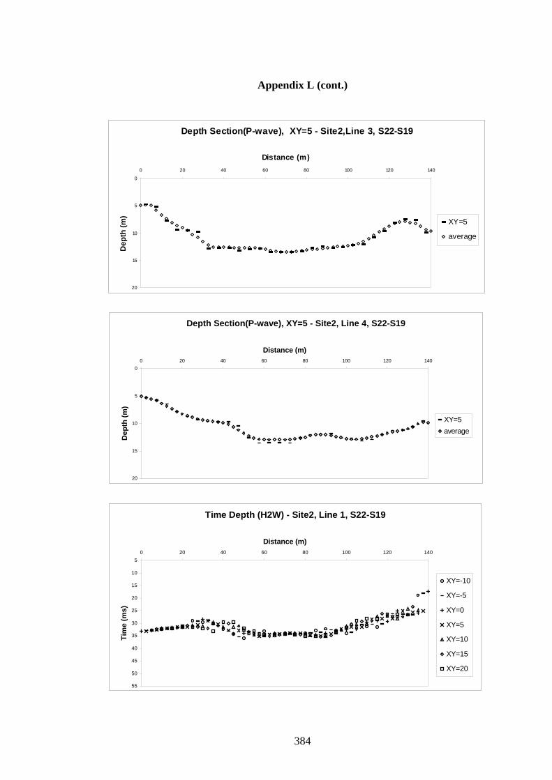
Appendix L (cont.)
Depth Section(P-wave), XY=5 - Site2,Line 3, S22-S19
0
5
10
15
20
0 20 40 60 80 100 120 140
Distance (m)
Dep
th (m
)
XY=5
average
Depth Section(P-wave), XY=5 - Site2, Line 4, S22-S19
0
5
10
15
20
0 20 40 60 80 100 120 140
Distance (m)
Dep
th (m
)
XY=5average
Time Depth (H2W) - Site2, Line 1, S22-S19
5
10
15
20
25
30
35
40
45
50
55
0 20 40 60 80 100 120 140
Distance (m)
Tim
e (m
s)
XY=-10
XY=-5
XY=0
XY=5
XY=10
XY=15
XY=20
384
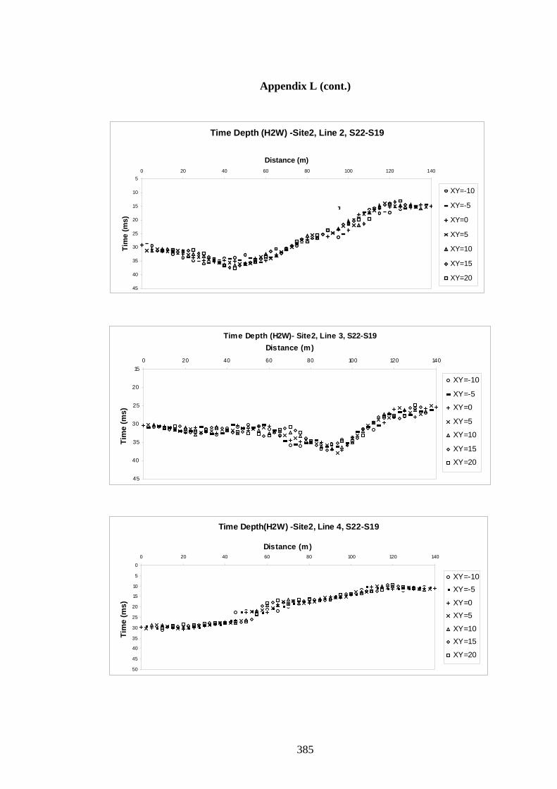
Appendix L (cont.)
Time Depth (H2W) -Site2, Line 2, S22-S19
5
10
15
20
25
30
35
40
45
0 20 40 60 80 100 120 140
Distance (m)
Tim
e (m
s)
XY=-10
XY=-5
XY=0
XY=5
XY=10
XY=15
XY=20
Time Depth (H2W)- Site2, Line 3, S22-S19
15
20
25
30
35
40
45
0 20 40 60 80 100 120 140
Distance (m)
Tim
e (m
s)
XY=-10
XY=-5
XY=0
XY=5
XY=10
XY=15
XY=20
Time Depth(H2W) -Site2, Line 4, S22-S19
0
5
10
15
20
25
30
35
40
45
50
0 20 40 60 80 100 120 140
Distance (m)
Tim
e (m
s)
XY=-10XY=-5
XY=0XY=5
XY=10XY=15
XY=20
385
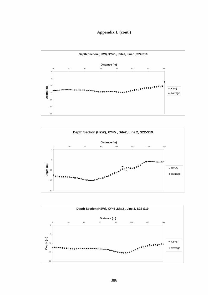
Appendix L (cont.)
Depth Section (H2W), XY=5 , Site2, Line 1, S22-S19
0
5
10
15
20
25
30
0 20 40 60 80 100 120 140
Distance (m)
Dep
th (m
)
XY=5average
Depth Section (H2W), XY=5 , Site2, Line 2, S22-S19
0
5
10
15
20
0 20 40 60 80 100 120 140
Distance (m)
Dep
th (m
)
XY=5
average
Depth Section (H2W), XY=5 ,Site2 , Line 3, S22-S19
0
5
10
15
20
0 20 40 60 80 100 120 140
Distance (m)
Dep
th (m
)
XY=5
average
386
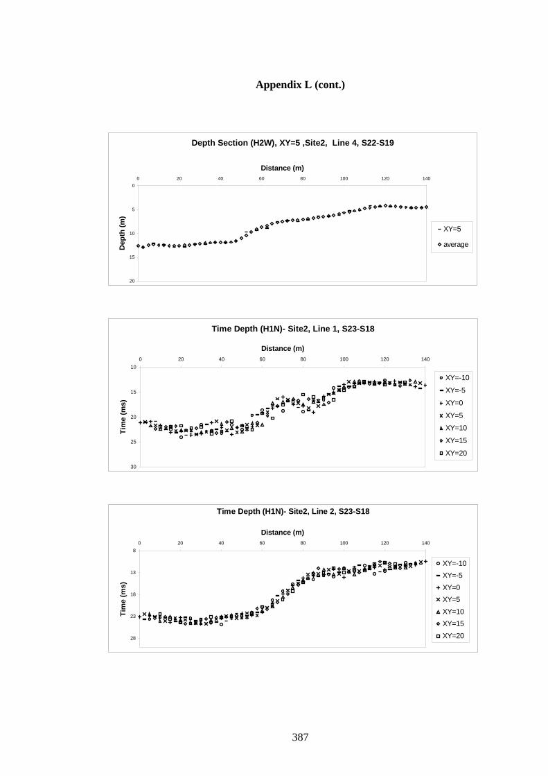
Appendix L (cont.)
Depth Section (H2W), XY=5 ,Site2, Line 4, S22-S19
0
5
10
15
20
0 20 40 60 80 100 120 140
Distance (m)
Dep
th (m
)
XY=5
average
Time Depth (H1N)- Site2, Line 1, S23-S18
10
15
20
25
30
0 20 40 60 80 100 120 140
Distance (m)
Tim
e (m
s)
XY=-10
XY=-5
XY=0
XY=5
XY=10
XY=15
XY=20
Time Depth (H1N)- Site2, Line 2, S23-S18
8
13
18
23
28
0 20 40 60 80 100 120 140
Distance (m)
Tim
e (m
s)
XY=-10XY=-5
XY=0XY=5
XY=10XY=15
XY=20
387
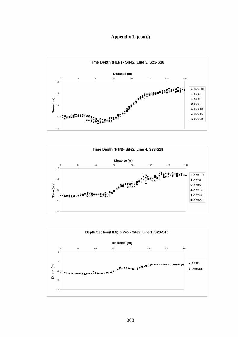
Appendix L (cont.)
Time Depth (H1N) - Site2, Line 3, S23-S18
10
15
20
25
30
0 20 40 60 80 100 120 140
Distance (m)
Tim
e (m
s)
XY=-10XY=-5XY=0XY=5XY=10XY=15XY=20
Time Depth (H1N)- Site2, Line 4, S23-S18
10
15
20
25
30
0 20 40 60 80 100 120 140
Distance (m)
Tim
e (m
s)
XY=-10XY=0XY=5XY=10XY=15XY=20
Depth Section(H1N), XY=5 - Site2, Line 1, S23-S18
0
5
10
15
20
0 20 40 60 80 100 120 140
Distance (m)
Dep
th (m
) XY=5
average
388
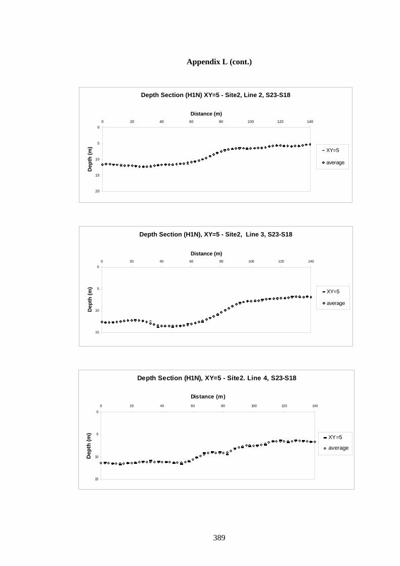
Appendix L (cont.)
Depth Section (H1N) XY=5 - Site2, Line 2, S23-S18
0
5
10
15
20
0 20 40 60 80 100 120 140
Distance (m)
Dep
th (m
) XY=5
average
Depth Section (H1N), XY=5 - Site2, Line 3, S23-S18
0
5
10
15
0 20 40 60 80 100 120 140
Distance (m)
Dep
th (m
)
XY=5
average
Depth Section (H1N), XY=5 - Site2. Line 4, S23-S18
0
5
10
15
0 20 40 60 80 100 120 140
Distance (m)
Dep
th (m
)
XY=5
average
389
Appendix M: Wavepath Eikonal Traveltime Inversion
There are several methods of asymptotic tomography using the back projection
of traveltime residuals for the inversion of slowness fields in an acoustic
medium. These methods include ray-tracing (RT) tomography described by
Cerveny et al. (1977), the Woodward-Rocca (WR) method described by
Woodward and Rocca (1988), wave-equation traveltime (WT) inversion such as
described by Luo and Schuster (1991), and Schuster’s and Quintus-Bosz’s
(1993) wavepath eikonal traveltime (WET) inversion. It can be shown that
these methods are all derived from the general asymptotic back-projection
formula with different choices of the arbitrary weighting factor.
Wavepath eikonal traveltime inversion is so named because it computes
wavepaths using finite-difference solutions to the eikonal equation. Of the
asymptotic tomography methods, it is the most desirable in terms of
computational cost, robustness and effectiveness. It is generally better than the
WT and WR methods since it is an order of magnitude faster, yet is comparable
in effectiveness. It is also better than RT tomography since, whilst being
computationally comparable, it accounts for bandwidth and shadow effects in
the data by modelling multiple signal propagation paths contributing to one first-
arrival (which RT tomography does not).
The first step of the WET inversion algorithm is to propose an initial slowness
model, which may be generated assuming constant vertical velocity gradients
such as with 1D tau-p inversion, or assuming discrete velocity changes such as
390
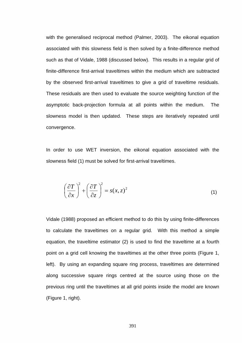
with the generalised reciprocal method (Palmer, 2003). The eikonal equation
associated with this slowness field is then solved by a finite-difference method
such as that of Vidale, 1988 (discussed below). This results in a regular grid of
finite-difference first-arrival traveltimes within the medium which are subtracted
by the observed first-arrival traveltimes to give a grid of traveltime residuals.
These residuals are then used to evaluate the source weighting function of the
asymptotic back-projection formula at all points within the medium. The
slowness model is then updated. These steps are iteratively repeated until
convergence.
In order to use WET inversion, the eikonal equation associated with the
slowness field (1) must be solved for first-arrival traveltimes.
222
),( zxszT
xT
=⎟⎠⎞
⎜⎝⎛∂∂
+⎟⎠⎞
⎜⎝⎛∂∂
(1)
Vidale (1988) proposed an efficient method to do this by using finite-differences
to calculate the traveltimes on a regular grid. With this method a simple
equation, the traveltime estimator (2) is used to find the traveltime at a fourth
point on a grid cell knowing the traveltimes at the other three points (Figure 1,
left). By using an expanding square ring process, traveltimes are determined
along successive square rings centred at the source using those on the
previous ring until the traveltimes at all grid points inside the model are known
(Figure 1, right).
391
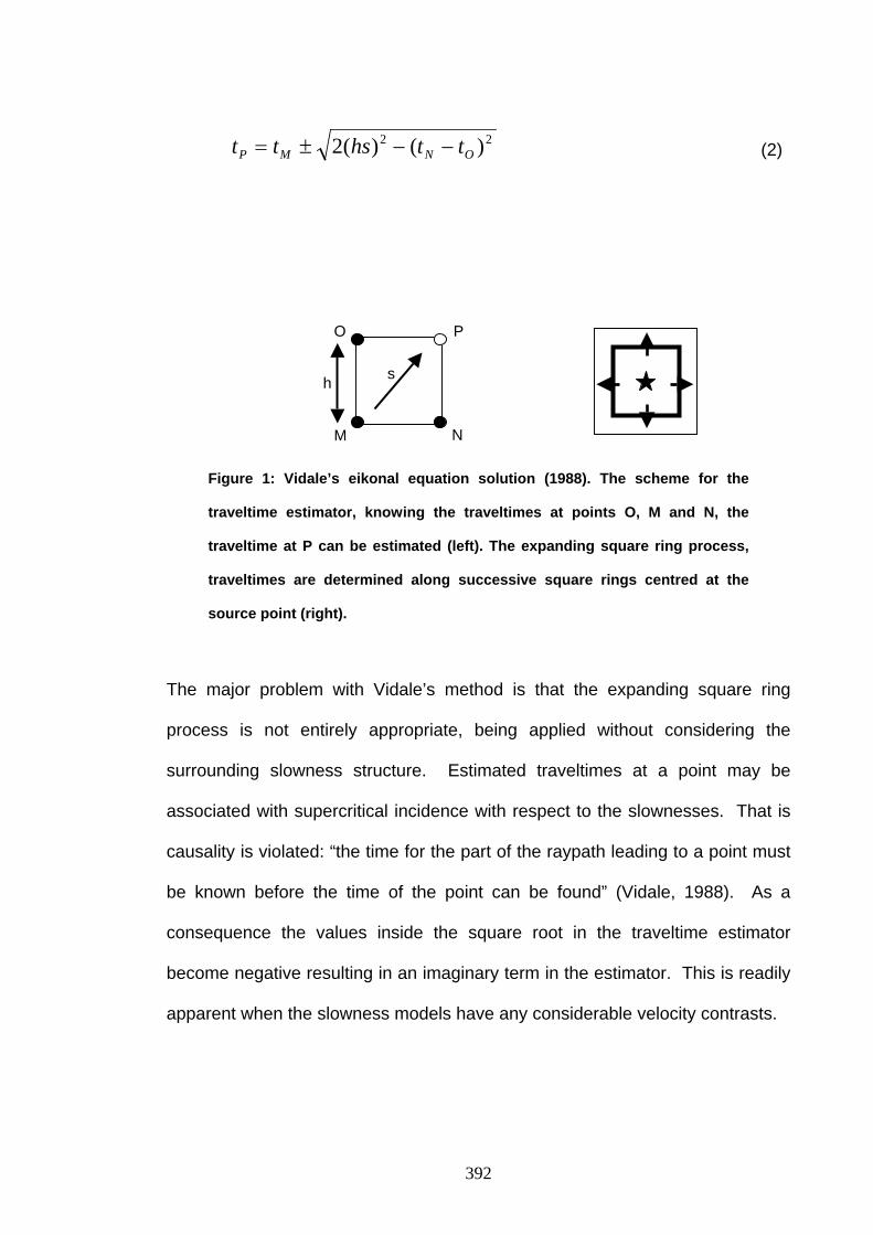
22 )()(2 ONMP tthstt −−±= (2)
s
O P
h
NM
Figure 1: Vidale’s eikonal equation solution (1988). The scheme for the
traveltime estimator, knowing the traveltimes at points O, M and N, the
traveltime at P can be estimated (left). The expanding square ring process,
traveltimes are determined along successive square rings centred at the
source point (right).
The major problem with Vidale’s method is that the expanding square ring
process is not entirely appropriate, being applied without considering the
surrounding slowness structure. Estimated traveltimes at a point may be
associated with supercritical incidence with respect to the slownesses. That is
causality is violated: “the time for the part of the raypath leading to a point must
be known before the time of the point can be found” (Vidale, 1988). As a
consequence the values inside the square root in the traveltime estimator
become negative resulting in an imaginary term in the estimator. This is readily
apparent when the slowness models have any considerable velocity contrasts.
392
The problem arising from solving the eikonal equation along an expanding
square ring can be largely eliminated by instead solving it along an expanding
wavefront (Qin et al., 1992). Such a strategy ensures that any point about to be
timed will have had its associated ray completely timed up to that point and
hence observing causality. This strategy gives accurate traveltimes in complex
velocity models and is stable in problem areas such as shadow zones and
waveguides. However as with the expanding square ring process this method
can still return negative square root arguments in extremely complex slowness
models.
Another way to overcome negative values inside the square root in the
traveltime estimator was proposed by Lecomte et al., 2000. Their method
achieves this by using five different traveltime estimators at each point and
taking the minimum estimated traveltime. Also, instead of using the expanding
square ring it uses an active point process where the central point is active and
may update the traveltimes at its eight surrounding points using different
estimators. The method can handle complex slowness models with strong
velocity contrasts. As well as this, its robustness allows for the recovery of
more than the first-arrival traveltime with later head waves able to be obtained
by masking fast deep layers with a high slowness mask.
Wavepath eikonal traveltime inversion is a high frequency traveltime
tomographic method. It is a computationally efficient method, being an order of
magnitude faster than wave-equation traveltime inversion (yet comparable in
effectiveness) since only solutions to the eikonal equation are involved. It
393
models multiple signal propagation paths contributing to one first-arrival and as
such is superior to conventional ray-tracing tomography which is limited to the
modelling of just one ray per first-arrival.
References:
Cerveny, V., Molotkov, I. A., Psencik, I., 1977, Ray Method in Seismology: Praha, Universita, Karlova.
Lecomte, I., Gjoystdal, H., Dahle, A., Pedersen, O.C., 2000, Improving modelling and inversion in refraction seismics with a first-order Eikonal solver: Geophysical Prospecting, 48, 437-454.
Luo, Y., Schuster, G. T., 1991, Wave equation traveltime inversion: Geophysics, 56, 645-653.
Palmer, D., 2003, Application of amplitudes in shallow seismic refraction inversion: 16th Conf., ASEG, extended abstracts.
Qin, F., Luo, Y., Olsen, K., Cai, W., Schuster, G., 1992, Finite-difference solution of the eikonal equation along expanding wavefronts: Geophysics, 57, 478-487.
Schuster, G.T., Quintus-Bosz, A., 1993, Wavepath eikonal traveltime inversion: Theory: Geophysics, 58, 1314-1323.
Vidale, J., 1988, Finite-difference calculation of traveltimes: Bull. Seis. Soc. Am., 78, 2062-2076.
Woodward, M., Rocca, F., 1988, Wave-equation tomography: 58th Ann. Internat. Mtg., SEG, extended abstracts, 1232-1235.
394
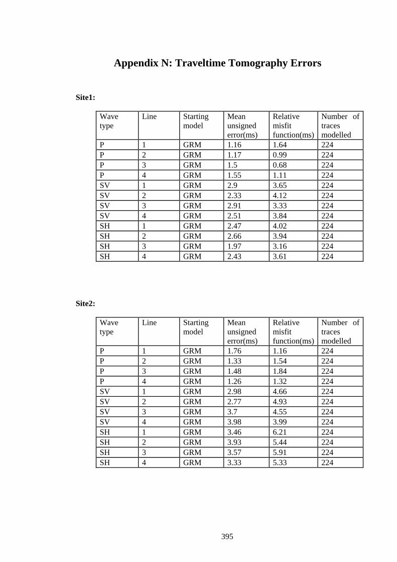
Appendix N: Traveltime Tomography Errors
Site1:
Wave type
Line Starting model
Mean unsigned error(ms)
Relative misfit function(ms)
Number of traces modelled
P 1 GRM 1.16 1.64 224 P 2 GRM 1.17 0.99 224 P 3 GRM 1.5 0.68 224 P 4 GRM 1.55 1.11 224 SV 1 GRM 2.9 3.65 224 SV 2 GRM 2.33 4.12 224 SV 3 GRM 2.91 3.33 224 SV 4 GRM 2.51 3.84 224 SH 1 GRM 2.47 4.02 224 SH 2 GRM 2.66 3.94 224 SH 3 GRM 1.97 3.16 224 SH 4 GRM 2.43 3.61 224
Site2:
Wave type
Line Starting model
Mean unsigned error(ms)
Relative misfit function(ms)
Number of traces modelled
P 1 GRM 1.76 1.16 224 P 2 GRM 1.33 1.54 224 P 3 GRM 1.48 1.84 224 P 4 GRM 1.26 1.32 224 SV 1 GRM 2.98 4.66 224 SV 2 GRM 2.77 4.93 224 SV 3 GRM 3.7 4.55 224 SV 4 GRM 3.98 3.99 224 SH 1 GRM 3.46 6.21 224 SH 2 GRM 3.93 5.44 224 SH 3 GRM 3.57 5.91 224 SH 4 GRM 3.33 5.33 224
395
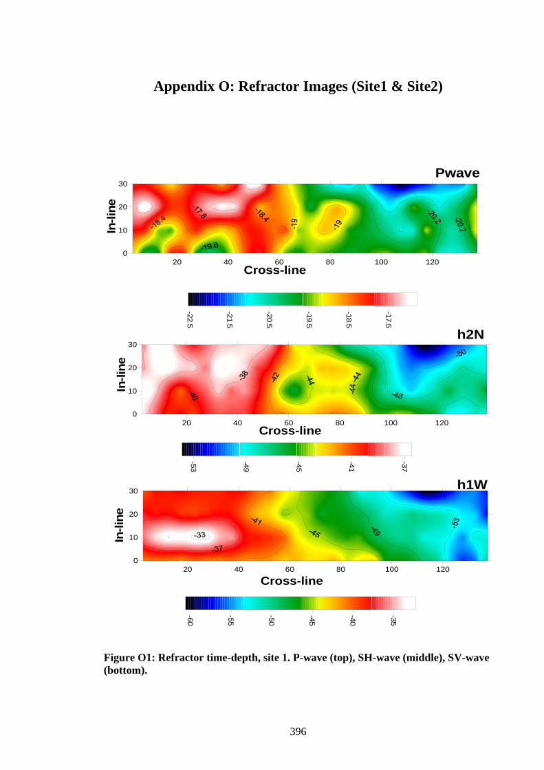
Appendix O: Refractor Images (Site1 & Site2)
20 40 60 80 100 1200
10
20
30
-22.5
-21.5
-20.5
-19.5
-18.5
-17.5
Refractor Time-depth, Site1
20 40 60 80 100 1200
10
20
30-53
-49
-45
-41
-37
20 40 60 80 100 1200
10
20
30
-60
-55
-50
-45
-40
-35
Cross-line
In-li
ne
Cross-line
In-li
ne
Cross-line
In-li
ne
Pwave
h2N
h1W
Figure O1: Refractor time-depth, site 1. P-wave (top), SH-wave (middle), SV-wave (bottom).
396
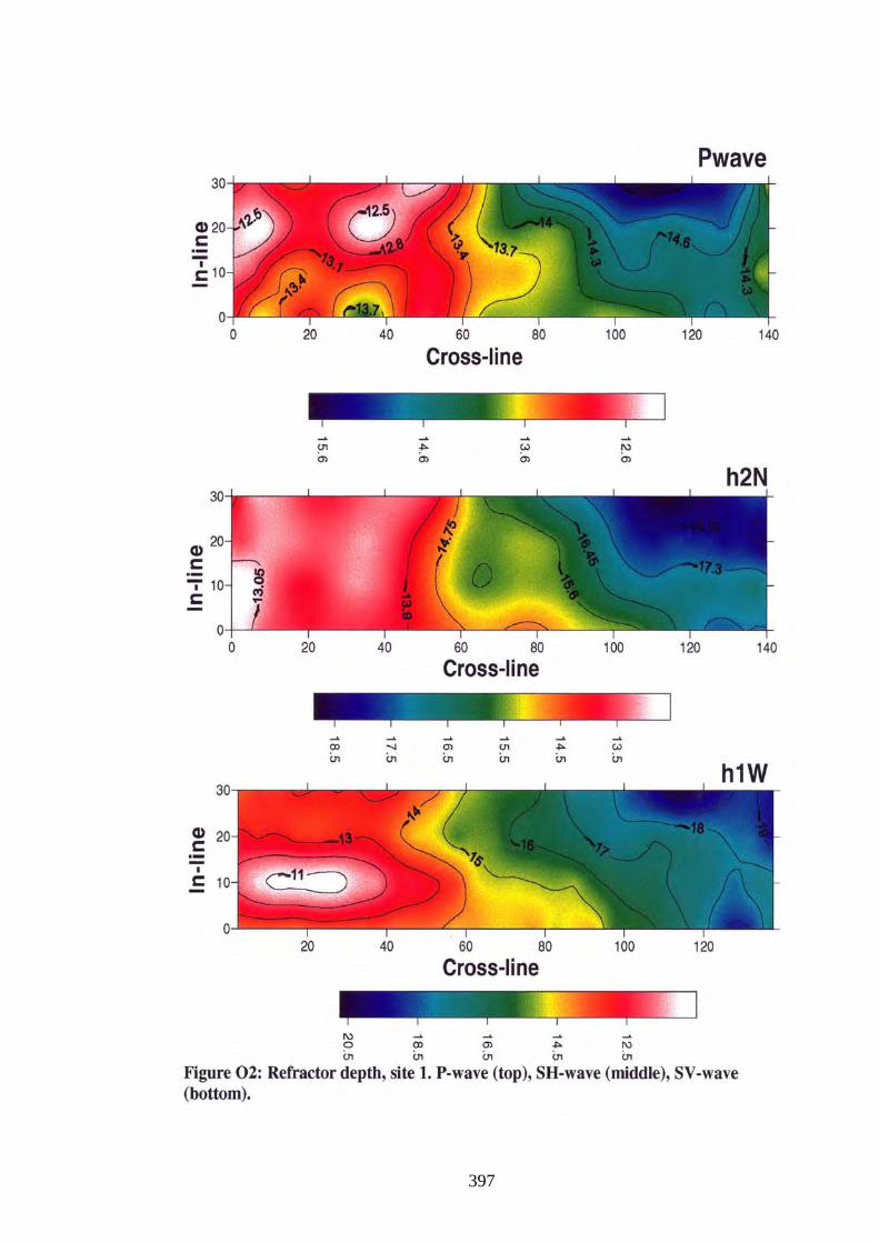
397
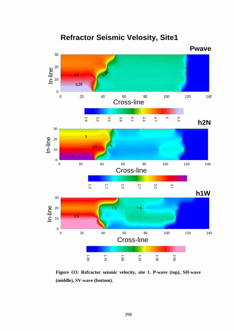
0 20 40 60 80 100 120 1400
10
20
30
2.9
3.2
3.5
3.8
4.1
4.4
4.7
5 5.3
Refractor Seismic Velosity, Site1
0 20 40 60 80 100 120 1400
10
20
30
1.2
1.7
2.2
2.7
3.2
3.7
0 20 40 60 80 100 120 1400
10
20
30
1.55
1.75
1.95
2.15
2.35
2.55
Pwave
h2N
h1W
Cross-line
In-li
ne
Cross-line
Cross-line
In-li
neIn
-line
Figure O3: Refractor seismic velocity, site 1. P-wave (top), SH-wave
(middle), SV-wave (bottom).
398
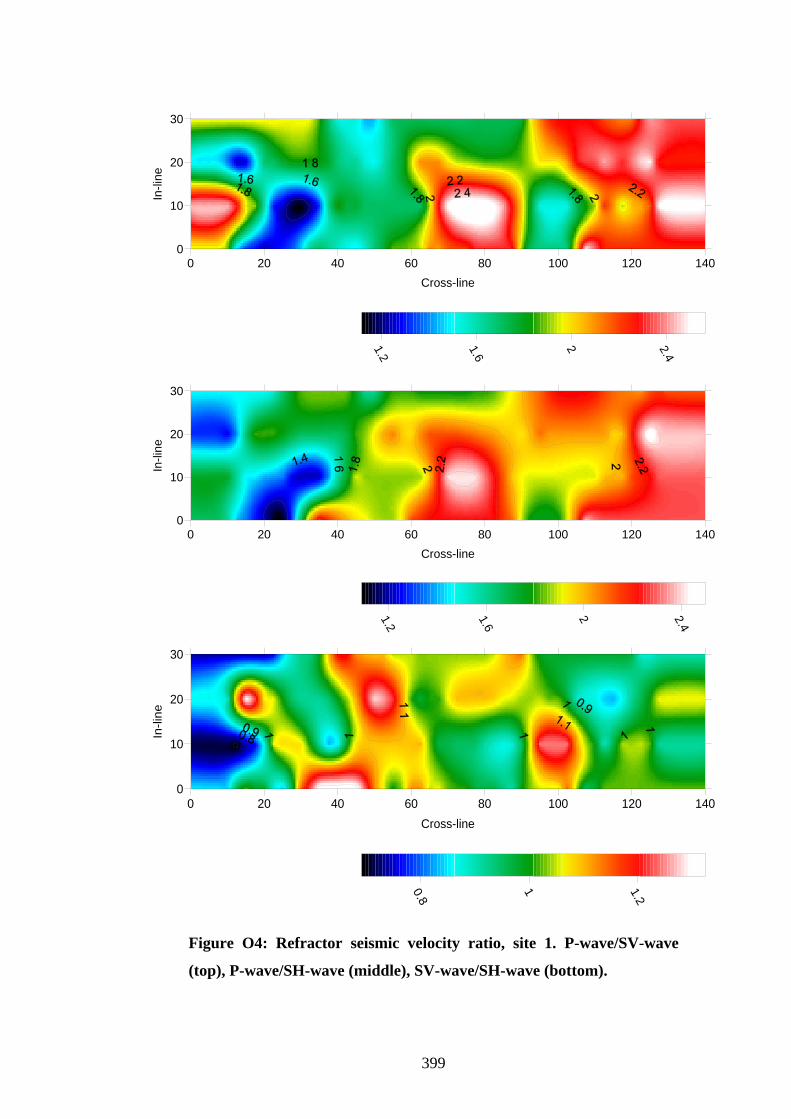
0 20 40 60 80 100 120Cross-line
1400
10
20
30
In-li
ne
1.2
1.6
2 2.4
0 20 40 60 80 100 120 140Cross-line
0
10
20
30
In-li
ne
1.2
1.6
2 2.4
0 20 40 60 80 100 120Cross-line
1400
10
20
30
In-li
ne
0.8
1 1.2
Figure O4: Refractor seismic velocity ratio, site 1. P-wave/SV-wave
(top), P-wave/SH-wave (middle), SV-wave/SH-wave (bottom).
399
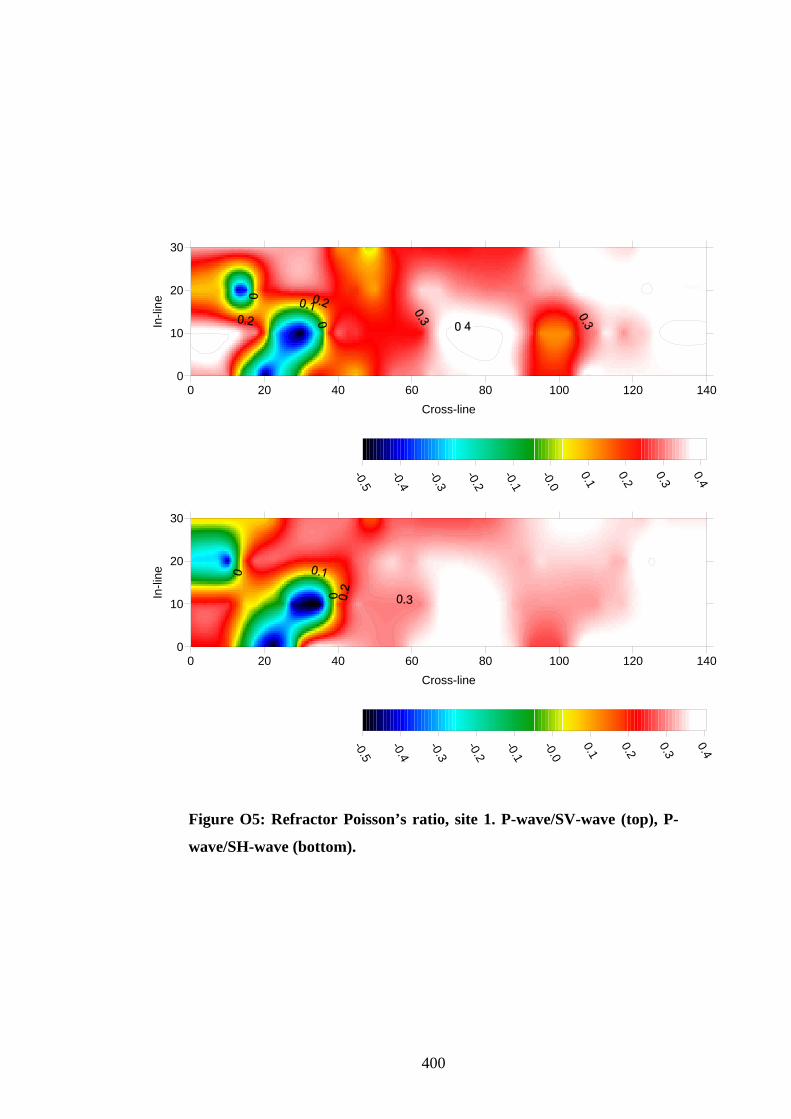
0 20 40 60 80 100 120 140Cross-line
0
10
20
30
In-li
ne
-0.5
-0.4
-0.3
-0.2
-0.1
-0.0
0.1
0.2
0.3
0.4
0 20 40 60 80 100 120 140Cross-line
0
10
20
30
In-li
ne
-0.5
-0.4
-0.3
-0.2
-0.1
-0.0
0.1
0.2
0.3
0.4
Figure O5: Refractor Poisson’s ratio, site 1. P-wave/SV-wave (top), P-
wave/SH-wave (bottom).
400
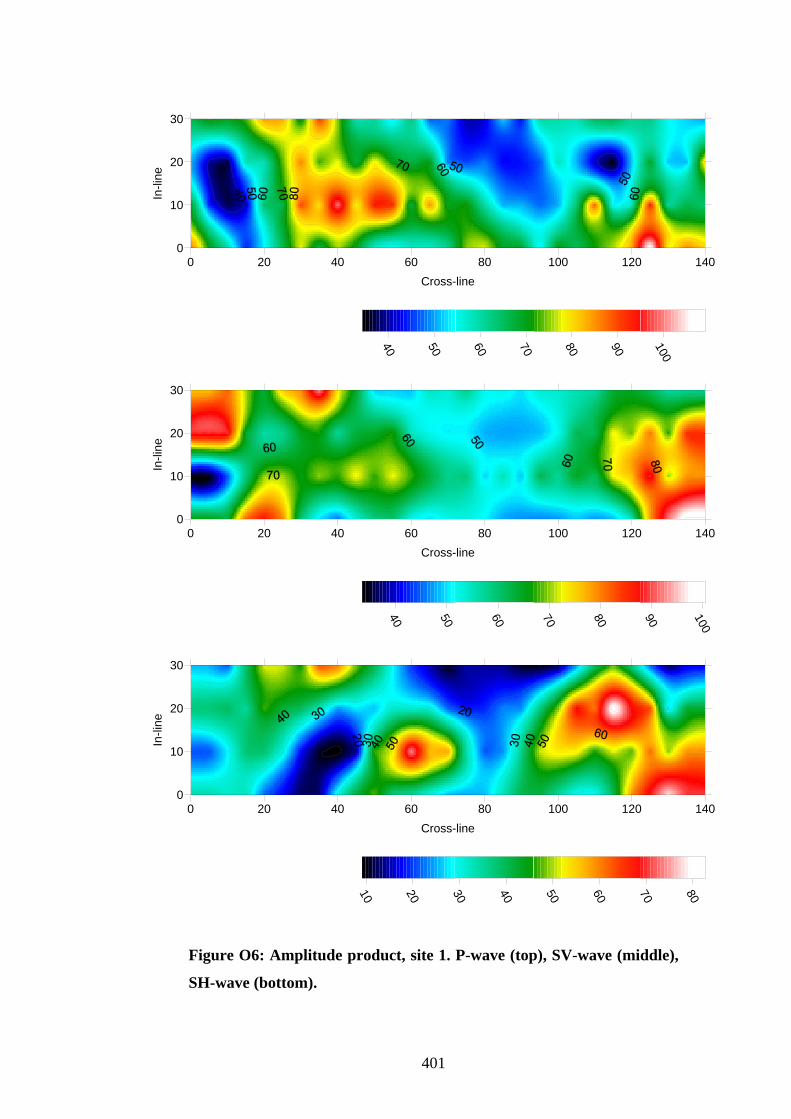
0 20 40 60 80 100 120Cross-line
1400
10
20
30
In-li
ne
40 50 60 70 80 90 100
0 20 40 60 80 100 120Cross-line
1400
10
20
30
In-li
ne
40 50 60 70 80 90 100
0 20 40 60 80 100 120 140Cross-line
0
10
20
30
In-li
ne
10 20 30 40 50 60 70 80
Figure O6: Amplitude product, site 1. P-wave (top), SV-wave (middle),
SH-wave (bottom).
401
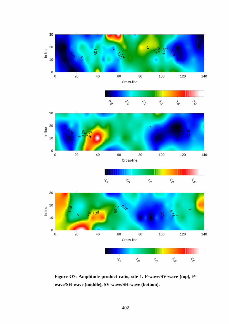
0 20 40 60 80 100 120Cross-line
1400
10
20
30
In-li
ne
0.5
1.0
1.5
2.0
2.5
3.0
0 20 40 60 80 100 120Cross-line
1400
10
20
30
In-li
ne
0.5
1.0
1.5
2.0
2.5
0 20 40 60 80 100 120Cross-line
1400
10
20
30
In-li
ne
0.5
1.0
1.5
2.0
2.5
Figure O7: Amplitude product ratio, site 1. P-wave/SV-wave (top), P-
wave/SH-wave (middle), SV-wave/SH-wave (bottom).
402
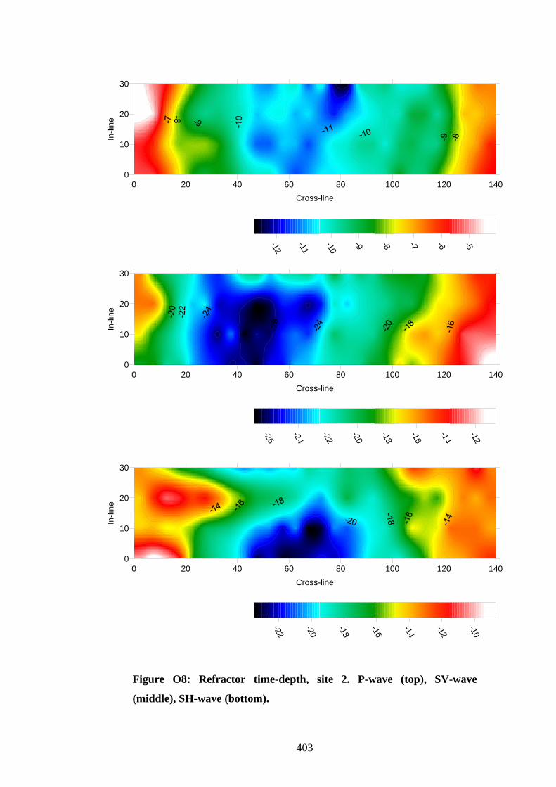
0 20 40 60 80 100 120Cross-line
1400
10
20
30
In-li
ne
-12
-11
-10
-9 -8 -7 -6 -5
0 20 40 60 80 100 120 140Cross-line
0
10
20
30
In-li
ne
-26
-24
-22
-20
-18
-16
-14
-12
0 20 40 60 80 100 120Cross-line
1400
10
20
30
In-li
ne
-22
-20
-18
-16
-14
-12
-10
Figure O8: Refractor time-depth, site 2. P-wave (top), SV-wave
(middle), SH-wave (bottom).
403
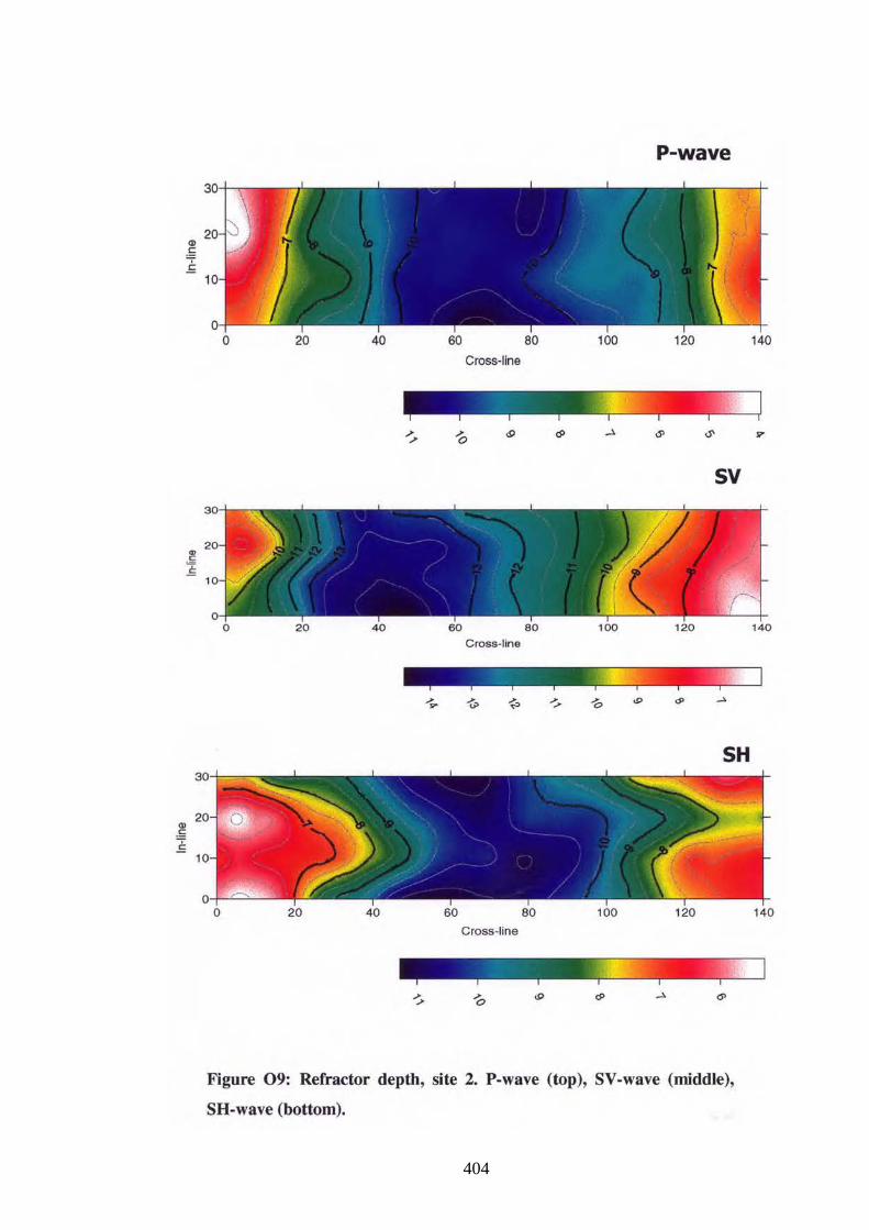
404
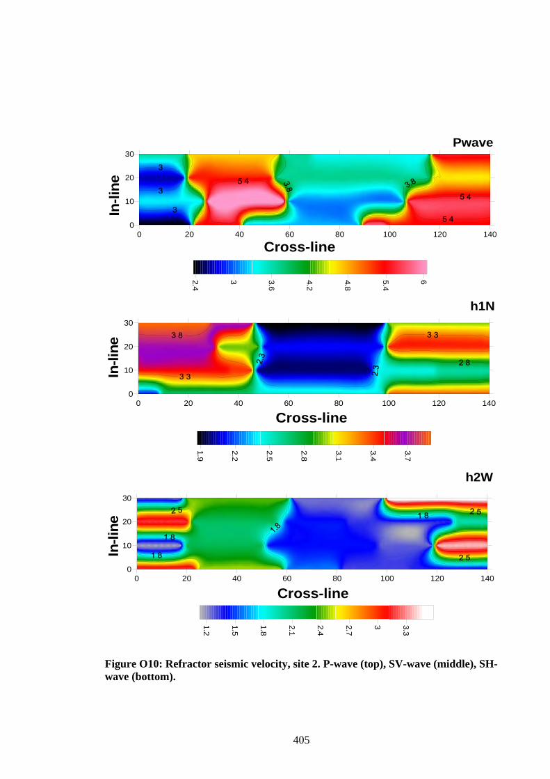
Site2, Refractor Seismic Velocity
0 20 40 60 80 100 120 1400
10
20
30
2.4
3 3.6
4.2
4.8
5.4
6
0 20 40 60 80 100 120 1400
10
20
30
1.9
2.2
2.5
2.8
3.1
3.4
3.7
0 20 40 60 80 100 120 1400
10
20
30
1.2
1.5
1.8
2.1
2.4
2.7
3 3.3
Cross-line
In-li
ne
Cross-line
Cross-line
In-li
neIn
-line
h2W
h1N
Pwave
Figure O10: Refractor seismic velocity, site 2. P-wave (top), SV-wave (middle), SH-wave (bottom).
405
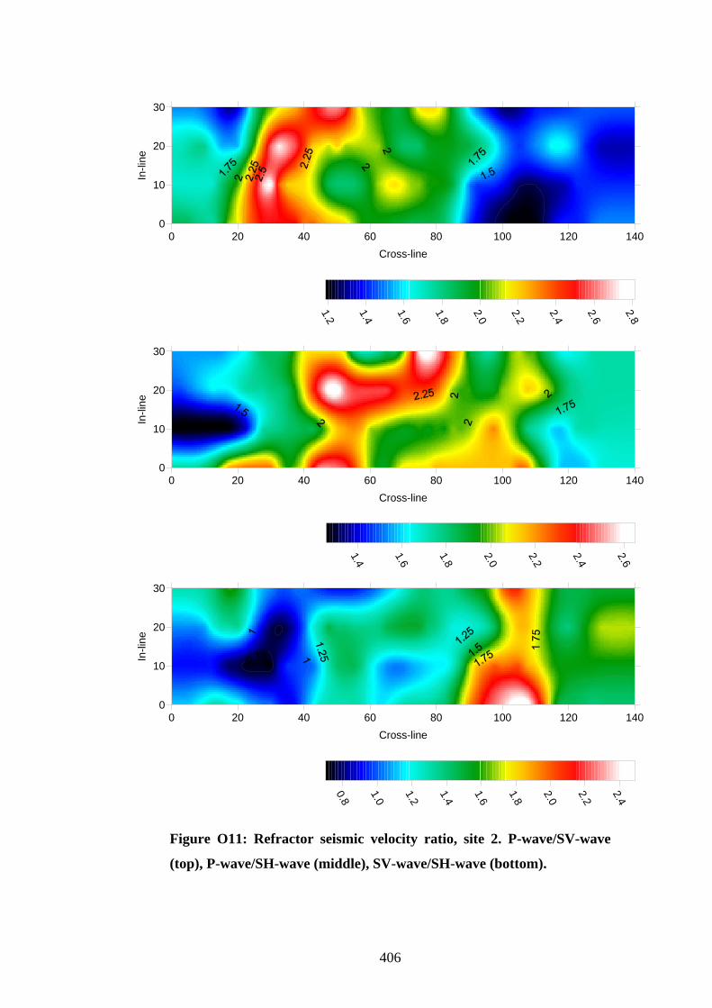
0 20 40 60 80 100 120 140Cross-line
0
10
20
30
In-li
ne
1.2
1.4
1.6
1.8
2.0
2.2
2.4
2.6
2.8
0 20 40 60 80 100 120 140Cross-line
0
10
20
30
In-li
ne
1.4
1.6
1.8
2.0
2.2
2.4
2.6
0 20 40 60 80 100 120 140Cross-line
0
10
20
30
In-li
ne
0.8
1.0
1.2
1.4
1.6
1.8
2.0
2.2
2.4
Figure O11: Refractor seismic velocity ratio, site 2. P-wave/SV-wave
(top), P-wave/SH-wave (middle), SV-wave/SH-wave (bottom).
406
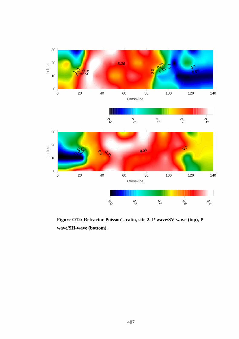
0 20 40 60 80 100 120Cross-line
1400
10
20
30In
-line
0.0
0.1
0.2
0.3
0.4
0 20 40 60 80 100 120Cross-line
1400
10
20
30
In-li
ne
0.0
0.1
0.2
0.3
0.4
Figure O12: Refractor Poisson’s ratio, site 2. P-wave/SV-wave (top), P-
wave/SH-wave (bottom).
407
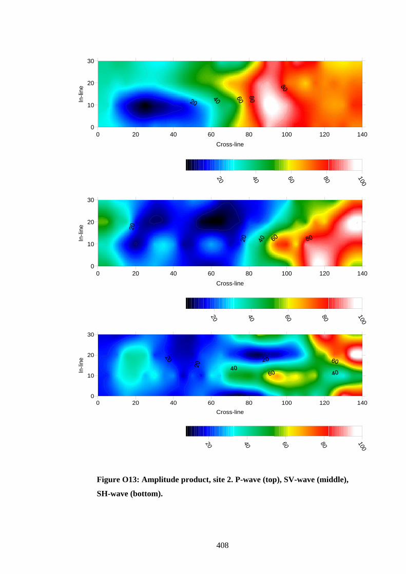
0 20 40 60 80 100 120 140Cross-line
0
10
20
30
In-li
ne
20 40 60 80 100
0 20 40 60 80 100 120 140Cross-line
0
10
20
30
In-li
ne
20 40 60 80 100
0 20 40 60 80 100 120 140Cross-line
0
10
20
30
In-li
ne
20 40 60 80 100
Figure O13: Amplitude product, site 2. P-wave (top), SV-wave (middle),
SH-wave (bottom).
408
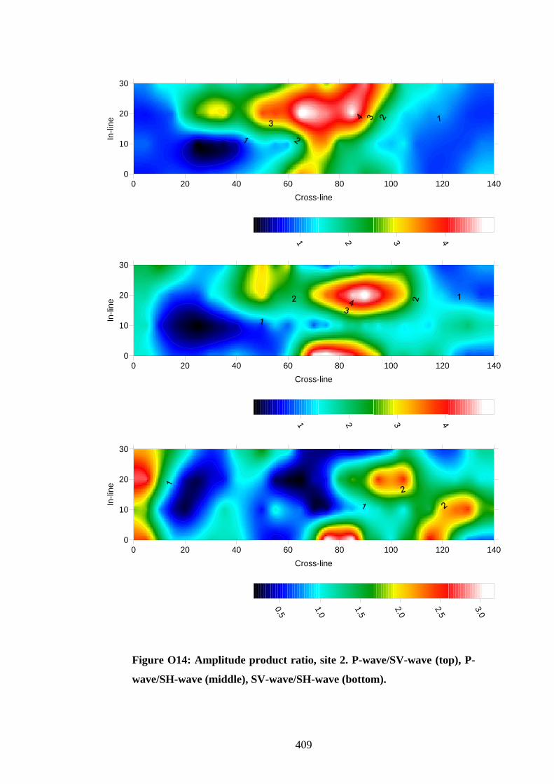
0 20 40 60 80 100 120 140Cross-line
0
10
20
30
In-li
ne
1 2 3 4
0 20 40 60 80 100 120Cross-line
1400
10
20
30
In-li
ne
1 2 3 4
0 20 40 60 80 100 120Cross-line
1400
10
20
30
In-li
ne
0.5
1.0
1.5
2.0
2.5
3.0
Figure O14: Amplitude product ratio, site 2. P-wave/SV-wave (top), P-
wave/SH-wave (middle), SV-wave/SH-wave (bottom).
409
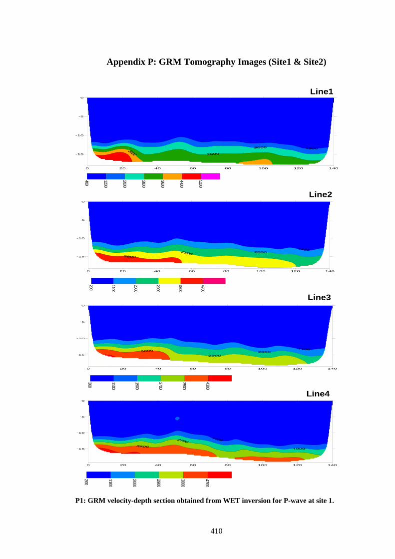
Appendix P: GRM Tomography Images (Site1 & Site2)
GRM Velocity Images, Pwave, Site1
0 20 40 60 80 100 120 140
-15
-10
-5
0
400
1200
2000
2800
3600
4400
5200
0 20 40 60 80 100 120 140
-15
-10
-5
0
0 20 40 60 80 100 120 140
-15
-10
-5
0
0 20 40 60 80 100 120 140
-15
-10
-5
0
200
1100
2000
2900
3800
4700
200
110 0
2000
2900
3800
4700
300
1100
1900
2700
3500
4300
Line1
Line2
Line3
Line4
P1: GRM velocity-depth section obtained from WET inversion for P-wave at site 1.
410
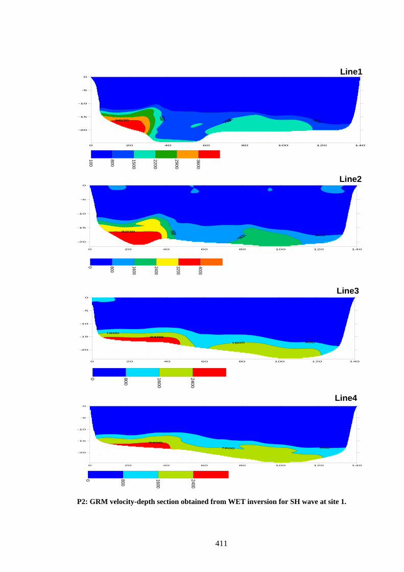
GRM Velocity Images, h2N, Site1
0 20 40 60 80 100 120 140
-20
-15
-10
-5
0
0 20 40 60 80 100 120 140
-20
-15
-10
-5
0
0 20 40 60 80 100 120 140
-20
-15
-10
-5
0
0 20 40 60 80 100 120 140
-20
-15
-10
-5
0
100
800
1500
2200
2900
3600
0 800
1600
2400
3200
4000
0 800
1600
2400
0 800
1600
2400
Line1
Line2
Line3
Line4
P2: GRM velocity-depth section obtained from WET inversion for SH wave at site 1.
411
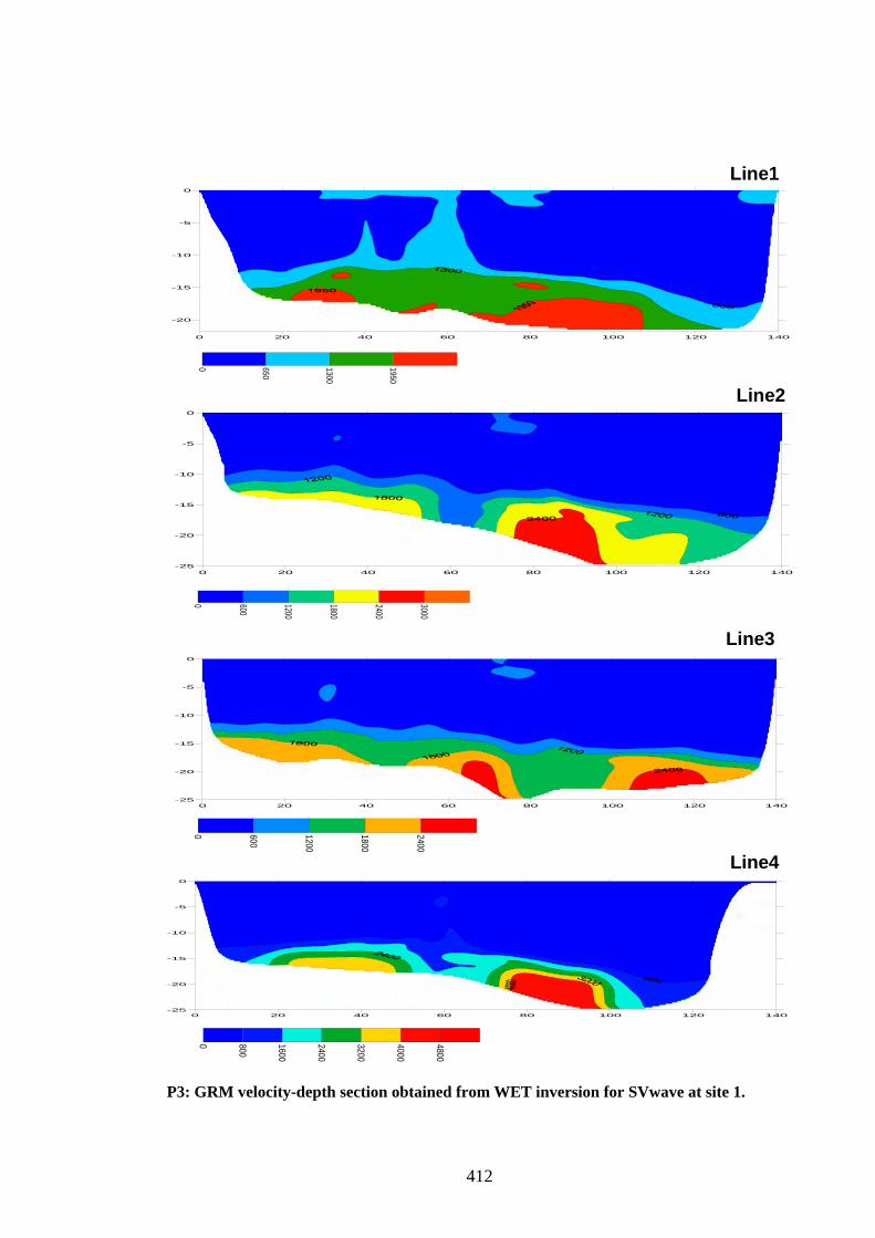
0 20 40 60 80 100 120 140
-20
-15
-10
-5
0
0 20 40 60 80 100 120 140-25
-20
-15
-10
-5
0
0 20 40 60 80 100 120 140-25
-20
-15
-10
-5
0
0 20 40 60 80 100 120 140-25
-20
-15
-10
-5
0
0 650
1300
1950
0 600
1200
1800
2400
3000
0 600
1200
1800
2400
0 800
1600
2400
3200
4000
4800
Line1
Line2
Line3
Line4
GRM Velocity Images, h1W, Site1
P3: GRM velocity-depth section obtained from WET inversion for SVwave at site 1.
412
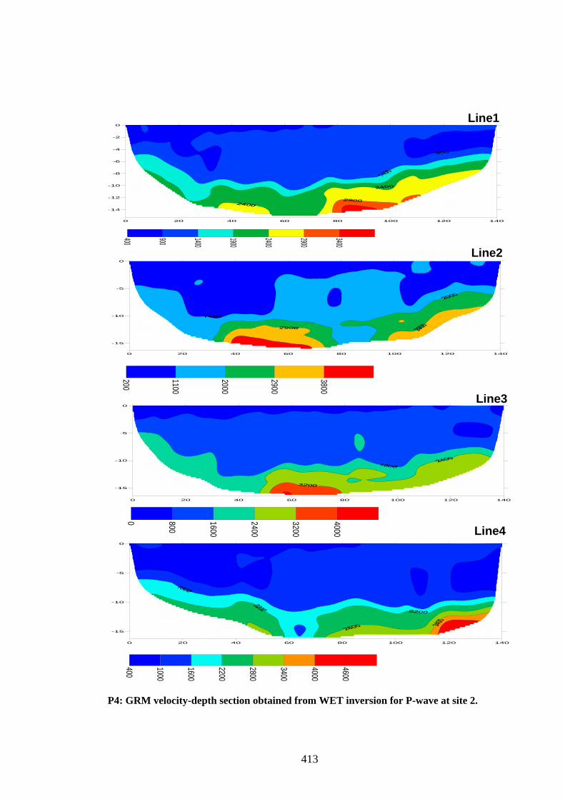
GRM Velocity Images, Pwave, Site 2
0 20 40 60 80 100 120 140
-14
-12
-10
-8
-6
-4
-2
0
0 20 40 60 80 100 120 140
-15
-10
-5
0
0 20 40 60 80 100 120 140
-15
-10
-5
0
0 20 40 60 80 100 120 140
-15
-10
-5
0
400 900 1400
1900
2400
2900
3400
200
1100
2000
2900
3800
0 800
1600
2400
3200
4000
400
1000
1600
2200
2800
3400
4000
4600
Line1
Line2
Line3
Line4
P4: GRM velocity-depth section obtained from WET inversion for P-wave at site 2.
413
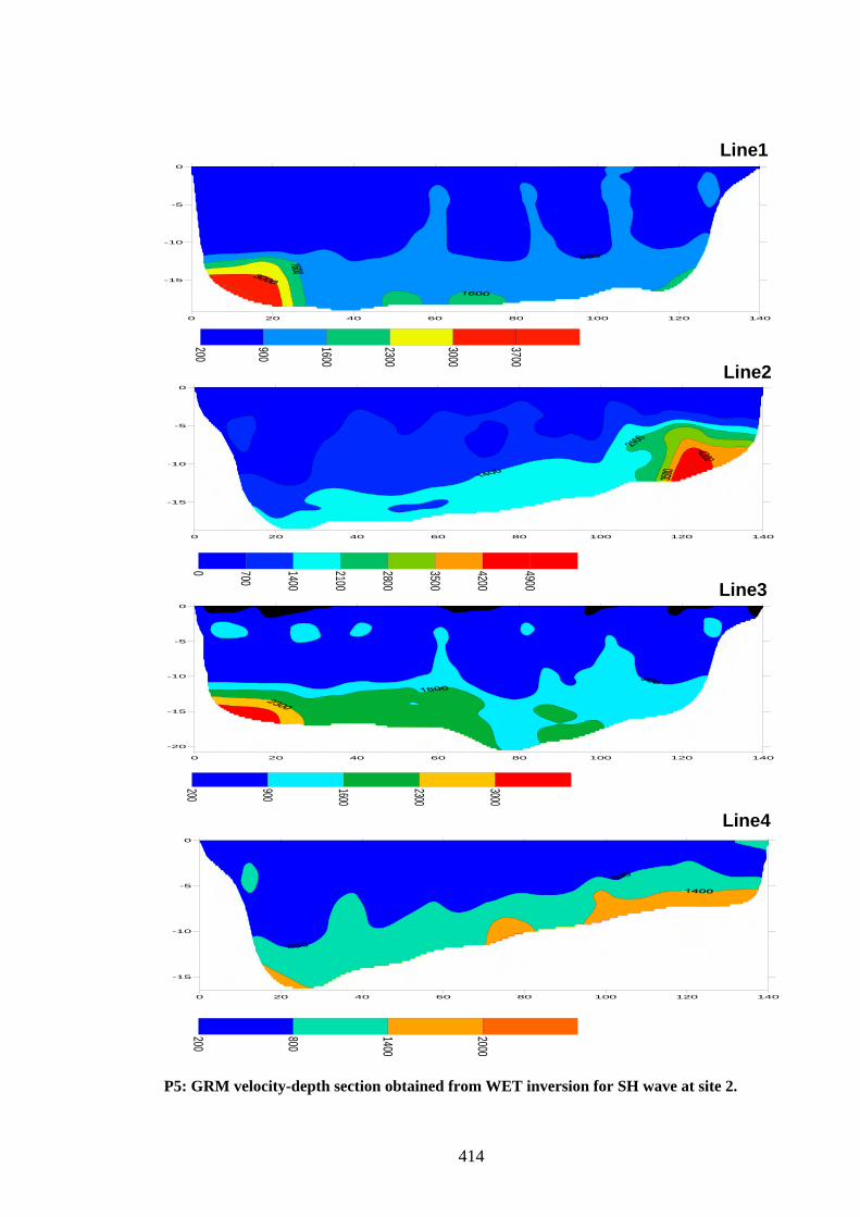
GRM Velocity Images, h2W, Site 2
0 20 40 60 80 100 120 140
-15
-10
-5
0
0 20 40 60 80 100 120 140
-15
-10
-5
0
0 20 40 60 80 100 120 140
-20
-15
-10
-5
0
0 20 40 60 80 100 120 140
-15
-10
-5
0
200
900
1600
2300
3000
3700
0 700
1400
2100
2800
3500
4200
4900
200 900 1600
2300
3000
200
800
1400
2000
Line1
Line2
Line3
Line4
P5: GRM velocity-depth section obtained from WET inversion for SH wave at site 2.
414
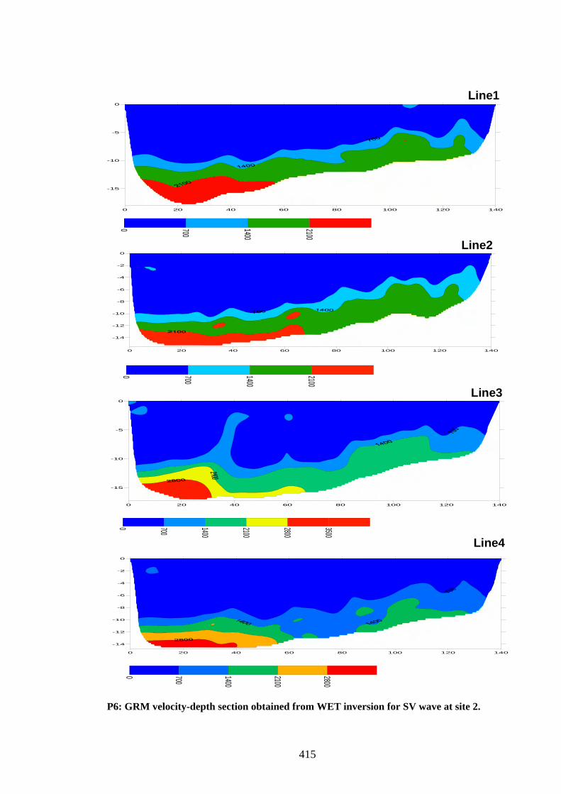
GRM Velocity Images, h1N, Site 2
0 20 40 60 80 100 120 140
-15
-10
-5
0
0 20 40 60 80 100 120 140
-14
-12
-10
-8
-6
-4
-2
0
0 20 40 60 80 100 120 140
-15
-10
-5
0
0 20 40 60 80 100 120 140
-14
-12
-10
-8
-6
-4
-2
0
0 700 1400
2100
0 700 1400
2100
0 700 1400
2100
2800
3500
0 700 1400
2100
2800
Line1
Line2
Line3
Line4
P6: GRM velocity-depth section obtained from WET inversion for SV wave at site 2.
415
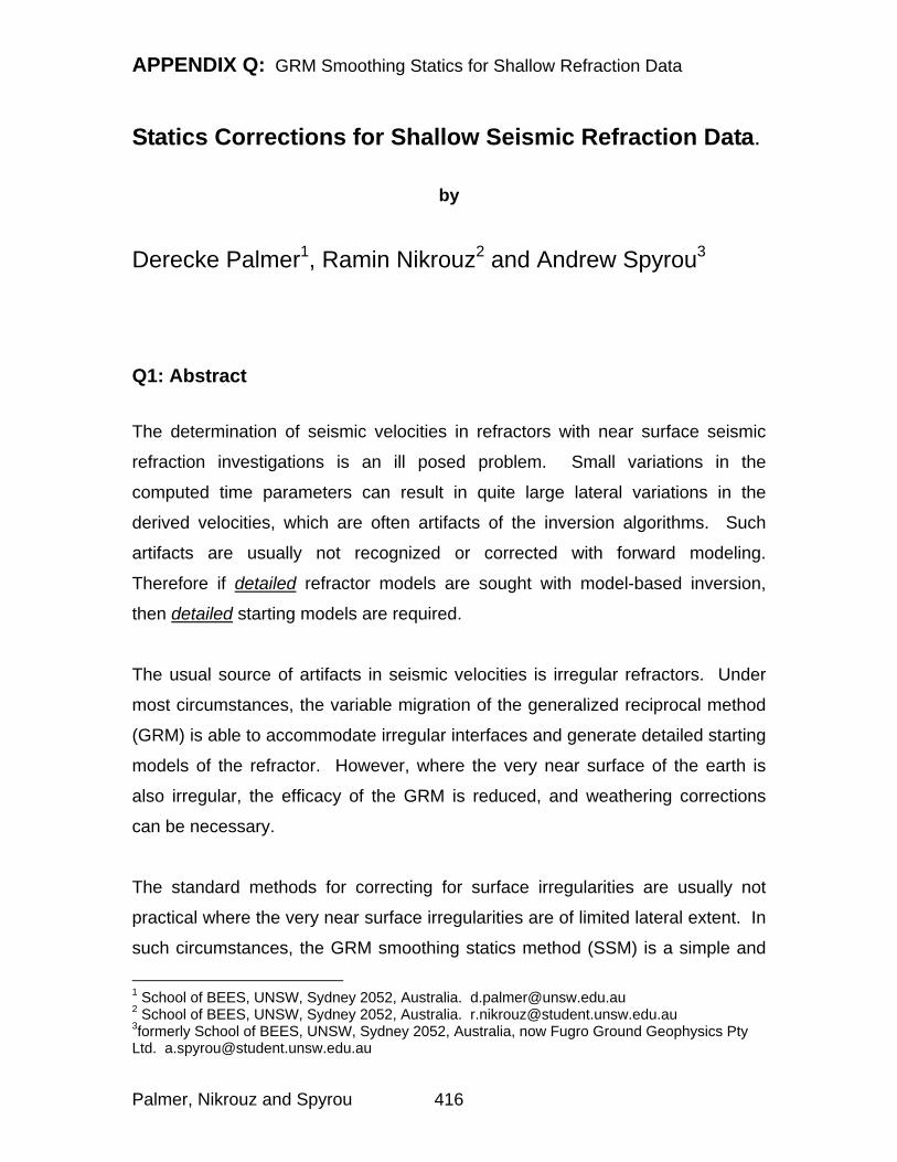
APPENDIX Q: GRM Smoothing Statics for Shallow Refraction Data
Statics Corrections for Shallow Seismic Refraction Data.
by
Derecke Palmer1, Ramin Nikrouz2 and Andrew Spyrou3
Q1: Abstract
The determination of seismic velocities in refractors with near surface seismic
refraction investigations is an ill posed problem. Small variations in the
computed time parameters can result in quite large lateral variations in the
derived velocities, which are often artifacts of the inversion algorithms. Such
artifacts are usually not recognized or corrected with forward modeling.
Therefore if detailed refractor models are sought with model-based inversion,
then detailed starting models are required.
The usual source of artifacts in seismic velocities is irregular refractors. Under
most circumstances, the variable migration of the generalized reciprocal method
(GRM) is able to accommodate irregular interfaces and generate detailed starting
models of the refractor. However, where the very near surface of the earth is
also irregular, the efficacy of the GRM is reduced, and weathering corrections
can be necessary.
The standard methods for correcting for surface irregularities are usually not
practical where the very near surface irregularities are of limited lateral extent. In
such circumstances, the GRM smoothing statics method (SSM) is a simple and
1 School of BEES, UNSW, Sydney 2052, Australia. [email protected] 2 School of BEES, UNSW, Sydney 2052, Australia. [email protected] 3formerly School of BEES, UNSW, Sydney 2052, Australia, now Fugro Ground Geophysics Pty Ltd. [email protected]
Palmer, Nikrouz and Spyrou 416
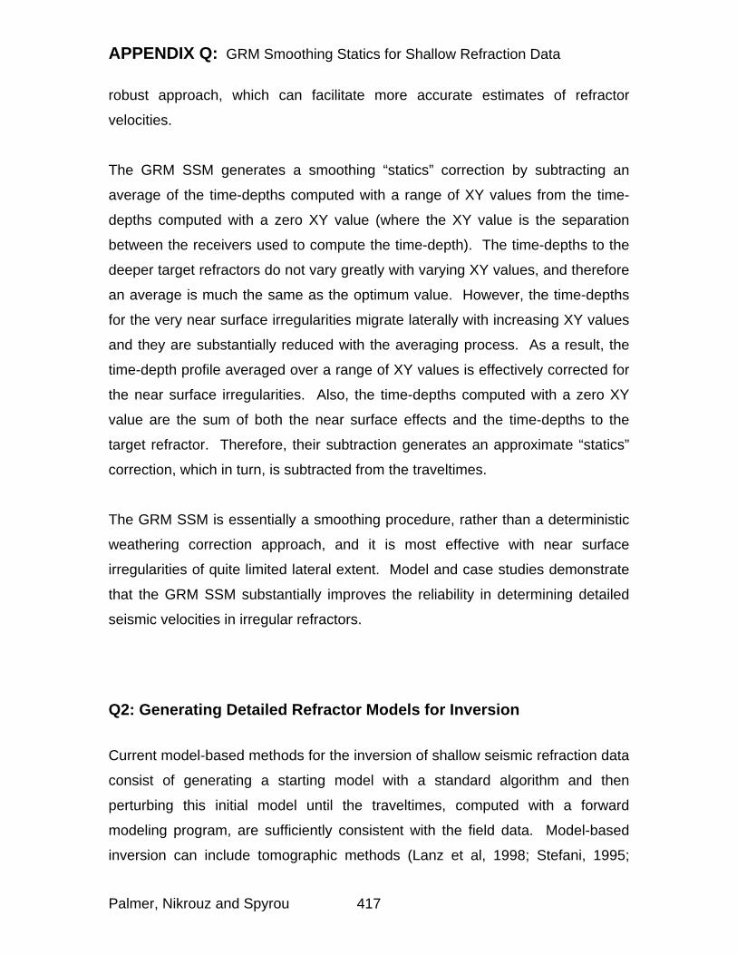
APPENDIX Q: GRM Smoothing Statics for Shallow Refraction Data
robust approach, which can facilitate more accurate estimates of refractor
velocities.
The GRM SSM generates a smoothing “statics” correction by subtracting an
average of the time-depths computed with a range of XY values from the time-
depths computed with a zero XY value (where the XY value is the separation
between the receivers used to compute the time-depth). The time-depths to the
deeper target refractors do not vary greatly with varying XY values, and therefore
an average is much the same as the optimum value. However, the time-depths
for the very near surface irregularities migrate laterally with increasing XY values
and they are substantially reduced with the averaging process. As a result, the
time-depth profile averaged over a range of XY values is effectively corrected for
the near surface irregularities. Also, the time-depths computed with a zero XY
value are the sum of both the near surface effects and the time-depths to the
target refractor. Therefore, their subtraction generates an approximate “statics”
correction, which in turn, is subtracted from the traveltimes.
The GRM SSM is essentially a smoothing procedure, rather than a deterministic
weathering correction approach, and it is most effective with near surface
irregularities of quite limited lateral extent. Model and case studies demonstrate
that the GRM SSM substantially improves the reliability in determining detailed
seismic velocities in irregular refractors.
Q2: Generating Detailed Refractor Models for Inversion
Current model-based methods for the inversion of shallow seismic refraction data
consist of generating a starting model with a standard algorithm and then
perturbing this initial model until the traveltimes, computed with a forward
modeling program, are sufficiently consistent with the field data. Model-based
inversion can include tomographic methods (Lanz et al, 1998; Stefani, 1995;
Palmer, Nikrouz and Spyrou 417
APPENDIX Q: GRM Smoothing Statics for Shallow Refraction Data
Zhang and Toksoz, 1998; Zhu et al, 1992), for which the entire process is
automated, as well as the more time-consuming interactive manual methods
(Whiteley, 2004).
While most approaches to model-based inversion can produce a result which is
consistent with the original field data, it is not uncommon for there to be
significant differences between the final results with different approaches. For
example, Palmer (2003) compares the results obtained with a tomographic
method in which two starting models are generated automatically with the one-
dimensional (1-D) tau-p algorithm, and manually with the two-dimensional
algorithms (2-D) of the generalized reciprocal method (GRM) (Palmer, 1980,
1981, 1986). Although both starting models are refined with the eikonal wave
equation (Schuster and Quintus-Bosz, 1993), the final results are quite different
in both the depths to the main refractor and in the lateral positioning of a low
velocity shear zone.
The differences in depths can be largely attributed to the use of linear velocity
gradients with the 1-D tau-p method, whereas constant overburden velocities
were used with the GRM. Although linear velocity functions are employed with
most tomographic approaches, there is very little petrophysical evidence to
support the parameterization of the near surface layers in this manner. In
general, most velocity gradients in the earth are relatively gentle, and as a result,
the penetration of the ray paths is rarely more than 30% of the layer thickness.
Because each layer is incompletely sampled, virtually any standard velocity
function can be fitted to traveltime data with acceptable accuracy (Hagedoorn,
1955; Palmer, 1986, p.169-175; 1992). Furthermore, hyperbolic velocity
functions can be readily fitted to traveltime graphs consisting of linear segments
(Slichter, 1932; Healy, 1963; Berry, 1971; Aki and Richards, 2002, p.422). Such
velocity functions can result in the computed depths being more than 70%
greater than would be the case if constant seismic velocities were fitted to the
Palmer, Nikrouz and Spyrou 418
APPENDIX Q: GRM Smoothing Statics for Shallow Refraction Data
same traveltime graphs. The issues related to the parameterization of the
overburden layers will not be considered further in this study.
The differences in the lateral positioning of the zone with the low seismic velocity
in the refractor are related primarily to the algorithm used to generate the starting
model, and it is the subject of this paper. This study addresses this issue in two
parts.
The first part seeks to show that the detailed lateral resolution of seismic
velocities in the refractor is an ill posed problem, that is, small variations in the
computed time parameters can result in large variations in the derived seismic
velocities. This problem can be especially acute with seismic refraction surveys
carried out for near surface targets, because the traveltime differences between
receivers, which are often separated by as little as 2.5 m, can be much the same
as the errors in measuring those traveltimes. The major conclusion of this part of
the study is that simplified algorithms for computing seismic velocities in the
refractor can generate artifacts, which are not necessarily recognized nor
corrected with most approaches to model-based inversion. Therefore, if detailed
lateral variations in refractor velocities are the objective, then algorithms, which
can generate detailed starting models, are required, so that the inversion process
can converge to a most likely model.
Frequently, irregular refracting interfaces are the major source of artifacts in the
initial refractor model. Model and case studies (Palmer, 1980, 1981, 1986, 1991)
demonstrate that the GRM is usually able to determine useful refractor
parameters with irregular interfaces.
However, the effectiveness of the GRM algorithms can often be reduced where
there are irregularities in the very near surface layers (Palmer, 1980, p.22-24). In
many cases, these irregularities can be defined and corrected with standard
methods (Dobrin, 1976, p. 334-336; Palmer, 1986, p.152-155), using traveltimes
Palmer, Nikrouz and Spyrou 419
APPENDIX Q: GRM Smoothing Statics for Shallow Refraction Data
obtained with intermediate shot-to-receiver spacings. Unfortunately, this
approach is not efficacious where the near surface irregularities extend over very
limited lateral distances, because they cannot be mapped directly with reversed
traveltime data. As a result, neither their seismic velocities nor their thickness
can be computed with the standard approach. Furthermore, the methods
normally employed for the acquisition of common midpoint reflection data, such
as the use of extended receiver arrays and extended surface source arrays,
usually do not generate traveltime data of sufficient quality from the surface
layers. Accordingly, another method is required to correct for the very near
surface irregularities.
The second and major part of this study presents a new method for
accommodating the very near surface irregularities or “statics”, in order to
generate more accurate starting models of the refractor velocities. It is based on
the GRM, it uses traveltimes from a deeper refractor, and it is termed the GRM
smoothing statics method (GRM SSM).
The significance of the near surface irregularities has been highlighted with a
recent three-dimensional (3D) shallow refraction survey carried over a major
shear zone associated with dryland salinity at Spicers Creek, near Dubbo in
southeastern Australia (Nikouz, Spyrou and Palmer, in prep). While the GRM
velocity analysis algorithm was able to generate useful starting models for
inversion for each line, the consistency between adjacent parallel lines, which
were separated by 10 m, was not always obvious. As discussed within this
study, relatively small variations in the refractor velocity analysis algorithm
resulted in significant changes in both the computed values of the seismic
velocities as well as their lateral extent. The use of the GRM SSM described
herein, was a major factor in achieving improved consistency between adjacent
lines, and in turn, with improving the spatial resolution of the shallow seismic
refraction results.
Palmer, Nikrouz and Spyrou 420
APPENDIX Q: GRM Smoothing Statics for Shallow Refraction Data
However, even routine 2D refraction investigations can benefit significantly from
the application of the GRM SSM. The case study describes a single seismic
refraction profile recorded across a narrow massive sulphide orebody at Mt Bulga
in southeastern Australia. This survey was carried out to test whether a density
model could be derived from the head wave amplitudes. As it was anticipated
that there would be an unambiguous increase in density associated with the
mineralization, any variations in head wave amplitudes would provide a first step
in assessing the feasibility of the concept.
The determination of in-situ density models with shallow seismic refraction
methods could prove useful for the detailed inversion of gravity data, such as that
obtained with high resolution airborne gravity gradiometers. Furthermore, the
determination of densities together with seismic velocities could facilitate the
computation of bulk in-situ elastic constants for geotechnical studies.
The theoretical basis for the derivation of in-situ densities from head wave
amplitudes is relatively straightforward. Palmer (2001a) demonstrates that the
product of the forward and reverse head wave amplitudes compensates for
geometric spreading and that the result is proportional to the head coefficient.
(The head coefficient is analogous to the transmission coefficient of the Zoeppritz
equations and it describes the head wave amplitude in terms of the petrophysical
properties in the two media.) Furthermore, Palmer (2001b) shows that the head
coefficient is proportional to the ratio of the specific acoustic impedances, which
is the product of the seismic velocities and densities, in the overburden and the
refractor. Therefore, if the detailed lateral variations in the refractor velocities can
be resolved with the traveltime data, then the possibility exists for the derivation
of a model of the lateral variations in the bulk in-situ densities from the amplitude
data.
The irregular near surface conditions at the Mt Bulga site generated numerous
traveltime anomalies, which were a limiting factor in unambiguously determining
Palmer, Nikrouz and Spyrou 421
APPENDIX Q: GRM Smoothing Statics for Shallow Refraction Data
the seismic velocities in the main refractor. As a result, the uncertainties in the
seismic velocities limited the accuracies in deriving estimates for the in-situ
densities from the head wave amplitudes.
Q3: Non-Uniqueness in Determining Detailed Refractor Velocities
That the determination of the seismic velocities in the refractor is an ill posed
problem can be readily demonstrated with the simple model in Figure 1. It
consists of a small irregularity in an otherwise uniform refractor. All of the first
arrival traveltimes associated with the irregularity are diffractions. The station
interval is 5 m.
The inversion algorithms of the conventional reciprocal method (Hagiwara and
Omote, 1939; Hagedoorn, 1959; Hawkins, 1961) provide one of the simplest
approaches to deriving a starting model (Whiteley, 2004). The first task is to
determine the seismic velocity in the refractor through the differencing of the
forward and reverse traveltimes with equation (1), namely
( )2
reciprocalreverseforwardV
tttt +−= (1)
The values computed with equation (1) are shown in Figure 2. The seismic
velocity in the refractor Vn, is the reciprocal of the gradient, as in equation (2).
n
VVdx
td 1= (2)
Although the application of equation (1) is quite straightforward, the
determination of the refractor velocity(s) with equation (2) is subject to
considerable personal judgment. Figure 2 shows that the computed values are
Palmer, Nikrouz and Spyrou 422
APPENDIX Q: GRM Smoothing Statics for Shallow Refraction Data
strongly linearly correlated, and that a single line, representative of a seismic
velocity of 5220 m/s can be fitted with an accuracy of better than one millisecond.
However, the vast majority of geoscientists would fit three segments with seismic
velocities of 4210 m/s, 7250 m/s and 4210 m/s, as is shown in Figure 2, simply
because the much improved visual fit results in residuals which are essentially
zero. The change in seismic velocities from 4210 m/s to 7250 m/s, representing
an increase of 72%, is very large and for that reason alone, it would normally be
accepted as a genuine lateral variation. Furthermore, such a large increase in
seismic velocities would have important implications in most shallow seismic
investigations. Nevertheless, the lateral variations in the refractor velocities are
artifacts of the inversion algorithm.
This example demonstrates some of the deficiencies with the conventional
reciprocal method and most importantly, the fact that the determination of
refractor velocities is an ill posed problem: small variations in the refractor
velocity analysis function can result in major changes in the computed seismic
velocities. In Figure 2, variations of approximately one millisecond in the velocity
analysis function can lead to the inference of lateral variations, which differ from
the true refractor velocity of 5000 m/s by 16% and 45%. Furthermore, it is not
possible to infer whether even large lateral variations in the refractor velocities,
are genuine or whether they are artifacts of the velocity analysis algorithm of the
conventional reciprocal method, because there are no accepted objective criteria
for distinguishing either.
Figure 3 shows the time-depths generated using equation (3) with XY values of
zero, which is the conventional reciprocal method, and 40 m, which is
approximately the optimum value. (The time-depth is mathematically equivalent
to the half intercept time or the mean delay time, and it is a measure of the depth
to the refractor in units of time.) The XY distance, which is the separation
between the reverse and forward traveltimes, seeks to accommodate the offset
Palmer, Nikrouz and Spyrou 423
APPENDIX Q: GRM Smoothing Statics for Shallow Refraction Data
distance, which the horizontal separation between the point of refraction on the
interface and the point of measurement on the surface.
2⎟⎠⎞⎜
⎝⎛ −−+
= nreciprocalreverseforward
GV
XYtttt (3)
The time-depths computed with a zero XY value show two regions approximately
45 m wide on either side of station 12, for which the values are smaller due to the
irregularity in the refractor. Furthermore, the minimum time-depths occur at
stations 8 and 16 with a zero XY value rather than at station 12, which is the
apex of the irregularity in the refractor.
Figure 4 shows the depth section computed with a zero XY value, that is, with the
conventional reciprocal method. The depths are computed with equation (4),
where,
DCFtVV
VVtZ
G
n
nGG
=
−=
21
21
(4)
where DCF is the depth conversion factor and,
nn
nn
n
VVi
and
iV
VVVVDCF
11
1
12
12
1
sin
cos
=
=−
=
(5)
Figure 4 demonstrates that the conventional reciprocal method has done a barely
adequate job in reproducing the model. There are errors in depths, related both
to refractor velocity “pull-ups” and “pull-downs” and to the unfocussed time-
Palmer, Nikrouz and Spyrou 424
APPENDIX Q: GRM Smoothing Statics for Shallow Refraction Data
depths on either side of station 12. Although, the decrease in depths in the
vicinity of station 12 can still be recognized, the apex is now reproduced as a 20
m wide region. Furthermore, its correlation with the increase in refractor
velocities gives it geologic verisimilitude, and therefore under most
circumstances, the depth cross-section would be considered acceptable.
Forward modeling of Figure 5, which is derived from Figure 4, with the eikonal
wave equation (Schuster and Quintus-Bosz, 1993), produces a mean unsigned
error of 0.894 ms, and a relative misfit function of 0.554 ms (Schuster and
Quintus-Bosz, 1993, p. 1315). Therefore, when the conventional reciprocal
method is applied objectively without editing for which there are no clearly
defined criteria, the depth cross sections shown in Figures 4 and 5 would be the
most likely result. Clearly, forward modeling neither recognizes nor corrects the
artifacts in the refractor velocities.
Figure 6 shows the depth cross-section derived from 1D inversion using the tau-p
algorithm and linear velocity gradients. Forward modeling with the eikonal wave
equation (Schuster and Quintus-Bosz, 1993), produces a mean unsigned error of
0.388 ms, and a relative misfit function of 0.230 ms (Schuster and Quintus-Bosz,
1993, p. 1315). The depths to the 5000 m/s contour are approximately 85 m,
which is an error of 70%, while the refractor irregularity at station 12 occurs over
approximately 60 m between stations 6 and 18.
A GRM analysis of the model in Figure 2 (Palmer, 1986, p 111-117) produces the
result shown in Figure 7. The computed refractor velocity is 5100 m/s, for an
error of 2%. Figure 7 demonstrates that the GRM both accommodates
diffractions associated with the refractor irregularity and only images those parts
of the refractor from which first arrival energy is received. As a corollary, this
study shows that an important consequence of the occurrence of diffractions with
irregular refractors is that they result in an incomplete definition of the interface
(Palmer, 1980, p.29; 1986, p.117; Sjogren, 1984, p.84-95). Only those parts of
Palmer, Nikrouz and Spyrou 425
APPENDIX Q: GRM Smoothing Statics for Shallow Refraction Data
the interface are defined where the radius of curvature is greater than the layer
thickness, and as a result, a smoothed version of refractor is obtained.
Therefore, the use of ray tracing routines which rigorously apply Snell’s law, such
as the modified Ackermann version (Ackermann et al, 1986) employed by Leung
(1997, 2003) and (Whiteley, 2004), can be inappropriate with irregular interfaces,
because the true position and in turn, the true dips of the interface are not known.
Forward modeling routines, which can accommodate diffractions, such as
wavefront reconstruction (Schuster and Quintus-Bosz, 1993) can be a more
useful alternative approach. Forward modeling of Figure 7 with the eikonal wave
equation produces the depth cross section in Figure 8, with a mean unsigned
error of 0.769 ms, and a relative misfit function of 0.420 ms (Schuster and
Quintus-Bosz, 1993, p. 1315).
These results demonstrate that it is possible to obtain satisfactory agreement
with the traveltime data for a range of starting models. Therefore, while
agreement with the traveltime data can demonstrate that any particular model is
acceptable, it does not demonstrate that the model is either “correct” or unique.
Non-uniqueness has yet to be adequately addressed in the inversion of shallow
seismic refraction data. Perhaps one of the more useful statements of non-
uniqueness, which alludes to the importance of the algorithm used to generate
the starting model, is the following paragraph from Oldenburg (1984, p666).
“For many investigators the primary goal of inverse theory is to generate a
model which reproduces the observations. The structure observed on m(z)
(Oldenburg’s model parameters) may be interpreted directly, or m(z) may
be the input to further modeling. A fundamental problem, however, is that
m(z) is a function on the Hilbert space H[0,a] (Oldenburg defines the model
over the interval [0,a]), and consequently there will be infinitely many
functions in that space which can reproduce a finite number of
observations. This non-uniqueness becomes more severe when the data
Palmer, Nikrouz and Spyrou 426

APPENDIX Q: GRM Smoothing Statics for Shallow Refraction Data
are inaccurate and when models which do not fit the data precisely are
considered acceptable. Loosely speaking, a particular algorithm generates
a particular type of model. This, coupled with the non-uniqueness of the
solution, suggests that a good approach to the construction problem is to
design a number of different algorithms which can reproduce a variety of
acceptable models. Not only will such an approach provide valuable insight
regarding non-uniqueness but some models which are judged to be more
likely from a physical basis (or personal prejudice) may be selected as best
“guesses” to the true model.”
Not only is Oldenburg stating that non-uniqueness is an essential aspect of
model-based inversion (see also Treitel and Lines, 1988) but he is also stating
that the generation of a multiplicity of models is to be encouraged. The GRM can
generate such a multiplicity of models, simply by employing different XY values.
Each of these models agrees with the traveltime data (Palmer, 1980, p.50;
Palmer, 1986, p. 156-162). Furthermore, the minimum variance criterion of the
GRM facilitates the recognition of a most likely starting model.
Q4: “Statics” Corrections for Shallow Refraction Data – Model Study
The new method for correcting for near surface irregularities, the GRM SSM, will
be demonstrated with the model shown in Figure 9, which is taken from Palmer
(1980, Fig.14). This model, which is rather extreme with both an irregular
refractor, as well as irregular topography, has a lateral change in the seismic
velocity in the refractor.
The first step is to generate the refractor velocity analysis function for a range of
XY values from less than to greater than the optimum XY value with equation (1).
The results are shown in Figure 10. The graphs for individual XY values have
Palmer, Nikrouz and Spyrou 427
APPENDIX Q: GRM Smoothing Statics for Shallow Refraction Data
been separated for clarity by adding a constant value, which is readily achieved
by systematically increasing the reciprocal time for each XY value.
The graphs are irregular because both the refractor and the topography are
irregular. Palmer (1980, Fig. 6) shows that, for an irregular refractor and flat
topography, the velocity analysis graphs are essentially symmetrical about that
computed with a 20 m XY value, while the graphs are symmetrical about the set
computed with a zero XY value for a flat refractor and irregular topography
(Palmer, 1980, Fig. 11). The graphs in Figure 10 exhibit no clear symmetry
about any particular XY value because of these two separate competing effects.
The aim of the GRM SSM is to minimize the effects of the near surface
irregularities, so that the symmetry of the velocity analysis graphs about an
optimum value, which is representative of the target refractor, can be more easily
recognized.
An average for XY values from zero to 30 m has been computed, and is also
shown in Figure 10. Although this average is not as irregular as the graphs
computed with individual XY values, there are still a number of changes in slope
to which the detailed application of equation (2) would result in the generation of
artifacts in the refractor velocities.
The second step is to compute time-depths with equation (3). The results are
shown in Figure 11. The term XY / Vn is approximated with the difference in the
averaged velocity analysis function over the same interval, ie
XY / Vn = averaged velocity analysis function at Y
- averaged velocity analysis function at X (6)
Where the surface topography is flat, there are usually relatively small
differences in the time-depths computed with different XY values for an irregular
refractor (Palmer, 1980, Fig. 7). (As an aside, the differences are much the
Palmer, Nikrouz and Spyrou 428
APPENDIX Q: GRM Smoothing Statics for Shallow Refraction Data
same as those differences obtained with the refractor velocity analysis function
(Palmer, 1980, Fig. 6). While these differences can result in the computation of a
wide range of seismic velocities in the refractor with equation (2), they are not as
critical with the time-depths.)
However, the time-depth anomalies associated with the irregular surface
topography propagate laterally throughout the time-depths as the XY value is
varied (Palmer, 1986, p.107-111). For example, suppose that there is a single
near surface irregularity, which results in coincident anomalies on the forward
and reverse traveltime graphs. For a zero XY value, the time-depths will exhibit
an anomaly equal to that in the traveltime graphs. As the XY value is increased,
the coincidence between the forward and reverse traveltime graphs is lost, and
two time-depth anomalies, half the traveltime anomaly and separated by the XY
distance, are generated. The pattern of the lateral migration of the surface
anomalies can be recognized with the escarpment features at 130 m and 250 m
in Figure 11, and with the anomaly centred on station 56 in Figure 18.
The third step is the generation of the “statics” corrections by subtracting the
time-depths averaged over a range of XY values from the time-depths computed
with a zero XY value. When an average of the time-depths is computed, the loss
in resolution of the refracting interface is relatively minor. However, the
anomalies due to the near surface irregularities are greatly reduced through the
averaging process, because they systematically propagate laterally with
increasing XY values. Therefore, to a reasonable first approximation, the
averaged time-depth profile represents the values for the target refractor, which
has been partially corrected for the near surface irregularities. Furthermore, the
time-depth profile computed with a zero XY value represents the sum of the time-
depths for both the near surface irregularities and the target refractor. Therefore,
the difference between the time-depths computed with a zero XY value and the
time-depths averaged over a range of XY values generates the smoothed
anomalies due to the near surface irregularities. These anomalies are then
Palmer, Nikrouz and Spyrou 429
APPENDIX Q: GRM Smoothing Statics for Shallow Refraction Data
subtracted from the traveltime data, and the computation of the velocity analysis
graphs and the time-depths is repeated.
The corrections computed with this procedure show very little correlation with the
surface topography. Accordingly, they represent more of a smoothing process,
rather than a deterministic weathering correction procedure (Dobrin, 1976, p.
334-336; Palmer, 1986, p.152-155). This is also supported by the fact that, for
the maximum elevation changes of ±5 m in Figure 9, the maximum statics would
be approximately 3 ms (5 m / 1500 m/s), whereas the maximum correction
computed with the GRM SSM is 0.97 ms, the average is 0.01 ms and the
standard deviation is 0.40 ms.
Figures 12 and 13 show the refractor velocity analysis and the time-depth
functions after one application of the GRM SSM. There is a clear improvement in
the symmetry of the refractor velocity analysis graphs about the graph for 15 m
XY value. Also, the time-depths exhibit considerably less variation.
While the GRM SSM has significantly reduced the artifacts related to the
topographic irregularities, the compensation is not complete. It has been found
that several iterations of the GRM SSM can produce systematic improvements in
the symmetry of velocity analysis graphs about an optimum, and that there is a
systematic reduction in refractor velocity artifacts as a result.
Furthermore and contrary to normal expectations, the method appears to work
much better with normal field data, than with model data, as will be demonstrated
in the case study to follow. In such cases, one application of the GRM SSM has
usually proven to be sufficient.
Palmer, Nikrouz and Spyrou 430
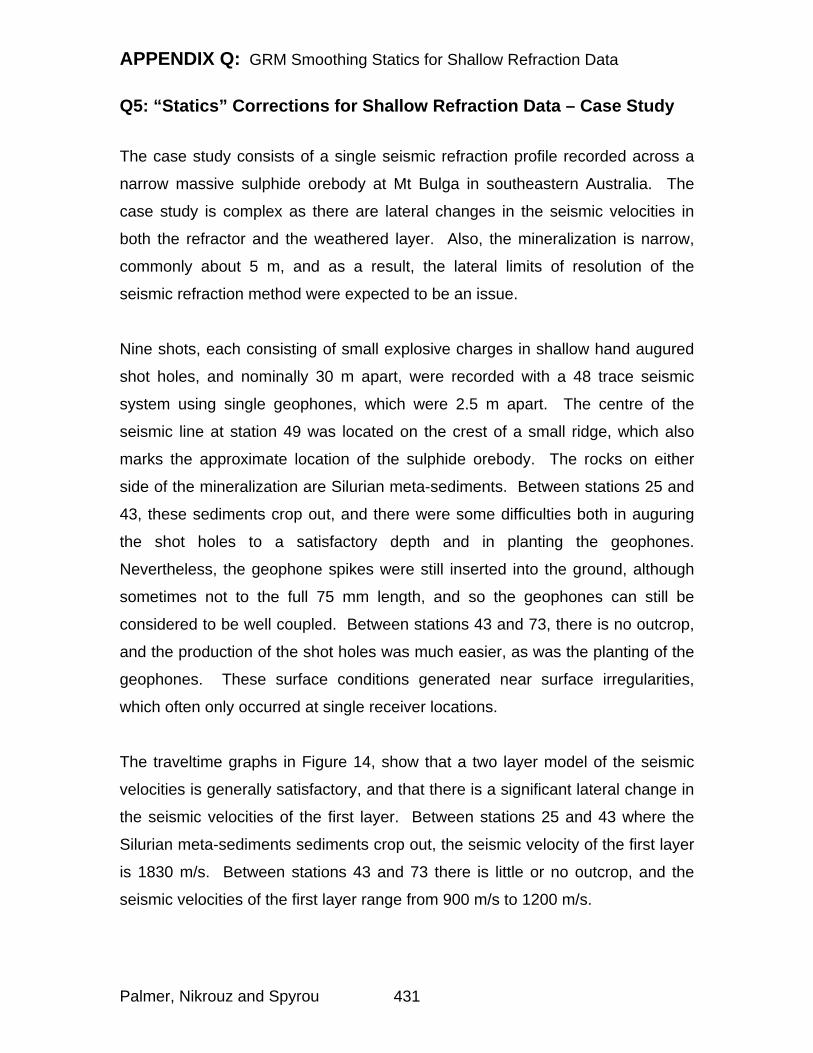
APPENDIX Q: GRM Smoothing Statics for Shallow Refraction Data
Q5: “Statics” Corrections for Shallow Refraction Data – Case Study
The case study consists of a single seismic refraction profile recorded across a
narrow massive sulphide orebody at Mt Bulga in southeastern Australia. The
case study is complex as there are lateral changes in the seismic velocities in
both the refractor and the weathered layer. Also, the mineralization is narrow,
commonly about 5 m, and as a result, the lateral limits of resolution of the
seismic refraction method were expected to be an issue.
Nine shots, each consisting of small explosive charges in shallow hand augured
shot holes, and nominally 30 m apart, were recorded with a 48 trace seismic
system using single geophones, which were 2.5 m apart. The centre of the
seismic line at station 49 was located on the crest of a small ridge, which also
marks the approximate location of the sulphide orebody. The rocks on either
side of the mineralization are Silurian meta-sediments. Between stations 25 and
43, these sediments crop out, and there were some difficulties both in auguring
the shot holes to a satisfactory depth and in planting the geophones.
Nevertheless, the geophone spikes were still inserted into the ground, although
sometimes not to the full 75 mm length, and so the geophones can still be
considered to be well coupled. Between stations 43 and 73, there is no outcrop,
and the production of the shot holes was much easier, as was the planting of the
geophones. These surface conditions generated near surface irregularities,
which often only occurred at single receiver locations.
The traveltime graphs in Figure 14, show that a two layer model of the seismic
velocities is generally satisfactory, and that there is a significant lateral change in
the seismic velocities of the first layer. Between stations 25 and 43 where the
Silurian meta-sediments sediments crop out, the seismic velocity of the first layer
is 1830 m/s. Between stations 43 and 73 there is little or no outcrop, and the
seismic velocities of the first layer range from 900 m/s to 1200 m/s.
Palmer, Nikrouz and Spyrou 431
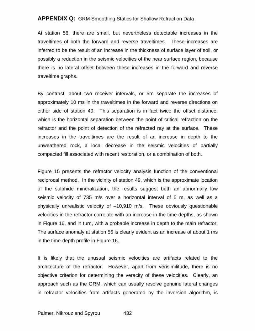
APPENDIX Q: GRM Smoothing Statics for Shallow Refraction Data
At station 56, there are small, but nevertheless detectable increases in the
traveltimes of both the forward and reverse traveltimes. These increases are
inferred to be the result of an increase in the thickness of surface layer of soil, or
possibly a reduction in the seismic velocities of the near surface region, because
there is no lateral offset between these increases in the forward and reverse
traveltime graphs.
By contrast, about two receiver intervals, or 5m separate the increases of
approximately 10 ms in the traveltimes in the forward and reverse directions on
either side of station 49. This separation is in fact twice the offset distance,
which is the horizontal separation between the point of critical refraction on the
refractor and the point of detection of the refracted ray at the surface. These
increases in the traveltimes are the result of an increase in depth to the
unweathered rock, a local decrease in the seismic velocities of partially
compacted fill associated with recent restoration, or a combination of both.
Figure 15 presents the refractor velocity analysis function of the conventional
reciprocal method. In the vicinity of station 49, which is the approximate location
of the sulphide mineralization, the results suggest both an abnormally low
seismic velocity of 735 m/s over a horizontal interval of 5 m, as well as a
physically unrealistic velocity of –10,910 m/s. These obviously questionable
velocities in the refractor correlate with an increase in the time-depths, as shown
in Figure 16, and in turn, with a probable increase in depth to the main refractor.
The surface anomaly at station 56 is clearly evident as an increase of about 1 ms
in the time-depth profile in Figure 16.
It is likely that the unusual seismic velocities are artifacts related to the
architecture of the refractor. However, apart from verisimilitude, there is no
objective criterion for determining the veracity of these velocities. Clearly, an
approach such as the GRM, which can usually resolve genuine lateral changes
in refractor velocities from artifacts generated by the inversion algorithm, is
Palmer, Nikrouz and Spyrou 432

APPENDIX Q: GRM Smoothing Statics for Shallow Refraction Data
required. Figure 17 presents the GRM refractor velocity analysis algorithm for
XY values from –2.5 m to 10 m.
While there is probably limited geophysical significance for negative XY values,
the computed graphs can facilitate the definition of the symmetrical pattern about
the optimum XY value, especially where the optimum is much the same value as
the receiver spacing. Furthermore, these graphs can be very useful where the
averaging of several sets of graphs, which are symmetrical about the optimum,
are employed to reduce the effects of artifacts caused by refractor architecture.
The velocity analysis graphs exhibit the familiar symmetry about the optimum XY
value, which in this case appears to be between 2.5 m and 5 m. An average of
the graphs, which are symmetrical about the optimum, that is, for XY values
between –2.5 m and 10 m, greatly minimizes the artifacts due to the refractor
architecture.
The results in Figure 17 indicate that there is a narrow region between stations
48 and 49 where the seismic velocity in the refractor is quite high. However, this
region also appears to exhibit the same signature due to a surface anomaly, as
that at station 56 (see also Palmer, 1986, Figure 8-9). The coincidence of the
possible near surface irregularity, probably caused by the recent restoration of
the site, with the large increase in time-depths in the refractor introduces some
uncertainty in the detailed resolution of the refractor velocities.
Figure 18 shows the time-depths computed for a range of XY values from zero to
10 m, together with the average of these values. Several near surface
irregularities, such as that at station 56, can be recognized by their lateral
migration through the time-depths with increasing XY distances. The average of
the time-depths has removed the time anomalies associated with these near
surface irregularities, but nevertheless, it has still largely preserved the
architecture of the refractor.
Palmer, Nikrouz and Spyrou 433
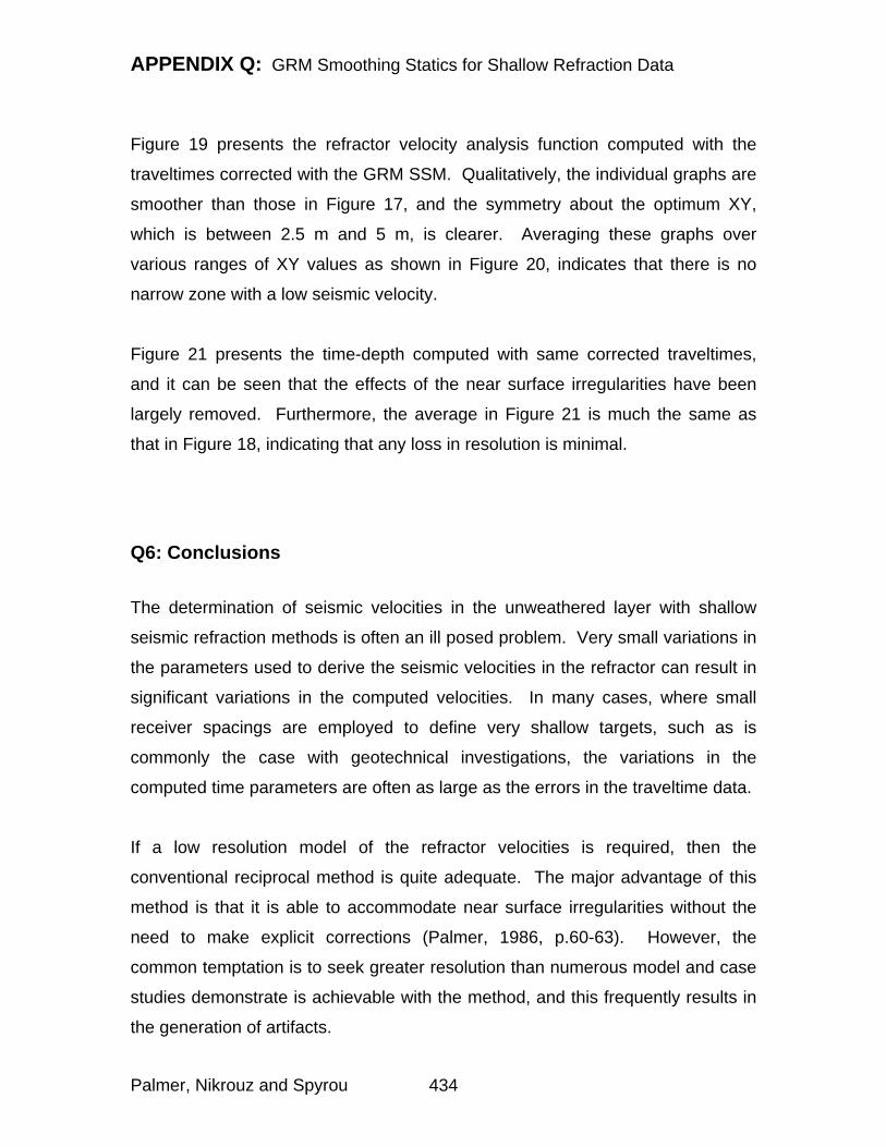
APPENDIX Q: GRM Smoothing Statics for Shallow Refraction Data
Figure 19 presents the refractor velocity analysis function computed with the
traveltimes corrected with the GRM SSM. Qualitatively, the individual graphs are
smoother than those in Figure 17, and the symmetry about the optimum XY,
which is between 2.5 m and 5 m, is clearer. Averaging these graphs over
various ranges of XY values as shown in Figure 20, indicates that there is no
narrow zone with a low seismic velocity.
Figure 21 presents the time-depth computed with same corrected traveltimes,
and it can be seen that the effects of the near surface irregularities have been
largely removed. Furthermore, the average in Figure 21 is much the same as
that in Figure 18, indicating that any loss in resolution is minimal.
Q6: Conclusions
The determination of seismic velocities in the unweathered layer with shallow
seismic refraction methods is often an ill posed problem. Very small variations in
the parameters used to derive the seismic velocities in the refractor can result in
significant variations in the computed velocities. In many cases, where small
receiver spacings are employed to define very shallow targets, such as is
commonly the case with geotechnical investigations, the variations in the
computed time parameters are often as large as the errors in the traveltime data.
If a low resolution model of the refractor velocities is required, then the
conventional reciprocal method is quite adequate. The major advantage of this
method is that it is able to accommodate near surface irregularities without the
need to make explicit corrections (Palmer, 1986, p.60-63). However, the
common temptation is to seek greater resolution than numerous model and case
studies demonstrate is achievable with the method, and this frequently results in
the generation of artifacts.
Palmer, Nikrouz and Spyrou 434
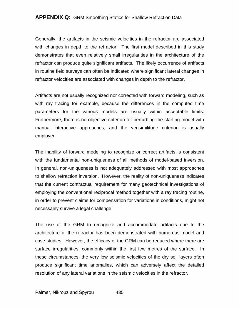
APPENDIX Q: GRM Smoothing Statics for Shallow Refraction Data
Generally, the artifacts in the seismic velocities in the refractor are associated
with changes in depth to the refractor. The first model described in this study
demonstrates that even relatively small irregularities in the architecture of the
refractor can produce quite significant artifacts. The likely occurrence of artifacts
in routine field surveys can often be indicated where significant lateral changes in
refractor velocities are associated with changes in depth to the refractor.
Artifacts are not usually recognized nor corrected with forward modeling, such as
with ray tracing for example, because the differences in the computed time
parameters for the various models are usually within acceptable limits.
Furthermore, there is no objective criterion for perturbing the starting model with
manual interactive approaches, and the verisimilitude criterion is usually
employed.
The inability of forward modeling to recognize or correct artifacts is consistent
with the fundamental non-uniqueness of all methods of model-based inversion.
In general, non-uniqueness is not adequately addressed with most approaches
to shallow refraction inversion. However, the reality of non-uniqueness indicates
that the current contractual requirement for many geotechnical investigations of
employing the conventional reciprocal method together with a ray tracing routine,
in order to prevent claims for compensation for variations in conditions, might not
necessarily survive a legal challenge.
The use of the GRM to recognize and accommodate artifacts due to the
architecture of the refractor has been demonstrated with numerous model and
case studies. However, the efficacy of the GRM can be reduced where there are
surface irregularities, commonly within the first few metres of the surface. In
these circumstances, the very low seismic velocities of the dry soil layers often
produce significant time anomalies, which can adversely affect the detailed
resolution of any lateral variations in the seismic velocities in the refractor.
Palmer, Nikrouz and Spyrou 435
APPENDIX Q: GRM Smoothing Statics for Shallow Refraction Data
In many cases, the near surface layers are sufficiently thick and of sufficient
lateral extent to be adequately mapped with the standard methods using
traveltime data recorded with intermediate shot-to-receiver offsets. However,
these methods are not applicable where the near surface irregularities extend
over only a few receiver stations at most. Under those conditions, an alternative
approach is required.
The GRM SSM is a simple but robust method to compensate for near surface
irregularities, which uses the traveltimes from a deeper refractor, usually the
target refractor. It is based on the fact that the time-depths for an irregular
refractor do not alter substantially with varying XY distances, whereas the time-
depths for a near surface irregularity propagate laterally with increasing XY
values. An average of the time-depths over a range of XY values generates a
profile of the refractor which is very similar to that obtained with the optimum XY
value. However, the time-depths for the near surface irregularities are reduced
through the averaging process. Therefore when the averaged time-depth profile
is subtracted from that computed with a zero XY value, the result is a correction
for the near surface “statics”.
The application of these “static” corrections to the traveltime data usually
produces velocity analysis graphs which exhibit better symmetry about the
optimum XY value, and which therefore facilitate more reliable estimations of the
seismic velocities in the refractor. However, the “statics” corrections are usually
less than a millisecond and therefore, they do not substantially alter the average
time-depth profile of the target refractor.
The GRM SSM is a smoothing operation, rather than a deterministic static
correction. Experience to date suggests that the method is most effective with
near surface irregularities which are of limited lateral extent and which are not
adequately defined with traveltimes from intermediate shot-to-receiver distances.
Palmer, Nikrouz and Spyrou 436
APPENDIX Q: GRM Smoothing Statics for Shallow Refraction Data
Furthermore, the GRM SSM appears to correct minor errors in picking
traveltimes due to variations in signal-to-noise ratios.
As might be anticipated, near surface irregularities also generate amplitude
anomalies, in addition to time anomalies (Palmer, 2001c). A companion paper
(Palmer, in prep) describes an analogous process of correcting for the amplitude
anomalies, using the geometric mean, in order to facilitate detailed inversion of
the head wave amplitudes.
As with the GRM, the computations for the GRM SSM are simple arithmetic
operations, which are readily implemented with any spreadsheet. Therefore, it is
a relatively straightforward task to include both of these methods into any stream
for the routine processing of shallow refraction data, in order to generate detailed
starting models for further modeling with either tomographic methods or
interactive manual methods of model-based inversion.
The application of the GRM and the GRM SSM can result is a significant
improvement in the detailed lateral resolution of seismic velocities within the
refractor. Equivalent resolution is not as easily achieved with model-based
inversion methods, which employ simple algorithms to generate starting models.
Q7: References
Ackermann, H. D., Pankratz, L. W., and Dansereau, D., 1986, Resolution of
ambiguities of seismic traveltime curves: Geophysics 51, 223-235.
Aki, K., and Richards, P. G., 2002, Quantitative Seismology: University Science
Books.
Palmer, Nikrouz and Spyrou 437

APPENDIX Q: GRM Smoothing Statics for Shallow Refraction Data
Berry, M. J., 1971, Depth uncertainties from seismic first arrival studies: Journal
of Geophysical Research 76, 6464-6468.
Dobrin M. B. 1976, Introduction To Geophysical Prospecting, 3rd edn: McGraw-
Hill Inc.
Hagedoorn, J. G., 1955, Templates for fitting smooth velocity functions to seismic
refraction and reflection data: Geophysical Prospecting 3, 325-338.
Hagedoorn, J G, 1959, The plus-minus method of interpreting seismic refraction
sections: Geophysical Prospecting 7, 158-182.
Hagiwara, T, and Omote, S, 1939, Land creep at Mt Tyausu-Yama
(Determination of slip plane by seismic prospecting): Tokyo University
Earthquake Research Institute Bulletin, 17 118-137.
Hawkins, L. V., 1961, The reciprocal method of routine shallow seismic refraction
investigations: Geophysics 26, 806-819.
Healy, J. H., 1963, Crustal structure along the coast of California from seismic-
refraction measurements: Journal of Geophysical Research 68, 5777-5787.
Lanz E., Maurer H. and Green A. G. 1998, Refraction tomography over a buried
waste disposal site: Geophysics 63, 1414-1433.
Leung, T. K., 1997, Evaluation of seismic refraction interpretation using first
arrival ray tracing, in McCann, D. M., Eddleston, M., Fleming, P. J., and Reeves,
G. M., eds., Modern geophysics in engineering geology: The Geological Society,
391-398.
Palmer, Nikrouz and Spyrou 438
APPENDIX Q: GRM Smoothing Statics for Shallow Refraction Data
Leung, T. K., 2003, Controls of traveltime data and problems of the generalized
reciprocal method: Geophysics 68, 1626-1632.
Nikrouz, R., Spyrou, A., and Palmer, D., Three dimensional (3D) three
component (3C) shallow seismic refraction surveys across a shear zone
associated with dryland salinity: in prep.
Oldenburg, D. W., 1984, An introduction to linear inverse theory: Trans IEEE
Geoscience and Remote Sensing GE-22(6), 666.
Palmer D. 1980, The Generalized Reciprocal Method Of Seismic Refraction
Interpretation: Society of Exploration Geophysicists, Tulsa, OK.
Palmer, D., 1981, An introduction to the generalized reciprocal method of seismic
refraction interpretation: Geophysics 46, 1508-1518.
Palmer D. 1986, Refraction Seismics: The Lateral Resolution of Structure and
Seismic Velocity: Geophysical Press.
Palmer, D., 1991, The resolution of narrow low-velocity zones with the
generalized reciprocal method: Geophysical Prospecting 39, 1031-1060.
Palmer D. 1992, Is forward modeling as efficacious as minimum variance for
refraction inversion?: Exploration Geophysics 23, 261-266, 521.
Palmer, D, 2001a, Imaging refractors with the convolution section: Geophysics
66, 1582-1589.
Palmer, D, 2001b, Resolving refractor ambiguities with amplitudes: Geophysics
66, 1590-1593.
Palmer, Nikrouz and Spyrou 439
APPENDIX Q: GRM Smoothing Statics for Shallow Refraction Data
Palmer, D, 2001c, Amplitude “statics” in shallow refraction seismology: ASEG
15th Geophysical Conference and Exhibition, August 2001, Brisbane.
Palmer, D., 2003, Application of amplitudes in shallow seismic refraction
inversion: ASEG 16th Geophysical Conference and Exhibition, February 2003,
Adelaide.
Palmer, D., Effects of near surface irregularities on refraction amplitudes, in prep.
Schuster, G. T., and Quintus-Bosz, A., 1993, Wavepath eikonal traveltime
inversion: theory: Geophysics 58, 1314-1323.
Sjogren, B., 1984, Shallow refraction seismics: Chapman and Hall.
Slichter, L. B., 1932, Theory of the interpretation of seismic travel-time curves in
horizontal structures: Physics 3, 273-295.
Stefani J. P. 1995, Turning-ray tomography: Geophysics 60, 1917-1929
Treitel, S., and Lines, L., 1988, Geophysical examples of inversion (with a grain
of salt): The Leading Edge 7, 32-35.
Whiteley, R. J., 2004, Shallow seismic refraction interpretation with visual
interactive ray trace (VIRT) modeling: Exploration Geophysics 35, 116-123.
Zhang, J. and Toksoz, M. N. 1998, Nonlinear refraction traveltime tomography:
Geophysics 63, 1726-1737.
Zhu X., Sixta D. P. and Andstman B. G. 1992, Tomostatics: turning-ray
tomography + static corrections: The Leading Edge 11, 15-23.
Palmer, Nikrouz and Spyrou 440
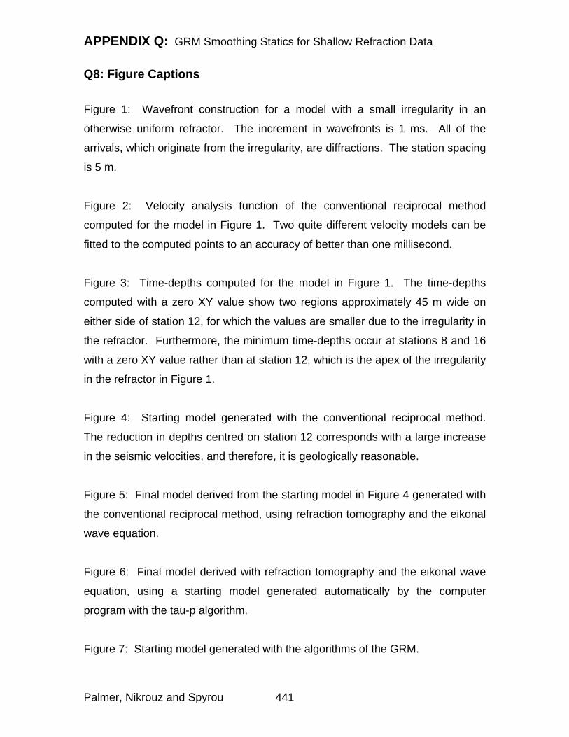
APPENDIX Q: GRM Smoothing Statics for Shallow Refraction Data
Q8: Figure Captions
Figure 1: Wavefront construction for a model with a small irregularity in an
otherwise uniform refractor. The increment in wavefronts is 1 ms. All of the
arrivals, which originate from the irregularity, are diffractions. The station spacing
is 5 m.
Figure 2: Velocity analysis function of the conventional reciprocal method
computed for the model in Figure 1. Two quite different velocity models can be
fitted to the computed points to an accuracy of better than one millisecond.
Figure 3: Time-depths computed for the model in Figure 1. The time-depths
computed with a zero XY value show two regions approximately 45 m wide on
either side of station 12, for which the values are smaller due to the irregularity in
the refractor. Furthermore, the minimum time-depths occur at stations 8 and 16
with a zero XY value rather than at station 12, which is the apex of the irregularity
in the refractor in Figure 1.
Figure 4: Starting model generated with the conventional reciprocal method.
The reduction in depths centred on station 12 corresponds with a large increase
in the seismic velocities, and therefore, it is geologically reasonable.
Figure 5: Final model derived from the starting model in Figure 4 generated with
the conventional reciprocal method, using refraction tomography and the eikonal
wave equation.
Figure 6: Final model derived with refraction tomography and the eikonal wave
equation, using a starting model generated automatically by the computer
program with the tau-p algorithm.
Figure 7: Starting model generated with the algorithms of the GRM.
Palmer, Nikrouz and Spyrou 441
APPENDIX Q: GRM Smoothing Statics for Shallow Refraction Data
Figure 8: Final model derived from the starting model in Figure 7 generated with
the GRM, using refraction tomography and the eikonal wave equation.
Figure 9: Model showing an irregular refractor with a lateral change in the
seismic velocity and an irregular surface topography. The model extends over
an horizontal distance of 350 m.
Figure 10: The refractor velocity analysis function for a range of XY values from
zero to 30 m. The graphs for individual XY values have been separated for
clarity by adding a constant value. Individual graphs are irregular because both
the refractor and the topography are irregular. The average of these graphs is
smoother, but still sufficiently irregular to generate artifacts.
Figure 11: Time-depths generated with XY values from zero to 30 m. The time-
depths reflect the irregularities in both the surface topography and the refractor.
The abrupt changes in the surface topography at 130 m and 250 m generate
anomalies, which propagate laterally through the time-depth profiles with
increasing XY values.
Figure 12: GRM refractor velocity analysis graphs, which have been corrected
with the GRM SSM. There is a clear improvement in the symmetry of the
refractor velocity analysis graphs about the graph for 15 m XY value, compared
with Figure 10.
Figure 13: GRM time-depth graphs, which have been corrected with the GRM
SSM. The time-depths exhibit considerably less variation, compared with Figure
11.
Figure 14: Traveltime graphs recorded across a narrow massive sulphide
orebody. Traveltime anomalies are caused by both near surface irregularities
Palmer, Nikrouz and Spyrou 442
APPENDIX Q: GRM Smoothing Statics for Shallow Refraction Data
and significant changes in the depth to and the seismic velocity within the main
refractor.
Figure 15: The refractor velocity analysis function of the conventional reciprocal
method. The abnormally low seismic velocity of 735 m/s as well as a physically
unrealistic velocity of –19,910 m/s occur in the vicinity of station 49, which is the
approximate location of the sulphide mineralization.
Figure 16: Time-depth profile computed with the conventional reciprocal method.
The large increase at station 49 indicates that the refractor velocities are likely to
be artifacts
Figure 17: GRM refractor velocity analysis function for XY values from –2.5 m to
10 m. The average has minimized the artifacts caused by the increase in depths
to the refractor around station 49. However, the probable occurrence of a near
surface irregularity at 48 introduces some uncertainty in the detailed velocity
determinations.
Figure 18: The GRM time-depth profiles for XY values from zero to 10 m. The
near surface irregularities and their lateral migration with increasing XY distances
are highlighted. The averaged time-depth profile is largely unaffected by the
near surface irregularities.
Figure 19: GRM refractor velocity analysis graphs computed with traveltimes
which have been corrected with the GRM SSM. The effective removal of the
near surface anomalies results in a clear improvement in the symmetry of the
graphs about the average.
Figure 20: The averaging of the refractor velocity graphs in Figure 19 greatly
reduces the artifacts caused by refractor architecture. From Figure 19, the
optimum XY value appears to be between 2.5 m and 5 m. Therefore, the range
Palmer, Nikrouz and Spyrou 443

APPENDIX Q: GRM Smoothing Statics for Shallow Refraction Data
of the XY values used in the averaging process is symmetrical about these
values. It is interpreted that the interval with the seismic velocity of 7500 m/s
does not exist.
Figure 21: GRM time-depths computed with the traveltimes corrected for the
near surface irregularities. They have been largely removed.
Palmer, Nikrouz and Spyrou 444
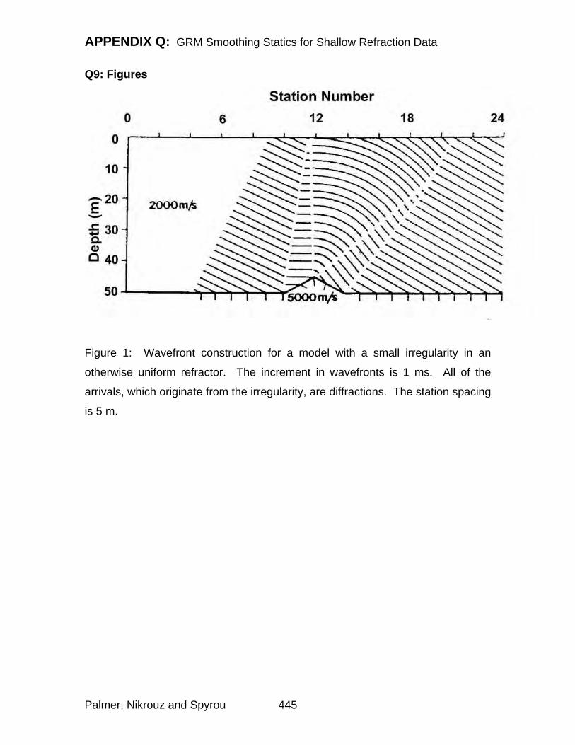
APPENDIX Q: GRM Smoothing Statics for Shallow Refraction Data
Q9: Figures
Figure 1: Wavefront construction for a model with a small irregularity in an
otherwise uniform refractor. The increment in wavefronts is 1 ms. All of the
arrivals, which originate from the irregularity, are diffractions. The station spacing
is 5 m.
Palmer, Nikrouz and Spyrou 445
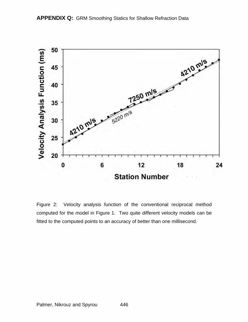
APPENDIX Q: GRM Smoothing Statics for Shallow Refraction Data
Figure 2: Velocity analysis function of the conventional reciprocal method
computed for the model in Figure 1. Two quite different velocity models can be
fitted to the computed points to an accuracy of better than one millisecond.
Palmer, Nikrouz and Spyrou 446
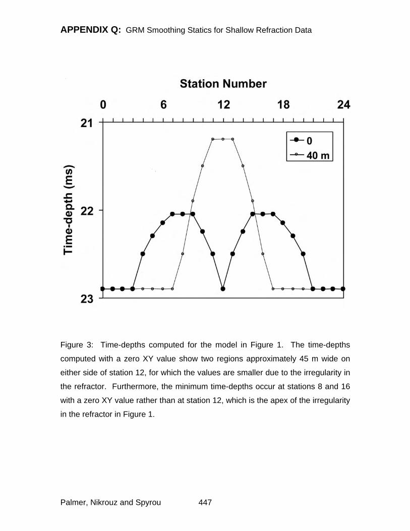
APPENDIX Q: GRM Smoothing Statics for Shallow Refraction Data
Figure 3: Time-depths computed for the model in Figure 1. The time-depths
computed with a zero XY value show two regions approximately 45 m wide on
either side of station 12, for which the values are smaller due to the irregularity in
the refractor. Furthermore, the minimum time-depths occur at stations 8 and 16
with a zero XY value rather than at station 12, which is the apex of the irregularity
in the refractor in Figure 1.
Palmer, Nikrouz and Spyrou 447
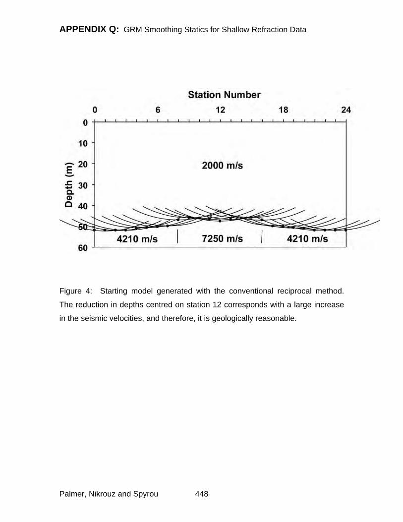
APPENDIX Q: GRM Smoothing Statics for Shallow Refraction Data
Figure 4: Starting model generated with the conventional reciprocal method.
The reduction in depths centred on station 12 corresponds with a large increase
in the seismic velocities, and therefore, it is geologically reasonable.
Palmer, Nikrouz and Spyrou 448
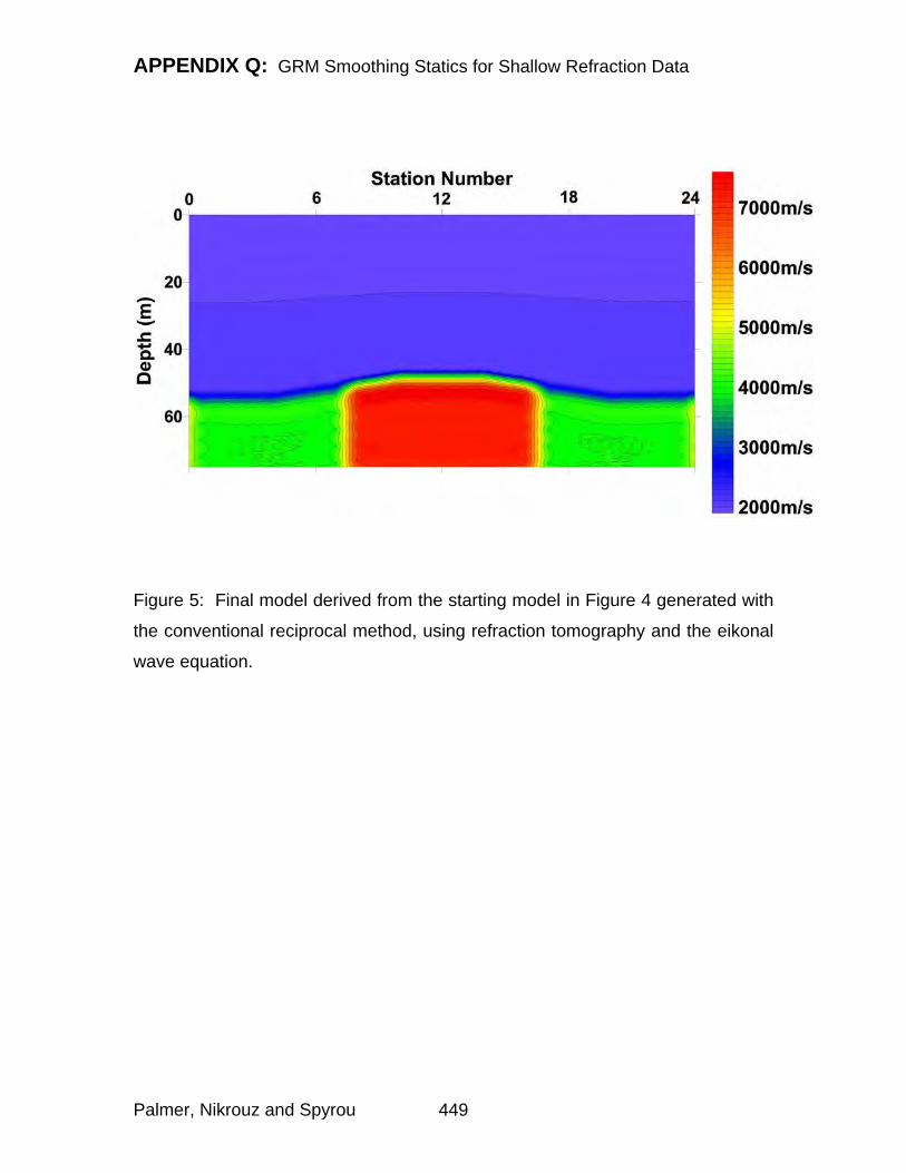
APPENDIX Q: GRM Smoothing Statics for Shallow Refraction Data
Figure 5: Final model derived from the starting model in Figure 4 generated with
the conventional reciprocal method, using refraction tomography and the eikonal
wave equation.
Palmer, Nikrouz and Spyrou 449
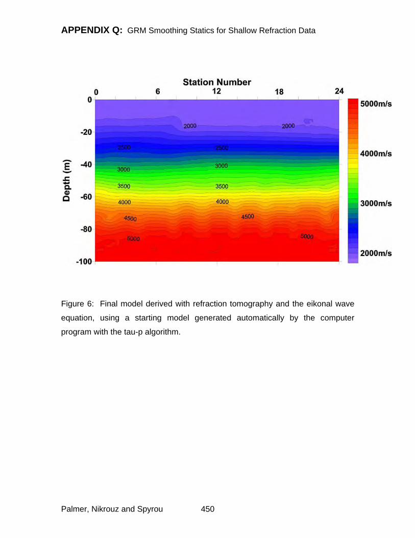
APPENDIX Q: GRM Smoothing Statics for Shallow Refraction Data
Figure 6: Final model derived with refraction tomography and the eikonal wave
equation, using a starting model generated automatically by the computer
program with the tau-p algorithm.
Palmer, Nikrouz and Spyrou 450
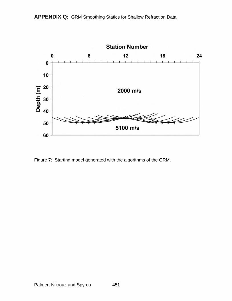
APPENDIX Q: GRM Smoothing Statics for Shallow Refraction Data
Figure 7: Starting model generated with the algorithms of the GRM.
Palmer, Nikrouz and Spyrou 451
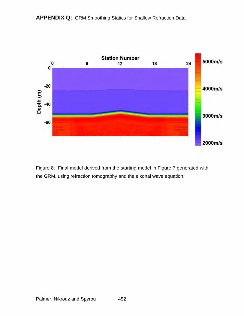
APPENDIX Q: GRM Smoothing Statics for Shallow Refraction Data
Figure 8: Final model derived from the starting model in Figure 7 generated with
the GRM, using refraction tomography and the eikonal wave equation.
Palmer, Nikrouz and Spyrou 452
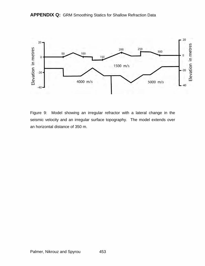
APPENDIX Q: GRM Smoothing Statics for Shallow Refraction Data
Figure 9: Model showing an irregular refractor with a lateral change in the
seismic velocity and an irregular surface topography. The model extends over
an horizontal distance of 350 m.
Palmer, Nikrouz and Spyrou 453
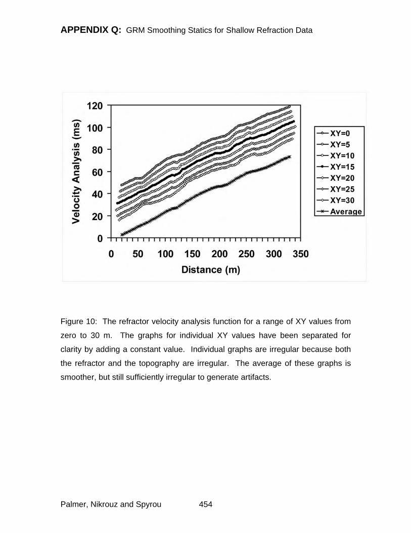
APPENDIX Q: GRM Smoothing Statics for Shallow Refraction Data
Figure 10: The refractor velocity analysis function for a range of XY values from
zero to 30 m. The graphs for individual XY values have been separated for
clarity by adding a constant value. Individual graphs are irregular because both
the refractor and the topography are irregular. The average of these graphs is
smoother, but still sufficiently irregular to generate artifacts.
Palmer, Nikrouz and Spyrou 454
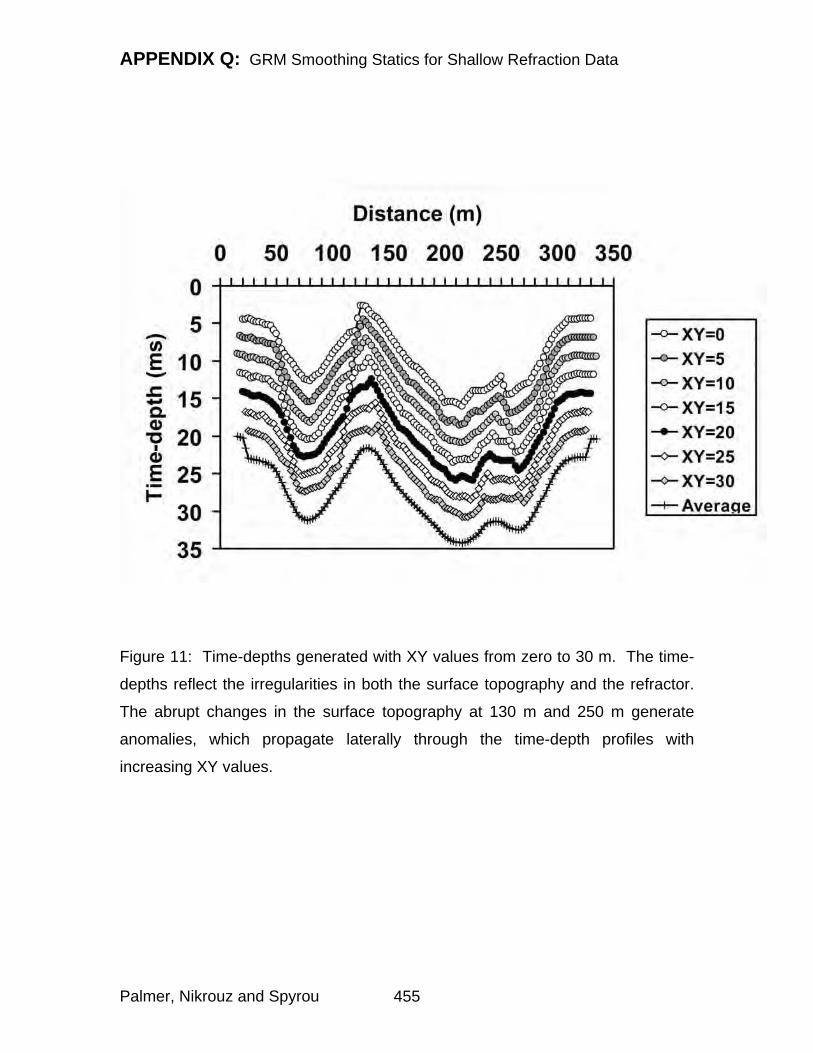
APPENDIX Q: GRM Smoothing Statics for Shallow Refraction Data
Figure 11: Time-depths generated with XY values from zero to 30 m. The time-
depths reflect the irregularities in both the surface topography and the refractor.
The abrupt changes in the surface topography at 130 m and 250 m generate
anomalies, which propagate laterally through the time-depth profiles with
increasing XY values.
Palmer, Nikrouz and Spyrou 455
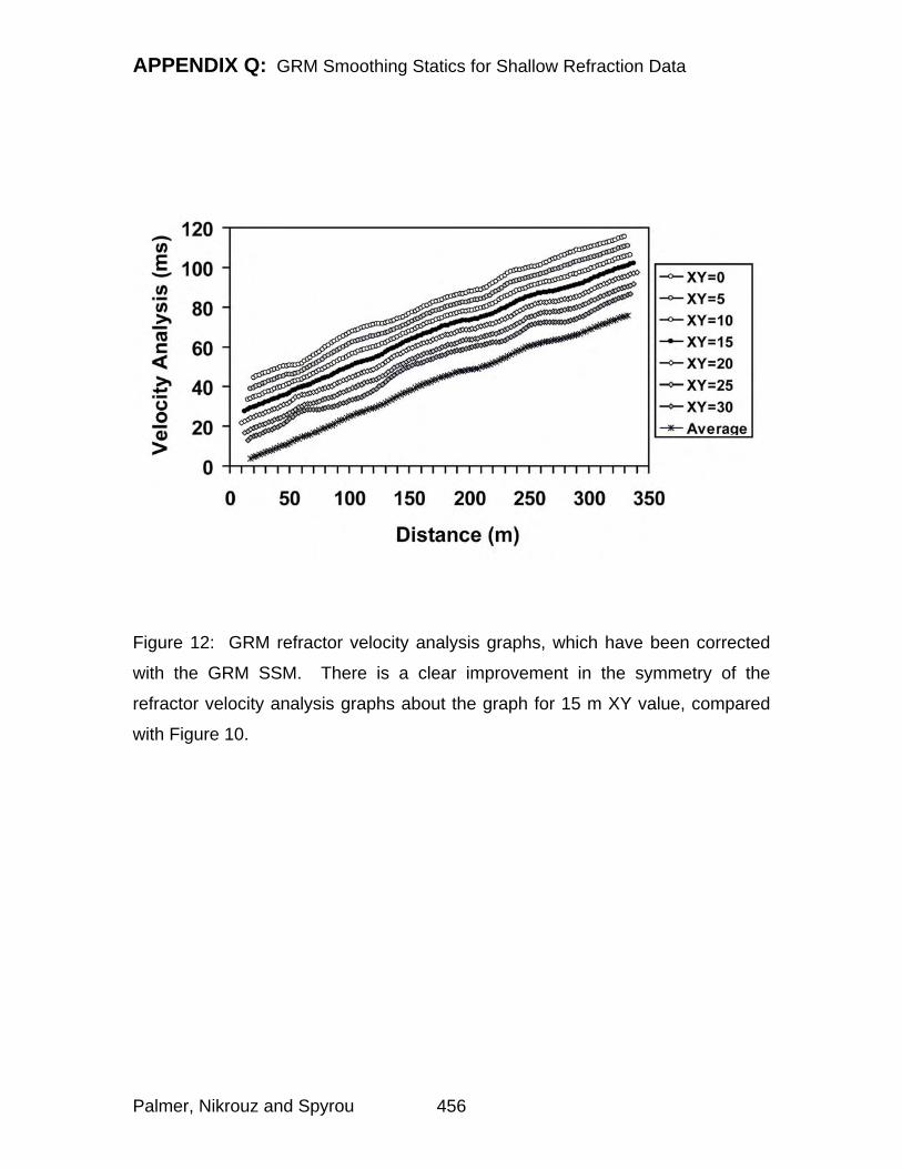
APPENDIX Q: GRM Smoothing Statics for Shallow Refraction Data
Figure 12: GRM refractor velocity analysis graphs, which have been corrected
with the GRM SSM. There is a clear improvement in the symmetry of the
refractor velocity analysis graphs about the graph for 15 m XY value, compared
with Figure 10.
Palmer, Nikrouz and Spyrou 456
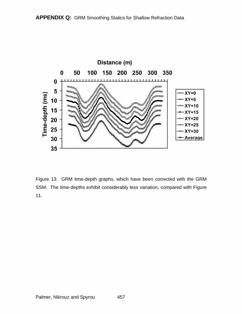
APPENDIX Q: GRM Smoothing Statics for Shallow Refraction Data
Figure 13: GRM time-depth graphs, which have been corrected with the GRM
SSM. The time-depths exhibit considerably less variation, compared with Figure
11.
Palmer, Nikrouz and Spyrou 457
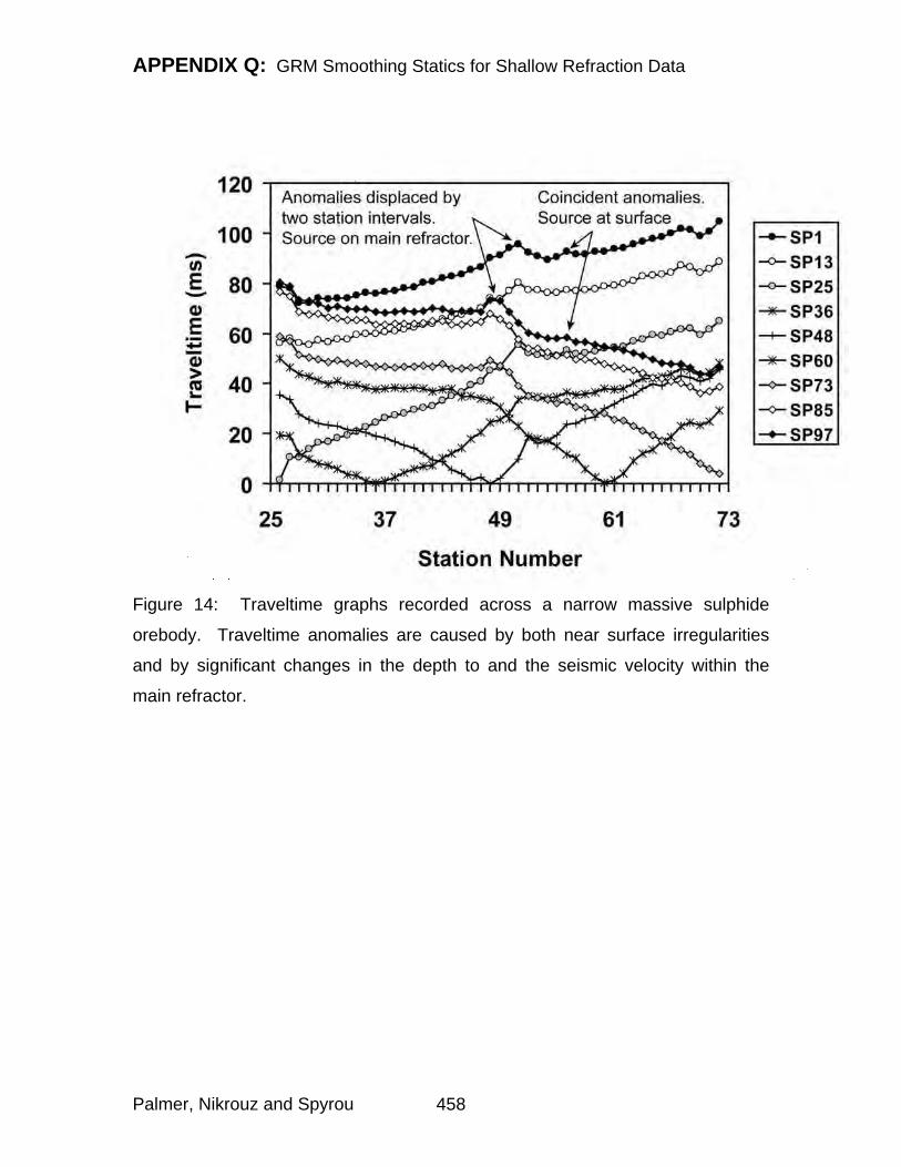
APPENDIX Q: GRM Smoothing Statics for Shallow Refraction Data
Figure 14: Traveltime graphs recorded across a narrow massive sulphide
orebody. Traveltime anomalies are caused by both near surface irregularities
and by significant changes in the depth to and the seismic velocity within the
main refractor.
Palmer, Nikrouz and Spyrou 458
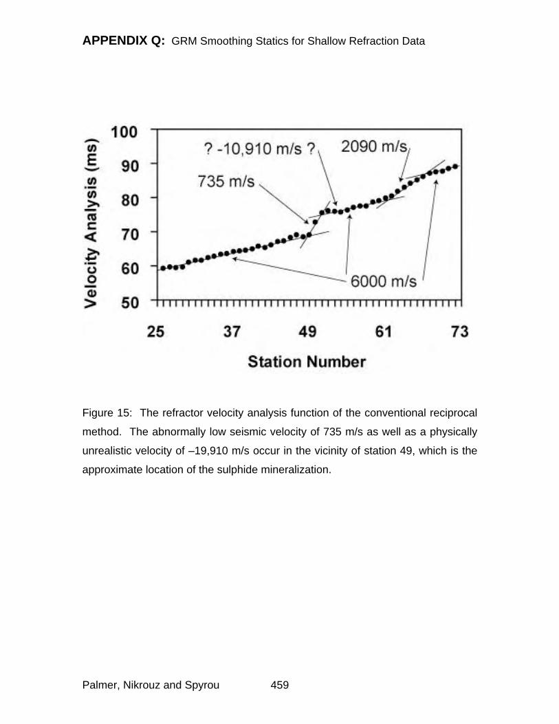
APPENDIX Q: GRM Smoothing Statics for Shallow Refraction Data
Figure 15: The refractor velocity analysis function of the conventional reciprocal
method. The abnormally low seismic velocity of 735 m/s as well as a physically
unrealistic velocity of –19,910 m/s occur in the vicinity of station 49, which is the
approximate location of the sulphide mineralization.
Palmer, Nikrouz and Spyrou 459
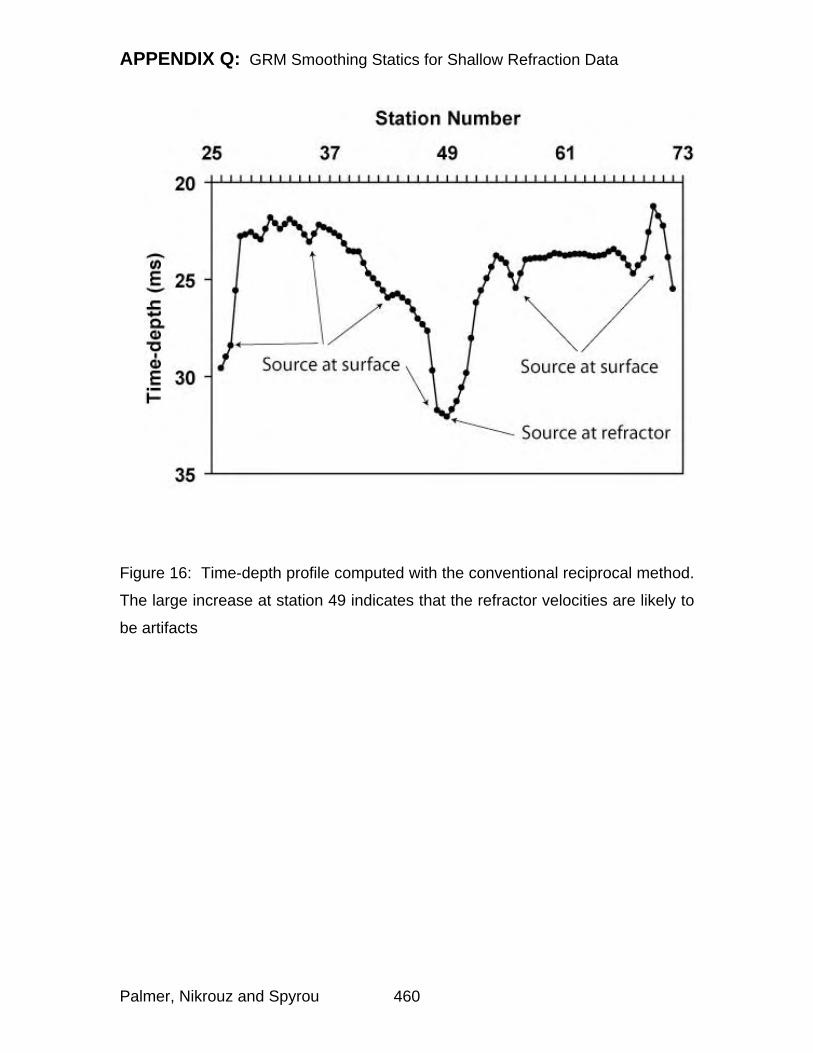
APPENDIX Q: GRM Smoothing Statics for Shallow Refraction Data
Figure 16: Time-depth profile computed with the conventional reciprocal method.
The large increase at station 49 indicates that the refractor velocities are likely to
be artifacts
Palmer, Nikrouz and Spyrou 460
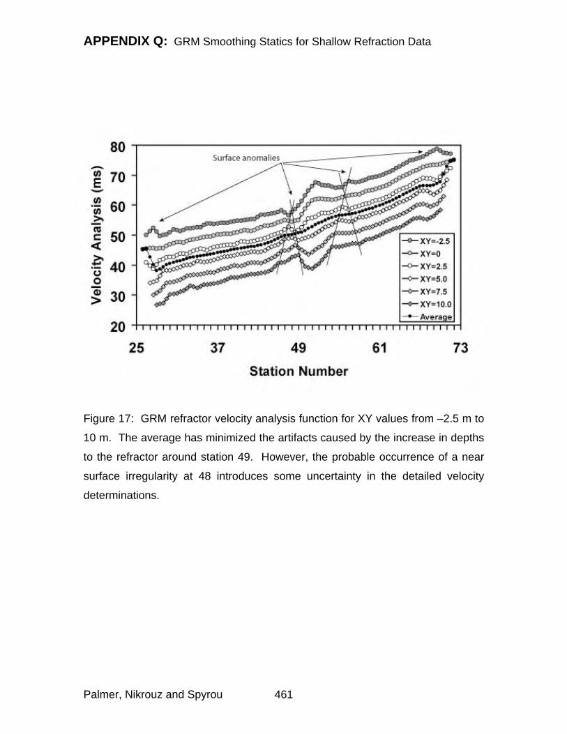
APPENDIX Q: GRM Smoothing Statics for Shallow Refraction Data
Figure 17: GRM refractor velocity analysis function for XY values from –2.5 m to
10 m. The average has minimized the artifacts caused by the increase in depths
to the refractor around station 49. However, the probable occurrence of a near
surface irregularity at 48 introduces some uncertainty in the detailed velocity
determinations.
Palmer, Nikrouz and Spyrou 461
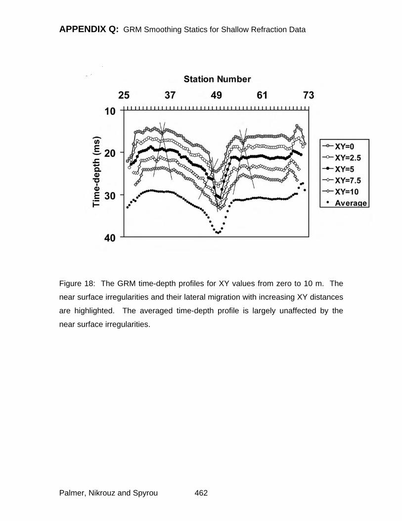
APPENDIX Q: GRM Smoothing Statics for Shallow Refraction Data
Figure 18: The GRM time-depth profiles for XY values from zero to 10 m. The
near surface irregularities and their lateral migration with increasing XY distances
are highlighted. The averaged time-depth profile is largely unaffected by the
near surface irregularities.
Palmer, Nikrouz and Spyrou 462

APPENDIX Q: GRM Smoothing Statics for Shallow Refraction Data
Figure 19: GRM refractor velocity analysis graphs computed with traveltimes
which have been corrected with the GRM SSM. The effective removal of the
near surface anomalies results in a clear improvement in the symmetry of the
graphs about the average.
Palmer, Nikrouz and Spyrou 463
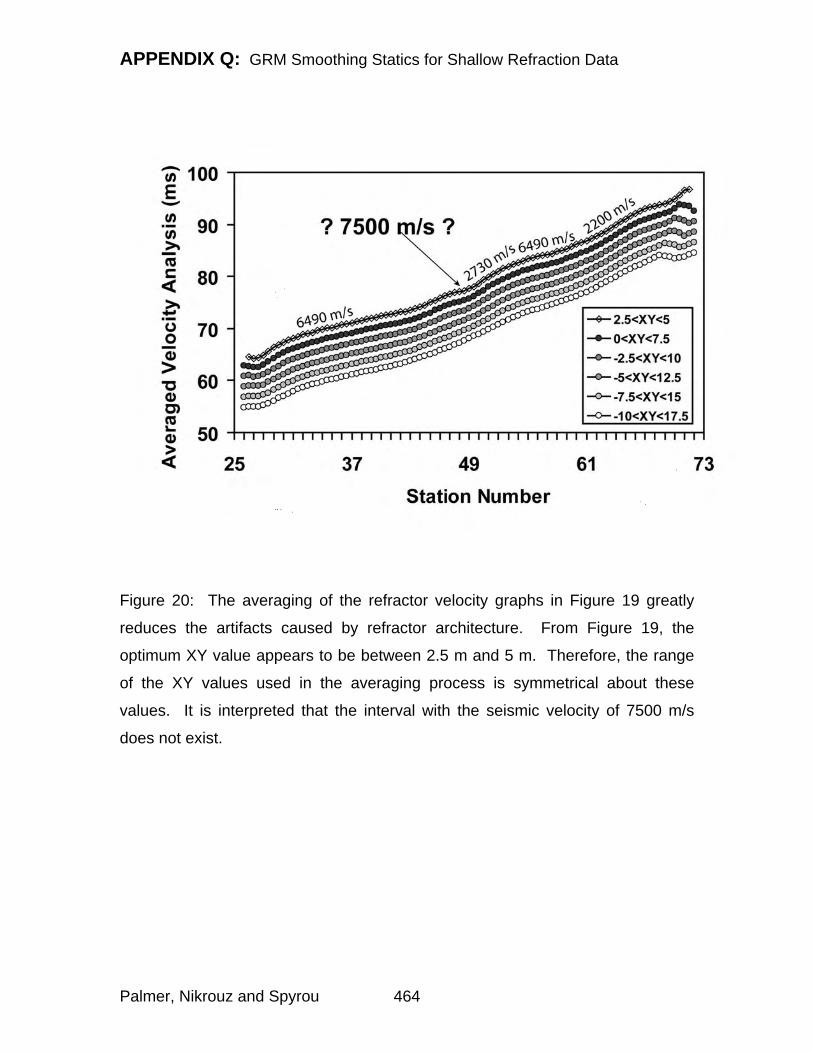
APPENDIX Q: GRM Smoothing Statics for Shallow Refraction Data
Figure 20: The averaging of the refractor velocity graphs in Figure 19 greatly
reduces the artifacts caused by refractor architecture. From Figure 19, the
optimum XY value appears to be between 2.5 m and 5 m. Therefore, the range
of the XY values used in the averaging process is symmetrical about these
values. It is interpreted that the interval with the seismic velocity of 7500 m/s
does not exist.
Palmer, Nikrouz and Spyrou 464
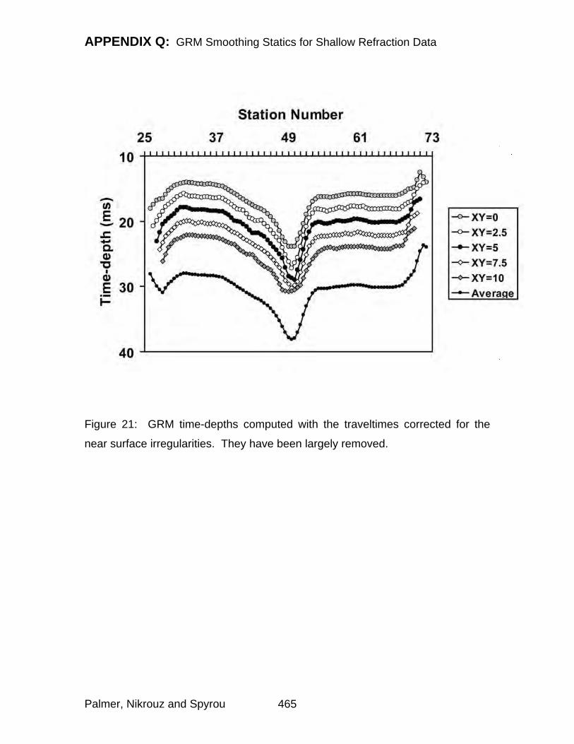
APPENDIX Q: GRM Smoothing Statics for Shallow Refraction Data
Figure 21: GRM time-depths computed with the traveltimes corrected for the
near surface irregularities. They have been largely removed.
Palmer, Nikrouz and Spyrou 465