IOWA STATE UNIVERSITY
Department of Economics Working Papers Series
Ames, Iowa 50011
Iowa State University does not discriminate on the basis of race, color, age, national origin, sexual orientation, sex, marital status, disability or status as a U.S. Vietnam Era Veteran. Any persons having inquiries concerning this may contact the Director of Equal Opportunity and Diversity, 3680 Beardshear Hall, 515-294-7612.
Is the Taylor Rule Missing? A Statistical Investigation
Helle Bunzel, Walter Enders
May 2005
Working Paper # 05015
Is the Taylor Rule Missing? A Statistical Investigation1
by
Helle Bunzel♣
and
Walter Enders♠
This draft: April 18, 2005
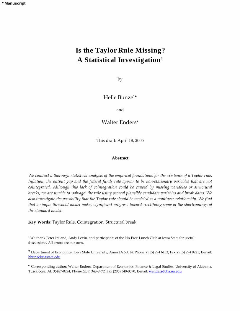
Abstract We conduct a thorough statistical analysis of the empirical foundations for the existence of a Taylor rule. Inflation, the output gap and the federal funds rate appear to be non-stationary variables that are not cointegrated. Although this lack of cointegration could be caused by missing variables or structural breaks, we are unable to �salvage� the rule using several plausible candidate variables and break dates. We also investigate the possibility that the Taylor rule should be modeled as a nonlinear relationship. We find that a simple threshold model makes significant progress towards rectifying some of the shortcomings of the standard model. Key Words: Taylor Rule, Cointegration, Structural break
1 We thank Peter Ireland, Andy Levin, and participants of the No-Free-Lunch Club at Iowa State for useful discussions. All errors are our own. ♣ Department of Economics, Iowa State University, Ames IA 50014; Phone: (515) 294 6163; Fax: (515) 294 0221; E-mail: [email protected] ♠ Corresponding author: Walter Enders, Department of Economics, Finance & Legal Studies, University of Alabama, Tuscaloosa, AL 35487-0224, Phone (205) 348-8972, Fax (205) 348-0590, E-mail: [email protected]
* Manuscript
2
1. Introduction
Determining the reaction of monetary authorities to changes in fundamental economic variables
has long been a goal of fed watchers and monetary economists. In particular, economists have
focused on how the Federal Reserve Bank responds to economic fundamentals when
determining the short term interest rates. The majority of this research is based on the monetary
policy rule introduced by Taylor (1993). This is an algebraic, linear rule and is defined as it = r* +
πt + α (πt - π*) + βỹt , where i is the nominal Federal funds rate, r* is the target real federal funds
rate, πt is the inflation rate over the last four quarters, π* is the target inflation rate and ỹ is the
percentage deviation of real GDP from the target real GDP. Taylor sets both the target real
federal funds rate and the target inflation rate equal to 2 and puts equal weights, 0.5, on
deviation from the inflation target and deviation from the real GDP target. While this original
specification seemed robust using the data from 1987 to 1993, it became clear as more data
accumulated over time that modification of the original rule was required.
In order to improve the performance of the rule, it became almost standard to add lagged
values of the federal funds rate as explanatory variables.2 The economic interpretation of this
addition is that the Fed smoothes interest rates over time, moving gradually towards the target.
Lately, however, this practice has been questioned. In particular, Rudebusch (2002) argued that
if the fed does indeed smooth interest rates, the addition of the lagged federal funds rate to the
monetary rule should increase our ability to forecast the future federal funds rate. He finds that
this is not the case and hence concludes that the statistical significance of the lagged federal
funds rate in the regressions is actually due to highly serially correlated errors.3
2 See for example Clarida et al. (2000), Woodford (1999), Goodhart (1999), Levin et al. (1999), Amato and Laubach (1999), and Sack (1998). 3 English, Nelson and Sack (2003) estimate a model which expressly allows for both a lagged federal funds rate and serially correlated errors. They conclude that both are present and significant.
3
Another direction that has been explored by a number of researchers is potential nonlinearity of
the Taylor rule. There are several reasons why a nonlinear specification might seem reasonable.
The standard derivation of the Taylor rule posits a Federal Reserve loss function that depends
on the squared deviation of inflation from the target and the square of the output gap. The
solution from this quadratic specification is a linear Taylor rule similar to the original Taylor
(1993) rule. There are, however, many reasons to suppose that this linear framework is
problematic. Among them is the possibility that the effect of the federal funds rate on the output
gap or on the inflation rate may not be linear; for example it may be more difficult to eliminate a
negative output gap than a positive gap, or, as a number of theoretical and empirical papers
suggest, inflation may increase more readily than it decreases. Another cause for nonlinearity in
the Taylor rule might be that the Fed�s loss function is asymmetric, suggesting that the Fed has
higher tolerance for inflation that is slightly below the target than inflation that is slightly above
the target.4 Yet another potential cause for nonlinearities is uncovered in a number of papers
which find that several key macroeconomic variables follow asymmetric paths over the course
of the business cycle. These nonlinearities can manifest themselves in a nonlinear Taylor rule.
Finally, nonlinearity of the Taylor rule could be caused by the fact that the parameters are not
stable over time. 5
The goal of this paper is to carry out a thorough statistical analysis of the data in an attempt to
determine whether a stable linear or nonlinear relationship does in fact exist. We describe the
data and perform some preliminary tests for stationarity in Section 2. In Section 3, we show that
there is no meaningful cointegrating relationship between inflation, output gap and federal
funds rates.6 Without cointegration, any estimated relationship between the variables is
4 See Surico (2004 ) for an exploration of this avenue. 5 One type of nonlinearity which is almost always incorporated in models of monetary policy is permanent regime shifts. These are believed to be caused by policy changes due to changes in the chairman of the Federal Reserve Bank or changes of power in Congress and/or the White House which may have driven the Federal Reserve bank to change its policies. Papers by Dolado, Maria-Dolores and Naveira (2004), Kim, Osborne and Sensier (2004), Nobay and Peel (2003), and Ruge-Murcia (2003) consider other types of nonlinearity. 6 A similar result has been obtained by Ősterholm (2005).
4
spurious, calling into question whether a Taylor rule exists. To obtain additional insight into the
failure of the cointegration tests, we carry out recursive estimates of the (invalid) equation to get
a sense of how the parameter estimates change over time. Since the lack of cointegration could
be caused by missing variables, in Section 4, we investigate several plausible candidate
variables without success. Next, we examine the possibility of structural breaks in the data. All
empirical work in this area has estimated the Taylor rule for limited periods of time under the
assumption that there have been several permanent regime shifts, mostly in connection with
shifts in the leadership of the Federal Reserve Bank. Nevertheless, when we use break dates
coinciding with changes in the chairmanship of the Fed, we cannot reject the null hypothesis of
no cointegration. We consider the possibility that the data appears not to be cointegrated
because the shifts are placed at incorrect dates. Instead of using intuitive break dates obtained
by looking at events, we also use a data-driven selection method due to Bai and Perron (2003).
This does not change the result that there is no stable cointegration relationship.
In the final portion of Section 4, we investigate the possibility that the Taylor rule should be
modeled as a nonlinear relationship. The tests indicate that there are indeed nonlinearities in
the model, but do not seem to indicate that one specific parameter is the cause. We therefore
proceed to investigate the possibility that a threshold model is a reasonable approach to
modeling the determination of the federal funds rate; that is, if a given variable exceeds a
threshold, the Fed reacts in one manner, and otherwise it has a different response. We find that
when the inflation is low (less than about 2.3%) the Fed does not interfere at all, but when
inflation is high, a relationship similar to the standard Taylor rule holds! This model makes
significant progress towards explaining the misspecifications of the standard model, such as
seemingly unreasonable high smoothing of the interest rates, unstable parameter estimates and
lack of cointegration. While it is not, to our knowledge, possible to formally test whether this
model is stable over the long run, informal checks seem to indicate that this might indeed be the
case. Conclusions and directions for further research are contained in Section 5.
5
2. The Data
The data we used was obtained from FRED II (Federal Reserve Economic Data).7 We have
quarterly observations from 1954:3 to 2003:4. We chose to follow the variable definitions used in
Rudebusch (2002). Specifically, inflation is constructed using the chain-weighted GDP deflator
(pt) and the four-quarter inflation rate, πt, is computed as the simple average of the individual
inflation rates. Hence,
πt = 0.25*3
10
where 400(ln ln )t t t tt
p p p p −=
= −∑ ! ! .
We constructed the output gap (yt) as the percentage difference between real GDP (qt) and
potential output ( *tq ) so that:
yt = 100*(qt/ *tq − 1) .
Measurements of output, the potential output and the price index can change over time due to
factors such as definitional changes and revisions in the data. In order to see how our variables
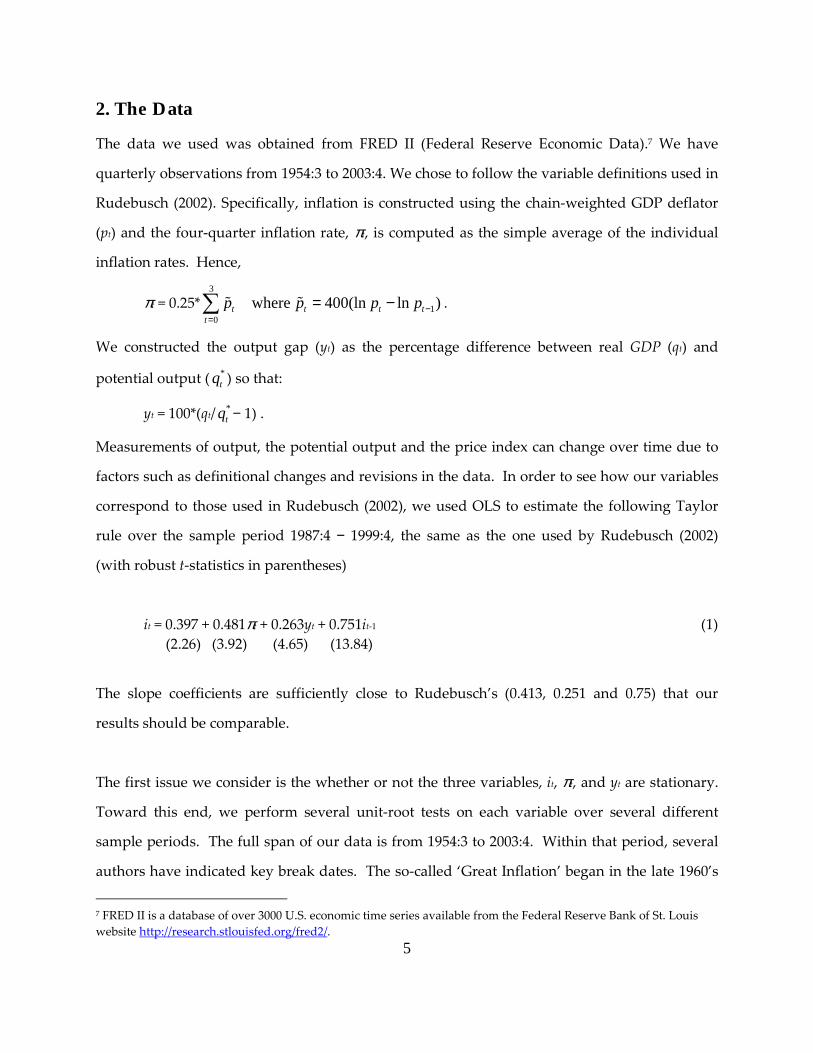
correspond to those used in Rudebusch (2002), we used OLS to estimate the following Taylor
rule over the sample period 1987:4 − 1999:4, the same as the one used by Rudebusch (2002)
(with robust t-statistics in parentheses)
it = 0.397 + 0.481πt + 0.263yt + 0.751it-1 (1) (2.26) (3.92) (4.65) (13.84)
The slope coefficients are sufficiently close to Rudebusch�s (0.413, 0.251 and 0.75) that our
results should be comparable.
The first issue we consider is the whether or not the three variables, it, πt, and yt are stationary.
Toward this end, we perform several unit-root tests on each variable over several different
sample periods. The full span of our data is from 1954:3 to 2003:4. Within that period, several
authors have indicated key break dates. The so-called �Great Inflation� began in the late 1960�s
7 FRED II is a database of over 3000 U.S. economic time series available from the Federal Reserve Bank of St. Louis website http://research.stlouisfed.org/fred2/.
6
(we use 1968:4 as a break date). The early 1970s saw the end of the Bretton Woods system; as
such it seems reasonable to use 1973:4 as a potential break date. The change in the Federal
Reserve�s operating procedures in began in 1979:4, and the Volker disinflation ended by 1983:1.
For each variable and for each sample period with more than 25 observations, we estimated an
equation of the form:
∆yt = a0 + ρyt-1 + 1
n
i t ii
yβ −=
∆∑ + εt
We did not include a deterministic time trend since there is little reason to believe that any of
the variables are trend stationary. The lag length n was selected by the general-to-specific
methodology. Beginning with n = 7, we tested the statistical significance of βn using the 5%
significance level. If βn was not statistically different from zero, we reduced n by 1 and repeated
the procedure until βn was statistically significant. Given this lag length, we then obtained the t-
statistic (denoted by τ ) for the null hypothesis ρ = 0. The number of lags and the estimated
values of ρ and τ are given in Table 1 for various sample periods.
From the results presented in Table 1, it is clear that the federal funds rate and the weighted
inflation rate show little evidence of mean reversion over any sample period. In particular, this
is true for both of the samples beginning with Alan Greenspan�s tenure as Fed chairman in
1987:4. For the output gap, however, the results of the Dickey-Fuller tests are very dependent
on the sample period under consideration. For example, the output gap shows some evidence
of mean reversion over the very long sample periods. Although we cannot reject the unit-root
hypothesis for the samples beginning in 1979:4, there appears to be strong evidence of mean
reversion for the samples beginning with 1983:1. Moreover, if we begin with 1981:1 (a date not
shown in the table), or in 1987:4 (as Rudebusch did), the unit-root hypothesis cannot be rejected.
Notice that ρ is actually positive for the 1987:4 − 1994:4 period.
7
We have now completed thorough testing for unit roots, using the standard textbook methods.
Because much of what follows relies on the fact that the series are indeed I(1), we will proceed a
little further using the latest techniques for unit root testing. In a recent paper Müller and Elliott
(2003) highlighted the dependence of the power of unit root tests on the deviation of the initial
observation of the series from its underlying deterministic component. They show that the
Dickey-Fuller test we employed above has excellent power properties for large values of this
initial deviation, while the test proposed by Elliott, Rothenberg, and Stock (1996) (henceforth
ERS) is optimal when the initial deviation is 0. A recent paper by Harvey and Leybourne (2003)
(henceforth HL) proposes a unit root test which combines the strengths of the two statistics.
They use a data-dependent weighted average of the Dickey-Fuller test ( DFτ ) and the ERS
statistic, with the weight determined by an estimate of the deviation of the initial observation
from the underlying deterministics.
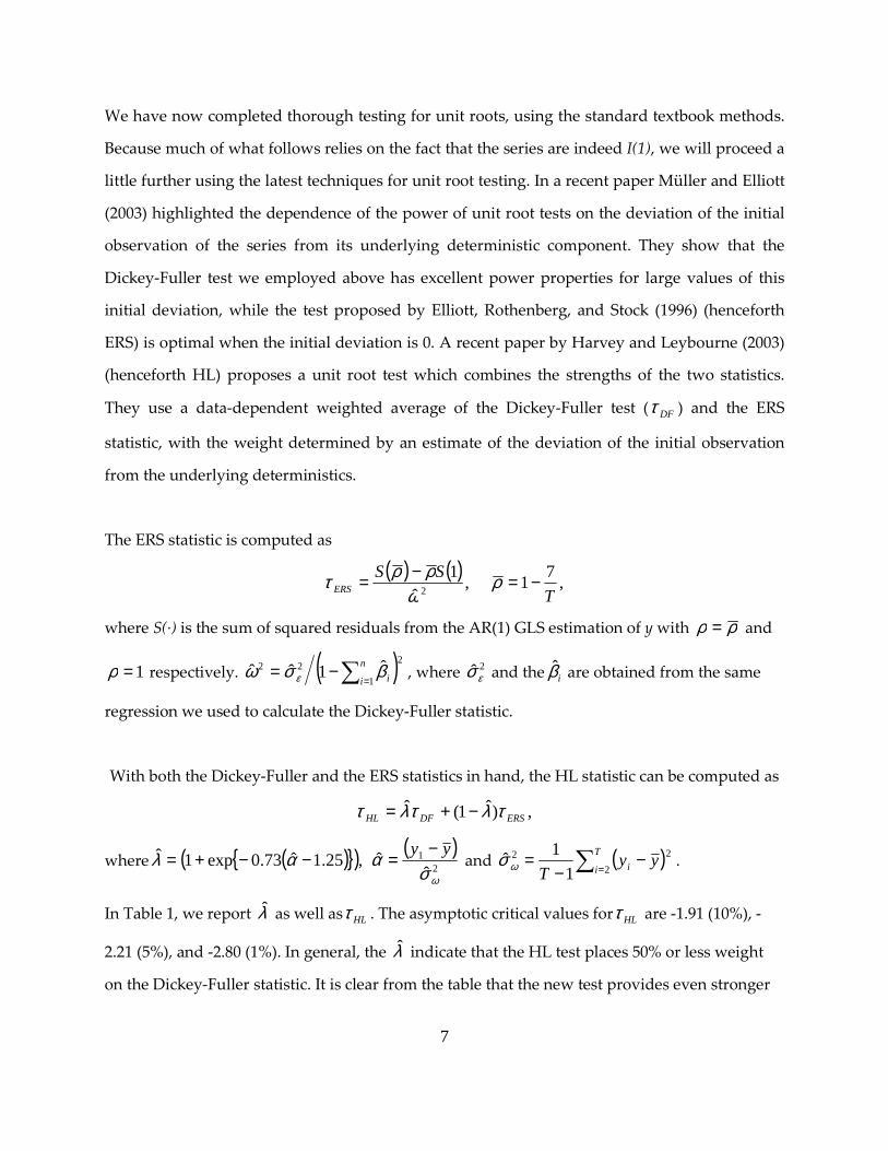
The ERS statistic is computed as
( ) ( ) ,71,ˆ
12 T
SSERS −=−= ρ
ωρρτ
where S(·) is the sum of squared residuals from the AR(1) GLS estimation of y with ρρ = and
1=ρ respectively. ( )2
122 ˆ1ˆˆ ∑ =
−= n
i iβσω ε , where 2ˆεσ and the iβ̂ are obtained from the same
regression we used to calculate the Dickey-Fuller statistic.
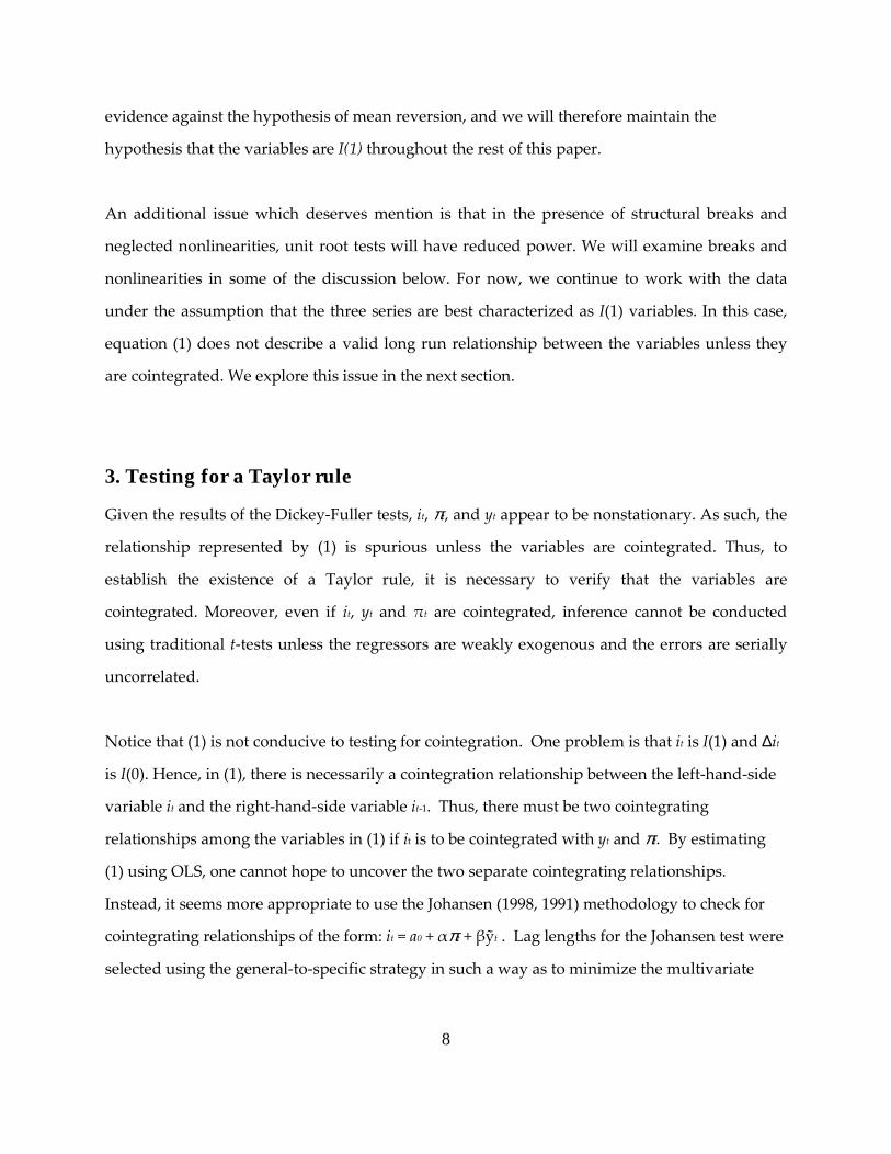
With both the Dickey-Fuller and the ERS statistics in hand, the HL statistic can be computed as
,)ˆ1(ˆERSDFHL τλτλτ −+=
where ( ){ }( ),25.1ˆ73.0exp1ˆ −−+= αλ ( )
21
ˆˆ
ωσα yy −
= and ( )∑ =−
−= T
i i yyT 2
22
11ˆωσ .
In Table 1, we report λ̂ as well as HLτ . The asymptotic critical values for HLτ are -1.91 (10%), -
2.21 (5%), and -2.80 (1%). In general, the λ̂ indicate that the HL test places 50% or less weight
on the Dickey-Fuller statistic. It is clear from the table that the new test provides even stronger
8
evidence against the hypothesis of mean reversion, and we will therefore maintain the
hypothesis that the variables are I(1) throughout the rest of this paper.
An additional issue which deserves mention is that in the presence of structural breaks and
neglected nonlinearities, unit root tests will have reduced power. We will examine breaks and
nonlinearities in some of the discussion below. For now, we continue to work with the data
under the assumption that the three series are best characterized as I(1) variables. In this case,
equation (1) does not describe a valid long run relationship between the variables unless they
are cointegrated. We explore this issue in the next section.
3. Testing for a Taylor rule
Given the results of the Dickey-Fuller tests, it, πt, and yt appear to be nonstationary. As such, the
relationship represented by (1) is spurious unless the variables are cointegrated. Thus, to
establish the existence of a Taylor rule, it is necessary to verify that the variables are
cointegrated. Moreover, even if it, yt and πt are cointegrated, inference cannot be conducted
using traditional t-tests unless the regressors are weakly exogenous and the errors are serially
uncorrelated.
Notice that (1) is not conducive to testing for cointegration. One problem is that it is I(1) and ∆it
is I(0). Hence, in (1), there is necessarily a cointegration relationship between the left-hand-side
variable it and the right-hand-side variable it-1. Thus, there must be two cointegrating
relationships among the variables in (1) if it is to be cointegrated with yt and πt. By estimating
(1) using OLS, one cannot hope to uncover the two separate cointegrating relationships.
Instead, it seems more appropriate to use the Johansen (1998, 1991) methodology to check for
cointegrating relationships of the form: it = a0 + απt + βỹt . Lag lengths for the Johansen test were
selected using the general-to-specific strategy in such a way as to minimize the multivariate
9
Akaike Information Criterion (AIC).8 The results for the various sample periods are reported in
Table 2. Columns 3 − 5 of the table report the sample values of λmax(r) for the null hypothesis of
exactly r cointegrating vectors against the alternative hypothesis of r + 1 cointegrating vectors.
Columns 6 − 8 show the estimated parameters of the (potential) cointegrating vector.
Notice that the Taylor rule fails for all periods with a starting date prior to 1979:4. In those
instances where it is possible to reject the null hypothesis of no cointegration, at least one of the
estimated coefficients of the cointegrating vector has the incorrect sign. For example, in the
1955:3 − 1968:4 period, the sample value of λmax(0) = 11.31 is less than the 5% critical value of
22.00. In the 1955:3 − 2003:4 period, the null of no cointegration can be rejected at the 5% level,
but the signs of α and β are both incorrect.
The samples beginning with 1979:4 are problematic in that the Fed temporarily switched from
targeting the federal funds rate to controlling non-borrowed reserves during 1979:3�1982:3. As
such, we follow the example of most applied papers on the Taylor rule and eliminate this
period from serious consideration. For the 1983:4 − 2003:4 period, the null hypothesis of no
cointegration can be rejected in favor of the alternative of exactly one cointegrating vector at the
5% significance level. There is no evidence of a second cointegrating vector and the estimated
values of α and β are all of the correct sign. Nevertheless, substantial care must be exercised
before concluding that the Taylor rule holds in the Volcker-Greenspan period since: There is no
cointegration for the 1983:4 − 1999:4 period and these cointegration results break down when
the starting date is changed to coincide with Alan Greenspan�s tenure as Federal Reserve
Chairman. As shown in last two rows of Table 2, the sample values for λmax(0) are both well
below the 10% critical value of 19.77.
8 We also used the lag lengths selected by the multivariate Schwartz Bayesian Criterion (SBC). The results were sufficiently similar that we do not report them here. In the few cases where there were significant autocorrelations in the residuals, additional lags were added to eliminate the problem.
10
In our view, it strains credibility to argue that the results support the existence of a Taylor rule
during the entire Volcker-Greenspan period. Nevertheless, someone might be tempted claim
that the use of the two subsamples results in enough loss of power such that Johansen test is not
able to detect a significant cointegrating relationship. To challenge this claim, notice that the
estimated cointegrating relationship for the 1983:1 − 2003:4 period is:
it = −1.22 + 3.07πt + 1.44yt + et (2)
Consider the estimates of the error-correcting model (with t-statistics in parentheses):
∆it = -0.035[ it-1 − 1.22 − 3.07πt-1 − 1.44yt-1 ] + stationary dynamics (-1.60)
∆πt = −0.016[ it-1 − 1.22 − 3.07πt-1 − 1.44yt-1 ] + stationary dynamics (−1.36)
∆yt = 0.106[ it-1 − 1.22 − 3.07πt-1 − 1.44yt-1 ] + stationary dynamics (4.29)
Even though the Johansen test is unable to reject the null hypothesis of no cointegration, this
model does not tally with our requirements for a Taylor rule. The first issue is that since the
coefficient -0.035 on the error-correction component of the federal funds rate is insignificant, the
federal funds rate is weakly exogenous. Hence, the point estimates suggest that the federal
funds rate does not respond to a deviation from the cointegrating relationship. This is clearly
inconsistent with the spirit of a Taylor rule. Furthermore, the t-statistic for the speed-of-
adjustment coefficient for the four-quarter inflation rate provides mild evidence that inflation
responds to a discrepancy from the equilibrium relationship by moving in the �wrong�
direction. For example, if inflation is 1 percentage point higher than that suggested by the long-
run relationship, it is estimated that inflation increases by another 0.05 (0.016*3.07 ≅ 0.049) of a
percentage point. Finally, the output gap does respond significantly and in the correct direction
to restore long-run equilibrium. For example, if the output gap is one unit higher than that
11
suggested by the long-run relationship, is estimated that the gap decreases by 0.15 units
(1.06*1.44 ≅ 0.15). Unfortunately, given the prolonged nature of the business expansion in the
Clinton period, this speed of adjustment seems overly strong. Overall, (2) is more likely to be an
output determination equation than a Taylor rule.
As shown on the right-hand side of Table 2, a similar pattern emerges when we examine the
forward-looking version of the Taylor rule given by it = a0 + απt+1 + βỹt+1. Of course, the large
sample properties of the cointegration tests are identical since cointegration between variables yt
and xt, implies cointegration between yt and xt+1. Again, cointegration fails for most of the early
periods. For our purposes, the important point is that there does not appear to be a significant
cointegrating relationship for any period beginning in 1983:1 or 1987:4.
To better understand the failure of the Taylor rule, we confine our attention to the Greenspan
periods of 1987:4 − 1999:4 and 1987:4 − 2003:4. Toward this end, we will examine equation (1)
for parameter stability. First, however, we re-estimated equation (1) to check for and remove
any serial correlation in the residuals. Specifically, if ρi denotes the ith-order correlation
coefficient constructed from the first eight residual autocorrelations are:
ρ1 ρ2 ρ3 ρ4 ρ5 ρ6 ρ7 ρ8
0.58 0.39 0.36 0.22 0.12 0.09 −0.04 −0.14
When we included an additional lag of the federal funds rate in the estimation equation we
obtained:
it = 0.409 + 0.318πt + 0.184yt + 1.29it-1 − 0.505it-2 (3)
(2.77) (3.96) (4.05) (13.75) (−6.19)
12
Diagnostic checking indicated no remaining serial correlation in the residuals. Estimation over
the entire sample period also suggested the second lag was appropriate, and we will therefore
proceed with the specification in (3) below.
To examine (3) for parameter stability, we performed recursive estimates of the Taylor rule
equation for the entire 1989:4 � 2003:4 period. Specifically, for each time period in the interval
1989:4 to 2003:4, we estimated an equation of the form in (3) using observations 1984:4 through
T. Since 2 observations are lost as a result of the lagged dependent variable, we obtained 55
regression equations. Beginning with 1994:1, the time paths of the estimated intercepts,
inflation coefficients, output gap coefficients and the sum of the autoregressive coefficients are
displayed in Panels 1 through 4, respectively. If the parameters are constant over time, we
would not expect any particular pattern in the coefficients. However, Panel 1 of the figure
clearly reveals that the intercept term seems to drift downward beginning in 1995. The
implication is that the Federal Reserve�s inflation target was lowered over this part of the
sample period. In addition the point estimate of the coefficient on inflation in the early part of
the sample is significantly above that in the latter part. This indicates that the Federal Reserve
responded less severely to deviations of inflation from the target in the late 1990�s than in the
earlier part of the sample period. Finally, there is a significant and steady decline in the
coefficient on the output gap as well as a sharp increase in the sum of the coefficients on the
lagged interest rates beginning in 1995. Thus, the phenomenon of interest rate smoothing was
far more marked in the latter part of the sample than the earlier part.
The point is that the Federal Reserve seemed more responsive to current economic phenomena
in the early 1990s than the late 1990s. The late 1990s are characterized by high degrees of
interest rate smoothing and low degrees of responsiveness to deviations of inflation from target
and to the output gap. Hence, even though the output gap declined substantially, the Federal
Reserve�s response was limited.
13
To summarize, since the variables are best modeled as I(1), a cointegration relationship
must exist for there to be a stable relationship among the three variables. It is clear however,
that even in the instances where the tests do not reject such a cointegration relationship, the
results do not support the existence of a stable Taylor rule. Adherents of the standard Taylor
rule might be unimpressed with the finding that the federal funds rate is not cointegrated with
the output gap and inflation. After all, cointegration tests have very little power over relatively
short sample periods. Our view is that the instability of the parameter estimates over various
sample periods and the unduly high persistence of the federal funds rate calls the entire Taylor
rule into question. After all, it was a monetary economist, Milton Friedman, who pioneered the
idea that a rule must be a stable function of a limited number of explanatory variables. Since (3)
does not provide a stable relationship between the relevant variables, we are left with two
possibilities: The first is that (3) is misspecified in some manner and therefore does not provide
the desired long run relationship. The other, more disturbing possibility (to economists
anyway), is that there is no fixed rule governing how the fed determines interest rates. Before
resigning ourselves to the second possibility, we will thoroughly explore the first. In the next
section we will explore possible misspecifications which might be the cause of the parameter
instability as well as the lack of cointegration.
4. The Search For the Missing Money Rule
In this section, we will explore a number of possible causes for misspecification of (3) with the
hope of finding a specification which leads to a stable cointegration relationship and parameter
estimates which do not vary systematically over time. First, we focus on the possibility of a
missing variable from the standard Taylor rule specification. Next we consider the possibility
that the break dates determined by looking at significant economic events are wrong. Instead of
relying on intuition we apply several data-driven methods to choose the break dates. Finally,
we will proceed to explore the possibility that it is the assumption of linearity which leads to
14
misspecification. In Section 4.3 we will discuss potential causes for nonlinearity and examine
several nonlinear extensions of equations (1) and (3).
4.1 An examination of the variables
One possible cause of misspecification is that there is a variable missing from the
standard Taylor rule specification. Suppose that the Federal Reserve is concerned about the
magnitude of the output gap, the inflation rate, and a third macroeconomic variable. The
omission of this key variable from (2) could explain the findings of the previous section.
Changes in the magnitude of this variable would manifest themselves as structural breaks in the
standard specification, leading to parameter instability. If changes in this third variable were
persistent, the federal funds rate would appear to be persistent. Finally, if there were a single
cointegrating relationship between these three variables and the federal funds rate, the rate
would not be cointegrated with the output gap and inflation.
We obtained several likely candidates for the missing variable. In testimony to congress, talks,
speeches and interviews, Chairman Alan Greenspan indicated that the Federal Reserve was
concerned about the so-called �irrational exuberance� of the stock market. Since �irrational
exuberance� is not a well-defined concept, we tried several different measures. One natural
measure is a run-up of stock prices relative to earnings. As such, we obtained Shiller�s (2000)
quarterly values of the price-earnings ratio over the 1881:1− 2003:4 period.9 The variable is
constructed as the real value of the S & P Composite Index (SP) divided by the total real value
of the earnings of the companies included in the index. As discussed in more detail below, we
also used several measures of actual movements in SP.
We also obtained quarterly values of the Index of Consumer Sentiment from University of
Michigan�s survey of households (www.sca.isr.umich.edu/main.php). Consumer confidence
(cons_con) is generally deemed to be a leading indicator of consumer expenditures on durables
9 The data as well as a detailed description are available at http://www.econ.yale.edu/~shiller/data.htm
15
and of overall economic activity. The variable is one of ten included in the Conference Board�s
Index of Leading Economic Indicators. The other forward-looking variable we obtained was the
University of Michigan�s measure of expected changes in interest rates. The survey records the
response to the following question: �No one can say for sure, but what do you think will
happen to interest rates for borrowing money during the next 12 months−−will they go up, stay
the same, or go down?� We used the proportion of people indicating that rates will go up.
Prior to introducing the price-earnings ratio into equation (3) we performed standard unit-root
tests, which indicated that {SPt} behaves as an I(1) variable over the sample periods under
consideration. As such, we used the Johansen (1988, 1991) methodology to check for a
cointegrating relationship between it, πt, yt and SPt. The results for the 1987:4 − 1999:4 and
1987:4 − 2003:4 sample periods are reported in Table 4. At the 5% level, the critical value of the
Johansen λmax statistic is 28.14. The sample values of T ln (1 − λ1) are 20.86 and 22.69 for the
1987:4 − 1999:4 and 1987:4 − 2003:4 periods, respectively. Hence, at conventional significance
levels, we are not able to reject the null hypothesis of no cointegration.
We also included SPt into the standard linear equation in the form of (3). Consider the estimated
equation for the sample period 1984:1 − 2003:4
it = 0.140 + 0.24πt + 0.16yt − 0.03 SPt + 1.29it-1 − 0.40it-2 (4)
(3.05) (3.98) (1.50) (−3.13) (11.57) (−4.05)
For this sample period, the coefficients for πt and yt are reasonably close to those in equation (3).
The point estimates are such that the federal funds rate is predicted to decline as SPt increases.
In fact, the point estimates of the SPt coefficients reported in Table 5 are quite consistent over
the various sample periods. The possible explanation is that there is reverse causality such that
decreases in interest rates lead to increases in SPt. Nevertheless, the single equation approach
does nothing to support that claim that SPt belongs in the Taylor rule equation. These results
16
support the findings using the Johansen cointegration tests (that make no particular
assumptions concerning weak exogeneity).
Next we consider the possibility that {cons_cont} is a variable missing from equation (3). Since
{cons_cont} also behaves like an I(1) variable, we used the Johansen methodology to check for a
cointegrating relationship between it, πt, yt and cons_cont. As reported in the lower portion of
Table 4, at the 5% significance level, we were able to reject the null hypothesis of no
cointegration for the 1987:4 − 1999:4 period. However, the estimated cointegrating vector (also
reported in the table) had a negative coefficient on yt. Since a negative response to the output
gap is inconsistent with a standard model of the Taylor rule, we do not believe that the reported
equation is meaningful. Moreover, we were not able to reject the null hypothesis of no
cointegration for the extended 1987:4 − 2003:4 sample period.
We experimented with the notion that only recent movements in the index, rather than its
overall level, might be deemed important by the Federal Reserve. Towards this end, we
constructed other measures of �irrational exuberance,� such as a four-quarter moving average of
the logarithmic change in the S & P Composite Index. Since a moving average of stock market
returns is stationary, we did not search for a cointegrating relationship for it, πt, yt and our
constructed measures. However, as suggested by Johansen and Juselius (1992), a stationary
variable can be used as a conditioning variable in a test for cointegration. The notion is that a
stationary covariate might enhance the power of the cointegration test since it controls for some
of the deviations from the long-run equilibrium relationship. Dickey-Fuller tests indicated that
the University of Michigan�s expected change in interest rate (∆ie) variable is I(0) over all sample
periods considered. We did not find any reasonable cointegrating relationship among it, πt, yt,
with any stationary measure of �irrational exuberance� or with ∆ie.
This concludes our exploration of the choice of variables. Since none of the other potential
choices we explored improved the model, we will proceed with the original model as specified
17
in equation (3). In the next section, we will explore the possibility that the subsamples used to
estimate the model are improperly chosen.
4.2 Subsample choice
One possible reason for the poor performance of the Taylor rule is that the subsamples
used in the estimations are improperly chosen. As such, it might be the case that an equation in
the form of (1) is properly specified but that the break dates are incorrect. Estimating the model
with a break where there is none will reduce the power of the cointegration test, increasing the
likelihood that we are unable to reject the hypothesis of no cointegration. Testing for
cointegration when a shift is undetected, will make the residuals appear to be integrated, and
therefore make less likely that cointegration will be detected. Instead of prespecifying the
breakpoints of each subsample, it is possible to use a completely data-driven method to select
the break points. Bai and Perron (2003) show how to estimate the number of breaks and the
break dates when the number and the location of breaks is unknown. As such, we applied the
Bai-Perron procedure to the specification used in (3) using the full sample period. Specifically,
we estimated the equation
it = α0j + α1jyt + α2jπt + α3jit-1 + α4jit-2 + εt (4)
where: j = 1, � , m + 1 and m is the number of breaks. Equation (4) allows for m breaks that
manifest themselves by shifts in any or all of the coefficients in the equation. The first break
occurs at t1 so that the duration of the first regime is from t = 1 until t = 1t and the duration of the
second regime is from 1t + 1 to 2t . Because the m-th break occurs at ,mt t= the last regime
begins at mt + 1 and lasts until the end of the data set. In applied work, the maximum number
of breaks needs to be specified. We allowed for a maximum of number of 5 breaks. The
procedure also required that we specify the minimum regime size (i.e., the minimum number of
observations between breaks). We set the minimum duration of any regime to be 8 quarters.
18
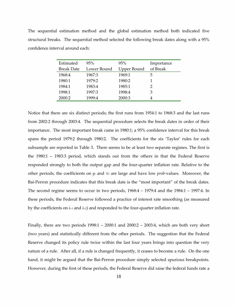
The sequential estimation method and the global estimation method both indicated five
structural breaks. The sequential method selected the following break dates along with a 95%
confidence interval around each:
Estimated Break Date
95% Lower Bound
95% Upper Bound
Importance of Break
1968:4 1967:3 1969:1 5 1980:1 1979:2 1980:2 1 1984:1 1983:4 1985:1 2 1998:1 1997:3 1998:4 3 2000:2 1999:4 2000:3 4
Notice that there are six distinct periods; the first runs from 1954:1 to 1968:3 and the last runs
from 2002:2 through 2003:4. The sequential procedure selects the break dates in order of their
importance. The most important break came in 1980:1; a 95% confidence interval for this break
spans the period 1979:2 through 1980:2. The coefficients for the six �Taylor� rules for each
subsample are reported in Table 3. There seems to be at least two separate regimes. The first is
the 1980:1 � 1983:3 period, which stands out from the others in that the Federal Reserve
responded strongly to both the output gap and the four-quarter inflation rate. Relative to the
other periods, the coefficients on yt and πt are large and have low prob-values. Moreover, the
Bai-Perron procedure indicates that this break date is the �most important� of the break dates.
The second regime seems to occur in two periods, 1968:4 � 1979:4 and the 1984:1 � 1997:4. In
these periods, the Federal Reserve followed a practice of interest rate smoothing (as measured
by the coefficients on it-1 and it-2) and responded to the four-quarter inflation rate.
Finally, there are two periods 1998:1 � 2000:1 and 2000:2 � 2003:4, which are both very short
(two years) and statistically different from the other periods. The suggestion that the Federal
Reserve changed its policy rule twice within the last four years brings into question the very
nature of a rule. After all, if a rule is changed frequently, it ceases to become a rule. On the one
hand, it might be argued that the Bai-Perron procedure simply selected spurious breakpoints.
However, during the first of these periods, the Federal Reserve did raise the federal funds rate a
19
number of times in order to stem the so-called �irrational exuberance� of the stock market. In
the second period, the Federal Reserve substantially decreased the federal funds rate in order to
stimulate economic activity. For these last two periods, we are skeptical on the actual
coefficients (and their t-statistics) since each of these periods contain only eight observations
which are used to estimate five coefficients.
If the BIC criterion is used to select the break dates instead of the sequential method, similar
break dates are chosen. The important difference is that 1984:3 � 2003:4 is estimated to be a
single�contiguous period. The estimated model for this sample period is
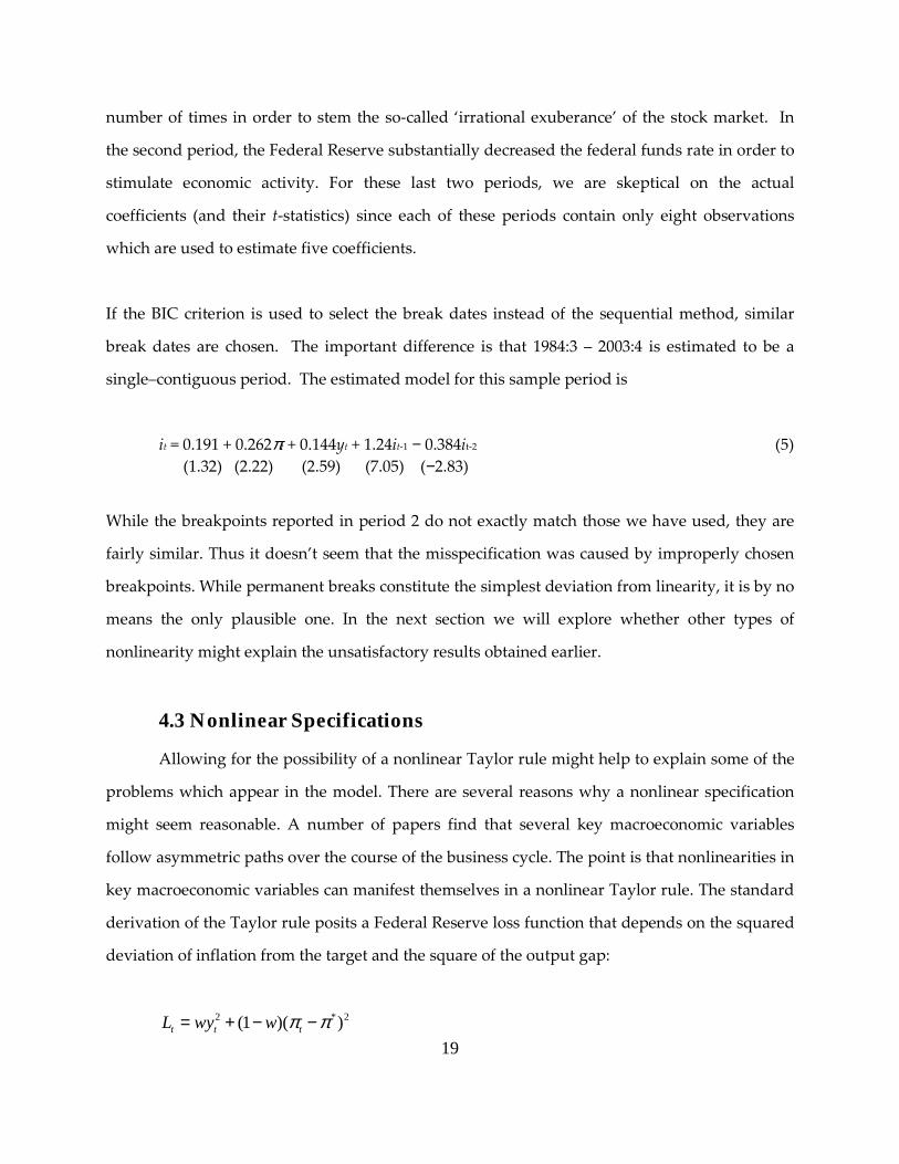
it = 0.191 + 0.262πt + 0.144yt + 1.24it-1 − 0.384it-2 (5)
(1.32) (2.22) (2.59) (7.05) (−2.83)
While the breakpoints reported in period 2 do not exactly match those we have used, they are
fairly similar. Thus it doesn�t seem that the misspecification was caused by improperly chosen
breakpoints. While permanent breaks constitute the simplest deviation from linearity, it is by no
means the only plausible one. In the next section we will explore whether other types of
nonlinearity might explain the unsatisfactory results obtained earlier.
4.3 Nonlinear Specifications
Allowing for the possibility of a nonlinear Taylor rule might help to explain some of the
problems which appear in the model. There are several reasons why a nonlinear specification
might seem reasonable. A number of papers find that several key macroeconomic variables
follow asymmetric paths over the course of the business cycle. The point is that nonlinearities in
key macroeconomic variables can manifest themselves in a nonlinear Taylor rule. The standard
derivation of the Taylor rule posits a Federal Reserve loss function that depends on the squared
deviation of inflation from the target and the square of the output gap:
2 * 2(1 )( )t t tL wy w π π= + − −
20
where L is a measure of the Federal Reserve�s overall loss, π* is the target inflation rate, and w is
the weight placed on the output gap in the loss function.
Since yt and πt are linear functions of the federal funds rate, the control problem is to select the
magnitude of the rate that minimizes the loss. A more complicated control problem would
allow for some rigidity in the system so that the rate exhibits some persistence. Nevertheless,
the solution from this linear-quadratic specification is a linear Taylor rule so that it is a linear
function of yt and πt.
There are many reasons to suppose that the linear-quadratic framework is problematic. One
possible source of nonlinearity is that the effect of the federal funds rate on the output gap or on
the inflation rate may not be linear. It is often claimed that monetary policy is like �pushing on a
string.� To the extent that it is more difficult to eliminate a negative output gap than a positive
gap, the Federal Reserve needs to decrease the federal funds rate more sharply than it increases
the rate. Similarly, there are a number of theoretical and empirical papers suggesting that
inflation increases more readily than it decreases. If it is more difficult to check inflation than to
allow inflation, the Federal Reserve needs to produce a relatively small reduction in the federal
funds rate when inflation is below the target. Another potential problem with the basic linear
model is that a quadratic loss function implies that the Federal Reserve is equally concerned
about high inflation and low inflation relative to the target rate. However, the recent concern
about deflation implies that losses from a small negative inflation are larger than the losses from
a small positive inflation. Even if we abstract from deflation, there is substantial reason to
believe that the loss function is not symmetric around π*. The so-called �inflation hawks� at the
Fed would be more tolerant of an inflation rate that is 1% below target than inflation that is 1%
above target. Similarly, a quadratic loss function assumes that the Fed is unconcerned about the
sign of the output gap; 1-unit shortfall of output from potential produces the same loss as a 1-
unit increase in output over potential. However, to many observers, negative output gaps in the
21
two Bush presidencies were more substantial problems than the positive output gap in the
Clinton years. These types of nonlinearities would imply that some sort of threshold model is
reasonable. Yet another source of nonlinearity would be if the standard assumption that the two
losses in the loss function are separable were relaxed such that the loss resulting from inflation
depended on the magnitude of the output gap. The non-separability of the loss function could
help explain why the combination of low output and high inflation is more intolerable than
high output and low inflation. Finally it is possible that changes in economic and political
circumstances can induce changes in the weight that the Federal Reserve places on the output
gap. Moreover, the target inflation rate need not be constant over time. These types of
nonlinearities would imply either permanent breaks, which we examined in Section 4.2, or that
we do not have a Taylor rule, in the case of a constantly changing inflation target.
To uncover any nonlinearities, we began by performing a number of diagnostic tests to help
uncover any nonlinearities using various sample periods. The Regression Error Specification
Test (RESET) posits the null hypothesis of linearity against a general alternative hypothesis of
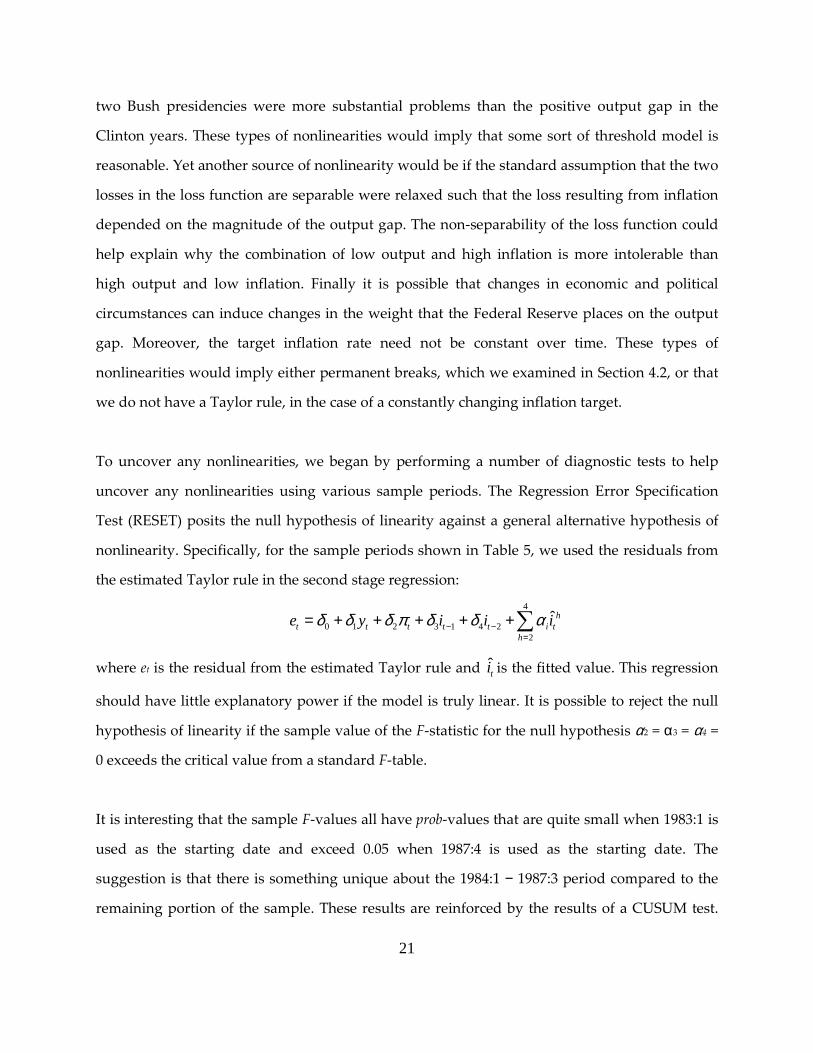
nonlinearity. Specifically, for the sample periods shown in Table 5, we used the residuals from
the estimated Taylor rule in the second stage regression:
4
0 1 2 3 1 4 22
ˆht t t t t i t
he y i i iδ δ δ π δ δ α− −
== + + + + +∑
where et is the residual from the estimated Taylor rule and t̂i is the fitted value. This regression
should have little explanatory power if the model is truly linear. It is possible to reject the null
hypothesis of linearity if the sample value of the F-statistic for the null hypothesis α2 = α3 = α4 =
0 exceeds the critical value from a standard F-table.
It is interesting that the sample F-values all have prob-values that are quite small when 1983:1 is
used as the starting date and exceed 0.05 when 1987:4 is used as the starting date. The
suggestion is that there is something unique about the 1984:1 − 1987:3 period compared to the
remaining portion of the sample. These results are reinforced by the results of a CUSUM test.
22
As shown in Panel 1 of Figure 5, if a starting date of 1983:1 is used, the cusums begin to depart
from the lower 5% confidence bound beginning almost immediately. Instead, if 1987:4 is used as
the initial starting date, the cusums stay bounded within a ± 5% band for almost the entire
sample period. Next we test for coefficient stability. We would not expect the coefficients to be
stable over time given the results we have so far, but we are hoping to obtain some more
concrete information. We use the coefficient stability test introduced in Hansen (1991).
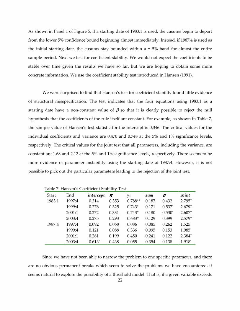
We were surprised to find that Hansen�s test for coefficient stability found little evidence
of structural misspecification. The test indicates that the four equations using 1983:1 as a
starting date have a non-constant value of β so that it is clearly possible to reject the null
hypothesis that the coefficients of the rule itself are constant. For example, as shown in Table 7,
the sample value of Hansen�s test statistic for the intercept is 0.346. The critical values for the
individual coefficients and variance are 0.470 and 0.748 at the 5% and 1% significance levels,
respectively. The critical values for the joint test that all parameters, including the variance, are
constant are 1.68 and 2.12 at the 5% and 1% significance levels, respectively. There seems to be
more evidence of parameter instability using the starting date of 1987:4. However, it is not
possible to pick out the particular parameters leading to the rejection of the joint test.
Table 7: Hansen�s Coefficient Stability Test Start End intercept ππππt yt sum σσσσ2 Joint 1983:1 1997:4 0.314 0.353 0.788** 0.187 0.432 2.795** 1999:4 0.276 0.325 0.743* 0.171 0.537* 2.679** 2001:1 0.272 0.331 0.743* 0.180 0.530* 2.607** 2003:4 0.275 0.293 0.683* 0.129 0.399 2.579** 1987:4 1997:4 0.092 0.068 0.086 0.085 0.262 1.525 1999:4 0.121 0.088 0.336 0.095 0.153 1.985* 2001:1 0.261 0.199 0.450 0.241 0.122 2.384** 2003:4 0.613* 0.438 0.055 0.354 0.138 1.918*
Since we have not been able to narrow the problem to one specific parameter, and there
are no obvious permanent breaks which seem to solve the problems we have encountered, it
seems natural to explore the possibility of a threshold model. That is, if a given variable exceeds
23
a threshold, the fed reacts in one manner, otherwise it has a different response. Judging from
the press releases of the fed, the most natural candidate for a threshold variable would seem to
be inflation, but we investigate all three variables as possible threshold variables. To this end,
we performed Hansen�s (1997) test for a threshold process. Specifically, Hansen develops a test
to determine whether all values of βi in the following equation are equal to zero:10
it = α0 + α1πt + α2yt + α3it-1 + α4∆it-2 + It(β0 + β1πt + β2yt + β3it-1 +β4∆it-2 ) + εt
where: It = 1 if xt-d > τ and It = 0 otherwise. We let d take on the values of 1 and 2. The consistent
estimate of d is obtained from the regression with the best fit. The consistent estimate of τ is
obtained using a grid search over all potential thresholds. We followed the customary
procedure by eliminating the lowest and highest 15% of the ordered values of xt-d in order to
ensure an adequate number of observations on each side of the threshold. Notice that It is an
indicator function that denotes whether the magnitude of xt-d exceeds a particular threshold
value. The essence of the model is that there are two linear segments for the Taylor rule. If the
value of xt-d exceeds the threshold, the federal funds rate is given by it = α0 + α1πt + α2yt + α3it-1 +
α4∆it-2 + εt. Alternatively, if xt-d ≤ τ the federal funds rate is given by it = (α0 + β0) + (α1 + β1)πt + (α2
+ β2)yt + (α3 + β3)it-1 + (α4 + β4)∆it-2 + εt. If all values of βi equal zero, the model is linear. Since the
threshold is estimated along with the other parameters of the model, the test for the null
hypothesis of linearity (i.e., all values of βi = 0) cannot be performed using a standard F-test.
Hansen (1997) shows how to appropriately perform an F-test test using a bootstrapping
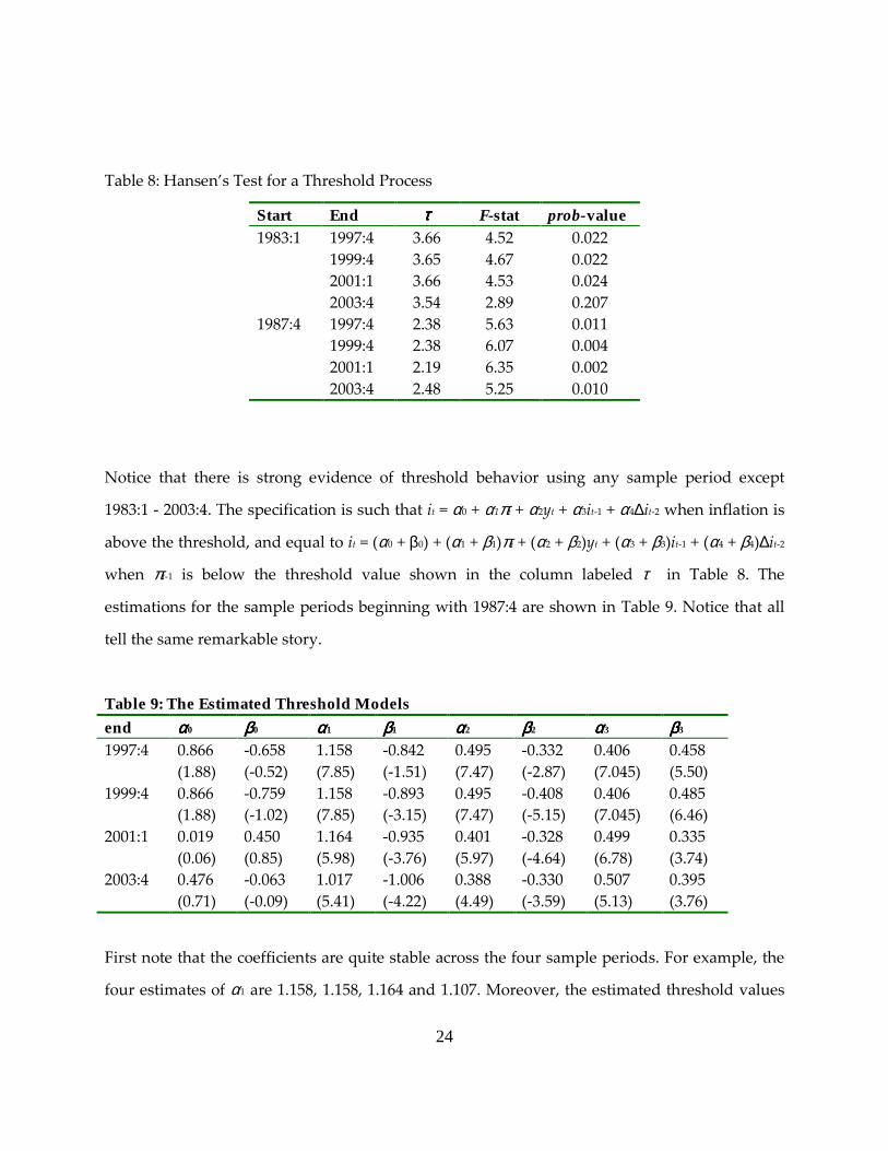
procedure. We used 4000 bootstrap replications for each of the sample periods listed in Table 8
and as expected, we found πt-1 was a better candidate for the threshold variable than πt-2, yt-1 or
yt-2. When we used πt-1 as the threshold variable, we obtained:
10 Notice that it = α0 + α1πt + α2yt + a1it-1 + a2it-2 is easily transformed into it = α0 + α1πt + α2yt + α3it-1 + α4∆it-1 where α3 = a1 + a2 and α4 = − a2. Hence, the coefficient on it-1 is the standard measure of autoregressive persistence.
24
Table 8: Hansen�s Test for a Threshold Process
Start End ττττ F-stat prob-value 1983:1 1997:4 3.66 4.52 0.022 1999:4 3.65 4.67 0.022 2001:1 3.66 4.53 0.024 2003:4 3.54 2.89 0.207 1987:4 1997:4 2.38 5.63 0.011 1999:4 2.38 6.07 0.004 2001:1 2.19 6.35 0.002 2003:4 2.48 5.25 0.010
Notice that there is strong evidence of threshold behavior using any sample period except
1983:1 - 2003:4. The specification is such that it = α0 + α1πt + α2yt + α3it-1 + α4∆it-2 when inflation is
above the threshold, and equal to it = (α0 + β0) + (α1 + β1)πt + (α2 + β2)yt + (α3 + β3)it-1 + (α4 + β4)∆it-2
when πt-1 is below the threshold value shown in the column labeled τ in Table 8. The
estimations for the sample periods beginning with 1987:4 are shown in Table 9. Notice that all
tell the same remarkable story.
Table 9: The Estimated Threshold Models end αααα0 ββββ0 αααα1 ββββ1 αααα2 ββββ2 αααα3 ββββ3
1997:4 0.866 -0.658 1.158 -0.842 0.495 -0.332 0.406 0.458 (1.88) (-0.52) (7.85) (-1.51) (7.47) (-2.87) (7.045) (5.50) 1999:4 0.866 -0.759 1.158 -0.893 0.495 -0.408 0.406 0.485 (1.88) (-1.02) (7.85) (-3.15) (7.47) (-5.15) (7.045) (6.46) 2001:1 0.019 0.450 1.164 -0.935 0.401 -0.328 0.499 0.335 (0.06) (0.85) (5.98) (-3.76) (5.97) (-4.64) (6.78) (3.74) 2003:4 0.476 -0.063 1.017 -1.006 0.388 -0.330 0.507 0.395 (0.71) (-0.09) (5.41) (-4.22) (4.49) (-3.59) (5.13) (3.76)
First note that the coefficients are quite stable across the four sample periods. For example, the
four estimates of α1 are 1.158, 1.158, 1.164 and 1.107. Moreover, the estimated threshold values
25
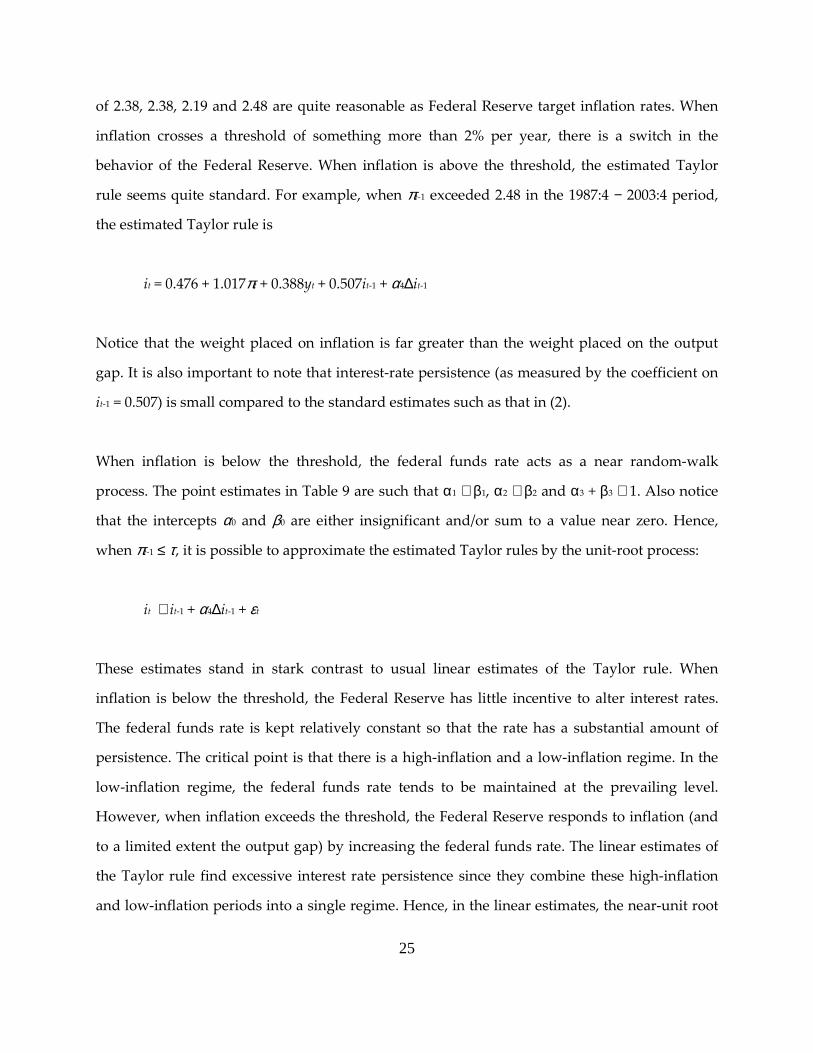
of 2.38, 2.38, 2.19 and 2.48 are quite reasonable as Federal Reserve target inflation rates. When
inflation crosses a threshold of something more than 2% per year, there is a switch in the
behavior of the Federal Reserve. When inflation is above the threshold, the estimated Taylor
rule seems quite standard. For example, when πt-1 exceeded 2.48 in the 1987:4 − 2003:4 period,
the estimated Taylor rule is
it = 0.476 + 1.017πt + 0.388yt + 0.507it-1 + α4∆it-1
Notice that the weight placed on inflation is far greater than the weight placed on the output
gap. It is also important to note that interest-rate persistence (as measured by the coefficient on
it-1 = 0.507) is small compared to the standard estimates such as that in (2).
When inflation is below the threshold, the federal funds rate acts as a near random-walk
process. The point estimates in Table 9 are such that α1 ≅ β1, α2 ≅ β2 and α3 + β3 ≅ 1. Also notice
that the intercepts α0 and β0 are either insignificant and/or sum to a value near zero. Hence,
when πt-1 ≤ τ, it is possible to approximate the estimated Taylor rules by the unit-root process:
it ≅ it-1 + α4∆it-1 + εt
These estimates stand in stark contrast to usual linear estimates of the Taylor rule. When
inflation is below the threshold, the Federal Reserve has little incentive to alter interest rates.
The federal funds rate is kept relatively constant so that the rate has a substantial amount of
persistence. The critical point is that there is a high-inflation and a low-inflation regime. In the
low-inflation regime, the federal funds rate tends to be maintained at the prevailing level.
However, when inflation exceeds the threshold, the Federal Reserve responds to inflation (and
to a limited extent the output gap) by increasing the federal funds rate. The linear estimates of
the Taylor rule find excessive interest rate persistence since they combine these high-inflation
and low-inflation periods into a single regime. Hence, in the linear estimates, the near-unit root
26
regime is �averaged� with a regime with moderate interest rate persistence. In addition this
model explains why reaction to the output gap decreased over time when we estimated
equation (3). In the latter part of the sample most of the observations fall in the low inflation
regime where there is no reaction to the output gap. Similarly, the fact that the federal reserve
bank let the federal funds rate �float� in this period would account for the appearance that the
response to inflation decreased over time.
The threshold model seemingly provides a plausible explanation of the results obtained in the
literature so far. Nevertheless, we seem to have come full circle since the threshold model acts
as a model with a structural break. To explain, the Panel a in Figure 6 shows the time path of πt
and Panel b shows the estimated thresholds obtained from using a recursive estimation
procedure. Specifically, for each time period in the interval T ≥ 1997:4 to 2003:4, we estimated a
threshold model with inflation as the threshold variable using observations 1987:4 through T.
The first point in Panel b shows the estimated threshold for the sample period ending in 1997:4.
The second point in Panel b shows the estimated threshold for the sample period ending in
1998:1, and so on. A comparison of Panels a and b shows that the thresholds actually split the
Greenspan period into two distinct regimes since inflation is almost always above the threshold
until 1991:1 and is almost always below the threshold after 1991:2. For all practical purposes, the
threshold model is the equivalent of a break at 1991:1.
Panel c shows the coefficients for inflation and the output gap for the regime in which
inflation is above the threshold (i.e., α1 and β1). When we examine Panel b and compare the
coefficients in Panel c to their counterparts in Figure 4, it is clear that the parameters of the
threshold process are very stable. The significance levels of Hansen�s test for a threshold process
are shown in Panel d. Notice that it is usually possible to reject the null of no threshold process
at the 1% significance level.
When we use the Johansen procedure to check for cointegration over the 1991:1 � 2003:4
period we are not able to reject the null of no cointegration at conventional significance levels.
This finding of no cointegration supports the notion that the federal funds rate is not adjusted to
27
the inflation rate or output gap in the low-inflation regime. Moreover, if we estimate a standard
Taylor rule for this period we obtain:
it = 0.392 + 0.019πt + 0.064yt + 1.53it-1 � 0.625∆it-1 (2.09) (0.148) (1.50) (13.48) (−5.84)
As such, the inflation rate and the income gap are insignificant so that the federal funds rate acts
as a univariate process with a characteristic root near unity.
The point is that it is very hard to maintain the existence of a Taylor rule during the
Greenspan period. We tried estimating the Taylor rule as smooth transition LSTAR and ESTAR
processes. However, the estimations were very similar to that of the threshold model. This
should not be too surprising since, as shown in Figure 6, the there are really only two regimes
and the transition occurs rather abruptly.
5. Conclusion
In his original paper, Taylor (1993) made it clear that his rule was not intended to be a precise
formula. In the Abstract, he states �An objective of the paper is to preserve the concept of such a
policy rule in a policy environment where it is practically impossible to follow mechanically any
particular algebraic formula that describes the policy rule.� Similarly, in a recent theoretical
paper, Svensson (2003) raised serious doubts about the Taylor rule, because it is �incomplete
and too vague to be operational� since �there are no rules for when deviations from the
instrument rule are appropriate.� Our findings generally support this view. The nonstationary
variables comprising the rule are not cointegrated within any reasonable subsample of the
1954:3 − 2003:4 period. In the few cases where cointegration seems to hold, the signs of the
coefficients are incorrect and/or the federal funds rate appears to be weakly exogenous. For the
Greenspan period, the performance of the rule is not improved by adding additional variables
such as a measure of irrational exuberance or a measure of consumer confidence. Nonlinear
models seem to indicate that the federal reserve was passive for the entire period beginning in
1991.
28
Given what we know about Alan Greenspan and the conduct of monetary policy, the
only conclusion we can draw is that Taylor (1993) and Svensson (2003) were right. There is no
doubt that the Federal Reserve pays attention to inflation and the output gap when deciding the
course of monetary policy. The question is whether a simple mechanistic rule adequately
describes the behavior of the federal funds rate. Our findings support the notion that there is no
simple rule that is consistent with the data.

29
References
Amato, J., Laubach, T., 1999. The value of interest rate smoothing: how the private sector helps the Federal Reserve. Economic Review, Federal Reserve Bank of Kansas City, 84, 47�64.
Bai, J., Perron, P., 2003. Computation and Analysis of Multiple Structural Change Models. Journal of Applied Econometrics, 18, 1-22.
Clarida, R., Gali, J., Gertler, M., 2000. Monetary policy rules and macroeconomic stability: evidence and some theory. Quarterly Journal of Economics 115, 147�180. Dolado, J.J., R. Maria-Dolores and M. Naveira, 2004, Are Monetary-Policy Reaction Functions Asymmetric? The Role of Nonlinearity in the Phillips Curve. European Economic Review, forthcoming. Elliott, G., Rothenberg, T. J., and Stock, J. H. 1996. Efficient Tests for an Autoregressive Unit Root, Econometrica, 64, 813-836. English, W.B., Nelson, W.R. and B.P. Sack 2002. Interpreting the Significance of the Lagged Interest Rate in Estimated Monetary Policy Rules. Finance and Economics Discussion Series Working Paper No. 2002-24, Board of Governors of the Federal Reserve System. Goodhart, C., 1999. Central bankers and uncertainty. Bank of England Quarterly Bulletin, 39, 102�115. Harvey, D.I, Leybourne S.J. 2003. On Testing for Unit Roots and the Initial Observation. Mimeo. Kim, D.H., D.R. Osborne and M. Sensier, 2004, Nonlinearity in the Fed�s Monetary Policy Rule, Journal of Applied Econometrics, forthcoming. Levin, A., Wieland, V., Williams, J.C., 1999. Robustness of simple monetary policy rules under model uncertainty. In: Taylor, J.B. (Ed.), Monetary Policy Rules. University of Chicago Press, Chicago, pp. 263�299. Müller, U. K., and Elliott, G. 2003. Tests for Unit Roots and the Initial Condition, Econometrica, forthcoming. Nobay, R. and D. Peel, 2003, Optimal Discretionary Monetary Policy in a Model of Asymmetric Central Bank Preferences, Economic Journal 113, 657-665.
Österholm, P. (2005), ʺThe Taylor Rule: A Spurious Regression?ʺ, Bulletin of Economic Research, forthcoming.
Rudebusch, G.D., 2002. Term structure evidence on interest rate smoothing and monetary policy inertia. Journal of Monetary Economics, 49, 1161-1187.
30
Ruge-Murcia, F.J., 2003, Inflation Targeting under Asymmetric Preferences, Journal of Money, Credit and Banking 35, 763-785. Sack, B., 1998. Uncertainty, learning and gradual monetary policy. FEDS Working Paper 34, Federal Reserve Board. Shiller, R. J. 2000, Irrational Exuberance. Princeton, NJ: Princeton University Press Paolo Surico, P. 2004. Inflation Targeting and Nonlinear Policy Rules: the Case of Asymmetric Preferences. Computing in Economics and Finance 108 Svensson, L.E.O., 2003 What Is Wrong with Taylor Rules? Using Judgment in Monetary Policy through Targeting Rules. Journal of Economic Literature, 41, 426-477. Taylor, John B., 1993. Discretion versus policy rules in practice. Carnegie-Rochester Conference Series on Public Policy 39, 195-214. Woodford, M., 1999. Optimal monetary policy inertia. The Manchester School Supplement 1�35.
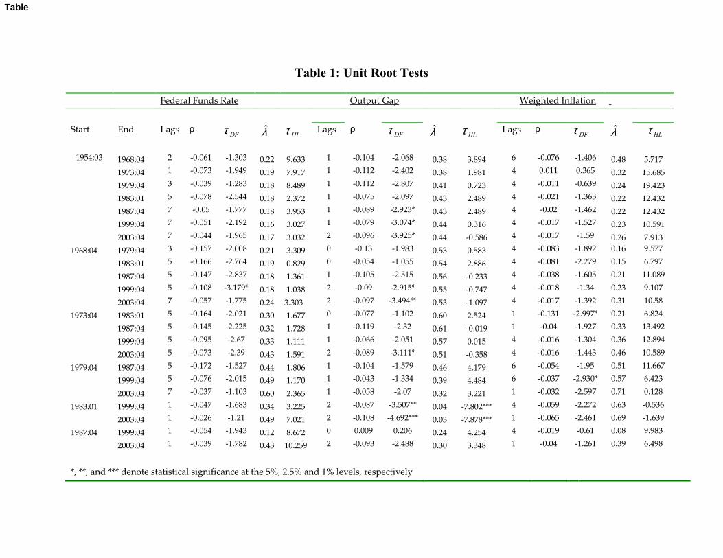
Table 1: Unit Root Tests
Federal Funds Rate Output Gap Weighted Inflation Start End Lags ρ Lags ρ Lags ρ
1954:03 1968:04 2 -0.061 -1.303 0.22 9.633 1 -0.104 -2.068 0.38 3.894 6 -0.076 -1.406 0.48 5.717 1973:04 1 -0.073 -1.949 0.19 7.917 1 -0.112 -2.402 0.38 1.981 4 0.011 0.365 0.32 15.685 1979:04 3 -0.039 -1.283 0.18 8.489 1 -0.112 -2.807 0.41 0.723 4 -0.011 -0.639 0.24 19.423 1983:01 5 -0.078 -2.544 0.18 2.372 1 -0.075 -2.097 0.43 2.489 4 -0.021 -1.363 0.22 12.432 1987:04 7 -0.05 -1.777 0.18 3.953 1 -0.089 -2.923* 0.43 2.489 4 -0.02 -1.462 0.22 12.432 1999:04 7 -0.051 -2.192 0.16 3.027 1 -0.079 -3.074* 0.44 0.316 4 -0.017 -1.527 0.23 10.591 2003:04 7 -0.044 -1.965 0.17 3.032 2 -0.096 -3.925* 0.44 -0.586 4 -0.017 -1.59 0.26 7.913
1968:04 1979:04 3 -0.157 -2.008 0.21 3.309 0 -0.13 -1.983 0.53 0.583 4 -0.083 -1.892 0.16 9.577 1983:01 5 -0.166 -2.764 0.19 0.829 0 -0.054 -1.055 0.54 2.886 4 -0.081 -2.279 0.15 6.797 1987:04 5 -0.147 -2.837 0.18 1.361 1 -0.105 -2.515 0.56 -0.233 4 -0.038 -1.605 0.21 11.089 1999:04 5 -0.108 -3.179* 0.18 1.038 2 -0.09 -2.915* 0.55 -0.747 4 -0.018 -1.34 0.23 9.107 2003:04 7 -0.057 -1.775 0.24 3.303 2 -0.097 -3.494** 0.53 -1.097 4 -0.017 -1.392 0.31 10.58
1973:04 1983:01 5 -0.164 -2.021 0.30 1.677 0 -0.077 -1.102 0.60 2.524 1 -0.131 -2.997* 0.21 6.824 1987:04 5 -0.145 -2.225 0.32 1.728 1 -0.119 -2.32 0.61 -0.019 1 -0.04 -1.927 0.33 13.492 1999:04 5 -0.095 -2.67 0.33 1.111 1 -0.066 -2.051 0.57 0.015 4 -0.016 -1.304 0.36 12.894 2003:04 5 -0.073 -2.39 0.43 1.591 2 -0.089 -3.111* 0.51 -0.358 4 -0.016 -1.443 0.46 10.589
1979:04 1987:04 5 -0.172 -1.527 0.44 1.806 1 -0.104 -1.579 0.46 4.179 6 -0.054 -1.95 0.51 11.667 1999:04 5 -0.076 -2.015 0.49 1.170 1 -0.043 -1.334 0.39 4.484 6 -0.037 -2.930* 0.57 6.423 2003:04 7 -0.037 -1.103 0.60 2.365 1 -0.058 -2.07 0.32 3.221 1 -0.032 -2.597 0.71 0.128
1983:01 1999:04 1 -0.047 -1.683 0.34 3.225 2 -0.087 -3.507** 0.04 -7.802*** 4 -0.059 -2.272 0.63 -0.536 2003:04 1 -0.026 -1.21 0.49 7.021 2 -0.108 -4.692*** 0.03 -7.878*** 1 -0.065 -2.461 0.69 -1.639
1987:04 1999:04 1 -0.054 -1.943 0.12 8.672 0 0.009 0.206 0.24 4.254 4 -0.019 -0.61 0.08 9.983 2003:04 1 -0.039 -1.782 0.43 10.259 2 -0.093 -2.488 0.30 3.348 1 -0.04 -1.261 0.39 6.498
*, **, and *** denote statistical significance at the 5%, 2.5% and 1% levels, respectively
DFτ DFτ DFτ λ̂ HLτλ̂ HLτHLτλ̂
Table
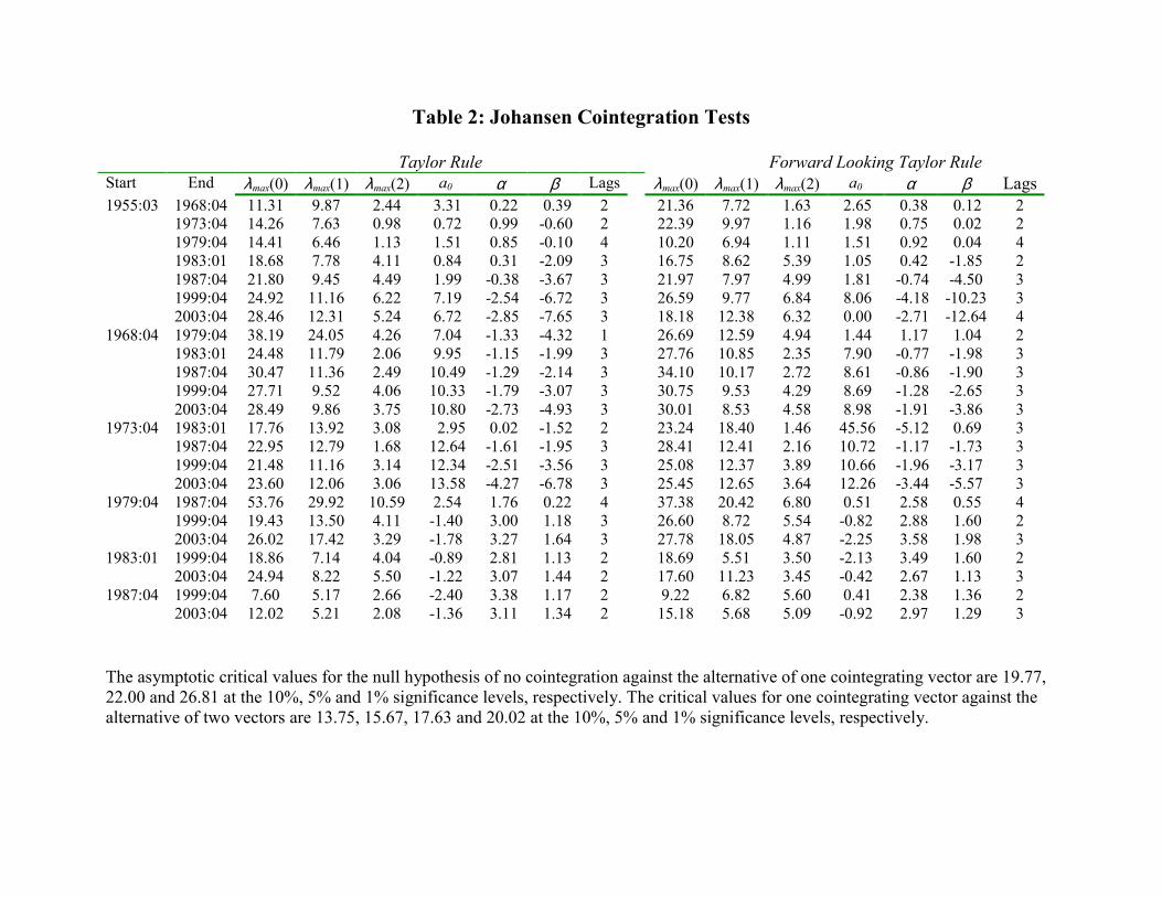
Table 2: Johansen Cointegration Tests Taylor Rule Forward Looking Taylor Rule Start End λmax(0) λmax(1) λmax(2) a0 α β Lags λmax(0) λmax(1) λmax(2) a0 α β Lags1955:03 1968:04 11.31 9.87 2.44 3.31 0.22 0.39 2 21.36 7.72 1.63 2.65 0.38 0.12 2 1973:04 14.26 7.63 0.98 0.72 0.99 -0.60 2 22.39 9.97 1.16 1.98 0.75 0.02 2 1979:04 14.41 6.46 1.13 1.51 0.85 -0.10 4 10.20 6.94 1.11 1.51 0.92 0.04 4 1983:01 18.68 7.78 4.11 0.84 0.31 -2.09 3 16.75 8.62 5.39 1.05 0.42 -1.85 2 1987:04 21.80 9.45 4.49 1.99 -0.38 -3.67 3 21.97 7.97 4.99 1.81 -0.74 -4.50 3 1999:04 24.92 11.16 6.22 7.19 -2.54 -6.72 3 26.59 9.77 6.84 8.06 -4.18 -10.23 3 2003:04 28.46 12.31 5.24 6.72 -2.85 -7.65 3 18.18 12.38 6.32 0.00 -2.71 -12.64 4 1968:04 1979:04 38.19 24.05 4.26 7.04 -1.33 -4.32 1 26.69 12.59 4.94 1.44 1.17 1.04 2 1983:01 24.48 11.79 2.06 9.95 -1.15 -1.99 3 27.76 10.85 2.35 7.90 -0.77 -1.98 3 1987:04 30.47 11.36 2.49 10.49 -1.29 -2.14 3 34.10 10.17 2.72 8.61 -0.86 -1.90 3 1999:04 27.71 9.52 4.06 10.33 -1.79 -3.07 3 30.75 9.53 4.29 8.69 -1.28 -2.65 3 2003:04 28.49 9.86 3.75 10.80 -2.73 -4.93 3 30.01 8.53 4.58 8.98 -1.91 -3.86 3 1973:04 1983:01 17.76 13.92 3.08 2.95 0.02 -1.52 2 23.24 18.40 1.46 45.56 -5.12 0.69 3 1987:04 22.95 12.79 1.68 12.64 -1.61 -1.95 3 28.41 12.41 2.16 10.72 -1.17 -1.73 3 1999:04 21.48 11.16 3.14 12.34 -2.51 -3.56 3 25.08 12.37 3.89 10.66 -1.96 -3.17 3 2003:04 23.60 12.06 3.06 13.58 -4.27 -6.78 3 25.45 12.65 3.64 12.26 -3.44 -5.57 3 1979:04 1987:04 53.76 29.92 10.59 2.54 1.76 0.22 4 37.38 20.42 6.80 0.51 2.58 0.55 4 1999:04 19.43 13.50 4.11 -1.40 3.00 1.18 3 26.60 8.72 5.54 -0.82 2.88 1.60 2 2003:04 26.02 17.42 3.29 -1.78 3.27 1.64 3 27.78 18.05 4.87 -2.25 3.58 1.98 3 1983:01 1999:04 18.86 7.14 4.04 -0.89 2.81 1.13 2 18.69 5.51 3.50 -2.13 3.49 1.60 2 2003:04 24.94 8.22 5.50 -1.22 3.07 1.44 2 17.60 11.23 3.45 -0.42 2.67 1.13 3 1987:04 1999:04 7.60 5.17 2.66 -2.40 3.38 1.17 2 9.22 6.82 5.60 0.41 2.38 1.36 2 2003:04 12.02 5.21 2.08 -1.36 3.11 1.34 2 15.18 5.68 5.09 -0.92 2.97 1.29 3 The asymptotic critical values for the null hypothesis of no cointegration against the alternative of one cointegrating vector are 19.77, 22.00 and 26.81 at the 10%, 5% and 1% significance levels, respectively. The critical values for one cointegrating vector against the alternative of two vectors are 13.75, 15.67, 17.63 and 20.02 at the 10%, 5% and 1% significance levels, respectively.
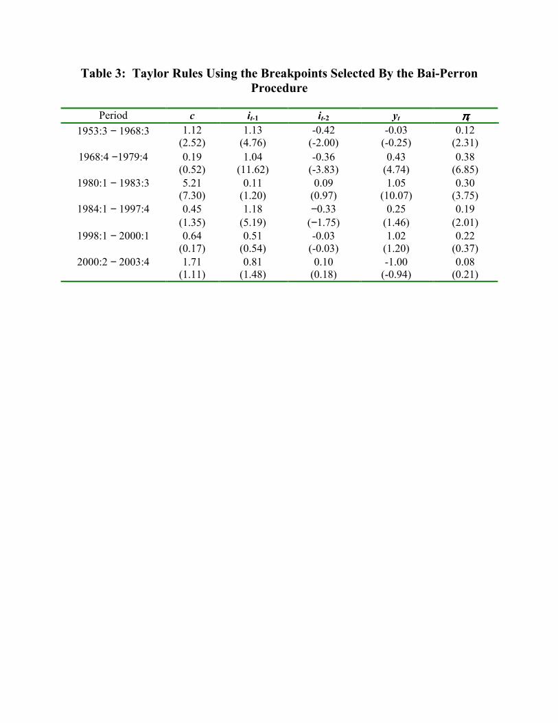
Table 3: Taylor Rules Using the Breakpoints Selected By the Bai-Perron Procedure
Period c it-1 it-2 yt ππππt
1953:3 − 1968:3
1.12 (2.52)
1.13 (4.76)
-0.42 (-2.00)
-0.03 (-0.25)
0.12 (2.31)
1968:4 −1979:4
0.19 (0.52)
1.04 (11.62)
-0.36 (-3.83)
0.43 (4.74)
0.38 (6.85)
1980:1 − 1983:3 5.21 0.11 0.09 1.05 0.30 (7.30) (1.20) (0.97) (10.07) (3.75)
1984:1 − 1997:4 0.45 1.18 −0.33 0.25 0.19 (1.35) (5.19) (−1.75) (1.46) (2.01)
1998:1 − 2000:1 0.64 0.51 -0.03 1.02 0.22 (0.17) (0.54) (-0.03) (1.20) (0.37)
2000:2 − 2003:4 1.71 0.81 0.10 -1.00 0.08 (1.11) (1.48) (0.18) (-0.94) (0.21)
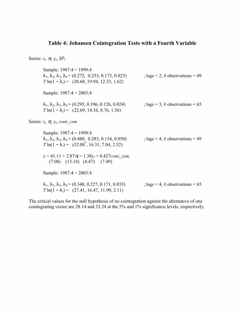
Table 4: Johansen Cointegration Tests with a Fourth Variable Series: it, πt, yt, SPt
Sample: 1987:4 − 1999:4 λ1, λ2, λ3, λ4 = (0.272, 0.253, 0.173, 0.025) ; lags = 2, # observations = 49 T ln(1 − λ i) = (20.68, 19.94, 12.33, 1.62)
Sample: 1987:4 − 2003:4
λ1, λ2, λ3, λ4 = (0.295, 0.196, 0.126, 0.024) ; lags = 3, # observations = 65 T ln(1 − λ i) = (22.69, 14.16, 8.76, 1.56)
Series: it, πt, yt, cons_con
Sample: 1987:4 − 1999:4 λ1, λ2, λ3, λ4 = (0.480, 0.283, 0.134, 0.050) ; lags = 4, # observations = 49 T ln(1 − λ i) = (32.08*, 16.31, 7.04, 2.52)
it = 41.11 + 2.87πt − 1.38yt + 0.427cons_cont (7.08) (13.14) (4.47) (7.49)
Sample: 1987:4 − 2003:4
λ1, λ2, λ3, λ4 = (0.348, 0.227, 0.171, 0.033) ; lags = 4, # observations = 65 T ln(1 − λ i) = (27.41, 16.47, 11.99, 2.11)
The critical values for the null hypothesis of no cointegration against the alternative of one cointegrating vector are 28.14 and 33.24 at the 5% and 1% significance levels, respectively.
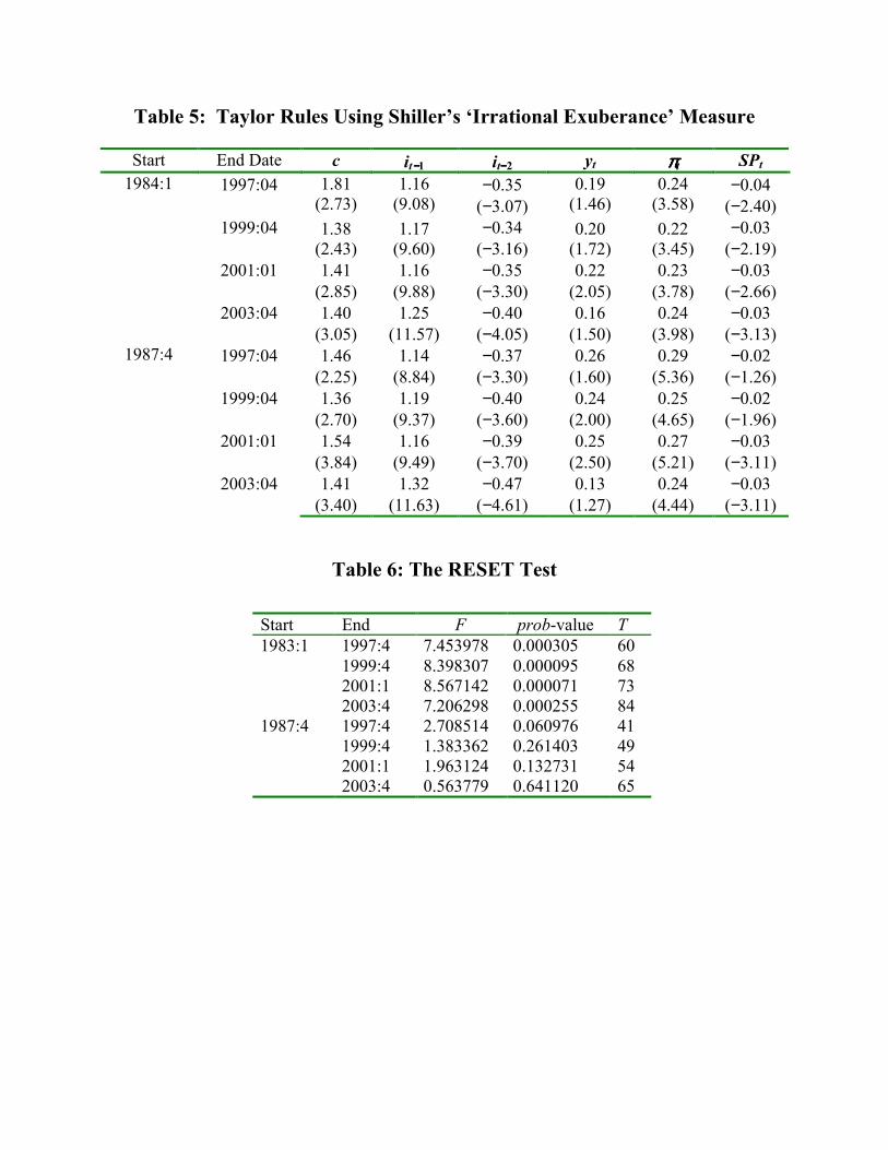
Table 5: Taylor Rules Using Shiller’s ‘Irrational Exuberance’ Measure
Start End Date c it−−−−1 it−−−−2 yt ππππt SPt
1984:1 1997:04 −0.04
1.81 (2.73)
1.16 (9.08)
−0.35 (−3.07)
0.19 (1.46)
0.24 (3.58) (−2.40)
1999:04 −0.03
1.38 (2.43)
1.17 (9.60)
−0.34 (−3.16)
0.20 (1.72)
0.22 (3.45) (−2.19)
2001:01 1.41 1.16 −0.35 0.22 0.23 −0.03 (2.85) (9.88) (−3.30) (2.05) (3.78) (−2.66) 2003:04 1.40 1.25 −0.40 0.16 0.24 −0.03 (3.05) (11.57) (−4.05) (1.50) (3.98) (−3.13)
1987:4 1997:04 1.46 1.14 −0.37 0.26 0.29 −0.02 (2.25) (8.84) (−3.30) (1.60) (5.36) (−1.26) 1999:04 1.36 1.19 −0.40 0.24 0.25 −0.02 (2.70) (9.37) (−3.60) (2.00) (4.65) (−1.96) 2001:01 1.54 1.16 −0.39 0.25 0.27 −0.03 (3.84) (9.49) (−3.70) (2.50) (5.21) (−3.11) 2003:04 1.41 1.32 −0.47 0.13 0.24 −0.03 (3.40) (11.63) (−4.61) (1.27) (4.44) (−3.11)
Table 6: The RESET Test
Start End F prob-value T 1983:1 1997:4 7.453978 0.000305 60 1999:4 8.398307 0.000095 68 2001:1 8.567142 0.000071 73 2003:4 7.206298 0.000255 84 1987:4 1997:4 2.708514 0.060976 41 1999:4 1.383362 0.261403 49 2001:1 1.963124 0.132731 54 2003:4 0.563779 0.641120 65
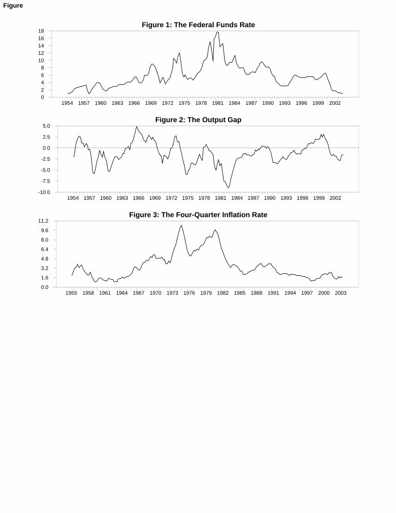
Figure 1: The Federal Funds Rate
1954 1957 1960 1963 1966 1969 1972 1975 1978 1981 1984 1987 1990 1993 1996 1999 200202468
1012141618
Figure 2: The Output Gap
1954 1957 1960 1963 1966 1969 1972 1975 1978 1981 1984 1987 1990 1993 1996 1999 2002-10.0
-7.5
-5.0
-2.5
0.0
2.5
5.0
Figure 3: The Four-Quarter Inflation Rate
1955 1958 1961 1964 1967 1970 1973 1976 1979 1982 1985 1988 1991 1994 1997 2000 20030.0
1.6
3.2
4.8
6.4
8.0
9.6
11.2
Figure
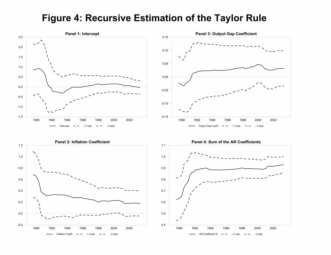
Figure 4: Recursive Estimation of the Taylor Rule
Intercept + 2 sds. - 2 stds.
Panel 1: Intercept
1990 1992 1994 1996 1998 2000 2002-1.5
-1.0
-0.5
0.0
0.5
1.0
1.5
2.0
2.5
Inflation Coeffi + 2 sds. - 2 stds.
Panel 2: Inflation Coefficient
1990 1992 1994 1996 1998 2000 2002-0.2
0.0
0.2
0.4
0.6
0.8
1.0
1.2
Output Gap Coeff + 2 sds. - 2 stds.
Panel 3: Output Gap Coefficient
1990 1992 1994 1996 1998 2000 2002-0.15
-0.10
-0.05
0.00
0.05
0.10
0.15
AR Coefficient S + 2 sds. - 2 stds.
Panel 4: Sum of the AR Coefficients
1990 1992 1994 1996 1998 2000 20020.4
0.5
0.6
0.7
0.8
0.9
1.0
1.1
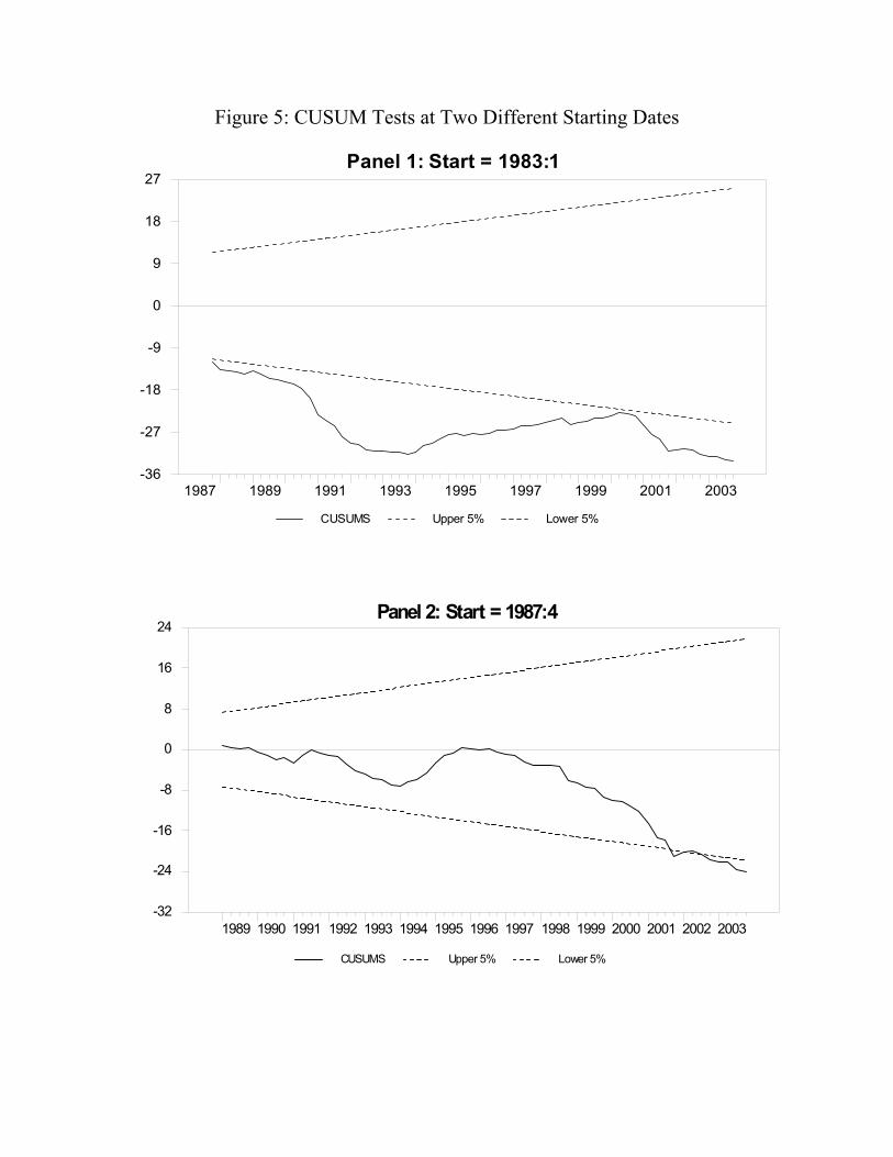
Figure 5: CUSUM Tests at Two Different Starting Dates
CUSUMS Upper 5% Lower 5%
Panel 1: Start = 1983:1
1987 1989 1991 1993 1995 1997 1999 2001 2003-36
-27
-18
-9
0
9
18
27
CUSUMS Upper 5% Lower 5%
Panel 2: Start = 1987:4
1989 1990 1991 1992 1993 1994 1995 1996 1997 1998 1999 2000 2001 2002 2003-32
-24
-16
-8
0
8
16
24
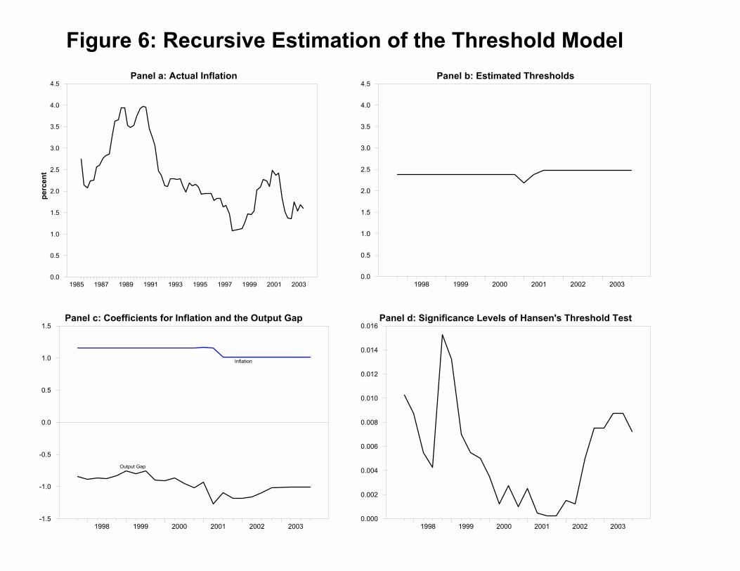
Figure 6: Recursive Estimation of the Threshold ModelPanel a: Actual Inflation
perc
ent
1985 1987 1989 1991 1993 1995 1997 1999 2001 20030.0
0.5
1.0
1.5
2.0
2.5
3.0
3.5
4.0
4.5
Panel c: Coefficients for Inflation and the Output Gap
1998 1999 2000 2001 2002 2003-1.5
-1.0
-0.5
0.0
0.5
1.0
1.5
Output Gap
Inflation
Panel b: Estimated Thresholds
1998 1999 2000 2001 2002 20030.0
0.5
1.0
1.5
2.0
2.5
3.0
3.5
4.0
4.5
Panel d: Significance Levels of Hansen's Threshold Test
1998 1999 2000 2001 2002 20030.000
0.002
0.004
0.006
0.008
0.010
0.012
0.014
0.016