Air Force Institute of TechnologyAFIT Scholar
Theses and Dissertations Student Graduate Works
3-23-2018
The Impact of Changing RequirementsJames C. Ellis
Follow this and additional works at: https://scholar.afit.edu/etd
Part of the Statistics and Probability Commons
This Thesis is brought to you for free and open access by the Student Graduate Works at AFIT Scholar. It has been accepted for inclusion in Theses andDissertations by an authorized administrator of AFIT Scholar. For more information, please contact [email protected].
Recommended CitationEllis, James C., "The Impact of Changing Requirements" (2018). Theses and Dissertations. 1736.https://scholar.afit.edu/etd/1736

THE IMPACT OF CHANGING REQUIREMENTS
THESIS
James C. Ellis, Captain, USAF
AFIT-ENC-MS-18-M-200
DEPARTMENT OF THE AIR FORCE AIR UNIVERSITY
AIR FORCE INSTITUTE OF TECHNOLOGY
Wright-Patterson Air Force Base, Ohio
DISTRIBUTION STATEMENT A. APPROVED FOR PUBLIC RELEASE; DISTRIBUTION UNLIMITED.

The views expressed in this thesis are those of the author and do not reflect the official policy or position of the United States Air Force, Department of Defense, or the United States Government. This material is declared a work of the U.S. Government and is not subject to copyright protection in the United States.

AFIT-ENC-MS-18-M-200
THE IMPACT OF CHANGING REQUIREMENTS
THESIS
Presented to the Faculty
Department of Mathematics and Statistics
Graduate School of Engineering and Management
Air Force Institute of Technology
Air University
Air Education and Training Command
In Partial Fulfillment of the Requirements for the
Degree of Master of Science in Cost Analysis
James C. Ellis, B.S.
Captain, USAF
March 2018
DISTRIBUTION STATEMENT A. APPROVED FOR PUBLIC RELEASE; DISTRIBUTION UNLIMITED.

AFIT-ENC-MS-18-M-200
The Impact of Changing Requirements
James C. Ellis,
Captain, USAF
Committee Membership:
Dr. Edward White Chair
Lt Col Brandon Lucas, Ph.D. Member
Dr. Jonathan Ritschel Member
Mr. Shawn Valentine Member

iv
AFIT-ENC-MS-18-M-200 Abstract
The fundamental purpose of an Engineering Change Proposal (ECP) is to change
the requirements of a contract. To build in flexibility, the acquisition practice is to
estimate a dollar value to hold in reserve after the contract is awarded. There appears to
be no empirical-based method for estimating this ECP withhold in the literature. Using
the Cost Assessment Data Enterprise (CADE) database, 533 contracts were randomly
selected to build two regression models: one to predict the likelihood of a contract
experiencing an ECP, and the other to determine the expected median percent increase in
baseline contract cost if an ECP was likely. Results suggest that this two-step approach
works well over a managed portfolio of contracts in contrast to three investigated rules-
of-thumb. Significant drivers are the basic contract cost and the number of contract line
items.

v
Acknowledgments
I would like to thank everyone that spent the time to listen to my ramblings about this
work. As time goes on, I am sure I will look back with a fondness and dislike at both the
good times creating the work and at how much more I could have done. Most
importantly, I want to thank my loving wife, not for her help on the thesis, but for her
general love and support.
James C. Ellis

Contents
Abstract . . . . . . . . . . . . . . . . . . . . . . . . . . . . . . . . . . . iv
Acknowledgements . . . . . . . . . . . . . . . . . . . . . . . . . . . . . . . v
List of Tables . . . . . . . . . . . . . . . . . . . . . . . . . . . . . . . . . viii
List of Figures . . . . . . . . . . . . . . . . . . . . . . . . . . . . . . . . . x
I. Introduction. . . . . . . . . . . . . . . . . . . . . . . . . . . . . . . . . 1
Background . . . . . . . . . . . . . . . . . . . . . . . . . . . . . . . . 1
Problem Statement . . . . . . . . . . . . . . . . . . . . . . . . . . . . . . 2
Research Objectives . . . . . . . . . . . . . . . . . . . . . . . . . . . . . 3
Research Questions . . . . . . . . . . . . . . . . . . . . . . . . . . . . . . 3
Methodology . . . . . . . . . . . . . . . . . . . . . . . . . . . . . . . . 3
Summary . . . . . . . . . . . . . . . . . . . . . . . . . . . . . . . . . 4
II. Literature Review . . . . . . . . . . . . . . . . . . . . . . . . . . . . . . 5
Engineering Change Proposals Defined. . . . . . . . . . . . . . . . . . . . . . . 5
Past and current state of cost growth . . . . . . . . . . . . . . . . . . . . . . . 6
ECPs Place in Cost Growth. . . . . . . . . . . . . . . . . . . . . . . . . . . 8
Causes of ECPs . . . . . . . . . . . . . . . . . . . . . . . . . . . . . . . 9
Program Level . . . . . . . . . . . . . . . . . . . . . . . . . . . . . 9
Contract Level . . . . . . . . . . . . . . . . . . . . . . . . . . . . . 10
Current Practice for Managing ECP. . . . . . . . . . . . . . . . . . . . . . . . 10
Ten percent rule of thumb. . . . . . . . . . . . . . . . . . . . . . . . . 11
Summary . . . . . . . . . . . . . . . . . . . . . . . . . . . . . . . . . 12
III. Methodology . . . . . . . . . . . . . . . . . . . . . . . . . . . . . . . . 13
Data . . . . . . . . . . . . . . . . . . . . . . . . . . . . . . . . . . . 13
Database Modifications . . . . . . . . . . . . . . . . . . . . . . . . . . . . 14
Missing Data . . . . . . . . . . . . . . . . . . . . . . . . . . . . . 14
Schedule Errors . . . . . . . . . . . . . . . . . . . . . . . . . . . . 15
Dollar Value Error . . . . . . . . . . . . . . . . . . . . . . . . . . . 15
Final Database to be Sampled . . . . . . . . . . . . . . . . . . . . . . . . . . 15
Limitations. . . . . . . . . . . . . . . . . . . . . . . . . . . . . . . . . 15
Stratifying Methods . . . . . . . . . . . . . . . . . . . . . . . . . . . . . 17
Model Diagnostic . . . . . . . . . . . . . . . . . . . . . . . . . . . . 18
vi

Validation . . . . . . . . . . . . . . . . . . . . . . . . . . . . . . 20
Comparison . . . . . . . . . . . . . . . . . . . . . . . . . . . . . . . . 20
IV. Journal - Likelihood and Cost Impact of Engineering Change Requirements for DoD Contracts . . 22
Introduction and Background . . . . . . . . . . . . . . . . . . . . . . . . . . 22
Database and Methodology . . . . . . . . . . . . . . . . . . . . . . . . . . . 23
Model Analysis . . . . . . . . . . . . . . . . . . . . . . . . . . . . . . . 26
Logistic Model . . . . . . . . . . . . . . . . . . . . . . . . . . . . . 27
OLS Model . . . . . . . . . . . . . . . . . . . . . . . . . . . . . . 28
Discussion and Conclusion . . . . . . . . . . . . . . . . . . . . . . . . . . . 29
References . . . . . . . . . . . . . . . . . . . . . . . . . . . . . . . . . 31
Appendix: Department of Defense programs used in the modeling database . . . . . . . . . 33
V. Conclusion . . . . . . . . . . . . . . . . . . . . . . . . . . . . . . . . . 40
Future Research . . . . . . . . . . . . . . . . . . . . . . . . . . . . . . . 41
References . . . . . . . . . . . . . . . . . . . . . . . . . . . . . . . . . . 43
vii

List of Tables
1 R Packages . . . . . . . . . . . . . . . . . . . . . . . . . . . . . . . . . . . . . . . . . . . . . 14
2 Final Database - Population . . . . . . . . . . . . . . . . . . . . . . . . . . . . . . . . . . . . 15
3 Filter History of Removing Errors . . . . . . . . . . . . . . . . . . . . . . . . . . . . . . . . 16
4 Unremoved Potential Errors . . . . . . . . . . . . . . . . . . . . . . . . . . . . . . . . . . . . 16
5 F18 Compared to Other Programs . . . . . . . . . . . . . . . . . . . . . . . . . . . . . . . . 17
6 Primary Exclusion Reasons. Percentages rounded to two decimal places. . . . . . . . . . . . 35
7 Initial population stratum characteristics. Strata pairs 1/2, 3/4, 5/6, and 7/8 are complemen-
tary events. All dollars presented in base year 2016 values. Baseline contract cost equals initial
contract cost plus all priced options. . . . . . . . . . . . . . . . . . . . . . . . . . . . . . . . 35
8 Population breakdown of the 5,927 contracts and associated percentages. Percentages rounded
to the nearest whole number. Note: the 0* denotes a percentage less than 1. . . . . . . . . . 35
9 Consolidated strata for study sample along with population and matching sample characteristics.
Percentages rounded to the nearest tenth. . . . . . . . . . . . . . . . . . . . . . . . . . . . . 36
10 Population and sample characteristics by acquisition phase, service, and commodity type.
Commodity Other group consists of contracts for unmanned aerial vehicles, decoys, engines,
guns, lasers, non-lethal systems, radar, ships, space, or targets/drones, AIS stands for Auto-
mated Information Systems contracts, while MO stands for Munitions and Ordnance contracts.
Percentages rounded to the nearest tenths. . . . . . . . . . . . . . . . . . . . . . . . . . . . . 36
11 Explanatory variables considered in the development of the logistic regression model to predict
the likelihood of a contract having an Engineering Change Proposal (ECP) and the expected
median percentage increase caused by the ECP. . . . . . . . . . . . . . . . . . . . . . . . . . 37
12 Candidate models for predicting the likelihood of a contract experiencing an Engineering
Change Proposal (ECP). All values rounded to two significant digits. . . . . . . . . . . . . . 37
13 Confusion matrices for the two logistic regression candidate models for predicting the likelihood
of a contract experiencing an Engineering Change Proposal (ECP). Parenthetical percentages
reflect the accuracy rate of the chosen metric. Information is reflective of both the modeling
dataset (Model; 265 contracts) and validation set (Test; 268 contracts). Percentages rounded
to two decimal places. . . . . . . . . . . . . . . . . . . . . . . . . . . . . . . . . . . . . . . . 38
14 Candidate linear model for predicting the natural logarithm of the expected percentage contract
increase due to experiencing an Engineering Change Proposal (ECP). Numbers truncated to
two decimal places. . . . . . . . . . . . . . . . . . . . . . . . . . . . . . . . . . . . . . . . . . 38
viii

15 Final linear model for predicting the natural logarithm of the expected percentage contract
increase due to experiencing an Engineering Change Proposal (ECP). Numbers truncated to
two decimal places. . . . . . . . . . . . . . . . . . . . . . . . . . . . . . . . . . . . . . . . . . 38
16 Comparison of the method presented in this paper (Equation 1) to having no ECP withhold,
engaging the apparent current practice of 6 percent ECP withhold for development contracts
and 10 percent ECP withhold for non-development contracts, and applying a straight average
ECP percent to all contracts (5.9 for the sample database). All dollar amounts rounded to the
nearest dollar (BY 16). . . . . . . . . . . . . . . . . . . . . . . . . . . . . . . . . . . . . . . . 38
17 Comparison of the all 4 withhold methods with respect to contract phase. . . . . . . . . . . 41
18 Comparing likelihood of adding additional schedule for ECP contracts vs nonECP contracts 41
19 Comparison of the all 4 withhold methods with respect amount of schedule added. . . . . . 42
ix

List of Figures
1 Upper graph displays typical presentation of either basic contract cost, baseline contract cost,
ECP percentage increase, or contract length. Lower graph shows the same data but after
transforming using the natural logarithm. Illustrative graphs are just for basic contract cost. 39
x

I. Introduction
An Engineering Change Proposal (ECP) is a scope change to a contract, usually technical in nature. A
Government Accountability Office (GAO) report (2008) found that 63 percent of major defense programs had
requirement changes after system development began. The major defense programs with requirement changes
encountered cost growth of 72 percent, while costs grew by only 11 percent among those programs that did
not change requirements (2008). With such a large amount of preparation required before the military can
spend money or purchase anything, how can 63 percent of programs change their requirements? How can
programs experience 72 percent cost growth? Perhaps more importantly, what factors led to 63 percent of
programs incurring an 72 percent increase in cost? We need to better understand the factors that lead to
changing requirements along with their respective cost and schedule impact.
Background
Once a contract is awarded to a contractor, the scope or work requested is set. It requires multiple
actions to change this now established work. The action of changing the established work is called a change
order or contract modification. ECPs are a specific type of change order, as they initiate an engineering
or technical change rather than an administrative or contracting change. They can be initiated by the
acquisition agency, the contractor, or even feedback from the users. Yet despite a large amount preparation
required before awarding a contract and a large amount required to modify a contract, history suggests that,
by and large, the Department of Defense (DoD) and the military departments have underestimated the cost
of buying new weapon systems.
Arena et al. (2006) analyzed major DoD programs and discovered these experienced nearly 46% cost
growth before the end of Milestone B and another 16% growth by Milestone C. This cost growth trend
continued with the Joint Strike Fighter (JSF) program. As of the 2009 Selected Acquisition Report (SAR)
the JSF per-unit estimate has grown 57% from its initial October 2001 estimated value. To combat this cost
growth, Congress led a reform labeled The Weapon System Acquisition Reform Act of 2009, often called
WSARA. The act created a Pentagon office - Office of Cost Assessment and Program Evaluation (CAPE) -
to analyze the cost of defense programs. A highlighted trend since this reform act is giving more accurate
information to decision makers sooner allowing decision makers to control their domain (US Congress, 2009).
In this light, this research analyzes the factors related to cost growth; specifically, we analyze the technical
changes to a contract that cause an increase in price.
ECPs can occur for many reasons. The fundamental purpose of an ECP is to change the requirements of
a contract (ECP, 2017). To build in flexibility, the acquisition practice is to estimate a dollar value to hold in
1

reserve after the contract is awarded. This amount has several names, for the purpose of this article, we call
it ECP withhold since it is the amount of money the Government withholds for ECPs.
This research builds on Cordell’s (2017) logistical regression model for estimating the probability a
contract will experience an ECP. With this research, cost estimators can use project-specific factors to
derive a unique withhold estimate for ECPs; additionally, decision makers will be aware of the likelihood of
experiencing an ECP. They will be able to better support programs with analytically backed information as
well as streamline reporting, program reviews, and financial what-ifs scenarios. This research provides an
alternative to the analogy or phased based methods for estimating ECPs. The intent is to develop a unique
probability of an ECP and the dollar value of the ECPs for every contract; allowing each program office to
use informed risk management.
Problem Statement
There are three major cost estimating guides in use by the Air Force today: The Air Force Cost Analysis
Handbook (AFCAH), The GAO Cost Estimating and Assessment Guide, and The U.S. Air Force - Cost Risk
and Uncertainty Analysis Handbook (AFCRUH). Each provide overlapping material and views in order to
best estimate cost and risk, however, none of the guides provide an empirical-based method for estimating
ECP withhold. Given this lack of guidance, practitioners employ common rules-of-thumb for ECP withhold.
The current practice for estimating ECPs is to use a static factor. This fixed static factor is multiplied
by the total award price of the contract and then put into a separate accounting line for further use. The
Air Force standard for estimating this withhold is to follow the 10% rule-of-thumb or to base it on a similar
completed contract and adjust based on the opinion of a subject matter expert (AFCAH, 2007; Valentine
2017).
For both methods, this factor does not account for project risk, contract type, location, or project
complexity, nor is there any statistical foundation. Using this static factor leads to overfunding some contracts
and underfunding the other contracts. This impact is perhaps impossible to quantify, but it is something
nearly every acquisition member understands. Inaccurate budgets create extra work to re-balance; however,
that re-balancing is surface-level disruption. Inaccuracy causes other rippling effects as well. Projects with
insufficient ECP funding may experience execution delays, which in turn may affect cost, morale, and project
capability loss. Inadequate funding may force managers to accept too much programmatic risk; in contrast,
excess funding may allow managers to be financially wasteful.
The purpose of this research is to present empirically-based models via historical data that can be used
to estimate not only the likelihood of a contract experiencing an ECP but to also determine the amount of
2

ECP withhold as a percentage of the total contract cost. In addition, the study compares these models to
the rule-of-thumb that a straight percentage is applied to all contracts for ECP withhold, which has the tacit
assumption that all contracts experience an ECP. The analysis presented in this paper is at the contract
level, not a program level.
Research Objectives
There are two main objectives of this research. The first objective is to verify and build on Cordell’s
(2017) logistical regression model for estimating the probability that a contract will experience an ECP. The
second objective is to develop a multiple regression model to output the percentage increase in cost due to
ECPs over the baseline estimate.
Research Questions
1. What factors affect the probability of experiencing an ECP?
2. What factors contribute to the magnitude of total ECP growth on a contract?
Methodology
The identification of data and methodology for this study are straightforward. We identified a large
database of contracts stored on the Cost Assessment Data Enterprise’s (CADE) website. This data contains
information on over 7000 unique contracts and their respective modifications. Additionally, the data has
many specific contract details, such as award date, service, phase, and modification descriptions that serve
may useful in understanding ECPs.
To analyze this data, we use two regression-based models. Specifically, we use logistic regression to
understand what factors affect the probability of experiencing an ECP. The results of the logistic regression
return a probability of experiencing an ECP for a given contract. We then use this output to feed into a
linear regression model. We use multiple linear regression to understand what factors affect the magnitude of
total ECP growth. The output of this model is in the form of percent growth in the baseline cost of a contract
due to expected ECPs. Both regression models utilize mixed stepwise fitting to determine the input variables.
Additionally, both regression models are validated using a holdout validation. Each model is created and
then validated on separate data points.
Cordell (2017) recommended reclassifying some modifications rather than using the standard/strictest
definition of an ECP. He noticed that many outliers in ECP growth are occasions in which the Government
would have prior knowledge and desire to spend money. If the Government has prior knowledge of a follow-on
3

effort, this confounds the relationship study of ECPs. To create this modified database, we created a stratified
random sampling from the CADE database; reading each contract modification and applying the additional
restriction/reclassification appropriately. This modified and sampled database is the data used for all analysis.
Summary
This research investigates the impact of changing requirements on a contract and is broken into five
chapters. Chapter I is the introduction, briefly giving an overview on each chapter and purpose. Chapter
II is the literature review, reviewing and synthesizing on previous literature. This allows us to start where
others have left off and use their recommendations to aid in our approach. Chapter II also identifies the
current method of estimating ECP withhold and the gaps in research associated with it. Chapter III dives
into the methodology of this research. It lays out the near step-by-step process we used to obtain and sample
contracts. Additionally, it addresses the statistical approach used in developing and testing the regression
models. Chapter IV is the journal article submitted for publication. It contains a cursory introduction, review,
methodology and then all of the results from creating and validating the regression models. Additionally, we
compare and contrast the regression model vs the alternative withhold methods. Lastly, Chapter V is the
conclusion and discussion section. Here we summarize the findings, discuss how the findings are relevant to
the acquisition community, and suggest future research topics.
4

II. Literature Review
In this chapter we conduct a review of previous studies relating to ECPs. Understanding cost growth,
the over-arching discipline, is required in order to understand what factors may predict ECPs as well as
why ECPs are even a concern at all. For that reason, we also reference much in the cost growth field to
build a foundation for ECPs. The first section defines the Engineering Change Proposals (ECP) and the
standard process the acquisition community uses to manage them. Then we further explain the history of
cost growth, touching on the past and current state of acquisitions. We review the specific research that
predicts ECPs/cost growth, hoping to use their foundation to aid in our study. Lastly, we display the lack of
statistical studies specifically for ECP and springboard into the proposed analysis in this thesis.
Engineering Change Proposals Defined
First, we need to start with a clear understanding of what ECPs are and how they are implemented.
The Defense Acquisition Guide (DAG) defines an ECP as
“the documentation by which a proposed engineering change is submitted to the responsible
authority recommending that a change to an original item of equipment be considered, and
the design or engineering change be incorporated into the article to modify, add to, delete, or
supersede original parts.” (Defense Acquisition University, 2017)
To expand and clarify the above, lets break down the different elements the word ECP. Engineering: This
is the type of change performed/requested. They are usually technical in nature and include performance
specifications and details. Contracting and Administrative changes are other types of changes listed in the
Federal Acquisition Regulation (FAR)(DC, 2017). Today, we are only concerned about the technical changes.
Change: this is the action being performed/requested. You cannot change a contract that does not exist.
Changes are signed by the contracting officer, directing the contractor to make a change to the established
contract. The Changes Clause may authorize the contracting officer to make this modification order with or
without the contractor’s consent.
Proposal: A proposal is often provided by the contractor given to the Government for review. A proposal
can be requested by the Government or given without solicitation to the Government by the contractor.
Since change management falls within the systems engineering disciple and is not DoD specific, there may be
multiple other synonymous definitions to replace what we define as an ECP. The other common names include,
Engineering Change, Engineering Change Order, Engineering Change Request, Engineering Change Notice.
For the purposes of this research, we will use the phrase Engineering Change Proposal as the encompassing
system of requirements change.
5

ECPs are then further classified into multiple buckets. For our purposes, we will identify the two most
broad classifications: Class I and Class II. Class I ECPs initiate changes that require Government approval
before being implemented. Class I ECPS tend to be larger in cost and complexity or of greater impact to the
contract. These changes can result from a number of reasons. For example, they can arise from problems
with the baseline requirement, safety, interfaces, operating/servicing capability, preset adjustments, human
interface including skill level, or training. Class I changes can be made to a contract in any phase of the
acquisition lifecycle whether the product is fielding or still in development. Class I ECPs are also used to
change contractual provisions that do not directly impact the configuration baseline; for example, changes
affecting cost, warranties, deliveries, or data requirements. As with nearly everything, there is an official
procedure to obtain program office approval and officially modify the contract. This process is usually handled
through a formal Configuration Control Board (CCB), chaired by the Government Program Manager (PM)
or delegated representative.
Class II changes correct minor conflicts, typos, and other minor changes that basically correct the
documentation to reflect the current configuration. Class II applies only if the overall configuration is not
changed. Class II ECPs are usually handled by the in-plant Government representative or PM. Class II ECPs
normally require only government concurrence to ensure the change is properly classified and documented
(Defense Acquisition University, 2017).
The process of incorporating an ECP is simplified as follows. The contractor provides the Government
with a proposal to change the technical details of the contract - changes in price are included in this proposal.
This proposal may or may not have been requested by the Government, it does not matter. The Government
reviews and collectively agrees or disagrees to the proposal’s information. The Procurement Contracting
Officer (PCO) then modifies the current contract by adding a new description of work. The contractor then
proceeds to fulfill the contract (now changed). There are many steps that happened during these processes,
this is a simplification. Now that there is an understanding of what ECPs are, we need to understand the
broader acquisition role that they fall in: cost growth.
Past and current state of cost growth
Arena et al. (2006) analyzed historical cost growth within Air Force major weapon systems. This study
is part of a broader multi-study effort examining cost risk analysis requested by the U.S. Air Force. In the
broader study, they are examining methods of assessing cost risk and biases introduced into the estimating
process. Arena et al.’s stated goal is to provide an empirical way to evaluate cost risk.
Their primary source of data for assessing cost growth are Selected Acquisition Reports (SARs). They
6

state that SARs provide data in the form of annual reports that summarize the current program status of
major defense acquisition programs (MDAPs). Arena et al., selected SAR data from 68 major programs,
spanning from 1968 to 2003. They found these programs had nearly a 46% cost growth before the end of
Milestone II. Additionally, those programs experienced another 16% growth by Milestone III. The median
cost growth factor is nearly 1.25, meaning the median cost growth is 25% above the Milestone II estimate.
Arena, et al. state that
“Our analysis also shows that, by and large, the Department of Defense (DoD) and the military
departments have underestimated the cost of buying new weapon systems. (Arena et al., xi)
Their results find very few factors with any significant correlation with cost growth. Arena et al. found
that schedule and commodity may have an impact. Programs with longer duration had greater cost growth.
Also, Electronics programs tended to have lower cost growth. Although they did notice some differences in
the mean total cost growth among the military departments, the differences are not statistically significant.
Lastly, newer programs appear to have lower cost growth, however they do not conclude that acquisition
policies had any influence. From this study, we use commodity, schedule and service as potential predictors.
Additionally, we will create a variable to potentially account for the major acquisition policy reforms that
occurred during our data.
Office of the Secretary of Defense (OSD) is the principal staff element of the Secretary of Defense in the
exercise of policy development, planning, resource management, fiscal, and program evaluation responsibilities.
Annually, OSD releases Performance of the Defense Acquisition System. Their recent report discusses many
cost growth concepts. They found the median total cost growth of programs is 49% with the median annual
growth at over 1% (OSD, 2016). They discussed in detail that the median cost growth is the appropriate
metric to report. OSD found that there are a few very large outliers skewing results. In fact, they claim
cost growth on major programs generally is at or improving compared to historical levels, but extreme
outliers remain a problem. Outliers negatively influence the overall perceptions about the defense acquisition
system. Understanding why a program may exhibit such a large percentage cost growth requires an individual
examination of each individual case. For example, the C-130J originally was envisioned as a non-developmental
aircraft acquisition with a negligible developmental effort planned. Several years into the program, a decision
was made to install the Global Air Traffic Management system, causing the total development funding growth
to climb upward of 3,000 percent. This is an example of a major change in the program rather than poor
execution although still classified as a change in requirements.
7

ECPs Place in Cost Growth
The concept of a few substantial cost growth outliers is supported by GAO (2015) in their ECP research.
The GAO report focuses on analyzing MDAP programs and their systems engineering processes. The
study concluded that high level requirements did not frequently change. High level requirements refer to
Key Performance Parameters (KPP). In fact, only 5 of 78 programs (2009-2013) reported changes to key
performance parameters. However, changing high level requirements can be a potential indicator for outliers
for extreme cost growth despite the fact that changing requirements does not require a change in cost (GAO,
2015). Collectively, we start to see the similarities between cost growth and ECPs. Additionally, it appears
that there are large outliers in both fields.
An NRO Cost Group (2005) study was one of the first to focus on engineering changes and their impact
on the final total cost of a program. This study shed light on the issues surrounding how much should be
included in an estimate to best compensate for requirements changes. The NRO Cost Group analyzed 21
space related programs that ranged from 4 million dollars to 4 billion dollars. The research showed that of the
expected cost growth contained in the program, approximately 20%-30% would be for new technical scope.
Bolten et al. (2008) support the NRO research. Bolten et al. assessed SAR inputs for 35 major programs
that were considered greater than 90% complete. They aggregated the justifications provided for cost growth
by each program. The study is not specifically assessing the impacts of changing requirements; however,
they find that changing requirements contributes to cost growth. They show that between 10% - 18% of a
program’s cost is attributable to requirements changing (Bolten et al., 2008). This percent is relatively close
to the fixed amount used by current practitioners (10%).
Neither of these reports attempt to discover factors that cause cost growth or lead to changing requirements.
Instead, they describe the major sources/reasons of cost growth. Rather than mistakes or errors in procurement
or execution, Bolten et al. conclude that “total (development plus procurement) cost growth is dominated by
decisions, which account for more than two-thirds of the growth” (Bolten et al., 2008, pg. xvi). Changing
requirements is classified as a decision by the Government. The other major source of cost growth is a change
in quantity. Changing the quantity of a contract accounts for nearly 41% of cost growth on procurement
contracts (Bolten et al., 2008). In order to create more flexibility in our regression model, we decide to
create a variable to help account for known changes quantity. While changes in quantity are by the strictest
definition an ECP since it is a technical change to the requirements, we recorded it as a separate variable to
potentially explain additional cost variance.
The GAO (2011) released a 12-page report with details regarding Nunn-McCurdy breaches since 1997.
Since 1997 there have been 74 unique program breaches. Of the 74, 34 state changing requirement as a factor
8

related to their breach (GAO, 2011). This percent is higher percent than found by Bolten et al. and the
NRO cost group. We believe this to be since the GAO report did not randomly sample 74 programs, rather
they assessed 74 “failing” programs. With this information, we hypothesize that programs experiencing cost
growth/requirements changes tend to experience even more cost growth/requirements changes. Again, this
idea of outliers emerges. The GAO report provides additional insight of the 74 programs. Forty-one programs
state a change in quantity, further validating that we need to account for quantity changes in our regression
models.
Following this same trend, Harmon and Arnold (2013) state that 11 of 16 development programs
that had positive year over year cost growth, added unplanned capability. Programs that have modified
requirements will continue to modify requirements. They state a strong correlation between programs that
have requirements changes and those that have cost growth. Increasing the capabilities of a program beyond
the established contract adds cost and potential risk to mature weapon systems already in production. This
report also performed an assessment of contract type, which is discussed in the next section.
Causes of ECPs
Program Level
On the program level, Christensen and Templin (2000) tested whether the median Management Reserve
(MR) percent on fixed-price contracts was greater than the MR on cost reimbursable contracts. They conclude
that fixed-price contracts have a lower MR. While MR is not identical to ECP withhold, MR is the contractor’s
expectations of riskiness. As previously stated in the literature review, whenever a program starts to have
trouble, it tends to continue having trouble. We expect programs with more perceived riskiness to have a
higher probability of needing an ECP. For these reasons, we will include Firm Fixed Price (FFP) contracts as
a potential variable in our regression model.
Since we know that cost growth and ECPs are related, factors predicting cost growth may help predict
ECPs. Trudelle, White, Ritschel, Koshnick, Lucas (2017) found several variables to be predictive factors
for determining if a program will experience only a limited cost and schedule growth. They found that
Electronic System Programs, Projected Milestone II to Initial Operational Capability (IOC) duration of less
than 58 months, and extra-large programs to be statically significant. All three of these variables are already
documented in this literature review: commodity, schedule and project size. The Trudelle article supports
Arena et al.’s (2006) report that electronic programs and shorter schedules experience less cost growth.
In contrast, Trudelle et al. found that programs that are fixed wing aircraft, longer that 28 months
between Milestone I and Milestone II, started after 1985, and spending at least $272M (FY17) of RDT&E
9

funding to be predictive that programs are likely to experience more cost growth and schedule slippage. From
this research, they conclude that schedule length is related to program cost and schedule growth. Since
a program is the summation of contracts, perhaps schedule is related to whether or not a contract will
experience the same delays and overruns. This leads us into the contract level factors of predicting ECPs.
Contract Level
Davis and Anton (2016) analyzed cost growth for individual contracts on an annual basis. They assessed
growth in contract cost using summary Earned Value (EV) data on 1,123 major contracts from FY1981-2015
for 239 major defense acquisition programs. These included the combined results from 9,680 Engineering and
Manufacturing Development (EMD) reports and 8,790 early production reports (Davis and Anton, 2016).
They concluded that there are three statistically significant factors in modeling cost growth for development
contracts. The first is the DoD budget. An increase in the 5-year average DoD budget, leads to an increase
in average annual cost growth. The second is the acquisition related policy era. They found that cost growth
is greatly reduced during the Better Buying Power era (post 2012) and was increasing leading into 1985. The
third and final factor is the amount of growth in the current year above the previous year. If programs spent
more than their average in any year, they tend to spend less than average the following year. Davis and
Anton concluded that the 31-year average annual cost growth is ~7%.
Harmon and Arnold (2013) performed an assessment on contracts types, attempting to understand the
impact of overall contract price. They determined that for a series of production contracts in which the
system design is mature and stable, the best choice of contract type is FFP. The FFP contract provides the
most incentive for the contractor to invest in cost-reducing innovations, as the contractor can keep more of
the value of the cost savings in comparison to any other contract type. Harmon and Arnold’s assessment
aligns with the conclusions of Christensen and Templin (2000). Both studies conclude that contract type,
FFP specifically, influence the execution of a contract.
Current Practice for Managing ECP
There are three major cost estimating guides in use today: The Air Force Cost Analysis Handbook
(AFCAH), GAO Cost Estimating and Assessment Guide, and U.S. Air Force - Cost Risk and Uncertainty
Analysis Handbook (AFCRUH). Each provide overlapping material and views in order to best estimate cost
and risk. None of the guides provide a definite empirical starting location for estimating ECP withhold.
They each recommend consulting a subject matter expert. The AFCAH provides an additional statement
that an analogy program should be used to develop the ECP withhold: “. . . during the early stages of a
10

program, cost analysts generally estimate ECOs for the development and production phases as a percentage
of total development and production program cost, respectively. The factors are based on experience from
analogous programs.” (AFCAH, 2007) Collectively, all three fail to provide a good standard or empirical
starting location for estimating ECP withhold.
Ten percent rule of thumb
A relatively common rule of thumb among the acquisition community is that estimates may vary by ten
percent. This is seen in several separate fields and disciplines. The starting location for estimating MR is
5% - 10% (PMI, 2017). The level of accuracy of cost realism for cost estimating is plus or minus 10% (PMI,
2017). The amount over cost for an Acquisition Program Baseline (APB) breach is 10 percent (Department
of Defense, 2015). For development cost estimates, a 10 percent cost is added above the total estimate
(Valentine, 2017) and lastly, the Automated Cost Estimating Integrated Tools (ACEIT) software package
ranges an ECP estimate between 6-10 percent.
Deep diving into the two factors relating to ECPs, ACEIT and Valentine. The ACEIT factors were
developed by internally in the 1980s and are currently maintained by Tecolote Research, Incorporated. These
factors were derived from assessing previous (historic) contracts and isolating the amount of cost caused
by requirement changes. ACEIT uses at least two factors - one for the development phase and another for
the production phase. Their survey resulted in a range of potential ECP production phase factors from 1.2
to 17.2 percent. The average percent (6%) is recommended as the factor for production contracts. ACEIT
developed the recommended factor for development contracts by examining 6 programs and their total system
development cost. ACEIT recommends using 10% as the development phase factor with a range of 6 to 25
percent. Additionally, ACEIT suggests using analogous contracts to modify the ECP factors.
Valentine (2017) stated that the current practice in for developing ECP withhold is to use a static factor
multiplied by the total estimated cost. The current factor for development contracts is to use 10% and
for production contracts is 6%. These percentages match the ACEIT recommendations exactly. However,
Valentine (S. Valentine, personal communication, multiple dates, 2009-2017) found that the current ECP
withhold factor is outdated. For development contracts, Valentine found that the factor should be over 20%.
He also found that the distribution of percent growth may follow an exponential distribution. This type of
distribution may lead to extreme over/under funding contracts if a static average is used.
Valentine’s preliminary findings led to research performed by Cordell (2017). Cordell took an exploratory
approach in assessing the best method to estimate ECP withhold. He used logistic regression to determine a
contract’s probability of having an ECP and then linear regression to determine the magnitude of that all
ECPs on the contract. He found that the logistic regression model is valid and accurate with 81% accuracy.
11

Also, linear regression model to predict the magnitude of ECPs is too volatile and noisy. He referred to several
potential errors in classification that may confound results. The data is too general in the classification of
ECPs. This led Cordell to suggest additional study into the exact causes for and amount of ECPs without
classifying them into the larger generalized classification. This would reduce the size of the dataset but allow
for much more precise and accurate modeling. This recommendation is where we pick up our research.
Summary
With cost growth being a fundamental aspect of acquisitions, it is no surprise that there are numerous
articles relating to cost growth. We uncovered the definition as well as the historical results of cost growth
within Air Force Acquisitions; describing several potential causes as well. With the knowledge of prior
research, specifically building on Cordell’s logistic and linear models, we are able to identify our starting point
and strategy moving forward to our methodology. As identified earlier, there are several potential predictors
we use in our regression model. We integrate schedule, baseline cost, contract type, and commodity into
the models. It is clear that limited research exists in understanding factors that are highly correlated with
cost growth, and even less when focusing on individual contracts. By reviewing the literature, we now know
that there is this need in the community and we can fill it. In the next chapter, Methodology, we use the
foundation gained here to build upon.
12

III. Methodology
In this chapter, we discuss the step-by-step process to create our regression models. First are the database
details and procedures used to modify and remove errors from the dataset. This step is intensive as the
original data needed heavy modification and editing as it contained numerous errors. Next, we discuss the
procedures to conduct our research, including defining our response variable for both the logistic regression
and the linear regression model. Then we discuss the regression techniques we use and experiment-wise error
rate we accept. Afterwards, we outline the tests and procedures we must conduct to ensure our predictive
models are stable and applicable to the data analyzed. From there we discuss the validation of our model
and the updating of the validation pool to create the final models.
Data
The data was extracted on 11 April 2017 from the Cost Assessment Data Enterprise (CADE) website,
and comprises of basic contracts and their modifications. The data contains 7,343 unique basic contracts
consisting of 147,562 contract modifications. The original database includes 23 columns/variables, containing
information specific to each modification. All missing, omitted and not applicable values are recorded as
blank cells.
This database Excel file is influenced by several different organizations. The database information
is collected from Electronic Document Access (EDA). EDA is an online resource in which Government
contacting agencies upload scanned copies of the actual contractual documents (EDA, 2017). These actual
contracts are the documents used to create the database Excel file. The Excel file itself is accessed through
the Cost Assessment Data Enterprise (CADE) website. Technomics Inc. is the contracted entity maintaining
and updating the data transfer from EDA to CADE. The purpose of this database is purely informational.
Technomics claims that the database is a non-biased collection of contracts from EDA; this cannot be verified.
The update schedule of Technomics is performed quarterly.
All dollar amounts are converted to Base Year (BY) 2016 dollars to account for the effects of inflation.
The Total Manufacturing Producer Price Index as reported by the Bureau of Labor Statistics is used for the
conversions. Because we do not have the “color of money” for every CLIN or contract, we cannot escalate
prices with the respect to OSD Price Indices. This leaves us using a more commercial inflation technique.
Total Manufacturing Producer Inflation is more representative than the Consumer Price Index (CPI) in the
context of military procurement. All analysis used either JMP13 Pro by the SAS Corporation or RStudio
(1.0.143). Table 1 shows the specific packages used in R.
For both the OLS model and the logistic model, a mixed stepwise procedure is used to arrive at the final
13
models. A level of significance is set to 0.01 to determine initial predictive ability of an explanatory variable.
This means that a variable’s p-value must be below .01 to enter the model, and above .01 to leave the model.
The stepwise procedure ends with a selected model with all variables being significant at .01 alpha. From
there, we then run diagnostics and validation.
Database Modifications
We performed over twenty (20) different filters and removals to obtain a “clean” database. In removing
errors from the database, any contract with an error was removed along with all of its modifications. This
technique was used because leaving in error filled contracts could bias the results. Several new columns are
needed to accurately filter the database. We created new columns based on schedule, cost, contract type and
count of ECPs.
The cleaned version reduced the number of unique contracts down to approx. 6,000 and the total rows
down to approx. 100,000. The exact figures are shown in Table 2. Since the CADE database is growing in
usage, a major desire of this research is to leave a lasting tool/table behind to identify errors that exist. To
accomplish this, an error table was created. Table 3 summarizes and displays the type of error with the
number of contracts that have this error. This summary does not identify the exact contract with the error,
just a summary of errors. The general methods of database modification and filter are as follows:
Table 1: R Packages
Package Title Maintainer Version URLpROC Display and Analyze ROC Curves Xavier Robin <[email protected]> 1.10.0knitr A General-Purpose Package for Dynamic Report Generation in R Yihui Xie <[email protected]> 1.17kableExtra Construct Complex Table with ’kable’ and Pipe Syntax Hao Zhu <[email protected]> 0.5.2 http://haozhu233.github.io/kableExtra/,scales Scale Functions for Visualization Hadley Wickham <[email protected]> 0.5.0car Companion to Applied Regression John Fox <[email protected]> 2.1-5 https://r-forge.r-project.org/projects/car/,lubridate Make Dealing with Dates a Little Easier Vitalie Spinu <[email protected]> 1.6.0tidyverse Easily Install and Load ’Tidyverse’ Packages Hadley Wickham <[email protected]> 1.1.1 http://tidyverse.org,lmtest Testing Linear Regression Models Achim Zeileis <[email protected]> 0.9-35stats The R Stats Package R Core Team <[email protected]> 3.4.2readxl Read Excel Files Jennifer Bryan <[email protected]> 1.0.0 http://readxl.tidyverse.org,
Missing Data
Removing contracts with missing data is a multiple step process. We first removed any contracts that
were missing award dates, end dates or contract type along with a dollar value. This step allows us to assess
initial schedule as an independent variable and bring each contract dollar value to a single base year. Missing
values in variables such as service, were not eliminated unless all contract entries were also missing that
variable. If only one (1) modification of a contract was missing service, this was considered an entry type error.
The missing value was assumed to take the same value as every other entry within that specific contract.
14

Schedule Errors
Any contract that was ongoing was removed. We classified ongoing as any contract that had a Period of
Performance (PoP) that extended past the date of starting analysis (11 April 2017). Additionally, there are
date errors with award dates. Many modifications are listed as starting before the start date of the basic
contract. This is an error and as such, we removed the entire contract.
Dollar Value Error
Several contracts listed as having negative total cost. We considered this an error. Along similar logic,
any contract with a missing dollar or a negative dollar value on the basic contract is considered an error since
the Government cannot require a contractor to perform an action for free or for payment.
Final Database to be Sampled
Table 2: Final Database - Population
Category 25th Percentile 50th Percentile 75th Percentile Mean StdevBaseline Cost $45,485 $394,277 $2,813,981 $25,435,452 $274,055,487Basic Cost $43,640 $354,143 $2,436,080 $15,973,967 $185,569,402Final Schedule 271 451 755 615 559Initial Schedule 201 363 548 420 315# of ECPs 0 0 0 1 5Total Cost $46,711 $430,968 $3,487,682 $33,694,318 $315,432,494
Table 3 shows the reasons we removed contracts. It lists the procedures in order of being accomplished.
This table only references unique contracts. Since we started with 7343 unique contracts, that is the first row.
The last row displays the total number of contracts after removing errors.
Limitations
There are many limitations to all research. Presented are our three primary limitations. One error that
may still bias the population is an error with the award date of a modification. There are occurrences in
which a modification date occurs after an ended PoP. Within the dataset there are many occurrences of
adding scope to an ended contract and also deobligating money from an ended contract. These are shown
in Table 4. There is no sure method of removing additional errors associated with award dates occurring
after the end date without manually reading each modification. Because of all the other contracts removed
and the errors eliminated, we do not feel that this will bias or alter the use of either the logistic or linear
regression models. Table 4 should be compared to Table 2 for an assessment of this assumption.
15

Table 3: Filter History of Removing Errors
Inclusion.Criteria Contracts.Added Cumlative.Removed Contracts.RemainingCADE Database 7343 7343Missing Date with Dollar Value 12 7331Missing Contract Type with Dollar Value 615 6728Service Missing 638 6705Commodity Missing 638 6705Contract Type Missing 639 6704Mod Date Missing 639 6704TY Dollar Missing 641 6702PoP End Date Missing 954 6389No End Date on Basic 1137 6206No Basic 1145 6198No Start Date on Basic 1145 6198Ongoing Contract 1215 6128PoP Date Error (0) 1219 6124Mod Date Error (0) 1219 6124No Money on Basic 1224 6119No Money on Baseline 1229 6114Negative Contract Value 1308 6035Missing Baseline Cost 1310 6033NA as Modification Type 1340 6003Schedule Error 1409 5934ECP Date Before Basic 1412 5931Modification Date Before Basic 1416 5927Final Total 1416 5927
The second limitation is the color of money assumption in the comparison section. When comparing
projects, we assumed that money can be transferred between contracts and that all money is current (not
expired). This allows for over-funded contracts to help under-funded contracts. In reality this is only possible
when the color of money is the same. Transferring funds is limited by the color of money and the restrictions
of using different money (time and purpose). We maintain that the comparison is fair/even for all models
and thus valid.
Table 4: Unremoved Potential Errors
Category 25th Percentile 50th Percentile 75th Percentile Mean StdevBaseline Cost $436,405 $2,009,429 $26,403,626 $63,219,098 $198,168,457Basic Cost $356,061 $1,618,468 $18,140,428 $38,157,190 $104,589,590Final Schedule 276 543 1032 773 696Initial Schedule 170 350 537 411 354# of ECPs 1 2 6.75 6 11Total Cost $533,294 $3,905,482 $36,169,597 $91,222,672 $335,245,343
16

The last major limitation is the collection of data. There are 5927 unique contracts and over 130 unique
programs within the database, however we cannot be certain if there was bias in the collection. There may
be reasons that these contracts were requested to be the database. Additionally, one (1) program represents
a large number of contracts: F18 Super Hornet. This program represents nearly 40% of all contracts in the
database. The F18 program was used by Technomics as a demonstration of the database’s capability. The
database, full of F18 contracts, was then pitched to various services. Currently the Air Force Cost Analysis
Agency (AFCAA) manages the Technomics contract for the Air Force. Table 5 shows the breakout of median
ECP percent growth per contract and the median percent of contracts that have ECPs within each phase.
Because Chapter IV is a copy of the submitted journal article and to account for the F18 collection bias,
we perform a two-tailed two-sample t-test in this section. This t-test is to determine if the F18 program is
different from the rest of the database. Specifically, it tests if the ECP percent of all F18 contracts (2481) is
equal to that of non-F18 contracts (3446). The t-score is -4.21 resulting in a p-value of 2.672e-05. These
results suggest that there is a very strong possibility that the F18 is different from the remaining dataset.
Since the F18 data is such a large representation of our population and potentially very different, we added a
variable to account for if the program is F18 Super Hornet. This variable is a binary dummy variable. It will
be a 1 if the contract it from and F18 contract else a 0. We run stepwise just the same.
Table 5: F18 Compared to Other Programs
F18 Phase Median.per Median.ECPper ContractsNo Development 75% 20.6% 612No O&S 33.3% 32.6% 1680No Production 88.9% 11.1% 1013Yes Development 33.7% 71.5% 95Yes O&S 8.7% 37.3% 1058Yes Production 3.54% 18.5% 1329
Stratifying Methods
Stratification is the process of dividing members of the population into homogeneous subgroups before
sampling. The strata should be mutually exclusive: every element in the population must be assigned to only
one stratum. The strata should also be collectively exhaustive: no population element can be excluded. This
often improves the representation of the sample by reducing sampling error. Table 7 in Chapter IV shows
all strata/bins and their definition while Table 8 in Chapter IV shows the breakout and percentages of the
population with respect to the strata. Based on the literature review, we used four strata for this database;
Phase, Schedule, Size, and Contract Type. Due to the size of the database, we are not able to sample every
17

contract. Using these four strata allowed us to stratify the population while also limiting the number bins.
To choose the number of bins, we continued adding bins until the binned sample accounted for at least 80%
of the population. Stratifying at least 80% of the population ensures we do not unintentionally bias our
sample. In the end, we have eight (8) unique bins that we then used to sample the population. This is best
shown in Table 9 in Chapter IV.
Each stratum contained one “IF” statement to separate the contracts; making a possible of 16 combina-
tions/strata. Phase is divided into Development phase vs Other. Schedule is divided into contracts that have
an initial schedule longer than 365 days. Size separates contracts by their baseline cost. Contracts that have
a baseline cost greater than $5,000,000 vs contracts that have a baseline cost less than $5,000,000. Contract
Type splits contracts by those with greater than 90% FFP. In the results section, we compare the sample vs
the population using a Chi-square test of independence.
Lastly, to ensure we have an accurate representation of the population, we perform a t-test on the sample
vs population. This is a Paired T-test comparing the percentages of the population strata to that of the
sample strata. The desired result is that respective p-value is above alpha (.05). This helps determine that
the sample is or is not different from the population. It is important to have the sample equivalent because of
it allows us to assume that conclusions drawn from the sample apply to the entire population. The breakout
of this test is shown in Table 10 in Chapter IV.
Model Diagnostic
As a general rule, we want p-values from any diagnostic to be above alpha. This is because most
diagnostic tests assume that everything is acceptable (null hypothesis). The diagnostic attempts to “prove”
(alternative hypothesis) that the assumption is wrong. For our tests, we use .05 as the alpha. What follows
are the diagnostics we use:
Shapiro-Wilk’s Test
In order for our multiple regression models to be valid, we must test several assumptions made with linear
regression. First, we use the Shapiro-Wilk’s test for the assumption of normality. The Shapiro-Wilks test is
performed on the residuals from the linear model. It tests whether the residuals are a normal distribution or
not. This is our weakest test as a linear regression model can still be valid even if the assumption of normality
is incorrect. If normality is not present, we must make a distinction between the Maximum Likelihood
Estimation (MLE) and Least Squares Estimation (LSE). The null hypothesis for the Shapiro-Wilks test is
that the residuals from our model are normally distributed; the alternative hypothesis is that they are not.
We test this at a threshold of .05. If the p-value for the test is larger than .05, then we satisfy the assumption
18

of normality for our model (Kutner, Nachtsheim, Neter & Li, 2005). To help ensure we pass this test, we
take the natural log of the ECP percent. Taking the natural log of a variable is more common when there is
a skewed distribution as shown in Figure 1 in Chapter IV. Because the dependent variable is in natural log
form, the end result of the OLS model is the predicted median (vs mean) percent of ECP withhold.
Studentized Residuals
Studentized residuals are analyzed to detect any potential outliers in the data. Studentized residuals are
the residuals from regression standardized by the standard deviation of the residuals. This normalizes the
results, allowing for easier assessment. For our research, any data is considered to be a potential outlier if
the studentized residual is greater than three standard deviations from the mean. To measure this, we will
simply count the number of points beyond three standard deviations. More than the expected number may
suggest there is an issue with the data.
Cook’s Distance
Cook’s Distance is used to detect overly influential data points within the dataset that are possibly
skewing the results. Cook’s Distance is commonly used in multiple regression analysis to interpret each data
point’s influence on the regression results. An overly-influential data point can potentially bias the inclusion
of independent variables in a regression model, due to the fact that we over-fit the regression output to
include that one instance. When utilizing Cook’s Distance, we are alerted to any possible points which need
to be analyzed more closely by a score above .5 or any significantly different/separate points. If the Cook’s
Distance is higher than .5, we look into the exact cause to determine why.
Variance Inflation Factors
Variance Inflation Factors (VIF) scores show the relationship between independent variables. The
VIF score measures how much multicollinearity is present. In the background, VIF scores show how well
one independent variable predicts another independent variable. High multicollineaity results in unstable
coefficients and interpretations; we want the VIF scores to be lower rather than higher. In our model
selection process, we use a score of 5 as the cutoff point for main effects and 10 for interaction variables.
Interaction effects are allowed to have a higher VIF score because the main effect variable is in the model.
By default, JMP centers interaction variables, this decreases the respective VIF score. No other remediation
is automatically performed.
Constant Variance Test
The Breusch-Pagan (B-P) test is used to statistically prove whether a model exhibits constant variance or
19

not. In order for our model to be valid, the variance from the errors in the model must not be dependent on
the independent variables. This test is used to determine whether heteroscedasticity is present in the model,
which identifies the variance in the model created as being non-constant. In order to pass the assumption of
constant variance we use a p-value of .05. If the p-value for the test is larger than .05, then we satisfy the
assumption of constant variance for our model
Validation
Prior to any model building, the study’s database is partitioned into two components: the modeling data
set and the validation data set. For the logistic model, due to the sample size (approximately 550 contracts),
50% of the contracts are set aside for model validation. For the OLS model, 20% of the contracts that
experienced an ECP are set aside for validation since the sample is greatly reduced due to now modeling just
those contracts with an ECP. None of the contracts in the validation set were used to create the respective
statistical models.
The Confusion Matrix is used to assess validity of the developed logistic regression model. [Note: a
confusion matrix assesses the number of true positives, true negatives, false positives, and false negatives,
respectively.] A cutoff criterion of 0.5 is set as the prediction threshold to separate a contract into “Yes
ECP” vs “No ECP”. The validity of the OLS model is assessed in multiple criteria: Mean Absolute Percent
Error (MAPE), Median Absolute Percent Error (MdAPE), and Pearson’s Correlation Coefficient. MAPE is
calculated as mean of each absolute value of Predicted minus Actual then divided by Actual with respect to
the ECP percent growth. MdAPE is simply the median value of the same percent error.
Comparison
To finalize the presented results, we compare four different methods for budgeting ECP withhold. The
four methods are 1) regression models in this paper, 2) Having no ECP withhold for any contract, 3) Assuming
the more traditional amounts of 6% for development and 10% for procurement contracts, and 4) Using the
mean of all contracts as a flat budget percent. This comparison is key for a “real” assessment of the quality
of each method. We are comparing the only known methods, trying to determine differences and potential
impacts of using that method.
To compare the four (4) methods, we use several metrics. We compare and assess the percent of contracts
overfunded and underfunded. Comparing the percent of contracts funded correctly puts all contracts on an
even field - disregarding the dollar value of a contract. This helps show how well the methods perform across
all dollar values. Next, we compare the deviation in terms of dollars rather than percent. This is the sum of
20

dollars that each method overfunds and underfunds; as well as the sum of all deviations in dollars. Comparing
dollars weights bigger contracts more than smaller contracts. Lastly, we rank each metric 1-4 for best to
worst. A 1 represents the best method in that metric while a 4 represents the worst method in that metric.
This allows an average assessment to be made, potentially giving insight into the rank of each method overall.
Chapter IV is the journal article submitted for publication. It contains a cursory introduction, review,
methodology and then all of the results from creating and validating the regression models. Additionally, we
compare and contrast the regression model vs the alternative withhold methods. The tables and figures are
at the end of the Chapter. This allows for the publisher to place the tables as spacing allows. Note that
there are bracketed place holders for where we desire the referenced tables/figure.
21

IV. Journal - Likelihood and Cost Impact of Engineering Change
Requirements for DoD Contracts
Introduction and Background
History suggests that, by and large, the Department of Defense (DoD) and the military departments
have underestimated the cost of buying new weapon systems. Arena et al. (2006) analyzed major DoD
programs and discovered these experienced nearly 46% cost growth before the end of Milestone B and another
16% growth by Milestone C. This cost growth trend continued with the Joint Strike Fighter (JSF) program.
As of the 2009 Selected Acquisition Report (SAR) the JSF per-unit estimate has grown 57% from its initial
October 2001 estimated value.
To combat and possibly militate against cost growth, Congress enacted the Weapon System Acquisition
Reform Act of 2009, often called WSARA. The act created a Pentagon office - Office of Cost Assessment and
Program Evaluation (CAPE) - to analyze the cost of new programs. One particular factor related to cost
growth are technical changes. These Engineering Change Proposals (ECPs) can occur for many reasons. An
ECP is a scope change to a contract, usually technical in nature. They can be initiated by the Government,
the contractor, or even feedback from the users.
The Government Accountability Office (GAO) found that 63 percent of major defense programs had
requirement changes after system development began (GAO, 2008). Additionally, those programs with
requirement changes encountered, on average, cost growth of 72 percent, while costs grew by only 11 percent
among those programs that did not change requirements. The fundamental purpose of an ECP is to change
the requirements of a contract (ECP, 2017). To build in flexibility, the acquisition practice is to estimate a
dollar value to hold in reserve after the contract is awarded. This amount has several names, for the purpose
of this article, we call it ECP withhold since it is the amount of money the Government withholds for ECPs.
There are three major cost estimating guides in use today: The Air Force Cost Analysis Handbook
(AFCAH), The GAO Cost Estimating and Assessment Guide, and The U.S. Air Force - Cost Risk and
Uncertainty Analysis Handbook (AFCRUH). Each provide overlapping material and views in order to best
estimate cost and risk, however, none of the guides provide an empirical-based method for estimating ECP
withhold. Yet despite this, common rules-of-thumb are being used for ECP withhold.
A relatively common one among the acquisition community is that estimates may vary by 10%. This is
seen in several separate fields and disciplines. The starting amount for estimating management reserve is 5%
- 10% (Program Management Institute, 2017). The amount over cost for an Acquisition Program Baseline
(APB) breach is 10 percent (DoD, 2015). Currently, the Air Force Life Cycle Management Center allots the
22

following percentages. For development cost estimates, a 10 percent cost is added above the total estimate,
while for procurement estimates that percentage lowers to 6% (S. Valentine, personal communication, multiple
dates, 2015-2017). Lastly, the Automated Cost Estimating Integrated Tools (ACEIT) software package ranges
this estimate between 6-10 percent.
The purpose of this article is to present empirically-based models via historical data that can be used to
estimate not only the likelihood of a contract experiencing an ECP but to also determine the amount of ECP
withhold as a percentage of the total contract cost. In addition, the study compares these models to the
rule-of-thumb that a straight percentage is applied to all contracts for ECP withhold, which has the tacit
assumption that all contracts experience an ECP. The analysis presented in this paper is at the contract level
and not a program level.
Database and Methodology
As described by them, CAPE’s mission is to provide independent program analyses and insights as
requested by the Under Secretary of Defense for Acquisition, Technology and Logistics and Congress.
Additionally, CAPE reviews programs that may be, or already are, struggling in the acquisition process.
To facilitate their mission, CAPE initiated the development of Cost Assessment Data Enterprise (CADE),
the Department’s initiative to identify and integrate data from disparate databases and systems for better
decision-making, management of, and oversight of the Department’s acquisition portfolio.
As of 11 April 2017, CADE hosted a contract level database consisting of 7,343 unique contracts with
details extracted from Electronic Document Access (EDA). EDA is a web-based system that provides for
storage and retrieval of not only DoD contracts but also contract modifications (EDA, 2017). It is from this
database that provides the starting point from which to build the study’s database. This database in turn
forms the basis from which to develop empirical regression models to not only predict the likelihood of a
contract of having an ECP but to also predict the additional percent increase.
Both the large number of available contracts and the requisite time to manually check contract details
necessitated using a stratified sampling plan. Initial stratification included four main criteria consisting of
the following contract elements: Phase, Schedule, Size, and Type. Phase is divided into Development versus
Other (Production/Operations and Support). Schedule is divided into contracts that have an initial schedule
longer than one year or those equal to or less than a year. Size separates contracts that have a baseline cost
greater than 5M ($5,000,000) versus contracts that have a baseline cost less than or equal to 5M. Contract
Type splits contracts by those with greater than 90% Fixed Firm Price (FFP). An additional stratum takes
into consideration very large contracts, specifically those exceeding 400M. This was due to the preliminary
23

findings from Cordell (2017). [Note: all dollar amounts are in Base Year (BY) 2016 dollars.]
This 24 arrangement presents sixteen possible strata from which to sample in addition to the one
accounting for very large ECP contracts. As shown in the Results section these seventeen total strata
ultimately collapse to seven for sample collection purposes from the population. Sample percentages are
statistically matched to that of the population percentages to ensure these bins correspond accordingly and
are checked via a Paired T-test. In addition, another Paired T-test is conducted to show that the sample
matches that of that of the population with respect to percentile distributions of type of contract, branch of
service, and commodity. These inferential tests are conducted at a level of significance of 0.05.
Once the stratification plan is finalized, errant contracts are filtered out prior to populating the study’s
database. These errors may include, for example, missing contract dates, missing contract amounts, or even
a negative contract award since a contract cannot possess a negative value. Other errors may also include
modifications being incorrectly classified as a cost modification despite adding scope, which is an ECP by
definition. In the next section, we list the main errors detected in building the modeling database and the
number affected by each exclusion criteria. As mentioned previously, all dollar amounts are converted to
BY 2016 dollars to account for the effects of inflation. The Total Manufacturing Producer Price Index as
reported by the Bureau of Labor Statistics was used for the conversions. All analysis in this article used
JMP12 Pro, Excel or R.
The models presented in this article predict two response variables. The first is a binary (dichotomous)
variable for the logistic regression model. If a contract has any technical ECPs, the response is a 1. If the
contract has no technical ECPs, the response is a 0. The second is a continuous variable for the ordinary
least squares (OLS) model. This variable is the natural logarithm of the percent cost growth strictly relating
to changing requirements. The percent ECP growth is the sum of all modifications that are listed as a change
in requirements, divided by the contract’s baseline cost. The end result of the OLS model is the predicted
median percent of ECP withhold.
With respect to possible explanatory variables either associated with the likelihood of an ECP occurring
or the median percent of ECP withhold, we turn to previous research to include cited references therein.
Trudelle et al. (2017), Bolten et al. (2008), and Arena et al. (2006) document several potential variables to
be predictive factors for determining if a program will experience cost growth. Lastly, Harmon and Arnold
(2013) performed an assessment on contracts types, attempting to understand the impact of overall contract
price. They determined that for a series of production contracts in which the system design is mature and
stable, the best choice of contract type is FFP. This finding played a key role in determining one of the strata
in the sampling plan.
Prior to any model building, the study’s database is partitioned into two components: the modeling data
24

set and the validation data set. For the logistic model, due to the large sample size, approximately 50% of
the contracts are set aside for model validation. For the OLS model, approximately 20% of the contracts that
experienced an ECP are set aside for validation since the sample is greatly reduced due to now modeling just
those contracts with an ECP. None of the contracts in the validation set were used to create the respective
statistical models.
Before validating the OLS model, the customary residual assumptions of normality and constant variance
are tested by utilizing the Shapiro-Wilk test and the Breusch-Pagan test, respectively. Both are conducted
at the 0.05 level of significance. Additionally, multicollinearity, outliers, and influential data points are
investigated in order to prevent model bias. Variance Inflation Factors (VIF) highlight the linear relationship
between independent variables and a VIF score higher than 5 suggests multicollinearity. Regarding outliers,
any studentized residual greater than three standard deviations is categorized as an outlier and a possible
source of concern. Lastly, Cook’s Distance detects overly influential data points possibly skewing the results.
Any value greater than 0.5 is investigated closely.
To assess validity of the developed logistic regression model, the Confusion Matrix is used. This matrix
assesses the number of true positives, true negatives, false positives, and false negatives, respectively. A
cutoff criterion of 0.5 is set as the prediction threshold to separate a contract into “ECP likely” vs “ECP not
likely”. The validity of the OLS model is assessed in multiple criteria: Mean Absolute Percent Error (MAPE),
Median Absolute Percent Error (MdAPE), coefficient of determination (R2) and adjusted R2. Each absolute
percent error is calculated as the absolute value of the difference between a Predicted response minus the
Actual response divided by the Actual response.
For either the OLS model or the logistic model, a mixed stepwise procedure is adopted to arrive at the
models presented in the next section. A level of significance is set to 0.01 to determine initial predictive
ability of an explanatory variable. From there, the preliminary selected variables are then investigated to
determine their practical effect on the respective model. If a particular explanatory variable is determined
to have less than a 1% relative effect on a particular model’s response, then that variable is excluded from
being in the final model that is presented for practitioners’ use. This is done to minimize a variable being
statistically significant but have little practical effect.
To finalize the presented results, four different methods and their recommended ECP withholds are
compared descriptively. The first method utilizes the application of the presented regression models in this
article. The second method involves having no ECP withhold (essentially assuming no additional costs for a
contract). The third adopts the percent found anecdotally in the literature: 6% for development and 10% for
procurement contracts. The last method simply uses a flat average. This average is the average percent ECP
growth for all contracts with no discrimination between phase and applied indiscriminately to all contracts.
25

Model Analysis
From an initial population of 7,343 contracts housed within the CADE database on April 11, 2017,
1,416 were excluded due to missing or erroneous data, resulting in an effective population size of 5,927 or
approximately 81% of the total starting number. Table 6 highlights the main reasons that attributed to
approximately 84% of the exclusions. Of the 1,416 contracts removed prior to creating a stratified random
sample for the study’s analysis, missing contract type associated with a contractual amount was the dominant
exclusionary reason, accounting for approximately 43% of the 1,416 contracts removed for consideration. The
next highest was missing an end date to a modification to an initial contract. That reason accounted for 313
contracts or approximately 22% of the excluded contracts.
[Insert Table 6]
With respect to the initial strata or bin characteristics as discussed in the previous section, Tables 2 and
3 show the population and sample percentages, respectively, while Table 9 highlights the final seven strata
selected. The Paired T-test comparing the percentages of the population strata to that of the sample strata
results in a p-value of 0.96, which concludes in failing to the reject the null hypothesis. Therefore, at a 0.05
level of significance, the Paired T-test strongly suggests that the modeling database appears statistically
equivalent to the population.
[Insert Tables 7 - 9]
Regarding acquisition phase, branch of service, and commodity type, Table 10 lists the percentages by
both population and sample. Conducting another Paired T-test comparing the percentages of the population
strata to that of the sample strata results in a p-value of 0.99, which again supports the preceding results that
the modeling database appears statistically equivalent to the population. One other noticeable conclusion
from Table 10 highlights a high number of Navy or aircraft contracts in the population.
Delving further, a large percent of the population contracts stem from the F/A-18E/F (Super Hornet)
program only. Approximately 42% of all the contracts originated from the F/A-18E/F with the second
highest being approximately 4% for the AWACS (Airborne Warning and Control System) program. However,
in terms of total cost (sum of all contracts for a given program), the F-22 (Raptor) leads all programs and
account for approximately 7.6% of the total population contract cost, while the F/A-18E/F accounts for
approximately 5.9% of the total amount. In total, the population database contains 132 unique programs,
while the random sample contains 68 unique programs. Appendix A lists all the programs considered in the
sample database.
[Insert Table 10]
Table 11 lists the possible explanatory variables considered in the analysis to predict the likelihood of a
26

contract experiencing an ECP as well as the expected median percentage increase. As noted earlier, given
the large number of F/A-18E/F contracts in the population, a dichotomous predictor variable, labeled F18,
has been added to statistically test if that program overly influences the modeling database either with the
likelihood of a contract experiencing an ECP or the expected median percentage increase.
[Insert Table 11]
Logistic Model
Out of the 541 contracts in the sample database, 271 were randomly set aside for the validation set.
The remaining 270 were used as the modeling set for the logistic model. Customarily a 20/80 ratio is used,
however, due to the relatively large size of the sample database, a 50/50 split was more preferred to allow for
greater generalization testing.
Prior to commencing any analysis, a histogram reflecting the baseline cost for all 541 contracts highlighted
8 contracts (approximately 1.5% of the sample database) that noticeably appeared as outliers, whereas
the remaining 533 contracts (which were equal to or less 164M in FY 16 dollars) had a relatively smooth
lognormal distribution (p-value of approximately 0.04 for the Kolmogorov-Smirnov goodness of fit statistic,
which is reasonable given the large sample size). The smallest baseline cost of these 8 outliers was 260M,
while the largest was 2.6B. Given the sparsity and ten-fold difference between the lowest and largest baseline
contract cost of these eight, we chose at this point to remove from consideration these 8 contracts, which in
turns removes from consideration the explanatory variable of Contract Size Extra Large (programs exceeding
400M) and limits the paper’s inferential results to contracts 160M or less.
With this change in mind, the model building set reduced to 265 and the validation set lowered to 267.
Table 12 highlights two possible models for predicting the likelihood of a contract experiencing an ECP
as selected by stepwise regression. The explanatory variable Ln (Baseline cost) [the natural logarithm of
a contract’s baseline cost] and the explanatory variables Contract Size Large and Contract Size Small are
complementary in nature given both small and large contracts are included in the entire gambit of baseline
contract costs. Therefore, stepwise only flagged one model at a time as being significant, but we chose both
going forward into validation to determine which of the two might be ultimately better in predicting the
likelihood of an ECP. No other explanatory variable proved statistically significant given the cost of the
contract was already in the model, including the F18 variable. The overall takeaway is that the cost of the
contract appears to be the overwhelmingly dominant factor in determining the likelihood of an ECP.
[Insert Table 12]
With respect to how well both models predict a contract experiencing an ECP, Table 13 displays the
confusion matrix for the model building and validation datasets. Overall both models reflect a high predictive
27

ability for detecting contracts that do not experience an ECP, however, both reflect quite poorly at predicting
ECPs, with Model 1 displaying some ability to predict the true likelihood of an ECP. Model 2 (as evident from
Table 12) reflects that a breakpoint potentially occurs somewhere in the lower cost spectrum for contracts
equal to or less than 100K have a lower chance of incurring an ECP compared to contracts greater than 5M.
In fact, of the 533 contracts in the sample database whose baseline cost is less than or equal to 100K (171 in
total), only one contract had an ECP. We use this information later in terms of overall model application.
[Insert Table 13]
OLS Model
The linear (OLS) model is designed to predict the amount of cost growth solely attributable to ECPs.
This response is in the form of the natural logarithm of the percentile increase. To revert to the actual
expected percentage, one would take the natural exponent of the predicted value, which results in the expected
median percentile increase due to incurring an ECP. As mentioned in the previous section, contracts that
had a net negative ECP growth are not considered. This occurs whenever a contract de-scopes effort and
cannot be used to obtain an accurate ECP withhold before contract award.
Of the 541 contracts in the original sample database, 99 experienced a contract increase due to an ECP.
Of these 99, 20 were initially randomly set aside for the validation set, while the remaining 79 were used to
develop the OLS model. After accounting for the 8 contracts excluded due to a very large baseline contract
cost (exceeding 164M), these numbers changed to 71 for the modeling dataset with 20 remaining in the
validation set, respectively.
Given the highly skewed pattern of ECP percentage increase, basic contract cost, baseline contract cost,
and the schedule (in days) of the contract, all of these variables were transformed via the natural logarithm
function. As an example of this, see Figure 1, which displays the typical skewed right pattern of the basic
contract cost in addition to its distribution after the transformation.
[Insert Figure 1]
Table 14 highlights the preliminary model for predicting the expected natural log percentage increase in
contract cost due to an ECP. The model presents with an R2 of 0.37 and an adjusted R2 of 0.35, respectively.
No other explanatory variable proved statistically significant after accounting for the cost of the basic contract
along with the number of CLINs truncated at 5 (that is 5 or more CLINs are grouped into the 5 CLIN group).
In no iteration did the F18 variable prove statistically significant, similar to the findings of the logistic model.
The candidate model in Table 14 passed all model diagnostics with no issues with multicollinearity (largest
VIF score of 1.13), outliers (largest studentized residual value of 2.5), influential data points (largest Cook’s
D value of 0.13), normality (Shapiro-Wilk test p-value of 0.47), and constant variance (Breusch-Pagan test
28

p-value of 0.50).
[Insert Table 14]
With respect to the MAPE and MdAPE of the OLS model for both the modeling and validation datasets,
these values are 86% and 35% and 130% and 36%, respectively. The higher MAPEs in comparison to the
lower MdAPEs reflects moderate outliers in both datasets, while the relative comparable MdAPEs are a
better measure of the model’s consistency and generalization. Table 15 highlights the final empirical model
after updating with the validation dataset and used in conjunction with the results of the previously presented
logistic models. Equation (1) represents the user model in mathematical form, taking into consideration
back-transformation. Note: a user would only use Equation (1) for any contract whose baseline cost exceeds
100K but is less than or equal to 164M (both in BY 16 dollars). Otherwise, the expected median percentage
would be zero given a very, very low chance of lower cost contracts (equal to or less than 100K) incurring an
ECP.
[Insert Table 15]
Expected ECP percentage = e3.32−.30Ln(BasicCost)−.33(CLINsonBasicT runcatedat5) (1)
Table 16 compares using Equation (1) to three other ECP withhold methods. The first using no ECP
withhold. The second referenced in the literature as to using 6% for development and 10% for procurement
contracts. The last and third method uses a simple flat average applied indiscriminately regardless of phase.
The average of the 533 contracts in the sample database is approximately 5.9%. This is the value used for
the flat average method. Based on the average ranking of best (1) to worst (4), Equation (1) appears to be
the best method of the four presented with an average rank of 1.8. All methods used the true final cost of a
contract to determine the percentages and amounts. Final cost equaled total baseline cost in addition to any
ECP amounts documented.
[Insert Table 16]
Discussion and Conclusion
To the best of our knowledge, no peer-reviewed source could be found that documents the amount of
ECP withhold that should be set aside for DoD contracts. Only anecdotal amounts were present in the
literature. The aim of this paper served dual purposes: one, as a published reference point in the archival
forum; and two, derive an empirically-based method for determining percent ECP withhold.
Based on the analysis presented, several points became evident. One, not every contract incurs an ECP,
however, ECPs do occur and not budgeting accordingly results in a serious shortfall as shown in Table 16. Two,
both the likelihood of an ECP as well as additional amount incurred appears to be statistically independent
29

of acquisition phase, branch of service, commodity, contract type, or any other factor except for the basic
contract amount and the number of CLINs (Contract Line Item Numbers). Both of these variables equally
affected the contract percentage increase due to an ECP. Lastly, the logistic regression approach proved a
poor predictor of determining the likelihood of a DoD contract incurring an ECP. However, it did provide
invaluable insight that lower cost contracts appeared statistically less likely to incur an ECP. Preliminary
analysis suggests that this breakpoint might be around 100K, however, future research is encouraged to
further delve into this lower boundary.
As with any research, limitations do exist for the results in this paper. Quality statistical analysis
depends on quality data. Therefore, any errors within CAPE’s database pulled from EDA will pass down
to the sample database that formed the conclusions stated in this paper. Additionally, the encouraged use
of Equation (1) requires a portfolio managed approach to contracts in an organization. That is, an agency
or manager overseeing a multitude of contracts is able to move ECP withhold amounts from contract to
contract as needed. For if so, then the OLS model as shown in Table 16 shows an almost balanced approach.
Lastly, using (1) for contracts exceeding 164M in BY 16 dollars would be model extrapolation, and we caution
against such use.
The field of changing requirements and their impact at the contract level is full of opportunity. One
major recommendation we provide is to use or add a different source of data. Adding data from the Selected
Acquisition Reports might provide details on program elements that might increase the chance of all contracts
within that program experiencing an ECP. Another source of information is EVM reports. Not only could
the EVM metric provide a snapshot of contract health, but also research has shown that sentiment analysis
of EVM/Status Reports of programs might provide insightful information and prediction capability (Freeman,
2013).
Lastly, we suggest simultaneous analysis at the contract and the program level. From our experience,
many programs will let a new contract rather than adding requirements on an existing contract. This practice,
while valid and legal, may skew the analysis if performed solely at the contract level. That is, a program
might experience cost growth by adding new contracts, while existing contracts show no increased cost.
Overall, a broader and holistic view is needed to accurately assess the impact of changing requirements for
the final cost of a DoD program and elements that affect its bottom-line.
30
References
Arena, M.V., Leonard, R.S., Murray, S.E. and Younossi, O. (2006), Historical cost growth of completed
weapon system programs (TR-343), RAND Corporation, Santa Monica, CA.
Bolten, J.G., Leonard, R.S., Arena, M.V., Younossi, O. and Sollinger, J.M. (2008), Sources of Weapon System
Cost Growth: Analysis of 35 Major Defense Acquisition Programs (MG 670), RAND Corporation, Santa
Monica, CA.
Cordell, I.S. (2017), “Engineering Change Orders and their Impact on DoD Acquisition Contracts”,
Unpublished masters thesis, Air Force Institute of Technology, Dayton, OH.
Department of Defense (2015), Operation of the Defense Acquisition System (DoDI 5000.02), Office of the
Under Secretary of Defense for Acquisition, Technology, and Logistics, Washington, DC.
Engineering Change Proposal (2017), In AcqNotes [Online encyclopedia]. Available at http://acqnotes.com/
acqnote/careerfields/engineering-change-proposal-ecp (accessed 12 January 2018).
Electronic Document Access (2017), In AcqNotes [Online encyclopedia]. Available at http://acqnotes.com/
acqnote/careerfields/electronic-document-access-eda (accessed 12 January 2018).
Freeman, C.E. (2013), Multivariate and Naïve Bayes Text Classification Approach to Cost Growth Risk in.
Department of Defense Acquisition Programs, Defense Technical Information Center, Fort Belvoir, VA.
Available at www.dtic.mil/dtic/tr/fulltext/u2/a583708.pdf (accessed 12 January 2018).
Government Accountability Office (2008), Defense Acquisitions: Assessments of Selected Weapon Programs
(08-467SP), U.S. Government Printing Office, Washington, DC.
Harmon, B. R. and Arnold, S. A. (2013), Choice of Contract Type and Other Policy Initiatives for Reducing
Contract Prices (D-5002), Institute for Defense Analyses, Alexandria, VA.
Project Management Institute (2017), A Guide to the Project Management Body of Knowledge (PMBOK
Guide) (6th ed.), Project Management Institute, Newtown Square, PA.
31

Trudelle, R., White, E.D., Koschnick, C., Ritschel, J.D. and Lucas, B. (2017). “Estimating an acquisition
program’s likelihood of staying within cost and schedule bounds”, Defense Acquisition Research Journal,
Vol. 24 No. 4, pp. 600- 625. Available at https://doi.org/10.22594/dau.17-775.24.04 (accessed 12 January
2018).
32
Appendix: Department of Defense programs used in the modeling database
F/A-18E/F (Super Hornet)AWACS (Airborne Warning and Control System)
LVSR (Logistics Vehicle System)C-5 (Galaxy)
MTVR (Medium Tactical Vehicle Replacement)B-52 CONECT (B-52 Stratofortress Combat Network Communications Technology)
SH-60/HH-60H/MH-60 (Seahawk)AHLTA (Armed Forces Health Longitudinal Technology Application)
V-22 (Osprey)F-15 RMP (F-15 Radar Modernization Program (RMP))
B-2 (Spirit)GCSS-MC (Global Combat Support Systems - Marine Corps)
BGM-109 (Tomahawk Block IV)UH-60L/UH-60M/HH-60M (Black Hawk)
MRAP (Mine Resistant Ambush Protected Vehicle)MIM-104F (PAC-3) Patriot Missile upgrade
MIM-104A/B/C/D (Patriot Missile)F/A-18A-D (Hornet)P-8A (Poseidon)
H-1 (H-1 Upgrades)AGM-84/SLAM E (Harpoon Missile)AGM-154C (Joint Standoff Weapon)JDAM (Joint Direct Attack Munition)
JASSM (Joint Air-to-Surface Standoff Missile)AIM-9 (Sidewinder Missile)
F-35 (Lightning II)Essentris (Documentation and electronic medical record system)
MQ-9 (Reaper, unmanned aerial vehicle)GBU-53/B (Small Diameter Bomb II)
GBU-24 (Paveway III, laser-guided missile)AGM-158 (Joint Air-to Surface Standoff Missile)
LAIRCM (Large Aircraft Infrared Counter-Measure system)SLAM ER (Standoff Land Attack Missile Expanded Response, cruise missile)
F-22 (Raptor)GBU-12 (Paveway II)
AIM-120 (Advanced Medium-Range Air-to-Air Missile (AMRAAM))CHCS (Composite Health Care System)
GBU-39 (Small Diameter Bomb)DCGS-N (Distributed Common Ground Station-Navy)
AGM-88 HARM (HARM (High-speed Antiradiation Missile))RIM-66 (SM-2 BLK IVA, Missile Program)
E-3A (Sentry)BQM-34 (Firebee, target drone)
C-40 (Clipper)ADM-160 MALD (Miniature Air-Launched Decoy)
MHS (Military Health System)AV-8B (Harrier II)
F-16 (Fighting Falcon)CH-47 (Chinook)
CH-53E (Sea Stallion)Standard Missile Program (Shipborne guided missiles)
ASIP (Advanced Special Improvement Models, radio program)
33

WCMD (Wind Corrected Munitions Dispenser system)AGM-65 (Maverick, air-to-ground tactical missile)
EA-18G (Growler)CBU-97 (SFW, Sensor Fuzed Weapon)
C-130 (Hercules)JLTV (Joint Light Tactical Vehicle)B-2 DMS (B-2 DMS Modernization)
AEHF (Advanced Extremely High Frequency communication satellites)AWS (Affordable Weapon System, cruise missile program)
ASLS (Aircraft Structural Life Surveillance program)MGM-140 (ATACMS, Army Tactical Missile system)
AH-64 (Apache)F-136 Engine
E-2D (Advanced Hawkeye)GQM-163 (Coyote, supersonic sea skimming target)
MQ-4C (Triton, unmanned aircraft system)
34

Table 6: Primary Exclusion Reasons. Percentages rounded to two decimal places.
Criteria Number PercentNo contract type associated with the dollar value given 603 43Missing end date of a modification to an initial contract 313 22
Missing end date to the initial contract 183 13Contract summed (initial plus any modifications) to a negative dollar value 79 6
Table 7: Initial population stratum characteristics. Strata pairs 1/2, 3/4, 5/6, and 7/8 are complementaryevents. All dollars presented in base year 2016 values. Baseline contract cost equals initial contract cost plusall priced options.
Population Stratum Elements (Name) Characteristic Present
1 (DEV) Development contracts2 (Non-DEV) Production or Operations and Support contracts3 (Short) Initial contract duration equal to or less than a year4 (Long) Initial contract duration longer than a year5 (Small) Baseline contract cost equal to or less than $5,000,000
6 (Large) Baseline contract cost exceeds $5,000,000 but less than $400,000,0007 (FFP) Total percent of initial contract type and modification contract types greater than 90% Fixed
Firm Price (FFP)8 (Non-FFP) Total percent of initial contract type and modification contract types is equal to or less than
90% Fixed Firm Price (FFP)Special Baseline contract cost equals or exceeds $400,000,000
Table 8: Population breakdown of the 5,927 contracts and associated percentages. Percentages rounded tothe nearest whole number. Note: the 0* denotes a percentage less than 1.
Bin Number Contract Phase Contract Length Contract Cost Contract Type Number Population %1 Non-DEV Short Small FFP 1360 232 Non-DEV Short Small Non-FFP 1147 193 Non-DEV Long Small FFP 966 164 Non-DEV Long Small Non-FFP 767 135 Non-DEV Long Large FFP 367 66 DEV Short Small Non-FFP 264 47 Non-DEV Long Large Non-FFP 227 48 Non-DEV Short Large FFP 174 39 DEV Long Large Non-FFP 153 210 Non-DEV Short Large Non-FFP 135 211 DEV Long Small Non-FFP 99 212 DEV Short Small FFP 82 113 DEV Long Small FFP 52 114 DEV Short Large Non-FFP 50 115 DEV Long Large FFP 25 0*16 DEV Short Large FFP 7 0*17 N/A N/A N/A N/A 52 1
35
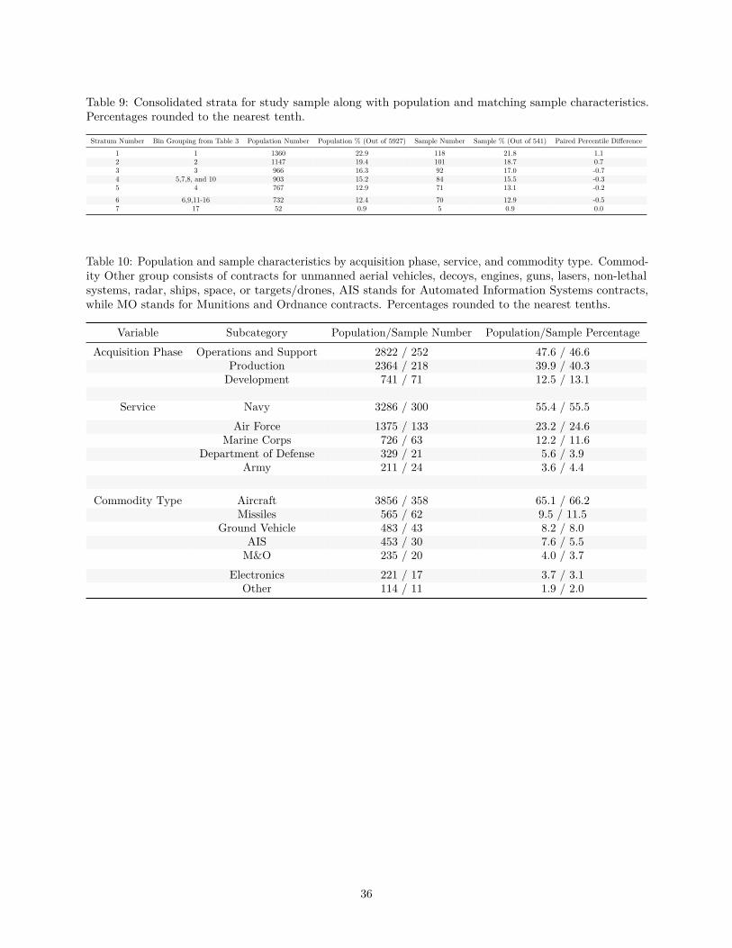
Table 9: Consolidated strata for study sample along with population and matching sample characteristics.Percentages rounded to the nearest tenth.
Stratum Number Bin Grouping from Table 3 Population Number Population % (Out of 5927) Sample Number Sample % (Out of 541) Paired Percentile Difference1 1 1360 22.9 118 21.8 1.12 2 1147 19.4 101 18.7 0.73 3 966 16.3 92 17.0 -0.74 5,7,8, and 10 903 15.2 84 15.5 -0.35 4 767 12.9 71 13.1 -0.26 6,9,11-16 732 12.4 70 12.9 -0.57 17 52 0.9 5 0.9 0.0
Table 10: Population and sample characteristics by acquisition phase, service, and commodity type. Commod-ity Other group consists of contracts for unmanned aerial vehicles, decoys, engines, guns, lasers, non-lethalsystems, radar, ships, space, or targets/drones, AIS stands for Automated Information Systems contracts,while MO stands for Munitions and Ordnance contracts. Percentages rounded to the nearest tenths.
Variable Subcategory Population/Sample Number Population/Sample PercentageAcquisition Phase Operations and Support 2822 / 252 47.6 / 46.6
Production 2364 / 218 39.9 / 40.3Development 741 / 71 12.5 / 13.1
Service Navy 3286 / 300 55.4 / 55.5Air Force 1375 / 133 23.2 / 24.6
Marine Corps 726 / 63 12.2 / 11.6Department of Defense 329 / 21 5.6 / 3.9
Army 211 / 24 3.6 / 4.4
Commodity Type Aircraft 3856 / 358 65.1 / 66.2Missiles 565 / 62 9.5 / 11.5
Ground Vehicle 483 / 43 8.2 / 8.0AIS 453 / 30 7.6 / 5.5M&O 235 / 20 4.0 / 3.7
Electronics 221 / 17 3.7 / 3.1Other 114 / 11 1.9 / 2.0
36

Table 11: Explanatory variables considered in the development of the logistic regression model to predict thelikelihood of a contract having an Engineering Change Proposal (ECP) and the expected median percentageincrease caused by the ECP.
Variable Name Description of Subcategories
Phase Acquisition phase of the contract: Operations and Support, Production, or Development.Service Branch in the Government that let the contract: Navy, Air Force, Marine Corps, Army, or
Department of Defense (Joint).Commodity Type Majority of product on contract. For example, Aircraft, Missile, Ground Vehicle, AIS (Automated
Information System), Munitions, Ordnance, Electronics, etc. A total of 17 types were considered.Contract Type Funding outlay as defined in Federal Acquisition Report (FAR) Part 16 Procurement. For example,
Fixed-Price Contracts, Cost-Reimbursement Contracts, or Incentive Contracts. A total of 9 typeswere considered.
Mod Category Assigned classification of the contract modification (technical, baseline, or schedule for example). Atotal of 8 categories were considered.
Baseline cost Cost in Fiscal Year (FY) 2016 dollars of the initial contract plus priced options.Basic Cost Cost in Fiscal Year (FY) 2016 dollars of the initial contract.Schedule Length of the contract in terms of days.
Contract Year Start / End Date the initial contract started or ended. Investigated years 2010, 2011, and 2012 to determine if theWeapon Systems Acquisition Reform Act (WSARA) of 2009 or Better Buying Power (BBP) initiatives
launched in 2010 had an effect on a contract.F18 This dichotomous variable assumes a value of 1 if the contract is a part of the F/A-18E/F program.
Few CLINs (Contract LineItem Number)
This dichotomous variable assumes a value of 1 if the number of Contract Line Item Numbers (CLINs)equaled 5 or less. This number was chosen since it represented the 90th percentile of CLINs in the
database. Only 10 percent of contracts have more than 5 CLINs on their basic contract.CLINs on Basic Truncated
at 5This continuous variable assumes the value equal to the number of Contract Line Item Numbers
(CLINs) if the number of CLINs equaled 5 or less, else it assumes the value of 5.CLINs on Basic This continuous variable assumes the value equal to the number of Contract Line Item Numbers
(CLINs) regardless of the number.Option Price This continuous variable is the value of all priced options divided by the Basic cost of the contract.
IDIQ (Indefinite DeliveryIndefinite Quantity)
This dichotomous variable assumes a value of 1 if the contract is from an IDIQ, else 0.
FMS (Foreign MilitarySales) Related
This dichotomous variable assumes a value of 1 if there is an FMS requirement on the Basic contract.
Program Past ECPs This dichotomous variable assumes a value of 1 if the encompassing program had an ECP on anycontract before the award date of the current contract. Else the value is 0.
Contract Size A total of 4 dichotomous variables. Each variable assumes the value of 1 if the Baseline cost of thecontract falls into the defined dollar value size. Small, medium, large, and extra large are the definedsizes. Small: Less than or equal to 100,000. Medium: Greater than 100,000 and less than or equal to5,000,000. Large: Greater than 5,000,000 and less than or equal to 400,000,000. Extra Large: Greaterthan 400,000,000. [Note: this last group was later removed from consideration.] All costs are in Fiscal
Year (FY) 2016 dollars.
Table 12: Candidate models for predicting the likelihood of a contract experiencing an Engineering ChangeProposal (ECP). All values rounded to two significant digits.
Model Number Variable Estimate P-value1 Intercept -8.41 < 0.0001
Ln (Baseline cost): Natural logarithm of the contract baseline cost 0.5 < 0.0001
2 Intercept -1.52 < 0.0001Contract Size Large 1.44 1E-4Contract Size Small -2.96 0.0041
37

Table 13: Confusion matrices for the two logistic regression candidate models for predicting the likelihood of acontract experiencing an Engineering Change Proposal (ECP). Parenthetical percentages reflect the accuracyrate of the chosen metric. Information is reflective of both the modeling dataset (Model; 265 contracts) andvalidation set (Test; 268 contracts). Percentages rounded to two decimal places.
Model Number True Positives True Negatives False Positives False Negatives1 Model 13 (28%) 208 (95%) 10 (5%) 34 (72%)1 Test 13 (28%) 199 (90%) 23 (10%) 33 (72%)2 Model 0 (0%) 218 (100%) 0 (0%) 47 (100%)2 Test 0 (0%) 222 (100%) 0 (0%) 46 (100%)
Table 14: Candidate linear model for predicting the natural logarithm of the expected percentage contractincrease due to experiencing an Engineering Change Proposal (ECP). Numbers truncated to two decimalplaces.
Variable Estimate T-ratio P-valueIntercept 3.34 2.42 1.84E-2
Ln (Basic Cost) -0.30 -3.13 0.0025CLINs on Basic Truncated at 5 -0.41 -4.14 < 0.0001
Table 15: Final linear model for predicting the natural logarithm of the expected percentage contract increasedue to experiencing an Engineering Change Proposal (ECP). Numbers truncated to two decimal places.
Variable Estimate T-ratio P-valueIntercept 3.32 2.93 0.0043
Ln (Basic Cost) -0.30 -3.87 0.0002CLINs on Basic Truncated at 5 -0.33 -3.76 0.0003
Table 16: Comparison of the method presented in this paper (Equation 1) to having no ECP withhold,engaging the apparent current practice of 6 percent ECP withhold for development contracts and 10 percentECP withhold for non-development contracts, and applying a straight average ECP percent to all contracts(5.9 for the sample database). All dollar amounts rounded to the nearest dollar (BY 16).
Model Method Underfund Percent Overfund Percent Underfund (Dollars) Overfund (Dollars) Portfolio Total Overall RankEquation (1) 0.0938 0.589 (178M) 197M 19M 1No Withhold 0.174 0 (262M) 0M (262M) 3
Current Practice 0.0957 0.893 (169M) 284M 116M 3Flat Average 0.113 0.887 (175M) 217M 42M 2
Rank Rank Rank Rank Rank Average RankEquation (1) 1 2 3 2 1 1.8No Withhold 4 1 4 1 4 2.8
Current Practice 2 4 1 4 3 2.8Flat Average 3 3 2 3 2 2.6
38

Figure 1: Upper graph displays typical presentation of either basic contract cost, baseline contract cost, ECPpercentage increase, or contract length. Lower graph shows the same data but after transforming using thenatural logarithm. Illustrative graphs are just for basic contract cost.
39

V. Conclusion
In this chapter, we summarize our entire research endeavor by discussing the relevant findings, irrelevant
findings, our limitations, and how future researchers can build upon what we have done. Through this we are
able to draw an end to what we have accomplished and simultaneously provide a stepping off point for others
to further our efforts. The findings contained within this research have the potential to impact future cost
analysts and program managers when faced with allocating resources and effort with respect to an individual
contract. To the best of our knowledge, no peer-reviewed source could be found that documents the amount
of ECP withhold that should be set aside for DoD contracts. Only anecdotal amounts were present in the
literature. The aim of this paper served dual purposes: one, as a published reference point in the archival
forum; and two, derive an empirically-based method for determining percent ECP withhold.
Based on the analysis presented, several points became evident. One, not every contract incurs an ECP,
however, ECPs do occur and not budgeting accordingly results in a serious shortfall as shown in Table 16. Two,
both the likelihood of an ECP as well as additional amount incurred appears to be statistically independent
of acquisition phase, branch of service, commodity, contract type, or any other factor except for the basic
contract amount and the number of CLINs (Contract Line Item Numbers). Both of these variables equally
affected the contract percentage increase due to an ECP. Lastly, the logistic regression approach proved a
poor predictor of determining the likelihood of a DoD contract incurring an ECP. However, it did provide
invaluable insight that lower cost contracts appeared statistically less likely to incur an ECP. Preliminary
analysis suggests that this breakpoint might be around 100K, however, future research is encouraged to
further delve into this lower boundary.
As with any research, limitations do exist for the results in this paper. Quality statistical analysis
depends on quality data. Therefore, any errors within CAPE’s database pulled from EDA will pass down to
the sample database that formed the conclusions stated in this paper. Additionally, the encouraged use of
Equation (1) requires a portfolio managed approach to contracts in an organization. That is, an agency or
manager overseeing a multitude of contracts is able to move ECP withhold amounts from contract to contract
as needed. For if so, then the OLS model as shown in Table 11 shows an almost balanced approach. Lastly,
using (1) for contracts exceeding 164M in BY 16 dollars would be model extrapolation, and we caution against
such use. Table Table 17, not shown in the journal article, is the same results as Table , however separated
by phase as well. This delivers a more detailed picture of if the equation works in all phases. The results are
similar to the overall assessment; this equation does a good job of estimating withhold and contract phase is
not a valid predictor.
40

Table 17: Comparison of the all 4 withhold methods with respect to contract phase.
Compare Model Practice Model Practice Model PracticeUnderfund Percent 20.0% 24.3% 6.4% 7.5% 9.5% 7.1%Overfund Percent 77.1% 74.3% 58.3% 92.5% 53.6% 90.5%Underfund Dollars $-67.38 $-66.98 $-15.32 $-11.37 $-95.51 $-90.36Overfund Dollars $74.02 $112.90 $70.19 $103.02 $52.78 $68.47
Total Abs Deviation Dollars $141.40 $179.88 $85.50 $114.39 $148.29 $158.83Total Portfolio $6.63 $45.92 $54.87 $91.65 $-42.73 $-21.89
Future Research
The field of changing requirements and their impact at the contract level is full of opportunity. One
major recommendation we provide is to use or add a different source of data. Adding data from Selected
Acquisition Reports will provide details on program elements that might increase the chance of all contracts
within that program experiencing an ECP. Another source of information is EVM reports. Not only could
the EVM metric provide a snapshot of contract health, but also research has shown that sentiment analysis
of EVM/Status Reports of programs might provide insightful information and prediction capability (Freeman,
2013).
Next, we suggest assessing the impact of ECPs to future cost and schedule. Since the results section
(Chapter IV) is the submittal as a journal article, we place our preliminary research into the impact to
schedule here. To assess the impact of an ECP to schedule, we used all ~6000 datapoints. We did this to allow
for a big picture assessment since schedule was not the focus of this research. The purpose is to determine in
a broad stroke if there is any impact. Table 18 shows the likelihood of a contract adding additional schedule.
In this case, if an ECP added schedule on that specific modification, we assume that is the new baseline
and assessed if the contract will then add even more schedule. This corrects for the fact that for additional
technical scope, additional schedule may be needed. Table 19 shows the amount of schedule added as a
percent of the basic schedule. This shows that the median contract with an ECP added an additional 18%
schedule. This is significantly different from contracts that did not have an ECP. Without further analysis we
cannot determine the cause of the additional schedule.
Table 18: Comparing likelihood of adding additional schedule for ECP contracts vs nonECP contracts
Contracts that Added Schedule Did Not Add ScheduleHad an ECP 62% 38%Had No ECP 23% 77%
41

Table 19: Comparison of the all 4 withhold methods with respect amount of schedule added.
Contracts that 25th Percentile Median 75th Percentile CountHad an ECP 0% 18% 27% 1,435Had No ECP 0% 0% 15% 4,492
Lastly, we suggest simultaneous analysis at the contract and the program level. From our experience,
many programs will let a new contract rather than adding requirements on an existing contract. This practice,
while valid and legal, may skew the analysis if performed solely at the contract level. That is, a program might
experience cost growth by adding new contracts, while existing contracts show no increased cost. Overall, a
broader and holistic view is needed to accurately assess the impact of changing requirements for the final cost
of a DoD program and elements that affect its bottom-line. Next we suggest a continuous application of
contract management That is, rather than setting/managing the budget only at contract award, creating
a model that can continuously provide ECP estimates. Providing a model that is continuously used will
provide much more benefit to the using community.
42

References
Arena, M.V., Leonard, R.S., Murray, S.E. and Younossi, O. (2006), Historical cost growth of completed
weapon system programs (TR-343), RAND Corporation, Santa Monica, CA.
Bolten, J.G., Leonard, R.S., Arena, M.V., Younossi, O. and Sollinger, J.M. (2008), Sources of Weapon System
Cost Growth: Analysis of 35 Major Defense Acquisition Programs (MG 670), RAND Corporation, Santa
Monica, CA.
Christensen, D., & Templin, C. (2000, Summer). An Analysis of Management Reserve Budget on Defense
Acquisition Contracts. Acquisition Review Quarterly, 7(3), 191-207.
Cordell, I.S. (2017), Engineering Change Orders and their Impact on DoD Acquisition Contracts, Unpublished
masters thesis, Air Force Institute of Technology, Dayton, OH.
Davis, D. and Anton, P.S. (2016), Annual Growth of Contract Costs for Major Programs in Develop-
ment and Early Production, Defense Technical Information Center, Fort Belvoir, VA. Available at
www.dtic.mil/docs/citations/AD1006106 (accessed 12 January 2018).
Defense Acquisition University. (2017). Defense Acquisition Guidebook, Chapter Four - Life Cycle
Sustainment, Retrieved from https://www.dau.mil/tools/dag, September 2017
Department of Defense (2015), Operation of the Defense Acquisition System (DoDI 5000.02), Office of the
Under Secretary of Defense for Acquisition, Technology, and Logistics, Washington, DC.
Engineering Change Proposal (2017), In AcqNotes [Online encyclopedia]. Available at http://acqnotes.com/
acqnote/careerfields/engineering-change-proposal-ecp (accessed 12 January 2018).
Electronic Document Access (2017), In AcqNotes [Online encyclopedia]. Available at http://acqnotes.com/
acqnote/careerfields/electronic-document-access-eda (accessed 12 January 2018).
Freeman, C.E. (2013), Multivariate and Naïve Bayes Text Classification Approach to Cost Growth Risk in
43

Department of Defense Acquisition Programs, Defense Technical Information Center, Fort Belvoir, VA.
Available at www.dtic.mil/dtic/tr/fulltext/u2/a583708.pdf (accessed 12 January 2018).
Government Accountability Office (2008), Defense Acquisitions: Assessments of Selected Weapon Programs
(08-467SP), U.S. Government Printing Office, Washington, DC.
Government Accountability Office (2011), DoD Cost Overruns: Trends in Nunn-McCurdy Breaches and Tools
to Manage Weapon Systems Acquisition Costs (11-499T), U.S. Government Printing Office, Washington,
DC.
Government Accountability Office, U. S. (2015). Report to the Honorable James Inhofe: Military Service
Chiefs’ Concerns Reflect Need to Better Define Requirements before Programs Start, U.S. Government
Printing Office, Washington, DC.
Harmon, B. R. and Arnold, S. A. (2013), Choice of Contract Type and Other Policy Initiatives for Reducing
Contract Prices (D-5002), Institute for Defense Analyses, Alexandria, VA.
Kutner, Nachtsheim, Neter, and Li (2005). Applied Linear Statistical Models (5th ed.), McGraw-Hill/Irwin,
New York, NY.
NRO Cost Group. (2005). A Study of Contract Changes and Their Impacts on ICEs, NRO Cost Group and
Air Force Costs Analysis Agency, Washington DC.
Office of the Secretary of Defense. (2016). Performance of the Defense Acquisition System, Section 1(2), Pg
506-507, U.S. Government Printing Office, Washington, DC.
Project Management Institute (2017), A Guide to the Project Management Body of Knowledge (PMBOK
Guide) (6th ed.), Project Management Institute, Newtown Square, PA.
Trudelle, R., White, E.D., Koschnick, C., Ritschel, J.D. and Lucas, B. (2017). “Estimating an acquisition
program’s likelihood of staying within cost and schedule bounds”, Defense Acquisition Research Journal,
Vol. 24 No. 4, pp. 600- 625. Available at https://doi.org/10.22594/dau.17-775.24.04 (accessed 12
January 2018).
44

U.S. Air Force (2015), U.S. Air Force Cost Risk and Uncertainty Handbook (AFCRUH), Air Force Cost
Analysis Agency, Washington DC.
U.S. Air Force (2007). Air Force Cost Analysis Handbook (AFCAH), Chapter 14 - Other Government Costs,
Air Force Cost Analysis Agency, Washington DC.
U.S. Congress. (2009). Weapon systems acquisition reform act of 2009. Public Law, 2009, 1-31. Retrieved
from https://www.congress.gov/111/plaws/publ23/PLAW-111publ23.pdf, June 2017.
U.S. Government Printing Office: Electronic Code of Federal Regulations, Title 48 - Federal Acquisition
Regulation, Subpart 43.2 - Change Orders
Valentine, S.,(2017). Analysis of Engineering Change Orders, AFLCMC/FZC WPAFB Newsletter, February
2017. Accessed via [email protected]
45

46
REPORT DOCUMENTATION PAGE Form Approved OMB No. 074-0188
The public reporting burden for this collection of information is estimated to average 1 hour per response, including the time for reviewing instructions, searching existing data sources, gathering and maintaining the data needed, and completing and reviewing the collection of information. Send comments regarding this burden estimate or any other aspect of the collection of information, including suggestions for reducing this burden to Department of Defense, Washington Headquarters Services, Directorate for Information Operations and Reports (0704-0188), 1215 Jefferson Davis Highway, Suite 1204, Arlington, VA 22202-4302. Respondents should be aware that notwithstanding any other provision of law, no person shall be subject to a penalty for failing to comply with a collection of information if it does not display a currently valid OMB control number. PLEASE DO NOT RETURN YOUR FORM TO THE ABOVE ADDRESS. 1. REPORT DATE (DD-MM-YYYY)
23-03-2018 2. REPORT TYPE
Master’s Thesis 3. DATES COVERED (From – To)
October 2016 – March 2018
4. TITLE AND SUBTITLE
The Impact of Changing Requirements 5a. CONTRACT NUMBER
5b. GRANT NUMBER
5c. PROGRAM ELEMENT NUMBER
6. AUTHOR(S) Ellis, James C., Captain, USAF
5d. PROJECT NUMBER
5e. TASK NUMBER
5f. WORK UNIT NUMBER
7. PERFORMING ORGANIZATION NAMES(S) AND ADDRESS(S)
Air Force Institute of Technology Graduate School of Engineering and Management (AFIT/ENC) 2950 Hobson Way, Building 640 WPAFB OH 45433-8865
8. PERFORMING ORGANIZATION REPORT NUMBER
AFIT-ENC-MS-18-M-200
9. SPONSORING/MONITORING AGENCY NAME(S) AND ADDRESS(ES) Air Force Life Cycle Management Center 5135 Pearson Road, Building 10 Wright-Patterson AFB, OH 45433 ATTN: Shawn Valentine ([email protected])
10. SPONSOR/MONITOR’S ACRONYM(S) AFLCMC/FZCE
11. SPONSOR/MONITOR’S REPORT NUMBER(S)
12. DISTRIBUTION/AVAILABILITY STATEMENT DISTRUBTION STATEMENT A. APPROVED FOR PUBLIC RELEASE; DISTRIBUTION UNLIMITED.
13. SUPPLEMENTARY NOTES This material is declared a work of the U.S. Government and is not subject to copyright protection in the United States.
14. ABSTRACT The fundamental purpose of an Engineering Change Proposal (ECP) is to change the requirements of a contract. To build in flexibility, the acquisition practice is to estimate a dollar value to hold in reserve after the contract is awarded. There appears to be no empirical-based method for estimating this ECP withhold in the literature. Using the Cost Assessment Data Enterprise (CADE) database, 533 contracts were randomly selected to build two regression models: one to predict the likelihood of a contract experiencing an ECP, and the other to determine the expected median percent increase in baseline contract cost if an ECP was likely. Results suggest that this two-step approach works well over a managed portfolio of contracts in contrast to three investigated rules-of-thumb. Significant drivers are the basic contract cost and the number of contract line items.
15. SUBJECT TERMS Engineering change order, Management reserve, logistic regression, multiple regression.
16. SECURITY CLASSIFICATION OF:
17. LIMITATION OF ABSTRACT
UU
18. NUMBER OF PAGES
57
19a. NAME OF RESPONSIBLE PERSON Dr. Edward White, AFIT/ENC
a. REPORT
U
b. ABSTRACT
U
c. THIS PAGE
U
19b. TELEPHONE NUMBER (Include area code) 937-255-3636 x4540 (Comm) ( [email protected])
Standard Form 298 (Rev. 8-98) Prescribed by ANSI Std. Z39-18